/


Автор: Wickerhauser M.V.
Теги: mathematics programming higher mathematics computer science applied mathematics wavelet analysis
ISBN: 1-56881-041-5
Год: 1994


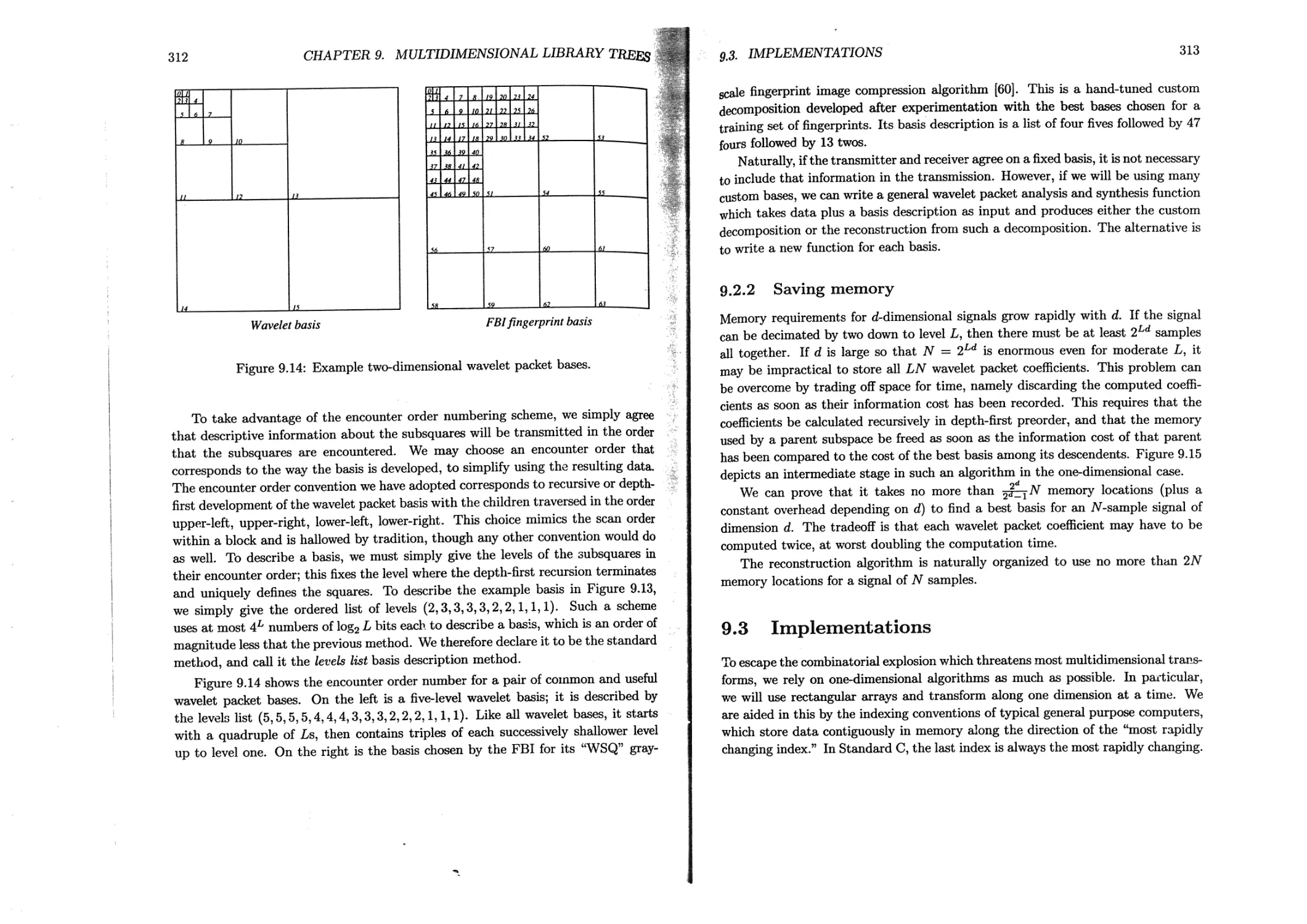
Текст
q
'я
Adapted Wavelet Analysis
id
from Theory to Software
Mladen Victor Wickerhauser
Washington University
St. Louis, Missouri
I
чу
•»
IEEE
PRESS
The Institute of Electrical
and Electronics Engineers, Inc.
New York
A К Peters
Wellesley, Massachusetts
Editorial, Sales, and Customer Service Office
A К Peters, Ltd.
289 Linden Street
Wellesley, MA 02181
Copyright © 1994 by A К Peters, Ltd.
All rights reserved. No part of the material protected by this copyright notice
may be reproduced or utilized in any form, electronic or mechanical, includ-
ing photocopying, recording, or by any information storage and retrieval sys-
tem, without written permission from the copyright owner.
Library of Congress Cataloging-in-Publication Data
Wickerhauser, Mladen Victor
Adapted wavelet analysis from theory to software / Mladen Victor
> Wickerhauser.
p, cm.
Includes bibliographical references and index.
ISBN 1-56881-041-5
1. Wavelets. I. Title.
QA403.3.W53 1993
621.382 ’ 2 ’ 015152433~dc20 94-14995
CIP
IEEE PRESS
P. O. Box 1331
445 Hoes Lane
Piscataway, NJ 08855-1331
IEEE Order Number: PC5656
Printed in the United States of America
98 97 96 10 9 8 7 6 5 4 3 2
Preface
In the past decade, wavelet analysis has grown from a mathematical curiosity into
a major source of new signal processing algorithms. The subject has branched out
to include wavelet packets, and has merged with other methods of transient signal
analysis such as Gabor expansions, Wilson bases, and adapted lapped orthogonal
transforms. Dozens of conferences and workshops on wavelet applications have been
sponsored on five continents. The 1993 Wavelet Literature Survey [89] contains 976
articles and books, a number which has doubled annually since 1991. Both the
March 1992 IEEE Transactions on Information Theory and the December 1993
IEEE Transactions on Signal Processing were special issues dedicated to applica-
tions of wavelet transforms. Seminal articles on the subject have appeared in a
remarkable variety of publications, ranging from Dr, Dobb’s Journal to the Journal
of Chemical Information and Computer Science to Revista Matemdtica Iberoameri-
cana. The Wavelet Digest electronic mailing list currently boasts 3255 subscribers,
including engineers, scientists, and mathematicians.
In spite of all this activity, there have been few works devoted to implementation.
Apart from a short book chapter ([90], §13.10) and three popular articles [16,17,18],
there is no wavelet programming guide. This may be due to the commercial value of
wavelet transform software, which has kept it hidden beneath a proprietary cloak.
Sources for discrete and lapped trigonometric transforms are easier to find ([92]
appendices; [75]), and there are innumerable implementations of the discrete Fourier
transform. But if we collect all these deeply interrelated transforms into a single
toolbox, then we can profit by choosing the right tool for each job. In adapted
wavelet analysis, choice makes the method more powerful than the sum of its parts.
This text goes beyond the existing literature to aid the engineer and applied
mathematician in writing computer programs to analyze real data. It addresses
the properties of wavelet and related transforms, to establish criteria by which the
proper analysis tool may be chosen, and then details software implementations to
perform the needed computation. It will also be useful to the pure mathematician
who is familiar with some parts of wavelet theory but has questions about the
applications. The worked exercises make this a useful textbook for self-study, or for
a course in the theory and practice of wavelet analysis.
vi
Beginning with an overview of the mathematical prerequisites, successive chap-
ters rigorously examine the properties of the waveforms used in adapted wavelet
analysis: discrete “fast” Fourier transforms, orthogonal and biorthogonal wavelets,
wavelet packets, and localized trigonometric or lapped orthogonal functions. Other
chapters discuss the “best basis” method, time-frequency analysis, and combina-
tions of these algorithms useful for signal analysis, de-noising, and compression.
Each chapter discusses the technicalities of implementation, giving examples in
pseudocode backed up with machine-readable Standard C source code available on
the optional diskette. Each chapter finishes with a list of worked exercises in both
the mathematics and the programming of adapted wavelet algorithms. Especially
emphasized are the pitfalls and limitations of the algorithms, with examples and
suggestions given to show how to avoid them.
Most of the adapted wavelet algorithms described here are the product of re-
search conducted at Yale University from 1989-1991, and at Washington University
in St. Louis from 1991-1994. Some of the algorithms have been reduced to practice
and patented by Aware, Inc., FMA&H Corporation, Positive Technologies, Inc.,
and Yale University.
The author gratefully acknowledges the support provided by the National Sci-
ence Foundation (NSF), the Air Force Office of Scientific Research (AFOSR), the Of-
fice of Naval Research (ONR), and the Defense Advanced Research Projects Agency
(DARPA) during the past several years. The author also wishes to thank Professor
Ronald R. Coifman of Yale University, Professor Yves Meyer of the University of
Paris-Dauphine, and Professor Alexander Grossmann of the Centre de Physique
Theorique in Luminy for many fruitful visits and conversations.
This book was written at a time when brutal war raged against the author’s
ancestral Croatian homeland. It is dedicated to fellow Croatians throughout the
world, in appreciation for many contributions to science and culture, and in honor
of the spirit which prevails against savagery.
University City, Missouri
9 May 1994
4
Contents
1 Mathematical Preliminaries 1
1.1 Basic analysis.............................................. 1
1.1.1 Convergence of series and products...................... 2
1.1.2 Measurability ...................................... 3
1.1.3 Integrability........................................... 5
1.1.4 Metrics, norms, and inner products ..................... 6
1.2 Function spaces............................................. 8
1.2.1 Continuous functions on the circle...................... 8
1.2.2 Lebesgue spaces....................................... 9
1.2.3 Spaces of test functions............................. 10
1.2.4 Dual spaces .......................................... 11
1.2.5 Frames, bases, and orthonormality...................... 13
1.3 Fourier analysis ............................................. 18
1.3.1 Fourier integrals..................................... 19
1.3.2 Fourier series.................................... 20
1.3.3 General orthogonal transformations .................... 22
1.3.4 Discrete Fourier transforms .......................... 23
1.3.5 Heisenberg’s inequality............................... 24
1.3.6 Convolution ....................................... 25
1.3.7 Dilation, decimation, and translation.................. 31
1.4 Approximation................................................. 32
1.4.1 Averaging and sampling ..................... 32
1.4.2 Band-limited functions .............................. 35
1.4.3 Approximation by polynomials........................... 36
1.4.4 Smooth functions and vanishing moments ........... 37
1.5 Exercises ................................................. 38
vn
viii CONTENTS
2 Programming Techniques 41
2.1 Computation in the real world ................................. 41
2.1.1 Finiteness............................................ 41
2.1.2 Validity . . . .................................... 43
2.1.3 Pseudocode.............................................. 44
2.1.4 Common utilities ....................................... 46
2.2 Structures..................................................... 47
2.2.1 Complex arithmetic...................................... 47
2.2.2 Intervals............................................... 48
2.2.3 Binary trees............................................ 51
2.2.4 Hedges.................................................. 55
2.2.5 Atoms................................................... 57
2.3 Manipulation............................................. . 58
2.3.1 Hedges and trees.................................... 58
2.3.2 Atoms and trees...................................... 61
2.3.3 Hedges to atoms......................................... 63
2.4 Exercises .................................................. 66
3 The Discrete Fourier Transform 67
3.1 The Fourier transform on CN.................................... 68
3.1.1 The “fast” Fourier transform.......................... 69
3.1.2 Implementation of DFT................................... 73
3.2 The discrete Hartley transform................................ 77
3.2.1 The “fast” discrete Hartley transform................... 78
3.2.2 Implementation of DHT................................... 81
3.3 Discrete sine and cosine transforms............................ 83
3.3.1 DCT-I and DST-I......................................... 85
3.3.2 DCT-II, DCT-III, DST-II, and DST-III..................... 90
3.3.3 DCT-IV and DST-IV ...................................... 94
3.3.4 Implementations of DCT and DST.......................... 96
3.4 Exercises .....................................................101
4 Local Trigonometric Transforms 103
4.1 Ingredients and examples..................................... 104
4.1.1 Unitary folding and unfolding...........................104
4.1.2 Smooth orthogonal projections...........................112
4.1.3 Periodization...........................................118
4.1.4 Some analytic properties................................122
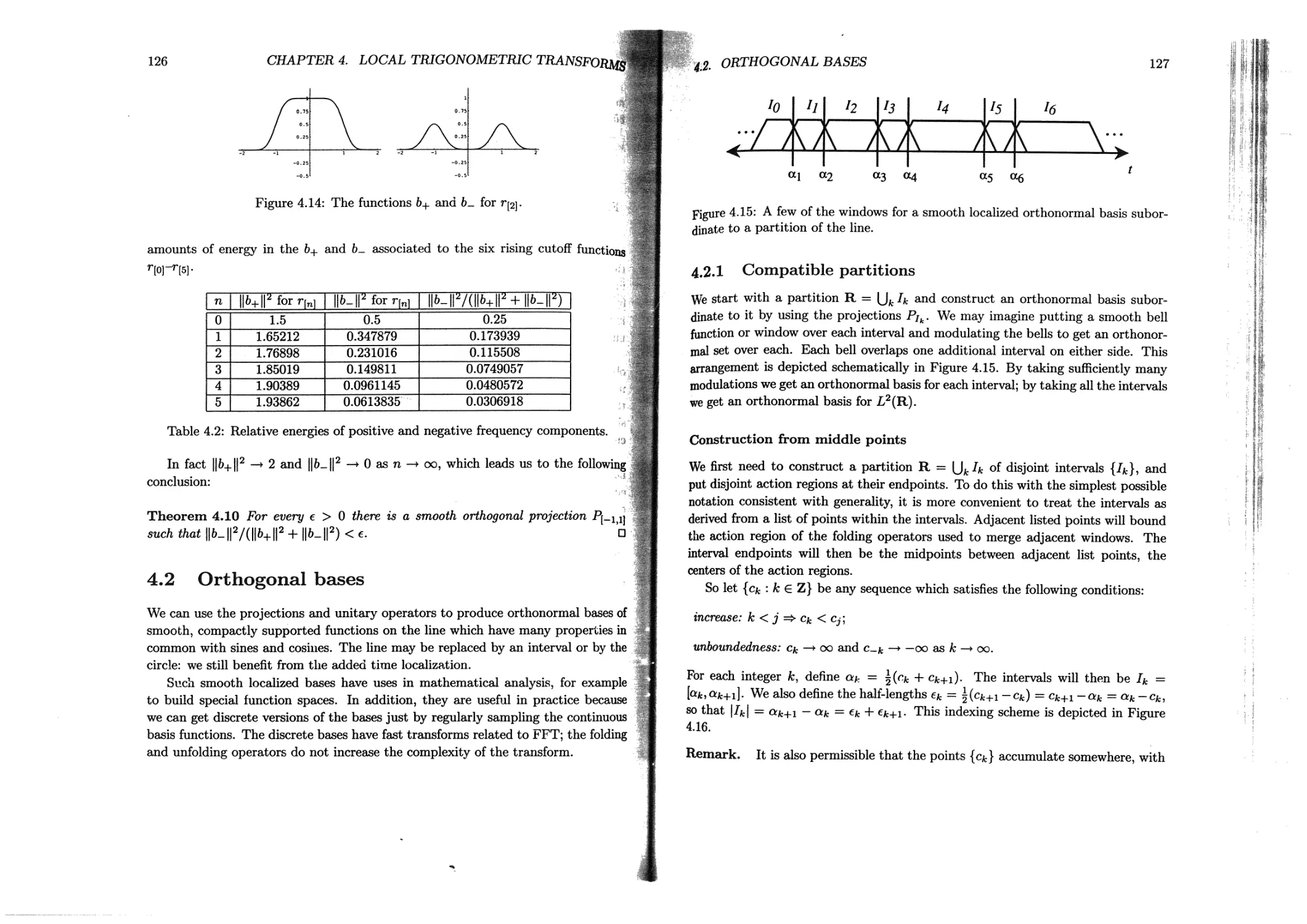
4.2 Orthogonal bases............................................. 126
CONTENTS
ix
4.2.1 Compatible partitions......................................127
4.2.2 Orthonormal bases on the line ........................... 130
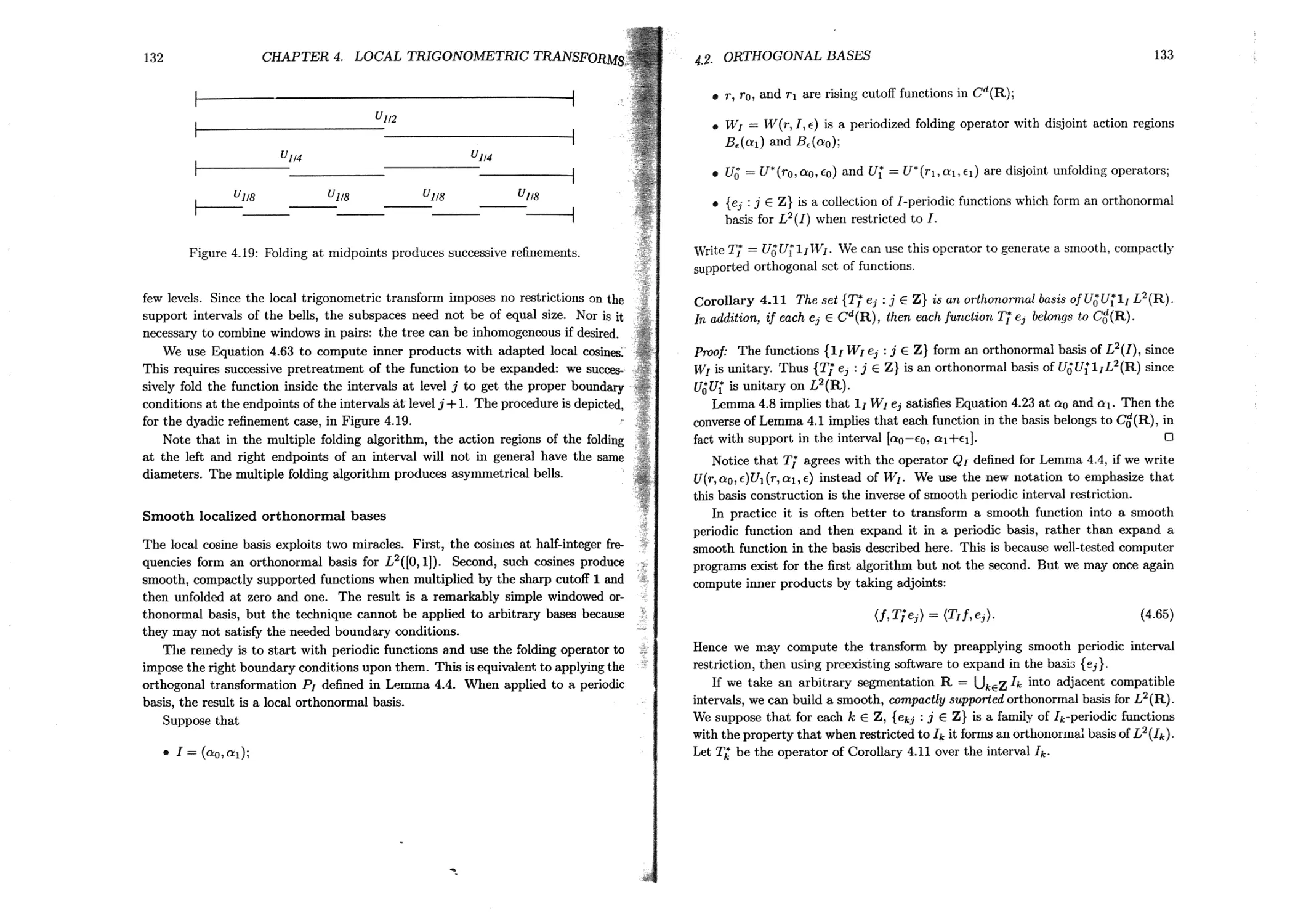
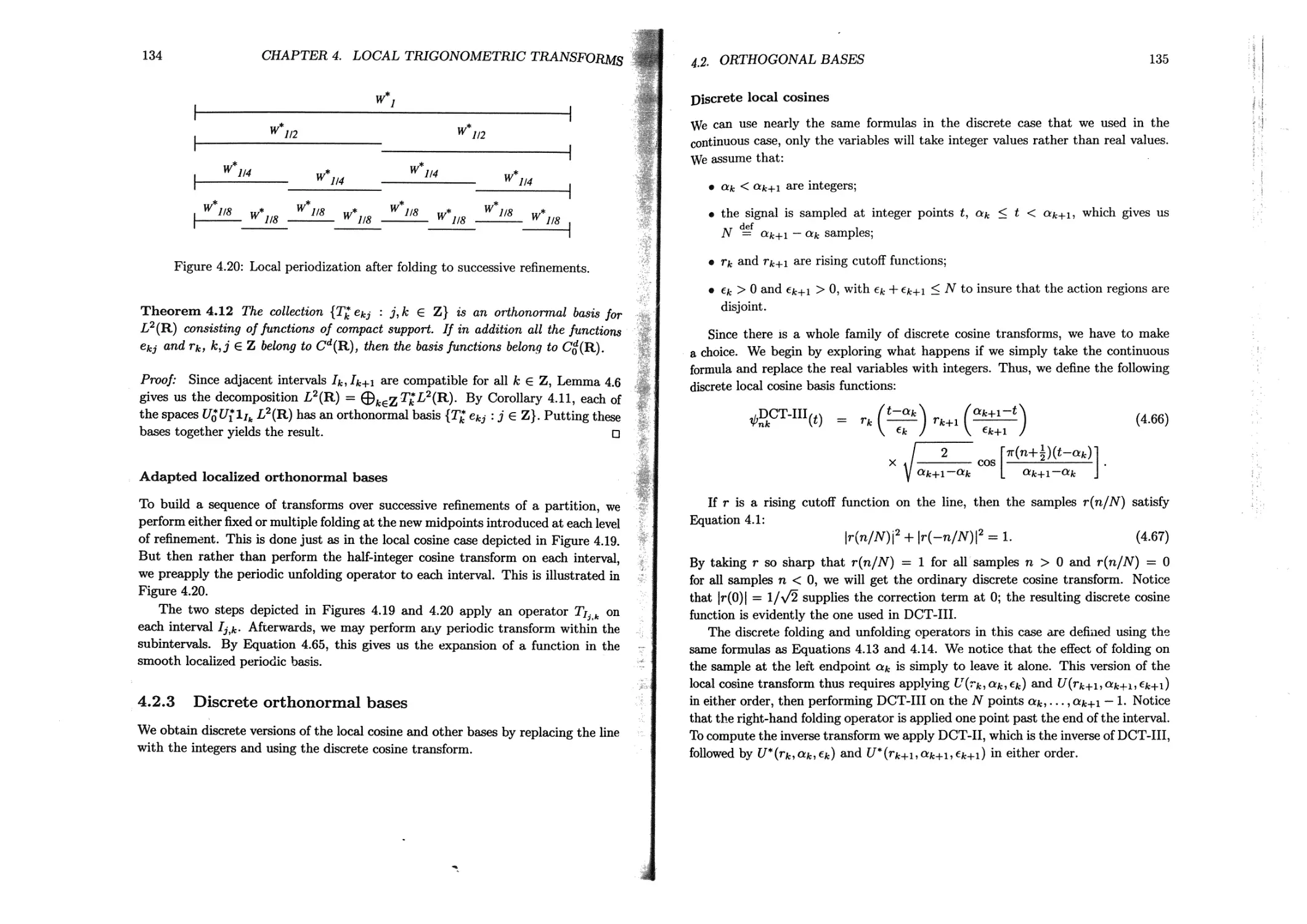
4.2.3 Discrete orthonormal bases.................................134
4.3 Basic implementation.............................................137
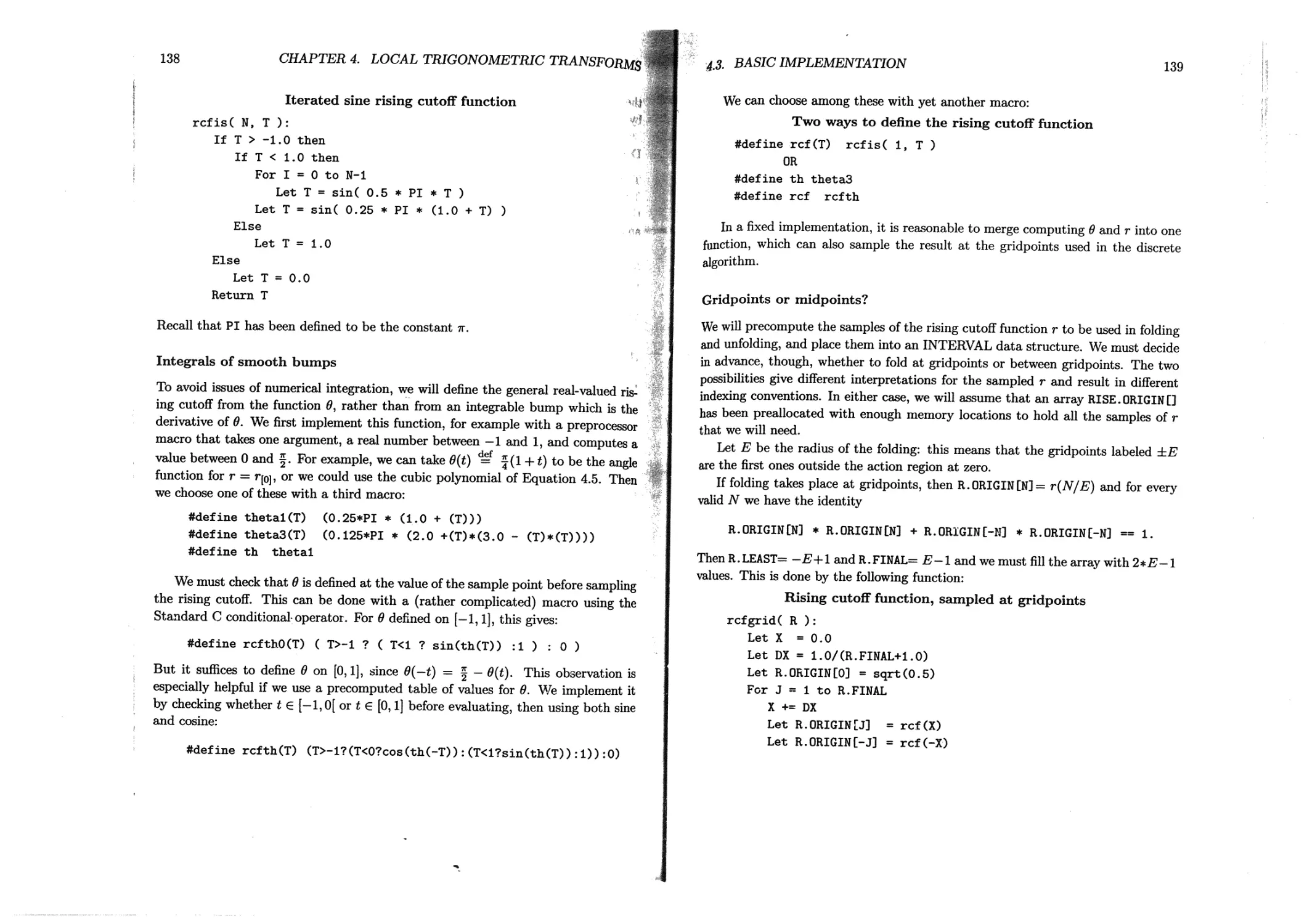
4.3.1 Rising cutoff functions.................................. 137
4.3.2 Midpoint folding and unfolding functions...................140
4.3.3 Midpoint local trigonometric transforms ...................143
4.3.4 Midpoint local periodization ..............................145
4.4 Implementation of adapted transforms............................ 146
4.4.1 Adapted local cosine analysis..............................146
4.4.2 Extraction of coefficients................................ 149
4.4.3 Adapted local cosine synthesis.............................151
4.5 Exercises ..................................................... 151
5 Quadrature Filters 153
5.1 Definitions and basic properties.................................154
5.1.1 Action on sequences........................................154
5.1.2 Biorthogonal QFs ...................................... . 156
5.1.3 Orthogonal QFs.............................................158
5.1.4 Action on functions .......................................160
5.2 Phase response...................................................163
5.2.1 Shifts for sequences................................... 164
5.2.2 Shifts in the periodic case................................171
5.3 Frequency response...............................................176
5.3.1 Effect of a single filter application......................177
5.3.2 Effect of iterated filter applications.....................182
5.4 Implementing convolution-decimation..............................191
5.4.1 General assumptions........................................191
5.4.2 Aperiodic convolution-decimation . ........................194
5.4.3 Adjoint aperiodic convolution-decimation...................197
5.4.4 Periodic convolution-decimation............................198
5.4.5 Adjoint periodic convolution-decimation.................. 207
5.4.6 Tricks.....................................................208
5.5 Exercises .......................................................210
6 The Discrete Wavelet Transform 213
6.1 Some wavelet basics..............................................214
6.1.1 Origins ...................................................214
6.1.2 The DWT family......................................... 215
X
CONTENTS
6.1.3 Multiresolution analysis...........................216
6.1.4 Sequences from functions .................... 217
6.2 Implementations ........................................ 218
6.2.1 Periodic DWT and iDWT............................. 220
6.2.2 Aperiodic DWT and iDWT.............................226
6.2.3 Remarks.......................................... 234
6.3 Exercises ............................................ 234
7 Wavelet Packets 237
7.1 Definitions and general properties........................238
7.1.1 Fixed-scale wavelet packets on R....................238
7.1.2 Multiscale wavelet packets on R................... 242
7.1.3 Numerical calculation of wavelet packet coefficients ...... 245
7.1.4 The discrete wavelet packet analysis family ........251
7.1.5 Orthonormal bases of wavelet packets ............. 254
7.2 Implementations...........................................257
7.2.1 Generic algorithms ............................... 258
7.2.2 Periodic DWPA and DWPS..............................260
7.2.3 Aperiodic DWPA and DWPS.............................265
7.2.4 Biorthogonal DWPA and DWPS ................ 271
7.3 Exercises............................................. 272
8 The Best Basis Algorithm 273
8.1 Definitions..................................................... 274
8.1.1 Information cost and the best basis.......................274
8.1.2 Entropy, information, and theoretical dimension ....... 276
8.2 Searching for the best basis................................ 282
8.2.1 Library trees.............................................283
8.2.2 Fast searches for minimum information cost................283
8.2.3 Adapted waveform analysis meta-algorithm .......... 286
8.3 Implementation..................................................287
8.3.1 Information cost functionals............................. 287
8.3.2 Extracting a basis subset............................. 289
8.3.3 Extracting a branch................................... 294
8.4 Exercises .................................................. 297
CONTENTS xi
g Multidimensional Library Trees 299
9.1 Multivariable splitting operators ...........................300
9.1.1 Tensor products of CQFs........... 301
9.1.2 Tensor products of DTTs and LTTs........................304
9.1.3 Complexity of the d-dimensional best basis algorithm .... 307
9.1.4 Anisotropic dilations in multidimensions ...............308
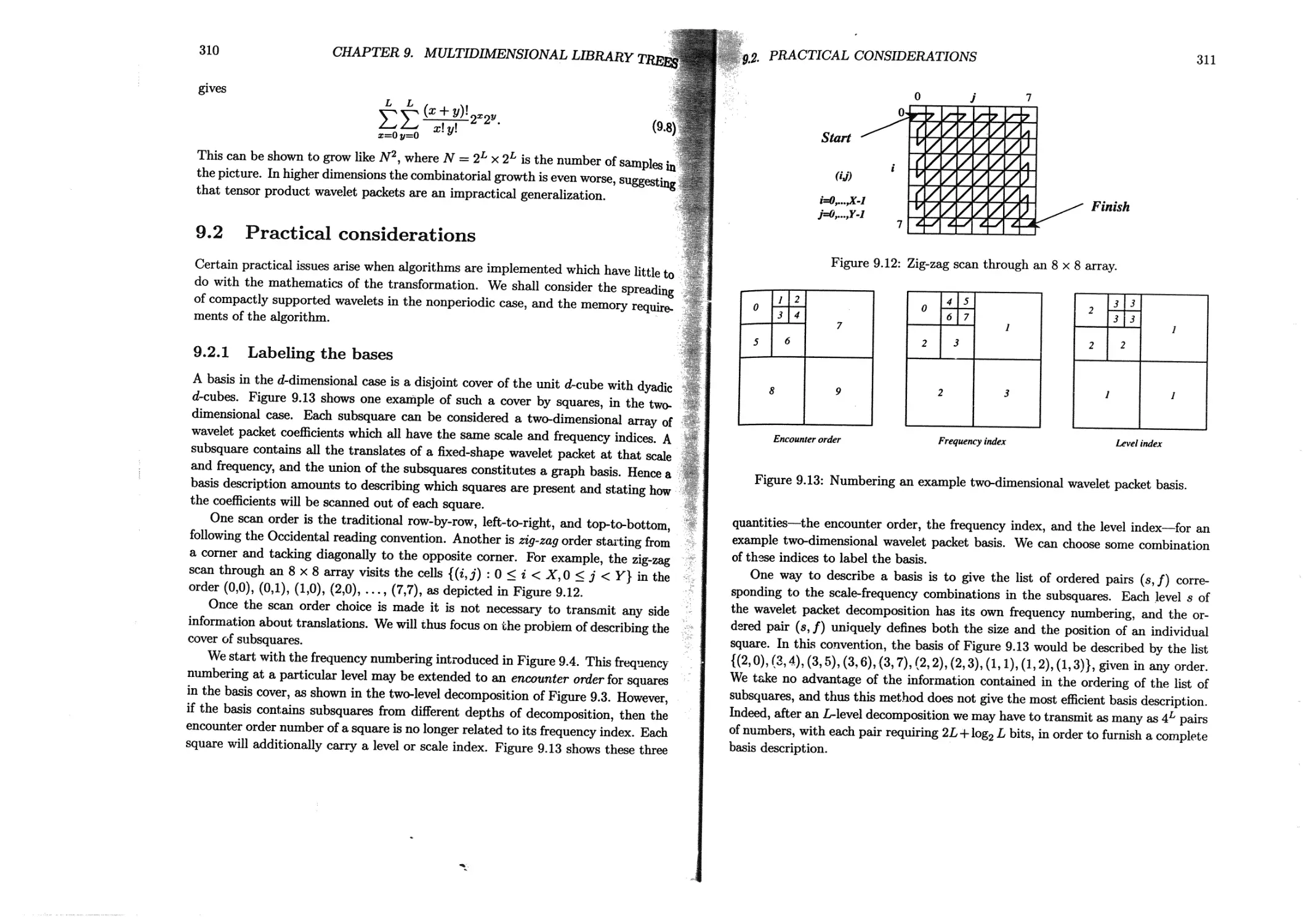
9.2 Practical considerations.....................................310
9.2.1 Labeling the bases......................................310
9.2.2 Saving memory.......................................... 313
9.3 Implementations............................................ 313
9.3.1 Transposition...........................................314
9.3.2 Separable convolution-decimation...................... 317
9.3.3 Separable adjoint convolution-decimation ........... 319
9.3.4 Separable wavelet packet bases ....................... 322
9.3.5 Separable folding and unfolding.........................326
9.4 Exercises ................................................. 327
10 Time-F¥equency Analysis 329
10.1 The time-frequency plane ................................. 329
10.1.1 Waveforms and time-frequency atoms ............. 329
10.1.2 The idealized time-frequency plane.....................333
10.1.3 Bases and tilings.................................... 336
10.1.4 Analysis and compression............................. 339
10.1.5 Time-frequency analysis with library trees ............340
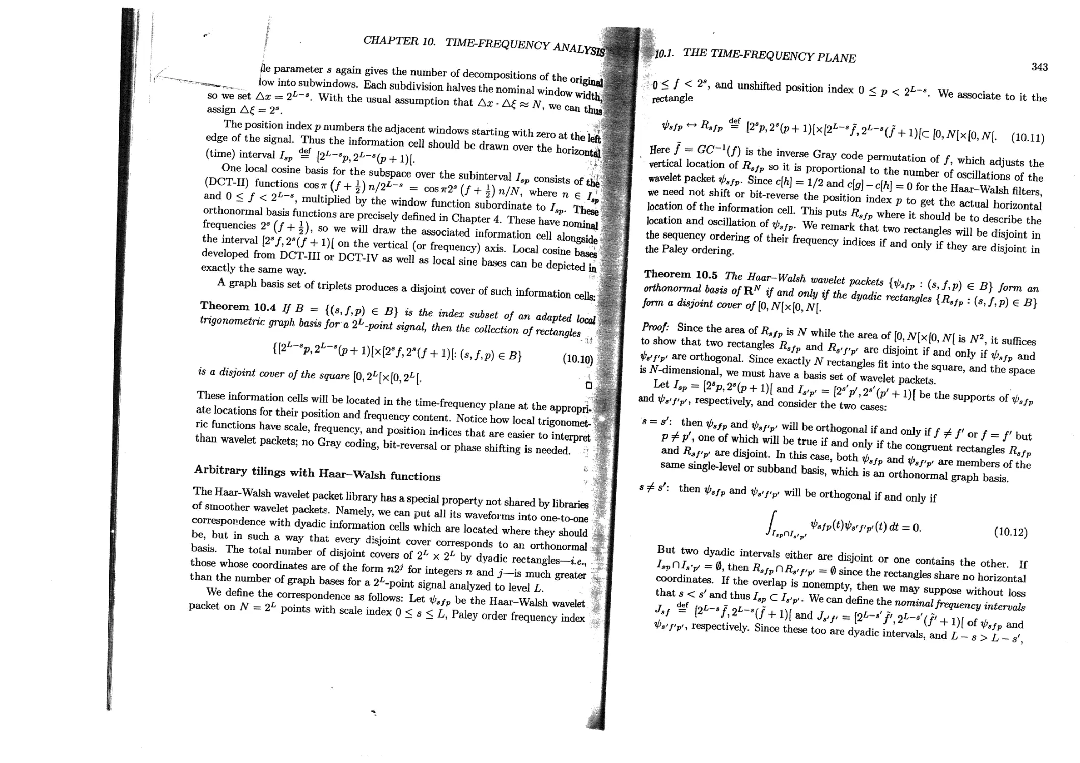
10.2 Time-frequency analysis of basic signals.....................345
10.2.1 Benefits of adaption ................................ 345
10.2.2 Wavelets versus wavelet packets........................348
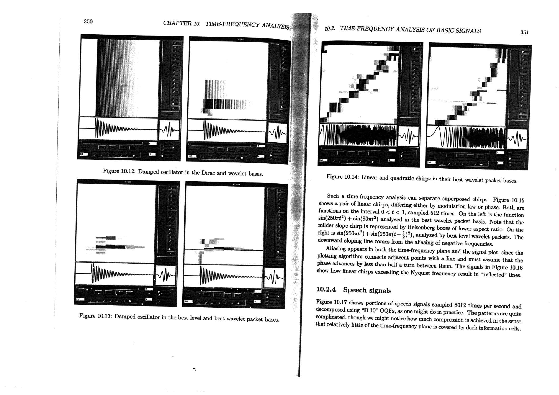
10.2.3 Chirps .............................................. 349
10.2.4 Speech signals . ................................ 351
10.3 Implementation .............................. 353
10.3.1 Drawing primitives................................... 354
10.3.2 Plotting the signal samples............................355
10.3.3 Plotting the time-frequency plane .....................356
10.3.4 Computing the atoms....................................358
10.4 Exercises ...................................................359
xii CONTENTS
11 Some Applications 361
11.1 Picture compression . .........................................361
11.1.1 Digital pictures........................................362
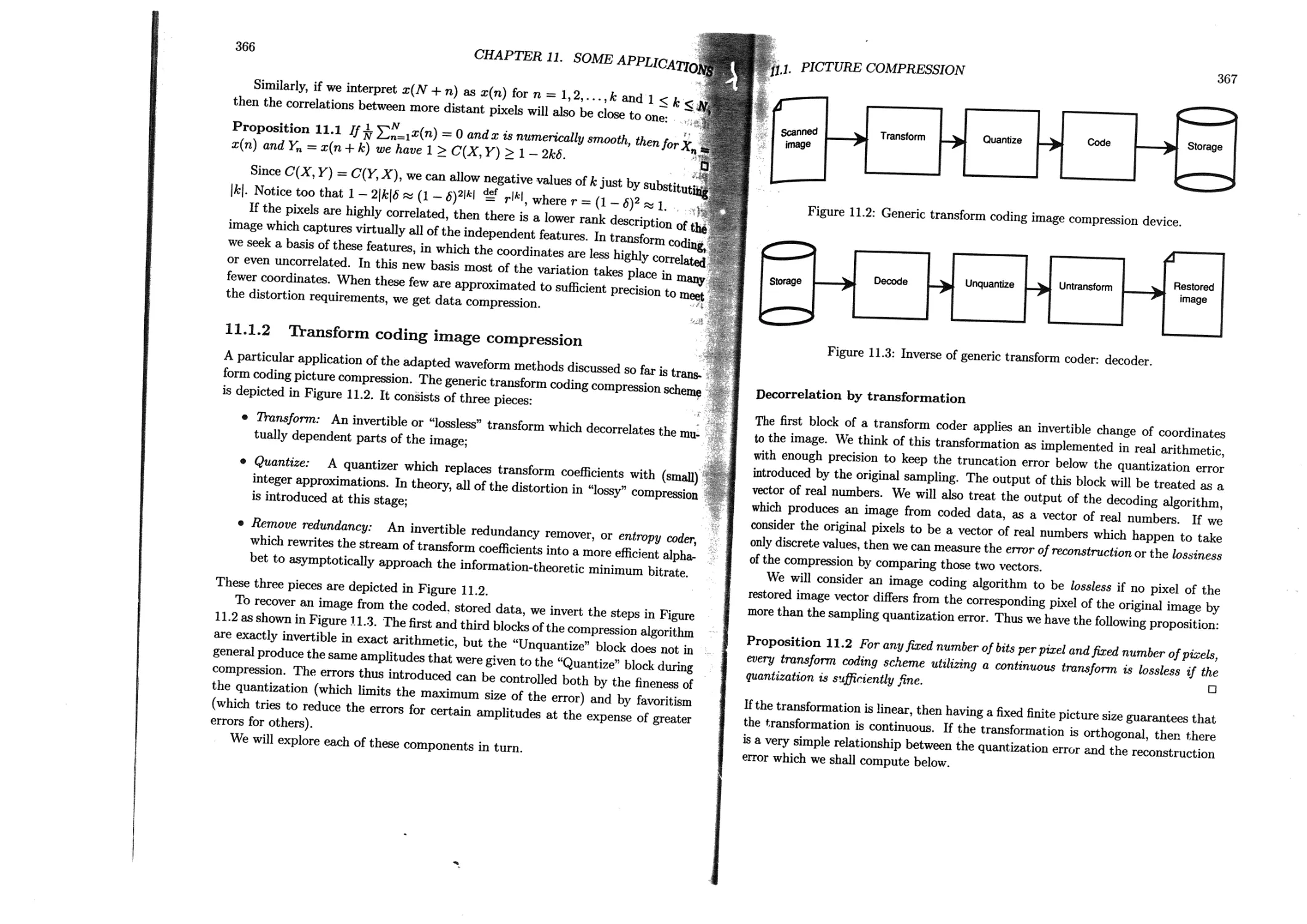
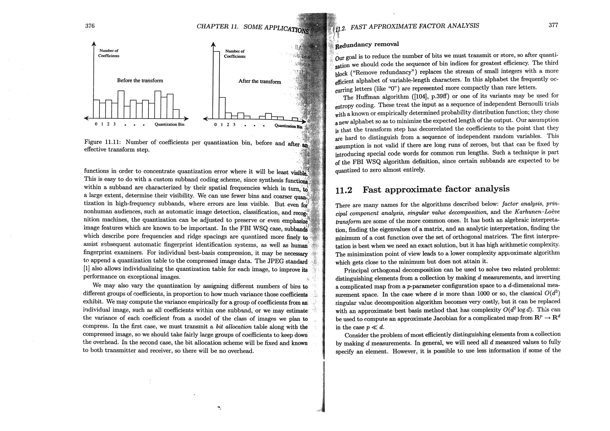
11.1.2 Transform coding image compression.................... 366
11.2 Fast approximate factor analysis...............................377
11.2.1 The approximate KL transform............................382
11.2.2 Classification in large data sets..................... 385
11.2.3 Jacobians of complicated maps ..........................389
11.3 Nonstandard matrix multiplication............................ 398
11.3.1 Two-dimensional best basis sparsification...............398
11.3.2 Applying operators to vectors...........................399
11.3.3 Composing operators.....................................408
11.4 Speech signal segmentation.....................................409
11.4.1 Adapted local spectral analysis....................... 410
11.4.2 Voiced-unvoiced segmentation.......................... 411
11.4.3 Experimental results....................................413
11.5 Speech scrambling..............................................415
11.5.1 Objects to be scrambled.................................416
11.5.2 Feature-preserving permutations.........................416
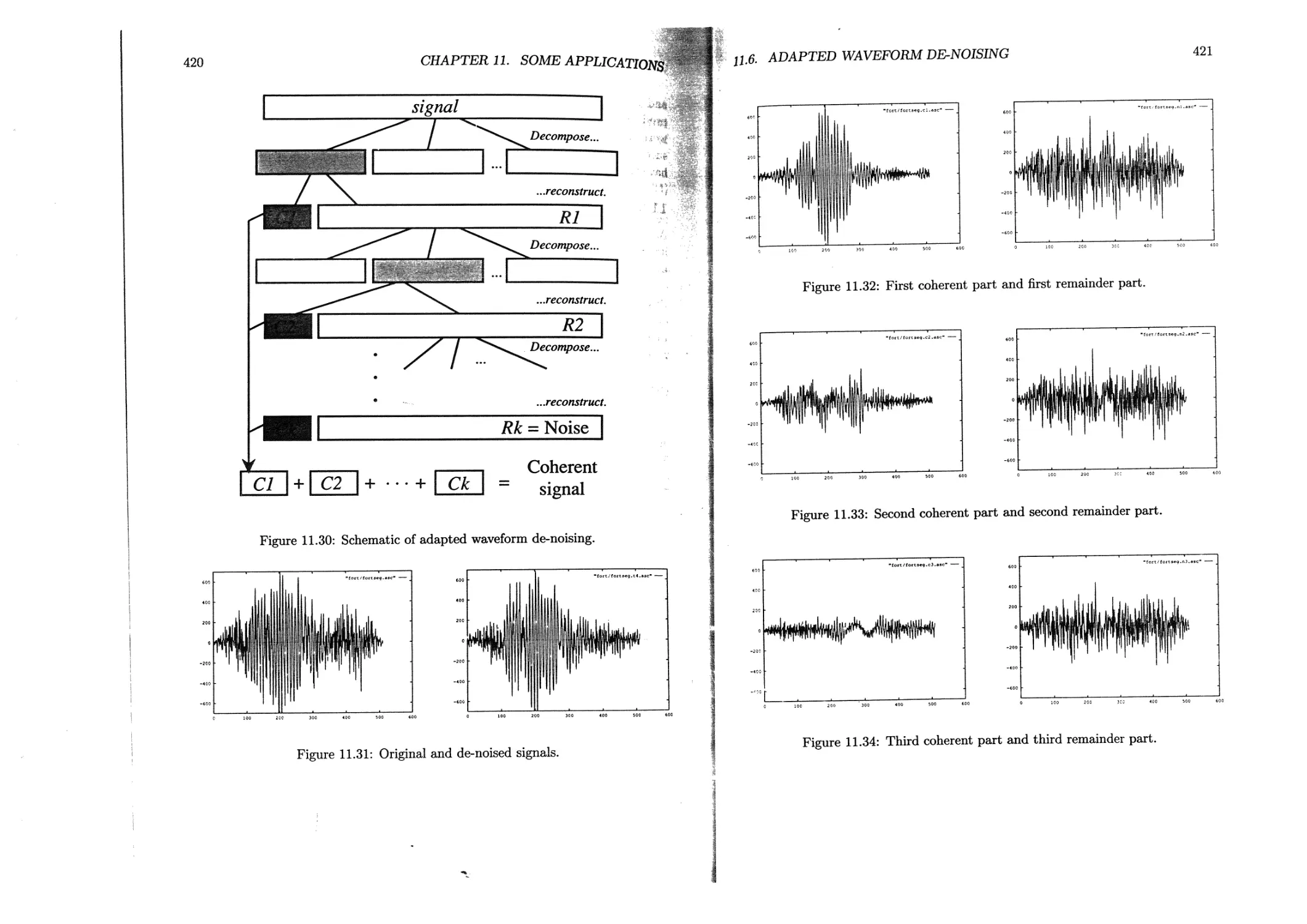
11.6 Adapted waveform de-noising....................................417
11.6.1 Coherency and noise.................................... 417
11.6.2 Experimental results....................................419
A Solutions to Some of the Exercises 425
В List of Symbols 441
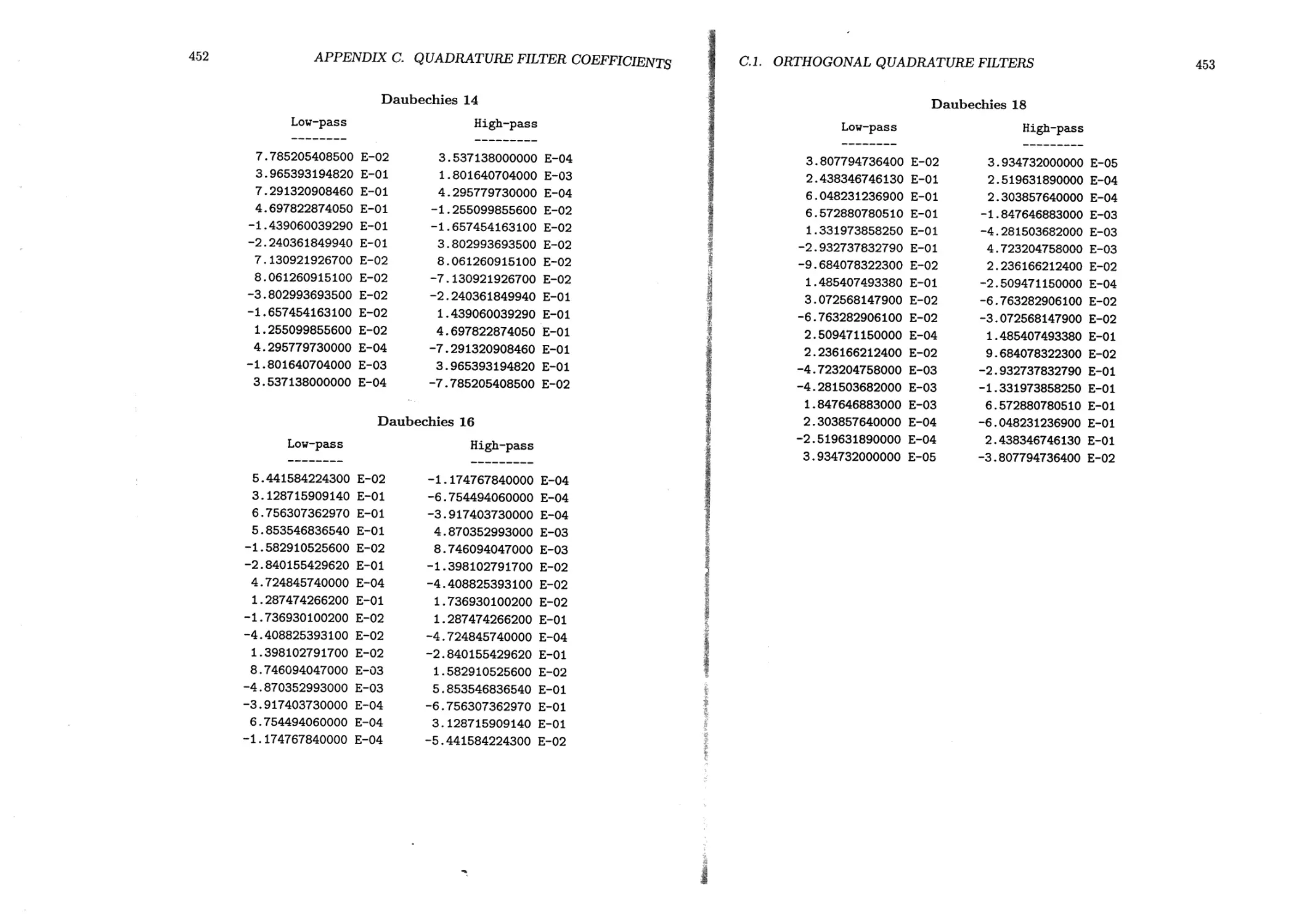
C Quadrature Filter Coefficients 443
C.l Orthogonal quadrature filters..................................443
C.1.1 Beylkin filters ....................................... 444
C.l.2 Coifman or “Coiflet” filters.............................444
C.1.3 Standard Daubechies filters............................ 449
C.1.4 Vaidyanathan filters.....................................454
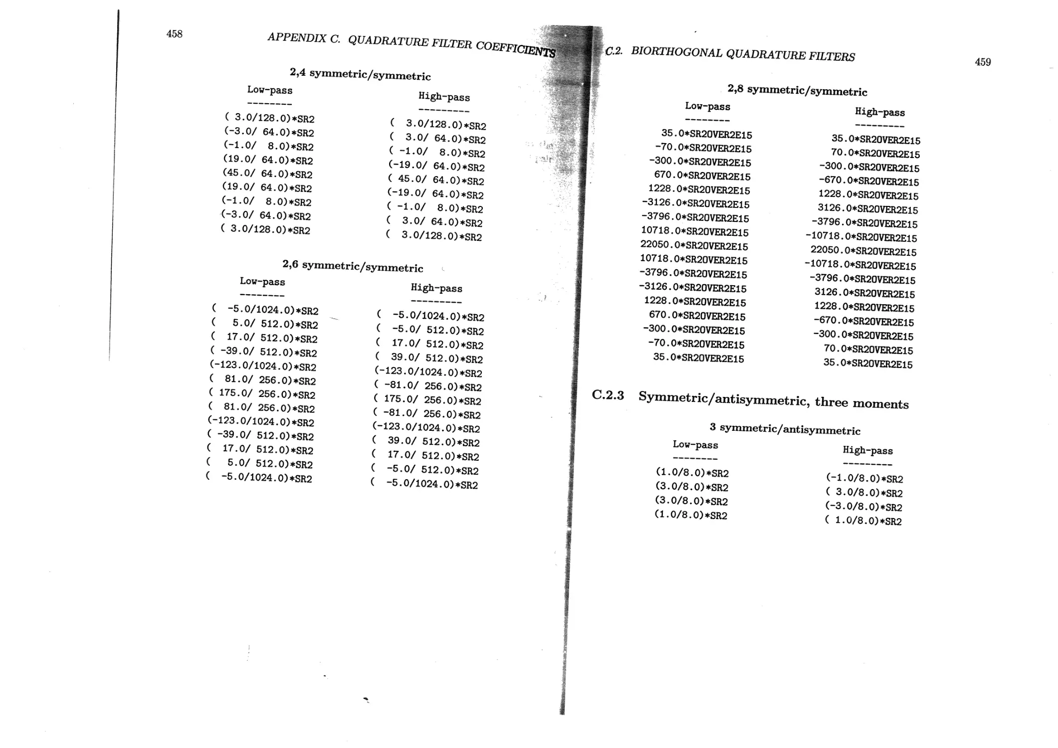
C.2 Biorthogonal quadrature filters ...............................455
C.2.1 Symmetric/antisymmetric, one moment......................456
C.2.2 Symmetric/symmetric, two moments..................... . 457
C.2.3 Symmetric/antisymmetric, three moments...................459
Bibliography
Index
463
475
Chapter 1
Mathematical Preliminaries
The behavior of the algorithms discussed in this volume cannot be understood
without some knowledge of the mathematical properties of the underlying functions.
Thus, we will go over a few facts from real and harmonic analysis. This chapter
can be skipped by those who are skimming the text, but the reader is advised to
try the exercises as preparation for the mathematical development later.
1.1 Basic analysis
Analysis is the mathematical theory of infinite algorithms: evaluation of infinite
sums, limits of arithmetic operations iterated infinitely many times, and so on.
While no such algorithm can ever be implemented, some of its properties can be
determined a priori without ever completing the calculation. What is more, a large
finite number of arithmetic operations from a convergent infinite algorithm will
produce a result close to the limit, whose properties will be similar to those of
the limit. We will have a truncated infinite algorithm if we simply stop after a
sufficiently large number of steps.
If a finite algorithm is a truncated infinite algorithm which has no limit, then
the finite algorithm will be unstable, i.e., the result will vary greatly with differing
truncations. On the other hand, truncating a convergent infinite process at any
sufficiently large number of steps will produce essentially the same result. This is
the idea behind Cauchy’s criterion for a sequence {n(n)}: For each € > 0 we can
find a sufficiently large N such that if both n and m are greater than TV, then
\a(n) — a(m)| < e. If a(n) is the output of an infinite algorithm after n operations,
then after sufficiently many (ЛГ) operations all the outputs will be within c of each
2
CHAPTER 1. MATHEMATICAL PRELIMINARIES
other. If |€/а(Я)| is smaller than the machine precision, then all outputs after a(N)
are indistinguishable and we might as well truncate the algorithm.
Algorithms whose outputs are themselves infinite sets, like solution functions for
differential equations, must be truncated still further. The output will always be a
finite set, such as a finite set of samples for a function or a finite list of coefficients in
an expansion for the function, and we may imagine that the rank of this set is fixed
in advance. For each such rank M there will be an error between the finite-rank
approximation and the actual infinite-rank solution, and we may ask how this error
behaves as M —> oo. At the very least the error must go to zero, but as a practical
matter we should also know how fast it goes to zero in comparison with various
functions of M, like M“2 or 1/logM or 2“M.
It has become abundantly clear that the successful interpretation of the numbers
produced by numerical and signal processing transformations requires some basic
results from measure theory and functional analysis.
1.1.1 Convergence of series and products
A sequence {a(n): n = 0,1,...} is absolutely summable if the following limit exists
and is finite:
<o°-
n=0
An absolutely summable sequence has the advantage that its elements can be added
up in any order and will yield the same result, up to roundoff error on a finite
precision machine. The sequence is square-summable if we have the following:
lim 22|a(n)|2 <oo.
/v—*oo *
n=0
Then {|a(n)|2} is absolutely summable. This is a weaker condition than absolute
summability for {a(n)}.
Doubly infinite sequences {a(n) : n = 0, ±1, ±2,...} are absolutely summable if
both the positive-indexed and the negative-indexed sides are absolutely summable.
They are square-summable if both sides are square-summable.
A sequence of functions {un = ttn(t)} is said to converge at a point to if the
sequence of numbers {un(to) • n = 1,2,...} converges as n oo. If {un(i)}
? converges at each t, then the limits define a function u(t) — limn__ooun(t). The
convergence is said to be uniform if un(t) —* u(t) at comparable rates for each t, £e.,
if for every e > 0 there is an N > 0 such that we have n > N => |un(t) — u(t)| < e
for every t.
1,1. BASIC ANALYSIS
3
Proposition 1.1 If un is a continuous function for each n and un(t) —* u(t) con-
verges uniformly in t, then и = u(t) is a continuous function. □
This result is proved as Theorem 9.2 of [3]. It implies that if {vn = vn(t)} is
a sequence of bounded continuous functions and {cn} is an absolutely summable
sequence, then CnVn is a continuous function.
The infinite product of a sequence {b(n) : n = 0,1,...} is defined by
П fc<n) d= Jim П 6(n)>
Л.Л. /V—+00 Л. A.
n=0 n=0
(1-1)
whenever this limit exists and has a finite, nonzero value.
Lemma 1.2 (Weierstrass Product Test) If the sequence a(ri) = b(ri) — 1 is ab-
solutely summable, then fl^=o^(n) ex^s^s an^ no larger than exp(J2n |a(n)|).
Proof: First note that 0 < log(l 4- |яг|) < |ж| for all real numbers x. Then, writing
|&(n)| = |1 4- u(n)| <14- |a(n)|, observe that
bg Г n = 22log ib(n)i - 22 22 ia(n)i < °°-
\n=0 / n=0 n=0 n=G
This also gives the upper bound on the size of the product.
Since {u(n)} is absolutely summable its elements must satisfy |a(n) | < 1/2 for all
sufficiently large n, so we may assume (extracting finitely many factors if necessary)
that a(n) > —1/2 for all n. Notice that log |14-ж| > —(2 log2) |x| for all x > —1/2.
We may thus write log |6(n)| = log |1 4- a(n)| > — (21og2)|a(n)|, and observe that
(N \ oo
П l6(n)lI -(2log2) 22 l“(n)l >
n=0 / n=0
This implies that П^=о l^(n)l > 0-
1.1.2 Measurability
Define Lebesgue measure on R to be the map E |E| defined on all subsets E C R
ЬУ oo oo
|£| = inf I - afc|: Я C (j (ak, bk) 1. (1.2)
lfc=0 fc=0 J
Here we are taking the infimum over all countable covers of E by open intervals
of the form (afc,hfc), where possibly some of the intervals are empty. This is often
4
CHAPTER 1, MATHEMATICAL PRELIMINARIES
called Lebesgue outer measure, but following Evans and Gariepy [44] we will not
treat the restriction of outer measure to well-behaved (“measurable”) subsets as
a different object. We will also treat the qualifier “Lebesgue” as optional. It is
elementary to prove that |0| = 0 and 0 < |E| < oo for each E C R, and that the
following properties hold:
• Countable subadditivity: If En for n = 0,1,2,... is a countable sequence of
subsets of R, then lU^Lo-^nl - EXo l£n|;
• Monotonicity: If E and F are any two subsets of R, then |F\ < \F П E| +
|F П Ec\, where Ec is the complement of E in R;
• Measure of an interval: |[a, b]| = |]a, b[| = | [a, b[| = |]a, b]| = b — a.
More generally, a positive measure on R is a map from subsets of R to R+ which
is countably subadditive and monotonic, but which measures intervals [a, 6] using
some otter nondecreasing function than b — a. A measure is the difference between
two positive measures.
We can construct Lebesgue measure on Rn, n > 1, simply by using products
of intervals. We will also denote the Lebesgue measure of a set E C Rn by |E|.
The properties described below continue to hold if we replace R with Rn. The
construction is completely abstract and applies to other measures as well.
A subset E C R has zero (Lebesgue) measure if for every e > 0 there is a
countable collection of open intervals Д, к e Z, such that l^fcl < 6 and
E C UfceZ a property holds for all points in R except possibly for a set of
measure 0, then we will say that it holds almost everywhere, or for almost every
x € R, or abbreviate a.e.x.
A subset E C R is (Lebesgue) measurable if for every F C R,
|F| = |EnF| 4- |EcnF|,
i.e., if equality holds in the monotonicity property. Lebesgue measure is countably
additive on measurable sets: If {^n}n€z a sequence of disjoint measurable sets,
then IUn€Z^nl = SneZl^nl- Intervals are measurable, and measurability is
preserved by countable unions, intersections and complements. But not all subsets
of R are Lebesgue measurable; see [3], p.304 for a counterexample.
A real-valued function и = u(x) of one real variable is said to be (Lebesgue)
measurable if for every a € R, the set Ea = {x : u(x) > a} is measurable. A
complex-valued function is said to be measurable if both its real and imaginary
parts are measurable.
и. BASIC ANALYSIS
5
1.1.3 Integrability
The Riemann integral of a function и = u(x) on an interval [a, b] is the limit of the
Riemann sums:
fb N-i
/ u(x)dx =f lim У2 u(xk)(ak+i -ak). (1.3)
Д^° IS
Here a = ao < ai < • • • < = b is an arbitrary partition, xk € [ak, Ofc+i] is
an arbitrary point in the fcth subinterval of the partition, and A = max{|a&+i -ak\ :
0 < к < N} is called the mesh of the partition. As A —> 0, it forces N —> oo. A
function и is Riemann integrable if this limit exists regardless of the exact manner
in which we choose the partition or the points of evaluation xk in the subintervals.
Riemann sums provide an infinite algorithm for computing the integral of a function;
Riemann integrability is just the guarantee that this algorithm can be truncated.
The following basic fact, proved for example as Theorem 7.48 in [3], shows that
most reasonable functions are Riemann integrable:
Proposition 1.3 If и is a bounded function defined on [a, 6] whose discontinuities
form a set of zero measure, then и is Riemann integrable on [a, &]. □
We also define the improper Riemann integral to be Нть-_оо tt(x) dx in the case
b = oo, and to be limc-4a+ f^u(x)dx in the case that |u(x)| —* oo as x —* .
However, Riemann sums are unwieldy in calculations, so we turn to a more general
notion of integral.
If и = u(x) is a measurable function on R taking only nonnegative real values,
then the function
au(r) == |{# € R: u(x) > r}| > 0 (1.4)
defined for r > 0 will be called the distribution function of u. Then r < s =>
ftu(r) > au(s), so otu is monotonic and decreasing and can therefore have at most
countably many discontinuities. Hence au is Riemann integrable on ]0, oof, though
the improper Riemann integral may be +oo. We now define
«+W
u_(x)
f u(x), if u(x) > 0;
| 0, if u(x) < 0;
f 0, if u(x) > 0;
1 —u(x), if u(x) < 0.
(1-5)
(1-6)
If и is measurable then so are both and tt_, hence so is |it| = u± 4- tt_. Also,
и = U_|_ — U-.
6
CHAPTER 1. MATHEMATICAL PRELIMINARIES
The Lebesgue integral of a measurable function it is the difference of the two
Riemann integrals below, in the case that both are finite:
/ u(x)dx~ / OLu^{r)dr— / ou_(r)dr. (1.7)
J Jo Jo
Measurable functions it for which both au+ and au_ have finite Riemann integral
will thus be called Lebesgue integrable.
These notions of integrability can be compared using a smooth positive function
u. The Riemann integral divides the domain of it into small simple pieces Д =
[afc,afc+i], each of known size |Д| < Д, then picks a random representative u(xk)
for the value of и in Д. For smooth it these representatives are close to all values
of it in Д, so that converges to Ja u(x) cte as Д 0. The Lebesgue
integral, on the other hand, fixes a small range [it*, itfc+i[ of values of it, and looks at
the approximate measure о(г^), it& < < itfe+i of the set of points x where it takes
on such values. We can also use the analogy of counting coins. Lebesgue integration
first arranges the coins into stacks by value and then measures the heights of the
stacks. Riemann integration, on the other hand, scatters the coins equally among
many little boxes and then picks one “average” coin from each box.
A measurable function / is Lebesgue integrable if and only if it is absolutely
integrable, meaning that |/| is Lebesgue integrable. Thus oscillation or cancellation
of negative and positive parts must not be essential to the existence of the integral.
Also, f is locally integrable if |f (ж)| dx exists and is finite for all finite numbers
a, b, or equivalently if l[a,6] (#)/(#) is Lebesgue integrable for every bounded interval
[a, 6]. Localizing distinguishes the two ways that the integral of a function might
diverge: there may be large values on small intervals, or there may be insufficient
decrease to zero at infinity.
A basic result is that we can exchange integration and differentiation under
certain conditions:
Proposition 1.4 If both и = u(x,t) and du(x,t}/dx are Lebesgue integrable func-
tions oft, then
[ u(x,t)dt— [ -^-u(x,t)dt.
dx J J dx
1.1.4 Metrics, norms, and inner products
A linear spo.ce or vector space in our context will be a set of vectors with scalars
taken from either R or C. We will consider both finite-dimensional and infinite
dimensional vector spaces.
и. BASIC ANALYSIS
7
A metric on a set S is a function dist : S x S —* R+ satisfying the following
conditions, for all ж, г/, z G S:
® Symmetry: dist(x,y) = dist{y^x)\
• Nondegeneracy: dist(x1t/) = 0 <=> x = y;
• Triangle inequality: dist(x,z) < distfay) + dist(y,z).
The pair (S,dist) is called a metric space. If S is a linear space and the metric
dist satisfies dist(x + z,y + z) = dist(x,y), or more generally if S is a group and
dist satisfies dist(xz^yz) = dist(x,y), then we will say that dist is invariant under
translation.
A Cauchy sequence in a metric space S is an ordered subset {un : n € N} such
that for every e > 0 there is a sufficiently large number M which will guarantee that
dist(ui, Uj) <6 whenever both i > M and j > M. The limit of a Cauchy sequence
is an element Uqo satisfying dist(un, Uqo) —♦ 0 as n —* co. The metric space S is
complete if every Cauchy sequence has a limit in S.
A norm on a vector space S is a map || • || : S —* R+ satisfying the following
properties for all x, y^ z G S and a G C:
® Scaling: = |а|]|ж||;
® Nondegeneracy: ||ж|| =0 <=> x = 0;
• Triangle inequality: ||ж — z|| < ||x — y\\ + \\y — z\\.
The function dist(x, y) = ||x — z/|| is thus an invariant metric.
A (Hermitean) inner product on a linear space S is a function S x S C
satisfying the following properties for all f,g,he S and a,b G C:
l
• Linearity: (f, ag + bh) = a{f,g) + b{f, h);
• Hermitean symmetry: (f,g) = {g,f);
• Positivity: (/,/)=0 <=> /=0.
The first and second properties imply that {af + bg, h) = a{f,g) + b(g, h}, which is
sometimes called sesquilinearity. Also, the third property implies that if (/, g) = 0
for all g e S, then f = 0, which is sometimes called nondegeneracy.
We can always define a norm from an inner product by the formula
IMI frx}1'2. (1.8)
8
CHAPTER 1. MATHEMATICAL PRELIMINARIES
Thus an inner product space is a normed linear space is a metric space with an
invariant metric. Some simple examples of inner product spaces are CN for each
N > 0. A complete inner product space is also called a Hilbert space. Some familiar
examples of Hilbert spaces are the TV-dimensional real (or complex) vector spaces
ВЛ (or CN), and the infinite-dimensional function space L2(R).
We can estimate the inner product from the norm using the Cauchy-Schwarz
inequality:
l</,s)l <11/11 hll-
(1-9)
If the norm is derived from an inner product, then we can recover the inner product
from the norm using polarization:
4W,P>} = IIZ + sll2 - + (1-10)
1.2 Function spaces
1.2.1 Continuous functions on the circle
We will denote the collection of all continuous, one-periodic real (or complex-valued)
functions by C(T). If we wish to indicate that we have relaxed the periodicity
condition so as to allow continuous functions и for which u(0) / u(l), then we will
use the notation C([0,1]). Either of these collections forms an inner product space
with the Hermitean inner product defined by the integral:
{f,g> = / fW>g(t)dt.
(1-11)
This is also a normed linear space with the derived norm ||/|| = (/, and a met-
ric space with the derived invariant metric dist(f, g) = || /—<j||. Neither (C(T), dist)
nor (C([0,1]), dist) is a complete metric space, however, because the metric permits
Cauchy sequences of continuous functions {/n : n = 1,2,...} whose limits are not
continuous functions. We will remedy this defect in two ways: by changing the met-
ric to impose better convergence on Cauchy sequences, or by enlarging the space of
functions to include all the limits.
We can alternatively define the uniform norm || • |joo, which gives a different
invariant metric on the continuous functions:
Moo = sup{|w(t)| : 0 < t < 1}.
(1.12)
The normed spaces (C(T), || • Ц^) and (C([0,1]), || • ||oo) are complete metric spaces.
1.2. FUNCTION SPACES
9
1.2.2 Lebesgue spaces
The (Lebesgue) Lp-norms || • ||p, for 1 < p < oo, are defined for measurable functions
и by
(f \u(t)\p dt)1/p = prp ^^(rjdr,
ess sup \u\ d= inf{r : au(r) = 0},
(1.13)
It can be shown (see [3]) that if Ц/ — g\\p = 0 in LP (for any p e [1, oo]) and / and g
are continuous functions, then f(x) = g(x) for every x. But measurable functions
need not be continuous, so to preserve the essential nondegeneracy property of the
IP norm we must change the notion of equality. All that we can conclude from
|| f || = 0 is that the points x where f(x) 0 form a set of measure zero. Thus the
IP “norms” fail to satisfy the nondegeneracy condition, but this can be remedied
by identifying as equal any two functions и and v for which ||u||p and ||v||p are both
finite and ||u — v||p = 0. Any pair u, v which are thus identified can be shown to
satisfy u(t) = v(t) at almost every t € R. The collection of equivalence classes of
measurable functions и satisfying ||u||p < oo is called the Lebesgue space LP(R). By
substituting T for R we similarly define LP(T).
Each LP-norm provides a derived invariant metric distp(x,y) = ||x — y\\p. For
each p, the metric space (IP, distp) is complete. L2 in particular is a Hilbert space,
where the inner product can be defined by polarization or directly in terms of the
Lebesgue integral:
II/li £2 (R)
(A 9)l2(R.)
(1-14)
(1.15)
We may also define L2(Rn) for any n > 1 just by integrating over Rn rather than R
in the definition of ||/||L2(Rn) and {fidj&fjRny Likewise, we can define L2([0, l]n)
to be the Hilbert space of functions of n real variables which are one-periodic in
each variable.
Square-summable sequences form the Hilbert space £2 = £2(Z), with inner prod-
uct and norm defined as below:
(1.16)
(1.17)
10
CHAPTER 1. MATHEMATICAL PRELIMINARIES
Likewise, we can define ^2(Zn) to be the Hilbert space of square-summable sequences
indexed by n integers.
Henceforth, we will use || • || and (•, •) without subscripts to denote the norm and
inner product in L2 or ^2, whenever the space is clear from the context.
1.2.3 Spaces of test functions
The support of a function w, denoted supp ti, is the complement of the largest open
set E with the property that t € E => u(t) = 0. Thus the support of a function
is always a closed subset of the domain of the function. We say that the function
и is compactly supported if supptt is compact. If the domain is N, Z, or Zn, then
the sequence и is compactly supported if and only if all but finitely many of its
elements are 0; we will call such и finitely supported. If the domain is Rn, then
и is compactly supported if and only if the support set is bounded: there exists
some R < oo such that s, t € suppn => \t — s| < R. The smallest R for which the
preceding implication holds is called the width or diameter of the support of и and
will be denoted diam supp u.
The support of a measurable function is a measurable set. It should be noted
that if E C Rn, then |£^р/п < diam E. However, diam I? and |£| are not compara-
ble quantities: for every € > 0 there is a set E C Rn for which < e diam £7.
In R = R1, an easy example is the set [0, e/2] U [1 — e/2,1].
We will say that a function и is smooth if dnu/dtn is a continuous function for
all n € N. We will use the weaker notion of smooth to degree d if dPu/dt71 is a
continuous function for all 0 < n < d.
We will say that a function и has rapid decrease at infinity if for every n € N
we have a finite constant Kn > 0 such that for all t € R, |tnu(t)| < Kn- This
is also called superalgebraic decay at infinity. It is not quite as strong a notion as
exponential decay at infinity, for which we need to have some constants K, a > 0
for which the estimate |u(t)| < Ke~a^ holds. To prove this, consider the example
f(t) = , which is the subject of one of the exercises. We will say that и
has degree d decay at infinity if Kn < oo at most for 0 < n < d. It is evident that
compactly supported functions have all possible kinds of decay at infinity.
The Schwaitz class S is the set of measurable smooth functions of superalge-
braic decay at infinity, z.e., the functions и = u(t) satisfying an inequality like the
following for each n,m € N:
I dm
sup I : t e R
Km,n < OO-
(1-18)
1.2. FUNCTION SPACES
11
This condition is equivalent to satisfying the inequality
for all n, m G N. Those Schwartz functions which are also compactly supported are
called test functions; the class of such functions is denoted by T>. Schwartz functions
(and test functions) are dense in all the Lp spaces with p < oo, and in larger classes
of spaces as well. For calculations, it is often useful to define formulas first on test
functions or Schwartz functions, and then extend them to a larger class of functions
by continuity.
1.2.4 Dual spaces
If X is a function space we can define its dual space X' to be the collection of
continuous linear functions T from X to R or C. Such maps themselves form a
normed linear space using the operator norm:
l|T||x- = ||T||OP d= sup ( : и G X, и + 0 >.
(1-20)
If X С У, then У' C Xf, since there are fewer continuous functions on a
larger space. Thus a highly restricted space like S has a very large dual space
which contains all sorts of interesting things. For example, it contains arbitrary
derivatives of certain discontinuous functions.
Duals of 17 spaces
If X = 17 for some 1 < p < oo, then the following theorem characterizes X':
Theorem 1.5 (Riesz Representation) LetT be a continuous linear function on
17, for 1 < p < oo. Then there is a function 0 = 0(x) in 17 , such that
T(u) = J 0(x)u(x) dx.
Here pf = p/(l — p) if p > 1 and p' = oo ifp = 1.
A proof of this may be found in [96], p.132. Note that if T(u) = f 0(x)u(x) dx =
f p(x)u(x) dx, then f (р(я) — 0(x})u(x) — 0 for all и € 17. This implies that
6(x) = p(x) for almost every x, so they are equal in the sense of Lp . Thus T 0
is a one-to-one correspondence, and we can identify (TZ) = 17 .
The dual index p' satisfies the equation = 1, showing how we are victims
Jr r
of a bad choice of notation (p rather than 1/p) made sometime in the dim past.
12
CHAPTER 1. MATHEMATICAL PRELIMINARIES
Measures and the dual of C
If X = C([0,1]) is the space of continuous functions on [0,1] with the uniform norm,
then X1 can be identified with the space of bounded measures /z on the interval [0,1],
namely the measures which satisfy /z([0,1]) < oo. The identification is through the
distribution function: for every bounded measure //, we get a linear function T = T^
defined on positive functions и by the formula:
T(u) = j u(x) dp(x) d= J //({я : u(x) > r}) dr.
def"
For real-valued continuous functions и we use T(u) = T(u+) — T(u_), and for
complex-valued и we separately compute and then add up the real and imaginary
parts.
Every locally integrable function m = m(x) generates a measure p by the for-
mula p([a, b]) = fb m(x) dx, but there are also some bounded measures which can-
not be realized in this way. Thus the dual space C([0,1])' contains more objects
than just functions. In particular, it contains the Dirac mass at 0, 6, which is
defined by the following formula:
6u = u(0).
(1.21)
The Dirac mass is a bounded measure for which there is no bounded function m.
It is very common to abuse notation and write 6 = 8(x) as the Dirac delta function
and to “evaluate the integral” 6u = f u(x)6(x)dx = tt(O). It is also common to
write the Dirac mass at c as a translate of the Dirac mass at zero, namely 6(x — c).
Distributions
The dual space V of the test functions contains what are called distributions, and
the dual space S' of the Schwartz functions contains tempered distributions. Since
D C S, we have S' C Df; both are proper inclusions.
Every measurable and locally integrable function 0 defines a distribution by the
formula T(</>) = J 0(х)ф(х) dx, where ф eD. This gives a natural inclusion of the
Lebesgue spaces into <$'; we have S C LP C S' for every 1 < p < oo.
Every distribution has a derivative which makes sense as a distribution, and
every tempered distribution has a derivative among the tempered distributions.
This derivative is evaluated by integration by parts: to compute the nth derivative
of the distribution T, we use the formula
т(п\ф) =( (-l)"T(</>(n)).
(1.22)
1.2. FUNCTION SPACES
13
For example, the derivative of lj^+ (rr), also known as the Heaviside function or the
unit step at zero, is the Dirac mass 6. Also, every measurable and locally integrable
function 0 has as many derivatives as we like among the distributions, given by the
formula
T<")(^) (-1)" [ е(х)ф(п\х)<1х.
We can define the Fourier transform of a tempered distribution, which is itself a
tempered distribution, by “passing the hat”: for all ф € 5,
Т(Ф) = Т(ф).
This works because <S is preserved by the Fourier transform; it does not hold for ТУ
since the compact support of ф € T> is destroyed by the Fourier transform.
A distribution T has compact support if there is a bounded interval I such
that Т(ф) = 0 whenever supp</> is in the complement of I. The Dirac mass at a
point has compact support. A measurable, locally integrable function of compact
support corresponds to a compactly supported distribution. A compactly supported
distribution is tempered, and its Fourier transform is given by integration against
a smooth function.
Convolution is defined for two tempered distributions by the formula
(Т^ТгХф) = W);
where 1 = y e R’
1 фу(х) = ф(х + у), x € R.
(1.23)
It is left as an exercise to show that ф € S => ф E S.
If Ti and T2 are defined by integration against functions and O2, then * T2
will be defined by integration against the function 0\ *02(#) <== J (y)&2(x — y) dy.
We note that the Dirac mass at a convolved with the mass at b is the Dirac mass
supported at a + b.
1.2.5 Frames, bases, and orthonormality
If If is a complete inner product space, then we say that a collection {фп : n € Z} is
an orthonormal basis (or Hilbert basis) for H if the following conditions are satisfied:
• Orthogonality: If n, m € Z and n m, then {фп, фт) =0;
• Normalization: For each n E Z, ||</>n|| = 1;
• Completeness: If f E H and ^,фп} — 0 for all n E Z, then f = 0.
14
CHAPTER 1. MATHEMATICAL PRELIMINARIES
Any collection satisfying the first two conditions, but not necessarily satisfying the
third, will be called simply orthonormal. If it satisfies only the first condition, it will
be called simply orthogonal. Note that our Hilbert basis has (at most) a countable
infinity of elements; any Hilbert space with a countable basis is called separable,
and all of the examples we have mentioned are separable.
An alternative notion to completeness in separable Hilbert spaces is density.
The collection {фп : n G Z} is dense in H if for every f G H and € > 0, we
can find a sufficiently large N and constants a_^,a_2v+i,... ,а^-1,а^ such that
ll-f-lX-N < €- Another way of saying this is that finite linear combinations
from the system {фп : n G Z} can be used to approximate functions in H arbitrarily
well, as measured by the norm. An orthonormal system {фп} is dense in H if and
only if it is complete.
If {0n} is a complete orthonormal system, then we can compute the norm of a
function from its inner products with the functions фп using Parseval’s formula:
oo
ii/ii2= E кло2-
n=—oo
(1-24)
Parseval’s formula implies that the inner products (/, фп) form a square-summable
sequence.
Note that orthogonality implies linear independence. We may wish to construct
a collection {фп : n G Z} which is neither orthogonal, nor even linearly independent,
but which can still be used to approximate functions. One important property to
preserve is comparability between ||/|| and the sum of the squares of its inner
products with the collection. We say that an arbitrary collection of functions {фп G
H : n G Z} is a frame if there are two constants A and B, with 0 < A < В < oo,
such that for every f e H we have:
oo
n= —OO
(1-25)
A and В are called frame bounds. If A = В then we have a tight frame. An
orthonormal basis is a tight frame for which A = В = 1, but not all such tight
frames are orthonormal bases. If the collection {фп : n G Z} is a frame and is aiso
linearly independent, then it is called a Riesz basis. Frames and Riesz bases are
complete by virtue of the left inequality in Equation 1.25: if (/, фп} = 0 for all n,
then 0 < ||/Ц < J20 — 0 => f = 0. Any Riesz basis can be made into a Hilbert
basis by Gram orthogonalization, which is described in [37].
1.2. FUNCTION SPACES
15
Standard orthonormal bases
If the Hilbert space H is Cn, then the Hermitean inner product is
(u.v) d=
k=i
(1.26)
where u(k) is the element in the kth row of the column vector u. The standard basis
consists of the vectors
(1.27)
Here Cfc is the column vector with a single in the kth row and zeroes elsewhere.
These are evidently orthonormal with respect to the inner product.
If H is an infinite-dimensional but separable Hilbert space, then H is isomorphic
to the space ^2(Z) of infinite, square-summable sequences. The Hermitean inner
product is
oc
(u, v) J" u(k)v(k). (1.28)
fc=—oc
There is a standard basis of elementary sequences = {efc(n)} consisting of a
single “1” at index к and zeroes elsewhere. How these look in the original space H
depends on the isomorphism, which is not always easy to compute.
Bases of eigenvectors
A straightforward calculation shows that for any n x n matrix A = (aij), and any
pair of vectors u, v € Cn, we have the identity
(u, Av) = (A* u, v), (1.29)
where A* = a*k is the adjoint or conjugated transpose of A, defined by a*k =f d^.
We say that the n x n matrix M is Hermitean or selfadjoint if for any pair of vectors
u, v E Cn we have
(u,Mv) = (Mu.v), (1.30)
or equivalently that M* = M. A real-valued symmetric matrix is Hermitean.
16
CHAPTER 1, MATHEMATICAL PRELIMINARIES
An eigenvalue for a matrix A is any number A such that there is a nonzero
solution vector у to the equation Ay — Xy. Such a у is then called the eigenvec-
tor associated to A. One way to find eigenvalues is to solve for the roots of the
polynomial in A that we obtain by expanding the equivalent condition
det(A — A/) = 0.
(1-31)
This method is not the best one if n is large because it is both computationally
complex and ill-conditioned.
Eigenvalues of a Hermitean matrix A = A* must be real numbers, since
АЦг/If2 = {Ay,y) = (y, A*y) = (y,Ay) = A||j/||2
(1.32)
and ||у || 7^ 0. Furthermore, if there are two distinct eigenvalues Ai A2, then their
associated eigenvectors yi and У2 must be orthogonal:
0 = {Ayi,y2} - {yi,Ay2) = (Ai - А2)0/1,г/2), =* (l/i,1/2) = 0. (1.33)
An important consequence of these elementary results is that we can make an
orthonormal basis out of the eigenvectors of a selfadjoint matrix:
Theorem 1.6 An nxn Hermitean matrix has n linearly independent eigenvectors
Уъ — чУп which, if suitably chosen and normalized so that ||р^|| = 1 for all k =
1,..., n, form an orthonormal basis for Cn. □
A proof of this theorem may be found, for example, on page 120 of [2] .
A result from Sturm—Liouville theory
The Sturm-Liouville differential operator acting on a twice-differentiable function
у = y(x), 0 < X < 1, is
Dy =f (py'Y + qy,
where q = q(x) is a continuous real-valued function, and p = p(x) is a differentiable
real-valued function. If p is never zero in the interval [0,1], then D is called a regular
Sturm-Liouville operator. We can of course replace [0,1] with any bounded interval
[a,b].
Notice that Dy makes sense as a distribution even for p € L2([0,1]). If у € L2
is regular enough so that Dy G L2, then qy e L2 so (ру’У € L2([0,1]) and is thus
integrable. Integrating twice shows that у must be continuous on [0,1]. We can
therefore impose additional conditions on such functions by specifying their values
at the boundary points 0 and 1.
1.2. FUNCTION SPACES
17
The Sturm-Liouville boundary conditions for у on the interval [0,1] are
ш/(0) + by'(0) = 0; cy(l) + dy'{l) = 0. (1.35)
Here a, b, c, d are four real numbers with not both a = 0 and b = 0, and not both
c = 0 and d = 0. Notice that if the differentiable functions и = u(x) and v = v(x)
both satisfy these conditions, then
u(0)u'(0) — i/(0)u(0) = 0 and u(l)v'(l) — u'(l)v(l) = 0. (1.36)
This is because the following two matrices must be singular, since they have the
nonzero vectors (a, b)T and (c, d)T in their null spaces:
/ w(0) wz(0) A ( UW \
у u(0) n'(0) ) ’ у v(l) v'(l) ) ’
Let H be the set of functions у € L2([0,1]) satisfying Dy E L2([0,1]) and also
satisfying the boundary conditions in Equation 1.35. All the conditions are linear,
so the result is a subspace of L2([0,1]) with the same Hermitean inner product. It
is not hard to show that H is a dense subspace, so any Hilbert basis for H will
automatically be a Hilbert basis for L2([0,1]).
Now D is a selfadjoint operator in the domain H. We compute the adjoint
through integration by parts:
{u, Dv) = {Du, v} ip(x) [u{x)v’{x) — u'{x)v{xf\ |*=0 = (Du,v). (1-37)
The boundary term vanishes because of Equation 1.36. In fact, D is the most
general form of a selfadjoint second-order linear differential operator.
The Sturm-Liouville eigenvalue problem for the operator D and the domain H
is to find eigenvalues A € R and eigenfunctions у € H such that
Dy(x) = Xy{x}, for all 0 < x < 1. (1.38)
The eigenvalues must be real numbers because of Equation 1.32 and the eigenfunc-
tions associated to distinct eigenvalues must be orthogonal because of Equation
1.33, since both of those equations are valid for every Hermitean inner product.
Not only are there solutions to this problem, but there will be enough of them
to construct a Hilbert basis. We have the following theorem about regular Sturm-
Liouville boundary value problems:
Theorem 1.7 Each regular Sturm-Liouville eigenvalue problem on [0,1] has an
infinite sequence of eigenvalues {Xk • к = 0,1,2,...} c R with |Afc| —* oo as
k —* oo. The associated eigenfunctions {yk • к = 0,1,2,...}, when normalized so
that = 1 for all к, form an orthonormal basis for L2([0,1]). □
18
CHAPTER 1. MATHEMATICAL PRELIMINARIES
A proof of this theorem may be found, for example, in [93]. Notice how it generalizes
Theorem 1.6.
1.3 Fourier analysis -
By Fourier transform we shall mean any one of several mathematical transfer- p
mations, with the specific transformation being unambiguously chosen from the
context. The function (or sequence, or vector) produced by the Fourier transform
contains spectral information about the function, in the sense that each Fourier
coefficient is an inner product with an oscillating basis function of, well-defined fre-
quency and phase.
Fourier’s representation of functions as superpositions of sines and cosines has
become ubiquitous for both the analytic and numerical solution of differential equa-
tions, and for the analysis and treatment of communication signals. Fourier’s orig-
inal idea was to write an “arbitrary” one-periodic function f = f(x) as a sum:
oo oo
/(ж) « a(0) + \/2 a(n) cos 2irnx + y/2 b(n) sin 2тгпх,
n=l n=l
(1.39)
where the constants a(0),a(l),... and 6(1), 6(2),..., called the Fourier coefficients
of /, are computed from f via integrals:
a(0) = a/(0)
a(n) = a/(n)
6(n) = bf(n)
def
def
def
cos 2тгпх dx,
sin 2тгпх dx,
for n > 1;
for n > 1.
(1.40)
(1.41)
(1-42)
There has been a tremendous amount of literature written on the question of what
“arbitrary” means, and on the interpretation of the symbol in this context.
Some of the deepest results in mathematics concern the convergence of such “Fourier
series” for nonsmooth or possibly discontinuous functions. However, if f is a contin-
uous one-periodic function with a continuous derivative, then the two infinite series
in Equation 1.39 will converge at every point x e R; in fact, the series of functions
will converge uniformly on R, and we can legitimately replace the ~ with =. This
elementary fact is proved, for example, in [3], which also gives several refinements.
It was known even to Riemann [94] that there were continuous but not differentiable
functions whose Fourier series diverged at some point x, but then it was shown by
1.3. FOURIER ANALYSIS
19
Carleson [13], using much deeper analysis, that even without the differentiability
hypothesis, we still get pointwise convergence in Equation 1.39, only now it holds
just for almost every point x e R.
1.3.1 Fourier integrals
Following Stein and Weiss [103], we define the Fourier integral of a function on the
line by
Zoo
/(z)e-2^ dx. (1.43)
-oo
Since the exponential e 27ггх£ is a bounded function of x, this integral converges
absolutely for all absolutely integrable functions f and for every £ € R. In addition
we have a few results from functional analysis.
Lemina 1.8 (Riemann-Lebesgue) If f is absolutely integrable, then f is con-
tinuous, and f(£) —* 0 as |£| —* oo. □
Absolutely integrable functions are dense in L2(R), and we can show that the
Fourier integral preserves the L2 norm for this dense subset so that by the Hahn-
Banach theorem there is a unique continuous extension of f »-> f to all of L2(R).
The Plancherel theorem shows that the Fourier integral behaves like a unitary ma-
trix.
Theorem 1.9 (Plancherel) If f € L2(R), then f € L2(R) and ||/|| = ||/||. Also,
{f, g) = {f,g) for any two functions f,g € L2. □
Since the Fourier transform is a unitary operator on L2, its inverse is its adjoint.
The adjoint is defined by the integral
Zoo
gtf)e2”ix<d£.
-oo
It is evident that f(y) = f(—y), and thus like the Fourier integral this transform also
has a unique continuous extension to L2(R). We also have the identity f(y) = f(y)-
Theorem 1.10 (Fourier Inversion) If f e L2(R) and g = f, then g e £2(R)
and g = f. Likewise, if h = f, then h € L2(R) and h = f. □
The Fourier integral, Planchcrel’s theorem, the Riemann-Lebesgue lemma, and
the Fourier inversion theorem can all be extended to functions of n variables just
by taking integrals over Rn and replacing with x • £ in the exponents.
20
CHAPTER 1. MATHEMATICAL PRELIMINARIES
The Fourier integral transforms functions of rapid decay into smooth functions,
and transforms smooth functions into functions of rapid decay. In short, it maps the
Schwartz class into itself. We state this result for R; it holds for higher dimensions,
too.
Theorem 1.11 If и belongs to the Schwartz class on R, then so do й and u.
Proof: We know that is Lebesgue integrable because it is continuous and
decreases rapidly as x —► ±oo. But then J[-^u(x)}e~2^x^ dx is bounded, and we
can integrate by parts to conclude that (2тгг£)п f и(х)е~2кгх^ dx = (2тгг£)пй(£) is
bounded as £ —> ±oo.
We can interchange integral and derivative: f u(x)e~2mx^ dx =
J(—2тх)пи(х)е~21ггх^ dx, because the integrand remains absolutely integrable due
to the rapid decrease of u. This is true for all n € N, so we conclude that й is a
smooth function of %.
We can combine the previous two results by Leibniz’ rule to conclude that u
belongs to the Schwartz class. The same conclusion evidently holds for й(£) = fi(—£)
as well. О
1.3.2 Fourier series
If f = f(t) is a one-periodic function, then its Fourier series (in the modern sense)
is the infinite sum
oo
/(x)« 52 <№e2*ikx. (1.45)
k=—oo
The numbers in the sequence {c(k) : к € Z} are called the Fourier coefficients of
the function /; they are computed via the formula
c(fc) = f(k) d= / f(x)e~2*ikx dx.
Jo
(1-46)
We have conserved notation by reusing the symbol for the Fourier transform of a
function on the line. In a similar way, we can refer to the inverse Fourier transform
of the sequence {c}:
oo
c(e) c(k)e2*ik(. (1.47)
k=—oo
This is a one-periodic function of the real variable %. If {c} is absolutely summable,
then c will be a continuous function because of Proposition 1.1. We may also define
1.3. FOURIER ANALYSIS
21
the Fourier transform of a sequence or a trigonometric series by
c(e) =f У2 c(k)e~21,iki. (1.48)
k=—oo
This is to be considered a periodic function defined on the whole real line. Evidently
c(£) = c(—£). Again we conserve notation by making its meaning dependent on the
context.
The coefficients c are related to the coefficients a,b of Equation 1.39:
<z(0) = c(0); a(fc) = 2= [c(-fc) + c(fe)]; &(fc) = 2= [c(-k) - c(fc)]. (1.49)
v2 v2
In return, the coefficients a, b are related to the coefficients c by these formulas:
c(0) = a(0); c(—k) = [a(k) + ib(k)]; c(k) = [a(k) — ib(k)]. (1.50)
v2 v2
In both cases к = 1,2,3,....
It is important to note that f is assumed to be one-periodic, which implies
among other things that f(k) = fz+1 f(x)e~2™kx dx for any real z. The properties
of the Fourier coefficients depend on the behavior of f as a periodic function on the
whole line, and not just on its behavior in the interior of one period interval such
as [0,1]. In particular, one should beware of discontinuities hiding at the endpoints
of a period interval.
There are analogs to the Riemann-Lebesgue lemma, the Plancherel theorem,
and the Fourier Inversion theorem for Fourier series as well:
Lemma 1.12 (Riemann—Lebesgue) Suppose f is one-periodic. If f is absolutely
integrable on the interval [0,1], then f(k) —* 0 as |A:| —* oo.
Proof: Let f — f(t) be a periodic function which is absolutely integrable on [0,1].
Then
/(&) = [ f(t)e~2™kt dt = [ f (t + exp (—‘Inikt — гтг) dt
Jo Jo \ J
by the continuity of the L1 norm with respect to translation.
22
CHAPTER 1. MATHEMATICAL PRELIMINARIES
Corollary 1.13 If f is one-periodic and absolutely integrable on the interval [0,1],
and f'(xo) exists, then the Fourier series for f converges at the point xq.
Proof: We may assume without loss that xq = 0 and that /(0) = 0, since if not we
can just translate f and subtract a constant. We now write /(t) = (e~27rtt — 1) g(t")
and note that the one-periodic function g is absolutely integrable, since the quotient
f(t)/ (e~27ri* — 1) has a finite limit as t —* 0. But then f(k) = g(k + 1) — g(k), so
that we obtain a telescoping Fourier series for /(0):
m—1
k——n
By the Riemann-Lebesgue lemma, this series converges to zero as n, m —* oo in any
manner. □
Remark. These two elegant proofs were brought to my attention by Guido Weiss,
who believes that they are both many years old.
Theorem 1.14 (Plancherel) If f € L2(T), then f € ^2(Z) and
Also, {g, f) = fg g(x)f(x) dx = £kez ff(k)f(k) = f) f°r апУ f-9^ b2(T). □
Theorem 1.15 (Fourier Inversion) If f € L2([0,1]) and we put
N—l
fN(x) = £ f(k)e2nikx,
k=—N
N = l,2,3,...,
then fw f in the sense of L2(T) as N —a oo.
Proofs of these fundamental results may be found in [3], for example.
1.3.3 General orthogonal transformations
The representation of f by Equation 1.39 may be put into a more general context as
an expansion in an orthonormal basis: {1, \/2 cos 27гпж, x/2sin27rn:r : n = 1,2,...}
is orthonormal with respect to the (Hermitean) inner product of Equation 1.11. If
1.3. FOURIER ANALYSIS
23
{фк : к G Z} is any orthonormal basis for L2([0,1]), we can get an expansion of
/ € L2 ([0,1]) in these functions as follows:
N-l
fN = fN(x)= СА<^Ж(*)-
k=-N
(1.51)
The completeness of the basis implies that \\f — f^\\ —► 0 as N —► oo.
The functions {ф^ : j = 1,2,...} defined by ф^(х) = x/2sin7rjj; form an or-
thonormal basis of Z/2 ([0,1]) and can be used to compute the sine transform in a
manner identical to that of the Fourier transform, as in Equation 1.51. Likewise, we
can use the functions ф^х) = cos irjx, j = 1,2,... to get the cosine transform.
Another orthogonal transformation is obtained using ф^х) = \/2sin7r(j + I)x,
j = 0,1,2,..or alternatively ф^х) = %/2costt(J + |)x, j = 0,1,2,.... Still more
variations of sine and cosine are possible, such as the Hartley transform given by
the functions фу(х) = sin^jrr+ cos7i j = 0,1,2,.... The orthonormality of these
sets can be shown directly, or else we can use the Sturm-Liouville theorem with a
suitable operator and boundary condition. Likewise, the Sturm-Liouville theorem
gives their completeness, which can also be derived directly from the completeness
of the set {e27rtJX} in L2([0,1]) by taking appropriate linear combinations.
1.3.4 Discrete Fourier transforms
We now turn to the discrete and finite-rank case. For a vector v € CN, v = {v(/c) :
к = 0,1,..., AT — 1}, we define the discrete Fourier transform or DFT of v to be
the vector v € CN given by the following formula:
N—l
v(k) = -= V v(j)e~2,rijk/N,
k = 0,l,...,N -1.
(1.52)
The identity = e-2Trij(-k)/N impijes large positive frequencies
N—k are indistinguishable from small negative frequencies — k, a phenomenon some-
times called aliasing. If N is an even number, we can identify half the coefficients
v(k) :k = у, у + 1,..., Af — 1 with the negative frequencies —у, — у + 1,..., —1.
The other half of the coefficients gives the positive frequencies 0,1,2,...,у — 1.
This is what we will mean when we write the coefficients of v as
*(—7 + 1)- • • • v(0),v(l),... ,v(— - 1)
(1.53)
The vector in Equation 1.53 is simply v with its coefficients rearranged to better
suit certain purposes; we will use it when convenient.
24
CHAPTER 1. MATHEMATICAL PRELIMINARIES
The vectors € CN, j = 0,1,..., N — 1 defined by = -^e2^k/N form
an orthonormal basis with respect to the Hermitean inner product on CN. This
means that the map v > v is a unitary transformation, so we have an easy proof
of the Plancherel theorem in this context:
Theorem 1.16 (Plancherel) (v,w) = (u,w) for any two vectors v,w € CN. In
particular, ||u|| = ||v||. О
1.3.5 Heisenberg’s inequality
A square-integrable function и defines two probability density functions: x i—►
|u(t)|2/||u||2 and £ > |u(£)|2/||u||2. It is not possible for both of these densities to
be arbitrarily concentrated, as we shall see from the inequalities below.
Suppose that и — u(x) belongs to the Schwartz class S. Then |и(ж) |2 =
x [и(ж)й'(ж) 4- й(ж)и'(ж)] is integrable and tends to 0 as |ж| oo. We can therefore
integrate by parts to get the following formula:
[ -x-^-\u(x)\2 dx = [ |и(ж)(2 dx = ||u||2. (1-54)
Jr dx Jtl
But also, the Cauchy-Schwarz inequality and the triangle inequality imply that
Combining the last two inequalities gives ||жи(ж)(| • ||и'(ж)|| > |||u(x)||2. Now u'(£) =
2тгг£й(£), and ||u|| = ||v|| by Plancherel’s theorem, so we can rewrite the inequality
as follows:
IWaQII # ||£ц($)|| > 1
||u(x)|| ||й(£)|| 47Г*
Since the right-hand side is not changed by translation u(x) u(x — x$) or modu-
lation u(£) u(£ — £o)> we have proved
mt I -----—-——----- i • mt I ----------- I — ~л—•
rro \ Ipwll / €o \ |p(C)|| J 47Г
(1.56)
Equation 1.56 is called Heisenberg’s inequality. We mention the usual names
Дж = Дж(и)
AC = A£(u)
def
def
Z ll(€ — €o)^(€)ll \
(1-57)
(1.58)
1.3. FOURIER ANALYSIS
25
The quantities Аж and A£ are called the uncertainties in position and momentum
respectively, and they provide an inverse measure of how well и and u are localized.
Then Heisenberg’s inequality assumes the guise of the uncertainty principle:
Дж-Д£>-^. (1.59)
It is not hard to show that the infima 1.57 and 1.58 are attained at the points xq
and £o defined by the following expressions:
ж0 = xQ(u) = jj^-p J^x\u(x)\2 dx; (1.60)
&> = &(«) = (1-61)
The Dirac mass 6(x — xq) is perfectly localized at position xq. with zero position
uncertainty, but both its frequency and frequency uncertainty are undefined. Like-
wise, the exponential e27rt^°x is perfectly localized in momentum (since its Fourier
transform is #(£ — £o))? but both its position and position uncertainty are unde-
fined. Equality is obtained in Equations 1.56 and 1.59 if we use the Gaussian
function u(x) = е-7ГЖ . It is possible to show, using the uniqueness theorem for
solutions to linear ordinary differential equations, that the only functions which
minimize Heisenberg’s inequality are scaled, translated, and modulated versions of
the Gaussian function.
If Аж and A£ are both finite, then the quantities xq and £o can be used to assign
a nominal position and momentum to an imperfectly localized function.
1.3.6 Convolution
Convolution is a multiplication-like operation between two functions. When the
functions depend upon one real variable, then it is implemented as an integral.
When the functions take values only at the integers, г.е., if they are sampled signals,
then convolution is implemented as a (possibly) infinite sum. If however the sampled
functions are periodic, then convolution reduces to a finite sum and we can also show
that the convolution of two periodic functions is itself periodic.
The abstract definition of convolution requires two measurable functions u, v
taking complex values on a locally compact group G.
u:G->C;
v:G->C.
We also need a left-invariant or Haar measure p on the group; see [21] for a definition
of this measure, and for some of its properties. The convolution of и and d, denoted
26
CHAPTER 1. MATHEMATICAL PRELIMINARIES <
u ♦ v, is another complex-valued function on the group defined by the following
abstract integral:
u*v(x) = J u{y)v(y~1x)dp.{y). (1.62)
In this integral, the property of “left-invariance” means that dpfxy) = dp,(y) for all
x € G. Thus by replacing у with xz-1, y~rx with 2, and d/i(?/) with dy(xz~l) =
dyL^z"1) we get
v*u(x) = I v(y)u(x~1y) dp,(y) = I u(z)v(x~1z) dyfz~ly).
Jg Jg
This is a different convolution taken with respect to the right-invariant measure
/2(z) /z(z-1). If [l = Ц, then convolution is commutative: * = *, and u*v = v*u.
All Abelian groups and all compact groups have this property.
We will be interested in four particular cases of G, all of which are Abelian. We
shall first establish some basic mathematical properties of convolution for functions
on R and T, then we will transfer these to the discrete case of Z and Z/<?Z.
Convolution on the line
Here G = R, the real number line with addition; и and v are real-valued (or
complex-valued) functions; the convolution of и and v is defined by the integral
/00
u(y)v(x — y) dy.
-00
Functions of a real variable represent a useful limiting case whose properties can be
conveniently described within the theory of classical harmonic analysis. We begin
by stating a few facts about convolution.
Theorem 1.17 (Fourier Convolution) If и = u(x) and v = v(x) are Schwartz
functions, then ?T*v(£) = u(£) v(£).
Proof:
— j!u(y)v(x — y)e~2™x^ dydx
= j ju(y)e~2™y£v(x — у)е~2пг^х~у^ dyd(x — y)
= u(y)e~2™y^ dy'j v(z)e~2™z^ dz^ =w
1.3. FOURIER ANALYSIS
27
The integrals converge since и and v are continuous and rapidly decreasing. □
In other words, the Fourier transform converts convolution into pointwise multipli-
cation. We can use this result together with Plancherel’s theorem to prove that
convolution with integrable functions preserves square-integrability.
Corollary 1.18 Suppose that и = u(x) is integrable. If v = v(x) belongs to Lp,
1 < p < oo, then so does the function и *v.
Proof: We will prove the easy case p = 2; the other cases are treated in Theorem
2 of [103]. Suppose that и and v are Schwartz functions. Then by Plancherel’s
theorem and the convolution theorem we have ||u*v|| = ||iT*v|| = ||wfi||. This gives
the estimate
||u*t?|| < llulloollvll = ||й||оо|Ь1| < 1ЫЫ1< (1.63)
The last inequality follows since is bounded by ||u||/,i. The result for inte-
grable и and square-integrable v follows since Schwartz functions are dense in L1
and L2. □
Convolution with integrable и is a bounded linear operator on L2, and we will
have occasion to estimate this bound with the following proposition:
Proposition 1.19 If и = u(x) is absolutely integrable on R, then the convolution
operator v u*v as a map from L2 to L2 has operator norm sup{|&(£)| : £ € R}.
Proof: By Equation 1.63, ||u * v|| < sup{|u(£)| ||v|| : £ € R}. By the Riemann-
Lebesgue lemma, u is bounded and continuous and |й{£)| —► 0 as |£| —* oo, so u
achieves its maximum amplitude sup{|iz(£)| : £ € R} < oo at some point € R. We
may assume without loss that = 0. To show that the operator norm inequality is
sharp, let c > 0 be given and find 6 > 0 such that — £*| < b => |fi(£) — w(£*)| < e.
If we take v(x) = —, then v(£) = and ||u * v|| = ||ш)|| > (1 —
e) |w(C*)l PH = (1 — e) |u(£*)| ||v||. □
Lemma 1.20 (Smoothing) If и is integrable on R and v is bounded and has a
bounded continuous derivative on R, then (u* v)' — u*vf.
Proof: (u * v)' = £: f u(y)v(x — y)dy = f u(y)v'(x — y)dy = u*v/. □
Thus a convolution has at least as many derivatives as the smoother of the two
functions.
Convolution widens the support of a function. Suppose that и and v are com-
pactly supported functions of R. Then they both have finite support width and
satisfy the following relation:
28 CHAPTER 1. MATHEMATICAL PRELIMINARIES
Lemma 1.21 (Support) diam supp и * v < diam supp и + diam supp v. О
This inequality is sharp, in the sense that we can find two compactly supported
functions и and v for which equality holds: for example, и = l[a 6] and v = l[Cj<q.
It is also sharp in the sense that support diameter is the right notion rather than
measure of the support set, since for every c > 0 we can find two functions и and v
with |supp w|, |suppv| < e 1 = diam supp и = diam supp v, but diam supp и * v =
|suppu * v\ = 2. One such example is constructed in the exercises.
Convolution on the circle
Here G = T, the circle of unit circumference with angle addition; и = w(e27rzx) and
v = г?(е27ггх) are real-valued (or complex-valued) periodic functions of x G T; the
convolution of и and v is given by the integral
u*v(e2'"ix) d= I u(e2*iv)v(e2^x~y'>) dy, (1.64)
Jo
and as before we have
Proposition 1.22 If и and v are functions on the circle T such that й and v exist,
then u*v(n) = fi(n)v(n) for n € Z. □
Proposition 1.23 IfuE L^T) and v G LP(T), 1 < p < oo, then u*v€ LP(T).D
Proposition 1.24 If и G L1(T), then the operator norm of the map v u*v
from L2(T) to L2(T) is sup{|fi(n)| : n G Z}. □
Convolution of doubly infinite sequences
Here G = Z, the integers with addition, and the abstract integral reduces to the
infinite sum
oo
U * v(x) = u{y)v(x — y).
y=—co
Proposition 1.25 IfuE ^(Z) and v G £P(Z) for 1 <p < oo, then □
We can compute convolutions efficiently by multiplication of Fourier transforms:
Proposition 1.26 If и and v are infinite sequences such that u and v exist a.e.,
then = u(£)v(fi') for almost every £ G T. □
Proposition 1.27 If и G ^(Z), then the map v и * v has operator norm
max^€gn |й(£)| as a map from L2(T) to L2(T). □
1.3. FOURIER ANALYSIS
29
The special case which will interest us the most is that of “finitely supported”
sequences, г.е., those for which u(x) = 0 except for finitely many integers x. Such
sequences are obviously summable, and it is easy to show that the convolution of
finitely supported sequences is also finitely supported. Furthermore, if и is finitely
supported, then й is a trigonometric polynomial and we may use many powerful
tools from classical analysis to study it.
So, let и = u(x) and v = v(x) be finitely supported sequences taking values at
integers x € Z, with u(x) = 0 unless a < x < b and v(x) = 0 unless c < x < d.
We call [a, b] and [c, d] the support intervals supp и and supp v, respectively, and
b — a and d — c the support widths for the sequences и and v. Then и * v(x) = 0
unless there is some у € Z for which у € [a, b] and x — у e [c, d], which requires
that c + a, < x < d + b. Hence и * v is also finitely supported, with the width of its
support growing to (d 4- b) — (c 4- a) = (6 — a) 4- (d — c), or the sum of the support
widths of и and v. The convolution at x is a sum over у E [a, 6] П [x — d, x — c], and
will take the following values:
и * v(x) = <
0,
EyJ U(y)v(x - y),
U(V)V(X - y),
Hy=x-du(y')v(x ~
0,
if x < c 4- a,
if c + a<x<c + b,
if c + b < x < d + a,
if d + a<x<d + b,
if x > d 4- b.
(1.65)
Note that the middle term will only be present if c — a < d — b, i.e., if |supptt| =
b — a < |supp v| = d — c. We call this the long signal case, since we will be thinking
of v as the signal and и as the filter, with Uv being a filtering operation on the
signal v. For theoretical purposes we may assume that this holds, without any loss
of generality, because и and v are interchangeable by the formula u* v(x) = v*u(x)
so we may simply choose и to be the shorter of the two. However, in the software
implementation of convolution it may be more convenient to allow arbitrary support
lengths for и and v, so we will also derive the formulas for и * v in the short signal
case b — a > d — c:
и * v(x) = <
0,
Иу=аи(.У)и(Х - У\
Y,y2x-dU(y)V(X ~ У)’
Hby=x-dU{y)V(X ~ VY
0,
if x < c 4- a.
if с-± a < x < d + a.
if d 4- a < x < c + b,
if c 4- b < x < d 4- b,
if x > d 4- b.
(1.66)
ЖИМ
30 CHAPTER 1. MATHEMATICAL PRELIMINARIES
Convolution of periodic sequences
Let G = Z/qZ be the integers {0,1,..., q — 1} with addition modulo g, for which
the convolution integral becomes a finite sum:
q—i
и * v(x) = YJ u(y)v(x — у mod q).
y=o
Since all sequences in this case are finite, there is no question of summability.
Convolution becomes multiplication if we use Equation 1.52:
Proposition 1.28 Ifu,v are q-periodic sequences, then u*v(y) = u(y)v(y). О
Thus we can compute the norm of discrete convolution operators:
Proposition 1.29 The operator norm of the map v ► u*v from £2(Z/qZ) to itself
is maxo<y<q |w(?/)|. j|
Proof: The maximum is achieved for the sequence v(x) = exp TxixyQ/q, where y0 Ц
is the maximum for |u|, since then v(y) = y/q6(y — yo). □
Periodic convolution is the efficient way to apply a convolution operator to a
periodic sequence. Suppose that v G £°°(Z) happens to be g-periodic, namely that |i
v(x + q) = v(x) for all x G Z. Then for и G £*(Z) we can compute the convolution ||
of и and v by decomposing у = к + qn: |
oo oo q—1
u * v(x) = u(y)v(x — у) = У2 u(k + qn)v(x — к — qn) Ц
y=—oo n=—oo fc=0 Jr
q—1 / oo \
= I У2 w(^ + <?n) j v(a; — fc).
fc=0 \n=—oo /
Now let us define the q-periodization uq of и £ £1(Z) to be the g-periodic function
oo
ttg(fc) У2 ^(& + gn). (1.67)
n=—oo
Thus starting with a single sequence u, we can get a family of convolution operators,
one on Z/qZj for each integer q > 0:
9-1
Uq : £2(Z/qZ) —> £2(Z/qZ)\ Uqv(x) = uq* v(x) = У^ uq(k)v{x - k). (1.68)
fc=o
In effect, we preperiodize the sequence и to any desired period q before applying the
convolution operator.
i
L3. FOURIER ANALYSIS
31
1.3.7 Dilation, decimation, and translation
Dilation by s, for s > 0, can be regarded as the process of stretching a function
over an s times larger domain. We will denote this by the operator <7S, which acts
on functions of a continuous variable by the following formula:
[asu](a:)
def
1
—7= U
Vs
(1.69)
The normalization by ^l^fs makes this operator unitary on L2. Observe that cri is
the identity. This operation has the following properties:
Proposition 1.30 ||crsu|| = ||u|| and f asu = y/s f u, whenever these make sense.
Also, if supp и = E C R, then suppasu = sE, where sx G sE <=> x € E. Hence
|supp crsu| = s |supp u\ and diam supp asu = s diam supp u. □
If и is a one-periodic function, then asu is s-periodic; we write и G T2(T) =>
asu G L2(sT).
Decimation by q, on the other hand, can be regarded as the process of discarding
all values of a sampled function except those indexed by a multiple of q > 0. We
denote it by dq, and we have
[dqu](n) =f u(qn).
(1.70)
If и — {u(n) : n G Z} is an infinite sequence, then the new infinite sequence dqu is
just {u(qn) : n G Z} or every gth element of the original sequence.
If и is finitely supported and suppu = [a, 6], then dqu is also finitely supported
and supp dqu = [a, 6] Q qZ. This set contains either
or
lb~Ql
я
-F1 elements.
If и is a periodic sequence of period p, then dqu has period q/ gcd(p, q). Counting
degrees of freedom, the number of g-decimated subsequences of ap-periodic sequence
needed to reproduce it is exactly gcd(p, q). If gcd(p, q) = 1, then decimation is just
a permutation of the original sequence and there is no reason to perform it. Thus,
in the typical case of q = 2 we will always assume that p is even.
The translation or shift operator ry is defined by
Tyu(x) = u(x - y).
(1-71)
Whatever properties и has at x = 0 the function ryu has at x = y. Observe that To
is the identity operator. Translation invariance is a common property of formulas
derived from physical models because the choice of “origin” 0 as in u(0) for an
infinite sequence is usually arbitrary. Any functional or measurement computed for
32
CHAPTER 1. MATHEMATICAL PRELIMINARIES
и which does not depend on this choice of origin must give the same value for the
sequence туи, regardless of y. For example, the energy in a sequence does not
depend on the choice of origin:
For all y, ||«||2 = ||-rv«||2- (1.72)
Such invariance can be used to algebraically simplify formulas for computing the
measurement.
Translation and dilation do not commute in general, but there is an “intertwin-
ing” relation
For all x, y,p, Ty(jpu(x) = apry/pu(x). (1.73)
Let us use ty to denote translation in the discrete case: tyu(n) d= u(n — y).
The intertwining relation in this case is tydpu = dptpyU, and we have an elementary
result:
Lemma 1.31 If ||u|| is finite, then so are ||(/рТри|| for у = 0,1,... ,p — 1, plus we
have the relation
|| w||2 = || dpt. «Ц2 + ||dpt2«||2 + • • + ||dptp«||2.
□
1.4 Approximation
We can use only finitely many parameters in any computation. A function of a
real variable must first be approximated by its projection into a finite-dimensional
subspace, the linear span of a finite collection Ф# = {(/>N,k(t) : к = 0,1,2,... ,N—1}
of synthesis functions. So that we can improve the approximation, we must fit Фдг
into a family of finite-dimensional collections Ф = {Фдг • N = 1,2,...}. Such
functions can be as simple as characteristic functions of translates and dilates of
a sampling interval, or as complicated as the eigenfunctions of a linear operator.
They can also be singular measures. When there is a choice of projections, there
can be competition between ease of evaluation and ease of subsequent computation.
1.4.1 Averaging and sampling
The rank-N approximation to f e L2, using the family Ф, is
N-l
fN(t) = У
k=0
(1-74)
1.4. APPROXIMATION
33
We insist that Ц/ — /n|| —* 0 as TV —► oo. The constants ey(fc) may be chosen, for
example, to minimize /дг|| for each fixed N: this is called Galerkin’s method and
results in an orthogonal projection f //y. In that case. a,v(fc) can be computed
as an inner product a^(k) = {$N,k, f), where Ф/v = {v.v.k : к = 0,1,..., N — 1} is
a collection of sampling or analysis functions, which is a dual set of the functions
— $(k — j)- The analysis functions are not uniquely determined
by the synthesis functions, in general.
If the family Ф# is orthonormal, then we can use the synthesis functions as
analysis functions and the minimizing constants are given by
This fact is a consequence of Bessel’s inequality; see [3]. p.309 for a proof.
The simplest finite-rank projection of a function / = /(t) is a sampling at
finitely many points: f «—► {f(to),... This is equivalent to using the
Dirac masses {b(t — tk) : к = 0,1,..., N — 1} as the analysis “functions” Ф/у. This
operation costs very few computations, namely O(N) function evaluations, and we
can refine the sampling by increasing N and refining the grid tk. One choice of
synthesis functions Ф# is then the characteristic functions lk(t) supported in the
interval [tk, tk+i] between adjacent sample points. In this case, f(t) is approximated
by the constant f(tk) whenever tk is the nearest sample point to the left of t. Another
choice of synthesis functions is the set of hat functions:
0,
tk-tk-i ’
tk+l—t
tk + l-tk'
if t < tk-i or t > tk±r-
iftk-i <t<tk:
if tk < t < tk^i.
(1-76)
Notice that hfc(tk) = 1 is the maximum. Figure 1.1 shows an example plot of
such a function. With hats, the approximating function will be piecewise linear
and continuous rather than piecewise constant as in the indicator function case. A
whole family of synthesis functions can be built by smoothing up the hat functions.
For example, we can use cubic splines centered at tk, with vanishing derivatives at
tk-i and tfc+1:
if t < tk-i or t > tk+i;
iftk-i <t<tK;
if tk < t < tM.
(1-77)
Figure 1.2 shows an example of such a cubic spline. Note that here, too, the maxi-
mum value is Ck(tfc) = 1. If we stick to lone Dirac masses as the analysis functions,
34
CHAPTER 1. MATHEMATICAL PRELIMINARIES
Figure 1.1: Hat function for piecewise linear approximation.
Figure 1.2: Cubic spline function for smoother approximation.
1.4. APPROXIMATION
35
then the synthesis functions will not know about trends and therefore cannot match
the derivatives of the approximated function at the sampling points. This problem
can be remedied by using basis splines (or В-splines), which are synthesis functions
dual to combinations of Dirac masses.
Regular sampling means that we take equally spaced sample points. In the Dirac
mass case just discussed, and for functions supported on the interval [0,1[, we can
compute the analysis and synthesis functions explicitly: = N6(Nt — к),
and ф^к(В) = l(Nt — к). Here 6 is the Dirac mass supported at zero and 1 is
the indicator function of the interval [0,1[. Thus фм,к is the unit Dirac mass at
X, while фм,к is the indicator function of the subinterval [-^, The projection
with these 0’s is
k=0
We should remark that fx is discontinuous at the sample points k/N\ this problem
can be remedied by sampling at (к + l/2)/A, or else using continuous synthesis
functions.
Analysis with Dirac masses makes sense only if f is a continuous function. Sam-
ples of more general functions in L2([0,1]) must be regarded as averages, and the
analysis functions must be at least regular enough to belong to L2. As a conse-
quence, they must spread out a bit. We will have to control both the analysis and
synthesis functions of the dual pair of function families; the analyzing functions
influence the coefficient sequence a#, while the synthesis functions determine the
properties of the approximating function /#.
1.4.2 Band-limited functions
Suppose that f = /(t) is a square-integrable function on all of R. It is called
band-limited if there is a finite К > 0 such that /(£) = 0 whenever |£| > К. The
values of f at any set of sampling points are well-defined because a band-limited
function must be continuous. In practice all signals are indistinguishable from band-
limited functions, since we are limited to finite sampling rates and finite precision.
Shannon’s sampling theorem ([99], p.53) asserts that / is determined exactly at all
points by its values at discrete points spaced 1/2 К apart:
/«) - f 1Ш
x—' \ZK / 'KtzJxt — n)
n=—oo 7
The Shannon synthesis function used here is sine (2Kt — n), where sine (t) = .
The function sine is perfectly band-limited to the interval [— |, |], but it is not
36
CHAPTER 1. MATHEMATICAL PRELIMINARIES
compactly supported in t and thus Equation 1.79 is not a finite sum. In fact, sine (t)
has quite poor decay as t —> ±oo, but for every square-integrable f the remainder
part of the series where n [—A, N] goes to zero as N —> oo. If \f(t) | —> 0 rapidly
as t —> ±oo, then we will have rapid convergence of /дг to f.
If the function f is periodic and band-limited to ]—K, K[, then at most 2R
samples in a period suffice to determine its exact value everywhere. This follows
from the observation that a polynomial of degree 2K — 1 is determined by its values
at any 2K distinct points.
Averages of a band-limited signal may be computed exactly from samples. Let
ф = ф(1) be any smooth and integrable (hence square-integrable) real-valued aver-
aging function; this means that ф has unit mass f ф = 1. Then
{Ф,/) = f; (7 ф(«) S1° n)n)) f(n/2K) dt
J n=—oo '
oo
n=—oo
f z v def [ ,/t.simr(2Kt — n) ,
The sequence {a} is square-summable, because the functions {sine (2Kt — n):
n € Z} are orthonormal in L2(R). We can evaluate a(n) by Plancherel’s formula;
<£(£) = 0 if |£| > K, so we have
1 f°° - 1
a(n) = 2K # = -^Ф(п/2К). (1.80)
This proves the following:
Proposition 1.32 If the functions f and ф are band-limited to ]—K, K\, with ф
real-valued, then
T £ ф(п/2К)/(n/2K).
In particular, if we take 0(t) = sinc(2Kt), then </>(n/2A') = 0 unless n = 0 while
</>(0) = 1. Thus (ф, f) — f(0); the inner product is just a single sample.
1.4.3 Approximation by polynomials
We can use the functions $&(£) = tn, n = 0,1,... as our synthesis functions on the
interval [—1,1], since polynomials are dense in £2([—1,1]). The easiest way to get
id. APPROXIMATION
37
a dual set is to orthogonalize them via the Gram-Schmidt algorithm. The result is
called the Legendre polynomials. The first few of these are 1, t, .
A trigonometric polynomial is a polynomial P(z), z E C, with the specialization
z = е27гг^. Alternatively, it may be defined explicitly as P(z) = ^2к=-м akzk =
^2к=-м ake2™k^- We will say that the degree of P is N 4- M.
Theorem 1.33 (Weierstrass Approximation) If f = /(f) is continuous onT,
then for each e> 0 we can find a trigonometric polynomial g(f) = J2|fc|<Ar а^е2™^
with the property that |/(f) - #(f)| < e for all f E T. □
Note that we may have to use extremely high degrees to get good approximations.
1.4.4 Smooth functions and vanishing moments
If f has d—1 continuous derivatives and a finite 4th derivative in a neighborhood of a
point to, then Taylor’s theorem ([3],p. 113) states that for each t in the neighborhood
we can find a = ti (t) in the neighborhood such that
fc=i
(t — to)fc0(t) dt = 0.
If the neighborhood is small and the dP1 derivative never gets too large, then the
unknown remainder term f J—^(t — to)d will be small.
We will say that a function ф has a vanishing kth moment at the point to if the
following equality holds with the integral converging absolutely:
(1.82)
We will say that ф has d vanishing moments if its first through d111 moments vanish.
We will discuss examples of such functions in a subsequent chapter. If f ф = 0,
then we will say that the 0th moment also vanishes; here it is meaningless to specify
to- If ф has d vanishing moments at zero, then the Fourier transform ф is d-times
differentiable at zero with 0<fe\O) = 0 for к = 1,2,... , d. Then too, the function
ф(а1 — to) will have d vanishing moments at to for every a > 0.
Now suppose that / has d continuous derivatives in a neighborhood of to, and
that |/(d)(t)| < M < oo in this neighborhood. Suppose that ф is a real-valued
function supported in the interval [—Л, R] with d vanishing moments at zero, and
/0=1. Define an approximate identity by 0a(t) = a0(at — to). Then we have the
38
CHAPTER 1. MATHEMATICAL PRELIMINARIES
following:
= J a<p(at — to)/(t) dt
= №) + ~ji j /(d) 010)) 0 ~ 1о)лаф{а1 -t0)dt.
Here we have used Equations 1.81 and 1.82 to get the second equality. Rewriting
and estimating the integral with the triangle inequality gives:
|^а>Л-/0о)|<
(1.83)
Thus the inner product has d?h order convergence to the sample as a —> oo, or
equivalently, the sample gives a (Ph order accurate estimate of the inner product.
1.5 Exercises
1. Show that for every N the function f(f) = e is O(|t| N) as t —> oo,
while there is no e > 0 such that f(t) — O(e~et) as t —► oo.
2. Let T be a tempered distribution, define фу(х) = ф(х + у) for a Schwartz
function ф, and define ф(у) = Т(фу). Show that ф is also a Schwartz function.
3. Show that the set of functions {1, л/2со82тгпж, \/2sin27rnx : n = 1,2,...} is
orthonormal with respect to the (Hermitean) inner product in Equation 1.11,
that is, show that
{V2 cos 2тгпж, V2 sin 2ivmx)
(V2 cos 2тгпж, \/2 cos 2тгтпх)
{\/2 sin 2imx, \/2 sin 2тгтж)
||1|| = ||x/2sin27mx||
0, for all n, m € Z;
0, for all n,m € Z, n m;
0, for all n,m € Z, n / m; and
||\/2cos27rnx|| = 1.
4. Show that if f = g in L2([0,1]) and / and g are continuous functions, then
f(x) = g(x) for every x.
5. Show that the functions фк(х) — l(Nx — fc),fc = 0,1,...,ДГ — 1 are an orthog-
onal collection in £2([0,1]). How can this collection be made orthonormal?
Show that it is not a complete system for any N.
6. Show that the vectors ujj € CN, j = 0,1,...,N — 1 defined by Wj(k) =
exp(2mjk/N) form an orthonormal basis.
1.5. EXERCISES
39
7. Prove that the infima Дж and Д£ are attained by taking xq as in Equation
1.60 and £0 as in Equation 1.61.
8. Show that if = ip(x) belongs to L2(R) and Дж(^) is finite, then ip belongs
to L1(R). (Hint: use the Cauchy-Schwarz inequality on / dx.)
9. Compute Дж(и) and Д£(&) for u(x) = e-7rx2/2. (Hint: |и(ж)|2(/ж = 1.)
10. Show that Дж(и) • Д£(и) is preserved if we replace и with v, where v = v(x)
is one of the following:
(a) v(x) =-s~1^2u(x/s) for any s > 0;
(b) v(x) = е27гг^хи(х) for any f € R;
(c) v(x) = u(x — p) for any p € R.
11. Set и = uq = l[o,i] and define un recursively by
un+i(t) = un(t) [un(3>t) + un(3t - 2)].
Show that diam supp un = 1 even though |suppun| = (2/3)n, and prove that
diamsuppun * un = |suppun *un\ =2.
Я*
Chapter 2
Programming Techniques
Our goal is to convert some of the algorithms of mathematical analysis into computer
programs. This requires as much thought and subtlety as devising the algorithms
themselves. It is also fraught with hazards, since there is no acceptable procedure for
proving that a computer implementation of a nontrivial algorithm is correct. Even
if the underlying algorithm is supported by mathematical proof, the peculiarities of
computation in practice might still lead to unexpected results. Thus the first part
of this chapter is devoted to listing some of the most common problems encountered
while transferring mathematical analysis into software.
The second part is devoted to listing some of the data structures used in the
analyses which follow. Others will be introduced as the need arises. The purpose
is to make the reader familiar with our scheme for presenting algorithms, as well
as to review some of the common manipulation techniques used with trees, arrays,
and so on.
2.1 Computation in the real world
Our algorithms are intended to be implemented on typical computing machines,
which are subject to many practical constraints.
2.1.1 Finiteness
A computer can only represent real numbers to a finite degree of precision. For
reasons of efficiency, this precision is normally fixed for all quantities used during
the calculation. Thus for each computer there is a small number €/ > 0 such that
for all 0 < e < €y, we have 1.0 4- e = 1.0 but 1.0 4- e' / 1.0 for all e' > €/. Then
41
42
CHAPTER 2. PROGRAMMING TECHNIQUES
log10(l/6y) is the maximum number of digits of accuracy for any calculation with
that machine; for a binary machine, there are no more than log2(l/ey) bits in the
mantissa of a floating-point number. In Standard C [98], ey is given the logical
name FLT-EPSILON. On one typical desk top computer, namely the one I am using
to write these lines, that quantity is 1.19209290 x IO-7.
For reasons of tradition, computers are also equipped to efficiently perform cal-
culations in “double” precision. The corresponding and much smaller ey is given
the logical name DBL_EPSILON in Standard C. On my rather typical machine it has
the value 2.2204460492503131 x IO"16.
Because of the precision limit, computer arithmetic has some peculiar differences
from exact arithmetic, such as:
• Addition is not associative: (1.0 + ey) + ey = 1.0 / 1.0 -f- (ey + ey).
• An infinite series a(n) converges if and only if a(n) —* 0 as n —> oo. If
a(n) —> 0 but the series diverges in exact arithmetic, then the limit in finite^
precision arithmetic depends both upon the value of ey and upon the order of
summation.
' 'i
• Every matrix is invertible. Every matrix is also diagonalizable. In general,
if a property is satisfied by a dense open subset of matrices, then in finite
precision arithmetic it is satisfied by all matrices.
1 < F
These peculiar properties may be avoided by two simple policies:
1. No two of the magnitudes in an arithmetic statement a = b + c should have a
ratio close to or less than ey;
2. We must avoid any algorithm which magnifies the relative error of the param-
eters by 1/cy or more.
We must adhere to the second policy because the error in a computed quantity can
never be less than the amount by which it varies when the input parameters are
changed by a relative error of ey or less. For operations like applying an n x n matrix
A to a vector, this error magnification is given by the condition number cond(A),
which might grow rapidly as n -> oo. An error magnification of 1/ey renders
the result completely meaningless, but sometimes even a smaller magnification will
result in an unacceptable loss of accuracy.
The second consideration is that the number of memory locations is finite, so that
any analysis must of necessity take place in a finite-dimensional space. All the values
of a “general” continuous function cannot be stored, since continuous functions even
COMPUTATION IN THE REAL WORLD
43
on the interval [0,1] form an infinite-dimensional space. We can at best store a finite-
rank approximation of a continuous function, such as a finite sequence of samples
= 0? 1> 2,..., TV — 1}. The details of the approximation influence any
subsequent computation.
2.1- 2 Validity
Between the mathematical derivation of an algorithm and the execution of a par-
ticular implementation on a particular machine, there are many opportunities to
introduce errors. The formulas of exact arithmetic may become unstable algorithms
on a finite-precision machine. Ambiguities in the programming language might re-
sult in unexpected results. Other errors might be introduced if there are automatic
translation steps such as compilation between the programmer and the machine in-
structions. Finally, the behavior of a real-world machine may not exactly match its
specifications, or those specifications may be ambiguous. We will therefore not at-
tempt to prove that a given computer program is correct. However, we can employ
certain sensible techniques to reduce the probability of error.
Rule 1: Keep the implementation simple. We use a well-defined language,
we stick to its simplest constructs, we will be explicit rather than rely on defaults,
and we will avoid combining calculations into long complex statements.
Rule 2: Keep track of the assumptions. Standard C comes with an assert ()
function which tests a logical expression and exits with an error message if the
expression evaluates to ‘false.’ This expression or “assertion” is the only input
parameter: for example,
assert( N>0 )
will return an error message and terminate the program if the variable N is zero
or negative. Each time we make an assumption, we can assert it before further
calculation. We will not attempt to recover from assertion failures.
Rule 3: Perform sanity checks on the input and the output. Each function
to be computed will have a valid range for each of its input parameters. Also,
there may be certain required relationships among the input parameters. We can
thus test the input for validity before execution. Likewise, each function will have
a valid range of output values and possible relationships among them. We can
test them upon exit or just prior. These steps prevent certain types of errors from
propagating.
Rule 4: Write short function definitions and test them individually. Our
algorithms break down into many small computations, so it is natural to imple-
ment them as many small functions. We will take full advantage of the resulting
44
CHAPTER 2. PROGRAMMING TECHNIQUES
opportunities for asserting our assumptions and testing them. We can also test the
individual pieces on inputs with known outputs, prior to assembling them into a
large whole which is too huge to test. If a function is invertible, then one simple
way of testing it is to implement the inverse and test whether the composition is
the identity on a large set of inputs.
2.1.3 Pseudocode
Standard C programming language implementations of all the algorithms in this
text can be found on the optional diskette, available as described in the back of the
book. My experience convinces me that the syntactic features of a real programming
language only obscure the reader’s understanding of the main steps in an algorithm.
Also, good use of white space for a video display is enormously wasteful of paper
so that the electronic form and the printed form of a function definition could look
quite different. Thus, rather than provide printouts of those implementations inside
the text, I have chosen to present the algorithms in pseudocode. In many cases,
the pseudocode of the text can be found in source code comments on the diskette.
Any reader objecting to pseudocode is free to reformat and print out any of the
Standard C language programs, and to study the algorithms from those instead.
The pseudocode bears some resemblance to Algol-based languages like Pascal,
FORTRAN, and BASIC as well as Standard С. I expect that the reader can easily
translate what is printed into any of those languages. Data type and variable
declarations are omitted. There is no naming convention, but data type can be
inferred from context, and variables will be set in upper-case letters to make them
easy to spot. A variable will always make its first appearance as the left-hand side of
an assignment statement. We will observe a strict taboo against using uninitialized
(global) variables.
Function names will always be in lower-case, followed by parentheses enclosing a
parameter list. When we define a function for the first time, we will use a colon after
the parameter list to signify the beginning of the definition. We will avoid most other
punctuation marks except to signify parts of data structures. Keywords and action
descriptions will either be capitalized or all lower-case, but can be distinguished
from function names by the absence of parentheses.
Array indexing is signified by placing the index inside square brackets. Members
of data structures are set apart with periods. Operations will always be evaluated
from left to right, so that Let LIST [J] .VAL = X-Y-Z means “assign the value of
(x — y) — z to member VAL of the data structure at index j in the array of data
structures LIST[].” Notice how we emphasize that a variable represents an array
by appending an empty set of brackets. An array of arrays can be denoted by two
2.1. COMPUTATION IN THE REAL WORLD
45
sets of empty brackets: MATRIX [] []. Likewise, writing sqrt() emphasizes that we
are discussing a function which may have a nonempty list of parameters, though at
the moment those parameters are not the focus of attention.
We will use the operators %, «, », &, I, and ~ from Standard C to mean re-
mainder, left-shift, right-shift, bitwise conjunction, bitwise disjunction, and bitwise
exclusive-or, respectively. Likewise, we will use the Standard C logical operators
!, &&, 11, == and ! = to signify NOT, AND, OR, EQUAL, and NOT EQUAL, re-
spectively. We also borrow the preprocessor syntax from Standard C. Consider the
following pair of expressions:
#define PI (3.141593)
#define SQUARE(X) ((X)*(X))
This means that an expression such as SQUARE(PI*Y) appearing in a pseudocode
fragment should be replaced by ((PI*Y)*(PI*Y)) and then further expanded into
( ( (3.141593)*Y)*((3.141593)*Y)).
We set the pseudocode apart from the text in a typewriter font for the amuse-
ment of old-time computer users. Indentation shows the structure. Our statements
and keywords will be similar to those in the following list of examples:
• Assignments:
Let VAR = VALUE
• Calls to previously defined functions, including recursive calls:
allocate( ARRAY, LENGTH )
• Increments and decrements, multipliers and normalizers:
VARI += INCR
VAR2 -= DECR
VAR3 ♦= MULT
VAR4 /= NORM
• Conditionals:
If X is even then
Let Y = X/2
Else
Let Y = (X+D/2
• For loops:
46
CHAPTER 2. PROGRAMMING TECHNIQUES
For J = A to В
Let ARRAY[J] = J
The loop index is incremented by +1 at each pass. If B<A, then no statement
in the body of the loop will ever be executed.
® While loops:
Let К = N
While К > 0
NFACFAC *= К
К -= 2
• Return statements, which indicate the value to be returned by a function:
Return OUTVAL
If no value is named it means that the function acts solely by side-effect and
returns no explicit output. Since a function returns by default after the last
line of its definition, we can omit the return statement in this case.
2.1.4 Common utilities
Certain functions are used so ubiquitously that we will suppose they are available
in every context:
• max(x,y)'. return the larger of x qt y. This can be implemented in Standard C
as a preprocessor macro which uses the conditional expression Z?X:Y, which
equals X if Z is true and Y if Z is false:
#def ine max(x,у) ((x)>(y)?(x):(y))
• min(x,y): return the smaller of x qt y. This can also be implemented in
Standard C as a preprocessor macro:
#define min(x,y) ((x)<(y)?(x):(y))
• absval(x): return the absolute value of x, independent of arithmetic type. In
Standard C we can use the following preprocessor macro:
#define absval(x)
((x)<0? -(x):(x))
S
Ц; 2.2. STRUCTURES
• sqrt(x): return the square root of the floating-point number x. We assume
that exceptions such as x < 0 cause immediate termination.
• sin(x),cos(x),exp(x),log(x) return the values of the sine, cosine, exponential
and logarithm functions evaluated at the floating-point number x. We assume
that exceptions such as x < 0 in logic cause immediate termination.
2.2 Structures
Here we collect the definitions of basic data structures and the functions that manip-
ulate them. Most of these are defined in standard texts on computer programming:
they are included here for completeness and to give examples of the pseudocode.
2.2.1 Complex arithmetic
We begin by choosing whether to do floating-point arithmetic in single or doubie
precision. In Standard C we can use the unreserved REAL data type to denote
floating-point numbers. This can be set using a preprocessor macro, so it can be
easily changed:
#ifndef REAL
# define REAL float
#endif
To switch to double precision, we simply override this definition:
#define REAL double
Next, we can define a COMPLEX data type to use for input and output to the
DFT. It should have two members:
• COMPLEX.RE, the real part,
• COMPLEX.IM, the imaginary part.
The two members should be of the same REAL data type as ordinary floating-poim
numbers.
Complex addition is simple enough to do componentwise when needed, but
complex multiplication is enough of a bother that we should implement it with
preprocessor macros:
48
CHAPTER 2. PROGRAMMING TECHNIQUES
least
-10 12
final
INTERVAL:
• origin
least
final
Figure 2.1: INTERVAL data structure and its array.
Multiplication of two COMPLEX data structures
#define CCMULRE(Z1, Z2) ( Z1.RE*Z2.RE - Z1.IM*Z2.IM )
#define CCMULIM(Z1, Z2) ( Z1.RE*Z2.IM + Z1.IM*Z2.RE )
Notice that we compute the real and imaginary parts of the product separately.
Also, if we wish to refer explicitly to the real and imaginary parts of the second
factor, we can use the following variants:
Multiplication of a COMPLEX data structure by two REALs
#define CRRMULRE(Z, YRE, YIM) ( Z.RE*YRE - Z.IM*YIM )
#define CRRMULIM(Z, YRE, YIM) ( Z.RE*YIM + Z.IM*YRE )
2.2.2 Intervals
To describe a segment of a sampled signal, we need an array of approximate real
numbers. For convenience, we would like to index this array using both positive and
negative integer indices, but then we must store the least and final indices as well
as a pointer to the origin of the array. So, we define an INTERVAL data structure,
which contains the following:
• INTERVAL.ORIGIN, a pointer to the origin of a data array,
• INTERVAL.LEAST, the least valid index in the array,
• INTERVAL.FIN AL, the final valid index in the array.
An INTERVAL X contains 1+X.FINAL-X.LEAST elements in its data array. This ar-
rangement is depicted in Figure 2.1, which also shows the ORIGIN member pointing
to the array.
We allocate an interval after giving the least and final values as parameters, and
copy a data array into it if one is provided:
2.2. STRUCTURES
4!
Allocate an INTERVAL and assign its data array
makeintervalC DATA, LEAST, FINAL ):
Allocate an INTERVAL at SEG with all members 0
Let LENGTH = 1+FINAL-LEAST
If LENGTHX) then
Allocate an array of LENGTH REALS at SEG.ORIGIN
Shift SEG.ORIGIN -= LEAST
If DATA != NULL then
For К = LEAST to FINAL
Let SEG.ORIGIN[K] = DATA[K-LEAST]
Let SEG.LEAST = LEAST
Let SEG.FINAL = FINAL
Return SEG
To deallocate an interval’s data array, it is necessary to shift its pointer back to
its position at allocation time:
Deallocate an INTERVAL and its data array
freeinterval( SEG ):
If SEG != NULL then
If SEG.ORIGIN ’= NULL then
Shift SEG.ORIGIN += LEAST
Free SEG.ORIGIN
Free SEG
Return NULL
We can add some elementary range checking so we reference only those arra
locations which are in bounds:
Check if an offset is within an INTERVAL
ininterval( SEGMENT, OFFSET ):
If SEGMENT.ORIGIN != NULL then
If OFFSET>=SEGMENT.LEAST && OFFSET<=SEGMENT.FINAL then
Return TRUE
Return FALSE
Here TRUE and FALSE are predefined constants which evaluate to “true” and “false'
respectively in conditional statements.
Next, we write a short loop to calculate the total length of an array of disjoin
intervals:
50 CHAPTER 2. PROGRAMMING TECHNIQUES
Total length in a list of nonoverlapping INTERVALS
intervalstotal( IN, N):
Let TOTAL = 0
For К = 0 to N-l
TOTAL += 1 + IN[К].FINAL - IN[K].LEAST
Return TOTAL
Finally, we write another utility to enlarge the data array in an interval to
accommodate a new offset. If there is already some data in the old interval, we
copy that into the newly enlarged array:
Enlarge an INTERVAL, preserving any contents
enlargeinterval( OLD, LEAST, FINAL ):
If OLD.ORIGIN == NULL then
Let LENGTH = 1+FINAL-LEAST
If LENGTH>0 then
Allocate an array of LENGTH REALs at OLD.ORIGIN
Shift OLD.ORIGIN -= LEAST
Let OLD.LEAST = LEAST
Let OLD.FINAL = FINAL
Else
If OLD.LEASTCLEAST II OLD.FINAL>FINAL then
Let LEAST = min( OLD.LEAST, LEAST )
Let FINAL = max( OLD.FINAL, FINAL )
Let LENGTH = 1 + FINAL-LEAST
If LENGTHX) then
Allocate an array of LENGTH REALs at NEWDATA
Shift NEWDATA -= LEAST
For J = OLD.LEAST to OLD.FINAL
Let NEWDATA[J] = OLD.ORIGIN[J]
Shift OLD.ORIGIN += OLD.LEAST
Deallocate OLD.ORIGIN[]
Let OLD.ORIGIN = NEWDATA
Let OLD.LEAST = LEAST
Let OLD.FINAL = FINAL
Return OLD
We assume that OLD is preallocated, though it may have a null pointer as its data
array. Notice that we test if the length of the new data array is positive. If not, then
2.2. STRUCTURES
51
One long array
N
offsets
Figure 2.2: Multilevel analyses concatenated into one long array.
LN
... arranged as a binary tree:
levels
o
we change nothing. This is for proper handling of certain degenerate inputs. Also,
it is important for the deallocation routine that OLD. ORIGIN+OLD. LEAST always be
the first location of the data array allocated to the INTERVAL.
2.2.3 Binary trees
Array binary trees
An adapted analysis contains multiple representations of the signal, divided into
successively smaller blocks and expanded in local bases in each block. If these can
be conventionally indexed, so that each subinterval is a portion of an array starting
at offset zero, then the multiple copies may be concatenated into one long array, as
depicted in Figure 2.2.
Using one long array has the advantage that only one allocation of storage is
needed. Accessing an element just requires knowing its offset in the array. Also,
almost every programming language has an array data type, so that no additional
types need to be defined. To make an array binary tree for L decompositions of a
signal of length A, we allocate an array of length (L + 1)N. Thenceforth we keep
track of the pointer to its first element until it is time to deallocate the storage.
The first index of a block in the array binary tree may be computed by a function
so simple, it is best implemented as a preprocessor macro:
#define abtblock(N,L,B) ((L)*(N)+(B)*((N)»(L)))
Likewise, the length of a block can be computed by another preprocessor macro:
#define abtblength(N,L) ((N)»(L))
Binary tree nodes
The basic element in a binary tree is a binary tree node data structure, which we
define as a type BTN containing at least the following members:
• BTN. CONTENT, the interval or whatnot represented by the node,
52
CHAPTER 2. PROGRAMMING TECHNIQUES
BTN:
left child
BTN:
Figure 2.3: Part of a tree of BTN data structures.
• BTN.LEFT, a pointer to the left descendent of this node,
• BTN.RIGHT, a pointer to the right descendent of this node.
It is often useful to store additional information in such a structure, so we include
a member that can be used to point to a block of identifying information:
• BTN. TAG, a pointer to a data structure containing further information about
this node.
Figure 2.3 gives one illustration of how the nodes are arranged into a tree. As
an example, the content member might be an INTERVAL data structure, which
might be separately allocated for each node. Alternatively, it may be a pointer
into a single long array that is shared by all nodes in the tree with the boundaries
computable from the position of the BTN within its tree.
When we allocate a BTN data structure, we can simultaneously assign to it
some content and a tag:
Allocate a BTN data structure with given members
makebtn( CONTENT, LEFT, RIGHT, TAG ):
Allocate a BTN data structure at NODE
Let NODE.TAG = TAG
Let NODE.CONTENT = CONTENT
Let NODE.LEFT = LEFT
Let NODE.RIGHT = RIGHT
Return NODE
By calling makebtn(CONTENT,NULL,NULL,TAG), we can allocate a node with null
pointers in place of its children.
To deallocate a BTN structure, we first check if it has valid content or tag
pointers and deallocate their targets first:
2.2. STRUCTURES
53
Deallocate a BTN structure, its content, and its tag
freebtn( NODE, FREECONTENT, FREETAG ):
If NODE != NULL then
If NODE.CONTENT != NULL && FREECONTENT != NULL then
Deallocate NODE.CONTENT with FREECONTENT()
If NODE.TAG != NULL && FREETAG ’= NULL then
Deallocate NODE.TAG with FREETAGO
Deallocate NODE
Return NULL
We are cheating here by not specifying how to deallocate the various kinds of
contents and tags. Those procedures may require separate utilities.
BTN trees
We build a completely empty tree down to a specified level with a recursive function:
Allocate a complete BTN tree of null contents to a specified depth
makebtnt( LEVEL ):
Let ROOT = makebtn(NULL,NULL,NULL,NULL)
If LEVEL>0 then
Let ROOT.LEFT = makebtnt( LEVEL-1 )
Let ROOT.RIGHT = makebtnt( LEVEL-1 )
Return ROOT
We get a pointer to a particular node in a BTN tree as follows:
Get a BTN from a binary tree
btnt2btn( ROOT, LEVEL, BLOCK )
If LEVEL==O I I R00T==NULL then
Let NODE = ROOT
Else
If the LEVEL bit of BLOCK is 0 then
Let NODE = btnt2btn( ROOT.LEFT, LEVEL-1, BLOCK )
Else
Let NODE = btnt2btn( ROOT.RIGHT, LEVEL-1, BLOCK )
Return NODE
To deallocate an entire tree of BTN structures, we employ a recursive function
that deallocates all the descendent nodes as well. We return a null pointer to save
54
CHAPTER 2. PROGRAMMING TECHNIQUES
root
leaf
Figure 2.4: One branch of a BTN tree.
a line of code later:
Deallocate a complete binary tree of BTN structures
freebtntC ROOT, FREECONTENT, FREETAG ):
If ROOT != NULL then
freebtntC ROOT.LEFT, FREECONTENT, FREETAG )
freebtntC ROOT.RIGHT, FREECONTENT, FREETAG )
freebtnC ROOT, FREECONTENT, FREETAG )
Return NULL
To preserve the contents while freeing the tree, we call freebtntC) with a NULL
argument for the FREECONTENT function. Likewise, to preserve the tag mem-
bers, we call freebtntC) with a NULL argument for the FREETAG function.
A branch of a BTN tree is a subset of nodes which all lie on a single path to the
root. This is illustrated in Figure 2.4.
To link together one branch of a BTN tree, the one between the root and a
target specified by its level and block indices, we use the following utility:
Allocate a BTN tree branch out to a target node
btn2branchC ROOT, LEVEL, BLOCK )
If ROOT==NULL then
Let ROOT = inakebtnC NULL, NULL, NULL, NULL )
If the LEVEL bit of BLOCK is 0 then
Let ROOT.LEFT = btn2branchC ROOT.LEFT, LEVEL-1, BLOCK )
Else
Let ROOT.RIGHT = btn2branchC ROOT.RIGHT, LEVEL-1, BLOCK )
Return ROOT
This function expects as input either a preallocated BTN data structure, re-
garded as the root of the binary tree, or a NULL pointer, plus valid level and block
indices. It returns a pointer to the root of a BTN tree, either the same one as the
input or a newly allocated one if ROOT was NULL, containing the complete branch
to the node at the specified level and block. It allocates any intermediate nodes
2.2. STRUCTURES
55
contents = {{а,а,ал,а,а,а,а}, (b,b), {c,c}, {d,d,d,d}}
levels ={1,3,3,2}
array: . ill
^la, a, a, a, a, a, a, alb,blc,cld,d,d,d
lengths: N/21 N/23 N/23 N/22
tree:
Figure 2.5: Interpretation of coefficients in a hedge.
along the branch, including the target BTN itself if that is necessary, and leaves
null pointers to any unused children in the allocated nodes.
2.2.4 Hedges
In an adapted analysis we must choose a basis subset from the library tree. Once
a subset is chosen, it is necessary to describe it in a convenient manner, so that
the subset and the coefficients from inner products with its elements may be used
in further computation. For example, they may be used to reconstruct a desired
portion of the original signal.
One method of describing a basis subset is to store an array of coefficients and
an array of levels, together with some additional information such as the maximum
decomposition level and the number of samples in the original signal. So let us in-
troduce a structure for all this data. We will call it a hedge, to suggest its connection
with a tree.
The HEDGE data structure contains the following elements:
• HEDGE. CONTENTS, an array of data structures containing the coefficients
of the signal in the adapted basis,
I
• HEDGE.LEVELS, the sequence of levels in encounter order,
• HEDGE.BLOCKS, the number of elements in the levels array, also the number
of elements in the contents array,
• HEDGE. TAG, a pointer to an optional structure containing extra information
about the decomposition.
Figure 2.5 shows the relationship between the contents of a HEDGE data struc-
ture and the numbers in an array binary tree.
56
CHAPTER 2. PROGRAMMING TECHNIQUES
We can simultaneously assign the members of a hedge when we allocate it. If
we write the allocation utility as below, then we can create a hedge containing zero
arrays of specified length just by using null pointers as parameters:
Allocate a hedge with given members
makehedge( BLOCKS, CONTENTS, LEVELS, TAG ):
Allocate a HEDGE data structure at OUT
Let OUT.BLOCKS = BLOCKS
If CONTENTS==NULL then
Allocate an array of BLOCKS pointers at OUT.CONTENTS
Else
Let OUT.CONTENTS = CONTENTS
If LEVELS==NULL then
Allocate an array of BLOCKS bytes at OUT.LEVELS
Else
Let OUT.LEVELS = LEVELS
Let OUT.TAG = TAG
Return OUT
Before deallocating the hedge itself, we deallocate the contents and levels arrays
and the tag pointer:
Deallocate a hedge and its members
freehedgeC IN, FREECONTENT, FREETAG ):
If IN.CONTENTS ’= NULL then
For В = 0 to IN.BLOCKS-1
Deallocate IN.CONTENTS[B] with FREECONTENT()
Deallocate IN.CONTENTS
If IN.LEVELS 5= NULL then
Deallocate IN.LEVELS
If IN.TAG •= NULL then
Deallocate IN.TAG with FREETAG()
Deallocate IN
Return NULL
We are being deliberately vague about the procedure for deallocating the contents,
levels and tag arrays; each may require its own separate function. Similar data
structures are useful in multidimensions as well, so we prefer not to make any
assumptions about the contents or the tag. The interpretation of the contents
might depend upon the dimension and the decomposition method, and can be
2.2. STRUCTURES
57
defined elsewhere. Likewise, the tag might store additional data to describe different
decomposition methods used at different levels. This could be done by making the
tag an array of data structures, one for each level.
2.2.5 Atoms
The coefficients in the output arrays of an adapted wavelet analysis consist of am-
plitudes tagged with associated scale, frequency, and position indices. To hold this
information we can define time-frequency atom data structures for one, two, and D
dimensions named TFA1, TFA2, and TFAD.
The one-dimensional atom has the following four members:
♦ TFA1. AMPLITUDE, the amplitude of the coefficient,
• TFA1.LEVEL, the scale index,
• TFA1.BLOCK, the frequency index,
• TFA1. OFFSET, the position index.
We will use these parameters to signify the level in the decomposition tree, the
block number within that level, and the offset within the data array of the block.
These quantities are related to the nominal width of 2scale sampling intervals, the
nominal frequency of | (frequency) oscillations over the nominal width, and the
nominal position of position sampling intervals with respect to the origin. How we
compute the relationship depends on the underlying waveform.
The two-dimensional TFA2 structure has seven members: an amplitude and six
tags.
• TFA2. AMPLITUDE, the amplitude of the coefficient,
• TFA2.XLEVEL, the scale index along the rows,
• TFA2. YLEVEL, the scale index along the columns,
• TFA2.XBL0CK, the number of oscillations along a row,
• TFA2. YBLOCK, the number of oscillations along a column,
• TFA2.X0FFSET, the position index within a row,
• TFA2. YOFFSET, the position index within a column.
58
CHAPTER 2. PROGRAMMING TECHNIQUES
Even at two dimensions we see the beginnings of combinatorial explosion. The
storage requirements for signals in the form of time-frequency atoms become pro-
hibitive as the dimension increases, and the problem is aggravated by the prolif-
eration of the number of tags needed to describe the atoms. Therefore, for the
D-dimensional atom TFAD we will combine the scale, frequency, and position tags
for all dimensions into a single coded integer:
• TFAD.AMPLITUDE, the amplitude of the coefficient,
• TFAD.DIMENSION, the number of dimensions of the signal,
• TFAD.LEVELS, a coded form of the D scale indices,
• TFAD.BLOCKS, a coded form of the D frequency indices,
• TFAD. OFFSETS, a coded form of the D position indices.
For example, if the computer uses 32-bit integers, it is possible to distinguish more
than 16 x 1018 different frequency and position combinations using just two integer
frequency and position tags. This is a comfortable margin larger than the biggest
data sets that present-day computers can easily handle.
2.3 Manipulation
2.3.1 Hedges and trees
Given a long array corresponding to a complete adapted wavelet analysis and an
array of levels describing a graph basis subset, we can extract the corresponding
hedge of coefficients with the following function:
Complete a levels-specified hedge from an array binary tree
abt2hedge( GRAPH, DATA, LENGTH ):
Let COLUMN = 0
For I = 0 to GRAPH.BLOCKS-1
Let GRAPH. CONTENTS [I] = DATA+COLUMN+LENGTH*GRaPH.LEVELS[I]
COLUMN += LENGTH»GRAPH. LEVELS [I]
Here LENGTH is the length of the original signal and we assume that OUT. CONTENTS!]
has been allocated with at least OUT.BLOCKS locations. We assume that the hedge’s
contents array has the same type as the binary tree; it holds pointers into the tree
indicating the origins of all the blocks in the hedge basis set. We also assume that
the list of levels is valid for the array binary tree at DATA [].
2.3. MANIPULATION
59
Given a valid hedge, we can superpose its amplitudes into an array binary tree.
The following code assumes that the output array at DATA [] has been preallocated
to an adequate size, and that the contents of the input hedge are pointers into an
array of the same type as DATAf]. It superposes the hedge amplitudes into the
array, for greater code generality:
Superpose amplitudes from a hedge into an array binary tree
hedge2abt( DATA, GRAPH, LENGTH ):
Let COLUMN = 0
For I = 0 to GRAPH.BLOCKS-1
Let BLENGTH = LENGTH»GRAPH. LEVELS [I]
Let BLOCK = DATA + LENGTH*GRAPH. LEVELS [I] + COLUMN
For J = 0 to BLENGTH-1
BLOCK[J] += GRAPH.CONTENTS[I][J]
COLUMN += BLENGTH
BTN trees
We first define a function to extract the content members from those BTNs specified
in the levels list of a hedge:
Fill a levels-specified hedge from a BTN tree
btnt2hedge( GRAPH, ROOT ):
Let MAXLEVEL = 0
Let FRACTION = 0
For I = 0 to GRAPH.BLOCKS-1
Let LEVEL = GRAPH.LEVELS[I]
If LEVEL>MAXLEVEL then
FRACTION «= LEVEL-MAXLEVEL
Let MAXLEVEL = LEVEL
Let BLOCK = FRACTION
Else
Let BLOCK = FRACTION» (MAXLEVEL-LEVEL)
Let NODE = btnt2btn( ROOT, LEVEL, BLOCK )
Let GRAPH.CONTENTS [I] = NODE. CONTENT
FRACTION += 1« (MAXLEVEL-LEVEL)
Return MAXLEVEL
Given a BTN tree corresponding to a complete adapted wavelet analysis and
60
CHAPTER 2. PROGRAMMING TECHNIQUES
a partially-assigned HEDGE with its levels array describing a graph basis subset
within the tree, btnt2hedge() extracts the content members of that graph. We
assume that the contents array is preallocated to a sufficient length to hold the
entire graph.
We extract the blocks in the hedge from left to right and append each one’s
content member to the contents array of the hedge. We assume that utilities already
exist for copying various kinds of contents from a BTN to the hedge contents array,
so we do not have to keep track of the exact type. We will also be vague about
what happens to the information in the tag data structure. It might be possible to
digest it and store it compactly in the hedge.
Conversely, given a valid hedge with both its levels and contents arrays properly
assigned, we can build a partial BTN tree to hold the contents in the levels-specified
nodes:
Make a partial BTN tree from a hedge
hedge2btnt( GRAPH ):
Let ROOT = 0
Let MAXLEVEL = 0
Let FRACTION = 0
For I = 0 to GRAPH.BLOCKS-1
Let LEVEL = GRAPH.LEVELS[I]
If LEVEL>MAXLEVEL then
FRACTION «= LEVEL-MAXLEVEL
Let MAXLEVEL = LEVEL
Let BLOCK = FRACTION
Else
Let BLOCK = FRACTION» (MAXLEVEL-LEVEL)
Let ROOT = btn2branch( ROOT, LEVEL, BLOCK )
Let NODE = btn2btn( ROOT, LEVEL, BLOCK )
Let NODE.CONTENT = GRAPH.CONTENTS[I]
FRACTION += 1« (MAXLEVEL-LEVEL)
Return ROOT
This function puts the hedge contents into the leaf nodes of a partial binary tree.
It also creates contentless nodes between the leaves and the root.
The hedge is finished when FRACTION==(1 «MAXLEVEL); this can be used as a
termination condition if we do not know the number of blocks in the hedge.
It should be noted that there are natural recursive versions of these algorithms
as well. The recursive versions are a preferred way to generalize to multidimensions.
2.3. MANIPULATION
61
2.3.2 Atoms and trees
We assume that an array binary tree has been preallocated at DATA and filled with
zeroes. Into it we can superpose amplitudes from a list ATOMS [] of TFA1 data
structures using the following loop:
Superpose TFAls into an array binary tree
tfals2abt( DATA, N, ATOMS, NUM ):
For К = 0 to NUM-1
Let START = abtblock( N, ATOMS[K].LEVEL, ATOMS[K] .BLOCK )
DATA[START + ATOMS[K].OFFSET] +» ATOMS[K].AMPLITUDE
It is wise to perform range checking before trying to fill the array. For example,
the following function tests whether an atom fits into the array binary tree of
dimensions N by 1+MAXLEVEL:
Verify that a TFA1 fits into an array binary tree
tfalinabt( ATOM, N, MAXLEVEL ):
If ATOM.LEVEL>=0 && ATOM.LEVEL<=MAXLEVEL then
If ATOM.BL0CK>=0 && AT0M.BL0CK<(l«AT0M. LEVEL) then
If AT0M.0FFSET>=0 && ATOM. OFFSET<(N>> ATOM. LEVEL) then
Return TRUE
Return FALSE
To test an array of atoms we use a loop:
Verify that a list of TFAs fits into an array binary tree
tfalsinabt( ATOMS, NUM, LENGTH, MAXLEVEL ):
For К = 0 to NUM-1
If !tfalinabt( ATOMS[K], LENGTH, MAXLEVEL ) then
Return FALSE
Return TRUE
We now define a function to superpose an amplitude from a BTN tree onto the
amplitude member of a TFA1 which specifies the location of the amplitude in an
array binary tree built from a signal of LENGTH samples:
Fill a partially defined TFA1 from an array binary tree
abt2tfal( ATOM, DATA, LENGTH ):
Let BLOCK = abtblock( LENGTH, ATOM.LEVEL, ATOM.BLOCK )
ATOM.AMPLITUDE += DATA[BLOCK+ATOM.OFFSET]
62
CHAPTER 2. PROGRAMMING TECHNIQUES
Into a preallocated array ATOMS [] of TFAls with valid level, block, and offset
indices, we can superpose amplitudes from an array binary tree at DATA:
Fill an array of TFAls from an array binary tree
abt2tfals( ATOMS, NUM, DATA, LENGTH ):
For К = 0 to NUM-1
abt2tfal( ATOMS[K], DATA, LENGTH )
Atoms and BTN trees
We suppose that the content member of a BTN tree at ROOT is an INTERVAL data
structure. Into it we can superpose one amplitude from a TFA1 data structure
ATOM, or several from an array ATOMS [] of TFAls, with the following functions:
Superpose one TFA1 into a partial BTN tree
tfal2btnt( ROOT, ATOM ):
Let ROOT = btn2branch( ROOT, ATOM.LEVEL, ATOM.BLOCK )
Let NODE = btnt2btn( ROOT, ATOM.LEVEL, ATOM.BLOCK )
If NODE.CONTENT is NULL then
Let NODE.CONTENT = makeinterval(NULL,ATOM.OFFSET,ATOM.OFFSET)
Else
Let LEAST = min( NODE.CONTENT.LEAST, ATOM.OFFSET )
Let FINAL « max( NODE.CONTENT.FINAL, ATOM.OFFSET )
enlargeinterval( NODE.CONTENT, LEAST, FINAL )
NODE.CONTENT.ORIGIN[ATOM.OFFSET] += ATOM.AMPLITUDE
Return ROOT
Superpose a list of TFAls into a BTN tree
tfals2btnt( ROOT, ATOMS, NUM ):
For К = 0 to NUM-1
Let ROOT = tfal2btnt( ROOT, ATOMS[K] )
Return ROOT
The efficiency of the latter depends greatly upon the order of the list of atoms.
Best efficiency comes with the fewest reallocations, which means that for every pair
(level, block) in the list of atoms, the least and greatest values of the offset members
should appear before any intermediate values. To get such an arrangement, we can
sort the atoms by their tags into lexicographical order by level and block, then
within each stretch of constant level and block we simply swap the second and the
2.3. MANIPULATION
63
last elements.
Given a TFA1 data structure ATOM with valid level, block, and offset indices
for the BTN tree at ROOT, calling btnt2tfal(ATOM,ROOT) superposes any nonzero
amplitude it finds in the tree onto the amplitude member of that atom:
Complete a TFA1 from a BTN tree of intervals
btnt2tfal( ATOM, ROOT ):
Let NODE = btnt2btn( ROOT, ATOM.LEVEL, ATOM.BLOCK )
If NODE != NULL
If NODE.CONTENT != NULL
If ininterval( NODE.CONTENT, ATOM.OFFSET ) then
ATOM.AMPLITUDE += NODE.CONTENT.ORIGIN[ATOM.OFFSET]
We can likewise complete a preallocated array ATOMS [] of TFAls. We assume
that the index subset is already assigned into the array, i.e., ATOMS[K] .LEVEL,
ATOMS [K] . BLOCK and ATOMS [K] . OFFSET are valid indices for all K=0,... , N-1. Then
we superpose an amplitude from the BTN tree at ROOT onto the remaining member
ATOMS[K] .AMPLITUDE for each К as follows:
Complete an array of TFAls from a BTN tree
btnt2tfals( ATOMS, NUM, ROOT ):
For К = 0 to NUM-1
btnt2tfal( ATOMS[K], ROOT )
2.3.3 Hedges to atoms
Given a hedge, we can produce an array of atoms by calculating the block and
offset indices from the sequence of levels, then copying the amplitudes from the
data arrays of the hedge contents.
We first write a utility that assigns TFAls from a list of amplitudes, assuming
that they are all from the same level and block and have offsets beginning with zero:
Assign TFAls from an array of amplitudes, a block, and a level
array2tfals( ATOMS, NUM, AMPLITUDES, BLOCK, LEVEL ):
For I = 0 to NUM-1
Let ATOMS[I].AMPLITUDE = AMPLITUDES[I]
Let ATOMS[I].BLOCK = BLOCK
Let ATOMS[I].LEVEL = LEVEL
Let ATOMS[I].OFFSET = I
64
CHAPTER 2. PROGRAMMING TECHNIQUES
Suppose we are given a hedge representing a basis in an array binary tree devel-
oped from a one-dimensional signal. Suppose that we are also given a preallocated
array of TFAls equal in length to the signal. In addition, we specify the length of
the signal and the depth of the decomposition. The following function fills the list
of atoms with the ordered quadruplets defined by the hedge:
Convert an array binary tree HEDGE of known depth to a list of TFAls
hedgeabt2tfals( ATOMS, GRAPH, LENGTH, MAXLEVEL ):
Let START = 0
For J = 0 to GRAPH.BLOCKS-1
Let LEVEL = GRAPH.LEVELS[J]
Let BLOCK = START» (MAXLEVEL-LEVEL)
Let NUM = abtblength( LENGTH, LEVEL )
START += NUM
array2tfals( ATOMS, NUM, GRAPH.CONTENTS*J, BLOCK, LEVEL )
ATOMS += NUM
We need not specify the maximum level in the hedge or tree at the outset, since
that can be computed as we go. Notice the great similarity between the following
function and btnt2hedge():
Convert an array binary tree HEDGE to a list of TFAls
abthedge2tfals( ATOMS, GRAPH, LENGTH ):
Let MAXLEVEL = 0
Let FRACTION = 0
For J = 0 to GRAPH.BLOCKS-1
Let LEVEL = GRAPH.LEVELS[J]
If LEVEL>MAXLEVEL then
FRACTION «= LEVEL-MAXLEVEL
Let MAXLEVEL = LEVEL
Let BLOCK = FRACTION
Else
Let BLOCK = FRACTION» (MAXLEVEL-LEVEL)
Let NUM = abtblength( LENGTH, LEVEL )
array2tfals( ATOMS, NUM, GRAPH.CONTENTS*J, BLOCK, LEVEL )
FRACTION += 1« (MAXLEVEL-LEVEL)
ATOMS += NUM
Return MAXLEVEL
In the more general case, we assume instead that the hedge contains INTER-
2.3. MANIPULATION
65
VAL data structures. The first task is to compute the total number of ampli-
tudes to be extracted, or the sum of the measures of all the intervals, and allo-
cate enough TFAls to hold the lot. This is the return value of the function call
intervalstotal(GRAPH.CONTENTS,GRAPH.BLOCKS), where GRAPH is the hedge in
question.
Next, we need a utility that writes an interval of amplitudes to a list of atoms
with a specified level and block:
Assign TFAls from an array of amplitudes, a block, and a level
interval2tfals( ATOMS, SEGMENT, BLOCK, LEVEL ):
For I = 0 to SEGMENT.FINAL-SEGMENT.LEAST
Let ATOMS [I] .AMPLITUDE = SEGMENT.ORIGIN[I+SEGMENT.LEAST]
Let ATOMS[I].BLOCK = BLOCK
Let ATOMS[I].LEVEL = LEVEL
Let ATOMS[I].OFFSET = I
Now suppose that we have enough TFAls allocated to hold all the atoms. The
following function assigns them with amplitudes from the hedge with their block,
level, and offset indices:
Convert a HEDGE of INTERVALS to a list of TFAls
intervalhedge2tfals( ATOMS, GRAPH ):
Let MAXLEVEL = 0
Let FRACTION = 0
For J = 0 to GRAPH.BLOCKS-1
Let LEVEL = GRAPH.LEVELS[J]
If LEVEL>MAXLEVEL then
FRACTION «= LEVEL-MAXLEVEL
Let MAXLEVEL = LEVEL
Let BLOCK = FRACTION
Else
Let BLOCK = FRACTION» (MAXLEVEL-LEVEL)
Let SEGMENT = GRAPH.CONTENTS + J
interval2tfals( ATOMS, SEGMENT, BLOCK, LEVEL )
ATOMS += 1 + SEGMENT.FINAL - SEGMENT.LEAST
FRACTION += 1« (MAXLEVEL-LEVEL)
Return MAXLEVEL
Remark. The HEDGE data structure is more efficient at storing the output of an
66 CHAPTER 2. PROGRAMMING TECHNIQUES
analysis, whereas an array of TFAls is easier to interpret and manipulate. We can
use the former for data compression and the latter for computation and processing.
2.4 Exercises
1. Find out what FLTJEPSILON and DBL-EPSILON are for your computer. Com-
pute their logarithms base two, to find out how many bits there are in the
mantissas of single and double-precision numbers on your machine.
2. Write a pseudocode function that returns the square root of a number. Use
Newton’s method and stop when the error is less than FLT_EPSILON.
3. Write a pseudocode utility to convert an array binary tree into a BTN tree.
4. Rewrite the following recursive function in pseudocode without using recur-
sion:
bisectC ARRAY, N, U ):
If N>0 then
If U is even then
Let ARRAY = bisectC ARRAY, N/2, U/2 )
Else
Let ARRAY = bisectC ARRAY+N/2, N/2, U/2 )
Return ARRAY
Chapter 3
The Discrete Fourier
Transform
To implement the Fourier transform directly, it is necessary to evaluate integrals
involving highly oscillatory integrands. In rare cases this can be done analytically,
such as for certain distributions or some rather simple functions. An exact analytical
formula gives considerable insight into a problem, but the Fourier transform is far
too useful to be restricted to just those few cases. In the more general case, we can
employ a numerical integration method such as the extended Simpson’s rule ([2],
p.605ff), but the rapid oscillation of егкх for large |fc| will necessitate many small
subintervals and much work. Also, Simpson’s rule gives good approximations only
when the function being transformed has four continuous derivatives.
Alternatively, we can approximate a function by samples and approximate the
Fourier integral by the discrete Fourier transform or DFT. This approach requires
applying a matrix whose order is the number of sample points. Since multiplying
an N xN matrix by a vector costs О(ЛГ2) arithmetic operations, the problem scales
rather badly as the number of sample points increases. However, if the samples are
uniformly spaced, then the Fourier matrix can be factored into a product of just a
few sparse matrices, and the resulting factors can be applied to a vector in a total
of O(TVTogAT) arithmetic operations. This is the so-called fast Fourier transform,
or FFT.
FFT plays an enormous role in numerical analysis and signal processing, and as
a consequence there exist many specialized and highly-engineered versions. Some
of the more exotic variations are described in [10, 108]. We will describe the rel-
atively simple FFT implementation based on the Danielson-Lanczos lemma and
67
68 CHAPTER 3. THE DISCRETE FOURIER TRANSFORM
popularized in [33]. In addition, we will consider the related discrete sine, cosine
and Hartley transforms. These can be obtained by slightly modifying the FFT
implementation, or else by composing it with a small number of additional low
complexity transformations.
3.1 The Fourier transform on CN
Suppose v € CN, v = {v(ri)}N=Q . The discrete Fourier transform of v is the vector
v € CN defined by
for n = 0,1,..., N — 1.
We will also denote the discrete Fourier transform by the matrix application
v = Fv, where F : ► C7^ is the matrix defined by
(3.1)
We will add a subscript and write F^ when this is necessary to emphasize the
dimension of the range and domain. If we write a>n = exp (—2тгг^), then Tjv is
given by the matrix below:
/11 1
1 (Ji UJi
1 1 / i / ,2
____ 1 ^2
• •
\ 1 ^N—1 1
?№ = ~ (a4) . (3.2)
^N-l
Such a matrix is called a Vandermonde matrix: its nth row consists of successive
powers {l,o;n,cu2,...} of tun. We can prove by induction on N that its determinant
is given by the following equation:
det F — I I ) •
0<n<m<W
Since for n m, this matrix is nonsingular. Also, (so F
is a symmetric matrix), cDn = a;”1 (since |wn| = 1), and = 1 for all n =
3,1. THE FOURIER TRANSFORM ON CN
69
0,1, • • • ’ N — 1- Thus we can show that T7 is unitary:
k=0
1,
! l-u,<—J>w
N ’
if n = j,
if njtj,
Since v can be represented by v = it lies in the column space of the adjoint
matrix Л*. These columns are the discrete Fourier basis functions exp (2тгг^).
Figure 3.1 shows the real and imaginary parts of an example with N = 256 and
j = 3. Notice that with so many sample points it is difficult to distinguish the
graph from that of a smooth function.
Figure 3.1: Real and imaginary parts of a Fourier basis function exp
3.1.1 The “fast” Fourier transform
Every coefficient of the matrix T(n,j) has absolute value one, so it is very far
from sparse. However, the remarkable properties of the exponential function allow
us to factor T into a product of just a few sparse matrices. The algorithm for
computing the discrete Fourier transform via this factorization is called the “fast”
Fourier transform (or FFT) and has a long history, although it is safe to say that
it became widely used only after the publication of Cooley and Tukey’s paper [33]
in 1965. Much effort has been devoted to this subject since then [10, 108]. We will
develop the basic algorithm below.
70
CHAPTER 3. THE DISCRETE FOURIER TRANSFORM
Lemma 3.1 (Danielson-Lanczos, 1942) Suppose that M is a positive integer.
Then the matrix ^2M of the 2M-point Fourier transform can be factored as follows:
•^2M = ~7= H2M (^M Ф Fm) ?2M
where P^ and P^ are M x 2M matrices given by Р^(т,п) d= 6 (2m — n) and
P^(m,n) =f b(2m + 1 — n) for m = 0,1,..., M — 1 and n = 0,1,..., 2M — 1, so
def ( Pe \
that P2m = { ) is a 2M x 2M permutation matrix. Also,
\ *m /
def f J~M 0 |
\ 0 Fm Г
and
rp def ( Im A
I t ] 4
\ iM —Um J
where Im is the M xM identity matrix and Ом is a diagonal MxM matrix defined
n л- n “27ri
Q,w=diag{L exp—, exp——,
Droof: For 0 < n < M, we have
____ 2i^1 — 2'Kikn
y/2MF2Mr(n) = v(k) exp.....
fc=0
- £”(ЗД«р=^
J=0
/0 — 2Tfijn
= / > exp ~m~ + 4
j=o
exp
M-l
—(M — 1)тгг
—2iri(2j+l)n
2M ’
j=0
. M-l n . .
-Tim . ..x — 2mjn
J=o
—7ГШ
M
Here ve(j) =f v(2j) and v°(j) =f v(2j + 1) for j = 0,1,..., M — 1. In particular,
we note that ve = Pev and v° = P°v.
If M < n < 2M — 1, then we observe that exp ~ exp (—^,7n) =
exp Г-2^Хп-м)\,
(— 2тгг(27'4-1)п\ / —irin\ (—2irijn
—2M—) = exp ЬН ехЧ-т-
3.1. THE FOURIER TRANSFORM ON CN
71
(—7rz(n — M) \ / — 2nij(n — M) \
м JeXp V м ) ’
since exp —^M = —1. This lets us reduce to the previous case by substituting
n — M for n:
= £2 V(2J')exP 22MJ^n + Z2 exP —
&J.V1 4wJ.VX
J=o J=O
V'1 /9 .4 -2irij(n - M)
= > , v(2j) exp-----—------
j=Q
—7vi(n — M) . — 2nij(n — M)
-exp M £ v(2j+1) exp--------------M-------
j=0
= VM^Mve(n -M)- VM (exp _ M\
\ MJ
We have thus produced in two pieces:
f VI ^мРе + ^лЛР) ^(n), if 0 < n < M,
^2мп(п) = <
I -тЛТмРе -QMFMP°)v(ri- M), ifM<n<2M-l.
ж, "v •
This can be now be written as the matrix form statement of the lemma. □
Notice that P2M is a 2M x 2M permutation matrix which may be written as
follows:
0
0
0 0
0 1
0 0
0
0 0 0 ••• 0 0 0 \
1 0 0 ••• 0 0 0
0 0 0 ••• 0 1 0
о о 0 ••• о о 0
0 1 0 ••• о о 0
0 0 0 • •• 0 0 1 /
Thus Lemma 3.1 implies that we can factor the dense matrix Ргм into sparser ma-
trices: E2M has exactly two elements per row or column, and P2M is a permutation
matrix. We now recursively factor the direct summands in the middle to get the
“fast” discrete Fourier transform factorization:
72 CHAPTER 3. THE DISCRETE FOURIER TRANSFORM 3
3
Theorem 3.2 (Fast Fourier Transform) IfN = 2q for a positive integer q, then S
the discrete Fourier transform on N points can be factored as follows:
FN = 4= Л)Т1 • • • Fq^PN,
where PN is an N x N permutation matrix, and
2k times
Fk = F^ — E^Nf2k) Ф • * • Ф E(N/2k)
is an N x N block diagonal matrix, having 2k blocks of order 2 kN = 2q k each.
Proof: If N = 2, then Fq = E2 = “1 ) an<i = *n Lemma 3.1, so that
F2 = ^FgP2 as claimed.
Now suppose that the formula holds for M = 2q. We show that it holds for
N = 2M = 2g+1. We first note that F^ ф F^1 = F2j^, and that En = Fq . Then
by Lemma 3.1 we have
Fn = “7=Fn(-Fm Ф Fm)Pn
\/2
= -f=EN • • FqM_,РМ) © (Fo^F" • • F^P1")) PN
V 2 у M
= -±=EN(F™ © F0M)... (F"! © F^PM © PM)PN
V2.M
The product PN =f (Рм Ф Pm)Pn is a permutation matrix.
Proposition 3.3 The permutation matrix PN in Theorem 3.2 gives the Appoint
bit-reversal involution n n': if n = (aq_\aq-2"'(^1^0)base 2 for ak £ {0,1}? 5
then n = (ao&i' ’ ’ o.q—2^q—i$base 2‘
Proof: If N = 2, then PN = Id which is the (trivial) two-point bit-reversal t
involution. Borrowing from the proof of Theorem 3.2, we must show that if PN is
Appoint bit-reversal, then P2N = ^PN Ф PN) P2N is 2AT-point bit reversal. But
if x e C2N, then P2NX = (P^x,P^x). If we take n = (aqaq~i •••«i«o)base 2’
3J. THE FOURIER TRANSFORM ON CN
73
then P2N exchanges x(n) with x(n"), where n" = (aoaqaq-i • • -ni)base 2* The
subsequent application of PN to the two half-vectors
(P^x(0),...,P^(N-l)) and (P^x(N),...,P°nx(2N-1))
performs two ЛГ-point bit-reversals on the lowest-order bits aqaq-\---a\ of n",
resulting in the exchange of x(n) and x(n'}. □
Each matrix F^ has exactly two nonzero elements in each row and column, so
it costs only 2N operations to apply F^ to a vector. The permutation matrix P
requires N operations to apply to a vector, and the scalar multiplication by
costs another N operations. Thus the total cost of applying Pjv this way for N = 2q
is (2q + 2)N = O(Nlog2 N) as N —>• 00. This has low complexity compared with
the О(ЛГ2) cost of applying a dense matrix to a vector.
The inverse discrete Fourier transform has virtually the same matrix as the
discrete Fourier transform, only with +i rather than —i in the exponential function:
= P. But P is also a symmetric matrix, so another way of saying this is that
P-1 = P*, or that the Fourier transform matrix is unitary.
Corollary 3.4 (Inverse Fast Fourier Transform) If N = 2q for a positive in-
teger q, then the inverse discrete Fourier transform on N points can be factored as
follows:
’ F^P”,
where PN is an N x N permutation matrix, and
2fc times
Fk = F^ = P(jV/2fc) Ф • • • Ф P(_v/2fc)
is an N x N block diagonal matrix, having 2k blocks of order 2~kN = 2q~k each.
This is equivalent to replacing Ям wit/i its complex conjugate Ям in each matrix
E2M- °.
In fact, PN is ЛГ-point bit-reversal, just like for py.
3.1.2 Implementation of DFT
The discrete Fourier transform can be easily implemented in any programming lan-
guage which supports complex arithmetic. Even when such a facility is absent, as in
Standard C which has no built-in complex types, we can substitute the COMPLEX
data structure plus the functions and utilities defined in Chapter 2. Using complex
arithmetic mainly serves to organize the calculation; it is of course possible to use
pairs of real numbers instead.
74 CHAPTER 3. THE DISCRETE FOURIER TRANSFORM
Factored DFT
We now implement the “fast” discrete Fourier transform described in Section 3.1Д
We first write a function which computes the initial bit-reversal permutation f
Pf needed by the “fast” discrete Fourier transform. The following function com-
putes and returns the integer и whose bits are the reverse of the input n. '
Return the input integer bit-reversed
br( N, L0G2LEN ):
Let U = N&l
For J = 1 to L0G2LEN
N »= 1
U «= 1
U += N&l
Return U
Note that bit-reversal is its own inverse: br (br (TV tL) ,L)==N for 0 < N < 2L.
Second, we construct a bit-reversal permutation between two arrays. We will
assume that IN[] and OUTf] are disjoint arrays of COMPLEX data structures:
Permute to a disjoint array by bit-reversing the indices
bitrevdC OUT, IN, Q ):
Let M = 1«Q
For N = 0 to M-l
Let U = br(N, Q)
Let OUTfU] = IN[N]
We could also perform the bit-reversal in place by exchanging elements:
Permute an array in place via index bit-reversal
bitrevi( X, Q ):
Let M = 1«Q
For N = 1 to M-2
Let U = br(N, Q)
If U > N then
Let TEMP = X[N]
Let X[N] = X[U]
Let X[U] = TEMP
The binary numbers 00... O2 and 111... I2 are never moved by bit-reversal permu-
tation, so we need only count from index 1 to index 2q — 2. Also, since bit-reversal is
75
' _____ _____ __ А г
3 l, THE FOURIER TRANSFORM ON CN
gn involution, we must at most make N/2 exchanges; the skipped exchanges would
invert the first ones. We arbitrarily choose to exchange index N for index U if and
only if U > N.
Third, we need a routine which generates the vectors Qjv/2, On/4, Q^r/8,.... We
observe that
^M/20) = *j)>
so that we need only compute Q7V/2 and then decimate to get the smaller vectors.
At this time it is easy to write a slightly more general routine which will produce
Qjv/2 35 we^- The following function fills the vector W[] of M COMPLEX’S with
the values , n = 0,1,..., |Af| — 1. If M < 0, then W[] is assigned the complex
conjugate of Цм|- In this and later routines, we use the tag PI for the constant тг.
It is also useful to define SQH = y/l/2 and SQ2 = >/2:
#define PI (3.1415926535897932385)
#define SQH (0.7071067811865475244)
#define SQ2 (1.4142135623730950488)
Remark. We can place these three constants and any others we might need into
a separate file, to be included in any computer program that requires them. That
will ensure that each portion of the software uses the same degree of precision for
its numerical constants.
Compute sines and cosines for DFT
fftomega( W, M ):
Let FACTOR = -PI/M
If M < 0 then
Let M = -M
For К = 0 to M-l
Let W[K].RE = cos(K*FACT0R)
Let W[K].IM = sin(K*FACT0R)
This should be compared to the function dhtcossinO, defined below.
Next, we define the function which applies the sparse factors F9_iFg_2 • • • FiF0
made from Q/v/2 to the permuted vector Pf. This can be done in place if we use just
one temporary variable. Note that the innermost loop requires just one complex
addition, one complex subtraction, and one complex multiplication. The function
below successively applies the sparse matrices {F9_i, Fg_2,..., Fi}, and finally Fo to
the complex input vector F, transforming it in place. Each Fk has 2k blocks E2m,
where 2M = 2q~k, and the matrix Eqm is defined as in Lemma 3.1.
76
CHAPTER 3. THE DISCRETE FOURIER TRANSFORM
Product of sparse matrices for DPT
fftproduct( F, Q, W ):
Let N = 1«Q
Let К = Q
While К > 0
К -= 1
Let N1 = N»K be the block size
Let M = Nl/2 be the butterfly size
В = 0
While В < N
Let TMP.RE = F[B+M].RE
Let TMP.IM = F[B+M].IM
Let F[B+M] .RE = FEB] .RE - TMP.RE
Let F[B+M].IM = FEB].IM - TMP.IM
F[B] .RE += TMP.RE
F[B].IM += TMP.IM
For J = 1 to M-l
Let TMP.RE = CCMULREC FEB+M+J], WEJ*(N/N1)] )
Let TMP.IM = CCMULIM( FEB+M+J], WEJ*(N/N1)] )
Let FEB+M+J].RE = FEB+J].RE - TMP.RE
Let F EB+M+J].IM = F EB+J].IM - TMP.IM
FEB+J].RE += TMP.RE
F EB+J].IM += TMP.IM
В += N1
Finally, we need a routine which multiplies a vector of length N by in order
to produce a unitary Fourier transform.
Normalization for unitary DFT
fftnormal( F, N ) :
Let NORM = sqrt(1.0/N)
For К = 0 to N-l
Let F.RE = NORM * F.RE
Let F.IM = NORM * F.IM
Now we put the bit-reversal permutation together with the loops which compute
the applications of the matrices Fk (or Fk) in Theorem 3.2. The function below
allocates, computes, and returns a vector of COMPLEX data structuress which is
the discrete Fourier transform of the complex input vector F E]. If the logarithm-
3 2. THE DISCRETE HARTLEY TRANSFORM 77
of-length parameter Q is negative, then it computes the inverse discrete Fourier
transform.
Unitary DFT and iDFT
dft ( F, Q ):
Let N = l«(absval(Q))
Allocate an array FHATf] of N COMPLEX’S
If N == 1 then
Let FHAT[0].RE = F[0].RE
Let FHAT[0].IM = F [0] .IM
Else
If N == 2 then
Let FHAT[0].RE = (F[0].RE + F[l].RE)*SQH
Let FHAT [0] . IM = (F[0].IM + F[1].IM)*SQH
Let FHAT[1] .RE = (F[0] .RE - F[l] .RE)*SQH
Let FHAT[1].IM = (F[0].IM - F[1].IM)*SQH
Else
Allocate an array W[] of N/2 COMPLEX’S
If Q < 0 then
Let Q = -Q
fftomega(W, -N/2)
Else
fftomega(W, N/2)
bitrevdC FHAT, F, Q)
fftproduct(FHAT, Q, W)
Deallocate the array W[]
fftnormal(FHAT, N)
Return FHAT
Remark. If we will be using the DFT function over and over, then it makes sense
to allocate and assign the array W [] once and reuse it.
3.2 The discrete Hartley transform
The Hartley or CAS transform is a more symmetric and purely real-valued version
of the Fourier transformation; its matrix is given by the following formula:
HN:R,N Rn; HN(n, m) =
2mm 2тгпт
cos ——----F sm ———
78
CHAPTER 3. THE DISCRETE FOURIER TRANSFORM
Figure 3.2: Hartley basis function A [cos 4- sin .
° J lo l zoo zoo J
An elementary identity shows that the Hartley basis functions are just cosines with
amplitude and with the origin translated by one-eighth of a period. Figure
3.2 compares one example of such a basis function with sine and cosine functions
of the same frequency.
3.2.1 The “fast” discrete Hartley transform
The Hartley transform can be recursively factored in virtually the same way as the
Fourier transform, using slightly different sparse factors. To obtain the analog of
Lemma 3.1, we use the following identity:
2ттт def 27гпт . 2irnm c
cas——— = cos.....- -hsin —= & e 27ri^-Se (3.3)
N N N v '
So if f € is purely real, then
HNf(m) = 52 /("0^ ex₽ ..- -7= 52 exP —
VN N VN N
T7l=U ТП—U
„ 1 v—1 .z 4 — 2'кгпт _ 1 .. x — 2irinm
= exp —n-------Im exp ——
* m~0 * m=O
= Re^jy/(n) — 37jv/(n).
If f e C , then we can use linearity to compute the transform in two pieces:
HNf = 37^(3?/)
+ гК Fn (9 /) + z9 J^N (9 /).
32 THE DISCRETE HARTLEY TRANSFORM
79
But a “fast” Hartley transform of a real vector can be performed purely in real
arithmetic. The Hartley transform is distinguished by its similarity to the Fourier
transform: the basis functions are cos 4- sin 27mm rather than cos —
i sin • This similarity produces an analog to the Danielson-Lanczos lemma:
Irmina 3.5 If M is a positive even number, then the 2 M-point Hartley transform
factors as follows:
H2M =
where Рм an^ Вм are M x 27И matrices given by Р^(т,п) =f 6(2m — n) and
— n) for m = 0,1,..., M — 1 and n — 0,1,..., 2M — 1, so
J & lit ill J
is a 2M x 2M permutation matrix. Also,
_ def
that Г2М =
def ( Нм 0
V 0 HM
and
Bm
where Im is the M x M identity matrix, and Bm is an M x M “butterfly” matrix
defined by
0
ci
si
def
Cm,
2 1
S m_i
2 1
0
~Cm_1
2 1
«1
for Cn =f cos and s
def
sin37'
0
0
S м 1
2 1
1
0
\ 0
Proof: Our basic identity is the following:
2M-1 2
V2MH2Mf(n) = 22
m=0
80
CHAPTER 3. THE DISCRETE FOURIER TRANSFORM
\ 2тт(2т) ^г-Ч1 ч 2тгп(2т 4-1)
= £ /(2m)cas + £ f(2m + l)cas —.
m=O m=O
M—1 n M—1 /n . -
Е_/л . 2ттт v-л / 2irnm тгп\
/(2m)cas + 2_, /(2m + i)cas ( —^— + I.
m=0 m—0 ' '
Now cas (A + B) = cos В cas A + sin В cas (—A), so this can be rewritten as
а/2Н2М/(п) = HMfe(n) + cos + sin HMf°(2M - n), (3.4)
where /e = P^f and f° = P^f- I*1 this formula, we treat Hwftn) as M-periodic
in the index n. Then we use the identities
7ГП cos M 7T(f + П) COS ^77 M 7r(n — M) . 7r(n — M) . 7ГП - cos M ' “m M ~ sm M’ ?r(^ - n) . 7Г(^ + n) _ . 7Г(^ - n) -cos M , .in M .m M ,
so that we only need to evaluate the trigonometric functions c\,... ,cm._x and
51,... jSM.p This shows that the sparse factor has the stated form. О
Now we apply this lemma recursively to obtain one of the “fast” Hartley trans-
forms (the radix-2 transform, described in [102]):
Theorem 3.6 (Radix-2 Fast Hartley Transform) If N = 2q for a positive in-
teger q, then the discrete Hartley transform on N points can be factored as follows:
HN =
q—
where P is the N x N “bit-reversal” permutation matrix, and
2fe times
Gk = Gk = A(x/2fe) Ф • • • Ф ^(iV/2fc)
is an N x N block diagonal matrix, whose 2k blocks of order 2 kN = 2q k each are
the sparse factors A of Lemma 3.5.
Proof: The proof is virtually identical to that of Theorem 3.2. We note that
/ 1 1 \
Gq-i = A2 Ф • • • Ф A2 with A2 = I 1 I is the same innermost sparse factor
as Fg_i
in the FFT.
з2. THE DISCRETE HARTLEY TRANSFORM
81
3,2.2 Implementation of DHT
The fast discrete Hartley transformation (or DHT) has much in common with FFT.
We obtain the factorization using a close cousin of the Danielson-Lanczos lemma.
The main difference is that we need a somewhat different inner loop to apply the
sparse factors.
The initial permutation f —* PN f is just bit-reversal, so we would use the same
integer bit-reversal functions bitreviO and bitrevdO as for FFT. We may need
to rewrite the permutation and normalization routines to handle arrays of REALs
rather than COMPLEX’S, but the amount of rewriting depends on the programming
language. For example, in Standard C it is possible to assign or exchange stored
values knowing only their size, regardless of their type. We will assume that any
changes to the initial permuation function are minor.
To illustrate how minor such changes are, we explicitly modify the normalization
routine to work with arrays of REAL data types:
Normalize an array
dhtnormal( F, N ):
Let NORM = sqrt(1.0/N)
For К = 0 to N-l
F[K] ♦= NORM
We also need to modify the routine which generates the table of sines and cosines,
as demanded by the comment before the function dhtproduct() below. This func-
tion fills the preallocated arrays C and S of REALs, each of length N/2, with the re-
spective values = cosfaK/N) and 5[K] = sm^K/AT) for К = 0,1,..., N/2—1.
Generate tables of sines and cosines
dhtcossin( C, S, N ):
Let FACTOR = PI/N
For К = 0 to (N/2)-l
Let C[K] = cos(K*FACT0R)
Let S[K] = sin(K*FACT0R)
The function dhtcossinO should be compared with the function fftomegaO used
by dft(). Besides writing REAL rather than COMPLEX output arrays, we need
only half as many angles.
Finally, we modify fftproductO to obtain a function which applies the sparse
factors Gq-\Gq-2 • • • GiGo of Theorem 3.5 to the bit-reversed vector PN f. As for
FFT, we use temporary variables so we can apply the factors in place. By dividing
82
CHAPTER 3. THE DISCRETE FOURIER TRANSFORM
up the arithmetic, we reduce the operations in the innermost loop to four real
multiplications and six real additions.
The function below assumes that q > 1:
Sparse matrices for the radix-2 Hartley transform
dhtproduct( F, Q, C, S ):
Let N = 1«Q
Let В = 0
While В < N
Let TEMP = FEB] - FEB+1]
Let F[B] = F[B] + F[B+1]
Let FEB+1] = TEMP
В += 2
Let К = Q-l
While К > 0
К -= 1
Let N1 = N»K be the block size
Let M = Nl/2 be the butterfly size
Let М2 = M/2 be the butterfly midpoint
Let В = 0
While В < N
Let TEMP = F[B] - FEB+M]
Let FEB] = FEB] + FEB+M]
Let FEB+M] = TEMP
Let TEMP = FEB+M2] - FEB+M+M2]
Let FEB+M2] = FEB+M2] + FEB+M+M2]
Let FEB+M+M2] = TEMP
For J = 1 to M2-1
Let TMP1 = FEB+M+J] *CEJ*N/N1] + FEB+N1-J]*SEJ*N/N1]
Let TMP2 = FEB+M+J]*SEJ*N/N1] - FEB+N1-J]*CEJ*N/N1]
Let FEB+M+J] = FEB+J] - TMP1
Let FEB+N1-J1 = FEB+M-J] - TMP2
Let FEB+J] = FEB+J] + TMP1
В += N1
We assemble the complete DHT from the bit-reversal, sparse matrix multiplica-
tion, and normalization functions just defined. We also allocate the temporary sine
and cosine arrays needed by intermediate stages of the transform, and allocate an
output array which will be filled and returned upon termination. We assume only
3.3. DISCRETE SINE AND COSINE TRANSFORMS
83
that q > 0, but we isolate the trivial one-point, two-point, and four-point Hartley
transforms as special cases. The DHT implementation given here performs those
three by explicit matrix multiplication, without factorization:
Radix-2 discrete Hartley transform
dht( F, Q ):
Let N = 1«Q
Allocate an output array FH[] of length N
If N == 1 then
Let FH[0] = F[0]
Else
If N == 2 then
Let FH[0] = (F [0] + F[1])*SQH
Let FH[1] = (F[0] - F[1])*SQH
Else
If N == 4 then
Let FHfO] = (F[0]+F[l]+F[2]+F[3])*0.5
Let FH[1] = (F[0]+F[l]-F[2]“F[3] )*0.5
Let FH[2] = (F[0]-F[l]+F[2]-F[3] )*0.5
Let FH[3] = (F[0]-F[l]~F[2]+F[3])*0.5
Else
If N > 4 then
bitrevd(FH, F, Q)
Allocate array C[] to length N/2
Allocate array S[] to length N/2
dhtcossin( C, S, N/2 )
dhtproduct( FH, Q, C, S )
dhtnormal( FH, N )
Deallocate C[] and S []
Return FH
Remark. As with the DFT, if we will be applying this function several times,
the arrays of sines and cosines may be allocated and assigned once and retained.
We can also modify dht() to perform DHT in place; this is left as an exercise.
3.3 Discrete sine and cosine transforms
There are several other real-valued transforms which are “near” the Fourier trans-
form in the sense that computing them requires only an additional sparse matrix
84
CHAPTER 3. THE DISCRETE FOURIER TRANSFORM
application after FFT. We classify these in the manner of [92], by listing the ba-
sis vectors in their conventional normalization. The numbers b(k) in the formulas
below are weights which are needed to insure orthonormality; we have
( 0, if A; < 0 or A; > TV;
6(A:) = < if A: = 0 or A: = TV; (3.5)
( 1, if 0 < к < N.
In the following list of matrices, the indices always start at zero.
DCT-I.
C‘N+1 : Rn+1 -► ВЛ+1; C^+1(n,m) = b(n)b(m) cos
У 1V J.N
DCT-IV.
C^R^r"; C^(n,m) = yicoST(n+fe+^).
DST-I.
Sh-i-.R” 1-»RJV SIN_l(n,m) = J — sin——,
у J. V 1. V
DST-II.
oil . , nW. m} — h(n 4- Ik/Acin 7Г(П+ j)
^1/ - b\Tl ~r */ у yy Sin
DST-IIL
gill . T>N . nN.
О. Jtv —► Jlv , м2V ) — О\ТП -г t / v sm----—------
DST-IV.
З.з. DISCRETE SINE AND COSINE TRANSFORMS
85
The inner products with these vectors can be rapidly computed using the FFT
algorithm with simple modifications. The trigonometric transforms are just conju-
gates of the FFT by an appropriate sparse matrix; we will compute these sparse
matrices below.
3.3.1 DCT-I and DST-I
200
Figure 3.3: DCT-I and DST-I basis functions.
We can relate S^_r to F2N by using the following substitutions:
тгпт
cos
. ттт
sm -..
2i
—2тг1пгп]
—2iri(2N — n)m
exp-------^7------+ exp 2N
2N
—2iri(2N — n)m
exp
—2irinm
2N
2N
(3.6)
2
We deduce that, for an
identity:
arbitrary function g
G C27V, we have the following
^2Ng(n)
^2n9(^N — n)
, 2V-1
—2mnm
2N
V2N
v m=0
Vr~ 2N—1
- g(m) sm —
m=0
rZ~N-l г
~2Tvi(2N — n)m
-exp
2N
E k<m)si
771=1 L
nnm . Tm(2N — m)
sm ———|- g(2N — m) sm---
86
CHAPTER 3. THE DISCRETE FOURIER TRANSFORM
—г
m=
тгпт
(3.8)
Now if we suppose that у € 1 and
—g(2N — m) = g(m) = iy(rri)/\/2 for m = 1,2,..., N — 1, with <?(0) = g(N) = 0,
then we get the following identity for n =
FzNg(n) — ^2Np(27V — n
. тгпт
Sm~N~
m=i
Note that if у = y(n) is purely real, then the right-hand side of Equation 3.9 is
purely real.
The map у •-* g can also be written in matrix form g = IV^y, where Vn is the
following 2N x (N — 1) matrix:
0
1
0
1
0
0
(3.10)
We observe that this is very similar to
^2Ng{^N — n) from J^2Ng\ in fact, we observe that
by VN-.
the matrix which produces J-2Ng(n) —
is just J~2n conjugated
Proposition 3.7
nJ~2nVn •
Likewise, we can relate Сдг+1 to Let f € C2N be an arbitrary vector. We
have the following identity for n = 1,2,... ,N:
27V—1
—2irinm
27ri(2N — ri)m
2N
2N
3.3. DISCRETE SINE AND COSINE TRANSFORMS
87
2N-1
тгпт
cos -...
m=0
N-l r
тгпт
> , /(m)cos-^-
m=l *-
Tm(2N — m)
f(Q) cos 0 + f(N) cos тгп
N-l
m=l
тгпт
COS 0 + f(N) COS 7ГП .
Now if we let x G ИЛ4-1 be arbitrary and put f(2N — m) = f(m) — x(m)/y/2 for
m = 1, • • •, N — 1, f(N) = x(N) and /(0) = #(0), then for n = 1,2,..., N — 1 we
have the following identity:
^2Nf(n) + F2n/(2N — n)
= У2С^+1ж(п).
(3-12)
For n = N we have F2Nf(N) + — N) = 2F2n/(N). Recalling that
b(N) = -U, we can write the following:
/ 2 иг- тгтп
^2Nf(N) = ^2 b(m)x(m) cos — = C!n+1x(N).
m=0
(3.13)
For n = 0 we have the identity
m)x(m) = Cjy+1
ж(0).
(3.14)
Note that if x = x(n) is purely real, then both sides of Equations 3.12 to 3.14 are
purely real.
The map x »—> f can also be written in matrix form f = Unx, where Un is the
88 CHAPTER 3. THE DISCRETE FOURIER TRANSFORif
following 27V x (N 4-1) matrix:
/ x/2 0 ••• 0 \
1
1
1
1
\ 0 1 0 ••• 0 /
We observe, as in the case of DST-I, that this is very similar to the matrix which
produces ^2Nf(n) + ^2n/(27V — n) from faf. In this case, we see that C^+1 is
just 7-2N conjugated by Un'
Proposition 3.8 Cjv-h = U^^nUn- □
We obtain the following technical result:
Lemma 3.9 The matrices Vn defined as in Equation 3.10 and Un defined as in
Equation 3.15 satisfy the following relations:
1. V^Vn = In-i,
2. U^Un = In+i,
3. U^Vn = ®(n+i)x(n-i),
4- VnUn = 0(jv_i)x(N+l),
5. У/уУдг + UnUn = ^2Ni with
/10 ••• 0 \
0 1 1
2 2
1 1
2 2
3.3. DISCRETE SINE AND COSINE TRANSFORMS
89
and
Thus VnV^ and UnU^ are orthogonal projections onto orthogonal subspaces of
C2N.
Proof: These calculations are left to the reader (Exercise 1).
We can form the 2N x 2N matrix
(3.16)
Then T*T = I2N1 so TT* = I%n- Also, T is sparse—it has at most two nonzero
elements in each row or column.
The DST-I and DCT-I transforms can be performed simultaneously by applying
T*FT to the two vectors x € R^1 and у € RN-1 concatenated as follows:
x(0)
x(l)
v^i(O)
z(l) + ijz(l)
x{N — 1) -b iy(N — 1)
€C2JV.
- 1)
x(N — 1) — iy(N — 1)
Theorem 3.10
T’j-2WT = cjV+1®(-i)sk1-
90
CHAPTER 3. THE DISCRETE FOURIER TRANSFORM
Proof: We will drop all subscripts for clarity. The matrix splits as follows:
т-гт-f U^U iU^v\
\ -iV'FU V*IFV ) '
The diagonal blocks are C1 and (—i^S1 by Propositions 3.8 and 3.7, respectively.
We need to show that the off-diagonal blocks are zero. But if we put g = Uy rather
than g = Vy in Equation 3.8 (that is, put g{m) = g(2N—m) forn = 1,2,..., 7V—1),
then the right-hand side vanishes identically, proving that V*FU = 0. Similarly, if
we put f = Vx in Equation 3.11 (or /(m) = —f(2N — m) for n = 1,2,..., N — 1,
and /(0) = f(N) = 0), then the right-hand side vanishes identically and we have
shown that U*IFV = 0. □
Remark. Since F2N has a sparse factorization requiring only 4N 4N log2 2N
operations to apply, and each of T and T* requires 4N operations, the total cost
for computing both Sf^^y and Cj^+1x is 47V(4 + log2 N) operations.
3.3.2 DCT-II, DCT-III, DST-II, and DST-III
Figure 3.4: DCT-II and DST-II basis functions.
We first observe that C™ (n,m) = Си^т^п) and Sj/fam) — Sjf^m^n) for all
0 < n, m < N. Thus it suffices to consider just the -II case.
Note that for / G C2jV we have the following:
F2Nf(n) =
22V—1
_ . . — 2-тггптп
/(m)e
m=0
(3-17)
y/2N
m=0
—2irinm
f(m)e 2^
+ f(2N - m - l)e
—2?r in (2 N — m — 1)
3.3. DISCRETE SINE AND COSINE TRANSFORMS
91
Figure 3.5: DCT-Ш and DST-III basis functions.
win N—l r-
e 4
—2?rin(m+A ) 2тг»п(тп+ A)
+ /(27V — m — l)e
Thus if we let /(m) = /(27V—m—1) = x(m)/y/2 for x € CN andn = 0,1,..., N~ 1,
we get
it in N— 1
gZN ----4
b(n)F2Nf(ri) = b(n) —= 2
TTtn
e 27Г
m=0
Then using the identities
COS7T
= — COS7T
and
7ri(2TV — n) — mn
= — exp - - ,
27V
27V
(3.20)
we obtain the formula below for n = 1,..
^2n/(27V - n)
-tin ГТ . тгп(т+|)
е"27п у — у х{т) cos
— чггп _гт .
= е~^~ С1^ х(п).
(3.21)
Thus letting w = е 2n , so w = e 5 gives the following formula:
У2 Corin') = I ifn = 0;
VZL-jvXW | wny2Nf(n) + wnF2Nf(2N - n), if0<n
(3.22)
92
CHAPTER 3. THE DISCRETE FOURIER TRANSFORM
Now we define the following 2N x N matrices:
Then the following proposition follows from our calculations:
Proposition 3.11 CjJ = P^nQn-
We can also let f(m) = -f(2N — m - 1) = iy(m)/\/2 in Equation 3.17 for
у € CN and n = 0,1,..., N — 1, to get
гЦд+i) N—1
—7=- > v У(™) sm
m=0
тг£(п4-1)
Using Equation 3.20 at n + 1 and the identity
SHITT
= sin7r
we obtain the formula below for n = 0,1,..., N — 1:
&(n+l)r2N/(27V-n-l)
-7Ti(n4-l) N — 1
e—5Л7
----7=~ > . ?/(m) sm
NN m=0
N
— R-t(n+l)
g 2N
Note that Equation 3.23 and Equation 3.25 agree at n = N — 1; in both cases the
coefficient before Sj/y(N — 1) is Thus for w — we obtain the following
formulas:
f wn+15'2N/(n + l)-wn+1772N/(2^-n-l), ifO<n<N-l;
( -iV2^2Nf(N), ifn = N-l.
3.3. DISCRETE SINE AND COSINE TRANSFORMS
93
So we define the 2N x N matrices and Qv by the following formulas:
Then similarly to the CfJ case we obtain the following proposition:
Proposition 3.12 S™ = iPfjp2NQN • □
By forming two 2N x 2N combinations of the above matrices, = (P^iP^)
and Qn = (QnIQn), we can compute the DCT-II and DST-П transforms simulta-
neously:
Theorem 3.13 P*nP2nQn = Ctf ф
Proof: Dropping subscripts, we have the following matrix:
= ( p*?Q \
V —iP*PQ P*PQ J ‘
Prom Equation 3.17, we see that P*PQ = P*PQ = 0. Referring to Propositions
3.11 and 3.12 completes the proof. □
Since CfJ1 is the transpose of C™ and Sjf1 is the transpose of Sjf, we have
also proved similar results for DCT-III and DST-IIL Note that P2n is its own
transpose, and that (F*)* = P and Q* = Q* = Q*, so that for example {P*PQ}1 =
Qijrt^y = Q*PP:
Proposition 3.14 CjJ1 = Q*n?2nPn-
Proposition 3.15 S™1 = iQ^p2NPN-
Theorem 3.16 Q^2nPn = CTNn ф
94
CHAPTER 3. THE DISCRETE FOURIER TRANSFORM
%!
Figure 3.6: DCT-IV and DST-IV basis functions.
DCT-IV and DST-IV
For any two constants a, /3 we have
a^2Nf(n) + - n - 1) =
! 2ЛГ-1
= ...7= /(m) ae
27V-1
— 2тггптп
—2wt(2N—n —l)m "
------2N------
N-l
-1Г1
ae
„ , . Trim
/(тп)е*5^
— irt(n+
ae
Trt(n-b^) m I
7Г
iri(2N — m—1)
2N
ТГ
wt(n+*)(2.
-----
—xi(n+|)m
ae
1 V
N
X
4- f(2N — m — l)e stt ~
tri(n+ ^)(m+l)
x ae n □_ /
— 1Г*(п +
Now suppose that x — x(n) is an arbitrary vector in CN. For DCT-IV, we let
o = ^exp—and/3 = 6= and put f(m) = ^ехр^г
and f (2N — m — 1) = exp —for m = 0,1,..., N — 1. This gives the
3.3. DISCRETE SINE AND COSINE TRANSFORMS
following equation for n = 0,1,N - 1:
95
ехр'~~2Я
exp-^lv
Kn/QN - n - 1)
N-l
x(m) cos
m=0
Thus, if we put w = exp and define the matrix
then we have proved the following proposition:
Proposition 3.17 C™ = e~^R^^nRn-
For DST-IV, we let a = exp —and /3 = —a = —^ exp —and
keep f (m) = exp as before but use
— x(m) m(m+l)
Then we get the following equation for n = 0,1,..., N — 1:
i —7ri(n+^^ .
^eXP~2N~
i 7гг(п + I)
7= exP--ОЛГ }^2Nf(2N -n-l)
V^1 z 4 . ?r(n+ I)(m-F I)
У j x(m) sm-------------—
7П=0
CHAPTER 3. THE DISCRETE FOURIER TRANSFORM
Thus, if we keep w = exp and define the matrix
/ 1
\ — w
then we have proved the following proposition:
Proposition 3.18 Sj^ = R^^nRn •
As before, we can define Rn — \Rn\IRnJ and we get the following theorem:
Theorem 3.19 R^^nRn = C™ ® iS™.
Proof: Dropping subscripts, we have the following matrix:
RftFR iR'FR
iRftFR -RfFR
From Equation 3.26, we see that RfFR = RflFR = 0. Referring to Propositions
3.17 and 3.18 completes the proof. О
3.3.4 Implementations of DCT and DST
The central ingredient of each of these algorithms is a 2N-point fast Fourier trans-
form. This must be done with the aid of a temporary array of 2N COMPLEX data
structures.
2N~point DFT fragment inside ЛГ-point DST or DCT
• • •
Let N = 1«Q
Allocate and zero an array F[] of 2*N COMPLEX’S
Allocate an array W[] of N COMPLEX’S
bitrevi(F, Q+l)
fftomegafW, N)
fftproduct(F, Q+l, W)
Deallocate the array W []
3.3. DISCRETE SINE AND COSINE TRANSFORMS 97
The normalization can be performed at the end, if at all. Also, the temporary
array F [] will be deallocated at the very end.
For each of the variations, there is a different routine which performs the con-
jugation. Each of these “pre-matrices” and “post-matrices” requires its own code
fragment; some involve just addition or subtraction:
UN: Inject the input vector X [] into F [] using U:
Let FfOj.RE = X[0]*SQ2
Let F[N] .RE = X[N]*SQ2
For К = 1 to N-l
Let F[2*N-K].RE = X[K]
Let F[K] .RE = X[K]
U^: Project back to the output array X[J using If*:
Let X[0] = F[0] .RE * SQ2
Let X[N] = F[N].RE * SQ2
For К = 1 to N-l
Let X[K] = F[2*N-K].RE + F[K] .RE
Vn' Inject the input vector X [] into F [] using V:
For К = 1 to N-l
Let F[K] .RE = X[K]
Let F[2*N-K].RE = -X[K] ;
V£: Project back to the output array X[] using zV*:
For К = 1 to N-l
Let X[K] = F[2*N-K].IM - FfKj.IM
Qn: Inject the input vector X[] into F [] using Q:
For К = 0 to N-l
Let FfKj.RE = X[K]
Let F[2*N-K] .RE = X[K]
Qn' Inject the input vector X [] into f [] using iQ:
98 CHAPTER 3. THE DISCRETE FOURIER TRANSFORM
For К = 0 to N-l
Let FfKj.IM = X[K]
Let F[2*N-K-1].IM « -X[K]
Q*N: Project back to the output array X[] using Q*:
For К = 0 to N-l
Let X[K] = F[2*N-K-1].RE + F[K] .RE
Q^’ Project back to the output array x[] using iQ*:
For К = 0 to N-l
Let X[K] = F[2*N-K-1] .IM - F[K].IM
Some of the conjugations require additional tables of cosines and sines, so we
must allocate and assign these. This may be done by a utility function, or we
may elect to include the following code fragment where necessary. It allocates
arrays C [] and S [], each of length N, and assigns them with the respective values
C[K] = cos(7rJf/2N), S[n] = sm(jrK/2N), for К = 0,1, ...,N — 1. Note how this
differs from dftomegaO and dhtcossinf).
Sine/cosine table fragment inside N-point DCT and DST
• • «
Allocate arrays C[] and S [] of length N
Let FACTOR = PI/(2*N)
For К = 0 to N-l
C[K] = cos(K*FACT0R)
S[K] = sin(K*FACT0R)
We continue with the code fragments giving the pre- and post-matrices for var-
ious DCTs and DSTs:
P^: Project back to the output array X[] using P*:
Let X[0] = FtOj.RE * SQ2
For К = 1 to N-l
Let X[K] = CRRMULREf F[K], C[K], -S[K] )
+ CRRMULREC F[2*N-K], C[K] , S[K] )
3.3. DISCRETE SINE AND COSINE TRANSFORMS
99
PL: Project back to the output array X[J using P*:
For К = 1 to N-l
Let X[K-1] = CRRMULRE(F[K], C[K] , -S[KJ)
+ CRRMULRE(F[2*N-K] , C[K], S[KJ)
Let X[N-1] = F[N].IM * SQ2
~Pn: Inject the input vector X[] into F[] using P:
Let F[O].RE = X[0] * SQ2
For К = 1 to N-l
Let F [2*N-K] . RE = X [К] * С [K]
Let F[2*N-K].IM = X[K] * S[K]
LetF[K].RE = F[2*N-K].RE
Let F[K].IM = -F[2*N-K].IM
Py: Inject the input array X [] into F [] using P:
For К = 1 to N-l
Let F[K].RE = XEK-1J * C[K]
Let F[K].IM = -X[K-1] * SEK]
Let F[2*N-K] .RE = -F[K] .RE
Let F [2*N-K] . IM = F [K] . IM
Let F[N].RE = -X[N-1] * SQ2
R^: Inject the input vector X[] into F[] using R:
Let F[OJ .RE = X[0]
Let F[N].IM = X[N-1]
For К = 1 to N-l
Let F[K].RE = X[K] ♦ C[K]
Let F[K] .IM = -X[KJ * S[K]
Let F[2*N-K].RE = X[K-1]
Let F[2*N-K].IM = X[K-1]
R*N: Project back to the output array X [J using uR‘:
Let W.RE = cos(-PI/(4*N))
Let W.IM = sin(-PI/(4*N))
Let TMP.RE = FEO] .RE + CRRMULRE(F[2*N-1] , C[l] , SCI])
100
CHAPTER 3. THE DISCRETE FOURIER TRANSFORM i
Let TMP.IM = F[0].IM + CRRMULIMCF[2*N-1] , C[l] , S [1] )
Let X[O] = CCMULRECTMP, W) ;
Let TMP.RE = CRRMULRE(F[N-1] , CEN-1] , -SEN-1]) -FEN], IM
Let TMP.IM = CRRMULIMCFEN-1] , -S[N-1]) +F[N] .RE
Let XEN-1] = CCMULRECTMP, W)
For К = 1 to N-2
Let TMP.RE = CRRMULREC F[K] , C[K] , -S[K] )
+ CRRMULREC F[2*N-K-1], CEK+1] , SEK+1])
Let TMP.IM = CRRMULIMCFEK] , C[K], -SEK])
+ CRRMULIM(F[2*N-K-1], CEK+1], SEK+1])
Let XEK] = CCMULRECTMP, W)
Rn'- Inject the input vector XE] into F[] using R:
Let F[0] .RE = X[0]
Let FEN]. IM = -X[N-1]
For К = 1 to N-l
Let F[K].RE = X[K] * C[K]
Let F[K] .IM = -XEK] * SEK]
Let F[2*N-K].RE = -X[K-1] * C[K]
Let F [2*N-K] . IM = -X [K-l] * S EK]
R*N: Project back to the array X EJ using iujR*:
Let W.RE = cosC-PI/CN/4))
Let W.IM = sinC-PI/CN/4))
Let TMP.RE = F[0].RE - CRRMULRE(F[2*N-1] , C[l] , S[1])
Let TMP.IM = FEO].IM - CRRMULIM(F[2*N-1] , CE1], S[l])
Let X[0] = -CCMULIMC TMP, W )
Let TMP.RE = CRRMULRECFEN-1J , C[N-1] , -SEN-1] ) +F[N].IM
Let TMP.IM = CRRMULIM(F[N-1] , CEN-1] , -SCN-1J) -F[N] .RE
Let XEN-1] = -CCMULIMC TMP, W )
For К = 1 to N-2
Let TMP.RE = CRRMULRECFLK] , C[K], -S[K])
- CRRMULRECF[2*N-K-1] , C[K+1] , SEK+1])
Let TMP.IM = CRRMULIMCFEK], C[K], -SEK])
- CRRMULIMCF[2*N-K-1], C[K+1] , S [K+l])
Let X[K] = -CCMULIMCTMP, W)
3.4. EXERCISES
101
The normalization is performed all at once at the end, combining the constants
in the conjugating matrices plus the factor l/\/2V from the 2JV-point FFT. Notice
that the normalizing factor will be a rational number if q is odd in N = 2q.
Normalization for the TV-point DCT or DST
If Q is odd then
Let NORM = 0.5/(l«((Q+l)/2))
Else
Let NORM = 0.5/sqrt(l«(Q+l))
For К = 0 to N-l
Let X[K] *= NORM
At the end, we can deallocate the temporary vectors C [], S [], and F []. The
DCT or DCT will be returned by side-effect in the input array X [].
3.4 Exercises
1. Prove Lemma 3.9.
2. Write out explicitly the matrices for the 2x2 and 4x4 DFT and DHT.
3. Write out explicitly the matrices for the 2x2 and 4x4 DCT-II, DCT-III,
and DCT-IV.
4. Implement DCT-I in pseudocode.
5. Implement DST-I in pseudocode.
6. Implement DCT-II in pseudocode.
7. Implement DST-II in pseudocode.
8. Implement DCT-III in pseudocode.
9. Implement DST-III in pseudocode.
10. Implement DCT-IV in pseudocode.
11. Implement DST-IV in pseudocode.
12. Find the “butterfly” matrix for the fast Hartley transform factorization in the
case of odd M.
13. Implement dft() as a transform in place.
14. Implement dht() as a transform in place.
Chapter 4
Local Trigonometric
Transforms
A remarkable observation made independently by several individuals [91, 40, 64,
74, 4, 24] allows us to construct smooth orthogonal bases subordinate to arbitrary
partitions of the line. The bases consist of sines or cosines multiplied by smooth,
compactly supported cutoff functions, or more generally they are arbitrary periodic
functions smoothly restricted to adjacent overlapping intervals. These localized
trigonometric functions remain orthogonal despite the overlap, and the decompo-
sition maps smooth functions to smooth compactly supported functions. We will
describe both the bases and transformations into those bases in this chapter.
A generalization introduced in [117] of the local trigonometric transform provides
an orthogonal projection onto periodic functions which also preserves smoothness.
This smooth local periodization permits us to study smooth functions restricted to
intervals with arbitrary smooth periodic bases, without creating any discontinuities
at the endpoints or introducing any redundancy. The inverse of periodization takes
a smooth periodic function and produces a smooth, compactly supported function
on the line. The injection is also orthogonal, so we can generate smooth, compactly
supported orthonormal bases on the line from arbitrary smooth periodic bases.
In particular, we get localized exponential functions by applying the injection to
complex exponentials.
The basis functions produced in this way are “windowed” in the sense that they
are just the original functions multiplied by a compactly supported bump function.
Hence we can control their analytic properties by choosing the bump, which we can
do in an almost arbitrary manner. In particular, we can arrange for the resulting
103
104
CHAPTER 4. LOCAL TRIGONOMETRIC TRANSFORMS
orthonormal bases to have a small Heisenberg product.
The method evades the Balian-Low obstruction, which prevents windowed ex-
ponential functions from simultaneously being a frame and having finite Heisenberg
product, by a modification of the definition of “window.” It also permits us to
construct smooth orthonormal wavelet and wavelet packet bases on the line, which
we will use later in Chapters 10 and 11.
Localized trigonometric functions can also be combined into a library of or-
thonormal bases. Elements of the library are windowed bases and we adapt the
window sizes by choosing an appropriate window-determining partition of the line.
Such a library can be made into a tree: two adjacent intervals I and J may be
regarded as branches of the interval ZU J, because the basis functions over I and J
span the space of windowed functions over ZU J. This fact will be used in Chapter 8
to construct search algorithms for the best-adapted local trigonometric transform.
4.1 Ingredients and examples
The smooth projections, smooth periodizations, and the library of adapted win-
dowed trigonometric transforms are all constructed by unitary conjugation of trivial
operations like restriction to an interval. We will first lay out these various construc-
tions, then we will study their analytic properties and see how the free parameters
affect them.
4.1.1 Unitary folding and unfolding
The main ingredient in the recipe for these transforms is a unitary operator which
conjugates a sharp cutoff into a smooth orthogonal projection. The unitary operator
depends on a function of one real variable, which must satisfy a simple algebraic
symmetry condition. The degree of smoothness preserved by the projection depends
on this parameter function’s smoothness.
Rising cutoff functions
Let r = r(t) be a function in the class Cd(R) for some 0 < d < oo, satisfying the
following conditions:
|r(t)I2 + |r(-t)I2 = 1 for all t e R; r(t) = { J’ “ J | (4.1)
The function r need not be increasing or even real-valued. We will call it a rising
cutoff function because r(t) rises from being identically zero to being identically one
as t goes from —oo to +00.
4.1. INGREDIENTS AND EXAMPLES
105
A general construction for such functions is given in [5], but we will repeat the
salient details here to clarify the implementations at the end of this chapter. We
notice that any function satisfying Equation 4.1 must be of the form
r(t) =f exp[ip(t)] sin[0(t)],
(4.2)
where p and 0 are real-valued functions satisfying
1 pW = (?n,r’ X’ 0(0 = ( °’ 0(t)+0(-O = (4.3)
Я I 2m7T, if t > 1; 1 if t > 1, x ’ 2
f| Since |r(—1)| = | sin[| — 0(t)]\ = | cos#(t)|, we have |r(t)|2 + |r(-t)|2 = 1.
|| Let r = r(t) be any differentiable rising cutoff functions. Then ^|r(t)|2 is
>| a symmetric continuous bump function supported on [—1,1]. This observation
Ц provides a mechanism for parametrizing the cutoffs: one way to obtain 0 is to start
Ц with an integrable bump function ф = 0(t) satisfying the following conditions:
Фф = 0 if |e| > 1;
<^(t) = ф(—t) for all t;
(4-4)
Then we take 0(t} = /lx^(5)ds. An example of this construction is to use a
quadratic polynomial for the bump, which gives a cubic spline for the angle function:
= —(l-t)(l + t); 0(t) = -[2 + 3i-t3]; -1 < t < 1. (4.5)
О о
Smooth cutoffs by sine iteration
We obtain real-valued cutoff functions by choosing p = 0. An example real-valued
continuous function which satisfies the conditions is the following:
( 0,
^sin(^) =
(4-6)
5
We can also obtain real-valued d-times continuously differentiable functions (r G
Cd) for arbitrarily large fixed d by repeatedly replacing t with sin(7rt/2):
r(0](t) d= rsin(t); r-[n+i](£) =f r(n](sm^i). (4.7)
Using induction we can show that qn](t) has 2n — 1 vanishing derivatives at t = -hl
and t — — 1; this is left as an exercise. It means that rjn] G C2”-1. The case
rpj G C1 is depicted in Figure 4.1.
Notice that the example cutoff of Equation 4.6 comes from 0(t) = f
which results in 0(t) = (1 + t) for t G [—1,1]. Likewise, taking <£(t) = cos
for t G [—1,1] yields qq from 0(t) = ^(1 -h sin ^t).
106
CHAPTER 4. LOCAL TRIGONOMETRIC TRANSFORMS
Figure 4.1: Example of C1 cutoff function.
Folding and unfolding
The folding operator U and its adjoint unfolding operator U* are defined as follows:
' r(0/(0 + r(-0/(-0, if t > 0,
4~0/(0 - r(t)f(-t), if t < 0;
lf*/(0
г(0/(0 - ’•(-0/(-*), if t > 0,
’’(-0/(0 + r(t)f(-t), if t < 0.
(4.8)
(4-9)
When it is necessary to emphasize that both of these operators depend on a rising j
cutoff function r we will write U(r) and U*(r), but in most cases this excess notation «
can be omitted without ambiguity. 4
Observe that Uf(t) = f(t) and U*f(t) = f(t) if t > 1 or t < —1. Also, 1
U*Uf(t) = = (|r(t)|2 + )r(-t)j2)/(t) = /(t) for all t / 0, so that U |
and U* are unitary isomorphisms of L2(R). As an example we compute Uf for |
the particularly simple case of the constant function f = 1. The cutoff function is |
the one defined in Equation 4.6. The result is plotted in Figure 4.2. Notice how
folding introduces a particular discontinuity at 0: Ul(t) smoothly approaches the 1
normalized even part (л/2) of 1 as t 04- and the normalized odd part (which is 0 1
for every continuous function) as t —► 0—. I
Arbitrary action regions
We now shift and dilate the folding operator so its action takes place on an interval 1
(a — 4- c) rather than [—1,1]. We do this with the translation and rescaling
operators:
ra/(t) = /(t—a);
<^/(0 = e-1/2/(t/«);
^/(О = /(*+»);
</(0 = c1/2/(et).
(4.Ю)
(4.П)
» I INGREDIENTS AND EXAMPLES 107
Figure 4.2: Action of U on the constant function f(t) = 1.
Here a. and e > 0 are real numbers. We dilate U and U* by conjugation with ae and
then translate by conjugation with ra. This gives folding and unfolding operators
indexed by the triple (r, a, e):
U(r, a,«) = raa€U(r)a*r*; U*(r, a, e) = raaeU*(r)a*T*. (4.12)
For future reference, we expand the formulas for U(r, a,e)f and and
write them explicitly:
U (r, a, e) f(t) = f(t) - - t),
U* (r,a,e) f(t) = J »-(sZ£)/W + r(Lr)/(2a “ *)-
( /(«),
if a < t < a 4- e,
if a — e < t < q,
otherwise;
if a < t < a + c,
if a — c < t < a,
otherwise.
(4-13)
(4-14)
Where convenient we will write Uo for I7(ro,ao?€o), and so on.
Let us denote the interval (a—6,a+e) by B€(a), the “ball” of radius e centered
at ex. We can call this the action region of the folding operator U = U(r, a, e), since
outside this ball it acts like the identity. Our later constructions will use families
of folding and unfolding operators with various action regions. We can abuse the
notation and say that a family of folding and unfolding operators is disjoint if the
following dichotomy applies to their action regions and rising cutoff functions:
• Every two distinct action regions are disjoint;
• Each action region has its own unique rising cutoff function.
Every pair of operators in a disjoint family will commute.
108
CHAPTER 4. LOCAL TRIGONOMETRIC TRANSFORMS
Figure 4.3: Cosine restricted to the right half-line, and unfolded.
Relation to windowing
If the function f = /(t) is purely even on [—1,1], i.e., if it satisfies the relation f(t) =
f(—t) for all —1 < t < 1, then the folding operator becomes just multiplication by
a function:
Uf(+\ — J [rW + r(—£)]/(£), if t > 0, (4 15)
On the other hand, if f(t) = — f(—t) is purely odd on [—1,1], then
Uf(t} — l ~ if > 0, /4
- I + if t < 0.
If r is real-valued, then these two multipliers are just reflections of each other.
Figure 4.2 may also be viewed as the plot of the first multiplier, since the constant
function f(t) = 1 is even.
If f is supported on the right half-line, then the unfolding operator likewise
simplifies to multiplication by the (complex conjugate of the) rising cutoff function:
vm - , J< 2: м
Here feven is the even extension of / to the left half-line. As an example, we
have cos(2?rt) = r(t) cos(2vrt), which is as smooth as r but supported in the
interval [—l,oo). Figure 4.3 shows the effect of this unfolding.
Similarly, if / is supported on the left half-line, then we just multiply the odd
extension fodd of f to the right half-line by the reflection of the rising cutoff function:
u-m-ri-q/-'!.) w {J
This time the example is sin(2Trt) = r(—t) sin(27rt), which has a smooth
odd extension. Figure 4.4 shows how this unfolding results in a smooth function
supported in (—oo, 1].
4.1. INGREDIENTS AND EXAMPLES
109
Figure 4.4: Sine restricted to the left half-line, and unfolded.
Local cosines and local sines
Let n be an integer and define Cn(t} = cos [тг(п + |)^], a cosine function at half-
integer frequency. Consider the function l(t)Cn(t), which is this cosine restricted to
the interval [0,1]; we may call this a block cosine. At zero, it looks like the chopped-
off cosine in the left part of Figure 4.3, but at one it looks like the chopped-off sine
of Figure 4.4. This is the main effect of the half-integer frequency.
Now suppose we apply two unfolding operators Uq = U*(r, 0,1/3) and U± =
U*(r, 1,1/2), whose action regions are disjoint and contain only one of the two ends
of the support interval each. Disjointness allows us to apply these in any order. An
example of the resulting function Uq U± 1C4 is plotted in the right half of Figure 4.5,
superposed under its envelope. It is an even extension of the block cosine function
to the left of the interval [0,1] and an odd extension to the right, multiplied by
r(3t)r(2 — 2t).
This multiplier is a bell or window function which is supported in the interval
|]. The left half of Figure 4.5 shows the bell function obtained by using the
rising cutoff гц] defined by Equation 4.7. Since qq is smooth on (—1,1) with
vanishing derivatives at the boundary points, the bell has a continuous derivative
on R. We can use r[m] with m > 1 to obtain additional derivatives.
The block cosine functions may be dilated, normalized, and translated to the
interval Ik = [ajt,afc+i] by the formulas СПД£) = and lik(t) =
1 We can then unfold ljk Cn,k with action regions of radii ek and €fc+i
respectively, possibly using different rising cutoffs rk and г&+1 in each action region.
This is equivalent to multiplying Cn,k by the window function bk, supported on
[«к — Q, ctfc+i + €fc+i] and defined by the following formula:
(4.19)
110
CHAPTER 4. LOCAL TRIGONOMETRIC TRANSFORMS
Figure 4.5: The bell and its local cosine function.
We will call such windowed or unfolded block cosine functions the local cosines.
For integers n > 0 and k, they have the following formulas:
^nk(t} — U (Tk) ^k) U (r^-j-i, €fc_j-i) lffc (t) (7n,fc(^)
(4.20)
= 5fc(t)Cn,fc(t)
/2 (t—ak\ f ak+i-t\ Гтг(п+|)(4-ак)’
У afc+1-afc k \ €fc J \ €fc+i J L <*k+i-ak
We note that cosine may be replaced by sine to get local sine functions. Other
modifications are possible as well; for example, we may use combinations of sines
and cosines on different intervals if we adjust the bell functions appropriately.
Boundary conditions at the point of folding
It does not matter how we define 17/(0) or U*f(0) for functions f € L2; for smooth
/ we may just as well define U/(0) =f /(0), and for / satisfying certain smoothness
and boundary limit conditions we will show that there is a unique smooth extension
of U*f across t = 0.
Lemma 4.1 Suppose r € Cd(R) for some 0 < d < oo. If f € Cd(R), then Uf
has d continuous derivatives in R \ {0}, and for all 0 < n < d there exist limits
ру](п)(0+) anrf [l7/](n)(0—) which satisfy the following conditions:
^lim^[(7/]^n\t) = 0 ifn is odd, (4.21)
lim [Uf]^(t) — 0 ifnis even. (4.22)
Conversely, if f belongs to Cd(R\ {0}) and has limits /^n\0+) and f^n\0—) for
allO <n < d which satisfy the equations
ton = 0 ifn is odd, (4.23)
4.1. INGREDIENTS AND EXAMPLES
111
0 ifnis even,
(4-24)
then U*f has a unique continuous extension (across t = 0) which belongs to Cd(R).
Proof: The smoothness of Uf and U*f on (0, oo) and (—oo, 0) follows from elemen-
tary calculus. We can calculate the one-sided limits of the derivatives as follows:
(lim (t)
r("-*;)(0)/(fc)(0+)
(4-25)
("-fc)(0)/<fc)(0-)
+ (-l)nr
tlim (t)
(-l)nr<n-fc)(0)/(k)(0-) (4.26)
k=0 x '
- Hn-fc)(0)/(fc)(0+) .
If n is odd, with 0 < n < d, then the summands in the right-hand side of
Equation 4.25 are r^n~fc\0)[/^(0+) — /^(0—)] = 0, since f(k^ is continuous at
zero for all 0 < к < d. If n is even, then the summands in the right-hand side of
Equation 4.26 are = 0 for the same reason.
The converse requires showing the equality of two one-sided limits:
[t/*/](n) (0+)
- [<r/](n) (0-)
(4-27)
r("-fc)(0)/'fc>(0+) - (-l)nr(n-fc>(0)/(/:)(0-)
- (—l)n-fcr^n-k\0)/^fc\0—) - (-l)fcH"-fc)(0)/(fc)(0+)
{1 - (-!)*} r("-fc)(0)/(k>(0+)
(-l)n {1 + (-l)fc} r<n-fc)(0)/<fc)(0-)
The right-hand side is zero, since {1 — (—l)fc} /^(0+) and {1 + (—l)fc} f^(O-)
both vanish for all k. Thus limt_>o \U*f]^ (t) exists for 0 < n < d, since the one-
sided limits agree. Now the function U*f has a unique continuous extension across
t = 0. By the mean value theorem, for each t / 0 there is some to between 0 and t
such that
p-Zl" (.) - If/]'" (0) _ p./|(.+„ ы (4 28)
L
112 CHAPTER 4. LOCAL TRIGONOMETRIC TRANSFORMS
By letting t —> 0 in this equation, we show that [U*f]^ (0) = limt—o [U* f]^ (t) =>
(0) = lim£_^o [£7*/]^fc+1^ (t) for 0 < к < d. Induction on к then shows
that the unique continuous extension of U*f belongs to Cd(R). □
This lemma shows that just a trivial boundary condition is needed to obtain
smoothness. In particular, the constant function f(t) = 0 satisfies the condition at
every point. This fact gives another perspective on Figures 4.3 and 4.4.
The boundary conditions at a after folding with action region Bc(o) will be
the same as the boundary conditions at zero described in Lemma 4.1. Likewise,
unfolding with this action region undoes the boundary conditions at a. Every e > 0
will yield the same boundary conditions.
4.1.2 Smooth orthogonal projections
In [5], two orthogonal projections were defined directly in terms of the rising cutoff
function:
•Po/(0 = |r(t)|2/(t) + f(t)r(—1)/(—t); (4.29)
P°/(t) = |r(-t)|2/(t)-r(t)r(-t)/(-t). (4.30)
We can relate Pq,P° to the trivial orthogonal projections given by restriction to
intervals. Define first the restriction operator:
iz/(t) = J lf ‘eZ: (4.3i) .
v 7 [ 0, otherwise. 4 7
-
A straightforward calculation shows that P° and Pq are just conjugates of restriction
to the half-line:
PO = U*1R+U-, P° = U’1RJJ. (4.32)
It is evident from both of the formulas that Pq 4- P° = I and that both Pq and P°
are selfadjoint. Also, we have P°Pq = PqP° = 0.
Since the operators Pq,P° are obtained from the trivial orthogonal projections
by unitary conjugation, they are themselves orthogonal projections on L2(R). We >
call them smooth projections onto half-lines because of the following property:
Corollary 4.2 If f € Cd(R), then the unique continuous extensions of Pq/ and
P°f belong to Cd(Tl), and suppP0/ C (—oo, 1] and suppPo/ C [—l,oo).
Proof: The result follows from two applications of Lemma 4.1, since lj^+l7/(t)
and lp_B/(t) satisfy Equation 4.23 at t = 0. □
41, INGREDIENTS AND EXAMPLES
113
We remark that these definitions follow the “local cosine” polarity, and that we
can just as well exchange the 4- and — in the equations for P° and Pq (likewise for
U and P*) to obtain the “local sine” polarity.
Historical note The projection operators P° and Pq were first described to me by
R. R. Coifman in 1985, in a discussion about some work of Y. Meyer. They were
originally used to approximate the Hilbert transform with He defined by (Hef) =
pOef — P°€f, a better behaved operator which retains the algebraic properties of
the original.
projection over intervals
The smooth projections P° and Po may also be shifted and rescaled to move their
action regions to (o — c, a 4- c) rather than [—1,1]. This is done with the translation
and rescaling operators та and defined in Equations 4.10 and 4.11:
= 7-q<7£Fo<T*; = T^P^T*. (4-33)
If 60+61 < «1—Oo? then the action regions BCo(ao) and BC1(ai) are disjoint and
the operators Pa°e° and PaiC1 will commute. In that case the following operator is
an orthogonal projection:
^(a0,«i) ~ PolqcqP 1 (4.34)
This projection maps smooth functions on the line into smooth functions supported
in [ao—€o5 cti+ci]. P may also be written in terms of translated and dilated folding
and unfolding operators, which themselves commute because of the disjointness:
P(oio,ot.x) == P0lfil(ao,ai)^1^0. (4.35)
Adjacent compatible intervals are defined in [5] to be the intervals I = (a0,Qi)
and J = (01,0:2) corresponding to mutually disjoint action regions Bc<(oi), i =
0,1,2, and with associated smooth rising cutoffs i = 0,1,2 satisfying Equation
4.1. Using the factorization of P, we can give a simple proof of one of the lemmas
which appears in that paper:
Lemma 4.3 If I and J are adjacent compatible intervals, then Pj 4- Pj — Pj\jj
and P/Pj = PjPj = 0.
Proof: The two sets of operators {РсьРьРг} and {Uq^U^U^} form commuting
families because of the disjointness condition. Furthermore, Uq and Uq commute
114
CHAPTER 4. LOCAL TRIGONOMETRIC TRANSFORMS
with lj and U2 and ITJ commute with 1/. Thus:
Pj + Pj = U^1iU1Uq4tU{U11jU2U1
= ^оВД*[1/ + Ъ]С/1С/2^о.
We note that Ui and U% commute past [1/ +1 j] = 1/uJ and cancel. This shows
that Pj + Pj = Pi\jj-
Similarly, after interchanging various commuting operators we obtain PjPj =
PiPj = U^hU^U^lj^Ur = U^U^hljU^Ur =0. О
Smooth orthogonal maps
The factored construction for Pi not only simplifies the proof of Lemma 4.3, it also
points the way to a natural generalization: we can use different rising cutoffs for
folding and unfolding. We make the following assumptions:
• I = (a0,ai) as before;
• го, Fi, Г2, Г3 are rising cutoff functions belonging to Cd(R);
• €q > 0, €1 > 0 are chosen so that Uq = (7(ro,ao^o) and U± = U(ri,ai,ei)
are disjoint folding operators;
• €2 > 0, €3 > 0 are chosen so that Vq = 17*(г2,ао» q) and Vf = (7*(r3,ai,e3)
are disjoint unfolding operators.
We define Qrf d= VJVfliUiUof.
Lemma 4.4 Qi is a unitary isomorphism of Hilbert spaces between Q^L2^) and
QiL2(R}, where Q*{ d= U£U{lrV0Vi. Furthermore, if f € Cd(R), then Qif
has a unique continuous extension in Cd(Jty which is supported in the interval
[ao—€2, «1+63] •
Proof: The smoothness and support properties of Qif follow from Lemma 4.1,
since I1U1 Ugf satisfies Equation 4.23 at t = &q and t = ai and has support in I.
Since Uq and U\ are isomorphisms we may write Q/L2(R) = pQcV1*lfL2(R).
Similarly we may write QJL2(R) == Uq U% 1jL2(R), which shows that Qi is an
isomorphism between Q}L2(R) and Qi L2(R), with the inverse map being Qj. О
Notice that Q/L2(R) is also unitarily isomorphic as a Hilbert space to L2(I),
with the isomorphism given by Vo^i- Now we restrict our attention to /-periodic
functions and show how they may be injected into QiL2(R):
4.1. INGREDIENTS AND EXAMPLES
115
Corollary 4.5 Suppose that Qi is the operator defined in Lemma 4-4- Then if f
and h are two orthogonal I-periodic functions, we have
{Qd,Qih) = Ud,nh).
Proof: To avoid repeating a tedious calculation, we defer part of the proof until
the next section. There we introduce a unitary operator W = W(r, I, c), and in
Lemma 4.7 and Equation 4.46 show that for /-periodic functions f it satisfies
hUoUd = Whf.
But then, since Vq and are also unitary, we have
{QifiQih} = ^VfhU^f^V^hU^h)
= {IiUqU^^UqU^ = {Whf.Whh} = {hfilih}.
□
In particular, if / is /-periodic, then ||Qz/|| = Ц1//Ц, and if / and h are I-
periodic and orthogonal then Qif and Qih are orthogonal.
This isomorphism can be used in place of the traditional windowing of periodic
functions as a method of smoothly restricting them to intervals. We remark that
Qi will be a projection if and only if VqUq = UqVq = Id and VfUi = UiVf = Id.
Since these are all unitary, it is equivalent that Uq = Vi and Ui = Vz.
If we take Uq Vi and Ui / V2, then the operator Qi will warp the function
near the endpoints of the interval. This may be used for certain signal processing
applications, particularly in the two-dimensional case.
Corollary 4.6 If I and J are adjacent compatible intervals, then Qi + Qj = Qiuj
and QiQj = QjQi = 0.
Proof: Replace U* with V*, i = 0,1,2, in the proof of Lemma 4.3. □
Relation with windowing
If /(t) = J(—t) for all — 1 < t < 1, then the two basic projection operators simplify
to multiplication:
Fo/(^) =
p°/(t) =
[|r(t)|2 + r(t)r(-t)]/(();
[H-<)|2 - f(t)r(-1)] /(t).
(4.36)
(4-37)
116
CHAPTER 4. LOCAL TRIGONOMETRIC TRANSFORMS
Figure 4.6: Multipliers for the smooth projections on R_ and R+, restricted to
purely even functions.
Figure 4.7: The projection of cos(4?rt) on R_ and R+.
On the other hand, if /(t) = — /(—t) is purely odd on [-1,1], then
Poftf) = [|r« - r(t)r(-f)]/(<); (4.38)
P°/(t) = [|r(-t)|2+f(t)r(-t)]f(t). (4.39)
The two multiplier functions sum to 1 for all t, and they have as many continuous
derivatives as the rising cutoff r. If we start with an even function such as cos(t),
then the smooth orthogonal projections are equivalent to multiplication by a smooth
partition of unity subordinate to the decomposition R = R_ UR-p We have plotted
an example of this case in Figure 4.6, again using the rising cutoff function гцр
Applying the projections to cos(4tf£) yields the plots in Figure 4.7.
Figure 4.8: The projection of sin(47rt) on R_ and R+.
4.1. INGREDIENTS AND EXAMPLES
117
Figure 4.9: The window and the smooth projection of a cosine function.
A similar result holds for an odd function like sin(t), but the multipliers will be
reflected as if we sent t —► — t and took complex conjugates. The example sin(47rt)
and its projections are plotted in Figure 4.8. Note the subtle difference at zero
between these projections and the ones for cos(4tt£).
If we combine these two smooth projection operators but move them to disjoint
action regions, then they will orthogonally project a smooth function to a smooth,
compactly supported function. Figure 4.9 shows the example function cos(4?rt)
projected using operators with action regions Вх/з(0) and Bi^W-
The plan for getting a smooth windowed orthonormal basis is to start with
a collection of functions which are either “locally even” or “locally odd” at the
endpoints of the interval I, then applying the shifted and rescaled smooth orthogonal
projection Pj. The orthogonality follows from the special properties of folding and
unfolding, but the result looks like multiplication by a smooth, compactly supported
window function.
Local exponential functions
Any smooth periodic function may be orthogonally mapped to a smooth, compactly
supported function. This is a convenient method for building test functions.
The complex exponential function Bn(t) = e27rm<, for integer n, has a real part
which is even about zero and one and an imaginary part which is odd at each of
those points. If we apply a smooth projection operator Pj to Bn, the effect will
be to multiply the real and imaginary parts of En by different window functions
supported mainly on I.
The example PjEi in Figure 4.10, where I — (0,4) and the action regions for
folding and unfolding are (—1,1) and (3,5), uses the rising cutoff function r = qq
defined in Equation 4.7.
118
CHAPTER 4. LOCAL TRIGONOMETRIC TRANSFORMS
Figure 4.10: Real and imaginary parts of a localized exponential.
4.1.3 Periodization
If we use a single € and a single r throughout, then the interval I = («о, <*1) and its
adjacent translate by |I| = ai — are compatible. The main consequence of this
observation is that Pj composed with /-periodization is still a unitary isomorphism.
The q-periodization fq of a function / = f(t) is defined by the following formula:
fceZ fceZ
(4.40)
If f belongs to L2(R) and is compactly supported, then fq belongs to Z/2OC(R) and
is periodic of period q. If in addition / belongs to Cd(R), then fq also belongs to
Cd(R). We will abuse notation in the interest of simplicity and write fi for fq with
q = |/|, just as we have written /-periodic rather than |/|-periodic.
Periodized folding and unfolding
We can now define versions of the folding and unfolding operators periodized to the
interval I = The periodization is hidden in the following formulas:
Wf(t) =
n(t) =
I 4- ai - t),
| Ж
W (r, I, e) /(t)
( - r(2^)/(ao + ai -t),
J r(2^)/(t) + f(^)/(«o + ai - t),
| f(t),
(4.41)
if Oo < ao + €,
if ai — e < t < ai,
otherwise;
(4.42)
if qq < 4"
if cq — € < t < ai,
otherwise.
ц, INGREDIENTS AND EXAMPLES
119
These operators fold and unfold the right end of the segment with the left end,
thereby avoiding the need to step out of the interval. We will assume that Be(a0)
and are disjoint, so that the operators are well-defined. We will also write
for W(r, I, c), suppressing the r and e when there is no possibility of confusion.
A direct calculation shows that Wj is unitary: WfWj = WjWj = Id. This
follows as before from the identity |r(t)|2 4- |r(—1)|2 = 1, all t G R.
The action region for Wj and Wf is the union of two half-balls [ao^o + e] U
[ai — e, oi]. If we restrict to I and periodize, then these two half-balls merge into
B€(ao) and its translates by fc|Z|, к e Z. Thus by using I-periodization, we can
write a relation between W and U:
Lemma 4.7 Suppose that Bto(ao) and B€1(ai) are disjoint and r is a smooth rising
cutoff. Then for any function f we have:
W^I^ljf = (4.43)
W*(r,Де)!// = (lIU^r,aQle)U\r1a^lIf)I. (4.44)
Proof: We observe that the following identity holds for the periodic function f =
(li/)j period \I\ = ai - o0:
f(a0 + «1 - t) = /(2o0 - t) = /(2ai - t). (4.45)
Also, f(t) = f(t) for all tel. Using these facts and Equation 4.13, the formula for
Wjf inside I becomes the following:
( + ifao<t<ao + e,
( /(t), otherwise;
{U(r, o0,e)/(t), if a0 < t < a0 + e,
U(r,ai,f)/(i), if ai - €<£<«!.
/(t), otherwise.
Because the two disjoint folding operators commute, the last formula can be rewrit-
ten as U(r,otQ, e)U(r,»i, e)/(t).
Finally, we note that for t /1, both sides of the equation are 0. О
Notice that if / is /-periodic, then f = (l//)z, so that
W(r, I, €) lz f = lz U(r, ao, €)U(r, Qi, €) f. (4.46)
This fact was used in the proof of Corollary 4.5.
We illustrate the action of Wj on cosines and sines restricted to an interval.
Figure 4.11 shows a plot of the real and imaginary parts of W/Ei, where I = (0,4)
and the action regions for periodized folding are (0,1) and (3,4). It uses the rising
cutoff function r = defined in Equation 4.7.
120
CHAPTER 4. LOCAL TRIGONOMETRIC TRANSFORMS
Figure 4.11: Block sine and cosine after periodic folding.
Boundary conditions and periodic extensions
We observe that Wj and Wf are unitary isomorphisms of L2(I) (г.е., WfWj =
W/Wj = Id) because |r(t)|2 + |r(—1)|2 = 1 for all t. Also, if t < ao or t >
then Wjf(t) = f(t) and W//(t) = /(£), so they are also unitary isomorphisms of
L2(R). Another consequence is that if I and J are disjoint intervals, the operators
Wj, Wj, and Wj ah commute.
Now fix I = («0,04) and suppose that
• B€(«o) and Be(ai) are disjoint for € > 0;
• r is a rising cutoff function in Cd;
• f e Cd(R) is /-periodic.
We take Wi = W(r,I,e). Note that if / belongs to Cd(I), then Wjf € Cd(I).
We now show that Wjf satisfies the same boundary conditions at cto+ and оц — as
UoUif did:
Lemma 4.8 If f belongs to Cd(R) then Wjf belongs to Cd(R\{ao, cti}), has one-
sided limits [Wf/](n\ao+) and [W//]^(ai—) for all 0 < n < d, and satisfies the
following conditions:
f lim (t) = 0,
lim [W]w (<) = 0,
t——
ifn is odd;
ifnis even.
(4-47)
(4.48)
Conversely, if f belongs to Cd(T) with one-sided limits f^n\ao+) and f^(tti-)
for allO <n< d which satisfy
lim /">(*) = 0,
lim f^(t) = 0,
t—>Cti —
ifnis odd;
ifn is even,
(4.49)
(4.50)
4.1. INGREDIENTS AND EXAMPLES
121
then Wjf satisfies the equation
lim [W/ f]^ (t) = lim (t), for all 0 < n < d.
t—+ao+ t——
(4-51)
Thus Wflif has a continuous periodic extension in CdfR).
Proof: If f is /-periodic, then (lif)j = f. Thus Equation 4.47 follows from Lemma
4.7 and an application of Lemma 4.1 at ao+ and cti—.
Given Equation 4.8 we deduce that f = satisfies the conditions
/W(Qo+)=/(")(ai+)=O,
/W(Qo-) = /(")(Q1-) = O,
if n is odd;
if n is even. (4.53)
We can evaluate the one-sided limits of Equation 4.51 by using Lemma 4.7:
[W* (r, I, e) /](n) (ao+) = [tfoV] («<>+),
for all 0 < n < d:
—' "‘I }
for all 0 < n < d.
(4.54)
(4.55)
(»!—). Finally, the converse of
Lemma 4.1 applied at cto (or just as well at »i) implies that Ufif
~1 (n)
U^f (ao~) for all 0 < n < d, from which follows Equation 4.51.
Smooth orthogonal periodization
The main result of this section is the following construction. We use folding and
unfolding to build an orthogonal transformation which restricts functions on the line
to intervals and then periodizes them while preserving smoothness. In practice it is
often useful to treat functions on intervals as periodic, for example for short-time
discrete Fourier analysis.
The ingredients are:
• Three rising cutoff functions ro, n, r in <7d(R);
• An interval I = (ao,<*i);
• Folding operators Uq = U(ro,ao,eo) and Ui = U(ri,ai,ei) at the endpoints
of I, with disjoint action regions;
122 CHAPTER 4. LOCAL TRIGONOMETRIC TRANSFORMS
• A periodized unfolding operator Wf = W*(r,I,c) whose two action regions
are disjoint.
The conditions 2c < Qi — «о and €q + 6i < — ao are enough to guarantee
disjointness.
We define a smooth periodic interval restriction operator with the formula
V <
I
Trf d= WthUoUi f. (4.56)
Then we have the main result of this section:
Theorem 4.9 If f belongs to Cd(R), then Tjf has an I-periodic extension which
belongs to Cd(R). In addition, Tj is a unitary isomorphism of Hilbert spaces map-
ping USUfhL2^) to L2(I).
Proof: Since IjUqUi f satisfies Equation 4.8, the converse part of Lemma 4.8
implies that for all 0 < n < d,
lim [iv;iztzo^i/](n)(t) = lim [W71zLZol7i/]<n)(t). (4.57)
t—♦ao+ — '
Hence Wf IjUoUif has a unique continuous periodic extension in Cd(R).
To prove the second part, we note that UqU\ provides a unitary isomorphism
from U^hL2{R) to 1/£2(R) L2(I), and Wflj is a unitary automorphism oh 1
1/L2(R). О
4.1.4 Some analytic properties
Time-frequency localization
Observe that each local cosine function V’nfc defined in Equation 4.20 is well-localized
in both time and frequency. In time, it is supported on [c^ — €&, + Q+i] and
thus has position uncertainty at most equal to the width of that compact interval.
In frequency, $nk consists of two modulated bumps centered at n + i and —n —
A
respectively, with uncertainty equal to that of the Fourier transform bk of the bell.
Let us drop the subscript and note that this frequency uncertainty depends upon
the relative steepness of the sides of the bell; in fact, it is exactly Ц^Ц/ЦЬЦ. Now
suppose that the bell b is real-valued, symmetric about t = 0, and supported in the
interval [—a, a]. Then b(i) = r(2t/a — l)r(l — 2t/a) for some rising cutoff function
r. In this case, b is subordinate to the interval [—a/2, a/2] and has action regions
41t INGREDIENTS AND EXAMPLES
123
Figure 4.12: Bells associated (from left to right) with qq, q3], and Г[5].
Bo/2(±«/2)- Thus
Also, a may also be called the characteristic width of 6, since by computing
J t2|6(t)|2 dt with the slowest and fastest possible decays of b we get the inequalities
a 1
Tn ~ м
If b has finite frequency uncertainty, then 6' must be in L2. Since b'(t) — 0 for
all |t| > a, it must also be integrable. Because b(—a) = 6(a) = 0 while 6(0) = 1,
the total variation of 6 on [—a, a] must be at least 2. Thus by the Cauchy-Schwarz
inequality,
Combining the two inequalities allows us to estimate the Heisenberg product for
this bell:
A x(b) A£(b) > 0.41. (4.58)
This is appreciably larger than the minimum « 0.08, but is still reasonably
small. There is no upper bound on this product; we can make it as large as we like
by steepening r. This steepening is visible in Figure 4.12, which plots, from left to
right, the 256-point approximations to the bell functions associated to rp], q3], and
П5].
124
CHAPTER 4. LOCAL TRIGONOMETRIC TRANSFORMS
Minimizing this variance is an exercise in the calculus of variations. We can
compute it for the iterated sine bells. First note that the product in Equation 4.5$
is independent of a, so we may use the most convenient value a = 2. Then
Some of these integrals can be evaluated analytically, the others must be done by
numerical quadrature. We will only be needing crude approximations; the first six
iterates are in Table 4.1. Notice that the Ax column is decreasing to l/\/3 « 0.577
even as the A£ column is increasing up to 4-oo.
n Лж(П„]) AfOln]) Ax • A£
0 (1-A)1/2« 0.723 5 « 0.785 0.568
1 0.653 ~ °-872 V 1*0 0.570
2 0.612 1.053 0.645
3 0.592 1.302 0.771
4 0.584 1.622 0.947
5 0.580 2.029 1.177
Table 4.1: Heisenberg products for the iterated sine bells.
Alternatively, we can set up the finite-dimensional optimization problem for the
discrete bell and its Fourier transform. We will not take this idea further than to
plot the 256-point discrete Fourier transforms of the bell functions associated to qq,
q3], and Г[5]. Notice that since the bells are even functions, their Fourier transforms
are real-valued. In Figure 4.13 we have plotted the most interesting of these values,
the ones very close to the zero frequency. Notice how the shoulders off the main
peak become larger as the sides of the bell become steeper.
Evading the Balian-Low obstruction
Let G = {g(t — n)e27rtTnt : n, m € Z} be a collection of functions in L2(R), where
g is some fixed square-integrable bump. The Balian-Low theorem (see [37], p.108)
states that if G is an orthogonal basis, then the Heisenberg product of g must be
infinite. This obstruction inhibits our strong legitimate urge to build orthonormal
4.1. INGREDIENTS AND EXAMPLES 125
—A—’л/V-'-
Figure 4.13: Fourier transforms of (from left to right) the qq, q3] and bells.
bases from windowed exponentials. The functions in such bases have a desirable
time-frequency localization property: in time, they consist of single bumps g, while
in frequency they are likewise single bumps g. The Gaussian function g(t) ~ e~l ,
or anything sufficiently like it, has the property that both g and g are virtually
indistinguishable from zero not far from their maxima. This means that we can say
unambiguously that the function g(t — ri)e2™mt has position n and frequency m.
Various “Wilson bases” have been constructed which evade the Balian-Low
obstruction: see [64, 40, 4, 117] for a few of the many examples. All are windowed,
modulated functions, and all have in common the use of sines and cosines rather
than exponentials. The local cosine and lapped orthogonal functions of [74, 24]
share this property. Such a mechanism results in basis functions that contain equal
energy at both positive and negative frequencies.
With smooth localized orthonormal bases, we can avoid the Balian-Low phe-
nomenon while using functions that have all but an arbitrarily small amount of
energy localized in just the positive part of the frequency spectrum. To see this,
consider the effect on the exponential function of the smooth projection operator
over I = [—1,1] defined in Equation 4.35:
= |r(l-Z)|2|r(t+l)|2/(f) +f(t+l)r(-t-l)/(-2-t) -f(t-l)r(l-t)/(2-t).
Here we have used e = 1 to get the maximal action regions Bi(±l). Applied to the
exponential, this gives us two terms:
Р/е2^7п« = |r(1 _ £)p |r(£ +
+ [г(г+1)г(-4-1)е-4”т - f(t—l)r(l-t)e4,rim]
=f b+(i)e2*imt + &_(i)e2”(-m)t.
The coefficient functions and b_ indicate the relative strengths of the positive
and negative frequency components of Pie2™mt. Figure 4.14 shows the graphs of the
absolute values of b+ and b- for the rising cutoff rpp Table 4.2 shows the relative
126
CHAPTER 4. LOCAL TRIGONOMETRIC TRANSFORMS
Figure 4.14: The functions b+ and b- for q2]-
amounts of energy in the b± and 6_ associated to the six rising cutoff functions
no]~W c
n 2 for r[n] b- 2 for r[n] b- 7( b+ 2 । b_ 2j~
0 1.5 0.5 0.25
1 1.65212 0.347879 0.173939
2 1.76898 0.231016 0.115508
3 1.85019 0.149811 0.0749057
4 1.90389 0.0961145 0.0480572
5 1.93862 0.0613835 0.0306918
Table 4.2: Relative energies of positive and negative frequency components.
In fact ||&4_||2 —* 2 and ||5_||2 —> 0 as n -+ oo, which leads us to the following
conclusion:
Theorem 4.10 For every e > 0 there is a smooth orthogonal projection
such that ||b_||2/(||M2 + IIM2) < °
4.2 Orthogonal bases
We can use the projections and unitary operators to produce orthonormal bases of
smooth, compactly supported functions on the line which have many properties in
common with sines and cosines. The line may be replaced by an interval or by the
circle: we still benefit from the added time localization.
Such smooth localized bases have uses in mathematical analysis, for example
to build special function spaces. In addition, they are useful in practice because
we can get discrete versions of the bases just by regularly sampling the continuous
basis functions. The discrete bases have fast transforms related to FFT; the folding
and unfolding operators do not increase the complexity of the transform.
^2. ORTHOGONAL BASES
127
Figure 4.15: A few of the windows for a smooth localized orthonormal basis subor-
dinate to a partition of the line.
4.2.1 Compatible partitions
We start with a partition R = |Jfc h and construct an orthonormal basis subor-
dinate to it by using the projections Pjk. We may imagine putting a smooth bell
function or window over each interval and modulating the bells to get an orthonor-
mal set over each. Each bell overlaps one additional interval on either side. This
arrangement is depicted schematically in Figure 4.15. By taking sufficiently many
modulations we get an orthonormal basis for each interval; by taking all the intervals
we get an orthonormal basis for L2(R).
Construction from middle points
We first need to construct a partition R = {JkIk of disjoint intervals {Д}, and
put disjoint action regions at their endpoints. To do this with the simplest possible
notation consistent with generality, it is more convenient to treat the intervals as
derived from a list of points within the intervals. Adjacent listed points will bound
the action region of the folding operators used to merge adjacent windows. The
interval endpoints will then be the midpoints between adjacent list points, the
centers of the action regions.
So let {cfc : к € Z} be any sequence which satisfies the following conditions:
increase: к < j => < cf,
unboundedness: ck —> oo and c_fc —> —oo as к —> oo.
For each integer k, define ak = |(cjt 4- с&+1). The intervals will then be Ik =
[afc,afc+i]. We also define the half-lengths ek = |(cfc+i -ck) = Cfc+i -ak = ak-ckl
so that |/fc| = ak+i — ak = ek + ek+i. This indexing scheme is depicted in Figure
4.16.
Remark. It is also permissible that the points {q} accumulate somewhere, with
128 CHAPTER 4. LOCAL TRIGONOMETRIC TRANSFORMS
Figure 4.16: Adjacent compatible intervals defined by middle points.
the windows there shrinking to zero width. This happens at zero in the local sine
and cosine construction of the Meyer wavelets [5].
The balls Bk B€k(otk) and Bk+i =f B€fc+1(aifc+i) define the action regions
at the left and right endpoints of Ik- They are disjoint by construction, since
&k + Q = Ck+i = Qfc+i — Thus we have produced a partition of R into
adjacent compatible intervals. The chosen points {ck} serve as the nominal centers
of the intervals. In the local sine and cosine case, they may also be regarded as the
“peaks” of the window functions we will use in our basis constructions.
We let rk = rk(t) be a family of smooth, real-valued rising cutoff functions with
action regions [—1,1]. We will move them to the action regions B£k (а&) = [q, с&+1]
by translation and dilation. Notice that we can use different functions at each point
of folding, although for simplicity we will normally keep rk = r constant on all the
intervals.
If we partition the integers instead of the line, and use discrete orthonormal
bases on the finite subsets of integers, then we will get an orthonormal basis of
€2. It is likewise possible to partition a finite interval of integers, or the “periodic”
integers, to obtain discrete versions of local bases for approximations on an interval
or on the circle.
Successive refinements
We may also consider several partitions at once. If these are a succession of refine-
ments, then there is a natural tree structure to the windows. The subintervals of an
interval after one refinement step may be regarded as its children, and the totality
of the intervals will form a forest of family trees with each interval at the coarsest
refinement being a root. This arrangement is depicted schematically in Figure 4.17,
which shows one tree with dyadic refinement at each level.
Suppose that we begin with the partition of the line into unit intervals with
4,2, ORTHOGONAL BASES
129
Figure 4.17: Tree of successive refinements to adjacent orthogonal windows.
integer endpoints:
R=(J[M + l)d= IJ/ол- (4-59)
fceZ fceZ
We then refine the partition by breaking the intervals at their midpoints. At the
jth level, the intervals will have width 2“J:
Лл = R = U (4-60)
fceZ
The genealogy of this refinement is expressed by the equation U
where the union is disjoint. By induction, we see that at le^el L we have
2l-i
Io,о = U (4-61)
k=0
After a refinement of Ij^k into its two descendents Ij+i,2k and Ij+i^k+i, we will
perform folding at the midpoint (AH-|)/25. There are two procedures we can employ.
In fixed folding, we build action regions whose radii are a fixed c > 0, then the folding
operators used in the refinement will remain disjoint only as long as 2--7-1 > e.
Thus fixed folding can only be used to produce a limited number of refinements.
However, it has the advantage that the support of the basis function built over Ijtk
is [(k — A |)/2J], which is always just twice the diameter of Thus
130 CHAPTER 4. LOCAL TRIGONOMETRIC TRANSFORMS
basis functions from small intervals will have small support. A disadvantage is that
the Heisenberg product of fixed folding basis functions grows with increasing j.
In multiple folding, we set the radius of the action region depending upon the
level of refinement. For example, at the midpoint (k + |)/2J we could use the
maximum radius <== 2-J-1 which keeps the folding operators disjoint. Then
there will be no a priori limit on the number of levels of refinement. However, the
support diameter of a multiple folding basis function at level j might be almost
one regardless of the depth j, because even small intervals might have quite distant
points folded in during early stages of the refinement. This phenomenon of spreading
is discussed in [45]. It may be controlled by judicious choice of the function j
We can use multiple folding to keep the Heisenberg product of the basis functions
uniformly small.
4.2.2 Orthonormal bases on the line x
We start with the construction of local cosine bases and other smooth localized
orthonormal bases on the line, since the formulas are simplest in that case. All the
constructions are “local” in the sense that we apply operators which act like the
identity outside the tiny region of interest. Thus the same constructions may be
applied to the circle or the interval case, since these differ from the line only in what
happens “far away” from the interior points.
Continuous local cosine bases
The functions {V% cos [тг(п + : n = 0,1,...} form an orthonormal basis for f
L2([0,1]) when restricted to the interval [0,1], since they are the complete set of
eigenfunctions for a Sturm-Liouville eigenvalue problem:
- y" = A?/; y'(P) = 0, y(l) = 0. (4.62)
The eigenvalues are {тг2 (n 4-1)2 : n = 0,1,2,...}. The restriction may also be
viewed as multiplication by the characteristic function 1 of [0,1].
If R = |Jfe Ik is a compatible partition into intervals, then the collection {фпк '
n € N, к € Z} defined in Equation 4.20 forms an orthonormal basis for L2(R). The
proof of this fact is left as an exercise.
Since 'фпк = we can compute the inner product of a function /
with a local cosine as follows:
(/jV’nfc) — {flkUk+if ,IikCnk} •
(4.63)
ORTHOGONAL BASES
131
Figure 4.18: Combining adjacent windows.
This simple observation has great importance in practice, since it means that we
can preprocess / by folding and then use an ordinary cosine transform to compute
the local cosine transform.
Multidimensions
If we define the functions • • • $ndkd(%d) for multi-indices n and
k, we will obtain an orthonormal basis for Rd made of tensor products. Of course,
it is possible to use a different partition in each dimension, as well as different
windows. The multidimensional case will be examined in detail in Chapter 9.
Adapted local cosine bases
The subspaces of L2(R) spanned by local cosines in adjacent windows are orthogo-
nal, and their direct sum equals the space of local cosines in the parent window. If
bj^ is the bell function subordinate to the interval then we have:
\bj,k (<) I2 = ibj+i,2fcW|2 + |&j+i,2fc+i(£) I2-
(4.64)
The overlap of these bells is displayed in Figure 4.18. Adjacent parent windows span
orthogonal subspaces, which may be combined into grandparent subspaces, and so
on. We will call the collection of local cosines built under these different-sized bells
the adapted local cosines.
We may draw the tree of the local trigonometric function library in the fixed
folding case schematically as in Figure 4.17, where we restrict ourselves to just a
132
CHAPTER 4. LOCAL TRIGONOMETRIC TRANSFORMS
UU2
UU8
UH4
Ul/4
U1I8
Ul/8
UU8
Figure 4.19 : Folding at midpoints produces successive refinements.
few levels. Since the local trigonometric transform imposes no restrictions on the I
support intervals of the bells, the subspaces need not be of equal size. Nor is it I
necessary to combine windows in pairs: the tree can be inhomogeneous if desired. -
We use Equation 4.63 to compute inner products with adapted local cosines.
This requires successive pretreatment of the function to be expanded: we succes- J
sively fold the function inside the intervals at level j to get the proper boundary
conditions at the endpoints of the intervals at level j 4-1. The procedure is depicted, f|
for the dyadic refinement case, in Figure 4.19. • f
Note that in the multiple folding algorithm, the action regions of the folding 3
at the left and right endpoints of an interval will not in general have the same |
diameters. The multiple folding algorithm produces asymmetrical bells.
- >
Smooth localized orthonormal bases 1
The local cosine basis exploits two miracles. First, the cosines at half-integer fre- S
quencies form an orthonormal basis for £2([0,1]). Second, such cosines produce
smooth, compactly supported functions when multiplied by the sharp cutoff 1 and A
then unfolded at zero and one. The result is a remarkably simple windowed or- c
thonormal basis, but the technique cannot be applied to arbitrary bases because ||
they may not satisfy the needed boundary conditions.
The remedy is to start with periodic functions and use the folding operator to >
impose the right boundary conditions upon them. This is equivalent to applying the
orthogonal transformation Pj defined in Lemma 4.4. When applied to a periodic
basis, the result is a local orthonormal basis.
Suppose that
42. ORTHOGONAL BASES
133
e r, ro, and n are rising cutoff functions in Cd(R);
• Wj = W(r, I, c) is a periodized folding operator with disjoint action regions
and Be(a0);
* Uq = (7*(ro,ao,^o) and U{ = ?7*(п,cti,€1) are disjoint unfolding operators;
• {ej : j E Z} is a collection of /-periodic functions which form an orthonormal
basis for L2(I) when restricted to I.
Write Tf = UqU^IiWi. We can use this operator to generate a smooth, compactly
supported orthogonal set of functions.
Corollary 4.11 The set {Т/ ej : j € Z} is an orthonormal basis o/UqU^Ii £2(R).
In addition, if each ej G Cd(R), then each function Tf ej belongs to Cq(R).
Proof: The functions {1/ Wj ej : j € Z} form an orthonormal basis of L2(I), since
Wj is unitary. Thus {Tf ej : j € Z} is an orthonormal basis of UqU{ 1/L2(R) since
ITgl/i is unitary on L2(R).
Lemma 4.8 implies that 1/ Wj ej satisfies Equation 4.23 at ao and ai. Then the
converse of Lemma 4.1 implies that each function in the basis belongs to Cq(R), in
fact with support in the interval [oo~€o, au-Hi]. □
Notice that Tf agrees with the operator Q[ defined for Lemma 4.4, if we write
U{r,aQ,e)U\(r, ai,c) instead of Wj. We use the new notation to emphasize that
this basis construction is the inverse of smooth periodic interval restriction.
In practice it is often better to transform a smooth function into a smooth
periodic function and then expand it in a periodic basis, rather than expand a
smooth function in the basis described here. This is because well-tested computer
programs exist for the first algorithm but not the second. But we may once again
compute inner products by taking adjoints:
(f,Tfej) = {Ttf,ej}.
(4.65)
Hence we may compute the transform by preapplying smooth periodic interval
restriction, then using preexisting software to expand in the basis {ej}.
If we take an arbitrary segmentation R = UfceZ^fc acUacenf compatible
intervals, we can build a smooth, compactly supported orthonormal basis for L2(R).
We suppose that for each к € Z, {e^- : j € Z} is a family of //^-periodic functions
with the property that when restricted to Ik it forms an orthonormal basis of L2(Zfc).
Let Tj* be the operator of Corollary 4.11 over the interval Д.
134
CHAPTER 4. LOCAL TRIGONOMETRIC TRANSFORMS
__________________________<_________________________
**112 W*H2
|---—-------- W*H4 ---------------------- W*1)4
| W2!L_ W*ll8 .7 . W*I/8 W W*II8 .....W W*U8
Figure 4.20 : Local periodization after folding to successive refinements.
Theorem 4.12 The collection {T£ e^j : j,k e Z} is an orthonormal basis for
£2(R) consisting of functions of compact support. If in addition all the functions
ekj and rk, k,j EZ belong to Cd(l&), then the basis functions belong to Cq(R).
Proof: Since adjacent intervals Д,Д+1 are compatible for all к € Z, Lemma 4.6
gives us the decomposition L2(R) = ®JfcegT^L2(R). By Corollary 4.11, each of
the spaces Uq Ufljk £2(R) has an orthonormal basis {T£ e^ : j € Z}. Putting these
bases together yields the result. О
Adapted localized orthonormal bases
To build a sequence of transforms over successive refinements of a partition, we
perform either fixed or multiple folding at the new midpoints introduced at each level
of refinement. This is done just as in the local cosine case depicted in Figure 4.19.
But then rather than perform the half-integer cosine transform on each interval,
we preapply the periodic unfolding operator to each interval. This is illustrated in
Figure 4.20.
The two steps depicted in Figures 4.19 and 4.20 apply an operator T/i fc on
each interval Afterwards, we may perform any periodic transform within the
subintervals. By Equation 4.65, this gives us the expansion of a function in the
smooth localized periodic basis.
4.2.3 Discrete orthonormal bases
We obtain discrete versions of the local cosine and other bases by replacing the line
with the integers and using the discrete cosine transform.
4.2. ORTHOGONAL BASES
135
Discrete local cosines
We can use nearly the same formulas in the discrete case that we used in the
continuous case, only the variables will take integer values rather than real values.
We assume that:
• Ofc < ctfc+i are integers;
• the signal is sampled at integer points t, Ofc < t < ctfc+i, which gives us
N =f ctfc+i — Qfc samples;
• Гк and Гк+i are rising cutoff functions;
® > 0 and > 0, with < N to insure that the action regions are
disjoint.
Since there is a whole family of discrete cosine transforms, we have to make
a choice. We begin by exploring what happens if we simply take the continuous
formula and replace the real variables with integers. Thus, we define the following
discrete local cosine basis functions:
^СТ-Ш« = (4.66)
\ Q J \ Qh-1 /
x I 2 cos Pr(n+5)(*_“fc)l
у (*k+i— Otk |_ Otk+1— Oik
If r is a rising cutoff function on the line, then the samples r(n/N) satisfy
Equation 4.1:
\r(n/N)\2 + |r(—n/N)|2 = 1. (4.67)
By taking r so sharp that r(n/N) = 1 for all samples n > 0 and r(n/N) = 0
for all samples n < 0, we will get the ordinary discrete cosine transform. Notice
that |r(0)| = \f\f2 supplies the correction term at 0; the resulting discrete cosine
function is evidently the one used in DCT-III.
The discrete folding and unfolding operators in this case are defined using the
same formulas as Equations 4.13 and 4.14. We notice that the effect of folding on
the sample at the left endpoint cut is simply to leave it alone. This version of the
local cosine transform thus requires applying Lr(rfc,afc,€fc) and f7(rfc+1,afc+1?Q+i)
in either order, then performing DCT-III on the N points «£,..., otk+i — 1. Notice
that the right-hand folding operator is applied one point past the end of the interval.
To compute the inverse transform we apply DCT-II, which is the inverse of DCT-III,
followed by U*(rk,ak^k) and U*(rk+i,oik+i,€k+i) in either order.
136
CHAPTER 4. LOCAL TRIGONOMETRIC TRANSFORMS
These formulas make a distinction between the left and right endpoints, because
we are sampling at the left endpoint of each sampling interval. It is more symmetric
to sample in the middle of the intervals, which can be accomplished by taking the
function in Equation 4.66 and replacing every instance of t by t +|. We may regard
the basis functions for this transform as being cosines sampled between grid points.
The rising cutoff function is also sampled between grid points. The result is the
following collection of discrete local cosines:
^kCT-W(t) = (4.68)
\ ek J \ Q-H /
I 2 r7r(n+|)(H-|-afc)‘
x 4/---------cos ------------------ .
у ацс+i— &k L ak+i-(*k
It is evident that ~^(^) = 4-|). The cosines are just those of
DCT-IV. The folding and unfolding operators in this case also need to be shifted
by 1/2.
To apply this DCT-IV version of the local cosine transform, we first fold at
ak and at then apply DCT-IV. The inverse transform is to apply DCT-IV,
which is its own inverse, then unfold at ak and at ctfc+i- The only subtlety is the
indexing of the samples. It is traditional in this shifted-by-1/2 case to treat the
signal indexed by к as being the sample from gridpoint к -F |. This means for
instance that the reflection of r(t) will be r(—t — 1) rather than r(—t). Thus there
is no unaffected zero-point for folding and unfolding; every sample of the signal is
changed by the discrete operator U. We will return to these technical points in the
section on implementation.
We can replace cosine with sine in all these formulas to get the local sine trans-
form. We can also use DCT-I on the odd intervals and DST-I on the even intervals,
and switch polarities at the points of folding depending on whether there are sines
or cosines in the left interval, to the get the mixed local cosine/sine basis. Some of
these variations are explored in the exercises.
Discrete adapted local cosine functions
Since the factored DCT algorithms work best when the number of sample points is
a power of two, it makes sense to start with a root interval N = 2L samples and use
dyadic refinement to produce the subintervals for an adapted local cosine analysis.
The resulting tree will have at most L levels of decomposition.
If we use fixed folding with an action region radius of 2R samples, 0 < R < L,
then we can descend at most L — R levels. If we use multiple folding and reduce
4,3. BASIC IMPLEMENTATION
137
the folding radius as we descend, then we can always descend the L levels allowed
by the number of samples.
Discrete versions of smooth localized orthonormal bases
The choice in this case is whether to sample at the integers or at the half-integers.
This affects the indexing of the folding and unfolding operators. In computing 7/,
the same indexing convention must be used by both the two folding operators Uq,Ui
and the periodized unfolding operator Wj.
The adapted version of this algorithm also comes in two variants: fixed folding
and multiple folding. It is a fruitful exercises to generate examples of the basis
functions in both cases, for various underlying periodic bases.
Likewise, the discrete version of smooth periodic interval restriction must use
the same indexing convention for all folding and unfolding operators.
4.3 Basic implementation
It is possible to compute numerical approximations to the continuous local trigono-
metric transform, using symbolic integration when possible or numerical quadrature
in general. The folding and unfolding operators can be applied prior to integration,
and the result will be either analytic formulas or numerical approximations to the
continuous transforms. Such an approach leads to the same difficulties with rapidly
oscillating integrands that we faced when considering numerical approximations to
the Fourier integral transform.
Instead, we shall only implement the discrete local sine and cosine transforms
and the discrete versions of the local periodization algorithm. This allows us to use
the FFT and its DCT and DST variants (see Chapter 3) rather than symbolic or nu-
merical quadrature. It places the burden of approximation on the user who provides
the sampled signal, but for band-limited signals we can obtain rapid convergence
to samples of the continuous transform by increasing the sampling rate.
4.3.1 Rising cutoff functions
We begin by writing some utility functions to fill an array with samples of a smoothly
rising cutoff function satisfying Equation 4.1.
Iterated sines
Given a desired number of iterations n and a point t, this function returns rjn](t)
using the formulas in Equations 4.6 and 4.7.
138
CHAPTER 4. LOCAL TRIGONOMETRIC TRANSFORMS
Iterated sine rising cutoff function
refis( N, T ):
If T > -1.0 then
If T < 1.0 then
For I = 0 to N-l
Let T = sin( 0.5 * PI * T )
Let T « sin( 0.25 * PI * (1.0 + T) )
Else
Let T = 1.0
Else
Let T = 0.0
Return T
Recall that PI has been defined to be the constant к.
Integrals of smooth bumps
To avoid issues of numerical integration, we will define the general real-valued ris^
ing cutoff from the function 0, rather than from an integrable bump which is the
derivative of 0. We first implement this function, for example with a preprocessor
macro that takes one argument, a real number between —1 and 1, and computes a
value between 0 and For example, we can take 0(t) =f 5(1 +1) to be the angle
function for r = rjo], or we could use the cubic polynomial of Equation 4.5. Then
we choose one of these with a third macro:
#define thetal(T) (0.25*PI * (1.0 + (T)))
#define theta3(T) (0.125*PI * (2.0 +(T)*(3.0 - (T)*(T))))
#define th thetal
We must check that 0 is defined at the value of the sample point before sampling
the rising cutoff. This can be done with a (rather complicated) macro using the
Standard C conditional-operator. For 0 defined on [—1,1], this gives:
#define rcfthO(T) ( T>-1 ? ( T<1 ? sin(th(T)) :1 ) : 0 )
But it suffices to define 0 on [0,1], since 0(—t) = ^ — 0(£). This observation is
especially helpful if we use a precomputed table of values for 0. We implement it
by checking whether t e [—1,0[ or t € [0,1] before evaluating, then using both sine
and cosine:
#define rcfth(T) (T>-l?(T<0?cos(th(-T)):(T<l?sin(th(T)):1)):0)
I з, BASIC IMPLEMENTATION 139
We can choose among these with yet another macro:
Two ways to define the rising cutoff function
#define rcf(T) refis( 1, T )
OR
#define th theta3
#define ref refth
In a fixed implementation, it is reasonable to merge computing 0 and r into one
function, which can also sample the result at the gridpoints used in the discrete
algorithm.
Gridpoints or midpoints?
We will precompute the samples of the rising cutoff function r to be used in folding
and unfolding, and place them into an INTERVAL data structure. We must decide
in advance, though, whether to fold at gridpoints or between gridpoints. The two
possibilities give different interpretations for the sampled r and result in different
indexing conventions. In either case, we will assume that an array RISE. ORIGIN []
has been preallocated with enough memory locations to hold all the samples of r
that we will need.
Let E be the radius of the folding: this means that the gridpoints labeled ±E
are the first ones outside the action region at zero.
If folding takes place at gridpoints, then R. ORIGIN [N] = r(N/E) and for every
valid N we have the identity
R.ORIGIN[N] * R. ORIGIN [N] + R. ORIGIN [-N] * R.ORIGIN[-N] == 1.
Then R. LEAST= —E4-1 and R. FINAL= E—1 and we must fill the array with 2*E—1
values. This is done by the following function:
Rising cutoff function, sampled at gridpoints
refgrid( R ):
Let X = 0.0
Let DX = 1.0/CR.FINAL+1.0)
Let R.ORIGIN[0] = sqrt(0.5)
For J = 1 to R.FINAL
X += DX
Let R.ORIGIN[J] = rcf(X)
Let R.ORIGIN[-J] = rcf(-X)
140
CHAPTER 4. LOCAL TRIGONOMETRIC TRANSFORMS
On the other hand, if our sampled function is to be folded between gridpoints |
—^У— j and the identity derived from Equation 4.1 is I
then R. ORIGIN [N] = r ^^y^ and the identity derived from Equation 4.1 is
R. ORIGIN [N]*R. ORIGIN [N] + R.ORIGIN[-N-1]*R.ORIGIN[-N-1] == 1
4 '?
This must hold for every N that indexes a valid sample. In this case, we must
the array with 2E values, R.LEAST= — E and R.FINAL= E — 1.
Rising cutoff function, sampled between gridpoints
*
i- яй
Let
Let
For
. X = 0.5/CR.FINAL+1.0)
DX = 1.0/CR.FINAL+1.0)
J = 0 to R.FINAL
Let R.ORIGIN[J] = rcf(X)
Let R.ORIGIN[-J-1] = rcf(-X)
X += DX
- V
4'
'j
Notice how in each case we start at the middle gridpoints and then move out to |
either side. The main advantage of doing this, rather than starting at one end and 4
advancing to the other, is that we preserve the identity |r(f)|2 + |r(—1)|2 = 1 to high |
order despite the truncation errors which accumulate as we compute gridpoints. Я
4.3.2 Midpoint folding and unfolding functions
1 л
We must distinguish the gridpoint and midpoint indexing conventions. To be spe-
cific, we will show the complete implementations for the midpoint folding case only.
This can be done by allocating an INTERVAL and preparing it with rcfmidpO.
Also, we will use two input arrays for the signal to the right and to the left of the
point of folding.
It is also useful to define both an in place and a disjoint version of the algorithm.
Folding in place can be used to save memory; folding while copying can be used in
multidimensions and in the adapted local cosine analysis to avoid some steps.
W
Disjoint input and output
We first implement the disjoint, or compute-and-copy version of folding and unfold-
ing at midpoints. Suppose that the input arrays contain N elements each. Then N
elements will be assigned to the output array, even if the radius of folding E is less
than N. The part of the input array which is outside the radius is copied to the
output array. The part inside the action region is computed.
W BASIC IMPLEMENTATION 141
Allowing for positive and negative halves of the output arrays and for the sine
gnd cosine polarities, there are four functions in all.
fdcn(): [F]old a given array into a [Disjoint output array, with [C]osine polarity
(odd to the left and even to the right), into the [N]egative part of the output array.
Fold disjoint cosine negative
fdcn( ONEG, STEP, INEG, IPOS, N, RISE ):
For К = -N to RISE.LEAST-1
Let ONEGfK*STEP] = INEGfK]
For К = RISE.LEAST to -1
Let ONEGfK*STEP] = RISE.ORIGIN[-1-K] * INEGfK]
- RISE.ORIGIN[K] * IPOSf-l-K]
fdcp(): [F]old a given array into a [Disjoint output array, with [C]osine polarity
(odd to the left and even to the right), into the [P]ositive part of the output array.
Fold disjoint cosine positive
fdcp( OPOS, STEP, INEG, IPOS, N, RISE ):
For К = 0 to RISE.FINAL
Let OPOSfK*STEP] = RISE.ORIGIN[K] * IPOSfK]
+ RISE.ORIGIN[-1-K] * INEGf-l-K]
For К = RISE.FINAL+1 to N-l
OPOS[K*STEP]=IP0S[K]
fdsn(): [F]old a given array into a [Disjoint output array, with [S]ine polarity
(even to the left and odd to the right), into the [Negative part of the output array.
The conditions are the same as for fdcn():
Fold disjoint sine negative
fdsn( ONEG, STEP, INEG, IPOS, N, RISE ):
For К = -N to RISE.LEAST-1
Let ONEGfK*STEP] = INEGfK]
For К = RISE.LEAST to -1
Let ONEGfK*STEP] = RISE.ORIGIN[-1-K] * INEGfK]
+ RISE.ORIGINfK] * IPOSf-l-K]
fdsp(): [F]old a given array into a [Disjoint output array, with [S]ine polarity
(even to the left and odd to the right), into the [Pjositive part of the output array.
The conditions are the same as for fdcpO:
142
CHAPTER 4. LOCAL TRIGONOMETRIC TRANSFORMS
Fold disjoint sine positive
fdsp( OPOS, STEP, INEG, IPOS, N, RISE ):
For К
Let
-««I
= 0 to RISE.FINAL
OPOS[K*STEPJ = RISE.ORIGIN[KJ * IPOS[Kj
- RISE.ORIGIN[-1-KJ * INEG[-1-KJ
= RISE.FINAL+1 to N-l
For К
OPOS [K*STEPJ =IPOS[KJ
ij
Since the input and output arrays are disjoint, we can perform multidimensional
array transposition at the same time as the folding and unfolding. For this extra
utility we need to allow output increments other than one. This is given as one
of the input parameters, STEP. The N output array locations will be separated by
offsets of STEP. In the disjoint case, these locations must not overlap with any of
the input arrays. We also assume that N > E > 0 and that STEP> 0. t
We observe that the unfolding functions are the same as the folding functions, |
only with the opposite polarities. Thus, they can be implemented using preprocessor |
macros which just rename:
-Si!
#define
#define
#define
#define
udcn fdsn /* [Ujnfold
udcp fdsp /* [Ujnfold
udsn fdcn /♦ [Ujnfold
udsp fdcp /♦ [Ujnfold
[Dj isj.
[Dj is j.
[DJ is j.
[DJ isj.
[Cj os. [NJegative.
[Cj os. [Pj ositive.
[SJ in. [NJ egat ive.
[SJ in. [Pj ositive.
>'!Л
'S|
ill
Folding and unfolding in place
•Я
With but a single temporary variable, we can perform the folding and unfolding
transformations on the same array. This is implemented as a transformation in
place of two arrays:
—the left half—
ONEG[-EJ ... ONEG[-1J
—the right half—
OPOS[OJ ... OPOS[E-1J
/’..«•г
Here E is a positive integer. This indexing is chosen so that OPOS and ONEG are
typically identical pointers to the first element of a block of the given array. The
function then folds the leading edge of the block into the trailing edge of the previous
block. The array locations ONEG [-EJ,... ,ONEG [— 1J, OPOS [OJ,... ,OPOS [E-1J must |||
not overlap.
There are two polarities, sine and cosine:
йй(ж
-
Ч'.'
♦4.3. BASIC IMPLEMENTATION
143
fipc(): Given an array, cosine polarity folding smoothly maps the odd part into
the left half and the even part into the right half.
Fold in place, cosine polarity
fipc( ONEG, OPOS, RISE ):
For К = 0 to RISE.FINAL
Let TEMP = RISE.ORIGIN[K] * OPOSfK]
+ RISE.ORIGIN[-K-1] * ONEGf-K-1]
Let ONEGf-K-1] = RISE.ORIGIN[K] * ONEGf-K-1]
- RISE.ORIGINf-K-1] * OPOSfK]
Let OPOSfK] = TEMP
fips(): Alternatively, we can smoothly fold the even part into the left half and the
odd part into the right half. This is the sine polarity:
Fold in place, sine polarity
fips( ONEG, OPOS, RISE ):
For К = 0 to RISE.FINAL
Let TEMP = RISE.ORIGINfK] * OPOSfK]
- RISE.ORIGINf-K-1] * ONEGfK]
Let ONEGf-K-1] = RISE.ORIGINfK] * ONEGf-K-1]
+ RISE.ORIGINf-K-1] * OPOSfK]
Let OPOSfK] = TEMP
Unfolding in one polarity is identical with folding in the opposite polarity, so we
can use preprocessor macros to define the corresponding unfolding functions:
#define uipc fips /* fU]nfold fl]n fP]lace, fC]os polarity */
#define uips fipc /♦ fU]nfold fl]n fP]lace, fS]in polarity */
4.3.3 Midpoint local trigonometric transforms
Suppose that we have an array SIG f] representing midpoint samples of a signal, and
we are interested in computing its local sine or cosine transform near the interval
[0,A — 1]. We need to include a few extra samples: if the sampled rising cutoff
function RISEf] is defined for indices —..., E — 1, where E is a positive number,
then we will have to involve SIGf-E], ..., SIGfN+E-1] in the calculation. We must
144
CHAPTER 4. LOCAL TRIGONOMETRIC TRANSFORMS
also assume that N > 2E. The local cosine transform on the array has the following!
generic form:
In place local cosine transform on N midpoints
: <4 •
'•‘4
’1
fipc( SIG+N, SIG+N, RISE )
dctiv( SIG, N )
1
J
In place local sine transform on N midpoints
1st( SIG, N, RISE ):
*
fips( SIG+N, SIG+N, RISE )
dstiv( SIG, N )
1
Folding the input array with the appropriate parity at the endpoints 0 and N im-
poses the boundary conditions which allow a smooth reconstruction later. We then
apply the discrete cosine or sine transforms which are adapted to these boundary
conditions.
We invert these transforms by first inverting the cosine or sine transform and
then unfolding:
In place inverse local cosine transform on N midpoints
f 1-Л
'*1
J
J
-
dctiv( SIG, N )
uipc( SIG, SIG, RISE )
uipc( SIG+N, SIG+N, RISE )
In place inverse local sine transform on N midpoints
ilst( SIG, N, RISE ):
dstiv( SIG, N )
uips( SIG, SIG, RISE )
uips( SIG+N, SIG+N, RISE )
I
I
4
All four local trigonometric transform functions require certain predefined auxil-
iary arrays, such as the sampled rising cutoff function and a table of sines or cosines
needed by DST or DCT. These may be prepared in advance by an initialization
function. If we are to perform several LCTs or LSTs, the auxiliary arrays can be
retained until the calculations are complete. t5
Ж 4.3. BASIC IMPLEMENTATION
145
Remark. The dctivO and dstivO transforms are their own inverses. Had we
sampled the signal at gridpoints and used dstiiiO or dstiiiO to perform the
cosine or sine transforms in the “forward” direction, we would need to use dctiiO
(respectively dstiiO) in the inverse direction.
4.3.4 Midpoint local periodization
With the same conditions on SIG[], namely that it stretches beyond the interval
[0, N — 1] to include enough extra samples for the folding functions, we can perform
an arbitrary locally periodic transform in place on the array:
In place local periodization to N points, cosine polarity
lpic( SIG, N, RISE ):
fipc( SIG, SIG, RISE )
fipc( SIG+N, SIG+N, RISE )
uipc( SIG+N, SIG, RISE )
The samples SIGfO],...,SIG [N-l] are transformed in place so that this portion
of the array can be treated as one period of a periodic signal without introducing
any new singularities.
We invert the local periodization on a single interval by first folding the right
end with the left and then unfolding the the left and right ends individually:
Inverse local periodization from N points, cosine polarity
ilpic( SIG, N, RISE ):
fipc( SIG+N, SIG, RISE )
uipc( SIG, SIG, RISE )
uipc( SIG+N, SIG+N, RISE )
Remark. We get an equivalent though different function IpisO by using the lo-
cal sine polarity. Likewise, sine polarity works as well for inverse local periodization,
though it gives different a different function ilpisC). Inverting a sine polarity pe-
riodization with cosine polarity does not return a smooth signal, since the affected
samples outside the main interval [0, N — 1] have the wrong polarity.
The extra samples SIG[N] through SIG[N+E-1] and SIG[-E] through SIG[-1]
are affected by folding and unfolding in place, but in a way that allows telescoping
the local periodization for a sequence of adjacent compatible intervals. The result
will be a segmentation of the input into a sequence of adjacent subarrays, each
representing one period of different smooth periodic function.
146
CHAPTER 4. LOCAL TRIGONOMETRIC TRANSFORMS
'1
To define such a segmentation, we must specify the lengths of the subarraysj
Suppose that LENGTHS [] is an array of NUM lengths which are all at least twice as
long as E but which add up to no more than the total length of the array SIG []. We |
can use these to decompose the signal into a succession of segments and perform
local periodization within each segment:
In place local periodizations of adjacent intervals
RISE ):
• Л?4
lpica( SIG, LENGTHS, NUM,
For I = 0 to NUM-1
*
uipc( SIG+LENGTHS[I]
SIG += LENGTHS[I]
SIG+LENGTHS[I], RISE )
SIG, RISE )
Si
Similarly, we can implement the local sine version IpisaO just by replacing
*
This implementations of adjacent-interval inverse local periodization functions
If we need greater generality, we may for example specify an array of different
action regions and different rising cutoff functions for each region.
•4
a
5
4.4 Implementation of adapted transforms
The adapted transform produces more data than a simple local cosine transform or
local periodic transform on an interval. We will use the various data structures and
functions defined in Chapter 2 to organize and manipulate this data.
To be specific, we will limit ourselves to the midpoint or DCT-IV based trans-
formations so we may use the already-defined rising cutoff and folding functions.
я
4
4.4.1 Adapted local cosine analysis
An adapted local cosine analysis has plenty of parameters in its full generality,
making it a bit too complex to use as the first example. We will instead concentrate
on the simpler dyadic case down to level L, which contains 14-£ copies of the signal
arranged as the levels of a binary tree. With an initial periodic signal of N > 2L
points, this means we will have a total of N(L -f-1) coefficients to compute.
i We will treat the fixed folding and multiple folding cases separately. In the fixed
folding case we will use an array binary tree to hold the coefficients; in the multiple
folding case we will arrange the output into a binary tree of BTN data structures.
'•Я
к
4.4. IMPLEMENTATION OF ADAPTED TRANSFORMS
147
Fixed folding
4
ti
Г*
The intervals at the bottom level L should have length N/2L > 1. We will assume
that this is a power of two so that we can use the fast factored DCT algorithm at
every level. Fixed folding means using at every level the same sampled rising cutoff
function with an action radius of half this minimal interval length.
We first need to allocate enough space to hold the L 4- 1 output arrays of
length N each, which are respectively the local cosine transforms at window widths
N/2, N/4,..., NI2l . This can be done with one single array binary tree of length
(L 4-1)A^, in the manner depicted in Figure 2.2 of Chapter 2.
We begin by copying the input array to the first N locations. If the original
signal is periodic, then it is necessary to fold the right end of the input with the left
end so that the proper boundary conditions are satisfied at the endpoints. Thus we
will use the disjoint folding routines to combine copying and preparing the endpoint
boundary conditions. The input parameter PARENT should be the array binary tree
with the initialized signal in its first row.
To descend the binary tree of successively smaller intervals, we loop over the
levels, folding and copying each parent interval into two child intervals before per-
forming the DCT-IV on the parent:
Complete dyadic adapted local cosine analysis with fixed folding
lcadf( PARENT, N, L, RISE ):
Let NP = N
For LEVEL = 0 to L-l
Let NC = NP/2
For PBLOCK = 1 to 1«LEVEL
Let MIDP = PARENT + NC
Let CHILD = MIDP + N
fdcnf CHILD, 1, MIDP, MIDP, NC, RISE )
fdcp( CHILD, 1, MIDP, MIDP, NC, RISE )
dctiv( PARENT, NP )
PARENT += NP
Let NP = NC
For PBLOCK к 1 to 1«L
dctiv( PARENT, NP )
PARENT += NP
We must also allocate and assign the auxiliary arrays used for DCT and folding.
For example, aUocating and assigning the sampled rising cutoff array can be done
with an initialization routine:
4
*1
'w||
'/•Я
148 CHAPTER 4. LOCAL TRIGONOMETRIC TRANSFORM
Allocate sampled rising cutoff function r
initrcf( E ):
Let RISE = makeinterval (NULL, -E, E-l )
refmidp( RISE ) “
Return RISE „
We assume that the angle and rising cutoff functions have already been defined asl
macros. We can deallocate the storage for this array later with freeinterval().
Remark. The function Icadf() assumes that E is less than half the minimal 'I
interval length n/2L. This should be tested with an assert О statement. |
Multiple folding
We can use a different action region radius at each level:
Different rising cutoffs for each level
initrcfs( N, L ):
Allocate an array of L INTERVALS at RS
For I = 0 to L-l
Let RS [I] = initrcf ( (N/2)»I )
Return RS
The action radius function for different levels can be adjusted to obtain variants of |
the algorithm. Taking a constant JV/2L+1 will give us the fixed folding transform. 3
If we wish to mix fixed folding and multiple folding we take constant radii to a |
certain depth and then let them decrease beyond that. But each radius can be no |
larger than half the corresponding interval width N/2K. |
We put the input array into the INTERVAL content of a BTN data structure, j
after folding one end against the other with suitable polarity:
Prepare input in a BTN node for local cosine analysis
initlcabtn( IN, N, RISE ) -
Let ROOT = makebtnC NULL, NULL, NULL, NULL ) |
Let ROOT.CONTENT = makeintervaH IN, 0, N-l ) 1
fipc( ROOT.CONTENT.ORIGIN+N, ROOT.CONTENT.ORIGIN, RISE ) I
Return ROOT
Subsequent nodes are allocated and assigned using a post-order recursive develop-
ment of the binary tree:
i IMPLEMENTATION OF ADAPTED TRANSFORMS 149
> Complete dyadic adapted local cosine analysis with multiple folding
lcadm( ROOT, S, L, RS ):
Let LENGTH = 1 + ROOT.CONTENT.FINAL
If S < L then
Let NC = LENGTH/2
Let MIDP = ROOT.CONTENT.ORIGIN + NC
Let LCHILD = makeinterval! NULL, 0, NC-1 )
Let ROOT.LEFT = makebtn! LCHILD, NULL, NULL, NULL )
fdcn( LCHILD.ORIGIN+NC, 1, MIDP, MIDP, NC, RS[S] )
lcadm( ROOT.LEFT, S+l, L, RS )
Let RCHILD = makeinterval( NULL, 0, NC-1 )
Let ROOT.RIGHT = makebtn! RCHILD, NULL, NULL, NULL )
fdcp( RCHILD.ORIGIN, 1, MIDP, MIDP, NC, RS[S] )
lcadm( ROOT.RIGHT, S+l, L, RS )
dctiv( ROOT.CONTENT.ORIGIN, LENGTH )
Return
We assume that each INTERVAL content of each BTN begins at initial index 0.
4.4.2 Extraction of coefficients
Most of the functions needed to extract the coefficients produced by a local trigono-
metric analysis have already been defined in Chapter 2.
Getting a hedge from a fixed folding analysis
Once we have filled an array with the local cosine transform coefficients for all
dyadic window sizes, we can extract a particular basis subset by specifying the sizes
of the intervals that make up the partition. Namely, we specify the levels array
of a HEDGE data structure and use the utility function abt2hedge() to fill the
coefficients portion of the structure.
Suppose that N is the length of the signal in the input array IN [], and L is the
deepest level of decomposition. The hedge must have a preallocated and assigned
levels array, and a preallocated contents array long enough to hold pointers to the
output blocks of coefficients. The return value is the start of the array binary tree
holding the entire analysis, which we must have in order to deallocate the storage.
The following pseudocode shows an example of a complete dyadic fixed folding
local cosine analysis, beginning with preparation of the periodic input by folding
150 CHAPTER 4. LOCAL TRIGONOMETRIC TRANSFORMS
one end against the other, and followed by the extraction of a basis subset to a
hedge:
Fixed folding dyadic adapted local cosine transform to a graph basis s
lcadf2hedge( GRAPH, IN, N, L )
Let RISE = initrcfC (N»L)/2 )
Allocate an array binary tree of length (1+L)*N at OUT
fdcp( OUT, 1, IN+N, IN, N/2, RISE )
fdcn( OUT+N, 1, IN+N, IN, N/2, RISE )
lcadf( OUT, N, L, RISE )
abt2hedge( GRAPH, OUT, N )
freeinterval( RISE )
Return OUT
It is useful to verify that the input levels list is valid for the given analysis. The
main thing to check is that the sum of the lengths of the intervals required by the
levels list is N. In addition, we should insure that the maximum level in the list
does not exceed the maximum depth of the analysis, and that no insane data such
as a negative level is present. All of this may be done with a short loop and a few
assert () statements.
Getting a hedge from a multiple folding analysis
’J
Suppose we have tree of BTN data structures produced by a complete dyadic local =
cosine analysis with multiple folding on an АГ-point periodic signal. We can extract
coefficients to fill a partially filled hedge as follows:
Multiple folding dyadic adapted local cosine transform to a graph basis
lcadm2hedge( GRAPH, IN, N, L )
Let RS = initrcfs( N, L )
Let ROOT = initlcabtn( IN, N, RS[0] )
lcadm( ROOT, 0, L, RS )
btnt2hedge( GRAPH, ROOT )
For I = 0 to L-l
freeinterval( RS[I] )
Deallocate the array at RS
Return ROOT
Again, N is the length of the original signal in the input array IN [], while L is the
desired number of levels of decomposition.
4.5. EXERCISES
151
4.4.3 Adapted local cosine synthesis
The inverse local cosine transform from a single interval has already been described.
How we consider the problem of reconstructing a signal from an adapted local cosine
analysis. We may call this an adapted local cosine synthesis, since it will involve the
superposition of local cosine basis functions in a manner akin to additive synthesis
in musical composition.
Let us suppose that we have a HEDGE data structure for a periodic signal
of length N > 2l, pointing into a joint input and output array DATA[] whose N
coefficients will be replaced with N signal samples. The following function then
reconstructs the periodic signal from its local cosine pieces:
Dyadic iLCT from a hedge, fixed midpoint folding
lcsdf( GRAPH, N, RISE ):
Let DATA = GRAPH.CONTENTS[0]
Let NSEG = N»GRAPH. LEVELS [0]
dctiv( DATA, NSEG )
For BLOCK = 1 to GRAPH.BLOCKS-1
Let SEG = GRAPH.CONTENTS[BLOCK]
Let NSEG = N»GRAPH. LEVELS [BLOCK]
dctiv( SEG, NSEG )
uipc( SEG, SEG, RISE )
uipc( DATA+N, DATA, RISE )
Calling uipcf) in the last statement unfolds the left end of the signal interval
with the right end, undoing the preparation made by Icadf(). This assumes that
the original signal was periodic, and avoids the question of what happens outside
the reconstructed interval. It is not much more difficult to perform an adapted local
cosine analysis on an “aperiodic” root interval that was smoothly extracted from
a longer signal. The modifications to the algorithm chiefly involve some additional
bookkeeping, and replacing the calls to fdcn() and fdcp() with simple copying.
4.5 Exercises
1. Prove that the function rn defined by Equation 4.7 has 2n — 1 continuous
derivatives at 4-1 and —1.
2. Prove that UU* = U*U = I for the operators U and U* defined by Equations
4.8 and 4.9
152 CHAPTER 4. LOCAL TRIGONOMETRIC TRANSFORMS
3. Prove that the operators P° and Pq, defined by Equations 4.30 and 4.29, are
indeed orthogonal projections. Namely, verify that PqPq = Pq, PqPq = po,
and that P° and Pq are selfadjoint. This can also be done by showing that
Equation 4.32 implies Equations 4.30 and 4.29.
4. Prove that, if f = f(t) satisfies the symmetry property f(t) = /(—t) for all
—1 < t < 1, then with any rising cutoff function r = r(t) satisfying Equation
4.1 we have
poo лоо
/ |r(t)|2/(t)dt= /
J—oo J 0
5. Prove that the functions Cfc(n) cos^(k + |)(n + |), defined for each
к = 0,1,..., N — 1 on the integers n = 0,1,2,..., N — 1, form an orthogonal
basis for RN. Note that the same result applies if cosine is replaced with sine.
6. Prove that the collection {ipnk : n > 0; к € Z} defined in Equation 4.20 forms
an orthonormal basis for L2(R).
7. Generate a few DCT-III local cosines and a few DCT-IV local cosines and
plot them. Can you see a difference? Are the differences greatest at low
frequencies or at high frequencies?
8. Consider the dyadic adapted local cosine transform on [0,1], descending three
levels, using the rising cutoff гщ. v
(a) Using fixed folding, what is the maximum radius of the action regions?
(b) Using multiple folding, what is the radius of the action region at each
level?
(c) Using the maximum radius in each case, what is the support of an
adapted local cosine function from each level?
9. Write a pseudocode implementation of the local sine versions lpis() and
ilpisO, respectively, of in place local periodization and its inverse. j
10. Write a pseudocode implementation of the inverse of IpicaO, namely inverse ; i
local periodization of successive adjacent intervals ilpicaO. Do the same for w =
ilpisaO, the inverse of lpisa(). j
Chapter 5
Quadrature Filters
We shall use the term quadrature filter or just filter to denote an operator which
convolves and then decimates. We will define filter operators both on sequences and
on functions of one real variable. We can also project such actions onto periodic
sequences and periodic functions, and define periodized filters.
In all cases where / is summable, the operation of convolution by f can be re-
garded as multiplication by the bounded, continuous Fourier transform of f. The
Weierstrass approximation theorem assures us that we can uniformly approximate
an arbitrary continuous one-periodic function by a trigonometric polynomial, in
other words by the Fourier transform f of a finitely supported sequence f. Thus
we can arrange for an operator F which involves only finitely many operations
per output value to multiply “on the Fourier transform side” by a function that
attenuates certain values (i.e., multiplies them by zero or a small number) while
it preserves or amplifies certain others (multiplies them by one or a large num-
ber). Since the Fourier transform of the input is a decomposition of the input into
monochromatic waves e2,rw^, the operator F modifies the frequency spectrum of
the input to produce the output. Hence the name “filter” which is inherited from
electrical engineering.
If the filter sequence is finitely supported, we have a finite impulse response or
FIR filter; otherwise we have an IIR or infinite impulse response filter.
An individual quadrature filter is not generally invertible; it loses information
during the decimation step. However, it is possible to find two complementary
filters with each preserving the information lost by the other; then the pair can be
combined into an invertible operator. Each of these complementary operators has an
adjoint operator: when we use filters in pairs to decompose functions and sequences
into pieces, it is the adjoint operators which put these pieces back together. The
153
154 CHAPTER 5. QUADRATURE FILTERS
operation is reversible and restores the original signal if we have so-called exact
reconstruction filters. The pieces will be orthogonal if we have orthogonal filters for
which the decomposition gives a pair of orthogonal projections which we will define
below. Such pairs must satisfy certain algebraic conditions which are completely
derived in [36], pp.156-166.
One way to guarantee exact reconstruction is to have “mirror symmetry” of
the Fourier transform of each filter about £ = this leads to what Esteban and
Galand [43] first called quadrature mirror filters or QMFs. Unfortunately, there are
no orthogonal exact reconstruction FIR QMFs.
Mintzer [86], Smith and Barnwell [101], and Vetterli [107] found a different
symmetry assumption which does allow orthogonal exact reconstruction FIR filters.
Smith and Barnwell called these conjugate quadrature filters or CQFs.
By relaxing the orthogonality condition, Cohen, Daubechies, and Feauveau [19]
obtained a large family of biorthogonal exact reconstruction filters. Such filters come
in two pairs: the analyzing filters which split the signal into two pieces, and the
synthesizing filters whose adjoints reassemble it. All of these can be FIRs, and the
extra degrees of freedom are very useful to the filter designer.
5.1 Definitions and basic properties
A convolution-decimation operator has at least three incarnations, depending upon
the domain of the functions upon which it is defined. We have three different
formulas for functions of one real variable, for doubly infinite sequences, and for
2q-periodic sequences. We will use the term quadrature filter or QF to refer to all
three, since the domain will usually be obvious from the context.
5.1.1 Action on sequences
Here и = u(n) for n G Z, the aperiodic case, or n G ЩсрЬ — {0,1,... ,q — 1}, the
periodic case. Convolution in this case is a sum.
Aperiodic filters
Suppose that / = {/(n) : n G Z} is an absolutely summable sequence. We define
a convolution-decimation operator F and its adjoint F* to be operators acting on
doubly infinite sequences, given respectively by the following formulas:
oo oo
Fu(i) = £2 /(2i — i)w(>) = 23 ieZ; (5-1)
j=—OO j=—oo
5.1. DEFINITIONS AND BASIC PROPERTIES
155
oo
oo
F*u(j) = /(2i - j)u(i) = <
i=z—oa
У2 /(2г)и(г +
i=—oo
Ё f(2i+i)u(i+3-±L),
£
г=—oo
j € Z even,
j € Z odd.
(5-2)
Periodic filters
If /2, is a 2</-periodic sequence (г.е., with even period), then it can be used to de-
fine a periodic convolution-decimation F2q from 2^-periodic to Q-periodic sequences
and its periodic adjoint F2q from (/-periodic to 2g-periodic sequences. These are,
respectively, the operators
2g-l 2g —1
F2qu(i) = У2 /2,(21 - j)u(j) = ^2 - j),
J=o j=0
0 < i < q- (5.3)
and
g-l
^2gu(j) = 52/2,(2г-»и(г) (5.4)
г=0
< q-1 _
У /2д(2г)^(« + x), if j € [0,2q-2] is even,
= < g-1 (5-5)
У2 Ад(2г+1)п(г-|-~—), if j € [1,2g-l] is odd.
Periodization commutes with convolution-decimation: we get the same periodic
sequence whether we first convolve and decimate an infinite sequence and then
periodize the result, or first periodize both the sequence and the filter and then
perform a periodic convolution-decimation. The following proposition makes this
precise:
Proposition 5.1 (Fu)g = F2qU2q and (F*u)2q = F2guq.
Proof: We have
oo oo oo
(Fu)?(i) = 22 Fu(i + qk)= /(2[г + gfc] - J)u(J)
k=—oo k=—ooj=—oo
oo / oo \ oo
£2 /(2г + 2qk - j) \ u(j) = /2?(2i ~ /)“(/)
j=z — oo \/c= —OO / j = ~ OO
156 CHAPTER 5. QUADRATURE FILTERS
2g-1 oo
= 52 52 /2<?(2г ^Qk)uU+2^)
j=0 k= — oo J
2g 1 oo 2g—1
f2q(2i-j) V u(j + 2qk) = V Л9(2г - j)u2<J0). >
j=0 k=—oo j=0 .
-
Also, : W'
/ .«АЪ\5®ч' ,
oo oo oo -4^
(f*m)29 o’) = 52 F*uu+2gfc) = 52 52 f(2i - у+29fc])«(o ?1
k=—oo k=—oc‘i——<x>
oo / oo \ oo
= 53 ( 52 /(2г ~ J - 2qA:) j w(x) = 52 /2д(2г - j)u(i) 2
i=—oo \/c=—oo / i=—oo
g—1 oo
= 52 52 faqffi + ZQk ~ f)u(i + qk)
г=0 fc=—oo
g—1 oo g—1
= E/2g(2i-J) 52 W(i + 9fc) =52/29(2i-j)«9(j).
i=0 k=—oo i=0
О
5.1.2 Biorthogonal QFs f
w
A quadruplet H,H(^G^G1 Qi convolution-decimation operators or filters is said to ai
form a set of biorthogonal quadrature filters or ВQFs if the filters satisfy the following ||
conditions: %
Duality: = G'G* = I = HH'* = GG^;
Independence: G'H^ = H'G* = 0 = GHf* = ЯС'*;
Exact reconstruction: Н*Н' 4- G*Gf = I = Н'*Я 4- G'*G\
Normalization: Hl — H'l = д/21 and G1 — G'l — 0, where 1 = 1,1,1,...}
is all ones and 0 = {..., 0,0,0,...} is all zeroes.
The first two conditions may be expressed in terms of the filter sequences 7i, h',g,g'
which respectively define Я, H', G, G':
52 (k)h(k 4- 2n) = 6(n) = У^ дг(к)д(к 4- 2n);
к к
(5-6)
52^(^)^(^+2n) = о = 52 ~ь 2n).
к к
5.1. DEFINITIONS AND BASIC PROPERTIES 157
The normalization condition allows us to say that H and H' are the low-pass filters
while G and G' are the high-pass filters. It may be restated as
(5.7)
к к к
Having four operators provides plenty of freedom to construct filters with special
properties, but there is also a regular method for constructing the G, G' filters from
H,Hf. If we have two sequences {h(k)} and {h'(k)} which satisfy Equation 5.6,
then we can obtain two conjugate quadrature filter sequences {g(k)} and {gf(k)} via
the formulas below, using any integer M:
g(k) = (2M + 1 - k\, y(Jc) = (-l)*7t(2M + l-fc). (5.8)
We also have the following result, which is related to Lemma 12 in [52] and a
similar result in [65]:
Lemina 5.2 The biorthogonal QF conditions imply H*1 — H'*l = ^1.
Proof: With exact reconstruction, 1= (#'*# + G'*G)l = л/2Я'*1, since Hl =
\/21 and G1 = 0. Likewise, 1 = (H*Hf + G*G')1 = \/2ЯТ, since H'l = \/21
and G'l = 0. □
Remark. The conclusion of Lemma 5.2 may be rewritten as follows:
If we have the duality, independence, and exact reconstruction conditions, together
with Hl = H'l = ч/21 but no normalization on G or G', then at least one of the
following must be true:
G'l = 0 and H*1 = 4=1, or G1 = 0 and H'*l = 4=1.
y/2 y/2
However, the BQF conditions as stated insure that the pairs H,G and H',G' are
interchangeable in our analyses.
If Lf, H', G, G' is a set of biorthogonal QFs, and p is any nonzero constant, then
H, Я'ipG'p^G' is another biorthogonal set. We can use this to normalize the G
158
CHAPTER 5. QUADRATURE FILTERS
and Gf filters so that
£>(2fc) = -£ff(2fc + l)= = 5>'(2fc) = -J>'(2fc+l).
к к к к
This will be called the conventional normalization for the high-pass filters.
Since Я*Я'Я*Я' = Я*Я' and = G*G', the combinations Я*Я' and
G*G' are projections although they will not in general be orthogonal projections.
That is because they need not be equal to their adjoint projections Я'*Я and Gf*G.
An argument similar to the one in Proposition 5.1 shows that periodization of
biorthogonal QFs to an even period 2q preserves the biorthogonality conditions.
Writing h2q, h2q, g2q, and g2q for the 2g-periodizations of h, h', g, and д’, respec-
tively, we have
+ 2n) = 6(n mod q)
к
Tg2OWfe2g(fc + 2n) = 0
к
= 22?2g(fc)P2g(fc + 2n);
к
= h'2q(k)g2q(k + 2n).
к
Here we define the periodized Kronecker delta as follows:
6(n mod q) <=
if n = 0 (mod q),
otherwise.
(5.12)
Periodization to an even period also preserves the sums over the even and odd
indices, and thus Lemma 5.2 remains true if we replace h, h!, g, and д' with h29,
92q, and p2^.
5.1.3 Orthogonal QFs
If Я = H' and G = G' in a biorthogonal set of QFs, then the pair Я, G is called an
orthogonal quadrature filter pair. In that case the following conditions hold:
Self-duality: HH* = GG* = I;
Independence: GH* = HG* = 0;
Exact reconstruction: H*H + G*G = I;
Normalization: Hl = \/21, where 1 = {..., 1,1,1,...}.
5.1. DEFINITIONS AND BASIC PROPERTIES
159
We will use the abbreviation OQF to refer to one or both elements of such a pair.
In this normalization, H is the low-pass filter while G is the high-pass filter.
If H and G are formed respectively from the sequences h and g, the duality and
independence conditions satisfied by an OQF pair are equivalent to the following
equations:
h(k)h(k + 2n) =
к
к
(5.13)
J2p(fc)/i(fc + 2n) =
к
h(k)g(k + 2n).
к
0
For orthogonal QFs, we have a stronger result than Lemma 5.2:
Lemma 5.3
= -Xi.
1^ ' y/2
The orthogonal QF conditions imply that G1 = 0, H*1 = A=1 and
Proof: These conditions may be rewritten as follows:
(5-14)
(5.15)
(5.16)
Using Hl = y/21 we calculate as follows:
2
22 = 22 52 +2j)+22 22 h(kwk+2>+i).
к j к j к
The first sum is 1, and the second sum may itself be decomposed into even and odd
parts to yield
i=я»? Г 22) 152 +1)I • (517)
\ к / \ j I
Putting X = h(2k) and Y = h(2k + 1), we observe that \X — Y\2 =
|X + Y\2 — 431XY = 0, so that X = Y = 4= or equivalently H*1 = 4=1. Then by
V " V **
independence we have 0 = = 4= GI.
160 CHAPTER 5. QUADRATURE FILTERS
Writing U = and V = ^2kg(2k + 1), we have \U + V|2 = 0 from W
G1 = 0. Self-duality for G implies \U — V|2 = 1; solving gives \U\ = |V| = -1». q
If H,G are a pair of orthogonal QFs and p is any constant with |p| = 1, then 2 -
Я, pG are also orthogonal QFs. Hence by taking p — \/2 ^k g(2k) we can arrange
that , '
= - ^g(.2k + 1) = -L. (5.18) ;.ф:
к к 'Jgr,
As in Equation 5.10, this will be called the conventional normalization of an or- S
thogonal high-pass filter.
Given h satisfying Equation 5.13, we can generate a conjugate g to satisfy the W
rest of the orthogonal QF conditions by choosing its coefficients as follows [36],
using any integer M: f
g(n) = (-l)nh(2M + l-n), neZ. (5.19)
Notice that this sequence g is conventionally normalized.
Proposition 5.1 shows that periodization of an orthogonal QF pair to an even 31 j
period 2q preserves the orthogonality conditions, and also preserves the sums over M l
the even and odd indices, and thus Lemma 5.3 remains true if we replace h and g
with h2q and g2q.
Self-duality gives Я*ЯЯ*Я = Я*Я and G*GG*G = G*G. Notice that Я*Я <
and G*G are selfadjoint, so Я*Я and G*G are orthogonal projections.
5.1.4 Action on functions
We can also define the action of a filter sequence f on a function of one real variable.
A convolution-decimation F and its adjoint F\ acting as operators on functions of
one real variable, are given respectively by the following formulas:
Fu(t)
F*u(t)
= %/2]P/(j)W(2t-j), teR,
jeZ
k^Z
(5.20)
(5-21)
Here и G £2(R) and t G R. We are abusing notation in the interest of simplicity.
The normalizing factors \/2 and l/\/2 appear because we are using dilation by 2
rather than decimation by 2 so as to preserve (| • || for functions on the line.
We must take care, though, since the action on L2 does not satisfy the orthogonal
QF conditions even if the filter satisfies Equation 5.13. We will see why using
Corollary 5.12 below. However, we still have the following lemma:
DEFINITIONS AND BASIC PROPERTIES 161
j^emma 5.4 If h, g, h',and д' are a biorthogonal set of conjugate QFs related by
Equation 5.8, and H, G, Hf, and Gf are the associated operators on L2(R), then
H'H* 4- G'G* = 2Z; H'G* 4- G'H* = 0;
Я*Я' 4- G*G' = 21: Я*С' 4- G*H' = 0.
proof: We begin by calculating the action of Я'Я*:
H'H*u(t) = У2 h'(j)h(k)u hf(j)h(k+j)u ft4-|^
j,fceZ jjke’Zi
= I У2 h\j)h(2k+j) j u(t+k) 4- У^ | У^ h\j)h(2k+j+l) I u(t+k+~)
fceZ \jeZ / fceZ \jeZ /
„ 1
= u(t) 4- > y ch'h(k)u(t + kF
fceZ
Here Ch'h(k) = h\j)h{2k 4- j 4-1). Likewise,
G'G*u(t) = u(t) 4- У2 cg'g(k)u(t 4- к 4- -);
fceZ
Я*Я'и(£) = u(t) 4- 52 chfh(k)u{t 4- 2k 4-1);
fceZ
G*G'u(t) = u(t) 4- У2 с9'9(кМ^ + 2k + !)•
fceZ
Now Equation 5.8 allows us to compute cg>g in terms of c^h'
c9's(fc) = 52 + 2fc + 1)
jeZ
= 52(-l)jft(2M+ 1 - j)(-iy+2k+1h'(2M - j -2k)
= - y2 k(2M+1 ~ -j-2k)
j^Z
= - У2 +2k+=
j'eZ
In the last step we substituted j = 2M — 2k — j' and summed over j'. But then
Ch'h^k) 4- Cg'gtk) = 0 for all к and thus the “twice identity” equations are proved.
162 CHAPTER 5. QUADRATURE FILTERS
For the “vanishing” equations, we note that
H'G*u(t) = Ch'g(k)u(t 4- к 4- |); G'H*u(t) = Cg'h(k)u(t 4- к 4-
fceZ fceZ
H*G'u(t) = У2 Cg'h(k)u(t 4- 2k 4- 1); G*H'u(t) = У^ Ch'g(k)u(t 4- 2k 4-1).
fceZ fceZ
Combining these with the identities Chfg + cg'h =0 and Chg> 4- cgh' = 0, which again
follow from Equation 5.8, finishes the proof. q
Remark. The sequences cgh and Chg are related by cgh(k) = Chg(~ 1 — k). Thus,
if H and G are orthogonal conjugate QFs, then Chh(k) — 1 — k) and cgg(k) =
cgg(—1 — к); these sequences are Hermitean symmetric about the point —1/2.
In the function case H’H* and G'G* do not in general equal the identity operator
Z, even for an orthogonal pair of QFs. Furthermore, H'G* and G'H* do not vanish
in general (neither do G*H' and H*G', for that matter), as we see from the following
example. Let H,G be the Haar-Walsh filters; then
„ flA- I 2’ if k = -1>
лл (0, otherwise;
— if к = —1,0;
0, otherwise;
chg(k) — cgh(k)
i
2’
0,
if к = 0;
otherwise.
Thus HH*u(t) = ^u(t — j) 4- u(t) 4- 4- |), while GG*u(t) = — ^u(t - |) 4-
u(t) — ±u(t 4- |); neither of these is the identity operator. Likewise, HG*u(t) =
— |) - ^u(t 4- |) and GH*u(t) = —— |) + 4- |), neither of which
vanishes in general. The remaining combinations are left as an exercise.
Effect on the support
Suppose that F is an FIR quadrature filter whose filter sequence / is supported w
on the index interval [a, 5]; i.e., f = {..., 0, 4-1),..., f(b — 1), /(h), 0,...}.
Because of the dilation t 2t, F shrinks the support of functions. This has the
beneficial side-effect of concentrating the energy of a square-integrable function into
the support interval of the filter. We make these notions precise with two lemmas: ац*
-
Lemma 5.5 Suppose that F is an FIR QF supported on the index interval [а,Ь]. 1Ц
Then supp it C [c, d] implies
supp Fu C
>
0, PHASE RESPONSE
163
supp F*u C [2c — 5,2d — a]. (5.23)
proof: For F, note that t € supp Fu implies 2t — j € [c, d\ for some j ~ a,..., b.
Thus 2t — a > c and 2t — b < d. F* is left as an easy exercise. □
Jfote that after N applications,
supp Fnu C [2~nc + (1 - 2"N)a, 2~Nd 4- (1 - 2~N)5]. (5.24)
This settles down to [a,b] as N —> oo.
If и is square-integrable, then an FIR filter F supported on [a, b] reduces the
energy of и lying outside that interval. To prove this, let e > 0 be given and suppose
that we choose M sufficiently large so that
f \u(t)|2 dt 4- f |u(t)|2dt < €||u||2.
J —oo J M
Write uq = and uoo = и — uq. Since uq is supported in the compact
interval [—M, M], the previous lemma implies that for sufficiently large N we have
supp Fnuq C [a — e, b 4- e]. The energy remaining outside [a, 6] for all N is bounded
by sup{||F7Vu0o||2 : N > 0}, but since F has unit operator norm we can estimate
||FAru00||2 < ||uoo||2 = e||u||2 for all N > 0. We have proved the following lemma:
Lemma 5.6 Suppose that F is an FIR QF supported on the index interval [a, 6].
If и is square-integrable, then for every e > 0 we can decompose и into two pieces
и = tto4-«oo such that for each sufficiently large N we have supp Fnuq C [a—e, b4-c]
and ||FNUoo||2 < e||w||2. □
5.2 Phase response
We wish to recognize features of the original signal from the coefficients produced
by transformations involving QFs, so it is necessary to keep track of which portion
of the sequence contributes energy to the filtered sequence.
Suppose that F is a finitely supported filter with filter sequence /(n). For any
sequence и G €2, if Fu(n) is large at some index n € Z, then we can conclude
that u(k) is large near the index к = 2n. Likewise, if F*u(n) is large, then there
must be significant energy in u(k) near к = n/2. We can quantify this assertion of
nearness using the support of /, or more generally by computing the position of f
and its uncertainty computed with Equations 1.57 and 1.60. When the support of
f is large, the position method gives a more precise notion of where the analyzed
function is concentrated.
164
CHAPTER 5. QUADRATURE FILTERS
Consider what happens when f(ri) is concentrated near n = 2T:
Fu(n) = 52 ~ f) = 52 Я.7 + 2T))u(2n ~j ~ 2TY (5.25)
jeZ jgZ
Since f(J + 2T) is concentrated about j = 0, we can conclude by our previous
reasoning that if Fu(n) is large, then u(k) is large when к « 2n — 2T. Similarly,
F*u(n) = /(2j - n)u(j) = 52 f(2j - n + 2T)MJ + T). (5.26)
jeZ jeZ
Since f(2j — n 4- 2T) is concentrated about 2j — n = 0, we conclude that if F*u(ri)
is big then u(j + T) must be big where j n/2, which implies that u(k) is big when
к « § + T.
Decimation by 2 and its adjoint respectively cause the doubling and halving of
the indices n to get the locations where и must be large. The translation by T or
—2T can be considered a “shift” induced by the filter convolution. We can precisely 3
quantify the location of portions of a signal, measure the shift, and correct for it e
when interpreting the coefficients produced by applications of F and F*. We will
see that nonsymmetric filters might shift different signals by different amounts, with
a variation that can be estimated by a simple expression in the filter coefficients, i
The details of the shift will be called the phase response of the filter.
-3м
5.2.1 Shifts for sequences
The notion of position for a sequence is the same as the one for functions defined
in Equation 1.60, only using sums instead of integrals:
31 = ui E (5-27)
11 11 *eZ
This quantity, whenever it is finite, may also be called the center of energy of the
sequence и € ^2 to distinguish it from the function case.
The center of energy is the first moment of the probability distribution function
(or pdf) defined by |u(n)|2/||u||2. We will say that the sequence и is well-localized if
the second moment of that pdf also exists, namely if
52 fc2|rt(fc)|2 = ||fcu||2 < oo. (5.28)
fceZ
$.2. PHASE RESPONSE
165
A finite second moment insures that the first moment is also finite, by the Cauchy-
Schwarz inequality (Equation 1.9):
fc|u(fc)|2 = (fcu,u} < ||A:u|| ||u|| < oo.
fccZ
If и € £2 is a finitely supported sequence (say in the interval [a, 6]) then a < c[u] < b.
Another way of writing c[u] is in Dirac’s bra and ket notation:
|ju||2c[w] = (u|X|u) =f (u,Xu) = y~^u(i)X(i,j)u(j), (5.29)
ieZ
where
« «<-/>-{£
= diag [..., -2, -1,0,1,2,3,...].
To simplify the formulas, we will always suppose that ||u|| = 1. We can also suppose
that f is an orthogonal QF, so f(k)f(k + 2j) = 6(j). Then FF* = /, F* is
an isometry and F*F is an orthogonal projection. Since ||F*u|| = ||u|| = 1, we can
compute the center of energy of F*u as c[F*it] = (F*u\X\F*u) = (u\FXF*\u).
We will call the the double sequence FXF* between the bra and the ket the phase
response of the adjoint convolution-decimation operator F* defined by the filter
sequence f. Namely,
FXF*(i,j) = fc/(2i - k)f(2j - k). (5.30)
к
Now
FXF*(i,j) = 52([M + fc)y([i-j] - fc)/(b'-i] - fc) =f 2X(i,j) - Cf(i, j).
k
Here 2X(i,j) = (i + j) f([i—j] — — k) = 2i6(i — j) as above, since f is
an orthogonal QF, while
Cf(i, j) d= 52 kKk - - b-«])• (5.31)
к
Thus c[F*u] = 2c[u] — (u|C/|u). Cf is evidently a convolution matrix: C/(i,j) =
7(г — j) so that C/u = у *u. The function 7 is defined by the following formula:
7(72) =f ^^kf(k — n)f(k-^-n). (5.32)
к
166
CHAPTER 5. QUADRATURE FILTERS
From this formula it is easy to see that 7(71) = 5(—n), thus 7(C) = 7(—C) = 5(C)
7 g R. This symmetry of 7 makes the matrix Cy selfadjoint. Along its main4
diagonal, Cf(i,i) = 7(0) = c[f]. Other diagonals of Cf are constant, and if f jg)
supported in the finite interval [a,6], then Cf(i,j) = 7(7—7) = 0 for \i —j| > |6—
We can subtract the diagonal from Cf by writing Cf = Cf + c[f]I, which is the
same as the decomposition 7(71) = 7°(ti) 4- c(/]6(n). This gives a decomposition of
the phase response matrix:
FIF* = 2X - c[f]I - Cj.
Thus FXF* is multiplication by the linear function 2x — c[f] minus convolution
with 70. We will say that f has a linear phase response if 70 = 0.
Proposition 5.7 Suppose that f = {f(n) : n G Z} satisfies f(k — ri)f(k + ri) =
6(n) for n G Z. If f is Hermitean symmetric or antisymmetric about some integer
or half integer T, then the phase response of f is linear.
Proof: We have /(n) = ±/(2T — n) for all 71 G Z, taking + in the symmetric case
and — in the antisymmetric case. Now 7°(0) = 0 for all filters. For n / 0 we have
>'
7°(n) = 52 - n)/(fc + n) = ^2 fc/(2T - A: + n)/(2T -/г - n)
к к
= 2T^2f(k + n)f(k-n)-^,kf(k + n)f(k-n')= 0-7°(n).
к к
Thus we have 7°(n) = 0 for all n G Z.
The linear function shifts the center of energy x to 2x—c[f], and the convolution
operator 70 perturbs this by a “deviation” (u,7° * u)/||u||2. We can denote the
Figure 5.1: 70, 7, and 70 for “Beylkin 18” high-pass OQF.
PHASE RESPONSE
167
Figure 5.2: 70, 7, and 70 for “Coiflet 18” low-pass OQF.
Figure 5.3: 70, 7, and 70
for “Daubechies 18” high-pass OQF.
Figure 5.4: 70, 7, and 70 for “Vaidyanathan 24” low-pass OQF.
168
CHAPTERS. QUADRATURE FILTERS
maximum value of this perturbation by d[f]. By Plancherel’s theorem and the
convolution theorem, the deviation is (u, 7°u)/||iz||2 and its maximum value is given
(using Proposition 1.19) by the maximum absolute value of 7°(£):
d[/] = sup{|7°(?)| : £ e [0,1]}. (5.33)
Now 7°(n) = 7°(—n) is symmetric just like 7, so its Fourier transform 70 is purely
real and can be computed using only cosines as follows:
00
7°(£) = 7(u) cos2?rn£.
(5.34) ®
The critical points of 70 are found by differentiating Equation 5.34:
OO
7o(C) = ~4tt \ ny(n) sin27rn£.
(5.35)
It is evident that £ = 0 and £ = | are critical points. For the QFs listed in the
appendix, we can show that |7°(C)I achieves its maximum at £ = |, where
Graphs of 70 for some examples of orthogonal OQFs can be seen in Figures 5.1
through 5.4.
Values of the quantities c[f] and d[f] for example OQFs are listed in Table 5.1.
Notice that if g(n) = (—l)nh(2M 4-1 — n), so that h and g are a conjugate pair of
filters, and |supp g\ = |supp h\ = 2M is the length of the filters, then d[g\ = d[h] and
c[p]4-c[h] = 2M—1. This also implies that Ch(i, j) = —Gp(i,y), so that the function
7° corresponding to the filter h is just the negative of the one corresponding to g.
We can put the preceding formulas together into a single theorem:
Theorem 5.8 (OQF Phase Shifts) Suppose that и e £2 and that F : £2 —► €2 is
convolution and decimation by two with an orthogonal QF f € I1. Suppose that c[u]
and c[f] both exist. Then
c[F*u] = 2c[u] — c[f] — (u,7° * u)/||u||2,
where 70 € I2 is the sequence
5.2. PHASE RESPONSE
169
y* supp/ Я or G c[f
в 18 H 2.4439712920 2.6048841893
G 14.5560287079 2.6048841893
c 6 H 3.6160691415 0.4990076823
G 1.3839308584 0.4990076823
12 H 4.0342243997 0.0868935216
G 6.9657756002 0.0868935217
18 H 6.0336041704 0.1453284669
G 10.9663958295 0.1453284670
24 H 8.0333521640 0.1953517707
G 14.9666478359 0.1953517692
30 H 10.0333426139 0.2400335062
G 18.9666573864 0.2400330874
D 2 H 0.5000000000 0.0000000000
G 0.5000000000 0.0000000000
4 H 0.8504809471 0.2165063509
G 2.1495190528 0.2165063509
6 H 1.1641377716 0.4604317871
G 3.8358622283 0.4604317871
8 H 1.4613339067 0.7136488576
G 5.5386660932 0.7136488576
10 H 1.7491114972 0.9711171403
G 7.2508885027 0.9711171403
12 H 2.0307505738 1.2308332718
G 8.9692494261 1.2308332718
14 H 2.3080529576 1.4918354676
G 10.6919470423 1.4918354676
16 H 2.5821186257 1.7536045071
G 12.4178813742 1.7536045071
18 H 2.8536703515 2.0158368941
G 14.1463296483 2.0158368941
20 H 3.1232095535 2.2783448731
G 15.8767904464 2.2783448731
24 H 19.8624838621 3.5116226595
G 3.1375161379 3.5116226595
Table 5.1: Center-of-energy shifts and errors for some example OQFs.
170
CHAPTER 5. QUADRATURE FILTERS
The last term satisfies the sharp inequality
|(u,7° *u)| < d[/] ||u||2,
where
<ад = 2
oo oo
52 ~ n^k+n)
fc=—oo n=l
WJ is small, then we can safely ignore the deviation of F*u from a pure shift of и
by c[f]. In that case, we will say that c[F*u] « 2c[u] — c[f] and c[Fu] « |c[u] 4- |c[f].
We note that the “C” filters have the smallest errors d[f]; these are the filters to
use if we wish to extract reasonably accurate position information.
If we apply a succession of filters FfFj • •' F£, f^en by induction on L we can
compute the shifts as follows:
c[F№ • • = 2Lc[u] - 2L~1c[fL]-------21c[f2] - с[Л] - €*, (5.37)
where
|e’| < 2Ь~Ч[/Ь] + • • + 2Ч[Ь] +
Similarly, if v = FfF^ • • • F^u, so that Fl • • • F2Fiv = u, then the following holds:
c[FL F2F1V] = 2-lcM + 2~Lc[fi] + 2~L+1c[f2] + + 2~1c[fL] + e, (5.39)
where
|e| < 2~1d[fL] + + 2~L+1d[f2] + 2-Ld[/!].
(5.40)
Now suppose that (h,g) is a conjugate pair of OQFs, so that fa € {h,g} for each
i = 1,2,..., L. Then d[fa] is constantly d[h] and we have the simpler estimates for
the deviation from a pure shift:
|e*| < (2Л - 1) d[h] « 2Ld[/i] and |e| < (1 - 2~L) d[/i] » d[ft]. (5.41)
Suppose that we encode the sequence of filters F^F^-'-Fl as the integer b —
bi2l“1 4- 522L-2 4-h 6l2°, where
_ f 0, ifFfc = #;
( 1, if Ffc = G.
(5.42)
Then we can write с[Д] = hfcc[^] 4- (1 — 6fc)c[h] = c{h\ 4- — c[h]). Notice
that the bit-reversal of 6, considered as an s-bit binary integer, is the integer b' =
612° 4-^2214------F6l2l-1. This simplifies the formula for the phase shift as follows:
J^. PHASE RESPONSE 171
J Corollary 5.9 If h and g are a conjugate pair of OQFs with centers of energy c[h]
andc[g], respectively, then
c\F;f; • • F£u] = 2Lc[u] - (2l - 1) с[Л] - (ф] - с[Л]) У - e‘, (5.43)
where |e*| < (2L — 1) d[A] and b = b^2L~1 + b22L~2 + • —1-6/, encodes the sequence
of filters as in Equation 5.42, and У is the bit-reversal of b considered as an L-bit
binary integer.
Proof: We observe that
c[F?F*..-Ffu]
+ 6/,-к+1(ф] - c[/l])
L-l L-l
= 2Lc[u] - c[6] £ 2s - (c[g] - c[A]) £ 6s+12s -
s=0 s=0
= 2lc[u] — (2l — 1) c[/i] — (c[<?] — с[Д])У — €*.
The estimate on e* follows from Equation 5.41.
5.2.2 Shifts in the periodic case
Defining a center of energy for a periodic signal is problematic. However, if a
periodic signal contains a component with a distinguishable scale much shorter than
the period, then it may be desirable to locate this component within the period. If
the component is characterized by a large amplitude found by filtering, then we can
locate it by interpreting the “position” information of the filter output. We must
adjust this position information by the center-of-energy shift caused by filtering,
and allow for the deviation due to phase nonlinearity. In the periodic case, the shift
can be approximated by a cyclic permutation of the output coefficients.
We can compute the center of energy of a nonzero ^-periodic sequence uq as
follows:
1
CW =
Since c[uq] is a convex combination of 0,1,..., q — 1, we have 0 < c[uq\ < q — 1.
Now suppose that uq is the g-periodization of и and that all but e of the energy in
the sequence и comes from coefficients in one period interval Jq =f [jaq, joq4- q — 1],
for some integer Jo and some positive e 1. We must also suppose that и has a
172
CHAPTER 5. QUADRATURE FILTERS
finite position uncertainty which is less than q. These conditions may be succinctly
combined into the following:
\ 5
2 I
п 2
(5.44)
Equation 5.44 has two immediate consequences. Since \j — (Jo + |)q| > | for all
j £ Jq, we have
i
\ 5
2 I
X
Also, for all к = 0,1,..., q — 1 we have
к _ 1 I
9 2
1
J-Jo “2’
so we can use the Cauchy-Schwarz inequality to get the following estimate:
9-1
2
9-1
2
fc=O
J/Jo
9-1
fc=O
J/Jo
1 2
2
k=0 \J/Jo
47Г29’1
- 392
j^jo L
2
1
2
k~Oj^j0 L
4тг2 v- Г.
= J +
j$Jo
1 2
2
Using Equation 5.44 and a cheap estimate for the constant, this reduces to the
following inequality:
<7-1
i
2\ 2
A;=0
j /Jo
We claim that for sufficiently small e, we can compute the center of energy of u4
in terms of the center of energy of u. We do this through a number of decompositions
5.2. PHASE RESPONSE
173
and estimates. First, we decompose:
IWI
Г Г 1 ?
[Ф,] - 2
+2Ж 52 52 k ~ I u'k+u^k+
fc=o j/jo
К u(k+jq)
rtio
(5.48)
(5.49)
2
We use the identity £Lo [fc “ 2] l«(fc + Jog)|2 = EjeJo [j - q(jo + 5)] |«(j)|2 and
temporarily denote [j — q(jo + |)] by j' to rewrite 5.47 as follows:
oo
J2j'I“U)i2 = 52 j" |w(j)i2 - 52 / i«u)i2
jeJo j=-oo j$J0
= ||u||2(c[u] - joq - |) - 52 luC?)|2 •
3^Jo
We estimate the second term using the Cauchy-Schwarz inequality and Equations
5.45 and 5.46:
In a similar way, we obtain an estimate for 5.48:
u(£+jo?) 52 u(k+
j^jo
u(k + jq)
j^jo
174
CHAPTER 5. QUADRATURE FILTERS
$,2. PHASE RESPONSE
175
Finally, we estimate 5.49 as follows:
I . |2
2
q-1
£ V
2 fe=0
«7-1 r
k-l]
2
J# Jo
fc=O
jVjO
Putting these estimates together, we get the following:
911
Now if we were to perform a similar decomposition and estimate for ||uj|2
than ||ug||2 [c[ug] — we would obtain the following inequality:
rather
(5.51)
We can thus replace ||ug||2 with ||u||2 in Equation 5.50:
We can summarize the calculation in Equations 5.44 to 5.52 as follows: if almost
all of the energy of и is concentrated on an interval of length q, then transient
features of и have a scale smaller than q and will become transient features of uq
upon g-periodization. Assuming that и satisfies Equation 5.44 with e < we
can use the following approximation to locate the center of energy of a periodized
sequence to within one index:
с[ид] =f c[w] mod q, (5.53)
We interpret the expression “x mod q” to mean the unique real number x' in the
interval [0, q[ such that x = x' + nq for some integer n.
We can use Proposition 5.1 to compute the following approximation:
Now (u, 7° * w)/||w||2 is bounded by d[f] so we plan to ignore it as before, though we
must still verify that the OQFs satisfy Equation 5.44 with sufficiently small e. Table
5.2 shows the value of e for a few example OQFs and a few example periodizations.
In all cases e < 1, so the table lists only the digits after the decimal point.
Since there is no unique way to deperiodize uq to an infinite sequence u, it is
necessary to adopt a convention. The simplest would be the following:
, ' f uq(n), if 0 < n < q, - .4
= 1 0 otherwise. (5’54)
If/ |supp/l H or G <5 II II 5 45 < II II 00 ® ° II II oo II II II ts3 Н-» О о II II tO H* о to 1 о ua II II Ю h- 00
S i H .703612 .001415 .279300 .142238 .074249 .033688 .014072 .005406
S I G .734120 .001590 .324821 .163452 .087139 .038976 .016137 .006156
6 H .247013 .102745
G .268885 .069768
12 H .263115 .072831 .033281 .010694 .001009
G .251051 .070544 .028711 .009039 .001205
—Г8 H .299435 .000040 .100032 .052849 .018963 .007231 .002661 .000621
.291211 .000045 .098243 .046702 .017889 .007332 .002556 .000708
H .329096 .000890 .120402 .000331 .065564 .000036 .027330 .000002 .014121 .005809 .002328
G .322880 .000936 .119051 .000367 .060292 .000039 .027004 .000002 .013983 .005754 .002531
30 H .354113 .002035 .136558 .000958 .075916 .000291 .035107 .000138 .020482 .000026 .009303 .000002 .004743 .000000
G .349093 .002111 .135636 .001051 .071338 .000285 .035330 .000134 .020121 .000024 .009401 .000002 .005009 .000000
H .171193
G .273971
6 H .304120 .050230
G .259392 .073125
8 H .308900 .102651 .017895
G .323009 .122720 .023634
10 .342554 .135552 .040530 .006627
G .449328 .116023 .053618 .008251
12 H .422494 .137647 .058646 .016224 .002475
G .463486 .160047 .064599 .020210 .002964
14 H .524235 .169394 .072909 .023686 .006412 .000924
G .508880 .223013 .076843 .029062 .007680 .001077
16 H .524480 .210433 .085366 .032061 .009408 .002489 .000344
G .587024 .220427 .103528 .038321 .011119 .002899 .000393
18 H .564454 .000128 .243878 .102607 .045068 .014338 .003662 .000948
G .636888 .000144 .238832 .128066 .050826 .016666 .004213 .001082
20 H .634131 .000354 .248979 .000047 .120135 .051443 .024453 .006775 .001411
G .672192 .000398 .282813 .000053 .138670 .060597 .025714 .007739 .001591
1 24 H .872011 .006270 .390176 .001937 .217686 .000629 .116186 .000191 .062451 .036782 .017151
G .829783 .005653 .355441 .001764 .190529 .000574 .101064 .000175 .057180 .034695 .015266
Table 5.2: Concentration of energy for some example orthogonal QFs.
176 CHAPTER 5. QUADRATURE FILTERS
5.3 Frequency response Ц
life
Applying a convolution-decimation operator to a signal и is equivalent to multi- МНЙ
plying the Fourier transform of it by a bounded periodic function. The bounded ill
function is determined by the filter coefficients: This bounded function will be
called the filter multiplier corresponding to a filter sequence /, and is defined by
the following formula:
m«) d= £ f(k)e~2^ = /«). (5.55)
This function is also called the frequency response of the filter.
With a summable filter sequences, the filter multiplier is a uniformly convergent
series of bounded continuous functions, hence is continuous by Proposition 1.1. If •
the filter sequence decreases rapidly at ±oo, then the frequency response function is j
smooth since the Fourier transform converts differentiation (of m) into multiplica- ।
tion (of f(k) by —2mk). A little bit of smoothness is very useful, so we will assume I<
that there is some a > 0 such that J
£ |/(fc)| |fc|“ < oo. (5.56)
fceZ j
This will guarantee that m satisfies a Holder condition at every point, in particular )
at 0. Namely, we have:
Lemma 5.10 If f satisfies Equation 5.56 for some 0 < a < 1, then for all £ we j
have |m(£) — m(0)| < С|^|а. '
Proof: We will show that \m(£) — m(0)| |£|“a is a bounded function. This is true '
wherever |£| > 1 since f is summable and |m(£) — m(0)| |£|-a < 2|m(£)| is therefore J
bounded. For the domain |£| < 1, we have the following:
(m(e) - m(0)) lera = E (е“2^ - X)
But if we write — k£, then we have
i
--27ГЙ7 _ i|
The last inequality holds for all a < 1. The result now follows from the triangle
inequality and the boundedness of the sum in Equation 5.56. □
5.3. FREQUENCY RESPONSE
177
If h and g are a conjugate QF pair related by Equation 5.19, then their filter
multipliers are related by the formula
mff(€) = e 27r^2M+1^^+2)m/i(^
1
2 '
(5.57)
5.3.1 Effect of a single filter application
In each of the contexts we are considering—sequences and functions, periodic and
aperiodic—it is possible to compute the action of the convolution-decimation oper-
ator on the signal in terms of m and the Fourier transform of the signal.
Lemma 5.11 If и E L2 (Rathen both Fu(£) E L2(R) and F*u(£) E L2(R), with
Fu(C) = -75”г(|)й(|) and F*u(£) = л/2т(£)й(2£).
Proof:
Fu(£)
[ Fu{t)e~2^ dt = i V2^f(k)u(2t-k)e-2^dt
JR JR
Y /(fc) jn u(t)e-2iri(^ dt
/с
1 MVM)
—m I - ) и ( - | ;
e~21riti dt
e~2^ dt
v к
= V2^2f(k) [ u(t)e-2^2t~k^dt
= f u(t)e~2*it<-2^> d
к
Corollary 5.12 If и E L2(R) then both FfF2u € L2(R) and FfF^u E L2(R), with
FfF2u(£) = mi(£)m2(£)u(£) and F^ufc) = mi(£/2)m2(£/2)u(£). □
In particular, F*Fu(£) = |m(£)|2^(£) and FF*u(£) = |m(£/2)|2u(£) for и E L2(R).
As we noted before, neither H'H* = I or G'G* = I as operators on L2(R).
In the orthogonal case, the operators H*H and G*G will be projections only if
|m|2 takes just the values zero or one. Such filter multipliers are either discon-
tinuous or constant and trivial. The discontinuous but nontrivial case m(£) =
178
CHAPTER 5. QUADRATURE FILTERS
Figure 5.5: A limiting case for the filter multiplier m.
\[2 ~ &), plotted in Figure 5.5, can never arise from a QF, since abso-
lutely summable filter sequences yield continuous filter multipliers. But that m will
nonetheless be useful for calculation because it is a limiting case for which certain
formulas become drastically simpler.
The action of the sequence operator is a bit more complicated: '
Lemma 5.13 If и G t2 then both Fu(£) G L2(T) and F*u(£) G L2(T), with
F*u(£) = m(£)fi(2£).
Proof: For Fu:
Fu^) = ^Fu(n)e~2^ = 52 "E f{k)u{2n-k)e-2^
п n к
—2k)e~2nin^ + 52 /(2fc+l)u(2n-2fc-l)e-2"n<; j
fc /
= E/(2fc)e-2^ik( ^2 M(2n)e-2’i"e
+ f(2k+l)e-2Tiki 52 “(2n+l)e-2,rinf.
к n
Thus
fu(£) = Л(е)йе(е)+А(е)йо(е), (5.58)
where we have denoted fe(n) = f(2n) and fo(ri) = f(2n 4-1) for all n G Z. Now,
/e(C) + = /(f)’ and since both fe and fo are one-periodic functions we
have Л(е) - Thus
5.3. FREQUENCY RESPONSE
179
л«) - i [/(0-/(f+<6»>
These formulas also hold if we replace f with u. Then substituting for fe,fo,ue, uo
in Equation 5.58 gives Fu(f) = |/(|)й(|) + |/(f + |)й(| + |), and the result
follows.
For F*u:
F*u(g)
= ^2 F*u(n)e-2,rin« =
n
-n)u(k)e~2^
п к
n)e-2^in« ^2 u(A.)e-2«(2fc)e = йг(^й(2^)_
n к
Corollary 5.14 If и € £2, then
Fi Fiufg) = ^7ni(C)m2(C)&(€) + + |)й(£ + x);
Z Z Z
FiF£u(£) = 5(mi(|)m2(f) + mi(|-l-|)m2(| + |)')fi«).
z \ Z Z Z Z Z Z j
Here mi is the frequency response for the filter operator Fil where i = 1,2. □
We can now reduce the BQF conditions to functional equations for the filter
multipliers.
Theorem 5.15 The (biorthogonal) quadrature filter conditions for H, H', G, and
G' are equivalent to the following equations for their filter multipliers mh, m^, mg,
and mg':
1. тЛ/«)тл(О + w(( + |)mh(£ + |) = 2/
2. mg'(g)mg(g) + mg'(f + |)m9(£ + |) = 2;
3. + |)m9(£ + 5) = 0;
4- mg>(£)mh(£) + m9<(^ + + |) = 0;
5. тл,(£)тл(£) + mgl^)mg(^) = 2, for all £ G R;
6. ть'(0) = пгл(0) = y/2 and m9'(0) = m9(0) = 0.
180
CHAPTER 5. QUADRATURE FILTERS
5j. FREQUENCY RESPONSE
181
Proof: We can use Corollary 5.14 to rewrite the duality condition as the first pair
of equations and independence as the second pair. The fifth equation is equivalent
to exact reconstruction by Corollary 5.4. The last pair of equations is equivalent to
the normalization conditions. q
The BQF conditions with the conventional normalization are equivalent to the
matrix equation M*M' = 21 with the “initial condition” M(0) = M'(0) = \/2Z}
where
м = м(е) =f
wihK)
+ |)
тд<Я+ I)
(5.61)
To get M' = M'(£), we simply replace every h with hf and every g with д' in
Equation 5.61. If h,gf and hf,g are conjugates, then we can use Equation 5.57 to
rewrite M and M' in terms of just and
We can also write mg in terms of in the conjugate QFs case, as in Equations
5.62 and 5.63. Since D is unitary, it is enough that 4= Mo be unitary:
Corollary 5.17 H and G are conjugate orthogonal QFs if and only if the following
matrix is unitary for all £ € R:
1
1)
-mh(C+ |)
mh(£)
Ц and G are conventionally normalized if and only if the above matrix takes the
value I at £ = 0. □
M = ( = M0D; (5.62)
M " lmh,(e+l) mh(i) JD-2(Mo) D. (5.63)
Here D = diag (l,e-27r^2M+1^) is a unitary diagonal matrix; notice that it is Ж I
cancelled out in the matrix equation M*M' = 21, since D*D = I. Thus the
BQF conditions, for conjugate filters, are equivalent to the the matrix equation
MJMJ, = 21.
If H = H' and G = G', then M = M' and the orthogonal QF conditions are
equivalent to the matrix equation M*M = 21. If the associated filter multipliers
are ть and mg, then for all £ € R we have:
|w(?)|2 + |тпЛ(< + |)|2 = 2; |m9(£)|2 + |m9(£ + |)|2 = 2;
(5.64)
w(?)m9(<() + mh(£ + |)m9(C + |) = 0.
This is equivalent to the following matrix being unitary for all
1 ( mh(£) mg(£) \
V2kmft(e+1) m9U+i)J- (5-65>
Corollary 5.16 If H and G are a pair of orthogonal QFs, then their multipliers I
mh and mg satisfy the equation
|w(£)|2 + hb(£)l2 = 2
for all £ € R. In particular, |т^(£)| л/2 and |m5(£)| < \/2. О
Remark. Corollary 5.17 and Equations 5.59 and 5.60 show that any sequence f
satisfying Equation 5.13 also satisfies:
I A(()l2 + l/o(€)l2 = 1- (5.66)
Remark. We can also use the filter multiplier of an orthogonal QF sequence /
to estimate the phase response of the filter operator F. Recalling the definition of
7 from Equation 5.32, we compute its Fourier transform:
n к
= 2kf(2k) f(2k + 2n)e-2’in5
к n
l)/(2fc + 1) V f (2k + 2n + l)e“27rinC
к Ti
= 2 V(2fc)e27rifc? /(2«)e2”n?
к n
+ J2(2k + l)/(2fc + 1)е2™** ^/(2n+ l)e2^
к ti
2kf(2k)e2*ikZ + /о(£) V (2М1)/(2А;4-1)е27гг^
к к
We can use Equations 5.59 and 5.60 plus the observation that /(£) = /(—£) to
reduce 7 to an expression involving only f and
8™7® = f ) f' (f) + f (f + j)/' (f + Л • (5.67)
\ x# / \ £ J \ J \ x# £ J
The deviation d[f] from linear phase response is just the essential maximum value
of 17(C) - 1|-
182 CHAPTER 5. QUADRATURE FILTERS
5.3.2 Effect of iterated filter applications
The seminal work of Daubechies [36] launched an encyclopedic investigation into the
properties of limits of iterated convolution-decimation operators. See, for example
[19, 28, 85, 65, 47].
Limits of iterated low-pass QFs
A thorough treatment of this subject may be found in [37]. Here we will consider just
two small aspects: the QF interpolation algorithm, and the formula for the scaling
function of one real variable. The first can be used to generate smooth curves and
sampling functions, as well as graphical approximations of the basis functions we
will be using later. The second is central to Daubechies’ method for estimating the
regularity of wavelets and the analytic properties of the basis functions.
Quadrature filter interpolation may be stated as follows: given samples {u0(z);
i e Z}, we interpolate new values at half-integers and adjust the old values at the
integers, using the adjoint H* of a low-pass QF: f
oo
Ui(i/2) = H*u0(i) = 5? - i)u0(j).
j— — OO
In general, we must account for the index shift caused by QFs when comparing the
values of with those of uq. This provides strong motivation to use symmetric
QFs centered at zero. Also, nothing prevents us from iterating this operation to
produce U2, u3,..., ul, the last of which is sampled on a grid with spacing 2"L.
A scaling function for a multiresolution analysis of L2(R) is any normalized fixed
point for the low-pass QF operator H. In other words, it is a function ф € L2 D L1
with ф = 1 satisfying ф = Нф, or
= -/2 л0')<^(2« - A t e R. (5.68)
jeZ
By repeated application of Lemma 5.11, this becomes the equation
№) = = L > 0.
Integrability and the normalization condition ф = 1 implies that <^(0) = 1 and ф
is continuous at 0, so —> 1 as L —* 00. Also, the filter multiplier m = m(£)
of a low-pass QF must take the value \/2 at £ = 0, because of Equation 5.9, so
that
2тг2 aL|£|a as L —> 00 by Lemma 5.10.
Since the series
75 -1
fl? 53. frequency response
183
|fl(n) = 2tt2 Qn|£|a : n = 0,1,...} is absolutely summable, the Weierstrass test
implies that the following infinite product converges at each point %:
(5.69)
Daubechies’ original method for insuring that ф is regular starts with Equation 5.69
and shows that, for appropriate choices of finitely supported filters h, the function
ф so defined will decrease to 0 as |£| —> oo. To explain how a smooth ф will develop
from iteration of /7, we examine two example filter multipliers m that need none of
the subtle analysis in [36].
Example 1: The Shannon scaling function. Take m to be the following step
function:
oo
= £ lH,i](e-fc). (5.70)
k=—oo
This function is one-periodic on R and Holder continuous (in fact infinitely dif-
ferentiable) at 0. Figure 5.5 shows the graph of a few periods of the absolute
value of this function. Let H be the “low-pass” convolution-decimation operator
whose frequency response is the special function m. We can exactly compute the
Fourier transform of the scaling function ф satisfying ф = Нф. In Equation 5.69,
we notice that if 2J < |£| < 2-7”*"1 with j > —1, then for к = 2 4- j > 1 we have
1/4 < |C|/2fc < 1/2. But this implies that m(£/2fe) = 0, so ф(£) = 0. On the
other hand, if |£| < 1/2, then for all к = 1,2,... we have |£|/2fc < 1/4 and so
•^m(^/2A:) = e~^^k. But then ф(£) = we have shown:
(5-71)
Thus for the special m of Equation 5.70, the normalized fixed-point function ф
satisfying ф = Нф has compactly supported Fourier transform and is consequently
real analytic. In fact, it is just a translation of the Shannon scaling function or sine
function:
,, . sin7r(t — I) ,
• (5-72)
7T(t 2)
The real-valued filter defined by h(n} — m(n) = Jgp m(£)e27rtn^ d£ will satisfy Equa-
tion 5.13, one of the orthogonal QF conditions. The associated operator H will
produce an orthogonal projection H*H and will satisfy the other orthogonal QF
conditions on functions as well as on sequences. However, h does not have finite
184 CHAPTERS. QUADRATURE FILTERS \
support: >
h(n}= [ \/2 e~^e2lrin<; dC = -2-\ (5.73)
J—1/4 7Г(72 2) В
Thus h(n) = <9(l/|n|) as n —> ±oo, which is not quite fast enough decay for
absolute summability. We can nonetheless approximate m as closely as we like in
the L2 norm (Plancherel’s theorem) or in the uniform norm off an arbitrarily small
set (Weierstrass’ theorem) using finitely supported orthogonal QFs.
Example 2: The Haar scaling function. The shortest sequence h which satisfies
Equation 5.13 is
x f l/%/2, ifn = 0orn=l, x
h^ = { 0, ifn £{0,1}. <5-74)
The filter multiplier associated to h is the following:
m(£) = 4= (1 + e-2**) = 72 e~** cos тг£. (5.75)
v2
We can compute ф exactly:
(5.76)
Since 2^ = the first factor is e 7r^. We show that the second factor is
sin(7r£)/7r£ by the following classical computation:
sin(rc)
2sin(a;/2) cos(x/2) = 4sin(x/4) cos(x/4) cos(x/2) = •••
L
2L sin(x/2L) JJ cos(x/2k)
k=i
L
JJ cos(x/2fc) =
k=l
sinrr x/2l
x sin(a;/2L) *
(5.77)
The right hand side tends to the limit as L —> oo. Therefore,
Ф^ = е~^5-^- =* <^(t) = l[0>11(t). (5.78)
This is called the Haar scaling function. Notice that the Haar and Shannon scaling
functions are almost each other’s Fourier transforms.
5.3. FREQUENCY RESPONSE
185
Support of the scaling function
If Я is a low-pass FIR quadrature filter and part of an orthogonal conjugate pair,
then there is a compactly supported solution to the fixed-point problem ф = Нф.
This solution may be constructed by iterating the filter and proving a slight gener-
alization of a basic result of Mallat [70]:
Theorem 5.18 Suppose that H,Gf and H' ,G are conjugate pairs of biorthogonal
FIR QFs, whose filter sequences h and h! are supported in the index intervals [a, b]
and [a', 6'], respectively. Suppose there are nonzero solutions ф,фг € L2 to the
fixed-point equations ф = Нф and ф' = Н'ф'. Then both ф and ф' are integrable,
supp</> = [a, b], supp^' = [a', b'], and if we normalize f ф = f ф' = 1 then the
solutions ф and ф' are unique.
Proof: We first note that the dual filters H and H' are interchangeable, so that all
of the results which apply to ф apply to ф' as well.
If ф is a square-integrable solution, then ф = Нф = HN ф for all N > 0. Lemma
5.6 implies that for every e > 0, the total energy of ф outside the interval [a—c, 6-be]
must be less than e, so we must have supp^ = [a, b].
By the Cauchy-Schwarz inequality, a compactly supported square-integrable
function is also integrable: ||0||i = |ф| < \/b — a ||<£|| < oo. Hence ф is also
integrable.
To show uniqueness, we note that the normalization f ф = 1 is preserved through
applications of H:
j Нф{1) dt =
<^(2t — k)dt =
-^= 22 h(k) У </>(«) dt =
1.
(5.79)
Now any normalized integrable solution to ф = Нф must have a continuous Fourier
transform ф = ф(£) which by Equation 5.69 is equal to fJfcXi 2-1/2m(£/2fc) at
each point £. Thus the difference between any two normalized solutions must have
identically zero Fourier transform, which means that any two such solutions must
be equal. □
Frequency response of the scaling function
The step function m of Example 1 is infinitely flat at the origin: |m(0)j2 = 2 and
all derivatives of |m|2 vanish at zero. The filter multiplier in Example 2 is only
flat to first order at the origin: in that case |m(£)|2 = 1 -|-cos27r£. With finite
filters we can only achieve a finite degree of flatness at the origin. However, this is
186
CHAPTERS. QUADRATURE FILTERS
sufficient to provide any desired degree of decay in |0(£)| as £ —> ±oo. Daubechiesl
has shown ([37],p.226) that for every sufficiently large d > 0, there is a finitely
supported low-pass orthogonal QF of support diameter less than d/10 such that
\ф(£)| < C(1 + |£|)~d. This decay in turn guarantees that ф will have at least d — 2
continuous derivatives.
To get the kind of sharp frequency localization present in the limiting case of
Example 1, it is necessary to use a multiplier similar to that special m. The families
of orthogonal QFs which we will be considering give rather good approximations, as
can be seen in Figure 5.6. Hence the results which are easy to compute for the step
function m can be used to compute at least roughly the properties of our example
QFs.
Figure 5.6: Power spectra of some example low-pass orthogonal QFs.
Gray code permutation
We define a map GC of the nonnegative integers by the formula GC(n)i =
(mod 2), where щ is the ith binary digit of n. Then GC(n) is called the Gray code
of n. It is a permutation since it is invertible with inverse GC^fjTfi = rii+ nj+i +
5.3. FREQUENCY RESPONSE
187
Hi+2 + * * * (mod 2), where the sum is finite because nj = 0 if n < 2J. This
permutation preserves all subsets of the form {0,1,..., 2L — 1}, since GC(ri)i = 0
if nj = 0 for all j >i. There is also a recursive definition of the inverse Gray code
permutation:
GC^n)
GC"1(2n + l)
2GC"1(n),
2GC~1(n) + l,
2GC~1(n) + l,
2GC~1(n),
if GC 1(n) is even,
if GC-1(n) is odd;
if GC-1(n) is even,
if GC~1{n) is odd.
(5.80)
(5.81)
The Gray code permutation relates Paley order to sequency order for Walsh func-
tions, and thus appears naturally in the frequency localization of the wavelet packets
which generalize them.
Gray coding was originally used in the manufacture of electrical counters. Since
GC(n) and GC(n 4-1) differ in exactly one bit, a binary counter which increments
itself in Gray code order is never forced to change two bits simultaneously and is
therefore immune to certain large transient errors.
In the C programming language, we can use the bitwise exclusive-or operator
(~) to implement bit addition modulo 2. Then GC(n) can be defined by a macro:
Gray code permutation
#define graycode(N) ((N)~((N)»1))
The inverse GC 1 (n) is computed with a loop:
Inverse Gray code permutation
igraycode( N ):
Let M = N»1
While M > 0
N M
M »= 1
Return N
Iteration of high-pass and low-pass QFs
If H and G are orthogonal QFs, they may be iterated to extract specific ranges of
frequencies from a signal. We use the Gray code permutation to find the sequence
of operators, such as HGHHG, which is needed to extract a particular frequency.
We will show the reason for this by using the previous two examples.
188
CHAPTER 5. QUADRATURE FILTERS
Let n be a nonnegative integer with binary representation r
n = (nj-i • •-П1По)2 =f H-----f-2ni+no, Л
where 2J > n. Consider the composition
Ф = V’n = FoFi • • • Fj-гф, (5.82)
where ф = Нф as before and we choose filters according to n:
( H. if nk = 0, r , г, л
(G, ifnfc = l. for A-0,1,...,j.
We determine G from H by the conventional normalization g(k) = (—l)kh(l ~k).
Notice that фп does not depend upon j: if we write n = (0 • • • 0п7_1П7_2 • • • П1По)2
with leading zeroes, this just gives Fq • • • Fj-iH • • • Нф = Fq • • • Fj-гф = фп.
Example 1: Shannon functions. Let nth be the filter multiplier of Equation
5.70, so that ф is defined by ф = as in Equation 5.71. The filter
sequence g and multiplier mg associated to G are given by
/ x / \/2sin £(n — |)
p(n) = -1 n------ 2V , 2> 5.83)
Tr(n-i)
oo
ms(e) = (б-84)
k=—oo
Theorem 5.19 фп is given by = e 7rt^+^n)l[o,i](2|£| — n'), where 2£n =
#{k : nfc = 1} is the number of Is in the dyadic expansion ofn, and nf = GC~\n}.
Proof: Since this is true for n' = 0 = <7C-1(0) because V>o = Ф, let us make the in-
ductive step and calculate ф2п and rfon+i from фп. But if n = (nj-inj-2 • • • ftino)2,
then 2n = (nj-i • - • П1ПоО)2, so
02n(C) = _3=^n(C/2)m/l(^/2)
V2
oo л
fc= —oo
_ ( (2|C| — 2n'), if nf is even,
[ e~7ri^+^n)l[0}1j (2|£| — (2n' + 1)), if n' is odd;
= e-’ri«+«2»’l[0,11(2|e|-(2n)/).
5.3. FREQUENCY RESPONSE
189
In the last step we use Equation 5.80. Notice that $2n = Cn-
Likewise, 2n 4- 1 = (tij-i • • • П1По1)2? so
^2n+l(C)
e-^+^n+iDlro X1 (2|CI - (2?г' + 1)).
e-^n+iDi'; 2K-2n'),
I”, J. J \ I J I / i
if n! is even,
if n! is odd;
e-<+f2Hi)i(01| (2|£| - (2n + 1)').
We use Equation 5.81 in the last step, and we compute £гп+1 = sn + |- To prove
that 2£n = #{k : Пк = 1}, observe that £o = 0 and that if the relation holds for n
it also holds for 2n and 2n + 1. О
Because of this theorem, we can say that the function has “frequency” n'/2,
since its Fourier transform is supported on the intervals [у, ^-^] and ["Ч^"1,
Example 2: Haar-Walsh functions. Let be the filter multiplier of Equation
5.75, so that ф is defined by ф = l[o,i] 95 *п Equation 5.78. The filter sequence g
and multiplier mg associated to G are given by
{1/a/2, if k = Q,
-1/V2, if к = 1,
0, if к i {0,1};
mp(£) = (1 — е-27Г^) = \/2е-7гг^”5) sin7r^.
(5.85)
(5.86)
Iterating this H and G produces the Walsh functions on the interval [0,1], which
can be defined by various formulas including the following recursion:
^2n(t) = Фп№) + ^n(2t - 1);
Vbn+I W = ^n(2i) - ^n(2t - 1).
(5.87)
(5.88)
Note that supp фп = [0,1] for all n, and that the function фп takes only the values
1 and —1 on [0,1]. In fact, has squeezed versions of фп as its left and right
halves, while V^n+i has a squeezed version of фп as its left half and a squeezed
version of —фп as its right half.
Theorem 5.20 The number of times фп(ф) changes sign as t moves from 0 to 1 is
given by GC~1(n).
190
CHAPTER 5. QUADRATURE FILTER^
Proof: Let n' be the number of zero-crossings of V’n- Since V’o = Ф = l[o.i] has no'
zero-crossings, we have O' = GC-1(0). Now suppose that fa has n' = GC~l{^
zero-crossings. If n' is even, then ^n(0) and V’n(l) have the same sign; then has
2n' zero-crossings while ^n+i has 2nf 4-1 zero-crossings. If nf is odd, then 0n(O)
and ^n(l) have opposite sign; then fan has 2n' 4-1 zero-crossings while fan^ has
2n' zero-crossings. Hence
2n', if n' is even, , < -«у _ J 2n' 4-1, if n' is even,
2n' 4-1, if n' is odd; * n ' 1 2n', if n' is odd.
(2n)' =
Comparing with Equations 5.80 and 5.81 completes the proof.
The number of sign changes or zero-crossings gives another notion of frequency.
Notice that the function cos kt, which has a “traditional” frequency k, has 2k zero-
crossings on a period interval [0,2тг]. Thus we will say that the frequency of fa in
the Haar-Walsh case is n'/2.
The two examples use two notions of frequency: localization of the Fourier
transform, and number of zero-crossings or “oscillations.” The first makes sense for
the Shannon scaling function and its descendents because the Fourier transforms of
those functions are compactly supported. The second makes sense for the Haar-
Walsh case because Walsh functions oscillate between the values 1 and —1. The
Shannon and Haar-Walsh examples are extremes, but the relationship between n
and the frequency is the same in both cases.
We would like to generalize this notion to other finitely supported filters, since
those will provide intermediate cases between Haar-Walsh and Shannon functions.
This can be done, but we will avoid the technicalities of that construction. We will
simply say that the frequency of the function fa generated by iterating conjugate
QFs H and G is
An interesting difference in all the finitely supported cases except Haar-Walsh
is that the £°° norm of the fa is not bounded. It grows no faster than n^, for
some 0 < Ь < 1/4 [28]. This implies that the support of fa spreads like as
n increases, making the frequency localization less and less precise. The practical
consequences of such spreading can be severe, but can be controlled in one of two
ways. We can limit the size of n by performing a windowed analysis, to prevent the
number of sample points within a window from exceeding a fixed limit determined
by the required frequency precision. We discussed techniques for extracting smooth
periodic segments from a long sampled signal in Chapter 4. Alternatively, we can
use longer filters with better frequency resolution or even increase the filter length as
we iterate. As described in [56], we can construct a family of filters whose length is
O(L2) at iteration number L, such that the functions fa will be uniformly bounded.
54. IMPLEMENTING CONVOLUTION-DECIMATION
191
5.4 Implementing convolution-decimation
will restrict our attention to convolution of sequences. We distinguish two cases:
periodic convolution-decimation of two finitely supported infinite sequences, and
p&iodic convolution-decimation of two periodic sequence.
5.4.1 General assumptions
h is simplest, safest, and most flexible to write a generic convolution-decimation
fcnction which can be reused in various transformations. This function will be last
the execution stack and first off, again and again, because it performs the most
hasir arithmetic and because the transforms we are considering are recursive. Hence
we can gain much speed and reliability by a careful design at this step.
It is good programming practice to confine memory manipulation tasks to the
test-called functions. It is also good practice to avoid restrictive assumptions about
which input values are read before an output value is written. Thus, we will always
assume that the input and output are distinct arrays (or streams) and have been
preallocated. We will also assume that any necessary scratch arrays are distinct
and have been preallocated.
Since convolution-decimation is a linear operation, it is most general to super-
pose rhe computed values onto the output array. But this requires that we initialize
the output array, either with zeroes or with some previously computed signal. We
will aho assume that the scratch array contains all zeroes, as well.
If the convolution-decimation is part of a separable multidimensional discrete
waretef transform (see Chapter 9), we may wish to write the output array coef-
ficients noncontiguously in order to eliminate the explicit transposition step. We
will assume that the input array is contiguous, however, since that is the typical
arrangement for line-scanned multidimensional signals.
These assumptions, plus the variable lengths of the filter arrays, force us to use
a rather large number of parameters in the generic convolution-decimation routine:
• A pointer to the output array;
e The increment to use between output values;
• A pointer to the input array;
• The integers describing the support of the input array;
« The quadrature filter specification.
192
CHAPTER 5. QUADRATURE FILTERS 1
From this data we can compute the length of the output array. Indeed, we must
compute this length before applying the convolution-decimation, since it is necessary
Ж
to preallocate that many memory locations.
Because the indexing of the QF affects the relationship between input indices
and output indices, it is necessary to adopt some conventions. We must specify
the support interval [o,u?] of the filter sequence, and the values of the sequence
f = {f(n)} on that interval, namely /(a), /(a 4-1),..., /(a;), which includes all of
the nonzero values. In some cases we have a bit of freedom to shift the sequence:
the free choice of M in Equation 5.19 is one example. We will adopt some standard
method of storing filter and signal sequences, and refer to them collectively as
conventional indexing.
The first assumption is that a filter sequence f supported in [a, w] will have its
extreme indices satisfy
a < 0 < w.
(5.89)
We can always arrange that both members of an orthogonal pair of QFs have this
property, and we will incorporate this convention into the functions that generate
filter specifications.
Conventional indexing will impose additional requirements depending upon the
type of filter we are using. For a conjugate orthogonal pair h,g of Daubechies-
type QFs, which will have equal and even support diameters 2R, conventional
indexing will also mean choosing a = 0 and w = 2R — 1. This implies that
0(п) = (-1)пЛ(2Я-1-п).
For a symmetric or antisymmetric quadruplet h,g,h',gf of biorthogonal fil-
ter sequences, we only need to store half the coefficients for each filter sequence.
Conventional indexing in this case will imply putting this determining half into
/(0), /(1),..., /(o>). However, we will also store the other half of the coefficients,
the ones in /(a),/(a 4- 1),...,/(—1), so that we can use the same convolution-
decimation function for this as well as the nonsymmetric case. The symmetry
implies the following relationships among the conventionally indexed arrays:
Symmetric about n = 0: h(—n) = h(n) for n — 1,2,... ,cu: there must be an odd
number of filter coefficients, 2cu 4-1 in all, and a = —ar,
Symmetric about n = —1/2; h(—ri) = h(n — 1) for n = 1,2,... ,ar there must be
an even number of filter coefficients, 2a; 4- 2 in all, and a = —w — 1;
Antisymmetric about n = —1/2; h(—n) = —h(n — 1) for n = 1,2,...,or there
must be an even number of filter coefficients, 2a; 4- 2 in all, and a = —w — 1.
5.4. IMPLEMENTING CONVOLUTION-DECIMATION
193
Using symmetry to reduce the space and time requirements falls into the category of
“speed tricks,” discussed at the end of this chapter, and requires writing a special-
purpose convolution-decimation function.
We will always assume that our QFs and input sequences are real-valued. This
means that F and F* can use the same filter sequence arrays, and that we can
use ordinary Standard C floating-point arithmetic. It also implies that the output
sequences will be real-valued. The filter sequence / can be packaged into a prepared
quadrature filter or PQF data structure with these members:
• PQF.F, the original conventionally indexed filter sequence,
• PQF. ALPHA, the least index of the original filter sequence for which the filter
coefficient is nonzero,
• PQF. OMEGA, the greatest index of the original filter sequence for which the
filter coefficient is nonzero.
Additionally, it is useful to precompute and store the quantities used to correct for
the phase shift of the filter:
• PQF. CENTER, the center of energy c[f] of the filter sequence,
• PQF.DEVIATION, the maximum deviation d[f] from linear phase.
Also, we will leave space for arrays of preperiodized coefficients, to be used in
periodic convolution-decimation:
• PQF.FP, one preperiodized sequence for each even period q > 0 which is less
than or equal to PQF. OMEGA-PQF. ALPHA.
Remark. We have a choice, whether to store the preperiodized sequence as a
list of individual arrays or as one long concatenated array. In the latter method,
which we shall adopt, it is necessary to write*an indexing function which returns
the starting offset of each preperiodized subarray.
To compute the center of energy and the deviation from linear phase of a fil-
ter sequence, we will use two utilities. These are more generally useful, and not
significantly slower, if they do not assume that the sequence has unit norm.
CHAPTER 5. QUADRATURE FILTERS
Center of energy for an arbitrary sequence
coe( U, LEAST, FINAL ):
Let ENERGY = О 4
Let CENTER = 0
For I = LEAST to FINAL >
Let USQUARED = U[I]*U[I] -
CENTER += I*USQUARED
ENERGY += USQUARED
If ENERGY>0 then
CENTER /= ENERGY ' •
Return CENTER
Deviation from linear phase for a filter sequence
lphdev( F, ALPHA, OMEGA ):
Let ENERGY = 0
For К = ALPHA to OMEGA
ENERGY += F[K]*F[K]
Let DEVIATION = 0
If ENERGY>0 then
Let SGN = -1
For N = 1 to IFH(OMEGA-ALPHA)
Let FX = 0
For К = N+ALPHA to OMEGA-N
FX += К * F[K-N] * F[K+N]
DEVIATION += SGN*FX
Let SGN = -SGN
Let DEVIATION = 2 * absval (DEVIATION) / ENERGY
Return DEVIATION
Utilities to compute the preperiodized filter coefficients will be defined in the
section on periodic convolution-decimation.
5.4.2 Aperiodic convolution-decimation
This algorithm can be applied to input sequences of arbitrary finite length. Sup-
pose that / is a filter sequence, supported in [a, w] with the conventional indexing.
Suppose too that и is a finitely supported sequence whose nonzero elements are
{u(a), u(a+1),.... u(0),..., u(b)} for a < 0 and b > 0. The convolution-decimation
5,4. implementing convolution-decimation
195
formula in the second half of Equation 5.1 then reduces to
Full) = /OX2» “ J)-
j=oc
(5.90)
Notice that the summand will be zero if 2i — a < a or 2i — to > b. Hence,
we need only compute the values of the convolution-decimation for indices i €
{д',..., 1,0,1,...,b'}, where
af = [(a 4- o)/2]; bf — [(b + cu)/2J.
(5.91)
Now,
{n/2, if n is even,
(n + l)/2, if n is odd;
[m/2j =
2, if m is even,
— l)/2, if m is odd.
Thus we can implement [n/2] and [m/2] by the following preprocessor macros:
#define ICH(n) ((n)&l?((n)+l)/2:(n)/2)
#define IFH(m) ((m)&l?((m)-l)/2:(m)/2)
Remark. In Standard C, integer division rounds the quotient toward zero. In
other words, the following holds true for integer expressions n:
( |n/2j, if n > 0,
{ n/2 , if n < 0.
Now b > 0 =£• b' > 0, and also a < 0 => a' < 0 if we use conventionally indexed
QFs. Hence, if we start with a sequence v whose support straddles zero, then we
can use simple integer division to compute a',b' from a, b. But using ICH() and
IFHO reduces the number of assumptions and is the safer method.
Equation 5.90 also shows that for each output index 2, the only values of j €
[o,cu] for which the summand will be nonzero are those which also satisfy a <
2i — j < b. Thus the range of the summation will be j = max{a, 2i — b} to
j = min{cj, 2i — a}. These endpoints can be computed with the aid of the two
preprocessor macros defined in Chapter 2
From Equation 5.90, we obtain the following implementation of an aperiodic
convolution-decimation function:
196
CHAPTER 5. QUADRATURE FILTERS
Aperiodic convolution-decimation: sequential output version
cdao( OUT, STEP, IN, A, B, F ):
Let APRIME = ICH(A+F.ALPHA)
Let BPRIME = IFHCB+F.OMEGA)
For I = APRIME to BPRIME
Let BEGIN = max( F.ALPHA, 2*I-B )
Let END = min( F.OMEGA, 2*I-A )
For J = BEGIN to END
OUT[INSTEP] += F.F[J]*IN[2*I-J]
This code finishes computing each successive value of OUT [] before affecting the
next one. Notice that this code includes a parameter STEP, possibly different from
1, by which to increment the array OUTf].
If we wish to assign output values rather than to superpose them, we need to
assign 0 to each successive element of OUT [] before superposing the result onto it.
Let us call the resulting modification of cdao() by the name cdae(); it has the
same parameter list.
Alternatively, we can interchange the order of the two “for” loops and imagine
“spraying” values of the input array onto the output array. Then we must consider
what output indices i are affected by each input value. From the first half of
Equation 5.1, we see that
b
Fu{i) = £2 /(2i - J )“(>) (5.92)
j=a
The summand will be zero unless a < 2г — j < lu, so that for fixed j € [a, 5] we must
compute the output for f(J + a)/2] < i < [(j + o/)/2j. Notice that these endpoints
can be of either sign so that we are forced to use ICH() and IFH() rather than integer
division. We get a second implementation of aperiodic convolution-decimation:
Aperiodic convolution-decimation: sequential input version
cdai( OUT, STEP, IN, A, B, F ):
For J = A to В
Let BEGIN = ICHQ+F.ALPHA)
Let END = IFHCJ+F.OMEGA)
For I « BEGIN to END
0UT[I*STEP] += F.F[2*I-J]*IN[J]
This implementation finishes using each input value before reading its successor.
5.4. IMPLEMENTING CONVOLUTION-DECIMATION
197
Which of the two implementations should be used in a particular case? If the output
values cannot be buffered, or must be written successively to a stream, then we
must use the sequential output version. If we are mixing the “superposition” and
“assignment” versions of the function, then it is better to use the sequential output
version since the order of summation will be the same in both versions. If we are
reading from a stream with no possibility of backtracking, then we must use the
sequential input version. The number of operations differs between versions, too,
due to the overhead required to compute loop ranges and indices. These differences,
however, are minor.
5.4.3 Adjoint aperiodic convolution-decimation
Using Equation 5.2 with a conventionally indexed real QF f and a sequence и
supported in [c, d] yields the following formula:
d
= (5.93)
i=c
The summand will be zero unless a < 2г — j < w and c < i < d. Hence, the output
index j is confined to the interval [c',d'], where
c' = 2c -d' = 2d — a. (5.94)
For any such j, the summation will range from the index i = max{ [(j+a)/2], c} up
to the index i = min{[(J + cu)/2j, d}. Thus one version of the adjoint convolution-
decimation algorithm can be implemented as follows:
Adjoint aperiodic convolution-decimation: sequential output
acdao( OUT, STEP, IN, C, D, F ):
Let CPRIME = 2*C-F.OMEGA
Let DPRIME = 2*D-F.ALPHA
For J = CPRIME to DPRIME
Let BEGIN = max( ICH(J+F.ALPHA ), C )
Let END = min( IFH(J+F.OMEGA ), D )
For I = BEGIN to END
0UT[J*STEP] += F.F[2*I-J] *IN[I]
There is also a second version in this adjoint case. Namely, we can read the
input values sequentially and build up the output values. But for each input index
i in the range [c, d], we will only have a (possibly) nonzero sum in Equation 5.93 if
a < 2i — j or 2г — ш < j < 2г — a as in the code fragment below:
198 CHAPTER 5. QUADRATURE FILTERS
• ♦ • . i
For I = C to D
Let BEGIN = 2*I-F.OMEGA
Let END = 2*I-F.ALPHA
For J = BEGIN to END
0UT[J*STEP] += F.F[2*I-J] *IN[I]
e • о
But it is wasteful to compute the shifted endpoints for j only to unshift them in the
innermost loop, so we replace j with 2г — j in the actual function implementation:
Adjoint aperiodic convolution-decimation: sequential input
acdai( OUT, STEP, IN, C, D, F ):
For I = C to D
For J = F.ALPHA to F.OMEGA
0UT[(2*I-J)*STEP] += F.F[J]*IN[I]
If we wish to assign output values rather than to superpose them, we need to
assign 0 to each successive element of OUT [] before superposing the result onto it.
Let us call the resulting modification of acdaoO by the name acdae(); it has the
same parameter list as acdaoO or acdai().
As before, there are situations in which either of the two versions would be
preferable. The criteria for the adjoint are the same as those for convolution-
decimation.
5.4.4 Periodic convolution-decimation
We will restrict our attention to convolution followed by decimation by two. In
the (/-periodic case, we will assume that the period is divisible by two so that the
two-decimated sequence has integer period q/2.
Preperiodized QFs
Starting with a single finitely supported and conventionally indexed filter sequence
/ = {/(a), • • •, /(<*’)}, we generate all the periodized sequences /2, A, • • • with even-
periods q less than the support length a of f. This is defined by the following
equation:
/«W =f 52 + for к = 0,1,...,?-1. (5.95)
5.4. IMPLEMENTING CONVOLUTION-DECIMATION
199
First we must decide how to store the coefficients. For the moment, let us
suppose that the PQF data structure’s FP member is a single long array, and
that the coefficients preperiodized to the even period Q begin at the offset FQ =
F.FP+PQF0(Q/2). We will define the offset calculation function PQFOO later.
The preperiodization calculation can be done with a simple utility program. The
only computation we must do is to find which values of к 4- jq fall in the support
of the filter. We can take advantage of conventional indexing and note that the
quantity a — к is never greater than zero for all к = 0,..., q — 1. Thus we can
compute — k)/q\ = (a — k)/q in Standard C by negative integer division. In
a language not conforming to the rule that integer quotients round to the integer
nearest to zero, we could insert a statement “If K+J*Q<ALPHA then J+=l” just
before the “while” loop:
(/-Periodization of a sequence
periodizef FQ, Q, F, ALPHA, OMEGA):
For К = 0 to Q-l
Let FQ[K] = 0
Let J = (ALPHA-K)/Q
While K+J*Q <= OMEGA
FQ[K] += F[K+J*Q]
J += 1
We have also assumed that the output array has been preallocated, although it need
not be initialized with zeroes.
Periodic convolution-decimation with the “mod” operator
If и and / are g-periodic sequences, it is only necessary to store q values of each,
namely u(0),..., u(q—1) and /(0),..., f(q—1). We use the second part of Equation
5.3 to get the periodized convolution-decimation formula, for i = 0,1,..., q/2 — 1:
j modg), if q > ш - a;
Fu(i) = <
g-1
(5.96)
fq(j)u(2i - j mod q), if q < w - a.
j=o
Notice that the summation uses different filter coefficients for different periods.
Let us assume that the filter sequence f has been packaged into the PQF data
structure described earlier. To implement the periodic convolution-decimation, we
200
CHAPTERS. QUADRATURE FILTERS
Figure 5.7: Index intervals q + 2i — j € [1,2q — 2] and 2i — j G [a, mod q.
can use the remainder or “mod” operator, which in Standard C is represented by
“%”. Notice how we add q to insure that the left argument of “mod” is nonnegative:
Modular convolution-decimation: sequential output
cdmo( OUT, STEP, IN, Q, F ):
Let Q2 = Q/2
If Q > F.OMEGA-F.ALPHA then
Let FILTER = F.F
For I = 0 to Q2-1
For J = F.ALPHA to F.OMEGA
0UT[I*STEP] += FILTER[J]*IN[(Q+2*I-J)%Q]
Else
Let FILTER = F.FP + PQF0CQ2)
For I = 0 to Q2-1
For J = 0 to Q-l
0UT[I*STEP] += FILTER[J] *IN[(Q+2*I”J)7eQ]
We can also interchange the order of summation and use the first part of Equa-
tion 5.3 to get a sequential input algorithm. There are two cases to consider:
• If q < ш — a, then fq(j) is defined for all j = 0,1,... ,q — 1; we use the
observation that 1 < q + 2i — j < 2q — 2 for all 0 < j < q and all 0 < i < q/2
to insure that the operands of mod are positive. This range of values is
depicted by the gray line in Figure 5.7.
• If q > a; — a, then fq(ri) will be nonzero for 0 < n < q only if n G [0, tv] U [q +
a, q — 1]. Now let n = 2i — j mod g; since — q + 2 < 2i — j < q — 1, we get
three contiguous intervals on which fq(2i — j) is nonzero. These are depicted
by the black lines in Figure 5.7.
5.4. IMPLEMENTING CONVOLUTION-DECIMATION
201
In the first case, we can reuse the double loop from cdmo(), with the i and j
summations interchanged so that we read input values sequentially. As before, we
augment the input index 2г — j by q to present the “mod” operator with a positive
argument.
The three г-intervals for the second of these two cases may be computed as
follows:
q + a <2i — j <q — 2 =>
Since 0 < г < £ — 1, we can narrow these г-intervals still further:
4Ы
Conventional indexing allows us to predict the values of some of the endpoints:
Q
0
i
max < 0,
i
• J 2
mm < -
(5.99)
г
Some of these intervals might be empty, and we must be sure that this will be
correctly handled by the loop semantics, as it is in our pseudocode. We can pre-
compute q/2, + a)/2], and [(J 4- u>)/2], storing them in temporary variables,
since they are reused throughout the calculation:
202
CHAPTERS. QUADRATURE FILTER^
Modular convolution-decimation: sequential input
cdmi( OUT, STEP, IN, Q, F ):
Let Q2 = Q/2
If Q > F.OMEGA-F.ALPHA then
Let FILTER = F.F
For J = 0 to Q-l
Let JA2 = ICHCJ+F.ALPHA)
Let J02 = IFH(J+F.OMEGA)
For I = 0 to J02-Q2
0UT[I*STEP] += FILTER[Q+2*I-J]*IN [J]
For I = max(0,JA2) to min(Q2-l,J02)
0UT[I*STEP] += FILTER[2*1-J]*IN[J]
For I = JA2+Q2 to Q2-1
0UT[I*STEP] += FILTER[2*1-J-Q]*IN[J]
Else
Let FILTER = F.FP + PQFO(Q)
For J = 0 to Q-l
For I = 0 to Q2-1
0UT[I*STEP] += FILTER[(Q+2*I-J)%Q]*IN[J]
Avoiding the “mod” operator
For 0 < i < | — 1 and 0 < j < q — 1, the quantity 2г — j lies between — q + 1 and
q—2. Thus if we extend the periodized filter sequence {/9(0), /g(l),..., fq(q—l)} by
prepending {/,(-?) = /,(0), fq(-q + 1) = /,(1), fq(-q + 2) = f,(2),..., /,(-1) =
fq(q — 1)}, we can avoid using the remainder operator.
The extended preperiodizations will be arrays of length 2+2,4+4,..., 2M+2M,
where M = [(ш — a)/2]. The total length of all arrays is 4(1 + 2 4----1- M) =
2M(M +1). If we concatenate the arrays in increasing order of length, starting
with the one of period two, then the “origin” of the subarray of length q = 2m will
be offset by 2m(m + 1) — 2m = 2m2 from the beginning of the array.
The following pair of preprocessor macros can be used to compute this offset
and the total length:
Length and origin for concatenated, preperiodized filter arrays
#define PQFL(m) (2*(m)*(m+l))
#define PQFO(m) (2*(m)*(m))
я 5.4. IMPLEMENTING CONVOLUTION-DECIMATION 203
The concatenated array FP[], preallocated to length PQFL(M), should contain
Д(п) at offset PQF0(Q/2)+N, for M = [(ш — a)/2j and — q < n < q. The following
utility performs the assignment:
Extension of a preperiodized QF
qfcirc(FP, F, ALPHA, OMEGA):
Let M = IFH(OMEGA-ALPHA)
For N = 1 to M
Let Q = 2*N
Let FQ = FP + PQFO(N)
periodize( FQ, Q, F, ALPHA, OMEGA )
For К = 0 to Q-l
Let FQ[K-Q] = FQ[K]
After such preparation, we can eliminate the “mod” operator from the sequential
input version of periodic convolution-decimation:
Periodic convolution-decimation: sequential input
cdpi( OUT, STEP, IN, Q, F ):
Let Q2 = Q/2
If Q > F.OMEGA-F.ALPHA then
Let FILTER = F.F
For J = 0 to Q-l
Let JA2 = ICHCJ+F.ALPHA)
Let J02 = IFH(J+F.OMEGA)
For I = 0 to J02-Q2
0UT[I*STEP] += FILTER[Q+2*I-J]*IN [J]
For I = max(0,JA2) to min(Q2-l,J02)
0UT[I*STEP] += FILTER [2*I-J]*IN [J]
For I = JA2+Q2 to Q2-1
0UT[I*STEP] += FILTER[2*I-J-Q]*IN[J]
Else
Let FILTER = F.FP+PQF0CQ2)
For J = 0 to Q-l
For I = 0 to Q2-1
0UT[I*STEP] += FILTER [2*I-J]*IN [J]
In the sequential output version, we must again eliminate the “mod” operator
from the q > w — a case. Again we use the first part of Equation 5.3 and assume
conventional indexing, only this time we solve for the J-intervals. There might be
204 CHAPTER 5. QUADRATURE FILTERS
as many as three of these:
—q+l<2i—j<—q + u) => 2i 4- q — cj < j < 2i 4- q — 1, 1
a<2i-j<uj => 2i -w < j < 2i - a, (5.100)
q + a<2i—j<q — 2 => 2i — q + 2<j<2i — q — a.
Since 0 < j < q — 1, we can narrow these j-intervals still further:
max{0,2i + q — w} < j < min{# — 1,2i 4- q — 1},
max{0,2г — и} < j < min{# — 1,2i — a}, (5.101)
max{0,2i — q 4- 2} < j < minfg — 1,2г — q — a}.
We simplify this using the conventional indexing assumptions:
2г 4- q - cu < j < q - 1,
max{0,2г — cu} < j < min{g — 1,2г — o}, (5.102)
0 < j < 2i — q — a.
We split up the j-summation accordingly, allowing for some of these intervals to be
empty:
Periodic convolution-decimation: sequential output (1)
cdpolC OUT, STEP, IN, Q, F ):
Let Q2 = Q/2
If Q > F.OMEGA-F.ALPHA then
Let FILTER = F.F
For I = 0 to Q2-1
Let A2I = 2*I-F.ALPHA
Let 021 = 2*I-F.OMEGA
For J = 0 to A2I-Q
0UT[I*STEP] += FILTER[2*I-J-Q]*IN[J]
For J = max(0,02I) to min(Q-l,A2I)
0UT[I*STEP] += FILTER[2*I-J]*IN[J]
For J = 02I+Q to Q-l
0UT[I*STEP] += FILTER[Q+2*I-J]*IN [J]
Else
Let FILTER = F.FP+PQF0CQ2)
For I = 0 to Q2-1
For J = 0 to Q-l
0UT[I*STEP] += FILTER[2*I-J]*IN[J]
5,4. IMPLEMENTING CONVOLUTION-DECIMATION
205
1 V
0 1 -CO q- Q -1 2q 2? -1 2q- 3q- -2—ex 3 3? 1 p -1
Figure 5.8: Index intervals q 4- 2г — j 6 [1,2q — 2] and j € [a, w\ mod q.
We can also use the second part of Equation 5.3 to obtain a variant of this
implementation. The ranges are now 0 < i < — 1 and a < j < cu, so that
l<q — &<q + 2i — j < 2q — 2 — a < 3q — 3. Thus j-summat ion might occur over
as many as three contiguous intervals, as depicted by the black lines in Figure 5.8.
The formulas for the endpoints of these intervals are given below:
Q — tu<g + 2z — j <q — 1 => 2г 4-1 < j < 2г 4-
q < q + 2г — j < 2q — 1 => 2г — q 4- 1 < j < 2i,
(5.103)
2g < q 4- 2г — j < 2q — 2 — a => 2i + a — q — 2 < j <21 — q.
We must also have a < j < so the j-intervals are as follows:
max {о , 2г 4- 1}
тах{а,2г — q 4-1}
max{a, 2г 4- a — q — 2}
min{cj, 2г 4-a>},
min{co, 2г},
min{cu, 2i — q}.
(5.104)
Conventional indexing allows us to predict the values of some of the endpoints:
2г 4-1
max{a, 2г — q 4-1}
a
min {co, 2г},
2г — q.
(5.105)
These j-intervals are arranged in reverse order; the last one is to the left of the
middle one, which is to the left of the first one. Also, some of them might be empty.
We combine the summation over these intervals, again assuming that the loop
syntax will handle the empty intervals correctly. We can save some effort by comput-
ing and retaining the values of endpoints between loop segments, since the segments
are adjacent.
206
CHAPTER 5. QUADRATURE FILTERS
Periodic convolution-decimation: sequential output (2)
cdpo2( OUT, STEP, IN, Q, F ):
Let Q2 = Q/2
If Q > F.OMEGA-F.ALPHA then
Let FILTER = F.F
For I = 0 to Q2-1
Let END = 2*I-Q
For J = F.ALPHA to END
0UT[I*STEP] += FILTERtJ]*IN[Q+2*I-J]
Let BEGIN = max(F.ALPHA, END+1)
Let END = min(F.OMEGA, 2*1)
For J = BEGIN to END
OUT[I*STEP] += FILTERfJ]*IN[2*I-J]
Let BEGIN = 2*1+1
For J = BEGIN to F.OMEGA
0UT[I*STEP] += FILTER[J]*IN[2*1-J-Q]
Else
Let FILTER = F.FP+PQF0(Q2)
For I = 0 to Q2-1
For J = 0 to Q-l
0UT[I*STEP] += FILTER[2*I-J]*IN[J]
Since the two implementations cdpolO and cdpo2() perform the same calcula-
tion in a different order, they may be used to validate the arithmetic on a particular
computer. Before doing that, they can help validate the competence of the program-
mer: the implementation is certainly incorrect if the two functions produce outputs
that differ by more than a small multiple of the machine precision.
In an actual implementation, we simply choose a default version with a prepro-
cessor macro:
Fix a default sequential-output convolution-decimation
#define cdpo cdpo2
Of course, cdpolO would work just as well for the default.
When reusing arrays, on occasion it is more efficient to assign values into the
output rather than to superpose them. For this we must use the sequential output
version of convolution-decimation, but we assign 0 to each successive element of
0UT[] before accumulating the result into it. Let us call the resulting function
cdpeO; it has the same parameter list as cdpiO and cdpoO.
«
IMPLEMENTING CONVOLUTION-DECIMATION
5.4.5 Adjoint periodic convolution-decimation
The adjoint of periodic convolution-decimation can also take advantage of zit
riodized and extended arrays. Here the filter fq is used to produce an стаж ет
of length q from an input array of length q/2.
We will leave the “mod” implementation as an exercise; what follows ix
implementations which avoid the “mod” operator. Consider first the зепвзсь!
output case: for j = 0,1,..., q — 1, we sum over i.
For q < uj — a, Equation 5.4 can be used directly in the implementation
For q > lj — a, the summation splits into pieces just as in Figure 5.7- sai the
i-interval endpoints are given by Equations 5.99. Not surprisingly, the жукгсгк
output adjoint convolution-decimation looks much like sequential input cazrazzacEr
decimation, only with i and j playing reversed roles:
Periodic adjoint convolution-decimation: sequential output
acdpo( OUT, STEP, IN, Q2, F ):
Let Q = 2*Q2
If Q > F.OMEGA-F.ALPHA then
Let FILTER = F.F
For J = 0 to Q-l
Let JA2 = ICHCJ+F.ALPHA)
Let J02 = IFHCJ+F.OMEGA)
For I = 0 to J02-Q2
0UT[I*STEP] += FILTER[Q+2*I-J]*IN[I]
For I = max(0,JA2) to min(Q2-l,J02)
0UT[I*STEP] += FILTER[2*I-J]*IN[I]
For I = JA2+Q2 to Q2-1
0UT[I*STEP] += FILTER[2*I-J-Q]*IN[I]
Else
Let FILTER = F.FP+PQF0(Q2)
For J = 0 to Q-l
For I = 0 to Q2-1
0UT[J*STEP] += FILTER[2*1-J] *IN[I]
Interchanging the i and j summations results in a sequential input
the same algorithm. There are at least two ways to implement it. One
Equation 5.5 and formulas analogous to Equations 5.103 to 5.105. Ое^ешмбе
adjoints of those formulas is a good test of the understanding of the pdacpees of
circular convolution, and is left as an exercise.
208
CHAPTERS. QUADRATURE FILTERS
Here too it is sometimes useful to assign output values rather than to superpose
them. For this we can use the sequential output algorithm but with assignments
rather than increments in all statements with OUT [] in their left-hand sides. Let us I
call the resulting function acdpe(); it has the same parameter list as acdpo(). i ?
The other method uses Equation 5.4 and lets j run over the appropriate subsets
of the indices 0,..., q— 1. This adjoint is nearly identical with the sequential output
version of convolution-decimation, except that the i and j variables exchange places
as input and output array indices.
If Q < w — a, there is nothing to else to do. If q > ш — a, then we use the three
J-intervals as given by Equation 5.102. The resulting function is given below.
Periodic adjoint convolution-decimation: sequential input
acdpi( OUT, STEP, IN, Q2, F ):
Let Q = 2*Q2
If Q > F.OMEGA-F.ALPHA then
Let FILTER = F.F
For I = 0 to Q2-1
Let A2I = 2*I-F.ALPHA
Let 021 = 2*I-F.OMEGA
For J = 0 to A2I-Q
0UT[J*STEP] += FILTER[2*I-J-Q]*IN[I]
For J = max(0,02I) to min(Q-l,A2I)
0UT[J*STEP] += FILTER[2*I-J]*IN[I]
For J = 02I+Q to Q-l
0UT[J*STEP] += FILTER[Q+2*I-J]*IN[I]
Else
Let FILTER = F.FP+PQF0(Q2)
For I = 0 to Q2-1
For J = 0 to Q-l
0UT[J*STEP] += FILTER[2*I-J]*IN [I]
5.4.6 Tricks
Validation
Since convolution-decimation and its adjoint are inverses if we use a dual pair of
QFs, it is possible to validate the implementations by seeing if we get perfect recon-
struction of test signals of varying lengths. A suite of signals should include ones
that are short compared to the filter as well as ones that are long.
5.4. IMPLEMENTING CONVOLUTION-DECIMATION
209
At the start, it is even useful to use the filter {...,0,1,1,0,...} which, although
it does not satisfy any of the biorthogonal QF conditions, nonetheless produces
results that can be checked by hand. If the input signals consist of integers, then
the output will also be integers. No convolution-decimation program should ever
be used without performing such elementary tests.
After the convolution-decimation functions are validated, they can be used to
validate QF sequences. Such sequences are themselves the product of calculations
which might be in error, or else they are copied from sources like Appendix C
and might contain typographical errors or misprints. It makes good sense to check
whether alleged perfect reconstruction filters give perfect reconstructions.
Fast convolution via FFT
The complexity of convolution and decimation can be reduced by using the convo-
lution theorem and the “fast” discrete Fourier transform. Because of the overhead
of complex multiplication, this becomes cost-effective only for long QFs.
Embedded coefficients for embedded software
For fixed-use or embedded software programs, the choice of quadrature filter will
sometimes be made at the time the convolution-decimation function is written.
This foreknowledge can be used to speed up the innermost loops at a cost of lost
generality. If the filter is not too long, then it is not difficult to hard-code a routine
which embeds the filter coefficients as numerical constants within the code. In some
complex instruction set computers (CISCs), the coefficient and the multiply instruc-
tion may be loaded simultaneously during a single clock cycle, eliminating the need
for an extra memory access and index computation. The practical constraint on
this trick is the size of the resulting executable program. Also, in some conforming
Standard C compilers the preprocessor symbol table will overflow if filled with the
preperiodized coefficients of a filter of length 30 or more. But it is wise to treat
short filters and especially Haar-Walsh filters as a special case.
Unrolling the loops
It may also be advantageous to “unroll” the innermost loops in the convolution. This
can reduce the overhead of initialization, testing the loop termination condition,
and incrementing the loop index. It also provides complete information about the
number of arithmetic expressions or “rvalues” ([98], p.36) at compilation time, which
can aid the optimizing compiler to make best use of any available registers. To write
one such file by hand is rather tedious, and if we need many such files it is almost
210 CHAPTER 5. QUADRATURE FILTERS
essential to first write a short program-generating utility and then to produce them
mechanically. * j
Using symmetry Л
If f(n) = ±f(—n — 1) and the filter f is supported on [—R, R — 1], then we can
rewrite the convolution-decimation formula as follows:
/
H-l jR—1
Fu(ri) = f(k)u(2n 4- k) = f(k) [u(2n 4- к) ± u(2n — к — 1)]. (5.106)
k=—R k=0
This has the advantage of reducing 2R multiplications down to just R, while pre-
serving the number (2R) of additions. It also reduces the storage requirements for
the filter from 2R memory locations to just R. To take advantage of these reduced
space and time requirements, we must write a special convolution-decimation func-
tion which uses Equation 5.106. What we gain in speed we lose in generality and
code reusability, so it is commercial and real-time applications which will benefit
most from such a tradeoff.
5.5 Exercises
1. Prove Equation 5.11, using the argument in Proposition 5.1.
2. Prove the estimate in Equation 5.51.
3. Prove that we can always conventionally normalize the high-pass filters in a
biorthogonal set of CDFs, as claimed after Lemma 5.2.
4. Compute G*Gu{t\ H*Gu(t), and G*Hu(t) for a pair H,G of or-
thogonal QFs acting on functions.
5. Prove Equation 5.23, the second part of Lemma 5.5.
6. Prove Equations 5.80 and 5.81.
7. Find V’n(^) in the Shannon case. That is, compute the inverse Fourier trans-
form of the function in Theorem 5.19. This is called the Shannon wavelet.
8. Write a pseudocode program that takes a low-pass QF sequence and produces
a complete PQF data structure. Then write a second program that produces
its conventionally indexed and normalized conjugate.
5.5. EXERCISES
211
9. Implement adjoint periodic convolution-decimation using the “mod” operator.
Compare its speed on your computer with the “non-mod” implementation.
10. Implement sequential output adjoint periodic convolution-decimation using
Equation 5.5. Compare its results with the implementation of acdpo() given
in the text.
11. Implement periodic convolution-decimation using FFT. For what length filters
does this realize a speed gain?
12. Start with an aperiodic sequence supported in [a, b] and apply the convolution-
decimation F (supported in [0, R— 1]) a total of L times. What is the support
of the resulting filtered sequence? Now apply F* L times to the filtered
sequence. What is the final support?
Chapter 6
The Discrete Wavelet
Transform
The field of Fourier analysis also includes the study of expansions of arbitrary func-
tions in bases other than the exponential functions or the trigonometric functions.
One of our goals will be to adapt appropriate basic waveforms to each particular
class of functions, so that the coefficients of the expansion convey maximal infor-
mation about the functions. To choose which bases are appropriate, it is necessary
to establish some mathematical properties of those waveforms, such as their size,
smoothness, orthogonality, and support. Some of these properties can best be de-
termined with classical methods involving the Fourier transform.
Once we fix the properties of other orthogonal function systems, possibly using
facts about sines, cosines, and exponentials, we can use the new transforms in
contexts where traditional Fourier analysis does not work well, where they may
work better. In this way, we can “bootstrap” a few deep results about a single basis
into broad knowledge about a whole catalog of basic waveforms.
Such is the case with wavelets. These are functions which have prescribed
smoothness, which are well localized in both time and frequency, and which form
well-behaved bases for many of the important function spaces of mathematical anal-
ysis. What makes wavelet bases especially interesting is their self-similarity: every
function in a wavelet basis is a dilated and translated version of one (or possibly
a few) mother functions. Once we know about the mother functions, we know
everything about the basis.
In the discrete case, we face the same complexity issue as for DFT since the
wavelet transform matrix is not sparse in general. We solve it in the same way
213
214 CHAPTER 6. THE DISCRETE WAVELET TRANSFORM
as FFT: we factor the discrete wavelet transform into a product of a few sparse
matrices using the self-similarity property. The result is an algorithm that requires
only O(N) operations to transform an N-sample vector. This is the “fast” discrete
wavelet transform of Mallat and Daubechies which we will now study in some detail
' • SIwll
6.1 Some wavelet basics <
’’ •
Unlike the Fourier transform, the discrete wavelet transform or DWT is not a single
object. A block diagram of the generic “fast” DWT is depicted in Figure 6.1, but
it really hides a whole family of transformations. Individual members of this family
are determined by which QFs are chosen for H and G, and whether we treat the
sequence x as periodic, finitely supported, or restricted to an interval.
л!
6.1.1 Origins
Like most mathematical animals, the fast or factored DWT has many parents. It
descends from a construction given by Stromberg [105], which itself generalizes
work by Haar [54] and Franklin [49], and more generally from the Littlewood-Paley
decomposition of operators and functions [88]. The subband coding construction
of a basis by convolution and decimation has been used by electrical engineers
for more than a decade, with the wavelet basis appearing as the octave subband
decomposition. The two-dimensional discrete wavelet transform descends from the
Laplacian pyramid scheme of Burt and Adelson [12]. Daubechies, Grossmann and
Meyer {39] observed the connection between pyramid schemes and Littlewood-Paley
expansions. Meyer noted the possibility of smooth and orthogonal wavelet bases.
Mallat [71, 70] showed that the octave subband coding algorithm was a multiscale
decomposition of arbitrary functions, related to the visual transformation proposed
by Marr [76]. Daubechies [36] showed that with the proper choice of filters one
could produce wavelets with compact support, any desired degree of regularity, and
any number of vanishing moments. The algorithm depicted in Figure 6.1 is the one
due to Mallat; the filters we will use in our implementations are the ones developed
by Daubechies and her coworkers.
The input to every DWT consists of the sequence x in the topmost or root block,
and the output consists of the sequences in the shaded leaf blocks. Traversing a
line between two blocks requires convolution and decimation with a QF operator
H or G. The natural data structure for this algorithm is a binary tree of arrays of
coefficients. The input array corresponds to sequential samples from a time series
and has its own natural ordering, but the ordering of the shaded output blocks and
£1. SOME WAVELET BASICS
215
Figure 6.1: Discrete wavelet transform.
even the coefficients within them is a matter of convention. The numbers inside
these output blocks havejtwo indices:
• a scale or level which indicates how many applications of H or G were required
to reach that block from the root;
• a position index within the block.
We will adopt an indexing convention which results in reasonably simple computer
programs.
6.1.2 The DWT family
If we regard the input as a finitely supported infinite sequence, then the output will
also be a finitely supported infinite sequence and we will have the aperiodic DWT.
This transform has the simplest mathematical description, but its implementation
requires more complicated indexing to keep track of the supports of the intermediate
sequences. We can eliminate these indexing difficulties if we modify the operators
H, G as in [20]; then we will have the DWT on the interval.
With an orthogonal pair of QFs H, G, we get the orthogonal DWT, while if H, G
are biorthogonal with duals Hf H,G' G then we have the biorthogonal DWT.
If the input sequence is ^-periodic, then the shaded blocks of the output will be
periodic sequences and Я, G can be considered periodized QFs. The subfamily of
DWTs with this assumption will be called periodic DWTs. The input sequence for
a (/-periodic DWT consists of just q numbers.
216 CHAPTER 6. THE DISCRETE WAVELET TRANSFORM
6.1.3 Multiresolution analysis
We need some abstract definitions to fix the notation. A multiresolution analysis
of L2(R), or MRA, is a chain of subspaces {Vj : j € Z} satisfying the following
conditions:
Containment: Vj C C L2 for all j € Z;
Decrease: lim^oc Vj = 0, z.e., Vj = {0} for all AT;
Increase: limj^-oo Vj = L2, i.e., |JJ<N Vi’ = L2 for all Af;
Dilation: v(2t) € Vj-i <==> v(t) € Vj;
Generator: There is a function ф e Vo whose translates {</>(£ — к) : к € Z} form a
Riesz basis for Vq.
Notice that {ф(2~Н — к) : к € Z} is a Riesz basis for V^. We may assume without
loss that || ф\\ = 1. An orthogonal MRA is one in which the Riesz basis for Vq is in
fact an orthonormal basis.
Remark. We have adopted the “Daubechies” indexing convention [37] for an
MRA: Vj -+ L2 as j' —oo. In this convention, the sampling interval is the
primary unit, the sampled signal belongs to Vq, and the scale of a wavelet, computed
in sampling intervals, increases with j. This corresponds directly to the indices
computed by our software implementations.
The alternative or “Mallat” indexing convention [71] reverses the sense of scale:
Vj L2 as j Ч-oo. There, the scale of the largest wavelet is the fundamental unit,
and if the sampling interval is 2~L then the signal belongs to Vl. This convention
gives simple formulas if the signal has fixed size but must be considered at different
resolutions.
The two conventions are equivalent and produce equal sets of coefficients; they
differ only in how the coefficients are tagged for subsequent processing.
We conclude from the containment, dilation, and generator properties that a
normalized ф satisfies a two-scale equation:
<t>(t) = V2 h{k)<f>(2t - k) d= H<j>(t). (6.1)
fccZ
Here {h(k)} is a square-summable sequence of coefficients which defines a linear
operator H. Note the resemblance of H to a quadrature filter.
6.1. SOME WAVELET BASICS
217
If we define complementary subspaces Wj = Vj-i — Vj so that Vj-i = Vj + Wj,
then we can telescope the union in the “increase” property to write
L2 = 52 Wj. (6.2)
JeZ
The subspaces Wj are called wavelet subspaces, and Equation 6.2 is called a wavelet
decomposition of L2. Wo has a Riesz basis generated by a function satisfying the
wavelet equation:
^(t) = Л 52 g(k)<t>(2t - fe) =f G^(t); g(k) = (-l)'W - k). (6.3)
The distinguished function ip is called the mother wavelet. If ф or equivalently
H is well-behaved, then {ip(2~it — к) : к € Z} gives a Riesz basis for Wj, and
[2~J/2ip(2~Jt — k) : j,k G Z} gives a Riesz basis for L2.
In an orthogonal MRA the functions {2~^2ip(2~H — k) : j, к e Z} provide an
orthonormal wavelet basis for L2. In that case Wj = Vj-iQ V^, the decomposition
Vj-i = Vj ф Wj is an orthogonal direct sum, and
L2 = ф Wj (6.4)
jeZ
is a decomposition of L2 into orthogonal subspaces. Orthogonal MRAs are obtained
by using orthogonal pairs of QFs in the two-scale and wavelet equations. References
[37] and [68] describe additional properties of orthogonal MRAs.
6.1.4 Sequences from functions
Let x = x(t) be a function in L2(R), and let {o?(p) : p € Z} be the coefficients of
its projection Pl onto Vl'
io(p) d= (<Т2ТРФ,х) = J 2~L/2<p(2~Lt — p) x(t) dt;
PLx(t) =f ^uj(p)a2Tp^(t) = '^ш{р')2^ь12ф{2~ь1-р'}.
p p
Here ф is the nice bump function whose integer translates provide an orthonormal
basis for the subspace Vl- The L2 function given by this projection will be denoted
xl = PlX- The error in this approximation, ||rc — xl\\, is controlled by the projec-
tion I — Pl of x onto the orthogonal complement V^ in L2. This complementary
projection is small if both x and ф are regular. We have the following results from
Littlewood-Paley theory:
218
CHAPTER 6. THE DISCRETE WAVELET TRANSFORM
Ж
^+1
ж
' fc
Figure 6.2: One step in a recursive DWT, one step in a recursive iDWT.
Proposition 6.1 If both x and ф have d continuous derivatives, then there is a
constant C such that ||# — xl\\ < C2dL||x||.
Proposition 6.2 If both x and ф have d continuous derivatives, and ф has vanish-
ing moments:
J 1кф(1) dt = 0 for all 0 < к < d,
then ||x — 2L/2o/(n)||* < С||ж||*2 dL, where ЦггЦ* = sup{|a?(t)| : n < 2Lt < n + 1}.O
Proofs of these facts may be found in the excellent two volume monograph by Meyer
[79, 80]. Now, if we make a physical measurement of a continuously varying quantity
x = x{t), we are actually computing an average {<p,x) with an unknown function
Ж In general, this sampling function or instrument response will differ from our
wavelet scaling function ф. However, under the reasonable assumptions that both
the quantity and the averaging function are smooth, we can apply Proposition 6.2 to
conclude that our unknown average is close to a sample x(tn). A second application
of Proposition 6.2 implies that we can approximate with the sample x(tn). The
quality of both approximations depends on the sampling interval 2L, but if this is
small enough then any physical measurements give good approximations to wavelet
scaling coefficients.
6.2 Implementations
The DWT has a particularly simple recursive structure. There is a natural index for
the depth of recursion, the number of filter applications, and the recursive steps are
always the same. Suppose that we sample a function at uniform intervals and declare
the sampling interval to be the unit. Then we can write Vq for the space in which the
signal is approximated, Vk for the approximation space к filter applications below
the signal, and Wk for the wavelet coefficients at scale к below the signal. Figure
6.2 depicts one step in the DWT and inverse DWT, respectively.
6.2. IMPLEMENTATIONS
219
The following is a skeleton implementation of the DWT:
Generic discrete wavelet transform
Allocate an array SUMS
Read the input into SUMS
Define MAXIMUM-LEVEL
Allocate MAXIMUM,LEVEL*1 arrays for DIFS
For L = 0 to MAXIMUM-LEVEL-1
Filter SUMS at L into DIFS at L+l with the high-pass QF
Filter SUMS at L into SUMS at L+l with the low-pass QF
Write SUMS into DIFS at 1+MAXIMUM,LEVEL
We can apply this to various concrete examples, in which we can be more specific
about the output data structures and the convolution-decimation subroutine. We
want a simple data indexing arrangement so we can write a simple nonrecursive
implementation when it is advantageous to do so. For embedded software with fixed
parameters, or for real-time signal processing applications, it may pay to eliminate
the overhead associated to recursive function calls. Also, the nonrecursive versions
can be implemented in a greater variety of programming languages.
The inverse (or adjoint) discrete wavelet transform has the following skeleton
implementation:
Generic inverse discrete wavelet transform
Read the MAXIMUM-LEVEL
Allocate MAXIMUM-LEVEL*1 arrays for DIFS
Read the input into DIFS
Allocate an array SUMS
Let L = MAXIMUM-LEVEL
While L > 0,
Adjoint-filter SUMS at L with the low-pass QF
Assign the result into SUMS at L-l
Adjoint-filter DIFS at L with the high-pass QF
Superpose the result into SUMS at L-l
Decrement L -= 1
Write SUMS into the output
The output data structures and the convolution-decimation subroutine used for
DWT should match the ones used by iDWT. If H, H', G, G' are a set of biorthogonal
filters, then we compute the inverse of the DWT computed with H,G using the
filters H',G'.
220
CHAPTER 6. THE DISCRETE WAVELET TRANSFORM
Offset:
Length:
DIFS[]:
Subspace:
0 1
12o 12o
wL
2L-3
Wj
w3
w2
The letters in each block define the order in which the low-pass
HH...HHx (H) and high-pass (G) CQF convolution-decimations should be
applied to compute the coefficients within the block.
Figure 6.3: Arrangement of 2L-periodic DWT of x into one array of length 2L.
6.2.1 Periodic DWT and iDWT
This is the simplest case of the discrete wavelet transform. With 2L inputs, we
can decimate by two as many as L times. After s decimations, for 1 < s < L,
we will have 2L~S coefficients to write into the output data structure. The array
at level s corresponds to the wavelet subspace Ws; it is produced from the input
array x by s — 1 convolution-decimations with the low-pass filter H followed by
one convolution-decimation with the high-pass filter G. In addition, there will be a
single array Vl at level L which is the result of L convolution-decimations with the
low-pass filter. The summed lengths of these Ы- 1 arrays are
scaling array
/2°"
wavelet arrays
and the output data structure can therefore be taken to be a single array of the
same length as the input array.
Periodic DWT on N = 2L points
We adopt the convention of ordering the concatenated output arrays like Vl, Wl,
IVl-i, IVl-2, ..., W2, Wi. This is depicted in Figure 6.3. The convention results in
the coefficients grouped by decreasing scale or equivalently by increasing bandwidth,
where we take the bandwidth of a function to be its momentum uncertainty A£ as
in Equation 1.58. Since A£ oc £0 for wavelets, and £0 is in some sense a “frequency”
parameter, our convention produces coefficients in increasing order of frequency
analogous to the Fourier transform.
We must compute coefficients of the form H • • • Hx as a side-effect of computing
the DWT, but since they can be useful we will provide them as part of the output
of our implementation. These numbers give the decomposition of x in the various
6.2. IMPLEMENTATIONS
221
Offset:
Length:
SUMS[]:
Subspace:
0 1 2l‘3 2l'2 2l'j 2l-1
I 2° 12° 1 2L*3 1 2L‘2 । 2Lq I
НН..ЛНх Coefficients in subspace V,s are computed by applying s
convolutions and decimation of the filter H to the signal x
Figure 6.4: Averages computed during the 2L-periodic DWT of x.
approximation spaces Vi, 14, • • • •> Kl-i, Vl. The original signal x is taken to be
coefficients from Vq. The space Vs in the 2L-periodic case requires 2b~s coefficients,
so the concatenation of all these arrays will require an array of total length 2L-1 +
---F21 +2° = 2L — 1, as depicted in Figure 6.4. We have chosen to leave SUMS [0] =0
so that the indexing formula is simple: the subarrays corresponding to subspaces
Vs and Ws both begin at the offset 2L~S.
We will use periodic convolution-decimation functions such as cdpo(), defined in
Chapter 5. We can substitute the sequential input version for the sequential output
version if that proves advantageous. Once we have implemented the convolution-
decimation function, coding the DWT takes just a few lines. We have two versions:
one which assumes that the input and output arrays are disjoint, and one which
transforms “in place” by replacing the input array with the wavelet (or differences)
coefficients. The following pseudocode implements the disjoint version:
Recursive disjoint L-level periodic DWT on N = 2L points
dwtpdOC DIFS, SUMS, IN, N, H, G ):
If N > 1 then
cdpoC DIFS+N/2, 1, IN, N, G )
cdpoC SUMS+N/2, 1, IN, N, H )
dwtpdOC DIFS, SUMS, SUMS+N/2, N/2, H, G )
Else
DIFSEO] += IN[0]
Return
This function should be called after allocating three disjoint arrays IN [], SUMS []
and DIFS [] with N = 2L members each, and reading the input into the array IN [].
Note that it is necessary to preassign zeroes to all the elements of SUMS []. While
SUMS [] contains useful information at the end of the calculation, it is used as a work
array and the result will not be meaningful if it contains nonzero elements at the
222 CHAPTER 6. THE DISCRETE WAVELET TRANSFORM
outset. Likewise, the DWT will be added into DIFS [], so that this array must also
be preassigned with zeroes, or else the DWT will simply be superposed onto it. To
compute a simple DWT we must either initialize the preallocated output arrays
with zeroes or else use cdpe() instead of cdpo().
Although it is the recursive version which we will evolve into more general DWTs,
it is also easy to implement nonrecursive version of dwtpdOO:
Nonrecursive disjoint L-level periodic DWT on N = 2L points
dwtpdOnC DIFS, SUMS, IN, N, H, G ):
While N > 1
cdpo( DIFS+CN/2), 1, IN, N, G )
cdpo( SUMS+CN/2), 1, IN, N, H )
Let IN = SUMS+CN/2)
N /= 2
DIFSfO] += IN[O]
If the input and output arrays are to be the same, then we must use a scratch ar-
ray to hold the low-pass filtered sequence. We can perform this “in place” transform
with or without recursion; we use cdpe() instead of zeroing the scratch array:
Nonrecursive in place L-level periodic DWT on N = 2L points
dwtpiOnC DATA, WORK, N, H, G ):
While N > 1
cdpe( WORK+N/2, 1, DATA, N, G )
cdpe( WORK, 1, DATA, N, H )
N /= 2
For I = 0 to N-l
Let DATA[I] = WORK[I]
Recursive in place £-level periodic DWT on N = 2L points
dwtpiOC DATA, WORK, N, H, G ):
If N > 1 then
cdpe( WORK+N/2, 1, DATA, N, G )
cdpe( WORK, 1, DATA, N, H )
For I = 0 to N/2-1
Let DATA[I] = WORK[I]
dwtpiOC DATA, WORK, N/2, H, G )
Return
6.2. IMPLEMENTATIONS
223
Offset:
Length:
DIFS[] :
SUMS[1:
0 M
Figure 6.5: L-level DWT of an M2L-periodic signal x.
Periodic L-level DWT on M2L inputs
A modification of the subroutine dwtpdOO permits us to compute the discrete
wavelet transform down to level £, when the number of inputs is not a power of
two but is nonetheless divisible by 2L. The new function dwtpdO uses the level
parameter L to control the depth of recursion. After N has been divided L times
by two, it is passed to the last invocation of dwtpdO with the value M. At that
invocation, the parameter IN is a pointer to element M of SUMS □, so that the final
loop copies SUMS [M] ,..., SUMS [2M - 1] into DIFS [0] ,... ,DIFS [M - 1]. After
the transform, the output will be the arrays DIFSf] and SUMSf], laid out as in
Figure 6.5.
Below is a pseudocode implementation of this transform:
Recursive disjoint L-level periodic DWT on N = M * 2L points
dwtpd( DIFS, SUMS, IN, N, L, H, G ):
If L > 0 then
cdpo( DIFS+N/2, 1, IN, N, G )
cdpo( SUMS+N/2, 1, IN, N, H )
dwtpd( DIFS, SUMS, SUMS+N/2, N/2, L-l, H, G )
Else
For К = 0 to N-l
DIFSfK] += IN[K]
Return
We have assumed that IN [], SUMS [], and DIFS [] are mutually disjoint arrays,
and that SUMS [] starts out full of zeroes. The latter assumption can be eliminated
by using cdpe() rather than cdpe().
The nonrecursive version dwtpdnO is left as an exercise.
Likewise, modifying dwtpiOO allows us to perform the previous transformation
in place. This is best done with convolution-decimations that assign rather than
superpose, since the data and scratch arrays must both be overwritten:
224 CHAPTER 6. THE DISCRETE WAVELET TRANSFORM
Recursive in-place L-level periodic DWT on N = M * 2L points
dwtpif DATA, WORK, N, L, H, G ):
If L > 0 then
cdpe( WORK+N/2, 1, DATA, N, G )
cdpe( WORK, 1, DATA, N, H )
For I = 0 to N/2-1
Let DATA [I] = WORK [I]
dwtpi( DATA, WORK, N/2, L-l, H, G )
Return
This too has a nonrecursive implementation dwtpinO, also left as an exercise.
All of the functions dwtpdnO, dwtpd(), dwtpinO, and dwtpiO handle the
’5Ъ'
" 3:^1
trivial case L = 0 by simply copying the N input values into the array DIFS[].
They also handle the case N = 2L correctly, thus generalizing dwtpdOnO, dwtpdOO,
dwtpiOnO, and dwtpiO(). However, it is the programmer’s responsibility to ensure
that N is divisible by 2^, for example by an assert ((N»L)«L == N) statement.
Inverse of periodic DWT on N = 2L points
The inverse periodic DWT can be implemented nonrecursively as follows:
Nonrecursive disjoint L-level periodic iDWT on N = 2L points
idwtpdOn( OUT, SUMS, IN, N, H, G ):
If N > 1 then
SUMS += 1
Let M = 1
Let SUMSEO] = IN[O]
IN += 1
While M < N/2
acdpo( SUMS+M, 1, SUMS, M, H )
acdpo( SUMS+M, 1, IN, M, G )
SUMS += M
IN += M
M *= 2
acdpo( OUT, 1, SUMS, N/2, H )
acdpo( OUT, 1, IN, N/2, G )
Else
OUTEO] += INEO]
6.2. IMPLEMENTATIONS
225
We have used the adjoint periodic convolution-decimation function acdpo()
defined in Chapter 5. We assume that the input to the inverse algorithm is arranged
as in Figure 6.3, and that the input, output, and scratch arrays are all disjoint. The
preallocated scratch array SUMSf] should be full of zeroes; it can be initialized
by the calling program, or we can add zeroing loops to each of idwtpdOO and
idwtpdOnO. The reconstructed values will be superposed onto the output array
OUT []; if we want just the values, then OUT [] too must be initialized with zeroes.
Alternatively, we could filter with the function acdpeO, which does the same
computation as acdpoO but assigns the result to the output array rather than
superposing it. This is how we will modify the functions idwtpdOO and idwtpdOnO
so that they reconstruct the signal in place. We save memory because the signal
overwrites its coefficients, but we will still use a scratch array as long as the signal:
Nonrecursive in place L-level periodic iDWT on N = 2L points
idwtpiOnC DATA, WORK, N, H, G ):
Let M = 1
While M < N
acdpe( WORK, 1, DATA, M, H )
acdpo( WORK, 1, DATA+M, M, G )
For I = 0 to 2*M-1
Let DATA[I] = WORK[I]
M ♦= 2
Inverse L-level periodic DWT on N — M2L points
We assume first that the input and output arrays are disjoint:
Recursive disjoint L-level periodic iDWT on N = M * 2L points
idwtpd( OUT, SUMS, IN, N, L, H, G ):
If L > 0 then
N /= 2
idwtpd( SUMS+N, SUMS, IN, N, L-l, H, G )
acdpo( OUT, 1, SUMS+N, N, H )
acdpo( OUT, 1, IN +N, N, G )
Else
For К = 0 to N-l
OUTfK] += IN[K]
Return
ДИ
226 CHAPTER 6. THE DISCRETE WAVELET TRANSFORM
We have assumed that the input to the inverse algorithm is arranged as in Figure
6.5. We have reused the adjoint periodic convolution-decimation function acdpo().
Thus it is again necessary that SUMS □ be initialized with all zeroes. The values of
this periodic iDWT will be superposed onto 0UT[].
Alternatively, we could replace acdpoO with acdpeO and assign the results;
then the contents of the output and scratch arrays will simply be overwritten. In
the same spirit, we may also perform the iDWT in place to save some space. We
will still use a scratch array of N elements:
Recursive in place L-level periodic iDWT on N = M *2L points
idwtpi( DATA, WORK, N, L, H, G ):
If L > 0 then
Let M = N/2
idwtpi( DATA, WORK, M, L-l, H, G )
acdpe( WORK, 1, DATA, M, H )
acdpo( WORK, 1, DATA+M, M, G )
For I = 0 to N-l
Let DATA[I] = WORK[I]
For the in place transforms, it is necessary to assume that DATAf] and W0RK[]
are disjoint arrays.
Both idwtpdO and idwtpiO have nonrecursive implementations idwtpdnQ
and idwtpinO which are left as exercises.
Once the DWT and iDWT are implemented, they can be validated by testing
whether they are inverses. This should be done first with short QFs like the Haar-
Walsh filters, using random signals of varying lengths. Also, one can cycle through
all the versions of the convolution-decimations: sequential output and sequential
input, modular and periodic, based on Equations 5.3 to 5.5.
6.2.2 Aperiodic DWT and iDWT
We assume that the input coefficient sequence is supported on the interval c,...,d,
so the signal has length N = 1 + d — c. In this case it does not matter whether 2V
is a power of two or divisible by a high power of two. We must specify the number
L Qi levels to decompose the signal, just as in the periodic N — M2L case. The
chief new feature of this variant is that each time we apply H or G we obtain a
new support interval, and the sum of the lengths of all the output arrays may in
general be longer than the input array. The result is a collection of arrays of varying
lengths, as seen in the “exploded” view in Figure 6.6.
6.2. IMPLEMENTATIONS
227
Decomposition
Level:
least 0 final
Input X
least °, Vi final \,eas' 0 V1 fina/f
Hx
8 II I
least final least final
Figure 6.6: Intervals for the L-level aperiodic DWT.
We must therefore use a more complicated storage method and indexing function
for the coefficients corresponding to the subspaces Vi,..., Vl and Wi,..., Wl- Our
chosen solution is to use the INTERVAL data structures defined in Chapter 2 to
store the subspace descriptions while using long concatenated arrays SUMSf] and
DIFSD for the actual coefficients. The ORIGIN members in the output Vk and
Wk INTERVALS will point into these long arrays, and their LEAST and FINAL
members will be the endpoint offsets relative to those origins.
Counting coefficients, going down
In the aperiodic case, if the filter sequence / is supported in the interval [a,cu]
and the input signal sequence x is supported in the interval [a, 6], then the output
sequence у is supported in the interval where a! = f(u + a)/2] and bf =
[(6 + tu)/2j are given by Equation 5.91. We can implement the maps a a! and
b bf in terms of the preprocessor macros ICH() and IFH() of Chapter 5:
Interval endpoints after aperiodic convolution-decimation
#def ine cdaleast(I, F) ICH(I.LEAST+F.ALPHA)
#def ine cdaf inal(I, F) IFH(I.FINAL+F.OMEGA)
For each level, we need to store the sequence produced by the G filter from
228
CHAPTER 6. THE DISCRETE WAVELET TRANSFORM
the previous level’s H sequence. We will first determine the interval endpoints of
the V and W arrays, which are determined by the endpoints of the input signal
interval. Suppose that V and W are preallocated arrays of L and L + l INTERVALS,
respectively:
V and W interval endpoints for aperiodic DWT
dwtaintervals( V, W, IN, L, H, G ):
If L>0 then
Let V.LEAST = cdaleast( IN, H )
Let V.FINAL = cdafinal( IN, H )
Let W.LEAST = cdaleast( IN, G )
Let W.FINAL = cdafinal( IN, G )
dwtaintervals( V+l, W+l, V, L-l, H, G )
Else
Let W.LEAST = IN.LEAST
Let W.FINAL = IN.FINAL
Return
Notice that we append a copy of Vl at the end of the W array, so that the single
array DIFS [] will in fact hold the entire transform. This is why the W array must
hold one extra INTERVAL.
We add up the lengths of the V intervals at levels 1 to L to get the total amount
of space needed for the SUMS [] array, and the lengths of the W intervals plus V& to
get the total length of DIFS []. Since the lengths of the two QFs H and G might be
different, the aperiodic case has the added complication that the SUMS [] and DIFS []
arrays (and each of their subarrays) might be of different lengths. The respective
lengths are computed and returned by the functions intervalstotal (V, L) and
intervalstotal(W,L+l), with the function defined in Chapter 2. We allocate
those arrays, then we assign pointers to the origins of the V and W subspaces so
that the output of the DWTA will exactly fit. This can be done in many ways; we
choose to arrange the coefficients in such a way that the coarsest scale or lowest
frequency subspace is at the beginning of W, so that the coefficients are arranged
in order of increasing frequency. This entails starting at the end of DIFS [].
Shifts to concatenate intervals from the end of the long array
#define shifttoorigin(I) (-1-1.FINAL)
#define shifttonextinterval(I) (I.LEAST-I.FINAL-1)
Or, by changing these shifts to their complements, we will end up with coeffi-
cients in decreasing order of frequency:
6.2. IMPLEMENTATIONS
229
Shifts to concatenate intervals from the start of the long array
#define shifttoorigin(I) (-1.LEAST)
#define shifttonextinterval(I) (1+1.FINAL-I.LEAST)
For consistency, we arrange the subintervals in SUMS [] and DIFS [] in the same
order, though we are under no obligation to do so:
Set ORIGIN pointers from V and W into long arrays
dwtaorigins( V, W, SUMS, DIFS, L ):
If L>0 then
Let V.ORIGIN = SUMS + shifttoorigin( V )
Let W.ORIGIN = DIFS + shifttoorigin( W )
SUMS += shifttonextinterval( V )
DIFS += shifttonextinterval( W )
dwtaorigins( V+l, W+l, SUMS, DIFS, L-l )
Else
Let W.ORIGIN = DIFS + shifttoorigin( V )
Return
Aperiodic DWT from an interval
Suppose that the input signal resides in an INTERVAL data structure. We compute
the coefficients in the wavelet spaces Wi, W2, and the approximation spaces
Vi, V2,..., VL and put the results into a long concatenated array while keeping track
of the individual subspaces with two arrays of INTERVALS.
Most of the work is done by the aperiodic convolution-decimation function
cdao() defined in Chapter 5. It takes an input array defined for a given inter-
val of indices, convolves it with the given QF, and writes the computed values to
an output array using a given increment. We can also use cdaiO, the sequential
input version of the same function. Notice that either function adds the computed
values into the output array. This feature may be used to superpose more than one
convolution-decimation operation into a single array, but it obliges us to make sure
that intermediate arrays are preassigned with zeroes.
We will only consider a recursive implementation of the aperiodic algorithm.
Naturally it is possible to eliminate the recursive function call with an appropriate
indexing scheme.
For input, we need to specify the following:
• IN [], the INTERVAL holding the original signal, which will not be changed,
230 CHAPTER 6. THE DISCRETE WAVELET TRANSFORM,
® V, an array of L INTERVALS to hold the endpoints and origins of the scaling
coefficient intervals:
• W, an array of L 4- 1 INTERVALS to hold the endpoints and origins of the
wavelet coefficient intervals plus the coarsest scaling interval;
• L, the number of levels of decomposition; - ,
• H,G, the low-pass and high-pass QFs in PQF data structures.
Behind the arrays of pointers are two long arrays of coefficients:
• SUMS [], an array of REALs long enough to hold all the scaling coefficients at
all levels;
• DIFS [], an array of REALs long enough to hold all the wavelet coefficients at
all levels, plus the deepest level scaling coefficients.
We assume that these have been allocated and assigned using calls to the functions
dwtaintervalsO, intervalstotalO, and dwtaoriginsO. The actual DWTA is
then a matter of a few lines:
L-level aperiodic DWT from an INTERVAL
dwta( V, W, IN, L, H, G ):
If L > 0
cdao( V.ORIGIN, 1, IN.ORIGIN, IN.LEAST, IN.FINAL, H )
cdao( W.ORIGIN, 1, IN.ORIGIN, IN.LEAST, IN.FINAL, G ) f
dwta( V+l, W+l, V, L-l, H, G )
Else
For N = IN.LEAST to IN.FINAL
Let W.ORIGIN[N] = IN.ORIGIN[N]
Return
Notice that at the bottom level, we copy the input interval to the last of the
wavelet intervals. In the typical case L > 0, this puts the coarsest scaling space Vl
at the end of the wavelet coefficients array. In the trivial L = 0 case it simply copies
the input sequence to the wavelet coefficients array. In all cases, it means that just
the DIFS □ and W [] arrays are needed to reconstruct the signal.
With the Standard C array indexing convention, where arrays start at index
zero, the subspace Wk will correspond to interval W[K-1], Vk will correspond to
V[K-1], and the coarsest scaling subspace Vl will correspond to intervals V[L-1]
and W[L].
в 6.2. IMPLEMENTATIONS
231
There is a need to justify including more than just the initial endpoints a and b
in the output of the aperiodic DWT, since those two integers completely determine
all the other offsets which can be recomputed whenever we desire. However, for
the sake of generality we will not assume that wavelet coefficients come from a
complete aperiodic wavelet analysis as done by dwta(). We will permit arbitrary
superpositions of wavelets from arbitrary combinations of scale subspaces, in order
to provide a more general inverse or aperiodic wavelet synthesis algorithm. We
choose to make the output of the analysis conform to the more general description
requirements of the synthesis.
Counting coefficients, coming up
The input to the inverse DWT consists of an array of INTERVALS, one for each
level, corresponding to the largest scale approximation space Vl and the wavelet
subspaces Wl, • . •, The arrangement of these subspaces is depicted as unshaded
boxes in Figure 6.7. We must also specify the number of INTERVALS in this list,
i.e., the number of levels L plus one. The total number of coefficients can be
computed by adding up the lengths of the INTERVALS. The total length of the
DIFSf] array filled by idwtaO is the return value of intervalstotal(W,L+l)-
If x is the result of adjoint aperiodic convolution-decimation of the input se-
quence у with a filter sequence f supported in [о, ш], and у is supported in the
interval [c, d], then x is supported in the interval [c',d'], where d = 2c — uj and
d! = 2d — a are given by Equation 5.94. These can be implemented with prepro-
cessor macros:
Interval endpoints after adjoint aperiodic convolution-decimation
#define acdaleast(I,F) (2*1.LEAST-F.OMEGA)
#define acdafinal(I,F)
(2*1.FINAL-F.ALPHA)
Since the aperiodic inverse DWT recursively reconstructs Vk-i from the adjoint
convolution-decimations of both Wk and 14, the temporary array 14-i must be
allocated with enough space for both. Namely, if the sequences of coefficients from
И4 and 14 are supported in the intervals [c^d™] and [cv, dvx], respectively, then
the adjoint filter operation will produce a sequence for 14-i supported on [c',d'],
where
d = min{2cw - 2cv - d' = min{2dw - ag, 2dv - a/J. (6.5)
Here h and g refer to the low-pass and high-pass QFs, respectively.
We can concatenate the array members of the INTERVALS into a single array,
much as the function dwta() concatenates the subarrays of the output intervals
232
CHAPTER 6. THE DISCRETE WAVELET TRANSFORM
into one contiguous array. The following function returns the total length of all
the arrays representing Vi, V2,.. •, Vl which will be used in the inverse aperiodic
DWT. We have arranged to allow the reconstructed signal to wind up in a separate
output array. We keep track of the interval endpoints and origins in the preallocated
array V of L INTERVALS, and also compute and assign the endpoints of the output
interval.
Compute interval endpoints and lengths for iDWTA
idwtaintervals( OUT, V, W, L, H, G ):
If L>0 then
idwtaintervals( V, V+l, W+l, L-l, H, G )
Let OUT.LEAST = min( acdaleast(V,H), acdaleast(W,G) )
Let OUT.FINAL = max( acdafinal(V,H), acdafinal(W,G) )
Else
Let OUT.LEAST = W.LEAST
Let OUT.FINAL = W.FINAL
Return
Once we have found the endpoints of the intermediate intervals, we can allocate
an array SUMS □ long enough to hold the concatenated interval contents. The length
is the return value of intervalstotal(V,L). Then, we assign pointers into this long
array to the ORIGIN members of the V intervals in such a way that all the scaling
coefficients will exactly fit:
Concatenate V subspace arrays into SUMS for iDWTA
idwtaorigins( V, SUMS, L ):
If L>0 then
Let V.ORIGIN = SUMS + shifttoorigin( V )
SUMS += shifttonextinterval( V )
idwtaorigins( V, SUMS, V+l, L-l )
Return
We reuse the preprocessor macro that allows us to choose whether to arrange the
data in increasing or decreasing order of frequency.
Inverse aperiodic DWT from an array of INTERVALS
For the inverse algorithm, we will use the adjoint aperiodic convolution-decimation
function, or filter, defined in Chapter 5: acdaoO takes a sequence supported in an
interval, computes the aperiodic adjoint convolution-decimation with the desired
6.2. IMPLEMENTATIONS
233
final |
v0
final
final
least
Wi
1
least ®
0
least
i
final
too Wbl
final
8
°, vl
SL
i l
least final
? wL
I i
least final
Input
Output
Intermediate results
Decomposition
Level
Figure 6.7: Input (blank) and output (shaded) for the £-level iDWTA.
filter, and adds the result into an output array using a given increment. It computes
the range of indices which will be affected, but it assumes that the output array
is already allocated to the proper length, which requires that the output range be
calculated by the calling program as well.
To contain the output, we must supply two preallocated arrays:
• SUMS[], for the scaling function coefficients in the intervals Vi,..., Vl. The
length is the return value of idwtaintervals(). This array is expected to be
full of zeroes;
• OUT.ORIGIN[], for the reconstructed signal. Indices OUT.LEAST to OUT.FINAL
must be valid, so the length must be at least 1+OUT.FINAL-OUT.LEAST. The
reconstructed signal will be superposed onto this array.
A call to idwtaintervalsО, idwtaorigins(), and intervalstotalO with the
given W defines the lengths of these two arrays. Then we can allocate them in the
usual way. The details are left as an exercise.
The other input parameters are the following:
• OUT, an interval with properly assigned LEAST and FINAL members, with
its ORIGIN member pointing to a preallocated array for which OUT.LEAST to
OUT. FINAL are valid indices;
• V, an array of L INTERVALS holding the endpoint offsets and origins of the
scaling coefficient intervals reconstructed on the way up;
234
CHAPTER 6. THE DISCRETE WAVELET TRANSFORM
• W, an array of L + 1 INTERVALS holding the endpoints and origins of the
wavelet coefficient intervals plus the coarsest scaling interval;
• L, the number of levels of decomposition; >
• H, G, the low-pass and high-pass QFs to use for adjoint convolution-decimation.
The arrays DIFS [] and SUMS [] are used implicitly, since the ORIGIN members of
the elements of W and W, respectively, are pointers into them.
L-level aperiodic iDWT from subspaces
idwta( OUT, V, W, L, H, G ):
If L>0 then
idwta( V, V+l, W+l, L-l, H, G )
acdao( OUT.ORIGIN, 1, V.ORIGIN, V.LEAST, V.FINAL, H )
acdao( OUT.ORIGIN, 1, W.ORIGIN, W.LEAST, W.FINAL, G )
Else
For N = W.LEAST to W.FINAL
Let OUT.ORIGIN[N] = W.ORIGIN[N]
Return
It is left as an exercise to assemble these steps into a complete implementation
of DWTA and iDWTA.
6.2.3 Remarks
We note that the only modification needed in order to use biorthogonal sets of QFs
is that one pair should be used for analysis while the dual pair should be used for
synthesis.
If one pair of orthogonal QFs is used for analysis while a different pair is used
for synthesis, the result is a smooth orthogonal transformation of the input signal.
To implement the wavelet transform on intervals, it is necessary to use different
convolution-decimation functions than the ones defined in Chapter 5. The main
difference is that output values near the boundary of the interval are computed in
a different manner than output values in the interior of the interval. A complete
description of this modification may be found in [20].
6.3 Exercises
1. Suppose we use a QF with R coefficients to compute a periodic DWT of L
levels on a signal of length M2L. How many additions and multiplications
в.З. EXERCISES
235
will be required? Test your result by timing one of the implementations.
2. Show that using the hat function defined in Equation 1.76 for ф generates
an MRA. Find the operator H such that ф = Нф. Is it an OQF? Find its
conjugates and duals.
3. Implement dwtpdnO, which is the nonrecursive version of dwtpdO. (Hint:
look at dwtpdOnC).)
4. Implement dwtpinO, the nonrecursive version of dwtpiO. (Hint: look at
dwtpiOnO.)
5. Implement idwtpdOO, the recursive version of IdwtpdOnO.
6. Implement idwtpiOO, the recursive version of idwtpiOnO.
7. Implement idwtpdnO, the nonrecursive version of idwtpdO.
8. Implement idwtpinO, the nonrecursive version of idwtpiO.
9. Implement dwtan(), the nonrecursive version of dwta().
10. Combine the functions defined so far to implement DWTA with a function
that, given an array and its length, returns just a pointer to an array of
INTERVALS describing the wavelet subspaces Wi,... ,Wl and the scaling
space Vl.
11. Combine the functions defined so far to implement iDWTA with a function
that, given an array of intervals describing Wi,..., Wl and Vh, returns just
an INTERVAL containing the reconstructed signal.
12. Implement dwta() so as to allocate intervals and coefficient arrays on the fly,
rather than using long concatenated arrays.
Chapter 7
Wavelet Packets
Wavelet packets are particular linear combinations or superpositions of wavelets.
They have also been called arborescent wavelets [87]. They form bases which retain
many of the orthogonality, smoothness, and localization properties of their parent
wavelets. The coefficients in the linear combinations are computed by a factored or
recursive algorithm, with the result that expansions in wavelet packet bases have
low computational complexity.
A discrete wavelet packet analysis, or DWPA, is a transformation into coordi-
nates with respect to a collection of wavelet packets, while a discrete wavelet packet
transform or DWPT is just the coordinates with respect to a basis subset. Since
there can be many wavelet packet bases in that collection, the DWPA is not fully
specified unless we describe the chosen basis. This basis choice overhead is reduced
to a manageable amount of information precisely because wavelet packets are effi-
ciently coded combinations of wavelets, which are themselves a fixed basis requiring
no description.
Going the other way, a discrete wavelet packet synthesis or DWPS takes a list
of wavelet packet coefficient sequences and superposes the corresponding wavelet
packets into the output sequence. If the input is a basis set of components, then
DWPS reconstructs the signal perfectly.
A discrete wavelet transform is one special case of a DWPA, and an inverse
discrete wavelet transform is a special case of DWPS. Thus DWPS and DWPA
implementations may be used instead of the specific DWT and iDWT implemen-
tations in Chapter 6. The more specific code, though, may have an advantage in
speed or storage.
DWPA has its own rather complicated history. Wavelet packets are the basis
functions behind subband coding, which has been used for more than a decade in
237
238
CHAPTER 7. WAVELET PACKETS
both speech and image coding. Daubechies’ construction of smooth orthonormal
wavelets was generalized into the wavelet packet construction in [25] and [30].
7.1 Definitions and general properties
We shall use the notation and terminology of Chapters 5 and 6, and assume the
results therein.
Let Я, G be a conjugate pair of quadrature filters from an orthogonal or biorthog-
onal set. There are two other QFs H' and G', possibly equal to H and G, for which
the maps H*Hr and G*G' are projections on Z'2, and H*H' + G*G' = I.
7.1.1 Fixed-scale wavelet packets on R
Using the QFs H and G we recursively define the following sequence of functions:
Л d= Я^о; = (7.1)
V>2„ =f Я^п; V>2n(t) = j), (7.2)
jeZ
’fen+i =f Gil>n; V’an+iW = \/2 g(j)V>n(2t - j). (7.3)
jeZ
The function фо is uniquely defined and can be identified with the function ф in
[36] and Equation 5.68. The normalization condition implies that it has unit total
mass. The function Vh is the mother wavelet associated to the filters H and G.
Its descendents фп can be identified with the functions фп of Equation 5.82. The
collection of these functions, for n = 0,1,..., makes up what we will call the (unit-
scale) wavelet packets associated to H and G. The recursive formulas in Equations
7.1 to 7.3 provide a natural arrangement in the form of a binary tree, as seen in
Figure 7.1. We also define the dual wavelet packets {ф'п : n > 0} using the dual
QFs H' and G':
[ ^(i) dt = 1; V-2n = Я'<; V>2n+1 =f (7-4)
JR
If we view a(j) =f \/2 ^>n(2t+j) as a sequence in j for (t, n) fixed, then we can
rewrite Equations 7.2 and 7.3 as follows:
^2n(i + i)
jel
(7-5)
7.1. DEFINITIONS AND GENERAL PROPERTIES
239
Figure 7.1: Fixed-scale wavelet packets.
V>2n+i(t + C = V2^2g(2i-j)^n(2t+j) = Ga(i). (7.6)
jgZ
Similar formulas hold for V’ni using the sequences h' and д'. We can use them to
prove that dual wavelet packets are the duals of wavelet packets:
Lemma 7.1 tyn(t - г^ф'^ - j))l2 = 6(n -
Proof: First we establish the result for n = m = 0. Let 1 be the characteristic
function of the interval [0,1]; then it is obvious that {l(t + г), l(t + j)} = <5(i — j).
If we define фп = Hnl and ф'п = then
(Kn(W). <£'n+1 (t+j)) = 2 £ zL h{2i—k)h\2j—k')$n(2t+k)<j>'n(2t+k') dt
k,k’
= ^h(2i-k)h'(2j-k,')6(k-k') =
k,k'
Also, Equation 5.79 implies that /цфп = 1 for all n > 0. The same holds for
so that each фп and ф'п satisfies the unit mass condition. Thus by putting
Фо = limn_+oo фп and ф'о = lim^oo ф'п, we have
+ г), ф'0(1 + j)} = 6(i - j). (7.7)
Now suppose that we have shown the result for all i. j e Z but with n, m < N.
Then by Equations 7.5 and 7.6 and a calculation virtually identical to the one
resulting in Equation 7.7 for фо, Фо we have
М>п+1 (i + i), + J)>
=-- 6(n - m)6(i - j);
= 6(n — m)6(i — j);
= 0;
= 0.
(7.8)
(7.9)
(7-Ю)
(7-11)
240
CHAPTER 7. WAVELET PACKETS
The first two follow from the duality of H, Hf and G, G', while the third and fourth
follow from the independence of H',G and G',H. This establishes the result for
0 < n, m < 2N, and induction establishes it for all n. To complete the proof, we
simply rename i <----i and j <---j. О
Corollary 7.2 The set {ip-nft — к) : n, к € > 0} is linearly independent.
Proof: If x(t) = ank^n(t - к) == 0, then ank = (ip'n(t - k),x(t)) =0. о
Corollary 7.3 If H,G are orthogonal QFs, then — к) : n, к € Z,n > 0} is
an orthonormal set. □
Let us denote by An the closed linear span of the integer translates of the unit-
scale wavelet packets
Л„ d= ] x(t) = 52 c(fc)V>„(t - A:) > c L2(R). (7.12)
К к J
Since translations intertwine with QFs, Equations 7.1 to 7.3 imply that
A2n = Hkn and А2П+1 = GKn. (7.13)
Notice that Ao = Vo, the unit-scale approximation space defined by the low-pass
filter H. We have a natural basis for each of these spaces:
Corollary 7.4 The set — к) : к € Z} is a basis for An. О
Corollary 7.5 If H,G are orthogonal QFs, then {ipn(f -к) : к E 7} is an or-
thonormal basis for kn. □
We now show that putting the bases for An,n > 0 together yields a basis
for L2(R). We do this by slightly adapting and translating to our notation the
method of Coifman and Meyer [23], so as to include the biorthogonal case. Us-
ing the dual filters Hr and G' and the exact reconstruction property we find:
52
ieZ
7.1. DEFINITIONS AND GENERAL PROPERTIES
241
Thus if x = x(t) = лп(^)^п(^ + k), then we can use Equation 7.14 to write
the following pair of series for x:
The right-hand side is an expansion for x, using dilates of basis functions in A2n and
A2n+i with coefficients HfXn and GfXn, respectively. Equivalently, for any x € An
we can write
ж(г) ~ G)+x/22 G) ’
for у € A2n and z e Л2п-ы- (7.16)
If we define ax(t) =
(j), and crAn = {ax : x € An}, then Equation 7.16 shows
that Л71 — aHАл 4* aGA^ — аА^ц 4~ аА2^_|-|, or
Ao = crAo 4- <rAi = • • • = afcAo + akA\ H--1- cr&A2fc-i, (7.17)
and in general,
An = <7fcA2fcn 4---1- ^Л2к(п+1)_1, for all n, к > 0. (7.18)
Likewise, for negative к we have
akAn = A2-kn 4-------h Л2-к(п+1)_!, for all n > 0, к < 0. (7.19)
The pieces of this decomposition expand to fill up all of L2:
Theorem 7.6 The functions {фп^ — j) :fneZ,n>0} are a basis for L2(R).
Proof: The functions are orthonormal and span Ac 4- Ai 4- • • •, which contains
<r“fcAo for every k. But a^Ao = a~kVo = VLfc, and ffi^o(t)dt = 1 is enough to
guarantee that ► L2(R) as к —> oo. Thus {^nft — j) : n > 0, n,j e Z} is
complete. □
Corollary 7.7 If H and G are orthogonal QFs, then {^n(t — j) : j,n € %,n > 0}
is an orthonormal basis for L2(R). □
242
CHAPTER 7. WAVELET PACKETS
We remark that the collection {^n : n > 0} is a generalization of Walsh fun<
tions, and n can be taken as a “frequency” index. Thus {An : n > 0} is a decompo-r
sition of L2 into (possibly orthogonal) subspaces of unit-scale functions of different
frequencies.
7.1.2 Multiscale wavelet packets on R
All of the functions in the preceding section have a fixed scale, but we observe
that multiple-scale decompositions of L2 are also possible. We will refer to the
translated, dilated, and normalized function ф3/р =f 2~s^2'ipf(2~st—p) as a wavelet
packet of scale index s, frequency index fr and position index p. The wavelet packets
{^sfp ' P € Z} are a basis for crsKf. If H, G are orthogonal QFs, then we will call
them orthonormal wavelet packets.
The scale index gives a relative estimate of extent. The scaled wavelet packet’s
position uncertainty Ax(^s/P), defined in Equation 1.57, is 2s times the position
uncertainty Дя(^) of t/jf. If H and G are conventionally indexed FIR filters
supported in (0,27], then ipf will be supported in the interval [0, R\ and V’s/p will be
supported in the interval [2sp,2s(p + R)], which has 2s times the diameter of the
interval [0, Я].
In the orthogonal Haar-Walsh and Shannon examples, the frequency index is
related by the Gray code permutation to sequency or mean frequency: see Equations
5.80 and 5.81. By analogy with Theorems 5.19 and 5.20 we will say that the
nominal frequency of ф/ is |GC-1(/). Dilation by 2s scales this nominal frequency
to \2sGC~l{f).
The position index is related to the center of energy xq of the function V’o,
adjusted for the phase shifts caused by the QFs. Consider first the unit-scale case:
the coefficients {Ao(n)} of xo(t) — фо(1 + Э) in Ao consist of a single 1 at n = j, all
others being 0. Thus c[Ao] = j in the notation of Equation 5.27. We then use the
OQF phase shifts theorem (5.8) to compute the approximate center of energy of фп
from the sequence of filters determined by n. Then we multiply this by 2~~s to get
the nominal position of the wavelet packet ф8/Р-
The position, scale, and frequency are easy to define and compute for the exam-
ple of Haar-Walsh wavelet packets. Let H = {^>, and G = {^2’ be
Haar-Walsh filters. Then
• фо = 1[Од] will be the characteristic function of the interval [0,1];
• фп will be supported in [0,1], where it takes just the values ±1;
• фп will have GC-1(n) zero-crossings, for a nominal frequency of |(7C-1(n);
7.1. DEFINITIONS AND GENERAL PROPERTIES
243
• = 2 fc/2V7n(2 kt — j) will be supported in the interval [2fcj, 2fc(j + 1)],
which has width 2fc.
We will denote the dual wavelet packet by $'sfp since (ф3/р, Ф^р} = 1, but the
duality is a bit more complicated here than in the fixed-scale case. We first define
a dyadic interval I^n C R by the formula
Л. - IJ.tI- <™>)
ZK ZK
Omitting the right endpoint allows adjacent dyadic intervals to be disjoint. Notice
that dyadic intervals are either disjoint or one of them contains the other.
There is a natural correspondence between dyadic subintervals and subspaces of
I2, namely
Isf <—> <rsAy.
(7.21)
This correspondence is faithful and preserves independence; using dyadic index
intervals to keep track of multiscale wavelet packets, we can generalize Lemma 7.1:
Lemma 7.8 If the dyadic intervals Is> and Isf are disjoint, or if Is‘ = Isj but
p'^P> then = 0.
Proof: If Isfff = Isf then s' = s and /' = /; rescaling by 2s preserves the inner
product which we compute as — p), ipf(t — p')) == $(P ~ P') by Lemma 7.1.
If s' = s but /' / /, we again rescale by s and compute the inner product
“ P)i ~ РУ) = 0 by the same lemma.
If s' / s, we may assume without loss that s' < s and put r = s — s' > 0. Then
^sfp belongs to a8Af, while by Equation 7.19,
2r(/'+i)-i
^7,p, € <ts'A}, = asu-rMf, = asA;.
If the dyadic intervals Is>jf and Isj are disjoint, then every component A'n, 2r f' <
n < 2r(/' + 1), is orthogonal to the single component Л/. □
We now refine the decomposition L2 = An by allowing the scale to vary. Let
Z be a disjoint dyadic cover of R+, namely a collection of disjoint dyadic intervals
Ikn whose union is the positive half line. To get a basis from a general dyadic
decomposition, we need certain technical conditions on the scaling function ф and
thus on its descendent wavelet packets. These conditions are described in [28]; they
are independent of the dyadic cover. Let us say that the wavelet packets satisfying
them are well-behaved.
244
CHAPTER 7. WAVELET PACKETS
Theorem 7.9 If T is a disjoint dyadic cover o/R+, then the well-behaved wavelet
packets {'tpsfp : Isf ^T^p E Z} form a basis for £2(R).
Proof: Since {^sfp : p € Z} is a basis for asAf and since two such spaces have
trivial intersection if their dyadic index intervals are disjoint, it suffices to show that
{&sAf : Isf € T} is dense in L2.
First consider the special case in which s < 0 for all Isj ET. Then by Equation
7.19, each Isj corresponds to crsA/ = A2-Sy 4---НЛ2-«(/+1)_1, and the subscripts
for these spaces are exactly the integers in the index interval Isf. Hence, if (Jfyy =
R+, we have 22<tsAj = An, whose closure is all of L2.
Likewise, if s < k for all intervals Isf in the cover, then = °k ISJXo An.
The closure of this sum is akL2, which is the same as L2.
The general case requires that the wavelet packets be well-behaved and is proved
in [28], Theorems 5 and 6. □
Theorem 7.9 may be called the graph theorem because disjoint dyadic covers
might be viewed as graphs from partitions of R+ to bases for L2. Plus, if we use
orthogonal filters we get orthonormal graph bases:
Corollary 7.10 If H and G are orthogonal QFs and T is a disjoint dyadic cover
of PL, then {i/jsfp : p E Z,Isf ET} is an orthonormal basis for L2(R). □
Remark. All the cases encountered in practice satisfy the scale condition s < L
for some finite maximum L. Moreover, for real sampled signals we have a minimum
scale: the sampling interval. Without loss of generality, we can make s = 0 the
minimum or sampling interval scale and refer to L as the depth of decomposition of
the wavelet packet basis. Then 2~L will be the width of the smallest intervals in
the dyadic cover.
An (orthonormal) wavelet packet basis of L2(R) is any (orthonormal) basis se-
lected from among the functions ips/p. Graph bases provide a large library of
these, though they do not exhaust the possibilities in general. Some easily de-
scribed examples of wavelet packet graph bases are the orthonormal Walsh-type
basis Ao Ф Ax ф • • • ф Afc Ф • • •, the subband basis <tlAo Ф <tlAi ф • • • ф crLKn ф • • •
and the wavelet basis • • • Ф <r-1Ai Ф Ai Ф aAi Ф • • • Ф <rfeAi Ф • •
If we restrict our attention to the unit dyadic subinterval [0,1[, we can charac-
terize graph bases for the approximation space Vq C L2(R) to which it corresponds.
Since we can write Vq = Uk=o ^ог апУ graph decompositions of this space
to a finite depth L will consist of pieces of the coarser approximation spaces Vfc,
0 < A; < L. These pieces are in one-to-one correspondence with the dyadic subin-
ter^als of the half-open interval [0,1[, and are defined for s > 0 and 0 < f < 2s.
7.1. DEFINITIONS AND GENERAL PROPERTIES
245
If two dyadic intervals are distinct, their subspaces of Vq are distinct, and if they
are disjoint, the corresponding subspaces are independent. Thus if T is a disjoint
dyadic cover of [0,1 [, it corresponds to an (orthonormal) wavelet packet basis:
Corollary 7.11 If T is a disjoint dyadic cover of [0, 1[, then the wavelet packets
{ipsfp : Isf G E Z} form a basis for Vq.
2s —1
Proof: If [J Isf = [0,1[, then asAf = = Ao = Vq. □
ISf(zT IgffzT 71 = 0
Corollary 7.12 If H and G are orthogonal QFs and T is a disjoint dyadic cover
o/[0,1[, then {'ifsfp ‘ p E Z,Isf ET} is an orthonormal basis for Vq. □
7.1.3 Numerical calculation of wavelet packet coefficients
Now let {Asy(p) : p € Z} be the sequence of inner products of a function x = x(t)
in L2(R) with the “backwards” basis functions in as Af.
Xsf(p) = {x, p) = J x(t)2~s^f(p - 2~st) dt. (7.22)
Here s,p e Z, f > 0, and ^fjp(t) d= 2~s/2tpf(p — 2~st). By duality, if x = ^'sfpi,
we will have Xsf(p) — <5(p — pf). Similarly, the numbers As/(p) are coefficients of
the expansion of x in the functions of
^(t) = 52 ^>f(p№sfP(.O => {x, $<}p) = Xsf(p). (7.23)
p
We will also use the notation {A} for {Aoo}, the backwards inner products of
x(t) with the basis functions of a0Ao = Vq. From these we may calculate the
inner products of x(t) with the wavelet packets in any space (j8Af^ for s > 0 and
0 < f < 2s, by applying the operators H and G a total of s times. This is a
consequence of the following:
Lemma 7.13 The coefficient sequences {Asy} satisfy the recursion relations
As+i,2/(p) = HXsf(p), (7.24)
Xs+i,2f+i(p) = GXsf(p). (7.25)
246
CHAPTER 7. WAVELET PACKETS^
Figure 7.2: Wavelet packet analysis and synthesis.
Proof:
A.+l,2/(p)
2* 52 h(fpl>f (2[p - 2-»-1
j’eZ
= HXsf(p).
= 52 /i(j)a«/(2p - •?)
jeZ
The proof for As+i52f+i(p) is the same with h replaced by g.
Remark. Using rather than in the inner product is a technical trick
that allows us to use the same filter convolution formulas for functions as for se-
quences.
The collection of wavelet packets {^sfp} = {2s^2ipf(2st — p)} used in the inner
products comprises a library of functions, with a natural organization deriving from
Lemma 7.13. We can form them into a binary tree whose nodes are the spaces crskf.
The root is Vq = Ao, the leaves are aLA0,..., <TLA2b_1, and the genealogy follows
the right-hand diagram in Figure 7.2. Each node is the sum of its two immediate
descendents, or children. If the QFs are orthogonal, the sum is an orthogonal direct
sum. Likewise, if we start with a sequence of unit-scale wavelet packet coefficients
A = Aoo, then the multiscale wavelet packet coefficient sequences Xsf form the nodes
of the binary tree in the left-hand diagram of Figure 7.2.
;j. DEFINITIONS AND GENERAL PROPERTIES 247
To obtain the wavelet packet analysis of a function, we first find its coeffi-
cient sequence in the root subspace, then follow the branches of the wavelet packet
coefficient tree to find the expansion in the descendent subspaces. Branches in
the tree correspond to indices s, / and thus to sequences of the filters H and G.
The correspondence may be computed using induction on Lemma 7.13. If we let
у = (fk-i • • • /1/0)2 be the binary representation of the integer / € [0,2k — 1], we
have the following:
Theorem 7.14 For all s > 0 and 0 < / < 2s we have
Xsf = Fq • • • Fs_i A(p),
where Fi = H if fi is 0 and Fi = G otherwise. □
The algorithm embodied in this theorem has low complexity in the following
sense. Suppose we are given the unit-scale wavelet packet coefficients {A(p) : p € Z}
of a function x = x(t). Suppose that |A(p)| is negligibly small unless |p| < N. Then
if we use finitely supported filters, each application of H or G to the coefficient
sequence costs O(N) multiply-adds. Then Theorem 7.14 gives a fast construction
for all of the nonnegligible inner products As/(p): the complexity of producing all
of them is O(sN) & G(WlogW). This bounds the cost of a wavelet packet analysis,
i.e., discovering the coefficients {As/(p)} given {A(p)}.
We can synthesize the root coefficients {A} = {Aoo} by applying the adjoints H'*
and G'* of the dual QFs H' and Gr to the sequence {As/}. In the following results,
we put 27* = and Fi = H if the ith binary digit fi of / is zero; otherwise
= (?'* and Fi = G:
Theorem 7.15 For s > 0 and 0 < / < 2s we can write ^fjp — ^(n)^oon>
where the coefficient sequence {A} is given by
X = F'*_1---F{*F'*1P,
where lp is the sequence of zeroes with a single “1 ” at index p. □
Note that by Lemma 7.1 a single wavelet packet ^Sfp is characterized by having a
coefficient sequence with As/(p) = 1 and As//(p') = 0 if / / /' or p / p'.
Theorem 7.15 gives the following formula for in terms of V’o and the coefficient
sequence A derived from Xsf = lp:
= E A(fc)2«/2^ {Vt + [fc - p]). (7.26)
к
248
CHAPTER?. WAVELET PACKETS
A superposition of wavelet packets can be expanded using the coefficient se-
quence obtained from the superposition of elementary sequences. Let В be аду
subset of index triplets (s, /,p) which satisfy s > 0, 0 < f < 2s, and p e Z. Then
a superposition of wavelet packets with these indices can be expanded as a suxn in
the approximation space V$. ;
Corollary 7.16 We can expand
x = 52 = 52 i’ ’:
neZ
using
(s,f,p)es
where lp is the sequence of zeroes with a single “1” at index p. □
By combining both the analysis and synthesis operations, we obtain projection
operators:
Corollary 7.17 Let P : Vq asA'f be defined by Px(t) = ^2pa(p)^p(t), where
for each x = A(p)V’oop we have
a = F'-i *'' F(*Fo*FoFi • *' A. (7.27)
Then P is a projection. If H = H' and G = G' are orthogonal QFs, then P is an
orthogonal projection. О
Each application of the finitely supported adjoint filters H'* or Gf* also costs
O(JV) multiply-adds. Thus wavelet packet synthesis, or reconstructing {Aoo} given
the coefficients {Asy(p)}, is also an algorithm of complexity O(sN) « <9(NlogN).
We will fix our attention onto the tree of coefficient sequences {As/}, since that
is what we compute in practice. It is useful to keep in mind a picture of this
tree for a small example, such as the case of an eight-point sequence A(n) = xn,
n = 0,1,..., 7, analyzed to three levels with Haar-Walsh filters. The complete
tree may then be depicted as in Figure 7.3, as a rectangle of rows of blocks. The
row number to the left of each row is the scale index s, starting with row 0 at the
top or “root.” The column number is a combination of the frequency index and
the position index: the subscript within each block is the position index, while the
number of the block counting from the left, which can be deduced from the sequence
of letters within the block, provides the frequency index.
17L definitions and general properties
249
Figure 7.3: Naturally ordered Haar-Walsh wavelet packet coefficients, rank 8.
Observe that if we put the rectangle over the unit interval, then the blocks of
coefficients lie over dyadic subintervals with the correspondence of Equation 7.21:
the coefficient sequence Asf is in the block over index interval Isf.
Each row of coefficients is computed from the row above it by one application of
either H or G, which we think of as “summing” (s) or “differencing” (d) operations,
respectively. Thus, for example, the subblock {ssq, $$i} comes from the application
of H to {5о,£1,$2,«з}, while {dso,dsi} comes similarly via G. Thus in the Haar-
The two descendent H and G subblocks on row n 4- 1 are determined by their
mutual parent on row n, which conversely is determined by them through the adjoint
anticonvolutions H'* and G'*. Let us draw the functions which correspond to the
entries in our example rectangle. These are Haar-Walsh wavelet packets, displayed
in Figure 7.4. Each waveform in the left half-column corresponds to the coefficient
in the darkened block of the right half-column. Notice that there are 24 waveforms
for this eight-dimensional space. There is more than a basis here, so we have the
option of choosing a basis subset adapted to a particular signal or problem. In
Chapter 8 we will discuss several selection methods.
Notice also that the number of oscillations in a waveform occasionally decreases
as we move from left to right along a level of the tree. This is because the algorithm
250
CHAPTER 7. WAVELET PACKETS
Figure 7.4: Haar-Walsh wavelet packets, rank 8.
produces a wavelet packet analysis in the Paley or natural order. It may be easily
modified to produce a sequency ordered wavelet packet analysis, which contains the
same coefficient sequences but rearranges them so that the nominal frequency of
the associated wavelet packets increases as we read from left to right. Figure 7.5
depicts the permuted wavelet packet analysis on an eight point signal which if we
use Haar-Walsh filters is equivalent to the Walsh transform in sequency order.
The rule for exchanging G and H to get the sequency ordered transform is to
exchange H and G at each parent with odd sequency. It is deduced from Equations
5.80 and 5.81 as follows. Suppose that we wish to produce the wavelet packet
analysis tree in such a way that the coefficients in the block Zsy, with level index s
and frequency index /, are produced by the filter sequence of length s determined
by n = GC(f). This will ensure that the the /th node from the left at level s has
nominal frequency |GC-1(n) = |/, which is a nice monotonic function. This holds
(trivially) for the top level 0, so we assume it is true for level s and proceed down
by induction. For the next level s + l, we change the indices as follows:
® if f = GC-1(n) is even, then 2/ = GC“1(2n) and 2/ + 1 = GC“1(2n + 1),
so we should use H to produce As+i,2/ and G to produce As+1,2/4-1;
• if f = GC-1(n) is odd, then 2/ = GC“1(2n +1) and 2/ + 1 = GC~1(2n)1 so
W 7j. DEFINITIONS AND GENERAL PROPERTIES
251
Figure 7.5: Sequency ordered wavelet packets, rank 8.
we should use G to produce As+i^j and H to produce As+it2/+i.
Figure 7.5 indicates by gray arrows those filters which were switched to produce
Gray coded frequency indices.
There are two drawbacks to performing the Gray code permutation in parallel
with the wavelet packet analysis. The less serious is that it forces us to label each
analysis with a marker indicating which of the two permutations we have used, thus
adding some overhead. The more serious drawback is that it forces us to keep track
of the current frequency index, which adds one parameter per dimension to the
node data. The advantage of the sequency ordered analysis, of course, is that we
can more easily interpret the frequency indices.
7.1.4 The discrete wavelet packet analysis family
Like the discrete wavelet transform or DWT, the discrete wavelet packet analysis
is really a whole family of transforms. Each member of the DWPA family provides
a decomposition of the input signal into the whole collection of its wavelet packet
components, which are more than a basis set. For each analysis we must specify
the following parameters:
• L: the number of levels of decomposition;
• H and G: the filters to use in descending a level;
252
CHAPTER 7. WAVELET PACKETS
• A; the input sequence, which is taken to be wavelet scaling coefficients.
In addition, to obtain a discrete wavelet packet transform or DWPT, we must
specify a basis subset. This can be done by giving a list of the scale, frequency,
and position tags of the wavelet packets in the chosen basis, or else in the case of
a graph basis the sequence of scales of the blocks in the graph, arranged in some
predetermined order.
If the input is a finitely supported infinite sequence, then the output will also be
a finitely supported infinite sequence; this is the aperiodic DWPA. This analysis has
the disadvantage that it does not preserve rank: the number of output coefficients
can in general be much larger than the number of input samples. Consider the
simplest case, namely H and G are QFs of equal length, supported in [ct, w\ with
oj — a > 0. Then a parent array supported in [a, b] produces a pair of children
supported in [a',b'] with af = [(u + a)/2’] and У = [(b + o>)/2j as in Equation 5.91.
The total length of the parent is 1 4- b — a; the total length of each child is
1 + У - a! = 1 +
(7.28)
def
Let E = — a — 1; this is 0 for Haar-Walsh filters, and positive for all others.
Each child has at least E/2 more coefficients than half its parent. These in turn
spawn their own extra descendents: the grandchildren contain at least E/4 + E/2
more coefficients than 1/4 the parent. After L levels of decomposition, the total
number of coefficients in a subspace is at least
1 + b-a E E E 1 + b-a 2L-1
2L + 2l + 21-1 + ’ ’ ’ + 2 “ 2L + 2L E~ ^7’29^
This is a sharp lower bound. The total number of extra coefficients in the 2L
subspaces at level L will be at least (2L — 1)E. The total number of coefficients
needed in an L-level aperiodic DWPA is therefore at least
L
[(1 + b - «) + (2s - 1)E] = (L + 1)(1 + b - a) + (2L+1 - L - 2)E. (7.30)
s=0
If E > 0, this quantity grows very rapidly with the number of levels.
We get a sharp upper bound in Equation 7.28 by using E + 2 instead of E, so
the total number of coefficients produced by an L-level aperiodic DWPA is at most
(L + 1)(1 + b - a) + (2l+1 - L - 2){E + 2). (7.31)
7J. DEFINITIONS AND GENERAL PROPERTIES
253
If JV = 1 4- 5 — a and we stop at L < log2 N, this tells us that the total number of
coefficients in the complete aperiodic analysis will be O(./V[2jF4-log2 AT]). Of course,
the exact number of extra coefficients can be different and must be computed in
advance if we wish to preallocate all the space needed for the analysis. If the QFs H
and G have different lengths, we have the additional complication that the support
of the coefficient sequence in a subspace Asf depends upon f and not just on s. The
analytic formulas are complicated, but the supports themselves are quite simple to
compute.
The number of coefficients can also grow during wavelet packet synthesis be-
cause adjoint aperiodic convolution-decimation with long filters more than doubles
the length of the input. Let us once again assume for simplicity that H' and G' have
equal support [a, a?]. If we start with a sequence Asy supported in [c, d], one applica-
tion of an adjoint QF will result in a sequence А5_15ц/2j, which has support in [c', df]
with c' = 2c — iv and d! = 2d — a. These endpoints are calculated in Equation 5.94.
Thus the length of the support grows from 1 + d — c to 14- d' — P = 2(14- d — c) + E,
where E = uj — a — lis defined above. After L levels, we will have a sequence in
Ao of support length
2l(1 + d - c) 4- (2l - 1)E. (7.32)
A superposition of M wavelet packets from different subspaces crsAy produces a
sequence Aqo with as many as M2L(1 4- E) coefficients, where L = max{s}. There
will be fewer coefficients if the wavelet packets overlap. Even with the greatest pos-
sible overlap, if the sequence Xl/ contains M nonzero coefficients then the aperiodic
DWPS will give a sequence Aqo which has length of order 2L[M 4- E\.
Remark. The projection operator of Corollary 7.17 can expand the support of
a function by a rather large amount. In projecting onto a subset of the wavelet
packet components, we may be discarding some which are needed for cancellation
out beyond the nominal support of the function.
If the input sequence is g-periodic, then the output will consist of periodic se-
quences and Л, G can be considered periodized QFs. The subfamily of DWPAs with
this assumption will be called periodic DWPAs. The input sequence for a g-periodic
DWPA consists of just q numbers.
The output of the DWPA will be a list of arrays, one for each sequence Asy
for 0 < s < L and 0 < / < 2s. These can be arranged in a binary tree data
structure with pointers, or else they may be concatenated into a single array in
some predefined arrangement. The latter method works only if we know in advance
the number and total length of all the output arrays.
254
CHAPTER 7. WAVELET PACKETS I
With an orthogonal pair of QFs H,G, we get the orthogonal DWPA, while if
H, G are biorthogonal with duals H' H,G’ G then we have the biorthogonal
DWPA. Modification of the filters to give special treatment to the endpoints of the
intervals gives the DWPA on an interval.
Likewise, we will distinguish the discrete wavelet packet transforms which consist
of restrictions to particular basis subsets of these DWPAs.
In the other direction, we have the periodic and aperiodic discrete wavelet packet
synthesis or DWPS, which can be orthogonal or biorthogonal or on an interval.
If the input to these algorithms is a basis set of the appropriate wavelet packet
components, then the output is a perfect reconstruction of the analyzed signal.
7.1.5 Orthonormal bases of wavelet packets
Because of the remarkable orthogonality properties which are a consequence of the
orthogonal QF conditions, there are very many subsets of wavelet packets which
constitute orthonormal bases for Vo = a°Ao. Some of the most useful are the
orthonormal graph bases given by Corollary 7.10. While these are not exhaustive,
they form a very large library, are easy to construct and label, and are organized in
such a way that they can be efficiently searched for extreme points of certain cost
functions.
Suppose that we fix L > 0 and construct a tree of wavelet packet coefficients
which has L additional levels below the root. From this tree, we may choose a
subset of nodes which correspond to an orthonormal basis; the coefficient sequences
in those nodes will be the coordinates in that basis.
The discrete wavelet transform provides one such basis. A three-level expansion
corresponds to the decomposition Vq = a3 Ao Ф a3Ai ф a2Ai Ф a1Ai. This is the
subset of the wavelet packet tree labeled as shaded boxes in Figure 7.6. Since the
frequency index of a wavelet coefficient is always one or zero, values which are
fixed by GC~\ it does not matter whether we compute the coefficients in Paley or
sequency order.
Other choices give other orthonormal basis subsets. A single row of the rectangle
corresponds to wavelet packets of equal scale, in loose analogy with windowed sines
and cosines. In the Haar-Walsh case described above, the bottom level is exactly the
Walsh basis, and intermediate levels are windowed Walsh bases at all dyadic window
widths. Longer filters give smoother Walsh-like functions which are more like sines
and cosines, though the analogy is never exact. The intermediate levels mix the
resolvable frequencies together into subbands. For example, the complete level in
Figure 7.7 corresponds to the decomposition Vq = a2 Ao Ф <t2Ai ф a2A2 Ф <т2Лз.
7.1. DEFINITIONS AND GENERAL PROPERTIES
255
Figure 7.6: Discrete wavelet basis, rank eight.
Figure 7.7: Fixed-level wavelet packet basis, Paley order, rank eight.
Figure 7.8: Another wavelet packet basis, Paley order, rank eight.
256 CHAPTER 7. WAVELET PACKETS
Figure 7.9: Counting graph bases recursively.
Any other subset corresponding to a disjoint dyadic decomposition will work as
well, such as the basis Vq = a1 Ao Ф Л4 Ф Л5 ф <т2Лз depicted in Figure 7.8.
The term “graph basis” originates in the observation that the bases described
by Theorem 7.9 can be depicted as the graph of a function relating the scale index
to the combined frequency and position indices.
By Corollary 7.11, every disjoint dyadic cover of [0,1[ corresponds to a basis
for Vq. The number of such covers with subintervals no smaller than 2~L may be
counted by induction on L. Let Al be the number of graph bases in the tree with
1 + L levels. Then Ao = 1, and Figure 7.9 shows how Al+i decomposes into two
pieces. The left subtree is independent of the right subtree, so we have the following
relation:
Al+1 = 1 + A2l. (7.33)
A simple estimate then gives Al+i > 22b for all L > 1.
If we start with a sequence of N - 2L nonzero coefficients, then we can decimate
by two at least L times, which will provide more than 2N bases. If the QFs are
orthogonal, these will be orthonormal bases.
Graph bases are pmticularly useful and quite numerous, but they are not all the
possible wavelet packet bases. In particular, if we use the Haar-Walsh filters, then
there are orthonormal wavelet packet bases not corresponding to decompositions
into whole blocks. This is proved in Chapter 10, Theorem 10.5. An example may
be picked out by inspection in Figure 7.4. Figure 7.10 lists the complete library
of seven Haar-Walsh wavelet packet bases for rank four, whereas there are only
five graph bases at that rank. The two rectangles on the right in the top row do
not correspond to disjoint dyadic covers of [0,1[. We will count the number of
orthonormal wavelet packet bases in Chapter 10, after introducing the notion of
information cells.
12. IMPLEMENTATIONS
257
Figure 7.10: Haar-Walsh wavelet packet bases for R4.
7.2 Implementations
Wavelet packet analysis is perfectly recursive. Each newly computed wavelet packet
coefficient sequence becomes the root of its own analysis tree, as depicted in the
left half of Figure 7.11. The right half of the figure shows one step in the wavelet
packet synthesis. This likewise is perfectly recursive, as we must first reconstruct
both the H and G descendents of a node before reconstructing the node itself from
its two descendents. The boxes in the figure are data structures which represent
nodes in the tree.
Figure 7.11: One step in a recursive DWPA and DWPS.
We can choose how much information will be stored in each node data struc-
ture. At the very least, we must store the array of wavelet packet coefficients. All
other information can be kept in side tables, or can be computed from a few basic
parameters like signal length and the depth of the analysis. This is what we shall do
in the periodic case, where we have indexing conventions that give simple formulas.
However, in the aperiodic case it is useful to keep handy the information about the
length or support of each coefficient array, so we will use data structures for the
coefficient spaces Asy which contain that length information, the coefficient array
258 CHAPTER 7. WAVELET PACKETS
itself, and pointers to the two immediate descendent subspaces.
7.2.1 Generic algorithms
We first sketch a skeleton DWTA implementation. It will be fleshed out later when
we consider the individual members of the DWTA family. In particular, we will
have to define the functions which allocate descendents of the proper size, as well
as specify how to apply the filters.
To avoid pseudocode which contains uninitialized global variables, our generic
implementation passes the filter structures HQF and GQF explicitly, as parameters. Of
course they should ultimately be made into global static arrays which are initialized
at some higher level.
Generic discrete wavelet packet analysis, natural order
dwpaOC SELF, LEVEL, HQF, GQF ):
If LEVEL>0 then
Filter SELF to its left descendent LEFT using H
dwpaOC LEFT, LEVEL-1, HQF, GQF)
Filter SELF to its right descendent RIGHT using G
dwpaOC RIGHT, LEVEL-1, HQF, GQF)
The level index is used to terminate the recursion. This implementation can
be used to produce a binary tree of linked data structures by side-effect. A data
structure can be recognized as a leaf if both its left and right descendents are null.
Each data structure is the root of its own aperiodic wavelet packet analysis tree,
and the input consists of a data structure containing the sequence Aqo-
Alternatively, this code can be used to fill different parts of a preallocated linear
array with periodic wavelet packet coefficients. Since the size of the tree is easily
calculated from the signal length and the number of levels, there is no need to use
null pointers to indicate leaves.
To illustrate the two implementations, we will use the binary tree structure in
the aperiodic case, and the long array structure in the periodic case. Notice the close
resemblance between the generic discrete wavelet packet analysis and the generic
discrete wavelet transform.
We now jump forward a few steps to sketch a skeleton implementation of the
discrete wavelet packet synthesis or DWPS algorithm. This code assumes that the
input consists of a binary tree data structure in which all the coefficient sequence
arrays are preallocated to the proper lengths needed to apply the adjoint QFs. The
lengths are determined separately for each member of the DWPA family. The code
72, IMPLEMENTATIONS
259
also supposes that the data arrays are initially filled with zeroes except at the indices
of the wavelet packets we wish to synthesize.
We also pass a level parameter to indicate how deeply we should go in our search
for wavelet packets. In some cases it is not necessary to specify the number of levels
of decomposition: if we are using data structures linked into a binary tree, and
we want a complete superposition of all the wavelet packets, then recursion should
terminate when both the left and right descendents are null pointers.
As in the generic DWPA, we pass the filters as parameters to avoid uninitialized
global variables in the pseudocode. A complete implementation would pass the
filter sequences more efficiently as global static variables; they would be set by a
higher level calling routine or interface.
Generic discrete wavelet packet synthesis, natural order
dwpsOC SELF, LEVEL, HQF, GQF ):
If there is a left descendent LEFT then
dwpsOC LEFT, LEVEL-1, HQF, GQF )
Adjoint filter LEFT to SELF using H
If there is a right descendent RIGHT then
dwpsOC RIGHT, LEVEL-1, HQF, GQF )
Adjoint filter RIGHT to SELF using G
Notice that, since wavelet packet analysis to depth L is redundant by a factor of
L+l, a wavelet packet synthesis from the output of an L-level analysis reconstructs
the original coefficient sequence multiplied by 1+L. This is in contrast to the inverse
discrete wavelet transform, which synthesizes the signal from a basis subset and thus
reconstructs the signal perfectly.
When we use data structures for a wavelet packet analysis, we will suppose
that they are the binary tree node or BTN data structures defined in Chapter 2.
In addition we can put additional identifying and precomputed data into the tag.
This might include a pointer to the parent node, the scale and frequency indices,
flags describing whether we are using Gray code reordering, measurements of the
coefficients such as the sum of their squares, identifiers for the filters, or other
operators used to compute the coefficients, and as many other incidental quantities
as might be useful for further processing.
The wavelet packet coefficients in the output arrays of the DWPA consist of
amplitudes tagged with associated scale, frequency, and position indices. To hold
this information we can use the TFA1 data structures define in Chapter 2, which have
level, block, and offset tags besides the amplitude member. For wavelet packets in
the natural or Paley ordered analysis, the level tag is the nominal scale index, the
260 CHAPTER 7. WAVELET PACKETS
block tag is the nominal frequency index in natural or Paley order, and the offset
tag indicates at what index the amplitude is found in the data array of the node.
Scale and frequency are interrelated. A wavelet packet of scale s which is nom-
inally 2s samples in extent and which has i/ oscillations per sampling interval has f?
a nominal centered frequency of + 2siJ. It therefore has GC(\^ + 21+si/J) as its sS
(centered) nominal frequency index. This is a trivial calculation involving a shift Де
and bitwise exclusive-or. Since the correspondence is so easy to compute, we will
decree that henceforth all trees will be in natural order. We will do any necessary
permuting after the coefficients are computed.
Likewise, given a nominal position p we need to determine the position index
from the phase response of the QFs and the frequency index f. It is possible to shift
the position indices in the data arrays of the nodes as we perform the analysis. But
to follow our programming principles and keep different aspects of the calculation as
independent as possible, we instead decree that henceforth all filter sequences and
coefficient arrays will be conventionally indexed. We will do any necessary index
shifting only after the coefficients are computed.
7.2.2 Periodic DWPA and DWPS |
In the periodic case the length of a child’s data array is half that of its parent
node. The tree may therefore be stored as a single linear array, and we can use an
indexing function to calculate the first index of the data array for any particular
node. Figure 7.12 shows one possible arrangement of the these data arrays. With
that arrangement, the coefficients array Asy for a signal of length N begins at an
offset of sN -F f2~sN in the linear array, which can be computed using the function
abtblock(N,S,F). Likewise, the length of the array Asy is 2~SN, which can be
computed with the function abtblength(N,S). The total length of the linear array
for an L-level analysis of a signal of period N is (L + 1)N. This can be allocated
all at once prior to the analysis. Naturally we must assume that N is divisible by
2L, that 0 < s < L, and that 0 < f < 2s. These conditions are tested by the
range-checking function tfalsinabtC).
Complete periodic DWPA
Now we modify the generic DWPA to use the data arrangement in Figure 7.12.
Since the locations of the children and the lengths of their data arrays are com-
pletely determined by the three parameters N, s, f, it is not necessary to use data
structures. Also, this code can just as well be implemented without recursion.
7.2. IMPLEMENTATIONS
261
Complete
periodic
DWPA
Actual arrangement in memory:
Logical arrangement
as a binary tree:
3,7
S=0,F = 0 | S = 1,F = O | S = 1,F=1 | 2,0
Figure 7.12: Arrangement of data structures in a periodic DWPA.
Complete periodic DWPA to a preallocated array binary tree
dwpap2abt0( DATA, N, MAXLEVEL, HQF, GQF ):
For L = 0 to MAXLEVEL-1
Let NPARENT = abtblength( N, L )
For В = 0 to (1«L)-1
Let PARENT = DATA + abtblock( N, L, В )
Let CHILD = DATA + abtblock( N, L+l, 2*B )
cdpe( CHILD, 1, PARENT, NPARENT, HQF )
Let CHILD = DATA + abtblock( N, L+l, 2*B+1 )
cdpe( CHILD, 1, PARENT, NPARENT, GQF )
To complete the implementation, we must encase the basic transform in a short
program which allocates an output array binary tree and copies the input array into
its first row. The following function performs these tasks and returns a pointer to
the output array binary tree:
Complete periodic DWPA
dwpap2abt( IN, N, MAXLEVEL, HQF, GQF ):
Allocate an array of (MAXLEVEL+1)*N REALs at DATA
For I = 0 to N-l
Let DATA[I] = IN[I]
dwpap2abt.0( DATA, N, MAXLEVEL, HQF, GQF )
Return DATA
Remark. The original signal survives this function unchanged. It should be clear
how we could save space by omitting the first row of the output array binary tree.
262
CHAPTER/. WAVELET PACKETS
Periodic DWPA to a graph basis
If we are given an input signal and the list of levels of a graph basis subset, we
do not need the complete periodic DWPA; we only need to compute the wavelet
packet amplitudes in the desired blocks. Since the total number of amplitudes in
the graph equals the original number of signal samples, the transformation can be ж
done “in place” using just one temporary array of the same length as the original 1g
signal. The computation and assignment can both be done by a recursive function: Ж
Recursion for periodic “in place” DWPA to a hedge
dwpap2hedger( GRAPH, J, N, S, HQF, GQF, WORK ):
If GRAPH.LEVELS[J]==S then
J += 1
Else
Let PARENT = GRAPH.CONTENTS[J]
cdpe( WORK, 1, PARENT, N, HQF )
cdpe( WORK+N/2, 1, PARENT, N, GQF )
For I = 0 to N-l
Let PARENT[I] = WORK[I]
Let J = dwpap2hedger( GRAPH, J, N/2, S+l, HQF, GQF, WORK )
Let GRAPH.CONTENTS[J] = PARENT + N/2
Let J = dwpap2hedger( GRAPH, J, N/2, S+l, HQF, GQF, WORK )
Return J
The counter J is incremented each time a pointer is added to the contents array; it
keeps track of the end of the levels and contents arrays.
We initialize by allocating a contents array to hold pointers into the input and
output array, placing it and the input levels array and its length into a HEDGE
data structure, and allocating a scratch array as long as the input:
Periodic “in place” DWPA to a hedge
dwpap2hedge( IN, LENGTH, LEVELS, BLOCKS, HQF, GQF ):
Let GRAPH = makehedge( BLOCKS, NULL, LEVELS, NULL )
Let GRAPH.CONTENTS[0] = IN
Allocate an array of LENGTH REALs at WORK
dwpap2hedger( GRAPH, 0, LENGTH, 0, HQF, GQF, WORK )
Deallocate WORKf]
Return GRAPH
Remark. Using dwpap2hedge() with a hedge having an L + 1 element levels list
J
7.2. IMPLEMENTATIONS
263
{L, L, L — 1, L — 2,..., 2,1} produces the periodic discrete wavelet transform. The
in place transform is equivalent to the implementation in Chapter 6.
Periodic DWPS from arbitrary atoms
The DWPS can be performed using the array binary tree in Figure 7.12. We first
assume that such an array has been preallocated with a zero at every location not
containing a wavelet packet amplitude. The length and the maximum decomposi-
tion level of the signal to be synthesized must be known to determine the size of the
tree. Then we adjoint filter from the bottom up, superposing the wavelet packets
corresponding to the amplitudes sprinkled throughout the array binary tree, leaving
the reconstructed signal in the first row:
Periodic DWPS from a prepared array binary tree
abt2dwpspC DATA, N, MAXLEVEL, HQF, GQF ):
Let L = MAXLEVEL
While L>0
Let NCHILD « abtblengthC N, L )
L -= 1
For В = 0 to (1«L)-1
Let DPARENT = DATA + abtblockC N, L, В )
Let DCHILD = DATA + abtblockC N, L+l, 2*B )
acdpiC DPARENT, 1, DCHILD, NCHILD, HQF )
Let DCHILD = DATA + abtblockC N, L+l, 2*B+1 )
acdpiC DPARENT, 1, DCHILD, NCHILD, GQF )
We prepare the array binary tree by superposing amplitudes from a list of atoms,
using tfals2abtC). Notice that amplitudes may be added to the same location
more than once, and may also be added into the output locations in the first row:
Periodic DWPS from a list of atoms
tfals2dwpspC ATOMS, NUM, N, HQF, GQF ):
Let MAXLEVEL « ATOMS[0].LEVEL
For I = 1 to NUM-1
Let MAXLEVEL = maxC MAXLEVEL, ATOMS [I] .LEVEL )
Allocate an array of N*CMAXLEVEL+1) Os at DATA
tfals2abtC DATA, N, ATOMS, NUM )
abt2dwpspC DATA, N, MAXLEVEL, HQF, GQF )
Return DATA
264
CHAPTER 7. WAVELET PACKETS
We can enhance this code to perform range checking with tfalsinabtO, to
make sure the atoms can be accommodated in the tree. Also, we can save time
by checking for totally zero children and not filtering them into the reconstruction.
However, if the coefficients are uniformly sprinkled throughout the tree, then the
complexity will remain O(AlogA).
Using tfals2dwpsp() with a one element atoms list reconstructs a single pe-
riodic wavelet packet. This is one way to produce plots to visualize the functions
underlying the wavelet packet transform, or to produce sample sequences which can
be played as sounds through a digital to analog converter.
Periodic DWPS from a hedge
We can also superpose amplitudes from a hedge into an array binary tree using the
function hedge2abt(). But it is better to take advantage of the equal lengths of a
signal and its graph basis amplitudes array and reconstruct the signal “in place:”
Recursion for in place periodic DWPS from hedge
hedge2dwpspr( GRAPH, J, N, S, HQF, GQF, WORK ):
If S < GRAPH.LEVELS[J] then
Let LEFT = GRAPH.CONTENTS[J]
Let J = hedge2dwpspr( GRAPH, J, N/2, S+l, HQF, GQF, WORK )
Let RIGHT = GRAPH.CONTENTS [J]
Let J я hedge2dwpspr( GRAPH, J, N/2, S+l, HQF, GQF, WORK )
acdpe( WORK, 1, LEFT, N/2, HQF )
acdpo( WORK, 1, RIGHT, N/2, GQF )
For I = 0 to N-l
Let LEFT [I] = WORK [I]
Else J += 1
Return J
We perform some initializations with a short calling program that returns a
pointer to the start of the reconstructed signal:
Periodic in place DWPS from a hedge
hedge2dwpsp( GRAPH, LENGTH, HQF, GQF ):
Allocate an array of LENGTH REALs at WORK
hedge2dwpspr( GRAPH, 0, LENGTH, 0, HQF, GQF, WORK )
Deallocate WORKf]
Return GRAPH.CONTENTS[0]
7.2. IMPLEMENTATIONS
265
ROOT ROOT.LEFT ROOT.RIGHT
Figure 7.13: Arrangement of data structures in a DWPA.
। least
left =
con- NULL
tent right -
tag NULL
Leaf
Remark. Using hedge2dwpsp() with a hedge having an L 4-1 element levels list
{L, £, L—1, L—2,..., 2,1} produces the inverse periodic discrete wavelet transform.
The result is equivalent to idwtpdO, defined in Chapter 6.
7.2.3 Aperiodic DWPA and DWPS
The aperiodic DWPA will allocate BTN data structures as needed and link them
together into a binary tree. It will also allocate separate INTERVAL data structures
for the nodes and fill them with wavelet packet coefficients. The result will be the
arrangement of data structures depicted in Figure 7.13.
The data arrays in a node can be of any length and the least and final indices
can be anything. We use Equation 5.91 to allocate and assign values to descendents.
We use cdai() to compute the filter convolution and decimation. The following
function performs the recursive step of convolving and decimating a parent interval
into its immediate descendent or child:
Allocate and compute a child interval by aperiodic DWPA
cdachild( CHILD, PARENT, F ):
If PARENT != NULL then
If PARENT.ORIGIN != NULL
Let CLEAST = cdaleastC PARENT, F )
Let CFINAL = cdafinalC PARENT, F )
Let CHILD = enlargeinterval( CHILD, CLEAST, CFINAL )
cdaiC CHILD.ORIGIN, 1, PARENT.ORIGIN,
PARENT.LEAST, PARENT.FINAL, F )
Return CHILD
We reuse the two macros cdaleastC) and cdafinalC) defined in Chapter 6 to
266
CHAPTER 7. WAVELET PACKETS
compute the size needed to hold the parent’s descendent.
If the child interval is null or too small, it will be created or enlarged by the
call to enlarge interval О. The calling routine should assign the return value to
its own child pointer to take advantage of any reallocation. If it exists, then the
values derived from the parent will be superposed over the existing values in the
child data array. If the parent is null or has a null data array, then the child is
returned unchanged.
Complete aperiodic wavelet packet analysis
Performing the recursive step to compute the contents of BTNs produces an entire
subtree. Using the low-pass filter H to move left, and the high-pass filter G to move
right results in the natural or Paley order:
Recursion to complete aperiodic DWPA subtree in natural order
dwpaa2btntr( NODE, LEVEL, HQF, GQF ):
If LEVEL>0 then
Let CHILD = cdachild( NULL, NODE.CONTENT, HQF )
Let NODE.LEFT = makebtnC CHILD, NULL, NULL, NULL )
dwpaa2btntrC NODE.LEFT, LEVEL-1, HQF, GQF )
Let CHILD = cdachildC NULL, NODE.CONTENT, GQF )
Let NODE.RIGHT = makebtnC CHILD, NULL, NULL, NULL )
dwpaa2btntrC NODE.RIGHT, LEVEL-1, HQF, GQF )
Return
To complete the implementation, we need to write a short interface function
which copies an input array into a properly assigned BTN data structure, sets the
maximum decomposition level, and selects the low-pass and high-pass QFs:
Complete aperiodic DWPA, natural order
dwpaa2btnt( IN, LEAST, FINAL, MAXLEVEL, HQF, GQF ):
Let ROOT = makebtnC NULL, NULL, NULL, NULL )
Let ROOT.CONTENT = makeinterval( IN, LEAST, FINAL )
dwpaa2btntr( ROOT, MAXLEVEL, HQF, GQF )
Return ROOT
The output is a binary tree of BTN data structures with variable-sized intervals as
their contents. The leaves can be recognized from having null pointers instead of
left or right descendents.
7.2. IMPLEMENTATIONS
267
Aperiodic DWPA to a hedge
We can expand a signal in an aperiodic graph basis by first finding its complete
DWPA and then extracting a hedge from the BTN tree with btnt2hedge C). Rather
than fill the entire tree, we can save some time by developing the tree only to those
nodes specified in the hedge. This is done with a recursive function that descends
the tree only until it hits a target level:
Descent in an aperiodic DWPA to a hedge level
dwpaa2hedgerC GRAPH, NODE, J, S, HQF, GQF ):
If GRAPH.LEVELS[J]==S then
Let GRAPH.CONTENTS[J] = NODE.CONTENT
Let NODE.CONTENT = NULL
J += 1
Else
Let CHILD = cdachildC NULL, NODE.CONTENT, HQF )
Let NODE.LEFT = makebtnC CHILD, NULL, NULL, NULL )
Let J = dwpaa2hedgerC GRAPH, NODE.LEFT, J, S+l, HQF, GQF )
Let CHILD = cdachildC NULL, NODE.CONTENT, GQF )
Let NODE.RIGHT = makebtnC CHILD, NULL, NULL, NULL )
Let J = dwpaa2hedgerC GRAPH, NODE.RIGHT, J, S+l, HQF, GQF )
Return J
We replace the content of each extracted node with a null pointer, so that we can
later deallocate the tree without affecting the selected intervals. It is necessary to
package the function with a few lines of interface:
Aperiodic DWPA to a hedge
dwpaa2hedgeC LEVELS, BLOCKS, DATA, LEAST, FINAL, HQF, GQF ):
Let ROOT = makebtnC NULL, NULL, NULL, NULL )
Let ROOT.CONTENT = makeintervalC DATA, LEAST, FINAL )
Let GRAPH = makehedgeC BLOCKS, NULL, LEVELS, NULL )
dwpaa2hedgerC GRAPH, ROOT, 0, HQF, GQF )
Let ROOT.CONTENT = NULL
freebtntC ROOT, freeinterval, free )
Return GRAPH
Remark. Using dwpaa2hedgeC) with the levels list {£, L, L — 1, L — 2,..., 2,1}
produces the aperiodic discrete wavelet transform. This method should be com-
pared with the aperiodic DWT implementation in Chapter 6, where we put all
268
CHAPTER 7. WAVELET PACKETS i
the amplitudes into a contiguous array and used INTERVALS just to keep track of
the offsets. Here we allocate lots of small arrays in the form of INTERVALS and
associate to each one its own index bounds.
Extracting wavelet packet amplitudes from BTN trees
When getting coefficients from the tree, the user should attempt to access only those
nodes which are actually in the tree. Alternatively, the programmer can include
some elementary range checks which are evaluated before a node is accessed. For
example, in a DWPA down to level L, a valid node index pair s, f must satisfy the
constraints 0 < s < L and 0 < f < 25.
Some of this range checking can be avoided by taking advantage of the behavior
of the utility functions defined in Chapter 2, which we use to extract BTNs. If LEVEL
and BLOCK are valid for the complete wavelet packet analysis tree at ROOT produced
by dwpaa2btnr(), then btnt2btn(ROOT,LEVEL,BLOCK) will return a pointer to the
desired BTN structure. Otherwise, it will return a null pointer. We can handle
most of the exceptions by treating null intervals as being completely zero.
If we get a non-null interval, then we can test whether the requested OFFSET is
between the least and final indices by using the function ininterval(). If not, we
can again suppose that the amplitude is zero. This is how the function btnt2tf al ()
handles exceptional cases.
Altogether, our utilities behave as follows:
• If ATOM is a TFA1 data structure with valid level, block and offset indices for
the tree at ROOT, then calling btnt2tf al (ATOM,ROOT) gets the amplitude of
the associated aperiodic wavelet packet;
• Otherwise, it puts zero into the amplitude member of ATOM.
This behavior may not be suitable for applications in which we must determine
the wavelet packet amplitude which has not been previously computed or which
is somehow missing from a partial DWPA tree. In those cases, it is necessary to
compute additional amplitudes before extraction. Note that computing individual
amplitudes is quite costly; wavelet packet analysis is efficient only because the large
amount of arithmetic is spread over a large number of coefficients.
Aperiodic wavelet packet synthesis
To compute the wavelet packet coefficients of a parent interval from the expansions
in one of its children, we must first make sure that the child exists and that the
7.2. IMPLEMENTATIONS
269
parent has enough room to store the output of the aperiodic adjoint convolution-
decimation. If the parent interval is null, or if it is too small to accommodate
the output of adjoint convolution and decimation, then it is reallocated and its new
location is returned when the function exits. We reuse the two macros acdaleast ()
and acdaf inalO, defined in Chapter 6, and the functions enlargeinterval()
defined in Chapter 2, to compute the required size of the parent:
Aperiodic DWPS of parent interval from a descendent
acdaparent( PARENT, CHILD, F ) :
If CHILD != NULL then
If CHILD.ORIGIN != NULL then
Let LEAST = acdaleast( CHILD, F )
Let FINAL = acdafinal( CHILD, F )
If PARENT != NULL then
Let LEAST = min( PARENT.LEAST, LEAST )
Let FINAL = max( PARENT.FINAL, FINAL )
Let PARENT = enlargeinterval( PARENT, LEAST, FINAL )
acdai( PARENT.ORIGIN, 1, CHILD.ORIGIN,
CHILD.LEAST, CHILD.FINAL, F )
Return PARENT
For the aperiodic DWPS, we start with a BTN tree containing some nonempty
nodes representing nonzero aperiodic wavelet packet amplitudes. To build the syn-
thesis tree, we start by allocating a root BTN data structure to hold the recon-
structed signal. This can be done using makebtnC), defined in Chapter 2.
Next we link together a partial BTN tree containing branches to all the nonempty
nodes, using the utility functions btn2branch() and btnt2btn(). The first func-
tion allocates any intermediate nodes along the branch, including the root and the
target node itself if necessary. It assigns NULL pointers to any unused children
along the way. The latter function returns a pointer to the target BTN which we
use to assign it by side effect.
Finally, we write the amplitudes into the target nodes’ INTERVAL structures.
This may require first enlarging some arrays to accommodate the new offsets.
We would use tfals2btnt() to perform these three tasks for an array of atoms,
which would produce a binary tree of BTN data structures with the following prop-
erties:
• Every leaf node has null pointers in its left and right members,
• Empty BTNs, z.e., those with no nonzero amplitudes, have null pointers in-
270
CHAPTER 7. WAVELET PACKETS
7.2. IMPLEMENTATIONS
271
stead of content,
• Every nonempty BTN has a valid INTERVAL as its content.
To synthesize, we recursively reconstruct the content intervals in the nodes be-
tween the leaves and the root. Intervals in the intermediate nodes have irregular
lengths in general and might need to be enlarged to accommodate partial recon-
structions of the signal. Ultimately, we reconstruct the coefficient sequence at the
root of the tree:
Aperiodic DWPS from a BTN tree, natural order
btnt2dwpsa( ROOT, HQF, GQF ):
If ROOT ’= NULL then
btnt2dwpsa( ROOT.LEFT, HQF, GQF )
If ROOT.LEFT != NULL then
Let ROOT.CONTENT = acdaparentC ROOT.CONTENT,
ROOT.LEFT.CONTENT, HQF )
btnt2dwpsa( ROOT.RIGHT, HQF, GQF )
If ROOT.RIGHT != NULL then
Let ROOT.CONTENT = acdaparentC ROOT.CONTENT,
ROOT.RIGHT.CONTENT, GQF )
Return
The reconstructed signal occupies only the INTERVAL content of the root BTN.
We can call freebtntC) to deallocate the unused remainder of the tree.
Remark. The expected number of memory locations used in a wavelet packet syn-
thesis is O(N log N) even if we start with at most a basis subset of O(-N) nonzero
amplitudes. This is because we must compute the intermediate coefficients between
the root sequence and the leaf sequences. If wavelet packet coefficients are approx-
imately equally distributed throughout the tree, then about half the leaves will be
at levels deeper than half the maximum level and we will have to allocate at least
half of the entire tree. But we can save some of this memory by deallocating nodes
as soon as we are done with them; this modification of btnt2dwpsaC) is left as an
easy exercise.
Aperiodic DWPS from a list of atoms
Starting from an arbitrary array of TFAls, we can produce a partial BTN tree with
the utility function tfals2btntC) defined in Chapter 2. Then we reconstruct the
root node, whose interval content is the reconstructed signal, extract that interval,
and deallocate the remainder of the tree:
Aperiodic DWPS from atoms
tfals2dwpsaC ATOMS, NUM, HQF, GQF ):
Let ROOT « makebtnC NULL,NULL, NULL, NULL )
tfals2btnt( ROOT, ATOMS, NUM )
btnt2dwpsa( ROOT, HQF, GQF )
Let OUT = ROOT.CONTENT
Let ROOT.CONTENT = NULL
freebtnt( ROOT, freeinterval, free )
Return OUT
Aperiodic DWPS from a hedge
Starting from a hedge or graph basis set, we can produce a partial BTN tree with
the utility function hedge2btntC) defined in Chapter 2. We apply btnt2dwpsaC)
to reconstruct the root node, extract the signal from the root interval, then tidy up:
Aperiodic DWPS from a hedge
hedge2dwpsaC GRAPH, HQF, GQF ):
Let ROOT = makebtnC NULL,NULL, NULL, NULL )
hedge2btntC ROOT, GRAPH )
btnt2dwpsaC ROOT, HQF, GQF )
Let OUT = ROOT.CONTENT
Let ROOT.CONTENT = NULL
freebtntC ROOT, freeinterval, free )
Return OUT
Remark. Using hedge2dwpsaC) from a hedge with levels list {£,£,£ - 1,£ -
2,..., 2,1} produces the aperiodic inverse discrete wavelet transform. Unlike the
implementation of aperiodic DWT in Chapter 6, where we kept all partial results
in a pair of contiguous arrays, here we use lots of small intermediate arrays in the
BTN branches and their INTERVALS.
j 7.2.4 Biorthogonal DWPA and DWPS
No change is necessary to make the DWPA and DWPS algorithms work in the
biorthogonal case. If we use filters H and G to analyze, we simply use the dual
filters H' and G' to synthesize.
272
CHAPTER 7, WAVELET PACKETS
The underlying functions are not orthogonal in L2, nor are their sample se-
quences orthogonal in unless the QFs are self-dual, i.e., orthogonal. How-
ever, since the functions have compact support, sufficiently separated biorthogonal
wavelet packets really are orthogonal, and even pairs of nearby functions have small
inner product.
7.3
Exercises
1. Prove the second part of Lemma 7.13, namely that As+i^f+i(p) = GXsf(p).
2. Complete the induction and prove Theorem 7.14.
3. Write a program that uses the function hedge2abt() to superpose amplitudes
from a hedge into an array binary tree and then performs the periodic discrete
wavelet packet synthesis.
4. Modify the function btnt2dwpsa() to deallocate BTN structures as soon as
their parents are reconstructed.
5. Explain how the functions hedge2dwpsp() and dwpap2hedge() know when
to stop looking for new blocks.
Chapter 8
The Best Basis Algorithm
When there is a choice of bases for the representation of a signal, then it is possible
to seek the best one by some criterion. If the choice algorithm is sufficiently cheap,
then it is possible to assign each signal its very own adapted basis, or basis of adapted
waveforms. The chosen basis carries substantial information about the signal; the
chosen waveforms are a good match for the signal. If the basis description is efficient,
then that information has been compressed.
Let В be a collection of (countable) bases for a (separable) Hilbert space X.
Some desirable properties for В to have are:
• Speedy computation of inner products with the basis functions in B, to keep
the expansion complexity low;
• Speedy superposition of the basis functions, to keep the reconstruction com-
plexity low;
• Good spatial localization, so we can identify the portion of a signal which
contributes a large component;
• Regularity, or good frequency localization, so we can identify oscillations in
the signal;
• Independence, so that not too many basis elements match the same portion
of the signal.
The first property makes sense for finite-rank approximations; it holds for factored,
recursive transformations like “fast” DFT or the wavelet transform. The second
property holds for fast orthogonal transformations, whose inverses have identical
273
CHAPTERS. THE BEST BASIS ALGORITHM
274
й
я
s
я
complexity. The spatial localization property requires compactly supported or at
least rapidly decreasing functions; in the sampled finite-rank case, good spatial local-
ization means that each basis element is supported on just a few clustered samples.
Good frequency localization means good localization for the Fourier transform of
the signal, or of the DFT in the finite-rank case. For example, test functions are
simultaneously well-localized in frequency and space.
Wavelets have attracted intense study because a compactly supported smooth
wavelet basis has all five desirable properties. Wavelet packet bases and localized
trigonometric bases possess them too, and they constitute huge collections of basis
from which we may pick and choose.
Given a vector x G X, we can expand it in each of the bases in B, looking
for a representation with two desirable properties: only a relatively tiny number
of coefficients in the expansion should be nonnegligible, and adding up the magni-
tudes of the individually negligible coefficients should give a negligible collective.
A rapidly decreasing coefficient sequence has these properties, as does a sequence
with a rapidly decreasing rearrangement. Thus, we will seek a basis in which the
coefficients, when rearranged into decreasing order, decrease as rapidly as possible.
We will use tools from classical harmonic analysis to measure rates of decrease.
These tools include entropy as well as other information cost functions.
If X is finite dimensional, its complete set of orthonormal bases is compact, hence
there is a global minimum for every continuous information cost M. Unfortunately,
this minimum will not be a rapidly computable basis in general, nor will the search
for a minimum be of low complexity. Therefore, we will restrict our attention
to discrete sets of bases sprinkled around the orthogonal group which have the
aforementioned desirable properties. Namely, in the rank-ЛГ case we want each
basis in В to have an associated transform of complexity O(TVlogjN) or better,
for which the inverse transform also has complexity at most O(N log N). We also
insist that В be organized so that the search for a global minimum of M converges
in O(N) operations.
The next section is devoted to means of measuring these desirable properties;
the rest of the chapter describes an algorithm for attaining them.
1
J
I
ж
Definitions
Information cost and the best basis
Before we can define an optimum representation we need to have a notion of in-
formation cost, or the expense of storing the chosen representation. So, define an
information cost functional on sequences of real (or complex) numbers to be any
8.1. DEFINITIONS 275
real-valued functional M satisfying the additivity condition below:
M(u) = 2>(|u(fc)|);
fceZ
/1(0) = 0.
(8-1)
Here is a real-valued function defined on [0, oo). We suppose that
converges absolutely; then M will be invariant under rearrangements of the sequence
u. Also, M is not changed if we replace u(k) by —u(k) for some fc, or, in the case of
complex-valued sequences u, if we multiply the elements of the sequence by complex
constants of modulus 1. We take M to be real-valued so that we can compare two
sequences и and v by comparing M(u) and M(y).
For each x € X we can take u(k) — B*x(k) = {bk,x), where bk € В is the kth
vector in the basis В € В. In the finite-rank case, we can think of bk as the kth
column of the matrix B, which is taken with respect to a standard basis of X. The
information cost of representing x in the basis В is then M(B*x). This defines a
functional Mx on the set of bases В for X:
B^M(B*x).
(8-2)
This will be called the M-information cost of x in the basis B.
We define the best basis for x € X, relative to a collection В of bases for X and
an information cost functional M, to be that В € В for which M(B*x) is minimal.
If we take В to be the complete set of orthonormal bases for X, then Mx defines
a functional on the group O(X) of orthogonal (or unitary) linear transformations
of X. We can use the group structure to construct information cost metrics and
interpret our algorithms geometrically.
We can define all sorts of real-valued functionals M, but the most useful are
those that measure concentration. By this we mean that M should be large when
elements of the sequence are roughly the same size and small when all but a few
elements are negligible. This property should hold on the unit sphere in Z2 if we
are comparing orthonormal bases, or on a spherical shell in Z2 if we are comparing
Riesz bases or frames.
Some examples of information cost functionals are:
• Number above a threshold
We can set an arbitrary threshold e and count the elements in the sequence x
whose absolute value exceeds e. Z.e., set
/z(w) =
kl,
0,
if |w| > €,
if I w\ < €.
276 CHAPTER 8. THE BEST BASIS ALGORITHM
^4111
This information cost functional counts the number of sequence elements
needed to transmit the signal to a receiver with precision threshold e.
• Concentration in £p
Choose an arbitrary 0 < p < 2 and set //(w) = \w\p so that M(u) = ||{u}||p.
Note that if we have two sequences of equal energy ||u|| = ||v|| but M(u) <
M(v), then и has more of its energy concentrated into fewer elements.
• Entropy
Define the entropy of a vector и = {u(k)} by
H(«) = $>(*) log
к
(8.3)
where p(k) = |u(/c)|2/||u||2 is the normalized energy of the kth element of
the sequence, and we set p log ± = 0 if p = 0. This is the entropy of the
probability distribution function (or pdf) given by p. It is not an information
cost functional, but the functional l(u) = ^,k |u(fc)|2 log(l/|u(fc)|2) is. By the
relation
W(u) = ||u|| ~2l(u) + log ||и||2, (8.4)
minimizing I over a set of equal length vectors и minimizes H on that set.
• Logarithm of energy
Let M(u) — log luWI2. This may be interpreted as the entropy of
a Gauss-Markov process к ь-> u(k) which produces TV-vectors whose coordi-
nates have variances <r2 = |w(l)|2,... = |?z(JV)|2. We must assume that
there are no unchanging components in the process, г.е., that <т2 0 for all
к = 1,...,2V. Minimizing M(u) over В G O(X) finds the Karhunen-Loeve
basis for the process; minimizing over a “fast” library В finds the best “fast”
approximation to the Karhunen-Loeve basis.
8.1.2 Entropy, information, and theoretical dimension
Suppose that {^(n)}^! belongs to both L2 and L2logL. If x(ri) = 0 for all
sufficiently large n, then in fact the signal is finite-dimensional. Generalizing this
notion, we can compare sequences by their rate of decay, i.e., the rate at which
their elements become negligible if they are rearranged in decreasing order.
We define the theoretical dimension of a sequence {x(ri) : n € Z} to be
d = exp £>(n) log -r-т
I » Jjy fb J
(8-5)
8.1. DEFINITIONS
277
where p(n) = |x(n)|2/||xj|2. Note that d = expTf(x) where H(x), defined in Equa-
tion 8.3 above, is the entropy of the sequence x.
Elementary theorems on the entropy functional
Suppose that we have a sequence {p(n) : n = 1,2,...} with p(n) > 0 for all n
and = 1- This sequence may be interpreted as a probability distribution
function (pdf) for the sample space N. Define
°°
w) = 52 P(n) l°g у (8.6)
to be the entropy of this pdf. As usual, we take 0 log(l/0) =f 0 to make the function
t t log I continuous at zero.
We now prove some elementary properties of entropy and theoretical dimension.
The first is that entropy is a convex functional on pdfs:
Proposition 8.1 If p and q are pdfs and 0 < 0 < 1, then Op 4- (1 — 0)q is a pdf,
and H(0p 4- (1 - 0)q) > 0H(p) 4- (1 - 0)Я(д).
Proof: We first check that Op 4- (1 — 0)q is a pdf. But 0 < Op(n) 4- (1 — 0)q(n) < 1
for every n = 1,2,..., and
oo / \ OO oo
52 ( +(i - o)q(n)}=+(i - e) 52 =e+(i - 6») = i.
n=l ' ' n=l 71=1
Next, observe that H(p) = £nf(p(n)), where f(t) = tlog|. Note that f(t) is
concave downward on the interval [0,1], since /"(t) = — |. Thus f(Ot 4- (1 — 0)s) >
0f(£) + (1 — O)f(s). We let t = p(n) and s = q(n) and sum both sides of the
inequality over n = 1,2,... to get the result. О
Corollary 8.2 If pi is a pdf for i — 1,2...., M and == 1 with G [0,1]
for each i, then q — c&iPi is a pdf, and H(q) > X^=1 &iH(Pi)- О
The entropy of a tensor product of two pdfs is the sum of their entropies:
Proposition 8.3 If p and q are pdfs over N, then p®q =f {p(i)q(j) : i,j € N}
is a pdf over N2 and H{p 0 g) = H(p) 4- H(q).
278
CHAPTER 8. THE BEST BASIS ALGORITHM
Proof: We first check that p 0 q is a pdf. But clearly 0 < p(i)q(j) < 1, and
Hi
> , > , P(i)9(i) =
jeN
Next we directly calculate H(p0g):
И
teN jeN
Lemma 8.4 If p and q are pdfs, then < £LtP(*)logдау, with
equality if and only if p(k) = q(k) for all к. , j
ДИМ
Proof: Since logt is a convex function, its graph lies below the tangent line at
t = 1. We thus have logt < t — 1 with equality if and only if t = 1. But then
log(#(fc)/p(A;)) < (q(k)/p(k)) — 1 with equality if and only if p(k) = q(k), so that by
multiplying by p(k) and summing over к we get
53p(fc) 10g P(fc)) = ^P(fc) 1OS pW - ^P(fc) 1Og <7(fc) ’
fc fc k к
with equality if and only if p(k) = q(k) for all k.
Proposition 8.5 Suppose that p is a pdf over an N-point sample space. Then
0 < H(p) < log AT, where H(p) = 0 if and only ifp(i) = 1 for a single i withpfri) = 0
for all n / i, and H(p) = log N if and only if p(l) = p(2) = ••♦ = p(N) =
Proof: It is clear that H(p) >0 with equality if and only if p(i) = 0 for all but
one value of г, since flog | > 0 for all t € [0,1] with equality iff t = 0 or t = 1.
? g,l. DEFINITIONS
279
By Lemma 8.4, we have Я(р) = £fcP(z)log^ < £tP(z)log^ = logX, with
equality iffp(i) = 1/N for all г! = 1,2,...,N.
Define a stochastic matrix to be a matrix A = (a(i,j) : it j = 12 ЛП
satisfying ’ ’ ’ )
• > 0 for all i,j = 1,2,...,N;
• ZXi °(m) = 1 for all j = 1,2,..., N.
If p is a pdf on N points, and we write p as a column vector
( P(l)
P(2)
\ p(N) )
then Ap is also a pdf.
We will say that A is doubly stochastic if in addition to the above two conditions
it also satisfies:
• 1X1 а(м) = 1 for all » = 1,2,..., N.
Applying a doubly stochastic matrix to a pdf results in another pdf whose proba-
bilities are averages of the first. The new pdf has higher entropy:
Proposition 8.6 If A = (a(i, j) : ifj = 1,2,..., N) is a doubly stochastic matrix
and p is a pdf then Ap is a pdf and H{Ap) > H(p).
Proof: This is a direct calculation. Putting f(t) = tlog we have:
Я(Ар)
N N f N
ЕлирК*))=52/1Еа<м)рО)
i=l г=1 \j=l
£Ee^w))
i=l j=l
since f is concave downwards,
N / N \ N
= $2(12 a^’ ) №b')) = E /(p(j)) = н(р).
J=1 \i=l / j=l
280 CHAPTER 8. THE BEST BASIS ALGORITHM
Concentration and decreasing rearrangements
More rapidly decreasing sequences have lower entropy, in a sense made precise
below. Given a sequence {p(i) : i = 1,2,...}, we define its partial sum sequence
S[p] by the formula S[p] (fc) =f ^=1 p(0- We will put S[p](0) = 0 to simplify some5
of the formulas. If p is a pdf, it is elementary to show that 0 < S[p] (k) < 1 for all
к = 0,1,..., that S\p] is a nondecreasing sequence, and that S[p](fc) —► 1 as к —► oo
Given a sequence q = {q(i) : i = 1,2,...}, we define its decreasing rearrangement
q* to be the result of renumbering the coefficients so that q*(0 > q*(i 4-1) for all
i = 1,2,.... If q is a pdf then so is q*. The decreasing rearrangement is uniquely *
defined, though the permutation used to obtain it from q may not be unique.
Decreasing rearrangements are extremal for certain functionals. For example,
Lemma 8.7 S[q*](k) > S[q](k) for all к = 0,1,... □
Since q* decreases, its running averages must also decrease, so we have
Lemma 8.8 If j < к then jS[q*](k) < kS[q*](j). □
We can apply Lemma 8.8 three times and conclude that the partial sums of a
decreasing rearrangement are convex:
Lemma 8.9 If i < j < k, then (k—i)S[q*](j) > (k— j)S[q*](i) + (j—i)S[q*](k). О
‘ 14
We will say that a pdf p is more concentrated than a pdf q if S[p*] > S[q*]. More
concentrated pdfs have lower entropy:
Proposition 8.10 If p and q are pdfs and S'fp*] > £[<?*], then H(p) < H(q).
Proof: To simplify the notation, we will assume without loss of generality that
q = q* and p = p*. If 5[p] > S[q], then 1 — S\p] < 1 — S[q\. Since q decreases, we
know that log[q(J)/q(J + 1)] > 0 for each j = 1,2,..., and we can define q(0) = 1 |
so that the formula holds for j = 0 as well. Then for each j = 0,1,..., we have >
(8-7)
Now 1 — S[p](J) = ХХ74-]. HO, so that Inequality 8.7 implies
’ J
OO OO 7 OO OO 7 .4 I
Bl. DEFINITIONS
281
Figure 8.1: Entropy is the area above the partial sums.
Interchanging the order of summation yields
oo i—1 / oo i—1 z .x
V p(i) V log < V q(i) V log .
ы + S' £5 +
The inner sum telescopes:
OO - OO
The quantity on the right is H(q). By Lemma 8.4, the quantity on the left is bigger
than H(p), which completes the proof. □
Remark. The relationship between entropy and the rate of increase of the partial
sum of a decreasing pdf is shown in Figure 8.1. If q = q* is a decreasing sequence,
then the widths of all the rectangles are nonnegative and the shaded area above
S[q] is equal to H(q).
A similar result holds for the sum of the rth powers of a pdf with r < 1:
Lemma 8.11 If p and q are pdfs with S'[p*](fc) > for all к = 1,2,..., then
EXiPW < E£i Q(k)r for allO <r < 1.
Proof: Since the sum of all the rth powers is invariant under rearrangements, we
may assume without loss that q = q* and p = p*. But then consider Figure 8.1,
only with intervals of length <?(l)r-1, <г(2)г-1 — д(1)г-1, ...along the horizontal
282 CHAPTERS. THE BEST BASIS ALGORITHM
axis. Then the area above the histogram will be q(tyr. If we use p{k} for ;|
the height of the kth rectangle, then the (smaller) area above the histogram will I
be > SfciiP(^)r by an argument similar to that in Lemma 8.4, >
since the graph of у = xr also lies below its tangents. q
Remark. The choice of r for which p(k}r best shows the more concentrated I
pdf is of course r = 0, though that choice is impossible to implement. However, s
David Donoho has pointed out that the entropy functional essentially gives the
linear approximation to starting from r = 1. Namely, let /(r) = ^p(k)r
for a pdf p. Then /(1) = 1 and we can write
Ж«/(1)-Л1)'1 = 1-тГр(Г = l + £p(fc)logl/p(fc). (8.8)
ar к ’=1 к
8.2 Searching for the best basis
A library of bases in a linear space X is a collection whose elements are constructed
by choosing individual basis subsets from a large set of vectors. The totality of these
vectors must span X, but we expect to have far more than a linearly independent
set. That way we can exploit the combinatorics of choosing independent subsets to
obtain plenty of individual bases.
Suppose that X is a (separable) Hilbert space and we pick a collection {ba :
a € T} С X of unit vectors in X which together span X. Here a runs over an
index set T which we will specify below for some examples of such collections. From
this collection of vectors we can pick various subsets {ba : a € Tp} С X, where /3
runs over some other index set, and then form the subspace Vp С X which is their
(closed) linear span:
Vp span{ba : a € Tp}. (8.9)
For example, take X = RN with N = 2L, and take the vectors to be the complete
set of Haar-Walsh wavelet packets on N points. Then the index set T contains all
the triplets a = (s,f,p) with 0 < s < L, 0 < / < 2s, and 0 < p < 2L-S. Thus
ba = ^(s,/,p) is the wavelet packet with scale index s, frequency index f and position
index p. The subspaces corresponding to blocks of wavelet packets in the complete
wavelet packet analysis down to level L may be identified with the pairs /3 = (s, f)
with 0 < s < £, 0 < f < 2s. Then Tp = T(sj) = {a = (s, f,p) : 0 < p < 2L~S}.
The library is the set of Haar-Walsh wavelet packet graph bases.
8.2. SEARCHING FOR THE BEST BASIS 283
I 8.2.1 Library trees
Any library of bases for a space X can be made into a tree by partially ordering the
collection of subspaces Vp using inclusion. Namely, we will say that Vp' < Vp <=$>
Vp C Vp>. Subspaces are “smaller” in this partial order if they are closer to the whole
space X, which forms the root or unique minimal element of the resulting tree. The
5 indices P inherit the partial ordering; we may say that Pf < P <=> Vp> <Vp. This
• structure becomes interesting if we can construct indices P for which this partial
Ц order is natural and easy to compute.
1 In the L-level Haar-Walsh case, we can use dyadic subintervals of [0,1[ as “in-
1 dices” for the wavelet packet subspaces: /3 = (s,f) corresponds to the interval
(8-10)
Then p' < P <=> p С P'\ and the inclusion relation for indices mirrors the
inclusion relation for subspaces. The root subspace X is indexed by the whole
interval [0,1[. Furthermore, subspaces corresponding to disjoint index intervals are
orthogonal:
pOp'^^Vp-LVp,.
(8.11)
Notice that Isf = Is+i,2f U' Ia^i^f+h where U' means disjoint union, and the
corresponding subspaces give an orthogonal decomposition:
К/ = К+1,2/ Ф K+l,2/4-1 •
(8.12)
Thus the Haar-Walsh library is organized like a homogeneous binary tree and it
is easy to characterize the orthogonal basis subsets. This tree structure is so useful
that we will formalize it and seek other libraries that have it, using the Haar-Walsh
example as the model.
8.2.2 Fast searches for minimum information cost
If the library is a tree with finite depth L, then we can find the best basis by
computing the information cost of a vector v in each node of the tree and comparing
children to parents starting from the bottom. This is a low complexity search since
the additive property of additive information cost functions means that each node
is examined only twice: once as a child and once as a parent. To search an L-level
decomposition of an N = 2L-sample periodic signal therefore requires just O(N)
comparisons.
284
CHAPTER 8. THE BEST BASIS ALGORITHM
Figure 8.2: Sample information costs in a library tree.
The algorithm to search the tree is perfectly recursive and finds a best basis
subset as follows. Denote by Bkn the standard basis for the node of the decompo-
sition tree indexed by the dyadic interval Дп- Now fix к and suppose that for all
0 < n < 2fc we have chosen from the library a basis Akn for v restricted to the span
of Bkn- Then we will choose Ak-i,n for 0 < n < 2fc“1 to minimize the information
cost function. Let Mb =f M(B^_lnv) and Ma =f M(A£2nv) + M(Al,2n+1v)
be the M-information costs of v when expanded in the vectors of Bk-itn and
Ak,2n Ф Ak,2n+i, respectively. To define Ak-i,n, we choose the cheaper expansion:
Лк,2п Ф
Bk—l,n,
if Ma < Mb,
otherwise.
(8.13)
Then we have the following:
Proposition 8.12 The algorithm in Equation 8.13 yields the best basis for each
fixed vector v € Vbo, relative to M and the library tree B.
Proof: This can be shown by induction on L. For L = 0, the library contains only
the standard basis for Vqq which wins the best basis contest unopposed.
Now suppose that the algorithm yields the best basis for any tree of depth L,
and let A = Aqq be the basis for Von which it choses for a tree of depth L + l. If
A' is any basis for Voo, then either Af = Bqq or A! = Aq Ф А\ is a direct sum of
bases for Vio and Vn. Let Аю and An denote the best bases in these subspaces,
which are found by the algorithm in the L-level left and right subtrees of the root.
By the inductive hypothesis, M(A*v) < M(A'*v) for i = 0,1. By Equation 8.13,
M(A*u) < min{M(B50v), M(A*Q1v) + M(A*nv)} < M(A'*v). □
To illustrate the algorithm, consider the following example expansion into a
three-level wavelet packet library tree. We have placed numbers representing infor-
mation costs inside the nodes of the tree in Figure 8.2. We start by marking all
8.2. SEARCHING FOR THE BEST BASIS
285
Figure 8.3: Step 1 in the best basis search: mark all bottom nodes.
Figure 8.4: Step 2 in the best basis search: mark all nodes of lower cost.
the bottom nodes, as indicated by the asterisks in Figure 8.3. Their total infor-
mation cost is an initial value which we will try to reduce. The finite number of
levels in the tree guarantees that the algorithm will terminate. Whenever a parent
node is of lower information cost than the children, we mark the parent with an
asterisk. If the children have lower information cost, we do not mark the parent,
but we assign the lower total information cost of the children to the parent. This
inductive step prevents our having to examine any node more than twice: once as a
child, and once as a parent. In Figure 8.4, the former information costs of adjusted
nodes are displayed in parentheses. This marking may be done at the same time
as the coefficient values in the nodes are calculated, if the construction of the tree
proceeds in depth-first order. In that case, the information cost of the best (graph)
basis below each node is known before the recursive descent into that node returns.
The depth-first search algorithm terminates because the tree has finite depth. By
induction, the topmost node (or the “root” of the tree) will return the minimum
information cost of any basis subset below itself, namely, the best basis.
Finally, after all the nodes have been examined, we take the topmost marked
nodes, which constitute a basis by Theorem 7.9. These best basis nodes are dis-
played as shaded blocks in Figure 8.5. When the topmost marked node is encoun-
tered, the remaining nodes in its subtree are pruned away.
286
CHAPTER 8. THE BEST BASIS ALGORITHM
Figure 8.5: Step 3 in the best basis search: retain topmost marked nodes.
The best basis search is most easily implemented as a recursive function. It
splits naturally into two pieces: searching for the nodes which comprise the best
basis, and then extracting the data in the marked nodes closest to the root.
The coefficients are extracted into an output list in some order. This may also
be done at the same time as the depth first search for topmost marked nodes. We
may assume that they are tagged by their node of origin, £e., that they come out
as quadruples (a,/, s,p) of amplitude, frequency, scale, and position. From the
original signal, therefore, to this tagged list takes O(N log AT) operations.
8.2.3 Adapted waveform analysis meta-algorithm
Yves Meyer [83] introduced the notion of a meta-algorithm for analysis. Given
a complicated function or operator (like a sampled speech signal) and an analysis
objective (such as separating the individual words), we proceed by determining
the quantities to measure in order to achieve the objective (such as the intervals
which contain particular frequencies). Next we choose a library of waveforms whose
members have properties well matched to the function and the properties to be
measured (similar smoothness, similar frequency spreading). We can choose from
a rich bounty of recently discovered libraries, but this selection can be based on
just a few simple criteria. We cannot in general be terribly selective because at the
start we expect to have little knowledge about the function. Finally, we adapt a
basis from the chosen library to represent the function, minimizing some measure
of information cost which defines our notion of efficiency (such as total number of
nonnegligible elements in a Gabor expansion of the signal).
We call the meta-algorithm an adapted waveform analysis. The result it pro-
duces is a choice of efficient representatives, the waveforms which match the compli-
cated function well, and a description sequence of coordinates with respect to those
waveforms, from which we can reconstruct a good approximation to the function.
The choice of representatives might contain information useful for feature detection,
8.3. IMPLEMENTATION
287
though it can be ill-conditioned in the sense that nearby functions might produce
very different choices. The description sequence can be used in further computations
with the function; if the underlying basis is orthonormal or nearly so and we hold
the choice of representatives fixed, then these numbers will be well-conditioned.
8.3 Implementation
The main ingredient in a best basis search algorithm is the library tree of coefficients
produced by computing the inner products of the input signal with the various
analyzing functions. We will suppose in this exposition that such expansions have
been carried out and that we have at our disposal various arrays of coefficients. We
must also keep track of how the coefficients assemble into basis subsets.
8.3.1 Information cost functionals
The properties of additive information cost functionals allow us to evaluate the
information cost of an array by looking at each element individually. Thus, all
the implementations will take an array and its length as input parameters and will
contain a loop over the elements of the array.
Additive cost functions
We can measure the cost of a sequence of coefficients by the number exceeding
a threshold. We choose a threshold e and simply count how many elements of
the input array have absolute values above this threshold. It uses the predefined
function absvalO which returns the absolute value of its argument:
Threshold information cost functional
thresh( U, LEAST, FINAL, EPSILON ):
Let COST = 0
For К = LEAST to FINAL
If absval(U[K]) > EPSILON then
COST += 1
Return COST
We can compare expansions for concentration in № by summing the pth powers
of their coefficients, for 0 < p < 2. Below is an example implementation for p = 1;
it also uses the predefined function absvalO:
288
CHAPTERS. THE BEST BASIS ALGORITHM^
I1 information cost functional
llnormC U, LEAST, FINAL ):
Let COST = 0
For К = LEAST to FINAL
COST += absval( U[K] )
Return COST
For p ф 1 we must test for the singularity |u(A)| = 0. We implement this using 3
the predefined exp () and log() functions as we would in Standard C; in FORTRAN |
we could use the exponentiation operator ♦* instead.
information cost functional
IpnormpC U, LEAST, FINAL, P ):
Let COST = 0
For К = LEAST to FINAL
Let ABSU = absval( U[K] )
If ABSU > 0 then
COST += exp( P*log( ABSU ) )
Return COST
Entropy itself is not an information cost functional, since it requires that the
sequence be normalized and is thus not additive. Instead, we use the ~^2logf2
“norm” which does satisfy the additivity condition in Equation 8.1 required of an
information cost functional and is monotonic with the entropy of a sequence. Below
is an example implementation:
—f2 log £2 or “entropy” information cost functional
ml21og!2( U, LEAST, FINAL ):
Let COST = 0
For К = LEAST to FINAL
Let USQ ~ U[K] * U[K]
If USQ > 0 then
COST -= USQ * log( USQ )
Return COST
Other cost functions
We will have occasion to use cost functions which are not additive, i.e., which do
not satisfy Equation 8.1.
| 8.3. IMPLEMENTATION
289
The entropy of a Gauss-Markov process is the sum of the logarithms of the vari-
ances of its components. If the components have zero mean, then these variances
may be approximated by the energies of the components. An example implemen-
tation is below.
log^2 or Gauss—Markov information cost functional
logl2( U, LEAST, FINAL ):
Let COST = 0
For К = LEAST to FINAL
COST += log( U[K] * U[K] )
Return COST
A simple Standard C function for computing theoretical dimension can be made
by building upon the function ml21ogl2() defined above. We need both the energy
and the £2 log £2 “norm” of the sequence, and we compute them both at once to
avoid having to square each array element twice.
Theoretical dimension of a sequence
tdim( U, LEAST, FINAL ):
Let MU2L0GU2 = 0
Let ENERGY = 0
For К = LEAST to FINAL
Let USQ = U[K] * U[K]
If USQ > 0 then
MU2L0GU2 -= USQ * log( USQ )
ENERGY += USQ
If ENERGY > 0 then
Let THEODIM = ENERGY * exp( MU2L0GU2 / ENERGY )
Else
Let THEODIM = 0
Return THEODIM
8.3.2 Extracting a basis subset
We need two pieces of information to reconstruct a signal: the basis description for
its expansion, and the coefficients of the signal with respect to that basis. There are
many forms in which these may be encoded, and the most appropriate form depends
on the application. For example, the form best suited to transmission of compressed
data will squeeze out all redundancy at the expense of easy reconstruction. On the
f
290
CHAPTER 8. THE BEST BASIS ALGORITHM
other hand, the form best suited for manipulation and computation will generally
contain some excess information as tags for the coefficients, to reduce the complexity
of computation by easily identifying the components.
Thus we will devise ways to produce two kinds of output. One kind will imitate
the HEDGE data structure introduced in Chapter 4, in which the basis description is
a separate and very compact piece of extra information from which with some work
we can reconstruct the locations of the coefficients in the original library tree. We
envision storing or transmitting the entire basis description, which must be exact,
plus the entire coefficient list to some degree of approximation.
The other kind will produce TFA1 data structures, also introduced in Chapter
4. In these we assign a tag to each coefficient which locates it in the library tree.
In this way, any number of the coefficients to be kept without degrading our ability
to reconstruct that portion of the signal.
In either case, the first step is to identify which nodes in the library tree belong
to the basis subset.
Getting the best basis
We perform a recursive search for the best basis in library tree using an additive in-
formation cost function. This information cost function must be chosen in advance;
it can be specified with a preprocessor definition:
Choose “entropy” as the information cost
#define infocost ml21ogl2
To use one of the information cost functions which has a different parameter list,
the definition must include the value of the missing parameter:
Choose as the information cost
#define infocost(IN,LEAST,FINAL) Ipnormp(IN,LEAST,FINAL,0.25)
The recursive step is to compare the information cost of the parent with the sum
of the information costs of the best bases of its children. If the parent BTN data
structure has lower information cost than any of the descendents, then the level
of that node is appended to the levels description of the best basis, the content of
that node is appended to the array of contents pointers, and the previously built
description of the best basis below the parent is flushed. This is done by resetting
the blocks counter back to the number of blocks encountered up to the parent, thus
ignoring the descendents encountered afterwards. The blocks counter is incremented
by one to account for the parent node. Then we return the parent’s information
IMPLEMENTATION
291
cost for comparison with its ancestors’.
If the parent BTN loses, we preserve the recursively developed descendent best
basis in the hedge and return the sum of the information costs of the best bases
for the children. We proceed this way from the bottom nodes or leaves of the tree,
which are best because they have no descendents, until we rise to the root node.
The information costs will be stored in the tag members of the BTN data struc-
tures. To make the search as generic as possible, we will assume that the infor-
mation cost tags of the input BTN tree have been precomputed, using some other
function tailored to the particular content arrays of amplitudes. The following pseu-
docode function performs the search from such a tree; note that it assumes that
GRAPH.BLOCKS is zero at the start of the search.
Best basis hedge from a BTN tree with cost tags
costs2bbasis( GRAPH, ROOT, LEVEL ):
If ROOT.LEFT==NULL && ROOT.RIGHT==NULL then
Let GRAPH.LEVELS[GRAPH.BLOCKS] = LEVEL
Let GRAPH.CONTENTS[GRAPH.BLOCKS] = ROOT.CONTENT
GRAPH.BLOCKS *= 1
Let BESTCOST = ROOT.TAG
Else
Let BLOCKS = GRAPH.BLOCKS
Let COST = 0
If ROOT.LEFT ’= NULL then
COST += costs2bbasis( GRAPH, ROOT.LEFT, LEVEL*1 )
If ROOT.RIGHT != NULL then
COST += costs2bbasis( GRAPH, ROOT.RIGHT, LEVEL*1 )
If ROOT.TAG>C0ST then
Let BESTCOST = COST
Else
Let BESTCOST = ROOT.TAG
Let GRAPH.BLOCKS = BLOCKS
Let GRAPH.LEVELS[GRAPH.BLOCKS] = LEVEL
Let GRAPH.CONTENTS [GRAPH.BLOCKS] = ROOT. CONTENT
GRAPH.BLOCKS += 1
Return BESTCOST
Remark. The recursion termination condition is that both the left and right
children are null pointers. This allows us to search partial BTN trees as well as
complete trees to a given level.
292 CHAPTER 8. THE BEST BASIS ALGORITHM '
To find the best basis in a BTN tree, we first fill its tag members with the
information costs using the following function:
Add costs tags to a BTN tree of INTERVALS
btnt2costs( ROOT ):
If ROOT != NULL then
Let I = NODE.CONTENT
Let ROOT.TAG = infocost(I.ORIGIN, I.LEAST, I.FINAL)
btnt2costs( ROOT.LEFT )
btnt2costs( ROOT.RIGHT )
Return
We need a few lines of initialization, then we can use the generic function
costs2bbasis() to search the tagged tree for the the best basis hedge:
Return a best basis hedge for a BTN tree of INTERVALS
btnt2bbasis( ROOT, MAXLEVEL ):
btnt2costs( ROOT )
Let GRAPH = makehedge( 1 «MAXLEVEL, NULL, NULL, NULL )
Let GRAPH.BLOCKS = 0
costs2bbasis( GRAPH, ROOT, 0 )
Return GRAPH
We next turn our attention to array binary trees. We reuse the BTN search
function after putting the information costs into a separate binary tree of BTN
data structures:
Build a costs BTN tree from an array binary tree
abt2costs( DATA, LENGTH, MAXLEVEL ):
Let COSTS = makebtnt( MAXLEVEL )
For LEVEL = 0 to MAXLEVEL
For BLOCK = 0 to (1«LEVEL)-1
Let ORIGIN = DATA + abtblock( LENGTH, LEVEL, BLOCK )
Let BLENGTH = abtblength( LENGTH, LEVEL )
Let CNODE = btnt2btn( COSTS, LEVEL, BLOCK )
Let CNODE.TAG = infocost( ORIGIN, 0, BLENGTH-1 )
Let CNODE.CONTENT = ORIGIN
Return COSTS
After finding the best basis hedge with costs2bbasis(), we get rid of the auxil-
iary BTN costs tree. Notice that we deallocate the nodes, but preserve the contents:
8,3. IMPLEMENTATION
293
Return the best basis hedge from an array binary tree
abt2bbasis( DATA, LENGTH, MAXLEVEL ):
Let COSTS = abt2costs( DATA, LENGTH, MAXLEVEL )
Let GRAPH = makehedge( 1 «MAXLEVEL, NULL, NULL, NULL )
Let GRAPH.BLOCKS = О
costs2bbasis( GRAPH, COSTS, 0 )
freebtnt( COSTS, NULL, free )
Return GRAPH
Getting the best level basis
We first define a function which returns the information cost of an entire level:
Information cost of one level in a BTN tree with cost tags
levelcost( ROOT, LEVEL ):
Let COST = 0
For BLOCK = 0 to (1«LEVEL)-1
Let NODE = btnt2btn( ROOT, LEVEL, BLOCK )
COST += NODE.TAG
Return COST
We get the best level basis from a BTN tree with cost tags, using a single step
of the bubble sorting algorithm:
Find the best level in a BTN tree with cost tags
costs2blevel( GRAPH, ROOT, MINLEVEL, MAXLEVEL ):
Let BESTLEVEL = MINLEVEL
Let BESTCOST = levelcost( ROOT, MINLEVEL )
For LEVEL = MINLEVEL*! to MAXLEVEL
Let COST = levelcost( ROOT, LEVEL )
If COST<BESTCOST then
Let BESTCOST = COST
Let BESTLEVEL = LEVEL
Let GRAPH.BLOCKS = 1 «BESTLEVEL
For BLOCK = 0 to GRAPH.BLOCKS-1
Let GRAPH.LEVELS [BLOCK] = BESTLEVEL
Let GRAPH.CONTENTS [BLOCK] = btnt2btn(ROOT,BESTLEVEL,BLOCK)
Return BESTCOST
294
CHAPTER 8. THE BEST BASIS ALGORITHM
We loop over the levels, computing the information cost of each, and return the
hedge of nodes from the least costly level.
The preceding function also allows us to specify the deepest and shallowest levels
to be included in the search. It assumes that the shallowest specified level is no
greater than the deepest; this should be tested with an assert () statement. We
also assume that all the levels between the shallowest and deepest are complete;
this can be tested by asserting that NODE is non-null in the levelcost () function.
We break ties by preferring the shallower level, on the grounds that deeper
decomposition levels cost more to compute. Notice that we initialize the candidate
best information cost with the cost of the shallowest level. This is because additive
information cost functions can take any real value, so there is no a priori maximum
information cost.
The combinations needed to implement btnt2blevel() and abt2blevel() are
left as exercises.
Extracting atoms
To extract an array of TFA1 data structures corresponding to the best basis, we
use the utility functions defined in Chapter 2. We use intervalhedge2tfals()
to produce a list of atoms from a hedge containing INTERVALS, and we use
abthedge2tfals() to produce atoms from a hedge containing pointers into an
array binary tree.
8.3.3 Extracting a branch
We can also select a branch from the root to a leaf in a BTN tree so as to minimize
the information cost of the contents of the nodes along the branch. This can be
done by building a BTN tree of costs tags, then recursively adding the cost of a
parent to each of its two children as we descend the tree from its root. When we are
done, the tag member of each leaf node in the costs tree will contain the total cost
of the branch from the root to that leaf. The implementation of this best branch
algorithm is left as an exercise.
Wavelet registration
We illustrate the best branch method with a specific application: an algorithm for
finding a translation invariant periodic discrete wavelet transform. This procedure
finds which periodic shift of a signal produces the lowest information cost. It was
partially described by Beylkin in [8]; he earlier observed that computing the DWTPs
of all N circulant shifts of an N-point periodic signal requires computing only
8.3. IMPLEMENTATION
295
N log2 N coefficients. If we build a complete BTN tree with information cost tags
computed from from appropriate subsets of the shifted coefficients, then the best
complete branch will give a representation of the circulant shift which yields the
lowest cost DWTP. After solving the technical problem of ties, the computed shift
can be used as a registration point for the signal.
The first step is to build a BTN tree of the information costs of the wavelet
subspaces computed with all circulant shifts. We accumulate the cost of a branch
into its leaf at the same time that we compute the coefficients.
The following function assumes that the Q-periodic input signal is Q 4-1 elements
long and has its first element IN [0] duplicated in its last location IN [Q]. It also
assumes that the output array is at least Q4-log2 Q elements long, to accommodate
all the intermediate outputs which have lengths Q/2k 4- 1, к = 1,..., log2 Q. Note
that we also allocate an empty initial BTN data structure to serve as the root of
the costs tree:
Costs of circulant shifts for DWTP, accumulated by branch
shiftscostsC COSTS, OUT, Q, IN, HQF, GQF ):
If Q>1 then
Let Q2 = Q/2
Let COSTS.LEFT = makebtnC NULL, NULL, NULL, COSTS.TAG )
cdpeC OUT, 1, IN, Q, GQF )
COSTS.LEFT.TAG += infocost( OUT, 0, Q2-1 )
Let COSTS.RIGHT = makebtnC NULL, NULL, NULL, COSTS.TAG )
cdpeC OUT, 1, IN+1, Q, GQF )
COSTS.RIGHT.TAG += infocost( OUT, 0, Q2-1 )
cdpeC OUT, 1, IN, Q, HQF )
Let 0UT[Q2] = OUTfO]
shiftscostsC COSTS.LEFT, 0UT+Q2+1, Q2, OUT, HQF, GQF )
cdpeC OUT, 1, IN+1, Q, HQF )
Let 0UT[Q2] = OUTfO]
shiftscostsC COSTS.RIGHT, 0UT+Q2+1, Q2, OUT, HQF, GQF )
Return
The function shiftscostsC) accumulates the costs of a branch as we descend.
Then the information cost of a 2L point DWPT shifted by T will be found in the
node at level L whose block index is the bit-reverse of T. We extract these values
using one of the utilities defined in Chapter 2, use a bubble sort to find the least
one while searching in bit-reversed order, and return its index. This finds the least
circulant shift which yields the minimal information cost:
296 CHAPTER 8. THE BEST BASIS ALGORITHM
Least circulant shift with minimal DWTP cost
registrationpoint( COSTS, MAXLEVEL ):
Let LEAF = btnt2btn( COSTS, 0, MAXLEVEL )
Let BESTCOST = LEAF.TAG
Let BESTSHIFT = 0
For SHIFT = 1 to (1 «MAXLEVEL)-1
Let BLOCK = brC SHIFT, MAXLEVEL )
Let LEAF = btnt2btn( COSTS, BLOCK, MAXLEVEL )
Let SHIFTCOST = LEAF.TAG
If SHIFTCOST<BESTCOST then
Let BESTCOST « SHIFTCOST
Let BESTSHIFT = SHIFT
Return BESTSHIFT
To register a periodic signal, we compute the registration point and then circu-
larly shift the signal so that the registration point becomes index zero:
Shift in place by least amount to get minimal DWTP cost
waveletregistration( IN, L, HQF, GQF ):
Let Q = 1«L
Allocate an array of Q+l REALs at DATA
For I = 0 to Q-l
Let DATA[I] = IN[I]
Let DATAfQ] « IN[0]
Allocate an array of Q+log2(Q) REALs at WORK
Let COSTS = makebtn( NULL, NULL, NULL, NULL )
shiftscosts( COSTS, WORK, Q, DATA, HQF, GQF )
Let REGPOINT = registrationpoint( COSTS, L )
If REGP0INT>0 then
For I = 0 to REGPOINT-1
Let DATA[Q+I-REGPOINT] = IN[I]
For I = REGPOINT to Q-l
Let DATA[I-REGPOINT] = IN[I]
For I = 0 to Q-l
Let IN[I] = DATA[I]
freebtnt( COSTS )
Deallocate WORKf] and DATA [J
Return REGPOINT
8.4. EXERCISES
297
It is also possible to avoid the use of a BTN tree by directly writing the costs
of circulant-shifted DWTPs to an array, but this is left as an exercise.
Wavelet registration works because the information cost of the wavelet subspace
Wk of a 2L-periodic signal is a 2fc-periodic function for each 0 < к < L. Thus the
tag in the node at level к, block n is the information cost of Wk with a circulant
shift by nf (mod 2fc), where nf is the length к bit-reversal of n. A branch to a leaf
node at block index n contains the wavelet subspaces Wi,..., Wl of the DWTP
with shift n'. The scaling subspace Vl in the periodic case always contains the
unweighted average of the coefficients, which is invariant under shifts.
We can define a shift cost function for a 2L-periodic signal to be the map /(n) =
c^x,, the information cost in the tag of the costs BTN at level L and block index
n', the bit-reverse of n.
Two 2L-signals whose principal difference is a circulant shift can be compared
by cross-correlating their shift cost functions. This is an alternative to traditional
cross-correlation of the signals themselves, or multiscale cross-correlation of their
wavelet and scaling subspaces as done in [58].
8.4 Exercises
1. Prove Lemma 8.7.
2. Prove Lemma 8.8.
3. Prove the following corollary to Lemma 8.8: If к < к' and j < j', then
W)-W) s\p^k')-sm)
k-j " k' - j’
4. Using the result of Exercise 3, prove Lemma 8.9.
5. Write a pseudocode implementation of the function btnt2bbhedge(), which
computes the information costs of the actual BTN tree of INTERVALS and
builds a complete hedge containing the best basis for that tree. (Hint: Model
your function after costs2bbasis().)
6. Implement btnt2blevel(), a function that returns a complete hedge describ-
ing the best level basis found between two specified levels in a tree of BTNs
containing INTERVALS.
7. Write a pseudocode implementation of the function btnt2blhedge(), which
builds a complete hedge containing the best level basis for the actual BTN
298 CHAPTER 8. THE BEST BASIS ALGORITHM
tree of INTERVALS. (Hint: Model your function after costs2blevel() and
write a new version of levelcost () which uses the original BTN tree.)
8. Implement abt2blevel (), a function that returns a complete hedge describing
the best level basis found between two specified levels in an array binary tree.
9. It is simpler to find the best level in an array binary tree directly from the tree,
since the amplitudes are stored contiguously by level. Write a pseudocode
implementation of abt2blhedge() which fills a preallocated hedge with a
complete description, including levels and contents, of the best level graph
basis in an array binary tree.
10. Implement the wavelet registration algorithm without using a BTN tree, by
directly superposing the costs of wavelet subspaces under shifts into an array.
11. Implement the best branch algorithm: take a costs BTN tree and recursively
accumulate branch costs into the leaf nodes, then search the leaves for the
minimal cost tag.
Chapter 9
Multidimensional Library
Trees
Both the local trigonometric and the conjugate quadrature filter algorithms extend
to multidimensional signals. We consider three methods of extension. The first two
consist of tensor products of one-dimensional basis elements, combined so that the d-
dimensional basis function is really the product of d one-dimensional basis functions:
b(x) = b(xi,.. .,Xd) = bi(xi) • • -bd(xd)* Such tensor product basis elements are
called separable because we can factor them across sums and integrals, to obtain a
sequence of d one-dimensional problems by treating each variable separately.
Consider the two-dimensional case for simplicity. Let E = {ek : к e 1} and
F = {fk : к € J} be bases for L2(R), where I and J are index sets for the basis
elements. Then we can produce two types of separable bases for £2(R2):
• E 0 F {en 0 fm : (n,m) € I x J}, the separable tensor product of the
bases E and F;
• {en 0 fm • (n,m) e B}, a basis of separable elementary tensors from a basis
subset В which is not necessarily all of I x J.
We will introduce a geometric organization for the index set in the second case,
to simplify the characterization of basis subsets in the multidimensional case. We
will devote most of our time to separable bases, since they typically provide low
complexity transforms which in addition can be run on several processors in parallel.
The diagram in Figure 9.1 depicts a decomposition of the unit square using
two iterations of a generic two-dimensional, separable splitting algorithm. Notice
that it produces a quadtree, or homogeneous tree with four children at each node,
299
300
CHAPTER 9. MULTIDIMENSIONAL LIBRARY TREES
Figure 9.1: Two-dimensional quadtree decomposition: levels zero, one, and two.
if we consider the squares to be nodes. In the wavelet packet case, applying the
CQFs recursively yields a homogeneous tree-structured decomposition organized
by frequency. In the block trigonometric transform case, successively dividing the
domain yields a segmentation into dyadic subblocks.
Alternatively, we can construct a basis for L2(Rd) by treating it as an abstract
space, ignoring the extra structure of “d-dimensionality” and performing a splitting
using nonseparable d-dimensional convolution-decimations or other orthogonal pro-
jections. Such nonseparable algorithms are much more general and hence harder to
characterize and implement, so we will mention them only in passing.
9.1 Multivariable splitting operators
Speaking abstractly, we have a splitting algorithm whenever we have a family
Fi,...,Fm of operators on a Hilbert space X, with dual operators F{,...,F4u
such that
F'F* = FiF'* = 6(i-j)I and F^ + • • • + F^Fm = I. (9.1)
If Fi = F/ for all г, then the second equation is an orthogonal decomposition. In
previous chapters we have fixed m = 2 and X = L2(R) or one of its approximation
space Vo, but the formulas remain valid in more general contexts. This is largely a
matter of language, as explained in [116].
9.1. MULTIVARIABLE SPLITTING OPERATORS
301
If x = (xi,... is a coordinate in Rd, then one way to realize the operator
F is to use quadratures with a kernel f = f(x):
Fu(a:) = /(z, y)u(y) = ^^f(x1,...,xd,yi,...,yd)u(yi,...,yd}.
у Ух yd
Such an operator generalizes a quadrature filter, for which d = 1 and f(x,y) =
h(2x — y) in the low-pass case. The complexity of computing a general Fu of this
form is proportional to the volume of the support of f. When / is more or less
isotropic and supported on a d-cube of side TV, then we will pay O(Nd) for each
value Fu(x), or O(N2d) for all the values if и has support comparable to f.
We thus specialize to the separable case in which the quadrature kernel is a
product of d functions of one variable. Then the summation can be performed in
each variable separately, so each output value costs us at most O(dN) operations,
and the total work is O(dNd+1). If the one-dimensional kernels have some spe-
cial properties and factor into sparse matrices, then the complexity will be still
lower. If the one-dimensional transforms are expansions in library trees, then we
automatically obtain a library tree for the multidimensional product.
The two kinds of separable tree constructions we will consider are wavelet packets
and local trigonometric functions. The associated splitting operators are tensor
product QFs, tensor products of Fourier sine and cosine transforms, and tensor
products of the unitary folding and unfolding operators.
9.1.1 Tensor products of CQFs
Let H and G be a conjugate pair of quadrature filters determined respectively by
the one-dimensional sequences h and g. We define the tensor product H ®G of H
and G to be the following operator on bivariate sequences и = u(x, y):
(H ® G) u(x, у) = У2 h(i)g(j)u(2x-i, 2y-j) = У2 h(2x-i)g(2y-j)u(i, j). (9.2)
We define the adjoint cf the tensor product by (H ®G)* =f H*®G*, which is
given by the following formula:
(Я* ® (?*)u(x,y) = ^^h(2x4,)g(2y-j)u(i,j). (9.3)
» 3
Notice that the first “factor” of the tensor product acts on the first variable, and
so on. We can write H®G= HxGy, which is a product of one-dimensional QFs
each acting in just that variable noted in the subscript.
302 CHAPTER 9. MULTIDIMENSIONAL LIBRARY TREES
Figure 9.2: One level of wavelet packet decomposition with tensor-product CQFs.
These definitions naturally generalize to an arbitrary number d of dimensions.
For example, if x = (жх,...,Xd) and F* € {2/, G} for г = 1,..., d, then we can
define a d-dimensional tensor product filter as follows:
(F1 0 • • • 0Fd) w(x) =f
fcl kd
= F^Fl-^u^). (9.4)
We will concentrate on the two-dimensional case, since it displays all the ingredients
of the more general case without being unnecessarily complex.
If H and G are a pair of orthogonal CQFs, then H= HxHy, H®G = HxGy,
G® H = GxHy, and G 0 G = GxGy are a family of four orthogonal filters for R2.
As such, they split the input signal into four descendents. We can number these
0 for HxHy, 1 for HxGy, 2 for GxHy, and 3 for GxGy. Each two-dimensional
filter decimates by two in both in the x and у directions, so it reduces the number
of coefficients by four. The coefficients in the various boxes of this picture are
calculated by the application of the filters as labeled in Figure 9.2.
Note that the numbering corresponds to q€2 in binary, where
_ f 0, if the ж-filter is H, _ ( 0, if the ^-filter is FT,
1, if the ж-filter is G; €2 ~~ [ 1, if the ^/-filter is G.
For convenience and simplicity of description we will regard two-dimensional
signals or pictures as periodic in both indices, and we shall assume that the x-
period (the “height” Nx = 2n*) and the ^/-period (the “width” Ny = 2Пу) are both
positive integer powers of two, so that we can always decimate by two and get
an integer period. The space of such pictures may be decomposed into a partially
ordered set W of subspaces W(m, n) called subbands, where m > 0, and 0 < n < 4m.
These are the images of orthogonal projections composed of products of convolution-
decimations. Denote the space of Nx x Ny pictures by W(0,0) (it is Nx x Ny
p.L MULTIVARIABLE SPLITTING OPERATORS
303
0 1
2 3
Level 1
0 1 4 5
2 3 6 7
8 9 12 13
10 11 14 15
Level 2
Figure 9.3: Two levels of subband decomposition.
dimensional), and define recursively
W(m + 1,4n + г) = F*FiW(m, n) C W(Q,0), for i = 0,1,2,3. (9.5)
The orthogonality condition on the CQFs implies that the projections from W(0,0)
onto PF(m,n) are orthogonal, i.e., they conserve energy. The subspace W(m, n)
is (Nx2~rn) x (7Vy2~m)-dimensional. These subspaces may be partially ordered by
inclusion. Subspaces of a space are called its descendents, while the first generation
of descendents will naturally be called children. By specializing the orthogonality
condition to the four tensor product CQFs, we obtain the relation
w = f^FqW ф F^Ft w e f$f2w e f*f3w.
(9-6)
The right hand side contains all the children of W.
The subspaces W(m, n) are called subbands, and this transform is the first step
in subband coding image compression, which we describe in greater detail in Chapter
11, Section 11.1. If S € VF(0,0) is a picture, then its orthogonal projection onto
W(m,n) can be computed in the standard coordinates of W(m,n) by the formula
0), where each filter F(j) is one of Fq, ..., F3, and the sequence of
these filters F^ ... F(m) is determined uniquely by n. Therefore we can compute
the orthogonal projections of Ж(0,0) onto the complete tree of subspaces simply
by recursively convolving and decimating.
Figure 9.3 shows the root picture and two generations of descendent subbands,
which are labeled by index n in W(m, n). If we had started with a picture of Z x Z
pixels, then we could have repeated this decomposition process log2(Z) times.
Notice that the frequency numbering within a particular level is generated by
the following simple rule, applied recursively:
Number the block at the upper left, proceed to the upper right neighbor,
then the lower left neighbor, and finally the lower right neighbor.
304
CHAPTER 9. MULTIDIMENSIONAL LIBRARY TREES
Rows (Y)
first:
Columns (X)
Numbering
convention
WyU
Wy"
(same for
either order)
WyU
Figure 9.4: Separable two-dimensional conjugate quadrature filtering.
' j
Here a “block” is a collection of 4s cubes, with s = 0,1,2,..., L. We start at the top I
with the original signal and its four children, descending to level L while keeping |
to the upper left. '
The two summations of Equations 9.2 and 9.3 may be performed individually as
depicted in Figure 9.4, where we first apply the filters in the ^-direction and then |
in the ж-direction. The x and у filterings commute in the separable case, so we may I
perform the summations in either order. But since arrays are usually presented as |
lists of rows it is most convenient to start with the ^/-direction. This influences our
convention for numbering the descendents. \||
In general, for d-dimensional signals, we will use a 2d member family of filters j
Fei 0- • -0F^d, where € {0,1} for i = 1,..., d, Fq = H, and Fi = G. We will label 1
the output of these separable filters with the binary number €i€2 ... td- The wavelet
packets produced by such filterings are products of one-dimensional wavelet packets |
Wn(x) = Ilf=i together with their isotropic dilations and translations to |
arbitrary lattice points. .
Inner products with multidimensional wavelet packets are computed from aver^l
ages at the smallest scale, just as in the one-dimensional case. The coefficients may
be organized into a stack of d-dimensional cubes, and there is a result analogous to. ~
the graph theorem (7.9) which characterizes basis subsets.
9.1.2 Tensor products of DTTs and LTTs .
A d-dimensional Fourier basis element is a tensor product of d one-dimensional
elements: e27r<a:^ = e2™3^1 x • • • x e2™Xd£d. Thus the Fourier transform, its discrete ;
version, and all of the derived trigonometric transforms like DCT and DST can be
computed separately in each dimension. In the bivariate g-periodic sequence case,
gi, MULTIVARIABLE SPLITTING OPERATORS
305
Rows first:
Columns first:
q[-periodic DTTon columns
q2~periodic DTT on rows
Figure 9.5: Two-dimensional discrete trigonometric transform.
Output
this is equivalent to replacing the double sum with an iterated summation:
(9-7)
If the bivariate sequence is Qi-periodic in the first index and (^-periodic in the
second index, then the Fourier basis element will be е27ггХ1&1/д1е27ггЖ2^2/92 and the
sums in Equation 9.7 will contain qi and q2 terms, respectively. If we view one
period of such a bivariate sequence as a (height) qi by (width) q2 rectangle of
coefficients, then the DFT can be applied in two steps as depicted in Figure 9.5.
The same procedure may be used for any of the discrete trigonometric transforms
(DTTs) such as DCT-I or DST-IV.
We can perform a two-dimensional DTT on four smaller subblocks of the signal
by first cutting the original signal into four pieces and then performing the DTT
on each piece. This is depicted in Figure 9.6. That procedure may be applied
recursively to obtain a decomposition into smaller and smaller blocks, if we make a
copy of each subblock after it is cut out but before we apply the DTT.
To obtain the two-dimensional local trigonometric transform (LTT) on sub-
blocks, we must first “fold” the signal in both the x and у directions and restrict it
into subblocks as depicted in Figure 9.7. The shaded regions indicate the coefficients
influenced by the folding operator.
Suppose that the signal itself is the result of previous folding and restriction.
Then the four subblocks satisfy the proper boundary conditions in both the x and
у directions, so that applying the two-dimensional DTT yields local trigonometric
306
CHAPTER 9. MULTIDIMENSIONAL LIBRARY TREES 1
Copy and decompose further
Figure 9.6: Two-dimensional block DTT.
Rows first:
II
Input
Columns first:
Figure 9.7: Two-dimensional folding in two steps.
gj. MULTIVARIABLE SPLITTING OPERATORS
307
Fold to 4
sub-blocks
DTT
Copy and decompose further
Figure 9.8: Two-dimensional discrete trigonometric transform.
transform coefficients. This combination of folding, restriction, and trigonometric
transform is depicted in Figure 9.8.
As in the block DTT case, if we wish to perform a recursive decomposition of
the signal into smaller and smaller pieces we must copy the subblocks after folding
and restriction but before the DTT.
9.1.3 Complexity of the d-dimensional best basis algorithm
Suppose for simplicity that we start with a d-dimensional periodic signal of size
N = 2L x... x 2l = 2Ld. This can be developed down to level L, at which point each
subspace will have a single element. Each level requires O(N) operations, where the
constant is proportional to the product of d and the length of the conjugate quadra-
ture filters. The total complexity for calculating the wavelet packet coefficients—
i.e., correlating with the entire collection of modulated bumps—is O(NlogTV).
Let Al be the number of covers in the tableau from levels 0 to L in the d-
dimensional case. Then Aq = 1 and Al+i = 1 + , so we have an estimate that
> 22 .In the periodic case with a signal sampled at N = 2Ld points, this
implies that there are more than 2N bases. The tree contains 1 + 2d 4-... 4- (2d)L =
(2<L+1)d — l)/(2d — 1) = O(N) subblocks, each of which is examined at most three
times in the search for a best basis. This shows that the extraction of a best basis
has complexity O(N) with small constant.
Reconstruction from an arbitrary basis is of the same complexity, since the
algorithm is an orthogonal transformation.
308
CHAPTER 9. MULTIDIMENSIONAL LIBRARY TREES
Figure 9.9: All tensor products of wavelet packets.
*
I
Sf,!|
1
Anisotropic dilations in multidimensions
-1
Ж
’J
<
We have so far considered only those multidimensional wavelets which have the J
same scale in each direction. If we consider bases of wavelet packets whose scales Ц
are different in different directions, then the number of coefficients and the number of ;|
bases increase substantially. Figure 9.9 shows one way to organize the calculation of |
two-dimensional wavelet packet coefficients. The arrows represent filter convolution- I
decimations in one of the dimensions, X or Y. The diagram shows that there will j
be O(N[logAT]2) coefficients in the two-dimensional case. More generally, it can be J
proved that there will be O(2V[log N]d) coefficients in the d-dimensional case.
With anisotropic dilations, wavelet packet coefficients no longer form a tree.
Each subspace has d parents, one for each filter, as illustrated in the two-dimensional |
case by the genealogy in Figure 9.10. The resulting structure can be made into
an inhomogeneous tree by including duplicate copies of the parent, one for each л
grandparent, recursively for each generation. The result is a very large tree even
for the 4x4 case, as the diagram in Figure 9.11 illustrates.
Each node within this dependency tree is indexed by the string of convolution-
decimation operators that produced it, i.e., Gm ... QjGi, where m < 2L and where
Gi is one of Fo(X), Fo(K), Fi(X), or Fi(F). Order is important, and there can be
no more than L convolution-decimations in each direction X or Y. Counting these
к
Я
J
яй
a
g,l. MULTIVARIABLE SPLITTING OPERATORS
309
X Child 1 X Child 0 Y Child 0 Y Child 1
Figure 9.10: Genealogy of tensor products of wavelet packets.
Figure 9.11: The anisotropic tree for a 4 x 4 signal includes duplicate nodes.
MULTIDIMENSIONAL LIBRARY T
310
'S
gives
1.^2x2y.
xlyl
(9.8)
x=0 y=0
This can be shown to grow like IV2, where N = 2L x 2L is the number of samples ini
the picture. In higher dimensions the combinatorial growth is even worse, suggesting!
that tensor product wavelet packets are an impractical generalization.
Practical considerations
и
Certain practical issues arise when algorithms are implemented which have little to
do with the mathematics of the transformation. We shall consider the spreading
of compactly supported wavelets in the nonperiodic case, and the memory require-
ments of the algorithm.
I-
r
9.2.1 Labeling the bases
A basis in the d-dimensional case is a disjoint cover of the unit d-cube with dyadic
d-cubes. Figure 9.13 shows one example of such a cover by squares, in the two-
dimensional case. Each subsquare can be considered a two-dimensional array of
wavelet packet coefficients which all have the same scale and frequency indices. A
subsquare contains all the translates of a fixed-shape wavelet packet at that scale
and frequency, and the union of the subsquares constitutes a graph basis. Hence a
basis description amounts to describing which squares are present and stating how
the coefficients will be scanned out of each square.
One scan order is the traditional row-by-row, left-to-right, and top-to-bottom,
following the Occidental reading convention. Another is zig-zag order starting from
a corner and tacking diagonally to the opposite corner. For example, the zig-zag
scan through an 8 x 8 array visits the cells {(г, J) : 0 < i < X,0 < j < Y} in the
order (0,0), (0,1), (1,0), (2,0), ..., (7,7), as depicted in Figure 9.12.
Once the scan order choice is made it is not necessary to transmit any side
information about translations. We will thus focus on the problem of describing the
cover of subsquares.
We start with the frequency numbering introduced in Figure 9.4. This frequency
numbering at a particular level may be extended to an encounter order for squares
in the basis cover, as shown in the two-level decomposition of Figure 9.3. However,
if the basis contains subsquares from different depths of decomposition, then the
encounter order number of a square is no longer related to its frequency index. Each
square will additionally carry a level or scale index. Figure 9.13 shows these three
/Й
r
>
PRACTICAL CONSIDERATIONS
311
Finish
Figure 9.13: Numbering an example two-dimensional wavelet packet basis.
quantities—the encounter order, the frequency index, and the level index—for an
example two-dimensional wavelet packet basis. We can choose some combination
of these indices to label the basis.
One way to describe a basis is to give the list of ordered pairs (s,f) corre-
sponding to the scale-frequency combinations in the subsquares. Each level s of
the wavelet packet decomposition has its own frequency numbering, and the or-
dered pair (s, /) uniquely defines both the size and the position of an individual
square. In this convention, the basis of Figure 9.13 would be described by the list
{(2,0), (3,4), (3,5), (3,6), (3,7), (2,2), (2,3), (1,1), (1,2), (1,3)}, given in any order.
We take no advantage of the information contained in the ordering of the list of
subsquares, and thus this method does not give the most efficient basis description.
Indeed, after an L-level decomposition we may have to transmit as many as 4L pairs
of numbers, with each pair requiring 2L + log2 L bits, in order to furnish a complete
basis description.
312 CHAPTER 9, MULTIDIMENSIONAL LIBRARY TREES
11 11 4 7 10 13
8 9
11 12
14 JI
Wavelet basis
ran RR 4 7 2 19 20 23 21 12 S3
9 10 21 22 23 26
I! 12 15 Id 27 28 11 12
13 11 Л. 12- 22. HL 11.
Id 39 40 11 11 .55
37 32 11 12
H 17 12
_£L J2- 19 30
12 11 Ю. 61
12 12 12 13.
FBI fingerprint basis
Figure 9.14: Example two-dimensional wavelet packet bases.
To take advantage of the encounter order numbering scheme, we simply agree
that descriptive information about the subsquares will be transmitted in the order
that the subsquares are encountered. We may choose an encounter order that
corresponds to the way the basis is developed, to simplify using the resulting data.
The encounter order convention we have adopted corresponds to recursive or depth-
first development of the wavelet packet basis with the children traversed in the order
upper-left, upper-right, lower-left, lower-right. This choice mimics the scan order
within a block and is hallowed by tradition, though any other convention would do
as well. To describe a basis, we must simply give the levels of the subsquares in
their encounter order; this fixes the level where the depth-first recursion terminates
and uniquely defines the squares. To describe the example basis in Figure 9.13,
we simply give the ordered list of levels (2,3,3,3,3,2,2,1,1,1). Such a scheme
uses at most 4L numbers of log2 L bits each to describe a basis, which is an order of
magnitude less that the previous method. We therefore declare it to be the standard
method, and call it the levels list basis description method.
Figure 9.14 shovrs the encounter order number for a pair of common and useful
wavelet packet bases. On the left is a five-level wavelet basis; it is described by
the levels list (5,5,5,5,4,4,4,3,3,3,2,2,2,1,1,1). Like all wavelet bases, it starts
with a quadruple of Ls, then contains triples of each successively shallower level
up to level one. On the right is the basis chosen by the FBI for its “WSQ” gray-
№. IMPLEMENTATIONS
313
scale fingerprint image compression algorithm [60]. This is a hand-tuned custom
decomposition developed after experimentation with the best bases chosen for a
training set of fingerprints. Its basis description is a list of four fives followed by 47
fours followed by 13 twos.
Naturally, if the transmitter and receiver agree on a fixed basis, it is not necessary
to include that information in the transmission. However, if we will be using many
custom bases, we can write a general wavelet packet analysis and synthesis function
which takes data plus a basis description as input and produces either the custom
decomposition or the reconstruction from such a decomposition. The alternative is
to write a new function for each basis.
9.2.2 Saving memory
Memory requirements for d-dimensional signals grow rapidly with d. If the signal
can be decimated by two down to level L, then there must be at least 2Ld samples
all together. If d is large so that N = 2Ld is enormous even for moderate L, it
may be impractical to store all LN wavelet packet coefficients. This problem can
be overcome by trading off space for time, namely discarding the computed coeffi-
cients as soon as their information cost has been recorded. This requires that the
coefficients be calculated recursively in depth-first preorder, and that the memory
used by a parent subspace be freed as soon as the information cost of that parent
has been compared to the cost of the best basis among its descendents. Figure 9.15
depicts an intermediate stage in such an algorithm in the one-dimensional case.
We can prove that it takes no more than memory locations (plus a
constant overhead depending on d) to find a best basis for an TV-sample signal of
dimension d. The tradeoff is that each wavelet packet coefficient may have to be
computed twice, at worst doubling the computation time.
The reconstruction algorithm is naturally organized to use no more than 2N
memory locations for a signal of N samples.
9.3 Implementations
To escape the combinatorial explosion which threatens most multidimensional trans-
forms, we rely on one-dimensional algorithms as much as possible. In particular,
we will use rectangular arrays and transform along one dimension at a time. We
are aided in this by the indexing conventions of typical general purpose computers,
which store data contiguously in memory along the direction of the “most rapidly
changing index.” In Standard C, the last index is always the most rapidly changing.
314
CHAPTER 9. MULTIDIMENSIONAL LIBRARY TREES
Computed and
deallocated
In memory
Not yet
computed
Current subtree path
Figure 9.15: Space-saving best basis search.
Some special-purpose computers have extra instructions for quickly perform-
ing certain multidimensional transformations such as transposition, or can perform
arithmetic on many operands simultaneously. We will not dwell on the special
techniques needed to squeeze the best performance out of such machines.
9.3.1 Transposition
We have invested some effort in writing our convolution-decimation functions and
our folding functions so that they may be used to perform a transposition merely
by writing output sequentially with an increment. We exploit this feature when
we have enough memory to store disjoint input and output arrays. The simple
problem of implement just transposition while copying to a disjoint array is left as
an exercise.
However, if we have only enough memory to store a single copy of the array,
then all transforms including transposition must be performed in place. To begin,
consider the two-dimensional case. Let the parameters X and Y be the numbers
of “rows” and “columns” of an array, respectively. For the easy case X = У,
transposition just exchanges pairs of array elements. If X / У, we must first
determine if each element of the array has already been moved to its proper place:
g,3. IMPLEMENTATIONS
315
In place two-dimensional transposition
xpi2( DATA, X, Y ):
For N = 1 to X*Y-2
If DATA[N] has not been permuted then
Let TEMP == DATA[N]
Let TARGET = N
Let SOURCE = (N*Y) 7. (X*Y-1)
While SOURCE > N
Let DATA[TARGET] = DATA[SOURCE]
Let TARGET = SOURCE
Let SOURCE = (SOURCE*Y) % (X*Y-1)
Let DATA [TARGET] = TEMP
DATA [] is a one-dimensional array masquerading as a two-dimensional array by way
of the indexing formula: we treat DATA[I*Y+J] as if it were DATA [I] [J].
We will assume that a d-dimensional array is stored in our computer’s memory
as a one-dimensional sequence of consecutive memory locations, with an indexing
formula that converts d-tuples into offsets into the array. In Standard C, the con-
vention is that the last (or d?h) index changes fastest as we move along the sequence.
For example, if a three-dimensional array A has dimensions x x у x z and we index
it with the triple [г][7][Л:], then the offset formula is
A[i][j] [k] = A[i yz + jz + k].
(9.9)
If we move to the location A -F io yz + jo z, then the next z locations will be the
elements -А|Хо][Уо](Р]> • • • M[^o]bo]fc — !]• This arrangement is suitable for applying
one-dimensional transformations along the к axis.
To perform a separable three-dimensional transform using a one-dimensional
function, we apply the function along the fc-axis of A, then transpose A so that
the j-index changes fastest and apply the function again, then transpose A so that
the г-index changes fastest and apply the function a third time, then transpose A a
final time so that its fc-index changes fastest as at the outset. We can use the same
transposition function for each step, one which cyclically permutes the three indices
WblM ИНЬ] “* ЫИИ ЙЫИ» which we shall call a cyclic transposition.
Two applications of the same cyclic transposition moves us from left to right in
Figure 9.16.
To perform the transposition we must replace the element indexed by (i][j][A:]
with the element indexed by The two offsets are n = iyz + j z + к and
316 CHAPTER 9. MULTIDIMENSIONAL LIBRARY TREES
Figure 9.16: Cyclic transpositions.
n' = к xy 4- i у + J, respectively, and we note that
n1 = nxy (mod xyz — 1); n = n'x (mod xyz — 1). (9.10)
We further note that xyz is the volume of the three-dimensional array A, and that J
xy is the surface area of the shaded face in the [A;] [z] [j]-indexed middle orientation
of Figure 9.16. With these notions, this transposition formula generalizes easily
to the d-dimensional case. Let #1,^2,... ,Xd be the dimensions of the array, and
let ii,Z2,...,id be the index variables. Suppose that the array A is presented
with indexing А[ц] [12]... [ij]. We compute the volume V = Xf-Xd and the area
S = Xi • • -Xd-i = V/xd, and then replace the element at offset n with the one at
n', where
n' = nxd (mod V — 1); n = n'S (mod V — 1). (9.11)
To do this, we can loop over n ranging from 0 to V—1, and only perform the cycle of
exchanges if n has never before been moved. Afterwards we must cyclically permute
the list of lengths so that the indexing algorithm is correct for the new arrangement
A[id][ii]... [id-1]. If these lengths were originally presented as the ordered d-tuple
(371,^2,••• the output should be the d-tuple (rcd,xi,X2,... ,a?d-i). Such a
function requires O(V) operations, and d applications returns us to the original
arrangement of A.
Below is an implementation of the d-dimensional cyclic transposition in place:
е
!Ц g_3. IMPLEMENTATIONS 317
In place cyclic d-dimensional transposition
xpid( DATA, LEN, D ):
Let VOLUME = LEN[O]
For К = 1 to D-l
VOLUME *= LEN[K]
For N = 1 to VOLUME-2
If DATA[N] has not been permuted then
Let TEMP = DATA[N]
Let TARGET = N
Let SOURCE = ( N*LEN[D-1] ) 7, (VOLUME-1)
While SOURCE > N
Let DATA[TARGET] = DATA[SOURCE]
Let TARGET = SOURCE
Let SOURCE = ( SOURCE*LEN[D-1] ) % (VOLUME-1)
Let DATA[TARGET] = TEMP
Let LTEMP « LEN[D-l]
For К = 1 to D-l
Let LEN[D-K] = LEN[D-K-1]
Let LEN[O] = LTEMP
9.3.2 Separable convolution-decimation
Our predefined convolution-decimation functions expect the input array to be con-
tiguous, but they can write the output array with any regular increment. We choose
this increment so as to transpose the output array, in the two-dimensional case.
We start by applying the low-pass filter Hy along the rows of IN [], writing the
output to the scratch array WORK [] in such a way that it ends up transposed. We
then successively apply the low-pass filter Hx and high-pass filter Gx to WORK [] as
shown in Figure 9.17. This yields 0UT0[] and 0UT2[]. Then we redo the procedure
as shown in Figure 9.18 to get 0UT1 [] and 0UT3[]. The input array is read twice,
once when it is low-pass filtered along rows and then again when it is high-pass
filtered along the rows. Each time we get a half-width intermediate result, stored
in the scratch array WORK []. Hence the scratch array can be half the size of the
largest input array. But since we write to the output arrays in between these two
readings of IN [], we must assume that the input and output arrays are disjoint.
The result is a separable two-dimensional periodic convolution-decimation of
the input array. The input array is a list of rows, i.e., IN[0] ,IN[1] ,... ,IN[IY-1]
318
CHAPTER 9. MULTIDIMENSIONAL LIBRARY TREES
О 1 2 3
4 5 6 7
8 9 a b
c d e f
0 4 8 c
1 5 9 d
WORK[]
OUTO[]
OUT2[]
Figure 9.17: First step in two-dimensional separable filtering.
0 12 3
4 5 6 7
8 9 a b
c d e f
WORK[]
Gx OUT3[]
OUT1[]
Figure 9.18: Second step in two-dimensional separable filtering.
are the contiguous elements of the first row of IN []. The scratch array WORK [] of
IX*OY elements stores intermediate results, and the output arrays OUTO [], 0UT1 [],
0UT2 [], and 0UT3 [] receive the four children of the input in the conventional order
0, 1, 2, 3, described in Figure 9.4.
Disjoint separable two-dimensional periodic convolution-decimation
scdpd2( OUTO, 0UT1, 0UT2, 0UT3, IN, IX, IY, WORK, HQF, GQF ):
Let 0Y = IY/2
For 1=0 to IX-1
cdpeC WORK+I, IX, IN+I*IY, IY, HQF )
For 1=0 to 0Y-1
cdpoC 0UT0+I, 0Y, W0RK+I*IX, IX, HQF )
cdpoC 0UT2+I, 0Y, W0RK+I*IX, IX, GQF )
For 1=0 to IX-1
cdpe( WORK+I, IX, IN+I*IY, IY, GQF )
For 1=0 to 0Y-1
cdpoC 0UT1+I, 0Y, W0RK+I*IX, IX, HQF )
cdpoC 0UT3+I, 0Y, W0RK+I*IX, IX, GQF )
9.3. IMPLEMENTATIONS
319
pass a pair of conjugate QFs as two data structures HQF and GQF, which are the
low-pass and high-pass filters, respectively. The output arrays are written as lists
of rows. Note that the number of output rows and columns is determined by the
number of input rows IX and columns IY. We assume that these dimensions are
both even, though they need not be equal. Note also that the output is superposed
rather than assigned to OUTOf], etc., because the convolution-decimation function
cdpoO superposes rather than assigns.
By replacing every cdpoO with cdpoO, we obtain a a variant scdpe2() of the
disjoint algorithm which assigns values to the output arrays rather than superposing
them. Alternatively, we can implement the same transform in place. We then have
to allocate twice the space (IX*IY elements) for the WORKf] array in order to process
all of the input in Figures 9.17 and 9.18 before writing to the output. This allows us
to overwrite the memory locations occupied by DATA [] with the four output arrays:
In place separable two-dimensional periodic convolution-decimation
scdpi2( DATA, IX, IY, WORK, HQF, GQF ):
Let OY = IY/2
Let N = 0Y*IX/2
Let W0RK1 = WORK
Let W0RK2 = WORK + 0Y*IX
For 1=0 to IX-1
cdpe( W0RK1+I, IX, DATA+I*IY, IY, HQF )
cdpe( W0RK2+I, IX, DATA+I*IY, IY, GQF )
For 1=0 to 0Y-1
cdpe( DATA+ I, OY, WORK1+I*IX, IX, HQF )
cdpe( DATA+2*N+I, OY, WORK1+I*IX, IX, GQF )
cdpe( DATA+ N +1, OY, W0RK2+I*IX, IX, HQF )
cdpef DATA+3*N+I, OY, W0RK2+I*IX, IX, GQF )
9.3.3 Separable adjoint convolution-decimation
We restrict our attention to the two-dimensional case. The adjoint operation re-
covers the parent from its four children. We first reconstruct the low-pass filtered
columns by applying H* to INOf] and G* to INI [J, writing the output to the
scratch array WORK f] in such a way that it ends up transposed. Then we can apply
H* to WORKf] to obtain a partial output. This is shown in Figure 9.19. We then
reconstruct the high-pass filtered columns in transposed form by applying H* to
IN2[] and G* to IN3f] and using the right increment to write the intermediate
if
CHAPTER 9. MULTIDIMENSIONAL LIBRARY TJU
320
Figure 9.19: First step in two-dimensional separable adjoint filtering
WORK[]
IN2[]
IN3[]
8
9
a
b
OUT[]
•8.
8 9
c d
a b
d
e
0
2
8
9
d
a
e
b
i
Figure 9.20: Second step in two-dimensional separable adjoint filtering.
result into WORK []. Finally, we apply G* to WORK [] to superpose the rest of the
output onto OUTf], as shown in Figure 9.20.
The following implements the transformation: j
Disjoint separable two-dimensional periodic adjoint
convolution-decimation
sacdpd2( OUT, INO, INI, IN2, IN3, IX,. IY, WORK, HQF, GQF ):
Let OY = 2*IY
For 1=0 to IX-1
acdpeC WORK+I, IX, IN0+I*IY, IY, HQF )
acdpoC WORK+I, IX, IN1+I*IY, IY, GQF )
For 1=0 to 0Y-1
acdpoC 0UT+I, 0Y, W0RK+I*IX, IX, HQF )
For 1=0 to IX-1
acdpeC WORK+I, IX, IN2+I*IY, IY, HQF )
acdpoC W0RK+I, IX, IN3+I*IY? IY, GQF )
For 1=0 to 0Y-1
acdpoC 0UT+I, 0Y, W0RK+I*IX, IX, GQF )
We assume that the input consists of four arrays of equal size, each having IX rows
g3 IMPLEMENTATIONS
321
IY columns, and that they are in the conventional order of Figure 9.4. We
further assume that the input arrays are presented as lists of rows, and that they
are disjoint with the first 4*IX*IY elements of the output array. Finally, we need a
predefined scratch array WORK [] which has enough space to hold two of the input
arrays, or 2*IY*IX memory locations. These arrangements are the responsibility of
the calling program.
By using acdpe() instead of the first acdpoC) to the output array, we obtain a
variant sacdpe2() which assigns output values rather than superposing them. But
as in the convolution-decimation case, we also can perform the operation “in place”
if we allocate 4*IX*IY memory locations for the WORKf] array:
In place separable two-dimensional periodic adjoint
convolution-decimation
sacdpi2( DATA, IX, IY, WORK, HQF, GQF ):
Let OY = 2*IY
Let N = IY*IX
Let W0RK1 = WORK
Let W0RK2 = WORK + 0Y*IX
For 1=0 to IX-1
acdpeC W0RK1+I, IX, DATA + I*IY, IY, HQF )
acdpoC W0RK1+I, IX, DATA+ N +I*IY, IY, GQF )
acdpeC W0RK2+I, IX, DATA+2*N+I*IY, IY, HQF )
acdpoC W0RK2+I, IX, DATA+3*N+I*IY, IY, GQF )
For 1=0 to 0Y-1
acdpeC DATA+I, OY, WORK1+I*IX, IX, HQF )
acdpoC DATA+I, OY, W0RK2+I*IX, IX, GQF )
Remark. We can test for null input arrays prior to calling acdpoC) or acdpeC)
in the adjoint algorithm, to handle the case of a totally zero child. Thus modified,
the algorithm can be used to reconstruct a parent from a single child. Alternatively,
we can extract pieces of the adjoint algorithm to superpose the children one by one.
Likewise, we can omit calling cdpoC) or cdpeC) in the convolution-decimation
algorithm if the output array is null; this test can be used to produce a single child
from an input array. Or, we can divide the convolution-decimation function into
individual pieces to produce the children one by one. But the individual methods
take twice as long per output coefficient as treating all four children at once, with
no savings in temporary storage.
322
CHAPTER 9. MULTIDIMENSIONAL LIBRARY TREE<
9.3.4 Separable wavelet packet bases
*
We now turn to the problem of computing the expansion of a signal into а basis
of separable wavelet packets. The tensor product QFs implemented in the preced-1
ing section must be called in the proper order to recursively develop the desired?
coefficients. ~
' ДО
If the basis is known in advance, then we will follow a definite path and develop-
the expansion in place. If we want an expansion in the tensor product of two one-'?
dimensional wavelet packet bases, then we can do one-dimensional transforms in
place on all the rows, transpose in place, then do one-dimensional wavelet packet
transforms on all the columns and transpose back to the original configuration.
The outcome will be the same array containing the various subspaces in segments
of rows and columns.
If we seek a two-dimensional graph basis, then the outcome will be a portion
of the complete quadtree of wavelet packet subspaces. The coefficients will be
conventionally arranged into concatenated, contiguous segments of the output array
one for each node. In the periodic case, the total length of the output will be the
same as the length of the input so this transform can be performed in place. In the
aperiodic case, we may have more output coefficients than input coefficients, but
it is still possible to use the conventional output arrangement. In either case, we
can use a HEDGE data structure for the output. We can assign a side array which
contains the coefficients and simply put pointers to this array into the contents
members of the hedge.
If we seek the best graph basis, then it will at various times be necessary to
store more intermediate results than there are input or output values. Thus we will
need some scratch storage in addition to the space for the final choice of coefficients.
We will implement the two-dimensional version using the memory-saving algorithm
of Figure 9.15, as a compromise between speed of computation and economy of
memory. This is because the best basis algorithm has practical applications in
image compression.
The best basis of wavelet packets
The main ingredient is a recursive function which filters a signal into its immedi-
ate descendents, then compares the entropy of the best basis expansions of those
descendents against its own. The signal must be retained until the best bases of
its four children are computed and written into the output array. Then, if the
signal’s information cost is lower than that of its children, the signal is written
to the output array over the previously written children. We can obtain such a
д.З. IMPLEMENTATIONS 323
data flow with the disjoint separable convolution-decimation functions scdpd2() or
gcdpe2 (). We also keep track of the position within the output array and the levels
encounter list, so that we can overwrite them if the children turn out to be losers:
Best basis of separable two-dimensional periodic wavelet packets
bbwp2( GRAPH, KD, IN, X,Y, S, L, WK, H, G ):
Let XY = X*Y
Let COST = infocost( IN, 0, XY-1 )
If S<L then
Let BLOCK = GRAPH.BLOCKS
For J = 0 to 3
Let К [J] = KD + J*XY/4
Let KD = K[3] + XY/4
scdpe2( K[0], K[l], K[2], K[3], IN, X,Y, WK, H, G)
Let KCOST = 0
For J = 0 to 3
KCOST += bbwp2(GRAPH,KD, K[J], X/2,Y/2, S+l, L, WK,H,G)
If KCOST < COST then
Let COST = KCOST
Else
Let GRAPH.LEVELS[BLOCK] = S
Let OUT = GRAPH.CONTENTS[BLOCK]
For I = 0 to XY-1
Let OUT [I] = IN [I]
Let GRAPH.BLOCKS = BLOCK+1
Let GRAPH. CONTENTS [GRAPH. BLOCKS] = OUT + XY
Else
Let GRAPH.LEVELS[GRAPH.BLOCKS] = L
Let OUT = GRAPH.CONTENTS[GRAPH.BLOCKS]
For I = 0 to Y*X-1
Let OUT [I] = IN [I]
GRAPH.BLOCKS += 1
Let GRAPH.CONTENTS [GRAPH.BLOCKS] = OUT + XY
Return COST
I The input consists of a preallocated HEDGE data structure to hold the graph,
with its first contents member pointing to a preallocated output array of length
X*Y; a separate output array KD[] of length at least |X*Y; the input array IN [];
the number of columns Y and rows X; the current level S; the maximum level L, a
324
CHAPTER 9. MULTIDIMENSIONAL LIBRARY TRI
Ж
working array WK[] for transposition; and the low and high-pass PQFs. .
The contents array of the hedge should be allocated with 2L 4-1 memory 1
tions, one more than the maximum number of blocks in any L-level graph baai^
since it will get one extra pointer to the first location after the last block of coeffi.^
cients. GRAPH. CONTENTS [0] should be an array with at least X*Y locations, since Й
will be filled with the best basis coefficients.
We can enhance this code in several ways. The children can be permuted befon^
convolution-decimation so that the frequency indices are in sequency rather than
Paley order. This requires passing one additional parameter, the “descendent num-
ber” of the current node, which is 0, 1, 2, or 3. This is defined by the convention in
Figure 9.4. To get sequency ordering, we replace array К [I] with К [J] in the call ;
to scdpd2(), where I = J~DN0 is the bitwise exclusive-or of the child’s descendent Ш
number and the parent’s. fl
The arrays WK[] and KD[] can share space, since the amount of room needed
by scdpd2() for transposition shrinks as we descend the tree and use up space I
for development. The total number of memory locations needed for WK[]+KD[] jg f
3*X*Y/2.
The function bbwp2() can be called from a short “main” program that allocates 2
the hedge, the scratch arrays and assigns global variables, so the parameter lists
in the recursive calls are not so long. It can also clean up after the transform by
deallocating the scratch arrays and shortening the hedge arrays to their proper
lengths. л
Custom wavelet packet bases
If the basis to be developed is known, then it is possible to compute the expansion
of a signal “in place” using scdpi2():
Separable two-dimensional custom basis of periodic wavelet packets
cbwp2( GRAPH, LEVEL, IX, IY, WORK, H, G ):
If LEVEL < GRAPH.LEVELS[GRAPH.BLOCKS] then
scdpi2( GRAPH.CONTENTS[GRAPH.BLOCKS], IX,IY, WORK, H, G )
For К = 0 to 3
cbwp2( GRAPH, LEVEL+1, IX/2, IY/2, WORK, H, G )
Else
Let GRAPH.CONTENTS[GRAPH.BLOCKS+1] =
GRAPH.CONTENTS[GRAPH.BLOCKS] + IX*IY
GRAPH.BLOCKS += 1
Return
,13
W
%
P.3. IMPLEMENTATIONS
325
Isotropic
Tensor
Figure 9.21: Two kinds of separable two-dimensional wavelet bases.
The array targeted by the hedge contents serves as both the input and the output
for this transform; it must be preallocated with IX*IY elements. In computing
these memory requirements, we depend heavily on the conservation of the number
of coefficients in the periodic wavelet packet case.
The wavelet basis is a special case. We can use cbwp2() with a levels list of four
Ls followed by three L — Is, three L — 2s, and so on up to three ones, where L is the
maximum level of the decomposition. This produces the isotropic two-dimensional
wavelet basis expansion of the input signal, as in the left part of Figure 9.21.
Tensor products of wavelet bases
Alternatively, we can compute the wavelet basis which is a tensor product of two
one-dimensional wavelet bases, whose decomposition is represented by the right part
of Figure 9.21. Notice that in that case it is not necessary to use the same number
of levels in the X and Y bases.
The tensor wavelet basis does not correspond to a quadtree, so we will compute
and store it in a different manner. Namely, we will perform a one-dimensional
periodized discrete wavelet transform to level YLEVEL on each row, transpose in
place, then perform a one-dimensional periodized discrete wavelet transform to
level XLEVEL on each row which is now really a column of the original array. The
pseudocode below implements this transformation:
326
CHAPTER 9. MULTIDIMENSIONAL LIBRARY
Tensor two-dimensional periodic wavelet basis
dwtpt2(DATA, IX,IY, XLEVEL,YLEVEL, HX,GX, HY,GY, WORK):
Let 1=0
While I < IY*IX
dwtpi( DATA+I, WORK, IY, YLEVEL, HY, GY )
I += IY
xpi2( DATA, IX, IY )
Let 1 = 0
While I < IY*IX
dwtpi( DATA+I, WORK, IX, XLEVEL, HX, GX )
I += IX
xpi2( DATA, IY, IX )
The resulting transformation leaves the data in the same one-dimensional array, |
but with a different interpretation for the coefficients. A simple generalization works |
for the d-dimensional case. We assume that the data is a d-dimensional rectangle |
of sides LENGTHS [0] x • • • x LENGTHS [D — 1]. So as not to obscure the main idea, we f
use the same filters HQF, GQF in each dimension: j
Tensor d-dimensional periodic wavelet basis 4
dwtptdC DATA, D, LENGTHS, LEVELS, HQF,GQF, WORK ): ‘I
Let VOLUME = LENGTHS[0] 1
For К = 1 to D-l
VOLUME *= LENGTHS[K] ; 1
For К = 1 to D
Let 1=0
While I < VOLUME
dwtpi( DATA+I, WORK, LENGTHS[D-l], LEVELS[D-К], HQF,GQF )
I += LENGTHS[D-l]
xpid( DATA, LENGTHS, D )
9.3.5 Separable folding and unfolding
We implement separable folding and unfolding very much like separable convolution- ]i|
decimation. The main difference is that we intend to perform an additional step,
the discrete cosine transform, after which the data will be unsuitable for further ||
decomposition. ||
We will examine only two-dimensional folding; separable two-dimensional un-
л 4, EXERCISES
327
I?""
^folding and higher dimensional versions are left as exercises. The parameters xq.
ХъУОч and У1 ё*¥е the number of rows and columns in the four subblocks, while rx
and ry are the rising cutoff functions to use in the X and Y directions:
Disjoint separable two-dimensional cosine folding
fdc2(0UT0,0UTl,0UT2,0UT3, IN, XO,X1,YO,Y1, WORK, RX,RY)
Let IX = XO + XI
Let IY = YO + Yl
Let IPTR = IN + YO
Let WPTR = WORK + Y0*IX
For I = 0 to IX-1
fdcn( WPTR+I, IX, IPTR, IPTR, YO, RY )
IPTR += IY
Let WPTR = WORK + XO
OUTO += YO*XO
For I = 0 to YO-1
fdcn( OUTO+I, YO, WPTR, WPTR, XO, RX )
fdcp( 0UT2+I, YO, WPT< WPTR, XI, RX )
WPTR += IX
Let IPTR = IN + YO
Let WPTR = WORK
For I = 0 to IX-1
fdcp( WPTR+I, IX, IPTR, IPTR, Yl, RY )
IPTR += IY
Let WPTR = WORK + XO
0UT1 += XO*Y1
For 1=0 to Yl-1
fdcn( 0UT1+I, Yl, WPTR, WPTR, XO, RX )
fdcp( 0UT3+I, Yl, WPTR, WPTR, XI, RX )
WPTR += IX
9.4 Exercises
1. Implement the d-dimensional tensor product wavelet transform so as to allow
rectangular data sets of varying side-length, different filters, and different
levels of decomposition in each dimension. Call it dwtpvdO.
2. Implement dwtpi2(), the two-dimensional isotropic DWTP, by transposing
328 CHAPTER 9. MULTIDIMENSIONAL LIBRARY TREES '
in place.
3. Describe how to modify dwtpt2(), dwtptdO, dwtpvdO, and dwtpi2() to
obtain their inverses idwtpt2(), idwtptdO, idwtpvdO, and idwtpi2().
4. Implement xpd2(), two-dimensional transposition and copying from an input
array to a disjoint output array.
5. Modify bbwp2() to produce a d-dimensional best basis of wavelet packets.
6. Modify cbwp2() to produce a d-dimensional custom wavelet packet basis.
7. Implement udc2(), two-dimensional separable cosine-polarity unfolding.
8. Describe how to modify fdc2() and udc2() to obtain the sine-polarity ver-
sions fds2() and uds2(). How could these be modified to use different po-
larities along different dimensions?
9. Implement d-dimensional separable folding.
10. Implement d-dimensional separable unfolding.
Chapter 10
Time-Frequency Analysis
We now turn to the problem of decomposing one-dimensional signals so as to illu-
minate two important properties: localization in time of transient phenomena, and
presence of specific frequencies. Our starting point will be Heisenberg’s inequality,
which limits how precisely we can compute these properties.
The main tool will be expansion in orthonormal bases whose elements have good
time-frequency localization. Features in this context are just the basis elements
which contribute large components to the expansion; they are detectable from their
size. Alternatively, we can look for combinations of large components, or of not-so-
large components that share similar time or frequency location. The localization of
the basis elements does most of our work for us; when we find a large component, we
can mark the time-frequency location of its basis element to build a time-frequency
picture of the analyzed signal.
10.1 The time-frequency plane
The time-frequency plane is a two-dimensional space useful for idealizing two mea-
surable quantities associated to transient signals. A signal may be represented in
this plane in a number of ways.
10.1.1 Waveforms and time-frequency atoms
The game is to choose the best representation for a given signal, and our strategy will
be to decomposing a signal into pieces called time-frequency atoms, then drawing
idealized representations of these atoms in the plane.
329
330
CHAPTER 10. TIME-FREQUENCY ANALYSE
Suppose that ф is a modulated waveform of finite total energy, and
both the position and momentum uncertainties of ф are finite:
Д х(ф) < oo; A£(V0 <
(10.1)
These quantities are defined in Equations 1.57 and 1.58. Finite Ax requires that on
average ф(х) decays faster than |x|-3/2 as |x| —► oo. Finite A£ requires that ф^
smooth, in the sense that ф' must also have finite energy. Note that every function
ф belonging to the Schwartz class S satisfies Equation 10.1.
If ф gives the instantaneous value of a time-varying signal, then it is reasonable
to speak of time and frequency rather than position and momentum, especially since
both pairs of quantities are related by the Fourier transform. We will say then that
ф is well localized in both time and frequency if the product of its time and frequency
uncertainties is small. A musical note is an example of a time-frequency atom. It
may be assigned two parameters, duration and pitch, which correspond to time
uncertainty and frequency. A third parameter, location in time, can be computed
from the location of the note in the score, since traditional music is laid out on a
grid of discrete times and frequencies. We may name these three parameters scale*
frequency, and position, to abstract them somewhat from the musical analogy.
Heisenberg’s inequality (Equations 1.56 and 1.59) imposes a lower bound on the
Heisenberg product: Ax A£ > 4- ~ 0.08. We need not be too precise about what we
mean by “small” in this context; it is enough to have a Heisenberg product of about
one. We will call such functions time-frequency atoms. Not every Schwartz function
is a time-frequency atom, but each one may be written as a linear combination of
“unit” time-frequency atoms using rapidly decreasing coefficients:
Theorem 10 .1 For each ф G <S, there is a sequence {фп : n = 1,2,...} C <S of
time-frequency atoms and a sequence of numbers {cn : n = 1,2,...} such that:
1. ф{1) = , with uniform convergence;
2. ll^nll = 1 for all n > 1;
3. Ах(фп) А£(фп) < 1 for all n > 1;
4- For each d > 0 there is a constant Мд such that |сп|па < Md < 00 for all
This theorem is proved by constructing the Littlewood-Paley decomposition of the
given function ф. Let us call a function ф a time-frequency molecule if it satisfies
the four conditions of Theorem 10.1. Notice that the last condition implies {cn} is
absolutely summable.
10.1. THE TIME-FREQUENCY PLANE
331
The theorem states that all functions in S are time-frequency molecules. It
also states that time-frequency atoms are dense in the Schwartz class. Since the
Schwartz class in turn is dense in many other function spaces, we see that less
regular functions can be decomposed into time-frequency atoms, though in general
the coefficients {cn} will not decay rapidly. We can now place into context the
surprising discovery by Yves Meyer [78] that a single sequence of orthonormal time-
frequency atoms works for all Schwartz functions, and thus for many useful function
spaces:
Theorem 10 .2 There is a sequence {фп : n = 1,2,...} C <S of time-frequency
atoms with the following properties:
1. ||0n|| = 1 for all n > 1;
2. Ifm^ n, then {фт, фп) = 0;
3. Дх(фп) Д£(фп) < 1 for all n > 1.
4. The set {фп : n = 1,2,...} is dense in S.
Also, for each ф € <S there is a sequence of numbers {cn : n = 1,2,...} such that
ip(t) = спФп(1) with uniform convergence, and for each d > 0 there is a
constant Md such that {с^п** < Md < 00 for all n > 1. □
Meyer’s theorem permits characterizing function spaces solely in terms of the rate of
decay of positive sequences [50, 79, 80], and vastly simplifies calculating properties
of operators such as continuity.
In an orthogonal adapted waveform analysis, the user is provided with a col-
lection of standard libraries of waveforms—called wavelets, wavelet packets, and
windowed trigonometric waveforms—which can be combined to fit specific classes
of signals. All these functions are time-frequency atoms. In addition, it is sometimes
useful to consider orthogonal libraries of functions which have large or unbounded
Heisenberg product, such as Haar-Walsh functions, block sines and block cosines.
Examples of such waveforms are displayed in Figure 10.1.
Nonorthogonal examples of time-frequency atoms are easy to construct by mod-
ifying smooth bump functions. Suppose ф has finite Heisenberg product, e.g., take
ф to be O(t~2) as |t| —* 00 and suppose ф' is continuous and O(t-1) as |t| —* 00.
Then ф might not be in the Schwartz class S, but it will be good enough for many
practical applications. We define the dilation, modulation, and translation operators
on ф by о^ф =f or2^>(t) = 2”e/2</>(2~st), = е27гг-^<Д(£), and трф(1) = фН — р),
respectively. If ф has small Heisenberg product, then the collection of dilated, mod-
ulated and translated ф'в are also time-frequency atoms since the transformations
332
CHAPTER 10. TIME-FREQUENCY ANALYSIS
Figure 10.1: Example waveforms: wavelet, wavelet packet, block cosine, and local
cosine functions.
a, p, r conserve the Heisenberg product. They also conserve the energy of ф, so we
may assume that the waveforms are all unit vectors in L2, г.е., they all have unit
energy. If Дж(</>) = 1, £0(</>) = 0 and х0(ф) — 0, then applying moves
these parameters to 2s, /, and p, respectively.
In our analyses, we will say that the component of a function и at s, f,p is the
inner product of и with the modulated waveform whose parameters are s,f,p. И
the component is large, we may conclude that и has considerable energy at scale s
near frequency / and position p.
We need to modify our notion of these parameters when we use real-valued
time-frequency atoms, because the uncertainty results will be misleading. Real-
valued function have Hermitean-symmetric Fourier transforms: if u(x) = й(ж),
then &(—£) = &(£). Such a function must have Co(^) = 0 no matter how much it
oscillates, just because £ |u(£)|2 is an odd function. Another notion of frequency is
needed in that case. For example, since /0°° |й|2 = /-оо |u|2 = ||u||2/2, we could
restrict our attention to the “positive” frequencies and use
+ d=ef (2/0°°е|й(с)|М)1/2
0 (Пад^)172 ’
(Ю.2)
This is equivalent to projecting the function и onto the Hardy space H2 prior to
10.1. THE TIME-FREQUENCY PLANE
333
calculating its power spectrum’s center. The orthogonal projection P : L2 i—> H2 is
defined by Pu(£) = 1r,+ (0 u(£), and the function Pu is called the analytic signal
associated to the signal u.
If и is real-valued, then the frequency uncertainty A£(Pu), computed with =
£0(Pu), is never larger than A£(u) computed with £o = Co(u). Unfortunately, P
destroys decay, so that even a compactly supported и might have Arr(Pu) = oo. The
hypothesis that Ая(Ри) < Ax(«) < oo implies, by the Cauchy-Schwarz inequality,
that both и € L1 and Pu € Ll. Now if Pu € L1, then Pu(£) must be continuous
at £ = 0, by the Riemann-Lebesgue lemma. This requires that fi(0) = 0.
10.1.2 The idealized time-frequency plane
We now consider an abstract two-dimensional signal representation in which time
and frequency are indicated along the the horizontal and vertical axes, respectively.
A waveform is represented by a rectangle in this plane with its sides parallel to the
time and frequency axes, as seen in Figure 10.2. Let us call such a rectangle an
information cell. The time and frequency of a cell can be read, for example, from
the coordinates of its lower left corner. The uncertainty in time and the uncertainty
in frequency are given by the width and height of the rectangle, respectively. Since
the time and frequency positions are uncertain by the respective dimensions of the
cell, it does not matter whether the nominal frequency and time position is taken
from the center or from a corner of the rectangle. The product of the uncertainties
is the area of the cell; it cannot be made smaller than the lower bound 1/4тг given
by Heisenberg’s inequality.
Three waveforms with information cells of approximately minimal area are
drawn schematically in the signal plot at the bottom of Figure 10.2. The two
at the left have small time uncertainty but big frequency uncertainty, with low and
high modulation, respectively. Since they are evidently orthogonal, we have chosen
to draw their information cells as disjoint rectangles. The wider waveform at the
right has smaller frequency uncertainty, so its information cell is not so tall as the
ones for the narrower waveforms. It also contains more energy, so its cell is darker
than the preceding two. Notice that each information cell sits above its (circled)
portion of the signal in this idealization.
The amplitude of a waveform can be encoded by darkening the rectangle in
proportion to its waveform’s energy. The idealized time-frequency plane closely
resembles a musical score, and the information cells play the role of notes. However,
musical notation does not indicate the pitch uncertainty by the shape of a note; for a
particular instrument, this is determined by the duration of the note and the timbre
of the instrument. Likewise, musical notation uses other means besides darkening
334
CHAPTER 10. TIME-FREQUENCY ANALYSIS
F
г
e
q
и
e
n
c
У
Information
cells
Figure 10.2: Information cells in the time-frequency plane.
Time
Signal
^0.1. THE TIME-FREQUENCY PLANE
335
the notes to indicate amplitude.
Heisenberg’s uncertainty principle for continuous waveforms implies that the
area of an information cell can never be less than 1/4тг. Only the Gaussian func-
tion = e~7rt ^2, suitably dilated, modulated, and translated, has the minimal
information cell area. The other atoms are not too far off, though, and we will
avoid the many restrictions of the Gaussian by relaxing the minimality condition.
The only price we will have to pay is that a single atom might in practice require a
few of the approximate atoms.
We now discuss in detail how to perform the approximate time-frequency anal-
ysis. If we have a signal of only finitely many points, then we can construct
a finite version of the time-frequency plane. We will treat the signal sequence
{a^(fc) : к = 0,1,..., N — 1} to be the coefficients of the function with respect to
a particular 7V-member synthesis family of time-frequency atoms:
N-l
fN(t) = (io.3)
k-Q
For any such finite signal approximation, the information cells will be confined to a
finite region of the time-frequency plane, and their corners will lie on a discrete set
of points determined by the samplmg interval. If the signal is uniformly sampled at
N points and we take the unit of length to be one sampling interval, then the width
of the visible and relevant portion of the time-frequency plane is N. If f € Z2([0,1])
and we use an ^dimensional approximation spanned by N time-frequency atoms
which are translates of a single time-frequency atom ф supported in [0,1], then
Equation 10.3 specializes to the following:
N-l
/nW = 12 - *)•
fc=0
(Ю.4)
The signal may then be represented by adjacent information cells lined up at the
grid points : 0 < к < ЛГ}, with equal areas and with the kfh cell shaded to
indicate its amplitude a(fc). The cells will be disjoint if the function ф is orthogonal
to its translates by integers, i.e., if к j => f ф(№ — к)ф{Ш — j) dt = 0.
The Fourier exponential functions l,e27r^N,..., form an orthog-
onal basis for all such ЛГ-sampled functions. If our basic oscillating function is
written as e2”4^, this means that the frequency index / ranges over the values
0,1,...,ЛГ — 1, so there are N discrete values for the frequency index and we may
introduce N equally spaced points on the frequency axis to account for these. Thus
the smallest region that contains all possible cells for a signal of length N must be
336
CHAPTER 10. TIME-FREQ UENCY ANALYSIS
N time units wide by N frequency units tall, for a total area of AT2 time-frequency
units.
If N is even, we may use the equivalent numbering — y,...,—1,0,
for the frequency indices. Notice that, since we cannot distinguish the exponential
of frequency f from the one at N — f just by counting oscillations, there are really
only N/2 distinguishable frequencies in the list. This, suitably rigorized, is called
the Nyquist theorem; the maximum distinguishable or Nyquist frequency for this
sampling rate is N/2 oscillations in N units, or 1/2.
10.1.3 Bases and tilings
A family of time-frequency atoms with uniformly bounded Heisenberg product may
be represented by information cells of approximately equal area. A basis of such
atoms corresponds to a cover of the plane by rectangles; an orthonormal basis may
be depicted as a cover by disjoint rectangles. Certain bases have characterizations
in terms of the shapes of the infoimation cells present in their cover of the time-
frequency plane. For example, the standard basis or Dirac basis consists of the cover
by the tallest, thinnest patches allowed by the sampling interval and the underlying
synthesis functions. The Dirac basis has optimal time localization and no frequency
localization, while the Fourier basis has optimal frequency localization, but no time
localization. These two bases are depicted in Figure 10.3.
The Fourier transform may be regarded as a rotation by 90° of the standard
basis, and as a result the information cells are transposed by interchanging time and
frequency. We may note that it is also possible to apply an element of the Hermite
group [48] (also called the angular Fourier transform) to obtain information cells
which make arbitrary angles with the time and frequency axes. This transform
is a pseudodifferential operator with origins in quantum mechanics; it is formally
represented by At = exp(-itH) where t is the angle from the horizontal which we
wish to make with our rotated atoms, and H is the selfadjoint Hamiltonian operator
obtained by quantization of the harmonic oscillator equation:
(10.5)
Then At is the evolution operator which produces the wave function u(x, t) =
Atu(x,0) from an initial state u(a?,0), assuming that the function и evolves to
satisfy the Schrodinger equation
(10.6)
10.1. THE TIME-FREQUENCY PLANE
337
Figure 10.3: Dirac and Fourier bases tile the time-frequency plane.
We bring all this up mainly to apprise the reader that many ideas used in the time-
frequency analysis of signals have their roots in quantum mechanics and have been
studied by physicists and mathematicians for several generations.
Windowed Fourier or trigonometric transforms with a fixed window size corre-
spond to covers with congruent information cells whose width Дж is proportional
to the window width. The ratio of frequency uncertainty to time uncertainty is the
aspect ratio of the information ?ells, as seen in Figure 10.4
The wavelet basis is an octave-band decomposition of the time-frequency plane,
depicted by the covering on the left in Figure 10.5. A wavelet packet basis gives a
more general covering; the one on the right in Figure 10.5 is appropriate for a signal
containing two almost pure tones near 1/3 and 3/4 of the Nyquist frequencies,
respectively. Tilings which come from graph basis in library trees built through
convolution and decimation must always contain complete rows of cells, since they
first partition the vertical (frequency) axis and then fill in all the horizontal (time)
positions.
An adapted local trigonometric transform tiles the plane like the left part of
Figure 10.6. Such bases are transposes of the wavelet packet bases, since wavelet
packets are related to local trigonometric functions by the Fourier transform. The
tilings corresponding to graphs in a local trigonometric library tree must contain
complete columns, since these first segment the horizontal (time) axis and then
represent all the vertical positions (or frequencies) within each segment.
338
CHAPTER 10. TIME-FREQUENCY ANALYSIS
w
Figure 10. 4: Windowed Fourier bases tile the time-frequency plane.
-
Figure 10. 5: Wavelet and wavelet packet bases tile the time-frequency plane.
10,1. THE TIME-FREQUENCY PLANE
339
*
— —-
Figure 10. 6: Adapted local trigonometric tiling and a general dyadic tiling.
The right part of Figure 10.6 shows a more general tiling of the time-frequency
plane, one which does not correspond to a graph in either a wavelet packet or
local trigonometric library tree. Such a decomposition is achievable using the Haar
quadrature filters and picking additional basis subsets besides graphs, or else by
combining the local trigonometric and wavelet packet bases on a segmented signal.
The number of such tilings is an order of magnitude greater than the number of
graph wavelet packet bases.
10.1.4 Analysis and compression
We can interpret choosing an entropy-minimizing basis from a library of time-
frequency atom bases in two ways. First, this fits a cover to the signal so as to
minimize the number of dark information cells. The compression of the sampled
signal achieved by such a fitted decomposition and a quantization threshold below
which information cells are invisibly light is the ratio of the total area of the time-
frequency plane (N x N for a signal sampled at N points) divided by the total area
of the dark visible information cells (each of area N). Different constraints on the
library result in different covers: the best basis tiling allows rectangles of all aspect
ratios, while the best level or adapted window basis fits a cover of equal aspect ratio
rectangles to the signal.
In the second interpretation, we imagine fitting together the smallest number
CHAPTER 10. TIME-FREQUENCY ANALYSIS 1
jhency atoms so as to obtain an acceptable approximation of the given
ho this, we need to find the interesting transients and the notable fre-
quencies of the signal, then capture each of those features with an appropriate
modulated waveform. The better the analysis, the more efficiently these features
will be described and the fewer will be the total number of atoms. Then drawing
the idealized time-frequency plane representation of the approximating sequence is
simply a convenient way of describing the result of the analysis. The negligible
components will not be drawn, as it is not relevant which particular basis is chosen
for a subspace containing negligible energy.
If we use an information cost function such as entropy, then the two interpre-
tations will produce the same time-frequency picture. Analysis of a signal is thus
equivalent to lossy data compression of that signal.
10.1.5 Time-frequency analysis with library trees
The scale, frequency, and position indices of an element in a library tree of wavelet
packets or local trigonometric functions can be used to draw an information cell in
the time-frequency plane. We now derive the formulas for the nominal values of x0,
£o? Arc, and A£ for such functions.
Wavelet packets
Let ipsfp be the wavelet packet with scale index s, frequency index /, and position
index p. We use conventional indexing for the filters and Paley or natural ordering
for the frequency. Let us further suppose that the signal consists of N = 2L equally
spaced samples, and that the library tree contains a complete wavelet packet analysis
down to level L. Then we have 0 < s < L, 0 < f < 2s, and 0 < p < 2L~S.
The scale parameter s gives the number of levels of decomposition below the
original signal. Each application of convolution and decimation doubles the nominal
width, so we set Ax = 2s. With the usual assumption that Ax • A£ « N, we can
thus assign = 2L-,S.
The frequency parameter must first be corrected by using the inverse Gray code
permutation, so we compute /' = GC-1(/). This produces an index which is again
in the range 0 to 2s — 1. The lower left-hand corner of the information cell should
then be placed at vertical position A£ • /' = 2L~8f'.
The position parameter p needs to be shifted to correct for the (frequency-
dependent) phase response of quadrature filters. We can use the corollary to the
phase shifts theorem (Corollary 5.9) to compute the amount by which to shift the
J0J. THE TIME-FREQUENCY PLANE
341
horizontal location of the information cell:
p' = 2sp + (2s - 1)с[Л] + (ф] - ф])/". (10.7)
Here c[h\ and c[g] are the centers of energy of the low-pass and high-pass QFs h and
g, respectively, and /" is the bit-reverse of f considered as an s-bit binary integer.
The result will be inaccurate by at most the deviation ен of the filter h from linear
phase, as defined in Theorem 5.8. If the wavelet packet coefficients were computed
using periodized convolution-decimation, then we should replace the equal sign in
Equation 10.7 with congruence modulo 2L and take p' in the range 0 to 2L — 1.
Since the horizontal position p' of the information cell is uncertain by Ax =
2s, we may as well slide its lower left-hand corner horizontally left to the nearest
multiple of 2s below pf. To emphasize this uncertainty, we will use a position index
p" in the range 0 to 2L~S — 1, with each integer value representing an interval
starting at an integer multiple of Ax = 2s:
p" = Lp'/2sJ = Lp + (1 - 2-s)c[/i] + 2~*(ф] - c[h])/"J . (10.8)
These conventions, in the periodic case, produce a disjoint tiling which exactly fills
the N x N = 2L x 2l square time-frequency plane:
Theorem 10.3 If В = {($, f,p) G B} is the index subset of a wavelet packet graph
basis for a 2L-point signal, then the collection of rectangles
{[2sp",2s(p" + 1)[x[2l-s/',2L-\f + 1)[: (s, f,p) e B} (10.9)
is a disjoint cover of the square [0,2L[x [0,2L[. □
By our discussions in Chapters 5 and 7, these information cells will be located
approximately where they should be to describe the time-frequency content of their
wavelet packets.
Adapted local trigonometric functions
For this discussion, it makes no difference whether we use local cosines or local sines.
The one is obtained from the other merely by reversing the direction of time, which
has no effect on the geometry of information cells. We again suppose that the signal
consists of N = 2l equally spaced samples, and that the library tree contains all the
local trigonometric analyses to level L, with windows of size 2L, 2L-1,..., 1. The
basis functions will be indexed by the triplet (s, f,p), and we will have 0 < s < L,
0 < f < 2L~S, and 0 < p < 2s.
f CHAPTER 10. TIME-FREQUENCY ANALYSIS
Де parameter s again gives the number of decompositions of the origu^j
low into subwindows. Each subdivision halves the nominal window width
so we set Дж = 2L~S. With the usual assumption that Дж • Д£ « TV, we can thus
assign Д£ = 2s.
The position index p numbers the adjacent windows starting with zero at the left
edge of the signal. Thus the information cell should be drawn over the horizontal
(time) interval Isp [2L~sp12L~s(p 4-1)[. !
One local cosine basis for the subspace over the subinterval I8p consists of the
(DCT-II) functions cos7r (/+ j) n/2L~s = cos?r2s (/ 4-1) n/N, where n e I8p
and 0 < / < 2l~s, multiplied by the window function subordinate to I8p. These
orthonormal basis functions are precisely defined in Chapter 4. These have nominal
frequencies 2s (/4-|), so we will draw the associated information cell alongside
the interval [2sf,2s(f 4-1)[ on the vertical (or frequency) axis. Local cosine bases
developed from DCT-III or DCT-IV as well as local sine bases can be depicted in
exactly the same way.
A graph basis set of triplets produces a disjoint cover of such information cells:
Theorem 10.4 If В = {(s,/,p) G B} is the index subset of an adapted local
trigonometric graph basis for a 2L-point signal, then the collection of rectangles
{[2L~sp,2L~s(p + 1)[x[2V,2s(/ + 1)[: (s,/,p) € B} (10.10)
is a disjoint cover of the square [0,2L[x[0,2L[. Q
"Г-
These information cells will be located in the time-frequency plane at the appropri-
ate locations for their position and frequency content. Notice how local trigonomet-
ric functions have scale, frequency, and position indices that are easier to interpret
than wavelet packets; no Gray coding, bit-reversal or phase shifting is needed. ?
Arbitrary tilings with Haar-Walsh functions
The Haar-Walsh wavelet packet library has a special property not shared by libraries
of smoother wavelet packets. Namely, we can put all its waveforms into one-to-one
correspondence with dyadic information cells which are located where they should
be, but in such a way that every disjoint cover corresponds to an orthonormal
basis. The total number of disjoint covers of 2L x 2L by dyadic rectangles—i.e,,
those whose coordinates are of the form n2J for integers n and j—is much greater
than the number of graph bases for a 2L-point signal analyzed to level L.
We define the correspondence as follows: Let ^sfp be the Haar-Walsh wavelet
packet on N = 2L points with scale index 0 < s < L, Paley order frequency index
fjO.l. THE TIME-FREQUENCY PLANE 343
|| g < / < 2s * *, and unshifted position index 0 < p < 2L~S. We associate to it the
rectangle
^sfp ~ Rsfp = [2sp,2s(p + l)[x[2L~sf,2L~s(f + 1)[C [0,W[x[0,W[. (10.11)
Here f = is the inverse Gray code permutation of /, which adjusts the
vertical location of Rsfp so it is proportional to the number of oscillations of the
wavelet packet ipsfp- Since c[/i] = 1/2 and c[g\ — c[h] = 0 for the Haar-Walsh filters,
we need not shift or bit-reverse the position index p to get the actual horizontal
location of the information cell. This puts RsfP where it should be to describe the
location and oscillation of $sfp’ We remark that two rectangles will be disjoint in
the sequency ordering of their frequency indices if and only if they are disjoint in
the Paley ordering.
Theorem 10.5 The Haar-Walsh wavelet packets {^sfp • (s,/,p) € B} form an
orthonormal basis ofHN if and only if the dyadic rectangles {RsfP : (s,f,p) € B}
form a disjoint cover of [0,W[x[0,W[.
Proof: Since the area of Rsfp is N while the area of [0, 7V[x [0, is AT2, it suffices
to show that two rectangles RsfP and Rs> f>p> are disjoint if and only if tysfp and
рр' are orthogonal. Since exactly N rectangles fit into the square, and the space
is ^dimensional, we must have a basis set of wavelet packets.
Let Isp = [2sp,28(p + 1)[ and ISfpr = [2s'p',2s'(p' + 1)[ be the supports of ^sfp
and ip8' f'pf, respectively, and consider the two cases:
s = s': then and ipsf‘p' will be orthogonal if and only if f / /' or / = /' but
p / p', one of which will be true if and only if the congruent rectangles Rafp
and Rsptf are disjoint. In this case, both V’s/p and ipsf'p' are members of the
same single-level or subband basis, which is an orthonormal graph basis.
s s': then V^/p and pp> will be orthogonal if and only if
/ dt = 0. (10.12)
d 1зрГ\1at pt
But two dyadic intervals either are disjoint or one contains the other. If
Isp^Is'p' = 0, then RsfPr\Rs'f'pf = 0 since the rectangles share no horizontal
coordinates. If the overlap is nonempty, then we may suppose without loss
that s < s' and thus Isp C I^p1- We can define the nominal frequency intervals
Jsf d= [2L-8/,2L-s(/+ 1)[ and J,,f. = [2l-s7',2l-s'(/' + 1)[ of ipsfp and
^s'f'p'j respectively. Since these too are dyadic intervals, and L~ s > L — s',
344
CHAPTER 10. TIME-FREQUENCY ANALYSIS
we have that either Jsf A Jsfff = 9, in which case RsfP and Rs>ppf are
or Js/fi C in which case RsfP and RS' f'P' overlap.
If Jsf and Js‘f> are disjoint, then V’s/p and V's'f'Pf come from different branches
of the wavelet packet tree and can be embedded in a graph basis, hence must
be orthogonal. Thus in all cases where RsfP and Rs'f>P> are disjoint, the
functions tfsfp and фвгj>p' are orthogonal. -
We now check the last remaining subcase, in which Rsfp and Rs>ffpf overlap*,
But then, the function is supported in one of the 2s ~s adjacent subin-
tervals of length 2s contained in 18»Р', and 'ф8,1,Р' is a direct descendent of
in the wavelet packet tree. From Equations 7.2 and 7.3 with the filters
h = {^, and g = {^5, -^=}, we observe that = ±2(s-s')/2^e/p
on each of those adjacent intervals. Thus the inner product in Equation 10.12
will be 2<s-s')/4 / 0.
The normalization part of the theorem is free, since all Haar-Walsh wavelet packets
have unit norm. q-
Coifman and Meyer have remarked that the proof works with smooth time^
frequency atoms as well, as long as we use Haar-Walsh filters to perform the fre-
quency decompositions:
Corollary 10.6 If ф is any time-frequency atom which is orthogonal to its integer
translates, and X is the vector space spanned by {ф(ф — n) : 0 < n < 2L}, then
every disjoint tiling of the square [0,2L[x[0,2L[ by dyadic rectangles corresponds to
an orthonormal basis for X made of time-frequency atoms. □
disjoint!
This corollary may be used to build plenty of smooth orthonormal bases in
a smooth approximation space. We iterate longer orthogonal filters to produce
smooth sampling functions ф of fixed scale, then use the Haar-Walsh filters to
do a fixed finite number of frequency decompositions. We thus avoid using Haar-
Walsh wavelet packets, which are not even time-frequency atoms since discontinuous
functions have infinite frequency uncertainty. However, the Heisenberg product of
these hybrid wavelet packets will blow up as the number of levels L of decomposition
increases.
The idea of decoupling the underlying sampling functions фк,к from the filters
used to decompose the time-frequency plane has also appears in the PhD thesis of
Hess-Nielsen [55]. He found that for each smooth sampling function ф, number of
decomposition levels L and desired filter length R, there is an optimal set of OQFs of
length R which maximizes the average frequency localization of the wavelet packets.
The localization criterion is energy within the desired band Jsf for the wavelet
packet ^sfp-
10.2. TIME-FREQUENCY ANALYSIS OF BASIC SIGNALS 345
10.2 Time-frequency analysis of basic signals
We now take certain canonical signals and analyze them in various wavelet packet
libraries with a program written for a desk top computer. The user selects a con-
jugate quadrature filter from a list sf 17 at the right, and the “mother wavelet”
determined by that filter is displayed in the small square window at the lower right.
The signal is plotted in the rectangular window at bottom, and the time-frequency
plane representation is drawn in the large main square window.
The first signal is a pair of well-separated modulated Gaussians. Figure 10.7
shows the output of an approximate analysis with “D 20” wavelet packets. It should
be noticed how several dark information cells lie above each modulated bump in
the signal plot. In addition, there is quite a bit of variation in the amplitude
of adjacent information cells, plus the centers of the cells do not exactly line up
with the perceived centers of the analyzed bumps. These artifacts devolve from
the rigidity of the grid pinning down the information cells and the imperfect time-
frequency localization of the approximate atoms. They can never be eliminated,
though the deviations can be made as small as the time and frequency uncertainty
of the analysis and synthesis functions.
10.2.1 Benefits of adaption
Whether we decide to decompose in frequency first or in time first, it is still nec-
essary to choose a window size appropriate to the analysis. We can visualize our
information cost function as the amount of area occupied by dark information cells,
or the number of nonnegligible waveforms, in the time-frequency analysis of a sig-
nal. Lots of white space means a low information cost; most of the components
have negligible energy, so that that the signal energy is concentrated into just a few
waveforms.
Very short (time) windows are most efficient for sharp impulses, while long
windows correspond to information cells all of which contain some of the energy
in the impulse, as seen in Figure 10.8. Conversely, long windows are more efficient
than short ones for nearly continuous tones, as depicted in Figure 10.9, because
they correlate well with nearly periodic behavior of long duration. This comparison
illustrates how it can be useful to examine the signal in many window sizes at once
and then to adapt a representation to maximize efficiency.
In these comparisons, we only examined fixed-level basis subsets, taken from one
level of a complete wavelet packet tree. We used “V 24” OQFs for these examples.
346
CHAPTER 10.
TIME-FREQUENCY ANALYSIS
MH
w
Figure 10.7: An actual analysis in the time-frequency plane.
10.2. TIME-FREQUENCY ANALYSIS OF BASIC SIGNALS
347
Figure 10.8: Time-frequency analyses of an impulse at increasing window sizes.
Figure 10.9: Time-frequency analyses of a pure tone at increasing window sizes.
348 CHAPTER 10. TIME-FREQUENCY ANALYSIS
Figure 10.10: Fast transient in the wavelet and best wavelet packet bases.
10.2.2 Wavelets versus wavelet packets
We now consider a relatively smooth transient, spread over seven samples out of
512. Its decomposition into information cells is depicted in Figure 10.10. Notice that
the wavelet analysis at the left correctly localizes the peak in the high frequency
components, but is forced to include poorly localized low frequency elements as
well. The best basis analysis on the right finds the optimal representation within
the library, which in this case is almost a single wavelet packet.
The second signal, shown in Figure 10.11, is taken from a recording (at 8012
samples per second) of a person whistling. Here the wavelet basis on the left is
only able to localize the frequency within an octave, even though the best basis
analysis on the right shows that it falls into a much narrower band. The vertical
stripes among the wavelet information cells may be used to further localize the
frequencies, but the best basis decomposition performs this analysis automatically.
Let us now combine the transient and periodic parts in different ways. In the
example in Figure 10.12, we take a damped oscillator which receives an impulse, and
decompose the resulting solution in the Dirac and wavelet bases. The Dirac basis
analysis indicates the envelope of the “ping” since the eye has a tendency to average
the amount of dark gray in the time-frequency plane. The wavelet decomposition
10.2. TIME-FREQUENCY ANALYSIS OF BASIC SIGNALS 349
Figure 10.11: Whistle in the wavelet and best wavelet packet bases.
locates the discontinuity at the impulse with large coefficients at all scales. The
exponential decay of the amplitude is visible in both analyses.
Figure 10.13 shows the damped oscillator in the best level and best basis wavelet
packet representations. Both are more efficient than the wavelet or Dirac represen-
tations. Both find the resonant frequency of the oscillator, though the best basis
analysis is more precise. The number of dark information cells is quite small. Here
we use the “D 20” filters.
10.2.3 Chirps
We will call an oscillatory signal with increasing modulation by the name chirp. We
note that some other authors prefer chirps to have decreasing modulation. Figure
10.14 shows two examples: the functions sin(2507rt2) and sin(1907rt3) on the interval
0 < x < 1, sampled 512 times. The modulation increases linearly and quadratically,
respectively. The information cells form a line and a parabolic arc. respectively. In
the wavelet packet best basis analysis of the linear chirp, most of the information
cells have the same aspect ratio, which is appropriate for a line. In the best basis
analysis of the quadratic chirp, the information cells near the zero-slope portion
have smaller aspect ratio than those near the large-slope portion.
350 CHAPTER 10. TIME-FREQUENCY ANALYSIS
Figure 10.12: Damped oscillator in the Dirac and wavelet bases.
Figure 10.13: Damped oscillator in the best level and best wavelet packet bases.
10.2. TIME-FREQUENCY ANALYSIS OF BASIC SIGNALS
351
Figure 10.14: Linear and quadratic chirp» Ь their best wavelet packet bases.
Such a time-frequency analysis can separate superposed chirps. Figure 10.15
shows a pair of linear chirps, differing either by modulation law or phase. Both are
functions on the interval 0 < t < 1, sampled 512 times. On the left is the function
sin(250Trt2) + sin(80Trt2) analyzed in the best wavelet packet basis. Note that the
milder slope chirp is represented by Heisenberg boxes of lower aspect ratio. On the
right is sin(250art2) +sin(2507r(t — |)2), analyzed by best level wavelet packets. The
downward-sloping line comes from the aliasing of negative frequencies.
Aliasing appears in both the time-frequency plane and the signal plot, since the
plotting algorithm connects adjacent points with a line and must assume that the
phase advances by less than half a turn between them. The signals in Figure 10.16
show how linear chirps exceeding the Nyquist frequency result in “reflected” lines.
10.2.4 Speech signals
Figure 10.17 shows portions of speech signals sampled 8012 times per second and
decomposed using “D 10” OQFs, as one might do in practice. The patterns are quite
complicated, though we might notice how much compression is achieved in the sense
that relatively little of the time-frequency plane is covered by dark information cells.
352 CHAPTER 10. TIME-FREQUENCY ANALYSIS
Figure 10.15: Superposed chirps.
Figure 10.16: Aliasing in chirps to two and three times the Nyquist frequency.
Шю.3. IMPLEMENTATION
353
Figure 10.17: Wavelet packet best basis analysis of speech.
10.3 Implementation
To display the idealized time-frequency plane and the information cells associated
to an image, it is necessary to perform three operations:
• Generate the desired signal samples, or read them from a file;
• Compute the expansion of the signal in a particular basis of time-frequency
atoms;
• Draw shaded rectangles on some output device.
We will assume that the first step has been performed and that the signal samples
are in an array of REAL data elements, at the indices 0 through M2L — 1 for some
positive integers M, L. We will then perform a decomposition down to level L. The
assumption that the number of samples is divisible by a reasonably large power of
two is not necessary, but it simplifies the implementation considerably.
We will confine our attention to orthonormal libraries of time-frequency atoms
so that we can represent the signal with disjoint information cells. We will further
restrict ourselves to wavelet packets and local trigonometric functions for the time-
frequency analysis. The user must choose which one of these to apply to a given
signal, as well as any associated parameters such as quadrature filter or cutoff
function. One point of the analysis is to choose an appropriate time-frequency
decomposition based on visual feedback, but we must keep the number of choices
reasonable so that we will have an understandable interface. Thus we will only have
a few QFs and a few choices of rising cutoff functions, with the option of adding
additional QFs and cutoffs and even additional libraries in the future.
354
CHAPTER 10. TIME-FREQUENCY ANALYSIS
10.3.1 Drawing primitives
To draw the rectangles, we will create a file of PostScript drawing commands in
' "«I
file, using the following primitives: J |
XVAL YVAL moveto
XNEW YNEW lineto
showpage
Basic PostScript operators
X0 Y0 translate XVAL XSCALE mul
closepath stroke AMPL setgray fill
/MACRO { ... commands ... } def
л
These commands are defined and fully explained in [59].
The following function sets up normalized drawing coordinates so that an in- J
formation cell and its gray level can always be in the range [0.0,1.0]. It works by |
writing a prologue which states the total dimensions of the time-frequency plane I
and defining two PostScript macros ‘xunits’ and ‘yunits’, which scale the normalized ||
values to the actual display dimensions:
Write prologue, scale and bounding box dimensions
epsprologue(PSFILE, BBXMIN, BBYMIN, BBXMAX, BBYMAX)
Write ”7,!” to PSFILE Щ
Write "7.7.Pages: 0 1" to PSFILE |t
Write "7.7.BoundingBox: BBXMIN BBYMIN BBXMAX BBYMAX" to PSFILE It
Write "7.7.EndComments" to PSFILE
Write "7/ZBeginSetup" to PSFILE "Л
Let XSCALE = BBXMAX-BBXMIN-4
Write "/xunits { XSCALE mul } def" to PSFILE
Let YSCALE = BBYMAX-BBYMIN-4
Write "/yunits { YSCALE mul } def" to PSFILE
Write "7, Outline the rectangle" to PSFILE
Let X = BBXMIN+1
Let Y = BBYMIN+1 and write "X Y moveto" to PSFILE
Let Y = BBYMAX-1 and write "X Y lineto" to PSFILE
Let X « BBXMAX-1
Let Y = BBYMAX-1 and write "X Y lineto" to PSFILE
Let Y - BBYMIN+1 and write "X Y lineto" to PSFILE
Write "closepath stroke" to PSFILE
Let X = BBXMIN+2
Let Y = BBYMIN+2 and write "X Y translate" to PSFILE
Write "7.7.EndSetup" to PSFILE
10.3. IMPLEMENTATION
355
The prologue fixes where on the page the time-frequency plane will be drawn, and
provides some comments. It also draws a rectangle one pixel inside the bounding
box and one pixel outside the plot area. It can be used to outline an area in which
the signal will be plotted and another area in which the information cells will be
plotted. Then, after all the plotting commands are written, we can write an epilogue
to cause the page to be printed out:
Write epilogue to draw the page and end the file
epsepilogue(PSFILE):
Write "% end of EPS commands" to PSFILE
Write "showpage" to PSFILE
Write "% all done" to PSFILE
10.3.2 Plotting the signal samples
To plot the signal as a polygon — i.e., to plot its samples and “connect the dots”
— we use a series of short programs, each of which writes instructions for a single
plot segment to an output file:
Write basic PostScript statements to a file
epslineto(PSFILE, XVAL, YVAL):
Write "XVAL xunits YVAL yunits lineto" to PSFILE
epsmoveto(PSFILE, XVAL, YVAL):
Write "XVAL xunits YVAL yunits moveto" to PSFILE
epsstroke(PSFILE):
Write "stroke" to PSFILE
epstranslate(PSFILE, XPTVAL, YPTVAL):
Write "XPTVAL YPTVAL translate" to PSFILE
The page coordinates of the signal portion of the time-frequency display are
a matter of taste. We choose to put the signal plot below the time-frequency
representation, as shown in Figure 10.2. Since this is the same location for all
like-sized pages, we can use preprocessor macros to set the bounding box dimen-
sions. The numbers given here are coordinates in PostScript points of the lower left
(LLXS,LLYS) and upper right (URXS,URYS) corners of the bounding box which
contains the plotted signal:
CHAPTER 10. TIME-FREQUENCY ANALYSIS^
Dimensions for a signal plot on 8.5" x 11" paper
#define LLXS 72
#define LLYS 72
#define URXS 528
1
1
#define URYS 254
We need a prologue, one line per sample, and an epilogue to ink the drawing: 3
Normalize and plot a sampled signal as a polygon
plotsig(PSFILE, SIGNAL, LENGTH):
epsprologue( PSFILE, LLXS, LLYS, URXS, URYS )
epstranslate( PSFILE, 0.0, (URYS - LLYS)/2.0 )
Let NORM = 0.0
For N = 0 to LENGTH-1
Let NORM = max( absval(SIGNAL[N]), NORM )
If NORM == 0.0
epsmoveto( PSFILE, 0.0, 0.0 )
epslineto( PSFILE, 1.0, 0.0 )
Else
Let NORM = 0.45 / NORM
Let YVAL = SIGNAL[0]*N0RM
epsmoveto( PSFILE, 0.0, YVAL )
If LENGTH == 1
epslineto( PSFILE, 1.0, YVAL )
Else
Let XVAL =0.0
Let INCR = 1.0 / (LENGTH - 1.0)
For N = 1 to LENGTH-1
XVAL += INCR
Let YVAL = SIGNAL[N]*N0RM
epslineto( PSFILE, XVAL, YVAL )
epsstroke( PSFILE )
epsepilogue( PSFILE )
10.3.3 Plotting the time-frequency plane
The following function writes commands to a file which will cause the rectangle
[XMIN,XMAX] x [YMIN,YMAX] to be drawn and filled to level GRAY. Notice that in
£ 10.3. IMPLEMENTATION
357
PostScript, the gray level indicates how much light hits the page, so that to indicate
Г a fully dark cell the gray level should be 0.0. We call this function once for each
nonnegligible information cell.
Plot a single shaded information cell
epsfrect(PSFILE, XMIN, YMIN, XMAX, YMAX, GRAY):
Write "% begin new rectangle:” to PSFILE
Write "XMIN xunits YMIN yunits moveto" to PSFILE
Write "XMIN xunits YMAX yunits lineto" to PSFILE
Write "XMAX xunits YMAX yunits lineto" to PSFILE
Write "XMAX xunits YMIN yunits lineto" to PSFILE
Write "closepath" to PSFILE
Write "GRAY setgra- fill" to PSFILE
We must begin with a prologue that centers the density plot in the top part of
an 8.5" x 11" page. The following definitions put the time-frequency plot directly
above the signal plot, at the same horizontal scale:
Dimensions for a time-frequency plot on 8.5" x 11" paper
#define
#define
#define
#define
LLXA 72
LLYA 264
URXA 528
URYA 720
We must also define the machine-dependent threshold of visibility for the plotted
information cells:
Minimum discernible gray-scale, with white = 0
#define MINGRAY 0.01
Remark. Information cells whose amplitudes result in a shading fighter than
MINGRAY will not be visible, so there is no reason to draw them. The threshold
is a fixed fraction of the maximum amplitude or some function thereof, depending
upon the chosen relationship between amplitude and gray-scale. Such thresholding
amounts to compression, and the more we boost the largest amplitude relative to
the rest, the more compression we will obtain.
To plot time-frequency atoms in a list, we use a loop. The following function
produces PostScript commands to draw a nominal time-frequency density plot from
an array of TFA1 data structures. It writes the results to the specified file.
358
CHAPTER 10. TIME-FREQUENCY ANALYSIS
Normalize and plot an idealized time-frequency plane
tfals2ps( PSFILE, SAMPLES, ATOMS, NUM ):
epsprologue( PSFILE, LLXA, LLYA, URXA, URYA )
Let ANORM =0.0
For N = 0 to NUM-1
Let ANORM = max( absval(ATOMS[N].AMPLITUDE), ANORM )
If ANORM > 0.0
Let ANORM = 1.0 / ANORM
For N = 0 to NUM-1
Let AMPL = ATOMS[N].AMPLITUDE
Let GRAY = ANORM * AMPL
If GRAY > MINGRAY then
Let WIDTH = ( 1 «ATOMS[N] .LEVEL ) / SAMPLES
Let XMIN = WIDTH * ATOMS[N].OFFSET
Let XMAX = XMIN + WIDTH
Let HEIGHT = 1.0 / WIDTH
Let YMIN = HEIGHT * ATOMS[N].BLOCK
Let YMAX = YMIN + HEIGHT
epsfrectC PSFILE, XMIN, YMIN, XMAX, YMAX, 1.0-GRAY )
epsepilogueC PSFILE )
We are assuming that the level, block, and offset indices are the nominal scale,
frequency, and position, respectively, as in the wavelet packet case. To obtain
these numbers, it is necessary to correct the phase shift and frequency permutation
induced by filtering (in the wavelet packet case), and interchange the role of block
index and offset in the local cosine case. These computations are left as exercises.
10.3.4 Computing the atoms
Computing a time-frequency analysis proceeds in four steps:
• Extract a smooth interval from the signal;
• Write the segment as a sum of time-frequency atoms;
• Calculate the positions, frequencies, and time-frequency uncertainties of the
atoms;
• Plot the information cells at their respective positions.
10.4. EXERCISES
359
In addition, it is necessary to choose the library of time-frequency atoms to
use in the analysis. The two cases we have considered, wavelet packets and local
trigonometric functions, require different interpretations for their scale, position,
and frequency indices and must be done separately. The first step, cutting out a
smooth segment of the signal, is the same for both libraries. We use the method
described in Chapter 4, namely smooth local periodization, since we will be using
periodized time-frequency atoms. It does not matter whether we use local sines
(IpdsO) or local cosines:
Local periodization to a disjoint interval, cosine polarity
lpdc( OUT, IN, N, RISE ):
fdcp( OUT, 1, IN, IN, N/2, RISE )
fdcn( OUT+N, 1, IN+N, IN+N, N/2, RISE )
uipc( OUT+N, OUT, RISE )
Before calling this function, we must ensure that the array IN 0 is defined at
all indices from RISE.LEAST to N+RISE.FINAL. In particular, we must make sure
that we have at least RISE.FINAL previous samples before our first offset into the
input array. This can be done by padding the input signal with zeroes, or else by
including a conditional statement which tests if we are at the beginning and then
acts appropriately. Likewise, we must also test for the end of the signal or else pad
the end with extra zeroes.
Notice that the function lpdc() copies the transformed signal samples and does
not affect the signal itself. This must be taken into account when we reassemble
the signal.
10.4 Exercises
1. Use the DFT on a suitably long periodic interval to approximate Дж • Д£ for
“D 4” and “D 20” wavelets. Do the same for the “C 6” and “C 30” wavelets.
2. Write a program that reads a sequence of N integers in the range 1 to 88,
which represent keys on a piano, and then writes an array of 10247V eight-bit
samples that can be played through a digital-to-analog converter at the stan-
dard CODEC rate of 8012 samples per second. Centered over each adjacent
interval of length 1024 should be a wavelet packet (or local cosine) whose fre-
quency corresponds to that of the piano note. Use your program to play J. S.
Bach’s “Prelude No. 1 in C” from The Well-Tempered Clavier. Try different
QFs (or different rising cutoffs) to compare timbres. (Hint: adjacent piano
360
CHAPTER 10. TIME-FREQUENCY ANALYSIS
notes have frequencies in the ratio l^2 : I, and — 1.059463... « 18/17.)
3. Consider the signal up = {u(k) = 1 F p6(k) : 0 < к < N = 2L}, which is
constantly one except at sample zero where it is 1 + p.
(a) Find the best basis time-frequency representation when p = 0.
(b) Find the best basis time-frequency representation when p = 1,000,000.
(c) Show that \\up — u9|| = \p — q\.
(d) Show that for every e > 0 there are p and q with \\up — ttg|| < e but
with the best wavelet packet bases for up and for uq sharing no common
element.
4. Write a pseudocode function that reads an input array of TFAls and the
length of their periodic signal, then produces an output array of TFAls with
corrected level, block and offset, members assuming it is a local cosine.
5. Write a pseudocode function like the previous one, only assuming that the
input TFAls are wavelet packets. Note that the QFs must be specified as
well.
6. Compare the time-frequency plane analyses of the 512-point signal
sin 190тг
: 0 < j < 512
in the local cosine case and in the wavelet packet case with C 6 and C 24
filters.
Chapter 11
Some Applications
We will briefly discuss the numerous applications of adapted wavelet analysis, some
of which are just being explored. These include image compression, fast numer-
ical methods for principal factor analysis and matrix application, acoustic signal
processing and compression, and de-noising.
Many of these applications were first described in survey articles [27, 25, 29,
26, 32, 31, 115, 81, 112], while others depend on novel numerical algorithms which
were individually analyzed [114, 111, 118, 9, 8, 11]. Still others were introduced
as methods used for numerical experiments [34, 46, 51, 57, 110, 113] with specific
signal processing problems. In a few cases we will go down a somewhat different
path than the one described in the literature. For example, we will examine a
fast approximate version of matching pursuit [72], and we will describe best basis
transform coding in addition to various quantization methods to be applied after a
fixed transform [77, 60].
There are plenty of other applications which are beyond the scope of this book.
For example, we will not discuss applications such as [63, 73, 53], which depend on
the continuous wavelet transform, or ones which depend on spline rather than QF
or local trigonometric constructions of adapted wavelets [14, 41].
11.1 Picture compression
We shall first consider the problem of storing, transmitting, and manipulating dig-
ital electronic images. Because of the file sizes involved, transmitting images will
always consume large amounts of bandwidth, and storing images will always re-
quire hefty resources. Because of the large number N of pixels in a high resolution
361
362
CHAPTER IL SOME APPLICATIONS
image, manipulation of digital images is unfeasible without low complexity algo,
rithms, i.e., O(N) or O(NlogN). Our methods, based on wavelets and the Fourier
transform, are firmly grounded in harmonic analysis and the mathematical theory
of function spaces. They combine effective image compression with low complexity
image processing.
11.1.1 Digital pictures
An image consists of a large-dimensional vector whose components we will call “pix-
els.” These represent measurements of total fight intensity or grayscale, or perhaps
the intensity of light in a primary band of color such as red, green, or blue. In prac-
tice these pixels take only discrete values, and only in a finite range. Typical values
for this range are 0,1,..., 255 (eight bits per pixel) or —1024, —1023,..., 1022,1023
(11 bits per pixel). The initial determination of this vector of values introduces at
least three types of errors:
• Measurement error: to create a digitized image requires making physical mea-
surements, which are always uncertain to some degree depending upon the
measuring device;
• Irregular sampling error: each pixel has a definite location in space, and each
measurement is made at a definite location in space, but these two locations
might not be the same.
• Sampling quantization error: no values can be represented other than the
discrete values allowed to the pixels. This is the error which is introduced by
rounding the measured sample value to one of these allowed pixel values.
After determining the pixel values, it is not generally possible to recover the mea-
surement error or the irregular sampling error. While these can be determined, they
play no role in the subsequent processing. Errors with physical origins do not affect
the precision of the pixel values, only their accuracy. On the other hand, sampling
quantization error plays a larger role because it limits the precision of the coding
scheme.
Sampling band-limited functions
A digitally sampled image can only represent a band-limited function. Nyquist’s
theorem implies that there is no way of resolving spatial frequencies higher than
half the pixel pitch. Band-limited functions are smooth: the Paley-Wiener theorem
implies that they are entire analytic, which means that at each point they can be
Ц.1. PICTURE COMPRESSION
363
differentiated arbitrarily often and the resulting Taylor series converges arbitrarily
far away. In practice we also require that the first few derivatives be small relative
to the size of the function.
Since digitally sampled images faithfully reproduce the originals as far as our
eyes can tell, we may confidently assume that our images are in fact smooth and
well-approximated by band-limited functions. It is a deep observation that “nat-
ural” pictures have a characteristic power spectrum, namely the energy at spatial
frequency ш drops off like a negative power of cu as ш > oo. This can be exploited
by so called fractal image synthesis algorithms [6] which perturb an image with
texture so as to create a particular power spectrum envelope. Such textures appear
remarkably realistic. The functions so produced can be made band-limited simply
by cutting off the power spectrum at a fixed point, and the visible result is an
imperceptible smoothing of the very finest textures.
Smoothness is correlation
Another notion of “smoothness” in this context is the correlation of adjacent pixels
when they are treated as random variables. Here we need some definitions from
probability theory. Let X — {Xn : n = 1,..., N} C Rd be an ensemble of vectors.
Write
B(X) d=f I^x,
(11-1)
for the average vector in the ensemble, i.e., the expectation of x over the set X.
Let a(X) C Rd be the vector of the standard deviations of the coefficients of X.
Namely,
a(X)(k) = [ 1 £[X„(fe) - F(X)(fc)]2
1/2
(U-2)
We define the variance ellipsoid of an ensemble X to be the ellipsoid centered
at E(X) e Rd, with semiaxes сг(Л')(1),а(Л’)(2),... ,<r(X)(d) aligned with the d
coordinate axes. Its volume is x [a(X)(l)] x (cr(A')(2)] x • • • x [<t(X)(d)], where
&d is the surface area of the unit sphere in Rd. As seen in Figure 11.1, the volume
of the variance ellipsoid depends a great deal upon the choice of coordinate axes.
The so-called Karhunen-Loeve coordinates, defined below, minimize this volume.
If the ensemble X is fixed forever, then we can assume without loss of generality
that = 0 for all & = 1,2,...,d, namely that E(X) = 0, because
this can always be arranged by subtracting the average vector E(X) from each of
364
Figure 11.1: The variance ellipsoids for the standard and Karhunen-Loeve bases.
Xi, X2,...,Xn> It results in a simpler formula for a(X):
E(X) = 0 => a(X)(k) =
Then the variance ellipsoid is centered at zero.
We write Var(X) for the total variance of the ensemble X. This is the sum of
the squares of the coordinates in the variance vector <r(X) € Rd. In other words,
Var(X) = ||cr(X)||2 d=f SLi or
21
n=l
The correlation coefficient C(X, Y) of two random variables is defined by the
following equation:
C(X У) = E{XY} ~ EWE№ (115)
k ’ 7 у/(Е(%2) - E(X)2) (E(Y2) - E(Y)2) 7 ‘ 7
Here E(XY) = ^n=iXnYn denotes the expectation of the variable xy, etc. We
have 0 < C(X, Y) < 1, with C(X,Y) = 0 if X and Y are independent random
!l
PICTURE COMPRESSION 365
Ч
variables, г.е., if knowledge of X confers no knowledge of Y. Likewise, C(X, Y) = 1
if and only if X = Y almost surely.
We will show that the correlation coefficient for adjacent pixels is controlled by
smoothness. For simplicity, consider the one-dimensional case with a periodic N-
pixel picture. Suppose that x(n) is the pixel at location n, where n e {1,2,..., ,/V}.
We treat {1,2,..., N} as the sample space, and define two random variables Xn =
x(n) and Yn = x(n 4- 1), namely adjacent pixel values, where x(N 4- 1) =f ж(1).
Without loss of generality, we may assume that 52^=1ж(п) = 0- Then E(X) =
E(Y) = 0 and jF(X2) = E(Y2), which simplifies the denominator:
4[£(X2) - E(X)2] [E(Y2) - E(Y)2] = E(X2) > 0.
Now suppose that x = {^(n)} is numerically smooth, which means that the following
assumption is valid:
0 < 6 =f
\x(n 4-1) — x(n)|
l<n<N k(n)| + |x(n+ 1)|
(11.6)
< 1.
Roughly speaking, this hypothesis guarantees that Aar(n) =f x(n 4-1) — x(ri) re-
mains small relative to |rr(n) | for all n = 1,2,..., N. Then we have the following
lower estimate for the numerator of C(X, Y):
x(n + 1) = x(n) 4- Arr(n)
=> x(n 4-1) > x(ri) — £(|x(n)| 4- \x(n 4- 1)|)
=> x(n 4- l)rr(n) > x(n)2 — 8 (|a:(n)|2 4- \x(n 4-1)| |rc(n)|);
x(n) = x(n 4-1) — Arr(n)
=> x(n) > x(n 4-1) — <5(|x(n)| 4- \x(n 4-1)|)
=> x(n 4- 1)ж(п) > x(n 4-1)2 — 8 (|x(n)|\x(n 4-1)| 4- |ж(п 4-1)|2).
We now average these two inequalities:
x(n 4- 1)ж(п)
> | (z(n)2 + x(n + I)2) - (|x(n)| + |x(n + 1)|)2
(ж(п)2 + x(n +1)2) ~ (k(n)l2 + k(n + i)l2)
E(XY) > E(X2) - 28E(X2).
We can therefore estimate the correlation coefficient as follows:
1 > C(X, Y)
E(X2) - 28E(X2)
E(X2)
= 1-25.
(11.7)
366
CHAPTER IL SOME APPLICATIO
Similarly, if we interpret x(N + ri) as x(n) for n = 1,2,..., к and 1 < fa <<
then the correlations between more distant pixels will also be close to one: Z*
Proposition 11.1 If ^2n=ix(n) = 0 andx is numerically smooth, then for X
x(n) and Yn — x(n 4- к) we have 1 > C(X, Y) > 1 — 2кб.
Since C{X, У) = C(Y, X), we can allow negative values of к just by substitute
|fc|. Notice too that 1 ~ 2|fc|6 « (1 — =f Hfcl, where r = (1 — 6)2 « 1.
If the pixels are highly correlated, then there is a lower rank description of ti
image which captures virtually all of the independent features. In transform coding*
we seek a basis of these features, in which the coordinates are less highly correlated
or even uncorrelated. In this new basis most of the variation takes place in ma®^
fewer coordinates. When these few are approximated to sufficient precision to meet
the distortion requirements, we get data compression.
11.1.2 Transform coding image compression
A particular application of the adapted waveform methods discussed so far is trans-
form coding picture compression. The generic transform coding compression scheme
is depicted in Figure 11.2. It consists of three pieces:
• Transform: An invertible or “lossless” transform which decorrelates the mu-
tually dependent parts of the image;
• Quantize: A quantizer which replaces transform coefficients with (small)
integer approximations. In theory, all of the distortion in “lossy” compression
is introduced at this stage;
• Remove redundancy: An invertible redundancy remover, or entropy coder,
which rewrites the stream of transform coefficients into a more efficient alpha-
bet to asymptotically approach the information-theoretic minimum bitrate.
These three pieces are depicted in Figure 11.2.
To recover an image from the coded, stored data, we invert the steps in Figure
11.2 as shown in Figure 11.3. The first and third blocks of the compression algorithm
are exactly invertible in exact arithmetic, but the “Unquantize” block does not in
general produce the same amplitudes that were given to the “Quantize” block during
compression. The errors thus introduced can be controlled both by the fineness of
the quantization (which limits the maximum size of the error) and by favoritism
(which tries to reduce the errors for certain amplitudes at the expense of greater
errors for others).
We will explore each of these components in turn.
и. PICTURE COMPRESSION
367
Figure 11.2: Generic transform coding image compression device.
Figure 11.3: Inverse of generic transform coder: decoder.
Decorrelation by transformation
The first block of a transform coder applies an invertible change of coordinates
to the image. We think of this transformation as implemented in real arithmetic,
with enough precision to keep the truncation error below the quantization error
introduced by the original sampling. The output of this block will be treated as a
vector of real numbers. We will also treat the output of the decoding algorithm,
which produces an image from coded data, as a vector of real numbers. If we
consider the original pixels to be a vector of real numbers which happen to take
only discrete values, then we can measure the error of reconstruction or the lossiness
of the compression by comparing those two vectors.
We will consider an image coding algorithm to be lossless if no pixel of the
restored image vector differs from the corresponding pixel of the original image by
more than the sampling quantization error. Thus we have the following proposition:
Proposition 11.2 For any fixed number of bits per pixel and fixed number of pixels,
every transform coding scheme utilizing a continuous transform is lossless if the
quantization is sufficiently fine. □
If the transformation is linear, then having a fixed finite picture size guarantees that
the transformation is continuous. If the transformation is orthogonal, then there
is a very simple relationship between the quantization error and the reconstruction
error which we shall compute below.
CHAPTER 11. SOME APPLICATIONS
368
H
We will consider six pixel transformations which have proven useful in d
lating smooth pictures.
Karhunen-Loeve. The autocovariance matrix for an ensemble X is defined by
A =f E(X ® X);
n=l
Here we have taken Xn Xn — E(X) to be the original vector with the average
vector subtracted. Thus E(X) = 0. The matrix coefficient А(г, j) is the covariance
of the ith and jth coordinate of the random vector X, using the ensemble as the
sample space. The matrix A is evidently symmetric. It is also positive (some would
say positive semidefinite) since for every vector Y e Rd we have
d d
{Y,AY} =
i=i j=i
1 N d d
n=li=lJ=1
N
n=l
Let us now fix an image size—say height H and width W, so that d = H x W
pixels—and treat the individual pixels as random variables. Our probability space
will consist of some finite collection of pictures S = {Si, S2, • • •, Szv}, where IV is
a big number. The intensity of the ith pixel S(z), 1 < i < d, is a random variable
that takes a real value for each individual picture S € S. *
As in the analysis of the smooth one-dimensional function in Proposition 11.1,
we can compute the correlations of adjacent pixels over the probability space. We
may assume without loss of generality that E(S) = 0, i.e., E"=A(i) = 0 for
all i. If Xn = Sn(i) is the ith pixel value of the nth picture and Yn = Sn(j) is the
jth pixel value of the nth picture, then
Ctx Yl - ^Sn=l^(i)Sn(i)
I ) \ 1/2 /
(£En=iSn(*)2) (^StACO2
К
(11.9)
Of course i = (ix,iy) and j = (jx,jy) are multi-indices. The numerator of this
expression is the autocovariance matrix of the collection of pictures S. If the collec-
tion is stationary, i.e., if it contains all translates of each picture, then the variance
Як
ПЛ. PICTURE COMPRESSION 369
of each pixel will be the same. Thus the denominator will be constant in i and J,
the autocovariance matrix and matrix of correlation coefficients will be indis-
tinguishable.
|||| This notion of adjacent pixel correlation is different from the one defined in
® Equation 11.5. In that case, we computed the correlation of two pixels a fixed
ScBstance apart, averaging over all the shifts of a single function, whereas here we are
computing the correlation of pixels at two fixed locations, averaging over a bunch
of different functions. The single function case is naturally stationary, or shift-
invariant: the correlation coefficient depends only on the distance \i — j\ between
the pixels. We can always make the second case stationary by enlarging an arbitrary
5 to include all (periodized) shifts of its pictures. This adds no new information,
but it lets us estimate the autocovariance matrix with our model of the correlation
coefficients. It also guarantees that A will be a convolution matrix: there will be
some function / such that Л(г, j) = f(]i — j|). We can use absolute values because
A(i,j) = A(j,z) is a symmetric real matrix.
Because of adjacent pixel correlation in smooth pictures, the autocovariance
matrix A will have off-diagonal terms. However, A can be diagonalized because it is
real and symmetric (see [2], Theorem 5.4, p.120, for a proof of this very general fact).
Also, we have shown that A is positive semidefinite so all of its (real) eigenvalues are
nonnegative. We can write К for the orthogonal matrix that diagonalizes A; then
K*AK is diagonal, and К is called the Karhunen-Loeve transform, or alternatively
the principal orthogonal decomposition. The columns of К are the vectors of the
Karhunen-Loeve basis for the collection S, or equivalently for the matrix A. The
number of positive eigenvalues on the diagonal of K*AK is the actual number of
uncorrelated parameters, or degrees of freedom, in the collection of pictures. Each
eigenvalue is the variance of its degree of freedom. K*Sn is Sn written in these
uncorrelated parameters: we can achieve compression by just transmitting this
lower number of coordinates.
Unfortunately, the above method is not practical because of the amount of com-
putation required. For typical pictures, d is in the range 104 to 106. To diagonalize
A and find К requires O(d3) operations in the general case. Furthermore, to apply
K* to each picture requires O(d?) operations in general. We will discuss a lower-
complexity approximate version of the algorithm in Section 11.2. However, we can
make some simplifying assumptions to get a rapidly computable substitute for the
full Karhunen-Loeve transform. We will assume that the autocovariance matrix for
a collection S of smooth pictures is of the form
А(г, j) = (11.10)
where the adjacent pixel correlation coefficient r satisfies 0 < 1 - r < 1. The
370
CHAPTER 11. SOME APPLICATIONS
Figure 11.4: Example DCT basis functions in one and two dimensions.
expression \i — should be interpreted as \ir — jr\ + \ic — Jch where ir and ic are
respectively the row and column indices of pixel г, and similarly for j. Experience
shows that this is quite close to the truth for small sections of large collections of
finely sampled smooth pictures.
DCT methods and JPEG. In the limit d —► oo, it is possible to compute the
Karhunen-Loeve basis exactly for the autocovariance matrix in Equation 11.10. In
that case A is the matrix of a two-dimensional convolution with an even function,
so it is diagonalized by the two-dimensional discrete cosine transform (DCT). The
basis functions for this transform in one and two dimensions are displayed in Figure
11.4. This limit transform can be used instead of the exact Karhunen-Loeve basis;
it has the added advantage of being rapidly computable via the fast DCT derived
from the fast Fourier transform. The Joint Photographic Experts Group (JPEG)
algorithm [1, 109] uses this transform and one other simplification, d is limited to
64 by taking 8x8 subblocks of the picture.
Lapped orthogonal or local trigonometric transforms. Chopping a picture into
8x8 blocks creates artifacts along the block boundaries which must be ameliorated
downstream. Or, we can fix this problem within the transform portion of the coder.
Rather than use disjoint blocks as in JPEG, it is possible to use “localized” or
“lapped” (but still orthogonal) discrete cosine functions which are supported on
overlapping patches of the picture. These local cosine transforms (LOT, as in [24])
or lapped orthogonal transforms (LOT, as in [74]) are modifications of DCT and are
1,1. PICTURE COMPRESSION
371
JOA -0.2 0 0.2 0.4 0.6 0.8 1 1.2 1.4
Figure 11.5: Example LCT basis functions in one and two dimensions.
described in Chapter 4. The basis functions chiefly differ from those of the DCT-IV
transform, which is the discrete cosine transform using half-integer grid points and
half-integer frequencies, in that they are multiplied by a smooth window. Figure
11.5 shows one and two dimensional versions of such functions, with d chosen large
enough so that the smoothness is evident. Overlapping functions of this form are
orthogonal because of the half-integer frequency indices. In Chapter 4 we described
how to use arbitrary periodic functions, albeit of a different form. The formulas
for the smooth overlapping basis functions in two dimensions are tensor products
of the formulas in one dimension; they are described in Chapter 9.
Rather than calculate inner products with the sequences we can preprocess
data so that standard fast DCT-IV algorithms may be used. This may be visualized
as “folding” the overlapping parts of the bells back into the interval; the formulas
are described in Chapter 4, and they require just 2d operations to implement for
an d-pixel picture. LOT therefore has the same order of complexity as DCT.
Adapted block cosines and local cosines. We can also build a library tree of block
LCT bases (or block DCT bases) and search it for the minimum of some cost
function. The chosen best LCT basis will be a patchwork of different sized blocks,
adapted to different sized embedded textures in the picture. An example of two
such functions is shown in Figure 11.6.
In addition to the transform coefficients, we will also have to transmit a descrip-
tion of which blocks were chosen. This is discussed in Chapter 9, Section 9.2.1.
372
373
j PICTURE COMPRESSION
CHAPTER 11. SOME APPLICATl^-l^ f]
Figure 11.6: Example adapted DCT and LCT basis functions in two dimensions.
Figure 11.7: Wavelets in one and two dimensions.
Custom subband coding. We can also choose the underlying basis functions to
be products of one-dimensional wavelets and wavelet packets. When these are
combined into functions of two variables, they produce the two-dimensional wavelets
and wavelet packets shown in Figures 11.7 and 11.8. Superpositions of such basis
functions produce textures and other image features, as shown in Figure 11.9.
The underlying functions are distinguishable by their spatial frequencies which
are extracted by filtering. A picture S may be thus divided into orthogonal spatial
frequency subbands by repeated application of a pair of digital filters, one high-pass
and one low-pass, with mutual orthogonality properties. If H and G are respec-
tively low-pass and high-pass conjugate quadrature filters (CQFs) defined on one-
dimensional signal sequences, then we can define four two-dimensional convolution-
decimation operators in terms of H and G, namely the tensor products of the
pair of conjugate quadrature filters: Fq =f H 0 H, Fi =f H 0 G, Fz =f G 0 Я,
F3 =f G<&G. These convolution-decimations have adjoints F/, i = 0,1,2,3. Their
orthogonality relations are those of Equation 9.1, specialized to four operators.
Since the conjugate quadrature filters H and G form a partition of unity in the
Fourier transform or wavenumber space, the same is true for the separable filters
Fi. They can be described as nominally dividing the support set of the Fourier
transform S of the picture into dyadic squares. If the filters were perfectly sharp,
then this would be literally true, and the children of S would correspond to the four
dyadic subsquares one scale smaller. We illustrate this in Figure 11.10.
Figure 11.8: Wavelet packets in one and two dimensions.
4b
374
CHAPTER 11. SOME APPLICATION
r }} I - PICTURE COMPRESSION
375
Figure 11.9: Superpositions: three wavelets, three wavelet packets.
Children
Д11 subbands together form a quadtree, in which each subspace forms a node
aad directed edges go from precursors to descendents. The orthogonality relation
enJong the subspaces implies that every connected subtree which contains the root
picture corresponds to an orthonormal subband decomposition of the original pic-
lipe determined by the leaves of the subtree. Individual subbands are in one-to-one
correspondence with rectangular regions in wavenumber space, and the quadtree
stacks these regions one on top of the other. We can idealize various orthogonal
gabband bases as disjoint covers of wavenumber space by squares: they preserve
their aspect ratio, since both axes are halved when we descend one level. A few
such bases are schematically represented in Figure 9.14 in Chapter 9.
Best basis of wavelet packets. Note that the wavelet basis, the FBI WSQ basis, and
the traditional bases of subband image coding are all custom wavelet packet bases
giving custom subband coding schemes. It is possible to design a custom scheme
for any class of pictures by using the two-dimensional best basis of wavelet packets
for each element and then finding a joint best basis. In the case of fingerprints, the
FBI expanded many sample pictures into individual best-bases before selecting the
fixed WSQ basis, thus bolstering confidence in the effectiveness of the fixed choice.
The low complexity and perceived freedom from patent protection of the resulting
fixed-basis transform justified the risk of poor compression for exceptional images.
But it is possible to use a wavelet packet best basis for each individual image, as
discussed in Chapters 8 and 9. We will then be forced to include basis description
data with the coefficients; if we use the levels list and encounter order convention,
the description overhead can be kept to a minimum.
Parent
Figure 11.10: Four subband descendents of a picture.
Quantization
The second (“Quantize”) block of the transform coding compression flow chart
replaces the real number coordinates with lower precision approximations which
can be coded in a (small) finite number of digits. The output of this block is
a stream of small integers. If the transform step was effective, then the output
integers are mostly very small (namely zero) and can be ignored, while only a few
are large enough to survive. The two sides of Figure 11.11 illustrate how coefficients
fall into quantization bins indexed by small integers, before and after an effective
transform step. If our goal is to reduce the rank of the representation, we can now
stop and take only the surviving large values, which correspond to nonnegligible
amplitudes, and tag them with some identifiers.
Not all coefficients need to be quantized into the same number of bins. For ex-
ample, if the images are intended for the human eye, we can combine a knowledge
of how distortion is perceived with a knowledge of the properties of our synthesis
CHAPTER 11. SOME APPLICATJ^
376
After the transform
0 12 3
Number of
Coefficients
Figure 11.11: Number of coefficients per quantization bin, before and after ял
effective transform step.
functions in order to concentrate quantization error where it will be least visible^
This is easy to do with a custom subband coding scheme, since synthesis functions
within a subband are characterized by their spatial frequencies which in turn, to
a large extent, determine their visibility. We can use fewer bins and coarser quanS
tization in high-frequency subbands, where errors are less visible. But even for
nonhuman audiences, such as automatic image detection, classification, and recog^
nition machines, the quantization can be adjusted to preserve or even emphasize1
image features which are known to be important. In the FBI WSQ case, subbandrl
which describe pore frequencies and ridge spacings are quantized more finely to I
assist subsequent automatic fingerprint identification systems, as well as human
fingerprint examiners. For individual best-basis compression, it may be necessary
to append a quantization table to the compressed image data. The JPEG standard
[1] also allows individualizing the quantization table for each image, to improve its
performance on exceptional images. й
We may also vary the quantization by assigning different numbers of bins to
different groups of coefficients, in proportion to how much variance those coefficients
exhibit. We may compute the variance empirically for a group of coefficients from an;
individual image, such as all coefficients within one subband, or we may estimate
the variance of each coefficient from a model of the class of images we plan to
compress. In the first case, we must transmit a bit allocation table along with the
compressed image, so we should take fairly large groups of coefficients to keep down
the overhead. In the second case, the bit allocation scheme will be fixed and known
to both transmitter and receiver, so there will be no overhead.
12. FAST APPROXIMATE FACTOR ANALYSIS
377
|| Redundancy removal
16
1 Our goal is to reduce the number of bits we must transmit or store, so after quanti-
le nation we should code the sequence of bin indices for greatest efficiency. The third
block (“Remove redundancy”) replaces the stream of small integers with a more
efficient alphabet of variable-length characters. In this alphabet the frequently oc-
curring letters (like “0”) are represented more compactly than rare letters.
The Huffman algorithm ([104], p.39ff) or one of its variants may be used for
entropy coding. These treat the input as a sequence of independent Bernoulli trials
^ith a known or empirically determined probability distribution function; they chose
a new alphabet so as to minimize the expected length of the output. Our assumption
js that the transform step has decorrelated the coefficients to the point that they
are hard to distinguish from a sequence of independent random variables. This
assumption is not valid if there are long runs of zeroes, but that can be fixed by
introducing special code words for common run lengths. Such a technique is part
of the FBI WSQ algorithm definition, since certain subbands are expected to be
quantized to zero almost entirely.
11.2 Fast approximate factor analysis
There are many names for the algorithms described below: factor analysis, prin-
cipal component analysis, singular value decomposition, and the Karhunen-Loeve
transform are some of the more common ones. It has both an algebraic interpreta-
tion, finding the eigenvalues of a matrix, and an analytic interpretation, finding the
minimum of a cost function over the set of orthogonal matrices. The first interpre-
tation is best when we need an exact solution, but it has high arithmetic complexity.
The minimization point of view leads to a lower complexity approximate algorithm
which gets close to the minimum but does not attain it.
Principal orthogonal decomposition can be used to solve two related problems:
distinguishing elements from a collection by making d measurements, and inverting
a complicated map from a p-parameter configuration space to a d-dimensional mea-
surement space. In the case where d is more than 1000 or so, the classical O(d3)
singular value decomposition algorithm becomes very costly, but it can be replaced
with an approximate best basis method that has complexity O(d? logd). This can
be used to compute an approximate Jacobian for a complicated map from Rr —> Rd
in the case p d.
Consider the problem of most efficiently distinguishing elements from a collection
by making d measurements. In general, we will need all d measured values to fully
specify an element. However, it is possible to use less information if some of the
378
CHAPTER 11. SOME APPLICATION
measurements are correlated. For example, if the objects are parametrized jj
small number p C d of parameters, then the d measurements should separate them
in a redundant fashion. That is, we can change basis locally in the ^-dimensional
measurement space to find just p combinations of measurements which change
the p parameters. This idea works even if there are many parameters but only p
them are relatively important.
Note the resemblance between the problem of distinguishing elements and tj
problem of inverting a complicated map from Rp to Rd. In the first problem* we
must find a discrete object given its description in Rd. In the second, we must figlS
the parameters in Rp from the description in Rd. These problems are identical
the collection of objects is produced by evaluating the complicated map at discretlrJ
grid points in Rp. Ф
The combinations of measurements which root out the underlying parameters
are called principal (orthogonal) components or factors; they have a precise mean
and the well-known and well-behaved method of singular value decomposition
SVD produces them with arbitrary accuracy. However, SVD has a complexity that
is asymptotically O(d3), making it impractical for problems larger than d « lOOQl
In this section, we will describe the classical principal factor algorithm, then give^
a lower complexity approximate principal factor algorithm. Finally, we will giv|
example applications of the approximate algorithm to the two mentioned problems.
I
The Karhunen-Loeve transform
The principal orthogonal or Karhunen-Loeve coordinates for an ensemble X
{Xn € Rd : n = 1,..., NJ correspond to the choice of axes in Hd which minimizes
the volume of the variance ellipsoid defined by Figure 11.1. These axes should be
the eigenvectors of the autocovariance matrix A = E(X 0 X) of the ensemble,
defined by Equation 11.8. Since this matrix is positive semidefinite, we can find
an orthonormal basis for Rd consisting of eigenvectors, and these eigenvectors will
have nonnegative real eigenvalues. Thus we are assured that the Karhunen-Loeve
basis exists for the ensemble X; this is the orthonormal basis of eigenvectors of A.
The Karhunen-Loeve basis eigenvectors are also called principal orthogonal com-
ponents or principal factors, and computing them for a given ensemble X is also
called factor analysis. Since the autocovariance matrix for the Karhunen-Loeve
eigenvectors is diagonal, it follows that the Karhunen-Loeve coordinates of the vec-
tors in the sample space X are uncorrelated random variables. Let us denote these
basis eigenvectors by {Yn : n = 1,..., N}, and let us denote by К the d x d matrix
whose columns are the vectors Yi,..., Y^. The adjoint of K, or K*, is the matrix
which changes from the standard coordinates into Karhunen-Loeve coordinates;
. ж
Ж-
Ц.2. FAST APPROXIMATE FACTOR ANALYSIS 379
this map is called the Karhunen-Loeve transform.
Unfortunately, finding these eigenvectors requires diagonalizing a matrix of order
f which has complexity О ((F). In addition, even after already computing the
Karhunen-Loeve eigenvectors of an ensemble, updating the basis with some extra
Д random vectors will cost an additional O(d3) operations since it requires another
Ж' diagonalization.
Such a high order of complexity imposes a ceiling on the size of problem we
• can do by this method. In many cases of interest, d is very large and X spans Rd,
implying N > d. Thus even to find the coefficients of the autocovariance matrix
requires O(d3) operations. At the present time, we are limited to d < 103 if we
must use common desk top computing equipment, and d < 104 for the very most
powerful computers.
So we shall take another perspective. We shall pose the problem of finding
the Karhunen-Loeve eigenvectors as an optimization over the set of orthogonal
transformations of the original ensemble X. The quantity to be maximized will be
a transform coding gain, or the amount of compression we achieve by using another
basis to represent the ensemble. This gain is increased if we can decrease the
volume of the variance ellipsoid for the signal ensemble, and is thus maximized by
the Karhunen-Loeve transform. We get an approximate Karhunen-Loeve transform
from any efficient transform which significantly increases the gain, even if does not
attain the maximum.
Alternatively, we could introduce a distance function on the set of orthonormal
bases for Rd, treat the Karhunen-Loeve basis as a distinguished point in this set,
and then try to find an efficiently computable basis which is close to the Karhunen-
Loeve basis.
A metric on the orthogonal matrices
Consider Figure 11.12, which schematically depicts all the orthonormal bases of Rd.
These can be identified with certain transformations of Rd, namely the orthogonal
dx d matrices. The points marked by “x” represent bases in some library of fast
transforms. The point marked “o” represents the optimal, or Karhunen-Loeve
basis, for a given ensemble of vectors. The point marked “xx” represents the fast
transform closest to the Karhunen-Loeve bases.
Let U be an orthogonal dx d matrix, and write Y = UX to signify that Yn =
UXn for each n = 1,2,..., N. Since U is linear, E(Y) = E(UX) = UE(X), which
will be zero if we started with E(X) = 0. Since U is orthogonal, it preserves sums of
squares, so Var(X) = Var(F). Using wavelet packets or adapted local trigonometric
functions, it is possible to build a library of more than 2d fast transforms U of Rd
380
CHAPTER 11. SOME APPLICATIONS
x = fast transform bases; о = Karhunen-Loeve basis; xx = best fast basis. Ж j
Figure 11.12: Orthonormal bases for Rd. 1
to use for the “x” points. We will illustrate the construction using wavelet packets. |
These transforms are arranged in a structure that permits us to search for the one J
closest to the “o” point in O(dlogd) operations. We will use a notion of closeness
that is derived from the function minimized by the Karhunen-Loeve transform.
As in [61], define the transform coding gain for an orthogonal matrix by the S ’
formula ?
1
Gtc(U) = Var(UX)/expH(UX), where H(X) = - ^1о^а(Х)(г). (11.11)
® i=l
From this formula we see that Gtc(UX) is maximized when H(UX) is minimized.
The quantity H has various interpretations. It is the entropy of the direct sum
of d independent Gaussian random variables with variances <т(Х)(г), i = 1,... ,d.
It is also equal to the logarithm of the volume of the variance ellipsoid (if we add
logwj), so we see that minimizing H(UX) or maximizing Gtc(UX) is equivalent
to minimizing the volume of the variance ellipsoid for the ensemble UX over all
orthogonal matrices U.
Since the Karhunen-Loeve transform is a global minimum for Я, we will there-
fore say that the best approximation to the Karhunen-Loeve transform from a
library U of orthogonal matrices is the minimum of H(UX) with the constraint
U Ell. We can define the approximate factor analysis algorithm to be the search
У Ц.2. FAST APPROXIMATE FACTOR ANALYSIS
381
Ct through a library of orthonormal bases for the one whose H is closest to that of the
' Karhunen-Loeve basis. If the library of bases is organized to facilitate a fast search,
we will dare to call the result a fast approximate Karhunen-Loeve algorithm.
The “closeness” of a basis U to the Karhunen-Loeve basis К can be measured
by computing the transform coding gain of U and subtracting that of K. This give
us a transform coding gain metric:
distx(U, V) = \H(UX) -
Notice that we get a different metric for each ensemble X. This is a degenerate
metric on the orthogonal group, since it gives a distance of zero between bases
which have the same transform coding gain for X. However, this technical point
can be overcome by constructing a topological quotient space in which such bases
are considered equivalent.
A minimum for H(VX) is the Karhunen-Loeve basis V = K, so minimizing
H(UX) over fast transforms U is equivalent to minimizing distxfff K): it finds
the closest fast transform for this ensemble in the transform coding sense.
The entropy metric
If U is a d x d orthogonal matrix, then we can define its entropy to be
d d
W) = - 5252 |Z7(i,j-)|2 log (|CZ(i,J)|2) . (11.12)
t=l J=1
We have the two inequalities
0 < < dlogd, (11.13)
which are elementary consequences of properties of the entropy of a probability
distribution function and the fact that the squares of the elements of each of the
d columns of U sum up to one. H is a functional on O(d), the compact Lie group
of orthogonal linear transformations of Rd. H can be used to define a distance
function.
The entropy metric on the orthogonal group is the function
dist(U, V) = disto(U, V) = =
defined for U,V e O(d). This function adds up the entropy of the coordinates of
the basis vectors for V when they are expanded in the basis U.
Note that 7i(Z) = 0 for the identity matrix I, and that 7Y(Z7*) = 7Y(17). These
two properties of H imply that dist(U, U) =0 and dist(U, V) = dist(V, U). We also
have the triangle inequality: dist(U, V) < dist(U, W) + dist(W, V).
382
CHAPTER 11. SOME APPLICATIt
11.2.1 The approximate KL transform
We now turn to the large library of rapidly computable orthonormal wavelet
bases, constructed to take advantage of the rapid growth of the number of sub|i
of a binary tree. We will fix our attention on wavelet packets; it is relatively easy
generalize this example to the other adapted wavelet approximate Karhunen-
expansions.
Let H and G be conjugate orthogonal QFs. Starting with a signal x =
j = 0,1,..., d — 1} of d = M2l samples, we recursively apply H and G a total o?
L times to get a complete wavelet packet analysis down to level L. We arrange thei
resulting sequences into a binary tree, which now contains very many basis subset?
Each graph, for example, gives a different orthonormal basis.
Suppose that the sequence of coefficients in block f of level s of the tree for the
signal Xn is called {A^(p)}. We then sum the coefficients of the N signal trees
into two accumulator trees:
• The tree of means, which contains ^2n=o *n location p of block /at
level s, and so on;
1
• The tree of squares, which contains J2n=o
at level s, and so on.
(n) I2
! (p) in location p of block /
Computing all the coefficients of all the blocks in an L-level tree starting from
d samples takes O(dL) = O(dlogd) operations per random vector, for a total of
O(2Vdlogd) operations. After we do this for all the random vectors Xn in the
ensemble X, we can produce the binary tree of variances by using Equation 11.2:
at index p Qi block / at level s, for example, it contains
n=0 _ n=0
This is the variance of the wavelet packet coefficient Xsf (p) defined by the filters
H,G. Forming this tree takes an additional O(rflogd) operations.
The tree of variances may now be searched for the graph basis which maximizes
transform coding gain. We use the log€2 information cost function:
d/2J —1
H(Vjn) logOjn(X)(fc). (11.15)
k=Q
Notice that each block is examined twice during the best basis search: once
when it is a parent and once when it is a child. This means that the search requires
ц.2. FAST APPROXIMATE FACTOR ANALYSIS 383
t as many comparison operations as there are blocks in the tree, which is O(d).
^Computing 7/ costs no more than a fixed number of arithmetic operations per
Coefficient in the tree, which is O(dlogd). Thus the total cost of the search is
JP(dlogd).
I Let U be the best basis in the variance tree; call it the joint best basis for the
ensemble X, in the wavelet packet library. We can also denote by U the d x d
orthogonal matrix which corresponds to the orthonormal basis. Abusing notation,
we write {Ui € Rd : i = 1,..., d} for the rows of U. We may suppose that these
rows are numbered so that a(UX) is in decreasing order; this can be done by sorting
all the d coefficients in all the blocks V € U into decreasing order, which can be
done in O(dlogd) operations.
If we fix e > 0 and let d! be the smallest integer such that
d'
£a(tfX)(n)>(l-€)Var(X),
n=l
then the projection of X onto the row span of U' = {J7i... U#} contains 1 — б of
the total variance of the ensemble X. Call this projected ensemble X'. The df row
vectors of Uf are already a good basis for the ensemble X', but they may be further
decorrelated by Karhunen-Loeve factor analysis. The row vectors of U' are just
Щ = Ui for 1 < i < d', and the autocovariance matrix for this new collection is
given by
Here X„ = X,n—E(Xr) is a vector in Rd , and E(Xf) = 0. Thus M' is a df xdf matrix
and can be diagonalized in O(d'3) operations. Let K' be the matrix of eigenvectors
of M'. Then K'* changes from the joint best basis coordinates (calculated from
the standard coordinates by Uf) into coordinates with respect to these decorrelated
eigenvectors. We may thus call the composition К'*и' the approximate Karhunen-
Loeve transform with relative variance error e.
Complexity
The approximate Karhunen-Loeve or joint best basis algorithm is fast because we
expect that even for small e we will obtain d! d. To count operations in the worst
case, we make the following assumptions:
384
CHAPTER 11. SOME APPLICATIQ.
Assumptions for computing complexity
1. There are N random vectors;
2. They belong to a d-dimensional parameter space Rd;
3. The autocovariance matrix has full rank, so N >d.
г •
FMbIM
- < Ь)в||
1
There are five parts to the algorithm to build the tree of variances and seaj^f
it for the joint best basis, which trains the algorithm to choose a particular decern*!
position:
Finding the approximate Karhunen-Loeve basis f
• Expanding N vectors {Xn € Rd : n = 1,2,...,N} into wavelet
packet coefficients: О (Nd log d);
<
•4
® Searching the variance tree for a best basis: O(d + dlogd);
• Sorting the best basis vectors into decreasing order: О (dlogd);
• Diagonalizing the autocovariance matrix of the top d! best basis
vectors: <9(d'3).
3
SI
Adding these up, we see that the total complexity of constructing the approxi-
mate Karhunen-Loeve transform K'^U^ is OfZVdlogd+d'3). This compares favor-
ably with the complexity О (Nd? 4-d3) of the full Karhunen-Loeve expansion, since
we expect d' <C d.
Depending on circumstances, the last step U' K'*Uf may not be necessary,
since a large reduction in the number of parameters is already achieved by trans-
forming into the orthonormal basis determined by U'. This reduces the complexity
to O(Ndlogd), with the penalty being less decorrelation of the factors.
After training to learn the joint best basis, the algorithm classifies new vectors
by expanding them in the chosen basis and separating them by their principal
components:
The approximate Karhunen-Loeve transform of one vector
• Computing the wavelet packet coefficients of one vector: О (dlogd).
• Applying the df x df matrix K'*: O(d'2).
^-55
,^4
Since d' d, this estimate compares favorably with the complexity of applying
the full Karhunen-Loeve transform to a vector, which is O(d?). Further savings
are possible, notably because only a small fraction d" d' of the Karhunen-Loeve
12. FAST APPROXIMATE FACTOR ANALYSIS 385
singular vectors are needed to capture almost all of the original ensemble variance,
pence we can take K" to be just the first du of the columns of K', and then the
total complexity of applying K"*U' is bounded by O(dlogd + d"d').
If we expect to update the Karhunen-Loeve basis, then we might also expect to
update the average vector and the average value of each coordinate in the library
of bases, as well as the variance of the ensemble. But since we keep a sum-of-
squares tree and a sum-of-coefficients or means tree rather than a variance tree,
each additional random vector just contributes its wavelet packet coordinates into
the means tree and the squares of its coordinates into the sum-of-squares tree. The
variance tree is updated at the end using the correct new means. This results in
the following update complexity:
Updating the approximate Karhunen-Loeve basis
• Expanding one vector into wavelet packet coefficients: O(d log d).
• Adding the coefficients into the means tree: O(dlogd).
• Adding the squared coefficients into the squares tree: О(dlogd).
• Forming the variance tree and computing the new information
costs: O(dlogd).
• Searching the variance tree for the joint best basis: O(d + dlogd).
So one new vector costs О(dlogd), and updating the basis with N > 1 new
vectors costs О(Ndlogd).
11.2.2 Classification in large data sets
The Karhunen-Loeve transform can be used to reparametrize a problem so as to
extract prominent features with the fewest measurements. When the number of
measurements is huge, the fast approximate algorithm must be used at least as a
“front end” to reduce the complexity of the SVD portion of finding the Karhunen-
Loeve basis.
We list a few examples to give some indication of the size of a problem that can
be treated by the approximate method on typical table top computing equipment.
The rogues’ gallery problem
The “rogues’ gallery” problem is to identify a face from among a collection of faces.
This problem was first suggested to me by Lawrence Sirovich, who also provided the
data used in this experiment. The random vectors were several thousand digitized
128 x 128 pixel, eight-bit gray-scale pictures of Brown University students, so d =
386
CHAPTER 11. SOME APPLICATIONS
Figure 11.13: Face, minus the average face, yields a caricature.
Figure 11.14: Accumulation of variance in the original basis and the joint best basis.
1282 = 16,384. These were initially normalized with the pupils impaled on two
fixed points near the center of the image. In [100, 62], a supercomputer was used to
compute the Karhunen-Loeve transform either of the complete set of pixels or else
of an oval subset centered about the eyes. In the following, we will follow Sirovich’s
methodology and nomenclature, only we will replace the Karhunen-Loeve transform
with the lower complexity approximate algorithm.
For the experiment described below, we start with a more limited data set
containing 143 pictures. Since the ensemble was fixed, we could subtract the average
vector at the outset. Thus we transformed the data to floating point numbers,
computed average values for the pixels, and then subtracted the average from each
pixel to obtain “caricatures,” or deviations from the average. Figure 11.13 is one of
these caricatures.
The left graph in Figure 11.14 shows how the variance accumulates pixel by
pixel, with the pixels sorted into decreasing order of variance.
Each caricature was treated as a picture and expanded into two-dimensional
wavelet packets. The squares of the amplitudes were summed into a tree of vari-
ances, which was then searched for the joint best basis. In the joint best basis,
FAST APPROXIMATE FACTOR ANALYSIS
387
i --------------------------------------
0.8
0.6
0.4
0.2
20 40 60 80 100 120 140
Figure 11.15: Accumulation of variance in the approximate Karhunen-Loeve basis.
400 coordinates (of 16,384) contained more than 90 percent of the variance of the
ensemble.
The right graph in Figure 11.14 shows the accumulation of total variance on the
first d' coordinates in the joint best basis, sorted in decreasing order, as a fraction
of the total variance of the ensemble, for 1 < d! < 1000. Using 1000 parameters
captures more than 95 percent of the ensemble variance, but requires somewhat
more computer power than is readily available on a desk top. A 400 parameter
system, on the other hand, can be analyzed on a typical workstation in minutes so
we choose d' = 400".
The top 400 coordinates were recomputed for each caricature and their auto-
covariance matrix over the ensemble was diagonalized using the UNPACK [42]
singular value decomposition routine.
Figure 11.15 shows the accumulation of total variance on the first d" coordinates
in the approximate Karhunen-Loeve basis, sorted in decreasing order, as a fraction
of the total variance of the 400 joint best basis coefficients, for 1 < d" < 143.
The Karhunen-Loeve post-processing for this small ensemble concentrates 98 per-
cent of the retained variance from the top 400 joint best basis parameters into ten
coefficients.
The fingerprint classification problem
Virtually the same method as the one applied to faces can be applied to fingerprints
for identification purposes. The United States FBI uses eight bits per pixel to define
the shade of gray and stores 500 pixels per inch, which works out to about 700,000
pixels and 0.7 megabytes per finger to store fingerprints in electronic form. This
means that d « 106, so we are forced to use the fast approximate algorithm if we
wish to compute the Karhunen-Loeve expansion of a fingerprint.
There is no apparent relation between the parameters chosen by the Karhunen-
Loeve transform and the traditional parameters (location of “minutiae” points in a
388
CHAPTER 11. SOME APPLICATIONS
fingerprint) which are used by police inspectors to describe fingerprints. Thus the
additional classifying values would have to be stored alongside the more traditional
values. But since the Karhunen-Loeve parameters occupy only a few hundred bytes
which is a negligible amount of space compared to the million bytes of raw data, this
subsidiary classification can be added to the fingerprint data base at a negligible
cost.
Rank reduction for complex classifiers
The principle behind the fast approximate Karhunen-Loeve transform is to em-
ploy a relatively low complexity O(d2 log d) “front end” to reduce the rank of the
subsequent high complexity O(d3) algorithm from d to df <£. d.
If some measurements on an ensemble of random vectors are to be processed
further by some other complex algorithm, we may similarly gain a significant speed
advantage by preprocessing the data to reduce the number of parameters. A typical
example would be processing for statistical classification from a large set of mea-
surements. Classes, or regions in the measurement space Rd, may have complicated
boundaries which must be approximated by high-order polynomial hypersurfaces.
Deciding at high orders whether a point lies in a particular region becomes very
expensive when the dimension d grows large, so a reduction in the number of pa-
rameters will gain speed even if does not by itself simplify the geometry of the
regions.
High complexity classifiers are used in speech recognition and machine vision
systems. Adding a front end to reduce their workload is like adding a hearing aid
or glasses so they can better focus on the most varying features. In some cases,
the speed is desirable because we wish to perform the classification in “real time*
or least fast enough to keep up with the inflowing data. Some examples are the
following:
Ranks of various feature detection problems
• Mechanical failure detection from strain gauge data: d « IO2;
• Target recognition from high-resolution radar range profiles: d «
102;
• Detection of irregular heartbeats from acoustic samples: d « 102;
• Phoneme detection: d « 103;
• Optical character recognition: d « 103;
• Detection of machine tool breakage from acoustic samples: d ~ 103.
Ц.2. FAST APPROXIMATE FACTOR ANALYSIS
389
11.2.3 Jacobians of complicated maps
Suppose that T : Rp —► Rd is some smooth vector field with p < d. We may think
of making plenty (d) of measurements of Tx for a variable x with only a few (p)
degrees of freedom. This situation models one course of action to determine what
a complicated map T is doing.
Approximating the tangent space in principal components
Recall that the Jacobian of T at a point x € Rp is the dxp matrix J ~ Jr И which
gives the best linear approximation to T in a neighborhood of x. The coefficients
of J are the various partial derivatives of T.
Jr[z](i,j) = Г(.?.+ ГеА~Л^у (11.16)
Here 1 < г < d, 1 < j < p, and e, is the ith standard basis vector. However,
the numerical computation of this Jacobian poses some difficulties because the dif-
ference quotient is ill-conditioned. Furthermore, the Jacobian might itself be an
ill-conditioned matrix, but this difference quotient procedure offers no way of esti-
mating the condition number of J. We will address these difficulties by replacing the
difference quotient formula with an approximation based on the Karhunen-Loeve
transform for the positive matrix J J*. The error will lie solely in the approximation,
since the Karhunen-Loeve transform is orthogonal and thus perfectly conditioned.
We will estimate the condition number of J from the singular value decomposition
of J* J. Then
cond(J) = \/cond(J*J) & pi/pp, (11.17)
where pi and pp are respectively the first and nth singular values of our estimate
for J* J.
Suppose first that T is a linear map, so that T = J is its own Jacobian. Fix
x € Rp. and consider the ball Br = Br(x) =f {y € Rp : \\y — x|| < r} of radius
r > 0, centered at x. We can consider the image JBr = {Jy : у E Br(x)} C Rd of
this ball under the transformation J to be an ensemble of random vectors. This will
have expectation E(JBr) = JE(Br) = Jx, and we can compute the autocovariance
matrix of the zero-mean ensemble JBr JBr — Jx as follows:
E(JBr®JBr) = Ey^Br^{Jy [Jy] )
= JEyeB^(.yy*)J* = r2JJ*.
390
CHAPTER 11. SOME APPLICATION
Неге у = у — x and the last equality holds since Еуевг(х)(уу*) = r2Id is justla
constant times the d x d identity matrix and thus commutes out from between J
Proposition 11.3 For every matrix J,
Rank JJ* = Rank J = Rank J* = Rank J* J.
Proof: To prove the first equality, notice that Range J J* C Range J implies
that Rank J > Rank JJ*. Now suppose that Range J J* Range J. There is
some у 0 with у € Range J and (y,JJ*z) = {J*y,J*z} — 0 for all z. Putting
z = у we see that J*y = 0. But by its definition, у = Jx for some x, so we
have ||p||2 = (y,Jx) = (J*y,x) = 0, a contradiction. The third equality follows
from the same argument if we substitute J* for J. For the middle equality, note ?
that Rank AB < min{Rank Л, Rank B}, so that the first equality gives Rank J <
Rank J* while the third gives Rank J > Rank J*.
О
Suppose J is an d x p matrix with d > p. If J has maximal rank p, then J* J
also has rank p. Now, the condition number of J is ? ?
cun/ ~ _4 nt / inf/ . 4» -Z Л1
₽{ПЙГ °7 f{ Цун •y * 0}-
If J* J has n nonzero singular values pi > • • • > pp > 0, counting multiplicities,
then the supremum is and the infimum is y/p^. To see this, let zi,... ,zp be
the orthonormal basis of Rp consisting of unit singular vectors for J* J, which is t
guaranteed to exist because J* J is a Hermitean matrix. Writing x = ^ittiZi we i
have
ll-M2 = = {J*Jx,x) = aim
Ы2 M2 Ikll2 1 J
This average is maximized when just a± is nonzero and minimized when just ap is
nonzero; it then equals pi and pp, respectively. Thus we can compute the condition
number of J using the formula in Equation 11.17.
Now suppose that T is any smooth vector field from Rp to Rd, and x is some
point in Rp. We compute zr = E(TBr), where TBr = TBr(x) = {Ту : ||p—rr|| < r};
this is the expected value of Ту for у in the ball Br(x) of radius r centered at x.
This average gives a second-order approximation to Tx:
Proposition 11.4 \\zr — Tx\\ = O(r2) as r —» 0.
Proof: We can use Taylor’s theorem to write T(x + y) = Tx -F Jy + O(||p||2)
for 1Ы1 r- But E(Jy) = JE(y) = 0 because we evaluate the expectation over
у € Br(0). Thus E(TBr) = Tx + O(r2). □
Ц.2. FAST APPROXIMATE FACTOR ANALYSIS 391
fi We now define a positive matrix
f A = Ar = E([TBr-zr]0[TBr-zr]\ (11.20)
where the expectation is taken over the ball of radius r. Our main theorem is the
Г following:
Theorem 11.5 lim = JJ*.
r—>o rz
Proof: Using Proposition 11.4 we write zr = Tx + O(r2}. We then use Taylor’s
theorem to get the following estimate:
[T(x+3/) - z] ® [T(x+y) -z] = [Jy+O(Из/ll2)] ® рз/+О(||з/||2)]
= (Jy)W)* + O(hll3)-
Taking the expectation of both sides over у € Br(0) gives Ar = r2 JJ* + O(r3),
yielding the desired result. The error estimate is || JJ* — ^Ar|| = O(r). □
Now suppose that x € Rp is a point for which the Jacobian Jr И has full rank
p. Full rank is an open condition, i.e., is it possessed by all matrices sufficiently
close to J as well, so we have the following reassuring fact:
Corollary 11.6 For all sufficiently small r > 0, Rank Ar > Rank J — p. О
Then we can approximate the map T in a neighborhood of Tx using the singular
vectors for Art
Corollary 11.7 If {zi,zp} C Rd is a set of unit orthogonal singular vectors
for Ar, then there are p linear functions cj,... ,Cp on Rp such that T(x + y) =
We are not really concerned with the rank of Ar being too small, since Ar is a
d x d matrix and d p is the interesting situation. Rather, we worry that choosing
a too large value for r will result in Rank Ar being too large, so that we will not
be able to identify the top few singular vectors which approximately span Range J.
The problem is that if T has nonvanishing higher order derivatives, then the range of
Ar will be higher-dimensional than the tangent space to T at Tx, which is the range
of J. Schematically, this is depicted in Figure 11.16. The range of Ar is drawn as the
two unit singular vectors zi, z% multiplied by their respective singular values pi,/z2.
Notice that д2 Д1, illustrating what happens with smooth T: the variation /z2
of TBr in the nontangential direction z2 is much smaller than the variation pi in
the tangent or Zi direction. In practice, we will always have Rank Ar = d because
392
CHAPTER 11. SOME APPLICATIONS
Figure 11.16: Tangent space (Range J) of T and its approximation (Range Ar).
to a finite precision machine every approximate matrix looks like it has full rank.
However, if we arrange the singular values of Ar (with multiplicity) in decreasing
order pi > • • • Цр > • - • > 0, then for small enough r we expect a steep drop between
and Др-i-i. This then provides a method of choosing the largest r for which the
singular vectors of Ar provide an accurate parametrization of T near x. Namely, we
let r increase until ^//Zp+1//ip reaches some preset threshold of precision Then
the nontangential components will contribute an error which is l/cM times smaller
than the tangential components.
The functions ci,... ,Cp in Corollary 11.7 correspond to partial derivatives, but J
they are computed by orthogonal projection. We define matrix coefficients using * r
the elementary basis vectors ej of Rp as follows:
=f ~ T(x + re>)- z) •
(11-21)
Then we extend this to the superposition у = аэез by taking linear combina-
tions as follows:
p
a(y) ^Cijaj. (11.22)
j=l
Comparing Equation 11.21 with Equation 11.16, we see that the d x p matrix J
has been replaced with the p x p matrix C, the limit has been reduced to a single
evaluation using the largest acceptable r, the initial point Tx is now an average z,
and the standard basis {ej : j' = 1,..., d} in the range space has been replaced with
a new orthonormal basis which is locally adapted to T.
| Ц.2. FAST APPROXIMATE FACTOR ANALYSIS
393
Figure 11.17: Cubes of various radii centered at zero.
Notice that the columns of the pxp matrix C = (Cij) are given by the top p
coordinates of the Karhunen-Loeve transform of the secant vectors
- [T(z + rex) - z], - [T(x + re2) - z],...,~ [T(z + rep) - z],
г T T
since the unit singular vectors zi,..., zp of Ar are the Karhunen-Loeve eigenvectors
for the ensemble TBr. These secant vectors are approximations to the directional
derivatives of T in the directions ei, в2,..., ep, and the Karhunen-Loeve transform
projects them onto the principal orthogonal components along Range T.
Fast approximate Jacobians
We can use the fast approximate Karhunen-Loeve algorithm to compute the ap-
proximate Jacobian. Suppose that the domain of T includes a cube centered at
the origin, namely Br = Br(0) =f {x 6 Rp : |a;i| < r,..., \xp\ < r}. Suppose we
lay down a uniform grid of points of the form Xi = k where к = 0, ±1, ±2,... and
i = 1,... ,p. The intersection of the cube with this grid, which we will also call Bri
contains (2r + l)p points in all. We now compute Tx at all points x € Br, and call
the resulting set TBr. This will be our ensemble of “random” vectors. Each x € Br
produces a vector Tx € RJ which requires d numbers to store, so TBr will contain
|Br|d = (2r + l)p x d floating-point numbers.
The approximation to T at zero using Br will be computed by the wavelet
packet best basis algorithm above. The mean vector z = E(TBr) is computed in
all wavelet packet bases at once in the means tree. We form the variance tree from
394
CHAPTER 11. SOME
the squares tree and the means tree, and search it for the joint best basis of ТВ
We may assume that this basis is sorted into decreasing order of variance. J
Now we take d' of the most varying terms out of the d in the joint best basis to
retain 1 — e of the total variance. We then form the d' x d' autocovariance matrix
for these d' joint best basis vectors and diagonalize it, finding the singular vectors
zi,..., z# and corresponding singular values > ... > pdf - We put the singular
vectors into the columns of a matrix Kf, and get the approximate Karhunen-Lofa
transform K'*, a d' x d' matrix which gives the approximate principal components
when applied to the top d' joint best basis coordinates.
We now test whether the cube Br is too large for the singular vectors to ap-
proximate the tangent space well. The rank of the Jacobian is at most p, so we
must have eM(r) = у/pP+i / pp C 1. This gives the first parameter of the algorithm:
we know that ep(r) —* 0 as r —► 0, so if it exceeds a preset threshold we need to
reduce r. However, if ep(r) meets our requirements, then we can discard all but
the first p columns of K' to get the dr x p matrix K". The range of K" serves as
the approximate tangent space at TO, and K"* computes coordinates in this space
from the top d' joint best basis coordinates. £
Finally, we form the approximate Jacobian into this approximate tangent space
by using Equation 11.21 with an approximate principal factor for Z{. One by one, J
we take the secant vectors ± [Т(ж + rej) — z] for j = 1,2,... ,p, which live in
and we find their joint best basis expansions. We then extract from each of those
expansions the previously chosen d' coordinates which have most of the variant^
over the ensemble and apply K"* to the vectors of these coordinates. That gives д
list of p vectors in Rp which approximate the coefficients of the partial derivatives
diT,... ,dpT in the approximate tangent space basis.
The approximate Jacobian data consists of the following: * |(|
Data needed to approximate the Jacobian
• The joint best basis description down to d! coordinates (d' num-
4
• The p vectors of the approximate tangent space expressed as com-
binations of the first d' joint best basis vectors (pd' numbers);
• The p x p matrix C of partial derivatives expressed as combinations
of the approximate tangent vectors.
Г
,r
4
Vi >
Computing these quantities will cost us O(|Br| x [d'3 + d2 logd]) arithmetic opera*
tions, where we expect d1 <^d. ?
1.2. FAST APPROXIMATE FACTOR ANALYSIS
395
Figure 11.18: Patches of gridpoints at various distances from zero.
Efficient storage of complicated maps
Suppose for this application that the domain of T is the unit cube in Q c Rp
defined by Q = {x e Rp : 0 < Xi < 1,..., 0 < xp < 1}, and suppose we lay down a
uniform grid of points of the form Xi = r/R where r = 0,1,..., R and i = 1,... ,p.
We will call this grid G; it has mesh 1/R and contains |G| = (R 4- l)p points in
all. We now compute Tx at all points x e G, and call the resulting set TG. This
is an enormous data set: each x E G produces a vector Tx € Rd which requires d
numbers to store, so TG will contain \G\d = (R + l)p x d floating-point numbers.
We now use approximate Jacobians to reduce the size of the data set. We will
do this by building up patches in the domain where T is well-approximated by its
approximate Jacobian. With the fast update algorithm, we can segment the domain
of T into patches on which we are sure that the approximation remains within a
preset error. Suppose we start at 0 € G, at one corner of the cube Q. For each
r = 0,1,2,... we define the set Qr = Qr(0) <= {% € G : 0 < Xi < r/R for i =
1,... ,p}. We also define the set Pr = Pr(0) =f Qr(0) \Qr_i(0), the partial cubical
shell at radius r/R. Then Qr+i = Qr U Pr+i- This arrangement is depicted for
the two-dimensional case p = 2 by the points enclosed in lightly colored boxes in
Figure 11.18. Note that Qr contains \Qr\ = (r + l)p points, while Pr contains
|Pr| = \Qr| - IQr-11 = (r + l)p - rp « prp~1 points.
The segmentation algorithm works by first initializing r = 1, and then iterating
through an algorithm that enlarges a patch on which T is linearly approximated
by its approximate Jacobian. We stop enlarging the patch Qr when the variance
of TQr along the approximate tangent vectors to T stops being much larger than
396
CHAPTER 11.
SOME applications
the variance along approximate normal vectors. In following, we assume that the
approximate Karhunen-Loeve basis for TQr~i has already been determined, using
the algorithm in Section 11.2.1 above. The update algorithm is also defined in that
section.
Segmentation into regions of good linear approximation
• Compute the wavelet packet means and sums-of-squares trees for
the extra vectors TPr,
• Update the joint best basis for TQr-i by adding in the data from
TPr to get the joint best basis for TQr\
• Compute and store the approximate Karhunen-Loeve basis Kfr for
TQr and the singular values pi > ... > p# > 0;
• If e^f) = ^//Zp+i/Др is too large, then:
— Compute and store z = ETQr-i for the center;
— Compute and store the approximate tangent vectors for
the patch TQr-i;
— Compute and store the approximate Jacobian using and
Equation 11.21;
— Reset к = 1;
— Move to the next free point in G;
• Else if еДг) is still small enough, then increment r by one;
• Repeat.
This algorithm will eat away at the domain G, producing a covering of patches
Q of various sizes, each with its center point zq = ETQ, its local approximate
tangent space Kq, and its approximate Jacobian Cq. These quantities will require
d', pd', and p2 real numbers to store, respectively. If there are a total of N patches*
then the total amount of data to store is N(d! +pd! 4-p2) = O(Npd') numbers since
p < d'. If p is small, N |G| and df d, then this compares favorably with the
storage requirements for TG, namely G(d|G|).
The complexity of computing these quantities on all of the patches can be esti-
mated from the complexity of finding the approximate Jacobian for the single patch
containing all of G, since this is the worst case. But from the previous section, we
see that this is O(|G| x [d/3 4- d2 logd]) arithmetic operations.
Applying this approximation of T to a vector x G Rp involves first finding the
patch Q with x G Q. Suppose that xq is the center grid point of Q. Then in the
first d' joint best basis coordinates,
Tx = zq + KqCq(x — Xq).
(11.23)
ц.2. FAST APPROXIMATE FACTOR ANALYSIS
397
We finally superpose the d! joint best basis vectors to get the coordinates of the
point Tx € Rd from Tx. The complexity of computing Tx this way is O(p + p2 +
pdf + d' + dlogd) which under our assumptions is bounded by O(dlogd).
precomputation for inverse problems
The final application is to use the local approximate Jacobians to invert the map
x Tx, which we suppose has already been computed at all points x on a finite
grid G.
One classical way is to use linear interpolation: given у € Rd, we find the nearest
points Txk € Rd computed from grid points Xk G G and write у = ^2ka,kTxk.
Then the linear approximation to T~*y is just ^2kakxk- This is exactly correct
for linear maps T and has at least O(ti) accuracy for a differentiable map T on
a grid with mesh h. However, it requires that we store the precomputed values
{Tx : x e G} and that we search the whole list for the points close to y. The last
step, in particular, requires computing |G| distances for a grid G.
If we have invested the effort to compute the approximate Jacobian representa-
tion of T, then the inverse can be approximated from that data instead. Let N be
the number of patches in the cover of G, and suppose that N C |G|. We also sup-
pose for the sake of simplicity that we keep the same number d' of joint best basis
components in each patch, although of course they may be different components in
different patches. Finally, we suppose that we have already computed the inverses
Cq1 of the approximate Jacobians on each patch Q, which requires a one-time in-
vestment of O(Np3). Then the necessary computations and their complexities for
computing Т~гу at a single у G Rd are the following:
Approximate inverse via approximate Jacobian
• Find the complete wavelet packet expansion of y, which simultane-
ously computes all joint best basis expansions y: O(dlogd);
• Compute the distances from у to the means zq for each patch Q,
and let Q henceforth be the patch with nearest mean: O(Nd');
• Compute the approximate inverse,
T ' у Xq + CQrK"*Q(y - Zq)
for the nearest patch Q: O(d! +pd! + p2 +p) = O(pd').
398
CHAPTER 11. SOME APPLICATIQ.
11.3 Nonstandard matrix multiplication
By decomposing a matrix into its two-dimensional best basis, we reduce the number
of nonnegligible coefficients and thus reduce the computational complexity of matrix
application.
11.3.1 Two-dimensional best basis sparsification
Write W(R) for the collection of one-dimensional wavelet packets. Let be a *
representative wavelet packet of frequency f at scale s and position p. Conjugate
quadrature filters may be chosen so that W(R) is dense in many common function 1
spaces. With minimal hypotheses, W(R) will be dense in L2(R). Using the Haar i
filters {l/x/2, l/\/2} and {l/\/2, ~1/\/2}, for example, produces W(R) which is £ J
dense in Z^R) for 1 < p < oo. Longer filters can generate smoother wave packets, О j
so we can also produce dense subsets of Sobolev spaces, etc.
Ordering wave packets
Wavelet packets ф8}р can be totally ordered. We say that ф < ф' it (s,f,p) <
(sf,f',p/). The triplets are compared lexicographically, counting the scale parame-
ters s, s' as most significant.
Write фх = etc., and observe that tensor products of wavelet packets
inherit this total order. We can say that фх 0 фу < Ф'х ® Фу # Фх < Ф'х or
else if фх = Ф'х but фу < ф'у- This is just lexicographical comparison of the lists,
(«X, fx,Px,8y, fy,Py) and (s'x, f'x,Pxi sy, fy^Py) from left to right. C f -
The adjoint order <* just exchanges X and Y indices: фх 0 фу <* Ф'х 0 Фу if
and only if фу 0 фх <* фу 0 Ф'х- fr is also a total order.
Projections
Let kV1 denote the space of bounded sequences indexed by the three wave packet
indices s, /, p. With the ordering above, we obtain a natural isomorphism between
£°° and W1. There is also a natural injection J1 : L2(R) W1 given by Jrx =
{Asy(p)} for x € L2(R), with Xsf = (л, Ф^р} being the sequence of backwards inner 1
products with functions in W(R). If В is a basis subset, then the composition
of J1 with projection onto the subsequences indexed by В is also injective. Jg is
an isomorphism of L2(R) onto Z2(B), which is defined to be the square-summable
sequences of W1 whose indices belong to B.
jl.3. NONSTANDARD MATRIX MULTIPLICATION
399
The inverse is a map R1 : W1 —> L2(R) defined by
Д1А(*) = X,
(s,f,p)eZ3
(11.24)
This map is defined and bounded on the closed subspace of W1 isomorphic to
I2 under the natural isomorphism mentioned above. In particular, R1 is defined
and bounded on the range of Jp for every basis subset В. The related restriction
Rb : b2(R) defined by BgA(t) = ^sj^eB Asfp^ptt) is a left inverse for
J1 and JB. In addition, JlRB is a projection of W1. Likewise, if = 1 and
is one of the above maps for each i, then J1 is also a projection of
W1. It is an orthogonal projection on any finite subset of W1.
Similarly, writing W2 for W1 x W1, the ordering of tensor products gives a
natural isomorphism between £°° and W2. Objects in the space L2(R2), г.е., the
Hilbert-Schmid г operators, inject into this sequence space W2 in the obvious way,
namely M (M, ^<xfxpx fYpY)- Call injection J2. If В is a basis subset
of W2, then the composition JB of J2 with projection onto subsequences indexed
by В is also injective. JB is an isomorphism of L2(R2) onto €2(B), the square
summable sequences of УУ2 whose indices belong to B.
The map R2 : W2 -* L2(R2) given by R2c(x,y) = ^2сху'Ф'х(х)'Фу'(У^ Is
bounded on that subset of W2 naturally isomorphic to £2. In particular, it is
bounded on the range of JB for every basis subset B.
We may also define the restrictions R?B of R2 to subsequences indexed by B,
defined by R2Bc(x,y) = ёхУФ'х (x№y 0/)- There is one for each basis
subset В of W2. Then R^ is a left inverse of J2 and Jg, and J2RB is a projection
of W2. As before, if oti = 1 and Bi is a basis subset for each i, then J2 R^
is also a projection of W2. It is an orthogonal projection on any finite subset of
W2.
11.3.2 Applying operators to vectors
For definiteness, let X and Y be two named copies of R. Let x e L2(X) be a
vector, whose coordinates with respect to wave packets form the sequence Jfx =
{{x^<):^xeW(X)}.
Let M : L2(X) —♦ L2(Y) be a Hilbert-Schmidt operator. Its matrix coeffi-
cients with respect to the complete set of tensor products of wave packets form
the sequence J2M = Ф'Фу) : V’x € W(X),^y € кУ(У)}. We obtain the
identity
® V'y) (11.25)
400
CHAPTER 11. SOME APPLICATIONS
This identity generalizes to a linear action of W2 on W1 defined by
£1
proper submanifold of W. Likewise, images
We can lift the action of M on x to these larg^^ll
Now, images of operators form a ;
vectors form a submanifold W1. We
spaces via the commutative diagram
VV1
J2BM
w1
Sis
(11.27)
м
—>
L2(R)
L2(R).
The significance of this lift is that by a suitable choice of В we can reduce the com-t Л
plexity of the map and therefore the complexity of the operator application Ж
Example 7,j
We illustrate the above ideas by considering nonstandard multiplication by square
matrices of order 16. Using wavelet packets of isotropic dilations, we obtain the
best isotropic basis action depicted in the Figure 11.19. The domain vector is first
injected into a 16 log 16-dimensional space by expansion into the complete domain
wavelet packet analysis tree at bottom. It then has its components multiplied by
the best basis coefficients in the matrix square at center, as indicated by the arrows.4
The products are summed into a range wavelet packet synthesis tree at right. The^t i
range tree is then projected onto the 16-dimensional range space by the adjoint of the" ‘
wavelet packet expansion. Notice that input blocks have the same size as the output'
blocks, so that this method reveals only how energy moves within scales. However,
the best isotropic basis expansion of the matrix makes explicit how frequencies and
positions are mixed. Of course it is possible to move energy between scales, but the
action is not immediately readable from the nonstandard matrix coefficients.
Figure 11.20 depicts the best basis expansion for the matrix rriij = sin with
0 < г, j < 1024. All coefficients smaller in magnitude than one percent of the largest
have been set to zero; the survivors are depicted as black dots in the location they
would occupy within the tree. No information about the chosen basis is available
in that picture; we have suppressed drawing the outlines of the subspace boxes in
order to avoid clutter.
If we allow all tensor products of wavelet packets in the decomposition of the
matrix, we get the best tensor basis nonstandard representation. Finding the best
11.3. NONSTANDARD MATRIX MULTIPLICATION
401
Figure 11.19: Nonstandard 16 x 16 matrix multiplication in isotropic best basis.
402
CHAPTER 11. SOME APPLICATIONS
t-
«.
V
W.
* »
t м i s
« V г « i' « e f y
1 ** « a. « •»
•»* A «4 «« •w
•>«» JT •Ж- »«• - a* •»
« *¥ • Tft> - fti ? ? H * • *6 • v * - - «4 - « « a Й:
‘ «>« . • H: • * » t в » ftB ? • a • • - 9*.
6*«
• »n • *>• • *<r :«C‘ ** • <4 ”*»
- •4?S. ••• •!H •
<*' «
ft *
•« ♦
a
ft
ft .ft
it
•»
г а
> <
» •
«
*
«
г
f> a
У а
•4»
«>
**» <
* «•»
W‘.B
J» *4₽
V
»#
tz ’t»
a#
»•♦ sa
v* ЦГЛ
*•*
«
а
•М
<
••& ft »
S'i
• »•
• *•♦
»«?а.
» «
♦ t
W‘®
«•'•f
»* a:
,ft«
«
Ж,
•«8‘
«ж.
*гк •
• *а *
»’
ал •
»* -
•«к
а».
4 ♦ » »
ft- * О U
•9 ••
» а
•₽» «в»
It
*жа»
к*
t.
ft
«
*Г ” ’ *1
*1.
« *t
*.
г
а
«
4
♦
а
а
•*
««
♦«
s-i
♦4
•ft t>t
•ft S5
9»Т
• а »•»
•v »»
**»»
* • •
tt •
i«i
• а» •
ф»
•♦»* *• V»
•s»ss
*
Ж
। «*Й?
♦
«
ft*
•r
•t»:
4
» *« » ! tt
• 99 •
, <м» •
4»f*
б>- <
» ft
«••й
ал
^а»--
аж-
» а
> а
й^й
• М '
’а
9 <s
» ft# »
№?
*%
»*t:
• Л«‘
«<♦-
‘»М
• «I
*
Г *
r a
» >
а..'*
»•
» ;
» *
»--х
»•**
♦
е
а
«
г
а
ft ft» >
4 ft • ♦•»
в^Н< ай-
ай»
• 9 Sa «а
•в» а« 99
•*й «»*!
«ь»
*•»
♦а в-*
-ft 8-4
•ftftt
•ft <8$
*•
а-
tft!
4-Л {
!«!
• »Я •
•я- ж-
♦ ®-
•л *г
г т •
»• •#
9*
а ♦
«;
<в - м-
•44. »*:.
ft* rt$* ФФ» *
♦« «>» rft ft ’s a# a a xa tx • a « ‘
a<e &•» »ft ft-» i ft ft-s * < «•< г « « » t*?
•• « o«r fte ss as «ф «pa • 4« «9 4
t« at am ma •8» ft* :» a: • ft ft • - »• • •fla 4« • в« ««« tmits
И» 4» f99l
-• •<♦ у*
О:
< V •ft t ё a if » «> * ft
»» ’W 4* ««• <•« •
•ё» twr *v- -Й w
ft • ** » . ai» < до • * H; л • • «-ft »
. >4 » « * - *» ? •• • • M * ' H 5 « ftft » » ♦ ' ««’
я t -ft* .'e^. •f •- ма«
•W • .»«• «ft- tftfts- • 99 ♦ ’ ftfc •
»4ИЙ • r • -4» •♦«• •ft* • а».
л 9 r <9 II ft в ж a * » a ft Й r i
ft- < • V Hit .» • r ♦ > * a r i ft ft » * t *
•ft ft/ «e* -«? а--® ft» ft 9И» «•'ft w -<u w* •»
•« *• «'•« «•ft &:» .* «. «»• •»
* * Ф* •« »< »•<> • ft »S г * •a ft» r « « . «ft tt
Й»-а ^-e » ♦ft •>♦ ti H •a »•* ft ft 4«в В-» • • « •
- «• > »Q9 ^4 •ft ft* t»»9 • • • •ft <*• eras
«<1 • ?»Я5 « • >fc ft« si»»* •ft ft» .« .* . tK »3 .«• V».
Figure 11.20: A 1024 x 1024 matrix in its isotropic best basis, analyzed with C30
filters.
Ц.З. NONSTANDARD MATRIX MULTIPLICATION
403
Figure 11.21: Nonstandard 16 x 16 matrix multiplication: anisotropic best basis.
basis for the matrix becomes harder, but the multiplication algorithm is practically
the same. Again we must develop the complete wavelet packet analysis of the input
to get the domain tree. Blocks in the nonstandard matrix send blocks in the domain
tree to possibly larger or smaller blocks in the range tree, where they are synthesized
into the output. This is depicted in Figure 11.21, for a 16 x 16 matrix. Such an
expansion explicitly shows how energy moves from one scale to another, as well as
how position and frequency are mixed.
Rather than choose a basis set among the two-dimensional wavelet packets,
we may also consider matrix multiplication to be a list of inner products. The
complexity of the operation may be reduced by expressing each row of the matrix
404
CHAPTER 11. SOME APPLICATIONS
in its individual best basis, expanding the domain vector into the complete tree of
wavelet packet coefficients, then evaluating the inner products row by row, up to
any desired accuracy. Schematically, this accelerated inner product may be depicted
as in the left-hand side of Figure 11.22. Notice how the wavelet components of the
input are gathered and summed to yield the output values.
A typical candidate for such a best row basis expansion is the 1024-point sine
transform matrix, depicted in Figure 11.23. In this schematic, enough coefficients
were retained to preserve 99 percent of the Hilbert-Schmidt norm of each row,
and the surviving coefficients are plotted as blaek dots in the locations they would
occupy. Approximately seven percent of the coefficients survived. No information
is provided about the chosen bases in that picture.
We may also expand the columns in their own individual best-bases and consider
matrix multiplication to be the superposition of a weighted sum of these wavelet
packet expansions. This best column basis algorithm is depicted schematically in
Figure 11.24. The input value is sprayed into the output wavelet packet synthesis
tree, then the output is reassembled from those components.
Operation count
Suppose that M is a nonsparse operator of rank r. Ordinary multiplication of a
vector by M takes at least O(r2) operations, with the minimum achievable only by
representing M as a matrix with respect to the bases of its r-dimensional domain
and range.
On the other hand, the injection J2 will require O(r2[logr]2) operations, and
each of J1 and R1 require O(rlogr) operations. For a fixed basis subset В of И
the application of JgM to Jxv requires at most #\J&M| operations, where #\U\
denotes the number of nonzero coefficients in U. We may choose our wavelet packet
library so that #| JpM\ = О (r2). Thus the multiplication method described above
costs an initial investment of O(r2[logr]2), plus at most an additional O(r2) per
right-hand side. Thus the method has asymptotic complexity O(r2) per vector in
its exact form, as expected for multiplication by a matrix of order r.
We can obtain lower complexity if we take into account the finite accuracy
of our calculation. Given a fixed matrix of coefficients C, write Cs for the same
matrix with all coefficients set to zero whose absolute values are less than 6. By the
continuity of the Hilbert-Schmidt norm, for every 6 > 0 there is a 6 > 0 such that
|| C — < e. Given M and e as well as a library of wavelet packets, we can
choose a basis subset В C W2 so as to minimize #|( The choice algorithm
has complexity O(r2[logr]2), as shown above. For a certain class of operators, there
11.3. NONSTANDARD MATRIX MULTIPLICATION
405
Figure 11.22: Nonstandard 16 x 16 matrix multiplication in best row basis.
Range
Domain
406 CHAPTER 11. SOME APPLICATIONS
11.3. NONSTANDARD MATRIX MULTIPLICATION
407
Figure 11.23: A 1024 x 1024 matrix in its best row basis, analyzed with C30 filters.
/к Range
I
Domain
Figure 11.24: Nonstandard 16 x 16 matrix multiplication: best column basis.
408
CHAPTER 11. SOME APPLICATIONS
is a library of wavelet packets such that for every fixed 6 > 0 we have
#|(jjM)6| = O(rlogr), (11.28)
with the constant depending, of course, on 6. Call this class with property 11.28
the sparsifiable Hilbert-Schmidt operators <S. By the estimate above, finite-precision
multiplication by sparsifiable rank-r operators has asymptotic complexity O(r log r).
The best row basis algorithm is also asymptotically O(rlogr) for sparsifiable
matrices, since it requires O(rlogr) operations to find the complete tree of wavelet
packet coefficients for the domain vector, then O(logr) multiply-adds to evaluate
each of the r inner products. Finding the best basis for each of the r rows of the
matrix requires an initial investment of O(r2 log r) operations.
11.3.3 Composing operators
Let X, Y,Z be three named copies of R. Suppose that M : L2(X) —> L2(Y) and
N : L2(Y) —> L2(Z) are Hilbert-Schmidt operators. We have the identity
This generalizes to an action of W2 on >V2, which is defined by the formula
^(d)sfps'f'pf = У P’sfps"f"p" \ltfllpl>s,f,p4
s,,f,,pu
where A and p are sequences in W2. Using J2, we can lift multiplication by A to
an action on these larger spaces via the commutative diagram
yp2 W2
J2 T о I R2 C11-29)
L2(R2) L2(R2).
Again, by a suitable choice of В the complexity of the operation may be reduced
to below that of ordinary operator composition.
Operation count
Suppose that M and N are rank-r operators. Standard multiplication of N and
M has complexity O(r3). The complexity of injecting N and M into W2 is
11.4. SPEECH SIGNAL SEGMENTATION
409
O(r2[logr]2). The action of JpN on J2M has complexity #|J^TVyz :
(syi/y.Py) = (s,/,p)|#|J2Mxy : (sy,/y,py) = (s,/,p)|). The second factor is a
constant rlogr, while the first when summed over all sfp is exactly #|Jjj7V|. Thus
the complexity of the nonstandard multiplication algorithm, including the conjuga-
tion into the basis set B, is rlogr). Since the first factor is r2 in general,
the complexity of the exact algorithm is O(r3logr) for generic matrices, reflecting
the extra cost of conjugating into the basis set В.
For the approximate algorithm, the complexity is <9(#|(7^А)й| rlogr). For the
sparsifiable matrices, this can be reduced by a suitable choice of В to a complexity
of O(r2[logr]2) for the complete algorithm. Since choosing В and evaluating Jp
each have this complexity, it is not possible to do any better by this method.
11.4 Speech signal segmentation
Here we apply the adapted local trigonometric transform to decompose digitized
speech signals into orthogonal elementary waveforms in such a way that the choice
of widths for the waveforms yields a segmentation of the signal. This algorithm
leads to a local time-frequency representation which can also be used for compres-
sion and recognition. We present some experimental results of signal compression
and automatic voiced-unvoiced segmentation, prepared by Eva Wesfreid [110]. The
compressed signal has been simplified but still appears to be useful for detecting
fundamental frequencies and characterizing formants.
We begin with a clean, digitized speech signal. The signal is decomposed by a
complete adapted local trigonometric analysis, into cosines or sines multiplied by
smooth cutoff functions. It is possible to compute several local cosine transforms
all at once, recursively subdividing segments of the signal into halves. The basis
functions on each subinterval are the orthogonal direct sum of the basis functions
on its left and right halves, and this orthogonality propagates up through the mul-
tiple levels of the binary “family tree” in Figure 4.17. We then apply the best
basis method obtained by entropy minimization [30]. This algorithm produces an
adapted orthogonal elementary waveform decomposition, which is a local spectral
representation for the speech signal. Roughly speaking, we get a windowed co-
sine transform of the signal, with the window size well-adapted to the spectrum it
contains. A superposition of these functions may be depicted by a sequence of adja-
cent envelopes or windows, with vertical lines drawn between the nominal window
boundaries. This is done in Figure 4.15.
The associated time partition, or choice of windows, appears to be useful for
segmentation into voiced and unvoiced portions, which can be recognized by the
410
CHAPTER П. SOME APPLICATION
number of peaks of the local spectrum. This number of peaks is related to the thj|
retical dimension of the decomposition. The time partition provides short segment
where there is fast frequency variation and long segments where there is slow
quency variation. The spectral representation is invertible and allows both perf^*j
reconstruction (analysis-synthesis) and lossy approximation (compression).
11.4.1 Adapted local spectral analysis •
We introduce a formant representation as follows. We examine the spectrum iji
each segment and locate the centers-of-mass for the top few peaks. Keeping
the top few peaks, or just a few of the most energetic waveform components, is a
kind of compression, and computing the centers of mass of the peaks is a drastic
reduction of the amount of data to be used for subsequent recognition. The formant
representation is the resulting set of locally constant spectral lines, or step function
approximations to the time-frequency function.
For comparison and to suggest variations of this algorithm, we point out that
other elementary waveform representations can be used in similar adapted decom-
positions and segmentations. Some of these are described in references [35], [66],
and [95].
The transform can be computed using a standard fast discrete cosine transform,
after preliminary “folding” step described in Chapter 4. This “folding” splits S(t)
into a set of local finite energy signals Sj(t) G L2(Ij), j G Z, such that applying
a standard discrete cosine transform to the coefficients in Sj(t) is equivalent to
computing all inner products with the functions Ф^. In other words,
5,(t) = £ 4 ^(t),
k^Z
with cj = (Sj(t)X(t)),
(11.30)
where
=whcos ^k+~ a^xii
(11.31)
Discrete sampled cosines at half-integer frequencies are the basis functions of
the DCT-IV transform. The characteristic function 1^(2) is equal to one if t G Ij
and zero otherwise. If S(t) is a sampled signal with t G {0,1,2,..., 2?/ — 1}, then we
can fold first at the boundaries which gives S°(t) and next recursively at the middle
points in a few levels. Therefore, this folding splits each function Sj(t) G L2(Ij)
into G and G We then calculate the standard
DCT-IV transform for each Sj which gives the spectral tree. This computation is
done by the functions Icadf () and lcadf () in Chapter 4.
1L4. speech signal segmentation
411
The orthogonality of the lapped orthogonal transform implies the following en-
ergy conservation identities:
||S||2 = ||SO||2 = ]|S>||2 <1* £ ||Sj||2. 11Si||2 = ||dj ](2
If {^fc} belongs to I2 and I2 log/2 then we can define the spectral entropy of {#&}
to be
^ = _^^log]i^P = pjjl+logw2> (11.32)
with A(:r) = - log |rrfc|2. Then ехр(Я(я:)) = ||з:||2ехр(^|) may be called
the theoretical dimension of the sequence {ж}.
The adapted local spectrum a*- over the time interval ij is just the best basis of
local cosines defined by this information cost function. See Chapter 8 for a detailed
description of this algorithm. It divides the signal into segments so as to minimize
the total spectral entropy. We will call the chosen division into intervals the adapted
(entropy-minimizing) time partition for the given signal.
11.4.2 Voiced-unvoiced segmentation
In this section we suppose that our signal S = S(t) is speech sampled over a total
time interval [0, T], and that we have calculated its adapted time-partition:
[0,T]= U I J.
0<j<N
The folding of S at the boundaries between subintervals can be viewed as a seg-
mentation of the function:
S —> (5o,5i,...,5//_i).
Using Equations 11.30 and 11.31, each Sj can be decomposed into a set of orthogonal
elementary waveforms:
E 4 m
0<fc<nj
Here nj is the number of samples in Ij, with cj. is a spectral coefficient computed via
the standard DCT-IV transform [92]. The analysis-synthesis may be represented
412
CHAPTER IL
by the following scheme:
DCT-IV
------>
DCT-IV
------>
>
fold
-----»
DCT-IV
------>
,N-1
k
DCT-IV
------>
-s
SOME APPLICATION
unfold
1 *
Ц|
gives the amplitude of an elementar^||||
lentary waveform’s period is 7k =- 2**
Each discrete local cosine coefficient cj -
orthogonal waveform component. This elementary waveform’s period is Th = —
with cufc = ifj(k + |), therefore its frequency is Wfc
i
2
-
к _ 2^ ~ 2|Г,-| ' (11-33)
’V
The maximum frequency that we can distinguish is about half the sampling rate/
This sampling rate is n7/1IjI, and thus
ч 1 2
2|lj| ’
If we start with a signal that is sampled uniformly over the entire interval [0,7];
then nj will be proportional to |/j| and each interval will have approximately ths? S
same top frequency. However, since the shorter intervals have fewer coefficients,*
their frequency resolution will be lower. In our experiments, the signal was sampled
uniformly at 8 kHz so the maximum detectable frequency was about 4 kHz. The
time subintervals ranged in length down to 32 samples, or 4 ms.
A voiced speech signal is produced by regular glottal excitation. Its fundamental
frequency is typically in the range 140 to 250 Hz for a female speaker and 100 to
150 Hz for a male speaker [110]. The frequency Fk = 250Hz corresponds to about
к = nj/16. Using this estimate, we shall introduce a criterion to distinguish voiced
from unvoiced speech segments. Define first the frequency index ко of the strongest
spectral component:
lc*ol=™a? |cfe|.
0<fc<n
We will call Fk0 the first fundamental frequency of the segment. We will say that
the signal segment Sj over Ij is voiced if ко < n/16; otherwise it is unvoiced.
For more sophisticated recognition problems, we may wish to use more than one
frequency to describe the spectrum in a segment. Having found a first fundamental
frequency, we suppress all the coefficients at its nearest neighbor frequencies and
• 11.4. SPEECH SIGNAL SEGMENTATION 413
then look for the strongest survivor. Consider for example a signal Sj over Ij with
two fundamental frequencies Fk0 and . To compute Fk0 and F^ we first calculate
from the last equality, set Ck equal to zero if |fc — &o| < T for a preset threshold
f (i.e., in a neighborhood of fco), and then deduce from
КI = max |cfc|.
0<«<n
Finally the two frequencies are obtained via Equation 11.33. This procedure may be
iterated as long as there are nonzero coefficients q. We can force the procedure to
terminate earlier by using only the top a percent of the spectrum, so that relatively
small peaks will not show up as fundamental frequencies in any segment. Then
T and a are parameters of the algorithm, which can be set empirically, but which
should depend upon on the signal-to-noise ratio of the signal. Our experiments
typically used a = 5 and T = 5 or a = 10 and T = 10.
The coefficients Ck with \к — ko\ < T are associated to the frequency Fk0 and
contain some extra information. We can average this information into the parameter
we extract. Consider the following notion of center-of-frequency associated to each
fundamental frequency F^ i
_Мг
Ei
where Ei= and Mi = for г = 0,1,2,....
k=ki~T k=ki~T
In this way, for each fundamental frequency F^, we can describe its (locally con-
stant) formants with the pair {/Zj,Ff}. The formant representation for a speech
signal consists of a list of intervals together with the top few most energetic locally
constant formants for each interval. This data can be used for recognition.
11.4.3 Experimental results
We consider the signal corresponding to the first second of the French sentence
“Des gens se sont leves dans les tribunes” uttered by a female speaker. Figure
11.25 shows the original signal on the top part, the local spectrum which minimizes
entropy in the center and the reconstructed signal at the bottom. The reconstructed
signal is obtained from the top five percent of the spectrum inside each subinterval.
The adapted time-partition associated to the local spectrum is drawn with vertical
lines.
After finding the adapted time-partition and testing whether the first funda-
mental frequency in each window is below the cutoff nj/16. We then merge the
adjacent voiced segments and the adjacent unvoiced segments to leave only the
414
CHAPTER 11. SOME APPLICATION'
Figure 11.25: Entropy-minimizing local spectral decomposition.
windows of Figure 11.26. This highlights just the transitions between voiced and
unvoiced segments.
We note that transitions are found where we expect. We extracted the time-
partitions and listened to the sounds they contain. This gave us the labels in Figure
11.26, namely /d/ - /е/ - /g/ - /еп/ - /s/ - /е/ - /s/. These are alternating voiced
and unvoiced segments.
A more sophisticated criterion may be applied to merge adjacent voiced segments
which have sufficiently similar formants. This can be done with by thresholding
with a low-dimensional metric, since the formant representation of each segment
has only four or five parameters in practice. Such a phoneme recognition algorithm
needs to be well-engineered and would probably require some understanding of the
speech content to resolve ambiguities, so it is beyond the scope of our discussion.
The present algorithm may be considered as a “front end” to a speech recognition
device, intended to simplify the representation of speech down to a few most relevant
parameters.
Remark. On the horizontal axis of Figure 11.25, we must simultaneously display
the sample number, the time in milliseconds, the locations of the window bound-
aries, and the local frequencies within each window. We solve this problem by not
using any labels at all. On the topmost and bottommost traces, the horizontal
axis represents time. All three traces are intersected by vertical lines indicating
the window boundaries, or the endpoints of the intervals Ij in the adapted time-
fll.5. SPEECH SCRAMBLING
415
Figure 11.26: Adapted time-partition after voiced-unvoiced recognition and merging
of adjacent similar segments.
partition. Within each window Jj, position along the horizontal axis of the middle
trace of Figure 11.25 gives the frequency number nJ 5 which must be scaled by Ij
to give the actual frequency. Thus the middle trace is mostly useful for counting
the number of formants and gauging their relative strengths and frequencies. This
style of presentation is due to Xiang Fang; similar graphs may be seen in [30].
11.5 Speech scrambling
A sequence {Ci : i = 1,2,...} of TFAls represents an encoded speech signal. The
sequence has an associated distribution of values. One may transform the sequence
with a permutation 7г : {Ci} —► {Ct'} so as to preserve this distribution. Signals
reconstructed from C rather than from C will be garbled, but in a way that makes
the garbled signal hard to distinguish automatically from ordinary speech. In effect,
the scrambled speech will seem like some other speaker using a different language.
The map 7Г : {Ci} —> {С[} may be taken to be invertible (or even a permuta-
tion of the indices s,f,p). The map can be determined by a public key encryption
method. Two individuals may each have a key, so that they may share a conver-
sation in confidence, with eavesdroppers facing a difficult problem unscrambling
either half, or even detecting that scrambling has occurred.
416 CHAPTER 11. SOME APPLICATION
| 1 | 2 j 3 I 4 | 5 | 6 I 7 I 8 I 9 | 101 11 | 121 131 14 [ 151 161 17| 181 191 ®
Frequency, Position Scale Amplitude
f, p s a
Figure 11.27: Tagged format for a one-dimensional wavelet packet coefficient IS
11.5,1 Objects to be scrambled ' ’ .
Suppose we digitally sample speech at 8012 eight-bit samples per second, as in I
telephony. We divide this into 256-sample (31 ms) windows and find the best
basis representation, quantizing and retaining the 13 most energetic coefficients
(around five percent) per window. These may be packaged as follows: The result
is 13 x 19 = 247 bits per window, or a rate of just under eight kbps without any
entropy coding or removal of silences. This kind of packaging is needed to keep
within the bandwidth limitations of telephone channels. Although the transmitted
coefficients will in general be further encoded, we will assume that this is done in a
lossless manner so that the parameters a, s, /,p may be extracted.
11.5.2 Feature-preserving permutations
Let Cf, i — 1,2,... be TFAls representing a speech signal in a time-frequency
analysis down to level L. To the index space C = {($,/, p) :0<s<£,0</<
2s, 0 < p < 2l~s} of these atoms, we associate a probability measure P : C —* [0,1].
The probability of an index is the average energy per unit time found in coefficients
with that index. This probability may be determined empirically from a sufficiently
long sample of speech. Then the probability density may be depicted as a graph
over the tree of wavelet packet coefficients.
Figure 11.28 is a freehand schematic of the situation, and is much less compli-
cated than what we expect to find in practice. To create such a picture with actual
data, we will accumulate |a|2 in the coefficient position for a reasonably
long segment of real speech. Figure 11.29 depicts P for the author’s recitation of
part of The Walrus and the Carpenter by Lewis Carroll, compressed to eight kbps
by discarding small coefficients of the best basis on windows of 512 samples in 62
ms.
We quantize the probability density into a small number of level regions with
approximately equal numbers of coefficients in each region. Suppose that we choose
five regions, as shown in the example. Encryption will consist of applying five
permutations on subsets of indices, each fixing one of the five index subregions.
ADAPTED WAVEFORM DE-NOISING
417
Example Coefficient Probability Density
Figure 11.28: Schematic distribution of wavelet packet coefficients.
Figure 11.29: Actual distribution of wavelet packet coefficients.
The deviation between the statistical distribution of the original and encrypted
coefficients may be made smaller by increasing the number of level regions. Of
course, this number must remain small compared to the number of wavelet packet
coefficients, otherwise there will be only trivial permutations within the regions.
11.6 Adapted waveform de-noising
We have considered expansions of a signal in several libraries of waveforms with the
idea of choosing the library which best represents it. If no library does particularly
well, we can peel off layers of a signal by taking one or a few waveforms out at a
time, then re-analyzing the remainders. This is an example of a meta-algorithm,
which can be used at a high level to choose an appropriate analysis for the given
signal.
11.6.1 Coherency and noise
As an application combining these ideas we now focus on an algorithm for de-noising
or, more precisely, coherent structure extraction. This is a difficult and ill-defined
418 CHAPTER 11. SOME APPLICATIONS
.' -ф':
'V
problem, not least because what is “noise” is often ill-defined. We chose instead to ®
view an TV-sample signal as being noisy or incoherent relative to a basis of waveforms >
if it does not correlate well with the waveforms of the basis, i.e., if its entropy is of
the same order of magnitude as
log(2V)-6 (11.34)
with small e. FYom this notion, we are led to the following iterative algorithm based
on the several previously defined libraries of orthonormal bases. We start with a
signal / of length N, find the best basis in each library and select from among them
the “best” best basis, the one minimizing the cost of representing f. We put the
coefficients of / with respect to this basis into decreasing order of amplitude.
The rate at which the coefficients decrease controls the theoretical dimension
Nq, which is a number between one and N describing how many of the coefficients
are significant. We can define Nq in several ways; the simplest is to count the
coefficients with amplitudes above some threshold. Another is to exponentiate the
entropy of the coefficient sequence, which matches the criterion in Equation 11.34.
Theoretical dimension is a kind of information cost. We will say that the signal
is incoherent if its theoretical dimension is greater than a preset “bankruptcy”
threshold ft > 0. The threshold /3 is chosen to determine if unacceptably bad
compression was obtained even with the best choice of waveforms. This condition
terminates the iteration when further decompositions gain nothing.
If the signal is not incoherent, i.e., if it contains components that we can rec- |
ognize as signals, then we can pick a fixed fraction 0 < 6 < 1 and decompose f j
into ci + n, where ci is reconstructed from the 6No big coefficients, while is the j
remainder reconstructed from the small ones. We proceed by using и, r2,... as the j
signal and iterating the decomposition. The procedure is depicted in Figure 11.30 |
below. We can stop after a fixed number of decompositions, or else we can iterate j
until we are left with a remainder whose theoretical dimension exceeds /3. We then i
superpose the coherent parts to get the coherent part of the signal. What remains 1
qualifies as noise to us, because it cannot be well-represented by any sequence of
our adapted waveforms. Thus the adapted waveform de-noising algorithm peels a
particular signal into layers; we take as many of the top layers as we want, assured
that the bottom layers are not cost-effective to represent.
The two parameters, (3 and 6, can be adjusted to match an a priori estimate of
the signal-to-noise ratio, or can be adjusted by feedback to get the cleanest looking
signal if no noise model is known.
Adapted waveform de-noising is a fast approximate version of the matching
pursuit procedure described by Mallat [72]. There the waveforms are Gaussians,
11.6. ADAPTED WAVEFORM DE-NOISING
419
and just one component is extracted at each iteration. That procedure always
produces the best decomposition, at the cost of many more iterations plus more
work for each iteration. Mallat’s stopping criterion is to test the amplitude ratio of
successive extracted amplitudes; this is a method of recognizing remainders which
have the statistics of random noise.
11.6.2 Experimental results
As an example, we start with a mechanical rumble masked by the noise of aquatic
life, recorded through an underwater microphone. The calculations were performed
by the program “denoise” [69, 22], using 6 = 0.5 and manually limiting the number
of iterations to four. This application is also described in [31]; the data was provided
through Ronald R. Coifman. Figure 11.31 shows the original signal paired with its
de-noised version. Note that very little smoothing of the signal has taken place.
Figures 11.32, 11.33, 11.34, and 11.35 respectively show the coherent parts and the
remainders of the first four iterations. Notice how the total energy in each successive
coherent part decreases, while the remainders continue to have roughly the same
energy as the original.
Figures 11.36, 11.37, 11.38, and 11.39 respectively show the successive recon-
structions from the coherent parts paired with a plot of the best basis coefficient
amplitudes of the remainders, rearranged into decreasing order. A visual estimate
of the theoretical dimension from these plots gives evidence after the fact that little
is gained after four iterations.
420
.у
CHAPTER 11. SOME APPLICATIONS
...reconstruct.
Rk = Noise
Figure 11.30: Schematic of adapted waveform de-noising.
+ Ck
Coherent
signal
Figure 11.31: Original and de-noised signals.
ц.6. ADAPTED WAVEFORM DE-NOISING
421
Figure 11.32: First coherent part and first remainder part.
600
400
20C
-200
100
300 400 500 600
Figure 11.33: Second coherent part and second remainder part.
Figure 11.34: Third coherent part and third remainder part.
422
CHAPTER 11. SOME APPLICATIONS
Figure 11.35: Fourth coherent part and fourth noise part.
Figure 11.36: First reconstruction and its sorted remainder coefficients.
ooo
400
200
0
-200
-400
-600
0 100 200 300 400 500 600
Figure 11.37: Second reconstruction and its sorted remainder coefficients.
11.6. ADAPTED WAVEFORM DE-NOISING
423
Figure 11.38: Third reconstruction and its sorted remainder coefficients.
ICO
200
300
500 600
Figure 11.39: Fourth reconstruction and its sorted remainder coefficients.
Appendix A
Solutions to Some of the
Exercises
Chapter 2: Programming Techniques
Chapter 2, Exercise 3. A BTN tree is more general than an array binary tree:
Convert an array binary tree into an BTN tree
abt2btnt( DATA, LENGTH, MAXLEVEL, LEVEL ):
Let ROOT = makebtn( DATA, NULL, NULL, NULL )
If LEVEL<MAXLEVEL then
Let CHILD = DATA+LENGTH
Let ROOT.LEFT = abt2btnt(CHILD, LENGTH, MAXLEVEL, LEVELED
Let CHILD = DATA+LENGTH+ (LENGTH»LEVEL) /2
Let ROOT.RIGHT = abt2btnt(CHILD, LENGTH, MAXLEVEL, LEVELED
Return ROOT
Chapter 2, Exercise 4. Avoiding recursion, we get:
bisectn( ARRAY, N, U ):
While N > 0
N /= 2
If U is odd then ARRAY += N
U /= 2
Return ARRAY
425
426
APPENDIX A. SOLUTIONS TO SOME OF THE EXERCISES
Chapter 4: Local Trigonometric Transforms
Chapter 4, Exercise 9. Notice that all we have to do is replace “c” with “s”
in lpic() and ilpicO:
In place local periodization to N points, sine polarity
lpis( SIG, N, RISE ):
fips( SIG, SIG, RISE )
fips( SIG+N, SIG+N, RISE )
uips( SIG+N, SIG, RISE )
Inverse local periodization from N points, sine polarity
ilpis( SIG, N, RISE ):
fips( SIG+N, SIG, RISE )
uips( SIG, SIG, RISE )
uips( SIG+N, SIG+N, RISE )
Chapter 4, Exercise 10. We must invert the order of operations used by
IpicaO:
Inverse local periodizations of adjacent intervals, cosine polarity
ilpica( SIG, LENGTHS, NUM, RISE ):
For I = 0 to NUM-1
fipc( SIG+LENGTHS[I], SIG, RISE )
uipc( SIG, SIG, RISE )
SIG += LENGTHS[I]
uipc( SIG, SIG, RISE )
To get the sine polarity version ilpisaO, we simply replace each fipcO with an
fipsO and each uipcO with a uips().
427
Chapter 5: Quadrature Filters
Chapter 5, Exercise 1. Let e and f be two filter sequences from a quadruplet
of biorthogonal quadrature filters. Then for 0 < n < 2q we have
2q—1
52 e2«(fc)A«(fc + 2n)
k=Q
2q—l / oo \ / oo
= I У2 j ( У2 /(& + 2n 4- 2qy)
k=0 \x=—oo / \j/=—oo
w=—oo z=—oo
Here we have substituted к <— z — 2qx => 2qx < z < 2q(x 4-1) and у <— w 4- x =>
—oo < w < oo. Then the sum over z and x can be combined into a sum over z with
—oo < z < oo.
We now use Equations 5.6. If e = g and /' = h' or e = h and /' = д', then the
sum in z vanishes for all n,w. If e = h and /' = h! or e = g and /' = д' are dual
filters, then the sum in z is nonzero only if n — qw, which is possible only if n = 0
and w = 0. The sum in z yields 1, while the sum in w collapses to a single term,
completeing the proof. □
Chapter 5, Exercise 4. The action of filters on functions yields combinations
of samples at intermediate points:
G*Gu(t) =
H*Gu(t) =
G*Hu(t) =
-u(t - 1) + u(t) +-u(t + 1),
-1)+«от - +1),
|w(t - 1) - L(t + 1),
-- 1) + + 1)-
428 APPENDIX A. SOLUTIONS TO SOME OF THE EXERCISES
Chapter 6: The Discrete Wavelet Transform
Chapter 6, Exercise 3. We use a loop instead of a recursive function call to
keep track of the decomposition level:
Nonrecursive disjoint L-level periodic DWT on N = M*2L points
dwtpdn( DIFS, SUMS, IN, N, L, H, G ):
While L > 0
cdpi( DIFS+N/2, 1, IN, N, G )
cdpi( SUMS+N/2, 1, IN, N, H )
L -= 1
N /= 2
Let IN = SUMS + N
For К = 0 to N-l
DIFS[K] += IN[KJ
We make the same disjointness and initialization assumptions about the three arrays
IN[], SUMSf], and DIFSf] in this case as for the recursive implementation.
Chapter 6, Exercise 4. The main difference between this and the disjoint
nonrecursive version is that we use cdpe() rather than cdpo(). After computing
the sums in the scratch array, we can overwrite the combined input/output array
with wavelet coefficients:
Nonrecursive in place L-level periodic DWT on N = M * 2L points
dwtpin( DATA, WORK, N, L, H, G ):
While L > 0
cdpe( WORK+N/2, 1, DATA, N, G )
cdpe( WORK, 1, DATA, N, H )
For I = 0 to N-l
Let DATAfl] = WORK[I]
N /= 2
L -= 1
429
Chapter 6, Exercise 5. We use a recursive function call and retain a local
variable in each instance of the function to keep track of the level of decomposition:
Recursive disjoint L-level periodic iDWT on N = 2L points
idwtpdOC OUT, SUMS, IN, N, H, G ):
If N > 1 then
N /=2
idwtpdOC SUMS+N, SUMS, IN, N, H, G)
acdpiC OUT, 1, SUMS+N, N, H )
acdpiC OUT, 1, IN +N, N, G )
Else
OUTfO] += IN[O]
Return
Chapter 6, Exercise 6. We retain a local variable in each instance of the recur-
sive function to keep track of the level of decomposition. Using acdpeC) overwrites
the combined input/output array with the reconstruction from the low-pass (H)
child; then the reconstructed high-pass (G) child is added in with acdpoC):
Recursive in place £-level periodic iDWT on Я = 2L points
idwtpiOC DATA, WORK, N, L, H, G ):
If N > 1 then
idwtpiOC DATA, WORK, N/2, H, G )
acdpeC WORK, 1, DATA, N/2, H )
acdpoC WORK, 1, DATA+CN/2), N/2, G )
For I = 0 to N-l
Let DATA[I] = WORK[I]
Return
430
APPENDIX A. SOLUTIONS TO SOME OF THE EXERCISES
Chapter 6, Exercise 7. The following function generalizes idwtpdOnQ.
keeps track of the decomposition level with a loop down to the desired depth.
Nonrecursive disjoint L-level periodic iDWT on N — M * 2L points
idwtpdnC OUT, SUMS, IN, N, L, H, G ):
If L > 0 then
M = N»L
SUMS += M
For K=0 to M-l
Let SUMSfK] = IN[K]
While M < N/2
acdpi( SUMS+M, 1, SUMS, M, H )
acdpi( SUMS+M, 1, IN, M, G )
SUMS += M
IN += M
M ♦= 2
acdpi( OUT, 1, SUMS, N/2, H )
acdpi( OUT, 1, IN, N/2, G )
Else
For K=0 to N-l
Let OUTfK] += IN[K]
Chapter 6, Exercise 8. The following function generalizes idwtpiOnO and
uses a loop to keep track of the decomposition level.
Nonrecursive in place L-level periodic iDWT on N = M * 2L points
idwtpin( DATA, WORK, N, L, H, G ):
Let M = N»L
While M < N
acdpe( WORK, 1, DATA, M, H )
acdpo( WORK, 1, DATA+M, M, G )
For I = 0 to 2*M-1
Let DATA[I] = WORK[I]
M *= 2
Notice that we first use acdpeO to write the H reconstruction, then superpose the
G reconstruction with acdpoO.
431
Chapter 6, Exercise 9. We use a loop to keep track of the depth of decompo-
sition:
L-level nonrecursive aperiodic DWT from an INTERVAL
dwtan( V, W, IN, L, H, G ):
For К = 0 to L-l
cdao( V[K]. ORIGIN, 1, IN.ORIGIN, IN.LEAST, IN.FINAL, H )
cdao( W[K].ORIGIN, 1, IN.ORIGIN, IN.LEAST, IN.FINAL, G )
Let IN = V[K]
For N = IN.LEAST to IN.FINAL
Let W[L].ORIGIN[N] = IN.ORIGIN[N]
The arrays V [] and W [] of INTERVALS hold the scaling and wavelet decomposition
subspaces, respectively. They must be preallocated with L + 1 INTERVALS in W []
and L INTERVALS in V[].
Output values are actually written to two preallocated arrays SUMS [] and DIFS [],
which must be long enough to hold all the wavelet and scaling amplitudes pro-
duced by the aperiodic DWT. Their respective lengths may be computed by calling
intervalstotal(V,L) and intervalstotal(W,L+l), as defined in Chapter 2, after
temporarily filling the endpoint members of the INTERVAL elements of V [] and
W[] by calling dwtaintervals О • Similarly, the origin members of V[] and W [] are
set by calling dwtaoriginsO.
432
APPENDIX A. SOLUTIONS TO SOME OF THE EXERCISES
Chapter 6, Exercise 10. Let shifttooriginO and shifttonextintervalQ
be defined so as to concatenate from the end. We pass the ends of the coefficient
arrays SUMSf] and DIFSf] to the function dwtaoriginsO.
L-level DWTA from an array
dwtacomplete( DATA, LENGTH, L, H, G ):
Allocate L empty INTERVALS at V
Allocate L+l empty INTERVALS at W
Let IN = makeinterval( DATA, 0, LENGTH-1 )
dwtaintervals( V, W, IN, L, H, G )
Let NS = intervalstotal( V, L )
Allocate an array of NS zeroes at SUMS
Let ND = intervalstotal( W, L+l )
Allocate an array of NS zeroes at DIFS
dwtaorigins( V, W, SUMS+NS, DIFS+ND, L )
dwta( V, W, IN, L, H, G )
Deallocate SUMSf]
Deallocate IN, but leave DATAf] alone
Deallocate V []
Return W
Chapter 6, Exercise 11. Let shifttooriginO and shifttonextinterval()
concatenate from the end. We pass the end of the array SUMS [] to idwtaorigins ():
L-level iDWTA from an array of INTERVALS
idwtacompleteC W, L, H, G ):
Allocate L empty INTERVALS at V
Allocate 1 empty INTERVAL at OUT
idwtaintervals( OUT, V, W, L, H, G )
Let OUT = enlargeinterval( OUT, OUT.LEAST, OUT.FINAL )
Let NS = intervalstotal( V, L )
Allocate an array of NS zeroes at SUMS
idwtaorigins( V, SUMS+NS, L )
idwta( OUT, V, W, L, H, G )
Deallocate SUMSf]
Deallocate V []
Return OUT
433
Chapter 6, Exercise 12. For input, we need to specify the following:
• V, an array of L empty INTERVAL pointers for the scaling subspaces;
• W, an array of L +1 empty INTERVAL pointers for the wavelet subspaces and
Vl;
• IN [], the input INTERVAL; levels;
• L, the number of levels of decomposition;
• H,G, the low-pass and high-pass QFs;
The output is written to the progressively allocated V and W arrays by side-effect:
L-level DWTA from an INTERVAL, local allocation
dwtalocal( V, W, IN, L, H, G ):
If L > 0
Let LEAST = cdaleast( IN, H )
Let FINAL = cdafinal( IN, H )
Let V = makeinterval( NULL, LEAST, FINAL )
cdai( V.ORIGIN, 1, IN.ORIGIN, IN.LEAST, IN.FINAL, H )
Let LEAST = cdaleast( IN, G )
Let FINAL = cdafinal( IN, G )
Let W = makeinterval( NULL, LEAST, FINAL )
cdai( W.ORIGIN, 1, IN.ORIGIN, IN.LEAST, IN.FINAL, G )
dwtalocal( V+l, W+l, V, L-l, H, G )
Else
Let W = makeinterval( NULL, IN.LEAST, IN.FINAL )
For N = IN.LEAST to IN.FINAL
Let W.ORIGIN[N] = IN.ORIGIN[N]
Return
434 APPENDIX A. SOLUTIONS TO SOME OF THE EXERCISE
Chapter 7: Wavelet Packets „ .
Chapter 7, Exercise 3. We combine sprinkling amplitudes from a hedge into
an array binary tree with a previously written periodic wavelet packet synthesis
function: I
Periodic DWPS from a hedge to an array binary tree
hedge2dwpspabt( GRAPH, N, HQF, GQF ) :
Let MAXLEVEL = GRAPH.LEVELS[0]
For I = 1 to GRAPH.BLOCKS-1
Let MAXLEVEL = max( MAXLEVEL, GRAPH.LEVELS[I] )
Allocate an array of N*(MAXLEVEL+1) Os at DATA
hedge2abt( DATA, GRAPH, N )
abt2dwpsp( DATA, N, MAXLEVEL, HQF, GQF )
Return DATA
Chapter 7, Exercise 4. The following modification to btnt2dwpsa() deallo-
cates each BTN as soon as its parent is reconstructed:
Aperiodic DWPS from a tree, immediate deallocation
btnt2dwpsa0( ROOT, HQF, GQF ):
If ROOT ! = NULL then
btnt2dwpsa0( ROOT.LEFT, HQF, GQF )
If ROOT.LEFT != NULL then
Let ROOT.CONTENT = acdaparent( ROOT.CONTENT,
ROOT.LEFT.CONTENT, HQF )
Let ROOT.LEFT ® freebtn( ROOT.LEFT, freeinterval, free )
btnt2dwpsa0( ROOT.RIGHT, HQF, GQF )
If ROOT.RIGHT != NULL then
Let ROOT.CONTENT = acdaparentC ROOT.CONTENT,
ROOT.RIGHT.CONTENT, GQF )
Let ROOT.RIGHT = freebtnC ROOT.RIGHT, freeinterval, free )
Return
435
Chapter 8: The Best Basis Algorithm
Chapter 8, Exercise 5. We assume that GRAPH.BLOCKS is zero at the outset:
Recursively find the best basis nodes in a complete BTN tree
btnt2bbhedge( GRAPH, ROOT, S, L ):
Let MYCOST = infocost( ROOT.CONTENT.ORIGIN,
ROOT.CONTENT.LEAST, ROOT.CONTENT.FINAL )
If S == L then
Let GRAPH.CONTENT[GRAPH.BLOCKS] = ROOT.CONTENT
Let GRAPH.LEVELS[GRAPH.BLOCKS] = L
GRAPH.BLOCKS += 1
Let BESTCOST = MYCOST
Else
Let BLOCKS = GRAPH.BLOCKS
Let LCOST = btnt2bbhedge( GRAPH, ROOT.LEFT, S+l, L )
Let RCOST = btnt2bbhedge( GRAPH, ROOT.RIGHT, S+l, L )
If MYCOST > LCOST + RCOST then
Let BESTCOST = LCOST + RCOST
Else
Let BESTCOST = MYCOST
Let GRAPH.BLOCKS = BLOCKS
Let GRAPH.CONTENTS[GRAPH.BLOCKS] = ROOT.CONTENT
Let GRAPH.LEVELS[GRAPH.BLOCKS] = S
GRAPH.BLOCKS += 1
Return BESTCOST
Chapter 8, Exercise 6. We call costs2blevel() after btnt2costs() :
Return a best level hedge for a BTN tree of INTERVALS
btnt2blevel( ROOT, MINLEVEL, MAXLEVEL ):
btnt2costs( ROOT )
Let GRAPH = makehedge( 1 «MAXLEVEL, NULL, NULL, NULL )
Let GRAPH.BLOCKS = 0
costs2blevel( GRAPH, ROOT, MINLEVEL, MAXLEVEL )
Return GRAPH
436
APPENDIX A. SOLUTIONS TO SOME OF THE EXERCISES
Chapter 8, Exercise 7. We first implement a function that computes and
returns the information cost of a level in the original BTN tree of INTERVALS:
Information cost of one level in a BTN tree of INTERVALS
btntlevelcost( ROOT, LEVEL ):
Let COST = 0
For BLOCK = 0 to (1«LEVEL)-1
Let NODE = btnt2btn( ROOT, LEVEL, BLOCK )
Let I = NODE.CONTENT
COST += infocost( I.ORIGIN, I.LEAST, I.FINAL )
Return COST
Then we use this function in an analog of btnt2blevel():
Find the best level basis in a BTN tree of INTERVALS
btnt2blhedge( GRAPH, ROOT, MINLEVEL, MAXLEVEL ):
Let BESTLEVEL « MINLEVEL
Let BESTCOST = btntlevelcost( ROOT, MINLEVEL )
For LEVEL = MINLEVEL+1 to MAXLEVEL
Let COST = btntlevelcost( ROOT, LEVEL )
If COST<BESTCOST then
Let BESTCOST = COST
Let BESTLEVEL = LEVEL
Let GRAPH.BLOCKS = 1 «BESTLEVEL
For BLOCK = 0 to GRAPH.BLOCKS-1
Let NODE = btnt2btn( ROOT, LEVEL, BLOCK )
Let GRAPH.CONTENTS[BLOCK] = NODE.CONTENT
Let GRAPH.LEVELS[BLOCK] = BESTLEVEL
Return BESTCOST
9
S' 437
\ *
Chapter 8, Exercise 8. We call costs2blevel() after preparation with
abt2costs():
Return the best level hedge from an array binary tree
abt2blevel( DATA, LENGTH, MINLEVEL, MAXLEVEL ):
Let COSTS = abt2costs( DATA, LENGTH, MAXLEVEL )
Let GRAPH = makehedge( 1«MAXLEVEL, NULL, NULL, NULL )
Let GRAPH.BLOCKS = 0
costs2blevel( GRAPH, COSTS, MINLEVEL, MAXLEVEL )
freebtnt( COSTS, NULL, free )
Return GRAPH
Chapter 8, Exercise 9. Since the amplitudes in an array binary tree are stored
contiguously by level, we can search for the level with least information cost without
introducing any additional data structures:
Find the best level basis in an array binary tree
abt2blhedge( GRAPH, DATA, LENGTH, MINLEVEL, MAXLEVEL ):
Let BESTLEVEL = MINLEVEL
Let BESTCOST = infocost(DATA+LENGTH*MINLEVEL, 0, LENGTH-1)
For LEVEL = MINLEVEL+1 to MAXLEVEL
Let COST = infocost(DATA+LENGTH*LEVEL, 0, LENGTH-1)
If C0ST<BESTC0ST then
Let BESTCOST = COST
Let BESTLEVEL = LEVEL
Let GRAPH.BLOCKS = 1 «BESTLEVEL
For BLOCK = 0 to GRAPH.BLOCKS-1
Let GRAPH.CONTENTS[BLOCK] =
DATA + abtblock( LENGTH, BESTLEVEL, BLOCK )
Let GRAPH.LEVELS[BLOCK] = BESTLEVEL
Return BESTCOST
The outermost loop computes the cost of each level and bubbles up the minimum;
it is then trivial to write the output hedge.
438 APPENDIX A. SOLUTIONS TO SOME OF THE EXERCISES
Chapter 9: Multidimensional Library Trees i
Chapter 9, Exercise 1. We first need to perform the following initializations*
.л
• Allocate an array of integer lengths LEN [] with d members and assign it the
dimensions of the initial data array;
• Allocate an array of small integer depths LVL [] with d members, and choose a
depth of decomposition for each dimension which is no more than the number
of times that two divides that dimension;
/ ' - . - „1 «
' -j-/
• Allocate an array of 2d PQF data structures and fill it with pairs of conjugate
QFs, one pair for each dimension. |
c * , \
® Allocate a scratch array at WORK[] and fill it with zeroes;
• Allocate an input/output array at DATA[], and read the input into it. hit 1
The following pseudocode implements a d-dimensional tensor wavelet transform
on data whose dimensions are LEN [0] x • • • xLEN [D-l], using the filters H=QFS [2*K],
G=QFS [2*K+1], down to level LVL[K] along the axis indexed by Kth variable:
In place d-dimensional periodic DWT with varying levels and
filters in each dimension
dwtpvd( DATA, D, LEN, LVL, QFS, WORK );
Let VOLUME = LEN[0]
For К = 1 to D-l
VOLUME *= LEN[K]
Let К = D-l
While К >= 0
Let 1=0
While I < VOLUME
dwtpi(DATA+I,WORK,LEN[D-l] ,LVL[K] ,QFS[2*K] ,QFS[2*K+1])
I += LEN[D-l]
xpid( DATA, LEN, D )
К -= 1
439
Chapter 9, Exercise 2. The same ideas used in Problem 1 work to produce
the isotropic two-dimensional wavelet transform. It is necessary to vary the level of
decomposition for a row depending upon the row index, and likewise to adjust the
level of decomposition for a column depending upon the column index. The result-
ing output does not follow the indexing convention of our quadtree two-dimensional
wavelet packet bases, but for some applications it may be more efficient. The follow-
ing implementation works for rectangular arrays and allows different decomposition
depths in the two dimensions:
In place isotropic two-dimensional periodic wavelet basis
dwtpi2(DATA, IX,IY, LX,LY, HX,GX, HY,GY, WORK):
Let M = IX»LX
Let 1=0
While I < M*IY
dwtpi( DATA, WORK, IY, LY, HY, GY )
I += IY
While M < IX
While I < 2*M*IY
dwtpi( DATA, WORK, IY, LY, HY, GY )
I += IY
M *= 2
xpi2( DATA, IX, IY )
Let M = IY»LY
Let 1=0
While I < M*IX
dwtpi( DATA, WORK, IX, LX, HX, GX )
I += IX
While M < IY
While I < 2*M*IX
dwtpi( DATA, WORK, IX, LX, HX, GX )
I += IX
M *= 2
xpi2( DATA, IY, IX )
Chapter 9, Exercise 3. Inverses idwtpt2(), idwtptdO, idwtpvdO, and
idwtpi2() are obtained by replacing each call to the function dwtpi () with a call
to idwtpiO. Note that the factors in a tensor product of transforms commute.
440 APPENDIX A. SOLUTIONS TO SOME OF THE EXERCIsB
Chapter 9, Exercise 4. With disjoint transposition, it is not necessary to use
a temporary variable, nor is it necessary to check whether the (г, j) coefficient has
a lower offset than the (J, г) coefficient. .
Two-dimensional transposition and copying between disjoint arrays
xpd2(0UT, IN, X, Y): w
For I = 0 to X-l
For J = 0 to Y-l
Let 0UT[J*X + I] « IN[I*Y + J]
Chapter 9, Exercise 7. The following implementation can be made more
efficient with a few extra variables:
Disjoint separable two-dimensional cosine unfolding
udc2( OUT, INO, INI, IN2, IN3, X0, XI, Y0, Yl, WORK, RX, RY ):
Let WPTR = WORK + YO*(XO+X1)
For I = 0 to X0-1
udcn( WPTR+I, X0+X1, IN0+Y0+I*Y0, IN1+I*Y1, Y0, RY )
Let WPTR = WORK + YO*(XO+X1) + X0
For I = 0 to X0-1
udcn( WPTR+I, X0+X1, IN2+Y0+I*Y0, IN3+I*Y1, Y0, RY )
Let WPTR = WORK + X0
OUT += (YO+Y1)*XO
For I = 0 to Y0-1
udcn( OUT+I, Y0+Y1, WPTR, WPTR, X0, RX )
udcp( OUT+I, Y0+Y1, WPTR, WPTR, XI, RX )
WPTR += X0+X1
For I = 0 to X0-1
udcp( WORK+I, X0+X1, IN0+Y0+I*Y0, IN1+I*Y1, Yl, RY )
Let WPTR = WORK + XO
For I = 0 to Xl-1
udcp( WPTR+I, X0+X1, IN2+Y0+I*Y0, IN3+I*Y1, Yl, RY )
Let WPTR = WORK + XO
OUT += YO
For I = 0 to Yl-1
udcn( OUT+T, Y0+Y1, WPTR, WPTR, XO, RX )
udcp( OUT+I, Y0+Y1, WPTR, WPTR, XI, RX )
WPTR += X0+X1
Appendix В
List of Sy
Symbol
Z
N
#5
gcd(p, q)
kJ
R
R+
C
a, 6
a, b
a,b
a,b
B£(a)
|E|
diamB
supX
infX
z
3tz
^sz
Definition
Implies.
Integers {..., —2, —1,0,1,2,3,...}.
Natural numbers {0,1,2,...}.
The number of elements in the set S.
Greatest common divisor of p and q.
Least integer greater than or equal to x.
Greatest integer less than or equal to x.
Real numbers.
Nonnegative real numbers; [0, oo[.
The circle of unit circumference; also, the interval [0,1].
Complex numbers; the complex plane.
The open interval {x : a < x < b}.
The closed interval {x : a < x < b}.
The half-open interval {x : a < x < b}.
The half-closed interval {x : a <x <b}.
The ball of radius e centered at a.
Lebesgue measure of a set E, E C Rd.
Diameter of a set E: inf{R : s,t € E => |s —1| < R}.
Supremum of a set X; the least L € R with x < L for all x € X.
Infimum of a set X; the greatest L € R with x < L for all x e X.
Complex conjugate; if z = a 4- ib for a, b real, then z ~ a — ib.
Real part of z; Iftz = |(z 4- z).
Imaginary part of z; ^z = ^(z — z).
441
442
Symbol
Ат
A*
cond(A)
(u,v)
IMI
supp/
distx(u, v)
<
&&
APPENDIX B. LIST OF SYMBOLS
Definition
• S jj
Transpose of the matrix A; AT(n, m) — A(m, n).
Adjoint of the matrix A; A*(n, m) = A(m,n).
(A 0 \
О В )
Condition number of a matrix; ||A|| ||A-11|.
Hermitean inner product; u,v € £2 => (u, v) = u(k)v(k).
Root-mean-square norm of it; y/{u,u).
Support of /; smallest closed set S with t £ S => f(t) = 0.
Distance between it and v in the metric space X.
Continuous one-periodic functions.
Lebesgue integrable functions.
Square-integrable functions.
Functions / such that |/|p is Lebesgue integrable.
Absolutely summable sequences.
Square-summable sequences.
Sequences it such that {|it(fc)|p} is summable.
Much less than.
Logical equality (EQUALS).
Logical disjunction (OR).
Logical conjunction (AND).
Bitwise exclusive-disjunction (XOR).
Replace A with its bitwise exclusive-disjunction with B.
Bit-shift A toward the left by В bits; 2BA.
Bit-shift A to the right by В bits; [A/2BJ.
Increment A by В and store the result in A.
Decrement A by В and store the result in A.
Multiply A by В and store the result in A.
Divide A by В and store the result in A.
The characteristic function of the interval [0,1].
The characteristic function of some interval I.
Even terms of the sequence /; fe(n) = f (2n).
Odd terms of the sequence /; fo(n) = /(2n + 1).
Backwards reflection of ^<(t) *=
Iteration n for a recursively-defined function r.
^-periodization of the function /; /g(t) = SteZ № +
Center of energy of the sequence f.
Deviation from linear phase of the filter sequence /.
Appendix С
Quadrature Filter
Coefficients
Here we give the coefficients of some of the quadrature filters mentioned in the text.
These are also listed on the diskette, in a form suitable for inclusion in Standard C
programs.
C.l Orthogonal quadrature filters
We first define a few quantities useful in getting full-precision values on arbitrary
machines. They are, respectively, y/2, >/3, \/10 and y/15.
«define SR2 (1.4142135623730950488)
«define SR3 (1.7320508075688772935)
«define SR10 (3.1622776601683793320)
«define SR15 (3.8729833462074168852)
In addition, we precompute the quantities A = |
«define A (2.6613644236006609279)
«define В (0.2818103350856762928)
443
444
APPENDIX C. QUADRATURE FILTER COEFFI^S
/ Я жж^.Ш J
C.1.1 Beylkin filters
The “Beylkin 18” filter was designed by placing roots for the frequency
polynomial close to the Nyquist frequency on the real axis, thus concentrating рот||р
spectrum energy in the desired band.
Beylkin 18
и
Low-pass
High-pass
9.93057653743539270
4.24215360812961410
6.99825214056600590
4.49718251149468670
-1.10927598348234300
-2.64497231446384820
2.69003088036903200
1.55538731877093800
-1.75207462665296490
-8.85436306229248350
1.96798660443221200
4.29163872741922730
-1.74604086960288290
-1.43658079688526110
1.00404118446319900
1.48423478247234610
-2.73603162625860610
6.40485328521245350
E-02
E-01
E-01
E-01
E-01
E-01
E-02
E-01
E-02
E-02
E-02
E-02
E-02
E-02
E-02
E-03
E-03
E-04
6.40485328521245350
2.73603162625860610
1.48423478247234610
-1.00404118446319900
-1.43658079688526110
1.74604086960288290
4.29163872741922730
-1.96798660443221200
-8.85436306229248350
1.75207462665296490
1.55538731877093800
-2.69003088036903200
-2.64497231446384820
1.10927598348234300
4.49718251149468670
-6.99825214056600590
4.24215360812961410
-9.93057653743539270
E-04
E-03
E-03
E-02
E-02
E-02
E-02
E-02
E-02
E-02
E-01
E-02
E-01
E-01
E-01
E-01
E-01
E-02
1
-4Ж
МП<|'
C.1.2 Coifman or “Coiflet” filters
The “Coifman” filters are designed so that both the scaling function and the mother
wavelet will have vanishing moments.
fol, ORTHOGONAL QUADRATURE FILTERS
445
Low-pass
Coifman 6
w
ж
ж
((SR15-3.0)/32.0)*SR2
( (1.0-SR15)/32.0)*SR2
((3.0-SR15)/16.0)*SR2
((SR15+3.0)/16.0)*SR2
( (SR15+13.0)/32.0)*SR2
( (9.0-SR15)/32.0)*SR2
3.85807777478867490
-1.26969125396205200
-7.71615554957734980
6.07491641385684120
7.45687558934434280
2.26584265197068560
E-02
E-01
E-02
E-01
E-01
E-01
High-pass
<(9.0-SR15)/32.0)*SR2 = 2.26584265197068560 E-01
(-(SR15+13.0)/32.0)*SR2 = -7.45687558934434280 E-01
((SR15+3.0)/16.0)*SR2 = 6.07491641385684120 E-01
((SR15-3.0)/16.0)*SR2 = 7.71615554957734980 E-02
((1.0-SR15)/32.0)*SR2 = -1.26969125396205200 E-01
((3.0-SR15)/32.0)*SR2 = -3.85807777478867490 E-02
Coifman 12
Low-pass
High-pass
1.63873364631797850 E-02
-4.14649367819664850 E-02
-6.73725547222998740 E-02
3.86110066823092900 E-01
8.12723635449606130 E-01
4.17005184423777600 E-01
-7.64885990782645940 E-02
-5.94344186464712400 E-02
2.36801719468767500 E-02
5.61143481936598850 E-03
-1.82320887091009920 E-03
-7.20549445368115120 E-04
-7.20549445368115120 E-04
1.82320887091009920 E-03
5.61143481936598850 E-03
-2.36801719468767500 E-02
-5.94344186464712400 E-02
7.64885990782645940 E-02
4.17005184423777600 E-01
-8.12723635449606130 E-01
3.86110066823092900 E-01
6.73725547222998740 E-02
-4.14649367819664850 E-02
-1.63873364631797850 E-02
446
APPENDIX C. QUADRATURE FILTER COEFFICIENTS
Coifman 18
Low-pass
High-pass
-3.79351286437787590 E-03
7.78259642567078690 E-03
2.34526961421191030 E-02
-6.57719112814312280 E-02
-6.11233900029556980 E-02
4.05176902409616790 E-01
7.93777222625620340 E-01
4.28483476377618690 E-01
•7.17998216191705900 E-02
•8.23019271063202830 E-02
3.45550275733444640 E-02
1.58805448636159010 E-02
9.00797613673228960 E-03
2.57451768812796920 E-03
1.11751877082696180 E-03
4.66216959820144030 E-04
7.09833025057049280 E-05
3.45997731974026950 E-05
-3.45997731974026950 E-05
7.09833025057049280 E-05
4.66216959820144030 E-04
-1.11751877082696180 E-03
-2.57451768812796920 E-03
9.00797613673228960 E-03
1.58805448636159010 E-02
-3.45550275733444640 E-02
-8.23019271063202830 E-02
7.17998216191705900 E-02
4.28483476377618690 E-01
-7.93777222625620340 E-01
4.05176902409616790 E-01
6.11233900029556980 E-02
-6.57719112814312280 E-02
-2.34526961421191030 E-02
7.78259642567078690 E-03
3.79351286437787590 E-03
C.l. ORTHOGONAL QUADRATURE FILTERS
447
Coiftnan 24
Low-pass
High-pass
8.92313668220275710 E-04
-1.62949201311084900 E-03
-7.34616632765623490 E-03
1.60689439640692360 E-02
2.66823001556288040 E-02
-8.12666996803130540 E-02
-5.60773133164719500 E-02
4.15308407030430150 E-01
7.82238930920498790 E-01
4.34386056491468390 E-01
-6.66274742630007520 E-02
-9.62204420335636970 E-02
3.93344271229132190 E-02
2.50822618451469330 E-02
-1.52117315272391490 E-02
-5.65828668594603800 E-03
3.75143615692490270 E-03
1.26656192867951870 E-03
-5.89020756811437840 E-04
-2.59974552319421750 E-04
6.23390338657646180 E-05
3.12298760780433580 E-05
-3.25968044485761290 E-06
-1.78498455869993380 E-06
-1.78498455869993380 E-06
3.25968044485761290 E-06
3.12298760780433580 E-05
-6.23390338657646180 E-05
-2.59974552319421750 E-04
5.89020756811437840 E-04
1.26656192867951870 E-03
-3.75143615692490270 E-03
-5.65828668594603800 E-03
1.52117315272391490 E-02
2.50822618451469330 E-02
-3.93344271229132190 E-02
-9.62204420335636970 E-02
6.66274742630007520 E-02
4.34386056491468390 E-01
-7.82238930920498790 E-01
4.15308407030430150 E-01
5.60773133164719500 E-02
-8.12666996803130540 E-02
-2.66823001556288040 E-02
1.60689439640692360 E-02
7.34616632765623490 E-03
-1.62949201311084900 E-03
-8.92313668220275710 E-04
448
APPENDIX C. QUADRATURE FILTER COEFFICIENTS
Coifman 30
Low-pass
High-pass
-2.12080863336306810 E-04
3.58589677255698600 E-04
2.17823630484128470 E-03
-4.15935878160399350 E-03
-1.01311175380455940 E-02
2.34081567615927950 E-02
2.81680290621414970 E-02
-9.19200105488064130 E-02
-5.20431632162377390 E-02
4.21566206728765440 E-01
7.74289603740284550 E-01
4.37991626228364130 E-01
-6.20359639056089690 E-02
-1.05574208705835340 E-01
4.12892087407341690 E-02
3.26835742832495350 E-02
-1.97617790117239590 E-02
-9.16423115304622680 E-03
6.76418541866332000 E-03
2.43337320922405380 E-03
-1.66286376908581340 E-03
-6.38131296151377520 E-04
3.02259519791840680 E-04
1.40541148901077230 E-04
-4.13404844919568560 E-05
-2.13150140622449170 E-05
3.73459674967156050 E-06
2.06380639023316330 E-06
-1.67408293749300630 E-07
-9.51579170468293560 E-08
-9.51579170468293560 E-08
1.67408293749300630 E-07
2.06380639023316330 E-06
-3.73459674967156050 E-06
-2.13150140622449170 E-05
4.13404844919568560 E-05
1.40541148901077230 E-04
-3.02259519791840680 E-04
-6.38131296151377520 E-04
1.66286376908581340 E-03
2.43337320922405380 E-03
-6.76418541866332000 E-03
-9.16423115304622680 E-03
1.97617790117239590 E-02
3.26835742832495350 E-02
-4.12892087407341690 E-02
-1.05574208705835340 E-01
6.20359639056089690 E-02
4.37991626228364130 E-01
-7.74289603740284550 E-01
4.21566206728765440 E-01
5.20431632162377390 E-02
-9.19200105488064130 E-02
-2.81680290621414970 E-02
2.34081567615927950 E-02
1.01311175380455940 E-02
-4.15935878160399350 E-03
-2.17823630484128470 E-03
3.58589677255698600 E-04
2.12080863336306810 E-04
C.l. ORTHOGONAL QUADRATURE FILTERS
449
C.1.3 Standard Daubechies filters
For a given length, the “Daubechies” filters [37] maximize the smoothness of the
I associated scaling function by maximizing the rate of decay of its Fourier transform.
Daubechies 2, or Haar—Walsh
I Low-pass High-pass
i _______ ______________________________
!
j SR2 = 7.07106781186547 E-01 SR2 = 7.07106781186547 E-01
'! SR2 = 7.07106781186547 E-01 -SR2 = -7.07106781186547 E-01
Daubechies 4
Low-pass
(1.0+SR3)/(4.0*SR2) = 4.82962913144534160 E-01
(3.0+SR3)/(4.0*SR2) = 8.36516303737807940 E-01
(3.0-SR3)/(4.0*SR2) = 2.24143868042013390 E-01
(1.0-SR3)/(4.0*SR2) = -1.29409522551260370 E-01
High-pass
(1.0-SR3)/(4.0*SR2)
(SR3-3.0)/(4.0*SR2)
(3.0+SR3)/(4.0*SR2)
-(1.0+SR3)/(4.0*SR2)
= -1.29409522551260370 E-01
= -2.24143868042013390 E-01
= 8.36516303737807940 E-01
= -4.82962913144534160 E-01
450
APPENDIX C. QUADRATURE FILTER COEFFICIENTS
Daubechies 6
Low-pass
0.125*A
0.125*(SR2+2.0*A-B)
0.125*(3.0*SR2-2.0*B) =
0.125*(3.0*SR2-2.0*A) =
0.125*(SR2+2.0*B-A)
3,32670552950082630 E-01
8.06891509311092550 E-01
4.59877502118491540 E-01
-1.35011020010254580 E-01
-8.54412738820266580 E-02
0.125*B
3.52262918857095330 E-02
High-pass
0.125*B
0.125*(A-SR2-2.0*B)
0.125*(3.0*SR2-2.0*A) =
0.125*(2.0*B-3.0*SR2) =
0.125*(SR2+2.O*A-B)
-0.125*A
3.52262918857095330 E-02
8.54412738820266580 E-02
-1.35011020010254580 E-01
-4.59877502118491540 E-01
8.06891509311092550 E-01
-3.32670552950082630 E-01
Daubechies 8
Low-pass
High-pass
2.303778133090 E-01
7.148465705530 E-01
6.308807679300 E-01
2.798376941700 E-02
1.870348117190 E-01
3.084138183600 E-02
3.288301166700 E-02
1.059740178500 E-02
-1.059740178500 E-02
-3.288301166700 E-02
3.084138183700 E-02
1.870348117190 E-01
-2.798376941700 E-02
-6.308807679300 E-01
7.148465705530 E-01
-2.303778133090 E-01
C.l. ORTHOGONAL QUADRATURE FILTERS
451
Daubechies 10
Low-pass
High-pass
1.601023979740 E-01 6.038292697970 E-01 3.335725285000 E-03 1.258075199900 E-02
7.243085284380 E-01 -6.241490213000 E-03
1.384281459010 E-01 -7.757149384000 E-02
-2.422948870660 E-01 -3.224486958500 E-02
-3.224486958500 E-02 2.422948870660 E-01
7.757149384000 E-02 1.384281459010 E-01
-6.241490213000 E-03 -7.243085284380 E-01
-1.258075199900 E-02 6.038292697970 E-01
3.335725285000 E-03 -1.601023979740 E-01
Daubechies 12
Low-pass High-pass
1.115407433500 E-01 -1.077301085000 E-03
4.946238903980 E-01 -4.777257511000 E-03
7.511339080210 E-01 5.538422010000 E-04
3.152503517090 E-01 3.158203931800 E-02
-2.262646939650 E-01 2.752286553000 E-02
-1.297668675670 E-01 -9.750160558700 E-02
9.750160558700 E-02 -1.297668675670 E-01
2.752286553000 E-02 2.262646939650 E-01
-3.158203931800 E-02 3.152503517090 E-01
5.538422010000 E-04 -7.511339080210 E-01
4.777257511000 E-03 4.946238903980 E-01
-1.077301085000 E-03 -1.115407433500 E-01
452
APPENDIX C. QUADRATURE FILTER COEFFICIENTS
Daubechies 14
Low-pass High-pass
7.785205408500 E-02 3.537138000000 E-04
3.965393194820 E-01 1.801640704000 E-03
7.291320908460 E-01 4.295779730000 E-04
4.697822874050 E-01 -1.255099855600 E-02
-1.439060039290 E-01 -1.657454163100 E-02
-2.240361849940 E-01 3.802993693500 E-02
7.130921926700 E-02 8.061260915100 E-02
8.061260915100 E-02 -7.130921926700 E-02
-3.802993693500 E-02 -2.240361849940 E-01
-1.657454163100 E-02 1.439060039290 E-01
1.255099855600 E-02 4.697822874050 E-01
4.295779730000 E-04 -7.291320908460 E-01
-1.801640704000 E-03 3.965393194820 E-01
3.537138000000 E-04 -7.785205408500 E-02
Daubechies 16
Low-pass High-pass
5.441584224300 E-02 3.128715909140 E-01 -1.174767840000 E-04 -6.754494060000 E-04
6.756307362970 E-01 -3.917403730000 E-04
5.853546836540 E-01 4.870352993000 E-03
-1.582910525600 E-02 8.746094047000 E-03
-2.840155429620 E-01 -1.398102791700 E-02
4.724845740000 E-04 -4.408825393100 E-02
1.287474266200 E-01 1.736930100200 E-02
-1.736930100200 E-02 1.287474266200 E-01
-4.408825393100 E-02 -4.724845740000 E-04
1.398102791700 E-02 -2.840155429620 E-01
8.746094047000 E-03 1.582910525600 E-02
-4.870352993000 E-03 5.853546836540 E-01
-3.917403730000 E-04 -6.756307362970 E-01
6.754494060000 E-04 3.128715909140 E-01
-1.174767840000 E-04 -5.441584224300 E-02
C.l. ORTHOGONAL QUADRATURE FILTERS
453
Daubechies 18
Low-pass
High-pass
3.807794736400 E-02
2.438346746130 E-01
6.048231236900 E-01
6.572880780510 E-01
1.331973858250 E-01
-2.932737832790 E-01
-9.684078322300 E-02
1.485407493380 E-01
3.072568147900 E-02
-6.763282906100 E-02
2.509471150000 E-04
2.236166212400 E-02
-4.723204758000 E-03
-4.281503682000 E-03
1.847646883000 E-03
2.303857640000 E-04
-2.519631890000 E-04
3.934732000000 E-05
3.934732000000 E-05
2.519631890000 E-04
2.303857640000 E-04
-1.847646883000 E-03
-4.281503682000 E-03
4.723204758000 E-03
2.236166212400 E-02
-2.509471150000 E-04
-6.763282906100 E-02
-3.072568147900 E-02
1.485407493380 E-01
9.684078322300 E-02
-2.932737832790 E-01
-1.331973858250 E-01
6.572880780510 E-01
-6.048231236900 E-01
2.438346746130 E-01
-3.807794736400 E-02
454
APPENDIX C. QUADRATURE FILTER COEFFICIENTS
Daubechies 20
Low-pass High-pass
2.667005790100 E-02 -1.326420300000 E-05
1.881768000780 E-01 -9.358867000000 E-05
5.272011889320 E-01 -1.164668550000 E-04
6.884590394540 E-01 6.858566950000 E-04
2.811723436610 E-01 1.992405295000 E-03
-2.498464243270 E-01 -1.395351747000 E-03
-1.959462743770 E-01 -1.073317548300 E-02
1.273693403360 E-01 -3.606553567000 E-03
9.305736460400 E-02 3.321267405900 E-02
-7.139414716600 E-02 2.945753682200 E-02
-2.945753682200 E-02 -7.139414716600 E-02
3.321267405900 E-02 -9.305736460400 E-02
3.606553567000 E-03 1.273693403360 E-01
-1.073317548300 E-02 1.959462743770 E-01
1.395351747000 E-03 -2.498464243270 E-01
1.992405295000 E-03 -2.811723436610 E-01
-6.858566950000 E-04 6.884590394540 E-01
-1.164668550000 E-04 -5.272011889320 E-01
9.358867000000 E-05 1.881768000780 E-01
-1.326420300000 E-05 -2.667005790100 E-02
C.1.4 Vaidyanathan filters
The “Vaidyanathan” coefficients correspond to the filter sequence #24B constructed
by Vaidyanathan and Huong in [106]. These coefficients give an exact reconstruction
scheme, but they do not satisfy any moment condition, including the normalization:
the sum of the low-pass filter coefficients is close but not equal to \/2. The function
one obtains after iterating the reconstruction procedure nine times looks continuous,
but is of course not differentiable. This filter has been optimized, for its length, to
satisfy the standard requirements for effective speech coding.
С.2. BIORTHOGONAL QUADRATURE FILTERS
455
Low-pass
Vaidyanathan 24
High-pass
-6.29061181907475230 E-05
3.43631904821029190 E-04
-4.53956619637219290 E-04
-9.44897136321949270 E-04
2.84383454683556460 E-03
7.08137504052444710 E-04
-8.83910340861387800 E-03
3.15384705589700400 E-03
1.96872150100727140 E-02
-1.48534480052300990 E-02
-3.54703986072834530 E-02
3.87426192934114400 E-02
5.58925236913735480 E-02
-7.77097509019694100 E-02
-8.39288843661128300 E-02
1.31971661416977720 E-01
1.35084227129481260 E-01
-1.94450471766478170 E-01
-2.63494802488459910 E-01
2.01612161775308660 E-01
6.35601059872214940 E-01
5.72797793210734320 E-01
2.50184129504662180 E-01
4.57993341109767180 E-02
4.57993341109767180 E-02
-2.50184129504662180 E-01
5.72797793210734320 E-01
-6.35601059872214940 E-01
2.01612161775308660 E-01
2.63494802488459910 E-01
-1.94450471766478170 E-01
-1.35084227129481260 E-01
1.31971661416977720 E-01
8.39288843661128300 E-02
-7.77097509019694100 E-02
-5.58925236913735480 E-02
3.87426192934114400 E-02
3.54703986072834530 E-02
-1.48534480052300990 E-02
-1.96872150100727140 E-02
3.15384705589700400 E-03
8.83910340861387800 E-03
7.08137504052444710 E-04
-2.84383454683556460 E-03
-9.44897136321949270 E-04
4.53956619637219290 E-04
3.43631904821029190 E-04
6.29061181907475230 E-05
C.2 Biorthogonal quadrature filters
All of the filters below are derived in [37]. They would have rational coefficient
sequences if we normalized them to have sum two rather than sum y/2 For conve-
nience, we introduce the constants \ and \/2/214:
456
APPENDIX C. QUADRATURE FILTER COEFFICIENTS
«define SR20VER2E17 (SR2/131072.0) /* sqrt(2.0)/(l«17) */
«define SR20VER2E15 (SR2/32768.0) /* sqrt(2.0)/(l«15) */
«define SR20VER2E14 (SR2/16384.0) /* sqrt(2.0)/(l«14) */
The low-pass and high-pass filters indexed by a single number (like 2) play the
role of H and G', and are dual to any of the filters indexed by a corresponding pair
(like 2,4), which play the role of H' and G.
C.2.1 Symmetric/antisymmetric, one moment
1 symmetric/antisymmetric, or Haar—Walsh
Low-pass
High-pass
SR2 = 7.07106781186547 E-01
SR2 = 7.07106781186547 E-01
SR2 = 7.07106781186547 E-01
-SR2 = -7.07106781186547 E-01
1,3 symmetric/antisymmetric
Low-pass High
High-pass
(-1.0/16.0)*SR2
( 1.0/16.0)*SR2
( 1.0/2.0)*SR2
( 1.0/2.0)*SR2
( 1.0/16.0)*SR2
(-1.0/16.0)*SR2
(-1.0/16.0)*SR2
(-1.0/16.0)*SR2
( 1.0/2.0)*SR2
(-1.0/2.0)*SR2
( 1.0/16.0)*SR2
( 1.0/16.0)*SR2
С.2. BIORTHOGONAL QUADRATURE FILTERS
457
1,5 symmetric/antisymmetric
Low-pass High-pass
( 3.0/256.0)*SR2
( -3.0/256.0)*SR2
(-11.0/128.0)*SR2
( 11.0/128.0)*SR2
( 1.0/ 2.0)*SR2
( 1.0/ 2.0)*SR2
( 11.0/128.0)*SR2
(-11.0/128.0)*SR2
( -3.0/256.0)*SR2
( 3.0/256.0)*SR2
( 3.0/256.0)*SR2
( 3.0/256.0)*SR2
(-11.0/128.0)*SR2
(-11.0/128.0)*SR2
( 1.0/ 2.0)*SR2
( -1.0/ 2.0)*SR2
( 11.0/128.0)*SR2
( 11.0/128.0)*SR2
( -3.0/256.0)*SR2
( -3.0/256.0)*SR2
C.2.2 Symmetric/symmetric, two moments
2 symmetric/symmetric
Low-pass High-pass
(1.0/4.0)*SR2
(1.0/2.0)*SR2
(1.0/4.0)*SR2
(-1.0/4.0)*SR2
( 1.0/2.0)*SR2
(-1.0/4.0)*SR2
2,2 symmetric/symmetric
Low-pass High-pass
(-1.0/8.0)*SR2
( 1.0/4.0)*SR2
( 3.0/4.0)*SR2
( 1.0/4.0)*SR2
(-1.0/8.0)*SR2
(-1.0/8.0)*SR2
(-1.0/4.0)*SR2
( 3.0/4.0)*SR2
(-1.0/4.0)*SR2
(-1.0/8.0)*SR2
458
APPENDIX C. QUADRATURE FILTER COEFFIC.
2,4 symmetric/symmetric
Low-pass
High-pass
( 3.0/128.O)*SR2
(-3.0/ 64.0)*SR2
(-1.0/ 8.0)*SR2
(19.0/ 64.0)*SR2
(45.0/ 64.0)*SR2
(19.0/ 64.0)*SR2
(-1.0/ 8.0)*SR2
<-3.0/ 64.0)*SR2
( 3.0/128.0)*SR2
( 3.0/128.0)*SR2
( 3.0/ 64.0)*SR2
( -1.0/ 8.0)*SR2
(-19.0/ 64.0)*SR2
( 45.0/ 64.0)*SR2
(-19.0/ 64.0)*SR2
( -1.0/ 8.0)*SR2
( 3.0/ 64.0)*SR2
( 3.0/128.0)*SR2
2,6 symmetric/symmetric
Low-pass
High-pass
( -5.0/1024.0)*SR2
( 5.0/ 512.0)*SR2
( 17.0/ 512.0)*SR2
( -39.0/ 512.0)*SR2
(-123.0/1024.0)*SR2
( 81.0/ 256.0)*SR2
( 175.0/ 256.0)*SR2
( 81.0/ 256.0)*SR2
(-123.0/1024.0)*SR2
( -39.0/ 512.0)*SR2
( 17.0/ 512.0)*SR2
( 5.0/ 512.0)*SR2
( -5.0/1024.0)*SR2
( -5.0/1024.0)*SR2
( -5.0/ 512.0)*SR2
( 17.0/ 512.0)*SR2
( 39.0/ 512.0)*SR2
(-123.0/1024.0)*SR2
( -81.0/ 256.0)*SR2
( 175.0/ 256.0)*SR2
( -81.0/ 256.0)*SR2
(-123.0/1024.0)*SR2
( 39.0/ 512.0)*SR2
( 17.0/ 512.0)*SR2
( -5.0/ 512.0)*SR2
( -5.0/1024.0)*SR2
Ю.2. BIORTHOGONAL QUADRATURE FILTERS
2,8 symmetric/symmetric
High-pass
459
Low-pass
35.0*SR20VER2E15
-70.0*SR20VER2E15
-300.0*SR20VER2E15
670.0*SR20VER2E15
1228.0*SR20VER2E15
35.0*SR20VER2E15
70.0*SR20VER2E15
-300.0*SR20VER2E15
-670.0*SR20VER2E15
1228.0*SR20VER2E15
-3126.0*SR20VER2E15
-3796.0*SR20VER2E15
10718.0*SR20VER2E15
22050.0*SR20VER2E15
10718.0*SR20VER2E15
-3796.0*SR20VER2E15
-3126.0*SR20VER2E15
1228.0*SR20VER2E15
670.0*SR20VER2E15
-300.0*SR20VER2E15
-70.0*SR20VER2E15
3126.0*SR20VER2E15
-3796.0*SR20VER2E15
-10718.0*SR20VER2E15
22050.0*SR20VER2E15
-10718.0*SR20VER2E15
-3796.0*SR20VER2E15
3126.0*SR20VER2E15
1228.0*SR20VER2E15
-670.0*SR20VER2E15
-300.0*SR20VER2E15
70.0*SR20VER2E15
35.0*SR20VER2E15
35.0*SR20VER2E15
C.2.3 Symmetric/antisymmetric, three moments
3 symmetric/antisymmetric
Low-pass
High-pass
(1.0/8.0)*SR2
(3.0/8.0)*SR2
(3.0/8.0)*SR2
(1.0/8.0)*SR2
(-1.0/8.0)*SR2
( 3.0/8.0)*SR2
(-3.0/8.0)*SR2
( 1.0/8.0)*SR2
I
460
APPENDIX С. QUADRATURE FILTER COEFFICIENTS
3,1 symmetric/antisymmetric
Low-pass
High-pass
(-1.0/4.0)*SR2
( 3.0/4.0)*SR2
( 3.0/4.0)*SR2
(-1.0/4.0)*SR2
( 1.0/4.0)*SR2
( 3.0/4.0)*SR2
(-3.0/4.0)*SR2
(-1.0/4.0)*SR2
3,3 symmetric/antisymmetric
Low-pass High-pass
( 3.0/64.0)*SR2
(-9.0/64.0)*SR2
(-7.0/64.0)*SR2
(45.0/64.0)*SR2
(45.0/64.0)*SR2
(-7.0/64.0)*SR2
(-9.0/64.0)*SR2
( 3.0/64.0)*SR2
( -3.0/64.0)*SR2
( -9.0/64.0)*SR2
( 7.0/64.0)*SR2
( 45.0/64.0)*SR2
(-45.0/64.0)*SR2
( -7.0/64.0)*SR2
( 9.0/64.0)*SR2
( 3.0/64.0)*SR2
3,5 symmetric/antisymmetric
Low-pass High-pass
( -5.0/512.0)*SR2
( 15.0/512.0)*SR2
( 19.0/512.0)*SR2
(-97.0/512.0)*SR2
(-13.0/256.0)*SR2
(175.0/256.0)*SR2
(175.0/256.0)*SR2
(-13.0/256.0)*SR2
(-97.0/512.0)*SR2
( 19.0/512.0)*SR2
( 15.0/512.0)*SR2
( -5.0/512.0)*SR2
( 5.0/512.0)*SR2
( 15.0/512.0)*SR2
( -19.0/512.0)*SR2
( -97.0/512.0)*SR2
( 13.0/256.0)*SR2
( 175.0/256.0)*SR2
(-175.0/256.0)*SR2
( -13.0/256.0)*SR2
( 97.0/512.0)*SR2
( 19.0/512.0)*SR2
( -15.0/512.0)*SR2
( -5.0/512.0)*SR2
С.2. BIORTHOGONAL QUADRATURE FILTERS
461
3,7 symmetric/antisymmetric
Low-pass High-pass
35.0*SR20VER2E14
-105.0*SR20VER2E14
-195.0*SR20VER2E14
865.0*SR20VER2E14
363.0*SR20VER2E14
-3489.0*SR20VER2E14
-307.0*SR20VER2E14
11025.0*SR20VER2E14
11025.0*SR20VER2E14
-307.0*SR20VER2E14
-3489.0*SR20VER2E14
363.0*SR20VER2E14
865.0*SR20VER2E14
-195.0*SR20VER2E14
-105.0*SR20VER2E14
35.0*SR20VER2E14
-35.0*SR20VER2E14
-105.0*SR20VER2E14
195.0*SR20VER2E14
865.0*SR20VER2E14
-363.0*SR20VER2E14
-3489.0*SR20VER2E14
307.0*SR20VER2E14
11025.0*SR20VER2E14
-11025.0*SR20VER2E14
-307.0*SR20VER2E14
3489.0*SR20VER2E14
363.0*SR20VER2E14
-865.0*SR20VER2E14
-195.0*SR20VER2E14
105.0*SR20VER2E14
35.0*SR20VER2E14
462
APPENDIX C. QUADRATURE FILTER COEFFICIENTS
3,9 symmetric/antisymmetric
Low-pass
High-pass
-63.0*SR20VER2E17
189.0*SR20VER2E17
469.0*SR20VER2E17
-1911.0*SR20VER2E17
-1308.0*SR20VER2E17
9188.0*SR20VER2E17
1140.0*SR20VER2E17
-29676.0*SR20VER2E17
190.0*SR20VER2E17
87318.0*SR20VER2E17
87318.0*SR20VER2E17
190.0*SR20VER2E17
-29676.0*SR20VER2E17
1140.0*SR20VER2E17
9188.0*SR20VER2E17
-1308.0*SR20VER2E17
-1911.0*SR20VER2E17
469.0*SR20VER2E17
189.0*SR20VER2E17
-63.0*SR20VER2E17
63.0*SR20VER2E17
189.0*SR20VER2E17
-469.0*SR20VER2E17
-1911.0*SR20VER2E17
1308.0*SR20VER2E17
9188.0*SR20VER2E17
-1140.0*SR20VER2E17
-29676.0*SR20VER2E17
-190.0*SR20VER2E17
87318.0*SR20VER2E17
-87318.0*SR20VER2E17
190.0*SR20VER2E17
29676.0*SR20VER2E17
1140.0*SR20VER2E17
-9188.0*SR20VER2E17
-1308.0*SR20VER2E17
1911.0*SR20VER2E17
469.0*SR20VER2E17
-189.0*SR20VER2E17
-63.0*SR20VER2E17
f
Bibliography
[1] ISO/IEC JTC1 Draft International Standard 10918-1. Digital compression
and coding of continuous-tone still images, part 1: Requirements and guide-
lines. Available from ANSI Sales, (212)642-4900, November 1991. ISO/IEC
CD 10918-1 (alternate number SC2 N2215).
[2] Tom M. Apostol. Calculus, volume II. John Wiley & Sons, New York, second
edition, 1969.
[3] Tom M. Apostol. Introduction to Mathematical Analysis. Addison-Wesley,
Reading, Massachusetts, second edition, January 1975.
[4] Pascal Auscher. Remarks on the local Fourier basis. In Benedetto and Frazier
[7], pages 203-218.
[5] Pascal Auscher, Guido Weiss, and Mladen Victor Wickerhauser. Local sine
and cosine bases of Coifman and Meyer and the construction of smooth
wavelets. In Chui [15], pages 237-256.
[6] Michael F. Barnsley and Lyman P. Hurd. Fractal Image Compression. AK
Peters, Ltd., Wellesley, Mass., 1993.
[7] John J. Benedetto and Michael Frazier, editors. Wavelets: Mathematics and
Applications. Studies in Advanced Mathematics. CRC Press, Boca Raton,
Florida, 1992.
[8] Gregory Beylkin. On the representation of operators in bases of compactly
supported wavelets. SIAM Journal of Numerical Analysis, 6-6:1716-1740,
1992.
[9] Gregory Beylkin, Ronald R. Coifman, and Vladimir Rokhlin. Fast wavelet
transforms and numerical algorithms I. Communications on Pure and Applied
Mathematics, XLIV:141-183, 1991.
463
464 BIBLIOGRAPHY
[10] Richard E. Blahut. Fast Algorithms for Digital Signal Processing. Addison
Wesley, Reading, Massachusetts, 1985.
[11] Brian Bradie, Ronald R. Coifman, and Alexander Grossmann. Fast numerical
computations of oscillatory integrals related to acoustic scattering, I. Applied
and Computational Harmonic Analysis, l(l):94-99, December 1993.
[12] P. J. Burt and E. H. Adelson. The Laplacian pyramid as a compact image
code. IEEE Transactions on Communication, 31 (4):532-540, 1983.
[13] Lennart Carleson. On convergence and growth of partial sums of Fourier
series. Acta Mathematica, 116:135-157, 1966.
[14] Charles K. Chui. An Introduction to Wavelets. Academic Press, Boston, 1992.
[15] Charles K. Chui, editor. Wavelets-A Tutorial in Theory and Applications.
Academic Press, Boston, 1992.
[16] Mac A. Cody. The fast wavelet transform. Dr. Dobb’s Journal, 17(4):44, April
1992.
[17] Mac A. Cody. A wavelet analyzer. Dr. Dobb’s Journal, 18(4):44, April 1993.
[18] Mac A. Cody. The wavelet packet transform. Dr. Dobb’s Journal, 19(4):44,
April 1994.
[19] Albert Cohen, Ingrid Daubechies, and Jean-Christophe Feauveau. Biorthog-
onal bases of compactly supported wavelets. Communications on Pure and
Applied Mathematics, 45:485-500, 1992.
[20] Albert Cohen, Ingrid Daubechies, and Pierre Vial. Wavelets on the interval
and fast wavelet transforms. Applied and Computational Harmonic Analysis,
1:54-81, December 1993.
[21] Donald L. Cohn. Measure Theory. Birkhauser, Boston, 1980.
[22] Ronald R. Coifman, Fazal Majid, and Mladen Victor Wickerhauser. Denoise.
Available from Fast Mathematical Algorithms and Hardware Corporation,
1020 Sherman Ave., Hamden, CT 06514 USA, 1992.
[23] Ronald R. Coifman and Yves Meyer. Nouvelles bases othonormees de L2(R)
ayant la structure du systeme de Walsh. Preprint, Department of Mathemat-
ics, Yale University, New Haven, 1989.
BIBLIOGRAPHY
465
[24] Ronald R. Coifman and Yves Meyer. Remarques sur 1’analyse de Fourier a
fenetre. Comptes Rendus de VAcademic des Sciences de Paris, 312:259-261,
1991.
[25] Ronald R. Coifman, Yves Meyer, Stephen R. Quake, and Mladen Victor Wick-
erhauser. Signal processing and compression with wavelet packets. In Meyer
and Roques [84], pages 77-93.
[26] Ronald R. Coifman, Yves Meyer, and Mladen Victor Wickerhauser. Numer-
ical adapted waveform analysis and harmonic analysis. In C. Fefferman, R.
Fefferman, and S. Wainger, editors, Essays on Fourier Analysis in Honor
of Elias M. Stein, pages 162-174, Princeton, New Jersey, 13-17 May 1991.
Princeton University Press, 1994.
[27] Ronald R. Coifman, Yves Meyer, and Mladen Victor Wickerhauser. Adapted
waveform analysis, wavelet-packets and applications. In Proceedings of ICIAM
‘91, pages 41-50, Washington, DC, 1991. SIAM Press, Philadelphia, 1992.
[28] Ronald R. Coifman, Yves Meyer, and Mladen Victor Wickerhauser. Size
properties of wavelet packets. In Ruskai et al. [97], pages 453-470.
[29] Ronald R. Coifman, Yves Meyer, and Mladen Victor Wickerhauser. Wavelet
analysis and signal processing. In Ruskai et al. [97], pages 153-178.
[30] Ronald R. Coifman and Mladen Victor Wickerhauser. Entropy based algo-
rithms for best basis selection. IEEE Transactions on Information Theory,
32:712-718, March 1992.
[31] Ronald R. Coifman and Mladen Victor Wickerhauser. Wavelets and adapted
waveform analysis. In Benedetto and Frazier [7], pages 399-423.
[32] Ronald R. Coifman and Mladen Victor Wickerhauser. Wavelets and adapted
waveform analysis: A toolkit for signal processing and numerical analysis. In
Daubechies [38], pages 119-153. Minicourse lecture notes.
[33] James W. Cooley and John W. Tukey. An algorithm for the machine calcu-
lation of complex Fourier series. Mathematics of Computation, 19:297-301,
1965.
[34] Christophe D’Alessandro, Xiang Fang, Eva Wesfreid, and Mladen Victor
Wickerhauser. Speech signal segmentation via Malvar wavelets. In Meyer
and Roques [84], pages 305-308.
466 BIBLIOGRAPHY
[35] Christophe D’Alessandro and Xavier Rodet. Synthese et analyse-synthfcsepar
fonction d’ondes formantiques. Journal d’Acoustique, 2:163-169, 1989.5
[36] Ingrid Daubechies. Orthonormal bases of compactly supported wavelets
Communications on Pure and Applied Mathematics, XLI:909-996 1988 r«
г i ’ ’
[37] Ingrid Daubechies. Ten Lectures on Wavelets, volume 61 of CBMS-NSF Re-
gional Conference Series in Applied Mathematics. SIAM Press, Philadelphia,
Pennsylvania, 1992. ri aI
[38] Ingrid Daubechies, editor. Different Perspectives on Wavelets, number 47 in
Proceedings of Symposia in Applied Mathematics, San Antonio, Texas 11-12
January 1993. American Mathematical Society.
[39] Ingrid Daubechies, Alexander Grossmann, and Yves Meyer. Painless
nonorthogonal expansions. Journal of Mathematical Physics, 27:1271-1283
1986.
[40] Ingrid Daubechies, Stephane Jaffard, and Jean-Lin Journe. A simple Wilson
orthonormal basis with exponential decay. SIAM Journal of Mathematical
Analysis, 22(2) :554-573, 1991.
[41] Ron Devore, Bj0rn Jawerth, and Bradley J. Lucier. Image compression
through wavelet transform coding. IEEE Transactions on Information ТЛе-
ory, 38:719-746, March 1992.
[42] J. J. Dongarra, J. R. Bunch, С. B. Moler, and G. W. Stewart. UNPACK
User’s Guide. SIAM Press, Philadelphia, 1979.
[43] D. Esteban and C. Galand. Application of quadrature mirror filters to split
band voice coding systems. In Proceedings of IEEE ICASSP-77, pages 191-
195, Washington, D.C., May 1977.
[44] Lawrence C. Evans and Ronald F. Gariepy. Measure Theory and Fine Proper-
ties of Functions. Studies in Advanced Mathematics. CRC Press, Boca Ratcn,
Florida, 1992.
[45] Xiang Fang and Eric Sere. Adapted multiple folding local trigonometric trans-
forms and wavelet packets. Applied and Computational Harmonic Analysis,
1(2):169-179, 1994.
[46] Marie Farge, Eric Goirand, Yves Meyer, Frederic Pascal, and Mladen Victor
Wickerhauser. Improved predictability of two-dimensional turbulent flows
i
BIBLIOGRAPHY 467
« using wavelet packet compression. Fluid Dynamics Research, 10:229-250,
I 1992.
11 [47] Jean-Christophe Feauveau. Filtres miroirs conjuges: un theorie pour les filtres
1 miroirs en quadrature et i’analyse multiresolution par ondelettes. Comptes
Ц Rendus de ГAcademic des Sciences de Paris, 309:853-856, 1989.
I [48] Gerald B. Folland. Harmonic Analysis in Phase Space. Number 122 in Annals
of Mathematics Studies. Princeton University Press, Princeton, New Jersey,
1989.
[49] P. FYanklin. A set of continuous orthogonal functions. Mathematische An-
nalen, 100:522-529, 1928.
[50] Michael Frazier, Bj0rn Jawerth, and Guido Weiss. Littlewood-Paley Theory
and the Study of Function Spaces. Number 79 in CBMS Regional Conference
Lecture Notes. American Mathematical Society, Providence, Rhode Island,
1990.
[51] Eric Goirand, Mladen Victor Wickerhauser, and Marie Farge. A parallel two
dimensional wavelet packet transform and its application to matrix-vector
multiplication. In Rodolphe L. Motard and Babu Joseph, editors, Wavelets
Applications in Chemical Engineering, pages 275-319. Kluwer Academic Pub-
lishers, Norwell, Massachusetts, 1994.
[52] Ramesh A. Gopinath and C. Sidney Burrus. Wavelet transforms and filter
banks. In Chui [15], pages 603-654.
[53] Philippe Guillemain, Richard Kronland-Martinet, and B. Martens. Estima-
tion of spectral lines with the help of the wavelet transform—applications in
NMR spectroscopy. In Meyer [82], pages 38-60.
[54] A. Haar. Zur theorie der orthogonalen funktionensysteme. Mathematische
Annalen, 69:331-371, 1910.
[55] Nikolaj Hess-Nielsen. Frequency Localization of Wavelet Packets. PhD thesis,
University of Aalborg, 1992.
[56] Nikolaj Hess-Nielsen. A comment on the frequency localization of wavelet
packets. Technical report, Washington University, Saint Louis, Missouri, 1993.
[57] Frederic Heurtaux, Fabrice Planchon, and Mladen Victor Wickerhauser. Scale
decomposition in Burgers’ equation. In Benedetto and FYazier [7], pages 505-
523.
468
BIBLIOGRAPHY
[58] P. G. Hjorth, Lars F. Villemoes, J. Teuber, and R. Florentin-Nielsen. Wavelet
analysis of ‘double quasar’ flux data. Astronomy and Astrophysics, 255:20-23
1992.
[59] David Holzgang. Understanding PostScript Programming. Sybex, San Fran-
cisco, 1987.
[60] IAFIS-IC-0110v2. WSQ gray-scale fingerprint image compression specifica-
tion. Version 2, US Department of Justice, Federal Bureau of Investigation
16 February 1993.
[61] Nuggehally S. Jayant and Peter Noll. Digital Coding of Waveforms: Principles
and Applications to Speech and Video. Prentice-Hall, Englewood Cliffs, New
Jersey, 1984.
[62] Michael Kirby and Lawrence Sirovich. Application of the Karhunen-Loeve
procedure for the characterization of human faces. IEEE Transactions on
Pattern Analysis and Machine Intelligence, 12:103-108, January 1990.
[63] Richard Kronland-Martinet, Jean Morlet, and Alexander Grossmann. Anal-
ysis of sound patterns through wavelet transforms. International Journal of
Pattern Recognition and Arificial Intelligence, l(2):273-302, 1987.
[64] Enrico Laeng. Une base orthonormale de L2(R), dont les elements sont bien
localises dans 1’espace de phase et leurs supports adaptes a toute partition
symetrique de 1’espace des frequences. Comptes Rendus de I’Academic des
Sciences de Paris, 311:677-680, 1990.
[65] Wayne M. Lawton. Necessary and sufficient conditions for existence of or-
thonormal wavelet bases. Journal of Mathematical Physics, 32:57-61, 1991.
[66] J. S. Lienard. Speech analysis and reconstruction using short time, elementary
waveforms. In Proceedings of IEEE ICASSP-87, pages 948-951, Dallas, Texas,
1987.
[67] Pierre-Louis Lyons, editor. Problemes Non-Lineaires Appliques, Ondelettes et
Paquets D’Ondes, Roquencourt, France, 17-21 June 1991. INRIA. Minicourse
lecture notes.
[68] Wblodymyr R. Madych. Some elementary properties of multiresolution anal-
yses of L2(Rn). In Chui [15], pages 259-294.
BIBLIOGRAPHY
469
[69] Fazal Majid. Applications des paquets d’ondelettes au debruitage du signal.
Preprint, Department of Mathematics, Yale University, 28 July 1992. Rapport
d’Option, Ecole Polytechnique.
[70] Stephane G. Mallat. Multiresolution approximation and wavelet orthonormal
bases of L2(R). Transactions of the AMS, 315:69-87, 1989.
[71] Stephane G. Mallat. A theory for multiresolution signal decomposition: The
wavelet decomposition. IEEE Transactions on Pattern Analysis and Machine
Intelligence, 11:674-693, 1989.
[72] Stephane G. Mallat and Zhifeng Zhang. Matching pursuits with time-
frequency dictionaries. IEEE Transactions on Signal Processing, 41(12):3397-
3415, December 1993.
[73] Stephane G. Mallat and Sifen Zhong. Wavelet transform maxima and multi-
scale edges. In Lyons [67], pages 141-177. Minicourse lecture notes.
[74] Henrique Malvar. Lapped transforms for efficient transform/subband coding.
IEEE Transactions on Acoustics, Speech, and Signal Processing, 38:969-978,
1990.
[75] Henrique Malvar. Signal Processing with Lapped Transforms. Artech House,
Norwood, Massachusetts, 1992.
[76] David Marr. Vision: A Computational Investigation Into the Human Repre-
sentation and Processing of Visual Information. W. H. Freeman, San Fran-
cisco, 1982.
[77] P. Mathieu, M. Barlaud, and M. Antonini. Compression d’images par
transformee en ondelette et quantification vectorielle. Traitment du Signal,
7(2);101-115, 1990.
[78] Yves Meyer. De la recherche petroliere a la geometric des espaces de Ba-
nach en passant par les paraproduits. Technical report, Ecole Poly technique,
Palaiseau, 1985-1986.
[79] Yves Meyer. Ondelettes et Operateurs, volume I: Ondelettes. Hermann, Paris,
1990.
[80] Yves Meyer. Ondelettes et Operateurs, volume II: Operateurs. Hermann,
Paris, 1990.
470
BIBLIOGRAPHY
[81] Yves Meyer. Methodes temps-frequences et methodes temps-echelle en traite-
ment du signal et de 1’image. In Lyons [67], pages 1-29. Minicourse lecture
notes.
[82] Yves Meyer, editor. Wavelets and Applications, Procedings of the Interna-
tional Conference “Wavelets and Applications” Marseille, May 1989. Park
1992. LMA/CNRS, Masson.
[83] Yves Meyer. Wavelets: Algorithms and Applications. SIAM Press, Philadel-
phia, 1993.
[84] Yves Meyer and Sylvie Roques, editors. Progress in Wavelet Analysis and
Applications, Procedings of the International Conference “Wavelets and Ap-
plications”, Toulouse, France, 8-13 June 1992. Observatoire Midi-Pyrenees de
I’Universite Paul Sabatier, Editions Frontieres.
[85] Charles A. Micchelli. Using the refinement equation for the construction of
pre-wavelets IV: Cube spline and elliptic splines united. IBM research report
number 76222, Thomas J. Watson Research Center, New York, 1991.
[86] F. Mintzer. Filters for distortion-free two-band multirate filter banks. IEEE
Transactions on Acoustics, Speech and Signal Processing, 33:626-630, 1985.
[87] J. M. Nicolas, J. C. Delvigne, and A. Lerner. Automatic identification of
transient biological noises in underwater acoustics using arborescent wavelets
and neural network. In Meyer [82].
[88] R. E. Paley. A remarkable series of orthogonal functions I. Proceeedings of
the London Mathematical Society, 34:241-279, 1932.
[89] Stefan Pittner, Josef Schneid, and Christoph W. Ueberhuber. Wavelet liter-
ature survey. Technical report, Institute for Applied and Numerical Mathe-
matics, Technical University in Vienna, Austria, 1993.
[90] William H. Press, Saul A. Teukolsky, William T. Vetterling, and Brian P.
Flannery. Numerical Recipes in C: The Ait of Scientific Computing. Cam-
bridge University Press, New York, second edition, 1992.
[91] John P. Princen and Alan Bernard Bradley. Analysis/synthesis filter bank
design based on time domain aliasing cancellation. IEEE Transactions on
Acoustics, Speech and Signal Processing, 34(5):1153-1161, October 1986.
[92] K. R. Rao and P. Yip. Discrete Cosine Transform. Academic Press, New
York, 1990.
BIBLIOGRAPHY
471
[93] Robert D. Richtmyer. Principles of Advanced Mathematical Physics, volume I
of Texts and Monographs in Physics. Springer-Verlag, New York, 1978.
[94] B. Riemann. Uber die darstellbarkeit einer funktion durch eine trigono-
metrische reihe. In Gessamelte Werke, pages 227-271. Reprinted by Dover
Books, 1953, First published in Leipzig, 1892, 1854.
[95] Xavier Rodet. Time domain formant-wave-function synthesis. In J. C. Simon,
editor, Spoken Language Generation and Understanding. D. Reidel Publishing
Company, Dordrecht, Holland, 1980.
[96] Halsey L. Royden. Real Analysis. Macmillan Publishing Company, 866 Third
Avenue, New York, New York 10022, third edition, 1988.
[97] Mary Beth Ruskai et al., editors. Wavelets and Their Applications. Jones and
Bartlett, Boston, 1992.
[98] Herbert Schildt. The Annotated ANSI C Standard: ANSI/ISO 9899-1990.
Osborne Megraw Hill, Berkeley, California, 1993.
[99] Claude E. Shannon and Warren Weaver. The Mathematical Theory of Com-
munication. The University of Illinois Press, Urbana, 1964.
[100] Lawrence Sirovich and Carole H. Sirovich. Low dimensional description of
complicated phenomena. Contemporary Mathematics, 99:277-305, 1989.
[101] M. J. T. Smith and T. P. Barnwell III. A procedure for designing exact
reconstruction filter banks for tree-structured sub-band coders. In Proceedings
of IEEE ICASSP-84, pages 27.1.1-27.1.4, San Diego, CA, March 1984.
[102] Henrik V. Sorensen, Douglas L. Jones, C. Sidney Burrus, and Michael T.
Heideman. On computing the discrete Hartley transform. IEEE Transactions
on Acoustics, Speech, and Signal Processing, ASSP-33(4):1231-1238, October
1985.
[103] Elias M. Stein and Guido Weiss. Introduction to Fourier Analysis on Eu-
clidean Spaces. Number 32 in Princeton Mathematical Series. Princeton Uni-
versity Press, Princeton, New Jersey, 1971.
[104] James Andrew Storer. Data Compression: Methods and Theory. Computer
Science Press, 1803 Research Boulevard, Rockville, Maryland 20850, 1988.
472 BIBLIOGRAPHY
[105] J. Stromberg. A modified Haar system and higher order spline systems on
Rn as unconditional bases for Hardy spaces. In William Beckner and others
editors, Conference in Harmonic Analysis in Honor of Antoni Zygmund II
pages 475-493, Belmont, California, 1981. Wadsworth.
[106] P. P. Vaidyanathan and Phuong-Quan Huong. Lattice structures for opti-
mal design and robust implementation of two-channel perfect-reconstruction
QMF banks. IEEE Transactions on Acoustics, Speech, and Signal Processing,
36(l):81-94, January 1988.
[107] Martin Vetterli. Filter banks allowing perfect reconstruction. Signal Process-
ing, 10(3):219-244, 1986.
[108] James S. Walker. Fast Fourier Transforms. CRC Press, Boca Raton, Florida
1992.
[109] Gregory K. Wallace. The JPEG still picture compression standard. Commu-
nications of the ACM, 34:30-44, April 1991.
[110] Eva Wesfreid and Mladen Victor Wickerhauser. Adapted local trigonometric
transform and speech processing. IEEE Transactions on Signal Processing,
41(12):3596-3600, December 1993.
[Ill] Mladen Victor Wickerhauser. Fast approximate factor analysis. In Curves
and Surfaces in Computer Vision and Graphics II, volume 1610, pages 23-32,
Boston, October 1991. SPIE.
[112] Mladen Victor Wickerhauser. INRIA lectures on wavelet packet algorithms.
In Lyons [67], pages 31-99. Minicourse lecture notes.
[113] Mladen Victor Wickerhauser. Acoustic signal compression with wavelet pack-
ets. In Chui [15], pages 679-700.
[114] Mladen Victor Wickerhauser. Computation with adapted time-frequency
atoms. In Meyer and Roques [84], pages 175-184.
[115] Mladen Victor Wickerhauser. High-resolution still picture compression. Dig-
ital Signal Processing: a Review Journal, 2(4):204-226, October 1992.
[116] Mladen Victor Wickerhauser. Best-adapted wavelet packet bases. In
Daubechies [38], pages 155-171. Minicourse lecture notes.
[117] Mladen Victor Wickerhauser. Smooth localized orthonormal bases. Comptes
Rendus de VAcademic des Sciences de Paris, 316:423-427, 1993.
BIBLIOGRAPHY
473
[118] Mladen Victor Wickerhauser. Large-rank approximate principal component
analysis with wavelets for signal feature discrimination and the inversion
of complicated maps. Journal of Chemical Information and Computer Sci-
ence, 34(5):1036-1046, September/October 1994. Proceedings of Math-Chem-
Comp 1993, Rovinj, Croatia.
Index
a.e.rr, 4
absolutely integrable, 6
absolutely summable, 2
absval(), 46
abt2bbasis(), 293
abt2blevel(), 437
abt2blhedge(), 437
abt2btnt(), 425
abt2costs(), 292
abt2dwpsp(), 263
abt2hedge(), 58
abt2tfal(), 61
abt2tfals(), 62
abtblength(), 51, 260
abtblock(), 51, 260
abthedge2tfals(), 64
accumulator trees, 382
acdae(), 198
acdafinal(), 269
acdai(), 198
acdaleast(), 269
acdaoQ, 197
acdaparent(), 269
acdpe(), 208
acdpi(), 208
acdpo(), 207
action region, 107
adapted local cosines, 131
analysis, 146
synthesis, 151
adapted waveform analysis, 286, 331
adjacent compatible intervals, 113
adjoint, 15, 153-154, 160
aliasing, 23
almost everywhere, 4
analysis, 1
functions, 33
objective, 286
analytic signal, 333
angular Fourier transform, 336
antisymmetric about — |, 192
aperiodic, 191, 254
DWPA, 252
DWT, 215
wavelet analysis and synthesis, 231
arborescent wavelets, 237
array2tfals(), 63
assert(), 43
assignments, 45
autocovariance matrix, 368
B-splines, 35
band-limited, 35
basis, 13
best, 275
column, 404
isotropic, 400
LCT, 371
level, 293
row, 404
tensor, 400
475
476
choice overhead, 237
compactly supported, 133
description, 289
Dirac, 336
fixed-level, 345
graph, 254
Hilbert, 13
Karhunen-Loeve, 378
of adapted waveforms, 273
orthonormal, 13
Riesz, 14
splines, 35
standard, 15, 336
subband, 244
subset, 299
wavelet, 217, 244
wavelet packet, 244
bbwp2(), 323
bell, 109
Bessel’s inequality, 33
best basis, 275, 371, 400
joint, 383
best branch, 294
binary tree node, 51, 259
biorthogonal, 154, 254
DWPA, 254
DWT, 215
quadrature filters, 156
bit allocation, 376
bit-reversal, 72
bitrevd(), 74
bitrevi(), 74
block cosine, 109, 331
block sines, 331
BQFs, 156
br(), 74
bra and ket notation, 165
branch, 54
index
BTN (data structure), 51
BTN.CONTENT, 51
BTN.LEFT, 52
BTN.RIGHT, 52
BTN.TAG, 52
btn2branch(), 54 *
btnt2bbasis(), 292
btnt2bbhedge(), 435
btnt2blevel(), 435
btnt2blhedge(), 436
btnt2btn(), 53
btnt2costs(), 292
btnt2dwpsa(), 270
btnt2dwpsa0(), 434
btnt2hedge(), 59
btnt2tfal(), 63
btnt2tfals(), 63
btntlevelcost(), 436
cas(), 78, 80
Cauchy, 1
sequence, 7
criterion, 1
Cauchy-Schwarz inequality, 8
cbwp2(), 324
CCMULIM(), 48
CCMULREO, 48
cdachild(), 265
cdae(), 196
cdafinal(), 227, 231, 265
cdai(), 196
cdaleast(), 227, 231, 265
cdao(), 196
cdmi(), 202
cdmo(), 200
cdpe(), 206
cdpi(), 203
cdpo(), 206
cdpol(), 204
INDEX
cdpo2(), 206
center of energy, 164
center-of-frequency, 413
centered frequency , 260
child, 147, 265
children, 246
chirp, 349
classifies, 384
coe(), 194
coefficients, 55, 289
coherent structure extraction, 417
compactly supported, 10
basis, 133
distribution, 13
function, 10
wavelets, 214
complementary subspaces, 217
complete metric space, 7
completeness, 13
COMPLEX (data structure), 47
COMPLEX.IM, 47
COMPLEX.RE, 47
complicated function, 286
compression, 339
concentration in £p, 276
condition number, 42, 389
conditional, 45
expression, 46
conjugate, 160
quadrature filter, 154
sequences, 157
containment, 216
conventional indexing, 192
conventional normalization, 158, 160
convergence, 2
pointwise, 2
uniform, 2
convex, 280
convolution, 25
and decimation, 154, 160
formulas, 246
of distributions, 13
with long signals, 29
with short signals, 29
correlation coefficient, 364
cos(), 47
cosine
polarity, 143
transform, 23
costs2bbasis(), 291
costs2blevel(), 293
countable subadditivity, 4
countably additive, 4
CQFs, 154
crooks, 375
CRRMULIMO, 48
CRRMULRE(), 48
cubic splines, 33
cyclic transposition, 315
DCT(), 96
DCT-IV, 410
de-noising, 417
decimation, 31
decrease, 216
decreasing rearrangement, 280
decrements, 45
def, 354
degree, 37
degree d decay, 10
deperiodize, 174
depth of decomposition, 244
description sequence, 286
DPT, 23
dft(), 77
dht(), 83
dhtcossin(), 81
index
478
dhtnormal(), 81
dhtproduct(), 82
diameter, 10
dilation, 31, 216, 331
Dirac
basis, 336
delta function, 12
mass, 12
discrete
Fourier transform, 23, 68
wavelet packets, 237
analysis (DWPA), 237
synthesis (DWPS), 237
transform (DWPT), 237
disjoint, 107
dyadic cover, 243
distribution function, 5
distributions, 12
double precision, 47
doubly infinite sequences, 2
doubly stochastic, 279
DST(), 96
dual
index, 11
set, 33
space, 11
wavelet packets, 238
duality, 156
DWPA, 237
on an interval, 254
dwpa0(), 258
dwpaa2btnt(), 266
dwpaa2btntr(), 266
dwpaa2hedge(), 267
dwpaa2hedger(), 267
dwpap2abt(), 261
dwpap2abt0(), 261
dwpap2hedge(), 262
dwpap2hedger(), 262
DWPS, 237
dwps0(), 259
DWPT, 237
DWT, 214
on the interval, 215
dwta(), 230
dwtacomplete(), 432
dwtaintervals(), 228, 431
dwtalocal(), 433
dwtan(), 431
dwtaoriginsQ, 229
dwtpd(), 223
dwtpd0(), 221
dwtpd0n(), 222
dwtpdn(), 428
dwtpi(), 224
dwtpi2(), 327, 439
dwtpi0(), 222
dwtpi0n(), 222
dwtpin(), 428
dwtpt2(), 326
dwtptdQ, 326
dwtpvd(), 327, 438
dyadic
interval, 243
dyadic cover, 243
disjoint, 107
efficient representatives, 286
eigenfunctions, 17
eigenvalue, 16
eigenvector, 16
elementary sequences, 15
encounter order, 310
enlargeinterval(), 50, 269
entropy, 274, 276, 277, 381
coding, 366
metric, 381
INDEX
479
epsepilogue(), 355
epsfrect(), 357
epslineto(), 355
epsmoveto(), 355
epsprologue(), 354
epsstroke(), 355
epstranslate(), 355
exp(), 47
expectation, 363
exponential decay, 10
factor analysis, 377-378
algorithm, 380
factors, principal, 378
approximate, 378
fdc2(), 327
fdcn(), 141
fdcp(), 141
fds2(), 328
fdsn(), 141
fdsp(), 142
FFT, 69
fftnormalQ, 76
fftomega(), 75
fftproduct(), 76
fill, 354
filter, 153
finite impulse response, 153
high-pass, 157
infinite impulse response, 153
low-pass, 157
multiplier, 176
periodized, 153
variable length, 191
final, 48
finitely supported, 10
fipc(), 143
fips(), 143
FIR, 153
first fundamental frequency, 412
fixed folding, 129, 147
fixed-level basis, 345
float, 47
folding, 106
for almost every x € R, 4
For loops, 45
formants, 409
representation, 410, 413
Fourier coefficients, 18, 20
Fourier integral, 19
Fourier series, 20
Fourier transform, 18
angular, 336
inverse, 20
of a sequence, 21
of a tempered distribution, 13
fractal image synthesis, 363
frame, 14
bounds, 14
tight, 14
freebtn(), 53
freebtnt(), 54
freehedge(), 56
freeinterval(), 49
frequency, 125, 330
index, 242
response, 176
Galerkin’s method, 33
Gaussian function, 25, 335
Gaussian random variables, 380
generator, 216
Gram-Schmidt, 37
graph bases, 244
graph theorem, 244
Gray code, 186
gray-scale, 362
graycode(), 187
480
INDEX
Holder condition, 176
Haar scaling function, 184
Haar-Walsh functions, 331
wavelet packets, 242
Hartley transform, 23
hat functions, 33
Heaviside function, 13
hedge, 55
HEDGE (data structure), 55
HEDGE.BLOCKS, 55
HEDGE.CONTENTS, 55
HEDGE.LEVELS, 55
HEDGE.TAG, 55
hedge2abt(), 59
hedge2btnt(), 60
hedge2dwpsa(), 271
hedge2dwpsp(), 264
hedge2dwpspabt, 434
hedge2dwpspr(), 264
hedgeabt2tfals(), 64
Heisenberg product, 330
Heisenberg’s inequality, 24
Hermite group, 336
Hermitean, 15
inner product, 7
symmetry, 7
Hilbert space, 8
ICH(), 195
idwta(), 234
idwtacomplete(), 432
idwtaintervals(), 232
idwtaoriginsQ, 232
idwtpd(), 225
idwtpd0(), 429
idwtpd0n(), 224
idwtpdn(), 430
idwtpi(), 226
idwtpi0(), 429
idwtpi0n(), 225
idwtpi2(), 328, 440
idwtpin(), 430
idwtpt2(), 328, 440
idwtptd(), 328, 440
idwtpvd(), 328, 440
IFH(), 195
igraycode(), 187
HR, 153
ilct(), 144
ilpic(), 145
ilpicaQ, 146, 152, 426
ilpis(), 145, 152, 426
ilpisa(), 146, 152, 426
ilst(), 144
incoherent, 418.
increase, 127, 216
increments, 45
independence, 156, 158
index intervals, 243
indexing, conventional, 192
infocost()
t1/4, 290
entropy, 290
information cell, 333
information cost, 274, 275
functions, 274
metrics, 275
ininterval(), 49
initlcabtn(), 148
initrcf(), 148
initrcfe(), 148
inner product space, 8
instrument response, 218
interpolation, quadrature filter, 182
INTERVAL (data structure), 48
INTERVAL.FINAL, 48
INTERVAL.LEAST, 48
INDEX
481
INTERVAL.ORIGIN, 48
interval2tfals(), 65
intervalhedge2tfals(), 65
intervalstotal(), 50, 431
invariant under translation, 7
Jacobian, 389
joint best basis, 383
Karhunen-Loeve, 378
basis, 276
transform, 369, 377, 379
approximate, 383, 394
fast approximate, 381
kernel, 301
llnorm(), 288
Laplacian pyramid scheme, 214
lcadf(), 147
lcadf2hedge(), 150
lcadm(), 149
lcadm2hedge(), 150
lcsdf(), 151
lct(), 144
leaf, 214
least, 48
leaves, 291
Lebesgue, 3
TAnorms, 9
integrable, 6
integral, 6
measurable, 4
function, 4
set, 4
measure, 3
outer measure, 4
space, 9
Legendre polynomials, 37
level, 215
levelcost(), 293
levels, 55
levels list, 312
library, 282
limit, 7
linear phase response, 166
linear space, 6
linearity, 7
lineto, 354
LLXS, 356
LLYS, 356
localized exponential functions, 103
localized, 164
in time and frequency, 330
trigonometric functions, 103
cosines, 110
sines, 110
well, 330
locally constant formants, 413
locally integrable, 6
log(), 47
logarithm of energy, 276
logl2(), 289
long signal convolution, 29
lossy, 367
lossless, 367
lpdc(), 359
lpds(), 359
lphdev(), 194
lpic(), 145
lpica(), 146
lpis(), 145, 152, 426
lpisa(), 146
lpnormp(), 288
lst(), 144
makebtn(), 52
makebtnt(), 53
makehedge(), 56
482
index
makeinterval(), 49
matching pursuit, 418
max(),46
measure, 4
of an interval, 4
positive, 4
merge, 413
mesh, 5
met a-algorithm, 286, 417
metric, 7
space, 7
min(), 46
MINGRAY, 357
ml21ogl2(), 288
modulation, 331
moment, 37
vanishing, 37
fcth, 37
zero, 37
monotonicity, 4
more concentrated pdf, 280
mother wavelet, 213, 217, 238
moveto, 354
mul, 354
multiple folding, 130
multipliers, 45
multiresolution analysis, 216
natural order, 250
noise, 418
nominal frequency, 242
intervals, 343
nominal position, 242
nondegeneracy, 7
norm, 7
normalization, 13, 156, 158
normalizers, 45
numerically smooth, 365
Nyquist, 336
frequency, 336
theorem, 336
octave subband decomposition, 214
operator norm, 11
OQF, 159
origin, 48
orthogonal, 214, 254
components, principal, 378
decomposition, principal, 369
DWPA, 254
DWT, 215
factors, principal, 378
filters, 154
MRA, 216
quadrature filter, 158
orthogonality, 13
orthonormal, 14
basis, 13
graph bases, 254
wavelet packets, 242
Paley order, 250
parent, 147
Parseval’s formula, 14
partial sum sequence, 280
pdf, 164, 276
periodic, 191, 254
adjoint, 155
convolution-decimation, 155
DWPA, 253
DWT, 215
periodization, 30, 118
periodize(), 199
periodized filters, 153
phase response, 164, 165
phoneme recognition, 414
PI (тг), 45, 75
plotsig(), 356
INDEX
483
pointwise convergence, 2
polarization, 8
position, 125, 215, 330
index, 242
nominal, 242
positive measure, 4
positivity, 7
PostScript, 354
PQF (data structure), 193
PQF.ALPHA, 193
PQF.CENTER, 193
PQF.DEVIATION, 193
PQF.F, 193
PQF.FP, 193
PQF.OMEGA, 193
PQFL(), 202
PQFO(), 202
preperiodize, 30
principal components, 378
analysis, 377
orthogonal, 378
product, infinite, 3
QF, 154
qfcirc(), 203
QMF, 154
quadrature, 301
quadrature filter, 153
conjugate, 154
interpolation, 182
mirror, 154
sequences, 157
conventional indexing, 192
conventional normalization, 158,
160
quadtree, 299, 375
quantization, 366
bins, 375
rapid decrease, 10
rcf(), 139
rcfgrid(), 139
rcfis(), 138
rcfmidp(), 140
rcfth(), 138
REAL, 47
reconstruction
error of, 367
exact, 154, 156, 158
redundancy removal, 366
registration, 296
point, 295
registrationpoint(), 296
regular sampling, 35
regularity of wavelets, 214
remainder, 37
Return, 46
Riemann integrable, 5
Riemann integral, 5
improper, 5
Riemann sums, 5
Riesz basis, 14
rising cutoff function, 104
root, 214, 283, 291
row-by-row scan, 310
sacdpd2(), 320
sacdpe2(), 321
sacdpi2(), 321
sample point, 33
sampling, 33
function, 218
interval, 32
scale, 244
scale, 215, 330
index, 242
scaling, 7
function, 182
484
scan order, 310
row-by-row, 310
zig-zag scan, 310
scdpd2(), 318
scdpe2(), 319
scdpi2(), 319
Schwartz class, 10
self-duality, 158
self-similarity, 213
selfadjoint, 15
separable, 299
sequency order, 250
sequential input, 196, 198, 200, 202,
203, 207, 208
sequential output, 196, 197, 200, 204,
206, 207
sesquilinearity, 7
setgray, 354
Shannon, 35
scaling function, 183
synthesis function, 35
wavelet, 211
shift, 31
cost function, 297
shiftscosts(), 295
shifttonext(), 228
from beginning, 229
from end, 228
shifttoorigin(), 228
from beginning, 229
from end, 228
short signal convolution, 29
showpage, 354
signal trees, 382
Simpson’s rule, 67
sin(), 47
sine function, 183
sine polarity, 143
index
sine transform, 23
single precision, 47
singular value decomposition, 377,378
smooth, 10, 214
local periodization, 103
periodic interval restriction, 122
projections, 112
to degree d, 10
space, 6
dual, 11
Hilbert, 8
separable, 299
inner product, 8
Lebesgue, 8
linear, 6
metric, 7
complete, 7
vector, 6
sparsifiable, 408
spectral entropy, 411
spectral information, 18
SQ2 (\/2), 75
SQH 75
sqrt(), 47
SQUARE(), 45
square-summable, 2
standard deviation, 363
stationary, 368
stochastic matrix, 279
stroke, 354
Sturm-Liouville, 16
boundary conditions, 17
differential operator, 16
eigenvalue problem, 17
regular operator, 16
subbands, 302, 372
basis, 244
coding, 214, 237, 303
INDEX
485
superalgebraic decay, 10
support, 10
intervals, 29
widths, 29
SVD, 378
symmetric, 192
about — 192
about 0, 192
symmetry, 7
synthesis functions, 32
synthesize, 247
tdim(), 289
tempered distributions, 12
tensor products, 299
of QFs, 301
test functions, 11
TFA1 (data structure), 57
TFA1.AMPLITUDE, 57
TFA1.BLOCK, 57
TFA1.LEVEL, 57
TFA1.OFFSET, 57
tfal2btnt(), 62
tfalinabt(), 61
tfals2abt(), 61
tfals2btnt(), 62
tfals2dwpsa(), 271
tfals2dwpsp(), 263
tfals2ps(), 358
tfalsinabt(), 61, 260
TFA2 (data structure), 57
TFA2.AMPLITUDE, 57
TFA2.XBLOCK, 57
TFA2.XLEVEL, 57
TFA2.XOFFSET, 57
TFA2.YBLOCK, 57
TFA2.YLEVEL, 57
TFA2.YOFFSET, 57
TFAD (data structure), 57, 58
TFAD.AMPLITUDE, 58
TFAD.BLOCKS, 58
TFAD.DIMENSION, 58
TFAD.LEVELS, 58
TFAD.OFFSETS, 58
theoretical dimension, 410-411, 418
thetal(), 138
theta3(), 138
thresh(), 287
threshold, 275
tight frame, 14
time-frequency
atom, 57, 329-330
molecule, 330
plane, 329
training, 384
transform coding, 366
gain, 379, 380
metric, 381
translation, 31, 331, 354
invariance of DWTP, 294
tree, 283
accumulator, 382
of means, 382
quad, 299, 375
signal, 382
of squares, 382
of variances, 382
triangle inequality, 7
trigonometric
functions, localized, 103
polynomial, 37
series, 21
waveforms, windowed, 331
truncated infinite algorithm, 1
two-scale equation, 216
udc2(), 328, 440
udcnQ, 142
486
udcp(), 142
uds2(), 328
udsn(), 142
udsp(), 142
uipc(), 143
uips(), 143
unboundedness, 127
uncertainty, 25
Heisenberg principle, 25
unfolding, 106
uniform, 2
convergence, 2
norm, 8
unit mass, 36
unstable, 1
unvoiced, 412
URXS, 356
URYS, 356
Vandermonde matrix, 68
variance ellipsoid, 363
vector space, 6
voiced, 412
voiced-unvoiced segmentation, 409
Walrus and the Carpenter, The, 416
Walsh functions, 189
Walsh-type, 244
warp, 115
wavelet, 213, 331
arborescent, 237
basis, 217, 244
compactly supported, 214
decomposition, 217
equation, 217
mother, 213, 217, 238
on an interval, 254
registration, 294
regular, 214
index
Shannon, 211
subspaces, 217
with vanishing moments, 214
wavelet packet, 237-238, 242, 331
analysis, 247
basis, 244
coefficients, 259
Haar-Walsh, 242
orthonormal, 242
synthesis, 248
waveletregistration(), 296
well-localized, 164
While loops, 46
width, 10
window, 109
windowed trigonometric waveforms, 331
xpi2(), 315
xpd2(), 328, 440
xpid(), 317
Z?X:Y, 46
zero measure, 4
zig-zag scan, 310