/


Автор: Rudin W.
Теги: mathematics mathematical physics higher mathematics mathematical analysis mcgraw-hill puplisher
ISBN: 0-07-054235-X
Год: 1976

Текст
INTERNATIONAL SERIES IN PURE
AND APPLIED MATHEMATICS
William Ted Martin, E. H. Spanier, G. Springer and
P. J. Davis. Consulting Editors
Ahlfors: Complex Analysis
Buck: Advanced Calculus
Busacker and Saaty: Finite Graphs and Networks
Cheney : Introduction to Approximation Theory
Chester : Techniques in Partial Differential Equations
Coddington and Levinson: Theory of Ordinary Differential Equations
Conte and de Boor : Elementary Numerical Analysis: An Algorithmic Approach
Dennemeyer: Introduction to Partial Differential Equations and Boundary Value
Problems
Dettman: Mathematical Methods in Physics and Engineering
Golomb and Shanks: Elements of Ordinary Differential Equations
Greenspan: Introduction to Partial Differential Equations
Hamming: Numerical Methods for Scientists and Engineers
Hildebrand : Introduction to Numerical Analysis
Householder: The Numerical Treatment of a Single Nonlinear Equation
Kalman, Falb, and Arbib: Topics in Mathematical Systems Theory
Lass : Vector and Tensor Analysis
McCarty: Topology: An Introduction with Applications to Topological Groups
Monk: Introduction to Set Theory
Moore: Elements of Linear Algebra and Matrix Theory
Mostow and Sampson: Linear Algebra
Moursund and Duris: Elementary Theory and Application of Numerical Analysis
Pearl: Matrix Theory and Finite Mathematics
Pipes and Harvill: Applied Mathematics for Engineers and Physicists
Ralston: A First Course in Numerical Analysis
Ritger and Rose: Differential Equations with Applications
Ritt: Fourier Series
Rudin: Principles of Mathematical Analysis
Shapiro: Introduction to Abstract Algebra
Simmons: Differential Equations with Applications and Historical Notes
Simmons: Introduction to Topology and Modern Analysis
Sneddon : Elements of Partial Differential Equations
Struble: Nonlinear Differential Equations
McGraw-Hill, Inc.
New York St. Louis San Francisco Auckland Bogota
Caracas Lisbon London Madrid Mexico City Milan
Montreal New Delhi San Juan Singapore
Sydney Tokyo Toronto
WALTER RUDIN
Professor of Mathematics
University of Wisconsin—Madison
Principles of
Mathematical
Analysis
THIRD EDITION
This book was set in Times New Roman.
The editors were A. Anthony Arthur and Shelly Levine Langman;
the production supervisor was Leroy A. Young.
R. R. Donnelley & Sons Company was printer and binder.
This book is printed on acid-free paper.
Library of Congress Cataloging in Publication Data
Rudin, Walter, date
Principles of mathematical analysis.
(International series in pure and applied mathematics)
Bibliography: p.
Includes index.
1. Mathematical analysis. I. Title.
QA3OO.R8 1976 515 75-17903
ISBN 0-07-054235-X
PRINCIPLES OF MATHEMATICAL ANALYSIS
Copyright © 1964,1976 by McGraw-Hill, Inc. All rights reserved.
Copyright 1953 by McGraw-Hill, Inc. All rights reserved.
Printed in the United States of America. No part of this publication
may be reproduced, stored in a retrieval system, or transmitted, in any
form or by any means, electronic, mechanical, photocopying, recording, or
otherwise, without the prior written permission of the publisher.
28 29 30 DOC/DOC 09876543210
CONTENTS
Preface
Chapter 1 The Real and Complex Number Systems
Introduction
Ordered Sets
Fields
The Real Field
The Extended Real Number System
The Complex Field
Euclidean Spaces
Appendix
Exercises
Chapter 2 Basic Topology
Finite, Countable, and Uncountable Sets
Metric Spaces
Compact Sets
Perfect Sets
IX
1
3
5
8
11
12
16
17
21
24
24
30
36
41
Vi CONTENTS
Connected Sets
Exercises
42
43
Chapter 3 Numerical Sequences and Series
Convergent Sequences
Subsequences
Cauchy Sequences
Upper and Lower Limits
Some Special Sequences
Series
Series of Nonnegative Terms
The Number e
The Root and Ratio Tests
Power Series
Summation by Parts
Absolute Convergence
Addition and Multiplication of Series
Rearrangements
Exercises
47
47
51
52
55
57
58
61
63
65
69
70
71
72
75
78
Chapter 4 Continuity
Limits of Functions
Continuous Functions
Continuity and Compactness
Continuity and Connectedness
Discontinuities
Monotonic Functions
Infinite Limits and Limits at Infinity
Exercises
83
83
85
89
93
94
95
97
Chapter 5 Differentiation
The Derivative of a Real Function
Mean Value Theorems
The Continuity of Derivatives
L'Hospital's Rule
Derivatives of Higher Order
Taylor's Theorem
Differentiation of Vector-valued Functions
Exercises
103
103
107
108
109
110
110
111
114
Chapter 6
Chapter 7
Chapter 8
Chapter 9
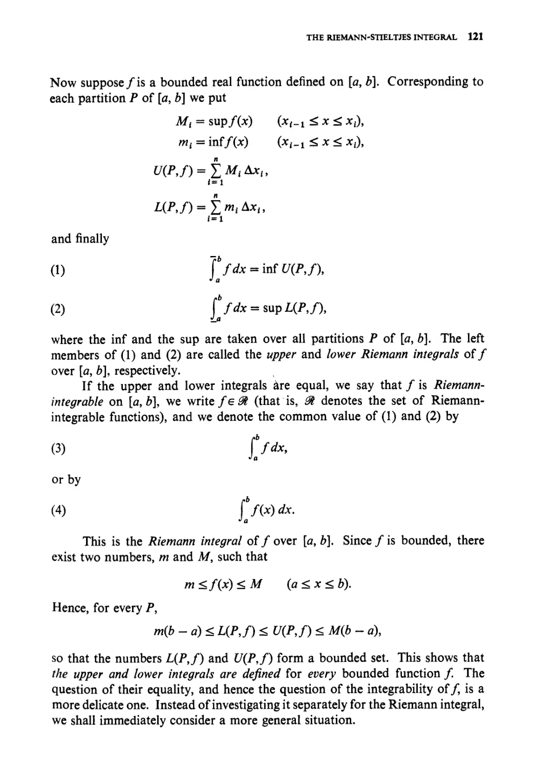
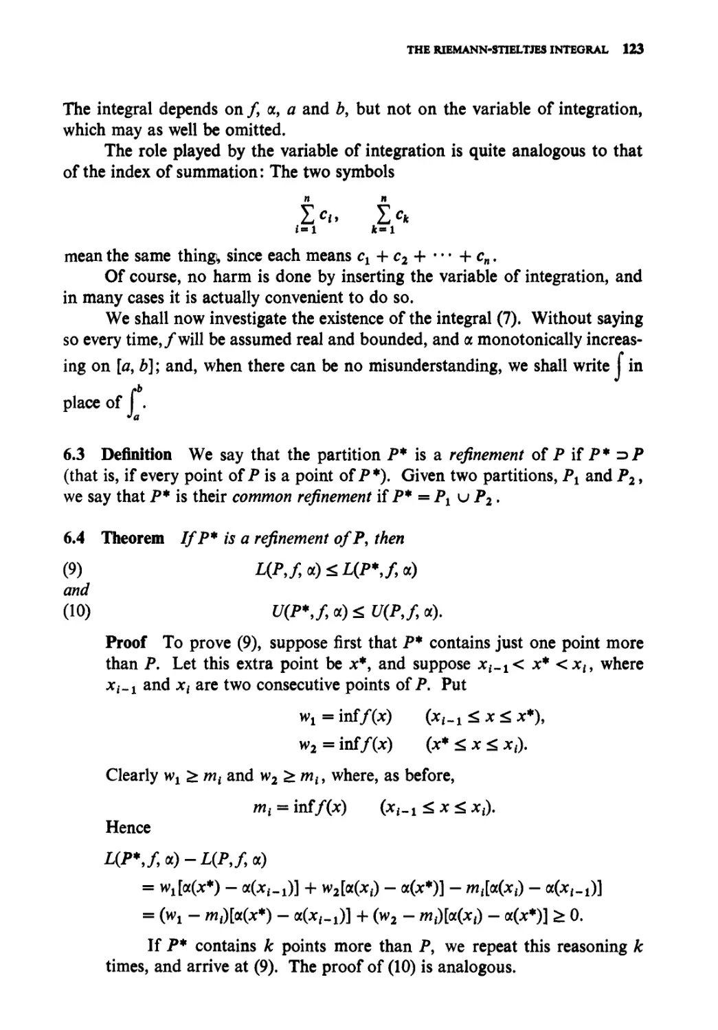
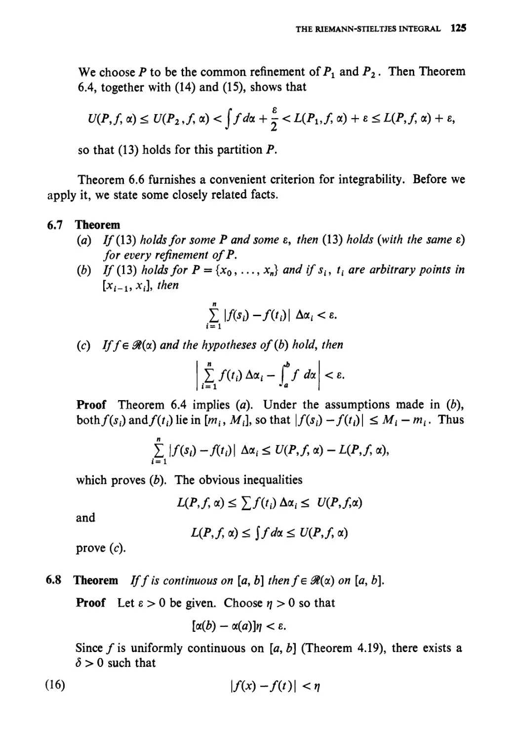
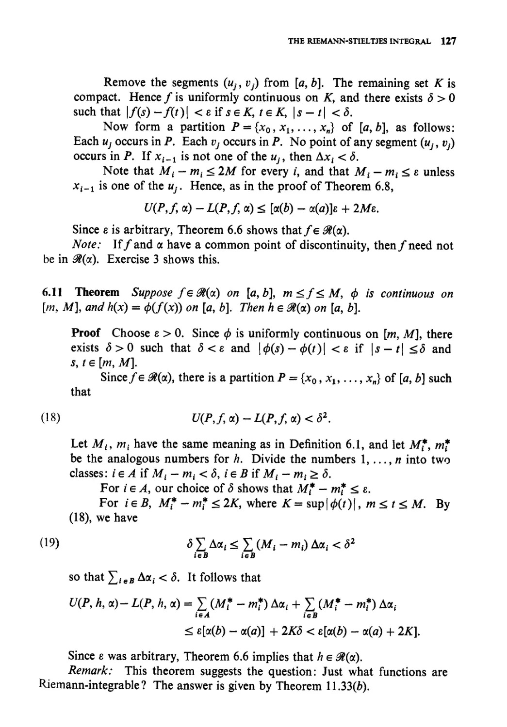
The Riemann-Stieltjes Integral
Definition and Existence of the Integral
Properties of the Integral
Integration and Differentiation
Integration of Vector-valued Functions
Rectifiable Curves
Exercises
Sequences and Series of Functions.
Discussion of Main Problem
Uniform Convergence
Uniform Convergence and Continuity
Uniform Convergence and Integration
Uniform Convergence and Differentiation
Equicontinuous Families of Functions
The Stone-Weierstrass Theorem
Exercises
Some Special Functions
Power Series
The Exponential and Logarithmic Functions
The Trigonometric Functions
The Algebraic Completeness of the Complex Field
Fourier Series
The Gamma Function
Exercises
Functions of Several Variables
Linear Transformations
Differentiation
The Contraction Principle
The Inverse Function Theorem
The Implicit Function Theorem
The Rank Theorem
Determinants
Derivatives of Higher Order
Differentiation of Integrals
Exercises
Integration of Differential Forms
Integration
CONTENTS VH
120
120
128
133
135
136
138
143
143
147
149
151
152
154
159
165
172
172
178
182
184
185
192
196
204
204
211
220
221
223
228
231
235
236
239
245
245
ЎШ CONTENTS
Primitive Mappings 248
Partitions of Unity 251
Change of Variables 252
Differential Forms 253
Simplexes and Chains 266
Stokes' Theorem 273
Closed Forms and Exact Forms 275
Vector Analysis 280
Exercises 288
Chapter 11 The Lebesgue Theory 300
Set Functions 300
Construction of the Lebesgue Measure 302
Measure Spaces 310
Measurable Functions 310
Simple Functions 313
Integration 314
Comparison with the Riemann Integral 322
Integration of Complex Functions 325
Functions of Class if2 325
Exercises 332
Bibliography 335
List of Special Symbols 337
Index 339
PREFACE
This book is intended to serve as a text for the course in analysis that is usually
taken by advanced undergraduates or by first-year students who study mathe-
mathematics.
The present edition covers essentially the same topics as the second one,
with some additions, a few minor omissions, and considerable rearrangement. I
hope that these changes will make the material more accessible amd more attrac-
attractive to the students who take such a course.
Experience has convinced me that it is pedagogically unsound (though
logically correct) to start off with the construction of the real numbers from the
rational ones. At the beginning, most students simply fail to appreciate the need
for doing this. Accordingly, the real number system is introduced as an ordered
field with the least-upper-bound property, and a few interesting applications of
this property are quickly made. However, Dedekind's construction is not omit-
omitted. It is now in an Appendix to Chapter 1, where it may be studied and enjoyed
whenever the time seems ripe.
The material on functions of several variables is almost completely re-
rewritten, with many details filled in, and with more examples and more motiva-
motivation. The proof of the inverse function theorem—the key item in Chapter 9—is
X PREFACE
simplified by means of the fixed point theorem about contraction mappings.
Differential forms are discussed in much greater detail. Several applications of
Stokes' theorem are included.
As regards other changes, the chapter on the Riemann-Stieltjes integral
has been trimmed a bit, a short do-it-yourself section on the gamma function
has been added to Chapter 8, and there is a large number of new exercises, most
of them with fairly detailed hints.
I have also included several references to articles appearing in the American
Mathematical Monthly and in Mathematics Magazine, in the hope that students
will develop the habit of looking into the journal literature. Most of these
references were kindly supplied by R. B. Burckel.
Over the years, many people, students as well as teachers, have sent me
corrections, criticisms, and other comments concerning the previous editions
of this book. I have appreciated these, and I take this opportunity to express
my sincere thanks to all who have written me.
WALTER RUDIN
1
THE REAL AND COMPLEX NUMBER SYSTEMS
INTRODUCTION
A satisfactory discussion of the main concepts of analysis (such as convergence,
continuity, differentiation, and integration) must be based on an accurately
defined number concept. We shall not, however, enter into any discussion of
the axioms that govern the arithmetic of the integers, but assume familiarity
with the rational numbers (i.e., the numbers of the form tn/n, where m and n
are integers and n Ф 0).
The rational number system is inadequate for many purposes, both as a
field and as an ordered set. (These terms will be defined in Sees. 1.6 and 1.12.)
For instance, there is no rational p such that p2 = 2. (We shall prove this
presently.) This leads to the introduction of so-called "irrational numbers"
which are often written as infinite decimal expansions and are considered to be
"approximated" by the corresponding finite decimals. Thus the sequence
1,1.4,1.41,1.414,1.4142,...
"tends to y/2." But unless the irrational number >/2 has been clearly defined,
the question must arise: Just what is it that this sequence "tends to"?
2 PRINCIPLES OF MATHEMATICAL ANALYSIS
This sort of question can be answered as soon as the so-called "real
number system" is constructed.
1.1 Example We now show that the equation
A) P2=2
is not satisfied by any rational p. If there were such a p, we could write p = m/n
where m and n are integers that are not both even. Let us assume this is done.
Then A) implies
B) m2 - 2л2,
This shows that m2 is even. Hence m is even (if m were odd, m2 would be odd),
and so m2 is divisible by 4. It follows that the right side of B) is divisible by 4,
so that n2 is even, which implies that n is even.
The assumption that A) holds thus leads to the conclusion that both m
and n are even, contrary to our choice of m and n. Hence A) is impossible for
rational p.
We now examine this situation a little more closely. Let A be the set of
all positive rationale p such that p2 < 2 and let В consist of all positive rationale
p such that p2 > 2. We shall show that A contains no largest number and В con-
contains no smallest.
More explicitly, for every p in A we can find a rational q in A such that
p < q, and for every p in В we can find a rational q in В such that q < p.
To do this, we associate with each rational p > 0 the number
Then
2 л 2(р2-2)
D) q2-2 =
(P + 2J
If p is in A then p2 — 2 < 0, C) shows that q > p, and D) shows that
q2 < 2. Thus q is in A.
Ifp is in В then p2 — 2 > 0, C) shows that 0 < q < p, and D) shows that
q2 > 2. Thus q is in B.
1.2 Remark The purpose of the above discussion has been to show that the
rational number system has certain gaps, in spite of the fact that between any
two rationals there is another: If r < s then r <(r + s)/2 < s. The real number
system fills these gaps. This is the principal reason for the fundamental role
which it plays in analysis.
THE REAL AND COMPLEX NUMBER SYSTEMS 3
In order to elucidate its structure, as well as that of the complex numbers,
we start with a brief discussion of the general concepts of ordered set and field.
Here is some of the standard set-theoretic terminology that will be used
throughout this book.
1.3 Definitions If A is any set (whose elements may be numbers or any other
objects), we write x e A to indicate that x is a member (or an element) of A.
If x is not a member of A, we write: x ф А.
The set which contains no element will be called the empty set. If a set has
at least one element, it is called nonempty.
If A and В are sets, and if every element of A is an element of B, we say
that Л is a subset of B, and write А с В, or В =э A. If, in addition, there is an
element of В which is not in A, then A is said to be a proper subset of B. Note
that Л с Л for every set A.
U Aa В and В с A, we write A — B. Otherwise АФВ.
1.4 Definition Throughout Chap. 1, the set of all rational numbers will be
denoted by Q.
ORDERED SETS
1.5 Definition Let S be a set. An order on S is a relation, denoted by <, with
the following two properties:
(i) If x e S and yeS then one and only one of the statements
x<y, x = y, y<x
is true.
(ii) If x, y, z e S, if x < у and у < z, then x < z.
The statement "x < y" may be read as "x is less than y" or "x is smaller
than y" or "x precedes y".
It is often convenient to write у > x in place of x < y.
The notation x <, у indicates that x < у or x — y, without specifying which
of these two is to hold. In other words, x й у is the negation of x > y.
1.6 Definition An ordered set is a set S in which an order is defined.
For example, Q is an ordered set if r < s is defined to mean that s — r is a
positive rational number.
1.7 Definition Suppose S is an ordered set, and E с S. If there exists a
($ e S such that x й P for every x e E, we say that E is bounded above, and call
f$ an upper bound of E.
Lower bounds are defined in the same way (with ^ in place of й).
4 PRINCIPLES OF MATHEMATICAL ANALYSIS
1.8 Definition Suppose S is an ordered set, E <=. S, and E is bounded above.
Suppose there exists an a e S with the following properties:
(i) a is an upper bound of E.
(ii) If у < a then у is not an upper bound of E.
Then a is called the least upper bound ofE [that there is at most one such
a is clear from (ii)] or the supremum ofE, and we write
a = sup E.
The greatest lower bound, or infimum, of a set E which is bounded below
is defined in the same manner: The statement
a = inf?
means that a is a lower bound of E and that no /? with /? > a is a lower bound
ofE.
1.9 Examples
(a) Consider the sets A and В of Example 1.1 as subsets of the ordered
set Q. The set A is bounded above. In fact, the upper bounds of A are
exactly the members of B. Since В contains no smallest member, A has
no least upper bound in Q.
Similarly, В is bounded below: The set of all lower bounds of В
consists of A and of all r e Q with г й 0. Since A has no lasgest member,
В has no greatest lower bound in Q.
(b) If a = sup E exists, then a may or may not be a member of E. For
instance, let Et be the set of all r e Q with r < 0. Let E2 be the set of all
r e Q with r <, 0. Then
sup Et = sup E2 = 0,
and 0фЕ1,0еЕ2.
(c) Let E consist of all numbers l//i, where и = 1, 2, 3, .... Then
sup E = 1, which is in E, and inf E = 0, which is not in E.
1.10 Definition An ordered set 5 is said to have the least-upper-bound property
if the following is true:
If E с S, E is not empty, and E is bounded above, then sup E exists in S.
Example 1.9(a) shows that Q does not have the least-upper-bound property.
We shall now show that there is a close relation between greatest lower
bounds and least upper bounds, and that every ordered set with the least-upper-
bound property also has the greatest-lower-bound property.
THE REAL AND COMPLEX NUMBER SYSTEMS 5
1.11 Theorem Suppose S is an ordered set with the least-upper-bound property,
В a S, В is not empty, and В is bounded below. Let L be the set of all lower
bounds of В. Then
a = sup L
exists in S, and a = inf B.
In particular, inf В exists in S.
Proof Since В is bounded below, L is not empty. Since L consists of
exactly those у e S which satisfy the inequality у <, x for every x e B, we
see that every xe В is an upper bound of L. Thus L is bounded above.
Our hypothesis about S implies therefore that L has a supremum in 5;
call it a.
If у < a then (see Definition 1.8) у is not an upper bound of L,
hence у фВ. It follows that a <; * for every xeB. Thus a eL.
If a < ft then /? ф L, since a is an upper bound of L.
We have shown that a e L but /? ф L if /? > a. In other words, a
is a lower bound of B, but /? is not if 0 > a. This means that a = inf B.
FIELDS
1.12 Definition A field is a set F with two operations, called addition and
multiplication, which satisfy the following so-called "field axioms" (A), (M),
and(D):
(A) Axioms for addition
(Al) U xe F and ye F, then their sum x + у ism F.
(A2) Addition is commutative: * + у = у + x for all *, у е F.
(A3) Addition is associative: (* + y) + z = x + (y + z) for all x,y,ze F.
(A4) Fcontains an element 0 such that 0 + x = x for every xeF.
(A5) To every xeF corresponds an element —xeF such that
*+(-*) = 0.
(M) Axioms for multiplication
(Ml) If x e F and yeF, then their product xy is in F.
(M2) Multiplication is commutative: xy = yx for all x, ye F.
(M3) Multiplication is associative: (xy)z = x{yz) for all x, y, ze F.
(M4) Fcontains an element 1 ф 0 such that 1* = * for every xeF.
(M5) If xeF and x Ф0 then there exists an element l/xe F such that
6 PRINCIPLES OF MATHEMATICAL ANALYSIS
(D) The distributive law
x(y + z) = xy + xz
holds for all x, y, z e F.
1.13 Remarks
(a) One usually writes (in any field)
x -y,-,x + y + z, xyz, x2, x3, 2x, Ъх,...
in place of
x + (~y), x • I -1, (x + y) + z, (xy)z, xx, xxx, x + x, x + x + x,
(jb) The field axioms clearly hold in Q, the set of all rational numbers, if
addition and multiplication have their customary meaning. Thus Q is a
field.
(c) Although it is not our purpose to study fields (or any other algebraic
structures) in detail, it is worthwhile to prove that some familiar properties
of Q are consequences of the field axioms; once we do this, we will not
need to do it again for the real numbers and for the complex numbers.
1.14 Proposition The axioms for addition imply the following statements.
(a) If x + у = x + z then у — z.
(b) Ifx + у = x then y = 0.
(c) Ifx + y = Otheny=-x.
{d) -(-*) = *.
Statement (a) is a cancellation law. Note that (b) asserts the uniqueness
of the element whose existence is assumed in (A4), and that (c) does the same
for (A5).
Proof If x + у = x + z, the axioms (A) give
у = о + у = {-x + x) + у = -x + (x + у)
= -x + (x + z) = {-x + x) + z = 0 + z = z.
This proves (a). Take z = 0 in (a) to obtain (b). Take z- -x in (a) to
obtain (c).
Since -x + x = 0, (c) (with -x in place of x) gives (d).
THE REAL AND COMPLEX NUMBER SYSTEMS 7
1.15 Proposition The axioms for multiplication imply the following statements.
(a) Ifx Ф 0 and xy = xz then у = z.
(b) If хФО and xy = x then у = 1.
(c) Ifx^O and xy = 1 then у = l/x.
(d) Ifx^O then 1/A/jc) = x.
The proof is so similar to that of Proposition 1.14 that we omit it.
1.16 Proposition The field axioms imply the following statements, for any x, y,
zeF.
(a) 0x = 0.
(b) Ifx^O and у Ф 0 then xy Ф 0.
(c) {-x)y= ~{xy) = x{-y).
(d) {-x){-y) = xy.
Proof Ox + Ox = @ + 0)x = Ox. Hence 1.14{b) implies that Ox = 0, and
(a) holds.
Next, assume x Ф0,у Ф0, but xy = 0. Then (a) gives
¦©©-¦9©"»
a contradiction. Thus (b) holds.
The first equality in (c) comes from
(-x)y + xy = (-x + x)y = Oy = 0,
combined with 1.14(c); the other half of (c) is proved in the same way.
Finally,
by(c)andl.l4(af).
1.17 Definition An ordered field is a. field F which, is also an ordered set, such
that
(i) x + у < x + zif x, y, ze-Fand у < z,
(ii) xy >0if xeF, j>e/s x > 0, and у > 0.
If x > 0, we call * positive; if x < 0, x is negative.
For example, Q is an ordered field.
All the familiar rules for working with inequalities apply in every ordered
field: Multiplication by positive [negative] quantities preserves [reverses] in-
inequalities, no square is negative, etc. The following proposition lists some of
these.
8 PRINCIPLES OF MATHEMATICAL ANALYSIS
1.18 Proposition The following statements are true in every ordered field.
(a) Ifx>0 then —x<0, and vice versa.
(b) Ifx>Oandy<zthenxy<xz.
(c) Ifx<0 and у <z then xy > xz.
(d) I/хфО then x2 > 0. In particular, 1 > 0.
0?) IfO<x<y then 0<l/y< l/x.
Proof
(a) If x > 0 then 0 = -x + x> -* + 0, so that -x < 0. If x < 0 then
0 = -* + * < -* + 0, so that -* > 0. This proves (a).
(b) Since z > y, we have z — у > у — у = 0, hence x{z — у) > 0, and
therefore
xz = x(z — y) + xy > 0 + xy = xy.
(c) By (a), (b), and Proposition 1.16(c),
so that x(z — y) < 0, hence xz < xy.
(of) If x > 0, part (ii) of Definition 1.17 gives x2 > 0. If x < 0, then
-x>0, hence (-л;J>0. But д:2 = (-д:J, by Proposition l.\6(d).
Since 1 = I2, 1 >0.
(e) If у > 0 and v < 0, then yv < 0. But у ¦ (\/y) = 1 > 0. Hence l/y > 0.
Likewise, 1/* > 0. If we multiply both sides of the inequality x < у by
the positive quantity (\/x)(l/y), we obtain \/y < l/x.
THE REAL FIELD
We now state the existence theorem which is the core of this chapter.
1.19 Theorem There exists an ordered field R which has the least-upper-bound
property.
Moreover, R contains Q as a subfield.
The second statement means that Q <=¦ R and that the operations of
addition and multiplication in R, when applied to members of Q, coincide with
the usual operations on rational numbers; also, the positive rational numbers
are positive elements of R.
The members of R are called real numbers.
The proof of Theorem 1.19 is rather long and a bit tedious and is therefore
presented in an Appendix to Chap. 1. The proof actually constructs R from Q.
THE REAL AND COMPLEX NUMBER SYSTEMS 9
The next theorem could be extracted from this construction with very
little extra effort. However, we prefer to derive it from Theorem 1.19 since this
provides a good illustration of what one can do with the least-upper-bound
property.
1.20 Theorem
(a) If x e R, у e R, and x>0, then there is a positive integer n such that
nx > y.
(b) Ifx e R,ye R, andx < y, then there exists a p e Q such that x <p <y.
Part (a) is usually referred to as the archimedean property of R. Part (b)
may be stated by saying that Q is dense in R: Between any two real numbers
there is a rational one.
Proof
(a) Let A be the set of all nx, where n runs through the positive integers.
If (a) were false, then у would be an upper bound of A. But then A has a
least upper bound in R. Put a = sup A. Since л; > 0, a — x < a, and
a — * is not an upper bound of A. Hence a — x < mx for some positive
integer m. But then a < (m + l)x e A, which is impossible, since a is an
upper bound of A.
(b) Since x < y, we have у - x > 0, and (a) furnishes a positive integer
n such that
n(y — x) > 1.
Apply (a) again, to obtain positive integers mt and m2 such that mt > nx,
m2 > —nx. Then
—тг <пх <mv
Hence there is an integer m (with —m1<m< wx) such that
m — 1 < nx < m.
If we combine these inequalities, we obtain
nx < m < 1 + nx < ny.
Since n > 0, it follows that
m
x < — < y.
n
This proves (b), with p = m/n.
10 PRINCIPLES OF MATHEMATICAL ANALYSIS
We shall now prove the existence of /ith roots of positive reals. This
proof will show how the difficulty pointed out in the Introduction (irration-
(irrationality of y/l) can be handled in R.
1.21 Theorem For every real x > 0 and every integer n > 0 there is one
and only one positive real у such that y" = x.
This number у is written f/x or xi/n.
Proof That there is at most one such у is clear, since 0 < yt <y2 implies
Л <A-
Let E be the set consisting of all positive real numbers t such that
tn < x.
If t = x/(l + x) then 0 ^ t < 1. Hence tn <, t < x. Thus t e E, and
E is not empty.
If / > 1 + x then tn > t > x, so that / ф E. Thus 1 + x is an upper
bound of E.
Hence Theorem 1.19 implies the existence of
у = sup E.
To prove that y" = x we will show that each of the inequalities y* < x
and y" > x leads to a contradiction.
The identity bn-an = (b- a)^" + ^a + • • • + л") yields
the inequality
when 0 < a < b.
Assume y* < x. Choose h so that 0 < h < 1 and
Put a = j>, 6 = j> + h. Then
0> + Л)" - у" < hn(y + hf'1 < hn(y + I)" < x - y".
Thus (y + h)n <x, and у + heE. Since у + h >y, this contradicts the
fact that у is an upper bound of E.
Assume У > х. Put
k
Then 0 < к < у. If t ^ у - к, we conclude that
У - tn <, / - (j> - k)n < kny"'1 = У - x.
Thus /n > x, and f ? ?. It follows that у - к is an upper bound of E.
THE REAL AND COMPLEX NUMBER SYSTEMS 11
But у — к < у, which contradicts the fact that у is the least upper bound
of?.
Hence y" = x, and the proof is complete.
Corollary If a and b are positive real numbers and n is a positive integer, then
(ab)iln = ai/nbi/n.
Proof Put a = a1/B, 0 = b1/n. Then
ab = aT = (фп,
since multiplication is commutative. [Axiom (M2) in Definition 1.12.]
The uniqueness assertion of Theorem 1.21 shows therefore that
1.22 Decimals We conclude this section by pointing out the relation between
real numbers and decimals.
Let * > 0 be real. Let n0 be the largest integer such that n0 < x. (Note that
the existence of n0 depends on the archimedean property of R.) Having chosen
n0, nu ..., «fc-i, let nk be the largest integer such that
n°+10 + "' + To* ^ x'
Let E be the set of these numbers
E) + Г5+"'+Г5* ^ = 0,1,2,...).
Then * = sup E. The decimal expansion of x is
F) /l0 • П^2 И3 ' ' ' .
Conversely, for any infinite decimal F) the set E of numbers E) is bounded
above, and F) is the decimal expansion of sup E.
Since we shall never use decimals, we do not enter into a detailed
discussion.
THE EXTENDED REAL NUMBER SYSTEM
1.23 Definition The extended real number system consists of the real field R
and two symbols, +oo and — oo. We preserve the original order in R, and
define
— 00 < * < +00
for every xeR.
12 PRINCIPLES OF MATHEMATICAL ANALYSIS
It is then clear that 4- oo is an upper bound of every subset of the extended
real number system, and that every nonempty subset has a least upper bound.
If, for example, E is a nonempty set of real numbers which is not bounded
above in R, then sup E = + oo in the extended real number system.
Exactly the same remarks apply to lower bounds.
The extended real number system does not form a field, but it is customary
to make the following conventions:
(a) If л: is real then
x x
x+oo=+oo, x — oo = — oo, = = 0.
4-ое —oo
(b) If x > 0 then x • (+oo) = 4-oo, x • (— oo) = — oo.
(c) If x <0 then х- (+oo) = -oo, x • (-oo) = +oo.
When it is desired to make the distinction between real numbers on the
one hand and the symbols 4- oo and — oo on the other quite explicit, the former
are called finite.
THE COMPLEX FIELD
1.24 Definition A complex number is an ordered pair (a, b) of real numbers.
"Ordered" means that (a, b) and (b, a) are regarded as distinct if а ф b.
Let x = (a, b), у = (с, d) be two complex numbers. We write x = у if and
only if a = с and b = d. (Note that this definition is not entirely superfluous;
think of equality of rational numbers, represented as quotients of integers.) We
define
xy = (ac — bd, ad + be).
1.25 Theorem These definitions of addition and multiplication turn the set of
all complex numbers into afield, with @, 0) and A,0) in the role ofO and 1.
Proof We simply verify the field axioms, as listed in Definition 1.12.
(Of course, we use the field structure of R.)
Let x = (a, b), у = (с, d), z = (e,f).
(Al) is clear.
(A2) )
THE REAL AND COMPLEX NUMBER SYSTEMS 13
(A3) (x + y) + z = (a + c,b + d)
= (a + c + e,b
= (a, b) + (c + e,d+f) = x + (y + z).
(A4) x + 0 = (a, b) + @, 0) = (a, b) = x.
(A5) Put -x = (-a, -b). Then x + (-x) = @, 0) = 0.
(Ml) is clear.
(M2) xy = (ac — bd, ad + be) = (ca — db, da + cb) = yx.
(M3) (xy)z = (ac - bd, ad + bc)(e,f)
= (ace — bde — adf— bef, acf — bdf+ ade + bee)
= (a, b)(ce - df, cf+ de) = x(yz).
(M4) lx = (l,0)(a,b) = (a,b) = x.
(M5) If x Ф 0 then (a, b) Ф @, 0), which means that at least one of the
real numbers a, b is different from 0. Hence a2 + b2 > 0, by Proposition
1.1 $(d), and we can define
± ~b \
W + b2' a2 + b2
Then
(D) x(y + z) = (a,b)(c + e,d+f)
= (ac + ae — bd — bf, ad + af+ be + be)
= (ac - bd, ad + be) + (ae - bf, af+ be)
= xy + xz.
1.26 Theorem For any real numbers a and b we have
(a, 0) + (b, 0) = (a + b, 0), (a, 0)(b, 0) = (ab, 0).
The proof is trivial.
Theorem 1.26 shows that the complex numbers of the form (a, 0) have the
same arithmetic properties as the corresponding real numbers a. We can there-
therefore identify (a, 0) with a. This identification gives us the real field as a subfield
of the complex field.
The reader may have noticed that we have defined the complex numbers
without any reference to the mysterious square root of — 1. We now show that
the notation (a, b) is equivalent to the more customary a + bi.
1.T7 Definition / = @, 1).
14 PRINCIPLES OF MATHEMATICAL ANALYSIS
1.28 Theorem i2 = -1.
Proof /2 = @, l)@, l) = (-l,0)= -1.
1.29 Theorem If a and b are real, then (a, b) = a + bi.
Proof
a + bi = (a,0) + (b,0)@, 1)
= (a, 0) + @,b) = (a, b).
1.30 Definition If a, b are real and z = a + bi, then the complex number
z = a — bi is called the conjugate of z. The numbers a and 6 are the real part
and the imaginary part of z, respectively.
We shall occasionally write
a = Re(z), b = Im(z).
1.31 Theorem Ifz and w are complex, then
(a) z + w = z + w,
(b) z~w = z • w,
(c) z + z = 2 Re(z), z-z = 2i Im(z),
(d) zz is real and positive (except when z = 0).
Proof (a), (b), and (c) are quite trivial. To prove (d), write z = a + bi,
and note that zz = a2 + b2.
1.32 Definition If z is a complex number, its absolute value \z\ is the non-
negative square root of zz; that is, \z\ — (zz)l/2.
The existence (and uniqueness) of \z\ follows from Theorem 1.21 and
part (d) of Theorem 1.31.
Note that when x is real, then x = x, hence \x\ =*Jx2. Thus \x\ = x
if x > 0, |л;| = -x if x < 0.
1.33 Theorem Let z and w be complex numbers. Then
(a) \z\ > 0 unless z = 0, |0| =0,
(b) |z|=|z|,
(c) | zw I = I z I I w I,
(d) |Rez|?|z|,
(e) \z + w\ <, \z\ + |w|.
THE REAL AND COMPLEX NUMBER SYSTEMS 15
Proof (a) and (b) are trivial. Put z = a + bi, w = c + di, with a, b, c, d
real. Then
|zw|2 = (ac - bdJ + (ad+bcJ = (a2 + Ь2)(с2 + d2) = \z\2\w\2
or |zw|2 = (|z| I w|J. Now (c) follows from the uniqueness assertion of
Theorem 1.21.
To prove (d), note that a2 < a2 + b2, hence
|e| = Ja2 <; Ja2 + b2.
To prove (e), note that zw is the conjugate of zw, so that zw + zw =
2 Re (zw). Hence
| z + w |2 — (z + w)(z + vv) = zz + zw + zw + ww
= \z\2+2Re(zw)+ \w\2
< |z|2 + 2|zh;| + \w\2
Now (e) follows by taking square roots.
1.34 Notation If xlf..., xn are complex numbers, we write
n
x^ + x2 + ''' + xn = 2_, Xj.
We conclude this section with an important inequality, usually known as
the Schwarz inequality.
1.35 Theorem If au ..., an and blf ..., bn are complex numbers, then
In n
Proof Put A = Z | aj |2, В = Z | bj |2, С = Say 5, (in all sums in this proof,
j runs over the values 1,...,«). If В = 0, then 6t = • • • = bn = 0, and the
conclusion is trivial. Assume therefore that В > 0. By Theorem 1.31 we
have
X \Baj - Cbj\2 = ? (Ai, - СЬДДЙ, - Cft))
16 PRINCIPLES OF MATHEMATICAL ANALYSIS
Since each term in the first sum is nonnegative, we see that
B(AB- |C|2)^0.
Since В > 0, it follows that AB - \ C\2 ^ 0. This is the desired inequality.
EUCLIDEAN SPACES
1.36 Definitions For each positive integer k, let Rk be the set of all ordered
fc-tuples
X = (xlt X2, • .., Xjf),
where xlf ..., xk are real numbers, called the coordinates of x. The elements of
Rk are called points, or vectors, especially when к > 1. We shall denote vectors
by boldfaced letters. If у = (yu ..., yk) and if a is a real number, put
ax = (a*!,..., a.xk)
so that x + у е i?k and ax e Rk. This defines addition of vectors, as well as
multiplication of a vector by a real number (a scalar). These two operations
satisfy the commutative, associative, and distributive laws (the proof is trivial,
in view of the analogous laws for the real numbers) and make Rk into a vector
space over the real field. The zero element of Rk (sometimes called the origin or
the null vector) is the point 0, all of whose coordinates are 0.
We also define the so-called "inner product" (or scalar product) of x and
У by
and the norm of x by
l/2
The structure now defined (the vector space Rk with the above inner
product and norm) is called euclidean A>space.
1.37 Theorem Suppose x, y, z e Rk, and a is real. Then
(a) |x|?0;
(b) |x| = 0 if and only ifx = 0;
(c) |ax| = |a||x|;
(«0 |x-y|<|x||y|;
(e) |x + y| <|x| + |y|;
(/) |x-z|<|x-y| + |y-z|.
THE REAL AND COMPLEX NUMBER SYSTEMS 17
Proof (a), (b), and (c) are obvious, and (d) is an immediate consequence
of the Schwarz inequality. By (d) we have
so that (e) is proved. Finally, (/) follows from (e) if we replace x by
x - у and у by у - z.
1.38 Remarks Theorem 1.37 (a), (b), and (/) will allow us (see Chap. 2) to
regard Rk as a metric space.
Rl (the set of all real numbers) is usually called the line, or the real line.
Likewise, R2 is called the plane, or the complex plane (compare Definitions 1.24
and 1.36). In these two cases the norm is just the absolute value of the corre-
corresponding real or complex number.
APPENDIX
Theorem 1.19 will be proved in this appendix by constructing R from Q. We
shall divide the construction into several steps.
Step 1 The members of R will be certain subsets of Q, called cuts. A cut is,
by definition, any set а с Q with the following three properties.
(I) a is not empty, and a # Q.
(II) If p e<x,qeQ, and q < p, then q e a.
(Ill) If p e a, then p < r for some re a.
The lettersp,q, r,... will always denote rational numbers, and a, p,y,...
will denote cuts.
Note that (III) simply says that a has no largest member; (II) implies two
facts which will be used freely:
If p e a and q ф a then p < q.
If г ф a and r < s then s ф а.
Step 2 Define "a < 0" to mean: a is a proper subset of p.
Let us check that this meets the requirements of Definition 1.5.
Ifcc<fi and ft < у it is clear that a < y. (A proper subset of a proper sub-
subset is a proper subset.) It is also clear that at most one of the three relations
18 PRINCIPLES OF MATHEMATICAL ANALYSIS
can hold for any pair a, p. To show that at least one holds, assume that the
first two fail. Then a is not a subset of p. Hence there is a pea with p ф p.
If q e p, it follows that q < p (since p ф p), hence qecc, by (II). Thus ^ca.
Since fi Ф a, we conclude: P < a.
Thus R is now an ordered set.
Step 3 The ordered set R has the least-upper-bound property.
To prove this, let A be a nonempty subset of R, and assume that p e R
is an upper bound of A. Define у to be the union of all a e A. In other words,
p e у if and only if p e a for some <xe A. We shall prove that у e R and that
у = sup 4.
Since A is not empty, there exists an a0 e A. This a0 is not empty. Since
a0 с у, у is not empty. Next, у с p (since a с /? for every a e Л), and therefore
у Ф Q. Thus у satisfies property (I). To prove (II) and (III), pick p e y. Then
peal for some ax e 4. If q <p, then # e at, hence # e y; this proves (II). If
r6at is so chosen that r >p, we see that rey (since o^ с у), and therefore у
satisfies (III).
Thus yeR.
It is clear that a < у for every осе A.
Suppose <5 < y. Then there is an se у and that sф5. Since je y, sea.
for some ue A. Hence 5 < a, and 5 is not an upper bound of A.
This gives the desired result: у — sup A.
Step 4 If осе R and /? e Л we define a + /? to be the set of all sums r + s, where
re a and s e /?.
We define 0* to be the set of all negative rational numbers. It is clear that
0* is a cut. We verify that the axioms for addition (see Definition 1.12) hold in
R, with 0* playing the role ofO.
(Al) We have to show that a + /? is a cut. It is clear that a + /? is а
nonempty subset of Q. Take г'фа., s'фp. Then r' + s' > r + s for all
choices of rea, jep. Thus r' + s'фа. + p. It follows that a + /? has
property (I).
Pick реал- p. Then p = r + s, with rea,sep. If q <p, then
q — s <r, so q — sea, and # = (# — j) + j e a + /?. Thus (II) holds.
Choose tea so that t > r. Thenp < t + s and t + sea + p. Thus (III)
holds.
(A2) a + p is the set of all r + ?, with r e a, s e p. By the same definition,
P + a is the set of all s + r. Since r + s = s + r for all r e Q, s e Q, we
have a + p = p + a.
(A3) As above, this follows from the associative law in Q.
(A4) If r e a and s e 0*, then r + s < r, hence r + sea. Thus a + 0* с a.
To obtain the opposite inclusion, pick pea, and pick recc,r>p. Then
THE REAL AND COMPLEX NUMBER SYSTEMS 19
p - r e 0*, and p = r +(p - r)e a + 0*. Thus a c a + 0*. We conclude
that a + 0* = a.
(A5) Fix oleR. Let 0 be the set of all p with the following property:
There exists r > 0 such that —p — гф<х.
In other words, some rational number smaller than — p fails to
be in a.
We show that fie Rand that a, + p = 0*.
If s фа andp = — s — 1, then — p — 1 фa, hencepe/?. So j? is not
empty. If # e a, then -qф /?. So /? # ?>. Hence /? satisfies (I).
Pick pg/?, and pick r > 0, so that —p — гфа. If q <p, then
—q — r> —p — r, hence —q — гфа.. Thus #e/?, and (II) holds. Put
Г = p +(r/2). Then f > p, and -1 - (r/2) = -p -гфа, so that t e p.
Hence /? satisfies (III).
We have proved that ft e R.
If r e a and s e /?, then — j ? a, hence r < — s, r + s < 0. Thus
a + l?c0*.
To prove the opposite inclusion, pick v e 0*, put w = — v/2. Then
w > 0, and there is an integer n such that nw e a but (и + l)w ? a. (Note
that this depends on the fact that Q has the archimedean property!) Put
p = — (n + 2)w. Then /? e /?, since —/? — w ^ a, and
Thus 0* с a + p.
We conclude that a + /? = 0*.
This /? will of course be denoted by —a.
Step 5 Having proved that the addition defined in Step 4 satisfies Axioms (A)
of Definition 1.12, it follows that Proposition 1.14 is valid in R, and we can
prove one of the requirements of Definition 1.17:
Ifa,f},yeR and/? < y, then a + /? < a + y.
Indeed, it is obvious from the definition of + in R that « + j5ca + y; if
we had a + /? = a + y, the cancellation law (Proposition 1.14) would imply
/? = y.
It also follows that a > 0* if and only if -a < 0*.
Step 6 Multiplication is a little more bothersome than addition in the present
context, since products of negative rationale are positive. For this reason we
confine ourselves first to R+, the set of all a e R with a > 0*.
If a g R+ and peR+, we define a/? to be the set of all p such that p < rs
for some choice of r e a, s e ft, r > 0, s > 0.
We define 1* to be the set of all q < 1.
20 PRINCIPLES OF MATHEMATICAL ANALYSIS
Then the axioms (M) and(D) of Definition 1.12 hold, with R+ in place ofF,
and with 1* in the role of\.
The proofs are so similar to the ones given in detail in Step 4 that we omit
them.
Note, in particular, that the second requirement of Definition 1.17 holds:
If a > 0* and p > 0* then ap > 0*.
Step 7 We complete the definition of multiplication by setting aO* = 0*a = 0*,
and by setting
ifa<O*,0<O*,
ifa<O*,0>O*,
ifa>0*, p<Q*.
The products on the right were defined in Step 6.
Having proved (in Step 6) that the axioms (M) hold in R+, it is now
perfectly simple to prove them in R, by repeated application of the identity
у = -(-у) which is part of Proposition 1.14. (See Step 5.)
The proof of the distributive law
*(P + У) = <*P + «У
breaks into cases. For instance, suppose a > 0*, /? < 0*, /? + у > 0*. Then
У = (fi + y) + (—P), and (since we already know that the distributive law holds
inR+)
ау = а@ + у)+ а •(-?).
But а • (-ft) = ~(ф. Thus
аР + ау = а(р + у).
The other cases are handled in the same way.
We have now completed the proof that R is an ordered field with the least-
upper-bound property.
Step 8 We associate with each r e Q the set r* which consists of all p e Q
such that/? < r. It is clear that each r* is a cut; that is, r* e R. These cuts satisfy
the following relations:
(a) r*+s* = (r + s)*,
ib) r*s* = (rs)*,
(c) r* < s* if and only ifr<s.
To prove (a), choose per* + s*. Then p = u + v, where и < r, v < s.
Hence p < r + s, which says that pe(r + s)*.
THE REAL AND COMPLEX NUMBER SYSTEMS 21
Conversely, suppose pe(r + s)*. Then p < r + s. Choose t so that
It = r + s - p, put
r' = r - t, s' = s - t.
Then r' e r*, s' e s*, and p = r' + s', so that per* + s*.
This proves (a). The proof of (b) is similar.
If r < s then r e s*, but гфг*; hence r* < s*.
If r* < $*, then there is apes* such that p ф г*. Hence r <,p <s, so
that r < s.
This proves (c).
Step 9 We saw in Step 8 that the replacement of the rational numbers r by the
corresponding "rational cuts" r* e R preserves sums, products, and order. This
fact may be expressed by saying that the ordered field Q is isomorphic to the
ordered field Q* whose elements are the rational cuts. Of course, r* is by no
means the same as r, but the properties we are concerned with (arithmetic and
order) are the same in the two fields.
It is this identification of Q with Q* which allows us to regard Q as a
subfieldofR.
The second part of Theorem 1.19 is to be understood in terms of this
identification. Note that the same phenomenon occurs when the real numbers
are regarded as a subfield of the complex field, and it also occurs at a much
more elementary level, when the integers are identified with a certain subset of Q.
It is a fact, which we will not prove here, that any two ordered fields with
the least-upper-bound property are isomorphic. The first part of Theorem 1.19
therefore characterizes the real field R completely.
The books by Landau and Thurston cited in the Bibliography are entirely
devoted to number systems. Chapter 1 of Knopp's book contains a more
leisurely description of how R can be obtained from Q. Another construction,
in which each real number is defined to be an equivalence class of Cauchy
sequences of rational numbers (see Chap. 3), is carried out in Sec. 5 of the book
by Hewitt and Stromberg.
The cuts in Q which we used here were invented by Dedekind. The
construction of R from Q by means of Cauchy sequences is due to Cantor.
Both Cantor and Dedekind published their constructions in 1872.
EXERCISES
Unless the contrary is explicitly stated, all numbers that are mentioned in these exer-
exercises are understood to be real.
1. If r is rational (г Ф 0) and x is irrational, prove that r + x and rx are irrational.
22 PRINCIPLES OF MATHEMATICAL ANALYSIS
2. Prove that there is no rational number whose square is 12.
3. Prove Proposition 1.15.
4. Let E be a nonempty subset of an ordered set; suppose a is a lower bound of E
and /? is an upper bound of E. Prove that a <; /?.
5. Let /4 be a nonempty set of real numbers which is bounded below. Let —A be
the set of all numbers — *, where xe A. Prove that
inf A = — sup(—A).
6. Fixb>l.
(a) If m, n, p, q are integers, n > 0, q > 0, and r = m/n =p/g, prove that
(ЬтУ1п = (Ь>У19.
Hence it makes sense to define br = (bm)lln.
(b) Prove that br+' = brb' if r and s are rational.
(c) If * is real, define B(x) to be the set of all numbers b\ where t is rational and
t<,x. Prove that
br = sup B(r)
when r is rational. Hence it makes sense to define
b* = sup B(x)
for every real x.
(d) Prove that bx+y = б*^ for all real x and ;>\
7. Fix b > 1, у >0, and prove that there is a unique real л; such that b* =y, by
completing the following outline. (This л: is called the logarithm of у to the base b.)
(a) For any positive integer n, bn — 1 > n{b — 1).
(b) Hence 6-1 ^n(b1/n- 1).
(c) If / > 1 and n > (b - l)/(t - 1), then b1 < t.
(d) If w is such that bw <y, then bw + a/n) <y for sufficiently large n; to see this,
apply part (c) with / —y • b~w.
(e) If bw >y, then 6W-A"I) >y for sufficiently large n.
(/) Let /1 be the set of all w such that bw < y, and show that x = sup A satisfies
bx=y.
(g) Prove that this x is unique.
8. Prove that no order can be defined in the complex field that turns it into an ordered
field. Hint: — 1 is a square.
9. Suppose z = a + bi, w = c + di. Define z < w if a < c, and also if a = с but
b < d. Prove that this turns the set of all complex numbers into an ordered set.
(This type of order relation is called a dictionary order, or lexicographic order, for
obvious reasons.) Does this ordered set have the least-upper-bound property?
10. Suppose z = a + bi, w = u + iv, and
1/2
THE REAL AND COMPLEX NUMBER SYSTEMS 23
Prove that z2 = w if v ^ 0 and that (zJ = w if v <; 0. Conclude that every complex
number (with one exception!) has two complex square roots.
11. If z is a complex number, prove that there exists anr^O and a complex number
w with | w | = 1 such that z = rw. Are w and r always uniquely determined by z ?
12. If zb ..., zn are complex, prove that
|z1 + z2 + -" + zn| «?|z,| + |z2| + --- + |zn|.
13. If x, у are complex, prove that
\\x\-\y\\<;\x-y\.
14. If z is a complex number such that \z\ =1, that is, such that zz = 1, compute
|l+z|2+|l-z|2.
15. Under what conditions does equality hold in the Schwarz inequality?
16. Suppose к ^ 3, x, у e Rk, |x - y| = d>0, and r > 0. Prove:
(а) If 2r > d, there are infinitely many z e Rk such that
|z-x| =|z-y| =r.
(б) If 2r = d, there is exactly one such z.
(c) If 2r < d, there is no such z.
How must these statements be modified if к is 2 or 1 ?
17. Prove that
if хе/г* and у е Rk. Interpret this geometrically, as a statement about parallel-
parallelograms.
18. If к ^ 2 and x e Rk, prove that there exists yeR" such that у Ф 0 but x • у = 0.
Is this also true if к = 1 ?
19. Suppose a e Rk, b б Д*. Find с е Д* and r > 0 such that
|x-a|=2|x-b|
if and only if | x — с | = r.
(Solution: 3c = 4b - a, 3r = 21 b - a |.)
20. With reference to the Appendix, suppose that property (III) were omitted from the
definition of a cut. Keep the same definitions of order and addition. Show that
the resulting ordered set has the least-upper-bound property, that addition satisfies
axioms (Al) to (A4) (with a slightly different zero-element!) but that (A5) fails.
BASIC TOPOLOGY
FINITE, COUNTABLE, AND UNCOUNTABLE SETS
We begin this section with a definition of the function concept.
2.1 Definition Consider two sets A and B, whose elements may be any objects
whatsoever, and suppose that with each element x of A there is associated, in
some manner, an element of B, which we denote byf(x). Then/is said to be a
function from A to В (or a mapping of A into B). The set A is called the domain
off (we also say / is defined on A), and the elements f(x) are called the values
off The set of all values of/is called the range off
2.2 Definition Let A and В be two sets and let / be a mapping of A into B.
If ? с A,f(E) is defined to be the set of all elements/(x), for x e E. We call
f(E) the image of E under/ In this notation,/^) is the range of/ It is clear
that/(^4) с В. If/04) = В, we say that/maps A onto B. (Note that, according
to this usage, onto is more specific than into.)
If ? с B,f~\E) denotes the set of all x e A such that f(x) e E. We call
f'1 (E) the inverse image of E under / If у e B,f~1(y) is the set of all x e A
BASIC TOPOLOGY 25
such that f(x) -y. If, for each yeB,f l(y) consists of at most one element
of A, then / is said to be a 1-1 (one-to-one) mapping of A into B. This may
also be expressed as follows:/is a 1-1 mapping of A into В provided that
/(*i) ^/fo) whenever x± ф x2, xt e A, x2 eA.
(The notation xx ф х2 means that xx and x2 are distinct elements; other-
otherwise we write xx — x2.)
2.3 Definition If there exists a 1-1 mapping of A onto B, we say that A and В
can be put in 1-1 correspondence, or that A and В have the same cardinal number,
or, briefly, that A and В are equivalent, and we write A ~ B. This relation
clearly has the following properties:
It is reflexive: A ~ A.
It is symmetric: If A ~ B, then В ~ A.
It is transitive: If A ~ В and В ~ C, then A ~ C.
Any relation with these three properties is called an equivalence relation.
2.4 Definition For any positive integer n, let /„ be the set whose elements are
the integers 1, 2,..., n; let / be the set consisting of all positive integers. For any
set A, we say:
(a) A is finite if A ~ /„ for some n (the empty set is also considered to be
finite).
(b) A is infinite if A is not finite.
(c) A is countable if A ~ /.
(tf?) /4 is uncountable if /4 is neither finite nor countable.
(e) A is at most countable if A is finite or countable.
Countable sets are sometimes called enumerable, or denumerable.
For two finite sets A and Д we evidently have A ~ В if and only if/4 and
5 contain the same number of elements. For infinite sets, however, the idea of
"having the same number of elements" becomes quite vague, whereas the notion
of 1-1 correspondence retains its clarity.
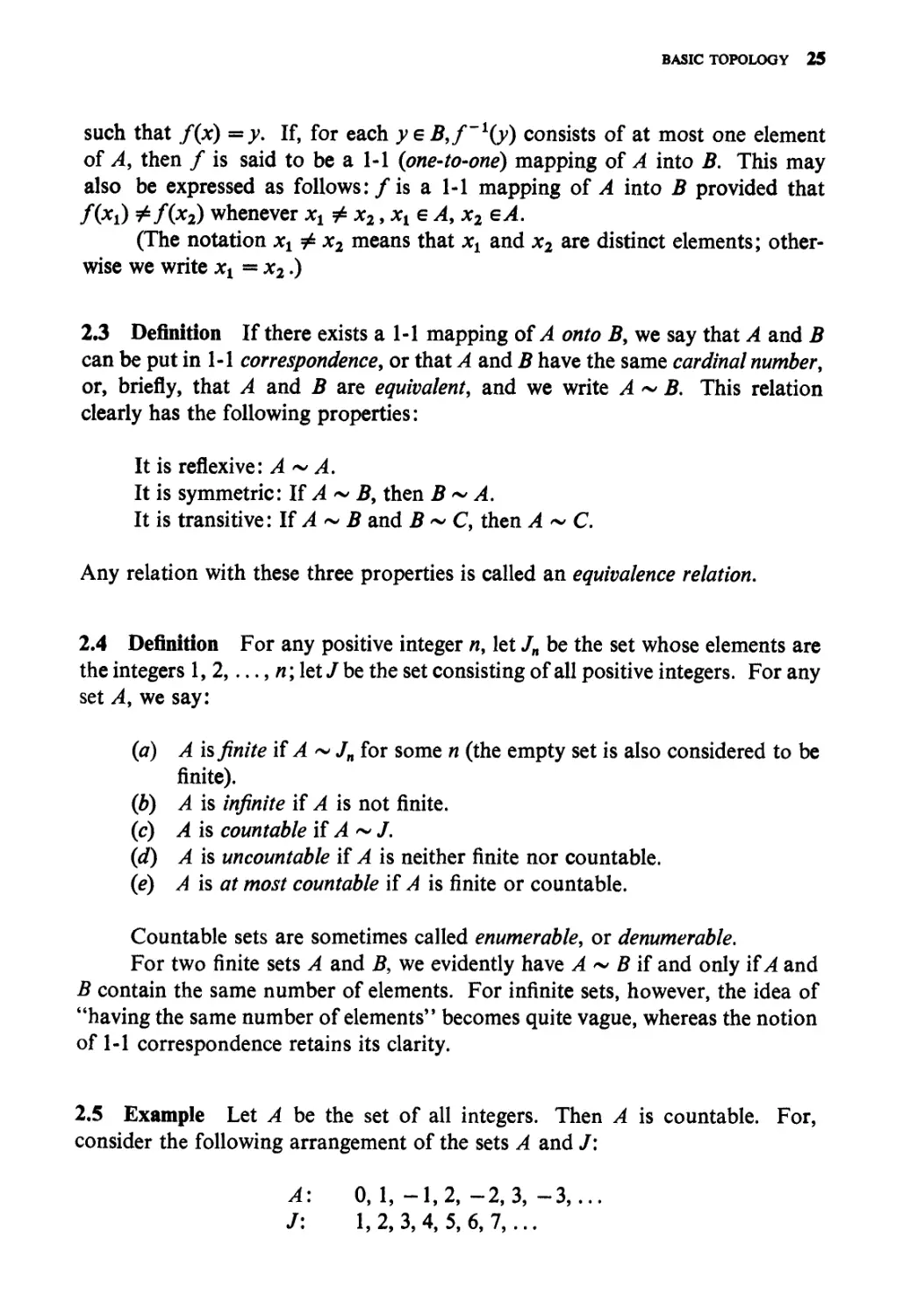
2.5 Example Let A be the set of all integers. Then A is countable. For,
consider the following arrangement of the sets A and /:
A: 0,1,-1,2,-2,3,-3,...
/: 1,2,3,4,5,6,7,...
26 PRINCIPLES OF MATHEMATICAL ANALYSIS
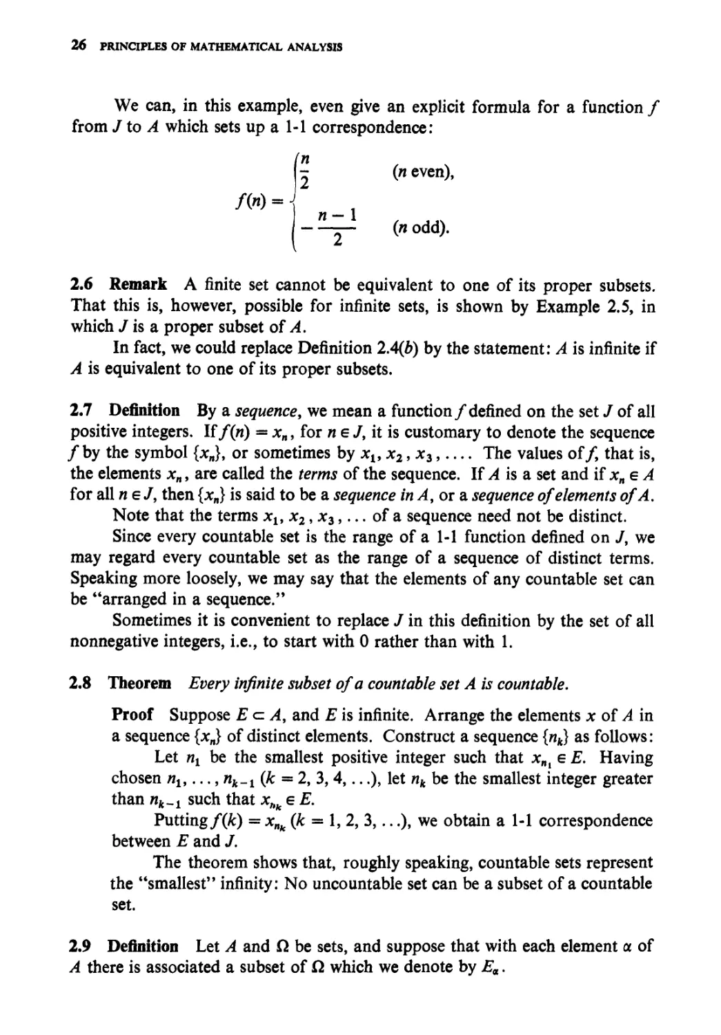
We can, in this example, even give an explicit formula for a function /
from J to A which sets up a 1-1 correspondence:
- (n even),
Л») - J
П— («odd).
2.6 Remark A finite set cannot be equivalent to one of its proper subsets.
That this is, however, possible for infinite sets, is shown by Example 2.5, in
which / is a proper subset of A.
In fact, we could replace Definition 2.4F) by the statement: A is infinite if
A is equivalent to one of its proper subsets.
2.7 Definition By a sequence, we mean a function/defined on the set / of all
positive integers. If/(и) = xn, for n e /, it is customary to denote the sequence
/by the symbol {#„}, or sometimes by xx, x2, хг, The values of/, that is,
the elements xn, are called the terms of the sequence. If A is a set and if xn e A
for all neJ, then {xn} is said to be a sequence in A, or a sequence of elements of A.
Note that the terms xl,x2,x3,... of a sequence need not be distinct.
Since every countable set is the range of a 1-1 function defined on /, we
may regard every countable set as the range of a sequence of distinct terms.
Speaking more loosely, we may say that the elements of any countable set can
be "arranged in a sequence."
Sometimes it is convenient to replace / in this definition by the set of all
nonnegative integers, i.e., to start with 0 rather than with 1.
2.8 Theorem Every infinite subset of a countable set A is countable.
Proof Suppose E <=. A, and E is infinite. Arrange the elements x of A in
a sequence {#„} of distinct elements. Construct a sequence {nk} as follows:
Let щ be the smallest positive integer such that xni e E. Having
chosen nu ..., nk-t (k — 2, 3,4,...), let nk be the smallest integer greater
than ик_! such that xhk e E.
Putting/(&) = х„к (к = 1, 2, 3,...), we obtain a 1-1 correspondence
between E and J.
The theorem shows that, roughly speaking, countable sets represent
the "smallest" infinity: No uncountable set can be a subset of a countable
set.
2.9 Definition Let A and Q be sets, and suppose that with each element a of
A there is associated a subset of Q which we denote by Ея.
BASIC TOPOLOGY 27
The set whose elements are the sets Ея will be denoted by {Ee}. Instead
of speaking of sets of sets, we shall sometimes speak of a collection of sets, or
a family of sets.
The union of the sets Ea is defined to be the set S such that x e S if and only
if x e Ея for at least one a e A. We use the notation
(U S = I I F
aeA
If A consists of the integers 1, 2,..., n, one usually writes
B) S=(jEm
or
V / 12 n *
If A is the set of all positive integers, the usual notation is
D) S=Q^m.
m=» I
The symbol сю in D) merely indicates that the union of a countable col-
collection of sets is taken, and should not be confused with the symbols + сю, — сю,
introduced in Definition 1.23.
The intersection of the sets Ee is defined to be the set P such that x e P if
and only if xe Ea for every aeA. We use the notation
aeA
or
n
\ ) | | iff 1 2 ft'
m=l
or
ao
G) P=()Em,
m=»l
as for unions. If A n В is not empty, we say that A and В intersect; otherwise
they are disjoint.
2.10 Examples
(a) Suppose Ex consists of 1, 2, 3 and E2 consists of 2, 3, 4. Then
Ex \j E2 consists of 1, 2, 3, 4, whereas Et n E2 consists of 2, 3.
28 PRINCIPLES OF MATHEMATICAL ANALYSIS
(b) Let A be the set of real numbers x such that 0 < x <, 1. For every
x e A, let Ex be the set of real numbers у such that 0 < у < х. Then
(i) Ex с Ег if and only if 0 < x <, z <, 1;
(ii) (jEx=Et;
xeA
(iii) П Ex is empty;
xeA
(i) and (ii) are clear. To prove (iii), we note that for every у > 0, у ф Ех
ifx<y. Henceуф(]Х€ЛЕх.
2.11 Remarks Many properties of unions and intersections are quite similar
to those of sums and products; in fact, the words sum and product were some-
sometimes used in this connection, and the symbols Z and П were written in place
of U and f].
The commutative and associative laws are trivial :
(8) A^jB~B\jA\ A n B = В о A.
(9) (Ь5)иС = ^иEиС); (АпВ)пС = Ап(Вп С).
Thus the omission of parentheses in C) and F) is justified.
The distributive law also holds:
A0) An(BuC) = (AnB)v(An C).
To prove this, let the left and right members of A0) be denoted by E and F,
respectively.
Suppose x e E. Then x e A and x e В и С, that is, x e В or x e С (pos-
(possibly both). Hence xe A n В or xeAnC, so that x e F. Thus E с F.
Next, suppose x e F. Then xeAnB or xeAn С That is, x e A, and
xeВ и С. Hence xeAn(B и С), so that Fc?.
It follows that E = F.
We list a few more relations which are easily verified:
A1) AczAkjB,
A2) AnBczA.
If 0 denotes the empty set, then
A3) AvO=A, Лп0 = 0.
If А с В, then
A4) AuB = B, AnB = A.
BASIC TOPOLOGY 29
2.12 Theorem Let {?„}, и = 1, 2, 3, ..., be a sequence of countable sets, and put
A5) \J
J
n=l
Then S is countable.
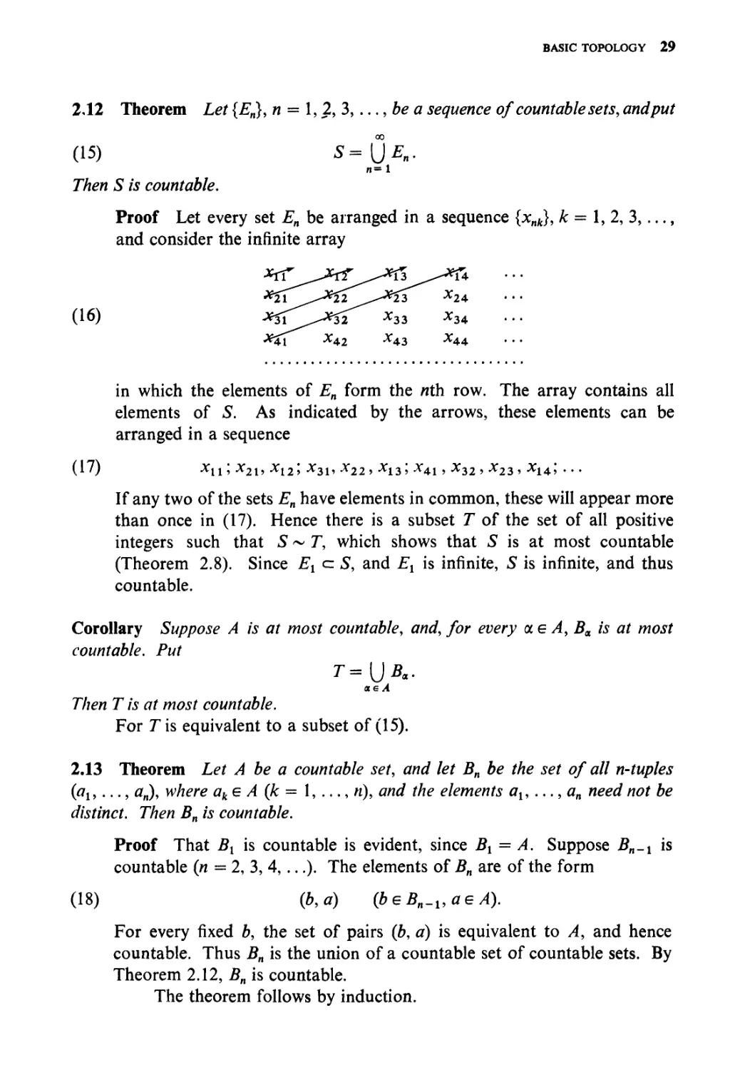
Proof Let every set ?„ be arranged in a sequence {xnj, к = 1, 2, 3,...,
and consider the infinite array
A6)
in which the elements of En form the nth row. The array contains all
elements of S. As indicated by the arrows, these elements can be
arranged in a sequence
A7) Xu ; X2\, Xl2> -^31' *22 > -^13» -*1 > *32 j -^23 ' *14» • • •
If any two of the sets En have elements in common, these will appear more
than once in A7). Hence there is a subset T of the set of all positive
integers such that S ~ T, which shows that S is at most countable
(Theorem 2.8). Since Ex <= S, and Ex is infinite, S is infinite, and thus
countable.
Corollary Suppose A is at most countable, and, for every a e A, Ba is at most
countable. Put
T=[jBa.
aeA
Then T is at most countable.
For T is equivalent to a subset of A5).
2.13 Theorem Let A be a countable set, and let Bn be the set of all n-tuples
(#!,..., йп), where ak e A (k = 1, ..., n), and the elements ax, ...,an need not be
distinct. Then Bn is countable.
Proof That Bx is countable is evident, since Bx = A. Suppose Bn.x is
countable (n = 2, 3, 4,...). The elements of Bn are of the form
A8) (b, а) (ЪеВп_х,аеА).
For every fixed b, the set of pairs (b, a) is equivalent to A, and hence
countable. Thus Bn is the union of a countable set of countable sets. By
Theorem 2.12, Bn is countable.
The theorem follows by induction.
30 PRINCIPLES OF MATHEMATICAL ANALYSIS
Corollary The set of all rational numbers is countable.
Proof We apply Theorem 2.13, with n = 2, noting that every rational r
is of the form b/a, where a and b are integers. The set of pairs (a, b), and
therefore the set of fractions b\a, is countable.
In fact, even the set of all algebraic numbers is countable (see Exer-
Exercise 2).
That not all infinite sets are, however, countable, is shown by the next
theorem.
2.14 Theorem Let A be the set of all sequences whose elements are the digits 0
and 1. This set A is uncountable.
The elements of A are sequences like 1, 0,0, 1, 0, 1, 1, 1,
Proof Let ? be a countable subset of A, and let E consist of the se-
sequences sl,s2,s3, We construct a sequence s as follows. If the nth
digit in sn is 1, we let the wth digit of s be 0, and vice versa. Then the
sequence s differs from every member of E in at least one place; hence
s ф Е. But clearly s e A, so that ? is a proper subset of A.
We have shown that every countable subset of A is a proper subset
of A. It follows that A is uncountable (for otherwise A would be a proper
subset of A, which is absurd).
The idea of the above proof was first used by Cantor, and is called Cantor's
diagonal process; for, if the sequences st, s2, s3,... are placed in an array like
A6), it is the elements on the diagonal which are involved in the construction of
the new sequence.
Readers who are familiar with the binary representation of the real
numbers (base 2 instead of 10) will notice that Theorem 2.14 implies that the
set of all real numbers is uncountable. We shall give a second proof of this
fact in Theorem 2.43.
METRIC SPACES
2.15 Definition A set X, whose elements we shall call points, is said to be a
metric space if with any two points p and q of X there is associated a real
number d(p, q), called the distance from p to q, such that
(a) d(p,q)>0ifp^q;d(p,p)=0;
(b) d(p,q)=d(q,p);
(c) d(p, q) < d(p, r) + d(r, q), for any r e X.
Any function with these three properties is called a distance function, or
a metric.
BASIC TOPOLOGY 31
2.16 Examples The most important examples of metric spaces, from our
standpoint, are the euclidean spaces Rk, especially Rl (the real line) and R2 (the
complex plane); the distance in Rk is defined by
A9) d(x,y)=\x-y\ (x,yeRk).
By Theorem 1.37, the conditions of Definition 2.15 are satisfied by A9).
It is important to observe that every subset У of a metric space X is a metric
space in its own right, with the same distance function. For it is clear that if
conditions (a) to (c) of Definition 2.15 hold for p, q,re X, they also hold if we
restrict p, q, r to lie in Y.
Thus every subset of a euclidean space is a metric space. Other examples
are the spaces ^(K) and &2(p), which are discussed in Chaps. 7 and 11, respec-
respectively.
2.17 Definition By the segment (a, b) we mean the set of all real numbers x
such that a < x < b.
By the interval [a, b] we mean the set of all real numbers x such that
a< x < b.
Occasionally we shall also encounter "half-open intervals" [a, b) and {a, b];
the first consists of all x such that a < x < b, the second of all x such that
a < x < b.
If ai < bt for / = 1, ..., k, the set of all points x = (jct,..., xk) in Rk whose
coordinates satisfy the inequalities at <х{<Ьг{\ < i < к) is called a k-cell.
Thus a 1-cell is an interval, a 2-cell is a rectangle, etc.
If x e Rk and r > 0, the open (or closed) ball В with center at x and radius r
is defined to be the set of all у e Rk such that | у — x| < r (or | у — x| <; r).
We call a set E a Rk convex if
Лх + A - Л)у е Е
whenever x б Е, у e E, and 0 < X < 1.
For example, balls are convex. For if | у — x | < r, | z — x | < r, and
0 < Я < 1, we have
| Ay + A - к)г - x| = \X(y - x) + A - A)(z - x)|
<Я|у-х| +A -Л)|ж-х| <Яг + A -Х)г
= г.
The same proof applies to closed balls. It is also easy to see that fc-cells are
convex.
32 PRINCIPLES OF MATHEMATICAL ANALYSIS
2.18 Definition Let X be a metric space. All points and sets mentioned below
are understood to be elements and subsets of X.
(a) A neighborhood of p is a set Nr(p) consisting of all q such that
d(p, q)<r, for some r > 0, The number r is called the radius of Nr(p).
(b) A point p is a limit point of the set E if eyery neighborhood of p
contains a point # Ф p such that # e E.
(c) IfpeE andp is not a limit point of E, then/? is called an isolated
point of E.
(d) E is closed if every limit point of ? is a point of E.
(e) A point p is an interior point of ?" if there is a neighborhood JV ofp
such that N с Е.
(/) ? is орел if every point of E is an interior point of E.
(g) The complement of E (denoted by E°) is the set of all points pe X
such that рф Е.
(h) E is perfect if ? is closed and if every point of ? is a limit point
of?.
(i) E is bounded if there is a real number M and a point ?eJ such that
d(p, q)<M for all peE.
(y) ? is dense in X if every point of A' is a limit point of E, or a point of
E (or both).
Let us note that in R1 neighborhoods are segments, whereas in R2 neigh-
neighborhoods are interiors of circles.
2.19 Theorem Every neighborhood is an open set.
Proof Consider a neighborhood E = Nr(p), and let q be any point of E.
Then there is a positive real number h such that
For all points s such that d(q, s) < h, we have then
d(p, s) < d(p, q) + d(q,s)<r-h + h=r,
so that se E. Thus q is an interior point of E.
2.20 Theorem If p is a limit point of a set E, then every neighborhood ofp
contains infinitely many points ofE.
Proof Suppose there is a neighborhood N of p which contains only a
finite number of points of E. Let qt,..., qn be those points of N n E,
which are distinct from p, and put
r = min d(p, qm)
BASIC TOPOLOGY 33
[we use this notation to denote the smallest of the numbers d(p, qt),...,
d(p, qn)]. The minimum of a finite set of positive numbers is clearly posi-
positive, so that r > 0.
The neighborhood Nr(p) contains no point q of E such that q Ф p,
so that p is not a limit point of E. This contradiction establishes the
theorem.
Corollary A finite point set has no limit points.
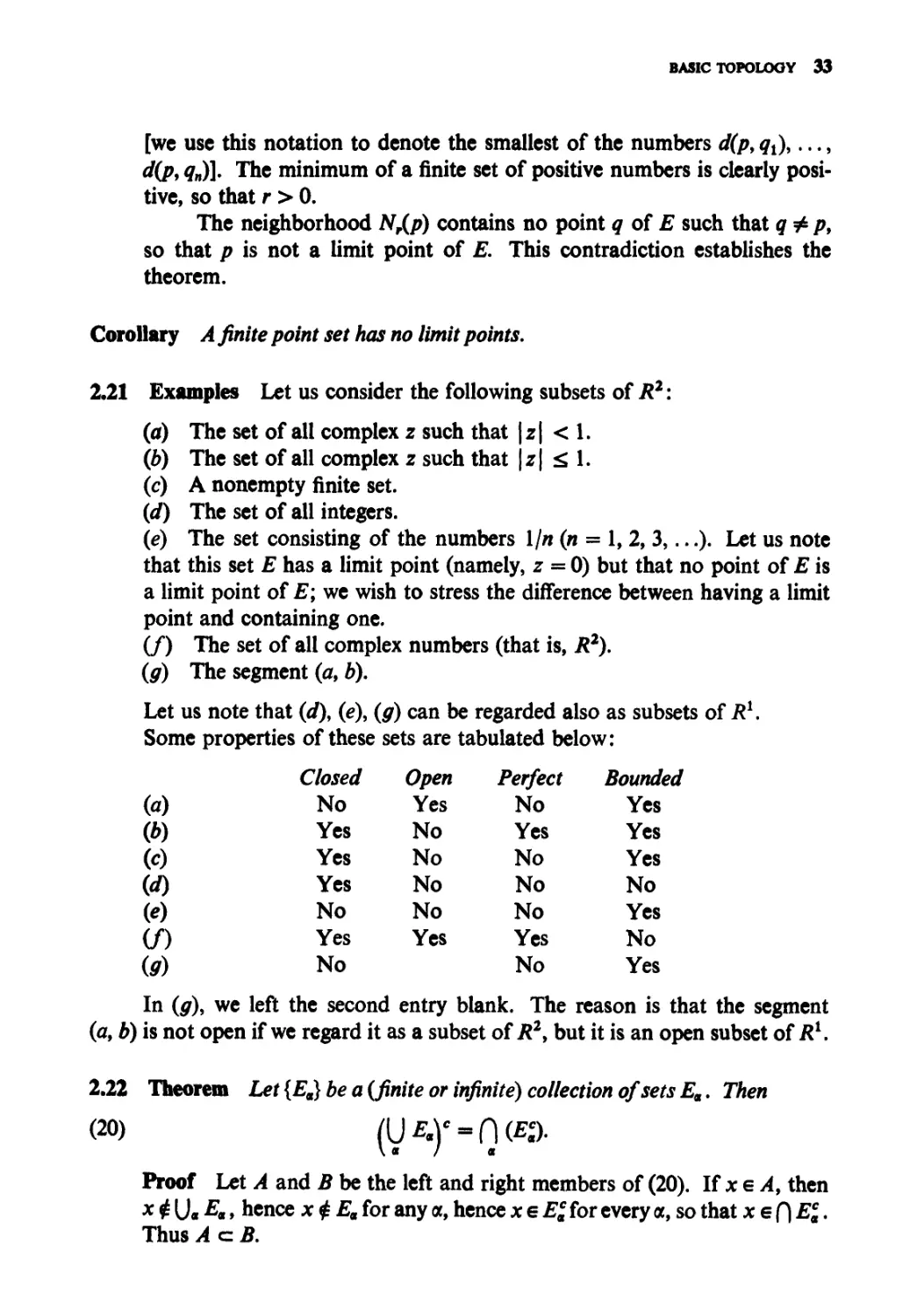
2.21 Examples Let us consider the following subsets of R2:
(a) The set of all complex z such that \z\ < 1.
(b) The set of all complex z such that \z\ <, 1.
(c) A nonempty finite set.
(d) The set of all integers.
(e) The set consisting of the numbers 1/л (и = 1, 2, 3,...). Let us note
that this set E has a limit point (namely, 2=0) but that no point of E is
a limit point of E; we wish to stress the difference between having a limit
point and containing one.
(/) The set of all complex numbers (that is, R2).
(g) The segment (a, b).
Let us note that (d), (e), (g) can be regarded also as subsets of R1.
Some properties of these sets are tabulated below:
Closed Open Perfect Bounded
(a) No Yes No Yes
<*)
Yes
Yes
Yes
No
Yes
No
No
No
No
No
Yes
Yes
No
No
No
Yes
No
Yes
Yes
No
Yes
No
Yes
(e)
if)
@)
In (g), we left the second entry blank. The reason is that the segment
(a, b) is not open if we regard it as a subset of R2, but it is an open subset of R1.
2.22 Theorem Let {Ee} be a {finite or infinite) collection of sets Ea. Then
B0)
Proof Let A and В be the left and right members of B0). If x 6 A, then
x ф (J, Ea, hence хфЕа for any a, hence x 6 El for every a, so that x e f) El.
Thus AcB.
34 PRINCIPLES OF MATHEMATICAL ANALYSIS
Conversely, if x 6 B, then xeEl for every a, hence хфЕл for any a,
hence x ф U« Ea, so that x 6 (Ua E*Y- Thus Bcz A.
It follows that A=B.
2.23 Theorem /4 .ye/ E is open if and only if its complement is closed.
Proof First, suppose Ec is closed. Choose xe E. Then x ф Ес, and x is
not a limit point of Ec. Hence there exists a neighborhood N of x such
that Ec n N is empty, that is, N с Е. Thus x is an interior point of E,
and ?" is open.
Next, suppose E is open. Let x be a limit point of Ec. Then every
neighborhood of x contains a point of Ec, so that x is not an interior point
of E. Since E is open, this means that x 6 Ec. It follows that Ec is closed.
Corollary A set F is closed if and only if its complement is open.
2.24 Theorem
(a) For any collection {Ga} of open sets, \Je Ga is open.
(b) For any collection {Fe} of closed sets, f)e Fe is closed.
(c) For any finite collection Glt..., Gn of open sets, П"= i Gt is open,
id) For any finite collection Fx,..., Fn of closed sets, (J"s x Ft is closed.
Proof Put G = (J« Ga. If x e G, then x 6 Ge for some a. Since x is an
interior point of Ge, x is also an interior point of G, and G is open. This
proves (a).
By Theorem 2.22,
B1)
and F$ is open, by Theorem 2.23. Hence (a) implies that B1) is open so
that f)a fe is closed.
Next, put H = [)"= i Gt. For any xeH, there exist neighborhoods
Nt of x, with radii rit such that Nt с Gt (i = 1,..., n). Put
r=min(rl5 ...,rn),
and let N be the neighborhood of x of radius r. Then N с Gt for i = 1,
...,«, so that N cz H, and Я is open.
By taking complements, (d) follows from (c):
BASIC TOPOLOGY 35
2.25 Examples In parts (c) and (d) of the preceding theorem, the finiteness of
the collections is essential. For let Gn be the segment I —, -I (« = 1, 2, 3,...).
\ n nj
Then Gn is an open subset of R1. Put G = (]%= t Gn. Then G consists of a single
point (namely, л: = 0) and is therefore not an open subset of R1.
Thus the intersection of an infinite collection of open sets need not be open.
Similarly, the union of an infinite collection of closed sets need not be closed.
2.26 Definition If X is a metric space, if E с X, and if E' denotes the set of
all limit points of E in X, then the closure of E is the set E = E и Е'.
2.27 Theorem If X is a metric space and E с X, then
(a) E is closed,
(b) E = E if and only ifE is closed,
(c) E c: Ffor every closed set F' <=¦ X such that E с F.
By (a) and (с), Е is the smallest closed subset of X that contains E.
Proof
(a) Ifp e X and p ф E then p is neither a point of E nor a limit point of E.
Hence p has a neighborhood which does not intersect E. The complement
of E is therefore open. Hence E is closed.
(b) If E = E, (a) implies that E is closed. If E is closed, then E' <=. E
[by Definitions 2.18(d) and 2.26], hence E = E.
(c) If F is closed and F => ?, then jF э F, hence F => ?'. Thus F => ?.
2.28 Theorem Lef ? fee a nonempty set of real numbers which is bounded above.
Let у = sup E. Then yeE. Hence yeEifEis closed.
Compare this with the examples in Sec. 1.9.
Proof If у 6 E then у е Е. Assume у ф Е. For every h > 0 there exists
then a point x e E such that у — h < x < y, for otherwise у — h would be
an upper bound of E. Thus у is a limit point of E. Hence j> e ?.
2.29 Remark Suppose Eс Kd, where Xis a metric space. To say that E
is an open subset of X means that to each point p e E there is associated a
positive number r such that the conditions d(p, q) <r,qe X imply that q e E.
But we have already observed (Sec. 2.16) that Y is also a metric space, so that
our definitions may equally well be made within Y. To be quite explicit, let us
say that E is open relative to Y if to each p e E there is associated an r > 0 such
that q e E whenever d(p, q)<r and qe Y. Example 2.2\(g) showed that a set
36 PRINCIPLES OF MATHEMATICAL ANALYSIS
may be open relative to Y without being an open subset of X. However, there
is a simple relation between these concepts, which we now state.
2.30 Theorem Suppose Y с X. A subset E of Y is open relative to Y if and
only ifE= Y r\ Gfor some open subset G ofX.
Proof Suppose E is open relative to Y. To each p e E there is a positive
number rp such that the conditions d(p, q)<rp,qe Y imply that q e E.
Let Vp be the set of all q e X such that d(p, q)<rp, and define
G=\JVP.
peE
Then G is an open subset of X, by Theorems 2.19 and 2.24.
Since p 6 Vp for all p e E, it is clear that E czG n Y.
By our choice of Vp, we have Vp n У с ? for every p e E, so that
G n Y <=. E. Thus E ^=G n Y, and one half of the theorem is proved.
Conversely, if G is open in X and E = G n Y, every /> e ? has a
neighborhood Vp <=¦ G. Then Vp n У c= ?, so that ? is open relative to Y.
COMPACT SETS
2.31 Definition By an open cover of a set ? in a metric space A1" we mean a
collection {(?«} of open subsets of X such that E <=. \Ja Ga.
2.32 Definition A subset К of a metric space X is said to be compact if every
open cover of К contains a finite subcover.
More explicitly, the requirement is that if {Ge} is an open cover of K, then
there are finitely many indices <xl5..., <х„ such that
К cz Gai и • • и Gan.
The notion of compactness is of great importance in analysis, especially
in connection with continuity (Chap. 4).
It is clear that every finite set is compact. The existence of a large class of
infinite compact sets in Rk will follow from Theorem 2.41.
We observed earlier (in Sec. 2.29) that if ? с Y <=: X, then E may be open
relative to Y without being open relative to X. The property of being open thus
depends on the space in which E is embedded. The same is true of the property
of being closed.
Compactness, however, behaves better, as we shall now see. To formu-
formulate the next theorem, let us say, temporarily, that К is compact relative to X if
the requirements of Definition 2.32 are met.
BASIC TOPOLOGY 37
2.33 Theorem Suppose AT с Y a X. Then К is compact relative to X if and
only if К is compact relative to Y.
By virtue of this theorem we are able, in many situations, to regard com-
compact sets as metric spaces in their own right, without paying any attention to
any embedding space. In particular, although it makes little sense to talk of
open spaces, or of closed spaces (every metric space X is an open subset of itself,
and is a closed subset of itself), it does make sense to talk of compact metric
spaces.
Proof Suppose К is compact relative to X, and let {Va] be a collection
of sets, open relative to Y, such that Kcz\JIIV<I. By theorem 2.30, there
are sets Ga, open relative to X, such that Va = Y n Ga, for all a; and since
К is compact relative to X, we have
B2) К с Gai и • • • и Gan
B3)
for some choice of finitely many indices at, ..., а„. Since Kc: Y, B2)
implies
This proves that К is compact relative to Y.
Conversely, suppose К is compact relative to Y, let {Ga} be a col-
collection of open subsets of X which covers K, and put Va = Y n Ga. Then
B3) will hold for some choice of al5 ..., <xn; and since Fac=Ga, B3)
implies B2).
This completes the proof.
2.34 Theorem Compact subsets of metric spaces are closed.
Proof Let К be a compact subset of a metric space X. We shall prove
that the complement of К is an open subset of X.
Suppose ре Х,рф К. ifqeK, let Vq and Wq be neighborhoods of p
and q, respectively, of radius less than \d{p,q) [see Definition 2.18(я)].
Since К is compact, there are finitely many points qy,..., qn in К such that
К cz Wqi и • • • и Wqn = W.
If v = Vqi n • • • n Vqn, then К is a neighborhood of p which does not
intersect W. Hence V c: Kc, so that p is an interior point of Kc. The
theorem follows.
2.35 Theorem Closed subsets of compact sets are compact.
Proof Suppose F а К с: X, F is closed (relative to X), and К is compact.
Let {Va} be an open cover of F. If Fc is adjoined to {Va}, we obtain an
38 PRINCIPLES OF MATHEMATICAL ANALYSIS
open cover Q of K. Since К is compact, there is a finite subcollection Ф
of Q which covers K, and hence F. If Fc is a member of Ф, we may remove
it from Ф and still retain an open cover of F. We have thus shown that a
finite subcollection of {Ke} covers F.
Corollary IfF is closed and К is compact, then Fr\ К is compact.
Proof Theorems 2.24{b) and 2.34 show that Fn К is closed; since
F n К с К, Theorem 2.35 shows that F n К is compact.
2.36 Theorem If{Ka} is a collection of compact subsets of a metric space X such
that the intersection of every finite subcollection of {Ka} is nonempty, then f) Ka
is nonempty.
Proof Fix a member Kt of {AT,} and put Ga = Kl. Assume that no point
of Kx belongs to every A!.. Then the sets Ga form an open cover of Kt;
and since K^ is compact, there are finitely many indices a},..., aR such
that AT, с Gei и • • • и G9n. But this means that
Kx о КЛ1 п ••• n КЯп
is empty, in contradiction to our hypothesis.
Corollary If{Kn} is a sequence of nonempty compact sets such that АГ„ => Kn+l
(n = 1, 2, 3,...), then f)f Kn is not empty.
2.37 Theorem If' E is an infinite subset of a compact set K, then Ehas a limit
point in K.
Proof If no point of К were a limit point of E, then each q e К would
have a neighborhood Vq which contains at most one point of E (namely,
q, if qeE). It is clear that no finite subcollection of {Vq} can cover E;
and the same is true of K, since E с К. This contradicts the compactness
of AT.
2.38 Theorem If {/„} is a sequence of intervals in R1, such that /„ => /n+1
(n = 1, 2, 3, ...), then Hf /„ is not empty.
Proof If /„ = [an, bn], let E be the set of all an. Then E is nonempty and
bounded above (by bt). Let x be the sup of E. If m and n are positive
integers, then
so that x<,bm for each m. Since it is obvious that am <, x, we see that
xelm for m = 1,2, 3,....
BASIC TOPOLOGY 39
2.39 Theorem Let к be a positive integer. If{In} is a sequence of k-cells such
that /„ => /n+i(« = 1, 2, 3,...), then f)? h is not empty.
Proof Let /„ consist of all points x = (jtb ..., xk) such that
anJ ^Xj< bnJ A <j < k; n = 1, 2, 3,...),
and put InJ = [anJi bnJ]. For each j, the sequence {InJ} satisfies the
hypotheses of Theorem 2.38. Hence there are real numbers x*(l <j <k)
such that
anJ <xj< bnJ A <y < ?; л = 1, 2, 3,...).
Setting x* = (x*,..., x*), we see that x* e/„ for n = 1, 2, 3, The
theorem follows.
2.40 Theorem Every k-cell is compact.
Proof Let / be a A>cell, consisting of all points x =(xlf ..., xk) such
that aj <Xj < bj A <j < k). Put
(k \l/2
Then |x - y| < 5, if xe/, у el.
Suppose, to get a contradiction, that there exists an open cover {Ga}
of / which contains no finite subcover of /. Put Cj = (aj + b})f2. The
intervals [л,-, Cj] and [cj, bj\ then determine 2k A:-cells Qt whose union is /.
At least one of these sets Qt, call it /1? cannot be covered by any finite
subcollection of {Ga} (otherwise / could be so covered). We next subdivide
It and continue the process. We obtain a sequence {/„} with the following
properties:
(a) / => /t => /2 => /3 => ¦ • • ;
(b) In is not covered by any finite subcollection of {Ga};
(c) if x e /„ and у e /„, then | x - у | < 2""S.
By (a) and Theorem 2.39, there is a point x* which lies in every /„.
For some a, x* e Ga. Since Ga is open, there exists r > 0 such that
| у - x* | < r implies that у e Ga. If и is so large that 2~nS < r (there is
such an n, for otherwise 2" < 5/r for all positive integers n, which is
absurd since R is archimedean), then (c) implies that InaGa, which con-
contradicts ф).
This completes the proof.
The equivalence of (a) and (b) in the next theorem is known as the Heine-
Borel theorem.
40 PRINCIPLES OF MATHEMATICAL ANALYSIS
2.41 Theorem If a set E in Rk has one of the following three properties, then it
has the other two:
(a) E is closed and bounded.
(b) E is compact.
(c) Every infinite subset ofE has a limit point in E.
Proof If (a) holds, then E cr / for some A>cell /, and (b) follows from
Theorems 2.40 and 2.35. Theorem 2.37 shows that (b) implies (c). It
remains to be shown that (c) implies (a).
If E is not bounded, then E contains points х„ with
|х„| >n (« = 1,2,3,...).
The set S consisting of these points х„ is infinite and clearly has no limit
point in Rk, hence has none in E. Thus (c) implies that E is bounded.
If E is not closed, then there is a point x0 e Rk which is a limit point
of E but not a point of E. For n = 1, 2, 3,..., there are points х„ е Е
such that |х„ — x01 < l/и. Let S be the set of these points х„. Then S is
infinite (otherwise | х„ — x01 would have a constant positive value, for
infinitely many ri), S has x0 as a limit point, and S has no other limit
point in Rk. For if у e Rk, у Ф x0, then
|х„-у| > I x0 — у I - |х„-хо|
|| 1|
for all but finitely many n\ this shows that у is not a limit point of S
(Theorem 2.20).
Thus S has no limit point in E; hence E must be closed if (c) holds.
We should remark, at this point, that (b) and (c) are equivalent in any
metric space (Exercise 26) but that (a) does not, in general, imply (b) and (c).
Examples are furnished by Exercise 16 and by the space jSf2, which is dis-
discussed in Chap. 11.
2.42 Theorem (Weierstrass) Every bounded infinite subset of Rk has a limit
point in Rk.
Proof Being bounded, the set E in question is a subset of a A>cell / cr Rk.
By Theorem 2.40, / is compact, and so E has a limit point in /, by
Theorem 2.37.
BASIC TOPOLOGY 41
PERFECT SETS
2.43 Theorem Let P be a nonempty perfect set in Rk. Then P is uncountable.
Proof Since P has limit points, P must be infinite. Suppose P is count-
countable, and denote the points of P by x1? x2, x3, We shall construct a
sequence {Vn} of neighborhoods, as follows.
Let Vy be any neighborhood of Xj. If Vx consists of all у e Rk such
that | у — Xj | < r, the closure Vx of Vx is the set of all у е Rk such that
|y-*il ^r-
Suppose Vn has been constructed, so that Vn n P is not empty. Since
every point of P is a limit point of P, there is a neighborhood Vn+i such
that (i) Vn+1 с Vn, (ii) х„? FB+1, (Hi) FB+1 n? is not empty. By (iii),
Vn+1 satisfies our induction hypothesis, and the construction can proceed.
Put Kn = Vn n P. Since Vn is closed and bounded, Vn is compact.
Since х„ ф Kn+l, no point of P lies in f]f Kn. Since Kn cr P, this implies
that fl* ^n is empty. But each Kn is nonempty, by (iii), and АГ„ => АГ„+1,
by (i); this contradicts the Corollary to Theorem 2.36.
Corollary Every interval [a, b] (a < b) is uncountable. In particular, the set of
all real numbers is uncountable.
2.44 The Cantor set The set which we are now going to construct shows
that there exist perfect sets in R1 which contain no segment.
Let Eo be the interval [0, 1]. Remove the segment (?, f), and let El be
the union of the intervals
Remove the middle thirds of these intervals, and let E2 be the union of the
intervals
Continuing in this way, we obtain a sequence of compact sets En, such that
(a) ?t =э?2з?3 =>•••;
(b) Е„ is the union of 2" intervals, each of length 3 ".
The set
n=l
is called the Cantor set. P is clearly compact, and Theorem 2.36 shows that P
is not empty.
42 PRINCIPLES OF MATHEMATICAL ANALYSIS
No segment of the form
where к and m are positive integers, has a point in common with P. Since every
segment (a, /?) contains a segment of the form B4), if
P contains no segment.
To show that P is perfect, it is enough to show that P contains no isolated
point. Let x 6 P, and let S be any segment containing x. Let /„ be that interval
of En which contains x. Choose n large enough, so that /„ с S. Let xn be an
endpoint of /„, such that xn Ф x.
It follows from the construction of P that xn e P. Hence дг is a limit point
of P, and P is perfect.
One of the most interesting properties of the Cantor set is that it provides
us with an example of an uncountable set of measure zero (the concept of
measure will be discussed in Chap. 11).
CONNECTED SETS
2.45 Definition Two subsets A and В of a metric space X are said to be
separated if both А о Б and Л п В are empty, i.e., if no point of A lies in the
closure of В and no point of В lies in the closure of A.
A set E с X is said to be connected if E is not a union of two nonempty
separated sets.
2.46 Remark Separated sets are of course disjoint, but disjoint sets need not
be separated. For example, the interval [0,1] and the segment A,2) are not
separated, since 1 is a limit point of A, 2). However, the segments @, 1) and
A, 2) are separated.
The connected subsets of the line have a particularly simple structure:
2.47 Theorem A subset E of the real line R1 is connected if and only if it has the
following property: If x e E, у e E, and x <z <y, then z e E.
Proof If there exist x e E, у е Е, and some z e (x, y) such that z ф Е, then
E = Az\j Bz where
Ax =En (-oo, z), Bz = En (z, oo).
BASIC TOPOLOGY 43
Since x e Az and у e Bz, A and В are nonempty. Since Az с (— оо, z) and
2?z с (z, oo), they are separated. Hence E is not connected.
To prove the converse, suppose E is not connected. Then there are
nonempty separated sets A and В such that А и В = E. Pick дг е Л, у е Д
and assume (without loss of generality) that x < y. Define
z = sup (A n [x, y]).
By Theorem 2.28, ze A; hence z ф В. In particular, x <,z <y.
If z $ A, it follows that x < z < у and z $ E.
If z e A, then z ^ B, hence there exists zt such that z <zt <y and
zy ф B. Then дг < zt < у and zt $ E.
EXERCISES
1. Prove that the empty set is a subset of every set.
2. A complex number z is said to be algebraic if there are integers a0,..., an, not all
zero, such that
aozn + aizn-i -\ + an-iz + an =0.
Prove that the set of all algebraic numbers is countable. Hint: For every positive
integer N there are only finitely many equations with
n+ \ao\ + |fli| +•••+ \an\ =N.
3. Prove that there exist real numbers which are not algebraic.
4. Is the set of all irrational real numbers countable ?
5. Construct a bounded set of real numbers with exactly three limit points.
6. Let E' be the set of all limit points of a set E. Prove that ?" is closed. Prove that
E and E have the same limit points. (Recall that E = Eu ?".) Do Eand E'always
have the same limit points?
7. Let A u A2, A3, ...be subsets of a metric space.
(а) If Bn = U"-i At, Prove that Д, = (J"=i Я,, for n = 1, 2, 3, ... .
(б) If В = Ur-i Л(, prove that В = U«°=i & ¦
Show, by an example, that this inclusion can be proper.
8. Is every point of every open set E с R2 a limit point of El Answer the same
question for closed sets in R2.
9. Let E° denote the set of all interior points of a set E. [See Definition 2.Ще);
E° is called the interior of E.]
(a) Prove that E° is always open.
(b) Prove that E is open if and only if E° = E.
(c) If G с E and G is open, prove that G <= E°.
id) Prove that the complement of E° is the closure of the complement of E.
(e) Do E and E always have the same interiors ?
(/) Do ?*and E° always have the same closures?
44 PRINCIPLES OF MATHEMATICAL ANALYSIS
10. Let Xbe an infinite set. Forpe Xandqe X, define
A (ifp*q)
d(p,q)= .
@ (if/? =
Prove that this is a metric. Which subsets of the resulting metric space are open?
Which are closed? Which are compact?
11. For xeR1 and у е Д1, define
di(x, y) = (x- yJ,
ds(x,y)=
l+\x-y\m
Determine, for each of these, whether it is a metric or not.
12. Let К <= R1 consist of 0 and the numbers l/n, for n = 1, 2, 3, .... Prove that К is
compact directly from the definition (without using the Heine-Borel theorem).
13. Construct a compact set of real numbers whose limit points form a countable set.
14. Give an example of an open cover of the segment @,1) which has no finite sub-
cover.
15. Show that Theorem 2.36 and its Corollary become false (in Rl, for example) if the
word "compact" is replaced by "closed" or by "bounded."
16. Regard Q, the set of all rational numbers, as a metric space, with d(p, q) = \p — q\.
Let E be the set of all p e Q such that 2 <p2 < 3. Show that E is closed and
bounded in Q, but that E is not compact. Is E open in Q ?
17. Let E be the set of all x e [0, 1] whose decimal expansion contains only the digits
4 and 7. Is E countable? Is E dense in [0,1]? Is Я compact? Is E perfect?
18. Is there a nonempty perfect set in Rl which contains no rational number?
19. (a) If A and В are disjoint closed sets in some metric space X, prove that they
are separated.
(b) Prove the same for disjoint open sets.
(c) Fix p e X, 8 > 0, define A to be the set of all q e X for which d(p, q) < 8, define
В similarly, with > in place of <. Prove that A and В are separated.
(d) Prove that every connected metric space with at least two points is uncount-
uncountable. Hint: Use(c).
20. Are closures and interiors of connected sets always connected ? (Look at subsets
of*2.)
21. Let A and В be separated subsets of some Rk, suppose a 6 A, b e B, and define
for t e Rl. Put Ao = Р~ЧЛ), Bo = P~\B). [Thus teAoif and only if p(t) e A.]
BASIC TOPOLOGY 45
(a) Prove that Ao and Bo are separated subsets of R1.
(b) Prove that there exists /0 e @, 1) such that p(/0) фАиВ.
(c) Prove that every convex subset of R" is connected.
22. A metric space is called separable if it contains a countable dense subset. Show
that Rk is separable. Hint: Consider the set of points which have only rational
coordinates.
23. A collection {V,} of open subsets of X is said to be a base for X if the following
is true: For every xe X and every open set G <= X such that x e G, we have
x e Fa c G for some a. In other words, every open set in X is the union of а
subcollection of {V,}.
Prove that every separable metric space has a countable base. Я/я/; Take
all neighborhoods with rational radius and center in some countable dense subset
of X.
24. Let Л' be a metric space in which every infinite subset has a limit point. Prove that
Л'is separable. Hint: Fix S > 0, and pick xx e X. Having chosen xu ..., Xj e X,
choose xJ + 1 e X, if possible, so that ^(л-,, xJ + 1)> 8 for / = 1, ...,/. Show that
this process must stop after a finite number of steps, and that X can therefore be
covered by finitely many neighborhoods of radius 8. Take 8 = 1/я (я = 1, 2, 3,...),
and consider the centers of the corresponding neighborhoods.
25. Prove that every compact metric space К has a countable base, and that К is
therefore separable. Hint: For every positive integer n, there are finitely many
neighborhoods of radius l/n whose union covers K.
26. Let X be a metric space in which every infinite subset has a limit point. Prove
that X is compact. Hint: By Exercises 23 and 24, X has a countable base. It
follows that every open cover of X has a countable subcover {Gn}, я = 1, 2, 3, ....
If no finite subcollection of {Gn} covers X, then the complement Fn of Gt и • • ¦ и Gn
is nonempty for each n, but f] Fn is empty. If ? is a set which contains a point
from each Fn, consider a limit point of E, and obtain a contradiction.
27. Define a point /? in a metric space Л' to be a condensation point of a set E с Л' if
every neighborhood of/? contains uncountably many points of E.
Suppose E <=¦ Rk, E is uncountable, and let P be the set of all condensation
points of E. Prove that P is perfect and that at most countably many points of E
are not in P. In other words, show that Pc n E is at most countable. Hint: Let
{Vn} be a countable base of Rk, let W be the union of those Vn for which E n Vn
is at most countable, and show that P = Wc.
28. Prove that every closed set in a separable metric space is the union of a (possibly
empty) perfect set and a set which is at most countable. {Corollary: Every count-
countable closed set in Rk has isolated points.) Hint: Use Exercise 27.
29. Prove that every open set in Rl is the union of an at most countable collection of
disjoint segments. Hint: Use Exercise 22.
46 PRINCIPLES OF MATHEMATICAL ANALYSIS
30. Imitate the proof of Theorem 2.43 to obtain the following result:
If Rk = [JfFn, where each Fn is a closed subset of Rk, then at least one Fn
has a nonempty interior.
Equivalent statement: If Gn is a dense open subset of R", for n = 1, 2, 3,...,
then (]TGn is not empty (in fact, it is dense in Rk).
(This is a special case of Baire's theorem; see Exercise 22, Chap. 3, for the general
case.)
NUMERICAL SEQUENCES AND SERIES
As the title indicates, this chapter will deal primarily with sequences and series
of complex numbers. The basic facts about convergence, however, are just as
easily explained in a more general setting. The first three sections will therefore
be concerned with sequences in euclidean spaces, or even in metric spaces.
CONVERGENT SEQUENCES
3.1 Definition A sequence {/?„} in a metric space X is said to converge if there
is a point/? e X with the following property: For every e > 0 there is an integer
N such that n > N implies that d(pn ,p)<e. (Here d denotes the distance in X.)
In this case we also say that {/?„} converges to p, or that p is the limit of
{р„} [see Theorem 3.2F)], and we write р„ ->р, or
lim pH = p.
If {/?„} does not converge, it is said to diverge.
48 PRINCIPLES OF MATHEMATICAL ANALYSIS
It might be well to point out that our definition of "convergent sequence"
depends not only on {/?„} but also on X; for instance, the sequence {1/w} con-
converges in Rl (to 0), but fails to converge in the set of all positive real numbers
[with d(x,y) = \x — y\]. In cases of possible ambiguity, we can be more
precise and specify "convergent in X" rather than "convergent."
We recall that the set of all points р„ (n = 1, 2, 3,...) is the range of {/?„}.
The range of a sequence may be a finite set, or it may be infinite. The sequence
{/?„} is said to be bounded if its range is bounded.
As examples, consider the following sequences of complex numbers
(that is, X = R2):
(a) lfsn = \/n, then limn_»00 sn = 0; the range is infinite, and the sequence
is bounded.
(b) If sn = n2, the sequence {sn} is unbounded, is divergent, and has
infinite range.
(c) If sn = 1 + [(— l)n/n], the sequence {sn} converges to 1, is bounded,
and has infinite range.
(d) If sn = i", the sequence {sn} is divergent, is bounded, and has finite
range.
(e) If sn = 1 (« = 1, 2, 3, ...), then {sn} converges to 1, is bounded, and
has finite range.
We now summarize some important properties of convergent sequences
in metric spaces.
3.2 Theorem Let {pn} be a sequence in a metric space X.
(a) (Pn) converges to p e X if and only if every neighborhood of p contains
pn for all but finitely many n.
(b) If p e X, p' e X, and if{pn} converges to p and to p', then p' = p.
(c) If{pn} converges, then {pn} is bounded.
(d) IfEczX and ifp is a limit point of E, then there is a sequence {р„} in E
such that p = lim pn.
n-*oo
Proof (a) Suppose pn-+p and let V be a neighborhood of p. For
some e > 0, the conditions d(q, p) < e, q e X imply q e V. Correspond-
Corresponding to this e, there exists N such that n > N implies d(pn ,p)<E. Thus
n > N implies pn e V.
Conversely, suppose every neighborhood of p contains all but
finitely many of the pn. Fix e > 0, and let V be the set of all q e X such
that d(p, q) < e. By assumption, there exists N (corresponding to this V)
such that pn e V if n > N. Thus d(pn,p) < e if n > N; hence pn -+p.
NUMERICAL SEQUENCES AND SERIES 49
(b) Let e > 0 be given. There exist integers N, N' such that
g
n > N implies d(pn,p)<->
e
n ^N' implies d(pn,//)<-•
Hence if n ^ max (N, N'), we have
d(p, p') <, d{p, pn) + d(pn, p') < e.
Since e was arbitrary, we conclude that d(p, p') = 0.
(c) Suppose р„ -*p. There is an integer N such that n > N
implies d(pn,p)<\. Put
r = max{1, d(pltp),..., d(pN,p)}.
Then d(pn, p) < r for n = 1, 2, 3,
(d) For each positive integer n, there is a point pne E such that
d(Pn>P) < Vя- Given e > 0, choose N so that Ne > 1. If и > TV, it
follows that </(/?„, p) < e. Hence /?„ -*/?.
This completes the proof.
For sequences in Rk we can study the relation between convergence, on
the one hand, and the algebraic operations on the other. We first consider
sequences of complex numbers.
3.3 Theorem Suppose {sn}, {tn} are complex sequences, and limn_»00 sn = s,
lim^f,,-/. Then
(a) \im(sn + tH) = s + t;
П-+ОО
(b) lim csn = cs, lim (c + sn) = с + s, for any number c\
n-*oo n-*oo
(c) \im sntn = st;
n-*oo
(d) lim - = -, provided sn Ф 0 (n = 1, 2, 3,...), and s ф 0.
П-> 00 "Уц S
Proof
(й) Given e > 0, there exist integers Nlf N2 such that
g
n^Ni implies \sn — s\<-,
g
n>N2 implies \tn — t\<~-
50 PRINCIPLES OF MATHEMATICAL ANALYSIS
If N = max (Nlf N2), then n ^ N implies
I toi + '») — \s + 01 ^ I sn ~s I + Kn — * <fi>
This proves (я). The proof of (b) is trivial.
(c) We use the identity
A) sntn -st = to, - s)(tn -t) + s(tn -t) + t(sn - s).
Given e > 0, there are integers Nit N2 such that
n^.Nt implies |sn — s\ < yje,
n^.N2 implies | tn — t\ < y/e.
If we take N = max (Nlt N2), n>N implies
lto-^-01 <e,
so that
lim to - s)(tn -0 = 0.
Л->00
We now apply (a) and (b) to A), and conclude that
lim (sntn — st) = 0.
n-*oo
(d) Choosing m such that \sn — s\ < \\s\ if n > m, we see that
Given e > 0, there is an integer N > m such that n ^ N implies
Hence, for n>N,
1 s. — s 2
<TZ72\sn-s\ <e.
I 1
sn s
sn-s
3.4 Theorem
(a) Suppose \n e Rk (n = 1, 2, 3, ...) and
Then {xn} converges to x = (ab ..., <xk) if and only if
B)
NUMERICAL SEQUENCES AND SERIES 51
(b) Suppose {xj, {у„} are sequences in Rk, {/?„} is a sequence of real numbers,
andxn-*x,yn^y,pn-+p. Then
lim (хя + у„) = x + у, lim х„ • у„ = х • у, lim & х„ = 0х.
и-юо п-*оо п-юо
Proof
(a) If х„ -> х, the inequalities
which follow immediately from the definition of the norm in Rk, show that
B) holds.
Conversely, if B) holds, then to each e > 0 there corresponds an
integer N such that n ^ N implies
Hence n ^ N implies
so that xn -> x. This proves (a).
Part (b) follows from (a) and Theorem 3.3.
SUBSEQUENCES
3.5 Definition Given a sequence {/?„}, consider a sequence {nk} of positive
integers, such that nx < n2 < «3 < • • •. Then the sequence {pm} is called a
subsequence of {/?„}. If {pni} converges, its limit is called a subsequential limit
of {ft}.
It is clear that {/?„} converges to p if and only if every subsequence of
{pn} converges to p. We leave the details of the proof to the reader.
3.6 Theorem
(a) If{pn} is a sequence in a compact metric space X, then some sub-
subsequence of{pn} converges to a point of X.
(b) Every bounded sequence in Rk contains a convergent subsequence.
52 PRINCIPLES OF MATHEMATICAL ANALYSIS
Proof
(a) Let E be the range of {/?„}. If E is finite then there is a p e E and a
sequence {я,} with щ < n2 < пъ < • • •, such that
The subsequence {pni} so obtained converges evidently to p.
If E is infinite, Theorem 2.37 shows that E has a limit point p e X.
Choose щ so that d(p,pni) < 1. Having chosen щ,..., nt-lt we see from
Theorem 2.20 that there is an integer nt > «,_! such that d(p,pni) < 1/i.
Then {pnt} converges to p.
(b) This follows from (a), since Theorem 2.41 implies that every bounded
subset of Rk lies in a compact subset of Rk.
3.7 Theorem The subsequential limits of a sequence {pn} in a metric space X
form a closed subset of X.
Proof Let E* be the set of all subsequential limits of {/?„} and let q be a
limit point of E*. We have to show that q e E*.
Choose щ so that pni^q. (If no such nt exists, then E* has only
one point, and there is nothing to prove.) Put S = d(q, pni). Suppose
«!,...,«,_! are chosen. Since q is a limit point of E*, there is an x e E*
with d(x,q) <2~l6. Since xeE*, there is an nl>ni-l such that
d(x,pnt) <2-'<5. Thus
for /= 1,2, 3, This says that {/?„,} converges to q. Hence # e E*.
CAUCHY SEQUENCES
3.8 Definition A sequence {р„} in a metric space X is said to be a Cauchy
sequence if for every e > 0 there is an integer iV such that d(pn, pm) < e if n ^ iV
and m^.N.
In our discussion of Cauchy sequences, as well as in other situations
which will arise later, the following geometric concept will be useful.
3.9 Definition Let ? be a nonempty subset of a metric space X, and let S be
the set of all real numbers of the form d(p, q), with p e E and qeE. The sup
of S is called the diameter of E.
NUMERICAL SEQUENCES AND SERIES 53
lf{pn}is a sequence in X and if EN consists of the points pN,pN+l,pN+2,...,
it is clear from the two preceding definitions that {pn} is a Cauchy sequence
if and only if
lim diam EN = 0.
N-*oo
3.10 Theorem
(a) IfE is the closure of a set E in a metric space X, then
diam ? = diam E.
(b) If Kn is a sequence of compact sets in X such that Kn=> Kn+l
(n = \,2,3,...)andif
lim diam Kn = 0,
n-*oo
then f]fKn consists of exactly one point.
Proof
(a) Since E с E, it is clear that
diam ? < diam E.
Fix e > 0, and choose p e E,q e E. By the definition of ?, there are
points p', q', in E such that d(p, p') < e, d(q, q') < e. Hence
d(p,q)<d(p,p') + d(p'q') + d(q',q)
<2e + d(p', q') < 2e 4- diam E.
It follows that
diam ? < 2e + diam E,
and since e was arbitrary, (a) is proved.
(b) Put K= f)?Kn. By Theorem 2.36, К is not empty. If К contains
more than one point, then diam К > 0. But for each n, Kn => K, so that
diam Kn > diam K. This contradicts the assumption that diam Kn -> 0.
3.11 Theorem
(a) In any metric space X, every convergent sequence is a Cauchy sequence.
(b) If X is a compact metric space and if{pn} is a Cauchy sequence in X,
then {pn} converges to some point of X.
(c) In Rk, every Cauchy sequence converges.
Note: The difference between the definition of convergence and
the definition of a Cauchy sequence is that the limit is explicitly involved
in the former, but not in the latter. Thus Theorem 3.11F) may enable us
54 PRINCIPLES OF MATHEMATICAL ANALYSIS
to decide whether or not a given sequence converges without knowledge
of the limit to which it may converge.
The fact (contained in Theorem 3.11) that a sequence converges in
Rk if and only if it is a Cauchy sequence is usually called the Cauchy
criterion for convergence.
Proof
(a) If /?„->/? and if e > 0, there is an integer N such that d(p,pn) < e
for all n>N. Hence
d(pn, Pm) < d(pn, P) + d(p, pm) < 2e
as soon as n > N and m> N. Thus {pn} is a Cauchy sequence.
(b) Let {pn} be a Cauchy sequence in the compact space X. For
N = 1, 2, 3, ..., let EN be the set consisting of pN, pN+i, Pn+2 > - • • •
Then
C) lim diam EN = 0,
JV-»oo
by Definition 3.9 and Theorem 3.10(л). Being a closed subset of the
compact space X, each EN is compact (Theorem 2.35). Also EN ^ EN + l,
so that EN =5 EN+l.
Theorem 3A0(b) shows now that there is a unique p e X which lies
in every EN.
Let e > 0 be given. By C) there is an integer Л^ such that
diam EN < e if N > No. Since p e EN, it follows that d(p, q) < e for
every q e EN, hence for every q e EN. In other words, d(p, pn) < e if
n > No • This says precisely that pn -*¦ p.
(c) Let {xn} be a Cauchy sequence in Rk. Define EN as in (b), with x,
in place of p{. For some N, diam EN < 1. The range of {xn} is the union
of EN and the finite set {xt, ....x^.J. Hence {xj is bounded. Since
every bounded subset of Rk has compact closure in Rk (Theorem 2.41),
(c) follows from (b).
3.12 Definition A metric space in which every Cauchy sequence converges is
said to be complete.
Thus Theorem 3.11 says that all compact metric spaces and all Euclidean
spaces are complete. Theorem 3.11 implies also that every closed subset E of a
complete metric space X is complete. (Every Cauchy sequence in E is a Cauchy
sequence in X, hence it converges to some p e X, and actually p e E since E is
closed.) An example of a metric space which is not complete is the space of all
rational numbers, with d(x, y) = \ x — у \.
NUMERICAL SEQUENCES AND SERIES 55
Theorem 3.2(c) and example (d) of Definition 3.1 show that convergent
sequences are bounded, but that bounded sequences in Rk need not converge.
However, there is one important case in which convergence is equivalent to
boundedness; this happens for monotonic sequences in Rl.
3.13 Definition A sequence {sn} of real numbers is said to be
(a) monotonically increasing if sn < sn+l (n = 1, 2, 3,...);
(b) monotonically decreasing if sn > sn+l (n = 1, 2, 3, ...).
The class of monotonic sequences consists of the increasing and the
decreasing sequences.
3.14 Theorem Suppose {sn} is monotonic. Then {sn} converges if and only if it
is bounded.
Proof Suppose sn <, sn+l (the proof is analogous in the other case).
Let E be the range of {sn}. If {sn} is bounded, let s be the least upper
bound of E. Then
sn?s (и = 1,2, 3,...).
For every e > 0, there is an integer N such that
s — e < sN < s,
for otherwise s — e would be an upper bound of E. Since {sn} increases,
n> N therefore implies
s - e < sn <, s,
which shows that {sn} converges (to s).
The converse follows from Theorem 3.2(c).
UPPER AND LOWER LIMITS
3.15 Definition Let {sn} be a sequence of real numbers with the following
property: For every real M there is an integer N such that n > N implies
sn ;> M. We then write
Similarly, if for every real M there is an integer iV such that n > N implies
sn <, M, we write
sn~> -oo.
56 PRINCIPLES OF MATHEMATICAL ANALYSIS
It should be noted that we now use the symbol -*¦ (introduced in Defini-
Definition 3.1) for certain types of divergent sequences, as well as for convergent
sequences, but that the definitions of convergence and of limit, given in Defini-
Definition 3.1, are in no way changed.
3.16 Definition Let {sn} be a sequence of real numbers. Let E be the set of
numbers x (in the extended real number system) such that snk -»x for some
subsequence {snk}. This set E contains all subsequential limits as defined in
Definition 3.5, plus possibly the numbers +oo, — oo.
We now recall Definitions 1.8 and 1.23 and put
s* = sup E,
s* = inf E.
The numbers s*, s* are called the upper and lower limits of {sn}; we use the
notation
lim sup sn = s*, lim inf sn = s*.
П-ЮО П-ЮО
3.17 Theorem Let {sn} be a sequence of real numbers. Let E and s* have the
same meaning as in Definition 3.16. Then s* has the following two properties:
(a) s*eE.
(b) If x> s*, there is an integer N such that n> N implies sn < x.
Moreover, s* is the only number with the properties (a) and (b).
Of course, an analogous result is true for 5*.
Proof
(a) If j* = + oo, then Eis not bounded above; hence {sn} is not bounded
above, and there is a subsequence {snk} such that snk -> + oo.
If s* is real, then E is bounded above, and at least one subsequential
limit exists, so that (a) follows from Theorems 3.7 and 2.28.
If s* = —oo, then E contains only one element, namely — oo, and
there is no subsequential limit. Hence, for any real M, sn> M for at
most a finite number of values of n, so that sn ~* — oo.
This establishes (a) in all cases.
(b) Suppose there is a number x > s* such that sn > x for infinitely
many values of n. In that case, there is a number у е Е such that
у ^ x > s*, contradicting the definition of s*.
Thus s* satisfies (a) and (b).
To show the uniqueness, suppose there are two numbers, p and q,
which satisfy (a) and (b), and suppose/? < q. Choose x such that/? < x < q.
Since p satisfies (b), we have sn < x for n > N. But then q cannot satisfy (a).
NUMERICAL SEQUENCES AND SERIES 57
3.18 Examples
(a) Let {sn} be a sequence containing all rationale. Then every real
number is a subsequential limit, and
lim sup sn = +00, lim inf sn = — oo.
n-»oo n-»oo
(ft) Let5n = (-ln)/[l+(l/n)]. Then
lim sup sn = \, lim inf sn = — 1.
П-» 00 FI-»OO
(c) For a real-valued sequence {sn}, lim jn = s if and only if
n-»oo
lim sup Jn = lim inf sn = s.
n-»oo n-»oo
We close this section with a theorem which is useful, and whose proof is
quite trivial:
3.19 Theorem Ifsn<,tn for n^.N, where N is fixed, then
lim inf sn <; lim inf tn,
n-»oo n-»oo
lim sup sn <, lim sup tn.
SOME SPECIAL SEQUENCES
We shall now compute the limits of some sequences which occur frequently.
The proofs will all be based on the following remark: If 0 <, xn <, sn for n ^ N,
where iv* is some fixed number, and if sn -*¦ 0, then xn -*¦ 0.
3.20 Theorem
(a) Ifp>0, then lim — = 0.
n-»oo П
(b) Ifp>O,then\iml/p = \.
П-+О0
(c) lim</n=l.
у
(d) Ifp > 0 and a is real, then lim = 0.
n-»oo(l + P)
(e) If\x\<\, then lim xn = 0.
58 PRINCIPLES OF MATHEMATICAL ANALYSIS
Proof
(a) Take n > (l/eI/p. (Note that the archimedean property of the real
number system is used here.)
(b) If p>\, put xn = ?Jp - 1. Then xn>0, and, by the binomial
theorem,
so that
p-\
<xn? —
Hence xn ->0. If/? = 1, (b) is trivial, and if 0 < p < 1, the result is obtained
by taking reciprocals.
(c) Put xn = Z]n — 1. Then xn ^ 0, and, by the binomial theorem,
Hence
- 1
(tff) Let A: be an integer such that A: > а, к > 0. For n > 2k,
и 2A:l
0 < < -Vw""" (« > 2k).
(l+p)n pk v
Hence
Since a - A: < 0, n*~k ->0, by (a),
(e) Take a = 0 in (^).
SERIES
In the remainder of this chapter, all sequences and series under consideration
will be complex-valued, unless the contrary is explicitly stated. Extensions of
some of the theorems which follow, to series with terms in Rk, are mentioned
in Exercise 15.
NUMERICAL SEQUENCES AND SERIES 59
3.21 Definition Given a sequence {«„}, we use the notation
? «¦ (
to denote the sum ap + ap+l + •¦• + aq. With {an} we associate a sequence
{*„}, where
n
k=l
For {jn} we also use the symbolic expression
at + a2 + аъ + • • •
or, more concisely,
D) ?«„.
n=l
The symbol D) we call an infinite series, or just a series. The numbers
.sn are called the partial sums of the series. If {sn} converges to s, we say that
the series converges, and write
n=l
The number s is called the sum of the series; but it should be clearly under-
understood that s is the limit of a sequence of sums, and is not obtained simply by
addition.
If {sn} diverges, the series is said to diverge.
Sometimes, for convenience of notation, we shall consider series of the
form
E) !>„.
n=0
And frequently, when there is no possible ambiguity, or when the distinction
is immaterial, we shall simply write Ъап in place of D) or E).
It is clear that every theorem about sequences can be stated in terms of
series (putting ax = su and an = sn — sn-l for n > 1), and vice versa. But it is
nevertheless useful to consider both concepts.
The Cauchy criterion (Theorem 3.11) can be restated in the following
form:
3.22 Theorem Ъап converges if and only if for every e > 0 there is an integer
N such that
60 PRINCIPLES OF MATHEMATICAL ANALYSIS
In particular, by taking m = n, F) becomes
\an\<,e (n^N).
In other words:
3.23 Theorem If?an converges, then lim,,..^ an = 0.
The condition а„ -> О is not, however, sufficient to ensure convergence
of San. For instance, the series
f-
n = 1 П
diverges; for the proof we refer to Theorem 3.28.
Theorem 3.14, concerning monotonic sequences, also has an immediate
counterpart for series.
3.24 Theorem A series of nonnegative1 terms converges if and only if its
partial sums form a bounded sequence.
We now turn to a convergence test of a different nature, the so-called
"comparison test."
3.25 Theorem
(a) If | an | <; cn for n^.N0, where No is some fixed integer, and if lcn
converges, then ?an converges.
(b) Ifan^.dn> Ofor n>N0, and ifLdn diverges, then San diverges.
Note that (b) applies only to series of nonnegative terms an.
Proof Given e > 0, there exists N^.N0 such that m>n>N implies
? ck < e,
fc-n
by the Cauchy criterion. Hence
m m
El/7 I <" V Г < P
\ak\ ^ L Ck ^ e>
k—n k=n k=n
and (a) follows.
Next, (b) follows from (a), for if 2an converges, so must ~Zdn [note
that (b) also follows from Theorem 3.24].
1 The expression " nonnegative" always refers to real numbers.
NUMERICAL SEQUENCES AND SERIES 61
The comparison test is a very useful one; to use it efficiently, we have to
become familiar with a number of series of nonnegative terms whose conver-
convergence or divergence is known.
SERIES OF NONNEGATIVE TERMS
The simplest of all is perhaps the geometric series.
3.26 Theorem IfO < x < 1, then
00 1
" " —
Xn =
1 -jc
If x > 1, the series diverges.
Proof If x Ф 1,
" ,. \-xn+l
The result follows if we let n -> oo. For x = 1, we get
1 + 1 + 1 + •••,
which evidently diverges.
In many cases which occur in applications, the terms of the series decrease
monotonically. The following theorem of Cauchy is therefore of particular
interest. The striking feature of the theorem is that a rather "thin" subsequence
of {an} determines the convergence or divergence of Xan.
3.27 Theorem Suppose al>a2>a3>-->0. Then the series ? *= t an con-
converges if and only if the series
00
G) ? 2ka2k = at+ 2a2 + 4я4 + 8я8 + • • •
fc=0
converges.
Proof By Theorem 3.24, it suffices to consider boundedness of the
partial sums. Let
sn = ax + a2 + • • • + an,
tk = al+2a2 + --- + 2ka2k.
62 PRINCIPLES OF MATHEMATICAL ANALYSIS
For n < 2k,
sn ^й! + (a2 + аг) + ••• + (a2k
?al+2a2 + --- + 2ka2k
= h,
so that
(8) sn<tk.
On the other hand, if n > 2k,
sn ^ й! + a2 + (л3 + л4) + • • • + (a
^ i^i + й2 + 2й4 + • • • + 2k~ia2k
= itk,
so that
(9) 2jn>ffc.
By (8) and (9), the sequences {sn} and {?fc} are either both bounded
or both unbounded. This completes the proof.
3.28 Theorem У — converges if p > 1 and diverges if p < 1.
np
Proof If p < 0, divergence follows from Theorem 3.23. If p > 0,
Theorem 3.27 is applicable, and we are led to the series
00 j 00
/c=o 2 y k=o
Now, 21~p < 1 if and only if 1 — p < 0, and the result follows by com-
comparison with the geometric series (take x = 2l~p in Theorem 3.26).
As a further application of Theorem 3.27, we prove:
3.29 Theorem Ifp>l,
oo 1
A01 У ———
converges; if p <\, the series diverges-
Remark "log «" denotes the logarithm of n to the base e (compare Exercise 7,
Chap. 1); the number e will be defined in a moment (see Definition 3.30). We
let the series start with n = 2, since log 1=0.
NUMERICAL SEQUENCES AND SERIES 63
Proof The monotonicity of the logarithmic function (which will be
discussed in more detail in Chap. 8) implies that {log «} increases. Hence
{l/«log«} decreases, and we can apply Theorem 3.27 to A0); this
leads us to the series
У 2* • l = V l = l У I
fct4 2*(log2*)' ^ (k log 2)" Qogiy&k''
and Theorem 3.29 follows from Theorem 3.28.
This procedure may evidently be continued. For instance,
00 1
A2) У
Hm;3 П lOg П lOg lOg П
diverges, whereas
A3)
converges.
у i
„=з n log «(log log «J
We may now observe that the terms of the series A2) differ very little
from those of A3). Still, one diverges, the other converges. If we continue the
process which led us from Theorem 3.28 to Theorem 3.29, and then to A2) and
A3), we get pairs of convergent and divergent series whose terms differ even
less than those of A2) and A3). One might thus be led to the conjecture that
there is a limiting situation of some sort, a "boundary" with all convergent
series on one side, all divergent series on the other side—at least as far as series
with monotonic coefficients are concerned. This notion of "boundary" is of
course quite vague. The point we wish to make is this: No matter how we make
this notion precise, the conjecture is false. Exercises 11 (b) and I2(b) may serve
as illustrations.
We do not wish to go any deeper into this aspect of convergence theory,
and refer the reader to Knopp's "Theory and Application of Infinite Series,"
Chap. IX, particularly Sec. 41.
THE NUMBER e
00 I
3.30 Definition e = У —
Here л! = 1 • 2 • 3 ••• n if n ^ 1, and 0! = 1.
64 PRINCIPLES OF MATHEMATICAL ANALYSIS
Since
. . 1 1
1-2 1-2-3 1 -2---И
11 1 .
the series converges, and the definition makes sense. In fact, the series converges
very rapidly and allows us to compute e with great accuracy.
It is of interest to note that e can also be defined by means of another
limit process; the proof provides a good illustration of operations with limits:
/ 1\"
im 1 + - = e.
-00 \ П)
3.31 Theorem lim
n->oo
Proof Let
By the binomial theorem,
Hence tn <, sn, so that
A4) lim sup tn < e,
n->oo
by Theorem 3.19. Next, if n > m,
2! \ n)
Let n -> oo, keeping m fixed. We get
liminfL> 1 + 1 + — + •••+—,
2! m\
so that
sm < lim inf tn.
n->oo
Letting m -> oo, we finally get
A5) e<liminf/n.
n-»oo
The theorem follows from A4) and A5).
NUMERICAL SEQUENCES AND SERIES 65
The rapidity with which the series ? — converges can be estimated as
follows: If sn has the same meaning as above, we have
1 1 1
c. I
(и + 1)! (и + 2)! (и + 3)!
1
so that
A6) 0<e-sn<
Thus sl0, for instance, approximates e with an error less than 10. The
inequality A6) is of theoretical interest as well, since it enables us to prove the
irrationality of e very easily.
3.32 Theorem e is irrational.
Proof Suppose e is rational. Then e =p/q, where p and q are positive
integers. By A6),
A7) 0 <?!(*-*,)<-.
q
By our assumption, q\e is an integer. Since
is an integer, we see that q\{e — sq) is an integer.
Since q > 1, A7) implies the existence of an integer between 0 and 1.
We have thus reached a contradiction.
Actually, e is not even an algebraic number. For a simple proof of this,
see page 25 of Niven's book, or page 176 of Herstein's, cited in the Bibliography.
THE ROOT AND RATIO TESTS
3.33 Theorem (Root Test) Given lan, put a = lim sapy/\aH\.
n->oo
Then
(a) ifa<l, ?л„ converges;
(b) ifct>l, Zan diverges;
(c) ifa = l, the test gives no information.
66 PRINCIPLES OF MATHEMATICAL ANALYSIS
Proof If a < 1, we can choose ft so that a < ft < 1, and an integer N
such that
for n ^ N [by Theorem 3.11(b)]. That is, n ^ N implies
Since 0 < f} < 1, EjS" converges. Convergence of 1л„ follows now from
the comparison test.
If a > 1, then, again by Theorem 3.17, there is a sequence {nk} such
that
Hence \а„\ > 1 for infinitely many values of n, so that the condition
an-+0, necessary for convergence of San, does not hold (Theorem 3.23).
To prove (c), we consider the series
У1 У--
For each of these series a = 1, but the first diverges, the second converges.
3.34 Theorem (Ratio Test) The series Ъап
(a) converges i/lim sup
(b) diverges if
1 for all n^n0, where n0 is some fixed integer.
Proof If condition (a) holds, we can find 0 < 1, and an integer N, such
that
for n ^ N. In particular,
NUMERICAL SEQUENCES AND SERIES 67
That is,
\an\<\aN\rN'Pn
for n^.N, and (a) follows from the comparison test, since L/?n converges.
If | an+11 ^ | an | for n ^ «o»it is easily seen that the condition а„ -* О
does not hold, and (b) follows.
Note: The knowledge that liman+]/a,, = 1 implies nothing about the
convergence of Ъап. The series Sl/« and Sl/«2 demonstrate this.
3.35 Examples
(a) Consider the series
1 l ! I 1 _L i i
for which
liminf^= lim(?V =0,
lim inf уа„ = hm /_ = __,
n-»oo n->oo \ 3" ^/3
/- 2 /I !
lim sup </<*„= lim2n/- = ^=,
1 /^\ "
limsup-!i:!:i= lim -I-1 = +oo.
n-»oo Qn n-»oo 2 \2/
The root test indicates convergence; the ratio test does not apply.
(b) The same is true for the series
11111 1 1
2+1+8 + 4 + 32 + l6 + l28 + 64 + '"'
where
liminf,
и-»» an 8
lim sup ^ii = 2,
n-»oo On
but
68 PRINCIPLES OF MATHEMATICAL ANALYSIS
3.36 Remarks The ratio test is frequently easier to apply than the root test,
since it is usually easier to compute ratios than «th roots. However, the root
test has wider scope. More precisely: Whenever the ratio test shows conver-
convergence, the root test does too; whenever the root test is inconclusive, the ratio
test is too. This is a consequence of Theorem 3.37, and is illustrated by the
above examples.
Neither of the two tests is subtle with regard to divergence. Both deduce
divergence from the fact that а„ does not tend to zero as n -* oo.
3.37 Theorem For any sequence {с„} of positive numbers,
lim sup j/cn < lim sup -^ •
n-*oo n->oo ~в
Proof We shall prove the second inequality; the proof of the first is
quite similar. Put
a = lim
n->
If a = +oo, there is nothing to prove. If a is finite, choose P > a. There
is an integer N such that
for n> N. In particular, for any p > 0,
Multiplying these inequalities, we obtain
Cjv + p < p CN,
or
Hence
so that
A8) lim sup tfcn
NUMERICAL SEQUENCES AND SERIES 69
by Theorem 3.20(b). Since A8) is true for every /? > a, we have
lim sup ffcn < a.
POWER SERIES
3.38 Definition Given a sequence {cn} of complex numbers, the series
A9) J>nz«
is called a power series. The numbers cn are called the coefficients of the series;
z is a complex number.
In general, the series will converge or diverge, depending on the choice
of z. More specifically, with every power series there is associated a circle, the
circle of convergence, such that A9) converges if z is in the interior of the circle
and diverges if z is in the exterior (to cover all cases, we have to consider the
plane as the interior of a circle of infinite radius, and a point as a circle of radius
zero). The behavior on the circle of convergence is much more varied and can-
cannot be described so simply.
3.39 Theorem Given the power series ?с„ zn, put
1
«->oo " ' a
(//"a = 0, R = + oo; if a = + oo, R = 0.) Then Icnzn converges if \z\ < R, and
diverges if \z\ > R.
Proof Put an = cnzn, and apply the root test:
\z\
= \z\ limsu
n-»oo
R
Note: R is called the radius of convergence of ?cn zn.
3.40 Examples
(a) The series Z«"z" has R = 0.
zn
(b) The series У — has R = + oo. (In this case the ratio test is easier to
n\
apply than the root test.)
70 PRINCIPLES OF MATHEMATICAL ANALYSIS
(c) The series Zz" has R = \. If \z\ = 1, the series diverges, since {zn}
does not tend to 0 as n -*¦ oo.
z"
(d) The series ? — has R = 1. It diverges if z = 1. It converges for all
other z with \z\ =1. (The last assertion will be proved in Theorem 3.44.)
z"
(e) The series Yj~1 ^as -K = 1- It converges for all z with |z| =1, by
the comparison test, since \zn/n2\ = l/n2.
SUMMATION BY PARTS
3.41 Theorem Given two sequences {an}, {bn}, put
n
ifn ? 0;put A^ = 0. Then, ifO<p^q,we have
B0) ? anbn = ~tAn{bn - bH+l) + Aqbq - Ap_xb
Proof
qbq - Ap_xbp
n = p n = p
q q q q- 1
T,anbn = Y,(An-An.l)bn = YjAnbn- ? 4A+i>
n=p n=p n=p n=p-l
and the last expression on the right is clearly equal to the right side of
B0).
Formula B0), the so-called "partial summation formula," is useful in the
investigation of series of the form Zanbn, particularly when {bn} is monotonic.
We shall now give applications.
3.42 Theorem Suppose
(a) the partial sums А„ of Zan form a bounded sequence;
(b) b0 ^ bx 2> b2 ^ • • • ;
(c) lim bn = 0.
n-»oo
Then Zan bn converges.
NUMERICAL SEQUENCES AND SERIES 71
Proof Choose M such that \An\ < M for all n. Given e > 0, there is an
integer N such that bN ^ (e/2M). For N <p < #, we have
8-1 I
n = p
8-1
<M
n-p
= 2Mbp < 2MbN < e.
Convergence now follows from the Cauchy criterion. We note that the
first inequality in the above chain depends of course on the fact that
3.43 Theorem Suppose
(a) \ct\
(b) c2m.l^O,c2m
(c) Ит„_оос„ = 0.
Then Zcn converges.
(m = 1,2,3,...);
Series for which (b) holds are called "alternating series"; the theorem was
known to Leibnitz.
Proof Apply Theorem 3.42, with an = (-1)"+1, bn = \cH\.
3.44 Theorem Suppose the radius of convergence of ?cn z" w 1, and suppose
c0 ^ Ci ^ c2 ^ • • •, Hnin^oo с„ = 0. 7%e« 2cnzn converges at every point on the
circle \z\ =1, except possibly at z = 1.
Proof Put an = z", bn = с„. The hypotheses of Theorem 3.42 are then
satisfied, since
Ш =
^
1 -z"-
1-z
1-zl
if \z\
ABSOLUTE CONVERGENCE
The series Zan is said to converge absolutely if the series 11 л„ | converges.
3.45 Theorem //"Zan converges absolutely, then 1,а„ converges.
72 PRINCIPLES OF MATHEMATICAL ANALYSIS
Proof The assertion follows from the inequality
k = n
plus the Cauchy criterion.
3.46 Remarks For series of positive terms, absolute convergence is the same
as convergence.
If Zan converges, but ?|an| diverges, we say that Zan converges non-
nonabsolutely. For instance, the series
E —
n
converges nonabsolutely (Theorem 3.43).
The comparison test, as well as the root and ratio tests, is really a test for
absolute convergence, and therefore cannot give any information about non-
nonabsolutely convergent series. Summation by parts can sometimes be used to
handle the latter. In particular, power series converge absolutely in the interior
of the circle of convergence.
We shall see that we may operate with absolutely convergent series very
much as with finite sums. We may multiply them term by term and we may
change the order in which the additions are carried out, without affecting the
sum of the series. But for nonabsolutely convergent series this is no longer true,
and more care has to be taken when dealing with them.
ADDITION AND MULTIPLICATION OF SERIES
3.47 Theorem // Ian = A, and ЪЪп = В, then Цап + bn) = A + В, and
= с A, for any fixed c.
Proof Let
Then
An+Bn = i(ak + bk).
Since Нтд^да An = A and lim,,.^ Bn = B, we see that
lim (An + Bn) = A+B.
n-*co
The proof of the second assertion is even simpler.
NUMERICAL SEQUENCES AND SERIES 73
Thus two convergent series may be added term by term, and the result-
resulting series converges to the sum of the two series. The situation becomes more
complicated when we consider multiplication of two series. To begin with, we
have to define the product. This can be done in several ways; we shall consider
the so-called "Cauchy product."
3.48 Definition Given ?а„ and Xbn, we put
cn = takbn.k (и = 0,1,2,...)
fe = 0
and call Dcn the product of the two given series.
This definition may be motivated as follows. If we take two power
series lan z" and S?n z", multiply them term by term, and collect terms contain-
containing the same power of z, we get
00 00
X anzn • X bnzn = (a0 + alZ + a2z2 + • • -)(b0 + hz + b2z2 + • • •)
= aobo + («o bt + alb0)z + (a0 b2 + axbx + a2 bo)z2 + • • •
= co + cxz + c2z2
Setting z = 1, we arrive at the above definition.
3.49 Example If
n n n
An = Y.ak> Bn = Y.bk> С„ = ^ск,
к=0 к=0 fe=0
and An ->A, Bn ->B, then it is not at all clear that {Cn} will converge to AB,
since we do not have Cn = AnBn. The dependence of {Cn} on {An} and {#„} is
quite a complicated one (see the proof of Theorem 3.50). We shall now show
that the product of two convergent series may actually diverge.
The series
f (-_}L-\ * i * * i --
n=ojn + l Jl ^3 JA
converges (Theorem 3.43). We form the product of this series with itself and
obtain
74 PRINCIPLES OF MATHEMATICAL ANALYSIS
so that
_ " 1_
k = 0 U(n — к +
Since
we have
so that the condition с„ -*¦ 0, which is necessary for the convergence of Dcn, is
not satisfied.
In view of the next theorem, due to Mertens, we note that we have here
considered the product of two nonabsolutely convergent series.
3.50 Theorem Suppose
CO
(a) Z an converges absolutely,
n = 0
(b) t"n = A,
n = 0
(c) Ъп = В,
id) cn = takbn.k (n = 0,1,2,...).
fc = 0
Then
n = 0
That is, the product of two convergent series converges, and to the right
value, if at least one of the two series converges absolutely.
Proof Put
4, ?>* n t t
fc=0 fc=0 fc=0
Then
Cn = aobo + (a(A + «i^o) + * * * + (aobn + aA-i + • • ¦ 4- anb0)
= ao(B + fij + a^B + /?„_!> + • • • + an(B + p0)
= AnB + аор„ + Oi^-i + • • • + ajo
NUMERICAL SEQUENCES AND SERIES 75
Put
We wish to show that С„ -> AB. Since А„ В -> AB, it suffices to
show that
B1) limyn = 0.
n-»oo
Put
Z
n = 0
[It is here that we use (a).] Let e > 0 be given. By (c), /?„ ->0. Hence we
can choose N such that | /?„ | < e for n ^ TV, in which case
N\ +ecc.
Keeping N fixed, and letting n -*¦ oo, we get
lim sup | yn | < ea,
n-»oo
since afc -*0 as к -* oo. Since e is arbitrary, B1) follows.
Another question which may be asked is whether the series Xcn, if con-
convergent, must have the sum AB. Abel showed that the answer is in the affirma-
affirmative.
3.51 Theorem If the series D«n, D?n, Dcn converge to А, В, С, and
cn = aobn + ••• + anb0, then С = AB.
Here no assumption is made concerning absolute convergence. We shall
give a simple proof (which depends on the continuity of power series) after
Theorem 8.2.
REARRANGEMENTS
3.52 Definition Let {к„}, n = 1,2, 3,..., be a sequence in which every
positive integer appears once and only once (that is, {к„} is a 1-1 function from
J onto J, in the notation of Definition 2.2). Putting
< = akn (« = 1,2,3,...),
we say that Ha'n is a rearrangement of 2on.
76 PRINCIPLES OF MATHEMATICAL ANALYSIS
If {sn}, {si,} are the sequences of partial sums of ?л„, ЗД, it is easily seen
that, in general, these two sequences consist of entirely different numbers.
We are thus led to the problem of determining under what conditions all
rearrangements of a convergent series will converge and whether the sums are
necessarily the same.
3.53 Example Consider the convergent series
B2) 1_.l + ?_? + !_? + ...
and one of its rearrangements
B3) l+i-i + i + |-i + i + 1ir-i + ---
in which two positive terms are always followed by one negative. If s is the
sum of B2), then
Since
4k - 3 4k - 1 2k
for к > 1, we see that s'3 < s'6 < s'g < • - •, where si, is wth partial sum of B3).
Hence
lim sup si, > s'3 = |,
n-»oo
so that B3) certainly does not converge to s [we leave it to the reader to verify
that B3) does, however, converge].
This example illustrates the following theorem, due to Riemann.
3.54 Theorem Let Don be a series of real numbers which converges, but not
absolutely. Suppose
— oo < a < (I < oo.
Then there exists a rearrangement Ха'„ with partial sums si, such that
B4) lim inf s'n = a, lim sup s'n = /?.
Proof Let
\an\ +gn \а„\ -а„ /„too ч
Pn = z ' Qn = = (л = 1,2,3,...).
NUMERICAL SEQUENCES AND SERIES 77
Then pn-qn = an,pn+qn= \an\,pn>0,qn>0. The series !/?„,
must both diverge.
For if both were convergent, then
would converge, contrary to hypothesis. Since
N N N N
Z Qn = Z (Pn ~ 4n) = Z Pn - Z ?« '
n= 1 n= 1 n= 1 n= 1
divergence of Xpn and convergence of Y,qn (or vice versa) implies diver-
divergence of ?я„, again contrary to hypothesis.
Now let Plf P2, P3,... denote the nonnegative terms of San, in the
order in which they occur, and let Qu Q2, <2з» • • • be the absolute values
of the negative terms of Ея„, also in their original order.
The series IPn, Е<2„ differ from !/?„, Y,qn only by zero terms, and
are therefore divergent.
We shall construct sequences {mn}, {kn}, such that the series
B5) Pi + -
+л.а-е*,+1-¦•¦-&, + •¦¦.
which clearly is a rearrangement of Ъап, satisfies B4).
Choose real-valued sequences {а„}, {^„} such that а„ -* a, fln -+ C,
<*.<&, Pi >0.
Let ml, ki be the smallest integers such that
let m2, /c2 be the smallest integers such that
Л + • •' + Pmi -Qi---Q
and continue in this way. This is possible since ЪРп and XQn diverge.
If х„, у„ denote the partial sums of B5) whose last terms are Pmn,
— Qkn, then
\хя-рп\ <Ртп, \уп-*„\ <Qkn.
Since Р„ -* 0 and Qn -* 0 as n -* oo, we see that xn -* /?, yn -* a.
Finally, it is clear that no number less than a or greater than /3 can
be a subsequential limit of the partial sums of B5).
78 PRINCIPLES OF MATHEMATICAL ANALYSIS
3.55 Theorem IfZan is a series of complex numbers which converges absolutely,
then every rearrangement oflLan converges, and they all converge to the same sum.
B6)
Proof Let Ъа'п be a rearrangement, with partial sums s'n. Given e > 0,
there exists an integer N such that m>n^.N implies
Now choose p such that the integers 1,2,...,N are all contained in the
set к it к 2, ..., kp (we use the notation of Definition 3.52). Then if n > p,
the numbers aif...,aN will cancel in the difference sn — s{,, so that
| sn — ^ | < e, by B6). Hence {^} converges to the same sum as {sn}.
EXERCISES
1. Prove that convergence of {sn} implies convergence of {| sn|}. Is the converse true?
2. Calculate lim (Vn2 + n — n).
Я-ЮО
3. If Sl = V% and
•у„ + 1 = V2+V^ (« = 1,2,3,...),
prove that {sn} converges, and that sn < 2 for «= 1, 2, 3, ... .
4. Find the upper and lower limits of the sequence {sn} defined by
Sl = 0; S2m = Z 1 ^2^ + 1 =: X г S2m •
5. For any two real sequences {а„}, {Ь„}, prove that
lim sup (an + bn) <, lim sup an + lim sup bn,
и->оо n-*oo и->«)
provided the sum on the right is not of the form со — 00.
6. Investigate the behavior (convergence or divergence) of 2а„ if
(a) an =Vn+l-Vn;
,.v Vn+\ - Vn .
(b) an = ;
n
(c) an = {Vn— 1)";
(d) an = и, for complex values of z.
7. Prove that the convergence of ?«„ implies the convergence of
NUMERICAL SEQUENCES AND SERIES 79
8. If Еяи converges, and if {bn} is monotonic and bounded, prove that San bn con-
converges.
9. Find the radius of convergence of each of the following power series:
2" n3
(c) H-2z", (d) Ij,:".
10. Suppose that the coefficients of the power series У,а„ z" are integers, infinitely many
of which are distinct from zero. Prove that the radius of convergence is at most 1.
11. Suppose an>0, sn=a1 + \- а„, and 2а„ diverges.
(a) Prove that X " diverges.
1 г On
(b) Prove that
tftf + l _, # .tftf+le ^ *
1***1 2^ 1
Sn+1 Stf+k
and deduce that У — diverges.
Sn
(c) Prove that
an ^ 1 1
S2n Sn-x Sn
and deduce that У -; converges.
Sn
(d) What can be said about
Етх2— and Zi ,g"a ?
12. Suppose «„ > 0 and 2«и converges. Put
00
(a) Prove that
''и
if m < «, and deduce that X — diverges.
80 PRINCIPLES OF MATHEMATICAL ANALYSIS
(b) Prove that
¦% <2(Vrn-Vrn.
and deduce that ?-7= converges.
Vrn
13. Prove that the Cauchy product of two absolutely convergent series converges
absolutely.
14. If {sn} is a complex sequence, define its arithmetic means ст„ by
Jo + Si + • ¦ ¦ + sn . 1
CTn = __^ (« = 0,1,2,...).
{a) If lim sn = s, prove thai lim ст„ = я.
(b) Construct a sequence {^„} which does not converge, although lim ст„ — 0.
(c) Can it happen that sn > 0 for all n and that lim sup sn = oo, although lim ст„ = 0 ?
(d) Put «„ = sn — sn_ i, for n > 1. Show that
1 *i
Assume that lim inan) = 0 and that {стя} converges. Prove that {sn} converges.
[This gives a converse of id), but under the additional assumption that па„^- О.]
ie) Derive the last conclusion from a weaker hypothesis: Assume M<oo,
I nan | <C M for all n, and lim ст„ = ст. Prove that lim sn = ст, by completing the
following outline:
If /w < n, then
/w+ 1, ч . 1 Д , ч
Jn — O"n = (CTn — CTm) H 2. (J» ~ J')-
n — m n — m i=m + i
For these /,
I _ (" - f)Af (/i-w-l)Af
||Уп J'' - i + l ~ /w + 2
Fix ? > 0 and associate with each n the integer m that satisfies
m< <m+ 1.
Then (w + l)/(« — w) < l/? and | jb — jj | < Me. Hence
lim sup | sn — cr | < Me.
П-+ 00
Since e was arbitrary, lim ^я = ст.
NUMERICAL SEQUENCES AND SERIES 81
15. Definition 3.21 can be extended to the case in which the an lie in some fixed Rk.
Absolute convergence is defined as convergence of 2 | а„ |. Show that Theorems
3.22, 3.23, 3.25(a), 3.33, 3.34, 3.42, 3.45, 3.47, and 3.55 are true in this more
general setting. (Only slight modifications are required in any of the proofs.)
16. Fix a positive number a. Choose xx > Va, and define x2, x3, лг4, ..., by the
recursion formula
(a) Prove that {л:и} decreases monotonically and that lim xn = Va.
(b) Put ?„ = xn — Va, and show that
e2 el
p " <---' ______
" + 1 2х„ 2Va
so that, setting j8 = 2Va,
/ \ 2"
(« = 1,2,3,...).
(c) This is a good algorithm for computing square roots, since the recursion
formula is simple and the convergence is extremely rapid. For example, if a = 3
and Xi=2, show that ?t//3 < T^- and that therefore
?5<4-10-16, ?6<4-10-32.
17. Fix a > 1. Take xy > Va, and define
_ a + xn _ a — x2n
-*п +1 л , лп "у"
+ Xn
(a) Prove that xx > x3 > xs > • • • .
(b) Prove that x2<xAr<x6 <•••.
(c) Prove that lim х„ = Va.
(d) Compare the rapidity of convergence of this process with the one described
in Exercise 16.
18. Replace the recursion formula of Exercise 16 by
лц + 1 п f Лд
P P
where p is a fixed positive integer, and describe the behavior of the resulting
sequences {xn}.
19. Associate to each sequence a = {<*„}, in which а„ is 0 or 2, the real number
Prove that the set of all x(a) is precisely the Cantor set described in Sec. 2.44.
82 PRINCIPLES OF MATHEMATICAL ANALYSIS
20. Suppose {pn} is a Cauchy sequence in a metric space X, and some subsequence
{Pnt) converges to a point p e X. Prove that the full sequence {р„} converges to p.
21. Prove the following analogue of Theorem 3.10(?): If {Е„} is a sequence of closed
nonempty and bounded sets in a complete metric space X, if En=> Ея+1, and if
lim diam En = 0,
n-»oo
then П *^n consists of exactly one point.
22. Suppose A' is a nonempty complete metric space, and {<?„} is a sequence of
dense open subsets of X. Prove Baire's theorem, namely, that f]iGn is not
empty. (In fact, it is dense in X.) Hint: Find a shrinking sequence of neighbor-
hoods Eh such that En^Gn, and apply Exercise 21.
23. Suppose {/»„} and {qn} are Cauchy sequences in a metric space X. Show that the
sequence {d(pH, qn)} converges. Hint: For any m, n,
d(pn, qn) <. d(pn, pm) + d(pm, qm) + d(qm, q«);
it follows that
\d(Pn,qn)-d(pm,qm)\
is small if m and n are large.
24. Let Л' be a metric space.
(a) Call two Cauchy sequences {ря}> {qn} in X equivalent if
Prove that this is an equivalence relation.
(b) Let X* be the set of all equivalence classes so obtained. If P e X*, Q e A"*,
{P,.} e P, Ы e Q, define
, 0=
by Exercise 23, this limit exists. Show that the number Д(Р, Q) is unchanged if
{pn} and {qn} are replaced by equivalent sequences, and hence that Д is a distance
function in X*.
(c) Prove that the resulting metric space X* is complete.
(d) For each p e X, there is a Cauchy sequence all of whose terms are p; let PP
be the element of X* which contains this sequence. Prove that
A(Pp,Pq)=d(p,q)
for all p, q e X. In other words, the mapping <p defined by <p(p) = Pp is an isometry
(i.e., a distance-preserving mapping) of X into X*.
(e) Prove that <p{X) is dense in X*, and that cp(X) = X* if X is complete. By (d),
we may identify X and 9?(A') and thus regard X as embedded in the complete
metric space X*. We call X* the completion of X
25. Let X be the metric space whose points are the rational numbers, with the metric
d(x, y) = | x — у |. What is the completion of this space? (Compare Exercise 24.)
CONTINUITY
The function concept and some of the related terminology were introduced in
Definitions 2.1 and 2.2. Although we shall (in later chapters) be mainly interested
in real and complex functions (i.e., in functions whose values are real or complex
numbers) we shall also discuss vector-valued functions (i.e., functions with
values in Rk) and functions with values in an arbitrary metric space. The theo-
theorems we shall discuss in this general setting would not become any easier if we
restricted ourselves to real functions, for instance, and it actually simplifies and
clarifies the picture to discard unnecessary hypotheses and to state and prove
theorems in an appropriately general context.
The domains of definition of our functions will also be metric spaces,
suitably specialized in various instances.
LIMITS OF FUNCTIONS
4.1 Definition Let X and Y be metric spaces; suppose E <=. Z,/maps E into
У, and p is a limit point of E. We write f(x) -> q as x ->/), or
A) \im f(x)=q
84 PRINCIPLES OF MATHEMATICAL ANALYSIS
if there is a point qe Y with the following property: For every e > 0 there
exists a <5 > 0 such that
B) dY(f(x),q)<e
for all points x e E for which
C) 0<dx(x,p)<5.
The symbols dx and dY refer to the distances in X and Y, respectively.
If X and/or Y are replaced by the real line, the complex plane, or by some
euclidean space jR*, the distances dx, dY are of course replaced by absolute values,
or by norms of differences (see Sec. 2.16).
It should be noted that pe X, but that p need not be a point of E
in the above definition. Moreover, even if p e E, we may very well have
/(/>)# lim^p/(x).
We can recast this definition in terms of limits of sequences:
4.2 Theorem Let X, Y, E,f, and p be as in Definition 4.1. Then
D)
if and only if
E) lim/(/>„)=?
«->00
for every sequence {pn} in E such that
F) РпФР, lim pn=P-
n->oo
Proof Suppose D) holds. Choose {/>„} in E satisfying F). Let e > 0
be given. Then there exists 6 > 0 such that dY(f(x\ q)< s if x e E
and 0 < dx(x, p) < д. Also, there exists N such that n > N implies
0 <dx(pn,p) < д. Thus, for n>N, we have dY(f(pn),q) < s, which
shows that E) holds.
Conversely, suppose D) is false. Then there exists some e > 0 such
that for every <5 > 0 there exists a point x e E (depending on 5), for which
drifix), q) ? e but 0 < dx(x, p) < д. Taking д„ = 1/и (и = 1, 2, 3,...), we
thus find a sequence in E satisfying F) for which E) is false.
Corollary Iff has a limit at p, this limit is unique.
This follows from Theorems 3.2(?) and 4.2.
CONTINUITY 85
4.3 Definition Suppose we have two complex functions,/and g, both defined
on ?. By /+ g we mean the function which assigns to each point a: of ? the
number/(a:) + g(x). Similarly we define the difference/-^, the product./^,
and the quotient//# of the two functions, with the understanding that the quo-
quotient is defined only at those points a: of ? at which g(x) ф 0. If/assigns to each
point a: of ? the same number c, then / is said to be a constant function, or
simply a constant, and we write / = с If / and g are real functions, and if
f(x) > g(x) for every a: e ?, we shall sometimes write/> g, for brevity.
Similarly, if f and g map ? into Rk, we define f + g and f • g by
and if Я is a real number, (Я)(аг) = Щх).
4.4 Theorem Suppose E <=. X, a metric space, p is a limit point of ?, / and g
are complex functions on E, and
lim f(x) = A, lim g(x) = B.
x-*p x-*p
Then (a) lim (f + g)(x) = A + B;
(b) XUm(fg)(x)=AB;
x-*p
(c) lim -
x^p \g,
Proof In view of Theorem 4.2, these assertions follow immediately from
the analogous properties of sequences (Theorem 3.3).
Remark If f and g map ? into Rk, then (a) remains true, and (b) becomes
(*') lim (f-g)(*)=A-B.
x-*p
(Compare Theorem 3.4.)
CONTINUOUS FUNCTIONS
4.5 Definition Suppose X and Y are metric spaces, E <= X, p e E, and/maps
E into Y. Then / is said to be continuous at p if for every e > 0 there exists a
S > 0 such that
dY{f(x),f{p)) < г
for all points x e E for which dx(x, p) <5.
If/ is continuous at every point of ?, then /is said to be continuous on E.
It should be noted that / has to be defined at the point p in order to be
continuous at/). (Compare this with the remark following Definition 4.1.)
86 PRINCIPLES OF MATHEMATICAL ANALYSIS
Ifp is an isolated point of E, then our definition implies that every function
/ which has E as its domain of definition is continuous at p. For, no matter
which e > 0 we choose, we can pick д > 0 so that the only point x e E for which
dx(x,p) < д is x =p; then
dY(f(x)J(p))=0<8.
4.6 Theorem In the situation given in Definition 4.5, assume also that p is a
limit point of E. Then f is continuous at p if and only iflimx^pf(x) =f(p).
Proof This is clear if we compare Definitions 4.1 and 4.5.
We now turn to compositions of functions. A brief statement of the
following theorem is that a continuous function of a continuous function is
continuous.
4.7 Theorem Suppose X, Y, Z are metric spaces, E <=¦ X, f maps E into Y, g
maps the range off, f(E), into Z, and h is the mapping of E into Z defined by
Kx)=g(f(x)) (xeE).
Iff is continuous at a point p e E and if g is continuous at the point f(p), then h is
continuous at p.
This function h is called the composition or the composite of/and g. The
notation
h=g°f
is frequently used in this context.
Proof Let e > 0 be given. Since g is continuous at f(p), there exists
rj > 0 such that
dz(g(y), 9(f{p))) < e if dY(y,f(p)) < rj and у еДЕ).
Since/is continuous at p, there exists S > 0 such that
dy(f(x),f(p)) < rj ifdx(x, p)<5&ndxe E.
It follows that
dziKx), h(p)) = dz(g(f(x)), g(f(p))) < г
if dx(x, p) < д and x € E. Thus h is continuous at p.
4.8 Theorem A mapping f of a metric space X into a metric space Y is con-
continuous on X if and only iff'^iV) is open in X for every open set V in Y.
(Inverse images are defined in Definition 2.2.) This is a very useful charac-
characterization of continuity.
CONTINUITY 87
Proof Suppose /is continuous on X and V is an open set in Y. We have
to show that every point of f~x(V) is an interior point off'^V). So,
suppose pe X and/Q?) e V. Since V is open, there exists e > 0 such that
у e V if dY(f(p)t y) < e; and since/is continuous at p, there exists 5 > 0
such that dy(f[x),f(p)) < e if </*(*,/>) < 8. Thus xe/'^F) as soon as
dx(x,p)<5.
Conversely, suppose/ 1(V) is open in Zfor every open set Fin Y.
Fix p e X and e > 0, let F be the set of all у е У such that dY{yJ(p)) < e.
Then Fis open; hence/" *(F) is open; hence there exists 5 > 0 such that
x €f~\V)&s soon as dx(p, x) < 5. But if x e/"ЧЮ» then f(x) e F, so
that dY(f(x),f(p)) < s.
This completes the proof.
Corollary A mapping f of a metric space X into a metric space Y is continuous if
and only iff'1^) is closed in X for every closed set С in Y.
This follows from the theorem, since a set is closed if and only if its com-
complement is open, and since/" 1(EC) = [f~i(E)]c for every E с Y.
We now turn to complex-valued and vector-valued functions, and to
functions defined on subsets of Rk.
4.9 Theorem Let f and g be complex continuous functions on a metric space X.
Then f+g, fg, and fig are continuous on X.
In the last case, we must of course assume that g(x) ф 0, for all xe X.
Proof At isolated points of X there is nothing to prove. At limit points,
the statement follows from Theorems 4.4 and 4.6.
4.10 Theorem
(a) Let f, ...,fk be real functions on a metric space X, and let f be the
mapping of X into Rk defined by
then f is continuous if and only if each ofthe functions fif ...,fkis continuous,
(b) Iff and g are continuous mappings of X into Rk, then f + g and f • g
are continuous on X.
The functions /l5 ..., fk are called the components of f. Note that
f + g is a mapping into Rk, whereas f • g is a real function on X.
88 PRINCIPLES OF MATHEMATICAL ANALYSIS
Proof Part {a) follows from the inequalities
\fj(x)-fj(y)\<^\f(x)
forj = l,...,k. Part (b) follows from (a) and Theorem 4.9.
4.11 Examples If xlt ..., xk are the coordinates of the point xeRk, the
functions ф{ defined by
(8) Ф,(х)=*( (хеД*)
are continuous on Rk, since the inequality
shows that we may take 5 = s in Definition 4.5. The functions ф{ are sometimes
called the coordinate functions.
Repeated application of Theorem 4.9 then shows that every monomial
(9) x\^i...xl-
where nu ..., nk are nonnegative integers, is continuous on Rk. The same is
true of constant multiples of (9), since constants are evidently continuous. It
follows that every polynomial P, given by
A0) 1к
is continuous on Rk. Here the coefficients спг..„к are complex numbers, nlt..., nk
are nonnegative integers, and the sum in A0) has finitely many terms.
Furthermore, every rational function in xu ..., xk, that is, every quotient
of two polynomials of the form A0), is continuous on Rk wherever the denomi-
denominator is different from zero.
From the triangle inequality one sees easily that
(П) ||x| -|y||?|x-y| (x,yeRk).
Hence the mapping x -> | x | is a continuous real function on Rk.
If now f is a continuous mapping from a metric space X into Rk, and if ф
is defined on X by setting ф(р) = \ f(p) \, it follows, by Theorem 4.7, that ф is a
continuous real function on X.
4.12 Remark We defined the notion of continuity for functions defined on a
subset ? of a metric space X. However, the complement of E in X plays no
role whatever in this definition (note that the situation was somewhat different
for limits of functions). Accordingly, we lose nothing of interest by discarding
the complement of the domain of/. This means that we may just as well talk
only about continuous mappings of one metric space into another, rather than
CONTINUITY 89
of mappings of subsets. This simplifies statements and proofs of some theorems.
We have already made use of this principle in Theorems 4.8 to 4.10, and will
continue to do so in the following section on compactness.
CONTINUITY AND COMPACTNESS
4.13 Definition A mapping f of a set E into Rk is said to be bounded if there is
a real number M such that | f(x) \ <, M for all x e E.
4.14 Theorem Suppose f is a continuous mapping of a compact metric space
X into a metric space Y. Then f(X) is compact.
Proof Let {Va} be an open cover off(X). Since/is continuous, Theorem
4.8 shows that each of the sets/^) is open. Since X is compact,
there are finitely many indices, say al5 ..., an, such that
A2) Zcr/-1(Fai)u---u/-1(Fan).
Since f(f~\E)) <= E for every E <= Y, A2) implies that
A3) /(I)cFaiu-uFv
This completes the proof.
Note: We have used the relation f(J~\E)) с E, valid for E с Y. If
E с X, then/~i(f(E)) => E; equality need not hold in either case.
We shall now deduce some consequences of Theorem 4.14.
4.15 Theorem If t is a continuous mapping of a compact metric space X into
Rk, then f(X) is closed and bounded. Thus, f is bounded.
This follows from Theorem 2.41. The result is particularly important
when/is real:
4.16 Theorem Suppose f is a continuous real function on a compact metric
space X, and
A4) M= sup/0?), m= inf/(/?).
peX peX
Then there exist points p, q e X such thatf(p) = M andf(q) = m.
The notation in A4) means that M is the least upper bound of the set of
all numbers J(p), where p ranges over X, and that m is the greatest lower bound
of this set of numbers.
90 PRINCIPLES OF MATHEMATICAL ANALYSIS
The conclusion may also be stated as follows: There exist points p and q
in X such that f(q) <f(x) <,f(p) for all x e X; that is, / attains its maximum
(at p) and its minimum (at q).
Proof By Theorem 4.15, f(X) is a closed and bounded set of real num-
numbers; hence f{X) contains
M = sup ДХ) and m = infДХ),
by Theorem 2.28.
4.17 Theorem Suppose f is a continuous 1-1 mapping of a compact metric
space X onto a metric space Y. Then the inverse mapping f~l defined on Y by
f-\f{x))=x (xeX)
is a continuous mapping of Y onto X.
Proof Applying Theorem 4.8 to/ in place of/, we see that it suffices
to prove that/(F) is an open set in У for every open set Fin X. Fix such
a set V.
The complement Vе of V is closed in X, hence compact (Theorem
2.35); hence f(Vc) is a compact subset of Y (Theorem 4.14) and so is
closed in Y(Theorem 2.34). Since/is one-to-one and onto, f(V) is the
complement of/(Fc). Hence/(F) is open.
4.18 Definition Let/be a mapping of a metric space X into a metric space Y.
We say that/is uniformly continuous on X if for every 8 > 0 there exists 6 > 0
such that
A5) dY(f(p),f(q)) < в
for all p and q in X for which dx(p, q) < S.
Let us consider the differences between the concepts of continuity and of
uniform continuity. First, uniform continuity is a property of a function on a
set, whereas continuity can be defined at a single point. To ask whether a given
function is uniformly continuous at a certain point is meaningless. Second, if
/ is continuous on X, then it is possible to find, for each e > 0 and for each
point/? of X, a number д > 0 having the property specified in Definition 4.5. This
д depends on s and on p. If/ is, however, uniformly continuous on X, then it is
possible, for each e > 0, to find one number д > 0 which will do for all points
pot X.
Evidently, every uniformly continuous function is continuous. That the
two concepts are equivalent on compact sets follows from the next theorem.
CONTINUITY 91
4.19 Theorem Let f be a continuous mapping of a compact metric space X
into a metric space Y. Then f is uniformly continuous on X.
Proof Let e > 0 be given. Since / is continuous, we can associate to
each point p e X a positive number ф(р) such that
A6) qeX,dx(p,q)<<j>(p) implies dY(f(p), f{q)) < ~
Let J(p) be the set of all q e X for which
Since p e J(p), the collection of all sets J(p) is an open cover of X; and
since X is compact, there is a finite set of points pu ...,pninX, such that
A8) X
We put
A9) д=$гтп[ф(Р1),...,ф(р„)].
Then д > 0. (This is one point where the finiteness of the covering, in-
inherent in the definition of compactness, is essential. The minimum of a
finite set of positive numbers is positive, whereas the inf of an infinite set
of positive numbers may very well be 0.)
Now let q and p be points of X, such that dx(p, q) < д. By A8), there
is an integer m,\<m<,n, such that p e J(pm); hence
B0)
and we also have
dx(q, pm) < dx(p, q) + dx(p,pm) <5+ \ф(рт) <, ф(рт).
Finally, A6) shows that therefore
dy(f(p),f(q)) ^ dY(f(p),f(pM)) + dY(f(q),f(Pm)) < 8.
This completes the proof.
An alternative proof is sketched in Exercise 10.
We now proceed to show that compactness is essential in the hypotheses
of Theorems 4.14, 4.15, 4.16, and 4.19.
4.20 Theorem Let E be a noncompact set in R1. Then
(a) there exists a continuous function on E which is not bounded;
(b) there exists a continuous and bounded function on E which has no
maximum.
If, in addition, E is bounded, then
92 PRINCIPLES OF MATHEMATICAL ANALYSIS
(с) there exists a continuous function on E which is not uniformly
continuous.
Proof Suppose first that E is bounded, so that there exists a limit point
x0 of E which is not a point of E. Consider
B1) Ax)=:J— {xeE).
X ~* Xq
This is continuous on E (Theorem 4.9), but evidently unbounded. To see
that B1) is not uniformly continuous, let e > 0 and д > 0 be arbitrary, and
choose a point xeE such that |x — x0\ <d. Taking t close enough to
*0, we can then make the difference \f(t) -f(x)\ greater than e, although
11 — x\ <d. Since this is true for every д > 0,/is not uniformly continu-
continuous on E.
The function g given by
B2) 9(x) = 2 (xeE)
1 -t {X — Xo)
is continuous on E, and is bounded, since 0 < g(x) < 1. It is clear that
sup g(x) = 1,
xeE
whereasg(x) < 1 for all xeE. Thusg has no maximum on E.
Having proved the theorem for bounded sets E, let us now suppose
that E is unbounded. Then/(x) = x establishes (a), whereas
B3) h(x) = j (x e E)
establishes (b), since
sup h(x) = 1
xeE
and h(x) < 1 for all xeE.
Assertion (c) would be false if boundedness were omitted from the
hypotheses. For, let E be the set of all integers. Then every function
defined on E is uniformly continuous on E. To see this, we need merely
take д < 1 in Definition 4.18.
We conclude this section by showing that compactness is also essential in
Theorem 4.17.
CONTINUITY 93
4.21 Example Let X be the half-open interval [0, 2я) on the real line, and
let f be the mapping of X onto the circle Y consisting of all points whose distance
from the origin is 1, given by
B4) f(f) = (cos t, sin t) @?t<2n).
The continuity of the trigonometric functions cosine and sine, as well as their
periodicity properties, will be established in Chap. 8. These results show that
f is a continuous 1-1 mapping of X onto Y.
However, the inverse mapping (which exists, since f is one-to-one and
onto) fails to be continuous at the point A,0)= f@). Of course, X is not com-
compact in this example. (It may be of interest to observe that f-1 fails to be
continuous in spite of the fact that Y is compact!)
CONTINUITY AND CONNECTEDNESS
4.22 Theorem Iff is a continuous mapping of a metric space X into a metric
space Y, and if E is a connected subset of X, thenf(E) is connected.
Proof Assume, on the contrary, thai f(E) = А и В, where A and В are
nonempty separated subsets of Y. Put G = E n f~\A), H = E n f~\B).
Then E = G и H, and neither G nor H is empty.
Since A<=. A (the closure of A), we have G c/^); the latter set is
closed, since/is continuous; hence G c/^). It follows that/(G) <=. А.
Since /(#) = В and A n В is empty, we conclude that G n H is empty.
The same argument shows that G n H is empty. Thus G and H are
separated. This is impossible if E is connected.
4.23 Theorem Let f be a continuous real function on the interval [a, b]. If
f{a) <f(b) and if с is a number such that f(a) < с <f(b), then there exists a
point x 6 (a, b) such that fix) = c.
A similar result holds, of course, if f(a) >f(b). Roughly speaking, the
theorem says that a continuous real function assumes all intermediate values on
an interval.
Proof By Theorem 2.47, [a, b] is connected; hence Theorem 4.22 shows
that/([a, b]) is a connected subset of R1, and the assertion follows if we
appeal once more to Theorem 2.47.
4.24 Remark At first glance, it might seem that Theorem 4.23 has a converse.
That is, one might think that if for any two points jq < x2 and for any number с
between f(xt) and/(*2) there is a point x in (jcx, jc2) such that/(jc) = c, then/
must be continuous.
That this is not so may be concluded from Example 4.27(af).
94 PRINCIPLES OF MATHEMATICAL ANALYSIS
DISCONTINUITIES
If x is a point in the domain of definition of the function / at which / is not
continuous, we say that /is discontinuous at x, or that/ has a discontinuity at x.
If/ is defined on an interval or on a segment, it is customary to divide discon-
discontinuities into two types. Before giving this classification, we have to define the
right-hand and the left-hand limits of/at л:, which we denote byf(x +) and/(;c—),
respectively.
4.25 Definition Let / be defined on (a, b). Consider any point x such that
a <, x < b. We write
f(x+)=q
if f(tn) -> q as n -> oo, for all sequences {/„} in (x, b) such that tn -> x. To obtain
the definition of/(*—), for a < x < b, we restrict ourselves to sequences {/„} in
(a, x).
It is clear that any point x of (a, b), \\mf(t) exists if and only if
t-*x
4.26 Definition Let /be defined on (a, b). If / is discontinuous at a point x,
and if/(x + ) and/(x —) exist, then/is said to have a discontinuity of the/?™?
&zW, or a simple discontinuity, at jc. Otherwise the discontinuity is said to be of
the second kind.
There are two ways in which a function can have a simple discontinuity:
either f(x+) Ф/(х—) [in which case the value/(x) is immaterial], or/(.x + ) =
f{x-)
4.27 Examples
(a) Define
ft \ _ \ 1 C* rational),
J{X)~ 10 (jc irrational).
Then/has a discontinuity of the second kind at every point x, since
neither f(x+) norf(x—) exists.
(b) Define
(x rational),
(x irrational).
CONTINUITY 95
Then/is continuous at x = 0 and has a discontinuity of the second
kind at every other point,
(c) Define
(О < х < 1).
Then / has a simple discontinuity at x = 0 and is continuous at
every other point of ( —3, 1).
id) Define
0 ix = 0).
Since neither/@ + ) nor/@—) exists,/has a discontinuity of the
second kind at x = 0. We have not yet shown that sin x is a continuous
function. If we assume this result for the moment, Theorem 4.7 implies
that/is continuous at every point x ф 0.
MONOTONIC FUNCTIONS
We shall now study those functions which never decrease (or never increase) on
a given segment.
4.28 Definition Let / be real on (a, b). Then / is said to be monotonically
increasing on (a, b) if a < x < у < b implies f(x) <,fiy). If the last inequality
is reversed, we obtain the definition of a monotonically decreasing function. The
class of monotonic functions consists of both the increasing and the decreasing
functions.
4.29 Theorem Let f be monotonically increasing on (a,b). Thenf(x+) and
fix—) exist at every point of x of {a, b). More precisely,
B5) sup f(t) =/(*-) </(*) <;/(*+) = inf f(t).
a<t<x x<t<b
Furthermore, if a < x < у < b, then
B6) f(x + )?fiy~).
Analogous results evidently hold for monotonically decreasing functions.
96 PRINCIPLES OF MATHEMATICAL ANALYSIS
Proof By hypothesis, the set of numbers/@, where a < t < x, is bounded
above by the number/(л:), and therefore has a least upper bound which
we shall denote by A. Evidently A <,f(x). We have to show that
A = /(*-).
Let e > 0 be given. It follows from the definition of A as a least
upper bound that there exists д > 0 such that a < x — д < х and
B7) A - e <f(x -S)<A.
Since/is monotonic, we have
B8) f(x-5)<,f(t)<A (x-5<t<x).
Combining B7) and B8), we see that
\J V ) л\ <. ь \х о -^ i <. X).
Hence f(x—) = A.
The second half of B5) is proved in precisely the same way.
Next, if a < x < у < b, we see from B5) that
B9) /(*+) = inf fit) = inf /@.
x<t<b x<t<y
The last equality is obtained by applying B5) to (a, y) in place of (ar, b).
Similarly,
C0) fiy-) = sup fit) = sup /(/).
x<t<y
Comparison of B9) and C0) gives B6).
Corollary Monotonic functions have no discontinuities of the second kind.
This corollary implies that every monotonic function is discontinuous at
a countable set of points at most. Instead of appealing to the general theorem
whose proof is sketched in Exercise 17, we give here a simple proof which is
applicable to monotonic functions.
4.30 Theorem Let f be monotonic on {a, b). Then the set of points of {a, b) at
which f is discontinuous is at most countable.
Proof Suppose, for the sake of definiteness, that / is increasing, and
let E be the set of points at which/is discontinuous.
With every point x of E we associate a rational number r(x) such
that
CONTINUITY 97
Since xt<x2 implies /(*i+) <f(x2-), we see that r(jcj) ф r(x2) if
Xi Ф X2 .
We have thus established a 1-1 correspondence between the set E and
a subset of the set of rational numbers. The latter, as we know, is count-
countable.
4.31 Remark It should be noted that the discontinuities of a monotonic
function need not be isolated. In fact, given any countable subset E of {a, b),
which may even be dense, we can construct a function /, monotonic on (a, b),
discontinuous at every point of E, and at no other point of {a, b).
To show this, let the points of E be arranged in a sequence {*„},
и = 1, 2, 3, Let {cn} be a sequence of positive numbers such that Scn
converges. Define
C1) f(x) = ? cn (a<x<b).
х„<х
The summation is to be understood as follows: Sum over those indices n
for which xn < x. If there are no points xn to the left of x, the sum is empty;
following the usual convention, we define it to be zero. Since C1) converges
absolutely, the order in which the terms are arranged is immaterial.
We leave the verification of the following properties of/ to the reader:
(a) /is monotonically increasing on (a, b);
(b) /is discontinuous at every point of E; in fact,
Дх„+)-Дхп-)=с„.
(c) /is continuous at every other point of (a, b).
Moreover, it is not hard to see that/(x—) =f(x) at all points of (a, b). If
a function satisfies this condition, we say that/is continuous from the left. If
the summation in C1) were taken over all indices n for which xn < x, we would
have/(;c+) =f(x) at every point of (a, b); that is, /would be continuous from
the right.
Functions of this sort can also be defined by another method; for an
example we refer to Theorem 6.16.
INFINITE LIMITS AND LIMITS AT INFINITY
To enable us to operate in the extended real number system, we shall now
enlarge the scope of Definition 4.1, by reformulating it in terms of neighborhoods.
For any real number x, we have already defined a neighborhood of x to
be any segment (x - d, x + 5).
98 PRINCIPLES OF MATHEMATICAL ANALYSIS
4.32 Definition For any real c, the set of real numbers x such that x > с is
called a neighborhood of + oo and is written (c, + oo). Similarly, the set (- oo, c)
is a neighborhood of — oo.
4.33 Definition Let/be a real function defined on ?<= JR. We say that
fit)-* A as t-*x,
where A and x are in the extended real number system, if for every neighborhood
U of A there is a neighborhood V of x such that V n E is not empty, and such
that f{t) € U for all t e V n E, t ф х.
A moment's consideration will show that this coincides with Definition
4.1 when A and x are real.
The analogue of Theorem 4.4 is still true, and the proof offers nothing
new. We state it, for the sake of completeness.
4.34 Theorem Let f and g be defined on E <= JR. Suppose
fit)-* A, g{t)^B ast-+x.
Then
{a) fit)-*A' implies A' = A.
Ф) Lf+gM-A + B,
(с) ШО-АВ,
id) if№)-*AIB,
provided the right members of{b\ (c), and id) are defined.
Note that oo — oo, 0 • oo, oo/oo, AjO are not defined (see Definition 1.23).
EXERCISES
1. Suppose/is a real function defined on Rl which satisfies
ton [/(x+ *)-/(*-A)] =0
k-»0
for every xeR1. Does this imply that/is continuous?
2. If /is a continuous mapping of a metric space A4nto a metric space Y, prove that
for every set E с X. (Ё denotes the closure of E.) Show, by an example, that
/(?) can be a proper subset of/(?).
3. Let/be a continuous real function on a metric space X. Let Z(/) (the zero set of/)
be the set of all p e X at which /(/>) = 0. Prove that Z(f) is closed.
4. Let / and g be continuous mappings of a metric space X into a metric space Y,
CONTINUITY 99
and let E be a dense subset of X. Prove that f(E) is dense in f(X). Ug(p) =f(p)
for all p e E, prove that g(p) =/(/>) for all pe X. (In other words, a continuous
mapping is determined by its values on a dense subset of its domain.)
5. If/is a real continuous function defined on a closed set E <= Л1, prove that there
exist continuous real functions g on R1 such that g(x) —f(x) for all xe E. (Such
functions # are called continuous extensions of/from E to Л1.) Show that the
result becomes false if the word "closed" is omitted. Extend the result to vector-
valued functions. Hint: Let the graph of g be a straight line on each of the seg-
segments which constitute the complement of E (compare Exercise 29, Chap. 2).
The result remains true if Rl is replaced by any metric space, but the proof is not
so simple.
6. If/is defined on E, the graph of/is the set of points (x, /(*)), for xe E. In partic-
particular, if E is a set of real numbers, and /is real-valued, the graph of /is a subset of
the plane.
Suppose E is compact, and prove thai /is continuous on E if and only if
its graph is compact.
7. If E <=¦ X and if/is a function defined on X, the restriction of/to E is the function
g whose domain of definition is E, such that #(;?) =/(/?) for /? e E. Define/and g
on Л2 by: /@, 0) = rfO, 0) = 0, f(x, y) = xy2/(x> + y% g(x, y) = xy2/(x2 + y6)
if (x, у) Ф @, 0). Prove that / is bounded on jR2, that g is unbounded in every
neighborhood of @, 0), and that /is not continuous at @, 0); nevertheless, the
restrictions of both /and g to every straight line in jR2 are continuous!
8. Let/be a real uniformly continuous function on the bounded set E in R1. Prove
that/is bounded on E.
Show that the conclusion is false if boundedness of E is omitted from the
hypothesis.
9. Show that the requirement in the definition of uniform continuity can be rephrased
as follows, in terms of diameters of sets: To every e > 0 there exists a 8 > 0 such
that diam f(E) < e for all E <=¦ X with diam E < 8.
10. Complete the details of the following alternative proof of Theorem 4.19: If/is not
uniformly continuous, then for some e > 0 there are sequences {pn}, {qn} in X such
that dx(pn ,qn)~+0 but dr(f(pn),f(qn)) > e. Use Theorem 2.37 to obtain a contra-
contradiction.
11. Suppose/is a uniformly continuous mapping of a metric space X into a metric
space Y and prove that {/(*„)} is a Cauchy sequence in Y for every Cauchy se-
sequence {*„} in X. Use this result to give an alternative proof of the theorem stated
in Exercise 13.
12. A uniformly continuous function of a uniformly continuous function is uniformly
continuous.
State this more precisely and prove it.
13. Let E be a dense subset of a metric space X, and let / be a uniformly continuous
real function defined on E. Prove that/has a continuous extension from Eto X
100 PRINCIPLES OF MATHEMATICAL ANALYSIS
(see Exercise 5 for terminology). (Uniqueness follows from Exercise 4.) Hint: For
each pe X and each positive integer n, let Vn(j>) be the set of all qeE with
dip, q) < I In. Use Exercise 9 to show that the intersection of the closures of the
sets fiViip)), fiViip)),..., consists of a single point, sayg(j>), of R1. Prove that
the function g so defined on X is the desired extension of/.
Could the range space R1 be replaced by /?*? By any compact metric space?
By any complete metric space? By any metric space?
14. Let / = [0,1] be the closed unit interval. Suppose/is a continuous mapping of /
into /. Prove that fix) — x for at least one xel.
15. Call a mapping of A" into Yopen if fiV) is an open set in Y whenever К is an open
set in X.
Prove that every continuous open mapping of R1 into jR1 is monotonic.
16. Let [x] denote the largest integer contained in x, that is, [x] is the integer such
that x — 1 < [x] < x; and let (x) = x — [x] denote the fractional part of x. What
discontinuities do the functions [x] and (x) have?
17. Let / be a real function defined on (a, b). Prove that the set of points at which /
has a simple discontinuity is at most countable. Hint: Let E be the set on which
fix—) <fix+). With each point x of E, associate a triple ip,q, r) of rational
numbers such that
ia)f(x-)<p<f(x+),
ib) a<q <t <x implies/(/) <p,
ic) x <t<r<b implies/(/) >p.
The set of all such triples is countable. Show that each triple is associated with at
most one point of E. Deal similarly with the other possible types of simple dis-
discontinuities.
18. Every rational x can be written in the form x = m/n, where n > 0, and m and n are
integers without any common divisors. When x = 0, we take n = 1. Consider the
function/defined on R1 by
@ ix irrational),
/(*) =
Prove that/is continuous at every irrational point, and that/has a simple discon-
discontinuity at every rational point.
19. Suppose / is a real function with domain R1 which has the intermediate value
property: If fid) < с <fib), then fix) = с for some x between a and b.
Suppose also, for every rational r, that the set of all x with/(x) = r is closed.
Prove that/is continuous.
Hint: If х„ -> л:0 but /(*„) > г >Дх0) for some r and all n, then /(/„) = r
for some tn between x0 and xn; thus /„ ->#o. Find a contradiction. (N« J- Fine,
Amer. Math. Monthly, vol. 73, 1966, p. 782.)
CONTINUITY 101
20. If E is a nonempty subset of a metric space X, define the distance from xe Xto E
by
Pe(x) = infd(x,z).
(a) Prove that pE(x) = 0 if and only if x e E.
(b) Prove that pE is a uniformly continuous function on X, by showing that
\рв(х)-рЕ(у)\ <Ld(x,y)
for all x e X, у е X.
Hint: pe(x) <, d(x, z) <, d(x, y) + d(y, z\ so that
21. Suppose К and F are disjoint sets in a metric space X, К is compact, F is closed.
Prove that there exists 8 > 0 such that d(pf q) > 8 if p e K, q e F. Hint: pF is a
continuous positive function on K.
Show that the conclusion may fail for two disjoint closed sets if neither is
compact.
22. Let A and В be disjoint nonempty closed sets in a metric space X, and define
Show that/is a continuous function on A" whose range lies in [0,1], that/(p) = 0
precisely on A and f(p) = 1 precisely on B. This establishes a converse of Exercise
3: Every closed set A <= X is Z(f) for some continuous real /on X. Setting
show that V and W are open and disjoint, and that A <=¦ V, В <= W. (Thus pairs of
disjoint closed sets in a metric space can be covered by pairs of disjoint open sets.
This property of metric spaces is called normality)
23. A real-valued function/defined in (a, b) is said to be convex if
/(Ax + A - \)y) <; \f(x) + A - X)f(y)
whenever a<x<b, a<y <b, O<A<1. Prove that every convex function is
continuous. Prove that every increasing convex function of a convex function is
convex. (For example, if/is convex, so is ef)
If/is convex in (a, b) and if a<s<t<u<bf show that
f(t)-f(s) Ли) ~ № < Ли) ~ ПО
t—s u—s ~ u—t
24. Assume that/is a continuous real function defined in (a, b) such that
,f(x)+f(y)
for all x, у е (a, b). Prove that/is convex.
102 PRINCIPLES OF MATHEMATICAL ANALYSIS
25. If А с д* and В с Rk, define A + 5 to be the set of all sums x + у with x e A,
ye B.
(a) If К is compact and С is closed in Rk, prove that К + С is closed.
Яш/: Take z ? 2sT + C, put F= z - C, the set of all z - у with yeC. Then
2sT and F are disjoint. Choose 8 as in Exercise 21. Show that the open ball with
center z and radius 8 does not intersect К + С.
(b) Let a be an irrational real number. Let Ci be the set of all integers, let C2 be
the set of all not. with neCi. Show that d and C2 are closed subsets of R1 whose
sum G + C2 is wo/ closed, by showing that Ci + C2 is a countable dense subset
of R1.
26. Suppose X, Y, Z are metric spaces, and Y is compact. Let / map X into Y, let
g be a continuous one-to-one mapping of Г into Z, and put h(x) = g(J(x)) for
xeX.
Prove that / is uniformly continuous if h is uniformly continuous.
Hint: g~l has compact domain g(Y), and f(x) = g~1(h(x)).
Prove also that / is continuous if h is continuous.
Show (by modifying Example 4.21, or by finding a different example) that
the compactness of У cannot be omitted from the hypotheses, even when X and
Z are compact.
DIFFERENTIATION
In this chapter we shall (except in the final section) confine our attention to real
functions defined on intervals or segments. This is not just a matter of con-
convenience, since genuine differences appear when we pass from real functions to
vector-valued ones. Differentiation of functions defined on Rk will be discussed
in Chap. 9.
THE DERIVATIVE OF A REAL FUNCTION
5.1 Definition Let/be defined (and real-valued) on [a, b]. For any x e [a, b]
form the quotient
О) Ф@=тЯх) (a<t<b,t*x),
and define
B) fix) = lim
104 PRINCIPLES OF MATHEMATICAL ANALYSIS
provided this limit exists in accordance with Definition 4.1.
We thus associate with the function / a function /' whose domain
is the set of points л: at which the limit B) exists; /' is called the derivative
of/
If/' is defined at a point x, we say that/is differentiable at x. If/' is
defined at every point of a set E с [a, b], we say that/is differentiable on E.
It is possible to consider right-hand and left-hand limits in B); this leads
to the definition of right-hand and left-hand derivatives. In particular, at the
endpoints a and b, the derivative, if it exists, is a right-hand or left-hand deriva-
derivative, respectively. We shall not, however, discuss one-sided derivatives in any
detail.
If/is defined on a segment (a, b) and if a < x < b, then/'(jc) is defined
by A) and B), as above. But/'(a) and/'(&) are not defined in this case.
5.2 Theorem Let f be defined on [a, b]. Iff is differentiable at a point x e [a, b],
then f is continuous at x.
Proof As t -> л:, we have, by Theorem 4.4,
fit) -fix) = f(t)-{(X) -it-x) ->/'(*) -0 = 0.
The converse of this theorem is not true. It is easy to construct continuous
functions which fail to be differentiable at isolated points. In Chap. 7 we shall
even become acquainted with a function which is continuous on the whole line
without being differentiable at any point!
5.3 Theorem Suppose f and g are defined on [a, b] and are differentiable at a
point x e [a, b]. Thenf+g,fg, and fig are differentiable at x, and
ia) if + 9)'ix)=f'(x)
Ф) if9)'ix) =f'ix)gix) +fix)g'(x);
ic)
©>¦
9ix)f'jx) - g\x)f{x)
92ix)
In (c), we assume of course that <7(л;) Ф 0.
Proof (a) is clear, by Theorem 4.4. Let h=fg. Then
hit) - h(x) =fit)[git) - g(x)] + gix)[fit) -
DIFFERENTIATION 105
If we divide this by t — x and note that/(/) ->/(*) as / -> л: (Theorem 5.2),
(b) follows. Next, let h =f/g. Then
h(t)-h(x) 1
t-x g{t)g(x)
Letting t -> x, and applying Theorems 4.4 and 5.2, we obtain (c).
5.4 Examples The derivative of any constant is clearly zero. If/ is defined
by/(*) = x, then/'(x) = 1. Repeated application of (b) and (c) then shows that
x" is differentiable, and that its derivative is nx"'1, for any integer n (if n < 0,
we have to restrict ourselves to x Ф 0). Thus every polynomial is differentiable,
and so is every rational function, except at the points where the denominator is
zero.
The following theorem is known as the "chain rule" for differentiation.
It deals with differentiation of composite functions and is probably the most
important theorem about derivatives. We shall meet more general versions of it
in Chap. 9.
5.5 Theorem Suppose f is continuous on [a, b],f'(x) exists at some point
x g [a, b], g is defined on an interval I which contains the range of f, and g is
differentiable at the point f(x). If
h(t) = g(f(t)) (a<t^b),
then h is differentiable at x, and
C) h'(x) = g'(f(x))f'(x).
Proof Let у =f(x). By the definition of the derivative, we have
D) f{t) -fix) = (t- x)[f'(x) + u(t)],
E) 9(s)-g(y) = (s-y)[g'(y) + v(s)],
where / e [a, b], sel, and u(t) -*• 0 as / -*• x, v(s) -*¦ 0 as s ->y. Let s =f(t).
Using first E) and then D), we obtain
= g(f(t))-g(f(x))
or, if / Ф x,
Kt)-h(x)
J, штт
Letting t->x, we see that s -*y, by the continuity of /, so that the right
side of F) tends to g'iy)f\x), which gives C).
106 PRINCIPLES OF MATHEMATICAL ANALYSIS
5.6 Examples
(a) Let/be defined by
G)
(8)
(9)
/(*)-
Jtsm
0
Taking for granted that the derivative of sin л: is cos x (we shall
discuss the trigonometric functions in Chap. 8), we can apply Theorems
5.3 and 5.5 whenever x Ф 0, and obtain
/'(*) = sin cos- (хФО).
XXX
At л: = 0, these theorems do not apply any longer, since \\x is not defined
there, and we appeal directly to the definition: for t ф 0,
/-0 /
As t -*¦ 0, this does not tend to any limit, so that/'@) does not exist.
(b) Let/be defined by
As above, we obtain
A0) f\x) = 2x sin - - cos - {x Ф 0).
л: x
At x = 0, we appeal to the definition, and obtain
fit) -/@)
. 1
t sin -
A1)
/-0
letting t -*¦ 0, we see that
Thus / is differentiable at all points x, but /' is not a continuous
function, since cos A/jc) in A0) does not tend to a limit as x -> 0.
DIFFERENTIATION 107
MEAN VALUE THEOREMS
5.7 Definition Let / be a real function defined on a metric space X. We say
that/has a local maximum at a point p e X if there exists <5 > 0 such that f(q) ^
/0) for all q 6 X with d(p, q) < д.
Local minima are defined likewise.
Our next theorem is the basis of many applications of differentiation.
5.8 Theorem Let f be defined on [a, b]; if f has a local maximum at a point
x e (a, b), and if fix) exists, thenf\x) = 0.
The analogous statement for local minima is of course also true.
Proof Choose <5 in accordance with Definition 5.7, so that
a<x-S<x<x + S<b.
If x — 5 < t < x, then
/(')-/(*) ^Q
t- x
Letting / -> x, we see that/'(*) ;> 0.
If x < t < x + 5, then
fit)-fix)
t-x
which shows that/'(*) < 0. Hence f'{x) = 0.
5.9 Theorem If f and g are continuous real functions on [a, b] which are
differentiable in (a, b), then there is a point x e (a, b) at which
[fib) -№}д\х) = [дф) - gia)]f\x).
Note that differentiability is not required at the endpoints.
Proof Put
Kt) = [fib) -fia)]git) - [дф) - gia)]f(t) (a^tz b).
Then h is continuous on [a, b], h is differentiable in (a, b), and
A2) hia) =fib)g(a) -fia)g(b) = h{b).
To prove the theorem, we have to show that h\x) = 0 for some x e (a, b).
If h is constant, this holds for every x e (a, b). If h(t) > h(a) for
some t e (a, b), let л: be a point on [a, b] at which h attains its maximum
108 PRINCIPLES OF MATHEMATICAL ANALYSIS
(Theorem 4.16). By A2), x e (a, b), and Theorem 5.8 shows that h\x) = 0.
If h(t) < h(a) for some / e (a, b), the same argument applies if we choose
for x a point on [a, b] where h attains its minimum.
This theorem is often called a generalized mean value theorem; the following
special case is usually referred to as "the" mean value theorem:
5.10 Theorem Iffis a real continuous function on [a, b] which is differentiable
in (a, b), then there is a point x e (a, b) at which
fib) -fia) = (b- a)f\x).
Proof Takegix) = * in Theorem 5.9.
5.11 Theorem Suppose f is differentiable in (a, b).
(a) lff'(x) > Ofor all x e (a, b), then f is monotonically increasing.
(b) lff'(x) = Ofor all x e (a, b), then f is constant.
(c) Iff'(x) < Ofor all x e (a, b), then f is monotonically decreasing.
Proof All conclusions can be read off from the equation
which is valid, for each pair of numbers xlt x2 in (a, b), for some x between
xt and x2.
THE CONTINUITY OF DERIVATIVES
We have already seen [Example 5.6(b)] that a function/may have a derivative
/' which exists at every point, but is discontinuous at some point. However, not
every function is a derivative. In particular, derivatives which exist at every
point of an interval have one important property in common with functions
which are continuous on an interval: Intermediate values are assumed (compare
Theorem 4.23). The precise statement follows.
5.12 Theorem Suppose f is a real differentiable function on [a, b] and suppose
f'{a) < Я <f'{b). Then there is a point x e (a, b) such thatf'{x) = L
A similar result holds of course if/'(я) >f\b).
Proof Put g{t) =f{t) - It. Then g'(a) < 0, so that g(tt) < g(a) for some
tt e (a, b), and g'(b) > 0, so that g(t2) < g(b) for some t2 e (a, b). Hence
g attains its minimum on [a, b] (Theorem 4.16) at some point л: such that
a<x<b. By Theorem 5.8, g\x) = 0. Hence f'(x) = L
DIFFERENTIATION 109
Corollary If f is differentiable on [a, b], then f cannot have any simple dis-
discontinuities on [a, b].
But/' may very well have discontinuities of the second kind.
L'HOSPITAL'S RULE
The following theorem is frequently useful in the evaluation of limits.
5.13 Theorem Suppose/andg are real and differentiable in (a, b), andg\x) Ф 0
for all x e (a, b), where —co<,a<b< +00. Suppose
f'(x)
A3) J~Y^^Aasx^a.
If
A4) f{x) -> 0 and g(x) -> 0 as x -> a,
or if
A5) g(x) -*¦ + 00 as x -*¦ a,
then
f(x)
A6) JA-L->Aasx^a.
9(x)
The analogous statement is of course also true if x -> b, or if g(x) -*• — 00
in A5). Let us note that we now use the limit concept in the extended sense of
Definition 4.33.
Proof We first consider the case in which — 00 < A < +00. Choose a
real number q such that A <q, and then choose r such that A <r <q.
By A3) there is a point с e (a, b) such that a < x < с implies
If a < x < у < с, then Theorem 5.9 shows that there is a point t e (x, y)
such that
A8)
A9) Щ*Г<Я (а<у<с).
9КУ)
9(x)-g(y) g\t)
Suppose A4) holds. Letting x -* a in A8), we see that
110 PRINCIPLES OF MATHEMATICAL ANALYSIS
Next, suppose A5) holds. Keeping у fixed in A8), we can choose
a point cx e (a, y) such that g(x) > g(y) and g{x) > 0 if a < x < cv Multi-
Multiplying A8) by [g(x) - g(y)]fg(x), we obtain
B0) &l<t.m (a<x<Ci).
9(x) g(x) g(x)
If we let x -*¦ a in B0), A5) shows that there is a point c2 e (a,
such that
B0 g<« (a<X<c2).
Summing up, A9) and B1) show that for any q, subject only to the
condition A <q, there is a point c2 such that f(x)fg(x) < q if a < x < c2.
In the same manner, if — oo < A < +oo, and p is chosen so that
p < A, we can find a point c3 such that
B2) p<
УК*)
and A6) follows from these two statements.
DERIVATIVES OF HIGHER ORDER
5.14 Definition If/has a derivative/' on an interval, and if/' is itself differen-
differentiable, we denote the derivative of/' by/" and call/" the second derivative of/.
Continuing in this manner, we obtain functions
each of which is the derivative of the preceding one. /(и) is called the nth deriva-
derivative, or the derivative of order n, of/.
In order for/(n) (x) to exist at a point x,/^'^ (t) must exist in a neighbor-
neighborhood of x (or in a one-sided neighborhood, if x is an endpoint of the interval
on which/is defined), and/("-1) must be differentiable at x. Since/*""^ must
exist in a neighborhood of jc,/(") must be differentiable in that neighborhood.
TAYLOR'S THEOREM
5.15 Theorem Suppose f is a real function on [a, b], n is a positive integer,
/t"* is continuous on [a, b],fin\t) exists for every t e (a, b). Let a, p be distinct
points of [a, b], and define
n
B3) P(t)= Z
DIFFERENTIATION 111
Then there exists a point x between a and ft such that
B4) J}
For n = 1, this is just the mean value theorem. In general, the theorem
shows that /can be approximated by a polynomial of degree n — 1, and that
B4) allows us to estimate the error, if we know bounds on \f{n)(x) |.
Proof Let M be the number defined by
B5) f(J3) = P<J}) + M(l3-«y
and put
B6) g(t) =f(t)- P(t) - M(t -a)" (a < t? b).
We have to show that n\M =f{n\x) for some x between a and ($. By
B3) and B6),
B7) g(n\t)=fn\t)-n\M (a<t<b).
Hence the proof will be complete if we can show that gin)(x) = 0 for some
x between a and /?.
Since Pw(a) =/(fc)(a) for к = 0 n - 1, we have
B8) 0(а)=0'(а)='--=<7(и~1)(а) = О.
Our choice of M shows that #(/?) = 0, so that #'(xi) = 0 for some jq
between a and /?, by the mean value theorem. Since g'(<x) = 0, we conclude
similarly that g"{x^) = 0 for some x2 between a and xt. After n steps we
arrive at the conclusion that gin\xn) = 0 for some xn between a and xn.u
that is, between a and /?.
DIFFERENTIATION OF VECTOR-VALUED FUNCTIONS
5.16 Remarks Definition 5.1 applies without any change to complex functions
/defined on [a, b], and Theorems 5.2 and 5.3, as well as their proofs, remain
valid. If/i and/2 are the real and imaginary parts of/, that is, if
fit) =
for a < t < b, where ft(t) and/2(f) are real, then we clearly have
B9) fix) =Д(х) + ifHx);
also,/is differentiable at x if and only if both/t and/2 are differentiable at x.
112 PRINCIPLES OF MATHEMATICAL ANALYSIS
Passing to vector-valued functions in general, i.e., to functions f which
map [a, b] into some Rk, we may still apply Definition 5.1 to define t'(x). The
term 0@ in A) is now, for each t, a point in Rk, and the limit in B) is taken with
respect to the norm of Rk. In other words, f'(*) is that point of Rk (if there is
one) for which
C0) lim
t-x
and f is again a function with values in Rk.
Iffi, ..., /fc are the components of f, as defined in Theorem 4.10, then
C1) V = (//,..., /Д
and f is differentiable at a point л; if and only if each of the functions ft, ...,fk
is differentiable at x.
Theorem 5.2 is true in this context as well, and so is Theorem 5.3(я) and
(b), xifg is replaced by the inner product f • g (see Definition 4.3).
When we turn to the mean value theorem, however, and to one of its
consequences, namely, L'Hospital's rule, the situation changes. The next two
examples will show that each of these, results fails to be true for complex-valued
functions.
5.17 Example Define, for real x,
C2) fix) = eix = cos x + i sin x.
(The last expression may be taken as the definition of the complex exponential
eix; see Chap. 8 for a full discussion of these functions.) Then
C3) /Bтг)-/@) = 1-1=0,
but
C4) f(x) = ieix,
so that |/'(*)| = 1 for all real x.
Thus Theorem 5.10 fails to hold in this case.
5.18 Example On the segment @, 1), define/(x) = л; and
C5) g(x) = x + x2ei/x\
Since \eu\ =1 for all real t, we see that
C6) li
DIFFERENTIATION 113
g\x) = 1 + \lx ~ ^J et/x2 @<x< 1),
, 2/
л;
Next,
C7)
so that
C8)
Hence
C9)
and so
D0)
By C6) and D0), L'Hospital's rule fails in this case. Note also that g'(x) ф 0
on @, 1), by C8).
However, there is a consequence of the mean value theorem which, for
purposes of applications, is almost as useful as Theorem 5.10, and which re-
remains true for vector-valued functions: From Theorem 5.10 it follows that
2-х
D1)
\/Ф)-/(а)\?{Ь-а) sup
a<x<b
5.19 Theorem Suppose f is a continuous mapping of [a, b] into Rk and f is
differentiable in (a, b). Then there exists x e (a, b) such that
\f(b)-f(a)\z(b-a)\f'(x)\.
Proof1 Put z = Щ - i(a), and define
(a<t<b).
Then <p is a real-valued continuous function on [a, b] which is differentia-
differentiable in (a, b). The mean value theorem shows therefore that
<№ - ф) = (b- a)<p'(x) = (b - a)z • f'(x)
for some л; е (a, b). On the other hand,
<p(b) - <p(a) = z • f(?) -z • f(a) =z • z = |z|2.
The Schwarz inequality now gives
\z\2 = (b-a)\z-r(x)\<(b-a)\z\\f'(x)\.
Hence |z| <, (b — a)\f'(x)\, which is the desired conclusion.
1V. P. Havin translated the second edition of this book into Russian and added this
proof to the original one.
114 PRINCIPLES OF MATHEMATICAL ANALYSIS
EXERCISES
1. Let / be defined for all real x, and suppose that
\f(x)-f(y)\<(x-yy
for all real x and y. Prove that/is constant.
2. Suppose /'(*) > 0 in (a, b). Prove that/is strictly increasing in (a, b), and let g be
its inverse function. Prove that g is differentiable, and that
9Wx))=j?) (a<x<b).
3. Suppose g is a real function on R1, with bounded derivative (say \g'\ <M). Fix
e > 0, and define fix) = x + eg(x). Prove that /is one-to-one if e is small enough.
(A set of admissible values of e can be determined which depends only on M.)
4. If
2 л я+1
where Co C, are real constants, prove that the equation
Co + Cxx + • • • + C-iX"-1 + Cxn =0
has at least one real root between 0 and 1.
5. Suppose/is defined and differentiable for every x > 0, and/'(x) -»• 0 as x -»• + go.
Put g(x) =f(x + 1) -f(x). Prove that gix) -*- 0 as x -> + oo.
6. Suppose
id) /is continuous for x ;> 0,
ib) fix) exists for x > 0,
(c)/@)=0,
(c?) /' is monotonically increasing.
Put
gix)=f-^- ix>0)
and prove that g is monotonically increasing.
7. Suppose/'(x), ?'(*) exist, ^'(x) ф 0, and/(x) =^(x) = 0. Prove that
,. /@ fix)
urn —— = ., . •
@ dix)
(This holds also for complex functions.)
8. Suppose /' is continuous on [a, b] and e > 0. Prove that there exists 8 > 0 such
that
DIFFERENTIATION 115
whenever 0<\t — x\ <8, a<,x<,b, a<.t<^b. (This could be expressed by
saying that/is uniformly differentiable on [a, b] if/' is continuous on [a, b].) Does
this hold for vector-valued functions too?
9. Let /be a continuous real function on R\ of which it is known that/'(x) exists
for all x ф 0 and that/'(x) -> 3 as x -> 0. Does it follow that/'(O) exists?
10. Suppose/and g are complex differentiable functions on @, 1 ),/(*) -> 0, g(x) -> 0,
f\x) -> A, g\x) -*- В as x -*¦ 0, where A and В are complex numbers, ВФ0. Prove
that
Compare with Example 5.18. Hint:
J W _ IJ W A\ ¦ \ A ¦
ff(x) { x j g{x) g(x)
Apply Theorem 5.13 to the real and imaginary parts of f(x)/x and g(x)/x.
11. Suppose /is defined in a neighborhood of x, and suppose/"(x) exists. Show that
Show by an example that the limit may exist even if f"(x) does not.
Я/я/: Use Theorem 5.13.
12. If/(x) = |x|3, compute/'(x),/*(x) for all real x, and show that/C)@) does not
exist.
13. Suppose a and с are real numbers, о 0, and/is defined on [— 1,1] by
/W = (o (ifx=0).
Prove the following statements:
(а) /is continuous if and only if a > 0.
(б) /'@) exists if and only if a > 1.
(c) /' is bounded if and only if a ;> 1 -f c.
id) /' is continuous if and only if a > 1 + c.
(«) /"@) exists if and only if a > 2 + с
(/) /" is bounded if and only if a ;> 2 + 2c.
(#) /* is continuous if and only if a > 2 + 2c.
14. Let /be a differentiable real function defined in (a, b). Prove that /is convex if
and only if /' is monotonically increasing. Assume next that f"(x) exists for
every x e (a, b), and prove that/is convex if and only if f"(x) ;> 0 for all x e (a, b).
15. Suppose a e Rl, /is a twice-differentiable real function on (a, oo), and Mo ,Мх,Мг
are the least upper bounds of |/(x)|, |/'(x)|, |/"(x)|> respectively, on (a, oo).
Prove that
116 PRINCIPLES OF MATHEMATICAL ANALYSIS
Hint: If h > 0, Taylor's theorem shows that
r(x)==Th
for some ? e (x, x + 2A). Hence
i
To show that Ml = 4M0M2 can actually happen, take a = — 1, define
Bx2 - 1 (- К x < 0),
x'-l
and show that Mo = 1, Mi = 4, M2 = 4.
Does Ml<L4M0M2 hold for vector-valued functions too?
16. Suppose/is twice-differentiable on @, oo),/" is bounded on @, oo), and/(x) -> 0
as x -> oo. Prove that f'(x) -*¦ 0 as x -> oo.
#//rt: Let a -> oo in Exercise 15.
17. Suppose /is a real, three times differentiable function on [—1, 1], such that
/(-l)=0, /@)=0, /0) = l, /'@)=0.
Prove that/C)(x) ^ 3 for some x e (-1, 1).
Note that equality holds for H*3 + *2)-
Hint: Use Theorem 5.15, with a = 0 and /3 = ±1, to show that there exist
s e @,1) and t e (-1, 0) such that
18. Suppose/is a real function on [a, b], я is a positive integer, and/^' exists for
every t e [a, b]. Let a, /3, and P be as in Taylor's theorem E.15). Define
for t e [a, 6], > Ф j8, differentiate
/(O
я — 1 times at f = a, and derive the following version of Taylor's theorem:
19. Suppose / is defined in (—1,1) and /'@) exists. Suppose —1 < an < /3n < 1,
an -> 0, and /3n -> 0 as n -*- oo. Define the difference quotients
n /Щ-/(«„)
DIFFERENTIATION 117
Prove the following statements:
(a) If an < 0 < )8n, then lim Dn =/'@).
(b) If 0 < an < ft, and {pn/(pn - an)} is bounded, then lim Dn =/'@).
(c) If/' is continuous in (-1, 1), then lim Dn =/'@).
Give an example in which/is differentiable in (—1, 1) (but/' is not contin-
continuous at 0) and in which an, /3„ tend to 0 in such a way that lim Dn exists but is differ-
different from/'@).
20. Formulate and prove an inequality which follows from Taylor's theorem and
which remains valid for vector-valued functions.
21. Let E be a closed subset of R1. We saw in Exercise 22, Chap. 4, that there is a
real continuous function/on i?1 whose zero set is E. Is it possible, for each closed
set E, to find such an / which is differentiable on R1, or one which is n times
differentiable, or even one which has derivatives of all orders on R1 ?
22. Suppose/is a real function on (— oo, oo). Call x & fixed point of/if/(x) = x.
(a) If/ is differentiable and/'@ Ф 1 for every real t, prove that /has at most one
fixed point.
(b) Show that the function/defined by
has no fixed point, although 0 <f'(t) < 1 for all real t.
(c) However, if there is a constant A < 1 such that \f'(t)\ <,A for all real t, prove
that a fixed point x of/exists, and that x = lim xn, where xx is an arbitrary real
number and
Xn + 1 =f(,Xn)
for я = 1,2,3
(d) Show that the process described in (c) can be visualized by the zig-zag path
(XU X2) -> (X2, X2) -> (X2 , ХЪ) -> (Хъ , Хз) -> (X3 , Ха) ->•••.
23. The function/defined by
ft л
fix) =
has three fixed points, say a, /8, y, where
For arbitrarily chosen xit define {х„} by setting xn + i =f(xn).
(a) If Xi < oc, prove that х„ -> — oo as n -> oo.
(b) If oc < xi < y, prove that лг„ -> /3 as л -> oo.
(c) If у < xi, prove that xn -*¦ + oo as n -> oo.
Thus j8 can be located by this method, but oc and у cannot.
118 PRINCIPLES OF MATHEMATICAL ANALYSIS
24. The process described in part (c) of Exercise 22 can of course also be applied to
functions that map @, oo) to @, oo).
Fix some a > 1, and put
ЧН)-
f(x)=*\x + -\, g{x) = ^—^.
Both/and g have Va as their only fixed point in @, oo). Try to explain, on the
basis of properties of/and g, why the convergence in Exercise 16, Chap. 3, is so
much more rapid than it is in Exercise 17. (Compare/' andg', draw the zig-zags
suggested in Exercise 22.)
Do the same when 0 < a < 1.
25. Suppose / is twice differentiable on [a, b], Да) < 0, f(b) > 0, f'(x) > 8 > 0, and
0 </"(*) ^ M for all x e [a, b]. Let ? be the unique point in (a, b) at which
Complete the details in the following outline of Newton's method for com-
computing ?.
(a) Choose Xi e (?, b), and define {х„} by
xn + 1-xn fXxn).
Interpret this geometrically, in terms of a tangent to the graph of/.
(b) Prove that xn +1 <х„ and that
lim х„ = ?.
n-»oo
(c) Use Taylor's theorem to show that
for some tn e (?, х„).
(d) If /4 = M/28, deduce that
(Compare with Exercises 16 and 18, Chap. 3.)
(e) Show that Newton's method amounts to finding a fixed point of the function
g defined by
How does g \x) behave for x near ??
(/) Put/(x) =x113 on (—oo, oo) and try Newton's method. What happens?
DIFFERENTIATION 119
26. Suppose / is differentiable on [a, b], f(a) = 0, and there is a real number A such
that \f'(x)\ <A\f(x)\ on [a, b]. Prove that/(x) -0 for all x e [a, b]. Hint: Fix
Xo e [a, 6], let
Mo = sup | fix) |, Mi = sup |/'(x) |
for a < x < x0. For any such x,
\f(x) | < МЛхо - a) < A(x0 - a)M0.
Hence Mo = 0 if A(x0 - a) < 1. That is, /= 0 on [a, x0]. Proceed.
27. Let ф be a real function defined on a rectangle i? in the plane, given by a < x < b,
a <y < /3. A solution of the initial-value problem
is, by definition, a differentiable function/on [a, b] such that/(а) = с, a <f(x) <, /8,
and
Г(х) = ф(х,Ях)) (a<x<b).
Prove that such a problem has at most one solution if there is a constant A such
that
whenever (x, yx) e i? and (x, y2) e Л.
Hint: Apply Exercise 26 to the difference of two solutions. Note that this
uniqueness theorem does not hold for the initial-value problem
У=УХ1\ X0)=0,
which has two solutions: /(x) = 0 and/(x) = x2/4. Find all other solutions.
28. Formulate and prove an analogous uniqueness theorem for systems of differential
equations of the form
y'j=<f>j(x,yi Ук), yM = Cj (/=1, ...,?).
Note that this can be rewritten in the form
У' = ФО, У), У(а) = с
where у = (yu ..., yk) ranges over a ?-cell, ф is the mapping of a (k + l)-cell
into the Euclidean &-space whose components are the functions <j>t,... ,фк, and с
is the vector (cx ck). Use Exercise 26, for vector-valued functions.
29. Specialize Exercise 28 by considering the system
y'j=yj + x (/ = 1,...,*-1),
к
ylc =f(x) - ? gj(x)yj,
j=i
where/, gt gk are continuous real functions on [a, b], and derive a uniqueness
theorem for solutions of the equation
yw + 0*(*)/* -1' + • • • + 9i{x)y' + gx(x)y =/(*),
subject to initial conditions
y(a) = cu y'(a) = c2 /* \a) = ck.
THE RIEMANN-STIELTJES INTEGRAL
The present chapter is based on a definition of the Riemann integral which
depends very explicitly on the order structure of the real line. Accordingly,
we begin by discussing integration of real-valued functions on intervals. Ex-
Extensions to complex- and vector-valued functions on intervals follow in later
sections. Integration over sets other than intervals is discussed in Chaps. 10
and 11.
DEFINITION AND EXISTENCE OF THE INTEGRAL
6.1 Definition Let [a, b] be a given interval. By a partition P of [a, b] we
mean a finite set of points x0, xlt ..., xn, where
a = Xq^Xi <¦••<, xn-i <xn = b.
We write
THE RIEMANN-STIELTJES INTEGRAL 121
Now suppose/is a bounded real function defined on [a, b]. Corresponding to
each partition P of [a, b] we put
Mt = sup/(x) (xt_! <> x ? xt),
mt = inf/(x) (хг_! ?х< xt),
and finally
A)
B)
where the inf and the sup are taken over all partitions P of [a, b]. The left
members of A) and B) are called the upper and lower Riemann integrals of/
over [a, b], respectively.
If the upper and lower integrals are equal, we say that / is Riemann-
integrable on [a,b], we write /e $ (that is, $ denotes the set of Riemann-
integrable functions), and we denote the common value of A) and B) by
C) ffdx,
or by
D)
This is the Riemann integral of/over [a,b]. Since/is bounded, there
exist two numbers, m and M, such that
m </(*) < M (a<x<b).
Hence, for every P,
m(b -a)< L(PJ) < U(PJ) < M(b - a),
so that the numbers L(P,f) and U(P,f) form a bounded set. This shows that
the upper and lower integrals are defined for every bounded function / The
question of their equality, and hence the question of the integrability of/, is a
more delicate one. Instead of investigating it separately for the Riemann integral,
we shall immediately consider a more general situation.
122 PRINCIPLES OF MATHEMATICAL ANALYSIS
6.2 Definition Let a be a monotonically increasing function on [a, b] (since
a(a) and a(b) are finite, it follows that a is bounded on [a, b]). Corresponding to
each partition P of [a, b], we write
It is clear that Aotj ^ 0. For any real function / which is bounded on [a, b]
we put
U(PJ,x)= ?мгД<х,,
i=l
n
L(P,f, a)= X fntAcCi,
where Mi,mi have the same meaning as in Definition 6.1, and we define
E)
F) С fda = sup L(PJ,x),
•La
the inf and sup again being taken over all partitions.
If the left members of E) and F) are equal, we denote their common
value by
G) ffda
or sometimes by
(8) ff(x)dat(x).
J a
This is the Riemann-Stieltjes integral (or simply the Stieltjes integral) of
/with respect to a, over [a, b].
If G) exists, i.e., if E) and F) are equal, we say that /is integrable with
respect to a, in the Riemann sense, and write/e 0t{d).
By taking a(x) = a:, the Riemann integral is seen to be a special case of
the Riemann-Stieltjes integral. Let us mention explicitly, however, that in the
general case a need not even be continuous.
A few words should be said about the notation. We prefer G) to (8), since
the letter a: which appears in (8) adds nothing to the content of G). It is im-
immaterial which letter we use to represent the so-called "variable of integration."
For instance, (8) is the same as
\bf(y)d*{y).
Ja
THE RIEMANN-STIELTJES INTEGRAL 123
The integral depends on /, a, a and b, but not on the variable of integration,
which may as well be omitted.
The role played by the variable of integration is quite analogous to that
of the index of summation: The two symbols
mean the same things since each means cy + c2 + • • • + cn.
Of course, no harm is done by inserting the variable of integration, and
in many cases it is actually convenient to do so.
We shall now investigate the existence of the integral G). Without saying
so every time,/will be assumed real and bounded, and a monotonically increas-
increasing on [a, b]; and, when there can be no misunderstanding, we shall write Г in
place of Г .
Ja
6.3 Definition We say that the partition P* is a refinement of P if P* =>P
(that is, if every point of P is a point of P*). Given two partitions, Pt and P2,
we say thatP* is their common refinement if P* = Px u?2,
6.4 Theorem IfP* is a refinement ofP, then
(9)
and
A0) U(P*J, a) <, U(PJ, a).
Proof To prove (9), suppose first that P* contains just one point more
than P. Let this extra point be x*, and suppose *j_i< x* <xt, where
*,_! and x{ are two consecutive points of P. Put
Wi = inf/(X) (jJTj.! <, X <, X*),
w2 = inf/(*) (x* <, x <, xt).
Clearly wt ^ mi and w2 ^ mit where, as before,
mt = inf/(*) (*j_! <, x <, xt).
Hence
L(P*,/,a)-L(P,/a)
= wx[«(*¦) - afo-i)] + щ[фд - Ф*)] - mMxd - a(xt-i)]
= (wi - ггцШх*) - <Xi-i)] + (w2 - тд[фд ~ Ф*)] ^ 0.
If P* contains к points more than P, we repeat this reasoning к
times, and arrive at (9). The proof of A0) is analogous.
124 PRINCIPLES OF MATHEMATICAL ANALYSIS
rb Jb
6.5 Theorem fdoc <, fdoi.
J a J a
Proof Let P* be the common refinement of two partitions Px and P2.
By Theorem 6.4,
ДЛ,/, a) <, L(P*,f a) <, U(P*,f, a) ^ U(P2,/, a).
Hence
A1) L(P1,fot)^U(P2ifa).
If P2 is fixed and the sup is taken over all Pl9 A1) gives
A2)
The theorem follows by taking the inf over all P2 in A2).
6.6 Theorem /e 0t{a) on [a, b] if and only if for every e>0 there exists a
partition P such that
A3) U(P,fa)-L(P,f<x)<e.
Proof For every P we have
L(P,f a) < jfda < J/rfa < U(P,f a).
Thus A3) implies
0 < If da - \fdoL < e.
Hence, if A3) can be satisfied for every в > 0, we have
]fda = ffd*,
Conversely, suppose /e M(a), and let e > 0 be given. Then there
exist partitions Px and P2 such that
A4)
A5) jfda-L(Pufx)<S-
THE RIEMANN-STIELTJES INTEGRAL 125
We choose P to be the common refinement of P^ and P2. Then Theorem
6.4, together with A4) and A5), shows that
U(P,f a) < U(P2,/, a) < \fda + &-< L(Puf a) + г < L(P,f a) + s,
so that A3) holds for this partition P.
Theorem 6.6 furnishes a convenient criterion for integrability. Before we
apply it, we state some closely related facts.
6.7 Theorem
(a) //"A3) holds for some P and some e, then A3) holds (with the same e)
for every refinement of P.
(b) If A3) holds for P = {x0, ...,xn} and if st, tt are arbitrary points in
I^C'—i x-"\ then
(c) Iffe Ж°0 and the hypotheses of(b) hold, then
Proof Theorem 6.4 implies (a). Under the assumptions made in (b),
both/(j,) and/(O lie in [m,, M,], so that \f(st) -f(tt)\ <, Mt - mt. Thus
which proves (Z»). The obvious inequalities
and
L(PJ, a) < J/^a < U(P,f, a)
prove (c).
6.8 Theorem If f is continuous on [a, b] thenfe 0l{v) on [a, b].
Proof Let e > 0 be given. Choose n > 0 so that
[<x(Z>) - ct.(a)]n < e.
Since/is uniformly continuous on [a, b] (Theorem 4.19), there exists a
S > 0 such that
\f{x)-f(t)\<n
126 PRINCIPLES OF MATHEMATICAL ANALYSIS
if х e [a, b], t e [a, b], and |x - t\ <5.
If P is any partition of [a, b] such that Д*г < S for all /, then A6)
implies that
A7) Mi-nii^n (/-I, ...,и)
and therefore
U(P,f, a) - L(PJ, a) = ? (Мг - mt) Aa,
By Theorem 6.6,/e ^(a).
6.9 Theorem Iff is monotonic on [a, b], and if a is continuous on [a, b], then
/e 0t{oi). {We still assume, of course, that a is monotonic.)
Proof Let e > 0 be given. For any positive integer n, choose a partition
such that
afl)-q(fl)
i = l,...,и).
This is possible since a is continuous (Theorem 4.23).
We suppose that/is monotonically increasing (the proof is analogous
in the other case). Then
Mt =f(xd, mi =/(*,_!) (i = 1,..., n),
so that
U(P,f a) - L(P,f, a) = а(г°~Ф) ? [/(*,) -/(*,_>)]
П j
if я is taken large enough. By Theorem 6.6, /e ^?(<x).
6.10 Theorem Suppose f is bounded on [a, b], f has only finitely many points
of discontinuity on [a, b], and a is continuous at every point at which f is discon-
discontinuous. Thenf€@(a).
Proof Let e > 0 be given. Put M = sup \f(x) |, let E be the set of points
at which/is discontinuous. Since E is finite and a is continuous at every
point of E, we can cover E by finitely many disjoint intervals [uj, vj\ с
[a, b] such that the sum of the corresponding differences a{vj) — a(uj) is
less than e. Furthermore, we can place these intervals in such a way that
every point of E n (a, b) lies in the interior of some [uj, vj\.
THE RIEMANN-STIELTJES INTEGRAL 127
Remove the segments (w,, vj) from [a, b]. The remaining set К is
compact. Hence / is uniformly continuous on K, and there exists <5 > 0
such that \f(s) -/@1 <eifseK,teK, \s - t\ <5.
Now form a partition P = {x0, xit..., х„} of [a, b], as follows:
Each Uj occurs in P. Each v} occurs in P. No point of any segment (uj, vj)
occurs in P. If л:^_! is not one of the Uj, then Ал^ < д.
Note that Mt — mt< 2M for every /, and that М{ — т{<,? unless
xt-! is one of the u}. Hence, as in the proof of Theorem 6.8,
U(PJ, a) - L(P,/ a) < Mb) - a(a)]e + 2Ms.
Since e is arbitrary, Theorem 6.6 shows that/e M(ol).
Note: If/and a have a common point of discontinuity, then/need not
be in M(ct). Exercise 3 shows this.
6.11 Theorem Suppose fe0t{u) on [a,b], m<f<M, ф is continuous on
[m, M], and h(x) = ф(/(х)) on [a, b]. Then h e ^(<x) on [a, b].
Proof Choose e > 0. Since ф is uniformly continuous on [m, M], there
exists <5 > 0 such that <5 < ? and |0(*) —0@1 <fi if \s ~ f\ ^ and
s, t e [w, M].
Since/e M(ai), there is a partition P = {a:0 , xlt..., л;„} of [a, b] such
that
A8) U(PJ,«)-L(PJ,oO<S2.
Let Mt, m{ have the same meaning as in Definition 6.1, and let Mf, m*
be the analogous numbers for h. Divide the numbers 1,..., n into two
classes: / e A if Mt — mt < <5, / e В if M{ — m^b.
For ie A, our choice of <5 shows that M* — mf <, e.
For i e B, Mf - mf < 2ЛГ, where К = sup| 0@1, m <, t < M. By
A8), we have
A9) 8 ? Ааг < S (Мг - mO Aaf < 52
ieB ieB
so that Xub Aa( < 8- It follows that
U(P, h, a)- L(P, Л, a) = X (Л/f - mf) Aat + X {Mf - mf) Да,
< e[a(Z>) - a(a)] + 2Kb < е[ф) - ф) + 2X].
Since e was arbitrary, Theorem 6.6 implies that h e
Remark: This theorem suggests the question: Just what functions are
Riemann-integrable ? The answer is given by Theorem
128 PRINCIPLES OF MATHEMATICAL ANALYSIS
PROPERTIES OF THE INTEGRAL
6.12 Theorem
(a) Iffy e M(a) andf2 e ^(a) on [a, b], then
cfe M(<x)for every constant c, and
rcfdoi = с \ fda.
(b) Iffx(x)<f2(x)on[a,b],then
\ Ada*] fi da.
Ja Ja
(c) Iffe M(ix) on [a, b] and if a<c <b, then fe 3%(u) on [a, c] and on
[c, b], and
ffd* + Cfda = ffdai.
Ja *c *a
id) Iffe @(<x) on [a, b] and if \f(x) \ <Z M on [a, b], then
\ fd*
M[a(b) - a(a)].
(e) Iffe ^(aj andfe ^(a2), thenfe 0t(u.y + a2) and
f fd{cLx + a2) = tbfdal + \bfdcL2 ;
Ja Ja Ja
iffe 0l(cc) and с is a positive constant, thenfe 0t{coi) and
fb f
Ja
Proof If/=/i +/2 and P is any partition of [a, b], we have
B0) ЦР,А, a) + L(PJ2, a) ^ L(P,f a)
< U(P,f a) ^ U(P,A, a) + U(PJ2, a).
If fy e @(<x) and /2 e @(a), let e > 0 be given. There are partitions
0"= 1,2) such that
U(Pj,fj,a)-L(Pj,fj,oi)<E.
THE RIEMANN-STIELTJES INTEGRAL 129
These inequalities persist if Pt and P2 are replaced by their common
refinement P. Then B0) implies
U(P,f«)-L(P,fa)<2s,
which proves that/e M(a).
With this same P we have
ja)<$fjda + e (/=1,2);
hence B0) implies
\fda < U(P,f a) < J/i da + J/2 da + 2s.
Since e was arbitrary, we conclude that
B1)
If we replace/! and/2 in B1) by — /t and —/2, the inequality is
reversed, and the equality is proved.
The proofs of the other assertions of Theorem 6.12 are so similar
that we omit the details. In part (c) the point is that (by passing to refine-
refinements) we may restrict ourselves to partitions which contain the point c,
in approximating J/da.
6.13 Theorem Iffe M(a) and g e M(a) on [a, b], then
(a) fgeM(a);
(b) |/| e 0t(v) and
\ fda<\ \f\da.
Proof If we take <f>(t) = t2, Theorem 6.11 shows that/2 e 0l{v) if/e 0t{a).
The identity
?g = (f+gJ-(f-gJ
completes the proof of (a).
If we take 0@ = M, Theorem 6.11 shows similarly that |/| e @(a).
Choose с = ±1, so that
с $fda 2> 0.
Then
since cf<, |/|.
6.14 Definition The unit step function /is defined by
130 PRINCIPLES OF MATHEMATICAL ANALYSIS
6.15 Theorem If a < s < b, f is bounded on [a, b], f is continuous at s, and
ot,(x) = I(x — s), then
ffda =f(s).
J a
Proof Consider partitions P = {x0, xlt x2, x3}, where x0 = a, and
*! = s < x2 < x3 = b. Then
Since / is continuous at s, we see that M2 and m2 converge to f(s) as
x2 ->s.
6.16 Theorem Suppose cn ^ Ofor 1, 2, 3, ..., Т,с„ converges, {sn} is a sequence
of distinct points in (a, b), and
B2) a(*) = |>„/(*-*„).
n=l
Let f be continuous on [a, b]. Then
B3) \hfda = ? cnf(sn).
Proof The comparison test shows that the series B2) converges for
every x. Its sum ct(x) is evidently monotonic, and tx(a) — 0, tx(b) = 1сп.
(This is the type of function that occurred in Remark 4.31.)
Let e > 0 be given, and choose N so that
Put
I Cn < E.
N+l
N oo
n=l N+l
By Theorems 6.12 and 6.15,
f
B4) ijtai-jLcJisJ.
Since a2(^) — a2(a) < e,
B5)
<Me,
THE RIEMANN-STIELTJES INTEGRAL 131
B6)
where M = sup|/(x)|. Since a = at + a2, it follows from B4) and B5)
that
N
If we let N -* oo, we obtain B3).
6.17 Theorem Assume a increases monotonically and a' e 0t on [a, b]. Let f
be a bounded real function on [a, b].
Thenfe M(<x) if and only if fa' e 01. In that case
B7)
Proof Let e > 0 be given and apply Theorem 6.6 to a': There is a par-
partition P = {x0,..., xn} of [a, b] such that
B8) U(P, <*') - L(P, a') < s.
The mean value theorem furnishes points tte [xt-i, xt] such that
Да,- = ct'(tt) Axt
for i = I, ..., n. If st e [a;,_i, x{], then
B9)
by B8) and Theorem 6.7(Z»). Put M = sup|/(x)|. Since
C0)
it follows from B9) that
In particular,
Да,-
i=i
for all choices of st e [х(_г, xt], so that
The same argument leads from C0) to
U(P,fa') < U(P,f a) + Ms.
Thus
C1)
132 PRINCIPLES OF MATHEMATICAL ANALYSIS
Now note that B8) remains true if P is replaced by any refinement.
Hence C1) also remains true. We conclude that
\bfd0L-}bf{Xy{x)dx
J a J a
<>Me.
But e is arbitrary. Hence
C2)
for any bounded/. The equality of the lower integrals follows from C0)
in exactly the same way. The theorem follows.
6.18 Remark The two preceding theorems illustrate the generality and
flexibility which are inherent in the Stieltjes process of integration. If a is a pure
step function [this is the name often given to functions of the form B2)], the
integral reduces to a finite or infinite series. If a has an integrable derivative,
the integral reduces to an ordinary Riemann integral. This makes it possible
in many cases to study series and integrals simultaneously, rather than separately.
To illustrate this point, consider a physical example. The moment of
inertia of a straight wire of unit length, about an axis through an endpoint, at
right angles to the wire, is
C3) f \2 dm
Jo
where m(x) is the mass contained in the interval [0, x]. If the wire is regarded
as having a continuous density p, that is, if m\x) = p(x), then C3) turns into
C4) fx2p(x)dx.
Jo
On the other hand, if the wire is composed of masses mt concentrated at
points xt, C3) becomes
C5) I*?m,.
Thus C3) contains C4) and C5) as special cases, but it contains much
more; for instance, the case in which m is continuous but not everywhere
differentiable.
6.19 Theorem (change of variable) Suppose q> is a strictly increasing continuous
function that maps an interval [A, B] onto [a, b]. Suppose a is monotonically
increasing on [a, b] andfe M(oc) on [a, b]. Define ft and g on [A, B] by
C6) P(y) = ф(у)), g(y) =f{cp(y)).
THE RIEMANN-STIELTJES INTEGRAL 133
Then g e Я(р) and
C7) fgdfi-ffd*.
JA Ja
Proof To each partition P = {x0,..., xn} of [a, b] corresponds a partition
Q = {y0, ...,у„} of [A, B], so that л^ = q>(yt). All partitions of [A, B]
are obtained in this way. Since the values taken by/on [л:,_1? xt] are
exactly the same as those taken by g on [jvi, jj, we see that
C8) U(Q, g, P) = U(P,f, a), L(Q, g, j8) = L(i>,/, a).
Since/e ^(a), P can be chosen so that both U(P,f, a) and L(P,f, a)
are close to If dec. Hence C8), combined with Theorem 6.6, shows that
g e ??(/?) and that C7) holds. This completes the proof.
Let us note the following special case:
Take ol(x) = x. Then ft = (p. Assume (p' e 9t on [A, B]. If Theorem
6.17 is applied to the left side of C7), we obtain
C9) ff(x) dx = \Bf{cp{y))cp'(y) dy.
Ja JA
INTEGRATION AND DIFFERENTIATION
We still confine ourselves to real functions in this section. We shall show that
integration and differentiation are, in a certain sense, inverse operations.
6.20 Theorem Letfe Я on [a, b]. Fora ?x?b, put
F{x)=\Xf{t)dt.
J a
Then F is continuous on [a, b]; furthermore, iff is continuous at a point xQ of
[a, b], then F is differentiable at x0, and
Proof Since /e @, f is bounded. Suppose |/(f )l ^ M for a<t<,b.
If a <, x < у <, b, then
\F(y)-F(x)\ =
M(y - x),
by Theorem 6.12(c) and (d). Given e > 0, we see that
\F(y)-F(x)\<e,
134 PRINCIPLES OF MATHEMATICAL ANALYSIS
provided that \y — x\ < e/M. This proves continuity (and, in fact,
uniform continuity) of F.
Now suppose/is continuous at x0. Given e > 0, choose 6 > 0 such
that
if 11 — x01 < <5, and a<t<Lb. Hence, if
x0 — d<s<,xo<,t<xo + d and a < s < t < b,
we have, by Theorem b.\2(d),
F(t)-F(s)
¦f(x0)
t-s
It follows that F'(x0) =f(x0).
7^-- Г [/X«)-/(*o)]
t — S Js
< e.
6.21 The fundamental theorem of calculus If f e M on [a, b] and if there is
a differentiable function F on [a, b] such that F' =/, then
= F(b)-F(a).
Proof Let e > 0 be given. Choose a partition P = {x0, ...,xn} of [a, b]
so that U(P,f) —L(P,f) < e. The mean value theorem furnishes points
tt e [Xi-i, x{] such that
t^) =f(tt)
for i= 1, ...,«. Thus
It now follows from Theorem 6J(c) that
F(b)-F(a)-faf(x)dx <e.
Since this holds for every e > 0, the proof is complete.
6.22 Theorem (integration by parts) Suppose F and G are differentiable func-
functions on [a, b], F' =/e M, and G' =geM. Then
\bF(x)g(x) dx = F(b)G(b) - F(a)G(a) - tf(x)G(x) dx.
Proof Put H(x) = F(x)G(x) and apply Theorem 6.21 to H and its deriv-
derivative. Note that Я' е 0t, by Theorem 6.13.
THE RIEMANN-STIELTJES INTEGRAL 135
INTEGRATION OF VECTOR-VALUED FUNCTIONS
6.23 Definition Let/b ... ,fk be real functions on [a, b], and let f = (fu ... ,fk)
be the corresponding mapping of [a, b] into Rk. If a increases monotonically
on [a, b], to say that f e 0l{a) means that/) e 0t{a) forj=l,...,k. If this is the
case, we define
-ft/,* />4
In other words, Jf da is the point in Rk whose/th coordinate is J/) da.
It is clear that parts (a), (c), and (e) of Theorem 6.12 are valid for these
vector-valued integrals; we simply apply the earlier results to each coordinate.
The same is true of Theorems 6.17, 6.20, and 6.21. To illustrate, we state the
analogue of Theorem 6.21.
6.24 Theorem Iff and F map [a, b] into Rk, iff e Ш on [a, b], and ifF' = f, then
f V) dt = F(b) - F(a).
The analogue of Theorem 6.13F) offers some new features, however, at
least in its proof.
6.25 Theorem If f maps [a, b] into Rk and iffe @(a) for some monotonically
increasing function a on [a, b], then |f| e^(a), and
D0) f fda ^ f \f\da.
Proof If /i, ..., fk are the components of f, then
D1) |f|=(/?+---
By Theorem 6.11, each of the functions ft belongs to ^(a); hence so does
their sum. Since x2 is a continuous function of x, Theorem 4.17 shows
that the square-root function is continuous on [0, M], for every real M.
If we apply Theorem 6.11 once more, D1) shows that |f | e ^?(a).
To prove D0), put у = (ylt..., yk), where yf = [fj da. Then we have
у = Jf da, and
M2 = E >-? = 1л/Л *=J(X лЛ) *•
By the Schwarz inequality,
D2)
136 PRINCIPLES OF MATHEMATICAL ANALYSIS
hence Theorem 6.12F) implies
D3) |У|2<Ь
If у = 0, D0) is trivial. If у Ф 0, division of D3) by | у | gives D0).
RECTIFIABLE CURVES
We conclude this chapter with a topic of geometric interest which provides an
application of some of the preceding theory. The case к = 2 (i.e., the case of
plane curves) is of considerable importance in the study of analytic functions
of a complex variable.
6.26 Definition A continuous mapping у of an interval [a, b] into Rk is called
a curve in Rk. To emphasize the parameter interval [a, b], we may also say that
у is a curve on [a, b].
If у is one-to-one, у is called an arc.
If y(a) = y(b), у is said to be a closed curve.
It should be noted that we define a curve to be a mapping, not a point set.
Of course, with each curve у in Rk there is associated a subset of Rk, namely
the range of y, but different curves may have the same range.
We associate to each partition P = {x0,..., xn} of [a, b] and to each
curve у on [a, b] the number
The rth term in this sum is the distance (in Rk) between the points y(x,--i) and
y(xt). Hence A(P, y) is the length of a polygonal path with vertices at y(x0),
y(*i)> • • • у у(хп)> m this order. As our partition becomes finer and finer, this
polygon approaches the range of у more and more closely. This makes it seem
reasonable to define the length of у as
Л(у) = sup A(P, y),
where the supremum is taken over all partitions of [a, b].
If Л(у) < oo, we say that у is rectifiable.
In certain cases, Л(у) is given by a Riemann integral. We shall prove this
for continuously differentiable curves, i.e., for curves у whose derivative / is
continuous.
THE RIEMANN-STIELTJES INTEGRAL 137
6.27 Theorem If y' is continuous on [a, b], then у is notifiable, and
Proof If a <, Xt-i <xt<b, then
Hence
Г y'(t)dt ? Г \y'(t)\dt.
Jxt-i Jxt-i
A(P,y)<f\y'(t)\dt
Ja
for every partition P of [a, b]. Consequently,
"* /@1 dt.
To prove the opposite inequality, let e > 0 be given. Since / is
uniformly continuous on [a, b], there exists 6 > 0 such that
|/(s)-/(Ol<e if \s-t\<8.
Let P = {x0,..., xn} be a partition of [a, b], with Axt < 5 for all i. If
л:{_! < t < Xi,it follows that
Hence
rxf
L,JyX
01 Л *
_
7'(Д
/:
с
/@*
+
Г*'
[у (хо -
JXi-i
+ e
If we add these inequalities, we obtain
Jj /@1 dt<A(P,y)
<, A(y) + 2eF — a).
Since e was arbitrary,
f\y'(t)\dt<LA(y).
This completes the proof.
138 PRINCIPLES OF MATHEMATICAL ANALYSIS
EXERCISES
1. Suppose a increases on [a, b], a <.x0 <,b, a. is continuous at x0, f(x0) = 1, and
f{x) = 0 if x ф xo. Prove that/e M(oc) and that If da. = 0.
л ь
2. Suppose /;> 0, / is continuous on [a, b], and f(x) dx — 0. Prove that f(x) = 0
for all x e [a, b]. (Compare this with Exercise 1.)
3. Define three functions j8lf p2, j83 as follows: ?,(*) = 0 if x <0, ?,(*) = 1 if x >0
for у = 1, 2, 3; and j8x@) = 0, ?2@) = 1, ?3@) = i. Let / be a bounded function on
[-1,1].
(a) Prove that/e #(?i) if and only if /@+) =/@) and that then
jfdpi =/@).
(b) State and prove a similar result for p2.
(c) Prove that/e ^(j83) if and only if/is continuous at 0.
(d) If/is continuous at 0 prove that
= jfdp2 = ffdp* =/@).
4. If/(jc) = 0 for all irrational x,f(x) = 1 for all rational x, prove that/? 32 on [я, 6]
for any a<b.
5. Suppose / is a bounded real function on [a, b], and f2 e& on [a, b]. Does it
follow that /e 9t ? Does the answer change if we assume that /3 e 01 ?
6. Let P be the Cantor set constructed in Sec. 2.44. Let /be a bounded real function
on [0,1] which is continuous at every point outside P. Prove that/e 01 on [0,1].
Hint: P can be covered by finitely many segments whose total length can be made
as small as desired. Proceed as in Theorem 6.10.
7. Suppose/is a real function on @,1] and/e 0i on [c, 1] for every с > 0. Define
f f(x) dx = lim f f(x) dx
Jo c-*0 Jс
if this limit exists (and is finite).
id) If /e 01 on [0,1], show that this definition of the integral agrees with the old
one.
ib) Construct a function/such that the above limit exists, although it fails to exist
with | /| in place of/.
8. Suppose /e 01 on [a, b] for every b > a where a is fixed. Define
f fix) dx = lim f fix) dx
Ja b-*oa Ja
if this limit exists (and is finite). In that case, we say that the integral on the left
converges. If it also converges after / has been replaced by |/|, it is said to con-
converge absolutely.
THE RIEMANN-STIELTJES INTEGRAL 139
Assume that f(x) ;>0 and that / decreases monotonically on [1, oo). Prove
that
converges if and only if
GO
z/w
converges. (This is the so-called "integral test" for convergence of series.)
9. Show that integration by parts can sometimes be applied to the "improper"
integrals defined in Exercises 7 and 8. (State appropriate hypotheses, formulate a
theorem, and prove it.) For instance show that
г°° cos x , f °
——dx=
Jo 1 + X Jo
sin x
Show that one of these integrals converges absolutely, but that the other does not.
10. Let p and q be positive real numbers such that
+
P Q
Prove the following statements.
(a) If и ^ 0 and v ^ 0, then
Up Vя
P Я
Equality holds if and only if up = v".
(b) If/e &(*), g e ^(a),/> 0, g > 0, and
Г С
pd*=\= g'da,
Ja Ja
then
(c) If/and g are complex functions in M(a), then
This is Holder's inequality. When p = q — 2 it is usually called the Schwarz
inequality. (Note that Theorem 1.35 is a very special case of this.)
(d) Show that Holder's inequality is also true for the "improper" integrals de-
described in Exercises 7 and 8.
140 PRINCIPLES OF MATHEMATICAL ANALYSIS
11. Let a be a fixed increasing function on [a, b]. For и е 0l{a), define
и|2Лс
Suppose/, g, h e 0t(at), and prove the triangle inequality
\\f-h\\2<^\\f-g\\2+\\g-h\\2
as a consequence of the Schwarz inequality, as in the proof of Theorem 1.37.
12. With the notations of Exercise 11, suppose feM(a) and e>0. Prove that
there exists a continuous function g on [a, b] such that \\f— g\\2 < e.
Hint: Let P = {x0,..., х„} be a suitable partition of [a, b], define
if **-i
13. Define
/(*)=
(a) Prove that \f(x)\ < l/x if x > 0.
Hint: Put tz = и and integrate by parts, to show that/(*) is equal to
cos (jc2) cos [(x 4-1J] f(J(+1J cos w
_ _ , , * ч I . ,.. (III.
2x 2(x +1) JX2 4u3'2
Replace cos и by —1.
(b) Prove that
2xf(x) = cos (*2) - cos [(x + IJ] + r(x)
where | г(дс)| < c/x and с is a constant.
(c) Find the upper and lower limits of xf(x), as x-> oo.
Лоо
(f/) Does sin it2) dt converge?
Jo
14. Deal similarly with
fix) = f sin ie*) dt.
Show that
and that
exfix) = cos iex) — e~x cos iex+i) + rix),
where \rix)\ < Ce~x, for some constant С
THE RIEMANN-STIELTJES INTEGRAL 141
15. Suppose /is a real, continuously differentiable function on [a, b],f(a) =f(b) = 0,
and
Cp(x)dx=h
Prove that
fxf(x)f'(x)dx=-i
and that
\\nx)]2dx- Cx*P(x)dx>l
•'a "a
16. For 1 < s < oo, define
(This is Riemann's zeta function, of great importance in the study of the distri-
distribution of prime numbers.) Prove that
(a) &) = *$ ^
and that
where [x] denotes the greatest integer <; x.
Prove that the integral in (b) converges for all s > 0.
Hint: To prove (a), compute the difference between the integral over [1, ./V]
and the Mh partial sum of the series that defines ?(s).
17. Suppose a increases monotonically on [a, b], g is continuous, and #(*) = G'(x)
for a <; x < b. Prove that
Г* Г*
a(xH(x) dx = G(b)a(b) - G(a)a(a) - Grfa.
/7mf: Take g real, without loss of generality. Given P = {x0, xi,..., *„},
choose ^ e (xt-i, xt) so that ^(?0 A*t = G(xt) — G(xt-i). Show that
t aU,)^<) Ajc, = G(b)a(b) - G(a)*(a) - ? GOcO Да,.
18. Let Yu У2, уз be curves in the complex plane, defined on [0, In] by
Yi(t) = e", y2(r) = e2", y3@ = e2nlt 8ln A/t).
Show that these three curves have the same range, that yi and y2 are rectifiable,
that the length of yt is 2n, that the length of y2 is 4tt, and that y3 is not rectifiable.
142 PRINCIPLES OF MATHEMATICAL ANALYSIS
19. Let уi be a curve in Rk, defined on [a, b\\ let ф be a continuous 1-1 mapping of
[c, d] onto [a, b], such that ф(с) = a; and define y2(s) = yi@(.s)). Prove that y2 is
an arc, a closed curve, or a rectifiable curve if and only if the same is true of yt.
Prove that y2 and yx have the same length.
7
SEQUENCES AND SERIES OF FUNCTIONS
In the present chapter we confine our attention to complex-valued functions
(including the real-valued ones, of course), although many of the theorems and
proofs which follow extend without difficulty to vector-valued functions, and
even to mappings into general metric spaces. We choose to stay within this
simple framework in order to focus attention on the most important aspects of
the problems that arise when limit processes are interchanged.
DISCUSSION OF MAIN PROBLEM
7.1 Definition Suppose {/„}, и = 1, 2, 3,..., is a sequence of functions
defined on a set E, and suppose that the sequence of numbers {/„(*)} converges
for every x e E. We can then define a function/by
A) f(x) = Umfn(x) (xeE).
144 PRINCIPLES OF MATHEMATICAL ANALYSIS
Under these circumstances we say that {/„} converges on E and that/is
the limit, or the limit function, of {/,}. Sometimes we shall use a more descriptive
terminology and shall say that "{/,} converges to fpointwise on ?"' if A) holds.
Similarly, if ?/,(*) converges for every x e E, and if we define
B) /(*)=?/„(*) (xeE),
the function/is called the sum of the series ?/,.
The main problem which arises is to determine whether important
properties of functions are preserved under the limit operations A) and B).
For instance, if the functions/, are continuous, or differentiable, or integrable,
is the same true of the limit function? What are the relations between/„ and/',
say, or between the integrals of/, and that of/?
To say that/is continuous at a limit point x means
lim/@ =/(*).
t-*x
Hence, to ask whether the limit of a sequence of continuous functions is con-
continuous is the same as to ask whether
C) lim lim/n@ = lim lim/n(O,
t~*X n~*OD П-*О0 t~*X
i.e., whether the order in which limit processes are carried out is immaterial.
On the left side of C), we first let n -* oo, then t -* x\ on the right side, t -> x
first, then n -* oo.
We shall now show by means of several examples that limit processes
cannot in general be interchanged without affecting the result. Afterward, we
shall prove that under certain conditions the order in which limit operations
are carried out is immaterial.
Our first example, and the simplest one, concerns a "double sequence."
7.2 Example For m = 1, 2, 3,..., n = 1, 2, 3,..., let
m
"»M И "~
'" m + n
Then, for every fixed n,
\imsm>n = l,
m-»oo
so that
D) lim lim sm<n = '.
m-*aa
SEQUENCES AND SERIES OF FUNCTIONS 145
On the other hand, for every fixed m,
so that
E) lim lim sWtn = 0.
nt^ со и^ со
7.3 Example Let
x2
/¦(*) = n , 2Y (*real;«= o, i, 2,...),
^1 T X )
and consider
oo oo y2
F) /W =nI/«(*) =nI TJ^y,'
Since/„@) = 0, we have/@) = 0. For х Ф 0, the last series in F) is a convergent
geometric series with sum 1 + x2 (Theorem 3.26). Hence
m f(r\ = /° <* = °>»
^ yW ll+^2 (ДС^О),
so that a convergent series of continuous functions may have a discontinuous
sum.
7.4 Example For m = 1, 2, 3, ..., put
/m(jt) = lim (cos m \nxJn.
n-*cc
When m Ix is an integer, /M(x;) = 1. For all other values of x, fm(x) — 0. Now let
/(*)-lim/.(*).
m-*oo
For irrational x, fm(x) = 0 for every m; hence f(x) = 0. For rational x, say
* = P/Q> where /? and ^ are integers, we see that m Ix is an integer if m > q, so
that fix) = 1. Hence
(o\ v r / i \2n @ (* irrational),
(8) lim lim (cos m \nxJn = {, ; . 14
m-oon-oo U (jc rational).
We have thus obtained an everywhere discontinuous limit function, which
is not Riemann-integrable (Exercise 4, Chap. 6).
146 PRINCIPLES OF MATHEMATICAL ANALYSIS
7.5 Example Let
(9) /„(*) = ^ (*геа1,л = 1,2,3,...),
and
Then /'(*) = 0, and
Ш = Jn
so that {/„'} does not converge to/'. For instance,
as n -*¦ oo, whereas/'@) = 0.
7.6 Example Let
A0) /„(*) = n2x(\ - x2f @ <, x < 1, n = 1, 2, 3, ...).
For 0 < x <, 1, we have
by Theorem 3.20(d). Since/„@) = 0, we see that
A1)
A simple calculation shows that
Thus, in spite of A1),
as n-+ oo.
If, in A0), we replace n2 by n, A1) still holds, but we now have
r1
lim fn(x) dx = lim
n->oo •'o n->oo
П _ 1
In + 2 ~ 2
whereas
f\limfn(x)]dx = O.
J0 Ln-»oo J
SEQUENCES AND SERIES OF FUNCTIONS 147
Thus the limit of the integral need not be equal to the integral of the limit,
even if both are finite.
After these examples, which show what can go wrong if limit processes
are interchanged carelessly, we now define a new mode of convergence, stronger
than pointwise convergence as defined in Definition 7.1, which will enable us to
arrive at positive results.
UNIFORM CONVERGENCE
7.7 Definition We say that a sequence of functions {fn}, n — 1, 2, 3,...,
converges uniformly on E to a function /if for every e > 0 there is an integer N
such that n > N implies
A2) \fn(x)-f(x)\^e
for all x e E.
It is clear that every uniformly convergent sequence is pointwise con-
convergent. Quite explicitly, the difference between the two concepts is this: If {fn}
converges pointwise on E, then there exists a function / such that, for every
e > 0, and for every x e E, there is an integer N, depending on e and on x, such
that A2) holds if n > N\ if{/,} converges uniformly on E, it is possible, for each
e > 0, to find one integer N which will do for all x e E.
We say that the series 2fn(x) converges uniformly on E if the sequence
{sn} of partial sums defined by
converges uniformly on E.
The Cauchy criterion for uniform convergence is as follows.
7.8 Theorem The sequence of functions {fn}, defined on E, converges uniformly
on E if and only if for every e > 0 there exists an integer N such that m> N,
n> N, x e E implies
03) \№-
Proof Suppose {/„} converges uniformly on E, and let / be the limit
function. Then there is an integer N such that n>N,xeE implies
so that
\fn(x) -Ш | ^ \fn(x) -ДХ) I + \f(X) -fm(X) I ^ 6
if n ^ N, m ^ N, x e E.
148 PRINCIPLES OF MATHEMATICAL ANALYSIS
Conversely, suppose the Cauchy condition holds. By Theorem 3.11,
the sequence {/,(*)} converges, for every x, to a limit which we may call
fix). Thus the sequence{fn} converges on E, to/. We have to prove that
the convergence is uniform.
Let e > 0 be given, and choose N such that A3) holds. Fix n, and
let m -* oo in A3). Since fm(x) -*•/(*) as m -* со, this gives
A4)
for every n ^ N and every x e E, which completes the proof.
The following criterion is sometimes useful.
7.9 Theorem Suppose
limfn(x)=f(x) (xeE).
n-»oo
Put
Mn = sup |fn(x) —fix) |.
xeE
Thenfn -+f uniformly on E if and only if Mn -> 0 as n -* со.
Since this is an immediate consequence of Definition 7.7, we omit the
details of the proof.
For series, there is a very convenient test for uniform convergence, due to
Weierstrass.
7.10 Theorem Suppose {fn} is a sequence of functions defined on E, and suppose
Then Ifn converges uniformly on E if%Mn converges.
Note that the converse is not asserted (and is, in fact, not true).
Proof If ~LMn converges, then, for arbitrary e > 0,
i=n
provided m and n are large enough. Uniform convergence now follows
from Theorem 7.8.
SEQUENCES AND SERIES OF FUNCTIONS 149
UNIFORM CONVERGENCE AND CONTINUITY
7.11 Theorem Suppose /„ ->/ uniformly on a set E in a metric space. Let x be
a limit point of E, and suppose that
A5) Нш/и@ = Л («=1,2,3,...).
t-*x
Then {An} converges, and
A6) lim/@ = lim4,.
t-*x п-юо
In other words, the conclusion is that
A7) lim lim/n(r) = lim lim/,(f).
t-*X n-*ao n-»oo t-*x
Proof Let e > 0 be given. By the uniform convergence of {/,}, there
exists N such that n^.N,m^. N,t e E imply
A8)
Letting t -* x in A8), we obtain
\An-Am\<,e
for n~?.N,m~?. N, so that {у4„} is a Cauchy sequence and therefore
converges, say to A.
Next,
A9) |/@ -A\4 |/@ -/„@1 + I/XO - Л I + \An - A |.
We first choose n such that
B0) |/@ -/„@ I ^ I
B1)
B2)
for all t e E (this is possible by the uniform convergence), and such that
\An-A\^y
Then, for this n, we choose a neighborhood V of x such that
Л1
if te VnE,
Substituting the inequalities B0) to B2) into A9), we see that
\f(t)-A\<,B,
provided t e VnE, (Фх. This is equivalent to A6).
150 PRINCIPLES OF MATHEMATICAL ANALYSIS
7.12 Theorem If{fn} is a sequence of continuous functions on E, and iffn-+f
uniformly on E, then f is continuous on E.
This very important result is an immediate corollary of Theorem 7.11.
The converse is not true; that is, a sequence of continuous functions may
converge to a continuous function, although the convergence is not uniform.
Example 7.6 is of this kind (to see this, apply Theorem 7.9). But there is a case
in which we can assert the converse.
7.13 Theorem Suppose К is compact, and
(a) {/„} is a sequence of continuous functions on K,
(b) {/„} converges pointwise to a continuous function f on K,
(c) fn(x) ^fn+l(x)for all x e K, n = 1, 2, 3,....
Thenfn -+/ uniformly on K.
Proof Put gn=fn—f Then gn is continuous, gn-*0 pointwise, and
9n ^ 9n+v We have to prove that gn -+0 uniformly on K.
Let 6 > 0 be given. Let Kn be the set of all xsK with gn(x) > e.
Since д„ is continuous, Kn is closed (Theorem 4.8), hence compact (Theorem
2.35). Since gn ^gn+i, we have Kn => Kn+l. Fix x e K. Since д„(х) -> О,
we see that x ф Kn if n is sufficiently large. Thus x ф f] Kn. In other words,
0 Kn is empty. Hence KN is empty for some N (Theorem 2.36). It follows
that 0 <, д„(х) < e for all x e AT and for all n^N. This proves the theorem.
Let us note that compactness is really needed here. For instance, if
Ш~ @<*<1;и = 1,2,3,...)
then/„(*) -»¦ 0 monotonically in @, 1), but the convergence is not uniform.
7.14 Definition If X is a metric space, ^(X) will denote the set of all complex-
valued, continuous, bounded functions with domain X.
[Note that boundedness is redundant if X is compact (Theorem 4.15).
Thus ^{X) consists of all complex continuous functions on X if X is compact.]
We associate with each/e ^(X) its supremum norm
||/|| = sup|/(*)|.
xeX
Since / is assumed to be bounded, ||/|| < oo. It is obvious that ||/|| = 0 only if
fix) = 0 for every x e X, that is, only if/= 0. If h =/+ g, then
|Л(*)|?|/(*I+ \9(x)\^\\f\\ + \\9\\
for all x e X; hence
SEQUENCES AND SERIES OF FUNCTIONS 151
If we define the distance between fe^(X) and g еЩХ) to be \\f-g\\,
it follows that Axioms 2.15 for a metric are satisfied.
We have thus made ^(X) into a metric space.
Theorem 7.9 can be rephrased as follows:
A sequence {/„} converges to f with respect to the metric of ^(X) if and
onty iffn -+f uniformly on X.
Accordingly, closed subsets of ^(X) are sometimes called uniformly
closed, the closure of a set s/ cz ^(X) is called its uniform closure, and so on.
7.15 Theorem The above metric makes ЩХ) into a complete metric space.
Proof Let {/„} be a Cauchy sequence in ^(X). This means that to each
e > 0 corresponds an N such that \\fH —fm\\ < e if n^N and m^.N.
It follows (by Theorem 7.8) that there is a function / with domain X to
which {fn} converges uniformly. By Theorem 7.12, / is continuous.
Moreover, /is bounded, since there is an n such that \f(x) —/„(*) | < 1
for all x e X, and/, is bounded.
Thus fe^X), and since /„-+/ uniformly on X, we have
UNIFORM CONVERGENCE AND INTEGRATION
7.16 Theorem Let a, be monotonically increasing on [a, b]. Suppose/„ e 9l(pi)
on [a, b], for n = 1, 2, 3,..., and suppose fn -*f uniformly on [a, b]. Thenfe @(cc)
on [a, b], and
B3) !bfda = ]im!bfnda.
Ja n-*aaJa
(The existence of the limit is part of the conclusion.)
Proof It suffices to prove this for real/,. Put
B4) en = sup |/,(*)-/(x) |,
the supremum being taken over a<,x <,b. Then
so that the upper and lower integrals of/(see Definition 6.2) satisfy
B5) f(fn - en) doi <,\fdoL <i]fda? \\fn + en) da.
Hence
0 <, jfda - jfda ? 2еп[ф) ~ Ф)].
152 PRINCIPLES OF MATHEMATICAL ANALYSIS
Since en -* 0 as n -* oo (Theorem 7.9), the upper and lower integrals of/
are equal.
Thus/e ^?(a). Another application of B5) now yields
B6)
.ь .ь
j fb-jf.
вп[ф) - «(a)].
This implies B3).
Corollary If/„ e Щ<х) on [a, b] and if
/(*) = ?/„(*) (a<x^b),
n=l
the series converging uniformly on [a, b], then
rb oo .b
Ja n=lJa
In other words, the series may be integrated term by term.
UNIFORM CONVERGENCE AND DIFFERENTIATION
We have already seen, in Example 7.5, that uniform convergence of {/„} implies
nothing about the sequence {/^}. Thus stronger hypotheses are required for the
assertion that/n' ->/'if/n -*f.
1.11 Theorem Suppose {/„} is a sequence of functions, differentiable on [a, b]
and such that {fn(x0)} converges for some point x0 on [a,b]. If {ft} converges
uniformly on [a, b], then {/„} converges uniformly on [a, b], to a function f and
B7) f(x) = \imf:(x) (a<x<b).
n-*oo
Proof Let e > 0 be given. Choose N such that и ^ N,m^ N, implies
B8) \fnM-fm(xo)\<l
and
B9) |/;@ -at) | < щ^-j (a^t< b).
SEQUENCES AND SERIES OF FUNCTIONS 153
If we apply the mean value theorem 5.19 to the function/„ —fm, B9)
shows that
C0) \Mx) -fjpc) -fn{t) +fm(t) | il=4? !
for any л: and t on [a, b], if n^ N,m^ N. The inequality
!/„(*) -Ш | <, \fn(X) -fjx) "/„(*„) +/тЫ I + 1Л(*о) -
implies, by B8) and C0), that
\fn(x) -fm(x) I < e (a^x^b,n>N,m^N),
so that {/„} converges uniformly on [a, b]. Let
Дх) =lim/n(x) (a?x?b).
П-* 00
Let us now fix a point л: on [a, b] and define
(з„ «0
for a ^t ^b,t^x. Then
C2) lim фя@-/Л*) (»= 1,2,3,...)-
The first inequality in C0) shows that
\<t>n(t) - ФМ I <; ^—^ (n>N,m> N),
so that {ф„} converges uniformly, for t Ф x. Since {/„} converges to/, we
conclude from C1) that
C3) lim <Ш
n-*oo
uniformly for a <> t ^ b, t Ф x.
If we now apply Theorem 7.11 to {фп}, C2) and C3) show that
t-*x
and this is B7), by the definition o
Remark: If the continuity of the functions/„' is assumed in addition to
the above hypotheses, then a much shorter proof of B7) can be based on
Theorem 7.16 and the fundamental theorem of calculus.
154 PRINCIPLES OF MATHEMATICAL ANALYSIS
7.18 Theorem There exists a real continuous function on the real line which is
nowhere differentiable.
Proof Define
C4) rt*)-l*l (-i<;x<;i)
and extend the definition of q>(x) to all real л: by requiring that
C5) <p(x + 2) = <p(x).
Then, for all s and t,
C6) \<p(s)-<p(t)\Z \s-t\.
In particular, q> is continuous on R1. Define
C7) !
n = 0
Since 0<<p<,l, Theorem 7.10 shows that the series C7) converges
uniformly on Rl. By Theorem 7.12,/is continuous on R1.
Now fix a real number л; and a positive integer m. Put
C8) 8m=±^4-m
where the sign is so chosen that no integer lies between 4mx and 4m(x + <5m).
This can be done, since 4m \5m \ —\. Define
In ~~
When n> m, then 4"<5,„ is an even integer, so that yn = 0. When 0 < n <, m,
C6) implies that \yn \ <, 4".
Since \ym\ = 4m, we conclude that
(x + dm)-f(x)
« /3\"
Ш 7n
m-l
> 3W - X 3"
n = 0
As m -*¦ oo, <5m -*¦ 0. It follows that/is not differentiable at л:.
EQUICONTINUOUS FAMILIES OF FUNCTIONS
In Theorem 3.6 we saw that every bounded sequence of complex numbers
contains a convergent subsequence, and the question arises whether something
similar is true for sequences of functions. To make the question more precise,
we shall define two kinds of boundedness.
SEQUENCES AND SERIES OF FUNCTIONS 155
7.19 Definition Let{/J be a sequence of functions defined on a set E.
We say that{/n} is pointwise bounded on E if the sequence {/,(*)} is bounded
for every x eE, that is, if there exists a finite-valued function ф defined on E
such that
\/„(х)\<ф(х) (*еЯ,я-1,2,3,...).
We say that {/„} is uniformly bounded on JE if there exists a number M
such that
\fn(x)\<M (x<=E,n = \,2,3,...).
Now if {/„} is pointwise bounded on E and Ex is a countable subset of E,
it is always possible to find a subsequence {fnk} such that {/„к(х)} converges for
every л: е Ex. This can be done by the diagonal process which is used in the
proof of Theorem 7.23.
However, even if {/„} is a uniformly bounded sequence of continuous
functions on a compact set E, there need not exist a subsequence which con-
converges pointwise on E. In the following example, this would be quite trouble-
troublesome to prove with the equipment which we have at hand so far, but the proof
is quite simple if we appeal to a theorem from Chap. 11.
7.20 Example Let
fn(x) = sin nx @ <, x <, In, n = 1, 2, 3,...).
Suppose there exists a sequence {nk} such that {sin«kx} converges, for every
x e [0, In]. In that case we must have
lim (sin nkx — sin nk+tx) = 0 @ <, x <, In);
*-*oo
hence
D0) lim (sin nkx — sin nk+1xJ = 0 @ <> x ^ In).
k-*<x>
By Lebesgue's theorem concerning integration of boundedly convergent
sequences (Theorem 11.32), D0) implies
D1) lim (sinnkx — sinnk+1xJ dx = 0.
k-*ooJ0
But a simple calculation shows that
(sin nkx — sin nk+lxJ dx = 2n,
which contradicts D1).
156 PRINCIPLES OF MATHEMATICAL ANALYSIS
Another question is whether every convergent sequence contains a
uniformly convergent subsequence. Our next example will show that this
need not be so, even if the sequence is uniformly bounded on a compact set.
(Example 7.6 shows that a sequence of bounded functions may converge
without being uniformly bounded; but it is trivial to see that uniform conver-
convergence of a sequence of bounded functions implies uniform boundedness.)
7.21 Example Let
Then \fn(x) | ^ 1, so that{/n} is uniformly bounded on [0, 1]. Also
but
Q l (» = 1,2,3,...),
so that no subsequence can converge uniformly on [0,1].
The concept which is needed in this connection is that of equicontinuity;
it is given in the following definition.
7.22 Definition A family 3F of complex functions / defined on a set E in a
metric space X is said to be equicontinuous on E if for every e > 0 there exists a
<5 > 0 such that
\A*)-f(y)\<*
whenever d(x, y) < 8, x e E, у e E, and/e 3F. Here d denotes the metric of X.
It is clear that every member of an equicontinuous family is uniformly
continuous.
The sequence of Example 7.21 is not equicontinuous.
Theorems 7.24 and 7.25 will show that there is a very close relation
between equicontinuity, on the one hand, and uniform convergence of sequences
of continuous functions, on the other. But first we describe a selection process
which has nothing to do with continuity.
7.23 Theorem If{fn} is a pointwise bounded sequence of complex functions on
a countable set E, then {/„} has a subsequence {/„J such that {fnk(x)} converges for
every x e E.
SEQUENCES AND SERIES OF FUNCTIONS 157
Proof Let {xi}, i — 1, 2, 3,..., be the points of E, arranged in a sequence.
Since {/„(xi)} is bounded, there exists a subsequence, which we shall
denote by {f1<k}, such that {/i Дл^)} converges as к -*¦ oo.
Let us now consider sequences Su S2, S3,..., which we represent
by the array
Si '¦ /1,1 /1,2 /1,3 /1,4
^2: /2,1 /2,2 /2,3 /2,4 *"
^3: /з,1 /з,2 /з,3 /з,4
and which have the following properties:
(а) Sn is a subsequence of Sn.u for и = 2, 3, 4,
(б) {/„>fc(xn)} converges, as A: -* 00 (the boundedness of {/„CO}
makes it possible to choose Sn in this way);
(c) The order in which the functions appear is the same in each se-
sequence; i.e., if one function precedes another inS^, they are in the same
relation in every Sn, until one or the other is deleted. Hence, when
going from one row in the above array to the next below, functions
may move to the left but never to the right.
We now go down the diagonal of the array; i.e., we consider the
sequence
S- /1,1 /2,2 /3,3 /4,4 ''' •
By (c), the sequence S (except possibly its first n — 1 terms) is a sub-
subsequence of Sn, for n = 1, 2, 3, Hence (b) implies that {/„^{xj}
converges, as n -* 00, for every л:^ е Е.
1.2Л Theorem If К is a compact metric space, iffn e ^{K)for n = 1, 2, 3,...,
and //{/„} converges uniformly on K, then {/„} /5 equicontinuous on K.
Proof Let e > 0 be given. Since {/„} converges uniformly, there is an
integer N such that
D2) ll/n-/J<e (n>N).
(See Definition 7.14.) Since continuous functions are uniformly con-
continuous on compact sets, there is a 5 > 0 such that
D3)
if 1 < i < N and d(x, у) < д.
If и > TV and d(x, y) < 5, it follows that
\fn(x) -fn(y) I <; |/n(x) -/*(*) I + \Ш -fN(y) | + \fN(y) -fn(y) I < 3e.
In conjunction with D3), this proves the theorem.
158 PRINCIPLES OF MATHEMATICAL ANALYSIS
7.25 Theorem If К is compact, if fn e ЩК) for n = 1, 2, 3,..., and if{fn} is
pointwise bounded and equicontinuous on K, then
(a) {/„} is uniformly bounded on K,
Ф) ifn) contains a uniformly convergent subsequence.
Proof
(a) Let e > 0 be given and choose 6 > 0, in accordance with Definition
7.22, so that
D4) Шх)-/Я(у)\<*
for all n, provided that d(x, у) < <5.
Since К is compact, there are finitely many points plt... ,pr in К
such that to every x e К corresponds at least one pt with d(x, pt) < <5.
Since {/,} is pointwise bounded, there exist Mt < oo such that \fn(pt) \ < M{
for all n. If M = max(Ml9..., Mr), then \fn(x)\ < M + e for every
x e K. This proves (a).
(b) Let ? be a countable dense subset of K. (For the existence of such a
set E, see Exercise 25, Chap. 2.) Theorem 7.23 shows that {/„} has a
subsequence {/„,} such that {/„,(*)} converges for every x e E.
^uifn, = 9it t0 simplify the notation. We shall prove that {gt}
converges uniformly on K.
Let e > 0, and pick <5 > 0 as in the beginning of this proof. Let
V(x, S) be the set of all у е К with d(x, y) < S. Since E is dense in K, and
К is compact, there are finitely many points xlf ...,xm in E such that
D5) Kc
Since {# ,•(*)} converges for every x e E, there is an integer N such
that
D6) \9i(xs)-9j(xs)\<8
whenever i^N,j"?.N, 1 <, s <, m.
If x e K, D5) shows that л: е V{xs, <5) for some s, so that
\9i(x)-9i(xs)\ <e
for every /. If i^N and у ^ N, it follows from D6) that
\9i(x) - gj(x) | ^ |flf((jf) - sr,(xs) | + \gt(x,) - gj(xs) | + |0/xs) - ?,(*) |
<3e.
This completes the proof.
SEQUENCES AND SERIES OF FUNCTIONS 159
THE STONE-WEIERSTRASS THEOREM
7.26 Theorem If f is a continuous complex function on [a, b], there exists a
sequence of polynomials Р„ such that
\imPn(x)=f(x)
n-*oo
uniformly on [a, b]. Iffis real, the Р„ may be taken real.
This is the form in which the theorem was originally discovered by
Weierstrass.
Proof We may assume, without loss of generality, that [a, b] = [0,1].
We may also assume that/(O) =/A) = 0. For if the theorem is proved
for this case, consider
g(x) =f(x) -/@) - x[f(l) -/@)] @ <; x <; 1).
Here gr(O) = g(l) = 0, and if g can be obtained as the limit of a uniformly
convergent sequence of polynomials, it is clear that the same is true for/,
since/— g is a polynomial.
Furthermore, we define f(x) to be zero for л: outside [0, 1]. Then/
is uniformly continuous on the whole line.
We put
D7) Qn(x) = cn{\ - x2f («=1,2,3,...),
where с„ is chosen so that
D8) f1 Qn{x)dx=\ (» = 1,2,3,...).
We need some information about the order of magnitude of cn. Since
.1 /Л
f A - x2)" dx = 2 f A - x2)" dx > 2 f "A - x2)"
? 2 A - «x2
dx
dx
¦/=»
it follows from D8) that
D9)
160 PRINCIPLES OF MATHEMATICAL ANALYSIS
The inequality A — л:2)" > 1 — nx2 which we used above is easily
shown to be true by considering the function
A - x2)" - 1 + nx2
which is zero at л: = 0 and whose derivative is positive in @, 1).
For any <5 > 0, D9) implies
E0) Qn(x) ?s/n(\- d2)" (dg \x | < 1),
so that Qn -* 0 uniformly in 5 < \x\ <,\.
Now set
E1) Pn(x) =f f(x + t)Qn{t)dt @<x< 1).
Our assumptions about/show, by a simple change of variable, that
Л(*) =f Xf(x + t)Qn{t) dt = f '/(Об-С - x) dt,
J-x J0
and the last integral is clearly a polynomial in л;. Thus {Pn} is a sequence
of polynomials, which are real if/ is real.
Given e > 0, we choose <5 > 0 such that \y — x \ <5 implies
Let M = sup |/(x)|. Using D8), E0), and the fact that Qn{x) > 0, we
see that for 0 ^x <> 1,
*)-/(*)! =
t)-f(x)]Qn(t)dt
<;J i\Ax + t)-f(x)\Qn(t)dt
^2MJ&(')* +^/_ Qn(t)dt + 2MJ Qn{t)dt
< e
for all large enough n, which proves the theorem.
It is instructive to sketch the graphs of Qn for a few values of w; also,
note that we needed uniform continuity of/to deduce uniform convergence
SEQUENCES AND SERIES OF FUNCTIONS 161
In the proof of Theorem 7.32 we shall not need the full strength of
Theorem 7.26, but only the following special case, which we state as a corollary.
7.27 Corollary For every interval [—a, a] there is a sequence of real poly-
polynomials Pn such that Pn@) = 0 and such that
lim/>„(*)= 1*1
n-*oo
uniformly on[— a, a].
Proof By Theorem 7.26, there exists a sequence {P*} of real polynomials
which converges to |л:| uniformly on [—a, a]. In particular, P*@)-*0
as n -* oo. The polynomials
Pn(x)=P!(x)-P!@) («=1,2,3,...)
have desired properties.
We shall now isolate those properties of the polynomials which make
the Weierstrass theorem possible.
7.28 Definition A family j/ of complex functions defined on a set E is said
to be an algebra if (i)/+ g e j/, (\i)fg e j/, and (Hi) cfes/ for all/e j/, g e j/
and for all complex constants c, that is, if j/ is closed under addition, multi-
multiplication, and scalar multiplication. We shall also have to consider algebras of
real functions; in this case, (iii) is of course only required to hold for all real с
If j/ has the property that /e j/ whenever /„ e j/ (n = 1, 2, 3,...) and
fn ~*f uniformly on E, then j/ is said to be uniformly closed.
Let 0$ be the set of all functions which are limits of uniformly convergent
sequences of members of j/. Then 0S is called the uniform closure of j/. (See
Definition 7.14.)
For example, the set of all polynomials is an algebra, and the Weierstrass
theorem may be stated by saying that the set of continuous functions on [a, b]
is the uniform closure of the set of polynomials on [a, b].
7.29 Theorem Let 08 be the uniform closure of an algebra s4 of bounded
functions. Then $ is a uniformly closed algebra.
Proof If/e^ and g e 08, there exist uniformly convergent sequences
Ш, {gn} such that/n ->/, д„ -> g and/n es/,gne s/. Since we are dealing
with bounded functions, it is easy to show that
fn + gn-*f+ g, fngn ->fg, cfn -»cf,
where с is any constant, the convergence being uniform in each case.
Hence/+ g s$,fg ej, and c/e 08, so that 0$ is an algebra.
By Theorem 2.27, 08 is (uniformly) closed.
162 PRINCIPLES OF MATHEMATICAL ANALYSIS
7.30 Definition Let л/ be a family of functions on a set E. Then $4 is said
to separate points on E if to every pair of distinct points xu x2 e E there corre-
corresponds a function/e л/ such that/C^) //(*2).
If to each x e ? there corresponds a function gr e л/ such that g(x) Ф 0,
we say that s4 vanishes at no point ofE.
The algebra of all polynomials in one variable clearly has these properties
on R1. An example of an algebra which does not separate points is the set of
all even polynomials, say on [ — 1,1 ], since f(—x)= f(x) for every even function /.
The following theorem will illustrate these concepts further.
7.31 Theorem Suppose s/ is an algebra of functions on a set E, sf separates
points on E, and s/ vanishes at no point of E. Suppose xlt x2 are distinct points
of ?, and cu c2 are constants (real if s/ is a real algebra). Then sf contains a
function f such that
= cu f(x2) = c2.
Proof The assumptions show that sf contains functions g, h, and к
such that
h(Xi) ф О,
Put
и = дк- gixjk, v = gh - g(x2)h.
Then и es/,v e s/, u(X)) = v(x2) — 0, u(x2) Ф 0, and v(xt) Ф 0. Therefore
cyv | c2u
has the desired properties.
We now have all the material needed for Stone's generalization of the
Weierstrass theorem.
7.32 Theorem Let s/ be an algebra of real continuous functions on a compact
set K. If si separates points on К and if si vanishes at no point ofK, then the
uniform closure 9& of s/ consists of all real continuous functions on K.
We shall divide the proof into four steps.
step 1 Iffe®, then \f\ e@.
Proof Let
E2) a = sup|/(x)| (xeK)
E3)
SEQUENCES AND SERIES OF FUNCTIONS 163
and let e > 0 be given. By Corollary 7.27 there exist real numbers
cu...yCn such that
<? (-a<,v<,a\
Since & is an algebra, the function
n
1=1
is a member of @. By E2) and E3), we have
\g(x)- \f(x)\\<e (xeK).
Since 08 is uniformly closed, this shows that |/| e 08.
step 2 Iff e @ and g e @, then max (/, gf) e Jf and min (/, gr) e 0S.
By max (/, gf) we mean the function h defined by
) if/(*)<*(*),
and min (/, g) is defined likewise.
Proof Step 2 follows from step 1 and the identities
min (/, g) =
2 2
/+* \f-g
By iteration, the result can of course be extended to any finite set
of functions: If /i fn e $, then max (/i /„) e Jf, and
step 3 Given a real function f continuous on K, a point x e K, and e > 0, there
exists a function gxe$B such that gx(x) =f(x) and
E4) 9x(t)>f(t)-B (re A
Proof Since jj/c Jf and sf satisfies the hypotheses of Theorem 7.31 so
does 0&. Hence, for every у e K, we can find a function hy e 0S such that
E5) A/*)-/(*).
164 PRINCIPLES OF MATHEMATICAL ANALYSIS
By the continuity of hy there exists an open set Jy, containing y,
such that
E6) hy(t)>f(t)-B (teJy).
Since К is compact, there is a finite set of points yu ..., yH such that
E7) K<zJyiv-vJyn.
Put
9x — max (hyi hyn).
By step 2, gx e 0&> and the relations E5) to E7) show that gx has the other
required properties.
step 4 Given a realfunction /, continuous on K, and e > 0, there exists a function
he@ such that
E8) \h(x)-f(x)\<8 (xeK).
Since $8 is uniformly closed, this statement is equivalent to the conclusion
of the theorem.
Proof Let us consider the functions gx, for each x e K, constructed in
step 3. By the continuity of gx, there exist open sets Vx containing x,
such that
E9) 9x(t)<f(t) + E (teVx).
Since К is compact, there exists a finite set of points xlt...,xm
such that
F0) K<zVXiu-uVXm.
Put
h = min(gxi gxj.
By step 2, h e Jf, and E4) implies
F1) h(t)>f(t)-e (teK),
whereas E9) and F0) imply
F2) Л@<Л0 + е (teK).
Finally, E8) follows from F1) and F2).
SEQUENCES AND SERIES OF FUNCTIONS 165
Theorem 7.32 does not hold for complex algebras. A counterexample is
given in Exercise 21. However, the conclusion of the theorem does hold, even
for complex algebras, if an extra condition is imposed on s/, namely, that si
be self-adjoint. This means that for every fes/ its complex conjugate / must
also belong to s/;fis defined by/(*) =/(*).
7.33 Theorem Suppose s/ is a self-adjoint algebra of complex continuous
functions on a compact set K, s/ separates points on K, and si vanishes at no
point of K. Then the uniform closure &ofs/ consists of all complex continuous
functions on K. In other words, s/ is dense
Proof Let s/R be the set of all real functions on К which belong to s/.
If/e s/ and/= и + iv, with u, v real, then 2w =/ + /, and since si
is self-adjoint, we see that и e s4R. If xt Ф x2, there exists fes/ such
that/^J = 1,/(лг2) = 0; hence 0 = u(x2) Ф w(*i) = 1, which shows that
s/R separates points on K. If x e K, then g(x) Ф 0 for some g es/, and
there is a complex number A such that Xg{x) > 0; if/= ty,f= и + iv, it
follows that u(x) > 0; hence sfR vanishes at no point of K.
Thus s/R satisfies the hypotheses of Theorem 7.32. It follows that
every real continuous function on К lies in the uniform closure of s#R,
hence lies in &. If / is a complex continuous function on K, f= и +iv,
then « g I, p e f, hence fe $. This completes the proof.
EXERCISES
1. Prove that every uniformly convergent sequence of bounded functions is uni-
uniformly bounded.
2. If {/„} and {д„} converge uniformly on a set E, prove that {/„ + gn) converges
uniformly on E. If, in addition, {/„} and {д„} are sequences of bounded functions,
prove that {fngn} converges uniformly on E.
3. Construct sequences {/„}, {д„} which converge uniformly on some set E, but such
that {/„#„} does not converge uniformly on E (of course, {/„#„} must converge on
E).
4. Consider
00 1
\l+n2x'
For what values of x does the series converge absolutely ? On what intervals does
it converge uniformly ? On what intervals does it fail to converge uniformly ? Is /
continuous wherever the series converges? Is /bounded?
166 PRINCIPLES OF MATHEMATICAL ANALYSIS
5. Let
=
sm2-
X
0
64
Show that {/„} converges to a continuous function, but not uniformly. Use the
series S/B to show that absolute convergence, even for all x, does not imply uni-
uniform convergence.
6. Prove that the series
converges uniformly in every bounded interval, but does not converge absolutely
for any value of x.
7. For n = 1, 2, 3,..., x real, put
/„(*) =
*+nx2'
Show that {/в} converges uniformly to a function /, and that the equation
/'(*) = \imfn(x)
B-»oO
is correct if x Ф 0, but false if x = 0.
8. If
if {xn} is a sequence of distinct points of (a, Z>), and if 21 cn | converges, prove that
the series
oo
я-1
converges uniformly, and that / is continuous for every x Ф xn.
9. Let {/„} be a sequence of continuous functions which converges uniformly to a
function /on a set E. Prove that
lim fn(xn) = f(x)
n-»oo
for every sequence of points xHe E such that х„ -> x, and дс е Е. Is the converse of
this true?
SEQUENCES AND SERIES OF FUNCTIONS 167
10. Letting (x) denote the fractional part of the real number x (see Exercise 16, Chap. 4,
for the definition), consider the function
Find all discontinuities of/, and show that they form a countable dense set.
Show that/is nevertheless Riemann-integrable on every bounded interval.
11. Suppose {/„}, {gn} are defined on E, and
(a) S/, has uniformly bounded partial sums;
(b) gn->0 uniformly on E;
(c) giix) ^g2(x) ^g3(x) ^ • • • for every xeE.
Prove that 2 fngn converges uniformly on E. Hint: Compare with Theorem
3.42.
12. Suppose g and/,(n = 1, 2, 3,...) are defined on @, oo), are Riemann-integrable on
[t, T] whenever 0 < t < T< oo, \fn\ <g,fn ->/uniformly on every compact sub-
subset of @, oo), and
r
g(x)dx< oo.
'0
Prove that
lim f fn(x)dx= f f(x)dx.
и-»оо Jn Jn
(See Exercises 7 and 8 of Chap. 6 for the relevant definitions.)
This is a rather weak form of Lebesgue's dominated convergence theorem
(Theorem 11.32). Even in the context of the Riemann integral, uniform conver-
convergence can be replaced by pointwise convergence if it is assumed that feffl. (See
the articles by F. Cunningham in Math. Mag., vol. 40, 1967, pp. 179-186, and
by H. Kestelman in Amer. Math. Monthly, vol. 77, 1970, pp. 182-187.)
13. Assume that {/„} is a sequence of monotonically increasing functions on Rl with
0 <.fn(x) <, 1 for all x and all n.
(a) Prove that there is a function/and a sequence {nk} such that
/(*)= lim/,k(x)
ft-» 00
for every x e Rl. (The existence of such a pointwise convergent subsequence is
usually called Hetty's selection theorem?)
(b) If, moreover,/is continuous, prove that/n|k ->/uniformly on compact sets.
Hint: (i) Some subsequence {/„,} converges at all rational points r, say, to
fir), (ii) Define/(дс), for any x e R\ to be sup/(r), the sup being taken over all
r <; jc. (iii) Show that /„,(*) ->/(*) at every дс at which / is continuous. (This is
where monotonicity is strongly used.) (iv) A subsequence of {/„,} converges at
every point of discontinuity of / since there are at most countably many such
points. This proves (a). To prove (b), modify your proof of (iii) appropriately.
168 PRINCIPLES OF MATHEMATICAL ANALYSIS
14. Let / be a continuous real function on R1 with the following properties:
0 ^ fit) < \J(t + 2) =/@ for every t, and
U (t<^l).
Put Ф@ = (x(t), y(t)\ where
x(f) = ? 2-ЛЗ*-1/), Х0 = ? 2-"/C2-
n-l n=l
Prove that Ф is continuous and that Ф maps / = [0, 1] onto the unit square P <= /?
If fact, show that Ф maps the Cantor set onto P.
Hint: Each (x0, Уо) е Р has the form
и=1
where each a, is 0 or 1. If
show that/C*f0) = ak, and hence that x(t0) = x0, y(t0) = y0.
(This simple example of a so-called "space-filling curve" is due to I. J.
Schoenberg, Bull. A.M.S., vol. 44, 1938, pp. 519.)
15. Suppose/is a real continuous function on Rl,fn(t) =f(nt) for n = 1, 2, 3,..., and
{/„} is equicontinuous on [0, 1]. What conclusion can you draw about/?
16. Suppose {/„} is an equicontinuous sequence of functions on a compact set K, and
{/„} converges pointwise on K. Prove that {/„} converges uniformly on K.
17. Define the notions of uniform convergence and equicontinuity for mappings into
any metric space. Show that Theorems 7.9 and 7.12 are valid for mappings into
any metric space, that Theorems 7.8 and 7.11 are valid for mappings into any
complete metric space, and that Theorems 7.10, 7.16, 7.17, 7.24, and 7.25 hold for
vector-valued functions, that is, for mappings into any Rk.
18. Let {/„} be a uniformly bounded sequence of functions which are Riemann-inte-
grable on [a, b], and put
X
Fn{x)=\ fn(t)dt (a<x<b).
Prove that there exists a subsequence {Fnk} which converges uniformly on [a, b].
19. Let A: be a compact metric space, let S be a subset of ЩК). Prove that S is compact
(with respect to the metric defined in Section 7.14) if and only if S is uniformly
closed, pointwise bounded, and equicontinuous. (If S is not equicontinuous,
then S contains a sequence which has no equicontinuous subsequence, hence has
no subsequence that converges uniformly on K.)
SEQUENCES AND SERIES OF FUNCTIONS 169
20. If/is continuous on [0, 1] and if
f f(x)xndx = 0 (« = 0,1,2,...),
prove that /(x) = 0 on [0, 1]. Hint: The integral of the product of/with any
polynomial is zero. Use the Weierstrass theorem to show that I q f\x) dx = 0.
21. Let К be the unit circle in the complex plane (i.e., the set of all z with \z\ =1), and
let s/ be the algebra of all functions of the form
/(*'«) = Zee9 F real).
n = O
Then s/ separates points on К and s/ vanishes at no point of K, but nevertheless
there are continuous functions on К which are not in the uniform closure of s/.
Hint: For every / e s/
f(eie)eie d6 = 0,
•'o
and this is also true for every / in the closure of s/.
22. Assume /e Mice) on [a, b], and prove that there are polynomials Р„ such that
lim \f-Pn\2da = 0.
и-юо Ja
(Compare with Exercise 12, Chap. 6.)
23. Put Po = 0, and define, for n = 0, 1, 2,...,
Prove that
lim Pn(x)=
n-rno
uniformly on [—1, 1].
(This makes it possible to prove the Stone-Weierstrass theorem without first
proving Theorem 7.26.)
Hint: Use the identity
to prove that 0<,Pn(x) <,Pn + i(x) ^ |*| if |*| <, 1, and that
if
170 PRINCIPLES OF MATHEMATICAL ANALYSIS
24. Let X be a metric space, with metric d. Fix a point a e X. Assign to each p e X
the function /„ defined by
fp(x) = d(x,p)-d(x,a) {xeX).
Prove that \fp(x)\ <.d(a,p) for all x e X, and that therefore/p ? ЩХ).
Prove that
II/,-/«11 = ««A*)
for all p,g e X.
If Ф(/>) =/p it follows that Ф is an isometry (a distance-preserving mapping)
of X onto Ф(Х) <= <#(Х).
Let F be the closure of Ф(Х) in #(Jf). Show that Y is complete.
Conclusion: X is isometric to a dense subset of a complete metric space Y.
(Exercise 24, Chap. 3 contains a different proof of this.)
25. Suppose ф is a continuous bounded real function in the strip defined by
0<дг<1, —oo <y < oo. Prove that the initial-value problem
/ = Ф(х,у), уф) = с
has a solution. (Note that the hypotheses of this existence theorem are less stringent
than those of the corresponding uniqueness theorem; see Exercise 27, Chap. 5.)
Hint: Fix n. For / = 0, ..., л, put xi — i/n. Let /„ be a continuous function
on [0, 1] such that/n(O) = c,
f'n{t) = ф{х1, /„(*,)) if xt < t < xt +!,
and put
Д«@ =/«(')-#*,
except at the points xt, where Л„@ = О. Then
/,(*) = с + f *[<?(',/»('))
J 0
Choose M < oo so that (ф \ <,M. Verify the following assertions.
(a) I/I| <M, |Л„( <2M, K<=@, and |/n| < \c\ + M= Mx, say, on [0, 1], for
alln.
(b) {/«} is equicontinuous on [0, 1], since \f'n\ <,M.
(c) Some {/„J converges to some/, uniformly on [0,1].
(d) Since ф is uniformly continuous on the rectangle 0<дс<1, \у\ <,Mi,
uniformly on [0,1].
(e) Ди(/)-»-0 uniformly on [0,1], since
An(t)= ф(х1у/п(хд)-
in (x )
SEQUENCES AND SERIES OF FUNCTIONS 171
(/) Hence
This / is a solution of the given problem.
26. Prove an analogous existence theorem for the initial-value problem
У' = *(*,У), У@) = с,
where now с e Rk,y e Rk, and Ф is a continuous bounded mapping of the part of
Rk + l defined by 0 <, x < 1, у е Rk into Rk. (Compare Exercise 28, Chap. 5.) Hint:
Use the vector-valued version of Theorem 7.25.
8
SOME SPECIAL FUNCTIONS
POWER SERIES
In this section we shall derive some properties of functions which are represented
by power series, i.e., functions of the form
0) f(x)^tcnxn
« = 0
or, more generally,
B) f(x) = tcn(x-a)\
«=o
These are called analytic functions.
We shall restrict ourselves to real values of x. Instead of circles of con-
convergence (see Theorem 3.39) we shall therefore encounter intervals of conver-
convergence.
If A) converges for all x in (-R, R), for some R > 0 (R may be + oo),
we say that/is expanded in a power series about the point x = 0. Similarly, if
B) converges for \x — a\ < R, /is said to be expanded in a power series about
the point x = a. As a matter of convenience, we shall often take a = 0 without
any loss of generality.
SOME SPECIAL FUNCTIONS 173
8.1 Theorem Suppose the series
C) 5 с.*"
в = 0
converges for \x\ < R, and define
Then C) converges uniformly on [—R + г, R — г], no matter which e > 0
is chosen. The function f is continuous and dijferentiable in (-R, R), and
E) /'(*) = f и*,*"-1 A*1 < Л).
в=1
Proof Let e > 0 be given. For \x\ < R — s, we have
\cnxn\<\cn(R-s)n\;
and since
converges absolutely (every power series converges absolutely in the
interior of its interval of convergence, by the root test), Theorem 7.10
shows the uniform convergence of C) on [—R + s, R — s].
Since ^/n -*¦ 1 as n -*¦ oo, we have
lim sup f/n\cn\ = lim sup У|сп\,
so that the series D) and E) have the same interval of convergence.
Since E) is a power series, it converges uniformly in [—R + e,
R — г], for every e > 0, and we can apply Theorem 7.17 (for series in-
instead of sequences). It follows that E) holds if \x\ < R — s.
But, given any л' such that | л; | < R, we can find an s > 0 such that
\x\<R-e. This shows that E) holds for | x\ < R.
Continuity of/follows from the existence of/' (Theorem 5.2).
Corollary Under the hypotheses of Theorem 8.1, / has derivatives of all
orders in (-R, R), which are given by
F) fw(x) = Yn(n-l)---(n-k+l)cnxn-k.
In particular,
G) /<k>@) = fc!ck (k = 0,1,2,...).
(Here/@) means/, and/(k) is the kth derivative of/, for к = 1, 2, 3, ...).
174 PRINCIPLES OF MATHEMATICAL ANALYSIS
Proof Equation F) follows if we apply Theorem 8.1 successively to/
/',/", .... Putting x = 0 in F), we obtain G).
Formula G) is very interesting. It shows, on the one hand, that the
coefficients of the power series development of/ are determined by the values
of/and of its derivatives at a single point. On the other hand, if the coefficients
are given, the values of the derivatives of/at the center of the interval of con-
convergence can be read off immediately from the power series.
Note, however, that although a function / may have derivatives of all
orders, the series 1>снх", where cn is computed by G), need not converge to/(*)
for any x Ф0. In this case,/cannot be expanded in a power series about x = 0.
For if we had/(x) = 2аи*", we should have
hence а„ = с„. An example of this situation is given in Exercise 1.
If the series C) converges at an endpoint, say at x = R, then/is continuous
not only in (—R, R), but also at x = R. This follows from Abel's theorem (for
simplicity of notation, we take R = 1):
8.2 Theorem Suppose Ес„ converges. Put
Then
(8)
Proof Let sn = c0 + '•¦ + cn, j_i = 0. Then
и=0 и=0 и=0
For \x\ < 1, we let m -+ oo and obtain
x-*l
(9) /(*) = A
Suppose s = lim sn. Let в > 0 be given. Choose N so that n > N
и~»оо
implies
в
SOME SPECIAL FUNCTIONS 175
Then, since
we obtain from (9)
N
\f(x\ _ с| —
\J \л) ° | V- "J 1__, VB "/" — \- "/ L-1 \~П ~ I I " I ' 'J
в = 0 ^
if х > 1 — б, for some suitably chosen д > 0. This implies (8).
As an application, let us prove Theorem 3.51, which asserts: IfZan, I,bn,
1с„, converge to A, B, C, and ifcn = aobn+ ••• + anb0, then С = AB. We let
f(x) = t "п А g{x) = tbn Л Kx) = ? cn x\
»=0 в=0 в=0
for 0 < л: < 1. For л: < 1, these series converge absolutely and hence may be
multiplied according to Definition 3.48; when the multiplication is carried out,
we see that
A0) fix) ¦ g(x) = h(x) @<x<l).
By Theorem 8.2,
A1) f(x)-*A, g(pc)-+B, Kx)-+C
as x -* 1. Equations A0) and A1) imply AB = С
We now require a theorem concerning an inversion in the order of sum-
summation. (See Exercises 2 and 3.)
8.3 Theorem Given a double sequence {atJ}, i = 1, 2, 3, ..., j = 1, 2, 3, ...,
suppose that
A2) fjeyl-*, (/=1,2,3,...)
and E&j converges. Then
00 00 00 00
i=lj=l J = 1 / = 1
Proof We could establish A3) by a direct procedure similar to (although
more involved than) the one used in Theorem 3.55. However, the following
method seems more interesting.
176 PRINCIPLES OF MATHEMATICAL ANALYSIS
Let E be a countable set, consisting of the points x0, xlt x2, ¦.., and
suppose xn -*¦ x0 as n -*¦ oo. Define
A4) /X*o) = f>»7 0'= 1,2,3,...),
A5) /,(*¦) = E«y 0", n = 1,2,3,...),
A6) #(*) = ?/<(*) (xeE)-
Now, A4) and A5), together with A2), show that each/) is con-
continuous at x0. Since |/)(x)| < b{ for л: е ?", A6) converges uniformly, so
that g is continuous at л:0 (Theorem 7.11). It follows that
00 00 П
Hm ? /iW = Hm ? X
«-»ooi=l «-»oo i=l j=
n oo oo oo
lim X E«V=X Jey.
n-»oo j=l i=l j=l i=l
8.4 Theorem Suppose
n-0
the series converging in \x\< R. If —R<a < R, then f can be expanded in a
power series about the point x = a which converges in \x — a\ < R — \a\, and
A7) f{x) = tf-^r-(x-")n (|*-«|<*-M).
This is an extension of Theorem 5.15 and is also known as Taylor's
theorem.
Proof We have
m = 0
SOME SPECIAL FUNCTIONS 177
This is the desired expansion about the point x = a. To prove its validity,
we have to justify the change which was made in the order of summation.
Theorem 8.3 shows that this is permissible if
z z
= 0 m = 0
converges. But A8) is the same as
„ \an m(x -
n \m)
09)
and A9) converges if \x — a\ + \a\< R.
Finally, the form of the coefficients in A7) follows from G).
It should be noted that A7) may actually converge in a larger interval than
the one given by \x — a\ < R — \a\.
If two power series converge to the same function in (—R, R), G) shows
that the two series must be identical, i.e., they must have the same coefficients.
It is interesting that the same conclusion can be deduced from much weaker
hypotheses:
8.5 Theorem Suppose the series Ъапхп and I,bnxn converge in the segment
S = {-R,R). Let E be the set of all xeS at which
B0) ? «¦*" =?*¦**.
в=0 в=0
If E has a limit point in S, then an = bnfor n = 0, 1, 2, — Hence B0) holds for
all xeS.
Proof Put cn = an — bn and
B1) /(*) = !>„*" (xeS).
« = 0
Тпеп/(л:) = 0оп?.
Let A be the set of all limit points of E in S, and let В consist of all
other points of S. It is clear from the definition of "limit point" that В
is open. Suppose we can prove that A is open. Then A and В are disjoint
open sets. Hence they are separated (Definition 2.45). Since S = А и В,
and S is connected, one of A and В must be empty. By hypothesis, A is
not empty. Hence В is empty, and A = S. Since / is continuous in S,
Ac:E. Thus E = S, and G) shows that cn = 0 for n = 0, 1, 2, ..., which
is the desired conclusion.
178 PRINCIPLES OF MATHEMATICAL ANALYSIS
Thus we have to prove that A is open. If x0 e A, Theorem 8.4 shows
that
B2) f(x) = f dn{x - xof (|x - jco| < R - |*ol).
« = 0
We claim that dn = 0 for all n. Otherwise, let к be the smallest non-
negative integer such that dk Ф 0. Then
B3) f{x) = ix - xo)kgix) i\x-xo\<R- \xo\),
where
B4) 0(x) = ? dk+mix-x0)m.
m = 0
Since g is continuous at x0 and
there exists a S > 0 such that gix) *?0 if \x - xo\ < S. It follows from
B3) that Дх) Ф 0 if 0 < |jc - xo\ < 3. But this contradicts the fact that
Xo is a limit point of E.
Thus dn = 0 for all n, so that Дх) = 0 for all x for which B2) holds,
i.e., in a neighborhood of л:0. This shows that A is open, and completes
the proof.
THE EXPONENTIAL AND LOGARITHMIC FUNCTIONS
We define
oo шп
B5) Eiz) =j-
The ratio test shows that this series converges for every complex z. Applying
Theorem 3.50 on multiplication of absolutely convergent series, we obtain
00 «r" 00 ш"* °0 W
ili\Z)ili[VV) -— / —— / ~~~* ^ / / ~
n =^0 VI! m = 0 AW ! и =^0 t =^0 '
zfcvv"~k =
и!
which gives us the important addition formula
B6) Eiz + w) = Eiz)Eiw) iz, w complex).
One consequence is that
B7) Eiz)Ei-z) = Eiz - z) = ?@) = 1 iz complex).
SOME SPECIAL FUNCTIONS 179
This shows that E(z) Ф 0 for all z. By B5), E(x) > 0 if x > 0; hence B7) shows
that E(x) > 0 for all real x. By B5), E(x) ->+ooasx->+oo; hence B7) shows
that E(x) -*¦ 0 as л; -*¦ — oo along the real axis. By B5), 0 < x < у implies that
E(x) < E(y); by B7), it follows that E(-y) < E(-x); hence E is strictly in-
increasing on the whole real axis.
The addition formula also shows that
B8) limS(z + /O-?(z) = ^|i
the last equality follows directly from B5).
Iteration of B6) gives
B9) E{zx+--+zn) = E{zx)---E{zn).
Let us take zx = • • • = zn = 1. Since ?"A) = e, where e is the number defined
in Definition 3.30, we obtain
C0) E(n) = en (« = 1,2,3,...).
If p = n/m, where n, m are positive integers, then
C1) [E(p)T = E{mp) = E(n) = e\
so that
C2) E(p) = ep (p>0,p rational).
It follows from B7) that E(-p) = e~p if p is positive and rational. Thus C2)
holds for all rational p.
In Exercise 6, Chap. 1, we suggested the definition
C3) xy = sup xp,
where the sup is taken over all rational p such that p < y, for any real y, and
x > 1. If we thus define, for any real x,
C4) ex = sup ep (p < x,p rational),
the continuity and monotonicity properties of E, together with C2), show that
C5) E(x) = ex
for all real x. Equation C5) explains why E is called the exponential function.
The notation exp (x) is often used in place of ex, expecially when л; is a
complicated expression.
Actually one may very well use C5) instead of C4) as the definition of ex;
C5) is a much more convenient starting point for the investigation of the
properties of ex. We shall see presently that C3) may also be replaced by a
more convenient definition [see D3)].
180 PRINCIPLES OF MATHEMATICAL ANALYSIS
We now revert to the customary notation, ex, in place of E(x), and sum-
summarize what we have proved so far.
8.6 Theorem Let ex be defined on Rx by C5) and B5). Then
(a) ex is continuous and differentiable for all x;
(b) (ex)' = ex;
(c) e* is a strictly increasing function ofx, and ex > 0;
(d) ex+y = exey;
(e) e* -> + oo as x -*¦ + oo, ex -*¦ 0 as x -* — oo;
(/) lim^ + ЮЛ" x = 0, for every n.
Proof We have already proved (a) to (e); B5) shows that
for л: > 0, so that
xne~x<
and (/) follows. Part (/) shows that ex tends to + oo "faster" than any
power of x, as л; -*¦ + oo.
Since E is strictly increasing and differentiable on R1, it has an inverse
function L which is also strictly increasing and differentiable and whose domain
is E(R1), that is, the set of all positive numbers. L is defined by
C6) E(L(y))=y (y>0),
or, equivalently, by
C7) L(E{x)) = x (x real).
Differentiating C7), we get (compare Theorem 5.5)
L'(E(x)) • E(x) = 1.
Writing у = Е(х), this gives us
C8) ?'O0 = - (У>0).
Taking x = 0 in C7), we see that L(l) = 0. Hence C8) implies
rydx
C9) ОД-/,"
SOME SPECIAL FUNCTIONS 181
Quite frequently, C9) is taken as the starting point of the theory of the logarithm
and the exponential function. Writing и = E(x), v = E(y), B6) gives
L(uv) = L(E(x) • E(y)) = ЦЕ(х + у)) = х + у,
so that
D0) L(uv) = L(u) + L(v) (u>0,v> 0).
This shows that L has the familiar property which makes logarithms useful
tools for computation. The customary notation for L(x) is of course log x.
As to the behavior of log x as x -* + oo and as x -* 0, Theorem 8.6(e)
shows that
logx-»+oo asx->+oo,
log л: -*¦ — oo as x -*¦ 0.
It is easily seen that
D1) хГ = Е(пЦх))
if x > 0 and n is an integer. Similarly, if m is a positive integer, we have
y\L) X = ?L \ — LA
\m
since each term of D2), when raised to the wth power, yields the corresponding
term of C6). Combining D1) and D2), we obtain
D3) x* = E(aL(x)) = e*lo*x
for any rational a.
We now define x*, for any real a and any x > 0, by D3). The continuity
and monotonicity of E and L show that this definition leads to the same result
as the previously suggested one. The facts stated in Exercise 6 of Chap. 1, are
trivial consequences of D3).
If we differentiate D3), we obtain, by Theorem 5.5,
D4) (x*Y = E(olL(x)) • - = ax*.
x
Note that we have previously used D4) only for integral values of a, in which
case D4) follows easily from Theorem 5.3(b). To prove D4) directly from the
definition of the derivative, if x* is defined by C3) and a is irrational, is quite
troublesome.
The well-known integration formula for Xя follows from D4) if а Ф — 1,
and from C8) if a = — 1. We wish to demonstrate one more property of log x,
namely,
D5) lim x""logx = 0
182 PRINCIPLES OF MATHEMATICAL ANALYSIS
for every a > 0. That is, log x -> + oo "slower" than any positive power of x,
as x-> +00.
For if 0 < e < a, and x > 1, then
= ;t~a t~1dt<x~a\ f~x dt
j1 Jt
JCe -
? ?
and D5) follows. We could also have used Theorem 8.6(/) to derive D5).
THE TRIGONOMETRIC FUNCTIONS
Let us define
D6) C(x) = \ [E(ix) + E(-ix)], S(x) = i [E(ix) - E(-ix)].
We shall show that C(x) and S(x) coincide with the functions cos x and sin x,
whose definition is usually based on geometric considerations. By B5), E(z) =
E(z). Hence D6) shows that C(x) and S(x) are real for real x. Also,
D7) E(ix) = C(x) + iS(x).
Thus C(x) and S(x) are the real and imaginary parts, respectively, of E(ix), if
x is real. By B7),
|?(ijc)|2 = E(ix)E(ix) = E(ix)E(-ix) = 1,
so that
D8) |?(ix)| =1 (xreal).
From D6) we can read off that C@) = 1, 5@) = 0, and B8) shows that
D9) C(x)=-S(x), S'(x) = C(x).
We assert that there exist positive numbers x such that C(x) = 0. For
suppose this is not so. Since C@) = 1, it then follows that C(x) > 0 for all
x > 0, hence S'(x) > 0, by D9), hence S is strictly increasing; and since 5@) = 0,
we have S(x) > 0 if x > 0. Hence if 0 < x < y, we have
E0) S{x)(y -x)<CS(t) dt = C(x) -C(y)< 2.
The last inequality follows from D8) and D7). Since S(x) > 0, E0) cannot be
true for large y, and we have a contradiction.
SOME SPECIAL FUNCTIONS 183
Let x0 be the smallest positive number such that C(x0) = 0. This exists,
since the set of zeros of a continuous function is closed, and C@) # 0. We
define the number я by
E1) я = 2x0.
Then С(я/2) = 0, and D8) shows that S(n/2) = ±1. Since C(x) > 0 in
@, я/2), S is increasing in @, я/2); hence S(n/2) = 1. Thus
and the addition formula gives
E2) E{ni)=-\, E{2ni)=\;
hence
E3) E(z + 2ni) = E(z) (z complex).
8.7 Theorem
(a) The function E is periodic, with period 2ni.
(b) The functions С and S are periodic, with period 2n.
(c) IfO<t<2n,thenE(it)^L
(d) If z is a complex number with \z\ = 1, there is a unique t in [0, 2я)
such that E{it) = z.
Proof By E3), (a) holds; and (b) follows from (a) and D6).
Suppose 0 < t < я/2 and E(it) = x + iy, with x, у real. Our preceding
work shows that 0<jc<1,0<j><1. Note that
E{4it) = (x + iyL = лг4 - 6*V + У* + 4ixy(x2 - /).
If ?D/7) is real, it follows that x2 - y2 = 0; since x2 + y2 = 1, by D8),
we have x2 = y1 = \, hence EDit) = -1. This proves (c).
If 0 ^ fi < t2 < 2n, then
by (c). This establishes the uniqueness assertion in (d).
To prove the existence assertion in (d), fix z so that \z\ = 1. Write
z = x + iy, with x and у real. Suppose first that x ^ 0 and у ^ 0. On
[0, я/2], С decreases from 1 to 0. Hence C(t) = x for some t e [0, я/2].
Since C2 + S2 = 1 and S ^ 0 on [0, я/2], it follows that z = E(it).
If x < 0 and у ^ 0, the preceding conditions are satisfied by — iz.
Hence -iz = E(it) for some f 6 [0, я/2], and since i = E(ni/2), we obtain
z = E(i(t + я/2)). Finally, if у < 0, the preceding two cases show that
184 PRINCIPLES OF MATHEMATICAL ANALYSIS
-z = E{it) for some t e @, тс). Hence z = -E{it) = E(i(t + л)).
This proves (d), and hence the theorem.
It follows from (d) and D8) that the curve у defined by
E4) y@ = E{it) @ < t < 2n)
is a simple closed curve whose range is the unit circle in the plane. Since
/@ =iE(it), the length of у is
JoV(oi* =
by Theorem 6.27. This is of course the expected result for the circumference of
a circle of radius 1. It shows that n, defined by E1), has the usual geometric
significance.
In the same way we see that the point y(t) describes a circular arc of length
t0 as t increases from 0 to t0. Consideration of the triangle whose vertices are
Zl =0, z2 = y(t0), z3 = C(t0)
shows that C(t) and S(t) are indeed identical with cos t and sin t, if the latter
are defined in the usual way as ratios of the sides of a right triangle.
It should be stressed that we derived the basic properties of the trigono-
trigonometric functions from D6) and B5), without any appeal to the geometric notion
of angle. There are other nongeometric approaches to these functions. The
papers by W. F. Eberlein (Amer. Math. Monthly, vol. 74, 1967, pp. 1223-1225)
and by G. B. Robison (Math. Mag., vol. 41, 1968, pp. 66-70) deal with these
topics.
THE ALGEBRAIC COMPLETENESS OF THE COMPLEX FIELD
We are now in a position to give a simple proof of the fact that the complex
field is algebraically complete, that is to say, that every nonconstant polynomial
with complex coefficients has a complex root.
8.8 Theorem Suppose a0, ..., an are complex numbers, n>\, а„Ф0,
P(z)=?akzk.
о
Then P(z) = Ofor some complex number z.
Proof Without loss of generality, assume an = 1. Put
E5) ц = inf \P(z)\ (zcomplex)
If \z\ =R, then
E6) \P(z)\ >R"[l - \an-t\R-1 ----- \ao\R-n].
SOME SPECIAL FUNCTIONS 185
The right side of E6) tends to oo as R -> oo. Hence there exists Ro such
that \P(z)\ > ц if \z\ > Ro. Since |P| is continuous on the closed disc
with center at 0 and radius Ro, Theorem 4.16 shows that | /*(г0) | = fi for
some z0.
We claim that \i = 0.
If not, put Q(z) = P(z + zo)/P(zo). Then б is a nonconstant poly-
polynomial, 6@) = 1, and | Q(z)\ ^ 1 for all z. There is a smallest integer k,
1 <,k <,n, such that
E7) Q(z) = l+bkzk+---+bnzn, bk*0.
By Theorem 8.7(t/) there is a real в such that
E8) e™bk=-\bk\.
If r > 0 and rk\bk\ < 1, E8) implies
|l+VV*e| = l-r*|U
so that
ie(^e)i<i-^(i^i-d^+ii г"-к\ь„\}.
For sufficiently small r, the expression in braces is positive; hence
| Q(reie)\ < 1, a contradiction.
Thus ц = 0, that is, P(z0) = 0.
Exercise 27 contains a more general result.
FOURIER SERIES
8.9 Definition A trigonometric polynomial is a finite sum of the form
JV
E9) f(x) = a0 + ? (яи cos их + bn sin их) (х real),
where й0 ,...,%, 6l5..., Z?N are complex numbers. On account of the identities
D6), E9) can also be written in the form
F0) f(x) = t^einx (*real),
-JV
which is more convenient for most purposes. It is clear that every trigonometric
polynomial is periodic, with period 2тг.
If и is a nonzero integer, einx is the derivative of einx/in, which also has
period 2n. Hence
0 (ifn=±l, +2,...).
186 PRINCIPLES OF MATHEMATICAL ANALYSIS
Let us multiply F0) by e~imx, where m is an integer; if we integrate the
product, F1) shows that
F2) Cm =
for \m\ <, N. If \m\ > N, the integral in F2) is 0.
The following observation can be read off from F0) and F2): The
trigonometric polynomial /, given by F0), is real if and only if с_„ = с„ for
n = 0,..., N.
In agreement with F0), we define a trigonometric series to be a series of
the form
F3) tcneinx (xreal);
- oo
the Mh partial sum of F3) is defined to be the right side of F0).
If/ is an integrable function on [ — n, re], the numbers cm defined by F2)
for all integers m are called the Fourier coefficients of/, and the series F3) formed
with these coefficients is called the Fourier series of/
The natural question which now arises is whether the Fourier series of/
converges to/, or, more generally, whether/is determined by its Fourier series.
That is to say, if we know the Fourier coefficients of a function, can we find
the function, and if so, how?
The study of such series, and, in particular, the problem of representing a
given function by a trigonometric series, originated in physical problems such
as the theory of oscillations and the theory of heat conduction (Fourier's
"Theorie analytique de la chaleur" was published in 1822). The many difficult
and delicate problems which arose during this study caused a thorough revision
and reformulation of the whole theory of functions of a real variable. Among
many prominent names, those of Riemann, Cantor, and Lebesgue are intimately
connected with this field, which nowadays, with all its generalizations and rami-
ramifications, may well be said to occupy a central position in the whole of analysis.
We shall be content to derive some basic theorems which are easily
accessible by the methods developed in the preceding chapters. For more
thorough investigations, the Lebesgue integral is a natural and indispensable
tool.
We shall first study more general systems of functions which share a
property analogous to F1).
8.10 Definition Let {ф„} (n = 1, 2, 3,...) be a sequence of complex functions
on [a, b], such that
F4)
SOME SPECIAL FUNCTIONS 187
Then {ф„} is said to be an orthogonal system of functions on [a, b]. If, in addition,
F5) (Ь\фп(х)\Чх = 1
Ja
for all n, {ф„} is said to be orthonormal.
For example, the functions Bn)~*einx form an orthonormal system on
[ — n, n]. So do the real functions
1 cos x sin x cos 2x sin 2x
Jin Jn
If {ф„} is orthonormal on [a, b] and if
F6) cn = (f{tmt) dt (n = 1, 2, 3,...),
we call с„ the nth Fourier coefficient of/relative to {ф„}. We write
F7) f(x)~tc*4>J(x)
l
and call this series the Fourier series of/(relative to {ф„}).
Note that the symbol ~ used in F7) implies nothing about the conver-
convergence of the series; it merely says that the coefficients are given by F6).
The following theorems show that the partial sums of the Fourier series
of/ have a certain minimum property. We shall assume here and in the rest of
this chapter that/e 0t, although this hypothesis can be weakened.
8.11 Theorem Let {ф„} be orthonormal on [a, b]. Let
F8) 5„(х) = ?стфт(х)
be the nth partial sum of the Fourier series off, and suppose
F9) Ф) = ?утфт(х).
Then
G0) f\f-sn\2dx< f\f-tn\2dx,
Ja Ja
and equality holds if and only if
G1) Ут = ст (m = \,...,n).
That is to say, among all functions tn, sn gives the best possible mean
square approximation to /.
188 PRINCIPLES OF MATHEMATICAL ANALYSIS
Proof Let J denote the integral over [a, b], ? the sum from 1 to n. Then
by the definition of {cm},
since {фт} is orthonormal, and so
J i/-oa-J i/i2-
= j \f\2 - Y, СтУт - Y, dm7m + Y, УтУ
which is evidently minimized if and only if ym = cm.
Putting ym = cm in this calculation, we obtain
G2) fb\sn(x)\2dx=t \cm\2 < !b\f(x)\2dx,
Ja 1 Ja
since i\f-tn\2^0.
8.12 Theorem If {ф„} is orthonormal on [a, b], and if
и=1
then
G3) t\cn\2^f\f(x)\2dx.
и=1 Ja
In particular,
G4) lim cn = 0.
n-»oo
Proof Letting n -> oo in G2), we obtain G3), the so-called "Bessel
inequality."
8.13 Trigonometric series From now on we shall deal only with the trigono-
trigonometric system. We shall consider functions / that have period 2n and that are
Riemann-integrable on [—ж, ж] (and hence on every bounded interval). The
Fourier series of/is then the series F3) whose coefficients cn are given by the
integrals F2), and
N
G5) SN\X) ~ SN\f'i x)= Z^cne
-N
SOME SPECIAL FUNCTIONS 189
is the Mh partial sum of the Fourier series of/. The inequality G2) now takes
the form
G6) J-f K(*)|2^ = Zk|2^f \f(x)\2dx.
In order to obtain an expression for sN that is more manageable than G5)
we introduce the Dirichlet kernel
1 ???
n=-N sin (x/z)
The first of these equalities is the definition of DN(x). The second follows if
both sides of the identity
(eix - l)DN(x) = eKN+1)x - e~iNx
are multiplied by e~lx/2.
By F2) and G5), we have
t
W; *) = t T- Г fit)e-intdtein
-N zn j -n
-N
so that
G8) sN(f; x) = ±-f f(t)DN(x -t)dt = ±-C f(x- t)DN(t) dt.
The periodicity of all functions involved shows that it is immaterial over which
interval we integrate, as long as its length is In. This shows that the two integrals
in G8) are equal.
We shall prove just one theorem about the pointwise convergence of
Fourier series.
8.14 Theorem If, for some x, there are constants д > 0 and M < oo such that
G9) \f(x + t)-f(x)\<M\t\
for all te(-S, <5), then
(80) lim sN(f; x) =f(x).
N-+ao
Proof Define
sin (,/2)
190 PRINCIPLES OF MATHEMATICAL ANALYSIS
for 0 < \t\ <, it, and put #@) = 0. By the definition G7),
Hence G8) shows that
sN(f; x) -f{x) = ^ J%@ sin
1 cn Г t~\ 1 гя Г Л
= 2nJ- [0@ cos-sin МЛ + —j_ \g(t) sin-\ cos Ntdt.
By G9) and (81), g(t) cos (f/2) and g(t) sin (f/2) are bounded. The last
two integrals thus tend to 0 as iV-> oo, by G4). This proves (80).
Corollary If f(x) = 0 for all x in some segment J, then lim sN(f; x) = 0 for
every xeJ.
Here is another formulation of this corollary:
If fit) = g(t) for all t in some neighborhood of x, then
; x) - sN(g; x) = sN(f- g; x) ->0 as N-+ oo.
This is usually called the localization theorem. It shows that the behavior
of the sequence {sN(f; x)}, as far as convergence is concerned, depends only on
the values of / in some (arbitrarily small) neighborhood of x. Two Fourier
series may thus have the same behavior in one interval, but may behave in
entirely different ways in some other interval. We have here a very striking
contrast between Fourier series and power series (Theorem 8.5).
We conclude with two other approximation theorems.
8.15 Theorem Iff is continuous (with period 2n) and if e > 0, then there is a
trigonometric polynomial P such that
\P(x)-f(x)\<e
for all real x.
Proof If we identify x and x + 2n, we may regard the 2я-рег^к func-
functions on R1 as functions on the unit circle T, by means of the mapping
x-*elx. The trigonometric polynomials, i.e., the functions of the form
F0), form a self-adjoint algebra s/, which separates points on T, and
which vanishes at no point of T. Since T is compact, Theorem 7.33 tells
us that s/ is dense in #(Г). This is exactly what the theorem asserts.
A more precise form of this theorem appears in Exercise 15.
SOME SPECIAL FUNCTIONS 191
8.16 Parseval's theorem Suppose f and g are Riemann-integrable functions
with period 2л, and
(82) №~tcneUa, g(x)~?yneinx.
Then
(83) limT-f \f(x)-sN(f;x)\2dx = 0,
(84)
(85)
Proof Let us use the notation
/ 1 .n \l/2
(86) цл||2 = {^/_я1адг^| •
Let e > 0 be given. Since /e 01 and f(n) =f(—n), the construction
described in Exercise 12 of Chap. 6 yields a continuous 2^-periodic func-
function h with
(87) ||/- h\\2 < e.
By Theorem 8.15, there is a trigonometric polynomial P such that
|Л(л:) - P(x)\ < e for all x. Hence \\h - P\\2 < e. If P has degree No,
Theorem 8.11 shows that
(88)
for all N>N0. By G2), with h -/in place of/,
(89) \\sN(h) - *N(/)||2 = \\sN(h -f)\\2 <; \\h -f\\2 < e.
Now the triangle inequality (Exercise 11, Chap. 6), combined with
(87), (88), and (89), shows that
(90) \\f-sN(f)\\2<3e (N^N0).
This proves (83). Next,
(9i) hf-ns«{f)°dx=%Cn hf/nx^dx=^NCn%'
and the Schwarz inequality shows that
11/2
(92) " ' " ' - ¦ -1
192 PRINCIPLES OF MATHEMATICAL ANALYSIS
which tends to 0, as N-*¦ oo, by (83). Comparison of (91) and (92) gives
(84). Finally, (85) is the special case g =/of (84).
A more general version of Theorem 8.16 appears in Chap. 11.
THE GAMMA FUNCTION
This function is closely related to factorials and crops up in many unexpected
places in analysis. Its origin, history, and development are very well described
in an interesting article by P. J. Davis (Amer. Math. Monthly, vol. 66, 1959,
pp. 849-869). Artin's book (cited in the Bibliography) is another good elemen-
elementary introduction.
Our presentation will be very condensed, with only a few comments after
each theorem. This section may thus be regarded as a large exercise, and as an
opportunity to apply some of the material that has been presented so far.
8.17 Definition For 0 < л: < oo,
(93) Г(х)= С ?-хе-Чи
The integral converges for these x. (When л: < 1, both 0 and oo have to
be looked at.)
8.18 Theorem
(a) The functional equation
Г(х + 1) = хГ(х)
holds ifO < x < oo.
(b) T{n + \) = n\forn = 1,2, 3, ....
(c) log Г is convex on @, oo).
Proof An integration by parts proves (a). Since ГA) = 1, (a) implies
(b), by induction. If 1 <p< oo and (l/p) + (l/q) = 1, apply Holder's
inequality (Exercise 10, Chap. 6) to (93), and obtain
кР
This is equivalent to (c).
It is a rather surprising fact, discovered by Bohr and Mollerup, that
these three properties characterize Г completely.
SOME SPECIAL FUNCTIONS 193
8.19 Theorem Iff is a positive function on @, oo) such that
(a) f(x+l) = xf(x),
Ф) /0) = l,
(c) log//л convex,
then f\x) = T(x).
Proof Since Г satisfies (a), (b), and (c), it is enough to prove that fix) is
uniquely determined by (a), (b), (c), for all л: > 0. By (a), it is enough to
do this for л: е @, 1).
Put (p = log/. Then
(94) <p(x + 1) = <p(x) + log л: @ < л: < oo),
= 0, and <p is convex. Suppose 0 < л: < 1, and и is a positive integer.
By (94), (p(n + 1) = log(«!). Consider the difference quotients of <p on the
intervals [n, n + 1], [n + 1, n + 1 + x], [n + 1, n + 2]. Since <p is convex
(p(n + 1 + x)-(p(n + 1) , .
log и < -^ —— <, log (n + 1).
Repeated application of (94) gives
<p(n + 1 + x) = <p(x) + log [x(x + 1) • • • (x + n)].
Thus
The last expression tends to 0 as n -*¦ oo. Hence <p(x) is determined, and
the proof is complete.
As a by-product we obtain the relation
n\nx
(95) Г(х) = lim
at least when 0 < л: < 1; from this one can deduce that (95) holds for all л: > 0,
since Г(х + 1) = хГ(л:).
8.20 Theorem Ifx>Qandy>0, then
(96)
This integral is the so-called beta function B(x, y).
194 PRINCIPLES OF MATHEMATICAL ANALYSIS
Proof Note that 5A, y) = \/y, that log B(x,y) is a convex function of
x, for each fixed y, by Holder's inequality, as in Theorem 8.18, and that
(97) B(x+l,y) = ^-B(x,y).
To prove (97), perform an integration by parts on
B(x + 1, y) =
These three properties of B(x, y) show, for each y, that Theorem 8.19
applies to the function/defined by
Hence fix) = Y{x).
8.21 Some consequences The substitution t = sin2 9 turns (96) into
(98) 2 Г^Сяп^-ЧсоввJ'-1^^^^.
Jo i(x + y)
The special case x = y = % gives
(99) Щ) = v^-
The substitution t = s2 turns (93) into
A00) T(x) = 2 Cs2*-1 e~s2 ds @ < x < oo).
The special case x = \ gives
A01) Г e-*2ds = jn.
J -OO
By (99), the identity
follows directly from Theorem 8.19.
8.22 Stirling's formula This provides a simple approximate expression for
Г(л: + 1) when л: is large (hence for n\ when n is large). The formula is
A03) lim n'+iL
(x/e)
SOME SPECIAL FUNCTIONS 195
Here is a proof. Put t = x(\ + u) in (93). This gives
A04) T(x + 1) = xx+1 e~x Г [A + u)e~u]x du.
Determine h(u) so that h@) = 1 and
A05) A+«У""
if -1 <u< oo, ифО. Then
A06) h(u) = -j [u - log A +«)].
It follows that h is continuous, and that h{u) decreases monotonically from oo
to 0 as и increases from — 1 to oo.
The substitution и = s ^2/x turns A04) into
A07) Г(л: + 1) = xxe~x jlx \J/X(s) ds
— OO
where
2 J) (-y/xJ2< s < oo),
Note the following facts about ij/x(s):
(а) For every s, \l/x(s) -*¦ e~s2 as л: -*¦ oo.
(б) The convergence in (л) is uniform on [ — A, A], for every A < oo.
(c) When ^ < 0, then 0 < ^(y) < e~s\
(d) When s > 0 and *> 1, then 0 < фх(я) < фг(я).
(e) №фl(s)ds< со.
The convergence theorem stated in Exercise 12 of Chap. 7 can therefore
be applied to the integral A07), and shows that this integral converges to y/n
as x -*¦ oo, by A01). This proves A03).
A more detailed version of this proof may be found in R. C. Buck's
"Advanced Calculus," pp. 216-218. For two other, entirely different, proofs,
see W. Feller's article in Amer. Math. Monthly, vol. 74, 1967, pp. 1223-1225
(with a correction in vol. 75, 1968, p. 518) and pp. 20-24 of Artin's book.
Exercise 20 gives a simpler proof of a less precise result.
196 PRINaPLES OF MATHEMATICAL ANALYSIS
EXERCISES
1. Define
0 (x = 0).
Prove that / has derivatives of all orders at x = 0, and that /<л)@) = О for
n= 1,2,3,....
2. Let аи be the number in the /th row andyth column of the array
-10 0 0 •••
i -1 0 0 •••
i i -1 0 •••
i i i -1 •••
so that
Prove that
3. Prove that
if atJ ;> 0 for all / and у (the case + oo = -f oo may occur).
4. Prove the following limit relations:
bx— 1
(a) lim = log b F > 0).
x->0 X
(c) lim A + x)llx =
(d) lim A + -) = i
SOME SPECIAL FUNCTIONS 197
5. Find the following limits
(*)И
и-
(c) lim
(d) lim
и-»» log и
tan x — х
х"о x(l — cos л:)'
л: — sin x
tan л: — x'
6. Suppose f(x)f(y) =f(x + y) for all real x and y.
(a) Assuming that/is differentiable and not zero, prove that
/(*) = ecx
where с is a constant.
(b) Prove the same thing, assuming only that/is continuous.
7. If 0 < x < ^, prove that
2 sin x
- < <1.
7Г X
8. For n = 0,1, 2, ..., and x real, prove that
|sin «д:| <n\sin x\.
Note that this inequality may be false for other values of n. For instance,
[sin ^tt| > ^|sin 7Г|.
9. (a) Put sN = 1 + Ш + • • • + A/Л0. Prove that
lim (sN — logiV)
iV-юо
exists. (The limit, often denoted by y, is called Euler's constant. Its numerical
value is 0.5772 It is not known whether у is rational or not.)
(b) Roughly how large must m be so that N= 10m satisfies sN > 100?
10. Prove that ? l/p diverges; the sum extends over all primes.
(This shows that the primes form a fairly substantial subset of the positive
integers.)
198 PRINCIPLES OF MATHEMATICAL ANALYSIS
Hint: Given N, let pi pk be those primes that divide at least one in-
integer <,N. Then
p2j
и »1 П Jm1
The last inequality holds because
(There are many proofs of this result. See, for instance, the article by
I. Niven in Amer. Math. Monthly, vol. 78, 1971, pp. 272-273, and the one by
R. Bellman in Amer. Math. Monthly, vol. 50, 1943, pp. 318-319.)
11. Suppose /e 3t on [0, A] for all A < oo, and fix) ->¦ 1 as x ->¦ -f oo. Prove that
f00
lim t e~txf(x) dx =
t-»O Jn
12. Suppose 0 <8 <ttJ(x) = 1 if \x\ <,b,f(x) = 0 if 8 < \x\ <,it, and f(x + In) =
f{x) for all x.
id) Compute the Fourier coefficients of/.
F) Conclude that
n-i n 2
(c) Deduce from Parseval's theorem that
(</) Let 8 ^- 0 and prove that
/sinx\2 , 7Г
\ x 2
ie) Put 8 =» тг/2 in (c). What do you get?
13. Put Дх) = л: if 0 <, x < 2тг, and apply Parseval's theorem to conclude that
V 1 = ^
Л-i n2 6 '
SOME SPECIAL FUNCTIONS 199
14. If f{x) = (тг - |л:|J on [-тг, тг], prove that
тг2 * 4_
and deduce that
»J__TT2 « j__/
B^i^~"' Л^~90"
(A recent article by E. L. Stark contains many references to series of the form
? и~'| where s is a positive integer. See MafA. Mag., vol. 47, 1974, pp. 197-202.)
15. With ?>„ as defined in G7), put
Prove that
1 1- cos (N+l)x
KN(x) =
N+l 1 — cos л:
and that
(a) KN^0,
Z7T J -„
If ,Ул = 5W(/; л:) is the Mh partial sum of the Fourier series of/, consider
the arithmetic means
So + Si + • • • + sN
Prove that
and hence prove Fejer's theorem:
Iff is continuous, with period 2тг, then aN(f; x) ->f{x) uniformly on [—щ тг].
Hint: Use properties (a), F), (c) to proceed as in Theorem 7.26.
16. Prove a pointwise version of Fejer's theorem:
If fs 01 and f(x +), f(x —) exist for some x, then
lim aN(f; x) = *[/(* +) +/(*-)].
N-юо
200 PRINCIPLES OF MATHEMATICAL ANALYSIS
17. Assume/is bounded and monotonic on [—тг, тг), with Fourier coefficients c, as
given by F2).
(а) Use Exercise 17 of Chap. 6 to prove that {ncn} is a bounded sequence.
(б) Combine id) with Exercise 16 and with Exercise 14(e) of Chap. 3, to conclude
that
lim sNif; x) = i[fix+) +fix-)]
Л-юо
for every x.
(c) Assume only that/e 0t on [—тг, тг] and that /is monotonic in some segment
(a, j8)<= [—тг, тг]. Prove that the conclusion of F) holds for every x e (a, jS).
(This is an application of the localization theorem.)
18. Define
fix) = x3 — sin2 x tan x
gix) = 2л:2 — sin2 x — x tan x.
Find out, for each of these two functions, whether it is positive or negative for all
x e @, тг/2), or whether it changes sign. Prove your answer.
19. Suppose/is a continuous function on R\fix -j- 2тг) =/(л:), and а/тг is irrational.
Prove that
lim ^ ? fix + ш) = ^- Г /(О Л
АГ-mo iV 11=1 ZTT J _я
for every x. Hint: Do it first for fix) = elkx.
20. The following simple computation yields a good approximation to Stirling's
formula.
For m = 1, 2, 3 define
fix) = im + 1 - л:) log m + (л: - m) log (m + 1)
if w ^ x ^ w + 1, and define
gix) = 1 + log m
m
\im—\<,x<m + \. Draw the graphs of/and g. Note that fix) <: log x <gix)
if x ^ 1 and that
J /(л-) </л: = log (л!) - i log n > -i + J" #(*) dx.
Integrate log x over [1, n]. Conclude that
I < log (и!) - (я -f ?) log я + n < 1
for я = 2, 3, 4 (Note: log V^ ~ 0.918... .) Thus
in/ey^n
SOME SPECIAL FUNCTIONS 201
21. Let
lC \Dn{t)\dt («=1,2,3,...).
Lit J -
Prove that there exists a constant С > 0 such that
Ln>C\ogn (и= 1,2,3,...),
or, more precisely, that the sequence
4
is bounded.
22. If a is real and — 1 < x < 1, prove Newton's binomial theorem
n=i W!
i'/tf: Denote the right side by /(л:). Prove that the series converges. Prove that
A+*)/'(*) = «/
and solve this differential equation.
Show also that
if — 1 < x < 1 and a > 0.
23. Let у be a continuously differentiable closed curve in the complex plane, with
parameter interval [a, b], and assume that y(t) Ф 0 for every t e [a, b]. Define the
index of у to be
y@
Prove that Ind (y) is always an integer.
Hint: There exists 9? on [a, b] with 9?' = y'/y, 9?(a) = 0. Hence у ехр(—9?)
is constant. Since y{a) = y{b) it follows that exp <p(b) = exp cp{a) = 1. Note that
9?F) = 2тг/ Ind (y).
Compute Ind (y) when y@ = eint, a = 0, b = 2тг.
Explain why Ind (y) is often called the winding number of у around 0.
24. Let у be as in Exercise 23, and assume in addition that the range of у does not
intersect the negative real axis. Prove that Ind (y) = 0. Hint: For 0<.c< 00,
Ind (y-fc) is a continuous integer-valued function of с Also, Ind(y + c)->-0
as с -> oo.
202 PRINCIPLES OF MATHEMATICAL ANALYSIS
25. Suppose yi and y2 are curves as in Exercise 23, and
|yi@-y2@l<|yi@l
Prove that Ind (yi) = Ind (y2).
Hint: Put у = y2/yi. Then 11 — y| < 1, hence Ind (y) = 0, by Exercise 24.
Also,
/_У?_У1
у y2 yi'
26. Let у be a closed curve in the complex plane (not necessarily differentiable) with
parameter interval [0, 2тт\, such that y(t) ф 0 for every / e [0, Ъп\.
Choose 8 > 0 so that \y(t)\ >8 for all t e [0, 2?r]. If P^ and P2 are trigo-
trigonometric polynomials such that |P/r) — y(t)\ < 8/4 for all t e [0, 2тт] (their exis-
existence is assured by Theorem 8.15), prove that
Ind (P0 = Ind (P2)
by applying Exercise 25.
Define this common value to be Ind (y).
Prove that the statements of Exercises 24 and 25 hold without any differenti-
differentiability assumption.
27. Let / be a continuous complex function defined in the complex plane. Suppose
there is a positive integer n and a complex number с Ф 0 such that
lim z~nf{z) = с
[г\-*Ф
Prove that/(z) = 0 for at least one complex number z.
Note that this is a generalization of Theorem 8.8.
Hint: Assume/(z) Ф0 for all z, define
Yr(t)=f(reu)
for 0 <r < oo, 0 <, t < 2n, and prove the following statements about the curves
yr:
(a) Ind(yo) = 0.
(b) Ind (yP) = n for all sufficiently large r.
(c) Ind (y,) is a continuous function of r, on [0, oo).
[In (b) and (c), use the last part of Exercise 26.]
Show that (a), (b), and (c) are contradictory, since n > 0.
28. Let D be the closed unit disc in the complex plane. (Thus z e D if and only if
\z\ < 1.) Let g be a continuous mapping of /5 into the unit circle T. (Thus,
\g(z)\ = 1 for every z e Д)
Prove that g(z) = — z for at least one zeT.
Hint: For 0 < r <, 1, 0 <, t < 2тг, put
y,@ = #("?"),
and put 0@ = <?-"yi@- If #(z) ^ -z for every z e T, then ^(r) # -1 for every
t e [0, 2тг]. Hence Ind (ф) - 0, by Exercises 24 and 26. It follows that Ind (yx) = 1.
But Ind (y0) = 0. Derive a contradiction, as in Exercise 27.
SOME SPECIAL FUNCTIONS 203
29. Prove that every continuous mapping/of D into D has a fixed point in A
(This is the 2-dimensional case of Brouwer's fixed-point theorem.)
Hint: Assume f(z) Ф z for every z e D. Associate to each z e D the point
g(z) e T which lies on the ray that starts at f(z) and passes through z. Then g
maps D into T, g(z) = zifzeT, and g is continuous, because
g(z) = z-s(z)[f(z)-z],
where s(z) is the unique nonnegative root of a certain quadratic equation whose
coefficients are continuous functions of/and z. Apply Exercise 28.
30. Use Stirling's formula to prove that
-« xcT(x)
for every real constant c.
31. In the proof of Theorem 7.26 it was shown that
f A - л:2)" dx ^
for n = 1, 2, 3 Use Theorem 8.20 and Exercise 30 to show the more precise
result
lim
- Г1 -
im Vn A - x2)" dx = Vn.
-¦00 " — 1
FUNCTIONS OF SEVERAL VARIABLES
LINEAR TRANSFORMATIONS
We begin this chapter with a discussion of sets of vectors in euclidean «-space R".
The algebraic facts presented here extend without change to finite-dimensional
vector spaces over any field of scalars. However, for our purposes it is quite
sufficient to stay within the familiar framework provided by the euclidean spaces.
9.1 Definitions
(a) A nonempty set X с Rn is a vector space if x + у e X and cxe X
for all x g X, у e X, and for all scalars с
(b) If xb ..., xk e Rn and ct ck are scalars, the vector
is called a linear combination ofxl,...,xk. If S <= Rn and if E is the set
of all linear combinations of elements of S, we say that S spans E, or that
E is the span of S.
Observe that every span is a vector space.
FUNCTIONS OF SEVERAL VARIABLES 205
(c) A set consisting of vectors xl9..., xk (we shall use the notation
{xl5... , xk} for such a set) is said to be independent if the relation
cixi + """ + ckxk = 0 implies that cx = • • • = ck = 0. Otherwise {xx,..., xfc}
is said to be dependent.
Observe that no independent set contains the null vector.
(d) If a vector space X contains an independent set of r vectors but con-
contains no independent set of r + 1 vectors, we say that X has dimension r,
and write: dim X — r.
The set consisting of 0 alone is a vector space; its dimension is 0.
(e) An independent subset of a vector space X which spans X is called
a basis of X.
Observe that if В = {хь ..., xr} is a basis of X, then every xel
has a unique representation of the form x = 'LcjXj . Such a representation
exists since В spans X, and it is unique since В is independent. The
numbers cl} ..., cr are called the coordinates of x with respect to the
basis B.
The most familiar example of a basis is the set {e^ ..., ej, where
e,- is the vector in Rn whose/th coordinate is 1 and whose other coordinates
are all 0. lfxeRn,x = (xu..., xn), then x = 1лгуеу. We shall call
{ei,...,ej
the standard basis of Rn.
9.2 Theorem Let r be a positive integer. If a vector space X is spanned by a
set of r vectors, then dim X < r.
Proof If this is false, there is a vector space X which contains an inde-
independent set Q = {y1?..., yr+ J and which is spanned by a set So consisting
of r vectors.
Suppose 0 </</-, and suppose a set St has been constructed which
spans X and which consists of all y,- with 1 <j<i plus a certain collection
of r — i members of So, say x1? ..., xr_ ,•. (In other words, St is obtained
from So by replacing / of its elements by members of Q, without altering
the span.) Since St spans X, yi+1 is in the span of St; hence there are
scalars ax, ..., ai+i, bu ..., br-t, with ai+1 = 1, such that
i+l r-i
j=l k=l
If all bk's were 0, the independence of Q would force all a/s to be 0, a
contradiction. It follows that some xk e St is a linear combination of the
other members of Tt = St u {yi+i}. Remove this xfe from Tt and call the
remaining set Si+i. Then Si+1 spans the same set as Tt, namely X, so
that Si+l has the properties postulated for St with / + 1 in place of /.
206 PRINCIPLES OF MATHEMATICAL ANALYSIS
Starting with So, we thus construct sets S^,... ,»Sr. The last of
these consists of у!,..., yr, and our construction shows that it spans X.
But Q is independent; hence yr+1 is not in the span of Sr. This contra-
contradiction establishes the theorem.
Corollary dim Rn = n.
Proof Since {el5 ..., ej spans Rn, the theorem shows that dim Rn < n.
Since {el5 ..., ej is independent, dim Rn > n.
9.3 Theorem Suppose X is a vector space, and dim X = n.
(a) A set E of n vectors in X spans X if and only if E is independent.
(b) X has a basis, and every basis consists ofn vectors.
(c) If 1 <> r < n and {y1?..., yr} is an independent set in X, then X has a
basis containing {yl5 ..., yr}.
Proof Suppose E = {xl5..., х„}. Since dim X = n, the set {xl5..., х„, у}
is dependent, for every у e X. If E is independent, it follows that у is in
the span of E; hence E spans X. Conversely, if E is dependent, one of its
members can be removed without changing the span of E. Hence E
cannot span X, by Theorem 9.2. This proves (a).
Since dim X = n, X contains an independent set of n vectors, and
(a) shows that every such set is a basis of X; (b) now follows from 9.\{d)
and 9.2.
To prove (c), let {xl5..., х„} be a basis of X. The set
spans X and is dependent, since it contains more than n vectors. The
argument used in the proof of Theorem 9.2 shows that one of the x/s is
a linear combination of the other members of S. If we remove this x{ from
S, the remaining set still spans X. This process can be repeated r times
and leads to a basis of X which contains {y1? ..., yr}, by (a).
9.4 Definitions A mapping A of a vector space X into a vector space Y is said
to be a linear transformation if
A(Xi + x2) = Axt + Ax2, A(cx) = с Ax
for all x, x1? x2 g X and all scalars с Note that one often writes Ax instead
of A(x) if A is linear.
Observe that АО = О if A is linear. Observe also that a linear transforma-
transformation A of X into Y is completely determined by its action on any basis: If
FUNCTIONS OF SEVERAL VARIABLES 207
{xj,..., xj is a basis of X, then every xe X has a unique representation of the
form
and the linearity of A allows us to compute Ax from the vectors Axx, ..., Ах„
and the coordinates cx, ..., cn by the formula
n
Ax=Y,ciAxi-
t=i
Linear transformations of X into X are often called linear operators on X.
If A is a linear operator on X which (i) is one-to-one and (ii) maps X onto
X, we say that A is invertible. In this case we can define an operator A~l on X
by requiring that A~^{Ax) = x for all xe X. It is trivial to verify that we then
also have A(A~*x) = x, for all xe X, and that A'1 is linear.
An important fact about linear operators on finite-dimensional vector
spaces is that each of the above conditions (i) and (ii) implies the other:
9.5 Theorem A linear operator A on a finite-dimensional vector space X is
one-to-one if and only if the range of A is all of X.
Proof Let {xx,..., х„} be a basis of X. The linearity of A shows that
its range ЩА) is the span of the set Q = {Axx,..., Axn}. We therefore
infer from Theorem 9.3(a) that 0t(A) — X if and only if Q is independent.
We have to prove that this happens if and only if A is one-to-one.
Suppose A is one-to-one and Lc; Axt = 0. Then /4(Lc;X;) = 0, hence
Zc,X{ = 0, hence cx = • • • = cn = 0, and we conclude that Q is independent.
Conversely, suppose Q is independent and /4Aсгх{)=0. Then
Lc,/4x,- = 0, hence cx = ¦ • • = cn = 0, and we conclude: Ax =0 only if
x = 0. If now Ax = Ay, then A(x — y) = Ax — Ay = 0, so that x — у = 0,
and this says that A is one-to-one.
9.6 Definitions
(a) Let L( X, Y) be the set of all linear transformations of the vector space
A4nto the vector space Y. Instead of L(X, X), we shall simply write L(X).
If Au A2eL(X, Y) and if cx, c2 are scalars, define cxA± + c2A2 by
(CiAi + c2 A2)x - cxAxx + c2 A2x (x e X).
It is then clear that схАх + c2A2e L(X, Y).
(b) If X, Y, Z are vector spaces, and if A e L(X, Y) and BeL{Y, Z), we
define their product В A to be the composition of A and B:
(BA)x = B(Ax) (x e X).
Then BA e L{X, Z).
208 PRINCIPLES OF MATHEMATICAL ANALYSIS
Note that BA need not be the same as AB, even if X = Y = Z.
(c) For AeL(Rn, Rm), define the norm \\A\\ of A to be the sup of all
numbers \A\\, where x ranges over all vectors in Rn with |x| < 1.
Observe that the inequality
\Ax\<\\A\\\x\
holds for all x e Rn. Also, if X is such that | Ax\ < k\x| for all x e Rn,
then || A || <L
9.7 Theorem
(a) If A eL(Rn, Rm), then \\A\\ < oo and A is a uniformly continuous
mapping of Rn into Rm.
(b) If A, Be L(Rn, Rm) and с is a scalar, then
With the distance between A and В defined as \\A - B\\, L(R", Rm) is a
metric space,
(c) IfAe L(Rn, Rm) and В е L(Rm, Rk), then
\\BA\\ < \\B\\ M||.
Proof
(a) Let {el5..., е„} be the standard basis in R" and suppose x = Ic,e,-,
| x | < 1, so that | ct | :< 1 for / = 1,..., n. Then
so that
\\A\\&?\Aet\<ao.
Since \Ax — Ay\ < \\A\\ \x — y| if x, у g R", we see that A is uniformly
continuous.
(b) The inequality in (b) follows from
\(A + B)x\ = \Ax + Bx\ <\Ax\ + \Bx\ < (\\A\\ + \\B\\) |x|.
The second part of (b) is proved in the same manner. If
A, B, CeL(R",Rm),
we have the triangle inequality
\\A - C\\ = \\(A -B) + (B- C)|| < \\A - ,5|| + \\B - C||,
FUNCTIONS OF SEVERAL VARIABLES 209
and it is easily verified that \\A — B\\ has the other properties of a metric
(Definition 2.15).
(c) Finally, (c) follows from
\(BA)x\ = \B(Ax)\ <; \\B\\ \Ax\ <: \\B\\ \\A\\ |x|.
Since we now have metrics in the spaces L(Rn, Rm), the concepts of open
set, continuity, etc., make sense for these spaces. Our next theorem utilizes
these concepts.
9.8 Theorem Let Q be the set of all invertible linear operators on Rn.
(a) IfAeQ,BeL(Rn),and
\\В-А\\-\\А-Ц<1,
then Вей.
(b) Q is an open subset ofL(Rn), and the mapping A-* A~y is continuous
on?l.
(This mapping is also obviously a 1 — 1 mapping of п onto Q,
which is its own inverse.)
Proof
(a) Put WA-'W = I/a, put \\B - A\\ = /?. Then p < a. For every x e Rn,
<oi\\A~x\\ ¦ \Ax\
= \Ax\< \{A-B)x\ + \BK\?fi\x\ + \Bx\,
so that
A) (a-/?)|x|<|i?X| (xeRn).
Since a - jff > 0, A) shows that Bx Ф 0 if x Ф 0. Hence В is 1 - 1.
By Theorem 9.5, Вей. This holds for all В with \\B - A\\ < a. Thus
we have (a) and the fact that Q is open.
(b) Next, replace x by B~ly in A). The resulting inequality
B) (a-C)\B-iy\?\BB-ly\ = \y\ (у е Rn)
shows that \\В~1\\ < (a - 0). The identity
combined with Theorem 9.7(c), implies therefore that
This establishes the continuity assertion made in (b), since /? -> 0 as В -> A.
210 PRINCIPLES OF MATHEMATICAL ANALYSIS
9.9 Matrices Suppose {xu ..., xj and {yl5..., ym} are bases of vector spaces
X and Y, respectively. Then every A e ЦХ, Y) determines a set of numbers
пц such that
m
C) AxJ=
i
It is convenient to visualize these numbers in a rectangular array of m rows
and n columns, called an m by n matrix:
[A]
an al2 ••• aiH
«21 «22 "• «2/i
Observe that the coordinates atJ of the vector Axj (with respect to the basis
(Уь • • • > Ут}) appear in theyth column of [A]. The vectors Axj are therefore
sometimes called the column vectors of [Л]. With this terminology, the range
of A is spanned by the column vectors of [A].
If x = ZcjXj , the linearity of A, combined with C), shows that
D) Лх = ХД2>^ у,-
Х
Thus the coordinates of Ax are Ъ^цС^ Note that in C) the summation
ranges over the first subscript of atj, but that we sum over the second subscript
when computing coordinates.
Suppose next that an m by n matrix is given, with real entries atj. If A is
then defined by D), it is clear that A eL(X, Y) and that [A] is the given matrix.
Thus there is a natural 1-1 correspondence between L(X, Y) and the set of all
real m by n matrices. We emphasize, though, that [A] depends not only on A
but also on the choice of bases in X and У. The same A may give rise to many
different matrices if we change bases, and vice versa. We shall not pursue this
observation any further, since we shall usually work with fixed bases. (Some
remarks on this may be found in Sec. 9.37.)
If Z is a third vector space, with basis {zu ..., zp], if A is given by C),
and if
Byi=Y.bki4> {BA)x} = X ckJzk,
к к
then A g L(X, Y), В e L(Y, Z), BA e L(X, Z), and since
i i
= Z au Z htz* = Z (Z hi au\ ч >
FUNCTIONS OF SEVERAL VARIABLES 211
the independence of {zl9..., zp} implies that
E) qy?
This shows how to compute the p by n matrix [BA] from [B] and [A]. If we
define the product [B][A] to be [BA], then E) describes the usual rule of matrix
multiplication.
Finally, suppose {xlf..., х„} and {yv ...,ym} are standard bases of Rn and
Rm, and A is given by D). The Schwarz inequality shows that
Thus
F) 2
\t,j
If we apply F) to В — A in place of A, where A, BeL(Rn, Rm), we see
that if the matrix elements au are continuous functions of a parameter, then the
same is true of A. More precisely:
IfS is a metric space, if яп, ..., amn are real continuous functions on S,
and if, for each pe S, Ap is the linear transformation of Rn into Rm whose matrix
has entries а^(р), then the mapping p-> Ap is a continuous mapping of S into
L(Rn, Rm).
DIFFERENTIATION
9.10 Preliminaries In order to arrive at a definition of the derivative of a
function whose domain is Rn (or an open subset of /?"), let us take another look
at the familiar case n = 1, and let us see how to interpret the derivative in that
case in a way which will naturally extend to n > 1.
If/ is a real function with domain (a, b) <=¦ Rx and if x e (a, b), then/'(я)
is usually defined to be the real number
provided, of course, that this limit exists. Thus
(8) f(x + h)-f(x)-f(x)h +
where the "remainder" r(h) is small, in the sense that
(9) lim^-0.
A-+0 h
212 PRINCIPLES OF MATHEMATICAL ANALYSIS
Note that (8) expresses the difference f(x + h) —f(x) as the sum of the
linear function that takes h to f\x)h, plus a small remainder.
We can therefore regard the derivative of/ at x, not as a real number,
but as the linear operator on R1 that takes h to f\x)h.
[Observe that every real number a gives rise to a linear operator on R1;
the operator in question is simply multiplication by a. Conversely, every linear
function that carries R1 to R1 is multiplication by some real number. It is this
natural 1-1 correspondence between R1 and L(R*) which motivates the pre-
preceding statements.]
Let us next consider a function f that maps (a, b) c: Rx into Rm. In that
case, f'(x) was defined to be that vector у е Rm (if there is one) for which
We can again rewrite this in the form
A1) f(x + h)-f(x)=hy + r(h),
where r(h)/h -> 0 as h -*0. The main term on the right side of A1) is again a
linear function of h. Every у е Rm induces a linear transformation of R1 into
Rm, by associating to each heR1 the vector Ay eRm. This identification of Rm
with L(R\ Rm) allows us to regard Г(х) as a member of L(R\ Rm).
Thus, if f is a differentiable mapping of (a, b) с R1 into i?m, and if л" е (a, &),
then f'(jt) is the linear transformation of R1 into i?M that satisfies
A2) lim
A-+0
or, equivalently,
A3) |
iim =o
A-+0 \h\
We are now ready for the case n > 1.
9.11 Definition Suppose is is an open set in R", Smaps Einto Rm, and xe?.
If there exists a linear transformation Л of Rn into i?m such that
„Jffr + bww
then we say that f is differentiable at x, and we write
A5) t'W-A.
If f is differentiable at every x e E, we say that f is differentiable in E.
FUNCTIONS OF SEVERAL VARIABLES 213
It is of course understood in A4) that he R". If | Ii | is small enough, then
x + he?, since E is open. Thus f(x + h) is defined, f (x + h) e Rm, and since
AeL(R", Rm), AheRm. Thus
f(x + h)-f(x)-,4heir.
The norm in the numerator of A4) is that of Rm. In the denominator we have
the i?"-norm of h.
There is an obvious uniqueness problem which has to be settled before
we go any further.
9.12 Theorem Suppose E and f are as in Definition 9.11, x e is, and A4) holds
with A = Ax and with A = A2. Then Ax = A2.
Proof If В = Ax ~ A2, the inequality
|5h|< \t(x + h)-f(x)-A1h\ + |f(x + h)-f(x)-^2h|
shows that | Bh\ /1 h| -> 0 as h -> 0. For fixed h Ф 0, it follows that
06)
The linearity of В shows that the left side of A6) is independent of t.
Thus Bh = 0 for every h e R". Hence В = 0.
9.13 Remarks
(a) The relation A4) can be rewritten in the form
A7) f(x + h) - f (x) = Г(x)h + r(h)
where the remainder r(h) satisfies
08) Ш
h->o |b|
We may interpret A7), as in Sec. 9.10, by saying that for fixed x and small
h, the left side of A7) is approximately equal to f'(x)h, that is, to the value
of a linear transformation applied to h.
(b) Suppose f and E are as in Definition 9.11, and f is differentiable in E.
For every xeE, f (x) is then a function, namely, a linear transformation
of Rn into Rm. But f' is also a function: f' maps E into L(Rn, Rm).
(c) A glance at A7) shows that f is continuous at any point at which f is
differentiable.
(d) The derivative defined by A4) or A7) is often called the differential
of f at x, or the total derivative of f at x, to distinguish it from the partial
derivatives that will occur later.
214 PRINCIPLES OF MATHEMATICAL ANALYSIS
9.14 Example We have defined derivatives of functions carrying R" to Rm to
be linear transformations of Rn into Rm. What is the derivative of such a linear
transformation? The answer is very simple.
If A e L(Rn, Rm) and ifxe Rn, then
A9) A'(x)=A.
Note that x appears on the left side of A9), but not on the right. Both
sides of A9) are members of L(R", Rm), whereas Ax e Rm.
The proof of A9) is a triviality, since
B0) A(x + h) - Ax = Ah,
by the linearity of A. With f (x) = Ax, the numerator in A4) is thus 0 for every
heR". In A7), r(h)=0.
We now extend the chain rule (Theorem 5.5) to the present situation.
9.15 Theorem Suppose E is an open set in R", f maps E into Rm, f is differentiable
at x0 e E, g maps an open set containing f(E) into Rk, and g is differentiable at
f (x0). Then the mapping F of E into Rk defined by
F(x)=g(f(x))
is differentiable at x0, and
B1) F(xo)=g'(f(xo))f'(xo).
On the right side of B1), we have the product of two linear transforma-
transformations, as defined in Sec. 9.6.
Proof Put y0 = f (x0), A = Г(х0), В = g'(y0), and define
= g(y0 + k) - g(y0) - Bk,
for all heR" and кe Rm for which f(x0 + h) and g(y0 + k) are defined.
Then
B2) |u(h)| =e(h)|h|, |v(k)|=^(k)|k|,
where e(h) -> 0 as h -> 0 and ^(k) -> 0 as к -> 0.
Given h, put к = f (x0 + h) - f (x0). Then
B3) |k| = ^h + u(h)|<[M||+fi(h)]|h|,
and
F(x0 + h) - F(x0) - BAh = g(y0 + k) - g(y0) - BAh
= Я(к - ЛИ) + v(k)
= Bu(h) + v(k).
FUNCTIONS OF SEVERAL VARIABLES 215
Hence B2) and B3) imply, for h Ф 0, that
Let h -> 0. Then e(h) -> 0. Also, к -> 0, by B3), so that ^(k) -»• 0.
It follows that F'(x0) = BA, which is what B1) asserts.
9.16 Partial derivatives We again consider a function f that maps an open
set E с R" into Rm. Let {el9..., еи} and {ub ..., uM} be the standard bases of
Rn and Rm. The components off are the real functions/!,... ,/M defined by
B4) f(x) = f/,(x)u( (xeE),
or, equivalently, by/,(x) = f(x) • ut, 1 <, i <, m.
For xeE, 1 <,i <,m, 1 <,j<,n, we define
B5)
»-+o «
provided the limit exists. Writing/(*!,..., xn) in place of /,(x), we see that
Djft is the derivative of/ with respect to Xj, keeping the other variables fixed.
The notation
is therefore often used in place of Djft, and Djft is called a partial derivative.
In many cases where the existence of a derivative is sufficient when dealing
with functions of one variable, continuity or at least boundedness of the partial
derivatives is needed for functions of several variables. For example, the
functions/and g described in Exercise 7, Chap. 4, are not continuous, although
their partial derivatives exist at every point of R2. Even for continuous functions,
the existence of all partial derivatives does not imply differentiability in the sense
of Definition 9.11; see Exercises 6 and 14, and Theorem 9.21.
However, if f is known to be differentiable at a point x, then its partial
derivatives exist at x, and they determine the linear transformation f'(x)
completely:
9.17 Theorem Suppose f maps an open set E c: R" into Rm, and f is differentiable
at a point xeE. Then the partial derivatives (Z)y/,)(x) exist, and
B7) Г(x)e, = ? (DjMx)^ (l<Lj<L n).
216 PRINCIPLES OF MATHEMATICAL ANALYSIS
Here, as in Sec. 9.16, {eb ..., еи} and {ut,..., um} are the standard bases
of Rn and Rm.
Proof Fix j. Since f is differentiable at x,
where |r(re^) |/r —¦ 0 as /->0. The linearity of f'(x) shows therefore that
B8) lim —
f->0 t
If we now represent f in terms of its components, as in B4), then B8)
becomes
B9) 1.m?/,(x + >eJ)-/,(x)ii[gf,Wej
t-+0 i=l t
It follows that each quotient in this sum has a limit, as / -»0 (see Theorem
4.10), so that each (?,/;)(х) exists, and then B7) follows from B9).
Here are some consequences of Theorem 9.17:
Let [f'(x)] be the matrix that represents f'(x) with respect to our standard
bases, as in Sec. 9.9.
Then Г(х)е,- is they'th column vector of [f'(x)], and B7) shows therefore
that the number (Z)y/f)(x) occupies the spot in the rth row and jth column of
[f'(x)]. Thus
[f'(x)]=
(A,/J(x)J
If h = ^hjtj is any vector in R", then B7) implies that
C0) f'(x)h=? [t
9.18 Example Let у be a differentiable mapping of the segment (a, b) a Rl
into an open set E с R", in other words, у is a differentiable curve in E. Let/
be a real-valued differentiable function with domain E. Thus/is a differentiable
mapping of E into R1. Define
C1) 9(t)=f{y{t)) (a<t<b).
The chain rule asserts then that
C2) 9\t)=nyit))y\t) (a<t<b).
FUNCTIONS OF SEVERAL VARIABLES 217
Since y'(t)eL(R\R") and f\y{t)) e L(R", R1), C2) defines g\t) as a linear
operator on R1. This agrees with the fact that g maps (a, b) into R1. However,
g'(t) can also be regarded as a real number. (This was discussed in Sec. 9.10.)
This number can be computed in terms of the partial derivatives of/ and the
derivatives of the components of y, as we shall now see.
With respect to the standard basis {eb ..., en} of R", [y'(t)] is the n by 1
matrix (a "column matrix") which has y\ (t) in the rth row, where yu ..., yn are
the components of y. For every x e E, [/'(x)]isthe 1 by я matrix (a "row matrix")
which has (Z)y/)(x) in theyth column. Hence [g'(t)] is the 1 by 1 matrix whose
only entry is the real number
C3) g'(t) = Yj (А/)(у@)у* @-
This is a frequently encountered special case of the chain rule. It can be
rephrased in the following manner.
Associate with each xeE a vector, the so-called "graHient" of/at x,
defined by
C4)
Since
C5)
C3) can be written in the form
C6)
the scalar product of the vectors (V/)(y@) and y\t).
Let us now fix an xe E, let ueifbea unit vector (that is, |u| = 1), and
specialize у so that
C7) y(t) = x + ta (- oo < t < oo).
Then y'(t) = u for every t. Hence C6) shows that
C8) <7'@) = (V/)(x)-u.
On the other hand, C7) shows that
Hence C8) gives
C9)
218 PRINCIPLES OF MATHEMATICAL ANALYSIS
The limit in C9) is usually called the directional derivative of/at x, in the
direction of the unit vector u, and may be denoted by (?>n/)(x).
If/and x are fixed, but u varies, then C9) shows that (Dn/)(x) attains its
maximum when u is a positive scalar multiple of (V/)(x). [The case (V/)(x) = 0
should be excluded here.]
If u = Хи<е<, then C9) shows that (Z>n/)(x) can be expressed in terms of
the partial derivatives of/at x by the formula
D0) (DJ)(x)
Some of these ideas will play a role in the following theorem.
9.19 Theorem Suppose f maps a convex open set E с Rn into Rm, f is differen-
tiable in E, and there is a real number M such that
II*'(x)|| < M
for every x e E. Then
|f(b)-f(a)|<M|b-a|
for all a eE, be E.
Proof Fix a e E, b e E. Define
yit) = A - r)a + th
for all t e R1 such that y(t) e E. Since E is convex, y(t) e E if 0 <, t < 1.
Put
g(O=f(y(O)-
Then
g'@ = Г(У(О)/(О = Г(У(О)(Ь - a),
so that
for all t e [0, 1 ]. By Theorem 5.19,
But g@) = f(a) and g(l) = f (b). This completes the proof.
Corollary If, in addition, Г(x) = Ofor all x e E, then f is constant.
Proof To prove this, note that the hypotheses of the theorem hold now
with M = 0.
FUNCTIONS OF SEVERAL VARIABLES 219
9.20 Definition A differentiable mapping f of an open set Ecz Rn into Rm is
said to be continuously differentiable in E if f' is a continuous mapping of E
into L(Rn, Rm).
More explicitly, it is required that to every xeE and to every e > 0
corresponds a 8 > 0 such that
if ye E and [x — y|< S.
If this is so, we also say that f is a ^"-mapping, or that
9.21 Theorem Suppose f maps an open set E с R" into Rm. Then f e ^\E) if
and only if the partial derivatives Djf exist and are continuous on Efor 1 <, i <, m,
1 <,j<n.
Proof Assume first that fe<$'(E). By B7),
for all /, j, and for all xeE. Hence
СВД(У) - WiXx) = iit'(У) - f'(
and since |u(| = |ey[ = 1, it follows that
Hence Djf is continuous.
For the converse, it suffices to consider the case m = 1. (Why?)
Fix x e E and e > 0. Since is is open, there is an open ball S с Е, with
center at x and radius r, and the continuity of the functions Djf shows
that r can be chosen so that
D1) I WXy) - tf>j/Xx)| < ^ (y e 5, l <;; <;«).
Suppose h = 1Ауву, |h| < r, put v0 = 0, and\k = h^ + • • • + hkek,
for 1 ^ к <, n. Then
D2) /(x + h) -/(x) = ? [f(x + yj) -fix + v,_ 0].
Since | vfc | < r for 1 ^ A: ^ n and since S is convex, the segments with end
points x + Vy_! and x + vy lie in S. Since vy = Vy_i + Ауву, the mean
value theorem E.10) shows that they'th summand in D2) is equal to
220 PRINCIPLES OF MATHEMATICAL ANALYSIS
for some 6} e @, 1), and this differs from hj(Djf)(x) by less than \hj\e/n,
using D1). By D2), it follows that
for all h such that |h| < r.
This says that / is differentiable at x and that /'(x) is the linear
function which assigns the number 2,hj(Djf)(x) to the vector h = Uijtj.
The matrix [/'(*)] consists of the row (ZI/)(x),..., (Z)n/)(x); and since
Dj/ ..., Dnf are continuous functions on E, the concluding remarks of
Sec. 9.9 show that/e #'(?)•
THE CONTRACTION PRINCIPLE
We now interrupt our discussion of differentiation to insert a fixed point
theorem that is valid in arbitrary complete metric spaces. It will be used in the
proof of the inverse function theorem.
9.22 Definition Let A' be a metric space, with metric d. If q> maps X into X
and if there is a number с <\ such that
D3)
for all x, ye X, then <p is said to be a contraction of Xinto X.
9.23 Theorem If X is a complete metric space, and if q> is a contraction of X
into X, then there exists one and only one x e X such that <p(x) = x.
In other words, <p has a unique fixed point. The uniqueness is a triviality,
for if <p(x) = x and q>(y) = y, then D3) gives d(x, y)<Lc d{x, y), which can only
happen when d{x, y) = 0.
The existence of a fixed point of <p is the essential part of the theorem.
The proof actually furnishes a constructive method for locating the fixed point.
Proof Pick xoe X arbitrarily, and define {xn} recursively, by setting
D4) хп+1=фп) A1 = 0,1,2,...).
Choose с < 1 so that D3) holds. For n ^ 1 we then have
d{xn+u xn) = d{q>(xn), <p(xn- 0) <? с d(xn, *„_ t).
Hence induction gives
D5) d(xn+1,xn)?cn dfa ,x0) (n = 0, 1, 2,...).
FUNCTIONS OF SEVERAL VARIABLES 221
If n < m, it follows that
m
a\Xn j Xm) ^ 2-i a\Xi' Xi~ 1/
<(c« + C«+l + ...+^-l)^ljXo)
^[(l-c)-M*i.*o)]c".
Thus {xn} is a Cauchy sequence. Since X is complete, lim xn = x for some
xe X.
Since (p is a contraction, <p is continuous (in fact, uniformly con-
continuous) on X. Hence
(p(x) = lim (р(л;„) = lim xn+l = x.
n->oo
THE INVERSE FUNCTION THEOREM
The inverse function theorem states, roughly speaking, that a continuously
differentiable mapping f is invertible in a neighborhood of any point x at which
the linear transformation f (x) is invertible:
9.24 Theorem Suppose f is a 4?'-mapping of an open set E с R" into R", f'(&)
is invertible for some a 6 E, and b = f (a). Then
(a) there exist open sets U and V in R" such that a e U, b e V, f is one-to-
one on U, andf(U) = V;
Ф) ifg ^ the inverse off [which exists, by (a)], defined in V by
g(f(x))=x (xeU),
then g e <Г(К).
Writing the equation у = f (x) in component form, we arrive at the follow-
following interpretation of the conclusion of the theorem: The system of n equations
can be solved for xlf..., х„ in terms of yu ..., у„, if we restrict x and у to small
enough neighborhoods of a and b; the solutions are unique and continuously
differentiable.
Proof
(a) Put f (a) = A, and choose к so that
D6) 2AM!! =-1.
222 PRINCIPLES OF MATHEMATICAL ANALYSIS
Since f is continuous at a, there is an open ball Uc E, with center at a,
such that
D7) ||Г(х)-Л||<Л (xeU).
We associate to each у e Rn a function q>, defined by
D8) q>(x)=x + A-\y-f(x)) (xeE).
Note that f (x) = у if and only ifx is a fixed point ofq>.
Since q>\x)=I-A-H\x) = A-\A-i\x)\ D6) and D7) imply
that
D9) ll^(x)||<i (X6l7).
Hence
E0) | ^(xj - q>(x2) | < \ | Xi - x21 (xl5 x2 6 U),
by Theorem 9.19. It follows that q> has at most one fixed point in 17, so
that f (x) = у for at most one xe U.
Thus fwl-1 in U.
Next, put V = f (I/), and pick y0 e V. Then y0 = f (x0) for some
x0 6 U. Let В be an open ball with center at x0 and radius r > 0, so small
that its closure В lies in U. We will show that у e К whenever | у — y01 < Xr.
This proves, of course, that V is open.
Fix y, | у — y01 < Xr. With q> as in D8),
If x 6 B, it therefore follows from E0) that
| q>(x) - x01 < | q>(x) - q>(x0) | + | ^(x0) - x01
1 i , r
<-|x-xo| +-2<r,
hence q>(x) e B. Note that E0) holds if xt e B,x2e B.
Thus q> is a contraction of В into B. Being a closed subset of R",
В is complete. Theorem 9.23 implies therefore that q> has a fixed point
x e B. For this x, /(x) = y. Thus у e f(B) с f(U) = V.
This proves part (a) of the theorem.
(b) Pick у 6 V, у + к б К Then there exist xe U, x + heU, so that
у = f (x), у + к = f (x + h). With q> as in D8),
q>(x + h) - q>(x) = h + ^-1[f(x) - f(x + h)] = h - Л-1к.
By E0), Ih-^-^l <i|h|. Hence l^kl > i|h|, and
E1) |h|1 ^l
FUNCTIONS OF SEVERAL VARIABLES 223
By D6), D7), and Theorem 9.8, f (x) has an inverse, say T. Since
g(y + k) - g(y) - Tk = h - Tk = -T[i(x + h) - f (x) - f (x)h],
E1) implies
• k) - g(y) - Tk\ \\T\\ )f(x + h) - f(x) - f '(x)h[
As к -» 0, E1) shows that h -» 0. The right side of the last inequality
thus tends to 0. Hence the same is true of the left. We have thus proved
that g'(y) = T. But Г was chosen to be the inverse of f (x) = f'(g(y)). Thus
E2) g'(y)={f'(g(y))}-1 (yeF).
Finally, note that g is a continuous mapping of V onto U (since g
is differentiable), that f is a continuous mapping of U into the set п of
all invertible elements of L(Rn), and that inversion is a continuous mapping
of ft onto ft, by Theorem 9.8. If we combine these facts with E2), we see
that g e Г(К).
This completes the proof.
Remark. The full force of the assumption that f e ^\E) was only used
in the last paragraph of the preceding proof. Everything else, down to Eq. E2),
was derived from the existence of f'(x) for x e E, the invertibility of f'(a), and
the continuity off at just the point a. In this connection, we refer to the article
by A. Nijenhuis in Amer. Math. Monthly, vol. 81, 1974, pp. 969-980.
The following is an immediate consequence of part (a) of the inverse
function theorem.
9.25 Theorem Iff is a <?'-mapping of an open set Ea R" into R" and iff'(x)
is invertible for every x e E, then i(W) is an open subset of R" for every open set
WcE.
In other words, f is an open mapping of E into R".
The hypotheses made in this theorem ensure that each point xe E has a
neighborhood in which f is 1-1. This may be expressed by saying that f is
locally one-to-one in E. But f need not be 1-1 in ? under these circumstances.
For an example, see Exercise 17.
THE IMPLICIT FUNCTION THEOREM
If/ is a continuously differentiable real function in the plane, then the equation
f(x, y) = 0 can be solved for у in terms of л: in a neighborhood of any point
224 PRINCIPLES OF MATHEMATICAL ANALYSIS
{a, b) at which/(a, b) = 0 and df/ду ф 0. Likewise, one can solve for x in terms
of у near {a, b) if df/дх Ф 0 at (a, b). For a simple example which illustrates
the need for assuming df/ду Ф 0, consider/(x, y) = x2 + y2 — 1.
The preceding very informal statement is the simplest case (the case
m = n = 1 of Theorem 9.28) of the so-called "implicit function theorem." Its
proof makes strong use of the fact that continuously diff erentiable transformations
behave locally very much like their derivatives. Accordingly, we first prove
Theorem 9.27, the linear version of Theorem 9.28.
9.26 Notation If x = (xu ..., xn) e R" and у = (ylt..., ym) e Rm, let us write
(x, y) for the point (or vector)
(xlt ...,xn,yu...,ym)eRn+m.
In what follows, the first entry in (x, y) or in a similar symbol will always be a
vector in R", the second will be a vector in Rm.
Every A e L(Rn+m, Rn) can be split into two linear transformations Ax and
Ay, defined by
E3) Axh=A(h,0), Ayk=A@,k)
for any h e Rn, к e Rm. Then Ax e L(Rn), Ay e L(Rm, Rn), and
E4) А(Ъ,к)=АхЪ + Аук.
The linear version of the implicit function theorem is now almost obvious.
9.27 Theorem If A e L(Rn+m, R") and if Ax is invertible, then there corresponds
to every к e Rm a unique h e R" such that А(Ъ, к) = 0.
This h can be computed from к by the formula
E5) h = -{AxYlAyk.
Proof By E4), А(Ь, к) = О if and only if
which is the same as E5) when Ax is invertible.
The conclusion of Theorem 9.27 is, in other words, that the equation
A(h, k) = 0 can be solved (uniquely) for h if к is given, and that the solution h
is a linear function of k. Those who have some acquaintance with linear algebra
will recognize this as a very familiar statement about systems of linear equations.
9.28 Theorem Let f be a <€'-mapping of an open set E с Rn+m into Rn, such
that f (a, b) = Ofor some point (a, b) e E.
Put A = f (a, b) and assume that Ax is invertible.
FUNCTIONS OF SEVERAL VARIABLES 225
Then there exist open sets U с Rn+m and We: Rm, with (a, b) e U and
be W, having the following property:
To every у e W corresponds a unique x such that
E6) (x,y)e?/ and f(x,y)=0.
If this x is defined to be g(y), then g is a ty -mapping of W into R", g(b) = a,
E7) f(g(y),y)=O (jeW),
and
E8) g'(b)=-(/Q-4-
The function g is "implicitly" defined by E7). Hence the name of the
theorem.
The equation f (x, y) = 0 can be written as a system of n equations in
n + m variables:
fl(xl,...,xn,yl,...,ym)=0
E9)
fn(xl,...,xn,yl,...,ym)=0.
The assumption that Ax is invertible means that the n by n matrix
evaluated at (a, b) defines an invertible linear operator in Я"; in other words,
its column vectors should be independent, or, equivalently, its determinant
should be 4=0. (See Theorem 9.36.) If, furthermore, E9) holds when x = a and
у = b, then the conclusion of the theorem is that E9) can be solved for xu ..., xn
in terms of ylt ..., ym, for every у near b, and that these solutions are continu-
continuously differentiable functions of y.
Proof Define F by
F0) F(x,y)=(f(x,y),y) ((x,y)e?).
Then F is a ^'-mapping of E into Rn+m. We claim that F'(a, b) is an
invertible element of L(Rn+m):
Since f (a, b) = 0, we have
f (a + h, b + к) = Л(Ь, к) + r(h, к),
where r is the remainder that occurs in the definition of f (a, b). Since
F(a + h, b + k) - F(a, b) = (f (a + h, b + к), к)
= (A(h,k),k) + (r(h,k),0)
226 PRINCIPLES OF MATHEMATICAL ANALYSIS
it follows that F'(a, b) is the linear operator on Rn+m that maps (h, k) to
(/4(h, k), k). If this image vector is 0, then A(h, k) = 0 and к = 0, hence
/*(h, 0) = 0, and Theorem 9.27 implies that h = 0. It follows that F'(a, b)
is 1-1; hence it is invertible (Theorem 9.5).
The inverse function theorem can therefore be applied to F. It shows
that there exist open sets Uand Kin Rtt+m, with (a, b) e U, @, b) e V, such
that F is a 1-1 mapping of U onto V.
We let W be the set of all у е Rm such that @, у) е V. Note that
be W.
It is clear that W is open since V is open.
If у 6 W, then @, y) = F(x, y) for some (x, y) 6 U. By F0), f (x, y) = 0
for this x.
Suppose, with the same y, that (x', y) e U and f (x', y) = 0. Then
F(x', y) = (f (x', у), у) = (f (x, у), у) = F(x, y).
Since F is 1-1 in U, it follows that x' = x.
This proves the first part of the theorem.
For the second part, define g(y), for у e W, so that (g(y), y)eU and
E7) holds. Then
F1) F(g(y),y) = @,y) (yeW).
If G is the mapping of V onto U that inverts F, then G e #', by the inverse
function theorem, and F1) gives
F2) (g(y),y) = G@,y) (jeW).
Since G e <€\ F2) shows that g e V.
Finally, to compute g'(b), put (g(y), у) = Ф(у). Then
F3) Ф'(у)к = (g'(y)k, к) (у е W, к е Rm).
By E7), f (Ф(у)) = 0 in W. The chain rule shows therefore that
When у = b, then Ф(у) = (a, b), and f '(Ф(у)) = A. Thus
F4) ЛФ'(Ь) = 0.
It now follows from F4), F3), and E4), that
Axg'(Jb)k + Ayk = ^(g'(b)k, к) = ЛФ'(Ь)к = О
for every к е Rm. Thus
F5) Axg'Q>) + Ay=0.
FUNCTIONS OF SEVERAL VARIABLES 227
This is equivalent to E8), and completes the proof.
Note. In terms of the components of f and g, F5) becomes
t(Djffa, b)(Dkgj)(b) = -(D^Jdia, b)
or
where 1 <, i <, n, 1 <, к < т.
For each к, this is a system of n linear equations in which the derivatives
ddj/дУк 0 ^j^n) are the unknowns.
9.29 Example Take n = 2, m = 3, and consider the mapping f = (/i,/2) of
i?5 into i?2 given by
T I V* V* 1J 1J 1J I ^^ V* f*{~\C Y Л V* I 711 . -m j
/^1л1, Л1 • 1/1. кт * KlJ — ло WUj Л1 " Uai t аи КЯ •
If a = @, 1) and b = C, 2, 7), then f (a, b) = 0.
With respect to the standard bases, the matrix of the transformation
A =f'(a,b)is
= [
2 3 l
-6 1 2
Hence
>]-
_?]•
We see that the column vectors of [Ax] are independent. Hence Ax is invertible
and the implicit function theorem asserts the existence of a ^"-mapping g, defined
in a neighborhood of C, 2, 7), such that gC, 2, 7) = @, 1) and f (g(y), y) = 0.
We can use E8) to compute g'C, 2,7): Since
E8) gives
V0 2 7I = -I [' -31 Г1 ~4 °1 = Г * * -*
228 PRINCIPLES OF MATHEMATICAL ANALYSIS
In terms of partial derivatives, the conclusion is that
i , D2gt =|
9i = -± D2g2=i
at the point C, 2, 7).
THE RANK THEOREM
Although this theorem is not as important as the inverse function theorem or
the implicit function theorem, we include it as another interesting illustration
of the general principle that the local behavior of a continuously differentiable
mapping F near a point x is similar to that of the linear transformation F'(x).
Before stating it, we need a few more facts about linear transformations.
9.30 Definitions Suppose X and Y are vector spaces, and A e L(X, Y), as in
Definition 9.6. The null space of А, Ж(Л), is the set of all x e X at which Ax = 0.
It is clear that Jf(A) is a vector space in X.
Likewise, the range of A, ffl(A), is a vector space in Y.
The rank of A is defined to be the dimension of 0t(A).
For example, the invertible elements of L(Rn) are precisely those whose
rank is n. This follows from Theorem 9.5.
If A e L(X, Y) and A has rank 0, then Ax = 0 for all л; e A, hence jV(A) = X.
In this connection, see Exercise 25.
9.31 Projections Let A" be a vector space. An operator P e L(X) is said to be
a projection in X if P2 = P.
More explicitly, the requirement is that P(Px) = Px for every xe X. In
other words, P fixes every vector in its range 0t{P).
Here are some elementary properties of projections :
(a) If P is a projection in X, then every xe X has a unique representation
of the form
x = xt +x2
where xx e M(P), x2 e jV(P).
To obtain the representation, put хх=Рх, х2=х —х^ Then
Px2 = Px — PXi = Px — P2x = 0. As regards the uniqueness, apply P to
the equation x = xx + x2. Since xt e ffl(P), Pxt = xt; since Px2 = 0, it
follows that xt = Px.
(b) If X is a finite-dimensional vector space and if Xx is a vector space in
X, then there is a projection P in X with ЩР) = Xy.
FUNCTIONS OF SEVERAL VARIABLES 229
If Xx contains only 0, this is trivial: put Px = 0 for all xe X.
Assume dim Xx = к > 0. By Theorem 9.3, X has then a basis
{ul5 ..., uj such that {ul5 ..., uk} is a basis of Xx. Define
P(cxux + • • • + cnun) = cxux + • • • + ckuk
for arbitrary scalars cx, ..., cn.
Then Px = x for every xe Xx, and Xx = ®{P).
Note that {uk+l5..., un) is a basis of Ж(Р). Note also that there are
infinitely many projections in X, with range Xx, if 0 < dim Xx < dim X.
9.32 Theorem Suppose m, n, r are nonnegative integers, m > r, n > r, F is a
W-mapping of an open set E а Я" into Rm, and F'(x) has rank r for every xe E.
Fix a e E, put A = F'(a), let Yx be the range of A, and let P be a projection
in Rm whose range is Yx. Let Y2 be the null space of P.
Then there are open sets U and V in R", with a e U, U a E, and there is a
1-1 W-mapping H of V onto U (whose inverse is also of class #') such that
F6) F(H(x)) = Ax + q>(Ax) (x e V)
where q> is a W-mapping of the open set A(V) a Yx into Y2.
After the proof we shall give a more geometric description of the informa-
information that F6) contains.
Proof If r = 0, Theorem 9.19 shows that F(x) is constant in a neighbor-
neighborhood U of a, and F6) holds trivially, with V = U, H(x) = x, <p@) = F(a).
From now on we assume r > 0. Since dim Yx = r, Yx has a basis
{yj,..., yr}. Choose Z; e R" so that Аг1 = уг A < / < r), and define a linear
mapping S of Yx into R" by setting
F7) S(cxyx + • • • + cryr) = cxzx + ••¦ + crzr
for all scalars cx,..., cr.
Then ASyt = Azt = y, for 1 <, i <, r. Thus
F8) ASy=y (yeYx).
Define a mapping G of E into R" by setting
F9) G(x) = x + SP[F(x) - Ax] (x e E).
Since F'(a) = A, differentiation of F9) shows that G'(a) = /, the identity
operator on R". By the inverse function theorem, there are open sets U
and V in R", with a e U, such that G is a 1-1 mapping of U onto V whose
inverse H is also of class #'. Moreover, by shrinking f/and V, if necessary,
we can arrange it so that V is convex and H'(x) is invertible for every xeV.
230 PRINCIPLES OF MATHEMATICAL ANALYSIS
Note that A SPA = A, since PA = A and F8) holds. Therefore F9)
gives
G0) ^G(x)=PF(x) (xeE).
In particular, G0) holds for x e U. If we replace x by H(x), we obtain
G1) P?(H(x)) = Ax (xeF).
Define
G2) \j/(x)=F(H(x))-Ax (xeF).
Since PA = A, G1) implies that P\j/(x) = 0 for all x e V. Thus ф is a
^'-mapping of V into Y2.
Since V is open, it is clear that A{V) is an open subset of its range
To complete the proof, i.e., to go from G2) to F6), we have to show
that there is a ^"-mapping q> of A(V) into Y2 which satisfies
G3) ср(Ах) = ф(х) (xeF).
As a step toward G3), we will first prove that
G4) <KXl)
if xx e V, x2 e K, /4xx = Ax2.
Put Ф(х) = F(H(x)), for xeV. Since H'(x) has rank n for every
x e F, and F'(x) has rank r for every x e U, it follows that
G5) rank Ф'(х) = rank F'(H(x))H'(x) = r (xe V).
Fix x e К Let M be the range of Ф'(х). Then M с Rm, dim M = r.
By G1),
G6) РФ'(х) = А.
Thus P maps M onto $?(Л) = Ух. Since M and Yt have the same di-
dimension, it follows that P (restricted to M) is 1-1.
Suppose now that Ah = 0. Then РФ'(х)Ь = О, by G6). But
Ф'(х)Ь e M, and P is 1-1 on M. Hence Ф'(х)Ь = 0. A look at G2) shows
now that we have proved the following:
IfxeV and Ah = 0, then ф'(х)Ъ = 0.
We can now prove G4). Suppose xt e V, x2 e V, Axt = Ax2. Put
h = x2 — xt and define
G7) g@ = ф(х, + th) @?t? 1).
The convexity of Vshows that xt + the Vfor these t. Hence
G8) g'@ = f(xi + /h)h=0 @ <;/<;!),
FUNCTIONS OF SEVERAL VARIABLES 231
so that g(l) = g@). But g(l) = \l/(\2) and g@) = ^(xj. This proves G4).
By G4), ф(х) depends only on Ax, for x e V. Hence G3) defines q>
unambiguously in A(V). It only remains to be proved that q> e #'.
Fix y0 e A(V), fix x0 e V so that Ax0 = y0. Since V is open, y0 has
a neighborhood W in Yt such that the vector
G9) x=xo + 5(y-yo)
lies in К for all ye W. By F8),
Ax = Ax0 + у - y0 = у.
Thus G3) and G9) give
(80) q>(y) = <Kx0 - Sy0 + Sy) (у е W).
This formula shows that q> e <&' in W, hence in A(V), since y0 was chosen
arbitrarily in A(V).
The proof is now complete.
Here is what the theorem tells us about the geometry of the mapping F.
If у e F(t7) then у = F(H(x)) for some x e V, and F6) shows that Py = Ax.
Therefore
(81) У=РУ + (Р(РУ) (yeF(l/)).
This shows that у is determined by its projection Py, and that P, restricted
to F((/), is a 1-1 mapping of F(U) onto A(V). Thus F(U) is an "/--dimensional
surface" with precisely one point "over" each point of A(V). We may also
regard F([/) as the graph of ср.
If Ф(х) = F(H(x)), as in the proof, then F6) shows that the level sets of Ф
(these are the sets on which Ф attains a given value) are precisely the level sets of
A in V. These are "flat" since they are intersections with V of translates of the
vector space Ж(А). Note that dim Jf(A) =n — r (Exercise 25).
The level sets of F in U are the images under H of the flat level sets of Ф
in V. They are thus "(« — /-)-dimensional surfaces" in U.
DETERMINANTS
Determinants are numbers associated to square matrices, and hence to the
operators represented by such matrices. They are 0 if and only if the corre-
corresponding operator fails to be invertible. They can therefore be used to decide
whether the hypotheses of some of the preceding theorems are satisfied. They
will play an even more important role in Chap. 10.
232 PRINCIPLES OF MATHEMATICAL ANALYSIS
9.33 Definition If (j\,... ,jn) is an ordered «-tuple of integers, define
(82) s(ju ..., jn) = Yl sSn Uq -JP)>
p<q
where sgn x = 1 if x > 0, sgn * = — 1 if x < 0, sgn л: = О if л: = О. Then
SU\> •••>•/¦) = 1> -1, or 0, and it changes sign if any two of the/s are inter-
interchanged.
Let [A] be the matrix of a linear operator A on R", relative to the standard
basis {el5..., е„}, with entries a(i,j) in the fth row andyth column. The deter-
determinant of [A] is defined to be the number
(83) det [A] = ? s(j\, ¦. . ,jn)a(\,j\)aB,j2) ¦ • • a(n,jn).
The sum in (83) extends over all ordered «-tuples of integers (ju ... ,jn) with
The column vectors x^ of [A] are
It will be convenient to think of det [A] as a function of the column vectors
of [A]. If we write
det(xl5 ...,xn)=det[/*],
det is now a real function on the set of all ordered «-tuples of vectors in R".
9.34 Theorem
(a) If I is the identity operator on R", then
det[/]=det(el5...,en) = l.
(b) det is a linear function of each of the column vectors x,-, if the others are
heldfixed.
(c) If [A]t is obtained from [A] by interchanging two columns, then
det[4h = -det [A].
(d) If [A] has two equal columns, then det [A] = 0.
Proof If A = I, then a(i, i) = 1 and a(i,j) = 0 for / Ф]. Hence
which proves (a). By (82), s(ju ...,_/„)= 0 if any two of the /"s are equal.
Each of the remaining «! products in (83) contains exactly one factor
from each column. This proves (b). Part (c) is an immediate consequence
of the fact that s(j\,... ,jn) changes sign if any two of the/s are inter-
interchanged, and (d) is a corollary of (c).
FUNCTIONS OF SEVERAL VARIABLES 233
9.35 Theorem If [A] and [B] are n by n matrices, then
Proof If xl5 ..., х„ are the columns of [A], define
(85) AB(xl5..., х„) = AB[A] = det ([B][A]).
The columns of [?][Л] are the vectors Bxu ..., Вх„. Thus
(86) AB(xl5..., х„) = det (Bxu ..., Bxn).
By (86) and Theorem 9.34, AB also has properties 9.34 (b) to (d). By (b)
and (84),
AB[A] = AB jY a(i, l)e,, x2,..., \n\ = ? a(i, 1) AB(e,-, x2, ..., х„).
Repeating this process with x2, ..., х„, we obtain
(87) AB[A] = X a(h, l)a(i2 , 2) • • • eft,, «) AB(efl,..., e J,
the sum being extended over all ordered n-tuples (iif..., in) with
1 < ir < n. By (c) and (d),
(88) AB(eh,..., ein) = r(/!,..., iB) AB(el5..., е„),
where t = 1, 0, or -1, and since [B][I] = [B], (85) shows that
(89) AB(ei,...,en)=det[?].
Substituting (89) and (88) into (87), we obtain
{ X a(iu 1) • • • eft,, «)f(/l5..., *,,)} det [Д],
for all n by w matrices [A] and [J?]. Taking В =/, we see that the above
sum in braces is det [A]. This proves the theorem.
9.36 Theorem A linear operator A on R" is invertible if and only if det [А] ф 0.
Proof If A is invertible, Theorem 9.35 shows that
det [A] det [A'1] = det [AA~X] = det [/] = 1,
so that det [А] ф 0.
(90)
If A is not invertible, the columns xl5 ..., х„ of [A] are dependent
(Theorem 9.5); hence there is one, say, \k, such that
for certain scalars Cj. By 9.34 (b) and (d), \k can be replaced by \k + Cj Xj
without altering the determinant, ifj ф к. Repeating, we see that xfc can
234 PRINCIPLES OF MATHEMATICAL ANALYSIS
be replaced by the left side of (90), i.e., by 0, without altering the deter-
determinant. But a matrix which has 0 for one column has determinant 0.
Hence det [A] = 0.
9.37 Remark Suppose {el9..., е„} and {uu ..., un} are bases in R".
Every linear operator A on R" determines matrices [A] and [A]v, with entries
au and оси, given by
If Uj = Bej = ^bij^i, then Auj is equal to
Z *kjB*k = Z «jy Z *» e* = Z (Z bik«*
and also to
ABftj = ^ X 6W ek = Z /Z лл М ei •
ThusI*ttaw=Zfltt6w, or
(91) [B][A]V = И][5].
Since В is invertible, det [5] ф 0. Hence (91), combined with Theorem 9.35,
shows that
(92) det^fo^detM.
The determinant of the matrix of a linear operator does therefore not
depend on the basis which is used to construct the matrix. It is thus meaningful
to speak of the determinant of a linear operator, without having any basis in mind.
9.38 Jacobians If f maps an open set Ecz Rn into R", and if f is differen-
tiable at a point xe E, the determinant of the linear operator f'(x) is called
the Jacobian ofi at x. In symbols,
(93) /f(x) = det f'(x).
We shall also use the notation
for Jf(x), if Ci» • • •, Уп) = f (*i,..., *„)•
In terms of Jacobians, the crucial hypothesis in the inverse function
theorem is that /f(a) ф 0 (compare Theorem 9.36). If the implicit function
theorem is stated in terms of the functions E9), the assumption made there on
A amounts to
d(xx,...,xn)
FUNCTIONS OF SEVERAL VARIABLES 235
DERIVATIVES OF HIGHER ORDER
9.39 Definition Suppose / is a real function defined in an open set E с JR",
with partial derivatives Dxf..., Dnf If the functions Djf are themselves
differentiable, then the second-order partial derivatives of/ are defined by
If all these functions D^/are continuous in E, we say that/is of class #" in E,
or that/e #"(?)•
A mapping f of E into Rm is said to be of class #" if each component of f
is of class T.
It can happen that Dtjf^ Djifzt some point, although both derivatives
exist (see Exercise 27). However, we shall see below that DXif = Dnf whenever
these derivatives are continuous.
For simplicity (and without loss of generality) we state our next two
theorems for real functions of two variables. The first one is a mean value
theorem.
9.40 Theorem Suppose f is defined in an open set Ec R2, and Dxf and D2Xf
exist at every point of E. Suppose Qa E is a closed rectangle with sides parallel
to the coordinate axes, having (a, b) and (a+h,b + k) as opposite vertices
ффО,кФ 0). Put
Q) =f(a + h,b + k) -f(a + h, b) -f(a, b + k) +f(a, b).
Then there is a point (x, y) in the interior of Q such that
(95) A(f,Q)=hk(D2J)(x,y).
Note the analogy between (95) and Theorem 5.10; the area of Q is hk.
Proof Put u(t) =f(t, b + k) -f(t, b). Two applications of Theorem 5.10
show that there is an x between a and a + h, and that there is а у between
b and b + k, such that
A(f,Q)=u(a + h)-u(a)
= hu'(x)
= hk{D2J)(x,y).
9.41 Theorem Suppose f is defined in an open set E с R2, suppose that Dxf,
D2lf, and D2f exist at every point of E, and D2ifis continuous at some point
(a, b) e E
236 PRINCIPLES OF MATHEMATICAL ANALYSIS
Then Dl2f exists at (a, b) and
(96) (D12f)(a,b)=(D2J)(a,b).
Corollary D21f= D12fiffe T{E).
Proof Put A - (D2lf)(a, b). Choose e > 0. If Q is a rectangle as in
Theorem 9.40, and if h and к are sufficiently small, we have
\A-(D2J)(x,y)\<E
for all (x, у) е Q. Thus
f,Q)_A
hk
by (95). Fix h, and let к -> 0. Since D2f exists in E, the last inequality
implies that
(97) (D2f)(a + h,b)-(D2f)(a,b)
- A
Since e was arbitrary, and since (97) holds for all sufficiently small
h Ф 0, it follows that (D12f)(a, b) = A. This gives (96).
DIFFERENTIATION OF INTEGRALS
Suppose q> is a function of two variables which can be integrated with respect
to one and which can be differentiated with respect to the other. Under what
conditions will the result be the same if these two limit processes are carried out
in the opposite order? To state the question more precisely: Under what
conditions on cp can one prove that the equation
(98) | jV(*, 0 dx = j^ ^ (x, t) dx
is true? (A counter example is furnished by Exercise 28.)
It will be convenient to use the notation
(99) cp\x) = ф, t).
Thus q>f is, for each t, a function of one variable.
9.42 Theorem Suppose
(a) q>(x, t) is defined for a <, x <, b, с <, t <, d;
(b) a is an increasing function on [a, b];
FUNCTIONS OF SEVERAL VARIABLES 237
(c) (p* e @(<x) for every t e [c, d];
(d) с < s <d, and to every e > 0 corresponds a S > 0 such that
\(D2(p)(x,t)-(D2(p)(x,s)\<e
for all x € [a, b] and for all t e (s — d, s + <5).
Define
A00) f{t) = \ cp(x, t) d<x(x) (c<t< d).
•*a
Then (D2 (p)s € 0t{v), f\s) exists, and
A01) f\s) = f (D2 <p)(x, s) d<x(x).
Note that (c) simply asserts the existence of the integrals A00) for all
/ e [c, d]. Note also that (d) certainly holds whenever D2 q> is continuous on the
rectangle on which cp is defined.
Proof Consider the difference quotients
cp{x, t) — q>(x, s)
t — s
for 0 < |/ — s\ < 8. By Theorem 5.10 there corresponds to each (jc, t) a
number и between s and t such that
ф(х, t) = (D2 (p)(x, u).
Hence (d) implies that
A02) \ф(х,0-ф2(р)(х^)\<е (a<x<b, 0<|f-j|<<5).
Note that
A03)
t - s
By A02), ф* ->(D2(p)s, uniformly on [a, b], as t -> s. Since each
ф* е ?%((x), the desired conclusion follows from A03) and Theorem 7.16.
9.43 Example One can of course prove analogues of Theorem 9.42 with
( — oo, oo) in place of [a, b]. Instead of doing this, let us simply look at an
example. Define
A04) /@= Г e~*2 cos (xt) dx
J —ГГ,
238 PRINCIPLES OF MATHEMATICAL ANALYSIS
and
A05)
Г*
g{t) = —
- 2
xe x sin
«foe,
for — oo <t < oo. Both integrals exist (they converge absolutely) since the
absolute values of the integrands are at most exp (—x2) and \x\ exp (—xz),
respectively.
Note that g is obtained from/by differentiating the integrand with respect
to t. We claim that/is differentiable and that
A06) /'@=0@ (-«<*< oo).
To prove this, let us first examine the difference quotients of the cosine:
), then
cos (a + /?) - cos a . 1 r*+p, ¦ ¦ ч ,
h sin a = - (sin a — sin 0 dt.
В В J n
A07)
Since | sin a — sin f | <, \t — a|, the right side of A07) is at most /?/2 in absolute
value; the case jS < 0 is handled similarly. Thus
A08)
cos (a + /?) — cos a
P
+ sin a
for all /? (if the left side is interpreted to be 0 when A — 0).
Now fix t, and fix h ф 0. Apply A08) with a = x?, /? = xh\ it follows from
A04) and A05) that
/(*+ *)-/(')
x2e~x2
dx.
that
A09)
When h -+ 0, we thus obtain A06).
Let us go a step further: An integration by parts, applied to A04), shows
r00
/@=2}
xe
_ 2 sin
Thus r/@ = — 2g(t), and A06) implies now that / satisfies the differential
equation
A10) 2/'@ + '/@ = 0.
If we solve this differential equation and use the fact that/(O) = -Jn (see Sec.
8.21), we find that
A11)
The integral A04) is thus explicitly determined.
FUNCTIONS OF SEVERAL VARIABLES 239
EXERCISES
1. If S is a nonempty subset of a vector space X, prove (as asserted in Sec. 9.1) that
the span of S is a vector space.
2. Prove (as asserted in Sec. 9.6) that В A is linear if A and В are linear transformations.
Prove also that A ~x is linear and invertible.
3. Assume A e L(X, Y) and Ax — 0 only when x = 0. Prove that A is then 1-1.
4. Prove (as asserted in Sec. 9.30) that null spaces and ranges of linear transforma-
transformations are vector spaces.
5. Prove that to every A e L(R", Rl) corresponds a unique у e Rn such that Ax = x • y.
Prove also that \\A\\= |y|.
Hint: Under certain conditions, equality holds in the Schwarz inequality.
6. If/@, 0) = 0 and
f(xy) if<*>0#@0)
prove that (Dtf)(x,y) and (D2f)(x, y) exist at every point of R2, although / is
not continuous at @, 0).
7. Suppose that / is a real-valued function defined in an open set E <= R", and that
the partial derivatives Dtf,..., Z>n/are bounded in E. Prove that /is continuous
in E.
Hint: Proceed as in the proof of Theorem 9.21.
8. Suppose that / is a differentiable real function in an open set E <=¦ R", and that /
has a local maximum at a point xe E. Prove that f'{x) = 0.
9. If f is a differentiable mapping of a connected open set ? <= R" into Rm, and if
f (x) = 0 for every x e E, prove that f is constant in E.
10. If/is a real function defined in a convex open set E с Rn, such that (Z>t/)(x) = 0
for every x e E, prove that /(x) depends only on x2,..., xn.
Show that the convexity of E can be replaced by a weaker condition, but
that some condition is required. For example, if n = 2 and E is shaped like a
horseshoe, the statement may be false.
11. If/and g are differentiable real functions in R", prove that
and that V(l//)= -/- 2V/ wherever /V0.
12. Fix two real numbers a and b,0<a <b. Define a mapping f=(/b/2,/з) of R2
into /?3 by
fi(s, t) = (b + a cos s) cos t
f2{s, t) — (b-\- a cos s) sin *
у, О = a sin s.
240 PRINCIPLES OF MATHEMATICAL ANALYSIS
Describe the range К of f. (It is a certain compact subset of R3.)
(a) Show that there are exactly 4 points p e К such that
Find these points.
(b) Determine the set of all q e К such that
(V/3)(f-4q)) = 0.
(c) Show that one of the points p found in part (a) corresponds to a local maxi-
maximum of Л, one corresponds to a local minimum, and that the other two are
neither (they are so-called "saddle points").
Which of the points q found in part F) correspond to maxima or minima ?
(d) Let Л be an irrational real number, and define g(r) = f(t, Xt). Prove that g is a
1-1 mapping of Rl onto a dense subset of K. Prove that
13. Suppose f is a differentiable mapping of/?1 into R3 such that |f@| = 1 for every /.
Prove that f'(O'f@ = 0.
Interpret this result geometrically.
14. Define/@, 0) = 0 and
/(*' У) = x*Xly* lf (ЛГ' У) Ф @' °)'
id) Prove that Z>i/and Z>2/are bounded functions in R2. (Hence/is continuous.)
Ф) Let u be any unit vector in R2. Show that the directional derivative (?>u/)@, 0)
exists, and that its absolute value is at most 1.
(c) Let у be a differentiable mapping of Rl into R2 (in other words, у is a differ-
differentiable curve in R2), with y@) = @, 0) and |y'@)|> 0. Put g(t)=fiyit)) and
prove that g is differentiable for every t e R1.
If ye %', prove that g e <?'.
id) In spite of this, prove that/is not differentiable at @, 0).
Hint: Formula D0) fails.
15. Define/@, 0) = 0, and put
4x6y2
fix, y) = x2 + y2 - 2x2y
if (х,у)Ф @,0).
(a) Prove, for all ix,y)eR2, that
Conclude that/is continuous.
FUNCTIONS OF SEVERAL VARIABLES 241
F) For 0 ^ в ^ 2tt, - oo < t < oo, define
9e(t) = f{t cos в, t sin в).
Show that 0e(O) = 0, gi@) = 0, g'g(O) = 2. Each ge has therefore a strict local
minimum at t = 0.
In other words, the restriction of / to each line through @, 0) has a strict
local minimum at @, 0).
(c) Show that @, 0) is nevertheless not a local minimum for/, since/(дс, x2) = — x*.
16. Show that the continuity of f at the point a is needed in the inverse function
theorem, even in the case n = 1: If
f(t)=t + 2t2sin(-\
for t ^0, and /@) = 0, then /'@) = 1, /' is bounded in (-1, 1), but / is not
one-to-one in any neighborhood of 0.
17. Let f = (/i,/2) be the mapping of R2 into R2 given by
A(x, y) = e* cos y, f2(x,y) = exsiny.
(a) What is the range of/?
(b) Show that the Jacobian of/is not zero at any point of R2. Thus every point
of R2 has a neighborhood in which/is one-to-one. Nevertheless, /is not one-to-
one on R2.
(c) Put a = @,7г/3), b = /(a), let g be the continuous inverse of f, defined in a
neighborhood of b, such that g(b) = a. Find an explicit formula for g, compute
f (a) and g'(b), and verify the formula E2).
(d) What are the images under f of lines parallel to the coordinate axes ?
18. Answer analogous questions for the mapping defined by
и = x2 — у2, v = 2xy.
19. Show that the system of equations
x-y
can be solved for x, у, и in terms of z; for x, z, и in terms of y; for y, z, и in terms
of x; but not for x, y, z in terms of u.
20. Take n — m = 1 in the implicit function theorem, and interpret the theorem (as
well as its proof) graphically.
21. Define/in*2by
fix, y) = 2x3 - Ъх2 + 2y3 + Ъу2.
(a) Find the four points in R2 at which the gradient of/is zero. Show that/has
exactly one local maximum and one local minimum in R2,
242 PRINCIPLES OF MATHEMATICAL ANALYSIS
(b) Let S be the set of all (x, y) e R2 at which f(x, y) = 0. Find those points of
S that have no neighborhoods in which the equation f(x, у) = 0 can be solved for
у in terms of x (or for x in terms of y). Describe S as precisely as you can.
22. Give a similar discussion for
f(x, y) = 2x3 + 6xy2 - 3x2 + 3y2.
23. Define/in/?3 by
f(x, yu y2) = x2y,. + ex + у г.
Show that ДО, 1, -l) = 0, (I>i/)@,1, -1) ^0, and that there exists therefore a
differentiable function g in some neighborhood of A,-1) in R2, such that
f(g(yi, у г), у и у 2) = 0.
Find (Dig)(l, -1) and (D2g)(\, -1).
24. For Ос, у) Ф @,0), define f = (/b/2) by
Compute the rank of f'(x, y), and find the range of f.
25. Suppose A e L(Rn, Rm), let r be the rank of A.
(a) Define S as in the proof of Theorem 9.32. Show that SA is a projection in R"
whose null space is Jf (A) and whose range is 0t{S). Hint: By F8), SASA = SA.
(b) Use (a) to show that
dim Jf(A) + dim M{A) = n.
26. Show that the existence (and even the continuity) of D12/does not imply the
existence of Dif. For example, let fix, y) = g(x), where g is nowhere differentiable.
27. Put/@,0) = 0, and
if (x> y) ф @,0). Prove that
(a) f, Dif, D2/are continuous in R2;
(b) D12/and D2i/exist at every point of R2, and are continuous except at @,0);
(c) (I>12/)@,0) = 1, and (Я21/)@,0) = -1.
28. For t ^ 0, put
(otherwise),
and put <p(x, t) = -<p(x, | /1) if t < 0.
FUNCTIONS OF SEVERAL VARIABLES 243
Show that 93 is continuous on R2, and
(I>2 ?)(*, 0) = 0
for all x. Define
Show that f(t) = f if | /1 < i. Hence
29. Let E be an open set in R". The classes 4>'(E) and ^"{E) are defined in the text.
By induction, ^W(E) can be defined as follows, for all positive integers k: To say
that/e #(k)(?) means that the partial derivatives ?>i/,..., ?>n/belong to Wk~ "(E).
Assume/e#(k)(?). and show (by repeated application of Theorem 9.41)
that the fcth-order derivative
Dtli2...tJ=DilD,2...D,J
is unchanged if the subscripts i\ ik are permuted.
For instance, if n ;> 3, then
for every /e#<4\
30. Let/e#(m)(?), where ? is an open subset of R". Fix a eE, and suppose
is so close to 0 that the points
p(/) = a + /x
lie in E whenever 0 < t <, 1. Define
for all / e R1 for which p(/) e E.
(a) For \<Lk<,m, show (by repeated application of the chain rule) that
The sum extends over all ordered /c-tuples (/b ..., ik) in which each i} is one of the
integers 1 n.
(b) By Taylor's theorem E.15),
m~lhw(G) him)(t)
for some / e @,1). Use this to prove Taylor's theorem in n variables by showing
that the formula
244 PRINCIPLES OF MATHEMATICAL ANALYSIS
/(a + x) = "? is (Ax... tJ)(u)xtl --.xtk + r(x)
k-o k\
represents /(a + x) as the sum of its so-called "Taylor polynomial of degree
m — 1," plus a remainder that satisfies
Kx)
hm. .у. =0.
x-0Ixl™
Each of the inner sums extends over all ordered A>tuples (/i /'»), as in
part (a); as usual, the zero-order derivative of /is simply/, so that the constant
term of the Taylor polynomial of/at a is /(a).
(c) Exercise 29 shows that repetition occurs in the Taylor polynomial as written in
part (b). For instance, Dn3 occurs three times, as ?>ш, D13U D3n. The sum of
the corresponding three terms can be written in the form
Prove (by calculating how often each derivative occurs) that the Taylor polynomial
in (b) can be written in the form
Here the summation extends over all ordered «-tuples (slt..., sn) such that each
Si is a nonnegative integer, and 5t H 1- sn < m — 1.
31. Suppose /e #<3) in some neighborhood of a point a e R2, the gradient of / is 0
at a, but not all second-order derivatives of/are 0 at a. Show how one can then
determine from the Taylor polynomial of/at a (of degree 2) whether/has a local
maximum, or a local minimum, or neither, at the point a.
Extend this to Rn in place of R2.
10
INTEGRATION OF DIFFERENTIAL FORMS
Integration can be studied on many levels. In Chap. 6, the theory was developed
for reasonably well-behaved functions on subintervals of the real line. In
Chap. 11 we shall encounter a very highly developed theory of integration that
can be applied to much larger classes of functions, whose domains are more
or less arbitrary sets, not necessarily subsets of Rn. The present chapter is
devoted to those aspects of integration theory that are closely related to the
geometry of euclidean spaces, such as the change of variables formula, line
integrals, and the machinery of differential forms that is used in the statement
and proof of the и-dimensional analogue of the fundamental theorem of calculus,
namely Stokes' theorem.
INTEGRATION
10.1 Definition Suppose Ik is a A>cell in Rk, consisting of all
x = (Xi, ..., xk)
such that
A) «,<;*,<;*, A = 1,...,*),
246 PRINCIPLES OF MATHEMATICAL ANALYSIS
V is the ./-cell in RJ defined by the first j inequalities A), and / is a real con-
continuous function on Ik.
Putf=fk, and define/ft_! on Ik~x by
fk-l\xl> • • •» xk-l) — J fk\xl> • • •> xk-l> xk) "xk-
The uniform continuity of/fc on Ik shows that/fc_! is continuous on Ik~x.
Hence we can repeat this process and obtain functions /), continuous on P, such
that/).! is the integral of/), with respect to Xj, over [a,, bj\. After к steps we
arrive at a number f0, which we call the integral of f over Ik; we write it in the
form
B) f f(x)dx or f /.
J[k JJk
A priori, this definition of the integral depends on the order in which the
к integrations are carried out. However, this dependence is only apparent. To
prove this, let us introduce the temporary notation L(f) for the integral B)
and L'{f) for the result obtained by carrying out the к integrations in some
other order.
10.2 Theorem For every fe<?(Ik), L(f) = L'{f).
Proof If A(x) = hi{xx) • • • hk(xk), where h} e ^([aj, bj]), then
If j/ is the set of all finite sums of such functions h, it follows that L{g) =
L'{g) for all g e j/. Also, j/ is an algebra of functions on Ik to which the
Stone-Weierstrass theorem applies.
к
Put V = f] (bt - at). If/e Щк) and e > 0, there exists g e s4 such
i
that \\f-g\\ < e/V, where ||/|| is defined as max |/(x)| (xelk). Then
W-9)\ < fi. \L'(f-g)\ < e, and since
Uf) ~ L'if) = Щ- g) + L\g -/),
we conclude that \L(f) - L'(f)\ < 2e.
In this connection, Exercise 2 is relevant.
10.3 Definition The support of a (real or complex) function / on Rk is the
closure of the set of all points x e Rk at which /(x) Ф 0. If/is a continuous
INTEGRATION OF DIFFERENTIAL FORMS 247
function with compact support, let Ik be any A>cell which contains the support
of/, and define
C) J /= f /
JRk Jtk
The integral so defined is evidently independent of the choice of /\ provided
only that Ik contains the support of/.
It is now tempting to extend the definition of the integral over Rk to
functions which are limits (in some sense) of continuous functions with compact
support. We do not want to discuss the conditions under which this can be
done; the proper setting for this question is the Lebesgue integral. We shall
merely describe one very simple example which will be used in the proof of
Stokes' theorem.
10.4 Example Let Qk be the A>simplex which consists of all points x =
(xlf..., xk) in Rk for which xt + ¦ • • + xk < 1 and xt ^ 0 foi / = 1, ..., k. If
к = 3, for example, Qk is a tetrahedron, with vertices at 0, eb e2, e3. If/e ^(Qk),
extend/to a function on Ik by setting/(x) = 0 off Qk, and define
D) f /= f /
JQk J[к
Here Ik is the "unit cube" defined by
O^x^l A <i<,k).
Since / may be discontinuous on Ik, the existence of the integral on the
right of D) needs proof. We also wish to show that this integral is independent
of the order in which the к single integrations are carried out.
To do this, suppose 0 < 8 < 1, put
E) (p(t) =\
0-0
[o (i < o,
and define
F) F(x) = cp(Xl +¦••+ xk)f(x) (x e /k).
Then F e#(/*).
Put у = (xlt..., xk-j), x = (y, xk). For each у eIk~l, the set of all xk
such that F(y, xk) Ф/{у; хк) is either empty or is a segment whose length does
not exceed 6. Since 0 <, q> ^ 1, it follows that
G) l^-i(y)-/*-i(y)| :
248 PRINCIPLES OF MATHEMATICAL ANALYSIS
where ||/|| has the same meaning as in the proof of Theorem 10.2, and Ffc_b
/fc_! are as in Definition 10.1.
As <5->0, G) exhibits/fc_! as a uniform limit of a sequence of continuous
functions. Thus/fc-! e Щ^'1), and the further integrations present no problem.
This proves the existence of the integral D). Moreover, G) shows that
(8)
f F{x)dx-\ f(x)dx\<S\\f\\.
J [к J [к
Note that (8) is true, regardless of the order in which the к single integrations
are carried out. Since F e Щ1к), J.F is unaffected by any change in this order.
Hence (8) shows that the same is true of J/.
This completes the proof.
Our next goal is the change of variables formula stated in Theorem 10.9.
To facilitate its proof, we first discuss so-called primitive mappings, and parti-
partitions of unity. Primitive mappings will enable us to get a clearer picture of the
local action of a ^'-mapping with invertible derivative, and partitions of unity
are a very useful device that makes it possible to use local information in a
global setting.
PRIMITIVE MAPPINGS
10.5 Definition If G maps an open set E <= R" into R", and if there is an
integer m and a real function g with domain E such that
(9) С(х)=2>гег + <7(х)ет (х e Е),
then we call G primitive. A primitive mapping is thus one that changes at most
one coordinate. Note that (9) can also be written in the form
A0) G(x) = x + [#(x)-xm]em.
If g is differentiable at some point ae?, so is G. The matrix [ay] of the
operator G'(a) has
A1) (DMu), ...,(Dm <7)(a),..., (Д. д)(п)
as its mth row. For У Ф m, we have ал = 1 and a,7 = 0 if г #у. The Jacobian
of G at a is thus given by
A2) /G(a) = det[G'(a)] = (Dm д)(п),
and we see (by Theorem 9.36) that G'(a) is invertible if and only if(Dm д)(п) ф 0.
INTEGRATION OF DIFFERENTIAL FORMS 249
10.6 Definition A linear operator В on Rn that interchanges some pair of
members of the standard basis and leaves the others fixed will be called a flip.
For example, the flip В on R4 that interchanges e2 and e4 has the form
A3) B(xt ej 4- x2 e2 + x3 e3 + x4 e4) = xtet + x2 e4 4- x3 e3 + x4 e2
or, equivalently,
A4) B(xt ej 4- x2 e2 4- x3 e3 4- x4 e4) = jq ex 4- x4 e2 4- x3 e3 4- jc2 e4.
Hence 5 can also be thought of as interchanging two of the coordinates, rather
than two basis vectors.
In the proof that follows, we shall use the projections Po, ..., Pn in Rn,
defined by Po x = 0 and
(]*>} P x = x e, 4- • • • 4- x e
for 1 < m < n. Thus Pm is the projection whose range and null space are
spanned by {е„ ..., em} and {em+1,..., е„}, respectively.
10.7 Theorem Suppose F is a %'-mapping of an open set E <= R" into R", 0 e E,
F@) = 0, and F'@) is invertible.
Then there is a neighborhood of 0 in R" in which a representation
\ J \ / 1 ft l/i IV/
is valid.
In A6), each G, is a primitive W-mapping in some neighborhood of 0;
G,@) = 0, Gj(O) is invertible, and each Bt is either a flip or the identity operator.
Briefly, A6) represents F locally as a composition of primitive mappings
and flips.
Proof Put F = FX. Assume I <m <n — 1, and make the following
induction hypothesis (which evidently holds for m — 1):
Vm is a neighborhood ofO, Fm e ^'(Ут) ,Fm@) = 0, F^@) is invertible,
and
A7) pm_jFm(x) = Pm_! x (x e Vm).
By A7), we have
08) Fm(x)=i>m_lX-
where ccm, ..., <xn are real ^'-functions in Vm. Hence
250 PRINCIPLES OF MATHEMATICAL ANALYSIS
Since F^@) is invertible, the left side of A9) is not 0, and therefore there
is a A: such that m < к <n and (Dm <хл)@) Ф 0.
Let Bm be the flip that interchanges m and this A: (if A: = m, Bm is the
identity) and define
B0) Gm(x) = x + K(x) - xm]em (x € Vm\
Then Gme^'(Vm), Gm is primitive, and G^@) is invertible, since
The inverse function theorem shows therefore that there is an open
set Um, with Qe Um<= Vm, such that Gm is a 1-1 mapping of Um onto a
neighborhood Vm+1 of 0, in which G is continuously differentiable.
Define Fm + 1 by
B1) Fw+1(y) = Bm?m о Gy) (У е Vm+1).
Then Fm+1eV'(Vm+1), Fm+1@) = 0, and F;+1@) is invertible (by
the chain rule). Also, for x e Um,
B2) Pm?m + 1(Gm(x)) = PmBmFm(x)
=i>m_1x 4- cck
so that
\ ~ / ttl ftt +1 \J / ТПу
Our induction hypothesis holds therefore with m 4- 1 in place of m.
[In B2), we first used B1), then A8) and the definition of Bm, then
the definition of Pm, and finally B0).]
Since BmBm = I, B1), with у = Gm(x), is equivalent to
B4) Fm(x) = BmFm+1(Gm(x)) (xe Um).
If we apply this with m = 1, ..., n — 1, we successively obtain
F — Fj = В\i?2 ° Gj
in some neighborhood of 0. By A7), Fn is primitive. This completes the
proof.
INTEGRATION OF DIFFERENTIAL FORMS 251
PARTITIONS OF UNITY
10.8 Theorem Suppose К is a compact subset of Rn, and {Va} is an open cover
of K. Then there exist functions ф1} ...,\J/Se #(/?") such that
(a) 0<il/i<lforl<i<s;
(b) each ф1 has its support in some Va, and
(c) ф1(х)+ ••• + фв(х) = 1 for every xeK.
Because of (с), {ф^ is called a partition of unity, and (b) is sometimes
expressed by saying that {ф{} is subordinate to the cover {Ул}.
Corollary Iffe <g(R") and the support off lies in K, then
B5) /= t *J.
i=l
Each ф if has its support in some Va.
The point of B5) is that it furnishes a representation of/as a sum of
continuous functions i/^/with "small" supports.
Proof Associate with each x e К an index a(x) so that x g Ka(x). Then
there are open balls B(x) and W(x), centered at x, with
B6) 5(x)c^(x)c^x)cKa{x).
Since К is compact, there are points xt xs in К such that
B7) K
By B6), there are functions q>lt ..., (pse^(Rn), such that (р((х) = 1 on
5(x,), (pi(x) = 0 outside W{x{\ and 0 < <pt{x) < 1 on R". Define фх = (px
and
B8) <Ai+i = 0 - <Pi) •' A
for / = 1, ..., s — 1.
Properties (a) and (b) are clear. The relation
B9) t/,1 + ...+t/,j==i_(i_(pi)...(i_(pi)
is trivial for / = 1. If B9) holds for some / < s, addition of B8) and B9)
yields B9) with / + 1 in place of /. It follows that
C0) t ФМ = 1 - П [1 - (Pi(x)} (x e R").
If x e K, then x e B(x() for some /, hence cp-^x) = 1, and the product in
C0) is 0. This proves (c).
252 PRINCIPLES OF MATHEMATICAL ANALYSIS
CHANGE OF VARIABLES
We can now describe the effect of a change of variables on a multiple integral.
For simplicity, we confine ourselves here to continuous functions with compact
support, although this is too restrictive for many applications. This is illustrated
by Exercises 9 to 13.
10.9 Theorem Suppose T is a 1-1 ^'-mapping of an open set E с Rk into Rk
such that JT(x) Ф Ofor all x e E. Iff is a continuous function on Rk whose support
is compact and lies in T(E), then
C1) f f(y)dy=\ f(T(x))\JT(x)\ dx.
JRk JRb
We recall that JT is the Jacobian of T. The assumption /г(х) ^ 0 implies,
by the inverse function theorem, that T~x is continuous on T(E), and this
ensures that the integrand on the right of C1) has compact support in E
(Theorem 4.14).
The appearance of the absolute value of JT(x) in C1) may call for a com-
comment. Take the case к = I, and suppose Г is a 1-1 ^'-mapping of R1 onto R1.
Then JT(x) = T'(x); and if T is increasing, we have
C2) f f(y)dy=! f(T(x))T'(x)dx,
jRi jRi
by Theorems 6.19 and 6.17, for all continuous / with compact support. But if
T decreases, then T'(x) < 0; and if/is positive in the interior of its support,
the left side of C2) is positive and the right side is negative. A correct equation
is obtained if T' is replaced by \T'\ in C2).
The point is that the integrals we are now considering are integrals of
functions over subsets of Rk, and we associate no direction or orientation with
these subsets. We shall adopt a different point of view when we come to inte-
integration of differential forms over surfaces.
Proof It follows from the remarks just made that C1) is true if Г is a
primitive ^'-mapping (see Definition 10.5), and Theorem 10.2 shows
that C1) is true if Г is a linear mapping which merely interchanges two
coordinates.
If the theorem is true for transformations P, Q, and if 5*(x) = P(Q(x)),
then
= jf(P(y))\JP(y)\dy
= jf(P(Q(x)))\MQ(x))\\JQ(x)\dx
= jf(S(x))\Js(x)\dx,
INTEGRATION OF DIFFERENTIAL FORMS 253
since
Jp(Q(x))Jq(x) = det/"(COO) det Q\x)
= dctP'(Q(x))Q'(x) = det 5"(x) = /s(x),
by the multiplication theorem for determinants and the chain.rule. Thus
the theorem is also true for S.
Each point a e E has a neighborhood U a E in which
C3) T(x) = Г(а) + Br- B^.G, о G^ «> ¦ • • „ G^x-a),
where Gt and Bt are as in Theorem 10.7. Setting V= T(U), it follows
that C1) holds if the support of/lies in V. Thus:
Each point у е T(E) lies in an open set Vy a T(E) such that C1) holds
for all continuous functions whose support lies in Vy.
Now let/be a continuous function with compact support К a T(E).
Since {Vy} covers K, the Corollary to Theorem 10.8 shews that/= E^/,
where each ф( is continuous, and each \j/t has its support in some Vy.
Thus C1) holds for each if/J, and hence also for their sum/
DIFFERENTIAL FORMS
We shall now develop some of the machinery that is needed for the «-dimen-
«-dimensional version of the fundamental theorem of calculus which is usually called
Stokes' theorem. The original form of Stokes' theorem arose in applications of
vector analysis to electromagnetism and was stated in terms of the curl of a
vector field. Green's theorem and the divergence theorem are other special
cases. These topics are briefly discussed at the end of the chapter.
It is a curious feature of Stokes' theorem that the only thing that is difficult
about it is the elaborate structure of definitions that are needed for its statement.
These definitions concern differential forms, their derivatives, boundaries, and
orientation. Once these concepts are understood, the statement of the theorem
is very brief and succinct, and its proof presents little difficulty.
Up to now we have considered derivatives of functions of several variables
only for functions defined in open sets. This was done to avoid difficulties that
can occur at boundary points. It will now be convenient, however, to discuss
differentiable functions on compact sets. We therefore adopt the following
convention:
To say that f is a "^"-mapping (or a "^"-mapping) of a compact set
D a Rk into R" means that there is a "^"-mapping (or a "^"-mapping) g of
an open set W a Rk into R" such that D a W and such that g(x) = f(x) for
all x € D.
254 PRINCIPLES OF MATHEMATICAL ANALYSIS
10.10 Definition Suppose E is an open set in R". A k-surface in E is a (€'-
mapping Ф from a compact set D с Rk into E.
D is called the parameter domain of Ф. Points of D will be denoted by
u = (u1,...,uk).
We shall confine ourselves to the simple situation in which D is either a
A>cell or the A:-simplex Qk described in Example 10.4. The reason for this is
that we shall have to integrate over D, and we have not yet discussed integration
over more complicated subsets of Rk. It will be seen that this restriction on D
(which will be tacitly made from now on) entails no significant loss of generality
in the resulting theory of differential forms.
We stress that A>surfaces in E are defined to be mappings into E, not
subsets of E. This agrees with our earlier definition of curves (Definition 6.26).
In fact, 1-surfaces are precisely the same as continuously differentiable curves.
10.11 Definition Suppose E is an open set in R". A differential form of order
k^. 1 in E (briefly, a k-form in E) is a function со, symbolically represented by
the sum
C4) со = X ah ... ik(x) dxh л • • • л dxik
(the indices ilf ..., ik range independently from 1 to ri), which assigns to each
A:-surface Ф in E a number со(Ф) = |ф со, according to the rule
where D is the parameter domain of Ф.
The functions ah ... ik are assumed to be real and continuous in E. If
фх, ..., фп are the components of Ф, the Jacobian in C5) is the one determined
by the mapping
Note that the right side of C5) is an integral over D, as defined in Defini-
Definition 10.1 (or Example 10.4) and that C5) is the definition of the symbol |ф со.
A A:-form со is said to be of class #' or <#" if the functions ah ... ik in C4)
are all of class <€' or <€'.
A 0-form in E is defined to be a continuous function in E.
10.12 Examples
(a) Let у be a 1-surface (a curve of class #') in R3, with parameter
domain [0, 1].
Write (x, y, z) in place of (xlt x2, x3), and put
со = x dy + у dx.
INTEGRATION OF DIFFERENTIAL FORMS 255
Then
f со = f1 Ы0у'2@ +У2(Оу1(О] dt = y1(l)y2(l) - 7i@)y2@).
Note that in this example jy со depends only on the initial point y@)
and on the end point y(l) of y. In particular, Jy со = О for every closed
curve y. (As we shall see later, this is true for every 1-form со which is
exact.)
Integrals of 1-forms are often called line integrals,
(b) Fix a > 0, b > 0, and define
= (a cos t, b sin t) @<t<2n),
so that у is a closed curve in R2. (Its range is an ellipse.) Then
\ x dy = ab cos2 t dt = nab,
whereas
г г2я
l у dx = - ab sin2 t dt = - nab.
Jy Jo
Note that Jy x dy is the area of the region bounded by y. This is a
special case of Green's theorem,
(c) Let D be the 3-cell defined by
0<г<1, 0<в<п, 0<q><2n.
Define Ф(г, в, ц>) = (x, у, z), where
x = r sin 9 cos ф
у = r sin в sin ф
z = r cos 9.
Then
иг,е,<р) р^\ гЫпе.
д(г, в, ф)
Hence
C6) f dxAdyAdz= f /ф = ~-
•4 Jd 3
Note that Ф maps D onto the closed unit ball of R3, that the mapping
is 1-1 in the interior of D (but certain boundary points are identified by
Ф), and that the integral C6) is equal to the volume of ФA>).
256 PRINCIPLES OF MATHEMATICAL ANALYSIS
10.13 Elementary properties Let со, соь co2 be fc-forms in E. We write cot = co2
if and only if сох(Ф) = со2(Ф) for every fc-surface Ф in E. In particular, со = О
means that со(Ф) = 0 for every A>surface Ф in E. If с is a real number, then
ceo is the A:-form defined by
C7) Г ceo = с Г со,
«ф •'ф
and со = coj + co2 means that
C8) f со = ! щ + f co2
«Ф •'ф •'ф
for every A>surface Ф in E. As a special case of C7), note that -co is defined so
that
C9) f (-co)=-[ dm.
Consider a fc-form
D0) со = a(x) dxh л • • • л dxik
and let со be the A>form obtained by interchanging some pair of subscripts in
D0). If C5) and C9) are combined with the fact that a determinant changes
sign if two of its rows are interchanged, we see that
D1) со = — со.
As a special case of this, note that the anticommutative relation
D2) dx{ a dxj — —dxj л dxt
holds for all / and j. In particular,
D3) dXiAdx^O (z=l,...,«).
More generally, let us return to D0), and assume that ir = is for some
г Ф s. If these two subscripts are interchanged, then со = со, hence со = 0, by
D1).
In other words, if со is given by D0), then со = 0 unless the subscripts
iu ..., ik are all distinct.
If со is as in C4), the summands with repeated subscripts can therefore
be omitted without changing со.
It follows that 0 is the only k-form in any open subset of R", if к > п.
The anticommutativity expressed by D2) is the reason for the inordinate
amount of attention that has to be paid to minus signs when studying differential
forms.
INTEGRATION OF DIFFERENTIAL FORMS 257
10.14 Basic A>forms If iu ..., 4 are integers such that 1 < ix < i2 < • • •
< ik < n, and if / is the ordered A:-tuple {/l5..., ik}, then we call / an increasing
k-index, and we use the brief notation
D4) dxj = dxh л • • • л dxik.
These forms dxj are the so-called basic k-forms in R".
It is not hard to verify that there are precisely n\/k\(n — k)\ basic A:-forms
in R"; we shall make no use of this, however.
Much more important is the fact that every A:-form can be represented in
terms of basic A>forms. To see this, note that every fc-tuple {ju ... ,jk} of distinct
integers can be converted to an increasing A>index / by a finite number of inter-
interchanges of pairs; each of these amounts to a multiplication by —1, as we saw
in Sec. 10.13; hence
D5) dxh л • • • л dxJk = e(/i, . • • ,jk) dxj
where e(j\, ...,jk) is 1 or —1, depending on the number of interchanges that
are needed. In fact, it is easy to see that
D6) e(/i, •••,Jk) = s(j1, ...Jk)
where s is as in Definition 9.33.
For example,
dxx л dxs л dx3 л dx2 = —dxt л dx2 л dx3 л dx5
and
dxA л dx2 л dx3 = dx2 л dx3 л dx4.
If every &-tuple in C4) is converted to an increasing A>index, then we
obtain the so-called standard presentation of со:
D7) co=2>(x)^/-
The summation in D7) extends over all increasing A>indices /. [Of course, every
increasing A>index arises from many (from k\, to be precise) ^-tuples. Each
bx in D7) may thus be a sum of several of the coefficients that occur in C4).]
For example,
xi dx2 л dxi — x2 dxj, л dx2 + x3 dx2 л dx3 + dxx л dx2
is a 2-form in Rl whose standard presentation is
A - xt) dXi л dx2 + (x2 + x3) dx2 л dx3.
The following uniqueness theorem is one of the main reasons for the
introduction of the standard presentation of a A:-form.
258 PRINCIPLES OF MATHEMATICAL ANALYSIS
10.15 Theorem Suppose
D8) со = X bfa) dxt
i
is the standard presentation of a k-form со in an open set E a R". Ifco = 0 in E,
then bt(x) = Ofor every increasing k-index I and for every x e E.
Note that the analogous statement would be false for sums such as C4),
since, for example,
dxt л dx2 + dx2 л dxi = 0.
Proof Assume, to reach a contradiction, that bj(y) > 0 for some v e E
and for some increasing A>index J = {ju .. ,,jk). Since b} is continuous,
there exists h > 0 such that bj(x) > 0 for all x e R" whose coordinates
satisfy | xt — vt | < h. Let D be the A>cell in Rk such that u e D if and
only if |ur\ < h for r = 1, ..., k. Define
D9) O(u) =
r=l
Then Ф is a A>surface in E, with parameter domain D, and bj(<b(u)) > 0
for every vle D.
We claim that
E0) Г со = f 6,@A1)) du.
Since the right side of E0) is positive, it follows that со(Ф) Ф 0. Hence
E0) gives our contradiction.
To prove E0), apply C5) to the presentation D8). More specifically,
compute the Jacobians that occur in C5). By D9),
d(xji,...,xJk)=l
д(ии...,ик)
For any other increasing A>index / # /, the Jacobian is 0, since it is the
determinant of a matrix with at least one row of zeros.
10.16 Products of basic A>forms Suppose
E1) / = {/1,...,g, J = {j\,...,jq}
where 1 < it < • • • < ip < n and 1 <j\ < • • • <jq<n. The product of the cor-
corresponding basic forms dxt and dx} in R" is a (p + ^)-form in R", denoted by
the symbol dxj л dxj, and defined by
E2) dxj л dxj = dxh л • • • л dxip л dxh л • • • л dxJq.
INTEGRATION OF DIFFERENTIAL FORMS 259
If / and / have an element in common, then the discussion in Sec. 10.13
shows that dxt л dxj = 0.
If / and / have no element in common, let us write [/, /] for the increasing
(P + #)-index which is obtained by arranging the members of / и /in increasing
order. Then dxUt 7] is a basic (p + q)-form. We claim that
E3) dxJAdxj = (-l)*dxUtji
where a is the number of differences jt — is that are negative. (The number of
positive differences is thus pq — a.)
To prove E3), perform the following operations on the numbers
E4) h,.--,ip',ji,---,jq-
Move ip to the right, step by step, until its right neighbor is larger than ip.
The number of steps is the number of subscripts t such that ip<jt. (Note that
0 steps are a distinct possibility.) Then do the same for /p_l5..., ix. The total
number of steps taken is a. The final arrangement reached is [/, /]. Each step,
when applied to the right side of E2), multiplies dxt л dxj by — I. Hence E3)
holds.
Note that the right side of E3) is the standard presentation of dxj л dxj.
Next, let К = (къ ..., kr) be an increasing /--index in {1, ..., «}. We shall
use E3) to prove that
E5) (dxj л dxj) л dxK = dxl л (dxj л dxK).
If any two of the sets /, /, К have an element in common, then each side
of E5) is 0, hence they are equal.
So let us assume that /, /, К are pairwise disjoint. Let [/, /, K] denote
the increasing (p + q + r)-index obtained from their union. Associate ft with
the ordered pair (/, K) and у with the ordered pair (/, K) in the way that a was
associated with (/, /) in E3). The left side of E5) is then
by two applications of E3), and the right side of E5) is
(-1У dxj л dx[JtK] = (-lY(-iy+v dx[I<J<KV
Hence E5) is correct.
10.17 Multiplication Suppose (o and X are p- and ^-forms, respectively, in
some open set E с R", with standard presentations
E6) a> = ? b^x) dxl9 к = J Cj(x) dxj
where / and / range over all increasing p-indices and over all increasing ^-indices
taken from the set {1,..., «}.
260 PRINCIPLES OF MATHEMATICAL ANALYSIS
Their product, denoted by the symbol со л Я, is defined to be
E7) со л Я = ? bj(x)Cj(x) dxj л dxj.
In this sum, /and /range independently over their possible values, and dxt л dxj
is as in Sec. 10.16. Thus со л Я is a (p + ^)-form in E.
It is quite easy to see (we leave the details as an exercise) that the distribu-
distributive laws
(coj + co2) л Я = (coj л Я) 4- (co2 л Я)
and
со л (Xt + Я2) = (со л Я^ 4- (со л Я2)
hold, with respect to the addition defined in Sec. 10.13. If these distributive
laws are combined with E5), we obtain the associative law
E8) (со л Я) л а = со л (Я л а)
for arbitrary forms со, Я, a in E.
In this discussion it was tacitly assumed that/? ;> 1 and q ;> 1. The product
of a 0-form/with the/>-form со given by E6) is simply defined to be the/>-form
fco = cof=Zf(x)bI(x)dxI.
i
It is customary to write/со, rather than/л со, when/is a 0-form.
10.18 Differentiation We shall now define a differentiation operator d which
associates a (k + l)-form dco to each A;-form со of class <%' in some open set
EcR".
A 0-form of class #' in E is just a real function fe ^\E), and we define
E9) df=t(Dif)(x)dxi.
If со = E?/(x) dxj is the standard presentation of a fc-form со, and bte ^'(E)
for each increasing A>index /, then we define
F0) dco ¦-
10.19 Example Suppose E is open in Rn, fe ^'(E), and у is a continuously
differentiable curve in E, with domain [0, 1]. By E9) and C5),
F1) J df= ? ^ (DJMtWtit)
INTEGRATION OF DIFFERENTIAL FORMS 261
By the chain rule, the last integrand is (/° y)'(t). Hence
F2) f df=f(y(\)) -
and we see that Jy df is the same for all у with the same initial point and the same
end point, as in (a) of Example 10.12.
Comparison with Example \0A2(b) shows therefore that the 1-form x dy
is not the derivative of any 0-form/. This could also be deduced from part (b)
of the following theorem, since
d(x dy) = dx Ady^O.
10.20 Theorem
(a) If со and к are k- and m-forms, respectively, of class W in E, then
F3) d(co aX) = (dco) а к + (-1)* со л dk.
(b) If со is of class <€" in E, then d2co = 0.
Here d2co means, of course, d(dco).
Proof Because of E7) and F0), (a) follows if F3) is proved for the
special case
F4) со =fdxj, k = gdxj
where/, ge^'(E), dxT is a basic k-fovm, and dx} is a basic w-form. [If
к or m or both are 0, simply omit dxT or dxj in F4); the proof that follows
is unaffected by this.] Then
со л Я =fgdxT a dxj.
Let us assume that / and / have no element in common. [In the other
case each of the three terms in F3) is 0.] Then, using E3),
d(co a k) = d(fg dxT a dxj) =(-1)" d(fg dxUt7]).
By E9), d(fg) =fdg + g df Hence F0) gives
d(co a k) = (-1)" (fdg + gdf)A dx[It J}
= (9df+fdg) a dxt a dxj.
Since dg is a 1-form and dxt is a A>form, we have
dg a dxj = (-!)* dxj л dg,
262 PRINCIPLES OF MATHEMATICAL ANALYSIS
by D2). Hence
d(a> л A) - (df a dxj) a (g dxj) + (- Ififdxj) л (dg л
which proves (a).
Note that the associative law E8) was used freely.
Let us prove (b) first for a 0-form/e <€"\
d2f=d(t(Djf){x)dx\
= t {Dijf){x)dxiAdxj.
Since Dijf= Djtf (Theorem 9.41) and dxt л dxi = — dx} л dxit we see
that d2f= 0.
If со =fdxIf as in F4), then dco = (df) л dxt. By F0), d(dxt) = 0.
Hence F3) shows that
d2to = (d2f) a dx, = 0.
10.21 Change of variables Suppose E is an open set in R", Г is a ^'-mapping
of E into an open set V с К", and со is a fc-form in V, whose standard presenta-
presentation is
F5) co
(We use у for points of V, x for points of E.)
Let tlt ..., tm be the components of Г: If
then 7г = /г(х). As in E9),
F6) dt^j
Thus each dtt is a 1-form in E.
The mapping Г transforms со into a Ar-form шт in E, whose definition is
F7) шг=2>/(Пх))^,л--- лЛ
In each summand of F7), I = {iit..., ik} is an increasing ?-index.
Our next theorem shows that addition, multiplication, and differentiation
of forms are defined in such a way that they commute with changes of variables.
INTEGRATION OF DIFFERENTIAL FORMS 263
10.22 Theorem With E and T as in Sec. 10.21, let со and X be k- and m-forms
in V, respectively. Then
(a) (со + X)T = coT + XT if к = т;
(b) (со a X)T = coT a XT;
(c) d(coT) = (dco)T if со is of class <€' and T is of class W.
Proof Part (a) follows immediately from the definitions. Part (b) is
almost as obvious, once we realize that
F8) (dyh л • • • л dyir)T = dth a • • • л dtir
regardless of whether {it,..., ir} is increasing or not; F8) holds because
the same number of minus signs are needed on each side of F8) to produce
increasing rearrangements.
We turn to the proof of (c). If/ is a 0-form of class #' in V, then
/r(x) = f(T(x)), df
By the chain rule, it follows that
F9) d(fT)=l(DjfT)(x)dxj
j
Z
J
= Yu(Dif)(T(x))dti
i
= (df)T.
If dyr = dyh л • • • л dyik, then (dyr)T = dth л • • • л dtik, and Theorem
10.20 shows that
G0) d((dyi)T) = 0.
(This is where the assumption T e #" is used.)
Assume now that со =fdyI. Then
coT=fT(x)(dyI)T
and the preceding calculations lead to
d(coT) = d(fT) a (dyr)T = (df)T a (dyr)T
= ((df)Adyi)T = (dco)T.
The first equality holds by F3) and G0), the second by F9), the third by
part (b), and the last by the definition of dco.
The general case of (c) follows from the special case just proved, if
we apply (a). This completes the proof.
264 PRINCIPLES OF MATHEMATICAL ANALYSIS
Our next objective is Theorem 10.25. This will follow directly from two
other important transformation properties of differential forms, which we state
first.
10.23 Theorem Suppose T is a &'-mapping of an open set E c: R" into an open
set V <= Rm, S is a W-mapping of V into an open set W a Rp, and со is a k-form
in W, so that cos is a k-form in V and both (cos)T and coST are k-forms in E, where
ST is defined by (ST)(x) = S(T(x)). Then
G1)
Proof If a) and A are forms in W, Theorem 10.22 shows that
((со л X)s)r = (cos a XS)T = (cos)T a (XS)T
and
(со a X)ST = coST a XST.
Thus if G1) holds for со and for A, it follows that G1) also holds for со а X.
Since every form can be built up from 0-forms and 1-forms by addition
and multiplication, and since G1) is trivial for 0-forms, it is enough to
prove G1) in the case со = dzq, q = 1, ..., p. (We denote the points of
E, V, W by x, y, z, respectively.)
Let fi,..., tm be the components of T, let su ..., sp be the compo-
components of S, and let rlt ..., rp be the components of ST. If со = dzq, then
coS = dsq=^jq
so that the chain rule implies
(cos)T=Y(r>jSq)(T(x))dtj
J
= E (Dirq)(X) dXi = drq =
i
10.24 Theorem Suppose со is a k-form in an open set E <= Rn, Ф is a k-surface
in E, with parameter domain D с Rk, and A is the k-surface in Rk, with parameter
domain D, defined by A(u) = u(u e D). Then
= соф,
'л
Proof We need only consider the case
со = a(x) dxh л • • • л dxik,
INTEGRATION OF DIFFERENTIAL FORMS 265
If 0i, ..., ф„ are the components of Ф, then
саф = а(Ф(и)) с1фк л • • • л d(f)ik.
The theorem will follow if we can show that
G2) d<f>h л ••• л d<j)ik = J(vi)dul л ••• л duk,
where
since G2) implies
Г ш = f а(Ф(и))У(и) du
= а(Ф(и))У(и) dut a - • • a duk = \ о)ф.
Let [A] be the к Ъу к matrix with entries
<P,q) = (Djip)(u) (p,q=l,...,k).
Then
#»p = Z «(/>> ^) ^,
q
so that
d<j>h a -• a dfyik = Xa(UiI>t °#>&) duqi a •¦¦ a duqk.
In this last sum, qu ..., qk range independently over 1, ..., k. The anti-
commutative relation D2) implies that
duqi a • • • л </мвк = s(qu ...,qk)du! л • • • л duk,
where s is as in Definition 9.33; applying this definition, we see that
dfyu л • • • л dfyik = det [A] dut л • • • л duk ;
and since J(u) = det [Л], G2) is proved.
The final result of this section combines the two preceding theorems.
10.25 Theorem Suppose T is a W -mapping of an open set E <=. Rn into an open
set V <=. Rm, Ф is a k-surface in E, and со is a k-form in V.
Then
J co=
coT
266 PRINCIPLES OF MATHEMATICAL ANALYSIS
Proof Let D be the parameter domain of Ф (hence also of ГФ) and
define A as in Theorem 10.24.
Then
f co= f соТФ= f (сот)ф= f coT.
JT<b J А. J А. ^Ф
The first of these equalities is Theorem 10.24, applied to ТФ in place of Ф.
The second follows from Theorem 10.23. The third is Theorem 10.24,
with o)T in place of со.
SIMPLEXES AND CHAINS
10.26 Affine simplexes A mapping f that carries a vector space X into a
vector space Г is said to be affine iff — f@) is linear. In other words, the require-
requirement is that
G3) f(x) = f@) + Ax
for some A e L(X, Y).
An affine mapping of Rk into Rn is thus determined if we know f@) and
f(e,) for 1 < i < k\ as usual, {et,..., ek} is the standard basis of Rk.
We define the standard simplex Qk to be the set of all u e Rk of the form
G4) ч=?а^
such that a; > 0 for / = 1, ..., к and Zaf < 1.
Assume now that p0, p1} ..., pfc are points of Rn. The oriented affine
k-simplex
G5) a = [po,Pi, ...,pk]
is defined to be the ^-surface in Rn with parameter domain Qk which is given
by the affine mapping
к
G6) oictfr + • • • + afcefc) = p0 + X a,(p, - p0).
Note that a is characterized by
G7) <t@) = po, <7(et.) = p( (for 1 < i <, k),
and that
G8) <t(u) = p0 + Аи (и е Qk)
where A eL(Rk, Rn) and Aet = p, - p0 for 1 <i<k.
INTEGRATION OF DIFFERENTIAL FORMS 267
We call a oriented to emphasize that the ordering of the vertices p0,..., pA
is taken into account. If
G9) *=[/V/V-••>/>.*],
where {i0 ,ilf..., ik} is a permutation of the ordered set {0, 1,..., k}, we adopt
the notation
(80) д = s(}q , /j,..., ik)o,
where s is the function defined in Definition 9.33. Thus a = ±a, depending on
whether s = 1 or s = — 1. Strictly speaking, having adopted G5) and G6) as
the definition of a, we should not write a = a unless i0 = 0, ..., ik = k, even
if s(i0,..., ik) = 1; what we have here is an equivalence relation, not an equality.
However, for our purposes the notation is justified by Theorem 10.27.
If a = eo (using the above convention) and if e = 1, we say that a and a
have the same orientation', if e = — 1, a and a are said to have opposite orienta-
orientations. Note that we have not defined what we mean by the "orientation of a
simplex." What we have defined is a relation between pairs of simplexes having
the same set of vertices, the relation being that of "having the same orientation."
There is, however, one situation where the orientation of a simplex can
be defined in a natural way. This happens when n = к and when the vectors
Pi — Po 0 ^ ' ^ k) are independent. In that case, the linear transformation A
that appears in G8) is invertible, and its determinant (which is the same as the
Jacobian of a) is not 0. Then a is said to be positively (or negatively) oriented if
det A is positive (or negative). In particular, the simplex [0, e1} ..., efc] in Rk,
given by the identity mapping, has positive orientation.
So far we have assumed that к > 1. An oriented 0-simplex is defined to
be a point with a sign attached. We write a = +p0 or a = — p0. If a = ep0
(e = ±1) and if/is a 0-form (i.e., a real function), we define
f /= 4/lPo).
10.27 Theorem If a is an oriented rectilinear k-simplex in an open set E <=. Rn
and if д = eg then
(81) !co = e!co
for every k-form a> in E.
Proof For к = 0, (81) follows from the preceding definition. So we
assume к ^ 1 and assume that a is given by G5).
268 PRINCIPLES OF MATHEMATICAL ANALYSIS
Suppose 1 <j<k, and suppose a is obtained from a by inter-
interchanging Po and p/. Then e = — 1, and
<t(u) = p, + Bu (u e efc),
where В is the linear mapping of Rk into R" defined by Btj = p0 — py,
^ei = P« — P/ if i ^J- If we write A*i = *i 0 < *'^ &), where A is given
by G8), the column vectors of В (that is, the vectors Bet) are
X1 — Xj, . . ., Xj_ ! — Xy, — Xj , Xj +! — Xj, . . ., Xk — Xy .
If we subtract they'th column from each of the others, none of the deter-
determinants in C5) are affected, and we obtain columns x1?..., Xj_1} — Xj,
xJ+1, ..., xfc. These differ from those of A only in the sign of thejth
column. Hence (81) holds for this case.
Suppose next that 0 < / <j < к and that a is obtained from a by
interchanging pf and p7-. Then a(u) = p0 + Си, where С has the same
columns as A, except that the /th and jth columns have been inter-
interchanged. This again implies that (81) holds, since e = — 1.
The general case follows, since every permutation of {0, 1,..., k} is
a composition of the special cases we have just dealt with.
10.28 Affine chains An affine k-chain Г in an open set E сЛ" is a collection
of finitely many oriented affine A>simplexes ou ..., ar in E. These need not be
distinct; a simplex may thus occur in Г with a certain multiplicity.
If Г is as above, and if со is a fc-form in E, we define
(82)
i=lJat
We may view a A>surface Ф in E as a function whose domain is the collec-
collection of all A>forms in E and which assigns the number |ф со to со. Since real-
valued functions can be added (as in Definition 4.3), this suggests the use of the
notation
(83) Г = at + • • • + ar
or, more compactly,
(84)
2>
to state the fact that (82) holds for every /c-form со in E.
To avoid misunderstanding, we point out explicitly that the notations
introduced by (83) and (80) have to be handled with care. The point is that
every oriented affine ^-simplex a in Rn is a function in two ways, with different
domains and different ranges, and that therefore two entirely different operations
INTEGRATION OF DIFFERENTIAL FORMS 269
of addition are possible. Originally, a was defined as an iT-valued function
with domain Qk; accordingly, <r1 + a2 could be interpreted to be the function
a that assigns the vector tr^u) + o^OO to every u e Qk; note that a is then again
an oriented affine A>simplex in Rn\ This is not what is meant by (83).
For example, if <т2 = — ay as in (80) (that is to say, if fft and a2 have the
same set of vertices but are oppositely oriented) and if Г = ax + a2, then
Jr со = 0 for all со, and we may express this by writing Г = 0 or Uj + <r2 = 0.
This does not mean that tr^u) + <r2(u) is the null vector of Rn.
10.29 Boundaries For к > 1, the boundary of the oriented affine A>simplex
о = [Po>Pi> •••> PJ
is defined to be the affine (k — l)-chain
к
(85) да= X(-1)l/[Po»---»Pj-i»Py+i»---»Pk]-
j = o
For example, if a = [p0, Pi, p2], then
fo = [Pi, p2] - [Po» P2] + [Po» Pil = [Po» Pil + [Pi, p2] + [p2» Po],
which coincides with the usual notion of the oriented boundary of a triangle.
For 1 <j<k, observe that the simplex tr, = [p0, ..., p^-i, P;+i, ..., pJ
which occurs in (85) has Qk~l as its parameter domain and that it is defined by
(86) <t» = po + 5u (uee*),
where В is the linear mapping from Rk~v to R" determined by
Яег = р;-р0 (if 1</<У-1),
Яе,- = pi+i - Po (if j<i<k- 1).
The simplex
<*o = [Pi> P2. ••-. Pk]»
which also occurs in (85), is given by the mapping
*o(n) = Pi + -Bu,
where i?ef = pi+1 — pt for 1 < / < к — 1.
10.30 Differentiable simplexes and chains Let Г be a ^"-mapping of an open
set E с Rn into an open set V с Rm; T need not be one-to-one. If a is an oriented
affine A>simplex in E, then the composite mapping Ф = Т о a (which we shall
sometimes write in the simpler form Та) is a fc-surface in V, with parameter
domain Qk. We call Ф an oriented k-simplex of class (€".
270 PRINCIPLES OF MATHEMATICAL ANALYSIS
A finite collection *F of oriented A>simplexes Ф15..., Фг of class W in V
is called a k-chain of class W in V. If со is a A>form in V, we define
(87) /^=.1/ф;<
and use the corresponding notation *F = 1Ф;.
If Г = Ictj is an affine chain and if Ф; = T ° at, we also write *Р = Г ° Г,
or
(88)
The boundary дФ of the oriented A>simplex Ф = T о a is defined to be the
(A: — 1) chain
(89) дФ = Т(да).
In justification of (89), observe that if T is affine, then Ф = To a is an
oriented affine A>simplex, in which case (89) is not a matter of definition, but is
seen to be a consequence of (85). Thus (89) generalizes this special case.
It is immediate that дФ is of class <&" if this is true of Ф.
Finally, we define the boundary d*? of the A>chain ? = 1Ф; to be the
(k — 1) chain
(90) дЧ/=^дФ1.
10.31 Positively oriented boundaries So far we have associated boundaries to
chains, not to subsets of Rn. This notion of boundary is exactly the one that is
most suitable for the statement and proof of Stokes' theorem. However, in
applications, especially in R2 or R3, it is customary and convenient to talk
about "oriented boundaries" of certain sets as well. We shall now describe
this briefly.
Let Qn be the standard simplex in Rn, let a0 be the identity mapping with
domain Qn. As we saw in Sec. 10.26, a0 may be regarded as a positively oriented
и-simplex in R". Its boundary da0 is an affine (n — l)-chain. This chain is
called the positively oriented boundary of the set Qn.
For example, the positively oriented boundary of Q3 is
[ei, e2, e3] - [0, e2, e3] + [0, e1? e3] - [0, eu e2].
Now let Г be a 1-1 mapping of Qn into Rn, of class %", whose Jacobian is
positive (at least in the interior of Qn). Let E = T(Qn). By the inverse function
theorem, E is the closure of an open subset of Rn. We define the positively
oriented boundary of the set E to be the (n — l)-chain
дТ=Т{да0),
and we may denote this (и — l)-chain by dE.
INTEGRATION OF DIFFERENTIAL FORMS 271
An obvious question occurs here: If E = TX{Q") = T2(Qn), and if both
7\ and T2 have positive Jacobians, is it true that дТх = дТ2 ? That is to say,
does the equality
Г Г
CO = I CO
hold for every (n — l)-form col The answer is yes, but we shall omit the proof.
(To see an example, compare the end of this section with Exercise 17.)
One can go further. Let
п = Et и • • • и Ег,
where Et = T[Qn), each Tt has the properties that Г had above, and the interiors
of the sets Et are pairwise disjoint. Then the (« — l)-chain
dTt + • • • + dTr = дп
is called the positively oriented boundary of Q.
For example, the unit square I2 in R2 is the union of o^Q2) and o2(Q2),
where
ff^n) = u, <72(u) = в! + e2 - u.
Both ax and a2 have Jacobian 1 > 0. Since
(Tj = [0, е1? e2], <t2 = [et + e2, e2, ej
we have
dfft = [eu e2] - [0, e2] + [0, ej,
da2 = [e2, ej - [et + e2, ej + [et + e2, e2];
The sum of these two boundaries is
dl2 = [0, ej + [elf et + e2] + fo + e2, e2] + [e2, 0],
the positively oriented boundary of/2. Note that [e1} e2] canceled [e2, ej.
If Ф is a 2-surface in Rm, with parameter domain I2, then Ф (regarded as
a function on 2-forms) is the same as the 2-chain
Ф о ax + Ф о a2 .
Thus
дф = д(ф о ог) + д(Ф о а2)
= Ф(да1) + Ф(да2) = Ф(д12).
In other words, if the parameter domain of Ф is the square I2, we need
not refer back to the simplex Q2, but can obtain дФ directly from dl2.
Other examples may be found in Exercises 17 to 19.
272 PRINCIPLES OF MATHEMATICAL ANALYSIS
10.32 Example For 0 ^ и < л, 0 < v ^ 2тг, define
S(w, v) = (sin и cos v, sin и sin u, cos u).
Then S is a 2-surface in i?3, whose parameter domain is a rectangle D <= i?2,
and whose range is the unit sphere in R3. Its boundary is
dl = l(dD) = yi + y2 + y3 + 74
where
¦^(w) = S(w, 0) = (sin u, 0, cos u),
y2(v) = 2(я,») = @,0,-1),
¦уз(и) = S(tt — м, 2тг) = (sin м, 0, —cos и),
У4(!0 = ЦО,27Г-!>) = @,0,1),
with [0, тг] and [0, 2тг] as parameter intervals for и and v, respectively.
Since y2 and yA are constant, their derivatives are 0, hence the integral of
any 1-form over y2 or yA is 0. [See Example 1.12(«).]
Since y3{u) — yx{n — u), direct application of C5) shows that
со = —
Jy3 Jy
со
for every 1-form со. Thus J5I со = 0, and we conclude that 3S = 0.
(In geographic terminology, &L starts at the north pole N, runs to the
south pole S along a meridian, pauses at S, returns to TV along the same meridian,
and finally pauses at N. The two passages along the meridian are in opposite
directions. The corresponding two line integrals therefore cancel each other.
In Exercise 32 there is also one curve which occurs twice in the boundary, but
without cancellation.)
STOKES' THEOREM
10.33 Theorem If Ч' is a k-chain of class <#" in an open set V ^ Rm and if со
is a (k — l)-form of class <#' in V, then
(91) //^l
со.
The case к = m = 1 is nothing but the fundamental theorem of calculus
(with an additional differentiability assumption). The case к = m = 2 is Green's
theorem, and k = т = Ъ gives the so-called "divergence theorem" of Gauss.
The case к = 2, m = 3 is the one originally discovered by Stokes. (Spivak's
INTEGRATION OF DIFFERENTIAL FORMS 273
book describes some of the historical background.) These special cases will be
discussed further at the end of the present chapter.
Proof It is enough to prove that
(92) ( do = !
со
for every oriented A:-simplex Ф of class #" in V. For if (92) is proved and
if 4? = ЕФ<, then (87) and (89) imply (91).
Fix such а Ф and put
(93) G=[0,el5 ...,ej.
Thus a is the oriented affine A>simplex with parameter domain Qk which
is defined by the identity mapping. Since Ф is also defined on Qk (see
Definition 10.30) and Ф e <#", there is an open set E с Rk which contains
Qk, and there is a ^"-mapping T of E into V such that Ф = T ° a. By
Theorems 10.25 and 10.22(c), the left side of (92) is equal to
[ da> = \ (da>)T = f d(a>T).
JTa Ja Ja
Another application of Theorem 10.25 shows, by (89), that the right side
of (92) is
I CO = CO = \ OiT,
'д(То) ^Т(да) ''да
Since сот is a (k — l)-form in E, we see that in order to prove (92)
we merely have to show that
(94) ( dX = ! I
for the special simplex (93) and for every (k — \)-form X of class <?' in E.
If к = 1, the definition of an oriented 0-simplex shows that (94)
merely asserts that
(95) f /'(«)</« =/(l)-/@)
for every continuously differentiable function / on [0, 1], which is true
by the fundamental theorem of calculus.
From now on we assume that к > 1, fix an integer r A <, r < k),
and choose /e ^'(E). It is then enough to prove (94) for the case
(96) X =/(x) dxy л • • • л dxr.t л dxr+l л • • • л dxk
since every (k — l)-form is a sum of these special ones, for r = 1, ..., k.
274 PRINCIPLES OF MATHEMATICAL ANALYSIS
By (85), the boundary of the simplex (93) is
aff=[e1,...,efc] + t(-l)'T<
i=i
where
Ti = [0, el5..., e,-_l5 ei+1,..., ek]
for i = 1, ..., k. Put
Note that т0 is obtained from [el5..., ek] by r — 1 successive interchanges
of er and its left neighbors. Thus
(97) 5G = (-ir1To + Z(-l)'Tl-.
i=l
Each Tj has Qk~l as parameter domain.
If x = to(u) and u g Qk~l, then
f«/ A<У<0,
(98) Xj= |l — C«i + •¦- + Mft-i) 0"=^
U-i (r<j<k).
If I < i < к, и e Qk~\ and x = t,(u), then
f«y A<У</),
(99) ^-=0 0'=0.
(uj_1 (i<j<k).
For 0< i < k, let У,- be the Jacobian of the mapping
A00) (uu ..., uk.x)->(xlt..., xr.u xr+l,..., xk)
induced by т,. When i = 0 and when i = r, (98) and (99) show that A00)
is the identity mapping. Thus Jo = 1, Jr = 1. For other /, the fact that
xt = 0 in (99) shows that Jt has a row of zeros, hence Jt = 0. Thus
A01) f Я = 0 (i * 0, i * r),
by C5) and (96). Consequently, (97) gives
A02) f л-(-lW
INTEGRATION OF DIFFERENTIAL FORMS 275
On the other hand,
dk = (Drf)(x)dxr л dxt л • • • л dxr_1 л dxr+l л • • • л dxk
= (-\y-1(DJXx)dx1A ••• Adxk
so that
A03) \dk = {-\)'-l\ (DJ)(x)dx.
->a JQk
We evaluate A03) by first integrating with respect to xr, over the interval
[0, 1 - (*! + • • • + *,_! +xr+1+ •¦• + xk)],
put (xu ..., xr_l5 xr+l,..., xk) = (w1?..., Mft_i), and see with the aid of
(98) that the integral over Qk in A03) is equal to the integral over Qk~l
in A02). Thus (94) holds, and the proof is complete.
CLOSED FORMS AND EXACT FORMS
10.34 Definition Let со be a ?>form in an open set E <= Rn. If there is a (k — 1)-
form Я in ? such that со = dk, then со is said to be exact in E.
If со is of class #' and dco = 0, then со is said to be closed.
Theorem 10.20F) shows that every exact form of class #' is closed.
In certain sets E, for example in convex ones, the converse is true; this
is the content of Theorem 10.39 (usually known as Poincare's lemma) and
Theorem 10.40. However, Examples 10.36 and 10.37 will exhibit closed forms
that are not exact.
10.35 Remarks
(a) Whether a given ?>form со is or is not closed can be verified by
simply differentiating the coefficients in the standard presentation of со.
For example, a 1-form
(Ю4) o
with fi g #'(?) f°r some open set E <= R", is closed if and only if the
equations
(Ю5) (Djfdix) = (DJXx)
hold for all /, j in {1,...,«} and for all x e E.
276 PRINCIPLES OF MATHEMATICAL ANALYSIS
Note that A05) is a "pointwise" condition; it does not involve any
global properties that depend on the shape of E.
On the other hand, to show that со is exact in E, one has to prove
the existence of a form k, defined in E, such that dk = со. This amounts
to solving a system of partial differential equations, not just locally, but
in all of E. For example, to show that A04) is exact in a set E, one has
to find a function (or 0-form) g e #\E) such that
A06) (Dig)(x) =/,(x) (x e E, 1 <, i<, n).
Of course, A05) is a necessary condition for the solvability of A06).
(b) Let со be an exact fc-form in E. Then there is a (k — l)-form к in E
with dk = со, and Stokes' theorem asserts that
A07) f cd = f dk = f Я
for every A>chain 4? of class #" in E.
If 4^ and 4*2 are such chains, and if they have the same boundaries,
it follows that
Г со = \
J4,l Jyf,
со.
In particular, the integral of an exact k-form in E is 0 over every
k-chain in E whose boundary is 0.
As an important special case of this, note that integrals of exact
1-forms in E are 0 over closed (differentiable) curves in E.
(c) Let со be a closed A:-form in E. Then dto = 0, and Stokes' theorem
asserts that
A08) f со = f dco = 0
for every (k + l)-chain Y of class <tn in E.
In other words, integrals of closed k-forms in E are 0 over k-chains
that are boundaries of(k + \)-chains in E.
(d) Let ? be a (k + l)-chain in E and let к be a (k - l)-form in E, both
of class <€". Since Л = 0, two applications of Stokes' theorem show that
A09) f к = f dk = f d2k = 0.
We conclude that <92xF = 0. In other words, the boundary of a
boundary is 0.
See Exercise 16 for a more direct proof of this.
INTEGRATION OF DIFFERENTIAL FORMS 277
10.36 Example Let E = R2 - {0}, the plane with the origin removed. The
1-form
,_.л. xdy—ydx
(no) '-^?7-
is closed in R2 — {0}. This is easily verified by differentiation. Fix r > 0, and
define
A11) y(t) = (r cos t, r sin t) @<t^2n).
Then у is a curve (an "oriented I-simplex") in R2 — {0}. Since y@) = yBn),
we have
A12) 5y = 0.
Direct computation shows that
A13)
The discussion in Remarks 10.35F) and (c) shows that we can draw two
conclusions from A13):
First, rj is not exact in R2 — {0}, for otherwise A12) would force the integral
A13) to be 0.
Secondly, у is not the boundary of any 2-chain in R2 — {0} (of class #"),
for otherwise the fact that rj is closed would force the integral A13) to be 0.
10.37 Example Let E = R3 — {0}, 3-space with the origin removed. Define
x dy a dz + у dz A dx + z dx a dy
A14)
(x2 + y2 + z2K12
where we have written (x, y, z) in place of (xu x2, x3). Differentiation shows
that d? = 0, so that С is a closed 2-form in R3 - {0}.
Let E be the 2-chain in R3 — {0} that was constructed in Example 10.32;
recall that S is a parametrization of the unit sphere in R3. Using the rectangle
D of Example 10.32 as parameter domain, it is easy to compute that
A15) ( C= f япи
As in the preceding example, we can now conclude that С is not exact in
R3 — {0} (since <9S = 0, as was shown in Example 10.32) and that the sphere S
is not the boundary of any 3-chain in R3 - {0} (of class #"), although 3S = 0.
The following result will be used in the proof of Theorem 10.39.
278 PRINCIPLES OF MATHEMATICAL ANALYSIS
10.38 Theorem Suppose E is a convex open set in R",fe ^'(E), p is an integer,
1 <p <n, and
(П6) (Zy)(x) = 0 (p<j<Ln,xeE).
Then there exists an Fe <#'(E) such that
A17) (DpF)(x)=f(x), (DjF)(x) = 0 (p<j^n,xeE).
Proof Write x = (x', xp, x"), where
X ^ \XU • • • 5 Xp-l)> X ~ \XP+U • • • » Xn)'
(When p = 1, x' is absent; when p = n, x" is absent.) Let V be the
set of all (x',xp)eRp such that (x', xp, x") e E for some x". Being a
projection of E, К is a convex open set in Rp. Since E is convex and A16)
holds, fix) does not depend on x". Hence there is a function cp, with
domain V, such that
f(x) = <p(x', *p)
for all xeE.
If /> = 1, К is a segment in Rl (possibly unbounded). Pick ceV
and define
F(x)=C<p{t)
dt
If p > 1, let t/ be the set of all x' e Rp~l such that (x\ xp) e V for
some xp. Then f/ is a convex open set in Rp~x, and there is a function
a e #'(G) such that (x\ a(x')) e К for every x' e U; in other words, the
graph of a lies in V (Exercise 29). Define
F(x) = Г (p{x\ t) dt (x g E).
In either case, F satisfies A17).
(Note: Recall the usual convention that J"* means — j"g if b < a.)
10.39 Theorem If E с R" is convex and open, if к > 1, if a> is a k-form of
class <€' in E, and if do = 0, then there is a(k — \)-form X in E such that a> = dX.
Briefly, closed forms are exact in convex sets.
Proof For p = 1,...,«, let Yp denote the set of all &-forms со, of class
#' in E, whose standard presentation
A18) co
does not involve dxp+l, ...,dxn. In other words, /<= {1,...,/?} if/Лх) ф 0
for some x e E.
INTEGRATION OF DIFFERENTIAL FORMS 279
We shall proceed by induction on p.
Assume first that со e Yv Then со =/(x) dxv Since dco = 0,
(Dy/)(x) = 0 for 1 <j <, n, x e E. By Theorem 10.38 there is an F e <g'(E)
such that D±F = /and DjF= 0 for 1 <j'? n. Thus
dF = (DiF)(x) dXi =/(x) dx^ = ш.
Now we take /? > 1 and make the following induction hypothesis:
Every closed k-form that belongs to Yp_x is exact in E.
Choose со e Yp so that dco = 0. By A18),
A19) X t W/)W *> л <**/ = ^ = 0-
Consider a fixed y', with p <j<> n. Each / that occurs in A18) lies in
{1, ...,p}. If /i, /2 are two of these A;-indices, and if It фI2, then the
(k + l)-indices {Iuj\ (I2J) are distinct. Thus there is no cancellation,
and we conclude from A19) that every coefficient in (H8) satisfies
A20) (Djfr)(x) = 0 (xeE,p<j<n).
We now gather those terms in A18) that contain dxp and rewrite со
in the form
A21) со = a + Z//(x) dxr0 л dxp *
/o
where ae Yp-\, each /0 is an increasing (k — l)-index in {1,...,p — 1},
and I=(I0,p). By A20), Theorem 10.38 furnishes functions Fre<g'(E)
such that
A22) D.Fj^fj, DjFj-0 (p<j?n).
Put
A23)
and define у = со - (-1)* dp. Since /? is a (? - l)-form, it follows that
у = со - X X (DjF,Xx) dxIo a dxj
/о У=1
p-1
= a - Z Z (DjFi)(x) dxIo л fify,
/о У=1
which is clearly in Yp^^. Since f/ш = 0 and d2p = 0, we have dy = 0.
Our induction hypothesis shows therefore that у = djj. for some
(k - l)-form fi in E. If Я = /г + (-1)*~ ^, we conclude that со = dh
By induction, this completes the proof.
280 PRINCIPLES OF MATHEMATICAL ANALYSIS
10.40 Theorem Fix k, 1 < к <, п. Let E с R" be an open set in which every
closed k-form is exact. Let T be a 1-1 ^"-mapping of' E onto an open set U с R"
whose inverse S is also of class <&".
Then every closed к-form in U is exact in U.
Note that every convex open set E satisfies the present hypothesis, by
Theorem 10.39. The relation between E and U may be expressed by saying
that they are <%"-equivalent.
Thus every closed form is exact in any set which is ^''-equivalent to a convex
open set.
Proof Let ш be a A>form in U, with da» = 0. By Theorem 10.22(c),
coT is a A:-form in E for which d((oT) = 0. Hence coT = dk for some
(k — l)-form X in E. By Theorem 10.23, and another application of
Theorem 10.22(c),
ш = (coT)s = (dX)s = d(ks).
Since 25 is a (k — l)-form in U, со is exact in U.
10.41 Remark In applications, cells (see Definition 2.17) are often more con-
convenient parameter domains than simplexes. If our whole development had
been based on cells rather than simplexes, the computation that occurs in the
proof of Stokes' theorem would be even simpler. (It is done that way in Spivak's
book.) The reason for preferring simplexes is that the definition of the boundary
of an oriented simplex seems easier and more natural than is the case for a cell.
(See Exercise 19.) Also, the partitioning of sets into simplexes (called "triangu-
lation") plays an important role in topology, and there are strong connections
between certain aspects of topology, on the one hand, and differential forms,
on the other. These are hinted at in Sec. 10.35. The book by Singer and Thorpe
contains a good introduction to this topic.
Since every cell can be triangulated, we may regard it as a chain. For
dimension 2, this was done in Example 10.32; for dimension 3, see Exercise 18.
Poincare's lemma (Theorem 10.39) can be proved in several ways. See,
for example, page 94 in Spivak's book, or page 280 in Fleming's. Two simple
proofs for certain special cases are indicated in Exercises 24 and 27.
VECTOR ANALYSIS
We conclude this chapter with a few applications of the preceding material to
theorems concerning vector analysis in R3. These are special cases of theorems
about differential forms, but are usually stated in different terminology. We
are thus faced with the job of translating from one language to another.
INTEGRATION OF DIFFERENTIAL FORMS 281
10.42 Vector fields Let F = Fx ex + F2 e2 + F3 e3 be a continuous mapping of
an open set E <= R3 into R3. Since F associates a vector to each point of E, F
is sometimes called a vector field, especially in physics. With every such F is
associated a 1-form
A24) AF = Ftdx + F2 dy + F3 dz
and a 2-form
A25) o)? = Ftdy л dz + F2 dz л dx + F3 dx л dy.
Here, and in the rest of this chapter, we use the customary notation (x, y, z)
in place of (xt, x2, x3).
It is clear, conversely, that every 1-form Я in E is AF for some vector field
F in E, and that every 2-form ш is coF for some F. In R3, the study of 1-forms
and 2-forms is thus coextensive with the study of vector fields.
If и е #'(?) is a real function, then its gradient
Vu = {Dxu)ex + (D2 w)e2 + (D3 u)e3
is an example of a vector field in E.
Suppose now that F is a vector field in E, of class #'. Its curl V x F is the
vector field defined in E by
V x F = (D2F3 - D3F2)et + (D3Fl - D,F3)e2 + (DtF2 - D2Ft)e3
and its divergence is the real function V • F defined in E by
V-F= ад + D2F2 + D3F3.
These quantities have various physical interpretations. We refer to the
book by O. D. Kellogg for more details.
Here are some relations between gradients, curls, and divergences.
10.43 Theorem Suppose E is an open set in R3, и е #"(?)> and G is a vector
field in E, of class C".
(a) //F = Vw, then V x F = 0.
(b) //F = V x G, then V • F = 0.
Furthermore, if E is %'"-equivalent to a convex set, then (a) and (b) have
converses, in which we assume that F is a vector field in E, of class <€'\
(a1) If V x F = 0, then F = Vufor some и е #"(?).
(b1) If V • F = 0, then F = V x Gfor some vector field G in E, of class <€"
Proof If we compare the definitions of Vw, V x F, and V • F with the
differential forms AF and coF given by A24) and A25), we obtain the
following four statements:
282 PRINCIPLES OF MATHEMATICAL ANALYSIS
F = Vt/ if and only if X? — du.
V x F = 0 if and only if dX? = 0.
F = V x G if and only if co? = dXG.
V-F = 0 if and only if dco? = 0.
Now if F = Vu, then X? = du, hence dX? = d2u = 0 (Theorem 10.20),
which means that V x F = 0. Thus (a) is proved.
As regards (a'), the hypothesis amounts to saying that dX? = 0 in E.
By Theorem 10.40, X? = du for some 0-form u. Hence F = Vu.
The proofs of (b) and (b') follow exactly the same pattern.
10.44 Volume elements The A>form
dxy л • • • л dxk
is called the volume element in Rk. It is often denoted by dV (or by dVk if it
seems desirable to indicate the dimension explicitly), and the notation
A26) j f(x)dXlA ••• Adxk = jfdV
is used when Ф is a positively oriented A>surface in Rk and / is a continuous
function on the range of Ф.
The reason for using this terminology is very simple: If D is a parameter
domain in Rk, and if Ф is a 1-1 ^'-mapping of D into Rk, with positive Jacobian
/ф, then the left side of A26) is
f ДФ(и))/ф(и)</и=[ f(x)dx,
by C5) and Theorem 10.9.
In particular, when/= 1, A26) defines the volume of Ф. We already saw
a special case of this in C6).
The usual notation for dV2 is dA.
10.45 Green's theorem Suppose E is an open set in R2, a 6 ^'(E), /? e ^'(E),
and Q is a closed subset of E, with positively oriented boundary 5Q, as described
in Sec. 10.31. Then
A27)
INTEGRATION OF DIFFERENTIAL FORMS 283
Proof Put к = a dx + p dy. Then
dk = (D2a) dy л dx + (Dtp) dx л dy
and A27) is the same as
•'an •'n
which is true by Theorem 10.33.
With a(x, y)= -y and p(x, y) = x, A27) becomes
A28) if (xdy-ydx) = A(Q),
the area of ft.
With a = 0, /? = x, a similar formula is obtained. Example 10.12F) con-
contains a special case of this.
10.46 Area elements in R3 Let Ф be a 2-surface in R3, of class #', with pa-
parameter domain D с R2. Associate with each point (u, v) e D the vector
(,29) NM)^,,^,^,,.
d(u, v) d(u, v) d(u, v)
The Jacobians in A29) correspond to the equation
A30) (x,y,z) = <b(u,v).
If/is a continuous function on Ф(/)), the area integral of/over Ф is
defined to be
A31) f fdA = f ДФ(и, v))\N(u, v)\ dudv.
In particular, when/= 1 we obtain the area of Ф, namely,
A32) Л(Ф)= f |N(t/, v)\ dudv.
The following discussion will show that A31) and its special case A32)
are reasonable definitions. It will also describe the geometric features of the
vector N.
Write Ф = (p^ + q>2e2 + q>3e3, fix a point ро = (ио» vo)eD, put
N=N(p0), put
A33) a, = (A<P,)(Po), Pt = № <P,)(Po) (/ = 1, 2, 3)
284 PRINCIPLES OF MATHEMATICAL ANALYSIS
and let T e L(R2, R3) be the linear transformation given by
A34) T(u, v) ¦-
Note that T = Ф'(Ро). in accordance with Definition 9.11.
Let us now assume that the rank of Г is 2. (If it is 1 or 0, then N = 0, and
the tangent plane mentioned below degenerates to a line or to a point.) The
range of the affine mapping
is then a plane П, called the tangent plane to Ф at p0. [One would like to call
П the tangent plane at Ф(р0), rather than at p0 ; if Ф is not one-to-one, this runs
into difficulties.]
If we use A33) in A29), we obtain
A35) N = (a2/?3 - «3^N! + (a^ - а^
and A34) shows that
A36) Гв1-Х>Л. Te2
A straightforward computation now leads to
A37) N
Hence N is perpendicular to П. It is therefore called the normal to Ф at p0.
A second property of N, also verified by a direct computation based on
A35) and A36), is that the determinant of the linear transformation of R3 that
takes {el5 e2, e3} to {Telt Ге2, N} is | N |2 > 0 (Exercise 30). The 3-simplex
A38) [0,7ei,re2,N]
is thus positively oriented.
The third property of N that we shall use is a consequence of the first two:
The above-mentioned determinant, whose value is | N |2, is the volume of the
parallelepiped with edges [0, TeJ, [0, Ге2], [0, N]. By A37), [0, N] is perpen-
perpendicular to the other two edges. The area of the parallelogram with vertices
A39) 0,Ге1,Ге2,Г(е1 + е2)
is therefore |N|.
This parallelogram is the image under T of the unit square in R2. If E
is any rectangle in R2, it follows (by the linearity of T) that the area of the
parallelogram T(E) is
A40) A(T(E)) - | N | A(E) = f | N(u0, v0)\ du dv.
INTEGRATION OF DIFFERENTIAL FORMS 285
We conclude that A32) is correct when Ф is affine. To justify the definition
A32) in the general case, divide D into small rectangles, pick a point (u0, v0)
in each, and replace Ф in each rectangle by the corresponding tangent plane.
The sum of the areas of the resulting parallelograms, obtained via A40), is then
an approximation to А(Ф). Finally, one can justify A31) from A32) by approxi-
approximating/by step functions.
10.47 Example Let 0 < a < b be fixed. Let К be the 3-cell determined by
0 < t < a, 0 ^ м < 2тг, 0^v<2n.
The equations
x = t cos и
A41) у = (b + t sin u) cos v
z = (b + t sin u) sin v
describe a mapping 4* of R3 into R3 which is 1-1 in the interior of K, such that
is a solid torus. Its Jacobian is
|W)= in
d(t,u,v)
which is positive on K, except on the face t = 0. If we integrate /4» over K, we
obtain
vol Q?(K)) = 2n2a2b
as the volume of our solid torus.
Now consider the 2-chain Ф = 34*. (See Exercise 19.) 4* maps the faces
и = 0 and и = In of К onto the same cylindrical strip, but with opposite orienta-
orientations. ? maps the faces v = 0 and v = 2n onto the same circular disc, but with
opposite orientations. 4* maps the face t = 0 onto a circle, which contributes 0
to the 2-chain 64*. (The relevant Jacobians are 0.) Thus Ф is simply the 2-surface
obtained by setting t = a in A41), with parameter domain D the square defined
by 0 < и < 2тг, 0 < v < 2n.
According to A29) and A41), the normal to Ф at (w, v) e D is thus the
vector
Щи, v) = a(b + a sin u)n(u, v)
where
n(u, v) = (cos u)ei + (sin и cos v)e2 + (sin и sin v)e3.
286 PRINCIPLES OF MATHEMATICAL ANALYSIS
Since |n(w, v)I = 1, we have |N(w, v)\ = a(b + a sin u), and if we integrate this
over D, A31) gives
А(Ф) = An2ab
as the surface area of our torus.
If we think of N = Щи, v) as a directed line segment, pointing from
Ф(м, v) to Ф(и, v) + Щи, v), then N points outward, that is to say, away from
. This is so because Jy > 0 when t = a.
For example, take и = v — n/2, t = a. This gives the largest value of z on
), and N = a(b + a)e3 points "upward" for this choice of (u, v).
10.48 Integrals of 1-forms in R3 Let у be a ^'-curve in an open set E с R3,
with parameter interval [0, 1], let F be a vector field in E, as in Sec. 10.42, and
define X F by A24). The integral of XT over у can be rewritten in a certain way
which we now describe.
For any ue [0, 1],
y'(u) = у [(ufa + у2'(м)е2 + Уз(«)е3
is called the tangent vector to у at u. We define t = t(w) to be the unit vector in
the direction of y'(u). Thus
У\и) =\y'(u) | t(u).
[If y'(u) = 0 for some u, put t(w) = et; any other choice would do just as well.]
By C5),
i=lJ0
A42) = [\{y{u))'y\u)du
= \\{y{u))-t{u)\y'{u)\du.
Theorem 6.27 makes it reasonable to call j y'(u) | du the element of arc
length along y. A customary notation for it is ds, and A42) is rewritten in the
form
A43) tx?=
Jy
Since t is a unit tangent vector to y, F • t is called the tangential component
of F along y.
INTEGRATION OF DIFFERENTIAL FORMS 287
The right side of A43) should be regarded as just an abbreviation for the
last integral in A42). The point is that F is defined on the range of y, but t is
defined on [0, 1]; thus F • t has to be properly interpreted. Of course, when у
is one-to-one, then t(w) can be replaced by t(y(u)), and this difficulty disappears.
10.49 Integrals of 2-forms in R3 Let Ф be a 2-surface in an open set E с R3,
of class <€', with parameter domain D с R2. Let F be a vector field in E, and
define cor by A25). As in the preceding section, we shall obtain a different
representation of the integral of a>T over Ф.
By C5) and A29),
f co? = ! (Fx dy a dz + F2 dz л dx + F3 dx л dy)
•"ф •'ф
d(u,v) J8(u,v) 'd(u,v)
= f ?(Ф(и, v)) ¦ Щи, v) du dv.
Now let n = n(w, v) be the unit vector in the direction of Щи, v). [If
Щи, v) = 0 for some (u, v) e D, take n(u, v) = e1#] Then N = |N|n, and there-
therefore the last integral becomes
f ?(Ф(и, v)) • n(u, v) | Щи, v) | du dv.
By A31), we can finally write this in the form
A44) f w?= f (F-n)dA.
J ф «Ф
With regard to the meaning of F • n, the remark made at the end of Sec. 10.48
applies here as well.
We can now state the original form of Stokes' theorem.
10.50 Stokes' formula If ? is a vector field of class %' in an open set E с R3,
and (/"Ф is a 2-surface of class 4>" in E, then
A45) Г (V x F) • n dA = f (F • t) ds.
Proof Put H = V x F. Then, as in the proof of Theorem 10.43, we have
A46) coH = dA?.
288 PRINCIPLES OF MATHEMATICAL ANALYSIS
Hence
f (V x F) • n dA = f (H • n) dA = f a>H
J ф ф * ф
= f dX?= f AF= f (F-t)ds.
" Ф " 5Ф * 5Ф
Here we used the definition of H, then A44) with H in place of F,
then A46), then—the main step—Theorem 10.33, and finally A43),
extended in the obvious way from curves to 1-chains.
10.51 The divergence theorem If F is a vector field of class <€' in an open set
E с R3, and if Q, is a closed subset of E with positively oriented boundary d?l
(as described in Sec. 10.31) then
A47) f (V-F)dV= f (F-n)dA.
Jn •'an
Proof By A25),
dcov = (V • F) dx л dy л dz = (V • F) dV.
Hence
f (V-F)dV= f dwT= f coF=f (F-n)dA,
by Theorem 10.33, applied to the 2-form coF, and A44).
EXERCISES
1. Let H be a compact convex set in Rk, with nonempty interior. Let/e Ч>(Н), put
/(x) = 0 in the complement of H, and define Jh/as in Definition 10.3.
Prove that JH/is independent of the order in which the к integrations are
carried out.
Hint: Approximate / by functions that are continuous on Rk and whose
supports are in H, as was done in Example 10.4.
2. For i = 1, 2, 3, ..., let <p, e ^(R1) have support in B~l, 21 -'), such that J<pt = 1.
Put
DO
f(x, У) = Ц [<pi(x) -<pt + i(x)]<pt(y)
1 = 1
Then/has compact support in R2,f is continuous except at @, 0), and
jdyff(x, y)dx = 0 but jdxjf(x, y)dy=\.
Observe that /is unbounded in every neighborhood of @, 0).
INTEGRATION OF DIFFERENTIAL FORMS 289
3. (a) If F is as in Theorem 10.7, put A = F'@), ?,(х) = A^Ffr). Then Fi@) = /.
Show that
in some neighborhood of 0, for certain primitive mappings Gi,...,Gn. This
gives another version of Theorem 10.7:
F(x) = F'@)GnoGn_1o-.-oG1(x).
(b) Prove that the mapping (x, y) ->G>, x) of R2 onto R2 is not the composition
of any two primitive mappings, in any neighborhood of the origin. (This shows
that the flips Bt cannot be omitted from the statement of Theorem 10.7.)
4. For (x, у) е R2, define
F(x, y) = (ex cosy—\,ex sin y).
Prove that F = G2 ° Gi, where
Gi(x, y) = (ex cos у - I, y)
G2(w, v) = (w, A + u) tan v)
are primitive in some neighborhood of @, 0).
Compute the Jacobians of Gi, G2, F at @, 0). Define
H2(x, y) = (x, ex sin y)
and find
Hi(w, v) = (h(u, v), v)
so that F = Hi о Н2 is some neighborhood of @,0).
5. Formulate and prove an analogue of Theorem 10.8, in which К is a compact
subset of an arbitrary metric space. (Replace the functions <pt that occur in the
proof of Theorem 10.8 by functions of the type constructed in Exercise 22 of
Chap. 4.)
6. Strengthen the conclusion of Theorem 10.8 by showing that the functions ifti can
be made differentiable, and even infinitely differentiable. (Use Exercise 1 of
Chap. 8 in the construction of the auxiliary functions <pt.)
7. (a) Show that the simplex Qk is the smallest convex subset of Rk that contains
0, eb ...,e*.
(b) Show that affine mappings take convex sets to convex sets.
8. Let H be the parallelogram in R2 whose vertices are A, 1), C, 2), D, 5), B,4).
Find the affine map T which sends @, 0) to A, 1), A, 0) to C, 2), @, 1) to B, 4).
Show that JT = 5. Use T to convert the integral
oc= ex~y dxdy
Jh
to an integral over I2 and thus compute a.
290 PRINCIPLES OF MATHEMATICAL ANALYSIS
9. Define (x, y) = T(r, в) on the rectangle
0^r<,a, 0<,в<,2тг
by the equations
x = r cos в, y = r sin в.
Show that T maps this rectangle onto the closed disc D with center at @, 0) and
radius a, that T is one-to-one in the interior of the rectangle, and that JT(r, в) = г.
If/e #(Z)), prove the formula for integration in polar coordinates:
f(x,y)dxdy =
f
d
Hint: Let Do be the interior of D, minus the interval from @, 0) to @, a).
As it stands, Theorem 10.9 applies to continuous functions/whose support lies in
Do. To remove this restriction, proceed as in Example 10.4.
10. Let a -> oo in Exercise 9 and prove that
f /(x, y)dxdy=T Г/(Т(г, в))г dr dd,
JR2 JO JO
for continuous functions / that decrease sufficiently rapidly as|x| + |^| ->-oo.
(Find a more precise formulation.) Apply this to
to derive formula A01) of Chap. 8.
11. Define (u, v) = T(s, t) on the strip
0<j<oo, 0</<l
by setting u = s — st,v = st. Show that Г is a 1-1 mapping of the strip onto the
positive quadrant Q in R2. Show that JT(s, t) = s.
For x > 0, у > 0, integrate
uX-le-uvy-le-v
over Q, use Theorem 10.9 to convert the integral to one over the strip, and derive
formula (96) of Chap. 8 in this way.
(For this application, Theorem 10.9 has to be extended so as to cover certain
improper integrals. Provide this extension.)
12. Let /* be the set of all u = (uu ...,uk)<=Rk with 0 ^ щ ^ 1 for all i; let Qk be the
set of all x = (xi,..., xk) e Rk with xt ^ 0, Sx, ^ 1. (/* is the unit cube; Qk is
the standard simplex in Rk.) Define x = Г(и) by
Xi = Mi
x2 = A - ut)u2
INTEGRATION OF DIFFERENTIAL FORMS 291
Show that
Show that T maps /* onto Qk, that Г is 1-1 in the interior of /\ and that its
inverse S is defined in the interior of Qk by Ui = *i and
u
' I у, ... j.
for i = 2,..., к. Show that
and
/S(X) = [A -
13. Let rlf..., rk be nonnegative integers, and prove that
I Xi ¦ ¦ ¦ Xk dx==
V
Яш/; Use Exercise 12, Theorems 10.9 and 8.20.
Note that the special case ri = ¦ - • = rk = 0 shows that the volume of Qk
is I/A:!.
14. Prove formula D6).
15. If cd and A are k- and m-forms, respectively, prove that
o> л A=(-l)*mA Л cd.
16. If A: ;> 2 and a = [p0, Pi,..., P*] is an oriented affine A:-simplex, prove that 82a = 0,
directly from the definition of the boundary operator д. Deduce from this that
02XF = 0 for every chain T.
Hint: For orientation, do it first for к = 2, к = 3. In general, if i <j, let otJ
be the (k — 2)-simplex obtained by deleting p, and p^ from a. Show that each atJ
occurs twice in d2a, with opposite sign.
17. Put J2 = Ti + т2, where
ti = [0, eb ei + e2], r2 = — [0, e2, e2 + ej.
Explain why it is reasonable to call J1 the positively oriented unit square in R2.
Show that dj2 is the sum of 4 oriented affine 1-simplexes. Find these. What is
18. Consider the oriented affine 3-simplex
<*i = [0, ei, ei + e2, ex + e2 + e3]
in R3. Show that cti (regarded as a linear transformation) has determinant 1.
Thus oi is positively oriented.
292 PRINCIPLES OF MATHEMATICAL ANALYSIS
Let a2 стб be five other oriented 3-simplexes, obtained as follows:
There are five permutations O'b i2, /3) of A, 2, 3), distinct from A, 2, 3). Associate
with each (/b i2, i3) the simplex
s(ii, i2, /з)[0, efl, eA -f e«2, etl + e«2 + e«3]
where s is the sign that occurs in the definition of the determinant. (This is how т2
was obtained from ti in Exercise 17.)
Show that o2,.... o6 are positively oriented.
Put J3 = cti -\ + o6. Then J3 may be called the positively oriented unit
cube in R3.
Show that dp is the sum of 12 oriented aflfine 2-simplexes. (These 12 tri-
triangles cover the surface of the unit cube /3.)
Show that x = (*i, x2, x3) is in the range of cti if and only if 0 ^лг3 <,х2
Show that the ranges of cti, ..., a6 have disjoint interiors, and that their
union covers /3. (Compare with Exercise 13; note that 3! = 6.)
19. Let J2 and J3 be as in Exercise 17 and 18. Define
Boi(u, v) = @, u, v), Вц(и, v) = A, м, v),
Boziu, v) = (u, 0, v), Bi2(u, v) = (и, 1, v),
ВОз(м, v) = (и, v, 0), Bl3(u, v) = (и, v, 1).
These are aflfine, and map R2 into R3.
Put fin = Bri(J2), for r = 0,1,/= 1,2, 3. Each j8r( is an aflfine-oriented
2-chain. (See Sec. 10.30.) Verify that
in agreement with Exercise 18.
20. State conditions under which the formula
f fd«>=\ /со- f (df)A
J* •'ял •'л
is valid, and show that it generalizes the formula for integration by parts.
Hint: d(fco) = (df) А со +fdu).
21. As in Example 10.36, consider the 1-form
xdy — ydx
V= x2+y2
in R2 - {0}.
(a) Сапу out the computation that leads to formula A13), and prove that dr) = 0.
(b) Let y(t) = (r cos t, r sin 0, for some r > 0, and let Г be a #"-curve in R2 — {0},
INTEGRATION OF DIFFERENTIAL FORMS 293
with parameter interval [0, 2тг], with Г@) = ГBтг), such that the intervals [y(t),
T(t)] do not contain 0 for any t e [0, 2тг]. Prove that
Hint: For 0 ^ t < 2тг, 0 < и < 1, define
Then Ф is a 2-surface in R2 — {0} whose parameter domain is the indicated rect-
rectangle. Because of cancellations (as in Example 10.32),
дФ = Г - у.
Use Stokes' theorem to deduce that
because d-q — 0.
= *?
(с) Take Г(*) = (a cos f, 6 sin t) where a > 0, b > 0 are fixed. Use part (b) to
show that
ab
dt = 2тг.
Г
Jn a2 cos2
,0 v* ^v,^ ^ + 62sin2
Show that
= f/(arc tan- j
1
in any convex open set in which x ф 0, and that
v = d\ — arc tan-I
\ У1
in any convex open set in which у Ф 0.
Explain why this justifies the notation 77 = dO, in spite of the fact that 77 is
not exact in R2 - {0}.
(e) Show that (b) can be derived from (d).
(/) If Г is any closed ^"-curve in R2 — {0}, prove that
(See Exercise 23 of Chap. 8 for the definition of the index of a curve.)
294 PRINCIPLES OF MATHEMATICAL ANALYSIS
22. As in Example 10.37, define ? in R3 - {0} by
„_xdy t\dz + ydz t\dx + zdx t\dy
where r = (x2 + ,y2 + г2I'2, let D be the rectangle given by 0 <, и <, it, 0 <, v <, 2тт,
and let 2 be the 2-surface in R3, with parameter domain D, given by
x = sin и cos y, j> = sin и sin v, 2 = cos и.
(a) Prove that </? = 0 in R3 - {0}.
(b) Let 5 denote the restriction of 2 to a parameter domain ?<=?). Prove that
f ? = f sin и </и dv =
where Л denotes area, as in Sec. 10.43. Note that this contains A15) as a special
case.
(c) Suppose g, hu h2, h3, are "^"-functions on [0,1], g > 0. Let (*, y, z) = ФE, О
define a 2-surface Ф, with parameter domain I2, by
), y = g(t)h2(s), z = g(t)h3(s).
Prove that
f C =
directly from C5).
Note the shape of the range of Ф: For fixed s, ФE, t) runs over an interval
on a line through 0. The range of Ф thus lies in a "cone" with vertex at the origin.
id) Let ? be a closed rectangle in Д with edges parallel to those of D. Suppose
/e <e"(D),f> 0. Let ft be the 2-surface with parameter domain E, defined by
Define S as in (b) and prove that
f f
I ? = I t =
«'n •'s
(Since ? is the "radial projection" of ft into the unit sphere, this result makes it
reasonable to call j"n? the "solid angle" subtended by the range of O. at the origin.)
Hint: Consider the 3-surface T given by
T(f, и, v) = [1 - t + tf(u, v)] S (и, v),
where (и, v) 6 ?¦, 0 ^ r ^ 1. For fixed v, the mapping (/, u) -> T(f, и, р) is a 2-sur-
INTEGRATION OF DIFFERENTIAL FORMS 295
face Ф to which (c) can be applied to show that |Ф? = 0. The same thing holds
when и is fixed. By (a) and Stokes' theorem,
je4f jy
(e) Put A = — (zjr)r), where
л; dy —y dx
V== x2 + y2 '
as in Exercise 21. Then A is a 1-form in the open set V «= R3 in which x2 + y2 > 0.
Show that ? is exact in V by showing that
(/) Derive id) from (e), without using (c).
Hint: To begin with, assume 0 < и < rr on E. By (e),
f ?=f A and f ?=f A.
•'n •'гп •'s •'es
Show that the two integrals of A are equal, by using part (d) of Exercise 21, and by
noting that z/r is the same at 2(w, v) as at ft(w, v).
(g) Is ? exact in the complement of every line through the origin ?
23. Fix n. Define rk = (xl-\ + x2I12 for 1 < к ^ n, let Ek be the set of all xeR"
at which rk > 0, and let wk be the (k — l)-form defined in Ek by
<*>k = (rk)-k X (—II*! dxi Л ••• Adxt-i Adxt + 1 Л ••• ЛЛск.
< = i
Note that co2 = т?, о>3 = ?, in the terminology of Exercises 21 and 22. Note
also that
Et. с ?2 с • • • с?и = R» - {0}.
(a) Prove that do)k = 0 in Ek.
(b) For к = 2,...,«, prove that a>* is exact in Ek-it by showing that
where/*(x) = (-l)*^*(xt/r*) and
= Г A-*2)(*
4nt: fk satisfies the differential equations
and
(Dkfk)(x) = ( ~ 1У.(Гк-
(гк)к
296 PRINCIPLES OF MATHEMATICAL ANALYSIS
(c) Is о>„ exact in Е„ ?
(d) Note that (b) is a generalization of part (e) of Exercise 22. Try to extend some
of the other assertions of Exercises 21 and 22 to о>„, for arbitrary n.
24. Let o> = 2a,(x) dxt be a 1-form of class #" in a convex open set E <=¦ Rn. Assume
doj = 0 and prove that o> is exact in ?, by completing the following outline:
Fix p e E. Define
ш (х 6 Е).
Apply Stokes' theorem to affine-oriented 2-simplexes [p, x, y] in E. Deduce that
/(У) ~ Дх) = t (yt ~ xd f a,((l - Ox + /y) dt
( = 1 Jo
for x б Е, у e ?. Hence (D(/)(x) = a,(x).
25. Assume that o> is a 1-form in an open set is <= Rn such that
for every closed curve у in ?, of class (€'. Prove that o> is exact in ?, by imitating
part of the argument sketched in Exercise 24.
26. Assume o> is a 1-form in R3 — {0}, of class (€' and dw =0. Prove that a» is exact in
R* - {0}.
Hint: Every closed continuously differentiable curve in R3 — {0} is the
boundary of a 2-surface in R3 — {0}. Apply Stokes' theorem and Exercise 25.
27. Let E be an open 3-cell in R3, with edges parallel to the coordinate axes. Suppose
(a, b, c) eE,f,e W(E) for i = 1, 2, 3,
«> =/i Ф Adz+f2dz Л d* +/з й?л; Л Ф,
and assume that rfo> = 0 in ?¦. Define
\ = gidx + g2 dy
where
.« r»
gt(x, y,z)= f2(x, y, s)ds- f3(x, t, c) dt
Jс Jb
g2(x, y,z)= - Г fi(x, y, s) ds,
J с
for (x, y, z) 6 E. Prove that dX = ш in E.
Evaluate these integrals when o> = ? and thus find the form A that occurs in
part (e) of Exercise 22.
INTEGRATION OF DIFFERENTIAL FORMS 297
28. Fix b > a > 0, define
Ф(г, в) = (r cos в, г sin в)
for a < г < b, 0 < в < 2тг. (The range of Ф is an annulus in R2.) Put ou = л:3 dy,
and compute both
dco and o>
to verify that they are equal.
29. Prove the existence of a function a with the properties needed in the proof of
Theorem 10.38, and prove that the resulting function F is of class #'. (Both
assertions become trivial if E is an open cell or an open ball, since a can then be
taken to be a constant. Refer to Theorem 9.42.)
30. If N is the vector given by A35), prove that
det\a2 $г а 301 — <х$3 = |N|2.
Also, verify Eq. A37).
31. Let E <=¦ R3 be open, suppose g e Я>"(Е), h e W(E\ and consider the vector field
(a) Prove that
where V2A = V • (VA) = Z82h/dxf is the so-called "Laplacian" of A.
(b) If ft is a closed subset of E with positively oriented boundary 5ft (as in
Theorem 10.51), prove that
8h
f [9 V2A + (Vg) ¦ (Vh)]dV= f *T-
Ja Jin 8n
where (as is customary) we have written dh/dn in place of (VA) • n. (Thus Щдп
is the directional derivative of h in the direction of the outward normal to dft, the
so-called normal derivative of A.) Interchange g and A, subtract the resulting
formula from the first one, to obtain
V"» - A
These two formulas are usually called Green's identities,
(c) Assume that h is harmonic in E; this means that V2A = 0. Take# = 1 and con-
conclude that
298 PRINCIPLES OF MATHEMATICAL ANALYSIS
Take g = h, and conclude that h = 0 in ft if h = 0 on 5ft.
(d) Show that Green's identities are also valid in R2.
32. Fix8,O<8<l. LetDbethesetofall@,
Let Ф be the 2-surface in R3, with parameter domain D, given by
x = A - t sin 6) cos 20
у = A - t sin в) sin 20
z = t cos 0
where (x, y, z) = Ф@, О- Note that Ф(тг, t) = Ф@, —t), and that Ф is one-to-one
on the rest of D.
The range M = Ф(Х>) of Ф is known as a Mobius band. It is the simplest
example of a nonorientable surface.
Prove the various assertions made in the following description: Put
Pi = @, -S), p2 = (тг, -S), p3 = (тг, S), p4 = @, S), p5 = Pi. Put уi = [p,, p, + 1],
/= 1,.... 4, and put Г, = Фоу,. Then
8Ф = I\ + Г2 + Г3 + Г4.
Put a = A, 0, -S), b = A, 0, 8). Then
*(Pi) = ф(Рз) = а, Ф(р2) = Ф(р4) = b,
and дФ can be described as follows.
I\ spirals up from a to b; its projection into the (x, j>)-plane has winding
number +1 around the origin. (See Exercise 23, Chap. 8.)
Г2 = [b, a].
r3 spirals up from a to b; its projection into the (x, y) plane has winding
number — 1 around the origin.
Г4 = [Ь,а].
Thus дФ = Tt. + r3 + 2Г2.
If we go from a to b along I\ and continue along the "edge" of M until we
return to a, the curve traced out is
Г = Г1-Гз,
which may also be represented on the parameter interval [0, 2тг] by the equations
х = A 4- S sin 6) cos 26
у = A + S sin в) sin 26
z= —Scos 6.
It should be emphasized that Г ^8Ф: Let 77 be the 1-form discussed in
Exercises 21 and 22. Since d-q = 0, Stokes' theorem shows that
f 4 = 0.
INTEGRATION OF DIFFERENTIAL FORMS 299
But although Г is the "geometric" boundary of M, we have
Г 7} = ATT.
In order to avoid this possible source of confusion, Stokes' formula (Theorem
10.50) is frequently stated only for orientable surfaces Ф.
11
THE LEBESGUE THEORY
It is the purpose of this chapter to present the fundamental concepts of the
Lebesgue theory of measure and integration and to prove some of the crucial
theorems in a rather general setting, without obscuring the main lines of the
development by a mass of comparatively trivial detail. Therefore proofs are
only sketched in some cases, and some of the easier propositions are stated
without proof. However, the reader who has become familiar with the tech-
techniques used in the preceding chapters will certainly find no difficulty in supply-
supplying the missing steps.
The theory of the Lebesgue integral can be developed in several distinct
ways. Only one of these methods will be discussed here. For alternative
procedures we refer to the more specialized treatises on integration listed in
the Bibliography.
SET FUNCTIONS
If A and В are any two sets, we write A — В for the set of all elements x such
that x eA, хфВ. The notation A - В does not imply that В с A. We denote
the empty set by 0, and say that A and В are disjoint if A n В = 0.
THE LEBESGUE THEORY 301
11.1 Definition A family 0t of sets is called a ring if A e 0t and 5ей implies
A) AkjBeM, A-Be®.
Since A n 5 = A — (A — B), we also have v4nJ?e^if^isa ring.
A ring 01 is called a a-ring if
00
и=1
whenever Ane 0! (n = 1,2,3, ...). Since
00 00
И=1 И=1
we also have
00
if ^ is a «r-ring.
11.2 Definition We say that ф is a set function defined on M if ф assigns to
every Л е 01 a number ф(Л) of the extended real number system, ф is additive
if A n В = 0 implies
C) ф(А и В) = ф(А) + ф(В),
and ф is countably additive if /4j о Лу = 0 (/ =^y) implies
D)
и=1
We shall always assume that the range of ф does not contain both + oo
and — oo; for if it did, the right side of C) could become meaningless. Also,
we exclude set functions whose only value is + oo or — oo.
It is interesting to note that the left side of D) is independent of the order
in which the An's are arranged. Hence the rearrangement theorem shows that
the right side of D) converges absolutely if it converges at all; if it does not
converge, the partial sums tend to +oo, or to — oo.
If ф is additive, the following properties are easily verified:
E) ф@)=0.
F) ф(А^ • • • uAn) = ф(Ах) + •¦¦ + ф(Ап)
if A( n Aj = 0 whenever / #y.
302 PRINCIPLES OF MATHEMATICAL ANALYSIS
G) ф(А, и А2) + ф(А, n A2) = ф{Ах) + ф(А2).
If ф(А) > 0 for all A, and AxaA2, then
(8) <KA) < Ф(А2).
Because of (8), nonnegative additive set functions are often called
monotonic.
(9) ф(А-В) = ф(А)-ф(В)
if В с A, and \(фВ)\ < + oo.
11.3 Theorem Suppose ф is countably additive on a ring 0t. Suppose Ane 3$
(n = 1, 2, 3,...), At с А2 с Л3 с • • •, A g 01, and
Л=[}Ап.
n=l
Then, as п-юэ,
ф(Ап)-+ф(А).
Proof Put BX=AX, and
Д, = 4,-/*„_! (« = 2,3,...).
Then Bt nBj = 0 for i #y, An = ^ u • • • и Я„, and Л = УД, • Hence
Ф(Л)=Д1
and
= I <KBt).
CONSTRUCTION OF THE LEBESGUE MEASURE
11.4 Definition Let R" denote /^-dimensional euclidean space. By an interval
in Rp we mean the set of points x = (jc15 ..., jcp) such that
A0) at?xt?bt (i = \,...,p),
or the set of points which is characterized by A0) with any or all of the <
signs replaced by <. The possibility that at = bt for any value of i is not ruled
out; in particular, the empty set is included among the intervals.
THE LEBESGUE THEORY 303
If A is the union of a finite number of intervals, A is said to be an elemen-
elementary set.
If / is an interval, we define
no matter whether equality is included or excluded in any of the inequalities A0).
If A = Ix и • • • и /„, and if these intervals are pairwise disjoint, we set
A1) m{A) = m(Il) + ¦••+m(In).
We let $ denote the family of all elementary subsets of RP.
At this point, the following properties should be verified:
A2) $ is a ring, but not a cr-ring.
A3) If A e S, then A is the union of a finite number of disjoint intervals.
A4) If A e S, m(A) is well defined by A1); that is, if two different decompo-
decompositions of A into disjoint intervals are used, each gives rise to the same
value of m(A).
A5) m is additive on i.
Note that if p = 1, 2, 3, then m is length, area, and volume, respectively.
11.5 Definition A nonnegative additive set function ф defined on $ is said to
be regular if the following is true: To every A e i and to every e > 0 there
exist sets Fe S,G eS such that Fis closed, G is open, Fez А с G, and
A6) 0(G) - e < ф(А)
11.6 Examples
(a) The set function m is regular.
If A is an interval, it is trivial that the requirements of Definition
11.5 are satisfied. The general case follows from A3).
(b) Take Rp = R1, and let a be a monotonically increasing func-
function, defined for all real jc. Put
Here [a, b) is the set a<>x<b, etc. Because of the possible discon-
discontinuities of a, these cases have to be distinguished. If ц is defined for
304 PRINCIPLES OF MATHEMATICAL ANALYSIS
elementary sets as in A1), ц is regular on $. The proof is just like that
of (a).
Our next objective is to show that every regular set function on S can be
extended to a countably additive set function on a cr-ring which contains $.
11.7 Definition Let ц be additive, regular, nonnegative, and finite on S.
Consider countable coverings of any set E с R? by open elementary sets An:
Ecz(jAn.
n=l
Define
A7)
n=l
the inf being taken over all countable coverings of E by open elementary sets.
ц*(Е) is called the outer measure of E, corresponding to ц.
It is clear that y*(E) ^ 0 for all E and that
A8) fi*
if Eyc E2.
11.8 Theorem
(a) For every Л е <?, ц*(А) =
(b) IfE=\jEn,then
l
A9) »*(E) <f /!*(?„).
n=l
Note that (a) asserts that /i* is an extension of \i from S to the family of
all subsets of Rp. The property A9) is called subadditivity.
Proof Choose A e i and e > 0.
The regularity of /i shows that A is contained in an open elementary
set G such that jx{G) < ц{А) + е. Since ц*(А) < ц(С) and since e was
arbitrary, we have
B0)
The definition of ц* shows that there is a sequence {An} of open
elementary sets whose union contains A, such that
f ц{Ап) < ц*(А) + в.
n=l
THE LEBESGUE THEORY 305
The regularity of fx shows that A contains a closed elementary set F such
that ju(F) ;> ц(А) — e; and since .Fis compact, we have
Fa A± и ••• и AN
for some N. Hence
N
ц(А) <: n(F) + e < ц(Ах и • • • и AN) + e < ? ц(Ап) + e < ц*(А) + 2e.
l
In conjunction with B0), this proves (a).
Next, suppose E = \JEn, and assume that ц*(Еп) < + oo for all n.
Given e > 0, there are coverings {Ank}, к = 1, 2, 3, ..., of En by open
elementary sets such that
B1) Z/*(^rt) ^ №п) + 2-е.
Then
n=lfc=l n=l
and A9) follows. In the excluded case, i.e., if ц*(Еп) = + оо for some n,
A9) is of course trivial.
11.9 Definition For any А с Rp, В с Rp, we define
B2) S(A, B) = (A-B)u(B- A),
B3) d(A, B) = n*(S(A, B)).
We write An -* A if
lim </(Л, Л„) = 0.
n-*oo
If there is a sequence {An} of elementary sets such that An -+A, we say
that A is finitely ц-measurable and write A 6 90if(ju).
If Л is the union of a countable collection of finitely /i-measurable sets,
we say that A is \i-measurable and write A e 9K(ju).
S(A, B) is the so-called "symmetric difference" of A and B. We shall see
that d(A, B) is essentially a distance function.
The following theorem will enable us to obtain the desired extension of /л.
11.10 Theorem 9Л(^) is a o-ring, and ju* is countably additive on
Before we turn to the proof of this theorem, we develop some of the
properties of S(A, B) and d(A, B). We have
306 PRINCIPLES OF MATHEMATICAL ANALYSIS
B4) S(A,B) = S(B,A), S(A,A) =
B5) S(A, В) с S(A, С) и S(C, B).
B6) S(AX nA2,Bx^B2)\cz S(AX, Bx) и S(A2, B2).
S(AX-A2,BX-B2)j
B4) is clear, and B5) follows from
{A - В) с (A - С) и (С - В), (В-А) с (С-А) и (В- С).
The first formula of B6) is obtained from
(А, и A2) - (Bx и В2) с (A, - Bx) и (А2 - B2).
Next, writing Ec for the complement of E, we have
S(AX nA2,Bin B2) = S(A\ и A\, B\ и Вс2)
с S{A\, B[) и S(AC2 , Bc2) = S(AU Bx) и 5(^2, B2);
and the last formula of B6) is obtained if we note that
Ax -A2 =AX r\Ac2.
By B3), A9), and A8), these properties of S(A, B) imply
B7) d(A,B) = d(B,A), d(A,A) = 0,
B8) d(A, B) ^ d(A, C) + d(C, B),
)
B9) d(Ax пА2,ВхглВ2)\? d(Ax, Bx) + d(A2, B2).
d(Ax-A2,Bx-B2)j
The relations B7) and B8) show that d(A, B) satisfies the requirements
of Definition 2.15, except that d(A, B) = 0 does not imply A = B. For instance,
if ju = m, A is countable, and В is empty, we have
to see this, cover the «th point of A by an interval /„ such that
m(ln)<2-4.
But if we define two sets A and В to be equivalent, provided
d(A,B) = 0,
we divide the subsets of RP into equivalence classes, and d(A, B) makes the set
of these equivalence classes into a metric space. 9Л*(/0 is then obtained as the
closure of i. This interpretation is not essential for the proof, but it explains
the underlying idea.
THE LEBESGUE THEORY 307
We need one more property of d(A, B), namely,
C0) \p*{A)-f(B)\ <d(A,B),
if at least one of ц*(А), [i*(B) is finite. For suppose 0 < р*(В) < ii*(A).
Then B8) shows that
d(A,0)<d(A,B)+d(B,0),
that is,
ц*(А) < d(A, В) + ц*(В).
Since ц*(В) is finite, it follows that
li*(A)-n*(B)<d(A,B).
Proof of Theorem 11.10 Suppose A e WiF(n), В е ШР(ц). Choose {An},
{Bn} such that An e S. Bn e tf, An -+A,Bn^ B. Then B9) and C0) show
that
C1) Л„иД,-ЛиЯ,
C2) AnnBn-+AnB,
C3) An-Bn-+A-B,
C4) >1*(Ап)-+И*(А),
and ц*{А) < + oo since d(An, A)-+Q. By C1) and C3), 9Wf(/i) is a ring.
By G),
ц{Ап) + ц{Вп) = ц(Ап и Вп) + ц(Ап п Вп).
Letting п -* oo, we obtain, by C4) and Theorem 11.8(я),
>i*(A) + ц*(В) = ц*{А иВ) + ц*(А п В).
lfAnB = 0, then ц*(А <^B) = Q.
It follows that ix* is additive on 9Л^(/г).
Now let A e Щ/г). Then A can be represented as the union of a
countable collection of disjoint sets of Шг(]л). For if A = (J A'n with
Л; ? 90tf(ji), write Ax = A I, and
C5)
C6)
Then
is the
required
и • • • и А'п) -
representation
A-
• By
%А)г
) '''
00
n =
A9)
00
si
A
1
A*'
' An-l)
n
*(An).
(« = 2,
3,
4,.
..).
308 PRINCIPLES OF MATHEMATICAL ANALYSIS
On the other hand, A "=> Ax и ••• и Ап; and by the additivity of
ix* on 9Л/-(]и) we obtain
C7) ц*(А) Z n*(At и • • • и Ап) = ц*{Ад + • • • + АЛ)-
Equations C6) and C7) imply
C8) fi\A) = Yti*{An).
n=l
Suppose /л*(А) is finite. Put Bn = At и • • • и Ап. Then C8) shows
that
d(A,Bn) = fx*( U At)= f ji%4i)->0
i = n+l j = n+l
as л-*оо. Hence Д.-+Л; and since 2?B e ШМ, it is easily seen that
We have thus shown that A e $Rf(/i) if Л е 5Ш(^) and ц*{А) < + oo.
It is now clear that ju* is countably additive on SOZ(ju). For if
where {An} is a sequence of disjoint sets of 90100, we have shown that C8)
holds if ц*(А„) < + oo for every n, and in the other case C8) is trivial.
Finally, we have to show that 9Л(/г) is a cr-ring. If An e Ш(/л), п = \,
2, 3,..., it is clear that (J An e 9ЭД (Theorem 2.12). Suppose A e ЗВД,
ВеШ(ц), and
A=\jAni B=\jBn,
n=l n=l
where An, В„ е ШР(/i). Then the identity
shows that Anr\ В е Ш(/л)', and since
ц*(АппВ)?И*(Ап)< + со,
А„пВе ШМ. Hence Л„ - В е 9Jif (/i), and A-Be 9ВД since
We now replace ц*(А) by ц(А) if A e 90i(/i). Thus ;i, originally only de-
defined on S, is extended to a countably additive set function on the cr-ring
Ш(р). This extended set function is called a measure. The special case (i = m
is called the Lebesgue measure on /?p.
THE LEBESGUE THEORY 309
11.11 Remarks
(a) If A is open, then A e 9P?(/i). For every open set in Rp is the union
of a countable collection of open intervals. To see this, it is sufficient to
construct a countable base whose members are open intervals.
By taking complements, it follows that every closed set is in
(b) ifAe Ш(ц) and e > 0, there exist sets F and G such that
FcAcG,
/ms closed, G is open, and
C9) /i(G -A)<e, ц(А - F) < e.
The first inequality holds since ц* was defined by means of coverings
by open elementary sets. The second inequality then follows by taking
complements.
(c) We say that E is a Borel set if E can be obtained by a countable
number of operations, starting from open sets, each operation consisting
in taking unions, intersections, or complements. The collection $& of all
Borel sets in Rp is a cr-ring; in fact, it is the smallest cr-ring which contains
all open sets. By Remark (a), E e Ш(ц) ifEe@.
(d) If A € ЩрО, there exist Borel sets F and G such that FcAczG,
and
D0) n(G -A) = ц(А -F) = 0.
This follows from (b) if we take e = l/n and let n -*¦ со.
Since A = F и (A — F), we see that every A e 9Л(/г) is the union of a
Borel set and a set of measure zero.
The Borel sets are /i-measurable for every \i. But the sets of measure
zero [that is, the sets E for which ц*(Е) = О] may be different for different
/i's.
(e) For every ц, the sets of measure zero form a cr-ring.
(/) In case of the Lebesgue measure, every countable set has measure
zero. But there are uncountable (in fact, perfect) sets of measure zero.
The Cantor set may be taken as an example: Using the notation of Sec.
2.44, it is easily seen that
(t)n (« = 1,2,3,...);
and since P = f) En,P а Е„ for every n, so that m(P) = 0.
310 PRINCIPLES OF MATHEMATICAL ANALYSIS
MEASURE SPACES
11.12 Definition Suppose X is a set, not necessarily a subset of a euclidean
space, or indeed of any metric space. X is said to be a measure space if there
exists a cr-ring 5Ш of subsets of X (which are called measurable sets) and a non-
negative countably additive set function \i (which is called a measure), defined
on Ю1.
If, in addition, X e 9Л, then X is said to be a measurable space.
For instance, we can take X = R", 5Ш the collection of all Lebesgue-
measurable subsets of Rp, and ju Lebesgue measure.
Or, let X be the set of all positive integers, Ш the collection of all subsets
of X, and ц{Е) the number of elements of E.
Another example is provided by probability theory, where events may be
considered as sets, and the probability of the occurrence of events is an additive
(or countably additive) set function.
In the following sections we shall always deal with measurable spaces.
It should be emphasized that the integration theory which we shall soon discuss
would not become simpler in any respect if we sacrificed the generality we have
now attained and restricted ourselves to Lebesgue measure, say, on an interval
of the real line. In fact, the essential features of the theory are brought out
with much greater clarity in the more general situation, where it is seen that
everything depends only on the countable additivity of /л on a cr-ring.
It will be convenient to introduce the notation
D1) {x\P}
for the set of all elements jc which have the property P.
MEASURABLE FUNCTIONS
11.13 Definition Let/be a function defined on the measurable spaced, with
values in the extended real number system. The function/is said to be measur-
measurable if the set
D2) {x\f(x)>a}
is measurable for every real a.
11.14 Example If X = Rp and Ш = Ш(ц) as defined in Definition 11.9,
every continuous/is measurable, since then D2) is an open set.
THE LEBESGUE THEORY 311
11.15 Theorem Each of the following four conditions implies the other three:
D3) {x\f(x) > a} is measurable for every real a.
D4) {x\f(x) ^ я} is measurable for every real a.
D5) {x\f(x) < a} is measurable for every real a.
D6) {x\f(x) <; a} is measurable for every real a.
Proof The relations
{x\f(x)^a}=f) [X\f(x)>a-X-
{x\f(x)<a}=f] [x\f(x)<a+lX
{x\f(x)>a} = X-{x\f(x)<a}
show successively that D3) implies D4), D4) implies D5), D5) implies
D6), and D6) implies D3).
Hence any of these conditions may be used instead of D2) to define
measurability.
11.16 Theorem Iff is measurable, then \f\ is measurable.
Proof
{*| |/(*)| <a} = {x\f(x) <a}n {x\f(x) > - a}.
11.17 Theorem Let {fn} be a sequence of measurable functions. For x e X, put
g(x) = supfn(x) (« = 1,2,3,...),
h(x) = lim sup/n(x).
n-*oo
Then g and h are measurable.
The same is of course true of the inf and lim inf.
Proof
{x\g(x)>a}=[} {x\fn(x)>a},
n=l
h{x) = infgjx),
where gjx) = sup/rt(x) (n ^ m).
312 PRINCIPLES OF MATHEMATICAL ANALYSIS
Corollaries
(a) Iff and g are measurable, then max (/, g) and min (/, g) are measurable.
If
D7) /+ = max (/, 0), /" = - min (/, 0),
it follows, in particular, thatf* andf~ are measurable.
(b) The limit of a convergent sequence of measurable functions is measurable.
11.18 Theorem Let f and g be measurable real-valued functions defined on X,
let F be real and continuous on R2, and put
h(x) = F(f(x),g(x)) (xeX).
Then h is measurable.
In particular, f+ g and fg are measurable.
Proof Let
Ga = {(u,v)\F(u,v)>a}.
Then Ga is an open subset of R2, and we can write
Ga= IK,
where {/„} is a sequence of open intervals:
h = {(«, v)\an<u<bn,cn<v< dn}.
Since
{x\an <f(x) < bn} = {x\f(x) > an} n {x\f(x) < bn}
is measurable, it follows that the set
{x|(/(*), g(x)) e !„} = {x\an< f(x) < bn} n{x\cn< g(x) < dn)
is measurable. Hence the same is true of
{x\h(x)>a} = {x\(f(x),g(x))eGa}
= \J{x\(f(x),g(x))eIn}.
n= 1
Summing up, we may say that all ordinary operations of analysis, includ-
including limit operations, when applied to measurable functions, lead to measurable
functions; in other words, all functions that are ordinarily met with are measur-
measurable.
That this is, however, only a rough statement is shown by the following
example (based on Lebesgue measure, on the real line): If h{x) =f(g(x)), where
THE LEBESGUE THEORY 313
/ is measurable and g is continuous, then h is not necessarily measurable.
(For the details, we refer to McShane, page 241.)
The reader may have noticed that measure has not been mentioned in
our discussion of measurable functions. In fact, the class of measurable func-
functions on X depends only on the a-ring Ш1 (using the notation of Definition 11.12).
For instance, we may speak of Borel-measurable functions on Rp, that is, of
function/for which
{x\f(x)>a}
is always a Borel set, without reference to any particular measure.
SIMPLE FUNCTIONS
11.19 Definition Let s be a real-valued function defined on X. If the range
of s is finite, we say that s is a simple function.
Let E с X, and put
(хфЕ).
КЕ is called the characteristic function of E.
Suppose the range of s consists of the distinct numbers cl5..., cn. Let
Et = {x\s(x) = ct} (i = 1, ...,ri).
Then
D9) s = tciKE<>
that is, every simple function is a finite linear combination of characteristic
functions. It is clear that s is measurable if and only if the sets Eu ..., En are
measurable.
It is of interest that every function can be approximated by simple
functions:
11.20 Theorem Let f be a real function on X. There exists a sequence {sn} of
simple functions such that sn(x) -+f(x) as я -> oo, for every x e X. Iff is measur-
measurable, {sn} may be chosen to be a sequence of measurable functions. Iff ;> 0, {sn}
may be chosen to be a monotonically increasing sequence.
Proof If/^0, define
i- 1
Eni = \x
314 PRINCIPLES OF MATHEMATICAL ANALYSIS
for n = 1, 2, 3, ...,/= 1, 2 w2". Put
E0) sn = Z ~уГ Кеп1 + n&Fn •
In the general case, let/=/+ —/~, and apply the preceding construction
to/+ and to/".
It may be noted that the sequence {sn} given by E0) converges
uniformly to/if/is bounded.
INTEGRATION
We shall define integration on a measurable space X, in which 9K is the ст-ring
of measurable sets, and ц is the measure. The reader who wishes to visualize
a more concrete situation may think of X as the real line, or an interval, and of
ц as the Lebesgue measure m.
11.21 DefinitioB Suppose
E1) s(x)= t^CiK^x) (xeX,Ci>0)
is measurable, and suppose E e 9K. We define
E2) Ш= ?^A(Е п Ег).
If/is measurable and nonnegative, we define
E3) f /ф = sup/?E),
JE
where the sup is taken over all measurable simple functions s such that 0 <, s <,/.
The left member of E3) is called the Lebesgue integral of/, with respect
to the measure ц, over the set E. It should be noted that the integral may have
the value +oo.
It is easily verified that
E4) ( sd(i = IE(s)
JE
for every nonnegative simple measurable function s.
11.22 Definition Let/be measurable, and consider the two integrals
E5) / /+ dfi, f /- dn,
where/+ and/" are defined as in D7).
THE LEBESGUE THEORY 315
If at least one of the integrals E5) is finite, we define
E6)
If both integrals in E5) are finite, then E6) is finite, and we say that /is
integrable (or summable) on E in the Lebesgue sense, with respect to /i; we write
/e •??(/*) on E. If ц = m, the usual notation is:/e j?? on E.
This terminology may be a little confusing: If E6) is +oo or — oo, then
the integral of/over E is defined, although/is not integrable in the above
sense of the word;/is integrable on E only if its integral over E is finite.
We shall be mainly interested in integrable functions, although in some
cases it is desirable to deal with the more general situation.
11.23 Remarks The following properties are evident:
(a) If/is measurable and bounded on E, and if p(E) < +oo, then
/e &(ц) on E.
(b) If a ^f(x) <bforxeE, and ц(Е) < + oo, then
E
(c) If/and g e &(jx) on E, and if fix) <, g(x) for x e E, then
'E
(d) If/e &(p) on E, then cfe S?(p) on E, for every finite constant c, and
f cfdfi = с f /ф.
(e) If ^(?) = 0, and /is measurable, then
E
(/) If/e •?%) on E, A e Wl, and AczE, then/e •?%) on /4.
11.24 Theorem
(a) Suppose f is measurable and nonnegative on X. For A e Ш, define
E7)
316 PRINCIPLES OF MATHEMATICAL ANALYSIS
Then ф is countably additive on ffl.
(b) The same conclusion holds iffe У(ц) on X.
Proof It is clear that (b) follows from (a) if we write/=/+ —/" and
apply (a) to/+ and to/".
To prove (a), we have to show that
E8) ф(А) = ? ф(Ап)
if An e Ш1 (n = 1, 2, 3,...), A{ n Aj = 0 for / ?j, and A = (J? An.
If/is a characteristic function, then the countable additivity of ф is
precisely the same as the countable additivity of fi, since
f KEdn =
If/is simple, then/is of the form E1), and the conclusion again
holds.
In the general case, we have, for every measurable simple function s
such that 0^
f sd» = t f
JA n=l JAn
Therefore, by E3),
E9) ф(А) <. f ф(Ап).
Now if ф(А„) = + oo for some n, E8) is trivial, since ф(А) > ф(А„).
Suppose ф(А„) < + oo for every n.
Given e > 0, we can choose a measurable function s such that
0 <>s <>f, and such that
F0) f sdn^\ fdfi-e, f sdp^f fdp-e.
JAi JAi JA2 JA2
Hence
d(i=(
At uA2 J
so that
A2) 7> фШ + ф(А2).
s
At uA2 JAt JA2
THE LEBESGUE THEORY 317
It follows that we have, for every n,
F1) ф(А, u — uAJ* ФШ + -•• + ф(Ап).
Since A z> Ax и • • • и А„, F1) implies
F2) ф(А) * t ф(А„),
n = l
and E8) follows from E9) and F2).
Corollary // A e 9И, В e Wl, В с A, and ц(А -B) = 0, then ,
f fdli = \ fdpL.
Since A = В и (А - В), this follows from Remark 11.23(e).
11.25 Remarks The preceding corollary shows that sets of measure zero are
negligible in integration.
Let us write /~ g on E if the set
{х\Ах)Фд(х)}пЕ
has measure zero.
Then/~/;/~g implies g~f\ and/~g, g~h implies/~ h. That is,
the relation ~ is an equivalence relation.
If/~ 9 on E, we clearly have
f fd\i = f gdfi,
J A J A
provided the integrals exist, for every measurable subset A of E.
If a property P holds for every x e E — A, and if (i(A) = 0, it is customary
to say that P holds for almost all x eE, or that P holds almost everywhere on
E. (This concept of "almost everywhere" depends of course on the particular
measure under consideration. In the literature, unless something is said to the
contrary, it usually refers to Lebesgue measure.)
If/e &(щ) on E, it is clear that/(x) must be finite almost everywhere on E.
In most cases we therefore do not lose any generality if we assume the given
functions to be finite-valued from the outset.
11.26 Theorem Iffe &(pi) on E, then \f\ e &{\i) on E, and
F3) \[fdn <;/ \f\dfx.
\JE JE
318 PRINCIPLES OF MATHEMATICAL ANALYSIS
Proof Write E = AuB, where f(x) ^ 0 on A and f{x) < 0 on B.
By Theorem 11.24,
f 1/1Ф / / / /
J? •'Л Jfl •'Л JB
so that |/| e <?(\i). Since/< |/| and -/< |/|, we see that
\f\dn, \\
E JE JE JE
and F3) follows.
Since the integrability of/implies that of |/|, the Lebesgue integral is
often called an absolutely convergent integral. It is of course possible to define
nonabsolutely convergent integrals, and in the treatment of some problems it is
essential to do so. But these integrals lack some of the most useful properties
of the Lebesgue integral and play a somewhat less important role in analysis.
11.27 Theorem Suppose f is measurable on E, \f\< g, and g e S?(д) on E.
Then f e &(ji) on E.
Proof We have/+ < g and/" < g.
11.28 Lebesgue's monotone convergence theorem Suppose EеШ. Let {/„} be
a sequence of measurable functions such that
F4) 0<Л(х)</2(х)^--- (хеЕ).
Let f be defined by
F5) Ш-Дх) (хеЕ)
as n -> oo. Then
F6) \fndn-+\fdn (n->o)).
Je je
\
e
Proof By F4) it is clear that, as n -* oo,
F7)
J
E
for some a; and since J/n <, J/, we have
F8) a <, f fdfi.
THE LEBESGUE THEORY 319
Choose с such that 0 < с < 1, and let s be a simple measurable
function such that 0 < s <f. Put
En = {x\fn(x) ^ csix)} (n = 1, 2, 3,...).
By F4), ?i с Е2 с Е3 c= • • •; and by F5),
F9) E = 5iE"'
For every n,
G0) f /„dfxzf fndii>c \ sdfi.
E * En En
We let n -> oo in G0). Since the integral is a countably additive set function
(Theorem 11.24), F9) shows that we may apply Theorem 11.3 to the last
integral in G0), and we obtain
G1) <x>c( sdfi.
JE
Letting с -> 1, we see that
and E3) implies
G2) о
The theorem follows from F7), F8), and G2).
| s
E
11.29 Theorem Suppose f=ft +f2, where ft e J^(/z) on E (i = 1, 2). Then
on E, and
G3) / /ф = / Adfi+f f2d(i.
je je je
Proof First, suppose/x > 0,/2 > 0. If/i and/2 are simple, G3) follows
trivially from E2) and E4). Otherwise, choose monotonically increasing
sequences {s'n}, {s'j,} of nonnegative measurable simple functions which
converge to /l5/2. Theorem 11.20 shows that this is possible. Put
sn = s^ + s'J,. Then
J sndfi= f s^
'E 'E JE
and G3) follows if we let n -> oo and appeal to Theorem 11.28.
320 PRINCIPLES OF MATHEMATICAL ANALYSIS
Next, suppose f ^ 0,/2 < 0. Put
A = {x \f(x) ?0}, В = {x \f(x) < 0}.
Then/,/i, and —/2 are nonnegative on A. Hence
G4) fd\i = fdfi + (—/2) ф = fdfi — /2 ф
Similarly, —/,/1, and —/2 are nonnegative on B, so that
•'в
or
G5) f
J D
and G3) follows if we add G4) and G5).
In the general case, E can be decomposed into four sets ?,• on each
of which fix) and/2(x) are of constant sign. The two cases we have proved
so far imply
/ f f2 dp (/=1,2,3,4),
Et JEt JEi
and G3) follows by adding these four equations.
We are now in a position to reformulate Theorem 11.28 for series.
11.30 Theorem Suppose E e SCR. If{fn} is a sequence of nonnegative measurable
functions and
G6) /(*) = I/„(*) (xeE),
n=l
then
/ /Ф = Х f ЛФ-
JE n=lJE
Proof The partial sums of G6) form a monotonically increasing sequence.
11.31 Fatou's theorem Suppose ЕеУЯ. If{fn} is a sequence of nonnegative
measurable functions and
= liminf/n(x) (xeE),
n-»oo
then
G7) Г/^^liminff /„ф.
J? n-юо •'f
THE LEBESGUE THEORY 321
Strict inequality may hold in G7). An example is given in Exercise 5.
Proof For n = 1, 2, 3,... and x e E, put
gn(x) = inf/X*) (i > ri).
Then д„ is measurable on E, and
G8) 0<gi(x)<:g2(x)<:---,
G9) gn(x) </„(*),
(80) &,(*)-/(*) (л-oo).
By G8), (80), and Theorem 11.28,
(81) f gndii^[ fda,
->E JE
so that G7) follows from G9) and (81).
11.32 Lebesgue's dominated convergence theorem Suppose E e 90i. Let {/„} be
a sequence of measurable functions such that
(82) fn(x)^f(x) (xeE)
as n -> oo. If there exists a function g e &(p) on E, such that
(83) \fn(x)\ zg(x) (n = \,2,3,...,xeE),
then
(84) limf /„ф= f fdfi.
Because of (83), {/„} is said to be dominated by g, and we talk about
dominated convergence. By Remark 11.25, the conclusion is the same if (82)
holds almost everywhere on E.
Proof First, (83) and Theorem 11.27 imply that /„ e &(ц) and /e
on E.
Since/„ + g > 0, Fatou's theorem shows that
f
JE
n-юо JE
ОГ
(85) f /^<liminff fndpi.
JE п-юо JE
322 PRINCIPLES OF MATHEMATICAL ANALYSIS
Since g — /„ ;> 0, we see similarly that
f (<?-
JE
f [
E n-*oo JE
so that
- f
JE
E n->oo
which is the same as
(86) f /ф > lim sup f fd\i.
JE п-юо JE
The existence of the limit in (84) and the equality asserted by (84)
now follow from (85) and (86).
Corollary If fi(E) < + oo, {/„} is uniformly bounded on E, andfn(x) ->f(x) on E,
then (84) holds.
A uniformly bounded convergent sequence is often said to be boundedly
convergent.
COMPARISON WITH THE RIEMANN INTEGRAL
Our next theorem will show that every function which is Riemann-integrable
on an interval is also Lebesgue-integrable, and that Riemann-integrable func-
functions are subject to rather stringent continuity conditions. Quite apart from the
fact that the Lebesgue theory therefore enables us to integrate a much larger
class of functions, its greatest advantage lies perhaps in the ease with which
many limit operations can be handled; from this point of view, Lebesgue's
convergence theorems may well be regarded as the core of the Lebesgue theory.
One of the difficulties which is encountered in the Riemann theory is
that limits of Riemann-integrable functions (or even continuous functions)
may fail to be Riemann-integrable. This difficulty is now almost eliminated,
since limits of measurable functions are always measurable.
Let the measure space X be the interval [a, b] of the real line, with \x — m
(the Lebesgue measure), and 9ДО the family of Lebesgue-measurable subsets
of [a, b]. Instead of
\ fdm
it is customary to use the familiar notation
fdx
THE LEBESGUE THEORY 323
for the Lebesgue integral of/over [a, b]. To distinguish Riemann integrals
from Lebesgue integrals, we shall now denote the former by
Л (fdx.
11.33 Theorem
(a) IffeM on [a, b], thenfe <? on [a, b], and
(87) f fdx = Л Г fdx.
Ja Ja
(b) Suppose f is bounded on [a, b]. Thenfe 01 on [a, b] if and only iffis
continuous almost everywhere on [a, b].
Proof Suppose/is bounded. By Definition 6.1 and Theorem 6.4 there
is a sequence {Pk} of partitions of [a, b], such that Pk+l is a refinement
of Pk, such that the distance between adjacent points of Pk is less than
\/k, and such that
(88) lim L(Pk, f) = 0t ! fdx, lim U(Pk ,f) = @ [fdx.
(In this proof, all integrals are taken over [a, b].)
lfPk = {x0,xt,..., xn}, with x0 = a,xn = b, define
Uk(a)=Lk(a)=f(a);
put Uk(x) = Mt and Lk(x) = тг for х(-г < x < xt, 1 < i < n, using the
notation introduced in Definition 6.1. Then
(89) L(Pk,/) = JLk dx, U(Pk,/) = \uk dx,
and
(90) L^x) <L2(x) <•¦¦ ?f(x) ^ < U2(x) <Z Ufa)
for all x e [a, b], since Pk+l refines Pk. By (90), there exist
(91) L(x) = lim Lk(x), U(x) = lim Uk(x).
Observe that L and U are bounded measurable functions on [a, b],
that
(92)
324 PRINCIPLES OF MATHEMATICAL ANALYSIS
and that
(93)
by (88), (90), and the monotone convergence theorem.
So far, nothing has been assumed about/except that/is a bounded
real function on [a, b].
To complete the proof, note that/e 01 if and only if its upper and
lower Riemann integrals are equal, hence if and only if
(94)
since L <, U, (94) happens if and only if L(x) = U(x) for almost all
x e [a, b] (Exercise 1).
In that case, (92) implies that
(95) Цх) =/(*) = U(x)
almost everywhere on [a, b], so that / is measurable, and (87) follows
from (93) and (95).
Furthermore, if л: belongs to no Pk, it is quite easy to see that U(x) =
L(x) if and only if/is continuous at*. Since the union of the sets Pk is count-
countable, its measure is 0, and we conclude that/is continuous almost every-
everywhere on [a, b] if and only if L(x) = U(x) almost everywhere, hence
(as we saw above) if and only if/e 0t.
This completes the proof.
The familiar connection between integration and differentiation is to a
large degree carried over into the Lebesgue theory. If/e JS? on [a, b], and
(96) F(x)=ffdt (a
then F'(x) =f(x) almost everywhere on [a, b].
Conversely, if F is differentiable at every point of [a, b] ("almost every-
everywhere" is not good enough here!) and if F' e JS? on [a, b], then
F(x) - F(a) = Г F\t) ia<zx<, b).
For the proofs of these two theorems, we refer the reader to any of the
works on integration cited in the Bibliography.
THE LEBESGUE THEORY 325
INTEGRATION OF COMPLEX FUNCTIONS
Suppose / is a complex-valued function defined on a measure space X, and
f=u + iv, where и and v are real. We say that/is measurable if and only if
both и and v are measurable.
It is easy to verify that sums and products of complex measurable functions
are again measurable. Since
|/| = (u2 + v2I'2,
Theorem 11.18 shows that |/| is measurable for every complex measurable/.
Suppose [i is a measure on X, E is a measurable subset of X, and / is a
complex function on X. We say that/ e JS?(ц) on E provided that/is measurable
and
(97)
and we define
Г fd[i = | и d[i + i | v dpi
jE jE je
if (97) holds. Since \u\ < \f\, \v\ < |/|, and |/| < |u| + \v\, it is clear that
(97) holds if and only if и е &(ц) and v e S? {[i) on E.
Theorems 11.23(a), (d), (e), (/), 11.24F), 11.26, 11.27, 11.29, and 11.32
can now be extended to Lebesgue integrals of complex functions. The proofs
are quite straightforward. That of Theorem 11.26 is the only one that offers
anything of interest:
If/e &([i) on E, there is a complex number c, \c\ =1, such that
с \ fd\x :> 0.
JE
Put g = cf= u + iv, и and v real. Then
Г Г С С f
fdpL = с fdpL — \ g dpi = \ и dpi < |/| dpi.
je jE je je je
The third of the above equalities holds since the preceding ones show that
\g dpi is real.
FUNCTIONS OF CLASS &1
As an application of the Lebesgue theory, we shall now extend the Parseval
theorem (which we proved only for Riemann-integrable functions in Chap. 8)
and prove the Riesz-Fischer theorem for orthonormal sets of functions.
326 PRINCIPLES OF MATHEMATICAL ANALYSIS
11.34 Definition Let J be a measurable space. We say that a complex
function/e JS?2(/i) on Zif/is measurable and if
| |/|2 d[i < + oo.
Jx
If pi is Lebesgue measure, we say/e jS?2. For /e SP2(ji) (we shall omit the
phrase "on A"' from now on) we define
11/11 ={jx I/I
and call ||/|| the j??2(^) norm of/.
11.35 Theorem Suppose fe &2(ц) and g e JSf2(^). Thenfg e
(98) f |/*|ф?||/Ш|.
This is the Schwarz inequality, which we have already encountered for
series and for Riemann integrals. It follows from the inequality
0 <, f (|/| + Я|^|J ф = Il/H2 + 2Я f \fg\ dn + X2\\ff\\2,
Jx Jx
which holds for every real Я.
11.36 Theorem /// e <?г(р) and g e <?2(ji), then f + ge &2{ц), and
II/+^II^II/II + MI.
Proof The Schwarz inequality shows that
?\\f\\l + 211/11 \\g\\ + \\g\\2
= (\\f\\ + \\g\\J.
11.37 Remark If we define the distance between two functions / and g in
S?2{p) to be II/— gr||, we see that the conditions of Definition 2.15 are satisfied,
except for the fact that ||/ — g\ =0 does not imply that/(x) = g(x) for all *,
but only for almost all x. Thus, if we identify functions which differ only on a
set of measure zero, &2([i) is a metric space.
We now consider jS?2 on an interval of the real line, with respect to
Lebesgue measure.
11.38 Theorem The continuous functions form a dense subset of S?2 on [a, b].
THE LEBESGUE THEORY 327
More explicitly, this means that for any/e if2 on [a, b], and any e > 0,
there is a function g, continuous on [a, b], such that
11/2
Proof We shall say that / is approximated in S?2 by a sequence {gn} if
II/- 0.11 ->0as«->oo.
Let A be a closed subset of [a, b], and KA its characteristic function.
Put
t(x) = M\x-y\ (ye A)
and
Then #„ is continuous on [a,b], gn{x) = 1 on A, and #„(.х:)->0 on B,
where 5 = [a, b] - A. Hence
/2
by Theorem 11.32. Thus characteristic functions of closed sets can be
approximated in jSf2 by continuous functions.
By C9) the same is true for the characteristic function of any
measurable set, and hence also for simple measurable functions.
If/^ 0 and/e &2, let {sn} be a monotonically increasing sequence
of simple nonnegative measurable functions such that sn(x) -*/(*).
Since |/- sH\2 <f2, Theorem 11.32 shows that \\f- sn\\ ->0.
The general case follows.
11.39 Definition We say that a sequence of complex functions {ф„} is an
orthonormal set of functions on a measurable space X if
In particular, we must have ф„ e &2{\x). If/e <??200 and if
=\ f$ndti («=1,2,3,...),
X
we write
n=l
as in Definition 8.10.
328 PRINCIPLES OF MATHEMATICAL ANALYSIS
The definition of a trigonometric Fourier series is extended in the same
way to JS?2 (or even to jS?) on [-я, я]. Theorems 8.11 and 8.12 (the Bessel
inequality) hold for any fe У2(ц). The proofs are the same, word for word.
We can now prove the Parseval theorem.
11.40 Theorem Suppose
(99) ДхЬХсЛ
- oo
where/e JS?2 on [-я, я]. Let sn be the nth partial sum of {99). Then
A00) lim||/-*J=0,
n-»oo
Хк12=^Г \f\2dx-
- oo ZnJ-n
Proof Let e>0 be given. By Theorem 11.38, there is a continuous
function g such that
Moreover, it is easy to see that we can arrange it so that g(n) =g( — n).
Then g can be extended to a periodic continuous function. By Theorem
8.16, there is a trigonometric polynomial T, of degree N, say, such that
\\9-T\\ <|.
Hence, by Theorem 8.11 (extended to JS?2), n > N implies
and A00) follows. Equation A01) is deduced from A00) as in the proof of
Theorem 8.16.
Corollary Iffe &1 on [-я, я], and if
f f{x)e~inx dx = 0 (n = 0, ± 1, ±2,...),
then Il/H = 0.
Thus if two functions in 3?1 have the same Fourier series, they differ at
most on a set of measure zero.
THE LEBESGUE THEORY 329
11.41 Definition Let / and /„ е &\ц) (n = 1, 2, 3,...). We say that {/„}
converges to/in &2(p) if ||/„ —/|| ->0. We say that{/n} is a Cauchy sequence
in jSf2(/*) if for every e > 0 there is an integer N such that я ;> N,m>N implies
ил -/«и <«.
11.42 Theorem If {/„} is a Cauchy sequence in ?P2(ii), then there exists a
function /e ??2{ц) such that{fn} converges to fin У2(ц).
This says, in other words, that S?2(ji) is a complete metric space.
Proof Since {/„} is a Cauchy sequence, we can find a sequence {nk},
к = 1, 2, 3,..., such that
\\/пк-/пк,Л<^ ^ = 1,2,3,...).
Choose a function g e ??2(ц). By the Schwarz inequality,
Hence
002) f f |0(/Ик-/„к+1)|ф<||<7||.
k=i Jx
By Theorem 11.30, we may interchange the summation and integration in
A02). It follows that
(ЮЗ) \g{x)\ t \fnk(x) -/„k + 1(*)| < + a
almost everywhere on X. Therefore
004) 11/Ик+1С*)-/Ик(*I < + о)
almost everywhere on ЛГ. For if the series in A04) were divergent on a
set E of positive measure, we could take g(x) to be nonzero on a subset of
E of positive measure, thus obtaining a contradiction to A03).
Since the /rth partial sum of the series
f (Лк+>(*)-/„„(*))>
which converges almost everywhere on X, is
330 PRINCIPLES OF MATHEMATICAL ANALYSIS
we see that the equation
f(x) = limfnk(x)
defines f(x) for almost all x e X, and it does not matter how we define
f(x) at the remaining points of X.
We shall now show that this function / has the desired properties.
Let e > 0 be given, and choose N as indicated in Definition 11.41. If
nk > N, Fatou's theorem shows that
||/-/nJ<limmf||/ni-/nJ<?.
Thus/-/nk e 2>2(ц), and since/ = (/-/Ик) +/„к, we see that/e &2(ц).
Also, since e is arbitrary,
lim||/-/nJ|=0.
fc-»oo
Finally, the inequality
A05) II/-/JI < \\f~fnk\\ + \\fnk -fn\\
shows that {/„} converges to / in ЛС2(ц); for if we take n and nk large
enough, each of the two terms on the right of A05) can be made arbi-
arbitrarily small.
11.43 The Riesz-Fischer theorem Let {ф„} be orthonormal on X. Suppose
21 с„ |2 converges, and put sn = с^ф^ + • • • + с„ф„. Then there exists a function
/e H?z(ii) such that {sn} converges to fin У2(р), and such that
/1
n=l
Proof For n> m,
so that {sn} is a Cauchy sequence in J??2(^). By Theorem 11.42, there is
a function/e &2([l) such that
lim ||/- 5j| =0.
n-»oo
Now, for n > k,
f /Фк Ф ~ ck = f fфk Ф - f янфк d[i,
THE LEBESGUE THEORY 331
so that
f /фк d\i - с
Jx
Letting n -*¦ со, we see that
= 1,2,3,
\
x
and the proof is complete.
11.44 Definition An orthonormal set {ф„} is said to be complete if, for
/e j??2(j0, the equations
Г/#„ф = 0 (« = 1,2,3,...)
Jx
imply that ||/||=0.
In the Corollary to Theorem 11.40 we deduced the completeness of the
trigonometric system from the Parseval equation A01). Conversely, the Parseval
equation holds for every complete orthonormal set:
11.45 Theorem Let {фп} be a complete orthonormal set. Iffe &2{p) and if
A06) f~YcK<b»,
n=l
then
A07) J
(Ю8)
J 5
X n=l
Proof By the Bessel inequality, 21 cn \2 converges. Putting
sn = c^i + ••• + с„ф„,
the Riesz-Fischer theorem shows that there is a function g e JS?2{ц) such
that
9~ЪспФп,
n=l
and such that \\g - sn\\ ->0. Hence ||.sj -* ||^||. Since
we have
(Ю9)
1|
n=l
332 PRINCIPLES OF MATHEMATICAL ANALYSIS
Now A06), A08), and the completeness of {ф„} show that \\f- g\\ = 0,
so that A09) implies A07).
Combining Theorems 11.43 and 11.45, we arrive at the very interesting
conclusion that every complete orthonormal set induces a 1-1 correspondence
between the functions /ej??2(/x) (identifying those which are equal almost
everywhere) on the one hand and the sequences {cj for which ? | cn \2 converges,
on the other. The representation
E „ф„
n=l
together with the Parseval equation, shows that J??2(/x) may be regarded as an
infinite-dimensional euclidean space (the so-called "Hilbert space"), in which
the point/has coordinates cn, and the functions фп are the coordinate vectors.
EXERCISES
1. If/^ 0 and U/dp = 0, prove that/(x) = 0 almost everywhere on E. Hint: Let En
be the subset of Eon which/(x) > l/«. Write A = []Е„. Then ц(А) = 0 if and only
if ц(Е„) = 0 for every n.
2. If lл fd\i = 0 for every measurable subset A of a measurable set E, then/(x) = 0
almost everywhere on E.
3. If {/„} is a sequence of measurable functions, prove that the set of points x at
which {fn(x)} converges is measurable.
4. If/e J??(/a) on E and g is bounded and measurable on E, then fg e j??(/*) on E.
5. Put
°
Show that
liminf/n(x) =
but
[Compare with G7).]
Jo
THE LEBESGUE THEORY 333
6. Let
[О (\х\>п).
Then/„(*)-> 0 uniformly on R\ but
П fndx=2 («=1,2,3,...).
J -00
(We write /"„ in place of jRl.) Thus uniform convergence does not imply domi-
dominated convergence in the sense of Theorem 11.32. However, on sets of finite
measure, uniformly convergent sequences of bounded functions do satisfy Theo-
Theorem 11.32.
7. Find a necessary and sufficient condition that/e ^2(<x) on [a, b]. Hint: Consider
Example 11.6F) and Theorem 11.33.
8. If /e 0t on [a, b] and if F(x) = ft /(/) dt, prove that F'(x) = f(x) almost every-
everywhere on [a, b].
9. Prove that the function F given by (96) is continuous on [a, b].
10. If n(X) < + oo and/e <?\ii) on X, prove that/e j2fy) on X. If
this is false. For instance, if
1
/(*) =
i "Г |Л|
then/e Se1 on R\ but /ф g on R1.
11. If/, # e jSf(/x) on X, define the distance between/and g by
]>-»!*¦
Prove that jSf (/x) is a complete metric space.
12. Suppose
(e) \f(x,y)\ <1 ifO^x^l.O^^^l,
F) for fixed x,f(x, y) is a continuous function of y,
(c) for fixed y,f(x, y) is a continuous function of x.
Put
Is fi' continuous ?
13. Consider the functions
fn(x) = sin nx (n= 1, 2, 3,..., — n<x <n)
334 PRINCIPLES OF MATHEMATICAL ANALYSIS
as points of j??2. Prove that the set of these points is closed and bounded, but
not compact.
14. Prove that a complex function / is measurable if and only if f~\V) is measurable
for every open set V in the plane.
15. Let 0t be the ring of all elementary subsets of @,1]. If 0 < a < b < 1, define
Ф([а, b]) = ф([а, Ь))=ф((a, b]) = ф((а, b)) = b- a,
but define
if 0 < b < 1. Show that this gives an additive set function ф on 01, which is not
regular and which cannot be extended to a countably additive set function on a
a-ring.
16. Suppose {nk} is an increasing sequence of positive integers and E is the set of all
x e (—7Г, v) at which {sin nkx) converges. Prove that m(E) = 0. Hint: For every
sin nkx dx -> 0,
Ja
and
2 (sin nkxJ dx = A — cos 2«fcx) Лс -> т(Л) as Л -> oo.
17. Suppose ?¦<= (—7Г, тг), w(?) >0, S >0. Use the Bessel inequality to prove that
there are at most finitely many integers n such that sin nx :> 8 for all x e E.
18. Suppose/e &2(ji),ge S?\\x). Prove that
if and only if there is a constant с such that g(x) = cf(x) almost everywhere.
(Compare Theorem 11.35.)
BIBLIOGRAPHY
artin, e.: "The Gamma Function," Holt, Rinehart and Winston, Inc., New York,
1964.
boas, r. p.: "A Primer of Real Functions," Carus Mathematical Monograph No. 13,
John Wiley & Sons, Inc., New York, 1960.
buck, r. c. (ed.): "Studies in Modern Analysis," Prentice-Hall, Inc., Englewood
Cliffs, N.J., 1962.
: "Advanced Calculus," 2d ed., McGraw-Hill Book Company, New York,
1965.
burkill, j. c.: "The Lebesgue Integral," Cambridge University Press, New York, 1951.
dieudonne, j.: "Foundations of Modern Analysis," Academic Press, Inc., New York,
1960.
Fleming, w. н.: "Functions of Several Variables," Addison-Wesley Publishing Com-
Company, Inc., Reading, Mass., 1965.
graves, l. м.: "The Theory of Functions of Real Variables," 2d ed., McGraw-Hill
Book Company, New York, 1956.
halmos, p. r. : "Measure Theory," D. Van Nostrand Company, Inc., Princeton, N.J.,
1950.
336 PRINCIPLES OF MATHEMATICAL ANALYSIS
: "Finite-dimensional Vector Spaces," 2d ed., D. Van Nostrand Company, Inc.,
Princeton, N.J., 1958.
hardy, g. н.: "Pure Mathematics," 9th ed., Cambridge University Press, New York,
1947.
and rogosinski, w.: "Fourier Series," 2d ed., Cambridge University Press,
New York, 1950.
herstein, i. n.: "Topics in Algebra," Blaisdell Publishing Company, New York, 1964.
hew/tt, e., and stromberg, к.: "Real and Abstract Analysis," Springer Publishing
Co., Inc., New York, 1965.
kellogg, o. d.: "Foundations of Potential Theory," Frederick Ungar Publishing Co.,
New York, 1940.
knopp, к.: "Theory and Application of Infinite Series," Blackie & Son, Ltd.,
Glasgow, 1928.
landau, e. g. н.: "Foundations of Analysis," Chelsea Publishing Company, New York,
1951.
mcshane, e. j.: "Integration," Princeton University Press, Princeton, N.J., 1944.
niven, i. m. : "Irrational Numbers," Carus Mathematical Monograph No. 11, John
Wiley & Sons, Inc., New York, 1956.
royden, н. l. : "Real Analysis," The Macmillan Company, New York, 1963.
rudin, w.: "Real and Complex Analysis," 2d ed., McGraw-Hill Book Company,
New York, 1974.
simmons, g. f. : "Topology and Modern Analysis," McGraw-Hill Book Company,
New York, 1963.
singer, i. м., and thorpe, j. a. : "Lecture Notes on Elementary Topology and Geom-
Geometry," Scott, Foresman and Company, Glenview, 111., 1967.
smith, к. т.: "Primer of Modern Analysis," Bogden and Quigley, Tarrytown-on-
Hudson, N.Y., 1971.
spivak, м.: "Calculus on Manifolds," W. A. Benjamin, Inc., New York, 1965.
thurston, н. a.: "The Number System," Blackie & Son, Ltd., London-Glasgow, 1956.
LIST OF SPECIAL SYMBOLS
The symbols listed below are followed by a brief statement of their meaning and by
the number of the page on which they are defined.
e belongs to 3
$ does not belong to 3
<=, = inclusion signs 3
Q rational field 3
<, <, >, > inequality signs 3
sup least upper bound 4
inf greatest lower bound 4
R real field 8
+ oo,—oo, ooinfinities 11,27
z complex conjugate 14
Re (z) real part 14
Im (z) imaginary part 14
\z\ absolute value 14
X summation sign 15, 59
Rk euclidean fc-space 16
0 null vector 16
x • у inner product 16
1 xl norm of vector x 16
{*„} sequence 26
(J, и union 27
О, о intersection 27
(a, b) segment 31
[a, b] interval 31
Ec complement of ? 32
?" limit points of ? 35
E closure of ? 35
lim limit 47
-> converges to 47, 98
lim sup upper limit 56
lim inf lower limit 56
g °f composition 86
/(*+) right-hand limit 94
f{x-) left-hand limit 94
/', Г (х) derivatives 103 ,112
U(P, /), U(P,f, a), L(P, /), ДЛ/, «)
Riemann sums 121, 122
338 PRINCIPLES OF MATHEMATICAL ANALYSIS
, M(<x) classes of Riemann (Stieltjes)
integrable functions 121, 122
space of continuous
functions 150
|| || norm 140, 150, 326
exp exponential function 179
DN Dirichlet kernel 189
Г(х) gamma function 192
{ei,..., en} standard basis 205
L(X), HX, Y) spaces of linear
transformations 207
[A] matrix 210
Djf partial derivative 215
V/ gradient 217
#', <€" classes of differentiable
functions 219, 235
det [A] determinant 232
/f(x) Jacobian 234
*» Уп} Jacobian 234
i xn)
Ik A>cell 245
Qk A>simplex 247
dxt basic ?-form 257
л multiplication symbol 254
d differentiation operator 260
wr transform of to 262
д boundary operator 269
V xF curl 281
V • F divergence 281
$ ring of elementary sets 303
m Lebesgue measure 303, 308
/a measure 303, 308
SOIf , SD1 families of measurable sets 305
{x\P} set with propertyP 310
/+,/~ positive (negative) part
of/ 312
KE characteristic function 313
&, J2fy), &\ Se\\i) classes of
Lebesgue-integrable
functions 315, 326
INDEX
Abel, N.H., 75, 174
Absolute convergence, 71
of integral, 138
Absolute value, 14
Addition {see Sum)
Addition formula, 178
Additivity, 301
Affine chain, 268
Affine mapping, 266
Affine simplex, 266
Algebra, 161
self-adjoint, 165
uniformly closed, 161
Algebraic numbers, 43
Almost everywhere, 317
Alternating series, 71
Analytic function, 172
Anticommutative law, 256
Arc, 136
Area element, 283
Arithmetic means, 80, 199
Artin, E., 192, 195
Associative law, 5, 28, 259
Axioms, 5
Baire's theorem, 46, 82
Ball, 31
Base, 45
Basic form, 257
Basis, 205
Bellman, R., 198
Bessel inequality, 188, 328
Beta function, 193
Binomial series, 201
Bohr-Mollerup theorem, 193
Borel-measurable function, 313
Borel set, 309
Boundary, 269
Bounded convergence, 322
Bounded function, 89
Bounded sequence, 48
Bounded set, 32
Brouwer's theorem, 203
Buck, R.C., 195
Cantor, G., 21, 30, 186
Cantor set, 41, 81, 138, 168, 309
Cardinal number, 25
Cauchy criterion, 54, 59, 147
Cauchy sequence, 21, 52, 82, 329
Cauchy's condensation test, 61
Cell, 31
¦^"'-equivalence, 280
Chain, 268
affine, 268
differentiable, 270
Chain rule, 105, 214
Change of variables, 132, 252, 262
Characteristic function, 313
Circle of convergence, 69
Closed curve, 136
Closed form, 275
Closed set, 32
Closure, 35
uniform, 151, 161
Collection, 27
Column matrix, 217
Column vector, 210
Common refinement, 123
Commutative law, 5, 28
Compact metric space, 36
Compact set, 36
Comparison test, 60
Complement, 32
Complete metric space, 54, 82,
151, 329
Complete orthonormal set, 331
Completion, 82
Complex field, 12, 184
Complex number, 12
Complex plane, 17
Component of a function, 87, 215
Composition, 86, 105, 127, 207
Condensation point, 45
Conjugate, 14
Connected set, 42
Constant function, 85
Continuity, 85
uniform, 90
Continuous functions, space of,
150
Continuous mapping, 85
Continuously differentiable curve,
136
Continuously differentiable map-
mapping, 219
Contraction, 220
Convergence, 47
absolute, 71
bounded, 322
dominated, 321
of integral, 138
pointwise, 144
radius of, 69, 79
of sequences, 47
of series, 59
uniform, 147
Convex function, 101
Convex set, 3 I
340 INDEX
Coordinate function, 88
Coordinates, 16, 205
Countable additivity, 301
Countable base, 45
Countable set, 25
Cover, 36
Cunningham, F., 167
Curl, 281
Curve, 136
closed, 136
continuously differentiable, 136
rectifiable, 136
space-filling, 168
Cut, 17
Davis, P.J., 192
Decimals, 11
Dedekind, R., 21
Dense subset, 9, 32
Dependent set, 205
Derivative, 104
directional, 218
of a form, 260
of higher order, 110
of an integral, 133, 236, 324
integration of, 134, 324
partial, 215
of power series, 173
total, 213
of a transformation, 214
of a vector-valued function, 112
Determinant, 232
of an operator, 234
product of, 233
Diagonal process, 30, 157
Diameter, 52
Differentiable function, 104, 212
Differential, 213
Differential equation, 119, 170
Differential form (see Form)
Differentiation (see Derivative)
Dimension, 205
Directional derivative, 218
Dirichlet's kernel, 189
Discontinuities, 94
Disjoint sets, 27
Distance, 30
Distributive law, 6, 20, 28
Divergence, 281
Divergence theorem, 253, 272,
288
Divergent sequence, 47
Divergent series, 59
Domain, 24
Dominated convergence theorem,
155, 167, 321
Double sequence, 144
e, 63
Eberlein, W. F., 184
Elementary set, 303
Empty set, 3
Equicontinuity, 156
Equivalence relation, 25
Euclidean space, 16, 30
Euler's constant, 197
Exact form, 275
Existence theorem, 170
Exponential function, 178
Extended real number system, 11
Extension, 99
Family, 27
Fatou's theorem, 320
Fejer's kernel, 199
Fejer's theorem, 199
Field axioms, 5
Fine, N.J., 100
Finite set, 25
Fixed point, 117
theorems, 117, 203, 220
Fleming, W. H., 280
Flip, 249
Form, 254
basic, 257
of class «",«"", 254
closed, 275
derivative of, 260
exact, 275
product of, 258, 260
sum of, 256
Fourier, J. В., 186
Fourier coefficients, 186, 187
Fourier series, 186, 187, 328
Function, 24
absolute value, 88
analytic, 172
Borel-measurable, 313
bounded, 89
characteristic, 313
component of, 87
constant, 85
continuous, 85
from left, 97
from right, 97
continuously differentiable, 219
convex, 101
decreasing, 95
differentiable, 104, 212
exponential, 178
harmonic, 297
increasing, 95
inverse, 90
Lebesgue-integrable, 315
limit, 144
linear, 206
logarithmic, 180
measurable, 310
monotonic, 95
nowhere differentiable continu-
continuous, 154
one-to-one, 25
orthogonal, 187
periodic, 183
product of, 85
rational, 88
Riemann-integrable, 121
Function:
simple, 313
sum of, 85
summable, 315
trigonometric, 182
uniformly continuous, 90
uniformly differentiable, 115
vector-valued, 85
Fundamental theorem of calculus,
134, 324
Gamma function, 192
Geometric series, 61
Gradient, 217, 281
Graph, 99
Greatest lower bound, 4
Green's identities, 297
Green's theorem, 253, 255, 272,
282
Half-open interval, 31
Harmonic function, 297
Havin, V.P., 113
Heine-Borel theorem, 39
Helly's selection theorem, 167
Herstein, I.N., 65
Hewitt, E., 21
Higher-order derivative, 110
Hilbert space, 332
Holder's inequality, 139
i, 13
Identity operator, 232
Image, 24
Imaginary part, 14
Implicit function theorem, 224
Improper integral, 139
Increasing index, 257
Increasing sequence, 55
Independent set, 205
Index of a curve, 201
Infimum, 4
Infinite series, 59
Infinite set, 25
Infinity, 11
Initial-value problem, 119, 170
Inner product, 16
Integrable functions, spaces of,
315, 326
Integral:
countable additivity of, 316
differentiation of, 133, 236, 324
Lebesgue, 314
lower, 121, 122
Riemann, 121
Stieltjes, 122
upper, 121, 122
Integral test, 139
Integration:
of derivative, 134, 324
by parts, 134, 139, 141
Interior, 43
INDEX 341
Interior point, 32
Intermediate value, 93, 100, 108
Intersection, 27
Interval, 31, 302
Into, 24
Inverse function, 90
Inverse function theorem, 221
Inverse image, 24
Inverse of linear operator, 207
Inverse mapping, 90
Invertible transformation, 207
Irrational number, 1, 10, 65
Isolated point, 32
Isometry, 82, 170
Isomorphism, 21
Jacobian, 234
Kellogg, O. D., 281
Kestelman, H., 167
Knopp, K., 21, 63
Landau, E.G.H., 21
Laplacian, 297
Least upper bound, 4
property, 4, 18
Lebesgue, H.1L., 186
Lebesgue-integrable function, 315
Lebesgue integral, 314
Lebesgue measure, 308
Lebesgue's theorem, 155, 167,
318, 321
Left-hand limit, 94
Leibnitz, G.W., 71
Length, 136
L'Hospital's rule, 109, 113
Limit, 47, 83, 144
left-hand, 94
lower, 56
pointwise, 144
right-hand, 94
subsequential, 51
upper, 56
Limit function, 144
Limit point, 32
Line, 17
Line integral, 255
Linear combination, 204
Linear function, 206
Linear mapping, 206
Linear operator, 207
Linear transformation, 206
Local maximum, 107
Localization theorem, 190
Locally one-to-one mapping, 223
Logarithm, 22, 180
Logarithmic function, 180
Lower bound, 3
Lower integral, 121, 122
Lower limit, 56
McShane. E.J., 313
Mapping, 24
affine, 266
continuous, 85
continuously differentiable, 219
linear, 206
open, 100, 223
primitive, 248
uniformly continuous, 90
(See also Function)
Matrix, 210
product, 211
Maximum, 90
Mean square approximation, 187
Mean value theorem, 108, 235
Measurable function, 310
Measurable set, 305, 310
Measurable space, 310
Measure, 308
outer, 304
Measure space, 310
Measure zero, set of, 309, 317
Mertens, F., 74
Metric space, 30
Minimum, 90
Mobius band, 298
Monotone convergence theorem,
318
Monotonic function, 95, 302
Monotonic sequence, 55
Multiplication (see Product)
Negative number, 7
Negative orientation, 267
Neighborhood, 32
Newton's method, 118
Nijenhuis, A., 223
Niven, I., 65, 198
Nonnegative number, 60
Norm, 16, 140, 150, 326
of operator, 208
Normal derivative, 297
Normal space, 101
Normal vector, 284
Nowhere differentiable function,
154
Null space, 228
Null vector, 16
Number:
algebraic, 43
cardinal, 25
complex, 12
decimal, 11
finite, 12
irrational, 1, 10, 65
negative, 7
nonnegative, 60
positive, 7, 8
rational, 1
real, 8
One-to-one correspondence, 25
Onto, 24
Open cover, 36
Open mapping, 100, 223
Open set, 32
Order, 3, 17
lexicographic, 22
Ordered field, 7, 20
&-tuple, 16
pair, 12
set, 3, 18, 22
Oriented simplex, 266
Origin, 16
Orthogonal set of functions, 187
Orthonormal set, 187, 327, 331
Outer measure, 304
Parameter domain, 254
Parameter interval, 136
Parseval's theorem, 191, 198,328,
331
Partial derivative, 215
Partial sum, 59, 186
Partition, 120
of unity, 251
Perfect set, 32
Periodic function, 183, 190
77, 183
Plane, 17
Poincare's lemma, 275, 280
Pointwise bounded sequence, 155
Pointwise convergence, 144
Polynomial, 88
trigonometric, 185
Positive orientation, 267
Power series, 69, 172
Primes, 197
Primitive mapping, 248
Product, 5
Cauchy, 73
of complex numbers, 12
of determinants, 233
of field elements, 5
of forms, 258, 260
of functions, 85
inner, 16
of matrices, 211
of real numbers, 19, 20
scalar, 16
of series, 73
of transformations, 207
Projection, 228
Proper subset, 3
Radius, 31, 32
of convergence, 69, 79
Range, 24, 207
Rank, 228
Rank theorem, 229
Ratio test, 66
Rational function, 88
Rational number, 1
Real field, 8
Real line, 17
Real number, 8
Real part, 14
342 INDEX
Rearrangement, 75
Rectifiable curve, 136
Refinement, 123
Reflexive property, 25
Regular set function, 303
Relatively open set, 35
Remainder, 211, 244
Restriction, 99
Riemann, В., 76, 186
Riemann integral, 121
Riemann-Stieltjes integral, 122
Riesz-Fischer theorem, 330
Right-hand limit, 94
Ring, 301
Robison, G.B., 184
Root, 10
Root test, 65
Row matrix, 217
Saddle point, 240
Scalar product, 16
Schoenberg, I.J., 168
Schwarz inequality, 15, 139, 326
Segment, 31
Self-adjoint algebra, 165
Separable space, 45
Separated sets, 42
Separation of points, 162
Sequence, 26
bounded, 48
Cauchy, 52, 82, 329
convergent, 47
divergent, 47
double, 144
of functions, 143
increasing, 55
monotonic, 55
pointwise bounded, 155
pointwise convergent, 144
uniformly bounded, 155
uniformly convergent, 157
Series, 59
absolutely convergent, 71
alternating, 71
convergent, 59
divergent, 59
geometric, 61
nonabsolutely convergent, 72
power, 69, 172
product of, 73
trigonometric, 186
uniformly convergent, 157
Set, 3
at most countable, 25
Borel, 309
bounded, 32
bounded above, 3
Cantor, 41, 81, 138, 168, 309
closed, 32
compact, 36
complete orthonormal, 331
connected, 42
convex, 31
countable, 25
Set,
dense, 9, 32
elementary, 303
empty, 3
finite, 25
independent, 205
infinite, 25
measurable, 305, 310
nonempty, 3
open, 32
ordered, 3
perfect, 32, 41
relatively open, 35
uncountable, 25, 30, 41
Set function, 301
o--ring, 301
Simple discontinuity, 94
Simple function, 313
Simplex, 247
affine, 266
differentiable, 269
oriented, 266
Singer, I. M., 280
Solid angle, 294
Space:
compact metric, 36
complete metric, 54
connected, 42
of continuous functions, 150
euclidean, 16
Hilbert, 332
of integrable functions, 315, 326
measurable, 310
measure, 310
metric, 30
normal, 101
separable, 45
Span, 204
Sphere, 272, 277, 294
Spivak, M., 272, 280
Square root, 2, 81, 118
Standard basis, 205
Standard presentation, 257
Standard simplex, 266
Stark, E. L., 199
Step function, 129
Stieltjes integral, 122
Stirling's formula, 194, 200
Stokes' theorem, 253, 272, 287
Stone-Weierstrass theorem, 162,
190, 246
Stromberg, K., 21
Subadditivity, 304
Subcover, 36
Subfield, 8, 13
Subsequence, 51
Subsequential limit, 51
Subset, 3
dense, 9, 32
proper, 3
Sum, 5
of complex numbers, 12
of field elements, 5
of forms, 256
of functions, 85
Sum,
of linear transformations, 207
of oriented simplexes, 268
of real numbers, 18
of series, 59
of vectors, 16
Summation by parts, 70
Support, 246
Supremum, 4
Supremum norm, 150
Surface, 254
Symmetric difference, 305
Tangent plane, 284
Tangent vector, 286
Tangential component, 286
Taylor polynomial, 244
Taylor's theorem, 110, 116, 176, 24.
Thorpe, J. A., 280
Thurston, H. A., 21
Torus, 239-240, 285
Total derivative, 213
Transformation (see Function;
Mapping)
Transitivity, 25
Triangle inequality, 14, 16, 30, 140
Trigonometric functions, 182
Trigonometric polynomial, 185
Trigonometric series, 186
Uncountable set, 25, 30, 41
Uniform boundedness, 155
Uniform closure, 151
Uniform continuity, 90
Uniform convergence, 147
Uniformly closed algebra, 161
Uniformly continuous mapping, 90
Union, 27
Uniqueness theorem, 119, 258
Unit cube, 247
Unit vector, 217
Upper bound, 3
Upper integral, 121, 122
Upper limit, 56
Value, 24
Variable of integration, 122
Vector, 16
Vector field, 281
Vector space, 16, 204
Vector-valued function, 85
derivative of, 112
Volume, 255, 282
Weierstrass test, 148
Weierstrass theorem, 40, 159
Winding number, 201
Zero set, 98, 117
Zeta function, 141