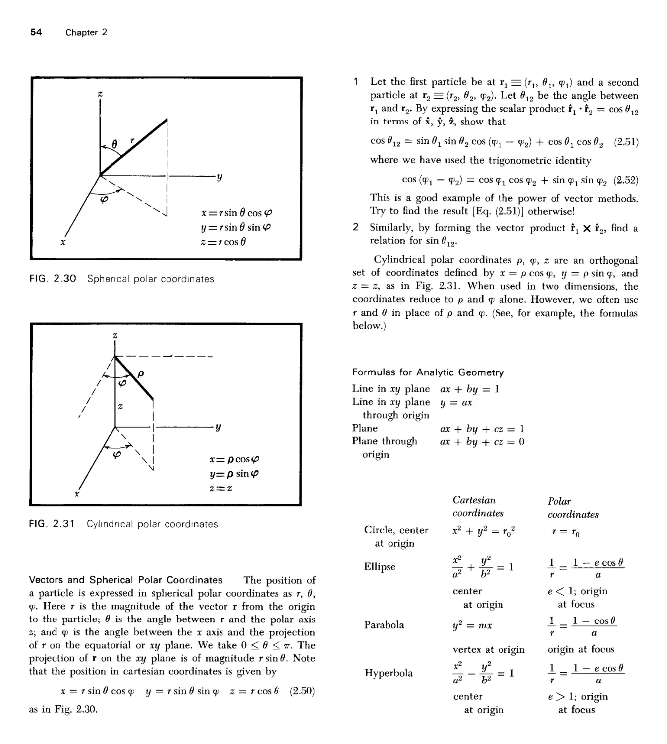
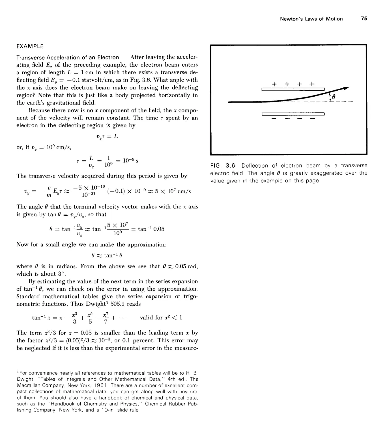
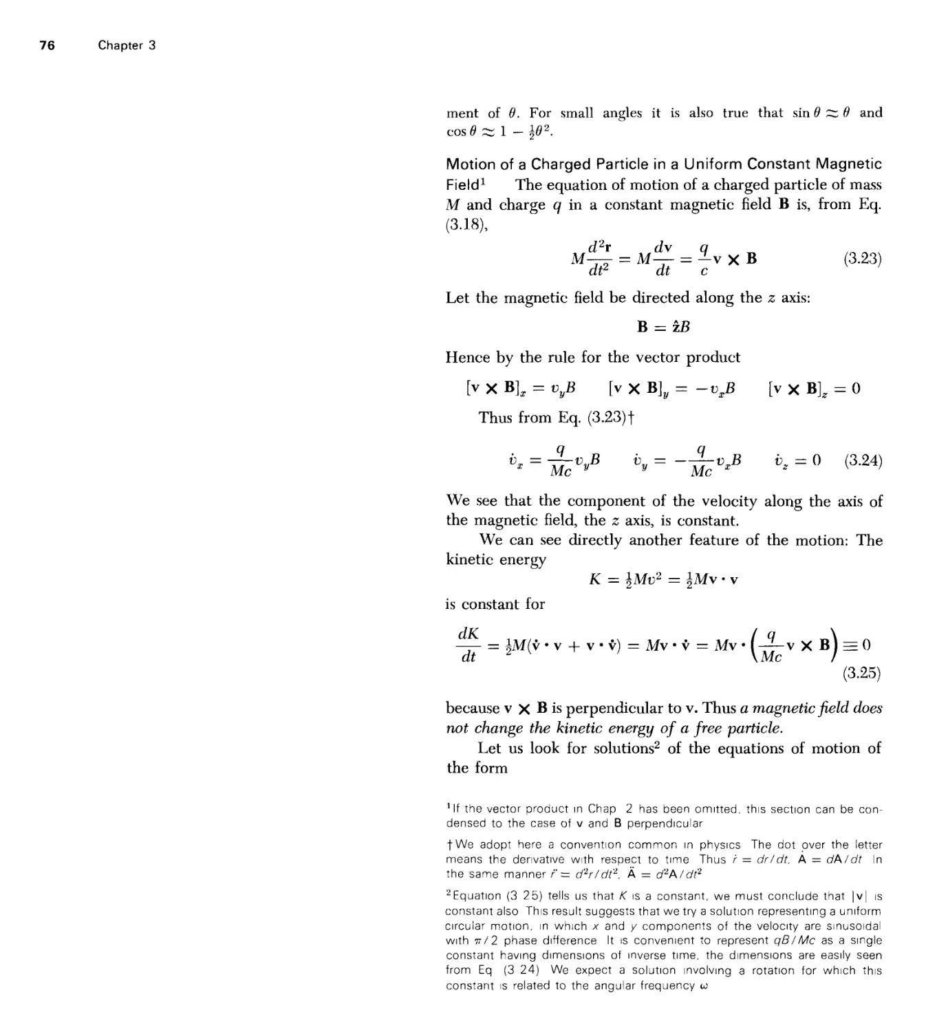
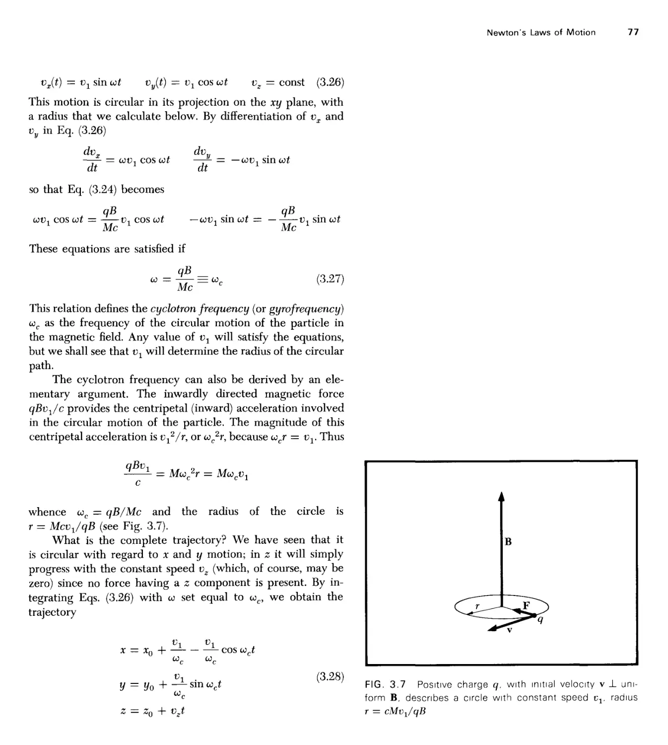
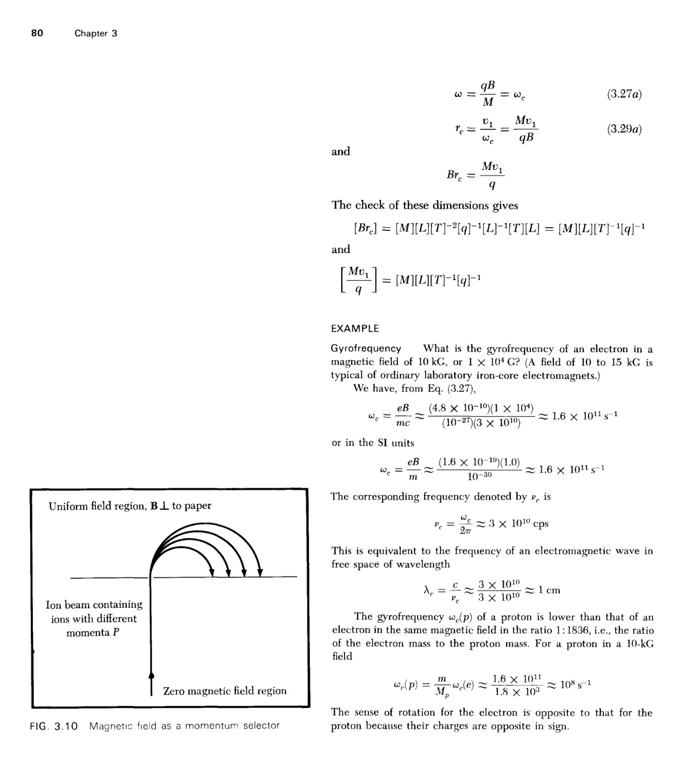
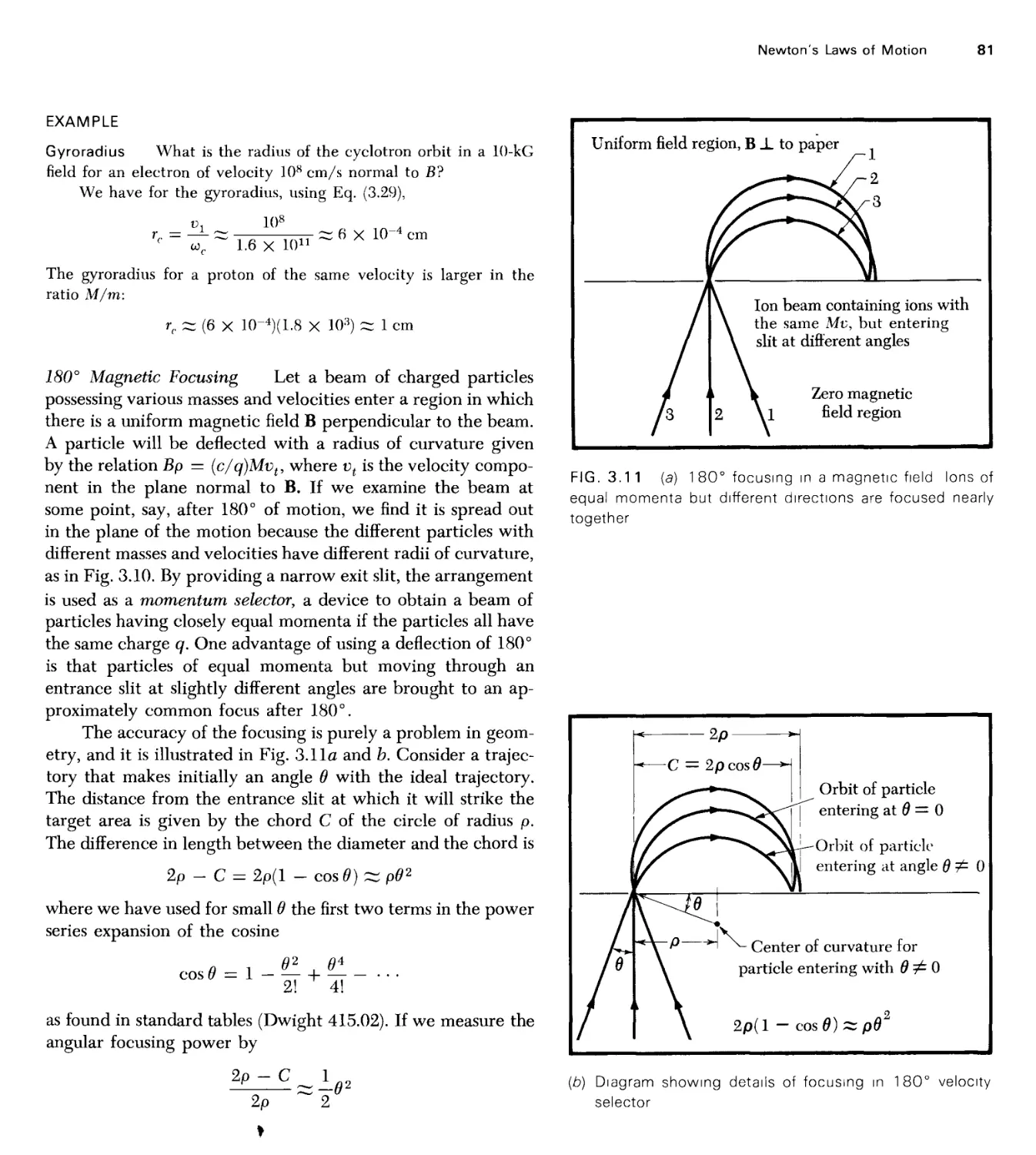
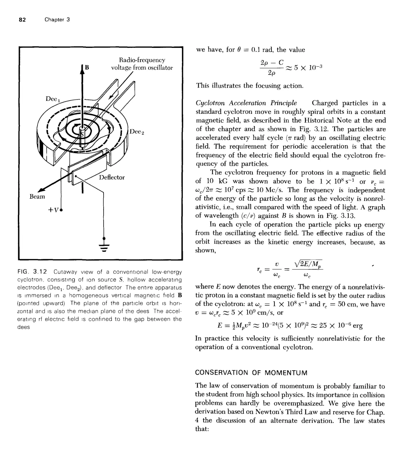
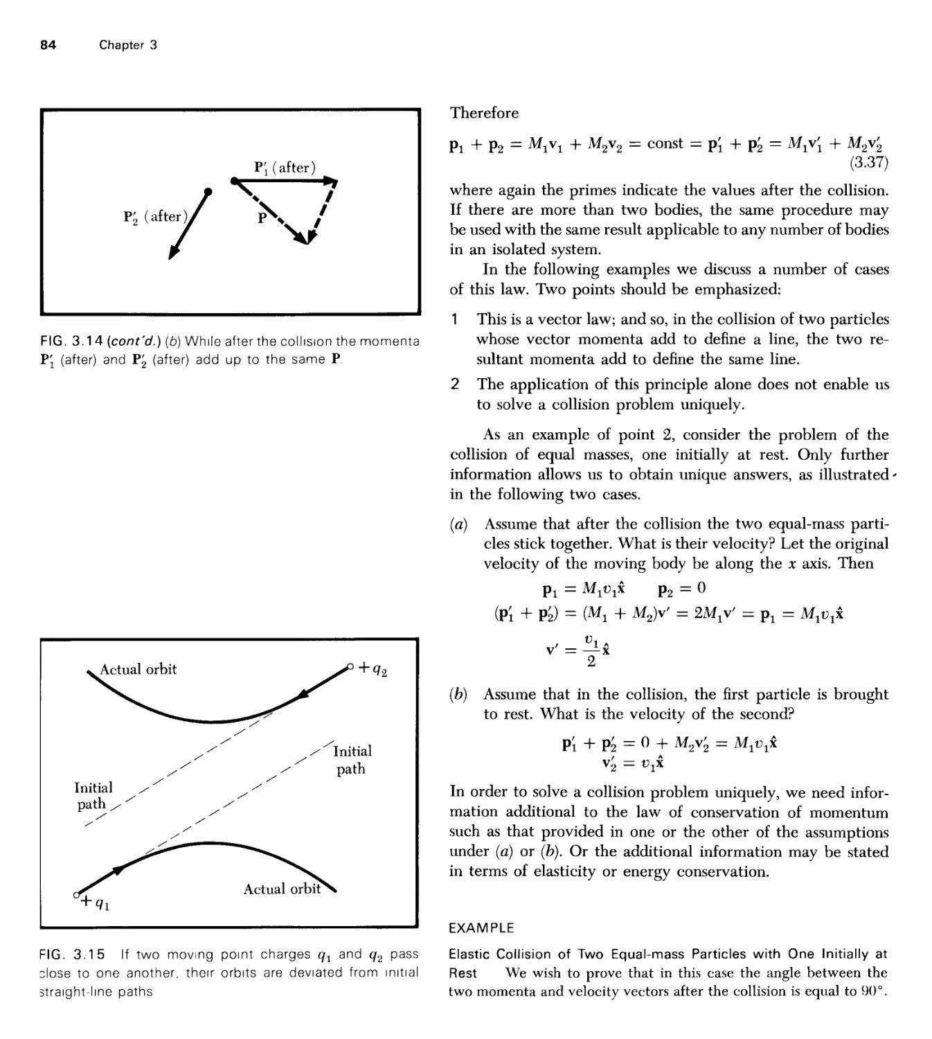
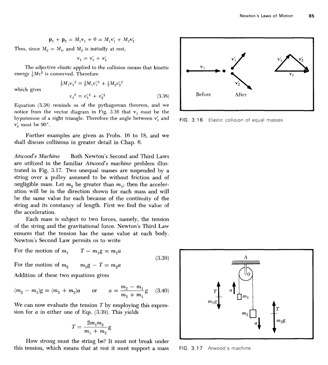
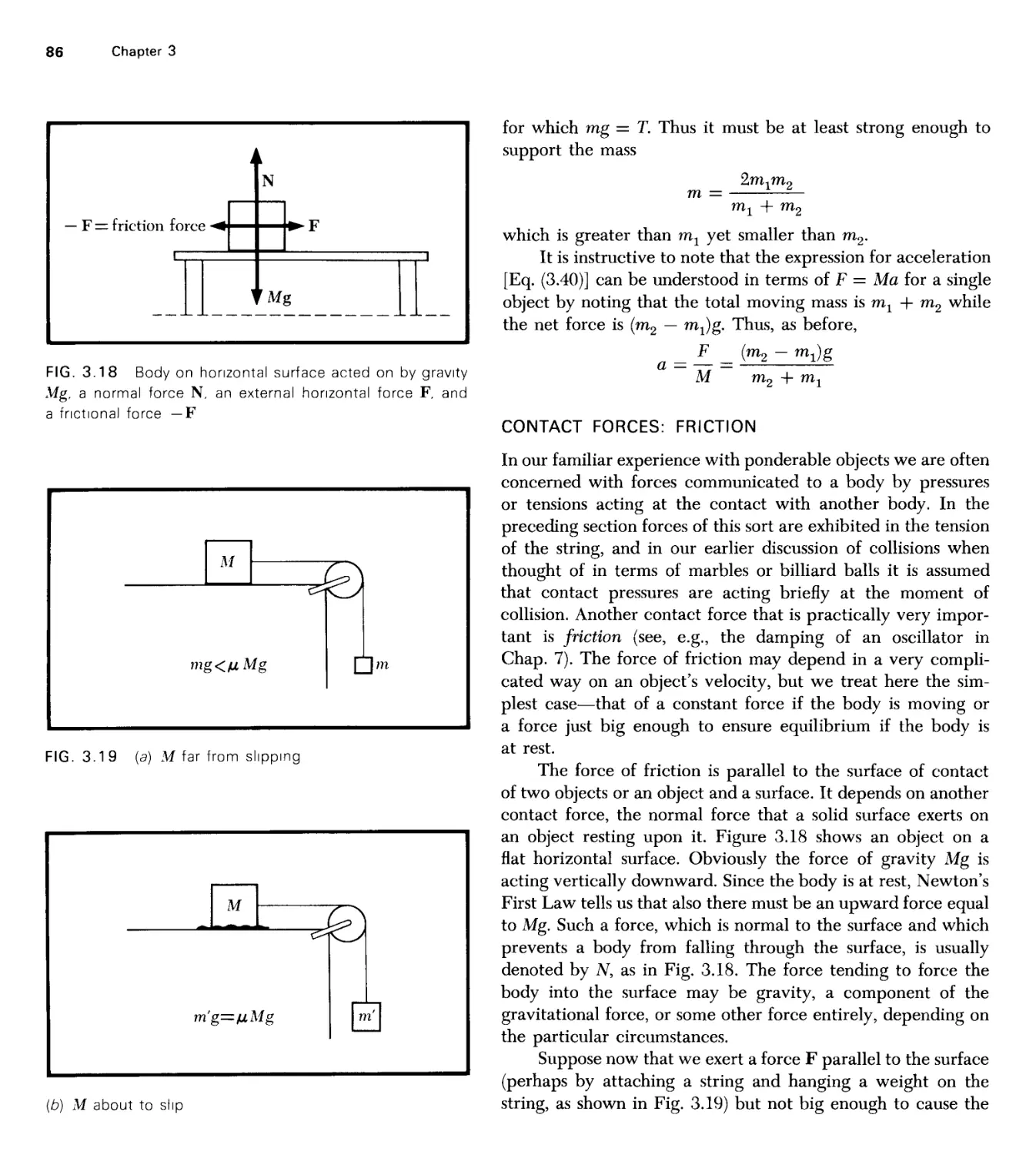
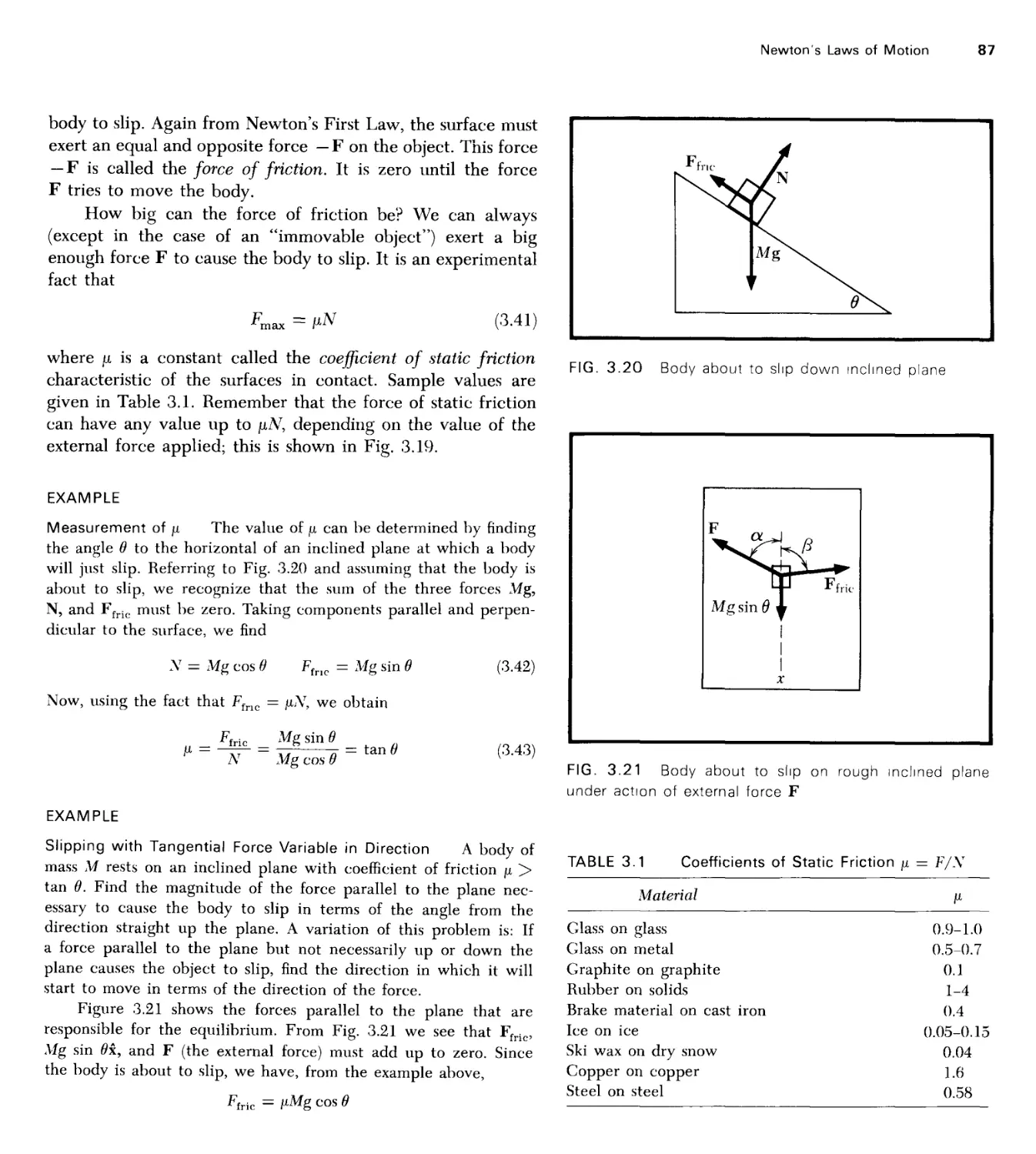
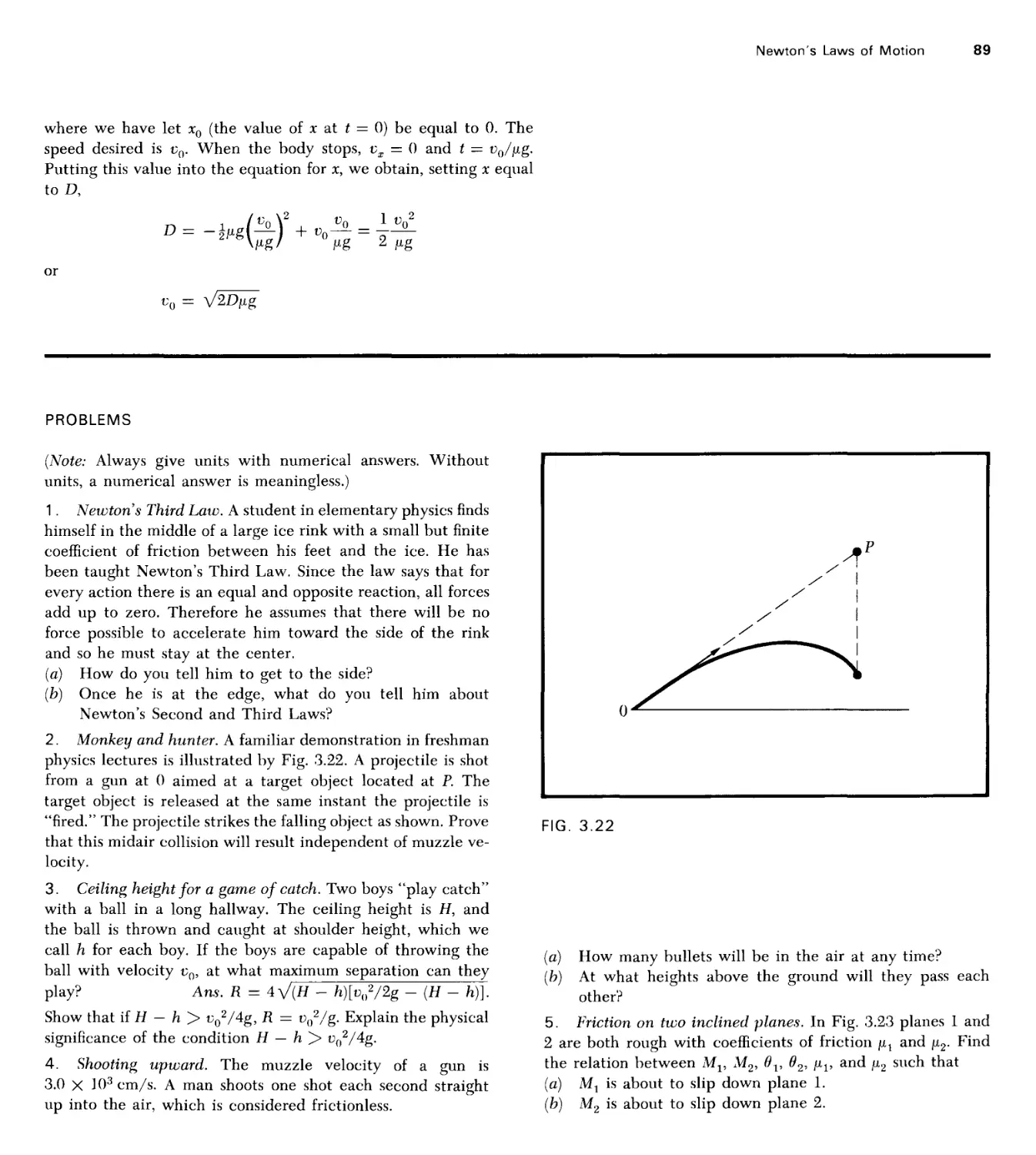
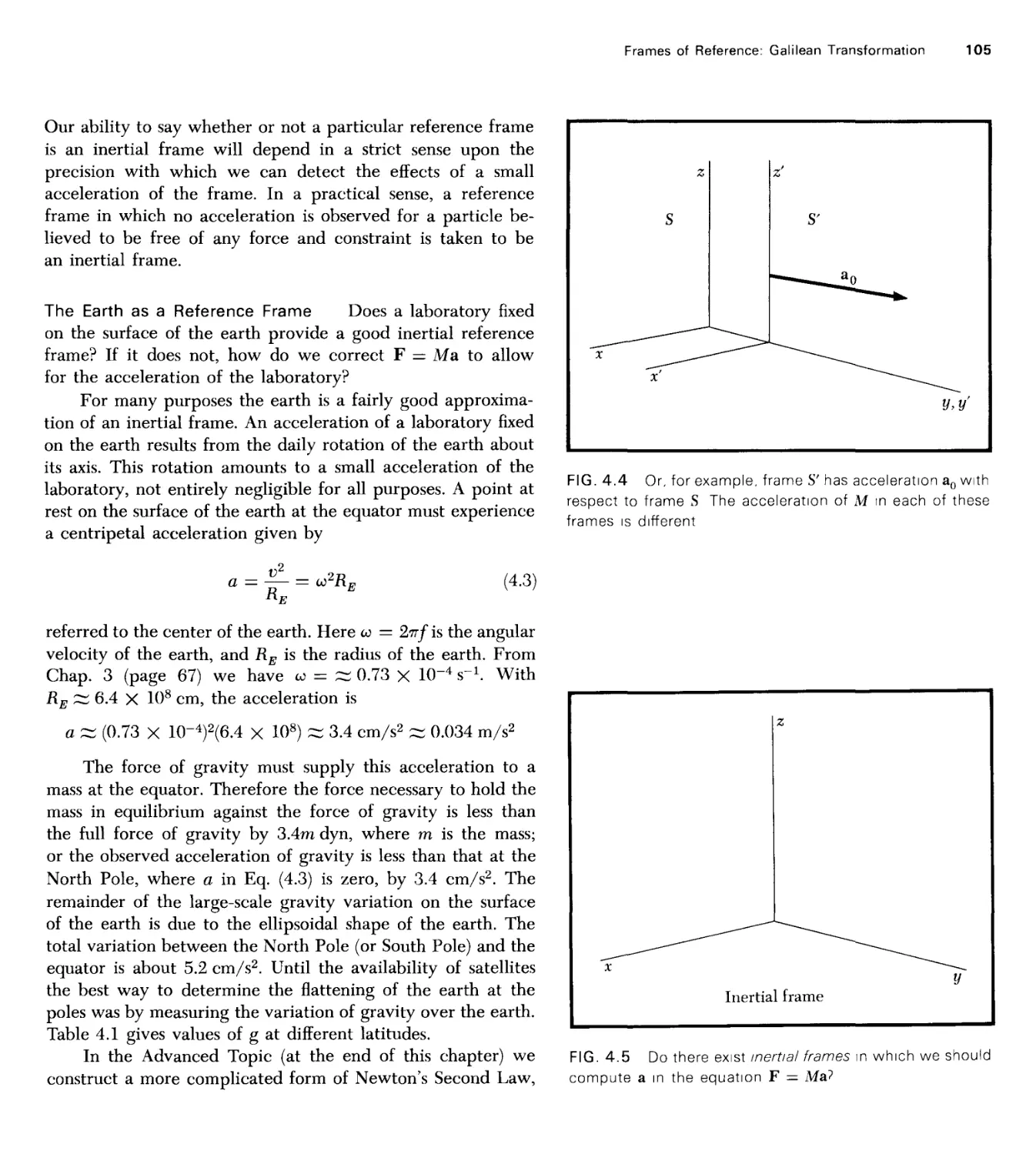
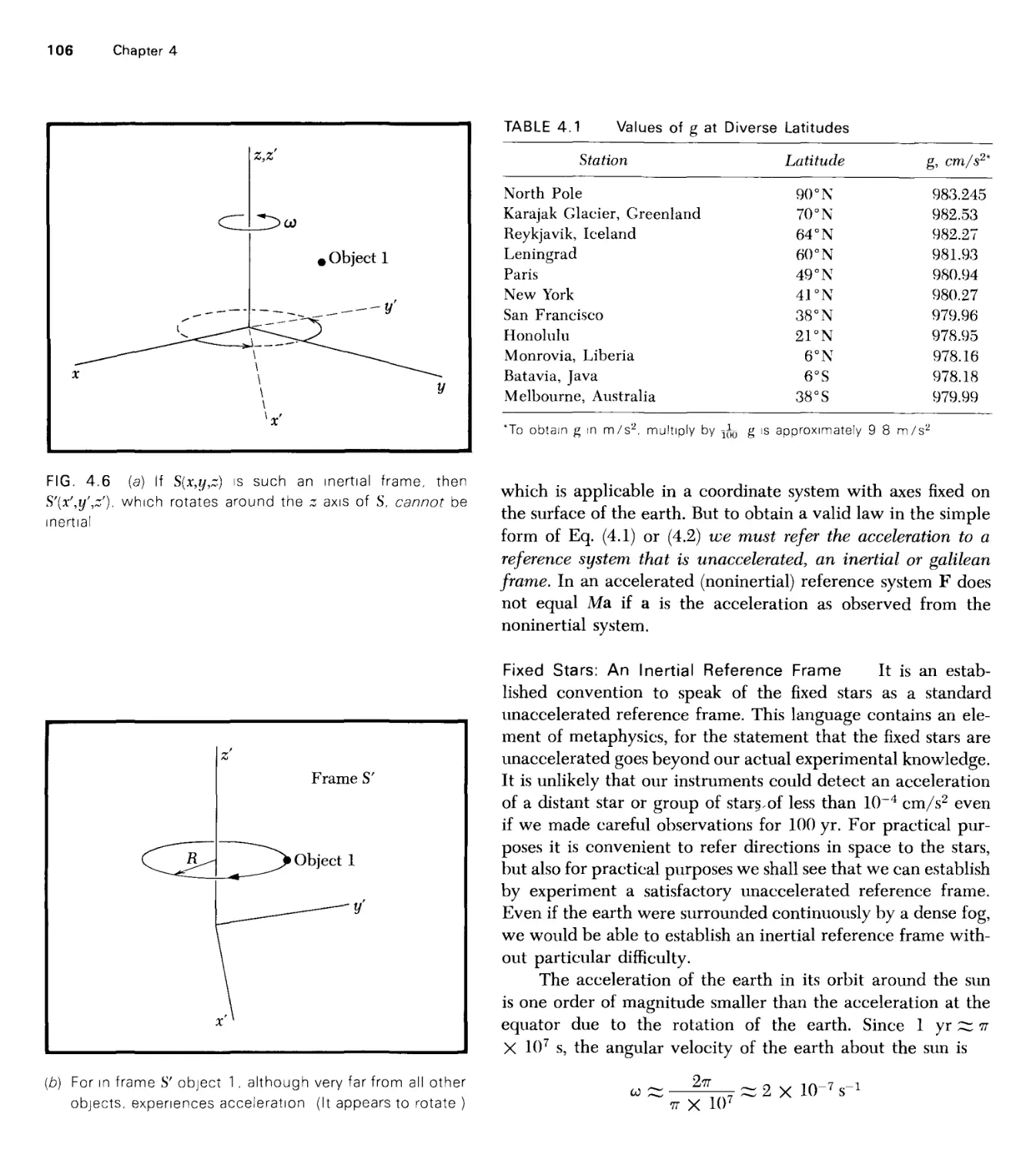
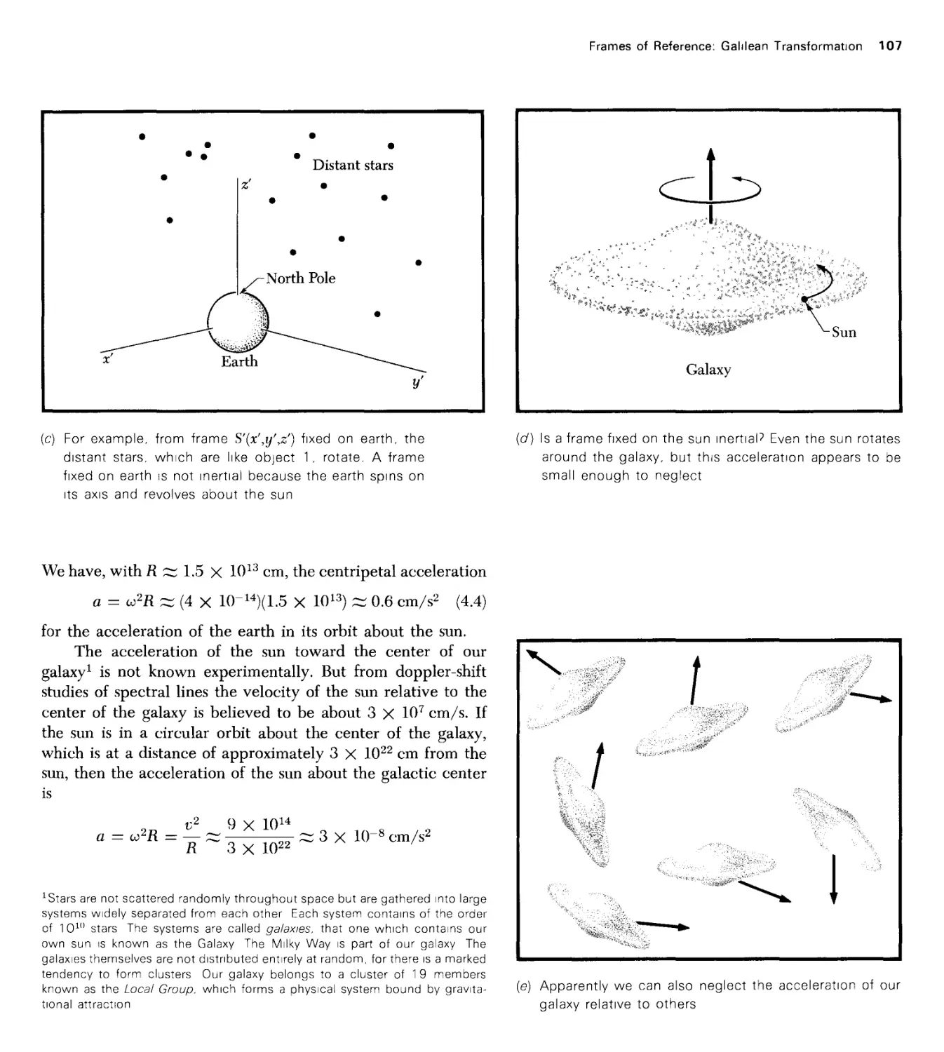
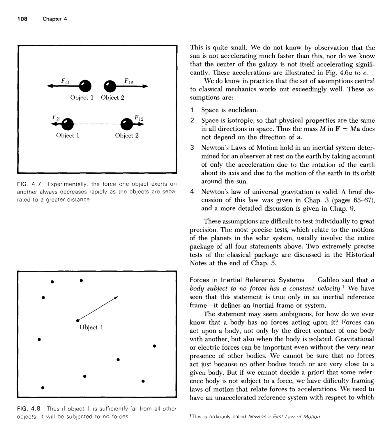
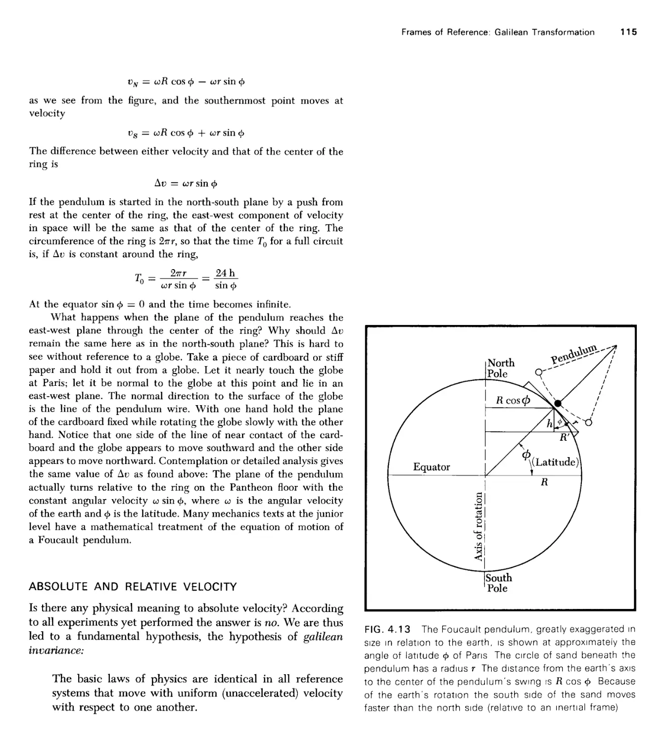
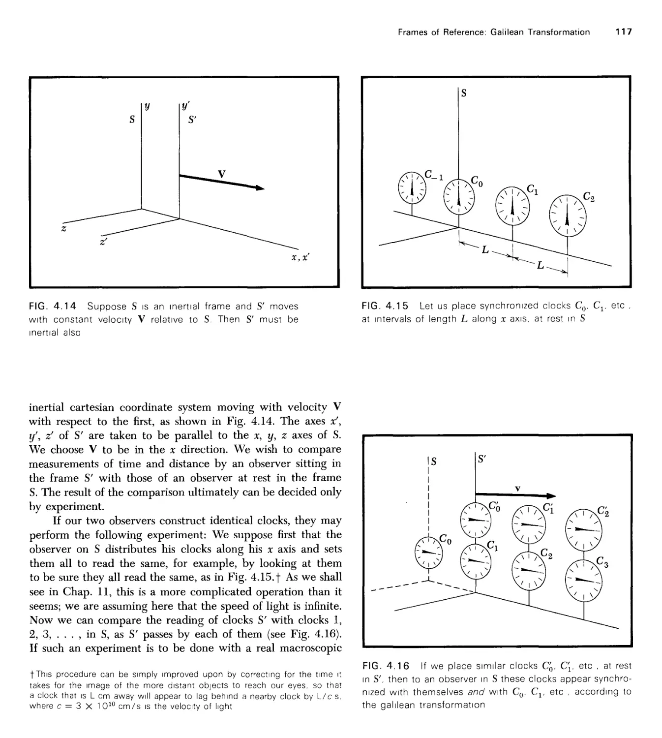
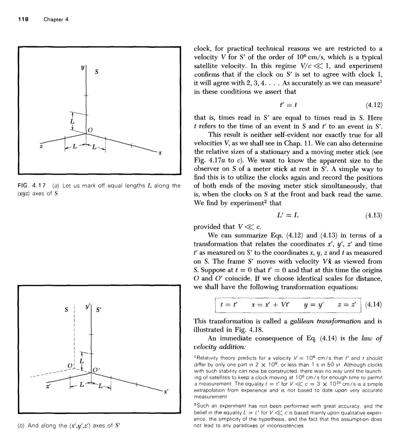
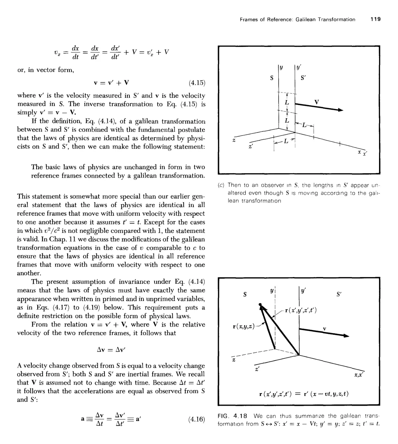
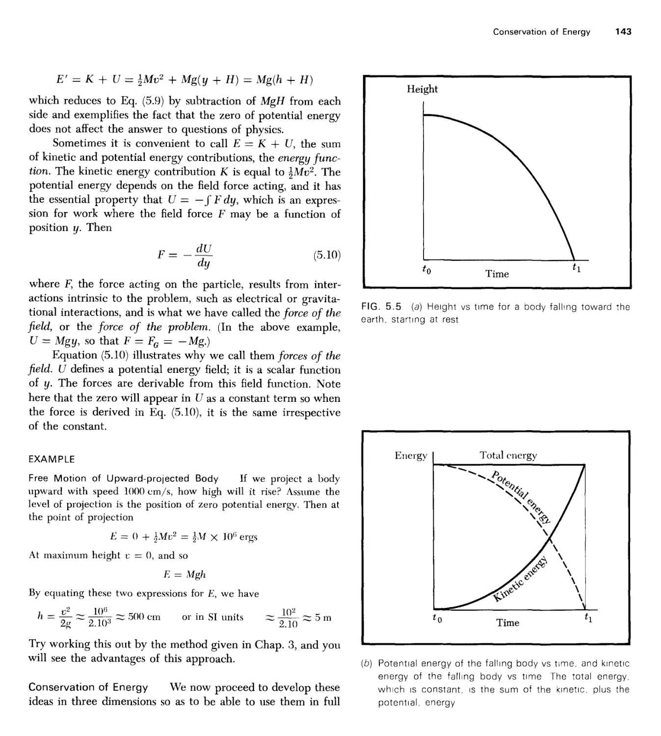
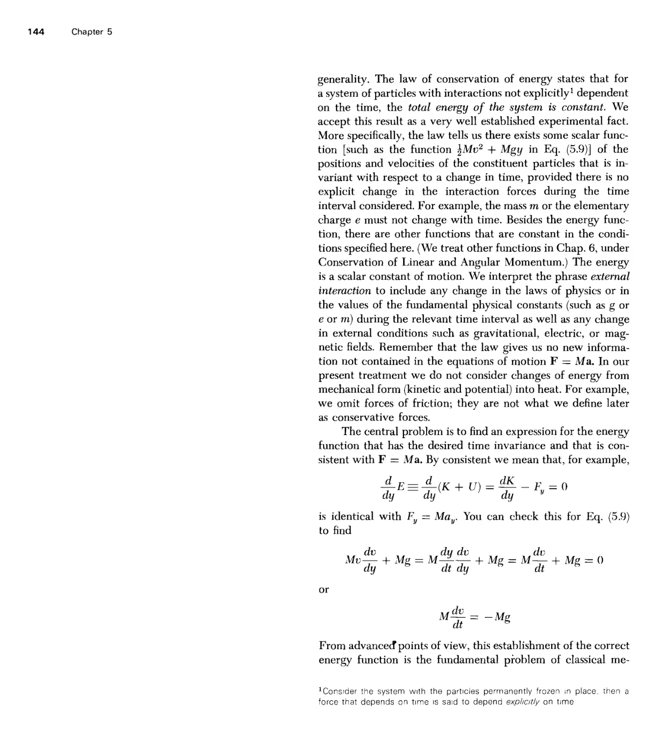
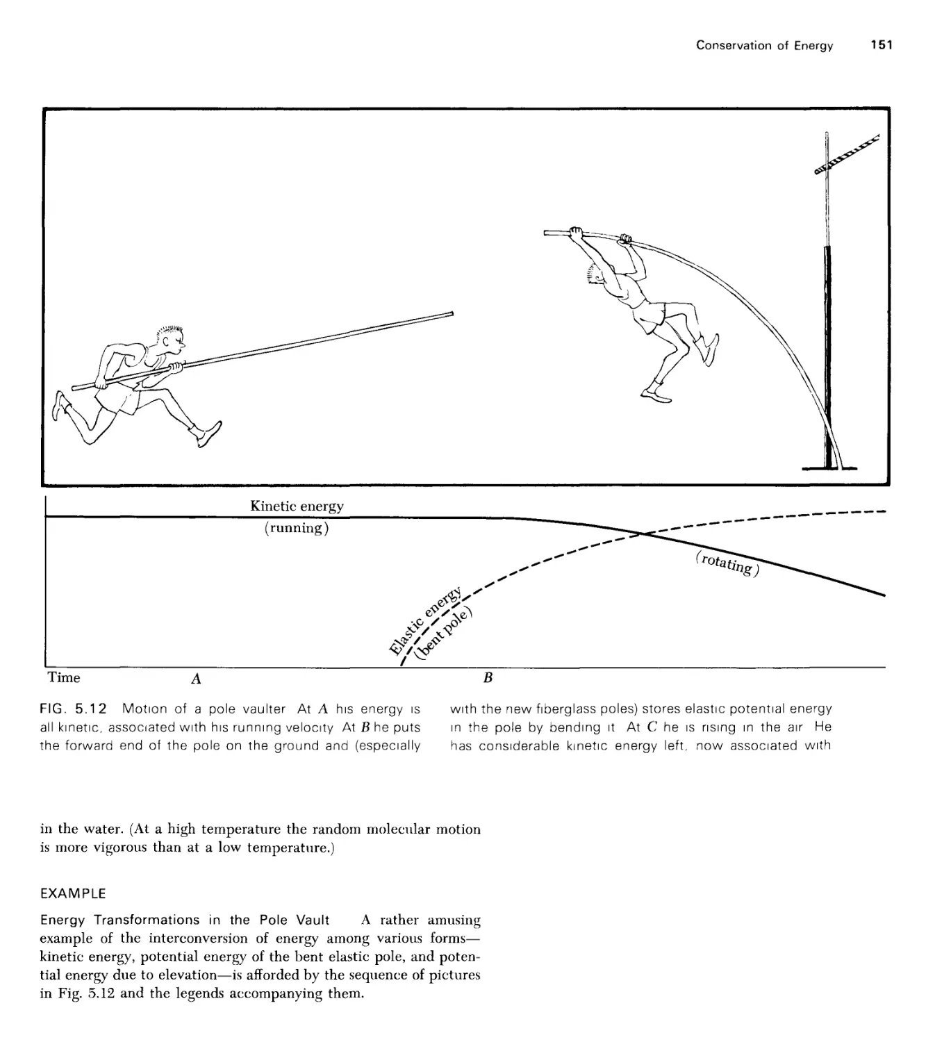
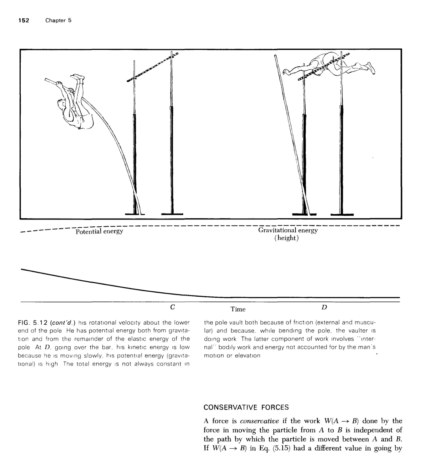
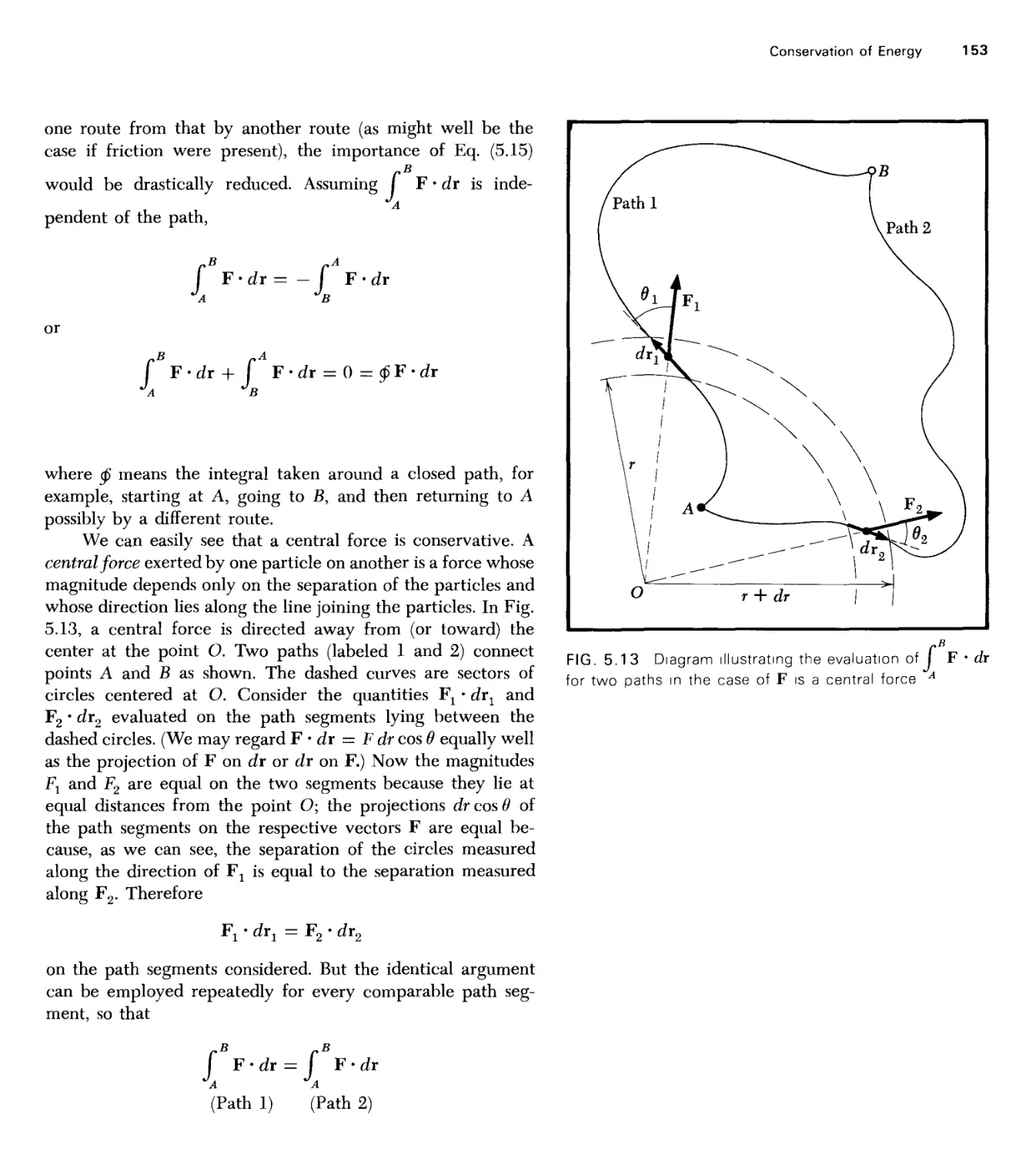
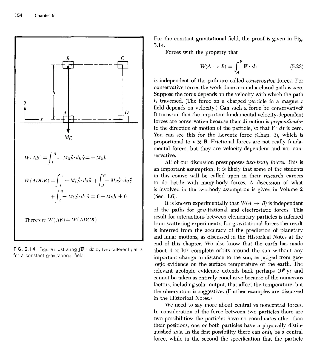
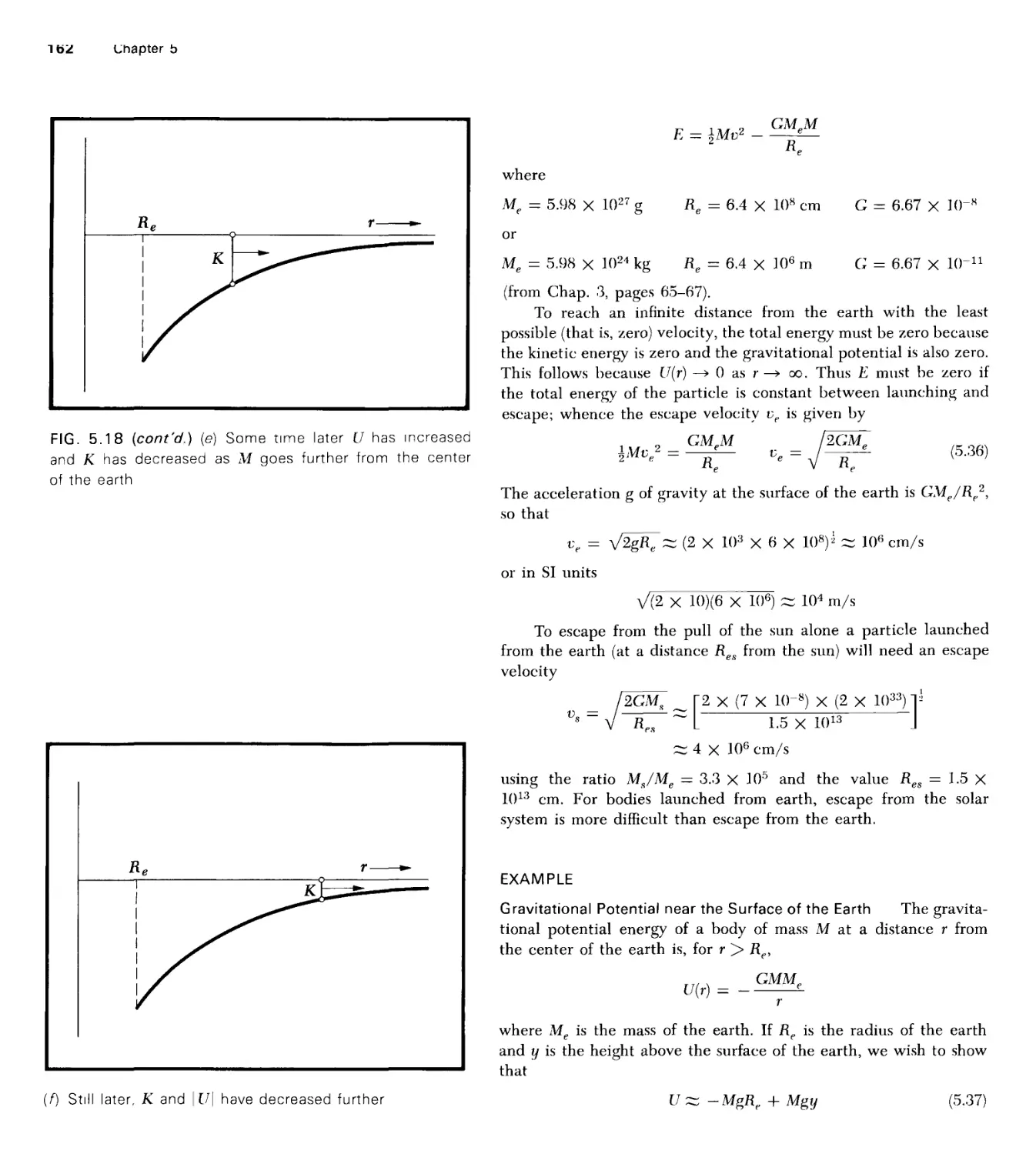
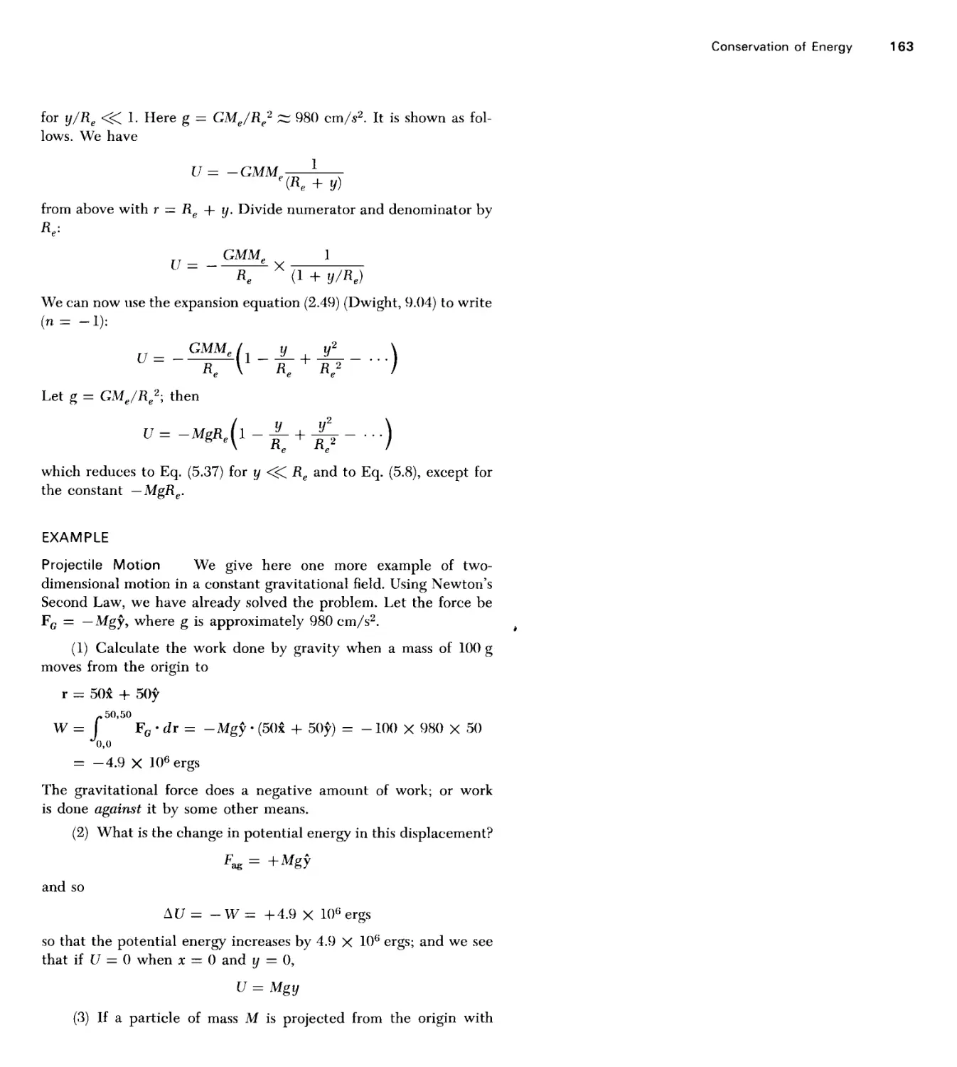
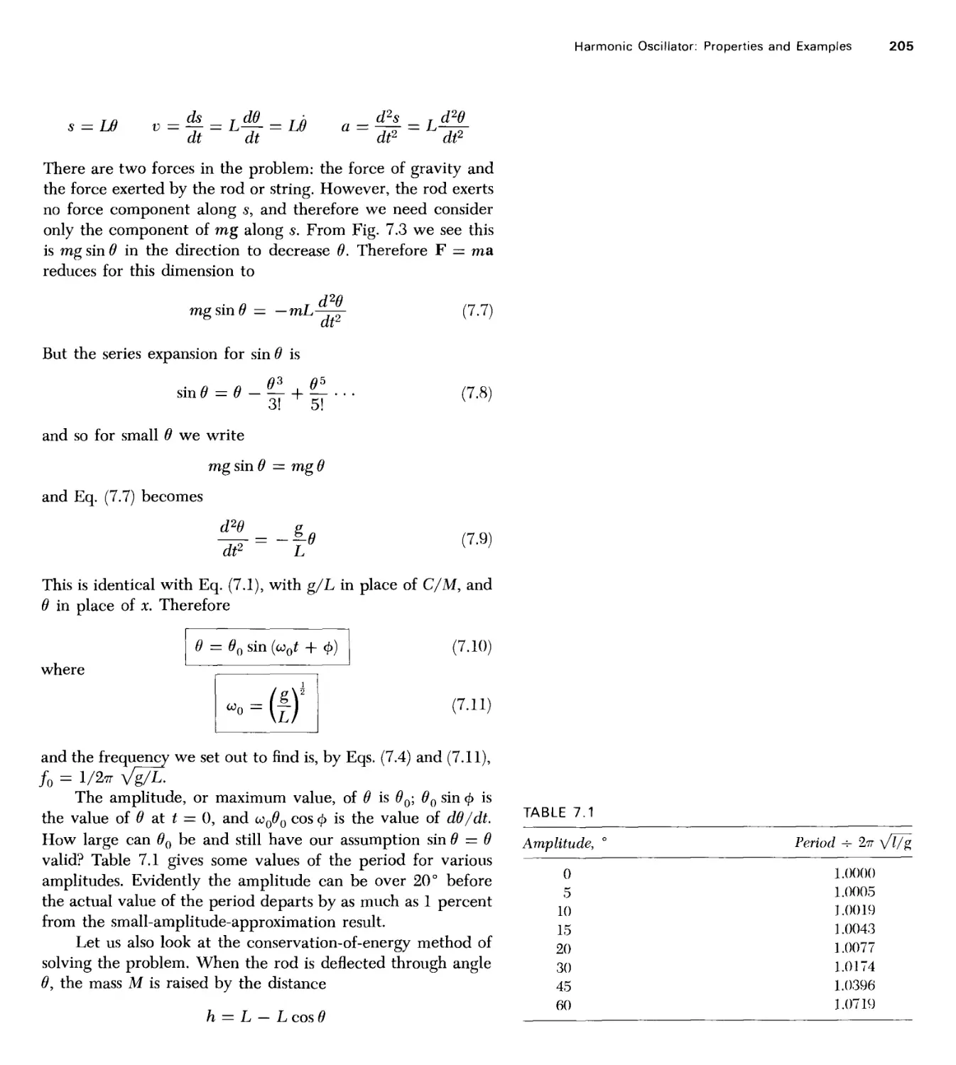
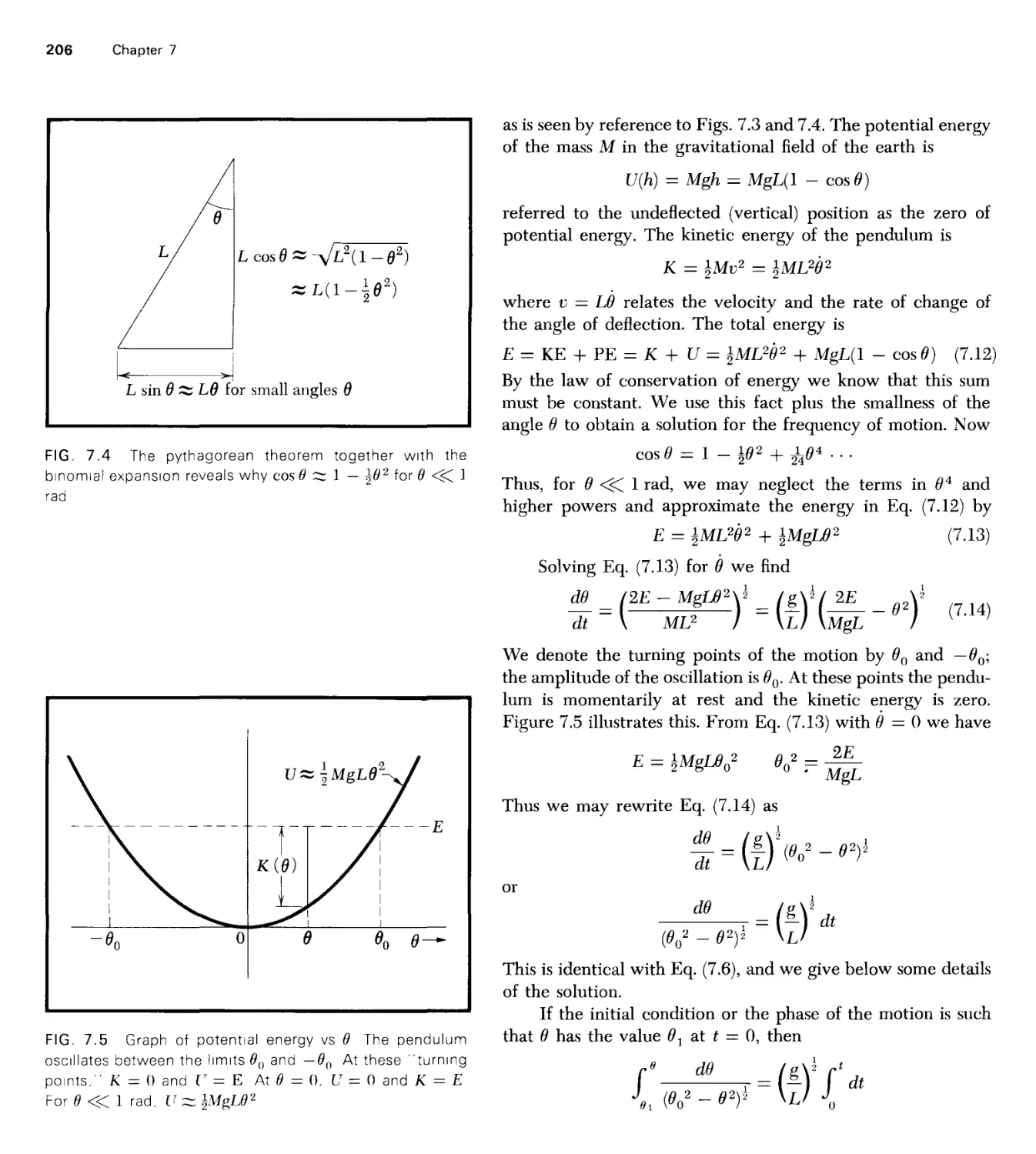
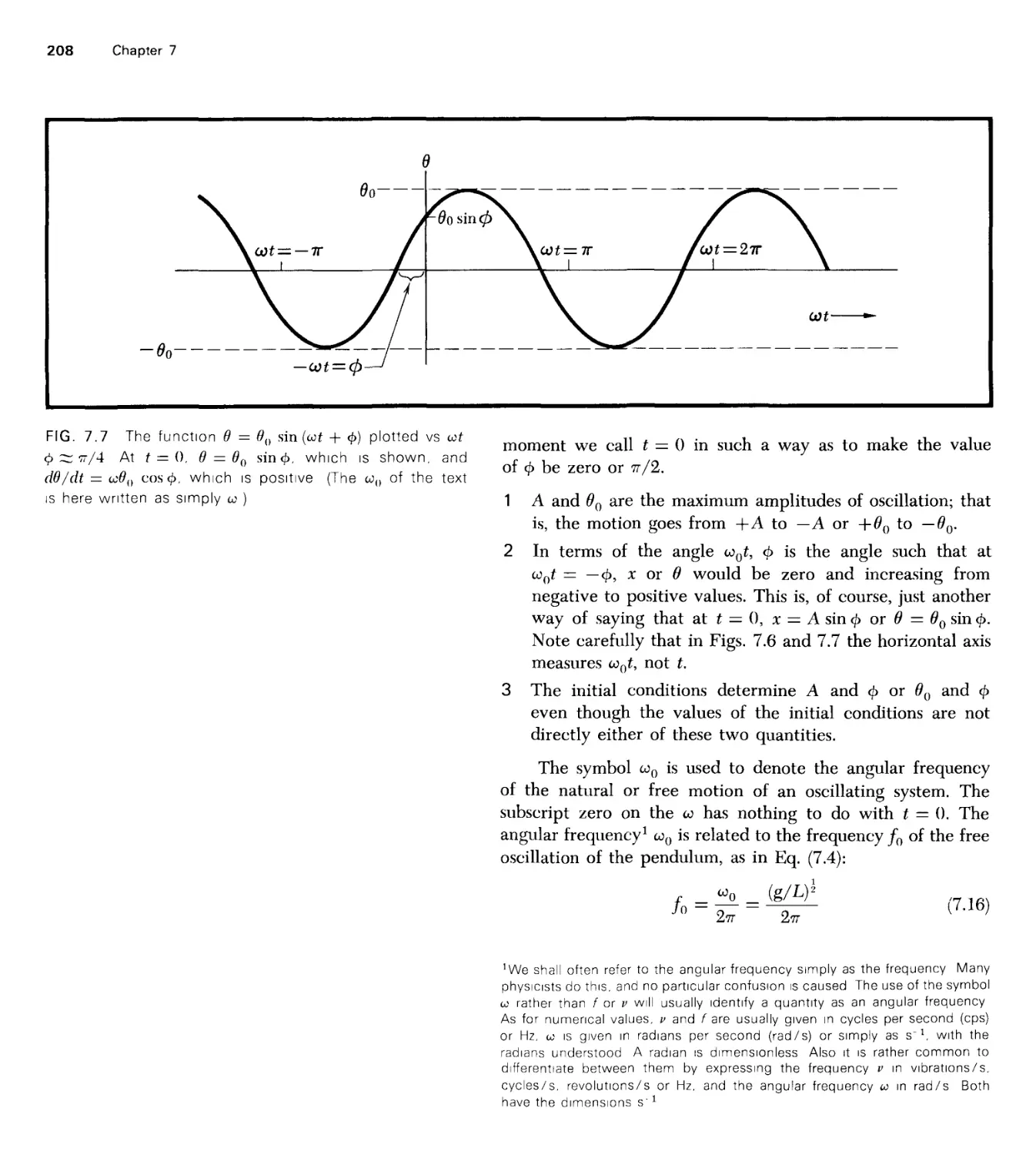
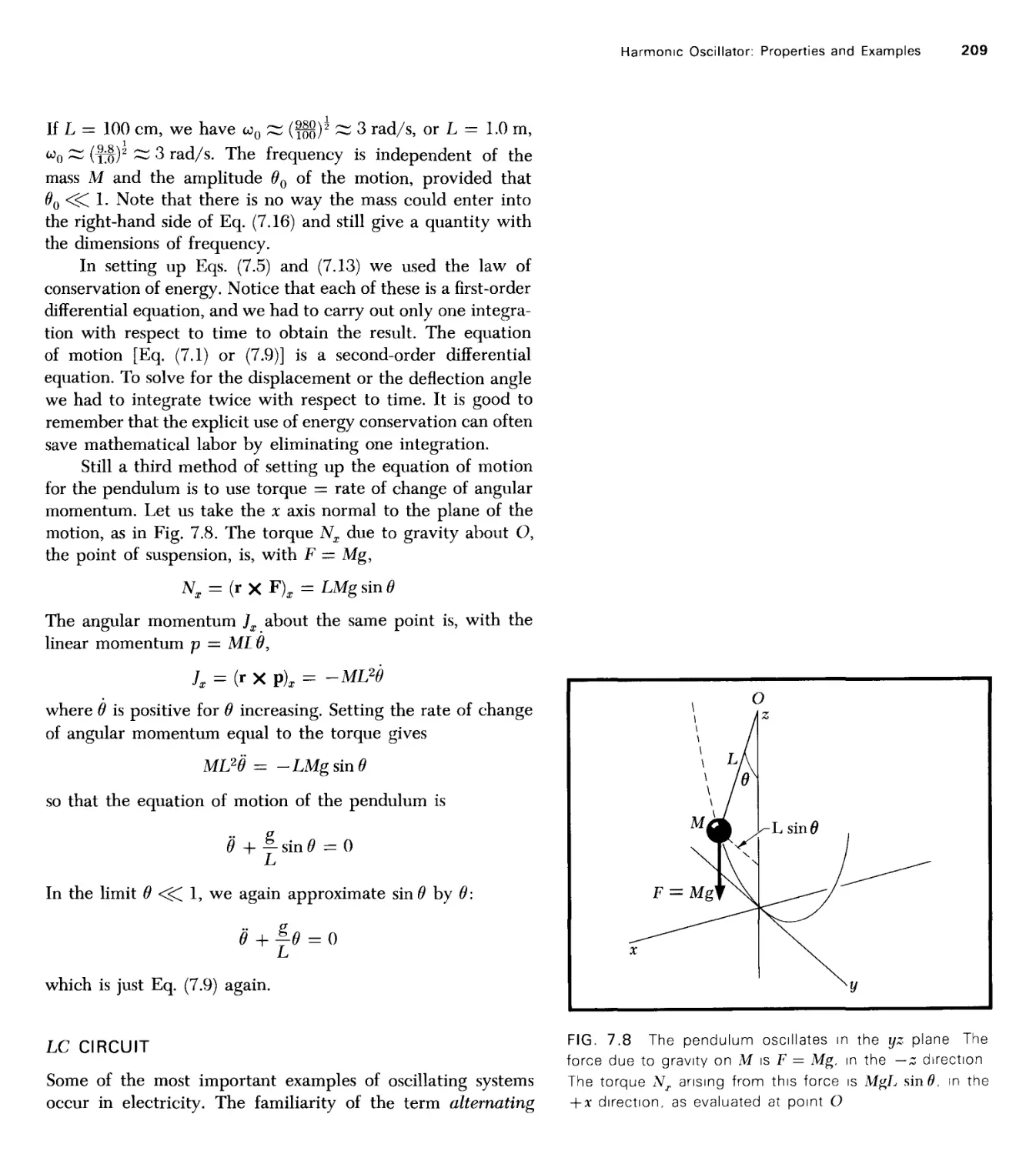
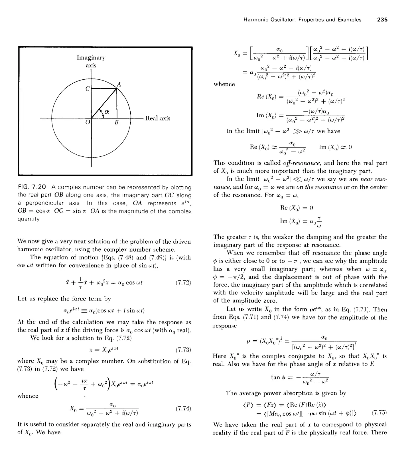
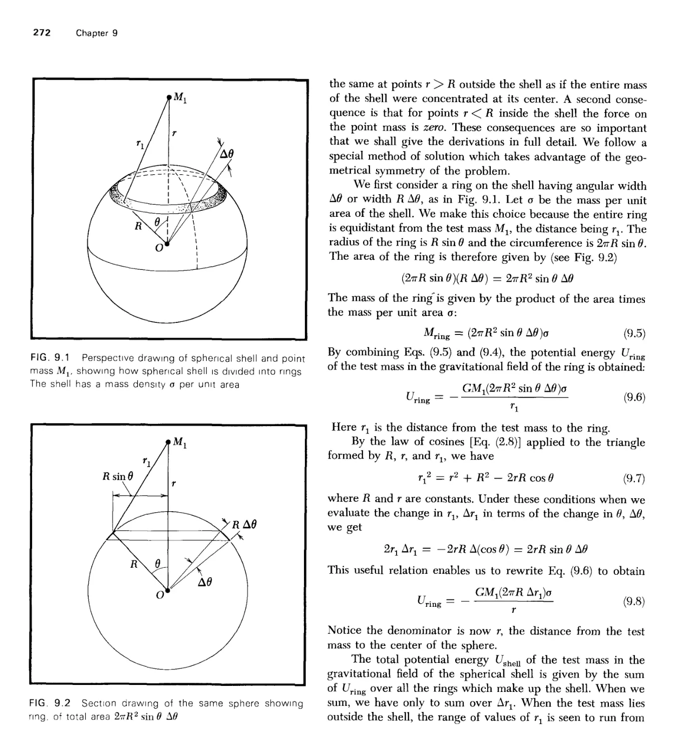
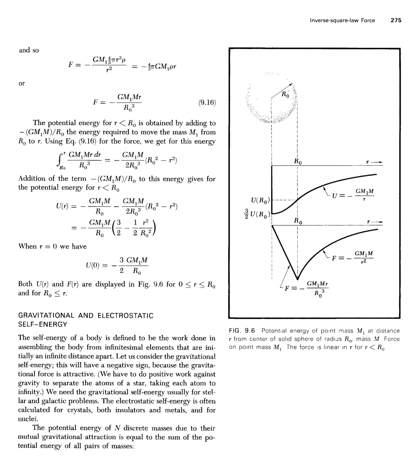
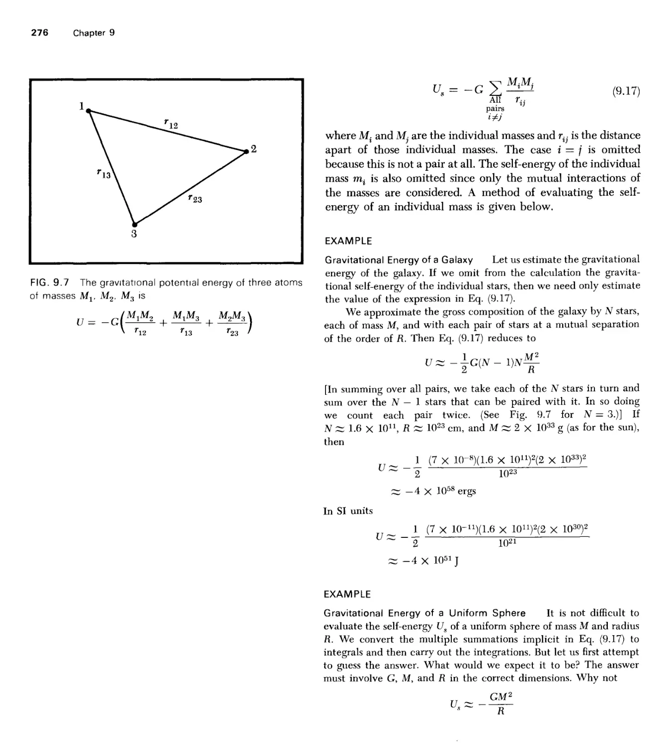
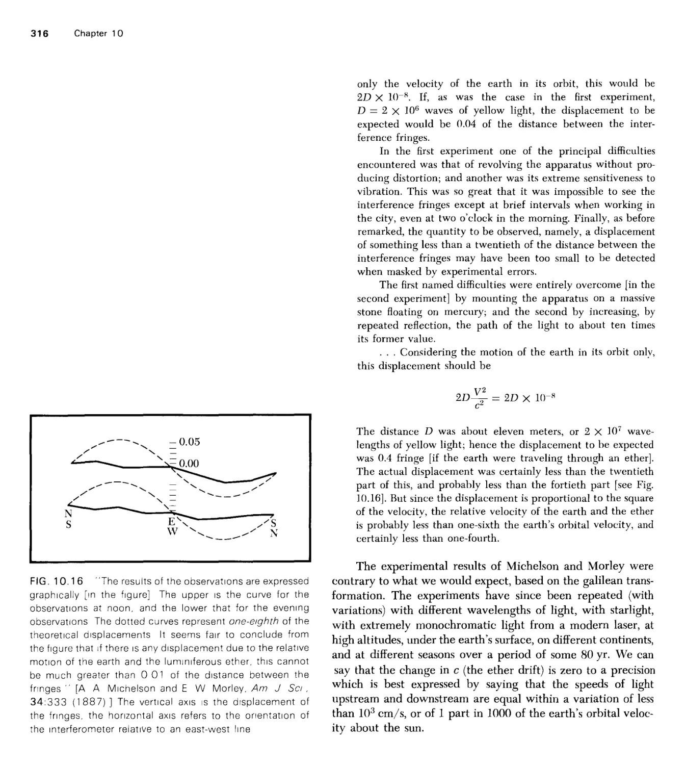
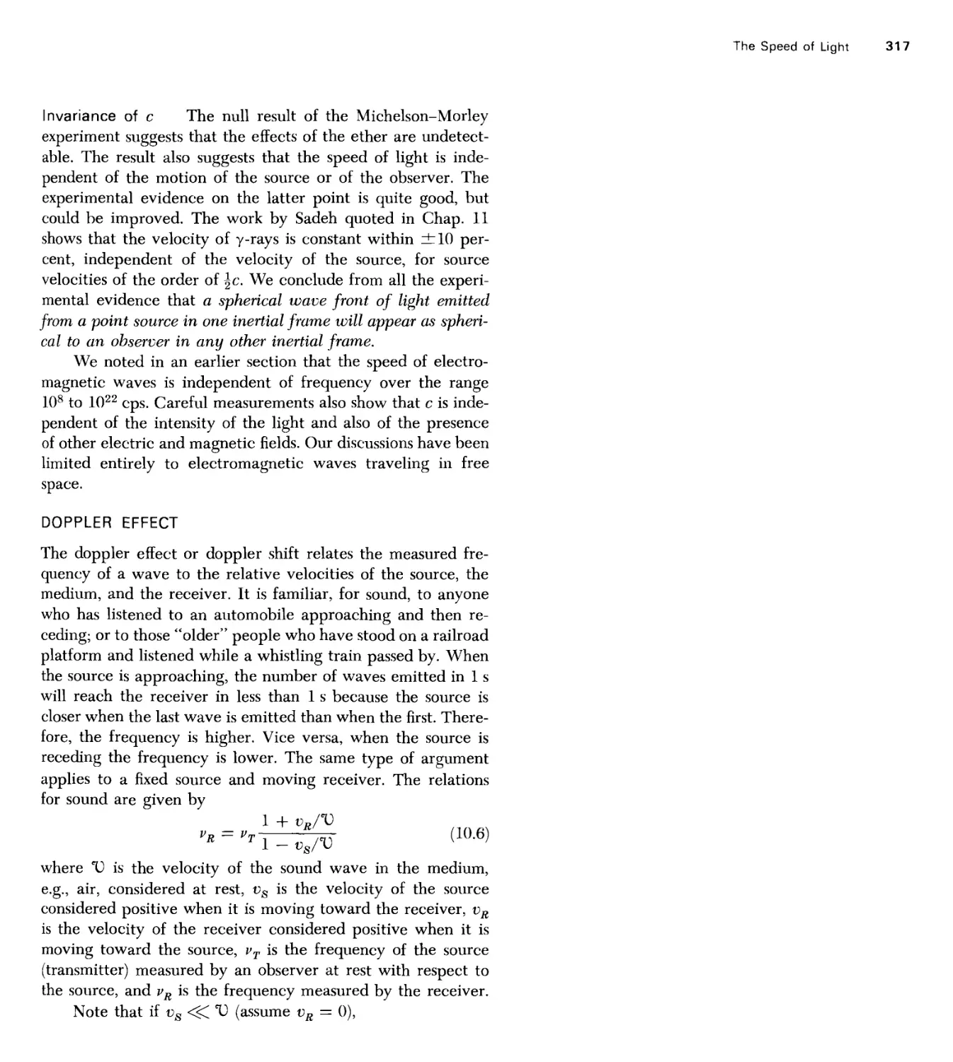
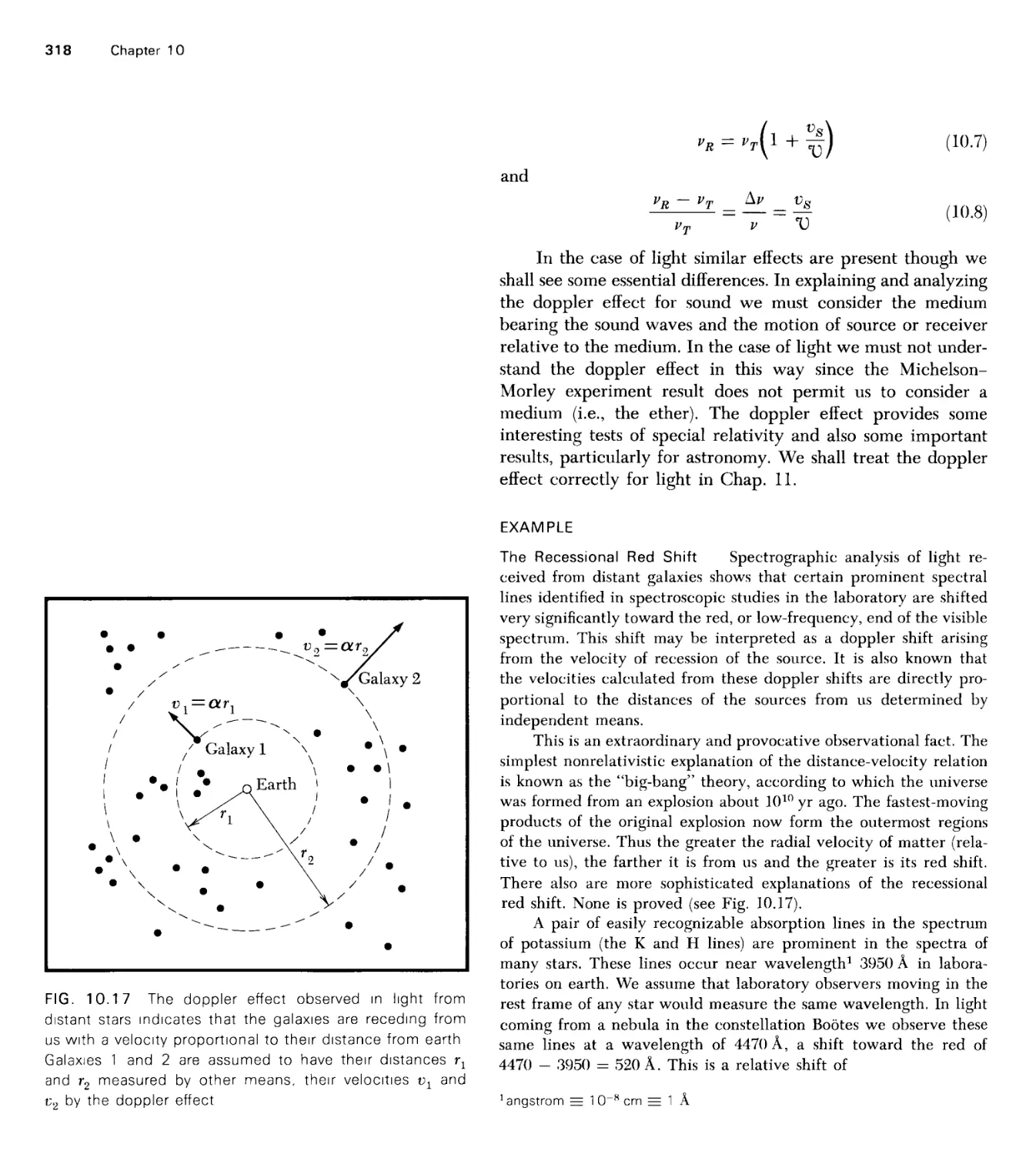
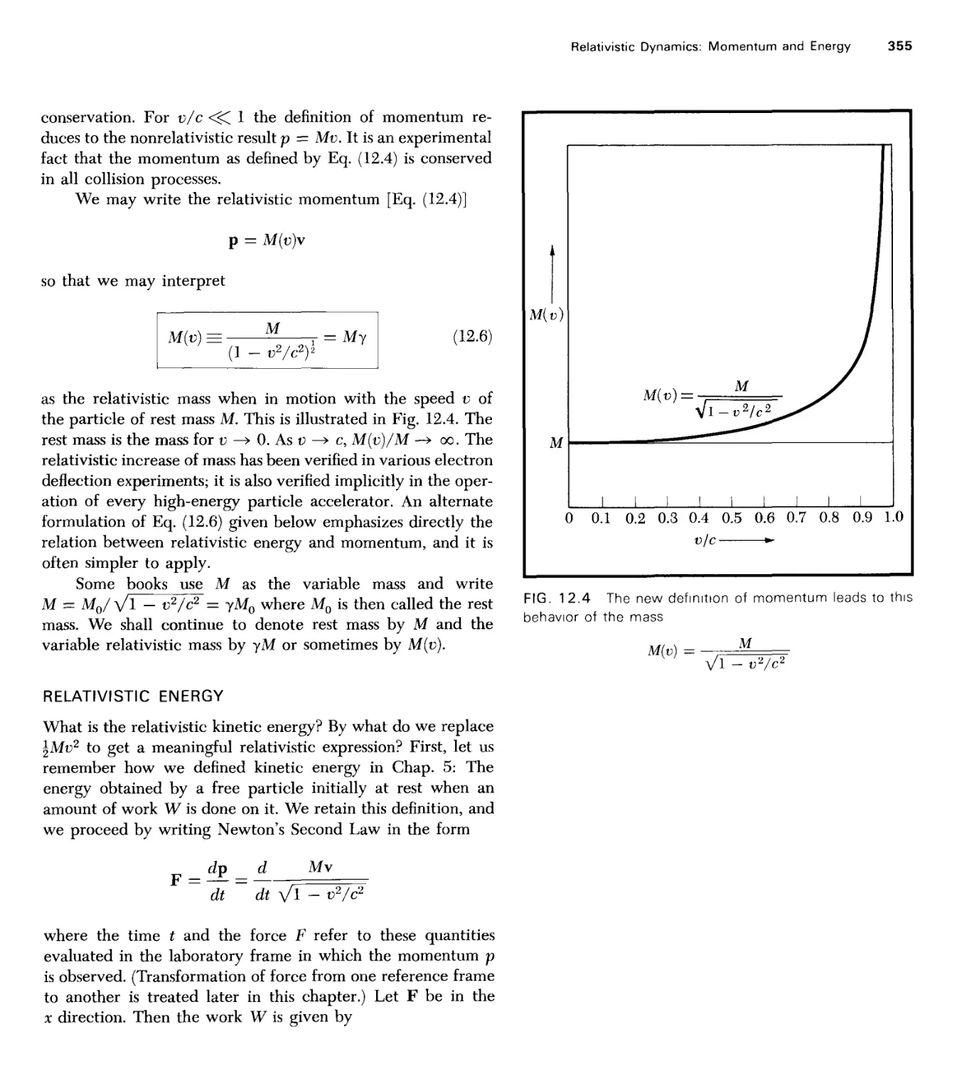
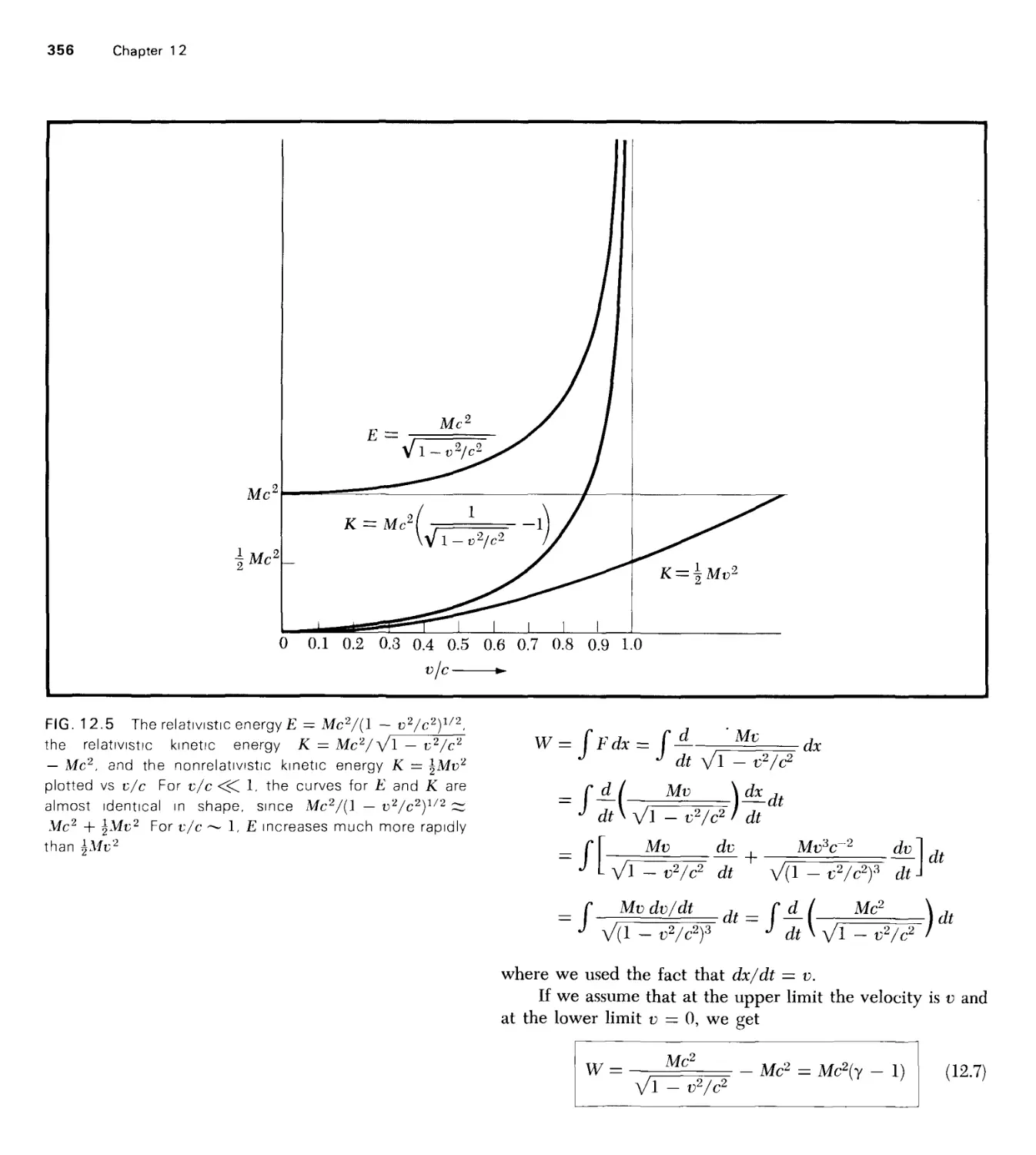
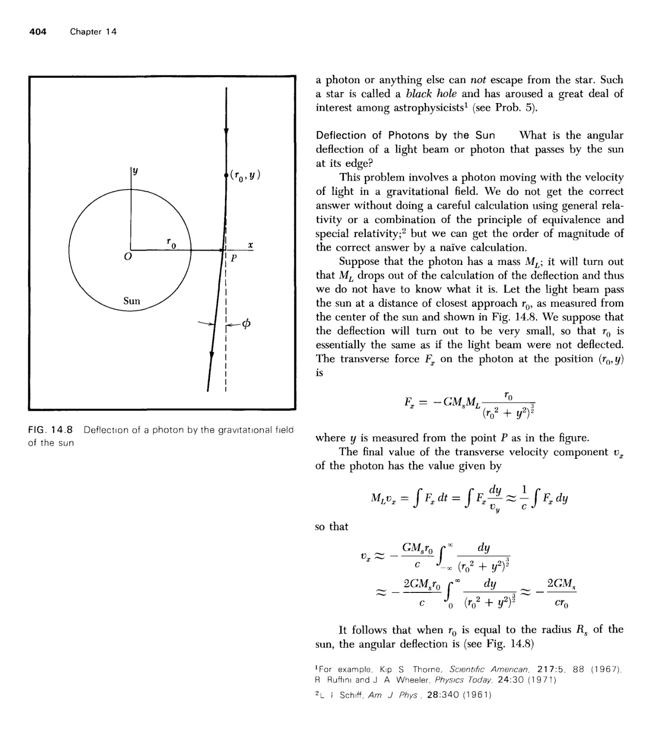
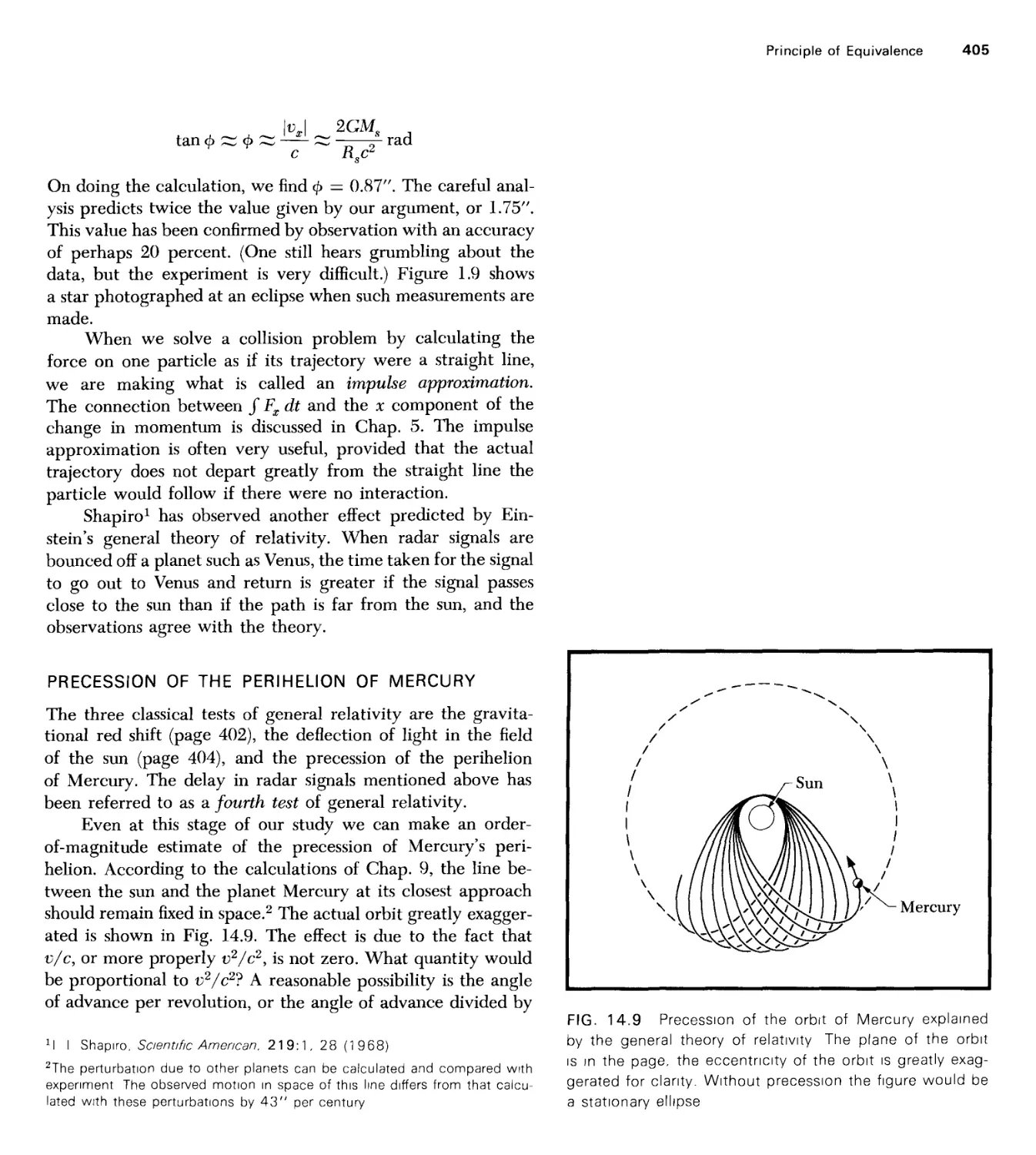
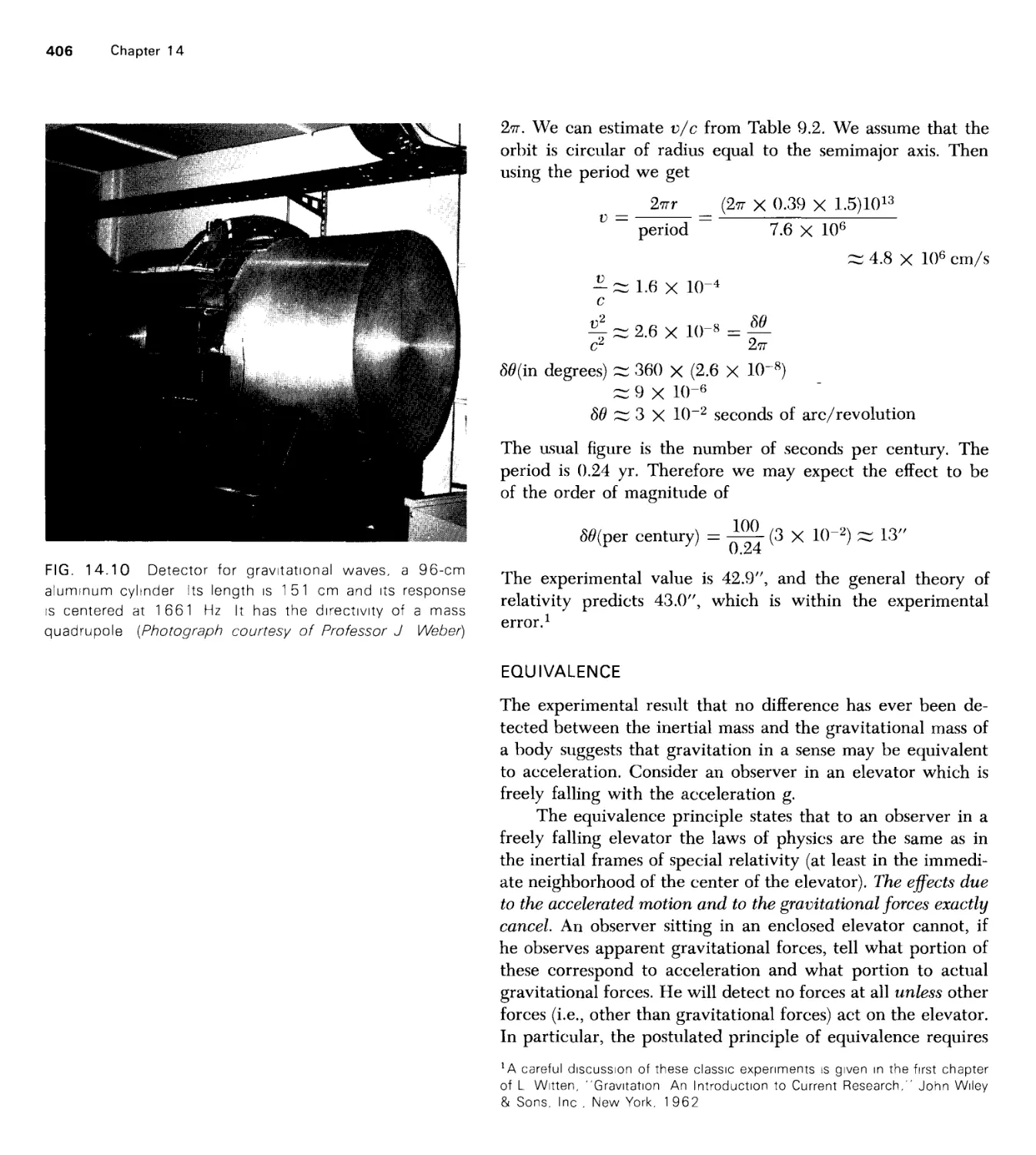
/


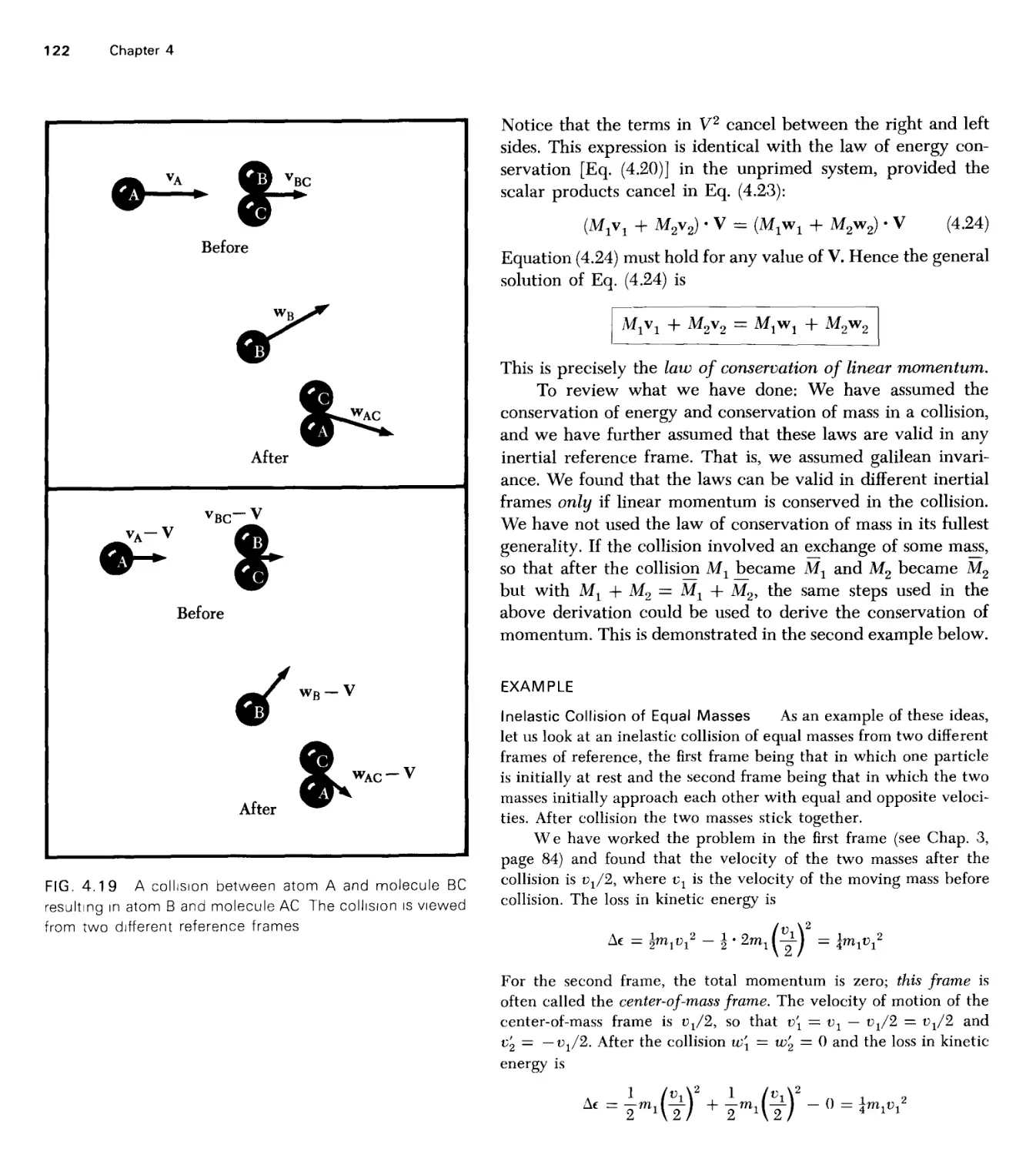
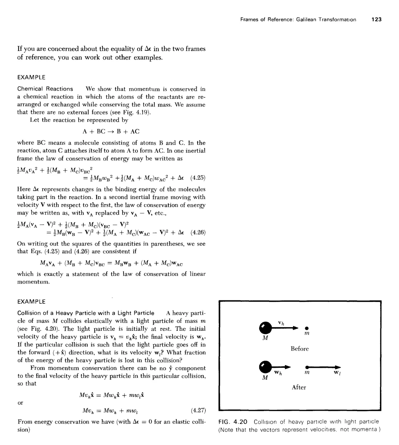


Текст
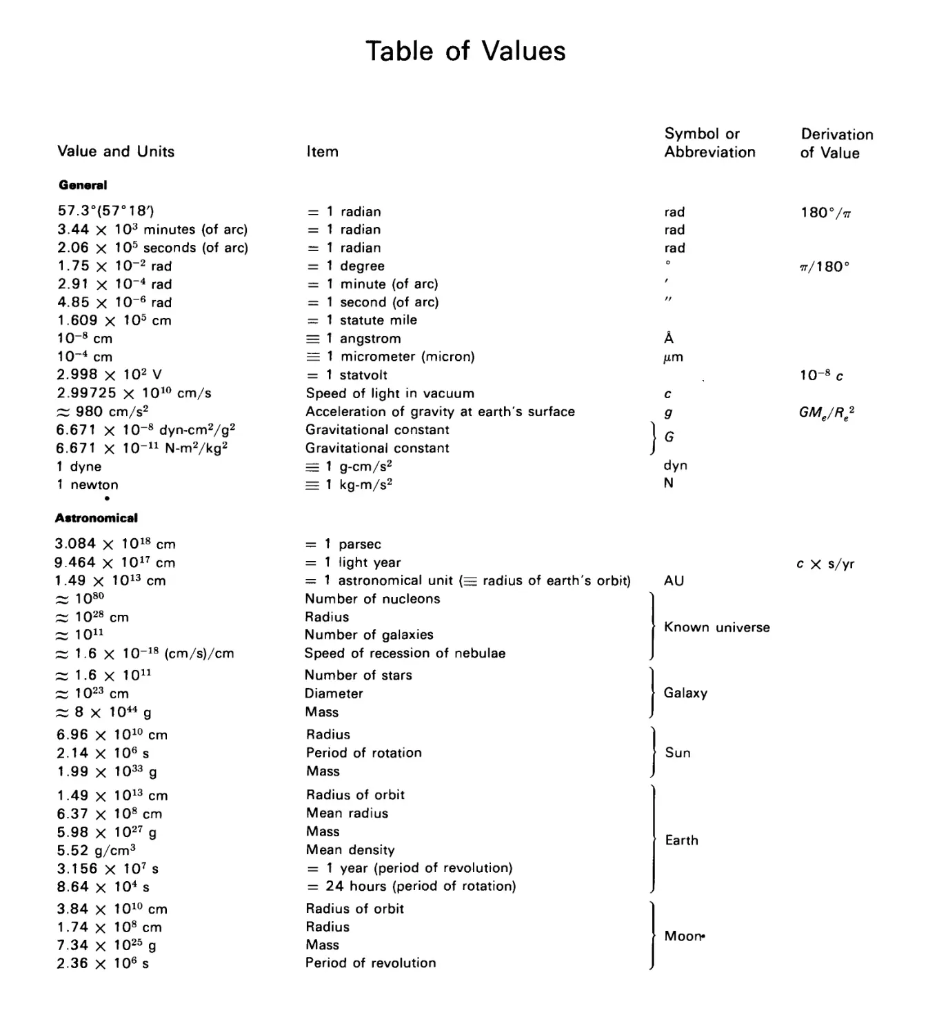
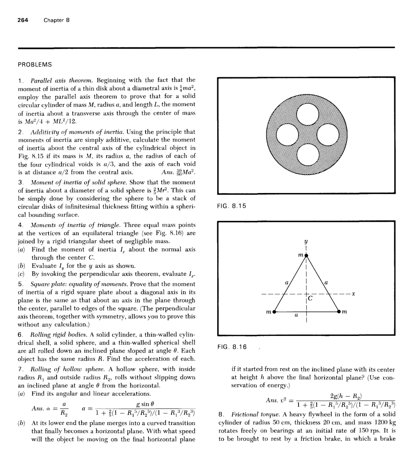
Table of Values
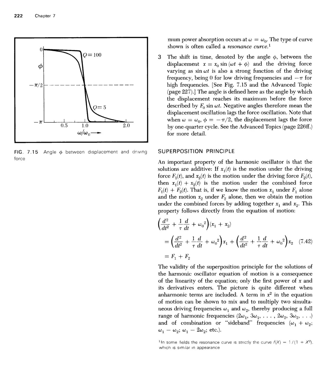
Value and Units
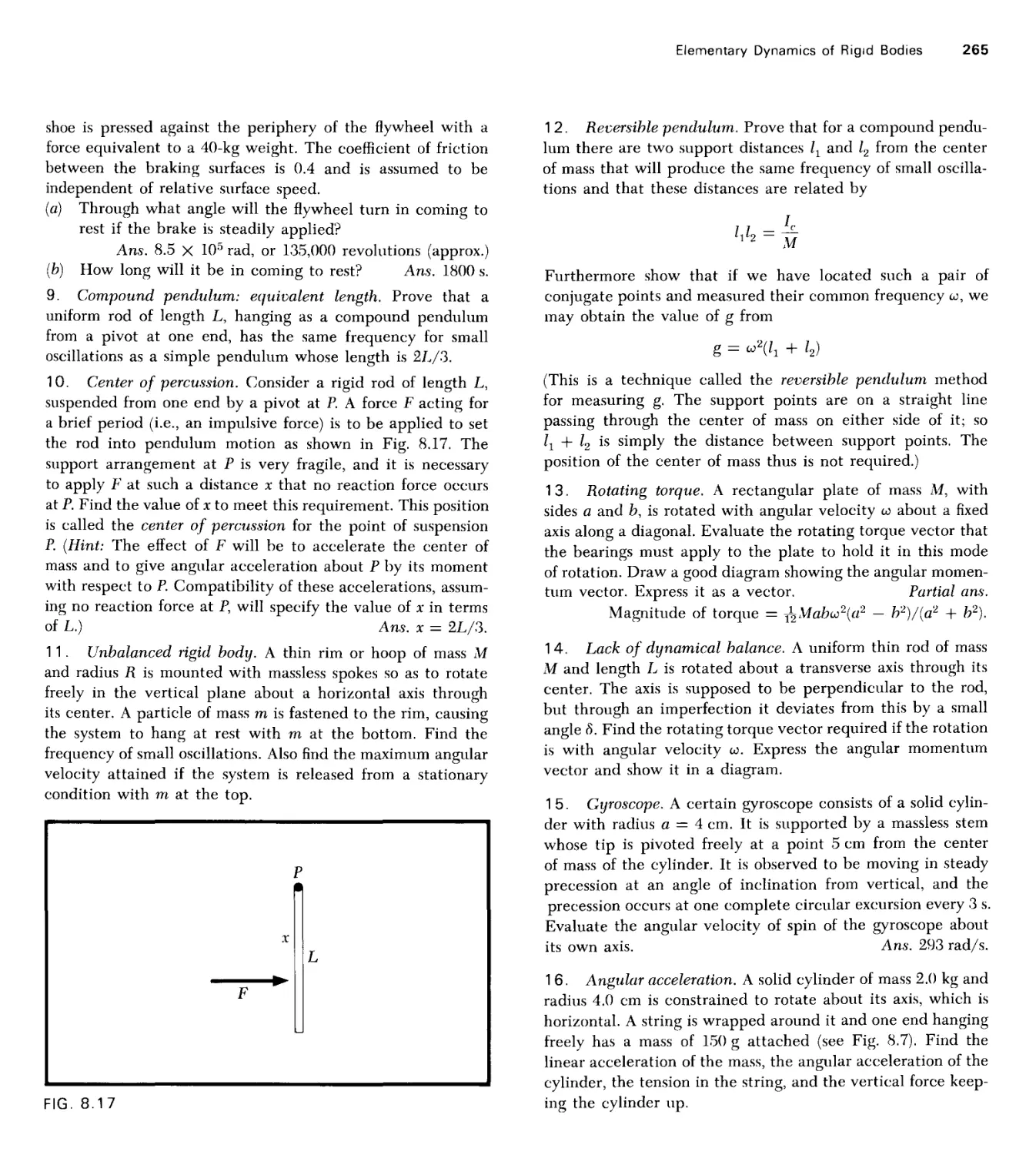
General
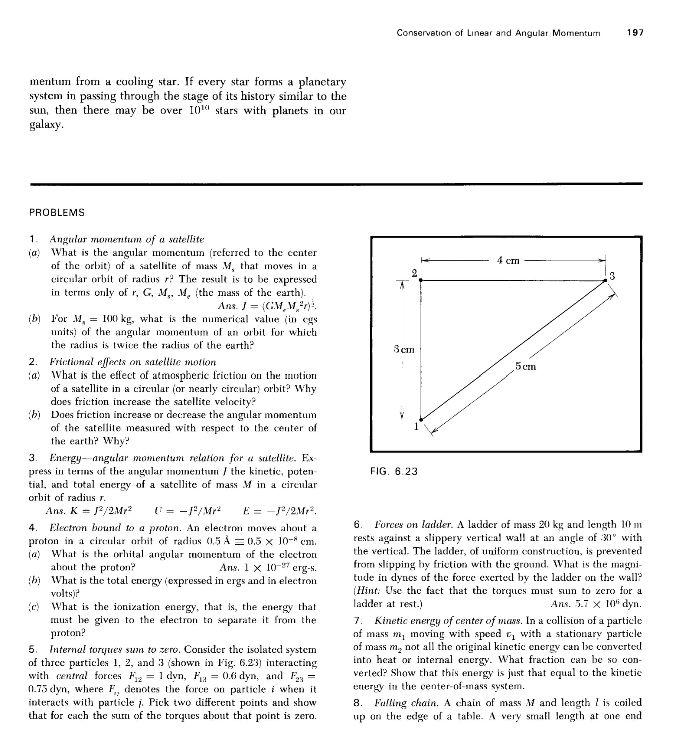
57.3°(57°18')
3.44 x 10³ minutes (of arc)
2.06 X 10⁵ seconds (of arc)
1.75 X 10"2 rad
2.91 x 10"4 rad
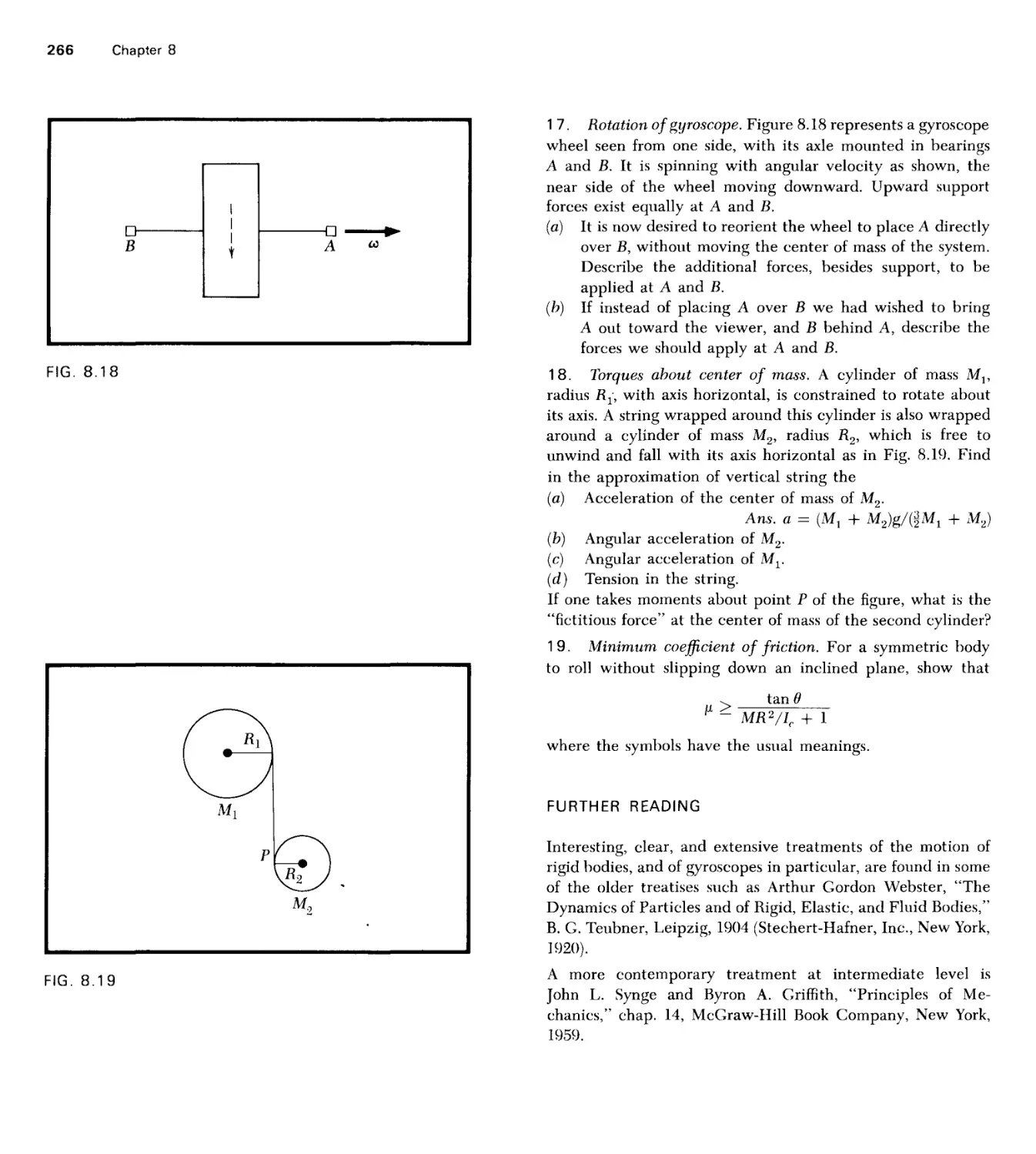
4.85 X 10"6 rad
1.609 X 105 cm
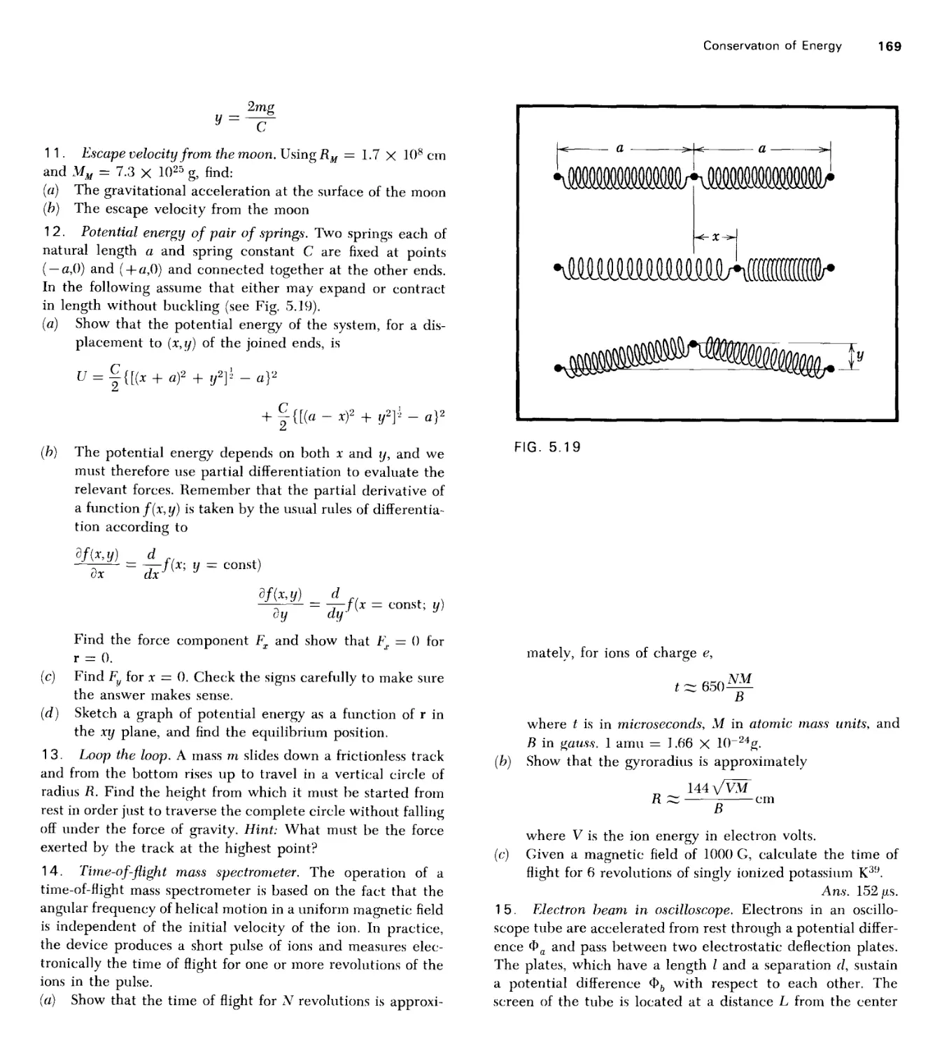
10"8 cm
10~4 cm
2.998 x 10² V
2.99725 X 1010 cm/s
s 980 cm/s2
6.671 X 10"8 dyn-cm2/g2
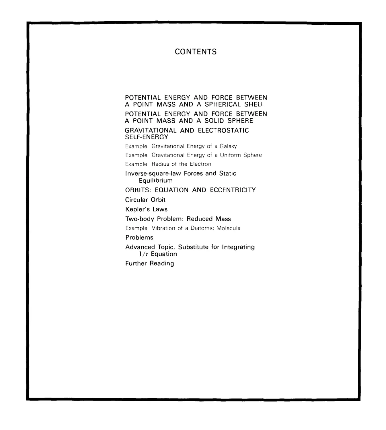
6.671 X 10"11 N-m2/kg2
1 dyne
1 newton
Astronomical
3.084 X 1018 cm
9.464 X 1017 cm
1.49 X 1013 cm
zz 1080
ZZ 1028 cm
= 1011
s 16 X 10"18 (cm/s)/cm
= 1.6 X 10¹¹
- 1023 cm
^8x 1044 g
6.96 X 1010 cm
2.14 X 10⁶s
1.99 X 1033 g
1.49 X 1013 cm
6.37 x 108 cm
5.98 X 1027 g
5.52 g/cm3
3.156 X 10⁷ s
8.64 X 10⁴ s
3.84 X 1010 cm
1.74 X 108 cm
7.34 X 1025 g
2.36 X 10⁶s
Item
= 1 radian
= 1 radian
= 1 radian
= 1 degree
= 1 minute (of arc)
= 1 second (of arc)
= 1 statute mile
= 1 angstrom
= 1 micrometer (micron)
= 1 statvolt
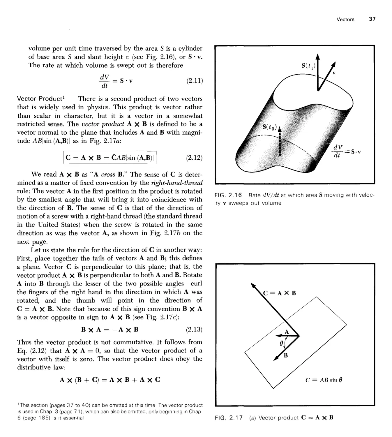
Speed of light in vacuum
Acceleration of gravity at earth's surface
Gravitational constant
Gravitational constant
= 1 g-cm/s2
= 1 kg-m/s2
= 1 parsec
= 1 light year
= 1 astronomical unit (= radius of earth's orbit)
Number of nucleons
Radius
Number of galaxies
Speed of recession of nebulae
Number of stars
Diameter
Mass
Radius
Period of rotation
Mass
Radius of orbit
Mean radius
Mass
Mean density
= 1 year (period of revolution)
= 24 hours (period of rotation)
Radius of orbit
Radius
Mass
Period of revolution
Symbol or
Abbreviation
rad
rad
rad
A
/xm
c
9
G
dyn
N
Derivation
of Value
180° /-a
77/180°
10"8 c
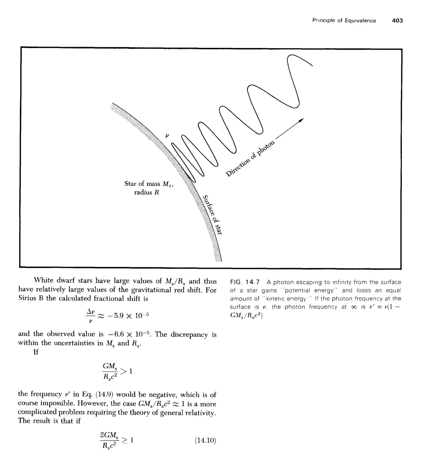
GMJR*
c X s/yr
AU
Known universe
Galaxy
Sun
Earth
Moon*
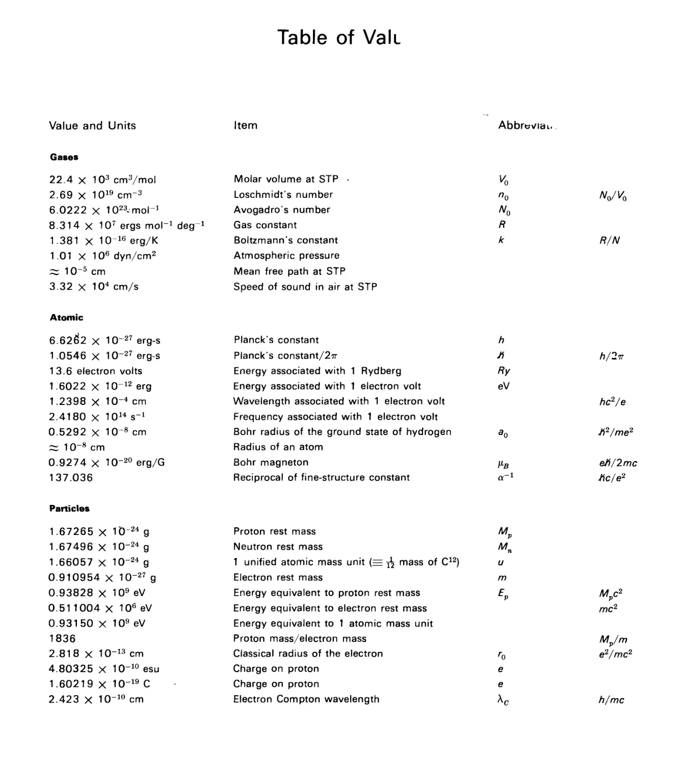
Table of Vali
Value and Units
Item
Abbr&viaL
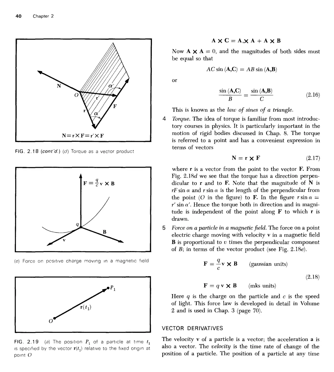
Gases
22.4 X 103 cm3/mol
2.69 X 1019 cm"3
6.0222 x lO^-mol-1
8.314 x 10⁷ ergs mol"1
1.381 X 10¹⁶ erg/K
1.01 X 10⁶ dyn/cm2
s 10~5 cm
3.32 X 104 cm/s
Molar volume at STP «
Loschmidt's number
Avogadro's number
Gas constant
Boltzmann's constant
Atmospheric pressure
Mean free path at STP
Speed of sound in air at STP
R
k
No/K
R/N
Atomic
6.62^2 X 10~27 erg-s
1.0546 X 10"27 ergs
1 3.6 electron volts
1.6022 X 10~12 erg
1.2398 X 10"4 cm
2.4180 X 10¹⁴ s"1
0.5292 X 10^8 cm
ss 10"8 cm
0.9274 X 10"20 erg/G
137.036
Planck's constant h
Planck's constant/27r /i
Energy associated with 1 Rydberg Ry
Energy associated with 1 electron volt eV
Wavelength associated with 1 electron volt
Frequency associated with 1 electron volt
Bohr radius of the ground state of hydrogen a0
Radius of an atom
Bohr magneton (iB
Reciprocal of fine-structure constant a-1
h/27T
hc2/e
fi2/me2
eJi/2mc
hole2
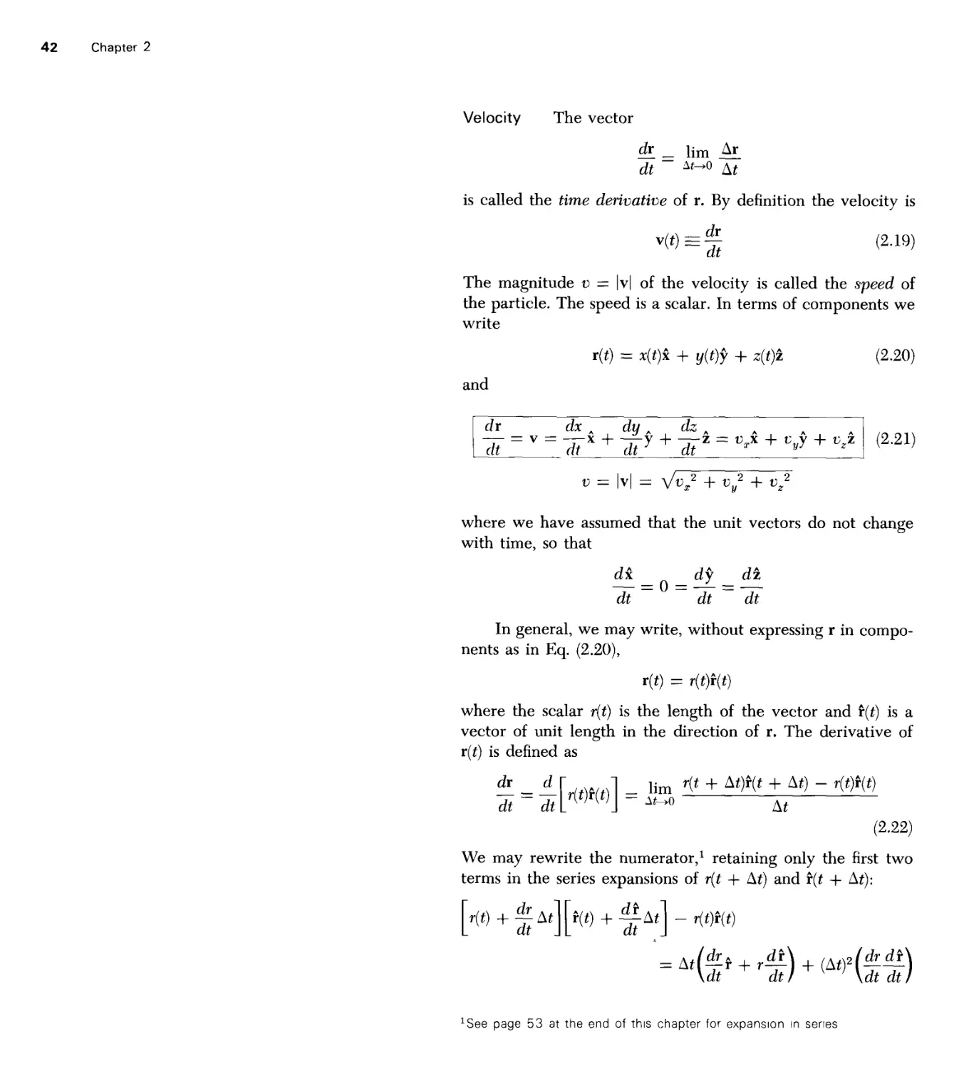
Particles
1.67265 X ID"24 g
1.67496 X 10⁻²⁴ g
1.66057 X 10⁻²⁴ g
0.910954 X 10"27 g
0.93828 X 10⁹ eV
0.511004 X 10⁶ eV
0.93150 X 10⁹ eV
1836
2.818 X 10"13 cm
4.80325 X 10⁻¹⁰ esu
1.60219 X 10~19 C
2.423 X 10"10 cm
Proton rest mass
Neutron rest mass
1 unified atomic mass unit (= ^ mass of C12)
Electron rest mass
Energy equivalent to proton rest mass
Energy equivalent to electron rest mass
Energy equivalent to 1 atomic mass unit
Proton mass/electron mass
Classical radius of the electron
Charge on proton
Charge on proton
Electron Compton wavelength
u
m
Mpc2
mc2
Mv/m
e2/mc2
h/mc
Mechanics
Charles Kittel
Professor of Physics
University of California
Berkeley
Walter D. Knight
Professor of Physics
University of California
Berkeley
Malvin A. Ruderman
Professor of Physics
New York University
Revised by
A. Carl Helmholz
Professor of Physics
University of California
Berkeley
Burton J. Moyer
Dean of the College of Liberal Arts
University of Oregon
Eugene
McGRAW-HILL BOOK COMPANY New York St. Louis San Francisco Dusseldorf Johannesburg, Kuala Lumpur London
Mexico Montreal New Delhi Panama Rio de Janeiro Singapore Sydney Toronto
Mechanics
Berkeley Physrcs"Course Volume 1, Second Edition
This book was set in Laurel by York Graphic Services, Inc. The editors
were Jack L. Farnsworth, Eva Marie Strock, and Ida Abrams Wolfson;
the designer was Michael A Rogondino, and the production super-
visor was Adam Jacobs The drawings were done by Ayxa Art
The printer was Halhday Lithograph Corporation.
Front cover' NGC 4594 spiral galaxy in Virgo, seen on edge, 200-in.
photograph. The dark band is due to absorption by a ring of matter
surrounding the bright central core (Photograph courtesy of the Hale
Observatories )
Back cover Hydrogen bubble chamber picture of the production of
an anti-i in the reaction K+ + p. (Photograph courtesy of the
Lawrence Berkeley Laboratory)
MECHANICS
Copyright© 1973 by McGraw-Hill, Inc All rights reserved Printed
in the United States of America. No part of this publication may be
reproduced, stored in a retrieval system, or transmitted, in any form
or by any means, electronic, mechanical, photocopying, recording,
or otherwise, without the prior written permission of the publisher.
Library of Congress Cataloging in Publication Data
Kittel, Charles
Mechanics
(Berkeley physics course, v 1)
1 Mechanics I Knight. Walter D , joint
author, II Ruderman, Malvin A , joint author
III Helmholz, A Carl, ed IV Mover, Burton J ,
ed V Title VI Series.
QC1 B375 vol 1 [QC125 2] 530'08s [531] 72-7444
ISBN 0-07-004880-0
6 7 8 9 10 HDHD 8543210
The first edition of the Berkeley Physics Course MECHANICS, Vol
1 copyright © 1963, 1964, 1965 by Educational Development
Center was supported by a grant from the National Science
Foundation to EDC This material is available to publishers and authors on
a royalty-free basis by applying to the Educational Development
Center
Foreword vi
Preface to the Second Edition of Volume 1 vii
Original Preface to the Berkeley Physics Course ix
Teaching Notes xi
Note to the Student xvi
Notation xvii
1 Introduction 2
2 Vectors 26
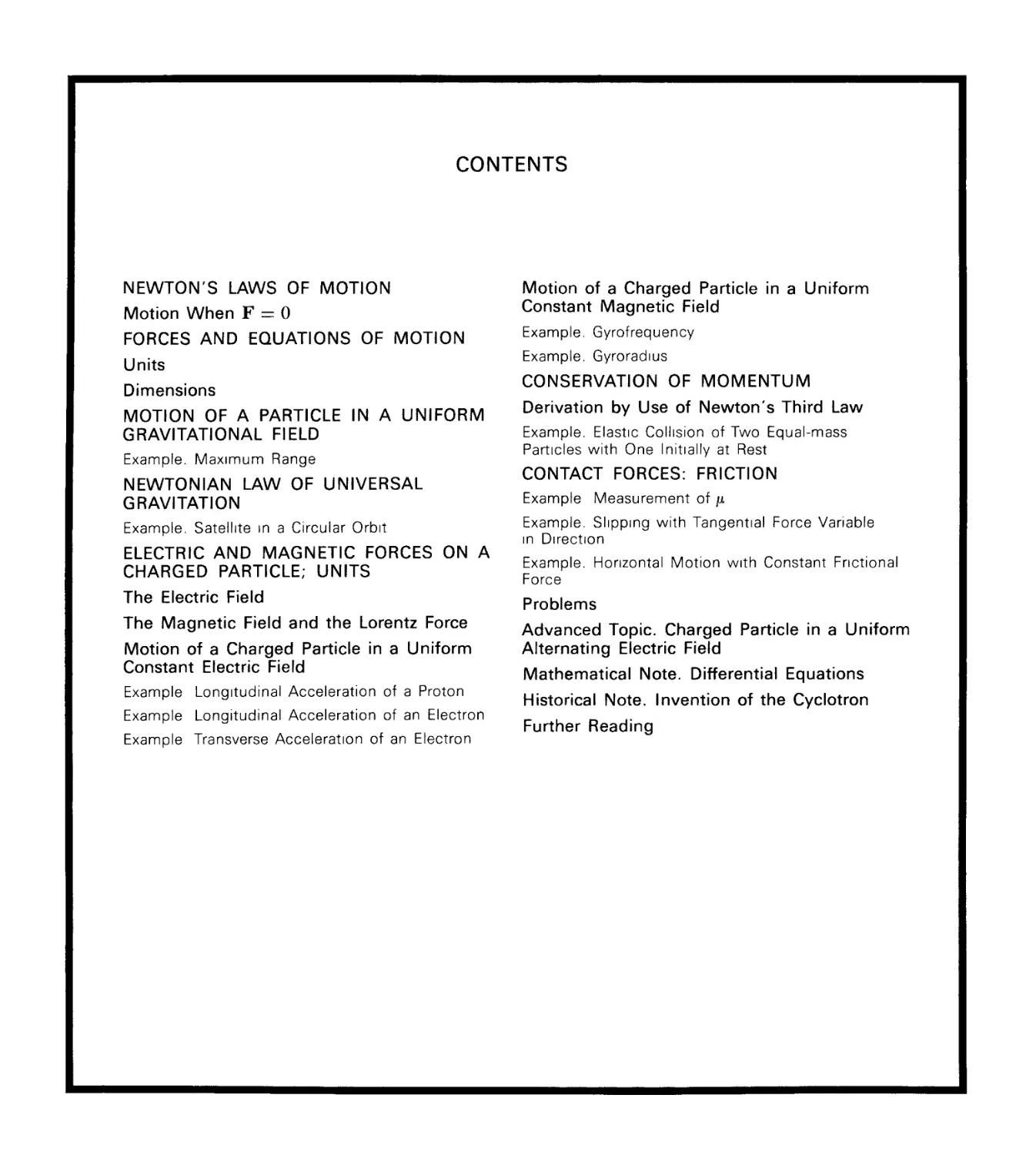
3 Newton's Laws of Motion 56
4 Frames of Reference: Galilean Transformation 100
5 Conservation of Energy 134
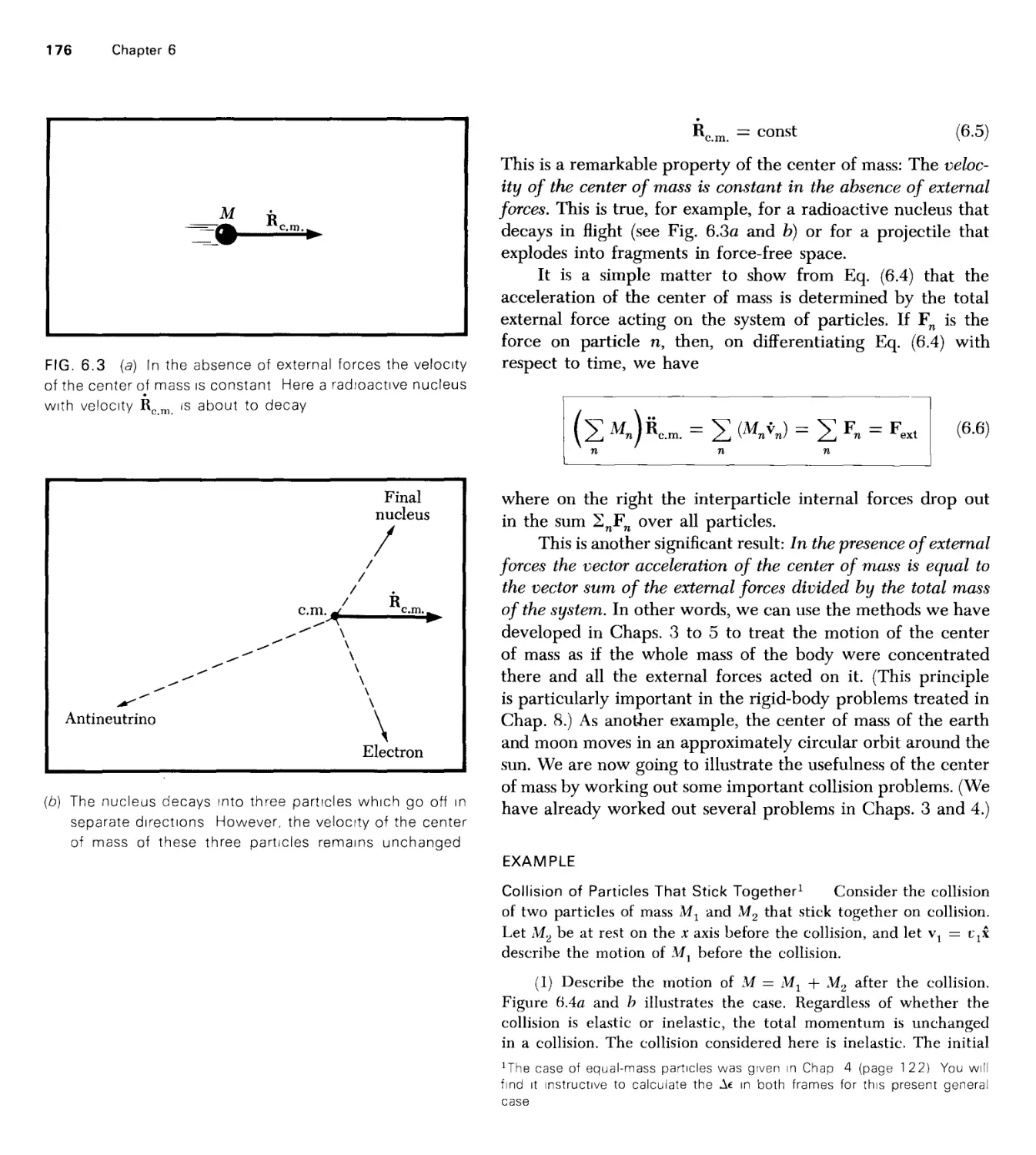
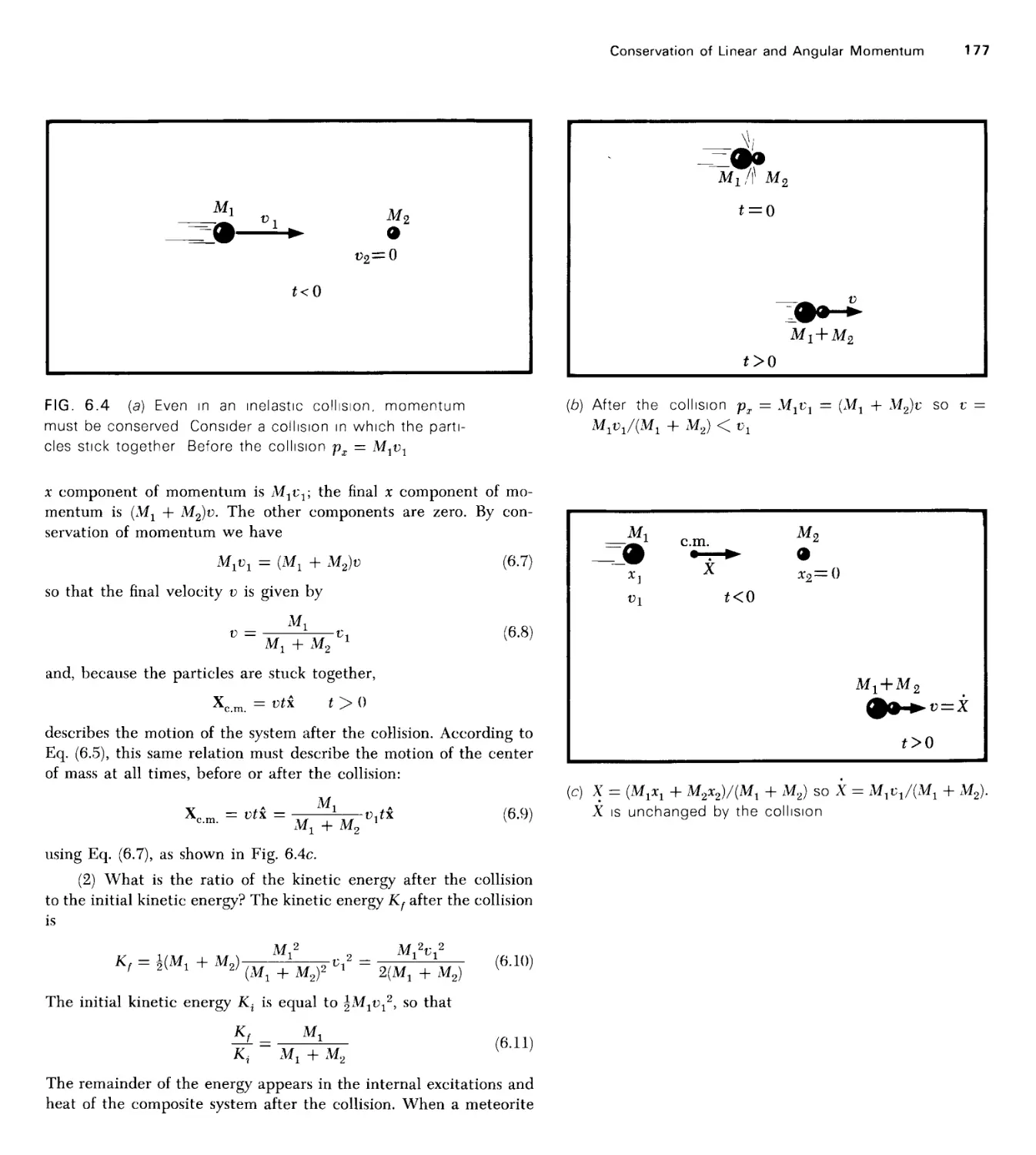
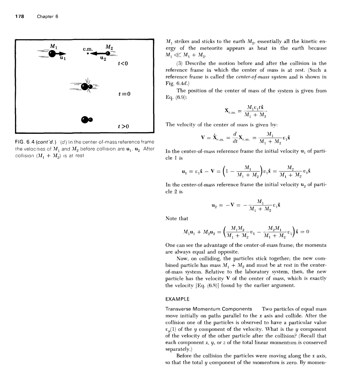
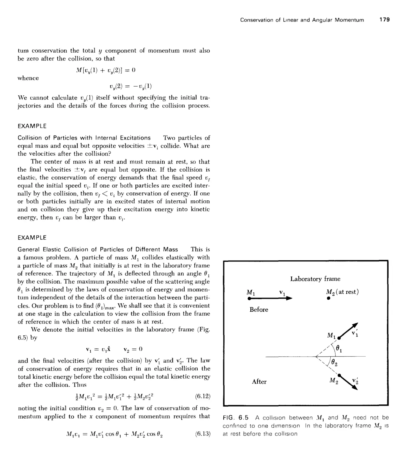
6 Conservation of Linear and Angular Momentum 1 72
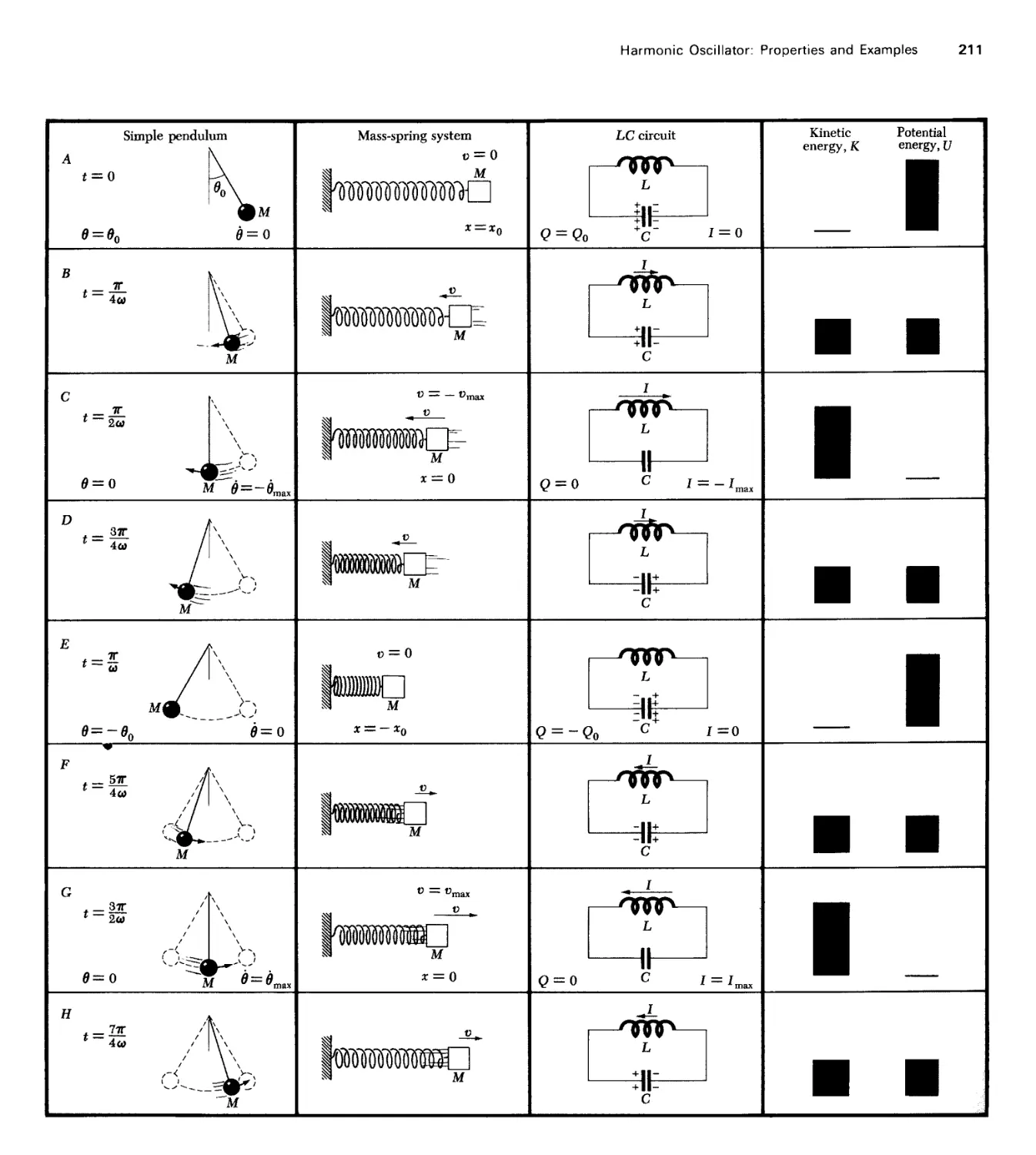
7 Harmonic Oscillator: Properties and Examples 200
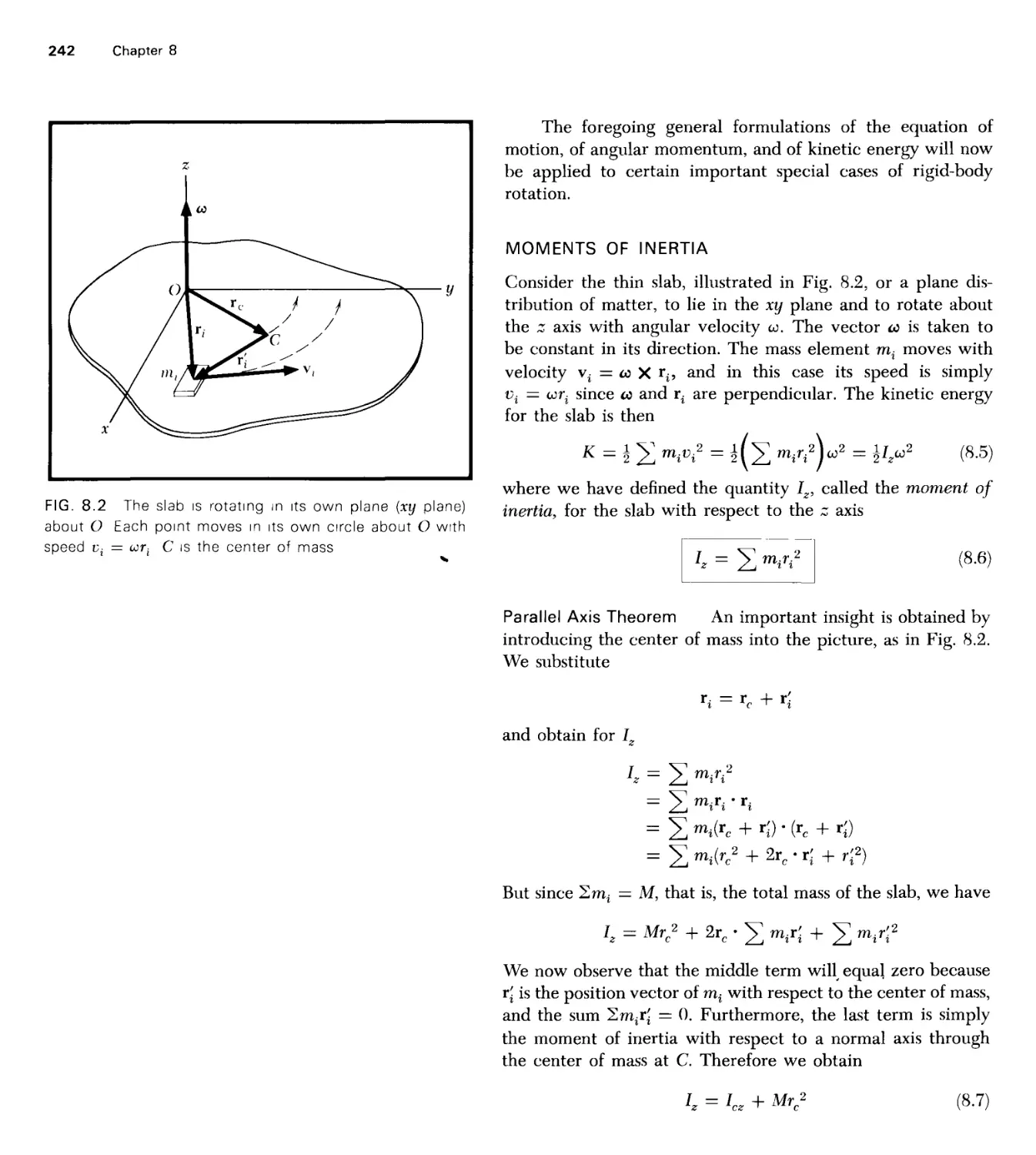
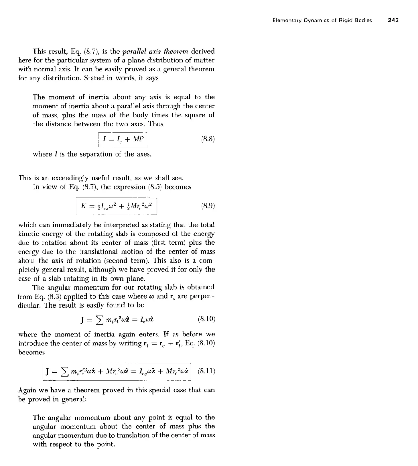
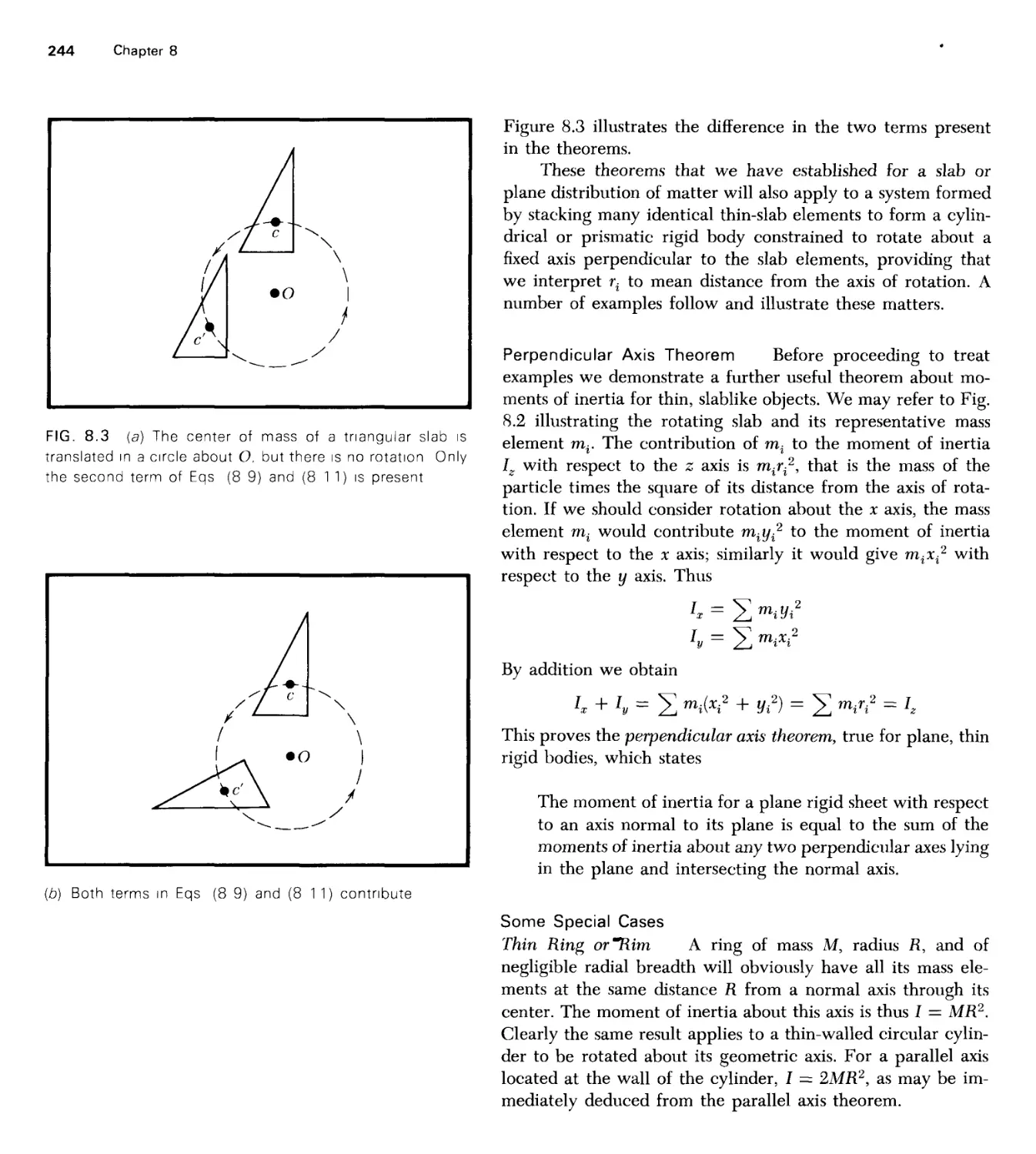
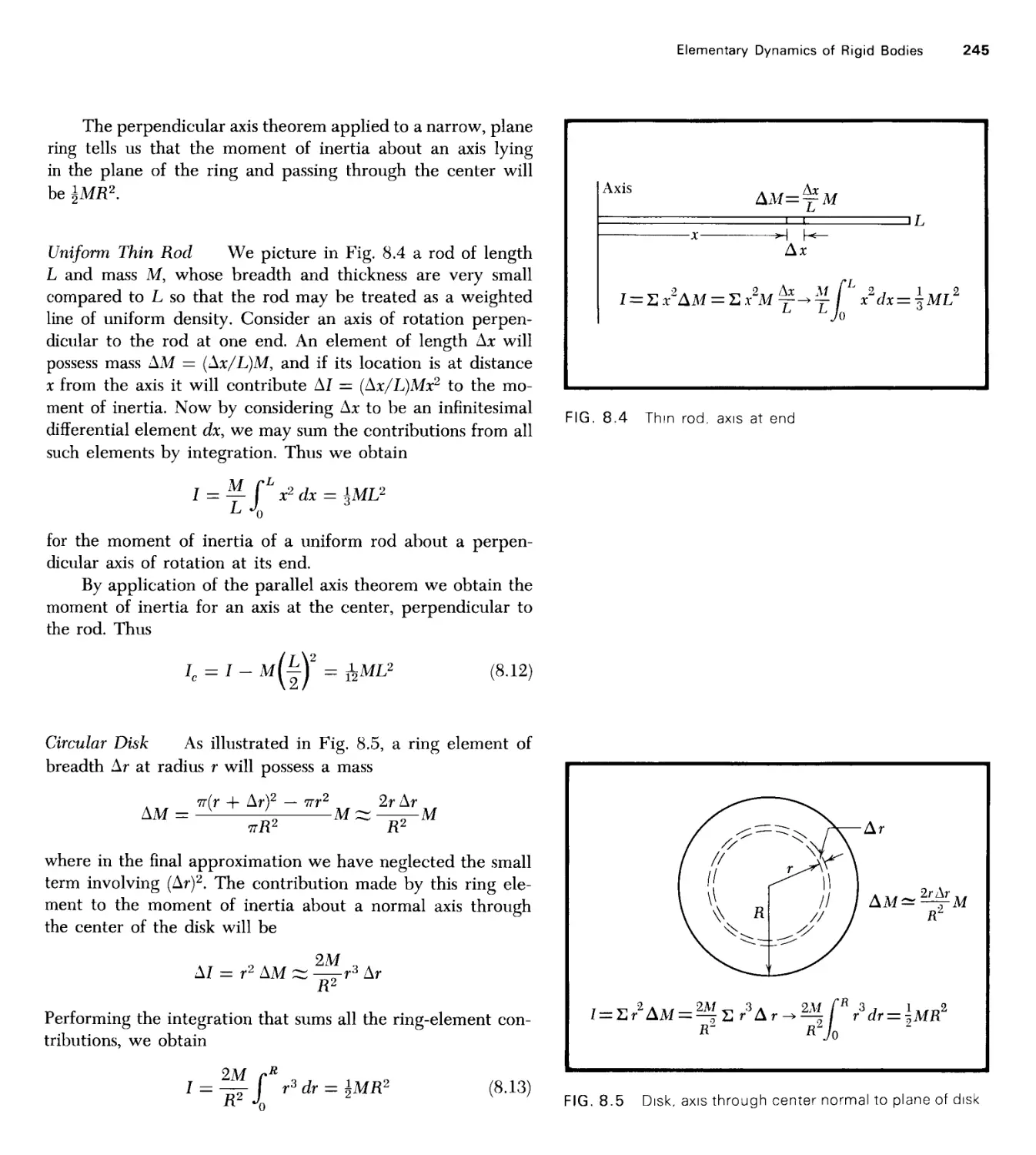
8 Elementary Dynamics of Rigid Bodies 238
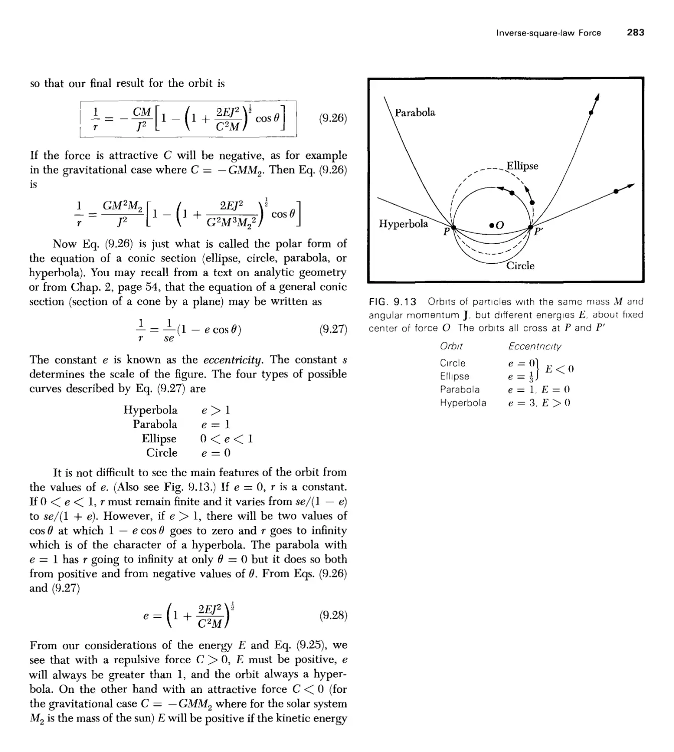
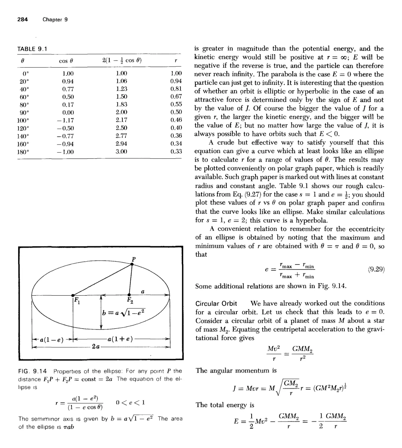
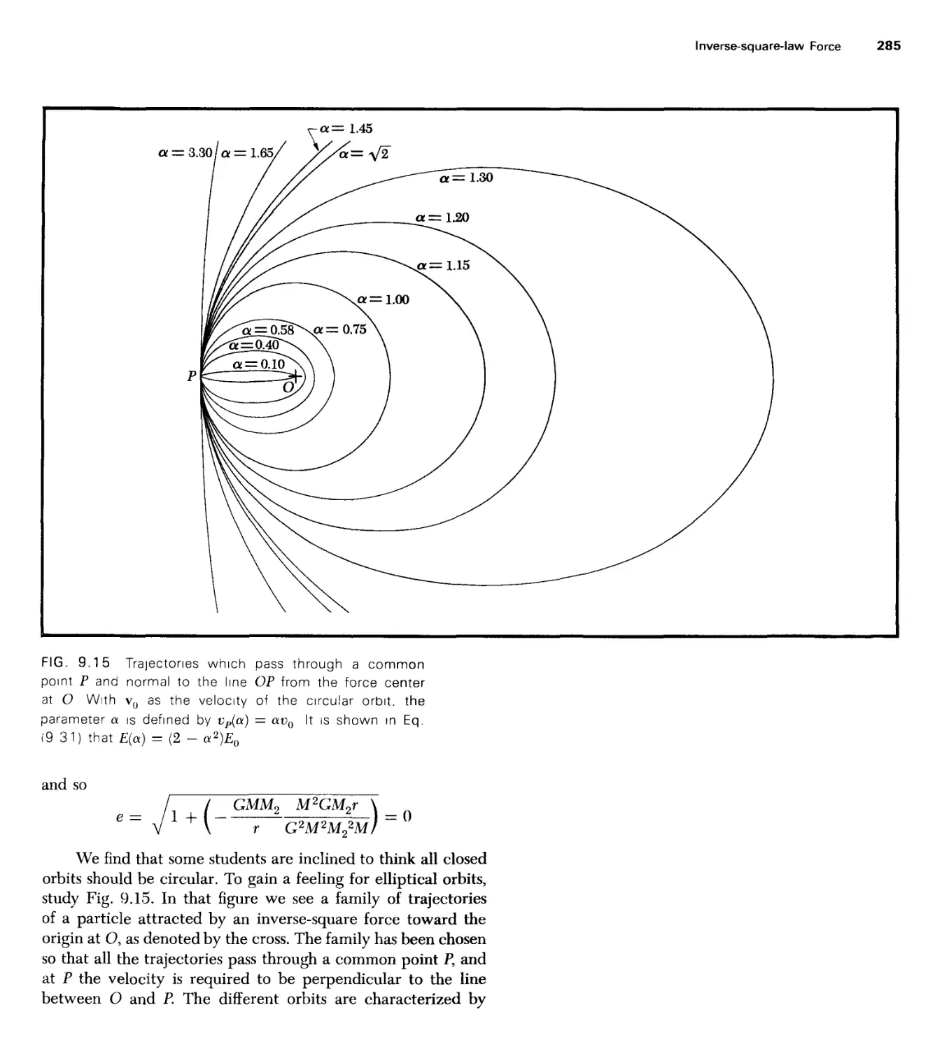
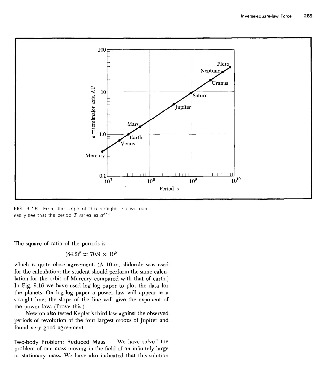
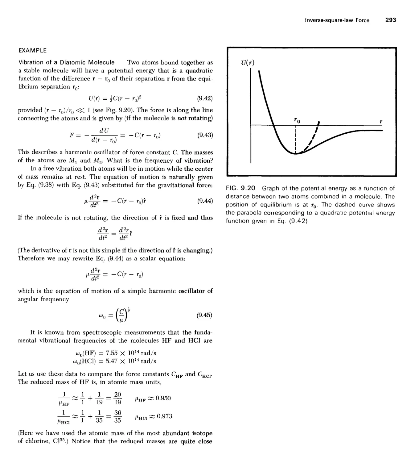
9 Inverse-square-law Force 268
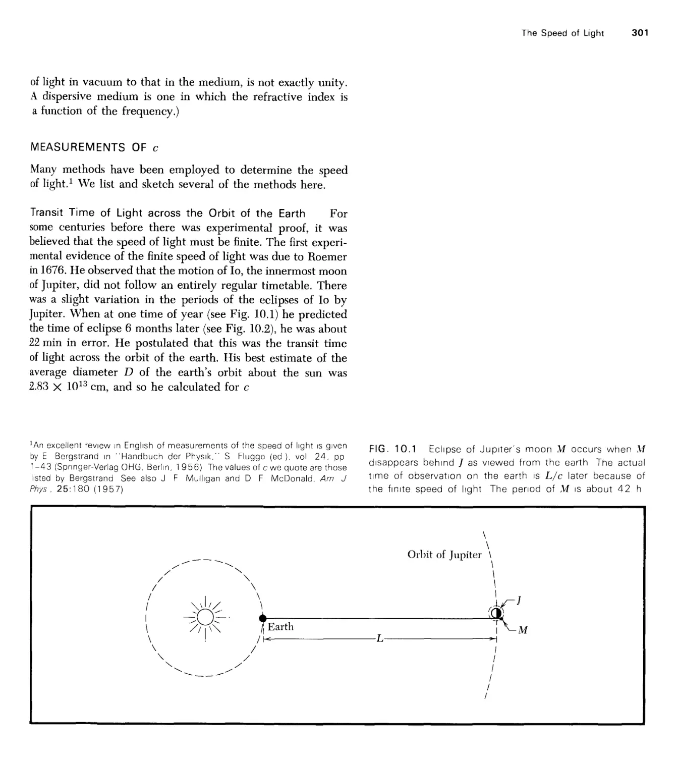
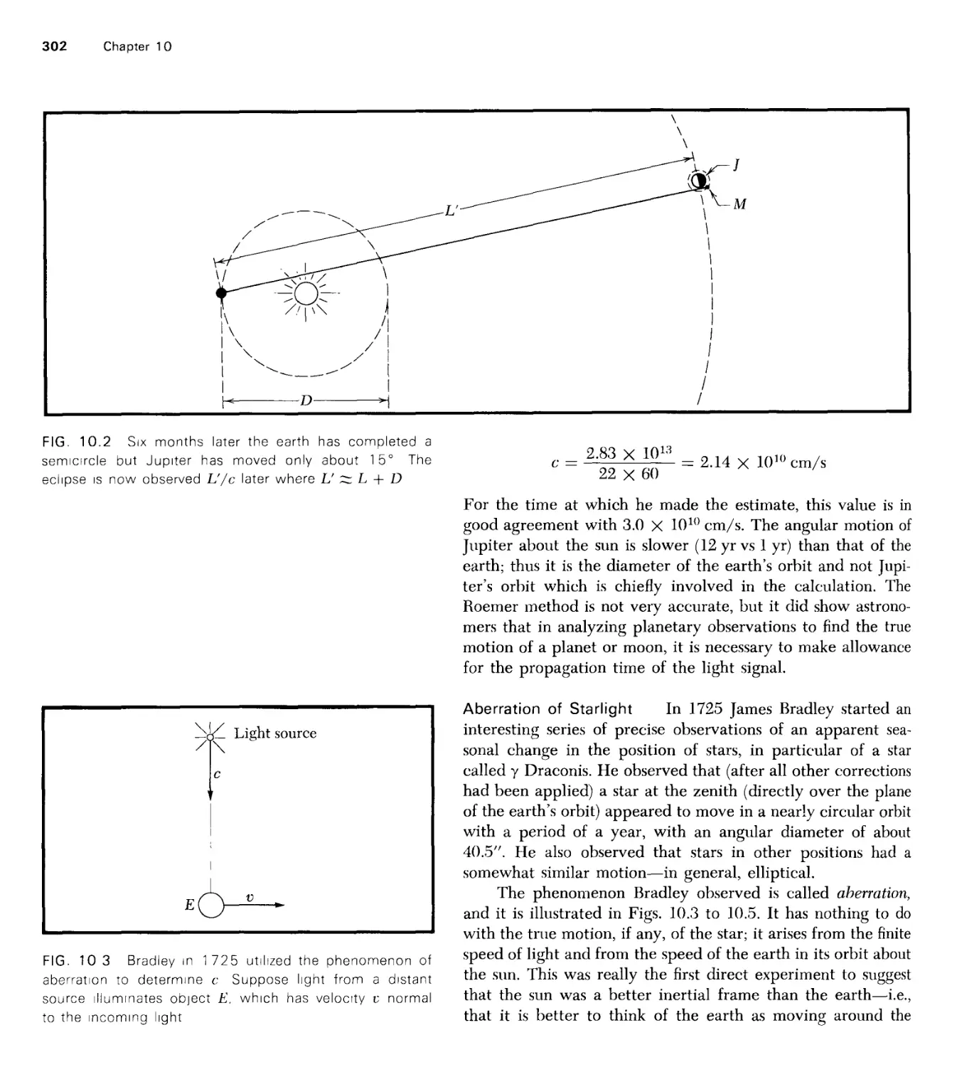
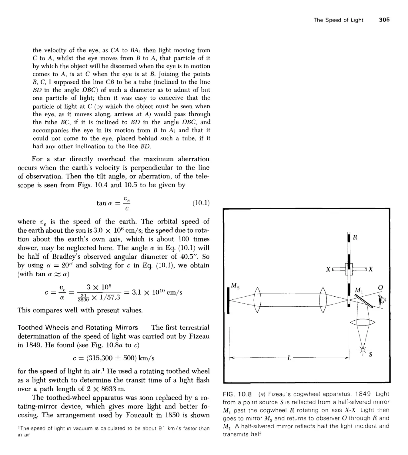
10 The Speed of Light 298
1 1 Special Relativity: The Lorentz Transformation 324
1 2 Relativistic Dynamics: Momentum and Energy 348
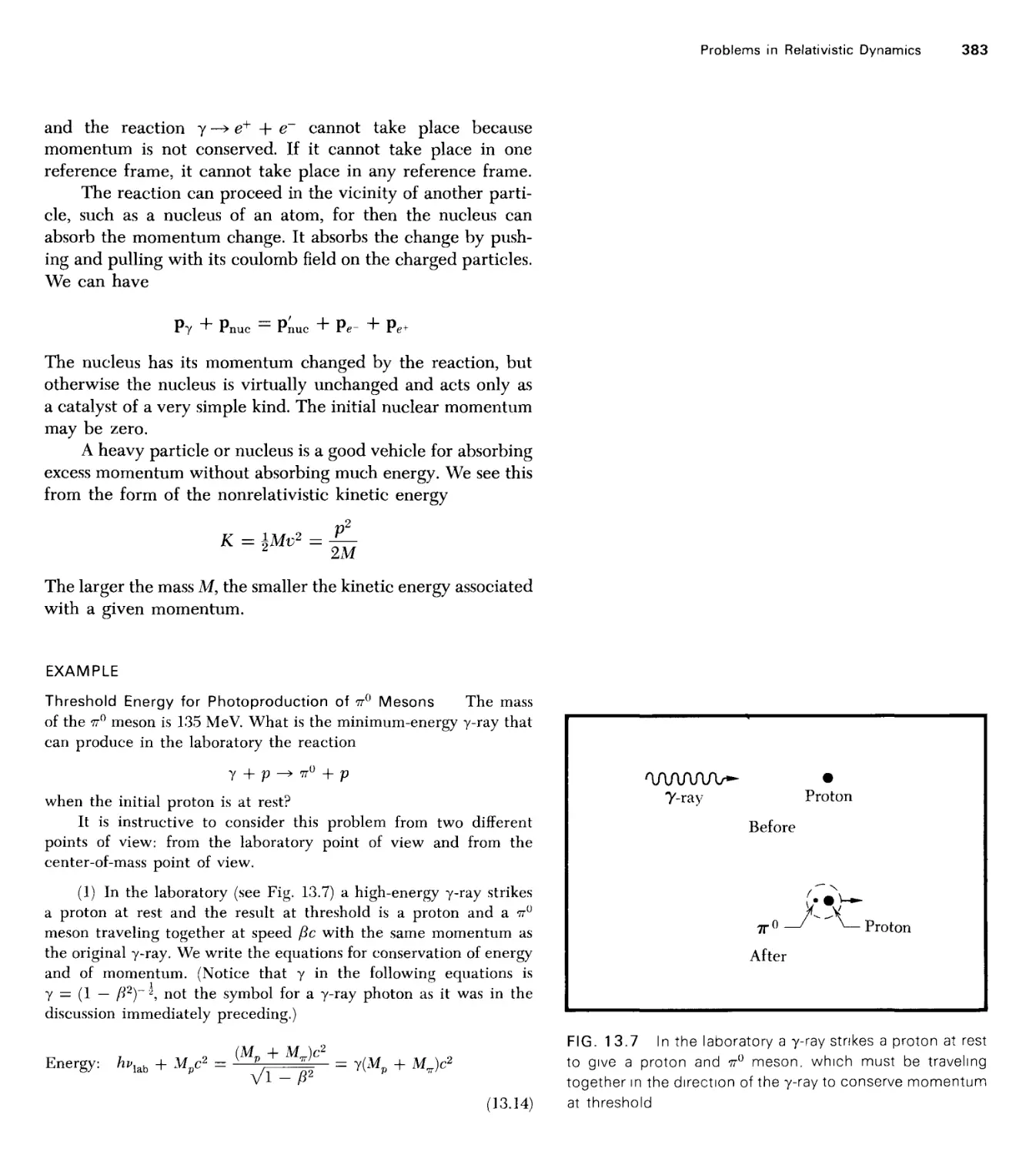
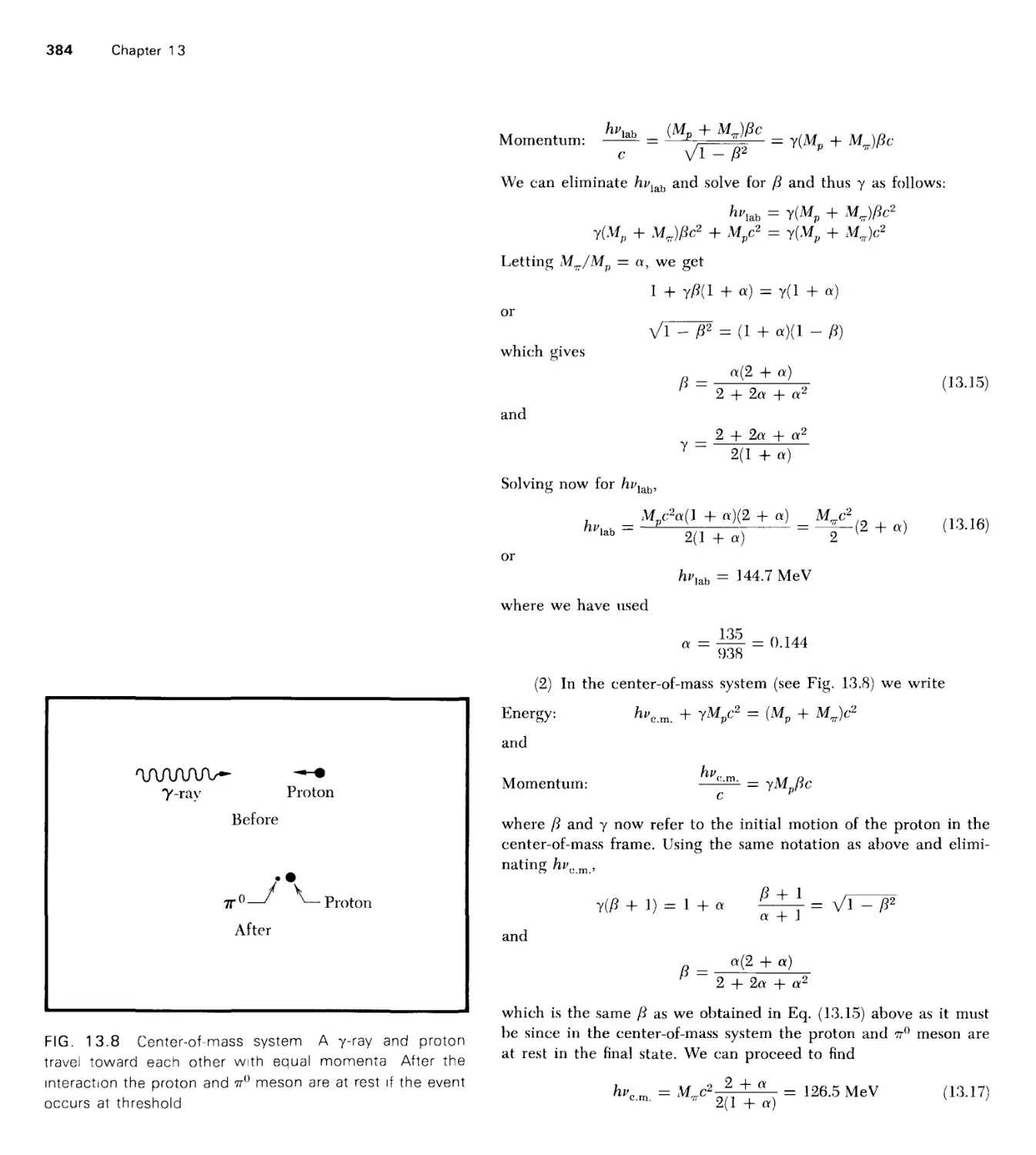
13 Problems in Relativistic Dynamics 374
14 Principle of Equivalence 396
Appendix 410
Film Lists 41 1
Index 415
Contents
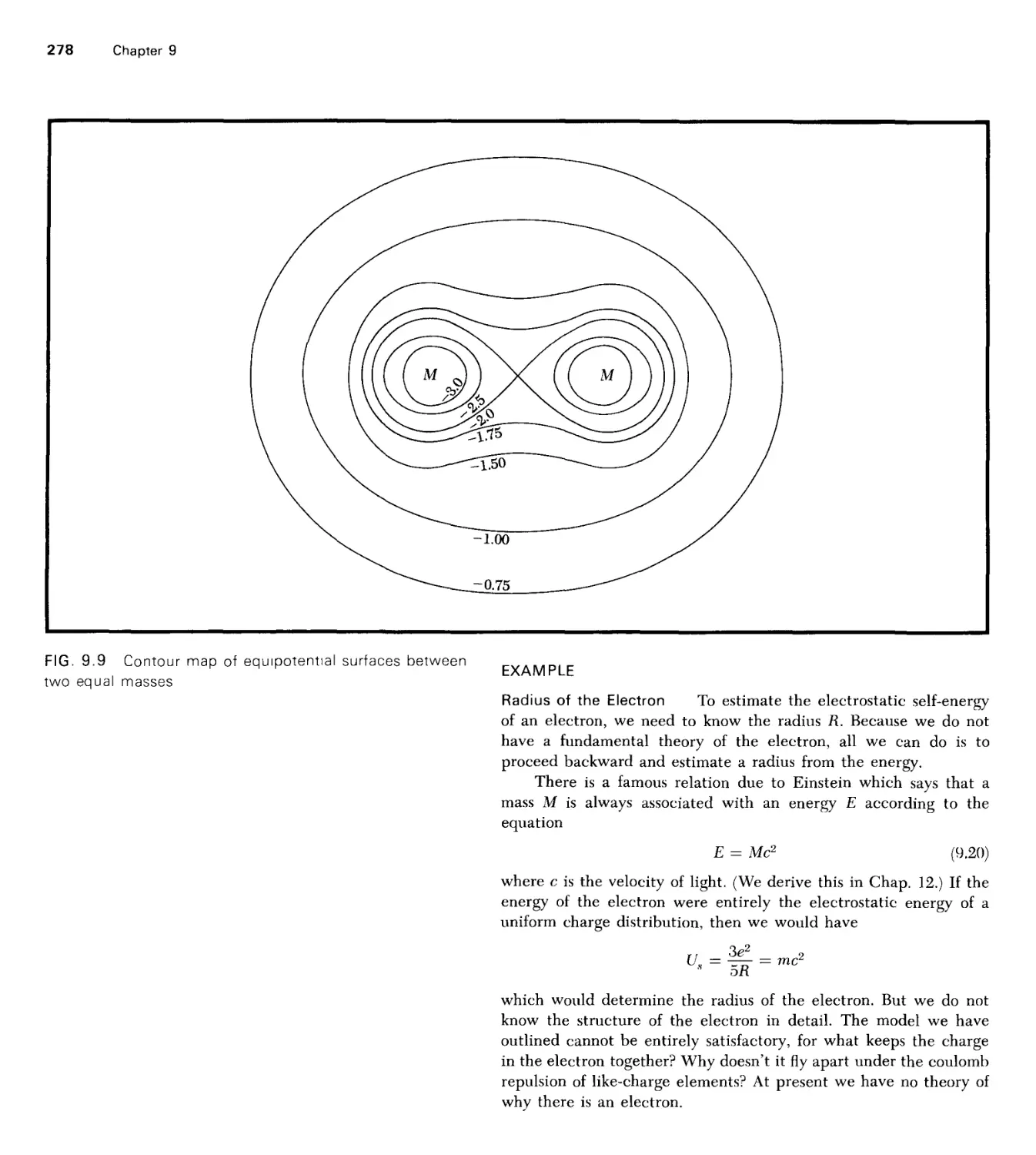
One of the urgent problems confronting universities today is that of
undergraduate teaching. As research has become more and more absorbing to
the faculty, a "subtle discounting of the teaching process" (to quote
philosopher Sidney Hook) has too often come into operation. Additionally,
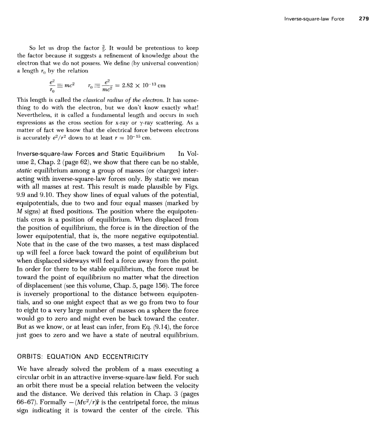
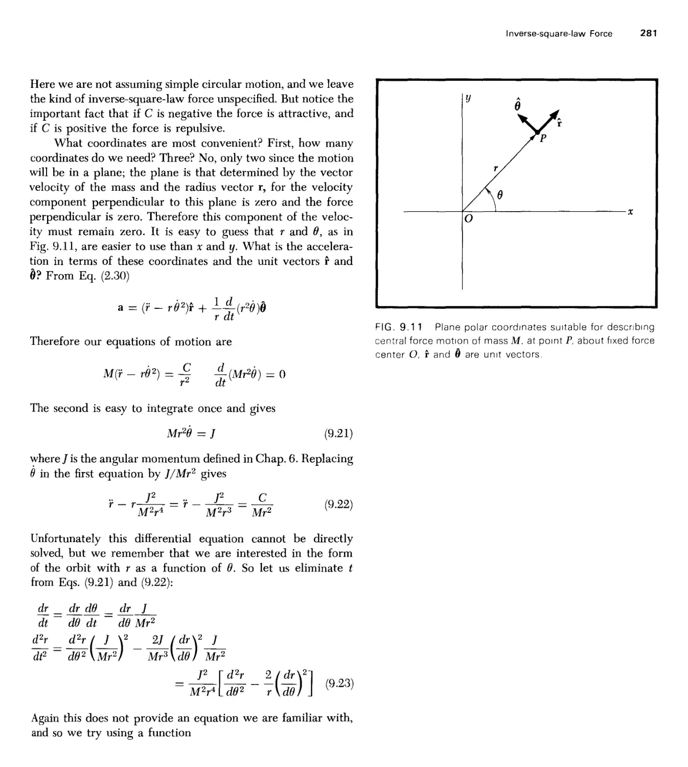
in many fields the changing content and structure of knowledge growing
out of research have created great need for curriculum revision. This is
particularly true, of course, in the physical sciences.
It is a pleasure, therefore, to contribute a foreword to the Berkeley
Physics Course and Laboratory, which is a major curriculum improvement
program at the undergraduate level designed to reflect the tremendous
revolutions in physics of the last hundred years. The course has enlisted
the efforts of many physicists working in forefront areas of research and
has been fortunate to have the support of the National Science Foundation,
through a grant to Educational Services Incorporated. It has been tested
successfully in lower division physics classes at the University of California,
Berkeley, over a period of several semesters. The course represents a marked
educational advance, and I hope it will be very widely used.
The University of California is happy to act as host to the inter-
university group responsible for developing this new course and laboratory
and pleased that a number of Berkeley students volunteered to help in
testing the course. The financial support of the National Science Foundation
and the cooperation of Educational Services Incorporated are much
appreciated. Most gratifying of all, perhaps, is the lively interest in
undergraduate teaching evinced by the substantial number of University of
California faculty members participating in the curriculum improvement
program. The scholar-teacher tradition is an old and honorable one; the
work devoted to this new physics course and laboratory shows that the
tradition is still honored at the University of California.
Clark Kerr
Foreword
Volume 1 of the Berkeley Physics Course has been in use in its bound form
for about seven years. Several years ago it seemed appropriate to consider
a revision. At this point each of us had taught the course in Berkeley several
times, and on the basis of our experience and talks with colleagues, both
in Berkeley and at other institutions, we had developed and considered
changes to make a more "teachable" text for an introductory course for
engineering and physical science students. Thus we proceeded to such a
revision.
We have tried to keep the fresh approach that was characteristic of
the whole Berkeley Physics Course, the use of examples drawn from
research laboratories, and the presentation of interesting topics often
previously judged to be too advanced for an introductory course. We have
removed some of the Advanced Topics from Vol. 1 and have removed Chap.
15, Particles of Modern Physics, in the belief that they are not often used
in a course at this level. The most substantial change has been the complete
rewriting of Chap. 8 on Rigid Body Motion. Although this chapter is
certainly more mundane now, it is more suited to the level of the students.
The order of presentation of topics remains the same except that Chaps.
3 and 4 have been interchanged in the hope that some familiarity with
the ordinary applications of Newton's Laws of Motion will provide the
student with background for a better understanding of the somewhat more
advanced concept of galilean transformations. Finally, because students
have encountered substantial difficulties with mathematics, particularly
differential equations, we have added a number of Mathematical Notes.
The Teaching Notes that follow give some detail of the philosophy
of using this book as a text. There is still a good deal more material than
can be comfortably used in a one-quarter or a one-semester course. An
instructor should make conscious choices of the material that he wishes
to use. In recent years the change to the quarter system at Berkeley has
unfortunately made it necessary to separate laboratory work from the first
quarter covering the subject of mechanics. An introductory course should
Preface to the Second Edition of Volume 1
viii Preface to the Second Edition of Volume 1
be tied to the laboratory, and the revision of the Berkeley Physics
Laboratory by Alan Portis and Hugh Young provides accompanying laboratory
work valuable for any introduction to mechanics.
We have benefited from the help and criticisms of many colleagues.
The help of Miss Miriam Machlis in preparing this revision has been
particularly extensive.
A. Carl Helmholz
Burton J. Moyer
This is a two-year elementary college physics course for students majoring
in science and engineering. The intention of the writers has been to present
elementary physics as far as possible in the way in which it is used by
physicists working on the forefront of their field. We have sought to make
a course that would vigorously emphasize the foundations of physics. Our
specific objectives were to introduce coherently into an elementary
curriculum the ideas of special relativity, of quantum physics, and of statistical
physics.
This course is intended for any student who has had a physics course
in high school. A mathematics course including the calculus should be taken
at the same time as this course.
There are several new college physics courses under development in
the United States at this time. The idea of making a new course has come
to many physicists, affected by the needs both of the advancement of science
and engineering and of the increasing emphasis on science in elementary
schools and in high schools. Our own course was conceived in a conversation
between Philip Morrison of Cornell University and Charles Kittel late in
1961. We were encouraged by John Mays and his colleagues of the National
Science Foundation and by Walter C. Michels, then the Chairman of the
Commission on College Physics. An informal committee was formed to
guide the course through the initial stages. The committee consisted
originally of Luis Alvarez, William B. Fretter, Charles Kittel, Walter D. Knight,
Philip Morrison, Edward M. Purcell, Malvin A. Ruderman, and Jerrold R.
Zacharias. The committee met first in May 1962, in Berkeley; at that time
it drew up a provisional outline of an entirely new physics course. Because
of heavy obligations of several of the original members, the committee was
partially reconstituted in January 1964 and now consists of the undersigned.
Contributions of others are acknowledged in the prefaces to the individual
volumes.
The provisional outline and its associated spirit were a powerful
influence on the course material finally produced. The outline covered in
detail the topics and attitudes that we believed should and could be taught
Original Preface to the Berkeley Physics Course
x Original Preface to the Berkeley Physics Course
to beginning college students of science and engineering. It was never our
intention to develop a course limited to honors students or to students with
advanced standing. We have sought to present the principles of physics
from fresh and unified viewpoints, and parts of the course may therefore
seem almost as new to the instructor as to the students.
The five volumes of the course as planned will include:
I. Mechanics (Kittel, Knight, Ruderman)
II. Electricity and Magnetism (Purcell)
III. Waves and Oscillations (Crawford)
IV. Quantum Physics (Wichmann)
V. Statistical Physics (Reif)
The authors of each volume have been free to choose that style and method
of presentation which seemed to them appropriate to their subject.
The initial course activity led Alan M. Portis to devise a new
elementary physics laboratory, now known as the Berkeley Physics Laboratory.
Because the course emphasizes the principles of physics, some teachers may
feel that it does not deal sufficiently with experimental physics. The
laboratory is rich in important experiments and is designed to balance the
course.
The financial support of the course development was provided by the
National Science Foundation, with considerable indirect support by the
University of California. The funds were administered by Educational
Services Incorporated, a nonprofit organization established to administer
curriculum improvement programs. We are particularly indebted to Gilbert
Oakley, James Aldrich, and William Jones, all of ESI, for their sympathetic
and vigorous support. ESI established in Berkeley an office under the very
competent direction of Mrs. Mary R. Maloney to assist in the development
of the course and the laboratory. The University of California has no official
connection with our program, but it has aided us in important ways. For
this help we thank in particular two successive Chairmen of the Department
of Physics, August C. Helmholz and Burton J. Moyer; the faculty and
nonacademic staff of the Department; Donald Coney, and many others in
the University. Abraham Olshen gave much help with the early
organizational problems.
Your corrections and suggestions will always be welcome.
Eugene D. Commins Edward M. Purcell
Frank S. Crawford, Jr. Frederick Reif
Walter D. Knight Malvin A. Ruderman
Berkeley, California Philip Morrison Eyvind H. Wichmann
January 1965 Alan M. Portis Charles Kittel, Chairman
This volume is obviously intended for use as a text. The level is that of
students who have had some calculus and are taking more and who have
had a high school physics course. At the University of California in
Berkeley, students in the physical sciences and engineering start calculus in the
first quarter of their freshman year and take a course such as this along
with calculus in their second quarter. They have had differential calculus
by the start of the physics course and reach integration at least by the
middle of the quarter. Such a tight scheduling does require fairly close
cooperation with those giving the mathematics course. Of course they have
not studied differential equations by this time, and so some material about
the solution of simple kinds of differential equations is included in the
Mathematical Notes at the ends of Chaps. 3 and 7. There are few enough
types to be solved in this kind of a mechanics course so that we believe
a student can learn each one of the types.
The teacher will find that the Film Lists have been put all together
at the end of the book rather than at the end of each chapter. The
Commission on College Physics Resource Letter is a very complete list of films.
Special ones have been singled out that seemed especially suitable for the
subject of mechanics. In recent years a great many film loops have been
made. Some of these are very helpful as short illustrations of special topics;
each instructor will find through his own use those that are well suited
to his teaching.
Although the problems that have been added in this revision are mostly
easier than the ones they have replaced, we have not included very simple
problems and plug-in problems. Some of these are valuable in giving the
student a little confidence. But we believe that each instructor can make
these up for himself or at least find them in other books. No two teachers
will want to give a mechanics course in exactly the same way, and the
use of special problems gives them a good opportunity for diversity. There
are also now several problem books that are useful. Some of them as well
as other books on mechanics at this level are listed in the Appendix.
Teaching Notes
There are of course several ways to use this book as a text. One of
the ways in which the first edition has apparently rarely been used, but
for which we believe there might be a very good use for the entire book,
is for a course in mechanics following a one-year noncalculus course, such
as one might find in smaller institutions that do not have the facilities
for both a calculus and a noncalculus introductory course. For such a
course, which might be given to second- or third-year college students,
the whole book could well be covered since many of the topics would
have been included in less advanced form in the first year.
For the regular introductory section of a general physics course, this
book contains too much material, and we urge the instructor to abstain
from trying to cover everything. Many introductory courses do not include
special relativity, so that the first nine chapters make up a coherent
introduction to classical mechanics. But even this much material, if one tries
to cover it all, is too great for a nine- or ten-week quarter course or
the fraction of a semester that is usually devoted to mechanics. Therefore
we give some suggestions below for minimum coverage of chapters.
Sometimes it is not desirable to include any electrical or magnetic problems
in the beginning course. We believe that the text can be used in this
fashion, but it is true that many students find the electrical problems very
interesting. Many instructors find it difficult to be ruthless in cutting
material. Our own experience is that it is better to cover some material well
than to cover more material less well. The advanced sections and the
Advanced Topics should give the talented students something with which
to stretch their abilities and the students who go on in physics a reference
work that can be used in connection with later studies.
With these comments we proceed to the details of the several
chapters.
Chapter 1. As in the first edition, this chapter is not an essential part of
the study of mechanics, but it may provide interesting reading for those
with broader interests. For instructors who wish to assign the reading, it
may provide a good place to illustrate the concept of order of magnitude.
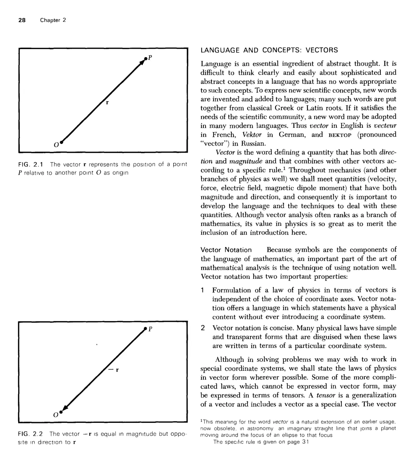
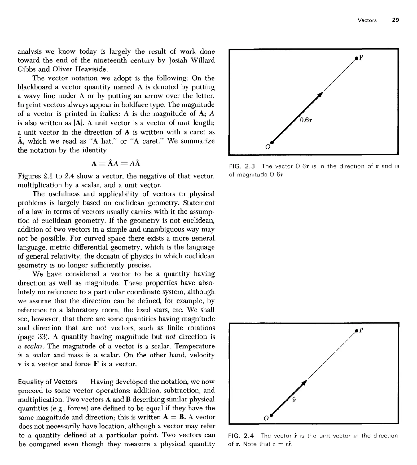
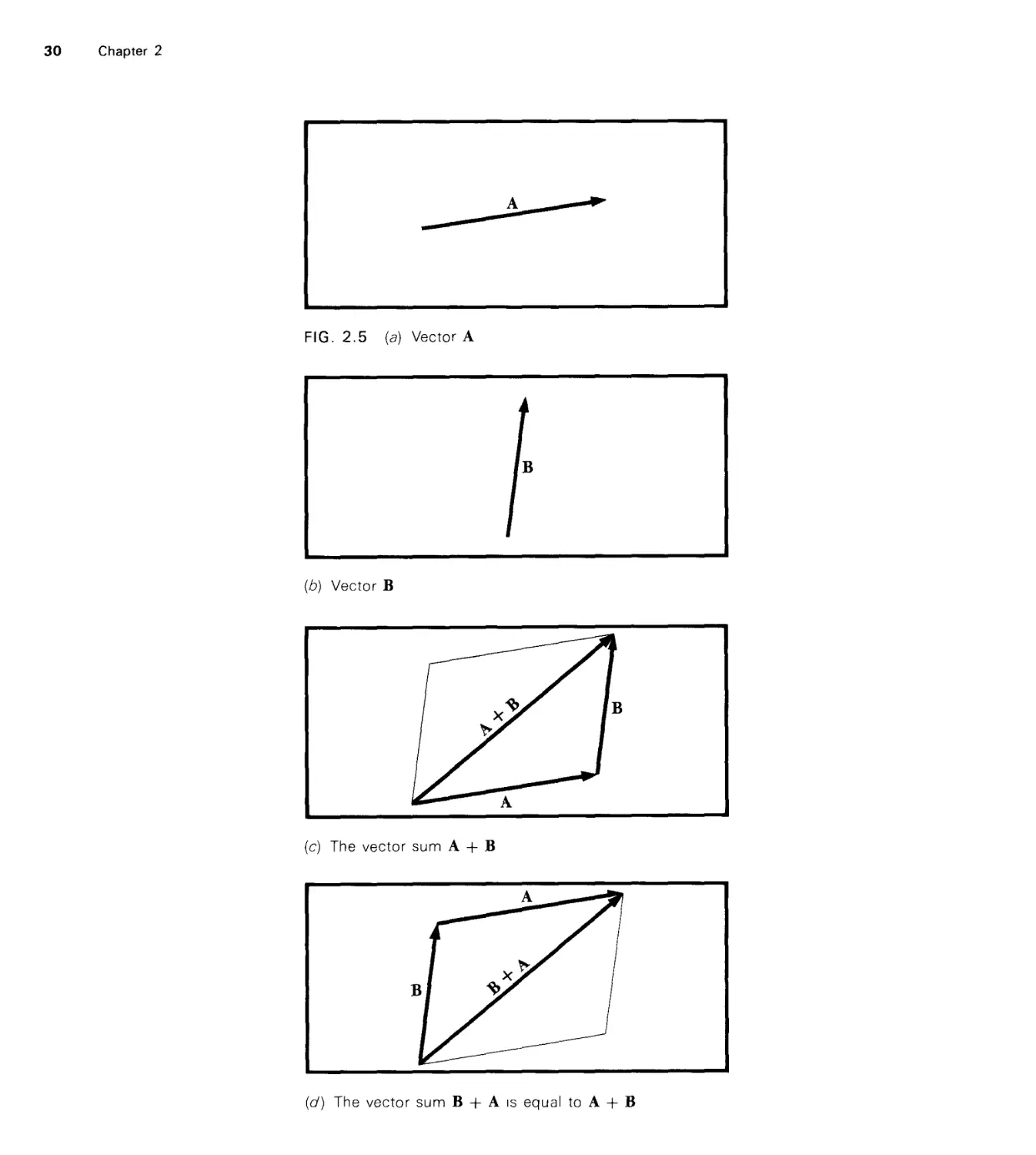
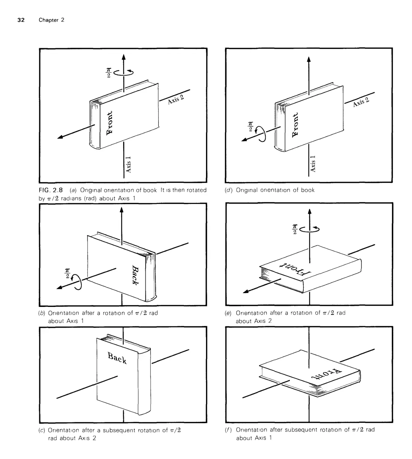
Chapter 2. Vectors introduce the student to the language that is very useful
in physics. As pointed out in the text, the vector product can be omitted
here along with the examples of magnetic forces in which v and B are
not perpendicular. One can proceed to Chap. 6 without needing the vector
product and return to it at that time. The scalar product is used often
in finding magnitudes and in Chap. 5 on work and energy, so it is highly
desirable to introduce it here. In addition it provides a tool for solving
numbers of interesting problems. The section on vector derivatives is also
useful, but the parts treating the unit vectors r and 0 can be omitted and
introduced much later. Hopefully, circular motion is a good introduction
of the dynamics to come.
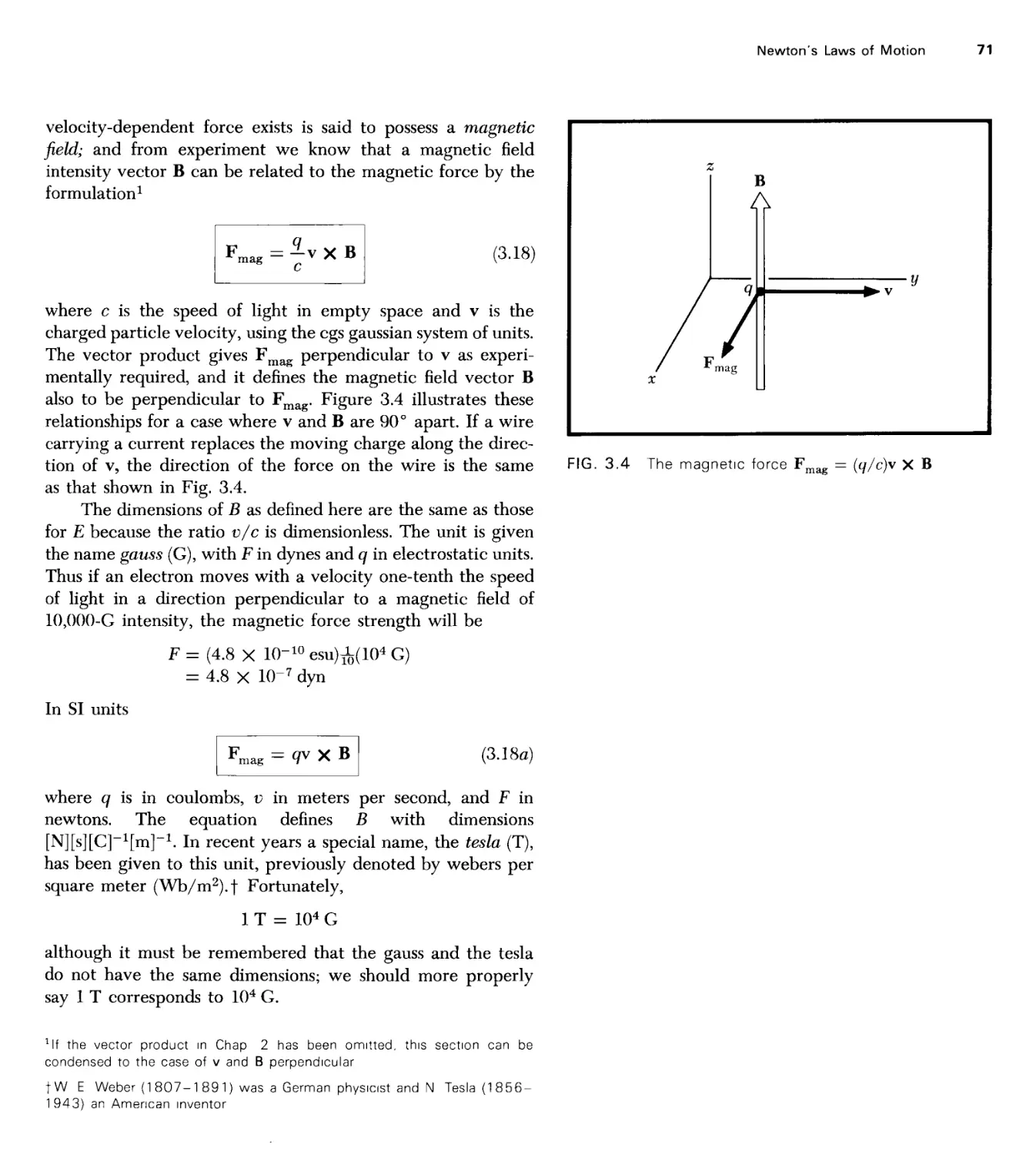
Chapter 3. This is a long chapter with a good many applications. Newton's
laws are introduced in conventional form and we proceed to applications
of the Second Law. For a shortened course or one that does not include
electrical and magnetic applications, the section on them can be omitted
entirely or the magnetic field can be treated only for the case of velocity
and magnetic field perpendicular. Conservation of momentum is then
introduced through Newton's Third Law. Kinetic energy is referred to
in collision problems even though it is not introduced until Chap. 5. Most
students have heard of it in high school and do not find difficulty with
it; but it can be omitted if desired.
Chapter 4. As pointed out in the text, this chapter is not of the conventional
type. Many physicists find appeal in the introduction of galilean
transformations, and for those planning to go on to special relativity, it does
provide a nice introduction to transformations of coordinates. However,
to nonphysics students and to those with limited time, it may be too much
"frosting on the cake" and should be omitted. Some reference to
accelerated frames of reference and fictitious forces should probably be included,
but these can be taken from the first few pages.
Chapter 5. Work and kinetic energy are introduced, first in one dimension
and then in three dimensions. The scalar product is really necessary here,
but certainly the use of the line integral can be skirted. Potential energy
is treated in detail. In a shorter course, the discussion of conservative fields
could well be omitted as could the discussion of electrical potential.
However, this is an important chapter and should not be hurried through.
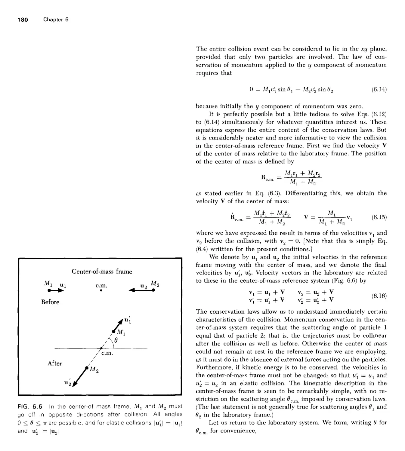
Chapter 6. This chapter treats collisions again and introduces the center-
of-mass system of reference. Center of mass is an important concept for
rigid bodies, and although the center-of-mass system is widely used, a
shortened version of a mechanics course could well omit this. The
introduction of angular momentum and torque requires the use of the vector
product. By this time, students have achieved a level where they can grasp
and use the vector product, and if it has been omitted earlier, it can be
taken up here. The conservation of angular momentum is an appealing
topic to many students.
Chapter 7. Here the Mathematical Notes should be studied first if the
students have had difficulty with differential equations. The mass on the
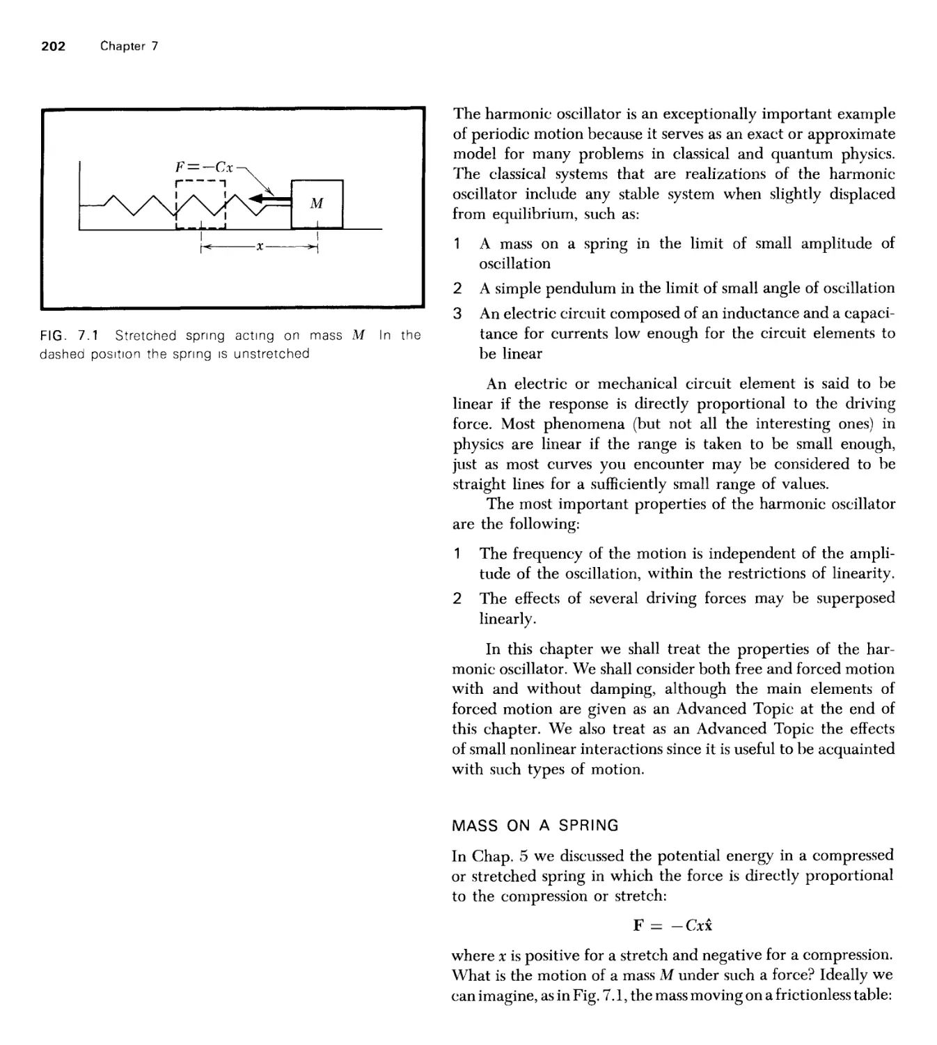
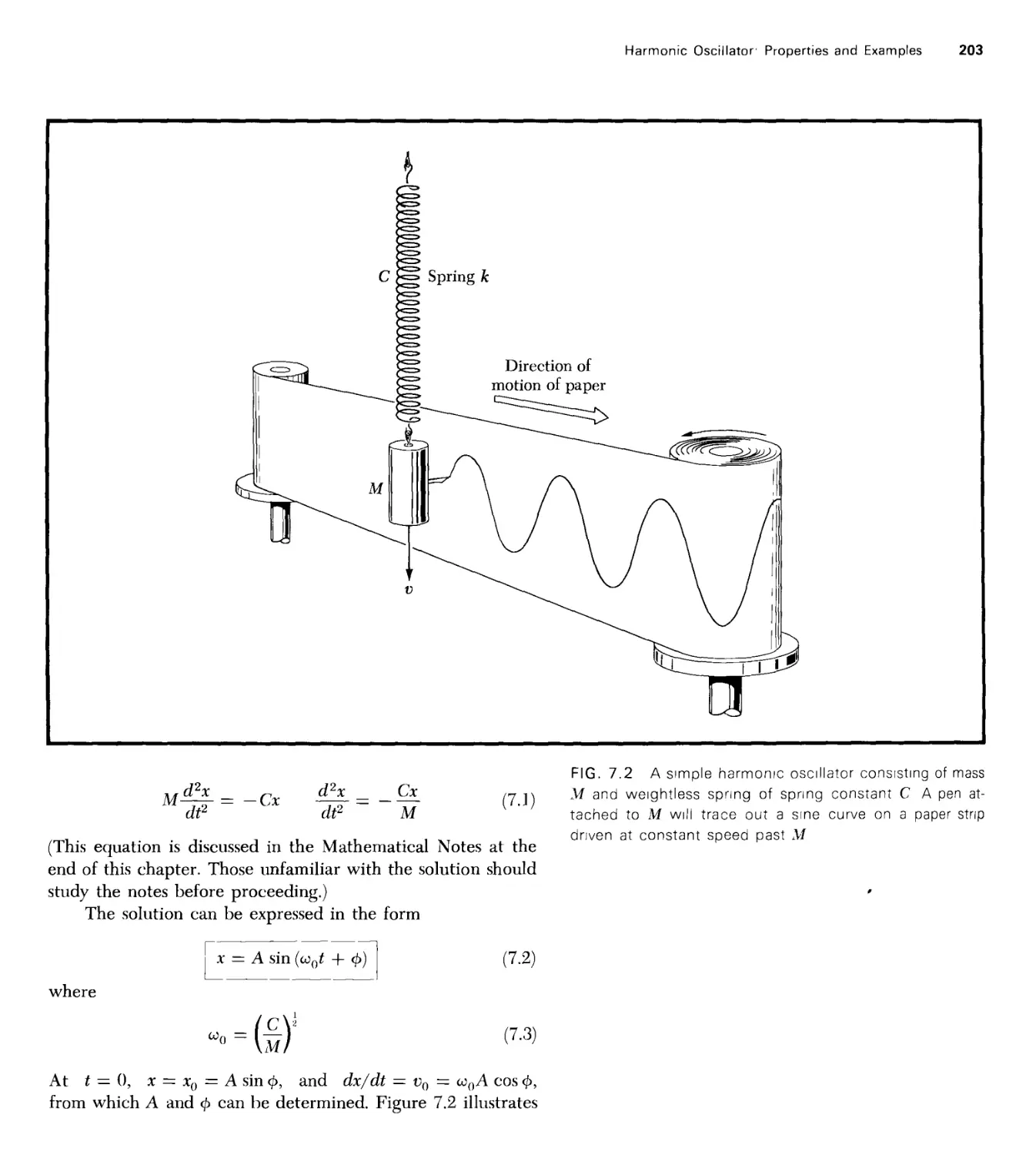
spring and the pendulum provide straightforward examples of this
important subject of oscillatory motion. In a shortened version, the sections on
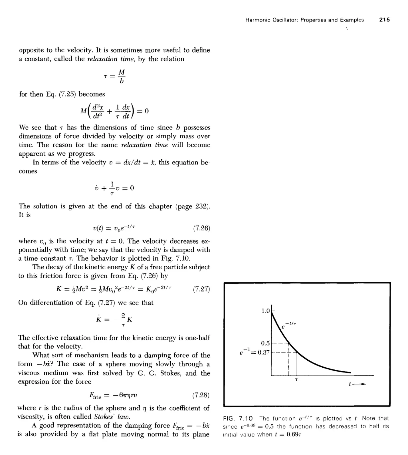
average values of kinetic and potential energy, damped motion, and forced
oscillations can be omitted completely. The laboratory can provide
excellent examples of this type of motion. The Advanced Topics on the Anhar-
monic Oscillator and the Driven Oscillator will be interesting to the more
advanced student.
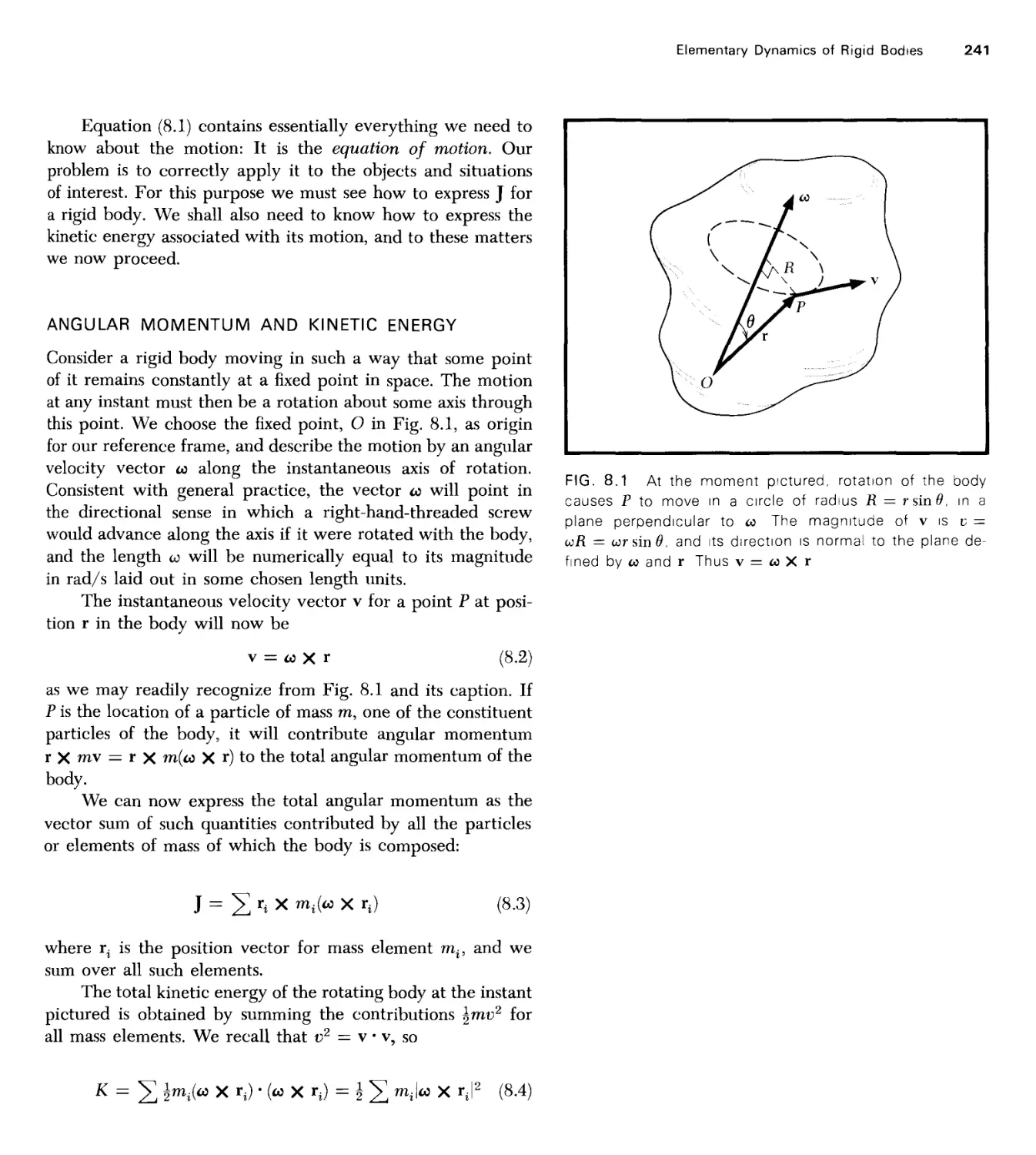
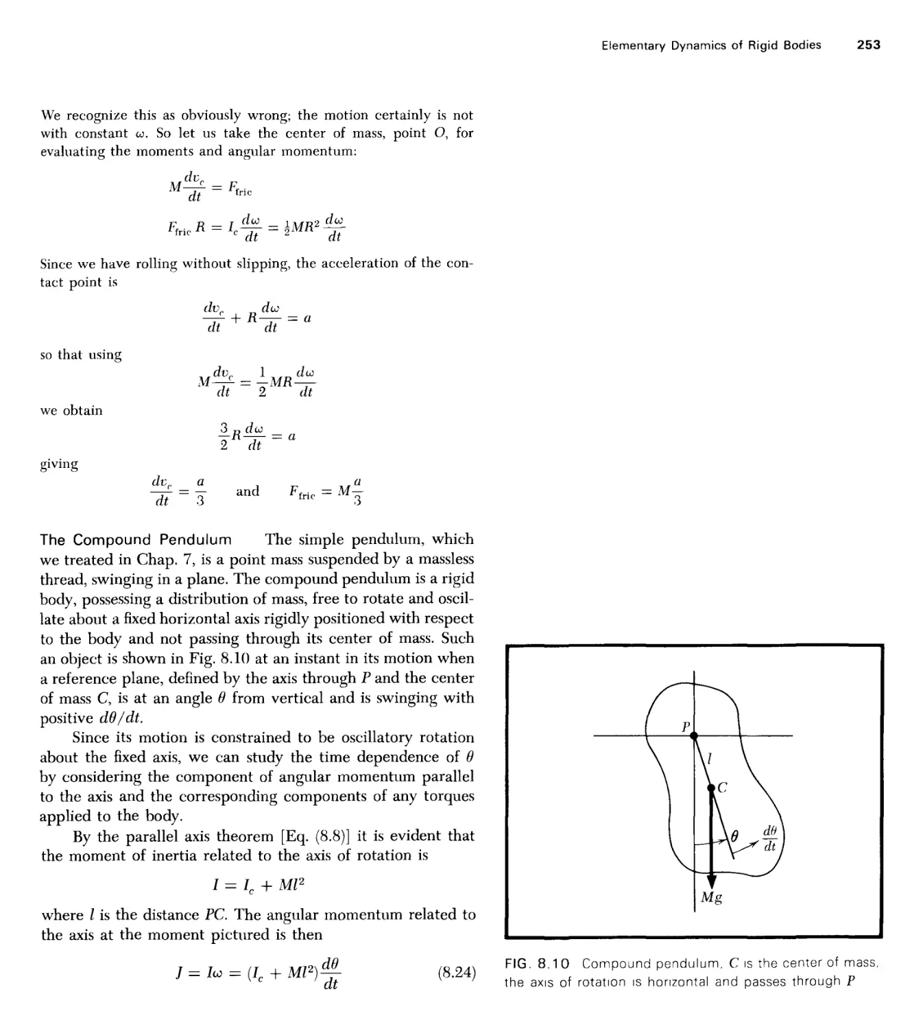
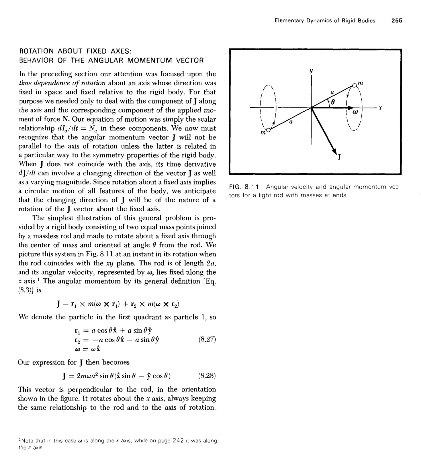
Chapter 8. The present authors believe that an introductory treatment of
rigid bodies is valuable to all students. The ideas of torque and angular
acceleration about a fixed axis are not difficult, and they provide the
student connections with the real, visible world. The simple treatment of
the gyro is also valuable; but the introduction of principal axes, products
of inertia, and rotating coordinate systems should probably be omitted in
most courses.
Chapter 9. Central-force problems are very important. Some instructors
may not wish to spend so much time on evaluating the potential inside
and outside spherical masses, and this of course can be omitted. They may
also find the labor of integrating the r equation of motion too much, in
which case they can omit it. They should enjoy the Advanced Topic. There
is a good deal that can be cut from this chapter if necessary, but the work
of mastering it is very rewarding. The two-body problem and the concept
of reduced mass are also useful but again can be omitted in a shortened
course.
Chapter 10. This chapter reviews a number of methods of determining
the speed of light. For a course in mechanics, this material is not essential.
We believe that students will be interested in it, but it could be assigned
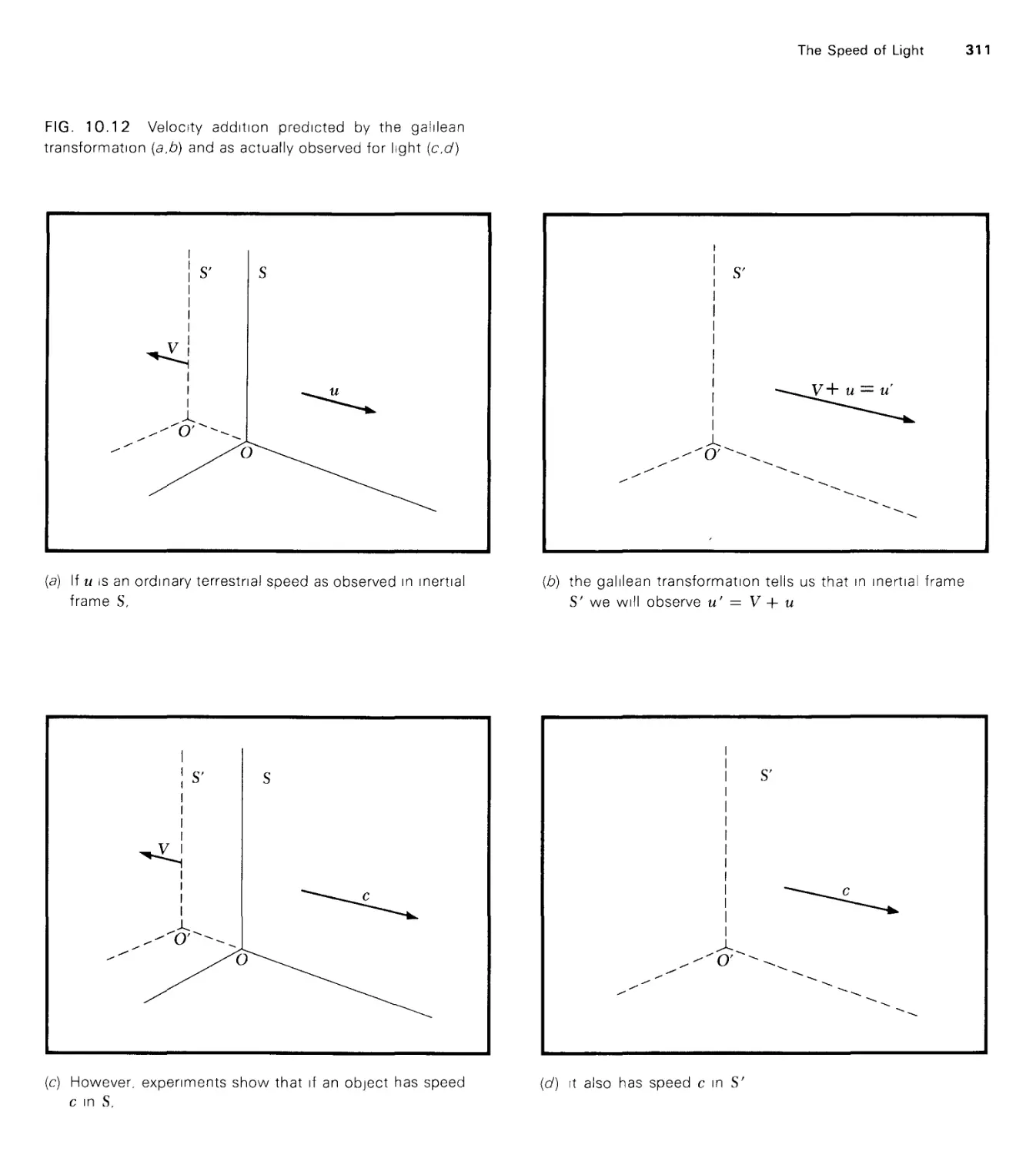
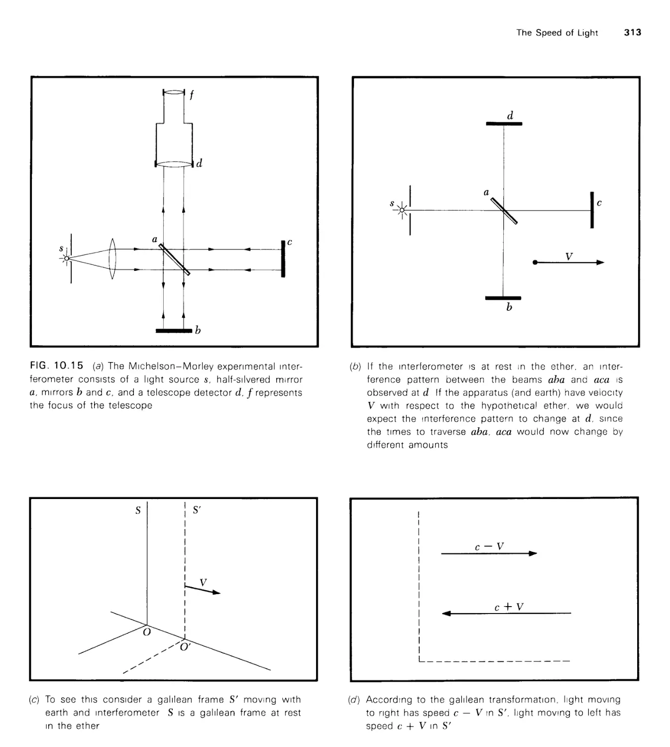
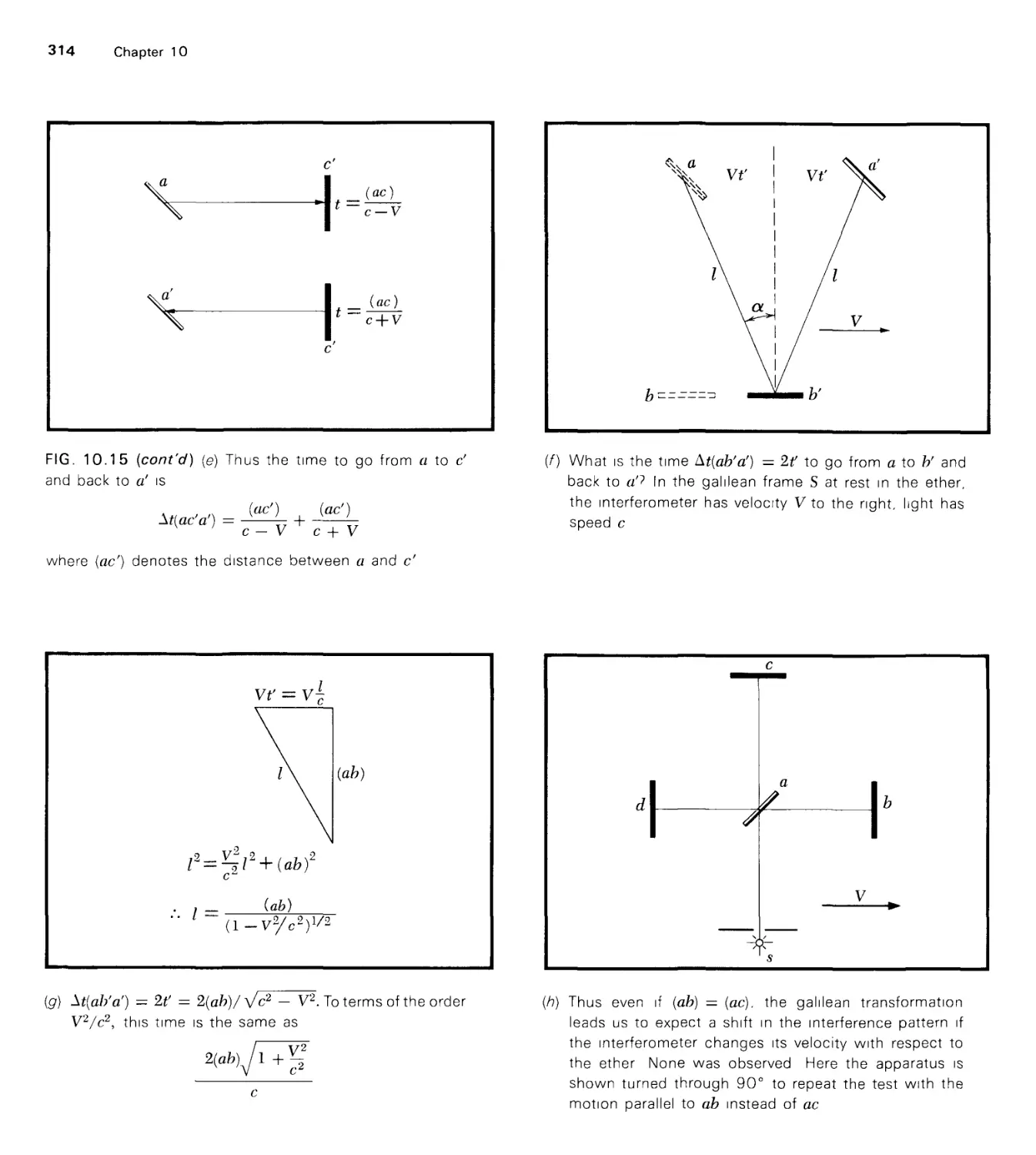
as outside reading. Then comes the Michelson-Morley experiment, which
in a course like this is the most convincing evidence of the need for a
change from the galilean transformation. The doppler effect is introduced
because of the evidence that the recessional doppler effect provides for
high speeds of distant stars, and the chapter closes with a section on the
speed of light as the ultimate speed for material objects and the failure
of the newtonian formula for kinetic energy. For those with limited time
for the study of special relativity, a cursory reading of the chapter might
be sufficient.
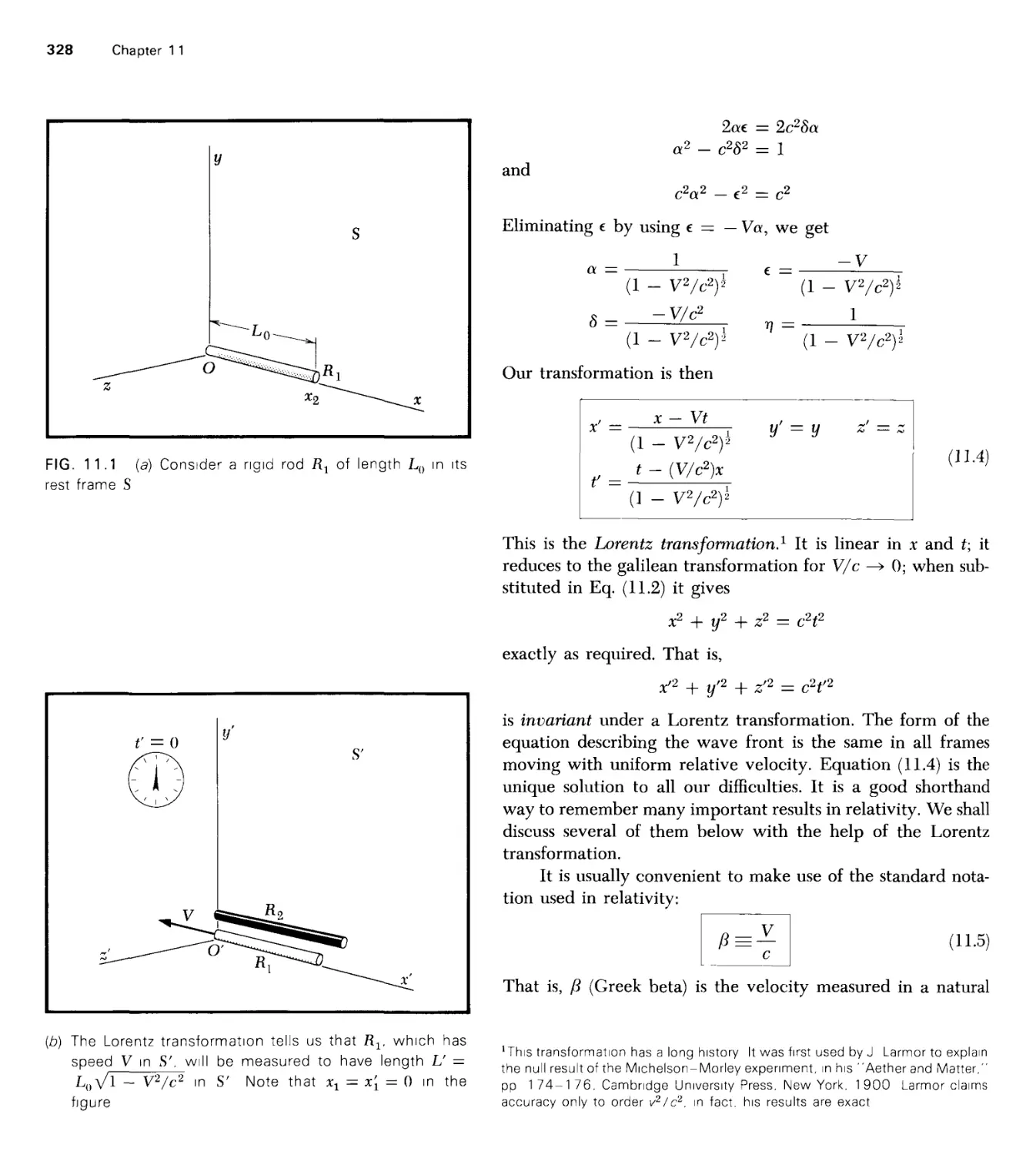
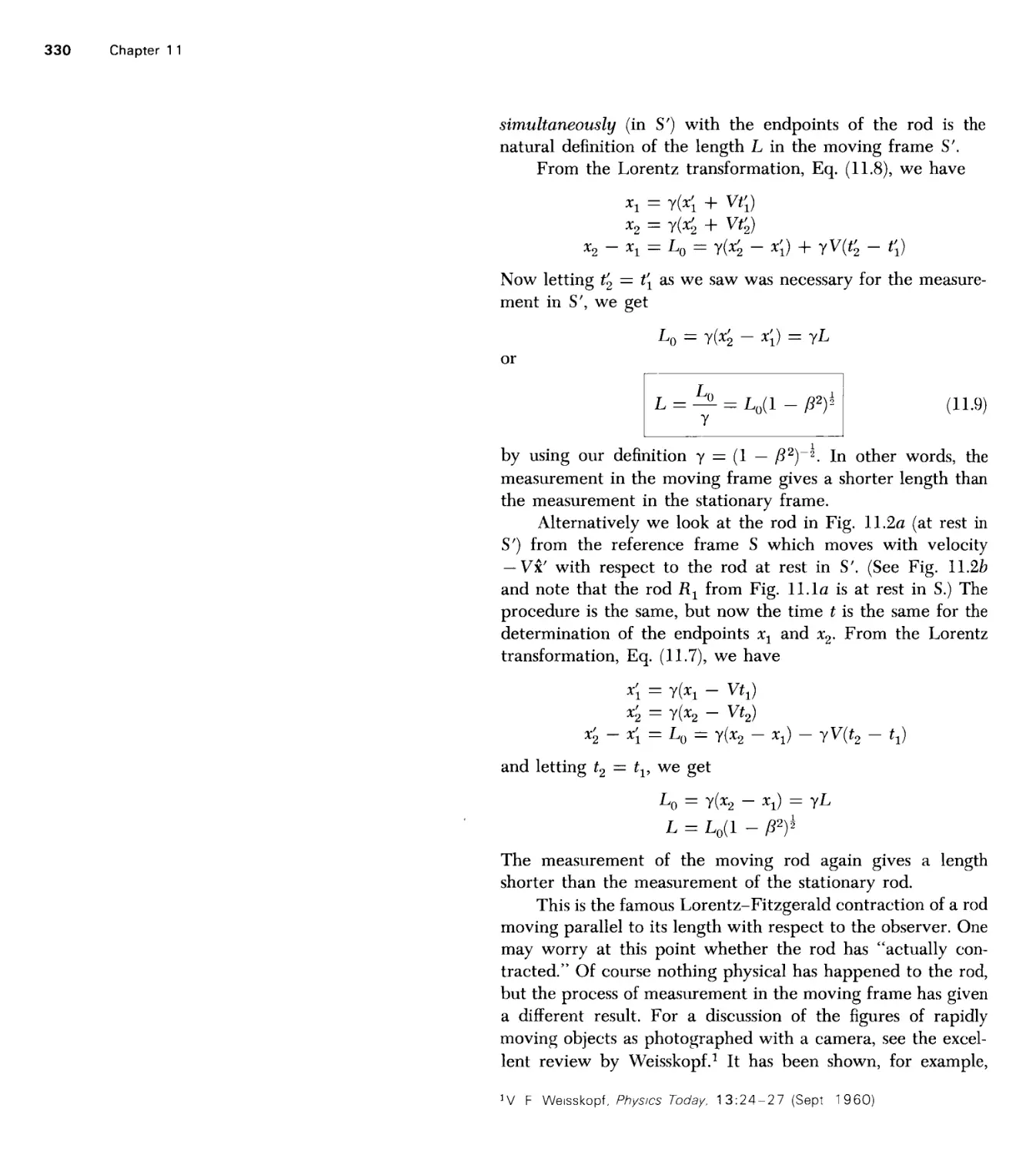
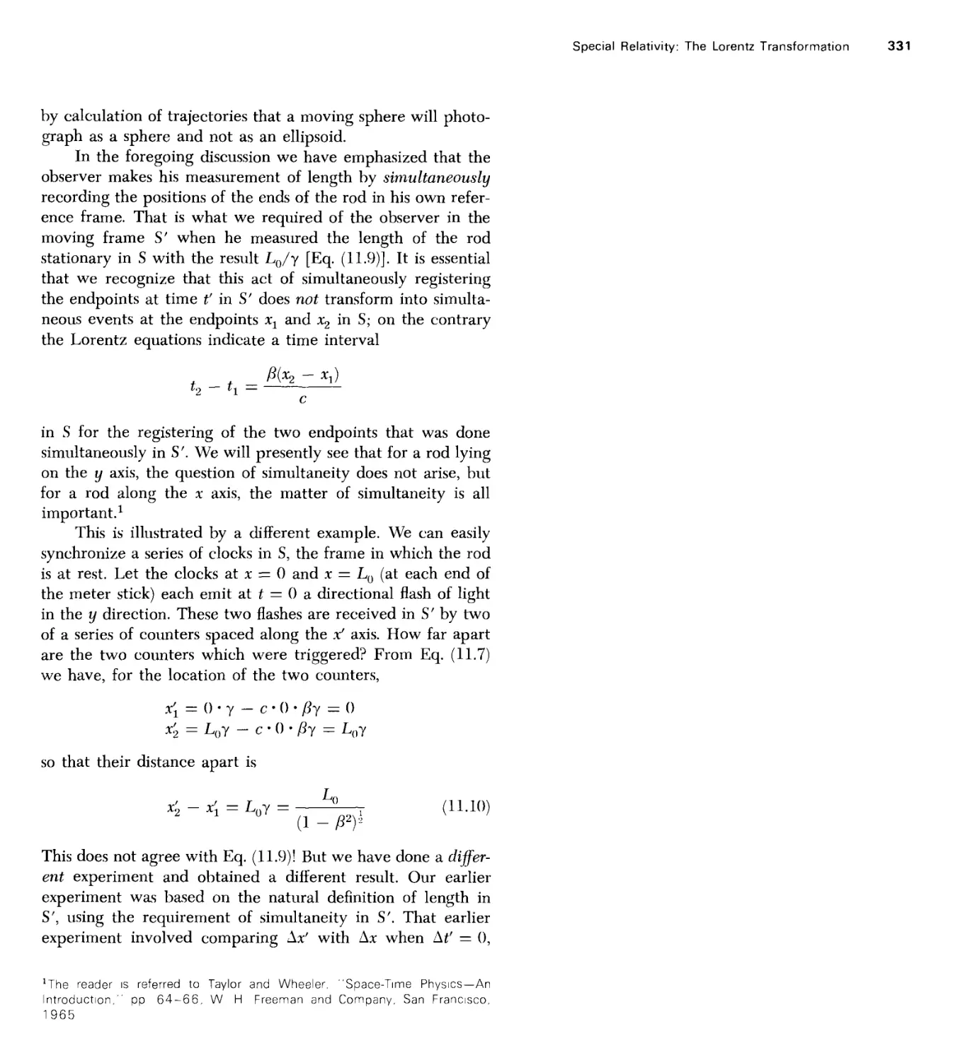
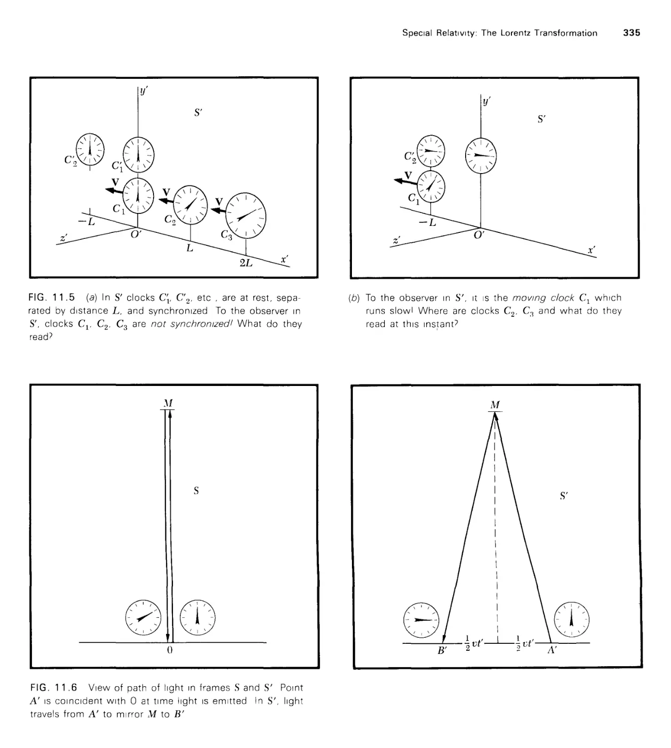
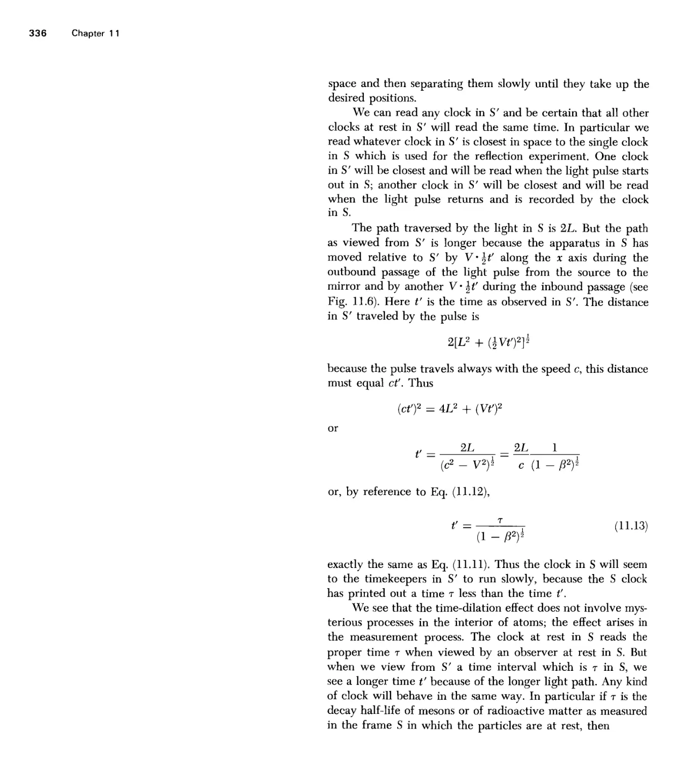
Chapter 11. In this chapter the Lorentz transformation equations are
derived and applied to the most common characteristics of special
relativity, length contraction, and time dilation. The velocity transformations
are introduced and some examples given. This chapter is the basis for the
following chapters, and consequently ample time should be allowed for
the study of it.
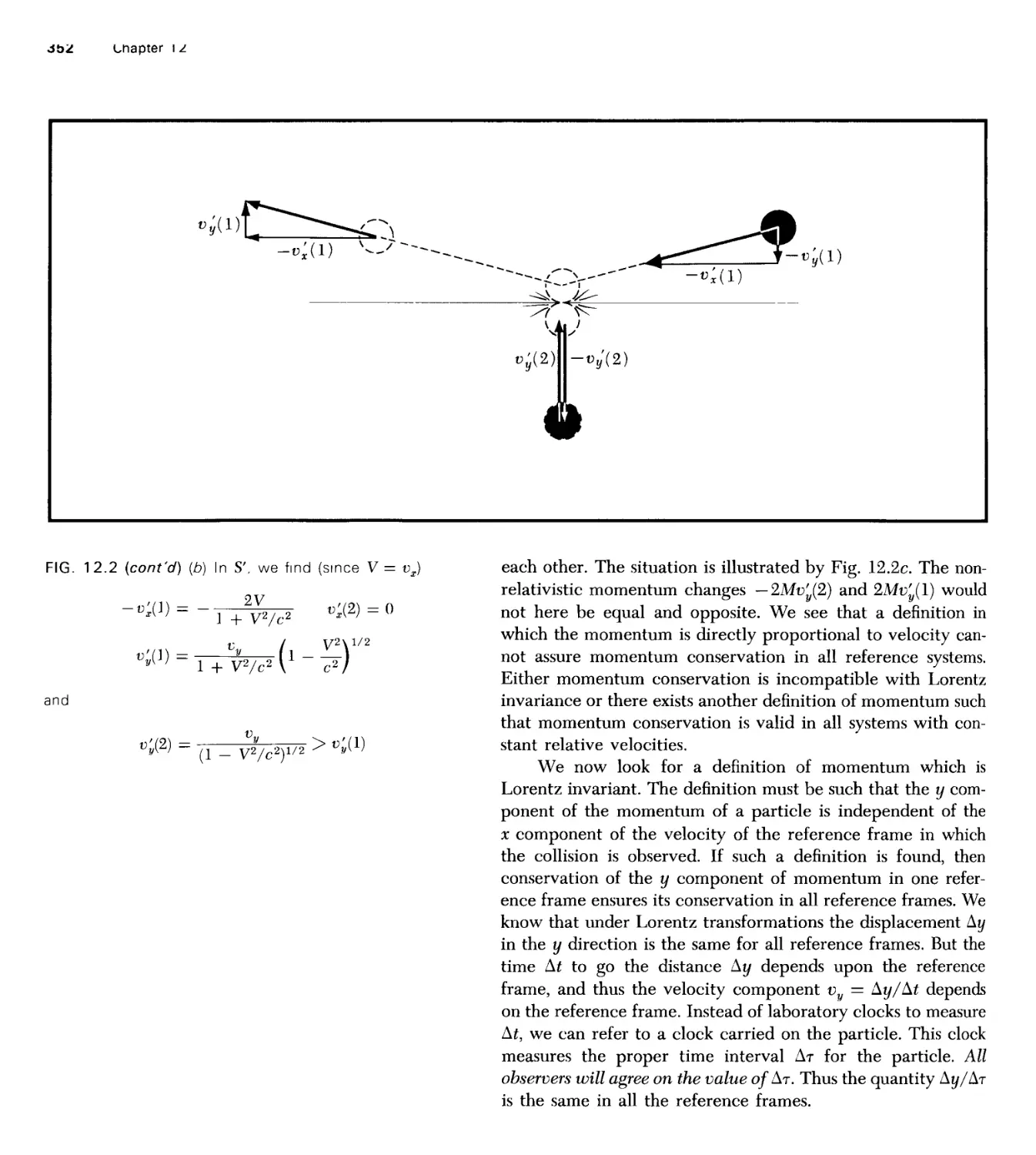
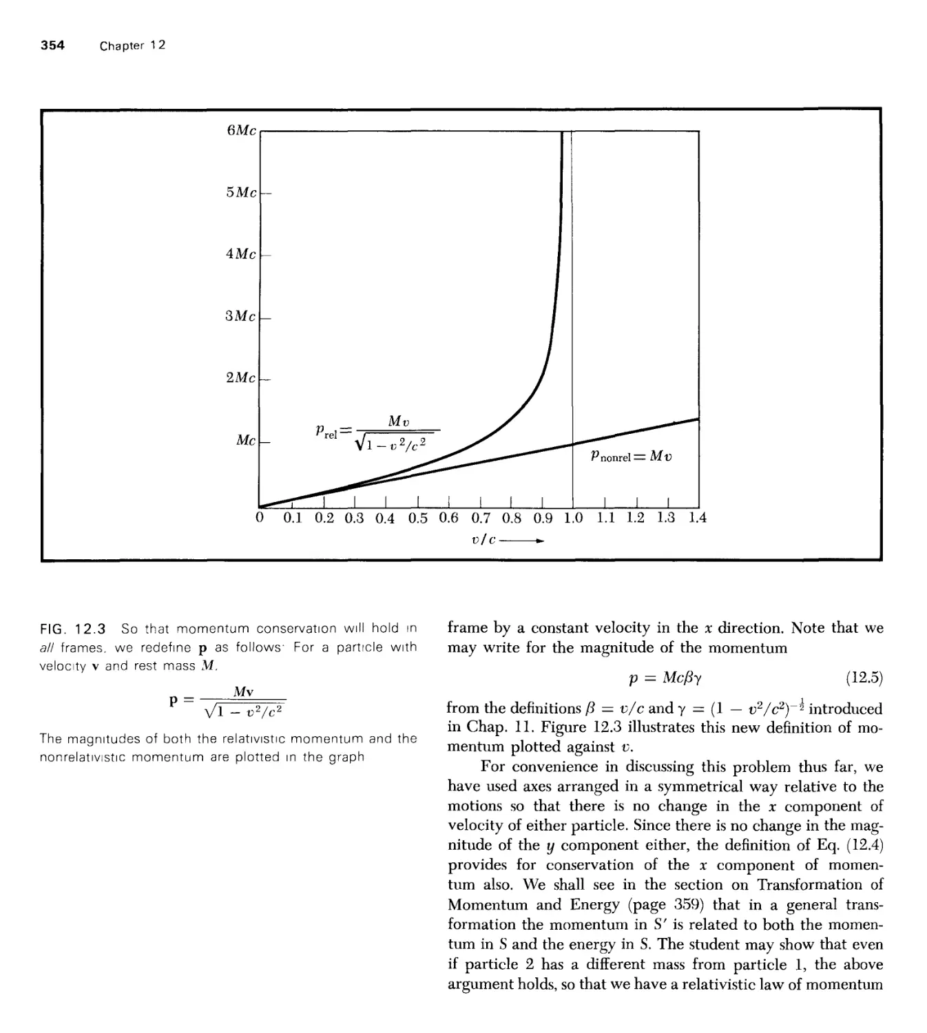
Chapter 12. The results of Chap. 11 are used to show the need for a change
in the definition of momentum, and of relativistic energy, and finally to
show the origin of E = mc2. The relation to experiments with high-energy
particles and to high-energy nuclear physics needs to be emphasized. At
this stage students may be only vaguely aware of, for example, nuclear
physics; but the examples are so pertinent to the public today that it should
be easy to teach. Finally the subject of particles with zero rest mass will
answer the questions of many alert students.
Chapter 13. A number of examples of the subjects developed in the
previous chapter are treated here. The center-of-mass system is brought in and
its advantages pointed out. In a shortened course all this can be omitted.
Good students will be interested in it, and it can be referred to as outside
reading in other physics courses treating special relativity.
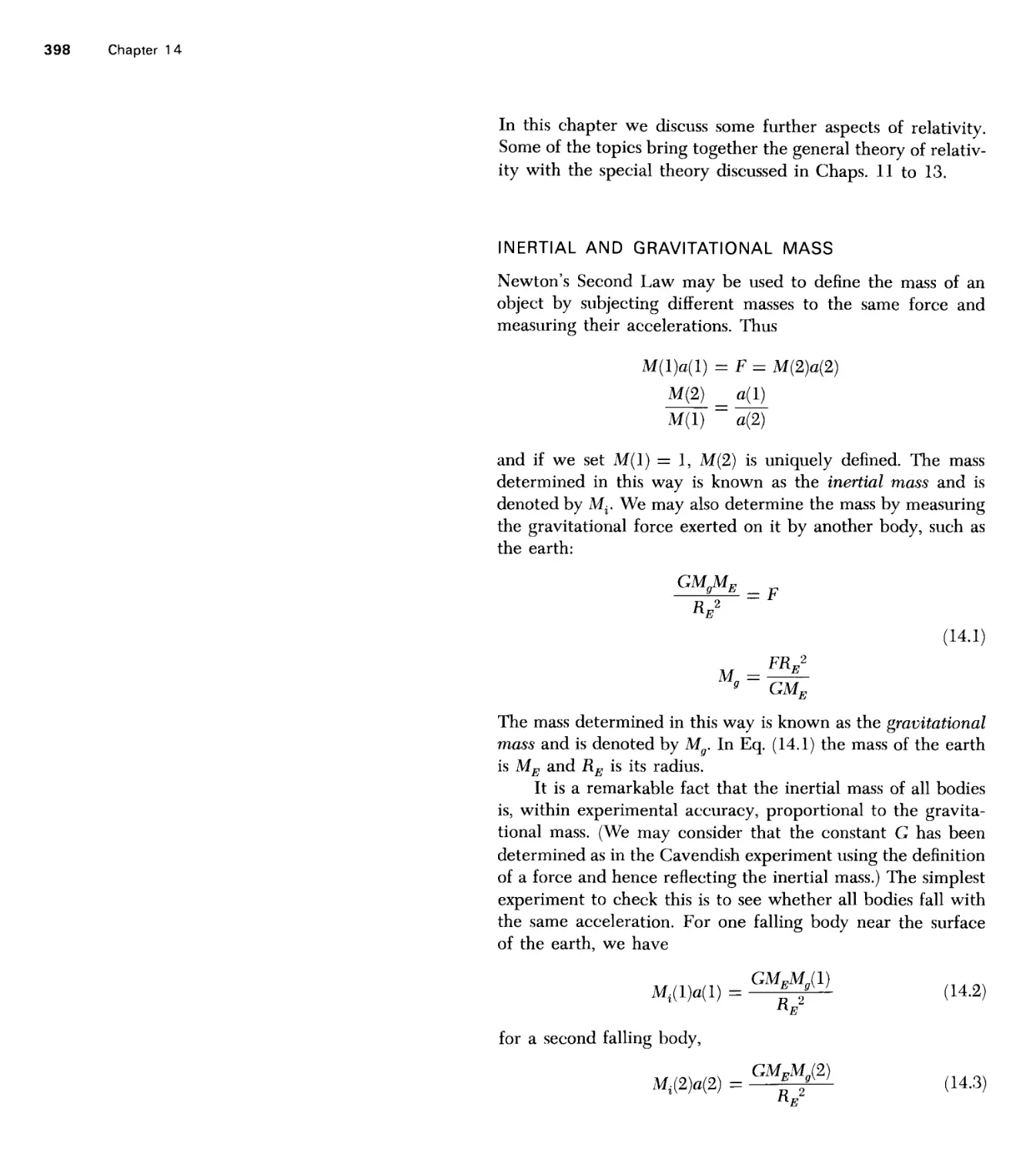
Chapter 14. In recent years the study of general relativity has become
quite popular, and this chapter could provide a bridge to reading in general
relativity. It is, of course, not central to the subject of special relativity
in the usual sense, but many students may be interested in the difference
between gravitational and inertial mass, and almost all will have heard
about the tests of general relativity.
The beginning year of college physics is usually the most difficult. In the
first year many more new ideas, concepts, and methods are developed than
in advanced undergraduate or graduate courses. A student who understands
clearly the basic physics developed in this first volume, even if he may
not yet be able to apply it easily to complex situations, has put behind
him many of the real difficulties in learning physics.
What should a student do who has difficulty in understanding parts
of the course and in working problems, even after reading and rereading
the text? First he should go back and reread the relevant parts of a high
school physics book. "Physics," the PSSC text, is particularly
recommended. "Harvard Project Physics" is also very good. Then he should
consult and study one of the many physics books at the introductory
college level. Many of these are noncalculus texts and so the difficulties
introduced by the mathematics will be minimized. The exercises,
particularly worked-out exercises, will probably be very helpful. Finally, when
he understands these more elementary books, he can go to some of the
other books at this level that are referred to in the Appendix. Of course,
he should remember that his instructors are the best source for answering
his questions and clearing up his misunderstandings.
Many students have difficulty with mathematics. In addition to your
regular calculus book, many paperbacks may be helpful. An excellent
review of the elements of calculus is available as a short manual of self-
instruction: "Quick Calculus," by Daniel Kleppner and Norman Ramsey
(John Wiley & Sons, Inc., New York, 1965).
Note to the Student
Units
Every mature field of science and engineering has its own special units
for quantities which occur frequently. The acre-foot is a natural unit of
volume to an irrigation engineer, a rancher, or an attorney in the western
United States. The MeV or million electron volts is a natural unit of energy
to a nuclear physicist; the kilocalorie is the chemist's unit of energy, and
the kilowatt-hour is the power engineer's unit of energy. The theoretical
physicist will often simply say: Choose units such that the speed of light
is equal to unity. A working scientist does not spend much of his time
converting from one system of units to another; he spends more time in
keeping track of factors of 2 and of plus or minus signs in his calculations.
Nor will he spend much time arguing about units, because no good science
has ever come out of such an argument.
Physics is carried out and published chiefly in the gaussian cgs and
the SI or mks units. Every scientist and engineer who wishes to have easy
access to the literature of physics will need to be familiar with these systems.
The text is written in the gaussian cgs system; but a number of
references are made to the SI units (Systeme Internationale), which until recently
were more commonly called mks or mksa units. The transformation from
cgs to SI units in mechanical problems is easy, as will be explained in the
text. However, when one comes to problems in electricity and magnetism
there is difficulty. In the text, explanation is given of both systems, and
some examples are worked in both systems. It is not clear whether the
change to the SI units that began more than twenty years ago will continue.
In the current physics literature there still seem to be more papers in the
cgs system, which is the reason for retaining it in this volume. In a course
such as this, we want to make it as easy as possible for both sceintists and
engineers to read the journals, particularly physics journals.
Notation
Physical Constants
Approximate values of physical constants and useful numerical
quantities are printed inside the front and back covers of this volume. More
precise values of physical constants are tabulated in E. K. Cohen and
J. W. M. DuMond, Rev. Mod. Phys., 37:537 (1965) and B. N. Taylor,
W. H. Parker, and D. N. Langenberg, Rev. Mod. Phys., 41:375 (1969).
Signs and Symbols
In general we have tried to adhere to the symbols and unit
abbreviations that are used in the physics literature—that are, for the most part,
agreed upon by international convention.
We summarize here several signs which are used freely throughout
the book.
= is equal to zz is approximately equal to;
is roughly equal to
= is identical with ~~ is of the order of magnitude of
oc is proportional to
Usage of the signs ~, =, and — is not standardized, but the definitions
we have given are employed fairly widely by physicists. The American
Institute of Physics encourages use of the sign ~ where others might write
either ~ or ^. (Style Manual, American Institute of Physics, rev. ed.,
November 1970)
n n
The sign ^or^ denotes summation over what stands to the right
i=i J
of 2 over all entries between / = 1 and j = N. The notation ^ denotes
double summation over the two indices i and /. The notation ^ or X
denotes summation over all values of i and / except i — /'.
Order of Magnitude
By this phrase we usually mean "within a factor of 10 or so." Free
and bold estimation of the order of magnitude of a quantity characterizes
the physicist's work and his mode of speech. It is an exceptionally valuable
professional habit, although it often troubles beginning students enormously.
We say, for example, that 104 is the order of magnitude of the numbers
5500 and 25,000. In cgs units the order of magnitude of the mass of the
electron is 10"27 g; the accurate value is (0.910954 ± 0.000005) X 10^27 g.
We say sometimes that a solution includes (is accurate to) terms of
order x2 or E, whatever the quantity may be. This is also written as 0(x2)
or O(E). The language implies that terms in the exact solution which involve
higher powers (such as x3 or E2) of the quantity may be neglected for
certain purposes in comparison with the terms retained in the approximate
solution.
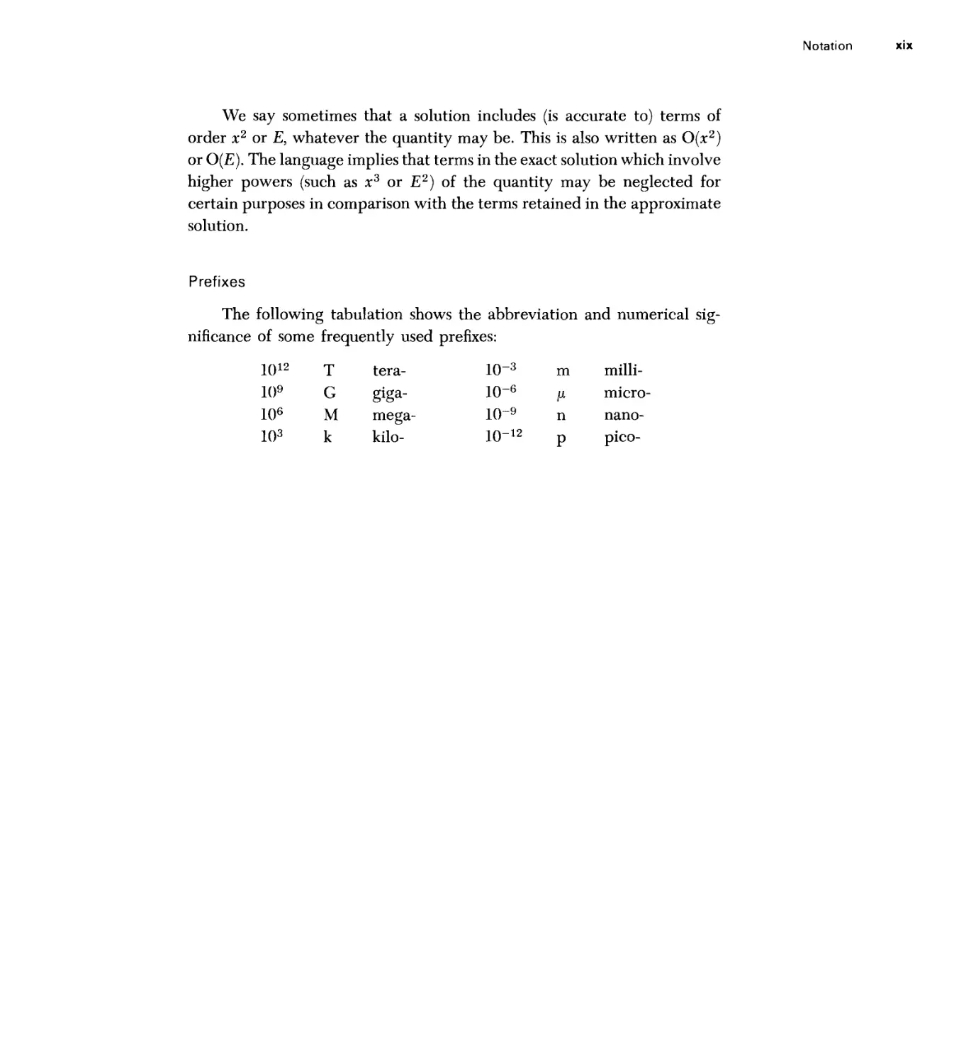
Prefixes
The following tabulation shows the abbreviation and numerical
significance of some frequently used prefixes:
1012 T tera- 10"3
1()9 G giga- 10"6
106 M mega- 10~9
103 k kilo- 10"12
m milli-
(i micro-
n nano-
p pico-
GREEK ALPHABET
a
P
y
3
€
£
V
e
m
K
X
M
V
i
m
IT
P
a
T
■
<j>cp
X
*
CO
alpha
beta
gamma
delta
epsilon
zeta
eta
theta
iota
kappa
lambda
mu
nu
xi
omicron
P1
rho
sigma
tau
upsilon
phi
chi
psi
omega
Characters not often used as symbols are shaded; for the most part they
are too close in form to roman characters to be of value as independent
symbols.
r
A
e
A
n
■
2
o
*
a
Mechanics
CONTENTS
THE NATURAL WORLD
THE ROLE OF THEORY
GEOMETRY AND PHYSICS
Estimates of the Curvature of Space
Geometry on a Smaller Scale
INVARIANCE
Invariance under Translation
Invariance under Rotation
Problems
Further Reading
Introduction
4 Chapter 1
THE NATURAL WORLD
To every man the natural world seems immense and complex,
the stage for a startling diversity of appearances and events.
These impressions are supported by estimates of the general
order of magnitude of the values of interesting quantities
concerning the natural world. At this stage we shall not enter into
the arguments and measurements that lead to the figures given.
The most remarkable thing about these numbers is that we
know them at all; it is not of pressing importance that some
of them are known only approximately.
The universe is immense. From astronomical observations
we infer the value 1028 centimeters (cm) or 1010 light years (yr)
for a characteristic dimension loosely called the radius of the
universe. The value is uncertain by perhaps a factor of 3. For
comparison, the distance of the earth from the sun is 1.5 X 10¹³
cm and the radius of the earth is 6.4 X 108 cm.
The number of atoms in the universe is very large. The
total number of protons and neutrons in the universe, with an
uncertainty perhaps of a factor of 100, is believed to be of
the order of 1080. Those in the sun number 1 X 1057, a*nd those
in the earth 4 X 1051. The total in the universe would provide
about 1080/1()57 (or 1023) stars equal in mass to our sun. [For
comparison, the number of atoms in an atomic weight
(Avogadro's number) is 6 X 10²³.] Most of the mass of the
universe is believed to lie in stars, and all known stars have
masses between 0.01 and 100 times that of our sun.
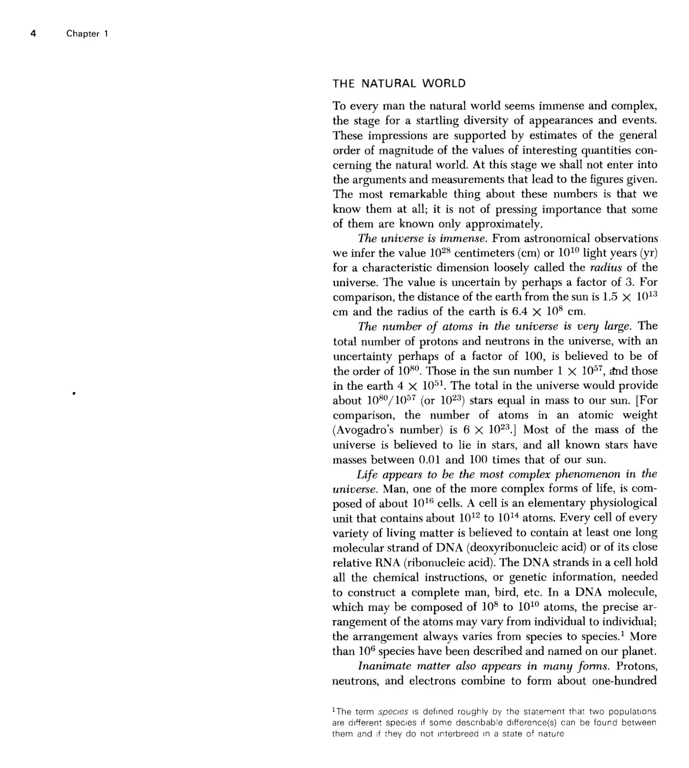
Life appears to be the most complex phenomenon in the
universe. Man, one of the more complex forms of life, is
composed of about 1016 cells. A cell is an elementary physiological
unit that contains about 1012 to 1014 atoms. Every cell of every
variety of living matter is believed to contain at least one long
molecular strand of DNA (deoxyribonucleic acid) or of its close
relative RNA (ribonucleic acid). The DNA strands in a cell hold
all the chemical instructions, or genetic information, needed
to construct a complete man, bird, etc. In a DNA molecule,
which may be composed of 108 to 1010 atoms, the precise
arrangement of the atoms may vary from individual to individual;
the arrangement always varies from species to species.1 More
than 106 species have been described and named on our planet.
Inanimate matter also appears in many forms. Protons,
neutrons, and electrons combine to form about one-hundred
1The term species is defined roughly by the statement that two populations
are different species if some descnbabte difference(s) can be found between
them and if they do not interbreed in a state of nature
different chemical elements and about 103 identified isotopes.
The individual elements have been combined in various
proportions to form perhaps 106 or more identified, differentiated
chemical compounds, and to this number may be added a vast
number of liquid and solid solutions and alloys of various
compositions having distinctive physical properties.
Through experimental science we have been able to learn
all these facts about the natural world, to classify the stars and
to estimate their masses, compositions, distances, and velocities;
to classify living species and to unravel their genetic relations;
to synthesize inorganic crystals, biochemicals, and new
chemical elements; to measure the spectral emission lines of atoms
and molecules over a frequency range from 100 to 1020 cycles
per second (cps);1 and to create new fundamental particles in
the laboratory.
These great accomplishments of experimental science
were achieved by men of many types: patient, persistent,
intuitive, inventive, energetic, lazy, lucky, narrow, and with skilled
hands. Some preferred to use only simple apparatus; others
invented or built instruments of great refinement, size, or
complexity. Most of these men had in common only a few things:
They were honest and actually made the observations they
recorded, and they published the results of their work in a form
permitting others to duplicate the experiment or observation.
THE ROLE OF THEORY
The description we have given of the natural universe as
immense and complex is not the whole story, for theoretical
understanding makes several parts of the world picture look
much simpler. We have gained a remarkable understanding of
some central and important aspects of the universe. The areas
that we believe we understand (summarized below), together
with the theories of relativity and of statistical mechanics, are
among the great intellectual achievements of mankind.
1 The laws of classical mechanics and gravitation (Volume
1), which allow us to predict with remarkable accuracy the
motions of the several parts of the solar system (including
comets and asteroids), have led to the prediction and
discovery of new planets. These laws suggest possible
mechanisms for the formation of stars and galaxies, and, together
1Jhe approved unit for cycles per second has become Hertz (Hz), and so this
phrase could have been written "from 100 to 1 020 Hz "
Introduction 5
Chapter 1
T
(A) Adenine
T
(T) Thymine
(G) Guanine
T
(C) Cytosine
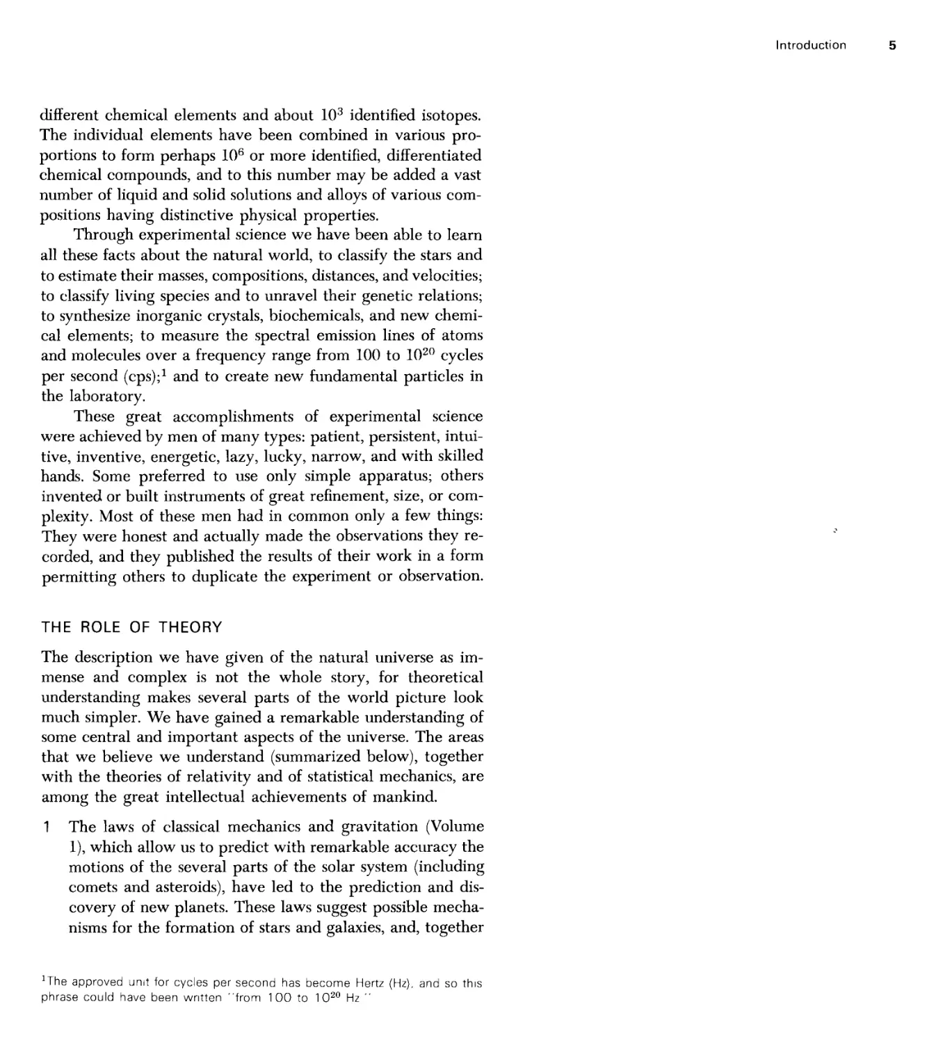
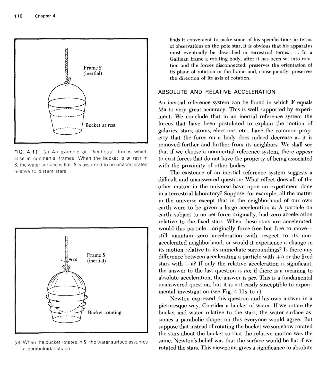
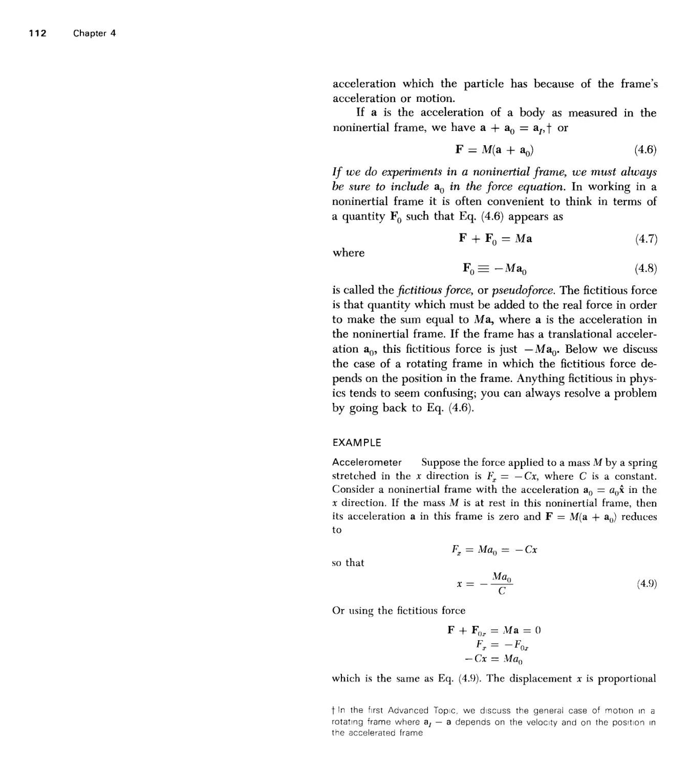
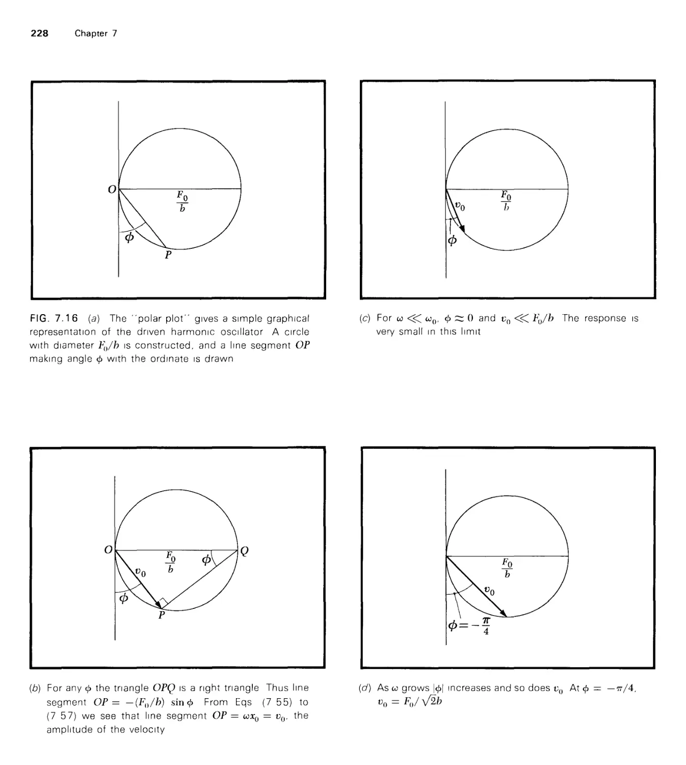
FIG. 1.1 (a) Schematic representation of the four
nucleotide bases from which the DNA molecule is derived
SPSPSPSPSPSPSPS
vu f\ A. >k r\ v vl/ A
ATCGTGAC
(b) The nucleotides are connected to sugar groups S which,
in turn, are bound to phosphate groups P to form a
chain
(c) The complete DNA molecule is composed of a double
chain in the form of a helix The two strands are
connected by hydrogen bonds between adenine and
thymine groups or between guanine and cytosine groups
with the laws of radiation, they give a good account of
the observed connection between the mass and luminosity
of stars. The astronomical applications of the laws of
classical mechanics are the most beautiful but not the only
successful applications. We use the laws constantly in
everyday life and in the engineering sciences. Our
contemporary ventures into space and the use of satellites are
based upon refined applications of the laws of classical
mechanics and gravitation.
2 The laws of quantum mechanics (Volume 4) give a very
good account of atomic phenomena. For simple atoms
predictions have been made that agree with experiment to
1 part in 105 or better. When applied to large-scale
terrestrial and celestial events, the laws of quantum mechanics
result in predictions indistinguishable from the laws of
classical mechanics. Quantum mechanics provides, in principle,
a precise theoretical basis for all of chemistry and
metallurgy and for much of physics, but often we cannot handle
the equations on existing or foreseeable computers. In some
fields nearly all the problems seem too difficult for a direct
theoretical attack based on first principles.
3 The laws of classical electrodynamics, which give an
excellent account of all electric and magnetic effects, except
on the atomic scale, are the basis of the electrical
engineering and communications industries. Electric and magnetic
effects on the atomic scale are described exactly by the
theory of quantum electrodynamics. Classical
electrodynamics is the subject of Volumes 2 and 3; some aspects
of quantum electrodynamics are touched on in Volume 4,
but a complete discussion of the field must be deferred until
a later course.
4 At another, narrower level, the principle of operation of
the genetic code is understood—in particular, the
mechanism of storage of genetic information. We find that the
information storage of the cell of a simple organism exceeds
that of the best present-day commercial computers. In
nearly all life on our planet the complete coding of genetic
information is carried in the DNA molecule by a double
linear sequence (possessing 106 to 109 entries, depending
on the organism) of only four different molecular groups,
with specific but simple rules governing the pairing of
members opposite each other in the double sequence (see
Fig. 1.1). These matters are a part of the subject of
molecular biology.
The physical laws and theoretical understanding
mentioned in the above summaries are different in character from
the direct results of experimental observations. The laws, which
summarize the essential parts of a large number of observations,
allow us to make successfully certain types of predictions,
limited in practice by the complexity of the system. Often the
laws suggest new and unusual types of experiments. Although
the laws can usually be stated in compact form,1 their
application may sometimes require lengthy mathematical analysis
and computation.
There is another aspect of the fundamental laws of physics:
Those laws of physics that we have come to understand have
an attractive simplicity and beauty.2 This does not mean that
everyone should stop doing experiments, for the laws of physics
have generally been discovered only after painstaking and
ingenious experiments. The statement does mean that we shall
be greatly surprised if future statements of physical theory
contain ugly and clumsy elements. The aesthetic quality of the
discovered laws of physics colors our expectations about the
laws still unknown. We tend to call a hypothesis attractive
when its simplicity and elegance single it out among the large
number of conceivable theories.
In this course we shall make an effort to state some of
the laws of physics from viewpoints that emphasize the features
of simplicity and elegance. This requires that we make
considerable use of mathematical formulations, although at the
present level of study this use normally will not exceed the bounds
of introductory calculus. As we go along, we shall try also to
give some of the flavor of good experimental physics, although
this is very hard to do in a textbook. The research laboratory
is the natural training ground in experimental physics.
GEOMETRY AND PHYSICS
Mathematics, which permits the attractive simplicity and
compactness of expression necessary for a reasonable discussion of
1The first sentence of a short paperback is "These lectures will cover all of
physics " R Feynman, "Theory of Fundamental Processes." W A Benjamin,
Inc . New York, 1961
2"lt seems that if one is working from the point of view of getting beauty
in one's equations, and if one has really a sound insight, one is on a sure
line of progress P A M Dirac, Scientific American, 208 (5) 45-53
(1963) But most physicists feel the real world is too subtle for such bold
attacks except by the greatest minds of the time, such as Einstein or Dirac
or a dozen others In the hands of a thousand others this approach has been
limited by the inadequate distribution among men of "a sound insight
Introduction 7
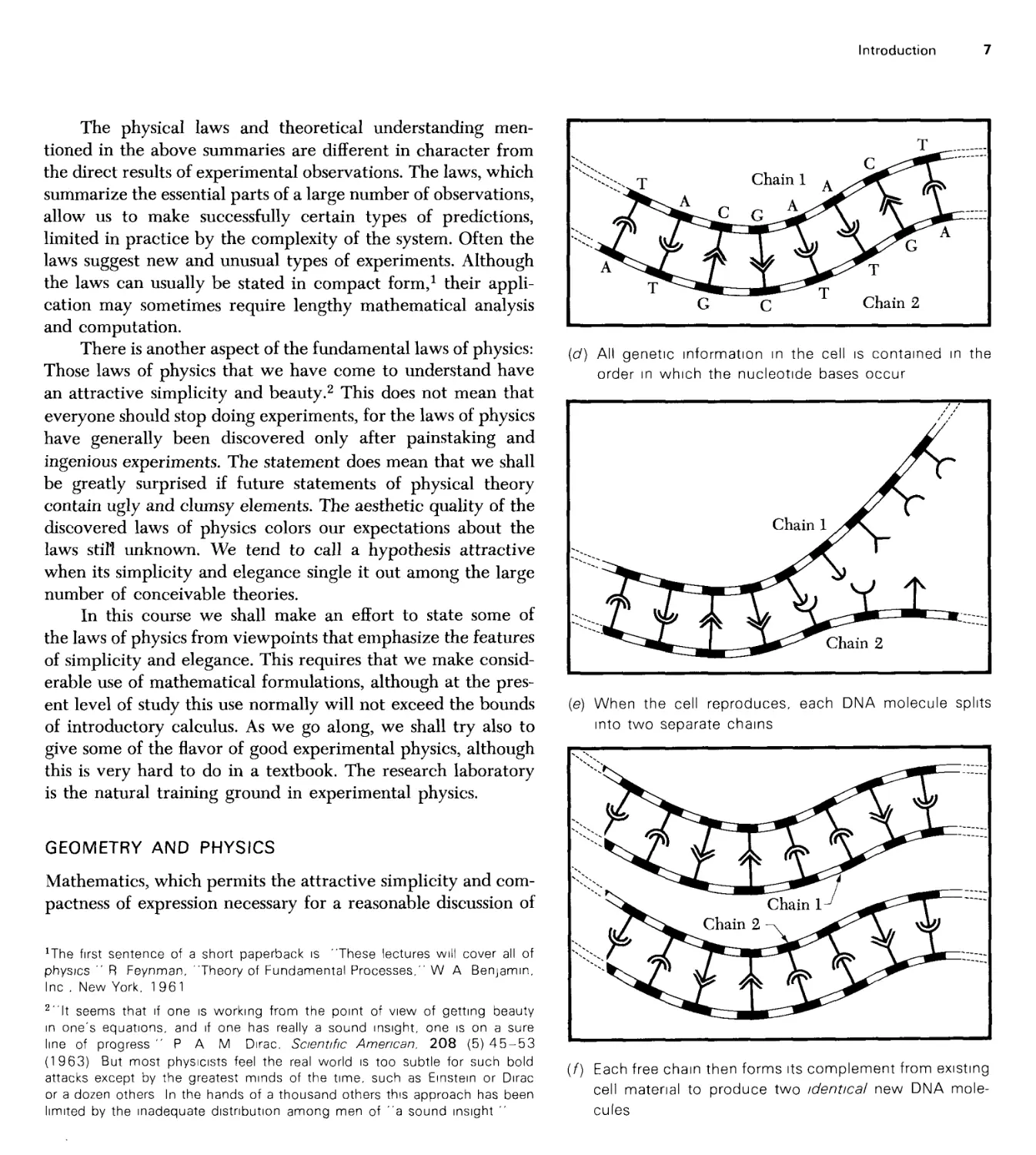
(d) All genetic information in the cell is contained in the
order in which the nucleotide bases occur
(e) When the cell reproduces, each DNA molecule splits
into two separate chains
(f) Each free chain then forms its complement from existing
cell material to produce two identical new DNA
molecules
Chapter 1
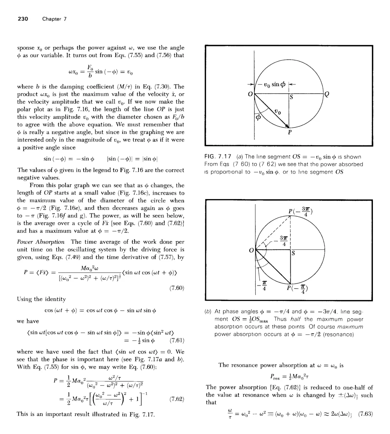
a2+b2 = c2
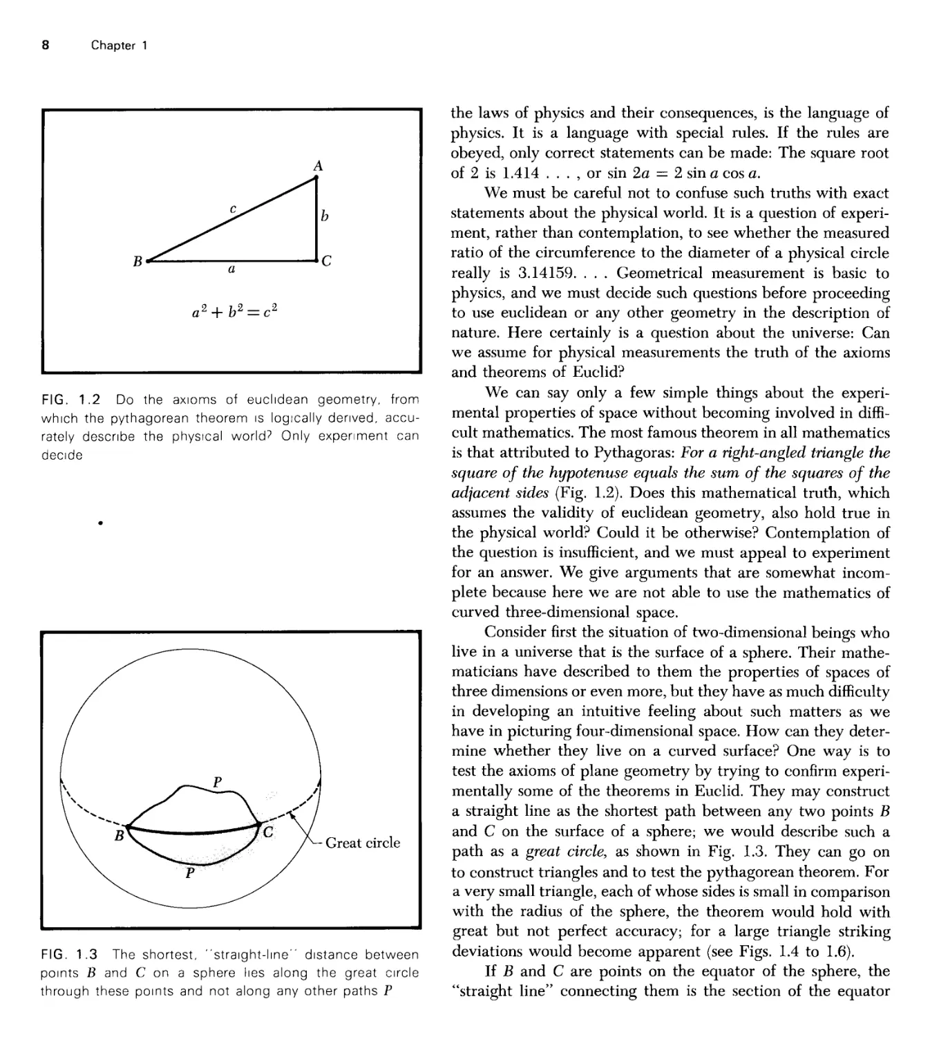
FIG. 1.2 Do the axioms of euchdean geometry, frorr
which the pythagorean theorem is logically derived, accu
rately describe the physical world? Only experiment car
decide
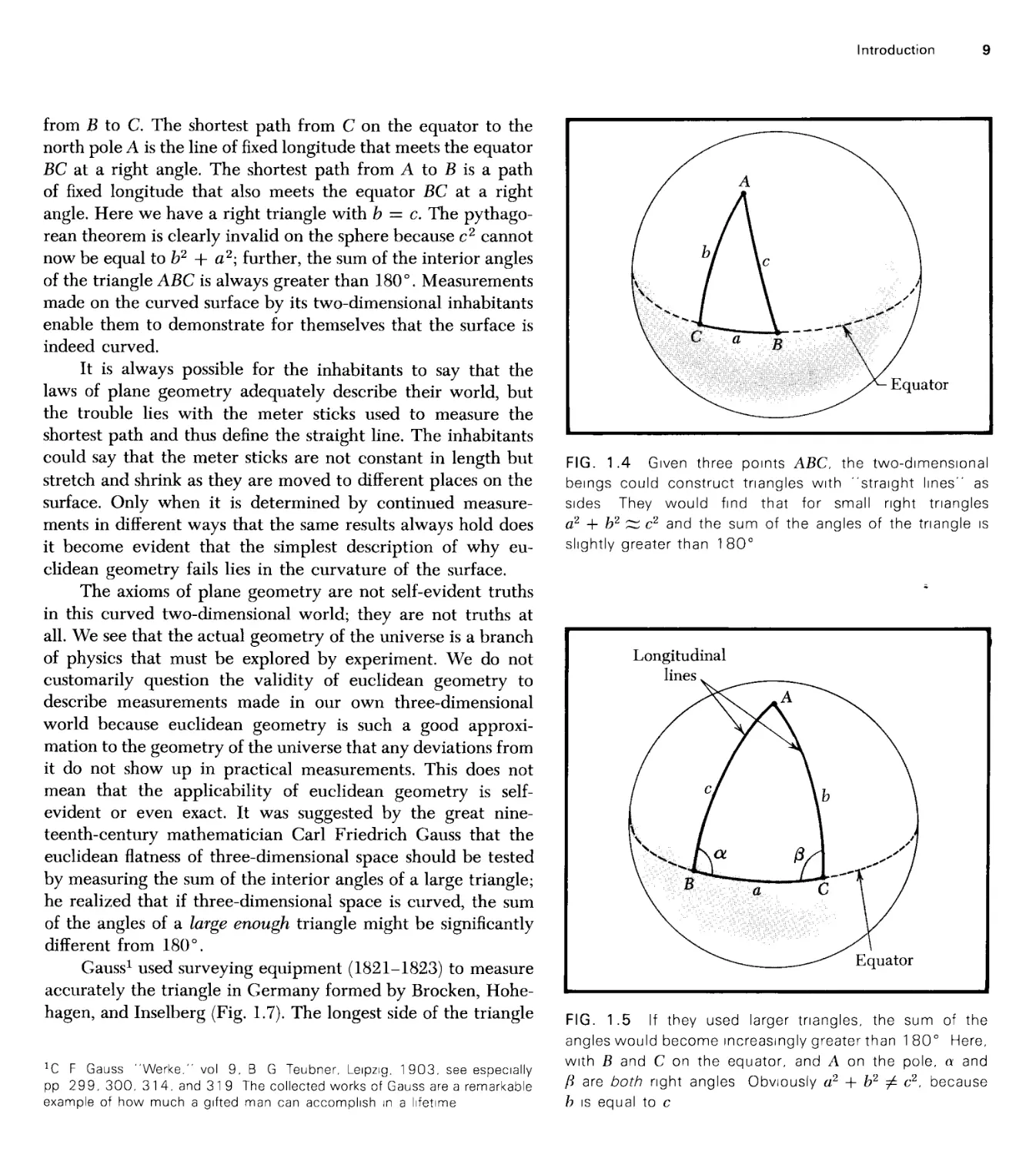
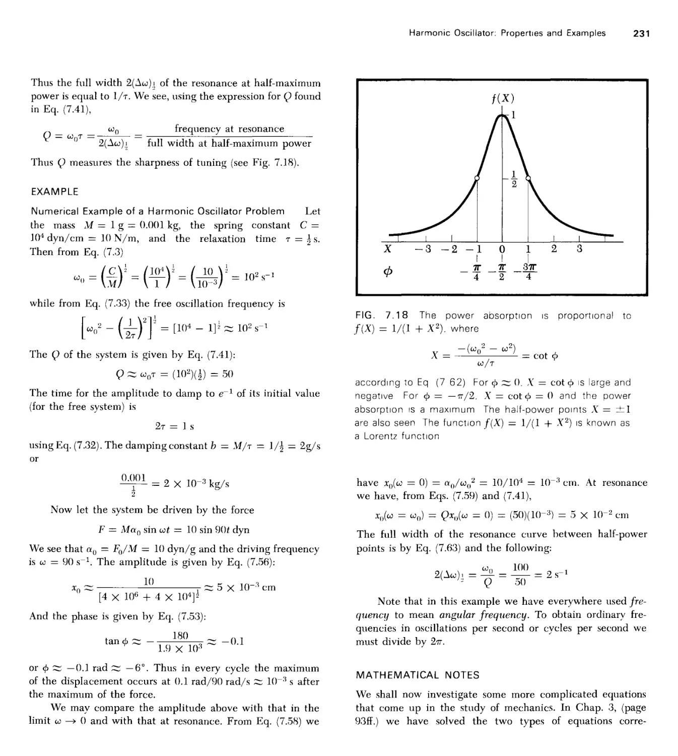
Great circle
FIG. 1.3 The shortest, "straight-line" distance between
points B and C on a sphere lies along the great circle
through these points and not along any other paths P
the laws of physics and their consequences, is the language of
physics. It is a language with special rules. If the rules are
obeyed, only correct statements can be made: The square root
of 2 is 1.414 . . . , or sin 2a = 2 sin a cos a.
We must be careful not to confuse such truths with exact
statements about the physical world. It is a question of
experiment, rather than contemplation, to see whether the measured
ratio of the circumference to the diameter of a physical circle
really is 3.14159. . . . Geometrical measurement is basic to
physics, and we must decide such questions before proceeding
to use euclidean or any other geometry in the description of
nature. Here certainly is a question about the universe: Can
we assume for physical measurements the truth of the axioms
and theorems of Euclid?
We can say only a few simple things about the
experimental properties of space without becoming involved in
difficult mathematics. The most famous theorem in all mathematics
is that attributed to Pythagoras: For a right-angled triangle the
square of the hypotenuse equals the sum of the squares of the
adjacent sides (Fig. 1.2). Does this mathematical truth, which
assumes the validity of euclidean geometry, also hold true in
the physical world? Could it be otherwise? Contemplation of
the question is insufficient, and we must appeal to experiment
for an answer. We give arguments that are somewhat
incomplete because here we are not able to use the mathematics of
curved three-dimensional space.
Consider first the situation of two-dimensional beings who
live in a universe that is the surface of a sphere. Their
mathematicians have described to them the properties of spaces of
three dimensions or even more, but they have as much difficulty
in developing an intuitive feeling about such matters as we
have in picturing four-dimensional space. How can they
determine whether they live on a curved surface? One way is to
test the axioms of plane geometry by trying to confirm
experimentally some of the theorems in Euclid. They may construct
a straight line as the shortest path between any two points B
and C on the surface of a sphere; we would describe such a
path as a great circle, as shown in Fig. 1.3. They can go on
to construct triangles and to test the pythagorean theorem. For
a very small triangle, each of whose sides is small in comparison
with the radius of the sphere, the theorem would hold with
great but not perfect accuracy; for a large triangle striking
deviations would become apparent (see Figs. 1.4 to 1.6).
If B and C are points on the equator of the sphere, the
"straight line" connecting them is the section of the equator
from B to C. The shortest path from C on the equator to the
north pole A is the line of fixed longitude that meets the equator
BC at a right angle. The shortest path from A to B is a path
of fixed longitude that also meets the equator BC at a right
angle. Here we have a right triangle with b — c. The pythago-
rean theorem is clearly invalid on the sphere because c2 cannot
now be equal to b2 + a2; further, the sum of the interior angles
of the triangle ABC is always greater than 180°. Measurements
made on the curved surface by its two-dimensional inhabitants
enable them to demonstrate for themselves that the surface is
indeed curved.
It is always possible for the inhabitants to say that the
laws of plane geometry adequately describe their world, but
the trouble lies with the meter sticks used to measure the
shortest path and thus define the straight line. The inhabitants
could say that the meter sticks are not constant in length but
stretch and shrink as they are moved to different places on the
surface. Only when it is determined by continued
measurements in different ways that the same results always hold does
it become evident that the simplest description of why eu-
clidean geometry fails lies in the curvature of the surface.
The axioms of plane geometry are not self-evident truths
in this curved two-dimensional world; they are not truths at
all. We see that the actual geometry of the universe is a branch
of physics that must be explored by experiment. We do not
customarily question the validity of euclidean geometry to
describe measurements made in our own three-dimensional
world because euclidean geometry is such a good
approximation to the geometry of the universe that any deviations from
it do not show up in practical measurements. This does not
mean that the applicability of euclidean geometry is self-
evident or even exact. It was suggested by the great
nineteenth-century mathematician Carl Friedrich Gauss that the
euclidean flatness of three-dimensional space should be tested
by measuring the sum of the interior angles of a large triangle;
he realized that if three-dimensional space is curved, the sum
of the angles of a large enough triangle might be significantly
different from 180°.
Gauss1 used surveying equipment (1821-1823) to measure
accurately the triangle in Germany formed by Brocken, Hohe-
hagen, and Inselberg (Fig. 1.7). The longest side of the triangle
JC F Gauss "Werke." vol 9, B G Teubner, Leipzig, 1903. see especially
pp 299, 300, 3 1 4, and 3 1 9 The collected works of Gauss are a remarkable
example of how much a gifted man can accomplish in a lifetime
Introduction 9
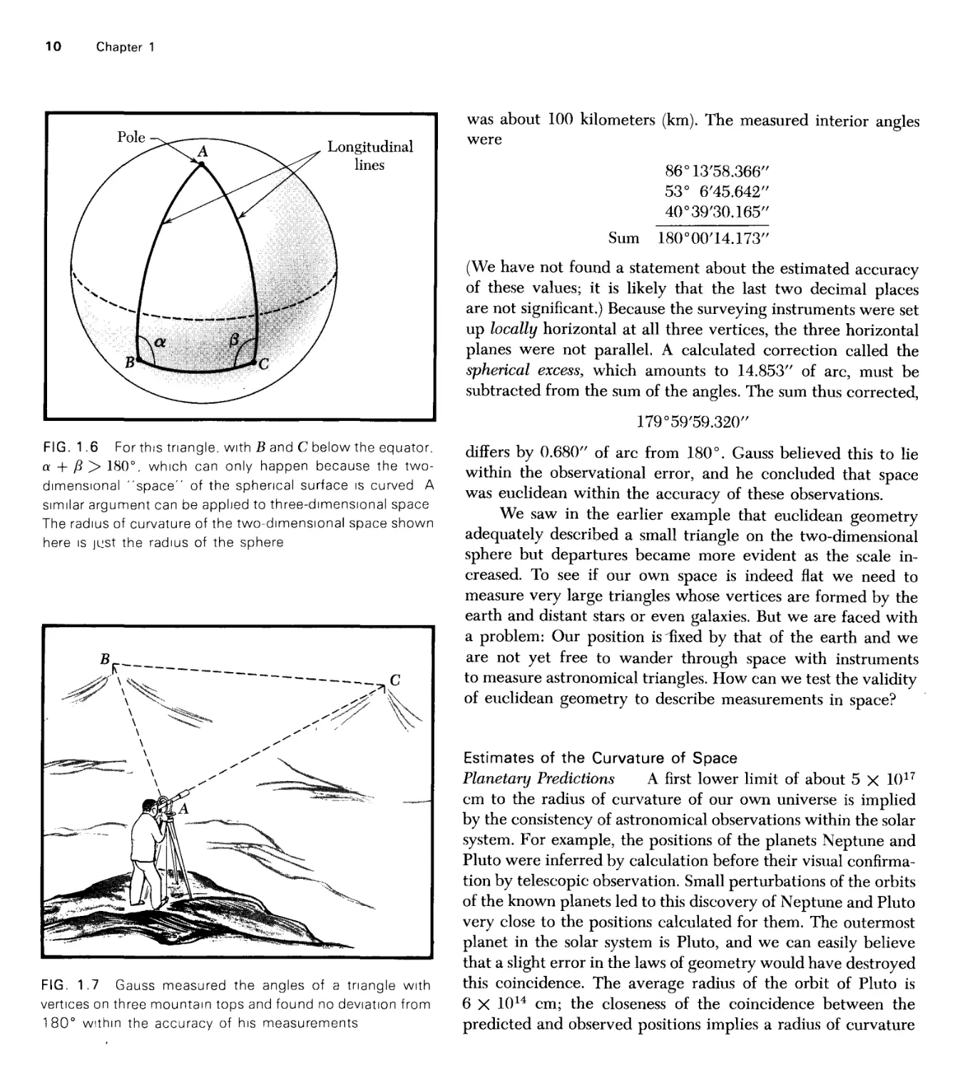
FIG. 1.4 Given three points ABC, the two-dimensional
beings could construct triangles with "straight lines" as
sides They would find that for small right triangles
a2 + b2 ~ c2 and the sum of the angles of the triangle is
slightly greater than 180°
FIG. 1.5 If they used larger triangles, the sum of the
angles would become increasingly greater than 1 80° Here,
with B and C on the equator, and A on the pole, a and
ft are both right angles Obviously a2 + b2 ^ c2, because
b is equal to c
10 Chapter 1
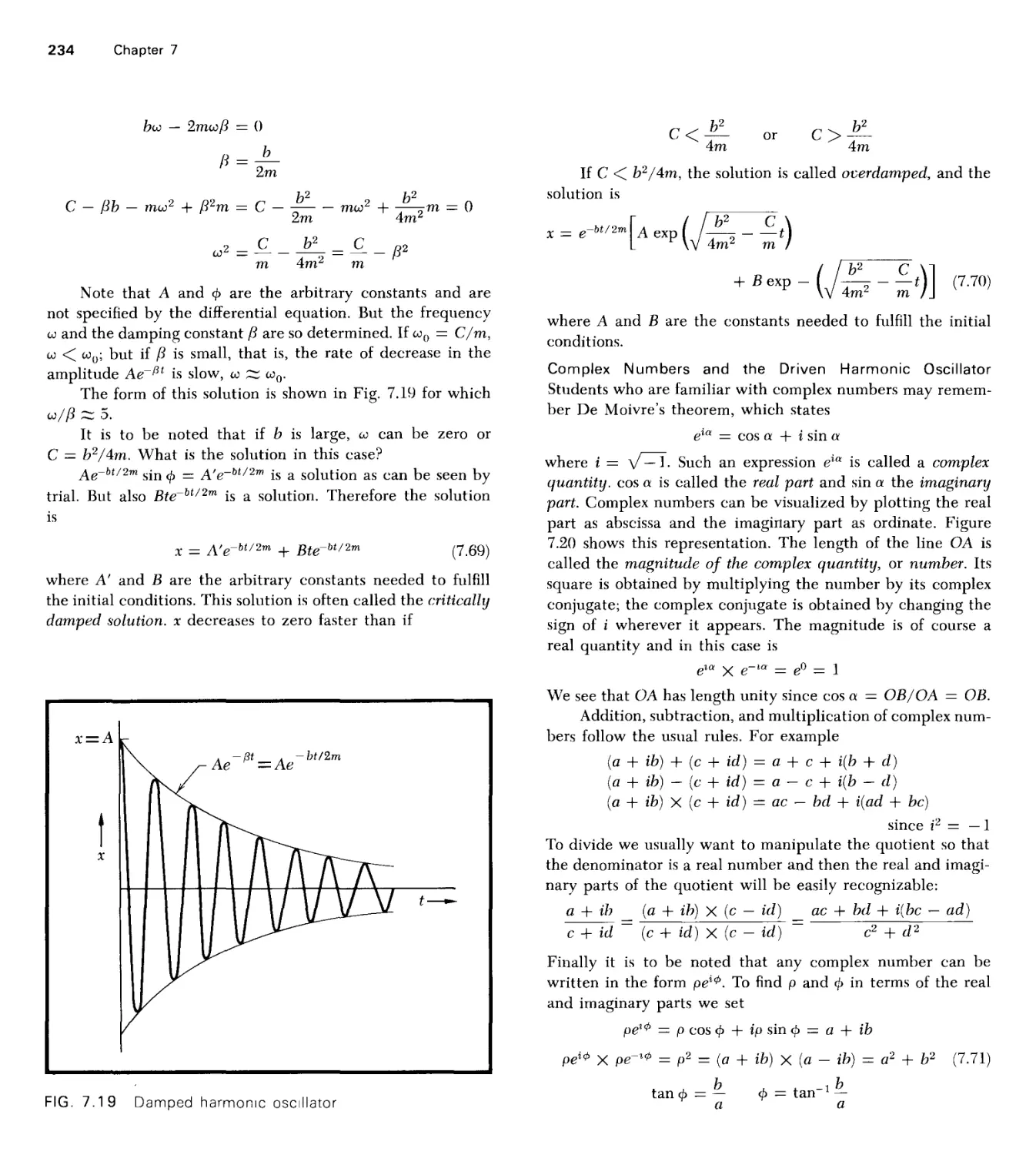
FIG. 1.6 Forthts triangle, with B and C below the equator,
a + P > 180°, which can only happen because the two-
dimensional "space" of the spherical surface is curved A
similar argument can be applied to three-dimensional space
The radius of curvature of the two-dimensional space shown
here is jest the radius of the sphere
FIG. 1.7 Gauss measured the angles of a triangle with
vertices on three mountain tops and found no deviation from
180° within the accuracy of his measurements
was about 100 kilometers (km). The measured interior angles
were
86°13'58.366"
53° 6'45.642"
40°39,30.165,/
Sum 180°00'14.173"
(We have not found a statement about the estimated accuracy
of these values; it is likely that the last two decimal places
are not significant.) Because the surveying instruments were set
up locally horizontal at all three vertices, the three horizontal
planes were not parallel. A calculated correction called the
spherical excess, which amounts to 14.853" of arc, must be
subtracted from the sum of the angles. The sum thus corrected,
179°59/59.320//
differs by 0.680" of arc from 180°. Gauss believed this to lie
within the observational error, and he concluded that space
was euclidean within the accuracy of these observations.
We saw in the earlier example that euclidean geometry
adequately described a small triangle on the two-dimensional
sphere but departures became more evident as the scale
increased. To see if our own space is indeed flat we need to
measure very large triangles whose vertices are formed by the
earth and distant stars or even galaxies. But we are faced with
a problem: Our position is fixed by that of the earth and we
are not yet free to wander through space with instruments
to measure astronomical triangles. How can we test the validity
of euclidean geometry to describe measurements in space?
Estimates of the Curvature of Space
Planetary Predictions A first lower limit of about 5 X 10¹⁷
cm to the radius of curvature of our own universe is implied
by the consistency of astronomical observations within the solar
system. For example, the positions of the planets Neptune and
Pluto were inferred by calculation before their visual
confirmation by telescopic observation. Small perturbations of the orbits
of the known planets led to this discovery of Neptune and Pluto
very close to the positions calculated for them. The outermost
planet in the solar system is Pluto, and we can easily believe
that a slight error in the laws of geometry would have destroyed
this coincidence. The average radius of the orbit of Pluto is
6 X 1014 cm; the closeness of the coincidence between the
predicted and observed positions implies a radius of curvature
of space of at least 5 X 1017 cm. An infinite radius of curvature
(flat space) is not incompatible with the data. It would take
us too far from our present purpose to discuss the numerical
details of how the estimate of 5 X 1017 cm is arrived at or
to define precisely what is meant by the radius of curvature
of a three-dimensional space. The two-dimensional analog of
the surface of a sphere can be used in this emergency as a
useful crutch.
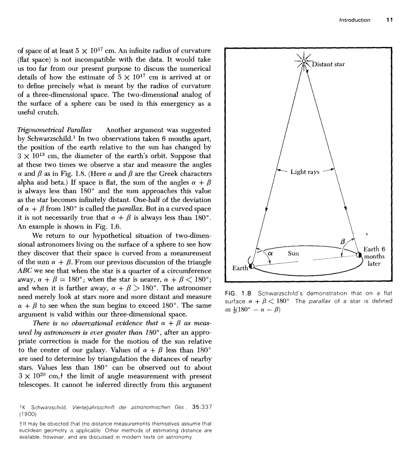
Trigonometrical Parallax Another argument was suggested
by Schwarzschild.1 In two observations taken 6 months apart,
the position of the earth relative to the sun has changed by
3 X 1013 cm, the diameter of the earth's orbit. Suppose that
at these two times we observe a star and measure the angles
a and /? as in Fig. 1.8. (Here a and /? are the Greek characters
alpha and beta.) If space is flat, the sum of the angles a + ft
is always less than 180° and the sum approaches this value
as the star becomes infinitely distant. One-half of the deviation
of a + ft from 180° is called the parallax. But in a curved space
it is not necessarily true that a + ft is always less than 180°.
An example is shown in Fig. 1.6.
We return to our hypothetical situation of
two-dimensional astronomers living on the surface of a sphere to see how
they discover that their space is curved from a measurement
of the sum a + ft. From our previous discussion of the triangle
ABC we see that when the star is a quarter of a circumference
away, a + ft = 180°; when the star is nearer, a + fi < 180°;
and when it is farther away, a + /? > 180°. The astronomer
need merely look at stars more and more distant and measure
a + ft to see when the sum begins to exceed 180°. The same
argument is valid within our three-dimensional space.
There is no observational evidence that a + ft as
measured by astronomers is ever greater than 180°, after an
appropriate correction is made for the motion of the sun relative
to the center of our galaxy. Values of a + ft less than 180°
are used to determine by triangulation the distances of nearby
stars. Values less than 180° can be observed out to about
3 X 1020 cm,f the limit of angle measurement with present
telescopes. It cannot be inferred directly from this argument
*K Schwarzschild, Vierteljahrsschnft der astronomischen Ges , 35:337
(1900)
t It may be objected that the distance measurements themselves assume that
euchdean geometry is applicable Other methods of estimating distance are
available, however, and are discussed in modern texts on astronomy
Introduction 11
FIG. 1.8 Schwarzschild's demonstration that on a flat
surface ol + fi < 180° The parallax of a star is defined
as J(180° - a - fi)
12 Chapter 1
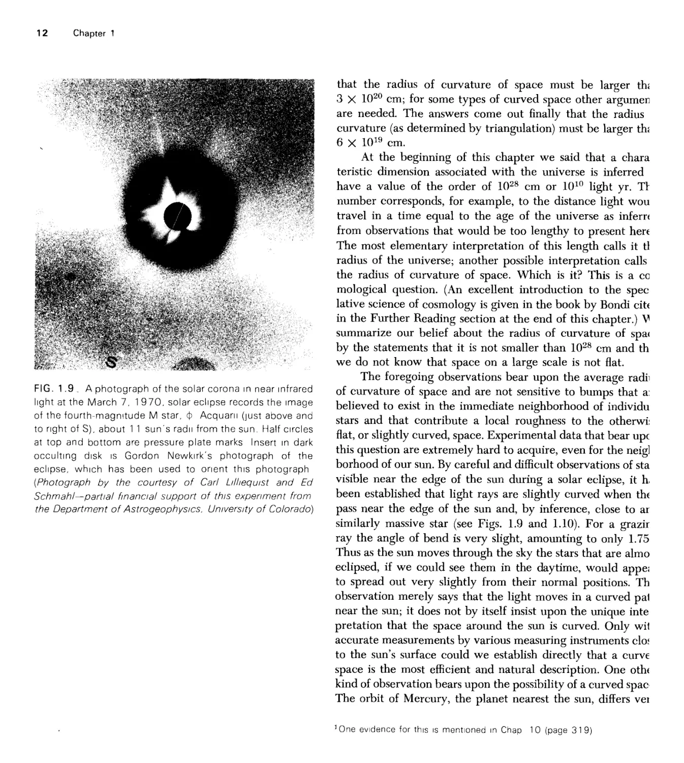
FIG. 1.9 _ A photograph of the solar corona in near infrared
light at the March 7, 1 970, solar eclipse records the image
of the fourth-magnitude M star, § Acquarn (just above and
to right of S), about 1 1 sun's radii from the sun. Half circles
at top and bottom are pressure plate marks Insert in dark
occulting disk is Gordon Newkirk's photograph of the
eclipse, which has been used to orient this photograph
(Photograph by the courtesy of Carl Lilltequist and Ed
Schmahl—part/al financial support of this experiment from
the Department of Astrogeophysics, University of Colorado)
that the radius of curvature of space must be larger tht
3 X 1020 cm; for some types of curved space other argumen
are needed. The answers come out finally that the radius
curvature (as determined by triangulation) must be larger th;
6 X 1019 cm.
At the beginning of this chapter we said that a chara
teristic dimension associated with the universe is inferred
have a value of the order of 1028 cm or 1010 light yr. Tr
number corresponds, for example, to the distance light wou
travel in a time equal to the age of the universe as inferr*
from observations that would be too lengthy to present her*
The most elementary interpretation of this length calls it tl
radius of the universe; another possible interpretation calls
the radius of curvature of space. Which is it? This is a cc
mological question. (An excellent introduction to the spec
lative science of cosmology is given in the book by Bondi cite
in the Further Reading section at the end of this chapter.) V
summarize our belief about the radius of curvature of spa<
by the statements that it is not smaller than 1028 cm and th
we do not know that space on a large scale is not flat.
The foregoing observations bear upon the average radii
of curvature of space and are not sensitive to bumps that a:
believed to exist in the immediate neighborhood of individu
stars and that contribute a local roughness to the otherwi:
flat, or slightly curved, space. Experimental data that bear upc
this question are extremely hard to acquire, even for the neig]
borhood of our sun. By careful and difficult observations of sta
visible near the edge of the sun during a solar eclipse, it h
been established that light rays are slightly curved when th(
pass near the edge of the sun and, by inference, close to ar
similarly massive star (see Figs. 1.9 and 1.10). For a grazir
ray the angle of bend is very slight, amounting to only 1.75
Thus as the sun moves through the sky the stars that are almo
eclipsed, if we could see them in the daytime, would appei
to spread out very slightly from their normal positions. Th
observation merely says that the light moves in a curved pal
near the sun; it does not by itself insist upon the unique inte
pretation that the space around the sun is curved. Only wil
accurate measurements by various measuring instruments clo?
to the sun's surface could we establish directly that a curve
space is the most efficient and natural description. One othe
kind of observation bears upon the possibility of a curved spac
The orbit of Mercury, the planet nearest the sun, differs vei
^One evidence for this is mentioned in Chap 10 (page 319)
Introduction 13
slightly from that predicted by application of Newton's laws
of universal gravitation and motion (see Fig. 14.9). Could this
be an effect of curved space near the sun? To answer such a
question we would have to know how a possible curvature
would affect the equations of motion for Mercury, and this
involves more than just geometry. [These topics are discussed
further (but briefly) in Chap. 14.]
In a remarkable and beautiful series of papers, Einstein
[A. Einstein, BerL Ber., 778, 799, 844 (1915); Ann. d. Phys. 49:
769 (1916)] described a theory of gravitation and geometry,
the general theory of relativity, which predicted, in
quantitative agreement with the observations, just the two effects
described above. There are still few confirmations of the
geometric predictions of the theory. However, despite the meager
evidence, the essential simplicity of the general theory has
made it widely accepted, although in recent years there has
been considerable research in this field (see Chap. 14).
Geometry on a Smaller Scale From astronomical
measurements we concluded that euclidean geometry gives an
extraordinarily good description of measurements of lengths, areas,
and angles, at least until we reach the enormous lengths of
the order of 1028 cm. But so far nothing has been said about
the use of euclidean geometry to describe very small
configurations comparable in size to the 10~8 cm of an atom or the
10~12 cm of a nucleus. The question of the validity of euclidean
geometry ultimately must be phrased as follows: Can we make
sense of the subatomic world, can we make a successful physical
theory to describe it, while assuming that euclidean geometry
is valid? If we can, then there is no reason at present to question
euclidean geometry as a successful approximation. We shall see
in Volume 4 that the theory of atomic and subatomic
phenomena does not seem to lead to any paradoxes that have thus
far blocked our understanding of them. Many facts are not
understood, but none appear to lead to contradictions. In this
sense euclidean geometry stands the test of experiment down
at least to 10~13 cm.
INVARIANCE
We shall summarize some of the consequences of the
experimental validity of euclidean geometry for empty space. The
homogeneity and isotropy of euclidean space can be expressed
by two invariance principles, which, in turn, imply two
fundamental conservation principles.
-
f
I Light ray
Sun
<p = 8X10"6rad~1.75"J
1 1
"*"
FIG. 1.10 The bending of light by the sun was predicted
by Einstein in 1915 and verified by observation shortly
afterward
14 Chapter 1
Invariance under Translation By this principle we mean
that empty space is homogeneous, i.e., that it is not different
from point to point. If figures are moved without rotation from
one location to another, there is no change in their size or
geometric properties. We assume also that the physical
properties of an object, such as its inertia or the forces between
its constituent particles, do not change merely upon displacing
the object to another region of empty space. Thus the natural
frequency of a tuning fork or the characteristic spectrum lines
of an atom are not altered by such displacement.
Invariance under Rotation By experiment it is known that
empty space is isotropic to high precision, so that all directions
are equivalent. Geometric and physical properties are
unaltered by the reorientation in direction of an object in empty
space. It is possible to imagine a space that is not isotropic;
for example, the speed of light in some direction could be
greater than its value in another direction at right angles to
the first. There is no evidence in free space for an effect of
this kind; within a crystal, however, many such anisotropic
effects are encountered. In regions of space close to massive
stars and other strong sources of gravitation, effects can be
observed that may be interpreted as slight departures from
homogeneity and isotropy of space. (We have alluded to two
such effects in the preceding section, and there are others.)
The property of invariance under translation leads to the
conservation of linear momentum; invariance under rotation
leads to the conservation of angular momentum. These
conservation principles are developed in Chaps. 4 and 6, and the
concept of invariance is developed in Chaps. 2 and 4.
The foregoing lengthy discussion about geometry and
physics is an example of the types of questions that physicists
must ask about the basic character of our universe. But we
shall not treat such matters further at this level of our study.
PROBLEMS
1 . The known universe. Using information in the text,
estimate the following:
(a) The total mass in the known universe.
Ans. sslO56 g.
(b) The average density of matter in the universe.
Ans. ~~10~29 g/cm3, equivalent to 10 hydrogen
atoms/m3.
(c) The ratio of the radius of the known universe to that of
a proton. Take the radius of the proton to be 1 X 10~13
cm and the mass of the proton to be 1.7 X 10~24 g.
2. Signals across a proton. Estimate the time required for
a signal traveling with the speed of light to move a distance
equal to the diameter of a proton. Take the diameter of the
Introduction 15
proton to be 2 X 10 13 cm. (This time is a convenient
reference interval in the physics of elementary particles and nuclei.)
3. Distance of Sirius. The parallax of a star is one-half the
angle subtended at the star by the extreme points in the earth's
orbit around the sun. The parallax of Sirius is 0.371". Find
its distance in centimeters, light years, and parsecs. One parsec
is the distance to a star whose parallax is 1". (See the table
of values inside the front and back covers.)
Ans. 8.3 X K)18 cm; 8.8 light yr; 2.7 parsecs.
4. Size of atoms. Using the value of Avogadro's number given
in the table inside the back cover of the book and your
estimate of an average density for common solids, estimate roughly
the diameter of an average atom, that is, the dimension of
the cubical space filled by the atom.
5. Angle subtended by moon. Obtain a millimeter scale and,
when viewing conditions are favorable, try the following
experiment: Hold the scale at arm's length and measure the
diameter of the moon; measure the distance from the scale
to your eye. (The radius of the moon's orbit is 3.8 X K)10 cm,
and the radius of the moon itself is 1.7 X 108 cm.)
(a) If you were able to try the measurement, what was the
result?
(b) If the measurement could not be made, from the data
given above calculate the angle subtended by the moon
at the earth. Ans. 9 X 10"3 radians (rad).
(c) What is the angle subtended at the moon by the earth?
(see p. 52, Chap. 2.) Ans. 3.3 X 10"2 rad.
6. Age of the universe. Assuming the radius of the universe
given on page 4, find the age of the universe from the
assumption that a star now on the radius has been traveling
outward from the center since the beginning at 0.6c = 1.8 X
1010 cm/s (c = speed of light in free space).
Ans. ^2 X 10¹⁰ yr.
7. Angles in a spherical triangle. Find the sum of the angles
in the spherical triangle shown in Fig. 1.5, assuming A is at
the pole and a = radius of sphere. In order to find the angle
at A, consider what would be the value of a in order for the
angle to be 90°.
FURTHER READING
These first two references are contemporary texts for the high
school level. They are excellent for review and clarification
of concepts. The second reference contains much material on
history and philosophy.
Physical Science Study Committee (PSSC), "Physics," chaps.
1-4, D. C. Heath and Company, Boston, 1965. Second edition.
F. J. Rutherford, G. Holton, and F. J. Watson, "Project Physics
Course," Holt, Rinehart and Winston, Inc., New York, 1970.
A product of Harvard Project Physics (HPP).
O. Struve, B. Lynds, and H. Pillans, "Elementary Astronomy,"
Oxford University Press, New York, 1959. Emphasizes the main
ideas of physics in relation to the universe; an excellent
book.
"Larousse Encyclopedia of Astronomy," Prometheus Press,
New York, 1962. This is a beautiful and informative book.
H. Bondi, "Cosmology," 2d ed., Cambridge University Press,
New York, 1960. Brief, clear, authoritative account, with
emphasis on the observational evidence, but lacking in substantial
recent work.
D. W. Sciama, "Modern Cosmology," Cambridge University
Press, New York, 1971. This account includes recent
developments.
Robert H. Haynes and Philip C. Hanawalt, "The Molecular
Basis of Life," W. H. Freeman and Company, San Francisco,
1968. A collection of Scientific American articles with some
relating text.
Gunther S. Stent, "Molecular Genetics," W. H. Freeman and
Company, San Francisco, 1971. An introductory account.
Ann Roe, "The Making of a Scientist," Dodd, Mead & Company,
New York, 1953; Apollo reprint, 1961. This is an excellent
sociological study of a group of leading American scientists
of the late 1940s. There have probably been some significant
changes in the scientific population since the book was first
published in 1953.
Bernice T. Eiduson, "Scientists: Their Psychological World,"
Basic Books, Inc., Publishers, New York, 1962.
A. Einstein, autobiographical notes in "Albert Einstein:
Philosopher-Scientist," P. A. Schilpp (ed.), Library of Living
Philosophers, Evanston, 1949. An excellent short
autobiography. It is a pity that there are so few really great biographies
of outstanding scientists, such as that of Freud by Ernest Jones.
There is little else comparable in depth and in honesty to the
great literary biographies, such as "James Joyce," by Richard
Ellman. The autobiography of Charles Darwin is a remarkable
exception. Writers about scientists appear to be overly
intimidated by Einstein's sentence: "For the essential of a man like
myself lies precisely in what he thinks and how he thinks, not
in what he does or suffers."
L. P. Wheeler, "Josiah Willard Gibbs; The History of a Great
Mind," Yale University Press, New Haven, Conn., 1962.
E. Segre, "Enrico Fermi, Physicist," The University of Chicago
Press, Chicago, 1971.
16 Chapter 1
Experimental Tools of Physics The photographs on this and the following pages show some of the instruments and
machines that are contributing actively to the advancement of the physical sciences
A nuclear magnetic resonance laboratory for chemical structure studies (ASUC Photography)
Introduction 17
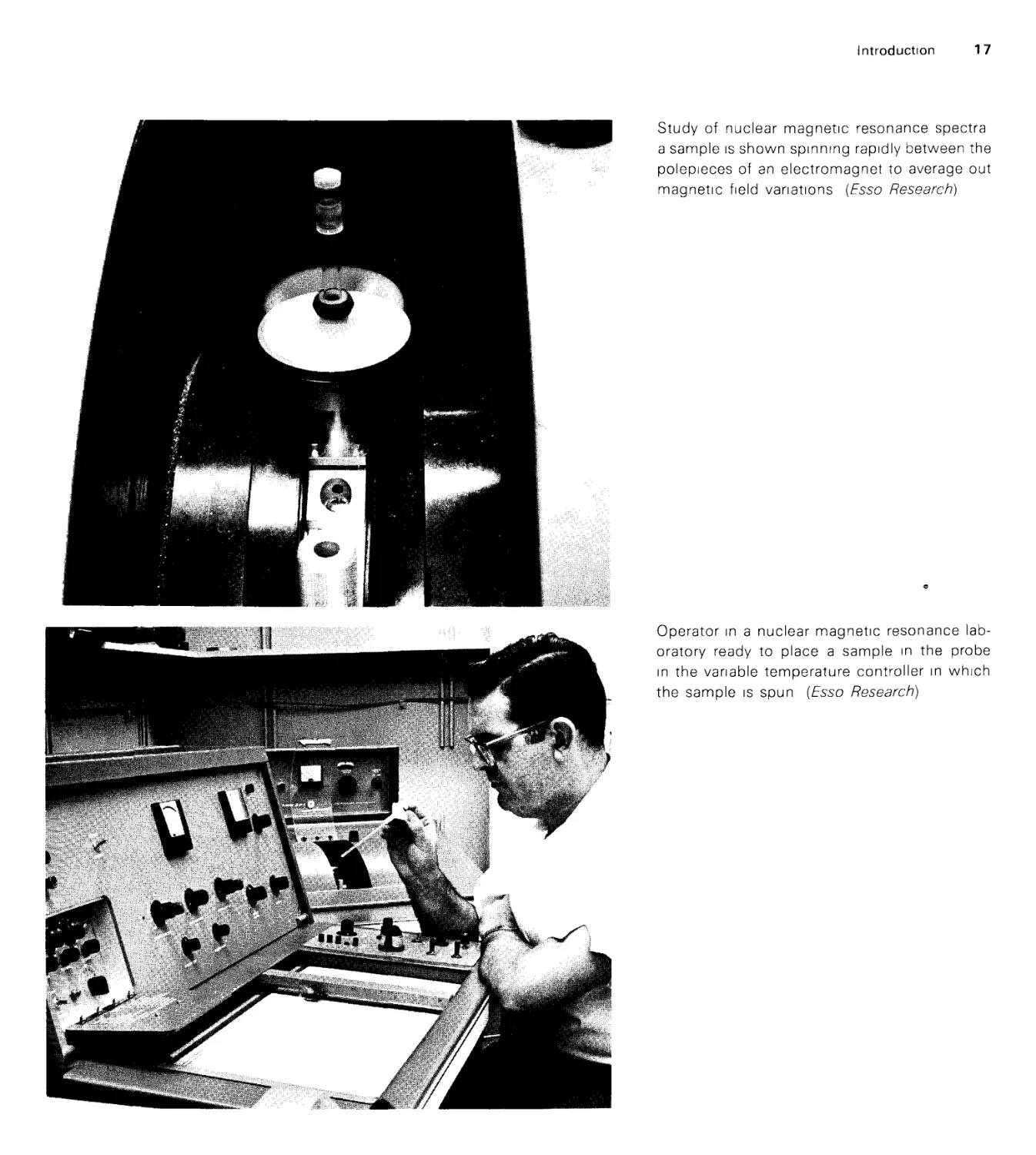
Study of nuclear magnetic resonance spectra
a sample is shown spinning rapidly between the
polepieces of an electromagnet to average out
magnetic field variations (Esso Research)
Operator in a nuclear magnetic resonance
laboratory ready to place a sample in the probe
in the variable temperature controller in which
the sample is spun {Esso Research)
18 Chapter 1
A magnet constructed of superconducting wire,
for operation at low temperature The coils
shown are rated to produce a magnetic field
of 54,000 gauss Such apparatus is the heart
of a modern low-temperature laboratory (Var/an
Associates)
The large radio telescope in Australia The dish is 210 ft in diameter. It
stands in a quiet valley 200 mi west of Sydney, New South Wales In
this remote location, there is a minimum of electrical interference.
(Australian News and Information Bureau)
^1P
W:
**&&&
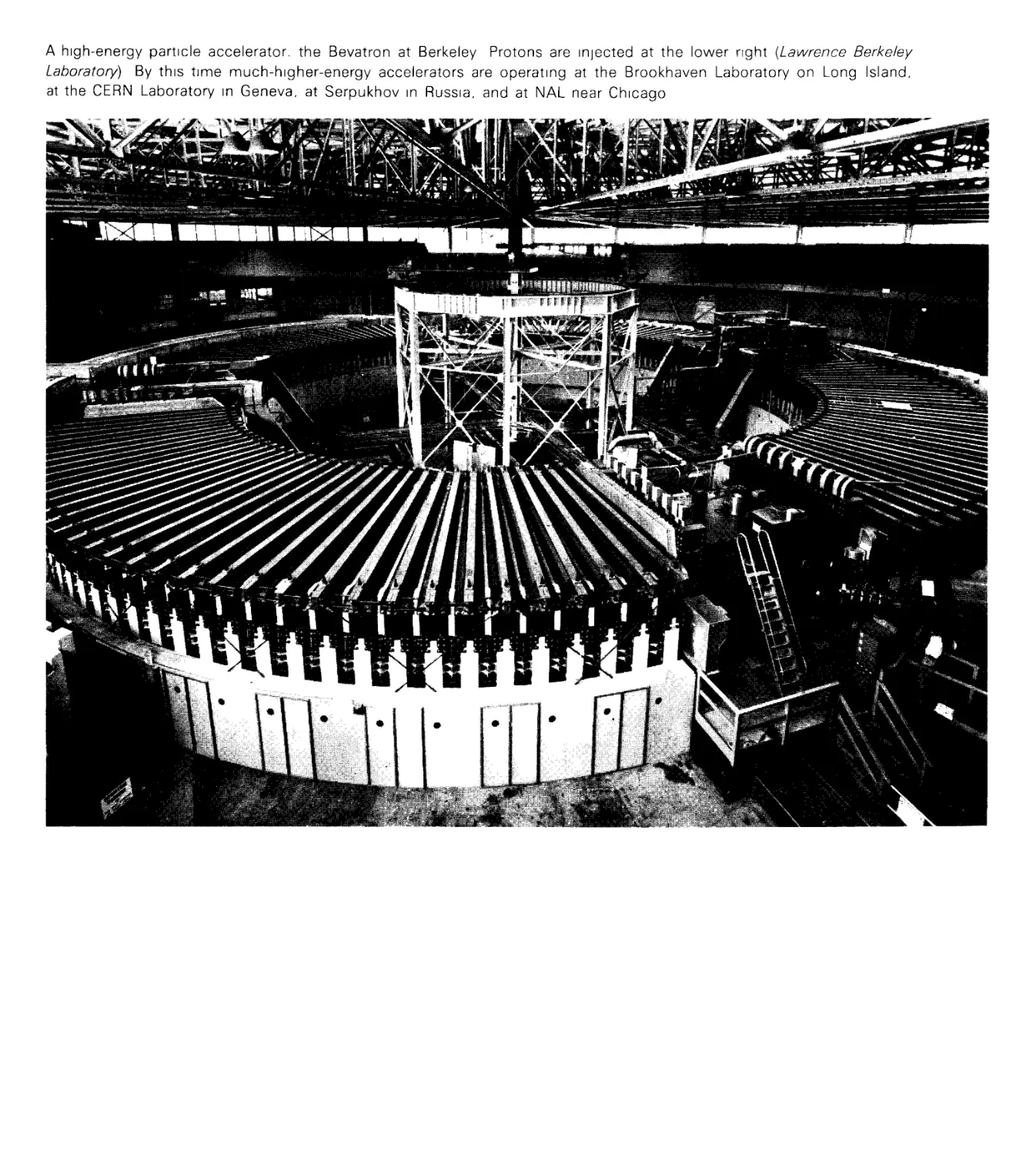
A high-energy particle accelerator, the Bevatron at Berkeley Protons are injected at the lower right (Lawrence Berkeley
Laboratory) By this time much-higher-energy accelerators are operating at the Brookhaven Laboratory on Long Island,
at the CERN Laboratory in Geneva, at Serpukhov in Russia, and at NAL near Chicago
20 Chapter 1
The 200-m Hale telescope pointing to zenith,
seen from the south (Photograph courtesy of
the Hale Observatories)
Reflecting surface of 200-in mirror of Hale
telescope and observer shown in prime-focus
cage (Photograph courtesy of the Hale
Observatories)
WKm&
Observer in prime-focus cage changing film
in the 200-in Hale telescope (Photograph
courtesy of the Hale Observatories)
NGC 4594 Spiral galaxy in Virgo, seen edge on, 200-in photograph (Photograph courtesy of the Hale Observatories)
Human red blood cells viewed by the scanning-electron
microscope and magnified 15,000 times Disklike objects
are the red blood cells connected by a mesh-work of fibrin
strands Note the realistic three-dimensional character of the
picture (Photograph courtesy of Dr Thomas L Hayes,
Donner Laboratory. Lawrence Berkeley Laboratory,
University of California, Berkeley)
Scanning-electron-microscope installation showing electron
optical column that forms probing electron beam (left) and
display console containing synchronous cathode-ray-tube
beam (right) Auxiliary equipment includes piezoelectric
micromanipulator in column of instrument, TV frame rate
display and TV tape recorder, Polaroid recording camera,
and signal monitor oscilloscope. (Photograph courtesy of
Dr Thomas L Hayes, Donner Laboratory, Lawrence Berkeley
Laboratory, University of California, Berkeley)
felfSklsf1
Introduction 23
A 43-mi-wide Martian crater (top) was photographed by
Mariner 9 on December 16, 1971 The sun shines from
the right The white dotted rectangle inscribes the area
shown in the bottom picture taken by Mariner's high-
resolution camera on December 22 The ridges, similar to
lunar mare ridges, are inferred to be breaks in the crust
along which extrusion of lava has taken place Both pictures
have been enhanced by computer processing (Photograph
courtesy of the Jet Propulsion Laboratory, California Institute
of Technology, NASA)
Chapter 1
9500ft)
a.Okm-j-l^m,
1.5km-|-.93i
This mosaic of two photographs of the Tithonius Lacus region on Mars taken by the Mariner 9 spacecraft revealed
a canyon twice as deep as the Grand Canyon in Arizona when the pictures were compared with pressure
measurements taken by the ultraviolet spectrometer experiment aboard the spacecraft The arrows connect the depths
deduced from the pressure measurements taken by the ultraviolet spectrometer and the corresponding features on the
photograph The dotted line is the scan path of the spectrometer The photographs were taken from an altitude of
1070 mi and cover an area of 400 mi across (Photograph courtesy of the Jet Propulsion Laboratory, California
Institute of Technology, NASA)
CONTENTS
LANGUAGE AND CONCEPTS: VECTORS
Vector Notation
Equality of Vectors
VECTOR ADDITJON
PRODUCTS OF VECTORS
Scalar Product
Vejctor Product
VECTOR DERIVATIVES
Velocity
Acceleration
Example Circular Motion
INVARIANTS
Examples of Various Elementary Vector
Operations
Problems
Mathematical Notes:
Time Derivatives, Velocity, and Acceleration
Angles
The Function ex
Expansion in Series
Vectors and Spherical Polar Coordinates
Formulas for Analytic Geometry
Useful Vector Identities
Further Reading
Vectors
28 Chapter 2
FIG. 2.1 The vector r represents the position of a pom
P relative to another point O as origin
FIG. 2.2 The vector —r is equal in magnitude but oppo
site in direction to r
LANGUAGE AND CONCEPTS: VECTORS
Language is an essential ingredient of abstract thought. It is
difficult to think clearly and easily about sophisticated and
abstract concepts in a language that has no words appropriate
to such concepts. To express new scientific concepts, new words
are invented and added to languages; many such words are put
together from classical Greek or Latin roots. If it satisfies the
needs of the scientific community, a new word may be adopted
in many modern languages. Thus vector in English is vecteur
in French, Vektor in German, and bektop (pronounced
"vector") in Russian.
Vector is the word defining a quantity that has both
direction and magnitude and that combines with other vectors
according to a specific rule.1 Throughout mechanics (and other
branches of physics as well) we shall meet quantities (velocity,
force, electric field, magnetic dipole moment) that have both
magnitude and direction, and consequently it is important to
develop the language and the techniques to deal with these
quantities. Although vector analysis often ranks as a branch of
mathematics, its value in physics is so great as to merit the
inclusion of an introduction here.
Vector Notation Because symbols are the components of
the language of mathematics, an important part of the art of
mathematical analysis is the technique of using notation well.
Vector notation has two important properties:
1 Formulation of a law of physics in terms of vectors is
independent of the choice of coordinate axes. Vector
notation offers a language in which statements have a physical
content without ever introducing a coordinate system.
2 Vector notation is concise. Many physical laws have simple
and transparent forms that are disguised when these laws
are written in terms of a particular coordinate system.
Although in solving problems we may wish to work in
special coordinate systems, we shall state the laws of physics
in vector form wherever possible. Some of the more
complicated laws, which cannot be expressed in vector form, may
be expressed in terms of tensors. A tensor is a generalization
of a vector and includes a vector as a special case. The vector
1This meaning for the word vector is a natural extension of an earlier usage,
now obsolete, in astronomy an imaginary straight line that joins a planet
moving around the focus of an ellipse to that focus
The specific rule is given on page 31
analysis we know today is largely the result of work done
toward the end of the nineteenth century by Josiah Willard
Gibbs and Oliver Heaviside.
The vector notation we adopt is the following: On the
blackboard a vector quantity named A is denoted by putting
a wavy line under A or by putting an arrow over the letter.
In print vectors always appear in boldface type. The magnitude
of a vector is printed in italics: A is the magnitude of A; A
is also written as |A|. A unit vector is a vector of unit length;
a unit vector in the direction of A is written with a caret as
A, which we read as "A hat," or "A caret." We summarize
the notation by the identity
A = AA = AA
Figures 2.1 to 2.4 show a vector, the negative of that vector,
multiplication by a scalar, and a unit vector.
The usefulness and applicability of vectors to physical
problems is largely based on euclidean geometry. Statement
of a law in terms of vectors usually carries with it the
assumption of euclidean geometry. If the geometry is not euclidean,
addition of two vectors in a simple and unambiguous way may
not be possible. For curved space there exists a more general
language, metric differential geometry, which is the language
of general relativity, the domain of physics in which euclidean
geometry is no longer sufficiently precise.
We have considered a vector to be a quantity having
direction as well as magnitude. These properties have
absolutely no reference to a particular coordinate system, although
we assume that the direction can be defined, for example, by
reference to a laboratory room, the fixed stars, etc. We shall
see, however, that there are some quantities having magnitude
and direction that are not vectors, such as finite rotations
(page 33). A quantity having magnitude but not direction is
a scalar. The magnitude of a vector is a scalar. Temperature
is a scalar and mass is a scalar. On the other hand, velocity
v is a vector and force F is a vector.
Equality of Vectors Having developed the notation, we now
proceed to some vector operations: addition, subtraction, and
multiplication. Two vectors A and B describing similar physical
quantities (e.g., forces) are defined to be equal if they have the
same magnitude and direction; this is written A = B. A vector
does not necessarily have location, although a vector may refer
to a quantity defined at a particular point. Two vectors can
be compared even though they measure a physical quantity
Vectors 29
FIG. 2.3 The vector 0 6r is in the direction of r and ts
of magnitude 0 6r
FIG. 2.4 The vector r is the unit vector in the direction
of r. Note that r = rr.
A
FIG. 2.5 (a) Vector A
n
(b) Vector B
[7/
X
I LC-r-
Tl
J
(c) The vector sum A + B
\_0
(d) The vector sum B + A is equal to A + B
defined at different points of space and time. If we did not
have confidence, based on experiment, that we can consider
space to be flat, i.e., euclidean—except perhaps at enormous
distances—then we could not unambiguously compare two
vectors at different points.
VECTOR ADDITION
A vector is represented geometrically by a directed straight-
line segment, or arrow, whose length in chosen scale units
equals the magnitude of the vector. The sum of two vectors
A and B is defined by the geometrical construction shown in
Fig. 2.5a to c. This construction is often called the
parallelogram law of addition of vectors. The sum A + B is defined by
carrying B parallel to itself until the tail of B coincides with
the head of A. The vector drawn from the tail of A to the
head of B is the sum A + B. From the figure it follows that
A + B = B + A, so that vector addition is said to be
commutative, as shown in Fig. 2.5a7. Vector subtraction is defined
by Fig. 2.6a and b with B + ( —B) = 0 defining the negative
vector.
Vector addition satisfies the relation A 4- (B + C) =
(A + B) + C, so that vector addition is said to be associative
(see Fig. 2.7). The sum of a finite number of vectors is
independent of the order in which they are added. If A — B = C5
then by adding B to both sides we obtain A — B + C. If k
is a scalar,
/c(A + B) = fcA + /cB (2.1)
so that multiplication of a vector by a scalar is said to be
distributive.
When Is a Physical Quantity Representahle by a Vector?
A displacement is a vector because it describes both the
direction of the line from the initial position to the final position
and the length of the line; the example of addition given above
is easily recognized as applying to displacements in euclidean
space. In addition to displacements, other physical quantities
have the same laws of combination and invariance properties
as displacements. Such quantities can also be represented by
vectors. To be a vector a quantity must satisfy two conditions:
1 It must satisfy the parallelogram law of addition.
2 It must have a magnitude and a direction independent of
the choice of coordinate system.
Vectors 31
| //-■
FIG. 2.6 (a) Vectors B and -B
{b) Formation of A — B, vector subtraction
FIG. 2.7 Sum of three vectors A + B + C Verify for
yourself that this sum is equal to B + A -h C
32
Chapter 2
FIG. 2.8 (a) Original orientation of book It is then rotated
by 7t72 radians (rad) about Axis 1
(b) Orientation after a rotation of tt/2 rad
about Axis 1
(c) Orientation after a subsequent rotation of tt/2
rad about Axis 2
(d) Original orientation of book
(e) Orientation after a rotation of 77/2 rad
about Axis 2
(f) Orientation after subsequent rotation of tt/2 rad
about Axis 1
Finite Rotations Are Not Vectors Not all quantities that have
magnitude and direction are necessarily vectors. For example,
a rotation of a rigid body about a particular axis fixed in space
has a magnitude (the angle of rotation) and a direction (the
direction of the axis). But two such rotations do not combine
according to the vector law of addition, unless the angles of
rotation are infinitesimally small.1 This is easily seen when the
two axes are perpendicular to each other and the rotations are
by 77/2 rad (90°). Consider the object (a book) in Fig. 2.8a.
The rotation (1) leaves it as in Fig. 2.8fr, and a subsequent
rotation (2) about another axis leaves the object as in Fig. 2.8c.
But if to the object as originally oriented (Fig. 2.8c/) we apply
first the rotation (2), (Fig. 2.8e) and then the rotation (1), the
object ends up as shown in Fig. 2.8/. The orientation in the
sixth figure is not the same as in the third. Obviously the
commutative law of addition is not satisfied by these rotations.
Despite the fact that they have a magnitude and a direction,
finite rotations cannot be represented as vectors.
PRODUCTS OF VECTORS
Although there is no reason to ask whether the sum of two
vectors is a scalar or a vector, such a question has importance
in reference to the product of two vectors. There are two
particularly useful ways in which to define the product of two
vectors. Both products satisfy the distributive law of
multiplication: The product of A into the sum of B + C is equal
to the sum of the products of A into B and A into C. One
type of product is a scalar, and the other is for many purposes
a vector. Both products are useful in physics. Other possible
definitions of product are not useful: Why is AB not a useful
definition of the product of two vectors? By AB we mean the
ordinary product |A[ |B| of the magnitudes of A and B. We
observe that if D = B + C, then, in general, AD ^ AB + AC.
This absence of the distributive property makes AB useless as
a product of A and B.
Scalar Product The scalar product of A and B is defined
as that number which is obtained by taking the magnitude of
A times the magnitude of B times the cosine of the angle
between them (see Fig. 2.9a to c). The scalar product is a scalar.
Angular velocities are vectors even though finite angular rotations are not
Vectors 33
FIG. 2.9 (a) In forming A • B, bring vectors A and B to
a common origin
(b) B(A cos 6) = A • B
(c) A(B cos 0) — A*B Here 0, the Greek character theta.
denotes the angle between A and B
34 Chapter 2
FIG. 2.10 (a) Cartesian orthogonal unit vectors x, y, z
(b) A = xA, + yAy + zAz
Often the scalar product is called the dot product because we
denote it by the symbol A • B where
A • B = AB cos (A,B)
(2.2)
Here cos (A,B) denqtes the cosine of the angle between A and
B. We see that no coordinate system is involved at all in the
definition of scalar product. We note that cos (A,B) = cos (B,A),
so that the scalar product is commutative:
A • B = B • A (2.3)
We read A • B as "A dot B."
If the angle between A and B should lie between 77/2 and
377/2, then cos (A,B) and A • B will be negative numbers. If
A = B, then cos (A,B) = 1 and
A-B = A2 = |A|2
If A • B = 0 and A ^ 0, B 76 0, we say that A is orthogonal
to B or perpendicular to B. Note that cos (A,B) = A • B, so that
the scalar product of two unit vectors is just the cosine of the
angle between them. The magnitude of the projection of B
on the direction of A is
B cos (A,B) = £A • B = B • A
where A is the unit vector in the direction of A. The projection
of A on the direction of B is
A cos (A,B) = A • B
Scalar product multiplication has no inverse: if A • X = b,
there is no unique solution for X. Division by a vector is a
meaningless, undefined operation.
Components, Magnitudes, and Direction Cosines Let x, y,
and z be three orthogonal1 unit vectors that define a cartesian
coordinate system as in Fig. 2.10a. An arbitrary vector A may
be written
A = Axx + Ayy + AJl (2.4)
where Ax, Ay, and Az are called the components of A, as
illustrated in Fig. 2.10Z?. It is readily seen that Ax = A • x since
A • x = Axx - x + Ayy • x + Azx • x — Ax
and
y • x = 0 = z • x
x * x = 1
Orthogonal as used here means mutually perpendicular
In terms of these components Ax, A , and Az, the magnitude
of A is
A = VA-A = V(Axi + A^ + Azz) • (Axx + Ayy + Azz)
= va7+a7Ta7 (2.5)
If we desire to write an expression for the unit vector A
(also shown in Fig. 2.10Z?), we can see that
- Ax • A AV'A Az*A
is such an expression. From Fig. 2.11 and Eq. (2.6) we deduce
that the angles that A makes with the x, y, and z axes have
cosines Ax/A, Ay/A, and Az/A, or x • A, y • A, and z • A. These
are called direction cosines and have the property that the sum
of the squares of the three direction cosines is equal to unity,
as can easily be seen with the help of Eq. (2.5).
The scalar product of two vectors A and B is conveniently
remembered in terms of the components
A • B = AXBX + AvBy + AZBZ
(2.7)
Applications of the Scalar Product We treat several
applications of the scalar product.
1 Law of cosines. Let A — B = C; then, on taking the scalar
product of each side of this expression with itself, we have
(A - B) • (A - B) = C • C
or
A2 + B2 - 2A ■ B = C2
which is exactly the famous trigonometric relation
A2 + B2 - 2AB cos (A,B) = C2 (2.8)
The cosine of the angle between the directions of two
vectors is given by
cos (A,B) = cos 0AB = -^~
as in Eq. (2.2) (see Fig. 2.12a and 6).
z
FIG. 2.1 1 Direction cosines refer to the angles indicated
C-A-B
FIG. 2.12 (5) OC = C2 = (A - B) ■ (A - B)
= A2 + B2 - 2A • B
= A2 + B2 - 2AB cos 6
(b) D • D = D2 = (A + B) • (A + B)
= A2 + B2 + 2AB cos 0.
36 Chapter 2
FIG. 2.13 Equation of a plane, N is the normal to thi
plane from the origin O The equation of the plane i:
N • r = A72
FIG. 2.14 Electric and magnetic fields in a plane
electromagnetic wave in free space are perpendicular to the propa
AAA
gation direction k Thus k « E = k • B = 0, E • B= 0
FIG .2.15 Rate at which a force F does work on a particle
moving with velocity v
Equation of a plane (Fig. 2.13). Let N be a normal to
the plane under consideration, which is drawn from an
origin O not in the plane. Let r be an arbitrary vector from
the origin O to any point P in the plane. The projection
of r on N must be equal in magnitude to N. Thus the plane
is described by the equation
r • N = N2 (2.9)
To establish the identity of this compact expression with
the usual expression in analytic geometry for the equation
of a plane
ax + by + cz — 1
write N and r in terms of their components A^, N , A^ and
x, y, z. Now Eq. (2.9) assumes the form
(xx + yy + zi) • (Nxx + Nyy + N£) = N2
which reduces to
K Ny Nz
N2 N2 N2
Electric and magnetic vectors in an electromagnetic wave.
If k is the unit vector in the direction of propagation of
a plane electromagnetic wave in free space (see Fig. 2.14),
then (as we shall see in Volumes 2 and 3) the electric and
magnetic intensity vectors E and B must lie in a plane
normal to k and must be perpendicular to each other. We
can express this geometric condition by the relations
k • E = 0 k-B = 0 E-B = 0
Rate of doing work. In elementary physics (also see Chap.
5) we learned that the rate at which a force F does work
on a particle moving with velocity v is equal to Fv cos (F,v).
We recognize this expression as just the scalar product
If we write generally the derivative dW/dt as a symbol
for the rate of doing work, then (Fig. 2.15)
^ = F-v (2.10)
dt K '
5 Rate at which volume is swept out. Let S be a vector normal
to a plane area and of magnitude equal to the area and
let v denote the velocity at which the area is moved. The
volume per unit time traversed by the area S is a cylinder
of base area S and slant height v (see Fig. 2.16), or S • v.
The rate at which volume is swept out is therefore
-^ = S-v (2.11)
Vector Product1 There is a second product of two vectors
that is widely used in physics. This product is vector rather
than scalar in character, but it is a vector in a somewhat
restricted sense. The vector product A X B is defined to be a
vector normal to the plane that includes A and B with
magnitude A£|sin(A,B)| as in Fig. 2.17a:
C = A X B = CA£|sin(A,B)l (2.12)
We read A X B as 'A cross B." The sense of C is
determined as a matter of fixed convention by the right-hand-thread
rule: The vector A in the first position in the product is rotated
by the smallest angle that will bring it into coincidence with
the direction of B. The sense of C is that of the direction of
motion of a screw with a right-hand thread (the standard thread
in the United States) when the screw is rotated in the same
direction as was the vector A, as shown in Fig. 2.17b on the
next page.
Let us state the rule for the direction of C in another way:
First, place together the tails of vectors A and B; this defines
a plane. Vector C is perpendicular to this plane; that is, the
vector product A X Bis perpendicular to both A and B. Rotate
A into B through the lesser of the two possible angles—curl
the fingers of the right hand in the direction in which A was
rotated, and the thumb will point in the direction of
C = A X B. Note that because of this sign convention B X A
is a vector opposite in sign to A X B (see Fig. 2.17c):
B X A = -A x B (2.13)
Thus the vector product is not commutative. It follows from
Eq. (2.12) that A X A = 0, so that the vector product of a
vector with itself is zero. The vector product does obey the
distributive law:
Ax(B + C) = AxB + AxC
1This section {pages 37 to 40) can be omitted at this time The vector product
is used in Chap 3 (page 7 1), which can also be omitted, only beginning in Chap
6 (page 185) is it essential
Vectors 37
FIG. 2.16 Rate dV/dt at which area S moving with
velocity v sweeps out volume
FIG. 2.17 (a) Vector product C = A X B
38 Chapter 2
Right-hand-thread rule.
FIG. 2.17 (cont'd.) (b) Methods of determining directioi
of vector A X B
B XA=-C
(c) Vector product B X A is opposite to A X B
The somewhat tedious proof may be found in any book on
vector analysis.1
Vector Product in Cartesian Components Just as we found
in Eq. (2.6) the direction cosines of a vector A, we can find
the sines of the angles that A makes with the cartesian axes.
This is inconvenient and the sines can more easily be found
from the cosines. However, it is often useful to have the
expression for the vector product of two vectors in terms of their
components:
A x B = (Axi + Ayy + A£) x (B,i + Byy + B,z)
= (x x y)AxBy + (x x i)AxBs + (y X z)AyBz
+ (y X ±)AyBx + (z X *)AA + (z X y)A,By
where we have used the result xXx = yXy = zXz = 0.
The question arises: What is x X y? Is it z or — z? We make
the choice that x X y = +z and construct the coordinate
directions accordingly. This is called a right-handed coordinate
system2 and is used conventionally in physics. We agree to work
only in the right-handed coordinate system, which is the kind
shown in Fig. 2.10a and h.
Now xXz= — y, y X z = x, and so on, and we see that
A X B = i(AyB, - AzBy)
+ y (AA - AA) + *(AA - \BX) (2.14)
Note that if the indices are cyclic with xyz, the term enters
the vector product with a positive sign; otherwise the sign is
negative. If you are familiar with determinants, you can
confirm readily that the representation
1 For example, see C E Weatherburn, "Elementary Vector Analysis/' p 57
G Bell & Sons, Ltd . London, 1928, J G Coffin, "Vector Analysis," p 35,
John Wiley & Sons, Inc , New York, 1911
2How would we communicate our definition of right-handed to a creature in
another solar system in our galaxy? We can do this by using circularly polarized
radio waves The signal carries a message that tells the remote observer in
which sense we defined the waves to be polarized The remote observer will
have constructed two receivers, one with the correct sense and one with the
incorrect sense, in terms of signal strength Any method requires clear
instructions In the original analysis of the spectroscopic Zeeman effect, its discoverer
incorrectly associated a positive sign to the oscillating charges in atoms
because he misunderstood the sense of circularly polarized radiation [See
P Zeeman, Philosophical Magazine, (5)43. 55 and 226 (1897) In a similar
connection the first Telstar transmission on July 11, 1962, was poorly
received in Great Britain because "of the reversal of a small component in the
aerial feed which arose from an ambiguity in the accepted definition of the
sense of rotation of radio waves " Times {London). July 13, 1962, p 11]
AXB =
« A A A
x y z
Ax Ay A J
Bx By Bz
is equivalent to Eq. (2.14) and it is easier to remember.
Applications of the Vector Product In the following
paragraphs we treat several applications of the vector product.
1 Area of a parallelogram. The magnitude
|A xB| = A£|sin(A,B)|
is the area of the parallelogram with sides A and B (or twice
the area of the triangle with sides A and B)(see Fig. 2.18a).
The direction of A X B is normal to the plane of the
parallelogram; thus we may think of A X B as the vector
area of the parallelogram. Because we have given signs to
the sides A and B? the vector area comes endowed with
a direction. There are physical applications where it is
convenient to be able to give a direction to an area [see
Eq. (2.11)].
2 Volume of a parallelepiped. The scalar
|(A x B) • C| = V
is the volume of the parallelepiped of which A X Bis the
area of the base and C the slant height or edge (Fig. 2.18b).
If the three vectors A, B, and C lie in the same plane, the
volume will be zero; thus three vectors are coplanar if and
only if (A X B) • C = 0.
We note from inspection of the figure that
A • (B X C) = (A X B) • C
so that the dot and the cross in the scalar triple product
may be interchanged without altering the value of the
product. However,
A-(BxC)= -A-(CxB)
A scalar triple product is not altered by permuting
cyclically the order of the vectors, but it is reversed in sign if
the cyclic order is changed. (Cyclic permutations of ABC
are BCA and CAB; noncylic orderings of ABC are BAC,
ACB, and CBA.)
3 Law of sines. Consider the triangle defined by C = A + B
(Fig. 2.18c), and take the vector product of both sides of
the equation with A:
Vectors 39
FIG. 2.1 8 (a) Vector area of parallelogram is C = A X B
= AB \sind\C
i
AXB
/ /
/ /
/ /
/ /
/ /
/ /
/ ^
| B
i J
s* ^i I
/c /
(b) AXB*C = base area X height = volume of
parallelepiped
Cy/
y/\Afi)
A
^-/
^"W
/b
N(A,B)
(c) Law of sines of triangle
Note- sin (A,B) = sin [77 - (A,B)]
40 Chapter 2
FIG. 2.18 (cont'd.) (d) Torque as a vector product
[e) Force on positive charge moving in a magnetic field
O
FIG. 2.19 (a) The position P1 of a particle at time t
is specified by the vector r(f1) relative to the fixed origin a
point O
A X C = A.x A + A x B
Now A X A = 0, and the magnitudes of both sides must
be equal so that
AC sin (A,C) = AB sin (A,B)
or
^n (A,C) sin(A,B)
-~B— = ~— (216)
This is known as the law of sines of a triangle.
4 Torque. The idea of torque is familiar from most
introductory courses in physics. It is particularly important in the
motion of rigid bodies discussed in Chap. 8. The torque
is referred to a point and has a convenient expression in
terms of vectors
N = r X F (2.17)
where r is a vector from the point to the vector F. From
Fig. 2AHd we see that the torque has a direction
perpendicular to r and to F. Note that the magnitude of N is
rF sin a and r sin a is the length of the perpendicular from
the point (O in the figure) to F. In the figure r sin a —
r' sin a'. Hence the torque both in direction and in
magnitude is independent of the point along F to which r is
drawn.
5 Force on a particle in a magnetic field. The force on a point
electric charge moving with velocity v in a magnetic field
B is proportional to v times the perpendicular component
of B; in terms of the vector product (see Fig. 2.18e).
F = — v X B (gaussian units)
(2.18)
F = q v X B (mks units)
Here q is the charge on the particle and c is the speed
of light. This force law is developed in detail in Volume
2 and is used in Chap. 3 (page 70).
VECTOR DERIVATIVES
The velocity v of a particle is a vector; the acceleration a is
also a vector. The velocity is the time rate of change of the
position of a particle. The position of a particle at any time
(b) The particle has advanced to P2 at time t2
t can be specified by the vector r(f), which goes from a fixed
point O to the particle as in Fig. 2.19a. As time advances, the
particle moves and the position vector changes direction and
magnitude (Fig. 2.19b). The difference between r(t2) and r(^)
is a vector as in Fig. 2.19c:
Ar = r(t2) - r(tr)
If the vector r can be regarded as a function (a vector function)
of the single scalar variable t, the value of Ar will be completely
determined when the two values tr and t2 are known. Thus
in Fig. 2.19d Ar is the chord PXP2. The ratio
Ar
A*
is a vector collinear with the chord PXP2 but magnified in the
ratio 1/Af. As At approaches zero, P2 approaches Px and the
chord PXP2 approaches the tangent at Pv Then the vector
-— will approach ^—-
At rF dt
which is a vector tangent to the curve at P1 directed in the
sense in which the variable t increases along the curve (Fig.
2.19e).
Vectors A
(c) The vector Ar is the difference between r(t2) and r(^)
(d) Ar is the chord between the points Px and P2 on the
trajectory of the particle
(e) As A£ = t2 — tx —> 0, the vector Ir/lt collinear with the
chord approaches the velocity vector dr/dt collinear with
the tangent to the trajectory at point P1
Velocity The vector
* = lim AL
dt ^° M
is called the time derivative of r. By definition the velocity is
v(t) = ft (2.19)
The magnitude v = |v| of the velocity is called the speed of
the particle. The speed is a scalar. In terms of components we
write
r(t) = x(t)x + y(t)y + z(t)z (2.20)
and
dr dx ^ dy A dz A
— = v = -—x + —y + -r-z = vTx + t^y + i; z
eft rff dt dt x yJ z
(2.21)
= lv| = W + vy2 + u.
where we have assumed that the unit vectors do not change
with time, so that
dx dy dz
at at at
In general, we may write, without expressing r in
components as in Eq. (2.20),
r(f) = r(t)r(t)
where the scalar r(t) is the length of the vector and r(t) is a
vector of unit length in the direction of r. The derivative of
r(t) is defined as
It " Jtlrmt)\ - A^° It
(2.22)
We may rewrite the numerator,1 retaining only the first two
terms in the series expansions of r(t + At) and r(t + At):
b+$Hb+fAiHw
\dt dt/ \dt dt!
See page 53 at the end of this chapter for expansion in series
When this is placed in Eq. (2.22), the second term in the
quotient goes to 0 as At -^ 0 and we have
dx dr a . dr /n oox
v = — = —-r + r— 2.23
dt dt dt v /
Here dr/dt represents the rate of change of direction of the
unit vector r. This is an example of the general rule for
differentiation of the product of a scalar a(t) and a vector b(t)
d u dau , db /ri n4,
— ab = —-b + a—— (2.24)
dt dt dt K '
One contribution to the velocity in Eq. (2.23) comes from the
change in the direction f; the other contribution comes from
the change in the length r.
Since we shall apply the form of Eq. (2.23) for v
(particularly in Chap. 9 for motion in a plane), we develop here an
expression of that form for dr/dt utilizing the unit radial vector
r and a unit vector perpendicular to it that we shall call 0.
In order to make clear these unit vectors and their time
derivatives, consider the motion of a point on a circular path;
in this case the unit vector r will change in a time interval
At by a vector increment Ar to become r + Ar, as shown in
Fig. 2.20a. If At is chosen so small as to approach zero, then
Ar takes the direction of the transverse unit vector 6 shown
in Fig. 2.20k.
Furthermore, as At and correspondingly A6 approach zero,
the magnitude of Ar becomes simply
|Ar| = |r|A0 = A0
(because |r| = 1) and so the vector Ar and the ratio Ar/Af
become
Ar = A0 & ^ = M-6
At to
When we pass to the limit of At —> 0, we obtain for the r unit
vector time derivative
4^-^-6 (2.25)
dt dt v '
By similar arguments utilizing Fig. 2.20c it is readily shown
that the 0 time derivative is
#=—?-* (2.26)
dt dt K J
Vectors 43
FIG. 2.20 (a) Ar is the change in the unit vector f
(£>) The unit vector 8 is perpendicular to r and in the
direction of increasing 6
(c) AS is the change in the unit vector 8
44 Chapter 2
FIG. 2.21 Components of velocity vector in terms of
and 6
Now when we consider a point moving in a plane on any
path, as suggested by Fig. 2.21, we recognize that the velocity
vector v at any instant is composed of the radial component
vector dr/dtx and the transverse component vector r df/dt —
r dd/dt d. The latter vector utilizes Eq. (2.25). Thus the
expression for v in the form of Eq. (2.23) is
dr dr * , d6 *
v = — = — r + r—B
dt dt dt
(2.27)
Acceleration Acceleration is also a vector; it is related to
v just as v is related to r. We define acceleration as
a = — — d2*
~ dt" dt2
Using Eq. (2.21) we obtain, in cartesian components,
(2.28)
dv
dt
d2x A d2y
~df
■x +
* + *?!*
dt2'7^ dt2"
(2.29)
For the future (Chap. 9) we also need a in terms of r and 6;
from Eq. (2.27)
dv
dt
d2r a , dr dr , dr dB &
d26
dt2 X dt dt dt dt T dt2
a . d0 dB
0 + r———
dt dt
By reference to Eqs. (2.25) and (2.26) for df/dt and db/dt, we
bring this expression into the terms
a = dv = d2^* ±M_q + *^g + rd*0 a
dt dt2 dt dt dt dt * dt2
s - -m
Then, by collecting terms and a little rearranging, we write
this in the usual fashion:
This expression is useful in the example of motion in a circle
(given below) and particularly in the study of the motion of
a particle about a center of force (given in Chap. 9).
EXAMPLE
Circular Motion This example (shown in Fig. 2.22) is extremely
important because of the many cases of circular motion in physics
and astronomy. We want to obtain explicit expressions for the veloc-
ity and acceleration of a particle moving at constant speed in a
circular orbit of constant radius r. A circular orbit can be described
by
r(t) = rr(t) (2.31)
where r is constant and the unit vector r rotates at a constant rate.
We can treat this problem in either of two ways: by using the
expressions in terms of r and 6, Eqs. (2.27) and (2.30), or by using
axes x and y fixed in space and Eqs. (2.21) and (2.29).
Method 1 Since r is constant, Eq. (2.27) gives us simply
v — r d6/dt 6. It is customary to designate the angular velocity dO/dt
by the Greek letter co. It is measured in radians1 per second (rad/s)
and in our present consideration is constant. Thus v = rco6 and the
constant speed of the particle is
v = cor (2.32)
For the acceleration we utilize Eq. (2.30), which becomes with
constant r and constant d6/dt — co
(2.33)
Thus the acceleration is constant in magnitude, and it is directed
toward the center of the circular path.
Method 2 In terms of cartesian components we write the
position vector of the particle at any time t in its circular motion in
the form of Eq. (2.20):
r(t) — r cos cotx + r sin coty (2.34)
The velocity vector, as given by Eq. (2.21), is then, with r constant,
dr
v = — = —cor sin cotx + cor cos coty (2.35)
The speed v is the magnitude of this velocity vector
v = Vv* v = cor Vsin2 cot + cos2 cot = cor (2.36)
in agreement with Eq. (2.32). The vector v can be shown to be
perpendicular to r by the fact that the scalar product of these vectors
is zero.
In keeping with Eq. (2.29) we find the acceleration vector as
the time derivative of v. Differentiation of Eq. (2.35) gives
a = —— = — to2r cos cotx — co2r sin wry
dt J
= — co2(r cos cotx + rainooty)
= -co2r = -co2rr (2.37)
1See page 52 at the end of this chapter for explanation of radians
Vectors 45
FIG. 2.22 Particle moving with constant speed in a circle
of radius r The constant angular velocity is co The particle
velocity and acceleration are shown as derived in Eqs
(2 31) to (2 38)
This is identical with the result obtained by Method 1 in Eq. (2.33).
The acceleration has the constant magnitude a — co2r, and it is
directed toward the center according to — r. By using v = ur from
Eq. (2.36) or (2.32) we may write the acceleration magnitude as
a = ^- (2.38)
r
It is called the centripetal (center-seeking) acceleration, and it may
be familiar to you from high school physics.
The angular velocity co has simple connection with the ordinary
frequency /. In unit time the vector r in Eq. (2.34) sweeps out co rad,
so that co denotes the number of radians swept out per unit time.
But the ordinary frequency / is defined as the number of complete
circles swept out per unit time. Since there are 277 rad in one cycle,
we must have
277/ = CO
The period T of the motion is defined as the time to complete one
cycle. We see from Eq. (2.34) that one cycle is completed in a time
T such that coT = 2t7, or
r _ 2?7 _ 1
CO "/
For numerical orientation, suppose that the frequency / is 60
revolutions or cycles per second (60 cps). Then the period
r = 7 = ^°-017s
and the angular frequency is
co = 277/ ~ 377 rad/s
If the radius of a circular orbit is 10 cm, then the velocity is
i; = cor - (377)(10) zz 3.8 X H)3 cm/s
The acceleration at any point of the orbit is
a = u2rzz (377)2(10) ^ 1.42 x 106 cm/s2
In Chap. 4 a numerical example is worked out which shows that
the acceleration of a point fixed on the surface of the earth at the
equator due to the rotation of the earth about its own axis is about
3.4 cm/s2.
INVARIANTS
We have mentioned (page 28) that independence of the choice
of coordinate axes is an important aspect of the laws of physics
and an important reason for using vector notation. Let us
consider the value of the magnitude of a vector in two different
coordinate systems that have a common origin but are rotated
with respect to each other as in Fig. 2.23. In the two coordinate
systems
A = Axx + Ayy + Azi
and
A = A;*' 4- A'yf + A^ (see Fig. 2.23)
Since A has not changed, A2 must be the same and so
V + A/ + A/ = A'/ + A'/ + A'/
In other words the magnitude of a vector is the same in all
cartesian coordinate systems that differ by a rigid rotation of
the coordinate axis; this is called a form invariant. Problem
20 (at the end of this chapter) provides a method of verifying
this invariant. It is evident from its definition that the scalar
product given in Eq. (2.7) is a form invariant and the magnitude
of the vector product is still another form invariant. We assume
that there is no change in scale; for example, the length
representing one unit is unchanged by the rotation.
We sometimes speak of a scalar function of position, such
as the temperature T(x,y,z) at the point (xyy,z) as a scalar field.
Similarly, a vector whose value is a function of position, such
as the velocity v(x9y,z) of a particle when at the point (x,y,z),
is spoken of as a vector field. Much of the subject of vector
analysis is concerned with scalar and vector fields and with
differential operations on vectors, which are discussed fully in
Volume 2.
Examples of Various Elementary Vector Operations We consider
the vector (Fig. 2.24)
A = 3x + y + 22
(1) Find the length of A. We form A2:
A2 = A-A = 32 + l2 + 22 = 14
so that A = ^f\A is the length of A.
(2) What is the length of the projection of A on the xy plane?
The vector which is the projection of A on the xy plane is 3x + y;
the square of the length of this vector is 32 + l2 = 10.
(3) Construct a vector in the xy plane and perpendicular to A.
We want a vector of the form
B = Bxx + Byy
Vectors
47
FIG. 2.23 The vector A can be described in coordinates
xyz or coordinates x'y'z' obtained from xyz by an arbitrary
rotation We say A2 is form invariant with respect to the
rotation This means A2 + A2 + A2 = A'T,2 + A'y,2 + A'z,2
FIG. 2.24 The vector A
tion on the xy plane.
: 3x -h y + 2z and its projec-
48
Chapter 2
FIG. 2.25 The vector B is in the xy plane and
perpendicular to A
FIG. 2.26 Projection on A of the vector C
A * C = (projection of C on A) times A
vf
z'
A^
-—
x'
FIG. 2.27 The primed reference frame x\ y\z' is generated
from the unprimed system x, y,z, by a rotation of +77/2 about
the z axis
FIG. 2.28 Vector A - C
with the property A • B = 0, or
(3x + y + 2z)-(BxZ + Byy) = 0
On taking the scalar product we find
3Br + By = 0
or
The length of the vector B is not determined by the specification
of the problem (see Fig. 2.25).
(4) Construct the unit vector B. We must have Bx2 + By2 .= 1
5/(12 + 32) = 10 Bx2 = 1
b - VIA - VSy = *—^
Thus
10
(5) Find the scalar product with A of the vector C = 2x (see
Fig. 2.26). This is seen directly to be 2x3 = 6.
(6) Find the form of A and C in a reference frame obtained
from the old reference frame by a rotation of tt/2 clockwise looking
along the positive z axis (Fig. 2.27). The new unit vectors x', y', z'
are related to the old x, y, z by
x' = y y' = — x z' = z
Where x appeared we now have — y' and where y appeared we now
have x', so that
A = x' - 3y' + 2z7 C = -2y'
Vectors 49
(7) Find the scalar product A • C in the primed coordinate
system. From the result of (6) we get ( —3)( —2) = 6 exactly as in
the unprimed system.
(8) Find the vector product A X C. In the unprimed system that
is
|x y z|
3 1 2i = 4y - 2z
12 0 ()|
By forming the scalar products, you may confirm that this vector
is perpendicular both to A and to C.
(9) Form the vector A - C. We have (see Fig. 2.28)
A - C = (3 - 2)x + y + 2z = x + y + 2z
PROBLEMS
1. Position vectors. Using the x axis as east, the y axis as north,
and the z axis as up, give the vector representing the following
points:
(a) 10 mi northeast and 2 mi up
(b) 5 yd southeast and 5 yd down
(c) 1 cm northwest and 6 cm up
Find the magnitude of each vector and the expression for the
unit vector in that direction.
2. Vector components. Using the axes of Prob. 1, find the
following:
(a) The components of a position vector from the origin to
a point in the horizontal plane directly southeast and of
length 5.0 m
(b) The components of a position vector to a point 15 m from
the origin such that the horizontal component is 60° west
from north and the vector makes an angle of 45° with
the vertical
3. Addition of vectors. Draw the result of the following
vector additions:
(a) Add a vector 2 cm east to one 3 cm northwest.
(b) Add a vector 8 cm east to one 12 cm northwest.
(c) Compare the results of parts (a) and (b), and frame a
theorem about adding a pair of vectors that are multiples
of another pair.
4. Multiplication by a scalar. Let A = 2.0 cm at 70° east of
north and B = 3.5 cm at 130° east of north. Use either a
protractor or polar coordinate graph paper in your solutions.
(a) Draw the vectors described above and two others 2.5
times as large.
(b) Multiply A by —2 and B by +3 and find the vector
sum. Ans. 9.2 cm at 152°.
(c) Place a point 10 cm due north of the origin. Find
multiples of A and B whose vector sum is the vector from the
origin to this point.
(d) Work out parts (b) and (c) analytically.
5. Scalar and vector products of two vectors. Given two
vectors a = 3x + 4y — 5z and b = — x + 2y + 6z, calculate by
vector methods:
(a) The length of each Ans. a = V50; b = Vil.
(b) The scalar product a»b Ans. —25.
(c) The included angle between them Ans. 123.5°.
(d) The direction cosines for each
(e) The vector sum and difference a + b and a — b
Ans. a + b = 2x + 6y + z.
(/) The vector product a X b Ans. 34x - 13y + 101
6. Vector algebra. Given two vectors such that a + b =
llx - y + 5z and a - b = -5x + lly + 9z:
(a) Find a and b.
(b) Find the angle included between a and (a + b) using
vector methods.
7. Vector addition of velocities. In still water a man can row
a boat 5 mi/h.
(a) If he heads straight across a stream which is flowing
50 Chapter 2
2 mi/h, what will be the direction of his path and his
velocity?
(b) In what direction must he point to travel perpendicular
to the flow of the stream and what will be his speed?
8. Composition of velocities. The pilot of an airplane wishes
to reach a point 200 mi east of his present position. A wind
blows 30 mi/h from the northwest. Calculate his vector
velocity with respect to the moving air mass if his schedule requires
him to arrive at his destination in 40 min.
Ans. v = 279x + 21ymi/h; x = east; y = north.
9. Vector operations; relative position vector. Two particles
are emitted from a common source and at a particular time
have displacements:
rt = 4x + 3y + 8z r2 = 2x + lOy + 5z
(a) Sketch the positions of the particles and write the
expression for the displacement r of particle 2 relative to
particle 1.
(b) Use the scalar product to find the magnitude of each
vector. Ans. r1 = 9.4; r2 = 11.4; r = 7.9.
(c) Calculate the angles between all possible pairs of the
three vectors.
(d) Calculate the projection of r on rr Ans. —1.2.
(e) Calculate the vector product r: X r2-
Ans. -65x - 4y + 34z.
10. Closest approach of two particles. Two particles 1 and
2 travel along the x and y axes with respective velocities
v1 = 2x cm/s and v2 = 3y cm/s. At t = 0 they are at
x1 = — 3 cm t/1 = 0 x2 = 0 y2 — — 3 cm
(a) Find the vector r2 — rT that represents the position of 2
relative to 1 as a function of time.
Ans. r = (3 - 2t)\ + (3f - 3)y cm.
(b) When and where are these two particles closest?
Ans. t = 1.15 s.
1 1. Body diagonals of a cube. What is the angle between
two intersecting body diagonals of a cube? (A body diagonal
connects two corners and passes through the interior of the
cube. A face diagonal connects two corners and runs on one
face of the cube.) Ans. cos"1 J.
1 2. Condition for alb. Show that a is perpendicular to b
if |a + b| = |a - b|.
1 3. Parallel and perpendicular vectors. Find x and y such
that the vectors B = xx + 3y and C = 2x + yy are each
perpendicular to A = 5x + 6y. Now prove that B and C are
parallel. Is it true in three dimensions that two vectors
perpendicular to a third are necessarily parallel?
14. Volume of parallelepiped. A parallelepiped has edges
described by the vectors x -j- 2y, 4y, and y + 3z from the
origin. Find the volume. Ans. 12.
1 5. Equilibrium of forces. Three forces F15 F2? and F3 act
simultaneously on a point particle. The resultant force F^ is
simply the vector sum of the forces. The particle is said to
be in equilibrium if F^ = 0.
(a) Show that if F^ = 0 the vectors representing three forces
form a triangle.
(b) If Fjj = 0 as above, is it possible for any one of the vectors
to lie outside the plane determined by the other two?
(c) A particle subject to a vertically downward force of 10
newtons (N) and suspended from a cord (tension 15 N)
making an angle of 0.1 rad from the vertical cannot be
in equilibrium. What third force is required to produce
equilibrium?
1 6. Work done by forces. The constant forces Fx = x +
2y + 3z (dynes) and F2 = 4x — 5y — 2z (dynes) act together
on a particle during a displacement from the point
A(20,15,0) (cm) to the point B(0,0,7) (cm).
(a) What is the work done (in ergs) on the particle? The work
done (Chap. 5) is given by F • r, where F is the resultant
force (here F = Fx + F2) and r is the displacement.
Ans. —48 ergs.
(b) Calculate separately the work done by F1 and F2.
(c) Suppose the same forces were acting, but the
displacement went from B to A. What is the work done on the
particle in this case?
1 7. Torque of force about a point. The torque or turning
moment N of a force about a given point is given by r x F,
where r is the vector from the given point to the point of
application of F. Consider a force F — — 3x + y + 5z (dynes)
acting at the point 7x -j- 3y + z (cm). Remember that F X r =
-r X F.
(a) What is the torque in dyn-cm about the origin? (Just give
the result for N as a linear combination of x, y, and z.)
Ans. 14x - 38y + 16z.
(b) What is the torque about the point (0,10,0)?
Ans. -36x - 38y - 14z.
1 8. Velocity and acceleration: differentiation of vectors. Find
the velocity and acceleration of the point described by the
following position vectors (t = time in seconds);
(a) r = 16t\ + 25t2y + 33z cm.
(b) r = 10 sin 15fx + 35ty + eGtz cm.
(For derivatives see the Mathematical Notes at the end of this
chapter.)
51
1 9. Random flights. A particle follows in space a path that
consists of N equal steps, each of length s. The direction in
space of each step is entirely random, with no relation or
correlation between any two steps. The total displacement is
N
Show that the mean square displacement between initial and
final positions is <S2> = Ns2, where < > denotes mean value.
[Hint: The assumption that the direction of every step is
independent of the direction of every other step means that
(si • s?) = 0 for all i and /, except i — /.]
20. Invariance. Consider a vector A in the cartesian
coordinate system with unit vectors x, y, and z. This system is now
rotated through an angle 6 about the z axis.
(a) Express the new unit vectors x' and y' in terms of x, y,
and 0; z' = z.
(b) Express A in terms of A'x>, A'y., A'z, and x', y\ z'; transform
to x, y, and z and so find the relations between A'x>, A'/,
A'z, and Ax, Ay, Az.
(c) Show that A2 + A2 + A2 = A'/ + A'/ + A'/.
(This problem with an arbitrary rotation in three dimensions
is complicated. One method is to use nine direction cosines
among which there are six relations, three from the
orthogonality of £', y', z' and three from the fact that the sum of the
squares of direction cosines is 1.)
MATHEMATICAL NOTES
Time Derivatives, Velocity, and Acceleration Dynamics
involves the motion of particles and objects and consequently
evolution in time; that is, some quantities describing the
particles or objects are changing in time. Very often we shall use
coordinates x, y, and z in our description of the physical
system. Two other important types of coordinate systems,
spherical polar and cylindrical, are introduced at the end of
this section.
A dynamical description will consist of giving the
coordinates x, y, and z as functions of the time. Figure 2.29 represents
such a description with x plotted as a function of the time
t. In understanding how x changes, the slope of the curve is
the important characteristic. Between A and B, x increases
uniformly and the slope, which is the tangent of the angle
between the curve and the t axis, is constant. Between B and
C the curve is parallel to the t axis and the slope is zero. We
note that x does not change, and so the slope is a reflection
of the x component of the velocity. Between C and D the slope
becomes negative, the tangent of the angle is negative, and
A BCD
I I
FIG. 2.29 Graph of x vs t
x is decreasing. At D the slope becomes zero and then
increases. From Eq. (2.21) we defined dx/dt as the velocity in
the x direction, and this is, of course, the definition of the slope.
It is important to remember that the velocity in any particular
direction has a magnitude that may be either positive or
negative.
It would be very time-consuming and wasteful of paper
if we had to make a graph every time we wished to describe
a motion. Instead we usually give a functional relation between
the coordinate x, y, or z and the time t. Such a relation is
x = vt. Since dx/dt = v, we see that the velocity is a constant
v. Another example is x = \at2\ in this case dx/dt = at = v.
We can now plot v as a function of t. What is the slope of
this curve? We have already discussed it [see Eq. (2.28)] and
know it is the acceleration in the x direction; thus d2x/dt2 =
dv/dt = a. In the following chapters we shall refer to and use
the acceleration very often.
It is worth noting here that the units of velocity are
distance divided by time. There are, of course, many units of
distance and many units of time. As mentioned in Chap. 1,
we shall commonly use centimeters for distance and seconds
for time, so that our unit of velocity is centimeters per second
(cm/s). However, miles per hour (mi/h), inches per century
(in./century), or kilometers per microsecond (km//xs) are
perfectly feasible units. [In SI units (the mks system) meters per
second (m/s) is the unit of velocity.]
In differentiating it is important to remember what is
sometimes called the chain rule—the rule for differentiating
a product of variables. The derivative of a product consists
of the derivative of the first factor times the other factors, plus
the derivative of the second factor times all other factors, plus
the derivative of the third element times all other factors, etc.
52 Chapter 2
Find the velocity and acceleration in the jc, y, or z
direction if:
x = 35/ x = 5 cos 8/ x = t2 sin 6t
y = ±At2 y2 = 25t y = f2 tan 5/
z = ^a4 + ±£>^ z = le-1 z = Alnt
If you are not familiar with differentiating sine or cosine,
the following is a derivation of the formula:
d um sin (t + It) — sin t
— sin t = J}-"'
lim sin t cos A/ + cos t sin A/ — sin t
= A^° At
_ lim sin * + cos t ^t — sin £
" ^° Tt
= cos t (2.39)
See Eqs. (2.44) and (2.45) for sin At and cos At. Likewise
-y-cosf = -sin* (2.40)
If we wish to differentiate sin cot, let ojt = z. Then
4sta6rf = -f sina-Sk-
a£ e/z dt
One can proceed to show
jLtant = 4—= —+
at a£ cos t cos t
= w cos z
sin t sin t
cos2 £
= CO COS (
1
cos2 t
(2.41)
sec2 t
Angles In describing the position of a particle as in the
case of circular motion (page 44), angles are very often useful
as one element in the description. Angular velocity is the
derivative of the angle with respect to time, with its vector
direction parallel to the axis of rotation. There is a natural
unit in the measure of an angle used throughout physics; it
is the radian (rad). A radian is the angle subtended by an arc
of a circle whose length is just equal to the radius. Since the
circumference is 277 times the radius, the angle of a complete
circle, which is often called 360°, is 277 rad. Dividing 360 by
2t7, we get 57.3°, the degree measure of 1 rad. An angular
velocity will be measured in rad/s. Knowing the angular
velocity, and if the radius is constant, we can easily obtain the linear
velocity by just multiplying by the radius [see Eq. (2.32)].
Notice that radians are without dimensions; that is, they are
a length divided by a length, the arc divided by the radius.
The following are some problems on angular measure:
1 Find in radians the angles 90°, 240°, and 315°.
2 If 6 = it, find the angular velocity. Assuming 6 is in
radians, find the angular velocity in degrees per second (°/s).
3 A particle moves in a circle of radius 15 cm with a speed
of 5 cm/s. Find the angular velocity.
The Function ex An interesting question from the
mathematical point of view is: What function has a derivative that
is equal to the function itself? If one imagines that this
function can be represented by an infinite series, then one can guess
such a series:
1x2^x^x^x^x^^ x^_
+ x + 2! + 3! + 4! + 5! + 6! + 7! " ' n! " '
If we differentiate this with respect to x, we see that the first
term gives 0, but the next gives 1, the next x, the next x2/2!,
and so on, so that we have just what we started with. We
now define this function as ex. What is e? Setting x = 1, we
have e1 = e. Thus e = 1 + 1 + 1/2 + 1/3! + 1/4! +
1/5! ■ ■ • = 2.7183. . . . One can also check that ex+v = exey.
We might wonder why it is that 10* is not a function like
this. In other words, where does this quantity e come from?
Suppose we calculate d(10x)/dx:
lim 10*+A* - 10* _ lim 10*10A* - 10*
11m 10*(10** - 1)
= 10* X 2.30 . . . = 2.30 ... X 10*t
From this point of view, we see that e is just such a quantity
that
4£ = e* (2.42)
ax
One of the reasons that such a quantity is important in physics
is that we very often meet with an equation dy/dx = ky or
the derivative of y is equal to a constant times y. We see
that we can write this dy/k dx = y; and if we let kx be the
independent variable z, then dy/dz = y. Remembering Eq.
(2.42), we see that y = e? — ekx is a function that satisfies our
equation. Therefore we have "found a solution" to the
equation dy/dx — ky.
Some properties of e* are: e° — 1; e~™ — 0; ex = e; and
ea ^r 1 + a, where a is very small. Note here that the series
fThefactor 2 30 is the natural logarithm of 1 0 Let 1 0Aj; = 1 +«
where both Ax and a are small quantities
log, 1 0Ax = 2 30 log10 1 0Ax = 2 30 Ax
109,(1 + a) = a
Therefore a = 2 30 Ax You can check this result by the use of a
table of logarithms
for ex looks a little like the series for sine and cosine, except
that in the sine and cosine the terms alternate in sign and
have only odd or even powers of x, respectively. Those with
experience in mathematics know that y — 1 = i when raised
to increasing powers alternates in sign. Let us see what eie
looks like:
it i -n W W3 W W
(2.43)
-i °2 i *4 0* i m W* , ^5 W
" 2! + 4! 6! + 3! + 5! 7! " '
which is just cos 9 + isin9. The relation
eie = cos 9 + i sin 9
is called De Moivres theorem, and we shall have occasion to
use it in Chap. 7 (in the Mathematical Notes).
In the derivation of Eq. (2.39), we noted that
sin (9 + A#) = sin 0 cos A0 + cos 9 sin A0 zz sin 9 + cos 0 A0,
where \9 is a small quantity. In other words, sin \9 ~ A#
and cos A^ 1, where A# is a small angle. Remember that the
angle is measured in radians. The reader can look up the sine
and cosine in the tables and prove this for himself. These are
just the first terms of the following series expressing the sine
and cosine:
cos6= i __ + ___... (2.4o)
Note that if 9 is small, say, 0.10, then the second term in the
series for the sine is 93/6 = ^n or ^ times the first. Thus
one makes only a small error by omitting the second term,
and in the limit, as 9 goes to zero, the approximation is strictly
accurate.
Expansion in Series Very often in physics it is important
to be able to calculate the value of a function at some
neighboring point when one knows it at one point. For this purpose
a Taylor expansion is suitable. In the vicinity of a point x(),
the value of a function f(x) is given by:
The ratio of the third term to the second is
Vectors 53
>-^m
mi
r-r_fz£i> =: (x - .v„
(*
-4TL.
(*). "sa""' <-"-"•»(■!). =j"Av"'
unless the derivatives are unusual in behavior. Therefore if
x — x() is small compared with 1, we can with a small error
(one which can at least be calculated) approximate f(x) by
using the formula
/(*)=/(*b)+ (*-*o) (13 _ (2-47)
x—.ru
For example, suppose y = Ax ° and that we know t/0 = Ax{)'y
and wish to calculate y at x = x0 + Ax. Then
'dy\ _B„_4 ,_ -s(<if\
and so
y = Ax()5 4- 5Ax()4 Ax • • • (2.48)
With expressions involving powers, one can write the following
equation:
(a + bx)n = an(l +"^V
and use the binomial expansion to give
/ bx\n T lhx\ n(n - 1) /bx\2
°T+v) =nl + n(7) + -4r(7)
n(n - l)(n - 2) lhx_Vs "1
+ - 5? '-[—) •••! <2-49)
If bx/a is small compared with 1, we can get a good
approximation by dropping all the terms after n(bx/a).
Applying this to our problem above, we write
y = A(x0 + Ixf = AxMl + ^V = A.v(l + 5T" • • • )
\ X0 / \ X() /
= Ax05 + 5Ax()4 Ax • • •
which agrees with Eq. (2.48).
Prove the following approximations when x is small
compared to 1:
54
Chapter 2
1 7
I X
^e
\
V
r^r 1
y
x = rsin0cos <P
y = r sin 6 sin <P
z = r cos 0 1
FIG. 2.30 Spherical polar coordinates
x= pcos(p
y= p sin <p
z^z
FIG. 2.31 Cylindrical polar coordinates
Vectors and Spherical Polar Coordinates The position of
a particle is expressed in spherical polar coordinates as r, 6,
(p. Here r is the magnitude of the vector r from the origin
to the particle; 6 is the angle between r and the polar axis
z\ and cp is the angle between the x axis and the projection
of r on the equatorial or xy plane. We take 0 < 6 < tt. The
projection of r on the xy plane is of magnitude r sin 6. Note
that the position in cartesian coordinates is given by
x = r sin 0 cos (p y = r sin 6 sin cp z = r cos 0 (2.50)
as in Fig. 2.30.
1 Let the first particle be at r1 = (r1, 6V cpj and a second
particle at r2 = (r2, 02, <p2). Let 012 be the angle between
rj and r2. By expressing the scalar product r1 - r2 — cos 012
in terms of x, y, z, show that
cos 012 = sin 6X sin 02 cos (cp1 — <p2) + cos 61 cos ^2 (2.51)
where we have used the trigonometric identity
cos (<px — <p2) = cos cpt cos cp2 + sin cp1 sin cp2 (2.52)
This is a good example of the power of vector methods.
Try to find the result [Eq. (2.51)] otherwise!
2 Similarly, by forming the vector product r1 X r2, find a
relation for sin 612.
Cylindrical polar coordinates p, (p, z are an orthogonal
set of coordinates defined by x = p cos cp, y = p sin <p, and
z = z, as in Fig. 2.31. When used in two dimensions, the
coordinates reduce to p and <p alone. However, we often use
r and 6 in place of p and (p. (See, for example, the formulas
below.)
Formulas for Analytic Geometry
Line in xy plane ax + by = 1
Line in xy plane y — ax
through origin
Plane ax + by -\- cz — \
Plane through ax + by + cz ~ 0
origin
Circle, center
at origin
Ellipse
Parabola
Hyperbola
Cartesian
coordinates
*2 + y2 = V
T9 +
?/Z
= 1
a" b2
center
at origin
y2 = mx
vertex at origin
a2 b2
center
at origin
Volar
coordinates
J_ _ 1 — g cos fl
r a
e < 1; origin
at focus
r
a
origin at focus
1
1 — e cos 6
e > 1; origin
at focus
Vectors 55
Useful Vector Identities
A*B = AA + AA+AA (2.53)
A X B = x(AyBz - AzBy) + y(AzBx - AXBZ)
+ z(AxBy - AyBx) (2.54)
(A X B) X C = (A • C)B - (B ■ C)A (2.55)
A X (B X C) = (A • C)B - (A • B)C (2.56)
(A X B) ■ (C X D) = (A • C)(B • D) - (A • D)(B - C) (2.57)
(A X B) X (C X D) = [A • (B x D)]C
- [A • (B X C)]D (2.58)
A X [B X (C X D)] = (A X C)(B • D)
- (A x D)(B - C) (2.59)
FURTHER READING
PSSC, "Physics," chap. 6, D. C. Heath and Company, Boston,
1965.
Banesh Hoffmann, "About Vectors," Prentice-Hall, Inc., Engle-
wood Cliffs, N.J., 1966. Not a textbook, but thought-provoking
to read for those with some knowledge of vectors.
G. E. Hay, "Vector and Tensor Analysis," Dover Publications,
Inc., New York, 1953.
D. E. Rutherford, "Vector Methods," Oliver & Boyd Ltd.,
Edinburgh, or Interscience Publishers, Inc., New York, 1949.
H. B. Phillips, "Vector Analysis," John Wiley & Sons, Inc., New
York, 1933. This is an old book, much used by a generation
of students.
CONTENTS
NEWTON'S LAWS OF MOTION
Motion When F - 0
FORCES AND EQUATIONS OF MOTION
Units
Dimensions
MOTION OF A PARTICLE IN A UNIFORM
GRAVITATIONAL FIELD
Example. Maximum Range
NEWTONIAN LAW OF UNIVERSAL
GRAVITATION
Example. Satellite in a Circular Orbit
ELECTRIC AND MAGNETIC FORCES ON A
CHARGED PARTICLE; UNITS
The Electric Field
The Magnetic Field and the Lorentz Force
Motion of a Charged Particle in a Uniform
Constant Electric Field
Example Longitudinal Acceleration of a Proton
Example Longitudinal Acceleration of an Electron
Example Transverse Acceleration of an Electron
Motion of a Charged Particle in a Uniform
Constant Magnetic Field
Example. Gyrofrequency
Example. Gyroradius
CONSERVATION OF MOMENTUM
Derivation by Use of Newton's Third Law
Example. Elastic Collision of Two Equal-mass
Particles with One Initially at Rest
CONTACT FORCES: FRICTION
Example Measurement of ju
Example. Slipping with Tangential Force Variable
in Direction
Example. Horizontal Motion with Constant Fnctional
Force
Problems
Advanced Topic. Charged Particle in a Uniform
Alternating Electric Field
Mathematical Note. Differential Equations
Historical Note. Invention of the Cyclotron
Further Reading
Newton's Laws of Motion
NEWTON'S LAWS OF MOTION
This chapter is concerned chiefly with Newton's Laws of
Motion. First we state the laws in their conventional forms, and
then we give some applications to help the student gain
confidence in using them. In Chap. 4 we treat some of the problems
related to choice of frames of reference and to the galilean
transformation. Although the material in Chap. 4 could be
considered before that in the present chapter, some experience
with straightforward applications of the laws will enhance the
appreciation of the more subtle aspects presented in Chap. 4.
Newton s First Law: A body remains in a state of rest or
constant velocity (zero acceleration) when no external
force acts upon it; that is,
a = 0 when F = 0
(The philosophical questions of what is the content of the First
Law, for example, whether it is entirely contained in the
Second Law, are not treated here.1)
Newton s Second Law: The rate of change of momentum
of a body is proportional to the force on the body.
Momentum is defined as Mv, where M is the mass and
v is the vector velocity, so that
F = X-f (Mv) = KM— = XMa
dV ' dt
where we have assumed in the third and fourth terms
that M is a constant. We choose our units so that K — 1.
M is measured in grams (g), a in centimeters per second
per second (cm/s2); then F is measured in dynes (dyn): The
dyne is thus a force that gives a mass of one gram an
acceleration of one centimeter per second per second. In
SI or International System of Units, M is measured in
kilograms (kg), a in meters per second per second (m/s2),
and F is measured in newtons (N). One newton is the force
which gives to a mass of one kilogram an acceleration of
one meter per second per second.
1 N = 103 g X 100 cm/s2 = 105 dyn
Therefore we write
1See, for example, E Mach, "The Science of Mechanics," 6th ed , p 302ff ,
The Open Court Publishing Company, La Salle, III , 1960
and if dM/dt = 0
F = -fMv
dt
F = Ma
(3.1)
(3.2)
. The assumption that M is constant automatically restricts
us to nonrelativistic problems with v <<C c. We treat special
relativity in Chaps. 10 to 14 and the variation of mass with
v in Chap. 12. It also restricts us in the consideration of some
interesting problems such as rockets and falling chains. (We
treat some of these topics in Chap. 6.) However, a rich variety
of important problems with M constant is available.
Newton s Third Law: Whenever two bodies interact, the
force F21f that body 1 exerts on body 2 is equal and
opposite to the force F12 that body 2 exerts on body 1.
L12
-F
21
(3.3)
We shall see that this law is a basis for the conservation of
momentum. The finite velocity of propagation of forces (special
relativity) introduces difficulties in the application of this law,
and we shall mention these in Chap. 4.
A point worth emphasizing here is that these two forces
F12 and F21 act on different bodies, and in the application of
Newton's Second Law to a particular body it is only the force
on that body that must be considered. The equal and opposite
force influences only the motion of the other body. (See Prob.
1 at the end of this chapter.)
We now present a number of examples of the application
of Newton's laws. Those unfamiliar with the solution of
differential equations should read the Mathematical Notes at the end
of the chapter in connection with the material that follows.
Motion When F = 0 This simple case is just that of
Newton's First Law. By writing
d\
M^- - F = 0
dt
(3.4)
|We adopt the convention here that Fxi is the force on body / due to bodyy
we can immediately see that v must be a constant. Here the
vector character of v is important because both the direction
and the magnitude of v must be constant. For example, a mass
moving with constant speed in a circle has a continuously
changing velocity direction and therefore cannot move in such
a path if F = 0.
If the constant velocity v is zero, the mass M remains at
rest. If it is not zero but
v = £ = v0 (3.5)
then we can integrate this equation to obtain
r = v0t + r0 (3.6)
where r0 is the value of r at t = 0. These equations can, of
course, be put in cartesian coordinate form.
FORCES AND EQUATIONS OF MOTION
Much more important, however, are the cases with F not equal
to zero. Under the influence of a net force F? a particle of
constant mass undergoes acceleration according to Newton's
Second Law:
F = M* = M^ (3.7)
This mathematical expression is an equation of motion. By this
we mean that upon successive integration of this differential
equation we obtain expressions for velocity and position of the
particle as functions of time.
In order to solve such an equation we need to know the
force F, its dependence upon the position and velocity of the
particle, and also its dependence upon time if it should
explicitly vary with passage of time. Clearly the solving of an
equation of motion can be a difficult problem if the force is
complicated in its dependence upon these variables; but
fortunately many important and instructive cases involve forces
constant in time and also independent of velocity.
There are several important kinds of forces known in
physics: the gravitational force, the electrostatic force, the
magnetic force, and, among others, the strong but short-range
nuclear forces. By such forces particles may interact with each
other even when separated in empty space. If a particle
experiences a resultant force due to gravitational interaction with
other particles or bodies, we may say that it is in a gravitational
field produced by those bodies. When an electrically charged
particle experiences a resultant force due to a distribution of
electric charges on other particles or bodies in its vicinity, we
consider it to be in an electric field.
For many applied problems in mechanics we speak of
contact forces such as the tension in the string supporting a
pendulum bob or the pressure of a plane against an object
resting upon it. Frequently both field forces and contact forces
are present, as in the swinging in a gravitational field of a
pendulum mass supported by the tension in a thread. In
ultimate analysis all contact forces are field forces, for they arise
from electromagnetic interactions between atomic particles.
However, for our present purposes it is often most convenient
to consider simply the contact force or forces. In treating the
mechanics of atomic particles we obviously are concerned only
with field forces; contact cannot be considered in its usual
simple meaning in the atomic domain.
Units In this section we depart briefly from the subject of
Newton's laws to discuss the question of units. Later in the
chapter when electric and magnetic forces are introduced, we
discuss the units to be used for electric charge and electric
and magnetic fields. Here we are concerned only with
mechanical units.
In order to communicate information about motions,
standards of length and time are certainly necessary.
Fortunately there is general worldwide agreement on a standard of
time: the second (s). Originally it was defined as a definite part
of a year, the year being defined in terms of astronomical
observations. However, there are practical difficulties in using
this definition, so that now the second is defined in terms of
the number of oscillations characteristic of an atomic system,
that of the element cesium. The exact definition is that one
second is the time in which there occur 9,192,631,770
oscillations of the cesium atom. Apart from experimental procedures,
it is exactly the same as using a grandfather clock and saying
that one second is the time for so many complete swings of
the pendulum.
When we come to a unit of length, there is no worldwide
agreement because the English-speaking countries use one
system and the rest of the world another. Scientists have found
the system of units used by the rest of the world simpler and
easier to use than the British system and consequently have
adopted it; hopefully the English-speaking countries will soon
adopt the system also. It involves a standard, the centimeter
or meter, with derived substandards that are exactly the
multiples of 10 times the standard. The original standard was the
distance between scratches on a bar kept in Paris, the distance
being by definition exactly 100 cm or 1 m. There are practical
difficulties in using this length, such as, for example, the width
of the scratches. Thus we now use a better standard, the
wavelength of red light from Kr86: one centimeter (cm) is
16,507.6373 wavelengths. The question of whether the meter
or the centimeter is the fundamental length is in a sense
academic because the conversion factor is exactly 100. In this book
we shall use the centimeter, although we shall give references
to the use of the meter, and many books use the meter as the
unit of length. The difficulties with the British system come
from the fact that different units of length are not simply
related to one another: for example, the foot is twelve inches,
the yard is three feet, and the mile is 1,760 yards.
Newton's Second Law involves two more quantities: mass
and force. Do we need standards for both these quantities? The
answer, as mentioned above, is no. We can set a standard for
one of them and use Newton's Second Law as the definition
of the other. Historically the unit of mass was established and
the unit of force derived from it. The unit of mass is the gram
or the kilogram, which is exactly one thousand grams. The
standard kilogram is also kept in Paris. The comparison of
masses is an easy process, so that the adoption of the mass of
a certain type of atom as a standard has not been necessary.
Again the British system is complicated by the fact that
the ounce, pound, and ton are not simply related. Therefore we
shall adopt the centimeter, the second, and the gram as our
fundamental units of length, time, and mass, respectively, and
we shall use units derived from these for force, momentum,
energy, power, etc. This system is called the cgs system. The
SI system, using the meter and the kilogram in place of the
centimeter and the gram, is also commonly employed. The
introduction of electricity and magnetism raises questions about
units, which are discussed in Volume 2, and introduces the
speed of light, which will be found in the section on magnetic
fields in this chapter.
Dimensions When working through a complicated
calculation, it is very important to be sure that the units on one side
of the resulting equation are the same as those on the other
side. For example, when calculating the distance traveled by
an object, one could be sure that some mistake had been made
if the answer came out in grams. An analysis of this sort is
usually called dimensional analysis. We do not need to specify
the units we are using but only the dimensions of mass, length,
and time as follows.
What are the dimensions of force? We use Eq. (3.7) to
see that force is mass times acceleration, that acceleration is
velocity divided by time, and that velocity is distance divided
by time; so that, using M, L, and T to denote mass, length,
and time, we obtain
Force = [M][accel] = [M][L][T]~2
Acceleration - ^_L_ = [L][T]~2
Velocity = H = [L][T]-i
As an example of the use of dimensional analysis, suppose
one arrives at an equation force = fpu2 where p is the mass
per unit volume, or density, and v is speed or velocity.
Dimensional analysis will never tell whether the factor § is correct
since it is dimensionless, that is, a pure number. However, let
us see about pv2.
p = [M][L]~3 v2 = [L]2[T]'2
Therefore pv2 = [M][L]-3[L]2[T]~2 = [M^L]"1^]-2 whereas
force, as we have seen, is [M][L][jr]_2. Thus we have made
some mistake in reaching our original equation. Those who are
familiar with the concept of pressure, which is force per unit
area, will see that pv2 has the dimensions of pressure.
MOTION OF A PARTICLE IN A UNIFORM
GRAVITATIONAL FIELD
We now proceed to some applications of Newton's Second
Law. If we restrict our consideration to a laboratory region
whose extent is very small compared with the size of the earth,
then we may in good approximation consider the gravitational
force on a particle to be everywhere downward and constant.
The downward acceleration due to this force is given by the
local value of the gravitational acceleration1 g, and so the
magnitude of the force upon a particle is thus mg. This force
as a vector may then be written F = — mgy, where x and y
axes have been chosen as shown in Fig. 3.1.
If we can omit other forces such as friction, the equation
of motion from Newton's Second Law [Eq. (3.7)] is then
Ag is usually assumed to be 980 cm/s2 = 9 80 m/s2 A table of values over
the surface of the earth is given in Table 4 1
Newton's Laws of Motion
63
I '
/
, _______^ (xu)
-^***n „ 1
»^^«^^^
FIG. 3.1 Motion of a free particle, projected initially at
(x0,i/0) with speed v0 at an elevation angle 0, under the
influence of a uniform gravitational field Position vector at
instant pictured r = xx + yy Acceleration vector
dh/dP = (d2x/dt2)x + (d2y/dt2)y = -gy
Since the component directions are orthogonal, we separate
this into two component equations and then no longer need
to retain the unit vector factors. Thus
d2y d2x
w=~* -dW = " (3-8)
The integration of these equations to obtain x and y as
functions of t is taken up in the Mathematical Notes at the
end of this chapter. With initial conditions as shown in Fig.
3.1, for which the initial component velocities are v0 cos 0 and
v0 sin 0 for the x and y directions, respectively, the solutions
are
x = x0 + (v0 cos 0)t (39)
Various special cases, such as dropping the particle from rest
at initial height h, can be explored by choice of initial
conditions of position and velocity and will lead to familiar results.
Some cases are given in Probs. 2 to 4.
A student who is familiar with analytic geometry will
recognize Eqs. (3.9) as being a parametric form, in the
parameter t, for a parabola. This can be made clear by eliminating
t between the two equations to obtain
va2 sin2 0 y
~2g >
y-(yo +
r / uo2sin0cos0\f
•I'-^ + ^-l—)J
2d02 cos2 0 I
This is a standard form for a parabola with vertex at
v02 sin 0 cos 0
Ki = xo ~l ~
vn2 sin2 0
yi = yo +
2g
and opening downward with a vertical axis of symmetry. If
air resistance were negligible, this analysis would correctly
describe the motion of a projectile. In fact, it is a good
approximation for objects of considerable mass moving in trajectories
of limited extent with small velocities (see Prob. 20).
The parabolic representation with vertex at (xl9 y±) as given
above reveals that the maximum height attained above the
launching position is
h = </i - y0 = —
2g
The horizontal range, i.e., the distance at which the projectile
returns to the launching elevation, is given by
2vn2 sin 0 cos 6 Vr? sin 26
R = 2(x1 - x0) = —^ = -^ (3.10)
EXAMPLE
Maximum Range At what angle should an object be projected
in order to make R a maximum? Before making the calculation, we
can readily see that there will be a maximum for R(0); for if 6 is
too small, the projectile does not stay in flight long enough to go
far, while if 6 is too large, the projectile just goes up and down and
not far horizontally. To solve the problem analytically we can simply
use the fact that for the maximum of R, dR/d6 = 0. Using Eq. (3.10),
4J = fgl2coS2* = o
dB g
20 =4r
T = 45°
NEWTONIAN LAW OF UNIVERSAL GRAVITATION
In the preceding section we treated the case of a constant
gravitational field. What happens if the distance between the
objects in gravitational interaction is large compared with their
size? Newton's law of gravitation states:
A particle of mass M1 attracts any other particle of mass
M2 in the universe with a force
F=-^r (3.11)
where r is the unit vector from M1 toward M2 and G is
a constant having the value determined by experiment to
be
6.67 X 10"8 dyn-cm2/g2 or 6.67 x 10"11 N-m2/kg2
Note that this is the force on M2. The minus sign indicates
that the force is attractive: it tends to decrease r.
Newton's Laws of Motion 65
The gravitational force is a central force: the force is
directed along the line connecting the two point masses. The
determination of the value of G is usually treated in high school
texts. The classic experiment is that of Cavendish. We shall
also see later (Chap. 9) that because the force depends inversely
upon the square of distance, an object possessing spherical
symmetry will interact as if it were a particle possessing the
entire mass of the object and located at its center.
Newton himself did not know the value of G. However,
he did know—in fact, he discovered—that the force law is an
inverse square law, and he knew that at the surface of the earth
(since the earth is essentially spherical)
GmMp
™g = -B^ (3-12)
where Me is the mass of the earth and Re is its radius. Therefore
he could find GMe, and he could find the force at any distance
r by
GmAf GmM0 R2
K
-<¥
Also it is known experimentally to a high degree of
accuracy that the gravitational and inertial masses of a body are
equal. (This will be discussed in Chap. 14.) What is meant is
that the value of the mass m to be used in the gravitational
force equation above is equal to the value of the mass of the
same body used in Newton's Second Law F = ma. The mass
in the gravitational equation is called the gravitational mass,
and the mass in Newton's Second Law is called the inertial
mass. The classical experiments on the equality of the two
masses were carried out by Eotvos; recent and more accurate
experiments are described by R. H. Dicke1 and P. G. Roll,
R. Krotkov, and R. H. Dicke.2 The Eotvos experiment is
described in Chap. 14. We have assumed the equality in Eq.
(3.12).
EXAMPLE
Satellite in a Circular Orbit Consider a satellite in a circular orbit
concentric and coplanar with the equator of the earth. At what
radius r of the orbit will the satellite appear to remain stationary
1 Scientific American, 205:84 (1961)
2Ann Phys (N Y ), 26:442 (1 964)
when viewed by observers fixed on the earth? We assume the sense
of rotation of the orbit is the same as that of the earth.
In a circular orbit the gravitational attraction is equal to the
mass times the centripetal acceleration:
GMM^
§-^ = Msu2r (3.13)
where Ms is the mass of the satellite. We rearrange Eq. (3.13) as
„ GM„ GMT2
(2T7)2
(3.14)
where T is the period. We want co for the satellite orbit to equal
the angular frequency coe of the earth about its axis, so that the
satellite will appear stationary. The angular frequency of the earth
is
277 277
e 1 day 8.64 x 10⁴
whence Eq. (3.14) becomes, with co =
3 _ (6.67 X 10-*)(5.98 X 10") „
~ (7.3 X 10⁻⁵)2 -7DX10
r ~ 4.2 X 109 cm
The radius of the earth is 6.38 X 108 cm. This distance is roughly
one-tenth of the distance to the moon and is about 6.6 times the
earth's radius.
ELECTRIC AND MAGNETIC FORCES ON A
CHARGED PARTICLE; UNITS
In this section we wish to consider problems involving electric
and magnetic forces acting upon charged particles. In
laboratory work most students will observe and measure effects of
such forces on particle motions, and the subject will be treated
in detail in Volume 2. At present we introduce briefly
definitions of units of electric and magnetic quantities so that we
can deal with the forces that occur in this important branch
of mechanics.
You will remember that electric charges of like sign repel
each other with forces directed along the straight line joining
them. The strength of the repulsion depends inversely upon
the square of the distance separating the charges, and it is
directly proportional to the product of the quantities of
electricity in the charges. This is Coulomb's law; it can be expressed
by the statement
68 Chapter 3
FIG. 3.2 Illustration of Coulomb's law F = (t/1r/2/r2)i
= (chcl2/r3)r
F =■
9l^2
9l%
(3.15)
where r is the vector separating point charge q2, which
experiences the force F? from point charge q1 taken to be at the
origin. The unit vector r is, of course, equal to r/r. Figure 3.2
illustrates the situation and reminds us that if F acts upon q2,
then — F will act upon qv
Equation (3.15) states Coulomb's law in the gaussian
system of units. In this system a unit quantity of charge q is defined
as follows: Two equal point charges that repel each other with
a force of 1 dyn when they are 1 cm apart are defined to be
gaussian unit charges. The quantity of electricity possessed by
each is said to be 1 electrostatic unit (esu), or 1 statcoulomb.
The "dimensions" of electric charge are seen from Eq. (3.15)
to be
[q] = [force] 2[distance] = [mass]5 [length]2 [time]"1
Thus, in the cgs system of these quantities the dimensions of
charge in the gaussian electrostatic system are
[q]
— g- cm- s
Clearly it is easier to use the name esu or statcoulomb than
always to write this combination.
As we have mentioned, the International System of Units
(SI) uses meters for distance and newtons for force. In place
of the definition of the unit charge from Coulomb's law, a
definition in terms of electric current, the ampere (A), is used.
The quantity of charge is 1 coulomb (C) = 1 ampere-second
(A-s). Then Coulomb's law must be written
F = k
9l</2
r2
F =
1 9l</2_*
4«77en
(3.15a)
where k has the dimensions
[Force] [length]2[charge]~2
and e0 the inverse dimensions. In electrostatics there are many
operations that introduce a factor of 4ir, and so the 4tt is put
in the denominator of Eq. (3.15a) and will cancel out in such
operations. The value of k is
1 = 8.988 X 10⁹ N-m2/C2
4<7T€0
The charge qp carried by the proton is the elementary
charge and is almost universally designated by the symbol e.
Its value in the cgs gaussian units is
In SI units it is
e = +1.60210 X 10"19C
1 C = 2.9979 X 10⁹ esu
The charge of an electron is equal to — e. The magnitude of
the repulsive force between two protons at a separation of
10"12 cm is
^ e2 (4.8 X 10⁻¹⁰)(4.8 X 10"10)
F=H=i 10-»xl0-» '^XlO'dyo
In SI units it is
?e2 „(1.6X 10⁻¹⁹)2
F=k-^ 9.0X10^ (io_M)2 S2.3N
The force between a proton and an electron is attractive
because the charges are of opposite sign.
The Electric Field When a charged particle is so situated
that an electric force acts upon it, we say that it is in an electric
field. The field and the related force on the particle receiving
our attention are due to another charge or a distribution of
charges in the vicinity. The field intensity E is defined by the
relationship
F = qE (3.16)
where q is the quantity of the "test charge" on which we
observe the force F. The field intensity vector E is thus the
force vector per unit positive charge at the position of the test
particle.
In Fig. 3.3 we display the same situation depicted in Fig.
3.2, but here we adopt the point of view that the force F on
q2 is due to the field intensity E produced by the charge qx
located at the origin. The vector E is in this case given by
the following expression:
E = %f (3.17)
T
Newton's Laws of Motion 69
FIG. 3.3 Illustration of the concept of electric field
intensity E E = {q1/r2)r F = q2E = (qtq2/r2) r
and the force F = q2E is thus the same as that expressed by
Eq. (3.15). The importance of the field point of view will
emerge in the study of electricity. It is particularly useful when
we must deal with the electric force produced on a charged
particle by distributions of electricity such as charged spheres
or planes and, as explained in Volume 2, by time-varying
magnetic fields.
The dimensions of field intensity clearly will be force per
unit charge; thus its unit may be expressed as 1 dyn/esu. For
reasons that will emerge later, field intensity is also expressed
as statvolts per centimeter (statvolts/cm). The two modes of
expression mean exactly the same thing:
1 dyn/esu = 1 statvolt/cm
the latter emphasizing the work involved in displacing a unit
charge by unit distance in the field, and the former emphasizing
the force acting upon a unit charge.
In the International System, Eq. (3.16) is also the defining
equation for the electric field E, and E will have the units
newtons per coulomb (N/C). In place of Eq. (3.17) for the
electric field due to a charge ql9 we have
E = k%r (3.17a)
Exactly as in the cgs system, E can also be expressed as volts
per meter (V/m) and
1 N/C = 1 V/m
The conversion factor from statvolts per centimeter to volts
per meter is
2.9979 X 10⁴ V/m = 1 statvolt/cm
1 V/m = statvolt/cm
2.9979 X 10⁴
ZZ - statvolt/cm
3 X 10⁴
The Magnetic Field and the Lorentz Force Up to this point
we have considered only the static situation, where the charged
particles are not moving with respect to each other or relative
to the observer, and we have expressed the electrostatic force
on a particle of charge q as Fel = qE. But if q is moving relative
to the observer, it is an experimental fact that an additional
force may be present in a direction perpendicular to its
velocity; this is the magnetic force. A region in which such a
velocity-dependent force exists is said to possess a magnetic
field; and from experiment we know that a magnetic field
intensity vector B can be related to the magnetic force by the
formulation1
Fmag = f v X B
(3.18)
where c is the speed of light in empty space and v is the
charged particle velocity, using the cgs gaussian system of units.
The vector product gives Fmag perpendicular to v as
experimentally required, and it defines the magnetic field vector B
also to be perpendicular to Fmag. Figure 3.4 illustrates these
relationships for a case where v and B are 90° apart. If a wire
carrying a current replaces the moving charge along the
direction of v, the direction of the force on the wire is the same
as that shown in Fig. 3.4.
The dimensions of B as defined here are the same as those
for E because the ratio v/c is dimensionless. The unit is given
the name gauss (G), with F in dynes and q in electrostatic units.
Thus if an electron moves with a velocity one-tenth the speed
of light in a direction perpendicular to a magnetic field of
10,000-G intensity, the magnetic force strength will be
F = (4.8 X 10⁻¹⁰ esu)^(104 G)
= 4.8 X 10"7 dyn
In SI units
Fmag - qv X B
(3.18a)
where q is in coulombs, v in meters per second, and F in
newtons. The equation defines B with dimensions
[N][s][C]~1[m]~1. In recent years a special name, the tesla (T),
has been given to this unit, previously denoted by webers per
square meter (Wb/m2).f Fortunately,
1 T = 104 G
although it must be remembered that the gauss and the tesla
do not have the same dimensions; we should more properly
say 1 T corresponds to 104 G.
1lf the vector product in Chap 2 has been omitted, this section can be
condensed to the case of v and B perpendicular
fW E Weber (1807-1891) was a German physicist and N Tesla (1856-
1943) an American inventor
Newton's Laws of Motion 71
FIG. 3.4 The magnetic force Fmag = (q/c)v X B
In SI units the preceding problem has B = 1 T,
v = 3 X 10⁷ m/s, q = e = 1.6 X 10"19, and
F = (1.6 X 10⁻¹⁹)(3 X 10⁷)(1.0) = 4.8 X 10"12 N
The total force on a moving charged particle is the vector
sum of electrostatic and magnetic forces. It is called the Lorentz
force. (The name is sometimes applied to the magnetic force
alone.) From Eqs. (3.16) and (3.18)
(3.19)
F
= qE
c
XB
sm, and
F
= qE
+ qy
XB
(3.19a)
in the SI. A great deal of physics comes out of Newton's Second
Law, F = Ma, used together with Eq. (3.19). Of course, an
important part of the history of physics consisted of the efforts
to establish these equations. [Writing Eq. (3.19) as an
experimental fact here does not relieve us of the need to discuss it
deeply in Volume 2.]
In this chapter we shall need the following numerical
values:
The speed of light:
c = 2.9979 X 1010 cm/s = 2.9979 X 10⁸ m/s
The mass m of the electron:
m = 0.9108 X 10"27 g = 0.9108 X lO"30 kg
The mass Mp of the proton:
Mp = 1.6724 X 10"24g = 1.6724 X 10"27 kg
In working with the Lorentz force [Eq. (3.19)] in cgs gauss-
ian units, we express F in dynes, E in statvolts/cm, v and c in
cm/s, B in gauss, and q in electrostatic units. In the SI, using
Eq. (3.19a), we express F in newtons, E in V/m, v in m/s, B in
teslas, and q in coulombs. The conversion factors mentioned
above (and derived in Volume 2) are collected here:
1 m/s — 100 cm/s
1 statvolt/cm = 3.0 X 10⁴ V/mf
fine exact values of the second and third relations are given on pages 69
and 70, these values are accurate enough for our problems
1 C - 3.0 X 10⁹ statcoulombs or esu
lTolxl04G
Motion of a Charged Particle in a Uniform Constant Electric
Field The equation of motion for a charge q and mass
M in an electric field E uniform in space and constant in time
is [Eq. (3.16)]
F = Ma = qE (3.20)
and so
_ d2r _ q
is an equation for the acceleration of the charge. This result
is quite similar to that for the motion of a particle in a uniform
gravitational field F = — Mgy at the surface of the earth,
where y is a unit vector that points out from the center of
the earth. For the gravitational problem the equation of motion
is Ma = —Mgy, or a = — gy.
Equation (3.20) can be seen by trial or by direct
integration to have the general solution
r« = f|'2 + ^ + r0 (3.21)
where r0 is the position vector for the particle at t — 0, and
v0 is its velocity vector at that time.
Differentiation of Eq. (3.21) will give the expression for
velocity at any time, namely,
dr qE
v(t) = ^ = ^-* + v0 (3.22)
from which we readily see that the initial velocity (when t — 0)
is indeed v0.
EXAMPLE
Longitudinal Acceleration of a Proton A proton is accelerated
from rest for 1 nanosecond (= 10~9 s) by an electric field
Ex = 1 statvolt/cm. What is the final velocity (see Fig. 3.5)?
The velocity is given by Eq. (3.22):
dr g r, .
—— = —Et + vn
dt M °
Newton's Laws of Motion 73
+ [
+
+
+
+
+
1 F = Ee [
ec^Y^
\ —fc^ 1
E
"""
~~
—
-
J —
FIG. 3.5 Longitudinal acceleration of proton in electric
field between charged metal plates
For our problem this1 reduces to
because we have specified that v = 0 at t = 0. Thus the final velocity
at t = 1 X 10~9 s is, roughly,
_ (4.8 X 10⁻¹⁰esu)(lstatvolt/cm)(l X 10~9 s)
Vl~ (2 X 10-24 g)
~ 2.4 X 105 cm/s
Note that 1 esu X 1 statvolt/cm = 1 dyn = 1 g-cm/s2. We have used
2 X 10~24 g for the order of magnitude of the mass of the proton.
In SI units
ET = 3.0 X 10⁴ V/m
_ (1.6 X 1()-19C)(3.0 X 10⁴V/m)(l X 10~9 s)
Vt ~ 2 X 10-27 kg
^ 2.4 X 10³ m/s
EXAMPLE
Longitudinal Acceleration of an Electron An electron initially at
rest is accelerated through 1 cm by an electric field of 1 statvolt/cm
directed in the negative sense of the x axis. What is the terminal
speed?
From Eq. (3.22) we have, with — e as the charge and m as the
mass of the electron,
We want to eliminate t and solve for vx in terms of x. It is convenient
to form vx2 and then rearrange factors:
e-' = (iE.')' = (^.)(A^) = -^
— 2 v 5 v H)-10
~ X0-27 (-!)X 1~10-»X 1027
^ 1018 cm2/s2
Thus the final speed is approximately
\vx\ zz 109 cm/s
This is one-thirtieth the speed of light and is small enough so that
we need not consider relativity (0.1 percent accuracy).
1The equation is a vector equation, with E = (£^,0.0) and v0 = 0 it reduces
to the three component equations
dx e dy dz
— = ~EJ — = 0 — = 0
dt M dt dt
EXAMPLE
Transverse Acceleration of an Electron After leaving the
accelerating field Ex of the preceding example, the electron beam enters
a region of length L = 1 cm in which there exists a transverse
deflecting field Ey — —0.1 statvolt/cm, as in Fig. 3.6. What angle with
the x axis does the electron beam make on leaving the deflecting
region? Note that this is just like a body projected horizontally in
the earth's gravitational field.
Because there now is no x component of the field, the x
component of the velocity will remain constant. The time r spent by an
electron in the deflecting region is given by
or, if v — 109 cm/s,
L - l = lO"9 s
vx 109
The transverse velocity acquired during this period is given by
p — ^ v TO-10
"» = " mE>r ~ lO-'? (-0-1) X lO"9 = 5x10' cm/s
The angle 6 that the terminal velocity vector makes with the x axis
is given by tan 6 — vy/vx, so that
13 ^ V 107
0 = tan"1^- ^ tan-1 * = tan"1 0.05
vx 109
Now for a small angle we can make the approximation
6 zz tan"1 6
where 6 is in radians. From the above we see that 6 ^r 0.05 rad,
which is about 3°.
By estimating the value of the next term in the series expansion
of tan_1 6, we can check on the error in using the approximation.
Standard mathematical tables give the series expansion of
trigonometric functions. Thus Dwight1 505.1 reads
tan"1 x = x-^- + ^--~-+ ••■ valid for x2 < 1
The term x3/3 for x — 0.05 is smaller than the leading term x by
the factor x2/3 = (0.05)2/3 ^ 10"3, or 0.1 percent. This error may
be neglected if it is less than the experimental error in the measure-
1For convenience nearly all references to mathematical tables will be to H B
Dwight, "Tables of Integrals and Other Mathematical Data," 4th ed , The
Macmillan Company, New York, 1 961 There are a number of excellent
compact collections of mathematical data, you can get along well with any one
of them You should also have a handbook of chemical and physical data,
such as the "Handbook of Chemistry and Physics," Chemical Rubber
Publishing Company, New York, and a 10-in slide rule
Newton's Laws of Motion 75
1 +
1 [
+
+
+
i
FIG. 3.6 Deflection of electron beam by a transverse
electric field The angle 0 is greatly exaggerated over the
value given in the example on this page
ment of 9. For small angles it is also true that sin 9 zz 9 and
cos0^ 1 -±92.
Motion of a Charged Particle in a Uniform Constant Magnetic
Field1 The equation of motion of a charged particle of mass
M and charge q in a constant magnetic field B is, from Eq.
(3.18),
*4t ^y^vXB (3.23)
ar dt c
Let the magnetic field be directed along the z axis:
B = z£
Hence by the rule for the vector product
[v X B], - vyB [v X B]y = -vxB [v XB]^0
Thus from Eq. (3.23) f
We see that the component of the velocity along the axis of
the magnetic field, the z axis, is constant.
We can see directly another feature of the motion: The
kinetic energy
K = \Mv2 = \M\ - v
is constant for
dK
dt
= ±M(v • v + v • v) = Mv • v = Mv • (^-v X B j = 0
(3.25)
because v X B is perpendicular to v. Thus a magnetic field does
not change the kinetic energy of a free particle.
Let us look for solutions2 of the equations of motion of
the form
Mf the vector product in Chap 2 has been omitted, this section can be
condensed to the case of v and B perpendicular
fWe adopt here a convention common in physics The dot over the letter
means the derivative with respect to time Thus r = dr I dt. A = dfKldt In
the same manner r ~ d2r/dt2, A = d2A/dt2
2Equation (3 25) tells us that K is a constant, we must conclude that |v| is
constant also This result suggests that we try a solution representing a uniform
circular motion, in which x and / components of the velocity are sinusoidal
with 77/2 phase difference It is convenient to represent qB/Mc as a single
constant having dimensions of inverse time, the dimensions are easily seen
from Eq (3 24) We expect a solution involving a rotation for which this
constant is related to the angular frequency w
vx(t) — vi sin °>t vy(t) = v1 cos to£ vz = const (3.26)
This motion is circular in its projection on the xy plane, with
a radius that we calculate below. By differentiation of vx and
vy in Eq. (3.26)
dvx dvv
—— = cot), cos cot —r~ =
dt 1 dt
so that Eq. (3.24) becomes
— oovx
qB
oov, cos cot = v-y cos cot — cou1 sin cot =
1 Mc x a
These equations are satisfied if
qB _
Mc
sin
to£
qB
v, sin co£
Mc *
(3.27
This relation defines the cyclotron frequency (or gyrofrequency)
ooc as the frequency of the circular motion of the particle in
the magnetic field. Any value of ta will satisfy the equations,
but we shall see that vt will determine the radius of the circular
path.
The cyclotron frequency can also be derived by an
elementary argument. The inwardly directed magnetic force
qBvJc provides the centripetal (inward) acceleration involved
in the circular motion of the particle. The magnitude of this
centripetal acceleration is t12/r, or toc2r, because cocr = vv Thus
qBv,
= Mco/r = Moocv1
whence coc — qB/Mc and the radius of the circle is
r = McvJqB (see Fig. 3.7).
What is the complete trajectory? We have seen that it
is circular with regard to x and y motion; in z it will simply
progress with the constant speed vz (which, of course, may be
zero) since no force having a z component is present. By
integrating Eqs. (3.26) with to set equal to toc, we obtain the
trajectory
x — x0 -\ cos co t
^_ vi ■ + (3.28)
y = !/o + —sin <V
Z = Z0 + V
Newton's Laws of Motion 77
A
c2
1
sJr0
B
fe
^*^q
V
FIG. 3.7 Positive charge q, with initial velocity v _L
uniform B, describes a circle with constant speed vv radius
r = cMvJqB
78
Chapter 3
FIG. 3.8 A positive charge q describes a helix of constan
pitch in a uniform magnetic field B The component o
velocity v\\ parallel to B is a constant If B = Bzz, v\\ = vz
where we have called the constants of integration x0 + t^/o^,
y0, and z0 in the respective equations.
Equation (3.28) describes the x, y position of a particle
moving in a circle with radius
v, Mcv,
r° = t = mr (3'29)
about the center located at (x0 + t;1/coc, t/0); and superimposed
upon this uniform circular motion is a steady drift in the z
direction at speed vz, beginning at z — z0 when t = 0. The
complete motion is thus a helix whose axis is parallel to the
magnetic field vector B, that is, along the z axis in this case.
It is illustrated in Fig. 3.8. The radius rc is frequently called
the gyroradius or cyclotron radius.
We should note the product of magnetic field intensity and
radius of path
Mv.c
Brc = ^ (3.30)
This is an important relation; we shall see in a later chapter
that it is valid in the relativistic region if the momentum,
appearing here as Mvv is changed to its relativistic expression.
The relation is used to determine the momentum of charged
particles, whether at high or low velocities (see Fig. 3.9).
Check of Dimensions It is good practice always to check
that the dimensions of both sides of a final equation are
identical. This is an easy way to catch massive mistakes. On the
right-hand side of Eq. (3.30) we have
where we have used the notation of page 63 but kept the
dimensions of q. On the left-hand side of Eq. (3.30)
t*j=raw=t^]
because according to the Lorentz force equation (3.18) the
dimensions of B in the gaussian system of units are those of
force divided by charge. We see that the dimensions in Eq.
(3.31) are the same as in Eq. (3.32).
In the SI units, where the force is (/vXB instead of
(q/c)v X B, we will have
Newton's Laws of Motion 79
FIG. 3.9 Hydrogen bubble chamber photograph of the path of a fast electron in a magnetic field The electron enters
at the lower right The electron shows up by losing energy by ionization of hydrogen molecules As the electron slows up,
its radius of curvature in the magnetic field decreases, hence the spiral orbit {Lawrence Berkeley Laboratory)
80 Chapter 3
Uniform field region, B J_ to paper
Ion beam containing
ions with different
momenta P
Zero magnetic field region
FIG. 3.10 Magnetic field as a momentum selector
and
CO
r
M
"c
Mv1
(3.27a)
(3.29a)
9
The check of these dimensions gives
[BrJ = [M\[L][T]-\q]-\L]-\T][L] = [M][L}[T]^[q]^
and
EXAMPLE
Gyrofrequency What is the gyrofrequency of an electron in a
magnetic field of 10 kG, or 1 X K)4 G? (A field of 10 to 15 kG is
typical of ordinary laboratory iron-core electromagnets.)
We have, from Eq. (3.27),
eB (4.8 X 10⁻¹⁰)(1 X 10⁴)
c mc (10"27)(3 X 10¹⁰) ~ i,b X 1U S
or in the SI units
eB (1.6 X 1()-19)(1.0) „ ,
co = ~ ^ - -16 y 1011 s"1
c m l()-30 ~ X 1U S
The corresponding frequency denoted by vc is
^f = ^3x 10¹⁰ cps
This is equivalent to the frequency of an electromagnetic wave in
free space of wavelength
x c _ 3 X 10¹⁰ _ ,
A" = ^^oo^~lcm
The gyrofrequency wc(p) of a proton is lower than that of an
electron in the same magnetic field in the ratio 1:1836, i.e., the ratio
of the electron mass to the proton mass. For a proton in a 10-kG
field
The sense of rotation for the electron is opposite to that for the
proton because their charges are opposite in sign.
EXAMPLE
Gyroradius What is the radius of the cyclotron orbit in a 10-kG
field for an electron of velocity 108 cm/s normal to B?
We have for the gyroradius, using Eq. (3.29),
u« 1()8
r^^l6^L0^6Xl° Cm
The gyroradius for a proton of the same velocity is larger in the
ratio M/m\
rc -(6X 10"4)(1.8 X 10³) zz 1 cm
180° Magnetic Focusing Let a beam of charged particles
possessing various masses and velocities enter a region in which
there is a uniform magnetic field B perpendicular to the beam.
A particle will be deflected with a radius of curvature given
by the relation Bp = (c/q)Mvt, where vt is the velocity
component in the plane normal to B. If we examine the beam at
some point, say, after 180° of motion, we find it is spread out
in the plane of the motion because the different particles with
different masses and velocities have different radii of curvature,
as in Fig. 3.10. By providing a narrow exit slit, the arrangement
is used as a momentum selector, a device to obtain a beam of
particles having closely equal momenta if the particles all have
the same charge q. One advantage of using a deflection of 180°
is that particles of equal momenta but moving through an
entrance slit at slightly different angles are brought to an
approximately common focus after 180°.
The accuracy of the focusing is purely a problem in
geometry, and it is illustrated in Fig. 3.11a and b. Consider a
trajectory that makes initially an angle 6 with the ideal trajectory.
The distance from the entrance slit at which it will strike the
target area is given by the chord C of the circle of radius p.
The difference in length between the diameter and the chord is
2p - C = 2p(l - cos0)~p02
where we have used for small 0 the first two terms in the power
series expansion of the cosine
COS0 = i _^_ + ^__ ...
2! 4!
as found in standard tables (Dwight 415.02). If we measure the
angular focusing power by
2p 2
Newton's Laws of Motion 81
Uniform field region, B _L to paper
Ion beam containing ions with
the same Mv, but entering
slit at different angles
Zero magnetic
1 field region
FIG. 3.1 1 (a) 1 80° focusing in a magnetic field Ions of
equal momenta but different directions are focused nearly
together
2p
C = 2pcos0-
Orbit of particle
entering at d = 0
Orbit of particle
entering at angle 0 7^0
p -H x_ Center of curvature for
particle entering with 6^ 0
2p(l - cos0)^p0
(b) Diagram showing details of focusing in 180° velocity
selector
82 Chapter 3
Radio-frequency
B voltage from oscillator
FIG. 3.12 Cutaway view of a conventional low-energy
cyclotron, consisting of ion source S, hollow accelerating
electrodes (Dee1; Dee2), and deflector The entire apparatus
is immersed in a homogeneous vertical magnetic field B
(pointed upward) The plane of the particle orbit is
horizontal and is also the median plane of the dees The
accelerating rf electric field is confined to the gap between the
dees
we have, for ^ = 0.1 rad, the value
^-^5x10-
2p
This illustrates the focusing action.
Cyclotron Acceleration Principle Charged particles in a
standard cyclotron move in roughly spiral orbits in a constant
magnetic field, as described in the Historical Note at the end
of the chapter and as shown in Fig. 3.12. The particles are
accelerated every half cycle (it rad) by an oscillating electric
field. The requirement for periodic acceleration is that the
frequency of the electric field should equal the cyclotron
frequency of the particles.
The cyclotron frequency for protons in a magnetic field
of 10 kG was shown above to be 1 X 10⁸ s-1 or vc —
coc/2tt ~ 107 cps ~ 10 Mc/s. The frequency is independent
of the energy of the particle so long as the velocity is nonrel-
ativistic, i.e., small compared with the speed of light. A graph
of wavelength (c/v) against B is shown in Fig. 3.13.
In each cycle of operation the particle picks up energy
from the oscillating electric field. The effective radius of the
orbit increases as the kinetic energy increases, because, as
shown,
v V2E/Mp
where E now denotes the energy. The energy of a nonrelativis-
tic proton in a constant magnetic field is set by the outer radius
of the cyclotron: at <oc — 1 X 10⁸ s_1 and rc — 50 cm, we have
v — cocrc ^5x 109 cm/s, or
E = \Mpv2 ~ 10"24(5 X 10⁹)2 ^ 25 X 10~6 erg
In practice this velocity is sufficiently nonrelativistic for the
operation of a conventional cyclotron.
CONSERVATION OF MOMENTUM
The law of conservation of momentum is probably familiar to
the student from high school physics. Its importance in collision
problems can hardly be overemphasized. We give here the
derivation based on Newton's Third Law and reserve for Chap.
4 the discussion of an alternate derivation. The law states
that:
For an isolated system, subject only to internal forces
(forces between members of the system), the total linear
momentum of the system is a constant; it does not change
in time.
Most familiarly it is applied to collisions of two particles
for which it may be stated: The sum of the momenta after
the collision is equal to the sum of the momenta before the
collision provided that the collision takes place in a region free
from external forces:
p^before) + p2(before) = p^(after) + p^after) (3.33)
where the momentum p has been defined by
p = Mv (3.34)
and we use primes (p') to indicate values after the collision.
See Fig. 3.14 for a depiction of the vector momenta and Fig.
3.15 for orbits. The collision may be either elastic or inelastic.
In an elastic collision all the kinetic energy of the incoming
particles reappears after the collision as kinetic energy but
usually divided differently between the particles. In the usual
inelastic collisions, part of the kinetic energy of the incoming
particles appears after the collision as some form of internal
excitation energy (such as heat) of one or more of the particles.
It is important to realize that momentum conservation applies
even to inelastic collisions, in which the kinetic energy is not
conserved.
Derivation by Use of Newton's Third Law We assume that
the bodies obey Newton's Third Law [Eq. (3.3)]. For body 1,
we have
F- = t- = i{M^ (3'35)
For body 2, we have
Adding these two, we obtain
= ^(MlVl + M2v2)
Newton's Laws of Motion
83
4 6 8 10 12
Magnetic field, GX103
FIG. 3.13 Resonance condition in the first cyclotron
(1 1 -in diameter) On the vertical scale is plotted the
wavelength in free space of the rf power supplied to the
accelerating electrodes (dees) The curves are the theoretical
relations for H+ and H2+ ions, the circles are the experimental
observations [Lawrence and Livingston, Rhys Rev , 40 1 9
(1932)]
K p=
P1 = MlVl
(before)
P -= total momentum
before
P2 = M2v2 (before)
FIG. 3.14 (5) Before the collision the momenta P:
(before) and P2 (before) add up to P
84
Chapter 3
JT2 (alter)/
P; (after)
X—f
FIG. 3.14 {cont'd.) (b) While after the collision the moment
P^ (after) and F'2 (after) add up to the same P.
^Actual orbit
Initial
path/
y
*+<li
^~^^
x-
y
^+</2
y /
s' / Initial
y' ' path
y
y
y
--
y
y
y
y
' i —
^^^*^
Actual orbit
FIG. 3.15 If two moving point charges q^ and q2 pas
close to one another, their orbits are deviated from mitic
straight-line paths
Therefore
Pi + P2 — ^ivi + ^2V2 — const — Pi + P2 = ^ivi + ^2V2
(3.37)
where again the primes indicate the values after the collision.
If there are more than two bodies, the same procedure may
be used with the same result applicable to any number of bodies
in an isolated system.
In the following examples we discuss a number of cases
of this law. Two points should be emphasized:
1 This is a vector law; and so, in the collision of two particles
whose vector momenta add to define a line, the two
resultant momenta add to define the same line.
2 The application of this principle alone does not enable us
to solve a collision problem uniquely.
As an example of point 2, consider the problem of the
collision of equal masses, one initially at rest. Only further
information allows us to obtain unique answers, as illustrated'
in the following two cases.
(a) Assume that after the collision the two equal-mass
particles stick together. What is their velocity? Let the original
velocity of the moving body be along the x axis. Then
px = M^x p2 = 0
(Pi + P2) = (Ma + M2)v' = 2MlV' = Pl = M^x
v' = ^x
2
(b) Assume that in the collision, the first particle is brought
to rest. What is the velocity of the second?
Pi + P2 = 0 + M2v2 = M^x
v2 = t^x
In order to solve a collision problem uniquely, we need
information additional to the law of conservation of momentum
such as that provided in one or the other of the assumptions
under (a) or (b). Or the additional information may be stated
in terms of elasticity or energy conservation.
EXAMPLE
Elastic Collision of Two Equal-mass Particles with One Initially at
Rest We wish to prove that in this case the angle between the
two momenta and velocity vectors after the collision is equal to 90°.
Pi + P2 = ^1V1 + 0 = M1V1 + M2V2
Thus, since M2 = Mv and M2 is initially at rest,
vi = vi + v2
The adjective elastic applied to the collision means that kinetic
energy \Mv2 is conserved. Therefore
JMjV = \Mf}\* + lM2v?
which gives
Vl2 = v'S + v'2* (3.38)
Equation (3.38) reminds us of the pythagorean theorem, and we
notice from the vector diagram in Fig. 3.16 that va must be the
hypotenuse of a right triangle. Therefore the angle between v'j and
v'2 must be 90°.
Further examples are given as Probs. 16 to 18, and we
shall discuss collisions in greater detail in Chap. 6.
Atwood9s Machine Both Newton's Second and Third Laws
are utilized in the familiar Atwood's machine problem
illustrated in Fig. 3.17. Two unequal masses are suspended by a
string over a pulley assumed to be without friction and of
negligible mass. Let m2 be greater than m:; then the
acceleration will be in the direction shown for each mass and will
be the same value for each because of the continuity of the
string and its constancy of length. First we find the value of
the acceleration.
Each mass is subject to two forces, namely, the tension
of the string and the gravitational force. Newton's Third Law
ensures that the tension has the same value at each body.
Newton's Second Law permits us to write
For the motion of m1 T — mxg = mAa
For the motion of m2 w2g — T — m2a
Addition of these two equations gives
(3.39)
(m2 — m^g = (m1 + m2)a or a — — ^g (3.40)
We can now evaluate the tension T by employing this
expression for a in either one of Eqs. (3.39). This yields
2mlm2
m1 + m2
How strong must the string be? It must not break under
this tension, which means that at rest it must support a mass
Newton's Laws of Motion 85
FIG. 3.16 Elastic collision of equal masses
i
T
A
^M^M
1 -t,
^y
Dmi
^ __,
I
m*U,
4 1
i
T
FIG. 3.17 Atwood's machine
86 Chapter 3
F — friction force *+
N
► F
f Afg
FIG. 3.18 Body on horizontal surface acted on by gravit'
Mg, a normal force N. an external horizontal force F, anc
a frictional force —F
M
^
mg<fiMg
D'
FIG. 3.19 (a) M far from slipping
M
S)
m'g=fJLMg
(b) M about to slip
for which mg = T. Thus it must be at least strong enough to
support the mass
Im.rrir,
m = L-^-
m1 + m2
which is greater than m1 yet smaller than m2.
It is instructive to note that the expression for acceleration
[Eq. (3.40)] can be understood in terms of F = Ma for a single
object by noting that the total moving mass is m1 + m2 while
the net force is (m2 — rn^jg. Thus, as before,
a = F = (m2 ~ mi)g
M m2 + m1
CONTACT FORCES: FRICTION
In our familiar experience with ponderable objects we are often
concerned with forces communicated to a body by pressures
or tensions acting at the contact with another body. In the
preceding section forces of this sort are exhibited in the tension
of the string, and in our earlier discussion of collisions when
thought of in terms of marbles or billiard balls it is assumed
that contact pressures are acting briefly at the moment of
collision. Another contact force that is practically very
important is friction (see, e.g., the damping of an oscillator in
Chap. 7). The force of friction may depend in a very
complicated way on an object's velocity, but we treat here the
simplest case—that of a constant force if the body is moving or
a force just big enough to ensure equilibrium if the body is
at rest.
The force of friction is parallel to the surface of contact
of two objects or an object and a surface. It depends on another
contact force, the normal force that a solid surface exerts on
an object resting upon it. Figure 3.18 shows an object on a
flat horizontal surface. Obviously the force of gravity Mg is
acting vertically downward. Since the body is at rest, Newton's
First Law tells us that also there must be an upward force equal
to Mg. Such a force, which is normal to the surface and which
prevents a body from falling through the surface, is usually
denoted by N, as in Fig. 3.18. The force tending to force the
body into the surface may be gravity, a component of the
gravitational force, or some other force entirely, depending on
the particular circumstances.
Suppose now that we exert a force F parallel to the surface
(perhaps by attaching a string and hanging a weight on the
string, as shown in Fig. 3.19) but not big enough to cause the
body to slip. Again from Newton's First Law, the surface must
exert an equal and opposite force — F on the object. This force
— F is called the force of friction. It is zero until the force
F tries to move the body.
How big can the force of friction be? We can always
(except in the case of an "immovable object") exert a big
enough force F to cause the body to slip. It is an experimental
fact that
Fmax = fjLN (3.41)
where \x is a constant called the coefficient of static friction
characteristic of the surfaces in contact. Sample values are
given in Table 3.1. Remember that the force of static friction
can have any value up to \xN, depending on the value of the
external force applied; this is shown in Fig. 3.19.
EXAMPLE
Measurement of /i The value of jii can be determined by finding
the angle 9 to the horizontal of an inclined plane at which a body
will just slip. Referring to Fig. 3.20 and assuming that the body is
about to slip, we recognize that the sum of the three forces Mg,
N, and Ffric must be zero. Taking components parallel and
perpendicular to the surface, we find
A7 = Mg cos 6 Ffric = Mg sin 6 (3.42)
Now, using the fact that Ffric = [iN, we obtain
M = % = #^4 = ta„* (3.43)
A7 Mgcosd v ;
EXAMPLE
Slipping with Tangential Force Variable in Direction A body of
mass M rests on an inclined plane with coefficient of friction \i >
tan 6. Find the magnitude of the force parallel to the plane
necessary to cause the body to slip in terms of the angle from the
direction straight up the plane. A variation of this problem is: If
a force parallel to the plane but not necessarily up or down the
plane causes the object to slip, find the direction in which it will
start to move in terms of the direction of the force.
Figure 3.21 shows the forces parallel to the plane that are
responsible for the equilibrium. From Fig. 3.21 we see that Ffric,
Mg sin 0x, and F (the external force) must add up to zero. Since
the body is about to slip, we have, from the example above,
Ffric = MMg COS 0
Newton's Laws of Motion 87
FIG. 3.20 Body about to slip down inclined plane
FIG. 3.21 Body about to slip on rough inclined plane
under action of external force F
TABLE 3.1 Coefficients of Static Friction /x = F/X
Material \i
Glass on glass
Glass on metal
Graphite on graphite
Rubber on solids
Brake material on cast iron
Ice on ice
Ski wax on dry snow
Copper on copper
Steel on steel
0.9-1.0
0.5-0.7
0.1
1-4
0.4
0.05-0.15
0.04
1.6
0.58
Taking components up and down the plane,
F cos a + Ffric cos fi — Mg sin 6=0
or
F cos a + fiMg cos 9 cos /? = Mg sin 6
and perpendicular to this direction
Ffrir sin /? — F sin a = 0 F sin a = /xMg cos 6 sin /?
Eliminating fi from these equations gives
— = cos a sin 9 ± Vcas2 a sin2 9 + /x2 cos2 0 - sin2 0 (3.44)
Mg
What is the meaning of the negative sign in Eq. (3.44)? To
determine this, we note that ju2 cos2 9 > sin2 9 since we have
assumed that fi > tan 0. Therefore the square-root term is greater than
cos a sin 9. If we use the negative sign, F will be a negative quantity.
But this is clearly an unacceptable solution since we have assumed
a positive F. Therefore we must use the positive sign. Note that
F = Mg sin 6 + juMg cos 6 when a = 0
= — Mg sin 6 + fiMg cos 9 when a = 77
which are straightforward to work out. One can also check that if
fi = tan 9 and a = 77, F = 0.
When F is just larger than the value given in Eq. (3.44), the
body will slip and the direction will be just opposite to Ffric. From
the above equations, the value of fi can be calculated giving
sin fi = ^^(cos a tan 9 + Vm2 - tan2 9 sin2 a)
A check on this equation can be made by the assumption that
fi = 7r/2, in which case the three forces F, Mg sin 0x, and Ffric form
a right triangle.
EXAMPLE
Horizontal Motion with Constant Frictional Force Suppose the
coefficient of friction between a horizontal surface and a moving
body is \x. With what speed must the body be projected parallel
to the surface to travel a distance D before stopping? We have a
one-dimensional problem with a constant force
We have already worked out a solution to a similar equation in the
section on gravity. See Eqs. (3.8) and (3.9). We have
vx = —pgt + v0 and x = - Jjngr2 + v0t
Newton's Laws of Motion 89
where we have let x0 (the value of x at t = 0) be equal to 0. The
speed desired is i;0. When the body stops, vx = 0 and t = u0/jUg.
Putting this value into the equation for x, we obtain, setting x equal
to D,
D
c0 = V2D/xg
PROBLEMS
(Note: Always give units with numerical answers. Without
units, a numerical answer is meaningless.)
1 . Newton s Third Law. A student in elementary physics finds
himself in the middle of a large ice rink with a small but finite
coefficient of friction between his feet and the ice. He has
been taught Newton's Third Law. Since the law says that for
every action there is an equal and opposite reaction, all forces
add up to zero. Therefore he assumes that there will be no
force possible to accelerate him toward the side of the rink
and so he must stay at the center.
(a) How do you tell him to get to the side?
(b) Once he is at the edge, what do you tell him about
Newton's Second and Third Laws?
2. Monkey and hunter. A familiar demonstration in freshman
physics lectures is illustrated by Fig. 3.22. A projectile is shot
from a gun at 0 aimed at a target object located at P. The
target object is released at the same instant the projectile is
"fired." The projectile strikes the falling object as shown. Prove
that this midair collision will result independent of muzzle
velocity.
3. Ceiling height for a game of catch. Two boys ''play catch"
with a ball in a long hallway. The ceiling height is H, and
the ball is thrown and caught at shoulder height, which we
call h for each boy. If the boys are capable of throwing the
ball with velocity t;0, at what maximum separation can they
play? Am. R = 4^(H - h)[v(?/2g - (H - h)].
Show that if H — h > t;02/4g, R = v02/g. Explain the physical
significance of the condition H — h > u02/4g.
4. Shooting upward. The muzzle velocity of a gun is
3.0 X 103 cm/s. A man shoots one shot each second straight
up into the air, which is considered frictionless.
FIG. 3.22
(a) How many bullets will be in the air at any time?
(b) At what heights above the ground will they pass each
other?
5. Friction on two inclined planes. In Fig. 3.23 planes 1 and
2 are both rough with coefficients of friction \xx and \i2. Find
the relation between M1, M2, 6V 02, /i1, and /x2 such that
(a) M1 is about to slip down plane 1.
(b) M2 is about to slip down plane 2.
90
Chapter 3
FIG. 3.23
1 1 '
—I" 1
FIG. 3.24
6. Friction not equal to \iMg. Figure 3.24 shows a force F
acting on a block of mass M resting on a horizontal rough
surface with coefficient of friction \x.
(a) Assuming F ^>> Mg, find the maximum angle 6 at which
the force F can not make the block slip, no matter how
large it is.
(b) Find the ratio F/Mg in terms of 0 and (i such that the block
will just slip. Show that the answer reduces to that of (a) in
the limit F ^> Mg-
7. Ahvood's machine. In the Atwood's machine shown in Fig.
3.17, find the tension in the string 0A supporting the pulley.
Show that the vector sum of the three forces—this tension,
rrijg, and m2g—is equal to the rate of change of the vertical
momentum.
8. Satellite and moon. Which travels faster, the moon or a
satellite traveling around the earth at a radius just greater than
the radius of the earth? What is the ratio of the speeds in
terms of the ratio of the radii? What is the ratio of the periods?
m(
1/
jq
p
/1 \
/ ' \
!
1
V
<K
)m
FIG. 3.25
From the facts that the moon has a period of about 27 days
and a radius of orbit 240,000 mi and that the radius of the
earth is 4000 mi, find the period of the satellite.
9. Electrostatic force. Two identical, small conducting
spheres are suspended from P by threads of equal length.
Initially the spheres hang in contact with each other, with
6 ^r 0. They are given electric charge that is shared equally,
and they then assume an equilibrium situation as shown in
Fig. 3.25. Find an expression giving q in terms of m, g, t, and
0. (Treat the small spheres as if they were point charges.)
1 0. Proton in an electric field
(a) What force (in dynes) acts upon a proton in an electric
field of 100 statvolts/cm?
(b) If a proton were released at rest in a uniform field of this
intensity, what would be its speed after 10~8 s?
(c) How far would it be from its release point after this time?
1 1. Proton in a magnetic field. A proton (e = 4.80 X
10~10 esu) is projected with a velocity vector v = 2 X 10⁸x cm/s
into a region where a uniform magnetic field exists described
by B = lOOOz G.
(a) Evaluate the force (in magnitude and direction) acting
on the proton immediately after its projection.
(b) What is the radius of curvature of its subsequent path?
(c) Locate the position of the center of its circular path if
the projection point is the origin.
1 2. Ratio of electric and gravitational forces between two
electrons. The magnitude of the electrostatic force between
two electrons is e2/r2; the magnitude of the gravitational force
is Gm?/r\ where G = 6.67 X 10"8 dyn-cm2/g2. What is the
order of magnitude of the ratio of the electrostatic to the
gravitational forces between two electrons? Ans. 1042.
1 3. Crossed electric and magnetic fields. A charged particle
moves in the x direction through a region in which there is
an electric field Ey and a perpendicular magnetic field Bz.
What is the condition necessary to ensure that the net force
on the particle will be zero? Show the v, E, and B vectors
on a diagram. What is the condition on vx if Ey = 10 stat-
volts/cm and Bz = 300 G? Arts. vx = 1 X 109 cm/s.
1 4. Deflection between condenser plates. A particle of charge
q and mass M with an initial velocity v0x enters an electric
field — Ey (see Fig. 3.26). We assume E is uniform, i.e., its
value is constant at all points in the region between plates
of length L (except for small variations near the edges of the
plates, which we shall neglect).
(a) What forces act in the x and y directions, respectively?
Ans. Fx = 0;Fy = -qEy.
(b) Will a force in the y direction influence the x component
of the velocity?
(c) Solve for vx and vy as functions of time, and write the
complete vector equation for v(t).
Ans. v0x — (qE/M)ty.
(d) Choose the origin at the point of entry, and write the
complete vector equation for the position of the particle
as a function of time while the particle is between the
plates.
15. Continuation of preceding problem. If the particle in
Prob. 14 is an electron of initial kinetic energy 1()~10 erg
(kinetic energy = \mv2; 1 erg is the kinetic energy of a mass
of 2 g moving with speed 1 cm/s), if the electric field strength
is 0.01 statvolt/cm, and if L = 2 cm, find:
(a) The vector velocity as it leaves the region between the
plates.
ib) The angle (v,x) for the particle as it leaves the plates.
Ans. 2.7°.
(c) The point of intersection between the x axis and the
direction of the particle as it leaves the field.
Ans. 1.0 cm.
1 6. Collision courses. Initially two particles are at positions
x1 = 5 cm, t/1 = 0; and x2 = 0, y2 = 10 cm, with vx = —4 X
104x cm/s, and v2 is along — y as in Fig. 3.27.
(a) What must be the value of v2 if they are to collide?
Ans. -8 X 10⁴ycm/s.
(b) What is the value of vr, the relative velocity?
Ans. 4 X 10⁴ (2y - x) cm/s.
(c) Establish a general criterion for recognizing a collision
course for two objects in terms of their positions rt, r2
and velocities vp v2.
1 7. Collision kinematics. Two masses constrained to move in
a horizontal plane collide. Given initially that M1 = 85 g,
92 Chapter 3
M2 = 200 g, v1 = 6.4x cm/s, and v2 = — 6.7x — 2.0y cm/s:
(a) Find the total linear momentum.
Ans. — 796x — 400y g-cm/s.
(fo) If after collision |wj = 9.23 cm/s and w2 = — 4.4x +
1.9ycm/s, what is the direction of wA? (For velocities
after collision we are using the symbol w.)
Ans. —84° with respect to x axis.
(c) What is the relative velocity wr = Wj — w2?
Ans. 5.4x — llycm/s.
(d) What are the initial and final total kinetic energies? Is
the collision elastic or inelastic?
18. Inelastic collision. Two objects (M1 = 2 g; M2 = 5 g)
possess velocities vx = lOx cm/s and v2 = 3x + 5y cm/s just
prior to a collision during which they become permanently
attached to each other.
(a) What is their final velocity?
(b) What fraction of the initial kinetic energy is lost in the
collision?
19. Satellite orbit. Consider a satellite orbit that lies just
outside the equator of a homogeneous spherical planet of mass
density p. Show that the period T of such an orbit depends
only on the density of the planet. Give the equation for T.
(It also contains C)
20. Range of mortar shells. The following are experimental
data on the range and muzzle velocity of mortar shells, all
fired at 45° to the horizontal. The time of flight is also
included. Compare these ranges and times with the simple
theory. Can you see any regularity? (Data from U.S. Department
of Army, Firing Tables FT4.2-F-1, December 1954.) Use
g = 32 ft/s2.
Muzzle velocity, ft/s
334
368
400
431
Range, yd
1063
1268
1475
1683
Time, s
14.4
15.7
17.0
18.2
ADVANCED TOPIC
Charged Particle in a Uniform Alternating Electric Field
Let
E = Exx - Ex{) sin co/x
where cj = 2irf is the angular frequency and Ex° is the
amplitude of the electric field vector. Often the superscript zero
(°) on the E is omitted if no ambiguity is introduced. The
equation of motion is, from Eq. (3.20),
In solving differential equations we shall often use the
excellent method of trial and error, guided by physical insight. We
look for a solution of the form1
x(t) = xt sin cot 4- v0t + x0 (3.46)
On differentiating Eq. (3.46), we find
d2x 2 ■ ,
—jY = — ojx1smoot
The derivatives of the sine and cosine are g.ven by
4rsin0 = cos q 4^sin<9 = -sin0
d6 d8z
4rcos0 = _sinfl 4^cos6 = -cosfl
dv d9l
Thus Eq. (3.46) is a solution of the equation of motion [Eq.
(3.45)] provided that
-u\ sin ut = —Er° sin at (3.47)
M
l\-\ere we participate in one of the common occupations of a physicist
finding the solution of a differential equation subject to prescribed initial
conditions This is an art in which intuitive guessing plays an important
part Often there are strictly prescribed mathematical procedures, but
often the physicist asks himself "What could happen?" or "What else
would you expect?" In the end the test is to substitute the guess in
the original equation to see if the solution works If the guess is wrong,
try again Intelligent guessing saves time, but even wrong guesses
illuminate the problem
Equation (3 45} states that the acceleration of a charged particle
is a sinusoidal function of the time if the applied force is sinusoidal
Because the acceleration is oscillatory, the displacement at least in part
must be oscillatory For this reason we include in Eq (3 46) such a
term as sin cof or cos cot We select sin ut because two successive
differentiations of a sine function give a sine function The term *u must
be included as the initial displacement Since we must provide also
for an initial velocity, we add a term v0t that provides for any initial
velocity, including zero The effect of the term v()t will persist at later
times as a constant velocity superimposed on the oscillating one The
form v0t is the only possibility, a higher power of t is not consistent with
Eq (3 45)
This requires that
1E*
Mcc2
(3.48)
On substituting Eq. (3.48) in (3.46), we have the following
result:
qE °
x(t) = - -77^-sin ut + V + *o
The velocity is
dx uE °
thus at t = 0
qE °
Do not confuse 1^(0), which is the velocity at t = (), with u(),
which is a constant to be selected to make i^.(0) have the
assigned value. If we choose the initial velocity to be zero
we must have
By substituting this in the expression for x(t) above, we have
qEx° . qET°
This is a somewhat unexpected result: With the boundary
condition vT = 0 at t — 0, the motion consists of an oscillation
superposed on a constant drift velocity of qEj]/Mco. This is
because the particle never reverses its velocity for this special
problem. The particle sidesteps continuously to the same side.
Note that v{) is not equal to vx(t = 0) in the present problem,
but x() is equal to x(t — 0).
The acceleration, velocity, and distance are shown as
functions of the time in Fig. 3.28.
MATHEMATICAL NOTE
Differential Equations We have seen that the acceleration
in cartesian coordinates is
d2x A d2y A d2z A
~WX +~d^y+~dfx
In other coordinates it will involve second and possibly first
derivatives with respect to time. Newton's Second Law then
reduces in one dimension to
M*w = F* (3-49)
Newton's Laws of Motion 93
7T 27T SlT 47T 57T
Cx)t- -
For a charge cj in field E = x£r° sin cot. we have
Ojr = 4l E-r° Sin Wf
M
and
qE °
vr(t) = J'ajdt = --L^cosoct + r0.
If vx(0) = 0, then
Vq =
Mo; '
vx{t) = ^-(1 ~ cos«0,
Now x(t) = jvAt) dt
lfx(0) = 0, then
J(l - coscof) dt + .v(0).
^) = -g™- + ii^
FIG. 3.28 Acceleration, velocity, and displacement
plotted against tot
94 Chapter 3
Our purpose in writing this equation is to find x as a function
of t: that is, to solve for x. The solution to this equation, which
is called a differential equation, will be x(t). How can we find
such a solution? Mathematicians have regular procedures for
this, but physicists very often just conjecture a solution and
test whether the conjecture satisfies Eq. (3.49). There are a
number of common types of differential equations that occur
so frequently in physics that it is useful to remember the
solutions. We discuss two of these equations below and more
at the ends of later chapters.
The simplest case will be for F — 0. We already know
the answer from Newton's First Law, but let us go over it
from the point of view of a solution to
4£ = 0 = ^ (3.50)
dt2 dt !
We know that the derivative of a constant is 0, and so
vx = const = v0
must be a solution. This means
f = «o (3-51)
We try as a solution
x — v0t + x0 (3.52)
When we differentiate once we find Eq. (3.51); when we
differentiate twice, Eq. (3.50). Therefore we say the equation
is solved, and it can be proved that this is the only solution.
What are v0 and x0? Obviously they are constants, but
where do they come from? They arise from the particular
problem under consideration. Suppose, for example, that we
have a particle at rest at x = 0 and no forces act on it. Then
v0 = 0, x0 = 0, and x = 0 is our solution: In other words, the
particle remains at x = 0 forever or until some force begins
to act. Suppose, however, that we consider a particle
under no forces that, at t = 0, is at x = +50 and is traveling in
the negative x direction with speed 25. Then x0 = +50,
v0 = —25, so that
x = _25* + 50
and we know x for all values of t > 0. If we know that for
t < 0 there were no forces acting, then this result also gives
us x for all negative t. These two constants x0 and v0 are often
called constants of integration and must be determined from
the conditions of the problem, often called initial conditions.
Second-order differential equations always have two arbitrary
constants; first-order differential equations have one.
The next simplest case is Fx — const = F0. We change
from x to y to enable the student to correlate the solutions
with the example at the beginning of the chapter:
d2u Fn
where a is the constant acceleration. Let us try a solution:
y = \at2 + v0t + y0 (3.54)
Differentiating twice gives us Eq. (3.53), and so we have a
solution; v0 and y0 are again the arbitrary constants, or
constants of integration, and must be determined for the problem
under consideration. You may recognize Eq. (3.54) from your
previous physics as that of a particle under the force of gravity.
If y is positive upward, a — —g where g is the acceleration
of gravity, 980 cm/s2. Below are given some examples:
1 For a body dropped from rest at y = 10,000 cm,
v0 = 0 y0 = 10,000
and so
y=-i980*2 + 10,000 in cm (3.55)
2 For a body projected upward from the origin with v0 =
980 cm/s,
y0 = 0 v0 = 980
y = _i 980*2 + 980* in cm (3.56)
From these we can work out the values of y for any t. For
example, in Eq. (3.56) what is the maximum height reached?
We set
^- = 0= -980* + 980
dt
t=ls
y = - l 980 X l2 + 980 X 1 = 490 cm
Note that dy/dt = 0 means vy = 0, which is the situation
when the body reaches maximum height.
From the mathematical point of view the initial
conditions can be understood as the values of y and dy/dt at some
point, which is, in the cases above, t = 0. The second-order
differential equation gives the curvature of y versus t, but the
slope and value are not given. Therefore to find the curve
uniquely it is necessary to specify both the slope and the value
for some point. The student might compare the graphs of Eqs.
(3.55) and (3.56).
HISTORICAL NOTE
Invention of the Cyclotron Most of the present high-energy
particle accelerators are descended from the first 1-MeV pro-
Newton's Laws of Motion 95
ton cyclotron built by E. O. Lawrence and M. S. Livingston
in LeConte Hall at Berkeley. The cyclotron was conceived
by Lawrence; the conception was first published by Lawrence
and Edlefsen in a talk abstracted in Science, 72:376, 377 (1930).
In 1932 the first results were published in a beautiful paper
in the Physical Review, principal physics journal of the
American Physical Society. Although this journal requires all papers
to be accompanied by informative abstracts, few are so clear
and informative as that reproduced here from the classic paper
by Lawrence and Livingston. Also reproduced are two figures
from the original paper. Professor Livingston is at MIT;
Professor Lawrence died in 1958.
The original 11-in. magnet was almost immediately
outgrown for accelerator applications; it has been rebuilt and is
still used for a variety of research projects in LeConte Hall.
The first successful experiments on cyclotron resonance of
charge carriers in crystals were carried out with this magnet.
For an interesting account of the early history of the
cyclotron, see E. O. Lawrence, "The Evolution of the
Cyclotron," Les Prix Nobel en 1951, pp. 127-140, Imprimerie Roy ale,
Stockholm, 1952. Picture of early cyclotron and reprint of
Phys. Rev. article follow here.
FURTHER READING
PSSC, "Physics," chaps. 19-21, 28 (sees. 1, 4, 6), 30 (sees. 6-8),
D. C. Heath and Company, Boston, 1965.
HPP, "Project Physics Course," chaps. 2-4, 9 (sees. 2-7), 14
(sees. 3, 4, 8, 13), Holt, Rinehart and Winston, Inc., New York,
1970.
A. French, "Newtonian Mechanics," W. W. Norton &
Company, Inc., New York, 1971. A complete book at this level;
part of the MIT series.
Ernst Mach, "The Science of Mechanics: A Critical and
Historical Account of Its Development," 6th ed., chaps. 2 and 3,
The Open Court Publishing Company, La Salle, 111., I960. A
classic account of the concepts of mechanics and their
development.
Herbert Butterfield, "The Origins of Modern Science, 1300-
1800," Free Press, The Macmillan Company, New York, 1965.
Chapter 1 presents a historian's view of the importance of a
correct understanding of motion and inertia.
L. Hopf, "Introduction to the Differential Equations of
Physics," translated by W. Nef, Dover Publications, Inc., New York,
1948. A compact and pleasant introduction to differential
equations that requires little mathematical preparation and is
well suited for independent study.
An early cyclotron
APRIL 1, 1932
PHYSICAL REVIEW
VOLUME 40
THE PRODUCTION OF HIGH SPEED LIGHT IONS
WITHOUT THE USE OF HIGH VOLTAGES
By Ernest O. Lawrence and M. Stanley Livingston
University of California
(Received February 20, 1932)
Abstract
The study of the nucleus would be greatly facilitated by the development of
sources of high speed ions, particularly protons and helium ions, having kinetic
energies in excess of 1,000,000 volt-electrons; for it appears that such swiftly moving
particles are best suited to the task of nuclear excitation. The straightforward method
of accelerating ions through the requisite differences of potential presents great
experimental difficulties associated with the high electric fields necessarily involved. The
present paper reports the development of a method that avoids these difficulties by
means of the multiple acceleration of ions to high speeds without the use of high
voltages. The method is as follows: Semi-circular hollow plates, not unlike duants of an
electrometer, are mounted with their diametral edges adjacent, in a vacuum and in
a uniform magnetic field that is normal to the plane of the plates. High frequency
oscillations are applied to the plate electrodes producing an oscillating electric field
over the diametral region between them. As a result during one half cycle the electric
field accelerates ions, formed in the diametral region, into the interior of one of the
electrodes, where they are bent around on circular paths by the magnetic field and
eventually emerge again into the region between the electrodes. The magnetic field is
adjusted so that the time required for traversal of a semi-circular path within the
electrodes equals a half period of the oscillations. In consequence, when the ions return to
the region between the electrodes, the electric field will have reversed direction, and
the ions thus receive second increments of velocity on passing into the other electrode.
Because the path radii within the electrodes are proportional to the velocities of the
ions, the time required for a traversal of a semi-circular path is independent of their
velocities. Hence if the ions take exactly one half cycle on their first semi-circles, they
do likewise on all succeeding ones and therefore spiral around in resonance with the
oscillating field until they reach the periphery of the apparatus. Their final kinetic
energies are as many times greater than that corresponding to the voltage applied
to the electrodes as the number of times they have crossed from one electrode to
the other. This method is primarily designed for the acceleration of light ions and
in the present experiments particular attention has been given to the production of
high speed protons because of their presumably unique utility for experimental
investigations of the atomic nucleus. Using a magnet with pole faces 11 inches in
diameter, a current of 10~9 ampere of 1,220,000 volt-protons has been produced in
a tube to which the maximum applied voltage was only 4000 volts. There are two
features of the developed experimental method which have contributed largely to its
success. First there is the focussing action of the electric and magnetic fields which
19
Newton's Laws
20 E. O. LAWRENCE AND M. 5. LIVINGSTON
prevents serious loss of ions as they are accelerated. In consequence of this, the
magnitudes of the high speed ion currents obtainable in this indirect manner are
comparable with those conceivably obtainable by direct high voltage methods. Moreover,
the focussing action results in the generation of very narrow beams of ions—less than
1 mm cross-sectional diameter—which are ideal for experimental studies of collision
processes. Of hardly less importance is the second feature of the method which is the
simple and highly effective means for the correction of the magnetic field along the
paths of the ions. This makes it possible, indeed easy, to operate the tube effectively
with a very high amplification factor (i.e., ratio of final equivalent voltage of
accelerated ions to applied voltage). In consequence, this method in its present stage of
development constitutes a highly reliable and experimentally convenient source of
high speed ions requiring relatively modest laboratory equipment. Moreover, the
present experiments indicate that this indirect method of multiple acceleration now
makes practicable the production in the laboratory of protons having kinetic energies
in excess of 10,000,000 volt-electrons. With this in mind, a magnet having pole faces
114 cm in diameter is being installed in our laboratory.
Introduction
THE classical experiments of Rutherford and his associates1 and Pose2 on
artificial disintegration,and of Bothe and Becker3on excitation of nuclear
radiation, substantiate the view that the nucleus is susceptible to the same
general methods of investigation that have been so successful in revealing the
extra-nuclear properties of the atom. Especially do the results of their work
point to the great fruitfulness of studies of nuclear transitions excited
artificially in the laboratory. The development of methods of nuclear excitation
on an extensive scale is thus a problem of great interest; its solution is
probably the key to a new world of phenomena, the world of the nucleus.
But it is as difficult as it is interesting, for the nucleus resists such
experimental attacks with a formidable wall of high binding energies. Nuclear
energy levels are widely separated and, in consequence, processes of nuclear
excitation involve enormous amounts of energy—millions of volt-electrons.
It is therefore of interest to inquire as to the most promising modes of
nuclear excitation. Two general methods present themselves; excitation by
absorption of radiation (gamma radiation), and excitation by intimate
nuclear collisions of high speed particles.
Of the first it may be said that recent experimental studies 4-5 of the
absorption of gamma radiation in matter show, for the heavier elements, varia-
1 See Chapter 10 of Radiations from Radioactive Substances by Rutherford, Chadwick
and Ellis.
* H. Pose, Zeits. f. Physik 64, 1 (1930).
3 W. Bothe and H. Becker, Zeits. f. Physik 66, 1289 (1930).
4 G. Beck, Naturwiss. 18, 896 (1930).
5 C. Y. Chao, Phys. Rev. 36, 1519 (1930).
98 Chapter 3
to
ozti I/q1 or
Newton's Laws of Motion 99
Copper /o $/ai
se a Is
Wt nc/ow
^Hjyffij^y
<5>-a
HO vo/t* AX.
> J >S,J , J JJJSJ J J'JJ
Z /SO yo//j DC
~uL*~^>~_ ft foment - f2 rt/fs AC.
4
De-flec + tny po/e/r //a/
E/ec irometer
CONTENTS
INERTIAL AND ACCELERATED REFERENCE
FRAMES
Example Uftracentnfuge
The Earth as a Reference Frame
Fixed Stars: An Inertial Reference Frame
Forces \n Inertial Reference Systems
ABSOLUTE AND RELATIVE ACCELERATION
Fictitious Forces
Example Accelerometer
Example. Centrifugal Force and Centripetal
Acceleration in a Uniformly Rotating Frame
Example. Experiments in a Freely Failing Elevator
Example. Foucault Pendulum
ABSOLUTE AND RELATIVE VELOCITY
GALILEAN TRANSFORMATION
Conservation of Momentum
Example Inelastic Collision of Equal Masses
Example Chemical Reactions
Example Collision of a Heavy Particle with a
Light Particle
Problems
Advanced Topics:
Velocity and Acceleration in Rotating Coordinate
Systems
Motion of a Proton in Crossed Electric
and Magnetic Fields
Mathematical Note. Differentiation of Products of
Vectors
Further Reading
J,
IT
Frames of Reference: Galilean Transformation
In this chapter we shall investigate some of the more subtle
aspects of Newton's Second and Third Laws. The question of
frames of reference was entirely omitted from Chap. 3 but is
treated in some detail here. Galilean invariance and an
alternative derivation of the law of conservation of momentum are
the other major topics. In a sense, this chapter is not essential
for proceeding to the later chapters, but it is important for
a well-rounded understanding of the subject of mechanics.
INERTIAL AND ACCELERATED REFERENCE FRAMES
Newton's first two laws hold only when observed in unac-
celerated reference frames. This is obvious from everyday
experience. If your reference frame is at rest on a rotating
merry-go-round, you do not have zero acceleration in this frame
in the absence of applied forces. You can stand still on the
merry-go-round platform only by pushing on some part of it,
thus, according to Newton's Third Law, causing that part to
exert a force Mco2r on your body toward the axis of rotation,
where M is the mass, co the angular velocity, and r the distance
from the axis of rotation. Or suppose your reference frame is at
rest in an aircraft that accelerates rapidly on takeoff. You "are
pressed back against your seat by the acceleration," and you
are held at rest relative to the airplane by the force exerted on
you by the back of the seat.
If you were content to remain at rest or in uniform motion
relative to an unaccelerated frame of reference, no force would
be needed. But if you must be at rest in an accelerated
reference frame, then you must experience a force such as that of
the part of the merry-go-round or the back of the seat. Such
forces that arise automatically in accelerated reference frames
are important in physics. It is particularly important to
understand forces that act in a reference frame in circular motion.
It is a good idea to review now this topic, which you studied
in high school. [An excellent PSSC film (PSSC MLA 0307),
Frames of Reference, clarifies beautifully some of the material
of this chapter. See the Film Lists for Chap. 4 at the end of
the book.]
EXAMPLE
Ultracentrifuge The effects of not being in an inertial reference
frame can be enormous! And the effects can be of great practical
importance. Consider a molecule suspended in a liquid in the test
chamber of an ultracentrifuge. Suppose that the molecule lies 10 cm
from the axis of rotation and that the ultracentrifuge rotates at 1000
revolutions per second (60,000 rpm). Then the angular velocity is
w = (2t7)(1 X 10³) ~ 6 X 10³ rad/s
and the linear velocity is
v = o>r zz (6 X 10³)(10) ^6X 1()4 cm/s
The magnitude of the acceleration associated with circular motion
is equal to co2r (see Chap. 2):
a = w2r ^(6X 10³)2(10) ^4x 1()8 cm/s2
Now the acceleration g due to gravity is only 980 cm/s2 at the surface
of the earth, so that the ratio of the rotational acceleration to the
gravitational acceleration is
a 4 X 1<>8 A ,n-
I^-Io3-^100
Thus the acceleration in the ultracentrifuge is 400,000 times as large
as the acceleration due to gravity. (These data are characteristic of
the ultracentrifuge shown in Fig. 4.1.) Suspended molecules whose
density (mass/volume) is different from that of the surrounding liquid
will experience in the ultracentrifuge cell a strong force tending
to separate them from the fluid. If their density is the same as the
liquid, there is no separation effect. If their density is less than that
of the liquid, the differential force is inward. For example, a floating
helium-filled balloon in a car rounding a curve will tend to move
toward the inside of the curve.
According to Newton's First Law the suspended molecule wants
to remain at rest (or moving at constant velocity in a straight line)
as viewed from the laboratory. (The laboratory is a fairly good
approximation to an unaccelerated reference frame.) The molecule does
not want to be dragged around madly at a high angular velocity
in the ultracentrifuge. To an observer at rest in the ultracentrifuge
test cell the molecule will act as if there were exerted on it a force
Mo)2r tending to pull it away from the axis of rotation toward the
outside of the test chamber in the centrifuge rotor. (This supposes
the molecule to have greater density than the liquid.) How big is
the force? Suppose the molecular weight of the molecule is 100,000,
which means roughly that the mass M of the molecule is 105 times
the mass of a proton:
M - (105)(1.7 X 10"24) ^2x 10"19 g
(The mass of a proton is approximately equal to one atomic mass
unit, as we see from the table of values inside the cover.) The force
associated with the rotational acceleration is
Ma = Mu2r ^(2x 10"19)(4 X 10⁸) ^8x 10"11 dyn
Frames of Reference: Galilean Transformation 103
FIG. 4.1 Rotor of an ultracentrifuge This operates at
60,000 rpm and provides a centrifugal acceleration slightly
below 400,000 times the acceleration of gravity (Beck-
mann Sp/nco Division)
104
Chapter 4
O
J
F = M
dt2
FIG. 4.2 Newton's Second Law says Force = mass X
acceleration But, acceleration relative to what frame?
I jx"""^ /
z,z
^^^^-ZZ^ —yf
x / ~"~*
1 ' /
X
FIG. 4.3 For instance frame S'(z',i/',£') rotates with respec
to frame S(x,y,z) The acceleration of M in each of thes<
frames is different
using the value of the acceleration given in the preceding
paragraph.1
This apparent force, which seems to pull the molecule toward
the outside of the test chamber, is called the centrifugal (center-
fleeing) force. The motion toward the outside is opposed by the drag
of the surrounding liquid on the molecule. Since different kinds of
molecules will experience different values of the centrifugal force
and different drags, they will accordingly move outward in the test
cell at different speeds. In the reference frame of the ultracentrifuge
cell this centrifugal force is like an artificial gravity directed outward
and with intensity increasing with distance from the axis. The various
species of molecules ultimately settle in this unusual gravitational
field into a succession of layers graduated according to density. The
ultracentrifuge thus provides an excellent method for the separation
from one another of different kinds of molecules. The method works
best on large molecules, which tend to be just the molecules of great
biological interest, and so the matter of whether a molecule is at
rest in an accelerated or an unaccelerated reference system turns
out to be important for biological and medical research.
We return now to our discussion of inertial and accelerated
reference frames. The fundamental law of classical mechanics,
Newton's Second Law, states
Force = —-(momentum) F = —-(p) (4.1)
at dt
or for the case of constant mass
F = M^- = M^L = Ma (4.2)
dt dt2 v '
where a is the acceleration. But with respect to what sort of
a frame of reference is the coordinate r, the velocity v, or the
acceleration a measured? The examples above clearly indicate
that the choice of frame of reference is very important, and
Figs. 4.2 to 4.6 illustrate the question.
Equation (4.1) or (4.2) may be viewed as defining in a
consistent way the true force F that acts on a particle or body
if we can be confident that the acceleration a is measured with
respect to a nonaccelerated reference frame. Conversely, we
could say that if we happen to know the true force F and can
find a reference frame in which the observed acceleration of
the particle or body satisfies Eq. (4.2), then that reference frame
is an inertial frame; i.e., it is without acceleration or rotation.
Mn SI units, M =r 2 X 1 0"22 kg. w ^ 6 X 1 03 rad/s. r=010m. and
F - (2 X 1 0"22)(4 X 1 06) ~ 8 X 1 0"16 N
Our ability to say whether or not a particular reference frame
is an inertial frame will depend in a strict sense upon the
precision with which we can detect the effects of a small
acceleration of the frame. In a practical sense, a reference
frame in which no acceleration is observed for a particle
believed to be free of any force and constraint is taken to be
an inertial frame.
The Earth as a Reference Frame Does a laboratory fixed
on the surface of the earth provide a good inertial reference
frame? If it does not, how do we correct F = Ma to allow
for the acceleration of the laboratory?
For many purposes the earth is a fairly good
approximation of an inertial frame. An acceleration of a laboratory fixed
on the earth results from the daily rotation of the earth about
its axis. This rotation amounts to a small acceleration of the
laboratory, not entirely negligible for all purposes. A point at
rest on the surface of the earth at the equator must experience
a centripetal acceleration given by
a = ^- = ^RE (4.3)
referred to the center of the earth. Here co = 27rfis the angular
velocity of the earth, and RE is the radius of the earth. From
Chap. 3 (page 67) we have co = ~ 0.73 x 10"4 s"1. With
RE ~ 6.4 X 108 cm, the acceleration is
a ~ (0.73 X 10"4)2(6.4 x 10⁸) ~ 3.4 cm/s2 — 0.034 m/s2
The force of gravity must supply this acceleration to a
mass at the equator. Therefore the force necessary to hold the
mass in equilibrium against the force of gravity is less than
the full force of gravity by 3.4m dyn, where m is the mass;
or the observed acceleration of gravity is less than that at the
North Pole, where a in Eq. (4.3) is zero, by 3.4 cm/s2. The
remainder of the large-scale gravity variation on the surface
of the earth is due to the ellipsoidal shape of the earth. The
total variation between the North Pole (or South Pole) and the
equator is about 5.2 cm/s2. Until the availability of satellites
the best way to determine the flattening of the earth at the
poles was by measuring the variation of gravity over the earth.
Table 4.1 gives values of g at different latitudes.
In the Advanced Topic (at the end of this chapter) we
construct a more complicated form of Newton's Second Law,
Frames of Reference: Galilean Transformation
105
z
S
X ^^^-
X
z'
-—^JL°_
y>y'
FIG. 4.4 Or, for example, frame S' has acceleration a0 with
respect to frame S The acceleration of M in each of these
frames is different
Inertial frame
FIG. 4.5 Do there exist inertial frames in which we should
compute a in the equation F = Ma?
106 Chapter 4
FIG. 4.6 (a) If S(x,y,z) is such an inertial frame, then
S'(x\y',z'). which rotates around the z axis of S, cannot be
inertial
CTj^
z
)
Frame S'
jy Object 1
(b) For in frame S' object 1 , although very far from all other
objects, experiences acceleration (It appears to rotate )
TABLE 4.1 Values of g at Diverse Latitudes
Station
North Pole
Karajak Glacier, Greenland
Reykjavik, Iceland
Leningrad
Paris
New York
San Francisco
Honolulu
Monrovia, Liberia
Batavia, Java
Melbourne, Australia
*To obtain g in m/s2, mi
Jltiply by jfo
Latitude
90 °N
70°N
64°N
60 °N
49°N
41 °N
38°N
21°N
6°N
6°S
38°S
g is approximately 9 8
g, cm/s2*
983.245
982.53
982.27
981.93
980.94
980.27
979.96
978.95
978.16
978.18
979.99
m/s2
which is applicable in a coordinate system with axes fixed on
the surface of the earth. But to obtain a valid law in the simple
form of Eq. (4.1) or (4.2) we must refer the acceleration to a
reference system that is unaccelerated, an inertial or galilean
frame. In an accelerated (noninertial) reference system F does
not equal Ma if a is the acceleration as observed from the
noninertial system.
Fixed Stars: An Inertial Reference Frame It is an
established convention to speak of the fixed stars as a standard
unaccelerated reference frame. This language contains an
element of metaphysics, for the statement that the fixed stars are
unaccelerated goes beyond our actual experimental knowledge.
It is unlikely that our instruments could detect an acceleration
of a distant star or group of stars.of less than 10~4 cm/s2 even
if we made careful observations for 100 yr. For practical
purposes it is convenient to refer directions in space to the stars,
but also for practical purposes we shall see that we can establish
by experiment a satisfactory unaccelerated reference frame.
Even if the earth were surrounded continuously by a dense fog,
we would be able to establish an inertial reference frame
without particular difficulty.
The acceleration of the earth in its orbit around the sun
is one order of magnitude smaller than the acceleration at the
equator due to the rotation of the earth. Since 1 yr zz ir
X 107 s, the angular velocity of the earth about the sun is
it X 107
x'
•
•
•
•
• •
• 1
• 1
•
Distant stars
z m
* *
•
•
•
S- North Pole
( ■% *
Earth ^^--^^
(c) For example, from frame S'(x\y\z'} fixed on earth, the
distant stars, which are like object 1, rotate. A frame
fixed on earth is not inertial because the earth spins on
its axis and revolves about the sun
We have, with fi ^ 1.5 X 1013 cm, the centripetal acceleration
a = co2R — (4 X 10¹⁴)(1.5 X 10¹³) — 0.6 cm/s2 (4.4)
for the acceleration of the earth in its orbit about the sun.
The acceleration of the sun toward the center of our
galaxy1 is not known experimentally. But from doppler-shift
studies of spectral lines the velocity of the sun relative to the
center of the galaxy is believed to be about 3 X 107 cm/s. If
the sun is in a circular orbit about the center of the galaxy,
which is at a distance of approximately 3 X 1022 cm from the
sun, then the acceleration of the sun about the galactic center
is
a = co2R =
^ 9 X 10¹⁴
R ~ 3 X 10²²
: 3 X 10"8 cm/s2
1Stars are not scattered randomly throughout space but are gathered into large
systems widely separated from each other Each system contains of the order
of 101() stars The systems are called galaxies, that one which contains our
own sun is known as the Galaxy The Milky Way is part of our galaxy The
galaxies themselves are not distributed entirely at random, for there is a marked
tendency to form clusters Our galaxy belongs to a cluster of 1 9 members
known as the Local Group, which forms a physical system bound by
gravitational attraction
Frames of Reference: Galilean Transformation 107
▲
l*''-'J':
L'.j;-*v.
.,..***"' .." -v ',";?'^ t.
Galaxy
y ■'■■''}#
vSun
1
(d) Is a frame fixed on the sun inertial? Even the sun rotates
around the galaxy, but this acceleration appears to be
small enough to neglect
(e) Apparently we can also neglect the acceleration of our
galaxy relative to others
108 Chapter 4
« F2l A ^ F12
• <•
Object 1 Object 2
F21^^ /^F.12
Object 1 Object 2
FIG. 4.7 Experimentally, the force one object exerts oi
another always decreases rapidly as the objects are sepa
rated to a greater distance
Object 1
FIG. 4.8 Thus if object 1 is sufficiently far from all othe
objects, it will be subjected to no forces
This is quite small. We do not know by observation that the
sun is not accelerating much faster than this, nor do we know
that the center of the galaxy is not itself accelerating
significantly. These accelerations are illustrated in Fig. 4.6a to e.
We do know in practice that the set of assumptions central
to classical mechanics works out exceedingly well. These
assumptions are:
1 Space is euclidean.
2 Space is isotropic, so that physical properties are the same
in all directions in space. Thus the mass M in F — Ma does
not depend on the direction of a.
3 Newton's Laws of Motion hold in an inertial system
determined for an observer at rest on the earth by taking account
of only the acceleration due to the rotation of the earth
about its axis and due to the motion of the earth in its orbit
around the sun.
4 Newton's law of universal gravitation is valid. A brief
discussion of this law was given in Chap. 3 (pages 65-67),
and a more detailed discussion is given in Chap. 9.
These assumptions are difficult to test individually to great
precision. The most precise tests, which relate to the motions
of the planets in the solar system, usually involve the entire
package of all four statements above. Two extremely precise
tests of the classical package are discussed in the Historical
Notes at the end of Chap. 5.
Forces in Inertial Reference Systems Galileo said that a
body subject to no forces has a constant velocity.1 We have
seen that this statement is true only in an inertial reference
frame—it defines an inertial frame or system.
The statement may seem ambiguous, for how do we ever
know that a body has no forces acting upon it? Forces can
act upon a body, not only by the direct contact of one body
with another, but also when the body is isolated. Gravitational
or electric forces can be important even without the very near
presence of other bodies. We cannot be sure that no forces
act just because no other bodies touch or are very close to a
given body. But if we cannot decide a priori that some
reference body is not subject to a force, we have difficulty framing
laws of motion that relate forces to accelerations. We need to
have an unaccelerated reference system with respect to which
1This is ordinarily called Newton's First Law of Motion
we can measure accelerations; Galileo's way of determining
such a system assumes that we have some independent way
of knowing that there is no force upon it. But we don't know
this because our criterion for no force is no acceleration, which
demands some reference against which to measure acceleration,
and so on around the circle of argument.
The situation is not hopeless, for we know the forces
between two bodies must fall off fairly rapidly as the distance
between the bodies grows, as in Fig. 4.7. If the forces did not
fall off rapidly, we could never isolate the interactions of two
bodies from among those of all other bodies in the universe.
All known forces between particles fall off with distance at
least as fast as that of the inverse square law. We and every
other body on the earth are attracted mainly toward the center
of the earth and not mainly toward some distant part of the
universe. If we were not supported by the floor, we would
accelerate toward the center at 980 cm/s2. We are pulled less
strongly by the sun; from Eq. (4.4), we accelerate toward it
at 0.6 cm/s2. In a reasonable description of acceleration, a body
far away from all other bodies is expected to have virtually
no forces exerted upon it and hence no acceleration (see Figs.
4.8 to 4.10). A typical star is at least 1018 cm from its nearest
neighbor1 and is expected to have only a small acceleration.
We are thus led to expect that the fixed stars may define a
convenient unaccelerated coordinate system to a good
approximation.
A good discussion of the establishment of an unaccelerated
reference system is given by P. W. Bridgman, Am. J. Phys.,
29:32 (1961), Several excerpts follow:
A system of three rigid orthogonal axes fixes a Galilean frame
if three force-free massive particles projected along the three
axes with arbitrary velocities continue to move along the axes
with uniform velocities. Our terrestrial laboratories do not
constitute such a frame, but we may construct such a frame in
our laboratories by measuring how three arbitrarily projected
masses deviate from the requirement . . . and incorporating
these deviations as negative corrections into our specifications
for the Galilean frame. There need be no reference to the stars,
but the behavior of bodies can be relevantly described in terms
of such immediately observable things as the rotation of the
plane of the Foucault pendulum with respect to the earth or
the deviation of a falling body from the perpendicular. Even
if the rocket operator who is trying to put a satellite into orbit
Excluding double (binary) stars, which have typical separations of the order
of 1 015 cm
Frames of Reference: Galilean Transformation
109
xo
Z0 SL= 0
v = const
v,***"
Object 1
^
FIG. 4.9 An inertial frame is one in which the acceleration
of an object like 1 is zero
I x
z a= 0 1
v=0
• 1
Object 1
y
FIG. 4.10 In particular there are inertial frames in which
object 1 is, and remains, at rest
110 Chapter 4
Frame S
(inertial)
Bucket at rest
FIG. 4.11 (a) An example of "fictitious" forces which
arise in noninertial frames When the bucket is at rest in
S, the water surface is flat S is assumed to be unaccelerated
relative to distant stars
Frame S
>(^ (inertial)
Bucket rotating
(b) When the bucket rotates in S, the water surface assumes
a paraboloidal shape
finds it convenient to make some of his specifications in terms
of observations on the pole star, it is obvious that his apparatus
must eventually be described in terrestrial terms. ... In a
Galilean frame a rotating body, after it has been set into
rotation and the forces disconnected, preserves the orientation of
its plane of rotation in the frame and, consequently, preserves
the direction of its axis of rotation.
ABSOLUTE AND RELATIVE ACCELERATION
An inertial reference system can be found in which F equals
Ma to very great accuracy. This is well supported by
experiment. We conclude that in an inertial reference system the
forces that have been postulated to explain the motion of
galaxies, stars, atoms, electrons, etc., have the common
property that the force on a body does indeed decrease as it is
removed further and further from its neighbors. We shall see
that if we choose a noninertial reference system, there appear
to exist forces that do not have the property of being associated
with the proximity of other bodies.
The existence of an inertial reference system suggests a
difficult and unanswered question: What effect does all of the
other matter in the universe have upon an experiment done
in a terrestrial laboratory? Suppose, for example, all the matter
in the universe except that in the neighborhood of our own
earth were to be given a large acceleration a. A particle on
earth, subject to no net force originally, had zero acceleration
relative to the fixed stars. When these stars are accelerated,
would this particle—originally force-free but free to move—
still maintain zero acceleration with respect to its
nonaccelerated neighborhood, or would it experience a change in
its motion relative to its immediate surroundings? Is there any
difference between accelerating a particle with + a or the fixed
stars with —a? If only the relative acceleration is significant,
the answer to the last question is no; if there is a meaning to
absolute acceleration, the answer is yes. This is a fundamental
unanswered question, but it is not easily susceptible to
experimental investigation (see Fig. 4.11a to c).
Newton expressed this question and his own answer in a
picturesque way. Consider a bucket of water. If we rotate the
bucket and water relative to the stars, the water surface
assumes a parabolic shape; on this everyone would agree. But
suppose that instead of rotating the bucket we somehow rotated
the stars about the bucket so that the relative motion was the
same. Newton's belief was that the surface would be flat if we
rotated the stars. This viewpoint gives a significance to absolute
rotation and absolute acceleration. What we do know
empirically is that all the phenomena of the rotating bucket of water
can be completely described and correlated with the results
of local measurements in the laboratory, with no reference
whatever to the stars.
The opposite point of view, that only acceleration relative
to the fixed stars has any significance, is a conjecture commonly
called MacKs principle. According to this point of view the
water in the bucket would adopt the parabolic form. Although
there is neither experimental confirmation nor objection to this
point of view, some physicists, including Einstein, have found
this principle to be attractive a priori, but others have not.
This is a matter for speculative cosmology.
If one believes that the average motion of the rest of the
universe affects the behavior of any single particle, a number
of related questions present themselves without offering any
clues to the answers. Are there other relations between the
properties of a single particle and the state of the rest of the
universe? Would the charge on the electron, or its mass, or
the interaction energy between nucleons1 change if the number
of particles in the universe or their density were somehow
altered? So far the answer to this deep question, the relation
of the distant universe to the properties of single particles,
remains unanswered.
Fictitious Forces We give here a few examples of forces
that seem to exist because a frame of reference is accelerated.
We start with Newton's Second Law, at first referring our
problem to an inertial frame since we know that this is valid.
We then proceed to include the acceleration of a noninertial
frame and relate this to the force that "seems to exist" when
we refer the problem to the latter frame. Newton's Second Law
states
F = Ma7 (4.5)
in which the left-hand side is the applied force and a7 is the
acceleration as observed in the inertial frame. The mass M is
assumed to be constant. The subscript J has been added to a
to emphasize the word inertial. In a noninertial frame, such
as on the rotating earth, we know that Eq. (4.5) is not valid
as it stands. The reason is that an acceleration a0 that should
have been included has been left out, namely, the inertial
1A nucieon is a proton or a neutron, an antinucleon is an antiproton or anti-
neutron
Frames of Reference: Galilean Transformation 111
(c) In rotating frame S', the bucket is at rest But the water
surface is still paraboloidal' A "fictitious" centrifugal
force acts on the water in the noninertial frame S'
acceleration which the particle has because of the frame's
acceleration or motion.
If a is the acceleration of a body as measured in the
noninertial frame, we have a + a0 = a7,f or
F = M(a + a0) (4.6)
If we do experiments in a noninertial frame, we must always
be sure to include a0 in the force equation. In working in a
noninertial frame it is often convenient to think in terms of
a quantity F0 such that Eq. (4.6) appears as
F + F0 = Ma (4.7)
where
F0=-Ma0 (4.8)
is called the fictitious force, or pseudoforce. The fictitious force
is that quantity which must be added to the real force in order
to make the sum equal to Ma, where a is the acceleration in
the noninertial frame. If the frame has a translational
acceleration a0, this fictitious force is just — Ma0. Below we discuss
the case of a rotating frame in which the fictitious force
depends on the position in the frame. Anything fictitious in
physics tends to seem confusing; you can always resolve a problem
by going back to Eq. (4.6).
EXAMPLE
Accelerometer Suppose the force applied to a mass M by a spring
stretched in the x direction is Fx = — Cx, where C is a constant.
Consider a noninertial frame with the acceleration a0 = a0x in the
x direction. If the mass M is at rest in this noninertial frame, then
its acceleration a in this frame is zero and F = M(a + a0) reduces
to
Fx = Ma0 = -Cx
so that
Or using the fictitious force
F + F0, = Ma = 0
F — — F
-Cx = Ma0
which is the same as Eq. (4.9). The displacement x is proportional
f In the first Advanced Topic, we discuss the general case of motion in a
rotating frame where ay — a depends on the velocity and on the position in
the accelerated frame
and opposite in direction to the acceleration a0 of the noninertial
frame. The noninertial frame might be an aircraft or an automobile.
We see that Eq. (4.9) describes the operation of an accelerometer
in which a mass M is attached to a spring and constrained to move
in the direction of the acceleration. The displacement x of the mass
measures the acceleration a0 of the noninertial reference frame.
EXAMPLE
Centrifugal Force and Centripetal Acceleration in a Uniformly
Rotating Frame Although we discuss rotating frames in some detail
in the Advanced Topics at the end of this chapter, it is worthwhile
to discuss a simple and common example. Consider a point mass
M at rest in a noninertial frame, so that in this frame a = 0. The
noninertial frame rotates uniformly about an axis fixed with respect
to an inertial frame. The acceleration of the point in question was
seen in Chap. 2 to be
a0 = -co2r (4.10)
with respect to the inertial frame, where r is directed outward to
the particle from the axis and is perpendicular to the axis.
Equation (4.10) expresses the famous centripetal acceleration.
The mass might be constrained to be at rest by a stretched spring.
The specification that in the noninertial frame a = 0 leads, by Eqs.
(4.7) and (4.8), to
F = -F0 = Ma0 = -Mw2r (4.11)
The fictitious force F0 in this example is called the centrifugal force;
it is F0 = Mcj2r; and it is directed away from the axis. The centrifugal
force is balanced in this example by the elastic force F of the spring
in order to produce zero acceleration (mass at rest) in the rotating
noninertial frame.
If M = 100 g, r = 10 cm, and the frame rotates at 100
revolutions per second, what is the value of the centrifugal force? We
have F0 = Mu2r = (102)(2<77 X 100)2(10) ^4x 10⁸ dyn, or (0.1)(2tt
X 100)2(0.1)^4 X 10³N.
EXAMPLE
Experiments in a Freely Falling Elevator Let the acceleration of
a noninertial frame, a freely falling elevator, be
ao = -gy
where y is measured upward from the surface of the earth and g
is the acceleration of gravity. This acceleration corresponds to free
fall under gravity. From Eq. (4.8) the fictitious force on a mass M
in the noninertial frame is
F0 = -Ma0 = Mgy
114 Chapter 4
FIG. 4.12 Foucault pendulum as installed in the United
Nations Headquarters in New York The sphere, seen at left,
is gold-plated and weighs 200 lb It is suspended from the
ceiling 75 ft above the floor of the lobby A stainless steel
wire holds it in such a manner as to allow it to swing freely
in any plane The sphere swings directly over the raised
metal ring, which is about 6 ft in diameter The sphere
swings continuously as a pendulum, its plane shifting slowly
in a clockwise direction, thus offering visual proof of the
rotation of the earth A complete cycle takes approximately
36 h and 45 mm Inscribed on it is a message by Queen
Juliana of The Netherlands "It is a privilege to live today
and tomorrow " {United Nations photograph)
An unattached body in the elevator is acted on by the sum of the
gravitational force F = — Mgy and the fictitious force F0 = Mgy so
that the total apparent force in the noninertial frame of the freely
falling elevator is zero:
F + F0 = 0
Thus the body is unaccelerated in the noninertial frame. This is a
form of "weightlessness." The body appears to remain suspended in
space if it has no initial velocity relative to the elevator.
EXAMPLE
Foucault Pendulum The Foucault pendulum demonstrates that
the earth is a rotating noninertial frame (see Fig. 4.12). The
experiment was first performed publicly by Foucault in 1851, under the
great dome of the Pantheon in Paris, using a 28-kg mass on a wire
suspension nearly 70 m long. The attachment of the upper end of
the wire allows the pendulum to swing with equal freedom in any
direction. The period (see Chap. 7) of a pendulum of this length
is about 17 s.
Around the point on the floor directly under the point of
suspension there was constructed a circular railing about 3 m in radius.
On this railing was piled a ridge of sand so that a metal point
extending downward from the pendulum brushed aside the sand at
each swing. With successive swings it appeared that the plane of
the motion of the pendulum moved in a clockwise direction as
viewed from above. In 1 h the pendulum changed the plane of its
swing by over 11°. A full circuit was completed in about 32 h. In
one swing the plane moved by 3 mm, as measured at the circle of
sand.
Why does the plane of the pendulum rotate? If the Foucault
experiment were carried out at the North Pole of the earth, we could
see immediately that the plane of motion of the pendulum would
remain fixed in an inertial frame while the earth rotates under the
pendulum once every 24 h. The rotation of the earth is
counterclockwise as viewed from above the North Pole (say, from Polaris),
and so to an observer on a ladder on the earth at the North Pole
the plane of the pendulum appears to rotate clockwise relative to
him.
The situation appears different (and more difficult to analyze)
when we leave the North Pole, and the time for a full circuit is
longer. Consider the relative velocities of the extreme north and
south points of the circle of sand of radius r as in Fig. 4.13. The
south point is farther from the axis of rotation of the earth and will
therefore move in space faster than the north point. If to denotes
the angular velocity of the earth and R denotes the radius of the
earth, then the center of the circle of sand moves at velocity
coR cos <t>, where (p is the latitude of Paris (48°51'N) as measured from
the equator of the earth. The northernmost point on the ring moves
at velocity
vN — o)R cos § — tor sin <^>
as we see from the figure, and the southernmost point moves at
velocity
vs = o)R cos § + cor sin <§>
The difference between either velocity and that of the center of the
ring is
At; = wr sin tf>
If the pendulum is started in the north-south plane by a push from
rest at the center of the ring, the east-west component of velocity
in space will be the same as that of the center of the ring. The
circumference of the ring is 27rr, so that the time T0 for a full circuit
is, if At; is constant around the ring,
T = 2ttt _ 24 h
0 cor sin </> sin <§>
At the equator sin <j> = 0 and the time becomes infinite.
What happens when the plane of the pendulum reaches the
east-west plane through the center of the ring? Why should At;
remain the same here as in the north-south plane? This is hard to
see without reference to a globe. Take a piece of cardboard or stiff
paper and hold it out from a globe. Let it nearly touch the globe
at Paris; let it be normal to the globe at this point and lie in an
east-west plane. The normal direction to the surface of the globe
is the line of the pendulum wire. With one hand hold the plane
of the cardboard fixed while rotating the globe slowly with the other
hand. Notice that one side of the line of near contact of the
cardboard and the globe appears to move southward and the other side
appears to move northward. Contemplation or detailed analysis gives
the same value of At; as found above: The plane of the pendulum
actually turns relative to the ring on the Pantheon floor with the
constant angular velocity to sin </>, where to is the angular velocity
of the earth and <£ is the latitude. Many mechanics texts at the junior
level have a mathematical treatment of the equation of motion of
a Foucault pendulum.
ABSOLUTE AND RELATIVE VELOCITY
Is there any physical meaning to absolute velocity? According
to all experiments yet performed the answer is no. We are thus
led to a fundamental hypothesis, the hypothesis of galilean
invariance:
The basic laws of physics are identical in all reference
systems that move with uniform (unaccelerated) velocity
with respect to one another.
Frames of Reference: Galilean Transformation 115
FIG. 4.13 The Foucault pendulum, greatly exaggerated in
size in relation to the earth, is shown at approximately the
angle of latitude $ of Paris The circle of sand beneath the
pendulum has a radius r The distance from the earth's axis
to the center of the pendulum's swing is R cos § Because
of the earth's rotation the south side of the sand moves
faster than the north side (relative to an inertial frame)
According to this hypothesis an observer confined to a
windowless box cannot tell by any experiment whether he is
stationary or in uniform motion with respect to the fixed stars.
Only by looking through a window, so that he can compare
his motion to that of the stars, can an observer tell that he
is in uniform motion with respect to them. Even then he cannot
decide whether he or the stars are moving. The galilean in-
variance principle was one of the first to be introduced into
physics. It was basic to Newton's view of the universe; it has
survived repeated experiments, and it is one of the cornerstones
of the theory of special relativity. It is such a remarkably simple
hypothesis that it would be considered seriously even in the
absence of strong evidence. The hypothesis of galilean in-
variance is entirely consistent with special relativity, as we shall
see in Chap. 11.
What use can we make of the hypothesis? The hypothesis
that absolute velocity has no meaning in physics restricts in
part the form and content of all physical laws, both known
and undiscovered. To two observers moving with different
velocities but without relative acceleration, the laws of physics
must be the same if the hypothesis is true. Suppose they both
observe some particular phenomenon, such as the collision of
two particles. Because of the different velocities of the
observers, the observed event will be described differently by each
of them. From the laws of physics we can predict what the
observations of one observer will be, how the particles interact,
and, finally, how they appear to the second observer.
The laws of physics of the second observer can therefore
be inferred, or obtained from those of the first, by two separate
lines of argument. On the one hand, they are by hypothesis
the same as those of the first. Alternatively, we can predict
the second observer's laws from what we predict about his
observations of the phenomena described by the first observer's
laws. The two methods give the same result for actual physical
laws. Before proceeding, we state some empirical results on
the manner in which two observers, one moving at uniform
velocity with respect to the other, describe the same physical
event.
GALILEAN TRANSFORMATION
If we now discuss how two observers measure a given length
and time interval, we can infer how their measurements will
compare for other physical quantities. Let S denote a particular
inertial cartesian coordinate system, and let S' denote another
s
z ^^^-—
z'
y
y'
S'
V
x,x
FIG. 4.14 Suppose S is an inertial frame and S' moves
with constant velocity V relative to S. Then S' must be
inertial also
inertial cartesian coordinate system moving with velocity V
with respect to the first, as shown in Fig. 4.14. The axes x\
y\ z' of S' are taken to be parallel to the x, y, z axes of S.
We choose V to be in the x direction. We wish to compare
measurements of time and distance by an observer sitting in
the frame S' with those of an observer at rest in the frame
S. The result of the comparison ultimately can be decided only
by experiment.
If our two observers construct identical clocks, they may
perform the following experiment: We suppose first that the
observer on S distributes his clocks along his x axis and sets
them all to read the same, for example, by looking at them
to be sure they all read the same, as in Fig. 4.15.f As we shall
see in Chap. 11, this is a more complicated operation than it
seems; we are assuming here that the speed of light is infinite.
Now we can compare the reading of clocks S' with clocks 1,
2, 3, . . . , in S, as S' passes by each of them (see Fig. 4.16).
If such an experiment is to be done with a real macroscopic
tThis procedure can be simply improved upon by correcting for the time it
takes for the image of the more distant objects to reach our eyes, so that
a clock that is L cm away will appear to lag behind a nearby clock by L/c s,
where c = 3 X 1 010 cm/s is the velocity of light
Frames of Reference: Galilean Transformation 117
S
FIG. 4.15 Let us place synchronized clocks C(), Cx. etc .
at intervals of length L along x axis, at rest in S
FIG. 4.16 If we place similar clocks C'Q. C[, etc , at rest
in S', then to an observer in S these clocks appear
synchronized with themselves and with C0, Cv etc . according to
the galilean transformation
118
Chapter 4
z
y
L
^L^
s
o
^L^| ^^^
^^~^x
FIG. 4.17 (5) Let us mark off equal lengths L along thi
(xyz) axes of S
S'
(b) And along the (x\y\z') axes of S'
clock, for practical technical reasons we are restricted to a
velocity V for S' of the order of 106 cm/s, which is a typical
satellite velocity. In this regime V/c <^C 1, and experiment
confirms that if the clock on S' is set to agree with clock 1,
it will agree with 2, 3,4. . . . As accurately as we can measure1
in these conditions we assert that
f = t (4.12)
that is, times read in S' are equal to times read in S. Here
t refers to the time of an event in S and t' to an event in S'.
This result is neither self-evident nor exactly true for all
velocities V, as we shall see in Chap. 11. We can also determine
the relative sizes of a stationary and a moving meter stick (see
Fig. 4.17a to c). We want to know the apparent size to the
observer on S of a meter stick at rest in S'. A simple way to
find this is to utilize the clocks again and record the positions
of both ends of the moving meter stick simultaneously, that
is, when the clocks on S at the front and back read the same.
We find by experiment2 that
U =L (4.13)
provided that V <§C c.
We can summarize Eqs. (4.12) and (4.13) in terms of a
transformation that relates the coordinates x\ y\ z' and time
t' as measured on S' to the coordinates x, y, z and t as measured
on S. The frame S' moves with velocity Vx as viewed from
S. Suppose at t = 0 that f — 0 and that at this time the origins
O and O' coincide. If we choose identical scales for distance,
we shall have the following transformation equations:
\ t — t' x = y! + W y = yf z = z' \ (4.14)
This transformation is called a galilean transformation and is
illustrated in Fig. 4.18.
An immediate consequence of Eq. (4.14) is the law of
velocity addition:
1 Relativity theory predicts for a velocity V = t 06 cm/s that t' and t should
differ by only one part in 2 X 10⁹, or less than 1 s in 50 yr Although clocks
with such stability can now be constructed, there was no way until the
launching of satellites to keep a clock moving at 1 06 cm/s for enough time to permit
a measurement The equality t = t' for V <<C c ~ 3 X 1 010 cm/s is a simple
extrapolation from experience and is not based to date upon very accurate
measurement
2Such an experiment has not been performed with great accuracy, and the
belief in the equality L — L' for V <<C c is based mainly upon qualitative
experience, the simplicity of the hypothesis, and the fact that this assumption does
not lead to any paradoxes or inconsistencies
dx dx dx' X7 , , T7
* dt dt' dt' ^ x
or, in vector form,
v = v' + V (4.15)
where v' is the velocity measured in S' and v is the velocity
measured in S. The inverse transformation to Eq. (4.15) is
simply v' = v — V.
If the definition, Eq. (4.14), of a galilean transformation
between S and S' is combined with the fundamental postulate
that the laws of physics are identical as determined by
physicists on S and S', then we can make the following statement:
The basic laws of physics are unchanged in form in two
reference frames connected by a galilean transformation.
This statement is somewhat more special than our earlier
general statement that the laws of physics are identical in all
reference frames that move with uniform velocity with respect
to one another because it assumes t' — t. Except for the cases
in which v2/c2 is not negligible compared with 1, the statement
is valid. In Chap. 11 we discuss the modifications of the galilean
transformation equations in the case of v comparable to c to
ensure that the laws of physics are identical in all reference
frames that move with uniform velocity with respect to one
another.
The present assumption of in variance under Eq. (4.14)
means that the laws of physics must have exactly the same
appearance when written in primed and in unprimed variables,
as in Eqs. (4.17) to (4.19) below. This requirement puts a
definite restriction on the possible form of physical laws.
From the relation v — v' + V, where V is the relative
velocity of the two reference frames, it follows that
Av = Av'
A velocity change observed from S is equal to a velocity change
observed from S'; both S and S' are inertial frames. We recall
that V is assumed not to change with time. Because Af = Af
it follows that the accelerations are equal as observed from S
and S':
Frames of Reference: Galilean Transformation
119
z
z
\y \y'
s
L
L
S'
^ V
^1
-~^pL1 ^^
xx'
(c) Then to an observer in S, the lengths in S' appear
unaltered even though S is moving according to the
galilean transformation
i
y' s-
^ i^rtxvxr)
r(x,yyz)-A \
\ 1 \
1 \ 1 X
\ X
—
z' ^^^-^. 1
x,x'
r(x\y'yz',t') = r' (x — vt,y,z,t)
FIG. 4.18 We can thus summarize the galilean
transformation from S <-^ S': x' — x — Vt; if = y; z' = z; t' = t.
How does the force F transform from S to S'? The
assumption that the laws of physics are the same in primed as
in unprimed variables means that
F' = Ma' (4.17)
if
F = Ma (4.18)
provided that the mass M is independent of velocity. But we
have shown in Eq. (4.16) that a' = a, whence
F = Ma' = F' (4.19)
and thus the forces are equal: F — F'. We conclude that if the
relation F = Ma is used to define the force, observers in all
inertial reference frames would agree on the magnitude and
direction of the force F independent of the relative velocities
of the reference frames.
Conservation of Momentum The law of conservation of
momentum was stated in Chap. 3 (page 83). We now derive
it assuming the validity of galilean invariance and conservation
of energy and mass. This derivation has the advantage of not
using the assumption that the forces of action and reaction are
equal, which can be questioned because of the finite velocity
of propagation of the force. Such problems as atomic collisions
often involve radiation, and at this point we are not able to
include the momentum of radiation.
We consider two free particles 1 and 2, which initially
have velocities v1, v2. The initial (and final) positions are
assumed to be widely separated, so that at the initial and final
epochs the particles do not interact. From earlier physics (or
from Chap. 5) the initial kinetic energy of the particles is
known to be
Now let the particles collide; it is not necessary that the
collision be elastic. Momentum is conserved even if the collision
is inelastic. The kinetic energy after the collision is
^M1n;;L2 + \M2w22
where wx and w2 are the velocities after the collision,1 long
enough after so that the particles no longer interact. The law
of conservation of energy tells us that
1 Note that we use w instead of the v' that was used in Chap 3 for the velocity
after the collision The primed symbols here are reserved to refer to frame
of reference S'
\Mxv2 + \M2v2 = ^M^w2 + JM2u;22 + Ae (4.20)
where At (which can be either positive or negative) is the
change in internal excitation energy of the particles consequent
to the collision. We must exclude from this present
consideration those collisions where sound or light are given off since
we are not yet prepared to include their momenta in our
calculations.
The internal excitation might be a rotation or an internal
vibration; it might be the excitation of a bound electron from
a low energy state to a high energy state. In an elastic collision
Ac = 0, but we need not restrict the derivation to elastic
collisions.1 We have assumed here that the masses Mv M2 of the
particles are unchanged in the collision.
Now view the same collision from the primed reference
frame moving with the uniform velocity V with respect to the
original unprimed frame. In the primed reference frame the
initial velocities are v^, v2 and the final velocities are w^, w2.
We have
Vj = vx — V v2 — v2 — V
w'1 = w1-\ w2 = w2 - V (4.21)
The statement of the law of conservation of energy in the
primed frame is
AA^K)2 + |M2(4)2 = WiW + W2(u>'2)2 + Ae (4.22)
We have assumed that the excitation energy Ae is unchanged
on changing reference frames. This agrees with experiment.
If the law of conservation of energy is to be invariant
under a galilean transformation, then in both the primed and
unprimed systems the initial kinetic energy must be equal to
the final kinetic energy plus Ac, the internal excitation energy.
That is, both Eqs. (4.20) and (4.22) must hold. Conservation
of energy in the primed system can also be expressed by
substituting the transformation equation (4.21) in (4.22) and noting
that (v'J2 = v2 - 2v1 • V + V2, etc., so that Eq. (4.22)
becomes
^M^v2 - 2vx ■ V + V2) + \M2(v2 - 2v2 • V + V2)
= ^M1(w12 - 2wx • V + V2)
+ \M2(w2 - 2w2 • V + V2) + Ac (4.23)
1ln an inelastic collision there is no violation of the principle of conservation
of energy What happens is that kinetic energy lost or gained from the motion
of the bodies appears as rotational, vibrational, or other exertional motion
of the interior of the bodies Such internal motion may often be called heat
or thermal motion (Volume 5)
122 Chapter 4
gfl VA
ff) VBC
Before
After 1
vBC-V
1 Before 1
oC WB_V
Sxwac_v
After ^* 1
FIG. 4.19 A collision between atom A and molecule BC
resulting in atom B and molecule AC The collision is viewed
from two different reference frames
Notice that the terms in V2 cancel between the right and left
sides. This expression is identical with the law of energy
conservation [Eq. (4.20)] in the unprimed system, provided the
scalar products cancel in Eq. (4.23):
(M1v1 + M2v2) • V = (M1w1 + M2w2) • V (4.24)
Equation (4.24) must hold for any value of V. Hence the general
solution of Eq. (4.24) is
M1v1 + M2v2 = M1w1 + M2w2
This is precisely the law of conservation of linear momentum.
To review what we have done: We have assumed the
conservation of energy and conservation of mass in a collision,
and we have further assumed that these laws are valid in any
inertial reference frame. That is, we assumed galilean invari-
ance. We found that the laws can be valid in different inertial
frames only if linear momentum is conserved in the collision.
We have not used the law of conservation of mass in its fullest
generality. If the collision involved an exchange of some mass,
so that after the collision Mx ^became M1 and M2 became M2
but with M1 + M2 = Mx + M2, the same steps used in the
above derivation could be used to derive the conservation of
momentum. This is demonstrated in the second example below.
EXAMPLE
Inelastic Collision of Equal Masses As an example of these ideas,
let us look at an inelastic collision of equal masses from two different
frames of reference, the first frame being that in which one particle
is initially at rest and the second frame being that in which the two
masses initially approach each other with equal and opposite
velocities. After collision the two masses stick together.
We have worked the problem in the first frame (see Chap. 3,
page 84) and found that the velocity of the two masses after the
collision is v1/2y where t;1 is the velocity of the moving mass before
collision. The loss in kinetic energy is
Ac = Im,^2 - i • 2mx \^-J = \mxv?
For the second frame, the total momentum is zero; this frame is
often called the center-of-mass frame. The velocity of motion of the
center-of-mass frame is vt/2, so that v\ = vx — ux/2 = vx/2 and
v2 — ~v\/^" After the collision w\ — w'2 = 0 and the loss in kinetic
energy is
Frames of Reference: Galilean Transformation 123
If you are concerned about the equality of Ac in the two frames
of reference, you can work out other examples.
EXAMPLE
Chemical Reactions We show that momentum is conserved in
a chemical reaction in which the atoms of the reactants are
rearranged or exchanged while conserving the total mass. We assume
that there are no external forces (see Fig. 4.19).
Let the reaction be represented by
A + BC -> B + AC
where BC means a molecule consisting of atoms B and C. In the
reaction, atom C attaches itself to atom A to form AC. In one inertial
frame the law of conservation of energy may be written as
±MAvA* + i(MB + Mc)vBC2
= |MBu;B2+J(MA + Mc)u;AC2 + AC (4.25)
Here Ae represents changes in the binding energy of the molecules
taking part in the reaction. In a second inertial frame moving with
velocity V with respect to the first, the law of conservation of energy
may be written as, with vA replaced by vA — V, etc.,
|MA(vA - V)* + i(MB + Mc)(vBC - V)^
= iMB(wB - V)* + J(MA + Mc)(wAC - V)2 + A< (4.26)
On writing out the squares of the quantities in parentheses, we see
that Eqs. (4.25) and (4.26) are consistent if
MAvA + (MB + Mc)vBC = MBwB + (MA + Mc)wAC
which is exactly a statement of the law of conservation of linear
momentum.
EXAMPLE
Collision of a Heavy Particle with a Light Particle A heavy
particle of mass M collides elastically with a light particle of mass m
(see Fig. 4.20). The light particle is initially at rest. The initial
velocity of the heavy particle is vh = vh\; the final velocity is w^.
If the particular collision is such that the light particle goes off in
the forward ( + x) direction, what is its velocity wz? What fraction
of the energy of the heavy particle is lost in this collision?
From momentum conservation there can be no y component
to the final velocity of the heavy particle in this particular collision,
so that
Mvhx — Mwh\ + mwfi
or
Mvh = Mwh + mwl (4.27)
From energy conservation we have (with Ae = 0 for an elastic colli- FIG. 4.20 Collision of heavy particle with light particle
sion) (Note that the vectors represent velocities, not momenta )
A
M
M
h-^«
Wfc
m
Before
m
After
W/ 1
124 Chapter 4
2Mvh2 = Wwh2 + 2mwi2
This may be written with the help of Eq. (4.27) as
\M(W»2 + ^Ww"w' + Ww*) = ^Mw"2 + *mw>2 (4'28)
If m <<C M, it is convenient to neglect the term of order m/M,
so that Eq. (4.28) reduces to
mwhwl zz \mw?
wl 7Z 2wh
(4.29)
Thus the light particle goes off at approximately twice the
velocity of the heavy particle. It follows further, from substituting
Eq. (4.29) in (4.27), that
Mvh ~ Mwh + 2mwh
^h _vh-wh
2m
~ 2m
vh vh ~ M + 2m ~ M
The fractional energy loss of the heavy particle is
(4.30)
jMV - ±Mwh
1- 2
( M \2 Am l4 nnx
'-(-mT^)^^ (4"31)
using Eq. (4.30).f Note that in both Eqs. (4.30) and (4.31) we have
neglected terms in m/M compared with 1.
Other examples of the application of the conservation of
linear momentum are treated in Chap. 6.
t Another way of writing this, using A as an operator, is
Air,
~M
A(i^O
2\vh _ Am
PROBLEMS
1. Block on rotating table. A block is to remain at rest relative
to a rough horizontal table that is rotating at 20 rpm. The
block is 150 cm from the axis of rotation that is vertical.
How big must the coefficient of friction be? Show the
centrifugal and the frictional forces on a diagram.
2. Moving frame. In a railroad car traveling at 500 cm/s
along a straight track, a head-on collision takes place between
a 100-g mass moving with velocity 100 cm/s in the same
direction as the train and a 50-g mass moving in the opposite
direction at 500 cm/s. Both velocities are relative to the train.
Frames of Reference: Galilean Transformation 125
After the collision, in the car the 50-g mass is at rest; what
is the velocity of the 100-g mass? How much kinetic energy
has been lost? Ans. —150 cm/s.
Now describe the collision from the point of view of an
observer at rest by the track. Is momentum conserved? How
much kinetic energy is lost in this frame?
3. Acceleration in circular motion. An object moves in a
circular path with a constant speed v of 50 cm/s. The velocity
vector v changes direction by 30° in 2 s.
(a) Find the magnitude of the change in velocity Av.
(b) Find the magnitude of the average acceleration during
the interval. Ans. 12.95 cm/s2.
(c) What is the centripetal acceleration of the uniform
circular motion? Ans. 13.16 cm/s2.
4. Effective force due to rotation. An object fixed with respect
to the surface of a planet identical in mass and radius to the
earth experiences zero gravitational acceleration at the
equator. What is the length of a day on that planet?
Ans. 1.4 h.
5. Motion in a noninertial reference frame. Consider an iner-
tial frame S on the surface of the earth and a noninertial frame
S' at rest in a freely falling elevator.
(a) What is the equation of motion in S' of a freely falling
particle in S?
(b) What are the applied and fictitious forces in S and S' on
the particle in (a)?
(c) What are the equations of motion in S' of a particle
moving in a horizontal circle in S? Assume y = y' = Q
at t = 0, and y is vertical.
6. Pendulum in accelerated car. A pendulum hangs vertically
in a car at rest. At what angle will it hang when the
acceleration of the car moving on a horizontal plane is 100 cm/s2?
7. Centrifuge for humans. In aviation medicine studies,
centrifuges, which are horizontal shafts rotating about a vertical
axis and carrying an experimental subject at one end of the
shaft, are used. If the distance of the subject from the center
of rotation is 700 cm, how fast must the centrifuge rotate in
order to subject the rider to 5 g? g — accel. of gravity.
8. Accelerated frame. A frame of reference has an upward
acceleration of 300 cm/s2. At t = 0, its origin is at rest and
coincident with that of an inertial frame on the surface of the
earth. (Neglect the rotation of the earth.)
(a) Assuming y is up and x is horizontal, find x(t) and y(t)
in both frames for an object that is projected horizontally
with a speed of 1000 cm/s at t = 0, neglecting gravity.
(b) Work (a) including gravity.
9. Collision kinematics; center of mass. Two particles of mass
M1 — 100 g and M2 — 40 g have initial velocities vx = 2.8x —
3.0y cm/s and v2 = 7.5y cm/s. They collide, and after the
collision the velocities are \\ = 1.2x — 2.0y cm/s and
v'2 = 4.0x + 5.0y cm/s.
(a) Find the total momentum.
(b) Find the velocity of a reference frame in which the total
momentum (before collision) is zero. This is called the
center-of-mass frame.
(c) Show that the momentum is zero in this frame after the
collision.
(d) What fraction of the initial kinetic energy is not present
as kinetic energy after the collision? Is the collision
elastic?
1 0. Unequal-mass collision. In the collision of two particles,
the reference frame in which one is initially at rest and the
other moving with velocity v is called the laboratory frame.
Suppose the moving mass is m and the stationary one is 2m.
(a) What is the velocity of the center-of-mass frame (see Prob.
9) with respect to the laboratory frame?
(b) How much kinetic energy is lost in both the laboratory
and center-of-mass frames in a completely inelastic
collision, i.e., one in which the particles stick together?
(c) If the collision is elastic, the velocities of the particles in the
center-of-mass frame are changed in direction but not in
magnitude. Find an expression relating the angle of
deviation (usually called angle of scattering) of the mass m in
the laboratory and in the center-of-mass frames.
Note that in the center-of-mass frame, the angle of the
second particle is always 180° from the angle of the first. In
the equal-mass collision, 0lab = #cm./2. Vector diagrams
are instructive.
1 1 . Acceleration and magnetic deflection of electrons. (This
problem and Probs. 12 to 14 are reviews of material in Chap.
3.) Suppose electrons are liberated at rest at point 0 on a
metallic plane (see Fig. 4.21) and are accelerated toward a
parallel plane 0.25 cm away by an electric field. A tiny hole
at P permits a beam of electrons to escape into a region free
of electric fields (all in a high vacuum, of course). The electric
field is produced by applying voltages of —300 and 0 V to
the metallic planes, as indicated. It is desired to bend the beam
through a 90° angle in a circular path of radius 0.5 cm
by a magnetic field B of circular outline as shown. Calculate
the field strength required; also state its direction. (Note: An
electric field intensity of 1 statvolt/cm is equal to 300 V/cm.)
1 2. Transit time of ions. A pulse of singly charged cesium
ions Cs+ is accelerated from rest by an electric field of
1 statvolt/cm acting for 0.33 cm and afterward travels 1 mm
126
Chapter 4
-300 V 0 V
Electron beam
FIG. 4.21
in 87 X 10 9 s in an evacuated field-free space.
(a) Derive from these data a value of the atomic mass of
Cs+. Ans. 2.4 X 10"22 g.
Compare with the value you will find in tables,
handbooks, or chemistry textbooks.
(b) What would be the time for protons to transit the 1-mm
region? Ans. 7.2 X 10~9 s.
1 3. Magnetic deflection of electron beam. Deflection of an
electron beam in a cathode-ray tube may be accomplished by
magnetic as well as by electrostatic means. A beam of electrons
of energy W enters a region of transverse uniform magnetic
field of strength B. (Neglect fringe effects. See Fig. 4.22.)
(a) If x is the distance from the point at which the electron
entered the field to the point at which it leaves it, show
that
\'-Mm
where r is the radius of curvature of the electron in the
transverse magnetic field. The radius of curvature is the
FIG. 4.22
radius of the circle that will match (coincide with) the
curved portion of the path.
(b) If R is the radius of the magnet poles, then x ~ 2R when
r ^>> R. Use the binomial expansion to show y ~ 2R2/r.
14. Acceleration in a cyclotron. Suppose in a cyclotron that
B = xB and
Ex = E cos uct Ey — —E sin cocf Ez — 0
with E constant. (In an actual cyclotron the electric field is
not uniform in space.) We see that the electric field intensity
vector sweeps around a circle with angular frequency cor. Show
that the displacement of a particle is described by
qE
x(t) = ^ (o>ct sin uct + cos wct - 1)
qE
y(t) = ; 2(<V cos uct — sin 03ct)
Mojc
where at t — 0 the particle is at rest at the origin. Sketch the
first few cycles of the displacement.
ADVANCED TOPICS
Velocity and Acceleration in Rotating Coordinate Systems
We now consider a noninertial reference frame that is rotating
with constant angular velocity to about the z axis of an inertial
frame. We restrict the discussion to the case of relative
coordinate rotation about a common z axis. (The formulas for the
general case are derived in books on intermediate mechanics
and are given at the end of this section.) The importance of
this problem lies in the fact that the earth is a rotating frame
of reference. In the analysis, besides the centripetal
acceleration, we pick up the Coriolis acceleration, which is important
in the large-scale motion of sea and air currents.
The coordinates (xR, yR, zR) of a point P viewed from the
rotating frame may be related simply to the coordinates (xf,
t/7, Zj) of the same point as viewed from the inertial frame.
We see on studying the geometry in Figs. 4.23 and 4.24 that
Xj = xR cos cot — yR sin cot
Ui = xr sin ^t + Vr cos w* (4,32)
zi — zr
The relations between the velocity components in the two
frames are found on differentiating Eq. (4.32) with respect to
time. (For compactness we use the dot over a quantity to
denote differentiation with respect to the time as introduced
on page 76, Chap. 3. Thus x = dx/dt = vx and x =
d2x/dt2 = vx = dvjdt) We have
Xj = xR cos cot — coxR sin cot — yR sin cot — coyR cos cot
[// = xR sin cot + ooxR cos cot + yR cos cot — coyR sin cot (4.33)
zi = zr
We have taken to to be constant, in the interest of simplicity.
Notice for a particle at rest (xR = yR = zR = ()) in the rotating
frame that Eq. (4.33) reduces to
Xj = —ooxR sin cot — coyR cos cot
y2 = coxR cos cot — coyR sin cot
Similarly, for a particle at rest in the inertial frame (Xj = y} =
Zj = 0), we have (following some algebra)
% - <*Vr = ° yR + <»xR = 0 zR = 0
from Eq. (4.33).
The acceleration components are found on differentiating
Eq. (4.33) with respect to the time:
Xj = xR cos cot — 2coxR sin cot — co2xR cos cot
— yR sin cot — 2coyR cos cot + co2yR sin cot
9i = xRsincot + 2coxR cos cot — co2xR sin cot (4.34)
+ yR cos cot — 2coyR sin cot — u2yR cos cot
Frames of Reference: Galilean Transformation 127
yj I
Vr
I \
\
\
\
\
\
\
\
\
\
\
\
\
\
\
\
•P
^*R
^^^ I
^ ** I
^.«-*'-,' I
N -■c" I
t^l I ~ I
l
FIG. 4.23 Point P in the xy plane of an inertial frame (x7,t/7)
and of a rotating frame (xB,yR) The axes coincide at t = 0
and the rotation is with angular velocity co about the z axis
FIG. 4.24 Point P can be described with coordinates
xiUizi °f t'ne mertial frame or with coordinates xRyRzR of
the rotating frame The rotation is about the z axis
128 Chapter 4
FIG. 4.25 (a) Path of particle projected radially outward
from center as viewed from inertial frame of reference
\ kl
R \
\ c7
Ay
(1) 77" 1
0) 77" 1
C~T~~l6R
(b) Path of particle projected radially outward from center
as viewed from rotating frame of reference
We notice for a particle at rest in the rotating frame that,
with the help of Eqs. (4.32), Eq. (4.34) reduces to
Xj — — co'2(xRcoscot — yR sin cot) — — co2xl (4.35)
ijj = — co2(xR sin cot + yR cos cot) = —u2yj (4.36)
Equations (4.35) and (4.36) may be combined in vector form
as
where a7 = r7 is the acceleration of the particle relative to
the inertial frame and r7 = x7x7 + t/7y7, as in Eq. (4.10).
Equation (4.37) is the expression of the usual centripetal
acceleration.
The first terms in Eqs. (4.34) are just the acceleration in
the rotating coordinates system (xR and yR) projected upon the
inertial coordinate axes. The second terms, however, depend
on the velocity in the rotating system (xR and yR) and will
be zero if x^ = yR = 0. They can be understood by considering
a particle projected radially outward with no real forces acting.
Its real path will be a straight radial line, as in Fig. 4.25a,
but in the rotating system its path will look like Fig. 4.25b.
This acceleration is called the Coriolis acceleration, and the
fictitious force derived from it is called the Coriolis force (see
Fig. 4.25). The third terms in Eqs. (4.34) are just the centripetal
acceleration terms, and the fictitious force derived from them
is the centrifugal force. As long as i; is small compared to cor,
the Coriolis force is small compared with the centrifugal force.
As an illustration of these fictitious forces and a
reconciliation of the views from inertial and rotating frames, let us
consider a supersonic plane moving eastward at the equator
at a ground speed of 2000 mi/h (or 8.8 X 104 cm/s). Figure
4.26 illustrates the situation. We consider the path of the plane
to be "level," so that it curves with the earth's surface; and
since its altitude is small with respect to the size of the earth,
we consider it to be at distance r, the earth's radius, from the
center.
First we shall view the situation from the standpoint of
the inertial frame. In this view the plane moves in a circle
of radius r with a speed cor + V. This speed is the combination
of the motion of the earth's surface at the equator plus the
speed of the plane relative to the ground. There must be a
centripetal force to provide the centripetal acceleration
related to this circular path, and that centripetal force is
provided by the combination of the force of gravity and the
aerodynamic lift force. We therefore write
GMm r m(cor + V)2 9 ^ mV2
h / = — = — mcozr — zmcoV ——
H r r
where / represents the lift force, m is the mass of the plane,
and the negative signs denote force or acceleration directed
toward the center. By solving for f we obtain
GMm mV2
j — mco^r — zmcov
. ,7 mV'2
f = rng — zmcoV
In the second expression we have simply recognized that
GMm/r2 — mco2r is the local effective "gravity" force mg at
the equator, as described on page 105. Our conclusion is that
because of the combined effects of the plane's ground speed
yn yi
\
\
/ \
/ \
/ \
^
V
^^> *
NNk
\
r h
^■-^
E
y
V \
V ^
\ cot
^XR
\w
<\- \
Xj
FIG. 4.26 Inertial frame and rotating frame for the earth
as viewed from space above the North Pole xR and yR are
in the equatorial plane The vector v is the velocity of a
supersonic plane relative to the ground, flying a "level" path
eastward as indicated by the curved dashed line The local
east and west directions are indicated
and the earth's rotation, the required aerodynamic lift force
is a little less than mg by the last two subtractive terms. If
we use the value of V given above, with co = 7.3 X 10~5 rad/s
and r = 6.4xl08cm, we find 2coV = 12.85 cm/s2 and
V2/r = 12.10 cm/s2. These are to be subtracted from
g = 978 cm/s2, the acceleration of a falling object at the
equator. The required lift force is reduced by about 2.6 percent.
Now let us view the same situation from the standpoint
of the rotating frame. We shall utilize the first equation of
(4.34) and choose our time to be at the instant t = 0 when
the rotating axes coincide with the inertial axes. The first
equation then becomes
*/ = % - 2o>yR - "2xr
Of course, m'xf is equal to the true force F, and by following
the pattern of Eq. (4.7) we can write our present equation
as
F + 2mcoyR + mco2xR = mxR
The second and third terms on the left side constitute the
fictitious forces that must be present if mxR is to be equated
to forces.
The conditions of our problem give the following values
to our variables:
Frames of Reference: Galilean Transformation 129
V2
XR = r XR = 0 XR=
r
yR = i) yR = v yR = o
because in the rotating frame the plane moves in a curved
path with speed V. [Incidentally, these conditions make all
terms zero in the second equation of (4.34).] As before, our true
force is
F=_GMn+f
where / is the aerodynamic lift force.
The substitution of these values and expressions in our
equation yields
_ ^MlH + f + 2mwV + mu2r = - m —
rz r
Again solving for / and writing GMm/r2 — mo)2r = mg as
before, we obtain
V2
f = mg — 2muV —■ m
This is the same result obtained from the standpoint of the
inertial frame. The term 2mcoV is a Coriolis force; the last
term m V2/r is a centrifugal force due to the plane's speed
in its curved path. The centrifugal force due to the earth's
rotation has been absorbed into the local force ascribed to
gravity. We shall not pursue this example further.
As a further example (mentioned on page 128), we know
that in an inertial frame a body projected from the center of
rotation will travel in a straight line outward:
xi = V Vi = ° zi = °
This gives in the rotating frame,
v0t = xR cos cot — yR sin cot (4.38)
0 = xR sin cot + yR cos cot (4.39)
Let us check that this satisfies Eqs. (4.34) with x7 ~ 0, yf = 0.
Multiplying the first of those equations by cos cot, the second
by sin cot, and adding, we obtain
xR - 2ooyR - co2xR = 0 (4.40)
From Eqs. (4.38) and (4.39),
Xfl = v()t cos cot yR = — v0t sin cot
and when we employ these in Eq. (4.40), we find it is satisfied.
When we consider motion in three dimensions and an
arbitrary direction for the coordinate angular velocity vector
ic, we obtain
130 Chapter 4
FIG. 4.27 (5) Consider a positive charge q at rest at the
origin in crossed E and B fields
and so
MaR = F - 2Mic X vR - Mco X (wX r)
where F is the true force. Then
~2Mic X yR is the Coriolis force (4.41)
and
— mic X (<o X r) is the centrifugal force (4.42)
Motion of a Proton in Crossed Electric and Magnetic Fields
This important example can be solved rather easily, and its
interpretation is made simple by a coordinate transformation
to a moving frame. Let B = Bz. and E = Ex, as illustrated in
Fig. 4.27a. From the definitions of the Lorentz force [given
by Eq. (3.19)] and of the gyrofrequency ccc [given by Eq. (3.27)]
we have for the equations of motion of a charged particle
^ = YiE + ^vy 6v = ~"<v* ** = ° (4'43)
There is a special solution to these equations, describing
motion with no acceleration, found by setting bT = vy = 0.
Then
c' = ° °»=-^:=-cf (4-44)
(b) The initial acceleration of q is a = qE/M
For a charged particle moving with this velocity there is no
net force because the electric and magnetic forces cancel each
other. Crossed fields are used in this manner as a velocity
selector in atomic and nuclear research.
If we transform the general problem of the motion to a
coordinate frame S' moving with the velocity given by Eq.
(4.44), we find that in this new frame the particle moves
uniformly in a circle. The velocity component transformations
are
Vr = Vr Vy = ~Cf + t?i (4-45)
Substitution into Eq. (4.43) yields (recall coc = eB/Mc)
K = "cu; i>'y = -arv'x (4.46)
These are the same as Eqs. (3.24), describing uniform circular
motion. Thus the behavior of the particle may be simply
described as a uniform circular motion with angular velocity
ccc = Be/Mc in the x'y' plane of the Sr frame superimposed
upon a steady motion of this frame with velocity v = — c E/B
relative to the laboratory frame. In S' the particle "feels" only
the magnetic field; the electric field is zero in this frame.
If we choose initial conditions having the charged particle
momentarily at rest at the laboratory frame origin at t = 0,
the subsequent motion is a cycloid. It is as if the particle were
1
Frame S
1 1 1
1 A 1
^-__
^--**00*^
£
\^-"""
^^-__
^^
t>0
\c) As soon as q acquires velocity in the direction of E,
it experiences a force F = (q/c)v X B The orbit then
curves in the — y direction
a point on the periphery of a wheel rolling with uniform speed
cE/B along the negative y axis.1 We shall now demonstrate
this fact, which is illustrated in Fig. 4.27a to d.
In S', the initial conditions of velocity corresponding to
zero velocity in the laboratory frame are v'x = 0 and v'y =
c E/B. Solutions of Eqs. (4.46) satisfying this initial condition
E ...
E
v'x = c— sin a>ct v'y = c-j- cos uct
B
B
(4.47)
These represent uniform circular motion, which is clockwise
when viewed from a position on the positive z' axis, with
angular velocity coc and radius
cE
(4.48)
When transformed into the laboratory frame, Eqs. (4.47) give,
by recalling Eq. (4.45),
dx E du E
t>, = — = c— sin ioct vy - — = c—( - 1 4- cos uct)
dt B
dt Bx
(4.49)
1\f the particle has an initial velocity, its motion will be that of a point
inside or outside the periphery of the wheel
Frames of Reference: Galilean Transformation 131
[ FrameS
i I
I 1
I T I
I ^^^-—.
^-^~00^^
E
\f ^ — ^""^N. I
^^—^ \
p^ -----
(d) q ultimately comes to rest at P. a point on the y axis
It then begins a new cycle of motion
Integration of Eqs. (4.49), with initial conditions that
x = y = 0 at t = 0 and recognition of Eq. (4.48), gives
x = r(l — cos uct) y = r( — coct + sin wflf)
These are just the equations for motion of a point on the rim
of a disk of radius r rolling in the negative y direction (see
Fig. 4.28a and b). Using SI units, the velocity of the moving
frame is —E/B, and, of course, coc = eB/M. Equation (4.48)
becomes
_ _£_= ME^
V cocB eB2
The description of the motion is the same.
MATHEMATICAL NOTE
Differentiation of Products of Vectors In Chap. 2 we
considered the differentiation of vectors; recall in particular that
if
r = xx + yy + zz
then
r = kit + yy + zz
132
Chapter 4
FIG. 4.28 (a) The orbit is a common cycloid (if the
particle starts from rest), and q has average velocity to the right
V = cE/B Note that the direction of the average velocity
cE/B is the direction of E X B In the second Advanced
Topic, E X B = Ex X Bz — —EBy, which is the result of
EqS (4 44) and (4 45)
---'
Frame S
A
—-*B
E
(b) The common cycloid is traced out by q on the
circumference of a circle which rolls on a straight line
provided that the basis vectors are constant in direction.
We now derive the relation
dt
(AxB) = AxB + AxB
Let F(i) denote A(t) X B(£) and consider the expression
P(f + At) - P(f) = A(t + At) X B(t + At) - A(t) X B(t)
~ [A(t) + HH X [B(t) + lit**] " A{t) * B(t)
= At[f xB + AXf] + (^[f Xf]
Thus we have
P =
lim P(f + At) - P(t)
A*-»0
At
A X B + A X B
Note that the order of terms in the vector products is
important in the result. By a similar argument we have
(A • B) = A • B + A • B
FURTHER READING
PSSC, "Physics," chaps. 20 (sees. 9-11), 22, D. C. Heath and
Company, Boston, 1965.
Ernst Mach, "The Science of Mechanics," chap. 2, sec. 6, The
Open Court Publishing Company, La Salle, 111., 1960.
"Collier's Encyclopedia," 1964. An excellent elementary
discussion of the Foucault pendulum is given under Foucault.
Mary Hesse, Resource Letter on Philosophical Foundations of
Classical Mechanics, Am. }. Phys. 32:905 (1964). This is a
quite complete list of works.
CONTENTS
CONSERVATION LAWS IN THE PHYSICAL
WORLD
DEFINITION OF CONCEPTS
Example Free Motion of Upward-projected Body
Conservation of Energy
Work
Kinetic Energy
Example. Free Fall
Potential Energy
Example Linear Restoring Force: Transformations
between Kinetic and Potential Energy
Example Energy Conversion in a Waterfall
Example Energy Transformations in the Pole Vault
CONSERVATIVE FORCES
Potential Energy and Conservation of Energy
in Gravitational and Electric Fields
Example Escape Velocity from the Earth and from
the Solar System
Example Gravitational Potential near the Surface
of the Earth
Example Projectile Motion
Examples:
Electrostatic Field
Potential
Potential Difference
Charged Particle Energy Derived from Potential
Difference
Proton Acceleration in a Uniform Electric Field
Example Electron Volts
POWER
Problems
Historical Notes:
Discovery of Ceres
Discovery of Neptune
Further Reading
Conservation of Energy
CONSERVATION LAWS IN THE PHYSICAL WORLD
In the physical world there exist a number of conservation laws,
some exact and some approximate. A conservation law is
usually the consequence of some underlying symmetry in the
universe. There are conservation laws relating to energy, linear
momentum, angular momentum, charge, number of baryons
(protons, neutrons, and heavier elementary particles),
strangeness, and various other quantities. In Chaps. 3 and 4 we
discussed conservation of linear momentum. In this chapter we
discuss the conservation of energy. In Chap. 6 we shall
generalize the discussion and take up angular momentum. The entire
discussion at present will be phrased for the nonrelativistic
regime, which means a restriction to galilean transformations,
speeds very much less than that of light, and independence of
mass and energy. In Chap. 12, after we have introduced the
Lorentz transformation and special relativity, we shall give the
appropriate forms of the energy and momentum conservation
laws in the relativistic regime.
If all the forces in a problem are known, and if we are
clever enough and have computers of adequate speed and
capacity to solve for the trajectories of all the particles, then
the conservation laws give us no additional information. But
since we do not have all this information and these abilities
and facilities, the conservation laws are very powerful tools.
Why are conservation laws powerful tools?
1 Conservation laws are independent of the details of the
trajectory and, often, of the details of the particular force.
The laws are therefore a way of stating very general and
significant consequences of the equations of motion. A
conservation law can sometimes assure us that something is
impossible. Thus we do not waste time analyzing an alleged
perpetual motion device if it is merely a closed system of
mechanical and electrical components, or a satellite
propulsion scheme that purportedly works by moving internal
weights.
2 Conservation laws may be used even when the force is
unknown; this applies particularly in the physics of
elementary particles.
3 Conservation laws have an intimate connection with in-
variance. In the exploration of new and not yet understood
phenomena the conservation laws are often the most
striking physical facts we know. They may suggest appropriate
invariance concepts. In Chap. 4 we saw that the con-
servation of linear momentum could be interpreted as a
direct consequence of the principle of galilean invariance.
4 Even when the force is known exactly, a conservation law
may be a convenient aid in solving for the motion of a
particle. Many physicists have a regular routine for solving
unknown problems: First they use the relevant conservation
laws one by one; only after this, if there is anything left
to the problem, will they get down to real work with
differential equations, variational and perturbation
methods, computers, intuition, and other tools at their
disposal. In Chaps. 7 to 9 we exploit the energy and
momentum conservation laws in this way.
DEFINITION OF CONCEPTS
The law of conservation of mechanical energy involves the
concepts of kinetic energy, potential energy, and work. These
concepts, which can be understood from a simple example,
arise very naturally from Newton's Second Law and will be
treated in detail later. To start with, we discuss forces and
motions in only one dimension, which simplifies the notation.
The development is repeated for three dimensions; the student
may find the repetition helpful.
To develop the concepts of work and kinetic energy we
consider a particle of mass M drifting in intergalactic space
and initially free of all external interactions. We observe the
particle from an inertial reference frame. A force F is applied
to the particle at time t — 0. The force thereafter is kept
constant in magnitude and direction; the direction is taken to
be the y direction. The particle will accelerate under the action
of the applied force. The motion at times t > 0 is described
by Newton's Second Law:
F=M^ = My\ (5.1)
Thus the velocity after time t is
I *=J>A = J[ M*
or
v - ,0 = ±t (5.2)
f We use / here rather than x orz purely for convenience in applying the results
to the constant gravitational field where we have used y in Chap 3
where v0 is the initial velocity supposed to lie in the y direction.
Notice that Eq. (5.2) may be written as
Ft = Mv(t) - Mv0
The right-hand side is the change of momentum of the particle
in the time t, and the left-hand side is called the impulse of
force in the same time. In case F is very large but the time
over which it acts is very short, it may be convenient to define
Impulse = f Fdt = A(Mv) (5.3)
Equation (5.3) tells us that the change in the momentum is equal
to the impulse.1
If the initial position is t/0, on integrating Eq. (5.2) with
respect to the time we find
(5.4)
We may solve Eq. (5.2) for the time t:
t = -p ip ~ «o) (5-5)
Now substitute Eq. (5.5) in Eq. (5.4) to obtain
y - yo = y(vvo - V) + ^-y (v - 2vvo + vo)
thus
iM02 - JMV = FX(y~ y0) (5.6)
If we define \Mv2 as the kinetic energy of the particle,
i.e., the energy it possesses by virtue of its motion, then the
left-hand side of Eq. (5.6) is the change in kinetic energy. The
change is caused by the force F acting for a distance (y — y0).
It is a useful definition of work to call F X (y — y0) the work
done on the particle by the applied force. With these definitions
Eq. (5.6) says that the work done by the applied force is equal
to the change of kinetic energy of the particle. This is all a mat-
!More advanced courses in mechanics often deal with impulse Problem 16
in this chapter and Prob 10 in Chap 8 use the concept
ter of definition, but the definitions are useful and they follow
from Newton's Second Law.
If M = 20 g and v = 100 cm/s, the kinetic energy
K = \Mv2 = i(20)(104) = 1 X 10⁵ g-cm2/s2
= 1 X 10⁵ergs
The erg is the unit of energy in the cgs system of units. If a
100-dyn force is applied through a distance of 103 cm,
F(y - y0) = (102)(1()3) = 105dyn-cm = 105 ergs
One erg is the quantity of work performed by a force of one
dyne acting through one centimeter. Work has the dimensions
[Work] ~~ [force] [distance] — [mass] [acceleration] [distance]
~ [mass] [velocity]2 — [M^7L] ~~ [ML2T~2] - [energy]
In the International System the unit of work is the joule, which
is the work done by a force of one newton acting through one
meter. To convert joules to ergs, multiply by 107 the value of
the work expressed in joules since we have seen in Chap. 3
that 1 N = 105 dyn and 1 m = 102 cm. In the above example
of kinetic energy, M = 0.020 kg, v = 1 m/s, and K = \
0.02 X 1.02 = 1 X 1()~2J-
In talking about work, one must always specify work done
by what. In the case above, the work is done by the force that
accelerates the particle. Such forces are often integral parts
of the system that we are investigating; for example, they may
be gravitational, electric, or magnetic forces. Later, when we
talk about potential energy, we shall call these forces of the
field, or forces of the system; but we shall also consider forces
applied by an external agent (perhaps by us), and it will be
important to distinguish work done by field forces from that
done by the agent. For example, if the agent applies a force
always equal and opposite to the field force, then the particle
will not be accelerated and no change in kinetic energy will
be produced. The work done by the field force is exactly
canceled by the work done by the agent, as indeed we should
expect since Fag — —F. (It is important to note that we are
excluding effects of friction forces in the present discussion;
we are using ideal situations to establish our definitions and
concepts.)
Consider now a body (particle), not in intergalactic space,
but released from a height h above the surface of the earth
140
Chapter 5
FIG. 5.1 In falling from rest at height h, the force of
gravity does work Mgh which is equal to the kinetic energy
generated
i
i
I Fs= +Mg
WM I
FG = -Mg
r
FIG. 5.2 (a) A mass M at rest on the earth's surface
experiences two equal and opposite forces FG, the
attractive gravitational force, Fs, the force exerted on M by the
supporting surface
r pMiu-
{M/*
I v
»»«l
-,
kmii»«^
^FG = -Mg I
{b) To raise M at constant velocity requires an applied force
*"« = +Afg
(y0 — h; v0 — 0). The gravitational force FG = — Mg pulls
downward on the body. As the body falls toward the surface
of the earth, the work done by gravity is equal to the gain
in kinetic energy of the body (see Fig. 5.1):
W(by gravity) = FG X (y - y0)
or, at the surface (y — 0) of the earth,
W(by gravity) = (-Mg)(0 - h) = Mgh
= ±Mv2 - iMt)02 = \Mv2 (5.7)
where v is the velocity of the body on reaching the surface
of the earth. Equation (5.7) suggests that we may say that at
height h the body has potential energy (capacity to do work
or to gain kinetic energy) of Mgh relative to the earth's surface.
What happens to the potential energy when a particle at
rest on the earth's surface is raised to a height h? To raise the
body, we must apply an upward force Fag( = — FG) to the body.
Now y0 — 0 and y — h. We do work
W(by us) = Fag X (y - y0) = (Mg)(h) = Mgh (5.8)
on the body, thereby giving the body the potential energy Mgh
that, as we have said earlier, it has at height h (see Fig. 5.2a
to c). Note that we call the force that we exert Fag; in other
words, we and the external agent are identical. Of course, it
is easy to talk about "we" and "us," and the terms are used
below; but the important point to remember is that here an
external agent is conceptually brought into the problem only
for the purpose of evaluating the potential energy.
In the absence of friction forces a specific definition of
the potential energy of a body (particle) at a point of interest
can now be formulated: Potential energy is the work we do
in moving the body without acceleration from an initial
location, arbitrarily assigned to be a zero of potential energy, to
the point of interest. A few comments may aid our
understanding of this definition. We are free to arbitrarily assign the
location of zero potential energy according to convenience, and
so the value at the point of interest will always be relative
to this assignment. Presumably there are field forces acting
upon the body, and to move it without acceleration we must
exert a force equal and opposite to their resultant force. Under
this condition we move the body without acceleration from
the zero position to the point where we wish to evaluate the
potential energy. The work we have done is equal to the
potential energy. Since, in the absence of friction, the force we apply
is always equal and opposite to the field forces present in the
problem, the work we do is equal and opposite to the work
done by those forces. Therefore, we can equally well define
potential energy as the work done by the forces of the problem,
the field forces, in moving the system in the other direction
from the point under consideration to the arbitrary zero. For
example, the work done by gravity [Eq. (5.7)] on the falling
body is equal to the work we do [Eq. (5.8)] against gravity
in lifting the particle up.
Equally valid is the definition of positive potential energy
at a point as the kinetic energy generated by the forces in the
free motion of the body to the arbitrary zero, as in Fig. 5.1.
This definition, as stated, does not apply to cases in which the
potential energy is negative relative to the zero; but an obvious
modification of the definition is valid. An example is given on
pages 161-162.
Two further points are worth emphasizing. First, the
potential energy is purely a function of position, i.e., of the
coordinates of the body or system.1 Second, the zero point must
always be specified. It is only the change in potential energy
that is meaningful; for example, it may be converted into
kinetic energy or, conversely, created from it. The absolute
value of the potential energy is meaningless. Since this is true,
the choice of the location of zero is arbitrary. In many cases
a certain zero is particularly convenient, e.g., the surface of
the earth, the plane of a table, but any other zero will give
the same answer to a question of physics.
The dimensions of work and potential energy [F][L] =
[M][L2]/[T2] are the same as those of kinetic energy. If
.Fag = 103 dyn and h = 102 cm, the potential energy is
103 X 102 = 105 dyn-cm = 105 ergs, or, in SI units, 10"2 X
1.0 = 10~2 J. We denote the potential energy by U or PE. If
in Eq. (5.7) we let v denote, not the velocity after falling a
distance h, but the velocity after falling a distance (h — y), then
the equation analogous to Eq. (5.7) is
\Mv2 = Mg(h - y)
or
\Mv2 + Mgy = Mgh = E (5.9)
where E is a constant having the value Mgh. This is illustrated
in Fig. 5.3. Because £ is a constant we have in Eq. (5.9) a
statement of the law of conservation of energy:
1ln more complicated problems, the student may encounter useful functions
like the potential energy involving other quantities
Conservation of Energy
141
(c) The amount of work done in raising M to height h is
W = Fag X h = +Mgh The potential energy V of the
mass M is thereby increased by an amount Mgh
FIG. 5.3 If the mass is released, the potential energy U
decreases and the kinetic energy K increases, but their sum
remains constant At height y, U(y) = Mgy and K(y) =
iMv(yf = Mg(h - y)
142 Chapter 5
FIG. 5.4 (a) Work done by student vs time in jacking a
car to change a tire [The work done on a 1 OOO-kg small
car in raising its center of mass by 1 0 cm will be Fh ~
Mgh zr (103 X 103 g) X (103 cm/s2)(10 cm) = 1010 ergs.]
The work done appears as gravitational potential energy
(b) Here the jack has slipped and the car falls back The
potential energy is converted into kinetic energy After
the car makes contact with the ground, the kinetic
energy is converted to heat in the shock absorbers,
springs, and tires
E = K 4- U
= kinetic energy + potential energy = const
= total energy
In Eq. (5.9) the term Mgy is the potential energy, where
we have chosen y = 0 as the zero of potential energy. The
symbol E denotes the total energy, which is constant in time
for an isolated system. Two illustrations are given in Figs. 5.4a
and b and 5.5a and b.
Suppose we had chosen the zero of potential energy at
y = —//. Then we would have
£' = £+[/ = \Mx? + Mg(y + H) = Mg(h + H)
which reduces to Eq. (5.9) by subtraction of MgH from each
side and exemplifies the fact that the zero of potential energy
does not affect the answer to questions of physics.
Sometimes it is convenient to call E — K + U, the sum
of kinetic and potential energy contributions, the energy
function. The kinetic energy contribution K is equal to \Mv2. The
potential energy depends on the field force acting, and it has
the essential property that U = —JFdy, which is an
expression for work where the field force F may be a function of
position y. Then
F= -~ (5.10)
dy
where F, the force acting on the particle, results from
interactions intrinsic to the problem, such as electrical or
gravitational interactions, and is what we have called the force of the
field, or the force of the problem. (In the above example,
U = Mgy, so that F = FG = —Mg.)
Equation (5.10) illustrates why we call them forces of the
field. U defines a potential energy field; it is a scalar function
of y. The forces are derivable from this field function. Note
here that the zero will appear in U as a constant term so when
the force is derived in Eq. (5.10), it is the same irrespective
of the constant.
EXAMPLE
Free Motion of Upward-projected Body If we project a body
upward with speed 1000 cm/s, how high will it rise? Assume the
level of projection is the position of zero potential energy. Then at
the point of projection
E = 0 + \Mv2 = \M X ]()6 ergs
At maximum height v — 0, and so
E = Ugh
By equating these two expressions for E, we have
h = lT~ ^T - 500 cm or in SI units - ^TTT ~ 5 m
2g 2.10*"* 2.10
Try working this out by the method given in Chap. 3, and you
will see the advantages of this approach.
Conservation of Energy We now proceed to develop these
ideas in three dimensions so as to be able to use them in full
Conservation of Energy
143
FIG. 5.5 (a) Height vs time for a body falling toward the
earth, starting at rest
Energy
Total energy
^ /
\V
—-— \
f« Time (l I
(b) Potential energy of the falling body vs time, and kinetic
energy of the falling body vs time The total energy,
which is constant, is the sum of the kinetic, plus the
potential, energy
generality. The law of conservation of energy states that for
a system of particles with interactions not explicitly1 dependent
on the time, the total energy of the system is constant. We
accept this result as a very well established experimental fact.
More specifically, the law tells us there exists some scalar
function [such as the function \Mv2 + Mgy in Eq. (5.9)] of the
positions and velocities of the constituent particles that is
invariant with respect to a change in time, provided there is no
explicit change in the interaction forces during the time
interval considered. For example, the mass m or the elementary
charge e must not change with time. Besides the energy
function, there are other functions that are constant in the
conditions specified here. (We treat other functions in Chap. 6, under
Conservation of Linear and Angular Momentum.) The energy
is a scalar constant of motion. We interpret the phrase external
interaction to include any change in the laws of physics or in
the values of the fundamental physical constants (such as g or
e or m) during the relevant time interval as well as any change
in external conditions such as gravitational, electric, or
magnetic fields. Remember that the law gives us no new
information not contained in the equations of motion F = Ma. In our
present treatment we do not consider changes of energy from
mechanical form (kinetic and potential) into heat. For example,
we omit forces of friction; they are not what we define later
as conservative forces.
The central problem is to find an expression for the energy
function that has the desired time invariance and that is
consistent with F = Ma. By consistent we mean that, for example,
4-E = 4-{K +U)=^-FV = Q
ay ay ay
is identical with Fy = May. You can check this for Eq. (5.9)
to find
, r dv _ dy dv dv
Mv— + Me = M-f-—- + Me = M~— + Afe = 0
dy to dt dy H dt H
or
M^ = -Me
dt &
From advancecf points of view, this establishment of the correct
energy function is the fundamental problem of classical me-
1Consider the system with the particles permanently frozen in place, then a
force that depends on time is said to depend explicitly on time
chanics, and its formal solution can be given in many ways,
some of which are quite elegant. The hamiltonian formulation
of mechanics, in particular, is one way that is very well suited
to reinterpretation in the language of quantum mechanics. But
here at the beginning of our course we need a simple direct
formulation more than we need the generality of the
hamiltonian or lagrangian formulations, which are the subject of later
Work We begin by generalizing the definition of work. The
work W done by a constant applied force F in a displacement
Ar is
W = F • Ar = F Ar cos (F, Ar)
in conformity with the definition that follows Eq. (5.6) above.
Suppose F is not constant but is a function of the position r.
Then we decompose the path into N line segments within each
of which F(r) is essentially constant and write the following
equation:
W = Ffo) • Art + F(r2) • Ar2 + • ■ • F(rN) • Ar^
= £ F(r,) • Ar,. (5.11)
i=i
where the symbol 2 stands for the sum indicated. Equation
(5.11) is strictly valid only in the limit of infinitesimal
displacements dr because in general a curved path cannot be
decomposed exactly into a finite number of line segments and F may
not be exactly constant over a segment.
The limit
JSo?^)-^ = /">>-)'
is the integral of the projection of F(r) on the displacement
vector dr. The integral is called the line integral of F from
A to B. The work done in the displacement by the force is
defined as
W(A -* B) = J F • d
B
" 'r
(5.12)
where the limits A and B stand for the positions r^ and rE
1The derivation of the lagrangian equations of motion requires several results
of the calculus of variations
Kinetic Energy We now return to the free particle subject
to forces. We want to generalize Eq. (5.6), which we here
repeat
iMt)2 - iMV = Fx(j-Jo)
to include applied forces that vary in direction and magnitude
but are known as functions of position throughout the region
where the motion occurs. By substituting F = Mdv/dt into
Eq. (5.12), where F is the vector sum of the forces, we find
for the work done by these forces
W(A -> B) = M f 4^* dr (5.13)
J a at
Now
so that
M dt
dr = —dt — v dt
dt
W(A -> B) = MfB(*J-*y)dt (5-14)
where the limits A and B now stand for the times tA and tB
when the particle is at the positions designated by A and B.
But we can rearrange the integrand
do d , \ ndv
—v2 = —-(v • v) = 2—— • v
dt dt dt
so that
r 2 « 2
On substitution in Eq. (5.14) we have an important result:
(5.15)
W(A -> B) = f F-dr = \MvBz - ±MvA
for the free particle. This is a generalization of Eq. (5.6).
We recognize
K = \Mv2 (5.16)
as the kinetic energy previously defined in Eq. (5.6). We see
from Eq. (5.15) that our definitions of work and kinetic energy
have the property that the work done on a free particle by an
arbitrary force is equal to the change in the kinetic energy of
the particle:
W(A ^B) = KB-KA (5.17)
EXAMPLE
Free Fall
(1) We repeat an example given before. If the y direction is
normal to the surface of the earth and directed upward, the
gravitational force is FG = — Mgy, where g is the acceleration of gravity
and has the approximate value 980 cm/s2. Calculate the work done
by gravity when a mass of 100 g falls through 10 cm. Here we can
set
va = ° rs= -10y Ar = vB - rA = -lOy
The work done by gravity is
W=FG.Ar = (-Mg£H-10y)
= (102)(980)(10)y-y = 9.8 X 10⁵ ergs
Note that W would be independent of any horizontal displacement
Ax. Here we have let the gravitational force play the role of the
force R
(2) If the particle in (1) initially had speed 1 X 102 cm/s, what
would be its kinetic energy and velocity at the end of its 10-cm
fall?
The initial value KA of the kinetic energy is \ X 100(100)2
= 5 X 10⁵ ergs; the terminal value KB according to Eq. (5.17) is
equal to the work done by gravity on the particle plus the kinetic
energy at A:
KB = W + \MvA2 = 9.8 X 10⁵ + 5 X 10⁵ ~ 15 X 105
2X15X1Q5
^ ~ 100 ~ J x io
vB ~ 1.7 X 102 cm/s
This result agrees with what we would calculate from F = Ma, but
note that we have not specified above the direction of the initial
speed 1 X 102 cm/s. If it were in the x direction, it would remain
constant and
|M(t;y2 + vx% - JM(v/)A = 9.8 X 10⁵
vyB 7z V2 X 102
VB = VV + VyB2
= Vl X 104 + 2 X 10*
— 1.7 X 102 cm/s
Or if vy were downward in the negative y direction, we could call
upon the familiar relationships for falling bodies:
h = v0t + igt2
« - vo = &
, v — i;n 1 /v — v0\z
2gh = v2- v02
148
Chapter 5
M
iivmmMMMf+
Equilibrium
M
*l-
->J Ax k—
Stretched
FIG. 5.6 (a) A massless spring is connected to mass M
If the spring is stretched a small amount Ax, it exerts £
restoring force F= — C Ax on M in the direction shown
Here C denotes the spring constant of the spring
1
i
M
WMia
M
ti-Ax^ Ax k-
Equilibrium
Compressed
(b) If the spring is compressed an amount —Ax, the spring
exerts a restoring force on M equal to — C( —Ax) =
C Ax, as shown
(c) The restoring force for small displacements from x1 is
proportional to the displacement
From this we again obtain the same work and kinetic energy
relationship:
Mgh = ±MvB
This is an example of what we mean when we say that the results
obtained from the conservation law must be consistent with the
equations of motion. Here, using conservation of energy, we obtained
the same result as by employing an equation v2 — u()2 = 2gh derived
from the equation of motion F = Ma (cf. Chap. 3).
Potential Energy We have mentioned (page 141) that only
differences of potential energy are meaningful. Our definition
of potential energy indicates that the difference in potential
energy at points B and A is the work that we must do in moving
the system without acceleration from A to B, so that
U(xB)-U(rA) = W(A^B)=J
ag
dx
(5.18)
Differences can be positive or negative: That is, if we expend
work against the field forces, the potential energy is increased
U(rB) > U(rA); if work is expended against us by the field
forces (we do a negative amount of work), the potential energy
is decreased. We can understand that if the potential energy
increases in going from A to B, the kinetic energy of a free
particle moving in that direction will decrease (of course, Fag
is not acting), whereas if the potential energy decreases, the
kinetic energy will increase. If we now specify U(A) — 0 in
Eq. (5.18), then the value of U(B) is uniquely defined provided
that the forces are conservative (see page 155).
EXAMPLE
Linear Restoring Force: Transformations between Kinetic and
Potential Energy A particle is subject to a linear restoring force in
the x direction. A linear restoring force is one that is directly
proportional to the displacement measured from some fixed point and in
a direction tending to reduce the displacement (see Fig. 5.6a to c).
If we take the fixed point as the origin,
F = -Cxk or FT = -Cx (5.19)
where C is some positive constant, the spring constant. This is called
Hooke's law. For sufficiently small displacements such a force may
be produced by a stretched or compressed spring. For large elastic
displacements we must add terms in higher powers of x to Eq. (5.19).
The sign of the force is such that the particle is always attracted
toward the origin x = 0.
(1) With the particle attached to the spring, we now supply
the force that takes the particle from a point xx to another point
x2. What is the work we do in this displacement?
Here the force on the particle is a function of position. To
calculate the work we do, we use the definition [Eq. (5.12)] and write
F^ = -F = Cxx.
W(xt -» x2) = J F^ • dr = Cj x dx = \C(x* - r,2)
If we choose x± = 0, the equilibrium position, as the zero of potential
energy, then
(5.20)
U(x) = \Cx
This is the famous result: The potential energy related to a linear
restoring force is proportional to the square of the displacement (see
Figs. 5.7 and 5.8).
(2) If the particle of mass M is released at rest at the position
*max' what is its kinetic energy when it reaches the origin?
We obtain the answer directly from Eqs. (5.15) and (5.20): The
work done by the spring in going from xmax to the origin is
W(*max -> 0) = iMvf
where we have used the fact that v = 0 at xmax; the particle is
assumed to be at rest there. The velocity at the origin is vv Thus
Conservation of Energy
149
i
I
l
i
i
i
i /y/
i
-mmmmmA-^£%
SrrPrrheH J^^^
C M
Compressed ^-^7
FIG. 5.7 In order to stretch (or compress) the spring, we
must exert a force in opposition to the restoring force In
displacing the spring an amount Ax from the equilibrium
position xlt we do work
W = J l C(x- *,) dx = \C(\x)2
FIG. 5.8 In doing this work you increase the potential
energy of the spring-mass system A spring-mass system
displaced \x = x — xY from equilibrium has potential energy
U = \C(\xf = JC(x - x,f
150
Chapter 5
FIG. 5.9 If the spring-mass system is stretched Ax and
then released, U will initially decrease and K will increase
2Cxmax2 = 5M^12
is the kinetic energy at the origin x — 0. Alternatively, we can use
the conservation of energy. At xmax, K = 0; so that U = %Cxmax2 = E.
Then at x = 0,
mVl2 =E = 2^max2
(5.21)
(see Figs. 5.9 and 5.10).
(3) What is the connection between the velocity of the particle
at the origin and the maximum displacement xmax?
« 2 _ _C 2
Vl - MXmax
(5.22)
FIG. 5.10 At x = x^ U=Q and K^) = ±C(Ax)2 as shown
EXAMPLE
Energy Conversion in a Waterfall The conversion of energy in
one form (potential) into energy of another form (kinetic) is
illustrated by the waterfall of Fig. 5.11. The water at the top of the
waterfall has gravitational potential energy, which in falling is
converted into kinetic energy. A mass M of water in falling from a height
h loses potential energy Mgh and gains kinetic energy ^M(v2 — u02)
= Mgh. (The velocity v is determined by this equation if the initial
velocity v0 of the water is known.) The kinetic energy of the falling
water can be converted in a powerhouse into the rotational kinetic
energy of a turbine; otherwise the kinetic energy of the falling water
is converted at the foot of the falls into thermal energy or heat.
Thermal energy is simply the random energy of molecular motion
Waterfall
Potential energy
Kinetic energy (flow)
Flow plus
thermal motion
(heat)
Region of
falling water
FIG. 5.11 Waterfall as illustration of conversion between forms of energy
Conservation of Energy 151
Time A
FIG. 5.12 Motion of a pole vaulter At A his energy is
all kinetic, associated with his running velocity At B he puts
the forward end of the pole on the ground and (especially
B
with the new fiberglass poles) stores elastic potential energy
in the pole by bending it At C he is rising in the air He
has considerable kinetic energy left, now associated with
in the water. (At a high temperature the random molecular motion
is more vigorous than at a low temperature.)
EXAMPLE
Energy Transformations in the Pole Vault A rather amusing
example of the interconversion of energy among various forms—
kinetic energy, potential energy of the bent elastic pole, and
potential energy due to elevation—is afforded by the sequence of pictures
in Fig. 5.12 and the legends accompanying them.
152 Chapter 5
Potential energy
Gravitational energy
(height)
FIG. 5.12 {cont'd.) his rotational velocity about the lower
end of the pole He has potential energy both from
gravitation and from the remainder of the elastic energy of the
pole At D, going over the bar, his kinetic energy is low
because he is moving slowly, his potential energy
(gravitational) is high The total energy is not always constant in
Time
D
the pole vault both because of friction (external and
muscular) and because, while bending the pole, the vaulter is
doing work The latter component of work involves
"internal" bodily work and energy not accounted for by the man's
motion or elevation
CONSERVATIVE FORCES
A force is conservative if the work W(A —» B) done by the
force in moving the particle from A to B is independent of
the path by which the particle is moved between A and B.
If W(A —> B) in Eq. (5.15) had a different value in going by
one route from that by another route (as might well be the
case if friction were present), the importance of Eq. (5.15)
rB
would be drastically reduced. Assuming J F • dr is
independent of the path,
f F'dr=-L F'd
or
f F-dr+C F-dr = 0 =$F-dr
"A B
where <p means the integral taken around a closed path, for
example, starting at A, going to B, and then returning to A
possibly by a different route.
We can easily see that a central force is conservative. A
central force exerted by one particle on another is a force whose
magnitude depends only on the separation of the particles and
whose direction lies along the line joining the particles. In Fig.
5.13, a central force is directed away from (or toward) the
center at the point O. Two paths (labeled 1 and 2) connect
points A and B as shown. The dashed curves are sectors of
circles centered at O. Consider the quantities Fx • dr1 and
F2 • dr2 evaluated on the path segments lying between the
dashed circles. (We may regard F • dr = F dr cos 0 equally well
as the projection of F on dr or dr on F.) Now the magnitudes
Fj and F2 are equal on the two segments because they lie at
equal distances from the point O; the projections dr cos 9 of
the path segments on the respective vectors F are equal
because, as we can see, the separation of the circles measured
along the direction of Fx is equal to the separation measured
along F2. Therefore
Fi' dri = F2 ' dr2
on the path segments considered. But the identical argument
can be employed repeatedly for every comparable path
segment, so that
J F • dr = J F • dr
A A
(Path 1) (Path 2)
Conservation of Energy 1 53
FIG. 5.13 Diagram illustrating the evaluation of I F • dr
for two paths in the case of F is a central force A
154 Chapter 5
1 /
)
~x 1
/
I
? c
"71 1 1
i
i
a| Id
[--FR- Kl 1
y
Mr I
W(AB)= / -Mfry-dyy=-Mgh
W(ADCB) = / - A/gy'dxx + l - A/gy• rf*/ y
+ / - A/gydxx = ()- A/gfi + 0
Therefore W (AB) = W (ADCB)
FIG. 5.1 4 Figure illustrating JF • dr by two different paths
for a constant gravitational field
For the constant gravitational field, the proof is given in Fig.
5.14.
Forces with the property that
rB
W(A -> B) = I F • dr (5.23)
is independent of the path are called conservative forces. For
conservative forces the work done around a closed path is zero.
Suppose the force depends on the velocity with which the path
is traversed. (The force on a charged particle in a magnetic
field depends on velocity.) Can such a force be conservative?
It turns out that the important fundamental velocity-dependent
forces are conservative because their direction is perpendicular
to the direction of motion of the particle, so that F ■ dr is zero.
You can see this for the Lorentz force (Chap. 3), which is
proportional to v X B. Frictional forces are not really
fundamental forces, but they are velocity-dependent and not
conservative.
All of our discussion presupposes two-body forces. This is
an important assumption; it is likely that some of the students
in this course will be called upon in their research careers
to do battle with many-body forces. A discussion of what
is involved in the two-body assumption is given in Volume 2
(Sec. 1.6).
It is known experimentally that W(A —» B) is independent
of the paths for gravitational and electrostatic forces. This
result for interactions between elementary particles is inferred
from scattering experiments; for gravitational forces the result
is inferred from the accuracy of the prediction of planetary
and lunar motions, as discussed in the Historical Notes at the
end of this chapter. We also know that the earth has made
about 4 X 10⁹ complete orbits around the sun without any
important change in distance to the sun, as judged from
geologic evidence on the surface temperature of the earth. The
relevant geologic evidence extends back perhaps 109 yr and
cannot be taken as entirely conclusive because of the numerous
factors, including solar output, that affect the temperature, but
the observation is suggestive. (Further examples are discussed
in the Historical Notes.)
We need to say more about central vs noncentral forces.
In consideration of the force between two particles there are
two possibilities: the particles have no coordinates other than
their positions; one or both particles have a physically
distinguished axis. In the first possibility there can only be a central
force, while in the second the specification that the particle
be moved from A to B is incomplete—we have also to specify
that the axis be kept in the same direction relative to
something. A bar magnet has a physically distinguished axis; if we
move the magnet bodily around a closed path in a uniform
magnetic field, we may or may not do a net amount of work
on the magnet. If the magnet ends up at the same location
and in the same orientation as it started out, no work is done.
If the location is the same but the orientation is different, work
will have been done. (The work may have a positive or negative
sign.)
It is easy to see that friction is not a conservative force.
It is always opposed to the direction of motion, and so the
work done by a constant frictional force in a motion from A
to B, a distance d, will be Ffric d\ if the motion is from B to
A, it will also be Ffric d. But if friction is a manifestation of
fundamental forces and they are conservative, how can friction
be nonconservative? This is a matter of the detail of our
analysis. If we analyze all motion on the atomic level, that of
fundamental forces, we shall find the "motion" conservative; but if
we see some of the motion as heat, which is useless in the
mechanical sense, we shall consider that friction has acted. The
identity of heat and random kinetic energy is treated in Volume
5. In the discussion of conservation of momentum in Chap. 4,
we considered an inelastic collision of two particles. Kinetic
energy was not conserved; but the sum of the kinetic and
internal excitation energy for the two particles was called the
total energy and was assumed to be conserved, in agreement
with all known experiments.
We return now to our discussion of potential energy. The
discussion of conservative forces emphasizes the remark (on
page 149) that the potential energy at a point can be uniquely
and hence usefully defined only in the case of conservative
forces. We have seen how to calculate the potential energy
from a knowledge of the forces acting in a problem; we choose
a zero and then calculate the work we do (or the agent does)
in moving the system slowly, without changing the kinetic
energy, from the zero to the desired position. Since F^ is
always exactly equal and opposite to the force F of the
problem, we see that knowing the forces of the problem enables
us to calculate the potential energy:
f'f. -dr = - fTF-dr = U(r) - (7(A) = l/(r) (5.24)
assuming [/(A) = 0.
156 Chapter 5
FIG. 5.1 5 (a) A one-dimensional potential energy function
U(x) plotted vs x At points x — xx. O, and x2 we have
dU/dx = 0 and thus the force F is zero at these points
These are, therefore, positions of equilibrium, not
necessarily stable
(c) At x = -Ax, dU/dx < 0, and F is to the right At
x = + Ax, dU/dx > 0, so that F is to the left Thus x = 0
is a position of stable equilibrium What about x2?
^"T^
I «!-Ax | *i
F
+ Ax \
F
U
° / X \
(b) At point x1 - Ax, dU/dx > 0, so that F < 0 (to the left)
At point x1 + Ax, dU/dx < 0, so F > 0 (to the right)
A small displacement from xv therefore, results in a
force tending to increase the displacement, and so x1
is a position of unstable equilibrium
Does the knowledge of the potential energy enable us to
calculate the forces? Yes. In one dimension
U(x) - U(A) = - f Fdx
whence, on differentiation, we have
dx
(5.25)
(5.26)
This result may be checked by substitution of Eq. (5.26) into
(5.25):
_ (X Fdx= f'^dx = fX dU = U(x) - U(A) (5.27)
Ja Ja dx Ja
Equation (5.27) is an example of the general result that
force is the negative of the space rate of change of potential
energy. In three dimensions the expression analogous to Eq.
(5.26) is1
[The symbol d/dx indicates partial differentiation and means that / and z are
held constant in the differentiation The same meaning applies to c/dy and
d/dz See, for example, page 1 60
KM-
'U(x)
FIG. 5.16 (a) The total energy E = K + U = cons* Thus,
given E. the motion can only occur between x' and x". the
"turning points " Between these points K = Mv2/2 =
E- U > 0
F =
at/
- y-
,d_u_
dy
z = — erad U
dz h
(5.28)
where "grad" denotes the gradient operator and is defined by
in cartesian coordinates
?rad = x— + y— + z—
ox oy dz
7) 1 r)
grad = r-—h 0——- in plane polar coordinates
dr r aO r r
(5.29)
The general properties of the gradient operator are considered
in Volume 2. It is shown there that the gradient of a scalar
is a vector whose direction is that of the maximum spatial rate
of increase of the scalar and whose magnitude is equal to the
rate of change. The gradient of a scalar U is written variously
as grad U or V(7. The operator V is read as "del," and V[7 is
read as "del you/'
The application of these ideas to the case dU/dx = 0, a
position of equilibrium, and to the stability of such equilibrium,
is shown in Fig. 5.15a to c.
Simple graphs of the potential energy U against a
coordinate x can often be very informative. Figures 5.16a to c are
examples; they use the fact that the kinetic energy K cannot
be negative. What would be the motion if the energy were
E' in Fig. 5.16b? Our statement
Conservation of Energy
157
(b) If E is increased, the turning points x' and x" are, in
general, changed Now K(x) = E — C(x) is greater The
motion can now also take place to the left of x'", if
started at x'"
-*o
/ T? 1
K(x)*
\ 1
O x xo 1
(c) The simple harmonic oscillator is in stable equilibrium
at x = 0 At x
:xn, K = 0
158 Chapter 5
1 Mx
1 ♦^^^■^■^^
r
.* Fag •
\M2
dr
FIG. 5.17 The force Fag is equal and opposite to the
attractive gravitational force and does work Fag • dr = Fag di
in the displacement dr
Kinetic energy + potential energy = const
of the law of conservation of energy will be generalized in
Chap. 12 to include processes in which some or all of the mass
is converted into energy. Such processes include most nuclear
reactions. The necessary generalization is a natural
consequence of the special theory of relativity.
Potential Energy and Conservation of Energy in Gravitational
and Electric Fields We have calculated the potential energy
for the case of a constant force and for the case of a spring-type
force — Cx. Another important case is the inverse-square-law
force, which we have met in Newton's law of gravitation
(Chap. 3, page 65) and Coulomb's law (Chap. 3, page 68).
Let us take the case of Newton's law of gravitation first.
We have seen that this force is a conservative force, and we
shall calculate the work in the easiest way possible. We assume
two masses Mx and M2 are initially a distance rA apart and
calculate the work we do in changing the distance to r. Let
Mx be fixed and let r be the vector from Mx to M2, as in Fig.
5.17. If we move M2 to a distance r + dr, as in Fig. 5.17, we
must do work
,„r - , GMM2 1 GM,M2 7
dW = F • dr = ^r • dr = \^-dr
Thus the work done for the entire displacement will be
GMXM2 GM^
-i
W - Tzdr = -
^_GM1M1+GM1M1
r rA
We can check that this is of the correct sign, for if r > rA,
the work is positive (we put work into the system); if r < rA,
the work is negative (we get work done for us).
Let us then apply this to the potential energy. What is
a convenient location for zero potential energy? If U = 0 at
r — rA, the expression Eq. (5.30) will be the value of U:
GM,M2 GMM2
U(r) = ^^ + 1~^-
But when we note that rA = oo would make the last term
vanish so that
(5.31)
GMAM9
U(r)= ^
this seems the most convenient choice: U = 0 at r — oo. The
potential energy then will always be negative since we can
always get work from the system by letting the masses come
together slowly from infinity.
We can now write the conservation of mechanical energy
for a body of mass Mx moving in the gravitational field of a
body of mass M (M ^> M1 so the motion of M can be
neglected).
1 „ GMM 1 Q GMM ^ x
E = jM1vA>-—±- = -M1vB*-—±- (5.32)
where vA and rA are the velocity and distance at one time,
vB and rB at another.
We now return to the electrical case:
for two charges q1 and q2. Let qY be fixed. We find the work
we do to move q2 slowly from rA to r. The force we must exert
is
F =-^r
ag r3 l
The increment of our work for a displacement dr is
dW=Fag-dr= -M2r-dr= -^-dr
since r and dr are parallel. Then for the total work we obtain
J rz r
9i?2 9i92
Again it is convenient to let U = 0 at r = oo, and so
t/ = M2
(5.33)
(7 is positive if q1 and q2 are the same sign and negative if
they are of opposite signs. We know that this is correct since
if they are of the same sign, we must do work in pushing them
together from infinity. When more than two point charges are
present, the total potential energy is the sum of terms like Eq.
(5.33) for each particle pair that can be formed in the system
of particles.
From the discussion in Chap. 3 (page 68), we can see that
U in SI units will be
160 Chapter 5
FIG. 5.18 (a) Consider the escape velocity required fo
a mass M to leave the earth's gravitational field starting frorr
the surface
(b) Trajectory if the kinetic energy is too low for escape
l/ = *™»
(5.33a)
We can check that this expression is correct by calculating F
from it by Eq. (5.29):
dr\ r / r2
and for the gravitational force
dr\ r I r2
If we write
r2 = x2 + y2 + z2
we can calculate Fx, Fy9 and Fz:
F d \ GM^ 1
3xL (x2 + y2 + z2f
GM^x GM^x
(x2 + y2 + z2)± '
or similarly for the electric field:
F _ a 9i<fe
dx (x2 + y2 + z2)* (x2
f3
9l<72*
+ y2 + z?f
qiq2x
r3
The electrostatic potential <£(r) at r is defined as the
potential energy per unit positive charge in the field of force of all
the other charges:
O(r) = —K-L = f E(r) • dx (5.34)
9 Jr
This is a very useful quantity. Notice that it is a scalar. It is
most important to distinguish 4> from the potential energy U.
Beware also of the use in experimental work of the symbol
V for both quantities, electrostatic potential and potential
energy.
If we know E(r) everywhere, then we can find the
electrostatic potential 0(r) everywhere. [This assumes we decide
on a zero for O(r).] It is convenient to work with O(r) because
it is a scalar, whereas E(r) is a vector.
The voltage drop or potential difference PD between two
points r2 and rx is defined as
PD = d>(r2) - 4>(ri) (5.35)
This is the change in the electrostatic potential energy of a
unit positive charge when taken from rt to r2. Thus, for a
charge q taken between these points, the potential energy
difference is
U(r2) - U(ri) = 9[<D(r2) - ^(r,)]
The unit of electrostatic potential, or potential difference,
in the gaussian cgs system is the statvolt. We saw in Chap. 3
that the unit of electric field intensity is called the statvolt
per centimeter (statvolt/cm); but 4> differs from E in dimensions
by a length, and thus O is measured in statvolts. It is also true
that <J> has the dimensions of [charge]/[length], so that the
statcoulomb/cm is a possible name for the unit of potential.
The practical unit of electrostatic potential or potential
difference is the volt (V). It is also the SI unit. The volt is used
in everyday life and widely in the laboratory. The volt is
defined so that
—^ X potential difference in statvolts
= potential difference in volts
where c is the speed of light in cm/s. Or, approximately,
300 X potential difference in statvolts
~ potential difference in volts
The electric field E in SI units is measured in volts per meter
(V/m); but it is not true that O can be given in coulombs per
meter (C/m). However joule per coulomb (J/C) is another name
for volt, just as ergs/statcoulomb is another name for statvolt.
We now give several examples of problems dealing with
potential energy and potential, some of which involve the
central force interaction of the gravitational and electrical
type.
EXAMPLE
Escape Velocity from the Earth and from the Solar System
Calculate the initial velocity needed for a particle of mass M to
escape (1) from the earth and (2) from the solar system. (Neglect
the rotation of the earth.)
Figure 5.18a to / illustrates the meaning and also the use of
potential energy diagrams for this kind of situation. Using Eq. (5.32),
we write the total energy E of a particle of mass M at a distance
Re, the radius of the earth, from the center of the earth:
Conservation of Energy
161
O
(c) Here we represent the initial kinetic energy as being too
small for escape To reach infinity, K > \ — U\
(d) Here we see M launched from the earth's surface
(radius Re) with the minimum necessary kinetic energy
X = 2^ve2 = GMeM/Rp The escape velocity from the
earth is denoted by ve
lb* Chapter b
FIG. 5.18 (cont'd.) (e) Some time later U has increased
and K has decreased as M goes further from the center
of the earth
(/) Still later, K and |[/| have decreased further
GM M
Re
where
Me = 5.98 X 1027 g Re = 6.4 X 108 cm G = 6.67 X H)"8
or
Me = 5.98 X 1024 kg Re = 6.4 X 10⁶ m G = 6.67 X K)"11
(from Chap. 3, pages 65-67).
To reach an infinite distance from the earth with the least
possible (that is, zero) velocity, the total energy must be zero because
the kinetic energy is zero and the gravitational potential is also zero.
This follows because U(r) —> 0 as r —> oo. Thus E must be zero if
the total energy of the particle is constant between launching and
escape; whence the escape velocity ve is given by
The acceleration g of gravity at the surface of the earth is GMe/Re2,
so that
ve = V2gS7^ (2 X 103 X 6 X 108)2 ~ 106 cm/s
or in SI units
V(2 X 10)(6 X 10⁶) ~ 104 m/s
To escape from the pull of the sun alone a particle launched
from the earth (at a distance Res from the sun) will need an escape
velocity
2GMS _ f2 X (7 X 1Q-8) X (2 X 1033) P
RM ^ L 1.5 X 10¹³ J
^ 4 X 106 cm/s
using the ratio MjMe = 3.3 X 10⁵ and the value Res = 1.5 X
1()13 cm. For bodies launched from earth, escape from the solar
system is more difficult than escape from the earth.
EXAMPLE
Gravitational Potential near the Surface of the Earth The
gravitational potential energy of a body of mass M at a distance r from
the center of the earth is, for r > Re,
where Me is the mass of the earth. If Re is the radius of the earth
and y is the height above the surface of the earth, we wish to show
that
U^ -MgRe + Mgy (5.37)
for y/Re <<C 1. Here g = GMe/Re2 zz 980 cm/52. It is shown as
follows. We have
[/= -GMM, l
e(K + y)
from above with r = Re + y. Divide numerator and denominator by
GMMe 1
U - ;r—- X
Re U + y/Re)
We can now use the expansion equation (2.49) (Dwight, 9.04) to write
(n= -1):
Re V Re + Re> )
Let g = GMe/Re2; then
U=-MgRe(l-^- + ^-...)
which reduces to Eq. (5.37) for y <<C^ Re and to Eq. (5.8), except for
the constant —MgRe.
EXAMPLE
Projectile Motion We give here one more example of two-
dimensional motion in a constant gravitational field. Using Newton's
Second Law, we have already solved the problem. Let the force be
FG = — Mgy, where g is approximately 980 cm/s2.
(1) Calculate the work done by gravity when a mass of 100 g
moves from the origin to
r = 50x + 50y
X50,50
FG • dr = -Mgy • (50x + 50y) = -100 X 980 X 50
u,o
= -4.9 X 10⁶ergs
The gravitational force does a negative amount of work; or work
is done against it by some other means.
(2) What is the change in potential energy in this displacement?
*ag = +Mgy
and so
AU = - W = +4.9 X 10⁶ ergs
so that the potential energy increases by 4.9 X 10⁶ ergs; and we see
that if U = 0 when x — 0 and y = 0,
U=Mgy
(3) If a particle of mass M is projected from the origin with
Conservation of Energy 163
speed v{) at angle 6 with the horizontal, how high will it rise? Here
we must use the fact that vx does not change.
E = ±Mv02 = iM(vx2 + v2) = %M{v(? cos2 6 + v{2 sin2 0)
= hMv02cos2e + Mgymax
u02 sin2 6
Umax — ^~ ~~
which can be derived from Eq. (3.9).
EXAMPLES
Electrostatic Field What is the magnitude of the electric field
at a distance of 1 A (= 10~8 cm) from a proton?
From Coulomb's law
e 5 X H)-10 statcoulomb „ _ , ,
E = —~ —-= -? zz o X 106 statvolts/cm
r2 (1 x 10"8cm)2
7Z (300)(5 X 10⁶) V/cm ^ 1.5 X 10'' V/cm
In SI units
The field is directed radially outward from the proton.
Potential What is the potential at this point? From Eqs. (5.33)
and (5.34) we have
, , x 1 qe e 5 X 10~10 statcoulomb
wlr) = —— = — ~ -
q r r 1 X 10⁻⁸ cm
^5x 10"2 statvolts ~ 15 V
from the conversion factor given above. In SI units
.£-(9xio»)1-6xlo"19c
r -(JX m; j x 1()_10m
*(r) = fcT = (9 X 10°) ;„„ ' = 15 V
Potential Difference What is the potential difference in volts
between positions 1 and 0.2 A from a proton?
The potential at 1 X 10"8 cm is 15 V; at 0.2 X 10"8 cm it is
75 V. The difference 75 - 15 = 60 V, or ^ ~ 0.2 statvolt.
Charged Particle Energy Derived from Potential Difference A
proton is released from rest at a distance of 1 A from another proton.
What is the kinetic energy when the protons have moved infinitely
far apart?
By conservation of energy we know that the kinetic energy must
equal the original potential energy, which is
e2 (4.8 X lO"10 statcoulomb)2 nn lrt 19
— ~ —-= — ~ 23 X 10-12 erg
r 1 X 10"8 cm h
If one proton is kept at rest while the other moves, the terminal
velocity of the moving proton is given by (using conservation of
energy)
; 27 X 1012 (cm/s)2
or
Using
%Mv2
V2
V
SI units,
^r
^
=r
23 X 10-3
2
5
X 23 X
1.67 X
L2 erg
10"12
10"24
X 106cm/s
erg
g
,^ (1-6 X IP"19)2
10-io
U = (9 X K)9)^ jQ_10 ' ~ 23 X 10-19 J
2 X 23 X 10-19
~~ 1.67X10- ^7X1°8^
t^5x 10⁴ m/s
If both protons are free to move, each proton will have the same
kinetic energy when they are widely separated, and so
±Mv* + \Mv22 = Mv2 — 23 X 10"12 erg
and
5 X 106cm/s o_
v zz 7=—— ^ 3.i> X 106 cm/s
Proton Acceleration in a Uniform Electric Field A proton is
accelerated from rest by a uniform electric field. The proton moves
through a potential drop of 100 V. What is its final kinetic energy?
(Note that 100 V zz 0.33 statvolt.)
The kinetic energy will be equal to the change in potential
energy, which is eA<£, or
(4.8 X 10"10 statcoulomb)(0.33 statvolt) ~ 1.6 X 10"10 erg
or in SI units
(1.6 X 10⁻¹⁹)(100) ^ 1.6 X 10"17 J
EXAMPLE
Electron Volts A convenient unit of energy in atomic and nuclear
physics is the electron volt (eV), defined as the potential energy
difference of a charge e between two points having a potential
difference of one volt, or as the kinetic energy gained by a charge
e in falling through a potential difference of one volt. Thus
1 eV ~ (4.80 X 10⁻¹⁰ statcoulombXaJo statvolt)
= 1.60 X 10"12erg
= 1.6 X 10"19C X 1 Volt
= 1.6 X 10"19J
An alpha particle (He4 nucleus or doubly ionized helium atom)
accelerated from rest through a potential difference of 1000 V has
a kinetic energy equal to
2e X 1000 V = 2000 eV
where
2000 eV = (2 X 10³)(1.60 X 10"12) = 3.2 X 10"9 erg
We have seen that the difference KB — KA in kinetic energy
of a particle between two points has the property that
KB-KA = fBF-dr
where F is the force acting on the particle. But we know from Eq.
(5.25) that
UB-UA= -fBF-dr
JA
so that on adding these two equations we have
(KB + UB) - (KA + UA) = 0 (5.38)
Thus the sum of the kinetic and potential energies is a constant,
independent of time. Rewriting Eq. (5.38), we have for a one-particle
system the energy function
E = \Mv2(A) + C7(A) = \Mv\B) + U(B)
(5.39)
where E is a constant called the energy, or total energy, of the system.
Equation (5.32) is just this equation for the case of gravitational
potential energy.
Let us write down the generalization of Eq. (5.39) to a two-
particle system in the field of an external potential:
E = K + U
= JA^V + \M2v* + U,fa) + U2(v2) + [/(r, - r2)
= const (5.40)
The first term is the kinetic energy of particle 1; the second term
is the kinetic energy of particle 2; the third and fourth terms are
the potential energies of particles 1 and 2 due to an external
potential; the fifth term is the potential energy due to the interaction
between particles 1 and 2. Notice that Ufa — r2) is put in only once:
If two particles interact, the interaction energy is mutual!
If particles 1 and 2 are protons in the earth's gravitational field,
the energy E in Eq. (5.40) is
E = \M(v* + V) + Mg(yt + y2)-™l + J^
ri2 ri2
where y is measured upward and r12 = |r2 — rj. The last term is
the coulomb energy of the two protons; the next-to-last term is their
mutual gravitational energy. The ratio of the last two terms is
GM2 lO"7 X 10-48
10"
10"
showing, since the forces depend on the distance in the same way,
that the gravitational force between protons is extremely weak in
comparison with the electrostatic force. In SI units, we have
GM2 10~10 X 10"54
ke2 ~ 1010 X 10-
10"
POWER
The power P is the time rate of transfer of energy. We have
defined the work done on the particle in a displacement Ar
by an applied force as
AW= F-Ar
The rate at which work is done by the force is
AW = F.^r
At At
In the limit At —> 0 we have the power
p _ dW _ F.^ _ F,
dt dt
(5.41)
From the power P(t) as a function of time we can write the
work input as
W('l-**2)= f2p(t)dt
In the cgs system the unit of power is one erg per second.
In SI units the unit of power is one joule per second (1 J/s),
which is called one watt (1 W). To find the power in erg/s,
multiply the power expressed in watts by 107. To obtain the
power in watts from the value expressed in horsepower,
multiply by 746, approximately.
168 Chapter 5
PROBLEMS
1. Potential and kinetic energy—falling body
(a) What is the potential energy of a mass of 1 kg at a height
of 1 km above the earth? Express the answer in ergs and
in joules, and refer the potential energy to the surface
of the earth. Ans. 9.8 X 10¹⁰ ergs = 9800 J.
(b) What is the kinetic energy just as it touches the earth
of a mass of 1 kg that is released from a height of 1 km?
Neglect friction. Ans. 9.8 X 101() ergs.
(c) What is the kinetic energy of the same mass when it has
fallen halfway?
(d) What is the potential energy when it has fallen halfway?
The sum of (c) and (d) should equal (a) or (b). Why?
2. Potential energy above earth
(a) What is the potential energy U(Re) of a mass of 1 kg on
the surface of the earth referred to zero potential energy
at infinite distance? [Note that U(Re) is negative.]
Ans. -6.25 X 10¹⁴ ergs.
(b) What is the potential energy of a mass of 1 kg at a
distance of 105km from the center of the earth referred to
zero potential energy at infinite distance?
Ans. -3.98 X 10¹³ ergs.
(c) What is the work needed to move the mass from the
surface of the earth to a point 105 km from the center
of the earth?
3. Electrostatic potential energy
(a) What is the electrostatic potential energy of an electron
and a proton at a separation of 1 A = 1()~8 cm referred
to zero potential energy at infinite separation? If charge
is expressed in esu, the result will be in ergs.
Ans. -2.3 X 10⁻¹¹ erg.
(b) What is the electrostatic potential energy of two protons
at the same separation? (Pay special attention to the sign
of the answer.)
4. Satellite in circular orbit
(a) What is the centrifugal force on a satellite moving in a
circular orbit about the earth at a distance r from the
center of the earth? The velocity of the satellite relative
to the center of the earth is v, and the mass is M.
(b) Equate the centrifugal force in {a) to the gravitational
force (M is in equilibrium in the rotating frame).
(c) Express v in terms of r, G, and Me.
(d) What is the ratio of the kinetic energy to the potential
energy assuming U = 0 at r = oo?
5. Moon—kinetic energy. What is the kinetic energy of the
moon relative to the earth? The relevant data are given in
the table of constants inside the cover of this volume.
6. Anharmonic spring. A peculiar spring has the force law
F= -Dr\
(a) What is the potential energy at x referred to U = 0 at
x = 0? Ans. \Dx*.
(b) How much work is done on the spring in stretching it
slowly from 0 to x?
7. Gravitational potential energy
(a) What is the potential energy relative to the surface of
the earth of a ] .0-kg shell on the edge of a cliff 500 m
high?
(b) If the shell is projected from the cliff with a speed of
9.0 X 103 cm/s, what will be its speed when it strikes the
ground? Does the angle of projection affect the answer?
8. AtwoooYs machine. An Atwood's machine was described
in Chap. 3 (page 85).
(a) Use the equation of conservation of energy to find the
velocities of the two masses when ra2 has descended a
distance y after starting from rest.
(b) From this expression for the velocity find the acceleration.
Compare with the result of Eq. (3.40).
9. Electron in bound orbit about proton. Suppose that an
electron moves in a circular orbit about a proton at a distance
of 2 X 10"8 cm. Consider the proton to be at rest.
(a) Solve for the velocity of the electron by equating the
centrifugal and electrostatic forces.
(b) What is the kinetic energy? Potential energy? Give values
both in ergs and in electron volts.
Ans. K = 5.8 X 10"12 erg = 3.6 eV; U = 11.5 X
10-12 erg = _7.2eV.
(c) How much energy is needed to ionize the system, that
is, to remove the electron to infinite distance with no final
kinetic energy? (Pay careful attention to the various
signs.)
1 0. Spring paradox. What is wrong with the following
argument? Consider a mass m held at rest at y = 0, the end of
an unstretched spring hanging vertically. The mass is now
attached to the spring, which will be stretched because of the
gravitational force mg on the mass. When the mass has lost
gravitational potential energy mgy and the spring has gained
the same amount of potential energy so that
the mass will come to equilibrium. Therefore the position of
equilibrium is given by
y = ^r
1 1. Escape velocity from the moon. Using RM = 1.7 X 108 cm
and MM = 7.3 X 1025 g, find:
(a) The gravitational acceleration at the surface of the moon
(b) The escape velocity from the moon
12. Potential energy of pair of springs. Two springs each of
natural length a and spring constant C are fixed at points
( —a,0) and ( + a,0) and connected together at the other ends.
In the following assume that either may expand or contract
in length without buckling (see Fig. 5.19).
(a) Show that the potential energy of the system, for a
displacement to (x,y) of the joined ends, is
£/ = §{[(* +a)2 + !/2]''- a}2
+ f {[(« " x? + </¥ - a}2
(b) The potential energy depends on both x and y, and we
must therefore use partial differentiation to evaluate the
relevant forces. Remember that the partial derivative of
a function f(x, y) is taken by the usual rules of
differentiation according to
^ = */<* y = const>
^ = f f(x = const; ,)
dy ay
Find the force component Fx and show that Fx = 0 for
r = 0.
(c) Find Fy for x = 0. Check the signs carefully to make sure
the answer makes sense.
(d) Sketch a graph of potential energy as a function of r in
the xy plane, and find the equilibrium position.
1 3. Loop the loop. A mass m slides down a frictionless track
and from the bottom rises up to travel in a vertical circle of
radius R. Find the height from which it must be started from
rest in order just to traverse the complete circle without falling
off under the force of gravity. Hint: What must be the force
exerted by the track at the highest point?
14. Time-of-flight mass spectrometer. The operation of a
time-of-fiight mass spectrometer is based on the fact that the
angular frequency of helical motion in a uniform magnetic field
is independent of the initial velocity of the ion. In practice,
the device produces a short pulse of ions and measures
electronically the time of flight for one or more revolutions of the
ions in the pulse.
(a) Show that the time of flight for N revolutions is approxi-
Conservation of Energy 169
l^—_^__ a H^ & -
"1
•mmmmmu^mmm*
FIG. 5.19
mately, for ions of charge e,
t zz 650
NM
(b)
(c)
15
where t is in microseconds, M in atomic mass units, and
R in gauss. 1 amu = 1.66 X 10~24g.
Show that the gyroradius is approximately
144 WM
Rzz
R
where V is the ion energy in electron volts.
Given a magnetic field of 1000 G, calculate the time of
flight for 6 revolutions of singly ionized potassium K39.
Ans. 152 jus.
Electron beam in oscilloscope. Electrons in an
oscilloscope tube are accelerated from rest through a potential
difference cPa and pass between two electrostatic deflection plates.
The plates, which have a length / and a separation d, sustain
a potential difference <J>6 with respect to each other. The
screen of the tube is located at a distance L from the center
170 Chapter 5
of the plates. Use the relation gA$ = |mt)2 between the
accelerating potential and the velocity v.
(a) Derive an expression for the linear deflection D of the
spot on the screen.
(b) Assume that Oa = 400 V; 0& = 10 V; 1 = 2 cm;
d = 0.5 cm; L — 15 cm; what is this deflection? The
apparatus is like that in Fig. 3.6, except that the plates are
closer together.
1 6. Impulse
(a) Calculate the impulse that one ball exerts on the other
in the completely inelastic head-on collision of two 500-g
balls, each of which is approaching the other with speed
100 cm/s.
(b) What is the impulse if the collision is elastic?
(c) If we assume that the time of the collision in (a) and (b)
is 1.0 X 10"3 s, find the average force in each case:
f Fdt
•'o
1 7. Power. A moving belt is used to carry sand from one
point to another. The sand falls from rest in a hopper onto
the belt moving horizontally at speed v. Neglecting friction
and what happens at the other end of the belt, find the power
necessary to keep the belt running in terms of v and the mass
of sand per second M = dM/dt that falls on the belt. How
much of the power is converted into kinetic energy per second?
(Neglect the gravitational energy in the falling sand.)
Arts. Mv'z; \.
HISTORICAL NOTES
Discovery of Ceres (This discussion illustrates the accuracy
of predictions based on classical mechanics.)
The first minor planet to be discovered was Ceres, found
visually by Piazzi in Palermo in Sicily on the first day of the
nineteenth century, January 1, 1801. Piazzi observed its
motions for a few weeks but then became ill and lost track of
it. A number of scientists calculated its orbit from the limited
number of positions observed by Piazzi, but only the orbit
computed by Gauss was accurate enough to predict where it
might be the next year. On January 1, 1802, the planet Ceres
was rediscovered by Olbers at an angular distance of only 30'
from the predicted location. As more observations
accumulated, Gauss and others were able to improve the
characteristics of the calculated orbit, and by 1830 the position of
the planet was only 8" from its predicted location. By
including the major perturbations of the orbit of Ceres due to Jupiter,
Enke found that he could reduce the residual error to an
average of 6"/vr- Later computations, taking perturbations
into account more accurately, produced predictions that
disagreed with observations only by some 30" after 30 yr.
Accounts of the discovery are given in vol. 12 of the
Philosophical Magazine, 1802; see the papers by Piazzi (p. 54),
Von Zach (p. 62), Tilloch (p. 80), and Lalande (p. 112). It is
amusing to find that a society of eminent astronomers of
Europe was organized at Lilienthal on September 21, 1800
for "the express purpose of searching out this planet supposed
to exist between Mars and Jupiter. . . . The plan of the society
was to divide the whole zodiac among the twenty-four
members. ..." Thanks to the postal delays of the Napoleonic war,
the invitation to participate in team research was not
transmitted to Piazzi until after he had made the discovery. Other
accounts of the discovery of Ceres are found in the Astrono-
misches Jahrbuch 1804/5. Calculations by Gauss are in vol.
6 of his Werke, pp. 199-211.
The astronomical tradition started in Palermo by the
Abbot Piazzi is believed to have reached Lampedusa (hero
of the novel "The Leopard," written by his descendant) by
way of the Abbot Pirrone, who was Lampedusa's spiritual
advisor and astronomical assistant.
Discovery of Neptune During the first half of the
nineteenth century, as the precision of observations and of theory
improved, it was found that the planet Uranus was not moving
according to the law of gravitation and the conservation of
energy and angular momentum (see Chaps. 6 and 9). The
planet erratically accelerated and decelerated by small but
very significant amounts. There was no way of explaining this
behavior on the basis of the known properties of the solar
system and the laws of physics. Finally, in 1846, Leverrier and
Adams independently discovered that the postulation of a
hypothetical new planet of a certain mass and of a certain
orbit exterior to that of Uranus would completely explain the
observed anomalous motion.1 They solved their equations for
the location of this unknown planet and after only a half hour
of search, the new planet, named Neptune, was found by Galle
*"\ proved it was not possible to account for the observations of this
planet [Uranus] by the theory of universal gravitation if the planet were
subject only to the combined action of the sun and of the known
planets But all the observed anomalies can be explained to the smallest
detail by the influence of a new [undiscovered] planet beyond
Uranus We predict [August 31,1 846] the following position for
the new planet on 1 January 1847 True heliocentric longitude
326°32' " U J Le Verner, Compt Rend, 23428 (1846)
only 1° from the predicted location.1 Present predictions of
the positions of the major planets agree within a few seconds
of arc with observations, even after an extrapolation of many
years. The accuracy seems completely dependent upon the
completeness of treatment of the various perturbing effects.
It is interesting to note that the planet Pluto, which is
still farther from the sun, was discovered in a similar way,
and that elements 93 and 94 beyond uranium (element 92)
were named neptunium and plutonium.
FURTHER READING
PSSC, "Physics," chaps. 23 and 24, D. C. Heath and Company,
Boston, 1965.
HPP, "Project Physics Course," chap. 10 (sees. 1-4), Holt,
Rinehart and Winston, Inc., New York, 1970.
E. P. Wigner, Symmetry and Conservation Laws, Physics
Today, 1 7 (3): 34 (1964).
Ernst Mach, "The Science of Mechanics," chap. 3, sec. 2, The
Open Court Publishing Company, La Salle, 111., 1960. On the
history of the concept of kinetic energy ("vis viva").
1"l wrote to M Galle on the 1 8th of September to ask his cooperation,
this able astronomer saw the planet the same day [September 23,
1846] he received my letter [Observed] heliocentric longitude
327°24' reduced to 1 January 1847 Difference [observed and
theory] 0°52' " U J Le Verrier, Compt Rend , 23 657 (1846)
"M Le Verrier saw the new planet without having need to glance
a single time at the sky, he saw it at the end of his pen. he determined
by the sole power of calculation the position and size of a body situated
well beyond the then known limits of our planetary system
Arago Compt Rend . 23:659 (1846)
For an introduction to a magnificent controversy about the
discovery, see pp 741-754 of the same volume of the Compt Rend
(Pans), see also M Grosser, "The Discovery of Neptune," (Harvard
University Press, Cambridge, Mass , 1962)
Conservation of Energy 171
Neptune as seen in the Lick Observatory 1 20-in reflector
The arrow points to Triton, a satellite of Neptune (Lick
Observatory photograph)
CONTENTS
INTERNAL FORCES AND MOMENTUM
CONSERVATION
CENTER OF MASS
Example Collision of Particles That Stick Together
Example Transverse Momentum Components
Example. Collision of Particles with Internal Excitations
Example General Elastic Collision of Particles
of Different Mass
SYSTEMS WITH VARIABLE MASS
Example. Satellite in interplanetary Dust
Example Space-vehicle Problem
Example Force due to a Falling Chain
CONSERVATION OF ANGULAR MOMENTUM
Torques due to Internal Forces Sum to Zero
Torque due to Gravity
Angular Momentum about the Center of Mass
Example Proton Scattering by a Heavy Nucleus
Example Angular Acceleration Accompanying
Contraction
Example Shape of the Galaxy
Problems
Further Reading
Conservation of Linear and Angular Momentum
In Chap. 4 we considered systems for which galilean invariance
was valid, and we showed that the conservation of linear
momentum of a system of interacting particles is a necessary
consequence of galilean invariance and conservation of energy,
provided that no external force acts. The conservation of linear
momentum, a law accurately verified by experiment, is an
essential part of the "classical package" discussed previously.
In this chapter we develop the implications of momentum
conservation in the motion of a collection of particles. We
define the center of mass of a particle system and learn to view
the motion of the system from a reference frame in which the
center of mass is at rest. Collision processes among pairs of
particles constitute important special cases. We also introduce
the important concept of angular momentum, the conservation
of angular momentum, and the concept of torque. These are
particularly important in the treatment of rigid bodies in
Chap. 8 and of central forces in Chap. 9.
INTERNAL FORCES AND MOMENTUM CONSERVATION
In treating the dynamic behavior of a system of particles we
find it useful to distinguish between forces of interaction
between the particles of the system and other forces due to factors
external to the system, such as a gravitational or an electrical
field in which the particle system may exist. We refer to the
interparticle forces as internal forces of the system.
Internal forces cannot affect the total momentum of the
collection of particles, where by total momentum we mean the
vector sum
N
p = 2 miyi (ai)
(A proof has been given in Chap. 3, and the reader is reminded
of it in the following discussion.) Considering these interparticle
forces to be newtonian, we understand that for the mutual
interaction of any two particles the forces obey
F = ~F
where F^ represents the force exerted upon particle i by
particle / and vice versa. Then, by Newton's Second Law, we
conclude that in any interval of time the momentum change
produced in particle i by the force F^ is vectorially equal and
opposite to that produced in particle /' by the force F;i, and
so the momentum change due to the mutual interaction of this
pair of particles is zero. This argument is valid for any and
all particle pairs in the collection, providing that the
interaction of any pair is not affected by the presence of other
particles. Thus we conclude that internal forces cannot affect
the total momentum of a system since the vector sum of all
these interparticle forces will be zero.
The foregoing paragraph relates to the total linear
momentum of the system. Later in this chapter we shall extend
the argument to show that the internal forces also cannot
produce a change in the angular momentum of a system of
particles. Recognition of these two principles of momentum
conservation in relation to internal forces greatly simplifies the
understanding and analysis of many problems of collective
motion.
CENTER OF MASS
Relative to a fixed origin O, the position Rcm of the center
of mass of a system of N particles is defined as
5XM«
Rem. = -^ ; (6-2)
5X
It is a weighted average position, weighted according to
particle mass. For a two-particle system
_ r«M, + r9M9
M1 + M2 { }
as shown in Figs. 6.1 and 6.2.
We differentiate Eq. (6.2) with respect to time to obtain
the center-of-mass velocity:
n n
Rc.m. = = ^ (6-4)
n n
but 2nvnMn is just the total momentum of the system. In the
absence of external forces the total momentum is constant, so
that
Conservation of Linear and Angular Momentum
175
FIG. 6.1 Two masses M1 and M2 at positions xA and x2
on the x axis have a center of mass located at
X = (MlXl + M2x2)/(M, + M2)
FIG. 6.2 For two masses M, and M2 at arbitrary positions
(M,ri + M2r2)/(M1 + M2)
176 Chapter 6
FIG. 6.3 (a) In the absence of external forces the velocity
of the center of mass is constant Here a radioactive nucleus
with velocity Rcm is about to decay
.—
1 **"
<*<
Antineutrino
-*"
^"
Final
nucleus
/
/
/
/
cm.-/ cm._ 1
\
\
\
\
\
\
\
Electron
(b) The nucleus decays into three particles which go off in
separate directions However, the velocity of the center
of mass of these three particles remains unchanged
Rc.m. = COnSt
(6.5)
This is a remarkable property of the center of mass: The
velocity of the center of mass is constant in the absence of external
forces. This is true, for example, for a radioactive nucleus that
decays in flight (see Fig. 6.3a and h) or for a projectile that
explodes into fragments in force-free space.
It is a simple matter to show from Eq. (6.4) that the
acceleration of the center of mass is determined by the total
external force acting on the system of particles. If Fn is the
force on particle n, then, on differentiating Eq. (6.4) with
respect to time, we have
(S Mn)Km. = 2 wj = S f„ = fk
(6.6)
where on the right the interparticle internal forces drop out
in the sum 2nFn over all particles.
This is another significant result: In the presence of external
forces the vector acceleration of the center of mass is equal to
the vector sum of the external forces divided by the total mass
of the system. In other words, we can use the methods we have
developed in Chaps. 3 to 5 to treat the motion of the center
of mass as if the whole mass of the body were concentrated
there and all the external forces acted on it. (This principle
is particularly important in the rigid-body problems treated in
Chap. 8.) As another example, the center of mass of the earth
and moon moves in an approximately circular orbit around the
sun. We are now going to illustrate the usefulness of the center
of mass by working out some important collision problems. (We
have already worked out several problems in Chaps. 3 and 4.)
EXAMPLE
Collision of Particles That Stick Together1 Consider the collision
of two particles of mass M1 and M2 that stick together on collision.
Let M2 be at rest on the x axis before the collision, and let v1 = t^x
describe the motion of M, before the collision.
(1) Describe the motion of M = M1 + M2 after the collision.
Figure 6.4a and h illustrates the case. Regardless of whether the
collision is elastic or inelastic, the total momentum is unchanged
in a collision. The collision considered here is inelastic. The initial
^he case of equal-mass particles was given in Chap 4 (page 1 22) You will
find it instructive to calculate the Ac in both frames for this present general
case
M:
^A
*^
Ci*
w
M2
9
«2=0
t<0
FIG. 6.4 (a) Even in an inelastic collision, momentum
must be conserved Consider a collision in which the
particles stick together Before the collision px — M^v1
x component of momentum is M1t;1; the final x component of
momentum is (Mx + M2)v. The other components are zero. By
conservation of momentum we have
MlVl = (M1 + M2)v (6.7)
so that the final velocity v is given by
° = m^v> (6-8)
and, because the particles are stuck together,
Xe.m. = °tx t> 0
describes the motion of the system after the collision. According to
Eq. (6.5), this same relation must describe the motion of the center
of mass at all times, before or after the collision:
Xcm = vtx = L 1 v^tx (6.9)
cm. M± + M2 * K J
using Eq. (6.7), as shown in Fig. 6.4c.
(2) What is the ratio of the kinetic energy after the collision
to the initial kinetic energy? The kinetic energy Kf after the collision
is
M 2 \4 2r 2
Kf = MM, + M9) i -v* = ' 1 x (6.10)
The initial kinetic energy Ki is equal to jM1t;12, so that
Kf = Mi
K{ Ml + M2
The remainder of the energy appears in the internal excitations and
heat of the composite system after the collision. When a meteorite
(6.11)
Conservation of Linear and Angular Momentum 177
(b) After the collision px = M^ — (Mt + M2)v so v
M1v1/(M1 + M2) < Vl
(c) X = (MlXl + M2x2)/(M1 + M2) so X = M,v1/(M1 + M2).
X is unchanged by the collision
178 Chapter 6
FIG. 6.4 (cont'd.) (d) In the center-of-mass reference frame
the velocities of A/1 and M2 before collision are u1. u2 After
collision (AJt + M2) is at rest
M1 strikes and sticks to the earth M2, essentially all the kinetic
energy of the meteorite appears as heat in the earth because
(3) Describe the motion before and after the collision in the
reference frame in which the center of mass is at rest. (Such a
reference frame is called the center-of-mass system and is shown in
Fig. 6Ad.)
The position of the center of mass of the system is given from
Eq. (6.9):
The
velocity
of the
V =
xr
center
x.
m.
j.>i
"'• ~ M,
+ M2
of mass is given by:
(It cm-
M,
M,
+ M2
In the center-of-mass reference frame the initial velocity U-, of
particle 1 is
V Af, + M21 1 M, + M2 '
In the center-of-mass reference frame the initial velocity u2 of
particle 2 is
Vf
M, + A/2 l
Note that
WlUl + M2u2 = 1# 1 * vx - -rr-t—^rvAx = ()
One can see the advantage of the center-of-mass frame; the momenta
are always equal and opposite.
Now, on colliding, the particles stick together; the new
combined particle has mass Mx + A/2 and must be at rest in the center-
of-mass system. Relative to the laboratory system, then, the new
particle has the velocity V of the center of mass, which is exactly
the velocity [Eq. (6.8)] found by the earlier argument.
EXAMPLE
Transverse Momentum Components Two particles of equal mass
move initially on paths parallel to the x axis and collide. After the
collision one of the particles is observed to have a particular value
Vy(l) of the y component of the velocity. What is the y component
of the velocity of the other particle after the collision? (Recall that
each component x, y, or z of the total linear momentum is conserved
separately.)
Before the collision the particles were moving along the x axis,
so that the total y component of the momentum is zero. By momen-
turn conservation the total y component of momentum must also
be zero after the collision, so that
M[vv(l) + vy(2)] = 0
whence
o,(2) = -vy(l)
We cannot calculate vy(l) itself without specifying the initial
trajectories and the details of the forces during the collision process.
EXAMPLE
Collision of Particles with Internal Excitations Two particles of
equal mass and equal but opposite velocities ±v4 collide. What are
the velocities after the collision?
The center of mass is at rest and must remain at rest, so that
the final velocities ±v, are equal but opposite. If the collision is
elastic, the conservation of energy demands that the final speed vf
equal the initial speed v{. If one or both particles are excited
internally by the collision, then vf < vt by conservation of energy. If one
or both particles initially are in excited states of internal motion
and on collision they give up their excitation energy into kinetic
energy, then vf can be larger than vt.
EXAMPLE
General Elastic Collision of Particles of Different Mass This is
a famous problem. A particle of mass M1 collides elastically with
a particle of mass M2 that initially is at rest in the laboratory frame
of reference. The trajectory of Mt is deflected through an angle 91
by the collision. The maximum possible value of the scattering angle
81 is determined by the laws of conservation of energy and
momentum independent of the details of the interaction between the
particles. Our problem is to find (^^^ We shall see that it is convenient
at one stage in the calculation to view the collision from the frame
of reference in which the center of mass is at rest.
We denote the initial velocities in the laboratory frame (Fig.
6.5) by
vi = "i* v2 = °
and the final velocities (after the collision) by v^ and v'2. The law
of conservation of energy requires that in an elastic collision the
total kinetic energy before the collision equal the total kinetic energy
after the collision. Thus
jAflCl2 = \Mxv'* + iM2c^ (6.12)
noting the initial condition v2 = 0. The law of conservation of
momentum applied to the x component of momentum requires that
MlVl = M^ cos 6X + M2v'2 cos 02 (6.13)
Conservation of Linear and Angular Momentum 179
1 M1
Before
After
Laboratory frame
vx M2(atrest)
A*
XA 1
X 1
X 1
FIG. 6.5 A collision between M1 and M2 need not be
confined to one dimension In the laboratory frame M2 is
at rest before the collision
180 Chapter 6
Center-of-mass frame
Mi ux cm. up M2
Before
^ ^-#
/Mj
/ cm.
After
u2j*
Mo
FIG. 6.6 In the center-of mass frame, MA and M2 mus
go off in opposite directions after collision All angle
0 < 6 < it are possible, and for elastic collisions |u.^_| = |u]
and ,Uo| = |u9|
The entire collision event can be considered to lie in the xy plane,
provided that only two particles are involved. The law of
conservation of momentum applied to the y component of momentum
requires that
0 = Mxv\ sin 0j - M2v'2 sin 02 (6.14)
because initially the y component of momentum was zero.
It is perfectly possible but a little tedious to solve Eqs. (6.12)
to (6.14) simultaneously for whatever quantities interest us. These
equations express the entire content of the conservation laws. But
it is considerably neater and more informative to view the collision
in the center-of-mass reference frame. First we find the velocity V
of the center of mass relative to the laboratory frame. The position
of the center of mass is defined by
M^ + M2r2
M, + M2
as stated earlier in Eq. (6.3). Differentiating this, we obtain the
velocity V of the center of mass:
• _ MA + M2r2 _ M1
where we have expressed the result in terms of the velocities v1 and
v2 before the collision, with v2 = 0. [Note that this is simply Eq.
(6.4) writtten for the present conditions.]
We denote by ut and u2 the initial velocities in the reference
frame moving with the center of mass, and we denote the final
velocities by u^, u2. Velocity vectors in the laboratory are related
to these in the center-of-mass reference system (Fig. 6.6) by
v = u + V v = u + V
v; = u; + v v2 = u2 + v
The conservation laws allow us to understand immediately certain
characteristics of the collision. Momentum conservation in the
center-of-mass system requires that the scattering angle of particle 1
equal that of particle 2; that is, the trajectories must be collinear
after the collision as well as before. Otherwise the center of mass
could not remain at rest in the reference frame we are employing,
as it must do in the absence of external forces acting on the particles.
Furthermore, if kinetic energy is to be conserved, the velocities in
the center-of-mass frame must not be changed; so that u\ ~ u1 and
u2 = u2 in an elastic collision. The kinematic description in the
center-of-mass frame is seen to be remarkably simple, with no
restriction on the scattering angle @cm imposed by conservation laws.
(The last statement is not generally true for scattering angles 01 and
02 in the laboratory frame.)
Let us return to the laboratory system. We form, writing 8 for
6n m for convenience,
Conservation of Linear and Angular Momentum 181
n Sin #1
v[ sin 6X
u\ sin 0
cos 01 v[ cos ^1 u[ cos # + V
where we have used the fact that the y component of the final
velocity of particle 1 is identical in the two reference frames.
Further, ux = u\ by the elastic collision assumption, so that
tan V. -
sin 6
i 0 + V/u,
(6.17)
Now Eqs. (6.15) and (6.16) may be combined to give the relations
= Mi
M<
"K + V)
MQ
whence Eq. (6.17) becomes
tan/
cos0 + M1/M2
(6.18)
Figure 6.7a and h shows this development.
We want to know the value of (01)max. If Af1 > M2, this can
be found graphically from Eq. (6.18) or by using calculus to
determine the maximum of tan 61 as a function of 6. We see by inspection
that for M1 > M2 the denominator can never be zero, and (01)max
Center-of-mass frame
u[ =u[sind
Uixz=Ui COSt
1 Laboratory frame
yri
y
/
1 m,i^^^^^^— *"-
*--^™ ' L -IIJ W
k
%="!«/
FIG. 6.7 (a) The final velocity u^ of M1 in the center-of-mass frame (b) In the laboratory frame the x and y components of v^
is resolved into x and y components in the figure are as shown Evidently (recall that u[ = u^
tan 6, =
cos 0 + V/uj cos 6 + Mt/M2
182 Chapter 6
1
J
7T /? 1 /t /} ^
f
FIG. 6.8 (a) For A^ < M2, tan 01 = sin 0/(cos 0 + Mj/M2
goes to infinity at 0 = 0{) = cos_1( — Ml/M^ Ail angle:
^ < #i < ^ are possible
G
1 4->
J
7T |7T ^ ^
2 '
(6) For Mj = M2, tan ^1 goes to infinity at 6 = 77 Thus af
angles 0 < 0A < 77/2 are possible as roots of the equa
tion for tan 6^
must then he less than \i
If My = M2, then (6X)
— Irrr
max 2 " '
If
M1 < M2, any value of 0X is allowed. Figure 6.8a to c shows the
relations graphically.
SYSTEMS WITH VARIABLE MASS
In Chap. 3 we expressed Newton's Second Law as
F = ^
dt
where p is the momentum Mv. For objects of constant mass
this becomes the familiar F = Ma, but there is a class of
mechanics problems in which the mass of a moving object may
not be constant and it is necessary to recognize the time
dependence of M when we express dp/dt. The Second Law then
becomes
F = dM-v + M^-
dt dt
(6.19)
Numerous interesting and important problems are treated by
Eq. (6.19), including rocket motion, the degrading of satellite
motion by an atmosphere, and the motions of objects such as
chains for which the portion in motion may vary in time. We
proceed to a few examples.
(c) For Af1>M2, tan0x does not go to infinity Thus
0 < 0! < sin"1 (Mj/AfJ < tt/2.
EXAMPLE
Satellite in Interplanetary Dust A satellite in force-free space
sweeps up stationary interplanetary debris at a rate dM/dt = cv,
where M is the mass and v the speed of the satellite; c is a constant
that depends upon the cross-section area of the volume swept out.
What is the deceleration?
We consider this problem from a reference frame in which the
interplanetary dust is at rest (see Fig. 6.9). The momentum of the
total system consisting of satellite and dust is constant because no
external force is present in the problem. Equation (6.19) then
requires us to state:
F = -y-(Afv) = Mv + Mv = 0
or, since the motion is in one dimension with M = cv, the
deceleration is
M
(An example is Prob. 16 at the end of this chapter.)
It is possible to view this problem in a different way by
considering that a resistive force due to the dust constantly acts to
decelerate the satellite. The resistive force will be the opposite
(Newton's Third Law) of the force exerted by the satellite upon the
dust medium as it moves through it. At any instant the force exerted
upon the medium will be the rate of change of momentum imparted
to dust particles, which is vdM/dt or cv2. The resistive force on
the satellite is then —cv2, and the satellite deceleration will be
obtained from Newton's Second Law employed in the usual manner:
Mb = /resist = -CV2 V = - *jj-
EXAMPLE
Space-vehicle Problem A space vehicle ejects fuel backward at
a velocity V0 relative to the vehicle; the rate of change of mass of
the vehicle is M = —a, a constant. Set up and solve the equation
of motion of the space vehicle, neglecting gravity.
Let the velocity of the vehicle at time t be v. The velocity of
the fuel viewed in an inertial (not in the vehicle) frame of reference
is — V() + v. We assume that V() and v are opposite, so that the
problem reduces to a one-dimensional problem, as shown in Fig. 6.10.
In the absence of any external force the momentum of the total
system consisting of vehicle plus exhausted gases is constant. Thus
F = dp/dt = 0, and we may write
-£- = Mv - va + (v - V0)« = 0 (6.20)
Conservation of Linear and Angular Momentum
183
./'■>■■ ■■■■- ,-r
.,---"": ""'"""■'/
s M
...............
U"
^mmmm^^ y
.........-■-'■■'""
FIG. 6.9 Object moving through dust cloud, referred to
reference frame related to cloud
V
mmmm^^m^^^^
—-y | aO
I
v~V0 |
FIG. 6.10 Vehicle moves with speed v in inerttal frame,
gas ejected with exhaust velocity V0 moves with speed
184
Chapter 6
1 i
t * >
i >
i
[
i
mmm^ymmmmm \
f
FIG. 6.1 1 The falling chain, of linear density p In time
interval dt a mass increment p ds arrives moving with speed
s Thus the rate of change of the chain's momentum due
to, collapse upon the platform is p(ds/dt) • s or p s2 The
platform must also support the weight p gs of what has
arrived
FIG. 6.12 (a) The angular momentum J with respect to
point O is defined by the figure
in which the terms have the physical interpretations:
Mb — vehicle momentum gain rate due to acceleration
— va = vehicle momentum loss rate due to loss of mass
(v — V0)a = rate of increase of momentum possessed by exhausted
gas cloud
Equation (6.20) simplifies to
Mb = «V0 (6.21)
Since the rate of mass loss is given as a constant —a, the vehicle
mass at time t is
M = M0 - at
where M0 is the initial vehicle mass at time t = 0. Equation (6.21)
becomes
(M0 — at)b = aV0
In order to obtain the vehicle velocity as a function of time, we
express
b= «V0/M0
1 - at/M0
and integrate, with the assumption that v = v0 at t = 0, to obtain
The term at can never become as great as M0 since the vehicle
is not all fuel; but it may be as much as 90 percent fuel. Equation
(6.22) exhibits the advantage of high-velocity propellant exhaust. The
ultimate in propellant efficiency would be obtained with photons,
i.e., light, for which V0 = c. But it is difficult to exhaust much mass
in this form'.
EXAMPLE
Force due to a Falling Chain A familiar illustration is provided
by the force upon a stationary platform while a uniform flexible chain
falls upon it from a hanging position. Consider such a chain to be
initially suspended by one end with the lower end just contacting
the platform. In Fig. 6.11 the chain is shown an instant after release,
i.e., when it has fallen a distance s and this length of chain has
collapsed upon the platform.
The total upward force required of the platform upon the chain
must both support the length of chain that has come to rest and
continually reduce to zero the momentum of arriving elements of
chain. These two contributions are expressed in1
/ = Pgs + ps2
1(pds) ds/dt is the momentum of the mass p ds which is reduced to 0 in
time dt So the rate of change of momentum = (p ds Idt)(ds/dt) = ps2.
where p is the linear density (i.e., mass per unit length) of the chain.
But since the freely falling part of the chain has acceleration g, we
have s2 = 2gs. Therefore
/ = 3f>Zs
Thus at any instant the platform exerts a force three times the weight
of the amount of chain that has arrived.
(You may find it instructive to view this problem in other ways,
such as by considering the acceleration of the center of mass of the
chain under the influence of both gravity and the platform force
upon it. The foregoing result is readily obtained.)
CONSERVATION OF ANGULAR MOMENTUM
We now turn to the important concept of angular momentum.
The angular momentum J of a single particle referred to an
arbitrary fixed point (fixed in an inertial reference frame) as
origin is defined as
J=rXp=rxMv
(6.23)
where p is the linear momentum (see Fig. 6.12a and b). The
units of angular momentum are g-cm2/s or erg-s. The
component of J along any line (or axis) passing through the fixed
reference point is often called the angular momentum of the
particle about this axis.
If the force F acts upon the particle, we define the torque,
or moment of force, about the same fixed point as
N = r X F
(6.24)
(This, you may remember, appeared in Chap. 2.) The units of
torque are dyn-cm. Figure 6.13 illustrates the relation. Now,
on differentiating Eq. (6.23), we have
d] d , x dr dp
^ = *(rxp) = drxp + r><i
But
yXp = vxMv = 0
at
and, by Newton's Second Law in an inertial reference frame,
dp ^
rX-r = rxF = N
at
Conservation of Linear and Angular Momentum 185
(h) The angular momentum with respect to another point
A is different even for the same particle with the same
momentum p
FIG. 6.1 3 The torque N effective at point O due to force
F applied at point A at position r is r X F N is normal
to the plane defined by r and F
186 Chapter 6
/ ^— Orbit of M
FIG. 6.14 Particle M subjected to repulsive central fore
F(r) centered at O Since the torque N = r X F = 0, w
have J = const J is a vector out of the paper
Thus we have the important result
dt
(6.25)
The time rate of change of angular momentum is equal to the
torque.
If the torque N = 0, then J = const. Angular momentum
is constant in the absence of torque; this is a statement of the
law of conservation of angular momentum. Note that the law
of conservation of angular momentum refers not only to
particles in closed orbits. It applies as well to open orbits (as in
Fig. 6.14) and to collision processes.
Consider a particle subjected to a central force of the form
F = r/(r)
A central force is one that is everywhere directed exactly
toward (or away from) a particular point. The torque is
N = r x F = r X r/(r) = 0
so that for central forces
d]
dt = ° (6'26)
and the angular momentum is constant. In such a case the
particle motion will be confined to a plane normal to the
constant J vector. (In Chap. 9 we make extensive use of this
result.) We now consider the extension of the torque equation
to a system of N interacting particles.
Torques due to Internal Forces Sum to Zero The
interaction forces that may be present among the particles of a
system give rise to internal torques. We now show that these
sum to zero, so that only torques due to external forces can
change the angular momentum of a system of particles.
Including all forces, we write for the total torque
N
2 h X F4 (6.27)
i = l
where the index i labels a particle and n is the total number
of particles comprising the system. But the force F^ on particle
i is due partly to agencies external to the system and partly
to its interactions with other particles; thus
where ft represents the external force and f^ is the force exerted
upon particle i by particle /'. 2' means that the term / — i is
excluded since the force of a particle upon itself has no meaning
here. This permits us to write Eq. (6.27) in the form
N = 2 r, X k + X 0 = £ '« >< fi + 2 2' r< >< f«
i J i i }
where the last term with the double sum is the vector sum
of torques due to internal forces of the system, which we shall
call Nint.
Detailed examination of this expression for Nint shows that
it can be decomposed into a double sum of pairs of terms:
Nint=S[r(riXfii + rJ.Xf.i)] (6.28)
i j
where for each value of i taken in turn we sum over all values
of /, excluding / = i. (This decomposition is readily recognized
by treating a system of a small number of particles; see Prob.
5.) Now, according to Newton's Third Law, f^ = — f^ and Eq.
(6.28) becomes
Ni„t = s [x ('i -r) x y]
i j
And if the forces between particles are directed along the lines
joining interacting pairs, i.e., if they are central forces, this
expression will be zero since i{- will be parallel to r^ — r;. Thus
Nint = 0 (6.29)
The result is also true for noncentral forces of interaction;
however, we shall not prove this fact here.
Torque due to Gravity A question of importance in
problems of motion on the surface of the earth is: Can we find a
point in an extended body (that is, a body made up of point
masses or of a continuous distribution of mass) such that the
torque about this point due to all the gravitational forces is
zero? For example, if a uniform stick is held at one end, gravity
will exert a torque about that end unless the stick is vertical.
Where can the stick be held so that there will be no torque?
188 Chapter 6
FIG. 6.15 Torque due to force of gravity, ?n-g, about
is r, X m,g
Mg
FIG. 6.16 Torque due to forces of gravity about A car
be expressed as Rc m_ X Mg, where O is the center of mass
Obviously, it can be held at the center, but let us treat the
problem generally.
Take a point O, as in Fig. 6.15:
No = 2 ri X m&
Since g, the acceleration of gravity, is constant, we can rewrite
this as
But
2 miYi = Rcm. S mi
Therefore, if O is the center of mass,
2 mPi = 0 and N0 = 0
This point is often called the center of gravity, which is
identical with the center of mass provided g is constant over the
body.
If the point is not the center of mass, what will be the
value of N? We know that
2 Fi = 2 mi& = MS = Fgrav (6-30)
when M is the total mass. Is the torque around a point A in
Fig. 6.16 simply related to this force Mg?
N^ ^ X rAi X^g-^ (R40 + r0i) X mig
(6.31)
= Rao X 2 miS = *ao XMg = Rc m X Mg
where we have used the fact that ^,mir0i = 0 because the point
O is the center of mass. Thus we see that the total effect of
the forces of gravity can be replaced by that of a single force
Mg acting through the center of mass (see Prob. 6).
Angular Momentum about the Center of Mass The total
angular momentum of a system of particles referred to an
arbitrary fixed point in an inertial reference frame as origin
is, by Eq. (6.23),
N
J = 2 Mitl X v4 (6.32)
1 = 1
Just as for the single particle the value of J depends on the
point we choose for origin O. With Rc m as the vector from
the origin to the position of the center of mass, we rewrite
J in a convenient and important form by subtracting and adding
the quantity
W
(6.33)
i
to expression Eq. (6.32). Thus
J = 2 Af^r, - R,m.) X v, + 2 M.R,^ X v,
~ Jem. ' -"^c.m. X -t
where Jc m is the angular momentum about the center of mass
and P = SM-v^ is the total linear momentum. The term
Rc m X P is the angular momentum due to motion of the center
of mass about the origin. This term depends on the choice of
origin; the term Jc m does not. In the physics of a molecule,
an atom, or a fundamental particle, we find it useful to call
Jem. the spin angular momentum, or just the spin.
By recognizing that Nint = 0, we have from Eqs. (6.25) and
(6.33)'
A
dt
J tot — Next
Jtot — Jem. "+" Rem. X "
(6.34)
(6.35)
Here Jc m is the angular momentum about the center of mass,
whereas Rc m X P is the angular momentum of the center of
mass about the arbitrary origin. It is usually a very good idea
to choose the origin at the center of mass. Then Eq. (6.34) may
be written as
A
dt
— T =N
i. Jem. ext
If no external forces act, then Next = 0 and Jc m is constant.
We saw that the motion of the center of mass is
determined by the total external force acting on the body. We see
now that the rotation about the center of mass is determined
by the total external torque. (In Chap. 8, we make particular
use of this result.)
The geometric meaning of the angular momentum of a
particle in an orbit enclosing the origin is suggested by Fig.
190
Chapter 6
AS = |rxAr
MX
/
/
/
Orbit of M
FIG. 6.17 Geometric meaning of angular momentum in
terms of area swept out per unit time
FIG. 6.18 The planet M has constant angular momentum
about the sun Thus Mr2v2 — Mr}vv where rx = greatest
the planetary orbits have much less eccentricity than shown
here The figure is exaggerated for clarity
6.17. The vector area AS of the triangle is given by
AS = ±r X Ar
Then
^^-rxv = —r X P = —J (6.36)
dt 2 2M F 2MJ V ;
We have seen that, with suitable choice of the origin, J =
constant for central forces.
If in a planetary problem the origin is taken at the sun,
then the angular momentum of a planet is constant, apart from
disturbances (perturbations) by other planets. For central forces
we see from Eqs. (6.26) and (6.36) that
1 The orbit lies in a plane.
2 The rate of sweeping out of area is a constant—this is one
of the three Kepler laws (discussed in Chap. 9).
The first result follows because r and Ar are in a plane
perpendicular to J and J is constant in magnitude and direction in
a central field.
The planets move in elliptical orbits about the sun at a
focus. In order to conserve angular momentum each planet
must move faster at the point of closest approach than at the
furthest point. This result follows because at these points r is
perpendicular to v and the angular momentum at these points
is Mvr. By the conservation of angular momentum the values
of Mvr at these points must be equal, so that the shorter r is
associated with the larger v (see Fig. 6.18).
For a particle moving in a circle the velocity v is
perpendicular to r? so that
/ = Mvr = Mcor2 (6.37)
For a particle moving along a straight line that misses the origin
by distance b, the student should prove for himself that
J = r X Mv = Mvbix
where u is a unit vector perpendicular to the plane defined
by the line of motion and the origin point.
EXAMPLE
Proton Scattering by a Heavy Nucleus A proton approaches a
very massive nucleus of charge Ze. At infinite separation the energy
of the proton is \Mpv^. A linear extrapolation to small separations
of the trajectory at large separations would pass at a minimum
distance b from the heavy nucleus, as in Fig. 6.19. This distance
is called the impact parameter. What is the distance of closest ap-
proach for the actual orbit? (Take the mass of the heavy nucleus
to be infinite, so that its recoil energy may be neglected; that is,
it may be considered stationary.)
The initial angular momentum of the proton taken about the
heavy nucleus is Mpv0b, where v0 is the initial velocity of the proton.
At the distance of closest approach, denoted by s, the angular
momentum is Mpvss, where vs is the velocity at this point. The force
is central, so that angular momentum is conserved and thus
v b
Mpv0b = Mpvss v, = -5-
Note that we have considered the heavy nucleus to remain at rest.
The energy of the proton is also conserved in the collision. The
initial energy is all kinetic and is \Mpv{2. The energy at the point
of closest approach is
7p2
2 M pl^ + —
where the first term is the kinetic energy and the second term is
the potential energy. Thus the law of conservation of energy tells
us that
PV/ + ^
. _ 1 Vf r 2
— 2AipV0
Eliminating vs gives
7o*
A6 — l\f v 2
- 2MpV0
M?r
This equation may be solved for s. (Note that the conservation laws
have told us quite a lot about the collision process.) If SI units are
used, these last three expressions become
l\r r 2 i kZg2 iw 2 j_ kZe2 _ iw 2
2lUpL.s + 2iV1pVs ^ c — 2iV1pu(>
and
kZe2 - i vr c i
1
&}
S
(The methods of Chap. 9 give the complete solution to this problem.)
Rotational Invariance Just as we found that the
conservation of linear momentum was a consequence of galilean
invariance and the conservation of energy, so we can deduce
that conservation of angular momentum is a consequence of
the invariance of the potential energy under rotation of the
reference frame (or system). If there is an external torque, we
shall, in general, do work against this torque in rotating the
system. If we do work, the potential energy must change. If
the potential energy U is unchanged by the rotation, there is
Conservation of Linear and Angular Momentum
191
/- Nucleus ^ ^ \f
/ ^ /
^ Trajectory
of proton
<V'"\ \ I
1 ""'i^,
FIG. 6.19 Motion of proton in coulomb field of a heavy
nucfeus The trajectory is a hyperbola (Chap 9) The
distance of closest approach is $ The impact parameter b is
the normal distance from the nucleus to the linear
extrapolation of the initial portion of the trajectory
no external torque. Zero external torque means that the angular
momentum is conserved.
The argument can be pursued analytically. Consider the
effect of a rotational displacement of a system of particles by
which any particle position vector r is converted into r'. Its
length is, of course, unchanged. We assert that the conservation
of angular momentum follows from
C7(ri^2,. . . , i^) = !7(r15r2,. .., rN)
This relationship implies restrictions upon the form of
dependence of U upon the r vectors. A form that can satisfy the
relationship is one depending only upon vector differences
among the r vectors, so that for a simple system of only two
particles we could write
The rotation operation changes the direction of r2 — r1 but not
the magnitude. U will be invariant if it depends only upon the
magnitude, i.e., the distance separating the particles, and not
upon the direction of the separation vector; thus
l/(ri,r2) = U(\r2 - rj)
This is equivalent to a statement of the homogeneity and iso-
tropy of space.
For a potential energy function of this form it is ensured
that F12 — — F21 and that these forces are directed along the
line r2 — rr Thus, the force is central and the torque vanishes.
This ensures that angular momentum will be conserved. For
N particles the rotational invariance of the potential is ensured
if U depends only on the magnitudes of the separations between
the several particles.
The potential seen by an individual electron or ion in a
crystal is not rotationally invariant because the electric field
due to the other ions in a crystal is highly nonuniform or non-
homogeneous. Therefore, in general, we do not expect to find
a conservation law for the angular momentum of the electronic
shells of an ion in a crystal, even though the angular momentum
is conserved for the same ion considered in free space. The
nonconservation of electronic angular momentum of ions in
crystals has been observed in studies of paramagnetic ions in
crystals, and the effect is called quenching of the orbital angular
momentum.
The angular momentum J of the earth is constant with
respect to the sun as origin because r X F = 0 for each mass
point in the earth, where F is the gravitational force acting
between the sun and the mass point.
EXAMPLE
Angular Acceleration Accompanying Contraction A particle of
mass M is attached to a string (Fig. 6.20) and constrained to move
in a horizontal plane (the plane of the dashed line). The particle
rotates with velocity v0 when the length of the string is r(). How
much work is done in shortening the string to r?
The force on the particle due to the string is radial, so that
the torque is zero as the string is shortened. Therefore the angular
momentum must remain constant as the string is shortened:
Mv0r0 = Mvr (6.38)
The kinetic energy at r0 is |Mu02; at r it has been increased to
±MV*=jMv0*fif (6.39)
because i; = v0r{)/r from above. It follows that the work W done
from outside in shortening the string from r0 to r is
This can also be calculated directly as
J ^centrip ' "r — ~ J ^centrip "r
r<> ro
We see that the angular momentum acts on the radial motion as
an effective repulsive force: We have to do extra work on the particle
on bringing it from large distances to small distances if we require
that the angular momentum be conserved in the process.
Compare this behavior with that of a particle rotating on a
string that is freely winding up on a smooth fixed peg of finite
diameter. Why is the kinetic energy now constant as the string winds
up? (See Prob. 12 at the end of the chapter.)
EXAMPLE
Shape of the Galaxy The result of the preceding example has
a probable bearing on the shape of the galaxy. Consider a very large
mass M of gas endowed initially with some angular momentum,1 as
in Fig. 6.21a. The gas contracts under its gravitational interaction.
As the volume occupied by the gas gets smaller, the conservation
1\t is not possible in the present state of knowledge to say where the gas
came from in the first place or why a given mass of gas should have an angular
momentum Masses without angular momentum will condense as spheres
Conservation of Linear and Angular Momentum
193
FIG. 6.20 Mass M describes circular motion of radius r0
and velocity v0 It is connected to a string which passes
through a tube The distance r0 can be shortened by pulling
on the string at P
FIG. 6.21 (5) Originally a diffuse cloud of gas, possessing
some angular momentum
194
Chapter 6
O
i*W(^)2 = f(*
V^f(r) + gM
FIG. 6.21 (cont'd.) (b) Contraction of the galaxy in the
plane normal to J is limited because the centrifugal "poten
tial energy" f(r) increases so rapidly as r^>() Thu:
f(r) + g{r) has a minimum at finite value of r, as shown
of angular momentum requires an increase in the angular velocity
and its kinetic energy increases. But we have just seen that work
is needed to produce the increase in angular velocity. Where does
the kinetic energy come from? It can only come from the
gravitational energy of the gas.
To work out problems such as this, physicists often use energy
considerations. A particle of mass M1 in the outer regions of the
galaxy will have a gravitational potential energy due to its
interaction with the galaxy of the order of magnitude of
GMM
1— 6.40
r
where r is the distance from the center of the galaxy and M is the
mass of the galaxy. As r gets smaller and smaller, this gravitational
potential energy gets more and more negative but the kinetic energy
of Eq. (6.39) gets more and more positive; in fact, it gets positive
faster than Eq. (6.40) gets negative. We treat this radius-dependent
kinetic energy as if it were a contribution to the potential energy
and term it the centrifugal potential energy (see Prob. 13). The
equilibrium condition is the minimum in the sum of the two, as
shown in Fig. 6.2}b. From Chap. 5, we remember that the derivative
of a potential energy is a force, and so the minimum in the sum
of these two energies corresponds to setting the sum of two forces
equal to zero. This condition is
d_
~dr
[-^4».^n-»
GM.M M 9r02
r°
which is equivalent to
GM.M v2
-~ ■ = M1— (6.41)
r^ r
when we replace vQr0/r by v from Eq. (6.38). We recognize Eq. (6.41)
as just the condition that the centripetal force due to gravity equals
the mass times centripetal acceleration.
But the cloud of gas is able to collapse in the direction parallel
to the axis of the total angular momentum without changing the
value of the angular momentum. The contraction is driven by
gravitational attraction; the energy gain in contraction must be dissipated
in some way, and this is believed to occur by radiation. The cloud
is therefore able to collapse rather completely in the direction
parallel to J, but the contraction in the equatorial plane is restricted (see
Fig. 6.21c and d). This model of galactic evolution is oversimplified;
as yet there is no generally accepted model.
The diameter of our galaxy is of the order of 3 X 10⁴ parsecs,
or 1023cm. (1 parsec = 3.084 X 1018 cm = 3.084 X 1016in.) The
thickness of the galaxy in the neighborhood of the sun depends
somewhat on how the thickness is defined, but the vast majority of
stars cluster about the median plane in a thickness of several hundred
(c) The galaxy begins to flatten as it contracts and rotates
faster
parsecs. Thus the galaxy is greatly flattened. The mass of the galaxy
is put at about 2 X 10¹¹ times the mass of the sun, or
(2 X 10u)(2 X 1033) -4x 1044 g or 4 X 1041 kg
An estimate of the mass may be made from Eq. (6.41) by
substituting the known values of v and r for the sun. The sun lies
toward the outer edge of the galaxy at about 104 parsecs ^3X
1()22 cm ~ 3 X 10²⁰ m from the axis of the galaxy. The orbital
velocity of the sun about the center of the galaxy is approximately
3 X 107 cm/s ^ 3 X HP m/s; from Eq. (6.41) we derive as an
estimate of the mass of the galaxy:
or, in SI units,
M " G ~ 7 X 10-11 ~ X g
We have neglected the effect of the mass that lies further from the
center of the galaxy than the sun.
Angular Momentum of the Solar System Figure 6.22 shows
the angular momenta of the several components of the solar
system. Let us make an estimate for ourselves of one of the
values given, as a check. Consider the planet Neptune, whose
orbit is very closely circular. The mean distance of Neptune
from the sun is given in reference works as 2.8 X 10⁹ mi~5 X
Conservation of Linear and Angular Momentum
195
'JMM^M
^^mS9KMM
(d) Finally it assumes a pancake shape with a more or less
spherical central core
1 1
190
1 Angular momentum in the solar |
£ 0.5 |
system (units of 10 g-cirT/s)
78
17 2,6
1 1 1 1 ' 1
Sun S \ Saturn Uranus Neptune Pluto
Jupiter 1
FIG. 6.22 Distribution of angular momentum in the solar
system, about the center of the sun The symbol 2 denotes
the sum of the four planets Mercury, Venus, Earth, and
Mars Note the relatively small contribution of the rotation
of the sun about its own axis
109 km ^5 X 1014 cm. The period of revolution of Neptune
about the sun is 165 yr ^r 5 X 10⁹ s. The mass of Neptune is
about 1 X 1029 g. The angular momentum of Neptune about
the sun is then
27tr (1029)(6)(25 X 1028)
/ = Mvr = M r - - ^ ~ -
T 5 X 10⁹
~ 30 X 1048 g-cm2/s
in approximate agreement with the value 26 X 1048 g-cm2/s
indicated in Fig. 6.22. In SI units this value is
/=o»2^5_xHn = 3oxi|i4,kg_m2/s
The direction of J is roughly the same for all the major planets.
The angular momentum of Neptune about its own center
of mass is much smaller. The angular momentum of a rotating
uniform sphere is of the order of MvR, where v is the surface
velocity from the rotation and R is the radius. Actually, because
the mass of a sphere is not concentrated at a distance R from
the axis but is distributed, this result must be reduced for
uniform distribution by a numerical factor, which, in Chap.
8, is found to be §. Thus
T = 2 2ttMR2
-'cm.
T
where T = 2ttR/v denotes the period of rotation of the planet
about its own axis. For Neptune T ~ 16 h ~ 6 X 10⁴ s and
r ~ 1.5 X 10⁴ mi ^r 2.4 X 109 cm, whence
^(0.4)(6)(KP)(6X10'^
-/cm. ~ 6 x 1()4 ~ ^ X 10 g cm /s
or
which is negligible compared with the orbital angular
momentum about the sun.
A similar estimate of Jcm for the sun gives 6 X 1048 g-
cm2/s (6 X 1041 kg-m2/s). The rotation of the sun about an axis
through its center accounts for only about 2 percent of the
total angular momentum in the solar system. A typical hotter
star may carry about 100 times as much angular momentum
as the sun. It thus appears that the formation of a planetary
system is an effective mechanism for carrying off angular mo-
Conservation of Linear and Angular Momentum 197
men turn from a cooling star. If every star forms a planetary
system in passing through the stage of its history similar to the
sun, then there may be over 1010 stars with planets in our
galaxy.
PROBLEMS
1. Angular momentum of a satellite
(a) What is the angular momentum (referred to the center
of the orbit) of a satellite of mass Ms that moves in a
circular orbit of radius r? The result is to be expressed
in terms only of r, G, Ms, Me (the mass of the earth).
Ans. J = (GMeM2r)K
(b) For Ms = 100 kg, what is the numerical value (in cgs
units) of the angular momentum of an orbit for which
the radius is twice the radius of the earth?
2. Frictional effects on satellite motion
(a) What is the effect of atmospheric friction on the motion
of a satellite in a circular (or nearly circular) orbit? Why
does friction increase the satellite velocity?
(h) Does friction increase or decrease the angular momentum
of the satellite measured with respect to the center of
the earth? Why?
3. Energy—angular momentum relation for a satellite.
Express in terms of the angular momentum / the kinetic,
potential, and total energy of a satellite of mass M in a circular
orbit of radius r.
Ans. K = J2/2Mr2 U = -J2/Mr2 E = -}2/2Mr2.
4. Electron bound to a proton. An electron moves about a
proton in a circular orbit of radius 0.5 A =0.5 X 10~8 cm.
(a) What is the orbital angular momentum of the electron
about the proton?
Ans. 1 X 10"27 erg-s.
(b) What is the total energy (expressed in ergs and in electron
volts)?
(c) What is the ionization energy, that is, the energy that
must be given to the electron to separate it from the
proton?
5. Internal torques sum to zero. Consider the isolated system
of three particles 1, 2, and 3 (shown in Fig. 6.23) interacting
with central forces Fvz = 1 dyn, F13 = 0.6 dyn, and F23 —
0.75 dyn, where Fl} denotes the force on particle i when it
interacts with particle /. Pick two different points and show
that for each the sum of the torques about that point is zero.
FIG. 6.23
6. Forces on ladder. A ladder of mass 20 kg and length 10 m
rests against a slippery vertical wall at an angle of 30° with
the vertical. The ladder, of uniform construction, is prevented
from slipping by friction with the ground. What is the
magnitude in dynes of the force exerted by the ladder on the wall?
(Hint: Use the fact that the torques must sum to zero for a
ladder at rest.) Ans. 5.7 X 10⁶dyn.
7. Kinetic energy of center of mass. In a collision of a particle
of mass m1 moving with speed vx with a stationary particle
of mass m2 not all the original kinetic energy can be converted
into heat or internal energy. What fraction can be so
converted? Show that this energy is just that equal to the kinetic
energy in the center-of-mass system.
8. Falling chain, A chain of mass M and length / is coiled
up on the edge of a table. A very small length at one end
198 Chapter 6
is pushed off the edge and starts to fall under the force of
gravity, pulling more and more of the chain off the table.
Assume that the velocity of each element remains zero until
it is jerked into motion with the velocity of the falling section.
Find the velocity when a length x has fallen off.
Ans. v2 = §gx.
When the entire length / is just off the table, what fraction
of the original potential energy has been converted into the
kinetic energy of translation of the chain?
9. Angular momentum in near collision of two particles. A
neutron of energy 1 MeV passes a proton at such a distance
that the angular momentum of the neutron relative to the
proton approximately equals 1()~26 erg-s. What is the distance
of closest approach? (We neglect the energy of interaction
between the two particles.)
Ans. Approximately 4 X 10~12 cm.
10. Coefficient of restitution. The coefficient of restitution r
is defined for two bodies as the velocity of separation divided
by the velocity of approach 0 < r < 1. It can be used in
collision problems to provide the solution that otherwise could
be provided by an energy relation.
FIG. 6.24
(a) Show that if the coefficient of restitution between a ball
and a massive flat horizontal plate is r, the height to which
the ball will rise after n bounces is h0r2n, where h0 is the
height from which it was dropped.
(h) Show that for a head-on collision of two bodies of masses
m1 and m2 with coefficient r, the loss in kinetic energy
is (1 — r2) times the kinetic energy in the center-of-mass
system.
1 1 . Particle-dumbbell collision. Two equal masses M are
connected by a rigid rod of negligible mass and of length a.
The center of mass of this dumbbell-like system is stationary
in gravity-free space, and the system rotates about the center
of mass with angular velocity <o. One of the rotating masses
strikes head-on a third stationary mass A/, and the two stick
together.
(a) Locate the center of mass of the three-particle system
at the instant prior to collision. What is the velocity of
the center of mass? (Note: This is not the velocity of the
point on the rigid rod that instantaneously coincides with
the center of mass.)
(b) What is the angular momentum of the three-mass system
about the center of mass at the instant prior to collision?
At the instant following collision?
(c) What is the angular velocity of the system about the
center of mass after the collision?
(d) What are the initial and final kinetic energies?
1 2. Angular momentum of tetherball. The object of the game
tetherball (Fig. 6.24) is to hit the ball hard enough and fast
enough to wind its tether cord in one direction about the
vertical post to which it is tied before the opposing player
can wind it in the opposite direction. The game is exciting,
and the dynamics of the ball's motion are complicated. Let
us examine a simple type of motion in which the ball moves
in a horizontal plane in a spiral of decreasing radius as the
cord winds round the post after a single blow that gives the
ball an initial speed t*0. The length of the cord is / and the
radius of the post is a <<C /.
{a) What is the instantaneous center of revolution?
(h) Is there a torque about the axis through the center of
the post? Is angular momentum conserved?
(c) Assume that kinetic energy is conserved and calculate
the speed as a function of time.
(d) What is the angular velocity after the ball has made five
complete revolutions?
Ans. to = (/ - l(hra)v0/[a2 + (/ - IOtto)2].
1 3. Effective centrifugal potential energy. It is convenient to
use plane polar coordinates r, 0 for motion in a plane
perpendicular to an axis of rotation (see Fig. 2.21).
(a) Show that the velocity in such a coordinate system may
be written
v = vTr + ve0
where vr is just dr/dt, the rate of change of the length
r, and
dO
6 dt
(b) Show that the kinetic energy of a particle in this
coordinate system is
K = \M(r2 + coV)
where to = dO/dt.
(c) Show that the total energy is
J2
E = U(r) + \Mr2 +
2Mr2
where / is the angular momentum of the particle about
the fixed axis normal to the plane of the motion. Hint:
Recall Eq. (6.37).
(d) Because the force is central there is no torque on the
particle and / is a constant of the motion. The term
J2/2Mr2 is sometimes called the centrifugal potential
energy. Show that the centrifugal potential energy
represents an outward radial force J2/Mr3.
(e) If U(r) = \Cr2, show that U(r) represents an inward radial
force — Cr.
(f) Show from (d) and (e) that the balance of these forces
is equivalent to the condition co2 = C/M.
1 4. Rocket in earth's field. A rocket of initial mass M() burns
an adjustable amount of fuel ft g/s. This fuel is ejected straight
downward with a velocity V0.
(a) Find fi as a function of time in order that the rocket can
remain stationary in space a short distance off the ground.
(b) Assuming that the amount of fuel used per second remains
constant at a value a but is greater than in (a), find the
velocity of the rocket upward as a function of the time.
Ans. With M = M0 - at and a = dM/dt, then
v= -gf + V0ln[M0/(M0 - at)}.
(c) Compare this velocity for the case of M = fM() with that
Conservation of Linear and Angular Momentum 199
given in Eq. (6.22). Calculate these two velocities if
V0 = 1.65 X 105 cm/s and a = 2M0gV„.
1 5. Ice skaters revolving on end of a rope. Two ice skaters,
each weighing 70 kg, are traveling in opposite directions with
speed 650 cm/s but separated by a distance of 1000 cm
perpendicular to their velocities. When they are just opposite
each other, each grabs one end of a 1000-cm-long rope.
(a) What is their angular momentum about the center of the
rope before they grab the ends? After?
(h) Each now pulls in on his end of the rope until the length
of the rope is 500 cm. What is the speed of each?
(c) If the rope breaks just as they get to 500 cm apart, what
mass would it hold up against the force of gravity?
(d) Calculate the work done by each skater in decreasing
their separation and show that this is equal to his change
in kinetic energy.
1 6. Slowing down of space vehicle. A space vehicle has mass
200 kg and cross-sectional area 2 X 104 cm2. It travels in a
region without appreciable gravitational field through a
rarefied atmosphere whose mass density is 2 X 10~lr^ g/cc with
initial speed 7.6 X 105 cm/s. (These would be approximate
values for a satellite 500 km above the surface of the earth.)
Assume that the conditions of the example on page 183 apply,
that all the gas the space vehicle encounters sticks to it.
(a) Work out the value of c. Consider the mass of gas picked
up in 1 s. Ans. c — 4 X 10"n g/cm.
(b) Using the conservation of momentum Mv = M0v0, find the
differential equation for v in terms of t and constants.
Ans. dv/dt = —cv3/M0v{).
(c) Solve for v and find the time required for the satellite
to slow down to 0.9 of its initial speed.
Ans. t zz 24 yr.
FURTHER READING
PSSC, "Physics," chap. 22, D. C. Heath and Company, Boston,
1965.
HPP, "Project Physics Course," chap. 9, Holt, Rinehart and
Winston, Inc., New York, 1970.
CONTENTS
MASS ON A SPRING
SIMPLE PENDULUM
LC CIRCUIT
MOTION OF SYSTEMS DISPLACED FROM A
POSITION OF STABLE EQUILIBRIUM
AVERAGE KINETIC AND POTENTIAL ENERGY
FRICTION
Terminal Velocity
DAMPED HARMONIC OSCILLATOR
Example Power Dissipation
Quality Factor Q
DRIVEN HARMONIC OSCILLATOR
SUPERPOSITION PRINCIPLE
Problems
Advanced Topics:
Anharmonic Oscillator
Driven Harmonic Oscillator with Damping Force
Example Numerical Example of a Harmonic Osciilator
Problem
Mathematical Notes:
Resisting Force
Terminal Velocity
Spring Force
Spring Force and Resisting Force
Complex Numbers and the Driven
Harmonic Oscillator
Further Reading
7
Harmonic Oscillator: Properties and Examples
The harmonic oscillator is an exceptionally important example
of periodic motion because it serves as an exact or approximate
model for many problems in classical and quantum physics.
The classical systems that are realizations of the harmonic
oscillator include any stable system when slightly displaced
from equilibrium, such as:
1 A mass on a spring in the limit of small amplitude of
oscillation
2 A simple pendulum in the limit of small angle of oscillation
3 An electric circuit composed of an inductance and a
capacitance for currents low enough for the circuit elements to
be linear
An electric or mechanical circuit element is said to be
linear if the response is directly proportional to the driving
force. Most phenomena (but not all the interesting ones) in
physics are linear if the range is taken to be small enough,
just as most curves you encounter may be considered to be
straight lines for a sufficiently small range of values.
The most important properties of the harmonic oscillator
are the following:
1 The frequency of the motion is independent of the
amplitude of the oscillation, within the restrictions of linearity.
2 The effects of several driving forces may be superposed
linearly.
In this chapter we shall treat the properties of the
harmonic oscillator. We shall consider both free and forced motion
with and without damping, although the main elements of
forced motion are given as an Advanced Topic at the end of
this chapter. We also treat as an Advanced Topic the effects
of small nonlinear interactions since it is useful to be acquainted
with such types of motion.
MASS ON A SPRING
In Chap. 5 we discussed the potential energy in a compressed
or stretched spring in which the force is directly proportional
to the compression or stretch:
F = -Cxx
where x is positive for a stretch and negative for a compression.
What is the motion of a mass M under such a force? Ideally we
can imagine, as in Fig. 7.1, the mass moving on a frictionless table:
Harmonic Oscillator Properties and Examples 203
C >S Spring k
Direction of
motion of paper
M
d2x
dt2
= -Cx
d2x
dt2
Cx
M
(7.1)
(This equation is discussed in the Mathematical Notes at the
end of this chapter. Those unfamiliar with the solution should
study the notes before proceeding.)
The solution can be expressed in the form
FIG. 7.2 A simple harmonic oscillator consisting of mass
M and weightless spring of spring constant C A pen
attached to M will trace out a sine curve on a paper strip
driven at constant speed past M
r
x = A sin (co0t 4- <£)
where
00 = (m)Z
(7.2)
(7.3)
At t — 0, x = jc0 = A sin </>, and dx/dt — v0 = co0A cos <^,
from which A and 0 can be determined. Figure 7,2 illustrates
204
Chapter 7
FIG. 7.3 The simple pendulum consists of a point mass
M on the end of a massless rod L The pendulum rotates
about an axis through P which is perpendicular to the paper
Line OP is vertical s is the arc length between O and the
position of M
the motion. A is called the amplitude and § the phase. The
frequency and period are given by
(7.4)
This is what we expect: The stiffer the spring, that is, the larger
C, the higher the frequency; the bigger the mass, the lower
the frequency.
We can also approach this problem from the point of view
of conservation of energy [see Eq. (5.21)]:
\Mv2 + \Cx2 = Wljff + \Cx2 = E (7.5)
Using A as the value of x when dx/dt = 0, E — \CA2 and
*,(£)V_^ (7.6,
The solution to this equation is
(£)'-
sin * h const
which is just Eq. (7.2)
if the constant is set equal to —<j>. Alternatively, we could
just have differentiated Eq. (7.5) to obtain
Md^^x +Cxdx=()
dt dt2 dt
which reduces to Eq. (7.1). (Problems 2 to 4 at the end of this
chapter are examples of the use of these ideas.)
SIMPLE PENDULUM
The simple pendulum consists of a point mass M at the lower
end of a massless rod or string of length L pivoted freely at
its upper end and moving in a vertical plane, as shown in Fig.
7.3. We know from observation that the motion is similar to
that of the mass on a spring. One question we might ask is:
What is the frequency? The most straightforward way of setting
up this problem is to write the appropriate form of F = Ma.
Referring to Fig. 7.3, we see that the distance s along the arc,
the velocity, and the acceleration of M are
TQ ds T dO Tq d2s T d26
s — Ud v — — — L—- = LO a = —r^r = L-
dt dt dt2 dt2
There are two forces in the problem: the force of gravity and
the force exerted by the rod or string. However, the rod exerts
no force component along 5, and therefore we need consider
only the component of mg along s. From Fig. 7.3 we see this
is mg sin 0 in the direction to decrease 0. Therefore F = ma
reduces for this dimension to
d26
mg sin u
But the series expansion for
and
and
sin 0 = 0 -
so for small 6 we write
mg sin
Eq. (7.7) becomes
d26
~df
sin 6
63
3!
L0 =
= -
""-&
is
+ e-..
5!
mgd
!«
(7.7)
(7.8)
(7.9)
This is identical with Eq. (7.1), with g/L in place of C/M, and
6 in place of x. Therefore
where
6 = 0osin(<V + 4>) (7.10)
(7.11)
and the frequency we set out to find is, by Eqs. (7.4) and (7.11),
f0 = 1/2,7 Vg/L-
The amplitude, or maximum value, of 6 is 00; 60 sin <£ is
the value of 0 at t = 0, and coo0o cos <J> is the value of dO/dt.
How large can 60 be and still have our assumption sin 6 = 0
valid? Table 7.1 gives some values of the period for various
amplitudes. Evidently the amplitude can be over 20° before
the actual value of the period departs by as much as 1 percent
from the small-amplitude-approximation result.
Let us also look at the conservation-of-energy method of
solving the problem. When the rod is deflected through angle
6, the mass M is raised by the distance
h — L — L cos 6
Harmonic Oscillator: Properties and Examples 205
TABLE 7.1
Amplitude, ° Period -r- 2v7 Vl/g
0 1. ()()()()
5 1.0005
10 1.0019
15 1.0043
20 1.0077
30 1.0174
45 1.0396
60 1.0719
206
Chapter 7
/0
l/
LsinOzz LO fc
Lcos6^^/L2(l-02)
~L(\-\62)
:>r small angles 6
FIG. 7.4 The pythagorean theorem together with the
binomial expansion reveals why cos 0 zz 1 — \02 for 9 <<C 1
rad
FIG. 7.5 Graph of potential energy vs 6 The pendulum
oscillates between the limits 60 and —0o At these "turning
points," K = 0 and U = E At 0 = 0, L7 = 0 and K = £
For 6 <<C 1 rad, [T ~ £MgL02
as is seen by reference to Figs. 7.3 and 7.4. The potential energy
of the mass M in the gravitational field of the earth is
U(h) = Mgh = MgL(l - cosfl)
referred to the undeflected (vertical) position as the zero of
potential energy. The kinetic energy of the pendulum is
K = \Mv2 = ±ML262
where v — L9 relates the velocity and the rate of change of
the angle of deflection. The total energy is
£ = KE + PE = K+(7 = \ML2Q2 + MgL(l - cos0) (7.12)
By the law of conservation of energy we know that this sum
must be constant. We use this fact plus the smallness of the
angle 6 to obtain a solution for the frequency of motion. Now
cos/9 = 1 ~\Q2 + «^04 ..-
Thus, for 6 <<C 1 rad, we may neglect the terms in 94 and
higher powers and approximate the energy in Eq. (7.12) by
E = ±ML202 + \MgLB2 (7.13)
Solving Eq. (7.13) for 6 we find
d6 _ (2E - MgL02>
dt
=F#)'=(£)'(£-••)' <-'
We denote the turning points of the motion by 90 and —0O;
the amplitude of the oscillation is 90. At these points the
pendulum is momentarily at rest and the kinetic energy is zero.
Figure 7.5 illustrates this. From Eq. (7.13) with 6 — 0 we have
E = \MgLB* B* = 2E
MgL
Thus we may rewrite Eq. (7.14) as
d6
*-(*)■«».'-••>'
or
de
7-G)'
dt
This is identical with Eq. (7.6), and we give below some details
of the solution.
If the initial condition or the phase of the motion is such
that 6 has the value 0r at t = 0, then
\ (V - <?2
0
Harmonic Oscillator: Properties and Examples 207
The integral on the left is given in Dwight 320.01, and we
obtain
[' " 1=U-^r = sin-A-sin-?! (7.15)
= (!)'«
We know that sin sin x (9/90) — 9/90, so that we may rewrite
Eq. (7.15) as
£=*[(f)''—£]
or
9 — 90 sin (w0t + </>)
where we identify the angular frequency co0 and phase $ with
co0 = (l)2 * = »to-^
These agree with the results given in Eqs. (7.10) and (7.11).
Even though <j> in Eq. (7.2) or (7.10) has the dimensions
of an angle, it is not an angle that you can visualize
immediately. It is important to understand the quantities A and <j>
in the case of the mass on the spring and 90 and <J> in the
case of the pendulum. Figures 7.6 and 7.7 illustrate the
meanings for these two cases. All cases of free oscillation will have
the same sorts of constants, although we can often choose the
FIG. 7.6 The function x = A sin (uit + <p) plotted vs cof
cj) zz 377/4 At t — 0, x — A sin c/>, which is shown and
dx/dt = coA cos (j>. which is negative (Note For
convenience we have dropped the subscript from oj0 )
s
208 Chapter 7
FIG. 7.7 The function 9 = 0{) sin (cof + <f>) plotted vs cof
<> ~ tt/4 At f = 0, 9 = 0O sin<>, which is shown, and
rffl/cft = oi0{) cos</>, which is positive (The co() of the text
is here written as sinnply u )
moment we call t — 0 in such a way as to make the value
of (J) be zero or 77/2.
1 A and 90 are the maximum amplitudes of oscillation; that
is, the motion goes from +A to —A or +60 to — 0O.
2 In terms of the angle co0£, ^> is the angle such that at
co()t = — <fi, x or 6 would be zero and increasing from
negative to positive values. This is, of course, just another
way of saying that at t — 0, x — A sin <J> or 0 — 90 sin <p.
Note carefully that in Figs. 7.6 and 7.7 the horizontal axis
measures co0£, not t.
3 The initial conditions determine A and $ or 00 and $
even though the values of the initial conditions are not
directly either of these two quantities.
The symbol w0 is used to denote the angular frequency
of the natural or free motion of an oscillating system. The
subscript zero on the co has nothing to do with t = 0. The
angular frequency1 co0 is related to the frequency f0 of the free
oscillation of the pendulum, as in Eq. (7.4):
/0 " 277 "
(g/l)2
277
(7.16)
^e shall often refer to the angular frequency simply as the frequency Many
physicists do this, and no particular confusion is caused The use of the symbol
w rather than f or v will usually identify a quantity as an angular frequency
As for numerical values, v and f are usually given in cycles per second (cps)
or Hz, to is given in radians per second (rad/s) or simply as s"1, with the
radians understood A radian is dimensionless Also it is rather common to
differentiate between them by expressing the frequency v in vibrations/s,
cycles/s, revolutions/s or Hz, and the angular frequency w in rad/s Both
have the dimensions s'1
If L = 100 cm, we have w0 ~ (fgg)^ ~ 3 rad/s, or L = 1.0 m,
wo ~ (fi)2 ~ 3 rad/s. The frequency is independent of the
mass M and the amplitude 60 of the motion, provided that
0o <$C 1- Note that there is no way the mass could enter into
the right-hand side of Eq. (7.16) and still give a quantity with
the dimensions of frequency.
In setting up Eqs. (7.5) and (7.13) we used the law of
conservation of energy. Notice that each of these is a first-order
differential equation, and we had to carry out only one
integration with respect to time to obtain the result. The equation
of motion [Eq. (7.1) or (7.9)] is a second-order differential
equation. To solve for the displacement or the deflection angle
we had to integrate twice with respect to time. It is good to
remember that the explicit use of energy conservation can often
save mathematical labor by eliminating one integration.
Still a third method of setting up the equation of motion
for the pendulum is to use torque = rate of change of angular
momentum. Let us take the x axis normal to the plane of the
motion, as in Fig. 7.8. The torque Nx due to gravity about O,
the point of suspension, is, with F = Mg,
Nx = (rxF)t = LMgsmO
The angular momentum Jx about the same point is, with the
linear momentum p = MLfl,
h = (r x p), = -Mm
where 0 is positive for 0 increasing. Setting the rate of change
of angular momentum equal to the torque gives
ML20 = -LMgsinfl
so that the equation of motion of the pendulum is
0 + — sin 0 = 0
L
In the limit 0 <§^ 1, we again approximate sin# by 6:
0 + j-0 = 0
which is just Eq. (7.9) again.
LC CIRCUIT
Some of the most important examples of oscillating systems
occur in electricity. The familiarity of the term alternating
Harmonic Oscillator: Properties and Examples
209
FIG. 7.8 The pendulum oscillates in the yz plane The
force due to gravity on M is F = Mg, in the — z direction
The torque Nx arising from this force is MgL sin0, in the
+ x direction, as evaluated at point O
current (ac), which is an oscillating electric current, shows the
importance of this example. Those students who have had some
background in electric circuits will readily see the relations
to mechanical systems; others may omit this section and
perhaps return to it when they have studied Chap. 8 of Volume
2.
The voltage across a capacitance C is
where Q is the charge on the capacitance. The current in a
circuit in series with this capacitance is
where we use the minus sign to indicate that the current flows
in such a direction as to decrease the charge on the capacitance.
The voltage across an inductance L is
v'=-if
If we consider a circuit in which there is only a capacitance
and an inductance, as in the third column of Fig. 7.9, and
remember that the sum of the voltages around the circuit is
zero, we obtain
dl Q d2Q Q
This is just the equation for the displacement of a spring with
Q <-> x L^ M -L ** (7
V Q SP
The solution will be
"° = fe)2
Q = Q0 sin (cV + </>) «0 = \^J (7.17)
and the current can be found from this. Figure 7.9 illustrates
these relations and compares them with a pendulum and a mass
on a spring.
FIG. 7.9 Three separate harmonic oscillators with the
same period a simple pendulum, a mass-spring system, and
an LC circuit. Time increases from Fig A to Fig H, the
next cycle begins again with Fig. A.
Harmonic Oscillator: Properties and Examples 211
Simple pendulum
i = 0
0 = *n
M
0 = 0
Mass-spring system
v = 0
M
LC circuit
i—OnHP-
L
1 = 0
Kinetic
energy,K
Potential
energy, JJ
I
t =
JL
4a
M
i—'imp-
L
—31=-
M
■ JL
0 = 0
r-^WF^
m e=~e^
net
M
x = 0
Mh
£ = 0
/ = -!„
I
37T
4a>
M
L
—3B-
M
t) = 0
M|
0=0
M
s = -z0
<? = -Qo "c
7=0
I
t —
57T
4o>
1
MM
i—onnn-
L
—Hl^—
* — O/.i
20J
' V,
0=0
M *=*„
M
x = 0
-hrrp-
C = 0
c
1 = I„
I
tf
* yl x.»
22t
4o>
M
-nppp^
-HK
M
212 Chapter 7
Students familiar with electricity will notice that the
voltage RI where R is the resistance is missing. RI = R dQ/dt and
by our correspondence above will occupy the place of a force
proportional to dx/dt. But this is just the type of frictional force
we discuss later in the chapter, and R corresponds to the
coefficient b that will relate the frictional force to velocity.
Cases of circuits with L and ft, with C and ft, and with L,
ft, and C are discussed in Volume 2, Chaps. 4, 7, and 8.
MOTION OF SYSTEMS DISPLACED
FROM A POSITION OF STABLE EQUILIBRIUM
One of the reasons that simple harmonic motion (as this type
of motion is called) is so important is that for small
displacements of any system in stable equilibrium, the resulting motion
except for frictional forces is simple harmonic. To see this, let
us describe by a coordinate a the deviation from the position
of stable equilibrium; a might be a distance, an angle, or some
more complicated type of coordinate. The condition of stable
equilibrium requires that at a = 0 the potential energy of the
system must be at a minimum, and the force, if a is a distance,
the torque, if a is an angle, etc., must be zero. Thus
f<«=o'=°=-(^L <7-i8>
where U is the potential energy.
We can always write by a Taylor's series expansion
(7.19)
where the subscript 0 refers to a = 0. Using Eq. (7.18) in (7.19)
and neglecting the terms in a3 and higher because a is small,
we obtain
and
«■>--£=-(0)o- **»
F, of course, is not necessarily a force, but may be a torque
or more complicated stress quantity. Now the condition for
stability of equilibrium is that
da2 ^
In Eq. (7.20) this means that the "force" tends to return the
system to a — 0. The equation of motion of the system will
then be
M^a
dt2
-m« <™>
where M is some sort of masslike term. Eq. (7.21) indicates
that a will describe simple harmonic motion. In practice, of
course, friction is important, but in its absence the above
analysis would apply to a bridge, a building, etc.—indeed to any
system for which a potential energy function exists that
possesses a minimum and is differentiable.
AVERAGE KINETIC AND POTENTIAL ENERGY
We now prove an important characteristic of a harmonic
oscillator related to the time average of the kinetic and
potential energies. The time average of a quantity K over a time
interval T is
(K)=^-fTK(t)
1 o
dt
(7.22)
Since the motion of an oscillator is repetitive, the time average
over one period is the same as over many periods and is unique.
Using the period T = 277-/co0, we write for the time average
of kinetic energy of an oscillator whose motion obeys
x = A sin (co0t + <j>)
XT r2TT/uo
\Mx2 dt I cos2 (u0t + <f>) dt
<X> = -y = -Mco02A2-^
N 7 T 2 ° 2tt/cc0
Because the integral is extended over a complete period, it does
not matter what the value of the phase <j> is, and we may
conveniently set <J> = 0. Then if we write y — w0£, we have
I cos2 co0£ dt = — f cos2 ydy= —
coo
277
0
by using the facts that
»2<7T -2-7T
'0
and
J sin2 y dy — \ cos2 y dy
X2TT
(sin2 y + cos2 y) dy — 2tt
214 Chapter 7
Therefore the time average of the kinetic energy is
<X> = {Mu^A2 (7.23)
The potential energy is (again with <J> ~ 0 since its value will
not matter)
U = %Cx2 = \CA2 sin2 ic0t
Since the average value of the sine squared is the same as that
of the cosine squared over one period1 and since co02 = C/M,
(U) = \CA2 = |Mco02A2 (7.24)
Thus (U) — (K) and the total energy of the harmonic
oscillator is
E = <K> + (U) = ±Mco02A2
Note that E = (E) because the total energy is a constant of
the motion.
The equality of the time average kinetic energy and
potential energy is a special property of the harmonic oscillator
and is worth remembering. It is not true for anharmonic
oscillators but is a good approximation for weakly damped
oscillators, as will be shown later.
FRICTION
Thus far we have neglected frictional effects in the harmonic
oscillator. We have discussed friction in Chap. 3, including only
the case of a constant frictional force. We now discuss the case
of a force that is proportional to the first power of the velocity.
For small velocities, this is in many cases a good approximation,
and so we shall find that our solution with this kind of a
retarding force is realistic. We shall first, however, consider some
cases in which only this force acts. We thus have
M$=*«• = -*£=-* <7-25>
where b is a positive constant called the damping coefficient.
The negative sign describes the fact that this is a force always
1This is easily seen by drawing the two curves and noting that they are identical
when displaced by one quarter period This type of argument can also be
applied to the average value of (x2) over the surface of a sphere If
x2 + y2 + z2 = R2, then <x2> + </2> + <z2> = R2 Because the sphere is
symmetric with respect to x. y, z. we must have (x2) = </2> — <z2> = ^R2
This result may be confirmed by direct calculation
opposite to the velocity. It is sometimes more useful to define
a constant, called the relaxation time, by the relation
for then Eq. (7.25) becomes
\ dt2 r dtl
We see that t has the dimensions of time since b possesses
dimensions of force divided by velocity or simply mass over
time. The reason for the name relaxation time will become
apparent as we progress.
In terms of the velocity v = dx/dt — x, this equation
becomes
v + — v = 0
T
The solution is given at the end of this chapter (page 232).
It is
v(t) = v0e~t/T (7.26)
where v0 is the velocity at t = 0. The velocity decreases
exponentially with time; we say that the velocity is damped with
a time constant t. The behavior is plotted in Fig. 7.10.
The decay of the kinetic energy K of a free particle subject
to this friction force is given from Eq. (7.26) by
K = ±Mv2 = £Aft?0V2t/T = K0e~2t/r (7.27)
On differentiation of Eq. (7.27) we see that
K = --K
T
The effective relaxation time for the kinetic energy is one-half
that for the velocity.
What sort of mechanism leads to a damping force of the
form — bx? The case of a sphere moving slowly through a
viscous medium was first solved by G. G. Stokes, and the
expression for the force
Ffric = -fov™ (7.28)
where r is the radius of the sphere and -q is the coefficient of
viscosity, is often called Stokes7 law.
A good representation of the damping force Ffric — —bx
is also provided by a flat plate moving normal to its plane
Harmonic Oscillator: Properties and Examples 215
10
0.5
e-1=0.37
\ -t/r
\e
—1_>
1
r 1
FIG. 7.10 The function e~t/r is plotted vs t Note that
since e~069 = 0.5 the function has decreased to half its
initial value when t = 0.69t
216 Chapter 7
FIG. 7.1 1 A flat plate moving normal to its plane through
a gas at very low pressure is subjected to a retarding force
proportional to its velocity V, if V is much less than the
average speed of the molecules of the gas
through a gas at very low pressure, as in Fig. 7.11, provided
the speed V of the plate is much slower than the average speed
v of the molecules of the gas. The pressure must be sufficiently
low that we can neglect the collisions of the molecules with
each other. The rate at which molecules strike the plate is
proportional to the relative velocity of the incoming molecules
and the plate. Suppose that the molecules move only in one
dimension. On one side of the plate the relative velocity is
v + V; on the other side it is v — V. The pressure is
proportional to the rate at which molecules strike the plate times
the average momentum transfer to the plate per molecule. The
average momentum transfer is itself proportional to the relative
velocity, so that the pressures Pr and P2 on the two sides of
the plate are
P1 OC (V + V)2 P2OC (v - V)2
The net pressure P is the difference of the pressures on the
opposite sides of the plate:
P = pi - P2 oc 4vV
so that the drag (the net force on the moving plate) is directly
proportional to the speed V of the plate. The direction of the
drag can be seen to oppose the motion of the plate.
Terminal Velocity If a constant force such as gravity is
applied to a particle under the action of a frictional force such
as discussed above, the velocity will increase if the particle
starts at rest or at a small velocity, or will decrease if it starts
at a very high velocity until the acceleration is zero. This
condition is
Fconst = fci or i = o = %* (7.29)
b
and the velocity so reached is called the terminal velocity. For
example, if a particle of mass M falls under the action of gravity
and a Stokes' law force, the terminal velocity is
67717 r
(See Probs. 10 and 11 at the end of the chapter.)
The concept of terminal velocity is applicable to problems
involving frictional forces proportional to other powers of the
velocity that often occur at higher speeds. If the frictional force
is given by
^fric — CX
Harmonic Oscillator: Properties and Examples 217
Ci
Direction of
motion of paper
where c is some constant and n is positive, the terminal velocity
will be
FIG. 7.12 All real harmonic oscillators are subject to
damping by friction a I forces, such as air resistance A
mass-spring system with light damping would describe such
a curve on the paper tape driven at constant speed if the
mass-spring system was originally set oscillating at / = 0
-(■
J7 \l/«
x const 1
>v
DAMPED HARMONIC OSCILLATOR
We now return to the oscillator and include the damping force
— bx. The type of motion is shown in Fig. 7.12. The equation
of motion is
Mx + bx + Cx = 0
This is still a linear equation. We may rewrite this in the form
x + -x + w02x = 0 (7.30)
T
where
t M "° M
We look for solutions to Eq. (7.30) in the form of damped
sinusoidal oscillations:
x = x0e-Pl sin (cot + <j>) (7.31)
where ft and to are to be determined and x0 and </> are the
constants to be determined by the initial conditions.1 This
solution is suggested by combining Eqs. (7.2) and (7.26). The
details of the solution are given in the Mathematical Notes at
the end of this chapter, where it is shown that
H=j- (7.32)
and
w=k - it)2]2=41 - (i^)2]1 (7-33)
Friction lowers the frequency. The frequency to is equal to co0
only if the relaxation time is infinite (no damping).
Inserting these values of ft and to into Eq. (7.31) we obtain
x = V--sin{^[l-(^-)2]l + <|,)
If co0t ^>> 1, we have the limit of low damping in which x may
be approximated by
x ~ x0e~t/2T sin (to0f + <j>) (7.34)
where to0 is the natural frequency of the undamped oscillation.
EXAMPLE
Power Dissipation Calculate the rate of energy dissipation by
a damped harmonic oscillator, in the weak damping limit with
tj()T ^>> 1, so that co ~ to0.
!The solution [Eq (7 31)] is not valid for all values of to0 and t It will be
apparent in the Mathematical Notes that under some conditions the solution
is not oscillatory If co02 < (1 I It)2. the solution is e~t/2T (Aegt + Be'0') where
A and B are the arbitrary constants and g — [(1 /2t)2 — to02]2, while if
w0 = 1 /2t, the solution is Ce~t/2T + Dte~t/2T where C and D are the arbitrary
constants This last case is "critically damped " See Eqs (7 69) and (7 70)
The kinetic energy is K = ^Mx2. From the approximate solution
[Eq. (7.34)] we have (letting </> = 0)
~ = - ^-x0e~t/2T sin co0* + w0x0e-i/2r cos u0t (7.35)
a£ 2t
Now
(i)2 = (^)V^/T^2<V + <»0W<t-t/Tcos2u0t
- l—JXQ2e-t/T sin w0£ cos u0t (7.36)
The integrals that arise when we take the time average of Eq. (7.36)
are given in Dwight, 861.13 to 861.15. But for co0t ^>> 1, it is a
good approximation to take the factor e~t/T in Eq. (7.36) outside the
angle brackets that denote time average. We can do this to
reasonable accuracy if the amplitude of the oscillation x()e~t/2T does not
change much in one cycle of the motion. We are left with the
averages:
<cos2 d) = <sin2 0> = I <cos 0 sin 0} = 0
The last average, which is new to us, is of considerable importance
<cos0sin0> = <±sin20> = 0
because the average of a sine or cosine is zero. Then the kinetic
energy averaged over the time of one cycle is
(K) =|-M[(^-)2<Sm2Wo*> + Wo*<cos*Wof>
-<cos o)()t sin co0t) x02e~t/T
but (1/2t)2 is assumed to be negligible in comparison to w()2, so that
the average kinetic energy is
<K>=rjMw0V«"'/T (7-37)
We see that the average kinetic energy decays exponentially. The
average potential energy is (see Fig. 7.13, page 220)
< U) = ^M<Vx02<e~'/r sin2 <V> ~ W"oWe-t/T (7-38)
The average power dissipation P is given by the negative of the rate
of change of energy:
-<p> = i<E> = l«K>+ <u» ~ -jd^oW^)
<P(t)> = ^^ (7.39)
220 Chapter 7
FIG. 7.13 Potential energy of oscillator with r = 8tt/co
and Q of Hit, plotted vs t/r In time r, in which four
oscillations occur, the envelope of the potential energy falls to
\/e of its initial value
We usually omit the < > on P(t) when the meaning is clear.
The student may be surprised that the averages expressed in
Eqs. (7.37) and (7.38) contain the time t, as these are averages over
time. We are viewing the motion of a damped oscillator over many
cycles, and what we have here is the average (kinetic or potential)
energy over one cycle at about the time t. Because energy is being
dissipated into heat, we expect the average energy (over a cycle)
to decrease as more and more cycles are completed.
We expect to find that the power dissipation is equal to the
negative of the average rate at which work is done by the frictional
force Ff= -bx = -(M/t)x [see Eq. (7.30)]. Using Eq. (7.35) and
assuming that w0t ^>> 1 so that e~t/r can be taken out of the ( ),
we obtain for this average rate of doing work
<*»
co02x02e */r(cos2 co0£>
T
in agreement with Eq. (7.39).
Quality Factor Q The Q, or quality factor, of an oscillatory
system is a very widely used term. It is particularly prevalent
in the terminology of alternating current electrical systems but
is applicable to all oscillating systems so long as the damping
is small. The Q is defined as 2tt times the ratio of the energy
stored to the average energy loss per period:
energy stored gsg=_E_ }
(energy loss per period) P/f P/u
because the period is l/f and 277/ = co. The time of 1 rad of
motion is 1/co. The damping must be small enough so that E
does not change appreciably in the one period. Note that Q
is dimensionless. For the lightly damped harmonic oscillator
(co0t ^>> 1) we have
<?--£--»<? (7.41)
from Eq. (7.39). We see that the value of co0t is indeed a good
measure of the lack of damping of an oscillator. High co0t or
high Q means that the oscillator is lightly damped. Note from
Eq. (7.38) that the energy of an oscillator decays to e~l of its
initial value in the time r; during this time the oscillator
performs to0T/277 oscillations. Several representative values of Q
are given in Table 7.2.
DRIVEN HARMONIC OSCILLATOR
The case of a harmonic oscillator driven by sinusoidally
varying force is an extremely important one in many branches of
physics. Because of the complexity of the problem, it is treated
in the Advanced Topics (at the end of this chapter). However,
several results are worth noting here.
1 As might be expected, the steady-state motion (after the
friction has damped out any motion corresponding to the
natural period of the undriven oscillator, t ^>> t) has the
same frequency as the driving force.
2 As also might be expected, particularly for the lightly
damped oscillator, the amplitude of the steady-state motion
depends strongly on the driving frequency being large when
that is close to the natural frequency. Figure 7.14 shows
the amplitude as a function of the driving frequency for
large and medium Q. Note that the maximum amplitude
occurs at
which is very close to co0 for a high-£) oscillator. The maxi-
Harmonic Oscillator: Properties and Examples 221
TABLE 7.2 Several Typical Values of Q (Wide
variation may be expected)
Earth, for earthquake wave
Copper cavity microwave resonator
Piano or violin string
Excited atom
Excited nucleus (Fe57)
250-1400
104
10^
107
3 X 1012
*0
Max = 100 for 0=100
Max = 5.Ofor0=5
FIG. 7.14 Amplitude of forced harmonic motion as
function of driving frequency Maximum value of x{) occurs at
co = w0Vl — l/(2p2), which would fall at slightly below
1 0 on the abscissa, at slightly different points for each
curve The scale of amplitude is purely arbitrary, and for
the same driving force and co0 the maximum amplitude for
Q = 100 will be 20 times that for Q = 5
222 Chapter 7
mum power absorption occurs at co = co0. The type of curve
shown is often called a resonance curve.1
3 The shift in time, denoted by the angle ^>, between the
displacement x — x0 sin (oot + </>) and the driving force
varying as sin cot is also a strong function of the driving
frequency, being 0 for low driving frequencies and — it for
high frequencies. [See Fig. 7.15 and the Advanced Topic
(page 227).] The angle is defined here as the angle by which
the displacement reaches its maximum before the force
described by F0 sin cot. Negative angles therefore mean the
displacement oscillation lags the force oscillation. Note that
when co = oo0, <j> = — it/2, the displacement lags the force
by one-quarter cycle. See the Advanced Topics (page 226fF.)
for more detail.
FIG. 7.15 Angle <j> between displacement and driving SUPERPOSITION PRINCIPLE
force
An important property of the harmonic oscillator is that the
solutions are additive: If xx(t) is the motion under the driving
force Fj(f), and x2(t) is the motion under the driving force F2(t),
then x^t) + x2(t) is the motion under the combined force
F^t) + F2(t). That is, if we know the motion xx under F1 alone
and the motion x2 under F2 alone, then we obtain the motion
under the combined forces by adding together x1 and x2. This
property follows directly from the equation of motion:
= F, + F,
The validity of the superposition principle for the solutions of
the harmonic oscillator equation of motion is a consequence
of the linearity of the equation; only the first power of x and
its derivatives enters. The picture is quite different when
anharmonic terms are included. A term in x2 in the equation
of motion can be shown to mix and to multiply two
simultaneous driving frequencies o)1 and co2, thereby producing a full
range of harmonic frequencies (2co1? 3cov . . . , 2co2, 3co2, . . .)
and of combination or "sideband" frequencies (co1 + co2;
1ln some fields the resonance curve is strictly the curve f(X) =1/(1 4- X2).
which is similar in appearance
0.5 1.0
PROBLEMS
1. Simple pendulum. A pendulum is constructed from a light
string of length L = 100 cm and a heavy mass M = 1 X 10³ g.
What is the period of the pendulum for small displacements?
Ans. 2.0 s.
2. Mass on a spring. Write the equation of motion for a mass
M moving in a vertical line under the action of gravity and
a spring of spring constant C. What is the effect of gravity
on:
(a) The period of oscillation?
(b) The center of oscillation, the point about which the
oscillation occurs?
3. Mass on a spring. A mass of 1.0 X 10³ g is suspended from
a linear spring with a spring constant C = 1.0 X 10⁶ dyn/cm.
(a) What is the period for small oscillations?
(b) If at t = 0 the displacement from equilibrium is
+ 0.5 cm and the velocity is + 15 cm/s, find the
displacement as a function of t.
4. Mass on a spring—data. The data in Tables 7.3 and 7.4
were obtained by observing the motion of a mass attached to
the end of a spring:
(a) Plot the square of the period of oscillation as a function
of mass. The tabulated values of mass exclude the mass
of the spring. Determine the effective mass of the spring
by proper extrapolation of the graph.
(b) Determine the spring constant C.
(c) Plot the natural logarithm of the amplitude as a function
of time and determine the relaxation time.
(d) Determine the damping factor b.
5. Mass in buoyant medium. A body partly (or completely)
submerged in liquid is buoyed up by a force equal to the
weight of the liquid displaced (Archimedes' principle). Show
that a body of uniform horizontal cross section constrained
to move vertically in a liquid of density greater than the
density of the body will execute simple harmonic oscillations.
What is the period? What is the limit of amplitude of the
oscillations?
6. Pendulum
(a) A pendulum of length 39.2 cm and mass 500 g is set in
motion so that at t = 0, 0 - 0.1, and 0 = -0.02/s. Find
6 as a function of t. Now use the equations of motion
to find the force on the mass at 0 = 0.
(b) The Foucault pendulum was set up by Foucault in 1851
in Paris to show the effect of the rotation of the earth
Harmonic Oscillator: Properties and Examples 223
TABLE 7.3 Period as a Function of Mass
Mass, g Observed periods, s
50 0.72
100 0.85
150 0.96
200 1.06
250 1.16
300 1.23
TABLE 7.4 Amplitude of Vibration as a Function of Time
for Mass 1 50 g
Time, s Amplitude, cm
0 4.5
30 4.0
80 3.5
125 3.0
180 2.5
235 2.0
340 1.5
455 1.0
224 Chapter 7
(see Chap. 4, page 114). Its length is 69 m. Find the
period. If the mass is 28 kg and the maximum swing is
10°, find the total energy of motion.
7. Energy of mass on spring. A mass of 50 g on the end of
a certain spring executes simple harmonic motion according
to the equation x — 2 sin lOt where x is in centimeters and
t is in seconds.
(a) Find the spring constant C.
(b) Find the maximum kinetic energy.
(c) What are the maximum potential energy and the total
energy?
8. Two-dimensional oscillator. A particle is free to move in
the x, y plane under the action of a force toward the origin
of magnitude — C(xx + yy) = — Cr. Assuming the mass is M,
find the x and y equations of motion and solve them.
(a) What are the conditions for motion in a circle and what
is the period?
(b) What are the conditions for motion along the line at 45°
to the x axis and what is the period?
9. Mass in spherical bowl. A mass slides freely in the bottom
of a spherical bowl of radius 1.0 m. Find the period for small
oscillations. What is the length of the equivalent pendulum?
1 0. Viscosity
(a) Consult a reference book to give and explain the
definition of viscosity.
(b) What are the dimensions of the coefficient of viscosity
7,?
(c) What is the value of the viscosity of water at 20° C?
(d) Evaluate (b) [see Eq. (7.28)] for a sphere of radius 5 cm
in a medium of viscosity 2.0 centipoises. (See Prob. 13.)
ADVANCED TOPICS
An harmonic Oscillator Following the discussion on pages
204-206, we consider now a pendulum that is oscillating with
an amplitude so large that we may not neglect the 63 term
in the expansion of sin 0, as we did in Eq. (7.9). What is the
effect on the motion of the pendulum of the term in 83? We
have seen the effect on the period in Table 7.1. Let us see
what we can do analytically.
Anharmonic, or nonlinear, problems are usually difficult
to solve exactly (although computers can readily provide any
desired precision), but approximate solutions are often
adequate to give us a good idea of what is happening. Equation
(7.8) gives
(e) If in (d) the density of the sphere is 2.7 g/cc and the
density of the liquid is 1.1 g/cc, find the terminal velocity.
Use the net vertical force, as explained in Prob. 5, and
the relaxation time.
1 1 . Motion under a viscous force
(a) A particle of mass M acted on by only the viscous force
of the medium —bv is projected from a point with
velocity v0. Write down the velocity as a function of time.
Remembering that v = dx/dt, find x(t). If M = 10 g,
b = 4.0 dyn-s/cm, and v{) = 100 cm/s, find the distance
the mass will travel.
(h) In the Millikan oil-drop experiment some drops had radius
2.0 X 10~4 cm. The density of the oil was 0.92 g/cc, and
the viscosity of air was 1.8 X 10"2 centipoises. Find the
relaxation time and the terminal velocity. Neglect the
buoyant correction.
12. Relaxation time. An oscillator has M — 10 g,
C = 490 dyn/cm, b = 1.0 dyn-s/cm. At t = 0, x = 2.0 cm,
x = 0:
(a) Find x as a function of t.
(b) What is the relaxation time for x; for K?
(c) What is the Q?
1 3. Damped oscillator. A spherical ball of radius 0.30 cm and
mass 0.5 g moves in water under the action of a spring of
constant C = 50 dyn/cm. 17 for water is 1.0 X 10"2 dyn-s/cm2,
or poises. Find the number of oscillations that will occur in
the time for the amplitude to drop to one-half the initial
amplitude. (Note that e"0693 = ±.) What is the Q of the
oscillator?
Sin0 = 6 - ±03 + ♦..
so that the equation of motion (7.7) becomes, to this order,
£™+Wo*-^3 = 0 (7.43)
where co02 denotes the quantity g/L. This is the equation of
motion of an anharmonic oscillator.
We shall see if we can find an approximate solution to
Eq. (7.43) of the form
9 - 0o sin ut + c0o sin Scot (7.44)
Harmonic Oscillator: Properties and Examples 225
where e is a dimensionless constant expected to be much less
than 1 for 6{) <<C. 1. That is, we shall see if the motion can
be represented approximately (or exactly—we don't know yet!)
as the superposition of two different motions, one in sin cot and
the other in sin 3cot. The presence of a term in sin 3cot is
suggested by the trigonometric identity [Dwight 403.03]
sin3 x = | sin x — \ sin 3x (7.45)
Thus the 03 term in the differential equation (7.43) will
generate from the cube of sin cot a term in sin 3cot. To satisfy
the differential equation we are forced to add to sin cot a term
such as e sin Scot just to cancel the sin 3cot term generated by
63. Going further, the new e sin 3cot term in the trial solution
will generate, on being cubed, a term in e3 sin 9co£, and so on.
There is no apparent reason why the process should stop; but
if e <<C 1, the series may be expected to converge rapidly
because higher and higher powers of e are involved as factors
in the higher-frequency terms. We thus see that Eq. (7.44) can
only be an approximate solution at best. It remains for us to
determine e and also co; although co must reduce to co0 at small
amplitudes, it may differ at large amplitudes. For simplicity
we suppose that 8 = 0 at t = 0.
An approximate solution of this type is called a
perturbation solution because one term in the differential equation
perturbs the motion that would occur without that term. As
you have seen, we arrived at the form of Eq. (7.44) by guided
guesswork. It is easy enough to try several guesses and to reject
the ones that do not work.
We have from Eq. (7.43)
6 — —co260 sin cot — 9co2e#0 sin 3cot
63 = 0o3(sin3 cot + 3e sin2 cot sin 3cot + • ■ •)
where we have discarded the terms of order c2 and e3 because
of our assumption that we can find a solution with c <<C 1-
Then the terms of Eq. (7.43) become, using the trigonometric
identity [Eq. (7.45)],
9 — — co20o sin cot — 9co2eO{) sin 3cot
coo20 = — co02#0 sin cot + co02e#() sin 3cot
1 ^2 2
- -co 263 = - -^-#3 sin cot + ^-83 sin 3cot (7.46)
6 24 24
co 2
—0n3e sin2 cot sin 3cot
2 °
Now add vertically the terms in Eq. (7.46) above. The sum
on the left-hand side is equal to zero according to Eq. (7.43).
If Eq. (7.44) is to be an approximate solution for all time t,
it is necessary that the coefficients of sin cot and sin 3cot vanish
separately on the right-hand side of Eq. (7.46). For suppose
the coefficients did not vanish; then we would have an
expression of the form A sin cot + B sin 3cot = 0, where A and B are
constants. But such an equation cannot be satisfied at all times
t; hence A and B must each be zero. By cutting off our assumed
solution [Eq. (7.44)] at 3cot we have not included all the terms
or frequencies that may occur, but we have included the most
important ones.
The requirement that the coefficients of sin wf in Eq.
(7.46) should sum to zero is that
-co2 + co02 - £coo20o2 = 0
or
"2 = "o2(l - AV) « = «o(l " M>2) (7.47)
using the binomial expansion for the square root. (See Chap.
2, Mathematical Notes, page 53.) Equation (7.47) gives the
dependence of co on 9{y Here co0 is the limit of co as 0{) —> 0,
that is, the small amplitude limit. For 0o = 0.3 rad, the
fractional frequency shift is Aco/co ~ —10~2, where Aco = co — co0.
Note that the frequency of the pendulum at large amplitudes
does depend on the amplitude.
The solution in Eq. (7.44) also contains a term in sin 3cot.
The amplitude of this term relative to the amplitude of the
term in sin cot is c, which is determined by the condition that
the coefficient of the term in sin 3cot in Eq. (7.46) vanish:
If we set co2 ~ co{)2, then this equation reduces to
192
We think of e as giving the fractional admixture of the sin 3cot
term in a solution for 6 dominated by the sin cot term. For
60 — 0.3 rad, we have e ~ 10~3, which is very small. The
coefficient of the term sin2 cousin 3cot in Eq. (7.46) is small by
O(e) or by O(0O2), compared with the terms we have used.
We have neglected this term in our approximation.
Why did we not include in Eq. (7.44) a term in sin 2cot?
Try for yourself a solution of the form
6 = 0Q sin cot + tj0o sin 2cot
and see what happens. You will find rj = 0. The pendulum
generates chiefly third harmonics, i.e., terms in sin 3cot, and
no terms in sin 2cot. The situation would be different for a
device for which the equation of motion included a term in
62. In such a case the solution will have a term in sin 2oot,
and the same technique can be used. There are many such
problems (e.g., the thermal expansion of solids) in which the
force is stronger for a positive (negative) value of the
displacement than it is for an equal negative (positive) value.
226 Chapter 7
What is the frequency of the pendulum at large
amplitudes? There is no single frequency in the motion. We have
seen that the most important term (the largest component)
is in sin cot, and we say that co is the fundamental frequency
of the pendulum. To our approximation co is given by Eq. (7.47).
The term in sin 3cot is called the third harmonic of the
fundamental frequency. Our argument following Eq. (7.44) suggests
that an infinite number of harmonics are present in the exact
motion but that most of these are very small. The amplitude
in Eq. (7.44) of the fundamental component of the motion is
0{); the amplitude of the third harmonic component is e0o.
Driven Harmonic Oscillator with Damping Force We now
consider in detail the driven, or forced, motion of a damped
harmonic oscillator. This is a problem of the greatest
importance. If, besides friction, there is an external force F(t) applied
to the oscillator, the equation of motion is
M'x + hx + Cx = F(t)
or, in a more compact notation with t = M/b and to()2 = C/M,
x + ~x + V* = M (7.48)
Here to() is the natural frequency of the system in the absence
of friction and in the absence of a driving force. When the
system is driven at a different frequency co(^co{)), we shall see
that the steady-state response will be at the driving frequency
and not at the natural frequency. But if the driving frequency
is suddenly switched off, the system will revert to a damped
oscillation at approximately the natural frequency, provided
that the damping is low.
Suppose in Eq. (7.48) that
Fit) F() sin cot F() irm Af.
so that the driving force is sinusoidal at frequency co. This
relation defines the quantity a0. The steady-state (the state of
the system after any transient effects have died down) response
of the system will be precisely at the driving frequency.
Otherwise the relative phase between force and response would
change with time. This is an important feature of the result—
the steady-state response of a driven harmonic oscillator (even
with damping) is at the driving frequency and not at the
natural frequency coir No frequency other than the driving
frequency will satisfy the equation of motion. By response we
can mean either the displacement x or the velocity x. We shall
speak here of x as the response.
We look for a solution of Eq. (7.48) of the form
x = x0 sin (cot + <f>) (7.50)
where we have to solve the equation of motion for the values
of the amplitude x() and the phase angle1 $. In Eq. (7.50) to
is the frequency of the driving force, not the natural frequency
of the oscillator; and <j> gives the phase between the driving
force and the displacement of the oscillator. Thus <$> here has
quite a different meaning from what we encountered in the
undriven harmonic oscillator, where $ was related to the initial
conditions. The initial conditions are irrelevant to the driven
oscillator if only the steady state is considered.
It is worthwhile to define precisely what we mean by the
phase <j> between the displacement and driving force. Both the
driving force and the displacement oscillate with simple
harmonic motion. The cycle from maximum to maximum of both
the force and displacement takes 360° or 2<n rad. The phase
<l> tells us by what angle the displacement reaches its maximum
before the force. For instance, suppose the force attains its
greatest positive value at the instant when the displacement
is zero and increasing in the positive direction. Then the
displacement will lag the force by it/2 rad. But <j> is defined
as the angle by which x leads F, so that </> equals —77/2 in
this instance.
Let us form the derivatives
-^ = oox0 cos (cot + <f>) -~ = -co2x0 sin (cot + <f>)
Then the equation of motion [Eq. (7.48)] is
(to()2 — w2)x0 sin (cot + <f>) H x0 cos (cot + (j>) = a0 sin cot (7.51
T
We simplify this by the trigonometric relations
sin (cot + <f>) = sin cot cos <£ + cos cot sin <J>
cos («£ + <£) = cos cot cos </> — sin cot sin <f>
Thus Eq. (7.51) becomes
(co02 — co2) cos 4> — — sin </> x0 sin cot
+ (to()2 — 0S2) sin <f> + — cos <H x0 cos cot — a0 sin cot (7.52)
Equation (7.52) can only be satisfied if the coefficient of
cos cot is zero. This condition may be written as
1We need to allow the angle cj> (called the phase angle of x relative
to the force F) to be different from zero No solution can be obtained
if <\> is left out In speaking of a phase angle, be sure to say the phase
of what, relative to what In electrical problems it is customary to speak
of the phase of the current referred to the voltage Here we speak of
the phase of the displacement x referred to the driving force F The
two phases are not equivalent because dx/dt. and not x, is the analog
of the current
, sin d> co/t /r~ ro\
tan<£ = ^ = ^ (/.53)
cos $ co0z — coz
It is also necessary that the coefficient of sin cot be equal to
«0:
0 (co()2 — co2) cos <j> — (co/t) sin $
(7.54)
From Eq. (7.53) it follows that
/., 2
cos 4>
sin 4>
[(U(* - W2)2 + (<o/T)2]
— co/t
(7.55)
[K2 - <o2)2 + (cVt)2]2
whence Eq. (7.54) becomes
[K2 - co2)2 + (co/t)'
.212
(7.56)
This is the amplitude of the motion.
Equations (7.55) and (7.56) give us the desired solution.
We now know the amplitude x0 and phase <^> of the response
of the system under the driving force F = MaQ sin cot:
• I i "A \
r sxn ( cot + tan^1 )
/t)*1* V 0)2 -Wn2/
[(cOQ2 - CO2)2 + (co/t)2
(7.57)
The amplitude in Eq. (7.57) is plotted against co in Fig. 7.14
and the phase angle ^ in Fig. 7.15. Note from that graph that
the phase angle is always negative. This can be understood
from Eq. (7.53) since 0 = 0 for co = 0, 0 > 0 > - tt/2 for
co < co(), and — 77/2 > <£ > — it for co > co0.
We can develop a feeling for this solution by examining
limiting cases. In our discussion we assume always that the
damping is light, so that co0r ^J> 1.
Low Driving Frequency 00 <<C to0 Here we see from Eq.
(7.55) that
cos 4> —>• 1 sin <j> —> — 0
whence 4> —* 0. This response at low frequency is said to be
in phase with the driving force. From Eq. (7.56)
^0
<V - ~C~ ~ "C (7'58)
The spring (and not the mass or the friction) controls the
response in this limit; the mass is simply displaced slowly back
Harmonic Oscillator: Properties and Examples 227
and forth by the force acting against the restoring force of
the spring.
Resonance Response co = co0 The response may be very
large at resonance. We often use resonance response in
applications, and we need to treat it carefully. At co = co0 the
driving frequency equals the natural frequency of the system
in the absence of friction. We have
cos $ —> ±0 sin 0 —> — 1 <j> —> —
2
The amplitude at co = co0 is given by
co0
(7.59)
The lower the damping, the higher are r and thus x0. Keeping
F0 constant, the ratio of the response at resonance to the
response at zero frequency is given from Eqs. (7.58) and (7.59):
XQ(C0 = C00) ft0T/cO0
*0(co = 0) «0/co()2 ° V
with the Q factor as defined by Eq. (7.41). This may be very
large—often 104 or more! The damping can be said to control
the response at resonance.
The maximum response x0 does not occur at exactly
co = co(). We note that the derivative of Eq. (7.56) has a
zero at
/ \9~\ n..
= 0
d
dco
(«o2-
or
- <o2)2 + (^)2] = 2K2 - <o2)(-2W) + ^
2 2 1
W = w° 2^
This is the position of the maximum response of the curve of
x0 vs co. If co0r ^>> 1, the maximum is very close to co = co0.
It might appear odd that the maximum response is
obtained with the phase angle close to — 77/2, that is, when the
force is 90° out of phase with the displacement. It might seem
that resonance would logically occur when $ = 0, not — it/2.
But here is the catch: The power absorbed by the oscillator
does not depend directly on the phase between driving force
and displacement, but rather on the phase between the driving
force and the velocity. It takes a moment's reflection to
see that we shall obtain the largest deflections when the
velocity is exactly in phase with the driving force. In this manner
the mass gets pushed at just the right times and places. When
the displacement is zero, the velocity is greatest. If at this
point it is moving in the positive direction, we wish the force
at this time to attain its greatest value in order to obtain
228 Chapter 7
0
l\
\\
0\
Fo 1 1
h
P
FIG. 7.1 6 (a) The "polar plot" gives a simple graphical
representation of the driven harmonic oscillator A circle
with diameter FJb is constructed, and a line segment OP
making angle <£ with the ordinate is drawn
o
\ ~°
\Vo b
0\^/
P
<t>y
/]
(b) For any <j) the triangle OPQ is a right triangle Thus line
segment OP = —(F0/h) sin <|> From Eqs (7 55) to
(7 57) we see that line segment OP = tox0 = v0. the
amplitude of the velocity
(c) For co <?C w(), ^0 and t;0 <<^ FJb The response is
very small in this limit
K fo )
\ X h J
(c/) As to grows |$[ increases and so does i;() At 4> = — 77/4,
v0 = FJ V2b
(e) At <ji = —77/2, co = co0 and v0 = FJb The velocity
amplitude is a max/mum at resonance
(f) For co > co0, v0 decreases again At <f> = —377/4,
v{) = F0/V%b again
Harmonic Oscillator. Properties and Examples 229
A \
\ ) Fo )
(g) For co ^> co0, v0 <^C FJb again and ^ zz —77
maximum motion. At the turning points where the velocity
changes its direction, if we want resonance, we wish the force
to change its direction in the same manner at that moment.
Thus resonance is best seen in terms of the phase between
velocity and driving force. We know that the velocity of an
oscillator leads its displacement by exactly 90°. Thus for
resonance, with force and velocity in phase, we must have the
force 90° ahead of the displacement, so that <j> = — tt/2.
Although, as pointed out above, the maximum amplitude occurs
at a frequency slightly lower than co(), the maximum power
is delivered when co = co0.
High Driving Frequency co ^> co0 Here
cos $ —* — 1 sin <£—>() </> —> — 77
and
o^_ Ma0 _ F{)
X° ~* co2 Mco2 Mco2
In this limit the response decreases as 1/co2. The inertia of
the mass controls the response in the high-frequency limit, and
the mass responds essentially like a free object, being rapidly
shaken back and forth by the force. Notice that the phase (j>
of the displacement x with respect to the driving force F starts
from zero at low frequencies, passes through — ^77 at
resonance, and attains — 77 at high frequencies. The displacement
always lags the driving force.
An interesting geometrical way of understanding these
phenomena is given in Fig. 7.16. Instead of plotting the re-
230 Chapter 7
sponse x0 or perhaps the power against co, we use the angle
(£ as our variable. It turns out from Eqs. (7.55) and (7.56) that
ux0 = y sin (-</>) = v0
where b is the damping coefficient (M/r) in Eq. (7.30). The
product oox0 is just the maximum value of the velocity x, or
the velocity amplitude that we call v0. If we now make the
polar plot as in Fig. 7.16, the length of the line OP is just
this velocity amplitude v0 with the diameter chosen as FJb
to agree with the above equation. We must remember that
4> is really a negative angle, but since in the graphing we are
interested only in the magnitude of v0, we treat $ as if it were
a positive angle since
sin( — <f>) = — sin ^ |sin ( — <{>)| = |sin<^|
The values of $ given in the legend to Fig. 7.16 are the correct
negative values.
From this polar graph we can see that as </> changes, the
length of OP starts at a small value (Fig. 7.16c), increases to
the maximum value of the diameter of the circle when
4> = —77/2 (Fig. 7.16e), and then decreases again as $ goes
to — 77 (Fig. 7.16/" and g). The power, as will be seen below,
is the average over a cycle of Fx [see Eqs. (7.60) and (7.62)]
and has a maximum value at 4> — —it/2.
Power Absorption The time average of the work done per
unit time on the oscillating system by the driving force is
given, using Eqs. (7.49) and the time derivative of (7.57), by
Man2co
P = (Fx) = r<sin cot cos (cot + <*>)>
[(co02 - co2)2 + (co/r)2P
(7.60)
Using the identity
cos (cot + </>) = cos cot cos cp — sin cot sin <£
we have
(sin cot[cos cot cos </> — sin cot sin $]) = —sin $(sin2 cot)
= -^sin<|> (7.61)
where we have used the fact that (sin cot cos 001) = 0. We
see that the phase is important here (see Fig. 7.17a and h).
With Eq. (7.55) for sin <£, we may write Eq. (7.60):
l.Vf/v 2 "7t
P 2 Ma° H2 - co2)2 + (co/r)2
= 2Mtt°Hr^r-)+1
(7.62)
This is an important result illustrated in Fig. 7.17.
0
/— vq sin 0
\r\ \
s \Q
?
FIG. 7.17 (a) The line segment OS = —v0 sin 4> is shown
From Eqs (7 60) to (7 62) we see that the power absorbed
is proportional to — u0 sin 4>, or to line segment OS
(b) At phase angles <f> = —it/4 and <f>
-3tt/4, line
segment OS = ^OSmax Thus half the maximum power
absorption occurs at these points Of course maximum
power absorption occurs at <j> = —77/2 (resonance)
The resonance power absorption at co — co0 is
-'res = 2^a0 T
The power absorption [Eq. (7.62)] is reduced to one-half of
the value at resonance when co is changed by :±(Aco)i such
that
— — co{)2 — co'2, ~ (co0 + w)(to0 — co) ^r 2co(Aco)i (7.63)
Thus the full width 2(Acj)i of the resonance at half-maximum
power is equal to 1/t. We see, using the expression for Q found
in Eq. (7.41),
^ o)n frequency at resonance
Q = W()T =— - H- 1 —
2(Ao))i full width at half-maximum power
Thus Q measures the sharpness of tuning (see Fig. 7.18).
EXAMPLE
Numerical Example of a Harmonic Oscillator Problem Let
the mass M = 1 g = 0.001 kg, the spring constant C =
104dyn/cm — 10 N/m, and the relaxation time t = \ s.
Then from Eq. (7.3)
while from Eq. (7.33) the free oscillation frequency is
[«02-(-^-)2]5 = [104-l]°:=:102s-i
The Q of the system is given by Eq. (7.41):
<? = <oot = (1()2)(I) = 50
The time for the amplitude to damp to e~l of its initial value
(for the free system) is
2t = 1 s
using Eq. (7.32). The damping constant b — M/t = \/\ — 2g/s
or
0.001 0 v ln_31 ,
—-— = 2 X 10 d kg/s
2
Now let the system be driven by the force
F = Ma0 sin cot = 10 sin 90f dyn
We see that a{) = F0/M — 10 dyn/g and the driving frequency
is w = 90 s_1. The amplitude is given by Eq. (7.56):
1() r^5x 10⁻³cm
[4 X 10⁶ + 4 X 10⁴]
And the phase is given by Eq. (7.53):
* A _ 180 _ n t
tan^-L9^K)^-01
or <ji ^r —0.1 rad ~ — 6°. Thus in every cycle the maximum
of the displacement occurs at 0.1 rad/90 rad/s ^r 10~3 s after
the maximum of the force.
We may compare the amplitude above with that in the
limit co —> 0 and with that at resonance. From Eq. (7.58) we
Harmonic Oscillator: Properties and Examples
231
FIG. 7.18 The power absorption is proportional to
f(X) = 1/(1 + X2), where
X
-K2 - ^2
oo/r
cot <£
according to Eq (7 62) For <f> zz 0, X = cot 6 is large and
negative For $ = —tt/2, X = cot (f> = 0 and the power
absorption is a maximum The half-power points X = ±1
are also seen The function f(X) = 1/(1 + X2) is known as
a Lorentz function
have x0(co = 0) = a()/oo02 = 10/104 = 10 3 cm. At resonance
we have, from Eqs. (7.59) and (7.41),
3c0(co = co0) = Qx{)(oo = 0) = (50)(1()-3) = 5 X 10⁻² cm
The full width of the resonance curve between half-power
points is by Eq. (7.63) and the following:
100
2(Aco),=^
50
= 2s"
Note that in this example we have everywhere used
frequency to mean angular frequency. To obtain ordinary
frequencies in oscillations per second or cycles per second we
must divide by 277.
MATHEMATICAL NOTES
We shall now investigate some more complicated equations
that come up in the study of mechanics. In Chap. 3, (page
93ff.) we have solved the two types of equations corre-
232 Chapter 7
sponding to the no force and constant force cases. From the
point of view of ease in solving the equation, we can next
consider the equation:
d2x
dt2
ht
where h is a constant and t is the time. If one differentiates
t3 twice he gets t, so that the solution of this equation will
be:
x = ^bt3 + c0t + d0
where we see that c0 and d0 are the arbitrary constants of
the same type that we met in the solutions of Eqs. (3.52) and
(3.54). At t — 0, x = d() and dx/dt — cQ. In a similar way, if
d2x/dt2 = bt2 or ft3, and so on, we can easily find a solution.
Unfortunately problems of this type are very few in number,
so that we must go on to some other cases which we will meet
more often in physics.
Resisting Force A fairly common problem in mechanics
is the case of a resisting force directly proportional to the
velocity. (This equation also arises in the case of the decay
of radioactive substances.) In this case Newton's Second Law
gives
d2x
'' dt2
-bv
}dx_
dt
(7.64)
The minus sign indicates that the force tends to reduce or
decrease the velocity. We can simplify the equation by
remembering that the acceleration d2x/dt2 is just equal to dv/dt,
so that Eq. (7.64) becomes
dv
t
dt
dv
v
— —hv
hdt
m
We now have an equation which we can integrate by the
standard methods.
/
dv
v
log^
/
bdt
m
ht
+ const
v = Ae~bt/m (7.65)
Here e is the base of natural logarithms and has the value
2.718. . . . The properties of natural logarithms are similar to
those of logarithms to the base 10. Values of natural logarithms
can be found in most mathematical tables. A number that is
worth remembering is e~0S9S = ^ = 0.500.
What is the constant A in Eq. (7.65)? At t = 0, e~[) = 1,
so that v — A. Therefore this is an arbitrary constant that we
can use to fit the initial conditions. Previously, however, we
had two arbitrary constants; here we have only one. But the
equation we have solved is a first-order equation and so we
have only one constant. We can now go back to t) = dx/dt
and write:
dx/dt = v0e-bt/m (7.66)
where we have written vQ for the velocity at t = 0. Let us
try a solution of the form:
x = B + Ce~bt/m
We put in the exponential because we remember that when
we differentiate e~l we get e~l again. Inserting this in Eq.
(7.66), we get
-b/mCe bt/m = v0e~ht/m
Therefore the constant C = —mvjh. What about the
constant B? We suspect that it will be the x0, the initial condition.
However, when we insert t — 0 in the solution we find that
b
Therefore if x = x0 at / = 0, B = x0 + mvjb. Our final
solution is then
x = xn + ■
(1 -tr
n)
As an example, suppose a particle of mass 25 g is acted on
by a force — 5v dyn, and starts at x = —10 with velocity
in the plus x direction of 40. Using the above we find:
x = -10 + 40 X f (1 - e~*/25t) = -10 + 200(1 - e~t/s)
t = Q x= -10
dx
dt
-200(-
Note that as t
00, X ■
+ 40 at t = 0
> 190, and v —>
0.
Terminal Velocity We can now proceed to some more
complicated equations, such as
dv
dt
bv
(7.67)
where F is a constant.
The final steady-state solution of this is seen to be
dv
dt
0
F = bv
F
This velocity is often called the terminal velocity. As a
solution, try
-f1
")
Harmonic Oscillator: Properties and Examples 233
dt
K'-H
_F_
m
which agrees with Eq. (7.67). We see from this solution that
at t = 0, v = 0. Therefore, if there is some other initial
condition we must arrange to satisfy it. We do note that as t —» oo,
v -> F/b.
Suppose at t = 0, i; = v0. Try
(i
+ "oe
(7.68)
Differentiation shows that this satisfies the original equation.
It is interesting that the general solution Eq. (7.68) above
is the sum of the solution of Eq. (7.67) that we tried first plus
the solution given by Eq. (7.66) for mdv/dt = — bv. To
look at this another way, consider the solution of m dv/dt +
bv — F. If we can find one solution to this, we can add any
solution of m dv/dt + bv ~ 0 to it and still have a solution.
Spring Force Now let us solve the equation of motion for
a spring-type force, one always toward the origin (or toward
some point which is conveniently chosen as the origin) and
increasing directly as the distance from the point or origin.
Mathematically, this is F = — Cx; if x is positive, the force
is negative; if x is negative, the force is positive. C is a positive
constant, often called the spring constant. Our equation is now
dt2
-Cx
d2x
dt2
Cx
m
As a trial solution let x = cos cot. Differentiating we get
dx
dt
= — co sin co t
d2x
dt2
o2 cos cot
Comparing this with the original equation, we see that
if co2 = C/m, our solution is valid. Also it is apparent that
x = sin cot works. But where are our constants for the initial
conditions? Let us try
x = A' sin cot + B' cos cot
This is still a solution and we notice that at t = 0, x — B'.
Therefore B' is the x() we have used before. When we
differentiate and set t = 0, we get dx/dt ~ coA'. This is the v{) we
have used before. Note that A' is not the initial velocity. An
alternative way of writing this solution is
x = A sin (cot + (/>)
At t = 0, x — A sin <£, and at t = 0, dx/dt = +Aco cos <j>. So
the two constants A and <f> have replaced the two constants
A' and B'. More often, this second type of the solution is
convenient to use, though you will find it useful to solve some
problems with the first type. A few examples may help. Assume
that C/m = 25 so that oo = 5.
1 The particle starts at the origin at t — 0 with a
velocity in the negative x direction of 10 cm/s. Assuming
x — A sin (5* + </>), x = A sin <j> at t = 0 and this must be
0. Therefore <£ is 0 or 77; dx/dt— +5Acos^ = —10.
Therefore we see that 0 must be 77 and A must be 2. So
our solution is
x — 2 sin (5t
- 2 sin 5t
2 At t — 0 the particle is at x = +5 and is at rest. Therefore
+ 5 = A sin (/> and dx/dt = coA cos </>
A — 5 and <J> = 77/2 and our solution is
0. Therefore
.(* + !) = *
5 cos 5t
At t = 0, x = —5 and the velocity is —25. This time
— 5 = A sincjj and —25 = + Aco cos <j> = +5A cos^.
Dividing we get tan </> = +1. Therefore 0 = tt/4 or 5tt/4.
But cos 577/4 = - 1/V2 while cos 77/4 = + 1/V2.
Therefore </> — 577/4. Substituting in the first equation gives
A = v2 X 5. Alternatively, one could choose A = — 5 y2,
and </> = 77/4:
5tt_>
4
Spring Force and Resisting Force A more difficult equation
arises in the case of a damped, harmonic oscillator. The force
is now the force —bv plus the force — Cx.
5V2sin^ + ^-\
-5V2
™(* + j)
d2x
1 dt2
dx
dt
d2x
dt2
f CX :
-bv — Cx where v
dx
dt
Try a solution of the form x = Ae ^' sin (wf + </>)
7 rix
d2X
1 dt2
-fibAe-P* sin (cot + <£) + booAe'^1 cos (art + cj>)
-2maPAe-fit cos (to* + 0)
+ [PmAe-P* sin (cot + </>) — mco2AeT'8/ sin (art + </>)
Then
d2x , 7 dx , ^
m—=-t- + o-j- + Cx
df2 dt
= Ae-Pf sin (cot + <f>)[C - 0ft - mco2 + 02m]
+ Ae"'8^ cos (cot + <f>)[hw - 2mto/?] = 0
The only way this equation can be satisfied for all values
of t is to have the coefficients in brackets each equal to zero.
234 Chapter 7
bu> — 2mco/2 = 0
/» = -*-
2m
C - fib - moo2 + /?2m = C -
2m
_^_
4m2
2 , ^2 n
mcoz + -—^m — 0
4m^
-^
Note that A and $ are the arbitrary constants and are
not specified by the differential equation. But the frequency
oj and the damping constant fi are so determined. If co0 = C/m,
co < w0; but if fi is small, that is, the rate of decrease in the
amplitude Ae~^1 is slow, to zz to0.
The form of this solution is shown in Fig. 7.19 for which
u/($ 7Z 5.
It is to be noted that if b is large, co can be zero or
C — b2/4m. What is the solution in this case?
Ae~bt/2m sin 4> — A'e~bi/2m is a solution as can be seen by
trial. But also Bte~bt/2m is a solution. Therefore the solution
x — A'e~
+ Bte-bt/2m
(7.69)
where A' and B are the arbitrary constants needed to fulfill
the initial conditions. This solution is often called the critically
damped solution, x decreases to zero faster than if
x = AL
M
X
a ~Pt A -bt/2m
y- Ae =Ae
FIG. 7.19 Damped harmonic oscillator
h2 h2
C < f- or C > A-
4m 4m
If C < b2/4m, the solution is called overdamped, and the
solution is
+B^-U^-^)} <™>
where A and B are the constants needed to fulfill the initial
conditions.
Complex Numbers and the Driven Harmonic Oscillator
Students who are familiar with complex numbers may
remember De Moivre's theorem, which states
eia = cos a + i sin a
where i = v—1 ■ Such an expression eia is called a complex
quantity, cos a is called the real part and sin a the imaginary
part. Complex numbers can be visualized by plotting the real
part as abscissa and the imaginary part as ordinate. Figure
7.20 shows this representation. The length of the line OA is
called the magnitude of the complex quantity, or number. Its
square is obtained by multiplying the number by its complex
conjugate; the complex conjugate is obtained by changing the
sign of i wherever it appears. The magnitude is of course a
real quantity and in this case is
exa x e-ia = e0 _ i
We see that OA has length unity since cos a — OB/OA = OB.
Addition, subtraction, and multiplication of complex
numbers follow the usual rules. For example
{a + ib) + (c + id) = a + c + i(b + d)
(a + ib) — (c + id) = a — c + i(b — d)
(a + ib) X (c + id) = ac — bd + i(ad + be)
since i2 = — 1
To divide we usually want to manipulate the quotient so that
the denominator is a real number and then the real and
imaginary parts of the quotient will be easily recognizable:
a + ib (a + ib) X (c — id) ac + bd + i(bc — ad)
c + id ~ (c + id) X (c — id) ~ c2 + d2
Finally it is to be noted that any complex number can be
written in the form pe1^. To find p and (/> in terms of the real
and imaginary parts we set
pe1^ = p cos 4> + ip sin <£ = a + ib
pel* X pe~x* = p2 = {a + ib) X {a - ib) = a2 + b2 (7.71)
b , 4. _i b
tan ^ = — <£ = tan : —
a a
Imaginary
axis
/ c
\ °
/%a
I
A
1 J
• Real axis
FIG. 7.20 A complex number can be represented by plotting
the real part OB along one axis, the imaginary part OC along
a perpendicular axis In this case, OA represents exa,
OB = cos a, OC = sin a OA is the magnitude of the complex
quantity
We now give a very neat solution of the problem of the driven
harmonic oscillator, using the complex number scheme.
The equation of motion [Eqs. (7.48) and (7.49)] is (with
cos cot written for convenience in place of sin cot),
x H x + co02x = «() cos cot
7
(7.72)
Let us replace the force term by
a0elut = «()(cos cot + i sin cot)
At the end of the calculation we may take the response as
the real part of x if the driving force is «0 cos cot (with «0 real).
We look for a solution to Eq. (7.72)
x = X^1 (7.73)
where X0 may be a complex number. On substitution of Eq.
(7.73) in (7.72) we have
(-co2
100 , 2
h co l
)xoe
whence
co2 + i(w/r)
(7.74)
It is useful to consider separately the real and imaginary parts
of Xn. We have
Harmonic Oscillator: Properties and Examples 235
whence
K _ [ ^o 1|~c0q2 - co2 - i{oo/r)l
0 U()2 - co2 + t(co/T)JL()2 - co2 - i(co/r)\
co02 — co2 — i(co/r)
= a°(cO()2-C02)2 + (co/T)2
(co()2 - co>()
Re(XQ)
Im (X()
(co()2 - co2)2 + (co/r)2
-(co/t)«0
In the limit |co()2 — co2| ^>> co/r we have
Re(jQ^ 2"° Im(X„)5 0
co0z — co^
This condition is called off-resonance, and here the real part
of X0 is much more important than the imaginary part.
In the limit |co02 — co2| <<C ^/T we say we are near
resonance, and for co() = co we are on the resonance or on the center
of the resonance. For co0 = co,
Re (X0) = 0
Im (X0) = af0 —
co
The greater r is, the weaker the damping and the greater the
imaginary part of the response at resonance.
When we remember that off resonance the phase angle
(p is either close to 0 or to — tt , we can see why the amplitude
has a very small imaginary part; whereas when co = co0,
4> — — v/2, and the displacement is out of phase with the
force, the imaginary part of the amplitude which is correlated
with the velocity amplitude will be large and the real part
of the amplitude zero.
Let us write X() in the form pe1^, as in Eq. (7.71). Then
from Eqs. (7.71) and (7.74) we have for the amplitude of the
response
P = (X„V)5 = r
[K2 _ W2)2 + (W/T)2]S
Here X()* is the complex conjugate to X0, so that X()X0 is
real. Also we have for the phase angle of x relative to F,
tan cj> — — —^ -
C0() — CO"
The average power absorption is given by
<F> = <Fx> = <Re(F)Re(J)>
= <[Ma0 cos cof][-pco sin (oot + <>)]> (7.75)
We have taken the real part of x to correspond to physical
reality if the real part of F is the physically real force. There
236 Chapter 7
are other valid forms for the time average—what turns out
to be important is to take that part of x which is in phase
with F. Using the equivalent of Eq. (7.61) and the relation
p sin ^ = Im (X0), we have from Eq. (7.75)
(P) = —Ma0pco (cos2 ut) sin ^ = — ^Ma0colm (X0)
This result is identical with the earlier result of Eq. (7.62).
FURTHER READING
PSSC, "Physics," chaps. 20 (sec. 8) and 24 (sec. 1), D. C. Heath
and Company, Boston, 1965.
Y. Rocard, "General Dynamics of Vibrations," Frederick Ungar
Publishing Co., New York, 1960. A simple and lucid book
written with a broad range of applications in mind.
B. L. Walsh, Parametric Amplification, International Science
and Technology, no. 17, p. 75, May 1963. An elementary
discussion of parametric amplifiers and their property of low
noise.
For an example of the treatment of harmonic oscillations, free,
damped, and driven, in a familiar textbook at intermediate
level, see John L. Synge and Byron A. Griffith, "Principles of
Mechanics," sec. 6.3, McGraw-Hill Book Company, New York,
1959.
CONTENTS
THE EQUATION OF MOTION
ANGULAR MOMENTUM AND KINETIC
ENERGY
MOMENTS OF INERTIA
Parallel Axis Theorem
Perpendicular Axis Theorem
Some Special Cases
ROTATIONS ABOUT FIXED AXES: TIME
DEPENDENCE OF THE MOTION
Example Angular Acceleration of a Solid Cylinder
Subject to Torque
Rolling without Slipping
Torques about a Center of Mass
Example Cylinder on an Accelerated Rough Plane
The Compound Pendulum
ROTATION ABOUT FIXED AXES: BEHAVIOR
OF THE ANGULAR MOMENTUM VECTOR
MOMENTS AND PRODUCTS OF INERTIA:
PRINCIPAL AXES AND EULER'S EQUATIONS
Some Simple Applications of Euler's Equations
Problems
Further Reading
Elementary Dynamics of Rigid Bodies
The dynamics of rigid bodies is a fascinating and complicated
subject, perhaps the highest point of classical mechanics and
the most difficult. The prototype of problems in this subject
is that of the gyroscope or spinning top whose subtle and
intriguing behavior has always challenged understanding. The
full development of the description of rigid-body motion
arrives at some surprising aspects of simplicity and beauty, but
these may not be apparent at the introductory level of
treatment required here. Much of the theory of the gyroscope has
been covered in a four-volume treatise, Theorie des Kreisels
by F. Klein and A. Sommerfeld.
By the term rigid body we mean an assembly of particles
with fixed interparticle distances; we shall exclude
consideration of vibrations or deformations attending the motion. The
motion of major concern to us will consist of rotation about
an axis that may be fixed or changing with time. The
understanding we shall develop has applications ranging from the
spinning electron and rotating atoms and molecules to rotating
machinery, gyroscopes, planets, and inertial guidance.
A certain division is inherent in the subject, based upon
whether the axis of rotation maintains a fixed direction in
inertial space or changes its direction as time progresses. The
treatment of the fixed-axis motion is markedly simpler than the
more general case, and many important systems are of that
type. Consequently a reduced treatment of rigid-body
dynamics at this level is sometimes limited to the fixed-direction-
axis case. However, we shall begin our study with the general
case; various important special cases will follow, with clear
indication of the special conditions or properties of the body
and its motion for each special case.
THE EQUATION OF MOTION
We have previously deduced (in Chap. 6) from Newton's
Second Law the relationship
§=n <*»
for motion of a system of particles in an inertial reference
frame, where J is the angular momentum vector referred to
a chosen origin point, and N is the moment-of-force, or torque,
vector, evaluated at the origin point, due to all external forces
effective upon the particles of the system. The internal forces
of the system do not produce any resultant torque, as we saw
in Chap. 6.
Equation (8.1) contains essentially everything we need to
know about the motion: It is the equation of motion. Our
problem is to correctly apply it to the objects and situations
of interest. For this purpose we must see how to express J for
a rigid body. We shall also need to know how to express the
kinetic energy associated with its motion, and to these matters
we now proceed.
ANGULAR MOMENTUM AND KINETIC ENERGY
Consider a rigid body moving in such a way that some point
of it remains constantly at a fixed point in space. The motion
at any instant must then be a rotation about some axis through
this point. We choose the fixed point, O in Fig. 8.1, as origin
for our reference frame, and describe the motion by an angular
velocity vector to along the instantaneous axis of rotation.
Consistent with general practice, the vector to will point in
the directional sense in which a right-hand-threaded screw
would advance along the axis if it were rotated with the body,
and the length to will be numerically equal to its magnitude
in rad/s laid out in some chosen length units.
The instantaneous velocity vector v for a point P at
position r in the body will now be
v = to X r (8.2)
as we may readily recognize from Fig. 8.1 and its caption. If
P is the location of a particle of mass m, one of the constituent
particles of the body, it will contribute angular momentum
r x m\ — r X m(to X r) to the total angular momentum of the
body.
We can now express the total angular momentum as the
vector sum of such quantities contributed by all the particles
or elements of mass of which the body is composed:
J = ^ r4 X ro> X i-) (8.3)
where rx is the position vector for mass element mi5 and we
sum over all such elements.
The total kinetic energy of the rotating body at the instant
pictured is obtained by summing the contributions \mv2 for
all mass elements. We recall that t>2 = v • v, so
K = ^ W« X r,) • (« X r,) = * £ m> X rj* (8.4)
Elementary Dynamics of Rigid Bodies
241
FIG. 8.1 At the moment pictured, rotation of the body
causes P to move in a circle of radius R = rsinO, in a
plane perpendicular to to The magnitude of v is v =
cojR = cor sin 6, and its direction is normal to the plane
defined by to and r Thus v = to X r
242 Chapter 8
FIG. 8.2 The slab is rotating in its own plane (xy plane)
about O Each point moves in its own circle about O with
speed v{ = cort C is the center of mass
The foregoing general formulations of the equation of
motion, of angular momentum, and of kinetic energy will now
be applied to certain important special cases of rigid-body
rotation.
MOMENTS OF INERTIA
Consider the thin slab, illustrated in Fig. 8.2, or a plane
distribution of matter, to lie in the xy plane and to rotate about
the z axis with angular velocity co. The vector co is taken to
be constant in its direction. The mass element mi moves with
velocity vi = <o X ri9 and in this case its speed is simply
v{ — wfj since to and r{ are perpendicular. The kinetic energy
for the slab is then
K = i ^ m4V = i(2 m^Y* = R"2 (8.5)
where we have defined the quantity Iz, called the moment of
inertia, for the slab with respect to the z axis
4 = £ mtf (8.6)
Parallel Axis Theorem An important insight is obtained by
introducing the center of mass into the picture, as in Fig. 8.2.
We substitute
ri = rc + K
and obtain for lz
= 2 miri • ri
= 2 mi(rc + o - (rc + o
= ^ m^ + 2rc • x\ + rj2)
But since ^mt — M, that is, the total mass of the slab, we have
Z, = Mr* + 2rc • £ m,r{ + £ ™i»12
We now observe that the middle term will equal zero because
r^ is the position vector of m{ with respect to the center of mass,
and the sum Sm^ = 0. Furthermore, the last term is simply
the moment of inertia with respect to a normal axis through
the center of mass at C. Therefore we obtain
Iz = /„ + Mr/ (8.7)
This result, Eq. (8.7), is the parallel axis theorem derived
here for the particular system of a plane distribution of matter
with normal axis. It can be easily proved as a general theorem
for any distribution. Stated in words, it says
The moment of inertia about any axis is equal to the
moment of inertia about a parallel axis through the center
of mass, plus the mass of the body times the square of
the distance between the two axes. Thus
/ = Ic + Ml2 (8.8)
where I is the separation of the axes.
This is an exceedingly useful result, as we shall see.
In view of Eq. (8.7), the expression (8.5) becomes
K = l/„co* + iMrfV (8.9)
which can immediately be interpreted as stating that the total
kinetic energy of the rotating slab is composed of the energy
due to rotation about its center of mass (first term) plus the
energy due to the translational motion of the center of mass
about the axis of rotation (second term). This also is a
completely general result, although we have proved it for only the
case of a slab rotating in its own plane.
The angular momentum for our rotating slab is obtained
from Eq. (8.3) applied to this case where co and r^ are
perpendicular. The result is easily found to be
J = ^ m^coz = lz<& (8.10)
where the moment of inertia again enters. If as before we
introduce the center of mass by writing r^ = rc + r-, Eq. (8.10)
becomes
J = ^ m^coz + Mrc2toz = Iczcoz + Mrc2ccz
(8.11)
Again we have a theorem proved in this special case that can
be proved in general:
The angular momentum about any point is equal to the
angular momentum about the center of mass plus the
angular momentum due to translation of the center of mass
with respect to the point.
244 Chapter 8
FIG. 8.3 (a) The center of mass of a triangular slab is
translated in a circle about O. but there is no rotation Only
the second term of Eqs (8 9) and (8 1 1) is present
(b) Both terms in Eqs (8 9) and (811) contribute
Figure 8.3 illustrates the difference in the two terms present
in the theorems.
These theorems that we have established for a slab or
plane distribution of matter will also apply to a system formed
by stacking many identical thin-slab elements to form a
cylindrical or prismatic rigid body constrained to rotate about a
fixed axis perpendicular to the slab elements, providing that
we interpret ri to mean distance from the axis of rotation. A
number of examples follow and illustrate these matters.
Perpendicular Axis Theorem Before proceeding to treat
examples we demonstrate a further useful theorem about
moments of inertia for thin, slablike objects. We may refer to Fig.
8.2 illustrating the rotating slab and its representative mass
element m{. The contribution of mi to the moment of inertia
lz with respect to the z axis is m^2, that is the mass of the
particle times the square of its distance from the axis of
rotation. If we should consider rotation about the x axis, the mass
element mi would contribute m^j2 to the moment of inertia
with respect to the x axis; similarly it would give m^2 with
respect to the y axis. Thus
h = 2 mi*i2
By addition we obtain
/, + Z„ = £ m,(V + X)?) = 2 "W2 = h
This proves the perpendicular axis theorem, true for plane, thin
rigid bodies, which states
The moment of inertia for a plane rigid sheet with respect
to an axis normal to its plane is equal to the sum of the
moments of inertia about any two perpendicular axes lying
in the plane and intersecting the normal axis.
Some Special Cases
Thin Ring or~Rim A ring of mass M, radius R, and of
negligible radial breadth will obviously have all its mass
elements at the same distance R from a normal axis through its
center. The moment of inertia about this axis is thus I = MR2.
Clearly the same result applies to a thin-walled circular
cylinder to be rotated about its geometric axis. For a parallel axis
located at the wall of the cylinder, I = 2MR2, as may be
immediately deduced from the parallel axis theorem.
The perpendicular axis theorem applied to a narrow, plane
ring tells us that the moment of inertia about an axis lying
in the plane of the ring and passing through the center will
be 1MB2.
Uniform Thin Rod We picture in Fig. 8.4 a rod of length
L and mass M, whose breadth and thickness are very small
compared to L so that the rod may be treated as a weighted
line of uniform density. Consider an axis of rotation
perpendicular to the rod at one end. An element of length Ax will
possess mass AM = (Ax/L)M, and if its location is at distance
x from the axis it will contribute A/ — (&x/L)Mx2 to the
moment of inertia. Now by considering Ax to be an infinitesimal
differential element dx, we may sum the contributions from all
such elements by integration. Thus we obtain
I = KfLx2dx = ±ML2
for the moment of inertia of a uniform rod about a
perpendicular axis of rotation at its end.
By application of the parallel axis theorem we obtain the
moment of inertia for an axis at the center, perpendicular to
the rod. Thus
7 = J - M
(|)2 = AML* (8.12)
Circular Disk As illustrated in Fig. 8.5, a ring element of
breadth Ar at radius r will possess a mass
irir + Ar)2 — irr2 2r Ar
AM = -±— }- M - ——M
ttR2 R2
where in the final approximation we have neglected the small
term involving (Ar)2. The contribution made by this ring
element to the moment of inertia about a normal axis through
the center of the disk will be
2M
AZ = r2 AM ~ —-r3 Ar
R2
Performing the integration that sums all the ring-element
contributions, we obtain
2M rR
/ = —- I r3dr = ±MR2 (8.13)
R J0
Elementary Dynamics of Rigid Bodies 245
Axis
AM=~M
i i
nL
Ax
T r, 2All ^ 2,. Ax M l " 2 j 1 _-_2
I^Hx AM = Hx M77^x / x dx=~3ML
FIG. 8.4 Thin rod, axis at end
AM^^M
Z = Sr
AM = — £ r A r -> —- f r dr = -~MR
H- R-J0
FIG. 8.5 Disk, axis through center normal to plane of disk
246 Chapter 8
Since a solid cylinder of uniform density can be regarded
as a stack of disks, it is obvious that the moment of inertia
of a solid circular cylinder about its axis is I = ^MR2.
Attending again to the thin disk, we recognize by the
perpendicular axis theorem that the moment of inertia about
a diametral axis in its plane is
/ = ±MR2 (8.14)
Rectangular Plate We picture in Fig. 8.6 a plate of length
a and breadth b and we desire to calculate the moment of
inertia about the z axis normal to the plate at its center of
mass. We can regard the plate as composed of narrow strips,
FIG. 8.6 Rectangular plate, normal axis at center one of which is illustrated with breadth Ax located at distance
x from the center; and we sum the contributions of the strips
to obtain the total moment of inertia about O, treating each
strip as a thin rod.
The strip illustrated will possess a mass of (\x/a)M and
a moment of inertia about a normal axis at its own center P
of ^ (&x/a)Mb2 as shown above in case 2, Eq. (8.12). The
contribution by this strip to the moment of inertia about the
normal axis at O is then obtained from the parallel axis
theorem, Eq. (8.8),
We now sum all such contributions by integration to obtain
M r+a/2 lb2 \ M
Since this calculation is related to rotation about the z axis,
we might call its result lz. The values of Ix and Iy are readily
seen to be [again using Eq. (8.12)]
L — -z~rb2 and /,. = -—a2
12 v 12
The perpendicular axis theorem lz — lx + Iy is obviously
fulfilled.
These cases illustrate the manner of calculating moments
of inertia. Other cases appear in the problems; among them
is the important case of a solid, uniform sphere with the axis
through its center. The result is
I = IMR2 (8.16)
y
I Ax
Many objects may be treated by superposition, i.e., addition
or subtraction, of the moments of inertia of simple forms. For
example, the value for a thick-walled hollow cylinder is
obtained by taking the difference between the moments of inertia
of two solid cylinders of appropriate radii.
ROTATIONS ABOUT FIXED AXES:
TIME DEPENDENCE OF THE MOTION
We are now ready to apply Eq. (8.1), the equation of motion
dj/dt = N, to problems dealing with rigid bodies rotating
about fixed axes, with the aim of learning the time dependence
of the rotation in response to given torques or moments of
force.
Since the direction of the rotation axis is constrained to
be fixed in space, and also fixed in relation to the body, the
inertial properties of the body will be constant in relation to
the axis. In deducing the motion we will need to concern
ourselves only with the component of angular momentum
related to this axis. Likewise, only that component of the applied
moment N need be considered. Consequently the equation
of motion can be treated simply as a scalar equation
dja/dt = Na, where Ja and Na refer to the components of J
and N parallel to the axis. In many important problems only
this component exists anyway, the vectors themselves being
parallel to the axis, but this is not always the case as we shall
see later.
The general formulation of the scalar equation of motion
in the axial components is easily obtained by simply projecting
the general vector equation upon the axial direction. The axial
direction is denoted by the unit vector <o/to. The axial
component of angular momentum is thus given by [referring to Eq.
(8.3)]
2 ri X m^a X Oj • a
i
The last expression can be simplified as follows:
- E ™i*i X (« X r<) 1 ■ to = 1 ^ "iil« X rj2
60 *7T L J OJ .
l l
= - 2 m<(wirisin ei?
CO
/« = J
60
60
where in the first step we have used Eq. (2.56) and the fact
that
Thus
r^co2 — (ri • to)2 = r^co2 — rfco2 cos2 0i
4 = 2 miRi2"
where, as in Fig. 8.1, R{ = r{ sin^i is the distance of particle
i from the axis of rotation.
But, as in the case of Eq. (8.5), we introduce the moment
of inertia of the body with respect to the rotation axis,
i
Thus the expression for Ja has been reduced to simply
h = *a« (8-17)
Similarly the axial component of the torque is obtained
from
AL =N-
So the equation of motion in axial components becomes
a dt a
(8.18)
In circumstances where there is no ambiguity the subscripts
are omitted.
By such considerations it is apparent that the kinetic
energy of rotation about a fixed axis is
Ka = R"2
(8.19)
Equations (8.17) and (8.19) correspond, respectively, to Eqs.
(8.10) and (8.5) for the slab rotating about the fixed z axis, but
they apply to a body of any shape rotating about any fixed
axis.
EXAMPLE
Angular Acceleration of a Solid Cylinder Subject to Torque A
typical simple example is afforded by a solid cylinder, free to rotate
about a fixed axis coinciding with its geometric axis, subject to an
applied torque. We picture such a case in Fig. 8.7, where the rotation
axis is horizontal and the torque is provided by a mass hanging from
a string wrapped around the cylinder.
The moment of inertia for the cylinder is, by Eq. (8.13),
I = ^MR2. Its angular momentum, at an instant when its angular
velocity is co, will then be / = loo = jMR2co. The torque is due to
the tension T in the string and is thus N = TR = (mg — ma)R, where
a is the acceleration in the descending motion of mass m. The
equation of motion is then, from Eq. (8.18),
MR2 du i x„ /0 nm
-riu=m{g-a)R (8-20)
The geometry of the arrangement requires
/tco = v R—r- = a
dt
and this, together with Eq. (8.20), yields for the angular acceleration
of the cylinder,
dco m g
a ~~dt ~ M/2 + m ~R
Rolling without Slipping We now consider, as in Fig. 8.8,
the rolling down an incline of an object with a circular
periphery and a mass distribution symmetric about its center. (It
might be a solid cylinder, a hollow cylinder, a sphere, etc.)
We shall find the translational acceleration of its motion down
the plane in three different ways, thus illustrating the
consistency of these different points of view in treating the problem.
Rotation about the Instantaneous Point of Contact At any
instant the motion consists of rotation about P, the point of
contact with the inclined surface. The direction of the axis of
rotation is constant, although its position advances down the
plane. The acceleration in the motion of the rolling object is
calculated by recognizing that instantaneously the motion is
simply a rotation about a point on the periphery of the object.
Thus we shall require the moment of force about P to equal
the rate of change of angular momentum about P (see Fig. 8.8).
If I represents the moment of inertia for the object about
an axis at its center parallel to the rotation axis at P, then we
can evaluate the required moment of inertia about P by the
parallel axis theorem [Eq. (8.7)]
Ip = / + MR2
The angular velocity of instantaneous rotation about P is
<o = v/r, where v is the momentary translational speed of the
Elementary Dynamics of Rigid Bodies 249
FIG. 8.7 The cylinder rotates freely about the horizontal
axis at O It is subject to the torque TR provided by tension
in the string supporting mass m
FIG. 8.8 The character of the motion of a rolling body
at any instant is rotation about the instantaneous point of
contact P.
center. Thus the angular momentum about P at any instant
is
/, = (! + MR2)|- (8.21)
The moment of force at P is provided by the gravitational force
effective at the center of mass. Thus
Np = MgR sin 0 (8.22)
In view of Eqs. (8.21) and (8.22), the equation of motion
N = dj/dt is
MgR sin 6 = (/ + MR2) —
where we have written a for dv/dt.
The translational acceleration in the rolling down the
plane is then
a = -e sin 0 (8.23)
1 + I/MR2 s v }
For a solid cylinder J = \MK2\ so a — §gsin#. For a solid
sphere, / = §MR2; so a — fg sin 0, and so on, for other
symmetric objects. Other cases are given as Prob. 6.
Energy Consideration As a second method of determining
the translational acceleration we use the conservation of
energy. The total energy at any instant will consist of three
contributions:
1 KE of translation of center of mass = \Mv2
2 KE of rotation about center of mass = ^Ico2 = ^Iv2/R2
3 PE due to elevation of center of mass = Mgh
where h is the height above a chosen level where PE is assigned
the value zero.
To a very good approximation the total energy is
conserved. Friction at the contact point produces rolling instead
of slipping, but this friction force does no work and does not
forbid conservation of the total energy:
• E^i(M + w)v2 + Mgh
Since E is constant we may set its time derivative equal
to zero:
dE
dt
- I\/t i I \ dv , ,, dh n
- = I M + —r} v —- + Me—— = 0
\ \ R2) dt ^ dt
But dh/dt = — v sin 6, and dv/dt — a; so this becomes
I M H 1 va — Mgu sin 0=0
We divide out the common factor t; and solve for a to obtain
_ 1
° 1 + I/MR2
in agreement with Eq. (8.23).
g sin <
Acceleration of the Center of Mass and Angular Acceleration
about the Center of Mass As a third method, we consider
the acceleration of the center of mass and the angular
acceleration about the center of mass.
Mac = 2 F
jd^=yN
dt ^ c
where ac is the acceleration of the center of mass and 2 F
includes all external forces. The second equation assumes that
the direction of the axis of rotation is fixed so that dj/dt —
I dco/dt, where co is the angular velocity about the center of
mass.
Referring to Fig. 8.8, we see that there are two forces
parallel to the plane: Mg sin 6 down the plane and Ff, the
fnational force up the plane. So
Mar = M— = Me sin 0 - Ff
c dt & f
Now taking moments about the center of mass, we see that
only Ff contributes a torque so that
N = FfR = /-%-
f dt
Because we are considering rolling without slipping,
D dco dv 1
co/i — v or —— — —
dt dt R
and so by combining the three preceding equations it follows
that
njfdv ^j, . n I dv
M—— = Mg sin 6 --—
dt & R2 dt
Elementary Dynamics of Rigid Bodies 251
252 Chapter 8
FIG. 8.9 Cylinder being accelerated when the rough
surface it rests on is accelerated
and
dv MgsinO 1
~to = a< = M + I/R2 = 1 + I/MR2 g
which again is the same as Eq. (8.23) since ac equals the a used
there.
This analysis shows clearly what force it is that "slows up"
the acceleration. It can also be used with the definition of the
coefficient of friction to determine what angle is required for
a given coefficient and a given J to cause the body to slip and
roll rather than rolling without slipping. (See Prob. 19 at the
end of this chapter.)
Torques about a Center of Mass We have not discussed
in our previous general discussions what point we should use
for calculating angular momentum and taking torques about.
In the preceding example of a rolling object we did indeed
treat the problem by alternative points of view using two
different centers of rotation. But some caution is needed in
choosing the center of rotation to be employed in evaluating
the torques and calculating the motion. Certainly we can use
a point fixed in inertial space. Also in Chap. 6 we derived
2 Fext = Mac.m.
where the torques are taken about the center of mass. These
two points, the fixed point and the center of mass, can always
be used. Other points, particularly accelerated points, can be
used only with great care, and sometimes a "fictitious force"
must be introduced. The following example illustrates this, as
does Prob. 18.
EXAMPLE
Cylinder on an Accelerated Rough Plane Figure 8.9 shows a
cylinder resting on a rough horizontal nig that is pulled out from
under it with acceleration a perpendicular to the axis of the cylinder.
What is the motion of the cylinder, assuming it does not slip?
The only horizontal force on the cylinder is that of friction at
P. Therefore let us take moments about P. The forces of gravity and
reaction at the surface pass through the point P, as does also the
friction force, so the net torque about P — 0. Therefore we say
^Ip = 0 ZDw = const = (MR2 + />
We recognize this as obviously wrong; the motion certainly is not
with constant co. So let us take the center of mass, point O, for
evaluating the moments and angular momentum:
.dv„
Since we have
tact point is
M
r
dt ~
Ffric R =
rolling
Mric
t d^ _ 1
c dt - *
without slipping,
dvr
~dt
„ do:
dt
MR2
the
= a
do:
dt
acceleration of the
con
so that using
we obtain
giving
^rdvr 1 ,n do:
dt 2 dt
3 v do:
2 dt
dVf a it- *Ma
The Compound Pendulum The simple pendulum, which
we treated in Chap. 7, is a point mass suspended by a massless
thread, swinging in a plane. The compound pendulum is a rigid
body, possessing a distribution of mass, free to rotate and
oscillate about a fixed horizontal axis rigidly positioned with respect
to the body and not passing through its center of mass. Such
an object is shown in Fig. 8.10 at an instant in its motion when
a reference plane, defined by the axis through P and the center
of mass C, is at an angle 0 from vertical and is swinging with
positive dO/dt.
Since its motion is constrained to be oscillatory rotation
about the fixed axis, we can study the time dependence of 0
by considering the component of angular momentum parallel
to the axis and the corresponding components of any torques
applied to the body.
By the parallel axis theorem [Eq. (8.8)] it is evident that
the moment of inertia related to the axis of rotation is
I = IC + Ml2
where / is the distance PC. The angular momentum related to
the axis at the moment pictured is then
/=Zco = (7c + Ml2)^ (8.24)
Elementary Dynamics of Rigid Bodies 253
( pi
\ r
w
JV
jv
~f
Mg
d(i\
* dtl
FIG. 8.1 0 Compound pendulum, C is the center of mass,
the axis of rotation is horizontal and passes through P
The torque about P is provided by the force of gravity
Mg, applied at the center of mass C (as shown in Chap. 6,
page 188). This torque with respect to the axis is
N= -MglsinO (8.25)
where the negative sign applies because its effect is in the
negative sense of the angle 0. The equation of motion
dj/dt = N, in view of Eqs. (8.24) and (8.25), is then
(Ic + Ml2)0 + Mgl sin 0 = 0
We now restrict our consideration to small oscillations and
take the familiar approximation for small angles, sin 0 ~ 0; also
we rearrange terms and factors to obtain
* + f(7Tw)' = 0
This is of course the differential equation for simple harmonic
motion; and if the value of the parenthetic factor were
unity it would be the equation for the simple pendulum of
length /. This factor carries the effect of the mass distribution
of the rigid body, giving a frequency
w = 7f(lTw) (8-26)
Many interesting and practical applications of these results
could be discussed; a few are presented in problems at the end
of the chapter. We shall illustrate only one example here, a
very simple case. Consider a thin circular rim or hoop of mass
M and radius r, suspended from a fixed point like a small nail
in the wall. What will be its frequency of small oscillations,
and what is the length of a simple pendulum possessing the
same frequency?
The parameter I is here equal to r, and the value of Ic
is Mr2. Consequently Eq. (8.26) gives
co =
A simple pendulum of length 2r has this frequency. So the hoop
and a simple pendulum whose length is equal to the hoop
diameter will move in unison if small oscillations are initiated
in phase.
ROTATION ABOUT FIXED AXES:
BEHAVIOR OF THE ANGULAR MOMENTUM VECTOR
In the preceding section our attention was focused upon the
time dependence of rotation about an axis whose direction was
fixed in space and fixed relative to the rigid body. For that
purpose we needed only to deal with the component of J along
the axis and the corresponding component of the applied
moment of force N. Our equation of motion was simply the scalar
relationship dja/dt = Na in these components. We now must
recognize that the angular momentum vector J will not be
parallel to the axis of rotation unless the latter is related in
a particular way to the symmetry properties of the rigid body.
When J does not coincide with the axis, its time derivative
dj/dt can involve a changing direction of the vector J as well
as a varying magnitude. Since rotation about a fixed axis implies
a circular motion of all features of the body, we anticipate
that the changing direction of J will be of the nature of a
rotation of the J vector about the fixed axis.
The simplest illustration of this general problem is
provided by a rigid body consisting of two equal mass points joined
by a massless rod and made to rotate about a fixed axis through
the center of mass and oriented at angle 6 from the rod. We
picture this system in Fig. 8.11 at an instant in its rotation when
the rod coincides with the xy plane. The rod is of length 2a,
and its angular velocity, represented by w, lies fixed along the
x axis.1 The angular momentum by its general definition [Eq.
(8.3)] is
J = r1 X m(co X rx) + r2 X m(ic X r2)
We denote the particle in the first quadrant as particle 1, so
rx = a cos Ox + a sin Oy
r2 = — a cos Ox — asinOy (8.27)
co — cox
Our expression for J then becomes
J = 2mwa2 sin 0(x sin 0 - y cos 0) (8.28)
This vector is perpendicular to the rod, in the orientation
shown in the figure. It rotates about the x axis, always keeping
the same relationship to the rod and to the axis of rotation.
JNote that in this case w is along the x axis, while on page 242 it was along
the z axis
Elementary Dynamics of Rigid Bodies 255
y
y^a
jQjn 1
\
j
FIG. 8.1 1 Angular velocity and angular momentum
vectors for a light rod with masses at ends
Now since J thus rotates, its time derivative dj/dt is not
zero. In fact, in this case
§ = «XJ (8.29)
for the same reason that we wrote
dr
in Eq. (8.2) in reference to Fig. 8.1. From Eqs. (8.27) and (8.28),
the cross product in Eq. (8.29) yields
—— = — 2mco2a2 sin 0 cos Oz
dt
where z points out of the plane of the diagram.
But if d]/dt is not zero, the general equation of motion,
Eq. (8.1), implies that a torque must exist, giving rise to the
changing angular momentum vector. In fact
N = Q- = - 2mcoV sin 9 cos 0 z (8.30)
dt
This torque vector (not shown in Fig. 8.11) also rotates with
the rod as does J. The rotating torque must be supplied by
the bearings (not shown) that hold the rod and constrain it to
rotate at angle 9 about the x axis.
Actually it is easy to see the reason for this torque if we
recognize the centripetal forces mco2a sin 9 required to hold
the two particles in their circular motions about the x axis.
These two equal and opposite centripetal forces times the
distance 2a cos 9 between them make up the moment of force
N. They have to be transmitted to the particles via the rigid
rod from the bearings.
We note that if the angle 9 is 90° then ic is along the
line of symmetry for this simple mass distribution, and J
coincides with the direction of to. Then if to is constant, so is J;
and no rotating torque is required to satisfy the motion.
A clear qualitative understanding of these matters is often
afforded by contriving an actual model of a system like this
one and performing rotations with it.
MOMENTS AND PRODUCTS OF INERTIA:
PRINCIPAL AXES AND EULER'S EQUATIONS1
Moving now from this simplest illustration of a situation where
the direction of J is changing, we return to the general
definition [Eq. (8.3)] for angular momentum of a rigid body:
J = 2 ri x m*(<° X ri)
i
and expand the expression for J using general expressions for
r{ and co:
ri = XA + yd + *fi
<° = <*>** + w„y + ^z
and consider the x, y, and z axes to be fixed in relation to the
rigid body. This operation yields for the x, y, and z components
of J the results
i i i
h = - S mi?/^w* + 2 mi(^2 + *i2K - 2 mi?/i-i^
(8.31)
4 = - 2 miZiXiUx - 2 m«Zi?/iW» + 2 mi(*i2 + !/i2K
i i i
For neatness and convenience we rewrite Eq. (8.31) as
h = ***W* + ^yW|/ + hz^z
h = hx^x + ^y"y + *,*"* (8.32)
h = Z**w* + V°t/ + 7zA
where the 1^, etc., are defined by comparing corresponding
terms of Eqs. (8.31) and (8.32).
Examination of the I coefficients reveals that the diagonal
members are simply the moments of inertia about the
respective axes; thus, for example, lzz is the moment of inertia about
the z axis since x? + yf is simply the square of the distance
of particle i from the z axis. The off-diagonal members are
called products of inertia; they occur in symmetric pairs, for
example, lyx = Ixy.
Mn an introductory course, the material from here through Eq {8 42) may
well be omitted
Now it is a remarkable fact, not immediately obvious, that
it is always possible to establish a coordinate system fixed in
relation to a rigid body in such a way that the products of
inertia vanish. For bodies with obvious forms of symmetry
(cylinders and rectangular prisms) this is easy to see, but it
is true for any rigid body and for any point of the body chosen
as origin. Sets of coordinate axes for which the products of
inertia vanish are termed principal axes for the rigid body.
We would like to express the angular momentum
components, and the kinetic energy, in reference to principal axes
so as to achieve this desirable simplicity; but we must recognize
that principal axes are fixed relative to the body, and for this
reason they do not in general constitute an inertial reference
frame. In fact they rotate with the body, or at least they
maintain a relationship to it such that the inertial properties of the
body are constant when referred to these axes.
Let us assume that a set of principal axes has been
identified in the body, rotating with it, and that we express the
angular velocity vector as
co = ujL + co^y + c^z
where the unit coordinate vectors are along the principal axes
and the component values of o) relate to these axes. The angular
momentum vector in terms of components pertaining to these
axes will be simply
J = ^ + Vy? + 7«w*y
since the products of inertia pertaining to these axes all vanish.
There is no longer a need to carry the double indices on the
inertial coefficients since only the moments of inertia about the
three principal axes remain. So we write Ixx = Ix, and so on;
and the expression for J becomes
J = Ixuxi + Iyuyy + Z,«,4 (8.33)
But now we need to express the time derivative of J in
order to use the equation of motion d]/dt — N. The moments
of inertia are constants, but the angular velocity components
cox, coy, and coz may vary, and the unit vectors x, y, and z are
changing with time because they rotate with the body.
Therefore, in taking the time derivative of Eq. (8.33), we obtain
d] T d<x>x A dwv A duz A
dt x dt v dt z dt
dx dy dz
Now the unit vectors vary only because they rotate with
angular velocity to, so their rates of change are [refer to Eq. (8.29)
or (8.2)]
dx dy di
^ = wxx ^ = wxy dF = wXZ
These relations allow us to write the equation preceding them
as
£ = f + -Xj (8.34)
where d']/dt means the contribution to the variation of J
arising from variation of the angular velocity component
values, and to X J is the contribution due to the rotation of
the principal axes to which J is referred. In the particular case
where J is constant relative to the principal axes, its time
derivative with respect to an inertial frame arises solely from
the last term, to x J (as in the problem on page 255, which
is treated again below).
By referring the torque vector N also to the principal axes,
so that its components are the moments of force about these
axes, we are able to state the equation of motion in the form
^ + «Xj = N (8.35)
and in principal axis components this reads
. _ (I - i )w co = N
lv^T ~ & " 7>A = Nv <8-36)
dt
do)t
dt
where we have dropped the prime. This set of three equations
is known as Eulers equations for the motion of a rigid body.
The kinetic energy, fundamentally expressed by Eq. (8.4),
takes the form
* = i(W + W + W)
when formulated with moments of inertia and angular velocity
components pertaining to principal axes.
260 Chapter 8
1) V
^ U'" \
(1,
'►J
\ 1
\ /
FIG. 8.12 Rigid two-particle rotator principal axes
Compare with Fig 8 11
FIG. 8.13 Circular disk rotating about an axis tilted from
the normal through the center
Some Simple Applications of Euler's Equations
Rigid Two-particle Rotator, Fixed Axis We return to the
system of two point masses joined by a massless rod, rotating
about a fixed axis through the center of mass but at an arbitrary
angle and illustrated in Fig. 8.11. This was treated on pages
255 and 256, but we will now consider the problem using
principal axes referring to Fig. 8.12. We choose the y axis to
coincide with the rod, with the origin at the center of mass.
The x axis is perpendicular to the rod in the plane determined
by the rod and to. The z axis (not shown) then extends outward
toward the viewer at the instant pictured. With this choice
of axes (note the differences between Figs. 8.11 and 8.12) we
have
Ix = 2ma2 Iy = Q Iz = 2ma2
cox = co sin 6 coy = co cos 6 uz — 0
Then, from Eq. (8.33), J = 2ma2 co sin 6x. It is thus
perpendicular to the rod, as found in Eq. (8.28), and it rotates with
the rod along with the x axis. We find the torque necessary
to constrain it to rotate about this axis by referring to Euler's
equations [Eq. 8.36)], and since co is considered to be constant
the result is
Nz = — 2ma2co2 sin 9 cos 6
in agreement with Eq. (8.30). It has only a z component, and
it rotates with the rod.
Circular Disk, Fixed Axis Inclined from Normal Here we
consider a disk, shown in Fig. 8.13, of mass m and radius a,
constrained to rotate about a fixed axis at an angle 6 from the
normal axis. We choose principal axes as indicated, with the
z axis normal and the x axis in the plane determined by co and
z. Then applying Eqs. (8.13) and (8.14),
j _ j _ ma2 j _ ma2
1x — *-y — a 2
o)x = — co sin 6 o)y = 0 co^ = co cos 6
So the angular momentum is
J— — ±ma2 co sin#x + \ma2 co cos#z
The angle a between co and J can be found from the scalar
product of these vectors, thus
co • J 1 + cos2 0
cos a = = —
co/ 1+3 cos2 0
As the motion progresses, J rotates about co, generating a cone
as pictured.
The rotating torque required to hold the disk in rotation
about this tilted direction for co is, from Eq. (8.35),
N = co X J = \ma2u2 sin 0 cos 0y
The examples in Probs. 13 and 14 belong to a class of rotating
systems that are not "dynamically balanced." The fact that J
does not coincide in direction with co means that a rotating
torque is required to hold the body in its rotation. The dynamic
balancing of crankshafts, wheels, etc., is the operation of
adjusting the mass distributions so that the required axis of rotation
will be a principal axis, thus causing J to lie along co and
eliminating unwanted rotating torques.
Spinning Top or Gyroscope—Approximate Treatment We
picture in Fig. 8.14 a simple form of spinning top consisting
of a circular disk of mass M and radius a, with a massless stem.
The tip of the stem is at O, and the center of mass of the disk
at C is at distance I from the tip. We show an inertial frame
XYZ and a rotating frame of principal axes xyz. The principal
axes move with the stem of the top, but do not spin with the
disk about its moving stem. The axis Oz is along the stem, Ox
is always in the horizontal XY plane, and Oy inclines below
this plane by an angle 0 which is the same as the angle by
which Oz inclines away from OZ. The projection of the center
of mass upon the XY plane falls at C, and OC is shown at
angle cp from the X axis in the horizontal plane. This is the
same as the angle between Ox and the negative sense of the
Y axis. So the orientation of the stem is specified by the polar
angle 0 and the azimuthal angle <p, and the motion of the stem
is described by variations of these angles. The principal axes
follow such motion.
The disk spins about its stem with the rate S rad/s as
viewed from the xyz frame, but the total angular velocity of
the top will generally involve also variations in <p and 0, so
the total angular velocity vector will be the sum
« = -0x + <pZ + Si (8.37)
To express this entirely in terms of principal axis components
we note that
2 = — sin#y + cosflz
Elementary Dynamics of Rigid Bodies 261
—
x~~"
<pj^
X
Z
O
(/s~" \^
^ h<\ i
y^\ i /
\ °
y
z
y I
FIG. 8.14 Spinning top Axes and angles used in the
description of the motion Also shown is the spin angular
velocity S
so Eq. (8.37) becomes
w = — 0x — cp sin 0y + (9 cos 0 + S)z
The moments of inertia for the principal axes are [again
with reference to Eqs. (8.13) and (8.14)]
Ig = \Md2 Ix = \Ma2 + Ml2 = ly
where in expressing lx and ly we have employed the parallel
axis theorem. By use of Eq. (8.33) we now write the angular
momentum vector about O:
J = (\Ma2 + MP)(-6x - tp sinfly) + %Ma2(<p cos6 + S)z
(8.38)
At this point we will cease from pursuing the general case
of the complex and fascinating motion of the spinning top and
limit our attention to the special case of steady precession at
angle 0. Thus 6 — 0; and (p and S will be constant since there
are no torques acting about either OZ or Oz. Moreover, in
keeping with familiar actual situations, we make the
approximation that S 3> <p, and consequently we neglect terms in <p
in the expression for J. Under these conditions, Eq. (8.38)
reduces to
J = ±Ma2Sz
And the angular velocity of the coordinate axes that do not
spin with motion Sz is simply (with 0 = 0)
to' = <pZ
The time derivative of J, obtained from Eq. (8.34), is
simply w'X J because of the constancy of <p and S. Thus from
the last two equations we have
^1 = to' X J = <pZ X jMa2Sz = ^Ma2cpS(Z X i)
dt
= -%Ma2Sq> sin 6x (8.39)
The torque about O effective upon the top is due to the
downward force of gravity acting at C, the only other force
being the support force at O. The result is
N = -Mgl sin 0x (8.40)
The equating of Eqs. (8.39) and (8.40) according to the
fundamental equation of motion [Eq. (8.1)] gives us, for the
precession rate,
We note that it is independent of the inclination 6.
The factor \Ma2, the value of lz for the disk, appears in
the denominator of Eq. (8.41). In the special case of steady
precession and in the approximation of S ^> <p, we may
correctly generalize Eq. (8.41) into
so as to include forms of tops and gyros other than simple disks.
This1 approximate result expressing the rate of steady
precession, when the spin angular velocity S is large compared
to the precession angular velocity cp, can be obtained directly
from application of the fundamental equation of motion, Eq.
(8.1). We proceed as follows.
When S is large the angular momentum of the spinning
top is almost completely given by
J = i.si
The rate of change of J is due to the steady rotation about
the vertical 2 direction with the precession angular velocity
<p. So (refer to Fig. 8.14)
-J- = <pZ X LSx = -LSq) sin Ox
dt
The torque is given by Eq. (8.40); and the equating of that
to this present expression for d]/dt gives again the result in
Eq. (8.42):
Mgl
If
It should be emphasized that this treatment of the
gyroscope problem involves only a simple though important case.
More general aspects of the motion can be demonstrated with
gyros in the classroom, and they are all subject to analysis by
Euler's equations [Eq. (8.36)]. This area of study is central to
the technology of inertial navigation and gyroscopic
stabilization. It also has applications, with modification, to spinning
molecules, atomic nuclei, and elementary particles that are
subject to torques in magnetic fields due to their intrinsic
magnetic moments.
'Those who omitted the discussion of Euler's equations, page 257, can use
the simple treatment of the gyroscope beginning here
264 Chapter 8
PROBLEMS
1. Parallel axis theorem. Beginning with the fact that the
moment of inertia of a thin disk about a diametral axis is Jmo2,
employ the parallel axis theorem to prove that for a solid
circular cylinder of mass M, radius a, and length L, the moment
of inertia about a transverse axis through the center of mass
is Ma2/4 + ML2/12.
2. Adclitivity of moments of inertia. Using the principle that
moments of inertia are simply additive, calculate the moment
of inertia about the central axis of the cylindrical object in
Fig. 8.15 if its mass is M, its radius a, the radius of each of
the four cylindrical voids is a/3, and the axis of each void
is at distance a/2 from the central axis. Ans. §§M«2.
3. Moment of inertia of solid sphere. Show that the moment
of inertia about a diameter of a solid sphere is '^Mr2. This can
be simply done by considering the sphere to be a stack of
circular disks of infinitesimal thickness fitting within a
spherical bounding surface.
4. Moments of inertia of triangle. Three equal mass points
at the vertices of an equilateral triangle (see Fig. 8.16) are
joined by a rigid triangular sheet of negligible mass.
(a) Find the moment of inertia Iz about the normal axis
through the center C.
(b) Evaluate ly for the y axis as shown.
(c) By invoking the perpendicular axis theorem, evaluate lT.
5. Square plate: equality of moments. Prove that the moment
of inertia of a rigid square plate about a diagonal axis in its
plane is the same as that about an axis in the plane through
the center, parallel to edges of the square. (The perpendicular
axis theorem, together with symmetry, allows you to prove this
without any calculation.)
6. Rolling rigid bodies. A solid cylinder, a thin-walled
cylindrical shell, a solid sphere, and a thin-walled spherical shell
are all rolled down an inclined plane sloped at angle 0. Each
object has the same radius R. Find the acceleration of each.
7. Rolling of hollow sphere. A hollow sphere, with inside
radius R1 and outside radius H2, rolls without slipping down
an inclined plane at angle 6 from the horizontal.
(a) Find its angular and linear accelerations.
a e sin 6
Ans. a = —— a = ——-^ =^— - —
fi2 i + i(i - fl/wva - v/V)
(b) At its lower end the plane merges into a curved transition
that finally becomes a horizontal plane. With what speed
will the object be moving on the final horizontal plane
FIG. 8.15
FIG. 8.16
if it started from rest on the inclined plane with its center
at height h above the final horizontal plane? (Use
conservation of energy.)
Ans. v2 —
2g(h - R2
1 + f(l - fl1s/fl25)/(l " fllVH*3)
8. Frietional torque. A heavy flywheel in the form of a solid
cylinder of radius 50 cm, thickness 20 cm, and mass 1200 kg
rotates freely on bearings at an initial rate of 150 rps. It is
to be brought to rest by a friction brake, in which a brake
shoe is pressed against the periphery of the flywheel with a
force equivalent to a 40-kg weight. The coefficient of friction
between the braking surfaces is 0.4 and is assumed to be
independent of relative surface speed.
(a) Through what angle will the flywheel turn in coming to
rest if the brake is steadily applied?
Ans. 8.5 X 10⁵ rad, or 135,000 revolutions (approx.)
(b) How long will it be in coming to rest? Ans. 1800 s.
9. Compound pendulum: equivalent length. Prove that a
uniform rod of length L, hanging as a compound pendulum
from a pivot at one end, has the same frequency for small
oscillations as a simple pendulum whose length is 2L/3.
10. Center of percussion. Consider a rigid rod of length L,
suspended from one end by a pivot at P. A force F acting for
a brief period (i.e., an impulsive force) is to be applied to set
the rod into pendulum motion as shown in Fig. 8.17. The
support arrangement at P is very fragile, and it is necessary
to apply F at such a distance x that no reaction force occurs
at P. Find the value of x to meet this requirement. This position
is called the center of percussion for the point of suspension
P. (Hint: The effect of F will be to accelerate the center of
mass and to give angular acceleration about P by its moment
with respect to P. Compatibility of these accelerations,
assuming no reaction force at P, will specify the value of x in terms
of L.) Ans. x = 2L/3.
1 1 . Unbalanced rigid body. A thin rim or hoop of mass M
and radius R is mounted with massless spokes so as to rotate
freely in the vertical plane about a horizontal axis through
its center. A particle of mass m is fastened to the rim, causing
the system to hang at rest with m at the bottom. Find the
frequency of small oscillations. Also find the maximum angular
velocity attained if the system is released from a stationary
condition with m at the top.
P
m
x
F
FIG. 8.17
Elementary Dynamics of Rigid Bodies 265
1 2. Reversible pendulum. Prove that for a compound
pendulum there are two support distances Z1 and l2 from the center
of mass that will produce the same frequency of small
oscillations and that these distances are related by
<,<2 - M
Furthermore show that if we have located such a pair of
conjugate points and measured their common frequency co, we
may obtain the value of g from
g = «% + l2)
(This is a technique called the reversible pendulum method
for measuring g. The support points are on a straight line
passing through the center of mass on either side of it; so
lx + l2 is simply the distance between support points. The
position of the center of mass thus is not required.)
1 3. Rotating torque. A rectangular plate of mass M, with
sides a and b, is rotated with angular velocity co about a fixed
axis along a diagonal. Evaluate the rotating torque vector that
the bearings must apply to the plate to hold it in this mode
of rotation. Draw a good diagram showing the angular
momentum vector. Express it as a vector. Partial ans.
Magnitude of torque = ^Mabu2(a2 — b2)/(az + b2).
1 4. Lack of dynamical balance. A uniform thin rod of mass
M and length L is rotated about a transverse axis through its
center. The axis is supposed to be perpendicular to the rod,
but through an imperfection it deviates from this by a small
angle o\ Find the rotating torque vector required if the rotation
is with angular velocity co. Express the angular momentum
vector and show it in a diagram.
1 5. Gyroscope. A certain gyroscope consists of a solid
cylinder with radius a — 4 cm. It is supported by a massless stem
whose tip is pivoted freely at a point 5 cm from the center
of mass of the cylinder. It is observed to be moving in steady
precession at an angle of inclination from vertical, and the
precession occurs at one complete circular excursion every 3 s.
Evaluate the angular velocity of spin of the gyroscope about
its own axis. Ans. 293 rad/s.
1 6. Angular acceleration. A solid cylinder of mass 2.0 kg and
radius 4.0 cm is constrained to rotate about its axis, which is
horizontal. A string is wrapped around it and one end hanging
freely has a mass of 150 g attached (see Fig. 8.7). Find the
linear acceleration of the mass, the angular acceleration of the
cylinder, the tension in the string, and the vertical force
keeping the cylinder up.
1 7. Rotation of gyroscope. Figure 8.18 represents a gyroscope
wheel seen from one side, with its axle mounted in bearings
A and B. It is spinning with angular velocity as shown, the
near side of the wheel moving downward. Upward support
forces exist equally at A and B.
(a) It is now desired to reorient the wheel to place A directly
over B, without moving the center of mass of the system.
Describe the additional forces, besides support, to be
applied at A and B.
(b) If instead of placing A over B we had wished to bring
A out toward the viewer, and B behind A, describe the
forces we should apply at A and B.
18. Torques about center of mass. A cylinder of mass Mj,
radius Kl5 with axis horizontal, is constrained to rotate about
its axis. A string wrapped around this cylinder is also wrapped
around a cylinder of mass M2, radius R2, which is free to
unwind and fall with its axis horizontal as in Fig. 8.19. Find
in the approximation of vertical string the
(a) Acceleration of the center of mass of M2.
Ans. a = (M, + M2)g/(^M1 + M2)
(b) Angular acceleration of M2.
(c) Angular acceleration of M1.
(d) Tension in the string.
If one takes moments about point P of the figure, what is the
"fictitious force" at the center of mass of the second cylinder?
19. Minimum coefficient of friction. For a symmetric body
to roll without slipping down an inclined plane, show that
> tanfl
M ~ MR*/IC + 1
where the symbols have the usual meanings.
FURTHER READING
Interesting, clear, and extensive treatments of the motion of
rigid bodies, and of gyroscopes in particular, are found in some
of the older treatises such as Arthur Gordon Webster, "The
Dynamics of Particles and of Rigid, Elastic, and Fluid Bodies,"
B. G. Teubner, Leipzig, 1904 (Stechert-Hafner, Inc., New York,
1920).
A more contemporary treatment at intermediate level is
John L. Synge and Byron A. Griffith, "Principles of
Mechanics," chap. 14, McGraw-Hill Book Company, New York,
1959.
CONTENTS
POTENTIAL ENERGY AND FORCE BETWEEN
A POINT MASS AND A SPHERICAL SHELL
POTENTIAL ENERGY AND FORCE BETWEEN
A POINT MASS AND A SOLID SPHERE
GRAVITATIONAL AND ELECTROSTATIC
SELF-ENERGY
Example Gravitational Energy of a Galaxy
Example Gravitational Energy of a Uniform Sphere
Example Radius of the Electron
Inverse-square-law Forces and Static
Equilibrium
ORBITS: EQUATION AND ECCENTRICITY
Circular Orbit
Kepler's Laws
Two-body Problem: Reduced Mass
Example Vibration of a Diatomic Molecule
Problems
Advanced Topic. Substitute for Integrating
1/r Equation
Further Reading
Inverse-square-law Force
The magnitudes of the electrostatic and gravitational forces
between two point particles at rest are given by
with C a constant. Such forces are called inverse-square-law
central forces. The word central means that the force is directed
along the line which connects the two particles. If one particle
is at the origin and the second particle is at position r, the
force on the second particle is given by
F = 4* (9-1)
where for the gravitational force between point masses M^M2\
C = -GMXM2
G = 6.67 X 10"8 cm3/g-s2 = 6.67 X 10"11 m3/kg-s2 (9.2)
and for the electrostatic force between point charges qt, q2\
C = qich (9.3)
provided that the charge is expressed in gaussian cgs units or
C = 9.0 x 1099i92 (9-3a)
if the charge, lengths, and forces are expressed in SI units (see
Chap. 3 pages 67 to 73). The gravitational force is always
attractive. The electrostatic (coulomb) force is attractive if the
charges qv q2 have opposite signs, and repulsive if qx, q2 have
the same sign.
The exponent of r in Eq. (9.1) is known very accurately
by experiment to be equal to 2.000 . . . ; for electrostatic forces
this is established down to distances as small as of the order
of 10~13 cm. A wide variety of experimental results would be
highly sensitive to small departures from an exact inverse-
square law of force. The central experiments are discussed in
Volume 2, Chap. 1, with special reference to electrostatic
forces. For gravitational forces we appeal for experimental
support chiefly to the excellent agreement between prediction
and observation of planetary motions in the solar system.
The inverse-square law of force is also expressed as an
inverse-first-power law of potential energy. As we saw in
Chap. 5, F is equal to — dU/dr. From Eq. (9.1), then
and
Q
U(r) — 1- const
r
If we choose U(r) to be zero when the particles are infinitely
far apart, then the constant of integration is zero and we have
where C is given by Eqs. (9.2), (9.3), or (9.3a) for gravitational
or electrostatic forces in the cgs or SI systems. Thus
W)=.9^h. or m=3*b. (c,4)
Alternatively,
U = ^L (9.4a)
The force law between two protons or two neutrons or
a proton and a neutron deviates very strongly from either the
gravitation or the coulomb law. The deviation is a very strong
attractive force when the particles are very close together, less
than about 2 X 10~13 cm, and the force is negligible when they
are farther apart. Such forces are treated in books on nuclear
physics. The electric force between two electrons is accurately
coulombic down to the smallest distances known. Electrons do
have magnetic dipole moments in addition to their charge, and
the magnetic moments give rise to a noncentral inverse-cube
law of force (Volume 2, Chap. 10).
Given an inverse-square law of force, what special
characteristics follow? In what vital respects does the universe reflect
an inverse-square law? We now turn to these important
questions. We shall often discuss the potential energy rather than
the force. In solving problems, the student will nearly always
find it easier to use the potential energy rather than the force.
He can obtain the force components by differentiating the
potential and can often use the potential energy in an energy
equation. The potential energy is a scalar; the force is a vector.
POTENTIAL ENERGY AND FORCE BETWEEN
A POINT MASS AND A SPHERICAL SHELL
One important consequence of the inverse-square law of force
is that the force on a point test mass Mx distant r from the
center of a uniform thin spherical shell of radius R is exactly
Inverse-square-law Force 271
272 Chapter 9
FIG. 9.1 Perspective drawing of spherical shell and poin
mass Mv showing how spherical shell is divided into rings
The shell has a mass density o per unit area
FIG. 9.2 Section drawing of the same sphere showin
ring, of total area 277ft2 sin 0 A0
the same at points r > R outside the shell as if the entire mass
of the shell were concentrated at its center. A second
consequence is that for points r < R inside the shell the force on
the point mass is zero. These consequences are so important
that we shall give the derivations in full detail. We follow a
special method of solution which takes advantage of the
geometrical symmetry of the problem.
We first consider a ring on the shell having angular width
A0 or width R A#, as in Fig. 9.1. Let a be the mass per unit
area of the shell. We make this choice because the entire ring
is equidistant from the test mass M1? the distance being rv The
radius of the ring is R sin 0 and the circumference is 2irR sin 6.
The area of the ring is therefore given by (see Fig. 9.2)
(2<irR sin 8)(R A/9) = 2ttR2 sin 6 A0
The mass of the ring'is given by the product of the area times
the mass per unit area a:
Mring = (2^fl2sin0A0)a (9.5)
By combining Eqs. (9.5) and (9.4), the potential energy U^^
of the test mass in the gravitational field of the ring is obtained:
GM^T^sinflA^a
^ring = 1 (9-6)
Here rx is the distance from the test mass to the ring.
By the law of cosines [Eq. (2.8)] applied to the triangle
formed by R, r, and rl5 we have
r2 = r2 + R2 - 2rR cos 6 (9.7)
where R and r are constants. Under these conditions when we
evaluate the change in rl5 Ara in terms of the change in 6, A#,
we get
2rx Arx = -2rR A(cos 9) = 2rR sin 0 A0
This useful relation enables us to rewrite Eq. (9.6) to obtain
r
Notice the denominator is now r, the distance from the test
mass to the center of the sphere.
The total potential energy Ushe]1 of the test mass in the
gravitational field of the spherical shell is given by the sum
of Uring over all the rings which make up the shell. When we
sum, we have only to sum over Arr When the test mass lies
outside the shell, the range of values of rx is seen to run from
r - R to r + ft, so that (see Fig. 9.3)
]T Afi = (r + R)-(r-R) = 2R (9.9)
It is very fortunate that the problem can be reduced to such
a simple summation. Using Eq. (9.9) to sum over Eq. (9.8), we
have
^ TT GM^ttRo ^ 4 GMAttR2o
^shell = Z ^ring = " £ Afl = ~
(9.10)
But 47tR2 is the surface area of the spherical shell, and 4ttR2o
is the mass Ms of the shell. We can therefore rewrite Eq. (9.10)
GM.M,
^sheii= — (r>R) (9.11)
r
where r is the distance between the test mass and the center
of the spherical shell. We have shown that the spherical shell
acts at points outside as if all its mass Ms were concentrated
at the center of the shell.
If the test mass lies anywhere within the shell, the
derivation is identical except that the range of summation of Arx in
2 C/ring is from R — r to R + r (see Fig. 9.4), so that now
^ Arx = (R + r) - (R - r) = 2r (9.12)
Using Eq. (9.12) to sum over Eq. (9.8), we obtain
= -GMAttRo = *
1 R
GM.M,
= ~^ (r<R) (9.13)
The potential [Eq. (9.13)] is constant at all points in the interior
of the shell and is equal to Eq. (9.11) evaluated at r — R.
Figure 9.5a shows U both inside and outside the shell.
We have seen before [Eqs. (5.28) and (5.29)] that the
magnitude of the force F on the test mass M1 is equal to
— dU/dr because the force is in the radial direction. From
Eqs. (9.11) and (9.13) we have, for the force due to the shell,
dr
GMtMs
r2
0
(r>R)
(r<fl)
F= -— = { r* x —/ (9U4)
Inverse-square-law Force 273
FIG. 9.3 Limits of summation for r > R. test mass M1
outside the spherical shell
FIG. 9.4 Limits of summation for r < R, test mass M1
inside the spherical shell
274 Chapter 9
*C[7 = _ GM1M*
r
\ I L7= GMlMs
(a)
(b)
FIG. 9.5 (a) Potential energy of point mass M1 at distance
r from center of shell of radius R, mass MH (b) Force on
point mass M1 (negative sign to indicate attraction) The
force is zero for r < R
Thus there is no force on a test mass inside the shell. This
is a very special property of an inverse-square-law force.
Outside the shell the force varies as 1/r2, where r is measured from
the center of the shell. Figure 9.5b shows the force as a function
of r.
POTENTIAL ENERGY AND FORCE BETWEEN A
POINT MASS AND A SOLID SPHERE
We may build up a solid sphere of mass M and radius R0 by
adding up a series of concentric shells. For points r outside
the sphere we have, using Eq. (9.11), the following result for
the potential energy of the test mass M1 in the gravitational
field of the solid sphere:
_v _ GM1 ^ _ _ GA^M
^sphere — 2-i ^shell — " Zj ^s — ~
Recall that r is the distance from the test mass to the center
of the sphere.
The magnitude of the force on Mx is, for r > i?0,
dU _ GMrM
dr r2
(9.15)
This is the central result of our analysis. It could have been
obtained also by a direct integration of the force components
over the shell, as in Prob. 13, but the mathematics is more
concise as we have done the problem. By an easy extension
of Eq. (9.15), we see that the force between two uniform
spheres of masses Ml9 M2 is equal to the force between two
point masses Mx, M2 at their respective centers. Having
replaced one sphere by a point mass, we can then replace the
second sphere by a point mass. This happy result simplifies
many calculations.
If a point mass is inside a solid sphere, the force will be
toward the center of the sphere and will be
If the sphere is of uniform density p then
Mins = ~Yr3P where M = ~^-Ro3P
and so
or
GM±7rr3p
F= -2 = -|77GMlPr
GM.Mr
F= -V- (9.16)
no
The potential energy for r < R0 is obtained by adding to
— (GM1M)/R0 the energy required to move the mass Mx from
R0 to r. Using Eq. (9.16) for the force, we get for this energy
r
GMMrdr GMM 0
1 = I (n 2
Rn3 2R 3
W
Ro ll0 ^ll0
Addition of the term ~(GM1M)/R0 to this energy gives for
the potential energy for r < R0
GMtM
«o
/3_1_r1_X
\2 2fln2/
When r — 0 we have
3 GMXM
17(0) = -
2 fl0
Both [/(r) and F(r) are displayed in Fig. 9.6 for 0 < r < R0
and for jR0 < r.
GRAVITATIONAL AND ELECTROSTATIC
SELF-ENERGY
The self-energy of a body is defined to be the work done in
assembling the body from infinitesimal elements that are
initially an infinite distance apart. Let us consider the gravitational
self-energy; this will have a negative sign, because the
gravitational force is attractive. (We have to do positive work against
gravity to separate the atoms of a star, taking each atom to
infinity.) We need the gravitational self-energy usually for
stellar and galactic problems. The electrostatic self-energy is often
calculated for crystals, both insulators and metals, and for
nuclei.
The potential energy of N discrete masses due to their
mutual gravitational attraction is equal to the sum of the
potential energy of all pairs of masses:
Inverse-square-law Force 275
FIG. 9.6 Potential energy of point mass M1 at distance
r from center of solid sphere of radius K0, mass M Force
on point mass M1 The force is linear in r for r < R0
276 Chapter 9
FIG. 9.7 The gravitational potential energy of three atoms
of masses Mv M2, M3 is
U= -G
(MM
2 + MXM2 + M^M.
*)
MM
TT ^ S? MiMi
us = ~G Z—^ (9.17)
All ri5 '
pairs
where M4 and M, are the individual masses and r4i is the distance
apart of those individual masses. The case i = j is omitted
because this is not a pair at all. The self-energy of the individual
mass mi is also omitted since only the mutual interactions of
the masses are considered. A method of evaluating the self-
energy of an individual mass is given below.
EXAMPLE
Gravitational Energy of a Galaxy Let us estimate the gravitational
energy of the galaxy. If we omit from the calculation the
gravitational self-energy of the individual stars, then we need only estimate
the value of the expression in Eq. (9.17).
We approximate the gross composition of the galaxy by N stars,
each of mass M, and with each pair of stars at a mutual separation
of the order of R. Then Eq. (9.17) reduces to
[In summing over all pairs, we take each of the N stars in turn and
sum over the N — 1 stars that can be paired with it. In so doing
we count each pair twice. (See Fig. 9.7 for N — 3.)] If
Af~1.6x 10¹¹, R sr 1023 cm, andM^2x 1033 g (as for the sun),
then
_ J_ (7 x 10⁻⁸)(1.6 X 10n)2(2 X 1033)2
U ~ ~ 2 1023
^ -4 X 1058ergs
In SI units
_ J_ (7 X 10-u)(1.6 X 10n)2(2 X 1030)2
2 1021
~ _4 x 1051J
EXAMPLE
Gravitational Energy of a Uniform Sphere It is not difficult to
evaluate the self-energy Us of a uniform sphere of mass M and radius
R. We convert the multiple summations implicit in Eq. (9.17) to
integrals and then carry out the integrations. But let us first attempt
to guess the answer. What would we expect it to be? The answer
must involve G, M, and R in the correct dimensions. Why not
' R
This is in fact correct, except for a numerical factor of the order
of unity.
In order to calculate exactly this factor we build up the solid
sphere in a special way. We first consider (see Fig. 9.8) the energy
of interactions between a solid spherical core of radius r and a
surrounding spherical shell of thickness dr. If p denotes the density,
the mass of the core is (4iT/3)r3p and the mass of the shell is
(4ttt2)(dr)p. Thus the gravitational potential energy of the shell due
to the presence of the core is, from Eq. (9.11),
-G(47rp)2r4 dr (9.18)
r 3
The self-energy of the solid sphere is given by the integral of
Eq. (9.18) between r = 0 and r = R. The integration corresponds
to adding successive shells to the core until the core has radius R.
Initially the core has zero radius. The symmetry of the sphere has
enabled us to reduce the multiple summations to a single integral.
On integrating Eq. (9.18), we obtain the result
because the
u.=
mass
-±G(4vp)'^R5
is given by
M =
=
4vr
3
5 V 3
3 GM2
5 R
pR?
(f*'U
(9.19)
The gravitational self-energy of the sun is, from Eq. (9.19),
MH zz 2 X 1033 g and Rs zz 7 X 1010 cm,
U ^ - (3)(? X 10"8)(2 X K)33)2 ~ -2 X 10-er.s
s (5)(7 X 10¹⁰) ~ X 1U ergS
- -2 X 1041J
This is a lot of energy when one remembers that the rate of energy
generation by the sun is 4 X 1033 ergs/s (4 X 1026 J/s) so that it
would take the sun \ X 1015 s or 2 X 10⁷ yr to radiate this much
energy.1 The sun may complete its evolution as a dense white dwarf
with a radius about 0.1 of its present radius. It is clear that a large
amount of gravitational energy will be released in such a contraction.
These considerations are very important in astrophysical studies and
may well be involved in the theory of novae stars. The electrostatic
self-energy of a uniform spherical distribution of total charge q and
radius R is obtained by substituting q2 for —GM2 (or kq2 for —GM2)
in Eq. (9.19).
1The energy now being radiated by the sun comes from nuclear processes,
not gravitational At the beginning of the twentieth century physicists had no
knowledge of these nuclear processes and estimated the age of the solar
system as about 1 06 yr
Inverse-square-law Force
277
FIG. 9.8 Spherical shell of thickness dr surrounding a
solid spherical core of radius r By adding successive shells
we construct a solid sphere of radius R The area of one
surface of the shell is Attt2, the thickness is dr, so that the
volume of the shell is 47jt2 dr
278 Chapter 9
FIG. 9.9 Contour map of equipotential surfaces between
two equal masses
EXAMPLE
Radius of the Electron To estimate the electrostatic self-energy
of an electron, we need to know the radius R. Because we do not
have a fundamental theory of the electron, all we can do is to
proceed backward and estimate a radius from the energy.
There is a famous relation due to Einstein which says that a
mass M is always associated with an energy E according to the
equation
E = Mc2 (9.20)
where c is the velocity of light. (We derive this in Chap. 12.) If the
energy of the electron were entirely the electrostatic energy of a
uniform charge distribution, then we would have
U =
3e2
5R
which would determine the radius of the electron. But we do not
know the structure of the electron in detail. The model we have
outlined cannot be entirely satisfactory, for what keeps the charge
in the electron together? Why doesn't it fly apart under the coulomb
repulsion of like-charge elements? At present we have no theory of
why there is an electron.
So let us drop the factor §. It would be pretentious to keep
the factor because it suggests a refinement of knowledge about the
electron that we do not possess. We define (by universal convention)
a length r{) by the relation
2 2
— = mc2 r0 = -^ = 2.82 X 10"13 cm
r0 mcz
This length is called the classical radius of the electron. It has
something to do with the electron, but we don't know exactly what!
Nevertheless, it is called a fundamental length and occurs in such
expressions as the cross section for x-ray or y-ray scattering. As a
matter of fact we know that the electrical force between electrons
is accurately e2/r2 down to at least r = 10~15 cm.
Inverse-square-law Forces and Static Equilibrium In
Volume 2, Chap. 2 (page 62), we show that there can be no stable,
static equilibrium among a group of masses (or charges)
interacting with inverse-square-law forces only. By static we mean
with all masses at rest. This result is made plausible by Figs.
9.9 and 9.10. They show lines of equal values of the potential,
equipotentials, due to two and four equal masses (marked by
M signs) at fixed positions. The position where the
equipotentials cross is a position of equilibrium. When displaced from
the position of equilibrium, the force is in the direction of the
lower equipotential, that is, the more negative equipotential.
Note that in the case of the two masses, a test mass displaced
up will feel a force back toward the point of equilibrium but
when displaced sideways will feel a force away from the point.
In order for there to be stable equilibrium, the force must be
toward the point of equilibrium no matter what the direction
of displacement (see this volume, Chap. 5, page 156). The force
is inversely proportional to the distance between
equipotentials, and so one might expect that as we go from two to four
to eight to a very large number of masses on a sphere the force
would go to zero and might even be back toward the center.
But as we know, or at least can infer, from Eq. (9.14), the force
just goes to zero and we have a state of neutral equilibrium.
ORBITS: EQUATION AND ECCENTRICITY
We have already solved the problem of a mass executing a
circular orbit in an attractive inverse-square-law field. For such
an orbit there must be a special relation between the velocity
and the distance. We derived this relation in Chap. 3 (pages
66-67). Formally — (Mv2/r)r is the centripetal force, the minus
sign indicating it is toward the center of the circle. This
280 Chapter 9
FIG. 9.1 0 Contour map of equipotential surfaces between
four equal masses The numbers are purely arbitrary
must be equal to the force (C/r2)r [Eq. (9.11)], and so we see
that unless C is negative, unless the force is attractive, there
can be no circular orbit. If C = —GMM2, then v = (GM2/rYz.
What is the form of the orbit if this special relation is
not met? This problem is often called the Kepler problem
because Kepler discovered that the orbits of the planets are
ellipses in the force field of the sun, which Newton later
deduced is an inverse-square-law field. We treat first the case in
which the origin of the force at r = 0 is fixed. This is
conceptually simple, but we shall see in the section on page 289
that the actual problem of any two masses can be reduced to
this. Our equation of motion is then
Ma =4*
Here we are not assuming simple circular motion, and we leave
the kind of inverse-square-law force unspecified. But notice the
important fact that if C is negative the force is attractive, and
if C is positive the force is repulsive.
What coordinates are most convenient? First, how many
coordinates do we need? Three? No, only two since the motion
will be in a plane; the plane is that determined by the vector
velocity of the mass and the radius vector r, for the velocity
component perpendicular to this plane is zero and the force
perpendicular is zero. Therefore this component of the
velocity must remain zero. It is easy to guess that r and 0, as in
Fig. 9.11, are easier to use than x and y. What is the
acceleration in terms of these coordinates and the unit vectors r and
0? From Eq. (2.30)
r at
Therefore our equations of motion are
M(r - rO2) = -§ 4-(Mr20) = 0
The second is easy to integrate once and gives
Mr20 = J (9.21)
where/is the angular momentum defined in Chap. 6. Replacing
9 in the first equation by J/Mr2 gives
T2 J2 C
r — r—1 — r I — ^ (q 99^
M2f4 M2f3 Mr2 ^ ' )
Unfortunately this differential equation cannot be directly
solved, but we remember that we are interested in the form
of the orbit with r as a function of 6. So let us eliminate t
from Eqs. (9.21) and (9.22):
dr _ dr dO _ dr J
dt dQ dt dO Mr2
d2r d2r I J \2 2/ (dr\2
Idr2
(fr _ d2r / J \2 2/ fdr\2 J
dt2 " de2\Mr2) ~ Mr3\d0/ ~M?
J2 [d2r 2/dr\2l
Again this does not provide an equation we are familiar with,
and so we try using a function
Inverse-square-law Force 281
e
r/
O
FIG. 9.1 1 Plane polar coordinates suitable for describing
central force motion of mass M. at point P, about fixed force
center O, r and 6 are unit vectors.
282 Chapter 9
f*sr$6
1 + • *
L' rx
xS
o
FIG. 9.1 2 Resolution of the velocity v of the particle into
radial and angular components The kinetic energy is K =
iMv2 = i\f(r2 + r262) The total energy is E = K +
U = \\lr2 + \Mr262 + U
w(9) =
dw
d6
d2w
de2
i
r(9)
1 dr
r2 de
1 d2r
r2 de2
+
r3\d0j
We then note that the combination of this result with Eq. (9.23)
yields
d2r _ J2 d2w
df " MV d02
which gives, when we replace 1/r by u; and use Eq. (9.22),
P d2w P _ C nr dh±^ __CM
M2 dO2 M2 M d02 + w " p
This equation we have met in Chap. 7, Eq. (7.1), and the
solution is
w — A cos (0 + <f>) —
CM
(The cosine rather than the sine is customarily used in this case.
Since the orientation of the orbit in the rO plane is un
important, we let <!> = 0 and get
J_ _ _ CM
2 + Acos0 (9.24)
It is convenient to use the equation of energy to determine
the constant A since the total energy E is easily interpretable
in terms of the types of orbit. The total energy is (see Fig.
9.12)
E = ~Mv2 + - = -M(r2 + r202) + £
where we have employed Eqs. (9.21) and (9.23) to obtain the
second line from the first. Note that the potential energy C/r
is positive for a repulsive force (C positive), and it is negative
for an attractive force (C negative). If we now use Eq. (9.24)
and its derivative to substitute for r and dr/d0 in Eq. (9.25),
we obtain an equation involving only A2 and other constants.
Solving for A in terms of the other quantities gives
A /2ME C2M2V CM ( 2EPV
so that our final result for the orbit is
CM
P
:■+#&)'h
(9.26)
If the force is attractive C will be negative, as for example
in the gravitational case where C = —GMM2. Then Eq. (9.26)
is
1 GM2M2 [ / 2EJ'
Mi+^y2H
Now Eq. (9.26) is just what is called the polar form of
the equation of a conic section (ellipse, circle, parabola, or
hyperbola). You may recall from a text on analytic geometry
or from Chap. 2, page 54, that the equation of a general conic
section (section of a cone by a plane) may be written as
- = —(1 - ecosfl) (9.27)
r se
The constant e is known as the eccentricity. The constant s
determines the scale of the figure. The four types of possible
curves described by Eq. (9.27) are
Hyperbola e > 1
Parabola e = 1
Ellipse 0 < e < 1
Circle e = 0
It is not difficult to see the main features of the orbit from
the values of e. (Also see Fig. 9.13.) If e = 0, r is a constant.
If 0 < e < 1, r must remain finite and it varies from se/(\ — e)
to se/(\ + e). However, if e > 1, there will be two values of
cos 0 at which 1 — e cos 6 goes to zero and r goes to infinity
which is of the character of a hyperbola. The parabola with
e = 1 has r going to infinity at only 0 = 0 but it does so both
from positive and from negative values of 0. From Eqs. (9.26)
and (9.27)
e = (l + f£)* (9-28)
From our considerations of the energy E and Eq. (9.25), we
see that with a repulsive force C > 0, E must be positive, e
will always be greater than 1, and the orbit always a
hyperbola. On the other hand with an attractive force C < 0 (for
the gravitational case C — — GMM2 where for the solar system
M2 is the mass of the sun) E will be positive if the kinetic energy
Inverse-square-law Force 283
FIG. 9.13 Orbits of particles with the same mass M and
angular momentum J, but different energies E, about fixed
center of force O The orbits all cross at P and P'
Eccentricity
e = 1. E = 0
e = 3. E > 0
Orbit
Circle
Ellipse
Parabola
Hyperbola
284 Chapter 9
TABLE 9.1
0
0°
20°
40°
60°
80°
90°
100°
120°
140°
160°
180°
cos 0
1.00
0.94
0.77
0.50
0.17
0.00
-1.17
-0.50
-0.77
-0.94
-1.00
2(1 - \ cos 9)
1.00
1.06
1.23
1.50
1.83
2.00
2.17
2.50
2.77
2.94
3.00
r
1.00
0.94
0.81
0.67
0.55
0.50
0.46
0.40
0.36
0.34
0.33
FIG. 9.14 Properties of the ellipse: For any point P the
distance FXP + F2P = const = 2a The equation of the
ellipse is
(1 — ecosv)
The semiminor axis is given by b — a\/l — e^ The area
of the ellipse is nab
is greater in magnitude than the potential energy, and the
kinetic energy would still be positive at r = oo; E will be
negative if the reverse is true, and the particle can therefore
never reach infinity. The parabola is the case E — 0 where the
particle can just get to infinity. It is interesting that the question
of whether an orbit is elliptic or hyperbolic in the case of an
attractive force is determined only by the sign of E and not
by the value of /. Of course the bigger the value of / for a
given r, the larger the kinetic energy, and the bigger will be
the value of E; but no matter how large the value of /, it is
always possible to have orbits such that E < 0.
A crude but effective way to satisfy yourself that this
equation can give a curve which at least looks like an ellipse
is to calculate r for a range of values of 0. The results may
be plotted conveniently on polar graph paper, which is readily
available. Such graph paper is marked out with lines at constant
radius and constant angle. Table 9.1 shows our rough
calculations from Eq. (9.27) for the case s = 1 and e = \; you should
plot these values of r vs 8 on polar graph paper and confirm
that the curve looks like an ellipse. Make similar calculations
for s = 1, e — 2; this curve is a hyperbola.
A convenient relation to remember for the eccentricity
of an ellipse is obtained by noting that the maximum and
minimum values of r are obtained with Q — it and 6 — 0, so
that
T
max
e = -^ 2™ (9>29)
r 4- r -
'max • #min
Some additional relations are shown in Fig. 9.14.
Circular Orbit We have already worked out the conditions
for a circular orbit. Let us check that this leads to e = 0.
Consider a circular orbit of a planet of mass M about a star
of mass M2. Equating the centripetal acceleration to the
gravitational force gives
Mv2 GMM0
L2
The angular momentum is
J=Mvr = M / 2-r = (GM2M2r)*
The total energy is
1 9 GMM2 1 GMM2
E = -Mv2 = 2-
2 r 2 r
Inverse-square-law Force 285
FIG. 9.15 Trajectories which pass through a common
point P and normal to the line OP from the force center
at O Wtth v0 as the velocity of the circular orbit, the
parameter a is defined by vP(a) = av0 It is shown in Eq.
(9 31) that E(a) = (2 - a2)E{)
and so
/ / GMM2 M2GM2r \ _
6= V 1 + \ r G2M2M22M/ ~°
We find that some students are inclined to think all closed
orbits should be circular. To gain a feeling for elliptical orbits,
study Fig. 9.15. In that figure we see a family of trajectories
of a particle attracted by an inverse-square force toward the
origin at O, as denoted by the cross. The family has been chosen
so that all the trajectories pass through a common point P, and
at P the velocity is required to be perpendicular to the line
between O and P. The different orbits are characterized by
different values of the velocity at P. The general velocity vp
is conveniently written as
— — a
where v0 is the velocity of the circular orbit centered at O
and passing through P. For a — 1, the orbit is circular; for
a < v2, the orbit is an ellipse; for a = \/2, the orbit is a
parabola; and for a > y2, the orbit is a hyperbola. [These
results are illuminated by Eq. (9.31) below.]
By calculation of the energy, we can verify that the
transition between open and closed trajectories occurs for a = y2.
At the point P the total energy may be written as
GMM0 ,,, 0 0 GMM,
E = \MvP2 2- = \Ma2v2 -
2
= %(a2 - l)Mi902 + Wvo2
GMM2
- E0 + l(a2 - l)Mv2 (9.30)
where E0 and v0 refer to the energy and velocity of the circular
orbit and r0 i
circular orbit
orbit and r0 is the distance between P and O. Now in the
Mv02 GMM2
where the term on the left is the mass times the centripetal
acceleration and the term on the right is the gravitational force.
Using this result, we can write the energy in the circular orbit
as
E0 = \Mv2 - ^^ = IMV - Mv2 = ~±Mv2
and Eq. (9.30) may be written
E = £0 - («2 - 1)£0 - (2 - Q2)£0 = («2 _ 2)|£0| (9.31)
If a2 > 2, the total energy is positive and the orbit is open.
If a2 < 2, the total energy is negative and the orbit is closed:
the particle cannot escape to an infinite distance. If a2 = 2,
the orbit is parabolic.
Kepler's Laws Kepler's determination that the orbits of the
planets are ellipses about the sun was one of the great
experimental discoveries in the history of science. Together with his
formulation of the empirical laws of planetary motion it
provided the original experimental evidence for Newton's laws of
mechanics and for the theory of gravitational attraction. Kepler
stated the three laws essentially as follows:
1 All planets move in elliptical paths, with the sun at one
focus.
2 A line drawn from the sun to a planet sweeps out equal
areas in equal times.
3 The squares of the periods of revolution of the several
planets about the sun are proportional to the cubes of the
semimajor axes of the ellipses. (This statement is more
general than the original formulation by Kepler.)
In our entire discussion we neglect the effects of the other
planets on the one under consideration.
We have demonstrated above that closed orbits are
elliptical. Kepler's second law was demonstrated in Chap. 6, Eq.
(6.36), where it was shown to be simply a statement of the
conservation of angular momentum.
We are now going to derive Kepler's third law. If dS is
the area swept out in time dt by the radius vector from the
sun to the planet, then we found that
4S=J- = const (9.32)
dt 2M v
where / is the angular momentum and M is the mass. On
integrating Eq. (9.32) over one period T of the motion we have
c JT rj, 2SM 2irabM /n QON
S=— or r = —= —p- (9.33)
Here S — vab is the area of an ellipse with a as the semimajor
axis and b as the semiminor axis.
Now 2a — rmax + rmin is an obvious property of an ellipse;
with the use of Eq. (9.27) we have
o se.se 2se
2a — h
1 + e I — e 1 - e2
With Eqs. (9.26) and (9.27) this becomes
2a = —^ 4 (9-34)
1 - e2 GM2M2 V }
On squaring Eq. (9.33) and using Eq. (9.34) for J2, we have
(2irqfeM)2 = 4^2ab2M
aGMM2M(l - e2) GMM2(1 - e2) ^ ' ;
Inverse-square-law Force 287
But it is a property of the eccentricity e that (see Fig. 9.14)
fc2 = fl2(X _ ^2)
whence Eq. (9.35) reduces to
T2 = ^^- (9.36)
GM2 { }
You should verify Eq. (9.36) for a circular orbit.
Table 9.2 gives details of the orbits of the major planets.
The inclination as given in the table is the angle between the
plane of a planet's orbit and the plane of earth's orbit (the
ecliptic). Notice that the orbit of earth is very nearly circular.
An astronomical unit (AU) of length is defined as one-half the
sum of the longest and shortest distances of earth from the sun.
1 AU = 1.495 X 1013 cm
This unit is not to be confused with the parsec. A parsec is
the distance at which one astronomical unit subtends an angle
of one second of arc.
1 parsec = 3.084 X 1018 cm
The distance to the nearest star from the sun is 1.31 parsecs.
Let us test Kepler's third law for the orbit of Uranus
compared with that of earth. The cube of the ratio of the
lengths of the semimajor axis is
\VZZl_\3 _ ?1 () x 1Q2
TABLE 9.2
Planet
Mercury
Venus
Earth
Mars
Jupiter
Saturn
Uranus
Neptune
Pluto
Semimajor
axis, AU
0.387
0.723
1.000
1.523
5.202
9.554
19.218
30.109
39.60
Period,
s
7.60 X 10⁶
1.94 X 10⁷
3.16 X 10⁷
5.94 X 10⁷
3.74 X 10⁸
9.30 X 10⁸
2.66 X 10⁹
5.20 X K)9
7.82 X 10⁹
Eccentricity
0.2056
0.0068
0.0167
0.0934
0.0481 *
0.0530°
0.0482°
0.0054°
0.251*
Inclination
7° 00
3°24'
rsr
1°18'
2°29'
0°46'
1°46'
17° 8'
Mass, relative t
suns jnass, g
1.671 X 10"7
2.448 X 10"e
3.003 X 10"6
3.227 x 10"7
9.548 X 10"4
2.858 X 10"4
4.361 X 10"5
5.192 X 10~5
5.519 X 10"7
* Eccentricity varies with the time because of perturbations of other planets.
These are values set for 1972.
Inverse-square-law Force 289
100
10
1.0
Mercury
0.1
p
h
E
~
-
—
"_
Mars^X^
v^Earth
^Venus
i ll
^X^Jupiter
1 1 1 II 1 II
Pluto
Neptune^^
^Xuranus
Saturn
I i i i l ill]
10'
10s
10y
10J
,io
Period,
FIG. 9.16 From the slope of this straight line we can
easily see that the period T varies as a3/2
The square of ratio of the periods is
(84.2)2 — 70.9 X 10²
which is quite close agreement. (A 10-in. sliderule was used
for the calculation; the student should perform the same
calculation for the orbit of Mercury compared with that of earth.)
In Fig. 9.16 we have used log-log paper to plot the data for
the planets. On log-log paper a power law will appear as a
straight line; the slope of the line will give the exponent of
the power law. (Prove this.)
Newton also tested Kepler's third law against the observed
periods of revolution of the four largest moons of Jupiter and
found very good agreement.
Two-body Problem: Reduced Mass We have solved the
problem of one mass moving in the field of an infinitely large
or stationary mass. We have also indicated that this solution
290 Chapter 9
FIG. 9.17 M1 and M2 interact via central force collinea
with vector r, rt and r2 are the position vectors of Mt anc
M2 referred to some inertial frame with origin O In the
absence of external forces, R{, m = const (see page 1 76)
can be applied to the case where the masses are comparable;
that is, neither mass is infinitely large. Let us see how this can
be done. In the process we shall meet a new concept, that of
reduced mass.
We shall assume that there are no external forces, that
the only forces acting are those of mutual interaction. Then,
as shown in Chap. 6, the velocity of the center of mass is
constant, and we can set this velocity equal to zero by an
appropriate galilean transformation. (If there were external
forces, the center of mass would be accelerated and we would
refer our solution to this accelerated point.) Figure 9.17 shows
the vectors we use:
M1r1 + M2r2
M1 + M2
Notice at this point that the forces on M1 and M2 are toward
the center of mass because the center of mass necessarily lies
on the line joining the masses. Since our analysis is valid for
any central force, we shall generalize the force on Mx and M2
to F(r12)r, where r12 is the distance between Mx and M2:
Instead of adding these two equations, which leads to the
constancy of the total momentum, we subtract, after dividing
by the mass:
d2rx d2r2 d2(r1 — r2)
'a¥~~~d^^ d?
=(k+w)F('"}>
From Fig. 9.17 we see that r1 — r2 = r, the vector position
of Mx relative to M2, and the unit vector r is along r: — r2.
If we now introduce the reduced mass ju,
\x M1 M2
MM2
M =
M, + M2
(9.37)
we get ji d2r/dt2 — F(r12)f. In the case of gravitational force,
d2r GMM2 A
which we have already solved.
We use Eqs. (9.37) and (9.38) in the following way: Recall
that r is the vector from M2 to M1. With Eq. (9.38) we may
solve for the motion of Mx relative to M2, exactly as though
M2 were the fixed origin of an inertial frame, except that we
must use ju instead of M1 as the mass. We have thus reduced
the two-body problem to a one-body problem involving the
motion of a body of mass ji. But note that the force in Eq.
(9.38) is not -GfiM2/r2\ To find the orbit for the two-body
problem we need only solve this one-body problem. The
reduction of the two-body problem to a one-body problem can be
accomplished in the same way for any central force; the
reduced mass will always appear.
How are the constants of our one-body solution / and E
defined now? We use Fig. 9.18, where the origin is at the center
of mass, with the special warning that rx and r2 are different
from those of Fig. 9.17. As before r = rx — r2, but
M1r1 + M2r2 = 0
and so
M1r1 = — M2r2 and M1f1 = — M2f2
because of the definition of the center of mass. Now J about
the center of mass or origin is, using the last relationship above,
J = ^ X MA + r2 X M2r2 = (r, - r2) X M^
= (ri-r2)xMrTi^(ri-r2) = rx^r
where we have utilized the following relationship:
M1(Ml + M2)t,
MA
M1 + M2
-M2f2 + MA)
M1
M1 + M2
MXM2
M1 + M2
t2) (9.39)
Therefore the angular momentum constant J is calculated
assuming the reduced mass moving around the one mass M2 as
if fixed.
For the energy E we again use the center of mass as fixed:
Inverse-square-law Force 291
rj — r2 = r ^
l 1
A
P2
'm2
/X2
/ v^c.m.
/y^ |
My
Pi
\
FIG. 9.18 Inan inertial frame in which the center of mass
is at rest and is at the origin M1r1 = —M2r2 The angular
momentum of M1 about the center of mass plus the angular
momentum of M2 about the center of mass is a constant,
the total angular momentum J Note the difference of r1
and r2 from those in Fig 9 1 7
292 Chapter 9
O-i
-6.8 eV
-13.6 eV
" Ground state
Positronium
1 Ground state
Hydrogen
FIG. 9.1 9 Energy levels of the hydrogen atom and of the
positronium atom The reduced mass for hydrogen is jli =
me/(l + j^q) £r me The reduced mass for positronium i<
Hi = \me This causes a difference of a factor of 2 in th*
energies
E = ±M1r1 ■ r1 + \M2r2 • f2
GMXM2
GM,M2
J M*\ GM,
iM /M2 + M1\rM/(r1-r2)-(r1-r2)l _ GM,M2
J\ M9 )V (M,+M9)2 J
-i2
(M1 + M2)2 J r
= i^f2 ?—?■ (9.40)
r
where we have used Eq. (9.39) to obtain Eq. (9.40) from the
first equation for E; so we again consider that the reduced mass
moves around M2 as fixed (see Prob. 11).
The reduced mass must have a value less than either M1
or M2. Note that for M1 = M2 = M,
.1 = A M = 4M (9.41)
If Mx ^C M2, we have from Eq. (9.37)
MM2 1 / M.X
u = ^-2— = MA zrMJl M
P M, + M9 a M./Mo +1 H M9/
We have expanded the fraction by the binomial theorem and
retained only the term of lowest order in M1/M2. If M1 is m
(the mass of the electron), and M2 is Mp (the mass of the proton),
the reduced mass is
The lighter of the two masses tends to dominate the value of
the reduced mass. The departure of /x from m is easily
detectable in the spectrum of atomic hydrogen.
Positronium is a hydrogenlike atom made up of a positron
and an electron, with no proton. A positron is a particle which
has a mass equal to the electron mass but has positive charge
e. The result [Eq. (9.41)] suggests correctly that there may be
a similarity between the line spectra of atomic hydrogen and
of positronium, provided we make allowance for the fact that
the reduced mass of positronium is about one-half that of
atomic hydrogen. The coulomb interaction between an
electron and a positron has the same form as between an electron
and a proton. The energy levels for hydrogen and positronium
are shown in Fig. 9.19.
EXAMPLE
Vibration of a Diatomic Molecule Two atoms bound together as
a stable molecule will have a potential energy that is a quadratic
function of the difference r — r0 of their separation r from the
equilibrium separation r0:
U(r) = \C(r - r0)2 (9.42)
provided (r — r0)/r0 <<C 1 (see Fig. 9.20). The force is along the line
connecting the atoms and is given by (if the molecule is not rotating)
dU -= -C(r-r0) (9.43)
d{r -
This describes a harmonic oscillator of force constant C. The masses
of the atoms are Ml and M2. What is the frequency of vibration?
In a free vibration both atoms will be in motion while the center
of mass remains at rest. The equation of motion is naturally given
by Eq. (9.38) with Eq. (9.43) substituted for the gravitational force:
M-§-= -C(r-r0)t (9.44)
If the molecule is not rotating, the direction of r is fixed and thus
d2x d2r.
dt2 dt2
(The derivative of r is not this simple if the direction of f is changing.)
Therefore we may rewrite Eq. (9.44) as a scalar equation:
d2r -,, v
>llfi = -C{r-ro)
which is the equation of motion of a simple harmonic oscillator of
angular frequency
w°=(? y
(9.45)
It is known from spectroscopic measurements that the
fundamental vibrational frequencies of the molecules HF and HC1 are
co0(HF) = 7.55 X 10¹⁴ rad/s
w0(HCl) = 5.47 X 10¹⁴ rad/s
Let us use these data to compare the force constants CHF and CHC1.
The reduced mass of HF is, in atomic mass units,
1 11 20
feF ~ 1 19 19
uwri 1 35 35
fiUF ss 0.950
^HC1 ^ 0.973
(Here we have used the atomic mass of the most abundant isotope
of chlorine, CI35.) Notice that the reduced masses are quite close
Inverse-square-law Force 293
FIG. 9.20 Graph of the potential energy as a function of
distance between two atoms combined in a molecule. The
position of equilibrium is at r0. The dashed curve shows
the parabola corresponding to a quadratic potential energy
function given in Eq. (9.42)
294 Chapter 9
to each other in value. This is because the hydrogen, being lightest,
does most of the oscillating.
Now from Eq. (9.45)
CHF (^q2)hf ^ 54.0 x 1028 _
CHci (M"o2)hc, ~ 29.0 X JO28 ~ •
while for an individual force constant
CHF zz (54 X 1028)(1.66 X 10"24) ~ 9.0 X 10⁵ dyn/cm
Here we have inserted the factor which converts the mass from
atomic mass units to grams.
Is this value of C reasonable? Suppose we stretch the molecule
(which is about 1 A or 1 X 10~8 cm in length) by 0.5 A. The work
needed to do this would probably be nearly enough to break up the
molecule into separate atoms of H and F. By Eq. (9.42) the work
to stretch 0.5 A should be of the order of magnitude
\C{r - r0)2 zz i(9 X 10⁵)(0.5 X 10"8)2 zz 1 X 10"11 erg
or —(1 X H)-n)/(].6 X 10"12) ^ 6 eV. This is not unreasonable for
an energy of decomposition into separate atoms. In making this
estimate we have used the form [Eq. (9.42)] beyond the region in
which it is valid. The actual intermolecular potential energy will
be more of the form shown in Fig. 9.20.
PROBLEMS
1. Gravitational attraction of infinite line. Show that
2GpM1/R is the gravitational force on a mass M1 located at
a distance R from an infinite line of mass p per unit length.
(Be careful about the direction of the force due to a line
element.)
2. Gravitational attraction of finite line. You are at a point
x on the perpendicular bisector of a line of length 2L. The
mass of the line is M; the origin of the coordinate system is
on the line.
(a) Find an expression for the potential energy, referred to
U = () at x — oo of a point mass m.
Ans. -(GMm/L) log {[L + (x2 + L2)*]/x}.
(b) Find an expression for the gravitational force exerted by
the line on a point mass m at x. In what direction is the
force?
(c) Show that your result for part (a) reduces to
LT ~ — GMm/x when x ^> L.
Consider a thin wire of length 2 m and linear density 2 g/cm.
{d) What is the value (in dynes) of the gravitational force
exerted by the wire on a point mass m = 0.5 g located
on the long axis of the wire at a distance of 3 m from
the center of the wire? Ans. 1.7 X 10~10dyn.
(e) What is the potential energy (in ergs) of the point mass
in the force field of the wire, at the position given in
part (d)? Ans. —4.6 X 10"8 erg.
3. Gravitational potential energy of array of stars. Find the
mutual gravitational potential energy (in ergs) of a system of
eight stars, each of mass equal to that of the sun, located at
the corners of a cube whose edge is 1 parsec. (Omit the
self-energy of each star.) Ans. 2 X 1042 erg.
4. Hole through earth. Consider a hole drilled through the
center of the earth. Show that if the rotation of the earth and
friction are neglected the motion of a particle will be simple
harmonic. Find the period. Comment on the relation between
this and the period of a satellite revolving close to the surface
of the earth. (Note: The rotation of the earth would not prevent
the motion from being simple harmonic, but the period would
be slightly changed. Can you show this to be true? How is
the period affected?)
Inverse-square-law Force 295
5. Motion in a galaxy. Consider a uniform spherical
distribution of stars in a galaxy of total mass M and radius R0. A star
of mass Ms at some distance r < R0 from the center will move
under the action of a central force whose magnitude depends
on the mass included within a sphere of radius r.
(a) What is the force at r? Ans. F = GMsMr/R03.
(b) What is the circumferential velocity of the star if it moves
about the center in a circular orbit?
Ans. v = (GMr2/R03)K
6. Meteor orbit. A meteor has velocity of 7.0 X 106 cm/s at
perihelion when its distance from the sun is 5.0 X 1012 cm.
Find its distance and velocity at aphelion and the eccentricity
of its orbit by using Eqs. (9.21), (9.25), and (9.28).
Ans: Distance = 5.5 X 1013 cm; velocity = 6.3 X 105 cm/s;
e = 0.83.
7. Earth satellite. Imagine that the moon has no mass so that
it does not influence the orbit of a satellite. What velocity
is necessary for a satellite perpendicular to a radius vector from
the center of the earth and 200 mi above the surface of the
earth in order that at the other end of its elliptic path it should
be at the moon, (240,000 mi from the center of the earth)?
8. Escape velocity. Neglecting friction, find the velocity that
must be given to a satellite at the surface of the earth in order
that it can just reach the point between the earth and moon
where the gravitational force is zero. If it just passed through
this point, with what velocity would it hit the moon?
Ans. u(escape) = 1.1 X 106 cm/s.
9. Change in suns mass. What would happen to the earth's
orbit, assumed circular, if the mass of the sun were suddenly
reduced to half its value?
10. Helium orbit. Assume that the energy level at —13.6 eV
in hydrogen results from an electron being in a circular orbit.
(fl) Calculate the angular momentum.
Ans. 1.1 X 10"27erg-s.
(b) What would be the radius and energy of an electron in
circular orbit about a helium nucleus (charge + 2e)
moving with the same angular momentum?
11. Orbital motion of binary stars. J. S. Plaskett's star is one
of the most massive stars known at present. It is a double,
or binary, star1; that is, it consists of two stars bound together
by gravity. From spectroscopic studies it is known that
(a) The period of revolution about their center of mass is 14.4
days (1.2 x 10⁶ s).
1There is a good discussion of binary stars in O Struve, B Lynds,
and H Pillans "Elementary Astronomy/' chap 29, Oxford University
Press, New York, 1959 At least half of the 50 stars nearest to the
sun are binary or multiple stars
(b) The velocity of each component is about 220 km/s.
Because both components have nearly equal (but opposite)
velocities, we may infer that they are nearly equidistant
from the center of mass, and hence that their masses are
nearly equal.
(c) The orbit is nearly circular.
From these data calculate the reduced mass and the separation
of the two components.
Ans. fi ^ 0.6 X 1035 g; separation ~ 0.8 x 1013 cm.
1 2. Form of the sea on a uniform earth. A uniform spherical
earth is covered by water. The surface of the sea assumes the
form of an oblate spheroid (a flattened sphere) when the earth
spins with angular velocity w. Find an approximate expression
for the difference in the depth of the sea at a pole and at
the equator, assuming that the surface of the sea is a surface
of constant potential energy. (Why is this a plausible
assumption?) Neglect the gravitational attraction of the sea upon
itself. Hint: We need a potential energy expression which will
represent the effect of the earth's rotation. This centrifugal
potential has been referred to in Fig. 6.21/? and in Chap. 6,
Prob. 13:
ucentrif — '210 r
where U refers to a unit mass. Since F = —dU/dr we see
^centrif — w r
which is the familiar "centrifugal force." Remember we wish
to use this expression only for r slightly greater than the radius
of the earth RE.
We wish to set the gravitational potential at the A7 pole
(or S pole) where C/Centrif = ^ (since the r in this expression
is the distance from the axis of rotation) equal to the
gravitational potential plus L/centrif at tne equator. The surface at the
pole will be RE + Dpole from the center of the earth, at the
equator RE + Deq, where £>pole and Deq are both much smaller
than RE. Ans. (Deq - Dpole)/RE ^ co2RE/2g ~ ±.
This is very close to the value of 298 f°r the actual earth.
1 3. Direct calculation of force. Use direct calculation to show
that Eq. (9.14) is true; that is, set up the differential element
of force and integrate. (Hint: Use the symmetry of the problem
to show that the force must lie along the line joining Mx and
the center of the shell so that the integration involves only
this component of the force.)
14. Satellite around moon. Find the period of a satellite
moving around the moon, assuming values on the inside cover
of this book.
296 Chapter 9
ADVANCED TOPIC
Substitute for Integrating 1/r Equation The labor of solving
the differential equation for r may be avoided by the use of
another constant of the motion
« = ^J XP + 1 <9-46)
MC r
where p — Mv = the momentum, and C is the constant in the
force law F = C/r2. The reader can check that this is a dimen-
sionless quantity. To show that e is a constant we need to prove
^ = 0
dt
We perform the differentiation
Now
and
de _
dt ~
*1
dt
i
Therefore
de _
dt
mM(1 x p) +
= 0 *Z = ±r
dt r3
(drr l
r • v = r • 1— 1- r
\dtr
1 Cr
1 " MC] X r3 +
(r X v) X r
r3
>*£K-
,d0_
dt
V
r
V
r
J = Mr X v
«)-di
1 / x
-—(vr)r
(vr)r
r3
1
dr
r —
dt
_ r2v (r ■ v)r v_ _ (r - v)r _
in which we have made use of the expression for the triple
vector product, Eq. (2.55).
From the definition of c, Eq. (9.46),
c • r = er cos 6 ~ ^r(J X p • r) + r
or
J'J_ J"
r(2 -«cos^)--^-"MC
where we have used the fact that
JXp-r = J-pXr=-J-rXp=-J"J
or
which is just Eq. (9.24).
We see that the vector c is of magnitude equal to the
eccentricity and of direction 0 = 0, the major axis of the ellipse
or axis of the hyperbola; e can of course now be found as
previously from the energy equation.
FURTHER READING
PSSC, "Physics," chap. 21, D. C. Heath and Company, Boston,
1965.
HPP, "Project Physics Course," chaps. 5-8, Holt, Rinehart and
Winston, Inc., New York, 1970. This gives a good elementary
account of the historical aspects of the understanding of
planetary motion.
P. van de Kamp, "Elements of Astromechanics," W. H.
Freeman and Company, San Francisco, 1964. Paperback; selected
elementary topics in celestial mechanics.
O. Struve, B. Lynds, and H. Pillans, "Elementary Astronomy,"
Oxford University Press, New York, 1959. Emphasizes the main
ideas of physics in relation to the universe; excellent.
T. S. Kuhn, "The Copernican Revolution," Vintage Books
(paperback), Random House, Inc., New York, 1962.
American Association of Physics Teachers, selected reprints,
"Kinematics and Dynamics of Satellite Orbits," American
Institute of Physics, New York, 1963.
Arthur Koestler, "The Watershed: A Biography of Johannes
Kepler," Anchor Books, Doubleday & Company, Inc., Garden
City, N. Y, 1960. A fascinating account of Kepler's intellectual
and spiritual pilgrimage in reaching a correct description of
planetary orbits.
CONTENTS
c AS A FUNDAMENTAL CONSTANT OF NATURE
MEASUREMENTS OF c
Transit Time of Light across the Orbit of
the Earth
Aberration of Starlight
Toothed Wheels and Rotating Mirrors
Cavity Resonator
Kerr Cell
SPEED OF LIGHT IN INERTIAL FRAMES
IN RELATIVE MOTION
Michelson-Morley Experiments
Invariance of c
DOPPLER EFFECT
Example The Recessional Red Shift
THE ULTIMATE SPEED
CONCLUSIONS
Problems
Further Reading
The Speed of Light
c AS A FUNDAMENTAL CONSTANT OF NATURE
The speed of light1 in vacuum c is one of the fundamental
constants of physics. Some of its characteristics are
1 It is the speed at which all electromagnetic radiation travels
in free space, independent of the frequency of the radiation.
2 No signal can be transmitted by any means whatsoever,
in free space or in a material medium, at a speed faster
than the speed of light c.
3 The speed of light in free space is independent of the
reference frame from which it is observed. If the speed of
a light signal is observed to be c = 2.99793 X 1010 cm/s
in one galilean frame, it will be observed to be c and not
c + V (or c — V) in a second galilean frame moving
parallel to the signal with a speed V with respect to the first
frame.
4 Maxwell's equations in electromagnetic theory and the
Lorentz force equation involve the speed of light. This is
particularly apparent when they are written in gaussian
units.
5 The dimensionless constant (which is called the reciprocal
of the fine-structure constant)
fir
~ ^ 137.04
el
involves the speed of light. Here 2irfi is Planck's constant
and e is the charge on the proton. This constant plays an
important role in atomic physics and will be discussed in
Volume 4. We do not have a theory that predicts the value
of this constant.
This chapter is concerned chiefly with experiments and
experimental results. We discuss the measurement of the speed
of light and experimental evidence for the invariance of the
speed of light with respect to the velocity of any inertial frame.
We leave for Volume 3 questions about the electromagnetic
nature of light and the propagation of light in refractive and
dispersive media such as solids and liquids. (A refractive
medium is one in which the refractive index, the ratio of the speed
^ote that the phrase speed of light should always be understood to mean
the speed of light in free space (c), unless it is explicitly stated otherwise
Thus the speed of light in a material medium is less than c and may even
be less than the speed of a charged particle in the same medium (Cerenkov
effect).
The Speed of Light
301
of light in vacuum to that in the medium, is not exactly unity.
A dispersive medium is one in which the refractive index is
a function of the frequency.)
MEASUREMENTS OF c
Many methods have been employed to determine the speed
of light.1 We list and sketch several of the methods here.
Transit Time of Light across the Orbit of the Earth For
some centuries before there was experimental proof, it was
believed that the speed of light must be finite. The first
experimental evidence of the finite speed of light was due to Roemer
in 1676. He observed that the motion of lo, the innermost moon
of Jupiter, did not follow an entirely regular timetable. There
was a slight variation in the periods of the eclipses of lo by
Jupiter. When at one time of year (see Fig. 10.1) he predicted
the time of eclipse 6 months later (see Fig. 10.2), he was about
22 min in error. He postulated that this was the transit time
of light across the orbit of the earth. His best estimate of the
average diameter D of the earth's orbit about the sun was
2.83 X 1013 cm, and so he calculated for c
*An excellent review in English of measurements of the speed of light is given
by E Bergstrand in "Handbuch der Physik," S Flugge (ed ), vol 24, pp
1-43 (Springer-Verlag OHG, Berlin, 19 56) The values of c we quote are those
listed by Bergstrand See also J F Mulligan and D F McDonald, Am J
Phys . 25:180 (1957)
FIG. 10.1 Eclipse of Jupiter's moon M occurs when M
disappears behind / as viewed from the earth The actual
time of observation on the earth is L/c later because of
the finite speed of light The period of M is about 42 h
302 Chapter 10
FIG. 10.2 Six months later the earth has completed a
semicircle but Jupiter has moved only about 1 5° The
eclipse is now observed L'/c later where U zz L + D
2.83 X 10¹³
22 X 60
= 2.14 X 1010cm/s
/
fC
^
£_ Light source
c
r
S • .
J
FIG. 10 3 Bradley in 1725 utilized the phenomenon of
aberration to determine c Suppose light from a distant
source illuminates object E. which has velocity v normal
to the incoming light
For the time at which he made the estimate, this value is in
good agreement with 3.0 X 101{) cm/s. The angular motion of
Jupiter about the sun is slower (12 yr vs 1 yr) than that of the
earth; thus it is the diameter of the earth's orbit and not
Jupiter's orbit which is chiefly involved in the calculation. The
Roemer method is not very accurate, but it did show
astronomers that in analyzing planetary observations to find the true
motion of a planet or moon, it is necessary to make allowance
for the propagation time of the light signal.
Aberration of Starlight In 1725 James Bradley started an
interesting series of precise observations of an apparent
seasonal change in the position of stars, in particular of a star
called y Draconis. He observed that (after all other corrections
had been applied) a star at the zenith (directly over the plane
of the earth's orbit) appeared to move in a nearly circular orbit
with a period of a year, with an angular diameter of about
40.5". He also observed that stars in other positions had a
somewhat similar motion—in general, elliptical.
The phenomenon Bradley observed is called aberration,
and it is illustrated in Figs. 10.3 to 10.5. It has nothing to do
with the true motion, if any, of the star; it arises from the finite
speed of light and from the speed of the earth in its orbit about
the sun. This was really the first direct experiment to suggest
that the sun was a better inertial frame than the earth—i.e.,
that it is better to think of the earth as moving around the
*o
/
A
t J
/ v
K
C
< 1
FIG. 10.4 According to an observer on E, the light has horizontal
velocity component v as well as vertical component c Thus the
light ray from the source is inclined at angle a, where tan a = v/c.
sun than of the sun as moving around the earth, for this
experiment detects directly the annual change in the direction of the
velocity of the earth relative to the stars.
The simplest explanation of aberration is the analogy of
light propagation to the fall of raindrops (see Fig. 10.6). If no
wind is blowing, raindrops fall vertically and a man at rest
with an umbrella directly over his head does not get wet. If
the man runs, holding the umbrella in the same position, the
front of his coat will get wet. Relative to the moving person,
the raindrops do not fall exactly vertically.
We quote from an account1 of how the explanation of his
observations came to Bradley:
At last, when he despaired of being able to account for the
phenomena which he had observed, a satisfactory explanation
of it occurred to him all at once, when he was not in search
of it.2 He accompanied a pleasure party in a sail upon the river
lJ Thomson, "History of the Royal Society," p 346, London. 1812
2Many inventions and discoveries are made when, after an initial failure, the
scientist has taken his thoughts away from the problem A distinguished
mathematician discusses this effect in a fascinating and important little book
J Hadamard, "An Essay on the Psychology of Invention in the Mathematical
Field," Princeton University Press, Princeton, N J , 1945, reprint Dover
Publications, Inc , New York, 1 954
-%
The Speed of Light 303
Earth's orbit
around sun
FIG. 10.5 Bradley used fight from a distant star at zenith
and the known velocity of the earth (ve = 30 km/s) to
determine c from measurements of a, tan a = ve/c.
304 Chapter 10
FIG. 10.6 A homely example of aberration This student
is caught in rain coming straight down If he stands still
under his umbrella, he keeps dry But if he runs for it he
gets wet In his new reference frame the ram has horizontal
velocity —v, where v is his velocity with respect to the
ground
C
DAB
FIG. 10.7 Velocity diagram used by Bradley
Thames. The boat in which they were was provided with a
mast, which had a [weather] vane at the top of it. It blew a
moderate wind, and the party sailed up and down the river
for a considerable time. Dr. Bradley remarked that, every time
the boat put about, the vane at the top of the boat's mast shifted
a little, as if there had been a slight change in the direction
of the wind. He observed this three or four times without
speaking; at last he mentioned it to the sailors, and expressed
his surprise that the wind should shift so regularly every time
they put about. The sailors told him that the wind had not
shifted, but that the apparent change was owing to the change
in the direction of the boat, and assured him that the same
thing invariably happened in all cases. This accidental
observation led him to conclude, that the phenomenon which had
puzzled him so much was owing to the combined motion of
light and of the earth.
This is the explanation of aberration in Bradley's words:1
I considered this matter in the following manner. I imagined
CA [see Fig. 10.7] to be a ray of light, falling perpendicularly
upon the line BD; then if the eye is at rest at A, the object
must appear in the direction AC, whether light be propagated
in time or in an instant. But if the eye is moving from B towards
A, and light is propagated in time, with a velocity that is to
1J Bradley, Phil Trans Roy Soc , London, 35:637 (1728)
the velocity of the eye, as CA to BA; then light moving from
C to A, whilst the eye moves from B to A, that particle of it
by which the object will be discerned when the eye is in motion
comes to A, is at C when the eye is at B. Joining the points
B, C, I supposed the line CB to be a tube (inclined to the line
BD in the angle DBC) of such a diameter as to admit of but
one particle of light; then it was easy to conceive that the
particle of light at C (by which the object must be seen when
the eye, as it moves along, arrives at A) would pass through
the tube BC, if it is inclined to BD in the angle DBC, and
accompanies the eye in its motion from B to A; and that it
could not come to the eye, placed behind such a tube, if it
had any other inclination to the line BD.
For a star directly overhead the maximum aberration
occurs when the earth's velocity is perpendicular to the line
of observation. Then the tilt angle, or aberration, of the
telescope is seen from Figs. 10.4 and 10.5 to be given by
tana =-^ (10.1)
where ve is the speed of the earth. The orbital speed of
the earth about the sun is 3.0 X 106 cm/s; the speed due to
rotation about the earth's own axis, which is about 100 times
slower, may be neglected here. The angle a in Eq. (10.1) will
be half of Bradley's observed angular diameter of 40.5". So
by using a = 20" and solving for c in Eq. (10.1), we obtain
(with tan a ~ a)
c —
v, 3 X 10⁶
a 3600 *
w = 3Jxl010cm/s
This compares well with present values.
Toothed Wheels and Rotating Mirrors The first terrestrial
determination of the speed of light was carried out by Fizeau
in 1849. He found (see Fig. 10.8a to c)
c = (315,300 =h 500) km/s
for the speed of light in air.1 He used a rotating toothed wheel
as a light switch to determine the transit time of a light flash
over a path length of 2 X 8633 m.
The toothed-wheel apparatus was soon replaced by a ro-
tating-mirror device, which gives more light and better
focusing. The arrangement used by Foucault in 1850 is shown
lThe speed of light in vacuum is calculated to be about 91 km/s faster than
in air
The Speed of Light
305
FIG. 10.8 (a) Fizeau's cogwheel apparatus, 1849 Light
from a point source S is reflected from a half-silvered mirror
Mj past the cogwheel R rotating on axis XX Light then
goes to mirror M2 and returns to observer O through R and
M1 A half-silvered mirror reflects half the light incident and
transmits half
306
Chapter 10
FIG. 10.8 {cont'd) (b) The pulse P with velocity c must
travel to M0 and return to R (total distance 2L) in a time
during which the cogs move over one space, if the pulse
is to be transmitted to O. Fizeau determined c from L and
the angular velocity of R
Marked cog
Light beam'
FIG. 10.9 (a) Foucault's rotating mirror apparatus, 1 850, consisting
of a source S, half-silvered mirror Mx. rotating mirror R (axis of
rotation normal to the page), and spherical mirror M2. Beam path
from S to M2 shown
in Fig. 10.9a to c. His best value (1862) for the speed of light
in air is
c = (298,000 ± 500) km/s
A development of the rotating-mirror arrangement was used
by Michelson (1927) over a path of 22 mi between Mt. Wilson
and Mt. San Antonio in California. His arrangement has the
light source at the focal point of a lens, giving parallel light
over a long path. He found
c = (299,796 ± 4) km/s
This work greatly exceeded in accuracy all previous work.
(Further details are given in Prob. 3.)
Cavity Resonator It is possible to determine very accurately
the frequency at which a resonant cavity of known dimensions
(a metal box) contains a known number of half wavelengths
of electromagnetic radiation. The speed of light is then
calculated from the theoretical relation
FIG. 1 0.8 (cont'd) (c) View of the light beam and cogwheel
R seen by observer O Rotation of R chops the light beam
from S, M-[ into short pulses (Light can only pass from M1
to M2 if no cog is in the way )
FIG. 10.9 {cont'd) (b) With R stationary, a light beam from M1
to R to M2 is reflected back along same path to Mv and detected
by O
c = \v
(10.2)
connecting the wavelength A and the frequency v. The cavity
is usually evacuated. It is necessary to correct the inside
dimensions of the cavity for the small penetration1 of the
electromagnetic field into the surface of the metal. Essen (1950) used
frequencies of 5960, 9000, and 9500 Mc/s to find
c = (299,792.5 ± 1) km/s
Kerr Cell When polarized light passes through a Kerr cell
(a liquid in which an electric field can affect the transmission
of polarized light) the intensity of light emerging and polarized
in the initial direction can be modulated by varying the voltage
between the plates producing the electric field. If the same
frequency voltage is used to modulate the sensitivity of a
photocell that detects the light, then a measurement of the
speed of light can be made with the apparatus diagramed
in Fig. 10.10. The response of the detector D will be a
maximum if light of maximum intensity reaches D at a time of
maximum sensitivity. If we assume that maximum intensity and
maximum sensitivity occur at the same time, this maximum
'The penetration region is known as the skin depth It is of the order of
1 micron (abbreviated /x, 1 ju = 1 0~4 cm) in thickness in copper at room
temperature at 1010 cps There are also other corrections to be applied
The Speed of Light
307
FIG. 10.9 {cont'd) (c) If mirror R rotates, light from S to
R to M2 returns when rotating mirror is in a new position
R' Thus O observes a displaced image on Aft Foucault
determined c from L, the image displacement, and the
mirror angular velocity
FIG. 10.10 A modern method for determination of c
Light from source S is amplitude-modulated in the Kerr cell
K, then passed to mirror M and the photoelectric detector
D through lenses L23 The photodetector sensitivity and
Kerr cell are synchronized by a modulated radio-frequency
voltage generator RF
308 Chapter 10
The intensity of light
entering the Kerr-cell system from
the source is steady. . . .
but the light coming out of
the Kerr-cell system is
modulated. The time of
transit of the light from K
to D can be varied by moving
M: M can be adjusted so
light arrives at D as shown.
If we move M out a little,
the light arrives later . . .
for M further out, light
arrival is still later . . .
for M further out. light
arrival is still later . . .
for M further out. light
arrival is still later.
Now suppose the sensitivity
of the detector is
modulated as shown here . . .
The detector responds only
when it is sensitive and
when light is coming in.
Thus we have this detector
response for condition a.
For condition h we have this:
The incoming light and the
detector sensitivity are in
phase.
For c we have this.
For d the arriving light and
the detector sensitivity are
180° out of phase, so there
is no response.
For e we have this.
As we continuously vary
the position of M, we
obtain this average
detector response.
The distance between two
successive maxima of this
curve corresponds to a
change in the light path 2AL
caused by displacement of M.
tLTLJU:
0_tUILJ_
arLQx
iiLimi^
Maximum
sensitivity
Time-
averaged
detector
response
—T-
elttxll
ELTLTU:
r*-T = i
[LIULJU
□JXn_n_L_i
ILJULJL ^
n_rL_n_rL
27T 37T 47T 57T
response will occur if the time taken by the light to go from
the Kerr cell K to mirror M and back to D is an integral number
N of periods of the radio frequency v. This time is N/v and
so
c = —
N
where L is the distance from K to D. In the actual experiment
it is of the order of 10 km. Some details of the method are
given in Fig. 10.11.
Using this method, Bergstrand measured
c = (299,793.1 ±0.3)km/s
Note that the estimated error is very low. The same device
is used (together with a standard value for c) to determine
geodetic lengths over distances up to 40 km; in this application
it is known as a geodimeter.
Hundreds of measurements of c have been made in the
past hundred years by these and a dozen or so other methods.
The present accepted value is
(2.997 925 ± 0.000 001) X 1010 cm/s
(10.3)
This represents a consensus of the most reliable recent
measurements by different methods in which electromagnetic waves
from 108 cps (radio frequency) to 1022 cps (y-rays) have been
investigated. The precision at the highest frequency is not as
great as at radio or optical frequencies, but there is at present
no reason to believe that c varies with the frequency of the
radiation.
SPEED OF LIGHT IN INERTIAL FRAMES IN
RELATIVE MOTION
An elementary application of the galilean transformation to
the problem of a moving receiver requires that the speed of
light in the frame of the receiver be different from c. According
to common sense we expect the speed of light cR relative to
the moving receiver to be given by
cR = c±V (10.4)
FIG. 10.11 Bergstrand's measurement of c is based on
the method of "phase-sensitive detection" and is similar
to the experiment described here
where V is the speed of the receiver that is supposed to be
moving toward ( + ) or away ( —) from the source. This seems
a perfectly reasonable way to add velocities and is illustrated
in Fig. 10.12a and b. The same relation should hold when the
source and receiver are at rest and the medium moves with
velocity V. The relation [Eq. (10.4)] is apparently obeyed in
countless everyday experiences, at least where light is not
involved. It holds for sound waves, if the velocity of sound is
written for c. But it is not true, even approximately, for light
waves in free space. It is found experimentally that (as shown
in Fig. 10.12c and d)
cR = c (10.5)
for any frame regardless of its velocity, and regardless of the
velocity relative to an imagined propagation medium. This
demonstrated fact lies at the root of the relativistic formulation
of physical laws.
We now examine the experimental basis of Eq. (10.5).
There are many different types of experiments which support
the special theory of relativity; those leading to Eq. (10.5) make
a convenient takeoff point. We consider the experiments which
show that the velocity of light is independent of the velocity
(3 X 106 cm/s) of the earth in its orbit.
First suppose, as did the physicists of the nineteenth
century, that light propagates as an oscillation in a medium,
just as sound propagates as an oscillation of atoms in a liquid,
solid, or gas. The luminiferous medium through which light
waves propagate in free space was called the ether.
What is the ether? Today we consider ether as only
another word for vacuum. But Maxwell and many others could
not imagine a field as a self-supporting entity propagating in
free space. Maxwell argued:
But in all these theories the question naturally occurs:—If
something is transmitted from one particle to another at a
distance, what is its condition after it has left the one particle
and before it has reached the other? If this something is the
potential energy of the two particles, as in Neumann's theory,
how are we to conceive this energy as existing in a point of
space, coinciding neither with the one particle nor with the
other? In fact, whenever energy is transmitted from one body
to another in time, there must be a medium or substance in
which the energy exists after it leaves one body and before it
reaches the other, for energy, as Torricelli remarked, "is a
quintessence of so subtle a nature that it cannot be contained
in any vessel except the inmost substance of material things."
Hence all these theories lead to the conception of a medium
The Speed of Light 311
FIG. 10.12 Velocity addition predicted by the galilean
transformation (a,b) and as actually observed for light (c,d)
(a) If u is an ordinary terrestrial speed as observed in mertial
frame S,
(b) the galilean transformation tells us that in mertial frame
S' we will observe u' = V + u
(c) However, experiments show that if an object has speed
c in S.
(d) it also has speed c in S'
312 Chapter 10
FIG. 10.13 A precision apparatus for a relativistic optica
experiment using two gas lasers The site is a former wine
cellar in Round Hill. Mass The workers are Charles H
Townes and Ah Javan
FIG. 10.14 Perspective of the apparatus described by
Michelson and Morley in their 1887 paper
in which the propagation takes place, and if we admit this
medium as an hypothesis, I think it ought to occupy a
prominent place in our investigations, and that we ought to endeavour
to construct a mental representation of all the details of its
action, and this has been my constant aim in this treatise.
The obvious direct experiment to test the possible
dependence of the velocity of light on the motion of the earth is to
time accurately the one-way passage of a pulse of light over
a measured path. This would be done separately in both
directions on a north-south line, and then on an east-west line, and
finally over again after 6 months, when the velocity of the earth
about the sun has a reversed direction. With the development
of lasers, sufficiently accurate clocks exist to permit such a
direct experiment; the limiting technological factor at present
appears to be the rise time of a pulse. At 10~9 s this introduces
an effective error of 10~9 c — 30 cm in the length of the path.
The clocks in such an experiment would have to be
synchronized at one spot and then separated slowly to their final
positions.
A number of experiments have been performed to test Eq.
(10.4), that is, to detect ether drift (see Fig. 10.13). All have
failed to show a movement of the earth through the ether; very
important and conceptually straightforward were those carried
out by Michelson and Morley.1
Michelson-Morley Experiments Two sets of light waves
derived from a common monochromatic source may interfere
constructively or destructively at a point, according to the
relative phase of the waves at that point. The relative phase
may be changed by requiring one wave train to travel farther
than the other. Michelson and Morley constructed an elaborate
interferometer, the essential parts of which are shown in Figs.
10.14 and 10.15a. A beam of light from a single source s was
split by a half-silvered mirror at a. We continue the description
of the experiment in essentially the words and notation of the
original workers:2
Let sa [see Fig. 10.15a to h] be a ray of light which is partly
reflected in ab, and partly transmitted in ac, being returned
^he influence of this experiment on Einstein in his work is discussed in an
interesting article by Holton, Am J Phys , 37:968 (1969)
2A A Michelson and E W Morley, Am J Sa , 34:333 (1887) This was
one of the most remarkable experiments of the nineteenth century Simple
in principle, the experiment led to a scientific revolution with far-reaching
consequences Note that the ratio of the speed of the earth in its orbit to
the speed of light is about 10~4 In reproducing the excerpt, we have written
c for their V. and 1/for their v, interpolated remarks are enclosed in brackets
-
1
1
A a
<z
,
X
1
I1
id
i. ' 1
mb
FIG. 10.15 (a) The Michelson-Morley experimental
interferometer consists of a light source s, half-silvered mirror
a, mirrors b and c, and a telescope detector d, f represents
the focus of the telescope
S'
(c) To see this consider a galilean frame S' moving with
earth and interferometer S is a galilean frame at rest
in the ether
The Speed of Light
313
(b) If the interferometer is at rest in the ether, an
interference pattern between the beams aha and aca is
observed at d If the apparatus (and earth) have velocity
V with respect to the hypothetical ether, we would
expect the interference pattern to change at d, since
the times to traverse aba. aca would now change by
different amounts
1 l c - V |
1 ! ^ c+v 1
L
(d) According to the galilean transformation, light moving
to right has speed c — V in S', light moving to left has
speed c + V in S'
314 Chapter 10
Sr
, (ac)
' c-V
U =
(ac)
c + V
FIG. 10.15 {cont'd) (e) Thus the time to go from a to c'
and back to a' is
\t(ac'a') = '- + /-
K ' c-V c+V
where (ac') denotes the distance between a and c'
vr = v|
C"
. , _ Ub)
(ah)
■■ /_(l_v2/c2)l/2
(g) \t(ab'a') = 2f = 2(ah)/\/c2 - V2. To terms of the order
V2/c2, this time is the same as
2(afo)/l+5
(f) What is the time ^t(ab'a') — 2f to go from a to b' and
back to a'? In the galilean frame S at rest in the ether,
the interferometer has velocity V to the right, light has
speed c
(h) Thus even if (ab) — (ac). the galilean transformation
leads us to expect a shift in the interference pattern if
the interferometer changes its velocity with respect to
the ether None was observed Here the apparatus is
shown turned through 90° to repeat the test with the
motion parallel to ab instead of ac
by the mirrors h and c\ along ha and ca. ha is partly transmitted
along ad, and ca is partly reflected along ad. If then the paths
ah and ac are equal, the two rays interfere along ad. Suppose
now, the ether being at rest, that the whole apparatus moves
in the direction sc with the velocity of the earth in its orbit;
the directions and distances traversed by the rays will be altered
thus:—The ray sa is reflected along ah' [as in Fig. 10.15/]; it
is returned along h'a', where the angle ah'a! is twice the
aberration angle, or 2a, and goes to the focus of the telescope, whose
direction is unaltered. The transmitted ray goes along ac\ is
returned along c'a! [as in Fig. 10.15^] and is reflected at a',
making c'a'd' [not shown] equal 90° — a, and therefore still
coinciding with the first ray. It may be remarked that the rays
h'a' and c'a' do not now meet exactly in the same point a',
though the difference is of the second order; this does not affect
the validity of the reasoning. Let it now be required to find
the difference in the two paths ah'a' and ac'a!'.
Let c = velocity of light
V = velocity of the earth in its orbit
D = distance ah or ac
T = time light occupies to pass from a to c'
T' = time light occupies to return from c' to a!
Then
T _ D T, _ D
c - V " c + V
The whole time of going and coming is
T + r = 2D^Tv*
and the distance traveled in this time is
2D7^ = 2d(i+-£)
neglecting terms of the fourth order. The length of the other
path is evidently
or to the same degree of accuracy,
The difference is therefore
cz
If now the whole apparatus be turned through 90°, the
difference will be in the opposite direction, hence the displacement
of the interference fringes should be 2D(V2/c2). Considering
316
Chapter 10
N
S
y
S
S
S*
—-^ -0.05
\ —
-->. \
"*»» — n.
\ — v.
\ —
\ —
W ^
--
—-
--
*^***s
S
y
FIG. 1 0.1 6 "The results of the observations are expressed
graphically [in the figure] The upper is the curve for the
observations at noon, and the lower that for the evening
observations The dotted curves represent one-eighth of the
theoretical displacements It seems fair to conclude from
the figure that if there is any displacement due to the relative
motion of the earth and the luminiferous ether, this cannot
be much greater than 0 01 of the distance between the
fringes " [A A Michelson and E W Morley, Am J Sci ,
34:333 (1887)] The vertical axis is the displacement of
the fringes, the horizontal axis refers to the orientation of
the interferometer relative to an east-west line
only the velocity of the earth in its orbit, this would be
2D X 10~8. If, as was the case in the first experiment,
D = 2 X 10⁶ waves of yellow light, the displacement to be
expected would be 0.04 of the distance between the
interference fringes.
In the first experiment one of the principal difficulties
encountered was that of revolving the apparatus without
producing distortion; and another was its extreme sensitiveness to
vibration. This was so great that it was impossible to see the
interference fringes except at brief intervals when working in
the city, even at two o'clock in the morning. Finally, as before
remarked, the quantity to be observed, namely, a displacement
of something less than a twentieth of the distance between the
interference fringes may have been too small to be detected
when masked by experimental errors.
The first named difficulties were entirely overcome [in the
second experiment] by mounting the apparatus on a massive
stone floating on mercury; and the second by increasing, by
repeated reflection, the path of the light to about ten times
its former value.
. . . Considering the motion of the earth in its orbit only,
this displacement should be
2D^- = 2D X 10"8
cz
The distance D was about eleven meters, or 2 X 10⁷
wavelengths of yellow light; hence the displacement to be expected
was 0.4 fringe [if the earth were traveling through an ether].
The actual displacement was certainly less than the twentieth
part of this, and probably less than the fortieth part [see Fig.
10.16]. But since the displacement is proportional to the square
of the velocity, the relative velocity of the earth and the ether
is probably less than one-sixth the earth's orbital velocity, and
certainly less than one-fourth.
The experimental results of Michelson and Morley were
contrary to what we would expect, based on the galilean
transformation. The experiments have since been repeated (with
variations) with different wavelengths of light, with starlight,
with extremely monochromatic light from a modern laser, at
high altitudes, under the earth's surface, on different continents,
and at different seasons over a period of some 80 yr. We can
say that the change in c (the ether drift) is zero to a precision
which is best expressed by saying that the speeds of light
upstream and downstream are equal within a variation of less
than 103 cm/s, or of 1 part in 1000 of the earth's orbital
velocity about the sun.
Invariance of c The null result of the Michelson-Morley
experiment suggests that the effects of the ether are
undetectable. The result also suggests that the speed of light is
independent of the motion of the source or of the observer. The
experimental evidence on the latter point is quite good, but
could be improved. The work by Sadeh quoted in Chap. 11
shows that the velocity of y-rays is constant within zblO
percent, independent of the velocity of the source, for source
velocities of the order of \c. We conclude from all the
experimental evidence that a spherical wave front of light emitted
from a point source in one inertial frame will appear as
spherical to an observer in any other inertial frame.
We noted in an earlier section that the speed of
electromagnetic waves is independent of frequency over the range
108 to 1022 cps. Careful measurements also show that c is
independent of the intensity of the light and also of the presence
of other electric and magnetic fields. Our discussions have been
limited entirely to electromagnetic waves traveling in free
space.
DOPPLER EFFECT
The doppler effect or doppler shift relates the measured
frequency of a wave to the relative velocities of the source, the
medium, and the receiver. It is familiar, for sound, to anyone
who has listened to an automobile approaching and then
receding; or to those "older" people who have stood on a railroad
platform and listened while a whistling train passed by. When
the source is approaching, the number of waves emitted in 1 s
will reach the receiver in less than 1 s because the source is
closer when the last wave is emitted than when the first.
Therefore, the frequency is higher. Vice versa, when the source is
receding the frequency is lower. The same type of argument
applies to a fixed source and moving receiver. The relations
for sound are given by
1 + vR/V
where V is the velocity of the sound wave in the medium,
e.g., air, considered at rest, vs is the velocity of the source
considered positive when it is moving toward the receiver, vR
is the velocity of the receiver considered positive when it is
moving toward the source, vT is the frequency of the source
(transmitter) measured by an observer at rest with respect to
the source, and vR is the frequency measured by the receiver.
Note that if vs <$C V (assume vR = 0),
318 Chapter 10
FIG. 10.17 The doppler effect observed in light from
distant stars indicates that the galaxies are receding from
us with a velocity proportional to their distance from earth
Galaxies 1 and 2 are assumed to have their distances r1
and r2 measured by other means, their velocities v± and
v2 by the doppler effect
"r = "r(l + ^f) (10-7)
and
(10.8)
VR ~ VT ^V VS
vT v X)
In the case of light similar effects are present though we
shall see some essential differences. In explaining and analyzing
the doppler effect for sound we must consider the medium
bearing the sound waves and the motion of source or receiver
relative to the medium. In the case of light we must not
understand the doppler effect in this way since the Michelson-
Morley experiment result does not permit us to consider a
medium (i.e., the ether). The doppler effect provides some
interesting tests of special relativity and also some important
results, particularly for astronomy. We shall treat the doppler
effect correctly for light in Chap. 11.
EXAMPLE
The Recessional Red Shift Spectrographic analysis of light
received from distant galaxies shows that certain prominent spectral
lines identified in spectroscopic studies in the laboratory are shifted
very significantly toward the red, or low-frequency, end of the visible
spectrum. This shift may be interpreted as a doppler shift arising
from the velocity of recession of the source. It is also known that
the velocities calculated from these doppler shifts are directly
proportional to the distances of the sources from us determined by
independent means.
This is an extraordinary and provocative observational fact. The
simplest nonrelativistic explanation of the distance-velocity relation
is known as the ''big-bang" theory, according to which the universe
was formed from an explosion about 1010 yr ago. The fastest-moving
products of the original explosion now form the outermost regions
of the universe. Thus the greater the radial velocity of matter
(relative to us), the farther it is from us and the greater is its red shift.
There also are more sophisticated explanations of the recessional
red shift. None is proved (see Fig. 10.17).
A pair of easily recognizable absorption lines in the spectrum
of potassium (the K and H lines) are prominent in the spectra of
many stars. These lines occur near wavelength1 3950 A in
laboratories on earth. We assume that laboratory observers moving in the
rest frame of any star would measure the same wavelength. In light
coming from a nebula in the constellation Bootes we observe these
same lines at a wavelength of 4470 A, a shift toward the red of
4470 - 3950 = 520 A. This is a relative shift of
1 angstrom = 1 0"8 cm = 1 A
The Speed of Light 319
niiiii'iiiiiiiiiriitiiiiiiiii 'iii'ffltiiiBiiiifc '
'•■Ip1 Wmmm MMM-W^w^mim^ ■■II* MWIIf _...-. „
Laboratory reference spectrum
Star approaching
Star receding
Laboratory reference spectrum
AA
A
520
3950
= 0.13
A^
- ■■- ^
p
AA
A
or
AA
—
A
We observe that, by using Eq. (10.8) with V equal to c (as will be
justified for light waves in Chap. 11), and differentiating1 v — c/\
with c constant,
(10.9)
We infer from Eqs. (10.8) and (10.9) that the nebula is receding
from us with a relative speed \v\ zz 0.13c, which is really quite fast.
For higher speeds we need to use one or another relation for the
doppler shift as modified by the theory of relativistic models of the
universe.2 Also, the approximate expressions in Eqs. (10.8) and (10.9)
suitable for either sound or light at speeds low compared to the
speeds of sound or light, respectively, must be replaced by the
correct expressions for light.
Similar observations on large numbers of galaxies can be
combined with independent estimates of their distances to obtain an
amazing empirical result: The relative velocity of a galaxy at distance
r from us may be represented by the relation
i; = ar (10.10)
where the constant a is empirically determined to be about
1.6 X 10~18 s_1. (The estimation of galactic distances is a complex
subject for which an astronomy text must be consulted.) The reciprocal
of a has the dimensions of time:
1
:6 X 10¹⁷sec~2 X 101() yr
(10.11)
FIG. 10.18 Two spectrograms (taken at different times)
of the binary star a1 Geminorum Only one of the two stars
in this binary emits enough light to be detected Notice that
the spectral lines from the star are shifted, with respect to
the laboratory reference lines, in different directions
corresponding to two phases of motion of the star In one phase
the star is moving toward the earth and the frequency of
the light is increased, in the other phase the star is moving
away from the earth and the frequency is decreased {Lick
Observatory photograph)
It is the time, beginning with the "big bang," taken by the star to
^ote a little computational trick Suppose that y = Axn, where A, n are
constants, and we want to find dy/y in terms of dx/x We take the natural
logarithm of both sides to form log y = log A + n log x We then take
differentials of both sides to obtain dy/y — n dx/x Here we have used the relation
d log x/dx = 1 lx
2See G C McVitties, Physics Today, p 70 (July 1964)
320 Chapter 10
FIG. 10.19 The general arrangement of the ultimate
speed experiment The electrons are accelerated in a
uniform field on the left and timed between A and B by the
oscilloscope
reach its present distance. When we multiply \/a by c, we obtain
a length:
-S(3X 10¹⁰)(6 X K)17) ^ 2 X 1028 cm (10.12)
The time [Eq. (10.11)] is loosely called the age of the universe; the
length [Eq. (10.12)] is loosely called the radius of the universe. The
real significance of these quantities is not known at present, although
several different cosmological models have been proposed to account
for the form of the relations.
THE ULTIMATE SPEED
We have seen that electromagnetic waves in free space can
only travel with the speed c. Can the speed of anything exceed
the speed limit c?
Consider the motion of charged particles in an accelerator.
Can particles be accelerated to travel faster than c? We have
not as yet in this course encountered directly any principle
which prevents the acceleration of charged particles to
arbitrarily high velocities (see Fig. 10.19).
The following experiment1 illustrates the proposition that
a particle cannot be accelerated to a speed greater than c.
Pulses of electrons are accelerated by successively larger
electrostatic fields in a Van de Graaff accelerator, after which the
electrons drift with constant velocity through a field-free
region. Their time of flight, and hence their velocity over a
measured distance AB, is measured directly, and the kinetic
energy (which is turned to heat at the target at the end of
the path) is measured by means of a calibrated thermocouple.
In the experiment the accelerating potential <I> is known
with good precision. The kinetic energy of an electron is
K = eEL = g$
where L is the distance over which acceleration occurs and
4> = EL is the difference in electric potential between the ends
of the accelerating path. If O = 106 V, the electron after
acceleration has an energy of 1 X 10⁶ eV (1 MeV). Now
106 V ~ 106/300 statvolts, so that the kinetic energy acquired
by an electron is
1This experiment was performed by W Bertozzi in connection with the PSSC
film "The Ultimate Speed " Our account draws directly from chap A-3 of
the PSSC Advanced Topics Program See Am J Phys , 32:551 (1964)
4.80 X 10"10 106
-^ 1.60 X 10"6ere
300 h
If A7 electrons per second travel in the beam, the power
delivered to the aluminum target at the end of the beam should
be 1.60 X 10~6iVerg/s. This agrees exactly with the direct
thermocouple determination of the power absorbed by the
target. This result confirms that the electrons deliver to the
target the kinetic energy acquired during their acceleration.
Further, on the basis of nonrelativistic mechanics, we expect
that
K = %mv2 (10.13)
so that a graph of v2 against the kinetic energy K should be
a straight line. For energies greater than about KP eV,
however, the linear relation between v2 and K does not hold
experimentally. Instead, the velocity is observed to approach the
limiting value 3 X 101(> cm/s at higher energies. So when the
measured velocity is compared with the velocity calculated
from Eq. (10.13) it is found to be less than Eq. (10.13) predicts.
In fact the graph of v2 against K bends over as shown in Fig.
10.20, approaching the value 9 X 1020 cm2/s2. The
experimental results may be summarized: The electrons absorb the
expected energy from the accelerating field, but their velocity
does not increase without limit. Our only recourse in
understanding this fact is to assume that m in Eq. (10.13) is not
constant as K becomes large. We shall deal with this problem
in Chap. 12. Many other experiments suggest, as this one does,
that c is the upper limit to the velocity of particles. Thus we
believe firmly that c is the maximum signaling speed with either
particles or electromagnetic waves: c is the ultimate speed.
CONCLUSIONS
We are now prepared to study special relativity in Chap. 11,
with the knowledge from experiment that
1 c is invariant among inertial frames, that is, frames of
reference moving with uniform velocity with respect to each
other.
2 c is the maximum speed at which energy can be
transmitted.
3 The absolute velocity of a frame of reference has no
meaning. Only relative velocities can be experimentally
determined.
The Speed of Light 321
16
14
12
CM
«L io
o
© 8
° 6
c 4
0 2
0
1 m
)— 1
0.5 1.0 1.5 2.0 2.5 3.0 3.5 4.0 4.5 1
Kinetic energyK, MeV
FIG. 10.20 Graph of v2 against kinetic energy Open dots
are experimental points
322 Chapter 10
4 Simple galilean transformations do not provide satisfactory
explanations of phenomena involving high speeds.
5 The newtonian formula for kinetic energy, \mv2, fails when
v approaches c.
We have reviewed only a very small fraction of the
experiments that support the special theory of relativity, which is
now very solidly established. Physicists place as much reliance
on this theory as any other part of physics. Our next endeavor
must be to formulate it precisely and to understand some of
its major consequences.
PROBLEMS
1. Doppler shift. A space navigator wishes to determine his
velocity of approach as he nears the moon. He sends a radio
signal of frequency v = 5000 Mc/s and compares this
frequency with its echo, observing a difference of 86 kc/s.
Calculate the velocity of the space vehicle relative to the moon.
(The nonrelativistic expression for the doppler effect is
sufficiently accurate for many purposes.) Ans. 2.6 X IO5 cm/s.
2. Recessional red shift. A spectral line appearing at a
wavelength of 5000 A in the laboratory is observed at 5200 A in
the spectrum of light coming from a distant galaxy.
[a) What is the recessional velocity of the galaxy?
Ans. 1.2 X 109cm/s.
(b) How far away is the galaxy? Ans. 8 X 1026 cm.
3. Speed of light. In Michelson's celebrated measurement of
the speed of light, an octagonal reflecting prism rotating
about the axis of the prism reflected a beam of light from a
distant light source and back to an observer near the source.
The timing provides that the transit time of the light equal
one-eighth of the period of rotation of the octagonal prism.
The one-way distance was L — 35.410 ± 0.003 km and the
frequency of rotation of the prism was v — 529 cps to an
accuracy of 3 X 10~5 cps.
(a) Calculate the speed of light from these data. (A fractional
correction of the order of 10~n for atmospheric effects had
to be applied.)
(b) The angle between any two adjacent prism faces was
135° ± 0.1". Estimate the overall precision of the
measurement of c.
4. Eclipses of Io. Jupiter's satellite Io moves in an orbit of
radius 4.21 X 1010 cm with an average period of 42.5 h.
Roemer observed that the period varied regularly during the
year, with a period of variation of about 1 yr. The maximum
deviation of the period from the average was 15 s, at times
approximately 6 months apart. Neglect the orbital travel of
Jupiter.
(a) Estimate the distance the earth travels in one period of
Io's motion about Jupiter. Ans. 4.5 X 1011 cm.
(b) When does Io's period appear to be greatest?
(c) Use the preceding result and the data provided to
estimate the velocity of light.
(d) Estimate the accumulated delay in the 6 months
following the point of zero delay when the earth is closest to
Jupiter.
5. Stellar parallax and aberration. Stellar parallax was
predicted by Aristarchus of Samos (ca. 200 B.C.) and it was finally
observed for certain by Bessel in 1838. A notably unsuccessful
attempt was made by Bradley, who discovered instead the
aberration of starlight. During the course of a year the
apparent position of a star shifts between extremes by approximately
40" of arc due to aberration.
(a) What would be the distance in parsecs of a star with a
parallax of 20"? The nearest known star is a Centauri
at a distance of about 1.3 parsecs.
Ans. 0.05 parsec.
(b) Show that the apparent annual motion from aberration
of stars near the ecliptic is a straight line whose ends
subtend a 40" angle. The ecliptic is the plane of the
earth's orbit.
6. Rotation of galaxies. In 1916, before the great distances
of the nebulae (galaxies) were known, the spiral M101 was
reported to rotate like a solid body with a period of 85,000
yr. The observed angular diameter is 22'. Calculate the
maximum possible distance of the nebula if the above period is
correct, supposing that the extremities of the nebula are not
to move faster than c. (Recent measurements of stars in M101
place it at a distance of 8.5 X 1024 cm. It is apparent that the
rotation period reported in 1916 was underestimated.)
7. Variable stars. The 200-in. Mt. Palomar telescope can
barely resolve individual stars in galaxies at a distance of
3 X 1025 cm. One method for calibrating distances of this order
of magnitude involves observation of the periods in the
luminosity of certain Cepheid-type variable stars. A Cepheid-type
star is a gravitationally unstable star that exhibits periodic
pulsations in which its radius may change by perhaps 5 to
10 percent. The period of a Cepheid is related to its average
luminosity. The temperature of the star changes with the
same period as the radius, so that one observes periodic
variations in brightness. Periods as short as a few hours have been
found. A Cepheid whose intrinsic luminosity is 2 X 10⁴ times
that of the sun has a period of 50 days in our galaxy.
(a) Estimate from the distance-velocity relation [Eq. (10.10)]
the radial velocity for a galaxy at a distance of
3 X 1025 cm.
(b) What would we expect to observe for the period of this
Cepheid in a galaxy at the distance cited above?
Ans. 50.08 days.
8. Novae. Occasionally a star is seen to experience an
explosion in which a portion of its outer layers is thrown out with
high velocity. Such a star is called a nova. A recent nova
was observed visually to have a surrounding shell after its
outburst. The angular diameter of the shell was found to
increase by 0.3"/yr. The spectrum of the nova is a normal
stellar spectrum with superimposed broad emission lines, the
widths (in wavelengths) of which remain constant at 10 A (in
the vicinity of a wavelength of 5000 A), though the lines are
dimming. The width is to be interpreted as a measure of the
doppler shift between the parts of the shell advancing toward
us and receding from us. Estimate the distance to the nova,
if the shell is optically thin (so that we receive as much light
from the far hemisphere as from the near).
Ans. 1.3 X 1021 cm.
9. Velocities of galaxies. Measured radial velocities of galaxies
The Speed of Light 323
relative to the earth are not isotropic over the sky. Non-
isotropy results from the motion of the sun (orbital velocity)
with respect to the center of our galaxy, and from our galaxy's
own motion with respect to the local extragalactic standard
of rest. Let us examine all galaxies at a particular distance,
say, 3.26 X 10⁷ light yr.
(a) What is the mean radial velocity of these galaxies?
Ans. The mean velocity of the galaxies as calculated from
the velocity-distance relation is 494 km/s.
(b) Where in their spectra will be the average location of
the Ha line of hydrogen? (In the laboratory, \lla —
6.563 X 1()-5 cm.)
Ans. The H« line will be, on the average, at 6.574 X
10"5 cm.
In our sample we find that in a certain direction the velocities
are 300 km/s larger than the average and in just the opposite
direction they are this much too small.
(c) What is the velocity of the sun in this frame of reference?
Ans. 300 km/s.
(d) Is that necessarily the orbital velocity of the sun around
the center of our galaxy?
Ans. No, for it can include any motion of our galaxy as
a whole in this reference frame.
(e) Assuming that this is the orbital velocity, estimate the
mass of our galaxy, taking all the mass to be at its center
and the orbit of the sun to be circular (the distance to
the center of the galaxy is 3500 light yr). Compare with
the mass of 8 X 1044 g quoted for the mass of the galaxy
and explain the difference.
Ans. 4.5 X 1043 g. This is less than that usually quoted
because much of the mass of our galaxy is not at the
center—in fact, much mass lies exterior to the sun, where
it would not affect the sun's motion or be detectable in
this way.
10. Rotation of stars. The sun is seen from its surface
features to rotate slowly, with a period of 25 days at the equator.
Some stars, however, rotate far faster. How can this be
determined in view of the fact that the stars are too distant to be
seen except as points of light?
FURTHER READING
HPP, "Project Physics Course," chaps. 16 (sec. 6) and 20 (sec.
1), Holt, Rinehart and Winston, New York, 1970.
A. A. Michelson, "Studies in Optics," The University of
Chicago Press, Chicago, 1927; paperback reprint, 1962.
CONTENTS
BASIC ASSUMPTIONS
LORENTZ TRANSFORMATION
Length Contraction
Measurement of Length Perpendicular to
Relative Velocity
Time Dilation of Moving Clocks
Example. Lifetime of tt+ Mesons
Velocity Transformation
Example Velocity Addition
Example Aberration of Light
Example Longitudinal Doppler Effect
Accelerated Clocks
Problems
Further Reading
Special Relativity: The Lorentz Transformation
326 Chapter 1 1
BASIC ASSUMPTIONS
The null result of the Michelson-Morley experiment to detect
the drift of the earth through an ether and the other results
discussed in Chap. 10 can only be understood by making a
revolutionary change in our thinking; the new principle we
need is simple and clear:
The speed of light is independent of the motion of the
light source or receiver.
That is, the speed of light is the same in all reference frames
in uniform motion with respect to the source. To this new
assumption must be added our earlier assumption:
Space is isotropic and uniform. The fundamental laws of
physics are identical for any two observers in uniform
relative motion.
All the vast consequences of the special theory of relativity
follow from these assumptions.
Electromagnetic waves or photons are not unique in
having a velocity independent of the motion of the source.
Physicists believe, with strong evidence, that there are other
particles, notably neutrinos and antineutrinos, that have
velocities equal to c. We shall, however, discuss photons because it
is easier to carry out experiments with them.
Consider first a light wave spreading out from a point
source. The wave front (surface of equal phase) will be a sphere
if viewed in the reference frame in which the source is at rest.
But according to our new principle the wave front must also
be a sphere when viewed in a reference frame in uniform
motion with respect to the source; otherwise we could tell from
the shape of the wave front that the source is moving. The
fundamental assumption that the speed of light is independent
of the motion of the source demands that we be unable to tell
from the shape of the wave front whether or not the source
is in uniform motion.
LORENTZ TRANSFORMATION
In Chap. 4 we introduced the galilean transformation in order
to understand how phenomena would look from two different
points of view. We shall use the same ideas here with two
different frames of reference S and S', moving with uniform
velocity V with respect to each other. We wish to find a
transformation of coordinates, and possibly of the time also, such
as the galilean transformation [Eq. (4.14)] relating the
coordinates and time in one frame of reference to the coordinates
and time in another frame of reference in such a way as to
be consistent with the relativity assumptions. If we assume that
in the frame S a light source is at the origin, the equation of
a spherical wave front emitted at t = 0 is
x2 + y2 + z2 _ c2f (1L1)
In the frame of reference S' in which the coordinates are x',
{/', z'y and f, the equation of the spherical wave front must
be
x'2 + y'2 + z'2 = c2t'2 (11.2)
The speed of light c is the same in both Eqs. (11.1) and (11.2).
We can try the galilean transformation to see whether it
gives results in agreement with Eqs. (11.1) and (11.2).
x' = x - Vt y' = y z' = z f = t (11.3)
When we substitute Eq. (11.3) in Eq. (11.2) we obtain directly
x2 - 2xVt + V2t2 + y2 4- z2 = c2t2
This result is certainly not in agreement with Eq. (11.1). Thus
the galilean transformation fails, and we must attempt to find
some other transformation. It must reduce to the galilean
transformation when the velocity V becomes very small compared
with the velocity of light c.
Let us try
x' — ax -h et !/' = !/ z' ■=■ z t' = Sx + i\t
We know that for x' = 0, dx/dt = V; and for x = 0,
dx'/dt' = — V. The algebra leads to
v=-±- -v = i-
a Tf
or
a = 7]
When we write, repeating Eq. (11.2),
x>2 + y'2 + z'2 = c2f2
we get
a2x2 + 2acxt + e2t2 + y2 + z2 = c2(82x2 + 28axt + a2t2)
This is to be compared to Eq. (11.1), and we see that
consistency is possible if
Special Relativity: The Lorentz Transformation 327
328 Chapter 1 1
FIG. 11.1 (a) Consider a rigid rod JR1 of length L() in its
rest frame S
(b) The Lorentz transformation tells us that Rv which has
speed V in S', will be measured to have length U —
S'
figure
Note that x-, = x\ = 0 in the
2at = 2c28a
a2 — c282 = 1
and
Eliminating e by using e = — Vet, we get
1 -V
8 =
(l - v2/c2y
-V/c2
(1 _ VVc2)2
Our transformation is then
(1 - V2/c2)*
1
(1 - V2/c2f
x, _ x~Vt
(1 _ y2/c2)i
f_ f-(V/c2)x
(] _ v2/c2)^
y' = y
Ai ^i
(11.4)
This is the Lorentz transformation.1 It is linear in x and t; it
reduces to the galilean transformation for V/c —> 0; when
substituted in Eq. (11.2) it gives
X2 + t/2 + £2 = G,2£2
exactly as required. That is,
X'2 + !//2 + Z'2 = C2t'2
is invariant under a Lorentz transformation. The form of the
equation describing the wave front is the same in all frames
moving with uniform relative velocity. Equation (11.4) is the
unique solution to all our difficulties. It is a good shorthand
way to remember many important results in relativity. We shall
discuss several of them below with the help of the Lorentz
transformation.
It is usually convenient to make use of the standard
notation used in relativity:
P-
(11.5)
That is, ft (Greek beta) is the velocity measured in a natural
1 This transformation has a long history It was first used by J Larmor to explain
the null result of the Michelson-Morley experiment, in his "Aether and Matter,"
pp 1 74-1 76. Cambridge University Press, New York. 1 900 Larmor claims
accuracy only to order v2/c2, in fact, his results are exact
y
(i
~(i
l
l
- V2/c2)>
system of units in which c ~ 1. It is also convenient to
introduce y (Greek gamma):
(11.6)
Note that y > 1. The Lorentz transformation Eq. (11.4) then
becomes
x' — y(x — [let) y' — \j z' — z t' — y\t 1
(11.7)
and the reader can prove (Prob. 2) that the inverse
transformation is
x = y(x' + fict') y ~y' z~z' t = ylf + —)
(11.8)
Length Contraction Consider a rod (see Fig. 11.1a) lying
along the x axis and at rest in reference frame S. Because the
rod is at rest in S, the position coordinates of its ends xx and
x2 are independent of time. Thus
M) — x2 ~ xl
is called the rest length or proper length of the rod. Also
consider a rod (see Fig. 11.2a) lying along the xf axis and at rest
in reference frame S'. For the same reason
is called the rest length or proper length of the rod in S'.
We now wish to determine the lengths of these rods when
viewed from a moving reference frame. First look at the rod
in Fig. 11.1a from the reference frame S' which moves with
velocity Vx with respect to the rod at rest in S. (See Fig. 11.lb
and note that the rod R2 from Fig. 11.2a is at rest in S'.) We
determine the length of the rod as viewed from S' by
determining at a given time t' the positions x[ and x'2 that coincide
with the ends of the rod. The important point here is that the
time t' is the same for x{ and x'2. To say this another way, the
distance between positions x\ and x2 in S' which coincide
Special Relativity. The Lorentz Transformation 329
z' —
-~-^c
v'
v~
S'
^o-^
)R2
X2^~^-^
"----£!.
FIG. 1 1 .2 (a) Consider a similar rigid rod R2 of length L(),
as measured in its rest frame S'
(b) The Lorentz transformation also tells us that R2, which
has speed V in S, will be measured to have length
/, = L0Vl — V2/c2 in S Note that x\ = x1 = 0 in the
figure
330 Chapter 1 1
simultaneously (in S') with the endpoints of the rod is the
natural definition of the length L in the moving frame S'.
From the Lorentz transformation, Eq. (11.8), we have
Xl = y(x[ + Vt[)
x2 = y(x2 + Vf2)
x2-x1 = L0 = y{xf2 - x[) + yV(t'2 - t'J
Now letting t2 — t[ as we saw was necessary for the
measurement in S\ we get
Lo = y(4 - x'i) = yL
or
L = h. = Lo(l - p)i
y
(11.9)
by using our definition y = (1 — fi2)~2. In other words, the
measurement in the moving frame gives a shorter length than
the measurement in the stationary frame.
Alternatively we look at the rod in Fig. 11.2a (at rest in
S') from the reference frame S which moves with velocity
— Vxr with respect to the rod at rest in S'. (See Fig. 11.2b
and note that the rod R1 from Fig. 11.1a is at rest in S.) The
procedure is the same, but now the time t is the same for the
determination of the endpoints xx and x2. From the Lorentz
transformation, Eq. (11.7), we have
*i = Y(*i " Vti)
x2 - x[ = L0 = y(x2 - xx) - yV(t2 - tj
and letting t2 = tl9 we get
Lo = Y(*2 - xi) = YL
L = L0(l - A*)*
The measurement of the moving rod again gives a length
shorter than the measurement of the stationary rod.
This is the famous Lorentz-Fitzgerald contraction of a rod
moving parallel to its length with respect to the observer. One
may worry at this point whether the rod has "actually
contracted." Of course nothing physical has happened to the rod,
but the process of measurement in the moving frame has given
a different result. For a discussion of the figures of rapidly
moving objects as photographed with a camera, see the
excellent review by Weisskopf.1 It has been shown, for example,
JV F Weisskopf, Physics Today, 13:24-27 (Sept 1960)
by calculation of trajectories that a moving sphere will
photograph as a sphere and not as an ellipsoid.
In the foregoing discussion we have emphasized that the
observer makes his measurement of length by simultaneously
recording the positions of the ends of the rod in his own
reference frame. That is what we required of the observer in the
moving frame S' when he measured the length of the rod
stationary in S with the result L0/y [Eq. (11.9)]. It is essential
that we recognize that this act of simultaneously registering
the endpoints at time f in S' does not transform into
simultaneous events at the endpoints x1 and x2 in S; on the contrary
the Lorentz equations indicate a time interval
_ ftfe - x,)
h ~~ Ti —
c
in S for the registering of the two endpoints that was done
simultaneously in S'. We will presently see that for a rod lying
on the y axis, the question of simultaneity does not arise, but
for a rod along the x axis, the matter of simultaneity is all
important.1
This is illustrated by a different example. We can easily
synchronize a series of clocks in S, the frame in which the rod
is at rest. Let the clocks at x = 0 and x = L0 (at each end of
the meter stick) each emit at t = 0 a directional flash of light
in the y direction. These two flashes are received in S' by two
of a series of counters spaced along the x' axis. How far apart
are the two counters which were triggered? From Eq. (11.7)
we have, for the location of the two counters,
x[ = 0 • y - c • 0 • Py = 0
x2 = LoY - c • 0 • 0y = L0y
so that their distance apart is
x'2 - x[ = Lo7 = —^—r (H.10)
(1 - PT
This does not agree with Eq. (11.9)! But we have done a
different experiment and obtained a different result. Our earlier
experiment was based on the natural definition of length in
S', using the requirement of simultaneity in S'. That earlier
experiment involved comparing Ax' with Ax when Af = 0,
1The reader is referred to Taylor and Wheeler, "Space-Time Physics—An
Introduction," pp 64-66, W H Freeman and Company, San Francisco,
1965
332 Chapter 1 1
M'l
z
y
s
m
FIG. 1 1.3 (a) Suppose we have two identical rods M' anc
M at rest in 5
M'l
z
Iv
>^
y
1m
s
"----**
(b) Suppose M' appears shorter to observer in 5 when i1
moves relative to 5
whereas the second experiment involved comparing Ax' with
Ax when to = 0.
We have learned indirectly from the result in Eq. (11.10)
of the second experiment that two events simultaneous in S
are not, in general, simultaneous in S'. Thus from Eq. (11.7)
we see that two events simultaneous (to = 0) in S, which are
separated by Ax in space, will be separated in S' in both space
and time:
Ax7 = y Ax c to? = -fiy Ax
Measurement of Length Perpendicular to Relative Velocity
Contrary to the measurement of the distance in the direction
of the relative velocity, we see from the Lorentz
transformation, Eq. (11.7), that
y' = y z? = z
These relations are equivalent to the statement that the
measurement of the length of a meter stick is independent of its
velocity if the meter stick moves perpendicular to its length.
How would we verify this statement experimentally? We
can take a meter stick and move it at uniform velocity past
another meter stick which is at rest. There is no problem in
making the origins of both meter sticks cross exactly. Then the
1-m mark of each will also cross exactly, or, if the motion
changes the length, we can arrange for the 1-m mark of the
shorter stick to make a scratch on the longer stick (see Fig.
11.3a to c). This provides a definite physical record of the
length.
Let S be the rest frame of one meter stick and S' the rest
frame of the other. Suppose the motion does change the
apparent length. Then if the laws of physics are to remain the same
for an observer on S as for an observer on S', it is necessary
that the stick which appeared the shorter to an observer on
S should appear the longer to an observer on S'. But this
reversal of the roles is incompatible with our physical record
that one meter stick is shorter than the other. Therefore, the
lengths must be equal when viewed from S and S' (see Fig.
11.3d and e). This discussion merely confirms that y — y' and
z — z'.
These results concerning the measurements of lengths
parallel and perpendicular to the relative velocity imply that the
measurements of angles involving x coordinates will be
different in the two frames. This is true, and the reader can work
out for himself the relations between the trigonometric
functions of the angles in the two frames. (See Prob. 5 at the end
FIG. 11.3 (cont'd) (c) Then we could arrange it so that the end
of M' leaves a scratch on M as it passes by
of the chapter.) Remember that the important point here is
to determine in which frame the measurements of the ends of
the length are simultaneous.
Time Dilation of Moving Clocks Used in the ordinary sense,
the word dilate means enlarge beyond normal size; in
connection with a clock, it means to lengthen an interval of time.
We now consider a clock which is at rest in reference frame
S.
The result of the measurement of a time interval in the
frame in which the clock is at rest is denoted as
and is called the proper time. Then using the Lorentz
transformation [Eq. (11.7)], we get
or
t:2 - t[ = y(t2 - tx) = yr = \ (11.11)
(1 — V)'1
where we have set x2 — xx — 0; the clock stays at the same
place in S. This is the time interval measured by a clock at
rest in S' moving with velocity Vx with respect to the frame
Special Relativity: The Lorentz Transformation 333
X""
z
M
*»>. ^
S'
pn
p
"^-^J
^Z
\m
y
(d) The scratch is a physical result of an experiment, and
it must be observed in another frame, for example,
upside down in the rest frame of M' But now M must
appear shorter than M1 since M is moving and M' is
at rest
(e) Thus we have a contradiction, which is resolved only
if M' and M have the same length even when one of
them is moving Thus / = y By a similar argument
Z1 =z
334 Chapter 1 1
FIG. 1 1.4 (a) Clocks Cx, C2, C3 are at rest in S, spaced
at equal intervals L along the x axis, and all synchronized
Clock C[ has velocity V with respect to S Suppose t' — 0
when t — 0, as shown
(b) The Lorentz transformation yields t' = (t — xV/c2) y =
tyj\ — V'2/c2 since x = L = Vt To the observer in
S, the moving clock C^ runs slow
S of the original clock. The time interval measured in S' is
longer than the time interval measured in the frame S. If,
however, we perform the experiment pictured in Fig. 11.4a
and b we find that the measurement in S of a time interval
in S' is longer than the clock in S' shows it to be.
The conclusion we must accept is this: Consider two
reference frames S and S' in constant relative motion. Each frame
has an observer with his own synchronized clocks held at rest
in that frame. If two events occur at a fixed location in S
separated by the time interval At as measured by the S
observer, the time interval measured by the S' observer will be
longer; it will be At' = y At. Conversely, for two events at a
fixed position in S' separated by time At\ the observer in S
will measure a longer interval; he will measure At = y At' (see
Fig. 11.5a and b).
This effect is called time dilation. Moving clocks appear
to advance more slowly than clocks at rest. This is not easy
to understand in an intuitive way and it may take you a long
time to feel content with time dilation. The root of the
apparent paradox is the invariance of c, and a straightforward
problem illustrates how time dilation is forced upon us by this
constancy of the speed of light. Let us construct a standard
clock in the reference frame S (see Fig. 11.6). The clock can
be used to measure the time r needed for a light pulse to travel
a fixed distance L from a source at rest to a mirror at rest,
and back again. The light path is along the y axis. Thus
r = — (11.12)
This time can be read on a dial or it can be printed out on
a piece of paper. Observers in any frame can look at the printed
record of the flight time of the pulse and they will all agree
that a clock in the rest frame S recorded the time t. But what
do their own clocks, not in S, record?
An observer in a frame S' (moving uniformly in the x
direction with respect to S) (see Fig. 11.6) can also time the
light-reflection experiment while it is carried out in S. The
observer in S' will do this by using a set of synchronized clocks
at rest in S'. We start two clocks at rest in S' at the same time
(synchronized) by flashing a light source located midway
between them; each starts from zero at the instant when the flash
reaches it. The procedure may be extended to other clocks.
We can also synchronize any number of clocks in one reference
frame by synchronizing them when they are close together in
FIG. 1 1.5 (a) In S' clocks C'v C'2, etc , are at rest,
separated by distance L, and synchronized To the observer in
S', clocks Cv C2, C3 are not synchronized/ What do they
read?
M
FIG. 1 1 .6 View of path of light in frames S and S' Point
A' is coincident with 0 at time light is emitted In S', light
travels from A' to mirror M to B'
Special Relativity: The Lorentz Transformation 335
(b) To the observer in S', it is the moving clock C\ which
runs slowl Where are clocks C2, C3 and what do they
read at this instant?
space and then separating them slowly until they take up the
desired positions.
We can read any clock in S' and be certain that all other
clocks at rest in S' will read the same time. In particular we
read whatever clock in S' is closest in space to the single clock
in S which is used for the reflection experiment. One clock
in S' will be closest and will be read when the light pulse starts
out in S; another clock in S' will be closest and will be read
when the light pulse returns and is recorded by the clock
in S.
The path traversed by the light in S is 2L. But the path
as viewed from S' is longer because the apparatus in S has
moved relative to S' by V'\t' along the x axis during the
outbound passage of the light pulse from the source to the
mirror and by another V* \if during the inbound passage (see
Fig. 11.6). Here V is the time as observed in S'. The distance
in S' traveled by the pulse is
2[L2 + (hVf)2^
because the pulse travels always with the speed c, this distance
must equal cf. Thus
(cff = 4L2 + (Vtf
or
if - 2L = 2L 1
" (C2 _ y2)h " C (1 _ £2)*
or, by reference to Eq. (11.12),
if = r (11.13)
(1 - /?*)*
exactly the same as Eq. (11.11). Thus the clock in S will seem
to the timekeepers in S' to run slowly, because the S clock
has printed out a time r less than the time f.
We see that the time-dilation effect does not involve
mysterious processes in the interior of atoms; the effect arises in
the measurement process. The clock at rest in S reads the
proper time r when viewed by an observer at rest in S. But
when we view from S' a time interval which is t in S, we
see a longer time t' because of the longer light path. Any kind
of clock will behave in the same way. In particular if r is the
decay half-life of mesons or of radioactive matter as measured
in the frame S in which the particles are at rest, then
f = r (11.14)
(1 - fi*)l
is the decay half-life observed in the frame S' in which the
particles are moving with velocity /?. This is illustrated in Fig.
11.7a to g, which refers to the following example.
EXAMPLE
Lifetime of 77+ Mesons It is known that a 77+ meson decays
into a /i+ meson and a neutrino. The 77+ meson in a frame in which
it is at rest has a mean life before decaying of about 2.5 X 10"8 s.f
If a beam of 7r+ mesons is produced with a velocity ft zz. 0.9, what
is the lifetime of the beam as viewed from the laboratory reference
frame? A tt+ meson is a positively charged unstable particle with
mass about 273m, where m is the mass of the electron. The fi+ meson
has a mass of about 207m; the neutrino has zero rest mass.
The proper lifetime r of the 7T+ meson is 2.5 X 10~8 s. If
P ^r 0.90, then fi2 ~ 0.81 and the expected lifetime in the laboratory
frame will be, from Eq. (11.14),
f ~ 2'5 x 10~* ~ 5.7 X 10"8 s
(1 - 0.81)*
Thus on the average, before decaying, the particle will travel over
twice as far as we would expect nonrelativistically from the product
of the velocity times the proper lifetime.
Experiments on the lifetime of 7r+ mesons (positive pions) are
reported by R. P. Durbin, H. H. Loar, and W. W. Havens, Jr., Phys.
Rev., 88:]79 (1952). The results are in good agreement with the
predicted time dilation for the appropriate velocity. Beams of tt+
mesons have been produced with
P = 1 - (5 X 10⁻³)
their mean life in the beam is 2.5 X 10~6 s, or 100 times the proper
lifetime of tt+ mesons at rest.
Consider a beam of ir+ mesons traveling with a velocity nearly
equal to c. If the relativistic time-dilation effect did not exist, they
would traverse a mean distance equal to (2.5 X 10"8 s)
(3 X 1010 cm/s) ~ 700 cm before decaying. They actually travel
much farther than this, because of time dilation. The hydrogen
bubble chamber at the Lawrence Berkeley Laboratory was about
100 m from the pion source in the Bevatron. The distance the pions
travel before decay is of the order of (2.5 X 10-fi)(3 X 101()) ~ 105 cm,
or about 100 times the distance they would travel before decay
without the time-dilation effect. The design of apparatus for high-
energy experiments in particle physics takes advantage of the long
t If A/n is the number of radioactive particles present at time t = 0, the number
left after time t is N()e~xt The mean life is 1 /A, A is the decay constant
Special Relativity: The Lorentz Transformation 337
FIG. 11.7 (a) Another example of time dilation An
unstable particle is at rest in S We begin to observe it at t = 0
(b) Time elapses
(c) The particle decays at time t = t
338 Chapter 1 1
FIG. 1 1 .7 (cont'd) (d) The same phenomenon observed
from S' Now the particle has speed V We begin to observe
it at f = 0 = t
(f) But at t' = t the particle has not yet decayed!
(e) Time elapses
(g) The particle decays at t' = t(1 — V2/c2)"1/2 according
to an observer in Sr
decay distance due to relativity. It has been said that almost every
high-energy physicist tests special relativity every day. He uses the
Lorentz transformation with the same confidence that physicists in
the nineteenth century used Newton's laws.
We repeat that there is nothing mysterious about the
clocks. If there is anything mysterious about special relativity,
it is the constancy of the speed of light. Granted that,
everything else follows directly and fairly simply. Every new
situation must be analyzed carefully, however. The field is rich in
apparent paradoxes. Perhaps the most famous of these is the
twin paradox.1
These two effects, length contraction and time dilation,
are the most famous effects predicted by special relativity and
verified by experiment. However, there are many more effects
that have been thoroughly verified by experiment and we give
some of them below. First we shall discuss transformations of
velocities. In the galilean transformation we saw that velocities
in the x direction simply add, and so we might expect that
when the velocities approach the speed of light they would
also add. However, we have seen in Chap. 10 that the speed
of light is the greatest possible speed, and therefore we must
change our conception derived from the galilean
transformation of how velocities add.
Velocity Transformation Suppose the S' reference frame
moves with uniform velocity Vx relative to the S reference
frame. A particle moves with uniform velocity components vx,
vy, vz relative to the S frame. What are the velocity
components v'x, v'y, vz of the particle relative to the S' frame (see
Fig. 11.8a and 6)?
From Eq. (11.7) we have
x' = y(x - fict) t' = y(t -J
whence
yfidx
dx/ = y dx — yfic dt df = y dt
c
Thus
dx' y dx — yfic dt vx — fie
V* ~ dt' ~ ydt-yfi dx/c ~ 1 - vxfi/c
xThis problem has recently been raised again See M Sachs, Physics Today,
24:23 (September 1971) and a group of letters in Physics Today, 25.9
(January 1972)
Special Relativity The Lorentz Transformation 339
FIG. 1 1.8 (a) Suppose a particle has velocity vx in S
Z -
-v
O
y
-"G
*/
S7^
S'
VX-V
v = —=
X Vvx
' ^^
•""^^
(galilean: v'x = v%— V)
^^~^~~~^^x, x
(b) Then in S' the Lorentz transformation predicts v'T =
(vx — V)/(l — VjV/c2) The galilean transformation
would predict v' = vx — V
340 Chapter 1 1
z
y
s
A
r
•
FIG. 1 1.9 (a) A particle has velocity vy in the y direction
in S
Z -
y
s
- v
o
z'
*/'
S'
vi
L
v'y=vy^1-
--^O'^^-^^
V2
c'2
^x, x 1
(6) Then it has the components shown in S', according to
the Lorentz transformation
v- V
V
V' =
1 - vxV/c2 1 - pvjc
(11.15)
This result may be compared with the galilean result
vx — vx — V as in Chap. 4. Similarly, because y = y' and
z = z' (see Fig. 11.9a and fe),
v, _ dxf dy
v dtf ydt - yfi dx/c
= °> (i _ a*
1 - u^V/c2 V c2 /
and
u* / v2y
Y(l - j8cx/c)
y(l - /3ox/c)
(11.16)
(11.17)
The inverse transformations follow from Eq. (11.8) or by
solving Eqs. (11.15) to (11.17) for the unprimed velocity
components.
«, =
t>: +v
< + v
1 + t;;V/c2 1 + Pv'x/c
V2\
^ 1 + v'V/c2 \ c2 / y(l + Bv'
y(l + Pv'x/c)
(11.18)
t, P« (l VV= °'
* i + u;v/c2 \ c2 / 7(1 + pvx/c)
Note that for V <<^ c, these reduce to the galilean
transformation.
Suppose that the particle is a photon, and vx = c in S.
From Eq. (11.15) we see that (Fig. 11.10)
.., _ c-V
1 - cV/c2
The velocity of the photon is also c in the frame S'. The Lorentz
transformation was designed to produce this result, and it is
a reassuring check that we obtain c in both reference frames.
If v = c and vx — 0, then (see Fig. 11.11)
so that
v'y c(l - V2/c2)*
and
V<2 + v'y2 = c
EXAMPLE
Velocity Addition Suppose that two particles are traveling
opposite to each other with velocity v'x = ±0.9c as observed in the S'
system. What is the velocity of one particle with respect to the other,
that is, as measured by the other? To solve this problem, let S be
the reference frame in which the —0.9c particle is at rest. Then
the velocity of S' relative to S is V = 0.9c so that the particle which
in S' has velocity v'T — +0.9c has a velocity in S [see Eq. (11.18)]
t; = V^V ~ L8C =i^c- 0 994c
* 1 + KV/c2 ~ 1 + (0.9)2 1.81
Notice that the relative velocity of the two particles is less than c.
If a photon is traveling at velocity + c in S', and S' is traveling
relative to S at velocity + c, the photon as viewed from S is traveling
only at velocity +c, and not at + 2c. This result is contained in
Eq. (11.18). The fact of an ultimate speed is a consequence of the
structure of the velocity-addition equations which we have derived
from the Lorentz transformation. Note further that there is no frame
in which a photon (light quantum) is at rest.
D. Sadeh has carried out [Phys. Rev. Letters, 10:271 (1963)]
a beautiful experiment which shows that the velocity of y-rays
is constant (±10 percent), independent of the velocity of the
source, for a source velocity close to \c compared with a source
at rest.f We quote from his paper:
In our experiments we used the annihilation in flight of
positrons. In the annihilation the center-of-mass system of the
positron and electron moves with a velocity close to Jc, and two
gamma rays are emitted. In the case of annihilation at rest,
the two gamma rays are emitted at an angle of 180° and their
velocity is c. In the case of annihilation in flight, the angle is
smaller than 180° and depends on the energy of the positron.
If the velocity of the gamma ray adds on to the velocity of
the center of mass according to classical vector addition, and
not according to the Lorentz transformation, then the gamma
ray traveling with a component of motion in the direction of
the positron flight will have a velocity greater than c, and that
having a component in the opposite direction will have a
velocity smaller than c. If it is found that the two gamma rays reach
f For a more detailed consideration, see J G Fox, J Opt Soc Am 57:967
(1967)
Special Relativity: The Lorentz Transformation 341
FIG. 11.10 As we know, if vr = c, v'r = c also,
according to the Lorentz transformation This was built into our
theory from the beginning
£——-
y
s
- v
o
y'
s'
ft
cV
\
c y
>
-^^O'^-^^^
/i--£
c"
X, X 1
FIG. 11.11 In particular if i;y = c, the resultant has
magnitude c in S' Thus
| tan a \
cVT - v2/c2
This is the relativistic theory of aberration
342 Chapter 1 1
the counters at the same time for equal distances between the
counters and the point of annihilation, this would prove that
even for a moving source the two gamma rays travel with the
same velocity.
EXAMPLE
Aberration of Light We saw in Eq. (10.1) that for a star directly
overhead (when the earth's velocity ve is perpendicular to the line
of observation) the tilt angle, or aberration, of the telescope is given
by
tana=^ (11.19)
c
This result was derived using a nonrelativistic argument. Now
consider the problem relativistically as an exercise in the use of the
Lorentz transformation.
Suppose that in reference frame S shown in Fig. 11.11 a star
located at rest at O is observed by receiving light rays from it emitted
along the y axis. What will be the trajectory in S' of these rays that
move along the y axis in S? In S their velocity components are
vx = 0, vy = c, vz — 0. The velocity components in S' may be
obtained by using Eqs. (11.15) to (11.17). Thus
So the direction of these rays in S' is at the angle given by
-v'x yV Q V/c
tan a = = -— = fly =
v' c vT^ V2/c2
(U-20)
or sin a = — = /?
c
This is the correct result; it agrees within the accuracy of
measurement with the nonrelativistic result of Eq. (11.19) only because V/c
for the earth's motion is small, being approximately 10~4.
EXAMPLE
Longitudinal Doppler Effect Consider two pulses of light sent out
at t = 0 and t = r by a transmitter at rest at x — 0 in reference
frame S. Reference frame S' moves with velocity Vx with respect
to S. The initial pulse is received at x7 = 0 in S' at time f — 0.
The point in S' which coincides with x = 0 at t = r is given by
the Lorentz transformation, Eq. (11.7),
x-Vt -Vt
(1 - /?*)* (1 - flrf
taking x = 0. The corresponding time in S' is
f, _ t - VX/C2 _ T
(1 - Pf- (1 - /?2)'i
The time needed for the second pulse to travel in S' from
-Vt/(1 - P2)1 to the origin is
(1 - /?*) =
so that the total time in S' between the reception at x' = 0 of the
two pulses is
,, , u, 1 + V/c /l+j8
t + ar = t r = t /
(] _ /32)2 V 1 - fi
The time between the two signals can equally well be
interpreted as the elapsed time between two successive nodes of a light
wave. The frequency is the reciprocal of the period of the wave,
so that
'='>4H dm)
Here v' is the frequency as received in S', and v is the frequency
as transmitted in S. If the receiver is receding from the source, then
P = V/c is positive and v' is less than v. If the receiver is approaching
the source, we take P to be negative and v' is greater than v. In
terms of wavelength, \ = c/v and A7 = c/v\ so that
y = Xj\±^ (11.22)
Equation (11.21) describes the relativistic longitudinal doppler
effect for light waves in a vacuum. The frequency shift agrees to
order P with the nonrelativistic result, Eq. (10.7) derived in Chap.
10.f The term of order P2 in the series expansion of Eq. (11.21) has
been confirmed experimentally by Ives and Stilwell.
H. E. Ives and G. R. Stilwell [/. Opt. Soc. Am., 28:215 (1938);
31:369 (1941)] have carried out spectroscopic experiments on beams
of hydrogen atoms in excited electronic states. The atoms were
accelerated as molecular hydrogen ions H2+ and H3+ in an intense
electric field. Atomic hydrogen was formed as a breakup product
of the ions. The velocity of the atoms was of the order of p = 0.005.
Ives and Stilwell looked for a shift in the average wavelength of a
particular spectral line emitted by the hydrogen atoms. The average
was taken over the forward and backward directions with respect
to the line of flight of the atoms. From Eq. (11.22) we have, using
ftwd = -/W^ the average wavelength
1 a \ n _ IW [YEA H±I\
^-(Afwd + Abkwd) " 2A0^ j + p + ^ 1 _ p)
2
Afl
(i - p*y
fThe reader should show that for fi <^ 1 , V(1 + /8)/(1 - P) = 1 + ,
(11.23)
Thus there is a shift of order fi2 in the mean position of the displaced
lines, with respect to the wavelength A0 emitted from an atom at
rest. In their 1941 paper Ives and Stilwell report an observed shift
of 0.074 A in the average wavelength, as compared with the value
0.072 A calculated from Eq. (11.23) for a value of fi deduced from
the accelerating potential applied to the original ions. This is an
excellent confirmation of the theory of the relativistic doppler effect.
The transverse doppler effect applies to observations made at
right angles to the direction of travel of the light source, which is
usually an atom. In the nonrelativistic approximation there is no
transverse doppler effect. A transverse doppler effect for light waves
is predicted by relativity theory; the frequencies must be related
as the inverse of the times in Eq. (11.11), so that
v* = (i - p2)K
where v is the frequency in the frame in which the atom is at rest,
and v' is the frequency as observed in a frame moving with velocity
V(=ftc) with respect to the atom.
Accelerated Clocks The special theory of relativity
describes and relates measurements which are independent of the
detailed structure of real bodies. It makes no prediction about
the dynamical effects of acceleration, such as the stresses
induced by acceleration. If such stresses are absent or may be
ignored, the theory does give us an unambiguous description
of the effect of acceleration on clock rates. The result is as
if at each instant an accelerated clock had a different velocity,
with a rate to be calculated using in Eq. (11.11) the appropriate
instantaneous velocity.
If this prediction is correct, two consequences follow:
1 If the speed is constant but the direction varies, Eq. (11.11)
holds without change. The frame of the clock is noninertial.
2 If the speed is constant except for brief moments of
acceleration or deceleration (moments negligibly short in
comparison with the total time), then Eq. (11.11) will still
describe accurately the relation between the proper time
and the stationary laboratory time.
A fast charged particle in a constant magnetic field
experiences an acceleration perpendicular to its motion, but the speed
never changes. If the particle is unstable, the measured half-life
should be exactly the same as if it moved with the same speed
in a straight line with no magnetic field present. This forecast
is confirmed by experiments on the ji~ meson, which decays
with a proper mean life of 2.2 X 10~6 s into an electron and
neutrinos. The same proper lifetime is observed for fi~ mesons
which are free or spiraling in a magnetic field or allowed to
come to rest. It is believed that the special theory of relativity
gives a good description of the circular (accelerated) motion
of particles in a magnetic field.
PROBLEMS
1. Lorentz invariant. Verify from Eq. (11.7) that
x2 - c2t2 = x'2 - c2r2
Note that if we write x1 = x; xA = ict, then x2 — c2t2 =
*i2 + x42- Here i = V—1-
2. Lorentz transformation. Given Eq. (11.7), demonstrate Eq.
(11.8).
3. Change of volume. Show that if L03 is the rest volume
of a cube, then
V(l - 02)1
is the volume viewed from a reference frame moving with
uniform velocity ft in a direction parallel to an edge of the
cube.
4. Simultaneity. Show from the Lorentz transformation that
two events simultaneous (fx = t2) at different positions
(x1 ^ x2) in reference frame S are not in general simultaneous
in reference frame S'.
5. Change of angle. Calculate in S' the length and angle with
the x' axis of a rod of length L0 and angle 6 with the x axis
in S. S' moves with velocity Vx with respect to S.
6. Addition of velocities. Show that if in the S' frame we
have v'y = c sin 6 and v'x — c cos 9, then in the S frame
vx2 + vy2 = c2
The S' frame moves with velocity Vx with respect to the S
frame.
7. 7r+ mesons
(a) What is the mean life of a burst of tt+ mesons traveling
with P = 0.73? (The proper mean lifetime r is
2.5 X 10"8 s.) Ans. 3.6 X 10~8 s.
(b) What distance is traveled at ft = 0.73 during one mean
life? Ans. 800 cm.
(c) What distance would be traveled without relativistic
effects? Ans. 550 cm.
Special Relativity: The Lorentz Transformation 345
(d) Answer parts (a) to (c) again, but for ft = 0.99.
8. fi mesons. The proper mean life of the fi meson is
approximately 2 X 10~6 s. Suppose that a large burst of ju mesons
produced at some height in the atmosphere travels downward
at v = 0.99c. The number of collisions in the atmosphere on
the way down is small.
(a) If 1 percent of those in the original burst survive to reach
the earth's surface, estimate the original height. [In the
fx meson frame of reference the number of particles which
survive to a time t is given by N(t) = N(Q)e~t/r.]
Ans. 2 X 106 cm.
(b) Calculate this distance of travel as measured by the ju
meson.
9. Two events. Consider two inertial frames S and S'. Let
S' move with velocity Vx, with respect to S. At a point x[
an event takes place at time fv At xf2 another event takes place
at time t'z. The origins coincide at time t — t' — 0. Find the
corresponding times and distances in S.
10. 7r+ mesons. A burst of 104 7T+ mesons travels in a circular
path of radius 20 m at a speed /? = 0.99c. The proper mean
life of the 7T+ meson is 2.5 X 10""8 s.
(a) How many survive when the burst returns to the point
of origin?
(b) How many mesons would be left in a burst that had
remained at rest at the origin for this same period of time?
1 1 . Recessional velocity of galaxy. We stated in Chap. 10
that red-shift data on distant galaxies gave a velocity of
recession proportional to distance, in the nonrelativistic region:
V= ar a ^ 1.6 X lO^s"1
Calculate the recession velocity of a galaxy at a distance of
3 X 10⁹ light yr. Is this velocity relativistic?
Ans. 4.5 X 109 cm/s.
1 2. Galactic velocities. We observe a galaxy receding in a
particular direction at a speed V = 0.3c, and another receding
346
Chapter 1 1
FIG. 11.12
in the opposite direction with the same speed. What speed
of recession would an observer in one of these galaxies observe
for the other galaxy?
13. Simultaneity. Consider the sources of two events to be
located at rest at the points A and B, equal distances from
the observer O in the frame S. Assume that at the particular
instant of time (as determined by observer O in S) at which
the two events occur, a second observer O' and his associated
reference frame S', moving with a velocity Vx with respect
to S, coincide with O and his frame S (see Fig. 11.12).
(a) Assume V/c — J. Sketch the positions of the two frames
and the points A,A',B,B' when the signal from B arrives
at the observer O'. Has this signal arrived at the observer
O? Why?
(h) Sketch the positions of S and S' as both signals arrive
at O.
(c) Sketch the positions of S and S' as the signal from A
arrives at O''.
(d) Assume that the two events are recorded physically at
the points A', B'; for example, on photographic plates.
Show under the assumptions of this problem that the
distances A'O' and B'O' are equal.
(e) Show that the two events are not simultaneous as viewed
by O'. The constancy of the velocity of light under all
circumstances is implicitly assumed in the definition of
simultaneity. To make this dependence clear consider the
following. Let the two events at A and B be the
simultaneous radiation of pulses of sound as observed by O, an
observer at rest with respect to the medium in which
the sound is propagated. Let O' be an observer moving
with a velocity V one-third that of sound.
(/) Use the galilean transformation to show that the velocity
of the sound pulses toward O' from A and B are not
the same as observed by O'.
(g) Show that even though the two signals arrive at O' at
different times, the fact that the pulses have traveled with
different velocities compensates for this fact and that the
two events are inferred to be simultaneous, even by the
observer O'.
14. Relativistic doppler shift. Protons are accelerated
through a potential of 20 kV, after which they drift with
constant velocity through a region where neutralization to H
atoms and associated light emission takes place. The H^
emission (A = 4861.33 A for an atom at rest) is observed in a
spectrometer. The optical axis of the spectrometer is parallel
to the motion of the ions. The spectrum is doppler-shifted
because of the motion of the ions in the direction of observed
emission. The apparatus also contains a mirror which is placed
so as to allow superposition of the spectrum of light emitted
in the reverse direction. Recall that 1 A = 10~8 cm.
(a) What is the velocity of the protons after acceleration?
Ans. 2 X 108cm/s.
(h) Calculate the first-order doppler shifts, depending on v/c,
appropriate to the forward and backward directions, and
indicate the appearance of the relevant part of the
spectrum on a diagram.
(c) Now consider the second-order, or v2/c2, effect which
arises from relativistic considerations. Show that the
second-order shift is =^\(v2/c2)i and evaluate this
numerically for this problem. Notice that it is the same for
both +v and —v motions. Ans. 0.10 A.
FURTHER READING
In recent years a number of books on relativity have been
published, some as paperbacks. The following constitute a
selection.
J. A. Wheeler and E. F. Taylor, "Space-Time Physics—An
Introduction," W. H. Freeman and Company, San Francisco,
1965. Highly recommended. Not a textbook; excellent for
self-study.
A. P. French, "Special Relativity," W. W. Norton and
Company, Inc., New York, 1968. One of the MIT Introductory
Physics Series.
Special Relativity. The Lorentz Transformation 347
C. Kacser, "Introduction to the Special Theory of Relativity,"
Co-Op Paperback, Prentice-Hall, Inc., Englewood Cliffs, N.J.,
1967.
R. S. Shankland, "Conversations with Albert Einstein," Am.
J. Phys., 31:47 (1963).
"Special Relativity Theory," selected reprints published for
A.A.P.T., American Institute of Physics, 335 East 45th St., New
York, 1962. This contains excellent discussion of the famous
twin paradox; see especially the papers by Darwin, Crawford,
and McMillan.
M. Born, "Einstein's Theory of Relativity," E. P. Dutton &
Co., Inc., New York, 1924; reprint, Dover Publications, Inc.,
New York, 1962. A patient, full, and clear discussion of the
special theory.
H. A. Lorentz, A. Einstein, H. Minkowski, and H. Weyl, "The
Principle of Relativity: A Collection of Original Memoirs,"
translated by W. Perrett and G. B. Jeffery, Methuen & Co.,
Ltd., London, 1923; reprint, Dover Publications, Inc., New
York, 1958.
W. Pauli, "Theory of Relativity," translated by G. Field, Per-
gamon Press, New York, 1958. A translation of an excellent
monograph in German (Relativitatstheorie, published by B. G.
Teubner, Leipzig, 1921). The contents of Part I are not
difficult.
E. Whittaker, "History of the Theories of Aether and
Electricity," 2 vols., Harper & Row, Publishers, Incorporated, New
York, paperback reprint, 1960.
CONTENTS
CONSERVATION OF MOMENTUM AND
DEFINITION OF RELATIVISTIC MOMENTUM
RELATIVISTIC ENERGY
TRANSFORMATION OF MOMENTUM AND ENERGY
Example Inelastic Collision
Equivalence of Mass and Energy
Example Mass-energy Conversions
Example Stellar Energy Reactions
Particles with Zero Rest Mass
TRANSFORMATION OF THE RATE OF CHANGE
OF MOMENTUM
CONSTANCY OF CHARGE
Problems
Advanced Topic. Recoilless Emission of
Gamma Rays
Historical Note. Mass-energy Relation
Further Reading
Relativistic Dynamics: Momentum and Energy
350
Chapter 1 2
« v V
Afte
Sphere 1
A
M
Before
Sphere 2
Before
\
After
FIG. 12.1 (a) A collision between two spheres of mass
M, taking place in the xy plane The velocities in the x and
y directions before and after collision are as shown.
1
-MVy
y
i
MVy
Before ,
i Sphere 1
r
i
1 Sphere 2
i
MVy
(
1
-Mvy
After '
i
» Sphere 1
► Sphere 2
r
(b) The individual nonrelativistic momenta in the y direction
are shown The total momentum in the y direction is
zero before and after the collision
The basic change in our concepts of space and time as
expressed in the Lorentz transformation deeply affects all of
physics. We must reexamine now the laws of physics as
developed and confirmed for low velocities (v <<C c) to see if they
are compatible with the theory of relativity. We should not
be surprised to find that the laws change when carried into
new domains. The laws change in such a way that at low
velocities we retrieve the newtonian forms, which we know
from experience are accurate in the limit of low velocities.
As in Chap. 4, we accept as possible physical laws only
those which are identical in all reference frames in unacceler-
ated relative motion. But instead of the galilean transformation
to tell us how to transform a physical law from one reference
frame to another, we now use the Lorentz transformation. The
Lorentz transformation reduces to the galilean when v/c <<C 1.
In place of insisting upon the invariance of physical laws under
galilean transformations, we now insist upon their invariance
under Lorentz transformations.
Two observers in different reference frames S and S'
deduce physical laws. Each expresses them in terms of lengths,
times, velocities, or accelerations, as measured in his own
system. The laws must be identical in form in the S frame variables
and in the S' frame variables. Thus when we use the Lorentz
transformation to transform from the x, y, z, t of S to the x\
y\ z\ if of S', any physical law deduced in S is translated to
the language of S' and should be unchanged in form. The
meaning of this will become clear as we examine particular
problems.
CONSERVATION OF MOMENTUM AND DEFINITION
OF RELATIVISTIC MOMENTUM
We want to find a definition of the momentum p which reduces
to Mv, where M is the rest mass,1 for v/c <$C 1, and which
assures momentum conservation in collisions regardless of the
velocities of the particles relative to the reference frame. We
will find the appropriate definition by consideration of a
particular collision. We first show by an example that the newtonian
(nonrelativistic) momentum Mv is not conserved in collisions
involving relativistic velocities.2 We can already see that
2The rest mass is defined as the inertial mass in the nonrelativistic limit
v/c <<C 1 . m particular when / = 0
2The question of how large v must be to be relativistic depends on the accuracy
of the experimental results We shall see that if (v/c)2 can be neglected
compared to 1, we can consider the velocity nonrelativistic
Newton's Second Law can not be valid if M is constant because
a would be F/M and if the force acts for a long enough time,
v would be greater than c.
Consider Figs. 12.1a and b that describe a collision
between particles of equal mass. We choose a reference frame
S such that the particles approach each other with equal and
opposite velocities: the y velocity component of particle 1 is
— vy before the collision and +vy after the collision. In this
reference frame the center of mass is at rest. The total y
component of momentum must be zero by symmetry, both before
and after the collision. This will be true no matter what
definition we use for momentum, provided that it has opposite signs
for ±t;y. We therefore encounter no trouble here (whether or
not the expression be correct) with the newtonian definition
p = Mv: the change in py of particle 1 is + 2Mvy, and the
change in py of particle 2 is —2Mvy, so that the total change
in the y component of the newtonian momentum is zero.
Now consider a primed reference frame S' moving with
the particular velocity V = vxx with respect to S as shown in
Fig. 12.2a. Note that vx is the x component of velocity of
particle 2 in S, and —vx is that for particle 1. The relativistic
addition of velocities is described in Eqs. (11.15) to (11.17), and
by utilizing these we find that the velocity components seen
in S' will be (remembering that V = vx)
1 +
1 +
««
1 -
vxV/c2
v»
vxV/(?
- V
vxV/c2
%
1 + v2/c2
V2vi
v( ' 1 + vxV/<? \ c2 / 1 + tyVc2 \ c2 I
(12.1)
(12.2)
1 - vxV/c2 \ c2 I (1 - vx2/dzY
These results are illustrated in Fig. 12.2&. [Note that the
expressions there are in terms of V, whereas in Eqs. (12.1) and
(12.2) they are in terms of vx and V and then in terms of vx
alone.]
Clearly the magnitudes of the y components of velocity
in S' given by Eqs. (12.1) and (12.2) are not equal, even though
they were equal in S. This difference in the (/-component
velocity magnitudes in S' arises from the fact that the x-component
velocities in S were not the same; they were the negatives of
Relativistic Dynamics: Momentum and Energy 351
z
St
s
y
z'
S'
y'
or^--^
~^~~-^V=vx
""""-"---—^^ x, x
FIG. 12.2 (a) We have viewed the collision in frame S
What if we view it in frame S'', which has the particular
velocity V — vx with respect to S, as shown?
JbZ Chapter \z
vy^L_
-0;(D
=0
v;(2)\
~N ^-^""
**=—
• J
-o»'(2)
41*
-«x(D
i-^d)
FIG. 12.2 (cont'd) (b) In S', we find (since V = vx)
-<m =
2V
1 + V2/c2
^^uVl1-?)
»;(2) = o
y2\ 1/2
and
«i(2) -
(1 - V2/c2)
W2>V*W
each other. The situation is illustrated by Fig. 12.2c. The non-
relativistic momentum changes — 2Mv'(2) and 2Mv'(l) would
not here be equal and opposite. We see that a definition in
which the momentum is directly proportional to velocity
cannot assure momentum conservation in all reference systems.
Either momentum conservation is incompatible with Lorentz
invariance or there exists another definition of momentum such
that momentum conservation is valid in all systems with
constant relative velocities.
We now look for a definition of momentum which is
Lorentz invariant. The definition must be such that the y
component of the momentum of a particle is independent of the
x component of the velocity of the reference frame in which
the collision is observed. If such a definition is found, then
conservation of the y component of momentum in one
reference frame ensures its conservation in all reference frames. We
know that under Lorentz transformations the displacement At/
in the y direction is the same for all reference frames. But the
time At to go the distance Ay depends upon the reference
frame, and thus the velocity component vy = Ay/At depends
on the reference frame. Instead of laboratory clocks to measure
At, we can refer to a clock carried on the particle. This clock
measures the proper time interval At for the particle. All
observers will agree on the value of At. Thus the quantity At//At
is the same in all the reference frames.
1 1
-Mv'y(\)
> Sphere 1
T
i
Mvy(2)
1 1
i
> Sphere 2
1 Before
1 1
Mvip)
i
i
-Mt>/,(2)
► Sphere 1 1
' Sphere 2 1
y
After
FIG. 12.2 (cont'd) (c) In the new frame S' the nonrelativistic
momentum is /^ctf the same in the y' direction before and after collision
We know that At and At differ by the time-dilation factor
Eq. (11.11), and so we have
At = A*
(>-#
(12.3)
where v is the speed of the particle relative to the reference
frame in which At is measured. Whence
Ay __ Ay At __ Ay
At A* At A* (1
1
(1 - v2/c2Y
We see that the y component of v/(l — v2/c2)2 will be
the same in all reference frames which differ only in their x
components of velocity. If we define the relativistic momentum
by
P =
Mv
(1 - v2/c2)
2\2
(12.4)
then conservation of the y component of momentum is valid
in any other inertial reference frame that differs from the rest
Relativistic Dynamics: Momentum and Energy 353
354 Chapter 12
6Mc
5Mc
4Mc
SMc
2Mc
Mc
r _ Mv /
L-i—ii i i i i i i
Pnonrel=Ml>
III
0 0.1 0.2 0.3 0.4 0.5 0.6 0.7 0.8 0.9 1.0 1.1 1.2 1.3 1.4
v/c »►
FIG. 12.3 So that momentum conservation will hold in
all frames, we redefine p as follows' For a particle with
velocity v and rest mass M,
P =
Mv
Vl - v2/c2
The magnitudes of both the relativistic momentum and the
nonrelativistic momentum are plotted in the graph
frame by a constant velocity in the x direction. Note that we
may write for the magnitude of the momentum
p = Mc/3y (12.5)
from the definitions j3 = v/c and y = (1 — v2/c2)~2 introduced
in Chap. 11. Figure 12.3 illustrates this new definition of
momentum plotted against v.
For convenience in discussing this problem thus far, we
have used axes arranged in a symmetrical way relative to the
motions so that there is no change in the x component of
velocity of either particle. Since there is no change in the
magnitude of the y component either, the definition of Eq. (12.4)
provides for conservation of the x component of
momentum also. We shall see in the section on Transformation of
Momentum and Energy (page 359) that in a general
transformation the momentum in S' is related to both the
momentum in S and the energy in S. The student may show that even
if particle 2 has a different mass from particle 1, the above
argument holds, so that we have a relativistic law of momentum
conservation. For v/c <^C 1 the definition of momentum
reduces to the nonrelativistic result p = Mv. It is an experimental
fact that the momentum as defined by Eq. (12.4) is conserved
in all collision processes.
We may write the relativistic momentum [Eq. (12.4)]
p = M(v)\
so that we may interpret
M(v) = - r = My
(1 - v2/c2)>
as the relativistic mass when in motion with the speed v of
the particle of rest mass M. This is illustrated in Fig. 12.4. The
rest mass is the mass for v —» 0. As v —> c, M(v)/M —» oo. The
relativistic increase of mass has been verified in various electron
deflection experiments; it is also verified implicitly in the
operation of every high-energy particle accelerator. An alternate
formulation of Eq. (12.6) given below emphasizes directly the
relation between relativistic energy and momentum, and it is
often simpler to apply.
Some books use M as the variable mass and write
M = M0/ Vl — v2/c2 = yM0 where M0 is then called the rest
mass. We shall continue to denote rest mass by M and the
variable relativistic mass by yM or sometimes by M(v).
RELATIVISTIC ENERGY
What is the relativistic kinetic energy? By what do we replace
\Mv2 to get a meaningful relativistic expression? First, let us
remember how we defined kinetic energy in Chap. 5: The
energy obtained by a free particle initially at rest when an
amount of work W is done on it. We retain this definition, and
we proceed by writing Newton's Second Law in the form
dp d Mv
dt dt \/l - v2/c2
where the time t and the force F refer to these quantities
evaluated in the laboratory frame in which the momentum p
is observed. (Transformation of force from one reference frame
to another is treated later in this chapter.) Let F be in the
x direction. Then the work W is given by
Relativistic Dynamics: Momentum and Energy 355
FIG. 12.4 The new definition of momentum leads to this
behavior of the mass
M(v)
M
^/l - t;2/c2
356 Chapter 1 2
FIG. 12.5 The relativists energy E = Mc2/{\ ~ v2/c2)1/2,
the relativistic kinetic energy K = Mc2/\/\ — v2/c'z
— Mc2, and the nonrelativistic kinetic energy K — \Mv2
plotted vs v/c For v/c <<C 1- the curves for E and K are
almost identical in shape, since Mc2/i\ — v2/c2)1/2 ~
Mc2 + \Mv2 For u/c — 1, E increases much more rapidly
than %Mv2
t/
Aft;
A Vl - v2/c?
dx
dt V Vl - t;2/c2 ' *
)^d*
/ /ft
dt;
+
Mv3c~
F dJ
d£
VT^v2^ a V(i - t2/c2;
= fMRMg=dt^ C±l rJ^=)dt
J V(l - v2/c2)3 J dM Vl -v2/J~J
where we used the fact that dx/dt — v.
If we assume that at the upper limit the velocity is v and
at the lower limit v = 0, we get
W ■
Mc2
Vl - v2/c
- Mc2 = Mc2(y - 1)
(12.7)
This will be the kinetic energy K and it is plotted against
v in Fig. 12.5. Using this expression for X, we find agreement
with the experimental results plotted in Fig. 10.20.
This new expression formally does not resemble ^Mv2 at
all, so let us see what it becomes for v/c <$C 1.
Therefore
■ = —- x =i4_l*!...
Vl - v2/c2 2c2
2 c*
and so
Mc2(y — 1) becomes ~-Mc2^r = — Mv2
2 cr 2
for small values of v/c, thus reducing to the newtonian
expression.
We now consider the relativistic energy from a formal
viewpoint. From Eq. (12.5) the square of the relativistic
momentum can be written as
p2 = M2c2/32y2 (12.8)
The identity
1 v2/c2 ,
1 _ „2/c2 I _ v2/tf
or
y2 - /?2y2 = 1
is a ready-made Lorentz invariant because 1 is a constant. On
multiplying by M2c4, we have
M2c4(y2 - /?2y2) = M2c4
or, by use of Eq. (12.8),
M2c4y2 - p2c2 = M2c4 (12.9)
Because the rest mass is a constant, we know that M2c4 is a
constant and therefore a Lorentz invariant as required. But
what physical quantity is M2c4y2? Its role in Eq. (12.9) strongly
suggests that it must be an important physical quantity, for
when p2c2 is subtracted from it, we have a number (M2c4)
which is invariant under Lorentz transformations.
Suppose we define the total relativistic energy £ of a free
particle by the equation
E = Mc^y = - Mc"
(1 - cVc2)2
(12.10)
Relativistic Dynamics: Momentum and Energy 357
Then Eq. (12.9) tells us that
E2-p2c2 = M2c4
(12.11)
which is a Lorentz invariant. If we transform from one
reference frame to another, with p —> p' and E —> E', then the
invariance of Eq. (12.11) means that
E'2 - p'2c2 = E2 - p2c2 = M2c4
This is what we mean when we say that Eq. (12.11) is a
Lorentz invariant. We emphasize that M denotes the rest mass
of the particle and is a number invariant under a Lorentz
transformation. Note that from Eq. (12.11)
E = \/p2c2 + MV (12.12)
If pc <^ Mc2, then
P2*2 _ w^/i , l PV
E = Mc2 J\ + T^fr = Mc2(l
= Mc2 +
M2c4 \ 2 M2c4
If
and K = \p2/M is the nonrelativistic result. However if
pc 3> Mc2, then
E — pc
This is an approximation made often by high-energy physicists.
We shall see later (page 365) that it is valid for light quanta
where M = 0.
In between these two limits, there is no simple relation
between E and p or between the kinetic energy K and p
(or v). Note that K, as given in Eq. (12.7), now becomes, with
the use of E = yMc2,
K = E- Mc2 or E = Mc2 + K (12.13)
It is important here to note that if v = 0, E — Mc2. In
other words, the mass M has energy even when at rest. This
energy is naturally called the rest energy, and we shall see some
examples of its importance. The difference between the energy
E (in case v > 0) and the rest energy is the kinetic energy K.
Note also that E = yMc2 [Eq. (12.10)] and yM is just the
relativistic mass, so that E is just the relativistic mass times c2.
Mass and energy are just different names for the same
quantity. It makes no particular sense to ask: Does a particle
have more mass because it has kinetic energy or does it have
kinetic energy because it has more mass? "More mass" and
"kinetic energy" must go together.
The conservation of energy for particles in collision
assumes the form
n
the same before and after a collision where Ei is the relativistic
energy of the fth particle as given in Eq. (12.12). The
conservation of relativistic energy holds even for what we have
called inelastic collisions because the loss of kinetic energy (into
internal excitation of the particles) appears in an increase in
particle mass. The conservation of momentum assumes the form
n
2 ^ = C0I1St
the same before and after a collision.
TRANSFORMATION OF MOMENTUM AND ENERGY
We now write Eq. (12.4) in components, using Eq. (12.3),
, r dx dy dz ,, ^ , ,,
Vx = M- Py = M-£ Pz = M- (12.14)
Similarly it follows from Eqs. (12.10) and (12.3) that we can
write E as
E = Mc2~ (12.15)
dr
Because M and t are Lorentz invariants, it follows from
Eqs. (12.14) and (12.15) that px, py7 pz, and E/c2 must
transform under a Lorentz transformation exactly as x, y, z, and
t transform. Because we know how the latter transform,
Eq. (12.16) follows simply. Using the transformations given in
Chap. 11, we have the transformation relations for momentum
and energy:
Px = y\Px - —) Py = Py Pt = Pz
E' = y(E- PrcP)
(12.16)
360 Chapter 12
The inverse transformations follow on changing — ft into +/?
and interchanging primed and unprimed quantities:
/ PE'\
E = y(E' + p'xc/3) ( ' '
We can determine the velocity of the particle from its
momentum and energy, using Eqs. (12.14) and (12.15):
dx dx dr pxMc2 c2px
v„ — ■ — — —
dt dr dt ME E
or
E
(12.18)
EXAMPLE
Inelastic Collision Suppose that two identical particles 1 and 2
collide and stick together to make a third particle 3. In the reference
frame S in which the center of mass is at rest we have (by definition
of the center of mass)
Pi + P2 = <}
The product particle must be at rest. In another reference frame
S' we have
Pi + P2 = Pa
We may express this in terms of quantities observed in S by means
of the transformation equation (12.16):
Kl + Vx2 = Tf(Prl + Pxt) -
C
= P',3 = TfP,., " ^ (12-19)
Here E± and E2 are the energies in S of the initial particles; E3 is
the energy in S of the product particle. But pz3 = 0 and
Vx\ + Px2 — ^' so tnat Eq. (12.19) reduces to
^3 = ^1 + ^2
This result tells us that the relativistic energy is conserved in the
collision. This discussion will remind you of our discussion of energy
and momentum conservation in Chap. 4.
Now because the particles are identical E1 = E2; using
Eq. (12.10) for Ev we have for E3 in frame S,
M 2 = 2Mcf— (12f2Qv
(1 - v2/c2)>
Here M3 is the rest mass of the product particle, and v is the initial
velocity of particle 1 or 2 in the frame S. The rest mass M3 of the
product particle is greater in this example than the sum 2M of the
rest masses of the initial particles. The kinetic energy of the initial
particles has been converted into a contribution to the rest mass
of the product particle.
In the consideration of the most general collisions it is found
that momentum can be conserved only if the sum
M r2
i (i - v,2/c>y
extended over the incoming particles is equal to the same sum
extended over the outgoing particles.1 We saw an example of this
in Eq. (12.20). That is, momentum can be conserved in a relativistic
collision only if the relativistic energy is also conserved.
The new rest mass M3 is greater than the sum 2M of the initial
rest masses. For /3 <<C 1 we can describe this increase partly in terms
of nonrelativistic concepts. Because
1 rSl+-2L+...
(1 _ i;2/c2)2 2C2
we have from Eq. (12.20) that
= ^M+kineti^nergyJ ^ ^
Thus the rest mass M3 is composed not only of the sum of the
rest masses of the incoming particles but also of a contribution
proportional to their kinetic energy. This example of an inelastic
collision shows that there has been a conversion of kinetic energy
to mass. [We wrote Eq. (12.22) for small fi only because this makes
it easier to appreciate the mass-energy conversion, but the conversion
is valid for all /?.] From Eq. (12.22) the relation between the mass
increase
AM = M3 - 2M (12.23)
and the kinetic energy which has disappeared is
Kinetic energy = c2 AM (12.24)
From the definition of kinetic energy given in Eq. (12.7), namely,
K = (y - l)Mc2, the results [Eqs. (12.22) to (12.24)] can be seen to
be true in general, not only for small /?.
1We cannot apply Eq (12 21) directly if photons are involved in the collision
because v = c for a photon In Eqs (1 2 26) and (1 2 27) we shall show how
to handle the problem for photons and for other particles having zero rest
mass
Equivalence of Mass and Energy The possibility of an
interchange between rest mass and energy (and the quantitative
relation between them) was considered by Einstein to be the
most significant contribution of the theory of relativity. As long
as particles never acquire velocities that are significant relative
to c, we may use the nonrelativistic definition of kinetic energy,
from which we conclude that in any collision among particles
(even if the numbers incident and outgoing are different) any
net loss or gain in rest mass times c2 equals the net gain or
loss in kinetic energy. Conversely, in an inelastic collision in
which there is a loss of kinetic energy, there must be an increase
in the rest masses of the outgoing particles.
We see from Eqs. (12.6) and (12.10) that we can write
E = M(v)c2. Thus the natural definition of energy in relativity
theory is such that the statement [Eq. (12.24)] is exactly valid
for the total energy without restriction to v/c <<C 1:
AE = c2 AM
(An exact derivation is given in the Historical Note at the end
of this chapter.) The mass change AM associated with
conversion of kinetic energy into rest mass is generally very small
in everyday processes because c is so much greater than
common velocities.
Because mass is equivalent to energy, a system with total
relativistic energy E has associated with it an inertial mass
M = E/c2. Consider a massless box which contains N particles
at rest, each of mass M. The box displays an inertial mass NM
when we try to accelerate it. The momentum is NM\ if the
box is given velocity V. But if each of the particles has a
velocity v and a kinetic energy \Mv2 in the box, then the
inertial mass of the box is N(M + Mv2/2c2) and its momentum
is N\(M + Mv2/2c2). In these expressions the velocities V and
v have been assumed to be much less than c.
Similarly, a compressed spring has a greater mass than an
uncompressed one, by the work needed to compress it divided
by c2. If the compressed spring is completely dissolved in acid,
the reaction products are slightly (but too small to measure)
more massive than if the spring had not been under stress. This
would reveal itself as a slightly elevated temperature of the
solution, if the elevation could be measured.
EXAMPLE
Mass-energy Conversions
(1) If two 1-g masses with equal and opposite velocities of
105 cm/s collide and stick together, the additional rest mass of the
joined pair is
TABLE 12.1 Comparison of Calculated and Observed Energies
of Disintegration*
Be9 + H^Li6 + He4
Li6 + H2 -> He4 + He4
Bio + H2^CU + n1
N14 + H2 -> C12 + He4
Ni4 + He4-^017 + H1
Si28 + He4 -> psi + H1
Decrease
of mass,
u
0.00242
0.02381
0.00685
0.01436
-0.00124
-0.00242
Energy released, MeV
AM c2
2.25
22.17
6.38
13.37
-1.15
-2.25
AE
2.28
22.20
6.08
13.40
-1.16
-2.23
*S Dushman, General Electric Review, 47: 6-13 (October 1944)
AM = AE~2(|MJ)~lXlO-"g
This is less than the precision with which a mass of 1 g can be
measured.
(2) A hydrogen atom consists of an electron bound by the force
of an electrical attraction to a proton: its rest mass MH is lighter
than the sum of the rest mass m of the free electron and Mp of the
proton. The extra mass of the free particles is equal to the ionization
(binding) energy divided by c2. The mass MH of an H atom is
1.6736 X 10~24 g. The binding energy of the electron to the proton
is known to be 13.6 eV or 22 x 10~12 erg, so that
Mp + m - MH = 22 X 210~12 ^ 2.4 X K)"32 g
which is 1 part in 1()8 of the H atom mass, again too small to be
measured.1
(3) The sum of the rest masses of the proton and neutron is
Mp + Mn = (1.67265 + 1.67496) X K)~24
= 3.34761 X 10~24 g
However the mass of the deuteron is 3.34365 X 10~24 g. The
difference, 0.00396 X 10⁻²⁴ g, is equal to 3.56 X K)'6 erg or 2.23 MeV
which is just the energy necessary to dissociate the deuteron into
a free neutron and proton and is called the binding energy of the
deuteron (Figure 12.6 shows the binding energy of nuclei plotted
against the mass number.) Actually these data provide one method
of getting the neutron mass. The disintegration of the neutron into
proton, electron, and neutrino provides another and the agreement
is very good,
(4) In Table 12.1 the observed energy release AE is compared
with the observed mass change AM for several nuclear reactions.
1 Present measurements are 10 to 100 times less accurate The effects of
electronic binding have been observed in a nuclear reaction
364 Chapter 1 2
1800
1600
1400
1200
> iooo
« 800
600
400
200
—■ H '"i "~-1—'jr\—~~i—~~—I *~—~~i h~—H
0 20 40 60 80 100 120 140 160 180 200 220 240
Mass number A
FIG. 1 2.6 Binding energy of nuclei, in MeV, as a function
of the mass number A of the nucleus Recall that 1 MeV
is equivalent to a mass of 1.76 X 10~27 g Not all nuclei
are represented in the graph
One unified atomic mass unit (u) is equal to one-twelfth the mass
of one atom of C12.
EXAMPLE
Stellar Energy Reactions The most important source of energy
in the sun and in most stars arises from the nuclear burning of protons
to form helium.
The energy release per helium atom (see Fig. 12.7) formed can
be calculated from the net mass change in the reaction:
4M(H1) - M(He4) = 4(1.6736 X 10~24);
zz 0.0478 X 1()-24 g
~ 52 m
6.6466 x 10"24) g
(12.25)
where m denotes the mass of the electron. The result is equivalent
to 26.7 MeV. Atomic masses as tabulated include the mass of the
normal number of atomic electrons. The positrons in the reactions
below annihilate with electrons to give y-rays.
The temperature at the center of the sun is —2 X 10⁷° K. At
this temperature the nuclear processes are believed to be dominated
by the following set of reactions (illustrated in Fig. 12.8, p. 366):
Relativistic Dynamics: Momentum and Energy 365
10 r
9
8
G 7
1 c
*o 6
£ 5
1 c
1 CU I
> 4
1 v
S 3
4
l[
L
»
sa
mm
1
«■» *
j__
i*^
— n
i i
**»*
- --H
—I
. _»»»
- —
1
-
1
1 20 40 60 80 100 120 140 160 180 200 220 240 1
Mass number A
H1 + p = H2 + e+ + neutrino
HP + H1 = Re3 + Y
He3 + He3 = He4 + 2H1
The net effect is to burn hydrogen to produce He4. Note that a
neutrino (massless neutral particle) is given out in the first step, so
that the sun is a powerful source of neutrinos. Neutrinos interact
very weakly with matter; thus nearly all the neutrinos produced in
nuclear reactions in stars escape into space. They may carry off up
to 10 percent of the energy emitted from the sun.1
Particles with Zero Rest Mass When M — 0 in Eq. (12.11)
we have
E = pc (12.26)
so that Eq. (12.18) becomes
v = c (12.27)
and we see that a particle with zero rest mass always moves
with the speed of light. It has this same speed for any observer
1For an excellent discussion of the origin of the elements, see William A
Fowler, Proc Nat Acad Sci , 52:524-548 (1964)
FIG. 12.7 The binding energy per nucleon in MeV per
nucleon, as a function of the mass number A The point
labeled a corresponds to He4, which has a relatively large
binding energy
and the same zero rest mass for any observer. Except for the
fact that we do not always think of it as a particle, a light
pulse in vacuum has just the property v = c. In many
phenomena in which the quantum nature of light is prominent,
we find that light acts as if made up of particles which we
call photons or light quanta. A photon is a particle of zero
rest mass; it is not the only particle of zero rest mass, for as
mentioned in Chap. 11 neutrinos also have this property. All
particles of zero rest mass have the particularly simple property
expressed by E — pc. The energy of a photon is related to its
frequency v by E — hv, where h is Planck's constant. Thus
E — hv = pc, or p = hv/c.
There is always a momentum E/c associated with a photon
of energy £. When a photon is absorbed by an atom, a quantity
of momentum E/c is transferred to the atom. If the photon
is reflected (absorbed and reemitted in the reverse direction),
the momentum transfer is 2E/c.
Let us calculate the pressure of radiation inside a large
cube of edge L which contains many photons, with total radiant
energy U per unit volume. We assume the photons move in
random directions; this is equivalent to one-third of them
moving parallel to any one edge of the cube. In unit time a
given cube face sustains ( —)(-^—) collisions, where N is the
total number of photons in the box. The momentum change
per collision is 2E/c. The time-average force on the face is
F — (collisions per unit time) (momentum change per collision)
\6L/\ c I 3L
If n is the number of photons per unit volume, then N — nL3,
and we have
F=nL2- or p = ±ui
3 3
f For nonrelativistic particles (kinetic theory of gases) the relation is
D Nmv2 2 /1 Nmv2\ 2 . + ,
P = — = —I- —J = — kinetic energy density
3L3 3 \2 L3 I 3 y
The transition from P = $ kinetic energy density to P = ^ energy density
(which the pressure will be if v ~ c) corresponds to the transition from
K = — to K = E = pc
2/7?
FIG. 12.8 Diagram of the fusion of hydrogen into helium by the
p-p chain which occurs in mainsequence stars of one solar mass or
less Density 102g/cm3 Temperature 107°K (After W A Fowler)
for the radiation pressure, where P — F/L2 and U = nE.
It is easy to derive the expression for the doppler effect
from the expression for p and E and the Lorentz transformation
[Eq. (12.16)]. If in frame S, E — hv, px = hv/c, what are E'
and p' in frame S?
* = '(t-'v) *' = ^-0
Therefore,
P; = ^-(1 - p)y e> = mi - 0)y
/w /l -/? /l - /?
* = Wtt7t E'= '"" = '"'Viri (12-28)
E' is, of course, equal to p'c.
Sunlight deposits on the earth's surface as radiant energy
about 106 ergs/cm2-s. If all the incident energy is absorbed,
the resulting pressure is (U)6/c) dyn/cm2 ^3x 10" 5 dyn/cm2.
The pressure is twice as much if the energy is all reflected.
This is an extremely small pressure and has an entirely
negligible effect on the motion of the earth. On the very diffuse tail
of a comet or on Echo satellites, the surface area is large for
a given mass and the cumulative effect of such a pressure may
not be negligible. Figure 12.9 is an illustration. Bombardment
of the comet tail by material particles from the sun may be
more important, however. Inside a very hot low-density star
the radiation pressure can become enormously significant.
Any particle with sufficiently high energy so that
E ^>> Mc2 will have approximately the same momentum and
energy relations as a photon. For a particle we can always
postulate a moving observer for whom the particle is at rest.
But the photon, although its energy and momentum differ for
different observers, will always have v = c = E/p and it can
never be brought to rest by changing reference frames.
Consider a single hydrogen atom at rest but in an excited
electronic state. The hydrogen atom emits a light quantum of
energy E and momentum (£/c)x. The atom recoils with
momentum — (E/c)x. In consequence of the recoil, the center of
mass of the system (atom plus light quantum) cannot remain
FIG. 12.9 The Mkros comet, August 27, 1957 {Mount Wilson
and Palomar Obsen/atones photograph)
at rest unless the light quantum possesses a mass, say My. To
find My we set
R
_ ^H*H + Myty =
c'm- _ Mu + My
1U -T ±V±y
Now MHfH = — (E/c)x and fy = ex, so that
_| + MyC = 0 My = J-
This mass is just that given by the Einstein relation. The mass
of the light quantum is not a rest mass; it is the mass equivalent
of the energy E. The rest mass of a light quantum is zero.
TRANSFORMATION OF THE RATE OF CHANGE
OF MOMENTUM
We are interested in Newton's Second Law
_ dp d v
F = — = M-
dt dt Vl - t?2/c2
and how it transforms. It is apparent that
dp dp'
~dt^~dtr
Let us consider the frame S' as that in which the mass M is
instantaneously at rest. Then S' moves with velocity dx with
respect to S. From Eq. (12.16)
Apy = Ap'y Apz = Ap;
and from Eq. (12.3)
/ v2
where At is the proper time. Therefore
±pv = Ap; Vl - v2/c2 = 1 Ap;
A* ~ Af " y Af
Since
we see that
l\=^ and F;=M
" At " At'
Fy=±F'y and F, = ±F't
The x components of Ap/A£ are not so simple.
A£'
% = y *p'x + vv— (12.29)
We wish to evaluate AE' in terms of kp'x
E' = (M02c4 + c2p'2)i
VM0V + c2p'2
But p^,; p^, and p£ are all equal to zero. So A£' = 0, and
returning to Eq. (12.29),
A*
or
and
These equations play a fundamental role in Volume 2,
Chap. 5. They are, of course, special cases of more general
results.
CONSTANCY OF CHARGE
The law of motion q~E = p of a particle of charge q in an
electric field E is incomplete unless we know the dependence
of the charge on the speed and acceleration of the particle
whose momentum is p. The best experimental evidence that
the charge on a proton or electron is very accurately constant
is the observation that beams of hydrogen atoms or molecules
suffer no deflection in uniform electric fields perpendicular to
the beam. The hydrogen atom consists of an electron e and
a proton p. The H2 molecule consists of two electrons and two
protons. Even when the protons are moving very slowly, the
electrons move around the protons with an average velocity
of about l()~2c.t An undeviated molecule has constant
momentum, so that the experimental result tells us that pp + pe =
() = (ep + ee)E. Thus it follows from experiment that in the
atom or molecule ee — —ep, despite the fact that the electron
has a high velocity and the proton low velocity, and even
fThe simple Bohr theory of the atom gives for the ground state v = cl 1 3 7
y ^; Af y ap; i
At' At At' y
dPx _ dPx
dt df
W*
At'
F = F'
(12.30)
370 Chapter 1 2
though the average velocity of the electron differs in the atom
and the molecule. Quantitatively, the electron charge is known
to be independent of velocity and equal to that of the proton
to at least one part in 109 up to an electron velocity of 10~2c.
In addition it is known that charge occurs only in multiples
of the electronic charge, so that total charge can be determined
by the simple process of counting, which is independent of the
frame of reference.
The experimental situation is discussed in Volume 2. The
experimental result is that the charge is observed to be
independent of the velocity of the particle or the observer. Thus
charge and mass transform in different ways when the frame
of reference is changed.
PROBLEMS
1 . Relativistic momentum. What is the momentum of a
proton having kinetic energy1 ] BeV? (If E is measured in BeV,
we may measure p in BeV/c.) Ans. 1.7 BeV/c.
2. Relativistic momentum. What is the momentum of an
electron having kinetic energy 1 BeV? Ans. 1.0005 BeV/c.
3. Photon momentum. What is the momentum of a photon
of energy 1 BeV?
4. Energy and momentum of fast proton. Given a proton
whose ft = 0.995 measured in the laboratory; what are the
corresponding relativistic total energy and momentum? What
is the kinetic energy?
5. Energetic cosmic-ray particles. It is known that cosmic-ray
particles have energies up to 1019 eV, and perhaps higher.
(a) What is the apparent mass of such a particle
(approximately)? Ans. 1.8 X 10~14g.
{b) What is the momentum (approximately)?
Ans. 5 X 10"4 g-cm/s.
6. Transformation of energy and momentum. A proton has
ft = 0.999 in the laboratory. Find the energy and momentum
as observed in a frame traveling in the same direction, with
/?' = 0.990 with respect to the laboratory.
1The word billion has different meanings in different countries In the
United States it means 109, but in British usage it means 1012 The
prefix giga (abbreviated G) is often used to denote 1 09 Thus 1 BeV
(American) = 1 GeV = 1 09 eV
7. Energy of fast electron. An electron has ft = 0.99. What
is its kinetic energy? Ans. 3.1 MeV.
8. Recoil in y-ray emission. What is the recoil momentum
in the laboratory of an Fe57 nucleus recoiling due to the
emission of a 14-keV photon? Is the momentum of the nucleus
relativistic? Ans. 7.5 X 10"19 g-cm/s.
9. Consider a y-ray of energy Ey directed toward a proton
at rest in the laboratory.
(a) In the laboratory frame what is the momentum of the
y-ray?
(b) Show that the velocity V of the center of mass in the
laboratory frame is given by
V _ Ey
c " Ey + Mpc2
(c) What is the y-ray energy in the center-of-mass frame?
Also the proton energy in the center-of-mass frame?
1 0. Neutron decay. Use values given in Chap. 12 to calculate
the amount of energy released as a neutron decays into a
proton and an electron. Ans. 0.79 MeV.
1 1 . Lorentz invariance in two-particle system. Let the
total momentum and energy for a two-particle system be
P = Pi + P2 and E = Ex + E2, respectively. Show explicitly
that the Lorentz transformations on p and E are consistent
with the invariance of the quantity E2 — p2c2.
12. Transformation to rest frame from center-of-mass
reference frame. Two protons travel in opposite directions from
a common point with velocities ft = 0.5.
(a) What are the energy and momentum of one proton
relative to the common point?
(b) Use the Lorentz transformation to find the energy and
momentum of one proton in the rest frame of the other.
(In problems of this sort, it is usually convenient to express
the energy as a multiple of some rest mass energy.)
1 3. Radiation of mass by radio transmitter. What is the mass
equivalent of the energy from an antenna radiating 1000 W
of radio energy for 24 h? (1 W = ]07 ergs/s.)
1 4. Solar energy. The solar constant is the flux of solar energy
per square centimeter per second at the distance of the earth
from the sun. By measurement it is found that the value of
the constant is 1.4 X 10⁶ ergs/s-cm2.
(a) Show that the total energy generation of the sun is
^4 X 1033 ergs/s.
(b) Show that the average rate of energy generation per gram
of matter on the sun is Zz2 ergs/g-s ~6x 10⁷ ergs/g-yr.
(c) Show that the energy equivalent of 1 g of hydrogen
burned to produce He4 is ~6 X 10¹⁸ ergs.
(d) Show that if the mass of the sun were one-third hydrogen
and the nuclear burning process continued without
change, then the sun could continue to radiate at its
present rate for 3 X 10¹⁰ yr.
1 5. Radiation propulsion. One possible means of propulsion
in space is a large reflecting metallic sheet connected to a
small vehicle. Make reasonable estimates of the accelerations
which might result for some typical vehicle at a distance of
1 AU from the sun.
16. Momentum of laser pulse. A large laser can produce a
pulse of light having an energy of 2000 J. (1 J = 107 ergs.)
(a) Show that the momentum of the pulse is of the order of
1 g-cm/s.
(b) Discuss how you might detect this momentum. The
duration of the pulse might be 1 ms (10~3 s).
ADVANCED TOPIC
Recoilless Emission of Gamma Rays A nucleus in an
excited energy state may emit a photon (y-ray) in making a
transition to the ground, or unexcited, state of the nucleus.
The inverse process also may occur: A nucleus in its ground
state may absorb a photon, leaving the nucleus in an excited
state (see Fig. 12.10).
Suppose we prepare a source containing excited nuclei.
In the course of time the source will emit photons. We allow
Relativistic Dynamics: Momentum and Energy 371
H
yr Energy levels or "states"
Emitter
*
WX/VV^
Initial 1
condition 1
Absorber 1
• 1
• 1
T Final
condition 1
FIG. 12.10 Nuclear energy level changes in the emission and
absorption of radiation
the photons to strike an absorber which contains similar nuclei
in their ground state. These nuclei will absorb the incident
photons and will then reemit photons. The phenomenon of
absorption and reemission is known as nuclear fluorescence.
The photons emitted (by both the source and the absorber)
will have a range of energy of approximate width V, as shown
in Fig. 12.11. Here T is the Greek character capital gamma.
A good example is the nucleus Fe57. This is formed in
an excited state as the product of the radioactive decay of
Co57. The excited state of Fe57 emits a photon of energy
14.4 keV, leaving the Fe57 nucleus in its ground state.
Consider an Fe°7 nucleus in an excited state, and suppose
that the nucleus is initially at rest in free space. When the
photon is emitted, the nucleus will recoil in the direction
opposite to the photon.
(a) What is the frequency v of a photon of energy 14.4 keV?
Recall that E — hv, where h is Planck's constant and E
is the energy. Ans. 3.5 X 10¹⁸ cps.
(b) The momentum of the photon is hv/c. What is the recoil
momentum of the nucleus? Ans. 7.7 X 10~19 g-cm/s.
(c) Show that the recoil energy R of the nucleus is
F2
~ 2Mc2
372
Chapter 12
photons
o
umber
Z
o
J
_y
^r—j
A
V
£
—^
2 max
1
^
FIG. 12.11 Gamma-ray energy distribution caused by nuclear
energy level width
where M is the mass of the nucleus and E is the energy
of the photon. Evaluate R in electron volts for Fe57.
Ans. 2 X 10⁻³ eV.
Nuclear energy levels are not perfectly sharp but have
a width T according to the uncertainty principle
IV ~^-
h_
2tt
where t is the mean life of the state. For low-energy y-rays
like those from Fe57, the spread in energy of the nuclear energy
levels may be much less than the recoil energy R. In this
situation the emitted y-ray cannot normally be reabsorbed by
a nucleus in the ground state because the frequency is not
right (see Figs. 12.11 and 12.12).
One method of bringing emitter and absorber frequencies
effectively into tune is to give the source a velocity relative
to the absorber.
(d) What is the required magnitude of this velocity for Fe57?
(e) Mossbauer observed that in some of the emissions from
certain crystals, the recoil momentum is taken by the
crvstal as a whole rather than by the individual nucleus.
At room temperature, about 70 percent of the photons
from an Fe crystal are almost recoilless in this sense.
Calculate R for a recoilless photon if the mass of the
crvstal of Fe is 1 g.
Ans. 2 X \0~2b eV, which is entirely negligible.
HISTORICAL NOTE
Mass-energy Relation Einstein's first paper on the special
theorv of relativity, titled "On the electrodynamics of moving
1 </3
c
o
o
r>4
~o
*-■
CD
-°
s
3
£
Emitter
v
/
/
/
/
/
J
-■ AF -».
«r A F -a.
^ LlEi -*"
\ /> ^
\ /
\ $
\ 1
\
\ i
Sc
\ /
\ /
^ /
\ 1
\ 1
y.
Absorber
<
\
\
\
\
\
V
E-AE E = 14.4keV E + AE 1
E -
FIG. 12.12 Shifts in gamma-ray energy distribution for
nuclear emission and nuclear absorption
bodies," appeared in Annalen tier Physik, 17:891-921 (1905).
This volume of the Annalen contains three classic papers by
Einstein: one on the quantum interpretation of the
photoelectric effect (pp. 132-148); one on the theory of Brownian
motion (pp. 549-560); and that on special relativity cited
above (many of the results in this paper had been anticipated
by Larmor, Lorentz, and others). In the same year a short
paper by Einstein appeared in vol. 18, pp. 639-641; this was
entitled "Does the inertia of a body depend on its energy
content?" We paraphrase here Einstein's argument:
Consider (as in Einstein's paper on electrodynamics) a
packet or group of plane waves of light. Let the packet possess
the energy e and move in the positive x direction in the frame
S. As viewed in the frame S', which moves with velocity Vx
relative to S, the wave packet has the energy
£=£lTTl) fi = T (12'31)
This result was derived in Einstein's paper on
electrodynamics, without reference to the notion of a photon. It
follows most directly from another argument: We note from
the result [Eq. (12.28)] of the longitudinal doppler effect that
the frequencies seen by observers at rest in S' and S are related
by
"' = '(it! )* (12-32)
According to the quantum picture a light pulse may be viewed
as made up of an integral number of light quanta or photons,
each of energy hv (as viewed in S), where h is Planck's
constant. When we view the pulse from S', the number of photons
remains unchanged, but the energy of a photon becomes hv'.
(We suppose that the value of h is the same in S' as in S.)
It follows that the energy e' of the light pulse is proportional
to v\ whence Eq. (12.31) follows from Eq. (12.32).
Now let there be a stationary body in the system S, and
let its initial energy be E() in S and E'{) in S'. We suppose that
the body emits a light pulse of energy ^e in the positive x
direction and a similar pulse of energy %e in the negative
x direction. The body will remain at rest in S. Let Ev E\
denote in S, S' the energy of the body after emission of the
two light pulses. Then by conservation of energy,
E{) = £: + Je + ±e (12.33)
= E\ + e (12.34)
(1 - /*2)2
from which, on subtraction of Eq. (12.34) from Eq. (12.33),
we have
E0 - E>() = E,-E\+(. ^ p (12.35)
(1 - fl*y-
Now the difference in energy E'0 — E() must be just the initial
kinetic energy K0 of the body as viewed in S\ because the
body is initially at rest in S. Similarly, E\ — Ex is the final
kinetic energy K-, as viewed in S'. Thus Eq. (12.35) may be
written as
K()~ K, = c(— r- l)
V(l -^)^ /
We see that the kinetic energy of the body diminishes
as a result of the emission of light. The amount of diminution
is independent of the properties of the body. If ft <^C I
Relativistic Dynamics1 Momentum and Energy 373
K0 - X. ~-efl2 =rl-^V2
A 2 2 c2
so that the rest mass of the body decreases by
c/
From this relation Einstein concluded:
If a body giv.es off the energy e in the form of radiation,
its mass diminishes by c/c2. The fact that the energy
withdrawn from the body becomes energy of radiation
evidently makes no difference, so that we are led to the
more general conclusion that
The mass of a body is a measure of its energy
content; if the energy changes by e, the mass changes in the
same sense by c/(9 X 102()), the energy being measured
in ergs, and the mass in grams.
It is not impossible that with bodies whose energy
content is variable to a high degree (e.g. with radium
salts), the theory may be successfully put to the test.
If the theory corresponds to the facts, radiation
conveys inertia between the emitting and absorbing bod-
FURTHER READING
M. Born, "Einstein's Theory of Relativity,'' chap. 6, sees. 7-9,
(reprint) Dover Publications, Inc., New York, 1962.
A. P. French, "Special Relativity," chap. 7, W. W. Norton and
Company, Inc., New York, 1968.
C. Kacser, "Introduction to the Special Theory of Relativity,"
chaps. 5-7, Co-Op Paperback, Prentice-Hall, Inc., Englewood
Cliffs, N.J., 1967.
CONTENTS
ACCELERATION OF A CHARGED PARTICLE
BY CONSTANT LONGITUDINAL ELECTRIC
FIELD
ACCELERATION BY A TRANSVERSE ELECTRIC
FIELD
CHARGED PARTICLE IN A MAGNETIC FIELD
CENTER-OF-MASS SYSTEM AND THRESHOLD
ENERGY
Example Threshold Energy for Photoproduction of
7T() Mesons
Example Energy Available from a Moving Particle
Example Antiproton Threshold
Example Compton Effect
Problems
Historical Note. Synchrotron
Further Reading
Problems in Relativistic Dynamics
In Chap. 3 we discussed a number of problems involving the
nonrelativistic motion of particles in electric and magnetic
fields. In Chaps. 3 and 4 and again in Chap. 6, we discussed
elastic and inelastic collisions of two nonrelativistic particles.
Now we extend several of the earlier solutions to the relativistic
region. Often the solutions present no special difficulty, and
several of them are of very great importance to the worlds
of high-energy particle physics and to astrophysics.
It is well known that in collisions of high-energy particles
new particles not present before the collision may be created
by conversion of energy into matter. In the center-of-mass
system, all the kinetic energy of incident particles can go into
production of new particles and into possible internal energy
states of particles. For any reaction leading to a particular
array of new particles or excited states there is a threshold
energy necessary to produce them. If the reaction involves
relativistic energies, the fraction of the laboratory energy
represented by this center-of-mass threshold energy is less than if
the situation is nonrelativistic. This is an important
consideration in high-energy-particle physics experiments. An
example is given on page 387.
The fact that the momentum of an accelerated relativistic
particle can increase indefinitely, even though the velocity
changes little when close to c, is at the basis of the great
accelerators and of the momentum analysis of high-energy
particles by means of a deflecting magnetic field. Magnetic
deflection methods are widely used in research with high-
energy particles.
We treat first the acceleration of a relativistic particle by
an electric field in order to gain familiarity with the use of
certain standard manipulations.
ACCELERATION OF A CHARGED PARTICLE BY
CONSTANT LONGITUDINAL ELECTRIC FIELD1
The equation of motion of a particle of charge q and rest mass
M in a uniform constant electric field2 8x is
px = qZx (13.1)
or, with p = Mv/(1 — v2/c2)*
^he student who is concerned with whether we are correct in Eq (13 1)
should remember Eq (12 30) A detailed discussion is given in Volume 2,
pp 168-171
2Here we denote the electric field intensity by £ to avoid confusion with the
energy E
Problems in Relativistic Dynamics 377
1.2 r-
1.1
1.0
0.9
0.8
0.7
0.6
v/c
0.5
0.4
0.3
0.2
0.1
-
-J
t
1
1 V =2
/ M
1
i
1
1
1
1 ^*
1 ^^
/ J^
/ X
/ /
i X
1 X
/ /
1 /
If
if
If
if
if
f
q&t/M
\Il + (qZt/Mc)2
f ^ 1
M-
dt (1 - ©7c2)
:^r = 9£
2«
(13.2)
where we assume vy = vz = 0, as required for acceleration
from rest in the x direction. On integrating Eq. (13.2) with
respect to the time, we see directly that
p — M-
q&t
(1 - v2/c2f
with v(0) = 0. After squaring both sides and rearranging, or
using Eqs. (12.11) and (12.18), we obtain
(q&t/Mc)2
1 + (q&t/Mc)2
(13.3)
v/c is plotted against t in Fig. 13.1. For short times1
t < Mc/q£, the denominator in Eq. (13.3) may be replaced by
unity and we have
1 With £ = 1 statvolt/cm, we have for an electron
mc (10"27)(3 X 10¹⁰)
e£
5X10
-10
10"
FIG. 13.1 The velocity v of a charge q of rest mass M.
accelerated from rest by a uniform electric field 8, is plotted
vs time The velocity v approaches the limit c for t ^>> 0
The dotted line represents the velocity of the charge as
predicted by nonrelativistic mechanics
378 Chapter 13
l
I q
\Px-PO
1
i
,,
i -
i i
1 ,
I ,
i ,
I i
i -
i ■
1 ,
I ,
i ,
i .
1 ,
1 ,
I ,
i i
l i
1 i
i i
i -
1 ,
i
8
FIG. 13.2 Suppose a charge q with initial momentum p,
enters a transverse field 8
~/96
\M ) M2
just as in the nonrelativistic approximation in Chap. 3.
For long times t ^>> Mc/qS, we have
b-mn
(Mc/qZtf + 1 L \q£>t
where Mc/q&t is a small quantity. This last equation shows how
v approaches c as a limiting velocity. In this approximation,
using fi = v/c
1 _ q&t
(i - p2y Mc
Using this value of 1/(1 - ft2)* = y in Eq. (12.10), the rela-
tivistic energy1 is given by
E = r ~ q&ct
(i - p)*
again in the long time limit t ^>> Mc/q&. The limiting result
is just the force times the distance traveled in time t at
velocity c. In the same limit the momentum is
pZZ qZt~ r = —
(1 - 02)* c
Note the characteristic relativistic feature that the momentum
and the energy may go on increasing even after the velocity
has for all practical purposes leveled off and that the energy
is proportional to p rather than to p2.
The displacement x is found from the square root of Eq.
(13.3), writing dx/dt for v:
(q£/Mc)t
dx = / KH j c dt 13.4
Vl + (q2&2t2/M2c2)
After integrating between 0 and t, we obtain the displacement
=£{M£)7-')
,8 „-..„.,, -, («.5)
We have assumed x — 0 and v = 0 at t = 0. Note that if
qZt/Mc ^>> 1, x ^ ct, whereas if qZt/Mc «l,i^ \{qZ/M)t2,
which is the nonrelativistic case.
1The general expression for E is obtained from Eq (12 11)
£2 = M2c4 + q2£>2t2c2
ACCELERATION BY A TRANSVERSE ELECTRIC FIELD
We consider a charged particle that moves along the x axis
with a high momentum p0 and enters a region of length L in
which there is a transverse electric field Sy. Find the angle
through which the particle is deflected by the electric field (see
Fig. 13.2).
The equations of motion are
dt dt ^
from which
Vx =Po Py = q&
as shown in Fig. 13.3. We want to find the velocity v. If we
can find the energy E, then we can find the velocity from the
momentum by using the relation v = pc2/E derived in Eq.
(12.18).
The energy is given by
E2 = M2c4 + p2c2 = M2c4 + p0V + (qZtc)2
= £02 + (qZtc)2 (13.6)
where £0 is the initial energy. Therefore from Eq. (13.6) and
the velocity-momentum relation we have
vt = ^ r (13.7)
* [V + WtcfY
qZtc2
vy = 2 (13.8)
[V + fas*)2]*
Note that vx decreases as t increases (see Fig. 13.4). We see
also that vy is always less than the nonrelativistic value q&t/M.
At a time t, the angle 6 the trajectory makes with the x axis
is given by
.. , v.. q8>tc2 q£t
tan 6{t) = -2- = = -i—
vx V^ Po
The time tL required to traverse the distance L is found
on integrating Eq. (13.7)
J dx = p0c2 J
tL dt
\ [E{)2 + (qEtc)'
or, by Dwight 728.1,
L==Msinh-i^£
98 £0
Problems in Relativistic Dynamics 379
FIG. 1 3.3 The force in the y direction is g£, so py — q&t.
while px remains constant The energy
E = cV(px2 + Vy2) + M2c2
increases
FIG. 13.4 Since vx — c2px/E, vx actually decreases when
the particle is accelerated in the y direction Nonrelativistic
mechanics would, of course, predict vx = const
380 Chapter 1 3
mm
FIG. 13.5 A charge with velocity v perpendicular to i
uniform magnetic field describes circular motion, with radium
p = pc/qB
so that
*L = -^-sinh-^
q8>c p0c
CHARGED PARTICLE IN A MAGNETIC FIELD
We next consider an important practical problem dealing with
the motion of a particle of charge q in a uniform constant
magnetic field B. The equation of motion is, by reference to
Eq. (3.23),
4 = -vXB (13.9)
at c
Just as in the nonrelativistic problem (Chap. 3, page 76), we
have dp2/dt = 0 because
-TV =2p--£ = 2-i-p-vX B
dv dt c
and p is always parallel to v, so that the triple product is zero.
Thus the magnitude of the momentum and consequently the
magnitude of the velocity of the particle are unchanged by
a constant magnetic field. But if only the direction is altered
by the field, then the factor
M (13.10)
2)2
(1 - V2/C2Y
which enters into the definition of p, is constant.
The equation of motion [Eq. (13.9)] can now be written
dp M dv a
-z- = r— - ^v X B (13.11)
dt (1 - v2/c2)2 dt c
Because of the constancy of expression (13.10), this equation
has solutions in which the particle moves in a circle in a plane
perpendicular to B (refer to Chap. 3, pages 76 to 81). Let
p denote the radius of the circle and coc the angular frequency
of the motion for the case v perpendicular to B (see Fig. 13.5).
On substituting in Eq. (13.11) the centripetal acceleration cor2p
for dy/dt and cocp for v, we have
fsinh 9 = {e8 — e~8)/2, thus for small values of 6. stnh 9 ~ 9. while for large
values of 0. smh 0 ^ e9/2
Problems in Relativistic Dynamics 381
M
2n _ CI
(i - v2/c2y
-cor2p = — ucPB
from which
qB(\ - v2/c2y
(13.12)
We see that the frequency of the motion is lower for fast
particles than for slow particles. Thus a cyclotron can be used
to accelerate particles to relativistic energies only if the
frequency of the rf accelerating field (or the magnetic field
intensity) is modulated to remain synchronous according to Eq.
(13.12) as the energy of the particles is increased. This
relationship is plotted in Fig. 13.6. For nonrelativistic particles the
dependence of the frequency on the velocity may be neglected
as we saw in Chap. 3.
Values for coc predicted from Eq. (13.12) have been
confirmed experimentally in the operation of high-energy
accelerators. The relation has been confirmed for electrons
accelerated in a synchrotron in situations where 1/(1 — f$2)* ~ 12,000;
that is, when the apparent mass of the particle is 12,000 times
the rest mass. It is interesting to see what this means in terms
of c — v, the amount by which the speed of light exceeds the
speed of the particle. We have
(1 - [P) = (i + 0)(i - P)
~ 2(1 -P)tz (12,000)"2 ^ 7.0 X lO"9 (13.13)
Note that we have set (1 + P) ~ 2. From Eq. (13.13) we have
FIG. 13.6 The cyclotron frequency cof. for circular motion
of a charge q, rest mass M, in a plane perpendicular to
a uniform magnetic field B, is plotted vs the velocity ratio
v/c The nonrelativistic cyclotron frequency <o0 is
represented by the horizontal line
P
: 3.5 X 10-
100 cm/s
In the proton accelerator at Serpukhov, Russia, the protons are
injected at an energy of 100 MeV into the circular orbit in a
magnetic field and accelerated to about 80,000 MeV. This
corresponds to a change in fi from 0.43 to 1 — 6.8 X 10~5.
Using Eq. (13.12) the gyroradius p of a relativistic particle
in a magnetic field is given by
v
cMv
qB(l - P2Y
But the right-hand side contains the momentum p, so that
Bp =
CJ)
or in SI units
Therefore the radius p of the circle traced out by a charged
particle in a magnetic field is a direct measure of the relativistic
momentum. This relation is the most important single method
for measuring the momentum of charged relativistic particles.
CENTER-OF-MASS SYSTEM AND THRESHOLD ENERGY
Conservation of energy imposes a general limitation on the
nuclear reactions or events which can take place when two
particles collide. For example, a high-energy photon (y-ray) can
produce an electron-positron pair according to the reaction
y —» e~ 4- e+
only if the energy of the y-ray exceeds the energy equivalent
of the rest masses of the electron and positron. Thus
conservation of energy alone dictates that the threshold or
minimum energy for the production of an electron-positron pair is
Ey = 2mc2~ 1.02 X 10⁶ eV
We recall from Chap. 9, page 292, that the rest mass of the
positron is equal to the rest mass of the electron.
This reaction, however, is impossible in free space at any
energy because momentum cannot be conserved. We saw in
Chap. 12 that the momentum of the photon is py = Ey/c. We
choose to view the reaction in the reference frame in which
the center of mass of the electron-positron pair is at rest. In
this frame the sum of the electron momentum and positron
momentum is zero:
Pe + Pe+ = °
But in this frame the momentum of the incident photon is not
zero, because there is no reference frame in which the
momentum of a photon can be made to vanish.1 Therefore in the
center-of-mass frame
Py ^ Pe- + Pe+ = °
^e change the frequency of a photon by changing reference frames, but
we can neither make it disappear nor bring it to rest in this way
and the reaction y —» e+ + e~ cannot take place because
momentum is not conserved. If it cannot take place in one
reference frame, it cannot take place in any reference frame.
The reaction can proceed in the vicinity of another
particle, such as a nucleus of an atom, for then the nucleus can
absorb the momentum change. It absorbs the change by
pushing and pulling with its coulomb field on the charged particles.
We can have
Py + Pnuc = Pnuc + Pe + Pe+
The nucleus has its momentum changed by the reaction, but
otherwise the nucleus is virtually unchanged and acts only as
a catalyst of a very simple kind. The initial nuclear momentum
may be zero.
A heavy particle or nucleus is a good vehicle for absorbing
excess momentum without absorbing much energy. We see this
from the form of the nonrelativistic kinetic energy
K = ±Mv2 = -£-
2 2M
The larger the mass M, the smaller the kinetic energy associated
with a given momentum.
EXAMPLE
Threshold Energy for Photoproduction of ir° Mesons The mass
of the 77° meson is 135 MeV. What is the minimum-energy y-ray that
can produce in the laboratory the reaction
y + p —> 77° + p
when the initial proton is at rest?
It is instructive to consider this problem from two different
points of view: from the laboratory point of view and from the
center-of-mass point of view.
(1) In the laboratory (see Fig. 13.7) a high-energy y-ray strikes
a proton at rest and the result at threshold is a proton and a tt0
meson traveling together at speed /3c with the same momentum as
the original y-ray. We write the equations for conservation of energy
and of momentum. (Notice that y in the following equations is
y = (1 — ft2)"'2, not the symbol for a y-ray photon as it was in the
discussion immediately preceding.)
(\f J_ A/f V'2
Energy: hV]Mb + M^ = [ P^~ = Y(Mp + MJc*
(13.14)
Problems in Relativistic Dynamics 383
OTIAAAA^-
7-ray
•
Proton 1
Before 1
7T° ~J V-Proton
After
FIG. 1 3.7 In the laboratory a y-ray strikes a proton at rest
to give a proton and 77° meson, which must be traveling
together in the direction of the y-ray to conserve momentum
at threshold
384 Chapter 1 3
Y-ray
Before
7T°^
After
Proton
•
\
x— Proton
FIG. 13.8 Center-of-mass system A y-ray and proton
travel toward each other with equal momenta After the
interaction the proton and tt° meson are at rest if the event
occurs at threshold
Momentum: -^ = (M* + M^C = y(Mp + M^c
c VI - ft2
We can eliminate hvlah and solve for ft and thus y as follows:
^iab = y(Mp + MJftc2
y(Mp + Mjftc2 + Mpc2 = y(Mp + Mw)c2
Letting M^/Mp = a, we get
1 + yP(l + a) = Y(l + «)
which gives
and
VT3^2 = (1 + a)(1 _ ^
/» = °(2a + +a)» (13.15)
2 + 2a + «z
_ 2 + 2a + a2
7 ~ 2(1 4- «)
Solving now for ^i^lab.
Mpc2a(l + «)(2 + a) _ M^c2
2(1 + a
hviRh = ^ctt^«^-r«; = ^_(2 + a) (13>16)
where we have used
a = if = °-144
(2) In the center-of-mass system (see Fig. 13.8) we write
Energy: hvcm + yMpc2 - (Mp + MJc2
and
Momentum: —^^ = yMnftc
c l
where ft and y now refer to the initial motion of the proton in the
center-of-mass frame. Using the same notation as above and
eliminating hvv m ,
y(ft + 1) = 1 + a £±j = W^W
and
a (2 + a)
ft
2 + 2a + a2
which is the same ft as we obtained in Eq. (13.15) above as it must
be since in the center-of-mass system the proton and tt0 meson are
at rest in the final state. We can proceed to find
K.m. = M^2(\\aa) = 126-5 MeV (13J7)
We can also find hvQ m from hi>lab by the doppler effect formula [Eq.
(12.28)]:
/l - P M^c2/n x 1
k.». = ^-Vtt^ = ~t-(2 + a)(TT^y
which agrees with the value in Eq. (13.17).
Still a simpler way of working this problem is to remember that
E2 — p2c2 is an invariant. We write this down for the situation before
and after the reaction in the laboratory to get
(Ka„ + MpC^ - C"^)2
= [y(Mp + MJc2]2 - \fiy(Mp + MJc2]2 (13.18)
which gives
2h^Mpc2 + MJc* = (Mp + MJV
where we have used
y2 - fj2y2 = 1
Then
h^=^MP- + -^r=MAl + 2)
which agrees with the value above in Eq. (13.16).
In collision events in which new particles are created, the
requirement of momentum conservation usually makes it
impossible to convert all the initial kinetic energy in the
laboratory system into rest mass of new particles formed in the
collision. If there is a net momentum in the initial state before the
collision, there must be an equal momentum in the final state
after the collision. Therefore the particles remaining after the
collision will not be at rest; some of the initial kinetic energy
is transferred as kinetic energy of the final particles.
The only situation in which all the initial kinetic energy
is available for the reaction occurs when the momentum of
the initial state is zero. The momentum can always be made
to appear zero by viewing the collision from a suitable
reference frame, the center-of-mass reference frame.
EXAMPLE
Energy Available from a Moving Particle How much energy is
available in the collision of a moving proton with a proton at rest?
Suppose first that the kinetic energy of the incident proton is
much less than Mpc2, so that the collision may be treated nonrela-
tivistically. If the incident proton has velocity v in the laboratory
reference frame, its kinetic energy is
386 Chapter 13
Klab = wy (i3.i9)
In the center-of-mass reference frame one proton has velocity ^v and
the other has velocity — £v. In the center-of-mass reference frame
all the kinetic energy is available for the production of further
particles; this kinetic energy is
K0.m. = W&»)2 + Wp&f = Wy (13.20)
From Eqs. (13.19) and (13.20) we have the nonrelativistic result
thus one-half of the energy in the laboratory system is available. If
we accelerate a proton to 50 MeV, only about 25 MeV of this energy
is available in a collision with another proton at rest to create other
particles.
The efficiency is lower in the relativistic region, and it is
straightforward to calculate it.
We can relate the total relativistic energy in the laboratory
system to the total relativistic energy in the center-of-mass system
by using the invariance property [Eq. (12.11), also used in Eq. (13.18)
above] applied to the system of two protons:
(fi, + E2f - (p, + pJV = {El + £2)2 - (p, + p2)V (13.21)
laboratory center of mass
By definition of the center-of-mass system, (p1 + p2)c.m = 0* ^ Pr0~
ton 2 is at rest in the laboratory system, E2,iab = Mpc2 and p2<iab — ^-
Using
F 2 _ r» 2 r2 — M 2r4
^1 ,lab Pi ,lab6 — mp c
we see that Eq. (13.21) reduces to
2E1MbMpc* + 2Mp*C = £ Vc.». <13-22)
where Etotcm denotes the sum E1 + E2 in the center-of-mass system.
If we let £tot lab denote the total energy Ex + Mpc2 in the laboratory
system, we have from Eq. (13.22)
^tot,lab^pC = E tot.cm.
Etot,c.m. _ 2MpC2
^tot,lab ^tot,c.m.
(13.23)
This is a measure of the "efficiency/' To get a total energy of 20 BeV
in the center-of-mass system, for Mpc2 ^z 1 BeV, we need
£2tot,c.m. ^ 400
2Mpc2 ~ 2
: 200 BeV
In this case about 20 BeV of the kinetic energy of the 200-BeV
proton in the laboratory system is available to create new particles.
Problems jn Relativistic Dynamics 387
Because of this low efficiency in the case of collision of a relativistic
particle with a particle at rest, colliding-beam machines tor
electrons, in which two beams of electrons with equal and opposite
momenta collide, have been built and a new ring has been built
for the 28-GeV proton accelerator at CERN1 so that colliding-beam
experiments with protons can be done.
EXAMPLE
Antiproton Threshold The energy of the Bevatron at Berkeley
was designed to make possible the production of antiprotons (denoted
by p) by bombarding stationary protons with high-energy protons.
The reaction may be written
that is, a proton-antiproton pair is produced. This conserves charge,
because the antiproton carries charge —e. What is the threshold
energy for the reaction?
The rest energy of a proton-antiproton pair is 2Mpc2 because
the rest mass of the antiproton is equal to the rest mass of the proton.
In the center-of-mass system the kinetic energy must therefore be
at least 2Mpc2, which is Mpc2 for each of the two initial protons.
To this must be added the rest energy M c2 for each of the initial
protons, so that the minimum total energy in the center-of-mass
system is
F — 4M r2
In the laboratory system the corresponding energy is, from
Eq. (13.23),
F2 16
^tot,lab " 2A^c2 " 2 MPC
of which 2M c2 is rest energy of the two protons and 6Mpc2 is kinetic
energy. Thus the threshold energy is
6Mpc2 = 6(0.938 BeV) sz 5.63 BeV
If the incident proton collides with a proton bound in a nucleus,
the threshold energy is lower because the target proton is bound.
Can you see why? The observed threshold energy for antiproton
production when protons collide with nuclei is about 4.4 MeV, which
is 1.2 BeV lower than calculated for free target protons at rest. This
threshold is the minimum kinetic energy required of the incident
proton, as seen in the laboratory system, to make the reaction go.
EXAMPLE
Compton Effect The Compton effect is one of the most
convincing manifestations of the particle nature of electromagnetic
1Conseil Europeen pour la Recherche Nucleaire, a research institution in
Geneva, Switzerland, operated jointly by a number of European nations
388 Chapter 1 3
FIG. 13 9 Compton effect Momenta before and after
FIG. 13.10 Inverse Compton effect A and B show
laboratory states The transformation referred to in the text
changes A to C C —> D in the Compton effect (0 = it) and
the transformation takes D back to B
waves. We assume that students are familiar with the wave character
of light such as the fact that the wavelength can be determined from
interference effects. Compton in 1922 (see Volume 4, page 152ff. for
a thorough discussion of the Compton effect) showed that when
electromagnetic waves in the x-ray wavelength region (~~ 1()~8 cm)
interact with free electrons they behave like particles in elastic
collisions. We have already seen that the characteristic energy, or
quantum energy, related to electromagnetic waves of frequency v
is hv\ and the associated momentum is hv/c. Figure 13.9 shows the
momenta in a collision with an electron in which the x-ray is
scattered at angle 0 with reduced frequency v'.
hv hv'
c
hv'
Longitudinal momentum:
■ cos 0 + ymfic cos g
Transverse momentum:
- sin 0 = ympc sin <f>
Energy: mc2 + hv = hv' + ymc2
Let us find v' in terms of 0, eliminating fi and </>. Let
hv
mc2
hv'
,.2
a = ft' cos 8 + yft cos <j>
ft' sin 0 — yft sin <f>
After some slightly complicated algebra we obtain
ft — ft' = ftft'(l — cos 6)
_hv_
mc2
-
v'
X'
hv'
mc2
_ _1_
V
-X
=
=
=
h2vv' ,-.
An-
mcz
-*-o-
mc
- cos 6)
- cos 6)
cosO)
A
Laser photon
c ,
High-energy
electron
'
r\J\J\PJ\l\r^ • Electron
Doppler-shifted
laser photon
B
High-energy Low-energy
y-ray electron
I
D
—vAAT
Back-scattered
photon
V 1
•—*- Electron
One can reach this same result by solving the problem in the
center-of-mass system and then transforming back to the laboratory
system, but this involves more calculation.
A recent development involving the Compton effect is the use
of high-energy electron accelerators and lasers to make high-energy
y-rays by the inverse Compton effect. We look at such a collision
as in Fig. 13.10. To calculate the energy of the y-ray, we make a
transformation to the system that we worked out above in which
the electron is at rest.
The doppler-shifted laser photon has energy
/u.c = W(l +0)/(l - P)
[Eq. (12.28)] (we use vc for reference to Fig. 13.10C) or
where ft is the v/c of the electron and is ^rl. Now we consider
the backward scattering of the doppler-shifted photon so
h /-, , 2h
A' — Xc =■ (1 — cos 77) =
mc mc
If
then
mc
P^l so that Xc <^C ^7 t
mc
Vow we transform back to the laboratory system and A' will again
je doppler-shifted. Thus
2h Vl - ,
1 + p ~ mc V2
3ut if the initial electron energy is
£lab - ymc2 =
A
~ ^h 1 mcZ ~ h mc'2
mc \/2 V2£lab ~ mc £lab
n this approximation, then
c _ mc2 Elab _
Alab^ h m^~"lab
nd
hv^ ~ £lab
yhere E is the electron energy; nearly all the kinetic energy goes
nto the photon. The inverse Compton effect is important in astro-
>hysical considerations (see Probs. 12 and 13).
In Prob 1 3 at the end of this chapter the exact solution is asked for
390 Chapter 1 3
PROBLEMS
1. Proton in magnetic field. Calculate the gyroradius and
gyrofrequency of a proton of total relativistic energy 30 BeV
in a magnetic field of 15,000 G.
Ans. uc = 4.5 X 10⁶ rad/s.
2. Nuclear recoil. What is the recoil energy in ergs and in
electron volts of a nucleus of mass 10~23 g after the emission
of a y-ray of energy 1 MeV? (See Chap. 12, Advanced Topic.)
Ans. 1.4 X 10⁻¹⁰erg; 90 eV.
3. Electron-proton collision. An electron of energy 10 BeV
collides with a proton at rest.
(a) What is the velocity of the center-of-mass system?
(b) What energy is available to produce new particles?
(Express in units of M c2.)
4. High-energy cyclotron frequency. At high energies the
cyclotron frequency depends on the speed of the particle
which is being accelerated. In order to maintain synchronism
between the cycling particle and the alternating electric field
that accelerates it, the designer must require that the applied
radio frequency or the magnetic field (or both) be modulated
as the acceleration progresses. Show that w cc B/E, where cj
is the radio frequency, B is the magnetic field, and E is the
total energy of the particle.
5. Nonrelativistic and relativistic cyclotron frequencies. The
Berkeley 184-in. cyclotron operates at a fixed magnetic field
of approximately 23,000 C.
(a) Calculate the nonrelativistic cyclotron frequency for
protons in this field. Ans. 2.2 X 10⁸ rad/s.
(b) Calculate the frequency appropriate for a final kinetic
energy of 720 MeV.
6. Conservation laws
(a) Show that a free electron moving in a vacuum at velocity
v cannot emit a single light quantum. That is, show that
such an emission process would violate the conservation
laws.
(b) A hydrogen atom in an excited electronic state can emit
a light quantum. Show that such a process can satisfy the
conservation laws. What is the reason for the difference
between parts (a) and (b)?
1. High-energy proton. Calculate the momentum, total
energy, and kinetic energy of a proton (Mpc2 = 0.94 BeV) for
which ft = v/c = 0.99 in the following cases:
(a) In the laboratory frame.
Ans. 6.58 BeV/c; 6.65 BeV; 5.71 BeV
(b) In a frame moving with the particle.
(c) In a frame stationary with respect to the center of mass
of the proton and a stationary helium nucleus
(MHe = 4Mp).
(d) In the center-of-mass frame of the proton and a stationary
proton.
8. Cosmic-ray particle. Find the radius of the orbit of a
particle of charge e and of energy 1019 eV in a magnetic field
of 10-6 G. (A magnetic field of 10~6 G is not unreasonable for
a magnetic field in our galaxy.) Compare this with the diameter
of our galaxy. (Particles causing "events" of this tremendous
energy have been detected in cosmic rays; such particles give
rise to what are called extensive air showers of electrons,
positrons, y-rays, and mesons.)
9. Curvature in electric and magnetic fields
(a) Calculate the radius of curvature of the path of a proton
of kinetic energy 1 BeV in a transverse magnetic field of
20,000 G. Ans. 283 cm.
(b) What transverse electric field is required to produce about
the same radius of curvature? Use the fact that the radius
of curvature of a curve y(x) is given by p = [1 +
(dy/dx)2]'2/(d2y/dx2), and calculate p at a point where
the proton enters the electric field, dy/dx — 0, and
d2y/dx2 can be calculated from d2y/dt2 and x — vt.
Ans. 1.75 X 10⁴ statvolts/cm = 5.25 X 10⁸ practical
volts/m.
(c) Consider the magnitude of the electric field in part (h)
and comment on the practicability of using electric fields
for the deflection of relativistic particles.
10. Deuteron disintegration. Consider the nuclear reaction
in which an incident proton of kinetic energy Kp strikes and
splits a stationary deuteron according to
p+d^p+p+n
Near threshold the two protons and the neutron move in an
unbound cluster with approximately the same velocity. Write
down nonrelativistic expressions for momentum and energy
and show that the threshold kinetic energy Kp° of the incident
proton is
where EB (~2 MeV) is the binding energy of the deuteron,
with respect to a free neutron and proton.
FIG. 13.11 First electron synchrotron (Lawrence Berkeley
Laboratory photograph)
1 1 . Nonrelativistic vr° threshold. Use the nonrelativistic
expressions for the kinetic energy and momentum of the proton
and 77° meson in calculating the photothreshold [compare Eqs.
(13.14)]. What is the difference of the calculated threshold
from Eq. (13.16)? What is the correct kinetic energy of the
proton plus 77° meson at threshold? What is the nonrelativistic
kinetic energy at threshold?
Ans. Khresh = Mpc2[l + a - (1 - a2)*]
Problems in Relativistic Dynamics 391
ffHfiff
12. Electron-photon elastic collision. What is the kinetic
energy of an electron which will be scattered without energy
loss or gain by a photon whose energy is 10,000 eV? (Hint:
Compare with elastic scattering in the center-of-mass
system.) Ans. 98 eV.
1 3. Inverse Compton effect. Work out the exact formula for
the wavelength of a photon of wavelength A scattered straight
backward by an electron of velocity fie.
392 Chapter 1 3
FIG. 13.12 The first picture of the synchrotron beam
{Lawrence Berkeley Laboratory photograph)
Apply to the case in which the incident photon has energy
(hv) = 3.0 eV and the electron has total energy 1.02 MeV
(y = 2) to find the energy of the scattered photon.
Ans. 41 eV.
HISTORICAL NOTE
Synchrotron The synchrotron principle is utilized in all
high-energy accelerators in the region over 1 BeV, except for
electron linear accelerators such as that at Stanford. The
synchrotron is a device to accelerate particles to high energies.
It is essentially a cyclotron in which either the magnetic field
or the applied radio frequency is varied during the
acceleration, and in which the phase of the particles with respect
to the rf electric field automatically adjusts itself to the proper
value for acceleration. The idea of frequency or field
modulation was not new at the time; what was new was the
demonstration that particle orbits could be stable during the
modulation. The synchrotron principle was discovered by V. Veksler
in Moscow and independently by E. M. McMillan in Berkeley.
A full account of Veksler's work appeared in Journal of Physics
(USSR), 9:153-158 (1945). McMillan's account appeared in the
Physical Review, 68:143 (1945). We reproduce McMillan's
publication. Figure 13.11 shows the first synchrotron built
under McMillan's direction, and Fig. 13.12 shows the first
exposure recorded from the x-ray beam.
FURTHER READING
C. Kacser, "Introduction to the Special Theory of Relativity,"
chap. 7, Co-Op Paperback, Prentice-Hall, Inc., Englewood
Cliffs, N.J., 1967.
A. P. French, "Special Relativity," chap. 6, W. \V. Norton and
Company, Inc., New York, 1968.
Lawrence Radiation Laboratory, "Introduction to the
Detection of Nuclear Particles in a Rubble Chamber," Ealing Press,
Cambridge, Mass., 1964. A wonderful collection of bubble-
chamber photographs of particle tracks (complete with
stereoscopic viewer).
Problems in Relativistic Dynamics 393
The Synchrotron—A Proposed High
Energy Particle Accelerator
Edwin M. McMillan
University <>>' California, Berkeley, California
September, 5, 1945
ONE of the most successful methods for accelerating
charged particles to very high energies involves the
repeated application of an oscillating electric field, as in
the cyclotron. If a very large number of individual
accelerations is required, there may be difficulty in keeping the
particles in step with the electric field. In the case of the
cyclotron this difficulty appears when the relativistic mass
change causes an appreciable variation in the angular
velocity of the particles.
The device proposed here makes use of a "phase
stability" possessed by certain orbits in a cyclotron. Consider,
for example, a particle whose energy is such that its angular
velocity is just right to match the frequency of the electric
field. This will be called the equilibrium energy. Suppose
further that the particle crosses the accelerating gaps just
as the electric field passes through zero, changing in such a
sense that an earlier arrival of the particle would result in
an acceleration. This orbit is obviously stationary. To show-
that it is stable, suppose that a displacement in phase is
made such that the particle arrives at the gaps too early.
It is then accelerated; the increase in energy causes a
decrease in angular velocity, which makes the time of
arrival tend to become later. A similar argument shows
that a change of energy from the equilibrium value tends
to correct itself. These displaced orbits will continue to
oscillate, with both phase and energy varying about their
equilibrium values.
In order to accelerate the particles it is now necessary
to change the value of the equilibrium energy, which can
be done by varying either the magnetic field or the
frequency. While the equilibrium energy is changing, the
phase of the motion will shift ahead just enough to provide
the necessary accelerating force; the similarity of this
behavior to that of a synchronous motor suggested the
name of the device.
The equations describing the phase and energy
variations have been derived by taking into account time
variation of both magnetic field and frequency, acceleration by
the "betatron effect" (rate of change of flux), variation of
the latter with orbit radius during the oscillations, and
energy losses by ionization or radiation. It wras assumed
that the period of the phase oscillations is long compared
to the period of orbital motion. The charge was taken to
be one electronic charge. Equation (1) defines the
equilibrium energy; (2) gives the instantaneous energy in terms
of the equilibrium value and the phase variation, and (3) is
the "equation of motion" for the phase. Equation (4)
determines the radius of the orbit.
£o=(300c//)/(27r/), (1)
£ = Eo[l-(<**)/(d0)], (2)
"If dt c dt + rifdtjdO' UJ
R=(E2-Er2)*/300H. (4)
The symbols are:
E = total energy of particle (kinetic plus rest energy),
Eo =equilibrium value of E,
fir = rest energy,
V =energy gain per turn from electric field, at most favorable phase for
acceleration,
L =Ioss of energy per turn from ionization and radiation,
// = magnetic field at orbit,
F0=magnetic flux through equilibrium orbit,
0 =phase of particle (angular position with respect to gap when
electric field =0),
8 —angular displacement of particle,
/ = frequency of electric field,
c =!ight velocity,
R =radius of orbit.
(Energies are in electron volts, magnetic quantities in
e.m.u., angles in radians, other quantities in c.g.s. units.)
Equation (3) is seen to be identical with the equation of
motion of a pendulum of unrestricted amplitude, the terms
on the right representing a constant torque and a damping
force. The phase variation is, therefore, oscillatory so long
as the amplitude is not too great, the allowable amplitude
being d=7r when the first bracket on the right is zero, and
vanishing when that bracket is equal to K. According to
the adiabatic theorem, the amplitude will diminish as the
inverse fourth root of Eo, since E0 occupies the role of a
slowly varying mass in the first term of the equation; if the
frequency is diminished, the last term on the right
furnishes additional damping.
The application of the method will depend on the type
of particles to be accelerated, since the initial energy will
in any case be near the rest energy. In the case of electrons,
Eo will vary during the acceleration by a large factor. It
is not practical at present to vary the frequency by such a
large factor, so one would choose to vary H, which has the
additional advantage that the orbit approaches a constant
radius. In the case of heavy particles E0 will vary much
less; for example, in the acceleration of protons to 300
Mev it changes by 30 percent. Thus it may be practical
to vary the frequency for heavy particle acceleration.
A possible design for a 300 Mev electron accelerator is
outlined below:
peak H =10.000 gauss,
final radius of orbit =100 cm,
frequency =48 megacycles/sec,
injection energy =300 kv,
initial radius of orbit =78 cm.
Since the radius expands 22 cm during the acceleration,
the magnetic field needs to cover only a ring of this width,
394 Chapter 13
with of course some additional width to shape the field
properly. The field should decrease with radius slightly in
order to give radial and axial stability to the orbits. The
total magnetic flux is about J of what would be needed to
satisfy the betatron flux condition for the same final energy.
The voltage needed on the accelerating electrodes
depends on the rate of change of the magnetic field.
If the magnet is excited at 60 cycles, the peak value of
(l/f)(dEo/dt) is 2300 volts. (The betatron term containing
dFo/dt is about \ of this and will be neglected.) If we let
V= 10,000 volts, the greatest phase shift will be 13°. The
number of turns per phase oscillation will vary from 22 to
440 during the acceleration. The relative variation of Eq
during one period of the phase oscillation will be 6.3
percent at the time of injection, and will then diminish.
Therefore, the assumptions of slow variation during a
period used in deriving the equations are valid. The energy
loss by radiation is discussed in the letter following this,
and is shown not to be serious in the above case.
The application to heavy particles will not be discussed
in detail, but it seems probable that the best method will
be the variation of frequency. Since this variation does not
have to be extremely rapid, it could be accomplished by
means of motor-driven mechanical tuning devices.
The synchrotron offers the possibility of reaching energies
in the billion-volt range with either electrons or heavy
particles; in the former case, it will accomplish this end at
a smaller cost in materials and power than the betatron;
in the latter, it lacks the relativistic energy limit of the
cyclotron.
Construction of a 300-Mev electron accelerator using the
above principle at the Radiation Laboratory of the
University of California at Berkeley is now being planned.
CONTENTS
INERTIAL AND GRAVITATIONAL MASS
GRAVITATIONAL MASS OF PHOTONS
Gravitational Red Shift
Deflection of Photons by the Sun
PRECESSION OF THE PERIHELION OF
MERCURY
EQUIVALENCE
GRAVITATIONAL WAVES
Problems
Historical Note. Newton's Pendulums
Further Reading
Principle of Equivalence
In this chapter we discuss some further aspects of relativity.
Some of the topics bring together the general theory of
relativity with the special theory discussed in Chaps. 11 to 13.
INERTIAL AND GRAVITATIONAL MASS
Newton's Second Law may be used to define the mass of an
object by subjecting different masses to the same force and
measuring their accelerations. Thus
M(l)a(l) = F = M(2)a(2)
M(2) _ fl(l)
M(iy~^2y
and if we set M(l) = 1, M(2) is uniquely defined. The mass
determined in this way is known as the inertial mass and is
denoted by Mv We may also determine the mass by measuring
the gravitational force exerted on it by another body, such as
the earth:
GMgME
V
Mo
= F
(14.1)
FRJ
GM„
The mass determined in this way is known as the gravitational
mass and is denoted by M . In Eq. (14.1) the mass of the earth
is ME and RE is its radius.
It is a remarkable fact that the inertial mass of all bodies
is, within experimental accuracy, proportional to the
gravitational mass. (We may consider that the constant G has been
determined as in the Cavendish experiment using the definition
of a force and hence reflecting the inertial mass.) The simplest
experiment to check this is to see whether all bodies fall with
the same acceleration. For one falling body near the surface
of the earth, we have
GMEMg(l)
R*
M,(l)a(l) = ' I / 7 (14.2)
for a second falling body,
,W)=«> <1«,
On dividing Eq. (14.2) by (14.3), we have
M^lMl) = Mg(l)
Mi(2)a(2) Mg(2)
Mt(l) = M<(2) _ a(2)
M,(l) MJL2) a(l)
But falling bodies in a vacuum are always observed to fall at
the same rate, so that a(2) — a(l) within the experimental
accuracy, and therefore we have for the ratio of inertial to
gravitational mass
MJ1) MA2)
lK - l{ j (14.4)
Mg(l) Mg(2)
As long as this ratio of masses is constant, we can always make
the value of the ratios in Eq. (14.4) equal to unity by adjusting
appropriately the value of G; that is, we determine as in the
Cavendish experiment the force F between two masses M^l)
and M^(2), measured in the inertial system, a distance r apart
and set
Ft2
The experimental task is to determine whether variations of
the ratio MJMg exist for different particles, materials, and
objects.
The classical determinations were carried out by Newton,
using the pendulum method of Prob. 1 at the end of this
chapter. Other famous determinations include those by R. Eotvos,
which he started about 1890 and continued for about 25 yr.
His ingenious method can be understood by considering a
pendulum suspended at the surface of the earth and at a
latitude of 45°, as in Fig. 14.1. The pendulum is acted on by a
gravitational force Mgg directed toward the center of the earth.
It is acted on also by a centrifugal force1 M^R^ y/2, where
RE/ v 2 is the radius of the circle in which the pendulum bob
moves due to the rotation of the earth. The centrifugal force
is directed normal to the axis of rotation, and its horizontal
component is obtained by a further multiplication by cos 45°,
or 1/ y2. The resultant of the two forces makes an angle
B ^ M^RE/2 M^RE
We place ourselves in a frame of reference rotating with the earth
Principle of Equivalence 399
North
Pendulum ,
bob-^/
Support
point
Pendulum
rod
Centrifugal
*■ force
Horizontal component
of centrifugal force
South
FIG. 14.1 Illustration of how a pendulum is deflected from
vertical by small angle 0 because of centrifugal force arising
from earth's rotation In the figure the angle 0, the distance
of the bob above the surface of the earth, and the
centrifugal force are all greatly exaggerated
400
Chapter 14
I ////////////////////////
r
I I L-
I ' ' I
I Telescope
Vertical
torsion
fiber
Mirror
Mx M2
Side view
FIG. 14.2 Side view of an apparatus similar to that
employed by Eotvos to determine the ratio of inertia! to gravita
tional mass M1 and M2 are two dissimilar objects of the
same gravitational mass
North
_^i^ Source of light
West
Af,
Mirror
South
Top view
{)- East
FIG. 14.3 If inertial masses of M1. M2 are equal, the
horizontal components of centrifugal force (two arrows) are
equal, and there is no net torsion on fiber.
with the direction toward the center of the earth. Here we
have used the fact that the ratio Mico2H^/Mffg is a small number
and so tan 0 = 0. Using the data given at the beginning of
Chap. 4, we see that the ratio has a value of about 0.003.
Now suppose that a torsion suspension is made as shown
in Fig. 14.2, with the two bobs made of different materials but
of equal gravitational mass, so that Mg(l) = Mg(2). If Mi(l) is
equal to Mi(2), there will be no torque tending to turn the
torsion fiber; this situation is illustrated in Fig. 14.3. However,
if M|(l) is greater than Mi(2), the horizontal component of the
centrifugal force on M(l) will be greater than that on M(2)
and a net torque will twist the fiber, as shown in Fig. 14.4.
The measurement is repeated with the apparatus turned
through 180°; this helps determine the zero position of the
balance. The experiment is a good example of a null
experiment: an effect will be observed only if Atf^l) ^ Mi(2). Eotvos
compared eight different materials against platinum (Pt) as a
standard. He found that
Mt(l) = Mt(Ft)
MJL1) M9(Pt)
within less than 1 part in 108. Dicke et al.1 have improved
the experiment using the same general technique. Their results
show the ratio equal to unity within 1 part in 3 X 10¹⁰.
The present experimental situation can be summarized as
follows;
If we denote the ratio Mg/Mi by Q, then
1 The value of Q for an electron plus a proton equals the
value of Q for a neutron up to 1 part in 107. (This
comparison follows directly from a comparison of light and
heavy elements in the periodic table; heavy elements have
a higher proportion of neutrons than light elements have.)
2 The value of Q for that part of the nuclear mass associated
with nuclear binding equals one within 1 part in 105.
3 The value of Q for that part of the atomic mass associated
with the binding of the orbital electrons equals one within
1 part in 200.
4 Q for aluminum relative to gold equals l±3x 10-11.
GRAVITATIONAL MASS OF PHOTONS
We saw in Chap. 12 that a photon of energy hv, where v is
lP G Roll, R Krotkov, R H Dicke. Ann Phys (NY), 26:442 (1964)
North
U^
7'^^
1 ""^^^
1 West --i=sa
1 i«k. ^_-—""•
I ^ /■
Ml T^ ''
1 /
/\
/
/
/
/
/
/
1/
r
/ South
t
Reflected
light
1 op view
-QM*
1 TTaci- 1
i Hiast i
FIG. 14.4 If inertial mass of M1 is greater than that of
M2, there will be a twist in the fiber, and the mirror will
rotate
the frequency, must have an inertial mass equal to hv/c?. Does
the photon also have a gravitational mass? Experimental
evidence strongly indicates that it does, and that the gravitational
mass is equal in value to the inertial mass. (The rest mass, of
course, is zero.)
Consider a photon that, when at a height L above the
surface of the earth, has frequency v and energy hv. After
falling through the distance L, it will have lost potential energy
mgL = (hv/c2)gL and will itself have gained this much energy
so that the energy of the photon will become hv\ where
hv' ^hv+ ^gL (14.5)
assuming a constant mass hv/c2 for the photon during the fall
(the argument being that v' is not much different from v). The
frequency v' measured for the photon after the fall is then, from
Eq. (14.5),
''-'(i + fr) (14-6)
Figure 14.5 illustrates this effect. If L = 20 m, the fractional
frequency shift is
Principle of Equivalence 401
FIG. 14.5 Schematic picture of gravitational red-shift
experiment. A photon emitted at the source in a direction
toward the earth's center loses "potential energy"
A(7 = (hv/c2)gL and gains an equal amount of "kinetic
energy" in falling a distance L The photon frequency at
the detector is v' = v{\ + gL/c2): the photon frequency at
the source is v (This is a blue shift as here described. It
would be a red shift if the photon moved upward )
402 Chapter 14
FIG. 14.6 Lower end of the Pound falling-photon
experiment at Harvard, showing G A Rebka, Jr , adjusting
photomultiphers on instruction from the control center In
a later version of the experiment means are provided for
controlling the temperature of the source and absorber The
whole gravitational shift measured is only about 1 /500 of
the line width To measure with accuracy such a small shift
requires the aid of a few tricks {Courtesy of R V Pound)
A, gL _ (1Q3)(2 X 10") ^2 10_1B (M7)
This extremely small effect has actually been observed by
Pound and Rebka1 using a 7-ray source (see Fig. 14.6). They
find, with Ar = v' — v,
(A^)exp = L05±()10
(Ap]
calc
where the calculated value is obtained from Eq. (14.6).
A photon with frequency v emitted at an infinite distance
from the earth will have the frequency v' on reaching the
surface of the earth, where, by a generalization of Eqs. (14.5)
and (14.6),
'H1+f?) (M-S)
Note that the frequency shift involves the ratio of the
gravitational length GME/c2 of the earth2 to the radius RE of the earth.
This ratio has the value 6 X 10~10. The larger effect here is
of the same kind as that considered in Eq. (14.6), but now the
light source is an infinite distance from the earth.
Gravitational Red Shift As illustrated in Fig. 14.7, a photon
of frequency v that leaves a star and escapes to infinity will
be observed at infinity with a frequency
where Ms is the mass and Rs the radius of the star. This follows
by a modification of Eq. (14.8); the photon now has lost energy
in escaping from the gravitational field of the star. A photon
in the blue region of the visible spectrum will be shifted in
frequency toward the red end of the spectrum: for this reason
the effect is known as the gravitational red shift. It must not
be confused with the recessional red shift of distant stars
believed to arise from their apparent radial motion away from
the earth, as discussed in Chap. 10.
'R V Pound and G A Rebka, Jr. Phys Rev Letters, 4:337 (1960).
R V Pound and J L Snider, Phys Rev. 140'B788 (1 965)
'^Defined by analogy with the radius of the electron (Chap 9, page 279)
., GMe2 GMe
Principle of Equivalence 403
Star of mass M,
radius R
White dwarf stars have large values of Ms/Rs and thus
have relatively large values of the gravitational red shift. For
Sirius B the calculated fractional shift is
— ^ -5.9 X 10"5
v
and the observed value is —6.6 X 10⁻⁵. The discrepancy is
within the uncertainties in Ms and Rs.
If
FIG. 14.7 A photon escaping to infinity from the surface
of a star gains "potential energy" and loses an equal
amount of "kinetic energy " If the photon frequency at the
surface is v, the photon frequency at oo is p' = ^(1 —
GMS/Rsc2)
■>1
the frequency v' in Eq. (14.9) would be negative, which is of
course impossible. However, the case GMS/Rsc2 ~ 1 is a more
complicated problem requiring the theory of general relativity.
The result is that if
2GMS
fl,c2
> 1
(14.10)
404 Chapter 14
\{ro>y)
FIG. 1 4.8 Deflection of a photon by the gravitational fiel
of the sun
a photon or anything else can not escape from the star. Such
a star is called a black hole and has aroused a great deal of
interest among astrophysicists1 (see Prob. 5).
Deflection of Photons by the Sun What is the angular
deflection of a light beam or photon that passes by the sun
at its edge?
This problem involves a photon moving with the velocity
of light in a gravitational field. We do not get the correct
answer without doing a careful calculation using general
relativity or a combination of the principle of equivalence and
special relativity;2 but we can get the order of magnitude of
the correct answer by a naive calculation.
Suppose that the photon has a mass ML; it will turn out
that ML drops out of the calculation of the deflection and thus
we do not have to know what it is. Let the light beam pass
the sun at a distance of closest approach r0, as measured from
the center of the sun and shown in Fig. 14.8. We suppose that
the deflection will turn out to be very small, so that r0 is
essentially the same as if the light beam were not deflected.
The transverse force Fx on the photon at the position (r0,y)
is
Fx = -GMSML
(tf + y2)'2
where y is measured from the point P as in the figure.
The final value of the transverse velocity component vx
of the photon has the value given by
ML
W^J'-f^/'-*
so that
GMsr0 r~ dy
2GMsr0 r°° dy 2CM,
*/
c o (ro2 + y2f cro
It follows that when r0 is equal to the radius Rs of the
sun, the angular deflection is (see Fig. 14.8)
1For example, Kip S Thorne, Scientific American, 217:5, 88 (196 7).
R Ruffini and J A Wheeler, Physics Today, 24:30 (1971)
2L I Schtff, Am J Phys . 28:340 (1961)
tan $ ~ <p ~ ~ ——7T rad
c Rscz
On doing the calculation, we find $ — 0.87". The careful
analysis predicts twice the value given by our argument, or 1.75".
This value has been confirmed by observation with an accuracy
of perhaps 20 percent. (One still hears grumbling about the
data, but the experiment is very difficult.) Figure 1.9 shows
a star photographed at an eclipse when such measurements are
made.
When we solve a collision problem by calculating the
force on one particle as if its trajectory were a straight line,
we are making what is called an impulse approximation.
The connection between / Fx dt and the x component of the
change in momentum is discussed in Chap. 5. The impulse
approximation is often very useful, provided that the actual
trajectory does not depart greatly from the straight line the
particle would follow if there were no interaction.
Shapiro1 has observed another effect predicted by
Einstein's general theory of relativity. When radar signals are
bounced off a planet such as Venus, the time taken for the signal
to go out to Venus and return is greater if the signal passes
close to the sun than if the path is far from the sun, and the
observations agree with the theory.
PRECESSION OF THE PERIHELION OF MERCURY
The three classical tests of general relativity are the
gravitational red shift (page 402), the deflection of light in the field
of the sun (page 404), and the precession of the perihelion
of Mercury. The delay in radar signals mentioned above has
been referred to as a fourth test of general relativity.
Even at this stage of our study we can make an order-
of-magnitude estimate of the precession of Mercury's
perihelion. According to the calculations of Chap. 9, the line
between the sun and the planet Mercury at its closest approach
should remain fixed in space.2 The actual orbit greatly
exaggerated is shown in Fig. 14.9. The effect is due to the fact that
v/c, or more properly v2/c2, is not zero. What quantity would
be proportional to v2/c2? A reasonable possibility is the angle
of advance per revolution, or the angle of advance divided by
1\ I Shapiro, Scientific American, 219:1, 28 (1968)
2The perturbation due to other planets can be calculated and compared with
experiment The observed motion in space of this line differs from that
calculated with these perturbations by 43" per century
Principle of Equivalence 405
FIG. 14.9 Precession of the orbit of Mercury explained
by the general theory of relativity The plane of the orbit
is in the page, the eccentricity of the orbit is greatly
exaggerated for clarity. Without precession the figure would be
a stationary ellipse
406 Chapter 14
FIG. 14.10 Detector for gravitational waves, a 96-cm
aluminum cylinder Its length is 151 cm and its response
is centered at 1661 Hz It has the directivity of a mass
quadrupole (Photograph courtesy of Professor J Weber)
2tt. We can estimate v/c from Table 9.2. We assume that the
orbit is circular of radius equal to the semimajor axis. Then
using the period we get
2<nr __ (2?7 X 0.39 X 1.5)1013
~~ period ~" 7.6 X 10⁶
zz 4.8 X 106 cm/s
- ^ 1.6 X 10"4
c
4 ~ 2.6 X 10-8 = —
CZ 277
S0(in degrees) zz 360 X (2.6 X 10'8)
^ 9 X 10"6
5^3x 10~2 seconds of arc/revolution
The usual figure is the number of seconds per century. The
period is 0.24 yr. Therefore we may expect the effect to be
of the order of magnitude of
80(per century) = ~- (3 X 10"2) ~ 13"
The experimental value is 42.9", and the general theory of
relativity predicts 43.0", which is within the experimental
error.1
EQUIVALENCE
The experimental result that no difference has ever been
detected between the inertial mass and the gravitational mass of
a body suggests that gravitation in a sense may be equivalent
to acceleration. Consider an observer in an elevator which is
freely falling with the acceleration g.
The equivalence principle states that to an observer in a
freely falling elevator the laws of physics are the same as in
the inertial frames of special relativity (at least in the
immediate neighborhood of the center of the elevator). The effects due
to the accelerated motion and to the gravitational forces exactly
cancel. An observer sitting in an enclosed elevator cannot, if
he observes apparent gravitational forces, tell what portion of
these correspond to acceleration and what portion to actual
gravitational forces. He will detect no forces at all unless other
forces (i.e., other than gravitational forces) act on the elevator.
In particular, the postulated principle of equivalence requires
lA careful discussion of these classic experiments is given in the first chapter
of L Witten, "Gravitation An Introduction to Current Research/' John Wiley
& Sons, Inc . New York. 1962
Principle of Equivalence 407
that the ratio of the inertial and gravitational masses be
MJM = 1. The "weightlessness" of a man in orbit in a satellite
is a consequence of the equivalence principle.
Pursuit of the mathematical consequences of the principle
of equivalence leads to the general theory of relativity; for
further discussion, consult the references suggested at the end
of Chap. 11.
GRAVITATIONAL WAVES
Just as oscillating electric charges give out electromagnetic
waves, the general theory of relativity predicts that oscillating
gravitational masses, such as double stars, should give out
gravitational waves. Because of the small value of G these are
difficult to detect, but recently Weber1 has reported results
indicating the arrival from outer space of gravitational waves.
Figure 14.10 shows a detector for gravitational waves.
XS Weber, Phys Rev Letters, 24:276 (1970), Scientific American, 224:5,
22 (1971)
PROBLEMS
1 . Pendulum in terms of gravitational and inertial masses.
Show that the frequency of a pendulum of length L is given
by
277 2t7 VM^L/
where M , M- are the gravitational and inertial masses. (Bessel
in the early days made careful pendulum observations and
showed that MQ was equal to Mt within 1 part in 6 X 10⁴.)
2. Gravitational red shift. Find an expression for the
gravitational red shift in which you do not use the assumption that
\v/v <<C 1. (Neglect any effects associated with the curvature
of space.) Start with h \v = — (hv/c2)(MsG/r2) Ar, and
integrate over dr from Rs to infinity, and over dv from v to v'.
Ans. v' = ve-Gu>/B*\
3. Red shift from our galaxy. Estimate the gravitational red
shift for light leaving the center of our galaxy, as observed
far outside the galaxy. (Treat the distribution of mass as
uniform within a sphere of radius 10,000 parsecs. The mass of
the galaxy is —8 X 1044 g.) Ans. \v/v = -3 x 10'6.
4. Radio galaxy. In 1962 an intense extraterrestrial source
of radio radiation was optically identified as a starlike object
with an angular radius of approximately \" of arc. It was at
first thought to be a star in our galaxy giving off radio waves,
but subsequently its spectrum was obtained and its spectral
lines were found to be very considerably red-shifted. For
instance, an atomic oxygen line with wavelength A normally
3.727 X H)-3 cm was identified at A = 5.097 X 10"5 cm. One
explanation took it to be an exceedingly massive star with a
spectrum gravnationally red-shifted. If this hypothetical radio
star is in our galaxy, its distance must be less than 1022 cm
from the earth.1
(a) Calculate from the angular diameter and the red shift,
the mass and mean density of the star under this hypothe-
^or further details see J L Greenstein, Quasi-stellar Radio Sources,
Scientific American, 209-54 (December 1963)
408 Chapter 14
sis, assuming the distance to be 1022 cm. Is this a
reasonable explanation of this object?
Ans. Mass is 1.0 X 1044 g, mean density is 1.7 X
10~6 g/cm3. This does not seem reasonable, as the mass
is about 0.1 of the total mass of our galaxy (use the result
of Prob. 2).
(b) An alternative suggestion was that it might be a peculiar
"radio galaxy," with its red shift following the usual
recessional red-shift relation given in Chap. 10. Calculate
its distance on this second hypothesis.
Ans. 6 X 10⁹ light yr (5.6 X 1027 cm).
(c) Does the radio-galaxy hypothesis conform with this
expectation?
Ans. Yes; it has a radius of about 1022 cm. This is in the
usual range of galactic radii.
5. Black hole. What would the radius of the sun have to be
in order for it to be a black hole [see (Eq. 14.10)]? Compare
the density it would then have to the density of a nucleus.
Ans. ~~3 X 105 cm.
HISTORICAL NOTE
Newton's Pendulums We quote from Newton's account in
the Principia of his experiments with pendulums to investigate
possible variations in the ratio of gravitational and inertial
masses.
But it has been long ago observed by others, that
(allowance being made for the small resistance of the air) all
bodies descended through equal spaces in equal times;
and, by the help of pendulums, that equality of times
may be distinguished to great exactness.
I tried the thing in gold, silver, lead, glass, sand,
common salt, wood, water, and wheat. I provided two
equal wooden boxes. I filled the one with wood, and
suspended an equal weight of gold (as exactly as I could)
in the centre of oscillation of the other. The boxes, hung
by equal threads of 11 feet, made a couple of pendulums
perfectly equal in weight and figure, and equally exposed
to the resistance of the air: and, placing the one by the
other, I observed them to play together forwards and
backwards for a long while, with equal vibrations. And
therefore (by Cor. I and VI, Prop. XXIV, Book II) the
quantity of matter in the gold was to the quantity of
matter in the wood as the action of the motive force upon
all the gold to the action of the same upon all the wood;
that is, as the weight of the one to the weight of the
other.
And by these experiments, in bodies of the same
weight, could have discovered a difference of matter less
than the thousandth part of the whole.
FURTHER READING
C. Kacser, "Introduction to the Special Theory of Relativity,"
chap. 8, Co-Op Paperback, Prentice-Hall, Inc., Englewood
Cliffs, N.J., 1967.
Appendix
The following books about mechanics are at approximately the same level as this text; the student may find them helpful for studying
and for consulting while he is studying mechanics. The student should look at a number of the books before buying or spending
a great deal of time on any one.
H. D. Young, "Fundamentals of Mechanics and Heat,"
McGraw-Hill Book Company, New York, 1964. Good text.
Somewhat less advanced. Brief treatment of special relativity.
R. Resnick and D. Halliday, "Physics for Students of Science
and Engineering," John Wiley & Sons, Inc., New York, 1966.
Vol. I, 2d ed., or vols. I and II combined. Many examples.
Good conventional text.
R. Resnick and D. Halliday, "Fundamentals of Physics/' John
Wiley & Sons, Inc., New York, 1970. Shortened version of their
previous text.
A. P. French, "Newtonian Mechanics," W. W. Norton and
Company, Inc., New York, 1971. Part of M.I.T. series. Excellent
and very extensive book.
M. Alonso and E. J. Finn, "Fundamental University Physics,"
vol. I, "Mechanics," Addison-Wesley Publishing Company,
Inc., Reading, Mass., 1967. Good, short, and concise book, but
perhaps too brief for this level.
R. T. Weidner and R. L. Sells, "Elementary Classical Physics,"
vol. I, Allyn and Bacon, Inc., Boston, 1965. Not as advanced
as the other texts.
R. P. Feynman, R. B. Leighton, and M. Sands, "The Feynman
Lectures on Physics," vol. I, Addison-Wesley Publishing
Company, Inc., Reading, Mass., 1963. Remarkable series of lectures,
with keen insights on many aspects of mechanics. Not a
textbook.
In recent years a number of "problems" books have appeared.
Although for most there are ample problems in the books
mentioned above and in this text, some students may wish
more.
J. A. Taylor, "Programmed Study Aid for Introductory
Physics," part I, "Mechanics," Addison-Wesley Publishing
Company, Inc., Reading, Mass., 1970. Good, with many less-
advanced problems.
R. B. Leighton and E. Vogt, "Exercises in Introductory Physics,"
Addison-Wesley Publishing Company, Inc., Reading, Mass.,
1969. Written to accompany vol. I of Feynman lectures.
Excellent problems.
D. Schaum, "Theory and Problems of College Physics," Schaum
Publishing Co., New York, 1961. Many problems, with
solutions to about half.
Film Lists
There are many excellent films that deal with subjects in mechanics. The Resource Letter, BSPF-1, Physics Films by W. R. Riley,
Am. J. Phys., 36:475 (1968), provides a good list of 16-mm films as well as information about catalogs, places where the films can
be obtained, etc. Many of the comments given below are directly from this review.
In recent years there have been many film loops produced. They are very useful, particularly since they are easy to show for
individual instruction. The Commission on College Physics has published a catalog, "Short Films for Physics Teaching," available
from AIP, Division of Education and Manpower, Information Pool, State University of New York, Stony Brook, N.Y. 11790.
The reader will note that many films referred to below are PSSC films and so are at a more elementary level than this course.
Nevertheless, these films are very well thought out and made and are helpful even to students who see them for the second time.
Recently a National Committee for Physics Demonstration Films [George Appleton, James Strickland, Am. J. Phys., 38:1945
(1970)] was formed; Strickland can be contacted at Education Development Center, Newton, Mass. 02160.
The films are listed by the chapter in which they seem to fit most coherently. Places where they may be obtained are listed
at the end.
Chapter 1
The Evolution of Physical Ideas (49 min). P. A. M. Dirac; SUNY.
Dirac's personal approach to theoretical physics; suggests that
physicists' attempts to improve existing theories involve a
search for mathematical beauty.
Measuring Large Distances (29 min). F. Watson; PSSC ML A
0103. Shows by triangulation and parallax measurements how
distances to the moon and then to stars up to 500 light yr
away can be measured.
Change of Scale (23 min). R. W. Williams; PSSC MLA 0106.
For orientation in the ideas of estimating and scaling. Presents
several nice examples of scaling stresses and of scaling where
something depends on the scale of the velocity (ship design).
Chapter 2
Measurement (21 min). William Siebert; MLA. Measurement
of speed of a rifle bullet, with emphasis on the relation of
accuracy to the asking of appropriate questions.
Symmetry (10 min). P. Stapp, J. Bregman, R. Davisson,
A. Holden; BTL. Interesting contemporary presentation of
reflection, rotation, and translation symmetries and their uses.
Uniform Circular Motion (8 min). MGH. Shows changes in
velocity vector, explaining that the motion is accelerated even
though speed is constant. Centripetal force illustrated with
several animations.
Vector Kinematics (16 min). Francis Friedman; PSSC MLA
0109. A computer traces out on a cathode-ray tube the velocity
and acceleration vectors corresponding to various types of
displacements of a spot: circular, simple harmonic, and free
fall
Straight Line Kinematics (34 min). E. M. Hafner; PSSC MLA.
Graphs of distance, speed, and acceleration vs time are
generated using special equipment in a test car; relationships among
them are analyzed.
The Relation of Mathematics to Physics (57 min). Richard
Feynman; EDC. Emphasizes that without having some deep
understanding of mathematics honest explanation of the
beauties of the laws of nature is impossible.
Chapter 3
Force, Mass and Motion (10 min). F. W. Sinden; Bell and EDC.
Computer-animated film illustrating the motion of massive
bodies under gravity and other forces. Orbits traced, and
conservation of momentum observed.
Forces (23 min). Jerrold Zacharias; PSSC MLA 0301. Discusses
forces found in nature, with experimental demonstrations.
Cavendish experiment illustrated. Eight-minute version of
Cavendish experiment also available.
412 Film Lists
Electrons in a Uniform Magnetic Field (11 min). Dorothy
Montgomery; PSSC MLA 0412. Shows electrons in Leybold
e/m tube.
Coulomb's Law (30 min). Eric Rogers; PSSC MLA 0403. Shows
dependence of electrical forces on charge and distance.
Coulomb Force Constant (34 min). Eric Rogers; PSSC MLA
0405. Large-scale Millikan apparatus used to determine the
constant of proportionality in Coulomb's law of force between
electric charges.
Mass of the Electron (18 min). Eric Rogers; PSSC MLA 0413.
Shows how observation of electron motion leads to mass
measurement.
The Law of Gravitation, an Example of Physical Law (55 min).
Richard Feynman; EDC. Excellent account of the discovery
of the law and some of its consequences.
Inertia (26 min). E. M. Purcell; PSSC MLA 0302. Motion of
constant-mass-dry-ice puck under no forces and under external
forces.
Inertial Mass (19 min). E. M. Purcell; PSSC MLA 0303. Motion
of different masses under constant force using dry-ice pucks.
Free Fall and Projectile Motion (27 min). Nathaniel Frank;
PSSC MLA 0304. Study of free fall and of inertial and
gravitational masses leads to projectile motion.
Chapter 4
Frames of Reference (28 min). Patterson Hume and Donald
Ivey; PSSC MLA 0307. Excellent demonstrations of motion
relative to inertial and accelerated frames of reference. Also
available (EDC) in 6-min version on linearly accelerated
frames and 7-min version on rotating reference frames.
Inertial Forces—Centripetal Acceleration (3| min). Franklin
Miller, Jr.; OSU 16-mm loop. Shows amusement-park rotor
ride.
Inertial Forces—Translational Acceleration (2 min). Franklin
Miller, Jr.; OSU 16-mm loop. Shows forces in constant velocity
or accelerated motion, both up and down.
Chapter 5
Energy and Work (28 min). Dorothy Montgomery; PSSC MLA
0311. Discusses work done by constant force and by a variable
force, and determination of the energy produced by such work.
Elastic Collisions and Stored Energy (28 min). James Strickland;
PSSC MLA 0318. Quantitative demonstrations of the
transformations between kinetic and potential energy in elastic
collisions.
The Great Conservation Principles (56 min). Richard Feynman;
EDC. Very interesting discussion of a number of conservation
principles and their relation to physics.
Chapter 6
Vorticity (44 min). Ascher H. Shapiro; EBEC. Interesting film
with references to angular momentum (see also Chap. 8).
Chapter 7
Periodic Motion (33 min). Patterson Hume and Donald Ivey;
PSSC MLA 0306. Excellent film about simple harmonic
motion, using frictionless puck mounted between springs.
Simple Harmonic Motion (10 min). MGH. Spring-influenced
mass moving horizontally illustrates simple harmonic motion.
Tacoma Narrows Bridge Collapse (4 min, 40 sec). OSU.
Spectacular pictures of the wind-excited resonant vibrations that
destroyed the bridge.
The Wilberforce Pendulum (5 min). Franklin Miller, Jr.; OSU.
Interesting case of resonance between torsional and
translational vibrations.
Chapter 8
Angular Momentum, a Vector Quantity (27 min). Aaron
Lemonick; ESI MLA 0451. Shows that angular momenta add
vectorially and that torque applied to a system which already
has angular momentum causes the angular momentum to pre-
cess.
Moving with the Center of Mass (26 min). Herman Branson;
PSSC MLA 0320. Validity of the conservation of energy and
momentum demonstrated for several magnetic-puck
interactions viewed in two different reference frames.
Chapter 9
Elliptic Orbits (19 min). Albert Baez; PSSC MLA 0310.
Geometric demonstration of Kepler's first two laws and the
inverse-square law.
Measurement of "G"—Cavendish Experiment (4 min, 25 sec).
Franklin Miller, Jr.; OSU. Short film about the Cavendish
torsion pendulum.
Universal Gravitation (31 min). Patterson Hume and Donald
Ivey; PSSC MLA 0309. The law of gravitation is derived on
Planet X from observations on satellites and a planet.
Chapter 10
Measurement of the Speed of Light (8 min). MGH. Very good
explanation of several terrestrial measurements of the speed
of light, including the methods of Fizeau, Foucault, and
Michelson.
Film Lists 413
Doppler Effect (8 min). MGH. Clear exposition of source in
motion and observer in motion cases.
Doppler Effect and Shock Waves (8 min). James Strickland;
MLA 0464. Part of a series taken with a ripple tank. Shows
effects produced by a source of periodic waves moving at
various speeds with respect to the wave medium.
The Ultimate Speed, an Exploration with High-energy Electrons
(38 min). William Bertozzi; ESI MLA 0452. The relationship
between the kinetic energy of electrons and their speed;
investigated by time-of-flight and calorimetric techniques. The
results indicate a limiting speed equal to c in agreement with
the special theory of relativity.
Speed of Light (21 min). William Siebert; PSSC MLA. The
velocity of light is measured by the time of flight of a light
pulse and also by the rotating-mirror method.
Chapter 1 1
The Large World of Albert Einstein (60 min). Edward Teller;
SUNY. Extension of ordinary time-distance relationships to the
realm of relativity. Discusses impact of special relativity on
physics.
Time Dilation, an Experiment with Mu-Mesons (36 min). David
Frisch and James Smith; ESI MLA 0453. Using the radioactive
decay of cosmic-ray mu-mesons, the dilation of time is shown
in an experiment that takes place at Mt. Washington, N.H.
(5300 ft) and Cambridge, Mass. (sea level). A detailed report
of this experiment appears in Am. J. Phys. 31:342 (1963).
BELL (Bell System): contact local Bell Telephone Company
(BTL) business office or Bell Telephone Laboratories (BTL),
Film Library, Murray Hill, N.J. 17971.
BTL: see BELL
EBEC: Encyclopedia Britannica Educational Corporation, 425
North Michigan Avenue, Chicago, 111. 60611.
EDC: Education Development Center (formerly Educational
Services, Inc.), Film Librarian, Education Development
Center, 39 Chapel Street, Newton, Mass. 02160.
ESI MLA: ESI College Physics Films produced by Educational
Services, Inc. Available from Modern Learning Aids, 1212
Avenue of the Americas, N.Y. 10036. Available for purchase,
lease-to-buy, or subscription.
MGH: McGraw-Hill Book Company, Text-Film Division, 327
West 41st Street, N.Y. 10036. Sale only.
MLA: see ESI MLA
OSU: Ohio State University, Film Distribution Supervisor,
Motion Picture Division, 1885 Neil Avenue, Columbus, Ohio
43210. 16-mm, loop.
PSSC MLA: Physical Sciences Study Committee-Modern
Learning Aids. Rentals are handled by Modern Talking Picture
Service, Inc. For purchase information contact the MLA
division of Ward's Natural Science Establishment, Inc., P.O. Box
302, Rochester, N.Y. 14603.
SUNY: The State University of New York, Educational
Communications Office, Room 2332, 60 East 42nd Street, N.Y.
10017.
Aberration, 302-305, 342
Absolute acceleration, 110-111
velocity, 115-116
Accelerated reference frames, 102,
111-115
Acceleration, 44, 51, 58, 60
absolute and relative, 110-111
angular, 193, 248, 251
of center of mass, 175-176,
251-252
centripetal, 46, 105, 107
in circular motion, 44-46, 127-130
Coriolis, 127-130
of earth as a body, 106-107
gravitational, 63-65, 147, 162
(See also g)
longitudinal: of charge, 376-378
of electron, 74
of proton, 73
in Newton's second law, 58, 60
relativistic, 376-379
in rotating system, 127-130
of sun as a body, 107-108
transverse, 75, 379
Accelerometer, 112
Adams, J. C, 170
Age of universe, 15, 320
Alternating current, 209-212
Alternating electric field, 92-93
Ampere, 68
Amplitude, 204, 206, 208
Analytic geometry, formulas, 54
Angle change in special relativity,
345
Angles, 52
Angular acceleration (see
Acceleration, angular)
Angular frequency («), 46, 207-208
Angular momentum (J), 174, 185-
197, 240-266, 281-287, 291
about center of mass, 188-189,
243-244
conservation of, 14, 185-197
in solar system, 195-196
spin, 189
vector, 255-256
Angular velocity (w), 45-46,
241-263
of earth, 67
Anharmonic oscillator, 202, 224-226
Antiproton (p),387
Antiproton threshold, 387
Archimedes principle, 223
Area:
of ellipse, 284, 287
of parallelogram, 39
Associative law, 31
Astronomical unit (AU), 288
Atomic mass unit, 364
Atwood's machine, 85, 168
Available energy in collision, 385
Average kinetic and potential
energy, 213-214, 219-220
Axes:
of ellipse, 284, 287
principal, 258
rotating, 127, 259
Bending of light rays by sun, 12, 13,
404
Index
Bergstrand,E.,301,309
Bertozzi,W.,320
Bessel, F. W., 322, 407
Bevatron, 19
"Big-bang" theory, 318
Binary star, 109
Binding energy, 363-365
Binomial expansion, 53
Black hole, 404,408
Bohr theory of hydrogen atom, 369
Bondi, H., 12
Bradley, James, 302-305
Bridgman, P. W., 109
Brookhaven National Laboratory,
19
Bubble chamber, 79
c, constant, 300-301
ultimate speed, 320-321
Capacitance, 202, 210-212
Cartesian coordinate system, 34, 38
Cavendish experiment, 66, 398
Cavity resonator, 306-307
Cells of living matter, 4-7
Center of gravity, 188
Center of mass, 175-181, 242,
251-252,290
Center-of-mass reference frame, 122,
176-181,382-389
Center of percussion, 265
Centimeter, definition, 62
Central force, 66y 153-154, 190, 270
Centrifugal force, 104, 111, 113,194
Centrifugal potential energy, 194,
295
Centripetal acceleration, 46, 67, 77,
113,128,193
Centripetal force, 113,128,130, 256
Cerenkov effect, 300
Ceres, discovery of, 170
CERN (ConseilEuropeenpour la
Recherche Nucleaire), 19, 387
CGS units, 61-62, 67-72
Chain, falling, 184-185
Chain rule, 51
Charge:
constancy of, 369
elementary, 69
Charged particles:
in constant electric field, 73—75,
376-380
in magnetic field, 76-82, 380-382
in uniform alternating electric field,
92-93
Chemical reactions, 123
Circuit:
hC, 209-211
LCR, 212
Circular disk, 260
Circular motion, 44-46, 66-67, 77,
283-284
Circular orbit, 66-67
Classical package, 108,174
Clocks, 117-118
accelerated, 344
time dilation of, 333-339
Coefficient of restitution, 198
Cogwheel apparatus (Fizeau),305
Colliding beam machines, 378
Collision:
of atom and molecule, 123
elastic, 84,178-182
inelastic, 122,179
energy from, 382-387
heavy and light particles,
123-124
with internal excitations, 179
relativistic, 360
sticking together, 176-177
kinematics, 34-35,179-182
of particles, 82-85
relativistic dynamics, 385-387
Comet, 367
radiation pressure in tail, 367
Complex conjugate, 234
Complex numbers, 234—235
Components:
cartesian, 34-36
radial and transverse, 44, 282
Compound pendulum, 253-254
Compresed spring, 362
Compton effect, 387-389
Conic section, 283
Conservation:
of angular momentum, 14,187,
190
of energy, 136-137,174,204-206
Conservation:
of energy and momentum,
relativistic, 350-359
of linear momentum, 14, 59,
82-85,120-124,174-175
Conservation laws, 136-171,
174-199, 350-354
Conservative forces, 152-155
Contact forces, 61, 86-89
Contraction, length, 329-333
Contraction and angular
acceleration, 193
Conversion factors, 70, 72-73
Coordinate systems, 29, 38, 54,
116-118,318
Coriolis acceleration, 127-130
Coriolis force, 127-130
Cosines:
direction, 35
law of, 35
Cosmic-ray particles, 370
Coulomb, charge unit, 68, 73
Coulomb force, 68, 270
Coulomb's law, 67-68
Critical damping, 218, 234
Cross product [see Vector (s),
vector product]
Curvature of space, 10-12
Cyclic order (permutations), 39
Cycloid, 130-131
Cyclotron, 82, 94-99,126
relativistic, 380, 381
Cyclotron frequency, 77, 381
Cyclotron radius, 78, 381
Damped harmonic oscillator,
217-220, 226-231
Damping coefficient, 214, 234
Damping force, 214-216
Deflection of photons, 404
De Moivre's theorem, 53, 234
Density, 103
Deoxyribonucleic acid (DNA),4,
6-7
Derivatives, vector, 40-44
Determinants, 38-39
Deuteron, 363
Diatomic molecule, 293
Dicke,R.,66,400
Differential equations, 93-94,
231-234
Differentiation, 51-52
partial, 156-157
of products of vectors, 131-132
of trigonometric functions, 52
of vectors, 40^4
Dilation, time, 333-339
Dimensions, 62-63, 68-72, 78, 80
Dirac,P.A. M.,7
Direction cosines, 35
Disintegration energies, 363
Dispersive medium, 301
DNA (deoxyribonucleicacid), 4,
6-7
Doppler effect, 317-320, 342-344,
388-389
longitudinal, 342-344
relativistic, 342-344
transverse, 344
Doppler shift (see Doppler effect;
Red shift)
Dot product (see Scalar product)
Draconis, star, 302
Driven harmonic oscillator, 221—222,
226-231
Durbin, R. P., 337
Dushman, L., 363
Dynamics:
particle, 58-89
relativistic, 350-370, 376-389
of rigid bodies, 240-263
Dyne, 58
Earth:
center of force, 66-67
data, 288
ellipsoidal shape, 105
noninertial reference frame,
105-106, 114-115,
127-129,399
as reference frame, 105—106
Eccentrictiy (e), 283-288
Eclipses of Io, satellite of Jupiter,
301-302, 322
Effective centrifugal potential
energy, 198-199,295
Einstein, Albert, 13, 15, 111,
372-373, 405
general theory of relativity,
398-407
principle of equivalence,
398-407
special theory of relativity,
326-344
Electric charge, 68-69
Electric field, 69-70, 72-76,
376-380
alternating, 92-93
and magnetic crossed, 130-131
Electric field intensity (E), 69-74
Electric forces, 67-70, 72-76,
164-167
Electrodynamics, laws of, 6, 372
Electromagnetic waves, 36
Electron(s):
acceleration, 74-75
bound to a proton, 197
charge, 69
classical radius of, 278-279
mass, 72
Electron-positron pair, 292, 382
Electron volts (eV), 165-166
Electrostatic force, 68-70, 270
Electrostatic potential, 159-161,
164-165
Electrostatic self-energy, 277-278
Elementary charge (e), 69
Elementary particles, 136, 263
Elevator, freely falling, 113-114
Ellipse, 54, 283-288
area of, 287
Energy:
conservation of, 84,137-166
conversion between kinetic and
potential, 149-152
function, 143-144
of harmonic oscillator, 204-206,
213-214, 218-220
kinetic (see Kinetic energy)
potential (see Potential energy)
relativistic, 355-368, 378-387
solar, 364-365
stellar, 364-365
threshold, 376, 382-387
Energy function, 138, 143
Energy levels of positronium, 292
Eotvos, R., 66, 399-400
Equation of motion, 60, 241
Equilibrium, 50, 279
stable, 156-157, 213, 279
unstable, 156
Equipotential surfaces, 278, 280
Equivalence:
Einstein, principle of, 406-407
of mass and energy, 362-365,
372-373
Erg, 139
Escape velocity, 161-163
Essen, L., 307
Ether, 310, 312
Ether drift, 312, 316
Euclidean geometry, 8-13, 29
Euler's equations, 250, 259-260
Expansion in series, 53, 75, 81
Exponential function, 52-53
External agent, 139-140,148-149
External forces, 176, 240
Fermi, E., 15
Feynman, R. P., 7
Fictitious forces, 111-115, 129
Fields:
crossed, 130-131
electric, 69-70, 72-75, 376-379
gravitational, 60, 63,104
magnetic, 70-72, 76-82, 380-382
scalar and vector, 47
Fitzgerald contraction, 329-332
Fixed stars, 106-108
Fizeau's cogwheel apparatus, 305
Force (s):
central, 66, 153-154, 186-187,
270
centrifugal, 104-105, 111, 113,
194
centripetal, 113,128, 130, 256
conservative, 152—155
contact, 61, 86-89
Coriolis, 127-130
damping, 214-221, 226-236
electrostatic, 60, 67-70
fictitious, 111-115, 129
field, 60-61, 139-143
Force (s):
friction, 86-89, 154-155,
214-215, 250-252
gravitational, 63-67, 106,139-
141,205,250-252,254,
270-271
inverse-square-law, 66, 270-293
on ladder, 197
linear restoring, 149-150,
202-204, 233
Lorentz, 72,154
magnetic, 40,60,71-72,76-78,
380-382
in Newton's Second Law, 58, 60,
104
noncentral, 154-155
and potential energy, 155-157
relativistic, 368-369
resistive, 183, 232-233
two-body, 154
units of, 58
Form invariance of physical laws,
119
Form invariant, 47
Foucault pendulum, 109,114-115
Foucault rotating mirror, 305-306
Frames of reference, 102-124
313-314
Galilean, 116-123
inertial, 102-110, 309-312
relativistic, 326-344, 350-353
Free fall, 113,147
Frequency, 5, 46, 202-222
angular, 46, 207-208
cyclotron, 77, 381
driving, 226-230
fundamental, 226
harmonic, 225-226
Friction, 86-89,154-155, 214-215,
250-252
coefficient of, 87, 266
Fundamental frequency, 226
Fundamental length, 279
g, 63-65
centrifugal correction to, 105-106
values of, 106
Galaxy (ies), 107
Galaxy (ies):
diameter, 194
gravitational energy, 276
mass, 195
motion in, 295
rotation, 323
shape, 193-195
velocity, 318-319
Galilean frames of reference, 116-] 23
Galilean invariance, 102, 115-122,
174
Galilean transformation, 116-122
failure of, 309, 313, 326-327
Galileo Galilei, 108-109
GalleJ. G., 170
Gamma rays, 371-372, 382-385
recoil from, 371-372
Gauss, C. F., 9,10, 170
Gauss, unit of magnetic field, 71, 73
Gaussian units, 67-70
Genetics, DNA molecule in, 6
Geodimeter, 309
Geometry, 7-14
GibbsJ.W., 15,29
Gram, definition, 62
Gravitational attraction, 5, 65-67,
270-292
Gravitational energy, 275
of galaxy, 276
of sphere, 276-277
of stars, 294
of sun, 277
Gravitational field, 60, 63, 104
uniform, 63-65, 154
Gravitational length, 402
Gravitational mass, 66, 398-403
of photons, 400-403
Gravitational potential, 158-163,
271-279
Gravitational red shift, 402-405
Gravitational self-energy, 275-277
Gravitational waves, 407
Greenstein, J. L., 407
Ground speed, 128
Guidance, inertial, 240
Gyrofrequency, 77, 80, 381
Gyroradius,78,80,81,381
Gyroscope, 240, 261-263
Gyroscopic stabilization, 263
Hadamard,J.,303
Hamiltonian, 145
Harmonic frequency, 225-226
Harmonic motion about equilibrium,
212
Harmonic oscillator, 157, 202-236,
293
damped, 217-221, 226-231,
233-234
driven, 221-222, 226-231,
234-236
energy, 204-206, 213-214,
218-220
power absorption, 230-231
power dissipation, 218-220
Havens, W. W., Jr., 337
Hayes, T. L., 22
HCL (hydrogen chloride), 293-294
Heat, 155
Heaviside, O., 29
Helium, 364-365
Helium-filled balloon, 103
Helix, 78
Hertz (unit), 5, 208
HF (hydrogen fluoride), 293-294
Hole through earth, 294
Hooke's law, 149
Horsepower, 167
Hydrogen, burning of, 364-365
Hydrogen atom, 363
Hydrogen chloride, 293-294
Hydrogen flouride, 293-294
Hyperbola, 54,191,283
Impulse, 138
Impulse approximation, 405
Inclined plane, 87, 249
Inductance, 202, 210-212
Inelastic collision, 83-84, 120-122,
360-361
Inertia (see Moment of inertia)
Inertial mass, 66, 398-400
Inertial reference frames, 102-120,
185, 309-312
Initial conditions, 94
Integral, line, 145
Interferometer, 312-316
Internal excitation, 121
Internal forces, 174-175,186-187,
240
Internal torques, 186-187, 240
International System of units, SI
units, 68-72, 159-161
Invariance, 13, 51, 136
Galilean, 119-122
Lorentz, 328
rotational, 14, 191-192
translational, 14
of velocity of light (c), 317
Invariants, 46-47, 50, 328, 357-358
Inverse Compton effect, 389, 391
Inverse-square-law force, 66,
158-160, 270-292
Io, eclipses of, 301,322
Ionization energy, 197
Ions, high-speed, 96-97
Isotropy of space, 326
Ives, H. E., 343
Joule, 139
Jupiter, eclipses of Io by, 301, 322
Kepler problem, 280-284
Kepler's laws, 190, 286-289
Kerr cell, 307-309
Kilogram, definition, 62
Kinetic energy, 76, 85, 120-124,
137-167, 283-284
dimensions of, 141
of harmonic oscillator, 213-214
random, 155
relativistic, 320-321, 355-357
of rotation, 241-263
Klein, F, 240
Krotkov,R.,66,400
Laboratory frame of reference,
180-181,383-387
Ladder, forces on, 197
Lagrangian, 145
Larmor, J., 328
Law(s):
of classical mechanics, 5
of cosines, 35
Law (s):
of electrodynamics, 6
Hooke's, 149
of physics, 5-7,119,326
of quantum mechanics, 6
of sines, 38-39
(See also Kepler's laws;
Newton's laws of gravitation;
Newton's laws of motion)
Lawrence, E. O., 95-99
LC circuit, 209-212
LCR circuit, 212
Length:
contraction parallel to relative
velocity, 329-332
in Galilean transformation,
116-118
perpendicular to relative velocity,
332-333
Leverrier, U. J. J., 171
Life, 4
Lifetime of particles, 336-339
Lift force, 129
Light:
curved path of, 12-13, 404-405
speed of, 72, 300-322, 326-327
Light year, 4,12,15
Lilliequist, Carl, 12
Line integral, 145
Linear equation, 218
Linear momentum, conservation of,
14, 82-85,120-124,174-181,
350-355
Linear response, 202, 222
Linear restoring force, 149-150
Livingston, M. S., 95-99
Loar,H.H.,337
Local group, 107
Longitudinal acceleration, 73-74,
376-378
Longitudinal Doppler effect,
342-344
Loop the loop, 169
Lorentz-Fitzgerald contraction, 330
Lorentz force, 72,154
Lorentz invariant, 328, 352, 357
Lorentz transformation, 136,
326-343,350-309
McDonald, D. F., 301
Mach's principle, 111
McMillan, E. M., 392-395
McVitties,G. C.,319
Magnetic field, 70-72, 76-78,
81-82,97,154,380-382
and electric, crossed, 130-131
Magnetic focusing, 81
Magnetic force, 40,70-72, 76-78,
81-82,380-382
Magnitude of vector, 28, 29, 35,
46-47
Mars, 23, 24
Mass, 58, 60, 62
of earth, 4
of electron, 72
gravitational, 66, 398-403
inertial, 66,398-401
of photon, 400-405
of proton, 72
reduced, 290-293
relativistic, 355
rest, 355, 357, 358
on spring, 202-204
of sun, 4
units of, 62
Mass-energy conversions, 362-365,
372
Mass-energy equivalence, 357-359,
362-365, 372
Mass spectrometer, 169
Mathematical notes, 51-53, 93-94,
231-236
Maxwell, J. C, 310
Momentum-energy transformation,
359-360
Momentum selector, 81
Morley, E.W.,312
Mossbauer effect, 372
Moving clocks, 333
M mesons (see Mesons)
Mulligan, J. F., 301
Mechanics, classical, 5
Mercury, orbit of, 12-13, 405-406
Mesons:
m, 344-345
ir, 337
tt\ 337
tt°, photo production, 383-385
Meter, definition, 62
Meter stick (length), 118
Michelson, A. A, 306, 312, 322
Michelson-Morley experiments,
312-317,326
Milky Way, 107
Molecules, vibration of, 293-294
Moment of force (see Torque)
Moment of inertia, 242-246, 257
of disk, 245
of plate, 246
of ring, 244
of rod, 245
of sphere, 246,264
of triangle, 264
Momentum:
angular (see Angular momentum)
conservation of, 59, 82-85,
120-124,174, 350-355
linear, 58, 83, 174-181
of photon, 366
relativistic, 350-355, 376-382
total, for particle system, 174
transverse, 178
Neptune:
angular momentum of, 195-196
discovery of, 10,170-171
Neutrino, 326, 337, 344, 365
Neutron decay, 370
Neutron-proton force, 271
New particles, 376, 385-387
Newkirk, Gordon, 12
Newton (unit), 58
Newton pendulum, 399, 408
Newton rotating bucket example,
110-111
Newton's law of gravitation, 65-67
Newton's laws of motion, 13, 58-60,
102, 398
Noninertial frame, 111-115
Nonrelativistic dynamics, 58
Novae, 321
Nuclear reactions, 362—365
Nuclei, binding energy, 363-365
One-body problem (from two-body
problem), 289-294
Orbits:
circular, 44-46, 66-67, 284-286
equation and eccentricity,
279-289
of planets, 288
Origin of elements, 365
Orthogonal axes, 34, 38
Oscillator, 202-236
anharmonic, 224-226
critically damped, 234
damped, 217-221, 226-231
driven, 221-222, 226-231,
234-236
harmonic (see Harmonic
oscillator)
overdamped, 234
Parabola, 54, 64, 283, 286
Parallax, 11,15
stellar, 322
Parallel-axis theorem, 242-247
Parallelogram, area of, 39
Parallelogram law of addition, 31
Parallelopiped, volume of, 39, 50
Parsec, 15, 288, 289
Partial derivatives, 156-157
Particles:
acceleration of, 45
charged (see Charged particles)
collision of (see Collision)
interacting, 174-175
lifetime of, 337-339
orbits of, 279-292
in rigid body, 240-241
velocity of, 42
with zero rest mass, 365-368
Path integral, 153
Pendulum, 204-206
compound, 253
Foucault, 114-115
large amplitude, 226
Newton, 399, 408
nonlinear effects, 224-226
reversible, 265
Perihelion of Mercury, precession,
13, 405-406
Period, 46
oscillator, 204-212
Period:
planets, 288-289
satellite, 67
Perpendicular axis theorem, 244
Perpetual motion device, 136
Perturbation, 225
Phase, 204, 206-207
Phase angle, driven oscillator, 222,
226-231, 235
Photon, 366
Photon deflection by sun, 12-13,
404-405
Physical laws, 5-7
Piazzi, G., 170
Pions, 337-339, 383-385
Planck's constant, 300, 366
Plane, equation of, 36
Planets:
angular momentum of, 195-197,
240
discovery of, 10,170-171
orbits of, 288-289
Kepler's laws, 190, 286-288
periods, 288-289
Pluto, discovery of, 10
Point of contact, 249
Polar coordinates, 54
Position vector, 40-41
Positron, 292, 382
Positronium, 292
Potential, 160-161
electrostatic, 158-161, 164-166
gravitational, 158-159, 161-164,
270-274
Potential difference, 160-161,164
Potential energy, 137-143, 148-152,
155-166, 270-277
effective centrifugal, 193-194,
198-199, 295
in electric field, 158-159, 164
electrostatic, 160, 164-167
of harmonic oscillator, 204, 206
inverse-first-power law of,
158-159, 271
Pound, R. V., 402
Power, 167
Power absorption, harmonic
oscillator, 222, 230-231, 235
Power dissipation, harmonic
oscillator, 218-221
Precession of gyroscope, 263
of perihelion of Mercury, 13,
405-406
Pressure, radiation, 366-367
Principal axes, 258-261
Products of inertia, 257
Projectile, 63-65, 163-164
Projection, 34, 47
Proper length, 329
Proper time, 333-339, 352
Proton, 69, 73-74, 80,164-165, 387
in crossed electric and magnetic
fields, 130-131
Proton scattering by heavy nucleus,
191
Pseudoforce, 112
Psychology of invention, 303
Pythagorean theorem, 8, 9, 206
Quality factor (<?), 220-221
Quantum mechanics, laws of, 6, 145
Radians, 15, 52
per second, 45
Radiation pressure, 366-368
Radius:
of earth, 4
of electron, 278-279
of universe, 4, 320
Random energy, heat, 150, 155
Random flight, 51
Range, 65
Rebka, G. A, Jr., 402
Recessional red shift, 318-320
Recessional velocity of galaxy, 345
Recoilless emission, 371-372
Red shift:
gravitational, 402-404
recessional, 318-320
(Sec also Doppler effect)
Reduced mass, 289-293
Reference frames, 102-131
accelerated, 102-104, 111-115
center of mass, 122, 178, 382
Galilean, 106, 109-110, 115-122
Reference frames:
inertial, 102-110
noninertial, 112-115
rotating, 113,127-130
transformations of, 115-120,
326-329
Refractive medium, 300
Relativistic acceleration, 376-382
Relativistic cyclotron, 381
Relativistic dynamics, 350-392
Relativistic energy, 355-368
Relativistic mass, 355
Relativistic momentum, 350—355
Relativity:
general theory of, 13, 398-407
special theory of, 5,116,118,
326-406
Relaxation time, 215, 224
Resistance, 212
Resisting force, 232
Resonance, 222, 228, 235
Rest mass, 355
energy, 358
Restitution coefficient, 198
Restoring force, linear, 149
Reversible pendulum, 265
Right-hand-thread rule, 37-38
Right-handed coordinate system, 38
Rigid bodies, 240-266
equations of motion, 240—241
particles in, 240
two-particle rotator, 255-256, 260
RNA,4
Rocket, 199
(See also Space vehicle)
Roemer,0., 301-302
Roll, P. G., 66,400
Rolling without slipping, 249-251
Rotating bucket, 110-111
Rotating coordinate systems,
102-108,113,127-130,259
Rotating mirrors, 305-306
Rotation:
finite, 33
about fixed axes, 255
of galaxies, 323
kinetic energy of, 241, 243, 250
of rigid body, 240-266
Rotational invariance, 191-192
Sachs, M., 339
Sadeh,D.,341
Satellites:
angular momentum of, 197
deceleration of, 183
in orbit, 66-67, 168
period of, 66-67
speed of, 183
Scalar, 29
multiplication by, 31
Scalar field, 47
Scalar product, 33-37, 48,49
Scalar triple product, 39
Scattering, angle, 180-182
Schiff, L. L, 404
Schwarzschild, K., 11
Sea, on earth, 295
Second, definition, 61
Self-energy, 275-277
Semi-major, semi-minor axes of
ellipse, 284,287
Series expansion, 53
Serpukov (accelerator), 19,381
Shapiro, 1.1., 405
SI units:
electrical, 68
mechanical, 62,69
Simple harmonic motion, 202-223,
253-254, 293
Simple pendulum, 204-206
Simultaneity, 330-332
Sines, law of, 39-40
Sirius, B., 15
Skin depth, 307
Solar constant, 371
Solar energy, 279, 364-365
Solar system, angular momentum,
195-196
Solid sphere, potential energy of
point mass, 274-275
Sound, Doppler shift, 317, 346
Sommerfield, A., 240
Space, properties of, 8—10, 13,14,
108, 326
Space vehicle, 183-184
Speed of fight, (c), 72,300-322,
326-327
ultimate, 320-321
Sphere, gravitational self-energy,
275-277
Spherical excess, 10
Spherical polar coordinates, 54
Spherical shell, potential energy in
field of, 271-274
Spherical triangle, 8-9,15
Spin, 189
Spinning top, 240,261-263
Spring, 149, 202-204
Spring constant, 149, 204, 233
Stable equilibrium, 212
Starlight, aberration of, 302-305
Stars:
binary, 295
novae, 277, 323
rotation, 323
variable, 323
Statcoulomb, 68, 73
Static equilibrium, 279
Statistical mechanics, 5
Statvolt, 70,72, 74,161,164-165
Steady state, harmonic oscillator,
221, 226
Stellar energy, 277, 364-365
Stellar parallax, 322
Stilwell, G. R., 343
Stokes' law, 215
Sun:
energy, 277, 364-365
photon deflection, 12, 404-405
Sunlight, 367
Superposition, 202, 222
Superposition principle, 222
Supersonic plane, 129
Symmetry, 136, 258
Synchronization, 334—336
Synchrotron, 392-394
Taylor, J. H., 331
Taylor expansion, 53
Tension in string, 85, 249
Tensor, 28
Terminal velocity, 216-217, 232-233
Tesla, N., 71
Tesla, unit, 71
Tests of general relativity, 405
Tetherball, 198
Thermal energy, 150
Thermal expansion, 225
Third harmonic, 226
Threshold energy, 376, 382-387
of antiproton, 387
Time, proper, 333—339,352
Time derivative, 42—45
Time dilation, 333—339
Top, spinning, 261-263
Torque, 40, 50,174,185-189,
240-266
about center of mass, 252
due to gravity, 187-188
internal, 186-187
rotating, 256, 260-261
Torricelli, E., 310
Transformation:
of force, 368
Galilean, 116-122
Lorentz, 326-346
of momentum and energy,
359-360, 367
of rate of change of momentum,
368-369
Transverse Doppler effect, 344
Transverse electric field, 344
Transverse momentum components,
178-179
Trigonometrical parallax, 11
Triple product of vectors, 39
Turning points, 157, 206
Twin paradox, 339
Two-body problem, 289-293
Ultimate speed, 320-321
Ultracentrifuge, 102-104
Unit, astronomical, 288
Unit vector, 29, 34-35, 42-43,48
derivatives of, 43
Units, 61-62, 67-72
Universal gravitation, 65—67
Universe:
age of, 15,319-320
mass of, 4
radius of, 4,14, 320
Uranus, 170, 288-289
Van de Graaff accelerator, 320
Variable mass systems, 182-185
Variable stars, 323
Vector(s), 28-49, 55
acceleration, 44-46
addition, 31, 49
components*, 34-35, 49
derivatives, 40-46, 131-132
identities, 55
magnitude, 34
notation, 28-29
position, 40-41
products, triple, 39
scalar product, 33-37,48-49
subtraction, 31
triple product, scalar, 39
unit, 29, 35,42-43, 48
vector product, 37-40, 71, 76
Vector field, 47
Veksler, V., 392
Velocity, 28, 40, 42-44, 49, 50,
83-86, 89
absolute and relative, 115-116
angular, 45, 52, 241
of earth, 310-317
escape, 161-162, 295
of light, 300-322
in rotating system, 127-129
terminal, 216-217, 232-233
in viscous medium, 215
Velocity addition (see Velocity
transformation)
Velocity selector, 130
Velocity transformation:
nonrelativistic, 118-119
Velocity transformation:
relativistic, 339-342
Venus (planet), 405
Vibrational frequencies, 293
Viscosity, 215, 224
Volt, 70, 72,160-161
Volume:
of parallelopiped, 39
rate of sweeping out, 36
Volume change, 345
Waterfall, energy conversion, 150
Watt, 167
Weber, J., 407
Weber, W. E., 71
Webers/m2, 71
Weightlessness, 114, 407
Weisskopf,V.F.,330
Wheeler, J. A., 331
White dwarf star, 403
Work, 50,137,140, 145-147,
152-155
around closed path, 152-155
dimensions of, 141
rate of doing, 36
and relativistic energy, 355
units of, 139
Zeeman, P., 38
Zeeman effect, 38
Zero of potential energy, 140-141,
149,155,158-159
Zero rest mass, 363, 365-368