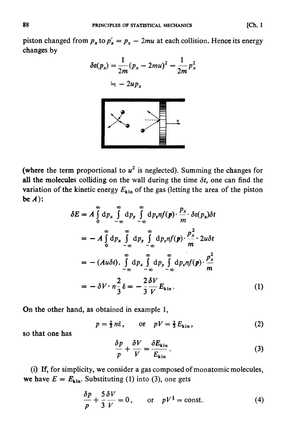
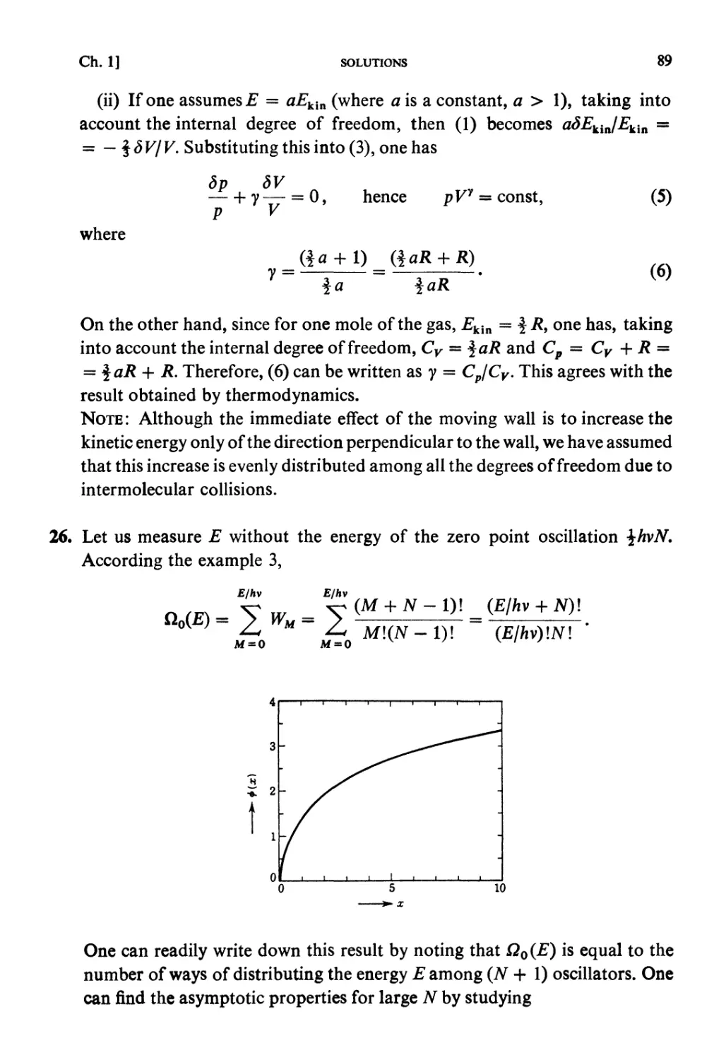
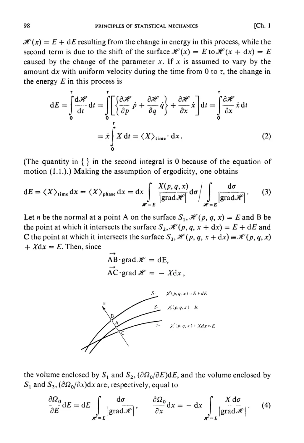
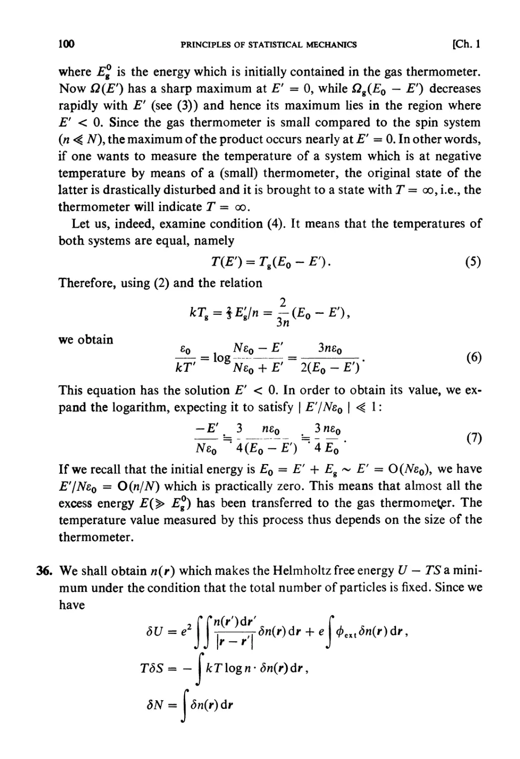
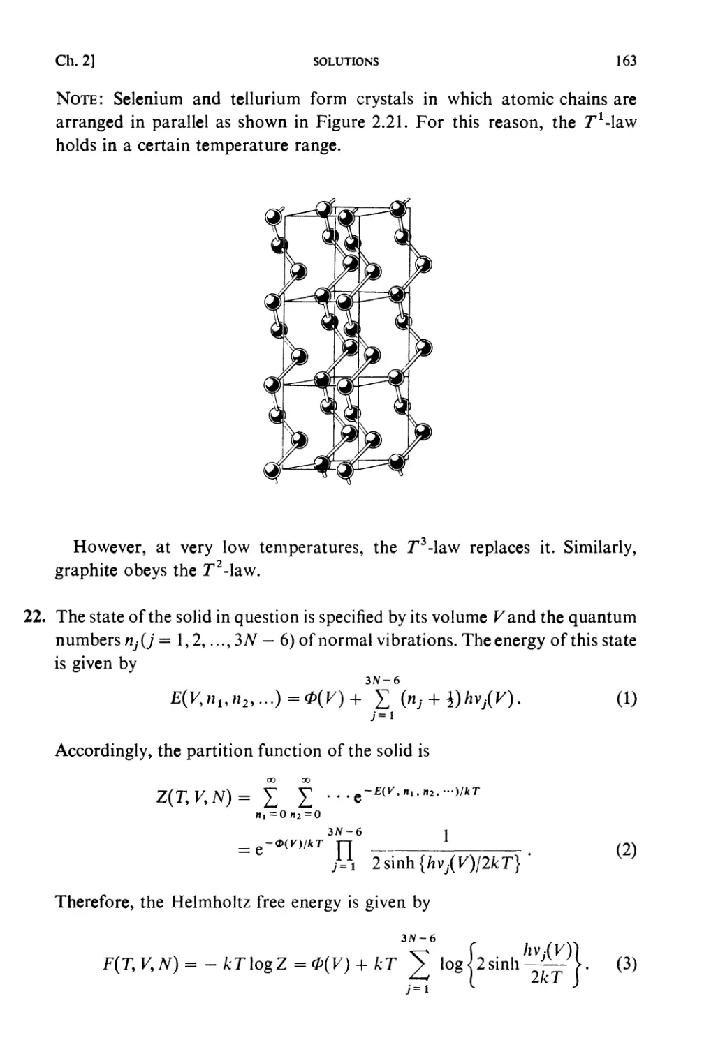
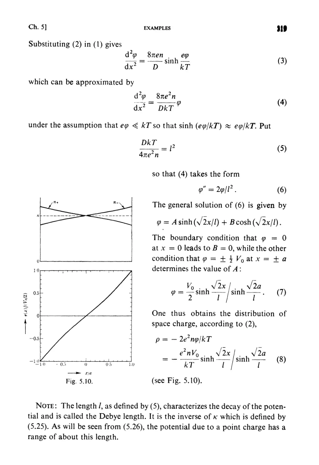
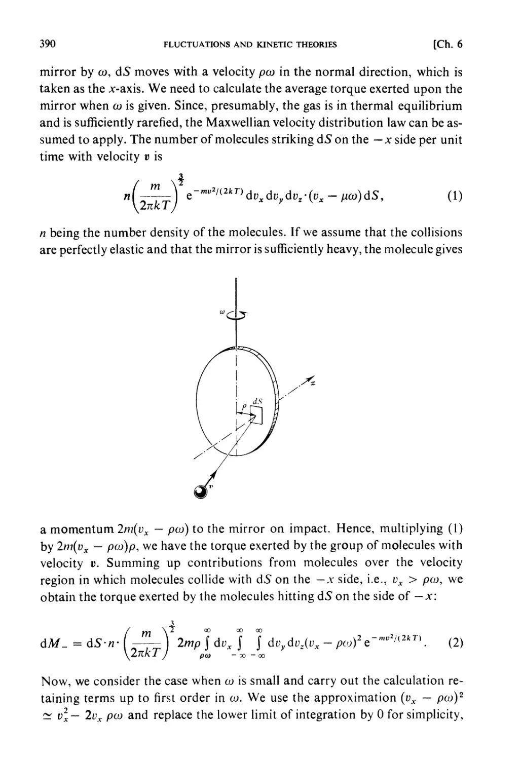
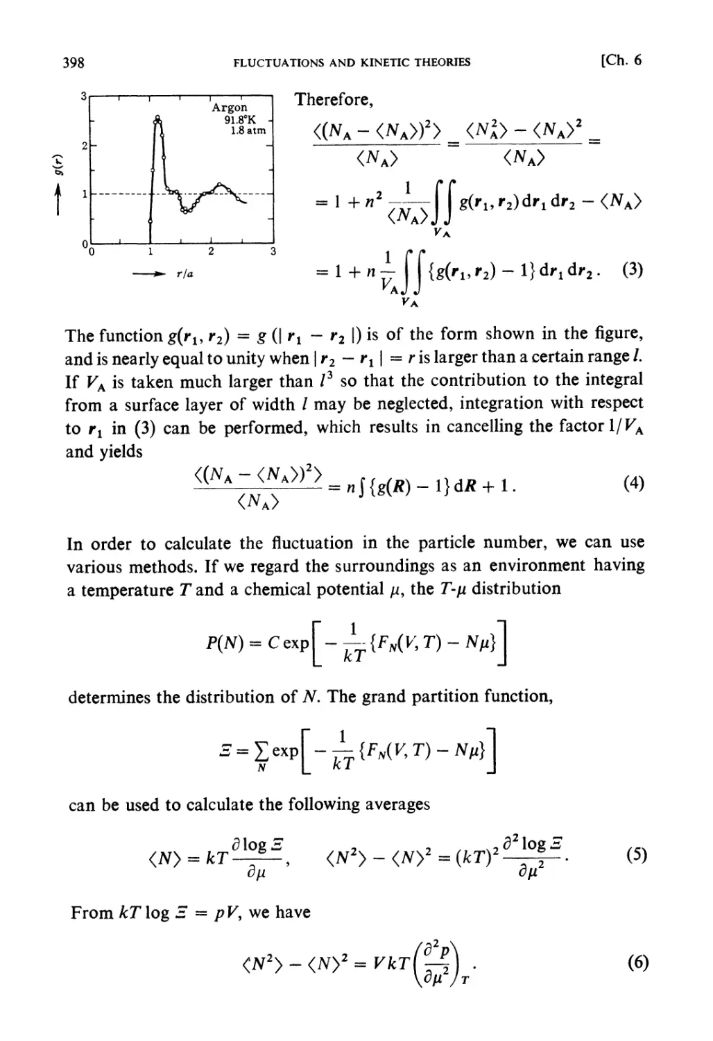
/


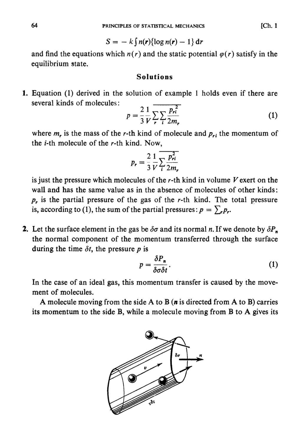
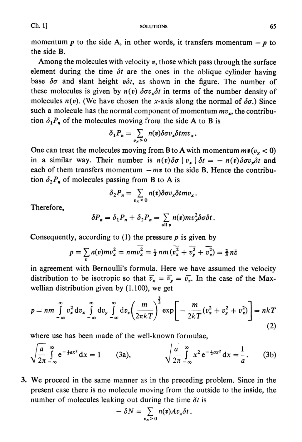


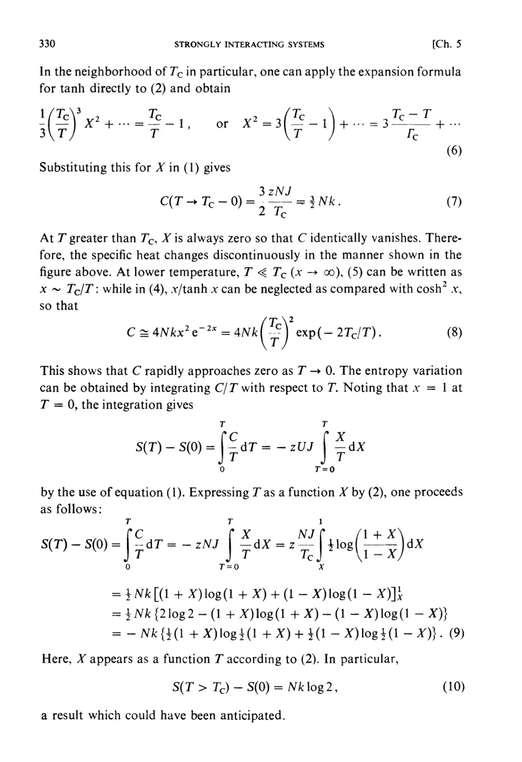
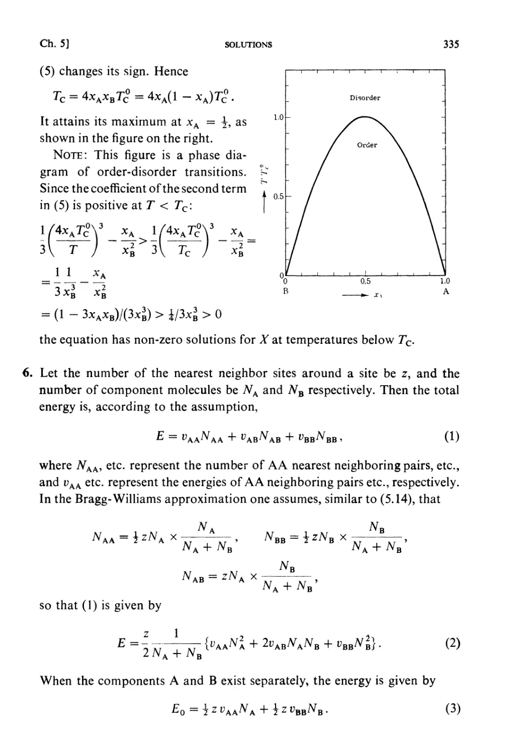


Автор: Kubo R. Ichimura H. Usui T. Hashitsume N.
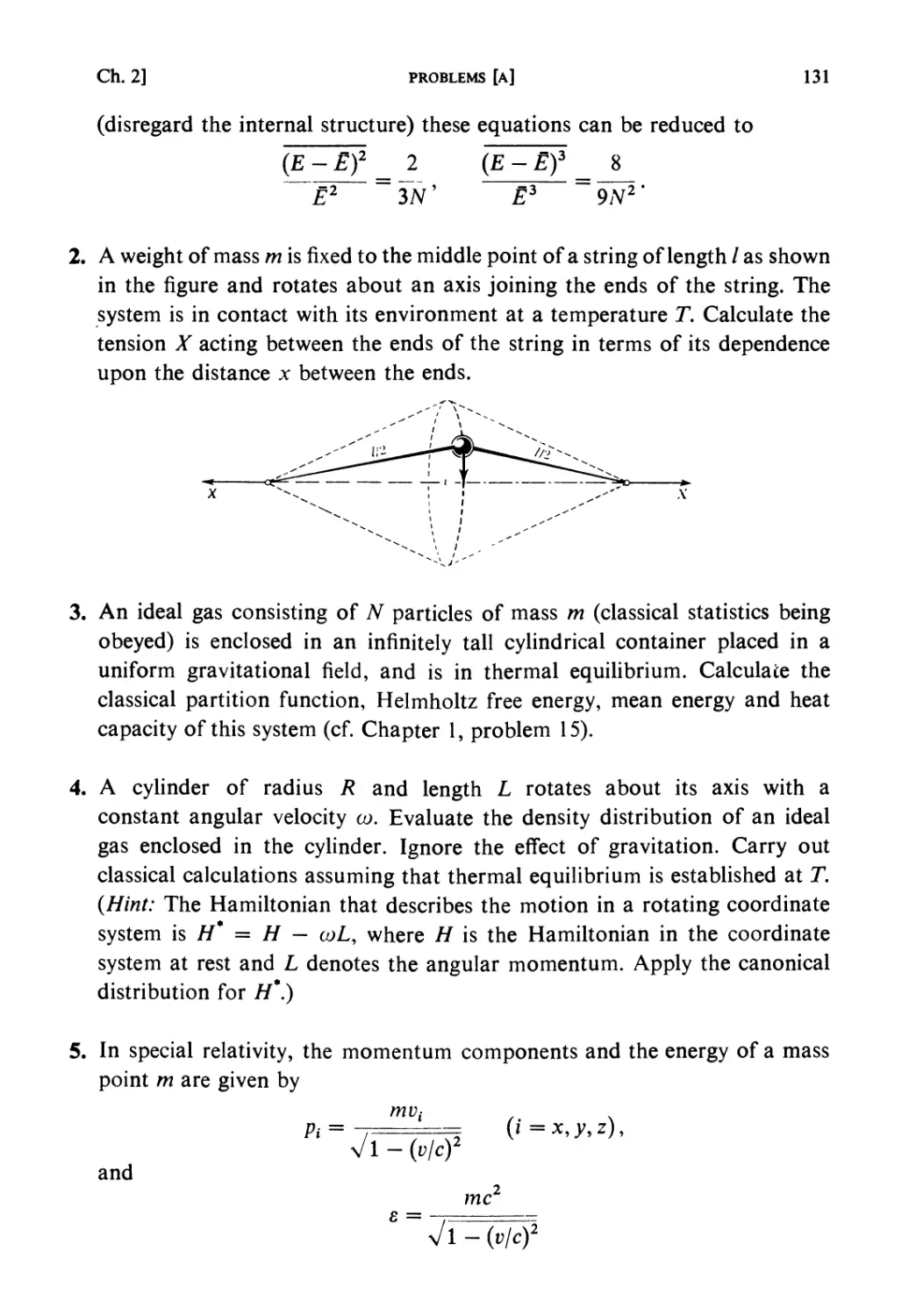
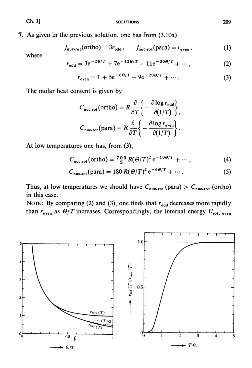
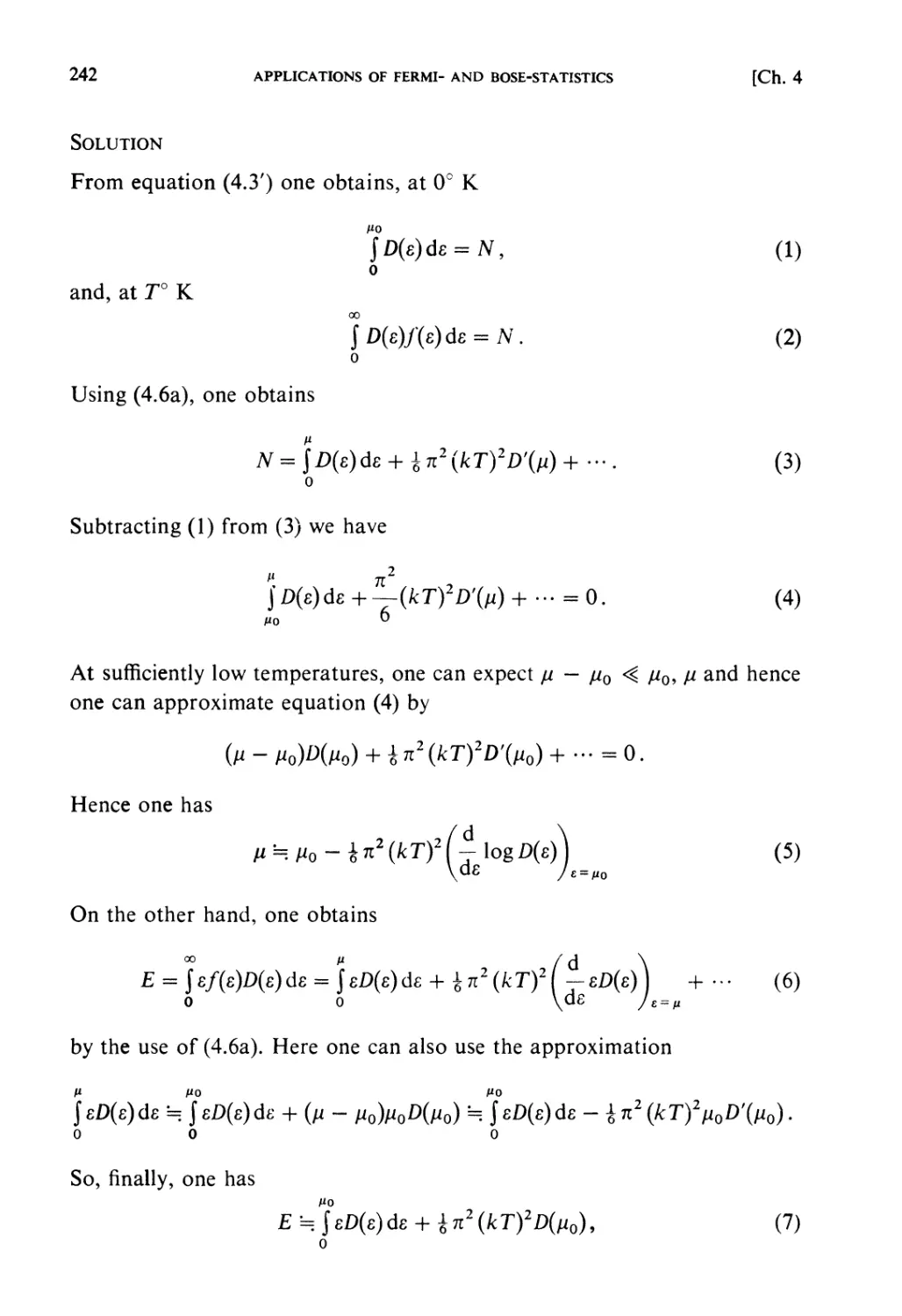
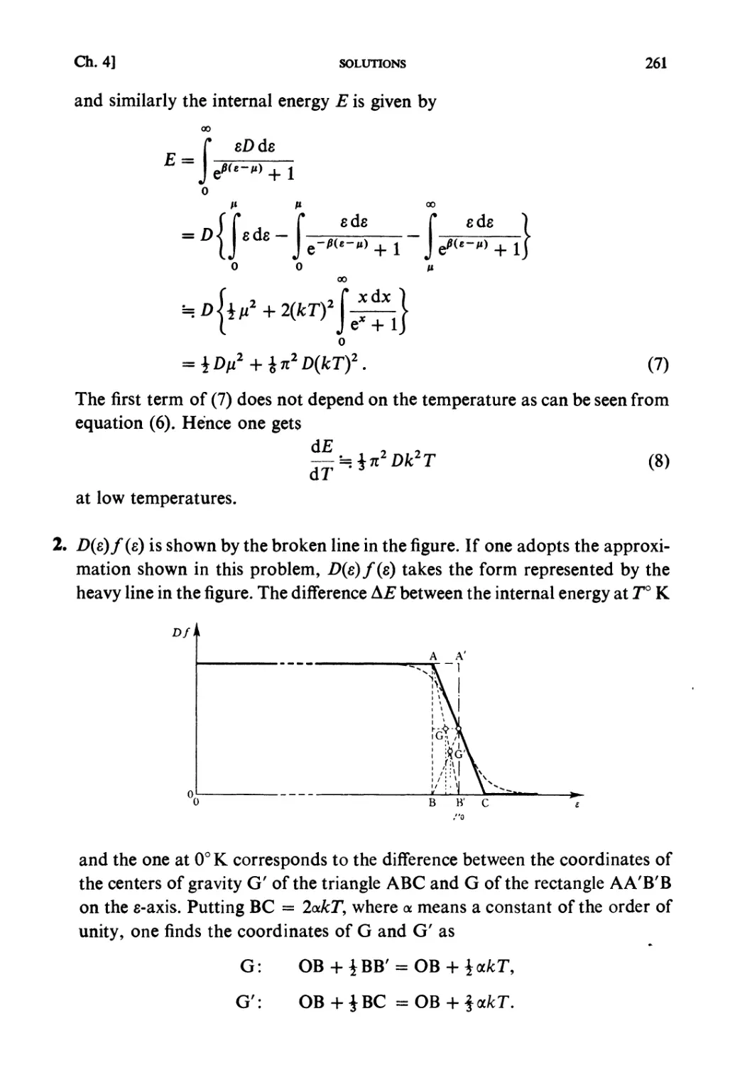
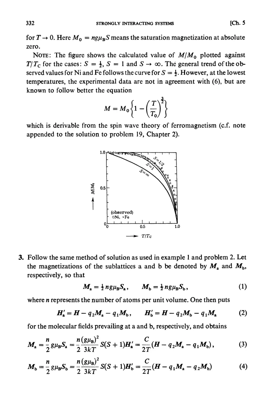
Теги: physics mechanics statistical physics
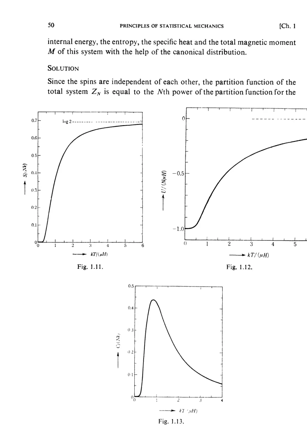
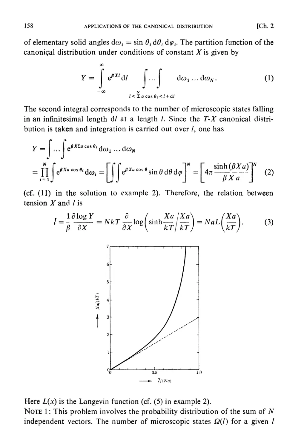
ISBN: 0 444 87103 9
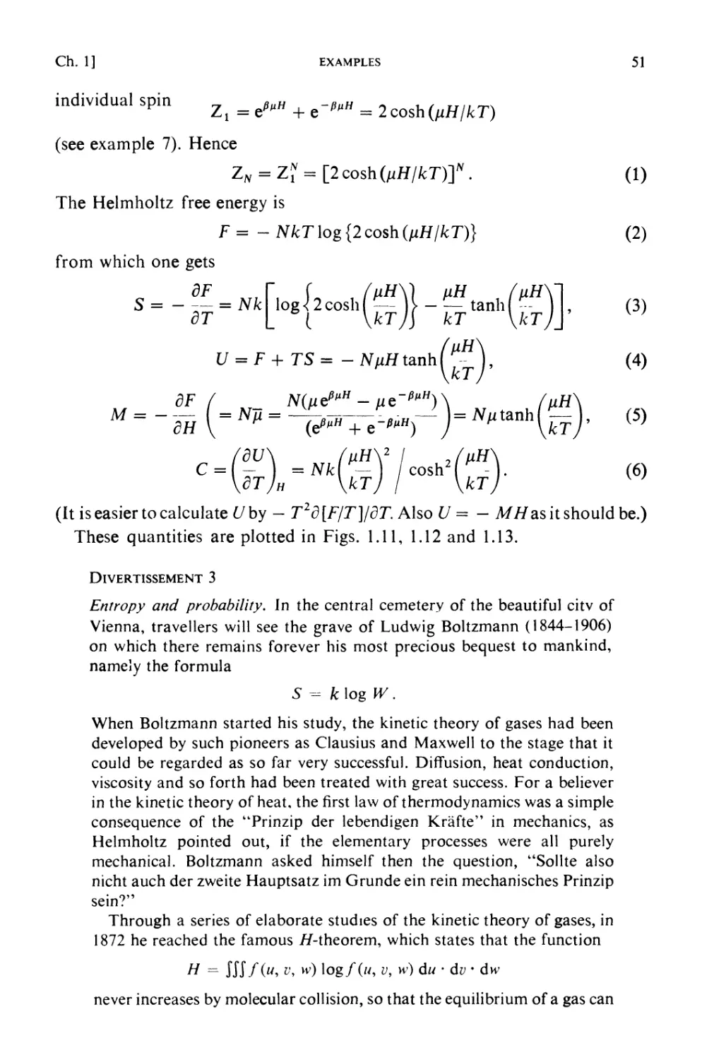
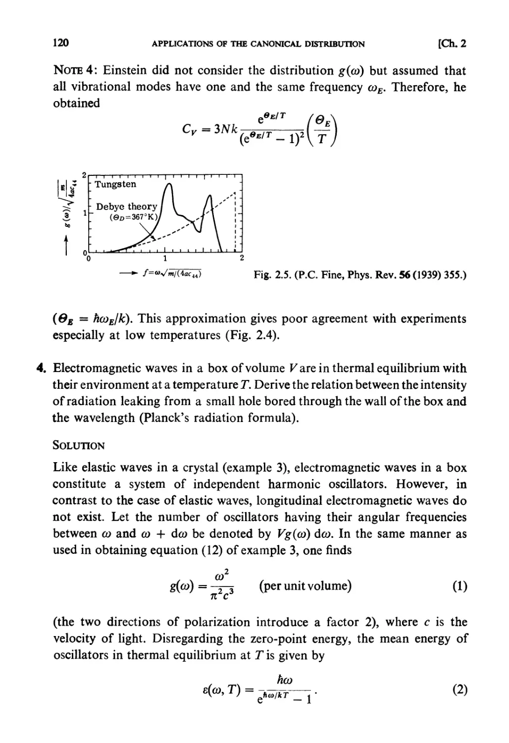
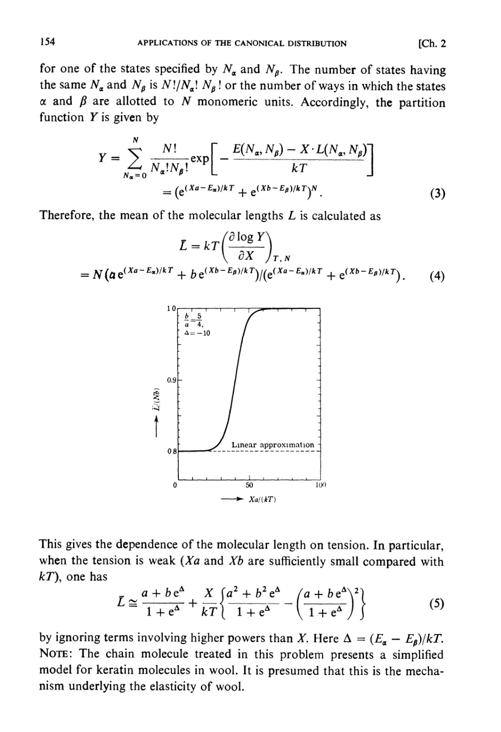
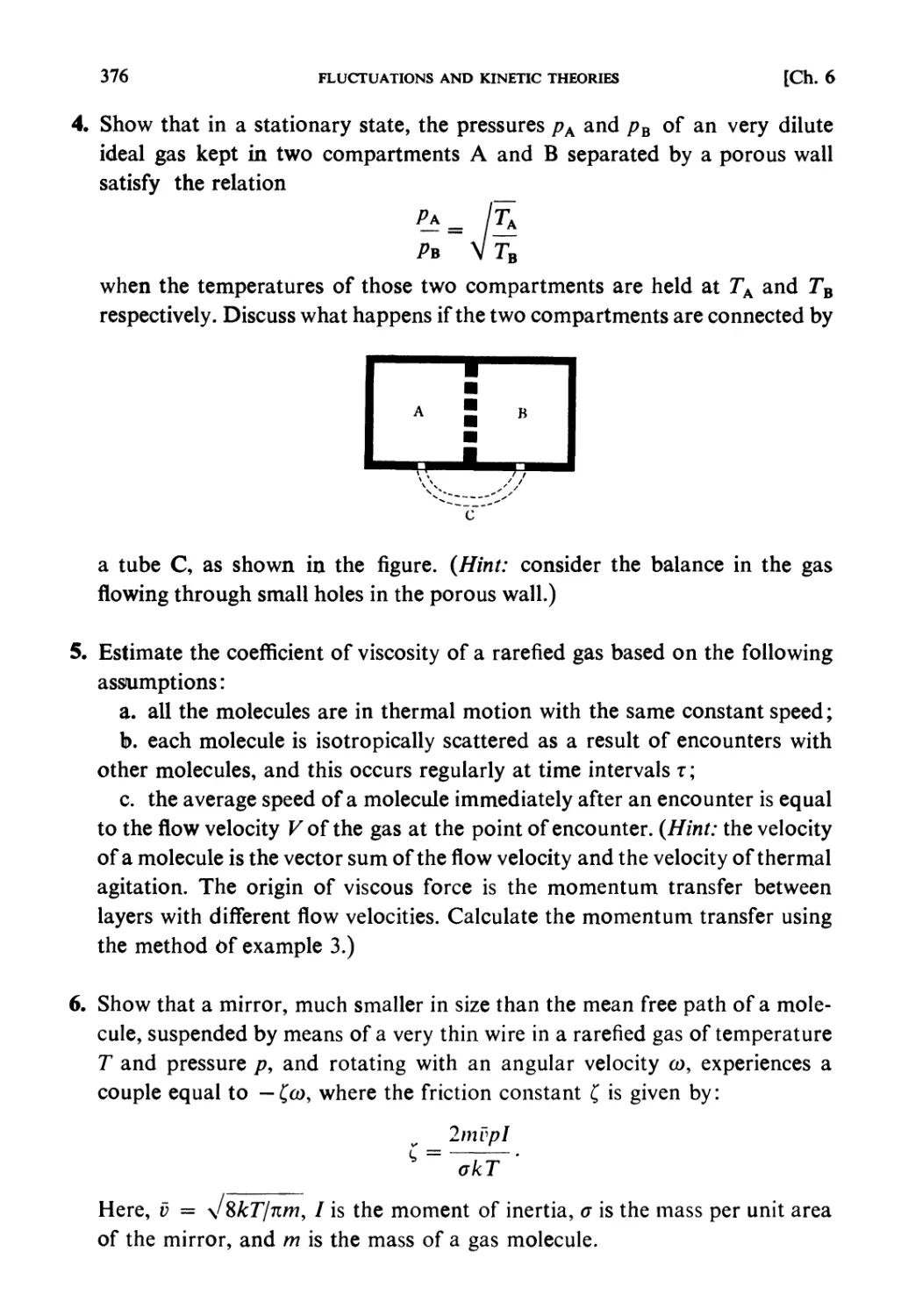
Год: 1990


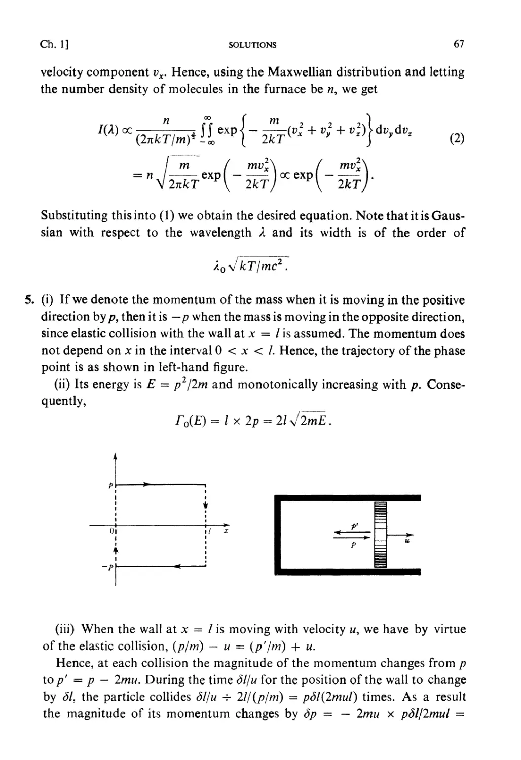
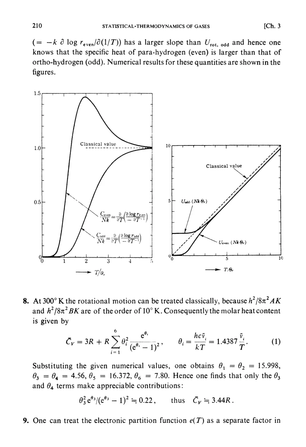
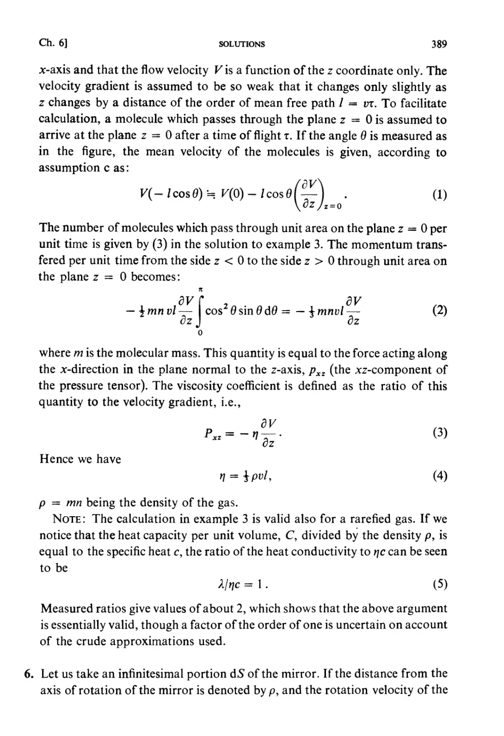
Текст
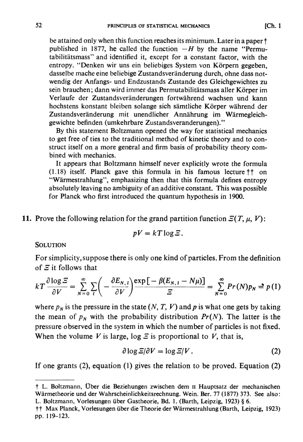
STATISTICAL MECHANICS
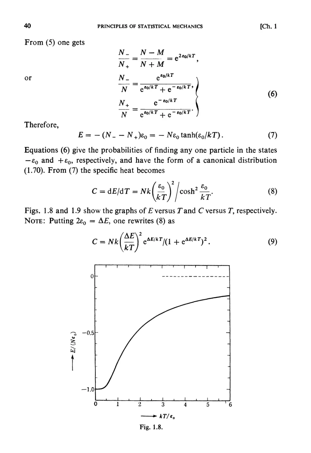
An Advanced Course with
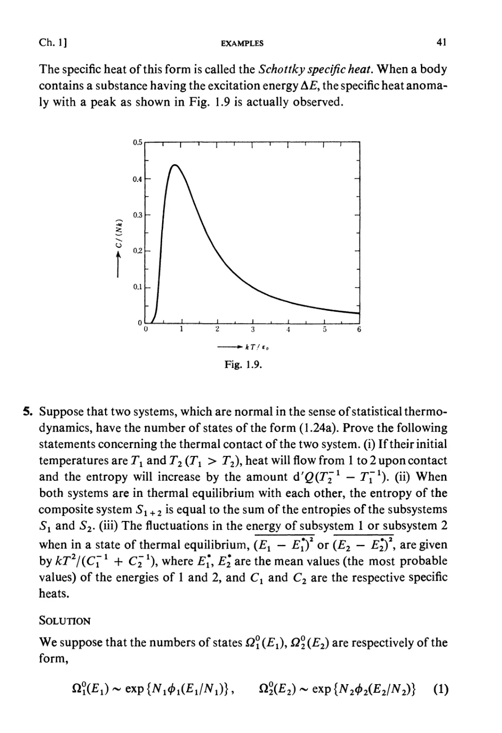
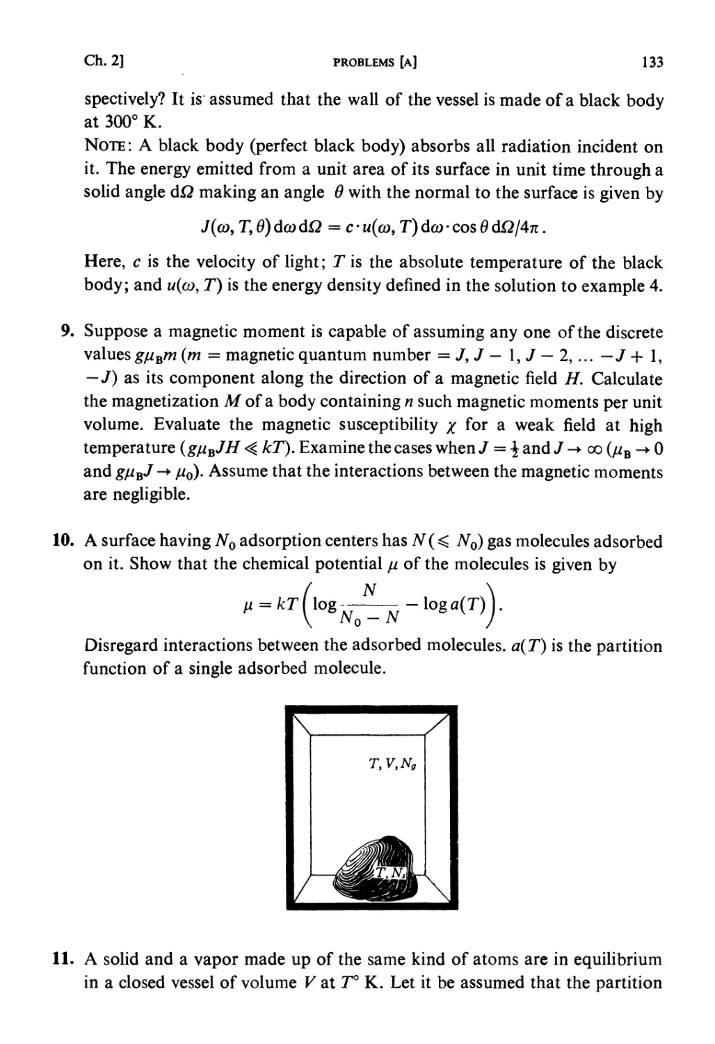
Problems and Solutions
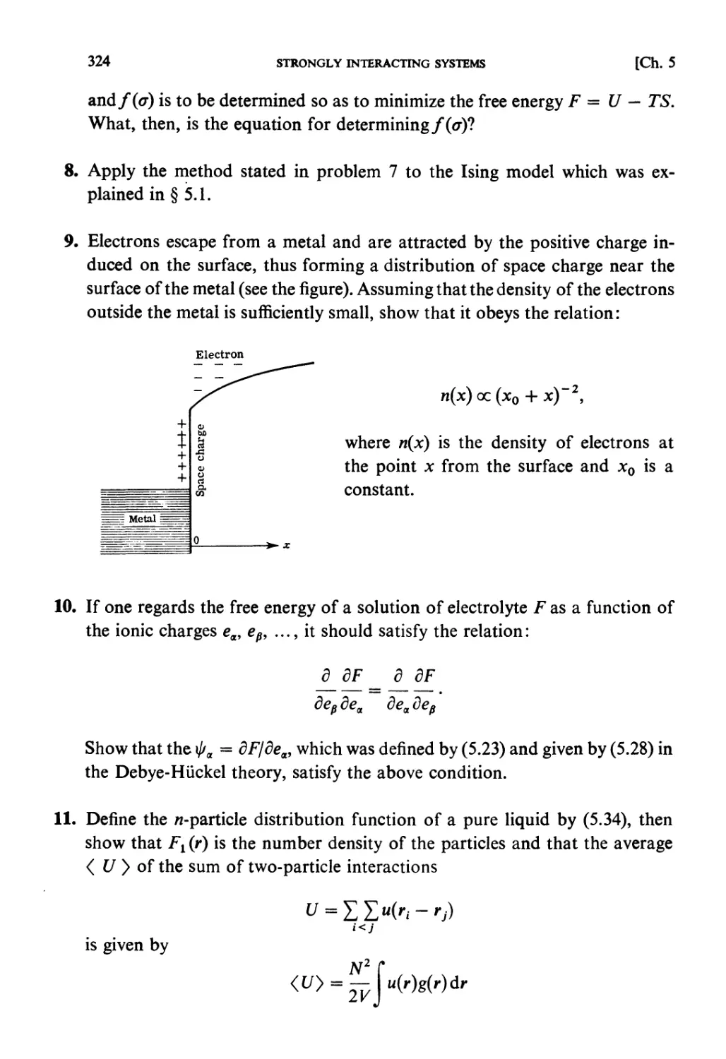
RYOGO KUBO
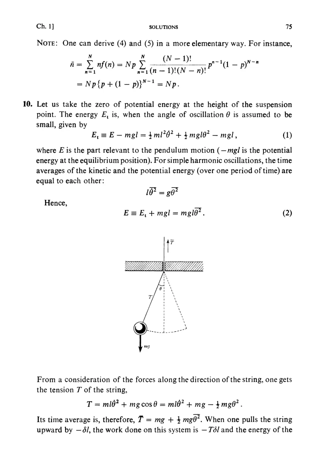
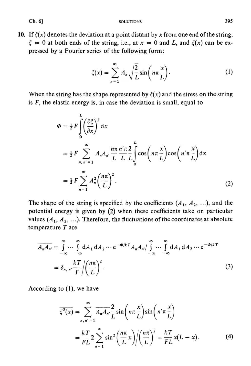
University of Tokyo
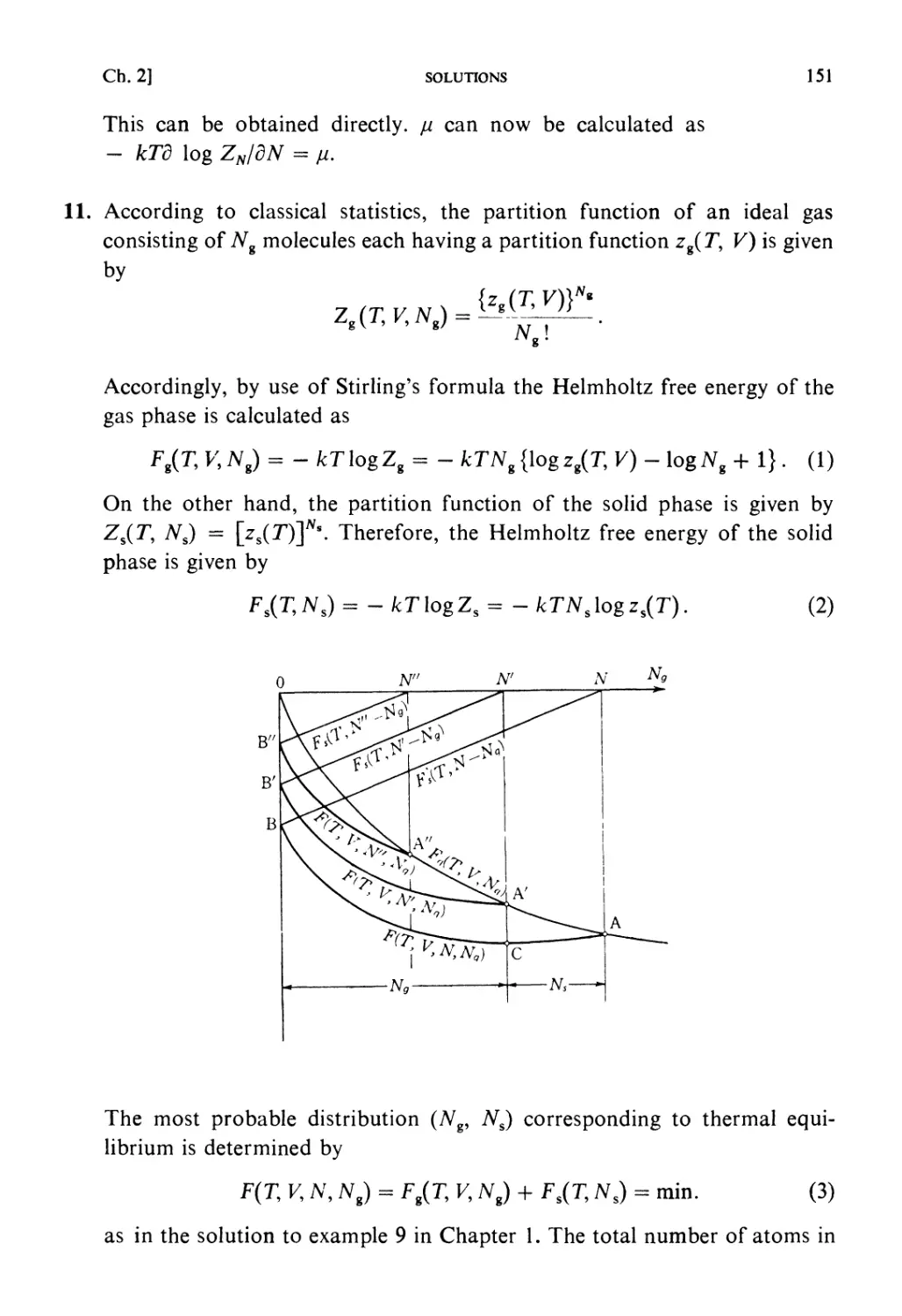
in cooperation with
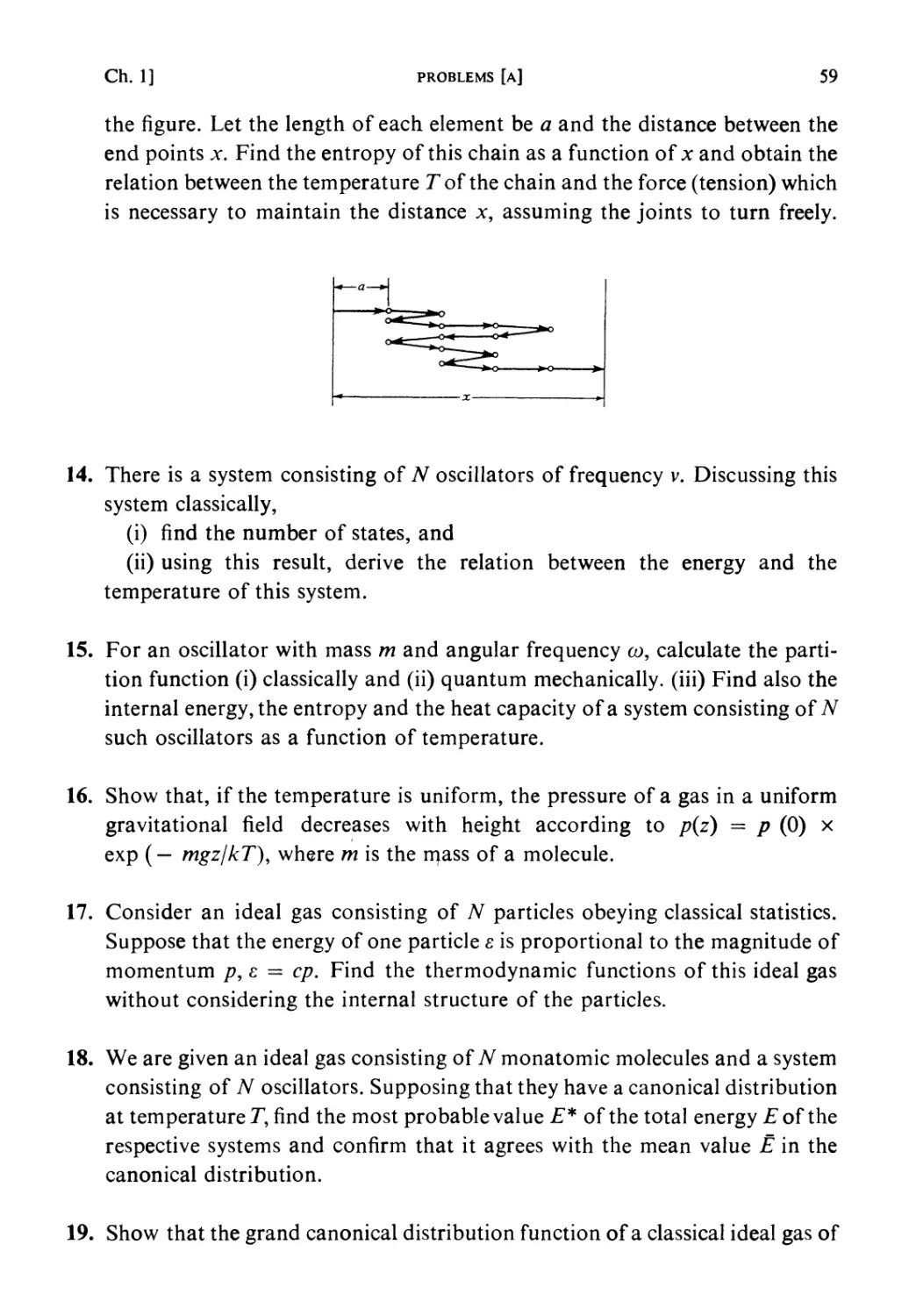
HIROSHI ICHIMURA TSUNEMARU USUI NATSUKI HASHITSUME
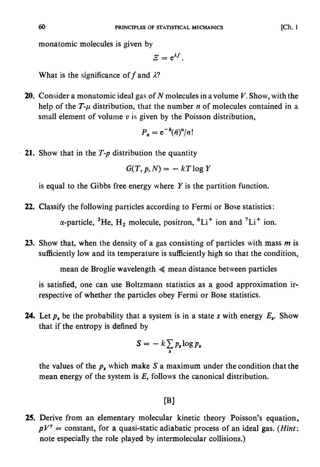
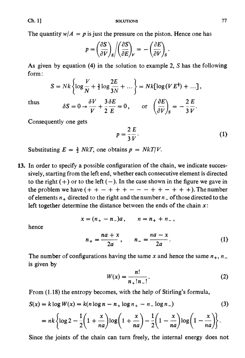
Tokyo Institute of Technology Kyoto University Ochanomizu University
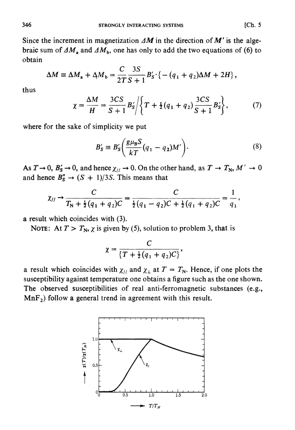
NH
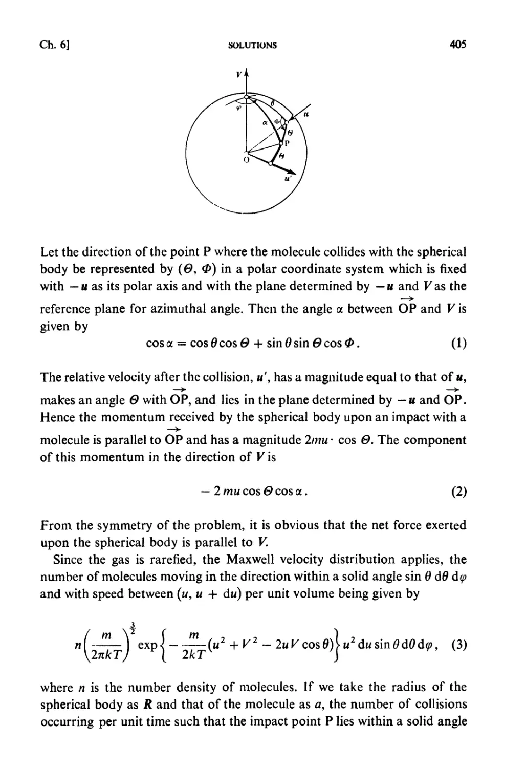
NORTH-HOLLAND
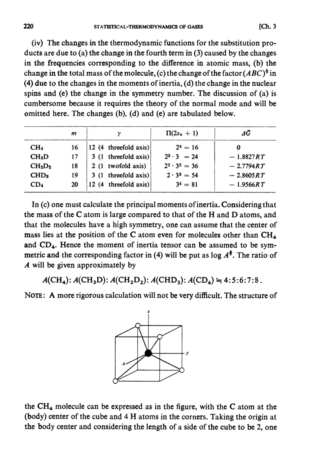
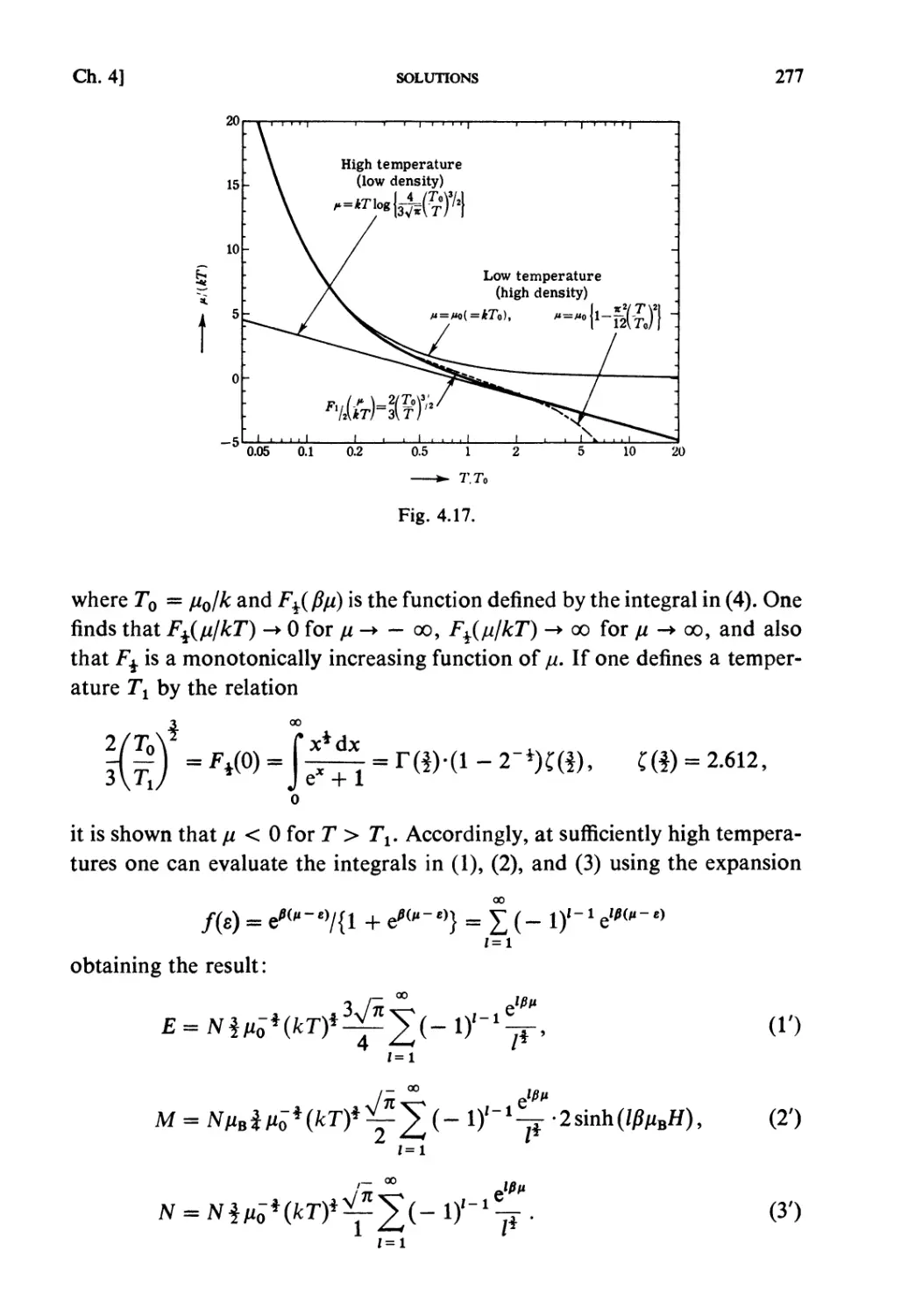
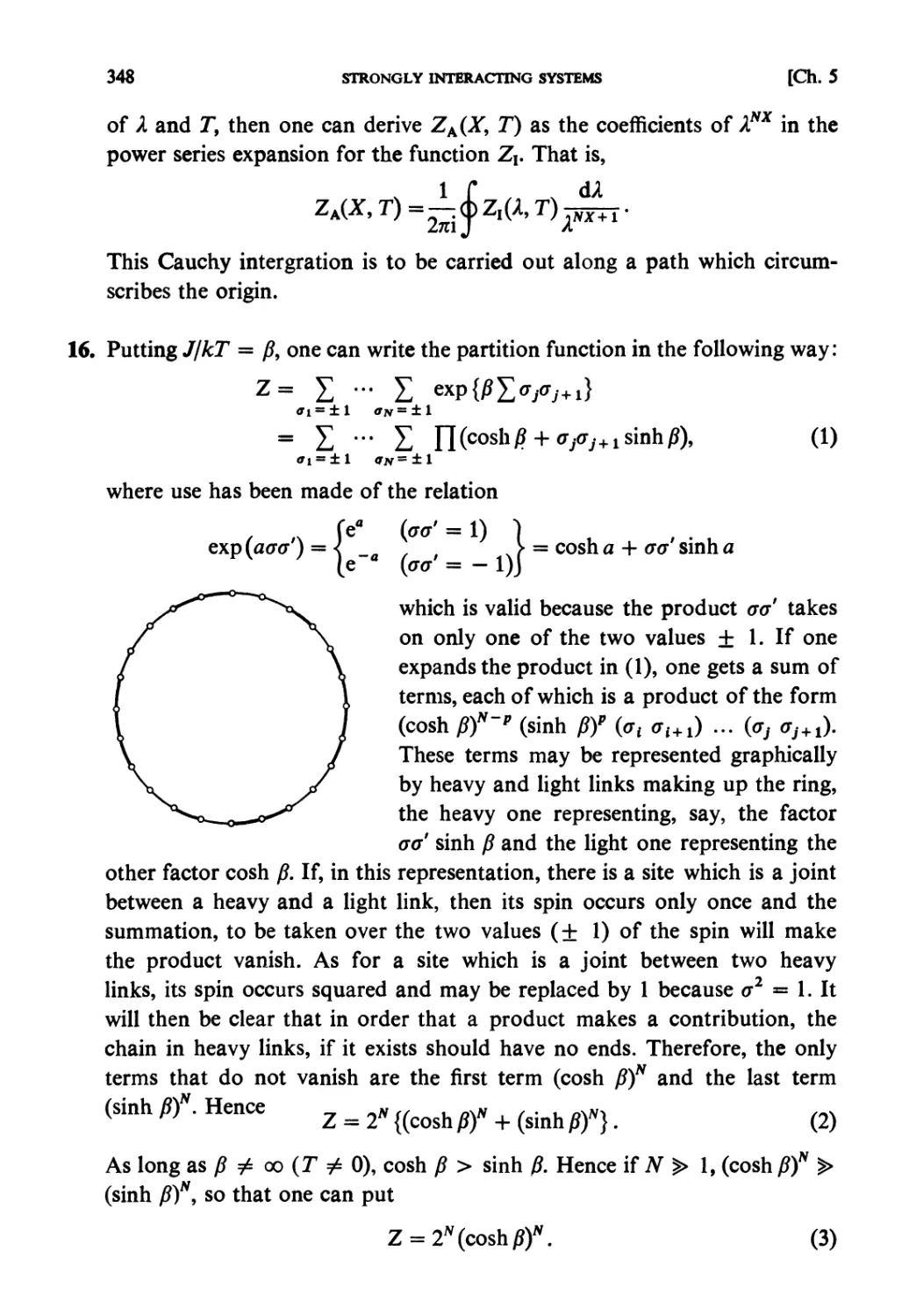
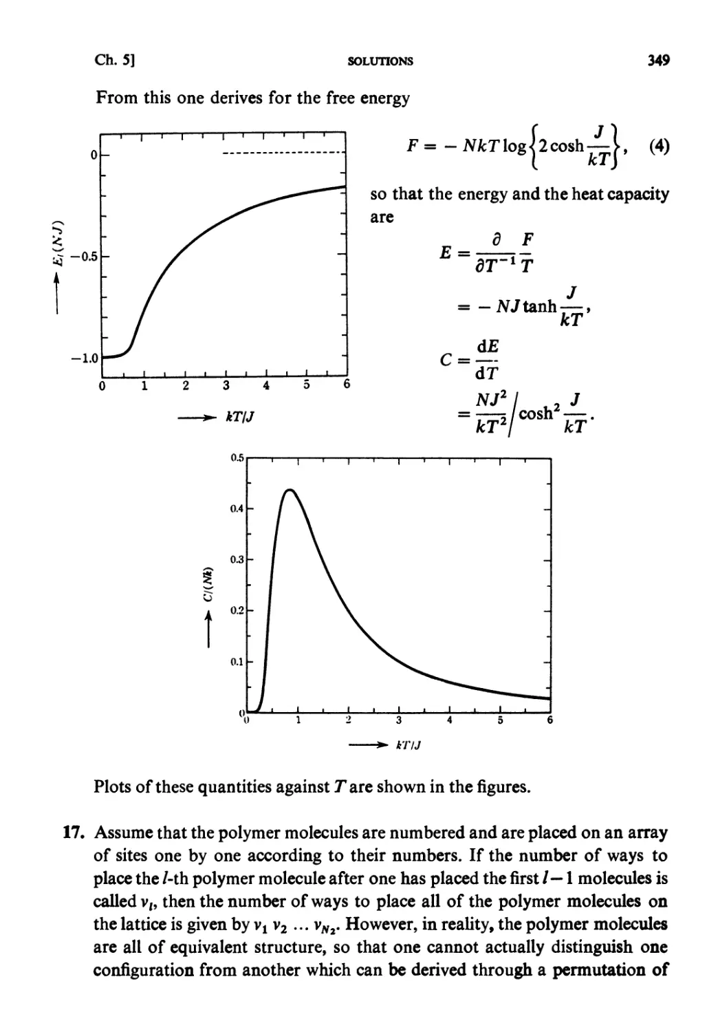
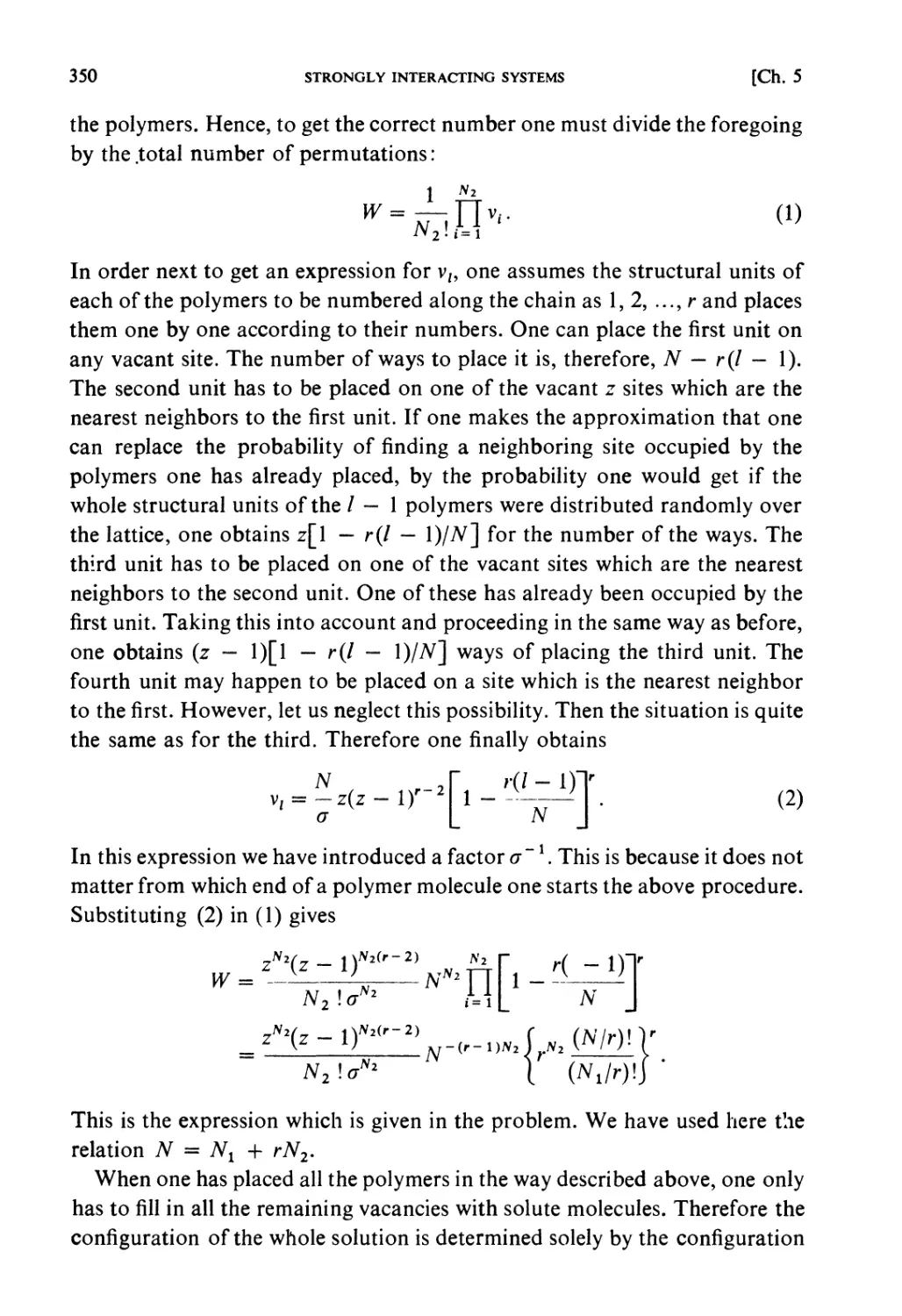
AMSTERDAM • OXFORD • NEW YORK • TOKYO
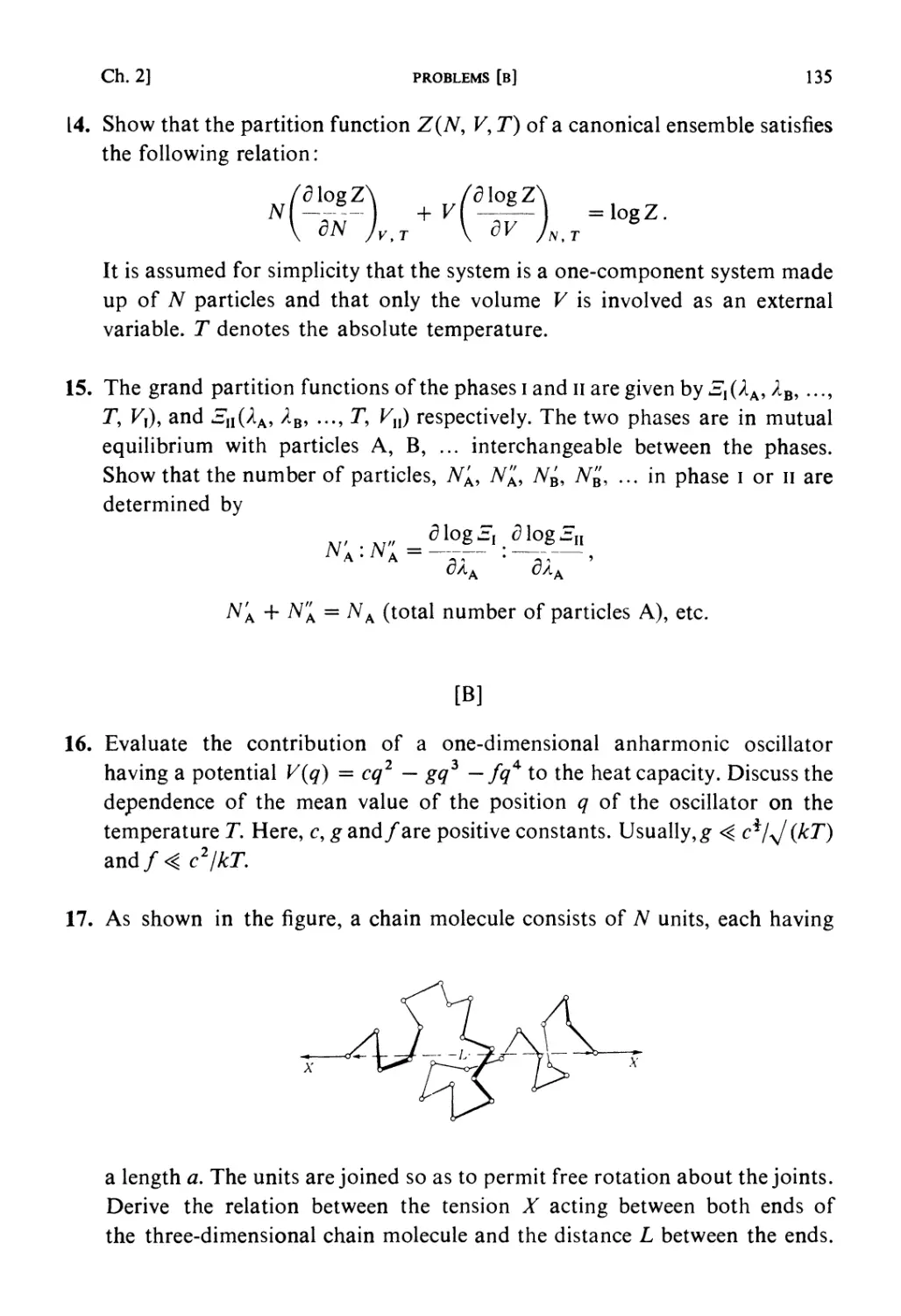
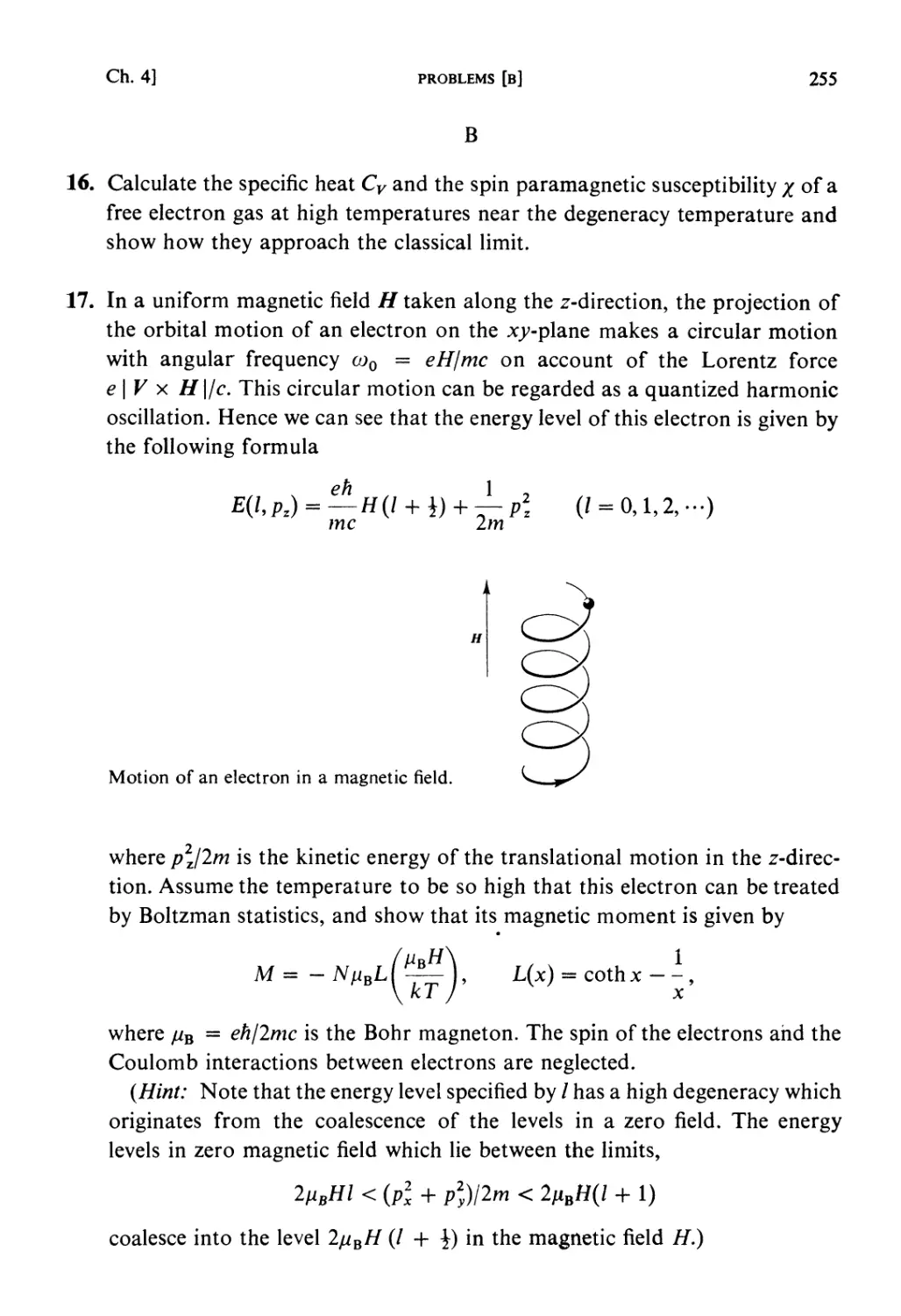
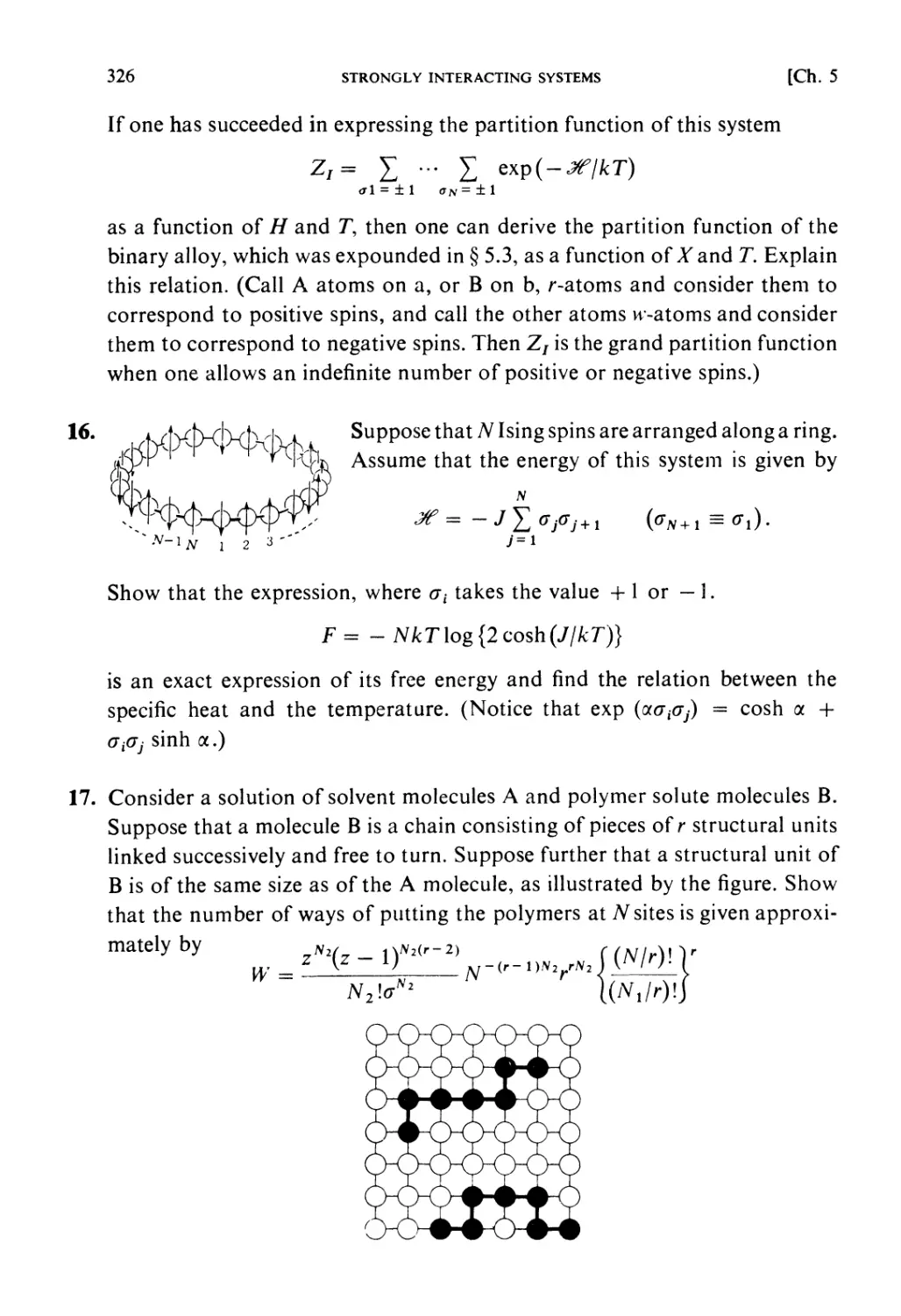
Elsevier Science Publishers B.V., 1965
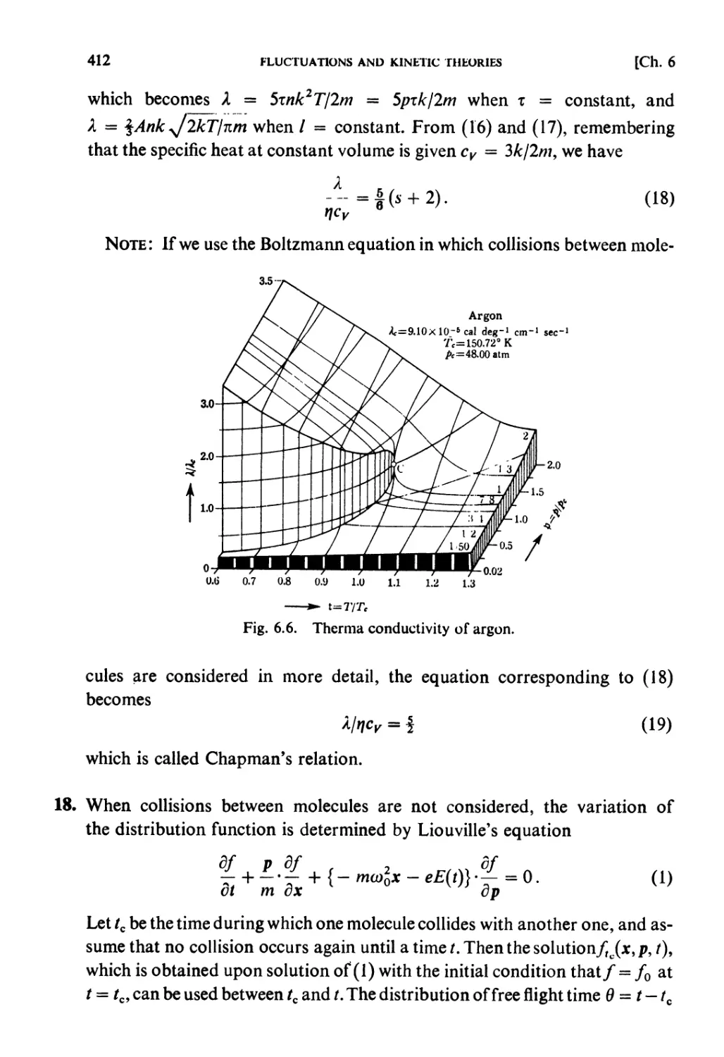
All rights reserved. No part of this publication may be reproduced, stored in a retrieval system, or
transmitted, in any form or by any means, electronic, mechanical, photocopying, recording or
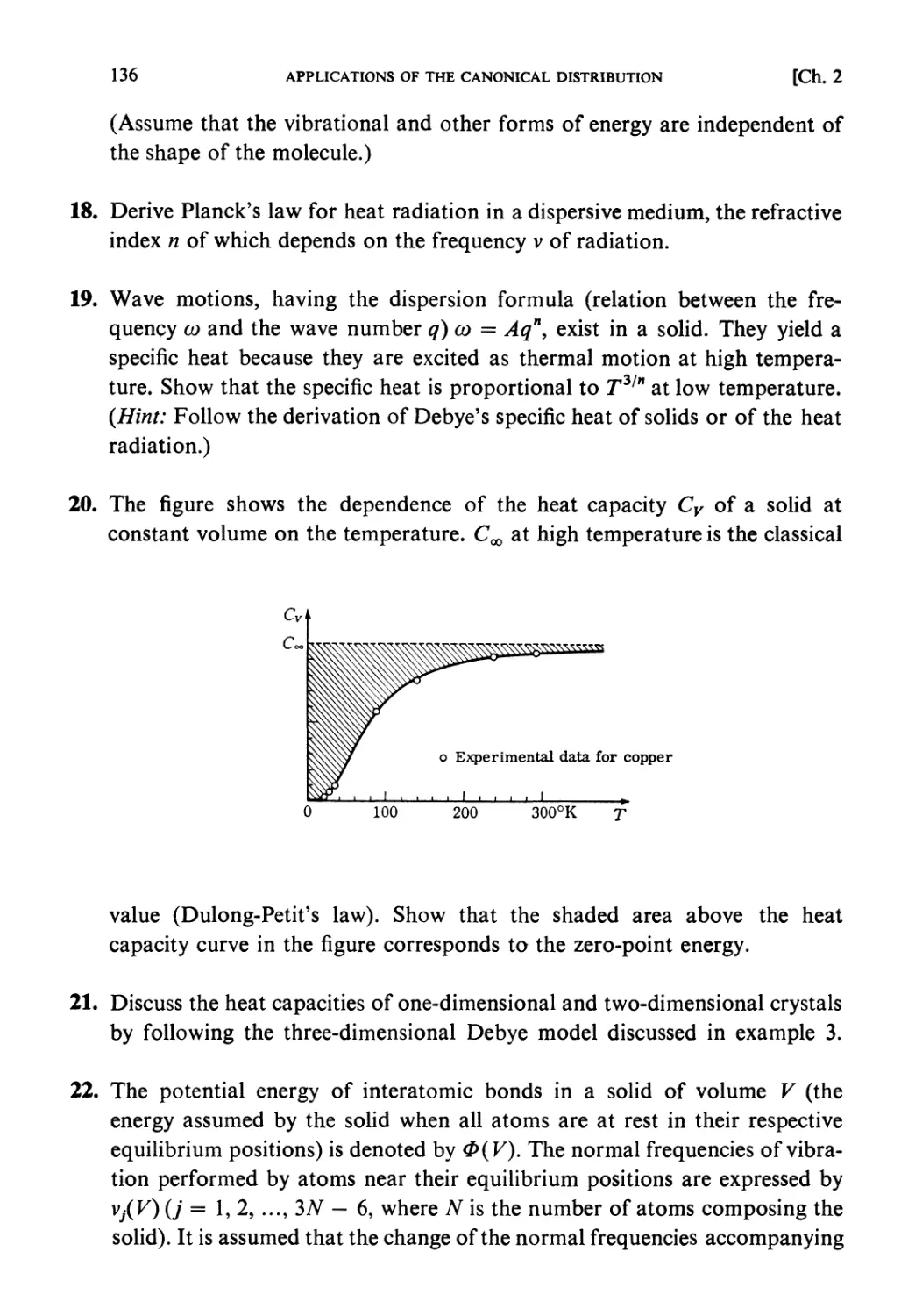
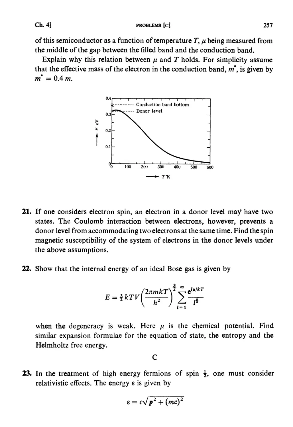
otherwise, without the prior permission of the publisher, Elsevier Science Publishers B.V. (North-
Holland Physics Publishing Division), P.O. Box 103, 1000 AC Amsterdam, The Netherlands.
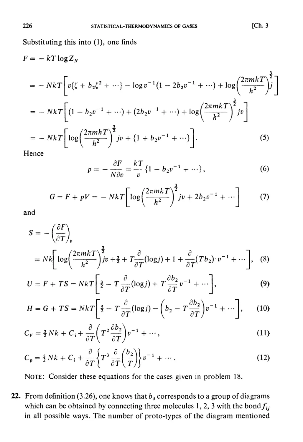
Special regulations for readers in the USA: This publication has been registered with the Copyright
Clearance Center Inc. (CCC), Salem, Massachusetts. Information can be obtained from the CCC
about conditions under which photocopies of parts of this publication may be made in the USA.
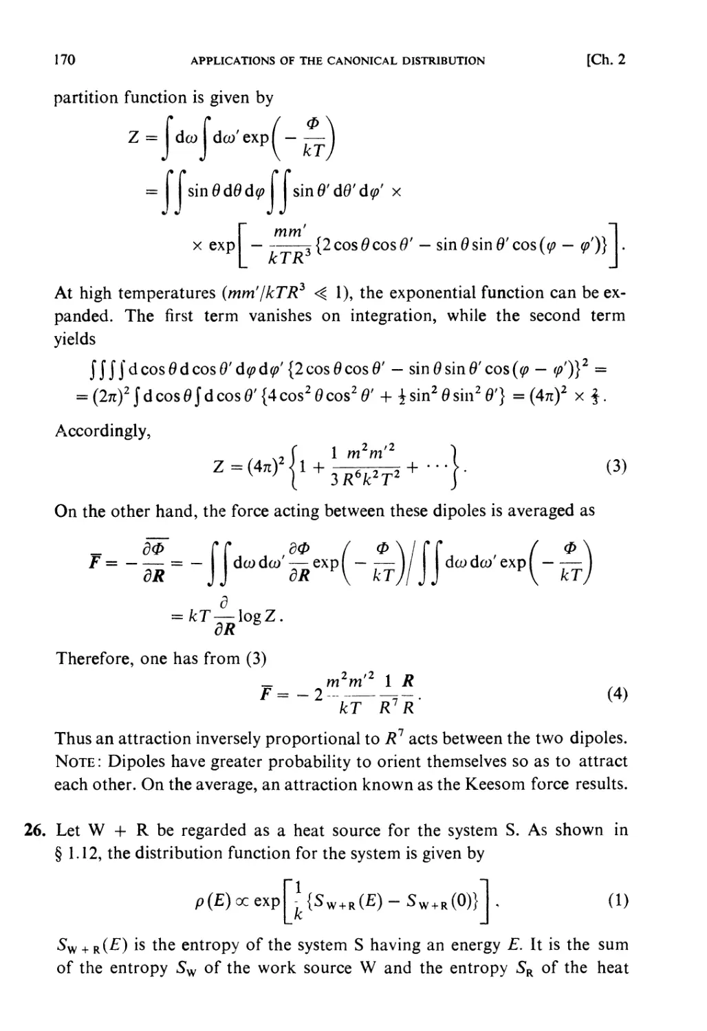
All other copyright questions, including photocopying outside of the USA, should be referred to
the publisher.
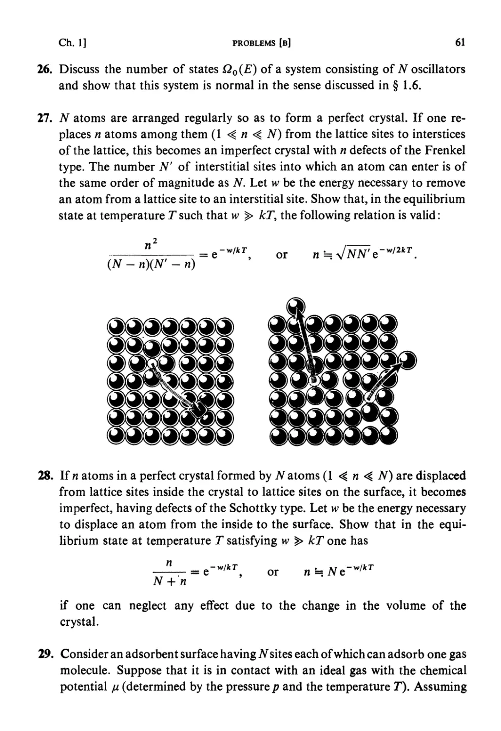
ISBN: 0 444 87103 9 Paperback
First edition (hardbound) 1965
Second edition (hardbound) 1967
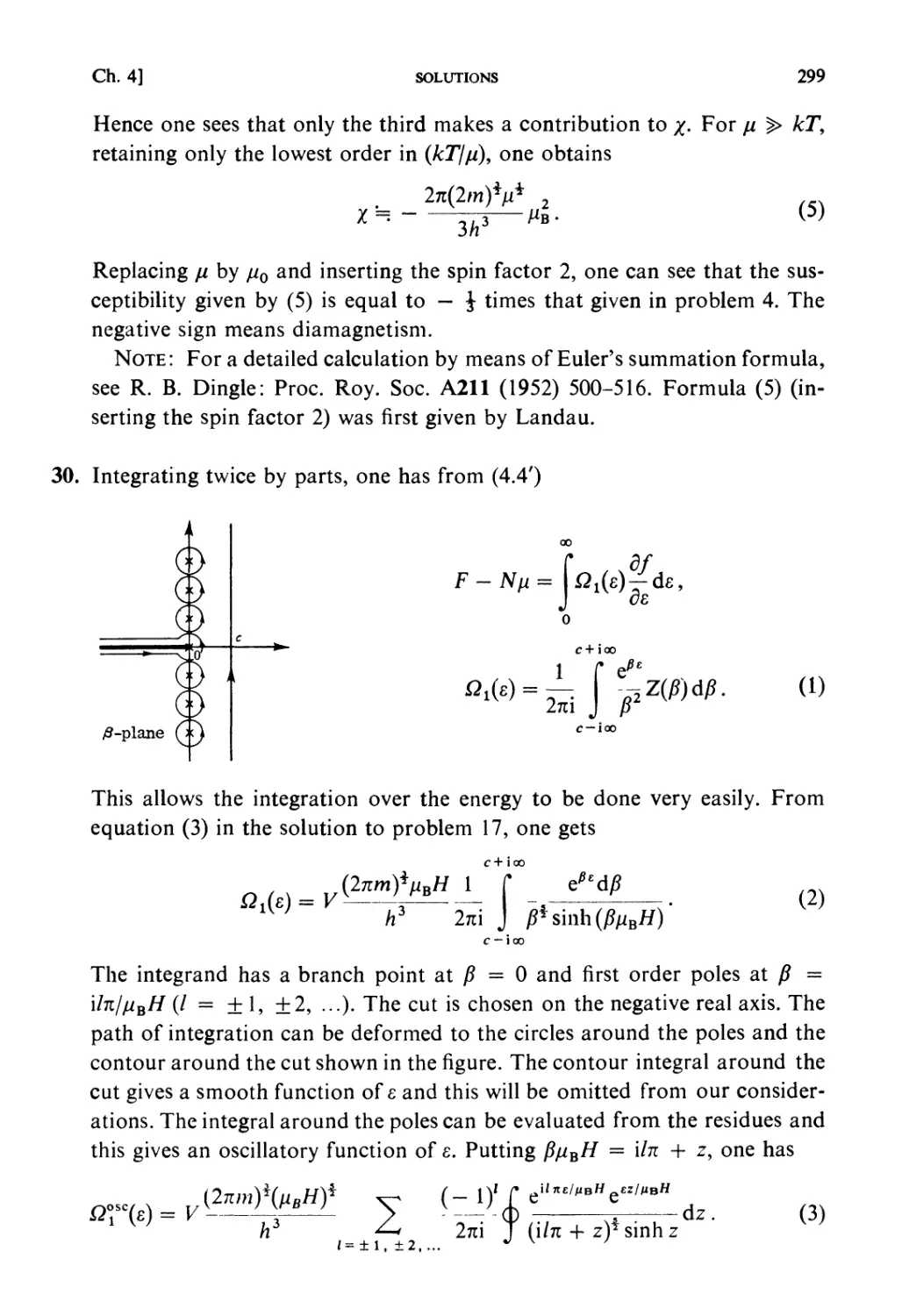
Third edition (hardbound) 1971
Fourth edition (hardbound) 1974
Fifth edition (hardbound) 1978
Sixth edition (hardbound) 1981
Seventh edition (paperback) 1988
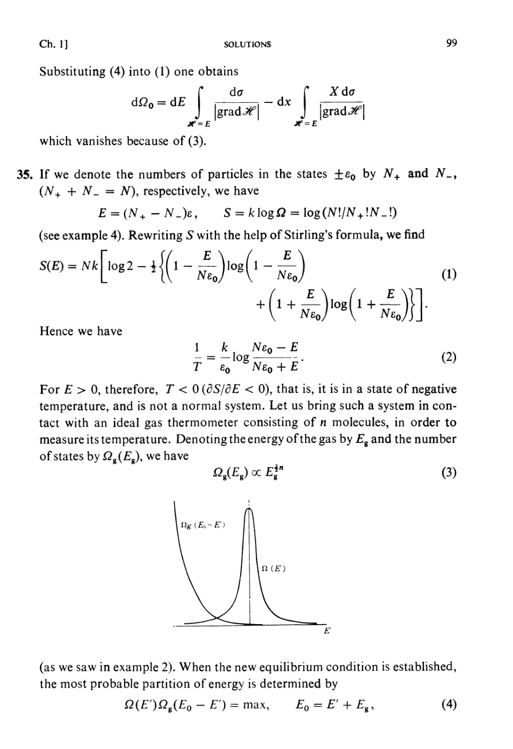
Published by:
North-Holland Physics Publishing
a division of
Elsevier Science Publishers B.V.
P.O. Box 103
1000 AC Amsterdam
The Netherlands
Sole distributors for the USA and Canada:
Elsevier Science Publishing Company, Inc.
52 Vanderbilt Avenue
New York, NY 10017
USA
'North-Holland Personal Library: paperback'
Library of Congress Catalog Card Number 67-20003
Printed in The Netherlands
PREFACE TO ENGLISH EDITION
The original text of this volume is part of the book "Problems and Solutions
in Thermodynamics and Statistical Mechanics", itself one of the "University
Series" published by the Shokabo Publishing Company. At the request of
the present publisher, the English edition is being published in two volumes,
one on thermodynamics and the other on statistical mechanics. Considering
the more urgent interest of university students in statistical mechanics,
this volume has been translated and published first. The volume on
thermodynamics is expected to be published within a year.
The translation was made from the Japanese text by the original authors,
together with a few collaborators. As the editor of the original Japanese
edition and of the English edition, I wish to express my deep appreciation to
Drs. Masaji Kubo, Toshihiko Tsuneto and Satoru Miyake who did the
translation work with the authors, and particularly to Professor Donald C. Worth
of International Christian University, Tokyo, who kindly took the trouble of
helping us with linguistic difficulties. The authors are also indebted to Miss
N. Tokuda for the preparation of the manuscript.
1964
Ryogo Kubo
PREFACE TO JAPANESE EDITION
Thermodynamics and statistical mechanics are indispensable tools in studying
the physics of the properties of matter. Statistical mechanics, together with
quantum mechanics, provides a foundation for modern physics which aims at
the thorough understanding of physical phenomena from the microscopic
viewpoint of atomic physics. Fundamental knowledge and training in
statistical mechanics are therefore of vital importance not only for students
studying the physical properties of matter but also for those who study
nuclear physics or even astrophysics. Outside the realm of physics, its
importance is rapidly penetrating into chemistry, biology and into those vast
areas of technology which owe their growth to the advances in modern
physics.
Thermodynamics belongs completely to classical physics and is
sometimes regarded as unimportant by students of physics who are over-occupied
in learning modern physics. Even for students in chemistry, the present
is different from the time some decades ago when physical chemistry was
almost nothing but chemical thermodynamics. However, it must be stressed
here that the usefulness and unique significance of thermodynamics as
a fundamental science remain as basic today as they were in the latter
half of the last century. Thermodynamics teaches us the value of a
phenomenological approach. It avoids explicit use of physical images
or models such as atoms and molecules. Instead it deals with relations
between somewhat abstract quantities such as energy, entropy, free energy
and so forth. Admittedly it does not give intuitive pictures as atomic theories
do, which is one of the reasons why students find it difficult to gain sufficient
understanding and familiarity to use thermodynamics in real problems. But
the simplicity of the logic of thermodynamics sometimes makes us see more
clearly into the nature of the basic physics of a given problem from very
general principles. This is the great advantage of a phenomenological
approach.
Obviously, however, it is impossible to explore more deeply the
underlying atomic processes in a given physical phenomenon if we confine our
attention to thermodynamics. Such progress is made possible only by
quantum mechanics and statistical mechanics. Statistical mechanics provides
PREFACE TO JAPANESE EDITION
vn
us with a means to link the physical laws of the microscopic world to those
of the macroscopic world. Without close cooperation with statistical
mechanics, quantum mechanics itself would not be able to represent the physics of
the real world. In this sense, statistical mechanics is indispensable as one of
the keystones of modern physics.
Like any other science, statistical mechanics cannot be mastered easily just
by learning its principles once. One has to think by oneself a great deal before
one grasps the way in which to use the statistical approach in one's
thinking, and to apply statistical mechanics to real physical problems. In
statistical mechanics and in thermodynamics, there are certain aspects which are
quite different from other fields of physics. We often meet students who
find difficulty in mastering thermodynamics or statistical mechanics, lacking
confidence in applying it to real problems, although they know the
principles. Such difficulties are due to insufficient and inadequate training.
The purpose of the present book is to provide a guide for students studying
and acquiring facility in thermodynamics and statistical mechanics. Thus it
contains fundamental topics, examples and a fairly large number of problems
with complete solutions. The fundamental topics are rather condensed, but
still they cover all of the points which are basic. This book is meant to be
readable without reference to other textbooks. By reading through these topics
only, one would be able to obtain fundamental knowledge of
thermodynamics and statistical mechanics. The examples are partly to supplement
the fundamental topics, but they are primarily meant to show the reader how
the principles are applied to physical problems.
The problems are classified into three groups, A, B and C, in order of
increasing difficulty. If a reader has enough time he may go through all problems in
each chapter. But, if not, it is recommended that he studies first the problems
in group A throughout the whole book and then later comes back to try B and
C. By just finishing group A problems, he will find himself to have obtained a
much better understanding of physics. The number of group A problems
is fairly large, so that he may even select about half of these and come back
later to the other half. The subjects in the fundamental topics and examples
which are marked by + are not needed in solving problems in group A.
In this bookf, thermodynamics and statistical mechanical problems are
mostly limited to those of equilibrium states. It might be desirable to include
kinetic methods and extensions of thermodynamics and statistical mechanics
t The reader is reminded that this text is a translation of the Preface to the original
Japanese edition, in which thermodynamics and statistical mechanics are contained in
one volume.
vra
PREFACE TO JAPANESE EDITION
which apply to non-equilibrium problems. We had, however, to content
ourselves in treating such topics in a limited way only in the last chapter
(Chapter 6 of the present English edition). This is because the whole volume
had become much larger than the original plan and also because such non-
equilibrium problems are certainly somewhat advanced.
As mentioned previously in this preface, quantum mechanics is the
fundamental dynamics of the microscopic world. In this sense, statistical mechanics
ought to be essentially quantum-statistics. However, since the present book
devotes itself to clear understanding of the nature of statistical
considerations, only an elementary knowledge of quantum mechanics is required in
studying problems in groups A and B. Therefore, even those students who
are not specializing in physics but have only an elementary background
in quantum mechanics will not find any serious difficulty in starting to
study this book.
What is most important in studying a physical problem is to grasp it as a
problem in physics. Mathematical manipulations may sometimes be tedious
and sometimes may require specialized techniques. Training in mathematical
methods should not be ignored, but it would be a serious mistake if one was
to be dazzled by the mathematics and to forget the physics. Teachers often
meet students' papers in which the student seems to be in no doubt about the
numerical answers although they are in error by two or three orders of
magnitudes or are dimensionally incorrect. Professor H. Nagaoka (a pioneer
physicist in Japan) was carrying out calculations on a blackboard in his class.
He changed the sign of his answer saying "It is plus rather than minus.
Isn't it?" Mathematical calculations may very often be in error. A physical
mind is very important, for this can give you the right sign even when your
calculation betrays you. An answer obtained by calculation is in many cases
easily understood, at least qualitatively. It may not be guessed before making
calculations, but one should not forget to think it over again in order to
see if one can see some physical meaning contained in it. Such remarks are
not given in each solution of the problems, so that we should like to
emphasize here the importance of such reasoning.
Here and there between the pages some comments t are inserted under the
title "Divertissement". While giving seminars to students we sometimes take
a rest to drink a cup of tea and chat. We hope that the reader will spare a few
minutes at these spots to listen to a chat from the authors, drinking tea or
coffee or just smoking.
t These are revised in this English edition.
PREFACE TO JAPANESE EDITION
IX
The fundamental topics were mostly written by R. K. Examples and
problems were selected after repeated discussion by all the authors. The final check
of the solutions was made by R. K. and the whole design of the book was
made by N. H. The authors would appreciate it if readers would kindly
point out any mistakes which may have escaped our notice.
Five years have passed since this book was originally planned, and two
years since we started actually to write it. The undertaking proved to be
much more difficult than we anticipated. The authors are particularly
grateful to Mr. K. Endo, editor of Shokabo Publishing Company, for his continual
encouragement and help.
January, 1961
Ryogo Kubo
CONTENTS
CHAPTER 1. PRINCIPLES OF STATISTICAL MECHANICS
Fundamental Topics
§1.1. Microscopic States 1
§1.2. Statistical Treatment 3
§ 1.3. The Principle of Equal Weight and the Microcanonical
Ensemble 5
§ 1.4. The Thermodynamic Weight of a Macroscopic State and
Entropy 7
§ 1.5. Number of States and the Density of States 8
§ 1.6. Normal Systems in Statistical Thermodynamics 10
§1.7. Contact between Two Systems 11
§1.8. Quasi-Static Adiabatic Process 14
§1.9. Equilibrium between Two Systems in Contact 15
§1.10. Fundamental Laws of Thermodynamics 18
§ 1.11. The Most Probable State and Fluctuations 19
§1.12. Canonical Distributions 21
§ 1.13. Generalized Canonical Distributions 23
§ 1.14. Partition Functions and Thermodynamic Functions. . 25
§ 1.15. Fermi-, Bose-, and Boltzmann- Statistics 28
§ 1.16. Generalized Entropy 31
Examples 32
Problems 56
Solutions 64
CHAPTER 2. APPLICATIONS OF THE
CANONICAL DISTRIBUTION
Fundamental Topics
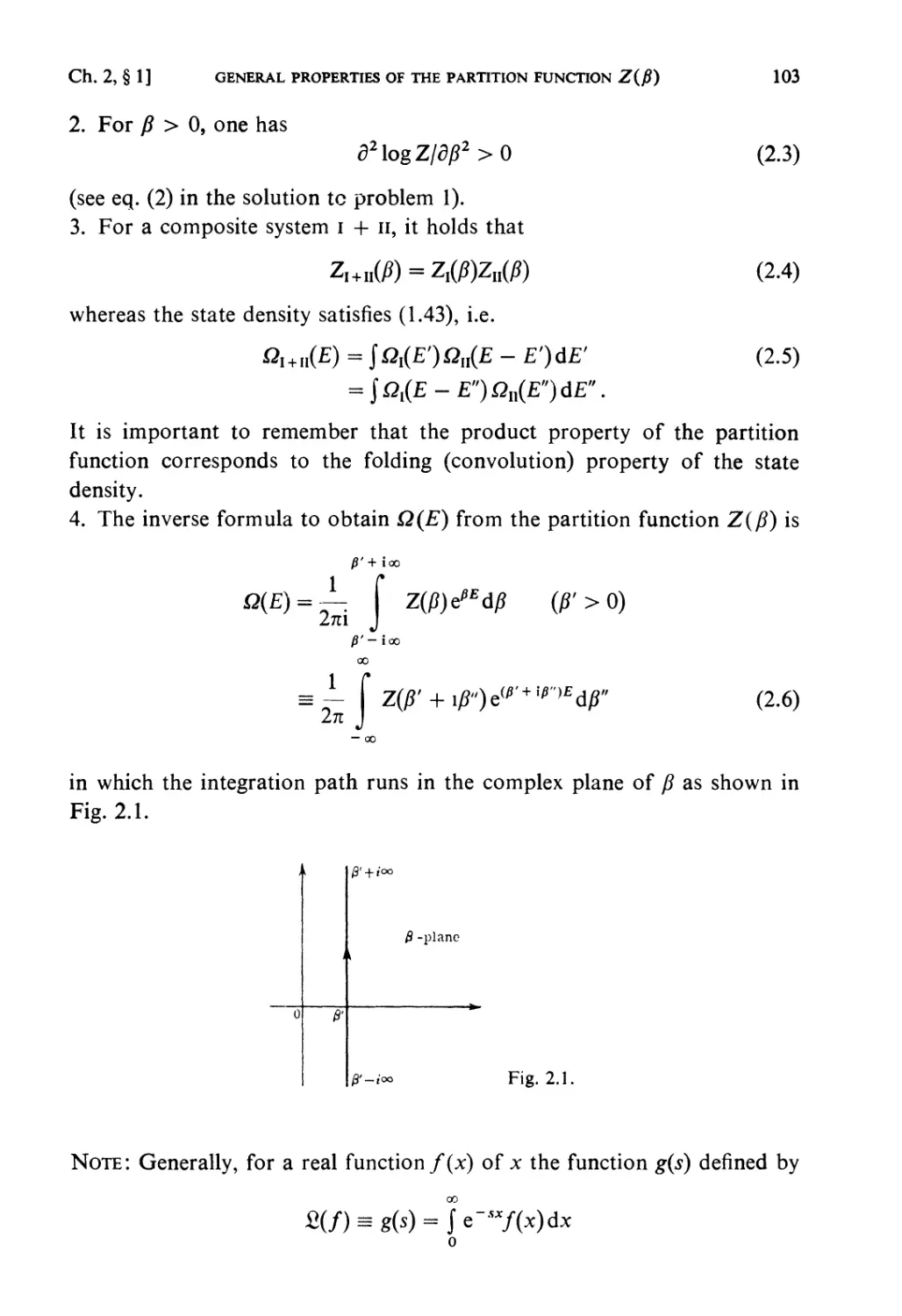
§2.1. General Properties of the Partition Function Z(/?) .... 102
§ 2.2+. Asymptotic Evaluations for Large Systems 104
§ 2.3+. Asymptotic Evaluations and Legendre Transformations of
Thermodynamic Functions 107
§ 2.4+. Grand Partition Function S (X) 107
CONTENTS XI
§ 2.5+. Partition Functions for Generalized Canonical Distributions . 109
§ 2.6. Classical Configurational Partition Functions 109
§2.7+. Density Matrices 110
Examples 112
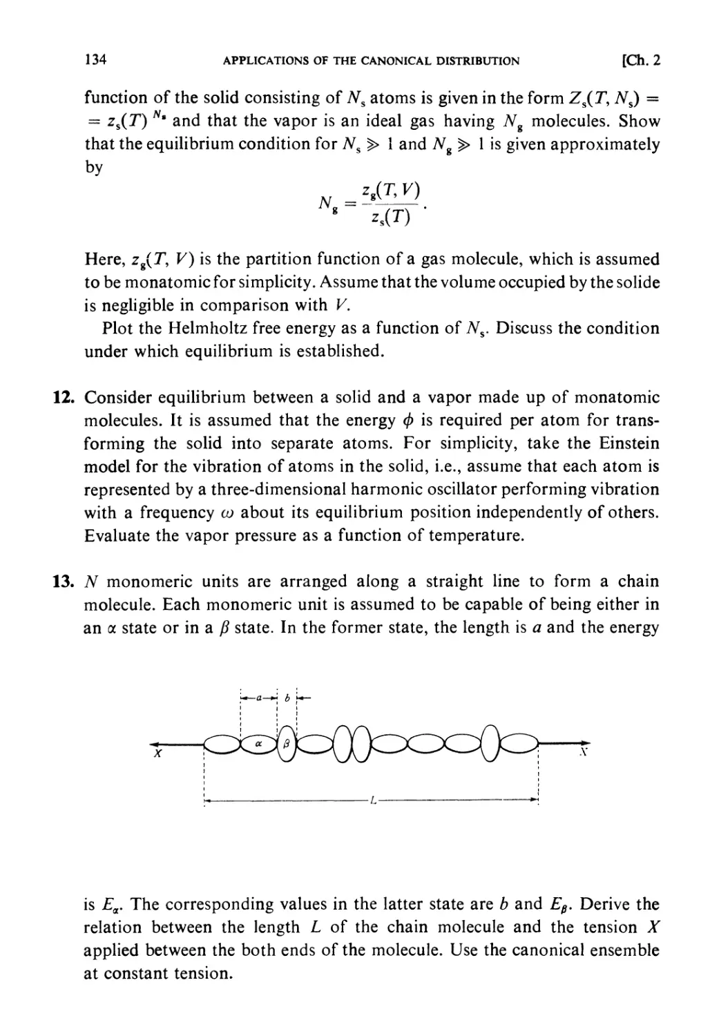
Problems 130
Solutions 139
CHAPTER 3. STATISTICAL THERMODYNAMICS OF GASES
Fundamental Topics
§3.1. Partition Functions of Ideal Gases 183
§ 3.2. Internal Degrees of Freedom and Internal Partition Functions. 184
§3.3. Mixtures of Ideal Gases 188
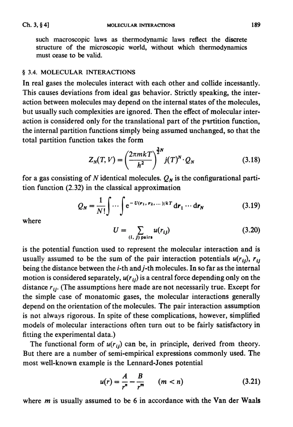
§3.4. Molecular Interactions 189
§ 3.5. Cluster Expansion 190
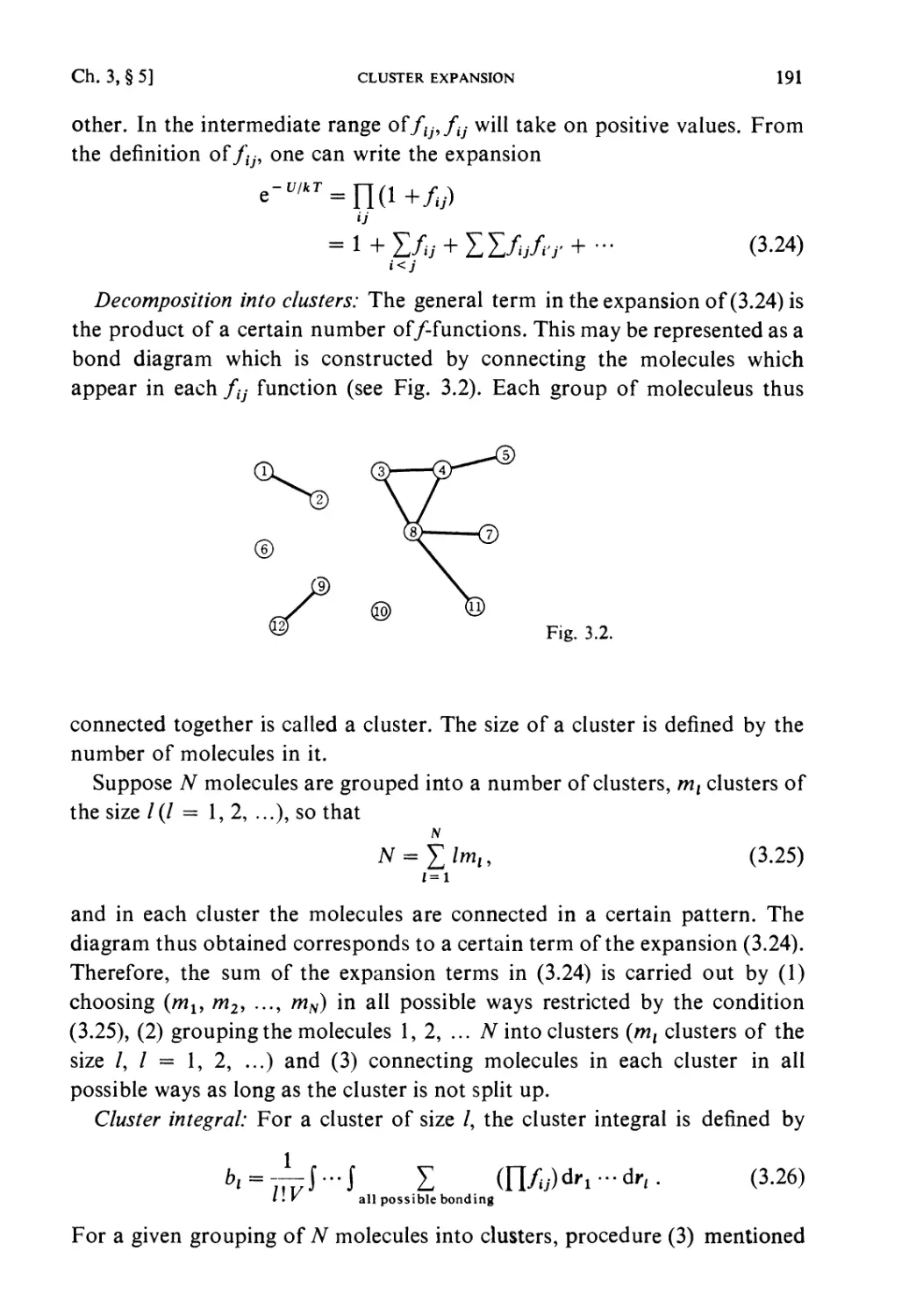
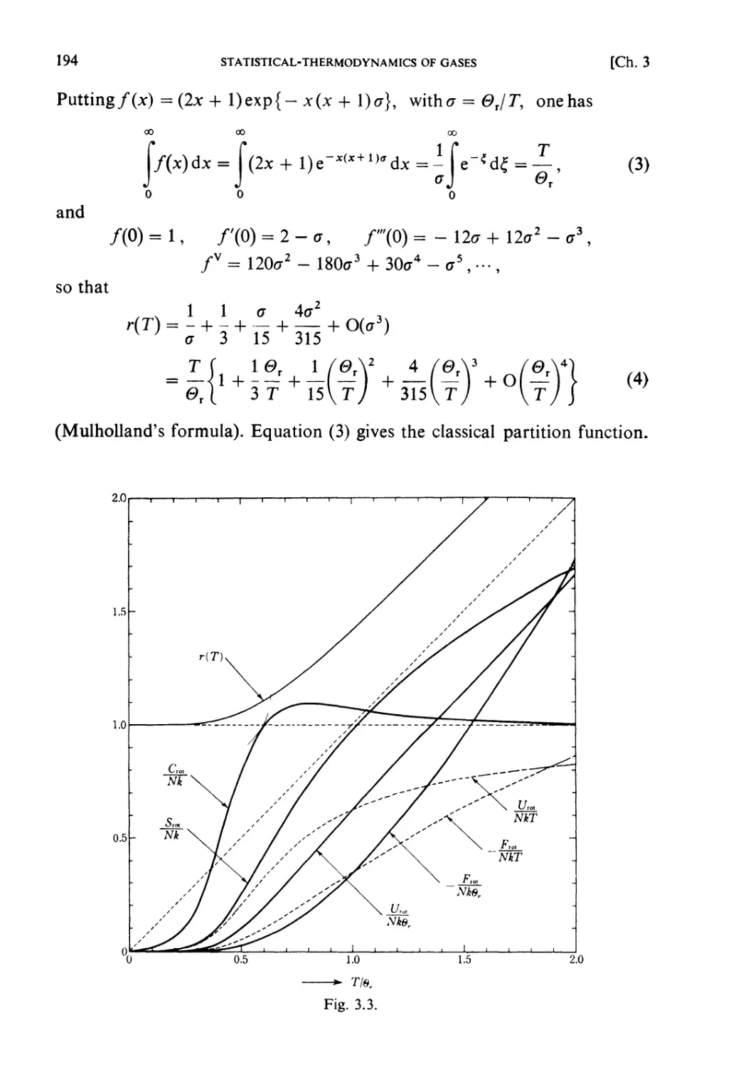
Examples 193
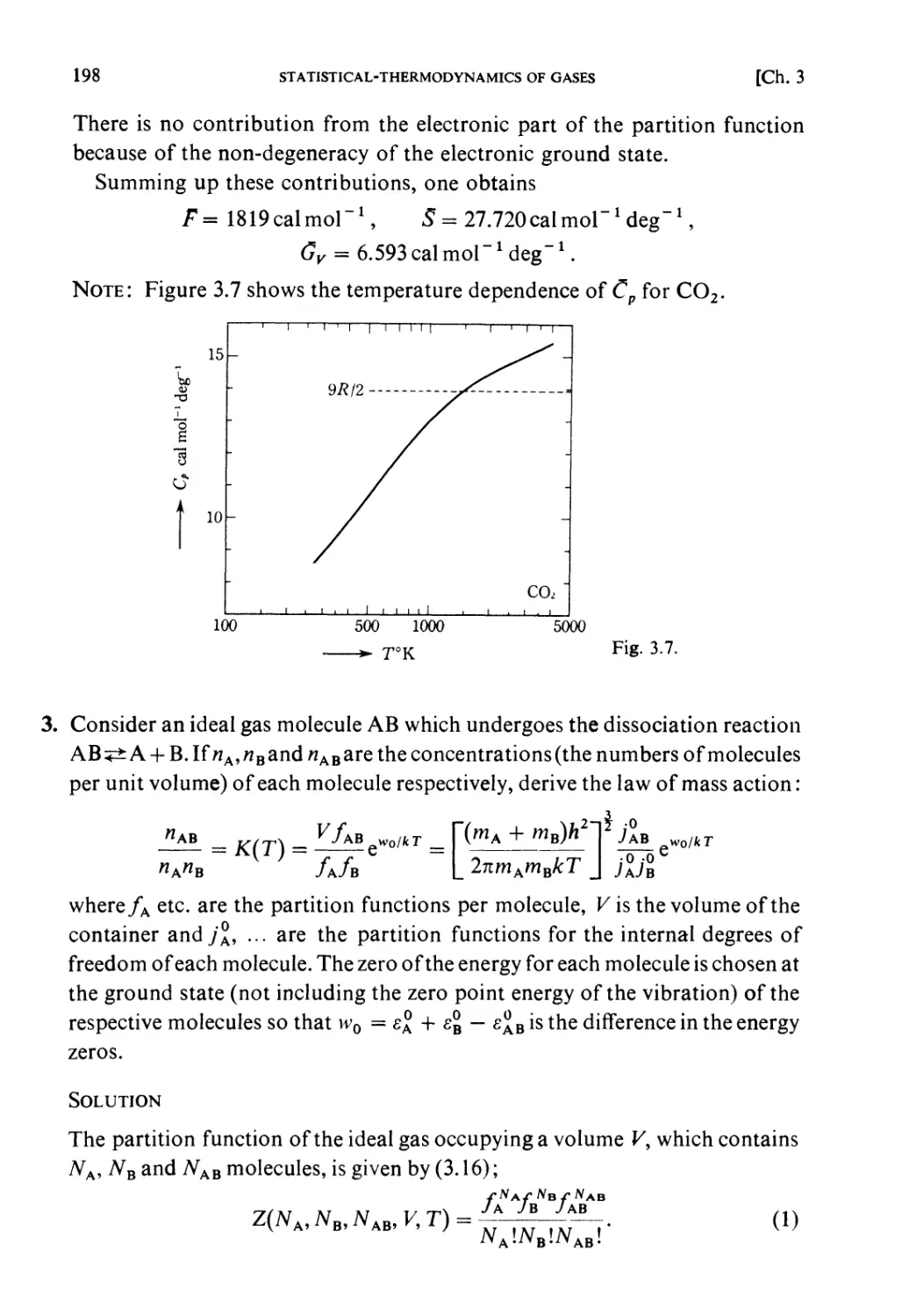
Problems 199
Solutions 205
CHAPTER 4. APPLICATIONS OF FERMI- AND
BOSE- STATISTICS
Fundamental Topics
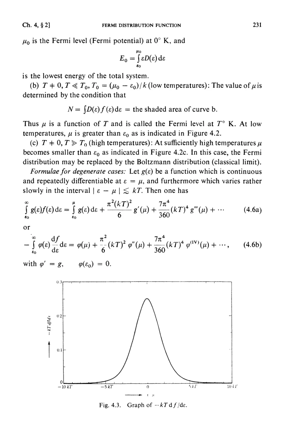
§4.1. Fundamental Formulae of Fermi-Statistics 228
§ 4.2. Fermi Distribution Function 229
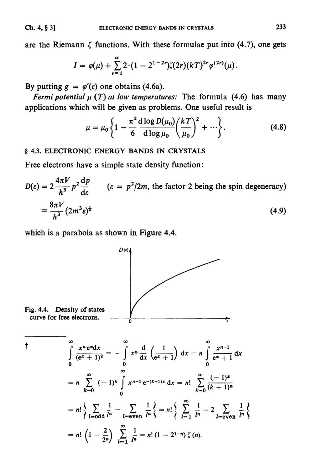
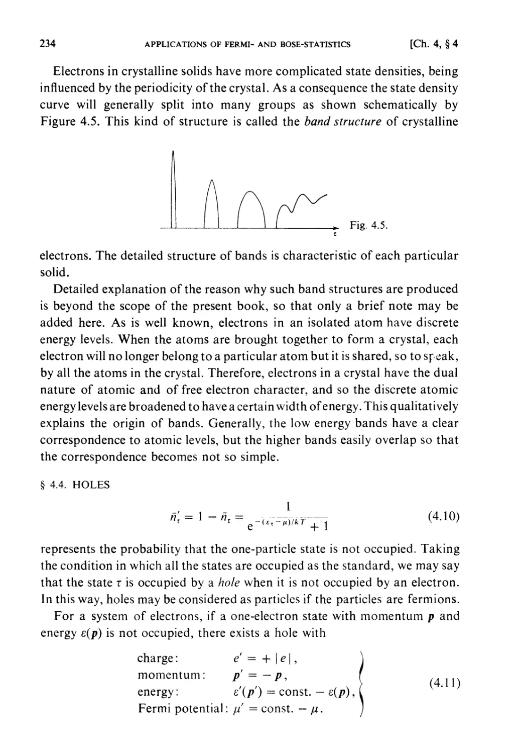
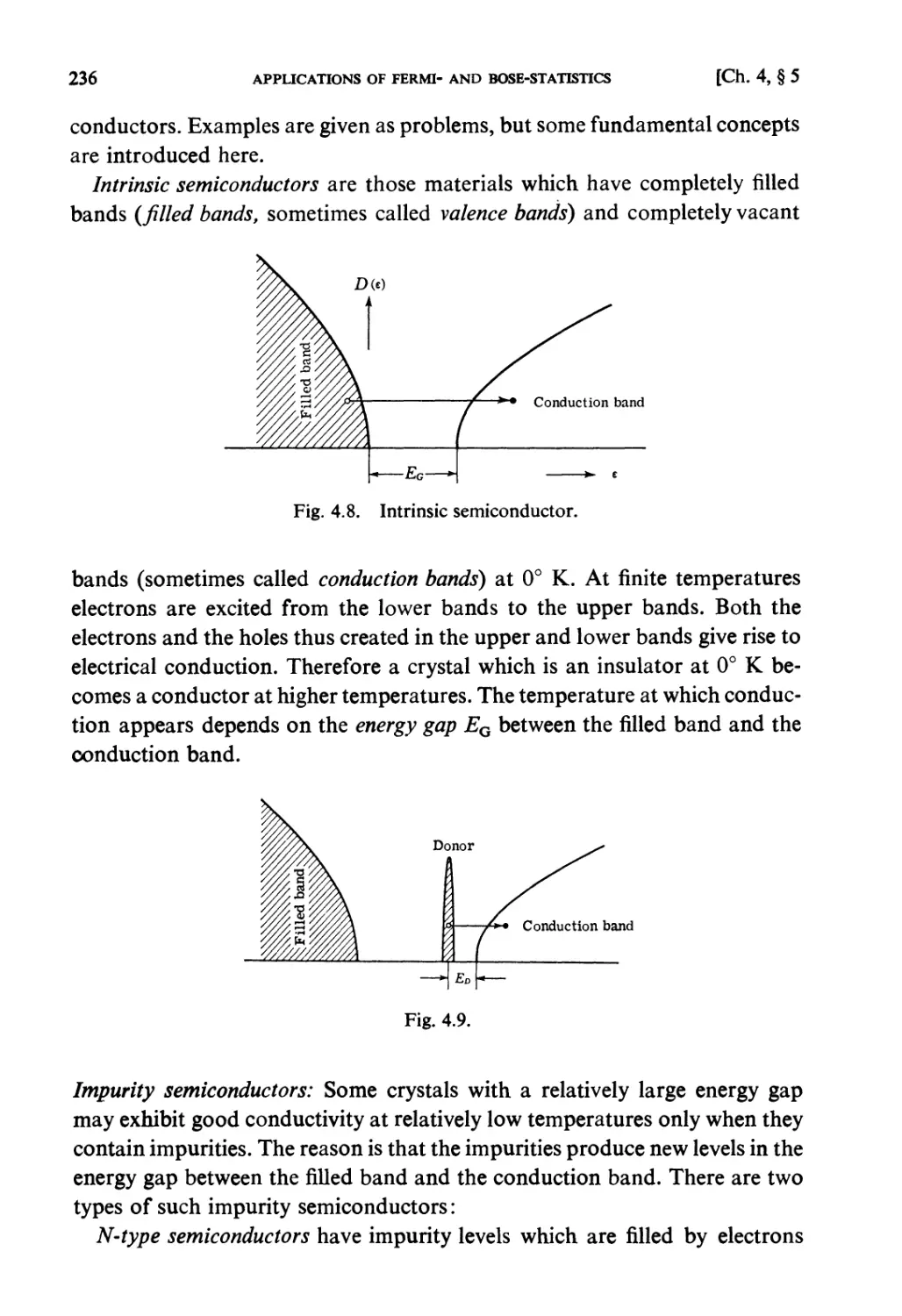
§ 4.3. Electronic Energy Bands in Crystals 233
§4.4. Holes 234
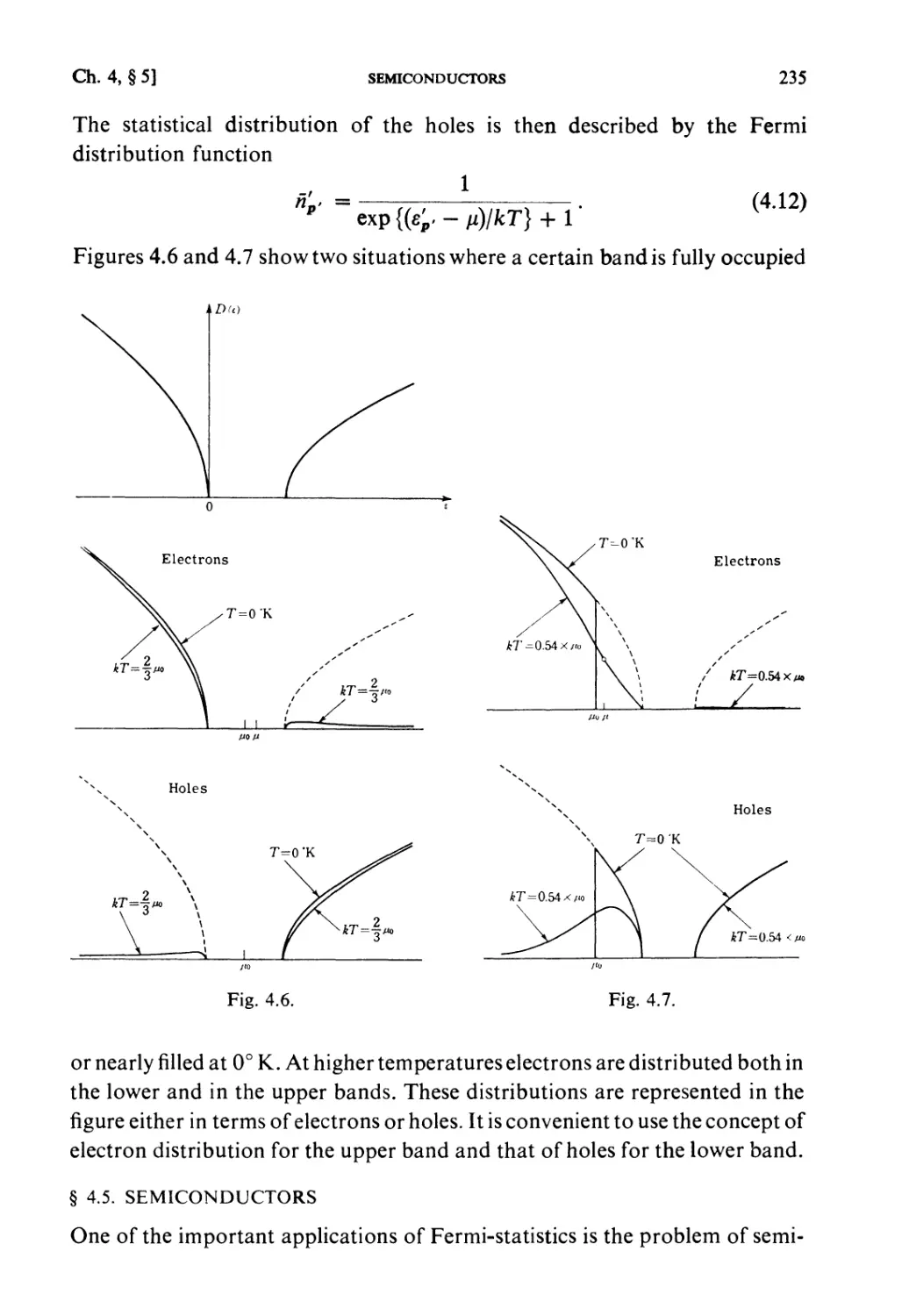
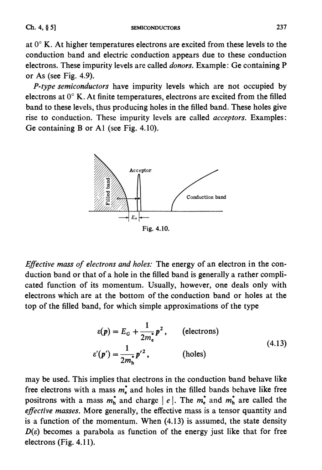
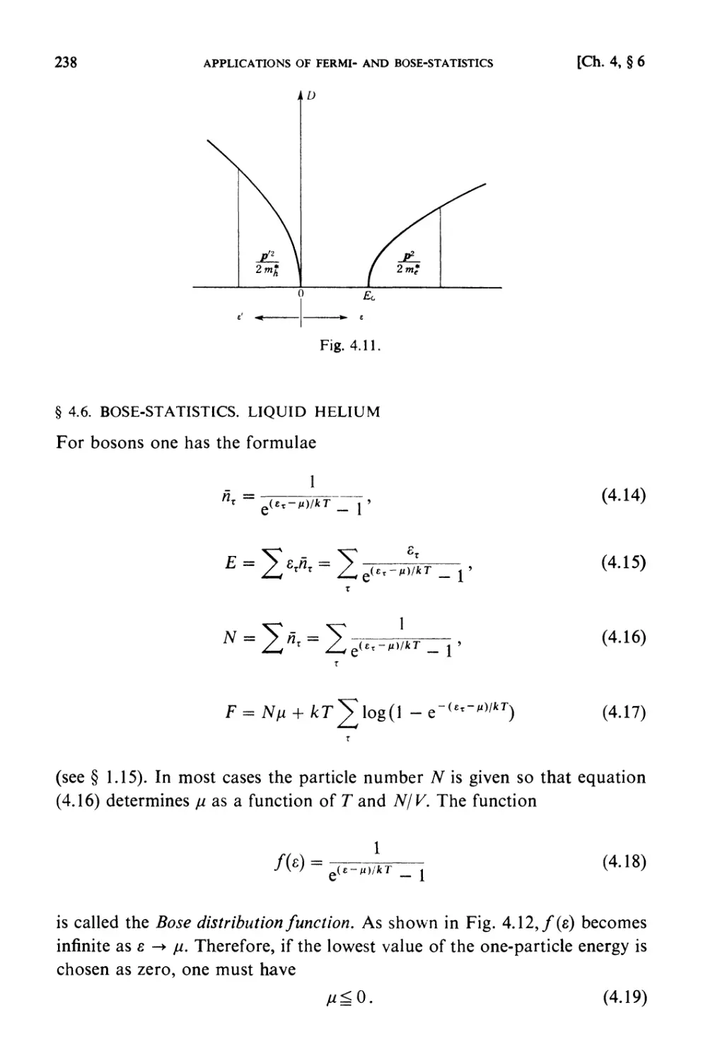
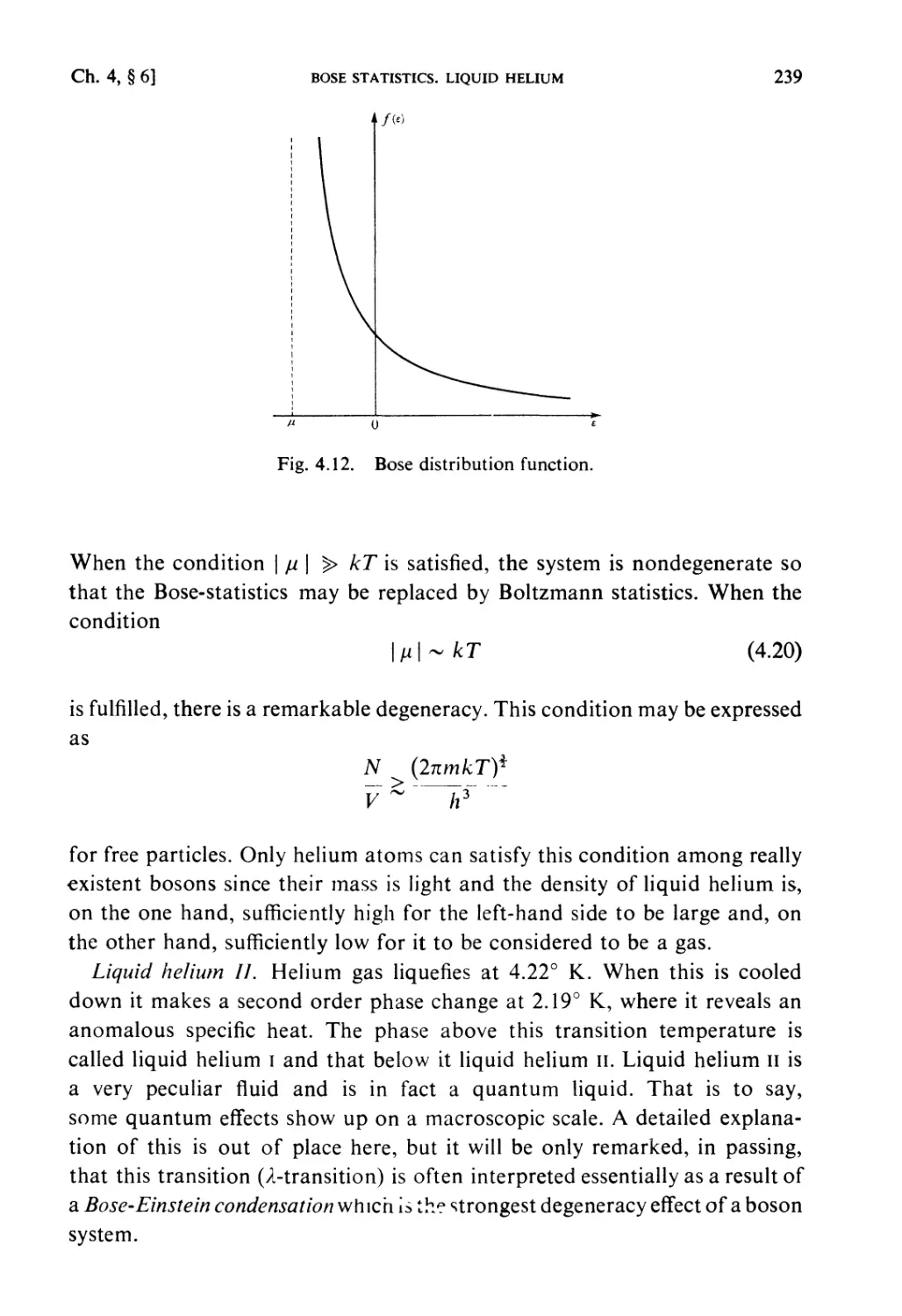
§ 4.5. Semiconductors 235
§ 4.6. Bose-Statistics. Liquid Helium 238
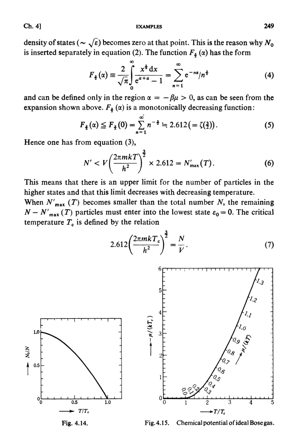
Examples 240
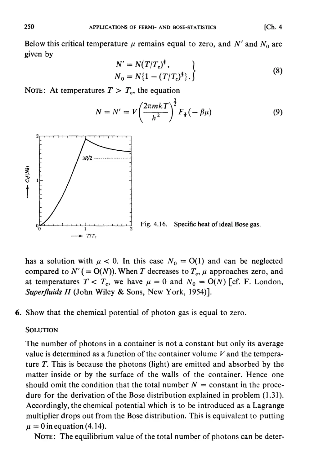
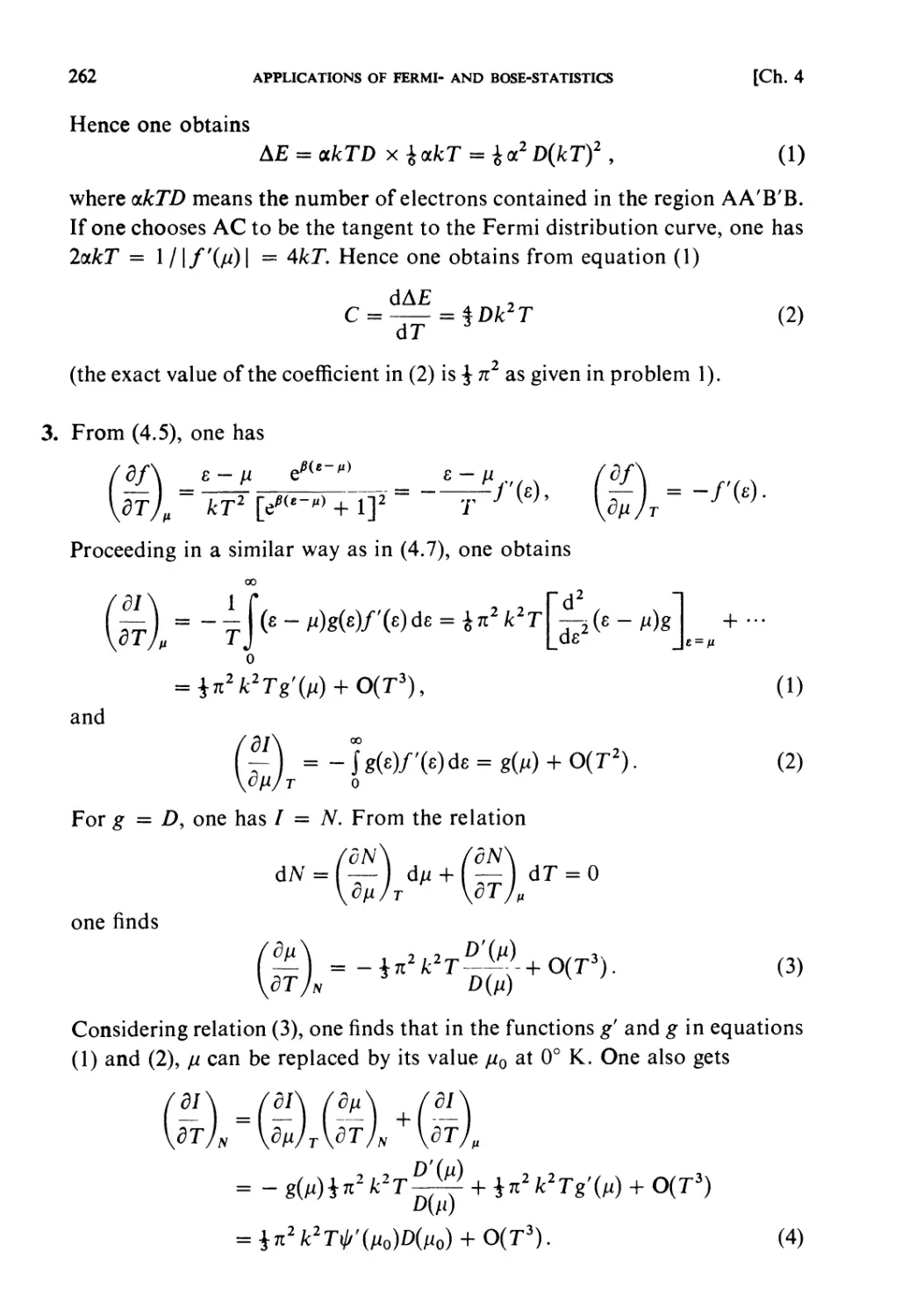
Problems 251
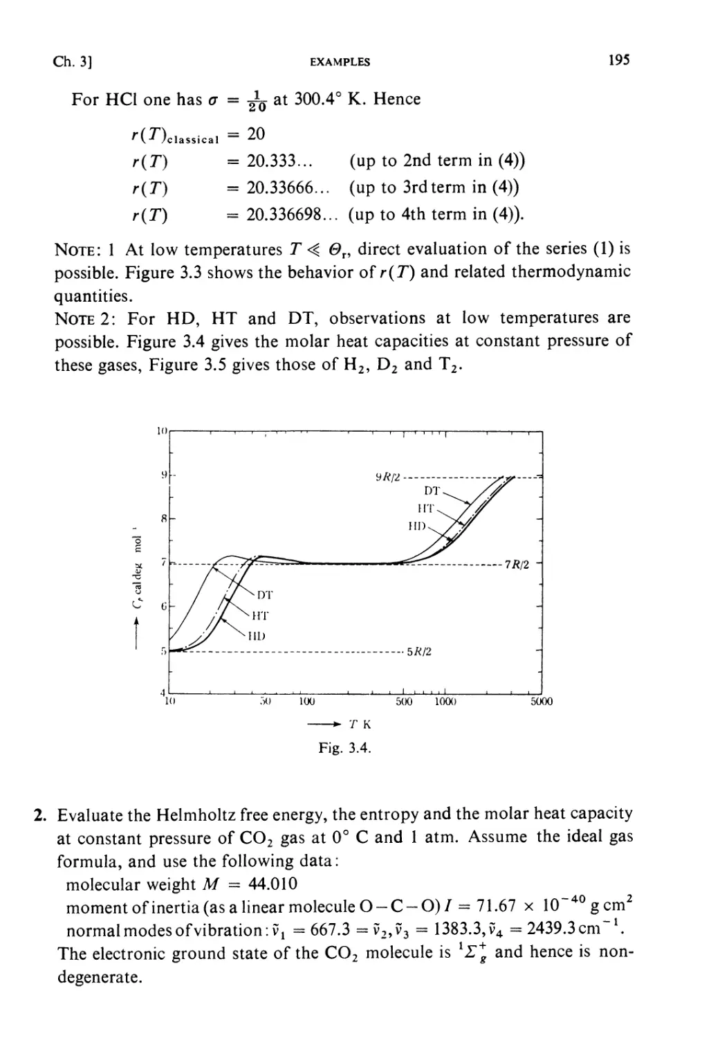
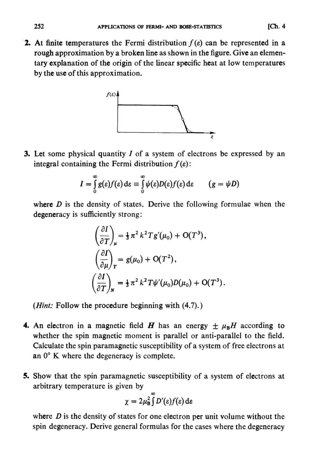
Solutions 259
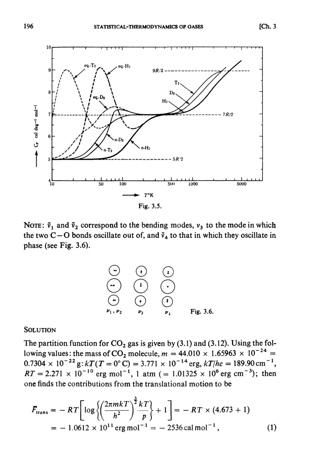
CHAPTER 5. STRONGLY INTERACTING SYSTEMS
Fundamental Topics
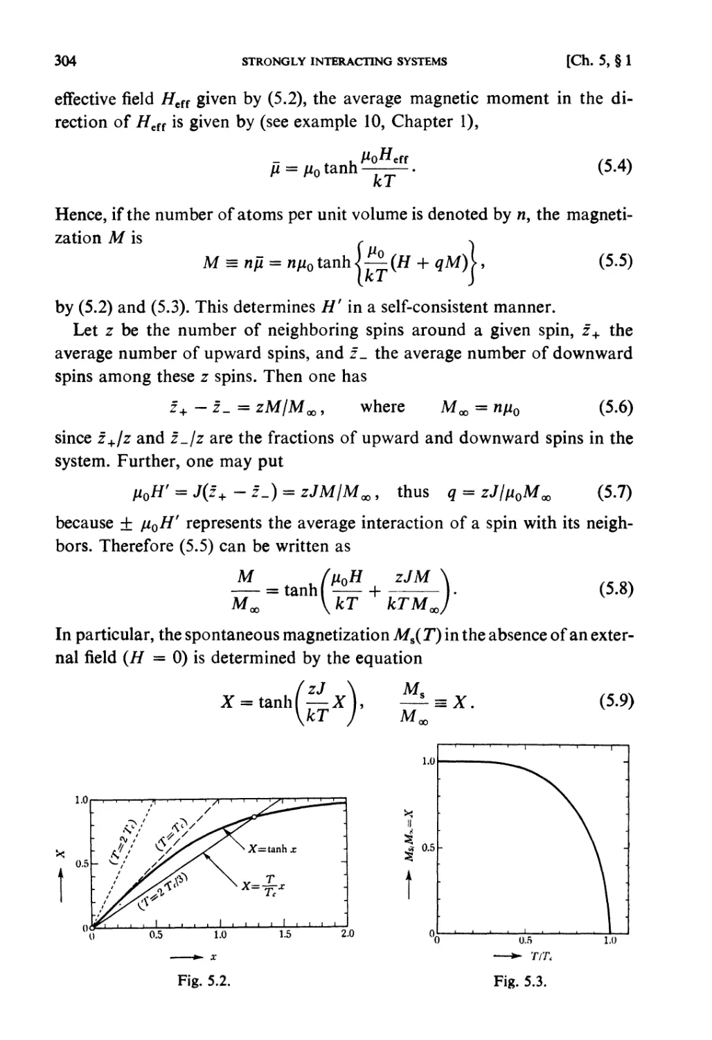
§ 5.1. Molecular Field Approximation : . 302
§ 5.2. Bragg-Williams Approximation 305
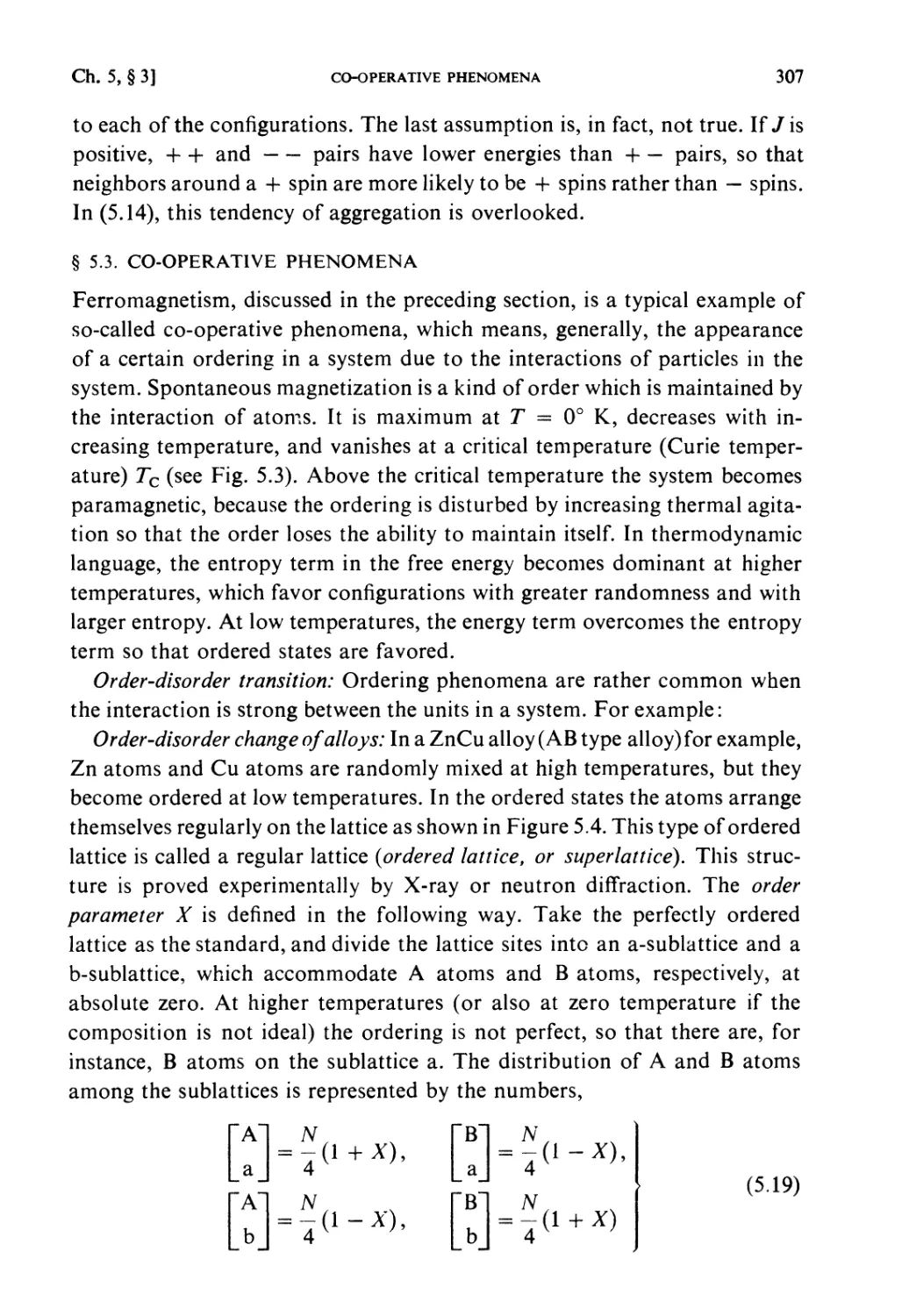
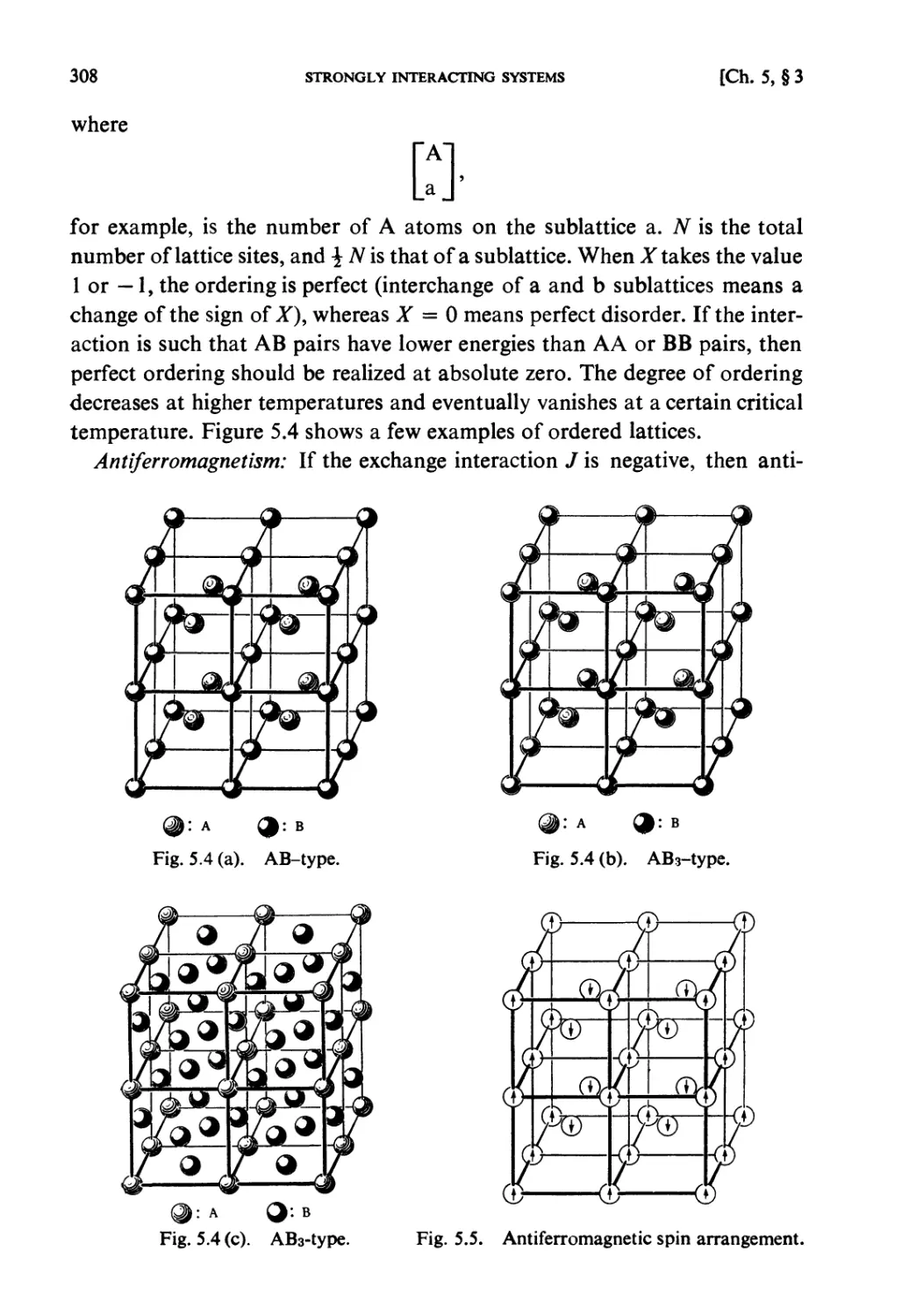
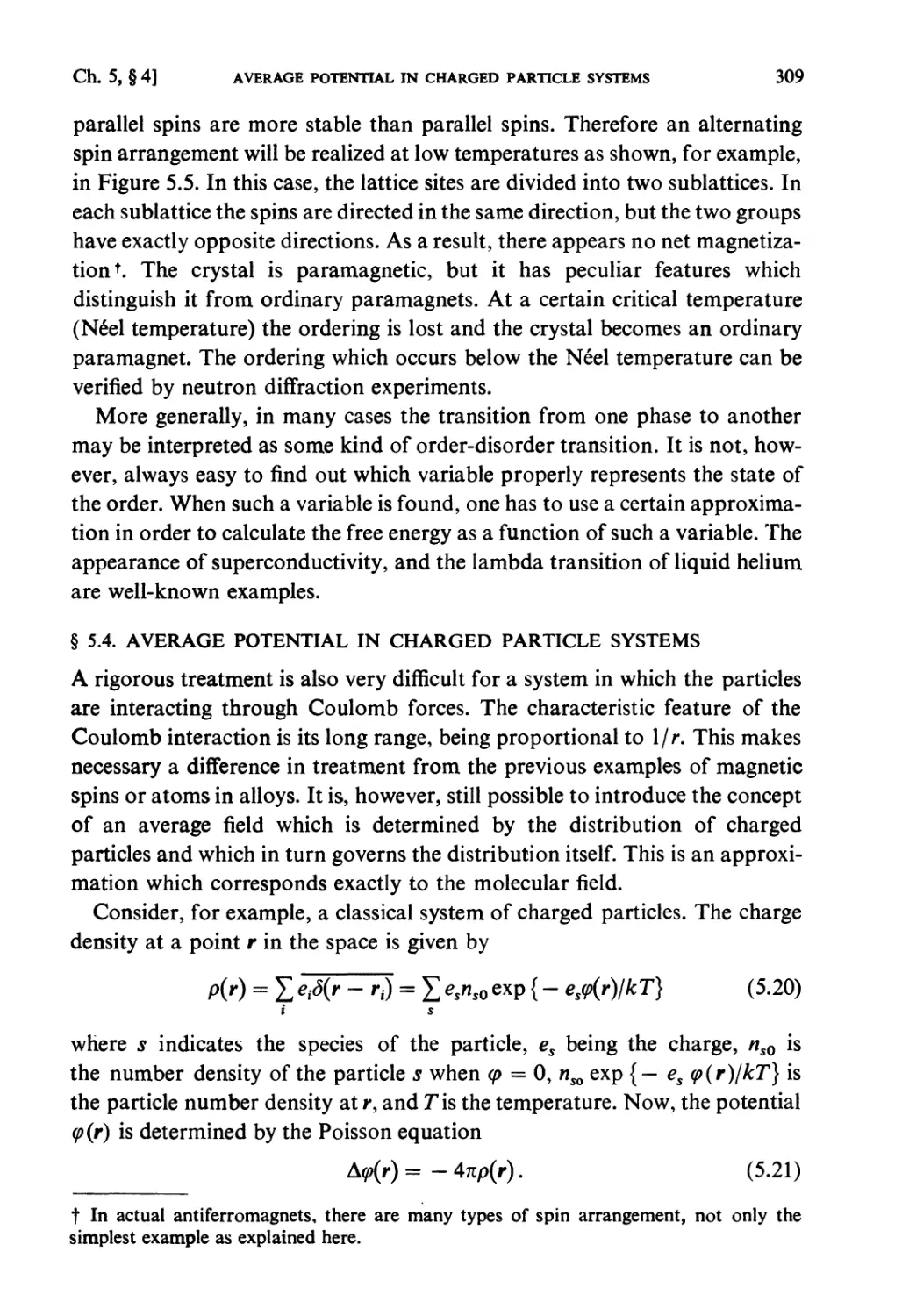
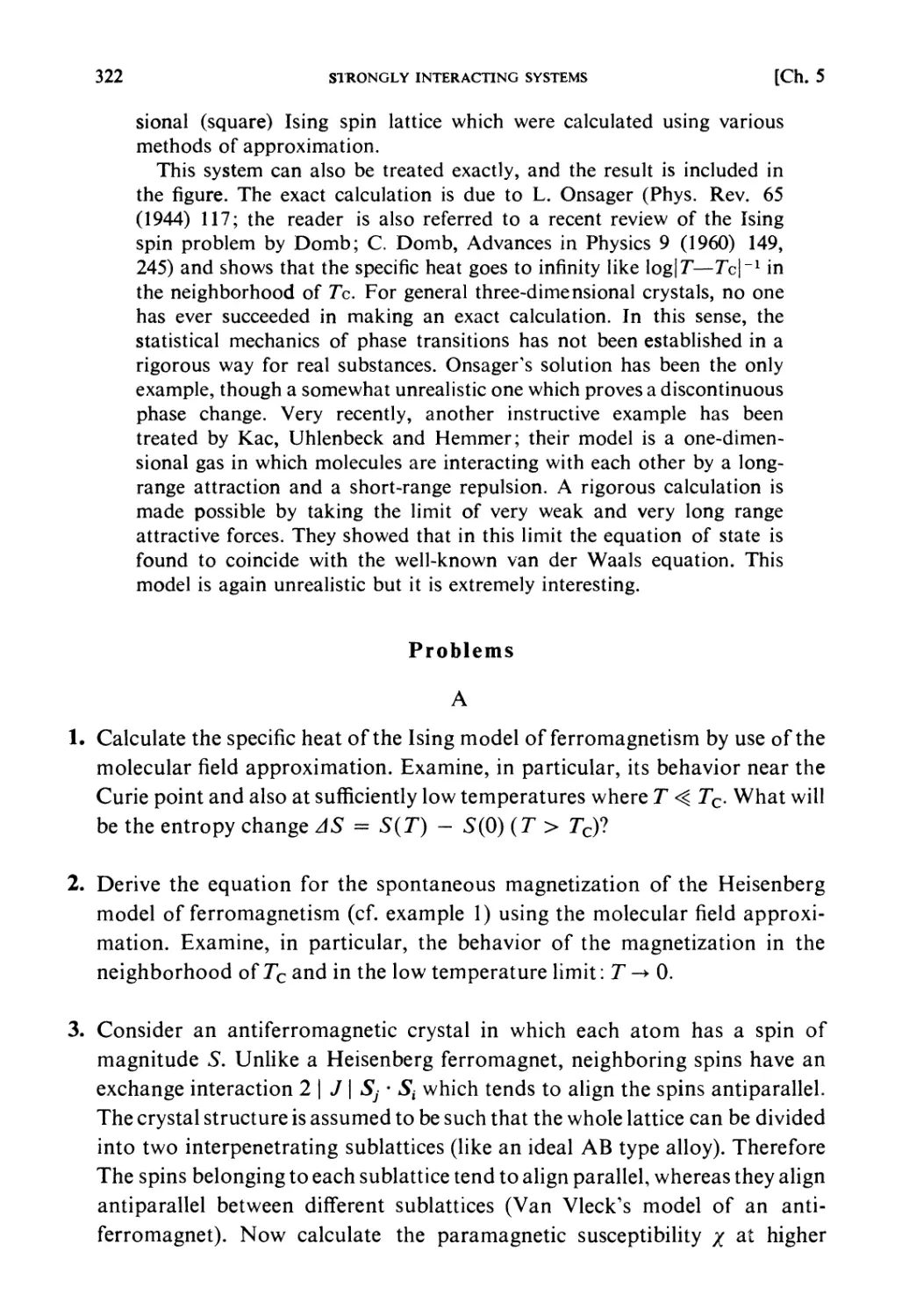
§ 5.3. Co-operative Phenomena 307
§ 5.4. Average Potential in Charged Particle Systems 309
§5.5. Debye-Huckel Theory 310
§5.6. Distribution Functions in a Particle System 312
XII CONTENTS
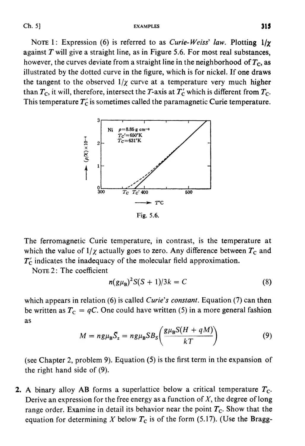
Examples 313
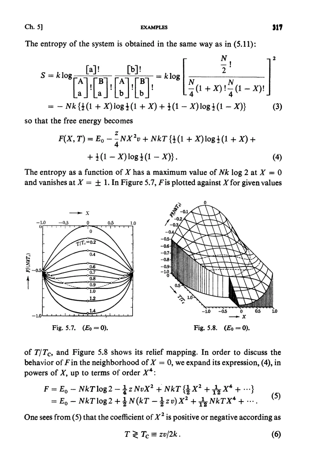
Problems 322
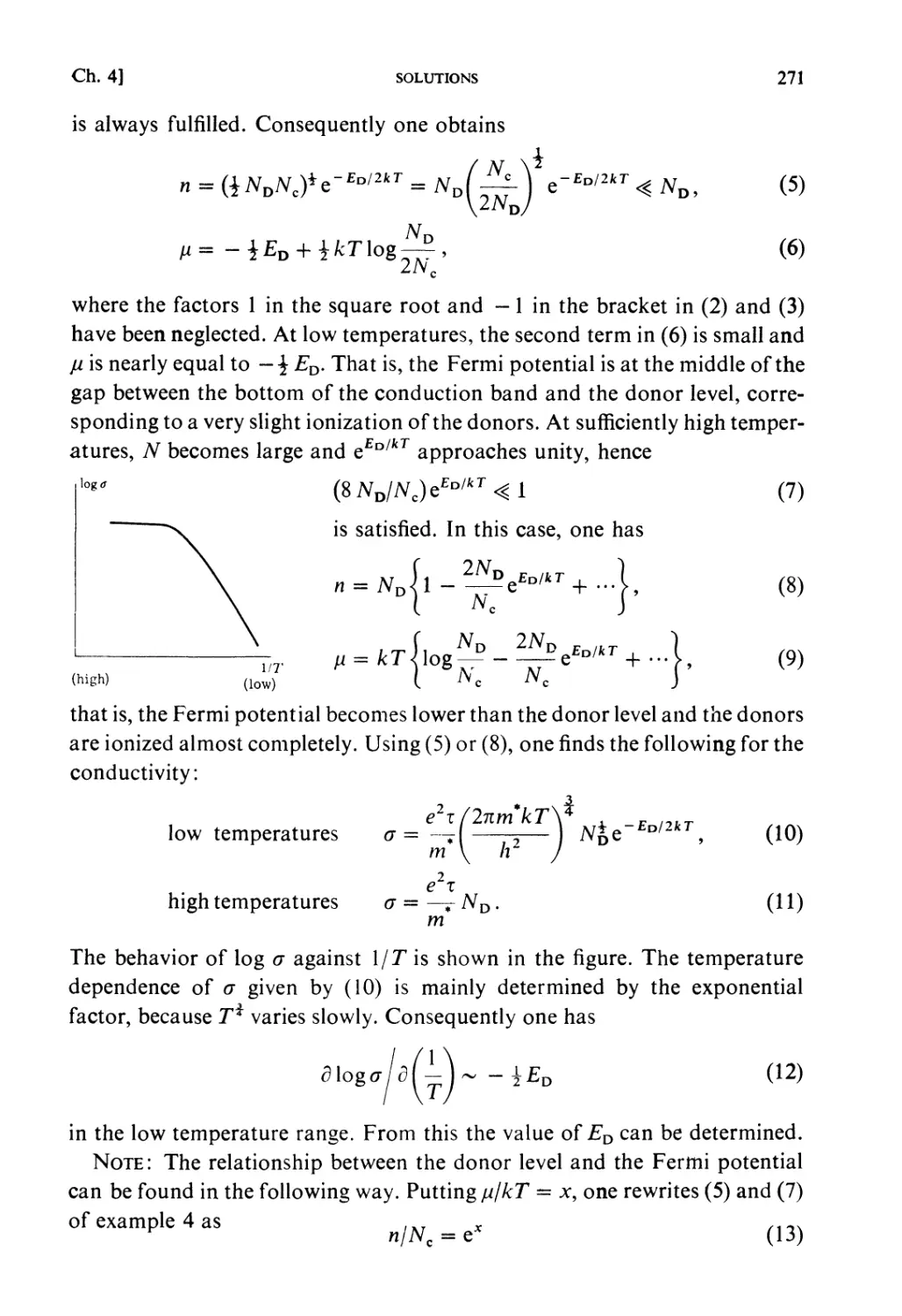
Solutions 329
CHAPTER 6. FLUCTUATIONS AND KINETIC THEORIES
Fundamental Topics
§6.1. Fluctuations 361
§ 6.2. Collision Frequency 362
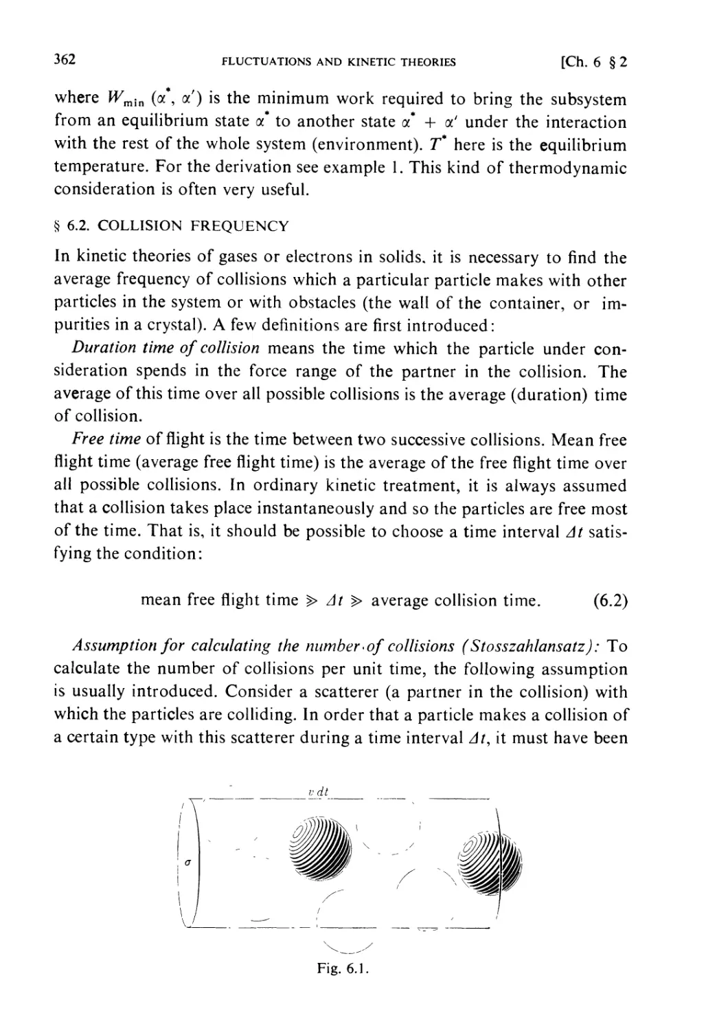
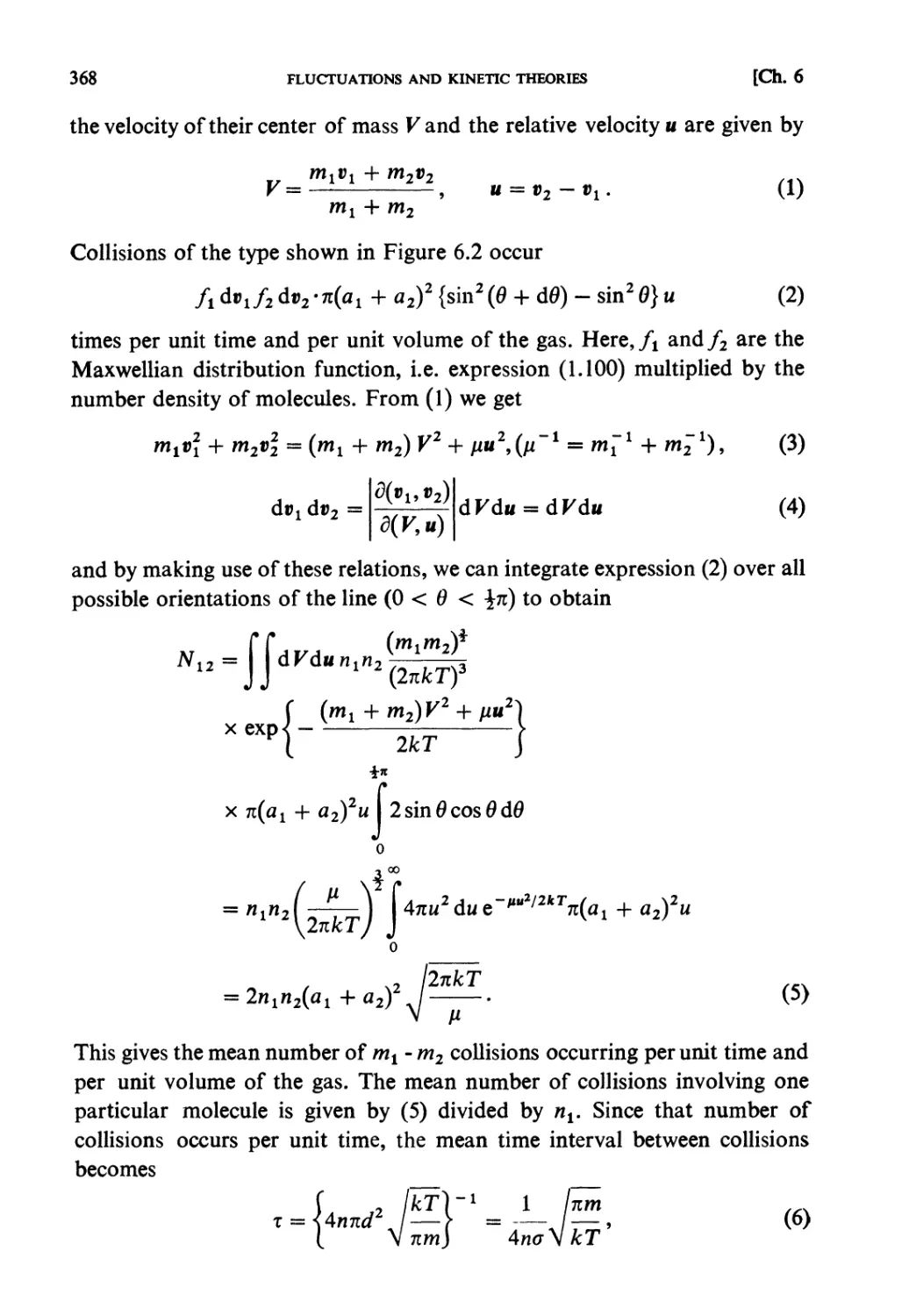
§ 6.3. Boltzmann Transport Equation 363
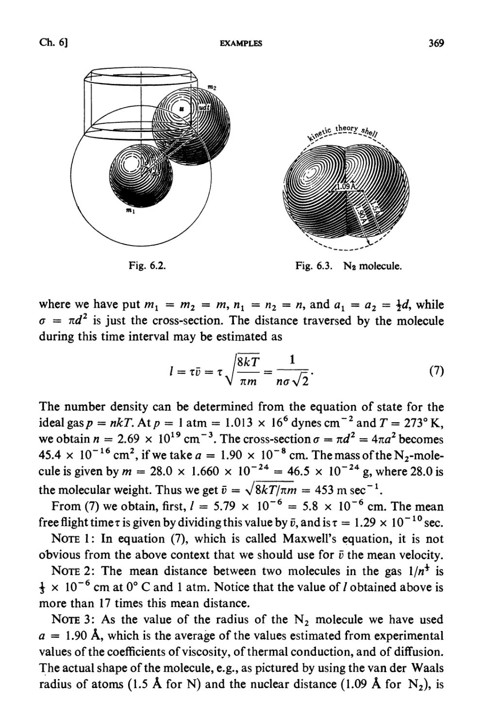
Examples 366
Problems 375
Solutions 381
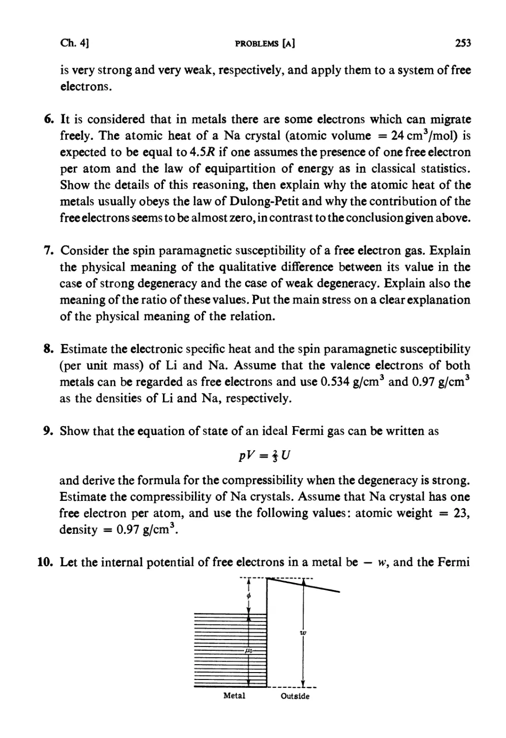
Index 418
Chapter 1
PRINCIPLES OF STATISTICAL MECHANICS
Thermodynamics is a phenomenological theory based upon a few
fundamental laws derived from empirical facts. In contrast to this, statistical
mechanics aims to provide a deductive method which leads us from the
microscopic physical world to the macroscopic world starting from the atomic or
molecular structure of matter and the fundamental dynamical principles of
the atomic world and combining with these the logic of probability theory.
It answers the questions what are the physical laws of the microscopic world
behind the thermodynamic laws, how the thermodynamics can be "explained"
from such laws and why a specific physical system exhibits such
thermodynamic characteristics. The fundamental principles of statistical mechanics
involve, in fact, very profound and difficult questions if one meditates upon
them, but it would not be very wise for the beginners to be too much
concerned with such questions. The most important thing is to learn how one
thinks in statistical mechanics and how one applies statistical considerations
to physical problems.
Fundamental Topics
§1.1. MICROSCOPIC STATES
Microscopic and macroscopic states: A physical system which one observes
usually consists of a great number of atoms or molecules and so has an
enormously large number of degrees of dynamical freedom. But in the usual
case, only a few physical quantities, say the temperature, the pressure and the
density, are measured, by means of which the "state" of the system is
specified. A state defined in this crude manner is called a macroscopic state
(example: a thermodynamic state). On the other hand, from a dynamical
point of view, each state of a system can be defined, at least in principle, as
precisely as possible by specifying all of the dynamical variables of the system.
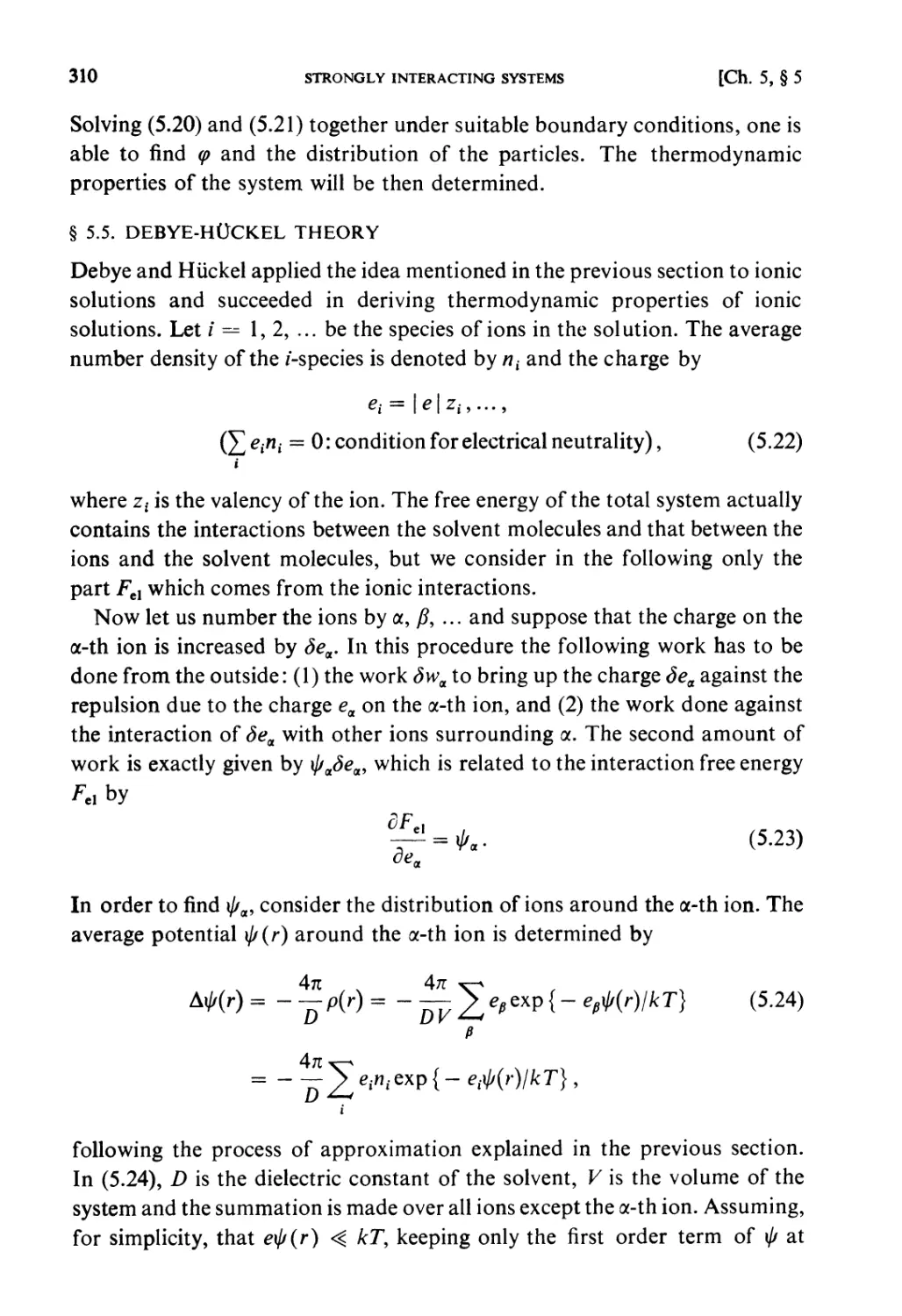
Such a state is called a microscopic state.
Classical statistical mechanics and quantum statistical mechanics: The
statistical mechanics based on classical mechanics is called classical statistical
mechanics and that based on quantum mechanics is called quantum statistical
mechanics. Since rigorous mechanics in the atomic world is quantum
mechanics, rigorous statistical mechanics must be quantum statistical mechanics
1
2
PRINCIPLES OF STATISTICAL MECHANICS
[Ch. 1, § 1
and so classical statistical mechanics may be said to be useful only as a
certain approximation to quantum statistical mechanics. But the classical
theory has even today a great value from theoretical and educational
points of view because it makes us understand more clearly the basic ways
of thinking in statistical mechanics.
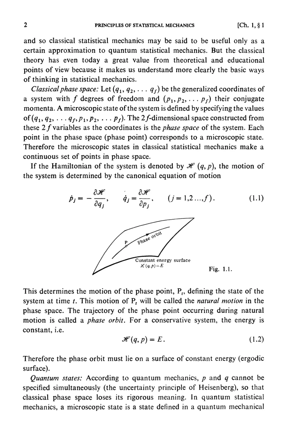
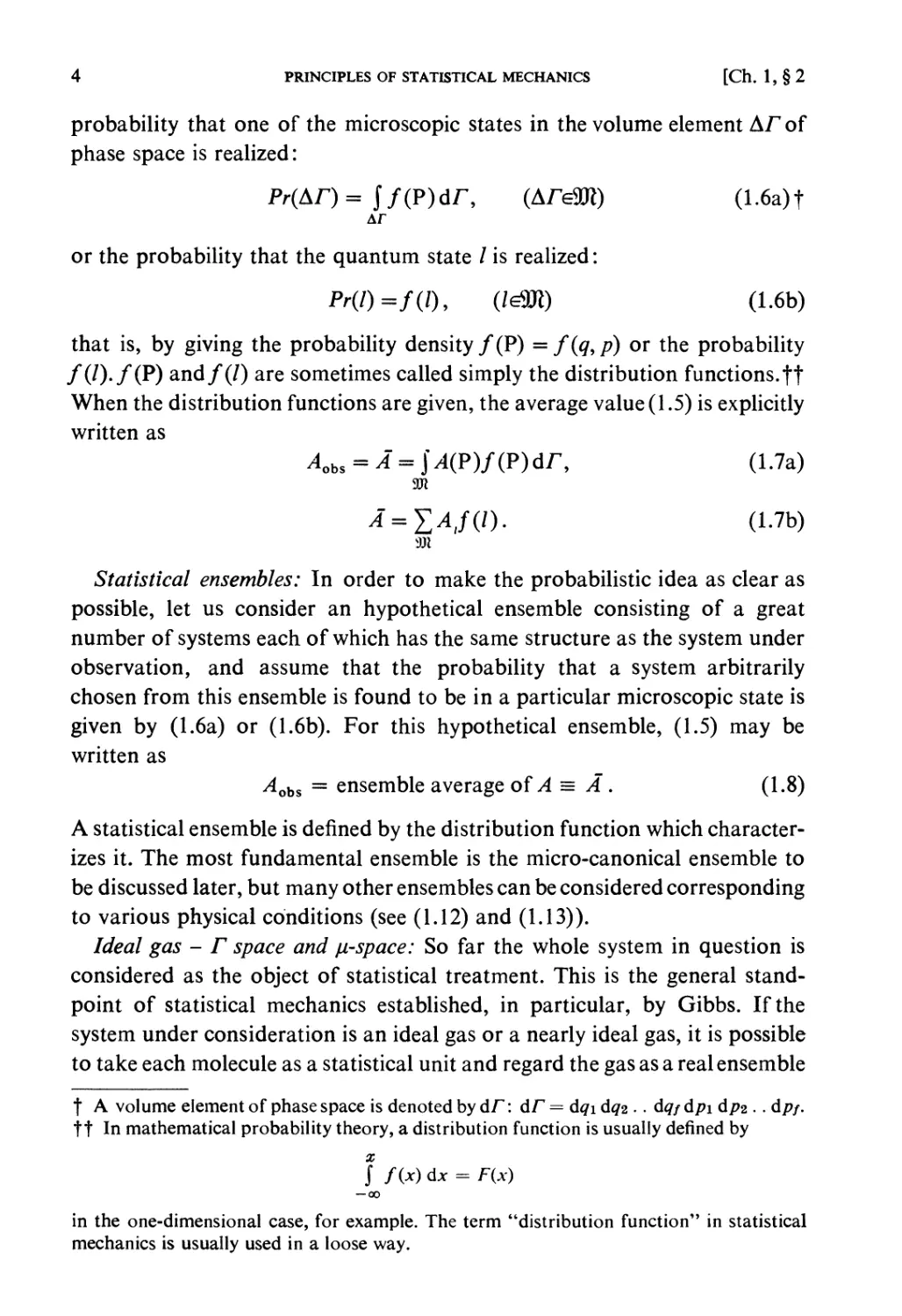
Classical phase space: Let (qu q2, • • . qf) be the generalized coordinates of
a system with / degrees of freedom and (pup2> • • • Pf) their conjugate
momenta. A microscopic state of the system is defined by specifying the values
°f (tfi> #2> • • • qfiPuPi* • • • Pf)- The 2/-dimensional space constructed from
these 2/variables as the coordinates is the phase space of the system. Each
point in the phase space (phase point) corresponds to a microscopic state.
Therefore the microscopic states in classical statistical mechanics make a
continuous set of points in phase space.
If the Hamiltonian of the system is denoted by 3tf (q, /?), the motion of
the system is determined by the canonical equation of motion
Pj= -
*; =
dpj'
(y= 1,2...,/).
(i.i)
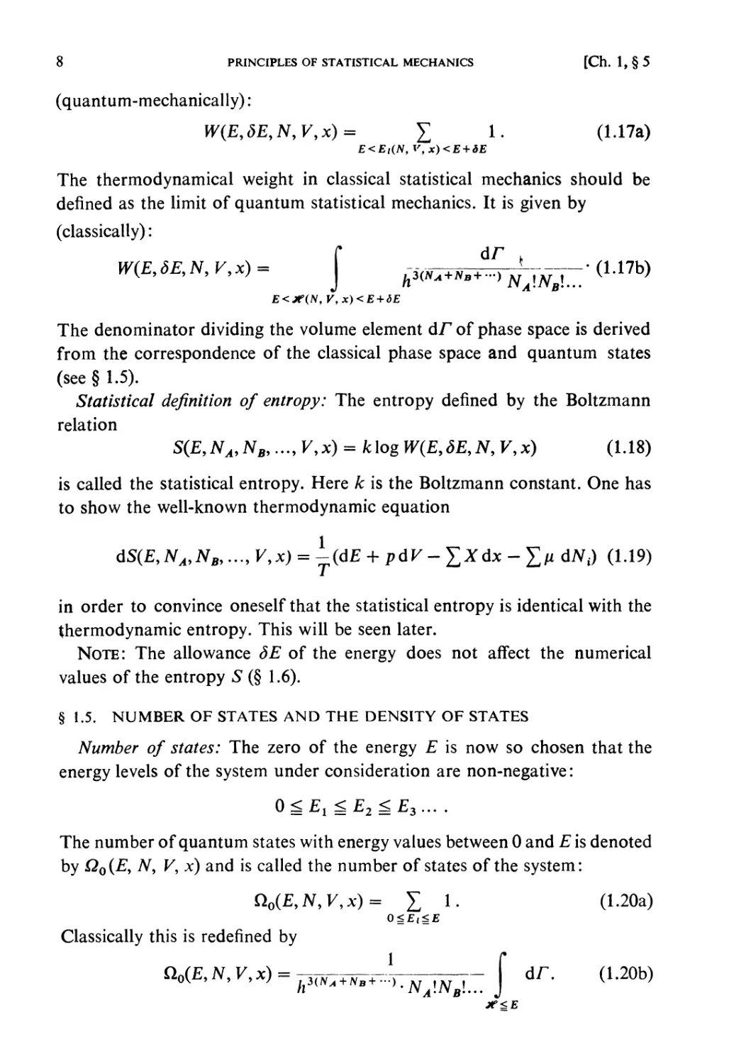
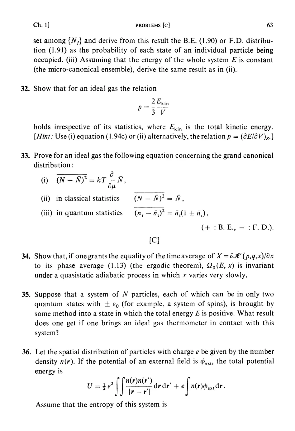
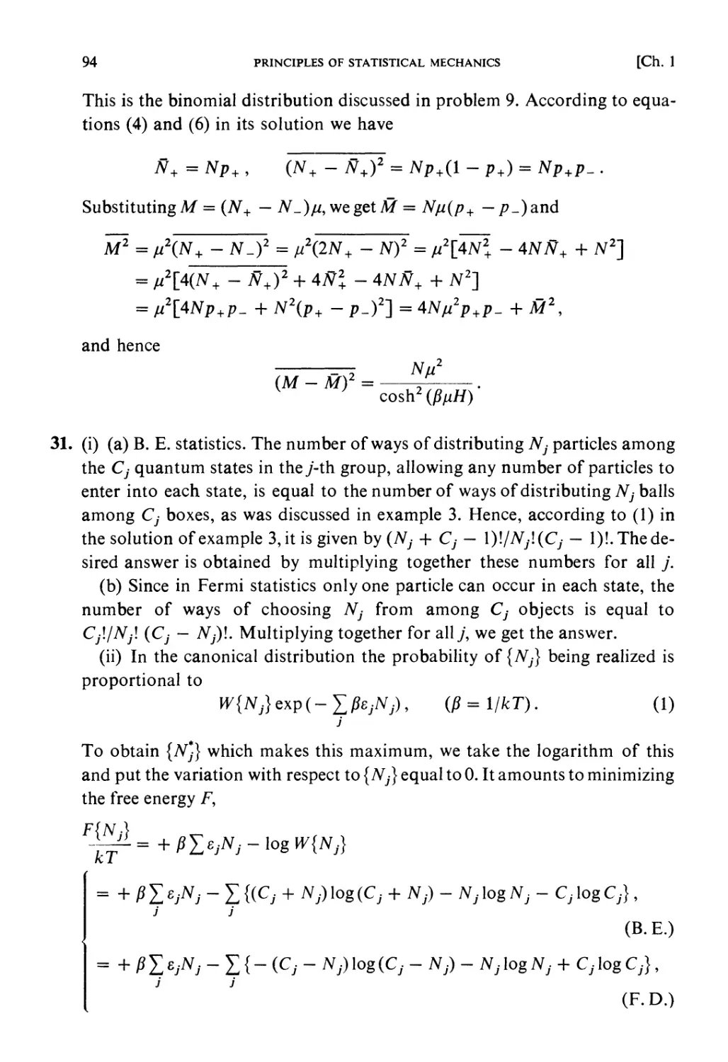
Constant energy surface
X (9,/>)=■£
Fig. 1.1.
This determines the motion of the phase point, Pr, defining the state of the
system at time t. This motion of P, will be called the natural motion in the
phase space. The trajectory of the phase point occurring during natural
motion is called a phase orbit. For a conservative system, the energy is
constant, i.e.
JT(q,p) = E. (1.2)
Therefore the phase orbit must lie on a surface of constant energy (ergodic
surface).
Quantum states: According to quantum mechanics, p and q cannot be
specified simultaneously (the uncertainty principle of Heisenberg), so that
classical phase space loses its rigorous meaning. In quantum statistical
mechanics, a microscopic state is a state defined in a quantum mechanical
Ch. 1,§2]
STATISTICAL TREATMENT
3
sense. In particular, a stationary dynamical state of a system must be one of
the quantum states determined by the equation
#^ = Em (/ = 1,2,...). (1.3)
Here 3tf is the Hamiltonian of the system, Et the energy of the quantum state
/ and cpt is the wave function representing the quantum state /.
The set of microscopic states in quantum statistical mechanics is thus a
discrete denumerable set of quantum states denoted by the quantum number
/. (In statistical mechanics, one usually considers a system confined in a
limited space, so that the quantum number / is usually discrete. A system with
infinite extension is considered as the limit of one of finite extension.)
§ 1.2. STATISTICAL TREATMENT
Whenever a system is kept in equilibrium and remains constant according to
macroscopic observations, it never stays constant from the microscopic point
of view, and so one can never say precisely in which microscopic state the
system is found. One can only define the probability for the set of all possible
microscopic states of the system.
Fundamental assumption for observed values of physical quantities: Suppose
a physical quantity A is observed for the system under consideration. A is a
dynamical quantity from the microscopic point of view and is a function
of microscopic states. The microscopic value of A is represented by
^ (#> P) = A (P) in classical mechanics (P is a phase point) and by the
expectation value t
^ = J^^dT = </M|/> (1.4)
in the quantum state / in quantum mechanics. The observed value Aohs in the
macroscopic sense must be a certain average of microscopic A: i.e.
Aohs = A. (1.5)
Realization probability of a microscopic state: Let 2ft be the set of all
possible microscopic states which can be realized by the system under a certain
macroscopic condition. 2ft is classically a certain subspace of the phase
space and quantum-mechanically it is a set of quantum states of the system.
The probability that these microscopic states are realized is defined as the
t The integration in the following expression is carried out over the variables which are
used to represent the wave function, say qu Qi, ... q/. Here dr is a volume element of the
space of these variables. Note that a quantum state corresponds to a phase orbit in classical
mechanics and so Ai corresponds to the average taken over such an orbit.
4
PRINCIPLES OF STATISTICAL MECHANICS
[Ch. 1,§2
probability that one of the microscopic states in the volume element Ar of
phase space is realized:
Pr(Ar)= J/(P)dT, (Are9K) (1.6a) f
Ar
or the probability that the quantum state / is realized:
Pr(0=f(l), (l*m) (1.6b)
that is, by giving the probability density /(P) = f{q,p) or the probability
/(/)./(P) and/(/) are sometimes called simply the distribution functions.ft
When the distribution functions are given, the average value (1.5) is explicitly
written as
4obi = ^ = j4(P)/(P)d/\ (1.7a)
arc
i = E^,/(0. (1.7b)
Statistical ensembles: In order to make the probabilistic idea as clear as
possible, let us consider an hypothetical ensemble consisting of a great
number of systems each of which has the same structure as the system under
observation, and assume that the probability that a system arbitrarily
chosen from this ensemble is found to be in a particular microscopic state is
given by (1.6a) or (1.6b). For this hypothetical ensemble, (1.5) may be
written as
^obs = ensemble average of A = A . (1.8)
A statistical ensemble is defined by the distribution function which
characterizes it. The most fundamental ensemble is the micro-canonical ensemble to
be discussed later, but many other ensembles can be considered corresponding
to various physical conditions (see (1.12) and (1.13)).
Ideal gas - r space and ju-space: So far the whole system in question is
considered as the object of statistical treatment. This is the general
standpoint of statistical mechanics established, in particular, by Gibbs. If the
system under consideration is an ideal gas or a nearly ideal gas, it is possible
to take each molecule as a statistical unit and regard the gas as a real ensemble
t A volume element of phase space is denoted by dr: dr = dqi dqi .. dqs dpi d/>2 .. dp/.
ft In mathematical probability theory, a distribution function is usually defined by
J f(x) dx = F(x)
— 00
in the one-dimensional case, for example. The term "distribution function" in statistical
mechanics is usually used in a loose way.
Ch.l,§3]
PRINCIPLE OF EQUAL WEIGHT
5
consisting of such units. This point of view was taken in the kinetic theory of
gases which became the prototype of statistical mechanics. From this
standpoint, the important thing is, in classical statistical mechanics, the
distribution function of the position x and the momentum p of a molecule, i.e.,
the probability that a molecule chosen from the ensemble of gas molecules
is found to have the coordinate and momentum values between x and
x -f dx, p and p -f dp is equal to
f(x,p)dxdp. (1.9)
Most of the properties of dilute gases can be derived from a knowledge of this
distribution function. This is a distribution in a six-dimensional space, which
is often called the ju-space. The phase space of the N molecules of the gas is
called the r space.
Maxwell distribution: In a thermal equilibrium state at high temperatures,
the distribution function/for a dilute gas is given by
/(>} = (2^W* CXP{ " IrnkT^ + * + &} (U0)
where T is the absolute temperature, m the mass of a molecule, and k the
Boltzmann constant. This Maxwell distribution can be derived by various
methods. The most general derivation will be described later § 1.15, eq. (1.100).
§ 1.3. THE PRINCIPLE OF EQUAL WEIGHT AND THE MICROCANONICAL
ENSEMBLE
When a system consisting of a great number of particles (more generally a
system having a great number of degrees of freedom) is isolated for a long
time from its environment, it will finally reach a thermal equilibrium state.
In this case, the energy of the system is constant, so that it is presumed
to be fixed at the value E with a certain allowance SE. This is the prescribed
macroscopic condition. The set 9K(is, SE) of the microscopic states to be
considered under such conditions f is
classically: the shell-like subspace of the phase space between the two
constant-energy surfaces for Jf? = E and 3tf = E -f SE;
and quantum-mechanically: the set of quantum states having the energy
eigenvalues in the interval E < Et < E + SE.
The principle of equal weight: In a thermal equilibrium state of an isolated
t Under certain circumstances, other constants of motion such as the total linear
momentum or the total angular momentum may be prescribed. In such a case, $ft is further
restricted.
6
PRINCIPLES OF STATISTICAL MECHANICS
[Ch. 1,§3
system, each of the microscopic states belonging to the set 9Jl(E9 SE) is
realized with equal probability, namely:
(classically)
/(P) = constant = f J dr
J v ' [ E<Jf <E + dE
(quantum-mechanically)
/(/) = constant = Z *
J V ' [£<£,<£ + ($£
, Pe9K(£,<5£) (1.11a)
/eSR(£,5£). (1.11b)
The microcanonical ensemble: A statistical ensemble defined by the principle
of equal weight, or more precisely by the probability distribution given by
(1.11a) or (1.11b), is called a microcanonical ensemble, and the distribution
is called a microcanonical distribution. A microcanonical ensemble thus
represents an isolated system which has reached thermal equilibrium.
Classical limit (SE -► 0): Using classical considerations, one may go to the
limit SE -► 0 and take the set o{E) on the surface of constant energy E
instead of 9KCE, SE). Then one has, instead of (1.6a) and (1.11a)
Pr(Aa) = j /(P) da, Pea(E) (1.12a)
Act
or,
da I C da
f(P)da= / , (1.12b)
JK Igrad^l/ J | gradJTl'
where da is a surface element on the constant energy surface, and
\\JpJ +{e-qJ
Equation (1.7a) becomes
f%^!f^. (1.,3)
J IgradJn /J |gradJT|
■*" = £ Jf = E
Ergodic theorem: In classical mechanics, the dynamical states of an isolated
system are represented by the motion of a phase point in phase space and so a
dynamical quantity A is represented by a time-dependent quantity At = A (Pr)
which changes in time according to the motion of the phase point. An
observed value Aohs of A is therefore to be considered as a time average of Ar
Since ^obs remains constant for the thermal equilibrium state of the system,
it may be an average over a sufficiently long period of time. In this way,
| grader | = fx{( ^- ) +(~t)
Ch. 1, § 4] THE THERMODYNAMIC WEIGHT AND ENTROPY 7
it appears possible to justify the principle of equal weight as
^obs = a long time average of At
= the phase average (1.13) of ^(P).
The second equality of the above equation,
^* time average ^ phase average V * • * ^)
is called the ergodic theorem. This theorem has been studied as a
mathematical problem. But there exist various arguments about its physical
significance as to whether it really provides convincing grounds for the principle of
equal weight.
The finite allowance of the energy SE: In quantum mechanics, the energy of
a system has an uncertainty
(5E)qu~h/t (1.16)
determined by the length of the time of observation, t. Here h is the Planck
constant. Therefore one has to choose SE > (SE)qxi.
SE may be small, but in this range there exist a great number of quantum
states if the system has a macroscopic size so that statistical considerations
become possible. (If the system stays certainly in one quantum state, there
would be no need of a statistical treatment.)
Note: The existence of the allowance SE is necessary. But its ambiguity
may cause concern for some readers. It can be seen, however, that the
magnitude of SE does not affect thermodynamic properties in macroscopic
systems (see § 1.6, (1.27)).
§ 1.4. THE THERMODYNAMIC WEIGHT OF A MACROSCOPIC STATE AND
ENTROPY
Variables defining a macroscopic state: As the variables defining a
macroscopic state of a system under consideration, one may choose the energy E
(with an allowance SE), the numbers NA9 NB ... of particles of various kinds
existing in the system, the volume V of the box which contains the system,
and other parameters x, ... to specify external forces, such as the electric field
strength acting on the system. The Hamiltonian Jf of the system involves
the variables NA, NB, ... K, x, ... .
Thermodynamic weight: In quantum statistical mechanics, the total number
W(E, SE, N, V, x) of the possible quantum states for the set of prescribed
values of the variables E(SE), NA NB, ... V, x, ... is called the
thermodynamic weight of that particular macroscopic state of the system. Namely
8 PRINCIPLES OF STATISTICAL MECHANICS [Ch. 1, § 5
(quantum-mechanically) :
W(E95E9N9V9x) = X !• (117a>
E<Ei(N, V,X)<E + SE
The thermodynamical weight in classical statistical mechanics should be
defined as the limit of quantum statistical mechanics. It is given by
(classically):
fc*^"»+---> NAT^Tm (L17b)
E<Jf(N, V,x)<E + 6E
W(E95E9N9V9x) =
The denominator dividing the volume element dr of phase space is derived
from the correspondence of the classical phase space and quantum states
(see §1.5).
Statistical definition of entropy: The entropy defined by the Boltzmann
relation
S(E9NA9NB9..., V9x) = /clog W(E9SE9N9 V9x) (1.18)
is called the statistical entropy. Here k is the Boltzmann constant. One has
to show the well-known thermodynamic equation
dS(E9NA9NB9..., V9x) = i(d£ + pdV - ^Xdx - J> dNJ (1.19)
in order to convince oneself that the statistical entropy is identical with the
thermodynamic entropy. This will be seen later.
Note: The allowance SE of the energy does not affect the numerical
values of the entropy S (§ 1.6).
§ 1.5. NUMBER OF STATES AND THE DENSITY OF STATES
Number of states: The zero of the energy E is now so chosen that the
energy levels of the system under consideration are non-negative:
The number of quantum states with energy values between 0 and E is denoted
by QQ{E9 N9 V, x) and is called the number of states of the system:
Q0(E9N9V9x)= ^ I- (L20a)
O^Ei^E
Classically this is redefined by
^EtN,V,x)~J^^JT1^^-j dr. (1.20b)
Ch. 1,§5]
NUMBER OF STATES AND DENSITY OF STATES
9
State density:
Q(E,iV,K,x) = ^-Cl0(E9N,V9x) (1.21)
aE
is called the state density of the system. If SE is small enough, one may write
Q(£, N9 V, x) SE = W(E9 SE, N9 K, x). (1.22)
Classical number of states (Phase integral) (Correspondence of classical
and quantum mechanics): Quantum mechanics reduces to classical mechanics
in the limit of h -+ 0, so that (1.20b) must be derived from (1.20a) by this
limiting process. A general proof of this is somewhat too advanced to be given
here (see problem 33, Chapter 2). Therefore only some explanation of
(1.20b) will be given in the following. There are two elements in the
correspondence of classical and quantum mechanics, which give rise to the two
factors appearing in (1.20b).
(1) Quantization of phase space: For a system with/degrees of freedom,
the set of microscopic states held in a volume element Ar corresponds, in the
limit h -+ 0 (not considering another factor to be stated in (2)), to a set of
Ar/hf (1.23)
quantum states (as long as h remains finite, this correspondence is an
approximation). This can be understood by means of the uncertainty principle
ApAq~ h9
since the classical states in a cell of h per degree of freedom, or hf per /
degrees of freedom, merge into a single quantum state which cannot be further
distinguished (see problems 7 and 8).
(2) Indistinguishability of identical particles: In quantum mechanics,
identical particles are indistinguishable in principle. For instance, the state in
which two identical particles have coordinates (/?', x') and (/?", x") respectively
is distinguished classically from another state in which the second particle
has coordinates (/>', x') and the first particle has coordinates (/?", x").
However, these are simply the same single state from a quantum-mechanical point
of view. This indistinguishability leads to the concept of Fermi and Bose
statistics (§ 1.15), but in the limit h -+ 0 it gives rise to the factor 1/iV^! NB\...
in equation (1.20b). For example, the expression
l_ r r dpldxl...dpNdxN
Niy~ J h™
10
PRINCIPLES OF STATISTICAL MECHANICS
[Ch. 1,§6
gives an approximation to the number of states below E for a system
consisting of N identical particles. The indistinguishability of identical particles
introduces the denominator AM in the above expression because the TV!
classical statest arising from a given phase point/?!, xu ... pN, xN must be
identified with each other by this principle (see the Note to Chapter 2,
problem 33 for a more rigorous discussion).
Note: The denominator AM was very difficult to understand before the
principle of the indistinguishability of identical particles was introduced into
quantum mechanics. In spite of this, the necessity for this denominator term
had long been recognized in order to make the entropy defined by (1.18) an
extensive quantity as it should be.
§ 1.6. NORMAL SYSTEMS IN STATISTICAL THERMODYNAMICS
Asymptotic forms of the number of states and state density of a macroscopic
system: A system consisting of a great number of particles, or of a system
with an indefinite number of particles but with a volume of macroscopic
extension usually has a number of states QQ{E) which shows the following
properties (in which case the system will be called normal in the statistical-
thermodynamic sense):
(1) When the number N of particles (or the volume V) is large, the number
of states Q0 (E) approaches asymptotically to
Q0 ~ expJn0^1 or expj^^j, (1.24a)
Qo~expW^^ or expW*,^}. (1.24b)
If E/N (or E/ V) is looked upon as a quantity of the order of 0( 1) 11» 0 ]S ^so
0(1) (the same holds for {//), and
(2) Therefore
0>O, 0'>O, (/>"<0. (1.25)
Q = dQ0/dE = V exp (Aty) > 0,
— = (V2 + -V* ~ $'2eN* ><>. (1.26)
&E \ N J
t When some of (pi, xi), (/72, JC2) ... (pn, xn) coincide with each other, the number of
classical states produced by the permutation of particle states is less than N\. But the
chance for such coincidence is negligible in the limit of h -► 0.
ft One writes y = 0{x) and z — o{x) if lim y\x = finite ^ 0 and lim z/x = 0.
Ch. 1, § 7] NORMAL SYSTEMS IN STATISTICAL THERMODYNAMICS 11
When TV (or V) is large, Q0 or Q increases very rapidly with energy E. No
general proof of these properties will be attempted here. If a system existed
which did not have these properties, it would show a rather strange
macroscopic behavior, very different from ordinary thermodynamic systems (see
example 4, Chapter 1).
Entropy of a normal system: For the statistical entropy defined by (1.18),
one finds the following from (1.24)-(1.26):
(1) S = k\og{Q(E)SE} * k\ogQ0(E) = fcAty. (1.27)
The error involved here is o(N) (or o(K)), and so is negligible for a
macroscopic system (for which N, K, or E is very large).
(2) The statistical temperature T(E) is introduced by means of the
definition,
dS 1
T<£>-ri7>0- <129>
k(p
By (1.24) and (1.25) it will be shown later that this temperature in fact agrees
with the thermodynamic temperature (see § 1.9).
The allowance of the energy and the definition of entropy: By (1.24)-(1.26),
the function Q0 (E) is positive and increases monotonically with E. Therefore
one has
Q(E)SE < C10(E) < Q(E)E 9
thus S = k log Q(E)SE < k logQ0(E) < k logQ(E)E.
Also by (1.24) and (1.25) and using the fact that E = O(N), one finds:
k{\ogQ(E)E-\ogQ0(E)} = k\ogE-(l)'= 0(\ogN) = o(N) (or o(V))
and
k{\ogQ(E)E - \ogQ(E)SE} = k\ogE/SE = o(JV)t (or o (K)).
Therefore (1.27) is seen to be valid.
§ 1.7. CONTACT BETWEEN TWO SYSTEMS
There can be various kinds of interactions between two systems in contact.
t If one supposes that log E/SE = O(TV) = ocN, then SE = Eexp (—aN). According to
the uncertainty principle (1.16) the time of the observation t is then t ~ h/SE = (h/E) exp aN.
If a = O(l), this t is astronomically long for a macroscopic system. Therefore, for a t
of ordinary length, SE cannot be so small and thus one must have log E/SE = o(N)
(namely a = o(l)).
12
PRINCIPLES OF STATISTICAL MECHANICS
[Ch. 1,§7
In phenomenological thermodynamics, these interactions are idealized as
thermodynamic contacts, i.e., mechanical, thermal or material-transferring
contacts. In statistical mechanics, correspondingly one considers the
following types of contact:
(1) Mechanical contact with a work source: If the outside world
(environment) is conceived simply as a source which exerts a force on the system under
consideration, this mechanical (or electromagnetic) effect can be represented
by the Hamiltonian^f (q, />, x), in which x is the coordinate (for instance, the
position of a piston in a box containing a gas), to describe the interaction
between the system and the environment and is regarded as a variable of the
system. Then
dJ?(q, p,x)
X = —w,jP) } (1.30)
dx
represents the force which the system exerts on the outside world.
(2) Thermal contact between two systems: When two systems with Hamil-
toniansc^j and^f n are in contact and are interacting with the interaction
Hamiltonian^f', then the total Hamiltonian for the composite system I + n
is written as
^1+11=^1+.^11+^ . (1.31)
The two systems are said to be in thermal contact if the interaction tf"
satisfies the following two conditions:
a) tf" is so small (the interaction is so weak) that each of the microscopic
states of the composite system I + n, say /, is specified by giving the
microscopic states /' and /" of the subsystems I and n, and the energy Et is to a good
approximation the sum of the energies of the subsystems, namely
/ = (/',/"), £, = £|,+ 2$. (1.32)
b) On the other hand, the existence of 3ff" allows a sufficiently frequent
exchange of energy between the systems I and n. As a result, after waiting
long enough one can certainly expect that the composite system I + n reaches
a final state, whatever the initial state was. In this final state every
microscopic state (/', /") of the composite system is realized with equal probability
in accordance with the principle of equal weight. This final state is called the
statistical equilibrium of the two systems and corresponds to thermal
equilibrium in thermodynamics. The two systems here may be locally
separated, or they can be different sets of dynamical degrees of freedom.
(3) Material-transferring contact: In similar fashion to (2), if the
interaction 2tf between two systems allows an exchange of material particles and
Ch. 1,§7]
CONTACT BETWEEN TWO SYSTEMS
13
still the microscopic states of the composite system can be represented by
(N, /) = (NT, NT), Ei(N) = E\.(N') + EJl(N") (1.33) f
to a good approximation (namely the interaction is weak enough), then the
interaction is called a material-transferring contact.
Divertissement 1
Maxwell's demon. Entropy never decreases spontaneously in an isolated
system. Who in the world has ever seen water in a kettle boiling by itself
taking heat from a block of ice on which the kettle has been placed? Who
has ever seen two boxes filled with gas at the same temperature and
pressure spontaneously producing an unbalance of temperature, one
becoming automatically heated up and the other cooled down, when they
are connected by an open window on the wall between the boxes? Of
course, nobody. Wouldn't it be possible, however, to find an extremely
clever creature who stands by the window watching gas molecules coming
by and who opens the window only when hot molecules, namely those
molecules having kinetic energy greater than the average, approach the window
from one side or when cold molecules come from the opposite side?
Maxwell imagined such a clever demon.
The second law of thermodynamics denies the existence of Maxwell's
demon. You may be able to find a demon who starts to do an extremely
fine job of selecting molecules passing through the window. But he will
never be able to continue the work indefinitely. Soon he will become
dazzled and get sick and lose his control. Then the whole system, the gas
molecules and the demon himself, will again approach a final equilibrium,
where the temperature difference the demon once succeeded in building up
disappears and the demon will run a fever at a temperature equal to that
of the gas. A living organism may look like a Maxwell's demon, but it is
not. A living organism is an open system, through which material, energy,
and entropy are flowing. But life itself cannot violate thermodynamic laws.
(4) Pressure-transmitting contact: When two systems are separated by a
movable wall, then an exchange of volume is possible between the two
systems. If the wall allows only volume exchange but not energy or particle
exchange, this is an example of a purely mechanical contact, but it may also
be regarded as an interaction of two subsystems for which the approximation
(V,l) = (FT, FT), EiV) = E\(V') + EJl(V") (1.34)
is possible.
t (N\ N") is the partition of N particles to the subsystems i and n. Evl(N') and Ev>ll(N")
denote the energies of quantum states of the subsystems containing N' and N" particles
respectively.
14
PRINCIPLES OF STATISTICAL MECHANICS
[Ch. 1, § 8
§ 1.8. QUASI-STATIC ADIABATIC PROCESS
Quasi-static adiabatic process in statistical mechanics^: This is a process
involving a very slow change of a parameter x which determines a purely
mechanical interaction of a system with an external work source, namely:
J^(q9 p, x) -> Jf(q, p, x + Ax), dx/df -> 0. (1.35)
Adiabatic theorem in dynamics: Dynamical quantities which are kept
invariant in a (quasi-static) adiabatic process are called adiabatic invariants. It
can be shown, in particular, that the number of states Q0{E) is an adiabatic
invariant. Namely,
Q0(£, x) = Q0(E + d£, x + dx), (dx/dt -> 0), (1.36)
where d£ is the increment of energy of the system in the process involving an
adiabatic increase dx of x. For this, it holds that
d£ = <*>timeaveragedx = Xdx ; (1.37)
X here means the phase average of X, or the average of X over a micro-
canonical ensemble.
Adiabatic theorem in statistical mechanics: It is a rather debatable question
whether the adiabatic theorem in pure dynamics retains its original
significance for systems with enormously large number of degrees of freedom
such as treated in statistical mechanics, but (1.36) and (1.37) will be assumed
valid here without examining any detailed arguments about this question
(see problem 34). Therefore one has, from (1.36) and (1.37),
dS/dx = 0, (dx/df->0) (1.38)
for a quasi-static adiabatic process. In other words,
dS= d£+ dx = 0, dE=Xdx (1.39)
dE dx
for an adiabatic reversible process. This equation gives the formulae
--(si/(D,-<a
t In mechanics, this is often called simply an adiabatic process.
Ch. 1,§9]
EQUILIBRIUM BETWEEN TWO SYSTEMS IN CONTACT
15
for the statistical mechanical force or the average of X. Here Tis the statistical
temperature (1.28). Also one has
dS = -(d£- Xdx).
(1.42)
§ 1.9. EQUILIBRIUM BETWEEN TWO SYSTEMS IN CONTACT
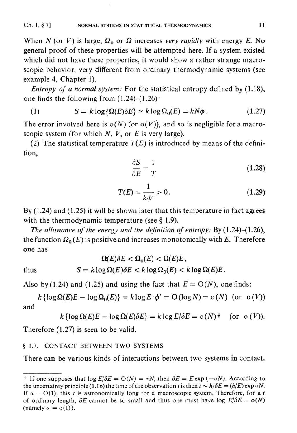
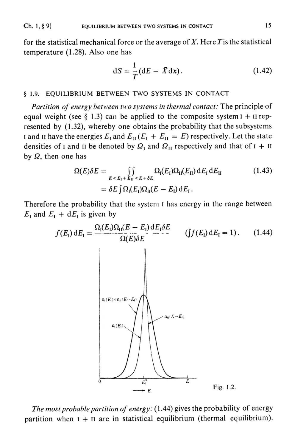
Partition of energy between two systems in thermal contact: The principle of
equal weight (see § 1.3) can be applied to the composite system I + n
represented by (1.32), whereby one obtains the probability that the subsystems
i and ii have the energies £, and Eu (E{ + Eu = E) respectively. Let the state
densities of i and n be denoted by QY and Qn respectively and that of I + n
by Q, then one has
Q(£)<3£ = J J 0,(^)0,,(¾) d£,d£n
E < Ei + Eu < E + SE
(1.43)
= 5£jnI(£I)QII(£:-£I)d£:I.
Therefore the probability that the system i has energy in the range between
£t and Ex + dE{ is given by
Q^QuiE- E^dE^E
"~d(E)SE
/(£I)d£1 =
(J/(£I)d£I = l). (1.44)
«„(£-£,)
Fig. 1.2.
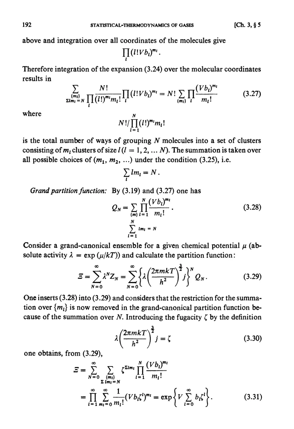
The most probable partition of energy: (1.44) gives the probability of energy
partition when i + n are in statistical equilibrium (thermal equilibrium).
16 PRINCIPLES OF STATISTICAL MECHANICS [Ch. 1, § 9
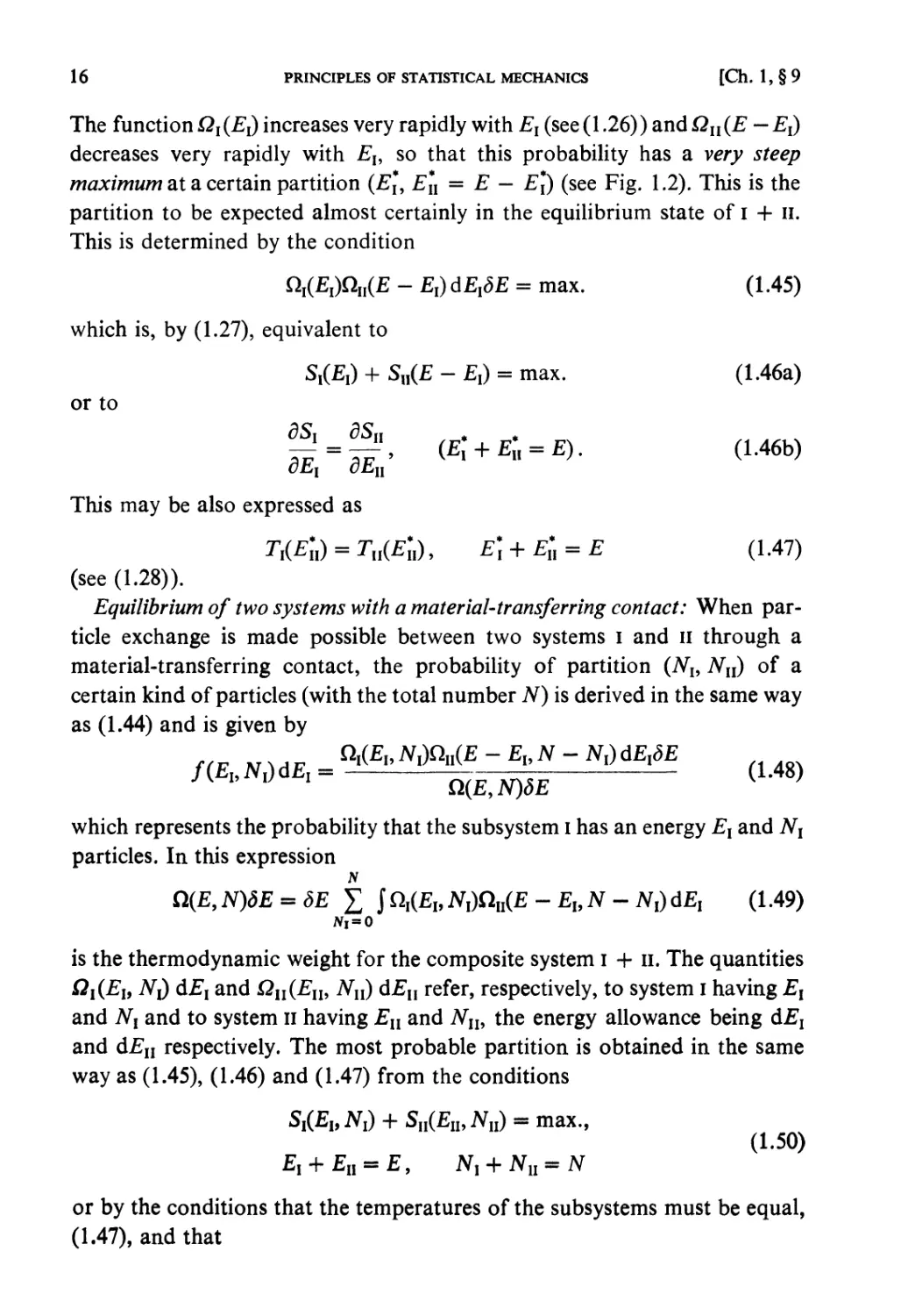
The function Qi{Ex) increases very rapidly with EY (see(1.26)) andQU{E — Ex)
decreases very rapidly with £,, so that this probability has a very steep
maximum at a certain partition (£,, £,*, = E — E*{) (see Fig. 1.2). This is the
partition to be expected almost certainly in the equilibrium state of I + 11.
This is determined by the condition
Q^EJOuiE - EJ AEfiE = max. (1.45)
which is, by (1.27), equivalent to
SX(EX) + S„(£ - Ex) = max. (1.46a)
or to
dSi dSu * *
--1 = -?, (e; + e;{ = e). (i.46b)
dEx dEn
This may be also expressed as
UE\X) = Tu(Eu), E\ + En = E (1.47)
(see (1.28)).
Equilibrium of two systems with a material-transferring contact: When
particle exchange is made possible between two systems I and ii through a
material-transferring contact, the probability of partition (Nl9 Nn) of a
certain kind of particles (with the total number N) is derived in the same way
as (1.44) and is given by
Q(E, N)5E
which represents the probability that the subsystem I has an energy £, and JV,
particles. In this expression
Cl(E, N)dE = SE £ J 0,(¾ #,)«„(£ - Eh N - Nx) d£, (1.49)
is the thermodynamic weight for the composite system I + ii. The quantities
Qi(El9 N^ d£, and £„(£„, Nu) d£n refer, respectively, to system I having Ex
and Nx and to system n having £„ and JV,,, the energy allowance being d£,
and d£n respectively. The most probable partition is obtained in the same
way as (1.45), (1.46) and (1.47) from the conditions
S£EuNd + Sn(ElhNn) = max.,
(1.50)
£, + £„ = £, #, + #,,«#
or by the conditions that the temperatures of the subsystems must be equal,
(1.47), and that
Ch. 1, § 9] EQUILIBRIUM BETWEEN TWO SYSTEMS IN CONTACT 17
5 (K N\) = ^1 (El Nn), N; + Nn = N . (1.51)
m Mi
Here the chemical potential ju is introduced by the definition
— S(E9N) = --. (1.52)
Equilibrium of two systems exerting pressure upon each other: When two
systems are in contact through a movable wall, so that an exchange of volume
i$ made possible (§ 1.7,(4)), the condition to determine the most probable
partition of volumes is given by
% (E\, N\, Vt)= £ (El N'u, Ift, V;+ Vn = V (1.53)
iI *II
where p is defined by
d p
— S(E9N9V)=-. (1.54)
dV T
This is derived in the same way as before. (If heat exchange is possible, then
one has also the condition (1.47).)
Additivity of entropy for systems in equilibrium: If the subsystems I and II
are normal in a statistical-thermodynamic sense, the additivity of entropy
holds for the composite system I + II, namely,
SI+II(E, JV, V) = Sl(E\9Nl V\)+ Sn(ElNl ^) (1.55)
where E*l9 etc., represent the most probable partitions (all quantities which
are not allowed to be exchanged by virtue of the nature of the contact are
fixed). Equation (1.55) means that the entropy of the composite system is the
sum of the entropies of the subsystems (example 5).
Increase of entropy by establishment of new equilibrium: Two separate
systems I and II are given with the partition (£,°, iV,0, K,0; £^, N°h V$) which
is different from (E\9 N\9 V\\ E^ A^, Kh). Then the two are brought into
contact and are made to reach a new equilibrium. In this new equilibrium,
the entropy of the total system becomes
SI+II(£,N,7)
= Sl(Eri9lfl9V^+Sn(Ern,!fn9VZ)
^ Stfl < 7,°) + SU(E& < KS)= Sinitial. (1.56)
If the systems I and n are separated again, they will almost certainly keep the
18
PRINCIPLES OF STATISTICAL MECHANICS
[Ch. 1, § 10
partition {E*u N*u V\; E^ N^, K,i). Therefore one has
Sf inai = St(El Nl V\) + Su(El Nl V;x) £ Slnltial. (1.56')
In other words, the entropy has been increased as a result of bringing I and n
into contact, and remains unchanged only when i and II were originally in
equilibrium with each other (namely the initial partition is equal to the most
probable partition after contact). When the two systems are separated after
contact, the entropy of the two systems is almost certainly found to be greater
than before contact, and they are almost certainly in equilibrium.
§ 1.10. FUNDAMENTAL LAWS OF THERMODYNAMICS
The first law of thermodynamics is, so to say, a self-evident consequence of
the dynamical laws which satisfy the conservation of energy. The internal
energy U is nothing but the energy E of the system, if the mechanical energy
is not included, and is therefore a function of the state.
Entropy: By the definitions (1.27), (1.28), (1.52) and (1.54), the entropy S
satisfies the relation
dS = -(d£ + pdV - Xdx - tidN) (1.57)
which gives the difference of entropy in the two neighboring equilibrium
states (£, K, x, N) and (E + d£, V + dV, x + dx, N + AN). When the
system suffers a change between these two states in a quasi-static process,
(1.57) can be written as
d£ = - pdV + Xdx + fidN + d'0, (1.58)
with
d'Q= TdS (1.59)
which represents the heat introduced into the system from the outside in the
course of the process (because the first two terms represent the mechanical
work given to the system from the outside, the third term is the energy
increase brought about by material transfer, and so the last term must be the
energy given from the outside in other forms, namely as heat flow).
Temperature: The temperature 7X£) defined by (1.28) coincides with the
thermodynamic absolute temperature and accordingly statistical entropy
coincides with the thermodynamic entropy (note that, however, statistical
entropy has been defined without an arbitrary additive constant), because (i)
T(E) gives the condition for thermal equilibrium as shown by (1.47) and (ii)
it becomes the integrating denominator for the differential form d'Q. The
Ch. 1, § 11]
FUNDAMENTAL LAWS OF THERMODYNAMICS
19
first is a characteristic general property for the temperature and the second
agrees with the definition of absolute temperature as introduced by the second
law of thermodynamics.
The second law of thermodynamics: This law is interpreted by a probabilistic
concept in statistical mechanics. When a certain inhibition (which, for
instance, prohibits mutual contact of two systems) is removed and two systems
are brought into contact, the entropy of the whole system will almost
certainly increase (see (1.56')).
Therefore a spontaneous decrease of entropy against the second law of
thermodynamics is extremely improbable.
For any process in which the system under consideration comes into
contact with an external environment, it very certainly holds that
dS + dSe^0. (1.60)
If the external environment is so large that its own change can be considered
as quasi-static and its temperature is equal to the temperature of the system,
then one may put dSe = — d'Q/T. Therefore the inequality
TdS^d'Q (1.61)
will be satisfied almost certainly for the entropy increase dS of the system
and the heat d'Q given to the system in the process.
The third law of thermodynamics: Entropy is defined by (1.18) in an
absolute manner. It is always non-negative by definition (W ^ 1). For a real quan-
tummechanical system the existence of the lowest ground state may be usually-
assumed. If the density of the system remains finite, log Q(E) will approach,
as E -+ 0 (the lowest energy value), a value which is independent of the size,
N or V, of the system. This means that the statement S -► 0 (as E -► 0) is a
consequence of the quantum-mechanical definition (1.18) for real physical
systems. It must be noted, however, that this does not necessarily assure that
an actual experimental measurement will give S -► 0 as T -► 0. It may happen
that the lowest state of the system is not attained in the course of the
experiment because the motion of particles is extremely slowed down as one goes to
T -► 0. When such freezing occurs, the observed entropy will approach a
value not equal to zero (example: glass).
§ 1.11. THE MOST PROBABLE STATE AND FLUCTUATIONS
Probability and entropy: Let a(a1? a2, . . .) be the parameters besides £, N9
and ^required to specify the macroscopic state of a system, and let W(E, N,
K, a) be the thermodynamic weight of the state (£, TV, K, a). Then the prob-
20 PRINCIPLES OF STATISTICAL MECHANICS [Ch. 1, § 11
ability for the realization of the state (£, N9 V, a) is, by the principle of equal
weight,
= WiEJ^cc) = 5(Wi.)/4
a
where
S(E9 N9 V,oc) = k log W(E9 N9 V9 a) (1.63)
is the entropy of the state (£, N, V, a).
Usually the most probable value a and the average value a of a coincide
with each other, because the maximum of the probability P(a) at a = a* is
extremely steep when the system is large. The most probable value a* is
determined by the condition that P(oc) is maximum or
S(E9 N, V9 a) = max., a = a* (1.64)
or
dS(E9N9V9*l9*29...)
dctj
= 0, j = 1,2,..., m. (1.65)
Determination of most probable values under constraints: When certain
constraints,
#„(ai,a2,...) = 0, n = 1,2,...,r (1.66)
are imposed on the variables olu oc2, ... am, the most probable values of a's
are determined by the condition (1.66) and
^ + I^" = 0, 7 = 1,2,... (1.67)
where Xl9 A2> • • • K are Lagrange's undetermined multipliers.!
Fluctuations: By (1.62)
P(a') = C'exp|-{S(E, AT, K,a* + a') - S(E9N9 K,a*)} | (1.68)
gives the probability for a realization of deviations of a's from their most
"t For the maximum probability one must have
.subject to the conditions
£ dS
SS= Z a-**i = 0 (1)
<5a, = 0 k = 1,..., r. (2)
i-i a«i
With r initially undetermined multipliers Ai, A2, ... , Ar, the following equations must
Ch. 1, § 12] CANONICAL DISTRIBUTIONS 21
probable values. If the a's are continuous, (1.68) may be written as
P(ai,ai,...)daidai... = c'exp|^S^^a^ [ daida2 •• (169)
which can be used for deviations which are not too large t-
§ 1.12. CANONICAL DISTRIBUTIONS
Canonical distribution: When a system with volume Kand NA, NB ...
particles is in equilibrium with a heat bath at temperature T9 the probability of
its microscopic states is given by
1 e~fi*"dr
(classically) Pr(dr) = =——^ —- , (1.70a)
\\NA\h ZN
(quantum-mechanically) Pr(/) =/(/) = ——, (1.70b)
where
P = l//cT, (fe = Boltzmann constant)
and^fN is the Hamiltonian of the system, ENtl being the energy of the /-th
quantum state. This distribution is called a canonical distribution, and an ensemble
obviously hold
6S+ t iWfc- Z (P + Z **?*)*>,-0. (3)
Now Ai, ... Ar are supposed to be chosen by the conditions
a^ £* aa,
Then equation (3) is reduced to
Since m — r variables out of ai, ... am are independent by the constraints (1.66),<5ar+i,...,
Socm can be regarded as independent variations, so that the conditions
0a, £* doc)
must also hold. Equations (4) and (5) together yield equation (1.67). The a's and A's are
determined from r + m equations (1.66) and (1.67).
t Generally speaking there exists a weight function ca(ai', 0*2', ... ). The choice of co
depends on the nature of the variables a. If they are originally expressed in terms of
dynamical variables (<?, p), the explicit form of co can be derived from the principle of
equal weight.
22
PRINCIPLES OF STATISTICAL MECHANICS
[Ch. 1, § 12
defined by this distribution is called a canonical ensemble. The system
considered here may be a small system with a rather few degrees of freedom, or
it may well be a large macroscopic system. ZN in (1.70a, b) is defined by
(classically) ZN = —L—^'f^ d£, (1.71a)
(quantum-mechanically) ZN = £e~'£jVi1' (1.71b)
or more generally by
ZN=]Q~0EQ(E)dE (1.71c)
o
and is called the partition function.
Note: The factor \/Y\NA\h3NA IS introduced in (1.71a), as was explained
in § 1.5, in order to secure the correct correspondence between classical and
quantum mechanics.
Derivation of canonical distribution: Let Q(E) be the state density of the
heat bath, £t the total energy of the composite system (the system under
consideration plus the heat bath), and £, the energy of/-th quantum state of
the system (£t = £ + £,). According to the principle of equal weight, the
probability that the quantum state / is realized is proportional to the number
of microscopic states allowed, which is equal to Q(Et — £,) SE. Therefore
Q(Et - Et)SE
[S(Et - £,) - S(Et)\
= exp< >. (1.72)
Since the heat bath is very large compared to the system considered it may be
assumed that £t §> Eh and so the exponent may be expanded as
dS 1 7d2S
MI+ 6
E = Et
E = Et
T{ 2CT
where
T = (dS/dEyl
is the temperature of the heat bath and C = dE/dT is its heat capacity.
Because of the assumed large size of the heat bath,
£/ << CT
Ch. 1, § 13]
GENERALIZED CANONICAL DISTRIBUTIONS
23
and the second term in the last brackets is so small that it may be ignored.
Then (1.72) reduces to
/(/)oce"£,/fcr.
§ 1.13. GENERALIZED CANONICAL DISTRIBUTIONS
T-fi distribution (Grand canonical distribution): When a system enclosed in
a volume V is in contact with a heat bath at temperature T and with a
particle source characterized by the chemical potentials fxA, juB, ... for
particles A,B, ... , then the number of particles it contains is also indeterminate.
The probability that the system has the microscopic state which contains NA,
NB9 ... particles is given by
(classical) Pr(N, dT) = yr^p^ ;= (1 -73a)
q-P(EN)i-1NaHa)
(quantum mechanical) Pr(N, I) = (1.73b)
where E is called the grand canonical partition function (or may be called
the T-fi partition function) defined by
(classical) _
00 °° i • r
-piJfN-HNAflA)
UNA^
NA = 0 Nb = 0 1X A
g-^-^M)^ (174a)
(quantum-mechanical)
00 00
-piENj-ZNAHA)
E = I I ...2>-'(£w',-I"^), (1.74b)
^ = 0 NB = 0
or more generally by
\Na=0Nb=0 J
00 00
= 11 -.UNAA-tiB Z„. (1.74c)
\Na=ONb=0 J
Instead of the chemical potentials, the absolute activities
xA = ^\...
are sometimes used.
If one wishes only the probability distribution of particle numbers, it is
given by
f%P(NAnA + NBHB + ...)7
Pr(NA,NB,...) = "
= ^^--zN (1?5)
24
PRINCIPLES OF STATISTICAL MECHANICS
[Ch. 1, § 13
Derivation ofT-jj. distribution: Let Nt be the total number of particles of a
given kind in the system considered and in the particle source, then the
probability -that the system has a partition of particles and energy (N, E)
becomes
Pr(N,E)acCl(Nt-N9Et-E)
oc exp - {S(Nt - N, Et - E) - S(Nt, Et)}.
The exponent may be expanded in the same way as for (1.72) since we may
assume that Nt^> N and Et > E. The higher order terms in the expansion
can safely be omitted. Then this reduces to (1.75) with the chemical potentials
defined by (1.52) (see example 6).
T-p distribution: When a system with given numbers of particles NA,
NB, ... is in contact with a bath at the temperature 7* and pressure/? through
a movable wall, then its volume Kis also indeterminate. The probability that
the system is found to be in a microscopic state with a volume V is given by
(classically)
Prw>dr>=nj^e~^+'r>^r- • (L76a)
(quantum-mechanically)
Pr(dK, 0 = , (1.76b)
where ^( K) is the Hamiltonian of the system with the volume V specified,
E^V) is its energy quantum energy and Y is the T-p partition function:
(classically)
0
(quantum-mechanically)
Y = ]dV^-HE,(V)+pV). (1.77b)
0
These may be written as
Y = ]zN(V)e-tpVdV. (1.77c)
o
The distribution in volume only is given by
e-*pVdV
Pr(dV) = ZN(V) . (1.78)
rv
dre-n*«n+*)t (177a)
Ch. 1, § 14] PARTITION FUNCTIONS AND THERMODYNAMIC FUNCTIONS
25
This distribution is derived in the same way as the canonical or grand canonical
distributions.
Note: The T-ju distribution and the T-p distribution, like the canonical
distribution, can be applied irrespective of the size of the system under
consideration.
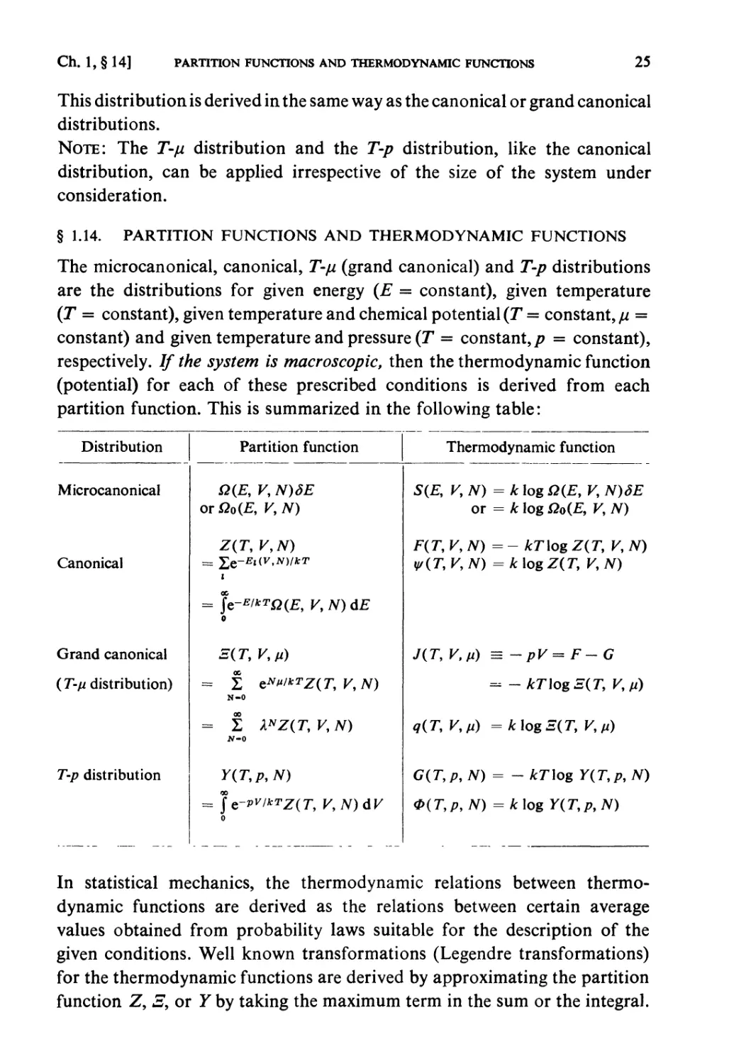
§ 1.14. PARTITION FUNCTIONS AND THERMODYNAMIC FUNCTIONS
The microcanonical, canonical, T-/J, (grand canonical) and T-p distributions
are the distributions for given energy (E = constant), given temperature
(T = constant), given temperature and chemical potential (T = constant, ju =
constant) and given temperature and pressure (T = constant,/? = constant),
respectively. If the system is macroscopic, then the thermodynamic function
(potential) for each of these prescribed conditions is derived from each
partition function. This is summarized in the following table:
Distribution
Microcanonical
Canonical
Grand canonical
(T-ji distribution)
T-p distribution
Partition function
Q(E, K, N)dE
orQo(E, V,N)
Z(T, V,N)
i
= ]e-E/*TQ(E, V,N)dE
0
Z(T,V,»)
= 2 eNt"*TZ(T,V,N)
N-0
= £ XNZ{T, V, N)
N-0
Y(T,p9N)
= Je-»wrZ(7\ V,N)dV
0
Thermodynamic function
S(£, K N) = k log Q(E, V, N)3E
or = k log Qo(E, K, N)
F(r, V,N)=- kT\og Z(T, V, N)
y/(T, V,N) = k log Z(T, V, N)
J(T, V,fi) = -pV= F-G
= -kT\ogE(T, Km)
q(T, V,») = klogS(T, V,fi)
G(T,p, N) = - kT\og Y(T,p, N)
0{T,p,N) =k\og Y(T,p,N)
In statistical mechanics, the thermodynamic relations between
thermodynamic functions are derived as the relations between certain average
values obtained from probability laws suitable for the description of the
given conditions. Well known transformations (Legendre transformations)
for the thermodynamic functions are derived by approximating the partition
function Z, S9 or Y by taking the maximum term in the sum or the integral.
26
PRINCIPLES OF STATISTICAL MECHANICS
[Ch. 1, § 14
This will be shown by the following argument for the canonical
distribution (see also § 2.3). Consider the quantum-mechanical case: the generalized
force X conjugate to a generalized coordinate x, involved in the Hamiltonian
^(P> q> x) is defined by
x = &r(q9p9x)
dx
The quantum-mechanical expectation value of this force in the quantum
state / is given by
dEt(x)
Xi = -^2 (1.79)
ox
where the energy El is regarded as a function of the parameter x. t The
averages of energy and force in the canonical distribution are given by
E =2£/e-W2e"'£'= -^logZ(/?,x), (1.80a)
x=2x,e-'*'/z=2^^/26-^ = -HlosZ^x)- (L80b)
I ' I • ' I P
t The energy Ei{x) is determined by the eigenvalue equation,
<^(/>, q, x)(pi = Ei(pi
where the eigenfunction (pi depends on the parameter x. When differentiated by x, this
becomes
dtf d(pi 8Ei t d(pi
— (pi -f JT -- = -- (pi + Ei — .
ox ox ox ox
This is multiplied by (pi* from the left and is integrated over the variables (r) of the wave
function,
r djf r 8(pi 8Ei r r dipt
(pi* —- (pi dr + (pi* tf - dr - - — (pi*(pi dr + Ei (pi* - dr
J dx J dx dx J J dx
or
XT , 17 f * 2^ J 8El < IT f *d(f>l A
Xi + Ei j (pi* - dr = -— + Ei J (pi* — dr.
Therefore, or
where the relations
c dJf
Xi = (pi* — (pi dr (definition of Xi)
dx
j" (pi*(pi dr = 1 (normalization)
j (pi*JFy/ dr = Ei \ (pi*y/ dr (Hermitian property)
are used.
Ch. 1, § 14] PARTITION FUNCTIONS AND THERMODYNAMIC FUNCTIONS
27
In particular, the average pressure is given by
j>=-*logZ(j8,7). (1.80c)
(1.81)
If one now i
equations (1
writes
-feTlogZ =
.80a-c) can be written
d
W'.
F
-- = £,
DT
as
dF
dx
F(T,
= x,
V,
>
x,...),
dF
dV =
p. (1.82)
This shows that F is nothing but the free energy of the system if £, X, and p
are identified with the thermodynamic energy, force and pressure.
The above can be shown in another way. In the integral
Z(T, V, N) = J e"£/*rQ(£, V,N)dE
= f exp I" - X-i~ - S(£, K, N)X\ dE/SE, (1.83)
the exponential function varies with £ extremely rapidly if £ and S ( =
k log Q - SE) are of the order Win magnitude (N is the total number of particles
in the system, which is very large), so that an overwhelming contribution to
the integral comes from the neighborhood of E* which is the most probable
value of £ in the canonical distribution. £* is determined by
E/T-S = min, thus 1/7 = dS/dE (E = £*).
The exponent in the integral is expanded in this neighborhood as
exp|~- ^{E'lT - S(E\ V,N)} - ^2^(E - E'f + ...1 (1.84)
where the relations
d2S/dE2 = dT~l/dE - - 1/T2C (C - dE/dT, E - £*)
are used (£ in these expressions should be put equal to £*). To the extent that
the difference £ — £* is small, or more exactly, of the order 0(N*) in
magnitude, the higher order terms in the expansion are of the order of
(£ - £*)m ' 0(JV~m + 1) = (N~*m+1) and can be ignored as JV -► oo. Hence
(1.83) is approximated by
Z - (Ink^C^dE-1 exp [- k~l{E*IT - S(E\ V9 AT)}] ,
28 PRINCIPLES OF STATISTICAL MECHANICS [Ch. 1, § 15
the logarithm of which gives
F(T, V9N) = E- TS(E, V, N)
if the free energy Fis introduced by (1.81). The above may be written as
- i F(T, V, N) = S(E9 V, N) - ~, (1.85a)
where JS'* is written simply as E. E on the right hand side of this equation is
regarded as a function of V, T, and N by the relation
«*™_i. (,.85,,)
dE T v '
Equations (1.85a) and (1.85b) show that -F/T is the Legendre transform
of S by which the independent variables are changed from E to l/T.
Therefore one finds
d (F\_/dS_ 1\ 8E
-E= -E.
The second and third equations of (1.82) are easily obtained from (1.85),
(1.52) and (1.54).
§ 1.15. FERMI-, BOSE-, AND BOLTZMANN-STATISTICS
One-particle states and the states of a system of particles: Let us consider a
system consisting of N particles of a certain kind. If the interaction of the
particles is weak enough, each particle has its own motion which is independent
of all others.f The quantum states allowed for this individual motion- one-
particle states - are determined by the Schrodinger equation
jri(P>x)<px(x) = ex<px(x) (1.86)
and are represented by the wave functions <pX9 the exs being the energies of
these quantum states.
Since identical particles are indistinguishable in quantum-mechanics, each
quantum state of the particle system is completely specified when the number
t Even for a system of particles with rather strong interaction, it often happens that the
one-particle approximation works surprisingly well when it is properly modified. We shall
not discuss such complicated cases here, but it should be recognized that the present
approach is also basic for many advanced problems. (1.88) will, however, then cease to be valid.
Ch. 1, § 15] FERMI-, BOSE-, AND BOLTZMANN-STATISTICS 29
occupying one-particle states is given precisely. That is, the set of occupation
numbers
/ = {«t}=(Wl,«2,...,nr,...) (1.87)
gives the quantum numbers of the whole system. The energy of the system is
then given by
£/ = £(,o = Iv*x. (1.88)
Fermi-statistics (F.D.) and Bose-statistics (B.E.) f: The occupation numbers,
or the number of particles in each one-particle state, are strongly restricted
by a general principle of quantum mechanics.ft There can be only the
following two cases:
for F. D. (Fermi-statistics) n = 0 or 1
(1.89)
for B. E. (Bose-statistics) n = 0, 1, 2, ... .
The difference between the two cases is determined by the nature of the
particle. Particles which follow Fermi-statistics are called Fermi-particles (Fer-
mions) and those which follow Bose-statistics are called Bose-particles
(Bosons).
Electrons (e), positrons (e+), protons (P), and neutrons (N) are
Fermi-particles, whereas photons are Bose-particles.
Generally, a particle consisting of an odd number of Fermi-particles
(example :D = P-fN-fe)isa Fermi-particle, and a particle consisting of
an even number of Fermi-particles (example: H = P -f e) is a Bose-particle
(a particle consisting of Bose-particles only is a Bose-particle). A Fermi-
particle has half-integral spin and a Bose-particle has integral spin.
Fermi distribution and Bose distribution: When the particle system is in
equilibrium (the total number of particles Wis assumed very large, of course),
the average occupation number for each one-particle state is shown to be
(example 12, problem 3)
1
*«=(..-,)/»•,, «> (FD) (L90)
»r = e(CT-ir _ t, (B.E.) (1.91)
t These are often called Fermi-Dirac statistics and Bose-Einstein statistics.
tt The wave function of a system of identical particles must be either symmetrical (Bose)
or antisymmetrical (Fermi) in permutation of the particle coordinates (including spin)
(see, for example, Schiff: Quantum Mechanics).
30
PRINCIPLES OF STATISTICAL MECHANICS
[Ch. 1, § 15
where T is the temperature of the system and // the chemical potential of the
particle. The energy of the total system is given by
£ = IM„ (1-92)
r
while the total number of particles is
JV = X>\. (1.93)
Meaning offi and T: // and J1 appearing in equation (1.90) and (1.91) may
be interpreted in different ways:
(1) If the system is isolated (microcanonical ensemble), equation (1.92)
and (1.93) determine T and // for prescribed E and N.
(2) When the system is in contact with a heat bath at temperature T
(canonical ensemble), equation (1.92) gives the average energy and (1.93)
determines // for prescribed T and N.
(3) When the system is in contact with a bath at temperature Tand with a
particle source characterized by the chemical potential // (grand canonical),
(1.92) and (1.93) give the average E and N.
Thermodynamic functions: The upper sign is for F. D. and the lower sign is
for B. E. (see example 12):
S = fcl [- nxlognx + (1+ «t)log(l + «%)] , (1.94a)
r
F = E-TS, G = Nfi, (1.94b)
J = - PV=F - Nfi= +/cTXlog(l =Mr)
r
= ± fcT£log(l + c("-e')/kT). (1.94c)
r
The classical limit (Boltzmann-statistics): When the particle density is so
low and the temperature so high that the condition
N /2nmkT\2
v*{—*-j (1'9!)
is satisfied, we have
«r<l, er-/i>/cT. (1.96)
Both F. D. and B. E. statistics are reduced to the classical limit, which
corresponds to the classical approximation mentioned in § 1.5. This limiting
law is called Boltzmann-statistics, and its distribution (the Boltzmann-
Ch. 1, § 16]
GENERALIZED ENTROPY
31
distribution, sometimes called the Boltzmann-Maxwell distribution) is given
by
(1.97)
«r = e(^^kT.
For Boltzmann statistics, the one-particle partition function can be defined by
/=Xe-'',lT = Ie^. (1.98)
r
With this definition the following formulae are obtained (see problem 19):
N = Xf,
k
aH/kT
N
8 log/
dp '
ZN =
*f
f
F = -NkT -NkTlog-
N
pV = NkT.
(1.99)
The Maxwell velocity distribution: The probability that a molecule (mass m)
in an ideal gas at temperature T will be found to have a velocity in a range
between (vx, vy, vz) and (vx + dvx, vy + dvy, vz + dvz) is given by
f(vx,vy,vz)dvxdvydvz =
m
2kT
(v2 + v2 + v2)
Kx y ^d^du-di;,. (1.100)
K2KkTJ
This is called the Maxwell (Boltzmann) velocity distribution law.
§ 1.16. GENERALIZED ENTROPY
It is possible to define the entropy for a statistical ensemble by
S= -fcI/(01og/(/)=-kl^g/,
(1.101)
where/(/) is the probability of the realization of the quantum state /. It is
recommended that the readers prove for themselves that this definition yields
the correct expressions for statistical entropies for microcanonical, canonical,
grand canonical and other ensembles. Equation (1.101) is related to general
H-theorems which include time explicitly.
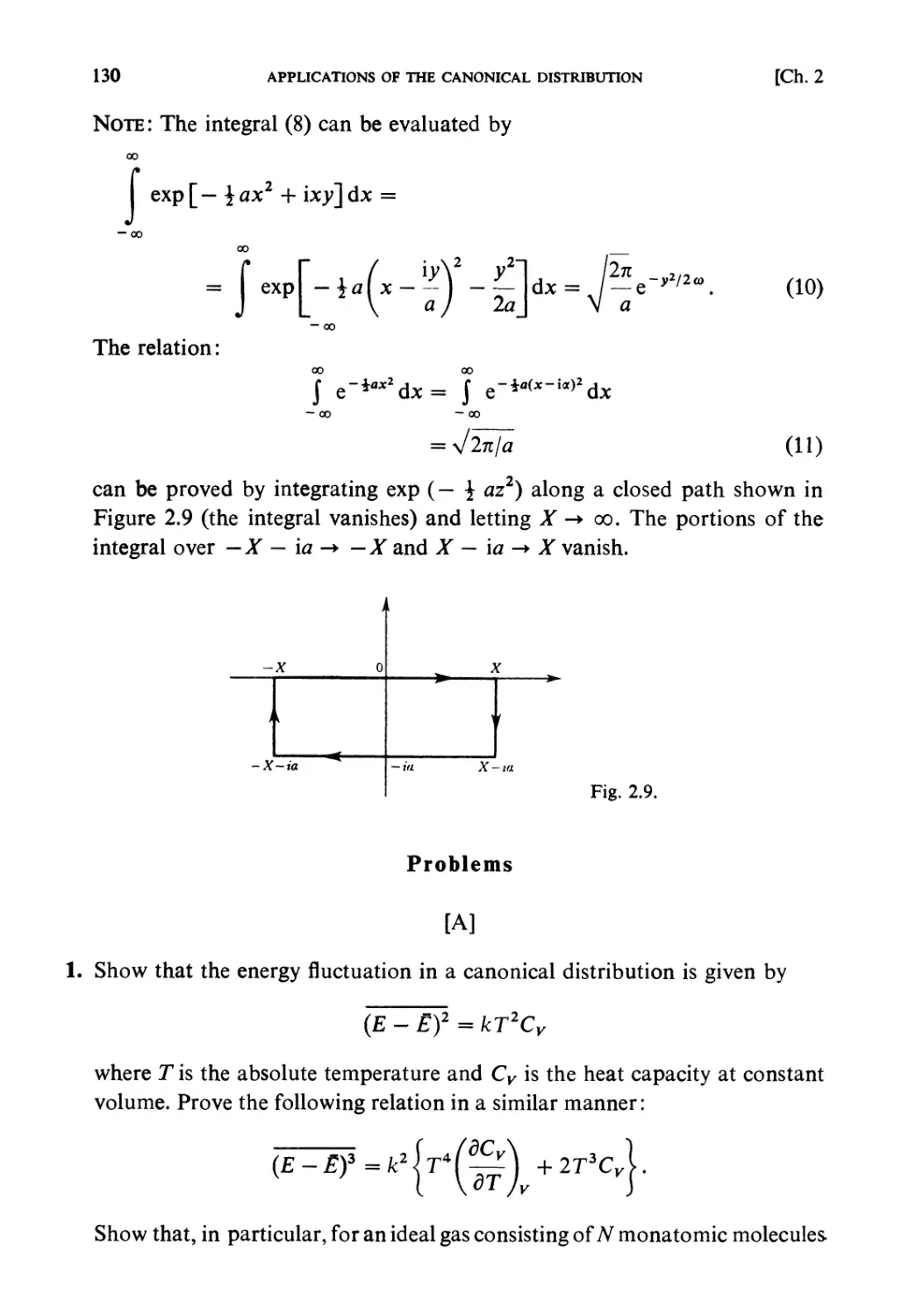
Divertissement 2
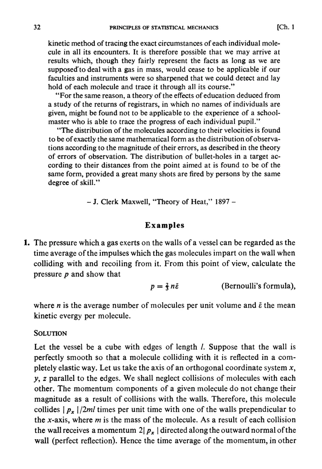
Statistical method. "And here I wish to point out that, in adopting this
statistical method of considering the average number of groups of
molecules selected according to their velocities, we have abandoned the strict
32
PRINCIPLES OF STATISTICAL MECHANICS
[Ch. 1
kinetic method of tracing the exact circumstances of each individual
molecule in all its encounters. It is therefore possible that we may arrive at
results which, though they fairly represent the facts as long as we are
supposed'to deal with a gas in mass, would cease to be applicable if our
faculties and instruments were so sharpened that we could detect and lay
hold of each molecule and trace it through all its course."
"For the same reason, a theory of the effects of education deduced from
a study of the returns of registrars, in which no names of individuals are
given, might be found not to be applicable to the experience of a
schoolmaster who is able to trace the progress of each individual pupil."
"The distribution of the molecules according to their velocities is found
to be of exactly the same mathematical form as the distribution of
observations according to the magnitude of their errors, as described in the theory
of errors of observation. The distribution of bullet-holes in a target
according to their distances from the point aimed at is found to be of the
same form, provided a great many shots are fired by persons by the same
degree of skill."
- J. Clerk Maxwell, "Theory of Heat," 1897 -
Examples
1. The pressure which a gas exerts on the walls of a vessel can be regarded as the
time average of the impulses which the gas molecules impart on the wall when
colliding with and recoiling from it. From this point of view, calculate the
pressure p and show that
p = \nl (Bernoulli's formula),
where n is the average number of molecules per unit volume and e the mean
kinetic evergy per molecule.
Solution
Let the vessel be a cube with edges of length /. Suppose that the wall is
perfectly smooth so that a molecule colliding with it is reflected in a
completely elastic way. Let us take the axis of an orthogonal coordinate system x9
y, z parallel to the edges. We shall neglect collisions of molecules with each
other. The momentum components of a given molecule do not change their
magnitude as a result of collisions with the walls. Therefore, this molecule
collides | px | /2ml times per unit time with one of the walls prependicular to
the x-axis, where m is the mass of the molecule. As a result of each collision
the wall receives a momentum 2\px\ directed along the outward normal of the
wall (perfect reflection). Hence the time average of the momentum, in other
Ch. 1]
EXAMPLES
33
words, the sum of the momentum imparted to the wall per unit time, is equal
to 2 | px | • | px | /2ml = pi/ml. Since the sum of these momenta yields a force,
the contribution of this molecule to the pressure is given by this sum divided
by the area of the wall I2 (V = /3 is the volume of the vessel). Therefore,
adding together the contributions from all the molecules, we obtain the
pressure exerted by all the molecules:
1 ^ VL + Pfy + Pfz
1 V?'
i=l
m
2 ^CPi 2N 2
= > — = £ = -/26.
3V^2m 3K 3
(1)
Fig. 1.3.
Alternative solution
(Method using the virial theorem). Denoting the position vector of the i-th
molecule by xh one has
£ N N N N N
. X Pi'Xi= X Pi'Xi+ X Pi'*i = £ Fi'Xi + 2% ^ (2)
dt
i=l
i=\
i=\
i= 1
i=l
where Ft is the force acting on the z-th molecule and ef its kinetic energy.
When the time average is taken of both sides, the left hand side vanishes,
since
t0 + t
d 1
-/4(0 = lim-
dt ,-oc *
J A(t) dt = lim - {A(t0 + 0 - ^4(^0)} (3)
at t^oot
is clearly equal to 0 for any time-dependent quantity ^4(0 which remains
finite and bounded at any instant. In the present case the quantity varies with
the motion of the gas molecules but always stays finite (since the momenta as
well as the coordinates remain finite). Therefore, one gets from (2)
2£e(= £F,-x,.
N
L
1=1
(4)
The right hand side is called the virial. If the intermodular force is negligible,
34 PRINCIPLES OF STATISTICAL MECHANICS [Ch. 1
Ft is simply the force exerted on the molecule by the walls. Its time average
per unit area being the pressure/?, the virial due to this force is given by
N
I
lF,-x,= - | pvxdS (5)
where v is the outward normal to the walls and the integral is evaluated over
the walls. By means of Gauss' theorem
one has
jVvdS = JdivadF
JvjcdS = JdivjcdF = 3 \<\V = 3V. (6)
Fig. 1.4. Calculation of the virial due to
the force exerted by the wall.
From (4), (5) and (6) one gets
2Ne = 3pV, or p = ^ne.
Note: The virial theorem (4) is valid also in the case where one must take
into account the intermolecular force explicitly. If Ftj is the force the /-th
molecule exerts on they'-th, one has Fu = /^because of the law of action
and reaction. The virial due to the intermolecular force is
From (4) one gets
P = lns+ -. (8)
3V
When the range of the intermolecular force is much smaller than the mean
intermolecular distance, 0 is almost zero and Bernoulli's formula holds. In
the general case one has to use (8) (see problem 6 in Chapter 2).
Ch. 1]
EXAMPLES
35
2. An ideal gas consisting of TV mass points is contained in a box of volume V.
Find the number of states (phase integral) QQ{E) (1.20b) classically and,
using it, derive the equation of state. {Hint: The volume of a unit sphere in a
w-dimensional space, Cn, is equal to tz*nIT{\n -f 1).)
Solution
The energy of this system is
jr=fpf/2m (1)
1=1
where we have labelled the momenta conjugate to the Cartesian coordinates
of each mass point with running index number: pl9 ... , p3N. The number
of states is given by (1.20b) where the integral over the coordinates gives VN9
VN
Q0(£,iV,F) = -3^-j... J dPl...dp3N. (2)
IPi2|2m£
1
Since this integral is equal to the volume of a 37V-dimensional sphere of
radius (2mE)* it is proportional to (2mE)3N/2, the proportionality coefficient
being the number C3N given in the hint. Hence,
VN (2nmE)3N/2
h3irNl I\iN + I)
By (1.27) the entropy becomes
Q0(£,N,K) =-3^-^-^-. (3)
f V IE (Inmfs*}
S{E,N, V) = /clogQ0 = Nkhog- + jlog— + logK—^— - L (4)
where use has been made of Stirling's formula
logN! - JVIog(N/e) = N\ogN - N. (5)
From (1.28) and (1.54) we get
1 fdS\ 3 IE
_=[_ =Nk — 9 or kT = — = fe, (6)
T \dEjv.N 2£ 3N T W
P fdS\
^ = (^) = Nklv> or PV = NkT. (7)
Note 1: There are a number of ways of calculating the volume of a «-dimen-
sional sphere. We shall give only one of them. If the volume of a «-dimen-
sional sphere of radius r is Vn{r) = Cnrn, the surface area of the sphere is
36 PRINCIPLES OF STATISTICAL MECHANICS [Ch. 1
equal to nCnrN~l. Using this relation we evaluate
00 00
h= J ... J exp{-a(x21 + ...+xl)}dxl...dxH
— oo — 00
by two different methods. First, because of the well-known formula,
00
J exp( — ax2)dx = (n/ci)*,
— oo
we get /„ = (n/a)*".
Secondly, by dividing the xu ... xn space into spherical shells we can
perform the integration:
ln=]z-a'2nCnrn-*<\r
o
= \nCn J e" V""1 dy = ^nCnr{\n)a^tt = Cnr{\n + l)*"*"
0
(]e-xxm-1dx = r(m)).
o
Equating the two expressions we have
Note 2: Stirling's formula
r(x + 1) = x! ~ xx+iQ~xy/2n9 (8a)
or
logx! ~ xlogx — x + ... (8b)
is an asymptotic formula valid for x > 1, which is frequently used in
statistical mechanics.
3. The energy level of an oscillator with frequency v is given by
e = Pv,jfcv,...,(n + i)fcv,... .
When a system consisting of TV almost independent oscillators has the total
energy
E = ±Nhv -f Mhv (M is an integer)
(i) find the thermodynamic weight WM, and (ii) determine the relation
between the temperature of this system and E.
Solution
(i) If the quantum number of the /-th oscillator is denoted by nh the state-
Ch. 1]
EXAMPLES
37
ment that the total energy of the system is equal to %Nhv -f Mhv implies that
nx + n2 + ... + nN = M.
Therefore, the thermodynamic weight WM of a macroscopic state with the
total energy E is equal to the number of ways of distributing M white balls
among TV labelled boxes. A box may be empty since n{ = 0 is possible. As is
evident from Fig. 1.5, one can get this number by finding the number of
permutations of placing in a row all the white balls together with (N — 1) red
balls that designate the dividing walls. If one labels all the balls with the
running numbers, 1, 2, ..., M -f N — 1, the number of permutations is
(M + N — 1)!. When one erases these numbers there appear
indistinguishable distributions, the number of which is equal to the number of
permutations among the (numbered) balls with the same color, M\{N — 1)!.
Therefore,
(M + N - 1)!
WM =
M\(N - 1)!
(1)
o
o
o o
o°o
o
0
o
o
OO #00000 •• OOOIO
Fig. 1.5.
(ii) From (1.18) the entropy is
S = k log WM .
Substituting (1) and using Stirling's formula under the assumption, N ^> \,
M > 1, one has
S = k{(M + N)log(M + N) - MlogM - NlogN} .
From (1.28)
1 _ dS _ dS dM
T~ dE~dM~dE
(M + N\ dM k M + ±N + ±N
= /clog ——— )• — = — log-
(2)
M dE hv M + iN -±N
= -log
\E/N -ihv)'
hv \E/N-ihv
38
Or, inversely,
PRINCIPLES OF STATISTICAL MECHANICS
[Ch. 1
E + iNhv
E - iNhv
= Qhv/kT
Solving this for E, one gets
E = NUhv +
hv
QH^kT _ 1
(3)
In Fig. 1.6, E/Nhv is plotted against kT/hv.
4. There is a system consisting of N independent particles. Each particle can
have only one of the two energy levels, -s0, e0. Find the thermodynamic
weight WM of a state with the total energy E = Ms0(M = -N9 ... ,N), and
discuss the statistical-thermodynamic properties of the system for the
range E < 0, deriving especially the relation between temperature and the
energy as well as the specific heat.
Solution
If 7V_ particles are in the state with energy -s0 and 7V+ particles in the state
with energy e0, the energy of the total system is
£ = Me0=-iV_£0 + N + e0 , M = N+ - N.
(1)
Ch. 1]
EXAMPLES
39
Since N = N+ + 7V_, one has
N_ =i(JV-M),
N+ =±(N + M).
(2)
Now, there are N\/(N-\N+!) possible ways of choosing JV_ particles out of
TV to occupy the state with — e0, each of which gives a different microscopic
state with the energy E. Hence the thermodynamic weight is
WM =
N\
(3)
[i(Ar-M)]![i(AT + M)]!'
According to (1.18) the entropy of the system is
S(E) = k log WM
~ lc{N\ogN - i(N - M)logi(iV - Af) - i(AT + M)logi(^V + M)}
= - /c{iV_ log(AT_/A0 + N+ \og(N+/N)} (4)
where Stirling's formula has been used. Defining the temperature by (1.28),
one has
1
' ' (5)
1 dS k N - M
-= = i -log .
T e0dM £0 N + M
As one can see from this equation or from the relation between S and E
(Fig. 1.7), T < 0 for M > 0 (E > 0), so that this system is «or normal in the
sense of statistical mechanics. Since, however, it is normal in the range
M < 0 (E < 0), one can discuss the property of this system within this range.
Fig. 1.7.
40
PRINCIPLES OF STATISTICAL MECHANICS
[Ch. 1
From (5) one gets
or
N.
N +
N.
N
N+
N — M ~ ,.-
_ _ Q^eo/kT
N + M
Qeo/kT
~ Qe0/kT + e-coAr>
c-eo/kT
N Qeo/kT+Q-eo/kT
Therefore,
E = - (AT. - iV+)e0 = - Ne0 tanh(e0/fcT).
(6)
(7)
Equations (6) give the probabilities of finding any one particle in the states
— s0 and +e0, respectively, and have the form of a canonical distribution
(1.70). From (7) the specific heat becomes
C = dE/dT = JVfc(f;)2//cosh^r.
(8)
Figs. 1.8 and 1.9 show the graphs of £ versus J and C versus T, respectively.
Note: Putting 2e0 = AE, one rewrites (8) as
C = Nk(^\\AB'kTl(l+^E,kT)2.
(9)
0
-0.5
-1.0
1 1 ' 1 ' 1 i 1 ' "J r I
: -~~\
|/]
1,1,1.1,1.1.,
2 3
► kT/e0
Fig. 1.8.
Ch. 1]
EXAMPLES
41
The specific heat of this form is called the Schottky specific heat. When a body
contains a substance having the excitation energy A£, the specific heat
anomaly with a peak as shown in Fig. 1.9 is actually observed.
0.5
0.4
0.3
0.1
"0 1 2 3 4 5 6
^kT/to
Fig. 1.9.
5. Suppose that two systems, which are normal in the sense of statistical
thermodynamics, have the number of states of the form (1.24a). Prove the following
statements concerning the thermal contact of the two system, (i) If their initial
temperatures are Tx and T2 (Tx > T2\ heat will flow from 1 to 2 upon contact
and the entropy will increase by the amount &'Q(T2l — T±l). (ii) When
both systems are in thermal equilibrium with each other, the entropy of the
composite system Sx + 2 is equal to the sum of the entropies of the subsystems
Sx and S2. (iii) The fluctuations in the energy of subsystem 1 or subsystem 2
when in a state of thermal equilibrium, (Ex — E[)2 or (E2 — E*2)2, are given
by/cJ2/^"1 + CJ1), where El9 E2 are the mean values (the most probable
values) of the energies of 1 and 2, and Cx and C2 are the respective specific
heats.
Solution
We suppose that the numbers of states Q^(Et)9 Q2(E2) are respectively of the
form,
Q?(£x) ~ exp {NrfAEJNJ}, C1°2(E2) ~ exp {N2<t>2{E2IN2)} (1)
42 PRINCIPLES OF STATISTICAL MECHANICS |Ch. 1
where Nu N2 are the number of particles in each system, both of them being
very large. The probability of a state in which 1 and 2 have energies
approximately equal to Ex and E2 respectively is given by
W(EUE2) = Q1(E1)Q2(E2)SElSE2
~ expfN^EJN,) + N2fa(E2IN2)}-pl(ElINl)<l>'2(E2IN2)6El5E2, (2)
where the widths of the energy uncertainty in each system are denoted by
SEX and SE2, and dQ°l(E)/dE = QX(E). Since Nx and N2 are large, the
exponential function dominates in (2), the rest of the factors ¢[, 02 being of
negligible influence (their influence is of the order of \/N).
(i) It is probable that upon thermal contact between 1 and 2 there occurs
an energy flow between the systems and, as a result, they will go into a state
with larger W(El9 E2). In other words, W(El, E2) almost certainly increases
as a result of thermal contact. Hence
k log W(EUE2) = S(El9E2) = kNrf^EJNJ + kN24>2(E2jN2) (3)
also increases. The amount of its increase due to the change dEt — — dE2 —
- d'Q is, according to (1.27) and (1.29),
dS(EuE2) = {k^EJNJ - W2(E2jN2)} d£\ = d'Q{T2l - 771}.
If 7\ > J2, we must have d'Q > 0 in order that dS(Eu E2) > 0. That is to
say, it is almost certain that heat flows from 1 to 2.
(ii) When the systems 1 and 2 are in thermal equilibrium, the total number
of microscopic states (thermodynamic weight) of the compound system 1 + 2
having a total energy of approximately E can be obtained by integrating (2):
W(E) - SE^Q^E^Q^E - E^d^i
(E2 = E-El).
Since under the condition El + E2 — E = constant, the exponential
function in the integrand has its maximum value at E[, E2 determined by
N^iEJN,) + N202(E2/N2) = max., or ^(E'JN,) = <i>2{E\lN2). (5)
Corresponding to (1.46) and (1.47), we can expand this function around the
maximum in the following way:
■
Ch. 1]
EXAMPLES
43
-!i+
= exp[«1*,(!) + «!*!(!)-(£'i^ + ...]. (6,
where
(using the condition (1.25)).
If 0(^) - 0(N2) = O(N), A2 - O(N). Since the higher order terms in
[ ] are proportional to Ar~(m_1) (El — £*)m (m > 3), they are of the order
0(Ar*m+1). £« if we put £i _ £* = ;vi£ Hence we may neglect them
(except the term m — 2) in the limit N -> oo. Because
Ei Ei Ei—Ei Ei s Ei
N[ = n[ + AT, = JVX + Nf ~* AT,"
the change in the values of the factors <j>[, </>2 in (4) can also be neglected.
Therefore, in the limit N -» oo, (4) becomes asymptotically equal to
W(E) ~ <5£exp JN^(¾ + A/2<£2(^)1 ■ fexp|- L(El - E\AdE,
= ^V27tAexp'|iV1^1^+ A^2(J
(8)
Taking the logarithm of this expression, we get
S1 + 2(£) = /clog ^ - /cLv^ ^1 ) + N202(^J (9)
= S^) + S2(£2)
since log A = 0(log N) may be neglected. The right-hand side is the sum of
the entropies when 1 and 2 have the energies E[ and El respectively.
(iii) The integrand of (4) is the probability of 1 and 2 having energies £x
and £2, respectively, in a state of thermal equilibrium. The probability of 1
44 PRINCIPLES OF STATISTICAL MECHANICS [Ch. 1
having energy in the range Ex and Ex -f dEx is equal to
.{»,*.(£)■
where C is the normalization constant. According to what we have said
earlier, when 0(^) = 0(N2) = 0(AO, we may put
P(E1)dE1 = Cexp[~-JL(E! - El)2! (11)
asymptotically in the limit N -+ co. Here A is given by (7). Since one gets
it can be rewritten as
f," (El\ = ~Nl ldll = _ Nl (Ci = the sPecific heat\ (l2\
\Nj kT2 J dT kT2Ct \of the system 1 /
*'-kTik+B' <i3)
Equation (11) holds when Ex — E[ is of the order 0(N*) and shows that
(Ex - £XT = A2. (When £x - £^ = 0(^), it will no longer be of the
Gaussian type. The probability that such a fluctuation will occur is, however,
extremely small and need not be considered.)
6. Show that a system in contact with a heat and particle source has particle
number N and energy E with the probability given by (1.73a, b).
Solution
Let Q(NS9 Es) be the density of states of the heat-particle source. We shall
denote by Nt and Et the total number of particles and the total energy of the
compound system composed by the system under consideration and this
heat-particle source, respectively. The probability Pr (N,E) that the system
under consideration is in a microscopic state with N and E is proportional to
the thermodynamic weight of a state of the heat-particle source with Nt — N
and Et — E:
Pr(N, E) oc Cl(Nt - N, Et - E) 5Et
oc exp- {S(Nt - Nf Et - £) - S(Nt9 Et)} . (1)
Ch. 1]
EXAMPLES
45
Since the heat-particle source is a very large system, we may put Nt > AT and
Et > E. Hence
S(Nt-N9Et-E)-S(Nt9Et) =
/ds\ /es\ if 2d2s d2s 2d2s)
= -JV -El —) +-\N2—, + 2NE + £2 — -> + ...
\dNjEt \dEjNt 2{ dN2 dNtdEt cE\\
-?"-i+iH-^)+£4)}+--
Here n and T are the chemical potential and the temperature of the heat-
particle source with Nt and Ei9 and A indicates the variations due to the
deviation of AT and E from Nt and Ev Since these changes are 0(N/Nt) and
0(E/Et)9 we can neglect them as long as TV < Nt9 E < Ev Since the
probability of having N ~ Nt9 E ~ Et is, at any rate, extremely small, we can use this
approximation. Therefore, from (1) we get
Pr(N, E) oc exp
Normalizing this, we obtain (1.73a). (The same argument applies to the case
where many kinds of particles are present.)
7. There are more than two systems A9 B9 C, ... , which are almost independent
of each other. Suppose that they interact with each other weakly, so that they
can be regarded as a compound system A + B + C ... Show that the
partition function ZA + B+ and the free energy FA+B+...are given by
Za+b+... ~ Za'Z-b •••» Fa+b+... — Fa + Fb + •••
respectively, where ZA, ZB, ... are the partition functions of the individual
systems.
Solution
If one denotes the energy of the quantum state / of the system A by EAl
(/=1,2,...)» one has, according to (1.71b),
Z^ = Ie-^''. (1)
Similarly, if one writes the energy of the quantum state m of the system B as
EB,mi.m = 1,2, ... ), one has
ZB = Ie-"EB"". (2)
liN-E
IcT
46
PRINCIPLES OF STATISTICAL MECHANICS
[Ch. 1
We have assumed that these systems are in contact with a heat reservoir at the
same temperature.
Since the subsystems are almost independent, the quantum state of the
compound system A + B + ... is determined if one specifies the quantum
states of the individual subsystems: it is specified by a set of the quantum
numbers (/, m, ... ), where /, m, ... take the values 1,2,... independently,
and its energy is approximated by EA { + EB m + . .. . Therefore, the
partition function defined by (1.71b) can be transformed as follows:
I m
Hence one has
^a + b... — ZAZB.... (3)
According to the table in § 1.14 the free energy is given by F = — kT log Z.
Substituting ZA, ZB, ..., ZA + B+ , one gets from (3)
Fa + b + ... = - kT\ogZA + B + _ = - kT\ogZAZB...
= - kT\ogZA - kT\ogZB... = FA + FB+ ....
8. Apply the canonical and the T-p distribution in classical statistical mechanics
to an ideal gas consisting of vVmonatomic molecules and derive the respective
thermodynamic functions.
Solution
Let us calculate them according to § 1.14. The Hamiltonian of this system is
3 A' 2
^ 2m
1 = 1
where we have adopted a Cartesian coordinate system and used the same
notation as in example 2. Let us first apply the canonical distribution.
According to (1.71a) the partition function is
/z3A/7V!J M Fl
Since the Hamiltonian is a function only of the momenta, the integration
over the coordinates can readily be performed, yielding ^(Fis the volume
of the vessel). The integral over the momenta is equal to the product of the
Ch. 1] EXAMPLES 47
integrals over each momentum coordinate since the Hamiltonian is the sum
of the terms for individual degrees of freedom. All the integrals being
identical, it is equal to the 3vV-th power of the integral with respect to one degree
of freedom, which is
thUS Z = -Jr- VN(2nmkT)*N . (1)
The thermodynamic function corresponding to this is the Helmholtz free
energy and is given by
F = - /cTlogZ = - NkThlogT + log - + logv—~— \ (2)
where we have used Stirling's formula, log N\ « TV log (N/q).
Next, the partition function for the T-p distribution is
00
Y(T,p,N)= $e-pVlkTZ(T,V,N)dV.
o
Substituting (1), one gets
Y = -j-J -(2nmkT)3m]e->r,kTV"dV.
h N\ o
Writingp/kT — a, one can evaluate this integral as follows:
1 /fcTV'1"1
thus Y(T,p,N) = -^-Ni(27imkT)^N\\^- ) »
*A3W(2nn,fcT)*^--J . (3)
Here the exponent is approximated by N + I -+ N because of N > 1. The
corresponding thermodynamic function is the Gibbs free energy,
G(T,p,N)=-kTlogY = - NkT HlogT-\ogp + logy—~-\.
(4)
Note: From/? = — (dF/dV)TtN or V = (dG/dp)TN one can readily obtain
pV = NkT. One can also confirm that the relation G = F + /7Kholds for (2)
48
PRINCIPLES OF STATISTICAL MECHANICS
[Ch. 1
and (4). The entropy can be obtained either from S = —(dF/dT)VtN or from
S = — (dG/dT)PtN9 the results being identical with each other because of
pV = NkT(sQQ example 2):
S = Nik | i log T + log- + log[(27rm/c)*e*//i3]i
= Nk{ilog T - logp + log[(27rm/c)*/ce*//*3]}. (5)
According to // = (dF/dN)TV or G = Np, the chemical potential is equal to
N( ** \*_ P ( hl \*
The internal energy is U - -T2d[F/T)/dT = fN/cJ, and CK = JMfc,
Cp = 1 M:.
9. Suppose there are two systems i and n in thermal contact with a heat bath at
temperature T and there exists some mechanism enabling the two systems to
exchange particles. Obtain the expression for the probability of having a
distribution (Nl9 Nu) of particles into I and n in terms of the partition
functions Zt(Nl9 T) and Zn(NIl9 T)9 and derive the condition for finding the most
probable distribution.
Solution
Since the composite system i + n of the systems i, ii is in contact with a heat
bath, its microscopic states are realized according to the canonical
distribution. The probability that the composite system I + ii is in a state in which
the system I has an energy in the range between E{ and E{ -f dE{ and a particle
number equal to Nl9 while the system n has an energy in the range (Ell9 Eu -f
dEn) and a particle number Nll9 is given by the sum of the elementary
probability (1.70) over all the possible microscopic states subject to the given
condition:
/(£„ Nl9 Ell9 Nll9 T) d£, d£„ = -— e "'<*+£"> 0,(2,, N{) d£, Q„(£„, JV„) d£„
A+ii
(i)
(/? = l/kT).Zl + u is the partition function of the composite system I + ii and,
as one can see from (1.49), is equal to
ZI+„(N,T)= ^ UNl9T)ZdLN-Nl9T) (2)
Ni = 0
Ch. 1]
EXAMPLES
49
where AT is the particle number. Since we are concerned only with the
probability of a particle distribution (Nh Nu)9 we integrate (1) over the energies
and obtain
/(N„Nn) =
(Nn = N-Nd.
(3)
ZI+II(N,T)
The most probable distribution (N*u n£) is given by the values of NY and Nu
which make this maximum,
Z,(N„ T)Zn(N - Nl9 T) = max. (4)
Introducing the Helmholtz free energy for the respective systems by
F = -ATlog Z, we have
Fx(Nl9 T) + FU(N - Nl9 T) = min., (5)
or
^-FtNl9T) = — FdNu,T)9
oNi dNn
(N, + Nn = N)
that is, in terms of the chemical potential dF/dN = //,
l*ANl9T) = iidLNn9T). (6)
Note: One can get the Helmholtz free energy of the composite system I + ii
from the partition function (2). However, when the systems i, n are both
sufficiently large (which condition is necessary for the most probable
distribution (A^i, JVn) to correspond to the values in the thermal equilibrium state),
one may approximate it by the left hand side of (5) with A^ = N\. This is
what is meant by the additivity of the free energy. One can prove it in the
same way as (ii) of example 5.
10. When a particle with spin \ is placed in a magnetic field H9 its energy level is
split into — //// and +//// and it has a magnetic moment // or —// along the
direction of the magnetic field, respectively. Suppose a system consisting of AT
such particles is in a magnetic field H and is kept at temperature T. Find the
k'Z
I V
g,
a
S
\H
1 c
1 1
■ )
i
i
"i
*
7
a
aJ
s
Fig. 1.10.
50
PRINCIPLES OF STATISTICAL MECHANICS
[Ch. 1
internal energy, the entropy, the specific heat and the total magnetic moment
M of this system with the help of the canonical distribution.
Solution
Since the spins are independent of each other, the partition function ofthe
total system ZN is equal to the Mh power ofthe partition function for the
Fig. 1.12.
Fig. 1.13.
Ch. 1] EXAMPLES 51
individual spin ^ = ^ + ^H = 2cosh(/i///fcT)
(see example 7). Hence
ZN = Z? = [2 cosh (fiHlkT)f . (1)
The Helmholtz free energy is
F = - NkT log {2 cosh (nH/kT)} (2)
from which one gets
-£-«hHg)l-S<
(3)
:[logj:
U = F + TS = - N/itf tanh( ^-- V (4)
(It is easier to calculate ¢/ by - T2d[F/T]/dT. Also ¢/=- A///as it should be.)
These quantities are plotted in Figs. 1.11, 1.12 and 1.13.
Divertissement 3
Entropy and probability. In the central cemetery of the beautiful citv of
Vienna, travellers will see the grave of Ludwig Boltzmann (1844-1906)
on which there remains forever his most precious bequest to mankind,
namely the formula
5 - k log W.
When Boltzmann started his study, the kinetic theory of gases had been
developed by such pioneers as Clausius and Maxwell to the stage that it
could be regarded as so far very successful. Diffusion, heat conduction,
viscosity and so forth had been treated with great success. For a believer
in the kinetic theory of heat, the first law of thermodynamics was a simple
consequence of the "Prinzip der lebendigen Krafte" in mechanics, as
Helmholtz pointed out, if the elementary processes were all purely
mechanical. Boltzmann asked himself then the question, "Sollte also
nicht auch der zweite Hauptsatz im Grunde ein rein mechanisches Prinzip
sein?"
Through a series of elaborate studies of the kinetic theory of gases, in
1872 he reached the famous //-theorem, which states that the function
H =" III f(u> v> w) log/(w, v, w) du - dv - dw
never increases by molecular collision, so that the equilibrium of a gas can
52 PRINCIPLES OF STATISTICAL MECHANICS [Ch. 1
be attained only when this function reaches its minimum. Later in a paper f
published in 1877, he called the function —H by the name "Permu-
tabilitatsmass" and identified it, except for a constant factor, with the
entropy. "Denken wir uns ein beliebiges System von Korpern gegeben,
dasselbe mache eine beliebige Zustandsveranderung durch, ohne dass not-
wendig der Anfangs- und Endzustands Zustande des Gleichgewichtes zu
sein brauchen; dann wird immer das Permutabilitatsmass aller Korper im
Verlaufe der Zustandsveranderungen fortwahrend wachsen und kann
hochstens konstant bleiben solange sich samtliche Korper wahrend der
Zustandsveranderung mit unendlicher Annahrung im Warmegleich-
gewichte befinden (umkehrbare Zustandsveranderungen)."
By this statement Boltzmann opened the way for statistical mechanics
to get free of ties to the traditional method of kinetic theory and to
construct itself on a more general and firm basis of probability theory
combined with mechanics.
It appears that Boltzmann himself never explicitly wrote the formula
(1.18) itself. Planck gave this formula in his famous lecture ft on
"Warmestrahlung", emphasizing then that this formula defines entropy
absolutely leaving no ambiguity of an additive constant. This was possible
for Planck who first introduced the quantum hypothesis in 1900.
11. Prove the following relation for the grand partition function E( T, ju9 V):
pV = kTlogE.
Solution
For simplicity, suppose there is only one kind of particles. From the definition
of E it follows that
kTdlogS= V y( ajgNtAexp[-/?(£Ntl-NAi)]
dV n=o i \ dV J E
wherepN is the pressure in the state (N, T, V) and/? is what one gets by taking
the mean of pN with the probability distribution Pr(N). The latter is the
pressure observed in the system in which the number of particles is not fixed.
When the volume V is large, log E is proportional to V, that is,
d\ogEldV = \ogEIV. (2)
If one grants (2), equation (1) gives the relation to be proved. Equation (2)
t L. Boltzmann, Ober die Beziehungen zwischen dem ii Hauptsatz der mechanischen
Warmetheorie und der Wahrscheinlichkeitsrechnung. Wein. Ber. 77 (1877) 373. See also:
L. Boltzmann, Vorlesungen iiber Gastheorie, Bd. 1. (Barth, Leipzig, 1923) § 6.
ft Max Planck, Vorlesungen iiber die Theorie der Warmestrahlung (Barth, Leipzig, 1923)
pp. 119-123.
LPr(N)pN^p(l)
Ch. 1]
EXAMPLES
53
can be proved in the following way. Let us divide the volume Kinto n parts of
equal volume V/n by inserting walls which can transmit both heat and
particles. The total system is in contact with a heat-particle source with
fixed ju and T. The macroscopic properties are not affected by the insertion of
the walls. In statistical mechanics one can regard each part as independent,
assuming the interaction between the system and the walls, as well as the
interactions between the parts, to be weak. Therefore, when Nu Nl9 ...
particles are distributed in the respective parts, the partition function of the
whole system Z(Nl9 N2, ... , T9 V) is equal to the product of the partition
functions of each part (example 7):
Z(Nl9N29..., T, V) = Z(Nl9 T, Vln)Z(N29 T, V/n)....
Substituting this into the definition (1.74c) we have
-(/*, T, V) = £ e^* ^ Z(Nu N2i..., T, V)
= Z Z ^N^+-^HNuT,Vln)UN2,T,Vln)....
N = 0 Ni + N2+... = N
Since the summation over the total number TV is equivalent to summing over
Nl9 N2 ... independently, we obtain
S(fi9T9V) = iS(fi9T9Vln)Y9
or log E(fi9 T9V) = n log E(fi9 T, V/n).
This is just the relation (2) (if we put \\n = a, log E (ju9 T9 olV) =
a logS (//, T9V)).
12. Using the method of grand canonical ensemble, prove that the distribution
function of an ideal quantum gas is given by
1 — for Bose-Einstein statistics,
* ^ = eP'-ri if 1' + for Fermi-Dirac statistics
and derive the expression for the entropy (1.94a) as well as the formula giving
the Helmholtz free energy.
Solution
Let the energy of a quantum state t of a particle be sx (z = 1, 2, ... ) and
denote the number of particles in this state by nx. A quantum state of the total
system is specified by {nx} = (nl9 nl9 ... ). The energy of the total system is
54 PRINCIPLES OF STATISTICAL MECHANICS [Ch. 1
Since the total number of particles is N9 one has
N = I«t. (2)
t
Hence, the partition function ZN is
ZN = £e-'*""*, (3)
where the summation is to be taken under condition (2).
From (1.74c) one has the grand partition function
2= X e^ZN= f; e^ Y.Q~PLxexnx= I £ e*1**11-0*.
N = 0 N = 0 {»t} N = 0{«T}
In the last form, the summation over TV allows us to get rid of the condition
(2), and we can sum over nx independently:
-=LZ-e^lT(ii"'t)"T5=nze'(',"it)"t- (4)
In carrying out the summation, one has to take into account the statistics.
In Bose-Einstein statistics, nx can take on the value of all positive integers
as well as zero (n = 0, 1, 2, ... ) so that
y eP(n-e*)n _ /j _ e0(M-et)\-l
« = 0
where it is necessary that fi < ex (for all t).
In Fermi-Dirac statistics, one has only the values nx = 0 or 1, so that
n
Assigning the — and + signs to the B. E. statistics and the F. D. statistics,
respectively, we can write the above results in the form
thus £^-^ = (1^-^1. (5)
E = Y\{i+^»-°<yi. (6)
T
The probability that nx particles occupy a single particle quantum state z is now
obtained by adding (1.73b) for all the quantum states {na} with the same nx
PK«t) = "^
-«<t)»<t
Ch. 1] EXAMPLES 55
where {"[' in the numerator means the product over all a excluding t. On
substitution of (4) this simplifies to
Pr(nx) = J<»-*»* J jy^-'O*. (7)
Hence the mean number hx of particles in the state x is
00 Yn e^(M~eT)Wt 1 d
Using result (5) for the sum we get
1 d e/*(M-er)
-—loell T^""80) - —
^iog(l+e /-1Te^-M e«^«T1
* - T ^.'og{l + ^-^} - , _ ^-et) -,<»-,) ^ , . (9)
To obtain the thermodynamic function, it is convenient to use J =
— ATlog .Ein the table of 1.14 (see example 11). From (6) one finds
J = -PV= -kT\ogS= ±kr£log{l +e^"e°} (10a)
= + kT £ log (1±>Q, (10b)
where use has been made of
11^ = (1^-^)-1. (11)
From the thermodynamic relation d/ = — SdT — pdV — Ndp, it follows that
s = - aj/ar = + *5>g{i + e»-'} - ^1-¾ 02a)
= -J-^ + £. (12b)
In (12b) we have used
1 s
N = W + r £ = ^e^^^i' (13)
The relation (12b) is obviously what one expects to get (TS = pV — G + £).
On the other hand, from (11) and (9) we have
ntl(l±nx) = J<>-*\ or log{#it/(l ± nx)} = fi<ji - et). (14)
By means of (11) and (14) one can rewrite (12a) in the form
S = ± fc£log(l + «)- /c£>\log{«\/(l ± *t)}
= fc£[- "rlOg«\ ± (1 ± ^)10g(l ± #!t)] • (15)
Since J = —pV = F — G — F — Nfi, the Helmholtz free energy is given as a
56 PRINCIPLES OF STATISTICAL MECHANICS [Ch. 1
function N, V, T by
F = J+Nfi = Nfi±kTY,log(l+^-^), |
N=Y l <16>
Problems
[A]
1. Explain Dalton's law for an ideal gas mixture on the basis of elementary
kinetic theory of gas molecules.
2. Imagine a fictitious surface element in an ideal gas. Supposing that
momentum transfer takes place through the surface element due to penetration by
gas molecules, find the formula for calculating the pressure which both sides
of the surface element exert upon each other (Lorentz's method). Assume
that the gas molecules obey a Maxwellian velocity distribution.
3. A rarefied gas is contained in a vessel of volume V at pressure p. Supposing
that the velocity distribution of molecules of the gas is Maxwellian, calculate
the rate at which the gas flows out of the vessel into a vacuum through a small
hole (of area A).
Taking the wall with the hole as the y-z plane, find the velocity distribution
in the x-direction of the gas molecules moving out of the hole.
4. There is a furnace containing a gas at high temperature. Through a small
window of the furnace one observes, using a spectrometer, a spectral line of
the gas molecules. The width of the observed spectral line is broadened (this
is called Doppler broadening). Show that the relation between spectral line
intensity I and wavelength k is given by the following formula:
} mc\X - X0)2\
Here J is the temperature of the furnace, c the velocity of light, m the mass of
a molecule, and k0 the wavelength of the spectral line when the molecule is
at rest.
5. A mass point with mass m moves within the range 0 ^ x ^ / and is reflected
Ch. 1]
PROBLEMS [A]
57
by walls at x = 0 and /. (i) Illustrate the trajectory of this mass point in the
phase space (x9 p), (ii) find the volume of the phase space r0(E) with energy
smaller than E and (iii) show that r0(E) is kept constant when the wall at
x = I is moved slowly (adiabatic invariance). (iv) Going over to quantum
mechanics, find the number QQ(E) of quantum states with energy below E
and compare it with r0(E).
6. Find the number of quantum states for a particle contained in a cubic box
with edge length /, and compare it with the volume in classical phase space.
Obtain also the density of states.
7. What does a surface of constant energy look like in the phase space of an
oscillator of frequency v? Find the volume r0(E) in the phase space with
energy below E. Then find the number of quantum states QQ(E) with energy
below E for this oscillator, and show that when E is large we have
r0(£)/fc~Q0(E).
8. (i) When a system of N oscillators (N > 1) with total energy E is in thermal
equilibrium, find the probability that a given oscillator among them is in a
quantum state n. {Hint: use WM of example 3.)
(ii) When an ideal gas of N monatomic molecules with total energy E is in
thermal equilibrium, show triat the probability of a given particle having an
energy e = p2/2m is proportional to exp(—e/fcJ). [Hint: use Q0(E, N) of
example 2.]
9. A vessel of volume V contains N gas molecules. Let n be the number of
molecules in a part of the vessel of volume v. Considering that the probability
of finding a certain molecule in v is equal to u/Kin the thermal equilibrium
state of this system,
(i) find the probability distribution/^) of the number n, and
(ii) calculate n and (n — n)2.
(iii) Making use of Stirling's formula, show that when N and n are both
large/(w) is approximately Gaussian.
(iv) Show that in the limit of v/V -► 0 and V -► oo, with N/V = constant,
f(ri) approaches the Poisson distribution/^) = e~n(n)n/n\.
10. As illustrated in the figure, a string with a lead ball of mass m is slowly pulled
upward through a small hole. Consider the work done on the system during
58
PRINCIPLES OF STATISTICAL MECHANICS
[Ch. 1
this process and find the change in energy and the frequency of this pendulum
during this "adiabatic process", assuming the amplitude of the pendulum
to be small.
11. Prove on the basis of the principle of entropy increase that, when a
coordinate x varies extremely slowly through a quasi-static adiabatic process (1.35),
the entropy S(x) does not change. (Hint: consider dS/dt as a function of dx/dt.)
12. As in the figure, a system under consideration is contained in a box made of
insulating walls and a movable piston. A weight w is placed on the piston.
Regarding the total system including the weight as an isolated system, derive
from the microcanonical ensemble the relation
Apply this formula to an ideal gas of monatomic molecules and prove the
equation of state p = \ E/V.
13. There is a one-dimensional chain consisting of «(> 1) elements, as is seen in
Ch. 1]
PROBLEMS [A]
59
the figure. Let the length of each element be a and the distance between the
end points x. Find the entropy of this chain as a function of x and obtain the
relation between the temperature T of the chain and the force (tension) which
is necessary to maintain the distance x, assuming the joints to turn freely.
#M>
14. There is a system consisting of TV oscillators of frequency v. Discussing this
system classically,
(i) find the number of states, and
(ii) using this result, derive the relation between the energy and the
temperature of this system.
15. For an oscillator with mass m and angular frequency co, calculate the
partition function (i) classically and (ii) quantum mechanically, (iii) Find also the
internal energy, the entropy and the heat capacity of a system consisting of TV
such oscillators as a function of temperature.
16. Show that, if the temperature is uniform, the pressure of a gas in a uniform
gravitational field decreases with height according to p{z) — p (0) x
exp (— mgz/kT), where m is the mass of a molecule.
17. Consider an ideal gas consisting of N particles obeying classical statistics.
Suppose that the energy of one particle s is proportional to the magnitude of
momentum p, £ = cp. Find the thermodynamic functions of this ideal gas
without considering the internal structure of the particles.
18. We are given an ideal gas consisting of TV monatomic molecules and a system
consisting of N oscillators. Supposing that they have a canonical distribution
at temperature J, find the most probable value E* of the total energy £ of the
respective systems and confirm that it agrees with the mean value £ in the
canonical distribution.
19. Show that the grand canonical distribution function of a classical ideal gas of
60
PRINCIPLES OF STATISTICAL MECHANICS
[Ch. 1
monatomic molecules is given by
~=e".
What is the significance of/and XI
20. Consider a monatomic ideal gas of N molecules in a volume V. Show, with the
help of the T-ju distribution, that the number n of molecules contained in a
small element of volume v is given by the Poisson distribution,
Pn = Q-\fi)nln\
21. Show that in the T-p distribution the quantity
G(T9p,N)= -kT log Y
is equal to the Gibbs free energy where Y is the partition function.
22. Classify the following particles according to Fermi or Bose statistics:
a-particle, 3He, H2 molecule, positron, 6Li+ ion and 7Li+ ion.
23. Show that, when the density of a gas consisting of particles with mass m is
sufficiently low and its temperature is sufficiently high so that the condition,
mean de Broglie wavelength <^ mean distance between particles
is satisfied, one can use Boltzmann statistics as a good approximation
irrespective of whether the particles obey Fermi or Bose statistics.
24. Let ps be the probability that a system is in a state s with energy E5. Show
that if the entropy is defined by
a
the values of the ps which make S a maximum under the condition that the
mean energy of the system is E9 follows the canonical distribution.
[B]
25. Derive from an elementary molecular kinetic theory Poisson's equation >
pVy = constant, for a quasi-static adiabatic process of an ideal gas. (Hint:
note especially the role played by intermolecular collisions.)
Ch. 1]
PROBLEMS [B]
61
26. Discuss the number of states Q0(E) of a system consisting of N oscillators
and show that this system is normal in the sense discussed in § 1.6.
27. N atoms are arranged regularly so as to form a perfect crystal. If one
replaces n atoms among them (1 < n < N) from the lattice sites to interstices
of the lattice, this becomes an imperfect crystal with n defects of the Frenkel
type. The number N' of interstitial sites into which an atom can enter is of
the same order of magnitude as N. Let w be the energy necessary to remove
an atom from a lattice site to an interstitial site. Show that, in the equilibrium
state at temperature T such that w > kT, the following relation is valid:
n2
= e"w/*r, or n = VNN' e~w/2*r.
(N - n)(N' - n)
28. If n atoms in a perfect crystal formed by N atoms (1 <^ n <^ N) are displaced
from lattice sites inside the crystal to lattice sites on the surface, it becomes
imperfect, having defects of the Schottky type. Let w be the energy necessary
to displace an atom from the inside to the surface. Show that in the
equilibrium state at temperature T satisfying w > kT one has
-^- = e"w/*r, or nNJVe"w/*r
N + n
if one can neglect any effect due to the change in the volume of the
crystal.
29. Consider an adsorbent surface having N sites each of which can adsorb one gas
molecule. Suppose that it is in contact with an ideal gas with the chemical
potential ju (determined by the pressure p and the temperature T). Assuming
62
PRINCIPLES OF STATISTICAL MECHANICS
[Ch. 1
that an adsorbed molecule has energy — £0 compared to one in a free state,
determine in this case the covering ratio 6 (the ratio of adsorbed molecules to
adsorbing sites). (Use the grand canonical ensemble.) Find, in particular, the
relation between 6 and p in the case of monatomic molecules, utilizing the
result for fi in example 8.
30. Find the fluctuation (A/ — A/)2 of the total magnetic moment M of the spin
system discussed in example 10.
31. Consider a system consisting of N particles. Let us divide all the quantum
states of an individual particle into groups each of which contains states with
nearly equal energy. Let the energy of they-th group be Sj and the number of
states contained in it be C,. A state of the whole system can then be specified
by the set of the number of particles Nj in each group, (i) Show that the
thermodynamic weight of the state specified by the set {Nj} is given by
W{N} = n(A0+Cy~1)!, (b. e.)
1 jS V Nj\(Cj -1)! V '
W{N:} = 11 > (F- D.)
1 jS ilNj\(Cj-Nj)l
d c,
—w++u mm
according to the statistics of the particle system, (ii) Supposing that the whole
system is in contact with a heat bath at temperature T, find the most probable
Ch. 1]
PROBLEMS [C]
63
set among {Nj} and derive from this result the B.E. (1.90) or F.D.
distribution (1.91) as the probability of each state of an individual particle being
occupied, (iii) Assuming that the energy of the whole system E is constant
(the micro-canonical ensemble), derive the same result as in (ii).
32. Show that for an ideal gas the relation
P
2Ekin
3 V
holds irrespective of its statistics, where £kin is the total kinetic energy.
[Hint: Use(i) equation (1.94c) or (ii) alternatively, the relation/? = (dE/dV)s.]
33. Prove for an ideal gas the following equation concerning the grand canonical
distribution:
d
(i) (N-fT)2 = kT~N,
3/i
(ii) in classical statistics (N — N)1 = N,
(iii) in quantum statistics (nz - nT)2 = «r(l + wT),
(+ :B. E., - :F.D.).
[C]
34. Show that, if one grants the equality of the time average of X = dJf (p,q,x)/dx
to its phase average (1.13) (the ergodic theorem), Q0(E, x) is invariant
under a quasistatic adiabatic process in which x varies very slowly.
35. Suppose that a system of N particles, each of which can be in only two
quantum states with ± £0 (for example, a system of spins), is brought by
some method into a state in which the total energy E is positive. What result
does one get if one brings an ideal gas thermometer in contact with this
system?
36. Let the spatial distribution of particles with charge e be given by the number
density n(r). If the potential of an external field is 0ext, the total potential
energy is
2
[[n(r)n(r') ,
drdr + e
' \r — r
Assume that the entropy of this system is
<r)(j)cxldr.
64
PRINCIPLES OF STATISTICAL MECHANICS
[Ch. 1
S= -fcJn(r){logn(r)-l}dr
and find the equations which n(r) and the static potential cp(r) satisfy in the
equilibrium state.
Solutions
1. Equation (1) derived in the solution of example 1 holds even if there are
several kinds of molecules: _
P = ^T/LL^— (1)
3 V r i 2mr
where mr is the mass of the r-th kind of molecule and pri the momentum of
the i-th molecule of the r-th kind. Now,
Pr 3V72mr
is just the pressure which molecules of the r-th kind in volume V exert on the
wall and has the same value as in the absence of molecules of other kinds:
pr is the partial pressure of the gas of the r-th kind. The total pressure
is, according to (1), the sum of the partial pressures: p = £r/>r.
2. Let the surface element in the gas be 8a and its normal n. If we denote by 8Pn
the normal component of the momentum transferred through the surface
during the time St9 the pressure p is
'-£*■ (1)
In the case of an ideal gas, this momentum transfer is caused by the
movement of molecules.
A molecule moving from the side A to B (n is directed from A to B) carries
its momentum to the side B, while a molecule moving from B to A gives its
Ch. 1]
SOLUTIONS
65
momentum p to the side A, in other words, it transfers momentum — p to
the side B.
Among the molecules with velocity v, those which pass through the surface
element during the time St are the ones in the oblique cylinder having
base Sa and slant height vSt, as shown in the figure. The number of
these molecules is given by n(v) SavxSt in terms of the number density of
molecules n(v). (We have chosen the x-axis along the normal of da.) Since
such a molecule has the normal component of momentum mvx, the
contribution SxPn of the molecules moving from the side A to B is
dxPn = Yj n(v)davxdtmvx.
vx>0
One can treat the molecules moving from B to A with momentum mv(vx < 0)
in a similar way. Their number is n(v)da \ vx \ St = — n(v)SavxSt and
each of them transfers momentum — mv to the side B. Hence the
contribution S2Pn of molecules passing from B to A is
^2^1 = X n(v)5avxdtmvx.
vx<0
Therefore,
5Pn = SxPn + d2Pn = ^ n(v)mv2xdadt.
ally
Consequently, according to (1) the pressure/? is given by
P = Z n(v)mvl = nmvl = £ nm (vl + v\ + v2z) = $ ns
V
in agreement with Bernoulli's formula. Here we have assumed the velocity
distribution to be isotropic so that v~x = v~y = Fz. In the case of the Max-
wellian distribution given by (1.100), we get
p=nm J ^di?x J di;y H^L"^;) exP " ^(^ + ^ + ^) " nfer
(2)
where use has been made of the well-known formulae,
t J c-^dx = 1 (3a), /- J x2e"^2dx =!. (3b)
\ 271-00 \27T-oo ^
3. We proceed in the same manner as in the preceding problem. Since in the
present case there is no molecule moving from the outside to the inside, the
number of molecules leaking out during the time St is
-SN= X n(v)AvxSt.
vx>0
66 PRINCIPLES OF STATISTICAL MECHANICS [Ch. 1
Consequently, the rate of leaking is
dM oo oo oo / m \ °°
-^ = ,4 JdPje J di,, J dvzvxnf(v) = An( — ) jvxc-^kT^dvx(l)
at o -oo -oo \2nklJ o
m V
i
\27cfeTy o \2/ V 2nm V 2nm
kT
(because of p = nkT). The velocity distribution of molecules leaking out is
given by the integrand of (1), so that the probability of the x-component of
the velocity being in the range between vx and vx + dvx is proportional to
m
*>*exp( ~ 2J^fv2x)dvx
Normalizing this we have
m
f(vx)dvx="\xc-^2kTdvx.
kT
(3)
4. When an observer views, through the window of the furnace the light of
wavelength A0 emitted by a molecule whose velocity has the velocity
component vx along the direction of the light ray, it appears to him to be light of
wavelength A = A0(l + vjc), due to the Doppler effect. Solving this for vx9
one gets
A- A0
vr — c
(1>
I
Spectrometer
^3
If one measures the intensity of light 1(/) as a function of wavelength A with a
spectrometer, it is proportional to the number of molecules which can direct
light of wavelength A toward the spectrometer. Such molecules must have the
Ch. 1]
SOLUTIONS
67
velocity component vx. Hence, using the Maxwellian distribution and letting
the number density of molecules in the furnace be «, we get
n °° f m )
/(A) k <wtm* Uexpr ^{vl+v>+vl)rdv* (2)
Substituting thisinto (1) we obtain the desired equation. Note that it is
Gaussian with respect to the wavelength A and its width is of the order of
AoVfcT/mc2.
5. (i) If we denote the momentum of the mass when it is moving in the positive
direction by/?, then it is — p when the mass is moving in the opposite direction,
since elastic collision with the wall at x = / is assumed. The momentum does
not depend on x in the interval 0 < x < L Hence, the trajectory of the phase
point is as shown in left-hand figure.
(ii) Its energy is E = p2/2m and monotonically increasing with p.
Consequently,
r0(E) - l x 2p - 2/ V2m£.
1
p
0
1
1
i
1
I/ x
i
~p\ -*■
(iii) When the wall at x = I is moving with velocity w, we have by virtue
of the elastic collision, (p/m) — u — (p'/m) + u.
Hence, at each collision the magnitude of the momentum changes from p
t0 p' = P ~ 2mu. During the time Sl/u for the position of the wall to change
by SI, the particle collides Sl/u -r 21/(p/m) = pSl{2mul) times. As a result
the magnitude of its momentum changes by Sp = — 2mu x pSl/2mul =
68 PRINCIPLES OF STATISTICAL MECHANICS [Ch. 1
—pdl/l. Hence, ISp + pdl = S(pl) = 0. Therefore, from the result of (ii) we
have<Sr0(£) = 0.
(iv). The Schrodinger equation is
h2 d2
2m ax
Its solution is, in general, given by il/(x) = A sin (V2m£x/A) -f
B cos (\/2mEx/h). Firstly, because \j/ (0) = 0, B = 0. Secondly, because \j/ (/) = 0,
we have v ImEljh = nn9 n = 1,2, ... Hence, the eigenvalues of the energy are
En = (h2/Sml2)n2 (n = 1,2,...)-
From (5.20a) one gets
^-^.-^4
where the square brackets mean the largest integer smaller than the number
inside. For large £, Q0(E) ~ HyJlmEjh = r0(E)/h.
h f cr
-—I—2 + f-2 + ^)^(x,^z) = B^. (1)
6. The Schrodinger equation is
fc2 / ^2 ^2
2m\dx2 ' 3y2 ' dz
If one assumes the form, \j/{x, y, z) = X{x) Y{y)Z{z), one gets
\2mdx2j J \2mdy2l J \2mdz2l J
Each term in the left hand side is a function, respectively of x, y, or z only
and their sum is equal to a constant E at any point (x, y, z) in V. Hence each
term has to be constant:
h2 d2X ,n ti2 d2Y .,. h2 d2Z ,„
2m dx2 2m dj>2 2m dz2
and £(1) + £<2) + £<3) = £.
Applying the result of the preceding problem to each term, one obtains
h2
8m/
Eni,n2,ni = Q—a(n2i + *l + «3). ("t = 1,2,...). (2)
The corresponding wave function is
lAm , n2 , n3 (*> >% Z) = ^4 Sin Ol W0 Sin (»2^/0 Sin ("3^/0 •
Ch. 1]
SOLUTIONS
69
One must also prove that these exhaust all the possible quantum states, but
we shall omit this here. Therefore,
Qo(B)= 11= Z 1. (3)
In a Cartesian coordinate system (nl9 n29 n3) each lattice point whose
coordinates are all positive integers corresponds to one of the quantum states.
Q0(E) is trien equal to the number of lattice points inside a sphere of radius
\/$ml2E/h2. It is, therefore, approximately equal to % of the volume of the
sphere for large E. Consequently,
$7t[8m/2B/fc2]* ± V
Qo(B) ~ L n J = f n r3 {2mEf. (4)
Cl(E) = ^ / = 2re r2 (2m)* £*. (6)
The volume of the classical phase space is simply
r0(E)= | dpd« = K|dp=F-f7t(2m£)*. (5)
p2<,2mE
If £ is large, one indeed has Q0(E) ~ r0(E)/h3. The density of states is,
from (4),
dCl0(E) V
= 2n -~
d£ h2
Note: f In this problem we have assumed that the walls of the box are rigid
and do not allow particles to penetrate, so that we required the wave function
to vanish at the walls. Instead of this boundary condition, one often uses the
periodic boundary condition. In this condition the wave function is to repeat
the same value with the period / in each direction of x, y9 z. In this case the
solution \ff of (1) is
T (nxx n2y w3zYl
= A exp [i(kxx + kyy + kzz)\ , kx = Inn JI, etc.
and the energy is given by
£ = L (fcj + k\ + k2z) = - (b? + n\ + n\), (2')
2m 8m/
where nl9 nl9 n39 are positive or negative integers. To obtain Q0{E), one has,
as before, only to count the number of lattice points inside a sphere of
t L. I. Schiff, Quantum Mechanics (McGraw-Hill, New York, 1949) Chapter n.
70
PRINCIPLES OF STATISTICAL MECHANICS
[Ch. 1
radius \'$ml2E/h2. In the present case, however, the lattice constant is 2n/l9
twice as large as before. But, since one considers the whole volume of the
sphere, the result for Q0(E) comes out the same.
7. If one denotes the mass by m, the coordinate by q and the momentum by/7,
the Hamiltonian is
2
2m
By setting up the canonical equations according to (1.1) one can see this
gives a harmonic oscillation with frequency v. The surface of constant energy,
^(QiP) — E> ls therefore given by
2mE
+
m(2nv)2
2E
«2 = 1.
This is an ellipse whose axes are the q and the p axis, with intercepts
\/2E/m(2nv)2 and \]2mE, respectively. Hence, the volume of the phase
space with energy below E is
f0(E) = 7i
2E ,- E
2\J2mE = -
m(2nv) v .
(i)
Note that this result does not contain the mass m. In fact, by the canonical
transformation,
p/Vm = P, qyJm = Q
(pSq - PSQ = 0)
one can get the Hamiltonian which does not contain m explicitly. Although
the shape of the energy surface changes by this transformation (though still
an ellipse), f0(E) is invariant.
Ch. 1]
SOLUTIONS
71
The energy of a quantum state for an oscillator is given by
En = ihv + nhv, (n = 0, 1, 2, ... ).
Hence,
n$E L hv J
where the square bracket means the largest integer smaller than the number
inside. Since one can neglect \hv when E is large, one gets Q0{E) ~ E/hv.
Since ro (E) = E/v9 one has
— i20(E) .
h
8. (i) According to equation (1) in the solution to example 3, when the total
energy of a system of N oscillators is E = %Nhv + Mhv its thermodynamic
weight is equal to
wMJM + N~1)].
M M!(iV-l)!
When, furthermore, a given oscillator has an energy en = i hv -f nhv the
subsystem consisting of the rest of the (N — 1) oscillators has an energy
E' — E — en = i(N — \)hv -f (M — n)hv. Hence, its thermodynamic weight is
given by
(M + N - n - 2)!
y/' _ — _
M~" (M-/i)!(JV-2)! "
By the principle of equal weight the desired probability is given by
Pr(n) = W"zi = M(M-0^(M-n + l)(N-l)
MkM (M + N-~l)...(Af+ JV-n - 1) '
Now, assuming that TV > 1 and M > n, we approximate it by
MnN JV / M
(mTn)"'1 " M + ~N\M + Ny
If we write M/N = m, the mean energy per oscillator in the whole system is
\ hv + mhv. In terms of m the above equation is rewritten as
1 ( m V
pr(„) = , (1)
1 + m\l + m/
P<in)'~,.M . .tvl+1
which can also be written in the form,
Pr{n)=^-~- (1')
e-**»
72
PRINCIPLES OF STATISTICAL MECHANICS
[Ch. 1
if we introduce /? by setting
-^— = e-fihv namely m = -^- . (2)
1 + m tfihv - 1 w
We note that, although we have made an approximation in deriving equation
(1), it satisfies the normalization condition, namely,
00 1 °° f m V
(ii) When the total energy of a system of N particles is approximately is,
the thermodynamic weight is, according to (3) in the solution to example 2,
given by
VN {2nmEfN dE
W(E9N) = Q^(E, JV)<5E = -^ fiV- — — .
' 0V } h3NN\ * I\iN + l)E
If one specifies the energy e of one particle, the thermodynamical weight
of the remaining N — 1 particles is then W{E — £, N — 1). The probability
of finding a particle in the microscopic state with energy e is, therefore,
. W(E-e,N-l) [E-e-f* f / e\|
p(s) = oc = exp<4AHog 1 >.
Here we take the limit of E -> oo, TV -► oo, with JS/TV -► \ kT. Expanding the
logarithm and keeping the term which is linear in e/E9 we get p(e) -►
exp (—s/kT). (One can easily get the normalized probability if one keeps the
other factors in W(E — £, N — \)jW{E, N) which were omitted above.)
9. (i) The probability of finding a molecule in v isp = v/ V and that of finding it
in V — v is obviously 1 — p. The probability of finding n molecules among Af
in v and the remaining N — n molecules in (V — v) is given by
n\(N - n)\
(Since the distribution of the position of each molecule is independent and we
do not specify which molecule is in v.)
(ii) It is convenient to use the generating function in order to calculate
the mean value. If we define
F(*)=I/(«)*" (2)
n = 0
Ch. 1] SOLUTIONS 73
and substitute (1), we obtain, with the help of the binomial theorem,
F(x) = {(l-p) + px}N. (3)
Since F(l) = £/(«) and F'(l) = ][>/(«), we have
"= £/(n)n = ^F(x)|
n=l dx '
x=l
N_1 JVi>
= Np{l -p + px} =Np = —. (4)
n=2 dxZ
N-2
= N(N - l)p2{l - p + px}
|x=l X=l
(5)
= N(N-l)p2.
Since (n — h2) = n*~ — n2 = n(n — I) -h n — fi2,v/e obtain from (4) and (5)
~Z&
N
(n - nf = N(iV - l)p2 + Np- N2p2 = JVp(l - p) = -i> 1 -
(6)
(iii) Assuming N and «to be large and using Stirling's formula, we obtain
(7)
log/(n) ~ N\og N — n log n — (N — n) log (N — n) + n log/> +
+ (# - n) log (1 -p) = ^n).
Hence, the value n of n which makes/(«) maximum is given by
4>'(n) = 0,
or
n p .
— log -» + log = 0, whence n = Np.
N — n 1 — jp
If we expand 4>{ri) around n, we have
<Kn) = <£(»*) + W (n*)(n-«V + •• •
(8)
2\n N-ri
(9)
The higher order terms in the expansion are proportional to (n — n)m x
0(N~m+1), so that they can be neglected in the range where (n — n) =
0(N*). Consequently, within this range one can put
f(n) oc exp
[->-v]
(10)
74 PRINCIPLES OF STATISTICAL MECHANICS [Ch. 1
(Gaussian distribution), where the dispersion A is found from (9) to be
, n\N - n)
S = -—^—^ = Np(l-p).
0.3
0.2
0.1
r
^
-
• Gaussian
^ Binomial
-^--^, ii.ii,! .^--4—.
Both n and A2 agree with (4) and (6).
(iv) In order to study the limit, it is most convenient to take this limit in the
generating function (3) and then determine the limiting form off(n) as the
expansion coefficient, occurring in (2). We thus write
lim F(x) = F(x) = lim exp {TV log [(1 - p) + px]} =
= exp [lim AHog {1 — p{\ — x)}]
= exp [lim {- Np(\ - x) + NO(p2)}].
Since Np = Nv/V -► n, and N x Q(p2) - NO(v2/V2) -> 0 ,
Hence
F(x)= I/(n)x" = exp[-ii(l-x)].
n = 0
M-^.~.
(ID
This is the Poisson distribution.
Ch. 1] SOLUTIONS 75
Note: One can derive (4) and (5) in a more elementary way. For instance,
N N (N - IV
n = £ nf(n) = Np £ , \ '" ../"'(I - pf"
»=i w=i(n- 1)!(JV - n)\
10. Let us take the zero of potential energy at the height of the suspension
point. The energy Et is, when the angle of oscillation 9 is assumed to be
small, given by
Et = E - mgl = i mlW + ± mgW2 - mgl, (1)
where E is the part relevant to the pendulum motion { — mgl is the potential
energy at the equilibrium position). For simple harmonic oscillations, the time
averages of the kinetic and the potential energy (over one period of time) are
equal to each other:
id1 ^ge1
Hence,
E = Et + mgl = mgl¥. (2)
From a consideration of the forces along the direction of the string, one gets
the tension T of the string,
T = mid2 + mgcosO = mid2 + mg-$mg02 .
Its time average is, therefore, T = mg + \ mgO2. When one pulls the string
upward by — <5/, the work done on this system is — TSl and the energy of the
76
PRINCIPLES OF STATISTICAL MECHANICS
[Ch. 1
system increases by this amount. Therefore,
(5Et= - TSl= -mgdl-imgFdl.
Hence
SE = S(Et +mgl)= -i mgFdl. (3)
From (2) and (3) one gets
SE _ 51 _ <5v
£T=~2/~7 (4)
(because v = yj(g/l)). Integrating this, one obtains E/v = constant (adia-
batic invariant). Since r0(E) = E/v as given in (1) of problem 7, this result is
in agreement with the adiabatic theorem (1.36).
11. Since dS/dt is a function of the time rate of change of x9 dx/dt, it is obviously
zero when dx/dt = 0. If one expands this in powers of dx/dt 9 one will not get
the term linear in dx/dt (and in general, the terms of odd powers). For,
otherwise, one would have dS/dt < 0 in the process of varying x in the opposite
direction, in contradiction with the principle of increase of entropy. Therefore,
it has the form,
dS /dx\2
from which one gets dS/dx = A(dx/dt) • dx -f ... This shows that during
the change dx, if dx/dt -► 0, dS = 0.
12. If the vertical coordinate of the weight is x, its potential energy is wx. If we
denote the cross-section of the piston by A9 the volume of the box is V = xA.
Let Q(E, V) be the density of states of the system under consideration. When
the whole system has a total energy in the range (£", E' + SE') and the weight
is at the position x9 the number of microscopic states of the whole system is
given by
G(E' - wx9xA)SE' .
The most probable value x* of x is determined as the value which makes this
a maximum:
dlogQ dlogQ
- w—— -{-A—^- = 0.
dE dv
With the help of (1.18) and (1.22) this can be written as
w dS(E, V) _ dS
A dE ~dV'
Ch. 1]
SOLUTIONS
77
The quantity wjA = p is just the pressure on the piston. Hence one has
Kdv)El\dE)v~ ~\dv)s'
As given by equation (4) in the solution to example 2, S has the following
form:
( V 2£ )
S = Nfcjlog- + flog — + ... U Nfc[log(KE*) + ...],
thus 5C A <5F 3<5£ /3£\ 2£
<5S = 0 -► — + = 0, or — = .
VIE \dVjs 3 V
Consequently one gets
IE
P = — • (1)
F 3V v 7
Substituting £ = | Afcr, one obtains/? = NkT/V.
13. In order to specify a possible configuration of the chain, we indicate
successively, starting from the left end, whether each consecutive element is directed
to the right (+) or to the left ( —). In the case shown in the figure we gave in
the problem we have (+ H h + H h H h + +). The number
of elements n+ directed to the right and the number «_ of those directed to the
left together determine the distance between the ends of the chain x:
x = (n+ — n_)#, n = n+ + «_ ,
hence
na + x na — x
n+=^T' "-—£- (1)
The number of configurations having the same x and hence the same n+9 n_
is given by
W(x)--^—r (2)
From (1.18) the entropy becomes, with the help of Stirling's formula,
S{x) = klogW(x) = fc(nlogn — n+ \ogn + — «_logn_) (3)
-"'H - K1 + ^)'°8('+ =) ~ K1" =)^(1" s)} ■
Since the joints of the chain can turn freely, the internal energy does not
78 PRINCIPLES OF STATISTICAL MECHANICS [Ch. 1
depend on x. Only the entropy makes a contribution to the tension X, which
can be obtained from the Helmholtz free energy
(d¥\ /dS\ kT l + xl(na) kT
\dx/T \dx/T 2a 1 — xj{na) na
The last equality is the expansion formula for x 4, na, and its first term
corresponds to Hooke's law.
Note 1: This chain is the simplest model embodying the essential property
of rubber elasticity. See example 6 in Chapter 2 for the 3-dimensional case.
Note 2: If one lets X correspond to a magnetic field H and x to
magnetization M9 this problem becomes identical to example 10, although the method
used is different.
14. (i) The Hamiltonian of this system is
^ = Z{iP? + i(27tv)V}. (1)
i
Hence the phase integral Q0(E) is
n n jezE i
Ch. 1] SOLUTIONS 79
By the transformation of variables,/?^' 2 = x^lnvqjyll = xN + b(l) reduced
to
2N
•* = £ x,2,
i = 1
so that
"o(£) = r^ J ffdx«-
(TT/TV) IXf2<£ i
This is the volume of a 2N dimensional sphere with radius E. Using the result
given in example 2, one gets
nN N 1 /E\N
(nhvfr(N + 1) JV!y*v
(ii) Using Stirling's formula, one gets from (1.27)
EN
S^ k\ogQ0 = Nklog Nlog-.
hv e
Hence, with the help of the relation (1.28) one obtains
1 dS Nk
or E = NkT.
T dE E
15. (i) Since the Hamiltonian is 3tif = p2/2m + \ mco2q2, the classical partition
function is given by
oo oo dnda 1 °° °°
Z„ = M e"^'r---= J e-p2/2m"'dp | e-""*2'"rd*
- oo - 00
1 / - 2nkT 2nkT kT
= - \J2nmkT / -2- = = — . (1)
h v mco hco hco
(ii) In quantum mechanics, since the energy level is en = (n -f i) hv the
partition function is given by
a-cn/fcT _ y -(n+l/2)hoi/kT _ -hio/2kT y f^-ha>/kT\n
n=0 n=0
Q-ho/2kT y
2 _ V g-en/fcT = y e-(n+l/2)ftco/fcT _ Q-ha>/2kT y cQ-fia>/kTy
(2)
l_e-»»/*r e»»/2*r_e-»«,/2*r 2 sinh {/ko/2fcT}'
We shall, in the following, consider only case (2), since the classical partition
function (1) is the limit of (2) when hiojkT -* 0.
80
PRINCIPLES OF STATISTICAL MECHANICS
[Ch. 1
(iii) Since the partition function Z of a system consisting of iV independent
oscillators is equal to the product of those for individual oscillators (example
7), we get
Z = ZN = \ 2sinh-- .
" [ 2kTJ
Writing P = 1/kT, we obtain the internal energy of the system U9
d d phoj hco hco
U = — — logZ = N — logsinh = N — coth
dp B dp B 2 2 2kT
(hco
hco
JmfkT
-1
(3)
(4)
The heat capacity C is given by differentiating the above equation with respect
to temperature T:
_(dU\ _ tne>IK1
1} 2\kTJ
(5)
Fig. 1.14. Thermodynamic functions of harmonic oscillators.
Ch. 1] SOLUTIONS 81
To obtain the entropy S, we use the Helmholtz free energy
F= - kT log Z = NkT log f 2 sinh 1= (6)
= N [ihco + kT log {1 - e-ftc>/*r}]
in the expression (U — F)jT\ then
f hco hco ( hcoX)
S = Nk\ coth log 2sinh )}. (7)
[2kT 2kT &\ 2kTJ) '
16. Since the temperature is constant the gas obeys the canonical distribution
(1.70a), in which we use
«** = Z ?" + Z «*d> u(z) = mgz. (1)
i=i2m i=i
The distribution of each of TV molecules being independent, the probability of
finding any one molecule in a volume element A V at height z is proportional
to Qxp(—mgz/kT)A V. Therefore, the density of the gas at z is given by
n{z) = n (0) exp (- mgz/kT). (2)
Since the pressure p is given by p(z) = n(z)kT, we get p{z) =
p(0) exp (-mgz/kT).
Note: Although equation (2) is obvious in this case, in order to obtain the
density in a general case one must calculate the mean value n(r) of
n(r) = X S(rt - r) = lim -L £ 4>Avi't ~ ') 0)
i=l AV->0A V i=l
where d(ri — r) = S(xi - x)S(yt — y)S(zi - z), the Dirac delta function, and
<l>Av(ri — 0 is a function which is equal to 1 when rt is in the volume element
A V around r and is 0 otherwise. Calculating this mean value by means of
(1.70a), we find
_ _ Nje-«''>*r' -r)dr' _ _
m" jV^ dr " " "
17. As has been shown in example 7, the partition function for an aggregate of
almost independent bodies is equal to the product of those for the individual
bodies. In the case of an ideal gas, however, one must divide the product of
82
PRINCIPLES OF STATISTICAL MECHANICS
[Ch. 1
the partition functions for individual particles by AM because of the in-
distinguishability of particles: (1.71a). Hence,
00
Z( V, T, N) = i jp f f f e "tlk Tdpx dp, dp\". (1)
- 00
Because e = cp9 the integral over the momenta of a particle (pX9py,pz)
becomes
Uie-"kT4Pxdp,*P, = 4*h-e"kTP2dp = Sn{kTlc)3. (2)
0
Using Stirling's formula, log AM = N\og(N/o)9 one gets the Helmholtz free
energy,
F(V9T9N)= - /cTlogZ= - NkTlogi-j^-T3]. (3)
Therefore, the pressure/7, the internal energy c/and the enthalpy H are given
by
/8F\ dlogF N/cT
'■-(avL"^"^—^' -^-^. <4>
U = -T2
r3
" 5 /F\"| , dlogT3
— - - ) = T2Nk ----- = 3NkT9 (5)
and
H=U + pV=4NkT (6)
respectively. One can write down the entropy S = (U — F)/Tas well as the
Gibbs free energy G = F + pV. The specific heats at constant volume Cv and
at constant pressure Cp can be found from (5) and (6):
(dU\ (dH\
Note: Since in relativistic mechanics the energy of a free particle is equal to
jf7 = c\lm2c2 + p2 (c being the velocity of light), one may put e = cp for a
particle with extremely large energy (an extreme relativistic particle) as was
done in this problem. Note in this case the pressure is/7 = %n I and the specific
heat at constant volume is twice the value %Nk for the non-relativistic energy,
s = p2/2m.
18. According to the result of example 2 the density of states of an ideal gas is
proportional to EiN~l. Therefore, E* giving
Ch. 1]
SOLUTIONS
83
e-£/*r£i*-i=max
(N > 1) is determined by —(E/kT) + \ Nlog E = max, from which one
readily gets E* = f NkT. This is equal to the mean value in the canonical
distribution
]e-E/kTEiNdE rQN + 1)
E = ^ = kT = $NkT.
jQ-E,kTEiN-ldE f(iN)
0
For a system of oscillators with energy E — \ Nhv -f Mhv the canonical
distribution with respect to M is given in terms of WM of example 3 by
hv 3
— = — log WM, (M = M ).
kT dM * M V '
This can be calculated in the same, way as in example 3 and the result is
equation (3) in the solution. This result agrees with (4) obtained in solution
15.
19. From (1.74a) and (1.74c) one has
z« - ss-J'-"""-- ^j?"'"-^']" = «V «>
where
is the partition function for a particle in a volume F (see example 8 for the
calculation). Substituting (2) into (1) one obtains
/v = o
By the definition of E the quantity X is the absolute activity. In fact,
Hence
TV /7 l/lnrnkTy
l-7-v {-*-)• (6)
84
PRINCIPLES OF STATISTICAL MECHANICS
[Ch. 1
and
ft , InmkT
;--i/cTlog—-
v h
kTiogX = kTlog- - }kT log |2 . (7)
Equation (7) gives kTlog X = // = the chemical potential. This equation agrees
with (6) in example 8.
Note : h/y/mkTh the de Broglie wavelength XB of a particle having an energy
p2/2m = \kT. X gives the mean number of particles in a volume X\l(2n)*.
20. If one considers the volume element fas a system, the remaining volume V — v
will play the role of a particle (as well as heat) source for this system.
Therefore, one can regard v as a system obeying the T-ju distribution. In
particular, the distribution of the number n of particles in v is, according to (1.75),
giVenbY P.-A-ZJS. (1)
Borrowing the results of the preceding problem, one has Z„ = fn/n\ and
S = eA/. Hence, Pn^XT^Xfln\. (2)
With the help of (5) in the solution to the preceding problem, n = Xf, (2) can
be rewritten as Pn = Q~n(n)n/nl.
Note: This result is in accord with (iv) of example 9.
21. Following example 11, one can first prove that log Y(T,p9 N) oc Wand then
derive the equation in question from the relation, — kTdlog Y/dN = ju(T,p)9
where n(T,p) is the mean of ju(T, N/V) (p = constant). Here we shall give
another proof.
By definition (1.77c),
y = JZ«(F)e-"KdF 03 = l/fcT).
0
Approximating the integrand by the largest term in the expansion, we have
y- }.~-z„(0«p[-^ ■ (k - V? + ...]dv,
0
higher order terms in [ ] being negligible. To the integral over V only the
neighborhood of V* makes a contribution. Since, however, the integral
contributes to log Ya. term of the order of log TV which is negligible compared to N,
we may put
- kT\og Y(T9p9N) = - kTlog ZN(T, V*) + pV* = FN(T9 V*) + pV*. (1)
Ch. 1]
SOLUTIONS
85
In the above equations V* is determined by the condition of maximum,
d\ogZN(V-) p dFN(T,V')
—dV^=-kT> °r -^- =~P- (2)
The equations (1) and (2) are just the procedure of obtaining the Gibbs free
energy G from F by the Legendre transformation. Therefore, G(T,p9 N) =
= -kTlog Y(T9p,N).
22. The proton = P, neutron = N, electron = e~, and positron = e+ obey
Fermi statistics. One can obtain the answer by seeing how many Fermi
particles a given particle is made of:
a-particle = 2P + 2N = (Bose particle),
3He = 2P + N + 2e~ = (Fermi particle),
H2 molecule = 2(P-fe~) = (Bose particle), positron = e + = (Fermi particle),
6Li+ ion = 3P + 3N + 2e~ = (Bose particle),
7Li+ ion = 3P + 4N + 2e~ = (Fermi particle).
23. If e (E^^kT > 1 in (1.90) and (1.91), one can make the approximation
nx = Q-(e*-MkT in both the F. D. and B. E. cases. In other words one can
apply Boltzmann statistics. Condition (1) may be expressed by nx <^ 1. (1)
Now, substituting (1) into (1.93), one has
N = efl/kTYJe~ev/kT.
Calculating the sum classically, one gets
N = etf*r r L-***Tdp = e„/*r v(.2nmkT) ^
SO that \r 1,3
e/*/*r iV n
V (2nmkT)*'
Therefore, in order that (1) is satisfied by all ex ^ 0, one
n**-* a.
\^/ y/lnmkT y/ln
j must have
(2)
i.e., it is necessary that the average de Broglie wavelength be much smaller
than the mean distance between particles.
As is stated in the note to the solution of problem 19, AB is the de Broglie
wavelength of a particle having a kinetic energy, and (2) requires that AB be
much smaller that the mean distance between particles (or that the number of
particles in a volume AB l(2n)* be much smaller than 1).
86
PRINCIPLES OF STATISTICAL MECHANICS
[Ch. 1
24. The problem is to maximize S under the condition
iLPs = U (1) X^sA = £ = constant. (2)
s s
We shall use Lagrange's method of undetermined multipliers (see Note to
§ 1.11). We multiply (1) and (2) by constants k and k, respectively, and add
them to S. Then, supposing all/?s to be independent, we maximize S + kE -f k.
In the expression
d(S + KE + k) = 5^{- kps\ogPs + kEsPs + kps}
s
= 2(- klogP* -k + kEs + X)5Ps + ^2(- -W)2+ •••
we put the coefficient of 8ps equal to 0 and get
Since this is positive, the coefficient of (Sps)2 is negative and we always have a
maximum. We determine A and k such that they satisfy (1) and (2).
Since Es has, in general, no upper limit, we must have k < 0 in order for £/?s
and YjEsPs to converge. Therefore, writing KJk = — /?(/? > 0), we get from (1)
S 5
Hence
By (2) P is determined as a function of E.
Divertissement 4
Ergodic Theorem. A physical quantity A defined by a function A(p, q)
changes in time since the dynamical state (/7, q) = P moves in the phase
space (as indicated by Ft) according to the Hamilton equation of motion
(1.1). Thus the time average of A may be defined by
■J
< A >time = lim -- I A{t) d/, A{t) = A(Pt).
T->oo T ^
0
The ergodic theorem states that < A >time =- A, A being the phase
average defined by (1.13). The weight | grad jf | ~l appearing in (1.13) can
be understood by recognizing that it represents the length of time for a
Ch. 1]
SOLUTIONS
87
phase point to pass the neighborhood of the point P, because | grad Jf | =
{I* (pj + Qi2)}k is the velocity of a phase point and ds/1 grad Jf | = dt
is the time for the phase point to traverse the length ds which is taken
along the phase trajectory (the surface element da is then written as
da = ds • d/, d/ being taken perpendicular to ds). This remark only
indicates that the phase average (1.13) is properly weighted, but provides no
verification of the ergodic theorem.
Boltzmann assumed that a phase trajectory P* passes in the course of
time any point on the ergodic surface, which he supposed to support the
equality (1.15). But this assumption cannot be true simply because a
manifold co1 can never cover a manifold co2/-1. Therefore the original
assumption of Boltzmann, which was called the ergodic hypothesis, was
replaced by another assumption, i.e. the quasi-ergodic hypothesis, that the
phase trajectory passes any neighborhood of any point on the ergodic
surface.
The conjecture made by physicists in the last decades of the nineteenth
century was proved only in the 1930's by mathematicians, namely by
BirkhorT, Neumann and Koopman, and the theory was further refined by
their followers like Hopf, Oxtoby and others. Physicists are now told by
mathematicians that the ergodic theorem has been completely proved.
The mathematical theory is based upon the observation that the
Hamiltonian equation of motion (1.1) defines a continuous point
transformation (or Abbildung) in phase space which conserves a certain
measure. This is a well-known theorem, called the Liouville theorem: Take an
arbitrary subset of phase points or more intuitively just a domain with a
certain volume. The phase points move by natural motion, if the
boundary of the domain will move in time, but the measure of the subset, or the
volume of the deformed domain, remains invariant. In other words,
natural motion resembles a flow of an incompressible fluid in 2
/-dimensional phase space. If certain integrals of motion exist, the motion of
phase points is restricted to limited parts of an ergodic surface. However,
usual dynamical systems do not have integrals other than such simple
integrals as the total energy, the total linear momentum or angular
momentum. By redefining the phase average referred to such a limited
part, if integrals are present, the ergodic theorem can be proved by the
above mentioned "measure-conserving" property of dynamical motion,
and the quasi-ergodic hypothesis is proved in such an indecomposable
part of the ergodic surface. A compact and critical review of ergodic
theories is available in Khinchin's booklet Mathematical Foundation of
Statistical Mechanics, translated by Gamow (Dover, 1948). One volume
of the proceedings of the International School of Physics at Varenna,
Italy, is devoted to ergodic theories [Ergodic Theories (Academic Press,
1961)]. (See also Divertissement 7.)
25. Let us move the piston slowly with velocity u, as in (iii) of problem 5. A
molecule has the component of its momentum perpendicular to the wall of the
88
PRINCIPLES OF STATISTICAL MECHANICS
[Ch. 1
piston changed from px top'x = px — 2mu at each collision. Hence its energy
changes by
HPX) = r-G>* - 2mw)2 - — p2x
2m 2m
= - 2upx
(where the term proportional to u2 is neglected). Summing the changes for
all the molecules colliding on the wall during the time St, one can find the
variation of the kinetic energy Ekin of the gas (letting the area of the piston
bcA):
8E = A ] dPx J dPy J dPznf(Py *?■ 8e(Px)5t
o -oo -oo m
= - A i <*Px J dPy J <*P2nf(p) * -- ' 2w(5f
o -oo -oo m
= -(Xnfc). J dp, J dp, J dpznf(p)^
— oo — oo — 00 Wl
2 25F
= -5V-n-e= -- — J5ki„.
3 3 F
(1)
On the other hand, as obtained in example 1,
p = $ns9 or pK = $Ekin
so that one has
dp | 5V = <5Ekin
P K Ekin
(2)
(3)
(i) If, for simplicity, we consider a gas composed of monatomic molecules,
we have E = 2?kin. Substituting (1) into (3), one gets
dp 5 5V
— +-- = 0,
p 3 V
or pK* = const.
(4)
Ch. 1]
SOLUTIONS
89
(ii) If one assumes E = aEkin (where a is a constant, a > 1), taking into
account the internal degree of freedom, then (1) becomes aSEkiJEkin =
= - £ S V/ V. Substituting this into (3), one has
where
dp W
h y — = 0, hence pV7 = const,
P V
(fa+ 1) GaR + R)
\a
\aR
(5)
(6)
On the other hand, since for one mole of the gas, Ekin = f R9 one has, taking
into account the internal degree of freedom, Cv = %aR and Cp = Cv + R =
= %aR + R. Therefore, (6) can be written as y = Cp/Cv. This agrees with the
result obtained by thermodynamics.
Note: Although the immediate effect of the moving wall is to increase the
kinetic energy only of the direction perpendicular to the wall, we have assumed
that this increase is evenly distributed among all the degrees of freedom due to
intermolecular collisions.
26. Let us measure E without the energy of the zero point oscillation ihvN.
According the example 3,
E/hv
E/hv
n,
)(£)=5>m=2
Af = 0
Af = 0
(M + JV-l)!_(E/fcv + iV)!
M!(iV-l)! " (JB/fcv)!AT! '
^ 2
One can readily write down this result by noting that Q0(E) is equal to the
number of ways of distributing the energy E among (N + 1) oscillators. One
can find the asymptotic properties for large N by studying
90
PRINCIPLES OF STATISTICAL MECHANICS
[Ch. 1
(E \ / F \ F F
7- + JV)log(—+ Ar)--log- -NlogN
hv J \hv J hv hv
obtained by means of Stirling's formula. Hence $ (x) of (1.24) is
(f)(x) = (1 + x)log(l +*)- xlogx .
For x > 0 one has
(f)'(x) = log( ) > 0, lim cj)'(x) = + oo ,
\ X J x->0 +
0-(x) = -l_-l<O.
1 + X X
Since, furthermore, lim cj)(x) = 0 and
*-► o +
lim 0(x)= lim ]log(l+-) + log(l + x)> = + oo,
(j)(x) > 0.
Consequently, condition (1.25) is satisfied.
27. Because n <^ N and n < N', one may assume that interstitial atoms and
vacancies are separated from each other by sufficiently large distances. In
this case one can suppose that the energy of the imperfect crystal is higher
than that of the perfect crystal by the amount
E(n) = nw. (1)
The number of possible ways of removing n atoms from N lattice points and
distributing them among N' interstitial sites is given by
AM AT!
Win) , . (2)
n\(N -n)\n\(N' - n)\
Therefore, that part of the partition function which is due to defects of the
Frenkel type is given by the following equation:
Z = £W(«)e-£(")/fcr. (3)
The energy E(n) increases with n and exp {— E(n)/kT} decreases rapidly. But,
Ch. 1]
SOLUTIONS
91
since W(n) increases rapidly with n, W{n) exp { — E(n)/kT} in (3) has a very
sharp maximum. The value of n giving this maximum (the most probable
value) corresponds to the value expected in thermal equilibrium. By Stirling's
formula,
log { W(n) e " E(n),kT} = N log N + N' log N' - In log n +
w
-(N-n)log(N-n)-(N'-n)log(N'-n) n . (4)
kT
Since the desired value n is to make this expression a maximum, one has
d w
0 = —log{W{n)e'BMIkT} = - 21ogn + log(iV - n) + Iog(JV" - n) ,
on kT
H- =e"^. (5)
(N - n)(N' -n) w
Because n <t N and n < N\ one may approximate the denominator by AW.
Note 1: When n is of the same order of magnitude as N and N\
approximations (1) and (2) become poor. When w > kT, however, we get n < TV, N'
from result (5), so that there is no inconsistency in using (1) and (2).
Note 2: According to (1.18) the entropy of the state of an imperfect
crystal specified by n is S(n) = k log W(n), so that F(n) = E(n) — TS(n) =
= — kTlog [W(n)exp {— E(n)/kT}] is the corresponding Helmholtz free
energy. The largest term in the sum of (3) is the term with n which makes this
free energy minimum. The value of F(n) for this n can be approximated
byF= - kTlogZ.
28. One can proceed as in the preceding problem. When n atoms are displaced to
the surface, there are n holes and TV atoms in TV + n lattice points. Hence the
entropy is
(N + n)\
S(n) = fclog- = k[(N + n)\og(N + n)-n\ogn- NlogN] . (1)
n\N\
((N + n)\/n\N\ is the number of ways of distributing holes and atoms.) Since
the energy is E(n) = nw as in the preceding problem, the free energy is
F(n) = E(n) - TS(n) = nw - kT{(N + n) \og(N + n) - n logn - NlogN} .
(2)
The n which minimizes this expression is the most probable value of n and
92
PRINCIPLES OF STATISTICAL MECHANICS
[Ch. 1
can be regarded as the equilibrium value:
[dF\ N + n
0= — =w-kTlog = 0.
\dnJTtN n
Hence _*_ = ^_wjkT ^ ^ = Q_w/kT ^
N + n
29. When Nx molecules are adsorbed, the energy is equal to —N^q. Since the
number of states is equal to the number of possible ways of distributing Nx
identical molecules among JV adsorbing points, which is Nl/N^N — Nt)\9
one has
AM
Nl NMN-NJl
Therefore, the partition function in the T-p distribution is, according to
(1.74c), given by
N
U"ZV -Zn^n-noi1 J ~L J' ()
The probability Pr(^) of Nx molecules being adsorbed is given by tfitlxliZNJE.
Hence the mean value of the number of adsorbed molecules is
N N
#,= 2 Nip><Ni)=^2 N^Ni"z^=jfx°zE-
Substituting this into (1), one obtains
i^i-~log[l+^-+^. (2)
Therefore, one obtains the covering ratio 6,
fii_ 1
N e"^(fi0+^ + 1
^ ~ xr "" --p(eo + H) . I* (3)
Since jx is the chemical potential of the particle source, that is, that of the
ideal gas (p9 T) which is in contact with the system, one obtains from
equation (6) in the solution of example 8
kT\2nmkT) ' W
Ch. 1]
SOLUTIONS
93
if one can apply the Boltzmann statistics. Substituting this into (3), one finds
"-ftW wh"e ^-(^)--^- <5>
Note: This equation for 6 is called Langmuir's isotherm. One can write
down p0(T) in a slightly more general form. If one denotes the partition
function of the gas per molecule (per unit volume) as zg(T) and that of a
molecule on the adsorbing point as zad(T), it follows that
Po(T)=zJHkT,
Zad(T)
30. Each magnetic moment is either oriented in the + direction (parallel to the
magnetic field) or — (antiparallel). The respective probabilities are
p+ = ePflHIZ1, and p_ = t'^jZ^, (Zx = lcosh(pfiH)). (1)
We label each spin with a number 1, ... , N and denote the moments by
/il9 ... , fiN. Each of the /^ takes on the value +// or —//independently with
probability (1). Hence we have
^=1^ = 1^ = *rfP+ ~ P-) = N/itahhWiiH)
and
N N
(M - Mf = (I (H, ~ /¾)2 = E (fii ~ ji)2
/=1 *=1
- E 6? -7¾) - Nn2{l - tanh2 (/fcH)} = V/cosh2 (pfiH),
where we have used the fact that the distributions of individual /Hi are
independent from each other so that (fxt — 7*1) (/f/"" /f/) = (Hi — /¾ ' (/f/ ~* Mj) =
= 0 (/*/).
Alternative solution
If one denotes the number of + spins by N+ and that — spins by iV_, the
energy is E = — (iV+ — NJ)fiH. Hence in the canonical distribution the
probability of having the state (JV + , NJ) is given by
AM / AM
N+\N-l I " N+!JV_!
N! -pS+v-pJ-1"
N+!(N-JV+)!
94
PRINCIPLES OF STATISTICAL MECHANICS
[Ch. 1
This is the binomial distribution discussed in problem 9. According to
equations (4) and (6) in its solution we have
N+ = Np+ , (aT+ - N+)2 = Np+(1 - p+) = Np+p_ .
Substituting M = (N+ — N_)fi, we get A/ = Nfi(p + — /?_)and
M2 = fi\N+ - JV_)2 = //2(2iV+ - N)2 = M2[4Nl - 4iV#+ + N2]
= fi2[4(N+ - N+)2 + AN\ - 4NN+ + N2~]
= M2l*Np + p- + N\p+ - p_)2] = 4NM2p+p_ + M2,
and hence
Nfi2
(M - A/)2 =
cosh2 (PfiH)'
31. (i) (a) B. E. statistics. The number of ways of distributing Nj particles among
the Cj quantum states in they-th group, allowing any number of particles to
enter into each state, is equal to the number of ways of distributing Nj balls
among Cj boxes, as was discussed in example 3. Hence, according to (1) in
the solution of example 3, it is given by (Nj + C, - \)\/Njl(Cj - l)!.Thede-
sired answer is obtained by multiplying together these numbers for all j.
(b) Since in Fermi statistics only one particle can occur in each state, the
number of ways of choosing Nj from among Cj objects is equal to
Cjl/Njl (Cj — Nj)l. Multiplying together for ally, we get the answer.
(ii) In the canonical distribution the probability of {Nj} being realized is
proportional to
W{Nj} exp (- X fiejNj), (j5 = 1/kT). (1)
j
To obtain {#*•} which makes this maximum, we take the logarithm of this
and put the variation with respect to {Nj} equal to 0. It amounts to minimizing
the free energy F,
FiN i
~= +Pl*jN j-log W{Nj}
= +PI ejNj - X {(Cj + NJ) log (Cj + Nj) - Nj log Nj - Cj log Cj} ,
j j
(B.E.)
= +PI ejNj - I {- {Cj - Nj) log (Cj - Nj) - Nj log Nj + Cj log C j) ,
j j
(F.D.)
Ch. 1] SOLUTIONS 95
which we obtain with the help of Stirling's formula, assuming Nj9 Cj and
Cj ± Nj are all very large. Taking the variation, we have
.--2[*, + log^J*N,, (2)
(+ or — sign refers to the B. E. or F. D.).
Since £ Nj = Nis given,
SN=YJSNJ = 0. (3)
We use Lagrange's method of undetermined multipliers denoting the
multiplier for (3) by —nlkT,
V) + log
!=2[/%
kT ^\^J C:±N:
J J J-
Hence we get the most probable distribution
= 0. (4)
^Q-H'j-f) or — = (5)
Cj±N) ' Cj e^-">q:r l'
The coefficient fi is determined by
N-2N^2^hiy (6)
(iii) In the microcanonical distribution the most probable distribution is
that which maximizes W{Nj} under the conditions E = £ SjNj and N = £ Nj.
Therefore, as in the case of (ii), one can find the desired condition from
Z log (C,+ iV,) n-
5N = ySNj = 0.
Multiplying equation (2) by -/?(= - 1/AT) and equation (3) by flfi
(Lagrange's undetermined multipliers) and adding them together, we again
obtain (4) as the variational equation. In this case the undetermined multipliers
P and fi are determined by requiring
£=2^=Z(e^Vr) (7)
as well as (6).
96
PRINCIPLES OF STATISTICAL MECHANICS
[Ol. 1
32. From (1.94c) one finds
If one denotes the density of states for one particle by Q(e) = Qo(e)9 this can
be written in integral form as
pK= ±-|log{l± e/,(M_£)}^(e)de.
o
Integrating by parts one obtains
00 00
PV= + ^[~log{l +e""-'>}Q0(£)J + j—L—Q^to. (1)
0 0
lfQ0(e) increases with e like any power of e, the upper limit of the first term
vanishes. Also the lower limit vanishes because of the condition Qo(0) = 0,
so that only the integral of the second term remains.
When the energy is of the form p2/2m, Q0(e) oc e* as we have seen in
problem 6. Hence
dQn
*—° = fa0. (2)
de
Substituting this into (1), we find
oo oo
0 0
Alternative solution
Since/? = T(dS/dV)E = (dSldV)E/(dS/dE)v = - (dE/dV)s ((1.40): also see
problem 12), one can find p by studying the change in the energy as V is
changed with the entropy kept constant. As given by (2) in the solution to
problem 6, the kinetic energy e of a particle is inversely proportional to the
second power of the length I of the edge of the box for given (nl9 n2, n3),
namely, e oc K~*. If one keeps the quantum numbers (nl9 n2, n3) fixed and
varies only the volume of the box, then obviously the entropy does not
change. Hence, under the condition S = constant,
dEkJEkin=-$5VIV.
Therefore
(dEkiJdV)s = - iEkJV, whence p = J EkJV.
Ch. 1] SOLUTIONS 97
33. (i) From (5.75) one has
^ = ^^-^ , S = Se*"%.
Hence,
a/=/? s fi P
= p(N2 - fit2) = jS(JV - ft)2.
(ii) In classical statistics, one has N = e*"/, by (1.99),
and thus — iV = 0 e"*/ = )?#.
Therefore using the result in (i), one obtains
(N - #)2 = N.
(iii) In the case of quantum statistics, one has from equation (7) of the
solution in example 12
Fr(«r) =
Q0(H - et)/ir
Therefore, if we write £t = X„re^(M~Bx)n\ we have, just as in (1), the relation
d _ =77
— nx = p(nx-nT)
between
n^—jr~> "* =—i—■
Using (1.90, 91), we get
d 1 e"*"-'0 _
Consequently we obtain the required relation.
34. When the parameter x is changed to x + dx, the change in Q0(E9 x) is
dQ0 = G0(E + d£, x + dx) - r20(E, x) = (~^\ dE + f -^ J dx. (1)
The first term is the change in Q0 due to the shift of the surface J^(x) = E to
98
PRINCIPLES OF STATISTICAL MECHANICS
[Ch. 1
JF(x) = E + dE resulting from the change in energy in this process, while the
second term is due to the shift of the surface Jf (x) = EtoJf(x + dx) = E
caused by the change of the parameter x. If x is assumed to vary by the
amount dx with uniform velocity during the time from 0 to t, the change in
the energy E in this process is
dE
-te-4
[dp dq
dJf
dx
*>'-
d#e
dx
xdt
= x\Xdt = (X>tin
o
dx.
(2)
(The quantity in {} in the second integral is 0 because of the equation of
motion (1.1.)-) Making the assumption of ergodicity, one obtains
d£ = <X>timedx = <X>phaS(
e dx = dx
X(p,q,x)
|grad^r|
do
1
Jf = E
da
jgrad^|'
(3)
Let n be the normal at a point A on the surface SuJf?(p, q, x) = E and B be
the point at which it intersects the surface S2,J^(p, q, x -f dx) = E -f dE and
C the point at which it intersects the surface S3,Jf(p, q, x + dx) =Jt?(p, q, x)
-f Xdx = E. Then, since
AB-grad^ = dE,
AC-grad^ = -Xdx,
-^. /(AV.-r) E
•V j((p,q,z)*Xdx=-E
the volume enclosed by St and S2, (dQ0/dE)dE, and the volume enclosed by
Sx and 53, (dQ0/dx)dx are, respectively, equal to
dQc
dE
dE = dE
da
IgradJrl
dQo
dx
dx = — dx
jr = E
Xda
|grad>|
(4)
Ch. 1]
SOLUTIONS
99
Substituting (4) into (1) one obtains
da
f
dQ0 = d£
Jf = E
which vanishes because of (3).
|gradJf|
-dx
I
X&o
|grad^|
35. If we denote the numbers of particles in the states +£0 by N+ and N.
(7V+ + N. = N), respectively, we have
E = (JV+ - JV_)£, S = klogQ = log(N!/iV+!N_!)
(see example 4). Rewriting S with the help of Stirling's formula, we find
S(E)
= Nk\
log2-i
1 - — ) log
Ne0'
1 -
Ne0.
(1)
+ 1 +
Ner
4ur,
Hence we have
1 k Ne0- E
- = —log .
T £0 *Ns0 + E
(2)
For E > 0, therefore, T < 0 (dS/dE < 0), that is, it is in a state of negative
temperature, and is not a normal system. Let us bring such a system in
contact with an ideal gas thermometer consisting of n molecules, in order to
measure its temperature. Denoting the energy of the gas by E% and the number
of states by Qg(Eg), we have
QsiEJccE? (3)
(as we saw in example 2). When the new equilibrium condition is established,
the most probable partition of energy is determined by
Q{E')Qg{E0 - E') = max, E0 = E' + £g, (4)
100
PRINCIPLES OF STATISTICAL MECHANICS
[Ch. 1
kTE = iE'Jn=-(E0-E')9
where E% is the energy which is initially contained in the gas thermometer.
Now Q(E') has a sharp maximum at E' = 0, while Qg(E0 — E') decreases
rapidly with E' (see (3)) and hence its maximum lies in the region where
E' < 0. Since the gas thermometer is small compared to the spin system
(n <^ N)9 the maximum of the product occurs nearly at E' = 0. In other words,
if one wants to measure the temperature of a system which is at negative
temperature by means of a (small) thermometer, the original state of the
latter is drastically disturbed and it is brought to a state with T = oo, i.e., the
thermometer will indicate T = oo.
Let us, indeed, examine condition (4). It means that the temperatures of
both systems are equal, namely
T(E') = Tg(E0-E'). (5)
Therefore, using (2) and the relation
2
3if
we obtain ,
% t Ne0 - E 3ne0
—- = log = . (6)
This equation has the solution E' < 0. In order to obtain its value, we
expand the logarithm, expecting it to satisfy | E'/Na0 | <^ 1:
Ns0 'V(E0-E') '4E0'
If we recall that the initial energy is E0 = E' + Eg ~ E' = O(Ns0), we have
E'/Ne0 = 0(n/N) which is practically zero. This means that almost all the
excess energy is(> E°) has been transferred to the gas thermometer. The
temperature value measured by this process thus depends on the size of the
thermometer.
36. We shall obtain n(r) which makes the Helmholtz free energy U — TS a
minimum under the condition that the total number of particles is fixed. Since we
have
SU = e2\\ _ ,.6n(r)dr + e 0extdn(r)dr,
= | 5w(r)dr
TSS= - \kT\ogn-dn(r)dr,
dN
Ch. 1] SOLUTIONS 101
we obtain the following equation for n:
kT log n + e2
n(r')
7Tdr# + «*„, -ji = 0, (1)
\r —r
where we have introduced Lagrange's undetermined multiplier //. Because the
electrostatic potential <j) is given by
<t> = 4>**t+e\] ndr', (2)
J lr ~ r I
we obtain from (1)
n = expj-— (e0-//)i, (3)
or writing the number density at the point <j) = 0 as n09
n = noQ-eWT (4)
Substituting (3) or (4) into (1), we obtain the equation for 0. When 0ext is
given, we can determine the spatial distribution of particles by solving this
equation.
Chapter 2
APPLICATIONS OF THE CANONICAL DISTRIBUTION
The canonical distribution is the most frequently used distribution in actual
applications of statistical mechanics. The reasons for this are: first, because
the canonical distribution represents the condition of constant temperature
which is certainly most easily realized in physical experiments and second,
because it is the most suited for mathematical manipulations. Some of the
basic aspects of the canonical distribution have been stated in the previous
chapter, but here they will again be summarized together with certain
additional remarks, particularly those on asymptotic evaluations for large
systems. These are important for a clear understanding of the relation
between thermodynamics and statistical mechanics. Similar methods can be
applied to other generalized canonical distributions. Problems A in this
chapter require only the knowledge contained in the Fundamental Topics
of Chapter 1 and in the elementary parts of Fundamental Topics of the
present chapter vin particular, advanced topics such as the Laplace
transformation and density matrices are not needed).
Fundamental Topics
§2.1. GENERAL PROPERTIES OF THE PARTITION FUNCTION Z(fi)
By definitions (1.71b) and (1.71c), the partition function of a system is given
by
00
Z(j8) = Xe_/,£' = J e~*£G(£)d£ (2.1)
I E0
where E0 is the lowest energy level and Q(E) is the state density of the system.
The latter satisfies the conditions
Q ^ 0, lim Q{E) e"a£ - 0 (a > 0) (2.2)
E-* go
(see § 1.6). From (2.1) and (2.2) one can see the following:
1. If /7 is a real number, then the integral (2.1) converges for /? > 0 and
Z(/?) is finite. If fi is a complex number, then the same applies for 9?/? > O.f
t 9fyff means the real part of /?.
102
Ch. 2, § 1] GENERAL PROPERTIES OF THE PARTITION FUNCTION Z(jff) 103
2. For P > 0, one has
d2\ogZldp2>0 (2.3)
(see eq. (2) in the solution tc problem 1).
3. For a composite system i + n, it holds that
Zmi(/0 = Zi(/?)Zn(/?) (2.4)
whereas the state density satisfies (1.43), i.e.
flI + II(£) - JQ,(£')Q,i(£ - E')dE' (2.5)
= iQlE - E")QxlE")<\E".
It is important to remember that the product property of the partition
function corresponds to the folding (convolution) property of the state
density.
4. The inverse formula to obtain Q(E) from the partition function Z(/?) is
/?'+ ioo
/?'- ioo
oo
In J
(2.6)
in which the integration path runs in the complex plane of /? as shown in
Fig. 2.1.
A |/9* + «°o
$ -plane
Fig. 2.1.
Note: Generally, for a real function/(x) of x the function g(s) defined by
00
£(/) = «(*) = J e-"/(x)dx
104 APPLICATIONS OF THE CANONICAL DISTRIBUTION [Ch. 2, § 2
is called its Laplace transform. Here, s is a complex number. This integral is
convergent over the half plane of s, satisfying 9ts > ^0. The convergence limit
s0 is called the convergence abscissa of the Laplace transform. For 9is > s0, g(s)
is an analytic function of s. It has at least one singular point on the line
9ts = s0. The inverse transform of a Laplace transform is given by
2711
g(s)e~ds
where the integration path is a straight line parallel to the imaginary axis,
but it can be continuously deformed as long as the integral converges. Z(/?)
is the Laplace transform of Q(E). Therefore general theorems concerning
Laplace transforms can be applied to these function. [Cf. Ian N. Sneddon,
Fourier Transforms (McGraw-Hill, New York, 1951).]
§ 2.2+. ASYMPTOTIC EVALUATIONS FOR LARGE SYSTEMS
If the system under consideration is a large system which has a particle
number N or a volume V of macroscopic size, its partition function Z(fi) will
generally behave as
Z(j5)=e*«» or eKW) (2.7)
(as N -> oo or V -► oo). Then an asymptotic evaluation of the state density
Q(E) (or an approximation which is valid for large N or V) is given as
log Q{E) ~ log Z(f) + fE (2.8)
where ft* is determined by the equation
31og Z(/T)
tf
= - E (2.9)
and so is a function of E. This formula is derived as follows:
Method of the steepest descent (Saddlepoint method):^ In calculating Q(E)
by (2.6) one writes the integrand in the form
Z(/?y£ = exp{logZO?) + j?E}
and chooses as integration path a straight line (/?* — ioo -> /?* + ioo) with
/?* determined by (2.9). The exponent of the above expression is expanded
t Fowler and Darwin made the first use of the steepest descent method in statistical
mechanics. Hence this is sometimes called the Fowler-Darwin method.
Ch. 2, § 2] ASYMPTOTIC EVALUATIONS FOR LARGE SYSTEMS 105
in the neighborhood of /?*. Then the integral (2.6) is approximated as follows:
1
m^ln
exp[,ogZOT + r£-^5^|«r! + ...]dr
-oo
= exp{logZ(/0+ /?*£} x [2*^^] {1 + ...}.
Since d2 log Z(fi*)/df}*2 > 0 by (2.3), the exponent has a maximum at
/?" = 0. This maximum is extremely steep because N or V in (2.7) is very
large. Therefore the most important contribution to the integral (2.6)
comes from the neighborhood of fi" ~ 0. By an approximate integration
over fi" one easily obtains the above result. The logarithm of this
expression gives _ -
logs ~ {log zoo+n}+[W2* d-^P\ +•••]•
The first term { } of this expression is 0(N) or 0( K), but the second term
[ ] is only 0(log N) or 0(log V). Therefore the second term may be ignored
in comparison with the first. Thus one gets (2.8).
Central limit theorem: Let xl9 x2, ... xn be random variables and consider
the probability distribution of their sum
X = xx -f x2 + ... + xn.
For simplicity xl9 x2, ... and xn are assumed to obey the same distribution
law
Pr (x, x + dx) =f(x) dx.
Then in the limit of large n the variable X obeys the normal distribution
Pr (X, X + dX) = ~jL= exp j - -1- (X - X)2 j dX (2.10)
where
X — nx = n J xf(x) dx,
A = {X- X)2 = n(x - xf = n J(x - x)2f(x)dx.
This theorem is generalized to variables xl9 x2, ... xn which have different
laws. The condition for the theorem is, qualitatively stated, that none of
these variables is very much superior to the rest. For rigorous statements
of the theorem, see: Cramer, Mathematical Methods of Statistics (Princeton
Univ. Press, 1946).
106 APPLICATIONS OF THE CANONICAL DISTRIBUTION [Ch. 2, § 2
Asymptotic evaluation by means of the central limit theorem:^ One may
assume a large system of macroscopic size to be composed of n (> 1)
subsystems each of which has the same structure. Then the partition function
has the form
Z(p) = {z{p)}\ where z(fi) = J e'fieco{e)de, (2.11)
co being the state density of the subsystem.
Let /? be an arbitrary real number and consider the distribution law of e,
/(e)de=~^r" (2*12)
for each subsystem. The energy E of the total system, which is the sum
E =el +£2 + ... +£„,
then follows, by the central limit theorem (2.10) if n is large, the normal
distribution
F(£)d£=(W*exp{-i(£-£)2}d£ ai3)
dlogz(P) d\ogZ(P) )
where
£ =
ne = —n
A = n(e — e) —n
dp dp '
d2log z(j5) d2logZ(p)
dp2 dp2
(2.14)
Since (2.12) is canonical, E must also obey a canonical law. Therefore (2.13)
must be an asymptotic form of such a canonical distribution function, i.e.
e-fBQ(E) 1 f 1 r »,1
If P here is chosen equal to /?* given by (2.9), then (2.15) yields
log" "
re-e*EQ(E)-]
This is equivalent to (2.8).
The maximum term in the partition function (see solution to problem 21,
Chapter 1): Let E* be the value of E which maximizes the integrand of (2.1)
t This method is first used by Khinchine, Mathematical Foundation of Statistical
Mechanics, translated by Gamow (Dover). This method has the advantage over the
steepest descent method that it is more suitable for a rigorous formulation.
Ch. 2, § 3, 4] GRAND PARTITION FUNCTION E(X) 107
of the partition function. If the integral is approximated by retaining only
the contribution from its neighborhood, then the logarithm of the partition
function is approximated by
logZ(j5) = -/*£* + \ogQ(E*), (2.16)
where log Z and log Q are assumed to be O(N) or O(K) so that corrections
in 0(log N) or 0(log V) are omitted from (2.16).
§ 2.3+. ASYMPTOTIC EVALUATIONS AND LEGENDRE TRANSFORMATIONS
OF THERMODYNAMIC FUNCTIONS
By putting /?* = 1/kT, one sees immediately that equations (2.8) and (2.9)
coincide with the Legendre transformation
S(E) = lf(E-F), 1^ =E (2.18)
which yields 5 (E) from F(T). Equations (2.8) and (2.9) also give
dlogQ(E) fdlogZ(jS*) )dB"
dEy ' = {~-^— + E\^ + P = P>l°SZ(P) = logi2- HE. (2.19)
This coincides with the inverse Legendre transformation
8S 1 F E ,_x
— =-, - = --S (2.20)
dE T T T
which yields F(T) from S (E). Equations (2.16) and (2.17) are also identical
with this transformation.
§ 2.4+. GRAND PARTITION FUNCTION E (A)
The grand partition function
E(X) = J k»ZN (2.21)
/v = o
for a grand canonical distribution is not a Laplace transformation but is
simply a power series constructed from ZN. However, its properties are
similar to the partition function Z (/?) as described in § 2.1:
1. £"(/) converges for |A| < /0.
108 APPLICATIONS OF THE CANONICAL DISTRIBUTION [Ch. 2, § 4
3. For a composite system,
^i+ii — —p-ii-
(2.23)
4- Z»=2TiHA (124)
where the integration is along a contour surrounding the origin.
5. The steepest descent method may be applied to the integral (2.24) by
writing the integrand and integration variable X as
~(X)X~N = exp{log ~ - NlogX} , X = AV*
and by carrying out the integration over 0 in the neighborhood of 0 ~ 0. Then
one obtains
log ZN = log E{£) - N log A*, (2.25)
aiogy*)
dX*
for very large N. Note that (2.25) gives log ZN as a function of N, since
X* (N) in it is a function of N defined implicitly by (2.26).
6. If Sis asymptotically approximated by the maximum term in the summand
(2.21), it becomes
log S(X) * log ZN. + N* log X (2.27)
where N*(X) is a function of X defined by the equation
d log ZN*
logA = -__?" (2.28)
oN
Note that (2.28) is equivalent to the relation which is obtained by
differentiating (2.25) by JV, i.e.,
SlogZ* (dlog 3(^) N\df ,.
7. Equations (2.25) and (2.26) correspond to the thermodynamic
transformation
F = Nfi + J, -r=N, (J = -pV), (2.29)
and equations (2.27) and (2.28) to
-J = pV = N(i-F, —=ti. (2.30)
dN
Ch. 2, § 5, 6] CLASSICAL CONFIGURATIONAL PARTITION FUNCTIONS
109
§ 2.5+. PARTITION FUNCTIONS FOR GENERALIZED CANONICAL
DISTRIBUTIONS
What has been explained concerning the relations between Z and Q and
between E and Z can be generalized to partition functions defined for other
generalized canonical distributions. To a canonical distribution for a given xy
there exists a corresponding canonical distribution in which the conjugate
force X is prescribed instead of x. The latter partition function Zx is a
Laplace transform (or a generating function) of the partition function Zx.
Zx and Zx can be transformed into one another by mathematical
transformations. If these transformations are evaluated asymptotically for a large
(macroscopic) system, then the transformations coincide with the
thermodynamic (Legendre) transformations between thermodynamic functions.
§ 2.6. CLASSICAL CONFIGURATIONAL PARTITION FUNCTIONS
Let a system consisting of NA, NB, ... particles of each species A, B,... have
the potential interaction energy U(rl9 r2, ...)• The classical partition function
of the system can be written in the form
in which the integration is already carried out for the momenta and drQ
represents the volume element of the configurational space for the coordinates
of the particles having the dimension 3(NA + iVB+...). Then the integral
1
Qn
Nb" NN\NBl.:
u/kTdrQ (2.32)
is called the configurational partition function. The probability that the
particles realize a certain configuration of their positions is given by
1 e~v/kTdr
Pr(drQ) = ?. (2.33)
V Q) NA\NB\... QN
Let {N} represent all of the coordinates rl9 r2, ... rN of a system consisting
of N identical particles. Then the configurational probability distribution
function for these iV particles can be written as
1 -U(N)/kT
FJN}= . (2.34)
In some cases, it is necessary to find out probability distribution functions
for one particle, two particles, ... and n particles picked out from the total
110 APPLICATIONS OF THE CANONICAL DISTRIBUTION [Ch. 2, § 7
of N particles. Such reduced distribution functions can be derived, in
principle, by integrating (2.34).
§ 2.7+. DENSITY MATRICES
Definition: Let \j/a>, \j/a»,... be the quantum states of the system under
consideration and let i/v, i/v, ... be their Hermitean conjugates. They are
mutually orthogonal and are normalized, namely,
W£,M = *.-.- ««'I «">-*.'.-)■ (2-35)
If wa gives the probability that the system is found to be in the state a, then
the statistical properties of the system are represented by the operator f
P=Zw»:=II«>wa<«|. (2.36)
a a
The probability wa is normalized as
£*« = !• (2-36')
a
The operator defined by (2.36) is called a density matrix (sometimes, the
normalization condition may not be fulfilled and yet the operator p is called
the density matrix).
Let <pn = \n > (n = 1,2,...) be an arbitrary ortho-normal system in Hilbert
space. Then the density matrix (2.36) is represented in this basis by
<n|p|m>=£>|a>vva<a|m>. (2.37)
a
By (2.37) one may write
Trp = Iwa = l(=X<*|pl"», (2.38)
a
where Tr means the diagonal sum or the trace of a matrix or an operator.
t An operator of the form ipo^pa* operates on a vector i/j in Hilbert space in such a way
that
Similarly it operates on a vector ip* in the conjugate space as
In Dirac's notation we may write iff* = \ <*> , j/^* = <a* | , and so
(«A«'*«A«") = <<*' | <*">
This way of writing the equations of operators and vectors is very convenient once one
gets used to it.
Ch. 2, § 7] DENSITY MATRICES 111
Remember that such a diagonal sum is independent of the choice of the basic
orthonormal system used to represent an operator as a matrix.
Expectation value of a dynamical quantity: For a statistical ensemble
described by a given density operator /?, the expectation value or the average
of a dynamical quantity A is given by
^ = Iwa<aM|a>=Trp4 (2.39)
where Tr pA is the trace of the product of p and A, namely the diagonal sum
of the product matrix of the matrices representing p and A in a certain
representation.
The density matrix to represent a micro-canonical distribution has the form
2<1>e4*e>
W(E,8E)
E<E'<E + dE x '
E<E'<E + dE
. J ^-^, (2.40)
^ W(E*E)
. W(E, SE)
where (j)E> = |£'> is the eigenvector corresponding to the eigenvalue E' of
the system.
The density matrix to represent a canonical distribution has the form
p=z-i.e-^ (/? = l//cT)
sZ-'-Xe-^'lE'XE'l (2.41)
£'
where (j)E> = |£"> is an eigenvector of the Hamiltonian ^, i.e.,
^0£,=£'</>£, (JT | £'>=£'!£'»,
and
Z = Tre-^ = Xe_/?£' (2-42)
£'
is the partition function of the system.
Note: In a canonical distribution, the average value of a dynamical variable
A may be written as
A = ^r-^—^r • (2-43)
Trexp(-^)
This corresponds to
J*-"AQ,,q)dr
A- je-"dr c '
112 APPLICATIONS OF THE CANONICAL DISTRIBUTION [Ch. 2, § 7
in classical statistical mechanics. In fact, one can prove that the trace
operation goes into an integral in phase space over in the limit of h -> 0
(see: problem 33).
The expression (2.43) is very important in applications of quantum statistical
mechanics. The traces may be calculated in some cases using explicit matrix
representation by choosing a certain basis in Hilbert space of the system, or
may be, under certain circumstances, more conveniently calculated by
direct operational calculation without referring to a particular
representation.
Examples
A classical system is in contact with a heat bath at T° K. Show (i) that the
mean kinetic energy per degree of freedom is equal to \ kT and (ii) that the
relation
holds (law of equipartition of energy), provided that the potential energy
V is -f oo at the ends of the domains of the coordinates qj.
Solution
Both (i) and (ii) can be proved in a similar way. Let the momentum conjugate
to a coordinate qt be denoted by pt. For the canonical distribution (1.70a),
one calculates the mean value:
Pi— =c\Pi — e-'*dr
dpj
kT dr
3Pj J
-c*rJ-J([-ft.-]^"+J-ft-^.-)*rw
- 00
= CkTSij | £-"*dr = kTdij, (1)
where C_1 = fe_/,jrdr( = Z\\NA\h3NA) .
The second equation (right-hand side) is transformed into the third one by
partial integration over/?,-, where dr(j) is d.T devoid of dpj. The relation (ii)
Ch.2]
EXAMPLES
113
can be proved by using q in place of p. In deriving (i) from equation (1), note
that usually the momenta appear only in the kinetic energy term K of the
Hamiltonian^and that A" is a homogeneous quadratic function of momenta.
Accordingly, one has, by Euler's theorem,
(2)
' dK dK
YiPi~- = 2K, and —
i = i dpi dpi
Therefore,
1 = 1 OPi i = l OPi
Specially, if tf = Y,iai(<?)P? + U{q) we have
i
iaiPi =iPi^— =ikT.
SPi '
or -R
f
■ikT. (3)
2. Show that the electric polarization P of an ideal gas consisting of N diatomic
molecules having a constant electric dipole moment ju is given by
-""MD-
kT
0.
where V is the volume of the gas and E is the external electric field. Prove
that if \fiE\ <^ kT, the dielectric constant of the gas is given by
e = 1 + 4n
N \t
V3kf'
(The induced polarization in the molecules is disregarded, and the electric
field acting on the molecules is assumed to be equal to the external field E.)
Fig. 2.2.
114
APPLICATIONS OF THE CANONICAL DISTRIBUTION
[Ch.2
Solution
Let the angle between the electric moment ji and the external field E be
denoted by 0. The potential energy is given by
u = — EficosQ . (1)
For a canonical distribution, the probability that the direction of fi is in a
solid angle element da; is given by
/(0) dco = Ce~u/fcrdco = Cexp{£/icos0//cT}dco, (2)
where C is the normalization constant. Accordingly, the mean value of
fi cos 6 along the direction of E is given by
/icos0=/iJ/(0)cos0dco=/i!f!fcos0e^cos0/fcrdco/!fJeEMCOS0/fcrdco. (3)
Let dco = sin 6 &6 d$, where 4> is an azimuthal angle about the axis. The
integrations over (j) cancel each other and one has
|xcosfl=|xJcosfle£'fCOSfl/*rsin0dfl/JeE'lcose/*TsinOdfl
0 0
= /i J Ce(£"/kr)CdC/ j e(£"*r*dC = /iL(Ejx/fcr). (4)
-1 -1
Calculations are carried out as follows:
l i
i f eflCdC=-sinha, \ | Ce^dC = — ± | eflCd£,
-i -i -i
l i
or Ce*cdC/ eflCdC=— log(- sinhaj=cotha -- =L(a). (5)
-l -l
Since the electric polarization P per unit volume is equal to the electric
dipole moment of Nj V molecules,
In particular, if Efi < kT, L(a) can be expanded for a < 1:
a a3
L(a) =---+.... (7)
Taking only the first term proportional to E, one has P = Nv2E/(3kTV).
Since the electric displacement D and the dielectric constant e are related by
Ch.2]
EXAMPLES
115
fc
I.U
0.5
0
1 [—
i
t
/
/
/ \^
■ / / x^
/ i
/ i
A 1 1 1 \ 1 l
^^—
^^ 1
\„ A' /«,,£
-^/.(1--^)
r""7-(*f)
Fig. 2.3.
D = eE = E + AnP
N /T
K 3/cT
Alternative solution
In the orthodox method, the partition function Z is evaluated as
Z=ZN1/Nl (8)
where Zx is the partition function for a single molecule,
%1 = ^trans'^rot • \7)
Ztrans = V(2nmkTI h2)* is the contribution from translational motions
while Zrot is that from rotational motions. Since the Hamiltonian is given by
„2 T,2
rot 2/ 2/ sin2 0
2fl + «(A)
(10)
(where 6 and ¢, the polar coordinates about the direction of E as an axis,
specify the direction of the molecular axis or fi), one has
2;r
=Mde.fi
dPedP<l>Q-^rojkT
IkT
"h2
F a/kT llkT iiE \iE
^Ecosd/kTsm6de = — ,-sinh — / - (11)
h2 kT kT
116
APPLICATIONS OF THE CANONICAL DISTRIBUTION
[Ch.2
(h = h/2n). On introducing this relation into (8), calculating F = —kTlog Z,
and evaluating P by means of VP = — (dF/dE)Tt Vt N, one is led to (6). The
rest of the solution is omitted [P. Debye: Polare Molekulen (Hirzel, Leipzig,
1929)].
Note 1: Note that in this orthodox calculation, the correct weight sin 9 for
9, 4> comes from the integral over pe and p^ involving the rotational kinetic
energy. This is general.
Note 2: For an HC1 molecule, the internuclear distance a = 1.27 A and the
electric dipole moment // = 1.03 x 10"18 e.s.u. If the molecule has the
structure H + CF, the electronic charge e — 4.802 x 10"10 e.s.u. leads to ju = ea =
= 6 x 10"18 e.s.u. The observed moment is much smaller, because the HC1
bond is largely covalent in character. In general, the electric dipole moments
of molecules are of the order of 10"18 e.s.u. or 1 Debye unit. In an electric
field of 1 e.s.u. = 300 V/cm at T = 300° K, /xE/kT is of the order of 10"4.
.3. Atoms in a solid vibrate about their respective equilibrium positions with
small amplitudes. Debye approximated the normal vibrations with the
elastic vibrations of an isotropic continuous body and assumed that the
number of vibrational mode g(co) dco having angular frequencies between
co and co -f dco is given by
= 0 ((0 > (DD) .
Here, ct and ct denote the velocities of longitudinal and transverse waves,
respectively. The Debye frequency ooD is determined by
J g((jo)d(o = 3N
0
where N is the number of atoms and hence 3N is the number of degrees of
freedom. Calculate the specific heat of a solid at constant volume with this
model. Examine its temperature dependence at high as well as at low
temperatures.
Solution
The partition function for a harmonic oscillator having an angular frequency
uOj is given by
00 T hco "l"1
Zj = X e-(r,+i)^/fcr= 2sinh ™ (1)
«=o L 2/c7j
Ch. 2] EXAMPLES 117
(see Chapter 1, problem 15). The partition function for a system of
independent harmonic oscillators having various characteristic frequencies is
given by Z = Yl Zp where the oscillators are numbered by j. Accordingly,
the Helmholtz free energy is given by
F = - kT log Z = kT S log (2 sinh ^A. (2)
Let the number of oscillators whose angular frequencies lie between co and
co + dco be denoted by g(co) dco. Then,
00
F(T,V,N) = kTl log (2 sinh ^ J g(to) dco (3)
0
where V is the volume of a crystal: N is the number of atoms in the crystal.
The internal energy is given by
00
u--T'[U?}l,-hmw)d°' (4)
where e(co, T) is the mean energy of harmonic oscillators having an angular
frequency co:
hco hco hco hco
— coth = h . /IrT
2 2/cT 2 e*"7*7-!
<<»>T) = —coth— = -- + h(0/kT 4 . (5)
Accordingly, the heat capacity at constant volume is given by
«v-(^k£^(£)W •
0
When this result is divided by the mass of the crystal, it gives the specific
heat.
Introducing into this equation the previous relation for g(co) on the basis
of Debye's approximation, one has
0
eD/T
118
APPLICATIONS OF THE CANONICAL DISTRIBUTION
[Ch.2
Here, hco/kT = ¢. Furthermore,
0D = hcoD/k
(8)
is called Debye's characteristic temperature or the Debye temperature. The
integral (7) can be evaluated as a function of 0D/T.
In particular, if T > <9D, 0D/T ^ 1 and f <t 1. Therefore, the integrand in
(7), £4e*/(e* — 1)2 ~ £2, can be approximated by £2. Integration yields
eD/T
3Nk
id I
t*di=3Nk.
(9)
This is the classical value: the relation is nothing but Dulong-Petit's law.
At low temperatures, T < <9D. The upper limit of the integral (7) is very
large and may be replaced by infinity:
Cv~3Nk-3
0D.
r p*»t
re*
(c« - 1)'
d£ = 3Nk'A
®d.
(10)
In other words, Cv is proportional to T3. The constant A is given by
J («' " 1)
d^=f7T4.
(11)
Enlarged by 10x10
0L-^^
Tfc);) or /'fcK
Fig. 2.4.
Ch.2]
EXAMPLES
119
Note 1: Numerical tables are available for the function/(x) in (7). [Fowler-
Guggenheim: Statistical Thermodynamics (Cambridge 1939, p. 144).] The
curve is shown in Fig. 2.4. At temperatures below 0.083 <9D the errors
involved in equation (10) amount to less than 1 %.
Note 2: In calculating (11), e*/(e* - 1)2 is expanded in a power series of
e~^ and each term is integrated. A formula for C-functions is applied to the
resulting series:
00
K 00
0 n_1
¢(2) = in2, ¢(3) = 1.202, ¢(4) = tt4/90 (Jahnke-Emde, Funktionentafeln,
p. 319).
Note 3: In the Debye approximation, g(co) is derived in the following way.
For longitudinal waves, a relation co = cxq holds between the frequency oo
and the wave number q. For a crystal of cubic shape and size L3, the number
of vibrational modes having their wave number vector q in a volume element
dq = dqxdqydqz is equal to (L3/Sn3) dqxdqydqz (see Chapter 1, problem 6).
Therefore, the number of modes lying between q = \q\ and q + dq is given by
L3 L3 V
—-3dqxdqydqz =—-3-4nq2dq =—-2q2dq. (12)
071 07T In
q<Vlx2 + qy2 + qz2<q + dq
Rewriting this in terms of co, one has (V/2n2 ct3) oo2doo for the number of
vibrational modes lying between co and co + dco. A similar relation holds for
transverse vibrations, except that for each q two planes of polarization
(directions of vibration) exist. Consequently, the number of modes of
transverse vibrations lying between co and co + dco is given by 2( V/2n2ct3)oo2 dco.
In total, one has g(co) given above. For TV atoms, the number of mechanical
degrees of freedom is 37V and the number of vibrational modes of a crystal
lattice is 37V — 6 — 37V (6 for translational and rotational motions of a
crystal as a whole). In order to have agreement between these numbers, the
distribution g(co) is assumed to terminate with coD. For rigorous calculations,
the equations for vibration must be solved by taking into account the specific
structure of the crystal lattice. The results show that for small co the curve
resembles that resulting from Debye's approximation and that for large co
a discrepancy appears (Fig. 2.5). However, the discrepancy is not appreciable
for averaged quantities such as specific heat: for this, Debye's approximation
agrees well with observations. <9D is constant for a given substance.
120
APPLICATIONS OF THE CANONICAL DISTRIBUTION
[Ch.2
Note 4: Einstein did not consider the distribution g(co) but assumed that
all vibrational modes have one and the same frequency coE. Therefore, he
obtained
q0e/t /0 \
(ee£/r-l)2\T/
— /=o,^m/(4ac44) pig. 2.5. (P.C. Fine, Phys. Rev. 56 (1939) 355.)
(9E = hcoE/k). This approximation gives poor agreement with experiments
especially at low temperatures (Fig. 2.4).
4. Electromagnetic waves in a box of volume K are in thermal equilibrium with
their environment at a temperature T. Derive the relation between the intensity
of radiation leaking from a small hole bored through the wall of the box and
the wavelength (Planck's radiation formula).
Solution
Like elastic waves in a crystal (example 3), electromagnetic waves in a box
constitute a system of independent harmonic oscillators. However, in
contrast to the case of elastic waves, longitudinal electromagnetic waves do
not exist. Let the number of oscillators having their angular frequencies
between co and co + dco be denoted by Vg(co) dco. In the same manner as
used in obtaining equation (12) of example 3, one finds
g(o>) = -x-3 (per unit volume) (1)
n c
(the two directions of polarization introduce a factor 2), where c is the
velocity of light. Disregarding the zero-point energy, the mean energy of
oscillators in thermal equilibrium at T is given by
^-^) = --^. (2)
Ch.2]
EXAMPLES
121
Hence, the energy (per unit volume) of electromagnetic waves having their
angular frequencies between co and co -f dco is given by
hco3 dco
u(co, T) dco = e(o>, T)g(co) dco = -^ ~ho)/kT A. (3)
n c e
-1
1
—^ w
Fig. 2.6.
Rewriting this in terms of wavelength k = 2nc/co, the energy of
electromagnetic waves having their wavelengths between k and k + dk is given by
87i/ic dA
u(A, T)dk = i,(a>, T)do> = —5- e,c/(Afcr) _ t. (4)
Equation (3) or (4) is Planck's radiation formula.
Fig. 2.7.
It is assumed that the thermal equilibrium of the electromagnetic waves is
not disturbed even when a small hole is bored through the wall of the box.
122
APPLICATIONS OF THE CANONICAL DISTRIBUTION
[Ch. 2
The area of the hole is dS. The energy which passes in unit time through a
solid angle dQ making an angle 6 with the normal to dS is
dQ
J(X, T, 9) dX dQ dS = en (X, T) dX • cos 0 — dS , (5)
4n
provided that only the contribution from electromagnetic waves having their
wavelengths between X and X + dX is taken into account.
The right hand side is divided by An, because the energy density u comprises
all waves propagating along different directions. J (X, T, 6) is a measure for
the intensity of radiation. Introducing equation (4) into (5), one finds
he2 1
J(X, T, 0) = 2 ~5- ^pny—t cos 0. (6)
Note 1: At high temperatures and for long wavelengths (XT > chjk = 1.437
cm deg) the exponential function in the denominator of Planck's radiation
formula (4) can be expanded and the following approximate equations are
obtained:
871
. u(A,T)3^fcT, or u((o, T) s g(a))kT. (7)
A
Equation (7) is called Rayleigh-Jeans' radiation formula, which can be
obtained if electromagnetic waves are treated as classical waves and the
mean energy kT is allotted to each degree of freedom in accordance with the
equipartition law. At low temperatures and for short wavelengths (XT < chjk),
the 1 in the denominator of (4) can be ignored and one has
u(X, T) s ^V*C/(*T), or u((D, T) s hcDe-h<alkTg(cD). (8)
A
This is Wien's radiation formula, which can be derived if electromagnetic
waves are represented by an ideal gas consisting of classical particles each
having an energy hco.
Note 2: For the internal energy U of electromagnetic waves enclosed in a
box, equation (3) gives
U = KJ tt(a>, T)dco = K^ j — = VaT* (9)
o o
where a = 7r2fc4/(15 c3/*3) = 7.569 x 10"15 erg cm"3 deg"4. Equation (9) is
Ch. 2] EXAMPLES 123
Stefan-Boltzmanris law. The integral in this equation is evaluated by means of
00
Xs e-"*dx = 31^-^=5^ +1), (j = 1,2,3,...).
as in Note 2 of the preceding example.
Divertissement 5
Heat radiation: The history of the theory of heat radiation has a very
important and unique position in the whole history of science. Towards
the end of the nineteenth century, three major fields of classical physics:
mechanics, electromagnetism and thermodynamics had already been
established. The problem of heat radiation was, so to say, the frontier
or a touchstone where all of these fields of classical physics were
focused, and in fact it disclosed all of their strengths and weaknesses. It
also marked the most brilliant rise of German physics headed by such
eminent physicists as Stefan, Boltzmann, Wien, Lummer and, finally,
Planck.
For those of us who grew up after the birth of quantum mechanics, it
may be difficult to realize fully the importance of the problem. It is still
interesting to note that the great discovery of h by Max Planck was made
through his study of such a macroscopic phenomena as heat radiation,
rather than through more direct study of atomic phenomena which were
already known at that time. In a sense, this is understandable. Statistical
mechanics had to suffer from serious difficulties which were, as we very
well know today, bound to classical mechanics. Classical statistical
mechanics had to face serious contradictions with physical reality,
because it aimed to explain nature by atomic pictures for which it had no
exact idea; but classical mechanics was doomed to be overthrown by
quantum theory. Readers are recommended to refer to: Max Planck,
Vorlesungen tiber die Theorie der Warmestrahlung (Barth, Leipzig); Max
Planck, Einfuhrung zur theoretischen Physik, Bd V., Theorie der Warme
(Hirzel, Leipzig).
5+. Derive the number of states W (E) for a given total energy from the partition
function ZN(fi) of a system of TV oscillators having a characteristic angular
frequency a>. Calculate the entropy S(E) by asymptotic calculation for large N.
Solution
The partition function for a single harmonic oscillator is
oo e-iPfio>
Z.W-Ie-"**'--—^-
n=o 1 — e
m~i\
124 APPLICATIONS OF THE CANONICAL DISTRIBUTION [Ch. 2
(see Chapter 1, problem 15). Accordingly, for a system of N oscillators,
ZN(p) = Zx(p)N = e"*w*(l - e^T" • (1)
In order to evaluate W(E) accurately, one finds from (1)
00
ZN(P) =6-**"»- J (~m)(- l)Me"M^
_ Y (N + M - 1)! M+iNmm
^ (N-l)\Ml ' K '
Compare this with Z defined as
Z^)=Je-"£i2(£)d£, (3)
then
, , (N + M - 1)! ,
Q(£)=(N-l)!M^(£-[M + iJV]to)'
(4)
where <5 is Dirac's delta function. Equation (4) implies that there are
W(M) = (N + M — \)l/(N — 1)!M! states for each discrete energy level
E = (M -f \N)ha> (M = 0, 1, ...). The result is identical with that obtained
in Chapter 1, example 3.
From (2.6), one has
Q(E) = ^ZN(PyEW
■sf<
Setting E' = E —iNhco, and applying the asymptotic formulae (2.8) and (2.9)
to this equation, one has
logfl = - ATlog(l - e'**") + 0E', (6)
hcoe
-pfi<o
NT^^^ssE'- (7)
Equation (7) yields
e-»- --%-l(l + S-X 1 - e-*- = (I + E'
Nhcol \ NhcoJ' \ Nhco
Ch.2]
EXAMPLES
125
Substituting this into (6), one has
S = k\ogQ(E) = fc iVlog/l + -^- ) - f- log-(^-/( 1 +
Nhco) hco0g\Nh(ol\ + Nhco)} J
The result is identical with that obtained by applying Stirling's formula to
k log W(M) (Chapter 1, example 3).
Note 1: For s' > 0 the following relation holds:
s' + ioo
Therefore, at least formally,
s' + ioo
(8)
On introducing the expansion formula (2) into (5) and applying the relation
(8) to each term, one is led to (4) (although mathematically this is not
rigorous).
Putting Q~fiho> = x9 one has from (2)
_(y + Af-l)l
M"~ (JV-1)!M!
= the coefficient of Xs* in the expansion of (1 — x)~N.
Note 2: Fowler-Darwin's method'. In general, if the energies of a system are
integral multiples of a unit e, the partition function can be defined as
/(*) = IWM e"'** * £ WMxM (x = e-"). (9)
Integration in the complex plane around the origin x = 0 in conformance
with Cauchy's theorem,
, M
27ci
s
rmal
'-ioo
ly,
s
i
27ci
s'
S
' + 100
J
— ioo
1°
esxdjc =
(*
8(x).
"--sJ'w^-Cs)™
(10)
x = 0
C
gives the number of states WM for E = Me. For log/(x) = O(N) and N > 1,
126
APPLICATIONS OF THE CANONICAL DISTRIBUTION
[Ch.2
the asymptotic evaluation is carried out as follows: x* (usually real and
positive) is determined by
g(x) = log/(x) - Mlogx, g'(x') = ~ logf(x) --.=0. (11)
ax x
Equation (10) is integrated along a circle passing through x*. On this path,
the integrand has a sharp maximum at x* (N > 1). Accordingly, as in § 1.2,
the integration is approximated near this point. Then,
WM = ^ fexp[g(x*) + ig"(**)(*V - x')2 + ...]
dip
1
Yn
exp [g(x*) - \x2 g"(x>2] dip = i
x \_2ng (x )J*
,*(**)
or
\ogWM~g(x*) + 0(\ogN).
x is fixed by (11). Considering that x* = e-/?*£, the results are identical with
(2.8) and (2.9). Instead of using Stirling's formula, Fowler and Darwin
carried out asymptotic evaluations along this line for actual calculations.
At the same time, they attempted to systematize statistical mechanics.
>+. For the system of N electric dipoles considered in example 2, the component
of the resultant moment M = Yj= i f*i along an arbitrary direction z is
specified between M2 and Mz -f dMz. The corresponding phase volume
(number of states) is Q(MZ) dMz. Show that the following asymptotic
estimation holds for large N:
log Q(MZ) ~ N [const. + log (sinh x/x) — £x] ,
Fig. 2.8.
where Mz/Njn = £ and x = L~l (£). (L is Langevin's functions; L~l is its
inverse function.) In particular, in the range MJNfi < 1, Q(MZ) oc
const. exp[— 3M2/(2Afy*2)]. Derive this approximate relation.
Ch.2]
EXAMPLES
127
Solution
The partition function Z evaluated in example 2 (2nd solution) is
Z = J exp (SM2\kT) Q(M2) dM2, (1)
where £ is the field strength and M2 is the component of M along the field
direction, because Mz appears only in the potential energy term — &M2 in
the total energy. The asymptotic estimation valid for large N is given by the
Legend re transformation of the thermodynamic function log Z(£) having <^as
its independent variable into another thermodynamic function log Q{M2)
having M2 as its independent variable.
\ogQ(Mz) = logZ(<f) - MzS\kT, (2)
d\ogZ(£)ld<? = MJkT ; (3)
here $ is evaluated from (3) as a function of Mz and is introduced into the
right-hand side of (2).
As given by (8), (9) and (11) in the alternative solution to example 2, the
partition function has the following form:
Z = — sinh — /—) (4)
N\\ kTjkTJ
(a is independent of &). Like (4) in example 2, (3) is given by
Mz/(N/i) = L(^//cT) (5)
On the other hand, (2) can be written as
log^) = const. + iVlog^sinh^ _j -N-.-. (6)
Setting {i£/kT = x and Mz/Njli = £, one has (5) and (6) in the form already
given.
For f <t 1, L(x) = $x, x = ITl (£) = 3f, and therefore
sinhx/x = 1 +£x2 + ... = 1 +¾^2 + ... .
From this, one has
log£(Mz) = const. + AT [log(1 + \? + ...) - 3£2] = const. - jN£2
= const. - 3M2/(2N//2).
Note: The asymptotic estimation by the saddle point method is strictly
128 APPLICATIONS OF THE CANONICAL DISTRIBUTION [Ch. 2
carried out in the following way: By setting Mjju = X and'jutf/kT = x> (1)
is transformed into
Z(x)=$QxXQ(X)dX. (7)
By inverse transformation we have
x* + i oo jc* + i oo
Q(X) = — | Z(x)e"xXdx=—. I exp[logZ(x)-xX]dx. (8)
x* — i oo x* - i oo
Now x*9 which is real in the convergence region of (7), is chosen as a saddle
point for log Z(x) — xX. The condition is
d\o%Z(x)
The exponent in (8) is written as log Z(x*) — xX -f i(52 log Z/dx2)x=x*•
(x — x*)2 + ... and x = x* + i^. With this approximation, (8) is integrated
over y from — oo to + oo:
therefore,
log0 = logZ(x*) - xX + o(iV) = const. + Nlog(sinhx*/x*) - x*X + o(N).
7+. Give the coordinate representation of the density matrix p = exp (-03^)
(tf =p2/2m) for a single free particle of mass m. Calculate its limiting value
for L -► oo, assuming that the wave function of the particle is periodic in a
cube of volume L3. (The wave function \//(x9 y, z) satisfies the boundary
condition that \//(x + L9 y9 z) = \//(x9 y9 z) and similar conditions for y and
*.)
Solution
For a free particle, the wave equation^ftpE = EtpE takes the following form:
fc2 / p2 *2 p2
+ ^2 + ^)^ = ^- (1)
Hence the solution has the form (pE(x9 y9z) = C exp [i (fcxx + fcyj> + fc2z)].
In order to satisfy the boundary conditions, one must have
kxL = 2nnx (nx is an integer. Similar relations hold for y and z). (2)
Ch. 2] EXAMPLES 129
The energy is given by
E(nx9 ny9 nz) = £, = _= _ (n2x + n\ + n\). (3)
By definition, the coordinate representation of the density matrix p (2.41) is
<r IPI r'> = I<r | E} e"'£<E |r'>=£ ^We"^')
£ £
(here /? is not normalized). Substituting the aforementioned eigenvalues and
eigenfunctions into this equation, one is led to
oo oo oo 2
<ripif>- 2 2 2 ^[-1^-+^+^
nx = — °o tiy — — oo n% — — oo
+ ~ {nx(x - x') + ny(y - /) + nz(z - z')}l. (4)
The coefficient 1/L3 is introduced in order to normalize the wave function
for volume L3. Equation (4) can now be factored into three parts involving
jc, y and z, respectively.
<r | p | r'> = <x | px | x'Xy IP, I /><z I Pz I z'> • (5)
Here
<*lp»l*>= 2, LCXP~ 2rol? "x + T "'^ ~ * T
(6)
In the limit of L -> oo,
<»„ |l',--L-n»|. (7)
2 "-1
nx- ~ oo
With this substitution, (6) can be transformed into
00
<x I PxI x'> = i f dfc.expf- ^- fc* + ikjnx _ X')l
i
exPi-^I5(*-*')2?- <8>
^f-^Vexpi--^
Since similar relations hold for y and z also, (4) yields
^^-(^)4-5^-4 (9)
130 APPLICATIONS OF THE CANONICAL DISTRIBUTION
Note: The integral (8) can be evaluated by
00
exp [— i ax2 -f ixy] dx =
— oo
[Ch.2
-y2/2<o
(10)
The relation:
J e-iax2dx= J e-io(x-ia)2dx
-oo - 00
= \j2nja
(11)
can be proved by integrating exp (— \ az2) along a closed path shown in
Figure 2.9 (the integral vanishes) and letting X -► oo. The portions of the
integral over — X — \a -► — X and X — \a -» X vanish.
-X
1
-X
>
0
<
— ia
,
X
1
-ia
X-
1
-m
Fig. 2.9.
Problems
[A]
1. Show that the energy fluctuation in a canonical distribution is given by
(JB - Ef = kT2Cv
where T is the absolute temperature and Cv is the heat capacity at constant
volume. Prove the following relation in a similar manner:
(E-£f = k2\T*[d-^)+2T3cA.
Show that, in particular, for an ideal gas consisting of TV monatomic molecules
Ch.2]
PROBLEMS [A]
131
(disregard the internal structure) these equations can be reduced to
(E - Ef _ 2 (E - E)3 _ 8
~~T2 3JV' E~3 ~9N~2'
A weight of mass m is fixed to the middle point of a string of length / as shown
in the figure and rotates about an axis joining the ends of the string. The
system is in contact with its environment at a temperature T. Calculate the
tension X acting between the ends of the string in terms of its dependence
upon the distance x between the ends.
An ideal gas consisting of TV particles of mass m (classical statistics being
obeyed) is enclosed in an infinitely tall cylindrical container placed in a
uniform gravitational field, and is in thermal equilibrium. Calculate the
classical partition function, Helmholtz free energy, mean energy and heat
capacity of this system (cf. Chapter 1, problem 15).
A cylinder of radius R and length L rotates about its axis with a
constant angular velocity co. Evaluate the density distribution of an ideal
gas enclosed in the cylinder. Ignore the effect of gravitation. Carry out
classical calculations assuming that thermal equilibrium is established at T.
(Hint: The Hamiltonian that describes the motion in a rotating coordinate
system is H* = H — a>L, where H is the Hamiltonian in the coordinate
system at rest and L denotes the angular momentum. Apply the canonical
distribution for //*.)
5. In special relativity, the momentum components and the energy of a mass
point m are given by
Pi= r -= (l=X,y,z),
and
Vl - (v/c)2
mc
132
APPLICATIONS OF THE CANONICAL DISTRIBUTION
[Ch.2
respectively, where c is the velocity of light; v = ^/(vx2 -f vy2 -f v22) is the
velocity; and vX9 vy and v2 are the velocity components of the mass point.
Show that the Maxwell-Boltzmann distribution yields
imy?/Vl-(Wc)2=i/cT.
(Hint: Rewrite e in terms of momenta and apply the results of example 1.)
6. Generalized coordinates specifying the state of a system having 3JV degrees
of freedom are denoted by ql9 q2, ..., #3n. The force corresponding to a
coordinate q} is Xj. (When the Hamiltonian of the system is expressed by H,
Xj = -dH/dqj.) Show that
£ qjXj = - 3NkT
./=1
where T is the absolute temperature. This is the virial theorem.
In particular, when a gas made up of N molecules having an intermodular
interaction potential U{qu q2, .., q3N) is enclosed in a vessel of volume V,
the virial theorem takes the following form:
3" dU
;=i Sqj
where p is the pressure exerted by the gas molecules on the wall of the vessel.
Here, ql9 q2, ..., q3N are Cartesian coordinates specifying the coordinates of
these N molecules.
7. An evacuated box of volume Kis in contact with a heat bath at T. Show that
the pressure exerted on the vessel wall by thermal radiation prevailing in this
empty box is equal to £ of the energy density u of thermal radiation.
8. How much energy (in watts) must be supplied to a black body of 1 cm3
placed in an evacuated vessel to maintain it at 500, 800 and 1000° K, re-
Ch.2]
PROBLEMS [A]
133
spectively? It is assumed that the wall of the vessel is made of a black body
at 300° K.
Note: A black body (perfect black body) absorbs all radiation incident on
it. The energy emitted from a unit area of its surface in unit time through a
solid angle dQ making an angle 0 with the normal to the surface is given by
J(co9 T9 0) dco dQ = c • u(co9 T) dco • cos 0 dQ/ln.
Here, c is the velocity of light; T is the absolute temperature of the black
body; and u(co, T) is the energy density defined in the solution to example 4.
9. Suppose a magnetic moment is capable of assuming any one of the discrete
values gfiBm (m = magnetic quantum number = J9J — 1, J — 2,... — J + 1,
— J) as its component along the direction of a magnetic field H. Calculate
the magnetization M of a body containing n such magnetic moments per unit
volume. Evaluate the magnetic susceptibility x f°r a weak field at high
temperature (g{iBJH <^ kT). Examine the cases when J = \ and J -► oo (//B -► 0
and gfiBJ -► fi0). Assume that the interactions between the magnetic moments
are negligible.
10. A surface having N0 adsorption centers has N(^ N0) gas molecules adsorbed
on it. Show that the chemical potential fi of the molecules is given by
^-^(log^-loga(r)).
Disregard interactions between the adsorbed molecules. a{T) is the partition
function of a single adsorbed molecule.
11. A solid and a vapor made up of the same kind of atoms are in equilibrium
in a closed vessel of volume V at T° K. Let it be assumed that the partition
134
APPLICATIONS OF THE CANONICAL DISTRIBUTION
[Ch.2
function of the solid consisting of Ns atoms is given in the form ZS(J, Ns) =
= zs(T) N' and that the vapor is an ideal gas having Ng molecules. Show
that the equilibrium condition for Ns > 1 and Ng > 1 is given approximately
by
tJJ, V)
"* =
z,(T)
Here, zg(T, V) is the partition function of a gas molecule, which is assumed
to be monatomic for simplicity. Assume that the volume occupied by the solide
is negligible in comparison with V.
Plot the Helmholtz free energy as a function of Ns. Discuss the condition
under which equilibrium is established.
12. Consider equilibrium between a solid and a vapor made up of monatomic
molecules. It is assumed that the energy 0 is required per atom for
transforming the solid into separate atoms. For simplicity, take the Einstein
model for the vibration of atoms in the solid, i.e., assume that each atom is
represented by a three-dimensional harmonic oscillator performing vibration
with a frequency co about its equilibrium position independently of others.
Evaluate the vapor pressure as a function of temperature.
13. TV monomeric units are arranged along a straight line to form a chain
molecule. Each monomeric unit is assumed to be capable of being either in
an a state or in a ^ state. In the former state, the length is a and the energy
oo0oQ}oooOq
is Ea. The corresponding values in the latter state are b and Ep. Derive the
relation between the length L of the chain molecule and the tension X
applied between the both ends of the molecule. Use the canonical ensemble
at constant tension.
Ch. 2]
PROBLEMS [B]
135
14. Show that the partition function Z(N, V, T) of a canonical ensemble satisfies
the following relation:
/31ogZ\ /31ogZ\
TV--5- + V (— — ) =logZ.
It is assumed for simplicity that the system is a one-component system made
up of TV particles and that only the volume V is involved as an external
variable. T denotes the absolute temperature.
15. The grand partition functions of the phases land n are given by E{{ AA, AB, ...,
J, K,), and *Sii(AA, AB, ..., T, Vu) respectively. The two phases are in mutual
equilibrium with particles A, B, ... interchangeable between the phases.
Show that the number of particles, NA, jVa, N^, N£, ... in phase i or n are
determined by
AJ, KJ„ dlogEl Slogan
NA: NA= : ,
6aa 6aa
^a + NA = NA (total number of particles A), etc.
[B]
16. Evaluate the contribution of a one-dimensional anharmonic oscillator
having a potential V{q) = cq2 — gq3 — fqA to the heat capacity. Discuss the
dependence of the mean value of the position q of the oscillator on the
temperature T. Here, c, g and/are positive constants. Usually, g <^ c*/y/(kT)
and/<g c2/kT.
17. As shown in the figure, a chain molecule consists of N units, each having
a length a. The units are joined so as to permit free rotation about the joints.
Derive the relation between the tension X acting between both ends of
the three-dimensional chain molecule and the distance L between the ends.
136
APPLICATIONS OF THE CANONICAL DISTRIBUTION
[Ch.2
(Assume that the vibrational and other forms of energy are independent of
the shape of the molecule.)
18. Derive Planck's law for heat radiation in a dispersive medium, the refractive
index n of which depends on the frequency v of radiation.
19. Wave motions, having the dispersion formula (relation between the
frequency co and the wave number q)co = Aqn, exist in a solid. They yield a
specific heat because they are excited as thermal motion at high
temperature. Show that the specific heat is proportional to T3/n at low temperature.
(Hint: Follow the derivation of Debye's specific heat of solids or of the heat
radiation.)
20. The figure shows the dependence of the heat capacity Cv of a solid at
constant volume on the temperature. C^ at high temperature is the classical
value (Dulong-Petit's law). Show that the shaded area above the heat
capacity curve in the figure corresponds to the zero-point energy.
21. Discuss the heat capacities of one-dimensional and two-dimensional crystals
by following the three-dimensional Debye model discussed in example 3.
22. The potential energy of interatomic bonds in a solid of volume V (the
energy assumed by the solid when all atoms are at rest in their respective
equilibrium positions) is denoted by 0( V). The normal frequencies of
vibration performed by atoms near their equilibrium positions are expressed by
Vj(V) (j = 1, 2, ..., 3TV — 6, where N is the number of atoms composing the
solid). It is assumed that the change of the normal frequencies accompanying
Ch.2]
PROBLEMS [C]
137
the change in the volume V can be expressed by
dlogv;
for all normal frequencies with a common constant y(> 0) (Griineisen's
assumption). Show that the pressure of the solid is given by
d& U
p = h y — .
dV rV
Explain the physical meaning of the first and the second term. (This
equation of state is known as Mie-Gruneisen's equation.) U is the part of
internal energy depending on atomic vibrations.
Let it be assumed that
(y _ y\2
0(K) = (/c0and F0are constants).
2jc0K0
Usually, y is of the order of 1 ~ 3 and k0CvT/V0 <^ 1. (Cv is the heat capacity
at constant volume: T is the absolute temperature.) Considering these
relations, discuss the thermal expansion of solids at constant pressure/? = 0.
23. Using expressions for the partition function of classical ideal gases, evaluate
the state density Q(E) by the transformation (2.6). For simplicity, the gas
molecules are assumed to be of one kind. Ignore the internal degrees of
freedom.
24. Evaluate the state density Q(E) for a system composed of TV (N > 1) classical
harmonic oscillators having a frequency a> by the inverse transformation
(2.6). Determine its asymptotic expression by the saddle-point method.
Derive Stirling's formula from it.
25. Two rigid dipoles are in thermal equilibrium, with the distance between their
centers equal to R . Calculate the mean force acting between these dipoles.
Examine this case at high temperatures.
[C]
26. A system S is in contact with a heat source R. By means of an appropriate
device W (work source), an energy nE (n is a positive or negative constant)
is supplied from W to R whenever an energy E is given from R to S. Show
138
APPLICATIONS OF THE CANONICAL DISTRIBUTION
[Ch. 2
that the canonical distribution for this system having such a special heat
source is given by ( . f ( . .
p(E) oc exp {- /?(1 — n)E).
27. Prove that the magnetic susceptibility of a system obeying classical mechanics
and classical statistics is strictly equal to zero (Bohr-van Leeuwen's theorem).
[Hint: Let the vector potential, from which the magnetic field can be derived
be A. The Hamiltonian for a system of charged particles in a magnetic field
can be written as
n 2
j=i J{^ *
28. TV particles on a line are subjected to an interaction potential expressible as a
function of mutual separation alone. Treat this system classically. Prove
that if only interactions between adjacent particles are taken into account,
the relation between the pressure and the volume (distance L between the
end particles) can be expressed by a simple single-valued function, and hence
no peculiar phenomenon corresponding to a phase transition takes place.
The order of arrangement of particles along the straight line is assumed to
be unaltered.
29. The Hamiltonian of an electron in a magnetic field //is given byJf = — //B<y • //,
where a is Pauli's spin operator and pB stands for the Bohr magneton.
Evaluate (i) the density matrix in the diagonalized representation of <rz,
(ii) the density matrix in the diagonalized representation of ax, and
(iii) the average values of az in these representations, the z-axis being taken
along the field direction.
30. Evaluate the matrix elements of the density matrix, p = exp ( — fi^f), £f —
p2j2m + \ mco2q2 of a one-dimensional harmonic oscillator in the
^-representation. Discuss, in particular, the limiting case of tico/kT = fines < 1. [Hint:
The eigenfunction ij/n(q) for the eigenvalue
En={n + \)h(D
is given by ]
\nh J V2"n! V h
The Hermite polynomials //„(£) are defined as
Ch. 2] solutions 139
00
Htf)=(- l)V2(^Ye-*2 =^= f (- 2iuye-2+2,«-d«.
— 00
Use the last expression in the integral form.]
31. Evaluate q2 and p2 from the density matrix in the ^-representation obtained
in the foregoing problem for a one-dimensional harmonic oscillator.
32. Show that the ^-representation of an (unnormalized) density matrix exp
( — fijT) for a Hamiltonian 3tf(p, q) is given by
Here,
(h d
is the ^-representation of^f and S(q' — q") is Dirac's delta function.
2/
Apply the results to a free particle Jf = /? /2m and evaluate the density
matrix in the ^-representation.
33. A system is made up of TV particles, the Hamiltonian being given by
*-*2m
The particles are assumed to be distinguishable. Calculate the #*-represen-
tation <rl9 ..., rN \e~fi*\r"u ..., #■#> of the density matrix exp(- ftidP) for the
system. Show that in the limit of h -> 0, the partition function Tr(exp(— fte^))
agrees with the classical value:
(Hint: Use the results of problem 32.)
Solutions
1. From the definition (2.1) of the partition function, one has
Z' d ( dZ 1
£-lJe->1 EO(E)dE ------ £logZ, ( T ~"~ J - ^ ). (1)
140
APPLICATIONS OF THE CANONICAL DISTRIBUTION
[Ch. 2
Differentiating both sides with respect to /?, one obtains
1--1^--1+(11--^=-^- <2»
82E 7J" Z'Z' /Z'V —r -r_ _, —^
—j= + 3 2(-) = E3 - 3E2E + 2E3 = {E- E)3. (3)
dp2 Z Z Z \ZJ
On the other hand,
dE 2dE ,
^7> = -kT w~ = ~kT2CV9
dp 8T v
—= = - kT2—(- kT2Cv) = k2\T*— + 2T3Cv\.
dp2 8Ty v) \ dT v)
Therefore, one is led to the equations given in the problem. In particular, for
an ideal gas consisting of N monatomic molecules,
E = iNkT, Cv=iNk.
Accordingly,
(E - Ef _ kT2Cv _ 2
E2 ~~E2~~~3N'
(E-E)3 _2k2T3Cv _ 8
E3 Y3 ~9N~2'
2. For a given distance x between the ends of the string, the position of the
weight is specified by an azimuthal angle about the axis joining the ends of
the string. The weight is r = \\jl2 — x2 distant from the axis. The canonical
momentum is p9 = mr2 d<p/dt. When the weight rotates with an angular
velocity co = d0/df, one must balance the centrifugal force mroo2 acting on it
with the tension
mroo2 _ xpl
4r/x 4mr (1)
= 2x • P*
I2 -x2 2mr2
applied to the ends of the string. Since the moment of inertia is mr2, the
kinetic energy is p<p/(2mr2)i the mean value of which is \ kT in accordance to
the equipartition law (cf. example 1). Accordingly, the mean value of the
tension to be applied to the ends of the string is caculated from (1) as
Ch.2]
SOLUTIONS
141
X =
l2-x
kT.
(2)
xll
Alternative solution
The Hamiltonian JP of this system is^f = />2/(2mr2) = 2p\\m{]2 - x2).
Therefore, the partition function Z = J Je~*lkT d<p dpjh has a factor involving x,
i.e., Z oc (/2 — x2)*. From X = — kTd log Z/dx one can readily derive (2).
3. The z-axis used to measure the vertical position of particles is taken along the
axis of the vessel. The translational Hamiltonian per particle is given by
Pl + P2y + Pi
2m
+ mgz,
(1)
where g is the gravitational constant; pX9 py and pz are momenta conjugate
to the coordinates, x9 y, and z, respectively. The partition function for a
single particle is given by
00 00
Ztrans = p-JTdxdj, fdz| J fdpxdpydPzC-'«"»<"T
<T 0 - 00
af m/lT , . kT{2nmkT\*
(2)
(z = 0 at the bottom of the vessel; a = cross section of the vessel). Therefore,
142
APPLICATIONS OF THE CANONICAL DISTRIBUTION
[Ch.2
the partition function and the Helmholtz free energy for N particles are
1 , .» 1 ( kT\N (InmkTX
F = - /cTlogZ = - NkTlog] --—( —,-2— I • (4)
(The latter is equal to the free energy of an ideal gas in a cylindrical vessel of
a cross section a and a height kTjmg in the absence of the gravitational field.)
The energy E and the heat capacity Cv are given by
-yd log Z
cT v
The latter is greater than the heat capacity Cv = % Nk of an ideal gas at
constant volume, because with increasing temperature, molecules rise and
increase the potential energy.
4. The gas is in thermal equilibrium with regard to the coordinate system
rotating with an angular velocity co. For simplicity, the internal structure of
the gas molecules is disregarded. The mass center of a gas molecule is at xj9
yj and Zj in the rotating coordinate system, the conjugate momenta are
denoted by pxji pyj and pzj. The Hamiltonian in the rotating coordinate
system is
* - i{—2!---■+#** W - wi>^ - wj a)
where N stands for the total number of molecules, m is the mass of a molecule,
and 0 is the potential due to the vessel wall.
,/ (0, (x2 + y2<R2, 0<z:gL) n.
0(x, y,z) = < , . ~ ~~ (2)
rv y J {+00, otherwise
where the z-axis is taken along the axis of the cylinder. The summation in
the second term of the right-hand side of (1) is the z-component of the total
angular momentum of gas molecules. The density of gas molecules at a point,
x, y and z, or r, (p and z in cylindrical coordinates, is given by
N
p(x, y,z) = mYJ S(x - Xj)S(y - yj)S(z - zj)
(3)
N J
^mYsKr- rj)S(<P ~ ^)-^(z - zj)-
./=1 r
Ch.2]
SOLUTIONS
143
Here, S is Dirac's delta function. By use of the Hamiltonian (1), (3) is
averaged over the canonical distribution (1.70a) to obtain the required
density distribution. First, the partition function (1.71a) is calculated as
1 N
z = —*T7
dz;
ZK 00
dPxj&Pyj&Pzj X
L i? 2ti
0 0
-Ijjdzj'rdrj'd,
o
= — TtR
\
InmkT
T2- I exP
mco2r2x~,/v
/InmkTy 2kT
V h2
mo;2K2)eXPV 2kT
mco
01
(4)
In calculating the average value of (3), the integral over momenta is the same
as before. Therefore,
3v L R 2n
1 IInmkT
P =
ZN\
0
Hr - n)
0 0
N
■ 6(<p - <p,)5(z - zt)
1 /2nmkT\$N /m<o2r2\
ZN\{-h*-) NmeXP{-2kT-)
x nRzL
2kT f /mco2R2
m~^2~R2[P\ 2kT~
- 1
JV-l
(5)
Here p = 0, when the point (r, ^, z) is outside the cylinder. Introducing (4)
into (5), one has
(mco2
Nm eXnikT(X+y)
p(x,y,z) =
mco
r f w*x t.(»^/s«!,oszSl).
nR2L 2/cT f /mw2i?
Note: Note that - (%mco2)(x2 + y2) appearing in (4) and (6) is the potential
144
APPLICATIONS OF THE CANONICAL DISTRIBUTION
[Ch.2
of the centrifugal force. In the classical treatment, Coriolis' force does not
affect the statistical properties.
5. This is an application of example 1. Let e be rewritten as a function of momenta.
Then
c = cjpl + p) + p2 + (mc)2. (1)
Therefore, de/dpi = ^pje. According to example 1 (i) with e in place of Jf,
one has
de c2PiP:
piJ~=-^=SijkT. (2)
dpj e
By expressing pt in terms of £ and vi9 one has
mt;^/Vl-(y/c)2=^/cT. (3)
The required relation is obtained if one puts i = j.
6. Equations already verified in example 1
dqj dqj
evidently lead to
X^=-3NfcT. (1)
It is assumed that conditions are satisfied for the term integrated by partial
integration to vanish.
In order to prove the second relation, note that Xj is made up of two parts:
one derived from the intermolecular potential U and the other due to the
potential of the vessel wall. The latter is denoted by Fj.
dU
Xj = - — +Fj9 (2)
dqj
Fj is the component of force exerted by the wall on a molecule along the
q} direction. It is appreciable only when the molecule having the coordinate
qj9 is close to the wall. Apposition vectors, rl9 r2,..., rN, are used inplaceof qu
?2> •••> ?3N- Correspondingly, Fl9 F2, ..., F3N are rewritten as Fl9 F2, ..., FN.
By this change of notation, one has
l9jFj=Irg-Fg. (3)
j=l S=l
When rs is on the waill surface, —Fs gives the force exerted by molecule s
Ch. 2] solutions 145
on the wall. When the force is summed up and averaged, it gives the pressure
exerted on the wall surface by the gas. Therefore, one has
E rsFs = JM- P*W= -pJJJdivrdK = - 3pV (4)
(cf. alternative solution of example 1 in Chapter 1)
3N N 3N
Z«jxj = Z ''•*'-19'jf:
j=l s=l j=l ^J
Finally, expressions (1) and (2) are substituted into this last relation.
Alternative solution
See the hint and solution for problem 12 in Chapter 4.
7. The number of modes of stationary electromagnetic waves (ranging over
angular frequencies between co and co -f da;) in a box of volume V can be
calculated from (1) in the solution of example 4 as
co2V
Vg(co) dco = —^dco.
n c
When the whole range of frequencies is considered, the free energy F(V, T)
may be calculated, in a similar manner to the derivation of (3) in the solution
to example 3, as
00
rVco2 ( hco\
F(V, T) = - kTlogZ = kT -=-. do>-log [ 2smh—
J n c \ 2kTJ
o
where Z = partition function. Therefore, one has
00
dF [co2 dco ( . hco \
Ceo dco ( , hco\
--tThv,o8(2smh^
By partial integration,
co3 ( hco\ °° Ceo3 dco h t hco
= - kT—^-Aog2sinh + kT \—^--—coth——
3tcV &\ 2kTj\0 J37cV 2kT 2kT
o
1 CcoIdco( hco } 1 Ceo2 dco , x ,
146
APPLICATIONS OF THE CANONICAL DISTRIBUTION
[Ch. 2
Here, e(co, T) is the mean energy of a single oscillator of frequency oo, and
hence u is the total energy of radiation per unit volume.
Alternative solution
The derivation is simple by use of/7 = — (dU/dV)s (problem 12 in Chapter 1).
The frequency and wave number of an electromagnetic wave are related by
a) = cq. For a given mode (qx, qy, qz) — (n/L)(nx, ny, nz) (nx, ny, and nz are
integers), q is proportional to L~l. During an adiabatic change of V, the
frequency co of each mode changes in proportion to L-1. Accordingly, for
each mode,
£ oc ha> oc 17l oc F_i.
Therefore,
de 1 e It/
--—= , thus p=-- =\u.
dV 3V 3V 3
8. Let the total energy emitted per unit time from a surface element dS of a black
body at J be denoted by JdS. Then one has
j=Jda;J J J(a>9T,0)sinOdOdcp
0 0 0
00 ^-71
= \c \u{a>,T)dco J cos#sin#d0
o o
= lc \u((D,T)d(D. (1)
0
Calculations performed in deriving (9) of the solution to example 4 yield
n2k4
J =(7T4, g = ,-, =5.672 x lO^ergcm^sec^deg"4. (2)
60-ch
The constant a is known as Stefan-Boltzmanris constant.
Since a cube of 1 cm edge length has a surface area of 6 cm2, the energy
emitted per unit time from a black body at temperature Tio its environment
is given by
W(T)=6 x 5.672 x 10"5 x T4 = 3.403 x 10"4x T4ergsec_1. (3)
This amount of energy is completely absorbed by the surrounding wall,
which in turn emits heat radiation as a black body at 300° K. The heat
radiation emitted by the wall is partly absorbed by the central black body,
the amount being equal to the energy the central black body would emit if
Ch. 2]
SOLUTIONS
147
it were at 300° K. This is evident from considerations on thermal equilibrium.
Accordingly, the net energy loss of the central black body per unit time is
given by
W(T) - W(300° K) = 3.403 x 10"4 x (T4 - 3004) erg sec"1. (4)
Unless this amount of energy is supplied to the black body, one cannot
maintain the black body at T. Put T = 500, 800 and 1000° K to obtain the
answer:
W(500°K)~ W(300° K) =
= 3.40 x 10"4 x (5004 - 3004) = 1.850 joule sec"1 (= watt),
W(S00°K)- W(300° K) =
= 3.40 x 10"4 x (8004 - 3004) = 13.64 joule sec"1 (= watt),
W(1000°K)~ W(300° K) =
= 3.40 x 10"4 x (10004 - 3004) = 33.8 joule sec"1 (= watt).
Divertissement 6
Negative temperature: What is the reason for the requirement that the
temperature must be positive? If the temperature Tis negative, a canonical
distribution function will be infinite for E -»» oo, which looks surely
absurd. Physical systems in the real world have those structures which
assure positive values of temperature. Thermodynamics indeed is based
upon this fact. The logical construction of statistical mechanics by means
of probability theory is general, but it yields thermodynamics only when
it is applied to normal systems in the sense mentioned in § 1.6.
Apart from reality, one may imagine systems which are not normal.
A system can be abnormal if its energy levels E are bounded from above
as well as from below. An example of this has been given in the spin system
as treated in example 5 and problem 35, Chapter 1. However, a real
physical system consists of a number of particles which have kinetic
energy of translational motion or of oscillation. As a result, E, the energy
of such a system, has no upper bound but certainly has a lower bound.
For example, the electron in a hydrogen atom feels the potential — e2/r,
but it can never be at rest at the origin r - 0. The reason for this is of
course the uncertainty principle of quantum mechanics i.e. ApAxl^h,
which would then make Ap = 0 and accordingly the kinetic energy
infinite. This statement may be made quite generally: namely, there should
exist a lowest value of energy for any real system because of the
uncertainty principle. More rigorously speaking, this statement depends
on the nature of the interaction potential of particles. But there seems to
be no interaction present in the real world which violates the above
assertion of the existence of a lowest level.
It must be observed, therefore, that the validity of thermodynamics
148
APPLICATIONS OF THE CANONICAL DISTRIBUTION
[Ch.2
implicitly rests upon the microscopic structure of matter and upon the
quantum-mechanical laws which govern the microscopic world.
Thus, a negative temperature can never exist in equilibrium states. It is,
however, possible to create it in certain transient processes. Suppose
that spins are aligned by a magnetic field and then the magnetic field
is suddenly reversed in its direction. If the spins cannot follow the
magnetic field, there must \>c more spins in higher Zeeman levels with respect
to the new field than in the lower levels. If this distribution is described
by a canonical distribution, the temperature must be negative.
Therefore, by this reversal of the magnetic field the spin system will be put in a
state of negative temperature. Other degrees of freedom of the system
must be at the original temperature which is positive, as usual. If the
spins have no interaction with such degrees of freedom, the spin system
remains in such a negative temperature state. In reality, a certain degree of
interaction must be present, and this drives the whole system to a new
equilibrium, so that the spin temperature must approach a final positive
value. Temperature may more conveniently be measured by \/T. Then
negative temperatures continue smoothly to change to positive
temperatures. In this sense, negative temperatures are hotter than positive
temperatures.
Purcell and Pound, Phys. Rev. 81 (1951) 279, see also N. F. Ramsey,
Phys. Rev. 103 (1956) 20, performed an experiment to create a state of
negative temperature for nuclear spins in LiF. The concept of negative
temperature has become more popular in recent times, particularly in
connection with masers.
9. Consider a unit volume. Its energy in a magnetic field H is given by
Fig. 2.10.
Ch. 2] solutions 149
E--AMT = -gj%ff £»!,. (1)
*=i
Here, mt stands for the magnetic quantum number of the i-th particle and M
is the total magnetic moment. The partition function Z is given by
Z= Z ... I expOJAffl)
IW i — ~~ J ffln — ~ J
= fl j Z cMPg^Hmd] OJ-l/kT)
= {sinhf )¾^ ?^ (2)
where use is made of the relation
*=-n / = 0 X (X — I) X* — X
The mean magnetization is given by
M^kT^logZ = ng,BJ-BJ(^L),
where
(3)
B/*)=Alog{sinh(^*)/sinh£J
2J + 1 ,./2/ + 1 \ 1 , x
=-^rcoth{-^rx)-2)coth2j (4)
is called the Brillouin function. Since for x <^ 1,
B,(x)s x,
one has
M = W 3feT "' X=aH = " 3feT (5)
forgnB JHftkT) -4 1. For/ = i, ^(x) = tanhx. Therefore, (5) leads to
X = ng2nZ/4kT. (6)
At the limit of 7 -» oo and #/½^ -»//o.
B^x) = coth x - 1/x = L(x). (7)
150
APPLICATIONS OF THE CANONICAL DISTRIBUTION
[Ch. 2
Therefore, (3) and (5) lead to
M = nfi0L- -, £=-. (8)
Note 1: jiB = eh/(2mc) is referred to as the Bohr magneton and g is called
Lande's g factor. For a single electron, g ~ 2 and J = \. In general, the
magnetic moments in paramagnetic substances are attributable to electron
spin and the orbital motion of electrons. J assumes integral or half-integral
values. Also, g depends on the substance.
Note 2: Equation (5) expresses Curie's law ((1.21) in Chapter 1). Fig. 2.10
illustrates (3).
Note 3: Here, particles are assumed to be capable of taking various magnetic
quantum states independently. This is valid when the particles exist separately
(for instance, as separate ions in crystals) or when they obey Boltzmann
statistics in gases (see the next problem). However, it does not apply to
degenerate gases (cf. example 2 and problem 3 in Chapter 4).
10. An adsorption center having no adsorbed molecule on it is referred to as
state 0, and that having a molecule of energy et is denoted by /. Each of N0
such centers can assume any of the states 0, 1,2, ... independently of others.
The absolute activity being expressed by X, the grand partition function is
given by
E = [I + a t exp(- 8,/fcT)]Wo = (1 + Aa)*> (1)
1=1
where
a =Y.QXP(-£ilkT)-
For a given X = exp (fi/kT) (// = chemical potential), the mean TV is given by
dlogS ka N
N = X — — = N0 , thus Aa
3X ° 1 + Xa' N0 - N'
r n i
and ft = kT\ log log a .
L BN0-N J
Note: By expanding (1), one has
N0\a"
Z,An(jv0-N)! Zv N
Therefore, .. .
ZN — —, - a
N\(N0-N)\ '
Ch.2]
SOLUTIONS
151
This can be obtained directly. // can now be calculated as
- kTd log ZN/dN = //.
11. According to classical statistics, the partition function of an ideal gas
consisting of iVg molecules each having a partition function zg(T, V) is given
z.(r, K.Wl).Si.^.
Accordingly, by use of Stirling's formula the Helmholtz free energy of the
gas phase is calculated as
Fg(T, V, Ng) = - /cTlogZg = - kTNg {logzg(7, V) - logiVg + 1} . (1)
On the other hand, the partition function of the solid phase is given by
ZS(T, Ns) = [zs(J)]Ns. Therefore, the Helmholtz free energy of the solid
phase is given by
FS(ZNS) = - /c71ogZs = - kTNs\ogzs(T). (2)
The most probable distribution (Ng, Ns) corresponding to thermal
equilibrium is determined by
F(T, V, N, Ng) = Fg(r, V, Ng) + FS(T, Ns) = min. (3)
as in the solution to example 9 in Chapter 1. The total number of atoms in
152
APPLICATIONS OF THE CANONICAL DISTRIBUTION
[Ch.2
the vessel is N = iVg -f Ns9 since the gas molecules are monatomic. This
number is kept constant. Therefore, from (1), (2) and (3), one has
*g(W
thus Ng = _;„/. (4)
At a given temperature T, Fs is proportional to Ns = N — Ng in accordance
to (2). Hence, Fs plotted against Ng gives a straight line. Its inclination is
determined by zs(T)9 which is constant at constant temperature. Fs is equal
to zero at iVg = N. This point moves with N even at constant T. Because
zg(T, V)jV is of the order of 1025 or more for common gases at room
temperature, zg(T, V)/Ng > 1. According to (1), the slope of the plot of Fg
decreases with increasing Ng. The shape of the curve is determined by
zg(J, V), i.e., by fixing both J and V. The free energy F of the entire system
as given by (3) is the sum of Fs and Fg. The curve of F coincides with Fs at
Ng=0 and with Fg at JVg = N. The figure illustrates the general trend of the
curves Fs,Fg and Ffor the total number of atoms equal to N9 N' or N". The
slope of the curve Fg decreases with increasing iVg and hence becomes less
than that of Fs for sufficiently large Ng = N. Accordingly, the curve AB of F
has a minimum at C, the JVg value of which is given by (4). When the total
number of atoms is as small as N'\ the slope of Fg is steep. Indeed, it is
always steeper than the slope of Fs for Ng ^ #''. In this case, no minimum
appears on the curve F. Since F is smallest at Ng = N", the corresponding
state is realized as the state of thermal equilibrium in the vessel. In other
words, only the gas phase exists in the volume V at T, because the number
of atoms in the vessel is small. At the point A', the slope of Fg is equal to
that of Fs (with the opposite sign). The number of atoms corresponding to
this point is denoted by W. For N > W, a minimum (Ng < N) (appears and
the solid is deposited. Accordingly, from (4) the condition for the formation
of a solid phase is given by
After the appearance of the solid phase, the increase of N leads only to the
increase of Ns (growth of the solid), Ng being maintained at a value given
by (4).
Note : The probability that, among the total of N atoms, N' atoms are in the
Ch.2]
SOLUTIONS
153
gas phase and N — N' atoms are in the solid phase is given by
ZJT, V,N')ZS(T,N-N')= ~zNt'z»-N' = z?(£J jN'!.
This is proportional to AN'/N'\ (A = zjzs). The condition for its being a
maximum is (3), while (4) is the corresponding value of N' or Nr When
N < Ng9 this maximum is not realized. The largest value of the probability
is at N' = N (all the molecules are in the gas phase).
12. By assumption, the partition function of this solid composed of Ns atoms is
given by
(An atom in the solid is stabilized by an energy <p compared with a free
atom.) On the other hand, the partition function of the gas is
1 /2nmkT\iN* N
Therefore, as in the foregoing problem, the condition that ZS(NS) Zg(Ng) =
= max. under condition that Ns + Ng = constant (or that the total free
energy is minimum) yields
_/2nmkT^ ev/kT
N* ~ V h2 ) VJTsinh(h<oJ2kT)f'
Introducing this into/> = NJcT/V, one has
(2nmkT$( hco V ,. _
p = kT[ . (2sinh— t~vlkT.
(InmkTYf hco V
'I 5—1 2sinh
V h2 J\ 2kTj
13. When Na monomeric units of the chain molecule are in the a state and
A^( = N — Na) units are in the fi state, the energy and the length of the
molecule are given by
E(N„ N,) = NaEa + N,Ep, L(N„ Np) = Naa + Npb. (1)
As in (1.76), the canonical ensemble for. the molecule under tension X
applied between both ends of the molecule gives the probability
P(Na9 N0) = exp f - -^{E(N„ Nfi)-X- L(N„ AT,)}1 / Y(X9 T) (2)
154
APPLICATIONS OF THE CANONICAL DISTRIBUTION
[Ch. 2
for one of the states specified by Na and Nfi. The number of states having
the same Na and A^ is Nl/NJ Np! or the number of ways in which the states
a and /? are allotted to N monomeric units. Accordingly, the partition
function Y is given by
= 2
AM
N. = 0
NJNA
J E(N.,N,)-X-L(N„N,y
exp
kT
__ uiXa-E^lkT + e(Xb-Efi)/kT\N
Therefore, the mean of the molecular lengths L is calculated as
\ dX JT,N
_ ff(ae(Xa~E')lkT + bc(Xb~E')lkT)l(e(Xa~E'),kT + e(**-£/»)/*r\
(3)
(4)
50 100
- Xal(kT)
This gives the dependence of the molecular length on tension. In particular,
when the tension is weak (Xa and Xb are sufficiently small compared with
kT), one has
a + beA X(V + b2eA /a + be'
L^
1 + eA + kT { 1 + eA
^\2
1 + e*
(5)
by ignoring terms involving higher powers than X. Here A = (Ea — Efi)/kT.
Note: The chain molecule treated in this problem presents a simplified
model for keratin molecules in wool. It is presumed that this is the
mechanism underlying the elasticity of wool.
Ch.2]
SOLUTIONS
155
Note: One may consider that the energy of a monomeric unit is Ea — Xa or
Ep — Xb depending on whether the unit is in the a or ft state. By this
reasoning, one can immediately write the last expression in (3) for the partition
function of TV independent units. In fact, it is unnecessary to be bothered
with the number of states N\/Na\Nfi\. This short cut is a merit of the use of
the general canonical distribution. The readers are advised to become
familiar with this way of reasoning.
14. The differential equation in question indicates that log Z is an extensive
quantity. When x identical systems are assembled at a temperature T, the
partition function of the resulting system is given by the partition function
of a single system raised to the x-th power, provided that each component
system is almost independent of others. Since the number of particles in the
resultant is xN and the volume is xV, one has
Z(xN,xKJ) = [Z(iV,KT)]\ (1)
Taking the logarithms of both sides and differentiating them partially with x,
one is led to
d(xN) d(x V))
The required equation can be obtained if x on the left-hand side is put equal
to 1.
Note: Since F = — kTXog Z is the Helmholtz free energy, the pressurep and
the chemical potential//are given by p = — (dF/dV)Nf Tt and // = (dF/dN)Vt r,
respectively. On the other hand, since the Gibbs free energy, F + pV, is N/j.
for a one-component system, the following relation holds:
\dv)N. tV = N\dNjv, t }
Rewriting this, one gets the differential equation in question.
15. Let the partition functions for the phases i and n having N^ and N'^ particles
of A, Ng and Ng particles of B, and so on, respectively, be denoted by
^i(A^, NB, ...) and Zn(N'^ Ng, ...). Then the most probable distribution
subject to the conditions that
7V^ -+- N'a = Na= const., Ng + NB' = NB = const.,...
156 APPLICATIONS OF THE CANONICAL DISTRIBUTION [Ch. 2
is determined by making ZX(A^, ...) ZU(NA9 ...) a maximum or by
d log Zi d log Zii
s log (z.Zn) = —^-sn; + -r-5-1 &v; = o, sn; + snz = o.
This condition is
dlogZj _dlogZn
3iv; " dN"A '
(1)
On the other hand, since the relation between grand partition functions,
^iOU> •••)> ^nW> •••)> and partition functions, Zh Zn, is given by (2.27),
(1) is nothing but XA = XA = AA, ... Since (2.26) holds for each phase in
addition, one has
v'.v-a dl°Ssim7 dlog3tt_dlogSlmdlogSa
^a • ^a — aa ~r« • *• a t: r: • r: •
OAA CkA OkA OkA
5. The part of the partition function of an oscillator originating from the
potential function V{q) is
— oo - oo
Since the coefficients g and/are small, the integral is largely determined by
the first exponential function, which is appreciable only in the range q1 <, kT/c.
In tWs range, gtel^fcT^^
fore, the second exponential function in (1) can be expanded:
— oo
-M-*)K-$y--}*
— oo
/itfcf f 3 f fkTV 115 g2 /kT\3 )
InkTf 3fkT l5g2kT \
-V-K'+iV + wV+ •••)• <2>
Ch. 2] solutions 157
The contribution to the internal energy per oscillator is
2d\ogz , d Tl TtkT f 3// 5g2\ )1
2 dT{4\c2 Ac3) J
-iw+!(^+i?)<*^ + -- (3)
Accordingly, the contribution to the heat capacity per oscillator is given by
du k 3 // 5g2\
5T 2 2 V 4 c3y
The first term in (3) as well as (4) is the value for a harmonic oscillator, while
the second term is due to anharmonicity.
The mean value of q is finite because V{q) is not an even function of q:
00
- 00
1 1 ( cq2\ f< , gq3+fq\ 1 gV , 1
— oo
_1 ll±T{3gkT \_3gkT
~'z^]~{4^ + -)~4~cir + -- (5)
The proportionality of q to J indicates that the position of the oscillator
shifts as in thermal expansion.
17. Segments are numbered as 1,..., N in sequence from one end. The state of the
/-th segment is specified by its direction, 0t and ¢^. (A line connecting the two
ends of the molecule is chosen as the polar axis of polar coordinates.) For
a given molecular shape, the number of microscopic states of the whole
molecule is proportional to the product
l\dco(
158
APPLICATIONS OF THE CANONICAL DISTRIBUTION
[Ch. 2
of elementary solid angles dcot = sin Qx 66,- d(pt. The partition function of the
canonical distribution under conditions of constant X is given by
00
= I e**'d/ f... J dot.-.d©*.
(1)
{< Iacos0,<f + d/
The second integral corresponds to the number of microscopic states failing
in an infinitesimal length d/ at a length /. Since the T-X canonical
distribution is taken and integration is carried out over /, one has
= q LexaCoseid(0i rrp*.eo,.sinfldfld t=r4^^^)T (2)
(cf. (11) in the solution to example 2). Therefore, the relation between
tension X and I is
. lcilogr d . XaXa\ Xa
/ = - —2— = NkT —log sinh—/— ) = NaL[ —
p dX dX B\ kT kT \kT
(3)
IhNa)
Here L(x) is the Langevin function (cf. (5) in example 2).
Note 1: This problem involves the probability distribution of the sum of N
independent vectors. The number of microscopic states Q{1) for a given /
Ch. 2]
SOLUTIONS
159
is equal to the second integral in (1). The integral has already been evaluated
in example 6. (Let Mz -> / and // -> a into Q{MZ)) Since
F(l)= -TS(l) = -kT\ogQ(l)
one has
dF('Kx= kTdlogQW
dl dl
If the tension Xis calculated from the results obtained in example 6, one gets
the same answer as (3). This is naturally to be expected. (Consider the
correspondence between this problem and example 2.)
Note 2: This problem presents an idealized model for rubber-like chain
molecules [cf. P. J. Flory, Principles of Polymer Chemistry (Cornell Univ.
Press, Ithaca, 1953)].
18. The wave number q of radiation in a medium having a refractive index
n(v) is given by
q = n{v)2nvjc. (1)
The number of modes in the wave number range from qtoq + dq of
electromagnetic vibration in a medium of volume V is given by Vq2dq/n2, as has
already been calculated in examples 3 and 4. By transforming this by means
of (1) into the distribution over frequencies, one has
dq =- nv+v— Vdv = — dv. (2)
c [ dv J c dlogv
Therefore, the number of states having frequencies in the range from v to
v + dv is given by
Fg(v)dv=-2 ^ v2""V^'dv. (3)
V (2nn(v)y> 2dlog{«(v)v}
n2\ c ) dlogv
Multiplying this by the mean energy of a harmonic oscillator,
e(v,70=eJrV_r (4)
one is led to Planck's radiation formula
87w3(v)/rv3dlog{n(v)v}
~? dldgv e*v/" - 1
19. As mentioned in example 3, the number of states of waves in the three-
160
APPLICATIONS OF THE CANONICAL DISTRIBUTION
[Ch.2
dimensional space having the wave number vector (qx9 qy9 q2) in a volume
dqxdqydqz is given by Vdqxdqydqz/(2n)3. According to the dispersion
formula, the distribution function (spectral function) g(co) of vibrational
modes is
, x V
dco
VA ~ 3/n
-5-0,(3-)/-, (ego,,,). (1)
2n n
{2nf
The spectrum is terminated at coc on the high-frequency side in conformity
with the number of degrees of freedom. With this spectral function, the
contribution to the specific heat is calculated by
«0C
-*J
' —t— to{ y dco
{ch<°/kT-l}2\kTj 2n2n
o
TIT
VA-3,nk(kT\*in f e^1 + 3/w
/ * l d£ (2)
3_*k{kT\3>n f
^W J
2n2n \h J J (e< - 1)2
o
by use of (6) in the solution to example 3. Here hcoc is written as kTc. At low
temperature T <^ TC9 one may integrate up to + oo. Therefore, C oc T3/n.
Note: n = 1 corresponds to elastic waves in solids (lattice vibrations) treated
in example 3 while n —2 applies to magnetization waves (spin waves) taking
place in ferromagnetic substances.
20. As discussed in the solution to example 3, the heat capacity of a solid at
constant volume can be expressed by means of the spectral distribution
g(co9 V9 N) of normal vibrations of a crystal lattice:
oo
CV{V, T, N) = \d-^~- g(co, V, N) do). (1)
0
Here e is the mean energy as a normal oscillator having an angular frequency
co:
, . hco hto ,-.
Since e(co9 T) -► kTat the limit as T-► oo, (1) gives the classical value:
00
CJV, T, N) = f^P g(o>, V, N)do> . (3)
0
Ch.2]
SOLUTIONS
161
I
This is equal to k multiplied by the number (3JV - 6 in example 3) of degrees
of freedom (Dulong-Petit's law), as is clear from the definition ofg(co, V9 N):
00
J g(<z>9 V, N)dco = degrees of freedom of a crystal —6. (4)
o
The shaded area in the figure is calculated from (1) and (3) as
[C«(V,T9N)-Cy(V9T9N)]dT
oo
=JT[^{feT ~<<o' T)}]g(a>' v'N^Td<o
0
00 00
= UkT - 8((0, T)I * g(co9 V9 N) dco = J 8(a), O)g(co, V, N) dco. (5)
As is clear from (2), e(co9 0) = -J hco is the zero-point energy of a harmonic
oscillator. Accordingly, (5) is equal to the zero-point energy U{V9 0, JV)of
the solid. The internal energy of the solid U(V9 T9 N) is given by (4) in the
solution to example 3.
21. The change in dimension does not affect (2) in the solution to example 3.
Only the distribution function g(co) of frequency is altered. Corresponding
to (12) in the solution to example 3, the number of normal frequencies lying
between q and q + dq of a one-dimensional crystal is (L/2n)dq. Let the
velocities of longitudinal and transverse waves be denoted by ct and ct9
respectively. For longitudinal and transverse vibrations, the relation between
the frequency co and the wave number q is given, respectively, by
cot = ctq , cot = ctq .
Accordingly,
g{(o)d(o = — - + - )dco = — dco (co<(oD),/
27C \C| cj coD £ (1)
= 0 (co>(oD).)
Here the terminating frequency coD in the Debye approximation is determined
162 APPLICATIONS OF THE CANONICAL DISTRIBUTION [Ch. 2
by
COD
Jg(u>)da> = 3N,
o
coD = — c = Incja {a = L/N, c~' = Kc/~' + 2ct~~')) (2)
Lj
(which can be considered as the mean frequency corresponding to the
wave length a). In the case of a two-dimensional crystal,
\\.
]} L2
(2^^=2^)271^^ (3>
q<(qx2+qy2)*<q + dq
Accordingly,
g(co)d(o = --+ - Jew do = 6^-^- (q) < coD),(
2n\ct cfj coD > (4)
= 0 (co > coD).)
By use of (6) in the solution to example 3, the heat capacity can be written
for one-dimensional and two-dimensional oscillators, respectively, as
cod 9/T
C, = 3Nk , .... -J - — = 3/Vfc
1 J {^"'"-l^Vfcry
0 0
d{, (5)
(e*-l):
0)D 0/T
C2 = 6Nk vTTTTFr 71 -- ~r = 6'VM - -, -, d£. (6)
J {e*«'*r-l}2V*77 <4 \©/ J (e« - 1)2
Here, 0 = hct)D/k. If T > ©, C -► 3M: in all cases (Dulong-Petit's classical
value). If T<0,
rf£Vd£ T
e) (e< - 1 2 6>
Cl ~ 3^ ©J ("e^^"2 = 3Nk -'2C(2)
T
= n2Nk-, (7)
6»
3^d£ /Tx2
p =Mc-36((3)(^-
/TV f £3e*d„
0
/T\2
cf. Note 2 to example 3 in calculations.
= 43.26N/cf-l , (8)
Ch.2]
SOLUTIONS
163
Note: Selenium and tellurium form crystals in which atomic chains are
arranged in parallel as shown in Figure 2.21. For this reason, the rMaw
holds in a certain temperature range.
However, at very low temperatures, the 7°-law replaces it. Similarly,
graphite obeys the J2-law.
22. The state of the solid in question is specified by its volume Fand the quantum
numbers nj(J = 1,2,..., 3 TV— 6) of normal vibrations. The energy of this state
is given by
E(V,nun29...)=0(V)+ £ (nj + t)hv£V). (1)
Accordingly, the partition function of the solid is
CO 00
Z(T,K,iV)= £ £ ■••c-W'"""2'-*'"
ni=0 n2 = 0
3/V-6 1
-*<K)/*T yi (2)
M 2sinh{hv/^)/2fcT} '
Therefore, the Helmholtz free energy is given by
3/V-6
F(t9V9N)= - kTlogZ =4>(V) + kT Y logJ2sinh-^J
j = i ^ J
(3)
164
APPLICATIONS OF THE CANONICAL DISTRIBUTION
[Ol.2
The
pressure is
P = -
= -
calculated as
~dV~
/T,N
3N-6
-21
d*
~d~V~
hhvj +
3N-6
■kT2
hVj
Qhvj/kT __
coth (-^-)
\2kTj:
| d log Vy
if dV
h
dVj
IkTdV
(4)
According to Griineisen's assumption, d log Vj/dV = — y/Vis independent of
the numbering j and can be factored outside the summation, which gives the
internal energy U(V, T9 N) due to atomic vibrations:
d0 U
F dV rV v
The first term on the right-hand side is a pressure originating from the
fact that the distances between the atoms at rest in the equilibrium state of
the solid differ from their normal lengths (which corresponds to the volume
V = V0 leading to dcP(K)/dK = 0). The second term stands for a pressure
which appears because, when the solid is compressed to decrease its volume
K, the vibrations of the atoms about their equilibrium positions become
more violent (v,- oc K-r) and resist the compression.
If the given formula of parabolic type is assumed for 4>(V), the equation
of state (5) can be transformed into
V-Vo , U(V.T,N)
p = h y . (6)
k0V0 V
The volume expansion coefficient at constant pressure is defined as
a = (dV/dT)PtNIV. Differentiating both sides of (6) partially with respect to
Tat fixed/? and N (V is a function of/?, N and T\ one gets
ocV ( U aV/dU\ 1 /dU
^K + y{ Vl(lV + V \dv)T,N + V \dfJv,N
Since the heat capacity at constant volume is Cv = (dU/dT)Vt N and the
vibrational part of the internal energy is
3N~6 ( h
U(T9V9N)= S pvi + 3J—V, (8)
e**jlkT_l(>
Ch.2]
SOLUTIONS
165
one has
k 2 W^-lAkT) ' (9)
^A.n jtj L 2 e*"'*r - 1 {efcv>/tT - 1}2 V^V J dV
CVT U (10)
' V V
Rewriting (7) by use of (10), one obtains
V U 2(U CVT\) Cy
Eliminating yU/V by use of (6), one has
ycK/fi , x , ,V-V0 ,CVT)
0^=^ \-+(^y)p + (2 + y)-—^-y2^- . (11)
for the volume expansion coefficient at constant pressure. Clearly, the
denominator is the reciprocal of the isothermal compressibility k = — (dV/dp)Tt N/V.
At temperatures satisfying kqCvTJV0 <^ 1 at p = 0, the second term of the
denominator in (11) vanishes and the fourth term is negligible compared
with the first term. Moreover, since the approximation of 4>(V) by means of
a parabolic function is feasible only for | V — V0\ <^ K0, the third term may be
disregarded in comparison with the first term. Then, (11) can be written as
a^^CyKo. (12)
In other words, a is proportional to Cv.
23. As shown by (1) in the solution to example 8 in Chapter 1, the classical
translational partition function of an ideal gas is
a)
O?'>0). (2)
According
to (2.6),
VN
m-
■-(
N\\
(2nm^N 1
\J?~) X 2^ri
e
f' + ioo
f e"£
'-ioo
166
APPLICATIONS OF THE CANONICAL DISTRIBUTION
[Ch.2
(i) If E < 0, a semicircle of radius Y with /?' as its center is conceived on the
right side as shown in figure (a). Within this semicircle, no singular points
exist for the integrand of (2). Therefore, the integral around the contour
vanishes: Jc = 0 (Cauchy's theorem).
At the limit of Y -> oo, the integral along the semicircle is evidently
zero, and thus
/T + ioo
J = J =0, therefore Q(E) = 0.
c- /r-ia>
This is to be expected, since no states with E < 0 exist.
(a)
(b)
(c)
(ii) If E > 0, one must treat the cases of even and odd N separately. For
even N9 a semicircle is conceived on the left side as shown in figure (b). The
semicircle encloses the origin O, which is a pole in the /?-plane. Therefore,
Cauchy's theorem
1
2ni
<bm
^■>»
Ch.2]
SOLUTIONS
167
leads to
1 fe^
2ni
c,
(iN-i)\
d\*N'
dp)
JE
/* = o
(3)
Now, the integral along the semi-circular arc vanishes at the limit of the
radius tending to infinity. Therefore, the integral (2) is evaluated as (3). For
odd N, the path of integration is chosen as shown in figure (c). In this
case, p = 0 is a branch point of the second rank. Since this closed integration
path encloses no singular points, the integral along the path vanishes. The
integral around each of the quadrants vanishes at the limit of infinite radius.
Therefore,
/T + ioo
*PE
1
27ri
Q*N
dP
"2ni]p
c
dj!.
/9-plane
■—c-Js/
Here C stands for the path of integration shown in the figure above. In order
to perform this integration, the power of /? in the denominator of the integrand
is reduced successively:
1 fe"£ E
2*iJ /?*N
c
1 fe^dj?
c
1 re"£
(4)
The last integral can be transformed into a integral along the real axis in the
y-plane by means of y = /?*/i:
1
27C1
p^
dj8 =
1
>-£y2
dy =
1
Vte£'
(£>0).
(5)
168
APPLICATIONS OF THE CANONICAL DISTRIBUTION
[Ch.2
By use of the relations for /*- functions, T(i) = y/n, and T(z) = (z — 1) T(z), (5)
is introduced into (4). The resulting expression can be written in the same form
as (3). Therefore,
(0, (£^o). w
For E = 0, one obtains the mean value of the aforementioned two expressions
at the limit of E -> 0. Since both are equal to zero, the result for E = 0 is
included in E ^ 0 of (6).
Note: For any positive number «, the following relation holds:
1 * f,0°esxd5_ 1 few _ xn
2ri J 7^ " 2^)7^1^ ~r(n + i)' (7)
s'-ioo C
This is rather a general definition of T- functions.
24. The partition function for a single oscillator is given by
zi=ll lexPl -^l^ + imcoV
i'-llh[-i
1
dpdg = —-.
pha>
Hence, for N oscillators,
ZN=(pha>yN. (1)
The state density is given by
/T + ioo
q(e)—L f tPyfuo)-"dp (W>o)
2m J
-100
r' + ioo
--- f
1 / £ \jv-i 1
ha)\h(oJ r(N)
(Calculations are similar to those for (3) in problem 23.) On the other hand,
the second integral (x > 1, N> 1)
z' + ioo z' + ioo
^)=-7 I e"z_,vdz = — I exp(zx-Mogz)dz
z'-ioo z'-ioo
can be evaluated by the saddle-point method, the point being determined by
d
—(zx - N log z)
dz
N , N
x ; = 0, or z = — .
Z X
Ch. 2] solutions 169
Accordingly,
log<£(x) ~ N - NlogN + Nlogx. (3)
Therefore, corresponding to (2), one has
E
\ogQ(E) ~ N log — + N - Nlog N. (4)
nco
Therefore,
\ogr(N)~ NlogN-N. (5)
This is identical with
logAM~ N\ogN-N (6)
if unity is disregarded in comparison with N.
25. Let two dipole moments be denoted by the vectors m and m'. The interaction
energy 0 between them is given by
3RR - R21 ,
¢= _m. .m' (1)
R5 K }
— 3- {2 cos 0 cos 0' — sin 9 sin 0' cos (^ — (p')} . (2)
Here, (1) is expressed in the form of a dyadic, while (2) is written by means of
angles shown in the figure. (Since as shown in example 2, the momenta
involved in the integral give only the weights, sin 6 and sin 6', for angular
variables and do not appear in (2), they are not taken into account explicitly.)
When these dipoles are distributed canonically at a temperature T, the
170
APPLICATIONS OF THE CANONICAL DISTRIBUTION
[Ch. 2
partition function is given by
Z =
da/expf-^
sin0d0dJ sin0'd0'd<p'
x exp
[-
kTR
{2 cos 0 cos 0' — sin 0 sin 0' cos (tp
-?')}]•
At high temperatures (mm'/kTR3 <^ 1), the exponential function can be
expanded. The first term vanishes on integration, while the second term
yields
JJ Jj dcos0dcos0'd^d^'{2cos0cos0' ~" sin 0 sin 0'cos (¢0 — <p')}2 =
= (2n)2 J d cos 0 J d cos 0' {4 cos2 0 cos2 0' + ± sin2 0 sin2 0'} = (4tt)2 x %.
Accordingly,
/ 0 f 1 m2m'2 )
Z=(4«>{1 + 3^W+'-j (3)
On the other hand, the force acting between these dipoles is averaged as
F=
dR
r 30 /^\/rr / *\
do) da/ — exp / \ dcodco exp
= kT — logZ.
Therefore, one has from (3)
F =
m2m'2 1 R
(4)
fcT K'K
Thus an attraction inversely proportional to R1 acts between the two dipoles.
Note : Dipoles have greater probability to orient themselves so as to attract
each other. On the average, an attraction known as the Keesom force results.
26. Let W + R be regarded as a heat source for the system S. As shown in
§ 1.12, the distribution function for the system is given by
p(E) oc exp
1
Ww + r(£) ~~ ^
,+R(0)}l
(1)
Sw + R(£) is the entropy of the system S having an energy E. It is the sum
of the entropy Sw of the work source W and the entropy SR of the heat
Ch. 2] SOLUTIONS 171
source R. Since the former is invariant, (1) can be transformed into
p (E) oc exp |~ * {SR (¾) - SR (£°)}1. (2)
Here, SR(ER) is the entropy of the heat source R when the energy of the
system S is £", and £^(££) is the corresponding value for E = 0.
When R gives energy E to S, it receives energy nE from W. Accordingly,
ER=ERi-E + nE. (3)
Introducing this into (2), one gets
p(E) cc exp ["1 {SK(E°K -(1- n)E) - SR(E°)}1. (4)
Further calculations can be made along the line shown in § 1.12.
27. In the presence of a magnetic field, the partition function for the given
Hamiltonian is
J • • •jexp(-JflkT)dpl • -dpNdri • • -drN.
Integration over/^, ...,pN yields only the factor (2nmkT)*N, which does not
depend on A. Accordingly, the free energy is independent of the magnetic
field H. Hence, the magnetization M = - dFjdH vanishes.
28. Let the coordinates and momenta of N particles be denoted by Xj and
Pj(j = 1, 2,..., N) and the interaction potential by (p{\xi — Xj\). The
Hamiltonian of the system takes the following form:
N 2 N-l
^=2^-.+2^-^-^- (1)
Since the volume (length) of the system is L = xN — xx ^ 0, the partition
function of the T-p distribution in (1.77) is
0 -oo
Here, integration over coordinates is performed under the conditions that
the center of mass of the system of particles is at rest, the volume is L, and
172
APPLICATIONS OF THE CANONICAL DISTRIBUTION
[Ch.2
xi < x2 < ••• < xis- Since (2) contains an integral over L, the condition of
constant volume is not obeyed.
00 Xpf X2 N
Q = j dxN j dxN.x • • • j dxt 5^2m'x')e"W<,+"L) • (3)
- 00 - 00 - 00
Here, 8 is Dirac's delta function and M = Yj = i ™i is the total mass of the
system, the center of mass being chosen as the origin of coordinates.
Introducing the new variables, £,- = Xj + x - Xj(j = 1,2,..., AT - 1) and using
the Fourier decomposition of the delta function,
00
d(x) = — f do>eioMC (4)
In J
- 00
one can rewrite (3) in the following form:
00 00 00
Q =i- f do, J dx^e1—jjf fexpj- P<p(Q - Up + ^JTrn^jd^.
- oo - oo 0
00 00
= f da> S(o>) n j exp | - MO - Up + ^ 2 m<) 4 d*
-oo 0 i=1
00
= rfexp{-MO-M}^T \ (5)
o
The mean value of the volume L is given by
L_ 1/0 log Y\ = l/glogg\ = N-ldlog l(fi,p)
p{ dP ),' }{ dp ),~ p dp
(6)
In (6), the following relations are used:
W. P) = f/(*) e _""d*, f(x) = e -'*w £ 0. (7)
0
Since this is the Laplace transformation of/(x), /(/?,/>) is normal and has no
singular points provided that p > 0 and that the integral converges. In order
to show that L is a monotonic function of the pressure/?, it suffices to show that
'dL\ _ N-ld2\ogI _ N-lII"-r2
jp)r~ ~T ~W " " 1 ^~~ (8)
Ch.2]
SOLUTIONS
173
does not change its sign on writing (dl/dp)fi = /'. According to (7), along with
w(x) =f(x)Q~0px ^ 0, one has
I = J vv(x) dx, /' = J (- fix)w(x) dx, I" = J ( - fix)2w(x) dx. (9)
0 0 0
Accordingly, I'/I is the mean value of — fix, while /"// is that of ( — fix)2,
both averaged with the weighting factor w(x). Therefore,
j-^-jj =-I^-px-Ijjw(x)dx>0 (10)
0
gives the square of fluctuations in -fix and hence is always positive.
According to (8), this implies
(?) <o. (ID
Divertissement 7
Foundation of Statistical Mechanics. Physics is the prime example
of the exact sciences, and statistical mechanics constitutes one of the
important bases of physics. Now, if one is told that the foundation of
statistical mechanics is not entirely clear, he would feel rather astounded
and puzzled. Being one of those engaged in this discipline, the writer
feels a little embarrassed to admit this, but it is indeed the fact. There is,
nevertheless, no doubt about the validity of statistical mechanics. When
one is concerned with its application, it would be better if one uses it
as much as possible without being too much disturbed.
The problem here is how to justify the principle of equal weight. There
are rather many physicists who are not satisfied with the ergodic theorem,
mentioned in § 1.3 and Divertissement 4. The mathematical proof of
this theorem is too general and does not make use of the characteristic
property of dynamical systems in physics such as we deal with in
statistical mechanics. We tend to think, therefore, that in this theory we
are not really grasping the physical circumstances which make statistical
mechanics successful. One would feel that the basis for relating the value
of actual observation to that which has to do with probability lies in
the fact that an actual system consists of a large number of particles.
Although this intuition is probably true, it has not been fully clarified.
Basic problems such as this are not raised just from philosophical
interest alone. Indeed, we cannot avoid these problems when we want
to advance the study of statistical mechanics to fields thus far unexplored,
such as the problem of irreversible processes. Besides Khinchin's book
174
APPLICATIONS OF THE CANONICAL DISTRIBUTION
[Ch.2
(see Divertissement 4), the appendix to ter Haar's textbook t is also
recommended as a concise introduction to this matter.
29. The components, ax, ay and az, of Pauli's spin operator are operators
satisfying the following relations:
<rx =(Ty = az = l9 oxGy = — ayax = \a2,
(1)
Since a • H is the scalar product of vectors, the Hamiltonian is
jT=-liBHaM9 (2)
the z-axis being taken along the direction of H.
(i) Since a \ = 1, the eigenvalue of az is ± 1. In the expression that diagona-
lizes az,
-U' -r;> -(o-0- °
In this expression, the density matrix p = e ^/Tr e fiJt can be written as
1 /e^BH 0 \
p = e^BH + e-^BH^ 0 e-^Bfy' (4)
The mean value of az is evaluated from (2.43) as
__ Q0nBH _ q-0hbH
oz = Tr(p<x2) = „ = tanh {fi^H). (5)
c ~T" e
(ii) From expression (3), the expression diagonalizing ax can be obtained
by carrying out the transformation:
1/V2 - 1/V2
1/V2 1/V2
and thus
(6)
1/V2 1/V2V0 1V1/V2 - 1/V2\ = /1 0'
1/V2 1/V2A1 0A1/V2 1/V27 Vo -1
Therefore, on applying this transformation to (4), one has
1 I 1/V2 l/V^Ve"1*" 0 V1/V2 -1/V2
P ^" + ^^"{-1^2 I/V2A 0 e-""BHAl/V2 1/V2
_ir 1 -tanhOW/)l
2L-tanh(/J/iBH) 1 J'
t D. ter Haar: Elements of Statistical Mechanics (Reinhart and Co., New York, 1954).
Ch.2]
SOLUTIONS
175
In this representation, az turns out to be
/ 1/V2 1/V2V1 0\/i/V2 -1/V2W 0 -l\
''■U1/V2 1/V2A0 -1A1/V2 1/V2J-I-1 o| (8)
Therefore, its mean value evaluated by (2.43) is
1/ 1 -tanh(/?/iBH)\/ 0 -1
r2V-tanh(/?/iB/f) 1 )\- 1 0
1 /tanh(j?/iBH) -1 \ ,,
in agreement with (5). This is naturally to be expected, because mean values
(trace) are independent of the representation used (cf. note 1).
Note 1: When a unitary transformation (UU = 1, U = U~l) is applied to
a matrix A to yield A' = UAU'1, Tr ^4 = Tr A'. This is because
alk = YLuuainMmk, and thus £>;,• = XZZwX^m = ZZ^im = Efl«-
/ m i I m I m I
Note 2: Since a22 = \, one has
00
/1 = 0 /1 even /1 odd
= cosh(jSfiBH) + <7Z sinh (PfiBH) .
Since Tr 1 = 2, Tr az = 0 and Tra, = 2,
Tr J"**" = 2 cosh (jSjiB/f), Tr o2 e^8""* = 2 sinh (M,#),
5; = Traze^BH<TVTre^Bf/<T' = tanh (jfyiB/f).
Thus, it is often convenient to carry out calculations without resort to
explicit expressions.
30. According to definition (2.41) (the normalization factor Z_1 being omitted),
<4f'|e"'*IO= ie"'£"W«W)
n = 0
-(^-^J J |(-^"e-("+^e--2-e----dMdy,
-oo"~
where the given integral expression is used. Summation over n yields, for the
integrand,
e"*'**exp{- u2 + 2i{'u - i;2 4- 2i{wi? - 2i/i?e"^}.
176
APPLICATIONS OF THE CANONICAL DISTRIBUTION
[Ch.2
By use of a general integral formula:
00
_ n n n
iiexp"2^2fl'*x/**+^S6***\dxi'"dx"
-oo J * *
[where det(>4) stands for the determinant corresponding to the matrix
(ajk) = A; A~jl is an element of the inverse matrix A'1 of(ajk) or AA~l =
= A'1 A = 1. See note for its proof], one has
- 2ph<o\
"2|
-1
U""*0
2(1-
>
1
e"
1 )
(
-2ph<o\\ _
), det(il)
1
.e-/r*o.
= 4(1
e-*«-
1
Accordingly,
x exp^'2 + £"2) - (1_ l-2^t2 ~ IZT*-**" + T2)]
= L , T/o, xl exp[" i(^'2 + r2)coth(Pc») + . l)" 1
L27r/isinh(jS/Ku)J F[_ sinh(j8fta>)J
=r ™ f x
L27c^sinh(jSftco)J
x exp - ^W + q'ftanhiphco + fa' - ^2coth±Pcol 1 . (2)
Here, use is made of
sinh (phco)
tanh(i£/*co) = {cosh(jS^co) - l}/sinh(j?^co) =
1 + cosh (phco)'
When phco <^ 1, sinh (/?/*<«) -> phco and tanh(i/?/*a>) -» \phco. Therefore, (2)
leads to
= exp( -^V )-5(q'-q") (3)
Ch. 2] solutions 177
where the relation:
lim /— e-*a(*-»2 = d(x - y) (4)
is used.
Note: Proof of formula (1): Vectors are written as (xu ..., xn) = x,
(bu ..., bn) = b9 etc. On introducing a new vector y defined by
Ay = b9 y = A~xb
and putting x = z 4- ij% one can transform the exponent in (1) into
- i(xAx) + i(*x) = - i((z + iy)A(z + i)0) + i(4(* + i,))
= - \{zAz) - \{zAy) + i(*z) + i(yAy) - (by)
= -±{zAz)-\{bA-'b).
Accordingly, by changing the integration variables from xl9 ..., xn to
zl5 ..., zB, the left-hand side of (1) is transformed into
exP[~ iIZ^7*lfcA]I''' Jexp(- iXZ^ziz*)dzi •" • dz„.
j k i k
By an appropriate orthogonal transformation, zt = £fc /ifc £fc, it is possible to
transform the second order expression £f £fc aik zt zk = z^z into a diagonal
form ]Taj £?. Since the relation dzx ... dz„ = d£i ... dC„ holds, the integral
given above becomes equal to
Since, on the other hand,
oc1 ... aB = product of the eigenvalues of A = det (A)9 (1) is proved.
31. By the use of density matrices, one can write
<q2> = Z-1Tr(e-^2) = Z-1Jd€-92<9le-'jr|«>, (D
</> = Z"' jd*' [(^J <,' | e"" | O^ ^, (2)
Z^Tre"^- Jd^<€|e-"Jt'|9>. (3)
In integral (2), differentiation is first carried out with respect to q' and then inte-
178 APPLICATIONS OF THE CANONICAL DISTRIBUTION [Ch. 2
gration is performed by putting q" equal to q' (diagonal elements ofp2e~fiH).
From the results of the foregoing problem, one has
f f mco 1* T mco ~ ~|
= JUsinh(p4 «P[-X«2t.nh(i/Wa,)jd,
(4)
[27cAsinh(i8Aa))J [mco tanh (i/?/ico)j 2 sinh (i/?/*co) 1 - e~fihm
as expected. By means of
00 00
d
= - 2- log
da
w d /2tc 1
e-^2dx=-2-log J- = - (5)
da \ a a
- 00
(1) is transformed into
<cz2> = -^-coth(i^co), (6)
2mco
so that
imco2(q2) = ihcocothiPhco = K<^>, <^> = W<o coth (iphco). (7)
Now, (2) can be calculated in an elementary way by performing
differentiation. The results are
^<p2> = i<^>, <y> = ™<^> (8)
2m
in correspondence to (7). Equations (7) and (8) are naturally to be expected,
because they imply that the energy is equally distributed between the kinetic
energy and the potential energy.
32. In the ^-representation of Schrodinger's equation,
^(t/7^')^'^^^ (1)
(pi{q') is a normalized eigenfunction and Et is an eigenvalue. According to
definition (2.41), the ^-representation of the density matrix is
<«'|e-"k"> = Ie-'EVi(«>X4f")- (2)
Ch. 2] solutions 179
On applying (1) to
exp(-/^)= £(-/0^7^.
/i = 0
repeatedly, one has
exp | -/fcf^A ^1 •«>,(«') = e-*£V((<?')- (3)
Therefore, (2) can be written at least formally as
<q I e~" | «"> = exp { - pjT(q')} £ ?,(<?>I(<7") (4)
= exp{-^f(«')}5(«'-4f").
Although ^/ (pi{q')<Pi(q") does not converge in the true sense, it may be
regarded as Dirac's 8 function. This is because if <pt (/ = 1,2,...) constitutes a
complete set (for a functional space satisfying given boundary conditions),
the relation
II ^>;(<7'W'/(<7") =/(<?') (5)
I
holds for an arbitrary function,/(#) = ]T, ctq>i(q) (i.e., (5) is a definition of
the 3 function).
If for a free particle, the d function is expressed by
00
5(x'-x") = (—Y f e'^'-'^dK,
one has
- 00
- 00
=f^fexPr-A(-'-o2l
V27TJ5AV L 2/^ J
(cf. example 7).
Note: In expression (4), an arbitrary functional system {(pt) can be used
for 8{q' — q") = £, <pi(q')(p"i{q"), provided that it is complete. They are not
required to be eigenfunctions of (1). Evidently, this is because (5) holds in
180 APPLICATIONS OF THE CANONICAL DISTRIBUTION [Ch. 2
general. Therefore, in the representation (4) of the density matrix, any set of
functions (for instance, plane waves) can be used as base.
33. As mentioned in the note to problem 32, any system of orthogonal functions
can be used for evaluating the ^-representation of the density matrix,
provided that it forms a complete set. If a particle exists in a box of volume
L3 and periodic conditions are imposed on it as boundary conditions, the
plane waves:
L-*"exp{ £ ikjrj}, (kjx = 2nnJx/L, ■ • •) (1)
j = i
constitute a complete set of orthogonal functions. Therefore,
5(r' - r") = Sir[ - rl)d(^ - r"2)...S(r'N - r"N)
^vj-jdfc, ...d*wexp jjfrX'i -#5)J. (2)
(2k)
This is the limit at L -> oo. By employing this, one has
</|e-"lO-«p[-/i{2^(*|;)2 + >'« rfl}]-*'-,-)
7^-^-•"Hs)**- (4)
Here
Hence
Ch. 2] SOLUTIONS 181
By repeated use of (4), (5) yields
On applying (5) to (3), one has
N
<f'|e""|r->.(-^jsJ...Jd*1...d*„expJ2it/r;-r;)|x
—'[-Is^ + T^)'-"^)]- <6>
On putting hkj = />> (this pj is an ordinary number rather than an operator),
(6) leads to
x-»[-25(" + I^)'-"V)]- (7)
In order to evaluate the partition function, one puts r) = r'j and integrates (7)
over fi,..., #^ in all space. In the limit of h -► 0, the last factor in (7) becomes
(8)
Therefore, the limiting value of the trace of (7) at h -> 0 is given by
limZ = lim ... drt ...drN<r|e"^|r>
»-♦0 ft-Oj J
= ... div.div^ ... d^-.d^exp "J^m^"^^
= ZC1 ' m (9)
in agreement with the classical partition function.
Note: This is a proof for the agreement between the quantum mechanical
results and those of classical statistics in the limit of h -► 0. This provides the
basis for dividing the phase space into cells of h3N in size and indicating a
correspondence between the number of cells and the number of quantum
182
APPLICATIONS OF THE CANONICAL DISTRIBUTION
[Ch.2
mechanical states. In order to derive the factor \/N\ originating from the
indistinguishability of identical particles, one must employ, in place of (1),
a system of wave functions:
tf*i ,-•.,**) = -j=L=^ z o(p) p n (c^vtf) (10)
\J Nlnlln2l... J
by taking into account the symmetry property of the particles. Here P stands
for a permutation operator, the numbering of the particles being interchanged
only among the set of r'u ..., r'N. In Bose statistics, 6(P) is identically equal
to 1, while in Fermi statistics, it is ± 1 depending on whether P is even or
odd. Now, nk is the number of particles in the A-th state. It can be proved
that when a 8 function corresponding to (2) is formed from (10), the quantum
mechanical 8 function that replaces (2) on taking into account the symmetry
property of the particles is
Mr'-r")=^Z0(P)Pd(r[ -^)6(^-^)...6(^-^). (11)
For Fermi statistics, the proof is simple, because (10) is a determinant. For
Bose statistics, however, it is fairly complicated. By use of this, calculations
can be made in a similar manner as in (3) et seq. The result indicates that in
the limit of h -> 0, all terms in (11) vanish except the first one (term with
P = 1). Accordingly, only \/N\ is introduced as a multiplication factor to
(9). The details of the proof are omitted.
Chapter 3
STATISTICAL THERMODYNAMICS OF GASES
This chapter deals mainly with thermodynamic properties of ideal gases and
nearly ideal gases. Real gases at ordinary temperatures and pressures may be
in fact regarded as such, though not at low temperatures or at high pressures.
In this approximation the translational motion of molecules is treated as
classical, the quantum effects being disregarded. In most cases the effects of
molecular interactions are considered only as corrections given by the second
virial coefficient. Problems A and B are limited to such cases. Only a few
examples are given in C which require more advanced treatment such as
general cluster expansions of imperfect gases.
Fundamental Topics
§ 3.1. PARTITION FUNCTIONS OF IDEAL GASES
The partition function of an ideal gas is given by
/2nmkT\^VN , N 1 „
ZN(ZV) = [rj2^ -j(T)^-r. (3.1)
This is valid when the temperature is so high and the density is so low that:
(1) the non-degeneracy condition (1.95)
N (InmkTf
is fulfilled, and (2) the effects of molecular interaction can be neglected. Then
Fermi- or Bose-statistics reduce simply to Boltzmann statistics (§ 1.15). In
(3.1)/is the partition function of a single molecule andy is the internal
partition function of a single particle. The thermodynamic functions are then
given by
{(InmkTf V
F = - RT\og\K -iY~J- kt \-RT- KTlogj(T), (3.2a)
G - RT
h3
•°g^ _:, ^,^} -[°zj ]. (3-2b>
(InmkTf k:
U=iRT+Ui9 U{= -RT2— log;, (3.2c)
uT
183
184
STATISTICAL-THERMODYNAMICS OF GASES
[Ch.3,§2
Cv = \R + Cl9 C{ = R — l- T2- log;J, (3.2d)
where /1 is the molar Helmholtz free energy, U the molar internal energy, G
the chemical potential or the molar Gibbs free energy, Cv the molar heat
capacity at constant volume, U{ the molar energy of the internal degrees of
freedom, and C{ is the corresponding internal molar heat capacity.
§ 3.2. INTERNAL DEGREES OF FREEDOM AND INTERNAL PARTITION
FUNCTIONS
The internal partition function is written as
j(T) = Zg,e-"/4r (3.3)
where e, is the energy of a single molecule, the translational part being
eliminated, and I represents the quantum number of such an internal quantum
state of a molecule, gt being the degeneracy.
The internal motion of a molecule consists of (1) the electronic state,
(2) the state of the nucleus, (3) the rotational state of the molecule as a whole
and (4) the vibrational states within the molecule. Rigorously speaking, these
four kinds of modes interact each other, but they may be approximately
separated in most cases. In the following such approximate formulae are
summarized for monatomic, diatomic, and polyatomic gases.
1. Monatomic molecules: Examples: He, Ne, A, ... In these monatomic
molecules, the electrons usually form closed shells. Each atom is usually at
the lowest level because the energy difference is very large between the ground
state and the next excited state. The lowest electronic state has no degeneracy
so that gt = 1. (This may not be true at extremely high temperatures or when
the atom is ionized.) The nucleus has the degeneracy gn = 2sn + 1 for
possible orientations of nuclear spin if its magnitude is ^n. Therefore the
internal partition function is
J = ge x gn = 2sn + 1. (3.4)
2. Diatomic molecules: In many cases the lowest electronic state is non-
degenerate and is separated by fairly large energy from the next excited state,
so that the electronic internal partition function is simply gc = 1. However,
in some cases the lowest electronic state has a finite angular momentum and
accordingly a finite degeneracy (example: 02, gt = 3). Also the excited states
may be low enough that they have to be considered even at ordinary
temperatures.
Ch.3,§2]
INTERNAL PARTITION FUNCTION
185
The vibrational motion of a molecule is influenced by the centrifugal force
due to molecular rotation. However, provided that the temperature is not too
high, this effect may be ignored, and the vibration and rotation may be
separated as a first approximation. The nuclear state and the molecular
rotation are independent in heteronuclear molecules, but they are closely
coupled in homonuclear molecules through the restriction of Fermi- or Bose-
statistics. Thus the internal partition function of a diatomic molecule is
given by
J = ge £nuc r(T)v(T) (heteronuclear molecule AB) (3.5a)
= geJnuc-rot^M'F) (homonuclear molecule AA) (3.5b)
— ige gnuc rc(T)v(T) (homonuclear molecule, high temperature) (3.5c)
where
(3.6)
ge = degeneracy of the lowest electronic state (ordinarily ge = 1)
gnuc = degeneracy due to nuclear spin
= (2s A + l)(2sB + 1) (AB molecule)
= (2s A + 1)2 (AA molecule)
v(T) = vibrational partition function with frequency v
e-*v/2r r- ^-1-1
= i~e-^/rSL2sinh2rJ ^ = M*), (3'7)t
r(T) = rotational partition function with moment of inertia/
- f (2/ + 1)exp{- /(/+1)^} (38m
= £ (2/+ i)e-,<l+1)^T (0r = h2/Sn2Ik)9
1 = 0
rc(T) = semi-classical rotational partition function (high temperature
approximation h2/Sn2IkT ^ 1)
87r2//cT T
2— = — (see example 1 and problem 3). (3.9)
t Vibrational quantum levels are given by
en = (« + i)hv , n = 0, 1, 2, ...
tt Rotational quantum levels of a linear rotator with the principal moments of inertia
(/, /, 0) are given by
fii =/(/+ W2l8n2L
The level; has the degeneracy (2/ + 1).
186
STATISTICAL-THERMODYNAMICS OF GASES
[Ch. 3, § 2
For a homonuclear molecule AA the nuclear-rotational partition function is
given by the following:
1. When the nucleus A is a Fermi-particle with half integral spin (sn = ■£,
i ...)
•/nuc-rot = Sn(2sn + iKven + (*n + l)(2sn + l)rodd . (3.10a)
Example: H2, sn = \
2. When the nucleus A is a Bose-particle with an integral spin (sn = 0, 1,
2, ...)
Jnxjc — rot (^n
+ l)(2sn + l)reven + sn(2sn + l)rodd . (3.10b)
Example: D2,sn = 1.
In the above expressions, reven and rodd are:
^even= I (2/+lW- V / , (3.11a)
/ = 0, 2,4, ... ( 07T iKl )
'- -.=.1 (2,+1)exi>{"'"^}- (3"b)
Note : The reason for the complexity of the coupling between the nuclear and
rotational degrees of freedom in homonuclear molecules is due to the
symmetry requirement of the nuclear-rotational wave function. According to a
fundamental principle of quantum mechanics, the wave function must be
symmetrical or anti-symmetrical with respect to a permutation of identical
particles. This means that the wave function must remain unchanged for Bose
particles when two Bose particles are interchanged, whereas it must change its
sign when two Fermi particles are interchanged. The rotational wave function
of a diatomic molecule is even or odd according to whether the quantum
number j is even or odd with respect to interchange of the coordinates of its
two atoms. For a giveny, therefore, the nuclear spin wave function must be
either symmetric or antisymmetric depending on the parity of/ and the
statistics of the nuclei. For two nuclei, each having the spin sn, there are (2sn + 1)2
states in total, among which (sn + l)(2sn + 1) are symmetric and sn(2sn + 1)
are antisymmetric with respect to permutation of the nuclear spin variables, t
Considering these, one can easily obtain (3.10a, b). In most cases, however,
the high temperature approximation (3.5c) is quite satisfactory because the
t Let/i , ... fm{m --^ 2sn + 1) be the s^in-functions representing different spin
orientations of a nucleus with the spin sn. Symmetric spin functions for two identical nuclei
have the form fi(\)fj(2) +/}(1)/H2), and anti-symmetric spin functions have the form
fi{\)fj(2) -fj(\)fi(2). There are \ ni(m + 1) of the former type and \m{m - 1) of the
latter type.
Ch. 3, § 2]
INTERNAL PARTITION FUNCTION
187
moment of inertia is so big that the rotational states may be treated in semi-
classical approximation, and hence the rotational-nuclear coupling does not
need to be considered in detail except for introduction of the symmetry
number. However, the hydrogen molecule requires particular caution,
because the rotational characteristic temperature Or is fairly high. Thus
we have ortho-hydrogen molecules (j = odd), para-hydrogen molecules
(j = even), ortho-deuterium molecules (j = even) and para-deuterium
molecules (j = odd).
3. Polyatomic molecules. In most cases, the lowest electronic state is far
below the excited states. The moments of inertia are so large that the rotational
motion can be treated classically (high temperature approximation).
Therefore the symmetry requirement of the wave function, when the molecule
contains identical atoms, need not be considered in such detail as (3.10). The
rotational-nuclear partition function becomes simply the product of the
classical rotational partition function and the degeneracy weight of nuclear
spin states divided by the symmetry number y. As an extension of (3.5c) the
partition function of a polyatomic molecule is written as
J = ge KT) (3-12)
y
which usually holds as a satisfactory approximation. Here
ge = degeneracy of the lowest electronic state,
gnuc = degeneracy of the nuclear spin states = Y\ (¾ + 0> (3.13)
r(T) = rotational partition function (classical, high temperature
approximation)
, /87E2i4fcT\* /Sn2BkT\^ /Sn2CkT\^
where A, B, C are the principal moments of inertia (see problem 4),
v(T) = vibrational partition function
3n-6 Q-ihvi/kT 3n-6 Q~Oi/2T
! 1 "i p-hvi/kT = 1 1 j ^ej/f
(e^hvjk), (3.15)
where v t (i = 1, 2,..., 3« — 6, n being the number of atoms in the molecule) are
the normal frequencies,
y = symmetry number = the number of identical configurations realized
by rotation of a molecule when it contains identical nuclei.
Note that, however, linear polyatomic molecules (example: C02) must
be treated by (3.9) rather than (3.14).
188
STATISTICAL-THERMODYNAMICS OF GASES
[Ch. 3, § 3
§ 3.3. MIXTURES OF IDEAL GASES
Except at low temperatures and at high densities, gas mixtures may also be
treated as ideal gases. The partition function of a mixture of NA molecules of
type A9 NB of type B9 ... confined in a box of volume V is given by
z <™ = A.(^f X>' -,.P_ %. <3">
where/A,/B, ... are tb<* partition functions of molecules A, B9 ..., and/A,
jB9 ... are the internal partition functions of each species of molecules. The
Gibbs free energy then becomes
G = £ NAfiA = ]T nAGA (nA = number of moles),
T ((2nmAkTfkTl fl NA~\
»A=-kTI log|V £ } - j + logjA - log^J, (3.17)
where/? = NkT/V = total pressure, N = ^ANA = total number of molecules.
Other thermodynamic functions can be easily derived.
Divertissement 8
Gibbs9 paradox: Imagine a gas mixture consisting of two kinds of
molecules, one being white balls and the other red balls. When they are
mixed at constant pressure and temperature the entropy increases by
the amount
ASmix =tfj ATwlog-^—r + iVrlog -^-1}
where Nw and Nr are the numbers of white and red balls respectively.
Now suppose that the red color is caused to be bleached continuously
from red to pink and then to white. Then how does the entropy of the
mixture behave in such a process? When the molecules are all white,
there cannot be any extra entropy of mixing. If it did exist, the entropy
would no longer be extensive, which fact is of course contradictory to
the basic property of entropy. But the mixing entropy must continue to
exist in so far as the pink color can be distinguished from the white.
Does it then suddenly jump down to zero at the moment when the pink
color is completely bleached? Put differently, is the entropy such a strange,
discontinuous function of the depth of color?
In the real physical world, a molecule can be identical with another,
or it is distinctly differentiated from the other. The structure of nature
is not continuous as with colored balls, but it is essentially discrete,
because molecules consist of atoms which again consist of different
numbers of protons, neutrons and electrons. It is interesting to point out that
Ch.3,§4]
MOLECULAR INTERACTIONS
189
such macroscopic laws as thermodynamic laws reflect the discrete
structure of the microscopic world, without which thermodynamics
must cease to be valid.
§ 3.4. MOLECULAR INTERACTIONS
In real gases the molecules interact with each other and collide incessantly.
This causes deviations from ideal gas behavior. Strictly speaking, the
interaction between molecules may depend on the internal states of the molecules,
but usually such complexities are ignored. Then the effect of molecular
interaction is considered only for the translational part of the partition function,
the internal partition functions simply being assumed unchanged, so that the
total partition function takes the form
ZN(T,K) = (^)V)"-e, (3.18)
for a gas consisting of N identical molecules. QN is the configurational
partition function (2.32) in the classical approximation
Qn=ml'"je~V("""'")lkTdri"'drw {3-19)
where
1/= £ u{rtj) (3.20)
d,j) pairs
is the potential function used to represent the molecular interaction and is
usually assumed to be the sum of the pair interaction potentials u(rtJ)9 rtJ
being the distance between the /-th andy-th molecules. In so far as the internal
motion is considered separately, u(rtj) is a central force depending only on the
distance rtJ. (The assumptions here made are not necessarily true. Except for
the simple case of monatomic gases, the molecular interactions generally
depend on the orientation of the molecules. The pair interaction assumption
is not always rigorous. In spite of these complications, however, simplified
models of molecular interactions often turn out to be fairly satisfactory in
fitting the experimental data.)
The functional form of w(ry) can be, in principle, derived from theory.
But there are a number of semi-empirical expressions commonly used. The
most well-known example is the Lennard-Jones potential
««-£-£ («<») (3-21)
where m is usually assumed to be 6 in accordance with the Van der Waals
190
STATISTICAL-THERMODYNAMICS OF GASES
[Ch. 3, § 5
force and n is assumed to be 12. This choice of n has no fundamental physical
basis but is made only for mathematical convenience.
§ 3.5. CLUSTER EXPANSION
Expansion of the configuration^ partition function: The distribution
function of TV molecules is given by
F{N} = Q~N l exp(- U/kT) = Q„ 1 \\ exp {- u^jkT) (3.22)
if (3.20) is assumed for the molecular interaction. Now define
e-«(^)/*r = j +y^ ^ = e-«(r(,)/*r _ j # (3 23)
Since the pair interaction potential w(r^) will behave like theupper curve of
xlOu
2
':
y
Argon 1
. 1 i i ■ , :
-
i J
a Argon ]
l\ T=1000°K }-
'-
i
Fig. 3.1.
Figure 3.1,/),- will vanish for rtj greater than the range of the molecular force
and will be — 1 at small values of r(7 where the molecules strongly repel each
Ch.3,§5]
CLUSTER EXPANSION
191
other. In the intermediate range of/0,/0- will take on positive values. From
the definition of /fj, one can write the expansion
e-v,kT = Y[(l+fu)
= l+I/y + ZI/y/*T + - (3-24)
Decomposition into clusters: The general term in the expansion of (3.24) is
the product of a certain number of/-functions. This may be represented as a
bond diagram which is constructed by connecting the molecules which
appear in each ftj function (see Fig. 3.2). Each group of moleculeus thus
connected together is called a cluster. The size of a cluster is defined by the
number of molecules in it.
Suppose TV molecules are grouped into a number of clusters, mt clusters of
the size /(/ = 1, 2, ...), so that
N
N = Y.lmi> (3-25)
and in each cluster the molecules are connected in a certain pattern. The
diagram thus obtained corresponds to a certain term of the expansion (3.24).
Therefore, the sum of the expansion terms in (3.24) is carried out by (1)
choosing (ml9 m2, .., mN) in all possible ways restricted by the condition
(3.25), (2) grouping the molecules 1, 2, ... TV into clusters (mt clusters of the
size /, / = 1, 2, ...) and (3) connecting molecules in each cluster in all
possible ways as long as the cluster is not split up.
Cluster integral: For a cluster of size /, the cluster integral is defined by
^ = -,^1-1 I ai/iy)*!-*.- (3-26)
I'V all possible bonding
For a given grouping of TV molecules into clusters, procedure (3) mentioned
192
STATISTICAL-THERMODYNAMICS OF GASES
[Ch. 3, § 5
above and integration over all coordinates of the molecules give
new-
i
Therefore integration of the expansion (3.24) over the molecular coordinates
results in
Y N\ (Vb,)mi
<-> nmy^n{uvbt)m, = Nl^^-^r (3-27>
umi=N Ll(li) m/I / {mi) i mtl
i
where N
Nllfliliy'mil
i = i
is the total number of ways of grouping N molecules into a set of clusters
consisting of mt clusters of size / (/ = 1,2,... N). The summation is taken over
all possible choices of (ml9 m29 ...) under the condition (3.25), i.e.
i
Grand partition function: By (3.19) and (3.27) one has
QN=lU{ljr- (3.28)
{w}/=i mil
N
I
/=1
V Inn = N
Consider a grand-canonical ensemble for a given chemical potential jjl
(absolute activity X = exp (fi/kT)) and calculate the partition function:
N=0 N = 0^ ^ ' '
One inserts (3.28) into (3.29) and considers that the restriction for the
summation over {m J is now removed in the grand-canonical partition function
because of the summation over N. Introducing the fugacity £ by the definition
/2nmkT\%
^-p-J; = C (3.30)
one obtains, from (3.29),
00 N (Vh.Y1
-= z z c-n^f
N = 0 {mi} /=1 mil
llmi = N
= ft 1 —WHY = exp\v t bA- (3-31)
/=lW| = 0m/i I /=0 J
Ch. 3] EXAMPLES 193
Equation of state: By (3.31) one has
ok d£ /=i
N 1 °°
or =__j;/W'. (3.33)
V V /=1
K/na/ expansion: By eliminating £ from (3.32) and (3.33), one obtains
the virial expansion formula
'-t[i-2.tt«'-]- (334>
U 5=1 J
Here the constants fis are called the irreducible cluster integrals. The general
proof of this expansion is fairly complicated and so is omitted here. [See
J. E. Mayer and M. G. Mayer, Statistical Mechanics (John Wiley and Sons)
Chapters 13, 14.]
Examples
1. Give the high temperature expansion of the rotational partition function
r(T) (3.8) for hetero-nuclear diatomic molecules using Euler-MacLaurin's
summation formula. Calculate the value of r(J) at T = 300.4° K for HCl
(0JT = h2/2Ik = 15.02° K) and find the deviation from the classical value
r\er.
Solution
r(T) is given by (3.8), i.e.,
■m - ft' + !>«*{- ^} " ZP' + »exp{-f «1 + 1)}.
(1)
At high temperatures T > 6>r, one can utilize Euler-MacLaurins' summation
formula:
t /(«) =]/(*)dx + £/(0) - TV'(0) + 7To/'"(°) - ^4o/» + -
"=0 ° (2)f
(/(x) being analytic for 0 < x < oo).
t Whittaker and Watson, A Course in Modern Analysis, p. 127.
194 STATISTICAL-THERMODYNAMICS OF GASES [Ch. 3
Putting/(x) =(2x+ l)exp{- x(x + \)a}, witha = 0JT, onehas
|/(x)dx=|
f(x)dx = (2x + l)e_x(Jt+1)<,dx
1
e~{d{
e:
and
/(0) = 1, /'(0) = 2 - o, /'"(0) = - 12a + 12a2 - ¢73,
/v = 120(72 - 180(73 + 30(74 - (75 , •••,
so that
, x 1 1 a 4(72
-^-5 + 3-15-315-01^
<9J 3T 15\T/ 315V T/ \T
(3)
(4)
(Mulholland's formula). Equation (3) gives the classical partition function.
Fig. 3.3.
Ch. 3]
EXAMPLES
195
For HC1 one has a = ^ at 300-4° K- Hence
r(^)classJcal = 20
r(T) = 20.333... (up to 2nd term in (4))
r(T) = 20.33666... (up to 3rdterm in (4))
r{T) = 20.336698... (up to 4th term in (4)).
Note: 1 At low temperatures T <t <9r, direct evaluation of the series (1) is
possible. Figure 3.3 shows the behavior of r(T) and related thermodynamic
quantities.
Note 2: For HD, HT and DT, observations at low temperatures are
possible. Figure 3.4 gives the molar heat capacities at constant pressure of
these gases, Figure 3.5 gives those of H2, D2 and T2.
4 I . 1 L__^_^ . J 1 I I ■ ■ I I 1 . L_J
10 :>() 100 500 1000 5000
► T K
Fig. 3.4.
2. Evaluate the Helmholtz free energy, the entropy and the molar heat capacity
at constant pressure of C02 gas at 0° C and 1 atm. Assume the ideal gas
formula, and use the following data:
molecular weight M — 44.010
moment of inertia (as a linear molecule O-C-O)/ = 71.67 x 10~40gcm2
normal modes of vibration :vx =667.3 =v2,v3 = 1383.3, v4 = 2439.3cm-1.
The electronic ground state of the C02 molecule is lI+g and hence is non-
degenerate.
196
STATISTICAL-THERMODYNAMICS OF GASES
[Ch.3
—i 1 1—
/y / r
_j—i i 11111
i 11111
► 7'°K
Fig. 3.5.
Note: vx and v2 correspond to the bending modes, v3 to the mode in which
the two C —O bonds oscillate out of, and v4 to that in which they oscillate in
phase (see Fig. 3.6).
0 0 0
0 © O
0 0 0
^1,^2
*3
Fig. 3.6.
Solution
The partition function for C02 gas is given by (3.1) and (3.12). Using the
following values: the mass of C02 molecule, m =44.010 x 1.65963 x 10"24 =
0.7304 x \0~22g:kT(T = 0°C) =3.771 x 10"14 erg, kT/hc = 189.90cm"1,
RT = 2.271 x lO'^ergmol"1, 1 atm (= 1.01325 x 10⁶erg cm"3); then
one finds the contributions from the translational motion to be
3i
r (/2nmkTYkT) 1
*»., = - RT\ logU —^-J —i + 1 I = - RT x (4.673 + 1)
= - 1.0612 x K^ergmol"1 = - 2536calmol"*,
(1)
Ch. 3] EXAMPLES 197
r (/InmkT^kT) 51
SltMS = R\ log jf -^-J _j. +_ = u x (4.673 + 2.500)
= 59.64 x lO'ergmol^deg"1 = 14.254calmol"1deg"1, (2)
Ct»n. = i« = 12471 x lO'ergmor^eg"1 = 2.981 calmorldeg_1. (3)
For the rotational motion, one can use the classical partition function (3.9)
because <9r = h2/(2Ik) = 40.26 x 10"40 + (71.67 x 10~40) = 0.5617° K is
small enough. The symmetry number y in (3.2) is equal to 2. One has, therefore,
r(T) T
Ftot = - RTlog±-t = - RTlog = - RT x 5.494
y y&,
= - 1.2477 x lO'^rgmol"1 = - 2982calmol_1, (4)
Snt = Rflog-L + l\ = R x (5.494 + 1)
= 53.99 x lO'ergmor'deg"1 = 12.905 calmol" Meg-1, (5)
Crol = R = 8.314 x lOVgmor'deg-1 = 1.98720^^^01-1 deg"1. (6)
The characteristic temperatures for the intra-molecular vibrations are found
to be:
6>i = hcvjk = 6>2 = 1.4387 x 667.3 = 960.0° K (ejT = 3.514),
03 = hcv3/k = 1990.1 ° K (03/T = 7.284),
6>4 = hcvjk = 13509° K (0JT = 12.844).
Hence one obtains from (3.15)
4
fvib = - RTlogv(T) = - *r2{- ^ - log(l - e-'1)}
i=l
= -KT(-13.578+ 0.061) = 3.070 xlO'^rgmol-1
= 7337calmor\ (7)
4
^ = ^21- Ml-e-^ + ^-i
,= 1 ^ J
= #(0.0612 + 0.2211) = 2.3470 x lOVgmol^deg"1
= 0.5610 calmoP1 deg"1, (8)
c^ = Rz)jM=w = R x °;8177
= 6.798 x KTergmol^deg-1
= 1.6249 calmoP1 deg"1. (9)
198
STATISTICAL-THERMODYNAMICS OF GASES
[Ch. 3
There is no contribution from the electronic part of the partition function
because of the non-degeneracy of the electronic ground state.
Summing up these contributions, one obtains
F= 1819calmor\ 5= ll.HOcalmor1 deg"1,
Gv = 6.593 cal mol"l deg"x.
Note: Figure 3.7 shows the temperature dependence of Cp for C02.
6
500 1000
->- T°K
5000
Fig. 3.7.
3. Consider an ideal gas molecule AB which undergoes the dissociation reaction
AB ^± A + B. If nA, nB and nAB are the concentrations (the numbers of molecules
per unit volume) of each molecule respectively, derive the law of mass action:
vf r/~ . ~ m.2-1*
K(T)= J/
«AB
^B^o/fcr
nxn
A^B
■C
"(mA + mB)fc2
■^ab ew0/fcr
/a/b " L 2nmAmBkT J j£/b
where/a etc. are the partition functions per molecule, V is the volume of the
container and7°. ••• are tne partition functions for the internal degrees of
freedom of each molecule. The zero of the energy for each molecule is chosen at
the ground state (not including the zero point energy of the vibration) of the
respective molecules so that w0 = sA + el - sAB is the difference in the energy
zeros.
Solution
The partition function of the ideal gas occupying a volume V9 which contains
vVA, NB and NAB molecules, is given by (3.16);
Z(NA,NB,NAB,V,T) =
fNAfNBfNAB
/a Jb Jab
(1)
Ch. 3]
PROBLEMS [A]
199
This can also be considered to be proportional to the probability of finding
NA, NB and NAB molecules in V at temperature T. The equilibrium
distribution is the most probable distribution and is determined by maximizing
this Z:
logZ(iVA, JVB,NAB) = ^ {VJogfa - NJogNa + JVa} = max. (2)
a = A, B, AB
This is subject to the constraints
the total number of A = NA + NAB = const (3)
the total number of B = vVB + NAB = const.
Therefore one obtains
<51ogZ = <5NA-log(/A/7VA) + 5NB-log(/B/JVB) + SNAB • log (/AB/NAB) = 0,
(4)
SNA + SNAB = 0, <5,VB + SNAB = 0, (5)
so that
<51ogZ = {- log(/A/JVA) - log(/B/JVB) + log(fABINAB)}SNAB = 0,
Wab /ab
and hence
or
Substituting
A^b /a/b
"aB = K/AB _
"a"b /a/b "
etc. and mAB = mA + mB, one has the final result for K.
Note: If one uses the internal partition function \\ 0 — e-<9v/r), which
does not include the zero point energy of the vibration, instead of (3.7), one
must put w0 = eA + sB - sAB + i£ {hvA + hvB - hvAB). This is equal to the
energy change in this reaction at 0° K.
Problems
[A]
1. Assuming the ideal gas formula for argon, calculate the Helmholtz free energy,
internal energy, entropy, and chemical potential per molecule. The atomic
weight of argon is 39.94.
200
STATISTICAL-THERMODYNAMICS OF GASES
[Ch. 3
2. The energy difference between the lowest electronic state XS0 and the first
excited state 3SX of the He atom is 159 843 cm-1. Evaluate the fraction of
excited atoms in He gas at 6000° K.
Note: iS09 3Sl9 etc. are symbols to indicate states of an atom. The
superscript represents the spin multiplicity. In the present problem, 1 and 3
correspond to the degeneracies of the two states.
3. The rotational motion of a diatomic molecule is specified by two angular
variables 0, <p and the corresponding canonical conjugate momenta p0 , p^.
Assuming the form of the kinetic energy of the rotational motion to be
1
1
\P<p >
21 r° ' 21 sin2 0 *
derive the classical formula for the rotational partition function
2IkT
r(T) =
(3.9)
and calculate the corresponding entropy and specific heat.
4. Let the Hamiltonian of a rotator with principal moments of inertia (A, B, C)
be
{(Pt - cos 0 Pj) cos \j/ — sin 0 sin \j/ p0}2
Jf =
2,4 sin2 0
1
2B sin2 0
{{Pt-cosep^sinil/ + sin0cosi/fp0} + — p+.
2CJ
Ch. 3] PROBLEMS [A] 201
Here 0, 4> and \j/ are the Eulerian angles as shown in the figure. Derive the
rotational partition function for the polyatomic molecule in the classical
approximation. (Hint: Carry out the integration in the order/>„, /fy,/ty.)
5. The observed values of the rotational specific heat of a HD molecule are given
in the figure. Explain the reason for the appearence of a maximum in this
1.5
l.Oh
1 1
y^o
i i
i
1
1
o U -=
HD
1
o
0> 0.5
20 30 40 50 60 70
*- 7-° K
curve using the high temperature formula of the rotational partition function
(cf. example 1).
6. Find the ratio of the number of ortho-hydrogen molecules to that of para-
hydrogen molecules in a high temperature H2 gas. How about the D2 gas?
Note: The ortho-hydrogen molecule has the greater nuclear spin weight.
The nuclear spin of the H atom is ^ and thai of the D atom is 1.
7. The rate of orthO-para conversion of hydrogen molecules is so slow that
ortho-hydrogen and para-hydrogen can be separated as though they are
202
STATISTICAL-THERMODYNAMICS OF GASES
[Ch. 3
different kinds of gases. Calculate the specific heat at low temperatures and
show that para-hydrogen gas has the larger specific heat.
8. Calculate the molar heat content of NH3 at 300° K. Assume the ideal gas
formula and use the following data:
principal moments of inertia:
A = 4.44 x 10-40cm2g, B - C - 2.816 x 10-40cm2g
normal modes of vibration:
Vj = v2 = 3336 cm"1, v3 = v4 = 950 cm-1,
v5 = 3414cm-1, P6 = 1627 cm-1.
9. Calculate the contribution of the first excited electronic state of the 02
molecule to the Helmholtz free energy of oxygen gas at 5000° K. Use:
/the first excited level *Ag\ /the ground state 3£g\ _ -l
\ (degeneracy ge = 2) / \ (degeneracy ge = 3)/
10. Evaluate the equilibrium constant Kp = Pn/Pn2 °f tne dissociative reaction
N2 <± 2N at 5000° K under the following assumptions: the characteristic
temperature of rotation and that of vibration of the N2 molecule are 0T — 2.84°
K and 6>v = 3.35 x 10³ °K respectively. The dissociation energy is D0 =
169.3 kcal mol-1 (including the correction for the zero point energy of the
vibrations). The electronic ground state of the N2 molecule has no degeneracy,
but that of the N atom has a degeneracy 4 due to electron spin.
11. Calculate, by statistical mechanics, the equilibrium constant for the reaction
D2 + H2 <± 2 HD at temperatures high enough to allow the use of the
classical approximation for the rotational motion.
12. Show that the equilibrium constant for a reaction such as HC1 + DBr ^±
DC1 + HBr approaches unity at sufficiently high temperatures.
13. Derive the formula for the pressure p of a real gas using the virial theorem
(problem 3.6)
p = k7Tl + ~ [{1 - e-"(r)/rr}4;rr2dr + oQl (v = V/N),
0
where the inter-molecular potential u(r) is assumed to be the function of the
distance r only.
Ch. 3]
PROBLEMS [B]
203
[B]
'{^♦'Cc-a
14. The energy levels of a symmetrical top molecule (which has two equal
principal moments of inertia) are given by
-I'
where A, A, and C are the principal moments of inertia and /, A, m are the
quantum numbers. Also, m and X take integral values between / and —/. The
energy is degenerate with respect to m. Calculate the rotational partition
function and derive the classical limit of the formula.
15. The vibration of a diatomic molecule exhibits anharmonicity, when the
amplitude becomes very large, owing to the characteristic form of the
potential as shown in the figure. The energy levels can be given approximately
12 3 4
Inter-nuclear distance A
by
en = („ + i)fcv - xe(n + i)2 hv (n = 0,1,2,--)
when xe is a parameter used to represent the degree of anharmonicity.
Calculate the effect of anharmonicity upon the vibrational specific heat up to
the first order in xe.
16. Answer the following questions concerning the CH4 gas:
(i) How many degrees of freedom does the intra-molecular vibration
have?
204 STATISTICAL-THERMODYNAMICS OF GASES [Ch. 3
(ii) Give the nuclear-rotational partition function in high temperature
approximation.
(iii) Give the chemical constant.
(iv) What are the important effects on the thermodynamic quantities when
H is replaced by D in the series CH4, CH3D, CH2D2, CHD3, CD4?
17. One can assume that the inter-molecular forces are not affected by
substituting atoms by their isotopes. Show that it is impossible to separate
isotopes by use of gas reactions at high temperatures (where the internal motion
of molecules can be treated classically).
18. Consider a gas composed of molecules interacting with the intermolecular
potential
(a) w(r) = <x/rn (n > 0)
!= oo r < a
= _Wo = const ( < 0) a < r <b
= 0 r > b.
Calculate the second virial coefficient and the Joule-Thomson coefficient.
Discuss the Joule-Thomson effect.
[C]
19. A H2 molecule decomposes into H atoms when it is adsorbed upon a certain
metallic surface. Derive the relationship between the quantity adsorbed and
the pressure of the H2 gas.
20. Consider a classical system of N identical molecules with no internal
structure. Let v~nFn (xl9 yu zl9 ... z„) d;^ ... dz„ (v = V/N, V being the volume)
be the probability with which n particles fall into the region (xu x1 -f dx^,
..., (z„, z„ + dz„). Derive the following relation assuming two-body
interactions between particles:
*-"" - (2-^)*{' + lw[]F^- ■ ••'■#..<". •••*.]
where m = the mass of the particle, fi = the chemical potential, f0i =
exp(— u0i/kT) — 1 and u0i is the potential of the inter-molecular force
between the 0-th and /-th molecule.
Ch. 3]
SOLUTIONS
205
21. Give the lowest order correction term which shows a deviation from the ideal
gas value for each of the following quantities of a real gas:
Helmholtz free energy F, Gibbs free energy G, entropy 5,
internal energy U9 specific heat at constant volume Cv,
and specific heat at constant pressure Cp.
(Hint: Start from equation (3.31) and (3.30).)
22. Give an explicit formula for the cluster integral b3 (3.26) and derive the
relation
where /?x and /?2 are the irreducible cluster integrals defined by
Pi = y\ /i2d'id'2> Pi ^Jv] K12^23^31^1^2^3 '
Solutions
1. From (3.1) and (3.2) one obtains the translational parts
C ( n / h2 \^l
[T,p), (1)
Mtrans ^ /w
^ = kT(X-l),
7
'-'trans
lVB{kT\2itmkTj r
T7 S!
^ trans 2>1 T ^trans
N ikT> N
= exp{-N(x-l)}.
= fe(i~x), (2)
(3)
At T = 300° K and p = 1 atm = 1.01325 x 10⁶ erg cm"3 one has kT =
4.1408 x 10"14 erg, log (kT) = - 30.81506, log p = 13.82868 and
log{/>/(^)*} =90.86633. Substituting these values and log h = - 62.11702,
log {/*3/(2tt)*} = - 183.594241, one obtains
X(300°K, 1 atm) = - 92.72791 - flogm = - 10.59475 - flog—. (4)
m
where m should be measured in grams and rn = 1.65963 x 10~24g is the mass
of the atom which has unit atomic weight. For argon (atomic weight 39.94),
one has x = — 16.126 from (4), //trans = — 0.6677 x 10"12 erg from
equation (1) so that FtraJN = - 0.7092 x 10"12 erg, UtraJN =
t Such a large number of significant figures is unnecessary in this case »but is given for
the sake of future reference.
206
STATISTICAL-THERMODYNAMICS OF GASES
[Ch. 3
0.6211 x 10"13erg,Strans/7V= 1.8808 x 10"15 erg deg"1 from equation (2)
and Ztrans = exp (17.126 x N) from equation (3). The number of atoms per
unit volume is N = pV/kT = 2.447 x 10¹⁹. Hence one has, finally,
Ztrans = - 1.7354 x 10⁷ erg,
Strans = 4.6023 x 10⁴ erg deg"1,
C/tr.n, = 1.5598 x 10⁶ erg
Ztrans = exp (4.189 x 10²⁰) = 10l°20'26.
2. In a gas in thermal equilibrium at a temperature T the probability P(l) of a
gas molecule occupying an internal energy level e, is given by
P(l) = g-^-— . (1)
j(T)
Here gt is the degeneracy of the/-th state and j (J) is the partition function
for the internal degree of freedom. Now only the lowest two states come
into consideration since higher states have negligible probability. Considering
the degeneracy, one has
3e"et/kT
P(3Sl)= r^. (2)
For el = 159 843 cm-1, T - 6000° K, one has e~£l/*r = e~2'3xl°5/r =
e~38.3 ._ 21 x iq-11^ an extremely small value. Hence the second term in
the denominator can be neglected, and one finds that the fraction in question
is only about 6 x 10-11.
3. The rotational partition function in classical statistics is given by
K 2 K OO 00
KT, . I, Jd.J* j" dp. Jdp,exp[- -'-(?' + jj^jP})].
0 0 - oo -oo
The integration over <j> is trivial and the integrations over pe and p^ can be
carried out using the formula
— 00
After the final integration over 9, one obtains the required result. The
Helmholtz free energy FTOi is given immediately by
Frot = - kTlogr(T) = - /cTlog(2//cT//z2),
and the corresponding entropy by
Srot = " (dFroJdT)v = k + /clog(2//cT//z2),
Ch. 3] solutions 207
and hence the specific heat is given by
CVTOi = T(dSTOJdT) = k (these formulas are given per molecule).
Note: The rotational partition function r(T) should always be greater than
unity as may be seen from (3.8). This shows that the classical formula (3.9)
becomes meaningless at temperatures T < 0T = h2/(2Ik).
4. The given Hamiltonian can be rewritten as
1/sin2^ cos2i/A
f /1 l\ smil/cosij/ / „ ?)2
\B Al . n/sin \\i cos ibx l
^ v sin 9 ( -I -
1 1 1
2ABsm 9 fsm xj/ cos {j/\ 2C
7~+—IT
Substituting this into the classical formula
it 2 it 2 it oo oo oo
0 0 0 —oo-oc-oc
one can perform the integrations successively using the formula
J Q-a(x+b)2dx= J e"flx2djc = (7t/a)*.
— oo - X
Integration over pe gives
,, fsin2^ cos2 il/) ~2
(2-fcT)*hr+ -r\ (3)
over /7^ gives
, /sin2 ^ cos2 ^V2
(27cfc7\4B)*sin0( + ) (4)
and over p^ gives
(InkTCf. (5)
The integrations over 9, 0 and ^ of the product (3), (4), (5) is trivial.
208
STATISTICAL-THERMODYNAMICS OF GASES
[Ch. 3
One obtains finally
, x ±f8n2AkT\^/8n2BkT\* /Sn2CkT\*
5. The expansion formula for the rotational partition function of a hetero-
nuclear diatomic molecule is given in (5) of example 1. Hence one has
£ = - vioiM = - fcriog[i{i + ? + £ + £ + <Xo}]
= *riog0-*r-Ji + -+- + o(<,>)}
6T 3 { 30 T 945\TJ \TJ J '
and
N dT\NTj 3 { 15T 315\r/ \ T/ J
(2)
JV dT\NJ \ 45\TJ 945\Tj \TJ J w
Equation (3) shows that the rotational molar heat content CTJN decreases
toward a limiting value k when the temperature goes to infinity. On the other
hand, Crot must go to zero as T -> 0. Consequently, the Crot versus T curve
should have at least one maximum. (Detailed investigation shows that there
is only one maximum.)
6. The nuclear spin of H is \. Therefore the nuclear spin weight of the ortho- or
para-hydrogen molecule H2 is 3 or 1 as given by (3.10a). The ratio of the
number of ortho- and para-hydrogen molecules is given by
Luc-rot (ortho) :;nuc.rot (para) = 3rodd : reven. (1)
At high temperatures, T > <9r, reven and rodd are both equal to \ rc (3.9).
Hence one obtains
n(ortho-H2): n(para-H2) = 3 :1 .
For the D2 molecule, the ortho- para ratio of the nuclear spin weight, i.e.
(sn + 1)(2^ + 1): sn(2sn + 1) becomes 6 :3 (sn = 1). Hence one has
n(ortho-D2): n(para-D2) = 2 :1.
Ch. 3] SOLUTIONS
7. As given in the previous solution, one has from (3.10a)
Auc-rot (ortho) = 3rodd, y'nuc-rot (pa™) = re V(
where
rodd = 3e"2*/r + 7e"12*/r + lle"30^ + ••
reven = l + 5e-6^r + 9e-20^r+....
The molar heat content is given by
dlogrodd)
nuc.rot(ortho) = R —^- a(l/T)
f glogrodd}
I S(l/T) J ,
t(para)
^r 8 C d\ogr(
8T{ 5(1/1
d(l/T)
At low temperatures one has, from (3),
t (ortho) = ^R(0IT)2e
-109/T
+
t(para)=180K(6>/r)2e
^-6«/r
209
(1)
(2)
(3)
(4)
(5)
Thus, at low temperatures we should have Cnuc.rot (para) > Cnuc.rot (ortho)
in this case.
Note: By comparing (2) and (3), one finds that rodd decreases more rapidly
than reven as 0/T increases. Correspondingly, the internal energy Urott cven
"► TGr
210
STATISTICAL-THERMODYNAMICS OF GASES
[Ch. 3
(= — k d log reveJd(l/T)) has a larger slope than UToU odd and hence one
knows that the specific heat of para-hydrogen (even) is larger than that of
ortho-hydrogen (odd). Numerical results for these quantities are shown in the
figures.
8. At 300° K the rotational motion can be treated classically, because h2/8n2AK
and h2/8n2BK are of the order of 10° K. Consequently the molar heat content
is given by
6 e, /-
^ , e ' hcv. v.
Cv = 3R + R > 02 7-5 t7 , 0t = —' = 1.4387 - . (1)
i=i /
Substituting the given numerical values, one obtains 0X = 62 — 15.998,
03 = #4 = 4.56, fl5 = 16.372, 66 = 7.80. Hence one finds that only the 03
and #4 terms make appreciable contributions:
e23 e*3/(e03 - 1)2 = 0.22, thus Cv = 3A4R .
9. One can treat the electronic partition function e(T) as a separate factor in
Ch. 3]
SOLUTIONS
211
j\T) because the first excited electronic level et = 7824 cm"* = 11256° K is
sufficiently high compared to the vibrational quantum (9y = 2229° K).
Neglecting the contribution of the second excited state e2 which is about
2 times that of el9 one obtains
e(T) = 3 + 2e-£l/*r. (1)
At T = 5000° K, one has e~e,/*r = e"225 = 0.105, and thus e(T) = 3.21.
Hence the contribution to the Helmholtz free energy is given by
Fe= -RT\oge(T)= -4.16 x 1011 x 1.166ergmol-1 =
= -4.85 x 101 Ergmol"1 = - 11.59kcalmol"J. (2)
So the correction term is seen to be
AFe = -KT{log(3 + 0.21)-log3} = - RTlog 1.07 c* -0.07KT,
and
AFe =-0.7 kcal mol ~' at 5000° K.
Note 1: The value of the total Helmholtz free energy is 3.20 x 10⁵ kcal
mole"1 at 5000° K.
Note 2: Moreover, the contribution of the electronic part to the molar heat
content cannot be neglected. The figure shows the experimental values
(indicated by open circles) of the mean molar heat content at constant volume
CV3l0 between 300° K and T° K. The dashed line is the calculated value
including only the vibrational term with <9V = 2229° K, the chain line includes
the rotational term also and the solid line is calculated including the term l Ag.
10. The equilibrium constant K given in example (3) can be rewritten as
Pn "n Vlnm^kT^ (j(N)}2
212
STATISTICAL-THERMODYNAMICS OF GASES
[Ch. 3
where w is the dissociation energy including the zero-point energy correction.
Hence the zero-point energy of the vibration can be omitted from j(N2)-
Treating the rotational motion classically, one has from (3.5c)
and
;'(N2)=^(1"e~*v/T)"le(N2)^
j(N)-«(N)gw.
(2)
(3)
15000 20000
TK
Substituting these into (1), one obtains
J-
*p(T) = fcT|-£-j y(l-e °"IT)
HN)}2 Po/Rr
e(N2)
D0 3 nm^kT , „, ^ , ,« _»/7s , MN)}2
logXp= -_|. + -iog-^_+log2k©r+log(l-e ••'O+logi^j-
(4)
Ch.3]
SOLUTIONS
213
in which the nuclear parts have disappeared. The following values are to be
inserted into equation (4): e(N) = 4, e(N2) = 1,
T = 5000°1C, /cT = 6.90x 10"13erg,
RT = 9.94 kcal mol"*, 0JT = 0.670,
<9r = 2.84° K, D0 = 169.3 kcal mol"1,
mN = 14.01 x 1.66 x 10"24 g = 23.3 x 10"24 g.
It is to be noted that (nm^kT/h2)^ • 2kOr on the right hand side, which is
evaluated in c.g.s. units, has the dimension of a pressure. Hence the value of
KP(T) calculated in atm is given by
logKp(atm) = - log (1.01325 x 10⁶) + log Xp(c.g.s.)
= - 13.83 + [- 17.02 + 62.38 - 34.78 - 0.72 + log4]
= -13.83 + 12.63= -1.20,
log10Kp(ztm)= -0.52.
Note: The figure shows the curve log10 Kp (atm) versus T.
11. As in example (3) one can obtain the numbers of molecules N(D2) and
iV(HD) from the conditions
zwu nou iv(HD)) .MT^flWr . M
v v 2h v 2>, v n N^y N^y N(HD)t
2N(H2) + N(HD) = const, 2AT(D2) + N(HD) = const
and hence
N(HD)2 /(HD)2
KP = KC =
N(H2)N(D2) /(H2)/(D2)
= f m(HD)2 y j(HD)2
jm(H2)m(D2jJ ,(H2);(D2)' K '
Here one has assumed that the molecular binding in H2, D2 and HD is
precisely the same and that there is no change in the ground state energy( the
internal partition function includes the zero-point vibration). At high
temperatures, where equation (3.5) and (3.6) can be used for the nuclear-rotational
partition functions, one has
jnuc.rol(HD)2 4/(HD)2
J„uc.rot(H2);nuc.rot(I>2) = J(H2)J(D2)
{m„roD/(m„ + roD)}2 mHmD
= 4 : — : = 16 -
(imHXimD) (mH + mD)
214
STATISTICAL-THERMODYNAMICS OF GASES
[Ch. 3
where the ratio of the moments of inertia has been replaced by the ratio of the
reduced masses because all the nuclear distances are assumed to be equal.
Now one obtains
K = 4-
*h + ™d (1 -e-*VH'/fc7)(l - e-*VD»/fcT)
" 2(mHmD)*
For <9HD > T,
(1-e
-hvHr>/kT\2
exp( - ifc(2vHD - vH2 - vD2)//c7).
(2)
0
HD — "VHD/
hvHD/k = 4324° K and
mH + w
K = 4-5 Jcxp{- ifc(2v„D - v„2 - vD2)/kT].
2(mHmD)
For 0HD <^ T, then
K„ = 4 :
mH + /wD vH2vD2
(3)
(4)
2{mHmDf v2m
Since the vibrational frequency is inversely proportional to the square root of
the reduced mass, one has
vHd ' vH2: vD2
mHmD
"i
Therefore, expression (4) becomes
K„=4.
Putting mD — 2mH, one has
mH
"i
"i
vhd ^ vH2: vD2
l:2/V3:V2/3
= 1 :1.155:0.817.
Hence one obtains from (3)
K = 3V2exp(- 0.0144 0HD/T)
= 4.24exp(- 62.3/7).
The figure shows the temperature dependence of Kp.
(5)
Ch. 3]
SOLUTIONS
215
12. As in the previous problem, one has
K =K = N(PCl)Af(HBr) =/(DCl)/(HBr)
" c N(HCl)iV(DBr) /(HCl)/(DBr)
rm(DCl)m(HBr)"|
|_m(HCl)m(DBr)J
* /(DCl)/(HBr) v(HCl)v(DBr)
" /(HCl)/(DBr)' v(DCl)v(HBr) (1)
where the temperature has been assumed to be so high that the approximation
(3.5a) for the rotation and the approximation v(T) = kT/hv, hv <^ A:7Torthe
vibration can be used. Assuming that the inter-nuclear distance and also the
binding force of the diatomic molecule do not change as a result of substitution
of isotopes, one has
/(DC1): /(HC1) = /i(DCl): MHC1),
/(HBr): /(DBr) = /i(HBr): //(DBr),
v(DCl): v(HCl) = /i(DCl)"* : //(HCl)_i,
v(HBr): v(DBr) = //(HBr)"* : /i(DBr)_i,
where // is the reduced mass. Hence the right hand side of equation (1)
becomes
12 ..^nnWHRiA rn/TviWunrVli
f(mD + ma)(mH + mBr)l2 ji(DClMHBr) rMDCl)ji(HBr)|
L(mH + ma)(mD + mBr)J ^(HCl)|i(DBr) LKHClHDBr)J
= r(mD + ma)(mH + mBr)^rKDClMHBr)^ =
L(m„ + mcl)(mD + mBr)J |ji(HCl)|i(DBr)J
1.
Divertissement 9
H-theorem: As was mentioned in a previous Divertissement 3, Boltzmann
introduced the concept of the //-function, which was shown never to
increase in time as gas molecules continue their motion colliding with one
another. Two serious objections were raised against this assertion.
Loschmidt argued that this property of the //-function is contradictory
to the reversible (symmetry in past and future) nature of mechanics. Zer-
melo, on the other hand, pointed out that it contradicts the well-known
recurrence theorem of Poincare. The latter theorem says that a phase
point will come back again to any neighborhood of its initial position
if one waits long enough (this is similar to the quasi-ergodic hypothesis),
so that the //-function should return to its initial value some time, though
one may have to wait for millions of years.
These objections caused very hot disputes at that time, but now they
are not so difficult to resolve. We note here only that Boltzmann never
216
STATISTICAL-THERMODYNAMICS OF GASES
[Ch.3
proved his theorem by pure mechanics, but he introduced an assumption
which is of a probabilistic nature and is usually called the Stosszahl-
ansatz. An excellent review with criticisms will be found in Ehrenfests'
article (Collected Scientific Papers, North-Holland Publ. Co., Amsterdam,
1959). We should also refer to ter Haar's book (see Divertissement 7).
It is still an important problem of statistical mechanics as to how to
understand the irreversible nature of physical processes, or, more
exactly, how to construct systematic theories of irreversible processes which
allow quantitative calculations for any given physical processes. Extensive
studies are still in progress in this direction throughout the world.
Quantum-mechanical and classical perturbation theories have been
formulated for this purpose by Van Hove, Prigogine and their
collaborators. Different approaches by the Russian school headed by Bogolu-
bov should be also mentioned. Useful review articles are found in:
Fundamental Problems in Statistical Mechanics, compiled by E. G. D.
Cohen (North-Holland Publ. Co., Amsterdam, 1962); Studies in
Statistical Mechanics, Vol. 1, edited by J. de Boer and G. E. Uhlenbeck
(North-Holland Publ. Co., Amsterdam, 1962).
13. Assuming the inter-molecular potential to be
tf-Eufo), ii(oo) = 0,
(£ means summation over the pair ij)9 one obtains the virial theorem
<y>
(Chapter 2, Problem (6))
>v-mT->{i'%)
lv/ d«
where
('5>-H'"£rw*'WH,"w,d'1 •••*>• <2)
For large V, one knows that (2) is of the order V~* to the first approximation.
Consequently, p can be obtained correctly up to the order V~2 from (1).
In the calculation, one can replace the denominator of (2) by VN and retain
only u(r12) in the numerator of (2). Then one has
amK v-2 r^ rdr2ri2^_e-.(r.,)/*r=v-i rdr.r^e-(D/*r (3)
>-«r-3-3<^ 0>
where r = r2 — ri9 r = | r |.
Ch. 3] solutions
After integration by parts, (3) becomes
217
-u(r)/kT
1 f 7 dw
V'1 \4nr2dr'r — e
J dr
o
00
= V-'kThnr3 {1 - e-tt(r)/fcr}r - I2n fr2dr {1 - e-tt(r)/*r}j
o
00
= -l^kTL2dr{l-t-^,kT}.
Hence one finally obtains
NkTf 2N
0
14. Putting
= (7,
h2 /1 1
r4-i-.
(1)
%n2AkT "* Zn2kT\C A
one has for the rotational partition function
00 I
r(T) = I I (2l +1) exP {- V + ly - *M ■
It will be difficult to express this in closed form. In the limit a -> 0 and t -> 0,
one has
00 i
r(T)-> f(2/ + l)e-^+1)ffd/fe-A2tdA
o -i
oo I
= _2fid{e-'(,+1)<'}-fe-^dA
0 0
1 oo
«ir_e-«'+"- fe-^dil °° + fe-'(,+l"-'2td/l
0 0
(integration by parts)
00 00
= -[e-'('+1>'-'2td/=^[e-'2(»+t)d/ = ^/((T + T)*. (2)
218 STATISTICAL-THERMODYNAMICS OF GASES [Ch. 3
(The use of the integration variable x = I *J a will justify the approximation
made in the next to last expression.) Substituting (1) into (2), one obtains
± %n2AkT /8n2CkT\*
,(^-^-(-^. (3)
This is simply equation (3.14) for the case B = A.
15. The vibrational partition function takes the form
( lVfcv"
, ■ + xe n + - ) —
]kT e\ 2/ kT
n = 0 u x 7
= exp< h xe- > 2\ exP{- nu + xen(n + 1)«}, u = hv/kT. (1)
Calculation of the series is generally difficult, so that the calculation up to the
first order in xe will be given here. In the following the first factor in v(T) will
be omitted because it has nothing to do with specific heat.
<?) = I e-"u{l + ;cen(H + l)" + -"}
n = 0
1 f/dV d) 1
+ *.M t- -T-?r-T^ +
(2)
1 — e u (\du/ dwj 1 — e "
1 I T e"" 1
Using the last expansion, one has
logv(T) = logp0(T) + 2x,ue-"/(l - e"")2 + - (3)
and hence, from
d \ , d2
c«»-Rnf{T'- '
one obtains
c^=R8f rVogy rRu2^logv
C*» = ^(e^^f1 + f^N" 2 + "(1 + 3e_" + 6e_2U)}]'
The second term in brackets is the correction term of order xe. In the high
temperature limit, u -> 0, one has
Ch. 3]
SOLUTIONS
219
One sees that the correction term 4xeR (kT/hv) increases with the temperature.
Note: In a cruder approximation, one defines the corrected characteristic
temperature <9V = (hv/k) (1 — 2xe) from the energy difference between the
ground level (n = 0) and the first excited level (n = 1), and then replaces the
system with a harmonic oscillator of the frequency defined above. For the
H2 molecule, one has xe = 0.02685 for the electronic ground state *]£*, but
the third order anharmonic term ye (n + \) 3hv will also be appreciable.
16. (i) The number of vibrational degrees of freedom = 9 (the total number of
degrees of freedom 3 x 5 = 15)-(the translational, and rotational degrees of
freedom = 6).
(ii) At high temperatures one can separate the nuclear spin and the
rotational motion. Putting sH (nuclear spin of H) = \, sc — 0 (nuclear spin of
C12 = 0) and the principal moments of inertia A = B = C, one obtains from
(3.12) the partition function for this partynuc.rot
1 w ^ Jin2AkT^ fin2BkT^fin2CkT^
7nuc.rot = -(2¾ + l)(2s„ + 1)V(—^j-J [—h—) \—tf-) - (1)
A methane molecule has four threefold axes and hence the symmetry number is
y = 3 x 4 = 12.
(iii) The partition function for methane gas will be given by (cf. (3.1))
/ , VN{2nmkT\iN, xjv/' e"*v'/2fcT \N
Zn{t>v)==w\-js~) °'™) (Br-^^v (2)
where the classical approximation is used for the translational and the
rotational motion, and the harmonic oscillator approximation is used for the
vibration. One can evaluate the Gibbs free energy G — F + pV, F =
— kT log ZN (per mole) as
9
G(T,p) = U0 + jRTlogp - 4RT\og T + RT £ log(l - Q~hVi/kT) - RTi0,
(3)
f(27tm)*/c* Zn2(2nkj*(ABC)*(2sc + l)(2sH + I)4 )
,o=logr~^ 1? y— gol (4)
where g0 = 1 is the degeneracy of the lowest electronic state, and /0 is the
chemical constant required.
220
STATISTICAL-THERMODYNAMICS OF GASES
[Ch.3
(iv) The changes in the thermodynamic functions for the substitution
products are due to (a) the change in the fourth term in (3) caused by the changes
in the frequencies corresponding to the difference in atomic mass, (b) the
change in the total mass of the molecule, (c) the change of the factor (A BC)* in
(4) due to the changes in the moments of inertia, (d) the change in the nuclear
spins and (e) the change in the symmetry number. The discussion of (a) is
cumbersome because it requires the theory of the normal mode and will be
omitted here. The changes (b), (d) and (e) are tabulated below.
m
CH4
CH3D
CH2D2
CHDs
CD*
16
17
18
19
20
y
12 (4 threefold axis)
3 (1 threefold axis)
2 (1 twofold axis)
3 (1 threefold axis)
12 (4 threefold axis)
U(2Sn + 1)
24 = 16
23-3 =24
22 • 32 = 36
2 • 33 = 54
34 = 81
JG
0
- 1M21RT
- 2.7794/? T
- 2.8605/? T
- 1.9566/? T
In (c) one must calculate the principal moments of inertia. Considering that
the mass of the C atom is large compared to that of the H and D atoms, and
that the molecules have a high symmetry, one can assume that the center of
mass lies at the position of the C atom even for molecules other than CH4
and CD4. Hence the moment of inertia tensor can be assumed to be
symmetric and the corresponding factor in (4) will be put as log A*. The ratio of
A will be given approximately by
A(CH4): A(CU3D): A(CH2D2): ^(CHD3): A(CD4) = 4:5:6:7:8.
Note : A more rigorous calculation will not be very difficult. The structure of
the CH4 molecule can be expressed as in the figure, with the C atom at the
(body) center of the cube and 4 H atoms in the corners. Taking the origin at
the body center and considering the length of a side of the cube to be 2, one
Ch.3]
SOLUTIONS
221
has the positions of the H atoms as (1, 1, 1), (1, 1, 1), (1, 1, 1), 1,1, 1). The
matrix of the moment of inertia tensor T is given by
T = I mtf 1 - m) + M(r2Q 1 - rQrQ) (r0 = £ m^/M, M = ^)
where 1 is the unit matrix. Substituting values of the coordinates and the
masses of H, D, and C atoms (1,2 and 12), one gets the tensor for each
molecule,
(8 0 0\
0 8 0),
0 0 8/
T(CH3D) =
T(CH2D2) =
T(CHD3) =
T(CD4) =
The value of the product ABC of the principal values can be given by the
value of the determinant of the matrix T.
17. Assuming the classical approximation for molecular motion including the
internal degrees of freedom, one has
for the partition function per molecule. Here gnuc is the nuclear spin
degeneracy, V is the volume of the container, n is the number of atoms in a
molecule, ap is the sum of the kinetic energies of these atoms:
h = Hpfl2mi
and eq is the potential energy of the internal motion along the coordinate q.
It is assumed that eq is invariant against substitution of isotopes, and hence
the contribution to the partition function is also invariant. The contribution
222
STATISTICAL-THERMODYNAMICS OF GASES
[Ch. 3
from the kinetic energy is given simply by WQnmJcTlh1)*. The equilibrium
constant for the reaction l
A + £ + ••• «± L + M + •••
is given by
K=iiA/n/A
(a generalization of example 3). The atoms which appear on both sides are
exactly equal in total. Consequently, the atomic masses cancel out completely
and K becomes independent of the isotopic mass. Hence chemical equilibrium
cannot be shifted by isotopic substitution. Therefore chemical reactions
cannot be used to separate isotopes under such conditions.
Note: At low temperatures, there will be some isotope effects in the
chemical reaction and they can be utilized for isotope separation.
18. The second virial coefficient is given by B(T) = — -J- py (3.24). From (3.32)
and (3.33) one has b2 = i /?i and then
B(T) = i]{l-e-u(r)/kT}4nr2dr (1)
o
(a) u(r) = <x/rn (a > 0, n > 3). A formula which can be obtained from (1) by
means of integration by parts will be convenient:
00 00
In f , ,,Td«(r) - 2nn<x f / a \ dr
B(T)= \c-u(r)/kT_LVdr= exp --— )—r.
V } 3/cTj dr 3kT] F\ rnkTJrn~2
0 0
Putting x = a/(rnkT), one has the formula which contains the /^function
(n > 3),
o
(b) One has immediately, then,
a b
B(T) = 1 i I 4nr2 dr + f (1 - eUo/kT)4nr2 drl
0 a
= -{a3- (c"°/kT - l)(b3 - a3)} = - {b3 - e"°'kT(b3 - a3)}. (2b)
Ch. 3]
SOLUTIONS
223
The Joule-Thomson coefficient is given by
'dT\ 1 /_d£
i - i T B). (3)
dpJH Cp\ dT j W
Substituting (2a, b) into (3), one obtains
\kTj
dpJH 3{ \ kT
I =-<-fc3+ l + ^W-aV0/'rWCp. (4b)
From (4a) one can see that (dT/dp)H < 0 for case (a). This means the
temperature increases by the Joule-Thomson expansion. In case (b), the
potential will become repulsive for u0 — 0. The Joule-Thomson coefficient
becomes (dT/dp)H = — £ na2, which is negative as in case (a). For u0 > 0,
there is an attractive region of potential. At temperatures below a certain
value, Ti9 the second term in the bracket of (4b) surpasses the first term.
Therefore one has (dT/dp)H > 0, which means the temperature decreases due
to Joule-Thomson expansion.
19. One has the equation H2 (gas) -> 2 H (adsorbed) 4- w, where w means the
energy change in the process - dissociation and adsorption - not including
the zero point vibration. The free energy of the adsorbed phase is given by
F(N)= - kT log
N0l
9Nl(N0-N)l
and hence
dF ( . hv\\\~2 / . hv
■l
2(2sinh^iV (2sinh^) e"'2"
2kTJ V 2kT
1 \ ^/2kT
/zH(adsorbed) = — = - /c71og2( 2sinh — I (2sinh^^
+ kTlogNj(N0-N){l)
is the chemical potential of the adsorbed H atom. Here, 2 is the nuclear spin
weight, v± and V|( are the frequencies of vibration of the H atom perpendicular
to and parallel to the adsorbing surface, A^ is the number of the adsorbing
centers and TV is the number of the adsorbed H atoms. The condition for
equilibrium between the hydrogen gas and the adsorbed hydrogen is given by
2juH (adsorbed) = /uHl (gas).
224 STATISTICAL-THERMODYNAMICS OF GASES [Ch. 3
Here ptHl is given by
I" (2nmkT)* kT 2 Sn2IkT f . hv ) - H ,
^=-fcT[lo*H^7+log2^rsmh^} J (2)
where /is the moment of inertia of the H2 molecule and v is the frequency of
vibration.
From (1) and (2) one obtains
N , N Ap*
= Ap*, or — =
i\0 - iV
h*
A =
N0-N r ' N0 1 + Ap*'
h* (2sinh/jv/2fcr)*ew/2*r
(2rt)*m*(fcT)*/i(2sinh/ivx/2fer)(2sinh/jV||/2fer)2
N ^^^^ ~ ^ " AV" + iw)lkT} '
where the last expression gives the approximate form assuming such a high
vibration frequency that only the zero point vibration may be considered.
20. From the Helmholtz free energy of the system F(N, T, V)y one has for N > 1
/dF\ ;
* = \dNj = F(N + L^-W T>v) =- fcTl0«-
or, by (3.18),
■ixl.r-™+™-™™--»"*m$r-
kT_(2nmkT\2Q(N + l,T,V)
"I A2 j' Q{N,T,V) ■ W
Let the particles which appear in Q (N + 1, T, V) of the numerator be
numbered as 0, 1, 2, ..., N. One has from (3.20)
1/(0,1,..-,N) = £ Moi+1/(1,2,.",N), (2)
thus n
e-i/(o,i,...^)/fcr = e-i/(i,2,...,Wfcrn(1+/of)f
From (3.19)
G(N + l,r,F) = (-^i^-!|...Je-t;<0'1'---^rdx0dy0d20dx1...dzN
= ^i/^od,0dZoiT|...Je--.,--,-><
xIKl+ZoOdxt-dz^. (3)
Ch. 3] solutions 225
In the expansion of the product of the 1 +/0i, there will be N\/(N — n)\n\
terms of the product of nfoi9s and these give the same contribution to Q
because of the identity of the particles.
Q(N+1,T9V)
^liw^n''va'm,u^'-^-
(4)
On the other hand, the probability Pn(xY,..., z„) dxt... dz„ that a particular
set of particles (1,2 n) falls into the region (*i,*i + d^), ...(x„,xn + dxn)
is given by
(5)
A similar probability for unspecified n particles v~~n Fn(xu ..., zn) dxt ... dzH
is given by
l-Fn{xu.~yzn) = N(N - 1)...(N - n + l)Prt(xl5...,zrt)
AM
P^.-.z,,). (6)
(N-«)!
Substituting (4), (5) and (6) into (1) one obtains the required result, using
y/(N + 1) = V/N = v for the first factor in (4).
21. Substituting (3.31) and (3.30) into (2.25) and (2.26)
log ZN = log E - AHog A, AT = A5 log2/5A
one has
logZN = F£ ft,C - iVlogC + AT log f —^-J j,
(1)
^Ib^^N/V^v'1. (2)
/ = i
Noting that bt = 1, one can rewrite (2) as
C + 2fc2C2 + - = iT\ thus C = ^_1~2fe2C2 + -. (3)
The first term gives the result for the ideal gas. One can proceed with the next
approximation in the following way. By successive approximation one
obtains
C = y_1~2M"2 + -. (4)
226 STATISTICAL-THERMODYNAMICS OF GASES [Ch. 3
Substituting this into (1), one finds
F= - kT\ogZN
= - NkT\ v{C + b2C2 + .-.} - logiT'O - 2fc2i> + -) + logf —jjf— )J
T x , flnmkT^ 1
= -NkT(l-fc2i> + -•) + (2^17-1 + -•) + logf—^- J jv\
T f2nmhT\% r 1
= - NkT\ logf -^2-) 7» + {1 + M"1 + -}J.
Hence
(5)
P=-l^=-{i-M-l + -}. (6)
T /2nmkT\* , , 1
G = F + pV= - NkT\ log! J ji> + 2&2d_1 + •••
(7)
and
= Nk\ logf-^-U+i + T—(logj)+ 1 + -(7^)-^1 + ...J, (8)
T 3 , x db2 , 1
U = F+TS = NkTU - T —(log./) + T—^-1 + -J,
H = G+TS = NkrU - T~(\ogj) - (b2 - T^V1 + -1,
(9)
(10)
8 ( ~> cb2 \ i
C, = fNHCi+-T2^)C-'+..., (11)
■m--
Cp = iNk + Ci + ^T3~^)}v-l + .... (12)
Note: Consider these equations for the cases given in problem 18.
22. From definition (3.26), one knows that b3 corresponds to a group of diagrams
which can be obtained by connecting three molecules 1, 2, 3 with the bond/^
in all possible ways. The number of proto-types of the diagram mentioned
Ch. 3] solutions 227
above is 2 as shown in the figure. The number of distributions of 1, 2, 3 in
type (A) is three and in type (B) is one. Hence one has
^3 =y^ {/12/13 +/23/21 +/31/32 +/12/23/31}drxdr2dr3. (1)
A A
(A) (B)
The terms of type (A) contribute the same values to the integral. For instance,
/j 2/13 can be integrated over r2 and r3 independently and yields the value /?x .
Hence one obtains from (1)
where /?j and fi2 are given in the problem.
Note: For cluster integrals higher than the third order, the analysis is
made in a similar way. Each term in the cluster integral containing / molecules
corresponds to a diagram which is obtained by connecting / molecules by
means of the bond/^-. A diagram will be called reducible if it can be split into
two parts by cutting one bond. In a reducible diagram, the integration can be
done independently on both sides of the bond which is cut in the reduction
(Fig. 3.2.). Using the reduction of the reducible diagram to the simplest
possible diagram, one can express a cluster integral as a combination of
irreducible cluster integrals. Here an irreducible cluster integral means the
integral re-defined by
A = rjrf •[ I n /Vd,v.dri+1.
summation over those diagrams
which cannot be reduced
/?! and /?2 earlier in the problem are simple examples of ftk. One can verify the
relation
lknk=l-l
and derive relation (3.34) [cf. J. E. Mayer and M. G. Mayer, Statistical
Mechanics (John Wiley and Sons, New York, 1940)].
Chapter 4
APPLICATIONS OF FERMI- AND BOSE-STATISTICS
This chapter is intended to provide a deeper understanding of Fermi- and
Bose-statistics and to develop further applications to real physical problems.
Fermi- and Bose-statistics exhibit characteristic features which are different
from classical Boltzmann statistics when the condition
N {InmkTf
V~ ft3 '
is fulfilled. In other words, quantum mechanical effects appear at low
temperatures and high densities. Particularly important applications are those
involving electrons in solids.
Fundamental Topics
§4.1. FUNDAMENTAL FORMULAE OF FERMI-STATISTICS
In a fermion system f the average occupation number of a one-particle state
t is given by
1 (4.1)
Q(ez-n)/kT + j
(see § 1.15), where ex is the energy of the quantum state t and // is the chemical
potential. For the Fermi distribution, jj, is sometimes called the Fermi level
or the Fermi potential (sometimes the Fermi energy, which is not very
suitable but which is becoming more common). If the total energy of the system is
simply the sum of the one-particle energies, then the average total energy E is
£ = 2£A = 2e"^ + r (42)
T T
The total number of particles in the system is
t Particles which obey Fermi-statistic are called fermions.
228
Ch.4,§2]
FERMI DISTRIBUTION FUNCTION
229
and the free energy is given by
F = Nn- /cT£log(l + e-^-'W*7). (4.4)
T
Equations (4.1)-(4.3) can be interpreted in the following different ways:
1) When Tand ju are given (when the system is in contact with a heat
reservoir and a particle reservoir), (4.1) gives the average occupation number of
each one-particle state, (4.2) the average total energy, and (4.3) the average
total number of particles in the system.
2) When Tand Ware given, ft is determined from (4.3) as a function of T
and N. Then (4.1) and (4.2) give the average occupation number and the
average total energy, respectively.
3) When £and Ware given, Tand fi can be found from equations (4.2) and
(4.3) as functions of E and N. Then (4.1) will give the average occupation
number.
One-particle state density: Let V be the volume of the space in which the
particles are confined. When V is made larger and larger, the one-particle
levels become more and more densely distributed. For a volume sufficiently
large the number of states which have energies between s and e + As may be
written as ^, \ a
which defines the one-particle state density D(e).
In terms of the state density, equations (4.2)-(4.4) can be written as
£ = Je/(e)D(e)de, (4.2')
AT = J/(8)D(6)dfif (4.3')
F = Nfi - /cTjD(e)delog(l + e^'"10'*7), (4.4')
where
A«)-?5=^1 0-i/*r). (4.5)
§ 4.2. FERMI DISTRIBUTION FUNCTION
The function/(e) defined by (4.5) is called the Fermi distribution function.
Figure 4.1 shows the form of this function when plotted against e. In the limit
of T -> 0, this looks like a sharp step, but at finite temperatures the step is
broadened with widths of about kT on both sides of s = ju. Figure 4.2 shows
examples of D(e)f(e). e0(= 0) is the lowest energy of the one-particle states,
(a) T = 0° K: The value /n0 of ju at 0° K is determined by
Mo
N = j" D(e) de = the shaded area of curve a.
eo
230
APPLICATIONS OF FERMI- AND BOSE-STATISTICS
[Ch.4,§2
/'-10 kT u~5kT
/,+5 kT /1+10*7
Fig. 4.1. Fermi distribution function.
a) T = 0°K
b) Low temperature: kT = n)M0
0 /<=0.9916 x/jo
c) High temperature: kT - 5;j0
_L_L
» o
A* =-13.5x
tmiutttw}},
Fig. 4.2. (eo = 0).
Ch.4,§2]
FERMI DISTRIBUTION FUNCTION
231
ju0 is the Fermi level (Fermi potential) at 0° K, and
Ho
E0 = JeD(e)de
eo
is the lowest energy of the total system.
(b) T =j= 0, T < jT0, T0 = (ju0 - e0)/k(\ow temperatures): The value of//is
determined by the condition that
N = JD(e)f(e)de = the shaded area of curve b.
Thus /u is a function of T and is called the Fermi level at T° K. At low
temperatures, ju is greater than e0 as is indicated in Figure 4.2.
(c) T =j= 0, T > T0 (high temperatures): At sufficiently high temperatures ju
becomes smaller than e0 as indicated in Figure 4.2c. In this case, the Fermi
distribution may be replaced by the Boltzmann distribution (classical limit).
Formulae for degenerate cases: Let g(e) be a function which is continuous
and repeatedly differentiable at e = //, and furthermore which varies rather
slowly in the interval | e — ju \ < kT. Then one has
Jg(e)/(e)d£= Jg(£)d£ +
or
—2—*(W + ^(fcr) g (/i) +
6 :>60
- J <p(s)d-fds = ^) + nAkTf <p"(n) + ^AkTf /VV) +
with <?' = g, (p(e0) = 0.
(4.6a)
(4.6b)
7
Fig. 4.3. Graph of -kTdf/de.
232 APPLICATIONS OF FERMI- AND BOSE-STATISTICS [Ch. 4, § 2
Proof: Consider the integral
00 00 00
i = f/(£)^d£ =/(«M«) I * - J <e)fede -- J rt8)^8 <4-7)
eo eo eo
where we assumed that q>(e0) = 0. Now the function
d/= ft
de {^-^ + 1)^-^-^+1}
takes on only very small values outside of the region | e — pi \ <, kT (see
Fig. 4.3). One may thus expand q>(e) as
q>{e) = iffji) + (e - /*y 00 + i(fi - /i)V00 + - ,
insert it into (4.7), and integrate term by term.
In integration the lower limit e0 of the integrals may be reduced to — oo
without any appreciable change of the results (strong degeneracy). The
necessary formulae for integration are
00
I
— oo
00
I
— de = - 1,
de
(£-^^ = 0 (n = odd)
de
j(£-M)-ds=--J {e^)+1}2de
<dx
I)2
= - 2(kT)"n\(l - 2""+lX(n) (n = even)?,
where
ft , , t
«•>-£'-. «»-«• W)-a
Footnote see pag. 233.
Ql. 4, § 3] ELECTRONIC ENERGY BANDS IN CRYSTALS 233
are the Riemann f functions. With these formulae put into (4.7), one gets
I = ¢,(/0 + £ 2-(1 - 2'-2%{2r){kT)2'<p«'\n).
r=l
By putting g = (p\e) one obtains (4.6a).
Fermi potential n (T) at low temperatures: The formula (4.6) has many
applications which will be given as problems. One useful result is
ii = ii0n- — -- — +•••>. (4.8)
[ 6 dlog/z0 V^o/ j
§ 4.3. ELECTRONIC ENERGY BANDS IN CRYSTALS
Free electrons have a simple state density function:
An V dp
D(e) = 2—-j-p2— (g = p2/2m, the factor 2 being the spin degeneracy)
h de
= —(2mh)*
which is a parabola as shown in Figure 4.4.
DWl
Fig. 4.4. Density of states
curve for free electrons.
(4.9)
WW QO
r xnexdx r d / 1 \ r *»-i
? 1-odd I" l-£en '" $ / l-1 /» j-£en '" S
00
234 APPLICATIONS OF FERMI- AND BOSE-STATISTICS [Ch. 4, § 4
Electrons in crystalline solids have more complicated state densities, being
influenced by the periodicity of the crystal. As a consequence the state density
curve will generally split into many groups as shown schematically by
Figure 4.5. This kind of structure is called the band structure of crystalline
_JJ L_L 1 L_[ ^ Fig. 4.5.
e
electrons. The detailed structure of bands is characteristic of each particular
solid.
Detailed explanation of the reason why such band structures are produced
is beyond the scope of the present book, so that only a brief note may be
added here. As is well known, electrons in an isolated atom have discrete
energy levels. When the atoms are brought together to form a crystal, each
electron will no longer belong to a particular atom but it is shared, so to speak,
by all the atoms in the crystal. Therefore, electrons in a crystal have the dual
nature of atomic and of free electron character, and so the discrete atomic
energy levels are broadened to have a certain width of energy. This qualitatively
explains the origin of bands. Generally, the low energy bands have a clear
correspondence to atomic levels, but the higher bands easily overlap so that
the correspondence becomes not so simple.
§ 4.4. HOLES
represents the probability that the one-particle state is not occupied. Taking
the condition in which all the states are occupied as the standard, we may say
that the state r is occupied by a hole when it is not occupied by an electron.
In this way, holes may be considered as particles if the particles are fermions.
For a system of electrons, if a one-electron state with momentum p and
energy e(p) is not occupied, there exists a hole with
charge: e = 4- \e\,
momentum: p = — p,
energy: z'(p') = const. — e(/>),
Fermi potential: // = const. — //.
(4.11)
Ch. 4, § 5] SEMICONDUCTORS 235
The statistical distribution of the holes is then described by the Fermi
distribution function
_, _ 1
V ~ exp {¢,,-^7) + 1 * (4'12)
Figures 4.6 and 4.7 show two situations where a certain band is fully occupied
Fig. 4.6. Fig. 4.7.
or nearly filled at 0° K. At higher temperatures electrons are distributed both in
the lower and in the upper bands. These distributions are represented in the
figure either in terms of electrons or holes. It is convenient to use the concept of
electron distribution for the upper band and that of holes for the lower band.
§ 4.5. SEMICONDUCTORS
One of the important applications of Fermi-statistics is the problem of semi-
236 APPLICATIONS OF FERMI- AND BOSE-STATISTICS [Ch. 4, § 5
conductors. Examples are given as problems, but some fundamental concepts
are introduced here.
Intrinsic semiconductors are those materials which have completely filled
bands {filled bands, sometimes called valence bands) and completely vacant
Fig. 4.8. Intrinsic semiconductor.
bands (sometimes called conduction bands) at 0° K. At finite temperatures
electrons are excited from the lower bands to the upper bands. Both the
electrons and the holes thus created in the upper and lower bands give rise to
electrical conduction. Therefore a crystal which is an insulator at 0° K
becomes a conductor at higher temperatures. The temperature at which
conduction appears depends on the energy gap EG between the filled band and the
conduction band.
Fig. 4.9.
Impurity semiconductors: Some crystals with a relatively large energy gap
may exhibit good conductivity at relatively low temperatures only when they
contain impurities. The reason is that the impurities produce new levels in the
energy gap between the filled band and the conduction band. There are two
types of such impurity semiconductors:
N-type semiconductors have impurity levels which are filled by electrons
Ch. 4, § 5]
SEMICONDUCTORS
237
at 0° K. At higher temperatures electrons are excited from these levels to the
conduction band and electric conduction appears due to these conduction
electrons. These impurity levels are called donors. Example: Ge containing P
or As (see Fig. 4.9).
P-type semiconductors have impurity levels which are not occupied by
electrons at 0° K. At finite temperatures, electrons are excited from the filled
band to these levels, thus producing holes in the filled band. These holes give
rise to conduction. These impurity levels are called acceptors. Examples:
Ge containing B or Al (see Fig. 4.10).
Fig. 4.10.
Effective mass of electrons and holes: The energy of an electron in the
conduction band or that of a hole in the filled band is generally a rather
complicated function of its momentum. Usually, however, one deals only with
electrons which are at the bottom of the conduction band or holes at the
top of the filled band, for which simple approximations of the type
may be used. This implies that electrons in the conduction band behave like
free electrons with a mass m\ and holes in the filled bands behave like free
positrons with a mass m^ and charge | e |. The m* and m^ are called the
effective masses. More generally, the effective mass is a tensor quantity and
is a function of the momentum. When (4.13) is assumed, the state density
D(e) becomes a parabola as function of the energy just like that for free
electrons (Fig. 4.11).
(electrons)
(4.13)
(holes)
238 APPLICATIONS OF FERMI- AND BOSE-STATISTICS [Ch. 4, § 6
ID
Ec
Fig. 4.11.
§ 4.6. BOSE-STATISTICS. LIQUID HELIUM
For bosons one has the formulae
1
(ez-n)/kT
r
2e^=Z(
,<£,-^)Mr
T
F=Nn + kT^\og(\ - e-<c<-»vkT)
(4.14)
(4.15)
(4.16)
(4.17)
(see § 1.15). In most cases the particle number N is given so that equation
(4.16) determines // as a function of T and 7V/K The function
/(£) = Iu^-,7
- 1
(4.18)
is called the Bose distribution function. As shown in Fig. 4.12,/(8) becomes
infinite as e -> ju. Therefore, if the lowest value of the one-particle energy is
chosen as zero, one must have
/^0. (4.19)
Ch. 4, § 6] BOSE STATISTICS. LIQUID HELIUM 239
Fig. 4.12. Bose distribution function.
When the condition | ju | > kT is satisfied, the system is nondegenerate so
that the Bose-statistics may be replaced by Boltzmann statistics. When the
condition
\n\~kT (4.20)
is fulfilled, there is a remarkable degeneracy. This condition may be expressed
as
N (2nmkTf
V h2
for free particles. Only helium atoms can satisfy this condition among really
existent bosons since their mass is light and the density of liquid helium is,
on the one hand, sufficiently high for the left-hand side to be large and, on
the other hand, sufficiently low for it to be considered to be a gas.
Liquid helium II. Helium gas liquefies at 4.22° K. When this is cooled
down it makes a second order phase change at 2.19° K, where it reveals an
anomalous specific heat. The phase above this transition temperature is
called liquid helium i and that below it liquid helium n. Liquid helium n is
a very peculiar fluid and is in fact a quantum liquid. That is to say,
some quantum effects show up on a macroscopic scale. A detailed
explanation of this is out of place here, but it will be only remarked, in passing,
that this transition (A-transition) is often interpreted essentially as a result of
a Bose-Einstein condensation which is the strongest degeneracy effect of a boson
system.
240
APPLICATIONS OF FERMI- AND BOSE-STATISTICS
[Ch. 4
Examples
1. Calculate the Fermi potential /u and the internal energy E of an ideal Fermi
gas composed of particles of spin \ up to terms of the order T4 when the
degeneracy is sufficiently high.
Solution
The state density D(e) for a free particle in a box of volume V is given in
problem 2.6 as
e
D(e) = -3 - I 4np2 dp (p2 = 2me)
0
3
= 2-2nv(j£\ 6*, (1)
where the factor 2 has appeared due to the spin degeneracy. At 0° K the
energy states are completely occupied up to the level e = /z0 which is
determined by the relation
HO 3 HO 3
C , , /2m V r ,- Sn (2m V
I D(8)d8 = 4^(-^-) |Vede = yWp-MoJ =N, (2)
0 0
or I
where N is the total number of particles. Hence one has
D(e) = $Ne*l>it. (3)
At finite temperatures one should use the formula (4.3):
J /(8)0(8) d£ = | NpZ* J 8*/(«) dfi = N. (4)
0 0
Using the formula (4.6a) with e0 = 0, g(e) = e* one obtains
(^4(?j^:(7)'-f'- »
Ch. 4] EXAMPLES 241
or
-4-^-^-} «
In the first approximation one obtains
.2 nrrr\2
H = Vo
and in the second approximation one has
,2 /LT\2 _4 /LT\4
'■"{'-ny-siy*-}- <7)
For the internal energy E one has
oo oo
E = teD(e)f(s)ds = f* f e*f(e)de (8)
by (4.2'). Using (4.6a) with g(e) — e*, one obtains
A
so that
«-5wu)'{,+t(7) -54(7) -f (9>
3 f 5n2fkTY n*/kTY 1
*-5M,+ «U)-iiU)+i <10)
by equation (7).
Note: In Figure 4.17 the graphs of// = //0 and ju = ju0 (I — ^\ n2 (kT/ju0)2)
are given.
2. Show that the specific heat Cv of an ideal Fermi gas is given by
Cv = %n2k2TD{ii0)
at sufficiently low temperatures. Here D{e) is the state density for one particle.
242 APPLICATIONS OF FERMI- AND BOSE-STATISTICS [Ch. 4
Solution
From equation (4.3') one obtains, at 0° K
MO
JD(£)d£ = iV, (1)
o
and, at T° K
]D(e)f(e)de = N. (2)
0
Using (4.6a), one obtains
N = JD(e)de + in2(kT)2Df(fi) + .... (3)
o
Subtracting (1) from (3) we have
" n2
^D(e)de+~-(kT)2Df(fi) +...=0. (4)
HO 0
At sufficiently low temperatures, one can expect ju — n0 <^ ju0, jli and hence
one can approximate equation (4) by
(fi - fio)D(fio) + in2(kT)2D\fi0) +...=0.
Hence one has
If = |io - i7i2(/cr)2^log/)(e)) _ (5)
On the other hand, one obtains
E = ]ef(e)D(e)de = ]eD(e)d£ + in2(kT)2(-eD(e)) + ••• (6)
o o \de J£ = fl
by the use of (4.6a). Here one can also use the approximation
fi no no
JeD(e)de = $eD(e)dz + (ji - fi0)fi0D(fi0) = JeD(e)de - in2(kT)2fi0Df(fi0).
0 0 0
So, finally, one has
Mo
£ = J£D(e)de + i7r2(/cr)2£>(/z0), (7)
o
Ch. 4]
243
1.5
0.5 h-
" ' ' '/ ' ; : ' ' ' /: '
1 ^^m r *""
1 ^ 1
1 J< /
1 xV I
1 / \cy /
/v/ <v* /
— ;Y /
' /\ /
i / \ / ^
//cv ^r / \ v^;
// M 2T0/ \c ''
- / /v
// / >^ / \
/ ^ >^ ^ \
/ / v^ x \
— / / ^x^ ^
/ Jr' E 3 +
" I ^^ / 2NfM> 10
—1 1 1
^ / —'
^ /
r S _
+ S
E
2'Nfto -
8\7o/
1 /' ^ -~-= -3- % (classical)
/ •' 2JV/io 4 7V ' -
L_J 1 L__, 1 i L_J 1 1 1 i ' ' ,
0.5
1.5
and hence
Fig. 4.13.
Cy = (dEldT)y N $n2k2TD(fi0).
If one adopts expression (4.9) for D(e), the formulae D(ii0) = 3N/2fi0 and
T
Cy'==inzNk
To
(T0 = Aio/fc)
(8)
follow immediately.
3. Consider an intrinsic semiconductor which has an energy gap of width EG,
conduction electrons of density n and holes of density p. Show that the
following relation holds:
n = p = 2i2K{m^)ikT\\-E^T
and also that the Fermi potential of the electron system is given by
Ai = i£G + **riog —
me
if the conduction electron and the hole are assumed to behave as free
particles of effective mass mc and mh respectively. Here the origin of energy is
taken at the top of the filled band and the assumption EG > kT is made.
Estimate the value of n (= p) for the case: EG = 0.7 eV, T = 300° K,
mh = mc — m.
244
APPLICATIONS OF FERMI- AND BOSE-STATISTICS
[Ch. 4
Solution
The total number N of electrons is given by
Z,e««<-#«) + l + Jte**'-10 + 1'
where e^ is an energy level in the conduction band and ey- is an energy level in
the filled band. In the case of an intrinsic semiconductor the total number of
electronic states in the full band is equal to N, that is Y,j 1 = ^. Hence one
has, from equation (1)
2,^-0) + 1 2,(1 e**'"10 + lj 2,^-^) + 1'
(2)
This equation shows the equality of the number of conduction electrons (the
left hand side) and the number of holes in the filled band (the right hand side),
that is,
n=p. (3)
€t and Ej can be approximately written as
£i=£G+^' Sj = -th (4)
where p is the momentum of the particle, and n and p are given by
dp
^(Eo-d + pJ/am.) + j>
(5)
(6)
At 0° K, « and p are both equal to zero. At temperatures which are not very
high, the relations EG — p > AT, and jj, > AT still hold and the magnitude
of n and/? can be considered very small. Hence one can assume the properties
of non-degeneracy for both conduction electrons and holes. Then one
obtains
B^^re-«*o-^#*/2-.)dJ>=2y?^z;\ e-(«o-#r( (7)
e-«.+#*/2-h)df .2./j^ij e-W*r (8)
Ch. 4]
EXAMPLES
245
From equations (7), (8) and (3) one can determine e"/kT as
Hence one
e"/fcT=:(
has from (7) and (8)
mM QEG/2kT
H = p = 2|2^mh)^e_Eo/2,r
From (9) one has
(9)
(10)
fi = iEG + ikT\og^. (11)
me
The Fermi potential which is determined by (11) lies very near the middle of
the energy gap provided that the value of log (mh/mc) is of the order of unity
and that the temperature is well below the value of EG/k. For EG = 0.7 eV
EG/k is 0.81 x 10⁴ °K. Hence at ordinary temperatures the relations EG/k > T,
EG - n > kT, and n > kT are satisfied. Putting T = 300° K and
me = mh = m,
oneobtainsn = p = 4.83 x 1015 x (300)*e-°-41xl°4/300 ~ 1.6 x 10¹³cnT3.
Divertissement 10
Electron theory of metals. The electron theory of metals was initiated
by Drude and Lorentz [H. A. Lorentz, Theory of Electrons (Teubner,
Leipzig, 1909)]. This classical theory assumed two kinds of electrons in
a metal: free electrons and bound electrons. This assumption was given
a sound basis many years later by the band theory in the modern quantum
theory of solids. The free electron model succeeded in explaining the
good electrical and heat conductivities of metals, but at the same time
it introduced a serious headache for the classical electron theory, because
each electron should then contribute \ k to the heat capacity according
to the equipartition law of classical statistical mechanics. This contradicts
the well-known Dulong-Petit's law. This difficulty was similar to that
of the Rayleigh-Jeans law of black body radiation. Unlike the latter,
the heat capacity difficulty could not be resolved by the quantum theory
of Planck, but could only be overcome by the birth of quantum
mechanics and the introduction of the idea of Fermi-statistics.
We owe the modern electron theory to A. Sommerfeld [see for instance,
Sommerfeld and Bethe, Elektronentheorie der Metalle, Handbuch
der Physik, 24/2 (1933)] who reformulated the whole of Drude-Lorentz's
electron theory by means of quantum mechanics. Besides the solution
of the heat capacity difficulty, another brilliant success of such modern
electron theory was achieved by W. Pauli who gave the first theory of the
spin paramagnetism of free electron gases (Zeits. f. Physik 41 (1926) 81).
246
APPLICATIONS OF FERMI- AND BOSE-STATISTICS
[Ch. 4
4. Consider an n-type semiconductor whose donor levels lie ED below the bottom
of the conduction band. Let ND, nD and n be the number of donors, the
number of electrons in the donor levels, and the number of conduction
electrons, per unit volume respectively. Derive the relation
n(ND-nD) i x7 ^_Eo/kT
"d
= ±Nce-
and interpret its physical meaning. Here it is assumed that the donor level
cannot be occupied by two electrons at the same time, that the system of
conduction electrons is not degenerate, and that Nc = 2(2nrnkT/h2)^9 in
which m* is the effective mass of the conduction electrons.
Solution
One considers a sample of unit volume. The free energy F of the electrons
which are on the donor levels is given by
F = - nDED - fcriogj—-^1---2"4 (1)
[nD\(ND-nD)\ J
= - nDED - /crj/iDlog2 - nDlog^ - (ND - n^log^'S (2)
I ^d ND J
where the number in the logarithm in the second term of (1) means the total
number of configurations of nD electrons (+ or — spin) distributed over ND
donor levels. In (2) this factor is simplified by the use of Stirling's formula.
The chemical potential ju of the electrons in the donor levels is given by
8F f wD )
\i =— = - ED - kThogl - log—5— I (3)
dnD { ND - nDJ
so that one has
or
ND-nD
— 2*e(£D + |i)/fcr (4)
^5.
lQ-{tD'+fi)/kl . j
WD ~ i-(ED + H)/kf~. < ' W
On the other hand, the number of conduction electrons n is given by
dp
n = -,
h3
e<e-„)/*r+1
(e = p2l2,n) (6)
Ch. 4]
EXAMPLES
247
where the factor 2 is due to the spin degeneracy. On account of the
assumption of weak degeneracy, equation (6) can be written as
i
■tf'kT = Nee'kT. (7)
2
h\
rc-(.-rt/*rd ,Y27tmfcT
dp--{ h*
Eliminating fi from (4) and (7), one has
"^-"p) = ;ye-'
(8)
The principle of the above reasoning is nothing but the determination of the
dissociative equilibrium shown by the following equation,
D«±D++e (9)
where D means the donor with its electron, D+ the ionized donor and e the
conduction electron. If one uses the notations [D] = wD,[D+] = ND — «Dand
[e] = a, equation (8) has the form of the law of mass action,
Alternative solution
The grand partition function ED for a system of electrons which are
distributed over ND donor levels can be set up as follows. The possible microscopic
states for a donor level are the empty state, the state occupied by an electron
of + spin and that of — spin. The energies of these occupied states are both
equal to —ED. All donor levels are assumed independent with each other.
One has
£D = {1 +2Ae£D/fcT}ND, (11)
where X = eM/&r is the absolute activity of the electron. The average number
of electrons distributed over ND donor levels is given by A Slog SD/dk and this
can be put equal to nD,
,SlogSD 2ktEolkT _ ND
D dk 1 + 2Ae£D/fcr D ~ ie-(£D+")/fcT + 1'
This is the same as equation (5). After this, one can proceed in the same way
as in the former solution. The above procedure is analogous to the one by
which the Fermi distribution is derived from the T—ju canonical distribution.
Note: The origin of the difference of (5) from the usual Fermi distribution
is the assumption that only one electron can enter into the donor level at the
248
APPLICATIONS OF FERMI- AND BOSE-STATISTICS
Ch. 4
same time. If one assumes that two electrons of different spins can occupy
independently one donor level, one gets instead of equation (5),
2ND
"d = -(ED+ft)/kT (2 is the spin degeneracy) (12)
e ~t" l
and then "(2Np ~ "d) = Nc e"™. (13)
5. Consider an ideal Bose gas composed of Nparticles in a volume V, and let N
and N' be the number of particles in the lowest one-particle state (momentum
p = 0) and of the number of particles in the higher states (p # 0) respectively.
Show that when the temperature falls below a temperature Tc, N0 suddenly
becomes comparable with the total number N and that in this region the
chemical potential jj, is equal to zero (Bose-Einstein condensation).
Solution
Let et be the one-particle energy levels. One finds
-2?k4ti ^=1^)
N=> eu,-^ , (fi=UkT) (1)
or equivalently,
N = N0 + N', N0--=g— N'-^,-^ (2)
where g0 is the degeneracy of the lowest energy state e0 = 0 and can be put
equal to unity. Concerning N'9 one can treat the equation in the usual way
(cf. problem 1.6), using the state density for the free particle D(e) =
2nV(2m/h2)h*
300
(2m y f e*de
N' = 2nVl -=
m.
0
= V
/2nmkTy 2 C xidx
o
(2nmkT^ , v
= ^-^2-) f*(«). («=-ftO-
(3)
This expression when integrated does not contain the state e0 = 0 because the
Ch.4]
EXAMPLES
249
density of states (~ y/e) becomes zero at that point. This is the reason why N0
is inserted separately in equation (2). The function F^ (a) has the form
V n »=1
(4)
and can be defined only in the region a = —/fy/ > 0, as can be seen from the
expansion shown above. F% (a) is a monotonically decreasing function:
F4(a) = F#(0) = I «-* = 2.612(= ¢(¾) •
Hence one has from equation (3),
AT < Vl -p-J x 2.612 = N^(T).
(5)
(6)
This means that there is an upper limit for the number of particles in the
higher states and that this limit decreases with decreasing temperature.
When N'max (T) becomes smaller than the total number N, the remaining
N — AT'max (T) particles must enter into the lowest state e0 = 0. The critical
temperature Tc is defined by the relation
2.612
/2nmkTc
\ h2
N
V'
(7)
Fig. 4.14.
0 12 3 4 5
+T/Te
Fig. 4.15. Chemical potential of ideal Bose gas.
250
APPLICATIONS OF FERMI- AND BOSE-STATISTICS
[Ch. 4
Below this critical temperature // remains equal to zero, and N' and A^ are
given by
N' = N(TlTe)*9
N0 = N{1-(TITC)*}.
Note: At temperatures T > jTc, the equation
(8)
{2nmkT\$ t
(9)
Fig. 4.16. Specific heat of ideal Bose gas.
TITC
has a solution with /u < 0. In this case N0 = 0(1) and can be neglected
compared to N' (= O(N)). When T decreases to Tc, ju approaches zero, and
at temperatures T < Tc, we have ju — 0 and N0 — O(N) [cf. F. London,
Superfluids II (John Wiley & Sons, New York, 1954)].
6. Show that the chemical potential of photon gas is equal to zero.
Solution
The number of photons in a container is not a constant but only its average
value is determined as a function of the container volume Kand the
temperature T. This is because the photons (light) are emitted and absorbed by the
matter inside or by the surface of the walls of the container. Hence one
should omit the condition that the total number N = constant in the
procedure for the derivation of the Bose distribution explained in problem (1.31).
Accordingly, the chemical potential which is to be introduced as a Lagrange
multiplier drops out from the Bose distribution. This is equivalent to putting
\x = 0 in equation (4.14).
Note: The equilibrium value of the total number of photons can be deter-
Ch. 4]
PROBLEMS[A]
251
mined by the condition of minimizing the free energy F(T, V, N) if one uses a
method which allows an approximate calculation of the canonical partition
function by its maximum term
(dF/dN)TtV=0.
This is merely the relation // = 0.
Alternative solution
Electromagnetic waves confined in a container can be regarded as
superpositions of the normal modes of oscillation. Let vt be the frequency of the
z-th normal mode and nt be the quantum number for that mode which can be
treated as a quantized harmonic oscillator. Then
£("o,"i, •••) = £ "M (1)
i
is the energy of the electromagnetic wave which is in the quantum state
specified by («0, nl9...). Here the zero point energy of the oscillator is omitted
by the adjustment of the energy zero. By (1), one can consider nt as the
number of photons with energy hvt. Hence the canonical partition function
for this photon gas is given by
Z(T,V)=t f ...expj-^^l-nU-c-*-''"}-1 (2)
no=0ni = 0 t Kl ) i
and the average value of rij is given by
nj = £ Byc-^"/f;c-^" = jj^-. (3)
n;=0 nj = 0 C — 1
One can interpret Z(J, V) as the grand partition function and hj as the
distribution function for an ideal gas with //=0 respectively.
Problems
A
1. Let the density of states of the electrons in some sample be assumed to be a
constant D for s > 0 (D = 0 for e < 0) and the total number of electrons
be equal to N.
(i) Calculate the Fermi potential ju0 at 0° K.
(ii) Derive the condition that the system is non-degenerate,
(iii) Show that the specific heat is proportional to T when the system is
highly degenerate.
252
APPLICATIONS OF FERMI- AND BOSE-STATBTICS
[Ol. 4
2. At finite temperatures the Fermi distribution/^) can be represented in a
rough approximation by a broken line as shown in the figure. Give an
elementary explanation of the origin of the linear specific heat at low temperatures
by the use of this approximation.
/(«)*
3. Let some physical quantity I of a system of electrons be expressed by an
integral containing the Fermi distribution/(g):
I = fgOO/00 te = J #0^00/00 de (g = *D)
0 0
where D is the density of states. Derive the following formulae when the
degeneracy is sufficiently strong:
~J=i7t2k2Tg'(n0) + O(T3),
) = in2 fc27Vr'0io)D0*o) + 0(T3).
dl
ef
(Hint: Follow the procedure beginning with (4.7).)
4. An electron in a magnetic field H has an energy + fiBH according to
whether the spin magnetic moment is parallel or anti-parallel to the field.
Calculate the spin paramagnetic susceptibility of a system of free electrons at
an 0° K where the degeneracy is complete.
5. Show that the spin paramagnetic susceptibility of a system of electrons at
arbitrary temperature is given by
X = 2^jD'(e)/(e)de
where D is the density of states for one electron per unit volume without the
spin degeneracy. Derive general formulas for the cases where the degeneracy
Ch. 4]
PROBLEMS [A]
253
is very strong and very weak, respectively, and apply them to a system of free
electrons.
6. It is considered that in metals there are some electrons which can migrate
freely. The atomic heat of a Na crystal (atomic volume = 24 cm3/mol) is
expected to be equal to 4.5R if one assumes the presence of one free electron
per atom and the law of equipartition of energy as in classical statistics.
Show the details of this reasoning, then explain why the atomic heat of the
metals usually obeys the law of Dulong-Petit and why the contribution of the
free electrons seems to be almost zero, in contrast to the conclusion given above.
7. Consider the spin paramagnetic susceptibility of a free electron gas. Explain
the physical meaning of the qualitative difference between its value in the
case of strong degeneracy and the case of weak degeneracy. Explain also the
meaning of the ratio of these values. Put the main stress on a clear explanation
of the physical meaning of the relation.
8. Estimate the electronic specific heat and the spin paramagnetic susceptibility
(per unit mass) of Li and Na. Assume that the valence electrons of both
metals can be regarded as free electrons and use 0.534 g/cm3 and 0.97 g/cm3
as the densities of Li and Na, respectively.
9. Show that the equation of state of an ideal Fermi gas can be written as
pV-iU
and derive the formula for the compressibility when the degeneracy is strong.
Estimate the compressibility of Na crystals. Assume that Na crystal has one
free electron per atom, and use the following values: atomic weight = 23,
density = 0.97 g/cm3.
10. Let the internal potential of free electrons in a metal be — w, and the Fermi
Metal
Outside
254
APPLICATIONS OF FERMI- AND BOSE-STATISTICS
[Ch. 4
potential ju0 at 0° K be - </> measured from the free vacuum. At finite
temperatures electrons having higher energies at the upper tail of the Fermi
distribution can escape to the exterior. When an appropriate potential difference is
applied between an anode and this metal (taken as a cathode), it is possible to
collect all of the electrons escaping from the metal. Show that the resulting
thermionic current I per unit area of the metal surface can be given by
the Richardson formula
(</> is usually of the order of 1 eV and is larger than kT by a factor of 102).
11. Consider a sample of a metal which contains N atoms and assume that an
energy band of this metal which can accomodate 2N electrons is being
occupied by 2N — N' electrons. Show that the contribution of these electrons to the
thermal properties of the metal is equivalent to that of an electron gas for which
the energy levels are — Et and the chemical potential is — ju, where 8t- and ju are
the energy levels and the chemical potential of the actual system of electrons.
12. In example 4, calculate the density of conduction electrons and their Fermi
potential at sufficiently low and high temperatures respectively. (Hint: Use
the condition of electrical neutrality n = ND — nD.) Assuming the electrical
conductivity g of this semiconductor to be given by
e2n
G = —T
m
with a constant relaxation time r, draw the curve log g versus \/kT. What
information can one get from the tangent of such a curve?
13. Consider a semiconductor which has N acceptors (per cm3) whose levels are
£A above the top of the filled band. Find the temperature dependence
of the density of holes which are created in the filled band. Here it is assumed
that the density of acceptors is so small that the holes are not degenerate and
that each acceptor level can accommodate only one electron.
14. The energy spectrum of the photon is given by E(q) = hcq, q = \ q |, where q
is the wave vector. Calculate the Helmholtz free energy, the entropy and the
internal energy of this photon gas, and the radiation pressure.
15. Show that a two-dimensional ideal Bose gas does not exhibit a Bose-
Einstein condensation.
Ch. 4]
PROBLEMS [B]
255
B
16. Calculate the specific heat Cv and the spin paramagnetic susceptibility / of a
free electron gas at high temperatures near the degeneracy temperature and
show how they approach the classical limit.
17. In a uniform magnetic field H taken along the z-direction, the projection of
the orbital motion of an electron on the .xy-plane makes a circular motion
with angular frequency a>0 — eH/mc on account of the Lorentz force
e | V x U\/c. This circular motion can be regarded as a quantized harmonic
oscillation. Hence we can see that the energy level of this electron is given by
the following formula
eh 1
E(l,pt) = — /J (/ + i) + — p\ (I = 0,1,2,-..)
mc 2m
1
Motion of an electron in a magnetic field.
where p2J2m is the kinetic energy of the translational motion in the
z-direction. Assume the temperature to be so high that this electron can be treated
by Boltzman statistics, and show that its magnetic moment is given by
M = -N^BL^J, L(x) = cothx-^,
where juB = ehjlmc is the Bohr magneton. The spin of the electrons and the
Coulomb interactions between electrons are neglected.
{Hint: Note that the energy level specified by / has a high degeneracy which
originates from the coalescence of the levels in a zero field. The energy
levels in zero magnetic field which lie between the limits,
2fiBHl < (p2x + p2y)j2m < 2nBH(l + 1)
coalesce into the level 2//B// (/ + 1) in the magnetic field H.)
256
APPLICATIONS OF FERMI- AND BOSE-STATESTICS
[Ch.4
18. Show that the magnetic susceptibility / of a non-degenerate electron gas is
given by
X =
kT
Here n is the electron density, piB is the Bohr magneton and /£ = ehjlmc is
the effective Bohr magneton for the orbital motion, m being the effective mass
of the electron. The Coulomb interactions between electrons can be ignored.
19. Show that the photo-current I which is induced by a light source having
frequency v and unit intensity is given by
/ocW^-vJ
')■
Photon
<H5) = Jlog(l+e*->)dj>,
where v0 is the threshold frequency of the photo-electric effect denned by
^vo = X (X — work function) and A is a constant. Further, derive the
following expansion formula for <f> (8):
22 32
n2 52 f . t~2> e~3' }
(SgO)
(*fcO).
Note : The external photo-electric effect in a metal occurs when a conduction
electron in the metal absorbs a photon and acquires enough additional
energy to escape from the surface. This is shown schematically in the figure.
Let the components of the momentum of the electron which are parallel to
the metallic surface be assumed to remain unchanged by the absorption of a
photon.
20. Consider a sample of semiconducting Ge which contains ND = 1015 cm"3
donors and NA = 1014 cm"3 acceptors. The donor levels lie ED = 0.04 eV
below the bottom of the conduction band. The graph shows the Fermi level pi
Ch.4]
PROBLEMS [C]
257
of this semiconductor as a function of temperature Ty // being measured from
the middle of the gap between the filled band and the conduction band.
Explain why this relation between jj, and T holds. For simplicity assume
that the effective mass of the electron in the conduction band, my is given by
rri = 0.4 m.
0.41 1 1 1 1 1 , 1 1 1 1 1 j
([k Conduction band bottom J
0.3
>
V
1.,
°0 100 200 300 400 500 600
*- T'K
21. If one considers electron spin, an electron in a donor level may have two
states. The Coulomb interaction between electrons, however, prevents a
donor level from accommodating two electrons at the same time. Find the spin
magnetic susceptibility of the system of electrons in the donor levels under
the above assumptions.
22. Show that the internal energy of an ideal Bose gas is given by
\ / /=1
when the degeneracy is weak. Here ju is the chemical potential. Find
similar expansion formulae for the equation of state, the entropy and the
Helmholtz free energy.
C
23. In the treatment of high energy fermions of spin i, one must consider
relativistic effects. The energy s is given by
258
APPLICATIONS OF FERMI- AND BOSE-STATISTICS
[Ch.4
where p is the momentum, m is the rest mass and c is the velocity of light in a
vacuum. Show that the average values of the total number N, the total
energy and the pressure are given by the following formulae:
mV f sinh20cosh0d0
N = 8tc V
h3 e-/?/i+/?mc2cosh0 + ^ >
0
00
^ f sinh20cc
^-Pfi + fimc*
>=■
/wV f sinh20cosh20d0
~^3~ ^//+ /?mc2 cosh 0 + j >
0
oo
8ti mVf sinh40d0
f—
0
3 h3 e-^+^mc2c<>shd _|_ j '
where the new variable 9 is introduced by the relation \ p \ = mc sinh 0,
p = 1/AT and /i is the chemical potential which includes the rest energy mc2.
Estimate the values of the above quantities at 0° K.
24. Assume that the relativistic ideal Fermi gas introduced in the previous
problem is completely degenerate. Derive the non-relativistic relation
E N E0 + K = Nlmc2 +-1^1 ), py = \K
\ 5 2m J
for the case
*-(*)* 41.
mc\%n/
and also the extreme-relativistic relation
E±K=Ni\p0\c9 pV = iK
for the case
mc\%nj
Here n = N/V is the number density of particles and p0 is the momentum
(Fermi momentum) at which the energy becomes equal to the chemical
potential at 0° K.
Ch. 4]
SOLUTIONS
259
25. Find the chemical potential and the heat capacity of the extreme relativistic
ideal Fermi gas (spin %) which is highly degenerate.
26. Consider an ideal Bose gas composed of particles which have internal
degrees of freedom. It is assumed for simplicity that only the first excited
level st of those internal levels has to be taken into account besides the ground
state level s0 = 0. Determine the Bose-Einstein condensation temperature of
this gas as a function of the energy et.
27. Find the first few terms in the virial expansion of an ideal quantum gas when
the degeneracy is weak.
28. Derive the density matrix of an ideal Fermi gas in the ^-representation. Neglect
the spin.
29. Find the magnetic susceptibility due to the orbital motion of the electrons in
problem 17, under the assumptions of strong degeneracy kT <^ ju and of
weak field /libH <t kT [Hint: Use Euler's summation formula
If(l + i) =. J/Wdx - & { f'(b) -f'(a)},
l = a a
(/(* + +)-/(*-*)-/'(*) </"(*)).]
30. In the magnetic susceptibility of the electron system treated in problem 29,
oscillatory terms appear as a function of H when the magnetic field becomes
fairly strong {kT < juBH <t //). Derive the expression for these oscillatory
terms (de Haas-van Alphen effect). {Hint: As shown in (2.6), the density of
states D{s) can be determined by the inverse Laplace transformation
2n\
e"Z(/*)d/J,
where Z(/?) is the partition function of one electron in Boltzmann statistics,
$ — 1/ATand c{> 0) is the convergence abscissa of Z(/?). It is assumed that
s is positive. Use the result of problem 17.)
Solutions
1. (i) At 0° K, the energy levels are occupied by electrons up to e = ju0. Hence
260 APPLICATIONS OF FERMI- AND BOSE-STATISTICS [Ch. 4
one has
D/i0 = N, thus n0 = NjD. (1)
(ii) The chemical potential // is determined by the relation
oo
f de
N = Z)Je^TT-
(2)
The condition which guarantees that there is no degeneracy is
e"'" > 1. (3)
When this is satisfied, one has from equation (2)
N C e"M
D J fi
0
Now condition (3) becomes equivalent to
N/DkT < 1. (4)
This means that the total number N of electrons is very small compared to
the number of electrons that can be accommodated in the energy range of
width kT, i.e.
N 4: DkT = the number of states in the energy interval kT (5)
is the required condition.
(iii) For fipt > 1, one has from equation (2)
ft ft oo
oo n
"Dr~Je-'(,-") + l+J e"«-<*> + lj
0 (i
Ch.4]
SOLUTIONS
261
and similarly the internal energy E is given by
E
r sDde
o
/I fl QO
0 0 Li
0
= \Dn2 + \n2D(kT)\
(7)
The first term of (7) does not depend on the temperature as can be seen from
equation (6). Hence one gets
d£
d7'
•=$nlDkzT
(8)
at low temperatures.
2. D(e)f(e) is shown by the broken line in the figure. If one adopts the
approximation shown in this problem, D{e)f{s) takes the form represented by the
heavy line in the figure. The difference AE between the internal energy at T° K
Dfk
and the one at 0°K corresponds to the difference between the coordinates of
the centers of gravity G' of the triangle ABC and G of the rectangle AA'B'B
on the s-axis. Putting BC = lockT, where a means a constant of the order of
unity, one finds the coordinates of G and G' as
G: OB + iBB' = OB + ia/cT,
G': OB+JBC =OB + $a/c7\
262 APPLICATIONS OF FERMI- AND BOSE-STATISTICS [Ch. 4
Hence one obtains
AE = cckTD x i cxkT = £ a2 D(kT)2, (1)
where akTD means the number of electrons contained in the region AA'B'B.
If one chooses AC to be the tangent to the Fermi distribution curve, one has
IcckT = 11 \f'(/i) | == 4/cjH. Hence one obtains from equation (1)
dA£ ,
C = = |D/c27 (2)
(the exact value of the coefficient in (2) is ^ n2 as given in problem 1).
3. From (4.5), one has
Proceeding in a similar way as in (4.7), one obtains
and
= - if (8 - fi)g(e)f'(e)de = \n2 /c2r|"i-2(e - /x)gl _^ + -
0
= i7t2fc2rg'(,i) + o(T3), (l)
(Sr = " Jg(e)/'(e)de = g(/l) + °(r2) • (2)
For g = D, one has I = N. From the relation
one finds
5/<\ , 2,2^(/0 , ^-Jv
, = -}7i2rT-f;-+0(r3). (3)
577* 7 D(//) ^ '
Considering relation (3), one finds that in the functions g' and g in equations
(1) and (2), /x can be replaced by its value fi0 at 0° K. One also gets
£).-(&£).♦(*).
= - g(n)i*2 k2T^ + irc2 k2Tg{n) + 0(T3)
= in2k2Tij/'(fio)D(Ho) + 0{T3). (4)
Ch. 4] SOLUTIONS
4. The energy of the electron is given by
263
2m
(i)
where the ± signs correspond to the two directions of the spin magnetic
moment. AtO° K the electrons under consideration occupy energy levels up to
the Fermi potential //0. Hence the kinetic energy p2/2m of the electron with +
spin ranges from 0 to /½ — MbH anc* that of — spin from 0 to ju0 + /libH.
Their numbers are given by
c,
v.
State density:
+ spin
0
-MbH
m 1
J
1 /
/
+ /
T /
'■mbH y
^^ - spin
+ 3/z3 F +
AnV ,
3/*3
1
2m
1
2m
P\ = ^-/^//, (2)
p2_ =/x0 + |iB// . (3)
The total magnetic moment is given by
M = - Mb(N+ - N_) = - -3- /zB(p3+ - />3_)
3/iJ
4/rK
= fiB -^3- [{2m(Mo + Mb# )}* " {2m(fi0 - Mb# )}*] •
Assuming jn0 ^>/libH9 one has
24nV / x, 3^N
M = 3//^-32^)¾ + .- = -™-H + .-, (4)
3« 2 fi0
where N = 2-47T V(2mju0)*/3h2 has been used. Hence one obtains finally
X = i*nliHo = }nnllkT0.
5. As in the previous problem, the magnetic moment per unit volume is given by
D(e)de
If D^d£
M = ^^(^^^-^- -
-Pie + nBH-n)
+ 1
= Mb
{D(e + iijfl) - D(e - pBH)}f(e)de.
0)
264
APPLICATIONS OF FERMI- AND BOSE-STATISTICS
[Ch. 4
Using the Taylor expansion ofD for small /iBH, one obtains to the first order
in//
M °°
X = ~ = 2^D'(e)f(E)ds. (2)
ri o
(i) At 0° K,/(e) = 0 for a > ft0. Then one has
Mo
Xo = 2/i|Jl>'(e)de = 2^D(/i0).
o
(3)
/ /^1^-^ (classical)
' i i i i L
(+ spin)
(- spin)
777 o
(ii) In the case of a high degree of degeneracy, one can use the results in
problem 3. Putting ij/ = l^lD'/D, one obtains
.2
S) = ^/^77)(^)-(^
^77„ 3
and this, together with equation (3), leads to
D'\' 2n2k2T dMogDOio)
D, :—3—/½0^)—n— (4)
d/io
^ = 2^/)(/10)^1+^^^7
{'
,2 72~2
d2 log 0(/½)
dfil
■}■
(5)
(iii) In the non-degenerate case, one can put/(e) = e p(e M). Then one has
oo oo
fD/(8)e^(e-',)dc = rDe"^(e"',)lG0 +/M DOOe'^^de = ijfo ,
o
thus
/ = nullkT,
(6)
Ch. 4]
SOLUTIONS
265
where n is the number of electrons per unit volume. In the case of free
electrons, one has D(e) = Cs* and then
MO
o
d2logD(/z0)^ld2log/z0^ _ J_
Hence equation (5) becomes
= 3w|igf 7i2/c2T2 ^ |
2^1 12/4 J
where T0 is the degeneracy temperature defined by T0 = ju0/k.
6. The system of free electrons considered as a classical ideal gas has a molar
specific heat at constant volume (Cv) equal to $i? as a consequence of the law
of equipartition of energy applied to its translational degrees of freedom. On
the other hand, lattice vibrations of the metalic crystal contribute 3R to CK,
because they have 3N0 — 6 ^ 3N0 (N0 — Avogadro's number) degrees of
freedom per mole and can be treated as a system of 3N0 harmonic oscillators
which obey classical statistics. Adding up these two contributions, one can
expect 4.5R as the atomic heat of the metal.
If the system of electrons is considered as a degenerate Fermi gas, the
electrons occupy the conduction band of the metal up to a level of the order of
the Fermi potential ju0 = kT0 (> kT). Thermal energy which is of the order of
kT cannot excite the electrons in the lower levels to empty upper levels,
because of the Pauli principle. Only the electrons near the Fermi potential can
absorb the thermal energy AT and jump up freely to empty levels, because the
degenerate Fermi distribution function falls off sharply from 1 to 0 within an
energy range of width kT around the Fermi potential. Consequently the
number of electrons which can excite thermally is of the order N x T/T0, and
their contribution to the atomic heat can be expected to be of the order of
\ R x T/T0 and will be negligible when T <^ T0. Assuming the density of
states (4.9), one can estimate ju0 as
h2{3N\$ h2/3N0\* lt .
266
APPLICATIONS OF FERMI- AND BOSE-STATISTICS
[Ch. 4
where VA refers to the atomic volume. For Na, one puts VA = 24 cm2 and
gets/^o = 5.0 x 10"12erg(=3.0eV),J0 = p0/k =3.6 x 10⁴°K. Accordingly
the relation T < T0 is well satisfied at ordinary temperatures.
Note : The effective mass m of the conduction electron of Na is 0.98 m.
7. In the non-degenerate case, the spin paramagnetic susceptibility is given by
(6) of the solution to problem 5,
Zoo = nAlkT, (1)
and in the strongly degenerate case, it is given by (2) of that solution:
Xo = infill kT0. (2)
Now their ratio
Xo =3 T
Zoo 2 T0
(3)
can be regarded as representing the ratio of the number of electrons which
can receive thermal energy to the total number of electrons which compose
the highly degenerate Fermi gas. In other words, if one assumes that ri —
n x f T/T0 electrons can be treated as classical (no degeneracy) and have
a magnetic susceptibility given by (1), one obtains the results given by (2). The
origin of this behavior is the Pauli principle. An electron of energy e cannot
absorb a quantum of thermal excitation if the state of the energy e + kT is
already filled. Electrons which occupy the energy region of width kT around
the Fermi potential can be freely excited, however.
Note: Equation (1) is a special case of the Langevin-Debye formula
Xs = "/4f/3/c7\ s = i, g = 2.
(Cf. (5) in the solution to problem 2.9.)
*. The formulae for the ideal Fermi gas can be used here.
Cv = Nn2k2TI2fi0 (Example2)
Xs = 3Npll2p0 (Problem 4)
h2
Ho = — {3 A//8ti V}* (Example 1),
2m
where N is the number of electrons per unit mass. In terms of the density /?,
Ch. 4]
SOLUTIONS
267
the molecular weight Af, the number of valence electrons z and Avogadro's
number N0, one has N = zN0/M and N/V = pN9 so that
4 s k2mNt _, z*
P
-/>"* — 7 = 0.3248 x 10"4 —
M* ' ' p*M*
Xs = 4-3*n* ,2 p"* —i =. 1.8646 x 10"6 -r—r
/i2 P M* p*M*
T cal/g-deg,
c.g.s.e.m.u/g.
If one puts z = l,p = 0.534 gem 3, M = 7 for Li, andz = 1, p = 0.97 gem 3,
M = 23 for Na, one obtains
Li \cv = 0.2579 x 10"4 Tcal/g-deg, xs = 1.4808 x 10"6c.g.s.e.m.u/g,
Na :cK = 0.1166 x 10"4 7cal/g-deg, /s = 0.6691 x 10"6c.g.s.e.m.u/g.
9. Using the grand partition function S9 one has
pV = kT\og~ = kT J D(e)delog{l+e*("-e)},
o
where Z)(g) is given by
for the free electron. Upon integrating by parts, one obtains
(1)
(2)
oo
pV = QNkTIrt) £*delog{l + cm~e)}
oo
(|Nfc774) jf*B*log{1 + e'("-e>}~T + f/? f e*de/{e'(,-',) + 1}|
*j
(JV/AiS) e*de/(e) = i
eD(e)/(e)de = i£.
(3)
In the strongly degenerate case, E is given by (10) of example 1. Consequently
one has
2 n0 n2k2T3
p = -— +
5 v 6 ix0v
+
(4)
268 APPLICATIONS OF FERMI- AND BOSE-STATISTICS [Ch. 4
and the compressibility k is given by
V\dpJT v{dpjdv)T
.2 ,2T2
[3 v 18 n0v J 2^01 1S\hoJ J
considering the volume dependence of /u0 (oc F *). At 0° K, one has
3d 3 VA I h1 ( 3N0 \*
2fi0 2N0 2m\$nVj
and, for VA = 23/0.97 cm3, this gives the value kq = 11.7 x 10"l2 cm2/dyne.
10. To escape from the metal, an electron must strike the surface from inside
with a kinetic energy larger than w in the direction normal to the surface.
Assuming that any electron which satisfies the above condition will certamly
escape from the surface, one finds for the number of electrons leaving the
surface per unit time and per unit aera:
*" J dp*'mJHd^ &=—^r- (1)
where/?z/w (= vz) is the velocity in the z-direction, and (2//z3)(e^(e"M) + l)~Ms
the number density of electrons which have an energy e. Putting/?2 + p2y = p'1
one has
oo
1
R- J 4v*Jw|
Pi
2>
AnmkT
fi^i+-»{(,-£)/«■}]
oo
.^logtl+ef^. (2)
Here one can assume ju(T) = ju0 and w — /½ = <j> > AT, and hence one can
Ch. 4]
SOLUTIONS
269
expand the integrand in terms of e^(" Bz) < 1. Retaining only the first term,
one has
oo
nkTL -<.
_ 4nm(kT)2 (ll0_wVkT _ 4nm(kT)2 HkT
" h3 e ~~~ir~e •
The current J = e$l is given by
(3)
Anmek2 ~ ...T
J = T2e~HkT. (4)
/r
Note : Strictly speaking, this phenomenon is not a process exhibiting thermal
equilibrium. We have assumed, however, that the number of electrons which
strike the surface of the metal per unit time from inside is equal to the value
at thermal equilibrium, notwithstanding the fact that electrons are flowing
out steadily through the surface (saturated thermionic current). This number
can also be given by the number 9t' of electrons which strike the surface of
the metal per unit time from outside the metal and that outside. The density
of the electron gas outside the metal can be considered to be very small. Hence
we can assume Boltzmann statistics so that the pressure/? is given by
± = J2nmkT\\^fkT ^
kT
■\—)
where 2 is the spin degeneracy. Here the energy zero is taken at the zero of the
kinetic energy, and hence the chemical potential has become equal to — ¢.
The relation between 31' and p is given by (2) in the solution to problem 6.4:
*'-(dbf <6)
Combining these two equations, one obtains the same expression for 9t' as in
equation (3).
11. The thermal properties of the free electron gas composed of IN — N'
electrons which occupy the energy band under consideration are determined by
the Helmholtz free energy given by
F=(2N - N> - /cTXlog{l + e^"e<)}, (1)
i
2iV-N'-JkT^-|T log {1+^--1}]. (2)
OH i
270
APPLICATIONS OF FERMI- AND BOSE-STATISTICS
[Ch. 4
One can transform these two equations quite formally as follows:
F = (2N- N')n - /cT£log{l + e^-*>} - £0* - et)
i i
= £ef - N'fi - kT^\og[i + e^-"-(-£'»], (3)
i i
and
2" -N'=2rr?^-> - 2(1 - n^M =2N - T~—
or j
*'-21+^-,-(-,.,- (5)
4*1+e^*-*)'
(4)
The term £,£,- in equation (3) is a constant which has nothing to do with the
thermal properties and which can be removed by the adjustment of the energy
zero. As one can see easily, (3) and (5) are nothing but the equations which
determine the Helmholtz free energy of the system of electrons which have an
energy —8, while the chemical potential is — ju.
Note: This can be regarded as an ideal Fermi gas composed of positive
holes (see (4.4)).
12. From equation (8) of example 4, one has
U iNce"£D/fcr (1)
ND-n
under the condition of electrical neutrality n — ND - nD. From this one can
determine n as a function of the temperature T and the donor density ND,
as follows:
ND 4ND \ \' Ne r
Substituting this into (7) of example 4, one has
n f { / 8N,
/z = fcriog~= -ED + fcTlog|ij-l+^l+-^e-
D aED/kT
(3)
(-H>kT).
At sufficiently low temperatures the condition
e£D/*T > jvc/(8iVD) (4)
Ch. 4]
SOLUTIONS
271
is always fulfilled. Consequently one obtains
« = pD^e-£^r = NDffl e-£D/2*^ND, (5)
m= -iED + ±fcriog^, (6)
where the factors 1 in the square root and - 1 in the bracket in (2) and (3)
have been neglected. At low temperatures, the second term in (6) is small and
p. is nearly equal to —\ ED. That is, the Fermi potential is at the middle of the
gap between the bottom of the conduction band and the donor level,
corresponding to a very slight ionization of the donors. At sufficiently high
temperatures, N becomes large and eEo/kT approaches unity, hence
log* (8ND/Nc)e£D/fcr^l (7)
is satisfied. In this case, one has
n = NDjl-2-^V°''r+...j, (8)
Tir , = *rjiog^-^V°'"+ -.}, (9)
(^gh) (low) { Nc Nc )
that is, the Fermi potential becomes lower than the donor level and the donors
are ionized almost completely. Using (5) or (8), one finds the following for the
conductivity:
low temperatures <x = —I 5— N£e"£D/2*T, (10)
m \ h J
high temperatures a = —^ ND. (11)
m
The behavior of log g against 1/7" is shown in the figure. The temperature
dependence of g given by (10) is mainly determined by the exponential
factor, because T* varies slowly. Consequently one has
31og<r/afi)~-±ED (12)
in the low temperature range. From this the value of ED can be determined.
Note: The relationship between the donor level and the Fermi potential
can be found in the following way. Putting ju/kT - x, one rewrites (5) and (7)
of example 4 as ... x /t,.
v n/Nc = e (13)
272
APPLICATIONS OF FERMI- AND BOSE-STATISTICS
[Ch.4
and
ND-nL
ND/NC
l+2e£D/fcTex
(14)
One may determine //(= xkT) graphically from the intersection of the curves
of log n/Nc and log (ND — nD)/Nc as a function of x (< 0). log njNc is linear
in x. Strictly speaking, this is not true for x ~ 0 or x > 0, because in those
cases the system is nearly or highly degenerate, and hence relation (13) does
not hold. In (14), the unity in the denominator can be neglected for the
case x + ED/kT > — log 2: on the other hand, the denominator is nearly
y//////////////
^Conduction band
equal to 1 for x + ED/kT < — log 2. Consequently one finds the curve
(log (ND — nD)/Nc) to have the behavior shown in the figure. This figure gives
two curves which correspond to two different values of ND/NC.
13. One can proceed in the same way as in example 4. The average number of
electrons which occupy the acceptor levels is given by
- Na f n
"A "~ le(£A"")/fcT + 1
(see (5) of example 4), taking the origin of the energy at the top of the filled
band. On the other hand, the number of electrons in the filled band is given
by
(2)
where D (e) is the state density at — e9 not including
Ch. 4]
SOLUTIONS
273
spin degeneracy. The number of positive holes in the filled band is given by
HI 1 /XJ f 2D(s)de f 2D(e)de
1 - c-(e+,)/fcr + JH')** = J e(.+,)Vr + t ■ J c(e-,;/r + t> (3)
0 0 0«
as can be seen easily. In the last expression of (3) the quantity //', defined as
// = -//, has been used. This is the Fermi distribution for holes of energy e
and the Fermi potential //'. The number of holes in the acceptor levels is
given by
Na - Na
Pa " N* ~ "A ~ 1 + 2e"(£A"")/fcT ~ 2e"(£A+"')/fcT+ 1"
Assuming no degeneracy for holes, one gets
p-lPZ^f^-N.*** (5)
from (3), and
"^ ~n^ 2ATce-£A/fcT (6)
Pa
from (4). Equation (4) represents the law of mass action for the reaction
A-> A" + h(h = hole).
Introducing the condition of electrical neutrality/? = NA — /?A, one obtains
p = (2AfcAg±e-£A/(2*T) = 2N* (^~) e^*2*",
at low temperatures and
P~ ^A
at high temperatures.
Note: Notice the effect of spin degeneracy on the hole distribution. In the
denominator of equation (4), the factor 2 appears instead of \ as in equation
(5) of solution to example 4. A donor level has a spin weight 2 for
accommodation of an electron. On the contrary, an acceptor level has no spin degeneracy
for the accommodation of the hole. If one removes the restriction of at most
one electron per donor or acceptor level and assumes the accommodation of
two electrons ( + , — spin) in one acceptor level to be possible, one obtains
2NA 2NA
nA e(EA-M)/fcr + ^ > ^a e-(£A + „')/*r + ^
instead of (1) and (2). These are completely symmetrical with the donor case.
274
APPLICATIONS OF FERMI- AND BOSE-STATISTICS
[Ch. 4
14. The Helmholtz free energy F (= Nju — p V) of the photon gas is equal to —p V
because the chemical potential ju of the photon gas is equal to zero, as shown
in example 6. Here p is the radiation pressure and V is the volume of the
radiation field. On the other hand, using the grand partition function E given
in (2) of example 6, one has
pV = kTlogE = - fcrX,.log{l - e-^7}. (1)
Here the summation over i is to be interpreted as that over the wave vectors
q, and this can be replaced by an integral. Taking into account the weight
2 which comes from the two different directions of polarization of the photon,
one obtains
00
,2 ,
log(l -e"x)-x2dx =
(/cryVf^^ _xN 1a (kT)AV (Vdx
n2(hcf
ex-T
(2)
3n2(hc)
o o
(x = hcqjkT)
after integration by parts. The above integral turns out to have the value^ 7r4.
Hence one has, finally
PV= -F=V-±-^=-VT\ (3)
45(//c)3 3c
where a = n2k4/(60h2c2) = 5.672 x 10"5 g sec"3 deg"4 is the Stefan-Boltz-
mann constant.
The entropy 5 is given by
16(7
S = — VT\ (4)
3c
and the internal energy U (= F + TS) is given by
U = - VT4 = 3pV. (5)
15. The energy levels of free particles (i.e., ideal gas molecules) in a two-
dimensional region of area Lx x Ly are given by
e(kX9ky) = h2(k2x + k2y)l2m9
kx = 2nnx/Lx, ky = 2nny/Ly, nx,ny = 0, ± 1, •••.
Ch. 4]
SOLUTIONS
275
One can use a formula which is established generally in the case of Bose
statistics, i.e.
A' = 2eu7^)/TT-_-l- W
i
where N is the total number of particles, /u is the chemical potential and the
summation is to be extended over all possible energy levels. Assuming Lx and
Ly to be sufficiently large, one can replace this summation by integration in
kxky - space:
MUr-')/"/-1
Hence one obtains
L,.LV f kdk m f de
f kdk m [
(2w)2 J \(h2k2 \l } ~x"'A2Je(-'rt'"'-r (3)
or
2nmkTsr^l ,„ILT
N = ^y—^- 2V' ■ (4)
/=1
From this equation, we know that one can always get a value of ju which is
not of the order \/N. Hence we can conclude that there are no levels which
are occupied by a number of molecules of order TV, so that Bose-Einstein
condensation does not occur.
Divertissement 11
Brownian Motion. Investigating the pollen of plants, the botanist,
Robert Brown, discovered in the year 1828 for the first time that the
pollen become dispersed in water in a great number of small particles
which were perceived to have an uninterrupted and irregular swarming
motion. In 1905, Einstein wrote: "In this paper it will be shown that
according to the molecular-kinetic theory of heat, bodies of
microscopically-visible size suspended in a liquid will perform movements of
such magnitude that they can be easily observed in a microscope, on
account of the molecular motions of heat. It is possible that the
movements to be discussed here are identical with the so-called "Brownian
molecular motion"; however, the information available to me regarding
the latter is so lacking in precision, that I can form no judgment in the
matter.
"If the movement discussed here can actually be observed (together
with the laws relating to it that one would expect to find), then classical
276
APPLICATIONS OF FERMI- AND BOSE-STATISTICS
[Ch.4
thermodynamics can no longer be looked upon as applicable with
precision to bodies even of dimensions distinguishable in a microscope;
an exact determination of actual atomic dimensions is then possible. On
the other hand, had the prediction of this movement proved to be
incorrect, a weighty argument would be provided against the molecular-
kinetic conception of heat" A. Einstein, Investigations on the Theory
of the Brownian Motion, edited by R. Fiirth (Dover Pub.).
211111022111232300000011001011122334534221213202210222123222
3222222138422
The above set of numbers is due to A. Westgren who made
intermittent observation of the number of colloidal particles in a given
element of volume in a colloidal solution under an ultramicroscope.
Such a series of numbers can be perfectly analysed by Smoluchowski's
theory of Brownian motion which appeared in 1906 following Einstein's
pioneer work. Even in equilibrium, a physical system never stops its
molecular thermal motion. This incessant motion of molecules, on the
one hand, proves statistical mechanics to be a most powerful and necessary
method of theoretical physics, and, on the other hand, it makes classical
thermodynamics no longer useful for such Brownian motions. The
stochastic theory of Brownian motion still remains one of the very
fascinating subjects of theoretical physics, for which a useful selection of
classical papers is available: Selected Papers on Noise and Stochastic
Processes, edited by N. Wax (Dover).
16. Using the Fermi distribution function/(e) = l/[exp fi(e — ju) + 1] and the
state density given in (3) of the solution to example 1, one finds for the
internal energy E and the spin paramagnetic moment M of the free electron gas:
E^Ninoihif(e)de, (1)
0
M = N/U/z0-*]£*{/(£ ~ »*H) -/(£ + fiBH)}de (2)
o
(cf. eq. (1) of solution to problem 5).
oc
N = N^fe±f(e)de9 (3)
Mo J
o
which gives the relation between N and ji, can be transformed, by the
substitution /¾ = x, into
\{%) =je^TT or 1{y) =f*(a^)' (4)
0
Ch.4]
SOLUTIONS
277
High temperature
(low density)
Low temperature
(high density)
Fig. 4.17.
where T0 = ju0/k and F^P/j) is the function defined by the integral in (4). One
finds that F±(fi/kT) -> 0 for fi -> — oo, F±(/u/kT) -> oo for ju -+ oo, and also
that F± is a monotonically increasing function of ju. If one defines a
temperature 7\ by the relation
^) = ^(0) =J^ = ^(1)-(1 - 2-*)C(i), C(f) = 2.612,
0
it is shown that jj, < 0 for T > Tt. Accordingly, at sufficiently high
temperatures one can evaluate the integrals in (1), (2), and (3) using the expansion
/(e) = e^-e)/{l + e'("-fi)} = £ (- 1)/_1 ^~e)
obtaining the result:
£ = ^1^(^)^2(-1)-1^.
(1')
/=1
/=1
/=i
M = NnsiftoHkTfY^i- i)'"1-]* -2smh(WBH), (2')
278
APPLICATIONS OF FERMI- AND BOSE-STATISTICS
[Ch. 4
Considering the relation
one knows that the first terms of (T), (2') and (3') give the classical limits
(non-degenerate values). Consequently, one can investigate the approach to
the classical limit taking into account the second term (/ = 2). From (3') one
has
/2nmkT\* { R 1 7R )
2V\—f-) |e" - ?e2'" + - j = N, (5)
and putting
[InmkT^ N N /z3
2(-/^J S "" ' S iV^ = 2>(WT)* (6>
one obtains
e^-2-V"+...=>/.
At high temperatures (rj <^ 1), this equation can be solved by successive
approximations:
^ = 1/ + 2~ V" +-=iy + 2~ V + •••. (7)
Substituting this into (f) and (2'), one obtains
E = iNkTrj'1^ - 2-V"1 + •••} = i Nk7{l + 2"^ + •••}, (8)
M = N/zB//_1 {e*"sinh(/tyB//) - 2~ V^sinh(2/W/) + •••}
= NjiB[sinh(/fcBJJ) + 2-^{sinh(/f|iBf/) - sinh(2j8/<B//)} + -]. (9)
Hence the specific heat and the magnetic susceptibility are given by
Cv = iNk{l -2-*j/+ ■••}, (10)
z==^{l_2-^ + ...}. (11)
k ykT\ if v ;
These correction terms are proportional to (T0/T)* and tend to zero as the
temperature increases.
17. Following the hint, the degeneracy of the /-th level can be obtained as follows.
For simplicity, the system of electrons under consideration is assumed to be
Ch. 4]
SOLUTIONS
279
confined to a cube of volume L3. In zero magnetic field (// = 0), the
number of energy levels in the region dpx dpy around px and/?y is given by
L2
p-dPxdPy (1)
In the presence of a magnetic field // in z direct ion, these levels coalesce into the
harmonic oscillator-like levels as seen in the figure. The energy levels of the
The scheme shows that the magnetic field Hmakes
the energy levels of the motion perpendicular to
H converge into ones of harmonic vibration.
kinetic motion perpendicular to the magnetic field coalesce into harmonic
oscillator levels. Hence the degeneracy of each of these harmonic
oscillatorlike levels is obtained as
dpxdpy
J.
Px2 + Pv2
2nBHl< yx „ yy <2/iBH(/+l)
2m
h2
f L2T ~|P2/2m = 2/iBH(/+l)
2npdp=T2\ np2
J n L Jp2/2m = 2nBHl
2nBHl < — < 2nBH(l+l)
2m
L2eH
= -jn'4pBHm =
h
he
(2)
Consequently the partition function Zj per electron is given by
— CO
(InmkTf
J- ^n
+
2m
(P = WT)
■L x
A
UeH e
~~hc~ \
-#MBH
*-2*W/
= v(2nmkT\ ^HJkT__
V h2 ) sinh(/iBH/fcT)"
(3)
280
APPLICATIONS OF FERMI- AND BOSE-STATISTICS
[Ch. 4
Thus the partition function Z for N electrons is given by
tt u Z = ZNJN\. (4)
Hence one has
Note: The equation of motion for an electron in a magnetic field H in
the z-direction is given by
eH eH
mvx = vv, mvv — — i? , mvz = 0.
c c
Putting eH/mc = a>0, one has vx = —co0vy, vy = co0vx. Comparing these
equations with the canonical equation of motion p = —colq,q = p of the
harmonic oscillator whose Hamiltonian is given by H = \p2 + \ colq2, one
sees that vx and vy are dynamical variables which are canonically
conjugate. Consequently the motion of the electron perpendicular to the magnetic
field is quantized as a harmonic oscillator and the energy levels are given by
ha>0 (/ + -^), (/ = 0,1,2,...). The degeneracy L2eH/hc for each of these levels
can be interpreted as the uncertainty of the center of the circular motion of
the electron.
18. This problem is a combination of problem 4 and the previous problem. The
energy levels of an electron are given by
e =—¥p22 + 2»BH(l + i) ± nBH.
2m
The partition function in the case of Boltzmann statistics is obtained from
the solutions to problems 17 and 4 as
z = —z1,
m
so that
thus
\phz J sinh (pfiBH)
z»ii).zWo){^^.«-i,owo]". (i)
M = kT -^- = NfiB tanh (/J/*BH) - N^L^H). (2)
uti
Ch.4]
SOLUTIONS
281
Hence one has for H -+ 0
M = N(p2-jpB2) ^
1 H kT W
19. The system of electrons in a metal is assumed to be an ideal Fermi gas of
particles having mass m. From the note given in the problem, one knows that
an electron must have a velocity pjrn in order to be able to come out of
the metal (z > 0) after absorbing a photon of energy hv, which satisfies
the condition
p\ ,
hv + 2rf>x + l*9 or pz>y/2mXx + ii-hv) = p0. (1)
Let a be the probability that an electron which strikes the surface from inside
with a momentum pz and which satisfies condition (1) will absorb a photon.
The flux S of electrons which satisfy (1), i.e. the number of electrons which
strike a unit area of the surface per unit time with momentum pz satisfying
(1), is given by
s"/?J»-dAJJ dMMexp kr +l ' ()
PO -oo
which is similar to equation (1) of the solution to problem 10. Introducing
planar polar coordinates and putting (pi + p2y)/(2m*kT) = //, one has
oo oo
4nrn
5 =
ft3
Anm
PO
Wfcr°°f p f /i - p2z/(2m*){ (3)
PO
-2/
Changing the integration variable to y = {p2zl(2m) — pi — x + hv}/kT in
order to reduce the lower limit of integration to zero, one gets
282
APPLICATIONS OF FERMI- AND BOSE-STATISTICS
[Ch. 4
The current I is obtained by multiplying with the electronic charge — e and
the above mentioned probability a, that is,
/= -aeS.
Expansion of the function ¢(3) in (4) can be done as follows (3 =
Kv - v0)/*!T)- For S ^ 0, one has td~y < 1 and the integration can be
performed term by term after expansion of the logarithm:
mr=
dylog(l+ed"*) =
e-"ydy
=2—
(-1)-1
(5)
For <5 ^ 0, dividing the region of integration, one obtains
W)
o oo
-((♦J)
dylog(l + e'-')
A-y\ —
dxlog(l + e*) +
dxlog(l+e_Jt)
00
00 r xdx
dx{x + log(l + e"*)} + [xlog(l + e"*)] + —-.
o J e + 1
(6)
The last integral which is equal to <j) (0) can be evaluated as ^ n2 (= \ £ (2)
as was shown in the second footnote in § 4.2). The first integral of (6) can be
shown to be
6
\:
..... ,
/
■/
/.
.... J. _ ...r_ . 1 ,
jp* Pd(x=4.97eV)
A 400°K
x 550
* 730
O 830
® 1008
D 1078
1 1 1 1
-
-
-
dxlog(l + e x) ■■
" = 1 0
00 ( iv-i
. 2(-^}-(i-.--)
e^dx
-5 0 5 10 15 20 25
► h(v-v0)/(kT) = d = 0(0) — <j)(— S).
(7)
Ch. 4}
SOLUTIONS
283
Hence one obtains, finally
¢(3) = \d2 + 20(0) - ¢(- S) = in2 + id2 - ¢(- 6), (8)
where for ¢(-6) one can use equation (5). The figure shows the behavior of
¢(3).
Note : The external photoelectric effect of a metal near threshold frequency
v0 can be explained well by this theory. The curve log (I/AT2) versus
h(v - v0)/kT is called the "Fowler Plot". Adjusting the observed values to this
plot, one can get v0 and hence the work function %•
20. (i) At 0° K, electrons take the configuration of minimum energy. The
electrons in the donors D fall into the acceptor levels until the acceptors are
all filled. One has the reaction equation
D + A -> D+ + A" + (EG - ED - £A),
where £G, ED and EA are the energy gap between the bands, the energy
difference between the bottom of the conduction band and the donor level,
and the difference between the top of the filled band and the acceptor level,
respectively. Now the electrons falling from the donors fill up the acceptors
and the fraction of the empty donors will be about ^ because ND is about
10 times larger than NA. In this configuration the Fermi level must lie at the
donor level,
/i(0°K) = ±EG-£D. (1)
(ii) At sufficiently high temperatures, the electrons in the filled band can be
excited to the conduction band. When the density of the holes in the filled
band and the density of the electrons in the conduction band become very
284
APPLICATIONS OF FERMI- AND BOSE-STATISTICS
[Ch. 4
much larger than ND and NA, the effects of donors and acceptors can be
neglected, and the sample shows characteristics similar to those of an intrinsic
semiconductor. In this case the Fermi level comes in the middle of the energy
gap EG and one has
/z(oo) = 0, (2)
as seen in example 3.
(iii) At temperatures between these two extreme cases (T = 0 and T = go),
pi has a value between those given by (1) and (2) and this can be determined
as follows. The following notation is used: n = the density of the conduction
electrons; nD = the density of the electrons in the donor levels; PA = the
density of the holes in the acceptor levels; p = the density of the holes in the
filled band. Then one has
f Dc(e)de {2nmckT\$ t/ x ,
J exp {(« + i EG - n)lkT) + 1 V * /
= Ncexp{(/z^i£G)/kr}, (3)
ATd
nn =
D iexp {(- ED + \EG - fi)/kT} + 1'
oo
- JI1 ~ ^{(-iEc-e'-ti/kT}*!]^*'
o
Dy(e')de'
(4)
0
(5)
exp{(}EG + e' + n)/kT} + l
A /r\
Pa = Na~ iexp {(- ±EG + EA - nJ/fcT} + 1
AT
A
l + 2exp{(i£G-£A + /z)/kr}
Here it is assumed that the conduction band consists of gc single bands of
effective mass mc. (This is not exact, but is sufficient for a qualitative
discussion.) Similar assumptions are made for the filled band, but a detailed
discussion is unnecessary.
Ch.4]
SOLUTIONS
285
The condition of electrical neutrality - the density of the positive charge
being equal to the density of the negative charge - can be rewritten as
ND - nD + p = NA - pA + n (7)
considering [D+]=ATD — wD, [A~] = NA—pA. [Conduction electron density]
= n and [Positive hole density] = p. In general, one obtains a fourth
order equation for exp (jJtjkT) by substituting equations (3)-(6) in (7). In this
problem, however, one can make a simplied analysis. At moderate
temperatures, the number of holes in acceptors or in the filled band can be neglected.
From equation (7) one has
n + nD = ND-NA. (8)
Putting
one obtains
exp{(-±£G + /z)/kr} = x
^c* + __gp/tr , „., = ND-NA (9)
2NDx
e-£D/*r + 2x
where Nc =gc -(0.4)*r* x 2.37 x 1015cm~3, as can be seen from the
definition in (3). Considering that ED/kT = 460/T, ND = 1015 cm"3, and NA = 1014
cm"3, one finds that the temperature Tt at which the relation
NJLTJ ~ 2NDe£D/fcr*, i.e. N^)^^71 ~ 2ND (10)
holds is about 80° K. (Note that $ log Tt ~ 460/ 7\ approximately.) At
T < Tl9 one has Nc <^ 2NDe£o/fcr and hence n 4, nD from (4). Neglecting
Ncx (= n) in (9), one has, approximately,
li = ±£G - ED + kTlogND~NA (T < 7\). (11)
2N A
Considering that (ND — NA)j2NA « -|, one sees that the second term of (11)
is positive and jj, increases with the temperature. At T > Tl9n cannot be said
to be smaller than nD. Assuming that
Nc^>2NDc'Eo/kT (12)
one can find, from (9),
x~(ND-NA)/Nc~NDlNc9 (13)
thus
H = iEG - /cTlog N\ (n ~ ND - NA).
Upon substituting (13), one has, from (12), 2x <£ exp(—ED/kT). The second
term of (9) turns out to be smaller than the first term. Considering that
286
APPLICATIONS OF FERMI- AND BOSE-STATISTICS
[Ch. 4
ND — NA ~ ND, one can see that x ~ ND/NC is the approximate solution of
(9) for. the case specified by (12). Consequently it is seen that // decreases with
increasing temperature (T > 7\) and also that // should have a maximum in
the range T < Tl. In fact, one can expect that // should approach the middle
of the gap between the donor level and the bottom of the conduction band if
ND — NA = ND is assumed, because this corresponds to the case where only
the donors are present (in example 4). In the temperature region from (11) up
to the range where the maximum of// occurs, one has n < nD. This region is
called a "bound region" because the donors still have a considerable number
of electrons. In the region where (12) and (13) are satisfied, the donor levels
become almost exhausted and the number n of conduction electrons will be
nearly equal to the constant value ND — NA. This region is called the
"saturation region". When the temperature rises still higher, the excitation
of electrons from the filled band becomes important. This region is called the
"intrinsic region". One can estimate the temperature of this region by putting
the density of conduction electrons for the case of the intrinsic semi-conductor
(example 3) equal to the above-mentioned saturated value ND. Substituting
\EG ~ 0.36eV in equation (10) of the solution to example 3, one has
mcmh) x 4.83 x 1015 x7*e-4140/rcm-3.
m )
Putting/z- 1015 cm-3,onegetsr*exp(-4140/7) ~ 1,i.e. \ x 2.31og10r~
~ 4140/7", and hence T ~ 450° K. Summarizing, one can say that the
behavior of// is as follows: At 0° K, // coincides with the donor level. It
increases with temperature and then decreases after passing a maximum at a
temperature of several tens of degrees Kelvin. Then it approaches the middle
of the gap between the conduction band and the filled band when the
temperature increases to several hundreds of degrees Kelvin. The figure given
in this problem shows the behavior mentioned above.
21. The grand partition function for electrons distributed over the ND donors is
given by
E = [~1 + ^{e(£D-/iB//)/fcr + Q{ED + HBH)/kT>-lND
= ri+2Ae£D/fcrcosh/'B//TD, (1)
where the three terms in the bracket correspond to the empty state, the state
occupied by an electron with positive spin and one with negative spin,
respectively. Also X — exp (n/kT) is the absolute activity of the electron. The origin
Ch. 4]
SOLUTIONS
287
of the chemical potential (Fermi potential) //, i.e., the origin of the energy, is
taken at the bottom of the conduction band. Hence the energy of an electron
in the donor level is — ED + juBH or —ED— nBH, according to whether the
electron spin is positive or negative. One has from (1)
3 log .= 21eE°<kTsmh(nBHlkT)
dH DMB1 + 2AQEo/kTcosh(fiBH/kT)
For small H, one gets
1 H kT ^e-(£D+M)/&r + l kT
per unit volume. This means that the nD electrons in the donor levels orient
their spins in the magnetic field independently. This can be easily understood
(Langevin-Debye formula).
Alternative solution
One can proceed as in example 4.
F = n+(-ED + nBH) + n. (- ED - fiBH) - /cTlog
?n+!/t_!(ND-n+-n_)!
(4)
where n+ and n. are the numbers of donors with positive and negative spins,
respectively. Using the Stirling formula, one can obtain
F = - (w+ + n.)ED + (fl+ - n_)nBH +
{ n+ ti- , ND — n+—n_)
+ kTln+ log — + "-log— + (ND - n+ - n_)log \ . (5)
[ ND /VD ND J
cF cF .,.
= \i = Fermi potential of electron (o)
o/t + on.
M=-(^-) = -(n+-n-)»B. (7)
and
From (6), one gets
^e(£D-/iB//)/*r |e(£D + /iBH)/*r
>U =
1 + 2Ae£D/*rcosh(/zB////cT)' " 1 + 2Ae£D/fcrcosh(/zB////cT)
(8)
and (2) from (7).
288 APPLICATIONS OF FERMI- AND BOSE-STATISTICS [Ch. 4
22. The internal energy is given by (4.15). Replacing the summation by an
integration over a = p2/2m, one has
r ^ ¥,/2m\*f s* de n 1
kT
When the degeneracy is weak (ji < 0), one can use the expansion in terms of
1=1 0
As in problem 17 one can verify pV = $ E. One can obtain the expansions
for F and S using the relations F = Npi - pV = Npi - $ E, and S =
(£-iO/r = (f£-AW/T.
23. The number of states which have a momentum with magnitude between/? =
\p | and p + dp is given by
2 -3 4?rp2 dp = -^-(mc)3 sinh2 0 cosh 0 d0
ft /i
where the spin weight 2 is included. Putting a = c(/>2 + m2c2)* =
mc2 cosh 0, one has from (4.3), (4.2) and (4.4)
oo
w-V l -*vfmc\3[ sinh20cosh0d0
N ~ ZeW-') + 1 " *nV\h) J exp {j8(mc2 cosh 0 - /*)} + 1' ()
„ ^ e o mVf
0
4-5' sinh2 0 cosh2 Odd
exp {j5(mc2 cosh 0 - /z)} + T
pV = N»-F = fcT£log(l + e"**-'0),
(2)
Ch. 4] solutions 289
thus p = 8?r f — ) - sinh2 0 cosh 0 d0 log [l + exp { - p(mc2 cosh 0 - p)}]
o
oo
__8;r mVf
4-5 ' sinh4 Od0
-, . (3)
exp {p(mc2 cosh 0 - p)} + 1
o
At T = 0° K (/? -» oo), the Fermi distribution function becomes a step
function. Hence, putting the chemical potential p0 as
p0 = mc2 cosh 0O, (4)
one has
3"3r , 8kwV
sinh2 0 cosh 0 d0 = 3- sinh3 0O, (5)
N m V f
- = 8tt—^-
3 h
0
£ m4c5 f ^ nm^c5
- = 8?r ^f- jsinh2 0 cosh2 0 d0 = ^ ^-f- {sinh (40o) - 40o}, (6)
V h5 J 4 /?
0
P = y^ J sinh40d0 = *~ jjsinh(40o) - 2sinh(20o) + 30ol. (7)
0
Defining the maximum momentum p0 (Fermi momentum), \p0\ = p0 =
mc sinh 0O, one obtains from (5)
N_87r/>o
(8)
As may be seen clearly, p0 (or 90) is determined as a function of A^/Kfrom (5)
or (8).
24. One can use the formulae (5), (6) and (7) of the previous problem which apply
to the completely degenerate case. Putting
— — =sinh0o
mc\87r/
(from (5)), one can discuss the cases where sinh 0O <^ 1 and sinh 60 > 1
which correspond to p0 <^ mc and p0 > mc9 respectively. For p0 <^ mc, one
can use the non-relativistic approximation for the energy, s = mc + p /2m.
290
APPLICATIONS OF-FERMI- AND BOSE-STATISTICS
[Ch. 4
Hence the required results will be evident from examples 1 and 9. One can
also derive these results using
**m _ 40o. i.(4eo)»+i(4eo)!+... „ f(^y{. 40(£f},
isinh(40o) - 2sinh(20o) + 30o = J-(40o)5 - ^-(20O)5 + - =^f—Y-
4-5! 5! 5\mc/
For /?0 > mc, one uses the extreme-relativistic formula e — cp. Putting
Po ~ i wc exp 0O (#0 > 1), one can use the following approximations for
equations (6) and (7) in the previous problem:
sinh(40o) - 40o ^iexp(40o) = 8(-) ,
\mc/
i sinh (40o) - 2 sinh (20o) + 30o - i exp (40o) = 2 ( —§ J .
Note: The relation between the pressure and the kinetic energy A^can be
discussed as follows. For a gas confined in a container of volume V, the
magnitude of the momentum p of the particle in a possible quantum state is
proportional to K~*. Hence for the non-relativistic case, e = mc2 + p2/2m, one
can see that the kinetic energy K is proportional to V~* apart from the rest
mass energy mc2; and then, from p = — (dE/dV)s, the pressure = 2K/3V.
For the extreme-relativistic case e = cp, e is proportional to K~*, and the
pressure is equal to £/3V = K/3V.
25. Putting e — cp, as mentioned in the solution to problem 24, one has from
(4.2) and (4.3).
00 00
„2 « n r J-,
N
V
_ 8tc f p2dp 8tt f e2de
o *b
00 00
7i C ep2 dp Sk C £3de
£ 871 f ep dp
For the strongly-degenerate case, formula (4.6a) can be used. Putting
g(e) = es, one has
J,/,.,*.^: + <^s/- + W(s- 1)(,_2y-» + .... (3)
0 5+1 0 JoO
Ch. 4]
SOLUTIONS
291
For s = 2 and 3, one gets
N 8V f /nkT\2)
v-M1+{-t)\- (4)
E Inn* f (nkT\2 7 /nkT\*)
From (4),
1 /rem2 1 /3n\*
is obtained. Substituting into (5), one obtains
E 2ti/4 f 2/nkTY ) E f 2/nkTV
and hence for the heat capacity at constant volume
(7)
(dE\ n2k2T 2n*k2T
Q= — =Nk +... = N-t—j + -. (8)
\cT/v,N fi0 Vhcrv
The first term of Cv shows the same temperature dependence as in the non-
relativistic case, but the coefficient becomes
(3«)* /i
2n mc
times that of the non-relativistic case and thus will be very much greater. The
calculation of the heat capacity at constant pressure will be left to the reader.
Note: The problem of the relativistic fermions treated above can be
applied to the theory of the structure of a star which is composed of high
energy particles.
26. One can proceed as in example 5. The energy of a particle will be the sum of
the kinetic energy ep = p2/2m and the energy of the internal motion Ej
(= 0, £^. One has, corresponding to equation (1) in example 5,
j p p p
292
APPLICATIONS OF FERMI- AND BOSE-STATISTICS
[Ch.4
At temperatures above the Bose-Einstein condensation temperature, the sum
over ep can be replaced by the integral to give
3
n, = F^eTj {p^_ ^ + ^(_ ^ _ gi))} (2)
where the function F%(x) is defined in equation (3) of example 5. At pi = 0, the
particles which are in the lowest state of internal motion begin to condense to
the state of zero kinetic energy (p = 0). The particles in the excited internal
state do not take part in the condensation. The condensation temperature Tc
is determined by the condition N' = N. At T < Tc, N' becomes smaller than
AT and N — N' particles condense to the zero state.
JV /2nmkTcY t , x
y=\—^) {FM + FfalkT,)}. (3)
From (4) of the solution to example 5, one has
Fi(Psl)=tc-"u'lni.
n=l
For fix -> oo (y^Ofei) <^ 1), one obtains T° from (3) reduced to
Using r°, one has
(2nmkT°A^ N
rt\* i
(?)
-1 + 531-,(--* + '"> (5)
and assuming e ti/kTo <^ 1
Tc = T°{l ---J—e-"'kT' + ...I = T°C{1 -0.255e-ei/*Tc° + •••}.
( 3 2.612 J
Tc is lower than T° which is naturally to be expected.
27. For the weakly-degenerate case, for a Bose gas pi (< 0) is not very near to
zero and for a Fermi gas pi < 0. One can calculate pV = kT log 3, N =
kTd log S/0/i, 5 = ["I* (1 + e*""*1*)* * (here and in the following the upper
Ch. 4]
SOLUTIONS
293
—► v/v0
(c) Ideal classical gas.
poVo=NkT0.
(a) Ideal Fermi-Dirac gas.
2 fla / 7V\ J
Fig. 4.18.
(b) Ideal Bose-Einstein gas.
294 APPLICATIONS OF FERMI- AND BOSE-STATISTICS [Ch. 4
sign is for the Bose gas and the lower one is for the Fermi gas) by expanding
intermsofe^"e)(< 1):
00
PV=TkT^tlog{lT^",-")} = kT^(±iy-1^Cm, (1)
N = ^(±iy-1X"C„, (2)
n=l
c 2.--^ .K(S)*p.-~-.-5^,
1 0
where g is the weight for the internal degrees of freedom and lT =
h/(2nmkT)^. From (3) and (2), one obtains
^M =
n=l
3/
Assuming the power series in x — NXTjgV for
a = atx + tf2*2 + ^3^3 + ••* (4)
one can determine ai9 a2 ... successively from (2'): ai = 1, a2 = + i*,
^3 = i — i*> •••• Substituting this value of a into (1), one obtains
1 a?N /1 2 \/A>r\2
t"- -;-G-*)Q"
(5)
where we put nc = g(2nmkT/h2)*.
Note: Figure 4.18 shows the surfaces for the equation of state of a
quantum gas.
28. The total wave function for a system of N fermions which occupy the one-
particle states specified by the wave vectors kt, k2, ..., kN is given by
N .
V* ^u---,rN)=-j^^(-l)P^P[i2kj-rPJ), (1)
where P means the permutation which operates on the numbering of the
Ch. 4] solutions 295
particles (1, 2, ..., N). The number j goes to Pj. The symbol £p means the
summation over all permutations and (— l)p is +1 for even permutations
and — 1 for odd permutations. The matrix element of the density matrix in
the canonical ensemble is given by
<ri,~-,rN\p\r'l9-9r'Ny =
(2 N \
~2mikr2ft5)tf'*i **(ri»-»rJv)¥*. kAr^'"^'s),
*i «N m 7=1 ' (2)
where Z is the partition function and the summation means the sum over all
different quantum states. The state (kl9 kl9 ..., kN) and the one which is
generated by the permutation of the numberings of kj should be considered
as the same state. This restriction on the summation can be removed by
dividing by N\. Substitution of (1) in (2) gives
=zw»22<- '>'<-'>" I «<-5Sr2*?)x
V ' P f k kN x }=l '
x exp I i 2 ki ■ (fpj ~ r'p-j) > ■ (3)
The summation over k can be replaced by an integration for large V:
1 ^ f h2k2 }
- 00
= lexp(-^2|rpy-r'P-J|2). (4)
AT \ AT J
where lT — 2nh\\!2nmkT. Decomposing the permutation P' into P and Q9
one can replace the summation over P' by a summation over Q.
<ri,'~,rN\p\r\9-9r'Ny =
where ( — l)p = (— l)p (— \)Q is used. The exponential factor becomes in-
296 APPLICATIONS OF FERMI- AND BOSE-STATISTICS [Ch. 4
dependent of P because it involves the summation over ally, and hence Pj
can be replaced byy,
<r1,-,rN\p\r'1,-,r'N} = -1^^(- l)cexp(-p£ | r,-- r'Q,|2Y
T Q V Tj=l '
(6)
Now the partition function Z (= Tr p) is given by
A set of numbers (£)1, ()2, ...5 QN) is divided into subgroups corresponding
to the decomposition of the permutation Q into cyclic permutations. The
numbers which belong to a certain subset are connected by the exponent
in (7). The numbers in the different subsets are not connected. For instance,
by
A,2,3,4,5\
U 1,2,5,4/
one has the subset (1, 2, 3) connected by | rt - r3 |2 + | r3 - r2 |2 +
| r2 — *"i |2 an(ltne subset (4,5) connected by | r4 — r5 I2 + j#*5 — r4 j2. The
subset which has / numbers contributes the factor
'-hH
eXP1 - T2 0rl -^1+1^2-^3
V
*i-\ ~ri\2 + ki-^il^Ufidra —dr,
to the integration in (7). If one considers the last rx as rx the integral in (8) is
a convolution of the Gauss transformation. For sufficiently large F(> XT)
one can extend the limits of integration to infinity and use the formula
00
1
e-(x-y)2/ae-0>-r)2/l> e-(x-z)2/(a + 6)
~dy= , =- (a,b>0). (9)
- oo
Van yjbn \l(a + b)n
After that one puts rx = r'x to obtain
Jt = Zi (v>#). (10)
Ch. 4] solutions 297
Let Nt be the numbers of the subsets of / numbers which appear in the
decomposition according to Q, then
N = Z/Nf. (11)
A set of numbers (Nl9 N2, ...) corresponds to a given Q. Then one has
from (7)
For a given (A^, A^2, ...) one cannot determine Q uniquely. The total number
of ways of dividing N numbered objects into Nx subsets of objects 1, N2 of
objects 2,... Nt of objects / is given by NI/J"!/^!)"'^!. Taking into account
the order of objects in each subset, one sees that
i
permutations contribute the same factor Y[i{ VIX\fi}Nl to (12). Every
permutation Q can be decomposed into a succession of exchanges of 2 numbers. A
cyclic permutation of/ numbers is decomposed into /— 1 exchanges, so one
has (- \)Q = (- l)1'*1-1)"'. Therefore (12) may be written as
where the summation should be taken over all possible sets (Nl9 N29...).
Note 1: In order to check the validity of formula (12), one can calculate the
grand partition function for this case:
~ y-i
2<~ r uhHrT-
V = 0 (Ni,N2,...) l K T J
= exP2log{l + e("-£k)/*T} = nU+e("_ek)/*T}, (14)
where formula (10) has been used for ]T e fUk.
298
APPLICATIONS OF FERMI- AND BOSE-STATISTICS
[Ch. 4
Note 2: For an idealBose gas,(- 1)Q in (6) and hence (- l/ Mn(13)
disappear from the formulae.
29. The energy levels and their degeneracy are given in the solution to problem
17. From (4.4) the Helmholtz free energy (including the potential energy in
the magnetic field) of the system of electrons is given by
00
/ = 0 J ^
F = Nn-kT ^- > | log<;i+exp — \dpz.
(1)
For pBH < /:7, the change of the integrand corresponding to the change
of / by 1 is very small, and hence the use of Euler's formula is permissible.
Then
00 00
AnmV ,, , r. _r-D—.- j-*,---,
F = iV|i--^3-|iB//fer|dx | dp2log<Jl+exp — \ +
dx dp2log|l +
0 -oo
nmV ,
~w^Hy
00
exp —
exp[{
- 2fiBHx
kf
p2J2m -
- P2zl2m
ii}lkfy
+ —t(ubH)2 ----- -i*_---_ . (2)
In the first integral, transform the integration variables to pz, e = 2pBHx +
p2J2m and integrate over/?z. In the second integral, putp2J2m = e. One has,
then,
00
F = Nn- 2n^p-kTV | log{e("-e)/*T + 1} Vede +
w(2m)* <* »"*<
o
+ ^-(^)2Kje<-^TT- (3)
The first and second terms give the expression for the free energy under
zero field conditions in which the chemical potential is replaced by that
existing in the presence of the magnetic field. The third term is the lowest
order correction term due to the quantization into the Landau level.
Considering {dFjdp)T%v%N = 0, the susceptibility for given N can be obtained
from
*-.--' H (4)
Ch. 4]
SOLUTIONS
299
Hence one sees that only the third makes a contribution to /. For jx > kT,
retaining only the lowest order in (kT/fi)9 one obtains
27r(2m)V 2
(5)
Replacing ju by ju0 and inserting the spin factor 2, one can see that the
susceptibility given by (5) is equal to — J times that given in problem 4. The
negative sign means diamagnetism.
Note: For a detailed calculation by means of Euler's summation formula,
see R. B. Dingle: Proc. Roy. Soc. A211 (1952) 500-516. Formula (5)
(inserting the spin factor 2) was first given by Landau.
30. Integrating twice by parts, one has from (4.4')
F-Nfi
0
/9-plane (X)
f M
hQi(e) — de,
o
c+ ioo
(i)
This allows the integration over the energy to be done very easily. From
equation (3) in the solution to problem 17, one gets
Q^s) = V
(Inmf^H 1
epedp
2ni J 0* sinh (PiiBH)
(2)
The integrand has a branch point at p = 0 and first order poles at P =
Uk/ilibH (I = ±1, ±2, ...). The cut is chosen on the negative real axis. The
path of integration can be deformed to the circles around the poles and the
contour around the cut shown in the figure. The contour integral around the
cut gives a smooth function of e and this will be omitted from our
considerations. The integral around the poles can be evaluated from the residues and
this gives an oscillatory function of e. Putting pjuBH = \ln + z, one has
QT(s)
Xlmnfi^Hf
I
/=±1, ±2,
2k\ J (\ln + zf sinhz
dz.
(3)
300
APPLICATIONS OF FERMI- AND BOSE-STATISTICS
[Ch. 4
Since the z-integration is performed around the origin, the approximation
sinh z = z and z = 0 can be made in the other factors, and one obtains
/= ±1, ±2, ...v '
h3 Z («0* VbH A)
1=1
Substituting this into the first equation of (1), one carries out the integration
over e. Note that df/de has a peak of width ATaround 8=//. Each term of (4)
undergoes oscillations with a period of the order fiBH/l. Hence if
fiBH <^ kT, cancellation occurs and the value of the integral is small. For
kT < jnBH, the integral gives an appreciable value and the de Haas-van
Alphen effect appears. At kT ~ juBH, the integration should be done
carefully:
2
o
f fine n\dfA
cosl ]—de
0
oo -*""
[^ p \ln(e-n)/nBH -l
(ilnn/»BH)-in/4. Z C
kT) {e(fi-")/2fcT + e-<e-">/2fcT}2J
o
oo
r /• 2nilkTz/nBH \
1 <II«„/,,.II)-i«/4 ^ j
\ J cosh2z J
a2rtiZfcTz//iBH
= ^5RJe(^WMBH)-in/4 | dzl (5)
The lower limit of the integral can be replaced by — oo because one always
has ju > kT. Then the path of integration can be closed by the upper
semicircle and the integral can be evaluated by the residues of the second order
poles atz = i (n + £)fr, n = 0,1,2,.... Replacingz byy = z — i(« + £)71, and
putting cosh z = i (— 1)" sinh >>, one obtains
^2n\lkTzltiBH j^ (• 2nilkTy/iiBH
/• 2nilkTz/ftBH ~ /•
costrz -^- T
dy
, sinh y . „
»=o ^ ' (6)
2n2lkT/fiBH
thus sinh{7i2/feT//iBH}'
2n2lkT/nBH
sinh {n2lkT I nBH}
-^==--(£-*)•
Ch. 4]
SOLUTIONS
301
Substituting this into (4) and (1), one gets
i-- - * - /-f2^fa»)'i^'cos{":T") ~ *,'}-
M h* Vtt vmb y £j Z* sinh {n2lkT/iiBH}
Hence the oscillatory term in the susceptibility is given by
Xosc VH\dH jr.v.s.t •""" h3 (nBH)2\ n ) *
(-l)1 sin {(lnnlfiBH)-jn}
/* sinh{^2/feT//iBif} '
(8)
(9)
where the terms of higher order in fiBH/kT and jn/kT are neglected.
Note: Using the density of the electron, n '== An (2m//)* (3/*3) (not
including the spin weight), one has from (9)
Xosc ' kT 2\iiBHJ V A* ] sinh {n2kT/fiBH} '
taking only the term / = 1. This shows that XoSJ(H* sinn [n2 kT/juBH"\) is a
periodic function of 1///with period 2jhb/ju. The condition kT < juBHTor the
appearance of this term is also the condition for sinh {n2kT/fiBH} to remain
small. The intensity of the magnetic field which satisfies fiBH = n2kT is
H = 1.469 x 10⁵ x Toersted (Tin ° K). This shows that observation will be
difficult except at low temperatures. Due to the presence of the factor
(//B/////)* in (10), the oscillatory term is very small compared to the constant
term calculated in problem 29, and observation requires very high accuracy.
Chapter 5
STRONGLY INTERACTING SYSTEMS
So far we have been dealing mostly with weakly interacting systems, that is,
such systems in which the interactions of the particles are so weak that their
motion can be regarded as nearly free (example: dilute gases) or such systems
in which some simple decomposition of the motion is possible as normal
modes (example: lattice vibrations in crystals). These examples are typical
and have many actual application. On the other hand, there are a good many
(and perhaps the most interesting) cases where the interactions between the
particles are so strong that such simplications are no longer possible. Ferro-
magnetism and phase change in general are good examples. A rigorous
treatment of such systems is extremely difficult, but various methods of
approximation can be devised which in fact reveal the essential points of the physical
phenomena due to such strong interactions. In this chapter, some of the most
typical problems will be treated, and these are to serve as a guide to more
advanced studies.
Fundamental Topics!
§5.1. MOLECULAR FIELD APPROXIMATION
Self-consistent molecular field: The following method is a most useful and
simple approximation in treating a system consisting of a number of
interacting particles. Let us now observe a representative particle in the system. It
experiences forces exerted by other particles surrounding it. This interaction
force field is approximated by an average field or a molecular field (although
it depends on the states of the surrounding particles and so realizes various
values probabilistically). Then the representative particle is treated by
statistical mechanics. From this one may in turn determine the average field
which this particle exerts on its neighbors. If the particles are identical, the
average field so calculated must coincide with that assumed before. This
requirement of self-consistency serves as a condition to determine the
molecular field, so that the statistical properties of the system are fixed and the
thermodynamic properties can be calculated.
t cf. C. Kittel, Introduction to Solid State Physics (John Wiley & Sons, New York,
1956), R. H. Fowler and E. A. Guggenheim, Statistical Thermodynamics (Cambridge
Univ. Press, 1939).
302
Ch. 5, § 1]
MOLECULAR FIELD APPROXIMATION
303
This approach is very basic and is used not only in statistical many-body
problems but also in quantum-mechanical many-body problems. In quantum
mechanics, the Hartree or Fock approximation is an example.
Ising model: A good example illustrating this concept is provided by a
simple model of ferromagnetism. Each atom in a crystal is supposed to have
a magnetic moment /li0 which may point upwards or downwards as shown in
Figure 5.1. These magnetic moments are called Ising spins. The states of each
Ising spin are represented by a variable o} (j = 1929 ... N; N being the total
number of atoms) which takes the values 1 or — 1. Neighboring spins in the
crystal have an interaction J (exchange interaction) whose sign depends on
whether the spins are parallel or anti-parallel, as follows:
cp
i
cp
A
CD
Cp
9
9
C)
cp
A
cp
A
C|)
9
9
A
9
A
9
A
0
j| i — J — — «7, J + — — J .
Therefore the interaction energy of the spins can
be expressed by
JTt.
= - YJ<ij>J<ji<jj>
(5.1)
Fig. 5.1.
where the summation is taken over interacting
neighboring pairs. If J > 0, then neighboring
spins tend to be parallel, so that there is a
possibility that ferromagnetism will appear. If J < 0, then neighboring spins tend
to be antiparallel, so that antiferromagnetism may arise (see § 5.3).
The Weiss field: When an external magnetic field is applied to this system,
each atom feels a field which is composed of this external field and the
exchange interaction with its neighbors. The latter, in fact, is a fluctuating
field, but is now replaced by an average field which is equivalent to a
magnetic field H' called the molecular field or the Weiss field. (Weiss was the
first to introduce this idea.) On this assumption one takes
/feff = // + //'
(5.2)
as the effective field acting on the spin under consideration. When the spin
system has no magnetization one has to put H' = 0. Therefore one may
generally assume that
H' = qM, (5.3)
that is, that the molecular field H' is proportional to the intensity of the
magnetization M. The constant q is called the molecular field constant. Under the
304
STRONGLY INTERACTING SYSTEMS
[Ch. 5, § 1
effective field Hcff given by (5.2), the average magnetic moment in the
direction of He{{ is given by (see example 10, Chapter 1),
\i = fi0 tanh
/*0#ef
kT
(5.4)
Hence, if the number of atoms per unit volume is denoted by n, the
magnetization M is r .
M = np = nn0 tanh ] — (// + qM) \, (5.5)
by (5.2) and (5.3). This determines H' in a self-consistent manner.
Let z be the number of neighboring spins around a given spin, i+ the
average number of upward spins, and z_ the average number of downward
spins among these z spins. Then one has
z + - z- = zMjM^, where Ma = nfi0 (5.6)
since z+/z and z_/z are the fractions of upward and downward spins in the
system. Further, one may put
li0H' = J(z+-z_) = zJMIMo0, thus q^zJInvM^ (5.7)
because ± fi0H' represents the average interaction of a spin with its
neighbors. Therefore (5.5) can be written as
M
~Mn
= tanh
flioH zJM \
\kT + kTMJ
(5.8)
In particular, the spontaneous magnetization MS(T) in the absence of an
external field (H = 0) is determined by the equation
X = tanh
m
Mi
= x.
(5.9)
Fig. 5.2.
Ch. 5, §2]
BRAGG-WILLIAMS APPROXIMATION
305
This means that the intersection of the two graphs
kT T
X = tanhx, X = — x = — x, (Tc = zJ/k) (5.10)
ZJ 1q
as shown in Figure 5.2 gives x(T) and so X(T) = MS(T)/M„. Ms is also called
the saturation magnetization. Afx is that at 0° K.
§ 5.2. BRAGG-WILLIAMS APPROXIMATION
The molecular field approximation was introduced in the previous section on
the basis of physical intuition, but it can also be derived by statistical-
mechanical reasoning as follows: Let N be the total number of atoms, and
N+ and N_ the numbers of atoms with upward spins or downward spins.
If these positive or negative spins make an ideal mixture, then the number
of the configurations of distributing these spins in the lattice is obviously
given by
W =( — = (N = N+ +JV_).
\N+J N+\N_l v + }
Therefore the entropy becomes
f N+ N.
S= /clog W = - k\N+\og—- + N_\og —
[ N N
= - kN {i(l + X)log±(1 + X) + i(l - X)log±(1 - X)} (5.11)
by virtue of the Stirling formula. Here X is defined by
^±-i(l + *)> ^-=i(l-*)- (5.12)
Now there are \ zN pairs of neighboring spins in the crystal, among which
N+ + are + + pairs, N_ _ are pairs, and N+ _ are + — pairs. Then the
interaction energy (5.1) can be written as
E= -J(N++ + N__ -JV+_). (5.13)
When N+ and N- are given, the numbers N++9 AT__ are not determined
306 STRONGLY INTERACTING SYSTEMS [Ch. 5, § 2
uniquely, but may take on various values. If they are averaged simply (see
note at the end of this page, they may be put as
N++ =izN + P+ = ±zN + ^ =|2]V(1 + Xf ,
N+_=zN + p_ =zN+^ = izN(l-X2),\ (5.14)
N__ =izN_p_ =izN_— =iziV(l -X)2.
Here/?+ =N+/Nandp_ = N_/Nare the probabilities that a particular site
on the lattice is occupied by a + spin or by a — spin. The factor \ appearing
in the expressions of N+ + and N_ _ takes account of the fact that each 4- + or
pair is counted twice in zN+p+. In the approximation that N+ + etc. in
(5.13) are replaced by those average numbers given by (5.14), the total energy
beCOmCS E=-tzJNX2. (5.15)
Considering (5.11), one then has
F = E-TS
= - $zNJX2 + NkT{i(l + X)\og$(l +X) + $(1 - X)\ogi(l - X)}.
(5.16)
The equilibrium value (the most probable value) of X is determined by the
condition, dF/dX = 0, or
l + X zJ l+X /c _
zNJX = \NkT\og , or — X = ilog , (5.17)
2 B\-X kT 2 &l-X
or
tanhf ~-X\ = X. (5.18)
\(Z—X) = X.
\kT J
The last equation is the same as (5.9). Therefore one can say that the
molecular field approximation is equivalent to the approximation which assumes
the entropy to be the mixing entropy of an ideal mixture and the energy to be
the average energy simply averaged over all possible configurations. These
assumptions for entropy and energy were first used for the problems of
alloys. This method is called Bragg and Williams' approximation (Bragg and
Williams, Proc. Roy. Soc. A145 (1934) 699). These assumptions are also used
for the theory of regular solutions (see problem 6).
Note: The average involved in (5.14) is simply the average over all
possible configurations of + and — spins in the lattice, giving equal weight
Ch. 5, §3]
CO-OPERATIVE PHENOMENA
307
to each of the configurations. The last assumption is, in fact, not true. If J is
positive, 4- + and pairs have lower energies than + — pairs, so that
neighbors around a 4- spin are more likely to be 4- spins rather than — spins.
In (5.14), this tendency of aggregation is overlooked.
§ 5.3. CO-OPERATIVE PHENOMENA
Ferromagnetism, discussed in the preceding section, is a typical example of
so-called co-operative phenomena, which means, generally, the appearance
of a certain ordering in a system due to the interactions of particles in the
system. Spontaneous magnetization is a kind of order which is maintained by
the interaction of atoms. It is maximum at T = 0° K, decreases with
increasing temperature, and vanishes at a critical temperature (Curie
temperature) Tc (see Fig. 5.3). Above the critical temperature the system becomes
paramagnetic, because the ordering is disturbed by increasing thermal
agitation so that the order loses the ability to maintain itself. In thermodynamic
language, the entropy term in the free energy becomes dominant at higher
temperatures, which favor configurations with greater randomness and with
larger entropy. At low temperatures, the energy term overcomes the entropy
term so that ordered states are favored.
Order-disorder transition: Ordering phenomena are rather common when
the interaction is strong between the units in a system. For example:
Order-disorder change of alloys: In a ZnCu alloy (AB type alloy) for example,
Zn atoms and Cu atoms are randomly mixed at high temperatures, but they
become ordered at low temperatures. In the ordered states the atoms arrange
themselves regularly on the lattice as shown in Figure 5.4. This type of ordered
lattice is called a regular lattice (ordered lattice, or superlattice). This
structure is proved experimentally by X-ray or neutron diffraction. The order
parameter X is defined in the following way. Take the perfectly ordered
lattice as the standard, and divide the lattice sites into an a-sublattice and a
b-sublattice, which accommodate A atoms and B atoms, respectively, at
absolute zero. At higher temperatures (or also at zero temperature if the
composition is not ideal) the ordering is not perfect, so that there are, for
instance, B atoms on the sublattice a. The distribution of A and B atoms
among the sublattices is represented by the numbers,
Al M, , fBl N, )
a_h('+X>' L.J-4(1-*H
\ (5 19)
TAl N, x rBl N, , K ' '
308
STRONGLY INTERACTING SYSTEMS
[Ch. 5, § 3
where
ft
for example, is the number of A atoms on the sublattice a. N is the total
number of lattice sites, and \ N is that of a sublattice. When Stakes the value
1 or — 1, the ordering is perfect (interchange of a and b sublattices means a
change of the sign of X), whereas X = 0 means perfect disorder. If the
interaction is such that AB pairs have lower energies than AA or BB pairs, then
perfect ordering should be realized at absolute zero. The degree of ordering
decreases at higher temperatures and eventually vanishes at a certain critical
temperature. Figure 5.4 shows a few examples of ordered lattices.
Antiferromagnetism: If the exchange interaction J is negative, then anti-
fl2L^!J_flfa(fl 41-WfiWfl
0: a g|: b
Fig. 5.4 (a). AB-type.
Fig. 5.4(c). AB3-type.
0: a q): b
Fig. 5.4 (b). AB3-type.
Fig. 5.5. Antiferromagnetic spin arrangement.
Ch. 5, § 4] AVERAGE POTENTIAL IN CHARGED PARTICLE SYSTEMS 309
parallel spins are more stable than parallel spins. Therefore an alternating
spin arrangement will be realized at low temperatures as shown, for example,
in Figure 5.5. In this case, the lattice sites are divided into two sublattices. In
each sublattice the spins are directed in the same direction, but the two groups
have exactly opposite directions. As a result, there appears no net
magnetizationf. The crystal is paramagnetic, but it has peculiar features which
distinguish it from ordinary paramagnets. At a certain critical temperature
(N6el temperature) the ordering is lost and the crystal becomes an ordinary
paramagnet. The ordering which occurs below the Neel temperature can be
verified by neutron diffraction experiments.
More generally, in many cases the transition from one phase to another
may be interpreted as some kind of order-disorder transition. It is not,
however, always easy to find out which variable properly represents the state of
the order. When such a variable is found, one has to use a certain
approximation in order to calculate the free energy as a function of such a variable. The
appearance of superconductivity, and the lambda transition of liquid helium
are well-known examples.
§ 5.4. AVERAGE POTENTIAL IN CHARGED PARTICLE SYSTEMS
A rigorous treatment is also very difficult for a system in which the particles
are interacting through Coulomb forces. The characteristic feature of the
Coulomb interaction is its long range, being proportional to 1/r. This makes
necessary a difference in treatment from the previous examples of magnetic
spins or atoms in alloys. It is, however, still possible to introduce the concept
of an average field which is determined by the distribution of charged
particles and which in turn governs the distribution itself. This is an
approximation which corresponds exactly to the molecular field.
Consider, for example, a classical system of charged particles. The charge
density at a point r in the space is given by
p(r) = X eAr-rd = I esns0 exp { - eMf)lkT) (5.20)
i s
where s indicates the species of the particle, es being the charge, ns0 is
the number density of the particle s when q> = 0, nso exp {— es cp(r)/kT} is
the particle number density at r, and Tis the temperature. Now, the potential
cp(r) is determined by the Poisson equation
A<p(r) = -4;ip(r). (5.21)
t In actual antiferromagnets, there are many types of spin arrangement, not only the
simplest example as explained here.
310
STRONGLY INTERACTING SYSTEMS
[Ch. 5, § 5
Solving (5.20) and (5.21) together under suitable boundary conditions, one is
able to find <p and the distribution of the particles. The thermodynamic
properties of the system will be then determined.
§ 5.5. DEBYE-HOCKEL THEORY
Debye and Hiickel applied the idea mentioned in the previous section to ionic
solutions and succeeded in deriving thermodynamic properties of ionic
solutions. Let i — 1, 2, ... be the species of ions in the solution. The average
number density of the {'-species is denoted by nt and the charge by
et= \e\zi9...9
(Z eini = 0: condition for electrical neutrality), (5.22)
i
where z( is the valency of the ion. The free energy of the total system actually
contains the interactions between the solvent molecules and that between the
ions and the solvent molecules, but we consider in the following only the
part Ftl which comes from the ionic interactions.
Now let us number the ions by a, /?, ... and suppose that the charge on the
a-th ion is increased by Sea. In this procedure the following work has to be
done from the outside: (1) the work Swa to bring up the charge Sea against the
repulsion due to the charge ea on the a-th ion, and (2) the work done against
the interaction of Sea with other ions surrounding a. The second amount of
work is exactly given by ij/^Se^ which is related to the interaction free energy
^eiby
dFel
7^ = ^- (5-23>
In order to find ^a, consider the distribution of ions around the a-th ion. The
average potential \jj( r) around the a-th ion is determined by
An An v-^
A*(r)= --P(r)= - —2^«P{-^W/*r} (5.24)
fi
An ^
= -—2/eiwiexp{-^(r)/k7},
i
following the process of approximation explained in the previous section.
In (5.24), D is the dielectric constant of the solvent, V is the volume of the
system and the summation is made over all ions except the a-th ion. Assuming,
for simplicity, that e\jj(r) <^ kT, keeping only the first order term of \j/ at
Ch. 5, § 5]
DEBYE-HUCKEL THEORY
311
the right hand side (the zero-th order term vanishes because of the neutrality
condition), one has
Ait v
A*(r) = K2Ur), k2 = —J«?"' • (5-25^
I
The solution of this equation satisfying the condition i^(oo) = 0 is i//(r) =
At~Krjr. Now the ions have a finite size so that neighboring ions cannot be
closer than a certain distance a. Since there are no other ions nor solvent
molecules within the distance a, r < a, the potential there must be ejr.
The constant A of the above solution is fixed by the continuity condition of
the electric displacement at r —a, i.e.,
dr
= ^e-Kr(l+icr)
Hi
„2 '
Thus the solution of (5.25) is given by
*W = KT^—- (5-26)
Dr 1 4- Ka
In particular, the potential at r = a becomes
^ = ^77-- (5-27>
Da 1 4- Ka
The energy {j/(a)Se(X is the sum of the work <5wa and il/JSe^ mentioned above.
The work Swa is exactly that amount of work to be done when the charge ea is
brought from infinity up to an ion (conductor) with a radius a and a charge
ea embedded in a dielectric medium having a dielectric constant D; this is
evidently equal to (eJDa)Sea. Therefore i//a in (5.23) is obtained as
*. = *(„)-£-=-£_£_. (5.28)
Da D1 + Ka
Using (5.23), the interaction free energy Fcl is obtained by the integration
f.i = lWk<U. (5.29)
a 0
where ^a(/) means the value of i//a (5.28) when all ea, ^, ... are replaced by
Aea, le^ ... . Carrying out the integration, one gets
l
F.,= - Y"^K-f^-= - Y^lcgM, (5.30)
o
rinoM -X. v'l _ v J. X v2^ - 1 3 „ i 3 „2
g(x)s-j{log(l +x)-x + ix2} = l -fx + fx
X
312
STRONGLY INTERACTING SYSTEMS
[Ch. 5, §6
If we assume that Ka 4. 1, (5.30) can be simplified to
This is the free energy per unit volume. When there are AT ions in the solution
in a volume Fand if all of them are ionized with +z or -z valencies, then
(5.31) may be written ^s
Fcl , AN*z2erf
—iL = _ $n±) 1 . (5.32)
NkT 3 ( DkT J v '
§ 5.6. DISTRIBUTION FUNCTIONS IN A PARTICLE SYSTEM
Consider a system of N identical particles confined in a volume V. The con-
figurational distribution function of these N particles may be denoted by
FN(ru ..., rN) = Ffi{N}. This distribution function must be symmetrical in
the coordinates rl9 r2, ... and is normalized,
l-!FN{N}d{N} = l9 (5.33)
where {N} represents the set of the coordinates rl9..., rN. By integrating^ N}
over N - n particles we are left with the n-body (reduced) distribution
function
(s0^WJ-jFw(ri'-'^)dr"+1-drN)-
(5.34)
The one-body (one-particle) distribution function in fluids (liquids or gases)
is simply a constant,
Fj(r) = N\- $FN{N}d{N - 1} = p(r) = const. = Pl (5.35)
which represents the number density. The two-body distribution function
may be written as
Fi(rl9r2) = N(N - l)f- $FN{N}d{N - 2} ee p\g{r)
(r = r2-ri) (5.36)
which defines the correlation function g(r\ i.e., g(r) dr is the probability
that a particle is found in the volume element dr surrounding r when there
is a particle at the origin r = 0.
Ch. 5]
EXAMPLES
313
Let U{N} be the potential function of the molecular interactions. For a
classical system of particles, the distribution function F{N} is explicity
expressed by
Fn{N} = — exp [(F - U{N})lkt] (5.37)
[~ (InmkT^ , "1
X = I 2— J » F = Helmnoltz free energy .
Then the n-particle distribution function is
F*{n} = (-^y!|-|exp[(F - l/{N})/kTJd{Af - n}. (5.38)
Most physical quantities to be observed for a particle system are sum
functions which have the form ^, . , . ,_ ._x
^ = ZfaW"} • (539)
Here a{n} is a symmetric function with respect to n particle coordinates.
The summation in (5.39) is over all possible choices of n out of N particles.
Averages of sum functions of this type can be expressed in terms of the reduced
distribution functions, namely
rH*
<A> = -\-\a{n}Fm{n)d{n}. (5.40)
Examples
Consider a ferromagnetic crystal, each atom of which has a magnetic moment
gfiBS. Assume that there is an exchange interaction —USj-St between each
atom and its nearest neighbors with a positive exchange integral /, where the
suffices represent the sites of the spins. This interaction causes the spins to
align parallel at low temperatures. This is a simple model of ferromagnetic
crystals, and is usually called the Heisenberg model. Now, derive the
paramagnetic susceptibility x as a function of T at high temperatures and obtain
an expression for the Curie temperature Tc in terms of /, S (= \S\) and the
number of nearest neighbors, z. Use the molecular field approximation.
Solution
Consider an atom of spin S0 and its nearest neighbors with spins Sl9 ... , 5Z.
The part of the energy that depends on the central spin S0 is
l/=-2JS0- tsm-gl*BH-S0 (1)
314
STRONGLY INTERACTING SYSTEMS
[Ch. 5
where H is the external field. In the molecular field approximation, one
replaces the surrounding spins Sm by their average value S and writes (1) as
I/ ~ - 2zJS- S0 - gfiBH- S0 = - gfiB(H + qM) • S0 . (2)
Here Mis the intensity of magnetization:
M=ngfiBS (3)
with n representing the number of spins per unit volume of the crystal, and
q = 2zJlngW (4)
is called the molecular field constant. Taking H + qM — //' as the
appropriate molecular field, as suggested by the form of equation (2), one
can easily calculate the average value S0 of S0 (see Chapter 2, problem 9).
Since the spins are all equivalent, S0 must be equal to S. This condition of
self-consistency, together with (3), gives an equation for determining M as a
function of //. At sufficiently high temperatures gnBH' <^ kT, and one only
has to calculate up to the first order in H'. If one takes the z-axis in the
direction of //, one will have a non-vanishing value only for the z-component
of M:
s s
M = ngfiB X mexp{pgiiBm(H + qM)}/ £ exp {pgfiBm(H + qM)}
m=-S m=-S
= nP(glxB)2(H + qM) X m2/(2S + 1) + -
m= -S
= ,^~iS(S + l)(H + qM)+-. (5)
Therefore, one finds for M, to first order in H,
( 2zJS(S+l)) n(gnBY ,
Ml i n=_^2/ S(S+l)H,
\ 3 kT J 3kT v '
or v /
n(gnB)2S(S + 1)
M = - H = XH, (6)
3 k(T - 7C)
WhCre Tc = |zJS(S + l)/fc. (7)
From (6) one has for the paramagnetic susceptibility
X = »(gMB)2S(S+l)/{3fc(T-Tc)}
which is valid at T > Tc. Tc, as given by (7), is the temperature at which
X -> oo, that is, the Curie temperature.
Ch. 5] EXAMPLES 313
Note 1: Expression (6) is referred to as Curie-Weiss' law. Plotting l/x
against T will give a straight line, as in Figure 5.6. For most real substances,
however, the curves deviate from a straight line in the neighborhood of Tc, as
illustrated by the dotted curve in the figure, which is for nickel. If one draws
the tangent to the observed l/x curve at a temperature very much higher
than rc, it will, therefore, intersect the T-axis at Tc which is different from Tc.
This temperature Tc is sometimes called the paramagnetic Curie temperature.
I
X
1
!
The ferromagnetic Curie temperature, in contrast, is the temperature at
which the value of l/x actually goes to zero. Any difference between Tc and
Tc indicates the inadequacy of the molecular field approximation.
Note 2: The coefficient
n(gfiB)2S(S + l)/3/c = C (8)
which appears in relation (6) is called Curie's constant. Equation (7) can then
be written as Tc = qC. One could have written (5) in a more general fashion
as
M = ngfiBSz = ngfiBSBs( ——— J (9)
(see Chapter 2, problem 9). Equation (5) is the first term in the expansion of
the right hand side of (9).
2. A binary alloy AB forms a superlattice below a critical temperature Tc.
Derive an expression for the free energy as a function of A', the degree of long
range order. Examine in detail its behavior near the point Tc. Show that the
equation for determining X below Tc is of the form (5.17). (Use the Bragg-
Ni /3=8.85gcm-»
Tc= 650°K
Tc=631°K
01—
300
316
STRONGLY INTERACTING SYSTEMS
[Ch. 5
Williams approximation. Take account of nearest neighbor interactions only.
Assume that the lattice can be decomposed into two sublattices a and b which
penetrate one another in such a way that any site on a sublattice is surrounded
by neighbors belonging to the other sublattice.)
Solution
Let the interaction energy of the nearest neighbor pairs AA, AB and BB be
vAA, vAB and i;BB, respectively. Further, let the number of sites belonging to
the sublattices a and b be denoted by [a] and by [b], respectively, and let
the number of A atoms which belong to the sublattice a be denoted by [A]
and the number of the nearest neighbor pairs of the type AA, that is a pair of
A atoms located on one of the a-sites and its neighboring b-site, be denoted by
[AA], and so forth. In the Bragg-Williams approximation one substitutes
appropriate average values in the same way as in (5.14) (see, however, the note
at the end of §5.2):
VA Al TAl VA~]lrn AT , N, JN zN, 2n
c a-fl
zN
zi(l + X) = — (l+X)2,
(1)
TB A~| TBI , x zN,
i: a-H
zN
Hence the interaction energy is given approximately by
£ = l4a b] + P-fa b] + [aB b]}+ -\l b]
zN
ZN, .- * . Z-.-,2/ ^AA + ^BB
Ka + 2tab + »bb) + 4N* [ »ab -
2..,,2 _"AA + "BB
= E0 - -NX2v, v - " "" - vAB > 0. (2)
4 2
Ch. 5]
EXAMPLES
»7
The entropy of the system is obtained in the same way as in (5.11):
N
S = fclog-
[a]!
[b]!
/clog
f
N N
-(1+*)!-(!-X)!
= - JVfc{±(l + X)logi(l + X) + i(l - *)logi(l - *)} (3)
so that the free energy becomes
F(X, T) = E0 - Z-NX2v + NkT{i(l + X)logi(l + X) +
+ Hl-*)logi(l-*)}- (4)
The entropy as a function of X has a maximum value of Nk log 2 at Z = 0
and vanishes at X = ± 1. In Figure 5.7, Fis plotted against Xfov given values
^1.0
Fig. 5.7. CEo = 0).
Fig. 5.8. (£o = 0).
of T/Tc, and Figure 5.8 shows its relief mapping. In order to discuss the
behavior of Fin the neighborhood of X = 0, we expand its expression, (4), in
powers of X, up to terms of order X4:
F = E0 - NkTlog2 - \zNvX1 + McT{lX2 + ^Z4 + -}
(5)
= E0 - NkTlogl + %N(kT -\zv)X2 + ^NkTX* + •••.
One sees from (5) that the coefficient of X2 is positive or negative according as
T^Tc = zv/2k. (6)
318
STRONGLY INTERACTING SYSTEMS
[Ch. 5
This means that for T > Tc, Fhas a minimum at X = 0, while for T < Tc, F
has a maximum at X = 0 and minima at X ^ 0. These values of A'at which
F becomes a minimum are determined by
or
dF
dX
= 0,
zv 1 + X
X = ilog .
2/cT 6i-a:
(7)
Fig. 5.9. (Eo = 0).
Figure 5.9 is a relief map of the energy.
An ionic solution fills the space between the electrodes of a parallel plate
capacitor having a certain potential difference V0. The capacitor once charged,
is disconnected from its potential source. Obtain an expression for the space
charge distribution which exists after the system has reached thermal
equilibrium. Assume, for the sake of simplicity, that the applied potential
difference is so small that eV0 4, kT.
Solution
The density of the positive ions should be equal to that of the negative ions
on the central plane bisecting the space between the capacitor plates. (Let this
plane be x — 0.) Writing the density as n+ = n_ = n, putting the potential
there equal to zero and using the dielectric constant D of the solution, we can
write (5.20) and (5.21), which determine the distribution of the space
charge, as
and
p(x) = e(n +
d2(p
d?
_) = en<Q\p
e(p
kf
4np
- expi
e(p
kf
= — 2en sinh
e(p
'kf'
(1)
(2)
Ch. 5]
EXAMPLES
III
Substituting (2) in (1) gives
d (p %nen ecp
■ sinh —
dxz
D
kT
which can be approximated by
d2(p %ne2n
dx2 ~ ~Dkf(f>
under the assumption that e(p <^ kT so that sinh {ecpjkT) « etpjkT. Put
DkT
4ne n
= l2
(3)
(4)
(5)
so that (4) takes the form
p" = 2W/2. (6)
The general solution of (6) is given by
<p = As'mh(yj2xll) + £cosh(V2x//).
The boundary condition that cp = 0
at x = 0 leads to B = 0, while the other
condition that (p — ± i K0 at x = ± a
determines the value of A:
a? — —sinh
^ 2 /
\j2x I . V2a
sinh-
/
(7)
One thus obtains the distribution of
space charge, according to (2),
p = — 2e2n(pjkT
(8)
eznV0 s]2x / V2a
sinh / sinh
kT I I
(see Fig. 5.10).
Note: The length /, as defined by (5), characterizes the decay of the
potential and is called the Debye length. It is the inverse of k which is defined by
(5.25). As will be seen from (5.26), the potential due to a point charge has a
range of about this length.
320 STRONGLY INTERACTING SYSTEMS [Ch. 5
4. Show that the n-particle distribution function which is defined by (5.38)
satisfies the following equation:
gF^ I 1 dU{"}F<,S. I 1 (d«r»'-"h /B + «dr -0
*tF'{n) + kf-£rF'{n)+kT) drt F»+1{n + l}drn+1-0
Whefe V{n}= £ Hrbrj) (n = 2,-,*).
Solution
Differentiating DH{N)map[fi(P.uml (1)
with respect to r,, one obtains
dDN{N\ ,dU{N\ , ,
ort drt
In accordance with the defining equation (5.38), i.e.,
(N
we multiply (2) by the factor XN/(N — n)! and integrate it with respect to
rB+1 rN. Since we can write
dU{N} d d
FM = 7zrr^ij-"jD»W&{N-*}
^-5^ + 5 2 «"•''>•
V=n+1
we obtain the following
The integration involved in the last term with respect to all the coordinates
but one, namely rk (k = n + 1,..., N), gives the function Fn+l(ru ... 9rn9 rk)/
(N — n). The factorial (N — n)\, in the last term is replaced by (N — n — 1)!
because the summation in front of the integration sign cancels out the
factor (N — n). Therefore the function in the integrand is represented by
Fn+1 {n + 1} by definition; that is
^,,^,.,^,^,.,,.^^.,
drt drt J drt
Ch. 5]
EXAMPLES
321
Divertissement 12
Statistical mechanics of co-operative phenomena. The molecular field
approximation or Bragg-Williams' approximation, the method of Kirk-
wood and Bethe's approximation were mentioned in this chapter.
These theoretical methods are very interesting as well as important in
the statistical-mechanical treatment of strongly-interacting systems.
However, it is forbiddingly difficult to construct an exact theory, or
even to proceed further in these approximations. Progress of a
sort has been made only for mathematical models such as the system
of Ising spins, and hence it has been so far hardly applicable to real
physical problems. In physical applications, we almost always have to
be satisfied with the crudest approximation methods such as the
molecular field approximation. Actually, such crude theories have proved to be
extremely useful to obtain at least a qualitative understanding of a number
of experimental facts, and therefore the molecular field approximation
method is one of the most powerful ways of approach. There are,
however, some cases where this approximation turns out to be insufficient.
For example, the anomalous heat capacity of ferromagnets or alloys has
a residual part above the transition temperature, which cannot be
explained so long as one adheres to this approximation. This phenomenon
comes from the fact that there still remains a certain degree of local order
even above the critical temperature 7c; e.g., in the neighborhood of a
plus atom the probability of finding plus atoms is larger than of finding
minus atoms. In Bethe's approximation, which was the point of problem
20, one takes account of this effect by use of the degree of short-range
order in addition to that of long-range order. In fact, we get R++ and
N__ larger than f5+_.
The figure below shows several specific heat curves for a two-dimen-
d 2
Two-dimensional
square lattice
Onsager v
—i—i—i—i—i—i—i i
Kramers-Wannier,
Kikuchi
322
STRONGLY INTERACTING SYSTEMS
[Ch. 5
sional (square) Ising spin lattice which were calculated using various
methods of approximation.
This system can also be treated exactly, and the result is included in
the figure. The exact calculation is due to L. Onsager (Phys. Rev. 65
(1944) 117; the reader is also referred to a recent review of the Ising
spin problem by Domb; C. Domb, Advances in Physics 9 (1960) 149,
245) and shows that the specific heat goes to infinity like log|T—7c|_1 in
the neighborhood of 7c. For general three-dimensional crystals, no one
has ever succeeded in making an exact calculation. In this sense, the
statistical mechanics of phase transitions has not been established in a
rigorous way for real substances. Onsager's solution has been the only
example, though a somewhat unrealistic one which proves a discontinuous
phase change. Very recently, another instructive example has been
treated by Kac, Uhlenbeck and Hemmer; their model is a
one-dimensional gas in which molecules are interacting with each other by a long-
range attraction and a short-range repulsion. A rigorous calculation is
made possible by taking the limit of very weak and very long range
attractive forces. They showed that in this limit the equation of state is
found to coincide with the well-known van der Waals equation. This
model is again unrealistic but it is extremely interesting.
Problems
A
1. Calculate the specific heat of the Ising model of ferromagnetism by use of the
molecular field approximation. Examine, in particular, its behavior near the
Curie point and also at sufficiently low temperatures where T < Tc. What will
be the entropy change AS = S(T) - 5(0) (T > Tc)l
2. Derive the equation for the spontaneous magnetization of the Heisenberg
model of ferromagnetism (cf. example 1) using the molecular field
approximation. Examine, in particular, the behavior of the magnetization in the
neighborhood of Tc and in the low temperature limit: !T-> 0.
3. Consider an antiferromagnetic crystal in which each atom has a spin of
magnitude 5. Unlike a Heisenberg ferromagnet, neighboring spins have an
exchange interaction 2\ J\ Sj- St which tends to align the spins antiparallel.
The crystal structure is assumed to be such that the whole lattice can be divided
into two interpenetrating sublattices (like an ideal AB type alloy). Therefore
The spins belonging to each sublattice tend to align parallel, whereas they align
antiparallel between different sublattices (Van Vleck's model of an anti-
ferromagnet). Now calculate the paramagnetic susceptibility x a^ higher
Ch. 5]
PROBLEMS [A]
323
temperatures than Tc, using the molecular field approximation. Assume that
the molecular field prevailing in the a sublattice is —q2Ma — qxMb, and that
in the b sublattice it is —q1M}o — Q^M^
4. Calculate the anomalous heat capacity of a binary alloy of AB type by use of
the Bragg-Williams approximation.
5. Derive an equation for determining the degree of long range order for an
alloy of AB type which has a ratio of atomic concentrations different from
1:1. Apply the Bragg-Williams approximation. Find the relation between
the transition temperature and the ratio of atomic concentrations. {Hint: Let
the total numbers of A and B atoms be denoted by Nk and 7VB, respectively,
and assume that NA < NB. Hence a'a = NJ(NA + NB) < i- Define the
degree of long range order, X, by
[~A1 N , , rAl JV 7
[aJ = -A(l+A'), |_bJ=2*A(l-*).
[~B1 N, , TBI N,
[a J = 2 (xb - xAX), M = -(xB + xAX),
where xB = \—xA and N = NA + NB).
6. Find the free energy and the chemical potentials of each component of a two-
component solution, assuming a lattice model for a liquid and using the
Bragg-Williams approximation. Only nearest neighbor interactions may be
assumed to be present. Note, in particular, the difference between miscible
and inmiscible cases.
7. Suppose each atom of a crystal can take any one of r internal states, which are
designated by <7, and that the interaction between an atom which is in state a
and its nearest neighbor which is in a" is given by u (a\ a"). (For simplicity,
assume u(a\ a") = u (<r", g').) One can treat this system in the following
approximate way, which is an analogue of the Bragg-Williams method: let
the probability that an atom is in state g be/(<r), and write the interaction
energy as i/ = ± n z £ £ M(ff', o")f{o')f(o")
a' a"
where the number of nearest neighbors is z. Then the entropy, in accordance
with (1.101), can be written as
S=-Nk 1/((7) 10g/(<7)
324
STRONGLY INTERACTING SYSTEMS
[Ch. 5
and f(p) is to be determined so as to minimize the free energy F = U — TS.
What, then, is the equation for determining/(a)?
8. Apply the method stated in problem 7 to the Ising model which was
explained in § 5.1.
9. Electrons escape from a metal and are attracted by the positive charge
induced on the surface, thus forming a distribution of space charge near the
surface of the metal (see the figure). Assuming that the density of the electrons
outside the metal is sufficiently small, show that it obeys the relation:
Electron
n(x)cc(x0 + x)~2,
where n{x) is the density of electrons at
the point x from the surface and x0 is a
constant.
10. If one regards the free energy of a solution of electrolyte F as a function of
the ionic charges ea, efi9 ..., it should satisfy the relation:
d dF _ d dF
Show that the ^a = dF/dea9 which was defined by (5.23) and given by (5.28) in
the Debye-Hiickel theory, satisfy the above condition.
11. Define the H-particle distribution function of a pure liquid by (5.34), then
show that Fx (r) is the number density of the particles and that the average
< U > of the sum of two-particle interactions
is given by
N2 C
<l/> = — u(r)g(r)dr
Ch. 5]
PROBLEMS [B]
325
where g(rx — r2) is defined by
^2(^1^2) = 1^1 -'2)
and represents the spatial correlation of two particles.
12. Show that the pressure of a gas consisting of particles which interact
according to a two-body central force interaction
is given by
00
2k ~ Cdu(r) , , ,
p = „fcr-y«2|-^g(r)r3dr
0
so long as classical statistical mechanics is valid. Here g(r) is the two-
particle correlation function as defined in the preceding problem. [Hint:
Perform the transformation rt -> OLr{ on all the co-ordinates in the partition
function QN, as defined by (3.19), and represent the derivative of QN with
respect to V by that with respect to a. In this manner derive a formula for p
(virial theorem) and transform it appropriately.]
B
13. One defines the Neel temperature TN of an antiferromagnetic material as the
critical point below which both of the sublattices have spontaneous
magnetizations Ma and Mh. Find the Neel point for the Van Vleck model which was
described in problem 3. Use the molecular field approximation.
14. Find the magnetic susceptibility for the Van Vleck model, which was treated
in problems 3 and 13, at temperatures T < TN. Again use the molecular
field approximation. (The magnetizations of sublattices below the Neel
temperature are equal in magnitude but opposite in direction: Ma =
— Mh = M'. Notice that there is a difference between the case when an
external field H is applied perpendicularly to M' (which defines the
perpendicular susceptibility^) and the case when Z/is parallel to M' (which defines
the parallel susceptibility /(().
15. The energy of an Ising spin system in a magnetic field //is, according to (5.1),
given by N
*=- g^H £ ffj - JY.°i°j'
326
STRONGLY INTERACTING SYSTEMS
[Ch. 5
If one has succeeded in expressing the partition function of this system
Z/= X - I exp(-.*7*r)
<r\ = ± 1 as = ± 1
as a function of // and T, then one can derive the partition function of the
binary alloy, which was expounded in § 5.3, as a function of A^ and T. Explain
this relation. (Call A atoms on a, or B on b, r-atoms and consider them to
correspond to positive spins, and call the other atoms w-atoms and consider
them to correspond to negative spins. Then Z7 is the grand partition function
when one allows an indefinite number of positive or negative spins.)
16. S/fyCWXl^ "h K Suppose that Wising spins are arranged along a ring.
yy I xi\ Assume that the energy of this system is given by
^N-lN I 2 3'" 7=1
Show that the expression, where g{ takes the value + 1 or — 1.
F = - NkT log {2 cosh (JIkT)}
is an exact expression of its free energy and find the relation between the
specific heat and the temperature. (Notice that exp (acTjCTy) = cosh a +
GiOj sinh a.)
17. Consider a solution of solvent molecules A and polymer solute molecules B.
Suppose that a molecule B is a chain consisting of pieces of r structural units
linked successively and free to turn. Suppose further that a structural unit of
B is of the same size as of the A molecule, as illustrated by the figure. Show
that the number of ways of putting the polymers at N sites is given
approximately by N2( _ yv2(r-2) {(N. v,
N2\(JN2 (OVj/r)!
Ch. 5]
PROBLEMS[C]
327
where Nx is the number of the solvent molecules and N2 is that of the solute
molecules, so that N = N1 + rN2 is the total number of lattice sites (Flory's
approximation). Here z denotes the number of nearest neighbor sites and a
is a symmetry number which has the value 2 when the polymer is
symmetrical with respect to its center and 1 otherwise. From W above, derive the
expression for the mixing entropy which can be written as
AS= -fc^log*^ +N2\og(j)2)
where
0 = 0 = __
N! + rN2 N{+rN2
are the volume concentrations of the solvent and the solute.
18. Suppose that positive charge is uniformly distributed with density n0e and on
this background electrons are distributed with an average number density
of n0. When an extra charge ze is introduced at a certain point (which may be
taken as the origin of the coordinate system) in this medium then the electrons
will be redistributed. Derive the expressions of the electronic distribution and
the potential for the following two cases: (i) when the temperature is so high
that the electron gas is non-degenerate and (ii) when it is 0° K and the gas is
completely degenerate. (Since the equation for determining the electronic
distribution will turn out to be non-linear, treat it by means of an appropriate
linear approximation.)
C
19. According to the correspondence mentioned in problem 15, the partition
function for a binary alloy can be written as
Z(X) = IOTexp{/?X <u> °Pj} = KW<exp(j8/0>
with p = v/2kT. Here J^(X) means the summation over the values ± 1 of
every Ising spin Oj under the condition that the degree of long-range order be
X and < A > is an average defined by
^ ""'"1(7)1" " " ~W\X) '
Hence W(X) = £(X) 1. Calculate log Z(X) up to terms of/?2 by expanding
the expression < exp(/L4) > in powers of P and calculating < An > in
328
STRONGLY INTERACTING SYSTEMS
[Ch. 5
elementary fashion (term by term), and thus find an approximate value of the
transition temperature Tc of order-disorder transformation. (Kirkwood's
method of approximation.)
20. A method of improving the molecular field approximation may be the
following one for the case of Ising spin system: one retains the interaction of a single
spin <70 and its surrounding z spins al9 ..., <rz, i.e., Ja0 £ Gj and takes into
account the rest only by way of a molecular field H' which is assumed to act
on the z spins gu ..., gz. That is, one assumes that the energy of the z + 1 spins
is given by
z z
■*% +1 = - ^o^o - Vo(H + H) Z aj - J E <*oaj •
7=1 j=l
The molecular field H' is to be determined by the condition that the average
<70 of a0 is equal to the average Gj of Gj (j = 1, 2, ..., z) (the condition of
self-consistency). Find the Curie point Tc of the Ising spin system in this way
(Bethe's approximation).
21. Find the average number of neighboring pairs in the system of Ising spins,
using Bethe's method of approximation described in the preceding problem.
Let them be denoted by N+ +, N_ _ and N+ _ for the cases + +, — — and
H pairs, respectively, and show that they satisfy the following relation:
N 2
22. The ^-particle distribution function Fs {s} = Fs(rl9..., rs) for a gas, which was
defined in (5.34), satisfies
lim Fs(rl9 — ,rs) = v~s
all | rij | -► oo
where v~l = N/ V indicates the number density of the particles. One can put
and expands the function g in such a way that
and can calculate, in principle, all the terms successively according to the
equation derived in example 4. Prove this statement and apply it to the
Ch. 5]
SOLUTIONS
329
formula for pressure which was given in problem 12 and find the espressions
for the second and the third virial coefficients.
Solutions
1. By (5.15) E = —izNJX2. Hence the heat capacity is given by
C = - zNJX — .
dT
Now X is determined by (5.18), i.e.,
tanh( —Zj = Z.
(1)
(2)
Differentiating (2) with respect to T:
1
cosh2 (TCX/T)\ T
Tc TcdX\ dX
TdTJ dT
and putting TCX/T = x gives
dX_ x
df" "~T
cosh2 x
(3)
Therefore, by using the relation zJjk = Tc, equation (1) can be expressed
in termsof x
I [ V )
(4)
and (2) becomes
C = Nkx2 /{cosh2 x —1
I { tanhxj
T/Tc = tanhx/x.
(5)
Equations (4) and (5) together are parametric expressions giving C as a
function of T/Tc. The point x = 0 corresponds to T = Tc, and x -> oo
corresponds to T -> 0.
330
STRONGLY INTERACTING SYSTEMS
(Ch. 5
In the neighborhood of Tc in particular, one can apply the expansion formula
for tanh directly to (2) and obtain
3\TJ T \T J rc
Substituting this for X in (1) gives
(6)
„ 3 zNJ
C(T->rc-0) = 2-- = lN/c. (7)
At T greater than Tc, X is always zero so that C identically vanishes.
Therefore, the specific heat changes discontinuously in the manner shown in the
figure above. At lower temperature, T < Tc (x -* oo), (5) can be written as
x ~ Tc/T: while in (4), .v/tanh x can be neglected as compared with cosh2 .v,
so that
Cs4Arfcx2e"2x = 4Arfc[---l exp(-2Tc/T). (8)
This shows that C rapidly approaches zero as T -> 0. The entropy variation
can be obtained by integrating C/T with respect to T. Noting that x = 1 at
T — 0, the integration gives
r r
S{T) - S(0) = f|dT = - zt/J [ |dX
o r = o
by the use of equation (1). Expressing J as a function X by (2), one proceeds
as follows:
T T 1
S(T)-S(0)= J ~dT =-zNJ J -dX = z —Jilog(j-^JdX
o r = o x
= }Wfc[(l + *)log(l + X) + (1 - X)log(l - X)]i
= iNfe {21og2 -(1+ X)log(l + X) - (1 - X)log(l - X)}
= - Nk{i(l + X)logi(l + *) + i(l - X)logi(l - A-)}. (9)
Here, X appears as a function T according to (2). In particular,
S(T > Tc) - S(0) = Nk\og2, (10)
a result which could have been anticipated.
Ch. 5]
SOLUTIONS
331
Note 1: From E — — \zNJX1 and from S of (9), one can obtain the free
energy Fas a function J and X, and determine the equilibrium ^according
to the condition (df/dX)T = 0 (cf. example 2). This is, in fact, the Bragg-
Williams method (§ 5.2).
Note 2: The anomalous heat capacity considered here together with
contributions from the other degrees of freedom make up the observed heat
capacity in real substances. The figure above shows the observed values for nickel.
2. If one puts
H'=H + qM (1)
for the molecular field, M will turn out to be parallel to H' and its magnitude
is given by (9) of example 1. Since the spontaneous magnetization is by
definition the value which M takes when H ^ 0, it is determined by the equation
M^n^SB^p). (2)
With the aid of the expansion formula (equation (4) of problem 9, Chapter 2):
BsW_£^ '<^>«^^ + .... ,3,
Equation (2) can be written in the form
a b
M = -M--^M3 + •••. (4)
T T3
Therefore, the non-zero solution is given by
2 T3/a \ Ti
M^b\T-Tl^-T) (5)
or
M~ A \/tc - T, A = Tc/yjb,
where we have put a = Tc. From (5) we see that Tc is the ferromagnetic Curie
point and (5) is valid only for T < Tc. On the other hand, for x > 1, Bs(x) =
1 — (1/5) e~x/s. Therefore, (2) can be written approximately as
M = M0 jl - 1™p(- ^M°)l (6)
332
STRONGLY INTERACTING SYSTEMS
[Ol. 5
for T -> 0. Here M0 = ngjnBS means the saturation magnetization at absolute
zero.
Note: The figure shows the calculated value of M/M0 plotted against
T/Tc for the cases: S = £, S = 1 and S -> oo. The general trend of the
observed values for Ni and Fe follows the curve for S = ½. However, at the lowest
temperatures, the experimental data are not in agreement with (6), but are
known to follow better the equation
which is derivable from the spin wave theory of ferromagnetism (c.f. note
appended to the solution to problem 19, Chapter 2).
3. Follow the same method of solution as used in example 1 and problem 2. Let
the magnetizations of the sublattices a and b be denoted by Ma and Mb,
respectively, so that
*f. = i WiA > Mh = i ngvBSh, (1)
where n represents the number of atoms per unit volume. One then puts
K = H-q2M> - qiMh, H^ = H- q2Mh - q,MA (2)
for the molecular fields prevailing at a and b, respectively, and obtains
Ma = ?gttA = Y^S(S + \)K = ^(H-q2Ma - qtMh), (3)
Mb = - gttA = ^¾^ S(S + l)Hb = ^{H - qtMa - q2Mb) (4)
Ch. 5]
SOLUTIONS
333
for the magnetizations of the two sublattices, similar to (5) in the solution to
example 1. Here C = n(gjuB)2S(S + l)/3&. The total magnetization is, from
(3) and (4),
(5)
or
M*=——H, where 0 = i(«i + «2>C.
Here, qi9 and q2 are given explicitly by
qx = 2zl | Jx \ftng2nly q2 = 2z2 | J2 \/ing2^9
where zx and z2 are, respectively, the number of nearest neighbors on the
other and on the same sublattice, while Jx and J2 are the corresponding
interaction energies.
Note: Compare (5) with the Curie-Weiss law, equation (6) of the solution
to example 1. The spins in an anti-ferromagnetic substance tend to align anti-
parallel, so that the susceptibility comes out smaller than that of Curie's law,
C/T.
4. Follow the method of solution used in example 2 and problem 1. By
equations (2) and (7) of the solution to example 2,
d£ dX
C = — = -izNvX— (1)
dT * AT
zv 1 + X ,-x
X = ilog • (2)
Putting zv/2k = TCy one rewrites (2) as
Tc „ , . 1 + A'
<5x)-x.
^X = ilog —-, or tanh(-"*) = *. (3)
Substituting \ z for / in (1) and (2) of the solution to problem 1, one obtains
precisely (1) and (3). Therefore the heat capacity behaves just as in the figure
for solution 1. The transition at Tc is of the second kind, since there is a
discontinuity of heat capacity there.
5. From the definition of X (as suggested in the hint), X = 0 represents the
334 STRONGLY INTERACTING SYSTEMS [Ch. 5
completely disordered state and X = 1 the completely ordered state. Follow
the method of solution used in example 2. By analogy with equation (2) of
example 2, one obtains for the energy
TA A"] ffA Bl TB All TB B~l
£ = t,4a bJ + Sla bJ + La bj} + H_a bj
= vAAizNxi(l - X2) + »ABizN{xA(l + X)(xB + xAX) +
+ xA(l - X)(xB - xAX)} + oBBizN(x2B - xlX2)
= \zN {vAAxl + 2uABxAxB + vBBxl} - zNxlvX2. (1)
The entropy, on the other hand, is given by
[a] ! [b] !
S = felog
felog
(iJV)! UN) I
'iNxx(l + X)liN(xB - xAX) !i-/VxA(l - X)liN(xB + xAX)!
= - iiV/c{xA(l + X)logxA(l + X) + (xB - xAA01og(xB - xAX) +
+ xA(l - X)logxA(l -X) + (xB + xAX)log(xB + xAX)}. (2)
The denning equation of X, which is derived from d(E — TS)/dX = 0, is
ZX'A^=ilog(l±^Xl-+X^Y (3)
kT \l - X xB- xAX
which can also be written as
X 2zxAv /4xA7c° \
, = tanh — X = tanh —— X). (4)
xB + xAX2 kT \ T J W
In the region X = 0 the foregoing can be written as
f4xA7c° 1) 3f xA l/4xArc°\3)
where Tq = zvjlk is the transition point for the case xA — xB — \. The
transition point is that temperature where the coefficient of the first term in
Ch. 5]
SOLUTIONS
335
(5) changes its sign. Hence
Tc = 4xAxBTc° = 4xA(l - xA)Tc°.
It attains its maximum at xA — %, as
shown in the figure on the right.
Note: This figure is a phase
diagram of order-disorder transitions.
Since the coefficient of the second term
in (5) is positive at T < Tc:
l/4xATc°
xA U4xA7g
xi 3\ Tc
xl
_ 1 1
~3x]
= (1 - 3xAxB)/(3xB) > i/3xB > 0
xB
the equation has non-zero solutions for X at temperatures below Tc
6. Let the number of the nearest neighbor sites around a site be z, and the
number of component molecules be NA and NB respectively. Then the total
energy is, according to the assumption,
E = vAANAA + uabjVAr + iWV
^BB^BB?
(1)
where JVAA, etc. represent the number of A A nearest neighboring pairs, etc.,
and t)AA etc. represent the energies of A A neighboring pairs etc., respectively.
In the Bragg-Williams approximation one assumes, similar to (5.14), that
^AA = i^AX
Nt
NA + N'
NBB = izNB x
N„
NK
NA + NB
NAB = z/VA x
NX + NB'
so that (1) is given by
z
£=--
1
• WaWa + 2vABN^NB + vBBN2B}.
2NA + NB
When the components A and B exist separately, the energy is given by
(2)
izfAA^A + iztWV
(3)
336
STRONGLY INTERACTING SYSTEMS
[Ch. 5
Inserting this into (2) gives
E = E0-zv A I , v = ±(vAA + vBB)-vAB. (4)
The entropy in the present approximation is given by
NA\NBl I NA + NB NA + JVBJ
(see (5.11)), so that the free energy is
F = E0 - NzvxAxB + NkT {xA log xA + xB log xB}, (6)
where N = NA + NB.
From this one can derive the chemical potentials fiA and juB as
dF 2
^ = ^- = izyAA - zvxB + /cTlogxA,
aF 2
/zB =—— = izvBB - zvxA + kTlogxB.
(7)
When v > 0, which means that molecules of different species can approach
more easily, the energy decreases by mixing. Since, moreover, the increase of
entropy by mixing stabilizes the state of mixture, A and B will mix at all
temperatures.
When v < 0, on the other hand, which means that molecules of the same
species have more affinity, the energy increases by mixing. What stabilizes the
state of mixture, then, is the increase of entropy by mixing, which effect
becomes smaller when the temperature is lower. Therefore, a solution of a
certain concentration is stable only above a certain critical temperature, while
below that point there occurs a separation of the solution into two phases.
Introducing x by
xA = ±(l+x), xB = i(l-x) (8)
one can transform (6) into
F = E0-iNzv(l -x2) +
+ NkT{i(l + x)log±(l + x) + i(l - x)log±(l - x)} . (9)
This expression has the same form as (4) in the solution to example 2.
Plotting this Fasa function x, one gets a curve which is similar to that in
Figure 5.7, for the case v < 0. If Tis less than Tc, which is defined by
T<Tc = z\v\l2k (10)
Ch. 5]
SOLUTIONS
337
there are two minima at x = ± x . Let these two values of x give (x'A, x^) and
(*a> *b) through relation (8). Then these are the concentrations of the two
phases which separate out of the solution. If, on the other hand, J is greater
than rc, the components mix for any concentration. The functional
dependence of x' on T is given by the minimizing condition of (9), which as a matter
of fact is the same as (7) in the solution to example 2.
Note 1: Any solution which is accompanied by an entropy change of the
form (5) by mixing was called regular by Hildebrand.
Note 2: In the case of a crystalline mixture, there is the possibility of an
ordered lattice occurring for the case v > 0, which was discussed in example 2.
Note 3: It may seem unrealistic to treat a liquid by a lattice model. Even
though this objection is quite valid in general, the treatment is not so poor as
long as only the effect of mixing is considered.
7. For the sake of simplicity, let us assume that u (a\ a") is symmetric with
respect to d and <r", and further that all the atoms are equivalent. The
variation of free energy when/is varied by the amount Sf is given by
SF = SU- T5S
= iNzXZ"K,0(/(^/(0 +/(O*/(<0} + NkTZSf(cj)\ogf(c7)
a' a" a
+ NkTZ5f(a)
a
= NzYL «(*'."'W) • -5/V) + NkT £ log/V) • 5f(a'), (1)
a' a" a'
where the symmetry of w, u (a\ g") = u (<r", a'), and the normalization condi-
tionof/: ^df=0 (2)
a
have been taken into account. The equilibrium/is to be determined by
<5F + A£<5/K) = 0, (3)
a'
where A is a Lagrange multiplier. Inserting (1) into (3) gives
z X u{a\ a")f(<r") + kT \ogf(a') + a = 0, (a = A/N)
a"
f(a') = C exp [ - ^ J «(</, *W)] (4)
where C is a normalization constant. The foregoing is just the equation we
are seeking.
or
338
STRONGLY INTERACTING SYSTEMS
[Ch. 5
Note 1: Without making such an assumption concerning the symmetry of
w, one proceeds in the following way: Looking upon one atom as the center,
which shall be denoted by 0, and numbering its neighbors by /, one should
write the interaction energy as
^ = ^ Z IX M*o, <>/K)M)
/ = 1 (To Ol
since in general the interaction will depend on the direction of the line which
connects the neighbor pair, as well as their internal states. Varying this one
gets
I = 1 Oq Ol
If the crystal consists only of equivalent sites, it has necessarily a symmetry of
inversion. Let the site which is derived by the inversion from / be denoted by /,
then uol (a, a') — u0j (<r' a). Therefore (5) can be transformed to
W = \N{t H%(^')/K)W + t 11u0l{a',a)f{a')5f{o)}
/=1 a a' /=1 a a'
= i N {t 11 {u0l(<7, a')f{a') + u0l(o, a')f (<,')} 8f(a)}
/=1 a a'
= Niu0l(a,<j')f(a'ySf(<r).
/=1
o
Notice that the summation over / is equivalent to
that over /. Therefore one obtains an equation for/,
0 0 0 f(a) = Ccxpl-~^u0l(a,a')f(a')\, (6)
L / = 1 J
o
which is a more general form of equation (4).
Note 2: One can apply this method to the case where the states of the atoms
or the molecules are continuous. In that case one has only to replace the
summation over the states by an integration. As an example, the rotational
phase transition may be mentioned. In certain molecular crystals, molecules
start to rotate above a certain critical temperature, so that an anomalous heat
capacity shows up in a similar way as in the alloys of AB type.
Ch. 5]
SOLUTIONS
339
(zJg
= Cexp< -
8. Ising's model is the case where the variable a takes only the values ± 1 and
the interaction is given explicitly by
u{g,g') = — Jgg' . (1)
Any function/ (a) of a takes only two values,/(l) and/(— 1). Hence we can
represent it by
/(a) = H/(i) +/(-1)} + *H/(i) -/(-1)} = fl + to.
One writes, therefore, for the probability/(a) in the solution to the foregoing
Pr°blem' /(o)-i(l+**) (2)
so that (4) in the foregoing solution becomes
i(l + Xa) = Cexpr^J/^1 + Xa')\
L J (3)
m
where use has been made of the identities: £^0-' = 0, £a. (<r')2 = £ 1 = 2.
From (3), it follows that
£i(l + *<x) = 1 = c{eJxlkT + e-zJX/fcr),
£i<x(l +Xa) = X = C{tzJxlkT - e-zWfcr),
or
X = tanh(zJX/'/cT),
a result which is identical with (5.9).
9. Put x = 0 at the surface of the metal and let <p(x) be the electric potential. If
the electron gas outside the metal is so rarefied that it can be treated classically,
then the electronic density at x is given by
n(x) = n0 exp {eq>(x)jkT} = n0 exp { — V/kT}, (1)
where the potential is assumed to be zero at x = 0. The potential energy for
an electron is given by V(x) = —e<p(x). This V(x) increases as x increases
from 0toward infinity.Then K(oo) = oo, becausen(oo) =0, and K'(oo) = 0,
because the electric field should vanish as x -> oo. In terms of V, equation
(5.12), i.e., ^
—r = 4nen(x) = 4nen 0 exp {e<p(x)/kT}
dx
can be written as _.„ . 2 -vikT ,^
V = - Ane nQt ' . (2)
340 STRONGLY INTERACTING SYSTEMS [Ch. 5
Multiplying the foregoing by V' and integrating it, using the boundary
conditions given above, one obtains
i(V')2 = 4nn0e2kTe-v/kTx
from which it follows that
V,=(%nn0e2kT)*e-v,2kT.
Integrating this result once again, one gets
eV/2tT=^^(x + Xo) (3)
Since we have assumed that V(0) = 0, on substituting x = 0 in (3), one
obtains the value of the integration constant x0:
\2nn0e2J
(4)
Hence (3) can be rewritten as exp ( VjlkT) = x/x0 + 1, from which
V = 2kT\og*^. (5)
On substituting this in (1), one finally obtains:
n(x) = n0(-^-)'. (6)
Note: The constant x0 here is a counterpart of the Debye length which was
introduced in the note to example 3.
(1)
K From (5.28) we have
e' d ( K
J>dK\l + ;
By differentiating the definition (5.25), i.e.,
k»--^_5
KaJ
By ,
3k
defi
DkTV<
y
with respect to ep, one obtains
3k 1 3 k2 4neB
dep licdep KDkTV
Ch. 5] solutions 341
Substituting this in (1), one sees that (1) is symmetric with respect to ea and
e':thatiS' tyjde, -ty,ldem.
Note: The integration of (5.29) to obtain Fel is justified by the fulfillment of
this symmetry relation. If this relation turns out inconsistent with a certain
approximation method, then that method may not be satisfactory. [See for
example: Fowler-Guggenheim; Statistical Thermodynamics (Cambridge Univ.
Press, 1939) pp. 392, 409.]
11. The number density n at the position r is the average of the quantity
n(r) = is(r-rt).
Taking account of the fact that the distribution function FN{N} is symmetric
with respect to the coordinates ru ..., rN, one can calculate this average as
follows:
n-<!*')>-MI*r-r«)-MJV}d{N}
= Ni-iS(r-r1)FN{N}d{N}
= N$S(r - rOdrJ - jFw{N}dr2 -drN = jS(r - r^Ffa)
= F1(r). (1)
In the case of a liquid, n is a constant independent of r, and hence Ft(r) does
not depend on r.
In quite a similar fashion one can calculate the average of the interaction
Since the summation here gives (2) terms of the same form,
= (2)Il"(ri'r2)dridr2I'"IFN{N}dr3'"drjV
= i\\u(rl,r2)dr1dr2F2(r1,r2). (2)
Replacing u(ru r2) by S(r — rx) S(r' — r2) gives
<W> = <H S(r - rt) dv x 5(r' - Fj) dv'} = F2(r, r') d^ dv'. (3)
342 STRONGLY INTERACTING SYSTEMS [Ch. 5
This is the average of the product of the numbers of the particles which exist
at the same time in the volume elements di; and dv' around r and r'
respectively. Hence the equation
F2(r, r) dv' F2(r, r) dv
FM »
gives us the expectation value for the number of particles one will find in
dv' when we know that there is a particle situated at r. This value approaches
ndv' in the case of a liquid as | r' — r | becomes sufficiently large. Hence
lim F2{r,r) = n2 .
I r-r' | -oo
Therefore, one can define a function g which represents the spatial
correlation of the particles by
F2(r,r') = n2g(r'-r). (4)
From the limiting property mentioned above,
lim g(r) = 1.
In terms of g, (2) can be rewritten as
U = i drj n2\ u(r2 - rl)g(r2 - ry)dr2
= iVn2 L(r)g(r)dr = ~ fu{r)g{r)dr. (5)
12. Making the transformation stated in the hint, one finds
V
V
Since V = a3V
80,
dV
' \ 5a/da/«=i L5a/aJ«=i 3k|_ da _]«=,'
Ch. 5]
Therefore
SOLUTIONS
dV V
j l r r l ^at/ f t/i
'G"-3J^J'ii^Z^"r'expi-itridri,"drw
TV
K *N 3/cTJV
drj-.-drN, (3)
where use has been made in the second line of the fact that
l/ = I«(iy).
Substituting the normalized distribution function (5.37), i.e.,
FN{N\ = expi u\
NX ' QNN\ F| kT J
in the foregoing, and using definition (5.34), one obtains
aioge^ l
p — hi = nkT
1
nkT
6V
J i<j lJ
dr1 dr2
F2^ur2)
n2 r
= nkT ,
dr12
d*-idr2r12-—g(r2 - rx)
dr12
= nkT
6
271
dr
3
fdw
dr
g(r)-r3dr.
13. One proceeds in the same way as in the solutions to problems 2 and 3.
Equation (2) in the solution to problem 2 determines the sublattice magnetizations.
The magnetization vectors are parallel to their respective molecular fields:
(i)
MJ!H: = H-q2Ma-qiMb,
MJIHl = H-qiMb-q2Mt
and their magnitudes are given by
Ma = 1 n gfiBSBs(g^SH:ikT), Mb = \ n g/iBSBs(g/<BS/f J/cT). (2)
344
STRONGLY INTERACTING SYSTEMS
[Ch. 5
If one puts H = 0 in the foregoing, then Af a and Mb are antiparallel to each
other and their magnitudes are given by
M. = - ingnBSBs(^-(q2M. + €imA
respectively. Expanding the right hand side of the foregoing series under the
assumption of small M so that one can use the expansion formula (4) of the
solution to problem 9, Chapter 2, one finds
C
M. = - ^(<hMa + «,Mb) + y(q2Mt + qtMbf + -,
C ,
Mb=- ^;(<hA*. + q2Mb) + y(4iMa + <?2Mb)3 + -
(4)
(cf. (4) of the solution to problem 2, and (3) and (4) of the solution to problem
3, Chapter 5), where y is a certain positive constant. Substituting Ma = — Mb =
M' in (4) gives
M'{1 ~§r(qi~ q2)} = "?(<h " qi)M'3 + - • (5)
If one has
4i > 42 > (6)
then at temperatures
T<T» = iC(qi-q2) (7)
the coefficients of both sides of (5) are negative, sq that there is a real solution
Af' ^ 0. Therefore, (6) is a condition for an anti-ferromagnetic spin ordering
and the Neel temperature is given by TN of (7).
Note 1: TN of (7) is different from 0 of (5), solution to problem 3, so long as
q2 ^0.
Note 2: If qx < q29 contrary to (6), there is no real colution M' ^ 0 at
T < jTn as can be seen from (5). That is, there can be no anti-ferromagnetic
ordering. Since the condition 0 < qt < q2 means that the interaction in the
same sub-lattice a has a tendency to align its spins anti-parallel, it is evident
that the ordering presupposed could not occur. (If the spins in a have a
tendency to align parallel, then q2 < 0: if the spins of a and b tend to align
anti-par? 1H7 then qx > 0. Therefore, qt — q2 > 0.)
Ch. 5]
SOLUTIONS
345
14. Consider first the case M' J_ H- Then the molecular fields prevailing at the
sublattices a and b are given, respectively, by
Since
H: = H-q2Ma-qiMb9
K = H-qiMa-q2Mh.
HU/Mm9 HU/Mb
(1)
(2)
the relation between these vectors will be as shown in the figure. Note that
-qiMh + H is parallel to Ma, and -qtMa + H is parallel to A/b. If one
writes 0 for the angle shown in the figure and also puts | Ma | = M', then one
has 2 0 = H/M'qi. The total magnetization M = Afa + Afblies parallel to H
and its magnitude is given by
Hence the perpendicular susceptibility x± is
Xi = l/«i- (3)
Next consider the case M' // H. Here one has to deal with
M. = ingnBSBs(^(H - q2M. - qiMb)\
Mb = ingnBSBs(^-(H - 9lM, - q2Mb)\
(4)
instead of (3), solution to problem 13. His so small that Af„ and Mh are both
nearly equal to M'. Putting, therefore,
Af. = M' + AMa, Mb=-M' + AMb,
(5)
substituting these in (4), expanding the function Bs and retaining first order
terms in H, AMt or JMb, one finds the following two equations:
n g2nlS2 fgnBSf . \
AMh =
x(-q2AM!,-qlAMb + H),
x (- «!AMa - q2AMb + H).
(6)
346
STRONGLY INTERACTING SYSTEMS
[Ch. 5
Since the increment in magnetization AM in the direction of M' is the
algebraic sum of AMa and AMb9 one has only to add the two equations of (6) to
obtain
C 3S
AM = AMa + AMb = —7r-r7Bfs'{-(q1 + q2)AM + 2H},
2TS + 1
thus
AM 3CS /f , , 3CS /)
'-H--sTTBVr+i<,, + '")s-TTBt (7)
where for the sake of simplicity we put
B'5^B's[^r(ql-q2)M'
'\~kf~
(8)
AsT-*0,Bs-* 0, and hence xt/ -* 0. On the other hand, as T -* TN, M' -> 0
and hence 2¾ -» (5 + 1)/35. This means that
Xif
TN + i(«i + «2)C i(«i-«2)C + i(«i+«2)C «i'
a result which coincides with (3).
Note: At T > TN, x is given by (5), solution to problem 3, that is
X =
{T + i(«t+«2)C}
a result which coincides with X// and %L at T = TN. Hence, if one plots the
susceptibility against temperature one obtains a figure such as the one shown.
The observed susceptibilities of real anti-ferromagnetic substances (e.g.,
MnF2) follow a general trend in agreement with this result.
Ch. 5]
SOLUTIONS
347
15. We may classify the atoms of a binary alloy into two species such that A
atoms situated on the sublattice a, and B atoms on the sublattice b are called
r atoms (right atoms), and the B's on a and the A's on b are called w atoms
(wrong atoms). Then the interaction between neighboring r atoms or w atoms
is —J while that between an r atom and a w atom is /. Therefore, if r is
made to correspond to an Ising spin of a = 1 and w to a spin of a = — 1, the
interaction energy of the alloy can be written in the form
^.,0,= -^1^^- (1)
The definition of the degree of long-range order Xcan be written as
x - ([*]+H - C] - [b])/N - <"• - n-)in • <n* - n-)in ■
From (1) and (2) one can write the partition function of an alloy in the form
exP(-^alloy//cr), (2)
where the summation is to be made over the values ± 1 of each of the
Oi(i — 1, ..., N) but with the restriction that
n+-n_ = ;>>,. (3)
j
should be equal to the given value NX.
On the other hand, the partition function of the Ising spin system can be
transformed in the following way:
N .
N' = 0 ^ J
N
= ]>V'zA(x,r) (x = N'iN),
N' = 0
where x signifies
a = e~* = exp(- gfiBH/kT).
Therefore, if one knows Z, as a function of H and J, and hence as a function
348
STRONGLY INTERACTING SYSTEMS
[Ch. 5
of A and T, then one can derive ZA(X, T) as the coefficients of A in the
power series expansion for the function Zx. That is,
dA
ZA(X,T)
2m J
Zt(X,T)
NX+l
This Cauchy intergration is to be carried out along a path which
circumscribes the origin.
16. Putting JjkT = /?, one can write the partition function in the following way:
(1)
z= Z • Z exp{j»5>/0+i}
<Ti = ±l <Tjv=±l
= z ••• z n(cosh#+*/^+isinh0)»
where use has been made of the relation
exp (aaaf) = <_<.,, x > = cosh a + ao-' sinh a
(e (gg = - 1)J
which is valid because the product gg takes
on only one of the two values ± 1. If one
expands the product in (1), one gets a sum of
terms, each of which is a product of the form
(cosh p)N~p (sinh p)p {Gt Gi+l) ... (Gj Gj+l).
These terms may be represented graphically
by heavy and light links making up the ring,
the heavy one representing, say, the factor
gg sinh p and the light one representing the
other factor cosh p. If, in this representation, there is a site which is a joint
between a heavy and a light link, then its spin occurs only once and the
summation, to be taken over the two values (+ 1) of the spin will make
the product vanish. As for a site which is a joint between two heavy
links, its spin occurs squared and may be replaced by 1 because g2 = 1. It
will then be clear that in order that a product makes a contribution, the
chain in heavy links, if it exists should have no ends. Therefore, the only
terms that do not vanish are the first term (cosh P)N and the last term
(sinh fif. Hence z = ^ {(cosh ^ + ^ p)N} (2)
As long as p # oo {T # 0), cosh p > sinh $. Hence if N > 1, (cosh 0)N >
(sinh /1)N, so that one can put
Z = 2N(coshi?)A'.
(3)
Ch. 5] SOLUTIONS
From this one derives for the free energy
349
<
-0.5h
-1.0
F=-McTlogJ2cosh^J, (4)
so
are
that the
E
C
energy
d
and the heat capacity
F
= - JVJtanh
d£
~d~T
NJ2
~kf~2i
^cosh:
J
kf'
kT'
I
kTU
Plots of these quantities against Tare shown in the figures.
17. Assume that the polymer molecules are numbered and are placed on an array
of sites one by one according to their numbers. If the number of ways to
place the /-th polymer molecule after one has placed the first /-1 molecules is
called v,, then the number of ways to place all of the polymer molecules on
the lattice is given by vt v2 ... vN2. However, in reality, the polymer molecules
are all of equivalent structure, so that one cannot actually distinguish one
configuration from another which can be derived through a permutation of
350
STRONGLY INTERACTING SYSTEMS
[Ch. 5
the polymers. Hence, to get the correct number one must divide the foregoing
by the .total number of permutations:
In order next to get an expression for v,, one assumes the structural units of
each of the polymers to be numbered along the chain as 1,2, ..., r and places
them one by one according to their numbers. One can place the first unit on
any vacant site. The number of ways to place it is, therefore, N — r(l — 1).
The second unit has to be placed on one of the vacant z sites which are the
nearest neighbors to the first unit. If one makes the approximation that one
can replace the probability of finding a neighboring site occupied by the
polymers one has already placed, by the probability one would get if the
whole structural units of the / — 1 polymers were distributed randomly over
the lattice, one obtains z[l — r(l — 1)/TV] for the number of the ways. The
third unit has to be placed on one of the vacant sites which are the nearest
neighbors to the second unit. One of these has already been occupied by the
first unit. Taking this into account and proceeding in the same way as before,
one obtains (z — l)[l — r(l — 1)/JV] ways of placing the third unit. The
fourth unit may happen to be placed on a site which is the nearest neighbor
to the first. However, let us neglect this possibility. Then the situation is quite
the same as for the third. Therefore one finally obtains
G
\
Ki -1)"
i-Vi- (2)
In this expression we have introduced a factor a~ . This is because it does not
matter from which end of a polymer molecule one starts the above procedure.
Substituting (2) in (1) gives
z"2(z-l)"2(r~2) H pr\ K -1)7
W = — ~ NNl TT 1 -
- -AT"■ ' 2<r
N2lo»* 1 (N,/r)!
This is the expression which is given in the problem. We have used here the
relation N = Nx + rN2.
When one has placed all the polymers in the way described above, one only
has to fill in all the remaining vacancies with solute molecules. Therefore the
configuration of the whole solution is determined solely by the configuration
Ch. 5] solutions 351
of the polymers and hence the entropy of the solution is given by 5 =
k log W. Inserting here the above expression of W and employing Stirling's
formula one obtains
S(NUN2) = N2felogZ(Z""r^ - Ic\nx log^ + ^2log^1. (3)
ere [ N N)
The entropy before mixing is 5(0,N2) + S(Nl9 0), which, inserted with (3),
becomes
S(09N2) + S(Nl90) = S(09N2)
z(z-l)r-2
= N2k log ^ J+— + kN2 log r.
ere
Therefore the mixing entropy, which is the increase in entropy by mixing,
is given by
( Ni rN2\
A5= -klN.log— + N2log—-]
V N 2 N J (4)
= - k(Nllog4>l + N2\og<t>2).
Note: Thermodynamic properties of polymer solutions may be treated on
the basis of the mixing entropy derived here. The details are given in solution
to problem 39, Chapter 4, vol. 1.
18. It is evident that both the distribution of electrons and the electrostatic
potential is spherically symmetric around the point charge. Note that (p(r)
obeys Poisson's equation
VV = 4ne(n - n0) (1)
everywhere (except at the origin) and satisfies the boundary conditions:
cp(r) ~ ze/r as r -> 0 (2)
and
(p(r) -> 0 as r -> 00. (2')
(i) According to Boltzmann's distribution law
n = n0Qxp(e(plkT)9 (3)
where we have taken n0 as a constant factor because n{r) should tend to n0
as r -> 00. Substituting this in (1) gives
V2<p = 47iert0 [exp(e<p/fcT) - l] .
352
STRONGLY INTERACTING SYSTEMS
[Ch. 5
Let us look for the solution in a region sufficiently far from the point charge.
Since eq>/kT ^ 1 there, we can expand the exponential function and retain
terms up to those of the second order. Thus we find
The spherically symmetric solution which satisfies (2') is
p(r) = ^\ (5)
From (2) it follows that A = ze and hence finally
ze
<p(r) = — exp(-fcr). (5')
The distribution of electrons can be derived in the following way:
From (1) and (4) we have 4ne(n — n0) = K2<p. Substituting (5') gives
n = n0 + zk2 e~Krl4nr.
(ii) Sufficiently far away from the origin there are many electrons in a
region across which the potential energy varies by a very much smaller amount
than the average kinetic energy. Under these circumstances one can estimate
the number of electronic states by putting it equal to the volume of the phase
space. Since at 0° K the electrons occupy the lowest possible states,
An
n(r) = 2-y/>(r)3/A3, (6)
where the factor 2 has been introduced in order to take into account the two
possible states of the electronic spin. P(r) here means the maximum
momentum the electrons have in the neighborhood of the point r. This quantity is
determined through the condition (of equilibrium) that the maximum energy
of the electrons (which is the Fermi potential at 0° K) is constant throughout:
By use of the condition n(oo) = n0 and of (6), it follows that
3A5
«0 = ^. (8)
Ch. 5]
SOLUTIONS
353
Eliminating P(r) from (6) and (7) gives
n(r)-^[/»i + 2m^r)]*. (9)
Expanding the right hand side of (9) in powers of2me <p\P\„ which may be
assumed to be far smaller than 1 except in regions very near the origin,
retaining terms up to the first order in (p and taking (8) into account, one obtains
we /3az0\ atwx
nil \ n )
Substituting this in (1) gives
vv-,v. ^-4^(¾1. CO)
The solution is, therefore, expression (5) or (5') with k replaced by q. One
can obtain the electronic distribution by just substituting this q> in (9').
Note : From expression (5') one can see that the point charge ze is screened
by the electrons. The characteristic inverse length appearing there is called
the screening constant. The factor /c of (4) is Debye's screening constant and q
of (10) is Thomas-Fermi's screening constant. The fact is, however, that though
the method described in (ii) is that of Thomas-Fermi, it was Mott who first
derived (10). So one might better call q Mott's screening constant. He
developed the analysis described in (ii) in order to understand the behavior of
the electric field arounds an impurity atom which is substituted in a metal. If
the host metal is a mono-valent one, such as Cu, Ag or Au and the substitute
atom is a di-valent one, such as Zn, or a tri-valent one, such as Al, one has to
use the values z = 1 or 2 respectively. The numerical value of \\q in these
examples is about 0.6 A. (See Mott and Jones, Theory of Metals and Alloys,
1936, p. 86.) It has been noticed by many authors that this Thomas-Fermi
screening theory is not sufficient to account for the actual behavior of many
alloys. It seems that the wave nature of metallic electrons can by no means
be neglected.
19. First, W(X) has already been calculated in example 2 as
W(X) = YAX)l = [(iN)H{iN(l + X)HN(l-X)\}]2. (1)
Next, the expansion of < exp (0A) > is easily seen to be
<exp(M)> = 1 + PY.vn<°fii> + if #!(«<«> <ffi<W/> + -• <2>
354
STRONGLY INTERACTING SYSTEMS
[Ch. 5
Now in order to evaluate the average, it is helpful to assume that /, k, ...
pertain to the sublattice a andy, I, ... pertain to the sublattice b, which by no
means makes any restriction. Then, a{ and g} can vary independently, so that
There are three cases for the third term: (i) i = k, j = /, (ii) i / k, j = / or
i = kj # /, and (iii) i ^ kj ^ /. The number of terms for each of these cases
is: (i) Q = \ Nz, (ii) Q(z - 1), and for (iii), Q2 minus (i) and (ii), namely,
Q2 - g - 2(z - 1) Q = Q (Q - 2z + 1). The average values in the three
co O—O
<••> o—o o—o
6* o
<»> o—o ' O
6<
cases above are: (i) just 1, because a2 = 1, (ii) for a pair of spins i, k which
are on the same sublattice
±N(iN-l) iN(*N-l) *JV(iN-l) (3)
= X1--
1
iN-1
JV
(1 - X2) = X2 - 5
and the same for < ffjff, >, (iii) < <7j0y<r*<r, > = < <7,<7* > < cyr, > .
(3) is also applicable here. Thus the third term, evaluated exactly up to
0(^) turns out to be
E (0'> (kl) (°iajakal> =
= Q + 2Q(z - 1)(X2 -5) + Q(Q -2z + l)(X2 - d)2
= Q + 2Q(z - l)X2 + Q2X*~ 2Q2X2d - Q{2z - \)XA + 0(1)
= Q2XA + Q{l+2(z- \)X2 - 2zX2(l - X2) - (2z - 1)X4} + 0(1)
= e2X4 + Q(l-A'2)2.
Ch. 5] solutions 355
Therefore the final result is
Z(X) = W(X){\ + piNzX2 + ip2(iNzX2)2 + ip2±Nz(l - X2)2 + •••},
from which it follows that
Fee -/cTlogZ= - n\-vX2 +-^-(1 -X2)2 +
+ NkT{i(l + X)logi(l + X) + i(l - X)log±(l - X)} .
One determines the value of the degree of long-range order by means of the
equation:
dF 1 + X ( zv zv2 ,
-=0, thus ±log = X{ —-,(1 -X2) +
ax T 1-X (2/cT 4(/cT)2V y
Its limiting form as X -+ 0 is
zv zv2
1 ~2kTc~~ 4(kTc)2 + '"'
which determines the transition temperature, Tc. Its solution, when treated
as an algebraic equation of second order in (zv/2kTc), gives
i-N-r-
(See Fowler and Guggenheim, Statistical Thermodynamics, p. 574; J. Kirk-
wood: J. Chem. Phys. 6 (1938).)
20. Calculate first the partition function Z according to the given Hamiltonian:
Z(H,H',T) =
= I I - E cxp[i-{AioHffo + Mff + ff')Z^+ ^1^0^1
<70=±l<Tl=±l <7r=±l [_*' J
= Z exP ta(7o + (a + a') X (jy + p X ^0^] (1)
where the following abbreviations are made:
a = , a = p = -—. (2)
kT kT H kT
Equation (1) can be divided into two parts according to a0 = ± 1: namely,
z = z+ +z_,
Z±= I - I exp{±a + (a + a'±/J)S^}
= e±o,[2cosh(a + a'±0)]z. (3)
356 STRONGLY INTERACTING SYSTEMS [Ch. 5
Then one can calculate the averages of the spins in the following way:
<?0 = (Z+-Z_)/Z, (4)
and
1A ldZl
= [Z+ tanh(a + a' + jS) + Z_ tanh(a + a' - /J)]/Z. (5)
Equating (4) with (5) gives
Z+ {1 - tanh(a + a' + j?)} = Z_ {1 + tanh(a + a' - 0)}; (6)
substitution of (3) into this expression finally gives
rcosh(a +a'+#]'-*
[cosh (a + a' -/?)J " V'
This is the condition of self-consistency which determines a'. In order to find
the Curie temperature, one uses equation (7) with a = 0 (H = 0), or,
cosh(a' + fl = 2^-d _o^ =UogCOSh(/? + a/) m
cosh(a' - /J) z - 1 * cosh(j? - a')" V '
a! = 0 is always a solution of this equation. In order to find out whether
another solution a' # 0 exists at small values, one expands the right hand
side of equation (8):
ol , coshj? + a'sinhj? + ia/2cosh/J + •••
z — 1 cosh/? — a'sinh/? + £a cosh/? + •••
= tanhj?{a' - ia'3/cosh2 p + -}.
Therefore, at temperatures lower than 7C, defined by
J 1
tanhj?c = tanh— = -, (9)
kTc z - 1
there exists a non-zero real solution a', which is defined by
. cosh3
sinh/? [
a. = 3^i|tanh/i__l_ + ..j. (10)
Thus Tc, as defined by (9), is an approximate value of the Curie temperature.
Note: If z > 1, the solution of (9) reduces to J/kTc ~ (z - l)"1 ca z~~i
Ch. 5]
SOLUTIONS
357
and agrees with (5.10), which is the answer in the simplest molecular field
approximation. Though z = 1 gives no solution for TCi and z = 2 gives
Tc = 0, Tc, as given by (9), is generally lower than that of (5.10) for the case
z > 2, and is a better value. A discussion of this approximation, primarily in
the case of alloys, is given by Fowler; Statistical Mechanics, p. 800; Fowler-
Guggenheim, Statistical Thermodynamics, p. 576; Bethe, Proc. Roy. Soc.
A 150 (1935) 552.
21. If in calculating the partition function, given as (1) in the solution of the
preceding problem, one performs the summation over + 1 of the variables
<r2, ..., gz with the exception of a0 and au one obtains
Z = X Z exP Wo + (a + a>i + P°o° l}" [2 cosh (a + a' + j^o)]* "* •
<TO= ± 1 <Tl = ± 1
(1)
Dividing this into three parts according the pair of values of a0 and at:
Z = Z+++Z+_+Z-_, (2)
one has
tf++:#+_:#__=Z++:Z + _:Z__. (3)
Performing this program explicitly and taking account of (7) in the previous
solution, one obtains
#++oce2<,+"'+/,[2cosh(a +a'+/?)]*-\
#+_ oce-*'-" [2 cosh (a + a' + j8)]z_1 + e""" [2 cosh (a + a' - p)]*'1 =
= 2e"«'"'[2cosh(a + a' + p)J~l,
N-. oce-2*-3a'+/,[2cosh(a + a' + 0)]2-1
From these it follows immediately that
-^-"— = 4e-^ = 4exp(-4J//cT).
Note: If one exchanges the two atoms between the two pairs (++) and
( ) of atoms, one will obtain two (H ) pairs as a result. One may regard
this process as a sort of chemical reaction. Then the relation obtained here
will represent an approximation to the equilibrium condition of the reaction
(law of mass action). On the other hand, there are evidently the following
relations between the quantities N+ +, N+ _ and N_ _ :
2N+ + + N+ _ = zN+ , 2N_ _ + N+ _ = zN_ .
358
STRONGLY INTERACTING SYSTEMS
[Ch. 5
With the use of these one can represent N+ + and 7V_ _ in terms of N+9 7V_
and N+ _ and solve the relation above for N+ _ as a function of N+ and 7V_.
This is another interpretation of Bethe's approximation and was called the
quasi-chemical method by Fowler and Guggenheim (c.f. Statistical
Thermodynamics, p. 576).
22. The equation derived in example 4 now becomes
d / x oU{s} /
T-gs(ru '">rs) + P— gs(ru ••-,*•,) +
+ - ; gs+i^i,--^5+1)^5+1 =0. (1)
vj or{
Substituting the expansion forgs(in powers oft;-1) in the foregoing and
putting the coefficient of each power equal to zero, one obtains
^ + /^^-0, (2)
V + e*mA» + P f^^g- (,,,- ,,.+ 1)d,.+ 1 = 0 (3)
drt drt J drt
and so on. Putting
g^-CrXr^.-.^expi-flUi'}) (4)
and substituting it in(2) reduces the latter to dC°Jdr1 = 0. Since C(s0) has to
be symmetric with respect to rl9..., rs, C*0) = constant. In particular C[0) = 1.
The condition | r(j | -+ 00, which is given in the text of the problem is
equivalent to
\imgs(rl9-9rs)-+l (| 1¾. |-+00). (5)
This in turn requires, since U{s} -+ 0 as all | rtj | -+ 00 , that
C^(ru ..., rs)- 1, as all | rly | - ao .
From this and the constancy of C(s°\ derived above, it follow that C(s0) = 1
and hence (4) reduces to
g<0)=:exp(-/?t/{s}). (6)
Next, on substituting (6) in (3) one finds
dg^ dU{s} af30(7,-,5+1) , nrr, ^m, n ,~
+ P—z—gl +£ z exp(- pU{s + l})drs+1 =0. (7)
dr, dr{
Ch. 5] SOLUTIONS 339
One can transform the integrand in (7) in the following way:
^(^^..+i))«p(-/?i/{S + i}) =
= - exp(- /?l/{s})^exp j- p^4>(rJtS+1)\
= -cxp(-/?t/{s})^-n{l+/(ry,,+ 1)},
where
/(r) = t~mr) - 1.
Therefore, (7) can be written as
5gJl) , 3[/{s} (1)
+ P8^ gj1' = e-^(^Jfl (1 +/(r,..+ 0} d,s+,
(8)
5r,
Examining the form of this equation, one again puts
gJl)(''i.-.r.) = C<1)(ri,-.r,)e-"'w (9)
and reduces (8) to an equation for C*1*, which turns out to be
dC(
~ ' " {l+/(rytS+1)}drs+1. (10)
The solution of the foregoing is readily seen to be
Cjl) = J n {l+/(r>.,+ 1)>dr,+ 1+fc,, (11)
where ks is a constant. To determine the value of ks we proceed in the
following way: Let rtj -+ oo for all pairs z, y (1 < i < j < s). Then, since
f(rj,s+i) Sets small rapidly as |rytS+1 | increases, terms up to the first order
in/remain in the expansion of the product in (11) and hence
gi^-C^-JO + i/K.+ iWdr^+fc,. (12)
7 = 1
However from (5) and (6) it is necessary that
g<l)-0, as all |r„|-oo.
This, then determines the constant ks. Thus we finally find that
gil) = e-'wwJ{n(l +f(rj.. + l))- 1 - I/(ry..+ l)}dr,+ 1. (13)
7=1 y=i
360
STRONGLY INTERACTING SYSTEMS
[Ol. 5
In particular, from (6) and (13)
-/Wri2)
%i = e
|l+if/(rl3)/(r23)dr3+ ---1. (14)
Substituting the foregoing in
kT
-\{l'k\'"^'")ir^ <l5)
which was derived in problem 12, gives the virial expansion
P_
kT
v I 2v 3 v J
where
dr12 dr12
= - iJri2i—f(r12)dr12 = J/(r12)dr12,
dr12
fii = ii»Jf ri2^^c-^»>/(r13)/(ra3)driadr3
ar12
= iJJ/(r12)/(r23)/(^i)dr2dr3.
The transformation to the last line is achieved through an appropriate
integration by parts, in much the same way as in the case of ^.
Chapter 6
FLUCTUATIONS AND KINETIC THEORIES
So far we have been mainly considering the averages of physical quantities.
It is, however, also one of the principal objects of statistical mechanics to
find the laws of fluctuations of observed values from the averages. If we go a
step further beyond the statistical mechanics of equilibrium states, we are
faced with non-equilibrium problems, that is to say, irreversible processes
which involve deviations from equilibrium. These may be stationary or non-
stationary, but in general depend on the time either explicitly or implicitly.
Traditional methods for treating such problems are known as kinetic methods,
and their prototype is found in the kinetic theory of gases. It would be beyond
the scope of this book to go too far into these theories, but a few
introductory problems are given in this chapter since a fundamental
understanding of these subjects is desirable.
Fundamental Topics
§6.1. FLUCTUATIONS
Statistical mechanics can tell us the probability distribution law of
microscopic states of a given system under certain prescribed conditions. For
instance, it will be a micro-canonical distribution law if the energy is prescribed,
a canonical distribution if the temperature is prescribed, and so on. Once
such a distribution law is known, the distribution law for any physical
quantity of the system may be calculated. Therefore, there is no new principle
required in the calculation of fluctuations.
Thermodynamical theory of fluctuations: It should be noticed, however,
that the probability of fluctuation of macroscopic quantities can be expressed
in terms of thermodynamic variables. Let a = (ax, a2, ...) be a set of such
quantities whose equilibrium values are a* = (ol\9 ol*2, ...). The probability
P(a') that a deviation from equilibrium, a' = (ai, a2, ...)> is realized has been
already given by (1.68) and (1.69) in Chapter 1. In particular, when these
variables are those for a subsystem of a large system, this probability can be
expressed as
P(a') = C exp { - Wmin(*\ a')//cT*}, (6.1)
361
362
FLUCTUATIONS AND KINETIC THEORIES
[Ch. 6 § 2
where Wmin (a*, a') is the minimum work required to bring the subsystem
from an equilibrium state a to another state a + a' under the interaction
with the rest of the whole system (environment). T* here is the equilibrium
temperature. For the derivation see example 1. This kind of thermodynamic
consideration is often very useful.
§ 6.2. COLLISION FREQUENCY
In kinetic theories of gases or electrons in solids, it is necessary to find the
average frequency of collisions which a particular particle makes with other
particles in the system or with obstacles (the wall of the container, or
impurities in a crystal). A few definitions are first introduced:
Duration time of collision means the time which the particle under
consideration spends in the force range of the partner in the collision. The
average of this time over all possible collisions is the average (duration) time
of collision.
Free time of flight is the time between two successive collisions. Mean free
flight time (average free flight time) is the average of the free flight time over
all possible collisions. In ordinary kinetic treatment, it is always assumed
that a collision takes place instantaneously and so the particles are free most
of the time. That is, it should be possible to choose a time interval At
satisfying the condition:
mean free flight time ^> At 5> average collision time.
(6.2)
Assumption for calculating the number'of collisions (Stosszahlansatz): To
calculate the number of collisions per unit time, the following assumption
is usually introduced. Consider a scatterer (a partner in the collision) with
which the particles are colliding. In order that a particle makes a collision of
a certain type with this scatterer during a time interval At, it must have been
/\
/
:dt
Fig. 6.1.
Ch. 6, § 3]
BOLTZMANN TRANSPORT EQUATION
363
in a certain region of the space in the immediate neighborhood of the scatterer
(see Fig. 6.1). Then it is assumed that
(number of \ /probability that the
collisions J = A V • I particles are found
in At / \in unit volume of space
where the second factor on the right hand side means the distribution function
given by (1.9).
For example, when there are s scatterers per unit volume, each having a
cross section a, the number of particles which collide per unit time with these
scatterers with velocities in the interval between v and v + dr is given by
d9t
— = trvnf(v)dvs. (6.4)
dt
Here n is the particle number density,/(u) is the velocity distribution function
(normalized as J/(u) dv = 1). This can be seen from Figure 6.1 which
shows a cylinder of volume vdt x a.
The assumption of molecular chaos means that the collision frequency can
be calculated by means of (6.2) as long as time intervals At which satisfy the
condition (6.2) are considered. Upon this assumption it is possible to set up the
Boltzmann equation (see the following section). In other words, the dynamic
relations between successive collisions are easily lost in chaos because the
scatterers are so numerous and randomly distributed in space.
§ 6.3. BOLTZMANN TRANSPORT EQUATION
Viscous forces in a streaming gas are related to the transport of momentum of
molecules, heat conduction to that of energy, and diffusion processes to that of
mass. These phenomena and similar phenomena such as electric conduction
are called transport phenomena. The viscosity coefficient, heat conductivity,
diffusion constant and electric conductivity are generally called the transport
coefficients of these phenomena. One of the main objects of kinetic theories is
the calculation of such transport coefficients from the microscopic motion of
particles.
In kinetic theories one usually considers the distribution function of
molecules in /i-space (see § 1.2). It is convenient to define the distribution
function f in such a way that f(x, p, t) dx dp represents the number of
molecules which are in the volume element dx around the coordinate x and
'the number \
v of scatterers/
364
FLUCTUATIONS AND KINETIC THEORIES
[Ch. 6, § 3
which have momenta between p and p + dp. The equation governing the
temporal change of this distribution function is called the Boltzmann
equation, which has the form
f+v.f + F.f,(f) , (6.5)
Ot OX Op \Ot /coll.
where x is the coordinate, p the momentum, and F the external force acting
on a particle.
Drift term: Equation (6.5) is written as
¥JS1) +(T) , m ._.£_,.*: m
dt \dt /drift \dtJcoii. \dt /drift dx dp
(df /dOdrift *s callec* the drift term, which represents the rate of change of the
distribution function/due to the motion of particles without collisions. Such
motion causes the changes
x -+ x' = x + » df, p-+ p' = p + p df =/? + Fdf
in a time interval df. This is a flow in //-space. The change of/must satisfy the
continuity condition
/(x',p',f + df)=/(x,p,f)
or
f{x + v df, p + .Fdf, f + df) =/(x, p, f). (6.7)
The second equation of (6.6) is easily obtained from (6.7).
Collision term: The right hand side of (6.5) represents the effect of collisions
between the particles and the scatterers or between the particles themselves.
In simple theories this term is obtained in a more or less intuitive manner by
making the assumptions mentioned in the previous section. To give a few
examples:
(1) Classical particles (for example, non-degenerate electrons) scattered by
foreign particles (scatterers). Let <ra(p,p') be the differential cross section of
the scattering of a particle by one of the scatterers of the a-th kind. This
means that the frequency of the process in which an incident particle with
momentum p makes per unit time and per unit volume a collision with a
scatterer of type a and is scattered with a momentum between p' and
p' + dp7 is given by
Vr«0>> P') AP' * V(P)/(P) > (6-8)
Ch. 6, § 3]
BOLTZMANN TRANSPORT EQUATION
365
sa being the number density of the scatterers of type a. The collision term
in this case can be written as
+ IsJ<7a(p',p)v(p')f(p')dp'. (6-9)
The first term on the right hand side means the rate of loss from the state p
and the second term is the gain from other states with all possible/j's.
(2) Degenerate particles scattered by foreign scatterers. In this case the
scattering probability (6.8) must be amended as
ssJt, p') *Mp)fip) {i - /00} • (610)
By the Pauli principle, a scattering process (p -> p) can only take place when
the state/?' is vacant. This restriction makes collisions less frequent. This effect
is taken into consideration by the last factor of (6.10). (If the electrons are
non-degenerate, this factor is not important since/ <^ 1.) Accordingly (6.9)
is now modified as
d/) = - l^at(p,p')v(p)f(p){l -f(p')}dp'
/coll. a
+ IsJox(p',p)v{p')f(p') {1 -/(/>)} dp'. (6.11)
a
(3) Collisions between the particles themselves (classical). In this case, let
&(Pi9 Pi \ Pu Pi) be the probability density describing the process in which
two particles with momenta px and p2 collide and make transitions to the
momenta p[ and p'2. Then the collision term may be written as
(I)
Tt ) = ~ \ J J *(*» Pi' Pi' P'i)f(p)f(P2) dJ>2 dpi dp'2
01 /coll.
+ J J \ *(j»i, P'i; P, P2)f(p'i)f(Pi) djfi dp2 dp2. (6.12)
The collision term of the Boltzmann equation is now written simply as
Ot /coll.
where r [/] indicates the action of an integral operator, which may be
linear or non-linear on the function/. As long as no creation or annihilation
occurs by collision processes, the particle number does not change, so that
we must have
jr[/]dj> = 0. (6.14)
366
FLUCTUATIONS AND KINETIC THEORIES
[Ch. 6
Also, if/e is the equilibrium distribution we must have
r[/.]=0, (6.15)
because the collision process is, in fact, a microscopic mechanism to bring the
particles into equilibrium.
The general problem of a kinetic theory which uses a Boltzmann equation
is to solve (6.5) for a given collision mechanism, and for a given external
force F under certain initial and boundary conditions. This equation is
generally an integro-difYerential equation and is usually non-linear except for
some fortunate cases like (6.9). Therefore, a rigorous solution is very difficult
to obtain. However, linearization is possible if the deviation from the
equilibrium state is small, because then one may put
/=/.+ g (6.16)
and assume that the deviation g is sufficiently small. By this procedure a
Boltzmann equation becomes a linear integro-diflerential equation.
Furthermore, the collision term is often replaced by a simple
approximation
— = = - g/t, (6.17)
\Ot J coll. T
which means that the deviation of the distribution function from equilibrium
decays simply in time due to collision processes. Here, x is sometimes assumed
simply as a constant or more generally a function of p. It measures the rate of
recovery from a non-equilibrium state and so is often called the relaxation
time. It is approximately of the same order as the mean free flight time, but
it is not exactly equal to it. This simplification is not rigorous but is useful
to obtain a qualitative understanding of many problems.
Examples
1. Show that, if in (1.68) the (semi-) macroscopic variable a characterizes the
state of a small subsystem I of the system under consideration, the probability
distribution governing its fluctuation can be written in the form
P(a) = Cexpj-- ~t. V,
where Wmin (a*, a') stands for the minimum work required to transfer the
subsystem I from the equilibrium state a* to the state a* + a' under action of
Ch. 6]
EXAMPLES
367
the remaining part n of the system, and T* is the equilibrium temperature,
i.e. the temperature of the subsystem n.
Solution
Equation (1.68) is valid for the composite system i + n. Let the total system
I + ii be transferred from the state A* into a state A* + A', when the
subsystem i is transferred from the state a* to the state a* + a', external work
being done. Then, since whenever work is done in a quasistatic (or reversible)
way it becomes a minimum, we obtain
A* + A'
Wmin(a\x')= | (dU-TdS), (1)
A*
where U and S denote the internal energy and the entropy of the composite
system I + n respectively, and Tis the temperature at each intermediate stage
of the process. Since a is the change in a sufficiently small subsystem I, we
may regard A' as a very small deviation for the total system I + n, and
therefore approximate T by the value T* at the state A*. When we discuss the
fluctuation, the composite system is considered to be isolated, so that the
internal energy at the state A* + A' must be equal to the value £in the state
A*. In this case, equation (1) may be written as
^min(«*, «') = - r* {5(£, N, K a* + a') - S(E, N9 V9 a)} . (2)
Substituting this into (1.68), we obtain the required expression.
2. For a rarefied gas obeying the Maxwellian velocity distribution law, find the
mean free flight time, i.e. the mean time between two successive collisions
suffered by one particular molecule, regarding the molecule as an elastic
sphere of radius a. Find the mean free path, i.e. the mean distance traversed
by a molecule during the mean free flight time.
Using the resulting formulae, calculate the respective values at standard
conditions (0° C, 1 atm) for N2 gas (using a = 1.90 A).
Solution
In order to clarify our calculations, let us assume a mixture of a gas composed
of molecules with mass ml and another gas composed of molecules with
mass m2, and consider a collision between molecules mx and m2. Let us denote
their radii by ax and a2, and their velocities by v1 and t>2, respectively. Then
368 FLUCTUATIONS AND KINETIC THEORIES [Ch. 6
the velocity of their center of mass Kand the relative velocity u are given by
mlvl + m2v2
V= ; , U = V2-Vl. (1)
mx + m2
Collisions of the type shown in Figure 6.2 occur
fidvlf2dv2-n(al + a2f {sin2(0 + d0) - sin20}u (2)
times per unit time and per unit volume of the gas. Here,/i and/2 are the
Maxwellian distribution function, i.e. expression (1.100) multiplied by the
number density of molecules. From (1) we get
mxv\ + m2v\ = {ml + m2) V2 + fiu2,(fi~l = m^1 + m2l), (3)
|3(»i,»2)|
d»x dv2 =
d(V,u)
dVdu = dVdu (4)
and by making use of these relations, we can integrate expression (2) over all
possible orientations of the line (0 < 9 < in) to obtain
ff (wim2)*
#12= [dVdun^ l 2'
12 J J l 2{2nkTf
XeXP| 2*T j
x 71^! + a2)2w 2sin0cos0d0
0
= ni»2(~) J4^2due-^2fcr^i + «2)2"
x, /2^/cT
= 2nln2(al + a2)2 / . (5)
This gives the mean number of m1 - m2 collisions occurring per unit time and
per unit volume of the gas. The mean number of collisions involving one
particular molecule is given by (5) divided by nv Since that number of
collisions occurs per unit time, the mean time interval between collisions
becomes
Ch. 6]
EXAMPLES
Fig. 6.2. Fig. 6.3. N2 molecule.
where we have put ml = m2 = m, nl = n2 = fl, and ax = a2 = id, while
(7 = nd2 is just the cross-section. The distance traversed by the molecule
during this time interval may be estimated as
JUT 1
/ = tD = t / = 7-. (7)
The number density can be determined from the equation of state for the
ideal gas/? = nkT. Atp = 1 atm = 1.013 x 166 dynes cm"2 and T = 273° K,
we obtain n = 2.69 x 1019 cm"3. The cross-section a = nd2 = Ana2 becomes
45.4 x 10"16 cm2, if we take a = 1.90 x 10" 8 cm. The mass of the
^-molecule is given by m = 28.0 x 1.660 x 10"24 = 46.5 x 10"24 g, where 28.0 is
the molecular weight. Thus we get v = y/SkT/nm = 453 m sec"l.
From (7) we obtain, first, / = 5.79 x 10"6 = 5.8 x 10"6 cm. The mean
free flight timer is given by dividing this value by v, and is t = 1.29 x 10~10sec.
Note 1: In equation (7), which is called Maxwell's equation, it is not
obvious from the above context that we should use for v the mean velocity.
Note 2: The mean distance between two molecules in the gas 1/n* is
i x 10~6 cm at 0° C and 1 atm. Notice that the value of / obtained above is
more than 17 times this mean distance.
Note 3: As the value of the radius of the N2 molecule we have used
a = 1.90 A, which is the average of the values estimated from experimental
values of the coefficients of viscosity, of thermal conduction, and of diffusion.
The actual shape of the molecule, e.g., as pictured by using the van der Waals
radius of atoms (1.5 A for N) and the nuclear distance (1.09 A for N2), is
370
FLUCTUATIONS AND KINETIC THEORIES
[Ch. 6
different from the sphere considered above, which is called the kinetic theory
shell.
3. Estimate the value of thermal conductivity of the electron gas in a metal
based on the following assumptions:
a. all electrons move with the same speed v\
b. each electron is scattered isotropically (by impurities contained in the
metal, say) at every time interval t, which is assumed to be the same for all
electrons;
c. after scattering, each electron has just the energy value equal to the
internal energy (per electron) of the electron gas u at the point where the
scattering occurred.
Solution
Let us suppose a weak temperature gradient in the direction of the z-axis: the
variation of temperature T(z) over a distance of the order of mean free path
/ = tv is assumed to be small compared with the value of T itself. The internal
energy u depends on the coordinate z through the temperature T: in this
sense we write it as a function w(z).
The heat flux q is defined as the energy transferred per unit time through
unit area on the plane z = 0, and the heat conductivity X by the relation
,--.?. (.)
oz
Since an electron passing through the plane z = 0 should move freely during
a time of the order of the mean free flight time t, let us assume, for the sake
of obtaining an estimate that each electron moves freely during exactly the
Fig. 6.4.
Ch. 6]
EXAMPLES
371
time r before reaching the plane z = 0. An electron whose path makes an
angle 0 with the — z axis should transfer internal energy of the amount
u ( — / cos 9) by virture of the assumption c. Since the temperature gradient
is assumed to be weak, we may put
w(-/cos0) = w(O)-/cos0( —) . (2)
\dzJz = o
According to assumption b, the probability of finding an electron path
making an angle within the interval (0, 0 + d0)with the — z axis is given by
2n sin 0 d6/4n, and hence the number of electrons passing through a unit
area on the plane z = 0 per unit time at such an angle is given by
nvcosO-isinOdO, (3)
n being the number density of electrons. Thus, integrating over 6 from 0 to 7i,
we obtain the net flow of energy through the plane z = 0, i.e. the heat flux:
n
du f , du
q = -±nvi— cos20sin0d0 = -$nvl —. (4)
dzj dz
o
Since du/dz = (du/dT) dT/dz, and since du/dTis the heat capacity per electron
and becomes the heat capacity per unit volume if multiplied by n, we
obtain, on comparing (4) with (1),
A = iCul. (5)
Note: The condition of zero electric current is necessary, and is, in fact,
mathematically satisfied by our model, as is seen by integrating (3) from 0 to
7i. However, for this condition to be satisfied, the pressure/? must be uniform,
and since the temperature Tis a function of z, the number density n must be
also a function of z. The internal energy u is, in general, a function of n and T,
so that the kind of heat capacity entering in the derivative du/dz is not
obvious in the above context.
The model used in the problem is, however, a fairly good approximation
for a strongly degenerate electron gas.
4. Find the electric conductivity of a homogeneous metal at temperature T by
assuming the Boltzmann equation for strongly degenerate conduction
electrons in the form
s/ ef rdf f-f0
dt dx dp t
372
FLUCTUATIONS AND KINETIC THEORIES
[Ch. 6
where — e denotes the electric charge of an electron, and p the momentum.
The equilibrium distribution function /0 is given by the Fermi function
/0(s), 6 = s(p) being the energy of an electron. The electric field E is assumed
to be uniform, and the relaxation time t to be a function of T and s only (i.e.
depending on p through s).
In particular, calculate the conductivity when s(p) is a quadratic form
p2l{2m\ m being the effective mass.
Solution
It is sufficient to find the current density in the form of a term proportional to
the electric field. Under the assumptions of steadiness and uniformity, the
Boltzmann equation reduces to
-eE-—= (1)
dp T
In order to determine an expression correct to first order in E, the
distribution function/on the right-hand side may be replaced by the zeroth
approximation/^, i.e. the solution in the case of E = 0. Noticing that/0 is a function
of 6, one obtains
/=/0 + — rev • E (de/dp = v = velocity). (2)
08
The current density is obtained by multiplying (2) by — ev and integrating over
all values of the momentum:
r 2dp 2cf df0\ 2dp
Here dp stands for dpx dpy dpz9 and the factor 2 accounts for the weight due to
the electron spin. Thus the components of the electric conductivity tensor
become
^=^™«^(-^j^ = eMT^ (*,P = x9y9z) (4)
where D(s) denotes the state density of the conduction band, and vjTp the
average of vavp taken over the energy surface s.
If the electron system is strongly degenerate, — df0/ds has a sharp maximum
at 6 = \i (fi being the chemical potential), so that (4) may be approximated as
aaP = e2T(fi)vy/D(fi), (5)
where v^T/ stands for the value of iy^j on the Fermi surface s = \i.
Ch. 6]
EXAMPLES
373
In the case of a spherical energy surface e(p) = p2/2rn, one has
v = p//n, v^rp = SaP 2e/3m* and D(e) = y/2sm**ln2 h3. Thus
, ~ , A2rnii\* ne2 , v
'=±e^teF = ^>- (6)
Here « = (2m*n)*/3n2h3 is the number density of the electrons.
p-space
/7///
r////
$/^//,
i
i
-2t/
I
Fermi surface
///\f^
////X ^
////\ N
////A *
/////A \ L
-yyyyyj !
/////1 /
////j *
' ///* *
v//''
//^r '
/*
v-(
-<£t 0
Fig. 6.5.
Note: According to (2), one sees that the electric current is produced by
a shift of the center of the Fermi distribution. This is most clearly seen in the
case of e(p) = p2/2rn:
/=/o(e + tct-JS) N/0(r^l P + xeE\2\ (7)
Here — e Ex gives the shift of the center.
Divertissement 13
Onsager's reciprocity relations and the thermodynamics of irreversible
processes. Many physical phenomena show a certain symmetry which is
often called the reciprocity. When a signal is sent out from a point A
and received at another point B, it is just as equally receivable as a signal
sent in the reverse way. The transmission of signals is reciprocal. In
irreversible processes, which we here suppose to be stationary, for the sake
374
FLUCTUATIONS AND KINETIC THEORIES
[Ch. 6
of simplicity, we usually are dealing with various kinds of flow such as
heat current, electric current, particle flow and so forth. These currents are
driven by forces which are produced by the general tendency of nature
to recover equilibrium once a system is shifted from it. So far as
the state of a system is not too far from equilibrium we may assume
linear relations between flows and forces; namely
k
where /{(/=1,2,...) denote flows of various sorts and the Xi's are forces,
Xi being the force conjugate to J%. The coefficients Lik are called kinetic
coefficients, examples of which are heat conductivity, diffusion constant,
electric conductivity and so on. Generally speaking, the off-diagonal
elements of the matrix (Lik) will not vanish; they are responsible for
cross effects. It had been long recognized empirically that reciprocal
relations such as Lik = Lki exist. For example, the tensor of heat
conductivity in an anisotropic crystal is symmetric. Why is this so? This
reciprocity looks somewhat different from the above mentioned example
of signal transmission, which is due to the dynamical laws of
electromagnetic waves or sound waves. (To be more exact, the reciprocity of signal
transmissions is also a case of Onsager's reciprocity.) The reciprocity of
kinetic coefficients is not a direct consequence of such dynamical laws.
L. Onsager raised this question and gave the answer to it. His proof,
appearing in 1931 (Phys. Rev. 37, 405; 38, 2265), was based upon the
analysis of fluctuation processes and the reversibility of dynamical laws
governing the microscopic processes behind observable macroscopic
phenomena.
The fundamental importance of Onsager's reciprocity law has only
fully recognized more recently. During and after World War II, the
so-called quasi-thermodynamics or thermodynamics of irreversible
processes was developed mainly in Europe. This is a phenomenological
approach to non-equilibrium phenomena which aims at establishing
internal relations between irreversible processes under different but
related conditions. The usefulness of this approach would be very much
restricted if we did not have Onsager's reciprocity relations which form
in fact, the most essential basis of the whole theory. For the subject
of quasi-thermodynamics we refer to the following books: S. R. de
Groot, Thermodynamics of Irreversible Processes (North-Holland Publ.
Co., Amsterdam, 1952); I. Prigogine, Introduction to Thermodynamics
of Irreversible Processes (Thomas, Springfield, 111., 1955); R. Becker,
Theorie der Warme (Springer, 1955) Chapter VII; S. R. de Groot and
P. Mazur, Non-Equilibrium Thermodynamics (North-Holland Publ. Co.,
Amsterdam, 1962).
It must also be mentioned that Onsager's reciprocity law has a deep
connection with the so-called dissipation-fluctuation theorem and the
recent development of statistical-mechanics of irreversible processes (see
Divertissement 14).
Ch. 6]
PROBLEMS [A]
375
Problems
A
1. One may use the result of example 1 to discuss fluctuations of thermo-
dynamical variables (a) characterizing a subsystem containing a certain
amount of mass (certain number of molecules) of a homogeneous large
system.
(i) Show that the probability of finding a departure a' of a from its
equilibrium value a* may generally be written in the form
P(a') = Ce*p[^r(JpJV-A
T* being the equilibrium temperature, provided that a' is not very large and
the probability may be regarded as Gaussian.
Hint: Use the equation for the minimum work,
Wmin = AU-T*AS+pAV
for a process in which the changes AU.AS and A Vare given, T* and/?* being
the equilibrium temperature and pressure. Then, expand A U up to the second
order terms in AS and A V. See volume I, (2.24) and (3.32b).
(ii) Take especially V and T as a, and find AV2, A VAT and AT.2
(iii) Find Ap .
2. The probability distribution of energy E and volume V of the subsystem
considered in the previous problem may be regarded as the T — p distribution
given in § 1.13 if the remaining part of the total system is treated as an
environment of constant temperature T* and constant pressure //"(for the
subsystem.. Based on this, derive the probability distribution discussed in (i)
of the previous problem, and find AE2, AV2 and AEAV.
3. Discuss the fluctuation in the number of solute molecules Nx contained in a
small part of a two-component solution which contains a constant number of
solvent molecules N0. Applying the result to a dilute solution, derive the
relation between the fluctuation in N1 and the osmotic pressure. The
temperature may be treated as constant, and its fluctuation may be neglected.
{Hint: Extend the solution to problem 1 to include a change in Nl9 or,
which amounts to the same thing, use the T—\jl distribution.)
376
FLUCTUATIONS AND KINETIC THEORIES
[Ch. 6
Show that in a stationary state, the pressures pA and pB of an very dilute
ideal gas kept in two compartments A and B separated by a porous wall
satisfy the relation
when the temperatures of those two compartments are held at TA and TB
respectively. Discuss what happens if the two compartments are connected by
a tube C, as shown in the figure. (Hint: consider the balance in the gas
flowing through small holes in the porous wall.)
5. Estimate the coefficient of viscosity of a rarefied gas based on the following
assumptions:
a. all the molecules are in thermal motion with the same constant speed;
b. each molecule is isotropically scattered as a result of encounters with
other molecules, and this occurs regularly at time intervals t;
c. the average speed of a molecule immediately after an encounter is equal
to the flow velocity V of the gas at the point of encounter. (Hint: the velocity
of a molecule is the vector sum of the flow velocity and the velocity of thermal
agitation. The origin of viscous force is the momentum transfer between
layers with different flow velocities. Calculate the momentum transfer using
the method Of example 3.)
6. Show that a mirror, much smaller in size than the mean free path of a
molecule, suspended by means of a very thin wire in a rarefied gas of temperature
T and pressure p, and rotating with an angular velocity co, experiences a
couple equal to — (,(0, where the friction constant ( is given by:
t =
hnvpl
okT
Here, v = \'SkT/nm9 I is the moment of inertia, a is the mass per unit area
of the mirror, and m is the mass of a gas molecule.
Ch. 6]
PROBLEMS [B]
377
7. Find the electric conductivity of a metal by calculating the average velocity of
an electron on the assumption that each electron is scattered isotropically
(e.g. by impurities in the metal) at constant time intervals t.
8. For non-degenerate electrons in a semiconductor,/0 appearing in the Boltz-
mann equation given in example 4 may be put equal to the Maxwell-Boltz-
mann distribution. Calculate the electric conductivity by assuming s(p) =
= p2/2tn and t = A \ v \8 (A > 0 and s > -7 are constants).
9. Calculate the electric conductivity tensor of a homogeneous metal under
action of a uniform static magnetic field H, assuming a Boltzmann equation
of the type treated in example 4 and the quadratic law e(p) = p2/2m*, m
being the effective mass.
B
10. Find the average fluctuation of the deviation of each point of a string stretched
between two fixed pins with constant stress, by assuming that the deviation is
small compared with the length of string. {Hint: expand the deviation £(x)
into a Fourier series, and regard the expansion coefficients Al9 A29 ... as the
coordinates describing the deviation.)
11. Show that, for the number of molecules NA contained in a macroscopic
region VA within a liquid, the relation
<(NA - <NA»2> = <NA> {1 + n J {g(R) -l}d/?}
holds, where n stands for the (average) number density of molecules, and
g(R) is the radial distribution function defined in equation (5.36).
Furthermore, show that
n J {g(R) - 1} dR = nkTKT - 1 (kt = isothermal compressibility).
378 FLUCTUATIONS AND KINETIC THEORIES [Ch. 6
12. The probability that a particle moving along the .x-axis, in such a way that it is
displaced by either + a or — a with equal probability during each time interval
t, reaches a point ya at a time t = m after it starts from a point xa, satisfies
the Smoluchowski equation
Pn(*\y)= I Pn.l(x\z)Pl(z\y)9 n^l,
z = - 00
Find /^(x | >>) by solving the Smoluchowski equation. In particular, discuss
the asymptotic form of the solution when n is very large. {Hint: put
y = - oo
and solve the equation for Qn, and then determine thePn(x | y) as the expansion
coefficients of Qn in powers of £.)
13. A velocity component v of a microscopic particle (e.g. colloidal particle)
of mass m suspended in a liquid of temperature T satisfies the equation of
motion
dv
m-= -tv + F(t),
at
where ( denotes the friction constant, and F(t) the fluctuating part of the
force exerted by liquid molecules on the particle. Assuming that the
fluctuating force is a stochastic variable and that its average and correlation function
are given by ^ = Q ^ ^^ = ^^ _ ^
respectively, find the average and the correlation function of the velocity
component v of the particle. Furthermore, calculate the mean-square
displacement of the particle for a sufficiently long time interval (t > w/().
(Hint: solve the given differential equation and express v in terms of F.)
Note: The above-mentioned equation of motion for a microscopic
particle is called the Langevin equation, and the thermal motion of such a
microscopic particle is called Brownian motion.
14. Calculate the heat conductivity of a metal by assuming the Boltzmann
equation treated in example 4, in which the electric field vanishes and instead
a uniform stationary temperature gradient is introduced. Consider the case
of the quadratic law e(p) = p2/2m* (m* being an effective mass) and
t = Avs (A > 0 and s > —7 are constants).
Ch. 6]
PROBLEMS [C]
379
15. Find the resistive force suffered by a sphere, which moves at constant velocity
in a rarefied gas in equilibrium at temperature Tand which has a radius large
compared with the radius of the gas molecules but small compared with the
mean free path of the gas molecules. Assume that the collisions between
the sphere and the gas molecules are completely elastic (the surface of the
sphere is smooth).
16. The temporal variation of the orientational distribution function/(0,(p,t) of
electric dipoles of molecules with effective radius a and permanent dipole
moment \i suspended in a liquid of viscosity coefficient rj under action of an
electric field E(t) is governed by the equation
dt s'm6d6{ \d6 kT /J sin2 6 dtp2
where the polar angle (0, (p) describes an orientation referred to the electric
field as the polar axis, and the orientation diffusion coefficient B is given by
kT/Snna3, T being the temperature of the liquid. Find the complex
dielectric constant based on the assumption | fiE(t) | < kT. (Hint: the complex
dielectric constant e(x) is defined as the Fourier transform of the relaxation
function (p(t):
0
provided that the electric displacement D(t) is given as a linear equation of
the electric field E(t) (assumed to vanish at the infinite past) in the form
D(t) = exE(t)+ J <p(t - t')E(t')dt'.
— 00
Solve the given equation for/, and calculate the electric polarization).
17. Derive expressions for the viscosity coefficients (bulk and shear) and the
thermal conductivity of a rarefied gas, for which the Boltzmann equation has
the form
df df df df f-f0
dt ox cy cz x
where /0 stands for the local equilibrium distribution, i.e. the Maxwellian
distribution corresponding to the local number density n(x) and the local
380
FLUCTUATIONS AND KINETIC THEORIES
[Ol. 6
temperature T(x) and extending around the local flow velocity V{x). Here
x = (x, y, z) denotes the radius vector, and v = (vX9 vy9 vz) the velocity vector.
The relaxation time t is assumed to be a function of | v — V\. Calculate these
expressions in the case of t = A\v — V\S(A > 0 and s > — 9 are constants).
18. The motion of an electron belonging to a molecule in a rarefied gas may, in
some cases, be replaced by that of a harmonic oscillator: it is determined by
dx p dp 2
-77 = -, T7 = ~ mo>ox - eE(t)9
dt m dt
where x and p denote the radius vector and the momentum of the electron
within the molecule respectively, m the mass, — e the electric charge, a>0 the
characteristic angular frequency, and E(t) an external electric field. Show that
the average/(x, p, t) of the electron distribution function/(x, p, /), taken
over all possible values of the time and of the position at which collisions
occur, obeys the equation
^ P df 2 8/ f-f0
-+-•— + {- mco0x - eE(t)}•— =
dt m ex dp x
by assuming that collisions between molecules occur with a mean free flight
time t, and that the electron distribution function immediately after a collision
reduces to a given distribution function/0(x, p, t).
19. Assume that the collision term in the Boltzmann equation of an electron
system is of the form (6.9), and that the operator D is defined by
(l"Li ^ ~Df= -fW^o'W + f W(»'.»)/(»')d«'
where W(vy v') dvf denotes the transition rate of electrons with velocity v into
a state with velocity in the interval between v' and v' + du' (for simplicity,
the collisions are assumed to be elastic). Solve the time-dependent Boltzmann
equation up through a term linear in £, with the initial condition that E
vanishes at t = — oo and that the electron distribution is the equilibrium
distribution/0, and show that the electric current density at a time t is generally
given in the form
Ht) = S } Etf)tf*itt - O (i, l = x,y,z)
I -00
With y . / \ . /Mx
Ch. 6] solutions 381
Here < j^j^O) > is the correlation function of the electric current, which
occurs as a fluctuation in an electron system at equilibrium. Based on this
result, express the static and dynamical electric conductivities in terms of the
correlation function.
Solutions
(i) Let AU, AS and AV be changes in £/, S and K, respectively, which
follow a', a change in a. The minimum work required is given as
Wmin = AU-rAS+pAV. (1)
Here T* and p* are the equilibrium temperature and pressure, respectively.
We expand A U in powers of AS and A V, to obtain
AU=T*AS-p*AV +
where quantities marked with an asterisk (*) represent their equilibrium
values. Inserting the equations
/du\ fd2u\ (d2u\
(du\ /e2u\ (d2u\
into (2), we obtain
Wm,n = \{ATAS-ApAV). (3)
Substitution of this equation into the equation in example 1 yields
P(a') = C exp ; {ApA V -ATAS}\, (C = normalization constant). (4)
(ii) To obtain the answer, we need to express the right hand side of (3) as a
quadratic form in AT and AV. If we substitute the relations
(where we have used both Maxwell's relation (3S/dV)T = (dp/dT)v and
(dS/dT)v = Cv/T) into (3), we find that the term proportional to A VAT
vanishes and we obtain
382
FLUCTUATIONS AND KINETIC THEORIES
[Ch. 6
From (6), it is apparent that AV and AT are independent of each other
(hence A VAT = 0), and we have
{AVf = - kT*(^)T = - kT*VKT9 (7a)
(kt — isothermal compressibility)
(AT)2 = kT*2/Cy. (7b)
(iii) Calculation becomes tedious or easy according to which is chosen as
an independent variable besides p. If we take p and S as independent
variables, expressing A V and AT in terms of Ap and AS, as in (5), and inserting
them into (3), we find that the term proportional to ApAS fortunately cancels
[with the aid of Maxwell's relation (d V/dS)p = (dT/dp)s, which can be
obtained from the derivatives of enthalpy //, (dH/dS)p = T and (dH/dp)s = K].
Finally, (4) takes the form
n^s) = c^[^yAPf-^ysf\ (8)
Therefore, we have
— J = —t— , (ks = adiabatic compressibility). (9)
Note: Instead of/? and S, we may take/? and T(orp and V) as independent
variables. In this case, however, the term proportional to ApA T(or ApA V) does
not cancel out.
2. Let the density of states be denoted by Q(E, V). Then the entropy is expressed
as S = k log Q(E, V). According to (1.76), the probability distribution of E
and V is given as
P(E, V) = Cexpj"- -^(E + p'V)\Q{E, V) =
= CexPr-^(E+/K-r-S)j.
(1)
The equilibrium values of E and V9 E* and K*, respectively, are determined
from the requirement that the argument of the exponential function should
be maximum, i.e.,
8S 1 dS p*
— =-, —=—*• (2)
dE T 3E T
Ch. 6] solutions 383
Putting i: = £* + AE and V = V* + AV, and retaining terms quadratic in
AE and A V, we have for (1)
P(AE,AV) = C'exp[i{(g)V + 2(0j*EAV + (g)V
(3)
As in the last problem, by virture of the equations T~l = dS/dE and
/?/r = dS/d V, the argument of the exponential function can be transformed
as
aea{y)+AVA (!)=?\fpAv-?ATAv - ^™eJ
= —.{ApAV -ATAS). (4)
Next, the covariance matrix for the normal distribution (3) of zlZT and zf K is
given as
J£2
AVAE
f d2S
dE2
c2S
AEAV\
AV* )
d2S
dEdV
d2S
= kl o* ™ov i =fci or. oy \ , (5)
de
~dE
dn
dE
de
~'dV
dn
~8V
dVdE dV2
the proof of which will be found in the note for this solution. In the above, we
have put 0 = 1/Tand n = p/T. Hereafter, we shall omit asterisks (*) and
simply write the equilibrium values as /?, T, and so on. With the help of a
formula for the Jacobian, (5) can be transformed as follows (note that 36/d V =
dn/dE):
the right hand side of (5)
_t^| -• -■ ,, ti ;:-;■ >;;■;• , m
384
FLUCTUATIONS AND KINETIC THEORIES
[Ch. 6
(note that (dE/dn)e = (dV/d0)n). In the last step, we have used relations
such as
d(E, V)fdn \ _ d(E, V) d(n, E) _ c(E, n) _ /dE\
5(0,7i) \ Jv)E " d(6,n) 8(V,E) ~ d(d,n) ~ \ddjn'
From (6), we immediately obtain
3V
AV1 = -k
t Kdpjr'
Kd(PlT)JT \dpjT9 (?)
AEAV=- k^—J^ = - kT\j-pJT = kT{dv)Tl\dv)T
Also, AE2 is obtained and rewritten as follows:
-4-^)M-"-{^*^i-
: above, we use the relation
dE\ d(E,P) id(T,P) (ce\ (dE\ (dP\ i/dP\
dTj, d(T,V)l 8(T,V) \8Tjv \dv)T\dTjvl\dv)T
and the identity for (dE/dp)T which has been used in the calculation of (8),
we have
where (dE/dV)T is given, of course, by (3.21b).
Note: Covariance matrix for n-dimensional normal distribution: For a
two-dimensional normal distribution, by virtue of the formula
In
J J exp [ - i (ax2 + 2bxy + cy2)] dx dy = -
V.
ac
(which is obtained by rewriting the argument of the exponential function as
ax2 + 2bxy + cy2 = a [x + (b/a) y]2 + [c - (b/a)] y2 and by integrating
with respect to x first, and to y next), we can easily evaluate <x2>, <*)>> and
Ch. 6] solutions 385
<>>2> (by taking the logarithmic derivatives of the above formula with
respect to a, b and c, respectively), i.e.,
/<*2> <*J>>\ __1 ( c -b
\<*y> <y2>J ac-b2\-b -r (10)
More generally, for the ^-dimensional normal distribution
^(*l > ''' >*n) = C eXP [ - i Z E OjkXjXk] (11)
the matrix consisting of the mean values <jc,- xk} as its elements is called
the covariance matrix. To obtain this matrix, it is convenient to introduce the
characteristic function:
<K«i,-,0 = <exp(i£to)>
7 = 1
n n n
= Cf...fexp{-iXZfly*V* + i!Wd*i-dxll. (12)
y * y
The integral in (12) is the same as given in (1) of the solution for problem 30,
Chapter 2, i.e.,
(2A)*n
If we set ^ = ... = <!;„ = 0, obviously we have G = 1 from (12). Hence the
normalization constant C cancels the factor in front of the exponential
function. Therefore, we get
G(£1(... ,Q = exp[- il^1 £,4], (13)
where Ajk~l is the jk element of A_1, the inverse matrix to the matrix
(aJk) — A. Differentiation of (12) with respect to £ yields
l ( d2G \
1^^4/^- = ^ = 0
whence <Xy a^> = AJkl, i.e.
((^,)) = /(-1. (14)
3. In problem 1, the change in the number of molecules was not considered. If
this is taken into account, the minimum work required is given as
Wmin = AU - TAS + pAV - ^ANX, (1)
386
FLUCTUATIONS AND KINETIC THEORIES
[Ch. 6
where Mi and Nx are the chemical potential and the number of solute
molecules. A transformation just like that in problem 1 yields
Wmin = \(ATAS - ApAV + A^AN,). (2)
Assuming AT — 0, and rewriting (3) in terms of Ap and ANU we find that the
term proportional to ApAN vanishes on account of Maxwell's relation
{dVjdN^j^ = (dHi/dp)TfNi (which can be deduced from V=(dG/dp)TtN
and pi = (dG/dN^T^) and that (2) becomes
w--ii^)rS*+mjMn <3>
Hence a normal distribution for ANX
1^.)-C„p[- ±^JAS^\ (4)
is obtained. [We can proceed in the same way as in problem 2 by considering
the system in contact with the environment with constant p and w, and by
taking the canonical distributionexp [ — (\/kT){F(T, V) + pV — Mi^}]. In
this way, (2) above and also (4) can easily be derived.] From (4), we get
(AN,)2 = kT (-^-) . (5)
On the other hand, the Gibbs-Duhem relation, £ ^ d/z,- = 0, tells us that
fyi N0d/i0 N0 8
-— = — = —(kT log a0)
8N, N18N1 N.dN^ 6 0J
N0 V0 dn V0 dn
— ~ , (6)
A^Na^i N^Noxdx
where NA = the Avogadro number, V0 = the molar volume of solvent,
x — mol fraction ~ NJNq, and n = osmotic pressure. In the above, a0 is the
activity of the solvent defined by the equation
Mo = Mo + kT log a0
where //° ls the chemical potential of a solvent molecule in its pure state
(see (4.42), Vol. 1). Note that the osmotic pressure n is related to this activity
by the equation
RT
n = --=-log a,
y o
Ch. 6]
SOLUTIONS
387
(see example 6, Chapter 4, Vol. 1). Substituting (6) into (5), we finally obtain
dn
(ANtf-RTNoxllPof). (7)
Note: Experiment on the Scattering of Light: When there exists a
fluctuation in the concentration of a solution, the refractive index also fluctuates
and gives rise to a scattering of light. This scattering is observed as turbidity.
Let the refractive index be v, which is given as v = v0 4- Av and
dv 1 /3v\
Av = — Ax = — [ — \ AN,.
dx N0\dxJo l
Then (Av)2 can be evaluated with the aid of (7) as
"T^h^li"1"^} <8)
Here, Fis the volume of the part under consideration, p the density, and M0
the molecular weight of the solvent. The turbidity, r, is defined as a quantity
representing the strength of scattering and is proportional to V(Av)2.
Therefore, measurements of r and dv/dx as a function of the concentration give us
dn/dx. When n is expressed in terms of the weight concentration c (~ Mx x/ V0,
M1 = the molecular weight of solute), the molecular weight Mx is obtained
from the relation
dn RT 2
— = h etc 4- fie 4- ••• (a and ft being constants).
dc Mx
These measurements afford an important method for obtaining molecular
weight, especially for polymer solutions [c.f. P. J. Flory, Principles of
Polymer Chemistry (Cornell Univ. Press, Ithaca, 1953)].
4. The number of molecules incident per unit time upon a hole with cross
section S is given, according to the Maxwellian velocity distribution law, as
follows: If the direction of the outward normal of S is chosen as that of the
388
FLUCTUATIONS AND KINETIC THEORIES
[Ch. 6
x-axis, the velocity components of molecules are denoted by (vx, vy, vz), and
the mass is m:
( m \*
J = n[
-V
V2,fcry J J^d,z|d^exp{-2-^(^ + ^ + ^)}^
= S«
2JrfcT
,00
e-«.»»/(2*T)d S|J
fcT
2nm
(1)
where «is the number density of gas molecules and T is the absolute
temperature. Since the pressure of an ideal gas is given by p = nkT, (1) can be
transformed into the following form:
J = S
P
oc -7=.
sIlnmkT y/T
(2)
Now the first part of the problem is answered, if we consider that in a
stationary state the flow per unit time through a tiny hole on the wall from
A to B is equal to that from B to A, which is expressed by the condition
PkNTk = pB/\JTB. The answer to the second part is as follows: When
Pa — Pb> tne A°w across the wall from A to B becomes smaller or larger than
that from B to A, according as TA > TB or TA < TB. Thus, a stationary flow
through the tube C is set up from A to B, or from B to A. (This is analogous
to thermoelectricity.)
Note: In reality, the above theory applies only when the collision between
molecules is not essential, i.e., when the gas is so rarefied that the dimensions
of the holes are comparable with the mean free path of molecules. When a gas
is in such a state of dilution, it is said to be in a Knudsen region.
5. We can proceed just as in example 3. Assume that the flow is parallel to the
Flow velocity
Ch. 6]
SOLUTIONS
389
x-axis and that the flow velocity Fis a function of the z coordinate only. The
velocity gradient is assumed to be so weak that it changes only slightly as
z changes by a distance of the order of mean free path / = w. To facilitate
calculation, a molecule which passes through the plane z = 0 is assumed to
arrive at the plane z = 0 after a time of flight t. If the angle 0 is measured as
in the figure, the mean velocity of the molecules is given, according to
assumption c as:
V( - I cos 0) N K(0) - / cos 0 ( — J . (1)
dzjz=
o
The number of molecules which pass through unit area on the plane z = 0 per
unit time is given by (3) in the solution to example 3. The momentum trans-
fered per unit time from the side z < 0 to the side z > 0 through unit area on
the plane z = 0 becomes:
dV f dV
— imnvl — cos2 0 sin 0 d0 = — $ mnv I — (2)
dz J dz
o
where m is the molecular mass. This quantity is equal to the force acting along
the ^-direction in the plane normal to the z-axis, pxz (the xz-component of
the pressure tensor). The viscosity coefficient is defined as the ratio of this
quantity to the velocity gradient, i.e.,
Pxz=-rj—- (3)
Hence we have
ri = ipvl, (4)
p — mn being the density of the gas.
Note: The calculation in example 3 is valid also for a rarefied gas. If we
notice that the heat capacity per unit volume, C, divided by the density p, is
equal to the specific heat c, the ratio of the heat conductivity to rjc can be seen
to be
x\nc = l. (5)
Measured ratios give values of about 2, which shows that the above argument
is essentially valid, though a factor of the order of one is uncertain on account
of the crude approximations used.
6. Let us take an infinitesimal portion dS of the mirror. If the distance from the
axis of rotation of the mirror is denoted by p, and the rotation velocity of the
390
FLUCTUATIONS AND KINETIC THEORIES
[Ch. 6
mirror by co, dS moves with a velocity pco in the normal direction, which is
taken as the x-axis. We need to calculate the average torque exerted upon the
mirror when co is given. Since, presumably, the gas is in thermal equilibrium
and is sufficiently rarefied, the Maxwellian velocity distribution law can be
assumed to apply. The number of molecules striking dS on the — x side per unit
time with velocity v is
m
2nkT
e-mv2K2kT)dvxdvydv2-(vx- ii(D)dS,
(1)
n being the number density of the molecules. If we assume that the collisions
are perfectly elastic and that the mirror is sufficiently heavy, the molecule gives
a momentum 2m(vx — pco) to the mirror on impact. Hence, multiplying (1)
by 2m(vx — pco)p, we have the torque exerted by the group of molecules with
velocity v. Summing up contributions from molecules over the velocity
region in which molecules collide with dS on the —x side, i.e., t^ > pco, we
obtain the torque exerted by the molecules hitting dS on the side of — x:
3
dM_ = dS-n- —_ Imp | dvx J J dvydvz(vx - pto)2e
\Z71K1 I pa) -oo-oo
2 (>-mv2/(2kT)
(2)
Now, we consider the case when co is small and carry out the calculation
retaining terms up to first order in co. We use the approximation (vx — pco)2
^ v2x— 2vx pco and replace the lower limit of integration by 0 for simplicity,
Ch. 6]
SOLUTIONS
391
noting that the error involved is only O (a>2). Thus, we easily arrive at the
expression
dM_ = pdS-p — nmvpcodS-p. (3)
Here we have used the equation p — nkT. Similarly, we obtain the torque
exerted by the molecules hitting dS on the +x side as
dM + = — pdS-p — nmvpcodS'p. (4)
Adding (3) and (4), and collecting contributions from all dS, we have the
average torque acting on the mirror when a> is given:
M(tf = J(dM_ +dM + )= -2nmv$p2dS-aj= -2nmv(Ila)a),
or
Af(0"=-C<». (5)
7. If a uniform electric field E is applied along the x-axis, a force — eE is
exerted upon the electrons, which undergo an acceleration —eE/m. Although
the electrons are in thermal motion, their mean velocity is zero in the absence
of the electric field. The effect of the electric field is to raise the mean velocity
of electrons by virtue of the acceleration —eE/m. Since the mean velocity of
the electrons just after each collision is zero, according to the assumption, the
mean velocity increases in proportion to time and reaches — eEx/m after the
electrons have been accelerated for a time x. Then the electrons are scattered
again and the mean velocity becomes zero. Therefore, if averaged over time
(since each electron is scattered at a different time), the mean velocity of the
electron system is of the order vx = — eEx/lm. Since each electron carries an
electric charge — e, the current density is given as
ne2
A =-' -envx = — TE (1)
Zm
where n is the number density of electrons. The electric conductivity is defined
by the relation jx = oE, and its approximate value is given by
ne~
a = -x. (2)
Zm
Note: The above is a theory due to Drude. Compare it with the result of
example 4. If the assumption is made that the scattering occurs randomly at a
mean free flight time interval x instead of the assumption of scattering at
392 FLUCTUATIONS AND KINETIC THEORIES [Ch. 6
constant time intervals, it is to be noted that according to (2) in the solution to
problem 18, the mean velocity becomes
oo
_ |f^,e-</M,/T=--T.
m m
8. Considerations leading to (4) in the solution to example 4 equally apply
when/o is the Maxwell-Boltzmann distribution. For the Maxwell-Boltzmann
distribution, the identity
holds, and we see that the electric conductivity is
* r
j
o = —\xv2f0(e)D{t)te. (2)
3kT
In the case where e(p) = p2/2m*, and t = A | v \s, we obtain Z)(e) =
sjltrn^ln^ti3 and |»| = V2e/w*, so that the conductivity becomes
e2 } /2e\^ , ,»T(W)*
a-- Ml— 6l"~'ykT^-2z%is. (3)
o
If we put e/kT = x, the integral is seen to be expressed in terms of the gamma
function:
^fU^'Me-lf-liY (4)
m \ m ) 3n2h3 \ 2 J
Since the number density of electrons is given by
» v ,x (kTmf
W = l/0(e)D(e)d8 = V-^T3-
0 71/2
(4) may be expressed in the following form:
(5)
m \ m J 2>yjn \ 2
When t = const., s = 0, it becomes
«e2 r
Ch. 6]
SOLUTIONS
393
and when the mean free path I = xv = const., i.e., s = -1, we have
ne2
,-^ (8)
m v 3k
where v = nm is the mean speed of the electrons.
9. When both a uniform electric field E and a uniform magnetic field H are
applied, the Boltzmann equation for the stationary state takes the form:
\ C J dp T
Here, c is the velocity of light. Since only the first order term in the electric
field is to be considered,/in the coefficient of E may be approximated by /0.
Noting that the coefficient of//vanishes if/0 is substituted for/(hence/0 is
the solution when E = 0), we are led to the equation
-g,-£^-VV(/-/o) --IZA. (2)
de c dp t
In the case where s(p) = p2/2m*9 we have p = rnv and the above equation is
solved if the solution is assumed to be of the form
f=fo-vc(e)f. (3)
OS
From (2), it is seen that the unknown vector c(e) satisfies the equation
-<?*•£+-4-(* xH)'C = —. (4)
m c t
Noting that (v x H) • c = (H x c) • », and comparing the coefficients of »,
we obtain
— eE + co x c - c/t , (5)
where co = eH/rnc is a vector having the direction of the magnetic field and
the magnitude co = eHjnic. To solve (5), we first take the scalar product of
(5) and co. Making use of the relation co • (co x c) = 0, we deduce that
co-c = — eT(o-E. (6)
394 FLUCTUATIONS AND KINETIC THEORIES [Ch. 6
Next we construct the vector product of (5) and ox If we note that
(o x (o) x c) ~ (to* c)o — co2 c* another relation is obtained:
to x c — — ere) x E + t(co-c)o) — tco2c . (7)
Eliminating co • c and co x c from (5), (6) and (7), we get an equation for c:
(1 + co2x2)c = - ex {E + t2(o) • £> + tco x £}, (8)
thus
/ = /0 + ^2 2 {» + t2(d-(o)(o + t(i> x o)} -£^u . (9)
ex 2 d/*0
-—j—2 {v + t (u • 0))(0 + t(» x ©)} • £ —
1+wt de
The current density is given as
e I "/ fc3
.2 dp
A5
.J*
= e2 (Y- ^) Vl (W + T2(!>-(0)l>(0 + T»(» X (0))-^2^. (10)
Noting the spherical symmetry of s(p), we obtain for the components of
the electric conductivity tensor
2 (7 df0\ x v2 2dj
*"= j v fo)rr^v1 * ■' T Wa^ ^ ^^^
ne2 x(ju)
m 1 + (o2r2(fi)
2dp
J?
{SaP + t2(mKc^ ± (1 - ^)T(/z)coy} . (11)
In the above, the double sign in front of the last term in the brackets should
be understood to represent + or — according as ocpy is an odd or even
permutation of xyz, respectively. Though the above expression is of the most
general form, the direction of the magnetic field can conveniently be chosen
as the z-axis without loss of generality, because e(p) is spherically symmetric.
Referred to this coordinate system, the electric conductivity is expressed as
follows:
ne2 x(fi) ne2
* « , 2 2/ \ > °zz = — t(/*) ,
m 1 + co x (fi) m
ne2 cox2{y)
~~* i , 2 2/ % > Gxz = Gzx = °yz = ^zy = 0 .
m 1 + co x (fi)
(12)
/4 x ffl x C; -- (A ■ C)B - (A • B)C.
Ch. 6] solutions 395
10. If £(x) denotes the deviation at a point distant by x from one end of the string,
S, = 0 at both ends of the string, i.e., at x = 0 and L, and £(x) can be
expressed by a Fourier series of the following form:
^x)=2^v^sin(n^)- (l)
n=l ^ '
When the string has the shape represented by £(x) and the stress on the string
is F, the elastic energy is, in case the deviation is small, equal to
—to1-
0
cos[ rin - \dx
-JO
o
oo
2nnn'n2 f ( x\
A"A"'TTl}coinnL)
n=l x '
The shape of the string is specified by the coefficients (Al9 A2, ...)> anc* the
potential energy is given by (2) when these coefficients take on particular
values (Al9 A2, ...). Therefore, the fluctuations of the coordinates at absolute
temperature T are
00 00 00 00
AnAn.= J - J AA,AA2.:t-"lkTAnAn,j J - j dA.dA,-^
— oo—oo —oo—oo
According to (1), we have
n, ri = 1
■s2?si" It')/(t) -n.**-*)- (4>
n = 1
396
FLUCTUATIONS AND KINETIC THEORIES
[Ol. 6
Alternative solution
If the shape of the string, £(x), is taken as in the figure to be a triangle for
which £ = £0 at x = x0, the deviation is given by
QKX)~\UL-x)i(L-x0),
X < X0
X > x0,
and according to (2) the elastic energy can immediately be written as
F\
0
'g;i+_L.i.
2 [x0 L - x0)
(5)
Regarding this as the potential energy for the coordinate £0, we can
determine the fluctuation of £0 as
00 00 h'T'
H = J eoe-*/kTdtol J e-*/*rd£0 = —x0(L - x0), (6)
— 00 — 00 t Li
which is the same as (2) if we substitute there x=x0. Generally, in
order to obtain the fluctuation of a deviation £0 at x = x0 according to
example 1, we determine the equilibrium shape of the string £(x) under the
condition f = £0 at x = x0, and calculate the minimum work Wmin = $
required to form this equilibrium shape. In the present problem, the minimum
work is
Wmin = F{yl*l + £o - *o) + F {V(L-x0)2 + ^ - (L - x0)}, (7)
which agrees with (5) when f 0 is small compared with x0 and L — x0.
Note : In the same way as above, we can calculate the correlation of the
deviations at two points from (1) and (3) with the help of the formula for
Fourier series. Calculation gives the result
x < x'
mtm-fL<**.*% cm-(^:¾
Ch. 6]
SOLUTIONS
397
Here, the function G(jc, x') is equal to what is called Green's function for an
eigenvalue equation u"(x) = — Xu, with w(0) = u(L) = 0. Since # is an
integral form quadratic in £(x), the calculation of £(x)£(x') is equivalent to
calculating the inverse to this integral kernel. (See note for problem 2. There, the
treatment is limited to a matrix of finite dimensions: however, extension to
the continuous case can easily be made by analogy.) This is nothing but
Green's function (8). With regard to Green's function applied to quantum
statistics, see, for example, D. J. Thouless, The Quantum Mechanics of Many-
Body Systems (Academic Press, New York, 1961) p. 59.
1. Let us introduce a function which has the following property:
. f 1, if r lies within the region VA.
m(r) = < t
(0, otherwise.
This function can be used to express the number of particles contained in
VA as tfA = ir=1iw(r£). Hence
<^A>-if-Jw(rl)F{AT}d{W}
= N$-$m(r1)drlF{N}d{N-l}
= lm(r)Fl{r)Ar.
If we take the limit TV -> oo under the condition N/V = n = constant, we
have F^r) = n and accordingly
<NA} = nVA. (1)
In a similar fashion, we can calculate
<Nl> = <ZZm(rM^)> = <{£E»»(iXr,) + I "»to}> •
i j i*j 1=1
To get the last form of the above equation, we have used the property
m(r)m(r) = m{r). Calculation gives
<JVl> = nVA + XIJ- Jm(r>(0)F{N}d{N}
i*j V
= «KA+N(Ar-l)J».Jiii(r1)m(ra)<lr1draF{N}d{N-2}
V
= «^a + JM'iM'a^^i. '2)d|,i d|,2
398
3
t ■
FLUCTUATIONS AND KINETIC THEORIES
[Ch. 6
Therefore,
<0Va - <Na»2> <NA> - <NA>2 _
<^a>
<Na>
= 1 +
1 +
"2 <^>fjg(ri'r2)dri df2 ~ <Na>
n-JUg^r^-^dr.dr,. (3)
The function g(ru r2) = g (\r1 - r2 |) is of the form shown in the figure,
and is nearly equal to unity when | r2 - r1 | = r is larger than a certain range /.
If FA is taken much larger than /3 so that the contribution to the integral
from a surface layer of width I may be neglected, integration with respect
to rx in (3) can be performed, which results in cancelling the factor l/VA
and yields
<(NA - <NA»2>
<iVA>
= »J{g(*)-l}d/? + l.
(4)
In order to calculate the fluctuation in the particle number, we can use
various methods. If we regard the surroundings as an environment having
a temperature T and a chemical potential //, the T-fi distribution
P(N) = Cexp[~- ~{F^V, T) - lty}l
determines the distribution of N. The grand partition function,
s = Z«p[-^{wr)-ATAi}l
can be used to calculate the following averages
, d\ogE
<N> = kT- ,
dp.
From kT log E = pV, we have
<JV2> - <JV>2 = (kT)
,d2\o%E
3A*2 '
<N2> - <iV>2 = ^fe)
(5)
(6)
Ch. 6]
SOLUTIONS
399
Using the relation dp. = vdp — sdT (v = V/N, s = S/N), we obtain
d2p\ /8 1\ 1 fdv\ 1 /dp\ /dv\ 1 /dv
^^2Jt \dpvjr v2\dfi/T v2\dfiJT\dpjT v3\dpJT'
or
<N2y _ <N>2
= nkTKT (kt = isothermal compressibility). (7)
<N>
Substitution of this identity into (4) will complete the proof.
12. In this problem, Pn(x0 \ x) satisfies
PJ(x\y) = ±PH-1(x\y + l) + ±PH-1(x\y-l). (1)
Multiplying this by £y and summing with respect to y, we easily obtain
e^) = i(« + |)fl.-i(«. (2)
Since
2o(0 = 1^(^1^ = 1^,^ = ^,
y y
the solution to equation (2) is given as
Qn(« = [Kc + i/c)]T. (3)
Comparing the expanded form
n
GtfJ-^Sior
i(n + m)!i(n - m)!
with the definition of £?„(£)> we get
n! )
pJLx\y) = 77-T xH7 ^^x2~"' l^-*!*",/ /4)
i(n+ >> - x)!K" - y+ *)! v W
= 0, |y — x| > n. )
This is nothing but a binomial distribution. For n P 1, use of the extended
Stirling's formula, which was given in (8a) of note 2 for example 2, Chapter 1,
leads to
y-xS
logPn(x\y)~(n + i)logn - ±(n + j; - x + l)loginl 1 +
- i(n - y + x + l)logiw(l - ^^ J - log7¾. (5)
400
FLUCTUATIONS AND KINETIC THEORIES
[Ch. 6
Moreover, if we assume | x — y \ < n, we arrive at
P„(x|y)~-7^exPr-(-?~^l, (6)
yjlnn L 2n J
which alternatively can be written as
L°nxly)~jkr[J^f\- D-°!'2<- <7)
Here D is the diffusion coefficient.
Note: A problem of this typdis called a random walk problem. Example 4
and problem 13, Chapter 1 are equivalent to the present problem, and
example 4 and problem 17, Chapter 2 are elementary examples of three-
dimensional random walk problems. The groggy steps of a drunkard, the
flight of a particle which suffers occasional scattering, and the Brownian
motion of a colloidal particle are all problems in the same category [cf.
Fundamental Problems in Statistical Mechanics, compiled by E. G. D. Cohen
(North-Holland Publ. Co., Amsterdam, 1962) p. 33, and S. Chandrasekhar,
Rev. Mod. Phys. 15 (1943) 1].
13. Putting t = m/C, and regarding F(t) as a given function of t9 we integrate the
equation of motion as
v(t) = i<f0)e-('-'0)/t + ~ |V('-s)/tF(5)d5, (t £ t0). (1)
to
If we keep v(t0) constant, and take the average of F(s)9 the above equality
shows that the average velocity decays with a relaxation time t. For simplicity,,
we take v(t0) finite and t0 -> — oo in the following; then equation (1) gives
r
v(t) = - f e-(,-s)/tF(s)ds, thus 1^) = 0. (2)
m J
— oo
The latter identity is obtained from the former by taking the average,
because F(s) = 0.
In order to calculate the correlation function, we multiply two equations
Ch. 6] solutions 401
which correspond to (2) for t and t\ respectively, and take the average using
F{t)F{t') = 2CkT8(t - t'):
t v
l*Mf) = —2 f di-e-('-s)/t f ds'e-(,'-s')/t2Cfer5(s-s')'
— oo — oo
oo oo
= —2 J due"M/t I du'e-u',T2t;kTd(t -t' -u + u').
0 0
Applying the formula \f{x)5{x — a) dx = f(a) J 8(x — a) dx to the integral
with respect to u'9 we obtain
2kT
v(t)v(t') = c(t-n/Tiduc-2u/^duf8(t -f -u + u').
mx o o
Noticing that if t — t' > 0 the u'-integral is zero for u < t — t\ we are led to
kTl
or
„(*)„(,') = e(r-r)/t J e-2M/tdu,
WJ T max(0,f-r')
kT
v(t)v(t')=— e-l'-''!'1.
m
(3)
The mean square of the displacement can be calculated as
t t t t
{x(t) - x(0)}2 = U'i d^K'iM'a) = — d^ J dt2 exp {- | tx - t2 |/t} . (4)
0 0
0 0
The integral region is the square shown in the figure. The integral is equal to
twice the contribution from the lower triangular region. Transforming the
integration variables to tt — t2 = ? and t2 (0 < t2 < t — /'), we calculate the
integral as follows:
t
2l(t-t')exp(-t'lx)dt' =
o
= 2(-(l -c—) + ^--(1 -e—)} (a=l/t)
[a da a J
= 2{T/-T2(l-e-'")},
whence for t > t,
kT kT
{x(/)-x(0)}2->2 — if = 2 — t. (5)
m C
402
FLUCTUATIONS AND KINETIC THEORIES
[Ch. 6
Note : When (5) is rewritten as
(Ax)2 = 2Dt (D = feT/0 (6)
D is-called the diffusion coefficient. If we observe the distribution of particles
which undergo Brownian motion, it obeys the diffusion equation
dt \dx2 dy2 dz2i
in a time scale longer than x. On the other hand, when a constant force F0 is
applied, the particle moves with a constant velocity v = F0/£. The
proportionality constant 1/( = \x (or e/C in case of ions) is called the mobility.
Therefore, the following identity {Einstein's relation)
D = ^ikT (or D = nkT/e) (7)
holds. [For a general discussion of the Einstein relation, see R. Kubo,
J. Phys. Soc. Japan 12 (1957) 570; R. Kubo, Some Aspects of the Statistical-
Mechanical Theory of Irreversible Processes, Lectures in Theoretical Physics,
Vol. I., ed. by Brittin and Dunham (Interscience Publ., New York, 1959).]
14. It suffices to consider terms up to first order in the temperature
gradient, dT/dx. Since, in the absence of a temperature gradient, the stationary
solution is/ =/0,/-/0 begins with the first order term in the temperature
gradient. Therefore, in the equation
Of f-fo m
v- = - ——— (1)
OX X
/on the left hand side may be replaced by /0. Although x generally depends
on the temperature T, it may be evaluated at the temperature existing in the
absence of a temperature gradient, i.e., the average temperature. Noting that
/o = {e<£-w)/'r+ir\ (2)
we have
v5fo = dfo Tv : ( ~q = Tvl - £^- - T _--d U, (3)
dx oz ox 1
/=io->-^-r ~ • (4)
Ch. 6]
SOLUTIONS
403
In order to obtain the thermal conductivity, the thermal current should be
calculated under the condition that no electric current flows. For this purpose,
it is necessary to choose properly the gradient of the chemical potential, fx.
The flow of electrons is given by
Since we take e(p) = p2/2ra\ we have, similarly to example 4, vavp =
dap2e/3m*9 D(e) — \J2em*^/n2h3, and also
o
=>K£f{i+s[,+i<s+3)](v+Kf)v} <7)
If we put J = 0 in (6), the gradient of the chemical potential can be expressed
in terms of the temperature gradient as
dx\Tj L0\ dx J
Hence the energy flow is given as
•"J^-K-IH-1-^-^}**- «
or
The energy flow in the case J = 0 is equal to the thermal current.
Substitution of (10) into (8) leads to
L0L2 — LlLldT LQL2 — LX
q= —, thus / = , (11)
TL0 ox TL0
where / is the thermal conductivity. If we take only the first term of the
expansion (7) as in example 4, (11) vanishes. In order to obtain the answer to even the
404 FLUCTUATIONS AND KINETIC THEORIES [Ch. 6
lowest approximation, we must retain the second term of (7). In this way, we
pbtain
n a /2/i0\ nl fnkT\2 n , , ,,
Note 1: The thermal current is produced by a higher order effect which
results from the deformation in shape of the electronic distribution from the
Fermi distribution without shifting its center.
Note 2: If we compare the thermal conductivity with the electric
conductivity obtained in example 4 (where we may replace \i by /z0), we have the
relation
A n2fk\2
jf-y(;J ■ <13)
The Wiedemann-Franz law is an empirical statement that at a given
temperature the ratio A/a is a constant irrespective of the material. Also, the rule that
A/a is proportional to T is called Lorentz' law. The quantity on the left hand
side of (13) is named the Lorentz number. According to Drude's theory,
which was described in example 3 and problem 7, we have vl = v2t = xlkTjm,
C = \kn so that
A fk\2
^~Xe) ■ ,14)
For standard metals near room temperature, (13) gives roughly the right
value. Measured values of the Lorentz number, however, exhibit a dependence
on temperature, and also vary somewhat from one metal to another.
Note 3: When an electric field E is present, a term — eE is added inside the
brackets of the second term in (6) and (10). The fact that the same coefficient
Lj appears in .(6) and (10) is a consequence of Onsager's reciprocal theorem.
This theorem states the reciprocity of interference effects between irreversible
processes. In the present case, it states that the two effects are closely
correlated, the one being that a flow of electrons is produced by a temperature
gradient and the other that thermal flow is generated by an electric field.
15. Let the velocity of the spherical body be Kand the velocity of a molecule v.
Then the relative velocity is given by u = v — V. Referred to a coordinate
system which translates with the spherical body, the molecule makes a
perfectly elastic collision at the surface of the spherical body. Take a polar
coordinate system which is fixed in space and has the direction of V as its
polar axis: let the direction of — u be specified by (0,(p) in this coordinate.
Ch. 6]
SOLUTIONS
405
Let the direction of the point P where the molecule collides with the spherical
body be represented by (0, ¢) in a polar coordinate system which is fixed
with -was its polar axis and with the plane determined by — u and Kas the
reference plane for azimuthal angle. Then the angle a between OP and V is
given by
cos a = cos0cos0 + sin 0 sin© cos ¢. (1)
The relative velocity after the collision, u\ has a magnitude equal to that of u,
—> —>
makes an angle 0 with OP, and lies in the plane determined by — w and OP.
Hence the momentum received by the spherical body upon an impact with a
—>
molecule is parallel to OP and has a magnitude 2mu • cos 0. The component
of this momentum in the direction of V is
2mwcos0cosa.
(2)
From the symmetry of the problem, it is obvious that the net force exerted
upon the spherical body is parallel to V.
Since the gas is rarefied, the Maxwell velocity distribution applies, the
number of molecules moving in the direction within a solid angle sin 0 d0 dtp
and with speed between (i/, u + dw) per unit volume being given by
n\ -
m
2^kT
) expj-
m
2kf
(w2 + K2-2wKcos
»)} u2
dusmOdOdp, (3)
where n is the number density of molecules. If we take the radius of the
spherical body as jR and that of the molecule as a, the number of collisions
occurring per unit time such that the impact point P lies within a solid angle
406
FLUCTUATIONS AND KINETIC THEORIES
[Ch. 6
sin 0 60 d0 in the direction (0, ¢), is equal to the number of molecules
contained in the volume
(R + a)2sin<9d<9d0wcos<9.
(4)
Therefore, the net force experienced by the spherical body due to the gas
molecules is obtained on multiplication of (2), (3) and (4) and summation over the
configuration 0^ 0 < \ n for which the collisions take place. Substitution
of (1) into (2) yields
in \
3 oo n
K--*»•[&*) <*+'fl*<"l
0 0
27rsin0d0
m
xexp^~2~'T,(W2+K2-2uKcos0)
in In
2
: cos2 0sin0d0 (
0 0
x cos 0 sill 060 d0(cos0cos<9 + sin 6sin 0cos 0)
o
3
2ihk
«L~I (* + «
\2nkT
it4du
o o
x exp
cos0sin0d0
m
Ikf
(w2 + K2-2«Kcos0)
-m(u-V)2/(2kT)
v ' \2nkT) mV2 J \\kT
o
+ ^M + lV-<»^)W*T,|du (5)
The last integral can be transformed into an error integral by the substitution
x = (u+ V)y/m/2kT. Putting x0 = V y/m/2kT, we obtain
.1(2
A'= -n/cr7r(/? + a)2-J—=
4 W71
(x + x0) (xx0 + x0 - ^) e * dx
2
(x - x0)2 (xx0 - x2, + i) e *2 dx L (6)
+ x0
Ch. 6] solutions 407
With the help of the formulae
2
7
oo oo
— e"x2dx = 1 T 0(xo), —=. xQ~x2dx = ~—i
± .to ± -to
oo
-l j" .x2e-2dx = i ± |^e--2 - i*(x0)J,
±*0
00 *0
4= f x^-^dx^^lic"^, 0(xo)=^fe^2dx
V71 J v * V nJ
±x0 0
and on introducing the pressure of the gas p — nkT, we are led to
K = - pn(R + a)2 j^- (1 + 2x2) + (lx20 + 2-^) *(x0)| • (7)
The quantity x0 is of the order of the ratio between V, the velocity of the
spherical body, and the mean velocity of the molecules. For the case x0 < 1,
the expansion
can be applied to expand (7) in powers of x0, the expansion beginning with
a term proportional to x0:
K = - pn(R + a)2----x0(l + £x2 + -). (9)
Since R > a, we finally obtain the following result:
2 16 I m ( , mK2 \
K=-pnR2- / Hl+i + •••)• (1°)
This result shows that if mV2 <t, kT, the spherical body is acted upon by a
resistive force which is proportional to V9 the speed of the spherical body.
16. The electric displacement is written as D(i) = £(/) + AnP{t), where the
electric polarization is given by the following equation:
71
P(0 = J/* cos 0/(0,p,f)27r sin 0d0. (1)
o
408 FLUCTUATIONS AND KINETIC THEORIES [Ch. 6
If the electric field does not depend on time, the orientational distribution is
given by the Boltzmann factor at equilibrium, i.e.,
/(0,M = £(l+^cos0Y (I//EKA-T) (2)
where n is the number density of molecules. Then we assume that the required
orientational distribution takes the following form:
/(0,M = £{l+-^cos0l, (I//FKAT). (3)
In the above, an unknown function F(t) is assumed to be linear in the electric
field. Since we may only keep linear terms in iiF(t)/kT and nE(t)/kT, the
equation determining F(t) is
—— + 2BF(t) = 2BE(t). (4)
dr
A solution which gives P(t) -> 0 when t = — oo also gives F{t) -> 0. Hence
we have t
F(r) = 2Bje-2B(r-nE(Odr/. (5)
— oo
Substitution of (3) into (1) leads to
P{t)=n3kTm thUS D(') = E(0 + ^F(0- (6)
Inserting (5) into the above equation, and comparing it with the equation in
the Hint, we can determine cw and the relaxation function as
«•-1. K0 = ^-2Be-2Bf, (7)
thus 2
, x Annu 1
c(«,) = l+_£-__. (8)
3kT 1 + 1C0T
Here, the relaxation time t is given by the following equation:
t-i-^-\ (9)
IB kT W
Note 1: By putting co = 0, we obtain the static dielectric constant as cs =
1 + 4 nnfi2/3kT. Hence (8) can be rewritten in the following form:
e(rt>) = c («>) + ic (w); c(w)-c„ =-——-3-5, c («) = 2 2 . (10)
1 + CO T 1 + (0 X
Ch. 6]
SOLUTIONS
409
In general, an equation of this type is called Debye's equation. It has the
characteristic that the curve which is drawn through points with e' and e" as
their rectangular coordinates (co being a parameter) becomes a semi-circle.
This curve is called the Cole-Cole plot.
Note 2: Equation (3) is not a general solution even in the approximation
under consideration. Nevertheless, it can be shown that the solution is
sufficiently precise for the present problem. It is advisable for the reader to
show this by making use of the expansion in terms of spherical harmonics.
Note 3: On substitution of (6) into (4), the equation satisfied by the electric
polarization can be found to be
«!>-!„<,>-«. ,.-£«„. <,„
Here, P0 is the equilibrium value expected for the instantaneous value of
the electric field.
17. Let the mass of the molecules be w, and dvx dvy dv2 = du. Then the
density of the gas p, the flow velocity K, and the internal energy density u are
given by the following equations, respectively:
p = mn = J mfdv = J mf0 dv, p V = J mvfdv = J mvf0 dv,
pu = iJm(v - V)2fdv = Ji mv2fdv -\pV2. (1)
Therefore, multiplying the Boltzmann equation by w, mv, and imv2
respectively, and integrating over all », we obtain*
^r> + i..(,^+P).0, or p^.-DivP; (3)
<?f dx at
^(pu + ipy2) + ~x{V(pu + ipV2) + P-V}=0, or
P^-=-P:|-K-divf. (4)
df dx
410
FLUCTUATIONS AND KINETIC THEORIES
[Ch. 6
In the above, d/dt — d/dt + V- d/dx denotes the temporal variation one
sees when one moves with the flow, and
^v=j™ov-^)k-Wd», 9,-h^-y)2(»,-y,)fd». (5)
Since (2) is the equation of continuity, (3) that of motion and (4) the first law
of thermodynamics, P represents the pressure tensor and q the thermal flow
vector. For a rarefied gas in which velocity gradient and temperature gradient
are moderate, such relations as
fdV, dVv\ „dT
11 —
dfo
-
dt
+ v
dfo
• :
dx
dfo
=
dt
P„ = {P + (irj-K) div V) &„ - >7 ( ^f + ~~J, q^-X^ (6)
(/i, v = x,y9 z)
are expected to hold, where the pressure is denoted by p — nkT. In (6), rj and k
are the coefficients of viscosity (shear viscosity and bulk viscosity, respectively),
X is the coefficient of thermal conductivity, and Snv is Kronecker's delta.
In order to calculate the coefficients of viscosity and of thermal
conductivity, the deviation of the distribution function/from its local equilibrium
value/0 should be obtained up to terms linear in the velocity gradient and the
temperature gradient. For this purpose,/may be approximated by/0 in the
left hand side of the Boltzmann equation:
-izA. (7)
T
Furthermore, for the calculation of dtf/d/, dK/d/, and dTjdt which occur
in the expression for d/0/d/, the quantities w, P, and q in (2), (3), and (4) may
be replaced by their values calculated using f0:
uHikT, P^HpS^ q/=.0. (8)
As a result, putting u = v — K, we obtain the equation
(fmuu mu2 \ d fmu2 5\ dlogT) f-f0
where 1 denotes the unit tensor. Since/0 is a function of u2 only, we see, on
substitution of (9) into (5), that only the velocity gradient term in (9)
contributes to P, while only the temperature gradient term contributes to q:
Ch. 6] SOLUTIONS 411
v^ r 2 /mu2 5\ d\ogT
If we take a component with n # v in (10), the only terms which contributes
occurs when uvuy = u„uv. Thus we have
(mUltuv)2 (mu2)2
? = J /o* fer d« = T51f«x ~£f-d« (12)
2« n
(V J J (sin2 0 cos p ship)2 sin 6^0^ = ^71). (13)
00
In the case where /z = v, only a term with /J = 7 is left, and with the help
of (13), the result
k = 0 (14)
can be derived. In the summation in (11), a term with y = \i remains, and the
following result is obtained:
k f mu2 ~'(mu2 5\
H^'l^-^K (15)
For the case x = Au\ we can calculate from (12)
4.W /J!LVL-e-^->du
' 15 fcr \27rfc7/ J
0
-^""VVJ —r"oT~- (16)
In particular, when s = 0, i.e., t = constant, (16) becomes >/ = «A:7t = px.
When j = — 1, i.e., the mean free path / = xu = constant, it follows that
, . /mkT\±
Similarly, we obtain from (15)
3 \2jt*r/ J 2A:T \2kT 2)
o
/2/cT\1+iss + 2 ,
Ank\ ^-T-rCiP + s]), (17)
412
FLUCTUATIONS AND KINETIC THEORIES
[Ch. 6
which becomes X = 5xnk2T/2m = 5prk/2m when % = constant, and
X = $Anky/2kTlnm when / = constant. From (16) and (17), remembering
that the specific heat at constant volume is given cv = 3k/2m, we have
rjcy
= *(5 + 2).
(18)
Note: If we use the Boltzmann equation in which collisions between mole-
Argon
^c=9.10xl0-6cal deg-1 cm-1 sec"1
Tc= 150.72° K
/»c=48.00 atm
► t=T/Te
Fig. 6.6. Therma conductivity of argon.
cules are considered in more detail, the equation corresponding to (18)
becomes
lllCy = i (19)
which is called Chapman's relation.
18. When collisions between molecules are not considered, the variation of
the distribution function is determined by Liouville's equation
3f t P df 2 of
ot m dx dp
(1)
Let tc be the time during which one molecule collides with another one, and
assume that no collision occurs again until a time t. Then the solution/^*, p, /),
which is obtained upon solution of (1) with the initial condition that/ = /0 at
t = fc, can be used between tQ and t. The distribution of free flight time 6 = t — tG
Ch. 6]
SOLUTIONS
413
can be calculated in the following way. The probability that a collision takes
place within a time interval (0, 0 + d#) is d0/x according to the definition of
the mean free flight time x. Hence, if the probability that the molecule does
not collide with any other one within (0, 0 + d0) is denoted by P(6) d0,
we have P(6 + dff) = P(6)(1 - d0/t), and
dP(6) P(0) , , 1 „,
dd x x
When the time t is fixed, this expression gives the probability distribution for
the time tc when the last collision took place. Therefore,
f e-(f-*c)/t
/(*, p, 0 = f /rc(*. r, 0 d'c (3)
- oo T
is the required average of the distribution function. As a factor 1/t is
contained in (3), P(0) is properly normalized. Performing partial differentiation
of (3) with respect to /, inserting (1) into this result, and noticing that
ft(x, p, t) = f0(x9 p, t), we finally obtain
of , 1 f dft e-(r"rc)/r 1 f e-(f-fc)/r
<9f T J £f X X J X
- oo - 00
/o [P Sf 3/1 / ...
t |_m ojc dp J t
which is the required equation.
Note: The above derivation of the Boltzmann equation makes clear its
intuitive meaning. The assumption used concerning the nature of the
collisions is called the assumption of strong collisions. The function/0 may be
given in various ways.
19. The Boltzmann equation (10.5) (with df/dx = 0) is
%--eE{t)dl=-Df. (1)
ct dp
In the approximation, retaining terms up to first order in £, the value of/
in the second term on the left hand side may be replaced by the equilibrium
distribution/0(e):
3/o dedf0 cf0 v
— = = v — = /0 . (?)
dp dp de ce kT
414 FLUCTUATIONS AND KINETIC THEORIES [Ch. 6
Putting/ = /0 4- g, and regarding g as a quantity which is linear in £, we
have an approximate equation valid to this order:
dg eE(t) • vf0
* + D«--T- <3)
A formal solution with £(— oo) = 0 and g(- oo) = 0 is easily obtained (by
the method of variation of constants) as
Therefore, the components of the electric current can be expressed in the form
t
Ut) = - ejvig(v,t)2^ = ^-^Eit'W f{e-D<'-'\/0}tv2dj>//>3. (5)
- OO
Since we have assumed that the energy does not change on scattering, we
can write
e-"<'-''V0 = {e-D('-'\}/0.
Here, D is the operator defined in the problem. With the notation
q-DzS(v-v0) = Q(v9v0\t), (6)
the integral representation of e"~Dt is given by
e_IH» = JO(v9 v' | r)»'d»'.
If we use this expression, (5) can be rewritten in the form
W) = li Elt')dt'0H{t-t'), (7)
with
0li{t " ° = hjVD('"''Wo<v2dW/>3
= ^tfviQ(v,v'\t-t')v'lf02dplh>
■ (v^v^t')} (n = density of electrons). (8)
e n
kT
In the last form of (8), <i>i(f)i>i (0) represents the correlations between r(f'),
the velocity of an electron at time /', and «(/), that at time t. This is because
Q in (6) represents the velocity distribution, at time t, of an electron originally
Ch. 6] solutions 415
moving with velocity v0 (which is guaranteed by the delta function) at t = 0,
i.e., the transition probability from v0 to v. Alternatively, (8) can be written
as
lA } kT kT
Here, jt(t) is the electric current which occurs as a fluctuation in conductors in
equilibrium, and (9) is proportional to its correlation. For a system in
equilibrium, this correlation is dependent only on the time difference t — t'.
Equation (9) can easily be derived from (8) on the assumption that the n
electrons per unit volume are independent of each other.
In particular, let us consider the case E = (£, 0, 0) (where we take
Ex{t) — £eef and let e -> 0). Then the static conductivity
00
(0A(o)>d* do)
is obtained from (7), (8) and (9). If we set E = (£cos oot, 0,0), the conductivity
for an oscillating electric field,
axx{ao) = -L» J <jJLtM0)>*-lm,&t (11)
kT o
can be derived (on substitution of Ex(t) = 9*£eicot into (7)). Since
<jx(t)jx(0)> = O*(0)L(- 0> = (even function of 0, (12)
(11) may be expressed as
00
°XM = ^f\ <L(0L(0)>e-io"dt. (13)
- 00
Note: From (13), we can obtain the inverse relation
00
kT r
<UtMO> = - I ^»e"°('"nd». (14)
- 00
In particular, if <rxx(oo) is assumed to be independent of w, we obtain, with the
aid of
] eicordw = 2^(0,
416 FLUCTUATIONS AND KINETIC THEORIES [Ch. 6
the result
<Jx(t)jx(0> = 2kT<jd(t-t'). (15)
When a bar conductor of cross-section S and length L is at temperature T, an
electric potential difference V(t) appears as a fluctuation between the two
ends of the bar. If we use the relation V(t) = Ljx{t)ja, we may rewrite (15) in
terms of V(t) as
<K(/)K(f')> = 2RkT-LS5(t - t')9
where R = L/S is the resistance of the bar. The expression per unit volume is
(v(t)v(t')} = 2RkTd(t-t').
If we take the Fourier component of v(t) as
v(oj) = (V2/2ti) J K')eicofdf,
— 00
we can write
2
(v(a>)v(a>')y = - RkTS(a> — co').
n
This relation is called Nyquisfs equation.
Nyquist's equation can be shown to be valid in its more general form (14)
or (13) under conditions much more general than those considered here. The
general theory is one of the most important foundations in the statistical
mechanics of irreversible processes (cf. H. Nyquist, Phys. Rev. 32 (1928) 110;
H. B. Callen and T. A. Welton, Phys. Rev. 83 (1951) 34; R. Kubo, J. Phys.
Soc. Japan 12 (1957) 570; R. Kubo: Some Aspects of the
Statistical-Mechanical Theory of Irreversible Processes, Lectures in Theoretical Physics, Vol. I
ed. by Brittin and Dunham (Interscience Publ., New York, 1959).
Divertissement 14
Fluctuation-dissipation theorem. When you are listening to a radio,
you can faintly hear a noise which the electrons at work in the apparatus
produce through the irregularity of their motion. Nyquist was the first
who recognized the important relationship between such thermal noise
and the impedance of a resistor across which an irregular voltage difference
is incessantly induced as the result of the thermal motion of the electrons.
The average power of thermal noise in a given \frequency band is
essentially proportional to the temperature (more precisely, to the average
energy of a harmonic oscillator with that frequency) and to the
impedance function of the resistor.
This phenomenon is, by its nature, very closely related to Brownian
motion, and so Nyquist's theorem can be greatly generalized. Such
6]
SOLUTIONS
a generalization has been stated by many authors, for example, by H.
Takahashi (J. Phys. Soc. Japan 7 (1952) '439); H. B. Callen and T. A.
Welton (Phys. Rev. 83 (1951) 34); and R. Kubo (J. Phys. Soc. Japan
12 (1957) 570). The generalized theorem is now called the fluctuation-
dissipation theorem, because it relates in a most general way the
fluctuations of a physical quantity of a system in equilibrium to a dissipation
process which can be realized when the system is subject to an external
force driving it away from equilibrium.
It has been recognized that this theorem makes it possible to find the
non-equilibrium properties of a system, for example an impedance
function defined with respect to a given external disturbance, from the
analysis of thermal fluctuations of the system in equilibrium states.
Therefore, the statistical mechanics of irreversible processes may, in a sense,
be reduced to that of equilibrium states, which however has to deal with
time-dependent fluctuation processes. Thus a new method of approach is
now opened to the theory of irreversible processes. The reader is referred
to the following article: R. Kubo, Some Aspects of the Statistical-
Mechanical Theory of Irreversible Processes, Lectures in Theoretical
Physics, Vol. I, ed. by Brittin and Dunham (Interscience Publ., New York,
1959).
INDEX
(absolute) activity 23, 83, 192, 247, 286
abnormal system 99, 147
acceptor 237, 254, 256, 273, 283
additivity of entropy 17, 188
adiabatic, - compressibility 382; - invariant
14; - process 14, 58,60,63; - theorem 14,
76
adsorbing surface 133, 150, 204, 223
adsorption center 133, 150
alloy 309, 321, 323, 326, 338, 347; A B-type
- 307, 315, 322; order-disorder change of
alloys 307; partition function for binary
alloy 326, 327
anharmonic, - oscillator 135, 156, 203;
- term 219
anomalous, - heatcapacity 331, 338; -
specific heat 41
antiferromagnetic, - crystal 322; - material
325, 344, 346; - spin ordering 344
antiferromagnetism 308
antisymmetric wave function 182, 186
asymptotic evaluation 106, 107
average, time - 63; - energy 26, 40; - field
309; - number density 326, 341; -
potential 309; - value of a dynamical
quantity 111
background electrons 327
band, conduction - 236, 246, 256, 265, 271,
283, 287; filled - 236, 254; valence - 236,
254
band structure (see energy bands)
band theory 245
Becker, R. 374
Bernoulli's formula 32, 65
Bethe's approximation 321, 328, 358
binomial, - distribution 399; - theorem 73
BirkhofT 87
black body 146
Bogolyubov 216
Bohr-magneton 138, 150, 255, 256
Bohr-Van Leeuwen theorem 138
Boltzmann 123, 126; - equation 363-365,
371, 372, 377, 378, 393, 409-412;
linearization of - equation 366
Boltzmann (-Maxwell) distribution 30, 231
Boltzmann statistics 30,60, 85,92,150, 183,
239, 255, 269, 280
Bose-distribution 29, 238
Bose-Einstein condensation 239, 248, 254,
259, 292; critical temperature of- 249
Bose-Einstein statistics 9, 28, 53, 60, 62, 94,
182,238,275
Bose gas, weak degeneracy of - 239
Bose gas, ideal - 30, 238, 248, 254, 257, 259,
288, 291, 298; chemical potential of
- 248, 275; internal energy of - 257;
partition function of - 298; specific heat of
- 450; thermodynamic properties of
- 257, 288
Bose-particle 29, 186, 239
Bose-system, degeneracy of - 239
Boson 29, 186, 239; state density of free
-248
Bragg-Williams' approximation 305, 315,
321,323,331,333,335
Brillouin function 149
Broglie, de - wavelength 84, 85
Brownian motion 275, 378, 400, 402, 416
bulk viscosity 378, 410
Callen H. B. 416
canonical (conjugate) momentum 140, 200
canonical ensemble {see distribution);
partition function of - 22
canonical equation of motion 2
Cauchy's theorem 125, 166
central limit theorem 105
centrifugal force 140
chainmolecule 134, 135, 153, 156, 159
chaos (see molecular-)
Chapman's relation 412
charged particles 63, 309; distribution of
-309
charged particles, system of -, density
matrix of - 139, 180; entropy of - 63;
Hamiltonian of - 138; Hemholtz free
energy of - 100
418
INDEX
419
chemical potential 17, 23, 30, 133, 224, 269,
403 (see also Fermi potential, Bose gas,
photon gas)
chemical reaction 357; equilibrium constant
of-202, 211, 222
classical limit 6, 9, 30, 139, 181, 183, 231,
255, 278
classical statistics (see Boltzmann statistics)
Clausius 51
closed shell 184
cluster 191, (irreducible) - integral 191, 205,
227; -expansion 183, 190
Cohen E. G. D. 216
Cole-Cole plot 409
collision, average duration of - 362;
collision - 362; - term 388
colloidal particles 276, 378, 400
compressibility, adiabatic - 382; isothermal
- 165. 377, 399; - of ideal Fermi gas 253,
268
condensation, Bose-Einstein - 239, 248,
254, 259, 292
conduction band 236, 246, 256, 265, 271,
283, 287; state density of - 372
conduction electron 243, 254, 256
conductivity (see electric -, heat -)
conductor 310, 415
conflgurational partition function 109
configurational probability distribution 109
conjugate, - momentum 2, 112, 140-142,
200; - force 109
conservative system 2
contact, material transferring - 12, 16, 44,
48; mechanical -12; thermal -12,15,46,
48 (see heat bath); pressure transmitting
-13, 17
convolution (folding) property 103
cooperative phenomenon 307, 321
coordinate representation 129, 259, 295;
- of density matrix 129, 178, 295; - of
Schrodinger equation 178
Coriolis' force 144
correlation, spatial - 325, 342; velocity
-414
correlation function 312, 325, 377, 378, 398,
400; - of electric current 381
covariance matrix 383, 384
covering ratio 62
Cramer 105
critical temperature 307, 308, 315, 321, 338;
- of Bose-Einstein condensation 249 (see
temperature)
cross-section 141, 363, 369, 387,416;
differential - 364
crystal 203, 234; antiferromagnetic - 322;
ferromagnetic - 313; heatcapacity of
- 136; imperfect - 61, 90; - imperfection
of Frenkel type 90; - lattice 160;
molecular - 338; paramagnetic - 309; perfect
- 61, 90
crystalline mixture 337
cubic expansion coefficient 164
Curie, - 's constant 315; - 's law 150, 333;
- point 322, 328, 356; - temperature 307,
313, 314; - temperature for para- and
ferromagnetism 315, 331; - -Weiss law
315, 333
cyclic permutation 296
Dalton's law 56, 64
Darwin 104
Debye 115, 136; - 's equation 409; -
frequency 116, 161; - -Hiickel theory 310,
324; - model, - theory 116, 118, 136;
- 's screening constant 353; - (screening)
length 319, 340
degeneracy 202, 248, 252, 253, 255, 278;
- in Bose system 239; - of lowest
electronic state 187; non - condition 30,183,
228; non - of conduction electrons 244;
- of nuclear spin states 184, 187, 221;
- of rotational states 185,206; spin - 247,
269; - temperature 265, 327, 364; weak
- of Bose gas 257
degenerate, - Fermi gas 265, 267; - Fermi
system 231, 232; non-electron gas 256,
327, 364, 377; -particles 365
density distribution 131, 143; - in rotating
coordinate system 131, 143
density of electrons 324, 339
density matrix, - for canonical distribution
or ensemble 111, 128, 138, 139, 1.74-178,
181; - for system of charged particles
139, 180; coordinate representation of
- 129, 178, 295; - for Fermi gas 259, 295;
- for harmonic oscillators 139; for micro-
canonical distribution or ensemble 111,
128, 138, 175
density of states 8, 15, 44, 57, 67, 76, 96,
102, 137, 165, 168, 229, 233, 382; - of
conduction band 372; - of electrons 251,
252, 263; - for free bosons 248
diagram 191; reducible - 227; irreducible
-227
420
INDEX
dielectric constant 113, 311, 318, 379, 408
dielectric medium 311
diffraction, neutron - 307, 309
diffusion constant or coefficient 369, 374,
379, 400, 402
dipole, electric - 113, 126, 379; rigid - 137,
169; interaction of two - s 169
dispersion formula 136, 160
dissipation-fluctuation theorem 374, 416
dissipative process 417
dissociation, - energy 202, 212, 223; -
reaction 198, 202
dissociative equilibrium 247
distribution (see also partition function),
Bose - 29, 238; Boltzmann (-Maxwell)
- 30, 231; Fermi - 29, 229, 247, 265, 373;
canonical - 21, 46, 60, 102, 360 (see
density matrix); generalized canonical
- 23, 109; grand canonical - (see T-n -);
microcanonical -, 4-6, 63, 95, 360 (see
density matrix); T-n - 23, 60-63, 84, 91,
247, 375; T-p - 24, 46, 60, 375; binomial
- 94, 399; Gaussian - 21, 57, 74, 375;
normal - 384; Poisson - 57, 60, 74;
density - 131, 143; - of charged
particles 309; electronic - 327, 352;
Maxwell - 5; - in number of particles 23;
probability - of fluctuations 366; - in
volume 24
distribution function 4, 109, 312; «-body
(reduced) - 110, 204, 312, 324, 328;
electron - 380, 404; orientational 379,
spectral-160, 161
Dorub 322
donor 237, 246, 254, 256, 257, 271, 273,
283, 287
Doppler broading 56, 66
drift term 364
Drude's electron theory 245, 391
Dulong-Petit's law 118, 136, 161, 245, 253
duration of a collision, average - 362
dynamical quantity or variable 1, 3, 111
effective mass 237, 243, 246, 256, 372, 378
Ehrenfest 216
eigenvalue 129; - equation 26, 397
eigenvector 111
Einstein 276; -s model 118, 120, 134;
- relation 402
elastic, - energy 395; - waves 120, 160
electric, condition of - neutrality 254, 270,
273, 284, 310; - conductivity (tensor)
254, 363, 371-374, 377, 381, 391-394;
- dipole 113, 126, 379; - displacement
115, 311, 379, 407; - polarization 113,
379, 407
electrolyte 324
electromagnetic, - vector potential 138,
171;-wave 120, 122, 145,251
electron 29, 85; background - 327; bound
- 245; conduction - 243, 254, 256;
density of - 324, 339; - distribution
function 380, 404; free - 245; non-
degenerate -s 377; - spin 257; state
density of - 251, 252, 263; valence - 253
electron gas, degenerate - 258, 259, 289,
327, 371; non degenerate - 256, 327, 364,
377; free energy of- 269; specific heat of
- 278, 255
electronic, - charge 116; - distribution 327,
352; - energy band 233, 234, 254, 269;
- partition function 198, 210; - state 184,
202, 219, 244; degeneracy of lowest
-state 184, 187
energy, average - 26, 40; - bands 233, 234,
254, 269 (see also bands); - gap 236, 243,
283; microscopic - (see Hamiltonian)
ensemble (see distribution)
enthalpy 82
entropy 7, 18, 60, 323, 382; additivity of
entropy 17, 188; - of 1-dimensol chain 59,
77; generalized definition of - 31;
increase of - 17, 58, 76; - of mixing 188,
327, 336; - of normal system 11;
probability and - 19, 51; statistical definition
of - 8, 18; thermodynamic definition of
-8, 18
equation of motion, canonical - 2
equation of state 35, 193, 257, 288; - of
Fermi gas 253, 268; van der Waals - 322
equilibrium, - condition for two phases
134, 153; - constant of chemical reaction
202, 211, 222; thermal - state 5, 15
equipartition, law of- of energy 112, 253,
265
ergodic, - hypothesis 87; - surface 2, 4, 87;
-theorem 6, 86, 215
error integral 406
Eulerian angles 201
Euler-MacLaurin summation formula 193
Euler's summation formula 259, 298
Euler's theorem 113
exchange, - integral 303, 313; - interaction
303, 308, 313, 322
INDEX
421
expansion coefficient, cubic - 164
expectation value, quantum mechanical - 3
Fermi-(Dirac) statistics 28, 53, 60, 62, 94,
182, 228, 245
Fermi-distribution 29, 229, 247, 252, 262,
265, 267, 373; - for holes 273
Fermi-gas, degenerate - 231, 232, 265, 267;
relativistic - 257-259, 288-291; density
matrix for - 259, 295
Fermi-gas, ideal - 228, 259, 266, 281, 295;
compressibility of - 253, 268; equation
of state of - 253, 268; Helmholtz free
energy of - 229; internal energy of- 240;
specific heat of - 241, 251-253, 262, 267;
thermodynamic functions of - 30
Fermi, - momentum 258, 289; - particle 29,
186, 228, 257; - potential (- level, -
energy) 228, 233, 240, 243, 251-256, 260, 263,
265, 273, 276, 287; - surface 372
fermion29, 186,228,257
ferromagnetic, - crystal 313; - substance
160, 321
ferromagnetism 302, 303, 307, 322, 329,
332; Heisenberg - 332
Flory, P. J. 159, 387; - 's approximation 327
fluctuating force 378
fluctuation 19, 361; - of coordinates 395;
- dissipation theorem 374, 416; - in
energy 41, 44, 130; - in number of solute
molecules 375; - in particle number 398;
probability distribution of- 366; -
process 374; - of thermodynamical variables
375; thermodynamic theory of - 361;
thermal - 417; - in total magnetic
moment 62
folding property 103
Fowler 104; - Darwin method (see saddle
point method); - and Guggenheim 119;
- plot 283, 341, 355, 357
free energy, Helmholtz - 27, 45, 47, 49, 82;
Gibb's-47, 82,219
Frenkel, lattice defects of - type 90
friction constant 376
fugacity 192
/"-space 4
^-function 168, 222
^-factor, Lande's - 150
Gauss, - transformation 296, - theorem 34
Gaussian distribution 21, 57, 74, 375
generalized, - coordinates 2, 132; - entropy
31;-force 26
generating function 72, 109
Gibbs 4; - -Duhem relation 386; - free
energy 47, 82, 219; - paradox 188
grand canonical ensemble (see distribution)
gravitational constant 141
Green's function 397
Groot, S. R. de - 374
Grtineisen's assumption 137, 164
H-theorem 31, 51, 215
Haar, D. ter - 174
Haas, de - van Alphen effect 259, 300
Hamiltonian 2, 3; - of electron in magnetic
field 138, 174; - for harmonic oscillators
70, 280; - for system of charged particles
138; - of system of interacting particles
171; - in rotating coordinate system 142;
- for rotational motion 115; - of a rotator
200; - of spins in electric field 313
harmonic oscillator 57, 59, 71, 78, 83, 120,
123, 134, 138, 251, 255, 265, 279, 380;
energy levels of - 36; Hamiltonian 70,
280; number of states of - 59, 61, 78;
partition function for a single - 123;
state density of class - 137, 168
harmonic oscillators, system of-; average
energy of - 38; density matrix of - 139;
energy of - 38; entropy of - 37, 81;
Helmholtz free energy of - 81, 117;
partition function of - 59, 80, 116; specific
heat of-218
Hartree - Fock approximation 303
heat bath 21, 23, 62, 132
heat capacity (see specific heat); - of solids
136;-of crystal 136
heat conductivity 362, 369, 370, 374, 378,
379, 389, 403, 410, 413, 415
heat flux 370, 374
heat radiation 123, 132, 136, 146
heat source 84
Heisenberg, - ferromagnetism 322; - model
313
Helmholtz free energy 27, 45, 47, 49
Hemmer, P. 322
Hermite polynomial 138
heteronuclear molecules 185
Hildebrand 337
hole, 91, 234, 243, 273
homonuclear molecule 185
Hooke's law 78
Hopf 87
422
INDEX
Hove, L. van - 216
hydrogen 223 (see also para-, ortho-)
ideal gas 4, 35, 46, 57, 59-61, 82, 83, 103,
131, 137; chemical potential of - 48;
entropy of - 35, 48; Gibbs' free energy
of - 47; Helmholtz free energy of - 27,
45, 47; mixtures of ideal gases 188
ideal mixture, entropy of - 305
ideal quantum gas 51 (see also Bose-gas,
Fermi-gas); entropy of - 51; (grand)
partition function of - 54; Helmholtz free
energy of - 51
imperfect crystal 90, 61; entropy of - 91
imperfection of Schottky type 61
impurity 377, - atom 353; - semiconductor
236
indistinguishability of identical particles 9,
82, 182
inertia (see moment of -)
integral kernel 397
internal partition function 184, 206
interstitial, - atoms 90; - sites 61
intrinsic semiconductor 236, 243, 286
inversion symmetry 338
ionic, - charge 324; - interactions 310;
-solution 310, 318
irreducible, - cluster integral 193, 205, 227;
- diagram 227
irreversible process 361, 373, 416, 417
Ising, - model 303, 324, 326; - spin 303,
321, 327, 328
Ising spin system, 328; energy of- 326, 349;
free energy of - 326, 349; partition
function of - 355; specific heat of - 322, 329
isotherm, Langmuir's - 93
isothermal compressibility 165, 377, 399
Jacobian 383
Joule-Thomson;
- effect 222
coefficient 204, 223:
Kac, M. 322
Keesom force 170
kernal, integral - 397
Khinchin 87, 106, 174
kinetic coefficients 374 (see transport-
coefficients)
kinetic theory of gases 5, 51, 60, 361
Kirkwood's approximation 321, 328
Knudsen (gas) region 388
Koopman 87
Kronecker's delta 410
Kubo 402, 416; - 's formula 415
A-transition 239, 309
Lagrange's undetermined multipliers 20,
86,95
Landau 299, - level 298
Langevin, - Debije formula 266, 287;
- equation 378; - 's function 126, 158
Langmuir's isotherm 93
Laplace transform 172; inverse - 104, 259
lattice 161, 307, 349; crystal - 160; - defects
of Frenkel type 90; - imperfection of
Schottki type 61; - model 337; - points
90; regular - (ordered -, superlattice)
307, 377; - site 61, 306; sub - 307, 316,
322; - vibration 160, 265, 302
Legendre transformation 25, 28, 85, 107,
127
Lennard-Jones potential 189
linearization of Boltzmann's equation 366
Liouville, - equation 412; - theorem 87
liquid helium 238, 239, 309
local, - equilibrium 410; - flow velocity
380; - number density 379; -
temperature 380
long range 309; - order 321, 323, 327, 347,
355
London 250
Lorentz 245, - force 255; - 's flow 404;
- 's number 404
Loschmidt 215
yu-space 4, 363
macroscopic state 7
magnetic moment 133, 263, 304; - of spin
252, 276, 303
magnetic quantum - number 133, 149;
- state 150
magnetic susceptibility 133, 138, 256, 257,
259, 299, 325, 346, (see para -)
magnetization 133, 149, 171, 303, 309, 322,
332; saturation - 305, 332;
spontaneous - 304, 307, 325, 331, 343; - waves
160
many body problem 303
masers 148
mass action, law of - 247, 357
Mayer, J. E. - and M. G. - 193, 227; -f(r)
function 190
Maxwell 51, - 's demon 13; - distribution 5,
31; - 's equation 369; - relation 381, 382
INDEX
423
maximum term method 106
Mazur, P. 374
mean free (flight) time 362, 366, 367, 369,
380,413
mean free path 366, 370, 379, 389, 393
mean number of collisions 368
mean square displacement 378
microcanonical ensemble (see distribution)
microscopic state 1
Mie-Gruneisen's equation 137
mobility 402
molecular, - chaos 363; - crystal 338;
- interaction 189
molecular field, - approximation 302, 306,
313, 314, 321-328, 332, 356, 357;
-constant 303, 314
moment, - of inertia (tensor) 185, 200, 202,
219, 224, 376; magnetic - 133, 263, 304;
magnetic - of spin 252, 276, 303
monatomic molecules 184
Mot-screening constant 353
Mulholland's formula 194
nearest neighbor, - interaction 323;
number of - 304, 327, 328, 335
nearly ideal gas, thermodynamic properties
of - 205, 226
Neel temperature 309, 325, 344
Neumann 87
neutron 29, 85; - diffraction 307, 309
non-degeneracy (see degeneracy)
non-degenerate (see degenerate)
normal distribution 384
normal, - modes, - vibrations 116, 120,
136, 160, 163, 251, 302
normal system 10, 147; entropy of - 11;
not - 39, 99
nuclear spin 184, 186, 201, 208, 219, 221;
degeneracy of- states 184, 187, 221
number density 326, 341, 365; local - 379
number of neighboring spins 304, 327, 328,
335
Nyquist's equation 416
occupation number 29; average - 29, 228
Onsager 322; - 's reciprocity relations 373,
404
order-disorder transition 307, 309, 328,
335;-of alloys 307
order parameter 307
ordering, perfect - 308
orientational distribution function 379
ortho-deuterium 187
ortho-hydrogen 187, 201, 208, 210
orthogonal transformation 177
oscillation (see zero point - )
oscillator (see harmonic -, anharmonic -)
osmotic pressure 375
Oxtoby 87
para-deuterium 187
para-hydrogen 187, 201, 208, 210
paramagnetic, - crystal 309; - substance
150; - susceptibility 252-255, 263, 266,
267, 278, 313, 314, 322
paramagnetism, spin - 245, 307
pair interaction 189
parallel susceptibility 325
partition, - of energy 15; - of volume 17
partition function 45; - and thermodynamic
functions 25; canonical - 22, 102; - for
generalized canonical distribution 109;
- for T-ju distribution 23; - for T-p
distribution 24, 47, 171; classical configu-
rational - 109; - for binary alloy 326,
327; - for composite system 108; - for
electron system 247; - for system of
harmonic oscillators 59, 80, 116; - for a
single harmonic oscillator 123; - for
Ising spin system 355; - for photon gas
251; - for one particle 31, 183, 221; -. for
two phases in equilibrium 135; -for
individual spin 50; - for symmetrical top 203;
electronic - 198, 210; internal - 184, 206;
rotational - 115, 185, 200, 206, 208, 213,
217; translational - 189; vibrational -
185, 218
Pauli 245, - principle 265, 266, 365; - spin
operators 138, 173
perfect, - black body 133; - crystal 61, 90;
entropy of - crystal 91; - disorder 308;
- gas (see ideal gas); perfect ordering 308
permutation, cyclic - 296; - operator 182
periodic boundary conditions 69
perpendicular susceptibility 325
phase, - average 63; - change 302; -
diagram 335;-equilibrium 133,134;equilib-
rium condition for two - s 134, 153;
- integral 9, 35, 78; - orbit 2; - point 2;
trajectory of - point 57, 67, 87; - space 2;
quantization of - space 9; - volume 126
(see density of states)
phase transition 138, 152 (see
order-disorder change); rotational - 338; - of
424
INDEX
second order 239
photo current 256
photo-electric effect 256, 283
photon 29, 250, 256, 281; polarization of
-274
photon gas, chemical potential of - 250;
partition function of - 251;
thermodynamic properties of - 254, 274
Planck 245, - 's law 136,159; - 's radiation
formula 120
plane wave 180
Poincare 215
Poisson, - distribution 57, 60, 74; -
equation 60, 309, 351
polarization 120; electric - 113, 379, 407;
plane of - 119; - of photon 274
polyatomic molecule 187, 201
polymer 159, 326, 349
positron 29, 85
pressure 27, 32, 52, 56, 64, 325, 343 (see
virial theorem)
pressure tensor 389, 410
Prigogine216, 374
probability density 4
proton 29, 85
Pound 148
Purcell 148
^-representation (see coordinate
representation)
quantization of phase space 9
quasi-chemical approximation (see Bethe's
approximation)
quasi-ergodic theorem 87, 215
radial distribution function (see correlation
function)
radiation formula, Planck's - 120;
Rayleigh-Jeans - 122, 245; Wien's - 122
radiation law, Planck's - 136, 159
radiation pressure 145
Ramsey, N. F. 148
random walk problem 400
randomness 307
rarefield gas 376, 379, 380, 405, 410;
viscosity of- 376, 389
Rayleigh-Jeans radiation formula 122, 245
reciprocity relations 373, 404
recurrence theorem 215
reducible diagram 227
reduced distribution function (see
distribution function)
reduced mass 215
refractive index 136, 159, 387
relativistic, - effects 257, 289; - Fermi gas
257-259, 288-291; - mechanics 82
relaxation, - function 379; - time 254, 379,
380
rest mass 258, 290
Richardson formula 245
Riemann £ - function 233
rotating coordinate system 131, 142;
density distribution in - 131, 143
rotational, - characteristic temperature 187,
202; - partition function 115, 185, 200,
206, 208, 213, 217; degeneracy of - states
185, 206; Hamiltonian for - motion 115;
- phase transition 338
rotator 185, 200; Hamiltonian of a - 200
saddle point method 104, 108, 125, 128,
137, 168
scatterer 362, 364
Schottky type anomaly in specific heat 41
Schottky type imperfection 61
Schrodinger equation 28, 68; - in <?-repre-
sentation 178
screening constants of Debye, Thomas-
Fermi, and Mot 353
screening length 319, 340
self consistent molecular field (see
molecular field)
semi conductor 233, 254, 256, 377; intrinsic
- 236, 243, 286; impurity - 236; N-type
-236, 246;P-type-237
shear viscosity (see viscosity)
Smoluchowski 276; - equation 378
solid 362
solvent molecules 310, 326, 375
Sommerfeld, electron theory of - 245
space charge 318, 324
spatial correlation 325, 342
special relativity, theory of - 131
specific heat, - of ideal Fermi gas 253, 267;
- of nearly ideal gas 205, 226; - of para-
and ortho-hydrogen 210; rotational
- 210; - of system of oscillators 218
spectral distribution (function) 160, 161
spin (see electron -, nuclear -, Ising -,
partition function for individual - 50
spin, - degeneracy 247, 269; Pauli -
operator 138, 173, anti-ferromagnetic -
ordering 344; - paramagnetism 245, 307;
negative absolute temperature of - sys-
INDEX
425
tem 99, 147; - temperature 148; - waves
160
spontaneous magnetization 304, 307, 322,
325, 331, 343
state, electronic - 184, 187, 202, 219, 244;
thermal equilibrium state 5, 15;
macroscopic - 7; most probable - 19; one-
particle - 28; stationary - 3
state density 8, 15, 44, 57, 69, 76, 96, 102,
137, 165, 168, 229, 233, 283; - of free
bosons 248; - of conduction band 372;
- of electrons 251, 252, 263; - of a
classical harmonic oscillator 137, 168
statistical ensemble {see distribution)
steepest descent {see saddle point method)
Stefan-Boltzmann, - constant 146, 274;
- 's law 123
stochastic, - theory 276; - variable 378
Stirling's formula 35
Stosszahlansatz 216, 362
sublattice 307, 316, 322
susceptibility {see magnetic -); parallel
- 325; pependicular - 325
symmetric wave function 182, 186
symmetrical top 203
symmetry, inversion - 338; - number 187,
219, 327
redistribution {see distribution)
^-^-distribution {see distribution)
Takahashi, H. 417
temperature, characteristic- for intra-mole-
cular vibrations 197; critical - 307, 308,
315, 321, 338; critical - for Bose-Einstein
condensation 249; Curie - {see Curie);
degeneracy - 265, 327, 364; local - 379;
Neel - 309, 325, 344; negative absolute
-99,147; rotational characteristic - 187,
202; spin - 148; statistical- 11;
thermodynamic - 18; transition - 321, 323, 328,
334, 355; vibrational characteristic - 197
temperature gradient 370, 402, 404, 410
thermal, - conductivity {see heat
conductivity); - fluctuation 417; - noise 416;
-radiation 123, 132, 136, 146
thermionic current 254, 268
Thouless, D. 397
Thomas-Fermi screening constant 353
time correlation function 381
transition temperature {see temperature)
translational partition function 189
transport, - coefficients 363; - of
momentum 363, 376; - phenomena 363
turbidity 387
Uhlenbeck, G. E. 322
uncertainty, — in energy 7, 42; - principle
2, 147
unitary transformation 175
valence, - band 236, 254; - electron 253
vector potential 138, 171
velocity, - correlation 414; - gradient 388
vibrational modes 116, 120, 136, 160, 163,
251, 302; characteristic temperature for
- 202, 219; - degrees of freedom 219;
- partition function 185, 218; - quantum
levels 185
virial 33; - coefficients 183, 204, 222, 329,
360; - expansion 193, - expansion of
ideal quantum gas 259, 293, 294; -
theorem 33, 132, 144, 202, 216, 325
viscosity 369, 379, 410; - of rarefied gas
376, 389
viscous forces 363, 376
Vleck, van - 's model 322, 325
Waals, van der, - equation 322; - force
189; - radius of atom 369
wave functipn, symmetric and
antisymmetric - 182, 186
Wax 276
weight, principle of equal - 5, 15, 173, 302;
thermodynamic - 7, 42, 62
Weissfield, 303
Welton416
Westgren 276
Wiedeman - Franzlaw 404
Wien's radiation formula 122
X-ray diffraction 307
Zeeman levels 147
zero point - energy 89, 120, 161, 198, 202,
212; - oscillation 89, 224
Zermelo 215