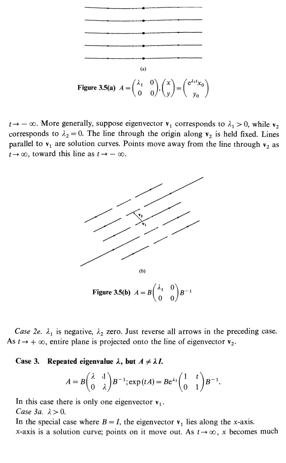
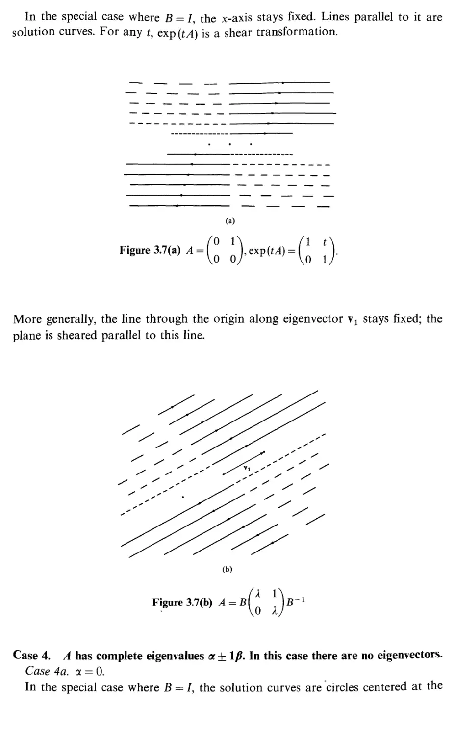
/


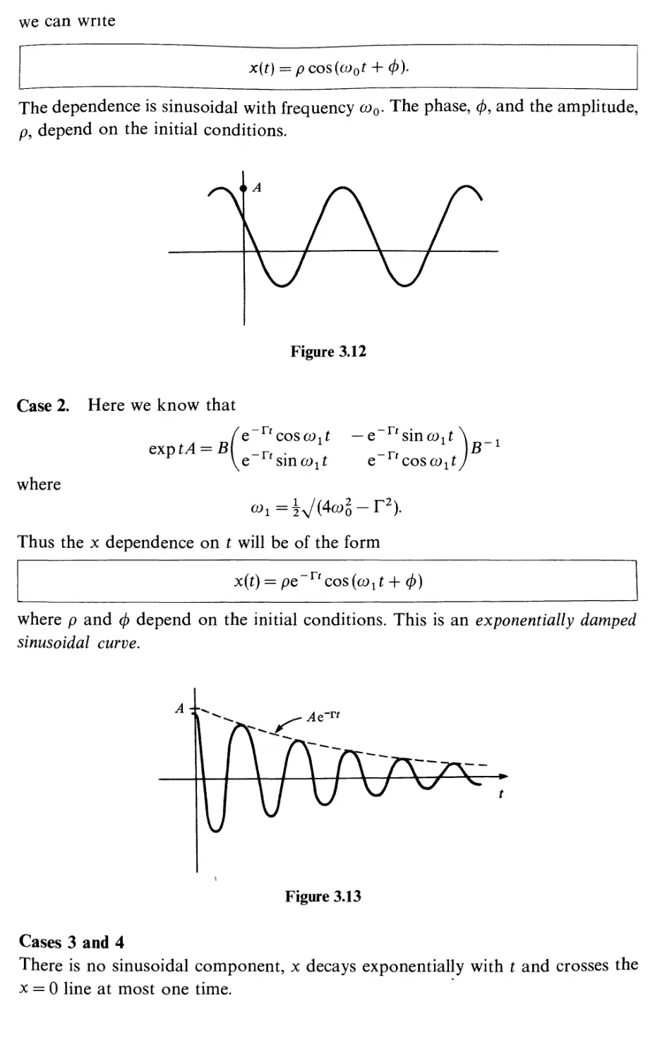
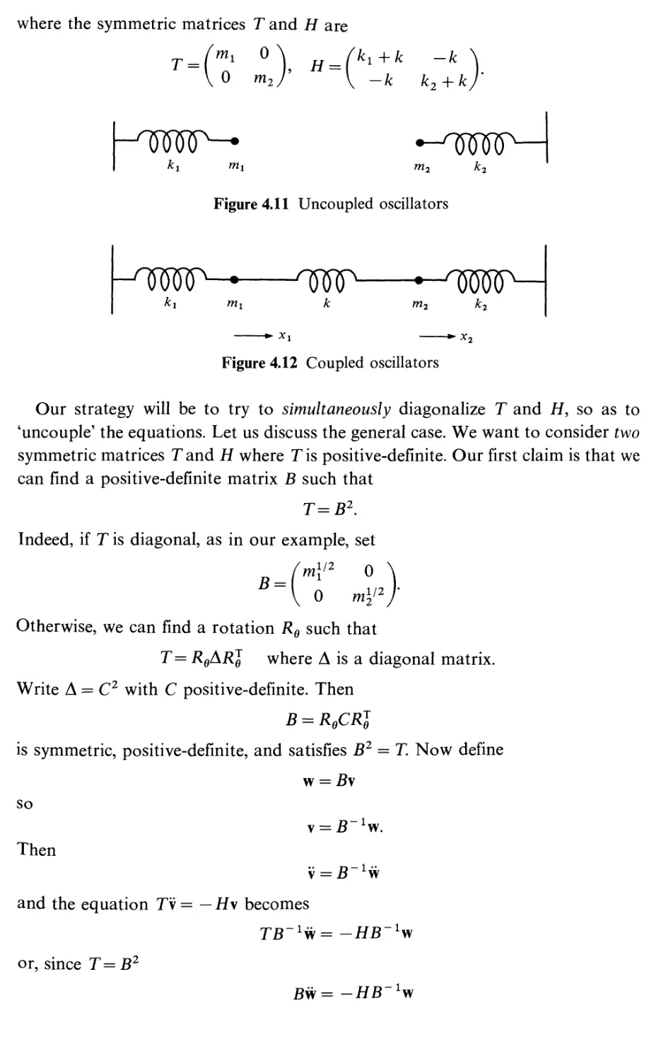
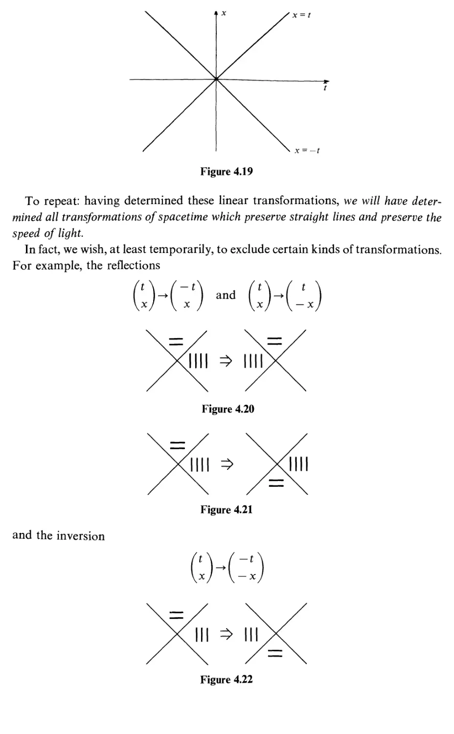
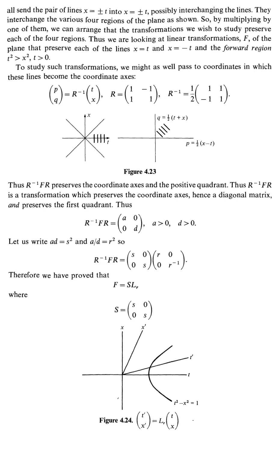
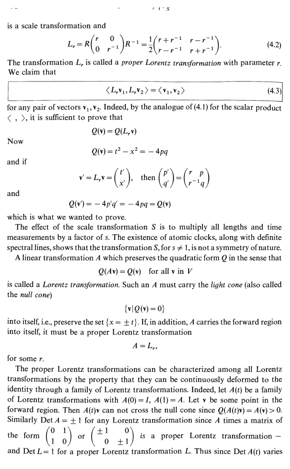
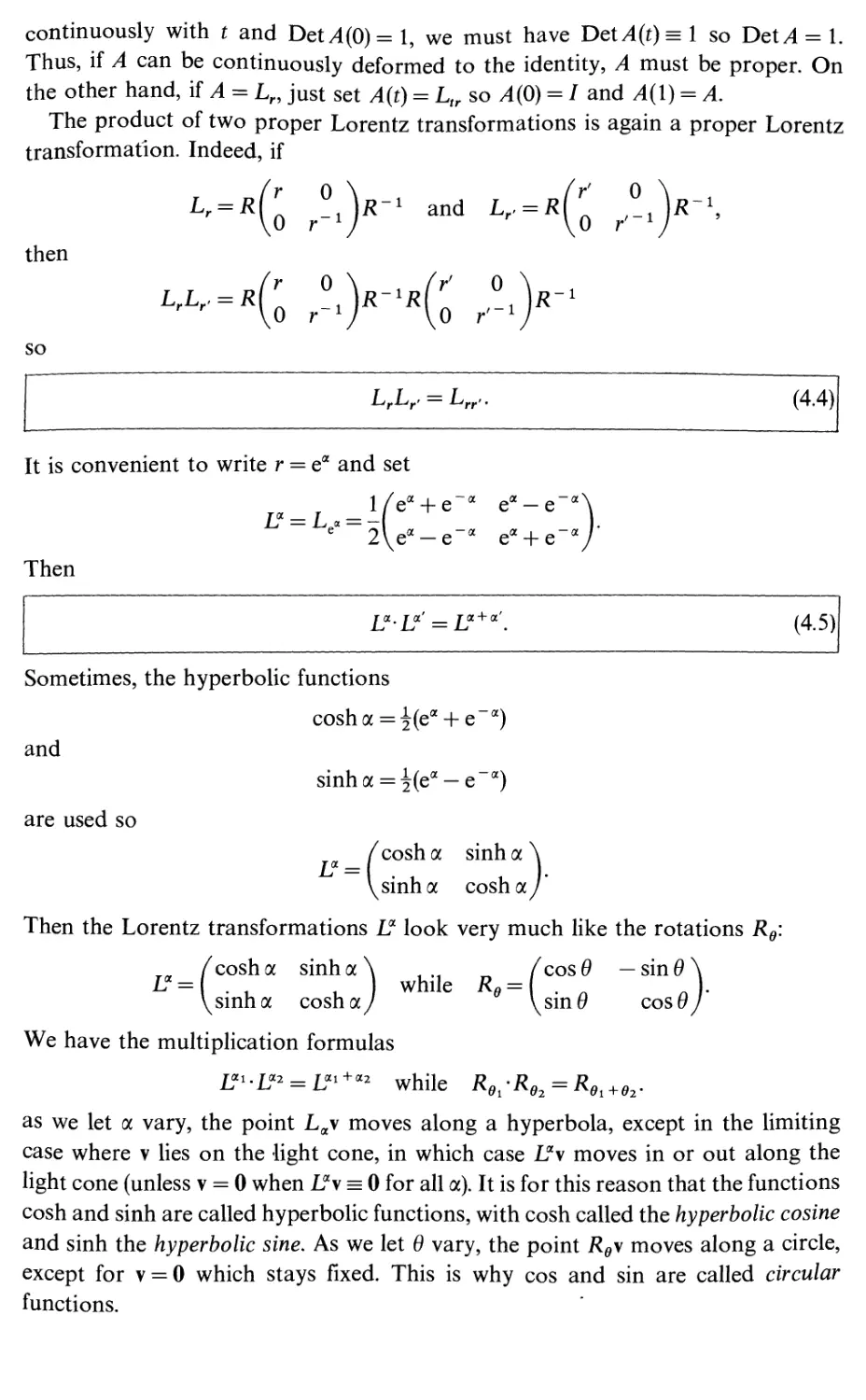
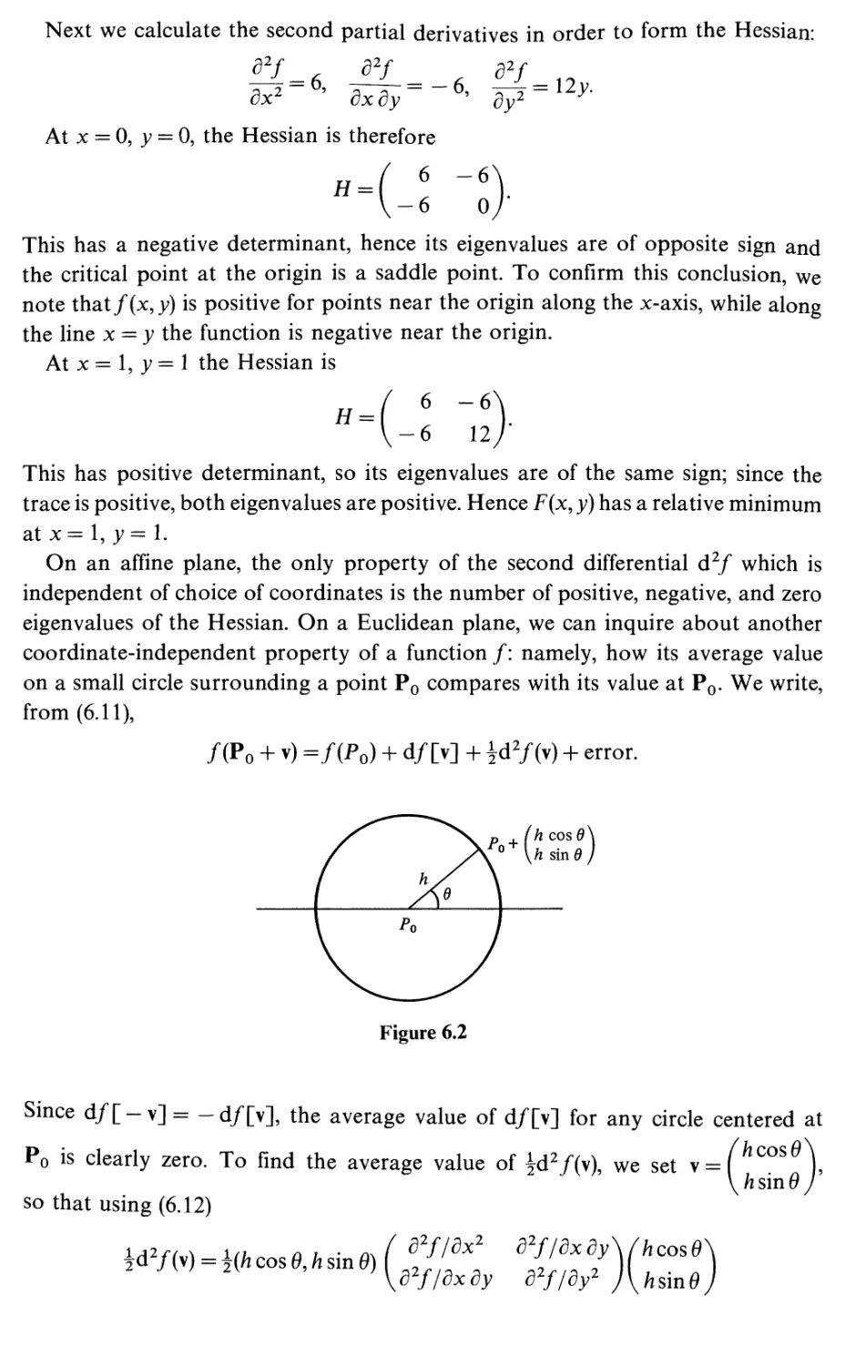
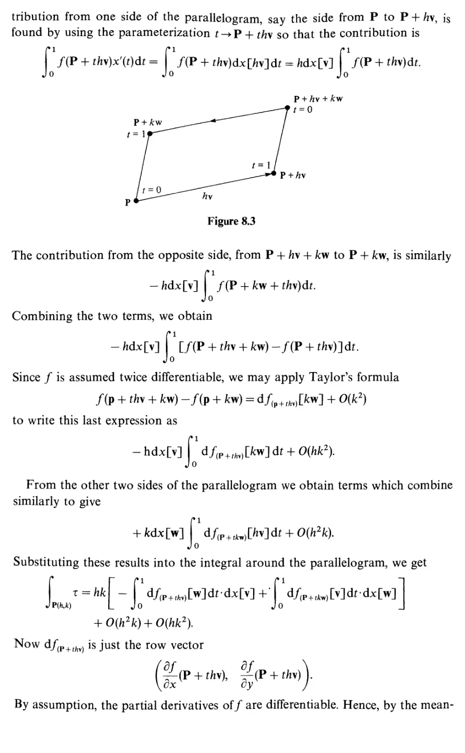
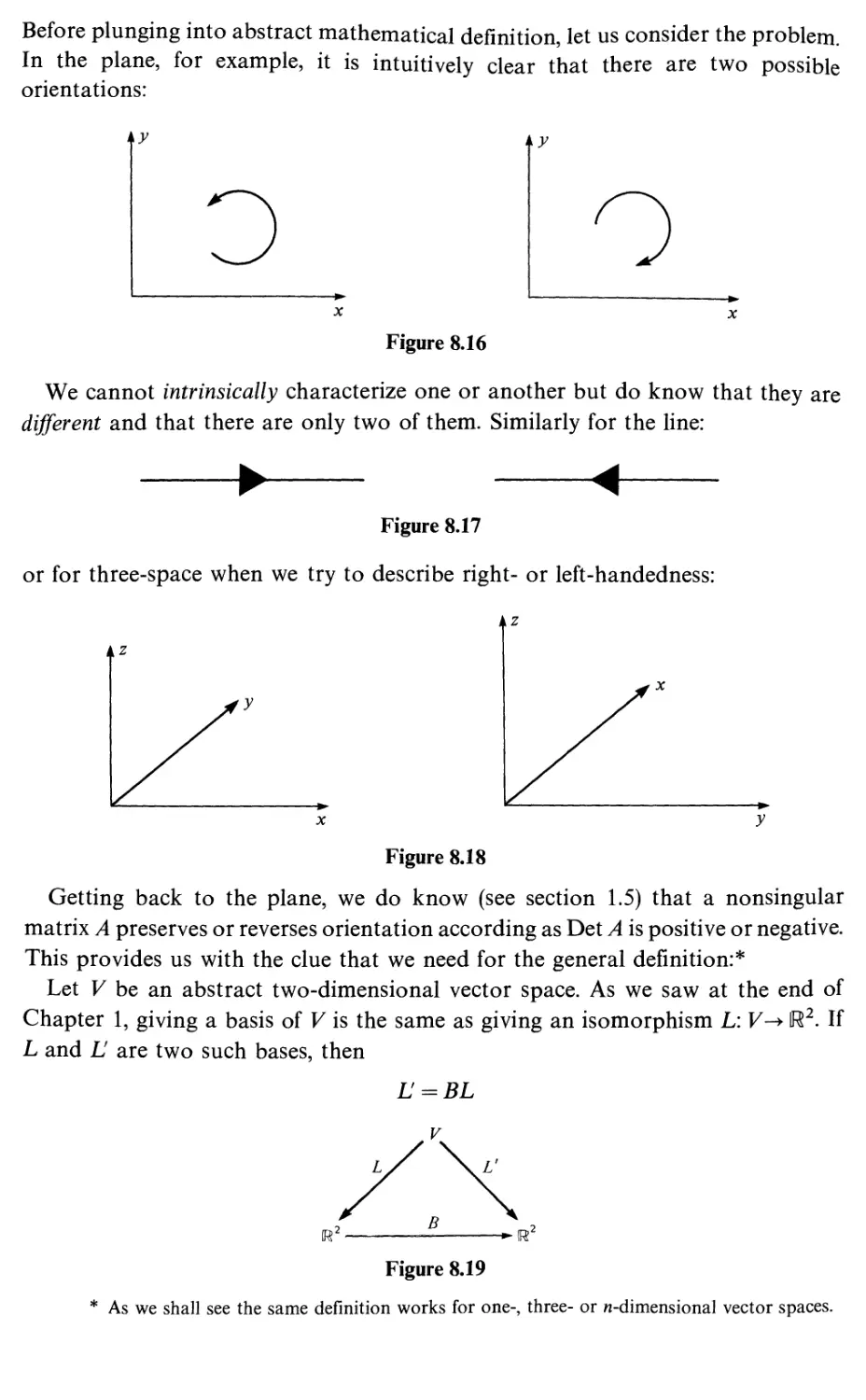


Текст
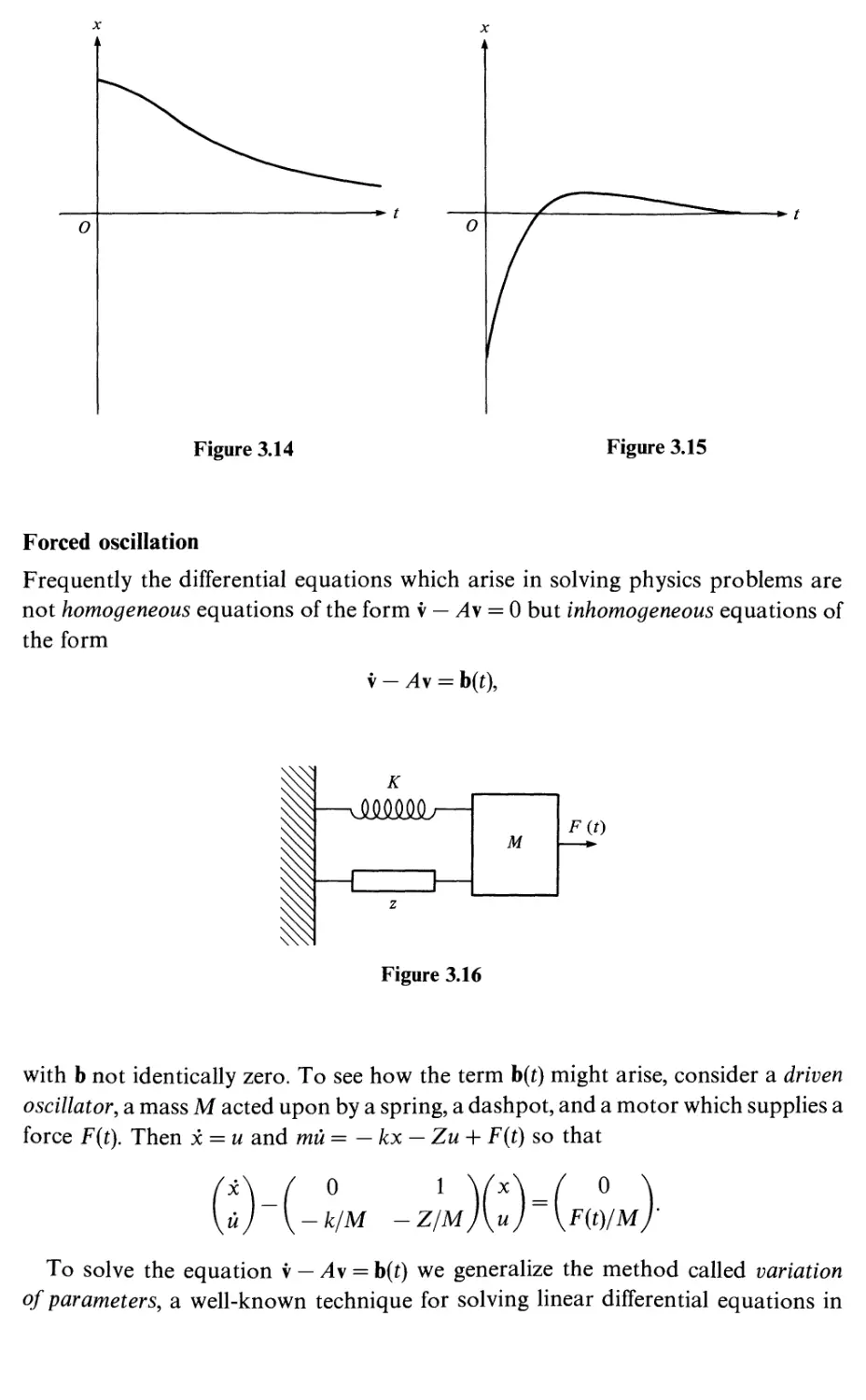
mathematics
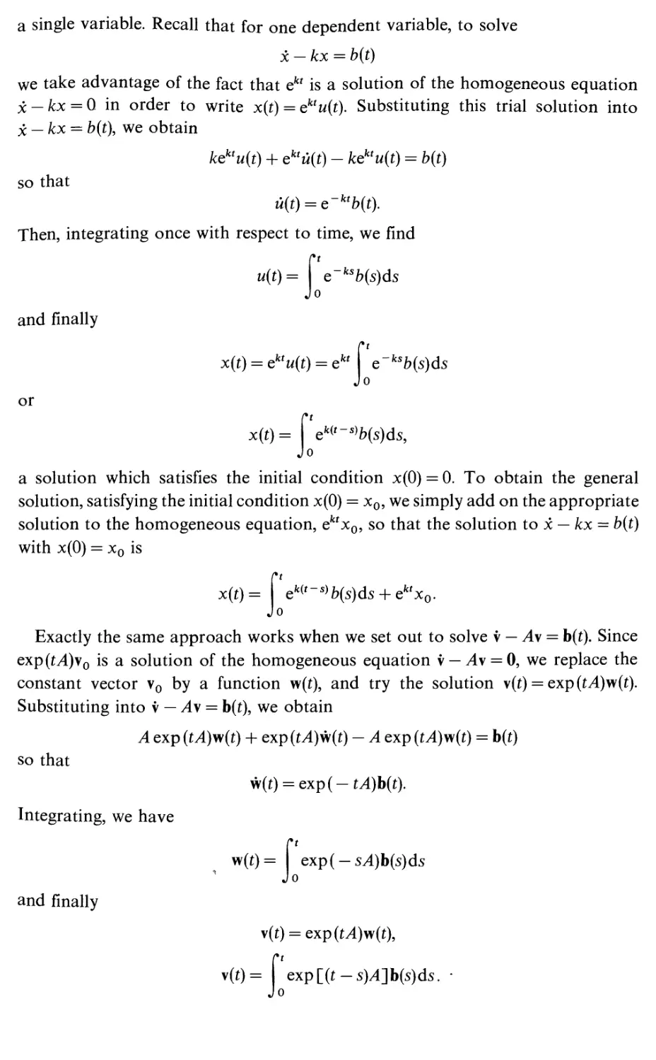
Paul Bamberg &Shlomo Sternberg
A COURSE IN
mathematics
FOR STUDENTS OF
PHYSICS: 1
PAUL BAMBERG
SHLOMO STERNBERG
Bg Cambridge
^P UNIVERSITY PRESS
Published by the Press Syndicate of the University of Cambridge
The Pitt Building, Trumpington Street, Cambridge CB2 IRP
40 West 20th Street, New York, NY 10011-4211, USA
10 Stamford Road, Oakleigh, Victoria 3166, Australia
© Cambridge University Press 1988
First published 1988
Reprinted 1990
First paperback edition 1991
Reprinted 1992
Printed in Great Britain at the University Press, Cambridge
British Library cataloguing in publication data
Bamberg, Paul
A course in mathematics for students of
physics: 1.
1. Mathematical physics.
I. Title. II. Sternberg, Shlomo
510'.2453 QC20
Library of Congress cataloguing in publication data
Bamberg, Paul G.
A course in mathematics for students of physics: 1
Bibliography
Includes index.
1. Mathematics-1961- I. Sternberg, Shlomo.
II. Title.
QA37.2.B36 1988 510 86-2230
ISBN 0 521 25017 X hardback
ISBN 0 521 40649 8 paperback
TM
CONTENTS OF VOLUME 1
1
1.1
1.2
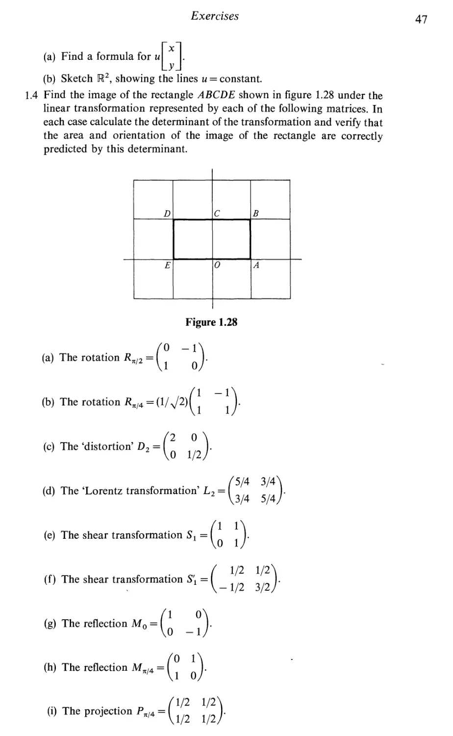
1.3
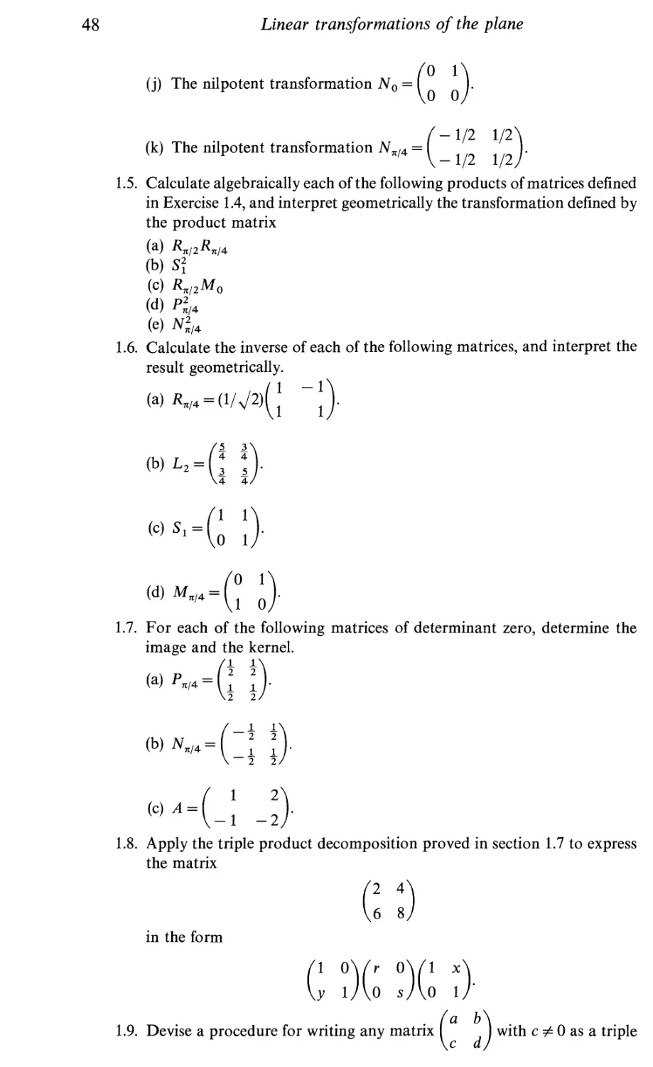
1.4
1.5
1.6
1.7
1.8
1.9
1.10
1.11
1.12
2
2.1
2.2
2.3
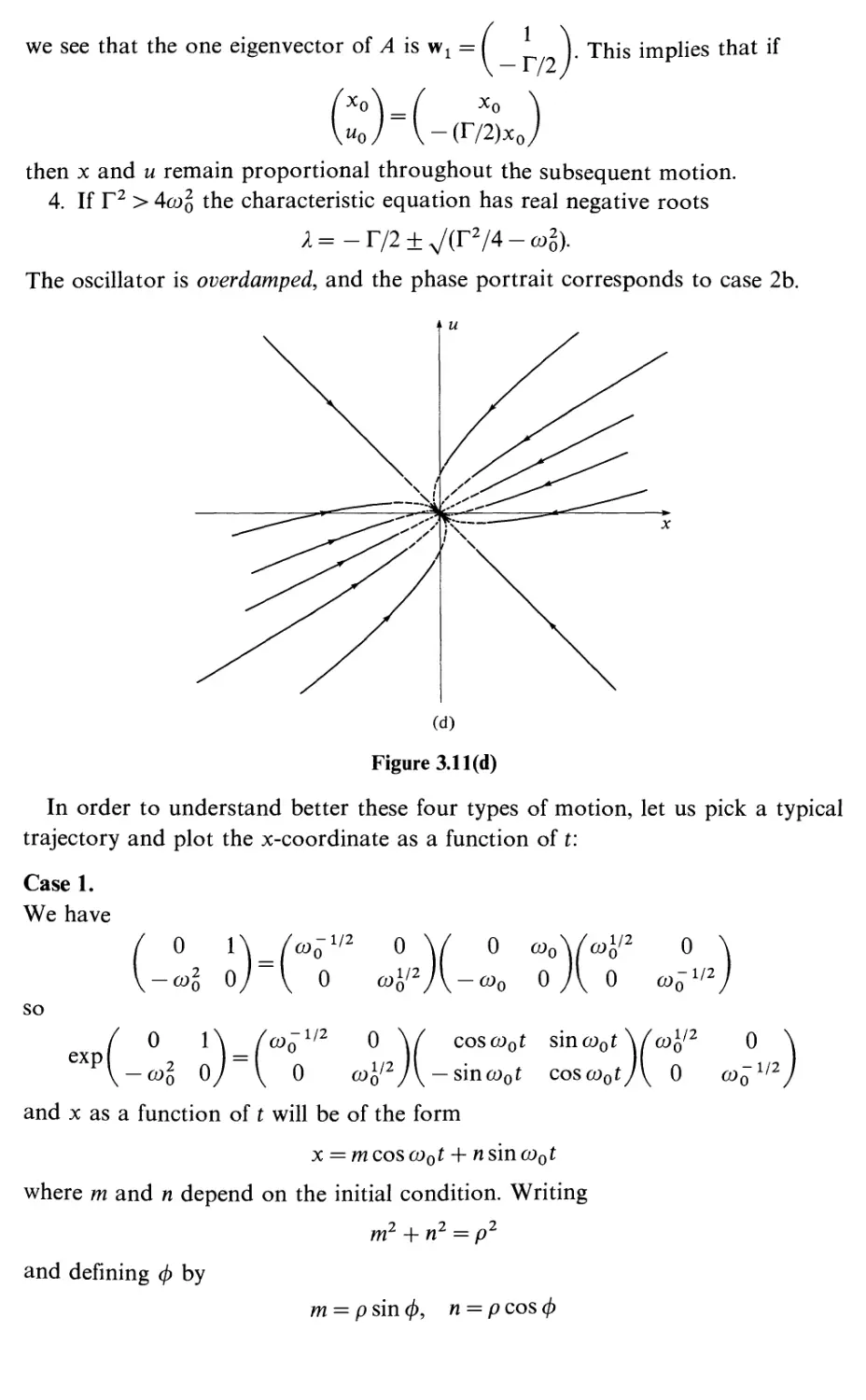
3
3.1
3.2
3.3
3.4
3.5
Contents of Volume 2
Preface
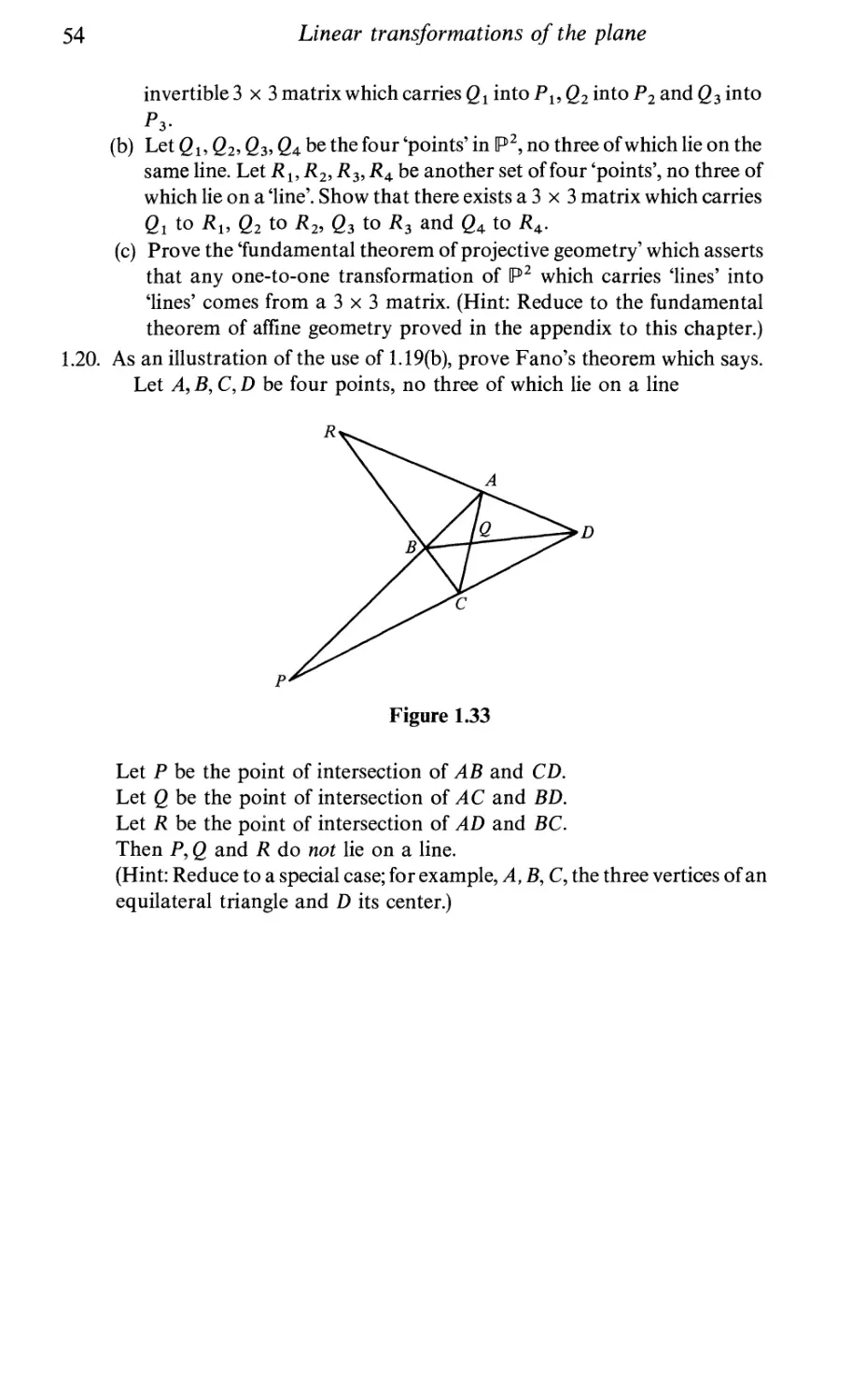
Linear transformations of the plane
Affine planes and vector spaces
Vector spaces and their affine spaces
Functions and affine functions
Euclidean and affine transformations
Linear transformations
The matrix of a linear transformation
Matrix multiplication
Matrix algebra
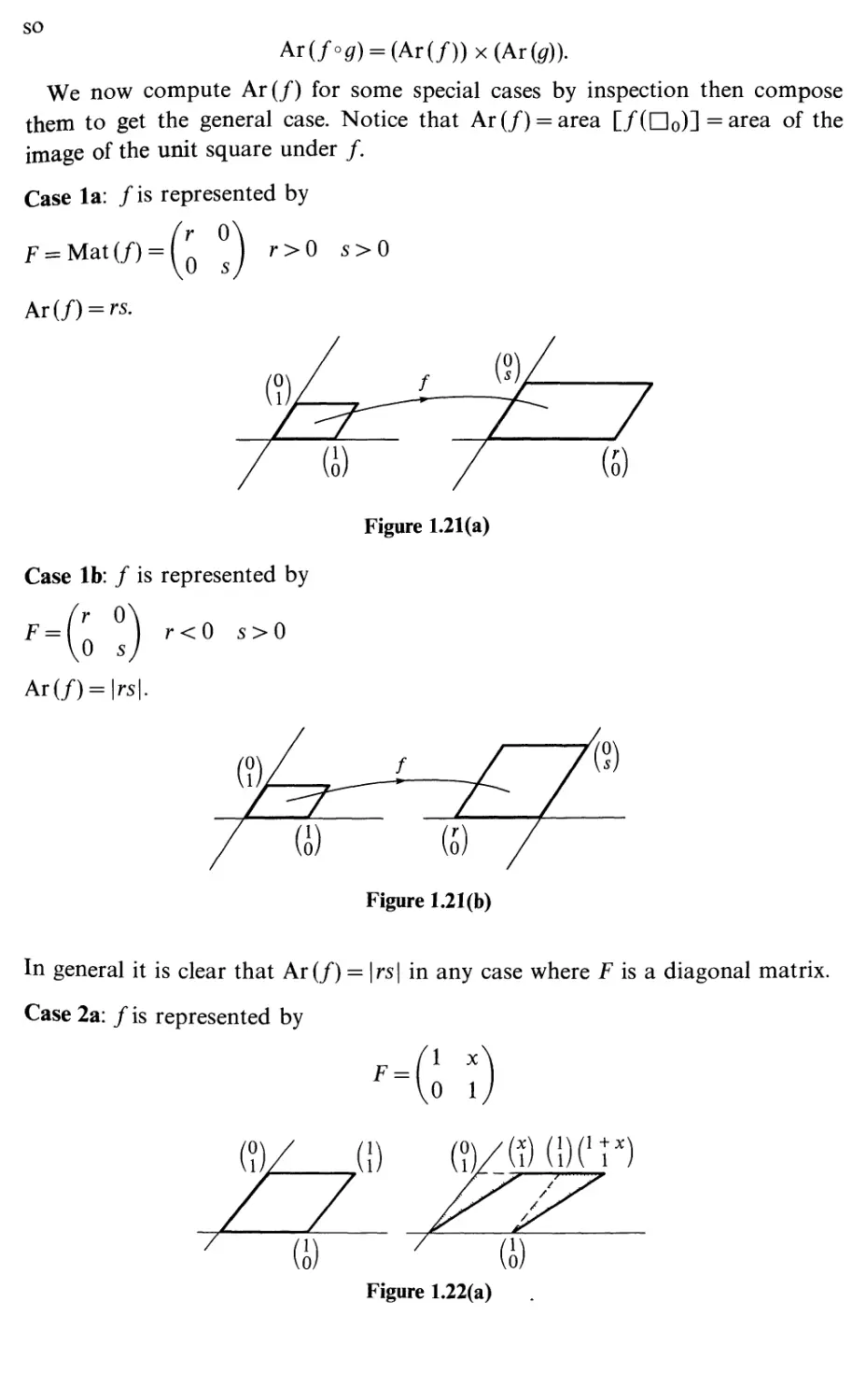
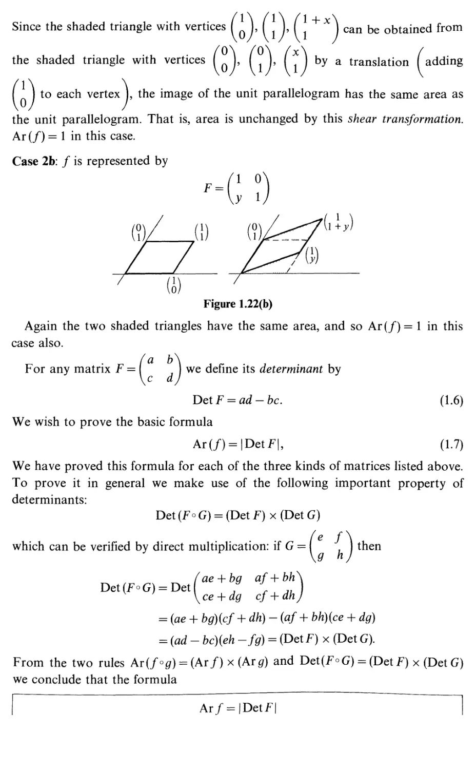
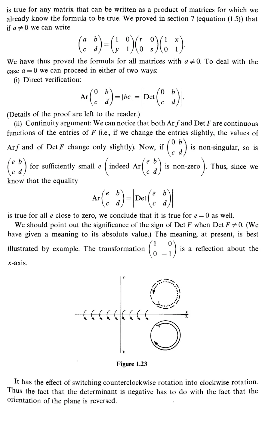
Areas and determinants
Inverses
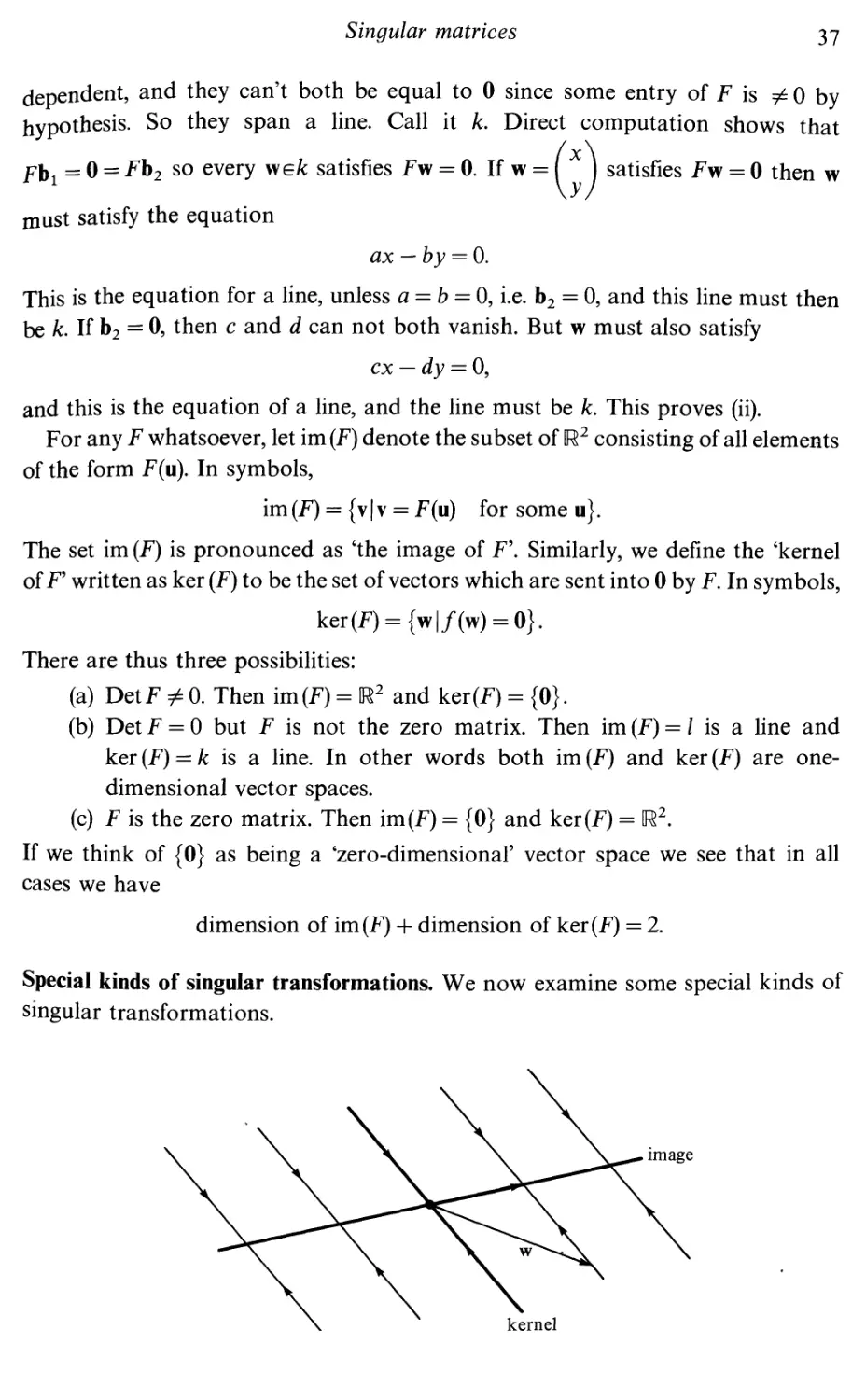
Singular matrices
Two-dimensional vector spaces
Appendix: the fundamental theorem of affine geometry
Summary
Exercises
Eigenvectors and eigenvalues
Conformal linear transformations
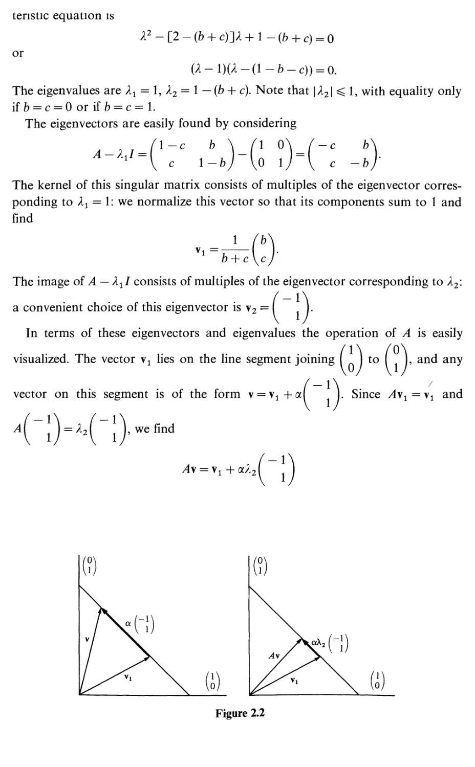
Eigenvectors and eigenvalues
Markov processes
Summary
Exercises
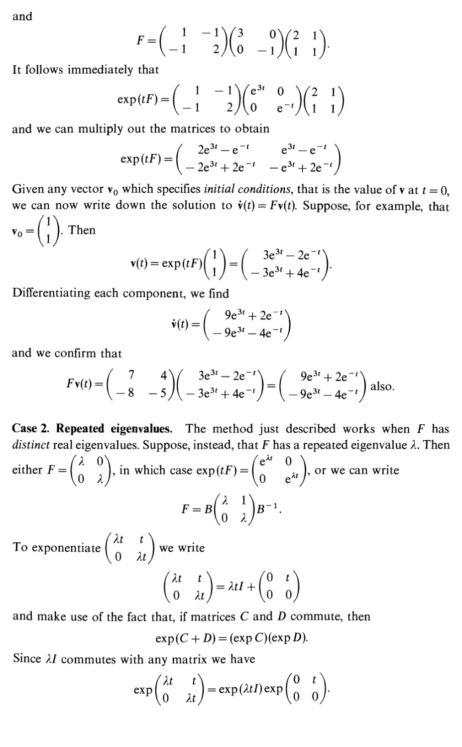
Linear differential equations in the plane
Functions of matrices
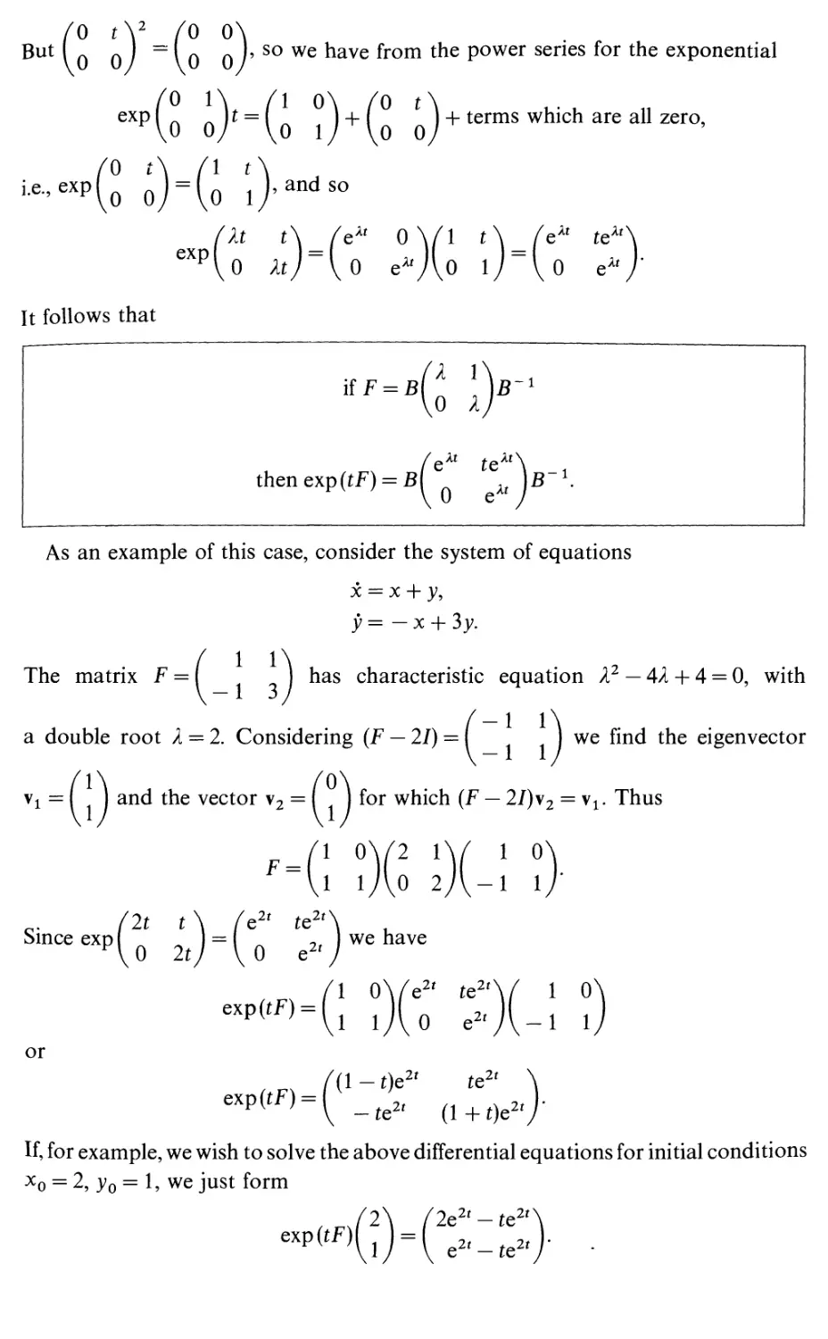
The exponential of a matrix
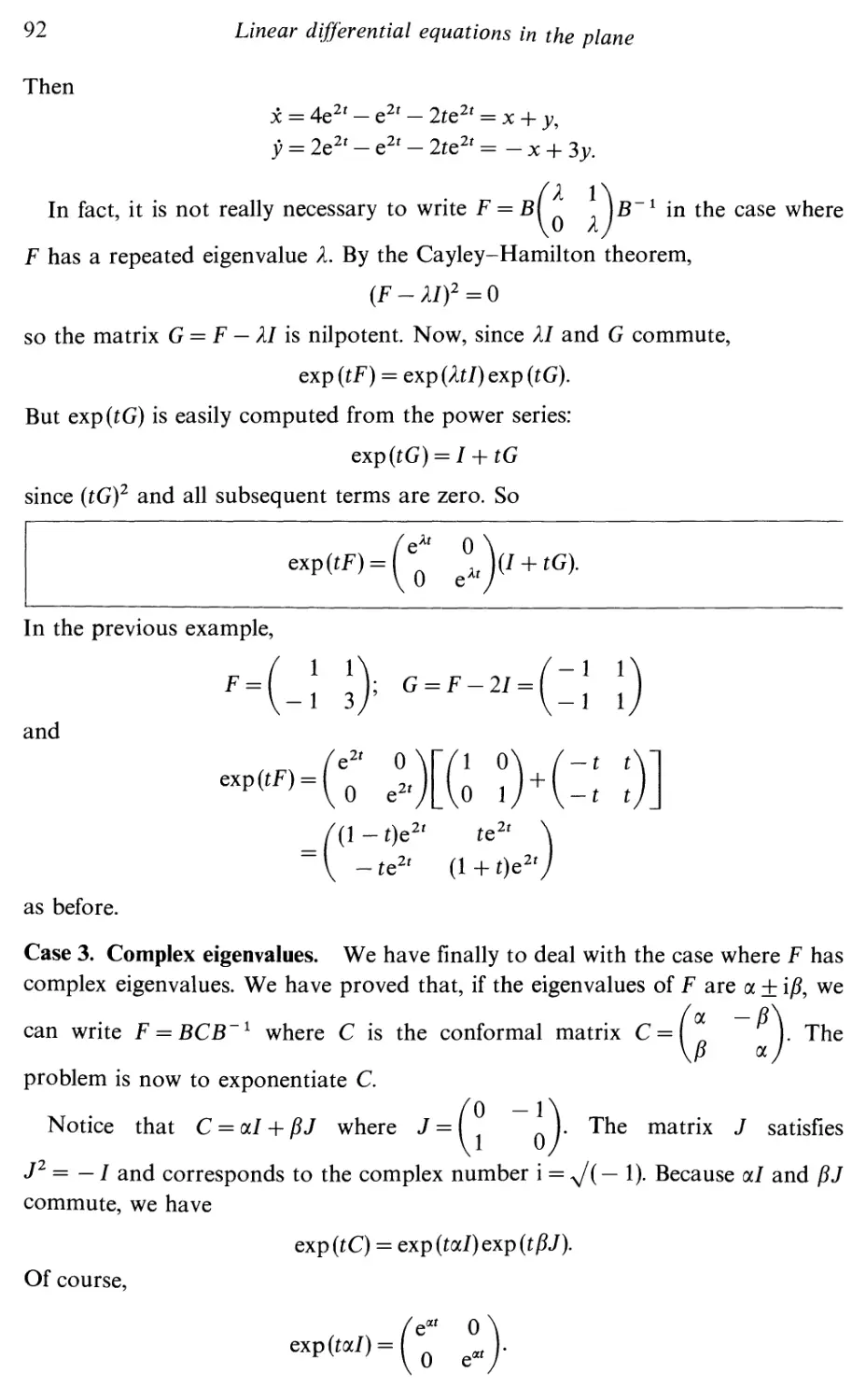
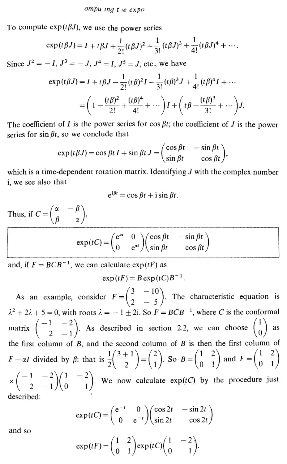
Computing the exponential of a matrix
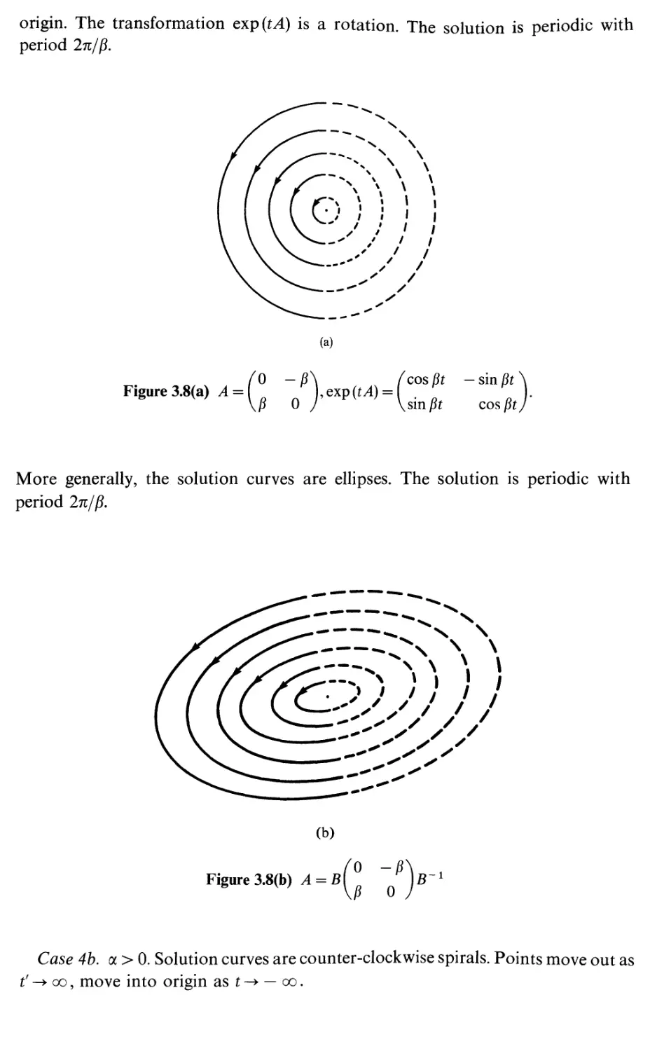
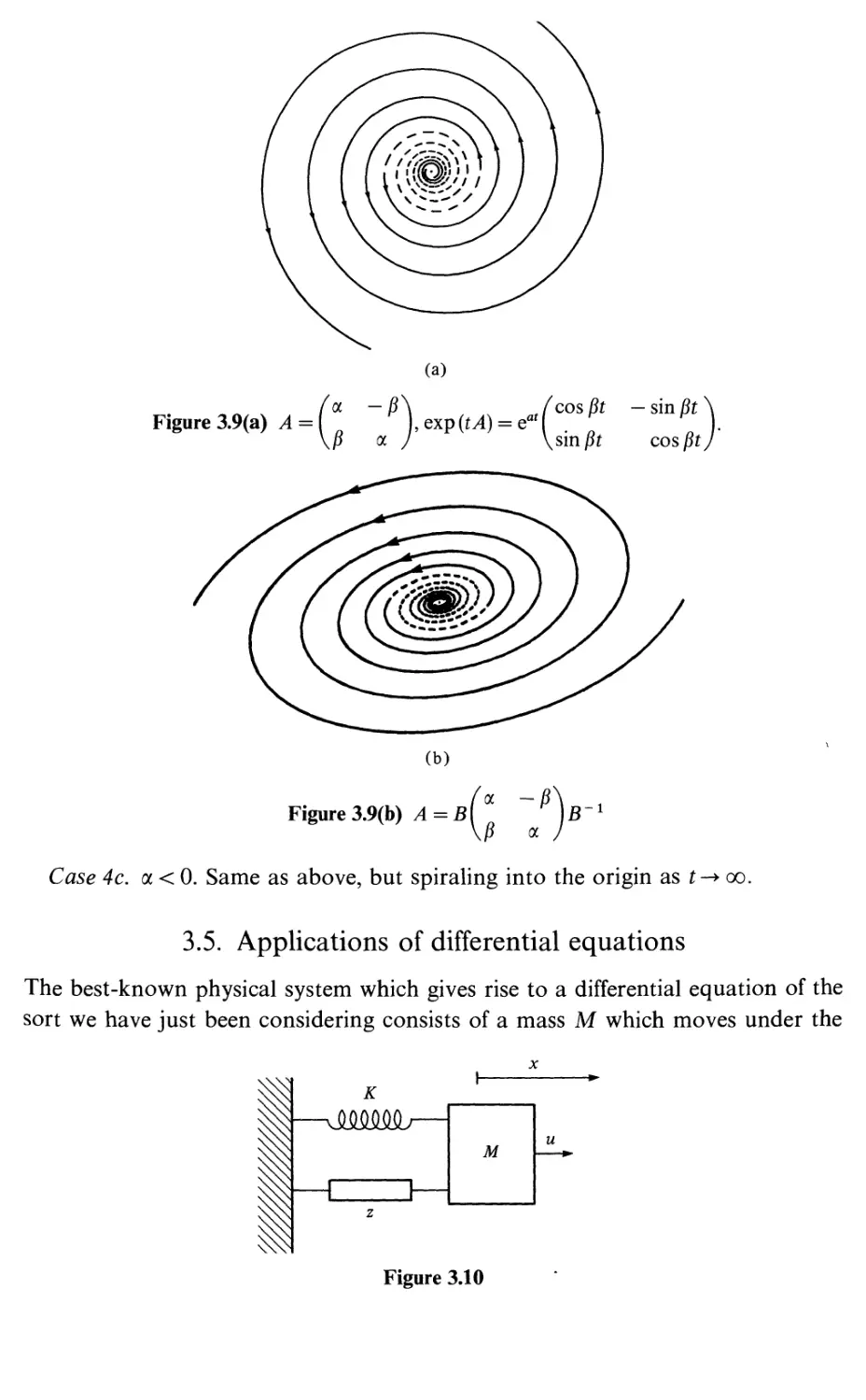
Differential equations and phase portraits
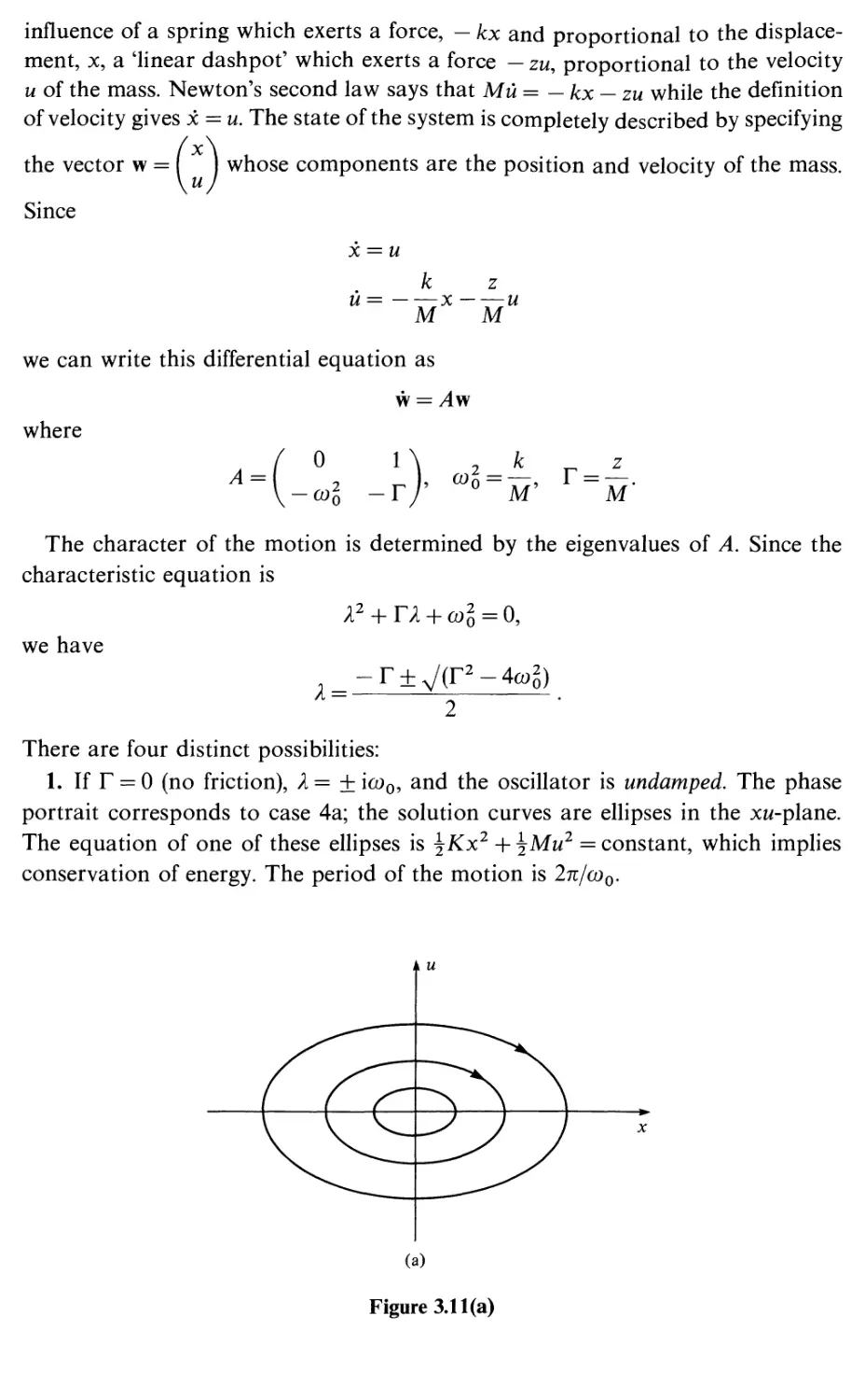
Applications of differential equations
Summary
Exercises
viii
xi
1
1
7
13
16
18
21
22
24
26
32
36
39
43
45
46
55
55
58
66
72
73
81
81
83
89
95
103
113
113
4
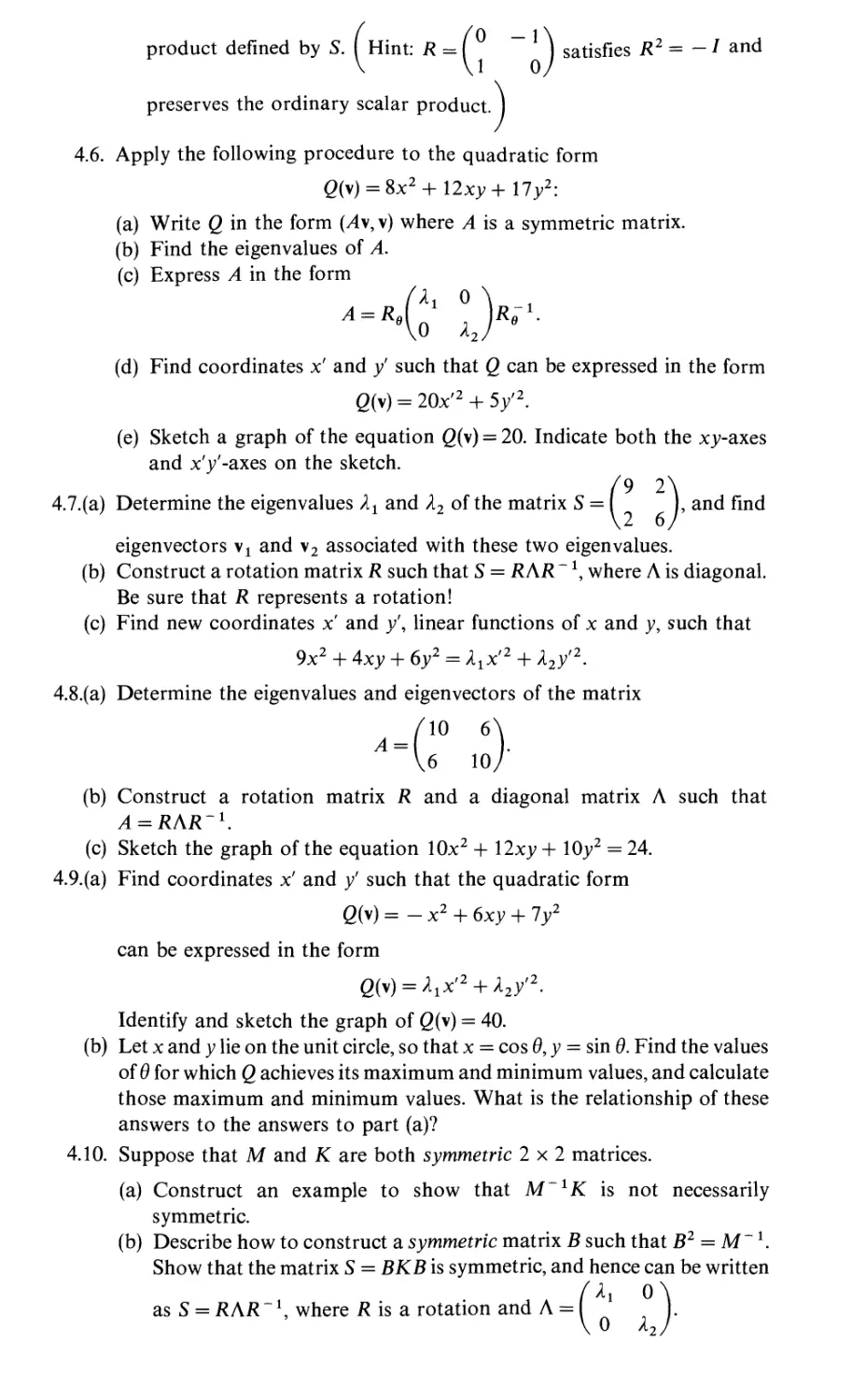
4.1
Scalar products
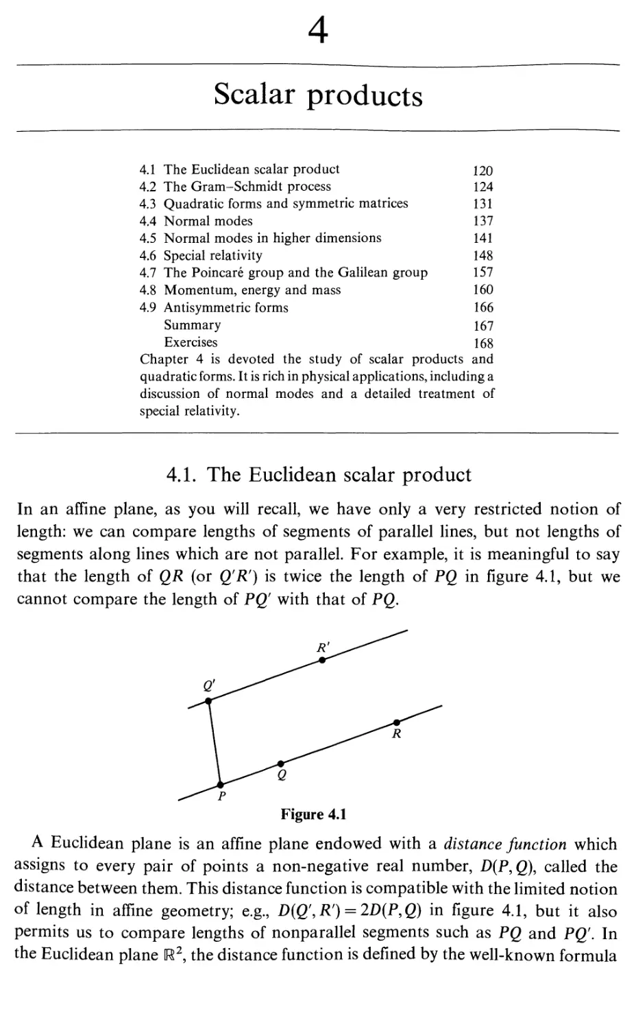
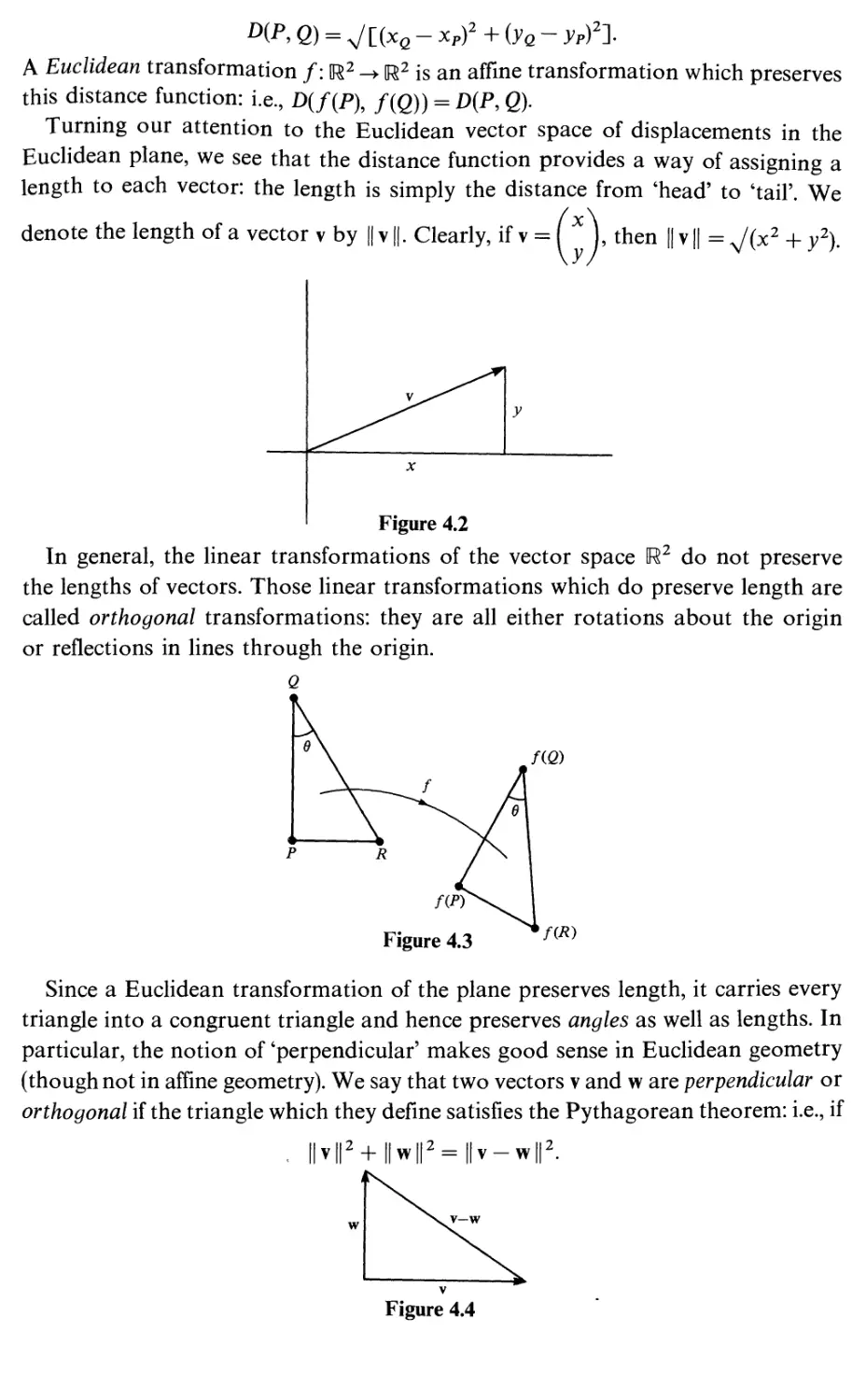
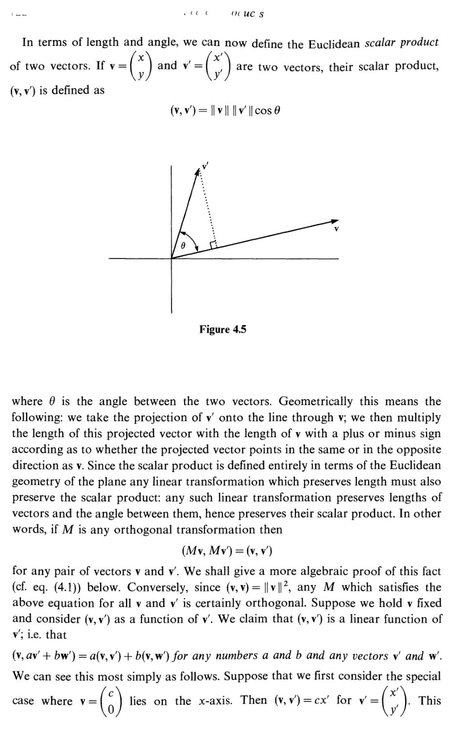
The euclidean scalar product
120
120
4.2 The Gram-Schmidt process 124
4.3 Quadratic forms and symmetric matrices 131
4.4 Normal modes 137
4.5 Normal modes in higher dimensions 141
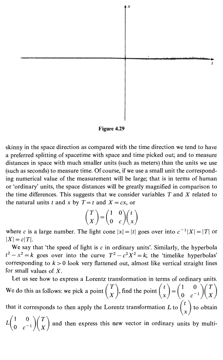
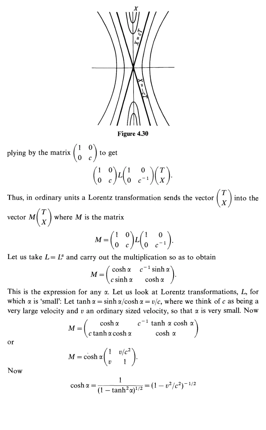
4.6 Special relativity 148
4.7 The Poincare group and the Galilean group 157
4.8 Momentum, energy and mass 160
4.9 Antisymmetric forms 166
Summary 167
Exercises 168
5 Calculus in the plane 175
Introduction 175
5.1 Big'oh'and little'oh' 178
5.2 The differential calculus 183
5.3 More examples of the chain rule 189
5.4 Partial derivatives and differential forms 197
5.5 Directional derivatives 205
5.6 The pullback notation 209
Summary 214
Exercises 215
6 Theorems of the differential calculus 219
6.1 The mean-value theorem 219
6.2 Higher derivatives and Taylor's formula 222
6.3 The inverse function theorem 230
6.4 Behavior near a critical point 240
Summary 242
Exercises 242
247
247
250
264
266
267
272
272
277
278
285
289
295
297
298
305
306
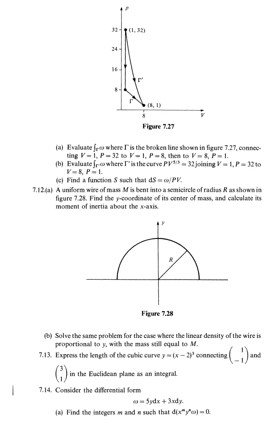
7
7.1
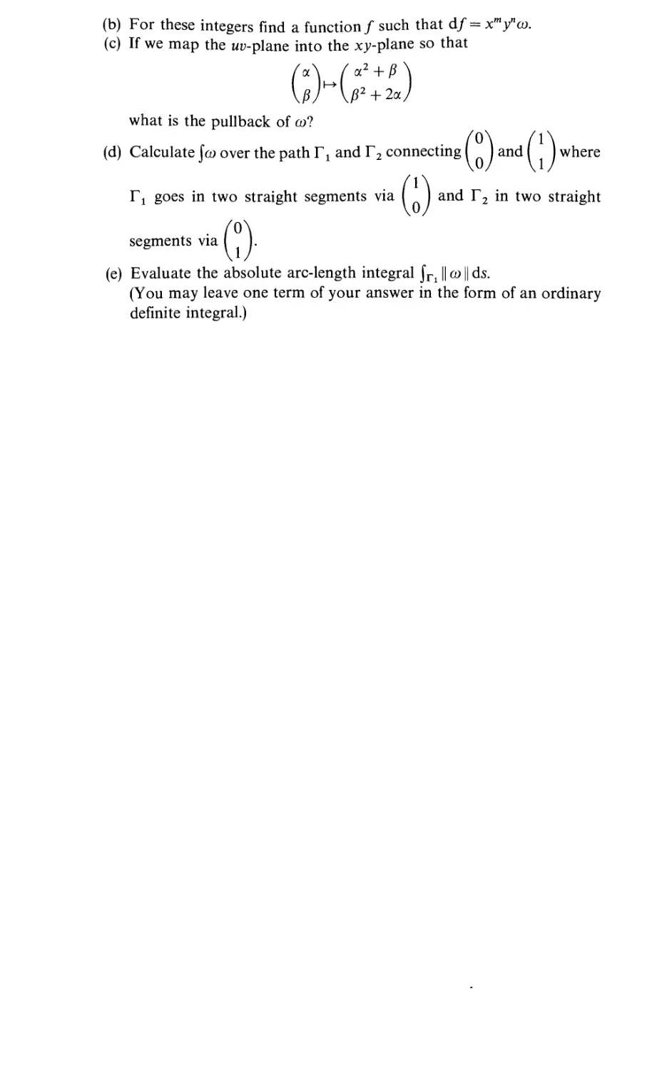
7.2
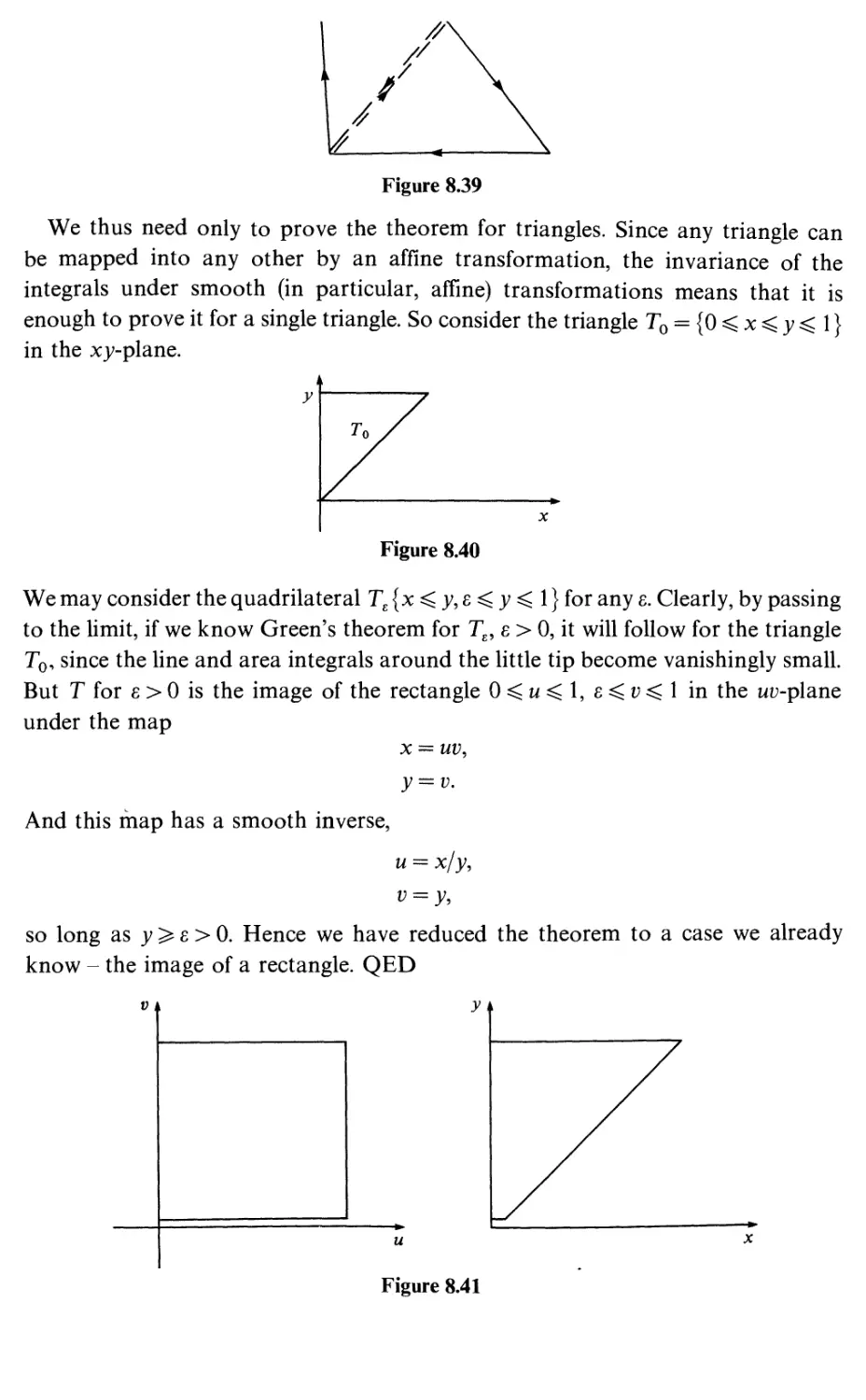
8
8.1
8.2
8.3
8.4
8.5
8.6
8.7
8.8
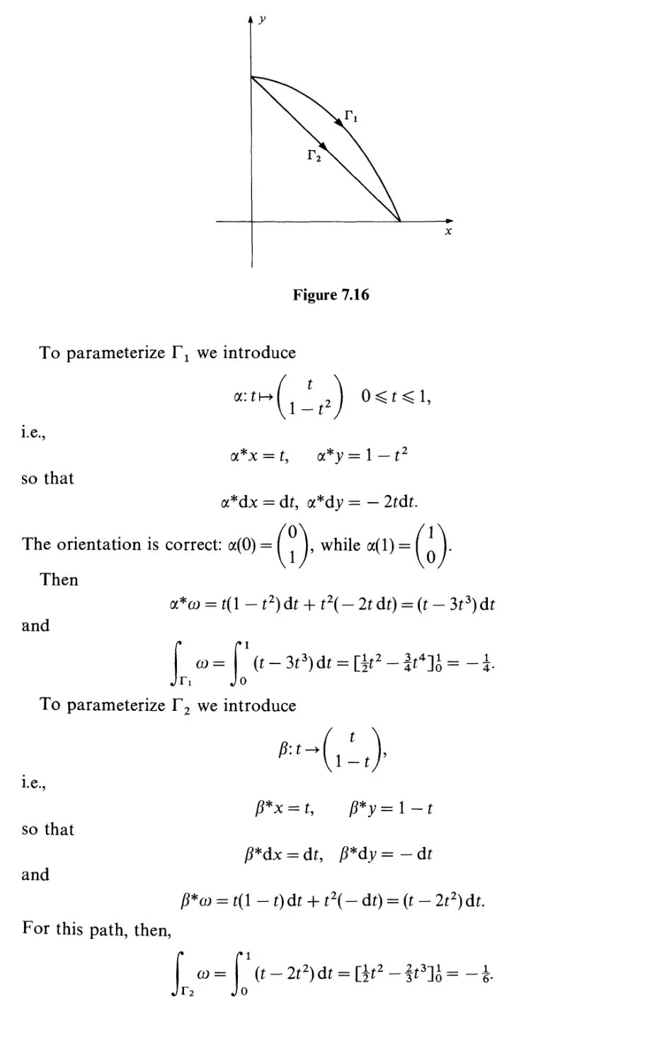
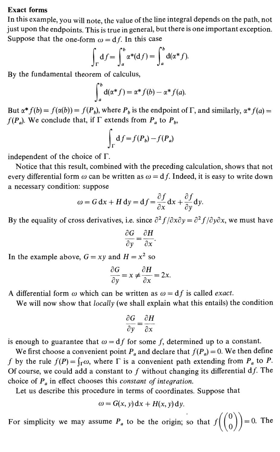
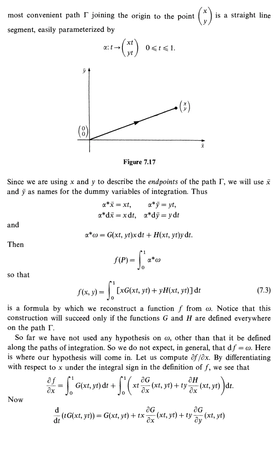
Differential forms and line integrals
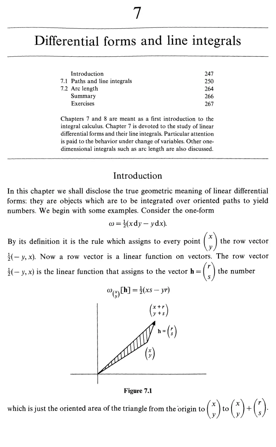
Introduction
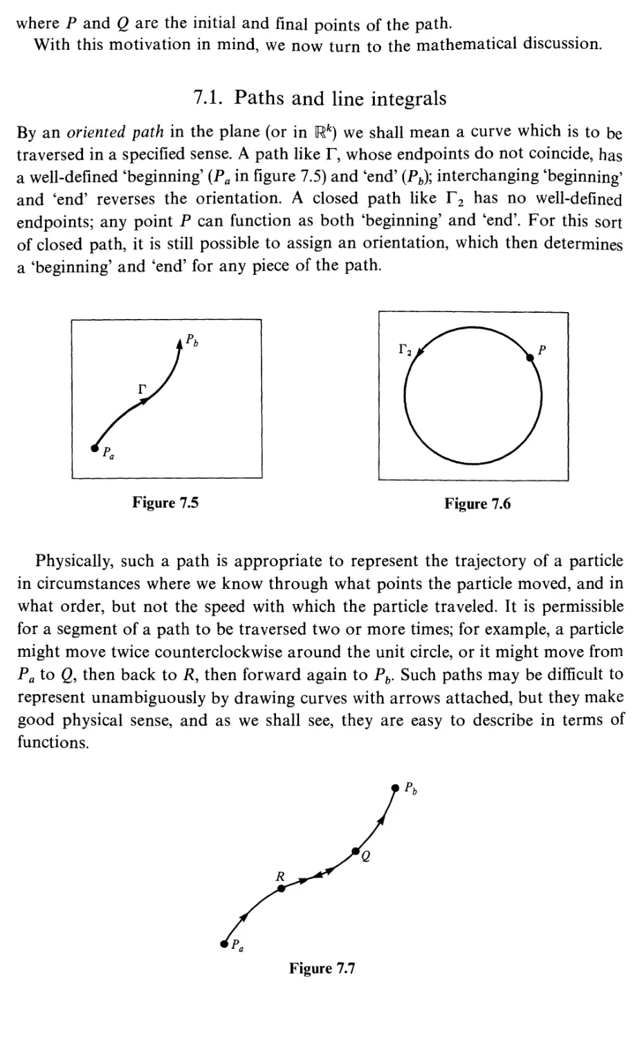
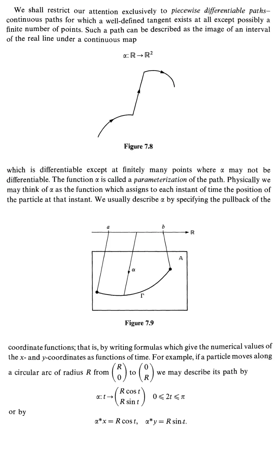
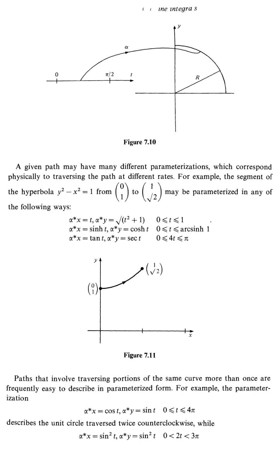
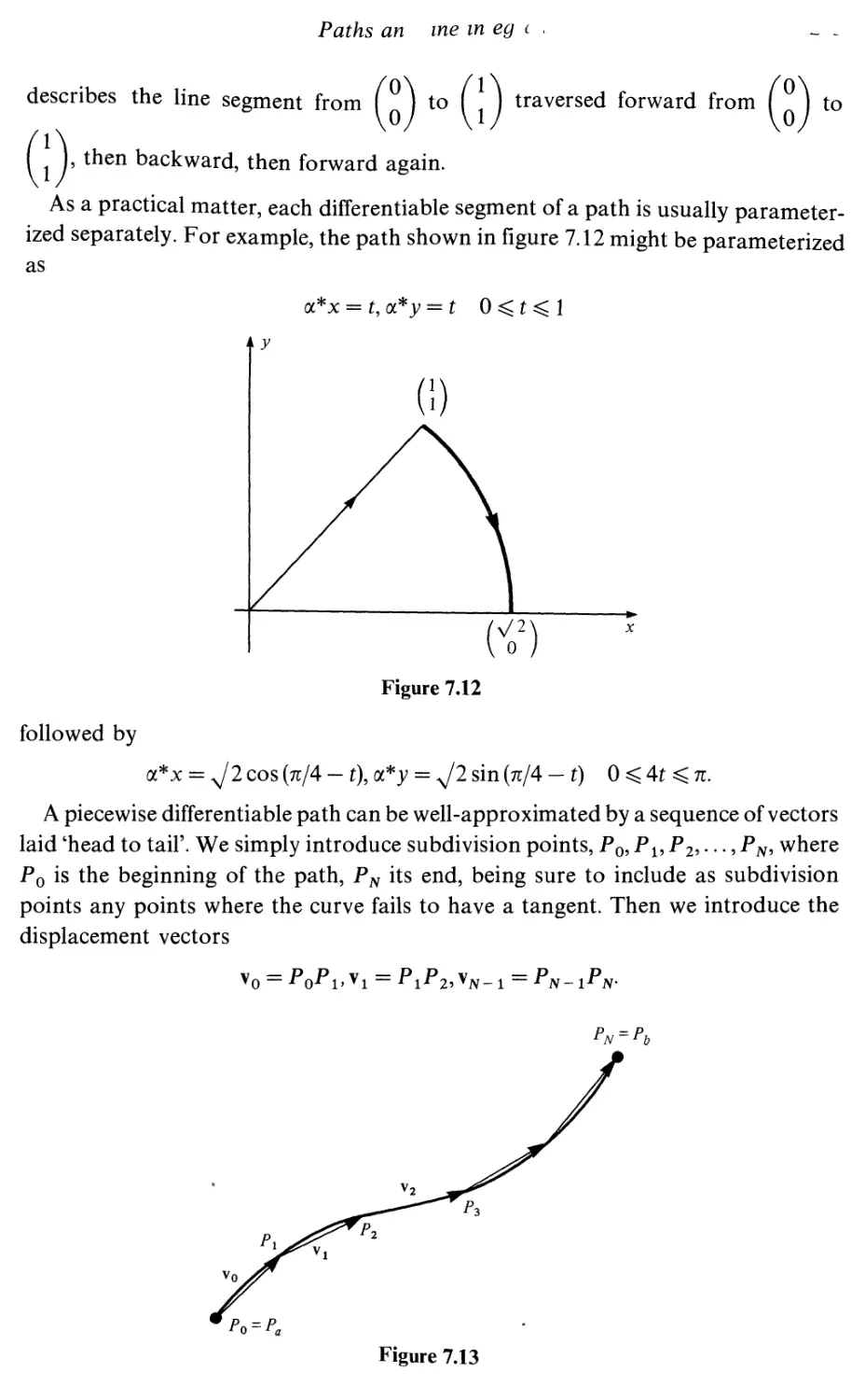
Paths and line integrals
Arc length
Summary
Exercises
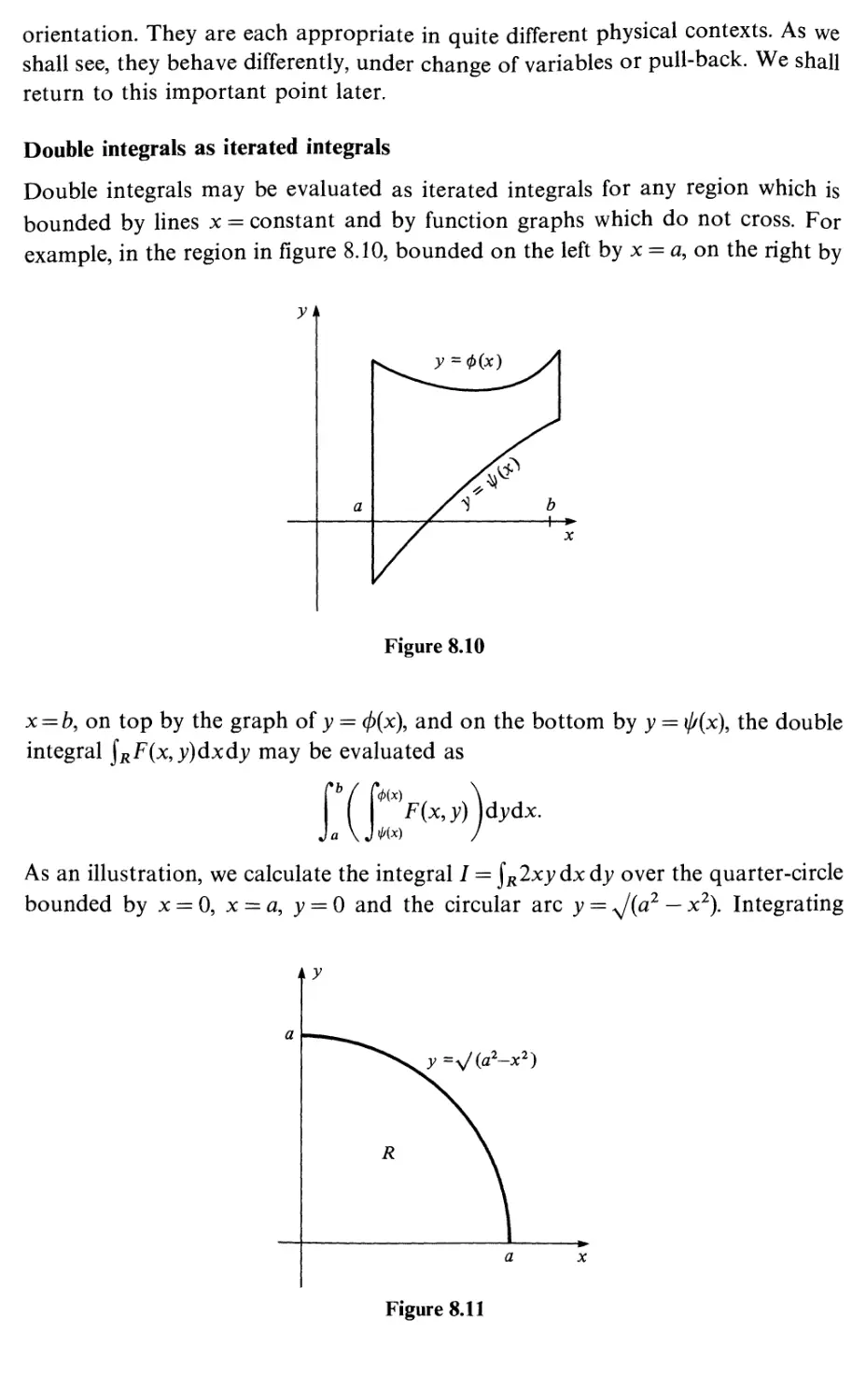
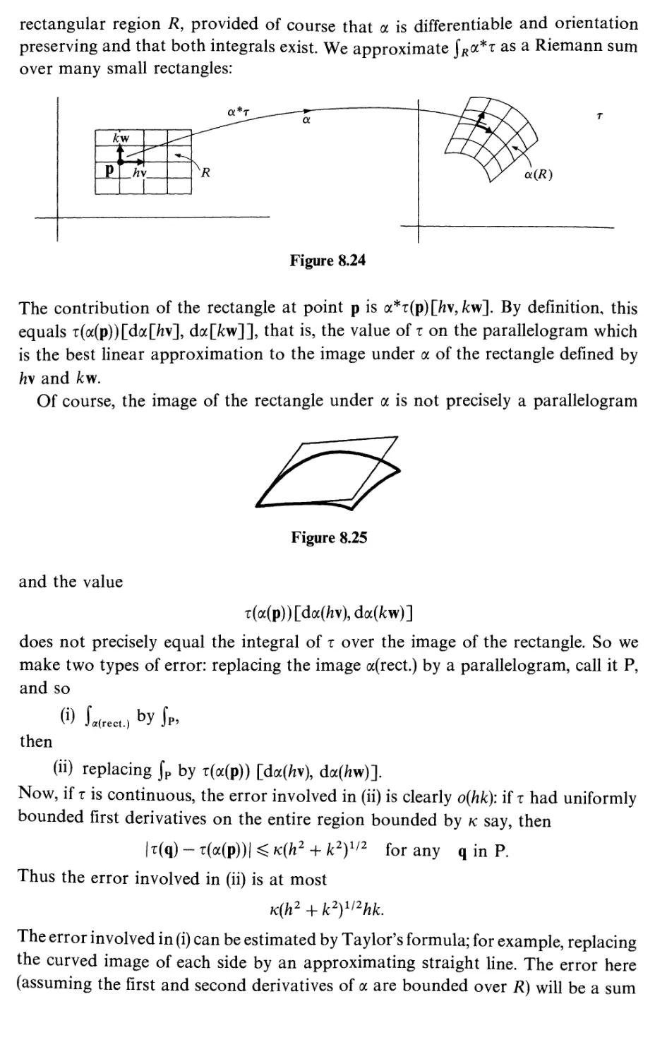
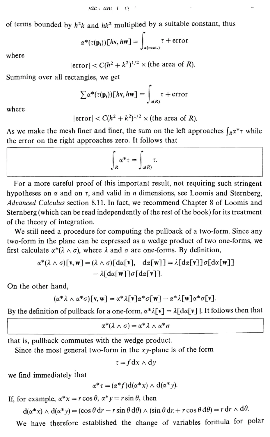
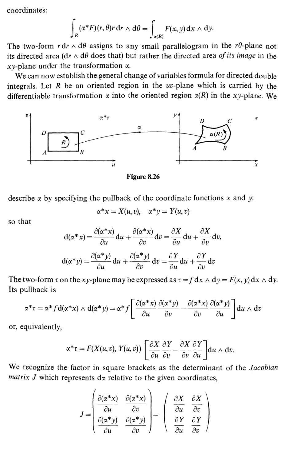
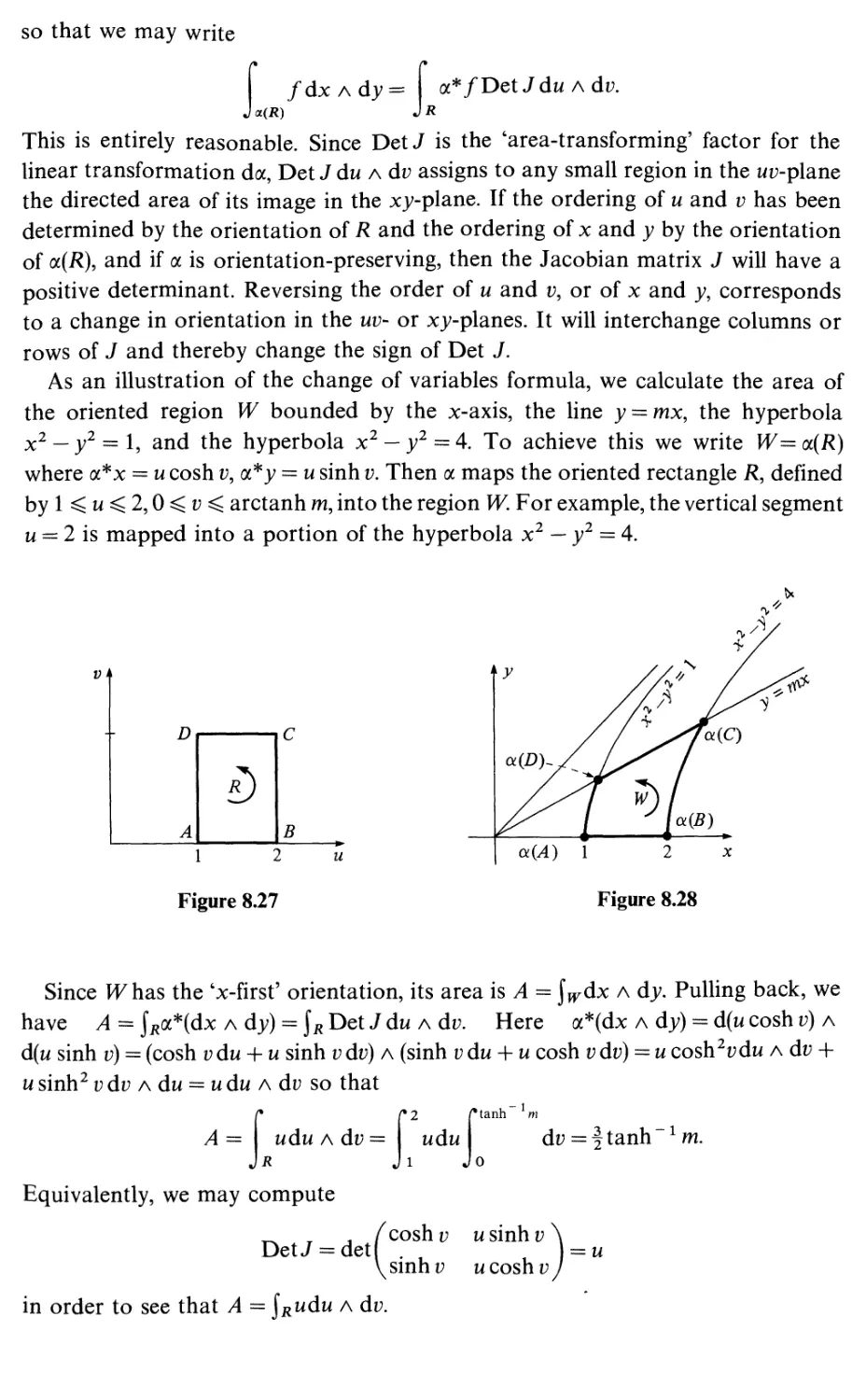
Double integrals
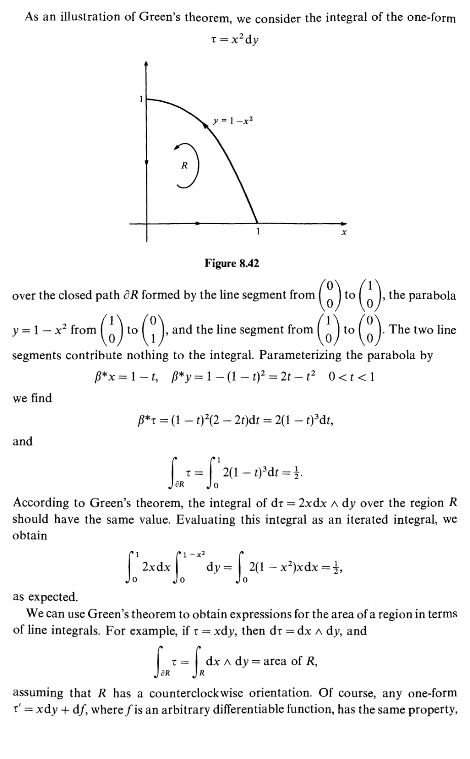
Exterior derivative
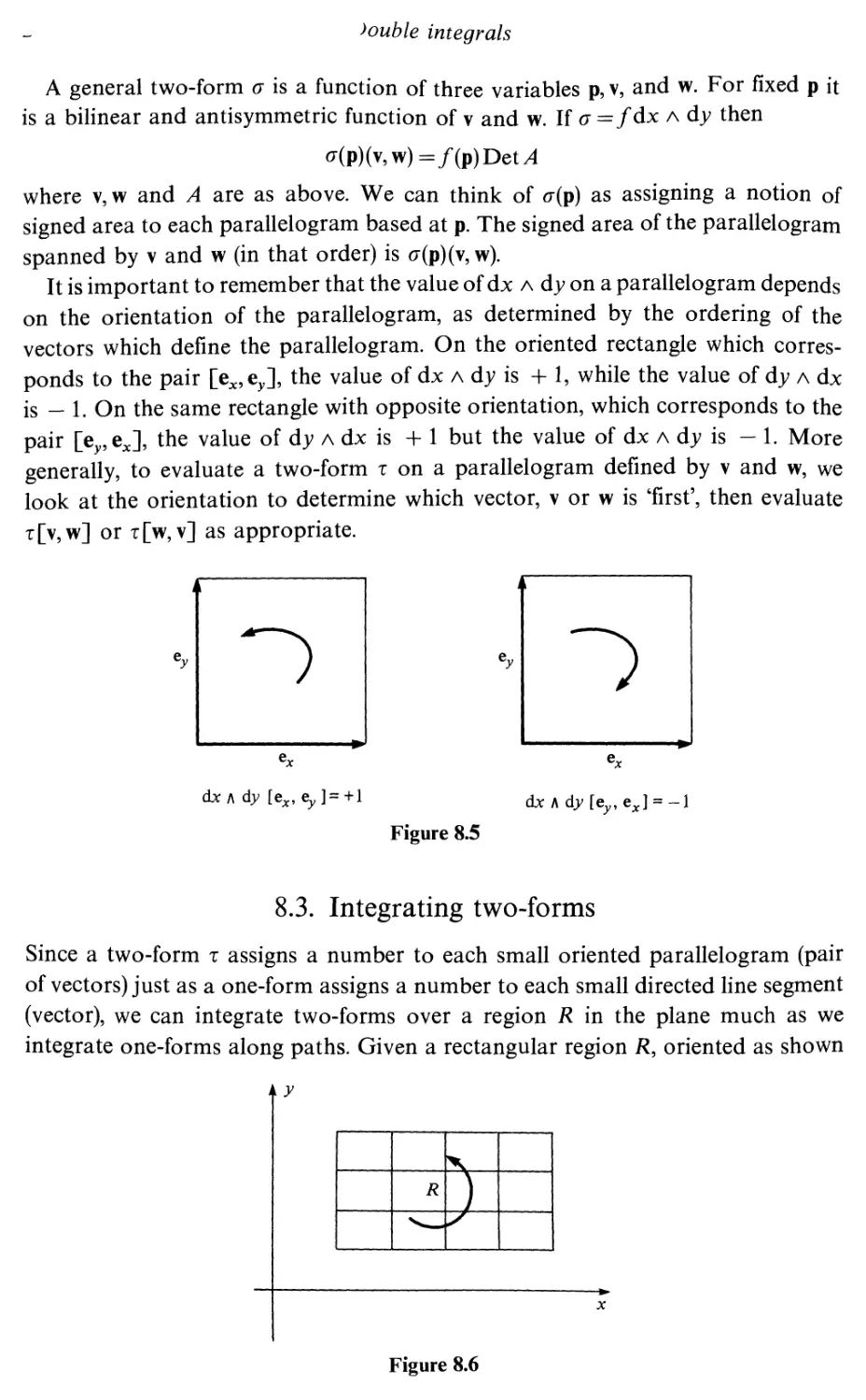
Two-forms
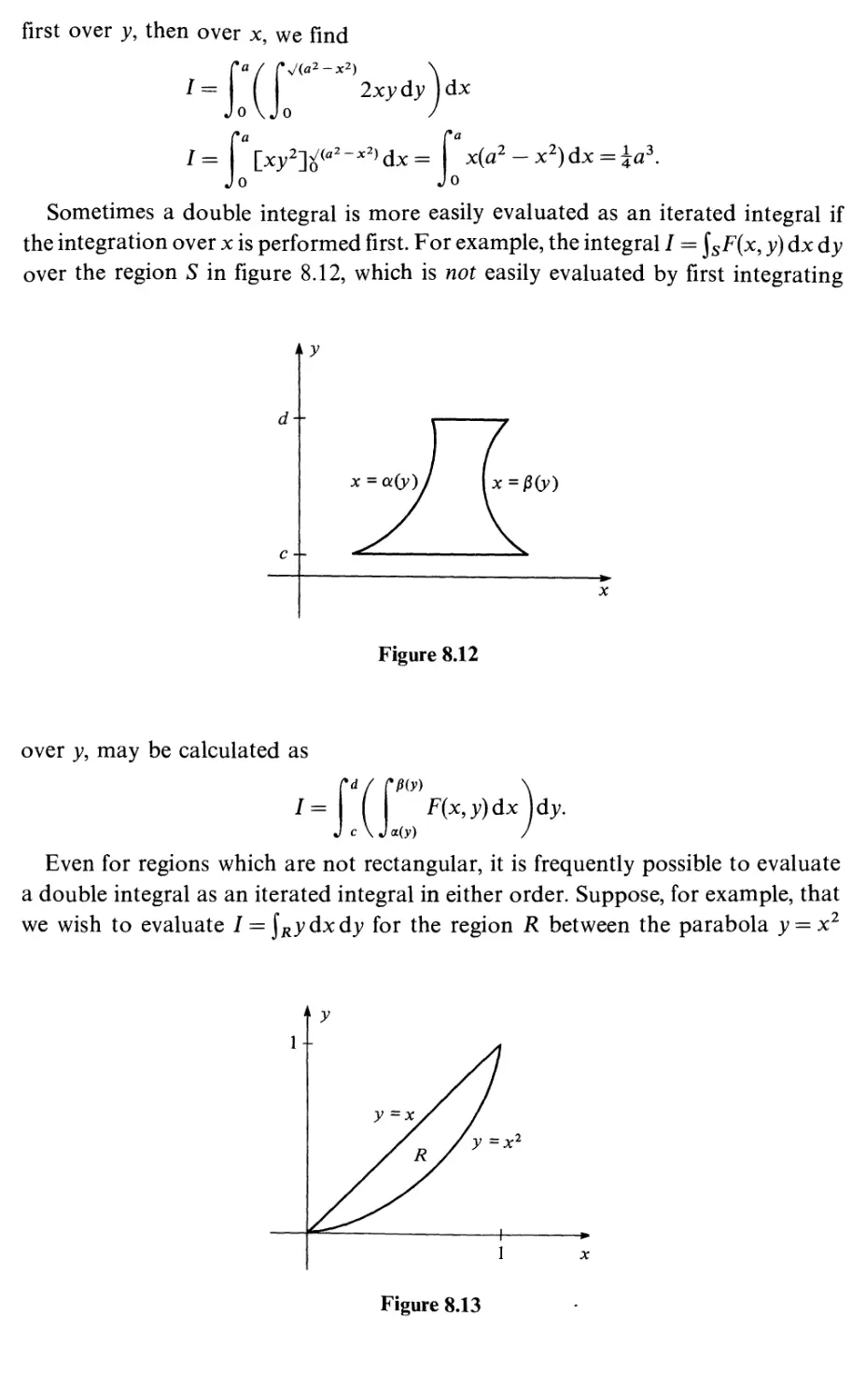
Integrating two-forms
Orientation
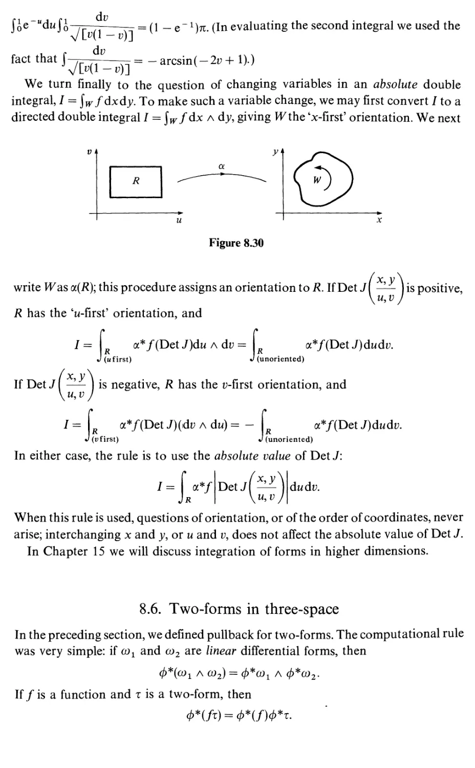
Pullback and integration for two-forms
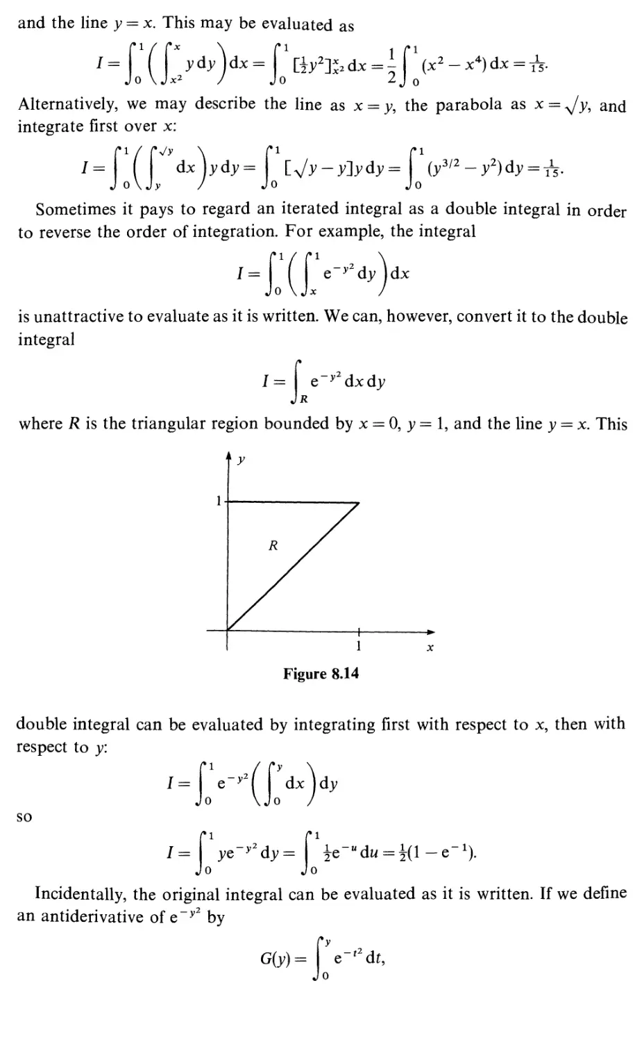
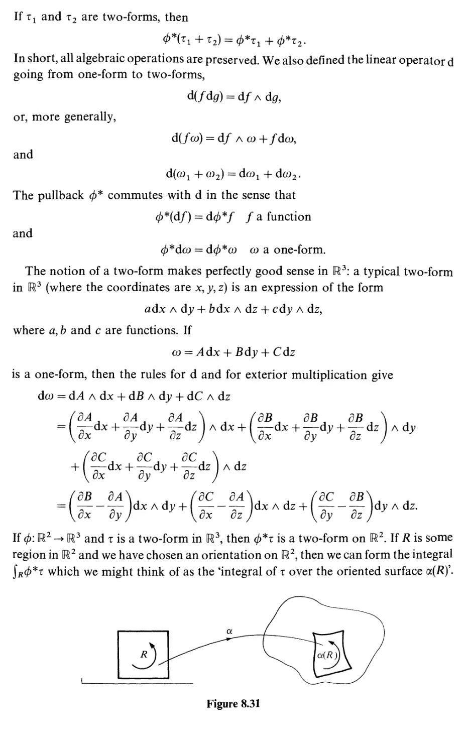
Two-forms in three-space
The difference between two-forms and densities
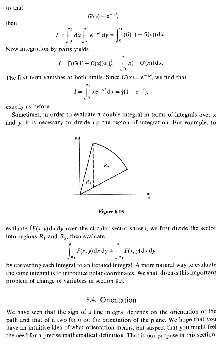
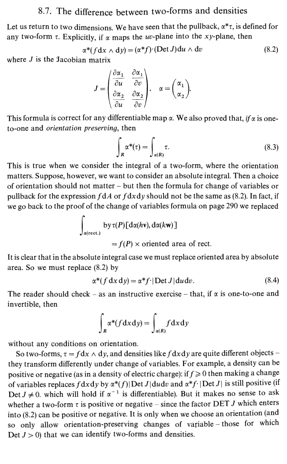
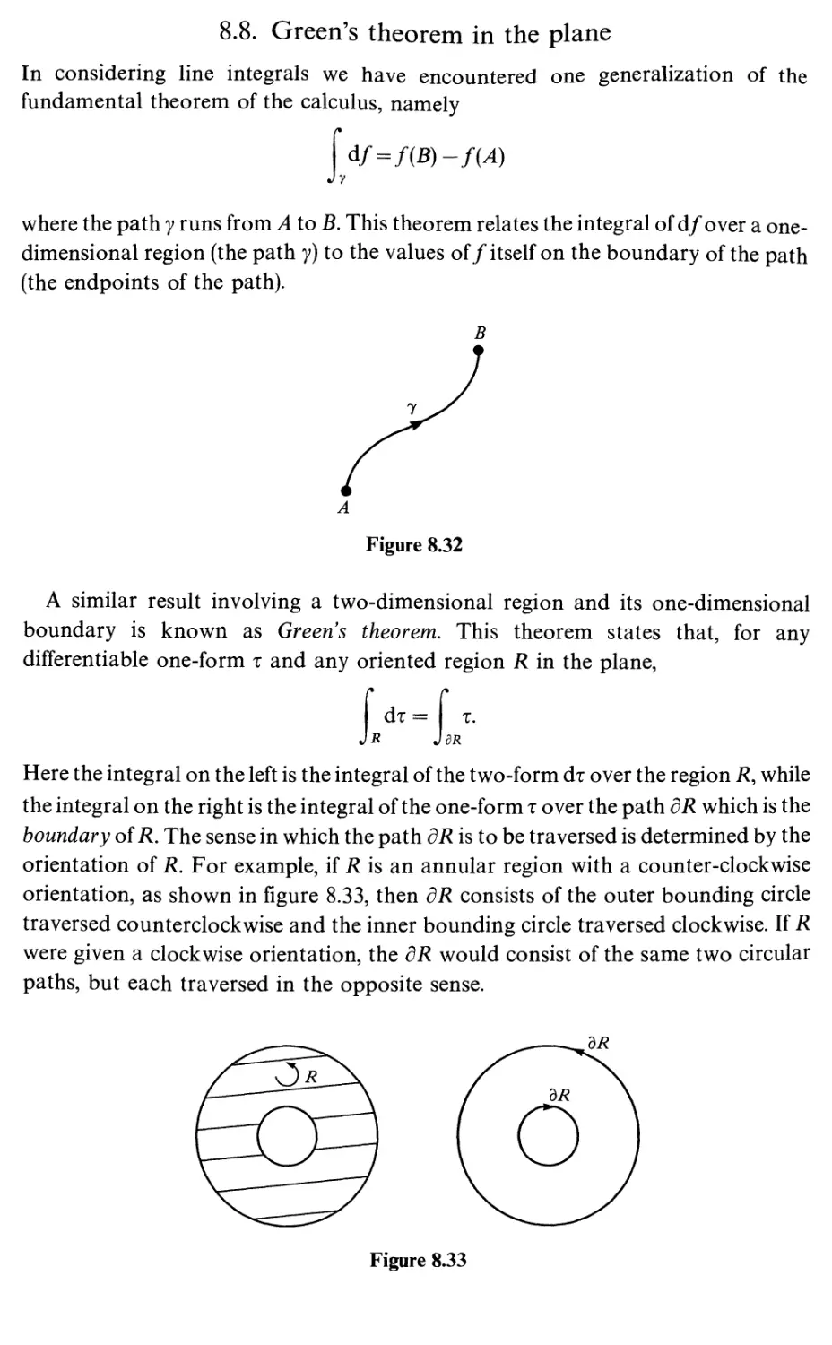
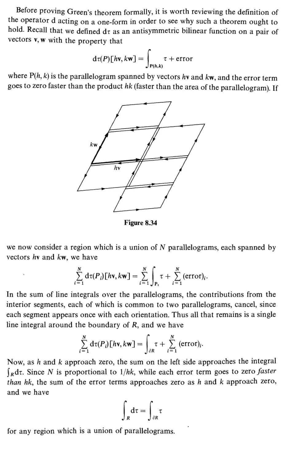
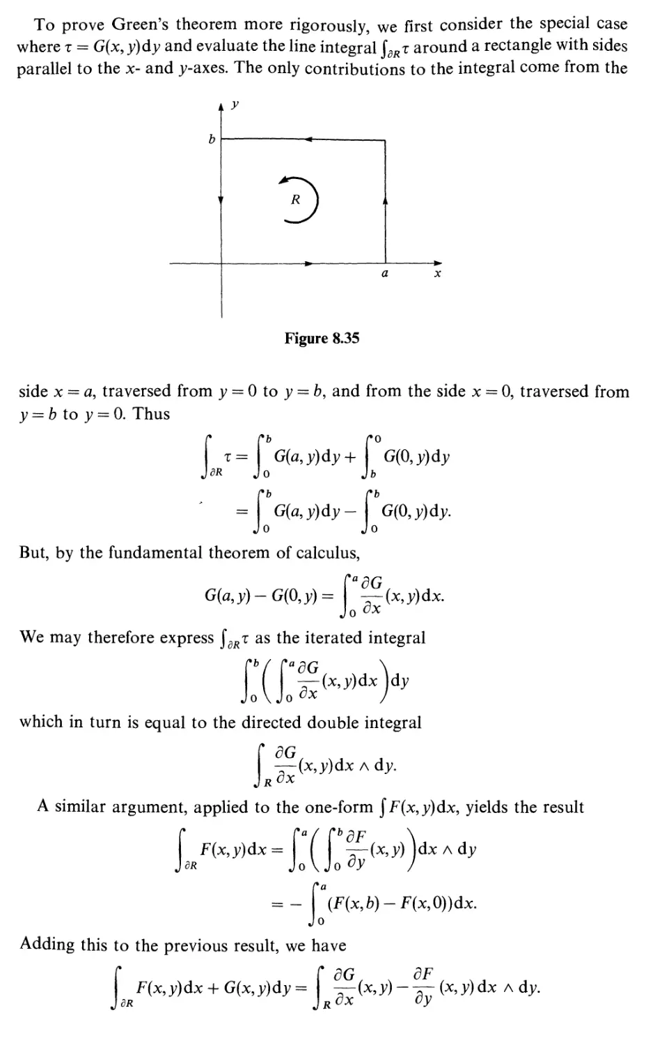
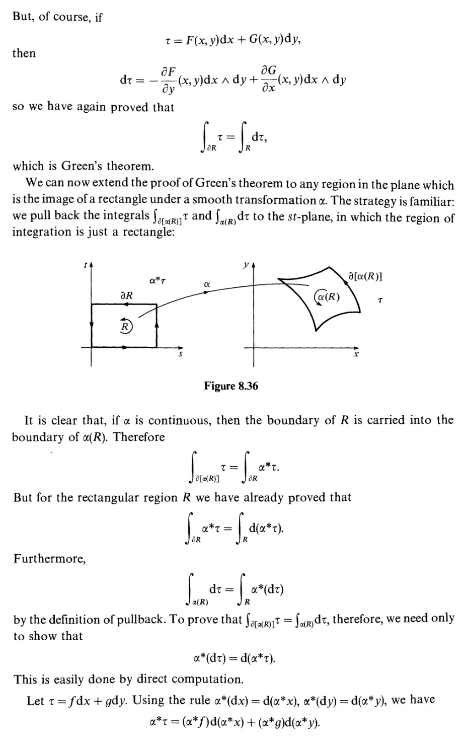
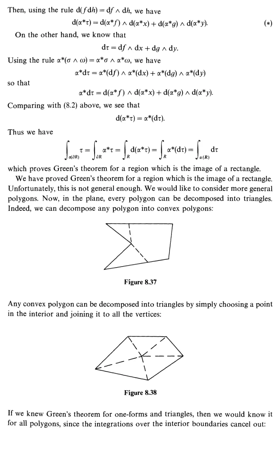
Green's theorem in the plane
Summary
Exercises
9
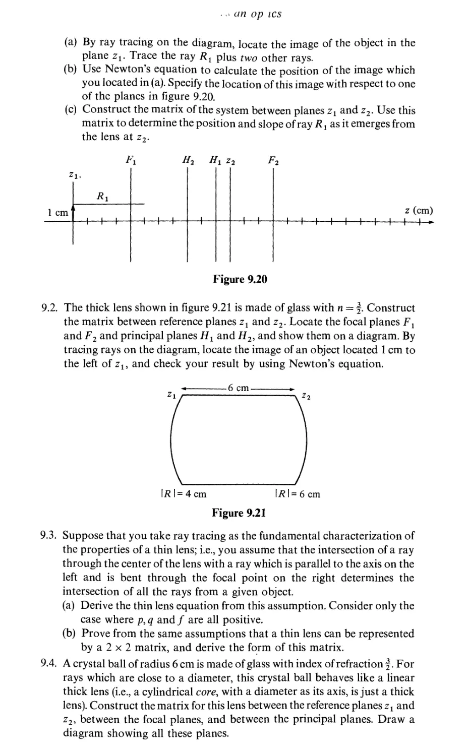
9.1
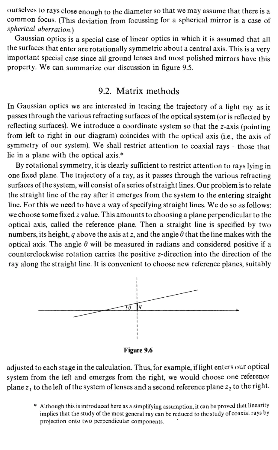
Gaussian optics
Theories of optics
311
311
on en s o o ume
vn
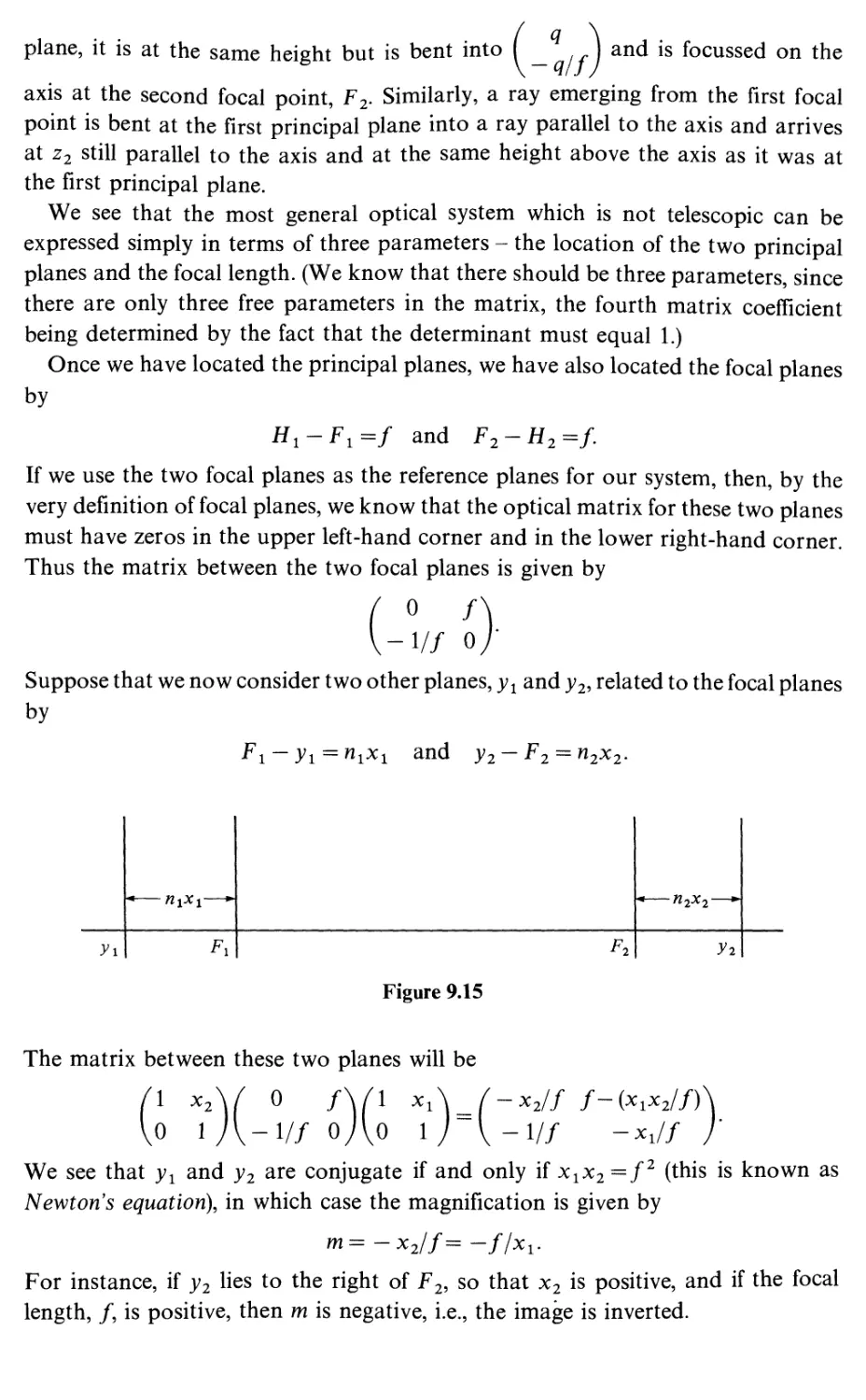
9.2
9.3
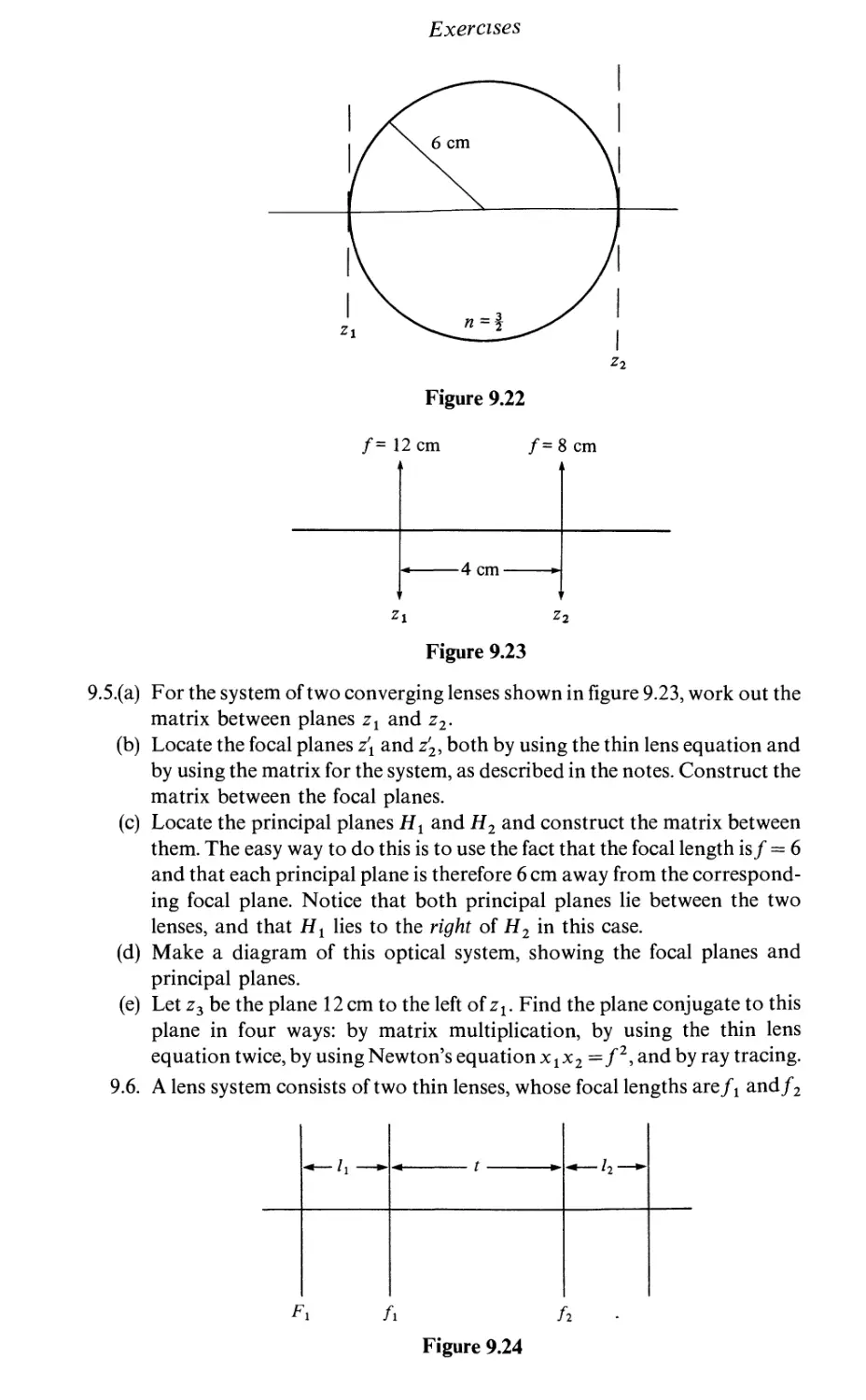
9.4
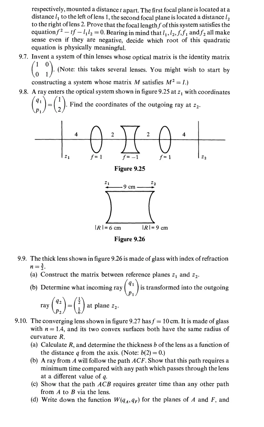
9.5
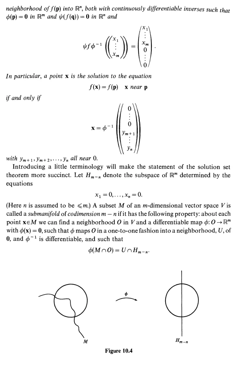
10
10.1
10.2
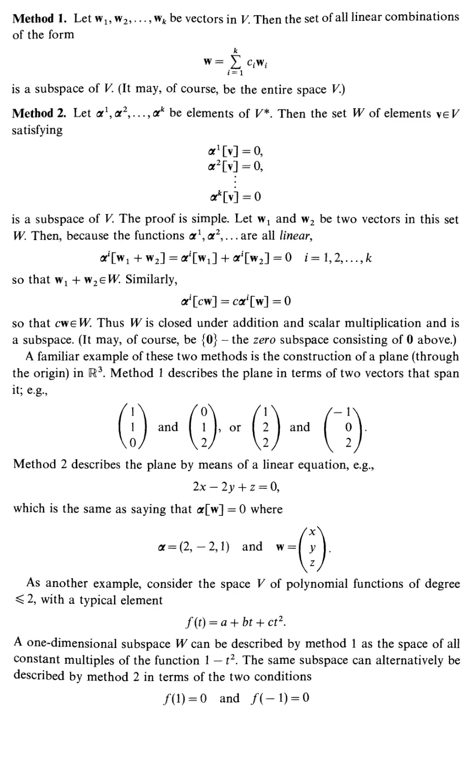
10.3
10.4
10.5
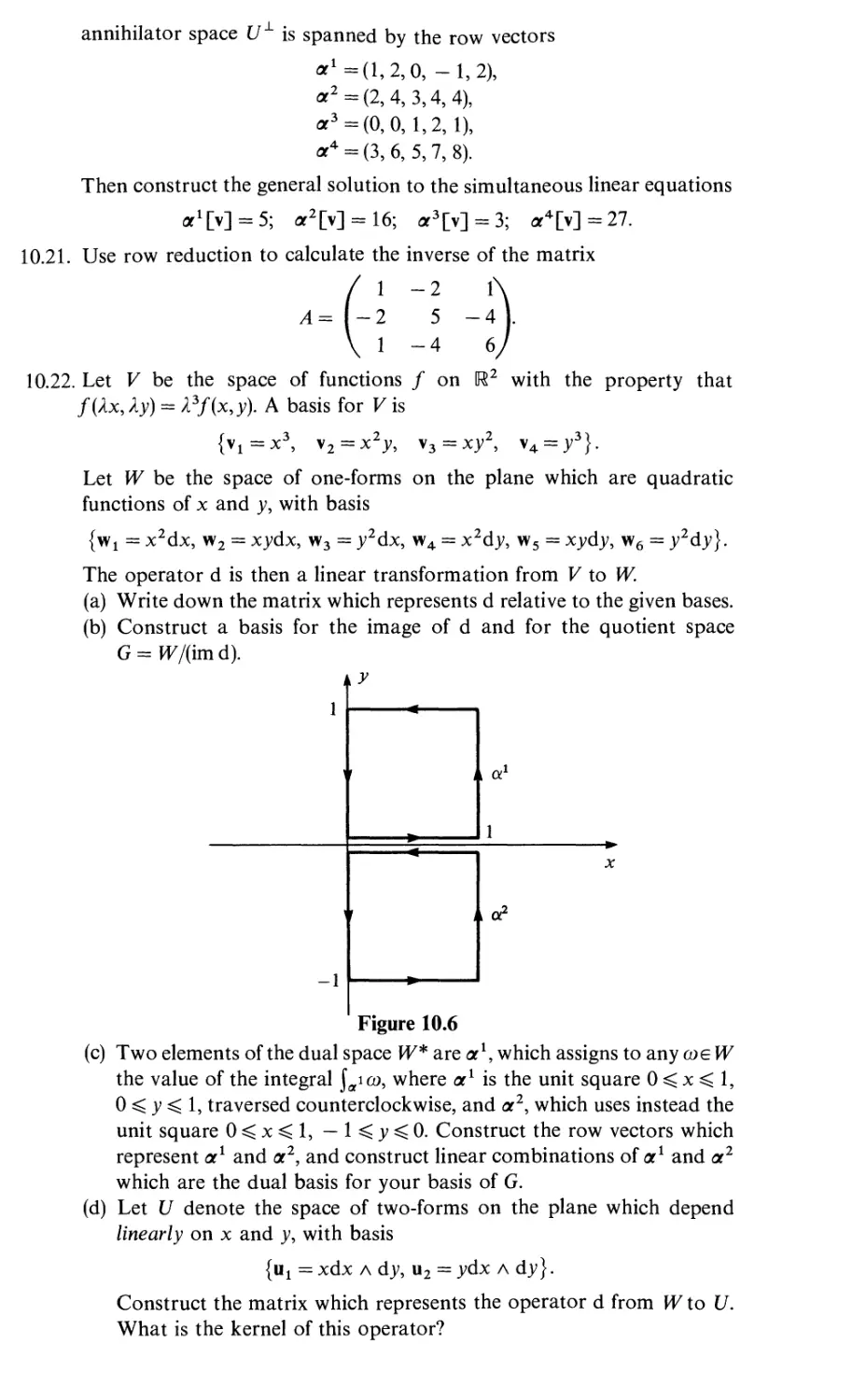
10.6
10.7
10.8
10.9
10.10
11
11.1
11.2
11.3
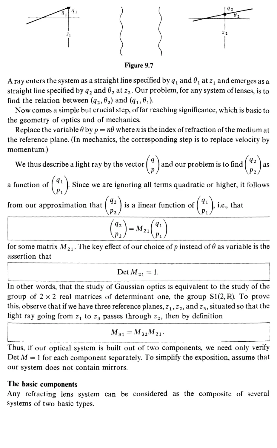
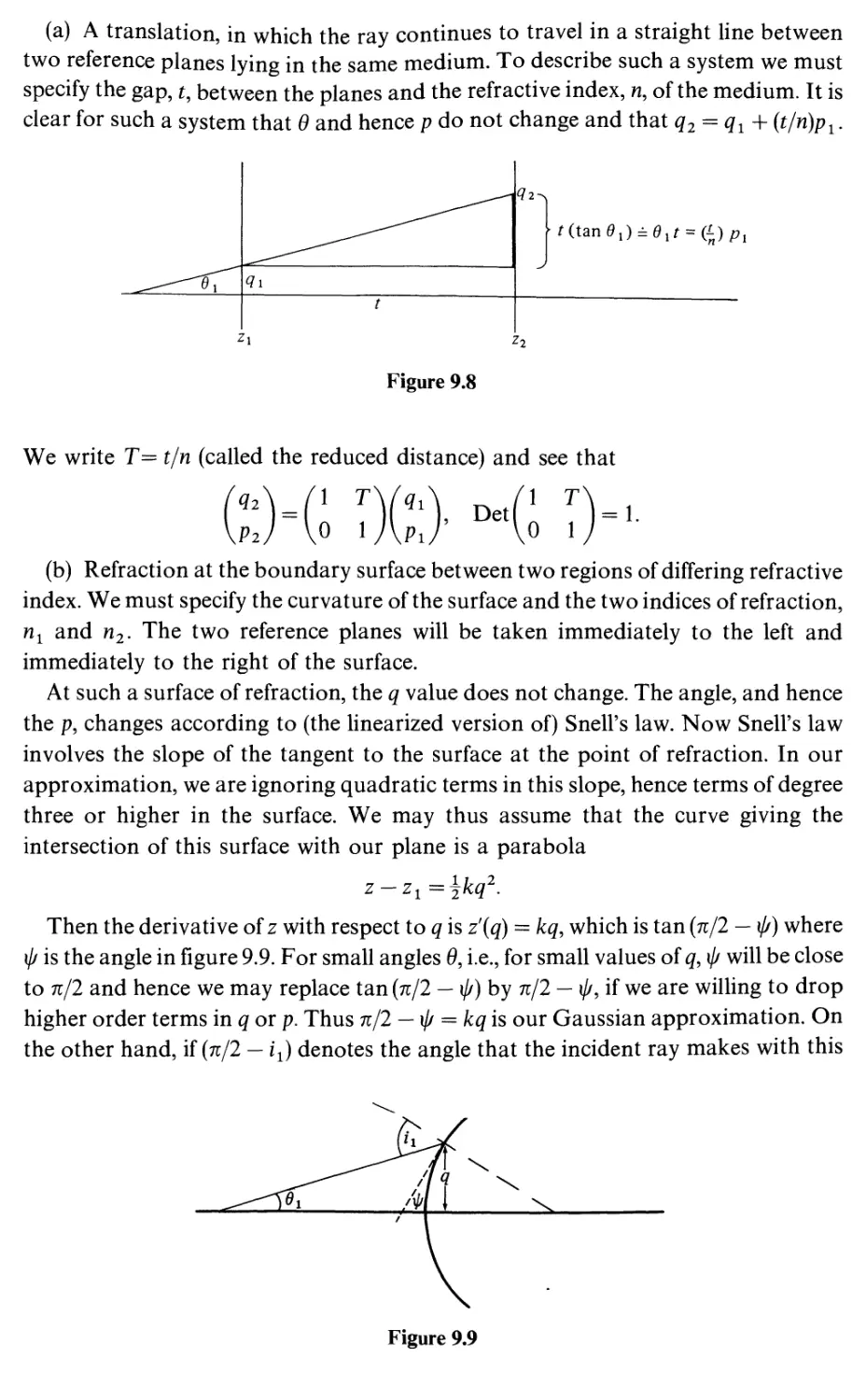
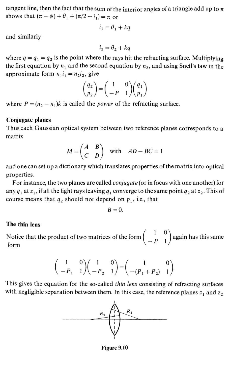
Matrix methods
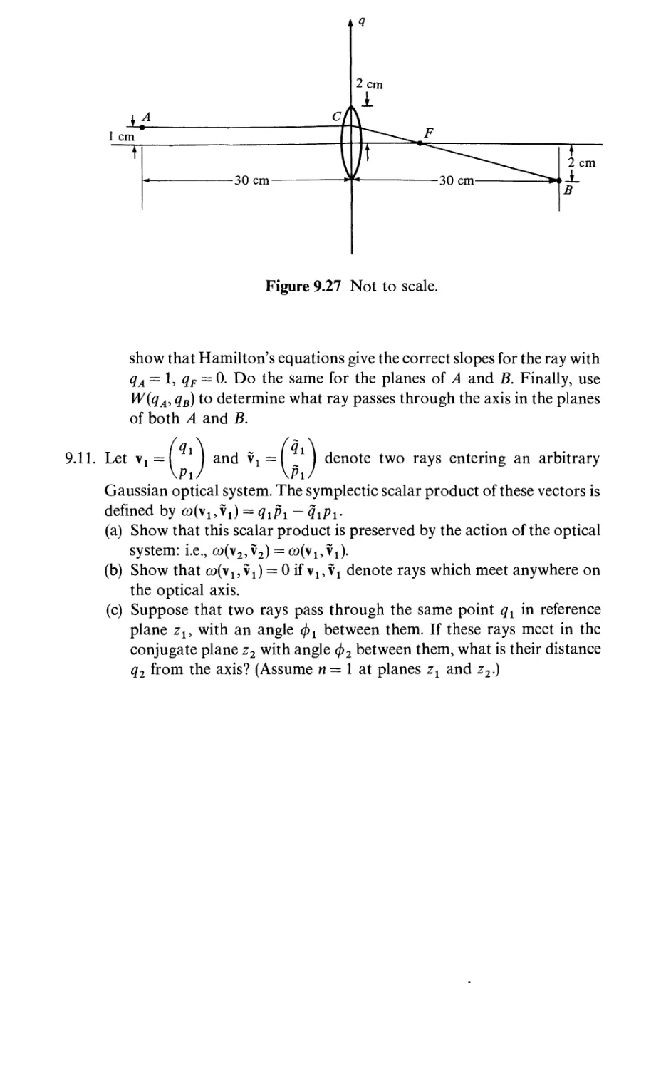
Hamilton's method in Gaussian optics
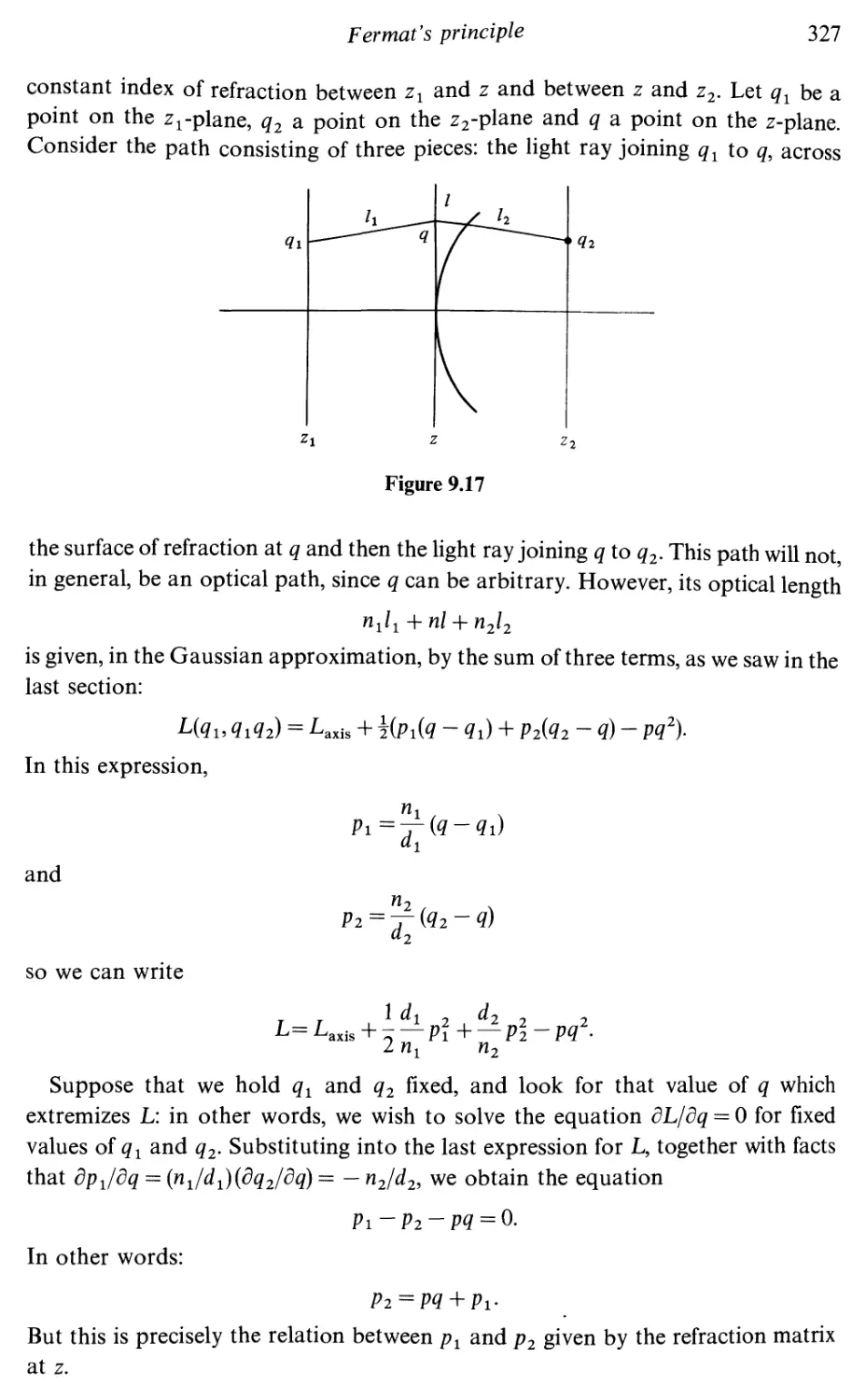
Fermat's principle
From Gaussian optics to linear optics
Summary
Exercises
Vector spaces and linear transformations
Introduction
Properties of vector spaces
The dual space
Subspaces
Dimension and basis
The dual basis
Quotient spaces
Linear transformations
Row reduction
The constant rank theorem
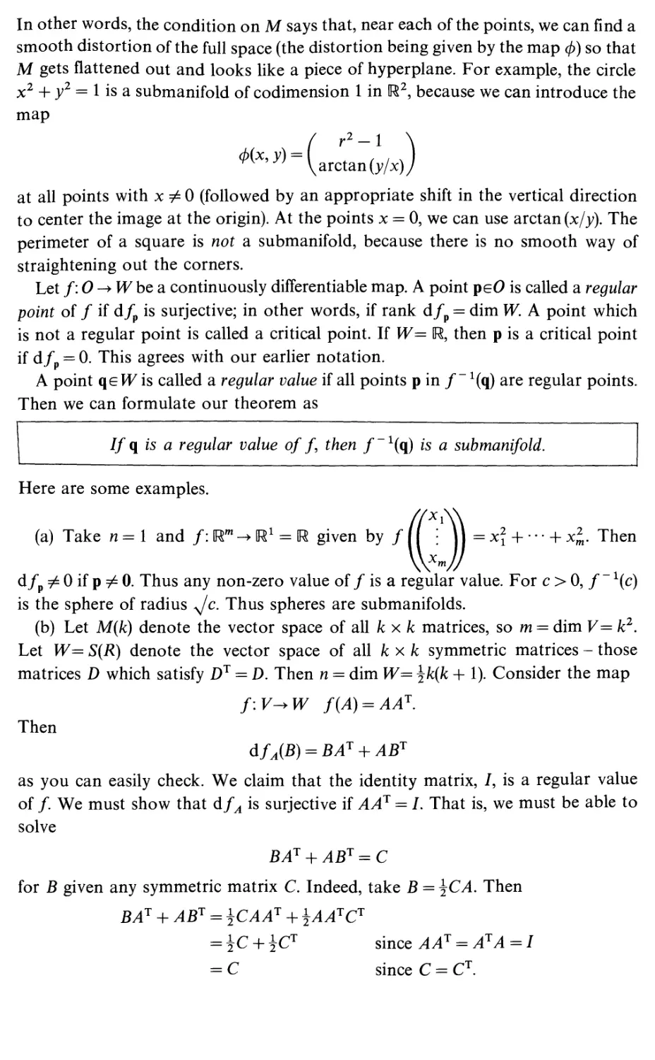
The adjoint transformation
Summary
Exercises
Determinants
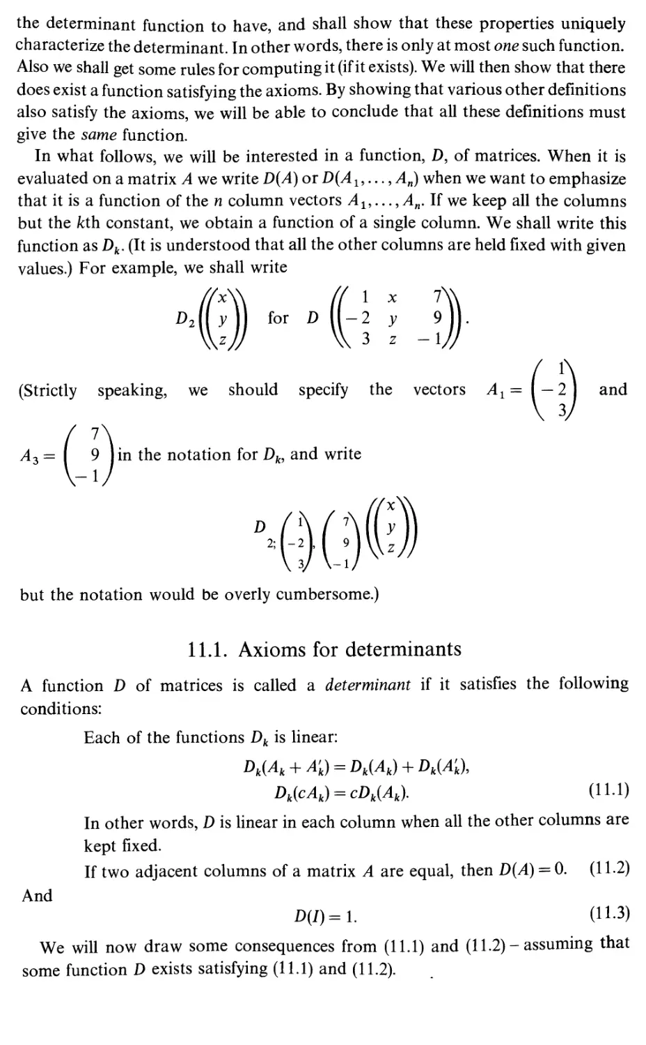
Introduction
Axioms for determinants
The multiplication law and
axioms
The existence of determinants
Summary
Exercises
other consequences of the
315
324
326
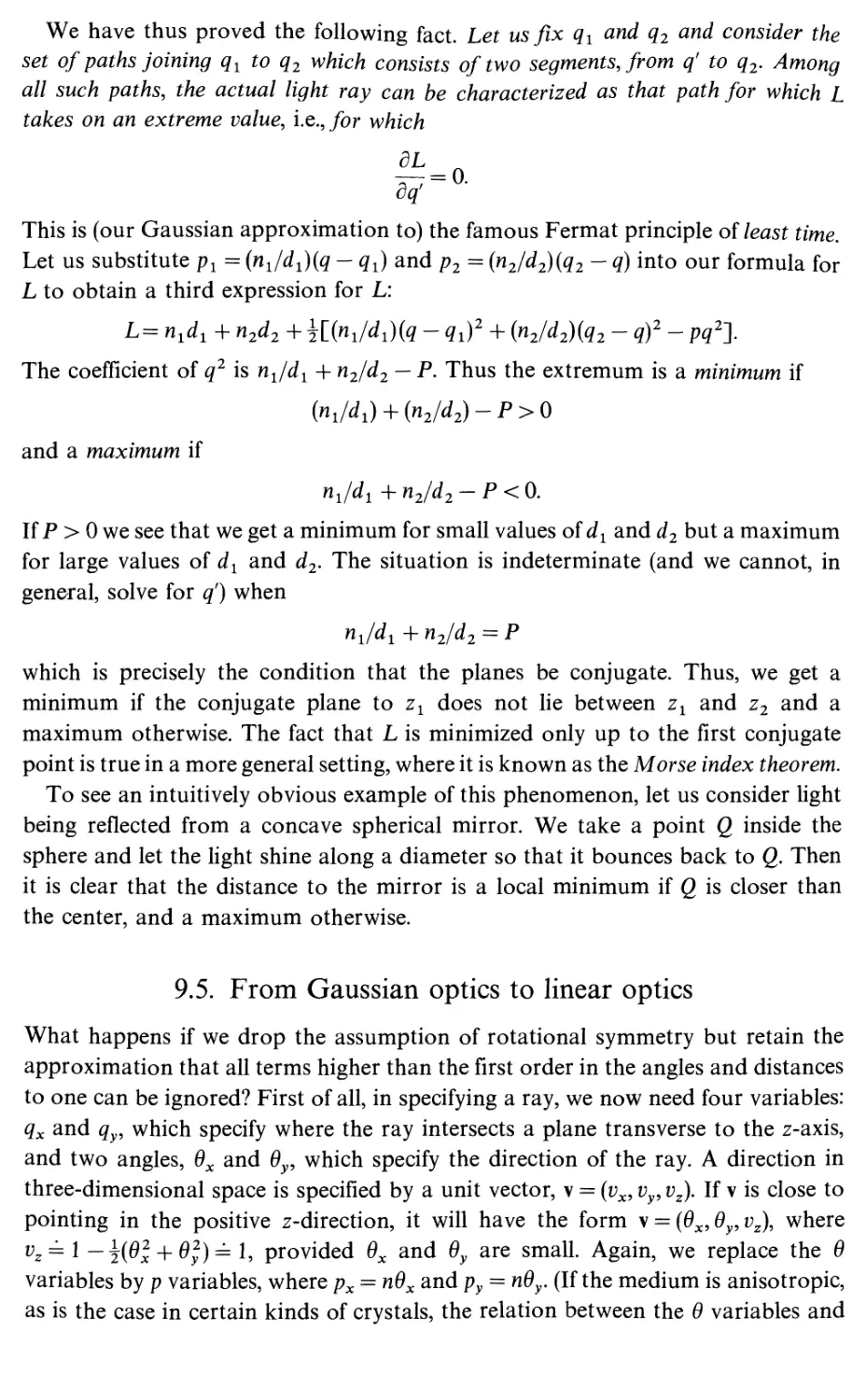
328
335
335
340
340
341
342
343
345
350
352
358
360
368
374
377
378
388
388
389
396
397
399
399
Further reading 401
Index
404
CONTENTS OF VOLUME 2
12 The theory of electrical networks 407
Introduction 407
12.1 Linear resistive circuits 411
12.2 The topology of one-dimensional complexes 419
12.3 Cochains and the d operator 429
12.4 Bases and dual bases 431
12.5 The Maxwell methods 433
12.6 Matrix expressions for the operators 436
12.7 Kirchhoff's theorem 444
12.8 Steady-state circuits and filters 446
Summary 451
Exercises 451
13 The method of orthogonal projection 458
13.1 Weyl's method of orthogonal projection 458
13.2 Kirchhoff's method 461
13.3 Green' s reciprocity theorem 466
13.4 Capacitive networks 469
13.5 B oundary-value problems 474
13.6 Solution of the boundary-value problem by Weyl's method
of orthogonal projection 477
13.7 Green's functions 482
13.8 The Poisson kernel and random walk 485
13.9 Green's reciprocity theorem in electrostatics 487
Summary 492
Exercises 492
14 High dimensional complexes 502
14.1 Introductory remarks 502
14.2 Dual spaces and cohomology 520
Summary 526
Exercises 526
15 Complexes situated in Un 532
Introduction 532
15.1 Exterior algebra 535
15.2 £-forms and the d operator 539
15.3 Integration of ^-forms 541
15.4 Stokes theorem 553
15.5 Differential forms and cohomology 564
Summary 574
Exercises 574
16 Electrostatics in U3 583
16.1 From the discrete to the continuous 583
16.2 The boundary operator 585
16.3 Solid angle 586
16.4 Electric field strength and dielectric displacement 588
16.5 The dielectric cofficient 596
16.6 The star operator in Euclidean three-dimensional space 597
16.7 Green's formulas 600
16.8 Harmonic functions 602
16.9 The method of orthogonal projection 604
16.10 Green' s functions 606
16.11 The Poisson integral formula 608
Summary 612
Exercises 612
17 Currents, flows and magnetostatics 615
17.1 Currents 615
17.2 Flows and vector fields 616
17.3 The interior product 621
17.4 Lie derivatives 626
17.5 Magnetism 628
Appendix: an alternative proof of the fundamental formula
of differential calculus 633
Summary 636
Exercises 636
18 The star operator 638
18.1 Scalar products and exterior algebra 638
18.2 The star operator 641
18.3 The Dirichlet integral and the Laplacian 646
18.4 The □ operator in spacetime 651
18.5 The Clifford algebra 653
18.6 The star operator and geometry 660
18.7 The star operator and vector calculus 662
Appendix: tensor products 664
Summary 674
Exercises 674
19 Maxwell's equations 686
19.1 The equations 686
19.2 The homogeneous wave equation in one dimension 689
19.3 The homogeneous wave equation in U3 692
19.4 The inhomogeneous wave equation in U3 695
19.5 The electromagnetic Lagrangian and the energy-
momentum sensor 697
19.6 Wave forms and Huyghens' principle 700
Summary 704
Exercises inA
20 Complex analysis 705
Introduction 706
20.1 Complex-valued functions 707
20.2 Complex-valued differential forms 709
20.3 Holomorphic functions 711
20.4 The calculus of residues 715
20.5 Applications and consequences 724
20.6 The local mapping 729
20.7 Contour integrals 735
20.8 Limits and series 740
Summary 744
Exercises 744
21 Asymptotic evaluation of integrals 750
Introduction 750
21.1 Laplace' s method 750
21.2 The method of stationary phase 755
21.3 Gaussian integrals 758
21.4 Group velocity 761
21.5 The Fourier inversion formula 762
21.6 Asymptotic evaluation of Helmholtz' formula 764
Summary 766
Exercises 766
22 Thermodynamics 768
22.1 Caratheodory's theorem 769
22.2 Classical thermodynamics according to Born and
Catheodory 775
22.3 Entropy and obsolute temperature 780
22.4 Systems with one configurational variable 785
22.5 Conditions for equilibrium 796
22.6 Systems and states in statistical mechanics 800
22.7 Products and images 805
22.8 Observables, expectations and internal energy 808
22.9 Entropy 814
22.10 Equilibrium statistical mechanics 816
22.11 Quantum and classical gases 823
22.12 Determinants and traces 826
22.13 Quantum states and quantum logic 831
Summary 835
Exercises 836
Appendix 838
Further reading 845
Index
848
PREFACE
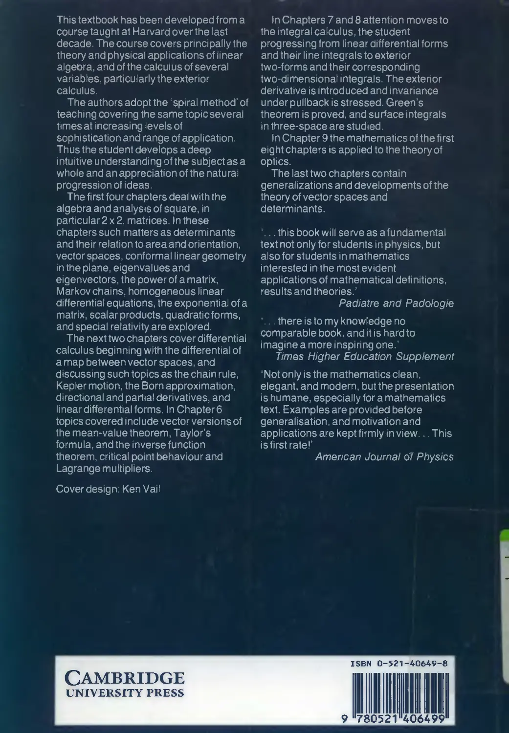
This book, with apologies for the pretentious title, represents the text of a course
we have been teaching at Harvard for the past eight years. The course is aimed
at students with an interest in physics who have a good grounding in one-
variable calculus. Some prior acquaintance with linear algebra is helpful but not
necessary. Most of the students simultaneously take an intensive course in physics
and so are able to integrate the material learned here with their physics education.
This also is helpful but not necessary. The main topics of the course are the theory
and physical application of linear algebra, and of the calculus of several variables,
particularly the exterior calculus. Our pedagogical approach follows the 'spiral
method' wherein we cover the same topic several times at increasing levels of
sophistication and range of application, rather than the 'rectilinear approach' of
strict logical order. There are, we hope, no vicious circles of logical error, but we
will frequently develop a special case of a subject, and then return to it for a more
general definition and setting only after a broader perspective can be achieved
through the introduction of related topics. This makes some demands of patience
and faith on the part of the student. But we hope that, at the end, the student is
rewarded by a deeper intuitive understanding of the subject as a whole.
Here is an outline of the contents of the book in some detail. The goal of the
first four chapters is to develop a familiarity with the algebra and analysis of
square matrices. Thus, by the end of these chapters, the student should be thinking
of a matrix as an object in its own right, and not as a square array of numbers.
We deal in these chapters almost exclusively with 2x2 matrices, where the most
complicated of the computations can be reduced to solving quadratic equations.
But we always formulate the results with the higher-dimensional case in mind. We
begin Chapter 1 by explaining the relation between the multiplication law of 2 x 2
matrices and the geometry of straight lines in the plane. We develop the algebra
of 2 x 2 matrices and discuss the determinant and its relation to area and
orientation. We define the notion of an abstract vector space, in general, and
explain the concepts of basis and change of basis for one- and two-dimensional
vector spaces.
In Chapter 2 we discuss conformal linear geometry in the plane, that is, the
geometry of lines and angles, and its relation to certain kinds of 2 x 2 matrices.
We also discuss the notion of eigenvalues and eigenvectors, so important in
quantum mechanics. We use these notions to give an algorithm for computing
the powers of a matrix. As an application we study the basic properties of Markov
chains.
The principal goal of Chapter 3 is to explain that a system of homogeneous
linear differential equations with constant coefficients can be written as du/dt = An
where A is a matrix and u is a vector, and that the solution can be written as
eAtu0 where u0 gives the initial conditions. This of course requires us to explain
what is meant by the exponential of a matrix. We also describe the qualitative
behavior of solutions and the inhomogeneous case, including a discussion of
resonance.
Chapter 4 is devoted to the study of scalar products and quadratic forms. It is
rich in physical applications, including a discussion of normal modes and a detailed
treatment of special relativity.
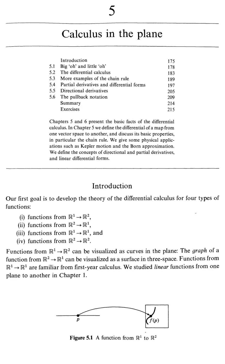
Chapters 5 and 6 present the basic facts of the differential calculus. In Chapter 5
we define the differential of a map from one vector space to another, and discuss
its basic properties, in particular the chain rule. We give some physical applications
such as Kepler motion and the Born approximation. We define the concepts of
directional and partial derivatives, and linear differential forms.
In Chapter 6 we continue the study of the differential calculus. We present the
vector versions of the mean-value theorem, of Taylor's formula and of the inverse
function theorem. We discuss critical point behavior and Lagrange multipliers.
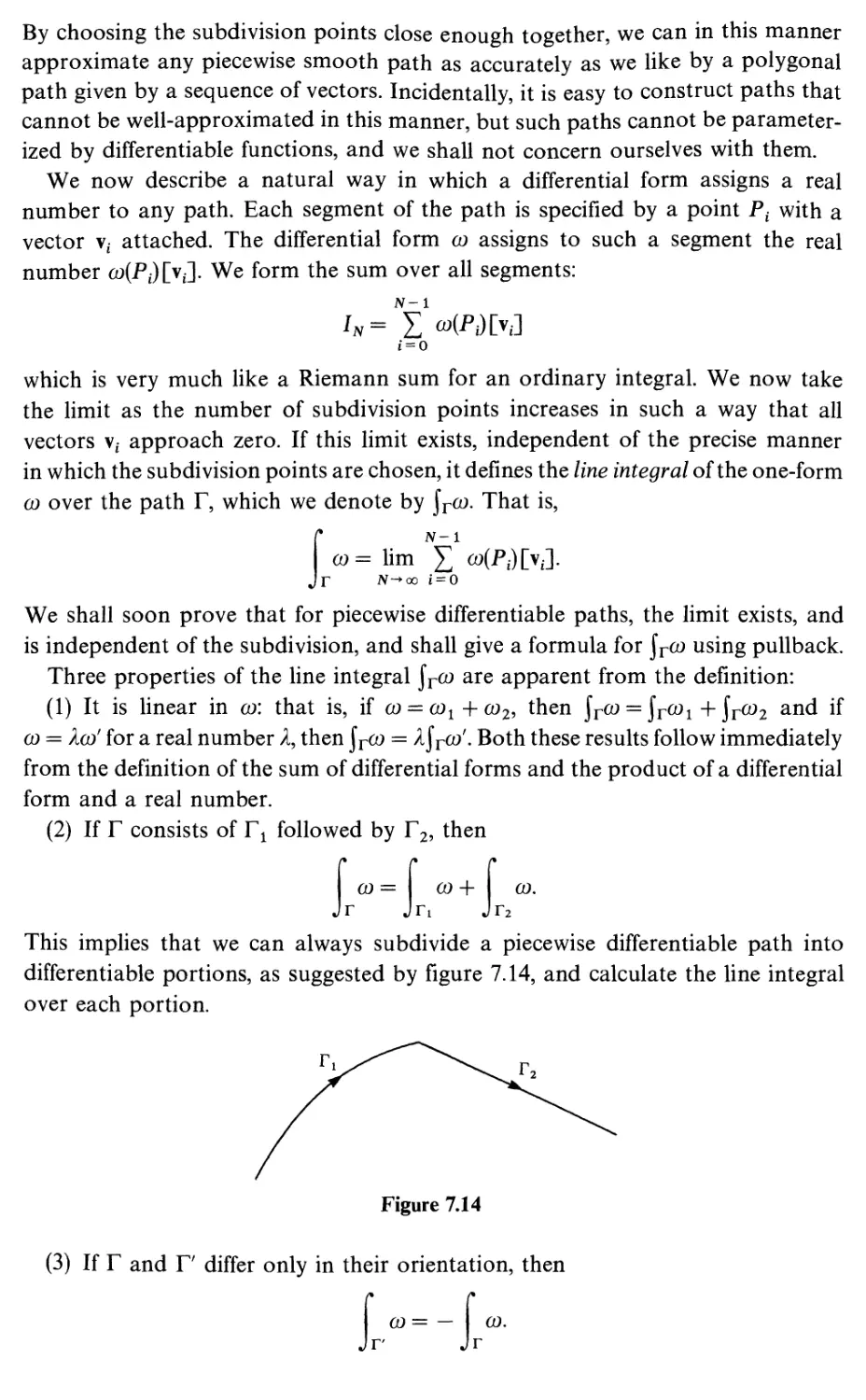
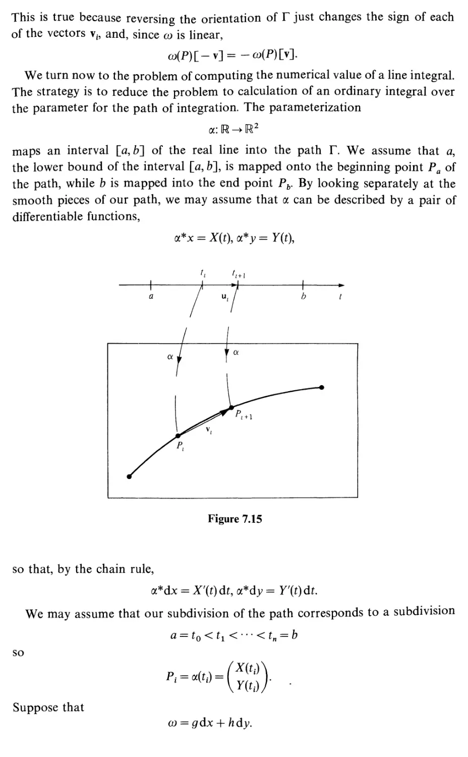
Chapters 7 and 8 are meant as a first introduction to the integral calculus.
Chapter 7 is devoted to the study of linear differential forms and their line integrals.
Particular attention is paid to the behavior under change of variables. Other
one-dimensional integrals such as arc length are also discussed.
Chapter 8 is devoted to the study of exterior two-forms and their corresponding
two-dimensional integrals. The exterior derivative is introduced and invariance
under pullback is stressed. The two-dimensional version of Stokes' theorem, i.e.
Green's theorem, is proved. Surface integrals in three-space are studied.
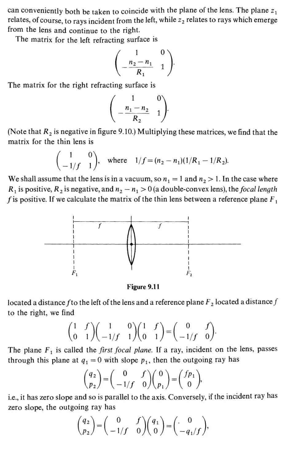
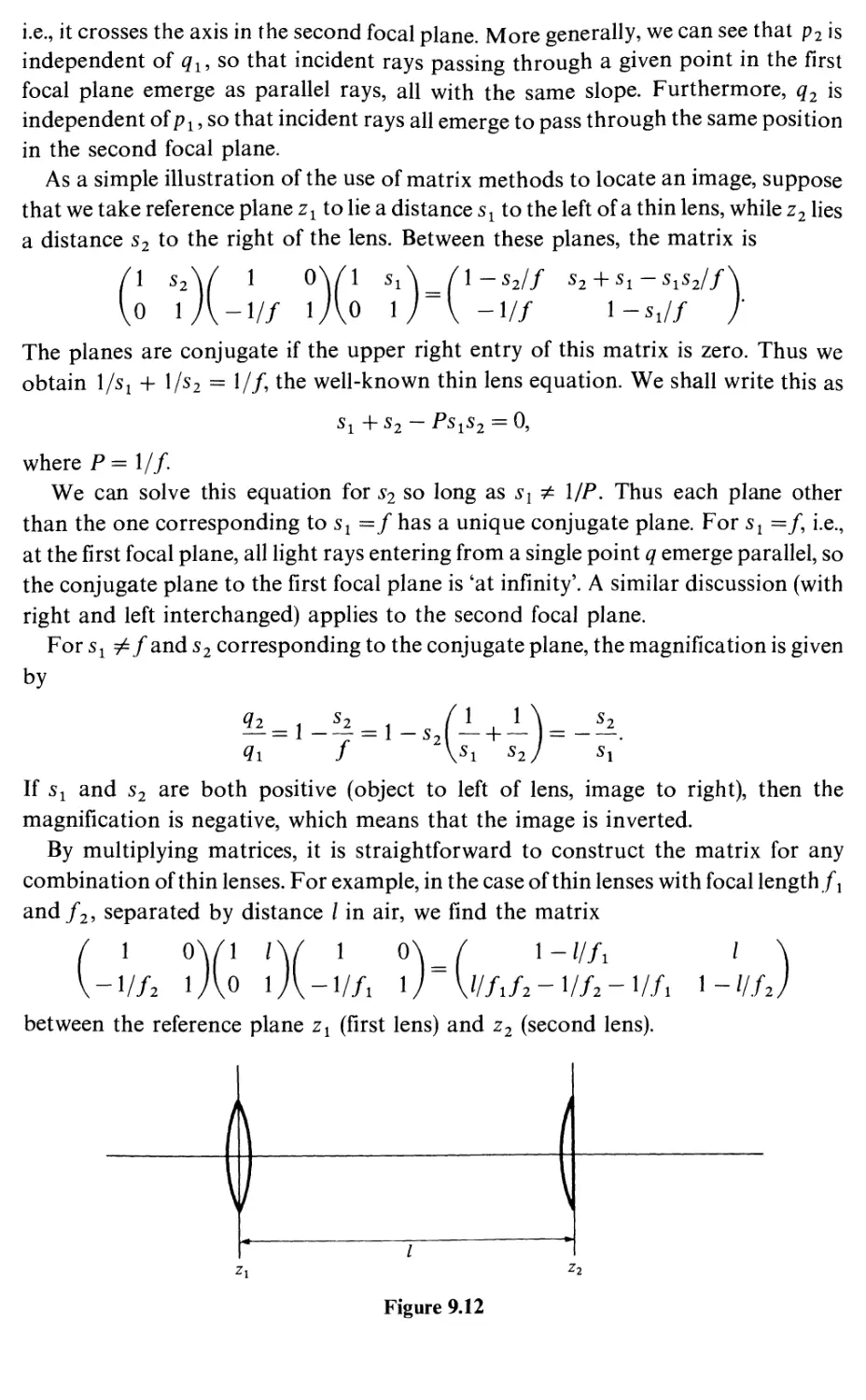
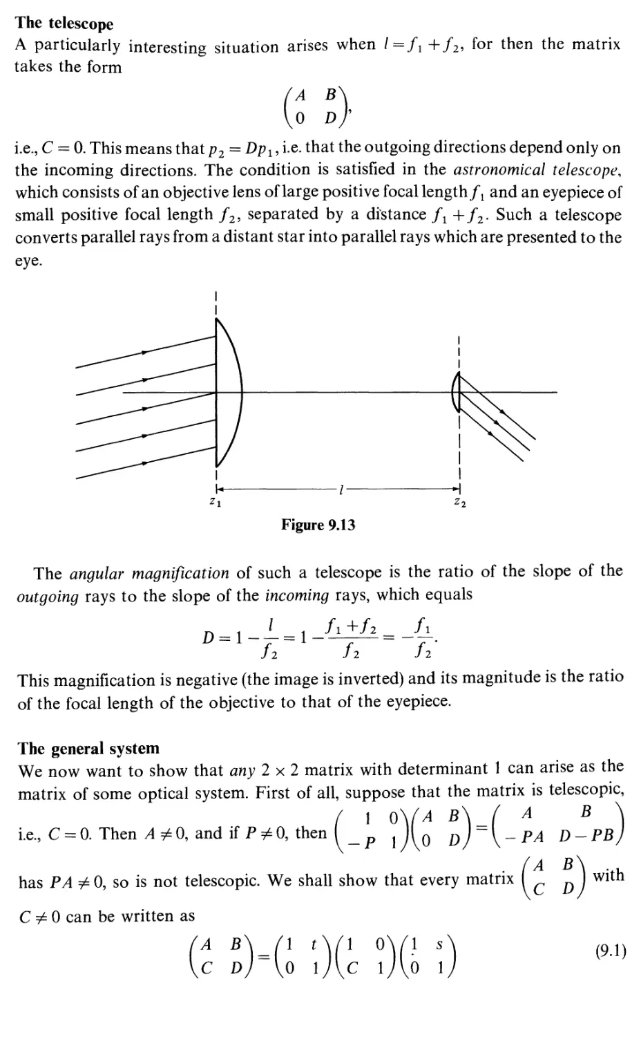
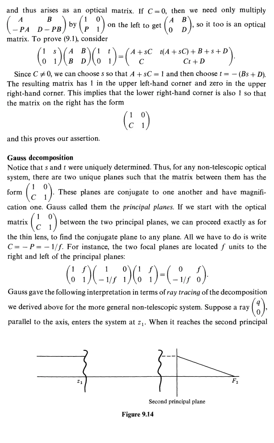
Chapter 9 presents an example of how the results of the first eight chapters can
be applied to a physical theory - optics. It is all in the nature of applications, and
can be omitted without any effect on the understanding of what follows.
In Chapter 10 we go back and prove the basic facts about finite-dimensional
vector spaces and their linear transformations. The treatment here is a
straightforward generalization, in the main, of the results obtained in the first four chapters
in the two-dimensional case. The one new algorithm is that of row reduction. Two
important new concepts (somewhat hard to get used to at first) are introduced:
those of the dual space and the quotient space. These concepts will prove crucial
in what follows.
Chapter 11 is devoted to proving the central facts about determinants ofnxn
}re ace
Xlll
matrices. The subject is developed axiomatically, and the basic computational
algorithms are presented.
Chapters 12-14 are meant as a gentle introduction to the mathematics of shape,
that is, algebraic topology. In Chapter 12 we begin the study of electrical networks.
This involves two aspects. One is the study of the 'wiring' of the network, that is,
how the various branches are interconnected. In mathematical language this is
known as the topology of one-dimensional complexes. The other is the study of
how the network as a whole responds when we know the behavior of the individual
branches, in particular, power and energy response. We give some applications to
physically interesting networks.
In Chapter 13 we continue the study of electrical networks. We examine the
boundary-value problems associated with capacitive networks and use these
methods to solve some classical problems in electrostatics involving conductors.
In Chapter 14 we give a sketch of how the one-dimensional results of Chapters 12
and 13 generalize to higher dimensions.
Chapters 15-18 develop the exterior differential calculus as a continuous version
of the discrete theory of complexes. In Chapter 15 the basic facts of the exterior
calculus are presented: exterior algebra, fc-forms, pullback, exterior derivative and
Stokes' theorem.
Chapter 16 is devoted to electrostatics. We suggest that the dielectric properties
of the vacuum give the continuous analog of the capacitance of a network, and
that these dielectric properties are what determine Euclidean geometry in three-
dimensional space. The basic facts of potential theory are presented.
Chapter 17 continues the study of the exterior differential calculus. The main
topics are vector fields and flows, interior products and Lie derivatives. These are
applied to magnetostatics.
Chapter 18 concludes the study of the exterior calculus with an in-depth
discussion of the star operator in a general context.
Chapter 19 can be thought of as the culmination of the course. It applies the
results of the preceding chapters to the study of Maxwell's equations and the
associated wave equations.
Chapters 20 and 21 are essentially independent of Chapters 9-19 and can be
read independently of them. They are not usually included in our one-year course.
But Chapters 1-9, 20 and 21 would form a self-contained unit for a shorter course.
The material in Chapter 20 is a relatively standard treatment of the theory of
functions of a complex variable, suitable for students at the level of this book.
Chapter 21 discusses some of the more elementary aspects of asymptotics.
Chapter 22 shows how the exterior calculus can be used in classical
thermodynamics, following the ideas of Born and Caratheodory.
The book is divided into two volumes, with Chapters 1-11 in volume 1.
Most of the mathematics and all of the physics presented in this book were
developed by the first decade of the twentieth century. The material is thus at
least seventy-five years old. Yet much of the material is not yet standard in the
elementary courses (although most of it with the possible exception of network
theory must be learned for a grasp of modern physics, and is studied at some stage
of the physicist's career). The reasons are largely historical. It was apparent to
Hamilton that the real and complex numbers were insufficient for the deeper study
of geometrical analysis, that one wants to treat the number pairs or triplets of
the Cartesian geometry in two and three dimensions as objects in their own right
with their own algebraic properties. To this end he developed the algebra of
quaternions, a theory which had a good deal of popularity in England in the
middle of the nineteenth century. Quaternions had several drawbacks: they more
naturally pertained to four, rather than to three dimensions - the geometry of
three dimensions appeared as a piece of a larger theory rather than having a
natural existence of its own; also, they have too much algebraic structure, the
relation between quaternion multiplication, for example, and geometric
constructions in three dimensions being somewhat complicated. (The first of these objections
would, of course be regarded far less seriously today. But it would be replaced by
an objection to a theory that is limited to four dimensions.) Eventually, the three-
dimensional vector algebra with its scalar and vector products was distilled from
the theory of quaternions. It was conjoined with the necessary differential
operations, and give rise to the vector analysis as finally developed by Gibbs and
promulgated by him in a famous and very influential text.
So vector analysis, with its grad, div, curl etc. became the standard language in
which the geometric laws of physics were taught. Now while vector analysis is
well suited to the geometry of three-dimensional Euclidean space, it has a number
of serious drawbacks. First, and least serious, is that the essential unity of the
subject is obscured. Thus the fundamental theorem of the calculus, Green's theorem,
Gauss' theorem and Stokes' theorem are all aspects of the same theorem (now
called Stokes' theorem). But this is not at all clear in the vector analysis treatment.
More serious is that the fundamental operators involve the Euclidean structure
(for example grad and div) or the three-dimensional structure and orientation as
well (for example curl). Thus the theory is wedded to a three-dimensional orientated
Euclidean space. A related problem is that the operators do not behave nicely
under general changes of coordinates - their expression in non-rectangular
coordinates being unwieldy. Already Poincare, in his fundamental scientific and
philosophical writings which led to the theory of relativity, stressed the need to
distinguish between those laws of geometry and physics which are 'topological',
i.e. depend only on the differential structure of space and so are invariant under
smooth deformations, and those which depend on more geometrical structure such
as the notion of distance. One of the major impacts of the theory of relativity on
mathematics was to encourage the study of higher-dimensional spaces, a study
which had existed in the previous mathematical literature, but was not regarded
as central to the study of geometry. Another was to emphasize general coordinate
changes. The vector analysis was not up to these two tasks and so was supplemented
in the more advanced literature by tensor analysis. But tensor analysis with its
Preface
xv
jumble 0f indices has a number of serious drawbacks, the most serious of which
being that it is extraordinarily difficult to tell which operations have any geometric
significance and which are artifacts of the coordinate system. Thus, while it is
reasonably well-suited for computation, it is hard to assess exactly what it is that
one is computing. The whole purpose of the development initiated by Hamilton - to
have a calculus whose objects have a perceived geometrical significance - was
vitiated. In order to make the theory work one had to introduce a relatively
sophisticated geometrical construct, such as an affine connection. Even with such
constructs the geometric meanings of the operations are obscure. In fact tensor
analysis never displaced the intuitively clear vector analysis from the elementary
curriculum.
It is generally accepted in the mathematics community, and gradually being
accepted in the physics community, that the most suitable framework for
geometrical analysis is the exterior differential calculus of Grassmann and Cartan. This
calculus has the advantage that its computational rules are simple and concise,
that its objects have a transparent geometrical significance, that it works in all
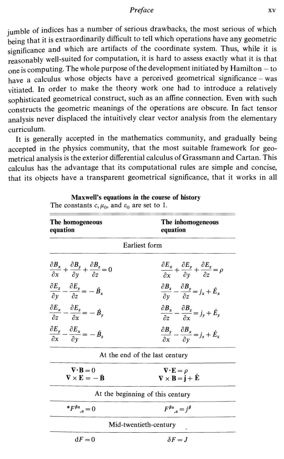
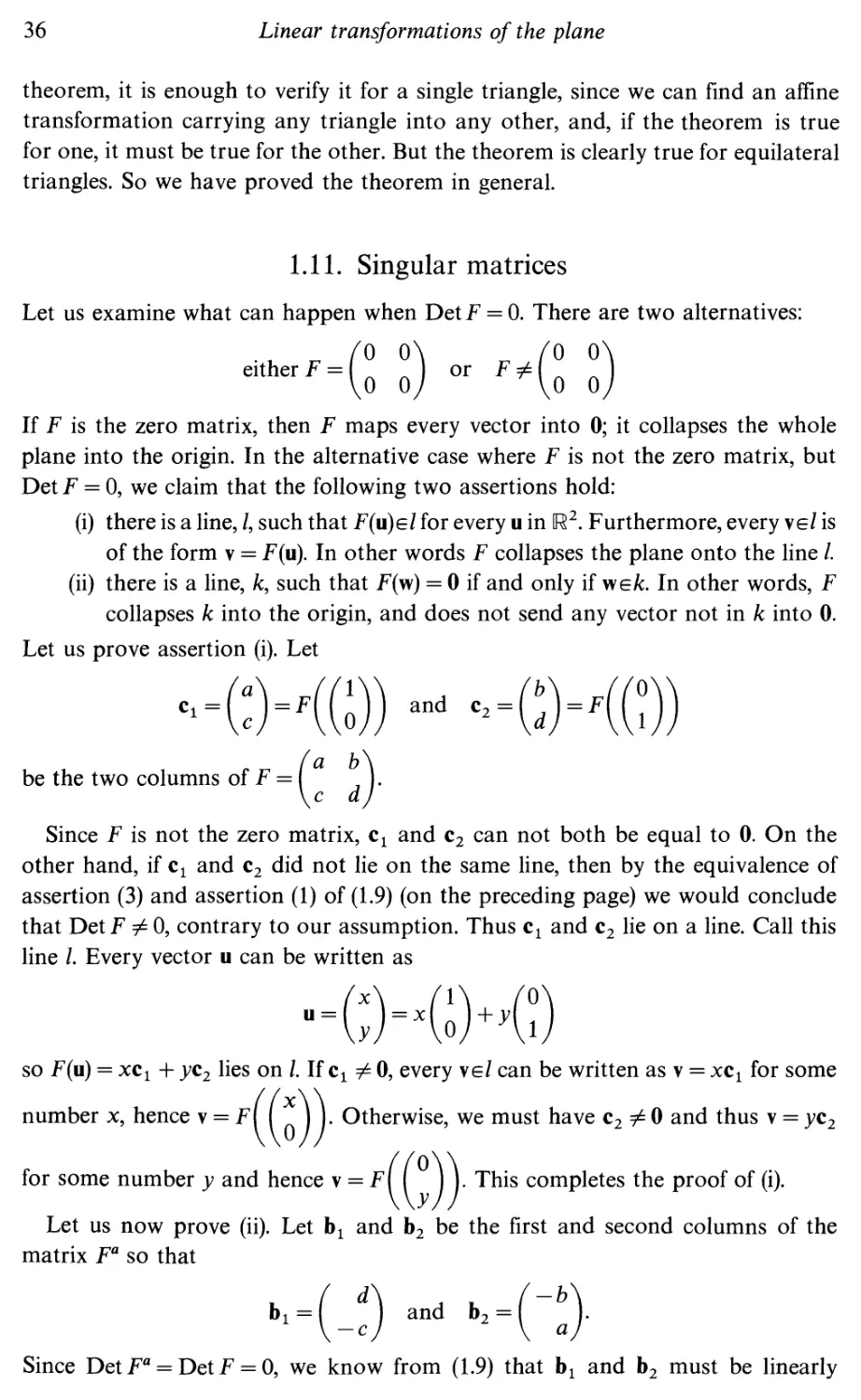
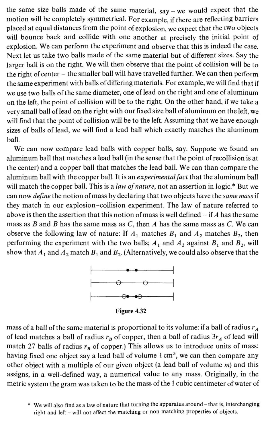
Maxwell's equations in the course of history
The constants c,/i0, and s0 are set to 1.
The homogeneous The inhomogeneous
equation equation
Earliest form
dBx dBv
—-H - +
dx dy
dEz dEy
dy dz
dEx dEz
dz dx
dEy dEx
dx dy
f-
-Bx
-By
-Bz
dEx dEy dEz
dx dy dz
/^ "i JX ' X
dy dz
dBx dBz .
~dz~~lx~-Jy + Ey
dBy dBx .
ox oy
At the end of the last century
= 0 V-E = p
= -B VxB = j+E
At the beginning of this century
= 0 Ffia,a=jfi
Mid-twentieth-century
dF = 0 SF = J
XVI
Preface
dimensions, that it behaves well under maps and changes of coordinates, that it
has an essential unity to its principal theorems and that it clearly distinguishes
between the 'topological' and 'metrical' properties. The geometrical laws of physics
take on a simple and elegant form in terms of the exterior calculus. To emphasize
this point, it might be useful to reproduce the above table, taken from Thirring's
Course on Mathematical Physics.
Hermann Grassmann (1809-77) published his Ausdehnungslehre in 1844. It was
not appreciated by the mathematical community and was dismissed by the leading
German mathematicians of his time. In fact, Grassmann was never able to get a
university position in mathematics. He remained a high-school teacher throughout
his career. (Nevertheless, he seemed to have a happy and productive life. He raised a
large family and was recognized as an expert on Sanskrit literature.) Towards the
end of his life he tried again, with another edition of his Ausdehnungslehre, but this
fared no better than the first. Only one or two mathematicians of his time, such as
Mobius, appreciated his work. Nevertheless, the Ausdehnungslehre (or calculus of
extension) contains for the first time many of the notions central to modern
mathematics and most of the algebraic structures used in this book. Thus vector
spaces, exterior algebra, exterior and interior products and a form of the generalized
Stokes' theorem all make their appearance.
Elie Cartan (1869-1951) is now universally recognized as the leading geometer
of our century. His early work, of such overwhelming importance for modern
mathematics, on Lie groups and on systems of partial differential equations was
done in relative obscurity. But, by the 1920s, his work became known to the broad
mathematical community, due, in part, to the writings of Hermann Weyl who
presented novel expositions of his work at a time when the theory of Lie groups
began to play a central role in mathematics and in physics. Cartan's work on the
theory of principal bundles and connections is now basic to the theory of elementary
particles (where it goes under the generic name of'gauge theories'). In 1922 Cartan
published his book Lecons sur les invariants integraux in which he showed how
the exterior differential calculus, which he had invented, was a flexible tool, not
only for geometry but also for the variational calculus and a wide variety of
physical applications. It has taken a while, but, as we have mentioned above, it
is now recognized by mathematicians and physicists that this calculus is the
appropriate vehicle for the formulation of the geometrical laws of physics.
Accordingly, we feel that it should displace the 'vector calculus' in the elementary
curriculum and have proceeded accordingly.
Some explanation is in order for the time and effort devoted to the theory of
electrical networks, a subject not usually considered as part of the elementary
curriculum. First of all there is a purely pedagogical justification. The subject
always goes over well with the students. It provides a down-to-earth illustration
of such concepts as dual space and quotient space, concepts which frequently seem
overly abstract and not readily accepted by the student. Also, in the discrete,
algebraic setting of network theory, Stokes' theorem appears as essentially a
Preface
xvn
definition, and a natural one at that. This serves to motivate the d operator and
Stokes' theorem in the setting of the exterior calculus. There are deeper, more
philosophical reasons for our decision to emphasize network theory. It has been
recognized for about a century that the forces that hold macroscopic bodies
together are essentially electrical in character. Thus (in the approximation where
the notion of rigid body and Euclidean geometry makes sense, that is, in the
non-relativistic realm) the concept of a rigid body, and hence of Euclidean geometry,
derives from electrostatics. The frontiers of physics, both in the very small (the
study of elementary particles) and the very large (the study of cosmology) have
already begun to reopen fundamental questions as to the geometry of space and
time. We thought it wise to bring some of the issues relating geometry to physics
before the student even at this early stage of the curriculum. The advent of the
computer, and also some of the recent theories of physics will, no doubt, call into
question the discrete versus the continuous character of space and time (an issue
raised by Riemann in his dissertation on the foundations of geometry). It is to be
hoped that our discussion may be of some use to those who will have to deal with
this problem in the future.
Of course, we have had to omit several important topics due to the limitation
of a one-year course. We do not discuss infinite-dimensional vector spaces, in
particular Hilbert spaces, nor do we define or study abstract differentiable manifolds
and their properties. It has been our experience that these topics make too heavy
a demand on the sophistication of the student, and the effort involved in explaining
them is best expended elsewhere. Of course, at various places in the text we have
to pay the price for not having these concepts at our disposal. More serious is the
omission of a serious discussion of Fourier analysis, classical mechanics and
probability theory. These topics are touched upon but not presented as a coherent
subject of study. Our only excuse is that a thorough study of each would probably
require a semester's course, and substantive treatments from the modern viewpoint
are available elsewhere. A suggested guide to further reading is given at the end
of the book.
We would like to thank Prof. Daniel Goroff for a careful reading of the
manuscript and for making many corrections and fruitful suggestions for
improvement. We would also like to thank Jeane Morris for her excellent typing and
her devoted handling of the production of the manuscript from the inception of
the project to its final form, over a period of eight years.
1
Linear transformations of the plane
1.1
1.2
1.3
1.4
1.5
1.6
1.7
1.8
1.9
1.10
1.11
1.12
Affine planes and vector spaces
Vector spaces and their affine spaces
Functions and affine functions
Euclidean and affine transformations
Linear transformations
The matrix of a linear transformation
Matrix multiplication
Matrix algebra
Areas and determinants
Inverses
Singular matrices
Two-dimensional vector spaces
Appendix: the fundamental theorem of affine
geometry
Summary
Exercises
1
7
13
16
18
21
22
24
26
32
36
39
43
45
46
In Chapter 1 we explain the relation between the
multiplication law of 2 x 2 matrices and the geometry of straight
lines in the plane. We develop the algebra of 2 x 2 matrices
and discuss the determinant and its relation to area and
orientation. We define the notion of an abstract vector space,
in general, and explain the concepts of basis and change of
basis for one- and two-dimensional vector spaces.
1.1. Affine planes and vector spaces
The familiar Euclidean plane of high-school plane geometry arose early in the
history of mathematics because its properties are readily discovered by physical
experiments with a tabletop or blackboard. Through our experience in using rulers
and protractors, we are inclined to accept 'length' and 'angle' as concepts which
are as fundamental as 'point' and 'line'. We frequently have occasion, though, both
in pure mathematics and in its applications to physics and other disciplines, to
consider planes for which straight lines are defined but in which no general notion
of length is defined, or in which the usual Euclidean notion of length is not
appropriate. Such a plane may be represented on a sheet of paper, but the physical
distance between two points on the paper, as measured by a ruler, or the angle
between two lines, as measured by a protractor, need have no significance.
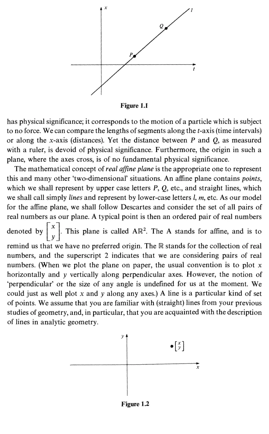
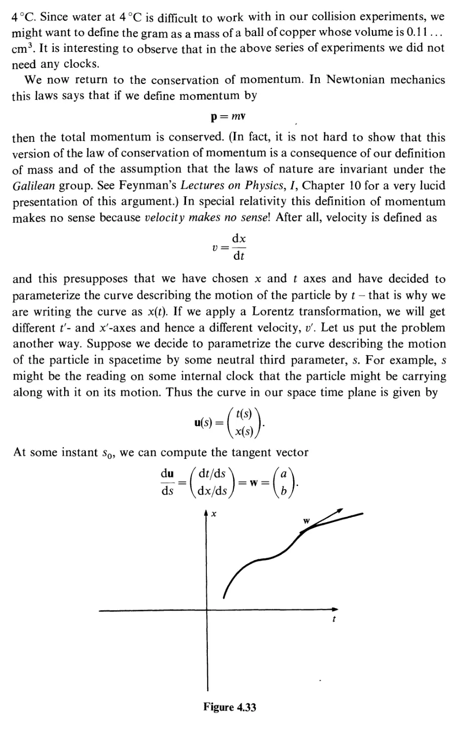
An example of such a plane is the one used to describe graphically the motion
of particles along a line (the x-axis). A point P or Q in this plane represents the
physical concept of event, something which has a time and place. A line I also
Figure 1.1
has physical significance; it corresponds to the motion of a particle which is subject
to no force. We can compare the lengths of segments along the £-axis (time intervals)
or along the x-axis (distances). Yet the distance between P and Q, as measured
with a ruler, is devoid of physical significance. Furthermore, the origin in such a
plane, where the axes cross, is of no fundamental physical significance.
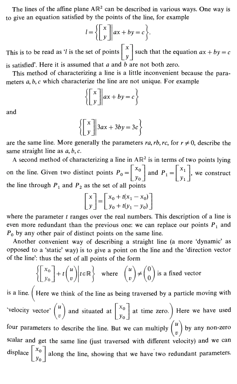
The mathematical concept of real affine plane is the appropriate one to represent
this and many other 'two-dimensional' situations. An affine plane contains points,
which we shall represent by upper case letters P, Q, etc., and straight lines, which
we shall call simply lines and represent by lower-case letters /, m, etc. As our model
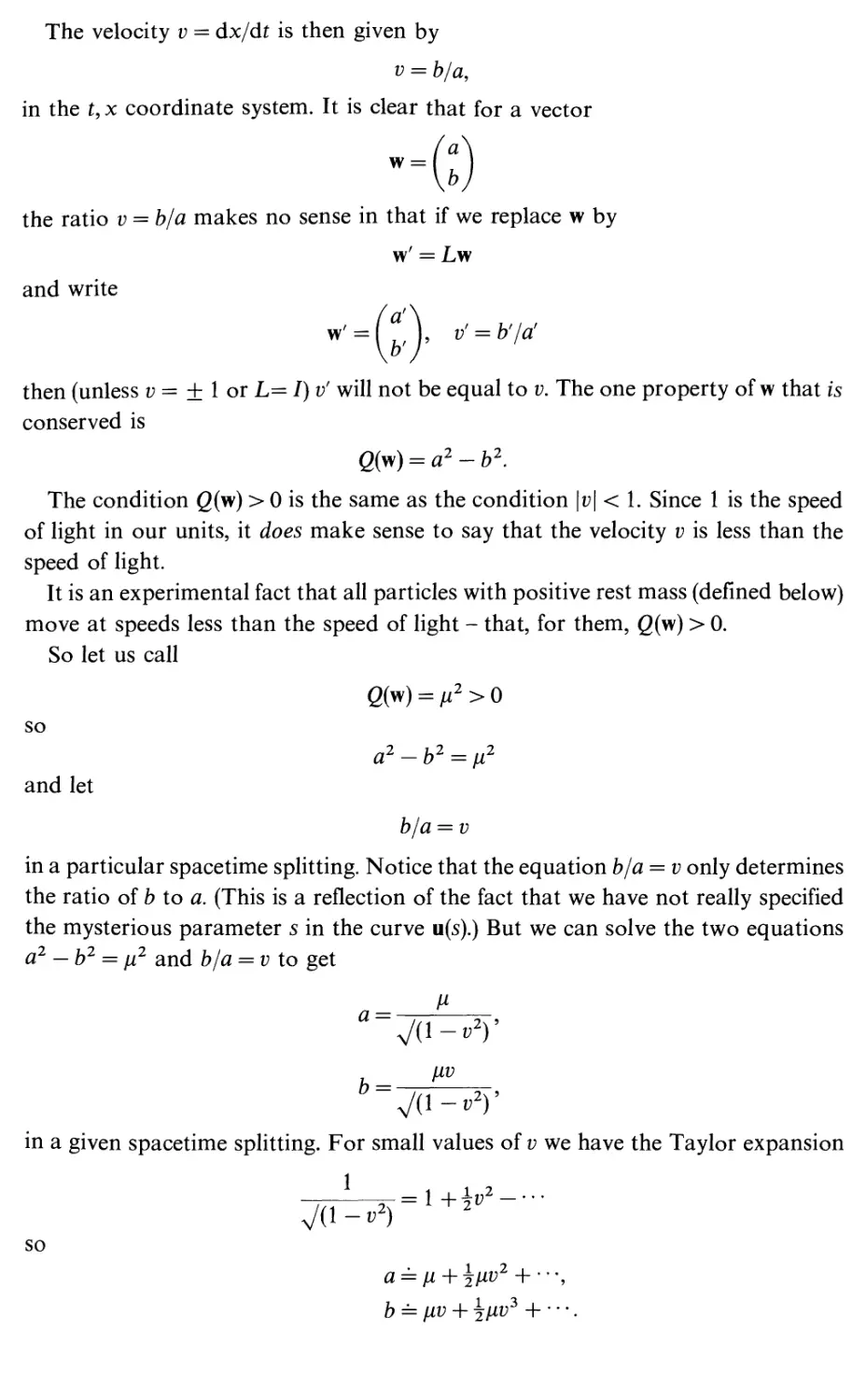
for the affine plane, we shall follow Descartes and consider the set of all pairs of
real numbers as our plane. A typical point is then an ordered pair of real numbers
denoted by
This plane is called AU2. The A stands for affine, and is to
remind us that we have no preferred origin. The U stands for the collection of real
numbers, and the superscript 2 indicates that we are considering pairs of real
numbers. (When we plot the plane on paper, the usual convention is to plot x
horizontally and y vertically along perpendicular axes. However, the notion of
'perpendicular' or the size of any angle is undefined for us at the moment. We
could just as well plot x and y along any axes.) A line is a particular kind of set
of points. We assume that you are familiar with (straight) lines from your previous
studies of geometry, and, in particular, that you are acquainted with the description
of lines in analytic geometry.
>[*}
Figure 1.2
The lines of the affine plane AIR2 can be described in various ways. One way is
to give an equation satisfied by the points of the line, for example
1 =
ax + by = c
This is to be read as 7 is the set of points
such that the equation ax + by = c
is satisfied'. Here it is assumed that a and b are not both zero.
This method of characterizing a line is a little inconvenient because the
parameters a, b, c which characterize the line are not unique. For example
ax + by = c
and
3ax + 3by = 3c
are the same line. More generally the parameters ra, rb, re, for r ^ 0, describe the
same straight line as a, b, c.
A second method of characterizing a line in AIR2 is in terms of two points lying
on the line. Given two distinct points P0 =
.^0.
and P1 =
, we construct
the line through Px and P2 as the set of all points
x Xq ~t tyX-^ Xq)
y] L3>o + '0>i-j>o)_
where the parameter t ranges over the real numbers. This description of a line is
even more redundant than the previous one: we can replace our points Px and
P0 by any other pair of distinct points on the same line.
Another convenient way of describing a straight line (a more 'dynamic' as
opposed to a 'static' way) is to give a point on the line and the 'direction vector
of the line': thus the set of all points of the form
'0N
-½
_^0_
u\
+ t(
w
£e0
where
is a fixed vector
is a line. ( Here we think of the line as being traversed by a particle moving with
'velocity vector' I 1 and situated at
yo.
at time zero. | Here we have used
four parameters to describe the line. But we can multiply ( U ) by any non-zero
scalar and get the same line (just traversed with different velocity) and we can
displace
L>V
along the line, showing that we have two redundant parameters.
Of course, this ties in with our second description if
1> = J>1-J>1.
There is a fourth, familiar description of a line which is not redundant, but has
the awkward feature that it does not describe absolutely all lines in the same way.
If a and b are any real numbers, the set
1 =
y = ax + b
is a straight line which intersects the y-axis at the point
and which has 'slope'
a; i.e., for points on the line, an increase in one unit of x implies an increase in a
units of y. This set is a line, and the description is not redundant, for we have
described a and b in terms of geometric properties of the line. But not all lines
are of this form. We must add the lines which are parallel to the y-axis, and which
have the description
1 =
x = d
From a strictly logical point of view, we should take one of the four descriptions
given above as our definition of a straight line; for example, we should say that,
by definition, a line is a subset, /, of AU2 such that there are three real numbers
a, b, and c with a and b not both zero such that
1 =
ax + by = c
We should then prove that such a subset can be given by either of the other three
descriptions. We shall not go into such logical niceties here, since you have seen,
or can construct, such arguments from elementary analytic geometry.
It is important to remember that an affine plane has no origin and that it makes
no sense to add points of an affine plane. We attach no special significance to the
point
and we resist the temptation to add points like
2
_1_
and
"3
6_
'coordinate by coordinate'. There is, however, a closely related mathematical
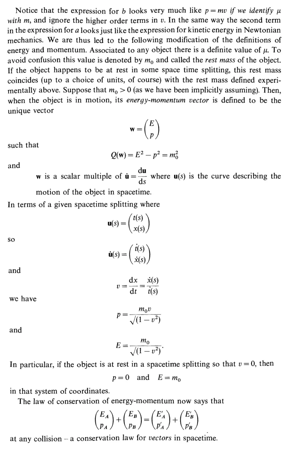
structure, called a two-dimensional vector space, in which an operation of addition
is defined. We construct a vector space from an affine plane by associating with
any pair of points the 'displacement vector' PQ whose 'tail' is at P and whose
'head' is at Q. We denote vectors by lowercase bold letters: v, w, etc. A vector v is
'5
also given as a pair of real numbers, for example v =
( ) for vectors and not [ ] as for points.) The vector v = ( " ) is to be thought
(Notice that we use
5N
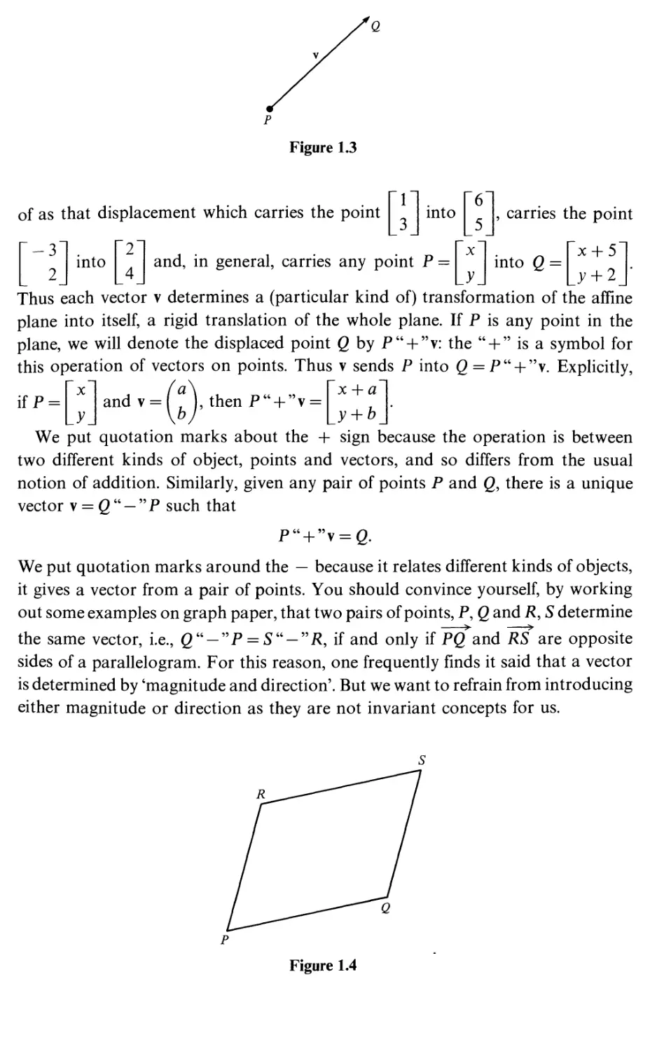
Figure 1.3
of as that displacement which carries the point
into
, carries the point
-3"
2_
into
"2
4
and, in general, carries any point P =
into Q =
"x + 5'
y + 2
Thus each vector v determines a (particular kind of) transformation of the affine
plane into itself, a rigid translation of the whole plane. If P is any point in the
plane, we will denote the displaced point Q by P" + "v: the " + " is a symbol for
this operation of vectors on points. Thus v sends P into Q = P" + "v. Explicitly,
ifP =
and v =
:)
,thenP" + "v =
x + aT\
_y + b_
We put quotation marks about the + sign because the operation is between
two different kinds of object, points and vectors, and so differs from the usual
notion of addition. Similarly, given any pair of points P and Q, there is a unique
vector v = Q " — "P such that
We put quotation marks around the — because it relates different kinds of objects,
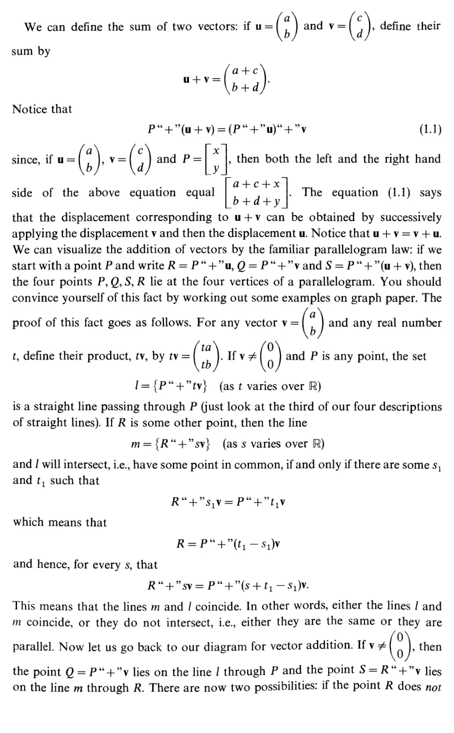
it gives a vector from a pair of points. You should convince yourself, by working
out some examples on graph paper, that two pairs of points, P, Q and R, S determine
the same vector, i.e., Q" — "P = S" — "R9 if and only if PQ and RS are opposite
sides of a parallelogram. For this reason, one frequently finds it said that a vector
is determined by 'magnitude and direction'. But we want to refrain from introducing
either magnitude or direction as they are not invariant concepts for us.
Figure 1.4
We can define the sum of two vectors: if u = ( 1 and v = ( ), define their
sum by
Notice that
since, if u = ( ), v = ( ) and P
a + c
P" + "(u + v) = (P" + "u)" + "v (1.1)
X
y.
side of the above equation equal
, then both the left and the right hand
. The equation (1.1) says
a + c + x
b + d + y_
that the displacement corresponding to u + v can be obtained by successively
applying the displacement v and then the displacement u. Notice that u + v = v + u.
We can visualize the addition of vectors by the familiar parallelogram law: if we
start with a point P and write R = P " + " u, Q = P " + " v and S = P " + " (u + v), then
the four points P, Q, 5, R lie at the four vertices of a parallelogram. You should
convince yourself of this fact by working out some examples on graph paper. The
(a\
proof of this fact goes as follows. For any vector v = I J and any real number
t, define their product, tv, by tv = I I. If v ^ ( I and P is any point, the set
I = {P " + " t\} (as t varies over U)
is a straight line passing through P (just look at the third of our four descriptions
of straight lines). If R is some other point, then the line
m = {R" + "s\} (as s varies over U)
and I will intersect, i.e., have some point in common, if and only if there are some sx
and t1 such that
K" + ''5lv = P" + "t1v
which means that
R = P" + "(t1-s1)v
and hence, for every 5, that
^" + "5V = P" + "(5 + ti-51)v.
This means that the lines m and I coincide. In other words, either the lines I and
m coincide, or they do not intersect, i.e., either they are the same or they are
parallel. Now let us go back to our diagram for vector addition. If v # ( j, then
the point (2 = P" + "v lies on the line I through P and the point S = K" + "V lies
on the line m through R. There are now two possibilities: if the point R does not
Vector spaces and their afflne spaces
1
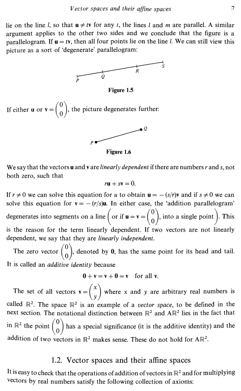
lie on the line /, so that u # t\ for any t, the lines / and m are parallel. A similar
argument applies to the other two sides and we conclude that the figure is a
parallelogram. If u = tv, then all four points lie on the line /. We can still view this
picture as a sort of 'degenerate' parallelogram:
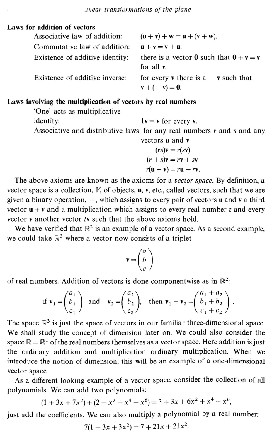
If either u or v = ( ), the picture degenerates further:
Figure 1.6
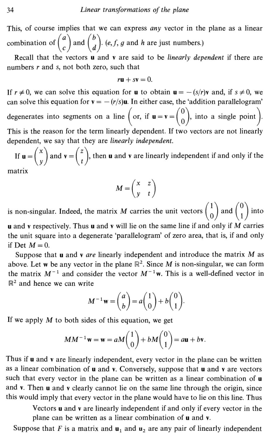
We say that the vectors u and v are linearly dependent if there are numbers r and s, not
both zero, such that
ru + s\ = 0.
If r 7^ 0 we can solve this equation for u to obtain u = — {s/r)\ and if s # 0 we can
solve this equation for v = — (r/s)u. In either case, the 'addition parallelogram'
degenerates into segments on a line ( or if u = v = ( I, into a single point J. This
is the reason for the term linearly dependent. If two vectors are not linearly
dependent, we say that they are linearly independent.
The zero vector I J, denoted by 0, has the same point for its head and tail.
It is called an additive identity because
0 + v = v + 0 = v for all v.
The set of all vectors v = I J where x and y are arbitrary real numbers is
called U2. The space U2 is an example of a vector space, to be defined in the
next section. The notational distinction between U2 and AU2 lies in the fact that
»2 -, • /0
in U the point I J has a special significance (it is the additive identity) and the
addition of two vectors in U2 makes sense. These do not hold for AIR2.
1.2. Vector spaces and their affine spaces
It is easy to check that the operations of addition of vectors in U2 and for multiplying
vectors by real numbers satisfy the following collection of axioms:
jnear transformations of the plane
Laws for addition of vectors
Associative law of addition: (u + v) + w = u + (v + w).
Commutative law of addition: u + v = v + u.
Existence of additive identity: there is a vector 0 such that 0 + v = v
for all v.
Existence of additive inverse: for every v there is a — v such that
v + (-v) = 0.
Laws involving the multiplication of vectors by real numbers
'One' acts as multiplicative
identity: lv = v for every v.
Associative and distributive laws: for any real numbers r and s and any
vectors u and v
(rs)v = r(s\)
(r + s)\ = r\ + s\
r(u + v) = ru + rv.
The above axioms are known as the axioms for a vector space. By definition, a
vector space is a collection, V, of objects, u, v, etc., called vectors, such that we are
given a binary operation, +, which assigns to every pair of vectors u and v a third
vector u + v and a multiplication which assigns to every real number t and every
vector v another vector t\ such that the above axioms hold.
We have verified that U2 is an example of a vector space. As a second example,
we could take U3 where a vector now consists of a triplet
of real numbers. Addition of vectors is done componentwise as in U2:
/a2\ /<*i+<*2\
and v2 =( b2 I thenv1+v2=[ b1 + b2 J.
\c2/ \Ci+C2/
The space U3 is just the space of vectors in our familiar three-dimensional space.
We shall study the concept of dimension later on. We could also consider the
space U = R1 of the real numbers themselves as a vector space. Here addition is just
the ordinary addition and multiplication ordinary multiplication. When we
introduce the notion of dimension, this will be an example of a one-dimensional
vector space.
As a different looking example of a vector space, consider the collection of all
polynomials. We can add two polynomials:
(l+3x + 7x2) + (2-x2 + x4-x6) = 3 + 3x + 6x2 + x4-x6,
just add the coefficients. We can also multiply a polynomial by a real number:
7(1 + 3x + 3x2) = 7 + 21x + 21x2.
Vector spaces and their afflne spaces
9
You should check that the axioms for a vector space are satisfied. We can also
consider the space of polynomials of at most a given degree. For example, the
most general polynomial of degree at most two is of the form
P = ax2 + bx + c.
The sum of two such polynomials
P1=a1x2 + b1x + c1 and P2 = a2x2 + b2x + c2
is
Pl + P2 = (al + alW + (bi + b2)x + c1 + c2.
For example, if
px = 3x2 + 2x + 1, P2 = lx2 - 10* + 2
then
p1+p2 = 10x2-8x + 3.
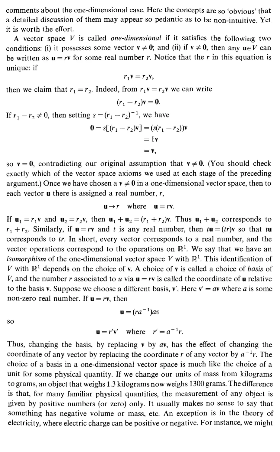
The set of polynomials of degree at most two is also a vector space. Notice that it
looks like' U3 in the sense that the preceding equations look like
GM--M-!)
We will return to this point later.
Suppose that we are given a vector space V\ for example, V could be U1, U2 or
U3. By an affine space associated to V, we mean a set A consisting of points P, <2,
etc., and an operation " + " which assigns to each PeA and each \eV another
point in A which is denoted by P" + "v. This rule is subject to the following axioms:
Associative law: (P" + "u)" + "v = p" + »(u + v) for any PeA
and u,vgK
'Zero' acts as identity: P" + "0 = P for any PeA.
Transitivity: given any two points P and QeA, there is a
veJ/such that P" + "v = g.
Faithfulness: if, for any P, the equality P" + "u = P" + "v
holds, then u = v.
Combining the last two axioms, we can say that, given any two points P and Q,
there is a unique vector v such that P" + "v = Q. It is then sometimes convenient
to write v = Q"-"P.
The notion of a vector space and associated affine space lies at the basis of three
centuries of physical thought, from Newtonian mechanics through special relativity
and quantum mechanics. The purpose of the present chapter is to develop most
of the key ideas in the study of these structures by examining the intuitively simple
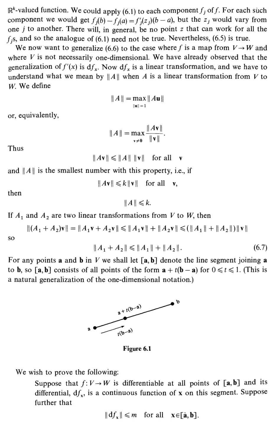
case of the two-dimensional* vector space !R2. Let us begin, however, with some
* We will give a precise definition of the term 'two-dimensional' in §1.12, of'one-dimensional i
a few lines, and of the general concept of the dimension of a vector space in Chapter 10.
comments about the one-dimensional case. Here the concepts are so 'obvious' that
a detailed discussion of them may appear so pedantic as to be non-intuitive. Yet
it is worth the effort.
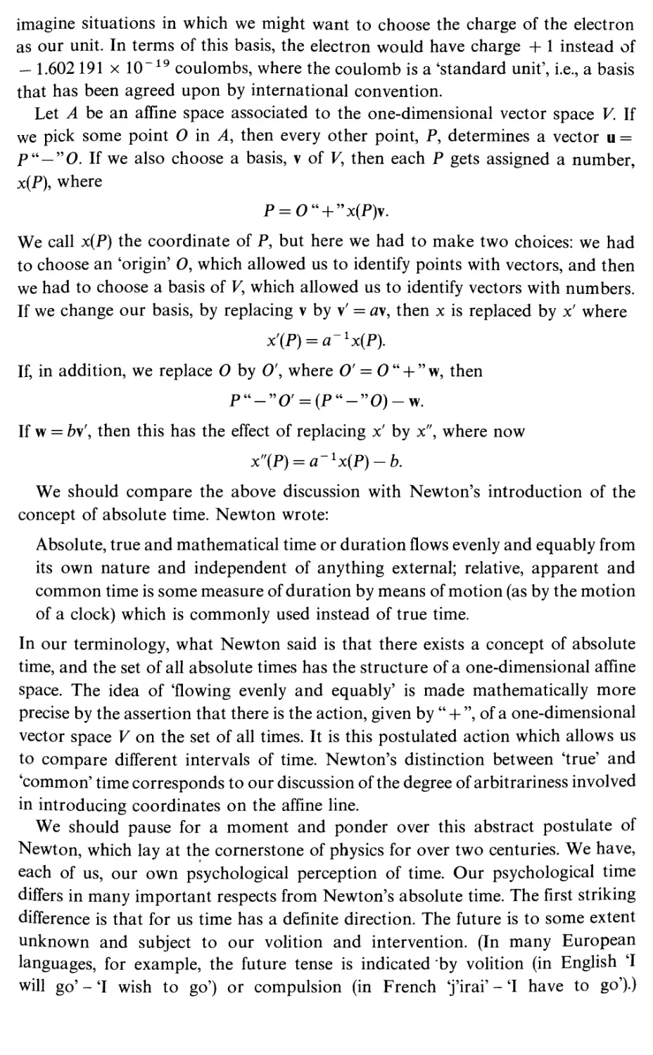
A vector space V is called one-dimensional if it satisfies the following two
conditions: (i) it possesses some vector v ^0; and (ii) if v ^0, then any ueK can
be written as u = rv for some real number r. Notice that the r in this equation is
unique: if
r1v = r2v,
then we claim that rx = r2. Indeed, from rxv = r2v we can write
(ri-r2)v = 0.
If r1 — r2¥z 0, then setting s = (r1— r2)~1, we have
0 = sl(rl - r2)v] = (s(r1 - r2))v
= lv
= v,
so v = 0, contradicting our original assumption that v ^ 0. (You should check
exactly which of the vector space axioms we used at each stage of the preceding
argument.) Once we have chosen a v ^ 0 in a one-dimensional vector space, then to
each vector u there is assigned a real number, r,
u -► r where u = rv.
If ux = rxv and u2 = r2v, then ux + u2 = (r1 + r2)v. Thus ux + u2 corresponds to
ri +r2- Similarly, if u = rv and t is any real number, then tu = (tr)\ so that tu
corresponds to tr. In short, every vector corresponds to a real number, and the
vector operations correspond to the operations on M1. We say that we have an
isomorphism of the one-dimensional vector space V with U1. This identification of
V with U1 depends on the choice of v. A choice of v is called a choice of basis of
V, and the number r associated to u via u = rv is called the coordinate of u relative
to the basis v. Suppose we choose a different basis, v'. Here v' = a\ where a is some
non-zero real number. If u = rv, then
u = (ra~1)av
so
u = /V where r' = a~ V.
Thus, changing the basis, by replacing v by ay, has the effect of changing the
coordinate of any vector by replacing the coordinate r of any vector by a~lr. The
choice of a basis in a one-dimensional vector space is much like the choice of a
unit for some physical quantity. If we change our units of mass from kilograms
to grams, an object that weighs 1.3 kilograms now weighs 1300 grams. The difference
is that, for many familiar physical quantities, the measurement of any object is
given by positive numbers (or zero) only. It usually makes no sense to say that
something has negative volume or mass, etc. An exception is in the theory of
electricity, where electric charge can be positive or negative. For instance, we might
imagine situations in which we might want to choose the charge of the electron
as our unit. In terms of this basis, the electron would have charge + 1 instead of
— 1.602 191 x 10"19 coulombs, where the coulomb is a 'standard unit', i.e., a basis
that has been agreed upon by international convention.
Let A be an affine space associated to the one-dimensional vector space V. If
we pick some point O in A, then every other point, P, determines a vector u =
p" — "0. If we also choose a basis, v of V, then each P gets assigned a number,
x(P), where
P = 0" + "x(P)v.
We call x(P) the coordinate of P, but here we had to make two choices: we had
to choose an 'origin' O, which allowed us to identify points with vectors, and then
we had to choose a basis of V, which allowed us to identify vectors with numbers.
If we change our basis, by replacing v by v' = ay, then x is replaced by x' where
xf(P) = a-1x(P).
If, in addition, we replace O by 0', where O' = 0 " + " w, then
P"-"0, = (P"-"0)-w.
If w = b\\ then this has the effect of replacing x' by x", where now
x,,(P) = a-1x{P)-b.
We should compare the above discussion with Newton's introduction of the
concept of absolute time. Newton wrote:
Absolute, true and mathematical time or duration flows evenly and equably from
its own nature and independent of anything external; relative, apparent and
common time is some measure of duration by means of motion (as by the motion
of a clock) which is commonly used instead of true time.
In our terminology, what Newton said is that there exists a concept of absolute
time, and the set of all absolute times has the structure of a one-dimensional affine
space. The idea of 'flowing evenly and equably' is made mathematically more
precise by the assertion that there is the action, given by " + ", of a one-dimensional
vector space V on the set of all times. It is this postulated action which allows us
to compare different intervals of time. Newton's distinction between 'true' and
'common' time corresponds to our discussion of the degree of arbitrariness involved
in introducing coordinates on the affine line.
We should pause for a moment and ponder over this abstract postulate of
Newton, which lay at the cornerstone of physics for over two centuries. We have,
each of us, our own psychological perception of time. Our psychological time
differs in many important respects from Newton's absolute time. The first striking
difference is that for us time has a definite direction. The future is to some extent
unknown and subject to our volition and intervention. (In many European
languages, for example, the future tense is indicated by volition (in English 'I
will go' - 'I wish to go') or compulsion (in French 'j'irai' - 'I have to go').)
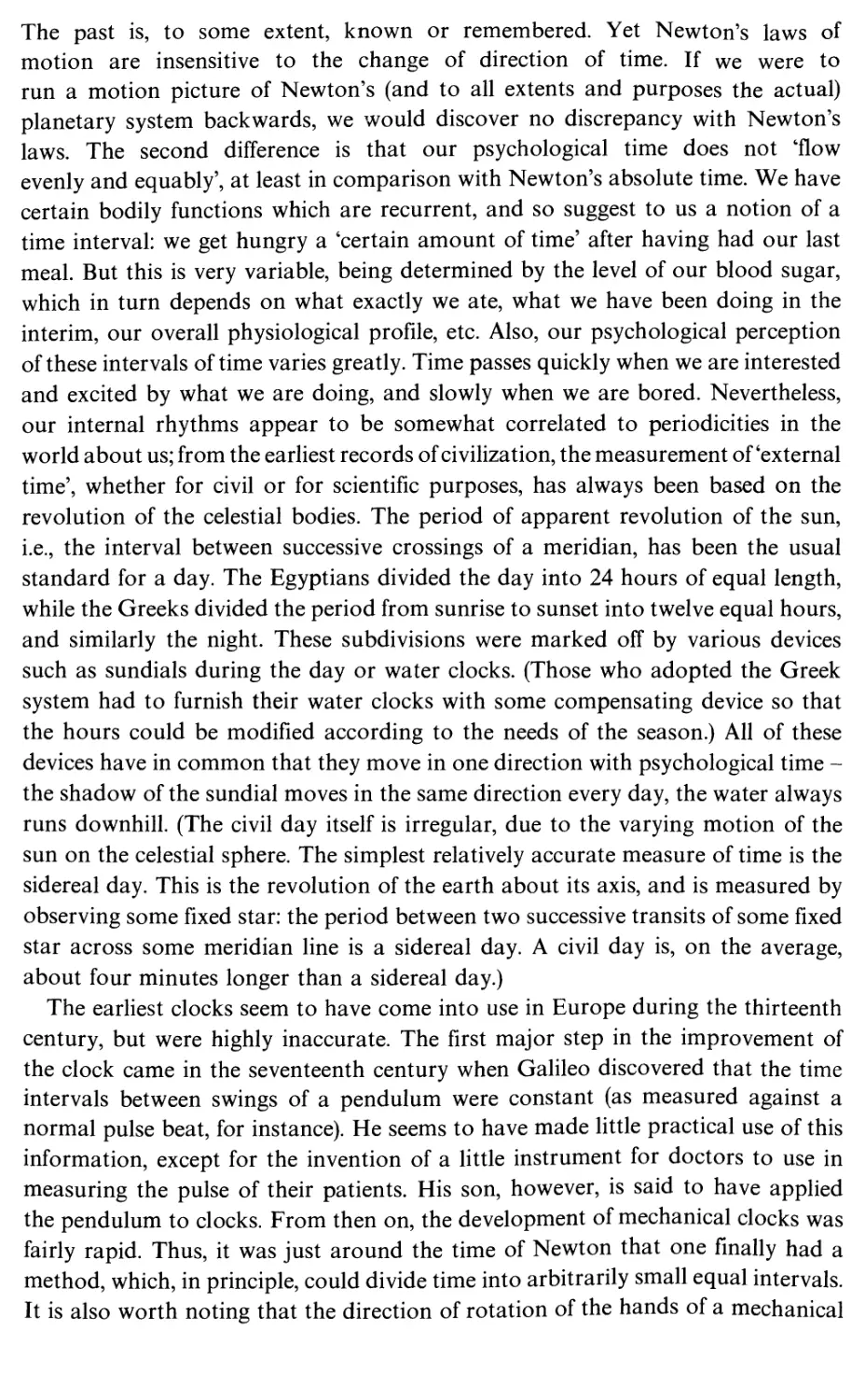
The past is, to some extent, known or remembered. Yet Newton's laws of
motion are insensitive to the change of direction of time. If we were to
run a motion picture of Newton's (and to all extents and purposes the actual)
planetary system backwards, we would discover no discrepancy with Newton's
laws. The second difference is that our psychological time does not 'flow
evenly and equably', at least in comparison with Newton's absolute time. We have
certain bodily functions which are recurrent, and so suggest to us a notion of a
time interval: we get hungry a 'certain amount of time' after having had our last
meal. But this is very variable, being determined by the level of our blood sugar,
which in turn depends on what exactly we ate, what we have been doing in the
interim, our overall physiological profile, etc. Also, our psychological perception
of these intervals of time varies greatly. Time passes quickly when we are interested
and excited by what we are doing, and slowly when we are bored. Nevertheless,
our internal rhythms appear to be somewhat correlated to periodicities in the
world about us; from the earliest records of civilization, the measurement of'external
time', whether for civil or for scientific purposes, has always been based on the
revolution of the celestial bodies. The period of apparent revolution of the sun,
i.e., the interval between successive crossings of a meridian, has been the usual
standard for a day. The Egyptians divided the day into 24 hours of equal length,
while the Greeks divided the period from sunrise to sunset into twelve equal hours,
and similarly the night. These subdivisions were marked off by various devices
such as sundials during the day or water clocks. (Those who adopted the Greek
system had to furnish their water clocks with some compensating device so that
the hours could be modified according to the needs of the season.) All of these
devices have in common that they move in one direction with psychological time -
the shadow of the sundial moves in the same direction every day, the water always
runs downhill. (The civil day itself is irregular, due to the varying motion of the
sun on the celestial sphere. The simplest relatively accurate measure of time is the
sidereal day. This is the revolution of the earth about its axis, and is measured by
observing some fixed star: the period between two successive transits of some fixed
star across some meridian line is a sidereal day. A civil day is, on the average,
about four minutes longer than a sidereal day.)
The earliest clocks seem to have come into use in Europe during the thirteenth
century, but were highly inaccurate. The first major step in the improvement of
the clock came in the seventeenth century when Galileo discovered that the time
intervals between swings of a pendulum were constant (as measured against a
normal pulse beat, for instance). He seems to have made little practical use of this
information, except for the invention of a little instrument for doctors to use in
measuring the pulse of their patients. His son, however, is said to have applied
the pendulum to clocks. From then on, the development of mechanical clocks was
fairly rapid. Thus, it was just around the time of Newton that one finally had a
method, which, in principle, could divide time into arbitrarily small equal intervals.
It is also worth noting that the direction of rotation of the hands of a mechanical
Functions and affine functions
13
clock is entirely conventional. It is also easily reversible. By a simple change of
the gearing, we can make the hands rotate counterclockwise instead of clockwise.
It is interesting to speculate how much the development of mechanical clocks had
to do with Newton's conception of time.
1.3. Functions and affine functions
In the next few sections we will study those transformations of AIR2 into itself
which carry straight lines into straight lines. We must begin with some general
discussion of the notion of 'transformation' or 'function'.
Let W and X be sets. A rule f: W^X which assigns one element f(w) of X to
each weW is called a function (or map, or mapping, or operator) from W to X. The
set W is called the domain of f If A is a subset of W9 we let f(A) denote the subset
of X consisting of the element f(w) where we A:
f(A)={f(w)\weA}.
The set f(W) is called the image of f: in general, it is a subset of X.
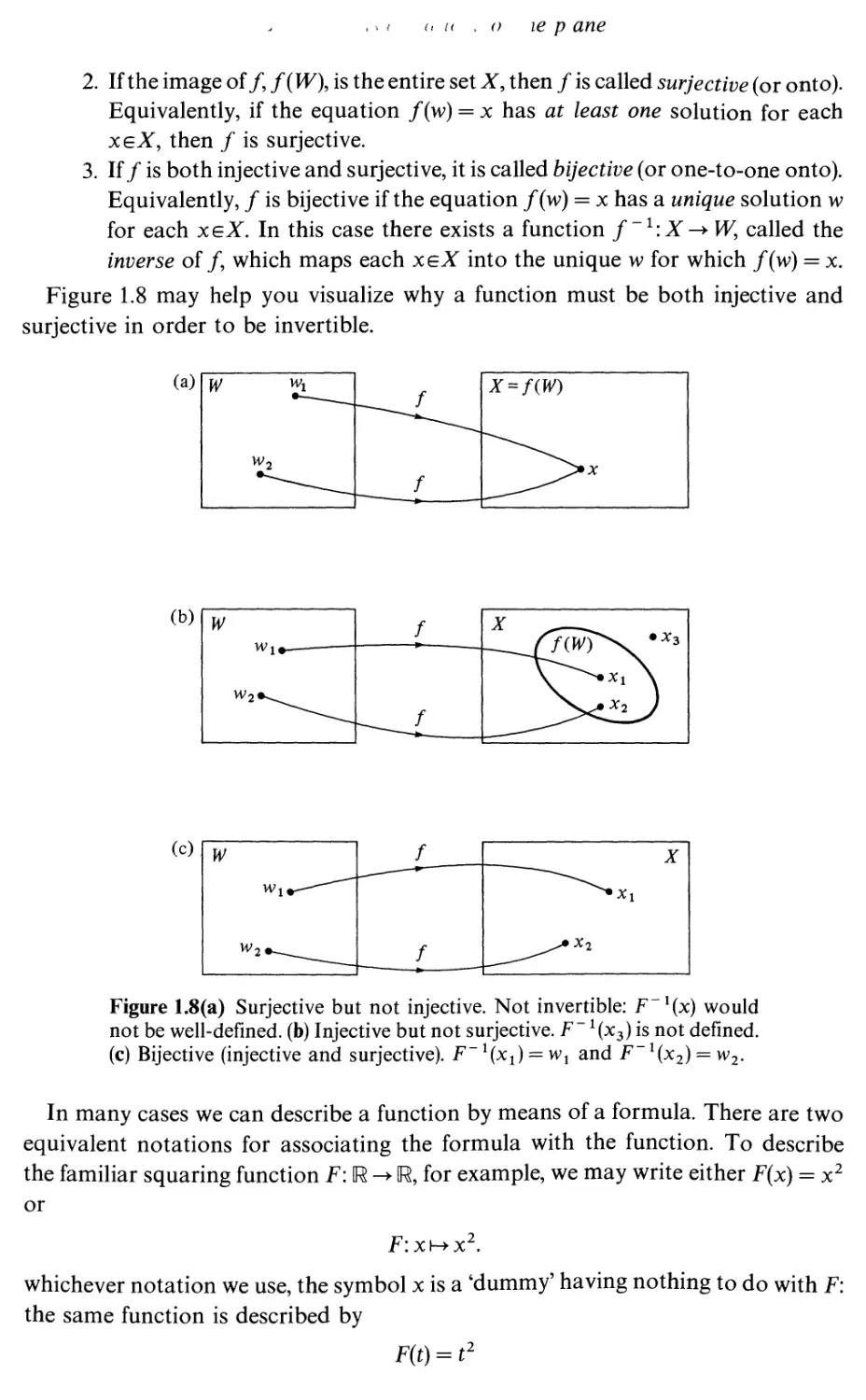
For example, suppose f is the map of U2 into itself given by /(P) = P" + "v
where v is a fixed vector. Then f(A) is obtained from A by 'translating A through
v\ If A = I = {P + tu} is a line, then f{l) = {P + v + tu} is another line. Thus the
image of a line under a translation is another line.
/(0
Figure 1.7
This notion of function is very general and powerful. The only restriction, really,
is that the 'output' of the function must be well-defined. It is not acceptable, for
example, to have a function f: U -> U with the property that /(1) = 2 and /(1) = 3.
There would be nothing wrong, however, with a function f:U^U2 for which
Certain standard terminology concerning the domain and range of / is worth
learning.
1. If two distinct elements wl9 w2eW are always mapped into distinct points
*i, x2el, then / is called infective (or one-to-one). Equivalently, / is
injective if /(wx) =/(w2) implies wx = w2.
(i (< ,0 le p arte
2. If the image of/, f{W\ is the entire set X, then f is called surjective (or onto).
Equivalently, if the equation f(w) = x has at least one solution for each
xeX, then f is surjective.
3. If/ is both injective and surjective, it is called bijective (or one-to-one onto).
Equivalently, / is bijective if the equation /(w) = x has a unique solution w
for each xeX. In this case there exists a function f~lm.X^> W, called the
inverse of/, which maps each xgX into the unique w for which /(w) = x.
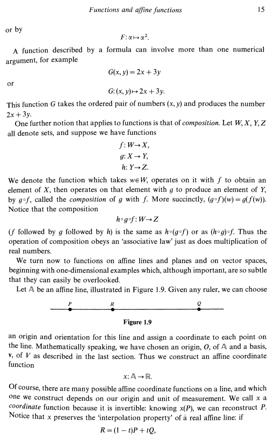
Figure 1.8 may help you visualize why a function must be both injective and
surjective in order to be invertible.
(b)
w
w2»^^
f
■ *—.
X
^^^2
•*3
Figure 1.8(a) Surjective but not injective. Not invertible: F~l(x) would
not be well-defined, (b) Injective but not surjective. F~ 1(x3) is not defined,
(c) Bijective (injective and surjective). F~1(x1) = w} and F~1(x2) = w2.
In many cases we can describe a function by means of a formula. There are two
equivalent notations for associating the formula with the function. To describe
the familiar squaring function F: U -> IR, for example, we may write either F(x) = x2
or
F:xkx2.
whichever notation we use, the symbol x is a 'dummy' having nothing to do with F:
the same function is described by
F(t) = t2
Functions and affine functions
15
or by
F:gc\->oc2.
A function described by a formula can involve more than one numerical
argument, for example
G(x, y) = 2x + 3y
or
G:(x,y)\-+2x + 3y.
This function G takes the ordered pair of numbers (x, y) and produces the number
2x + 3y.
One further notion that applies to functions is that of composition. Let W9 X, Y, Z
all denote sets, and suppose we have functions
f:W^X9
g:X^Y9
h:Y-+Z.
We denote the function which takes weW, operates on it with f to obtain an
element of X, then operates on that element with g to produce an element of Y,
by g°f9 called the composition of g with f. More succinctly, {g°f)(w) = g(f(w)).
Notice that the composition
h°g°f: W^>Z
(f followed by g followed by h) is the same as h°(g°f) or as {h°g)°f. Thus the
operation of composition obeys an 'associative law' just as does multiplication of
real numbers.
We turn now to functions on affine lines and planes and on vector spaces,
beginning with one-dimensional examples which, although important, are so subtle
that they can easily be overlooked.
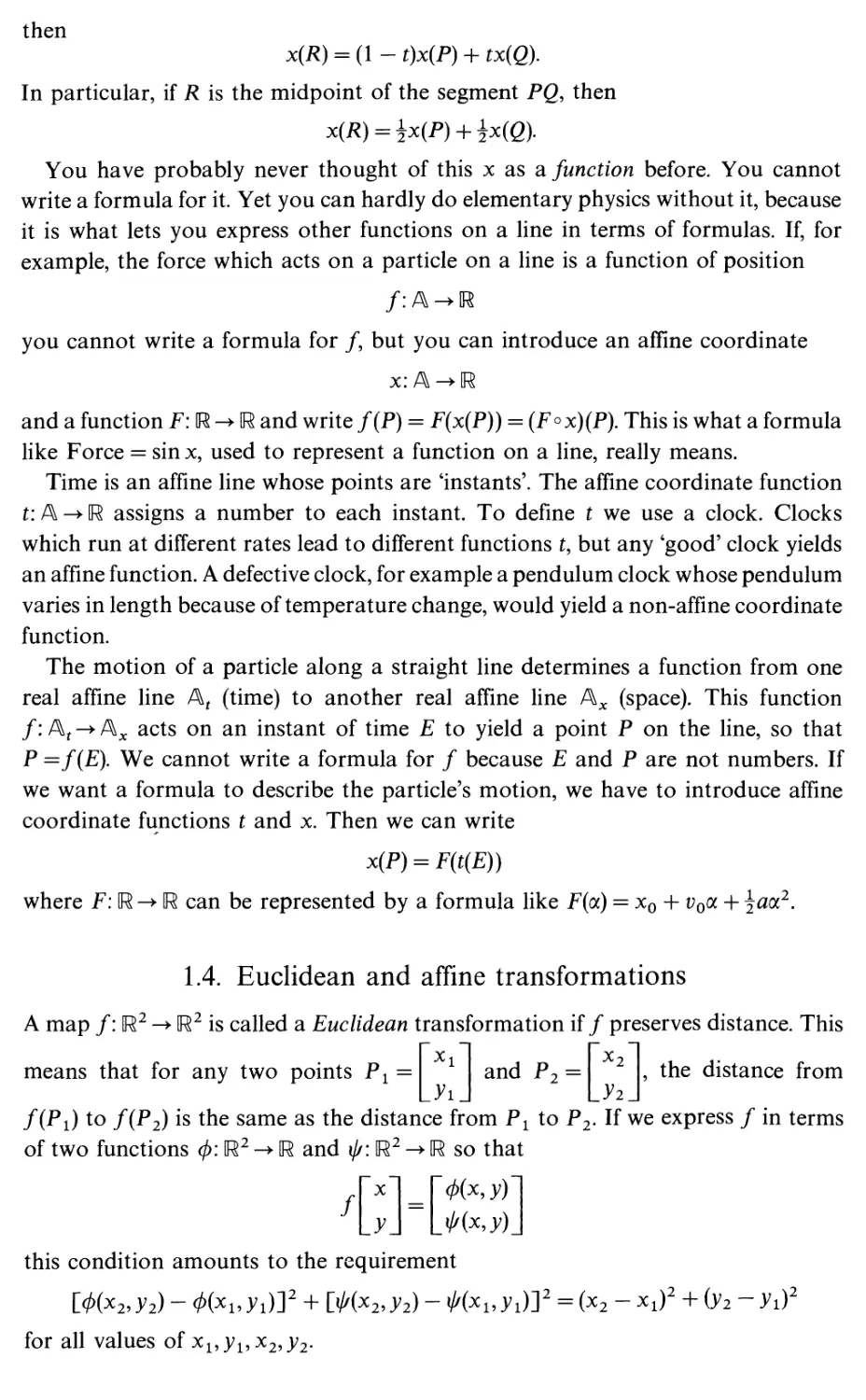
Let A be an affine line, illustrated in Figure 1.9. Given any ruler, we can choose
PR Q
• • •
Figure 1.9
an origin and orientation for this line and assign a coordinate to each point on
the line. Mathematically speaking, we have chosen an origin, O, of A and a basis,
v, of V as described in the last section. Thus we construct an affine coordinate
function
x:A->R.
Of course, there are many possible affine coordinate functions on a line, and which
one we construct depends on our origin and unit of measurement. We call x a
coordinate function because it is invertible: knowing x(P), we can reconstruct P.
Notice that x preserves the 'interpolation property' of a real affine line: if
R = (l-f)P + tQ,
then
x(R) = (1- t)x(P) + tx(Q).
In particular, if R is the midpoint of the segment Pg, then
x(R) = ±x(P) + ±x(Q).
You have probably never thought of this x as a function before. You cannot
write a formula for it. Yet you can hardly do elementary physics without it, because
it is what lets you express other functions on a line in terms of formulas. If, for
example, the force which acts on a particle on a line is a function of position
/:A->R
you cannot write a formula for /, but you can introduce an affine coordinate
x:A->IR
and a function F: U -► U and write /(P) = F(x(P)) = (P°x)(P). This is what a formula
like Force = sin x, used to represent a function on a line, really means.
Time is an affine line whose points are 'instants'. The affine coordinate function
t: A -► U assigns a number to each instant. To define t we use a clock. Clocks
which run at different rates lead to different functions t, but any 'good' clock yields
an affine function. A defective clock, for example a pendulum clock whose pendulum
varies in length because of temperature change, would yield a non-affine coordinate
function.
The motion of a particle along a straight line determines a function from one
real affine line A, (time) to another real affine line Ax (space). This function
/: A, -► Ax acts on an instant of time E to yield a point P on the line, so that
P =f(E). We cannot write a formula for / because E and P are not numbers. If
we want a formula to describe the particle's motion, we have to introduce affine
coordinate functions t and x. Then we can write
x(P) = F(t(E))
where F: U -► U can be represented by a formula like F{oc) = x0 + v0oc + jaoc2.
1.4. Euclidean and affine transformations
A map /: U2 -► [R2 is called a Euclidean transformation if / preserves distance. This
means that for any two points Px =
and P? =
x2
, the distance from
xl
/(Pi) to /(P2) is the same as the distance from Px to P2. If we express / in terms
of two functions ¢: U2^U and ^: U2->IR so that
,p~] = [">(x,y)~
this condition amounts to the requirement
[</>(x2, y2) - </>(*i> ^i)]2 +1>(*2> j>2) - <A(*i> yi)]2 = (*2 - ^1)2 + 0^2 - yi)2
for all values of xl9yl9x29y2-
Euclidean geometry can be thought of as the study of those properties of subsets
of the plane which are invariant under the application of any Euclidean
transformation. For instance, if A is a circle and / is a Euclidean transformation, then
f(A) is again a circle. If / is a straight line, then /(/) is again a straight line. It is
clear from the definition that, if/ and g are Euclidean transformations, then g°f
is again Euclidean.
A map /: U2 -► U2 is called an affine transformation if it carries straight lines
into straight lines. Thus /(/) must be a straight line for any straight line /. For
example, suppose / is the transformation defined by
2x + y +
y — x + 5
The most general straight line in the plane is given by an equation of the form
ax + by + c = 0.
That is,
' I ax + by + c = 0 !
f
.']■
i=
So
/(0 = 1
w
z
w = 2x + y+l,z = y — x + 5 and <2x + fry + c =
But we can solve the equations
w = 2x + y + 1
z = y — x + 5
for x and y in terms of w and z.
The solution is
x = i(w-l)-i(z-5),
y = i(w-i) + f(z-5)
so the condition
<2x + by + c = 0
can be written as
«[i(w-l)-i(z-5)] + &[i(w-l) + f(z-5)]+ c = 0
or as
i(fl + b)w + (f ft - ^)z + c + f a - ^b = 0.
In other words
= 0
where
and
f(A) =
ew + gz + h = 0
3«.
fc = c + fa—V-fe.
This is again a straight line.
Notice that f is not a Euclidean transformation. Affine geometry consists of the
study of those properties of subsets of the plane which are invariant under all
one-to-one affine transformations. Thus, if A is a circle, f(A) need not be a circle
(but will be an ellipse as we shall see later on).
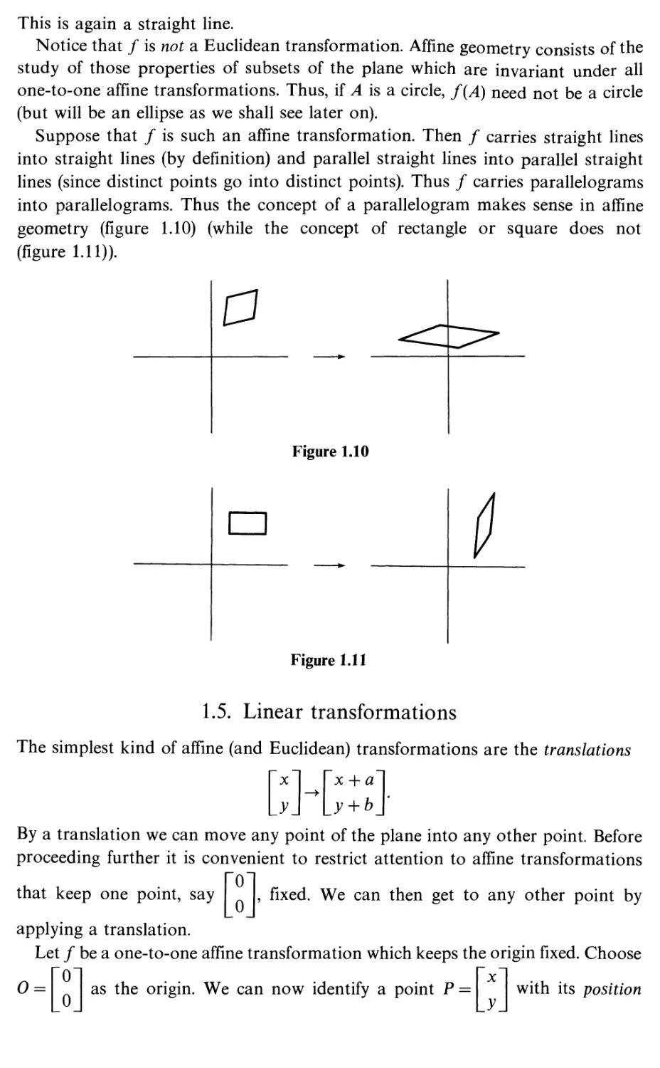
Suppose that f is such an affine transformation. Then f carries straight lines
into straight lines (by definition) and parallel straight lines into parallel straight
lines (since distinct points go into distinct points). Thus f carries parallelograms
into parallelograms. Thus the concept of a parallelogram makes sense in affine
geometry (figure 1.10) (while the concept of rectangle or square does not
(figure 1.11)).
a
Figure 1.10
n
Figure 1.11
1.5. Linear transformations
The simplest kind of affine (and Euclidean) transformations are the translations
x + a
y + b
By a translation we can move any point of the plane into any other point. Before
proceeding further it is convenient to restrict attention to affine transformations
, fixed. We can then get to any other point by
that keep one point, say
applying a translation.
Let f be a one-to-one affine transformation which keeps the origin fixed. Choose
0 =
as the origin. We can now identify a point P =
with its position
f(Q)
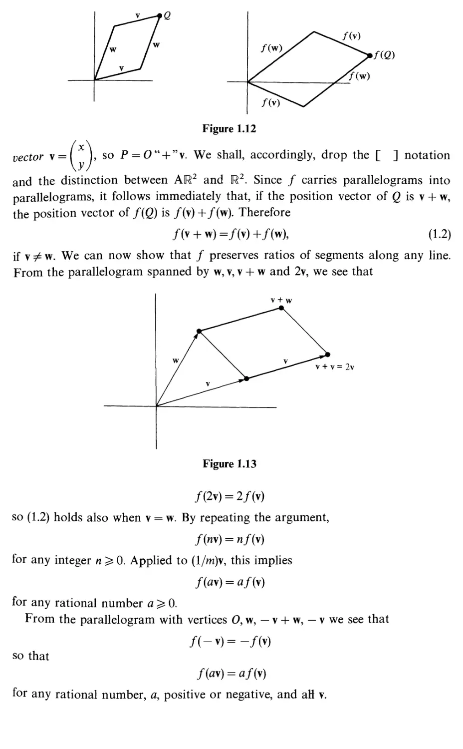
Figure 1.12
vector v = l ), so P = 0" + "v. We shall, accordingly, drop the [ ] notation
and the distinction between AIR2 and U2. Since f carries parallelograms into
parallelograms, it follows immediately that, if the position vector of Q is v + w,
the position vector of f{Q) is /(v) +/(w). Therefore
/(v + w)=/(v)+/(w), (1.2)
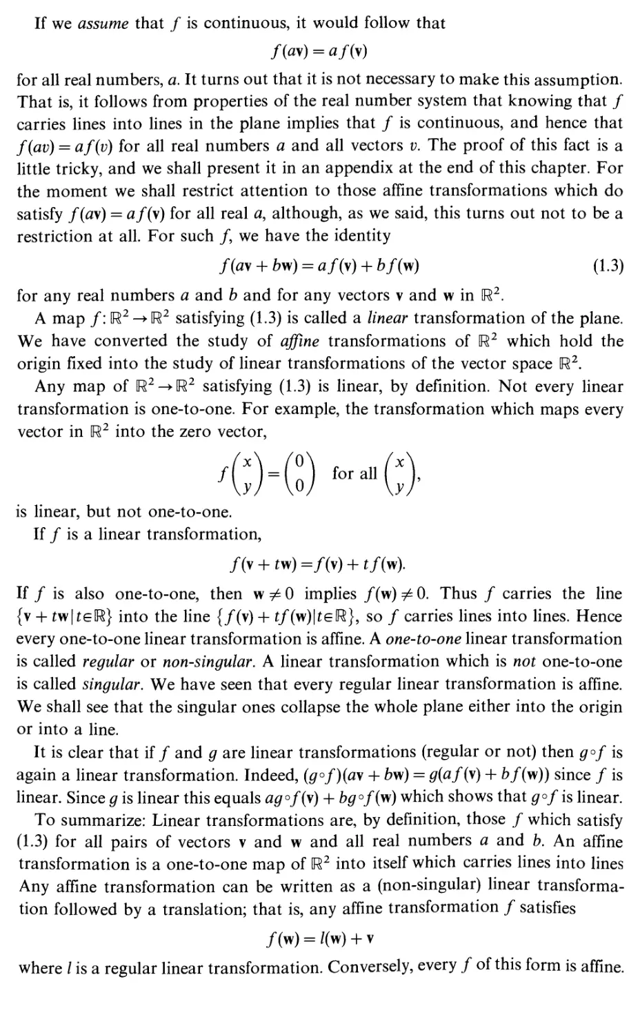
if y 7^ w. We can now show that f preserves ratios of segments along any line.
From the parallelogram spanned by w, v, v + w and 2v, we see that
v + w
v + v = 2v
Figure 1.13
/(2v) = 2/(t)
so (1.2) holds also when v = w. By repeating the argument,
f{n\) = n/(v)
for any integer n ^ 0. Applied to (l/m)v, this implies
f(av) = af(v)
for any rational number a ^ 0.
From the parallelogram with vertices O, w, — v + w, — v we see that
f(-y)=-m
so that
f(ay) = af(v)
for any rational number, a, positive or negative, and aH v.
If we assume that f is continuous, it would follow that
f(av) = af(v)
for all real numbers, a. It turns out that it is not necessary to make this assumption.
That is, it follows from properties of the real number system that knowing that f
carries lines into lines in the plane implies that f is continuous, and hence that
f(av) = af(v) for all real numbers a and all vectors v. The proof of this fact is a
little tricky, and we shall present it in an appendix at the end of this chapter. For
the moment we shall restrict attention to those affine transformations which do
satisfy f(a\) = af(\) for all real a, although, as we said, this turns out not to be a
restriction at all. For such f we have the identity
/(flv + fcw) = fl/(v) + fc/(w) (1.3)
for any real numbers a and b and for any vectors v and w in U2.
A map f: U2 -► U2 satisfying (1.3) is called a linear transformation of the plane.
We have converted the study of affine transformations of U2 which hold the
origin fixed into the study of linear transformations of the vector space U2.
Any map of [R2->[R2 satisfying (1.3) is linear, by definition. Not every linear
transformation is one-to-one. For example, the transformation which maps every
vector in U2 into the zero vector,
'(K) -»(;)•
is linear, but not one-to-one.
If f is a linear transformation,
/(v + tw) =/(v) + t/(w).
If f is also one-to-one, then w ^ 0 implies /(w) ^ 0. Thus f carries the line
{v + tw|teK} into the line {/(v) + tf(w)\teU}, so f carries lines into lines. Hence
every one-to-one linear transformation is affine. A one-to-one linear transformation
is called regular or non-singular. A linear transformation which is not one-to-one
is called singular. We have seen that every regular linear transformation is affine.
We shall see that the singular ones collapse the whole plane either into the origin
or into a line.
It is clear that if/ and g are linear transformations (regular or not) then gof is
again a linear transformation. Indeed, (g°f){a\ + bw) = g{af(v) + b/(w)) since / is
linear. Since g is linear this equals ag°f(\) + bg°f{y?) which shows that gof is linear.
To summarize: Linear transformations are, by definition, those / which satisfy
(1.3) for all pairs of vectors v and w and all real numbers a and b. An affine
transformation is a one-to-one map of U2 into itself which carries lines into lines
Any affine transformation can be written as a (non-singular) linear
transformation followed by a translation; that is, any affine transformation / satisfies
/(w) = Z(w) + v
where I is a regular linear transformation. Conversely, every / of this form is affine.
1.6. The matrix of a linear transformation
Let f be a linear transformation. We can write any ( ) in the plane as
so that
This formula shows how f is completely determined by what it does to the two
basis vectors ( j and ( j. Suppose that /( J = I j and /f j = I
Then / is completely determined by the four numbers a, b, c, and d,
Jx\/ax + by\
\yj \cx + dy)'
We write these four numbers as a square matrix
Ma„/, = (: \
where the first column is the image of ( j and the second column is the image
of ( J The image of any point ( J is then given by
a b\(x\ (ax + by\
c d){yr{cx + dy) (L4)
We regard (1.4) as a multiplication rule, telling us how to multiply the vector (
by the matrix ( 1, to give another vector. It says to take the row x column for
\c dj
each of the two components. Thus the top component is ax + by which is obtained
from the top row (a,b) of the matrix and the column { J. Similarly for the
bottom component.
For example, suppose that R9 is counterclockwise rotation of the plane through
angle 6. Then
and
'0\ /-sin0
RexlJ \ COS0
(J)
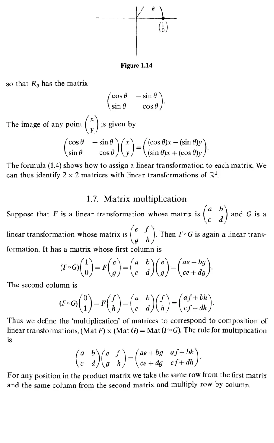
so that Re has the matrix
The image of any point 1 is given by
Figure 1.14
cost/
sin#
— sin#
COS0
cos 0 — sin 0 \ ( x \ ((cos 0)x — (sin 6)yN
sin 0 cos 0J\yJ \ (sin 0)x + (cos 9)y ,
The formula (1.4) shows how to assign a linear transformation to each matrix. We
can thus identify 2x2 matrices with linear transformations of U2.
1.7. Matrix multiplication
Suppose that F is a linear transformation whose matrix is ( J and G is a
formation. It has a matrix whose first column is
(F°G)
The second column is
(F°G)
= F
ae + bg
ce + dg
= F
f
af+bh
cf+dh
a
\J ~\h) = [c
Thus we define the 'multiplication' of matrices to correspond to composition of
linear transformations, (Mat F) x (Mat G) = Mat (F° G). The rule for multiplication
is
'e f\_(ae + bg af+bh"
Kg h)~\ce + dg cf+dh,
For any position in the product matrix we take the same row from the first matrix
and the same column from the second matrix and multiply row by column.
a b
c d
For example, if Rd is (counterclockwise) rotation through angle 9 and R^ is
rotation through angle ¢, then RdR(f) = R9+(j) and
'cos 9 — sin#\ /cos(/> — sin0
Ksin9 cos 9 J \sin0 cos(f)/
r cos 9 cos 0 — sin 9 sin 0 — cos 6 sin 0 — sin 9 cos 0N
vsin 0 cos </> + cos 9 sin 0 cos 9 cos 0 — sin 9 sin 0y
Comparing this with the matrix of Re+(j)
'cos (0 + 4) -sin (0 + 0)'
vsin (# + (/>) cos(9 + (p)/
gives the standard trigonometric formulae for cos (9 + (j>) and sin (9 + ¢). Thus you
need no longer remember the identities for the sine and cosine of the sum of
two angles. You can derive them from the more general rule of matrix multiplication.
Notice that matrix multiplication, in general, is not commutative: for example,
1 2V4 °\-(4 1qN
,0 3;V0 5J~\0 15,
while
'4 0\/l 2\_(4 8
(Two rotations of U2 do commute with one another since it does not matter through
which angle we rotate first. But, in general, two matrices need not commute.)
As an illustration of matrix multiplication, we prove a 'triple product
decomposition' which will be used later on. This decomposition states that any matrix
a b\
with a # 0 can be written as a triple product of the form
c d
a b\ (\ 0\/r 0\/l x
(1-5)
c dj \y lj\0 sj\0 1/ v ;
To prove this result we simply devise a procedure for determining y, r, s, and x.
We first multiply the matrices on the right. Since
r 0\/l x\_(r rx
0 s)\0 1/~V0 s
we want
'a fc\ _/l 0\/r rx\_fr rx
^c d) \y l/\0 sj \ry ryx + s
Now we can equate corresponding entries in the left-hand and right-hand matrices.
First, a = r, and since by assumption a ^ 0, r ^ 0. Next, b = rx and so x = b/r — b/a
(remember that a # 0). Similarly, c = ry and so y = c/r = c/a. Finally, d = rxy + s
and so
s = d — rxy = d — r(b/r)(c/r) = d^ (be)/a.
A similar decomposition, important in the analysis of lens systems, is
'a b\Jl A/0 A/1 ^
Kc d) \0 l)\e 0j\0 1,
valid for any matrix with c ^ 0. The proof of this decomposition is simple: again,
just multiply out the triple product and equate corresponding matrix entries on
both sides of the equation.
1.8. Matrix algebra
Let F and G be two linear transformations of U2. We define their sum by
(j7 + G)(v) = F(v) + G(v).
Notice that
(F + G)(a\ + few) = F(a\ + 6w) + G(a\ + bw)
= aF(\) + W(w) + aG(\) + 6G(w)
= a(F(v) + G(v)) + &(F(w) + G(w))
= <i(F + G)(v) + &(F + G)(w).
Thus i7 + G is again a linear transformation. It is clear that this addition is
associative and commutative, that the zero transformation, 0(v) = 0, for all v, is
the zero for this addition and that ( — F)(\) = — F(\) defines the negative of F, i.e.,
(— F) + F = 0, where 0 in this equation stands for the zero linear transformation.
If H is a third linear transformation, then composition, represented by matrix
multiplication, has the following property:
Ho(F + G)(v) = H[(F+G)(v)]
= H[F(v) + G(vn
= H[F(vn+H[G(vn
= (HoF)(v) + (HoG)(v)
for all v, or, in short,
Ho(F + G) = HoF + HoG,
and, similarly,
{F + G)°H = F°H + GoH.
Thus multiplication is distributive relative to this addition.
It follows directly from the definition of the sum of linear transformations that if
the matrices of F and G are
Mat(f)=(c bd)and C 0=Mat(G)
then the matrix of F + G is
M<it(F + G) = (a + e \ +{) = Mat(f) + Mat(G).
\c + g d+hj
In other words, we add matrices by adding the entries at each position. We can
i J* b\ (2a 2b\ _ . ,
also multiply a matrix by a number: 21 I = I I. Notice that
2(a b\-(2a 2b\-(2 °\(a b
\c d)~\2c 2d)~\0 2J\c d
We have now defined addition and multiplication for 2 x 2 matrices, and the
rules for addition and multiplication satisfy most of the familiar rules for adding
and multiplying numbers. Thus:
Addition is commutative and associative with the existence of a zero and a
negative;
Multiplication is associative with the existence of an identity, ( J, and
is distributive over addition.
There are, however, two important differences:
(1) multiplication is not commutative;
(2) the product of two non-zero matrices can be zero, so the cancellation law
for multiplication need not hold:
'0 l\ /0 l\_/0 0N
,0 (y\o o/~\o oy
Nevertheless, we shall see that in many respects we can deal with linear
transformations as if they were numbers.
Instead of linear transformations of the vector space U2, we could consider linear
fx\
transformations of the vector space U3. The vectors of U3 are described as I y land
there are now three basis vectors, 1 0 J, I 1 J and I 0 J. The most general linear
V V w
transformation of U3 is now described by a 3 x 3 matrix of the form
*31 u32 "33/
where the first column is the image of the first basis vector I 0 I, etc. The formula for
V
multiplication is
a3
where, for any i andj ranging over 1,2,3,
Cij = aabu + aiib2j + 0,-3^3./-
Again, for any position, the row from the first matrix multiplies the column from the
second. Thus, for example, taking i = 2 and j = 3 in the above formula corresponds
to the diagram
+33-
Figure 1.15
The law for addition is again positionwise addition. The various associative,
distributive laws apply as before, as does the commutative law for addition.
Equally well, we could consider 4 x 4, 5 x 5, or in general n x n matrices. Also
we can multiply a vector in U3 by a 3 x 3 matrix:
/a b c\ /x\ fax + by + cz\
[d e f\ly \ = ldx + ey+fz\
\g h i/ \zj \gx + hy + izj
and, more generally, vectors in Un by n x n matrices.
□v = 1v + s
0^s<l, 0^t<l
1.9. Areas and determinants
We return to the plane. Let f be a non-singular linear transformation of the plane.
Since /(v + tw) = f(\) + t/(w), we know that f carries lines into lines and hence is an
affine transformation. Thus f carries squares into parallelograms. Furthermore, let
□v be the unit square whose left-hand lower corner is at v,
xr
= {v + w|wgD0}-
Then the image of Dv under /, which we denote by /(□,), is just a translate of
the image of Q0 under f:
/(a)={/(v)+/(w)|w6D0}
= {/(v) + u|ug/(Do)}
and thus /(□ v) has the same area as /(Do)- The same clearly holds if we consider a
square of any size, not necessarily the unit square. On the other hand, we can
1
0
V | J
I
Figure 1.16
Figure 1.17
Figure 1.18
subdivide the unit square into four congruent squares and their images are all
congruent and fit together to form the image of D0; thus each of these images has
area equal to i x (the area of /(D0))-
By repeated subdivision we conclude that, if □ is any square whose side length is
1/2*, then
area/(D)
area □
is a number which is independent of □ (and of the size 2k). Let us denote this
number by Ar (/), so that
Ar(/) =
area-(/(D))
area □
If D is any region in the plane
Figure 1.19
ftrfn
\ /
M /i
Figure 1.20
we can approximate it by a union of squares (and its image by the image
parallelograms) so that
area/(D)
Ar(/) = -
areaD
for any (nice) region. (Strictly speaking, we should approximate it from the inside
and the outside. If we assume that we can cover the boundary by a finite union
of small squares whose total area can be made as small as we like, then the total
area of the parallelograms covering the image of the boundary will also be as
small as we like. Hence the approximation is legitimate. This is the meaning of
our qualification that the region be 'nice'.)
Thus Ar(/) gives the factor which tells us how area changes when we apply f.
If f and g are two non-singular linear transformations,
area (/00)(0) area/°#(D) area g( D)
area □
area g( □) area □
so
Ar(/o0) = (Ar(/))x(Arfa)).
We now compute Ar(/) for some special cases by inspection then compose
them to get the general case. Notice that Ar (/) = area [/(Do)]=area of the
image of the unit square under /
Case la: /is represented by
r 0N
F = Mat (/) = (' ") r>0 s>0
Ar (/) = rs.
Figure 1.21(a)
Case lb: / is represented by
F = \ ) r<0 s>0
\° SJ
Ar(/) = |rs|.
In general it is clear that Ar(/) = \rs\ in any case where F is a diagonal matrix.
Case 2a: /is represented by
0 1
.(1) (?)/(i)(i)('ix)
Figure 1.22(a)
Since the shaded triangle with vertices
oy'Viy'Vi
1 +x
can be obtained from
the shaded triangle with vertices I), I), (Xj by a translation (adding
( J to each vertex I, the image of the unit parallelogram has the
same area as
the unit parallelogram. That is, area is unchanged by this shear transformation.
Ar {f) = 1 in this case.
Case 2b: f is represented by
Figure 1.22(b)
Again the two shaded triangles have the same area, and so Ar(/)= 1 in this
case also.
For any matrix F = ( , we define its determinant by
\c dj
Det F = ad -be. (1.6)
We wish to prove the basic formula
Ar(/) = |DetF|, (1.7)
We have proved this formula for each of the three kinds of matrices listed above.
To prove it in general we make use of the following important property of
determinants:
Det (F° G) = (Det F) x (Det G)
(e f\
which can be verified by direct multiplication: if G = I then
\9 h
Det(F°G) = Det
ae + bg af+ bh
ce-\-dg cf + dh;
= {ae + bg)(cf + dh) - (af + bh)(ce + dg)
- (ad - bc){eh -fg) = (Det F) x (Det G).
From the two rules Ar(/°0) = (Ar/) x (Arg) and Det(F°G) = (DetF) x (Det G)
we conclude that the formula
Ar/=|Detf|
is true for any matrix that can be written as a product of matrices for which we
already know the formula to be true. We proved in section 7 (equation (1.5)) that
if a ^ 0 we can write
'a b\_fl 0\/r 0\/l xN
Kc d)"\y lA° SA° 1
We have thus proved the formula for all matrices with a ^ 0. To deal with the
case fl = 0we can proceed in either of two ways:
(i) Direct verification:
Ar
= \bc\ =
Det
(Details of the proof are left to the reader.)
(ii) Continuity argument: We can notice that both Ar/and Det F are continuous
functions of the entries of F (i.e., if we change the entries slightly, the values of
Ar/ and of Det F change only slightly). Now, if ( I is non-singular, so is
I for sufficiently small e ( indeed Ar(
c d \ \c d
is non-zero J. Thus,
since we
know that the equality
Ar
Det
is true for all e close to zero, we conclude that it is true for e = 0 as well.
We should point out the significance of the sign of Det F when Det F ^ 0. (We
have given a meaning to its absolute value.) The meaning, at present, is best
illustrated by example. The transformation
0
is a reflection about the
x-axis.
■fH-H
if
\
<*Ur
Figure 1.23
It has the effect of switching counterclockwise rotation into clockwise rotation.
Thus the fact that the determinant is negative has to do with the fact that the
orientation of the plane is reversed.
32 Linear transformations of the plane
As an illustration, let us consider a Euclidean linear transformation of the plane,
represented by F. Since fI\ has length 1, we can write
\0j \sin6
for some 6. Since F[ ) has length 1 and is perpendicular to ( . 1 we
\1/ \sin0
have the two possibilities
/0\ /-sin0\ /0\ ( sin0
*\\r\ cosfl] °r i7(lj = (v-cos0
In the first case we have a rotation through angle 6.
„ /cos0 — sin0\ , _
F = { . and DetF=l.
vsin0 cosy/
i r /cos0 sin0\ _ . . .
In the second case the transformation F = . , lor which
\sin0 —cos 6 J
/cos-0\
detF=— 1 is a reflection about the line through I ^ ). It follows from
\sin^0/
the addition formulas of trigonometry that
'cos0 sin0\/cos^0\ /cos^0
vsin0 — cos0/\sin^0/ \sin^0
so that the vector ( . * ) is fixed and the line through the origin containing
\smjO J
this vector is mapped into self. Furthermore, F°F = l j, so that F is indeed
a reflection.
1.10. Inverses
For any matrix F = I Lwe define Fa by
( d -b
\ — c a
Direct multiplication shows that
/DetF 0 \ /10
F*F = FF* = [„ ^ UDetW ,
\0 DetFJ \0 \f
G is called the (multiplicative) inverse of F if GF = FG = ( ). The above
Inverses
33
equation shows that F cannot have an inverse if DetF = 0: if FG = i \9
we see from the above that
^ = ™? = (0 DetWG = (Detf)G
which is impossible if DetF = 0 and ^7 ^ ( n n N if ^ = (n n) then il is
certainly impossible to find a G such that FG = ( J. The same equation,
Fa = (Det F)G, shows that if Det F ^ 0 then
G = (DetF)~"1iJ,a
is the inverse of F.
A direct check, by multiplication, shows that the above formula does give the
inverse of F. We have thus proved the following theorem:
A matrix F has an inverse if and only if Det F ^ 0. If Det F ^ 0 then the
inverse matrix, i7"1 has the formula
Id -b\
F-'=\
'
Det F Det F
— c a
\DetFDetFJ
| (1.8)
We should understand the geometric meaning of F *; it 'undoes' the effect of
F. If we apply first F and then F~1 then we are back to the identity transformation.
We see also that FF~x = ( ) (by direct multiplication if you like).
Notice that, if F is singular, it cannot have an inverse, since F\ = Fw implies
F_1F\ = F~1Fv/ or v = w for any F having an inverse.
It is reasonable that the condition Det F = 0 corresponds to the singularity of
F in view of the interpretation of Det F in terms of area. Indeed, suppose that the
parallelogram spanned by the origin and ( ) and ( ) has non-zero area,
meaning that ( j and ( J do not lie on same straight line through the origin.
This means that Det ( J ^ 0, since Det ( ) is the area of this parallelogram.
In this case the inverse matrix exists, so we can write
This is the same as saying that ( J = el U j + g( J and ( J =f( ) + ft( d
34
Linear transformations of the plane
This, of course implies that we can express any vector in the plane as a linear
combination of ( J and I J. (e, f g and h are just numbers.)
Recall that the vectors u and v are said to be linearly dependent if there are
numbers r and s, not both zero, such that
ru + sv = 0.
If r 7^ 0, we can solve this equation for u to obtain u = — (s/r)\ and, if s ^= 0, we
can solve this equation for v = — (r/s)u. In either case, the 'addition parallelogram'
degenerates into segments on a line I or, if u = v = ( ), into a single point ).
This is the reason for the term linearly dependent. If two vectors are not linearly
dependent, we say that they are linearly independent.
and v = ( ), then u and v are linearly independent if and only if the
-0
matrix
' x z
M =
\y l
is non-singular. Indeed, the matrix M carries the unit vectors ( 1 and ( 1 into
u and v respectively. Thus u and v will lie on the same line if and only if M carries
the unit square into a degenerate 'parallelogram' of zero area, that is, if and only
if Det M = 0.
Suppose that u and v are linearly independent and introduce the matrix M as
above. Let w be any vector in the plane U2. Since M is non-singular, we can form
the matrix M"1 and consider the vector M_1w. This is a well-defined vector in
U2 and hence we can write
If we apply M to both sides of this equation, we get
MM_1w = w = aM ) + frM( \ = au + b\.
Thus if u and v are linearly independent, every vector in the plane can be written
as a linear combination of u and v. Conversely, suppose that u and v are vectors
such that every vector in the plane can be written as a linear combination of u
and v. Then u and v clearly cannot lie on the same line through the origin, since
this would imply that every vector in the plane would have to lie on this line. Thus
Vectors u and v are linearly independent if and only if every vector in the
plane can be written as a linear combination of u and v.
Suppose that F is a matrix and ux and u2 are any pair of linearly independent
Inverses
35
vectors. The parallelogram spanned by ux and u2 has non-zero area, hence
FiUi) and F(u2) will be linearly independent if and only if Det F ^ 0.
Thus the following assertions are all equivalent:
/ T \
(1)^ = 1 J has an inverse;
(2) Det F # 0;
(3) the vectors 1 J and 1 J do not lie on the same line through the
(4) every vector in the plane is a linear combination of 1 1 and 1
(5) for some pair ul5u2 of vectors, the vectors F(u
independent;
(6) For any pair of linearly independent vectors,
and F(v2) are linearly independent;
(7) F is not singular.
origin;
5
x) and F(u2) are linearly
vl5v2, the vectors
Wl)
(1.9)
Let us use the preceding considerations to illustrate some reasoning in affine
geometry. We first remark that, in affine geometry, not only does the length of a
segment make no sense, but also the comparative lengths of two segments which
do not lie on the same line make no sense. Indeed, if u and v are two independent
vectors, there will be a unique linear transformation, f which sends u-»ru and
v-»sv for any non-zero numbers r and s. Thus, by adjusting s/r, we can make the
ratio of the lengths of /(u) and /(v) anything we please. On the other hand, the
ratio of lengths of two segments lying on the same line does make sense. Indeed,
since translations preserve length, we may assume that the line I and its image
f(l) both pass through the origin. Since rotations preserve length, we may apply
a rotation and assume that f{l) = I. But then if 0 ^ u c /, the image /(u) also lies
in / so /(u) = cu for some constant c and hence /(v) = cv for any v c I. Thus f
changes the length of all segments on / by the same factor |c|.
We should also point out that given any two triangles Ax and A2 there is an
affine transformation, f> with /(Ax) = A2. Indeed, by translating, we may assume
that one of the vertices of Ax is the origin. Let ux and vx be the two remaining
vertices. The vectors ux and vx are linearly independent since OjU^Vi are vertices
of a triangle so do not lie on a line. Similarly we may assume that the vertices of
A2 are 0, u2, v2. But then there is a unique linear f with /(uj = u2 and f{yx) = v2.
Now consider the following proposition: for any triangle, the three lines joining
the vertices to the midpoints of the opposite sides intersect at a single point.
This is an assertion in affine geometry - the notion of midpoint makes sense,
as does the assertion that three lines meet at a common point. To prove this
36
Linear transformations of the plane
theorem, it is enough to verify it for a single triangle, since we can find an affine
transformation carrying any triangle into any other, and, if the theorem is true
for one, it must be true for the other. But the theorem is clearly true for equilateral
triangles. So we have proved the theorem in general.
1.11. Singular matrices
Let us examine what can happen when DetF = 0. There are two alternatives:
either F = ( 1 or F # I ^
\0 0/ v° °
If F is the zero matrix, then F maps every vector into 0; it collapses the whole
plane into the origin. In the alternative case where F is not the zero matrix, but
Det F = 0, we claim that the following two assertions hold:
(i) there is a line, /, such that F(u)e/ for every u in U2. Furthermore, every ve/ is
of the form v = F(u). In other words F collapses the plane onto the line /.
(ii) there is a line, /c, such that F(w) = 0 if and only if we/c. In other words, F
collapses k into the origin, and does not send any vector not in k into 0.
Let us prove assertion (i). Let
:M(i)) - -CMC
(n h
c a
Since F is not the zero matrix, cx and c2 can not both be equal to 0. On the
other hand, if c1 and c2 did not lie on the same line, then by the equivalence of
assertion (3) and assertion (1) of (1.9) (on the preceding page) we would conclude
that Det F # 0, contrary to our assumption. Thus c1 and c2 lie on a line. Call this
line /. Every vector u can be written as
u=C)=*(oM?
so F(u) = xc1 + yc2 lies on /. If ct ^ 0, every ve/ can be written as v = xc1 for some
number x, hence v = FN ) J. Otherwise, we must have c2 # 0 and thus v = yc2
for some number y and hence v = F J ). This completes the proof of (i).
Let us now prove (ii). Let bx and b2 be the first and second columns of the
matrix Fa so that
bi = ( I and b2 =
\-cJ \ a
Since Det Fa = Det F = 0, we know from (1.9) that bx and b2 must be linearly
Singular matrices
37
dependent, and they can't both be equal to 0 since some entry of F is ^ 0 by
hypothesis. So they span a line. Call it k. Direct computation shows that
f\>1 = 0 = Fb2 so every we/c satisfies Fw = 0. If w = I I satisfies Fw = 0 then w
must satisfy the equation
ax — by = 0.
This is the equation for a line, unless a = b = 0, i.e. b2 = 0, and this line must then
be k. If b2 = 0, then c and d can not both vanish. But w must also satisfy
ex — dy = 0,
and this is the equation of a line, and the line must be k. This proves (ii).
For any F whatsoever, let im(F) denote the subset of U2 consisting of all elements
of the form F(u). In symbols,
im(F) = {\\\ = F(u) for some u}.
The set im (F) is pronounced as 'the image of F\ Similarly, we define the 'kernel
of i7' written as ker (F) to be the set of vectors which are sent into 0 by F. In symbols,
ker(F) = {w|/(w) = 0}.
There are thus three possibilities:
(a) DetF # 0. Then im(F) = U2 and ker(F) = {0}.
(b) Det F = 0 but F is not the zero matrix. Then im (F) = I is a line and
ker (i7) = k is a line. In other words both im (F) and ker (F) are one-
dimensional vector spaces.
(c) F is the zero matrix. Then im(F) = {0} and ker(F) = U2.
If we think of {0} as being a 'zero-dimensional' vector space we see that in all
cases we have
dimension of im(F) + dimension of ker(F) = 2.
Special kinds of singular transformations. We now examine some special kinds of
singular transformations.
38
Linear transformations of the plane
1. Projections
We call p a projection if it has the following property:
if v is a vector in the image of p, p(\) = v.
This is rather special, since all we can expect in general for a singular
transformation f is that f(\) lies on the same line as v; i.e., f(\) = av for some number
a. Now, if w is an arbitrary vector, v = p(w) is in the image of p, and
(P°P)(w) = p(v) = v = p(w).
It follows that p°p = p, and so the matrix P which represents a projection satisfies
P2 = P. Thus
fa b\/a b\_fa2 + bc ab + bd\_fa b\
\c d)\c d)~\ac-\-cd bc + d2J~\c d)
So ab + bd = b, and if fr^O, a + d=\. Furthermore, ac + cd = c, so if c^O,
a + d=\. Even if b = 0 and c = 0, we have a2 = a, d2 = d, and DetP = ad = 0, so
either a = I, d = 0 or a = 0, d = 1, or P = 0. Therefore, unless P = 0, the trace of
P defined as tr P = a + d must equal 1.
To summarize: a non-zero (singular) projection p satisfies p°p = p; its matrix P
satisfies P2 = P and has zero determinant (ad — bc = 0) and unit trace (a + d = 1).
Conversely, suppose that ad — bc = 0 and a + d = 1. Then ab-\-bd = (a-\- d)b = b
and AC + erf = c, while a2 -\-be = a2 -\-ad = a, and be + d2 = d. Thus P2 = P and p
is a projection onto a line.
More generally, let us call an operator p a projection if p2 = p. Then there are
three possibilities.
(1) P is non-singular. In this case, we can multiply the equation P2 = P on both
sides by P_1 to obtain
'-(i ?>
In this case, tr P = 2 = dim (image(P)), where we write dim for dimension.
(2) P is singular but not zero. This is the case considered earlier. Here P maps
[R2 onto a line and is the identity when restricted to this line. Here tr P =
1 = dim (im (/?)), where we write im for image.
(3) P = I ) so P maps the whole plane to the origin and tr P =
0 = dim(im(p)).
In all cases, we have tr P = dim (im (/?)).
2. Nilpotents
For a general singular matrix, the two lines imF and kerF will be
different. Let us consider a special kind of transformation, n, with the property
that its image and its kernel are the same. Applying n to any vector w yields a
vector v = n(w) which is the image of n and hence also in the kernel. It follows
Two-dimensional vector spaces
39
that n(v) = n°n(w) = 0. Thus n°n collapses the entire plane into the origin, and the
matrix N representing n must satisfy AT2 = 0. So
'a b\fa b\_fa2+bc ab + bd\_(0 0N
Kc d)\c d)~\ac-\-cd bc + d2)~\0 0y
In particular, ab + bd = 0 and ac + cd = 0, so if b ^ 0 or c # 0, then a + d = 0. If
be = 0, then a2 = d2 = 0, so N = ( J. In every case, then, AT has zero trace.
Conversely, iftrAT = fl + d = 0 and det N = ad — bc = 0, then N2 = 0.
Let us call a matrix nilpotent if some power of it vanishes. Thus N is nilpotent
if Nk = 0 for some k. For such a matrix, we must have det N = 0, for otherwise
we could keep multiplying the equation Nk = 0 by N~x until we get AT = 0. Thus
ad — bc = 0 and hence
'a bV _f(a + d)a (a + d)b^
Kc d) \{a + d)c (a + d)d>
Then
.(fl + d)*-^ {a + df-'d
This can only vanish if (a + d) = 0. But then, we already know that AT2 = 0. Thus,
in the plane, a matrix N is nilpotent if and only if AT2 = 0 and this holds if and only if
detN = 0 and trAT = 0.
1.12. Two-dimensional vector spaces
A vector space V is called two-dimensional if we can find two vectors, ux and u2 in V,
such that every veFcan be written uniquely as
\ = a1u1 + a2u2
The word 'uniquely' means that if
y = a1u1-\-a2u2 and v = b1u1+b2u2
then we must have
ax =b1 and a2 = b2.
An ordered pair, ul5u2 of vectors with the above property is called a basis of the
vector space. Such a choice of basis determines a map L= L 2 of V onto U2
L
by
L(v) = ( 1) if V = 01U1+02U2-
\a2)
The 'uniqueness' part of our assumption above guarantees that the map L is
well-defined; the components a1 and a2 are completely determined by v. The map
is also onto: given ( x I the vector v = a1u1 + a2u2 clearly satisfies L(v) = [ x ).
\a2J \a2J
If v = a1u1 + a2u2 and w = b1u1 + b2u2 then
v + w = a1u1 + a2u2 + b1u1 + fr2u2
= («i+6i)«i+ («2 + b2)u2
so
L(v + w) = L(v) + L(w)
and similarly
L(rv) = rL(v)
for any real number r and any vector v of V. We say that L is an isomorphism* of
F with [R2. It allows us to identify all operations on and properties of the vector
space V with operations on and properties of M2, just as in the one-dimensional
case, a choice of basis allowed us to translate properties of a one-dimensional
vector space into those of U1. Of course, just as in the one-dimensional case, the
isomorphism, L, depends on the choice of basis. Thus, the choice of basis, {ul5u2}
is the two-dimensional analog of a 'choice of units'. Only those properties which
are independent of the choice of basis will be interesting to us and of true geometrical
character. We shall shortly study how L changes with a change of basis. For the
moment, let us observe that the basis {ul5u2} can be recovered from L. Indeed
u^L-^M and "2 = WJ
So giving a basis is the same as giving an isomorphism, L:V^> U2. Given L, simply
define u1 and u2 by the preceding equation. Since every vector in U2 can be written
uniquely as a linear combination of I J and I J and since L is an isomorphism,
it follows that every vector of V can be written uniquely as a linear combination
of ux and u2, and the isomorphism associated with {ul5u2} is clearly L.
A linear transformation F: F-> V is a map of V into V which satisfies our usual
identity:
F(au + b\) = aF(u) + bF{\).
A choice of basis gives an identification L: V^U2 and we can define a linear
transformation of U2 by
LFL~\
Here L_1:IR2->K then F.V^V and L:V^U2. It is best to visualize the
situation by a diagram:
v *v
L
U2 ^0¾2
* In mathematics, the word isomorphism means a one-to-one mapping which preserves all the
relevant structure. For vector spaces, V and W, we say that a map L from V to W is an
isomorphism if it is linear, is one-to-one and onto.
Two-dimensional vector spaces
41
The transformation LFL~l going from [R2->[R2 along the bottom is obtained by
going up, across and down. Now any linear transformation of U2 -► U2 is given by a
matrix. Thus, once we have chosen the basis L, we have associated a matrix
MatL(F) = Mat {LFL'1)
to any linear operator F: V^> V. If G: K-» Fis a second linear transformation, then
LGFL-1=LGL~1LFL-1
so
MatL(G°F) = MatL(G)MatL(F).
In other words, composition of linear transformations goes over into matrix
multiplication. Similarly for addition of linear transformations. Thus the algebra of
linear transformations on V gets translated into the algebra of 2 x 2 matrices.
The space U2 is itself a vector space. It has a 'natural' basis consisting of (
and ( J. If f'M2 -► U2 is a linear transformation, its matrix relative to this natural
basis is the matrix F, in the language of the preceding few sections. The map
LM2 -► U2 = V corresponding to this basis is just the identity I. Thus the relation
between f and F should be written as
F=MatI(f).
From a strictly logical point of view we should have used the notation Matj(/)
instead of F from the very beginning, but it would have been too cumbersome.
From now on, once we have the idea of a linear transformation on a general vector
space, we shall drop the distinction between lower case letters and upper case letters.
The assignment of MatL(F) to F does depend on an artifact, namely on the
choice of basis. We now must examine what happens when we change the basis.
So suppose that we are given two bases. This means that we are given two
isomorphisms, L: V^U2 and M: V^U2. Then we can consider the matrix B = ML~1:
n2->n2,so
M = BL.
We can visualize the situation by the diagram:
v
u2
B
The matrix B is called the 'change of basis matrix' (relative to the bases L and M).
It is the two-dimensional analog of the factor 1000 by which we have to multiply
all numerical values of masses when we pass from kilograms to grams in our
choice of unit. To repeat: L(v) and M(v) are two points in U2 corresponding to
the same point v in V by the two choices, L and M, of bases. These two points in
K are related to one another by the change of basis matrix:
M(v) = BL(y).
42
Linear transformations of the plane
The matrix B gives an isomorphism of U2 -► U2, i.e. it is non-singular. (It is clear
that, if we are given L and also given a non-singular matrix B, then we can define
M = BL, and this M is an isomorphism of V with U2. Thus, once we have fixed
some basis, L, of V, the set of all other bases is parameterized by the set of all
invertible 2x2 matrices, B.)
Now suppose that F: V-+ V is a linear transformation. Then
MatL(F) = LFL~1
and
MatM(F) = MFM~l.
But MFM'1 = {BL)F{BLyl = BLFL~lB~l = B(LFL~^B'^so
MztM(F) = BMatL{F)B-K
This important formula tells us how the two matrices of the same linear
transformation are related to one another when we know the change of basis matrix, B.
For a given linear transformation, F.V^V, it may be possible to choose a basis,
L, so that MatL(F) has a particularly convenient or instructive form. For example,
suppose that F: V-+ V sends all of V onto a line and sends this line into 0, in other
words suppose that im F = ker F. Let us choose u2 to be some vector that does
not belong to ker F and set ux = F(u2), so ux ^ 0 and i7^) = 0. We take ul5u2 as
our basis. Then LFL~l{ ) = LF{u1) = L{0) = ( J and LFL"M ) = LF(u2) =
L(ux) = (1. So, for this choice of basis we have
MatL(F) = (° l0\ (1.10)
Now in this entire discussion, there is nothing to prevent us from considering the
case where our vector space, V, happens to be U2 itself. When we identified a linear
transformation with a matrix, it was with respect to the standard basis. In other
words, when we wrote F in sections 1.5 and 1.6, it should have been written
as Mat^i7). So, for example, let AT be a non-zero nilpotent matrix. Thus
N = Mat^i7), where F is a linear transformation of U2 with ker F = im F. (In words
we would say that N is the matrix of the linear transformation F relative to the
standard basis.) From the preceding considerations we know that we can find
some other basis, L, relative to which (1.10) holds. By the change of basis formula
(the change of basis from L to I) we know that
N = B(°0 J)*- (1.11)
We have thus proved: given any non-zero nilpotent matrix AT, we can find an
invertible matrix, B such that (1.11) holds. We shall return to these kinds of
considerations (and, in particular, how to find B) in the next chapter.
For an important application to physics of the results of this chapter please
Appendix 43
turn to Chapter 9. There we show how Gaussian optics is really the study of 2 x 2
matrices. Most of Chapter 9 can be read with only a knowledge of Chapter 1.
Appendix: the fundamental theorem of affine geometry
We wish to prove the following:
Let f be an affine transformation of U2 satisfying /( J = I 1. Then f is
linear.
In proving this theorem, we can make a number of simplifying reductions. Notice
that, if g is an invertible linear transformation, then g°f is linear if and only if/ is
linear. Now /( I and /( 1 ) cannot lie on the same line through the origin. They
are thus linearly independent and hence we can find a linear transformation g with
r/(o)=G)and!
prove the following:
°/( j = ( 1 and g°fl (1)) = (1)- Thus' replacing/ by g°f, it is enough to
Let f be an affine transformation satisfying /((n)) = (n)'/((n
J andfl ( J ) = ( ). Then f is the identity transformation.
Proof From section 1.2 we know that /"((J)) =-^((0)) "'"^(C1 )) = (o) +
I = ( ).( In fact, we proved that /( ( ))=( ) whenever r and s are rational. )
( ^°
Thus/ carries the x-axis, the y-axis and the line x = y[ which is the line through
and ( ) ) into themselves.
Thus, for any real number a
\°JJ V °
where 0 is some function. (We want to prove 4>(a) = a for all a.) Similarly/( (
0 \
, „ I for some function if/, and since
'(©MOMG
we have
f
Ha)
We claim that the functions <j> and i// are the same. Indeed, consider the line x = a.
It is parallel to the y-axis, and hence its image under f must be parallel to the
y-axis and hence its image must be the line x = 4>{a). Now the line x = a intersects
the line x = y at the point I I, and the line x = <j>{a) intersects the line x = y at
. Hence
and so <j>{a) = \j/{a) for all a.
f
U(«)
Figure 1.25
We know that/
a + b
0
=f
IMS-
0(fl + &) = 0(fl) + 0(&).
All of this is essentially the same level of argument as in section 1.2. We now
establish the surprising fact that
cj){ab) = (t){a)(l){b).
Indeed, consider figure 1.26:
The line joining ( ) to ( J is parallel to the line joining ( j to ( a J. Thus
the value ab can be obtained by parallels and intersections. Therefore, drawing
the same diagram for I ^ J and ( I we see that
0(fl*A Jab\ = U(a)4(b)\
(J) (S) (?)
Figure 1.26
so
cj)(ab) = <$>(a)<t>(b).
Now a real number x is positive if and only if x = y2 for some other number y. Then
<Kx) = <Ky2) = <l>(y)2
so
x > 0 implies 0(x) > 0.
Thus 0 — b > 0 implies 0(a) — cj)(b)> 0. Thus if
r <a<s
then
0(r) < 0(a) < 0(5).
Now for any real number a we can find rational numbers r and s with r <a<s
and s — r as small as we please. But, for rational numbers, (p(r) = r and 4>(s) = s. Thus
r < 4>(a) <s.
Hence \a — (j)(a)\ <s — r. Since s — r can be chosen arbitrarily small, this implies
that cf)(a) = a for all real numbers. QED
Summary
A Transformations of the plane
You should be able to define the terms affine transformation, linear transformation,
and Euclidean transformation.
You should be able to identify geometric properties that are preserved by affine
transformations and properties that are preserved by Euclidean transformation.
B Matrix algebra
You should know how to add and multiply two square matrices of the same size.
You should be able to calculate the determinant of a 2 x 2 matrix and to write
down the inverse of an invertible 2x2 matrix.
46
Linear transformations of the plane
C Matrices and linear transformations
Given sufficient information about a linear transformation of the plane, you should
be able to write down the 2x2 matrix that represents the transformation.
You should understand the significance of matrix multiplication in terms of
composition of linear transformations and be able to apply this relationship.
You should be able to determine the image and kernel of the transformation
represented by a given 2x2 matrix.
You should be able to identify 2x2 matrices that represent transformations with
special properties (rotations, reflections, projections, nilpotent transformations).
Exercises
1.1 Here are some theorems of Euclidean plane geometry. Decide whether
each is a valid statement in qffine plane geometry.
(a) The medians of a triangle meet at a point which is 2/3 of the way from
each vertex to the midpoint of the opposite side.
(b) The angle bisectors of an isosceles triangle are equal in length.
(c) The diagonals of a rhombus are perpendicular.
(d) The diagonals of a parallelogram bisect each other.
(e) Let PQR and P'QR' be two triangles such that the lines PQ and P'Q'
are parallel, QR and Q'R' are parallel, and PR and P'R' are parallel.
Then the three lines PP\ QQ', and RR' are either parallel or
concurrent.
1.2(a) Let Ax and A2 be affine lines. Let x be an affine coordinate function on A2;
let y be an affine coordinate function on A2. Let /:A1-»A2 be an
affine mapping. Associated with f is a function F:R->IR such that if
Q =f(P\ then y(Q) = F°x(P). Show that the most general formula for F is
F(a) = rex. + s.
(b) Let x' = ax + b, y' = cy + d, so that x' and y' are new affine coordinate
functions on Ax and A2 respectively. If y(Q) = Fox(P) where F(<x) = m + s,
find the formula for the function F'(f$) such that /((2) = F'°x'(P).
1.3 A function u\ U2 -» IR is affine if it is an affine function on each line of the
plane and if, for any parallelogram, u{P) + u(R) = u(Q) + u(S) where the
vertices are labeled as in figure 1.27. Suppose that u: U2 -> IR is affine and
m m r 21
thatw =3, u\ =8,w =9.
I_2j |_3J L-U
Figure 1.27
Exercises
47
{;}
(a) Find a formula for i
(b) Sketch U2, showing the lines u = constant.
1.4 Find the image of the rectangle ABCDE shown in figure 1.28 under the
linear transformation represented by each of the following matrices. In
each case calculate the determinant of the transformation and verify that
the area and orientation of the image of the rectangle are correctly
predicted by this determinant.
(a) The rotation Rn/2 =
Figure 1.28
o -r
1 0
(b) The rotation Rn/4 = (1/,/2)( ^
(c) The 'distortion' D2 =
2 0
0 1/2
(d) The 'Lorentz transformation' L2 =
5/4 3/4
3/4 5/4
(e) The shear transformation Sx =
(f) The shear transformation S\ =
(g) The reflection M0 =
(h) The reflection Mn/4 =
(i) The projection Pn/4 =
1 1
0 1
1/2 1/2
1/2 3/2
1 0
0 -1
0 1
i o
1/2 1/2
1/2 1/2
48
Linear transformations of the plane
/0 1
(j) The nilpotent transformation N0 = I
( - 1/2 1/2
(k) The nilpotent transformation AL/4 =
; V - 1/2 1/2
1.5. Calculate algebraically each of the following products of matrices defined
in Exercise 1.4, and interpret geometrically the transformation defined by
the product matrix
(a) Rn/2Rn/4
(b)S?
(c) KI2M0
(d) P„2/4
(e) Nln
1.6. Calculate the inverse of each of the following matrices, and interpret the
result geometrically.
1 -r
(a) ^ = (1/72)(^
(b)L2 = (
5 3
4 4
3 5.
4 4
(c) S, =
(d) M„/4
1 1
0 1
1.7. For each of the following matrices of determinant zero, determine the
image and the kernel.
(a) P,/4 =
(b) iV„/4 =
(c) A
1 1
_ 2 2
2 2
1 I
" 2 2
I i
" 2 2
1 2N
-1 -2,
1.8. Apply the triple product decomposition proved in section 1.7 to express
the matrix
in the form
1 0\/r 0\/l x
y lAo J\0 1
. (a b\
1.9. Devise a procedure for writing any matrix I I with c ^ 0 as a triple
\c dj
Exercises
product
0 f
e 0
and apply this procedure to the matrix
1 x
0 1
-12
- 4
26
1.10. Prove that Ar
0 b
Det
0 b
by
(a) direct verification (find the image of the unit square), and by
(b) using the decomposition in Exercise 1.9, which works even when a = 0.
1.11. Construct a 2 x 2 matrix which represents each of the following
transformations of the plane:
(a) A transformation P, satisfying P2 = P, which maps the entire plane
onto the line y = 2x and which maps the line y = — 2x into the origin.
(b) A shear transformation S which carries every point on the line y = 2x
into itself, which transforms the y-axis into the line y = — x, and which
satisfies the condition (S — I)2 = 0.
(c) A transformation which carries
into
and which carries
) into I "
-V V-i,
(d) A nilpotent transformation N, satisfying N2 = 0, whose image and
kernel are both the line y = 3x.
1.12. For practice in multiplying 3x3 matrices, consider the two matrices
/0 1 0\ /0 0 0\
[/=( 0 0 1 J L=l 1 0 0 ).
\0 0 0/ \0 1 0/
Calculate UL, LU and U3.
1.13. Define the determinant of a 3 x 3 matrix by
a*
?Det
«21
«31
-*33
+ fl13Det
«22
V«31 «32/
= <3na22«33 - «11«23«32 ~ «12«21«33 + «12«23«31
+ «13«21«32 — «13«22«31-
Prove that
Det(FoG) = DetFxDetG.
1.14. Show that, if the matrix
\=F
4'
satisfies the conditions an ^0anda11a22— ai2a2i ^ 0, then we can write
F as a triple product
(1 0 0\/e 0 0\ /l xl2 x13\
y21 1 0 0/00 1 x23
y3i y32 i/V° ° 0/\° ° V
1.15. In U3 we can define Vol F for any non-singular linear transformation F
much as we defined Ar in the plane. Thus
volume F(D)
VolF = —
volume D
for any region D and, in particular,
Vol(F°G) = VolFx VolG
and Vol F = volume F( □), where □ is the unit cube. Prove that
VolF = |DetF|.
1.16. Consider an affine transformation of the plane which does not leave the
origin fixed:
where A represents an affine transformation which leaves the origin fixed.
Show that such a transformation can be represented by a 3 x 3 matrix:
/ \a\
0 011,
where A is a 2 x 2 matrix, provided the vector I ) in the plane is
represented by the three-component vector! y J. You should verify the
w
following:
(a) Such a 3 x 3 matrix has determinant equal to Det A.
fx\
(b) When such a 3 x 3 matrix acts on I y Y the third component of the
V/
resulting vector is 1.
/l 0 a\
(c) The matrices T(a, b)=\ 0 1 b J represent pure translations, and
\o 0 1/
they obey the composition law
T(a, b)T(c, d) =T(a + c,b + d).
From a geometric point of view we can give the following interpretation to
Exercise 1.16: We are considering the affine plane as the plane z = 1 in U3. We
have identified the group of affine motions as a group of linear transformations
in U3. Now we can identify the point j y J in the plane z = 1 with the line
Exercises
51
i
,=,/
y
' /
j/ /
X
Figure 1.29
joining that point to the origin: any point on our plane determines a unique line
through the origin; a line through the origin that intersects the plane z = \ intersects
it at a unique point. We can thus identify 'points' in our affine plane with certain kinds
of lines through the origin in U3: those that intersect the plane z = 1. The advantage
to this interpretation is that it gives us a grip on the notion of (artistic) perspective:
two plane figures in U3 (not containing the origin) are 'in perspective' from the
origin if they determine the same family of lines through the origin. This suggests
Figure 1.30
that we consider a new geometry in which 'points' are lines through the origin in
B33; in other words, we drop the requirement that the line must intersect the z = 1
plane. The new 'points' that we have added are those lines through the origin in
K3 which lie in the z = P plane, as these are the only lines through the origin which
/a\ /0\
do not meet the plane z = 1. Let/ b JtM 0 Jbeapointof K3inthez = 0 plane and let
w w
M
P denote the line through the origin and lb J so P is one of our new 'points'. Thus
W
^)(^) (• From the point of view of 1R3, where P is a line, we can approximate
52
Linear transformations of the plane
P by the family of lines through the origin PE where
As £->0, Pe->P. But Pe intersects the z=l plane, when t = 1/e, at the point
/a/s\
Figure 1.31
The points PE in the affine plane tend to infinity as e^O in a definite direction
given by the vector ( J. We can thus think of the new 'point' P as a 'point at
infinity' of the affine plane. These new 'points at infinity' were first introduced in
the theoretical study of perspective by artists and geometers of the fifteenth and
sixteenth centuries.
We have thus introduced a new space, called P2, the projective plane. A 'point'
of P2 is just a line through the origin in U3. Let us now see how to define a 'line'
in P2. From the point of view of M3, a 'line' in the affine plane z = 1 consist of a
family of lines through the origin which intersect the plane z = 1 along a straight
line.
z=l
Figure 1.32
Exercises
53
But this means that the family of lines through the origin sweep out a plane
in U3. In other words, from the U3 point of view, a line in the affine plane is just
a plane through the origin in U3 which intersects the z = 1 plane. It is now clear
what to do: we drop this last intersection condition and define a line' in P2 to be
a plane through the origin in P3. There is only one plane through the origin in
U3 which does not intersect the plane z=\ and that is the plane z = 0. We have
thus to add just one 'line at infinity'. A 'point' P lies on the 'line' I if the line through
the origin lies in the plane through the origin, /. Two distinct 'points', P and Q
(that is, two distinct lines through the origin) determine a unique plane through
the origin, i.e., two distinct 'points' determine a unique 'line'. Any two distinct
planes through the origin in U3 intersect in a line through the origin. Thus any
two 'lines' in P2 intersect in a 'point'. (Notice that this is different from affine
geometry where two lines can be parallel. Two parallel lines in the affine plane
intersect 'at infinity' in the projective plane.)
To summarize:
A 'point' in P2 is a line through the origin in U3;
A 'line' in P2 is a plane through the origin in U3;
Any two distinct 'points' lie on a unique 'line';
Any two distinct 'lines' intersect at a unique 'point'.
Any invertible 3x3 matrix acts on U3 so as to carry lines through the origin into
lines through the origin and planes through the origin into planes through the
origin.
1.17. (a) Show that any invertible 3x3 matrix determines a one-to-one
transformation of the projective plane, P2, which carries lines' into
lines',
(b) Show that two invertible 3x3 matrices A and B determine the same
transformation of P2 if and only if A = cB for some non-zero real
number, c.
1.18. Three vectors u,v and w in U3 are called linearly independent if no
equation of the form
aii + by + cw = 0
can hold unless a, b and c are all zero. Show that if u, v and w are linearly
independent, then there exists a unique 3x3 matrix A such that
Au=\ 0 1, Ay =4 1 I and Aw =1 0 I
and that A is invertible. (The general version of this theorem for any finite-
dimensional vector space will be proved later.)
1.19. (a) Let Pi.P2.P3 be the'points' in P2 given by the lines through the origin
and 0 J, I 1 land I 0 I respectively. Let g1.Q2.Q3 be any three
'points' of P2 which do not lie on the same 'line'. Show that there is an
Linear transformations of the plane
invertible 3x3 matrix which carries Qx into Pl5 Q2 into P2 and Q3 into
(b) Let Qi, 62> 635 64 be the four 'points' in P2, no three of which lie on the
same line. Let Rl,R2,R3,R4.bQ another set of four 'points', no three of
which lie on a 'line'. Show that there exists a 3 x 3 matrix which carries
Q1 to Rl9 Q2 to P2, Q3 to R3 and Q4 to P4.
(c) Prove the 'fundamental theorem of projective geometry' which asserts
that any one-to-one transformation of P2 which carries 'lines' into
'lines' comes from a 3 x 3 matrix. (Hint: Reduce to the fundamental
theorem of affine geometry proved in the appendix to this chapter.)
As an illustration of the use of 1.19(b), prove Fano's theorem which says.
Let A, B, C, D be four points, no three of which lie on a line
Figure 1.33
Let P be the point of intersection of AB and CD.
Let Q be the point of intersection of AC and BD.
Let R be the point of intersection of AD and BC.
Then P, Q and R do not lie on a line.
(Hint: Reduce to a special case; for example, A, B, C, the three vertices of an
equilateral triangle and D its center.)
Eigenvectors and eigenvalues
2.1 Conformal linear transformations
2.2 Eigenvectors and eigenvalues
2.3 Markov processes
Summary
Exercises
55
58
66
72
73
In Chapter 2 we discuss conformal linear geometry in the
plane, that is, the geometry of lines and angles, and its relation
to certain kinds of 2 x 2 matrices. We also discuss the notion
of eigenvalues and eigenvectors, so important in quantum
mechanics. We use these notions to give an algorithm for
computing the powers of a matrix. As an application we
study the basic properties of Markov chains.
2.1. Conformal linear transformations
We wish to consider those linear transformations f of U2 that
(1) preserve angle,
(2) preserve orientation, i.e., Det F > 0,
where F is a matrix representing f. Notice that, if f and g are two such linear
transformations, so is their composition g°f.
Suppose that f preserves angle and orientation. We can find some rotation r_0
such that r__e°f takes ( ] into a point on the positive x-axis. Then r-o°/( ( 1 ) ) ^es
on the positive y-axis since r_0°/ preserves angles and Det(r_0°/) > 0. Thus the
Figure 2.1
matrix representing r_e°f is of the form
'r 0
9 J \ 0 5
with r > 0, s > 0. Since r-9°f preserves angles, it must carry the line through I
into itself. To say that ( J ( J lies on the line through ( J means that
r = s. Thus
'r 0
r-e°f=\ n
The matrix representing f is therefore of the form
(r O\/cos0 -sin0
\0 r/\sin0 cos0
rcosO —rsin6\ fa —b
rsinO rcosOj \b a
where a = r cos 9, b = r sin 9. It is clear that any such matrix preserves angle and
satisfies Det F = a2 + b2 = r2 > 0.
Conversely, any non-zero matrix of the form ( I preserves angle and
\b a)
orientation since, starting with
'I ~h\ «.' + 6**0
b a)
we can set r2 = a2 + b2 and then find 9 such that
cos9 = ar~1, sin9 = br~l
since a ^ r and sin20 + cos20 = {a2 + b2)/r2 = 1. And therefore it follows that
fa —b\ /rcosfl — rsinfl
Kb a) \rsin# rcosfl,
Thus the most general matrix of the form
fa -b\ a^ + b^O,
b a)
preserves angle and orientation, with
Hi ~$-*+*
The product of any two such matrices is clearly such a matrix, but notice in addition
that
a -b\/af -bf\_faa'-bb' -{baf+ a,bj\ = (a' ~b'\/a -b
b a)\b' a')~[ba' + ab' aa-bb' J \b' a')\b a
so that, in this case, multiplication is commutative. Furthermore, the inverse exists,
unless a = b = 0, since the determinant = a2 + b2. Finally
a -b\ (d -b'\_(a + a! ~{b + b')
b a)*\b' af)~\b + bf a + a!
so that the sum of two matrices of the form ( j is again of this type. This is
somewhat remarkable and not to have been expected from the definition. Let us call
a matrix of the form I , ) conformal (We allow the possibility that a = b = 0.
\b a)
Thus the non-zero conformal matrices are the ones that preserve angles and
orientation.)
We have proved that the set of all conformal matrices is closed under addition and
multiplication, that multiplication is commutative for such matrices, and each
nonzero conformal matrix has an inverse. Thus conformal matrices behave very much
like numbers.
We can write any conformal matrix as
a -b\ /1 0\ /0 -1
b a) = a[0 lJ + %1 0
'0 -1\
Notice that ( is rotation through ninety degrees and thus
0 — 1V = / — 1 0\_ /1 0
1 (W "I 0 -l)~ U 1
We write
and
so that
where
1 0
0 1
0 -1
1 0
1 for
i for
a —b .
) = a\ + b\
b a,
i2=-l
In other words, we can identify the set of conformal matrices with the set of complex
numbers.
The usual representation of a complex number as a point in the plane simply is the
identification of the complex number with image of ( J. For conformal matrices
the point ( ) determines the matrix I
It is very easy to compute the nth power of a conformal matrix. Indeed, if we write
ra — b\ (r 0\fcos6 —sinO^
A =
\b a J \0 rj\sin0 cosO
then, since ( ) commutes with all 2 x 2 matrices,
(r OY/cos0 -sinflV/r" O\/cosn0 -sinrcfl
\0 r) \sinO cos9j~ \0 rn)\sinn9 cosnO
Thus
'rcosfl — rsinflV frncosn6 —rnsinnO\
KrsinO rcosOJ \rnsinn6 rncosnOJ'
In the language of complex numbers, this says that if
z = r(cos 0 + i sin 0)
then
zn = rn(cos n6 + i sin nO)
and is known as DeMoivre's theorem.
Another way of computing An is to use the binomial formula: since
a °Wi ?\ and (° -b\=b<° -1
,0 a) \0 1/ \b 0/ \1 0/'
commute,
Bu'(? ~oj-(~o -i)so
,-(^-(^-v+(;y-v+...)(;j
In the next section we will provide an efficient algorithm for computing powers of
any 2x2 matrix, not necessarily conformal. It will involve the notion of eigenvalue,
a concept that plays a key role in quantum mechanics.
2.2. Eigenvectors and eigenvalues
Let F be a linear transformation. We can ask whether F carries some line through
the origin into itself. (No non-trivial rotation has this property, for example, while
any non-zero singular transformation carries its image into itself.)
If v is a non-zero vector lying on such a line, we must have
F(v) = X\
for some real number X. If this equation holds with v ^ 0, X is called an eigenvalue off
corresponding to the eigenvector v. We can rewrite the above equation as
'1 0N~
F-X
Since v is not zero, this implies that
0 1
= 0.
.*(,-,(; oy\.o
which is an equation for X. Explicitly, if F = ( ), so that
F-X
1 0\ fa-X
0 1
d-X
the preceding equation becomes
Det( , „ \ = {a-X){d-X)-bc = X2-{a + d)X + {ad-bc) = 0
c d — X
or
A2-(trF)A + DetF = 0.
The polynomial
P(X) = X2 - (a + d)JT + (fld - be)
is called the characteristic polynomial of ( ) and the equation
\c dj
P(X) = 0
is called the characteristic equation. It will have real roots
X = i[(fl + d) ± J {{a + d)2 - 4(ad - be)}]
= i[(a + ^)±V{(fl-^)2 + 4be}]
if and only if
(a-d)2 + 4bc^0.
If this occurs, we know that
'a — X b \/d — X^
and
c d — Xj\ — c
a — X b \ ( b
c d — Xj\—(a — X)
:0
= 0
so that if ( _ j or ( _ _ j are non-zero they are eigenvectors and they both
lie on the same line, since Det ( , I = — Det I | = 0. If
V -c -{a-X)J \ c d-XJ
they are both zero, then a = X, b = c = 0 and d = X so that
'a c\ (X 0N
b dj~\o xy F=A/
and every (non-zero) vector in the plane is an eigenvector.
Case 1. Real Distinct Roots
If (a — d)2 + 4bc > 0, so that there are two distinct real eigenvalues, Xx and X2, then
F t^XI and so there are only two lines through the origin left fixed, each spanned by
an eigenvector Vi = ( l ) or v2 = I 2 ). We have
\yj \y2j
and
If we let B be the matrix
a h\(x2\ = x (*i
c d)\y2) 2\y2
B = l l 2
'ji yi
then B is not singular since ( l I and ( 2 I do not lie on the same line, and we can
\yj \y2/
combine the two equations for the eigenvectors to read
FB = BA
where A is the matrix ( l I, or
F-BAB-., A = |A0' °
Conversely if F = BAB'1 with A = ( * j, then
B{io)]=BAB'iBdo
=BA(i
so the first column of B is an eigenvector of F with eigenvalue XY and, similarly, the
second column is an eigenvector with eigenvalue X2.
Case 2. Repeated Real Root
If (a — d)2 + 4bc = 0, so that P{X) = 0 has a double root, X, the situation is a little
more complicated. Consider the two matrices
o o) and [o 0
For both of these matrices the characteristic polynomial is P(X) = X2 so that X = 0 is
a double root. Every non-zero vector in the plane is an eigenvector of the first matrix
while only the vectors ( 1 are eigenvectors for the second. Notice, however, that
both matrices satisfy the equation F2 = 0, which we can write as P{F) = 0, i.e., we
substitute F (as if it were a number) into its own characteristic polynomial and we get
0. We claim that this is a general fact, called the Cayley-Hamilton theorem.
Given any matrix F whose characteristic polynomial is P{X) then
P(F) = 0
i.e.,
'a b\2 , /a b\ , , , J\ 0N
For our case of 2 x 2 matrices this can be verified by direct calculation:
'a b\2 [a2 + bc ab + bd^
Kca + cd cb + d2
'a b\_fa2 + ad ab-\-bd^
v c dj \ca + cd ad + d2
(a + d)
and
1 0\_/ad-bc 0
0 1 / V 0 ad-be
so
(ad — be)
'a b\2 , fa b\ ,, ,/1 0
c dj -(a + d\c d) + iad-bc\0 1 » = °-
If P(X) has a double root,
P(X) = (X-1)2
so that
there are two possibilities:
-< :))-•
or
F-Al'! %0 so F = (A- °
\0 1/ \o X
< >»
In this second case, let ( 1 I be an eigenvector of F and let ( %1 ) be some non-zero
vector which is not an eigenvector of F. Then
F-k
1 0
0 1
0 I
= 0, and so is some non-zero multiple of
is an eigenvector of F since ( F -
Xl ) By multiplying ( 2 J by a suitable non-zero constant, we can arrange that
yj \yij
F-X
Again the matrix
1 0
0 1
B =
is non-singular, and we can write the above equation as
/A r
FB = B
or
0 I
Conversely any matrix of the form
F =
i
-Bi
(x
vo
1N
Ay
\
V
-1
has the property that
checked.
F-l
1 0
0 1
2 (\ 0'
= 0 but F — I ( ) 7^ 0 as can easily be
Case 3. Complex Roots
We still have to deal with the case of a transformation that has no real eigenvalues
or eigenvectors. The most obvious example of such a transformation is a rotation
through an angle that is not a multiple of n. Such a rotation clearly does not carry
any non-zero vector into a multiple of itself. More generally, a conformal
transformation, which may be viewed as a rotation of the plane followed by a
uniform 'stretching', will have no real eigenvectors.
Consider, now, what happens if we try to find eigenvalues and eigenvectors for a
conformal matrix
-yN
C =
The characteristic equation is
(x-2)2 + y2 = 0
so that
(X-xf=-y2
X — x= + iy
and
I = x ± iy.
We previously observed, in section 2.1, that the conformal matrix ( ) can
be used to represent the complex number x + iy; now we see that this complex
number is an eigenvalue of the matrix. Furthermore, given any pair of complex
conjugate numbers, x + iy and x — iy, there is a real conformal matrix that has
these numbers as its eigenvalues. Of course, we cannot interpret these complex
eigenvalues geometrically, since the associated eigenvectors have complex
components and cannot be regarded as vectors in the real plane.
We will show that we can write a matrix F, whose eigenvalues are x + iy, in the
form
F = BCB~\ C = [* y
J x
Proof. Consider the matrix
G = F - xL
The Cayley-Hamilton theorem says that
(F-x/)2 + y2/ = 0.
Thus
G2 = - y2L
So pick any vector \x # 0 and define
v2 = y"1Gv1
Then
^2
Gv2 = y-1G2vl = -yv1
while, by definition
G\t = yv2.
Let B be the matrix whose columns are vi and v7. Then \A=B\ ) and
/0\ 12! yQj
y2 = Bl 1 so
Multiplying these equations by B~l shows that G=B[ ~y)B~1.
Thus
/0 -y
\y °
= B{xI)B~l +b( ~ jW1 since B(xl) = (xI)B
= B
*< -j
B~
So
F = B[X y)B~i
as was to be proved.
For example, we can make the convenient choice yx = I J, though any other
choice would have been equally suitable. Then, since G\x — yv2, we have v2 =
y~1G\l = y~lGl 1. Thus vl5 the first columi
column, is the first column of G divided by y.
To summan
BCB'\ where
y lG\x = y lGl 1. Thus vl5 the first column of B, is I ), while v2, the second
of G
To summarize: if F = [ J has eigenvalues x ± iy, with y # 0, then F =
/1 (a-x)/y\ ^ /x -y
Vo c/y ; Vy ^
Furthermore, G = F — xl satisfies the equation G2 = — y2I.
As in illustration of this decomposition, consider F = I J. Since Tr F = 6
and DetF = 13, the characteristic equation is X2 — 6X + 13 = 0 and
A = 6±V(36-52) = 3 + 2i
2 ~
Thus x = 3, y = 2. The matrix
'4 -10
G = F ~ 3/
\2 _ 4
satisfies G2 = — 4/, as expected. To construct the second column of B, we just
divide the first column of G by y: -( ) = ( J. Hence B = l J and F =
BCB-iJ1 2V3 ~2)(l ~2
\0 lj\2 3J\0 1
Powers of a Matrix
Suppose we are given a matrix F and want to compute F" for many (or for
large) values of n. (In the next section, we shall give an instance where this problem
is of interest.)
Case 1. Real Distinct Roots
If
then clearly
A« = fA" °
\0 X\
So computing the powers of a diagonal matrix is reduced to computing the powers
of real numbers. If
F = BAB~l
then
F2 = BAB-1BAB-l=BA2B~1
and (by induction)
Fn = BAnB~
Case 2. Repeated Real Root
Next let us examine the matrix
x i\_,a o\ /o r
o x)~[o ,J + vo oy
Now ( ) commutes with all 2 x 2 matrices and
0 IV
o o)=0
so, we may apply the binomial formula:
X IV ffX 0\ /0 l\Y /A 0Y /A 0V~V0 l
o x)={{o x) + {o oJj=U x)+n{o x) \o 0
(as the remaining terms in the binomial formula vanish). Thus
'X lY _(Xn nX"-ls
vo x) ~\o x-
So if
then
\o x) \o
IB-1.
X" )
Case 3. Complex Roots
Finally, if
F = BCB-'
where C = ( ) is a conformal matrix, then
\y XJ
Fn = BCnB~1
and where we can compute Cn by either of the two methods given at the end of
section 2.1.
Thus, for each of the three possibilities listed above (distinct real eigenvalues,
repeated eigenvalues, complex eigenvalues), we have a simple method for computing
the powers of a matrix F, once we have computed the eigenvalues and the change
of basis matrix B.
Actually, for the last two cases, we do not have to compute B: for case 2,
(F -M) = N satisfies N2 = 0
so
Fn = (U + N)n = Xnl + nXn~lN
by the binomial formula.
For case 3, with eigenvalues x ± iy,
F-xI = yH where H2 = -1
so
Fn = {xl + yH)n = xnI + nxn~lyH + ( " Jxn~2y2H2 + • • •
= (XM"(2)xM"V + *'0/ + ((OXMl>;~(3)XM"33;3 + ''')if'
2.3. Markov processes
In this section we give an application of matrix multiplication to probability. We
do not want to write a whole introductory treatise on the theory of probability.
We just summarize the most basic facts: Probability assignments assign real
numbers
0^p{A)^l 0<p(B)<l,...
to 'events' A, B, etc., according to certain rules. These are
The probability of an event that is certain is 1;
The probability of an event that is impossible is 0;
If the event A can occur in k mutually exclusive ways (we write this as
A = A1Kj'-vAk, Air\Aj = 0, i^j
then
p(A)=p(A1) + -- + p(AJ.
In particular, if Ac denotes the 'complementary event', the event that A does not
occur, then
A u Ac is certain (either A will occur or not)
and
Ar^Ac = 0
so
p{A) + p(Ac) = L
One also has 'conditional probabilities':
p{B\A) = the conditional probability of B given A.
Thus, if A is the event 'it is raining today' and B is the event 'it is clear tomorrow',
then p(B\A) is the probability that it will be clear tomorrow given that it is raining
today. We then have the rule
p(AnB) = p(B\A)p(A)
i.e.,
the probability of A and B equals the product of the conditional probability
of B given A with the probability of A.
In particular, if Au...,Ak are mutually exclusive alternatives, Atr^Aj = 0 and B
can occur only if one of the events At occurs:
B = BnAxu...uBnAk
then
p(B) = P(BnA1) + ~> + p{BnAJ
so
p(B) = m^MAJ + • • • + p(B\Ak)p(M
We shall now consider a system which can exist in one of two states; a switch
might be on or off, or, in a game of badminton, 'state 1' might denote the situation
where player number 1 is serving while 'state 2' is where player number 2 is serving.
We envisage a situation in which in one 'step' there can be a 'transition' from one
state to another. Thus, in our badminton example, at each 'step' in the process
(at each point of the game), the system can stay in the same state (server makes
the point and serves again) or make a transition from one state to the other (server
loses the point and opponent gets to serve). For example, we can imagine that at
some stage of the game if player 1 is serving, he has probability 0.8 of winning
the point and probability 0.2 of losing, while if player 2 is to serve, then she has
probability 0.7 of winning the point and probability 0.3 of losing. In a real game,
the probability of a given player winning a point at some stage of the game
will depend on a whole lot of factors (how encouraged or demoralized he is by
the game up to that stage, how tired she is, etc.). We make the drastic assumption
that none of these considerations matter, that all that matters is who are the
opponents and who is serving. We can thus summarize the above probability
assignments by the matrix
'0.8 0.3N
v0.2 0.7,
Thus 0.8 represents the conditional probability of the system being in state 1 after
the step if it is in state 1 before the step, while 0.2 represents the conditional
probability of being in state 2 after the step if the system was in state 1 before the step.
In general a (discrete time, two-state, stationary) Markov process is a process
in which the states can change in discrete units of time, but where the probability
of transition from one state to another depends only on the state the system is in,
not on the past history of the system or on the time that the transition is taking
place. Thus there are four 'transition probabilities' which can be arranged as a
matrix
-(::
where
a = probability of transition from state 1 to state 1;
b = probability of transition from state 2 to state 1;
c = probability of transition from state 1 to state 2;
d = probability of transition from state 2 to state 2.
Suppose that we do not know what state the system is in at a given time; all that
we know is that there is probability p that the system is in state 1 and probability
q=l —p that it is in state 2. This probability assignment can be represented by
the vector
\ =
After one step, the law for conditional probability says that
{probability of "1 f trans, prob.^j fprob. oH
being in state 1 >=< from state 1 > xl being in >
after the step J [to state 1 J [state 1 J
("trans, prob. 1 fprob. of"
+ < from state 2 > x 1 being in
[to state 1 J [state 2
= ap + bq
and similarly the probability of being in state 2 after one step is
cp + dq.
In other words, the new 'probability vector' is
'ap + bq\Ja b\(p\^
^cp + dqj \c dj\qj
Let us illustrate this in our badminton examples. Suppose we know that player 1
is to serve the first point. The vector
V
then represents the initial probability vector at the beginning of the game. After
the first point, the probability vector is
'0.8 0.3\/l\ = /0.8N
0.2 0.7 AO/ V0.2,
Vl = A\0 =
After the second point, it is
0.8 0.3\/0.8\ /0.7
^ = A^ = 0.2 0.7 J 0.2 = 0.3 =A^-
After the third point,
/0.8 0.3\/0.7\ /0.65\ j3
and so on. In general, the effect of playing n points is represented by the matrix An.
On thinking about this situation, you may realize that the probability vector
after a large number of steps ought to be practically independent of the initial
state: whether player 1 is serving for the fifteenth point is unlikely to depend
strongly on which player served for the first point. This suspicion is confirmed by
calculation: we find
A2 =
A* =
A8 =
0.8 0.3\/0.8 0.3\_/0.7 0.55
0.2 0.7/V0.2 0.7/ V0-3 °-45
0.7 0.55 V _/0.63 0.56
0.3 0.45/ ~\0.37 0.44
0.63 0.56 V _ /0.602 0.598
0.37 0.44/ \0.398 °-402
0.602 0.598V _/0.600006 0.599994
0.398 0.402/ \0.399 994 0.400006
and we might conjecture that
/0.6 0.6\
lim An = I A ^1 exactly.
V0-4 °-4/
In fact it is easy to show in general that, as long as b and c do not both equal
0 or both equal 1, lim^^A" exists. We need only determine the eigenvalues and
eigenvectors of A. Since <2 + c=l,b + d=l,we may write
'1-c b
A~' c \-b
Since TxA = 2-(b + c) and DetA= 1 -b-c + bc-bc= 1 —(b + c), the charac-
tenstic equation is
or
X2-t2-{b + c)-]X+\-{b + c) = 0
(A-l)(A-(l-b-c)) = 0.
The eigenvalues are Xx = 1, X2 = 1 — {b + c). Note that \X2\ ^ 1, with equality only
if b = c = 0 or if b = c = 1.
The eigenvectors are easily found by considering
'\-c b \_/l 0\_(-c b^
c l-b]~V0 l)~[ c -bt
A-XJ =
The kernel of this singular matrix consists of multiples of the eigenvector
corresponding to Xx = 1: we normalize this vector so that its components sum to 1 and
find
1
b + c \c
The image of A — Xxl consists of multiples of the eigenvector corresponding to X2:
a convenient choice of this eigenvector is v2 = I
In terms of these eigenvectors and eigenvalues the operation of A is easily
1\ /0N
visualized. The vector \t lies on the line segment joining
-1
to ( ), and any
vector on this segment is of the form v = \t + a
Since A\t = \t and
= h,
1
, we find
A\ = \t + od2
Figure
2.2
and more generally
-1
Anv = y,+a{X2)\ {
Since 1221 < 1, it is clear that, no matter what the vector v may be initially, Km Any = \x.
To diagonalize A explicitly, we write A = BAB"1 where
(b/(b + c) -1\ D_! / 1 { \ a x-f1 °
B = lc/(b + c) 1> * = U </(& + <> b/(b + c))*ndA-{0 X,
Then
Since
we find
lim An ■
An = BAnB~l
'1 0
lim An ■■
n~* 00
0 0
b/(b + c) -1\/1 OV 1 1
c/(b + c) lJVO Oj\-c/(b + c) b/{b + c)
6/(6 +c) -1\/1 1
c/(ft + c) lj\0 0
1 (b b
b + c\c c
Thus if v = I ) with p + q = 1,
n-oo \qJ \c/(b + c)
To summarize: if A is a stochastic 2x2 matrix, that is A = ( ) with
\c dJ
a ^0, fc^O, c^O, d^O, a + c = l, b + d=l, then its eigenvalues are 1 and
1 — {b + c), with eigenvectors ( ) and ( 4 ) respectively. If all its entries are
\c/(b + c)J \ 1/
strictly positive, then repeated action of A causes the system to approach the limiting
/b/(b + c)\
state ,,-, , \- The 'discrepancy' between the current state and this limiting state
\c/(b + c)J
(08 0 3\
J,
^2 = 0.5, and the limiting state is ( ' j. On wandering into a game after many
points have been played, we expect to find player 1 serving 60% of the time.
The matrix A = I J is a stochastic matrix which does not satisfy the strict
positivity conditions. It is clear that
\l if n is even,
1 A if n is odd.
The meaning of the matrix A is obvious. It represents a sure transition to the
other state. There is no limit as n -► go . (Yet, in a certain average sense, we expect
to find each state occupied about half the time.)
It is a straightforward matter to represent Markov processes for systems with
more than two states by larger matrices - a three-state process by a 3 x 3 matrix,
and so on. The entries in each column are non-negative and sum to unity. A
typical 3x3 stochastic matrix is
/0.5 0 0.1\
A= 0.3 0.6 0).
\0.2 0.4 0.9/
The important features of the 2x2 case persist, with some differences. For instance
0.5
0.5
0
0
0.3
0.7
0
0
0
0
0
1
0
0
1
0
represents a system in which it is impossible to get from the first two states to the
last two and vice versa. A probability vector concentrated in the first two states
will tend to a limit. A vector concentrated in the last two states (i.e., with first two
components zero) will move around and its value will depend on whether n is
even or odd. It is not difficult to characterize when this kind of phenomenon can
occur in terms of the matrix entries of A. With the exception of such cases, the
rc-dimensional case is the same as the two-dimensional one - the matrix has an
eigenvalue of 1, with an associated eigenvector describing a limiting state, the
other eigenvalues are all less than one, and lim^^A" is a singular matrix which
transforms any probability vector into the eigenvector corresponding to X= 1.
Summary
A Conformal matrices
You should be able to identify a conformal matrix and describe in geometric terms
the transformation that it represents.
You should be able to state and apply the isomorphism between conformal
matrices and complex numbers.
B Eigenvalues and eigenvectors
You should be able to form the characteristic equation of a 2 x 2 matrix and use it to
determine the eigenvalues of the matrix.
You should be able to determine eigenvectors corresponding to real eigenvalues
of a 2 x 2 matrix and discribe the action of the matrix in terms of its eigenvectors and
eigen-values.
C Similarity of matrices
Given a 2 x 2 matrix A, you should be able to construct a matrix B so that A =
BCB'1, where C is diagonal if A has distinct real eigenvalues, C is conformal if A
'X V
has complex eigenvalues, and C is of the form ( I if A has a repeated
eigenvalue, but A ^ XL In each case you should be able to interpret the columns of B
geometrically.
73 Markov processes
You should be able to write down the n x n matrix that represents a Markov process
with n states.
For a 2 x 2 matrix A that represents a Markov process, you should be able to
relate the eigenvalues and eigenvectors of A to the behavior of the probabilities of
the two states of the process.
Exercises
2.1 Consider the conformal matrices
/3 -4\ ( 4 3
(a) Write the complex numbers zi and z2 which correspond to these two
matrices.
(b) Express F1 and F2 each as the product of a multiple of the identity
matrix and a rotation. Using the identity eie = cos 6 + i sin 6, express zt
and z2 in 'polar form' z = r&e.
(c) Calculate Ff1. Calculate z^1, rationalizing the denominator.
Compare.
(d) Calculate F1F2 and F2F1. Calculate z1z2 and compare.
2.2 Explicitly verify DeMoivre's theorem for the conformal matrices F1 and
F2 of exercise 2.1; that is calculate F\ and F\.
/0.8 -0.6\
2.3(a) Show that R = represents a counterclockwise rotation
V0.6 0.8/ y
through an angle of about 37°. Calculate R_1.
A A 1 ,
(b) 5 = I J represents a shear along the + x-axis. Calculate S and
interpret it geometrically.
(c) Calculate A = RSR ~1 and interpret it geometrically. Do the same for A ~1,
for B = RS~1 R~ \ and for B~\
( — 1 18\
), as follows:
(a) Form the characteristic polynomial P(X) and set it equal to zero to find
the eigenvalues of F. (Answer. X = 2, X = — 1.)
(b) Check that P(F) = 0, as promised by the Cayley-Hamilton theorem.
(c) Find an eigenvector for each eigenvalue. Let y = 1 in each eigenvector.
(d) Form the matrices B and B'1, and confirm that F = BAB'1.
2.5 Diagonalize the 'Lorentztransformation' matrixL2 = ( \ 4 ), expressing
VI I/
it as L2 = BAB i, where B is a rotation and A is diagonal. Interpret the
result geometrically.
2.6 Find an invertible matrix B and a diagonal matrix D such that
B(-i ~fy~l=D-
/-1 9\
2.7 Diagonalize the matrix F = [ ), which has a repeated eigenvalue,
by the following procedure:
(a) Form the characteristic polynomial P(X) and find the eigenvalues.
(b) Find an eigenvector of F of the form I
(c) Form the matrix G = F — XL Show that the Cayley-Hamilton
theorem implies that G2 = 0, and confirm this explicitly. Find the
image and kernel of G.
(d) Find a vector! 2 J with the property that GI 2) = ( 1 ). Now form
the matrices B and B~1 and check that you have succeeded in writing
Fin the form F = B\ ]B~1.
2.8 Apply the 'diagonalization' procedure to the matrix
2 1
5 5
.4 1
5 5
which has a repeated eigenvalue. Find the image and kernel of G = F — XI,
and describe geometrically the transformation represented by F.
2.9 Let A be a 2 x 2 matrix with eigenvalues X1 > k2 > 0.
(a) Describe a procedure for calculating the matrix G„ = Xi"A" easily by
diagonalizing A. Show that the matrix F = lim„^00G„ is singular.
/3 -2\
(b) Carry through this procedure for the matrix A = I J,
calculating G„ and F explicitly. Find the eigenvalues and eigenvectors of A, and
find the image and kernel of the transformation F, and relate them to
the eigenvectors of A.
2.10 For any matrix A, the trace of the matrix, Tr A, is defined as the sum of the
entries on the principal diagonal. Thus, if A = I 1, Tr A = a + d.
\c dj
(a) Prove that if A and B are two 2 x 2 matrices, Tr {AB) = Tr (BA) even if
A and B do not commute.
(b) Prove that Tr A equals the sum of the eigenvalues of A. Conclude that
if A = SBS~\ then TvA = TrB.
(c) Using the result of (a), prove that Tr (ABC) = Tr(BCA) = Tr (CAB).
2.11 Express the matrix F = ( J, whose eigenvalues are complex, in the
form F = BCB~l by the following procedure.
(a) Find the eigenvalues of F.
(b) Construct a conformal matrix C with the same eigenvalues as F.
/1 cN
(c) Construct B in the form
\0 d
/4 -5\
2.12 Let A = \ 1. Find a conformal matrix C, and a matrix S that
represents a shear transformation, such that A = SCS~ *.
fa b\
2.13 Let F = 1 be a matrix with real distinct eigenvalues X1 and X2. Let
x = i(A1 +A2), ^ = 1(^-^).
(a) Show that H = F — xl obeys the equation H2 = y2 J.
(b) Show that S = has the same eigenvalues as F.
\y XJ
(c) Devise a procedure for constructing a matrix B, whose first column is
), such that H = b( y \b~x and F = B\ * V )B~
(d) Find a matrix R such that
x y^ „^i ^ \r.-l
y x/ \0 A2
Prove that BR I J and BR I I are eigenvectors of F.
2.14 Let F be a 2 x 2 matrix with distinct real eigenvalues X1 and X2. Define
F-X2I F-XJ
Pi= -, Pi = -•
A. i — A2 A2 — /Ij
Prove the following properties of Pi and P2:
(a) Pl and P2 are projections: P2 = Pu Pi = P2.
(b) P1P2 = P2Pl = 0.
(c) F = XiPi+X2P2.
(d) Fn = X\P,+Xn2P2.
( 3 4\
(e) Calculate Pt and P2 explicitly for the case F = I ), and use
1 -2
the result to calculate F7.
2.15 Let F be a 2 x 2 matrix whose characteristic equation has roots X = x ± iy.
We can alternatively write x + iy = re±1, where ^ = >/(x2 + y2) and
e±l£* = cos# ±isin^. If F is a conformal matrix, it rotates the plane
through angle 9 and stretches it uniformly by a factor of r. This problem
explores the case where F is not necessarily conformal.
(a) Show that F" is a multiple of the identity for integer n if and only if
n6 = mn for integer m, and that in this case
76
Eigenvectors an eigenvalues
F" = (-l)mr»I.
Hint: F = BCB~\ where C is conformal.
(b) Write F = ( J in the form BCB~\ and thereby find the
smallest integer n for which Fn is a multiple of the identity. Check your
answer by direct multiplication.
(c) Show that your answer to (b) follows from the Cayley-Hamilton
theorem.
/-2 -15\
(d) Find a 'square root' of G = I 1, i.e., find a matrix A such
that A2 = G. Reminder:
cos2^ = i(l + cos 0), sin2i# = ±(1 - cos 0)
2.16 Modernistic composer Allie A. Tory constructs his two-tone works by the
following Markov process:
1. If note N — 1 was an F, then the probability pN that note N is an F is f,
while the probability qN that note N is a G is ^.
2. If note JV — 1 was a G, then the probability pN that note JV is an F is \,
while the probability qN that note JV is a G is ^.
(a) Construct a 2 x 2 matrix A which transforms the probabilities
Pjv-i
<?N-1
into the probabilities
'Pn
(b) Suppose that note 1 is an F. Use the matrix A to find the probability
that note 3 is an F.
(c) Determine the eigenvalues of A and find an eigenvector of A
corresponding to each eigenvalue.
(d) Suppose that note 1 is an F, so that
Show on a diagram the sequence of vectors
'P2\ /P3N
Determine the limit of this sequence, and interpret it in terms of the
eigenvectors of A.
2.17 The quarterback of the Houston Eulers, who majored in probability
theory in college, has devised a play-calling procedure with the following
properties:
1. If play N - 1 was a pass, then the probability pN that play N is a pass is
i while the probability qN that play N is a run is f.
2. If play N - 1 was a run, then the probability pN that play N is a pass is
pN = J, while the probability qN that play N is a run is qN = f
(a) Construct the 2 x 2 matrix A which transforms the probabilities
into the probabilities
(b) Determine the eigenvalues of A and find an eigenvector of A
corresponding to each eigenvalue. Illustrate on a diagram the
action of A on each eigenvector.
(c) No one knows how the quarterback decides what to do for play 1,
but observation of game films shows that play 2 is a pass half the
time, a run half the time. What are the probabilities
for the first play?
2.18 Professor Constantine Bayes has been teaching his course 'Stochastic
Methods in Classical Archaeology' for decades. It is widely known that
Bayes selects examination questions by drawing colored balls from ancient
Greek urns which he keeps in his office, but the contents of the urns are
secret. However, by analyzing the pattern of Bayes' final examinations,
which are on file in Lamont Library, students have learned the following:
1. If the final examination in year N — 1 had a question on statues, the
final examination in year N will have a question on statues half the
time, a question on pottery half the time.
2. If the final examination in year N — 1 had a question on pottery, the
final examination in year N will have a question on statues J of the time,
a question on pottery \ of the time.
(a) Write the matrix M which transforms the probabilities I
for a statue question or pottery question respectively, into the
probabilities I I for the next year's final examination.
\<1n/
(b) Find the eigenvectors and eigenvalues of M, and write M in the
form SDS'1, where D is diagonal.
(c) By attending Bayes' office hours regularly, a student has finally
learned details of his method. Bayes has two urns, but he uses them
once for the hour examination, then once again for the final
examination, so that the matrix M represents two steps of a Markov
process! Ry using your diagonalization of M, find the two possible
matrices N for one step of the process.
2.19 John and Eli are playing a game with a ball that can roll into one of two
pockets labelled H and Y John wants to keep the ball in H and Eli wants
to keep it in Y When it is John's turn to play, if he finds the ball in H that is
fine with him and he does nothing; but if he finds it in Yhe attempts to roll
it into pocket H. This takes some skill; the probability that he succeeds is \,
c mes
there being a 5 chance that the ball will roll back into Y. When Eli's turn
comes, he does nothing if the ball is in Y, but tries to get it there if he finds it
in H. Eli is less skillful than John and his probability of succeeding in his
effort is only \.
(a) Starting with the ball in Y and John to play, what is the probability
that the ball will be in H after John's second play?
(b) Find a formula for the probability that the ball is in H after John's nth
play (i.e., after John has played n times and Eli (n— 1) times).
(c) Suppose the game has been going on for a long time' and you look in
just after Eli has played. What is the probability that the ball is now in
H? How many turns constitutes a 'long time' if we want to be certain
that this probability is correct within 0.001?
2.20 A bank has instituted a policy to prevent the tellers' lines from ever getting
more than two persons long. If a third person arrives, all three customers
are escorted into the manager's office to receive high-level personal
service, and the teller starts again with no line. Furthermore, an armed
guard at the entrance to the bank assures that no more than one customer
per minute can enter (it takes that long for a really thorough search). As a
result, the length of a teller's line is determined by the following Markov
process, which describes what happens in a one minute interval of time.
1. If the line has zero customers, the probability is \ that one customer
arrives, \ that no one arrives.
2. If the line has one customer, the probability is \ that the customer is
served and leaves, \ that a second customer joins the line, and \ that
nothing happens.
3. If the line has two customers, the probability is \ that one customer is
served, \ that a third customer arrives and all three are taken to the
manager, leaving no line, and f that nothing happens.
fPl\
(a) Construct the matrix M which carries the probabilities ! p2 J for
time t into the probabilities for time t + 1.
(b) At 9 am, when the bank opens, pl = \. What are the probabilities
/PA
lp2 at 9:03 am?
(c) Find the eigenvalues and eigenvectors of M.
/PA
(d) What is the limiting value of lp2 J after the bank has been open for
a long time? Estimate at what time the probabilities pu p2, and p3
will all be within 0.001 of these limiting values.
(e) On the average, how many customers per minute are served? How
many are taken to the manager's office?
The Ehrenfest model. Suppose we have two boxes and N balls. There can be i
balls in the first box and N - i balls in the second. The state of the system is given
by the integer i. So there are n + 1 states: i = 0, i = 1,..., i = N. At each instant of
time, one of the JV balls is picked at random (i.e., with probability 1/JV) and moved
from the box it is in to the other box. Thus i can change to either i — 1 or i + 1
according as the ball picked was in the first or second box. The probabilities of
these transitions are iiV"1 and (JV — i)N~l respectively. Thus
Pi-1., = iN~l
Pf+i.i=(AT-i)JV-1
Pj,i = 0, j^i-l or j + 1.
For example, if JV = 4, the 5 x 5 transition matrix is
0 0
0 + 0
P=\
!\
Notice that P transforms any state with i even into a state with i odd and vice
versa. Thus P2 transforms even states into even states and odd states into odd
states: P2 has the form
ft_2(l = i(i-i)Ar2
Pu = IW -i+l) + (N- i)(i + 1)]AT2
pi+2,i = (N-i)(N-i-l)N-2
pfi = 0 if j#i-2,U + 2.
Thus, for JV = 4, squaring the preceding matrix gives
0
P2 =
0
5
8
0
3
8
0
i o
0 I
1 o
n 1
0
0
0
3
4
0
i/
Since transitions for P2 are only between states of the same parity, we may as
well consider the states i = 0,2,4 and i = 1,3,5,... separately. (In the above matrix,
this means combining separately the matrices obtained by considering only the
even-even positions and the odd-odd positions:
R =
2.21.(a) For the matrix Q show that I 6 lis an eigenvector with eigenvalue 1 and
for R that ( ) is an eigenvector with eigenvalue 1.
(b) Do the same computations for N = 5: Show that the 'even' eigenvector
with eigenvalue 1 is proportional to [10 land the 'odd' one is
proportional to
(c) Prove in the general case that the 'even' and 'odd' eigenvectors with
eigenvalue 1 are proportional to the vector whose entries are the even or
odd binomial coefficients. In other words,
N
0
N
2/1 and
N
4
odd
eigenvector.
is called the Fibonacci sequence.
even
eigenvector
2.22. Fibonacci numbers.
The sequence 0,1,1,2,3,5,8,13,...
These numbers appear in the study of many interesting physical and
mathematical problems ranging from plant growth to celestial mechanics
(see, for example, D'Arcy Thompson's On Growth and Form). The
recursion which generates the sequence is
Xn + 2 = Xn+1 + Xn X0 = 0
(a) Compute the ratio xn + Jxn for n = 1 up to 8 or so. Do you think this
sequence has a limit?
(b) Find a matrix such that
vn+l
X„
Use A to express ( 1 in terms of (
Kfi+l/ \x0/
(c) Find an explicit expression for xn in terms of x1 and x0. (Hint:
Diagonalize A.)
(d) Show that \imn^o0xn + Jxn exists and compute its value.
(e) What does (d) tell you about the infinite continued fraction
1
1+ —
1+-
1
1+-
1
1+---
(f) Are there any values of x0 and xt such that 1^^^^ + ^ differs from
the value obtained in (d)?
3
Linear differential equations in the plane
3.1 Functions of matrices 81
3.2 The exponential of a matrix 83
3.3 Computing the exponential of a matrix 89
3.4 Differential equations and phase portraits 95
3.5 Applications of differential equations 103
Summary 113
Exercises 113
The principal goal of Chapter 3 is to explain that a system
of homogeneous linear differential equations with constant
coefficients can be written as du/dt = Au where A is a matrix
and u is a vector, and that the solution can be written as
e^'iio where u0 gives the initial conditions. This of course
requires us to explain what is meant by the exponential of
a matrix. We also describe the qualitative behavior of
solutions and the inhomogeneous case, including a discussion
of resonance.
3.1. Functions of matrices
We have already encountered (in our discussion of the Cayley-Hamilton theorem)
a 'polynomial in a matrix'. More generally, let Q(X) be any polynomial. If
Q{X) = anXn + an_ xXn~l + • • ■ + axX + a0
then we define the matrix Q(F) by
Q(F) = anFn + 0„ _ ^ " * + • • • + a x F + 0O •
Now we can multiply two polynomials (6162)(^) = 61PO62Wto obtain a third.
Similarly
6162(^=6i(f)e2(n
There is no problem with the fact that in general matrix multiplication is not
commutative, since powers of a fixed matrix always commute with one another.
pkpl _ pk + l _ plpk
on account of the associative law. Similarly,
(61 + 62)(^) = 61(^) + 62(^).
In short, there is no trouble in evaluating a polynomial function at a fixed matrix,
and the usual algebraic laws are satisfied. We would like to consider some more
general functions of matrices, and for this we need a slight digression about power
series.
An expression of the form
R(X) = a0 + axX + a2X2 + • • • + anXn + • • •
where the ai9 i = 0,1,..., are real numbers and X is a symbol (as is Xk for all k)
is called a formal power series. We add two power series according to the rule
(a0 + a,X + a2X2 + • • ■) + {b0 + ^X + b2X2 + ■ • •)
= (a0 + b0) + (a! + bx)X + («2 + b2)*2 + * •',
that is, we add the coefficients term by term. We multiply two power series by using
the rule Xk-Xl = Xk + l and collecting coefficients:
(a0 + axX + a2X2 + • • -)(&o + bix + b2*2 + '~)
= a0b0 + {axb0 + a0bx)X + {a2b0 + 0^ + a0b2)X2 + ' * * •
Thus, for instance,
(1 + X + X2 + • • -)-(1 + X + X2 + • • •) = 1 + 2X + 3X2 + • • •.
It is easy to check that all the usual rules for addition and multiplication of
polynomials hold equally well for formal power series.
Let t be any real number. We define the formal power series exp (tX) by
exp(tX)=l + tX + ^-t2X2+±-t3X3+±-t*X* + --- . (3.1)
2! 3! 4|
Then
exp(sX)exp(£X) = (l + sX+ ^-s2X2 + ---)(1 + tX + ^- t2X2 + --
= 1 + (s + t)X + — (s2 + 2sr + £2)X2 + • • •
where, on the right, the coefficient of Xn is
~( sn + nsn-h + n^-^-s"-2t2 + ••• + *"
n! \ 2
which, by the binomial theorem, is just (l/n!)(s + t)n. Since
1 + (s + t)X + ^-(s + 02^2 + ^- (s + 03^3 + • • • = exp (s + t)X
by definition, we conclude that
exp (sX) exp (tX) = exp (s + t)X (3.2)
as an identity in formal power series.
In contrast to polynomials we cannot, in general, 'evaluate' a formal power
series, R(X) at a number, r, or at a matrix F. That is, if we try to substitute the
real number r for the symbol X in
R(X) = a0 + axX + a2X2 + --
we get an 'infinite sum' of numbers
which, as it stands, makes no sense. One way of trying to make sense of such an
infinite sum is to chop off the end at some finite value, so as to get a finite sum
and to hope that place where we chop it off makes little difference - provided that
we go out far enough. We would then assign to R{r) the value obtained as the
limiting value' of the finite sum. Let us explain this procedure more precisely. For
any integer M, define RM(r) to be the finite sum
RM(r) = a0 + axr + a2r2 + ■ • • + aMrM.
We say that the power series R(X) converges at the number r if, for any positive
number a, no matter how small, we can find some large enough M0 so that for
any integers M and N > M0 we have
\RM(r)-RN{r)\<e.
In other words, if we go far enough out, all the values RM(r) lie in some interval
of length a. Thus the further out we go, the closer the RM(r) cluster about some
limiting value, and this limiting value is what we call R(r).
We can now make essentially the same definition for matrices. For any matrix
F the expression
RM(F) = a0 + axF + • ■ • + aMFM
makes perfectly good sense. The difference
RM(F) - RN(F)
is again a matrix, and we shall take the condition
\RM(F)-RN(F)\<s
to mean that each of the four entries of the matrix RM(F) — RN(F) has absolute
value less than a. We say that R{X) converges at F, if for any s > 0 there is an M0
such that \RM(F)- RN{F)\ < s for M and N > M0. When this happens each of the
entries of RM(F) clusters about some limiting value as we go out far enough. We
thus get a matrix of limiting values and this limiting matrix is denoted by R{F).
It is clear that if Rt{X), R2{X) and R3(X) are formal power series such that
R1{X)R2(X) = R3(X)
and if all three of these series converge at F then
R1(F)R2(F) = R3(F)
since we can replace each RX{X) by a finite approximation. Similarly for addition:
if RX{X) + R2{X) = R3{X) and the series all converge at F, then RX(F) + R2(F) =
R3(n
3.2. The exponential of a matrix
We have a formal power series (3.1) for the exponential function and we know
the identity (3.2). We will now prove that the power series for exp(^X) converges
84
Linear differential equations in the plane
when we substitute a 2 x 2 matrix A for the symbol X. As a first step, we review
the proof that the series converges absolutely when we substitute any real number
k for X. We consider the power series
expy=l+y + -y2+-y3 + --- (3.3)
where y = \tk\. By making y a positive number, we ensure that every term of the
series is positive and thereby guarantee absolute convergence of exp tk, once we
prove that (3.3) converges.
To show that the series for expy converges, we must demonstrate that the
'remainders' rmjfI formed by summing terms from the rath to the (ra + n)th term
become and remain as small as we like when we choose a sufficiently large value
of ra. This is easily shown by comparing the remainder series
r = — vmH vm+1 H vm + 2 + •••
m'n mV ra!(ra+l) ra!(ra + l)(ra + 2)
+ ym + n
ra!(ra + l)...(ra + n)
with the geometric series
v« = -,ym + A- ym+1+~l-^ym+2 + --- + ~ym+n.
ra! ra.'ra ra.'ra ra! ra
Clearly, rmn ^smn for all ra. But we can sum sm n explicitly:
ra!\ raVra/ \m/ \m
or
where
Thus
Kn+1
v \ ra
ym 1
sm=-
m\ 1 — y/ra
rm,n ^ Sm-
Suppose we choose ra > 2y, so that
1 ■< ' -2.
y-y/m 1-^
Then sm < 2ym/ra!, and, whenever we increase ra by 1, we multiply sm by a factor
which is less than \. Clearly, by choosing ra large enough, we can make sm as
small as we like, and since rmn ^ sm, we can thus make rm>II as small as we like. It
follows that the series
exp tk = 1 + tk + — {tk)2 + y(tk)3 + * * ■
le exponentia o a
converges absolutely. Incidentally, the well-known 'ratio-test', in which one proves
absolute convergence of a power series
ao + aiy + aiy2 + asy3 + •"
by showing that
vm+l
limflm+iym <1,
m^co ctmy
relies on the argument just presented.
Suppose now that A is a 2 x 2 matrix: A = I J, in which every entry is less
in magnitude than /c/2. Each entry in A2 = I JI 1 is the sum of two terms,
each of which is smaller in magnitude than (fe/2)2 = /c2/4, and thus each entry in
A2 is smaller than k2/2. By a similar argument, each entry in A3 is less than /c3/2,
and by induction we can prove that each entry in Am has absolute value less than
km/2. Thus when we sum the series
t2 t3
exp (tA) = I + tA + — A2 + — A3 + • • •
each of the summands of the four entries in the resulting matrix is less than the
corresponding summand of the series
k t2 k2 t3 k3
1 + r2 + 2!T + 3!T + '"-
It follows that, for any real number t and any 2x2 matrix A, the series for exp(L4)
converges. In fact, a similar argument, with /c/2 replaced by k/n, shows that the
series converges when A is an n x n matrix.
It now follows that the fundamental identity for the exponential function
exp (s + t)A = exp (sA) exp (tA)
holds for matrices.
You might ask, how about a more general identity of the form
exp (A + B) = (exp A) (exp B)
where A and B are arbitrary matrices? To see what is involved, let us expand both
sides
exp (A + B) = I + A + B + \(A + B)2 + ■ ■ •
= / + ,4 + £ + \(A2 + ^B + £4 + B2) + ■ • •
while
(expA)(expB) = (/ + ,4 + ^2 + -.)(/ + 5 + ^52+ •■■)
= / + ,4 + £ + &42 + A£ + |B2) +-• • •
where ••■ denotes a sum of terms of degree higher than 2 in A and B. If we compare
- tc c c c i equations in the plane
the quadratic terms, we see that they are not equal unless
UAB + BA) = AB,
i.e., unless
AB = BA.
Thus, if the matrices A and B do not commute, there is no reason to expect that
exp(/4 + B) = (exp^)(expB) and, in fact, it will not, in general, be true. For a
concrete example, take
'0 r
A = \o o
In this case A2 = 0, and hence all the higher order terms in exp A vanish and we
have the simple expression
exp A = I + A = I
Take
and
Then
B = [ l Q) so B2 = 0
/1 0
exp£ = / + £ = (
<-~H; DC k :
On the other hand
/0 1
A + B = {i 0
SO
1 0
Thus
Now
and
(A + B)>= {
exp (A + B) = I + (A + B) + \l + — (A + B) + — I + ■ ■
=(l+^+i+-)I+{l+h+li+-]{A+B)-
1+rt+'"=i(e+e_1)
1-1 1 1 '-'=Uq — Q l)
3! 5! 7!
so
exp(^ + B) = Ve + e"| e_e_!Wxp,4)(exp£).
2\e —e 1 e + e */
The reason that we do have
exp (s + t)A = exp (sA) exp {tA)
is that the matrices sA and tA commute.
Having shown that exp (tA) is well-defined by its power series, we next generalize
the well-known formula
d
— [exp (tk)] = k exp (tk). (3.4)
We define the derivative of exp (tA) with respect to the real number t by
d 1
— [exp (tA)] = Km- [exp ((t + h)A) - exp (tA)].
at h^on
(The limit on the right-hand side of this equation means that each of the matrix
entries tends to a limit.) Since exp((t + h)A) = exp (hA) exp (tA), we have
— [exp (tA)] = lim - [exp (hA) — I] exp (tA).
at h^oh
But
so
and
n ^ r i a ^ h"A3
exp(hA)-I = hA + -^ + -y~ +'
1 /f , , A hA2 h2A3
-(exp(hA)-I) = A+—+ — + >
lim - [exp (hA) — I] = A.
h^O h
We have thus proved that
d
-lexp(tA)] =
= A exp (tA),
which is just like (3.4) except that the multiplication on the right is now matrix
multiplication.
Now let v0 = I ° ) be a fixed vector in the plane, and consider the time-
\yoJ
dependent vector \(t) defined by
'a fcN
y(t) = exp (tA)\0 where A =
\c d
We can define \(t), the time derivative of v, by
v(0 = lim-[v(t + /z)-v(t)].
h^on
If we write v(t) = ( ), this simply means v(t) = ( *'*') since v0 is constant, we
\y(t)j \y(t)J
have
That is,
so that
v(t) = lim-[exp((t 4- h)A) - exp(L4)]v0.
d
v(0 = ^-exp(fi4)vo
\(t) = A exp (tA)\0 = A\{t).
We have shown that \(t) satisfies the differential equation
v(f) = Av(t), v(0) = vo
Writing \(t) = / I we see that
that is,
Thus
m)\c d)\mj'
x(t) = ax(t) + by{t\
y{t) = cx(t) + dy{t).
is a solution to the system of linear ordinary differential equations written above.
In fact, it is easy to prove that any solution to the differential equation v(£) —
A\(t) is of the form \(t) = exp (tA)\0. Simply consider the vector w(t) = exp (— tA)\(t).
Then
But
d
w(t) = — (exp (- tA))\(t) + exp (- tA)\(t).
at
d
— exp (— tA) = — A exp (— tA)
at
and by hypothesis
y(t) = Av(t).
so
w(t) = - A exp (- tA)\{t) + exp (- tA)A\(t) = 0
since the matrices A and exp (— tA) commute. It follows that w is a constant vector
(call it v0) and we have
\0 = exp{-tA)\(t)
or
v(t) = exp(M)v0.
We thus see that the function exp {tA) determines the general solution to a system
of differential equations with constant coefficients. It becomes important to discuss
various methods for computing exp {tA).
3.3. Computing the exponential of a matrix
Suppose F and G are matrices which are related as
F = BGB~K
Then
Fk = BGkB~l
for any k, and hence it follows from the power series expansion of exp (tA) that
exp(tF) = Bexp(tG)B~1.
Case 1. F has distinct real eigenvalues. We can now make use of our
ability to diagonalize 2x2 matrices. Suppose that F has distinct real eigenvalues
Xx and X2- Then we can write
Clearly
and it follows
so that
from the
power
exp|
exp
(o1
:]=(
fX\ 0
vo xi
)
series definition of the t
'Xxt
\0
(tF)-
X2t)
<
eA2'J
0
ex2t
B"1
exponential function that
)
( 1 4\
As a concrete example of this technique, take F = l I. The
characteristic polynomial of this matrix is /I2 — 2/1 — 3 = 0, so the eigenvalues are
( 4 4\
^1 = 3, A2=—1. Considering (F-3/)= , we find eigenvectors
vx = ( j, the kernel of F — 31, and v2 = I I, the image of F — 31. Thus
and
1 -IV3 0\/2 1
F \-l 2/VO -lj\l 1
It follows immediately that
1 -l\/e3t 0 \/2 1
«p(tF) = ,_1 2A0 e_,Al j
and we can multiply out the matrices to obtain
2e3'-e-'
exP(tF) = ( 2e3( + 2e-t _e3( + 2e-
Given any vector v0 which specifies initial conditions, that is the value of v at t = 0,
we can now write down the solution to \(t) = F\(t). Suppose, for example, that
Vo = (l)'Then
-0--^0-(-2^:
Differentiating each component, we find
9e3t + 2e-'
-9e3'-4e-'
and we confirm that
*W=i .,3,
7 4\/ 3e3'-2e-'\ ( 9e3< + 2e-<\ ,
FV(0 = ( " -5j(-3e3' + 4e-'J = (-9e3'-4e-lalS°-
Case 2. Repeated eigenvalues. The method just described works when F has
distinct real eigenvalues. Suppose, instead, that F has a repeated eigenvalue X. Then
'A 0\ . ... ,, /eAf 0
either F = ( J, in which case exp(tF) = ( kt ), or we can write
10 exponentiate I 1 we write
It t\ , r f0 t
0 ») = M + [o 0
and make use of the fact that, if matrices C and D commute, then
exp(C + D) = (exp C)(expD).
Since XI commutes with any matrix we have
(ti t\ /nw, ^0 t
,0 0,
exp(o' ^) = -P(^)exp(c
/0 A2 /0 0\
But lo 0 / V 0 o/'SOWe have from the Power sei"ies for the exponential
/0 1\ (\ 0\ /0 t\ .. .
exP r, « )f = ^ + I + terms which are all zero,
ie'exp(o o) = (o !)andso
Xt t\_/e* OVl t\_feXt tex>
It follows that
itF'< >-
thenexp(£F) = £( Af JB"
As an example of this case, consider the system of equations
x = x + y,
y = - x + 3y.
The matrix F = ( J has characteristic equation 22 — 4/1 + 4 = 0, with
a double root /1 = 2. Considering (F -21) = 1 J we find the eigenvector
and the vector v2 = ( 1 for which (F — 2/)v2 = vx. Thus
„ /1 0\/2 IV 1 0
since exp „ I = „ -., we have
F\0 It) \0 e2t J
exp(tF) = , , , „ n a2t
exp(tF) = , 2r
>2< f»2<\ / 1 0N
l iy\o e2,;v-i i,
or
'(1 - t)e2' te2'
- te2' (1 + t)e2
If, for example, we wish to solve the above differential equations for initial conditions
x0 = 2, y0 = 1, we just form
'2W2e2'-te2's
1/1 e2'-te2
exp(tF), ,,-, ^2t
92 Linear differential equations in the plane
Then
x = 4e2f - e2f - 2te2t = x + y,
y = 2e2t-e2t-2te2t=-x + 3y.
In fact, it is not really necessary to write F = Bl IB"1 in the case where
F has a repeated eigenvalue L By the Cayley-Hamilton theorem,
(F-U)2=0
so the matrix G = F —11 is nilpotent. Now, since U and G commute,
exp (tF) = exp (hi) exp (tG).
But exp(tG) is easily computed from the power series:
exp(£G) = / + £G
since (tG)2 and all subsequent terms are zero. So
CXp(tF) = ( 0 e^(/ + tG)-
In the previous example,
and
'- ; 3> -'-»-:;;
1 0\ f-t t
+
exp(tF) = l Q
0 \) \-t t
(1 - t)e2t te2t
- te2t (1 + t)e2t
as before.
Case 3. Complex eigenvalues. We have finally to deal with the case where F has
complex eigenvalues. We have proved that, if the eigenvalues of F are a + i/?, we
can write F = BCB~1 where C is the conformal matrix C = ( |. The
problem is now to exponentiate C.
Notice that C = olI + ($J where J = l J. The matrix J satisfies
J2 = — I and corresponds to the complex number i = y/(— 1). Because ocl and fiJ
commute, we have
exp(tC) = exp(ta/)exp(t/?J).
Of course,
exp(ta/) = ^ Q
ompu ing t le expo
To compute exp(t^J), we use the power series
exp(t/?J) = / + tfij + ^(£/?J)2 +^-(^J)3+^(^J)4 + ....
Since J2 = - I, J3 = - J, J* = /, J5 = J, etc, we have
exp(t/?J) = / + f/?J-l(t^
.(, _ <f+<f!+...),+(,,Jf+...),
The coefficient of / is the power series for cos /ft; the coefficient of J is the power
series for sin /ft, so we conclude that
/on D r • o i /cosi^ -sinj8t\
exp (tBJ) = cos /ft / + sin /ft J = [ ,n ,
\sin /ft cos/ft/
which is a time-dependent rotation matrix. Identifying J with the complex number
i, we see also that
ei/?f = cos/ft + isin/ft.
a -jSN
Thus, if C = . rt
and, if F = BCB *, we can calculate exp(tF) as
exp(tF) = Bexp(tC)B_1.
/3 -10\ .
As an example, consider F = l J. The characteristic equation is
X2 + 2X + 5 = 0, with roots /I = - 1 ± 2i. So F = BCB"\ where C is the conformal
matrix ( J. As described in section 2.2, we can choose ( J as
the first column of B, and the second column of B is then the first column of
F-ocI divided by /?: that is H3 + * J = (jY So B = (I \ J and F = K *
x ( ~ ~ )( ). We now calculate exp(tC) by the procedure just
described:
'e~f 0 \/cos2t — sin2t
exp(tC) = I
and so
exp(tC)-x Q e-r,.in2t cos2t
exp(tF) = (J ^jexp(tC)r J
Multiplying the matrices, we have
'e~f(cos2t + 2sin2t) -5e~rsin2t
exp(tF) = . -t • ~>
y e rsin2t e-f(cos2t-2sin2t)
You can check for yourself that
— exp(tF) = Fexp(tF).
at
Again in this case, it is not really necessary to do the decomposition F = BCB~1
explicitly. Suppose that F has eigenvalues a ± ijS so that its characteristic equation is
(A-ol)2 + P2 = 0.
Then, by the Cayley-Hamilton theorem,
(F - oil)2 + jS2/ = 0
so the traceless matrix G = F -ocl satisfies G2 = - jS21. Writing F = ocl + G, we
see that
exp(tF) = exp(at/)exp(tG).
Again we exponentiate tG by using the power series:
/ x t2G2 t3G3 t4G4
exp(tG) = / + tG + -2j-+ -^-+ -^-+-.
Taking advantage of the fact that G2 = — jS2/, we obtain
exp(rG) = / + £G-^/-/^ + ^r/+....
The coefficient of / is again the power series for cos /ft. The coefficient of G is
jS2t3 flV 1 / B3t3 B5t5 \
We conclude that
exp (tG) = cos ptl + [(sin pt)lp~\ G
and
/eaf 0 \
exp(tF) = ( Q eafjexp(tG).
Returning to the example F = ( ), for which a= —1, j8 = 2, we
form G = F + / = ( ), a traceless matrix satisfying G2 = — 4/. Then
,^ /cos2t 0 \ ! . ./4 -10
eXP(tG) = ( 0 cos2tj + "Sm2V -4
/cos2t + 2sin2t -5sin2f \
exp(tG) = (^ ^^ cos2r-2sin2tj-
On multiplying by exp(atJ) = ( e ) we obtain the earlier result for exp(tF),
V 0 e 7
but with much less effort.
3.4. Differential equations and phase portraits
We have seen that the differential equation v = Ay, with the initial condition
v(0) = v0, has the unique solution
\(t) = exp(tA)\0.
This solution \{t) defines a function from the time axis to a two-dimensional vector
space. Because exp(tA) is defined for negative t as well as positive t, the domain
of v(t) is — oo < t < oo. By plotting the point whose position vector is v for all
values of t, we obtain a solution curve for the differential equation. This curve is
like the path of a particle which moves in a plane, and the vector \(t) = A\(t\
which is like the velocity vector for that particle, is tangent to the path. Through
each point in the plane there passes a unique solution curve, and the effect of the
transformation exp(L4) is represented by moving t units along the solution curve.
y >
/
\t = o
\t= 1
\ x
VV=2
Figure 3.1
By plotting a whole family of solution curves, we can create a phase portrait
which conveys the important features of the solutions of the differential equation.
Although there are many different matrices A which could appear in the differential
equation v = A\, there are only a limited number of different types of phase portraits.
To be specific, if matrices A and F are conjugate, so that A = BFB~l, then the
solution curves for v = A\ are obtained from those for y/ = Fv/ by the linear
transformation \(t) = Bw(t). The proof is simple: since B is constant, \(t) = B\v(t),
and it follows that, if w = Fw, then
y = B\v = BFw = BFB ~1\ = Ay.
Thus the phase portraits for v = A\ are essentially the same as those for w = Fw
if A and F are conjugate. We can therefore determine possible phase portraits (up
to a linear transformation) by considering the different possibilities for the
eigenvalues of A.
We note first that if v0 is an eigenvector of A, with eigenvalue X, then
\(t) = exp(tA)\0 =
1 + tA+1(^4)2 +
l + t>l+ —(tA)2 + -
v0
v0 = eA'v0.
So in this case the solution curve is the straight line through the origin on which
v0 lies. If X is positive, \(t) moves away from the origin as t becomes large and
positive; if X is negative, \(t) moves in toward the origin as t-> oo. If X = 0 then
\(t) = v0 for all t, so each point on the line through v0 stays fixed.
We can now enumerate all possible cases.
Case 1. A is a multiple of the identity matrix.
Case la. A =
0 oH(M) = (o
0
. So all points stay fixed.
Caselb.A = {'o Yexp(ti4) = f®
Figure 3.2(a) X>0.
Figure 3.2(b) X < 0
Every vector is an eigenvector, so all solution curves are straight lines through the
origin. If X > 0, each point moves exponentially away from the origin as t-> oo; if
X < 0 each point moves towards the origin.
Case 2. A has real distinct eigenvalues Ax and X2-
Then
>ij erential equations am p iase portraits
97
Case 2a. lx and l2 both positive, lx> l2.
In the special case where B = J, the solution curves are as illustrated in figure 3.3(a).
The x- and y-axes are solution curves.
Since
\y) W2tyo)
and eAlt > eA2t, x/y becomes larger and larger as t -► oo. As t -► — oo, curves become
tangent to the y-axis.
(a)
Figure 3.3(a) ^ = (1 )
More generally, let vx and v2 be the eigenvectors of A. Lines along vx and v2 are
solution curves. Since Xx> l2, other curves become parallel to \x as t-»+oo,
tangent to v2 as t-> — oo, as illustrated in figure 3.3(b)
Case 2b. kx and l2 both negative, \XX\ < \X2\. This is similar to Case 2a, but all
arrows are reversed. As t -> go , all solution curves approach the origin.
Case 2c. Xx positive, X2 negative. In the special case where B = I, the x-axis and y-
axis are again both solution curves. As t increases, x becomes larger, y smaller.
Other solution curves approach the x-axis as t -► oo, the y-axis as t -► — oo, as
illustrated in figure 3.4(a).
/
\
/ III \
/ II \
/ II \
/ 1
/ I
/ 1
^^^^ 1
_[^2ZII— ^
_______
" ^""""^^ ^
^v \
\ I
1 \
\ \
\ \
\ ^^.^^^
Nv^^^
/ ^*-*~
j /^
! /
l1'
\ III
\ 1' '
\ II /
\ ill I
\ I
(a)
Figure 3.4(a) A =
X, 0
0 X7
e*2ty0
More generally, suppose eigenvector \t corresponds to eigenvalue Xx > 0, while
eigenvector v2 corresponds to eigenvalue X2 < 0. Points along line through \t move
out, those along line through v2 move in. Solution curves approach the line through
\t as t-> + oo, the line through v2 as £-> — oo, as illustrated in figure 3.4(b).
Figure 3.4(b) A = B[ * )B~l
Case 2d. Xx positive, X2 zero.
In the special case where B = I the y-axis is held fixed. Lines parallel to the x-axis are
solution curves. Points move away from the y-axis as t -► + oo, toward it as
(a)
Figure 3.5(a) A ■-
QXltX0
yo
£-> — oo. More generally, suppose eigenvector \x corresponds to Xx > 0, while v2
corresponds to l2 = 0- The line through the origin along v2 is held fixed. Lines
parallel to \t are solution curves. Points move away from the line through v2 as
t^oo, toward this line as t-> — oo.
Figure 3.5(b) A = B( * }B~l
Case 2e. Xx is negative, X2 zero- Just reverse all arrows in the preceding case.
As £-> + oo, entire plane is projected onto the line of eigenvector v2.
Case 3. Repeated eigenvalue A, but A^kl.
A = B(l JA)B-;exp(M) = ^(J [)b~K
In this case there is only one eigenvector \t.
Case 3a. 1>0.
In the special case where B = I, the eigenvector \x lies along the x-axis.
x-axis is a solution curve; points on it move out. As t->oo, x becomes much
greater than y; curve becomes parallel to x-axis. As t ~+ — oo, x becomes opposite
in sign to y. All curves cross the y-axis for t = — x0/y0.
x\ = e*t(xo + tyo\
(a)
Figure 3.6(a) A = ( )
More generally, the line through the origin along \1 is a solution curve; all other
curves become parallel to this line as t = oo. All curves cross every other line
through the origin.
Figure 3.6(b) A = Bl q JiT1
Case 3b. X < 0. Just reverse all arrows in the preceding case.
Case 3c. X = 0.
In the special case where B = I, the x-axis stays fixed. Lines parallel to it are
solution curves. For any t, exp (tA) is a shear transformation.
(a)
Figure 3.7(a) A = T Aexp(L4) = r j
More generally, the line through the origin along eigenvector \x stays fixed; the
plane is sheared parallel to this line.
(b)
Figure 3.7(b) A = B\^ * liT1
Case 4. A has complete eigenvalues a ± lfi. In this case there are no eigenvectors.
Case 4a. a = 0.
In the special case where B = /, the solution curves are circles centered at the
origin. The transformation exp{tA) is a rotation. The solution is periodic with
period 2n/p.
\
\
\ \
-, \ \ ) •
(a)
/0 -P\ (cos fit - sin Bt
Figure 3.8(a) A = ( H , exp (tA) = . £
\P 0 / \sm fit cos fit
More generally, the solution curves are ellipses. The solution is periodic with
period 2n/p.
•nN
">V,
\
(b)
Figure 3.8(b) A = b(° ~J* liT1
Case 4b. a > 0. Solution curves are counter-clockwise spirals. Points move out as
t' -► oo, move into origin as t -► — oo.
Figure 3.9(a) A-
a -p\ J cos Bt - sin Bt
,expM) = ear H H
P a ) \sin Pt cos pt
(b)
Figure 3.9(b) A = B\ ]B~x
\P a J
Case 4c. a < 0. Same as above, but spiraling into the origin as £-> oo.
3.5. Applications of differential equations
The best-known physical system which gives rise to a differential equation of the
sort we have just been considering consists of a mass M which moves under the
11-^MMM^f
Figure 3.10
influence of a spring which exerts a force, — kx and proportional to the
displacement, x, a 'linear dashpot' which exerts a force — zu, proportional to the velocity
u of the mass. Newton's second law says that Mu = —kx — zu while the definition
of velocity gives x = u. The state of the system is completely described by specifying
the vector w = ( J whose components are the position and velocity of the mass.
Since
x = u
k z
u = x u
M M
we can write this differential equation as
w = Aw
where
A =
0 1\ 2 k _ z
0 M' M
■©§ -r
The character of the motion is determined by the eigenvalues of A. Since the
characteristic equation is
,12 + 0 + cog = 0,
we have
1_-r + V(r2-4a;g)
X~ 2 •
There are four distinct possibilities:
1. If F = 0 (no friction), X= ± ico0, and the oscillator is undamped. The phase
portrait corresponds to case 4a; the solution curves are ellipses in the xw-plane.
The equation of one of these ellipses is jKx2 + \Mu2 = constant, which implies
conservation of energy. The period of the motion is 2k/(d0.
2. If T > 0 but T2 - 4co2 < 0, the eigenvalues are
- + i
The oscillator is called underdamped. The phase portrait corresponds to case 4c;
the solution curves spiral into the origin.
Figure 3.11(b)
3. If T2 = 4<x>o the characteristic equation has a double root X = — r/2. The
oscillator is critically damped and the phase portrait corresponds to case 3b. On
looking at
A-M =
r/2
■r2/4
l
•r/2
Figure 3.11(c)
we see that the one eigenvector of A is w-. = ( L ) This implies that if
\-r/2j'
do/ \-(r/2)x0/
then x and u remain proportional throughout the subsequent motion.
4. If T2 > 4<x>o the characteristic equation has real negative roots
^=-r/2±V(r2/4-^).
The oscillator is overdamped, and the phase portrait corresponds to case 2b.
(d)
Figure 3.11(d)
In order to understand better these four types of motion, let us pick a typical
trajectory and plot the x-coordinate as a function of t:
Case 1.
We have
2 0
o u
so
exp
0
-co2 0
coo 1/2
0
-1/2
(D0
0
CO0
co0
0
coy2
CD,
"1/2
0
0
co0
cos co0t sin co0t
- sinco0t cos co0t
,1/2
CO,
"1/2
and x as a function of t will be of the form
x = mcosco0t -h nsmco0t
where m and n depend on the initial condition. Writing
m2 + n2 = p2
and defining 0 by
m
= p sin (/>, n = p cos 0
we can write
x(t) = p cos {co01 + 0).
The dependence is sinusoidal with frequency co0. The phase, 0, and the amplitude,
p, depend on the initial conditions.
-N
i /\r
\j \j
Figure 3.12
Case 2. Here we know that
e'^cosco^ — e~rtsinco1t \ _x
e'^sinco^ e~ncosco1t/
where
«i=W(4^-r2).
Thus the x dependence on t will be of the form
x^^pe'^cos^t + 0)
where p and 0 depend on the initial conditions. This is an exponentially damped
sinusoidal curve.
Figure 3.13
Cases 3 and 4
There is no sinusoidal component, x decays exponentially with t and crosses the
x = 0 line at most one time.
exp tA = B
Figure 3.14
Figure 3.15
Forced oscillation
Frequently the differential equations which arise in solving physics problems are
not homogeneous equations of the form v — A\ = 0 but inhomogeneous equations of
the form
v - A\ = b(t),
m-^MM^
Figure 3.16
Fit)
with b not identically zero. To see how the term b(t) might arise, consider a driven
oscillator, a mass M acted upon by a spring, a dashpot, and a motor which supplies a
force F{t). Then x = u and mu = - kx — Zu + F(t) so that
0
■k/M
1 Y*
■Z/Mj\u
0
F(t)/Mj'
To solve the equation v — A\ = b(t) we generalize the method called variation
of parameters, a well-known technique for solving linear differential equations in
a single variable. Recall that for one dependent variable, to solve
x-kx = b(t)
we take advantage of the fact that ekt is a solution of the homogeneous equation
x-/cx = Q in order to write x{t) = ektu{t). Substituting this trial solution into
x — /ex = b(t\ we obtain
kektu{t) + ektu(t) - kektu(t) = b(t)
so that
u(t) = Q-ktb(t).
Then, integrating once with respect to time, we find
u(t) =
sb{s)ds
x{t) = ektu{t) = e* e-ksb{s)ds
and finally
or
x(t)= ekit-s)b(s)ds,
a solution which satisfies the initial condition x(0) = 0. To obtain the general
solution, satisfying the initial condition x(0) = x0, we simply add on the appropriate
solution to the homogeneous equation, ektx0, so that the solution to x — kx = b(t)
with x(0) = x0 is
X(t)= I ek('-s)
b(s)ds + ektx0.
Exactly the same approach works when we set out to solve v — A\ = b(t). Since
exp(L4)v0 is a solution of the homogeneous equation v — A\ = 0, we replace the
constant vector v0 by a function w(t), and try the solution v(£) = exp(L4)w(£).
Substituting into v — A\ = b(t), we obtain
A exp {tA)w(t) + exp {tA)w(t) - A exp {tA)w(t) = b(t)
so that
w(t) = exp(-t^)b(t).
Integrating, we have
w(t) =
exp( —s^)b(s)ds
and finally
v(t) = exp(t^)w(t),
v(t) =
exp[(t —s)A]b(s)ds.
w le p c
This solution clearly satisfies v(0) = ( J; to find a solution satisfying any other
initial conditions, we add on the general solution to the homogeneous equation,
obtaining
which satisfies v(0) = v0.
This general solution is not the one which is usually found in discussions of the
forced oscillator in physics textbooks. There it is usually assumed that the driving
term b(t) is sinusoidal with fixed frequency co; for example,
'sin cot + cos cot^
3 cos cot
Then b(t) satisfies b = — co2b, and we can use integration by parts to evaluate the
integral in the more general solution which we obtained above. The trick is the
same one used to evaluate antiderivatives like je~ks sin s ds: integrate by parts twice
to get an equation for the unknown integral.
Let
-£
exp [(£ — s),4]b(s) ds.
i
Integrating once by parts, and assuming that A is non-singular, we have
v = [-exp[(t-s)^]^-1b(s)]f0+ expl{t-s)A']A-1h(s)ds.
Integrating again by parts, we have
v = [- exp[(£ - s)A]A~^5)¾ - [exp(t - s)A-2h(s)]<0
+ exp[(t-s)^-2b(s)ds.
Replacing b(s) by — co2b(s), we see that the last term is just — A~2co2\. Thus
v + A~2co2\ = - [exp l{t - s)A]\_A~xb(s) + A~2h{s)liJ0
or
(A2 + co2I)v = - [exp [(£ - s)A] lh(s) + ^b(s)]]f0.
Unless the eigenvalues of A are ± ico, in which case (A2 + co2I) would be singular,
we can multiply both sides by (A2 + <x>2/)-1 to obtain the explicit solution
v = - (A2 + co2I)~ ^6(0 + Ab{t) - exp {tA)(h{0) + ^b(O))].
The term involving exp (tA) serves only to guarantee that v(0) = 0; if T > 0, then
exp tA times any vector tends to 0 as t-> + oo. Thus, for large t, we can drop this
term, obtaining the steady-state solution
-(A2 + o)2I)-1[h{t) + AW)l
To check this result, notice that
v = - (A2 + co2I)-l[b{t) + Ah(t)']
and
so that
Ay = - (A2 + afiy^AW) + A2b{tft
v - Ay = (A2 + co2iy ^coMt) + ^2b(t)] = b(t).
This check shows that the result is correct even if A is a singular matrix!
Suppose, for example, we wish to solve
Here
A =
1
2
-1
2
and B(t) = — 32b(t), so co = 3. Then
,42 + a// :
(i42+G>2/)_1 =
1
2
6
4
-2
-1
-4
6
-1
2
1
26
sin3t
cos3t
b(t) =
sin3t
cos3t
+
6
-4
-2
3
and
V="26
1
26
-2
3
-2
3
3 cos 3t\ / — sin 3t — 2 cos 3t
— 3sin3t/ \ 2sin3t —cos3t
cos3t —sin3tN
cos3t — sin 3t,
1 /sin3t —5cos3t\
26\5sin3t + cos3t/
This is the steady-state solution to the original differential equation. Notice that
the components of v are again sinusoidal functions of t with the same frequency
as the forcing term. However, both the amplitude of the wave form of the
components of v and its phase (the location of the crests and troughs) have been changed.
Let us examine what the steady-state behavior is for the case of the physical
system described at the beginning of the section, with sinusoidal forcing term, so
Then
A =
J2_
0
-cog
■to20
b(t) =
0
sin cot
Tto2
so
and
A2+co2I =
+ ar
Oil
Tto2
r2 + co2 - a>l
Det (A2 + co2/) = (to2 - co2)2 + T2(co2 - to2) + Y2to2 = (to2 - to20f + T2m2.
Therefore
(A2 + co2!)'1 =-
1
T2 + co2
-col
co2 -col
(co2-co2)2 + r2co2\ -Tco2
and our formula for the steady-state behavior of the system is given by
-{A2 + co2iy\h{t) + Ah{t))
l fr2 + (o2-to2 r
- rcol co2 -
2^2
{co2 - co2)2 + T2co
0
CO cos cot
sin cot
— T sin cot
Thus the x-component of the motion is
-1
x(t) =
(co2-co2)2 + r2co2
= p sin (cot + (/>)
\a>Y cos cot + {co — cofy sin cot]
where
1
P =
y/((0
^f + rv)
-,0 = arcsin (— Tco/p) = arccos (coq — co2)/p.
Notice that, if T is small, the amplification factor is large for co near co0. This
phenomenon is known as resonance. Notice also how the phase shift, 0, changes
from 0, for small values of co2, to — n/2 for co2 = col, to arccos(— 1)= —it for
large values of co2.
Figure 3.17. Response curve
Figure 3.18. Phase shift graph
Summary
A. The exponential of a matrix
You should be able to express the exponential function etX as a formal power
series in the matrix X and to evaluate this function in cases where the powers of
X have a particularly simple form.
You should be able to explain the meaning of the derivative (d/dt)etX and to
show that it equals XetX.
B. Linear differential equations
You should be able to show that every solution to \ = A\ is of the form v = e^fv0.
You should be able to calculate eAt for any 2x2 matrix A and thereby to solve
v = A\ for given initial conditions.
By determining the eigenvalues of a 2 x 2 matrix A, you should be able to
identify or sketch a phase portrait that represents solution curves for v = Ay.
C. Inhomogeneous equations and the harmonic oscillator
You should be able to convert the second-order differential equation that describes
a harmonic oscillator to the form v — A\ = b, where A is a 2 x 2 matrix and b a
time-dependent vector.
You should be able to solve the above equation and relate the solution to
properties of the behavior of an oscillator such as damping and resonance.
Exercises
3.1.(a) Write the power series expansions for (1 — X)-1 and for (1 — X)~2.
(b) Multiply these two series and compare the general term with the series for
(i-xy\
3.2.(a) Let F = (] ]). Prove that F2 = \F and that Fn = F/2n~l. Using this
result, evaluate the series expansion of (I — F)'1. Compute the inverse
1 1\-1
2 2
directly, and compare,
(b) Try to evaluate ( 2 \ I by writing it as (I + P)~l where P is the
(h h\
projection I I and using the series expansion of (1 + X) 1. Notice
that although the inverse exists, the series fails to converge.
(- 2 i\
3.3.(a) The matrix Nn/4. = I x I has the property that JV*/4 = 0. Taking
advantage of this property, evaluate the matrix F(t) = exp (tNn/4) and
check explicitly that F'{t) = Nn/4F(t).
(2 i\
(b) The matrix Pn/4 = I l 1j has the property that P\lAr = Pn/4. Taking
advantage of this property, evaluate G(t) = exp(tP /4) and check that
G'(t) = PK/4G(t).
3.4. Suppose that a matrix P satisfies the equation P2 = 3P.
(a) What are the eigenvalues of P? Explain your reasoning.
(b) Using the power series for the exponential, show that exp (tP) can be
expressed in the form
exp(tP) = I + g(t)P.
Find an expression for the function g(t).
3.5. Suppose that B is a 2 x 2 matrix which has a repeated eigenvalue X.
(a) Show that the matrix N = B - XI is nilpotent (i.e., N2 = 0).
(b) By writing B = N + XI and using the series for the exponential
function, show that
exp(tB) = (/ + tN)exp{tXI).
3.6. Use exercise 3.5 to solve the system of equations
x(t) = x(t)-y(t)
y(t) = x{t) + 3y(t)
Xn
for arbitrary initial conditions
3.7. Calculate exp(L4) for the following matrices, and verify that {d/dt)
exp (tA) = A exp (tA):
'-4 5N
(a) A =
-2 3
-1 9N
(b) A = I I. (Hint: A = 21 + N where N is nilpotent.)
(c) A =
-1 5
3 -1
5 -1
3.8. Let A be a 2 x 2 matrix which has two distinct real eigenvalues XY and A2>
with associated eigenvectors vY and v2.
(a) Show that the matrix Px = (A - k2l)l(k1 - X2) is a projection onto the
line determined by the eigenvector v^P? = Pl9 the image of Px is the
set of kvx and the kernel of Px is the set of ks2.
(b) Similarly P2 = (A — XJ)I{12 — XY) is a projection onto the line
determined by v2. Show that P1P2 = P2PX = 0, that P1+P2 = /, and that
X1P1+X2P2 = A.
(c) By using the power series for the exponential, show that
exp^iPi + tX2P2) = e^'Pi + QX2tP2.
(d) Use this result to solve the equations
x{t)=-4x(t) + 5y{t)9
y(t)=-2x(t) + 3y(t)
for arbitrary initial conditions I
\3>o/
3.9. Let A be a 2 x 2 matrix whose trace is 0 and whose determinant is 1.
(a) Write down the characteristic equation of A, and state what this
implies about A2.
(b) Using the power series expansion of the exponential function, develop
an expression for exp(L4) of the form
exp(tA) = F{t)I + G{t)A
where F(t) and G(i) involve trigonometric functions of t.
(c) The solution curve for the equation v = Xv, with initial condition
v = v0, is an ellipse as shown in figure 3.19. Prove that all chords
joining exp(M)v0 to exp(-L4)v0 are parallel to A\0 and that the
midpoint of each such chord lies on the diameter of the ellipse on
which v0 lies.
Figure 3.19
3.10. Suppose that G is a matrix whose trace is zero and whose determinant
is - £2.
(a) According to the Cayley-Hamilton theorem, what does G2 equal?
(b) Using the power series for the exponential function, show that exp G
+ exp (— G) is a multiple of the identity matrix. Find a function f such
that
* exp(G) + exp(-G) =/(0)/.
(c) By multiplying the above identity by exp G and applying the Cayley-
Hamilton theorem, show that Det(exp(G))= 1, and find an
expression for the trace of exp G.
(d) Let F = XI + G. Using the above results, show that Det (exp F) = e(trF).
3.11. For each of the following differential equations, determine which of the
phase portraits given in cases 1 through 4c best represents the nature of the
general solution, then solve the equation completely for initial conditions
(a) x = - Ay,
y = x — Ay.
(b) x = x — 2y,
y = - 2x + Ay.
(c) x = Ax — 5y,
y = Ax — Ay.
(d) x = 2x + y,
y = — x + Ay.
(e) x = x — 5y,
y = 2x — 5y.
(f) x = - 2x + Ay,
y= — x + 2y.
3.12. For each of the following differential equations, determine which of the
phase portraits given in cases 1 through 4c best represents the general
solution, then solve the equation completely for initial conditions
£)-(>•-*
(a) x = 3y,
y = x — 2y.
(b) x = — x + y,
y= — 5x + 3y.
(c) x = 3x + y,
y= — x + y.
(d) x = — 5x + Ay,
y= -Sx + ly.
(e) x = — Ax — 2y,
y = 5x + 2y
(f) x = x + 2y,
y = 2x — Ay.
3.13. By generalizing what you know about calculating and using the
exponential of a 2 x 2 matrix to the 3 x 3 case, solve the differential
equations
x = y,
y = z,
z = — 6x — lly — 6z
fx\ ( x\
for initial conditions I y J = I 2 J at t = 0.
(Note: The one tricky new step is inverting a 3 x 3 matrix. If you regard
this as the problem of solving three sets of simultaneous linear equations,
you can do it by brute force.)
3.14. By generalizing the techniques which you already know. Solve the
equations
x = x + y — z,
y= — x + 5y + z,
z = - 2x + 2y + 4z,
for initial conditions
3.15. By introducing the variable v = x, convert the second-order differential
equation
x + 4x + 5x = 0
to a pair of first-order equations, then solve these equations for arbitrary
initial conditions
3.16.(a) The differential equation for a critically damped harmonic oscillator,
expressed in units chosen so that col = 1, is
x + 2x + x = 0.
Solve this equation by matrix methods, introducing v = x as a new
variable. Write down the solution for initial conditions ( )=( ° I and
CM:
fx\ /0\
for = , and sketch phase portraits of these and other solutions.
W \vo/
Show that x = 0 or v = 0 can occur at most once.
(b) One way of solving the above equation without having to contend with a
repeated eigenvalue is first to solve x + 2x + (1 — s2)x = 0, which leads to a
matrix with distinct real eigenvalues, then let s-»0. (Physically, this
corresponds to using a slightly weaker spring.) Carry through the
fx0\ /0
procedure, first finding solutions for initial conditions I I and I
then letting s -> 0. Show what happens to the phase portraits as s > 0.
(c) Another alternative is first to solve x + 2x + (1 + s2)x = 0, which leads to a
matrix with complex eigenvalues, then let s -> 0. Do this, again showing
x0\ JO
what happens to the solutions for initial conditions I land! Land
0/ v-o
to the phase portraits, as e -> 0.
3.17. Consider the function cos tx.
(a) Show, by use of formal power series, that
d2
and that
—- (cos tx) = — x2 cos tx
dt
d
—(cosDc) = 0 for t = 0.
dt
(b) Suppose that ( ) = — B\ ), where B is a matrix which has a square
/*(0)\ .
root A. Show that cosL4 is a solution to the second-order
system of equations
d2
— V{t)=-A2v(t)
with initial conditions v{0) = v0 and dv/dt{0) = 0.
(c) Let B = ( 2 2 j. Find a matrix A, with positive eigenvalues, such
that A2 = B. (Hint: diagonalize B.)
(d) For the matrix A which you have just constructed, compute the matrix
cos (£,4). (Hint: You have already diagonalized A. Use procedure
similar to that for computing exp (tA).)
(e) Use the above results to solve the equations
x = - f x + f y,
y = \x-\y
for initial conditions x(0) = y(0) = 0, x(0) = x0, y{0) — y0.
3.18. Consider the system of differential equations
x = 4fix — y
y = 9x + fiy
where /? is a real-valued parameter.
(a) Solve the system for arbitrary initial conditions and /? = 0.
(b) Find two critical values of the parameter, fiY < 0 and /?2 > 0, at which
the nature of the solution changes. Discuss the solutions for f$ = Pi and
(c) Draw phase portraits which describe qualitatively the nature of the
solutions for /?</?!,/?!</?< /?2, and /? > /?2.
-2 r
3.19. Let A .
2 -1
(a) Find matrices D and B so that X = BDB'1.
(b) Construct the solution to the differential equation v = Ay for arbitrary
initial conditions v0 = ° I when t = 0. Please remember that e° = 1.
\yoJ
(c) Sketch a phase portrait for the equation v = A\. Determine the image
and kernel of the matrix
F = \im exp (At),
t->oo
and explain their significance in relation to the phase portrait.
(d) By using the trial solution \ = exp(At)w, construct a solution to the
differential equation v — A\ =
^2
3.20.(a) By introducing u = x as a new variable, convert
x + 2x — 3x = 3 sin It + 2 cos It
to an equation of the form
(b) Solve this equation for initial conditions x(0) = 0, w(0) = 0 by using the
results developed in section 3.4.
3.21. When an undamped oscillator is acted upon by a force at the natural
frequency of the oscillator, conventional methods of solution fail because
no steady state is ever achieved. The formula developed in the notes,
\(t)= exp[(£-sVt]b(s)d5,
Jo
works fine, however. Use it to solve
(*)J ° l)(*)J ° )
\uj \-co2 0/W Vsimxtf/
for initial conditions x(0) = 0, u(0) = 0.
4
Scalar products
4.1 The Euclidean scalar product 120
4.2 The Gram-Schmidt process 124
4.3 Quadratic forms and symmetric matrices 131
4.4 Normal modes 137
4.5 Normal modes in higher dimensions 141
4.6 Special relativity 148
4.7 The Poincare group and the Galilean group 157
4.8 Momentum, energy and mass 160
4.9 Antisymmetric forms 166
Summary 167
Exercises 168
Chapter 4 is devoted the study of scalar products and
quadratic forms. It is rich in physical applications, including a
discussion of normal modes and a detailed treatment of
special relativity.
4.1. The Euclidean scalar product
In an affine plane, as you will recall, we have only a very restricted notion of
length: we can compare lengths of segments of parallel lines, but not lengths of
segments along lines which are not parallel. For example, it is meaningful to say
that the length of QR (or QR') is twice the length of PQ in figure 4.1, but we
cannot compare the length of PQ with that of PQ.
Q
p
Figure 4.1
A Euclidean plane is an affine plane endowed with a distance function which
assigns to every pair of points a non-negative real number, D(P, Q), called the
distance between them. This distance function is compatible with the limited notion
of length in affine geometry; e.g., D(Q\R') = 2D{P,Q) in figure 4.1, but it also
permits us to compare lengths of nonparallel segments such as PQ and PQ'. In
the Euclidean plane [R2, the distance function is defined by the well-known formula
A Euclidean transformation f: U2 -► U2 is an affine transformation which preserves
this distance function: i.e., D{f(P\ f(Q)) = D(P, g).
Turning our attention to the Euclidean vector space of displacements in the
Euclidean plane, we see that the distance function provides a way of assigning a
length to each vector: the length is simply the distance from 'head' to 'tail'. We
denote the length of a vector v by || v ||. Clearly, if v = ( * J, then || v || = j(x2 + y2).
y
I x
' Figure 4.2
In general, the linear transformations of the vector space U2 do not preserve
the lengths of vectors. Those linear transformations which do preserve length are
called orthogonal transformations: they are all either rotations about the origin
or reflections in lines through the origin.
Since a Euclidean transformation of the plane preserves length, it carries every
triangle into a congruent triangle and hence preserves angles as well as lengths. In
particular, the notion of 'perpendicular' makes good sense in Euclidean geometry
(though not in affine geometry). We say that two vectors v and w are perpendicular or
orthogonal if the triangle which they define satisfies the Pythagorean theorem: i.e., if
, l|v||2 + ||W||2=||v-W||2.
Figure 4.4
(H uc s
In terms of length and angle, we can now define the Euclidean scalar product
of two vectors. If v = I j and v' = ( , ) are two vectors, their scalar product,
(v, v') is defined as
(v,v')=IM|||v'||cos0
Figure 4.5
where 6 is the angle between the two vectors. Geometrically this means the
following: we take the projection of v' onto the line through v; we then multiply
the length of this projected vector with the length of v with a plus or minus sign
according as to whether the projected vector points in the same or in the opposite
direction as v. Since the scalar product is defined entirely in terms of the Euclidean
geometry of the plane any linear transformation which preserves length must also
preserve the scalar product: any such linear transformation preserves lengths of
vectors and the angle between them, hence preserves their scalar product. In other
words, if M is any orthogonal transformation then
(Mv, My1) = (v, v')
for any pair of vectors v and v'. We shall give a more algebraic proof of this fact
(cf. eq. (4.1)) below. Conversely, since (v, v) = || v ||2, any M which satisfies the
above equation for all v and v' is certainly orthogonal. Suppose we hold v fixed
and consider (v, v') as a function of v'. We claim that (v, v') is a linear function of
v'; i.e. that
(y9ay' + byr,) = a(v9y,) + b(v9Yr')for any numbers a and b and any vectors y' and w'.
We can see this most simply as follows. Suppose that we first consider the special
case where v =
lies on the x-axis. Then (v, v') = ex' for v' =
This
expression clearly depends linearly on v', so we have verified the above assertion
for this special case. But now let v be any vector. We can find a rotation M which
moves v to the x-axis. But (v, v') = (Mv, Mv') depends linearly on Mv'; and Mv'
depends linearly on v' so we are done. To repeat the argument in more detail:
(v, as' + by/') = (Mv, M(a\' + bw')) since M is orthogonal
= (Mv, aMV + bMw') since M is linear
= fl(Mv, MV) + fr(Mv, Mw') because we have verified this in the
special case that Mv lies on the x-axis
= a(\, v') + b(\, w') since M is orthogonal.
Since the scalar product (v, v') is symmetrical in v and v', we see that (v, v') is also
linear as a function of v when we hold v' fixed. These two facts allow us to write
down the formula for the scalar product: write v = ( ) = x[ l + yf ) and
v' = ( /) = ^^) + /(1)- Now the scalar product of ( J with (
vanishes since the vectors are orthogonal, and each of these basis vectors has
length one. So,
(v, v') = x I I I, v' J + y( I ), v' I using the linearity in v
MG>G)H(OX:)H(G)C))-(C>(:
using linearity in v'
= xx' + yS since ((J)(0))= ! =(( 1 )0) ^
i>C))-(0G
We have thus found a convenient formula for the scalar product of two vectors in the
plane:
(v, v') = xx' + yy'.
We can summarize the important properties of the Euclidean scalar product as
follows:
(1) Symmetry: (v, v') = (v', v).
(2) Bilinearity: (v, a\' + frw')
(3) Positive definiteness: (v, i
= fl(v, v') + b(\
v) ^ 0, and (v,
,W).
v) = 0
only if v =
= 0.
Using these properties, it is easy to express the scalar product in terms of length.
Just consider
|| v — w ||2 = (v — w, v — w). *
Because the scalar product is linear in each factor,
|| v - w ||2 = (v, v) - (v, w) - (w, v) 4- (w, w).
But since (v, v) = || v ||2, (w, w) = || w ||2 and (w, v) = (v, w), we have
2(v,w)=||v||2+||w||2-||v-W||2
and so
(v,w) = i{||v||2 + ||w||2-||v-w||2}. (4.1)
This formula makes it clear that the Euclidean scalar product follows immediately
from the Euclidean notion of length. If you write (v, w) = || v || || w || cos 9 and look
at figure 4.6 you will see that (4.1) is nothing more than the law of cosines' in
disguise.
Figure 4.6
4.2. The Gram-Schmidt process
Let V be an abstract two-dimensional vector space and suppose that we are given
a positive-definite scalar product, ( , )v on V. That is, suppose we are given a
function which assigns to each pair of vectors vl9v2 in V a real number (vl9v2)v
and which satisfies the conditions of symmetry, bilinearity and positive definiteness.
We claim that there exists a linear isomorphism* L: V^>M2 such that
(vi, v2)K = (^1.^2)-
In other words, by the correct choice of a basis on V, we can arrange that the
scalar product ( , )v on V looks just like the Euclidean scalar product ( , ) on U2.
To prove this, choose some non-zero vector w in V. Since || w ||£ = (w, w)K > 0, the
vector
w
has unit length, i.e.,
IIei ||2 = (6^6^= lj—p-(w,wV=l.
* We recall that the word isomorphism means that L is linear, is one to one, surjective (and
therefore has a linear inverse), see §1.12.
Now let u be any vector in V which is linearly independent of ev We know that
such a u exists since V is two-dimensional. Let
u2 = u — (u9e1)vev
We observe that u2 is perpendicular to el9 that is,
(ll2, 6^=0.
Indeed,
(u2, ejy = (u - (u, eX^u *i V
= (u9el)v-(u9el)v(el9e1)v
= (u9el)v-(u9el)v = 0
since (e1,e1)v = l. Also u2^0, for otherwise ex and u would be linearly
dependent. Now set
Then (e2, ex V = (VII ui IIk)(u2> ei)y = 0> anc* II e2 IIk = 1- We will use el9 e2 as our basis
of V. The most general vector in V can be written as
v = xex + ye2.
Notice that
x = Mi)
since (e2)ei)= ® anc* (ei>ei) = 1- Similarly
y = (v,e2).
Suppose that
v1=x1e1+j;1e2
and
v2 = x2e1 + y2e2
so that the map L: K-» U2 by our basis satisfies
LVl=(Xl) and L\2 = (*2
Then
(vi, y2)v = (x^ + yie2, x2ex + y2e2V
= x1x2 + y1y2 as (el9e2)v =(e29el)v = 0
and (e^e^^e^^l
= (Lvl5Lv2).
This is what we wanted to prove.
On [R3 we can define the Euclidean scalar product by
yil h>2] )=x1x2 + y1y2 + z1z2.
Again, it is clear that if v = I y J then
IM|2 = (v,v)
represents the square of the Euclidean length of the vector v. The argument given
above shows that we can recover the scalar product from the length by the same
formula, (4.1):
(v,w)=i(||v||2 + ||w||2-||v-w||2).
So any rotation of three-dimensional space preserves the scalar product. In
particular, if we are given two vectors, v and w, we can rotate the plane that they
span into the z = 0 plane. For vectors in that plane, the scalar product reduces to
the scalar product for U2. For such vectors we know that
(V,W)=||V||||W||COS0
and hence (since both sides are invariant under rotation) it is true for all pairs of
vectors.
A vector space V is called three-dimensional if every four vectors are linearly
dependent but there are three vectors which are linearly independent. Thus given
any four vectors vl5v2,v3,v4 we can find four numbers a1,a2,a3,a4 not all zero
such that
a1\1 + a2\2 + #3V3 + a4 v4 = 0
but there exist three vectors u, v, w such that
cm + b\ + cw = 0
is not true unless a = b = c = 0. Suppose that V has a positive-definite scalar product
( , )v. We can now repeat the argument given above for the two-dimensional case.
Pick some non-zero vector. By multiplying by a scalar, we can arrange that it has
unit length. Call it e^ Choose some vector u so that e1 and u are linearly
independent. Set
u2 = u — (u,e1)ve1
and
1
2 l|u2||„ 2
Then ex and e2 satisfy
HeillK=l|e2llK=l and (ei>e2V = 0.
The set of all vectors of the form xex + ye2 is isomorphic to !R2 and hence is a
two-dimensional vector space. Thus it can not be all of V. (We can not find three
linearly independent vectors in this set.) Thus there must be some vector w in V
which is not of the form xex + ye2. Thus
w3 = w - (vf,e1)ve1 - (w, e2)Ke2
is not zero. Set
Then
1^^1^= ||e2||^= ||e3ll^= 1
and
(el5 e2)K = (el5 e3)K = (e2, e3V = 0.
If v is any vector in V, we claim that
v - (v, e1)vel - (v, e2)ve2 - (v, e3)ve3 = 0.
Indeed, by the same argument as before, we set
v4 = v - (v, e1)e1 - (v, e2)e2 - (v, e3)e3
then
(v4>eiV = (v4Je2)K = (v4,e3)K = 0.
But this means that if v4 ^ 0 the vectors el5 e2, e3, v4 would be linearly independent:
indeed, taking the scalar product of
a1e1 + <22e2 + a3e3 + a4\4 = 0
with el5e2 and e3 shows that ax = 0, a2 = 0, a3 = 0. Thus, if v4 ^0, a4 = 0. This
contradicts the assumption that V is three-dimensional.
Thus every vector in V can be written as
v = xex + ye2 + ze3 where x = (\,e1),y = (\\e2),z = (\,e3).
Just as in the two-dimensional case, we can define the map
L: K-» U3
if v = xex +ye2 + ze3.
This map is a linear, one-to-one, map of V onto !R3 and
(u,v)K = (Lu,Lv)R3.
It is clear that we can prove the same sort of result in four, five,..., n dimensions.
On Un define the Euclidean scalar product
11 =xlwl+-~+xnwn.
A vector space Fis called n-dimensional if there exist n linearly independent vectors
but every collection of n + 1 vectors is linearly dependent. We shall study the
general theory of n-dimensional vector spaces in Chapter 10. If Fis n-dimensional
and has a positive-definite scalar product, then we can find an orthonormal basis
el5..., e„. That is, we can find n vectors el5..., en such that
l|eillK=lle2|lK = ---=||eJ|K = l
and
(e.,e7)K = 0 i^j.
Every vector v in V can be written as
v = x1e1+--- + xnen, xt = (v, et)
and thus define the map L: F-» Un
Then
(v,w)K = (Lv,Lw).
In fact, if we start with n independent vectors vl5..., v„, we can get es by the algorithm
1
ei =-
"Vi,
«2 = ^2-(^ ^1»
1
e,=-
"2,
«3 = v3-(v35e1)e1-(v3,e2)e2,
1
e* = -
«3,
etc. This algorithm is known as the Gram-Schmidt orthonormalization procedure.
As a firstexample of the Gram-Schmidt process, let us apply it (or begin to apply
it) to vectors vl5v2, v3,v4 in U4 where
i\ h\
1
1
!/
(We will only carry it to the first two steps so v3 and v4 are irrelevant.) The scalar
product in U4 is the 'usual' one. That is, we are assuming that
Vi =
v* =
form an orthonormal basis.
The first step is to convert vx to a unit vector:
(Vl,Vl)=l2 + l2 + l2 + (-l)2 = 4
so
and
V(*i>vi) = 2
ei =tvi
Next we subtract the component of v2 along e^
w, =
w, =
Finally we convert w2 to a unit vector:
(w2, w2) =
so
+ 12 + 32 + 52 = 36
As a check, note that
Now we can easily write any vector v in U4 as the sum of a vector n\ which is a
linear combination of ex and e2 (and hence of vx and v2) and a vector which is
perpendicular to both e1 and e2. Consider, for example,
Define n\ by
n\^{\,e1)e1-i-{\,t2)e2
4\ / 1\\
Then you can check that
is orthogonal to ex and e2, either by verifying that it is orthogonal to the original
basis vectors vx and v2 or to the orthonormal vectors ex and e2. We say that
the transformation n sending v into n\ is orthogonal projection onto the subspace
W spanned by vx and v2.
As a second example of the Gram-Schmidt process, consider the (four-
dimensional) space of polynomials of degree ^ 3, with scalar product
(t8) =
f(t)g(t)dt.
(Check that this defines a scalar product!) We start with the ordered basis
Vi = l, v2 = t> v3 = t2, v4 = t3.
If we started with different basis elements, or even the same elements in a different
order, we would end up with a different orthonormal basis. We first calculate
At = 2
-i
(Vl,V!) =
and convert vx to a unit vector:
ei=v1/V(v1,v1)=l/v/2.
We next calculate
(ei,v2) = J' (tA/2)dt = 0
and conclude that v2 is already orthogonal to e1. Since
(v2,v2) = J' t2dt = 2/3
we have e2 = ¢/^(2/3) = ,/(3/2) t.
Next we calculate w3:
w3 = v3 - e^e!, v3) - e2(e2, v3)
2 1
— l 3-
>-l'L
t3dt
Since
(W3>W3) =
1 (t2-i)2dt = A
-1
e third normalized basis vector is
e* = t-J7^ = V(^)(£2 - i) = V(i)(3'2 - D-
VU5)
Finally, we calculate w4:
w4 = v4 - e^, v4) - e2(e2, v4) - e3(e3, v4)
= t3-i| t3dt—ft f1 t4dt-f(3t2-l)
J-i J-i ^
= t2 — 0—ft-f — 0
= t3-|t.
(3t5-
-1
- t3)dt
Dividing by ^(w4,w4) we obtain finally
--^-^-^
Clearly, proceeding in this manner, we could construct a sequence of orthogonal
polynomials of higher and higher degree. These polynomials, known as the
Legendre polynomials, will appear naturally in the solution of problems in
electrostatics using spherical polar coordinates. Indeed, it is usually true in physical
applications that vector spaces of functions, which frequently arise as solutions to
differential equations, have orthogonal bases which arise naturally from physical
considerations. For this reason it is rarely necessary in practice to carry out the
tedious Gram-Schmidt process.
4.3. Quadratic forms and symmetric matrices
In sections 4.1 and 4.2 we have studied the Euclidean scalar product which satisfied
three conditions: it was bilinear, symmetric, and positive-definite. We now want to
investigate more general 'scalar products', which are not necessarily positive-
definite. They play a central role in the theory of relativity.
We return to U2. Suppose that we are given a scalar product, < , > on U2, which
is not necessarily positive-definite. Thus we assume that < , > is
bilinear: <v, an + frw> = <2<v, u> + fr<v,w>
and
symmetric: <u, v> = <v, u>
for all vectors u, v, w and all real numbers a and b. We wish to compare < , > with
the Euclidean scalar product ( , ). We begin with the following elementary lemma.
Let I: U2 -► U be a linear map. Then there is a unique vector w such that
Z(v) = (v,w) for all v in U2.
Indeed, / is given by a 1 x 2 matrix (a b\ i.e.,
ll ) = ax + by for any
Then take
-(:)
so
(v,w)=(G)'C))=flx+fc3;
as desired, and it is clear that w is the unique vector in U2 with this property. Now
consider < u, v > as a function of v for fixed u. This is a linear function of v, hence there
is a vector w such that
<u, v> = (v, w) for all \eV.
The vector w depends on u, so we should write w(u) in the above equation. To repeat,
w(u) is that vector whose Euclidean scalar product with any v equals <u,v>. Let ux
and u2 be two vectors, and w(ux) and w(u2) their corresponding ws. Now
{au1 + bu2,v> = <v,aUi + bu2} by symmetry
= «<v,u1> + fr<v,u2> by bilinearity
= a<ul5v> +^<u2,v> by symmetry
= a(vMui)) + bfrMui))
= (v,aw(u1) + b(w(u2))).
Thus Yf(au1 + bu2) = av/iu^ + bw(u2). In other words, w depends linearly on u. Thus
we can write w(u) = ^u, where A is a linear transformation. Going back to the
definition of w = Au, we see that
<u, v> = (v, Au)
for all u and v in !R2. So far we have only used the fact that <u, v> is bilinear, i.e., linear
in u when v is fixed and linear in v when u is fixed. (This is how we used the symmetry
of < , >.) Now let us use the fact that < , > is symmetric. Since
<u,v> = <v,u>
this implies that
(v, Au) = (u, Av)
and, since (u, v) = (v, u), that
(\,Au)=(A\,u)
for all u and v in V. Let us see what this says for the matrix A.
For any matrix B, the expression (Bv, u) is linear in v and u separately. Thus, by our
preceding argument, there is a unique linear transformation, call it BT, the transpose
of B, such that
(Bv,u) = (v,BTu)
for v, u in V. To see what BT is, suppose
'=(;)• »$ -'-(: *)•
Then
(Bv, u) = (ex + fy)x' + fox + fcy)/
= exx' +fyx' + #xy' + hyy'
= x{ex' + gy') + y(/x' + ft/)
so
BT(X'\ = (eX' + gy'\
\yj Kfx' + hy')
or
In other words, the transpose of a matrix is obtained by flipping the matrix along the
diagonal.
Then our symmetry condition says that
A = /T,
in other words, A is a symmetric matrix. Thus A has the form
If we set
e(v)=<v,v>
then, as in section 4.1,
<u,v>=i(e(u)+e(v)-e(u-v))
and
Q(v) = (Ay, v) = ax2 + 2bxy + cy2
. -G>
A function Q of this type is called a quadratic form. Thus by the preceding formulas,
each quadratic form Q determines a scalar product < , >, and every scalar product
determines a quadratic form.
The coefficients a, 2b, c of the quadratic polynomial Q(\) give us the matrix A,
which is just another way of saying that Q determines* A and hence also < , >•
The characteristic polynomial of A is
x2 - {a + c)x + ac-b2
and
{a + c)2 - 4(ac - fr2) = {a- c)2 + 4fr2 ^ 0.
This expression, (a - c)2 + 4b2, is called the discriminant of the quadratic form Q.
The discriminant can equal zero if and only if
a = c and b = 0
(a 0\
and
<u,v> = a(u,v).
In this case, < , > is just a scalar multiple of ( , ).
Suppose that A has two distinct eigenvalues, Xl¥z^2 corresponding to
eigenvectors vx and v2. We claim that vx and v2 are orthogonal, i.e., that {\1, v2) = 0. The proof
is easy:
(A\1, v2) = (vx, A\2) because A is symmetric;
(A1vl5v2) =(vi,l2v2) because vx and v2 are eigenvectors;
^i(vi > v2) = ^(vi j yi) because the scalar product is linear;
(vi>v2) = 0 because Xl-^X2.
Conversely, suppose that we start with an eigenvector vx of A corresponding to
the eigenvalue kx. Let v2 be a non-zero vector orthogonal to vl5 so
(V!,V2) = 0.
(vi, A\2) = {A\l, v2) = A^Vi, v2) = 0
so ,4v2 is again orthogonal to vx. But there is only one line perpendicular to vx, and
0 # v2 lies on it. Hence A\2 must be some multiple of v2, i.e., A\2 = X2y2 for some
eigenvalue X2.
We have thus shown that any symmetric matrix A has two orthogonal
eigenvectors, vx and v2. By multiplying vx and v2 by suitable scalars, we can arrange
Xj_ X2 \ ( x^
that vx and v2 both have length 1, and that the matrix I, where vt =
and y2 = [ 2 ), is a rotation.
KyiJ
Thus A = Rl 1 jR'1 for some suitable rotation R. Since an orthogonal
matrix M satisfies (Mv, Mv) = (v, MTM\) = (v, v) for all v. We see that MT= M~ \
and we can equivalently write
1 -«('.'
:>■ 1
Suppose that we have chosen our eigenvectors so that kx> k2. Then the
eigenvector v15 which has been chosen to have unit length, can be characterized,
among all vectors v of unit length, as one for which Q{v) assumes its maximum value,
while v2 is the vector of unit length for which Q(v, v) assumes its minimum value: i.e.,
G(v!)>G(v)>G(v2)
for any v with (v,v)= 1. To prove this statement, we write v = \1cos6 + v2sin(
Clearly, since the eigenvectors vx and v2 are orthogonal and have unit length,
(v,v) = (v1,v1)cos20 + (v2,v2)sin2^= 1.
Then
Figure 4.7
Q(y) = (Av,v)
= (Ayx cos 9 + ,4v2 sin 9,\1 cos 9 + v2 sin 9)
= (2.1y1 cos 9 + 22v2 sin 9,\1 cos 9 + v2 sin 9)
= 21(v1,v1)cos2^ + 22(v2,v2)sin2 9, since (vl5v2) = 0
= ^ cos2 0 + 22sin2 9
= ^i —(^i — >l2)sin20.
Clearly Q(\) achieves its maximum value when sin2 9 = 0, (when v = ± vx) and its
minimum value when sin20 = 1 (when v = ± v2).
It is now apparent how to draw the graph of Q(\) = (A\, v) = constant. We can
diagonalize A by a rotation R:
so that
Since R is orthogonal, RT = R'1, and we have
If we write [ * ) = /rMX J = R-1t, then
If Xl and X2 are both positive, the graph of Q(v, v) = k is an ellipse if k> 0, the origin
only if k = 0, empty if /c < 0. If kx and A2 are both negative, the graph is an ellipse if
/c<0. If Xx and X2 have opposite signs, the graph of Q(v) is a hyperbola, which
degenerates to two straight lines if k = 0. The vertices of the ellipse or hyperbola,
where the distance from the origin is a local extremum, lie along the lines determined
by the eigenvectors of A.
'9 2N
Suppose, for example, that A = ( ), so that
Q(v) = 9x2 + 4xy + 6y2.
The eigenvalues of A are Ax = 10, A2 = 5, with associated eigenvectors
I. We can write A = Rl jR'1, where K is the rotation
and
-&?
By introducing new coordinates
= R-
1
2 1
-1 2
i.e.,
x' = -tj(2x + y),
we can write
/ =-7^(-^+ 2y),
The graph of Q(\) = 1, i.e., of
Q(v) = I0x'2 + 5y'2.
10x'2 + 5y'2 = 1
is an ellipse of minor axis ^/^6, major axis y/j. The axes coincide with the
eigenvectors of /4:( J and (
Figure 4.8
Suppose we allow not only rotations as changes of coordinates but also non-
orthogonal transformations such as x" = ax' and y" = /ty'. Then, in terms of x"
and y", we have
e(v)=^"2+^"2-
If ;wl ^0, we can choose a2 = \XX| so that /^/a2 = ± 1 and similarly for A2. We have
thus proved:
Let Q be any quadratic form in U2. We can then find coordinates x" and y" such
that Q has one of the following expressions:
x"2 + y"2
e(v)=
*-"2
^,"2
-x"2-y"2.
If there are two plus signs, Q(\) has a minimum at v = 0; if two minus signs, a
maximum. If there is one plus sign, one minus sign, then Q(v) has neither a
maximum nor a minimum, but rather a saddle point, as suggested in figure 4.10.
Figure 4.9
Figure 4.10
4.4. Normal modes
One of the most important applications of the results of the preceding section is to
the theory of coupled oscillators. To explain what is involved, consider the following
mechanical system. We have two undamped oscillators which we connect by a
spring with spring constant k. The equations of motion, from Newton's laws, are
Jfl^X-^ == K^X-^ KyXi -^2/5
^2 2 ^~ 2 2 ^V^2 — ^1/
or
where the symmetric matrices T and H are
T = (mi °) H = (kl+k ~k \
\ 0 m2J' \ -k k2 + k)'
I kt m1 m2 k2
Figure 4.11 Uncoupled oscillators
KMir-—nsw -^TO^H
&i m1 k m2 k2
*• *i ► x2
Figure 4.12 Coupled oscillators
Our strategy will be to try to simultaneously diagonalize T and H, so as to
'uncouple' the equations. Let us discuss the general case. We want to consider two
symmetric matrices Tand H where Tis positive-definite. Our first claim is that we
can find a positive-definite matrix B such that
T=B2.
Indeed, if T is diagonal, as in our example, set
Otherwise, we can find a rotation Re such that
T= R9AR] where A is a diagonal matrix.
Write A = C2 with C positive-definite. Then
B = RqCRq
is symmetric, positive-definite, and satisfies B2 = T Now define
w = B\
so
y^B'1*/.
Then
and the equation T\= —H\ becomes
TB~1Yi= -HB~1yi
or, since T=B2
By?= -HB~ly/
or
w= -Ay? where 4 = 5-1^-1.
Note that A is again symmetric, so we have reduced the problem to the case where
f = I. (The astute reader may have noticed that, from a geometric point of view, we
have simply passed to a coordinate system in which the quadratic function associated
to T takes on the normal form x2 + y2.)
To solve the equation w = —Aw, all we have to do is to find the eigenvalues and
eigenvectors of A. Suppose that vx is an eigenvector of A with eigenvalue a>\ > 0.
Then, for any choice of amplitude p and phase a, the function
w(t) = p cos (<w! t + oc)\1
is clearly a solution. Similarly for the second eigenvector and eigenvalue giving
pcos{co2t + a). These are called the normal modes of oscillation of the vibrating
system.
Suppose that
A = RDR~1
where D is a diagonal matrix. Then writing
w = Ru
we have
w = jRu= -RDR'iRu
or
u= -Du.
Since D is diagonal, this is just two separate differential equations for each of the
components. Assume that the eigenvalues of A are both positive - say co\ and a>\.
Then the general solution of
u= -Du
is
fui\fPicos(c°it + (Xi)\
\u2J \p2cos(<u2t + a2)/
If
are the two eigenvectors of A, we see that the most general solution of w = — Aw is
w = Pi cos(cDit + ajv! + p2 cos(<x>2£ + a2)v2.
Thus the general solution is a 'superposition' of normal modes.
Let us illustrate this result in the case of two identical coupled springs. We thus
assume that m1 = m2 and k1=k2. In the absence of the .coupling, the equation of
each spring would be
x = -<wgx, co0 = k^m^ = k2/m2.
In the presence of the coupling, it is
*i = -(a>o + s)*i + sx2, x2 = sxx - (col + s)x2, s = k/m
or
A A /^0
v = — Ay, A = [
col + s
-s col + s
By symmetry we see that the eigenvectors of A are
1
and
; with eigenvalue col
) with eigenvalue col + 2s.
These are the two normal modes of oscillation in this case. The first corresponds to
the bobs moving in tandem, the second to their moving in opposite directions.
Figure 4.13
co' = [col + 2s)1/2 ~ co0 + s/cq0,if slco0 is small.
Then the general solution for our differential equation is
*i = Pi cos(co0t + oti) + p2cos(co't + 0L2),
x2 — Pi cos(co0t + ax) — p2 cos(a/£ + a2).
Let us examine the particular solution where we excite one spring and let it go at
time t = 0. Thus we wish to consider the initial conditions.
Xl(0) = C, ^(0) = 0,
x2(0) = 0, i2(0) = 0.
Substituting into the above equations, we see that Pi = p2 = \C and a1=x2 = 0.
The particular solution is this:
Xl = 2^(CoS CO0t + CoS ^'0'
x2 = ^C(cos co0t — cos co't).
Recall that cos a =i(e'a + e~'a) and therefore
cos a + cos fi = 2 cos cos
cos a - cos p = - 2 sin ( —~- I sin
and similarly
2 J~"~\ 2
Substituting a = co0t and p = coft, we see that our particular solution is given by
xx = C cos (a/ - co0)t cos co0t,
x2= -C sin (a/ - co0)t sin <w0*-
In the case of small coupling co' - co0 is a small quantity. If we graph the motion of
both springs, we get figure 4.14. The oscillators of each spring (with natural
frequency co0) are modulated. The beats are determined by the modulating factors
cos (cof — co0)t, sin {cof — co0)t. The energy alternates between the two springs; when
one oscillates with maximum amplitude, the other is at rest. This phenomenon is
known as resonance.
N
IMllll^
ktll^^^^
Figure 4.14
In case the two springs are not identical, but are only slightly 'out of tune, the
behavior is similar. There will still be modulated harmonic motion at both springs.
The second spring will come to rest at periodic intervals, but the first will continue to
oscillate even when the second is oscillating at maximum amplitude. Imperfect
'tuning' results in an incomplete transfer of energy from the first spring to the second.
We will leave the details, which are a straightforward, if somewhat messy,
calculation of eigenvectors and eigenvalues of A, as an exercise to the reader.
4.5. Normal modes in higher dimensions
Let Vbe an n-dimensional vector space equipped with a positive-definite scalar
product. Let < , > be some other, not necessarily positive-definite, scalar product. An
examination of the argument given in section 4.3 will show that there exists a linear
transformation A: V^> V such that
<(Uj v> = (Au, v) for all u, v in V
and A is symmetric in that
(>4u,v) = (u,y4v).
In fact, we know from section 4.2 that we can find an isomorphism of V with Un so
that ( , ) is carried over into the Euclidean scalar product. Then the arguments of
section 4.3 work without any change to show that A is a symmetric matrix.
We claim that we can turn the argument of section 4.3 around to show that A has n
mutually perpendicular eigenvectors. Indeed, consider the quadratic form
<2(v)=<v,v>=(Av,v)
restricted to the unit sphere
WlMI = i}.
This function is continuous and is bounded. Indeed, if all the entries Atj of A satisfy
\AU\< M
for some number M, then if
we have ||v||2 = 2x? = 1 so |xf| ^ 1 for all i and
(Ay9y) = Y.Ai^ixi
so
|04v,v)|<X|,4o.| <nM.
Let v be a point on the unit sphere where Q(\) takes on its maximum value. (At this
juncture, we are really using some deep properties of the real number system which
guarantee that there will indeed exist a point on the sphere where Q takes on its
maximum value). We claim that v is an eigenvector of A. Indeed, define the vector w
by
w = A\ — (Ay,y)y.
We will show that w = 0 if Q takes its maximum at v. Since (v, v) = 1, the vector w is
perpendicular to v,
(w,v) = 0,
and hence
(/4v5w)= ||w||2.
Then, for any real number s
||v + sw||2 = (v + sw,v + sw) = ||v||2 + s2||w||2 = 1 +s2||w||2
and
(A(y + sw), v + sw) = {A\, v) + s(A¥f, v) + s(A\, w) + s2(Aw, w)
or, since (Ay, w) = (w, Ay),
(A(y + sw), v + sw) = (A v, v) + 2s(Ay, w) + s2(Ayv, w)
= (Ay, v) + 2s || w ||2 + s2(Aw, w).
Let us rescale the vector v + sw so as to make it of unit length: replace it by
1
u =
I v + sw |
r(v + sw).
Then
f(s) = (Au, u) = j(A(\ + sw), v + sw)
Jv + sw||2
1
l+s2||w||2
((Ay, v) + 2s II w II2 + s2(Ayv, w)).
This expression is a differentiable function of s. By hypothesis, it has a maximum at
s = 0. We conclude that its derivative, f'(0), at s = 0 must vanish. But f'(0) = 2 || w ||2.
So II wII2 = 0 and hence w = 0. Thus
A\ = (Ay, v)v.
In other words, v is an eigenvector of A with eigenvalue (Ay, v). Call this eigenvector
\1 and the eigenvalue (Ay1,y1) = Ax.
Now consider the space of all vectors z in V which are perpendicular to vx. Thus
we look at all z such that
(z,Vl) = 0.
For such z,
(Az, Vi) = (z, Ay J = A^z, vx) = 0, kx= (Ay1,y1).
Consider the set of all z of unit length, that is the set of all z such that
||z|| = l, (z,Vl) = 0
Figure 4.15
Let v2 be a point where Q takes a maximum among these vectors. Write
/4v2 = (Av2,v2)v2 + w2.
Since (v2, v^ = 0 and (Ay2,y1) = 0, we see that (w2, vx) = 0. As before, we conclude
that (w2, v2) = 0, then that
1
V2+SW2||2 2n
l+52||w ,,2((^2, v2) + 251|w21|2 + s2(Aw2, w2))
r2l
has a maximum at s = 0 and hence that w2 = 0, and v2 is an eigenvector of A.
We keep proceeding in this manner: Look at all z satisfying (z,\1) = (z, v2) = 0 and
|| z || = 1, etc. At each stage, we produce a new eigenvector of A, perpendicular to all
the previous ones. When does it all come to an end? When we run out of non-zero
vectors perpendicular to vx,..., vfc. This can happen only if k = n. Indeed, k can not
be > n since then vx,..., \n+ x would be mutually perpendicular and hence linearly
independent. This contradicts the assumption that V has no n + 1 linearly
independent vectors (one of the hypotheses is the assumption that V is n-
dimensional). On the other hand, if k < n, the equations
(vi,w) = 0
(vfc,w) = 0
in Un are a system of k homogeneous linear equations in n unknowns. This always
has a solution. We will prove this general fact among others in Chapter 10. Here is a
proof for the existence of w ^ 0. If the nth component of vfc is ^ 0, i.e.,
with xn 7^ 0,
the last equation is
x1w1 -\ hx„w„ = 0
which we can solve for w„ in terms of wx,..., w„_ 1:
xn
Substituting this into the preceding equation gives k — 1 equations in n — 1
unknowns and we can proceed by induction. If the nth component of any of the
vectors \1,...,\k does not vanish, we can still do the same-just use the v,- with
non-vanishing nth component to solve for w„. If the nth components of all the
v!,...,v„ vanish, then the vector
■■(•)
is a solution (all the first n - 1 components vanish).
So we must keep on going until k = n.
Normal Modes as Waves
Let us now work out an interesting n-dimensional example. We shall imagine a
sequence of identical mass points, each one connected to its nearest neighbor by a
spring, with all the springs identical as well. Thus the force acting on the ith mass
point is
- (k^- xi+1) + k{xt- Xi-J).
Newton's equations then say
mxt= -k{2xi-xi.1-xi+1)
We will also assume that the first and last point are also connected by the same
spring: so we can imagine the points arranged in a circle.
Figure 4.16
Thus with co2 = k/m, the equations are
x= -co2 Ax
where A is the matrix
/2-1 0--- 0 -1\
/-1 2 -1 ••• \
0-1 2 ..
; ; ; -M
\-l 0 -1 2/
Our problem is to find the eigenvalues and eigenvectors of A. Before describing the
general solution, let us work out a few low-dimensional cases, beginning with the
case n = 3.
(:: :■ :i)(:M:)
so I 1 J is an eigenvector with eigenvalue 0. We know the other eigenvectors must be
orthogonal to
So let us try
1
(T
So I - 1 ) and similarly I 1 I are eigenvectors with eigenvalue 3. Thus 0 and 3 are
V 0/ V-i/
the eigenvalues, with 3 occurring with multiplicity 2.
Now to n = 4:
A =
-1
2
-1
0
0
-1
2
-1
Then
i
i
W
as before. Also
The remaining eigenvectors must be orthogona
to these. Let us try
Then
and similarly
2
-1
0
-1
2
-1
0
-1
Thus 0 and 4 are eigenvalues occurring once and 2 occurs twice.
In order to deal with the n-dimensional case, we shall introduce some
methodology of far reaching significance. Notice that the problem is invariant under
the 'rotation' sending the first point into the nth, the second into the first, etc.,
with the nth into the (n - l)st. This is the matrix:
/:
s =
1
0
0
\l o
It is easy to check that
SA=AS.
We shall find eigenvectors of S. If Sw = Aw, then SAw = ASw = A (Aw) = XAw. So if w is
an eigenvector of S with eigenvalue A; so is Aw. We will find n distinct eigenvalues of
S. Then if Sw = Aw, Aw will have to be a multiple of w - hence an eigenvector of A.
The 'eigenvalues' of S that we will find will be complex numbers and the
'eigenvectors' will have complex entries. Both the real and imaginary parts of these
eigenvectors will be eigenvectors of A. Here are the details:
Let
so
Then
/A /'\
-r\
\w
= T
yT2(n-l)/ \T2(n-l)/
etc. The eigenvalues 1, t, t2, ..., xn~1 are all distinct. Thus each of the eigenvectors
of S must be an eigenvector of A. Let us call these 'eigenvectors' e1...en. We know
that
Aek = Akek
for some Ak, which we must now compute.
Now the entry of the second row of Aek is
(-1 2 -1 0...0)
1
r2k
= -l+2Tk-T2k = (-T-k + 2-rV
= 2(l-cos(27r/c/n))rk.
We conclude that the /cth eigenvalue is
Ak = 2(l-cos(27cfc/w)).
This is the same eigenvalue for k and for n — k. We may thus get real eigenvectors
by adding and subtracting the eigenvectors for k and for n — k. Thus
i ■ \ /
Icosilnkln) 1 \i
cos {Ink/n)
cos(4nk/n)
cos (6nk/n)
and
o \
sin(27c/c/n)
sin(47c/c/n)
sin (67ik/n)
are orthogonal eigenvectors with eigenvalue
2(1 +cos(27r/c/n)).
If n = 2m is even, then the second column vanishes for k = m. Otherwise all
the vectors do not vanish. We can thus consider each normal mode of the system
as a sine or cosine 'wave' of compression of the system.
4.6. Special relativity
In this section we wish to study in some detail the geometry of a two-dimensional
vector space with a quadratic form Q(v) = < v, v> which takes on both positive and
negative values. As we know, we can identify this space with U2 and the quadratic
form Q with
= r
q = o
Q = 0
Figure 4.17
We shall see that the geometry of this space gives a good model for understanding
special relativity. We use the word model in the following sense. Our ordinary
space is three-dimensional. Therefore, if we add time as an additional dimension,
we get a four-dimensional spacetime. In our model, we shall imagine that space
is one-dimensional, so that our spacetime becomes two-dimensional instead of
four, and we will be able to draw all the geometric constructs. Actually, most of
what we have to say works in the honest four-dimensional world, with little
modification from our two-dimensional model.
The first postulate of special relativity is to keep Newton's law which asserts
that particles not subject to any forces will move along straight lines. Thus the
geometry of our spacetime singles out the straight lines among all possible curves.
Our spacetime is the affine plane with, perhaps, some additional geometrical
structure.
The second postulate is that the speed of light is a finite absolute constant.
Thus, at each point of spacetime there are two well-defined lines representing light
moving to the right or to the left. The spatial and temporal invariance of the speed
of light says that translating P into Q will carry the two light rays through P into
the two light rays through Q.
Figure 4.18
We want to investigate those affine transformations that carry light rays into
light rays. Since translations do, we are reduced to investigating which linear
transformations preserve the light rays through the origin. We are thus given two
lines x = ±ct, and ask for the linear transformations which preserve these lines.
In doing our computations, it will be convenient to introduce natural units of
length and time so that the speed of light is unity. For example, we could measure
t in years and x in light-years. Or, if we choose a nanosecond (10-9 seconds) as
the unit of time, then the corresponding unit of length is one foot to remarkable
accuracy. So we could introduce natural units by measuring t in nanoseconds and
x in feet.
We thus are interested in studying those linear transformations which preserve
the figure given by the pair of lines x = t and x = — t:
Figure 4.19
To repeat: having determined these linear transformations, we will have
determined all transformations of spacetime which preserve straight lines and preserve the
speed of light.
In fact, we wish, at least temporarily, to exclude certain kinds of transformations.
For example, the reflections
\x/ V * / \*/ \-x)
Figure 4.20
Figure 4.21
and the inversion
CM::)
Figure 4.22
all send the pair of lines x = + t into x= ±t, possibly interchanging the lines. They
interchange the various four regions of the plane as shown. So, by multiplying by
one of them, we can arrange that the transformations we wish to study preserve
each of the four regions. Thus we are looking at linear transformations, F, of the
plane that preserve each of the lines x = t and x= —t and the forward region
t2 > x2, t > 0.
To study such transformations, we might as well pass to coordinates in which
these lines become the coordinate axes:
1 V
= R-'
R =
1 _1). *-i=I
1 1/ 2V-1 1
q=i(t+x)
&
X
p=i(x-t)
Figure 4.23
Thus R~ XFK preserves the coordinate axes and the positive quadrant. Thus R~XFR
is a transformation which preserves the coordinate axes, hence a diagonal matrix,
and preserves the first quadrant. Thus
R1FR = (a °\ a>0, d>0.
Let us write ad = s2 and a/d = r2 so
R-'FR =
Therefore we have proved that
where
S =
s 0\fr 0
0 s )\0 r"1
F = SLr
s 0
0 s
t2-x2= 1
Figure 4.24. [\\ = Lr(t
is a scale transformation and
L-=Ko , _x ,
The transformation Lr is called a proper Lorentz transformation with parameter
Wp rlaim that
Lr=Rr 01V^ifr+'"1 r-^_1Y (4.2)
<Lrv1,Lrv2> = <v1,v2> (4.3)
for any pair of vectors vl5 v2. Indeed, by the analogue of (4.1) for the scalar product
< , >, it is sufficient to prove that
Q(y) = Q(Lry)
Now
and if
and
Q{\) = t2-x2=-4pq
V
v' = L,v= , ), then
q'J \r^q
Q{V)=-Ap'q'=-Apq = Q{y)
which is what we wanted to prove.
The effect of the scale transformation S is to multiply all lengths and time
measurements by a factor of s. The existence of atomic clocks, along with definite
spectral lines, shows that the transformation S, for s ^ 1, is not a symmetry of nature.
A linear transformation A which preserves the quadratic form Q in the sense that
Q(A\) = Q{\) for all v in V
is called a Lorentz transformation. Such an A must carry the light cone (also called
the null cone)
{v|Q(v) = 0}
into itself, i.e., preserve the set {x = ±t}. If, in addition, A carries the forward region
into itself, it must be a proper Lorentz transformation
A = Lr,
for some r.
The proper Lorentz transformations can be characterized among all Lorentz
transformations by the property that they can be continuously deformed to the
identity through a family of Lorentz transformations. Indeed, let A(t) be a family
of Lorentz transformations with ,4(0) = /, A(1) = A. Let v be some point in the
forward region. Then A(t)\ can not cross the null cone since Q(A(t)\) = A(\) > 0.
Similarly Det A = ± 1 for any Lorentz transformation since A times a matrix of
the form ( I or f — I is a proper Lorentz transformation —
\l 0/ V ° ±1/
and DetL= 1 for a proper Lorentz transformation L. Thus since Det A(t) varies
continuously with t and Det /4(0)= 1, we must have Det A(t)= 1 so Det/4 = 1.
Thus, if ^ can be continuously deformed to the identity, A must be proper. On
the other hand, if A = L„ just set A(t) = Ltr so /4(0) = I and A{\) = A.
The product of two proper Lorentz transformations is again a proper Lorentz
transformation. Indeed, if
then
so
Lr = R(r0 r-0*"1 and L' = *(o r°-^R~
LrLr. = R[* °.)r-ir r' ° )/r
0 r"1/ V0
i n ^'-i
LrLr, = Lrr„ (4.4)
It is convenient to write r = ea and set
l/ea + e~a ea-e"a
e 2\ea-e"a ea + e"a
Then
UU=U+*\ (4.5)
Sometimes, the hyperbolic functions
cosha = ^(ea + e~a)
and
sinha = ^(ea-e~a)
are used so
/cosh a sinha
La = I
\sinha cosh a
Then the Lorentz transformations U look very much like the rotations Re
T/v /cosh a sinh a \ ,., „ /cos 6 — sinO
L = • u u ) whlle Re = [ • a a
\sinha cosh a/ \s\nv cosy
We have the multiplication formulas
LalmLa2 = La1+a2 wMe /^./^ = /^.
as we let a vary, the point Lav moves along a hyperbola, except in the limiting
case where v lies on the light cone, in which case Lav moves in or out along the
light cone (unless v = 0 when Lav = 0 for all a). It is for this reason that the functions
cosh and sinh are called hyperbolic functions, with cosh called the hyperbolic cosine
and sinh the hyperbolic sine. As we let 6 vary, the point Rd\ moves along a circle,
except for v = 0 which stays fixed. This is why cos and sin are called circular
functions.
A Euclidean motion of the plane is a transformation of the form I |h-»
R{ ) + (. ) where R is an orthogonal transformation; in other words, a
Euclidean transformation is the composite of a translation and an orthogonal
transformation. Euclidean geometry is the study of properties of subsets of the
plane which are invariant under all Euclidean transformations. A Poincare
transformation of the plane is a transformation of the form I J i-> Ll ) + (
where Lis a Lorentz transformation. The geometry of special relativity is concerned
with those properties which are invariant under all Poincare transformations. To
be parallel to the y-axis is not a Euclidean property of a line, /: if I is parallel to
the y-axis, then Rl will not be parallel to the y-axis if R is a rotation other than
through 0° or 180°. Similarly, to be parallel to the x-axis is not an admissible
property of a line in special relativity; if I is parallel to the x-axis, then Ll will not
be, for any proper Lorentz transformation L other than the identity. This last
assertion is usually formulated by saying that 'the notion of simultaneity does not
make sense for spatially separated points in the theory of special relativity'.
Similarly, the notion of a particle 'being at rest' makes no sense. We might want
to say that the line x = 0, the t-axis, represents a stationary particle at the origin.
But the Lorentz transformation Lr carries this line into the line through the
origin and
\0j 2\r-r~
Thus L applied to the t-axis is the line
r — r"1 r2 — 1
x = vt where v =
r2+l
This now looks like the line of a particle moving with constant velocity v. We can
solve the equation
y = (r2-l)/(r2 + l)
for r in terms of v
r = y/((l+v)/(l-v))
as can easily be checked. We can, if we like, use v as a parameter to describe L: define
L(v) = Lr = Le»
where
r = y/((l+ »)/(! -v)) = e°
r — r~l ea — e~a sinha
v = —r- = — = —-— = tanh a
r + r ea + e a cosh a
Notice that
L(v)L(v') = Lrr,, r = 7((1 + i;)/(l -!>)), r'= 7((1+1/)/(1 - t/)).
But
1 +
rr =
v + v' ni/2
1 +w'
v + v'
1 + vv'J
so
L(v)L(v') = L
v + v'
r
vv
(4.7)
This is the addition of velocity law in special relativity.
We are thus using three different parametrizations of the same proper Lorentz
transformation:
Lr = U = L{v)
where
r = e« = y]{{\+v){\-v)).
The formula for multiplying two of them is given by equations (4.4), (4.5), or (4.7),
depending on the parametrization.
We have shown that the linear transformations of special relativity preserve the
quadratic form Q(v). But we have not given a direct physical interpretation of Q(v).
Here is one involving only light rays and clocks: Consider the points tx and t2 on
the t-axis which are joined to ( J by light rays (lines parallel to t = x and t = — x).
Figure 4.25
Then
and
t — ti =x or t-L = t — x
t2 — t = x or t2 = t + x
so
hh = Q(v) for v =
Point ( J, at rest or in uniform motion, wishes to communicate with v. It records
the time t1 when a light signal emitted at t will reach v and records the time t2
when the return signal, issued immediately is received. The product, tlt2, is the
Minkowski distance Q(\) between the two events. Notice that if v lies on the line
x = 0 then t1 = t2 = t since the transmission will take no time at all. If v lies on a
light ray through ( J, then tx = 0. If g(v)< 0, then t1<0 and t2 >0.
Figure 4.26
Here is another important property of the geometry of Minkowski space: Recall
that in Euclidean geometry, we have the triangle inequality
||u + vK||u|| + ||v||,
with equality only if u and v lie on the same line and point in the same direction.
This is illustrated in figure 4.27.
c = a + b, a=||u||, fe=||v||.
Figure 4.27
The broken path is clearly longer than the straight line. This shows that 'the
straight line is the shortest distance between two points' in Euclidean geometry.
Now let us consider a similar diagram in our spacetime geometry, where the
circles
\\A-P\\2 = a2 and \\B-R\\2 = b2
are replaced by hyperbolas Q(A — P) = a2 and Q(B — R) = b2. But now for any
segments I and m which give a broken path from P to R we have
Q(l)<a2 and Q(m)<b2.
Figure 4.28
Now Q(l) is just the square of the length of time elapsed on a clock moving
uniformly along the line of I. Thus, we have the reverse triangle inequality.
The time measured by a clock moving uniformly from PtoR will be longer
than the time measured by a clock moving along any broken path joining P
to R.
This is called the twin effect. The twin moving along the broken paths (if he
survives the bumps) will be younger than the twin moving uniformly from P to
R. This is sometimes known as the twin paradox. It is, of course, no paradox, just
an immediate corollary of the reverse triangle inequality.
4.7. The Poincare group and the Galilean group
So far we have been describing the transformations of Euclidean geometry and of
special relativity in terms of natural units. The points of spacetime are sometimes
called events. They record when and where something happens. If we record the
total events of a single human consciousness (say roughly 70 years measured in
seconds) and several hundred or thousand meters measured in seconds we get a
set of events which is enormously stretched out in one particular time direction
compared to the space directions, by a factor of something like 1018. Being very
H V l l.l MJ M) 11) MI <\ 11MI iT.1 <jrt^ 1//////1'"' I-'''' ■''W' riW
Figure 4.29
skinny in the space direction as compared with the time direction we tend to have
a preferred splitting of spacetime with space and time picked out; and to measure
distances in space with much smaller units (such as meters) than the units we use
(such as seconds) to measure time. Of course, if we use a small unit the
corresponding numerical value of the measurement will be large; that is in terms of human
or 'ordinary' units, the space distances will be greatly magnified in comparison to
the time differences. This suggests that we consider variables T and X related to
the natural units t and x by T=t and X = ex, or
,XJ = \0 c)\x,
where c is a large number. The light cone |x| = |t| goes over into c_1|X| = \T\ or
\X\ = c\T\.
We say that 'the speed of light is c in ordinary units'. Similarly, the hyperbola
t2 — x2 = k goes over into the curve T2 — c2X2 = k; the 'timelike hyperbolas'
corresponding to k> 0 look very flattened out, almost like vertical straight lines
for small values of X.
Let us see how to express a Lorentz transformation in terms of ordinary units.
We do this as follows: we pick a point ( J, find the point ( 1 = 1 _ x U
that it corresponds to then apply the Lorentz transformation L to I I to obtain
1 0
X
and then express this new vector in ordinary units by multi-
Figure 4.30
/ 1 0
plying by the matrix ( ) to get
T
1 °)Ll °
0 c \0 c'1 )\X
Thus, in ordinary units a Lorentz transformation sends the vector I ) into the
vector Ml I where M is the matrix
M-
1 °Y(l \
0 c \0 c_1
M =
Let us take L = U and carry out the multiplication so as to obtain
/cosh a c_1sinhaN
\csinha cosh a
This is the expression for any a. Let us look at Lorentz transformations, L, for
which a is 'small': Let tanh a = sinh a/cosh a = v/c, where we think of c as being a
very large velocity and v an ordinary sized velocity, so that a is very small. Now
M =
or
M = cosh a
cosh a
c tanh a cosh a
1 v/c2
c x tanh a cosh a
cosh a
1
Now
cosh a =
1
(1 -tanh2 a)
172 = (1 ~v2/c2)
2/_2^-l/2
so
1,,2/„2
cosh a = 1 + jv /c2 + • • •.
Substituting into the above expression for M we get
M= 1 + -^- + w
or
where the entries of E are all of order c 2. The matrix
g--o r
\i; 1
is called a velocity transformation corresponding to velocity v. It preserves the lines
T= constant; in fact G„( ) = ( 1. We thus see that the velocity trans-
\Xj \X + vT)
formations can be regarded as limiting cases' of Lorentz transformations. When
considering the velocity of light to be very large, the timelike hyperbolas go over
into vertical straight lines, and Lorentz transformations with small values of a
become velocity transformations.
The collection of velocity transformations also forms a group, GVlGV2 = GVl+V2
as can easily be checked; and this group preserves the notion of simultaneity.
A transformation of the form I li;->GJ I + I J is known as a Galilean
transformation. Thus a Galilean transformation is a translation composed with a
velocity transformation. Newtonian mechanics was based on the geometry of
Galilean relativity - those concepts invariant under all Galilean transformations.
It was the genius of Lorentz, Poincare and Einstein to recognize that our notion of
simultaneity is only approximately valid, over small distances and velocities, and
that the velocity transformation Gv = ( \ must be regarded as an
\v \)
approximation to the Lorentz transformation:
/1/7(1 -v2/c2) v/c2J(l-v2/c2)
\v/y/(l-V2/c2) 1/7(1 ~V2/C2)
(expressed in ordinary units).
4.8. Momentum, energy and mass
The passage from the Galilean group to the Poincare group required a
reformulation of the basic concepts of mechanics. The outline for such a theory
was pointed out by Poincare in his address to the World's Fair in St Louis
in 1904 and was carried out by him, and, independently, by Einstein, in their
fundamental papers in 1905. We will describe some of the ideas here.
In classical mechanics there are two principles which are useful in describing the
motion of particles - the conservation of momentum and the conservation of
energy. For example, suppose we are studying the collision of two particles, A and B.
Let pA denote the momentum of particle A before the collision, and p'A denote its
momentum after the collision. Similarly for particle B. The law of conservation of
momentum says that
, , , conservation
PA + PB = PA + Ps ofmomentum-
The collision is called elastic if the total kinetic energy is conserved. An example of an
inelastic collision is one where the particles get stuck together upon impact.
Conversely, if two particles are initially in contact, and at rest, say, with an explosive
charge between them, when the charge is exploded the particles will move apart.
This can be regarded as a reverse 'collision': if we ran a film of it backwards, it would
look like two particles colliding and sticking together. Total kinetic energy is not
conserved - the total kinetic energy was zero before the explosion and positive after
the particles were set in motion. The energy released by the explosion was converted
into kinetic energy. Similarly, we believe that when two particles collide and stick
together, kinetic energy is converted into energy of some other form; heat or
potential energy. For an inelastic collision one still has the law of conservation of
momentum. In an elastic collision, there is no exchange between kinetic and other
forms of energy so the total kinetic energy is conserved:
77 _l f -F' a. *" conservation
of energy
where EA denotes the kinetic energy of particle A before the collision, E'A its kinetic
energy after the collision, etc.
It turns out that the laws of conservation of momentum and of energy hold in
special relativity just as they do in Newtonian mechanics. What must be changed is
the definition of momentum and of energy:
In Newtonian mechanics, the momentum of a particle is defined as
p = m\
where v is the velocity of a moving particle and m is its mass. The velocity (and hence
the momentum) is a vector in three-dimensional space. In our model universe it will
be considered as one-dimensional. (Alternatively, we can consider particles
constrained to move on a line.) The mass can, in principle, be defined by the following
series of experiments. Suppose we have a collection of objects - say little balls made
of different materials. We consider two held together at rest and then pulled apart by
an explosion set off between them or by a spring released between them. One object
will then move to the right and the other to the left. If the two objects are identical -
Figure 4.31
the same size balls made of the same material, say - we would expect that the
motion will be completely symmetrical. For example, if there are reflecting barriers
placed at equal distances from the point of explosion, we expect that the two objects
will bounce back and collide with one another at precisely the initial point of
explosion. We can perform the experiment and observe that this is indeed the case.
Next let us take two balls made of the same material but of different sizes. Say the
larger ball is on the right. We will then observe that the point of collision will be to
the right of center - the smaller ball will have travelled further. We can then perform
the same experiment with balls of differing materials. For example, we will find that if
we use two balls of the same diameter, one of lead on the right and one of aluminum
on the left, the point of collision will be to the right. On the other hand, if we take a
very small ball of lead on the right with our fixed size ball of aluminum on the left, we
will find that the point of collision will be to the left. Assuming that we have enough
sizes of balls of lead, we will find a lead ball which exactly matches the aluminum
ball.
We can now compare lead balls with copper balls, say. Suppose we found an
aluminum ball that matches a lead ball (in the sense that the point of recollision is at
the center) and a copper ball that matches the lead ball. We can than compare the
aluminum ball with the copper ball. It is an experimental fact that the aluminum ball
will match the copper ball. This is a law of nature, not an assertion in logic* But we
can now define the notion of mass by declaring that two objects have the same mass if
they match in our explosion-collision experiment. The law of nature referred to
above is then the assertion that this notion of mass is well defined - if A has the same
mass as B and B has the same mass as C, then A has the same mass as C We can
observe the following law of nature: If Ax matches B1 and A2 matches B2, then
performing the experiment with the two balls; Ax and A2 against B1 and B2, will
show that A x and A2 match Bx and B2. (Alternatively, we could also observe that the
I e e 1
| O O 1
Figure 4.32
mass of a ball of the same material is proportional to its volume: if a ball of radius rA
of lead matches a ball of radius rB of copper, then a ball of radius 3rA of lead will
match 27 balls of radius rB of copper.) This allows us to introduce units of mass:
having fixed one object say a lead ball of volume 1 cm3, we can then compare any
other object with a multiple of our given object (a lead ball of volume m) and this
assigns, in a well-defined way, a numerical value to any mass. Originally, in the
metric system the gram was taken to be the mass of the 1 cubic centimeter of water of
* We will also find as a law of nature that turning the apparatus around - that is, interchanging
right and left - will not affect the matching or non-matching properties of objects.
4 °C. Since water at 4 °C is difficult to work with in our collision experiments, we
might want to define the gram as a mass of a ball of copper whose volume is 0.11...
cm3. It is interesting to observe that in the above series of experiments we did not
need any clocks.
We now return to the conservation of momentum. In Newtonian mechanics
this laws says that if we define momentum by
p = mv
then the total momentum is conserved. (In fact, it is not hard to show that this
version of the law of conservation of momentum is a consequence of our definition
of mass and of the assumption that the laws of nature are invariant under the
Galilean group. See Feynman's Lectures on Physics, /, Chapter 10 for a very lucid
presentation of this argument.) In special relativity this definition of momentum
makes no sense because velocity makes no sensel After all, velocity is defined as
dx
v=Tt
and this presupposes that we have chosen x and t axes and have decided to
parameterize the curve describing the motion of the particle by t - that is why we
are writing the curve as x(t). If we apply a Lorentz transformation, we will get
different tf- and x'-axes and hence a different velocity, v'. Let us put the problem
another way. Suppose we decide to parametrize the curve describing the motion
of the particle in spacetime by some neutral third parameter, s. For example, s
might be the reading on some internal clock that the particle might be carrying
along with it on its motion. Thus the curve in our space time plane is given by
At some instant s0, we can compute the tangent vector
du_/dt/ds\_ _(a\
~&s=\&xl&s) = yS = \b)'
i
X ^
t
Figure 4.33
The velocity v = dx/dt is then given by
v = b/a,
in the £, x coordinate system. It is clear that for a vector
w = .
the ratio v = b/a makes no sense in that if we replace w by
w' = Lw
and write
*' = (£)' v' = h'ld
then (unless v = ± 1 or L= /) i/ will not be equal to v. The one property of w that is
conserved is
g(w) = a2 - b2.
The condition Q(w) > 0 is the same as the condition \v\ < 1. Since 1 is the speed
of light in our units, it does make sense to say that the velocity v is less than the
speed of light.
It is an experimental fact that all particles with positive rest mass (defined below)
move at speeds less than the speed of light - that, for them, Q(w) > 0.
So let us call
Q(w) = //2>0
so
a2-b2 = fi2
and let
b/a = v
in a particular spacetime splitting. Notice that the equation b/a = v only determines
the ratio of b to a. (This is a reflection of the fact that we have not really specified
the mysterious parameter s in the curve u(s).) But we can solve the two equations
a2 - b2 = fi2 and b/a = v to get
a =
b =
y/V-V2)'
fiV
y/d-V2)'
in a given spacetime splitting. For small values of v we have the Taylor expansion
1 =i+w----
V(i-»2) "2
so
1 ..,,2
a = /i-\-jfivz + •••,
b = fxv + jfiv3 + • • •
Notice that the expression for b looks very much like p = mv if we identify /x
with ra, and ignore the higher order terms in v. In the same way the second term
in the expression for a looks just like the expression for kinetic energy in Newtonian
mechanics. We are thus led to the following modification of the definitions of
energy and momentum. Associated to any object there is a definite value of /z. To
avoid confusion this value is denoted by m0 and called the rest mass of the object.
If the object happens to be at rest in some space time splitting, this rest mass
coincides (up to a choice of units, of course) with the rest mass defined
experimentally above. Suppose that ra0 > 0 (as we have been implicitly assuming). Then,
when the object is in motion, its energy-momentum vector is defined to be the
unique vector
such that
Q(w) = E2-p2 = m20
and ,
du
w is a scalar multiple of u = —— where u(s) is the curve describing the
as
motion of the object in spacetime.
In terms of a given spacetime splitting where
't(s)
so
and
we have
and
**> = 'M
--(5
dx x{s)
~~ dt i(s)
P =
y/(i~V2)
ma
y/(i-V2)'
In particular, if the object is at rest in a spacetime splitting so that v = 0, then
p = 0 and E = m0
in that system of coordinates.
The law of conservation of energy-momentum now says that
EA+(E°)=(E'A+(E'°
Pa J \PbJ \Pa/ \Pb
at any collision - a conservation law for vectors in spacetime.
We have written all of the above equations in terms of natural units where the
speed of light is one and v is a number, so an expression such as ^/(1 - v2) makes
sense. If we use 'psychological units', then v is not a number but a velocity expressed
in cm/s, for example. So an expression such as ^/(1 — v2) makes no sense as it
stands. We must replace it by ^/(1 - {v2/c2)). To make p look as it should in the
small v approximation, we must write
_ m0v/c
P = V(l-»2/c2)'
Similarly, to make the units of E and the kinetic energy term come out right, we
must write
E = m°c2
y/(l-V2/c2)'
This is the appropriate rescaling. For the particle at rest, we get the famous Einstein
mass-energy relation
E = mnc2.
IQL.
4.9. Antisymmetric forms
We have considered two kinds of scalar product between vectors in the plane,
the Euclidean scalar product defined by
(w, w') = xx' + yy' where w = ( ) and w' = (
\yj \y
and the Lorentz scalar product
(v, v') = W — xx' where v = ( I and v' = ( f
\x/ \x
Both of these scalar products are bilinear, that is, when one variable is held fixed,
we get a linear function of the other:
(aw1 + frw2, w') = fl(wl5 w') + b{w2>w')
and so on. Also, both of these scalar products are symmetric:
(w, w') = (w', w)
and
(v,v') = (v',v).
We now introduce a third kind of product between two vectors in the plane which
is bilinear, but anti-symmetric: we define
co(\, v') = qp' — q'p = Det ( , I where v = ( ) and v' = ( ,
\P P J \P/ \P
Here
co{\, v') = — co(v', v)
Figure 4.34.
which is what we mean by anti-symmetric. The geometric meaning of co(y, y') is
clear; it is the oriented area of the parallelogram spanned by v and v'. It is also
clear that co(v,v') is bilinear. Such an co is called a symplectic scalar product.
A linear transformation, A, is called symplectic if it preserves the scalar product
co. Thus A is symplectic if and only if
co(A\, Ay') = co(y, y')
for all v and v'. The matrix whose columns are Ay and Ay' is just the product of
the matrix A with the matrix ( ). Therefore
\P P'J
co{Ay, Ay') = Det A ( Q q\ = (Det A) ( Det ( q * ) j = Det Aco{y, y').
Thus A is symplectic if and only if Det ,4 = 1. Any symplectic matrix clearly has
an inverse which is again symplectic and the product of two symplectic matrices is
again symplectic. Thus the collection of all 2 x 2 symplectic matrices forms a group,
called the (two-dimensional) symplectic group. The symplectic group plays a very
important role in the study of optics, as we shall see in Chapter 9.
Summary
A Euclidean scalar product
You should be able to list and apply the properties of a Euclidean scalar product.
You should be able to write down the transpose of a matrix and to apply the
transpose operation in connection with scalar products and Euclidean
transformations.
Given a vector space of 2 or more dimensions, with a Euclidean scalar product,
you should know how to use the Gram-Schmidt process to construct an ortho-
normal basis and to find the orthogonal projection onto a subspace.
B Quadratic forms
You should be able to express a quadratic form Q(v,v) in terms of a symmetric
matrix A and relate maximum and minimum values of Q to the eigenvectors and
eigenvalues of A.
Given a quadratic form Q on the plane, you should be able to introduce
coordinates x' and y' so that
and to use these coordinates as an aid in graphing Q = constant.
C Coupled oscillations
You should be able to reduce the problem of two coupled oscillators to the form
w = — Aw and to solve for the normal modes in terms of the eigenvectors and
eigenvalues of A.
D Lorentz scalar product
You should be able to calculate the Lorentz scalar product of two vectors,
identifying Lorentz transformations that preserve this scalar product, and apply these
concepts to the special theory of relativity.
Exercises
4.1.(a) Using the three properties of the scalar product (symmetry, linearity,
positive-definiteness), prove the Cauchy'-Schwartz inequality
(v,wk7((v'v)(w'w))
for any pair of vectors v and w.
(Hint: Consider (v — aw, v — aw). This is a quadratic polynomial in a, but it
can not have any real roots unless v = aw.)
(b) Prove the triangle inequality
I|v + wK||v|| + ||w||
(where ||v||2 = (v,v), etc.) (Hint: square both sides and use (a))
4.2.(a) Let v and v' be two vectors in the plane. Show that a rotation Rd through
an angle 6 for which
(v,V)
cosy =
V(M)(*>'))
will carry v into a multiple of v'. Determine the angle between I ) and
4^
(b) Let v and v' be two vectors in two-dimensional spacetime which are either
both spacelike, both forward timelike, or both backward timelike. Show
that a proper Lorentz transformation La for which
{v,v'}
cosh a = ———— —
will carry v into a multiple of v'.
Use this result to find a Lorentz transformation which carries I ) into
/5
a multiple of I
What goes wrong if v is spacelike but v' is timelike? If v is forward
timelike but v' is backward timelike? If v or v' is lightlike?
4.3. For practice with the Lorentz scalar product, consider the following
vectors in two-dimensional spacetime. (The first coordinate is t; the second
is x.)
(a) Calculate the Lorentz scalar product {v, v} of each vector with itself.
Plot each vector on a spacetime diagram and identify each as
spacelike, forward or backward lightlike, or forward or backward
timelike.
(b) Calculate the Lorentz scalar products {v2,v3}, {v5,v6}, and {v3,v6}.
(c) Calculate the vectors wls...,w6 which result from applying the
Lorentz transformation:
1 3
4 4
3 5
4 4
to each of the vectors \l...\6. Plot the transformed vectors on the
spacetime diagram.
(d) Calculate {w2,w2}, {w6,w6}, {w2,w3}, {w5,w6}, and {w3,w6}. All
these scalar products should be the same as for the corresponding v
vectors.
4.4. Let S be a symmetric matrix with positive eigenvalues. Define a new scalar
product [v,w]s by the equation [v, w]s = (Sv, w).
(a) Show that this scalar product is symmetric, bilinear, and positive
definite.
(b) Show that a matrix C preserves this scalar product (i.e., [Cv, Cw]s =
[v, w]s if and only if CTSC = S).
(c) Describe a procedure for constructing a matrix B with the property
that if v' = B~l v, w' = B~ *w, then [v, w]s = (v', w'). Explain how, given
one matrix B with this property, you could construct many others.
/3.7 0.9
4.5 In the preceding problem, let S = I
(a) Find a vector v which is orthogonal to w = I J under the scalar
product defined by S, so that [v, w]s = 0.
(b) Construct a matrix B with the properties described in 4.4(c), and
verify that with v and w as in part (a), (B~ l\, B~ xw) = 0.
(c) Construct an orthogonal projection matrix P, satisfying P2 = P, whose
image consists of multiples of w= 1 and which satisfies
[w, Pv]s = [w, v]s for all vectors v.
(d) Construct a matrix C, satisfying C2 = — /, which preserves the scalar
product defined by S. I Hint: R = ( J satisfies R2 = -1 and
preserves the ordinary scalar product. )
4.6. Apply the following procedure to the quadratic form
Q(v) = %xijr\2xy+\ly2;
(a) Write Q in the form {A\,\) where A is a symmetric matrix.
(b) Find the eigenvalues of A.
(c) Express A in the form
% 0
(d) Find coordinates x' and y' such that Q can be expressed in the form
Q(v) = 20x'2 + 5y'2.
(e) Sketch a graph of the equation Q(\) = 20. Indicate both the xy-axes
and x'y'-axes on the sketch.
/9 2\
4.7.(a) Determine the eigenvalues Ax and k2 of the matrix S = I J, and find
eigenvectors vx and v2 associated with these two eigenvalues.
(b) Construct a rotation matrix R such that S = RAR ~1, where A is diagonal.
Be sure that R represents a rotation!
(c) Find new coordinates x' and /, linear functions of x and y, such that
9x2 + Axy + 6y2 = X^x'2 + A2/2.
4.8.(a) Determine the eigenvalues and eigenvectors of the matrix
'10 6^
A =
K6 10
(b) Construct a rotation matrix R and a diagonal matrix A such that
A = RAR~l.
(c) Sketch the graph of the equation 10x2 + \2xy + \0y2 = 24.
4.9.(a) Find coordinates x' and / such that the quadratic form
G(v) = - x2 + 6xy + 7y2
can be expressed in the form
Q{v) = X,x'2 + X2y'2.
Identify and sketch the graph of Q(v) = 40.
(b) Let x and y lie on the unit circle, so that x = cos 6, y = sin 6. Find the values
of 6 for which Q achieves its maximum and minimum values, and calculate
those maximum and minimum values. What is the relationship of these
answers to the answers to part (a)?
4.10. Suppose that M and K are both symmetric 2x2 matrices.
(a) Construct an example to show that M~lK is not necessarily
symmetric.
(b) Describe how to construct a symmetric matrix B such that B2 = M~l.
Show that the matrix S = BKB is symmetric, and hence can be written
' K ov
as S = RAR \ where R is a rotation and A = ,
0 L
(c) Show that if A = BR, then M~lK = AAA " 1. This proves that M~lK
has real eigenvalues.
(d) Define new coordinates x' and y by ( , 1 = >1~ * ( j. Show that, if
v = ( X J, then (Mv,v) = x'2 + y'2, while (/Cv,v) = Xxx'2 + X2y'2.
(Hints: B is symmetric, so (#v,w) = (v, #w). K is orthogonal, so
(Rv, w) = (v, K - J w).)
4 11.(a) Show that, if A = I , exp(M) is a Lorentz transformation.
\a 0/
(b) In relativistic mechanics, the total energy £ and the linear
momentum p of a particle of mass m moving along a line form a
/£\
vectorv = l )with<v,v> = E2 — p2 = m2. If the particle moves so that its
acceleration is always a according to an observer who sees the particle as
instantaneously at rest, then E and p are related by
d£ dp
— = ocp, — = ocE,
di di
where t is time as measured by a clock carried along with the particle.
Solve these equations to determine
(Eo\
for initial conditions I when x = 0.
\Po/
4.12. Suppose that distances along two perpendicular axes in the plane are
measured in units which differ by a large factor c. For example, in
considering straight lines which might be drawn along a straight
superhighway which is 1000 kilometers long (along x) but only 1000 centimeters
wide (along y), we might wish to define new 'ordinary' coordinates by
X = x and Y= cy, where c = 105, so that X is measured in kilometers
while Y is measured in centimeters. Construct the matrix that represents a
rotation through angle 6 in terms of coordinates X and Y, and show that
for lines whose slope Y/X in ordinary coordinates is a number of the order
of unity, the rotation matrix becomes a shear matrix in the limit c -»• oo.
Explain this phenomenon geometrically by considering what happens to
the circles x2 + y2 = k.
(Note: After working this problem, reread the discussion of the limit c -»• oo
for Lorentz transformations, in section 4.3.)
4.13. Calculate the symplectic scalar product co(v1,v2) for the vectors
'2\ /T
Confirm explicitly that this scalar product is preserved under the action of
the symplectic matrix
5 3N
■2 -1,
4.14. Consider the system of springs and masses shown in figure 4.35.
3K
4M
K
-W-
M
x2
Figure 4.35
(a) Show that, if xt and x2 represent displacements to the right of
equilibrium, then the motion of this system is governed by
where
T=
4 0
0 1
= -H
and H =
-1
-1
1
(b) Let B be the diagonal matrix with positive entries satisfying B2 = T.
Construct the matrix A = B~ lHB~ \ find its eigenvalues and
eigenvectors, and use them to determine the general solution to w = — Aw.
(c) Describe the normal modes of the system by specifying the frequency
of each in terms of co0 = ^/(K/M) and by specifying the ratio x2/xi.
4.15. Consider the system of masses and springs shown in figure 4.36. Let xi and
x2 denote displacements to the right of equilibrium.
/
/
/
/
/
2K
-^^-
2M
K
—r^^~
Xl
Figui
e4.36
M
*2
(a) Determine the frequencies coa and cob of the normal modes and
determine the ratio x2/x1 for each mode.
(b) Suppose the masses are released from rest, with initial displacements
x± = A, x2 = 0. Find expressions x^t) and x2(t) that describe the
subsequent motion of the system.
4.16. A particle whose energy-momentum vector is
Lorentz transform represented by the matrix
is subjected to a
r + r
r + r
Show that the sum of its energy and momentum is multiplied by r, while
their difference is divided by r. Interpret this result in terms of eigenvectors
and eigenvalues of L.
4.17. A particle of mass 15 (arbitrary units) moving at velocity u = {f (in units
where c = 1) collides with a stationary particle whose mass is 6 units, and
the two combine to form a single particle.
(a) Determine the energy-momentum vector ( j for each of the colliding
particles and for the single particle formed in the collision. Thereby
determine the mass and velocity of the particle that is formed.
(b) Using the Lorentz transformation matrix L=( * M, which
corresponds to a velocity of f c, determine the energy-momentum
[E'\
vector I I for each particle as viewed from a frame of reference
\P' J
moving to the right at speed f c.
4.18. Suppose that two particles have energy-momentum vectors wx = ( 1
\Pi
(E2\
and w2 = I ) respectively, where ml = E\ — p\, m2 = E\ — p\.
KPiJ
(a) Write the Lorentz scalar product.of these two vectors as {wl5w2} =
ml m2 cosh a. Show that v = tanh a = yj(cosh2a — l)/cosh a represents
the speed of one of these particles in a frame of reference where the
other is at rest.
(b) Determine v for the case where
13\ /5
.-5/' * V3
and for the case where
13\ /5
Wl=- 5
4.19 In units where c is not numerically equal to 1, the matrix that represents a
Lorentz transformation acting on I 1 is
cosh a (l/c)sinha
c sinh a cosh a
(E\
(a) Show that the matrix that transforms ( 1 is the transpose of this
matrix.
(b) Show that the same matrix L will serve to transform energy-
momentum if we represent it as a row vector, i.e.,
(E\p') = (E,p)L.
4.20. A photon has energy and momentum that are equal in magnitude (in units
where c = 1). That is, its energy-momentum vector is of the form El J or
E\ I, depending on its direction of motion.
(a) Suppose that a stationary particle of mass 2m decays into a particle of
mass m plus a photon. Use conservation of energy-momentum to
determine the speed of the particle of mass m and the energy of the
photon,
(b) Use the Lorentz transformation to describe this decay process in a
frame of reference where the particle of 2m is initially moving at speed
3
5-
4.21. A photon of energy Ey, whose energy-momentum vector is I y ) in units
where c = 1, collides with a stationary particle of mass mx to form a single
particle of mass m2. Show that
2 2
mi — m?
E=-
2m1
4.22. Using the scalar product (f,g) = \%f(t)g(t)dt, construct an orthonormal
basis for the space of functions which satisfy the differential equation
x + 3x + 2x = 0.
4.23. Construct an orthonormal basis for the subspace of [R4 spanned by the
three vectors
4.24. Define a scalar product on U2 by (v1,v2) = 4x1x2 + yiy2- Construct a
2x2 matrix P which projects any vector v orthogonally (with respect to
the above scalar product) onto the line I J. Show that (I — P)\ is
orthogonal to Pv.
5
Calculus in the plane
Introduction 175
5.1 Big 'oh' and little 'oh' 178
5.2 The differential calculus 183
5.3 More examples of the chain rule 189
5.4 Partial derivatives and differential forms 197
5.5 Directional derivatives 205
5.6 The pullback notation 209
Summary 214
Exercises 215
Chapters 5 and 6 present the basic facts of the differential
calculus. In Chapter 5 we define the differential of a map from
one vector space to another, and discuss its basic properties,
in particular the chain rule. We give some physical
applications such as Kepler motion and the Born approximation.
We define the concepts of directional and partial derivatives,
and linear differential forms.
Introduction
Our first goal is to develop the theory of the differential calculus for four types of
functions:
(i) functions from U1 -> M2,
(ii) functions from [R2-*^1,
(iii) functions from K1-^1, and
(iv) functions from U2 -► U2.
Functions from U1 -+M2 can be visualized as curves in the plane: The graph of a
function from U2 -► U1 can be visualized as a surface in three-space. Functions from
U1 -► U1 are familiar from first-year calculus. We studied linear functions from one
plane to another in Chapter 1.
Figure 5.1 A function from U1 to U2
c ane
Figure 5.2 A function from U2 to U1
We now want to extend that study to include nonlinear functions from one
plane to another: In order not to have to consider the various cases separately,
we will introduce some uniform notation when we develop the theory. In what
follows we will let V, W, Z, etc. stand for either
f:V^W
I1 or U2. So when we write
p
\ R2
f(p)
Figure 5.3
(read: '/ maps V to W or '/ is a function from V to W\ we can be in any of the
four cases according as V is U1 or U2 and W is U1 or U2. In fact, our notation
and proofs will be such that we can allow V, W, etc. to be the spaces Mn, or, more
generally, any finite-dimensional real vector spaces or affine spaces (when we get
to learn what these spaces are in Chapter 10). In fact, we shall illustrate some of
these more general computations in this chapter, even though we will not have
made all of the formal definitions.
We begin by pointing out a fact that the reader is probably aware of by now, as an
easy generalization of the discussion in Chapter 1: a linear map from Up to Uq is given
by a matrix with q rows and p columns. Thus
/5 2
4 = 14 1 -
\3 0
gives the linear map from U5 to U3 with
If
etc.
so that B maps U3 -► M4, then BA maps U5 -► [R4 and so is a matrix with four rows
and five columns whose entries are computed according to the usual rules of
matrix multiplication.
BA
x = (2)(1) + (6)( -1) + (10)(1) in our example.
In particular, a linear map from Up -> U1 = U (usually just called a linear function)
is given by a matrix with one row and p columns. This is usually called a row
vector. Thus
1 = (1,2,3,4)
is the linear map from U4 -► U such that
I =1> '[J 1 = 2,«*
Evaluated on any vector, we have
M
1 r | = x + 2y + 3z + 4w.
\w)
So again, the value of the row vector
1 = (a, b, c, d)
on the column vector
is given by the usual rule of matrix multiplication - this time with just one entry:
l(v) = ax + by + cz + dw.
If A:Up-+Uq and I:R«->R, then l°i4: RP->[R is again given by matrix
multiplication: a 1 x q matrix times a q x p matrix. For example, if q = 3 and p = 5
and
1 = (1,2,3)
then
/5 2 1 0 1\
4 = (1,2,3)14 1-10 3) = (22,4,2,3,7).
\3 0 110/
One final bit of notational reminder from section 4.1. On the space Uk we have
the Euclidean scalar product ( , ) and associated norm || || given by
||v||2 = (v,v) = x? + ...+xk2
when
v =
The triangle inequality says that
||u + v||<||u|| + ||v||.
5.1. Big 'oh' and little 'oh'
In the theory of the differential calculus of one variable, a function f is said to
have a derivative A at a point x if/ is defined in some neighborhood of x and the
difference quotient,
f{y + v)-f(x)
v
defined for all sufficiently small v 1^ 0, tends to the limit ^asu^O.We would like
to generalize this definition to maps/: V^W. Our first obstacle is that division
by a vector makes no sense, so we cannot use the notion of a difference quotient.
So we consider rather
/(x + v)-/(x) = Av + (/>(v). (5.1)
The condition that A be the derivative of/ at x is that the error term 0(v) go to
zero 'faster than v'. We can give a precise meaning to the assertion in quotation
marks by requiring that
IimW = 0 as IMI-0, (5.2)
or, to be even more precise, this means that
Given any e > 0 there exists a 5 > 0 such that
||0(v)ll<s|MI (5.3)
for all v such that ||v|| ^£.
In (5.2) and (5.3), the expression || v || denotes the length of the vector v in the space
V and perhaps we should make this explicit by writing ||v||F. Similarly, ||0(v)||
denotes the length of the vector 0(v) in the space W, so to emphasize this point,
we might want to write || </>(v)|| ^. We would then write the first inequality in
(5.3) as
U0(v)||^e||v||F.
Since these subscripts would tend to clutter up the notation, we will not use them,
but stick to the notation (5.2) and (5.3).
For example, suppose that/, and hence ¢, is a map from U2 to U1. Suppose that
we write the most general vector v in U2 as v = I j and, for typographical
simplicity, write 0(v) as (/>(*, y). Then || v || = {x2 + y2)1'2 and || 0(v) || = \<f>(x9 y) |. In this
case, condition (5.3) reads:
Given any s > 0 there exists a 3 > 0 such that
|c/>(x,y)|<8(x2 + y2)1/2
for all x and y such that
(x2 + y2)1/2 < (5.
A function <f>\ V-> W which is defined in some ball about the origin and which
satisfies (5.3) is said to be 'little oh of v'. In symbols, we write '(/> is o(v)' or, with some
abuse of notation, <j> = o(v). Thus we would write the condition that A is the
derivative of f at x as
f(x + v) —f(x) = A\ + c/>(v) where 0(v) is o(v) or 'where 0(v) = o(v)'
or, even more succinctly, as
/(x + v) -/(x) = A\ + o(v). * (5.4)
This last version is logically a bit sloppy but is the one that we will frequently use for
convenience. The expression o(v) in (5.4) really stands for 'some function (j)(\) which is
o(v)\ In many cases we are not interested in the error functions (/>, we just want to
know that they satisfy (5.3). So it is convenient not to have to introduce a separate
symbol for each function <\> that arises.
To get some feeling for the concept of o(v), let us prove the following lemma:
Suppose that <j>:V-+W is a linear transformation and that (j)(\) = o(\). Then
0 = 0. (5.5)
Proof. Suppose that 0(v) = By. Then 0(rv) = r0(v) for any real number r. For any
£>0, choose the 3 so that ||0(v)|| ^e||v|| when ||v|| <<5. Now for any vector w,
choose r= ||w||/<5, and write
w = rw' if w # 0.
Then || w' || = 5 so
II 0(w) || = r || 0(w') || ^ rs || w' || = er<5 = e || w ||.
So
||0(w)||<6||w|| for a// w#0
(and this is clearly true for w = 0 as well, since 0(0) = 0 if 0 is a linear map). But this
inequality is to hold for all s. So 0 = 0.
From (5.5) it follows that if (5.4) holds, then the A occurring in (5.4) is uniquely
determined. Indeed, suppose that
/(x + v)-/(x)=Av + 0(v)
and
/(x + v)-/(x)-A'v + 0'(v)
where both 0 and 0' are o(v). Then
(A'-^)v = 0(v)-0'(v).
But, we claim, the sum or difference of two functions that are both o(v) is again o(v).
Indeed, for any e > 0, we can find S1 > 0 and S2 > 0 such that
||0(v)||^£||v|| for ||vK^
and
||0'(v)Ki8||v|| for ||vK52.
Then choosing 6 to be the smaller of the two numbers S1 and S2, we obtain, by the
triangle inequality,
II 0(v) ± 0'(v) K || 0(v) || + || 0'(v) K £ || V ||.
The linear transformation A' — A is o(v) and hence must vanish; in other words,
A = A'.
A function / which satisfies (5.4) for some (and hence a unique) A is said to be
differ entiable at x. The unique linear transformation A is then called the differential of
/at x and will be denoted by d/x. To repeat, the differential of/at x is the unique
linear map from Fto Wwhich approximates the actual change in/at x for small v in
the sense that
/(x + T)-/(x) = d/,[y]+0(v).
In order to prove the basic theorems about the differential calculus, we will need
to assemble some facts about functions that are o(v), and for this it is convenient to
introduce some more notation.
A subset S of V is called a neighborhood of 0 if it contains some ball about the
origin, i.e., if, for some S > 0, it contains the set of all v with || v || ^ S. Clearly, the
intersection of two neighborhoods is again a neighborhood (just take the smaller of
the two balls, it is contained in the intersection). Similarly, we can talk of the
neighborhood of any point x. It will be a set which contains some ball about x, i.e.
which contains a set of the form {y 11| y — x || < $}-
If A is an invertible linear transformation from Kto W{so, in particular, Fand W
have the same dimension), then we can find constants k1 and k2 > 0 so that
MvlKfcJMI
and
M^wiKMwii
or, setting w = Av,
fcJMlvKMvll.
Thus the image of any ball of radius r is contained in a ball of radius kxr and contains
a ball of radius k^ xr. In particular, A carries neighborhoods into neighborhoods as
does A'1.
Figure 5.4
Let us now return to the general case where V and W do not necessarily have
the same dimension. We will let o(V, W) denote the space of all functions which
are o(v). Thus, a function <j> belongs to o(V, W) if <j> = o(v). In
detailed eo(K, W) if (j) is defined in some neighborhood of the origin and satisfies
(5.3).
We say that a function if/ is 0(v) (read as 'if/ is big oh of v') if \j/ is defined in some
neighborhood of 0 and there is some constant k > 0 such that
ll<A(v)K/c||v||
for all v in this neighborhood. For example, any linear map is automatically 0(v).
Also, clearly any function which is o(v) is certainly 0(v). We let 0(V, W) denote the
space of all functions which are 0(v). Finally, we let I(V, W) denote the space of
functions defined near 0 which tend to 0 as v -> 0. Thus
#e/(F, W) if x is defined in some neighborhood of the origin and, for every
s > 0, there is a S > 0 such that
Hz(v)||<6 when ||v||<<5.
Clearly
o(V,W)czO(V,W)<=I(V,W).
If for example we take V= W= U1 and define
0(x) = x2
il/(x) = x
and
X(x) = \x\1/2,
then
4eo(V9W)9
\l/eO(V,W) but i//fa(V9W)
and
*e/(K,W0 but x$0(V9W)
so the above inclusions are strict.
We have proved that the sum of two functions in o(V, W) is again in o(V, W). The
same proof shows that the sum of two functions in 0(V,W) is in 0(V,W) and
similarly for I(V,W).
We now study the behavior of these spaces under composition. Let X be a third
space. We will prove the following three useful facts:
If txeOiV, W) and ^2sO(W9X\ then ^2^^0{y9X)9 (5.6)
If ^i60(K, WO and ^2so(W9X)9 then ^2°^ieo(K,X), (5.7)
If ^ieo(K, WO and i//2eO{W,X), then ^o^eofK,*). (5.8)
Proo/.If ||Mv)KMi?|| for HvK^i and ||^2(w)|| ^/c2||w|| when ||w|| ^(52, then
^2°^i will be defined for ||v|| <<5 where (5 is the smaller of the two numbers <5X
and ^2//c1. For this range of v, we have
ll<A2°<Ai(v)ll = ll^i(v))KM<Ai(v)ll < Mi II v II
proving (5.6). If i//2eo(W,X) we can make k2 as small as we like by choosing 32
(and hence 3) small. This proves (5.7). If iI/1go(V,W), then we can choose kl as
small as we like by choosing Sx (and hence 3) sufficiently small. This proves (5.8).
If 0 is a function from V to W and g: V-> U a real-valued function, the product
#(v)0(v) makes sense for any v that lies in the domain of both <\> and g. So we can
form the function g<j> which is a map from a subset of V to W.
If ^eO(K, W) and #e/(F, R), then gi//eo{V, W). (5.9)
Proo/. We are told that there is a k such that || i//{\) || < /c || v || in some neighborhood
of the origin. Given any e > 0, choose 5 so small that || gr(v) || < s/k for all v with
II v || < S. Then, for such v,
||fif(v)^(v)K(fi/*)||^(v)||<fi||v||
proving (5.9). Similar arguments prove
If \lieI{V9 W) and geO{V, U\ then gi//eo(V9 W). (5.10)
If ^eo(K, W) and g is a bounded function from K-> U9 then gi//eo(V, W).
(5.11)
If if/ is a bounded map from V to W defined in some neighborhood of the
origin, and geo(V, U), then g\l/eo(V, W). (5.12)
(To say that a map \j/:V-*W is bounded means there is some positive
real number k such that || i//(v) || w ^ k for all v in V.)
We have collected all the necessary lemmas to begin the study of the differential
calculus.
5.2. The differential calculus
Let/: K-> Wbe defined in some neighborhood of a point xeK Define the function
SJJ by the formula
Vx/(h)=/(x + h)-/(x).
It is defined for all h in some neighborhood of 0 and measures the change in /
relative to its value at x. The function / is continuous at x if Vx/g/(F, W). (This
means that Vx/(h) tends to 0 as h -+0, so/(x + h)->/(x).) Recall that the function
/ is said to be differentiable at x if there is a linear transformation d/x: 7-> W
such that
V/x(h) = d/x[h] + 0(h).
The linear transformation d/x is uniquely determined by this equation and is called
the differential of/ at x. Any linear function belongs to 0(V, W), and the sum of
a function in 0(V,W) and a function in o(V,W) lies in 0(V, W). From this we
conclude that
If / is differentiable at x, then VfxeO{V, W). (5.13)
(In particular, since 0(V, W) a I(V, W), we conclude that, if/ is differentiable at x,
then it is certainly continuous at x.) If / is a linear function, /(x) = Ax, then
V/X[h] = A(x + h) - Ax = Ah, so,
A linear function /(x) = Ax is differentiable at all points, and its
differential is given by d/x = A, independent of x.
If / is a constant function, then V/x = 0, and (5.4) holds with A = 0, -so
A constant function is differentiable everywhere and its differential is
identically zero.
We now state and prove the rule about the differential of a sum:
If/ and g are two functions from V to W and both are differentiable at x,
then so is their t sum and
d(f + g\ = dfx + dgx. (5.14)
Proof. It is clear that V(/ + g)x = V/x + V#x. Since
and
v#* = dgx + 02
where 4>1 and 02 are in o(V, W\ we conclude that
Since (0! + 02)eo(F, W), this proves (5.14).
We can multiply an [R-valued function g with a MK-valued function to get a
W-valued function. For this combination we can state the usual rule for the
derivative of a product:
Suppose that/: K-> Wand g: V-> U are both differentiate at x. Then their
product, gf, is also differentiable at x and
<%/)x[h] = 0(x)d/x[h] + (dffx[h])/(x).
Proo/
VfoAPO = 3(x + h)/(x + h) - 3(x)/(x)
= ^(x + h)(/(x + h) -/(x)) + (g(x + h) - 3(x))/(x)
= a(x)(/(x + h) -/(x)) + (g(x + h) - o(x))/(x)
+ to(x + h)-ff(x))(/(x + h)-/(x))
= 0(x)Y/;[h] + (Vffx[h])/(x) + (V3x[h])(V/x[h])
= o(x)(d/x[h] + 0(h)) + (d0x[h] + o(h))/(x) + 0(h)0(h),
since / and # are both differentiable at x and hence both V/x and V#x are o(h) by
(5.13). Now the product of two functions which are 0(h) is o(h) by (5.9). Both /
and g are bounded near x since, in fact, g(x + h) — g(x) and f(\ + h) — /(x) both
tend to zero. The product of a bounded function and one which is o(h) is again
o(h). Putting these facts into the last expression above gives
V(<7/)x[h] = ff(x)d/x[h] + (dffx[h])/(x) + o(h)
which was to be proved.
We now come to the very important:
Chain
g:W^
rule. Suppose
that /: V-
X is differentiable at y =/(x)
x and its differential is
given by
d(<7°A =
-> W is differentiable
sW.Theng°f:V-+X
(d^(x))(d/x).
at xeV and that
is differentiable at
(5.15)
(On the right-hand side of this equation we have the composition of two linear
transformations, dgf(x):W-*X and dfx:V->W. On the left-hand side we
have the composition of g and/)
Proof.
Vtoo/)s[h] = ^(/(x + h))-^(/(x))
= 0(/W + V/x[h])-<7(/(x))
= V<//(X)[V/X[h]]
= d0/(x)[d/x[h]] + d^/(x)[o[h]] + (0^)(h),
where </>eo(F, X) (coming from the error term in Vgm) and if/ = V/xeO(F, W) by
(5.13). By (5.8) this composite function is in o(V, X). Also dgf{x) is linear, and hence in
0(W, X\ and thus the second term is a composite of an element in 0(W, X) with an
element of o(V, W) and so is o(V,X) by (5.7). Thus
V(0°/)x[h] = (dgm°dfx)[V] + o(h)
as was to be proved.
Examples
We now give some examples of differentials and the chain rule. For functions
ailR1-*^1, the differential da^ when evaluated on some heM is given by
multiplication by the derivative a'(x). Thus
dtfjcM = oc'(x)h.
This is just the definition of the derivative a'(x). For example, let a: U1 -^ U1 and
jfcR1-^1 be given by
a(y) = y2, £(x) = 5x3 + l
so that
aoj8(x) = (5x3 + l)2.
Then
so
and
or
d(xy is multiplication by 2y,
dfix is multiplication by 15x2,
d(a°j8)JC is multiplication by 2(5x3 + l)(15x2)
doLpix) is multiplication by 2(5x3 + 1)
d(xp(x)°dpx is multiplication by 15x2 followed by multiplication by
2(5x3 + 1) or
d(xP(x)°dPx is multiplication by 2(5x3 + 1) (15x2)
daLp(x)°df}x = d((x°P)x - the chain rule.
It is clear that the notation here is cumbersome. Leibniz's notation for functions of
one variable is better:
If a is a function of y write
, da
a ;r
dy
or rather
da = a'dy.
This last equation is taken to mean that at any value of y
dccy(h) = oc'(y)h.
In other words, dy is a dummy symbol into which we substitute the value of ft. Thus
d(y2) = 2ydy,
and, similarly,
d(5x3 + l)=15x2dx.
The chain rule now says substitute
and y = (5x3 + l)
dy = 15x2dx
into the formula for d(y2) to get the formula for d[(5x3 + 1)2]. The chain rule
becomes mechanical substitution in the Leibniz notation.
We will continue to do some examples in our more cumbersome notation where,
we hope, the meaning of the operations is clear.
Letf'.M^M2 and 0:R2-+11¾1 be given by
To evaluate dfx, we note that
V/x[s]=/(x + s)-/W
2xs\ (s2
2s Mo
2A
2 )s + o(s)
so that dfx is represented by the matrix
'2x
Similarly,
v'e>
d/,=. 2
= (x + s)2(y + £)-x2y
so that d*?,^ is the matrix
= x2t + 2sxy + 2sxt + s2y + s2t
-(2^^)(1)+.((1
d^/xx = (2xy, x2).
The composite function g°f: U1 -► B31 is given by
0°/(x) = (x2 + l)2(2x-l)
so that
d(g°f)x = 2(x2 + l)(2x)(2x -1) + 2(x2 + 1)2.
The chain rule says this must equal the matrix product dgf(x)°dfx which is given by
'2xN
ddf(X)°dfx = (2(x2 + l)(2x - 1), (x2 + 1)2)^ 2
= 2(x2 + l)(2x - l)(2x) + 2(x2 + 1)2
which equals d{g°f)x.
We can also form the composite function/°#: [R2->[R2 given by
-M 1../.-1 .,^,
To compute d(/° g),Xy we expand
V(/o,)
A\ A* + s)4(y + o2 + i\_/*V + i
t/J " \2{x + s)2(y + t) - 1) \2x2y - 1
(x4 + 4x3s + 6x2s2 + 4xs3 + s4)(y2 + 2yt + t2) - x4y2
2(x2 + 2xs + s2){y + t) - 2x2y
2x4y£ + 4x3y2s\
2x2£ + 4xys J
x4t2 + 4x3s(2yt + t2) + (6x2s2 + 4xs3 + s*){y + t)
4xs£ + s2y + s2£
4x3y2 2x4yVA ffs
4xy 2x2JU + °VV
so that
The chain rule says that this must equal df nx\\°dg(x, which is given by
A\y)) \y)
4x3y2 2x4y
4xy 2x2
which equals d{f°g)(xy
As another example of the chain rule, let F: U2 -> U2 and G: B32 -* 0¾2 be given by
We then have
s^ = f(x + 5)2 + (^ +1)\ fx2 4- y
xy
2xs + t
xt + syj \st
r 1)(0-((:
so that
Similarly
dF(x, =
(y) \y x
s\\ (3(x + s)(y + t) 2\ (3xy
VG(yA\t!) I (* + s)2
3sy2 + 3xy(2t)\ (3xt2 + 3s(2yt +12)\
2xs ) + { s2 J
so that
t ?)(;)-((;
dG0 = \2x 0
The composite function F°G\ U ^U is given by
9x2y4 + x2
3x3y2
We then have
W°G\)\\t
9{x + s)2(y + tf + (x + s)2\ _ (9x2yA + x2N
3(x + sf(y + t)2 J V 3*3y2
9{2xs)y* + 9x2(4y3£) + 2xsN
3(3x2s)y2 + 3x3(2yt)
(9x\6y2t2 + 4yt3 + At) + 18xs[(y + 1)4 - /] + 9s2(y + t)4
' V 3x3t2 + 3(3xs2 + s3)(y + t)2 + 9x2s{2yt + t2)
_/l8xy4 + 2x 36xVVs\ ffs
~{ 9x2y2 6x3y JW \V
so that
W°G)(X, = X n__2„2
I8xy4 + 2x 36x2y3
(J)"V 9x2y2 6x3y
By the chain rule, this must equal dF {{x^°dG(X, which is given by
G\\y)) \y)
/2(3 xy2) 1 \(3y2 6xy"
18xy4 + 2x 36x2y3
^3x2y2 + 6x2y2 6x3y
= d(FoG)e).
In the next few sections we will spend some time extracting important
consequences of the chain rule.
We first give some more 'abstract' examples of the chain rule and introduce some
notation.
5.3. More examples of the chain rule
Let us consider the multiplication map #: K2-^1 defined by
•(G))-
If v = ( J and h = ( r ], then
g(\ + h) = (x + r)(y + s) = xy + xs + yr+ rs
= g(\) + xs + yr + o(h)
so
dv#(h) = xs + yr,
and its matrix (with one row and two columns) is
Let f: U1 -► U2 be given. We can think of/ as describing a curve in the plane, or,
more simply, as giving a pair of real-valued functions of one real variable,
'x(0N
\y(t)
Then
'x(t + h)\ fx(t) + x'(t)fc + o(h)
so
/(t + fc) \y(t + ft)/ Vy(0 + y'(t)h + o(/z)
/(t + ^) -/(0 = ^(^(('j) + oW
or
\y(t)J
Multiplying the matrices
dgm = (y(t),x(t))
and
'x'(t)
\y(t)
gives
But (#o/)(0 = *(0y(0- Thus the chain rule implies Leibniz's formula for the
derivative of the product of two functions.
Before proceeding, it will be convenient to introduce and explain some further
notation. Instead of writing
d#v(h) = yr + xs where v = ( j, h = ( / and g\\X)) = xy>
it is more convenient to write all of this information as
d(xy) = ydx + xdy.
In this equation, the symbol dx occurring on the right-hand side is understood
as a linear map from IR2 —► DF51: the map which assigns to each vector its first
coordinate. Thus
dx(h) = r if h = [r
and similarly,
dy(h) = s.
In the expression ydx, the y is a function of v, that function which assigns to v its
second coordinate, where v = ( ). So the terms like ydx really depend on two
\yj
kinds of variables, the variable v which tells us where we are computing the
derivative and the h which is the measure of the small displacement. The d(xy) that occurs
on the left-hand side is a shorthand way of writing 'd#[v] where g is that function
defined by g(\) = xy when v = ). In applying the chain rule as in the above
\yj
example, we would say
Consider x as the function* on 1R2 which assigns to each vector its first
coordinate. Then (x°f)(t) = x(t) by the definition of the map/. By the chain rule,
* It might be instructive here to reread the lengthy discussion in section 1.3 where we discuss
how a coordinate, such as x, is to be viewed as a function.
d(x°/)f = x'(t)dt, where, in this equation, x'(t) is a function evaluated at the point t
where we are computing the derivative, and dt is the part which measures the
small increment. So when we think of x as a function of t given to us by the map/,
we make the 'substitution' dx = x'dt where now x' is a function of £. Similarly, the
chain rule tells us that if we consider y as a function of t given to us by the map f,
then we must 'substitute' dy = y'dt.
We would then write
d{g°f) = yx'dt + xy'dt
with x, y, x' and y' substituted on the right-hand side as explicit functions of t.
For example, suppose x{t) = t + sin t, y(t) = e2r. Then we would write
dg = d(xy) = ydx + xdy,
df=d{ e* ]=( ** )dt
and
d(0°/) = d((t + sin t)(e2f)) = (e2f(l + cos t) + 2e2f(t + sin t))dt.
Let us state the chain rule once more in diagrammatic form: We are given two
differentiable maps f:V^>W and g:W^Z, so we can form their composite
gof: K->Z. At some point v in V we can apply/ to get to/(v) and then g to get
t0 g{f{y))> In computing d(g °/)v(h) we can follow the maps along, by first applying
d/v to h and then dgf{y) to the image.
Figure 5.5
Let us now do some slightly more sophisticated computations with the chain
rule. In these computations we will take V, W etc. to be higher-dimensional vector
spaces, so the logical purist might want to postpone studying them until after
reading the chapter on linear algebra. Nevertheless, we recommend having a look
at them here. We begin with a computation of the derivative of a product of two
matrices. Let Kbe the vector space consisting of pairs ofnxn matrices, so a typical
vector in V is of the form
■ -G)
where A and B are n x n matrices. (This becomes a vector space by componentwise
addition and scalar multiplication:
Ifv = (^) and • = (£) then v + v' = (^,) and " = (^}
This obviously makes V into a vector space of dimension 2n2.) Let W denote the
vector space of all n x n matrices, and define the map g: V-* W by g(( ) I = AB.
If v = ( J and h = ( J then
g(v + h) -g(\) = (A+ X){B +Y)-AB = XB + AY+XY=XB + AY+ o(h)
so
dgy(h) = XB + AY (5.16)
In doing computations, we might want to use our more convenient notation which
drops the subscript v and the values at a particular h. We could write (5.16) as
d(AB) = (dA)B + AdB. (5.17)
In this notation, the AB occurring on the left is a sloppy but convenient way of
writing the function g. The dA occurring on the right is the derivative of the function
which assigns to I J the matrix A. This derivative when evaluated at the point
( J on the vector I J yields the value X. Thus dA is the linear map which
assigns to each I J the value X. So, for example, (dA)B is the linear map which
assigns to ( J the value XB. In this sense, (5.17) is a shorthand form of writing
(5.16).
As another example of this notation, let/ denote the map from W to V given by
™-C:>
Since f is linear, we know that its derivative is independent of A and is just the
same map again, evaluated on vectors, i.e.
dfA(X) = fX
In the differential notation we would write this as
(where again, dA is the linear function which assigns the value X to any element
X). Now let us consider the map h of W-+ W defined by
h(A) = A2.
We clearly have h(A) = g(f(A)) or h = g°f. So the chain rule applies:
^ <SN$
^XA+AX
Figure 5.6
It says:
dhA{Z) = d{gof)A{Z) = dgf(A)(dfA{Z)) = ddfiA^z) = ?* + AZ.
We would write this computation in the 'differential notation' as follows: Make
the 'substitutions' A = A and B = A in (5.17) to obtain
d{A2) = {dA)A + A{dA).
(Notice once again, that on account of the non-commutative nature of matrix
multiplication this is the correct generalization of the formula d(x2) = 2xdx of functions
of one variable. It is not true that d{A2) = 2AdA.)
The Born expansion
Let us now consider the map (inv) which assigns to each invertible matrix its
inverse, so
(in\)(A) = A-1.
The map (inv) is not defined on all of W, but only on that subset of W consisting
of all matrices which are invertible. Assuming that inv is differentiable where defined,
we shall show how to compute the derivative of the map (inv) using the chain
rule: Define the map f by
or, more symbolically,
\(inv)
Recall that g is the map defined by
Then (g°f)(A) = AA~l =1 where I is the unit matrix. In other words, g°f is a
constant, and hence d(g°f) = 0. By the chain rule,
df(X)Jd*mX)\( x \
JaK ' \dA(inv)(X)J \d(invUX)J
and, by the chain rule again,
0 = \.df{A)gWAf{X)) = XA-' + A(dA(inv)(X)).
Multiplying this equation on the left by A'1 and solving for d^(inv)(X) gives
dA{mw){X)=-A-1XA-1.
In 'differential notation' we would write the preceding argument as follows: Since
AA~l =1, we know that d(AA~1) = 0. 'Substituting' A and A'1 for A and B in
the formula d{AB) = {dA)B + A{dB) gives
0 = d(AA-1) = (dA)A~1 +Ad{A-x)
and solving this equation for d(A l) gives the formula
<UA-1)=-A-1(dA)A-\ (5-18)
I . . 1
(This is the correct generalization to matrices of the formula d(l/x)= -(l/x2)dx
of one-variable calculus.) We pause to give a slightly different explanation of the
preceding formula. Suppose that A is an invertible matrix, i.e. that Det A =£ 0. Then
if X is a matrix whose entries are sufficiently small, Det{A + X) ^ 0 so that A + X
is also invertible. We can write
A+X = (I + XA~1)A.
If X is sufficiently small the matrix XA ~1 will also be small and the series
(/ + XA~1y1=I -{XA-1) + {XA~1)2 -(XA-1)3*-
will converge. Then we have
(A + X)-1 = l(I + XA-1)A]-1 = A-1(I + XA-1y1
= A-1{I-{XA-1) + {XA-1)2 )
or
{A + X)'1 = A'1 - A~1XA~1 + A~1XA~lXA~1
-A-lXA~xXA-^XA-1 + ..-.
In the physics literature this series is known as the Born expansion after the famous
theoretical physicist Max Born. The formula (5.18) follows from the Born expansion
when we drop all terms which are of higher order in X. In the physics literature
the approximation given by (5.18) is known as the first Born approximation. It is
of basic importance in scattering theory. As we have seen, we did not have to know
the entire Born expansion in order to derive the first Born approximation; we got
it straight from the chain rule.
On the other hand, a moment's reflection shows that the Born expansion implies
that
(A + Xy1 - A-1 = - A~1XA-1 +o{X).
This proves that the function (inv) is differentiable - a fact that we had to assume
in applying the chain rule.
Let B be a constant matrix, and consider the map/(/4) = ABA'1. Then
d( ABA ~l) = [dA)BA ~1 + AB{dA "1)
= {dA)BA~l - ABA-\dA)A~l.
In other words,
dAf(X) = XBA-1-ABA~iXA-1.
Suppose that t^A(t) is some differentiable curve of matrices, and let
C{t) = A{t)BA{ty1
where B is a constant matrix and we assume that A(t) is invertible for all t. Applying
the chain rule and the preceding formula we see that
C'(t) = A'ftBAity1 - AftBAWA'MAity1.
Suppose that A(0) = I and A'(0) = X. Then setting t = 0 into the preceding formula
gives
C'(0) = XB- BX.
This formula is one of the most basic in mathematics and physics. The right-hand
side of this formula is called the commutator of X and B and is denoted by [X,£],
so
[X,B]=XB-BX.
For example, suppose that A(t) = exptX so
A{t) = I + tX + ±t2X2 + ---.
Then clearly A(0) = I and A'(0) = X so the above formula applies. Let us verify it
directly. We have ,4(0-1 = (exptX)"1 = exp(-tX) = 1- iX + \t2X2 + -.-so
A(t)BA(ty1= (I + tx +\t2x2 + ...)^(/ - tX + \i2X2 - -..)
= B + £(X£ - JMQ + it2(X2£ - 2XBX + £X2) + • • •.
Collecting the terms which are of degree two or higher in t gives
A(t)BA(ty' = B + t[X9 5] + o{t).
Kepler motion
We have seen that the chain rule implies Leibniz's rule for the derivative of a
product - even for the product of matrices where the multiplication is not
commutative. We now want to apply this same reasoning to the so-called vector
product in U3. (We will remind you of its definition in a moment.) As a consequence,
we will derive Kepler's second law for planetary motion.
In three-dimensional space there is a vector product defined as follows:
/yr - zq\
then v x w = I zp — xr J .
\xq - yp/
It follows immediately from the definition that
(vl + v2) X W = vl X W + V2 X W> V X (Wl + W2) = V X Wx + V X W2
{a\) x w = v x (aw) = a(v x w)
and
v x v = 0.
It follows from the first three equations that x acts like a multiplication and hence
that
d(v xw) = dvxw + vx dw.
In particular, if \(t) and w(t) are curves in U3 and if we set
u(t) = \(t) x w(t)
then
u'(t) = v'(£) x w(t) + v(t) x w'(t).
Suppose that r(t) denotes the position at time t of a particle moving in space, and
suppose that p(t) denotes the momentum at time t of the particle. The vector
P(t) = p(0 x r(t)
is called the angular momentum of the particle relative to the origin (at time t).
Suppose that the particle has mass m and that it is subject to a force ¥(t) pointing
along the line from the origin to the particle, so that ¥(t) = c(t)r(t). Then
r'(t) = (l/m)p(t) and p'(*) = F(t) = c(t)r(t)
and hence
fi'(t) = p'(t)xr(t) + i>(t)xr'(t)
= c{t)r{t) x r(t) + (l/w)p(t) x p(t) = 0.
In other words, /i must be a constant. This law is known as the conservation of
angular momentum. Let us suppose (for simplicity) that /# # 0. It follows easily from
the definition of vector multiplication that for any vectors v and w we always have
(v x w)-w = 0. Since /i = p(t) x r(t) we conclude that /iur(t) = 0 for all t. In other
words the particle always moves in a fixed plane, the plane perpendicular to/i. Let us
rotate our coordinate system in U3 so that /i lies along the z-axis, and hence the
particle lies in the xy-plane. Thus
/x(t)\ /x'(t)\ / 0 \
r(t) =[y(t) J and therefore p(t) = ml y\t) I and p = ml 0 I.
\0/ \0 / \x'(t)y(t)-x(t)y'(t)J
Thus the condition that /i be constant implies that the expression x'{t)y{t) — x(i)y'(t)
is constant. To understand the meaning of this condition, let us draw the trajectory
of the particle in the xy-plane. Up to terms which are o(h\ the area bounded by the
/*W\ , ,, fx{t + h)\. ,
vector , , the traiectory, and the vector , is the same as the area of the
\y(t)J \y(t + h)J
• 1 , -,, fx{t)\ Jx{t + h)\ .
triangle determined by the two vectors , I and , ,, ; i.e. we can ignore the
\y(t)J \y(t + h)J'
hatched region in figure 5.7. The area of the triangle is (up to sign) given by
i(x(t + h)y(t)-x(t)y(t + h)).
r(t + h)
Figure 5.7
But
x(t + fe) = x{t) + hx\t) + o(h)
and
y(t + h) = y(t) + hy'(t) + o(h)
so the area of the triangle is given by
k{x'{t)y(t)-x{t)y'{t))h + o{h).
We conclude that the rate at which 'area is swept out by the radius vector' is a
constant, Kepler's second law. Thus, by use of the chain rule, we see that Kepler's
second law, and the fact that the particle moves in a fixed plane, follow whenever
there is a central force law. The fact that the planets move in a fixed plane and
sweep out equal areas in equal times is a consequence of the fact that their motion
is determined by a force directed toward the sun. The preceding derivation of
Kepler's second law is due to Newton.
5.4. Partial derivatives and differential forms
In this section we will introduce some concepts and some notation that are
convenient for the chain rule. Let us consider a differentiate function f: Uk -> IR.
For example, take k = 3 and suppose that
Then d/v is a linear map from U3 -> IR. So d/v can be represented as a row vector. We
/x\
claim that, at any point v = I y I, the row vector is given by
d/, = (2xy3z4,3x2y2z\ 4x2y3z3).
'1W0\ /ON
To check this, we need only to evaluate on each of the vectors [ 0 ], [ 1 ] and [ 0
For example,
/fv + ioj)-/(v) = d/,/o )+0(8)
by the definition of d/v and the fact that d/v[h] is linear in h. Now
and the limit of this expansion as s-*0 is just the derivative off with respect to
the variable x when y and z are kept fixed. This is called the partial derivative of
f with respect to x and is denoted by df/dx. If
then
from elementary calculus. Thus
= x2y3z4
=2xy3z4
Similarly,
and
Thus
A direct check for /=x2y3z4 now verifies the computation claimed above. There
is a more convenient way of organizing this information. Recall that we have written
dx for the linear function which assigns to each vector its first component. Thus
dx = (1, 0,0)
and similarly
dy = (0, 1,0), dz = (0, 0,1).
Then we can write the equation
d/'=(^(v)'I(v)'I(v))=^(v)(1'°'0)+l(v)(0' ''^f(z)(0'0'1}
as
d/ = /dx+/dy + /dz.
dx dy oz
Thus
d(x Vz4) = 2xy3z4dx + 2x2y2z*dy + 4x Vz3 dz.
The expression on the right is a sum of three terms, each a function times a dx
or a dy or a dz. Such a sum is called a /inear differential form. Its meaning is that
it is a rule which assigns to each point of IR3 a row vector.
The formula is consistent in the sense that if we substitute the function
then
r-- ?="• f=°
dx cy oz
to get
d/ = dx.
With this notation, the chain rule reduces to substitution. Let us illustrate what we
mean. Consider the map ¢: U2 -> [R2 given by
♦((;))-(;*.'
Let/: [R2 -> IR be some function, say
f((x)) = x* + y2x.
Then
/°<M ( Vn ) ) = r3cos0.
The map A^>(r\ will be some 2x2 matrix: say
dhr(ac bd}
To find the top row of this matrix, we need only to multiply it on the left by the
row vector (1,0) so
(1.0)(^ J) = <«.»■
Now (1,0) is just dx. The chain rule says that
But x ° (j) ( ( I J = r cos 0, so
d(i°(/)ln = cos 9 dr — r sin 6 d6
\e)
= (cos 0, — r sin 0)
as a row vector. So a = cos 0, 6 = — r sin 0. Similarly
(c,d) = (0,1)( a J = dy^°d(/>„, = d(yo0Ux = sinfldr + rcos6d6
= (sin 0. r cos 0\
So &(j)(r\ is the matrix
'cos 6 -rsinQ'
vsin0 r cos 9 )'
Now
d/=(3x2 + y2)dx + 2yxdy,
and
d(/° </>) = 3r2 cos 9 dr - r3 sin 0 da
In principle, the chain rule says
(3r2 cos20 + r2 sin29,2r2 sin9cos 0)( C°S _ ~ TSm ^ J = (3r2 cos 0, - r3 sin0).
\sin0 rcos9J
This is, of course, correct. But in effect, the chain rule says substitute
x = r cos 0, dx = cos 9 dr — r sin 9 d0,
y = r sin 0, dy = sin 9 dr + r cos 9 d9
into the expression
d/ = (3x2 + y2)dy + (2xy)dy
then multiply, collect coefficients and you will get
d(/o0).
In other words, think of x as a function of r and 0, which it becomes by the
map (/), i.e., x is replaced by the function x°(/) = rcos0, and then take d of this
function.
In doing these computations it is convenient to remember that
d(gh) = gdh + hdg.
(Here, for example, in U2
, dg dg
dg = — dx + -—dy
ox oy
so
hdg = h^- dx + h-^dy.
ox oy
Then
dl(gh)o^=(go^d(ho(j)) + (ho(j))d(go(l)).
Thus, in our example
f( X J = x3 + y2x = (x2 + y2)x = gh( *
with
g = x2 + y2 and h = x.
Thus
f°cj) = r2-r cos 9
so
d(/°<£) = (r cos 9)2rdr + r2(cos 9dr - r sin 9d9)
= 3r2 cos 0 dr - r3 sin 9 d9.
This procedure is completely general: let yi,..., yt denote the coordinate functions
on Ul - so a typical point of M* is
OV
Ju
Let f: Ul -> U be a differentiable function. Then
oyx oyt
Suppose that xl9..., xk are coordinates on Uk. Let ¢: Uk -> [Rz be a differentiable map.
Define 0t =y1°<l)9 </>2 = yi°(l)> etc-> so
/<Mv)\ A,\
</>(v) = l J where v = j : J.
Then
d0! =-—dxt + —h-—axk
oxl oxk
AA 8^A _l _l d(t>lA
d<pz = -—dx1 + ••• + —-dxk
ox1 dxk
and the linear map d(/>v is given by the matrix
dxl
W
dxk l
\ dxl
dxh
(v)
/
or, put more simply,
d(/> =
The chain rule says that
301
3xx
5/
d(/°0) = —-°0d</>i +
dyx
dxk
dxk
+ —°<£d0,
dyz
where the expressions dd>1 = —-^dx1 + ••• + ——dxk are used in this formula.
ox1 oxk
We close this section with two theoretical points.
The differentiability of f at p was used to define the partial derivative. The
existence of the partial derivatives with respect to x and with respect to y does
not necessarily imply the differentiability of f at p as can be shown by some
pathological examples. Sufficient conditions for the differentiability of f at p are
given by the following theorem.
Theorem. Let f: U2-+U1 have continuous partial derivatives — and — at p.
ex dy
Then f is differentiahle at p.
Proof. If/ is differentiable at p, then the linear map df must be given by
d/p
= s
.Sf_
dx
+ t
Thus, if-^-
ox
and—1
dy
exist, then f is differentiable at p if and only if
Y/.
= S
df
dx
, +df
+ t-z-
p dy
+ o(
Letting p = ( p I, we can expand V/J I I I as
Wf[['t))=f(xr + s,yf+t)-f{xf,y^
=f(x, + s,yr + t) -f{xt,yf + t) +f{xf,yp + t) -f(xt,yp).
The continuity of
df
dx
and
dy
implies by the mean-value theorem of
one-variable calculus that
/(*, + s, y9 + t) -f{xf, yp + t) = s
dx
/(Wp + 0-/(Wp) = ^'
*0
yv+t
yo
for some x0 and y0 satisfying xp < x0 < xp + s and yp < y0 < yp + t. Therefore
".iiO-.M
so that
df
\yv+tj
\y0'
v/P
= S
t J J dx
dx
-t
dy
dx
M( + tW
df
x>) dy
yj
As
■yP+t; \yv/
tends to zero, the coefficients of s and t each tend to zero so that these
coefficients are in /(IR2, [R1). Since s and t considered as functions are each in
0([R2, R1), the entire expression is in o(R2, R1), completing the proof.
Another important property of partial derivatives is given by
Theorem: Let f: R2 -> R1 be differentiahle at p with continuous second partial
d fdf\ d /aA
— (V\\ =L(dl
dy\dxj\p dx\dy
The intuitive idea behind the proof of this important theorem is very simple.
/x\ /x + s\ ( x \ /x + sN
Consider the four points I I, I I, I I and
y + t
y + t
\y + tJ \y + t/
•(;) -er)
We can break up the sum
'x
f
-f
x + s
y
+/
X + s
y + t
-f
X
y + t
in two different ways as
f x + s
or as
f
f
y + t
x + s
y + t
-f
-f
x + s
y
X
y + t
- f
- f
x
y + t
x + s
y
-f
-f
(5.19)
(5.20)
So both of these expressions are equal. The first is
v/,
( x )
-v/,
(v)
Now
and
V/,
Gi»Mo
v/,
(v)
= S-
dx
dx
(A,)
+ o(s)
(Xy)
+ o(s).
If the error terms implied by the expressions o(s) were actually zero, then we would
have
V/(/+t)
-V/,:
(?)U0
dfffx + t
dx
dx
SV{dx)(Xy)\t
Apply the same argument to (5.20) and the sum will give
4(f)(;)+'°«
and hence, dividing by ts
JLdl = ±df_
dx dy dy dx
In order to make this argument work, we just need to take care in examining the
error terms. We can do this by appealing to the mean value theorem in the calculus
of one variable. Set
The function g is differentiable in y and our sum (5.20) is just
g(y + t) - g(y).
By the mean-value theorem
9{y + t)-g(y) = tg'(y)
where y is some point between y and y + t. But
g'{y) = \im-(g(y + s)-g(y))
-si«G::))-<(%+,))-WG:.)))-€
By assumption, the function df/dy is differentiable. So applying the mean-value
theorem once more we get
Thus the sum given by (5.20) equals
d d ffx
StrxTyf{{y
By assumption, the function —( — ) is continuous. So for any s > 0 we can find a
dx\dy J
§ > 0 such that
\dx dy
Thus (5.20) becomes
f
<9x dy
Kdx \ dy
<s if |s| + |t|<<$.
+ rx
where |rx| <e if \s\ + |t| <<5. Similarly, (5.19) is
~S \dy dx\\y
Assume \st\ >0. Dividing by st we see that
where
+ r,
dxdy\\yJJ dydx\
-3l<kil + |r2|<2 if
0)
<»"3
|s| + |t|<5.
Since the left-hand side of this inequality does not depend on S-it is just the
difference between two numbers - and r3 can be made as well as we like, we conclude
the equality of the crossed derivatives (i.e.,—-—- and
\ ox dy oyox
5.5. Directional derivatives
Let I be some interval containing 0 in U1 and let y: I -> V be differentiate at 0. (As
usual, Fcan be any of our choices of vector spaces, but let us visualize the case where
V= M2.) Suppose that y(0) = x. We will use the notation y'(0) to denote the vector
dy0(l) so that
Y(0) = dyo(l) = hml(l/t)(y(t)-y(0))l
The vector y'(0) is called the tangent vector to the curve y at t = 0. If y1 is a second
curve with yx(0) = y(0) and y'^O) = y'(0\ then we say that y and yi are tangent at 0, or
agree to first order at 0. If y is tangent to y 1 at zero and yx is tangent to y2 at zero, then
Figure 5.8
clearly y is tangent to y2 at zero. In other words, we have defined an equivalence
relation on differentiable curves; two curves are equivalent if they agree to first order
at zero. If/(0) = v, then the pair {x, v} determine the equivalence class. We visualize
this equivalence class as a (little) vector v whose tail starts at x, and we call it a tangent
vector at x. Any x and v comes from an equivalence class, because we can always
consider the straight line curve
y(t) = x + t\
which satisfies y(0) = x and y'(0) = v. We will sometimes use a single Greek letter such
as £ for a tangent vector at x. So £ specifies both x and v.
Suppose that V= U2. The curve y is then specified by giving the two functions x°y
and y°y, usually written as x(t) and y(t). Thus, for example
x(t) = t sin t + 1
y{t) = e
specifies the curve
,, /tsint+l\
y[t) = \ e< j
with
y(0) = (|)
and
Notice that
d(x°y) = d(t sin t + 1) = (sin t + t cos t)dt
d(y°y) = d(ef) = efdt
so that the first and second coordinates of
/sint + tcost\
^ = ( e )
can be recovered as the coefficients of dt in d(x°y) and d(y °y).
Let f: V-+ U be a function defined in some neighborhood of p. For each curve y
with y(0) = p, the function f°y is defined near 0 in IR. If/ is differentiable at p and
y is differentiable at 0, then, by the chain rule, f°y is a (real-valued) function which is
differentiable at 0 and its derivative is given by
(/°y)'(0) = d/p(y'(0))
according to the chain rule.
In terms of our differential form notation in [R2, we would substitute d(x°y) for dx,
d(y oy) for dy and df/dx, df/dy for df/dx and df/dy in the expression for d/. Thus, in
our preceding example, if we took
df = 2x dx + 2y dy,
d(/°y) = 2(t sint + l)(sin £ + f cos *)dt + 2ef-ef At
= 2(t sin t + l)(sin £ + t cos t) + 2e2' dt.
The coefficient of d£ is (f°y)\t). Setting t = 0 gives (f°y)'(0).
Notice that (/°y)'(0) depends on p and y'(0) but on no further information about
the curve y. In short, it depends on the tangent vector §. We shall write this value as
D,/. We call D^f the directional derivative of f with respect to §. Thus
D,/=d/p(v) if§={p,v}.
For example, if v = ( j then D5/ = —(p). Let/^ and/2 be two functions which are
differentiate at x, and let f = f1 + /2. Let y be a curve passing through x whose
tangent vector at p is £. From the calculus of functions of one variable we know that
(/°y)'(0) = (/ioy)'(0) + (/2oy)'(0)
and so we conclude that
1 D{(/i+/2) = D{/i + D4/2.
Similarly, if we set h=f1f2,'we know from elementary calculus that
(*°y)'(0) = (A °?)'(0)(/2oy)(0) + (A°y)(0)(/2o?y(0)
= (/i°yy(0)/2W+/i(x)(/2oyy(0x
since (/, °y)(0) =/,(7(0)) = /,(x) and similarly for /2. Thus we can write
D4(/,/2) = (^/0/2+./-, D{/2.
Another example of the directional derivative follows. Let y: U -*■ U2 with
t—1 \ „//xN
*H,,;2/+2) ^)1-^+^-
Then d/,^ and § = {y(0),y'(0)} are given by
d/(*} = (2xy, x2 + 3y2), £ = jf ~ U A
2/\2
so that
D,(/) = d/(-i}(Q^ = (-4,13)Q=-4 + 26 = 22.
To verify that this equals (f°y'){0), we note that
f°y(t) = {t- \)\t2 + It + 2) + {t2 + 2t + 2)3,
(/oy)'(t) = 2(t - l)(t2 + 2t + 2) + (t - l)2(2t + 2)
+ 3(t2 + 2t + 2)2(2t + 2)
so that
(/°V)'(0) = 2(-1)(2) + (- 1)2(2) + 3(2)2(2) = 22.
As an example of the formula for the directional derivative of a product, let
g: U2 -+ U be given by gll * J J = x2 - y2. Then the product mapping fg: U2 -> R is
The differentials dg and d(fg) are given by
dg^ = (2x9 -2y)
d(fg\Xy) = (2xy(x2 - y2) + (x2y + y3)(2x), (x2 + 3y2)(x2 - y2)
+ (x2y + y3)(-2y)).
We then have
V0g) = &{fg){-M\
= (-4(-3)+10(-2),13(-3) + 10(-4))
= -8-158= -166.
By the product formula, D^{fg) must also be given by
D4(/flf) = D4(/)flf( " ^ +/( " 2)°^'
with
so that
"2) = (-1)2 "22 =-3,/( ^) = (-l)22 + 23 = 10
D^) = d,ri)(Q) = (-2, -4)Q) 10
D^/#) = 22(-3)+10(-10) =-166
which agrees with the previous calculation. It will be convenient for us to think of the
set of all tangent vectors at x as constituting a vector space, called the tangent space
at x and denoted by TVx. Thus, if § = {x, v} and 17 = {x, w} are two tangent vectors at
x, then their sum is defined as § + 17 = {x, v + w}. Similarly, if § = {x, v} and a is any
real number, then a§ = {x, a\}. In short, TVX looks just like V except that it has the
extra dummy label x attached to everything. At present this seems like a
cumbersome piece of excess notational baggage, but its value will become clear later.
If § = {x, v} and 17 = {x, w}, then
D,+,/=d/x[v + W]
= d/xx[v]+d/x[w]
= D4/+D,/,
so
D{ + ,/=D,/ + D,/.
Similarly,
Da,f=aD,f.
5.6. The pullback notation
Let (/>: F-> W be a differentiable function with <p(x) = y. If f: W-* U is a function
defined near y, then /° 0 is a function defined near x. In order to emphasize a point of
view which will be central in this book, we will denote this function by 0*f and call it
the pullback of/under ¢. So
(**/)(*) =/(flx)).
We think of 0 as fixed and/as varying, so that (/>* pulls all functions on Wback to V.
Notice that
and
4>*{fxf2)=(rfiM*f2)
so algebraic operations are preserved by (/>*.
Thus, if ¢: U2 -► R2 is the map giving the transition from polar to rectangular
coordinates,
we would write
0*x = rcosfl,
0*y = rsin0.
We should pause to explain our point of view about these equations. We have
an rfl-plane and an xy-plane. We are thinking of <j) as the map which assigns to each
point of the rfl-plane a point in the xy-plane. We are considering x as a function on
the xy-plane: that function which assigns to each point its x-coordinate. Then 0*x
£^
o
4^
Figure 5.9
becomes a function on the r0-plane, and in fact,
</>*x = rcos0
and similarly
0*y = rsin0.
We now want to define the pullback under 0 of differential forms. We begin by
defining the pullback of the basic forms dx and dy. We define
</>*dx = d(0*x) = cos 0 dr - r sin 0 d0,
0*dy = d(0*y) = sin 0 dr + r cos 0 d0
and for any linear differential form such as
x2dx + y2dy
we define
0*(x2dx + y2dy) = 0*(x2)-(/>*dx + (/>*(y2)(/>*dy
= (r2 cos2 0)(cos 0 dr - r sin 0 d0) + (r2 sin2 0)(sin 0 dr + r cos 0 d0)
= r2(cos3 0 + sin3 0)dr + r3(sin2 0cos 0 - cos2 0 sin 0)d0.
In other words, for a differential form
adx + bdy
where a and b are functions, we define
0*(adx + 6dy) = 0*(<#*(dx) + <£*(fr)0*(d)/),
where we then collect coefficients of dr and d0. Notice that if/is any function in the
xy-plane
d/=—dx + —dy
dx dy
so
0*d/= (/>*( ^ U*dx + $*(?f)<l>*dy
— o0 jd(xo(/)) + f —o0jd(yo0)
= d(/o0)
by the chain rule. Thus
0*d/=d(0*/).
This notation works in complete generality for differentiable maps from IR*->IR
For example, consider the map <f> of [R2->[R3 given by
Then, if x, y, z denote the three coordinates on M, then
0*x = r2 so </>*dx = 2rdr,
4>*y = sr so 4>*dy = sdr + rds,
</>*z = s2 so </>*dz=2sds.
For any function / on R3
^ Va J* a Jf a
df=Txdx + Tydy + Tzdz
and we can compute <j)*{df) in either of two ways; either as
d(0*/)
or as
0W) = r(^)4>*dx + <t,*(^-y*dy + 4>*{^-\<f>*dz.
For example, suppose that
so
d/ = — zdx + 2ydy — xdz.
Then
so
0*d/=d(0*/) = O.
Computing 0*d/directly, we get
— s2-2rdr + 2sr(sdr + rds) — r2-2sds
= [-s2-2r + 2s2r]dr + [-r2-2s + 2r2s]ds
-0.
The general situation is now clear. If xl5...,xfc are the coordinates on Uk and
yx,..., yt are the coordinates on IR1, then a differentiate map ¢: Uk -> IR' is given by
/0i(v)\ AA
</>(v) = : L v= :
Then
0*^i = </>i, </>*dyi =d0! =—-dxt + ... +—ldxk,
cbq dxfc
<t>*yi = 4>u 0*dtt = d0,.
The operation 0* carries functions on R' to functions on Uk and linear differential
forms on Ul to linear differential forms on Uk. All algebraic operations, such as
adding or multiplying two functions, adding two forms, multiplying a function by a
form, are preserved by </>*. Furthermore, the chain rule says that
<t>*&f=d<t>%
for any function f on Ul.
Suppose that we have
4>:V-+W and \\j\W-*Z.
We can compose the two maps to obtain
ij/ofc V-+Z.
If g is any function on Z, we can form
which is a function on W and then
(j)*(\jj*g) = {g°\lj)°(l)
which is a function on V. By the associative law for composition, we know that
{go\jj)o(j) = go(ljjo(j)y
Thus
so that on functions
Notice the reversal of the order.
Suppose V=nk,W=Ul and Z=Um with coordinates x1,...,**; y1,...,/;
z\...,zm'9 then if
(D = axdzl + • • • + amdzm
is a differential form on [Rm, then
is a differential form on Ul and
is a differential form on Uk. If follows from the chain rule that
= d(/>*iA*/
Since (/>* and ^* preserve all algebraic operations, so does (ij/° (/>)*,
4>*t*(gdf) = W°<l>ngdf)9
and since the most general linear differential form is a sum of terms like gdf, i.e. is of
the form
a^z1 + ••• +amdzm,
it follows that
J (^o0)*(w) = 0*iA*co (5.21)
for all linear differential forms.
Let y:U->V be a curve passing through x i.e., y(0) = x. Then 0°y is a curve
passing through y. If y is differentiate at 0, then so is (j)°y and, by the chain rule,
(0°y)'(O) = d0x(/(O)).
The right-hand side of this equation depends only on the tangent vector § associated
to y. Thus d<fix maps tangent vectors at x to tangent vectors at </>(x):
d^:TV^TWm
where we define
d<^={(«x),d0x(v)} if £={x,v}.
We can thus visualize the differential d</>x as taking infinitesimal curves through x
into infinitesimal curves through <p(x).
Now let f: W-+ U be a function which is differentiable at 4>(x). Then by the
associative law for composition
{<l>*f)oy=fo4>oy
= /°W>°y).
Differentiating this equation at t = 0 gives
| DtW*f) = D**J- <5-22) |
This means we can pull f back by (/> and then take the directional derivative with
respect to §, or, we can push forward by d(/>x and then take the directional derivative
of/ with respect to d(/>x<f;. Both procedures yield the same answer.
Letting §= {x,v}, the above identity is given explicitly by
DM{<t>*f) = DmMSyl(f)
or equivalently,
d(/^)x[v] = d/,(x)[d0x[v]]
which states that
d(/°<a=d/,(x)°d</>x
which is a special case of the chain rule.
As an example of this identity, let f: W-^ U and ¢: V-> W be given by
'(©)«** *(G)M:r:>
Then
d/(xj = (2xy, x2)
/cos0 -rsin0\
d0G)~Vsm0 rcos 0^
so that
DW©*W/) = d/^od*G)M
» /cos0 -rsin0\/\
= (2(rcos0)(rsin0),(rcos^)^ine ^)(^
» /vrcos6— rvdsin6
= (2r2cos0sin0,r2cos20) ... ,
= 2r2 cos 0 sin 6{vr cos 0 - ™e sin 0) + r2 cos2 6(vr sin 0 + n;0 cos 0)
= 3r2 cos2 0 sin 0 i>r + r3( - 2 cos 0 sin2 0 + cos3 0)%
To verify that this equals De,r\ •>($*/), we note that
r\\ //rcos0N
</>*/( I ' ))=/( I ' ~"" ) ) = (rcos0)2rsin0 = r3cos20sin0
so that
d(0*/)(j) = (3r2 cos2 0 sin 0, r3(2 cos 0 (- sin 0)sin 0 + cos3 0)).
We then have
= 3r2 cos2 0 sin 0 ur + r3( - 2 cos 0 sin2 0 + cos3 6)ve.
Summary
A Differentials and partial derivatives
You should be able to state the definition of the differential d/of a function/in terms
of V and '0' notation.
You should be able to state and apply the rules for differentiating the sum,
product, or composition of functions.
You should be able to express the differential of a function in terms of partial
derivatives and to construct the matrix that represents the differential of a function
f=n2-*n2.
B Coordinate transformations
Given a transformation that can be used to introduce new coordinates on the plane,
you should be able to use the chain rule to express differentials and partial
derivatives in terms of these new coordinates.
C Applications of differentials
You should know how to determine the equation of the line or plane tangent to the
graph of a function at a given point.
You should be able to use the chain rule to solve 'related rate' problems that
involve functions on the plane.
Exercises
5.1. Show that if f: V-+ W is differentiate at a and if T.W-+Z is linear, then
T°f is differentiate at a and
d(Tof)a=Todfa.
5.2. Let F: V-+ U be differentiable at a and let f: R -> IR be a function whose
derivative exists at a = F(a). Prove that/°F is differentiable at a and that
d(f°F)a=f'(a)dFa.
5.3. Let F: V-> W and G: W-+ V be continuous maps with G°F(\) = v and
F o G(w) = w for all v in V and w in W. Suppose that F is differentiable at a
and G is differentiable at p = F(a). Prove that
dG, = ((^,)-1.
82 be the
5.4.
5.5.
Let/: 7-^
and that
Let y: U ->
mapping
IR be different!
IR2 denote the
able at a. She
dga=nfn
curve y(t) = i
>w thai
\sin^
'3xV
: # =/" is dif
|, and let F:
>•
(a) Compute the tangent vector for y at t = 0 and t = n/2
(b) Find the directional derivative of F with respect to each of these
tangent vectors.
5.6. Let /: IR2 -> IR2 and g: U2 -> IR2 be given by
€))-(?)• €)M:::
Verify the chain rule for the mapping g°f\
D2_
5.7. Let 0:F->VFbe the mapping df* ) ) = ( * ~ ), and let X: R->Fbethe
\\)V/ \cosx>v
straight line
(a) Find the tangent vector at ( j to the curve go I.
(b) Compute the directional derivative D, 3, (U(g) in two ways.
I-1M2)
(r\ /rcos6\
n)-*[ and let/: W-> U be given
0/ \rsinO/
by/:(X )->x3/. Verify that
D^*/) = D„,/
for all tangent vectors £ = (a, v).
5 9 Define mappings F: U2 - IR2, G: IR2 - IR2, /: IR1
Konr) €):
/V + l+cosA [fx\
Verify that
(a) d(F.G) -dF^odGgj
-> IR2, and #:
>-(?>
))=(x3y)
[R2-^1 by
(b)d(GoF)(rdGf((J)rdFG)
(c) d(g°f)m = dgm°dFm
(d)d(/o0)(;) = d/((J))od^)
0
5.10. Let/: IR2 -> IR be differentiable in some neighborhood of I u I and satisfy
\yo/
/(( ) ) # 0. Show that in some neighborhood of ( I the mapping g,
WW/ \yo/
given by g(( 11 = 1//(1 J J is differentiable and that
2
W W/ \ \\y0
5.11. A function/ on the plane is defined in terms of affine coordinates x and y
by
/(P) = V(|x(PW)|)
(a) Is / continuous at the origin P0(x = 0,3; = 0)? Justify your answer
carefully in terms of the definition of continuity.
(b) Isfdifferentiable at the origin? Justify your answer carefully in terms of
the definition of differentiability.
5.12. So-called parabolic coordinates on the plane are defined in terms of
Cartesian coordinates x and y by
'«\ /V(x2 + y2)-xN
v»/ \y/(x2+y2) + X,
(a) Express I ) in terms off * ) by means of a 2 x 2 matrix, then invert
\dvj \dyj y
f<*A Jdu\
this matrix to express I I in terms of I J.
(b) Invert the coordinate transformation by solving for ( J in terms of u
fdx\ fdu^
and v. Differentiate to express m terms of I
\dyj \dvy
(c) Show that the curves u = constant and v = constant are parabolas
which are perpendicular where they cross. Sketch these families of
curves.
(d) Consider the function/ on the plane defined by f(p) = l/{u(p) + v(p)).
Express d /, where q is the point with coordinates w(q) = 4, v(q) = 16, in
terms of du and dv, then in terms of dx and dy.
(e) Suppose that a particle moves along the path defined by the function
a:[R->[R2 such that
y
Calculate the derivatives of x°a, y°a, u°a, and v°a at t = 2.
5.13. Consider coordinates u and v in the plane which are related to x and y by
the equations
fx\ / 2uv
y) \u2 — v
(a) Calculate the derivative (the Jacobian matrix) of this transformation at
fdx\ (du\
the point u — 2, v = 1 (equivalently, express I in terms of I at
\dy/ \dv/
this point).
(b) Consider the function/(u, v) = u2v3. Find the equation, in terms of x
and y, of the line tangent to the curve/(w, v) = 4 at the point u = 2, v = 1
(i.e., at x = 4, y = 3). (Do not try to solve for u and v as functions of x
and y; just use the chain rule.)
(c) Suppose that a particle moves along the path
it3
y
At the instant t = 2, when the particle is passing through the point
) = ( I, at what rate are its u and v coordinates changing; i.e., what
are du/dt and dv/dt at this instant?
5.14. Let A denote an afflne plane, let PQ be a point in this plane. Invent a
function/: A -► R, satisfying f{P0) = 0, which has the property that for any
affine coordinates s(P\ t{P) on the plane, ( — I and ( — ) are defined and
equal to zero at P0, yet / is not differentiate at PQ. (Hint: replace
'differentiate' by 'continuous', 'partial derivative' by 'limit as a function of
one coordinate', and an answer would be
f° atP0,
f(P)=< *2y
I —7 otherwise
where x(P0) and y(P0) are both zero.)
5.15. In Quadratic Crater National Monument, the altitude above sea level is
described by the function
z(x, y) = yj(x2 + 4y2), (x, y, z in kilometers).
The Fahrenheit temperature is described by
T(x,);) = 100 + 2x-ix2);2.
(a) Express dz and dTin terms of dx and dy at the point x = 3, y = 2.
(b) Find the equation of the tangent plane to the crater at the point x = 3,
), = 2.
(c) At the point x = 3, y = 2, along what direction is the temperature
changing most rapidly? If one follows a path along this direction, what
is the rate of change of temperature with respect to altitude (accurate
to the nearest degree per kilometer)?
6
Theorems of the
differential calculus
6.1 The mean-value theorem 219
6.2 Higher derivatives and Taylor's formula 222
6.3 The inverse function theorem 230
6.4 Behavior near a critical point 240
Summary 242
Exercises 242
In Chapter 6 we continue the study of the differential calculus.
We present the vector versions of the mean-value theorem, of
Taylor's formula and of the inverse function theorem. We
discuss critical point behavior and Lagrange multipliers. You
might want to read the chapter quickly without concentrating
on details of the proofs. But do the exercises.
6.1. The mean-value theorem
This is one of the few theorems that we will not be able to state, in the higher-
dimensional calculus, with the same degree of precision as in the one-variable case.
We first recall the statement in one variable. It says that, if f is continuously
differentiate on some interval [a, b], then
f(b)-f(a)=f'(z)(b-a) (6.1)
where z is some interior point of the interval. The point z is in fact difficult to
determine explicitly, and the mean-value theorem is usually applied as an inequality:
If f'(x) ^ m for all xe[a, ft], then f{b)-f{a) ^ m{b - a). (6.2)
This inequality is of course an immediate consequence of the mean-value theorem as
stated above, since f'(z) ^ m. But it is easy to give a direct proof of this inequality
using the fundamental theorem of the calculus:
f(b) -f(a) =
f'(s)ds^
mds^m(b — a). (6.3)
For purposes of generalization to the higher-dimensional case, it is convenient to
rewrite argument (6.3) slightly:
f(b)-f(a) =
%i d p
faf(a + t(b - a))dt = f'(a + t{b - a))(b - a) dt
<(b-a)
f\a + t(b - a))dt < m(b - a).
(6.4)
(Notice that the second equality involved a use of the chain rule.) One advantage of
(6.2) or (6.4) over the original mean-value theorem (6.1) is that it extends immediately
to the case where/is a mapping from IR to Uk. Suppose that/is such a map, so/is
given as a function:
/w=( ;
\/*w,
Then f'(t) = lim^0(l//i)(/(t + h)-f(t)) = d/([l] (where we think of 1 as a vector in
0¾1 in the notation of the preceding sections). Clearly the vector/'(0 's given as
//'.W>
/'w= ;
We can now write, as in the first equations of (6.4),
f(b)-f(a) =
-f(a + t(b-a))dt =
f'(a + t{b - a))dt )(b - a). (6.5)
By the integral of a vector-valued function g we simply mean the vector whose
components are the integrals of the components:
/J<7i(0dt\
\g(t)dt = {
If g = \
then
\l9kWtJ
Of course, we have the direct definition of the integral from approximating sums:
f* n
|0(r)dr=lim(l/!i) ^ g(i/n).
Since each of the components of this approximating sum of vectors is an
approximating sum for the integral of the corresponding component function, the
two definitions of integral for a vector-valued function of one variable coincide.
Since \\\i + v21| ^ \\\i \\ + || v21|, it follows for the approximating sum and hence,
passing to the limit, for the integral that
g(t)dt
^
II0WII dr.
Substituting into (6.5) with g =/', we get
\\f(b)-f(a)\\^m(b-a) if ||/'(t)|<w for all te(a,b). (6.6)
At this point we can see the trouble involved in trying to generalize (6.1) to an
Uk-valued function. We could apply (6.1) to each component fj of/. For each such
component we would get /j(fe) —/-(a) =/}(z/)(ft — a)> but the z7- would vary from
one j to another. There will, in general, be no point z that can work for all the
/.s, and so the analogue of (6.1) need not be true. Nevertheless, (6.5) is true.
We now want to generalize (6.6) to the case where/ is a map from V-+W and
where V is not necessarily one-dimensional. We have already observed that the
generalization off'{x) is d/x. Now d/x is a linear transformation, and we have to
understand what we mean by \\A\\ when A is a linear transformation from V to
W. We define
|| A ||= max Mu||
nun —: 1
or, equivalently,
M|| = max——.
v*0 IM|
Thus
MvKMII IMI for all v
and Mil is tne smallest number with this property, i.e., if
MvK/c||v|| for all v,
then
MKfc.
If Ax and A2 are two linear transformations from V to W, then
II Mi + ^2)v|| = MiV + a2v\\ ^ M^n + M2vK(M,|| + M2||)||v||
so
Mi + ^2KMill + M2ll. (6.7)
For any points a and b in V we shall let [a,b] denote the line segment joining a
to b, so [a,b] consists of all points of the form a + t(b — a) for 0 ^ t ^ 1. (This is
a natural generalization of the one-dimensional notation.)
Figure 6.1
We wish to prove the following:
Suppose that /: F-> W is differentiate at all points of [a,b] and its
differential, d/x, is a continuous function of x on this segment. Suppose
further that
||d/x||<m for all xe[a,b].
Then
H/(b)-/(a)|| < w||b —a||.
(6.8)
Proof. Let h: [0,1] -> [a, b] be the map given by
h{t) = a + t(b - a).
Let F=f°h, so F(t) =/(a + f(b - a)). Then F is a differentiate map from
[0,1] -> W and, by the chain rule,
dirr = dA(f)°dAf.
Now d/zr[l] = b —a so
F(r) = dFf[l] = d/fc(f)[b-a],
Also
/(b)-/(a) = F(l)-F(0) =
F(t)dt
I h(t)
= X(b-a)
where X is the linear transformation
d/Mf)[b-a]dt
-£
d/ft(r)df-
(6.9)
(6.10)
In (6.10) we are integrating a linear-transformation-valued function, the function
which assigns to each t the linear transformation dfh(t). We can treat such integrals
just as we dealt with vector-valued integrals, for instance, since V and W have
standard bases, we can identify every linear transformation with a matrix. The
integral of a matrix-valued function g, where
g(t) = (gij(t))
is given as the matrix whose ijth entry is the integral of the numerical valued function
Oij. Or, as before, the integral can be given as a limit of approximating sums. It
follows then from (6.7) that
g(t)dt
^
100II dr.
In particular, substituting into (6.10) and using the hypothesis that || d/x || ^ m for all
xe[a, b], we conclude that
MKm
and hence, from (6.9), that (6.8) holds.
6.2. Higher derivatives and Taylor's formula
Let f: [R2-»[R be a function which is differentiate. If df/dx and df/dy are both
continuously differentiate, we can form
and
y\j~) which we denote by fo?>
— ( -J- ) which we denote by —j,
dy\dyj dy
-(-^-1 which we denote by —-—
^.^, which we denote by .
dx \dy/ dxdy
We have already seen that
,2JL=±(v
dxdy dy\dx/
Similarly we can define higher-order partial derivatives when they exist, and have
the appropriate equality among mixed partials. For example,
l-(±(i!L\\=±(JL(<!L))=JL(JL(<^
dx\dy\dx J J dy\dx\dx J J dx\dx\dy/
etc. The significance of the second (and similarly higher) derivatives is given by
Taylor's formula which we will now state and prove.
For notational simplicity, we first state and prove it at the origin. Suppose that
f has continuous first- and second-order derivatives near ( J. ( For convenience,
we will write f{x,y) for/11 J ). J Then
/(x, jO =/(0, 0) +
=/(0,0) +
Let
11 3/
11 d
—f(tx9ty)dt
o dt
— (tx9 ty)x + — (tx9 ty)y )dt.
fi(x>y) =
. (tx9ty)dt and /2(x,y) =
o d*
Mtx9ty)dt.
o dy
Then fi and /2 are differentiable functions, and
/(x, y) =/(0,0) + x/,(x, y) + y/2(x, y)
or, more succinctly.
f = f(090) + xf1+yf2.
Furthermore,
/i(0,0) = |£ (0,0) and /2(0,0) = ^(0,0).
Now apply the same argument tofi and/2:
/i(*> j>) =/i(0,0) + xfxl(x9 y) + yf[2{x9 y)
M^l
o dx
(tx,ty)dt and f12(x,y) =
d-f±{tx,ty)dt
o dy
fi =/2(0, 0) + x/21+x/22.
where
/11 (*>)>) =
and similarly,
Thus
/ =/(0, 0) + x/t(0, 0) + yf2(090) + x2/i 1 + xy(fi2 +/21).
If/ has continuous derivatives up to third order, we can repeat the process once
again to get
/ =/(0, 0) + x/^0, 0) + y/2(0,0) + x2/i i(0, 0) + xy(/12(0, 0) +/21(0,0))
+ //22(0, 0) + x3/ui+x2y(/112+/121+/211)
+ ^2(/l22 +/212 +/22l) + ^^222
where all the functions/lll5/112, etc., are continuous. If we compute the second
derivatives of both sides of this equation at the origin, we conclude that
dx2
2/u (0,0) = ^4 (0,0)
/12(0, 0)+/21 (0,0) =
JL
dxdy
(0,0)
and
Thus we have proved
2/^(0,0) = -^(0,0).
dp
dy2
f(x,y) =/(0,0) + x|£(0,0) + y^(0,0) + ix
d2f
dx2
(0,0)
dxdyx ' ' AJ dy2
+ ^^-3-(0,0) + ^^4(0.0) + °
(6.11)
It is clear that, if/ has still higher-order continuous derivatives, we can keep on
going. It is also clear that the same argument works in Uk as well as in U2. Finally,
we may replace the origin ( J by any vector u and I J by u + v:
Letf: Uk-> U have continuous derivatives up to order n -(- 1. Then there is a
polynomial Pn in the coordinates o/v such that
/(u + v) = P„(v) + 0(||v|r + 1).
The coefficients of P„(v) can be determined by successive differentiations and
evaluation at v = 0.
If/: U2 -> [R1, the matrix of second partial derivatives
HSf) =
ie2f
d2f
dxdy
(p) ii(p)
(PV
d2f
\dxdyKV) dy
is called the Hessian matrix and the corresponding quadratic form is denoted by
We use simply H when/ and p are understood. Thus we can rewrite (6.11) as
/(P + v) =/(p) + d/p(v) + id2/P(v) + o( || v ||2) (6.11)
where
d2/p(v) = vTtfv = (vl9v2)Hh\ (6.12)
The Hessian d2/p, as a quadratic form, is subject to the analysis we presented in
Chapter 4. For example, if/(P) = [x(P)]2y(F), then, at the point where x = 2, y = 3,
we have
^/ , n 3/ 2 d2f d2f d2f
dx dy dx dxdy dy
so that at p = ( Id/is represented by (12,4) and H by (
Maxima and minima
The Hessian is especially useful in analyzing the behavior of a function near
a critical point where its differential d/ is zero. If P0 = f ° | is such a point, then
w
/(P0 + v)=/(P0) + id2/p(v).
If the quadratic form d2/p is positive definite (H has two positive eigenvalues), then
it follows from Taylor's formula that/(P0 + v) >/(P0) for small v and/ achieves
a minimum at P0. If d2/ is negative definite (H has two negative eigenvalues), then
/(P0 + v) </(P0) and/ achieves a maximum at P0. Finally, if H has one positive
and one negative eigenvalue, then d2/(v) achieves both positive and negative
values for small v, so that/ achieves neither a maximum nor a minimum at P0;
what it has there is a saddle point. If H has one or more zero eigenvalues, and is
therefore singular, we have to inspect higher derivatives to determine whether/
has a maximum or a minimum at P0.
As an example of using the Hessian, we find and classify the critical points of
the function
f = 3x2 + 2y3 - 6xy.
To locate the critical points, we set the partial derivatives with respect to x and
y equal to zero:
-r- =/i(*> y) = 6x - 6y = 0 so x = y
ox
^=ff2(x,y) = 6y2-6x = 0 sox = y2
dy
The critical points are therefore at x = 0, y = 0 and x = 1, y = 1.
Next we calculate the second partial derivatives in order to form the Hessian:
At x = 0, y = 0, the Hessian is therefore
6 -6
""■-6 0
This has a negative determinant, hence its eigenvalues are of opposite sign and
the critical point at the origin is a saddle point. To confirm this conclusion, we
note that/(x,y) is positive for points near the origin along the x-axis, while along
the line x = y the function is negative near the origin.
At x = 1, y = 1 the Hessian is
6 -6N
H = .
■6 12
This has positive determinant, so its eigenvalues are of the same sign; since the
trace is positive, both eigenvalues are positive. Hence F(x, y) has a relative minimum
at x= 1, y = 1.
On an affine plane, the only property of the second differential d2f which is
independent of choice of coordinates is the number of positive, negative, and zero
eigenvalues of the Hessian. On a Euclidean plane, we can inquire about another
coordinate-independent property of a function f: namely, how its average value
on a small circle surrounding a point P0 compares with its value at P0. We write,
from (6.11),
/(Po + ▼) =f(Po) + d/[v] + id2/(v) + error.
Figure 6.2
Since d/[-v] = -d/[v], the average value of d/[v] for any circle centered at
P0 is clearly zero. To find the average value of ^d2f(\% we set v = ( C°S^ ),
\ h sin 6 J
so that using (6.12)
\d2f/dxdy d2f/dy2 J\hsm6
or
id2/(v)
dx2(
»—— cos 0 sin 0+^---sin2 0
dxdy dy2
Since the average value of cos2 6 or sin2 9 on [0,27i] is \, while the average value of
sin 9 cos 9 is zero, we see that
f~d2f d2f~
+ -
<id2/(v)>
average 4"
dx2 dy2
and that
</(Po + v)>average =/(P0) + ±h2( 0 + 0') + error.
The quantity d2f/dx2 + d2f /dy2, which determines whether/increases or decreases
'on the average' as we move away from P0, is called the Laplacian of/. By virtue of its
definition in terms of an average over a circle, for any coordinates obtained from x
and y by a rotation, the Laplacian will have the same value. For this reason the
equation
d2f d2f „
—-H - = 0
dx2 dy2 '
called Laplace's equation, describes a property of a function on a Euclidean plane
which does not depend on the choice of Euclidean coordinates. Not surprisingly,
this equation arises frequently in conjunction with functions on a plane which have a
physical significance: electric potential, for example, or temperature.
Before leaving the subject of maxima and minima, we shall consider the
constrained extremum problem on the plane: where, along the curve defined by g(P) =
constant, does the function/(P) achieve a maximum or minimum? The condition
g = constant
Figure 6.3
for such an extremum to occur at P0 is that d/P (v) = 0 for any vector v which lies
tangent to the curve g(P) = constant. But such a vector satisfies dg(\) = 0. It follows
that, at the point P0 where the maximum or minimum is achieved, d/po must be a
multiple ofdgP : say d/ = Mg. Thus we are led to the Lagrange multiplier method for
the constrained extremum problem: to maximize or minimize /(P) along the curve
g(P) = constant, consider the function f — Xg, where X is an undetermined scalar
called the Lagrange multiplier, and set d(/ - Jig) = 0. The resulting two equations,
along with g = constant, determine the unknown quantities x, y, and X. To
determine whether the extremum thus found is a maximum, a minimum, or neither,
we first find a vector v for which dg(\) = 0. This vector is tangent to the level curves
f= constant and g = constant at the critical point P. We then consider the function
h =f— Xg, which, by construction, has a critical point at P as a function on the plane.
We calculate the best quadratic approximation to h near this critical point and
evaluate it on our vector v for which d/(v) = dg(\) = 0. If this quantity, jd2h(y\ is
positive, we claim that /i(P) > h(P0) at all points near P0 on the curve. Indeed,
suppose we parameterize the curve g = 0 by p = p(t). That is, we choose a function
p:[R->[R2 such that
0(p(t)) = O, p(0) = po and p'(0) = v.
(That this is always possible will be proved in the next section - it is a consequence of
the implicit function theorem to be proved there.) Then
h°p=f°p since g°p = 0.
Also
(fc°p)'(0) = dfcPo(v) = 0
and
(fop)" = (hop)"(0) = d2hPo(v).
Thus (h°p)"(0) > 0 and hence f has a minimum at P0 along g = 0. Similarly, f has a
maximum along the curve g = 0 if d2/i(v) < 0.
For example, suppose we wish to maximize the quadratic form
Q(x,y) = 8x2-12xy+17y2
on the circle G(x, y) = x2 + y2 = 1. Setting the differential of Q — XG equal to zero,
we find
16x- 12y-2Xx = 0
and
-\2x + 34y-2Xy = 0.
On eliminating X between these equations, we find
16-12(y/x)=-12(x/j0 + 34
or
(x/y)-(y/x) = 3/2.
Thus
x2 — \xy — y2 = 0
so
(x-2y)(x + y) = 0.
The extreme values of Q therefore occur where the lines x = 2y and x = — \y
intersect the circle x2 + y2 = i at
We now investigate the nature of these critical points. The differentials of Q and G
are
dQ = (16x- 12y)dx + (- 12x + 34y)dy,
dG = 2xdx + 2ydy.
x = 2y
Figure 6.4
At Pl9 where x = 2y, we have
dQ = lOxdx + 5xdy, dG = 2xdx + xdy.
As we expected, dQ is a multiple of dG, with A = 5. A vector v for which dQ(v) =
dG(v) = 0 is I J. The Hessian of Q — XG is just the constant matrix which
represents the quadratic form Q — 5G:
3-6
H = \-6 12
We calculate (1, - 2)( * ~ ^ V _ M = (1, - 2)( _ ^ = 75 and conclude
that Q has a minimum on the circle at Px.
At the other critical point, where y= — 2x, we find
dQ = 40x dx - 80x dy; dG = 2x dx - 4x dy, so A = 20.
A vector for which dQ(v) = dG(v) = 0 is ( j, and, on evaluating the Hessian of
Q — 20G for this vector, we find that
so that Q has a local maximum on the circle x2 + y2 == 1 at the point
i/V5
■2/V5J
6.3. The inverse function theorem
Let U and V be vector spaces of the same dimension, and let f: U -► V be a
differentiate map with /(p0) = q0. We would like to know when there exists an
inverse map g:V-+U such that gof={± Before we formulate the appropriate
theorem, we first examine some necessary limitations on the problem.
If we expect that g is also to be differentiate, then the chain rule says that
d0/(P)°d/p = i<l.
Thus the linear map d/p had better be invertible. If it is, then we expect the formula
dg^Ldf^r1
to hold.
\ ty /
. ^*"**"i""**^ ►
X
Figure 6.5
A familiar case where d/ is not invertible is where U = V= U1 and f(x) = x2. At
0, d/0 = 0 and there is trouble with g(y) = Jy near y = 0. In fact, there are three
kinds of trouble. First of all, ^/y is not defined (over the reals) for y < 0. More
precisely, no point y < 0 is in the image of f. Secondly, the square root for y is not
uniquely specified: for a given y > 0 there are two values of x with x2 = y. Thirdly,
the derivative of <Jy blows up as y -+ 0. To get around the second of these difficulties,
we can proceed as follows. Suppose we choose some x0 7^ 0 with Xq = yQ. For
^0
Figure 6.6
the sake of argument, suppose x0 > 0. Then in a sufficiently small neighborhood
about y0 (small enough so as not to include y = 0), there is a unique inverse function,
the square root, specified by the requirement that the values be close enough to
x0. (In this case 'close enough' means not to be negative - once we specify that
the square root be positive, it is uniquely determined.)
We can not only assert the existence of the square root, we can give an
algorithm for computing as close an approximation to the square root as we like. We
recall one of these algorithms - Newton's method - but formulate it more generally.
Suppose we are given a map f:U->V with /(p0) = q0- We are given some q near
q0 and wish to find a p near p0 such that /(p) = q. Finding p is the same as
finding p — p0. We wish to have
/(Po + p - Po) = q
But
/(Po + P ~ Po) =/(Po) + d/Po(p - po) + o(p - p0)
= Qo + d/Po(p - Po) + o(P - Po)-
If we could ignore the term o(p — p0), we would obtain the approximate equation
q - q0 = d/Po(p - Po)
or, since d/Po has an inverse,
P^Po + d/^^q-qo).
This suggests defining
Pi=Po + d/Po1(q-q0)
as an approximate solution, then defining
Qi =/(Pi) ^)
and starting anew. Thus \ Newton's method
Pa^Pi+d^^q-qjJ
etc.
Suppose U=V=U1 and f(p) = p2. Then dfp is multiplication by 2p and hence
d/p_1(w) = w/2p. Thus, in this case,
2p0
For example, suppose we take
Po = 3 so q0 = 9
and take q = 10. Then
^ = 3+^(10-9) = 3.166....
Then
fli = Pi = 10.027 77....
(Notice that pt is already a much better approximation to ^/10.) The next
approximation is given by
^ = 3'15 + ^—T7Y(10 - 10027)
= 3.162 2816....
Then
02 = p|= 10.000024
so p2 is correct to four decimal places.
Let us give a second example, with U = V= U2. Suppose that the map f is given
Then df(x, is the linear transformation whose matrix is
'3x2 -3y2N
Suppose
so that
and
and
2y 2x
2
Po M
1\ (1
Qo
2-2-1/ V4/'
12 -3N
Suppose we take
Then
we get
An i 2 4
v J*>> 54V —2 12
7.5
3.8
Pi = Po + (d/p)_1(q-qo)
2\ J_/ 4 3\/ 0.5
l] + 54\-2 12/1-0.2
2.026
0.937
7.493
3.796
which is already quite close. Notice that at each successive stage in this algorithm
we have to compute a different value of d/"1.
A mathematical theorem will be formulated which asserts that, under suitable
hypotheses about f Newton's method will give a sequence of points pf which
converge to a solution p of /(p) = q, provided that q is sufficiently close to q0.
Another algorithm which converges much more slowly than Newton's method is
to set
and
p1 = p0 + L(q-q0),
Qi =/(Pi),
p2 = p1 + L(q-q1),
q2 =/(p2), etc
This is known as Picard's method. For example, with f:M-+R, f(p) = p2 and
p0 = 3, we get
Pi = 3-16
qx = 10.027,
as before, but
p2 = 3.16 + £(-0.027) = 3.162036,
q2 = 9.998 481 7, etc.
An advantage of Picard's method is that we only need to compute L once. It is
easier to formulate and prove the slow convergence of Picard's or Newton's method
with fewer assumptions about f than it is to prove the fast convergence of Newton's
method, which requires more hypotheses about f, as we shall see.
Proofs of convergence
We now formulate the hypotheses we need about f and prove the convergence of
both methods. Recall that, if f is differentiate at p, then
/(p1)=/(p) + d/p(p1-p) + o(p1-p)
which means that given any e we can find a d such that
ii r (p1) —y (p)—d^pCP1—p> it ^ b H p1—P ii (6.13)
whenever Up1 — p|| ^ <5. The 5 that is required for this inequality may depend on
the point p. Let us assume that f is uniformly differentiable in the sense that for
any e we can find a 5 such that (6.13) holds for all points p and p1 in some ball
centered at p0. So we assume that there is some a > 0 such that given any e we
can find a d such that (6.13) holds if
Upi-pll^, ||p-PoKa, Up1-pp|| <fl.
Let us also assume that d/~x is uniformly bounded, i.e., that there is some constant
K such that
UdfJ-'WKK for all llp-poK* (6.14)
We also assume that d/p itself is uniformly bounded, i.e., that
l|d/p||<M for all ||p-p0Kfl.
Finally, for the Picard method, let us assume that d/ is continuous in the sense that
for any e > 0 there is a 3 such that
Hd/p-d/piKifi if llp-pMl^llp-Poll^llp'-PoKa (6.15)
and we only need assume that (d/Po)_1 exists.
Convergence of Newton's method
Now let us look at Newton's method. The step going from p^ to pi+1 is given by
r~ P^i=P. + (d/Pi)-1(q-/(pO). "1
But
/(Pi) =/(P.--1 + Vi ~ Pt-i) =/(P*-1) + d/Pl_ X(P« - Pi-1) + °(Vi ~ Pt-i)
and
q-/fe-i) + d/Pk_1(pi -ft-i) = 0.
Also, (f ||p£ —Pi_ill <5 then Hp* - p,-i)|| <e||p£-pf_11| by (6.13). So
IIPi+i-PiK^fillPi-Pi-ill. (6.16)
We may choose e small enough so that Ke < \ and also Ks < %a, provided 5 is
sufficiently small. Now
Pi = Po + d/~ *(q " <lo)> Qo =/(Po)
so if
||q-q0||<(5/K
then
II Pi-Poll < ^.
If 23 < a, so in particular 5 < \a, the point pt will satisfy
IIPi-Poll <a
so that, in particular, px is in the domain of definition of /, and we can use the
algorithm to define p2. It follows from (6.16) that
IIP2-PiKi^i(i«)
so
IIP2 — Po II < II p2 - Pi II + II Pi — Po II < (i + l)i« ^ a.
Thus p2 is again in the ball of radius a so we can apply the algorithm and (6.16)
to get
IIP3-P2KillP2-PiKi<5
and hence
IIP3-PoK(i + i+i)i«^«
etc. We can always continue to the next step since (by induction)
II Pi - Pi-i IK 5/2'
and
IIPi-Po 11^(^ + 2^7 + -- + 0:^ ^2ia^a.
The sequence of points pt converges to some point p since
llp^fc-P/IKM^v + '-' + i^^^^^^0 as ^°°-
Finally,
II q -/(Pi) II = II d/Pi(P/+! - Pl) K M || pi +x - p, || -,0
so, by the continuity of /, we see that
/(P) = q-
Uniqueness of solution
We now look at uniqueness. Notice that K is determined by f. We are free to
choose a smaller value of a, if we wish, without changing K. This is at the expense
of choosing 5 and hence S/K smaller. In particular, we may assume that a has
been chosen so small to start with that (6.13) holds for any pair of points p and
p1 where sK < 1. Now for any pair of points
Hp-pMNIKd/pJ-^d/pOi-p^ll^Klld/ptp-p1)!!.
If /(p) ^/(p1), then (6.13) implies that \\dfp(px - p)|| ^eflp1 -p|| and combining
these two inequalities we get
IIp-pMI^kIIp-pMI, bK<i
which can only happen if || p — p11| = 0, i.e., p = p1. Thus there can be at most one
solution of /(p) = q with || p — p01| ^ a.
Convergence of Picard's method
Now let us look at Picard's method. Let L=(d/Po)_1. Then
Pi+i=Pi + ^(q-/(Pi))
= Pi + L(q -f(Pt -1) + d/Pl_ t(Pi - J?i -1) + °(Vi ~ R-1))
as before. Now
q -/(Pi+1) + d/po(Pi - Pi-1) = ©
so
II q-/(Pi-J+ (14^-^)11 = II (d A, _, - d/poXP* - Pi -1) H
<^IIP(-Pi-Ill
provided we take a small enough. Also, we can choose d small enough so that e
is replaced by \z in (6.13). Then
II P(+1 - P. II < fe& II Pi - Pi-1II + ie II Pi - Pi-1II )'< ke || Pi - ft-! II
so that (6.16) holds as before, where /c= ||L||. Actually, we can use the mean-value
theorem to rephrase the argument for the Picard method so as to avoid the
unnecessary assumption of uniform differentiability. Indeed, consider the map
fc(p) = p + L(q-/(p))
where L = (d/Po)~ *. By the continuity of d/p we can choose a small enough so that
HdVIH|/-Ld/p||<i.
Then
IIPi+i-Pill = l|ft(Pi)-h(Pi-i)KillPi-Pi-ill
by the mean-value theorem and we can proceed as before.
We can also understand why Newton's method converges so much more rapidly,
when it works. Suppose that f has two continuous derivatives. Then, by Taylor's
formula,
l/(P1)-/(p)-d/p(p1-p)|<c||p1-p||2
(where c is a constant given by the maximum of |d2/|), a much stronger inequality
than (6.13). Going back to the proof of (6.16) and substituting this inequality, we
get
IIP£ + i —Pill ^fcllPi —Pi-ill2-
If, for example, we started out with || p2 — p0|| small enough so that
k II Pi — Po II1/2 ^ 1 (and II Pi — Po II < 1)> tne above inequality would say that
IIPi + i-Pill^llPi-Pi-ill3/2
so
IIP.+i-p(IKIIPi-Poll(3/2)",
an exponential rate of decrease instead of the geometrical one \\pi+1 — pj ^
(eK)n II px — p01| given by the Picard method.
Let us summarize what we know so far. We have shown that under suitable
hypotheses there exists a ball B around q0 =/(p0) and a ball C around p0 such
that for each qeB there is a unique peC with /(p) = q. In other words, we have
defined a map
g.B^C
such that
/°0 = id
and
0°/=id.
Differentiability of solution
We now want to prove that g is differentiable. Notice that the uniqueness of g
implies that g is actually continuous. Indeed, suppose that g(q) = p. Draw a small
ball around p. Then apply the results obtained so far to p and q. This means that
there will be a small ball around q and a function inverse to f mapping into a
B C
Figure 6.7
small ball around p. But, by uniqueness, this inverse must coincide with g. Hence
g maps a small ball around q into a small ball around p, i.e., is continuous. Now
v =/te(q + v)) -f(g(q)) = dfp(g(q + v) - g(q)) + o(g(q + v) - g(q)).
Applying (d/p)_1 to both sides we get
(dfp)' V) = 0(q + v) - g(q) + o(g(q + v) - g(q)).
Since g is continuous we can choose v small enough so that || o(g(q + v) - g(q)) || is
smaller than i|| g(q + v) - g(q) ||. The preceding equation implies that
II (d/pT V) II + II o(g(q + v) - 0(q)) || > || tfq + v) - ^(q) ||
so
II ^(q + v) - sr(q) || ^ 21| (d/p)" ^v) ||
i.e., g(q + v) - g(q) = 0(v). But then
o(g(q + v) - 0(q)) = o(0(v)) = o(v)
so from the above we have
0(q + v)-g(p) = (d/p)-1(v) + o(v),
i.e., g is differentiable at q with derivative
d^Hd/p)-1.
We have thus proved the
Inverse function theorem. Let f:U->V be continuously differentiable with
/(Po) = Qo and d/po invertible. Then there exist balls B and C around q0 and p0
such that there is a unique map g:B-+C such that f°g =id. This map is
continuously differentiable and
dflw^d/p)"1.
The implicit function theorem
Let us draw some consequences of the inverse function theorem. Suppose
G: U2 -+ U1 with G(x0, y0) = 0 and
— ^0 at (x09y0). *
Let f: U2 -+ U2 be defined by
4;
Then
d/=
as a matrix, and is nonsingular at I ° J. By the inverse function theorem we
can find an inverse map g with f°g = id. We may write
'u\\ = /F(u,i;)N
sPJJ \H(W),
so that the equation f°g — id becomes
F(u, v) = u,
G{F{u, v\ H{u, v)) = v.
Substituting the first equation into the second gives
G(u9H{u9v)) = v
and setting v = 0, h(u) = H(w, 0) gives
G(w, h(u)) = 0.
The function h(u) is differ entiahle and is the unique solution to this equation. The
existence of uniqueness and differentiability of h is the content of the implicit
function theorem. Thus the implicit function theorem in one variable is a consequence
of the inverse function theorem in two variables. We state it once more as a formal
theorem.
The implicit function theorem. Let G be a differ entiahle function with
G(xo> yo) = 0 and {8G/dy)(x09 y0) ^ 0. Then there exists a unique function h(x) defined
near x = x0 such that h(x0) = y0 and G(x, h(x)) = 0. The function h is differ entiahle
and ft'(x) = - (dG/dx)/(dG/dy).
We can reformulate the preceding argument. The simplest map (other than the
constant map) that we can imagine from [R2-^1 is projection onto one of the
factors
TrrtR2-^1 n((U
Now let G.'tR2-^1 be any continuously differentiate map and suppose that
dGpo is surjective (which, in our case, where the range is one-dimensional, means
that dGpo 7^0). We claim that there are local changes of coordinates, i.e., maps
g:U2-+U2
locally defined and having a differentiable inverse so that
Indeed, since dGpo ^ 0, we can make a preliminary linear change of coordinates
in the plane so that dG/dy ^ 0. Then the above argument applies to give a map
g such that G°g = n. Thus, if we allow arbitrary changes of coordinates, the most
general continuously differentiable map with dGp surjective 'looks like' projection
onto a factor. For example
G(x,y)=(x2+y2)%
G°g(d,r) = r
s(d\_(rcosd\
s\r) \rsind)
Figure 6.8
The simplest non-trivial map from U1 -► U2 is the map i which simply injects U1 as
the 'x-axis'
i(x) =
We claim that if G:\
► U2 is any continuously differentiable map with dGpo =£ 0, we
can find a change of coordinates, i.e., a continuously differentiable map f with
differentiable inverse such that
Figure 6.9
Indeed, by a preliminary linear change of variables in the plane, we can arrange that
By a translation we may assume that G(p0) = ( ° ). Now define
G2(x) + y
where
Then
G(t) =
G2{t))-
1 0
dF(p0°r\o i
and hence F has a continuously differentiate inverse. Now
'•-(£)-°
by the definitions of F and i. Hence, taking f=F x
i=/oG.
Locally, we can 'straighten out any curve' by a change of variables.
6.4. Behavior near a critical point
Suppose that f has a critical point at p0. Let us assume that we have made a
preliminary choice of coordinates so that p0 = 0 in U2. Suppose d2fQ is non-
degenerate i.e. that Det(d2/0)^0. In other words, we assume that the symmetric
matrix-valued function
H =
Kdx^dx2
is non-degenerate at 0. By the results of section 4.2, we know that we can make a
linear change of coordinates L so that LH(0)LT has one of the three forms
'1 0N
LH(0)LJ
or
,0 l/
-1 0N
0 l/
-1 ' 0"
0 -1,
Let us assume that we have made this preliminary linear change of coordinates,
so that d2f0 already has one of these three standard forms. Now by our proof of the
Taylor expansion, we know that
f(x> y) =/(0) + bi i(*> yW + 2fe12(x, y)xy + b22(x, y)y2
'&ii b12\fx^
= f(0) + (x9y)
= f(0) + (x,y)B
b12
x
y
where the btJ are continuous functions of x and y and the matrix valued function
B when evaluated at the origin is just d2/0, i.e.,
5(0) = //(0)
or
^,(0) = ^(0),
^ = ,3^
MO) = ^4(0).
>2
Now £ is a symmetric matrix. Let us apply the Gram-Schmidt procedure to
B(x)( J and B(x)l J. By the continuity of B we know that the scalar products
(l,0)B(x)(\\
(l,0)B(x)(j
and
(0,l)B(x)(j
depend continuously on x. Hence for x close enough to zero we can find an invertible
matrix Q(x) (given by the Gram-Schmidt procedure) such that
B(x) = Q(x)TB(0)Q(x).
The Gram-Schmidt algorithm guarantees that Q is a differentiate function of x.
Thus
f(x) =/(0) + xTQ(x)T/Z(0)2(x)x
or
f(x) =/(0) + yT//(0)y,
where
y = Q(x)x.
Now the map xf->y given by this formula is invertible by the inverse function
theorem! In more detail: let ¢: U2f—>[R2 be defined by
<Kx) = Q(x)x.
Then, by the product formula,
d(/>o(x) = (dQo(x))0 + Q(0)x
or
d0o = id.
Thus the inverse function theorem guarantees that <j> has a differentiate inverse
x = i/,(y).
But then {\//*f)(y) =/(x) so
<A*/(y) =/(0) + yT//(0)y.
In other words, t//*(/-/(0,0)) is quadratic! We have proved that, near any non-
degenerate critical point, it is possible to introduce coordinates y1 and y2 such that
/(yuyi) =/(0)+ Q(yuy2)
where
Q(yi,y2)=±(yi+yl)> or -yl + yl
Which of the three alternatives holds is determined by the normal form (the number
of negative eigenvalues) of d2/0.
This proof is completely general - it works in n dimensions: So, if 0 is a non-
degenerate critical point of / it is possible to find coordinates in terms of which
/(y) =/(0)+ 6(y)
where
Q(y)=±y2i±y22 + '~.
The number of— signs (called the index o/Q) is the same as the number of negative
eigenvalues of the matrix d2/0. This result is known as Morse's lemma. We will
make use of this lemma in our study of asymptotic integrals in Chapter 21.
Summary
A Higher derivatives
You should be able to write down the Taylor expansion of a function on the plane
through terms involving second partial derivatives.
You should be able to apply the chain rule in order to express second partial
derivatives or second-order partial differential equations in terms of new
coordinates.
B Critical points
You should be able to locate the critical points of a function on the plane and to
classify each critical point as a maximum, minimum, or saddle point.
You should know how to use the method of Lagrange multipliers to find the
critical values of a function of several variables subject to constraints.
^ Inverse functions
You should be able to state and apply the inverse function theorem.
You should know how to use Newton's method to find an approximate solution
to /(P) = q where / is a function from U2 to U2.
Exercises
{0 if x = y = 0
x3y
—z r otherwise.
x2 + y2
(a) Calculate dF/dx and dF/dy. Are they continuous at (0,0)?
(b) Calculate d2F/dxdy and d2F/dydx. Are they continuous at (0,0)?
(Note: If they are not, you may not compute their values at the origin
by finding a general formula and trying to let x and y both approach
zero!)
(c) Show that (d2F/dxdy)(0,0)^(d2F/dydx)(0,0).
(d) Invent a smooth curve through the origin described by x = X(t\
y = Y(t) with X(0) = 7(0) = 0, such that the function G(t) = F(X{t),
Y(t)) is not differentiate at the origin.
6.2. Find and classify all the critical points of the function F: U2 -> IR given by
F(x, y) = x3 + y3 — 2>xy.
6.3. Let F(x, y) = x2y - 3xy + \x2 + y2.
(a) Find the equation of the tangent plane to the graph of z = F(x, y) at the
point x = 2, y = 2, z = 2.
(b) The function F(x, y) has three critical points, two of which lie on the
line x = y. Locate these critical points and classify each as
maximum, minimum or saddle point.
6.4. Consider the function F on U2 given by
F(x, y) = x2 — 4xy + y2 — 6x~l.
(a) Find the equation of the plane tangent to the graph z = F(x, y) at the
point corresponding to x= — \, y= —2.
(b) Locate the critical point of this function and determine its nature.
6.5. Find and classify all critical points of the function F(x, y) = y2 +
(x2 — 3x) log y, defined in the upper half-plane y > 0.
6.6. Show that the function F(x, y) = ^(e4"* -1) + 9x2 + 6y2 has a critical point
at the origin, and determine the nature of this critical point. Describe the
level curves of F(x, y) in the neighborhood of the origin. Sketch a couple of
typical curves. Describe the level curves of F(x, y) in the neighborhood of
the point x = 0, y = 1, and sketch typical curves.
6.7. Find the critical points of the following function:
F(x, y) = 5x3 - 3x2y + 6xy2 - Ay3 - 21 x + 21 y
and determine their nature. (At a suitable point in the calculation add two
equations. The resulting homogeneous polynomial factors. The critical
points have integer coordinates.)
6.8.(a) Find the critical points of the function F(x,y) = xy2e~ix+y\
(b) Determine the nature of the critical point which is not at the origin.
Sketch, as accurately as you can, some level curves near the point.
(c) For the critical point at the origin, the Hessian vanishes and is no help.
Figure out whether the critical point is a maximum, minimum, or saddle
point. Sketch some level curves near the origin.
6.9. Let x and y be the usual affme coordinate functions on a plane. Another
pair of coordinate function on the right half-plane {x > 0) is defined by the
equations.
u = x2 — y2, v = 2xy
(a) Express du and dv in terms of dx and dy, and write the matrix which
fdu\ fdx\
expresses in terms of at the point P with coordinates
\dvj \dyj
x = 2,y= l,ii = 3,t; = 4.
(b) Find the approximate x and y coordinates of a point Q such that
k(0) = 3.5,1*0 = 4.
(c) Let <j> denote the electric potential function on the plane. Given that at
the point P(x = 2, y = 1, u = 3, y = 4)(d$/du) = 2 and d0/dy =-1,
calculate d</>/dx and d<j>/dy at this point. Describe the direction along
which <j> increases most rapidly.
(d) At the same point, express d2(p/dydx in terms of partial derivatives of </>
with respect to u and v. Your answer may also involve explicit
functions of x and y, of course.
6.10. Suppose that coordinates u and v on the plane are expressed in terms of x
and y by
'cosa —sin a'
Kv J \sina cos a/ \y j
Let f be a twice-differentiable function on the plane. Show that
du2 dv2 dx2 dy2
6.11. Polar coordinates r, 0 on the plane are related to Cartesian coordinates by
the equations
Ky J \rsin0y
Suppose /: U2 -> R is a function satisfying Laplace's equation,
d2/ d2f
Express this equation entirely in terms of derivatives of f with respect to r
and 0.
fx\ frcosO
6.12. Let f:U2-+M be a twice-differentiable function. If =
\y/ \rsm0
express d2f/d92 in terms of partial derivatives of f with respect to x and y.
6.13. Let f: U2 -> R be a twice-differentiable function. If x ^ 0 and
0/ \arctan(};/x)/
express d2 f/dx2 in terms of partial derivatives of f with respect to r and 0.
6.14. Given that df/dx=f+df/dy, show that d2f/dx2-d2f/dy2 =
f+W/dy).
6.15. With polar coordinates as in exercise 6.11:
(a) Let f be a function on the plane. Suppose that at the point whose
coordinates are x = 3, y = 4, df/dx = 2 and df/dy = 1. Calculate
df/dr and 5//50 at this point.
(b) Suppose that / satisfies the partial differential equation
d2f l df l 52/
_H -h 1- = 0.
dr2 r 5r r2 502
Express this equation entirely in terms of partial derivatives of / with
respect to x and y.
6.16. Suppose that / is a function on the plane which satisfies Laplace's
equation d2f/dx2 + d2f/dy2 = 0. Express this equation in terms of the
parabolic coordinates of exercise 5.13. It may involve d2f/du2, d2f/dv2,
d2f/dudv, df/du, df/dv, w, and v, but not x, y, or any partial derivatives
with respect to x or y.
6.17. Let ¢: U2 -> U2 be the mapping
vJ/ \ex-e*
Show that (j) can be inverted in the neighborhood of any point and
compute the Jacobian of the inverse map.
6.18. Consider the surface in U3 defined by z = F{x,y\ where F(x,y) =
x2 - 2xy + 2y2 + 3x + Ay.
(a) Find the best afflne approximation to F near the point ( ) = ( ).
V
(b) Write the equation of the plane tangent to the surface at t
(c) Find the equation of the line normal to the surface at the same point.
(d) The equation F(x,y) = 8 defines a function y = g(x). Evaluate g'(\).
6.19. An important problem of statistical mechanics is the following: Consider
a physical system which can have energy + E, 0 or — E. Let x denote
the probability that the energy is + E\ let y denote the probability that
the energy is — E. Then 1 — x — y is the probability that the energy is
zero. Maximize the entropy S, defined as
S{x, y) = - xlogx - ylogy - {I - x - y)\og{l - x - y)
subject to the constraint that the average energy is E0; i.e.,
F(x, y) = xE — yE = E0.
Solve this problem using a Lagrange multiplier /?, and show that x oc e-/?£,
y = e+/?£, where E0 = — IE sinh /?E. (The Lagrange multiplier in this case
turns out to equal 1/T, where T is absolute temperature.)
6.20. Consider the function a: U2 -> U2 defined by the formula
(a) Calculate the 2 x 2 Jacobian matrix which represents the linear part of
the best affine approximation to a near the point ( ) = ( ). Use this
//4.2
matrix to determine the approximate value of F( I
(b) Use the matrix to obtain an approximate solution of F
'4.2N
v6.6y
6.21. Let /(x, y) = vfc V + 9x^
(a) Find the best afflne approximation to this function near the point x = 1,
y = 2.
(b) At the point x = \,y = 2, along what direction is the rate of change of
the function /(x, y) greatest?
(c) A solution of the equations
f(*,y) = 5,
x + y = 3
is x = 1, y = 2. Construct an approximate solution to the equations
f(x,y) = 5.34,
x + y = 3.05
by using the approximation from part (a).
6.22 Functions s and t are defined in terms of the affine coordinate functions x
and y on the region x > 0, y > 0 of the plane by
s = xy, t = log y — log x.
(a) Express the differentials ds and d£, at the point whose coordinates are
x = 1, y = 2, in terms of dx and dy.
(b) At the point x = l, y = 2, the values of s and t are s = 2, £ =
log 2 :¾ 0.693. Use the Jacobian matrix at this point to find the
approximate x and y coordinates of a point where s = 2.02, t = 0.723.
(c) Let f be a twice differentiable function on the plane. Express df/dx,
df/dy and d2f/{dydx) in terms of x, y, and partial derivatives of f with
respect to s and t.
7
Differential forms and line integrals
Introduction
7.1 Paths and line integrals
7.2 Arc length
Summary
Exercises
247
250
264
266
267
Chapters 7 and 8 are meant as a first introduction to the
integral calculus. Chapter 7 is devoted to the study of linear
differential forms and their line integrals. Particular attention
is paid to the behavior under change of variables. Other one-
dimensional integrals such as arc length are also discussed.
Introduction
In this chapter we shall disclose the true geometric meaning of linear differential
forms: they are objects which are to be integrated over oriented paths to yield
numbers. We begin with some examples. Consider the one-form
o) = j(xdy — ydx).
By its definition it is the rule which assigns to every point the row vector
■£( — y, x). Now a row vector is a linear function on vectors. The row vector
- y9 x) is the linear function that assigns to the vector h :
^[h]=i(xs-yr)
the number
Figure 7.1
which is just the oriented area of the triangle from the origin to ( I to ( 1 + (
Suppose we had a curve oc{t) = ( * M We can choose a number of points
\y(t)J
Pf on the curve and let hf = pf + x - p.. Then the sum
Figure 7.2
is the total oriented area of the various triangles. In the limit, as the polygon
joining the p^ approximates the curve, we expect this sum will tend to a limit - the
(oriented) area swept out by the radius vector moving along the curve. We have
already encountered this notion in our study of Kepler's second law.
A second example to keep in mind is the notion of a force field. In three
dimensions, a force field
(D = Fdx + Gdy + Hdz
gives a linear function
(F,G,H)
at each point of space. This linear function measures the resistance or impetus to
any infinitesimal motion - it assigns
(F9G9H)lvy\ = Fvx + Gvy + Hvz
to any displacement vector v at the point p. Along any path, T, we expect to be
able to integrate and get
(D = the work done by moving along T.
Notice that we wish to be able to assign work to all paths. We can imagine a
two-dimensional universe in which a force field would be
oj = F dx + G dy.
For example, see figure 7.3, we can imagine feeling the influence of gravity while
being constrained to move on a surface
z =f(x, y).
Figure 7.3
The force field would then be proportional to
(D = df=-^-dx + -^-dy.
ox oy
Suppose we had a perfectly reversible electric car. (By perfectly reversible we mean
that all the energy of braking is returned to the battery - no air or other kind of
resistance.) We could keep track, using a meter, of the total energy flow into and
out of the battery. Let us call this BF — Bx (the difference between the final and
initial readings of the battery). We can also consider the kinetic energy at the
beginning and end of the trip, KE, and KEF. The principle of conservation of
energy says that
KEF — KE, + BF — BY = a) = the work done along the path.
Jr
(Throughout this discussion we are assuming that the forces are not velocity
dependent: that there is a definite force field where the force depends only on the
location in space.)
Notice a subtle difference in viewpoint from the use of force in Newton's laws.
In Newton's laws, we are interested in predicting how a particle will move - if we
set a pebble rolling on our surface, how will it continue to move? Newton says
that the motion is determined by the equations
dp
—— = F p = mv = momentum v = velocity vector.
at
In our present discussion we are interested in how much energy is used in driving
along a given curve. The force field a> assigns energies to paths T. If co = d/, then
we expect that the total work done along the path is just the potential difference
f(Q)-f(P)
where P and Q are the initial and final points of the path.
With this motivation in mind, we now turn to the mathematical discussion.
7.1. Paths and line integrals
By an oriented path in the plane (or in Uk) we shall mean a curve which is to be
traversed in a specified sense. A path like T, whose endpoints do not coincide, has
a well-defined 'beginning' (Pa in figure 7.5) and 'end' (Pb); interchanging 'beginning'
and 'end' reverses the orientation. A closed path like T2 has no well-defined
endpoints; any point P can function as both 'beginning' and 'end'. For this sort
of closed path, it is still possible to assign an orientation, which then determines
a 'beginning' and 'end' for any piece of the path.
o
Figure 7.5 Figure 7.6
Physically, such a path is appropriate to represent the trajectory of a particle
in circumstances where we know through what points the particle moved, and in
what order, but not the speed with which the particle traveled. It is permissible
for a segment of a path to be traversed two or more times; for example, a particle
might move twice counterclockwise around the unit circle, or it might move from
Pa to Q, then back to R, then forward again to Pb. Such paths may be difficult to
represent unambiguously by drawing curves with arrows attached, but they make
good physical sense, and as we shall see, they are easy to describe in terms of
functions.
Figure 7.7
We shall restrict our attention exclusively to piecewise differentiable paths-
continuous paths for which a well-defined tangent exists at all except possibly a
finite number of points. Such a path can be described as the image of an interval
of the real line under a continuous map
a: l
Figure 7.8
which is differentiable except at finitely many points where a may not be
differentiable. The function a is called a parameterization of the path. Physically we
may think of a as the function which assigns to each instant of time the position of
the particle at that instant. We usually describe a by specifying the pullback of the
Figure 7.9
coordinate functions; that is, by writing formulas which give the numerical values of
the x- and ^-coordinates as functions of time. For example, if a particle moves along
a circular arc of radius R from
I to ( ) we may describe its path by
a: t-
Rcost
Rsint
O^lt^n
or by
a*x = R cos t, a*y = R sin-t.
c c ine Integra s
Figure 7.10
A given path may have many different parameterizations, which correspond
physically to traversing the path at different rates. For example, the segment of
the hyperbola y2 — x2 = 1 from
the following ways:
J to I , ) may be parameterized in any of
a*x = u a*y = <sj{t2 + 1) 0 ^ t ^ 1
a*x = sinh t, a*y = cosh t 0 ^ t ^ arcsinh 1
a*x = tan t, a*y = sec t 0 ^ At ^ n
Figure 7.11
Paths that involve traversing portions of the same curve more than once are
frequently easy to describe in parameterized form. For example, the
parameterization
a*x = cos t, <x*y = sin t 0^t^4n
describes the unit circle traversed twice counterclockwise, while
a*x = sin2 t, a*y = sin2 t 0<2t<3n
Paths an ine in eg
describes the line segment from ( ) to ( ) traversed forward from ( ) to
, then backward, then forward again.
As a practical matter, each differentiate segment of a path is usually
parameterized separately. For example, the path shown in figure 7.12 might be parameterized
as
a*x = t, a*y = t 0 ^ t ^ 1
4 y
Figure 7.12
followed by
a*x = yj2 cos (rc/4 - t\ a*y = ^/2 sin (rc/4 - t) 0^4t^n.
A piecewise differentiate path can be well-approximated by a sequence of vectors
laid 'head to tail'. We simply introduce subdivision points, F0, Pu P2> • • > pn> where
P0 is the beginning of the path, PN its end, being sure to include as subdivision
points any points where the curve fails to have a tangent. Then we introduce the
displacement vectors
Figure 7.13
By choosing the subdivision points close enough together, we can in this manner
approximate any piecewise smooth path as accurately as we like by a polygonal
path given by a sequence of vectors. Incidentally, it is easy to construct paths that
cannot be well-approximated in this manner, but such paths cannot be
parameterized by differentiable functions, and we shall not concern ourselves with them.
We now describe a natural way in which a differential form assigns a real
number to any path. Each segment of the path is specified by a point Pt with a
vector V; attached. The differential form cd assigns to such a segment the real
number <x>(P;)[vJ. We form the sum over all segments:
i = 0
which is very much like a Riemann sum for an ordinary integral. We now take
the limit as the number of subdivision points increases in such a way that all
vectors vf approach zero. If this limit exists, independent of the precise manner
in which the subdivision points are chosen, it defines the line integral of the one-form
a) over the path T, which we denote by jr<x>. That is,
co = lim £ <x>(P;)[vJ.
r JV-+00 i = 0
We shall soon prove that for piecewise differentiable paths, the limit exists, and
is independent of the subdivision, and shall give a formula for jr<x> using pullback.
Three properties of the line integral jr<x> are apparent from the definition:
(1) It is linear in co\ that is, if cd = (d1 + <x>2, then jr<x> = \tcd1 + jr<x>2 and if
(D = Xcd' for a real number A, then §ra> = /ljra/. Both these results follow immediately
from the definition of the sum of differential forms and the product of a differential
form and a real number.
(2) If r consists of I\ followed by T2, then
(D =
CO +
n
(D.
This implies that we can always subdivide a piecewise differentiable path into
differentiable portions, as suggested by figure 7.14, and calculate the line integral
over each portion.
Ti
r2
Figure 7.14
(3) If r and F differ only in their orientation, then
0) = — (O.
r Jr
This is true because reversing the orientation of T just changes the sign of each
of the vectors \ti and, since co is linear,
co(P)l-\^=-co(P)[y'].
We turn now to the problem of computing the numerical value of a line integral.
The strategy is to reduce the problem to calculation of an ordinary integral over
the parameter for the path of integration. The parameterization
maps an interval [a, fr] of the real line into the path T. We assume that a,
the lower bound of the interval [a, b], is mapped onto the beginning point Pa of
the path, while b is mapped into the end point Pb. By looking separately at the
smooth pieces of our path, we may assume that a can be described by a pair of
differentiable functions,
a*x = X{t\ a*y = Y{t\
1 -k H 1 -
a / "7 b t
r^M" 1
Figure 7.15
so that, by the chain rule,
a*dx = X'(t)dt, a*dy = Y'(t)dt.
We may assume that our subdivision of the path corresponds to a subdivision
a = t0 < tx < ■ ■ ■ < tn = b
so
*-*-0S> -
Suppose that
co = gdx + hdy.
Thus our approximating expression to the line integral can be written as
Y,a*PdWi + i)-«(tt)l
i
= Z{g(Pi)dx[_a(ti+1) - «(tf)] + h(Pddy[a(tl+l)- <#«)]}
i
= Z {g(*(ti))(X(ti+ ,) - *(*,)) + Wti))(Y(ti+ x) - Y(tt))}.
(7-1)
Recall that
where
cc*co=fdt
f{t) = g{*{t))X'{t) + h(*{t))Y\t\
We will show (under appropriate hypotheses on a, f and #) that the approximating
expression (7.1) converges to
fdt
(7.2)
as the subdivision (and hence the polygonal approximation to our path) gets more
and more refined. This will prove that the limit is independent of the choice of
subdivisions. So we wish to compare (7.1) and (7.2) for a fixed subdivision and
show that their difference tends to zero as the mesh size, ma.Xi(ti+1 — tt) goes to
zero. Now we can write
X(ti+i)-X(ti)'-
and
X'(s)ds
Y'(s)ds
X'(s)ds + %fo))
g(*(s))X'(s)ds +
Y'(s)ds
h(0L{s))Y'(s)ds}.
J h
Y(ti+1)-Y(td =
so (7.1) can be written as
lja(«fc))
while (7.2) can be written as
lf''+7(s)dS = x
The difference between these two expressions is that for (7.1) we have g(a(£f)) or
/i(a(t;)) occurring outside the integrals in each summand, while in (7.2) we have
g(cc(s)) and /i(a(s)) occurring under the integral sign. It is intuitively clear that, for
f and g continuous and a smooth, the sum of these differences is negligible for a
fine enough subdivision. Here are the assumptions we shall make in order to get
a precise estimate on the difference between (7.1) and (7.2). Weaker assumptions
would suffice, but require more careful argument.
(i) We assume that g and h are uniformly continuous, i.e., that for any e > 0
there is an r\ > 0 such that || P - Q \\ < r\ implies that \g(P) - g(Q)\ < e and \h{P) -
0(2)1 < £• This is an assumption about <u By the mean-value theorem it will hold
(with rjN = 8) if the derivatives dg and dh satisfy \\dg\\ < N and ||dfc|| < N at all
points.
(ii) We assume that there is a constant M such that
\X'(t)\<M
and
|7'(r)|<M
for all t. This is an assumption about the path a.
By the mean-value theorem, we can find a d > 0 such that for any f and t" with
\t' -t"\<d
we have
\cc(tf)-a(f)\<rj.
Let us choose our subdivision so that its mesh size is less than d, i.e., \ti+1 — tt\<d
for all i. Thus by (i) we have
\g(cc(s))-g{cc{ti))\<s for tt^s^ti + 1
with a similar estimate for h. Thus
0(a(O)
A"(r)dr-
g(x(s))X'(s)ds
^
*.+i
1^(0)-0W5))| | X'(S) |ds
Summing up, and with a similar estimate for the h term, we see that the difference
between (7.1) and (7.2) is at most
XfiM|ri+1-ri| + eM|ri+1-ri| = 2fiM|ft-fl|.
We can arrange to have 8 as small as we like by making (5, i.e., the mesh size,
small enough. This proves our assertion.
As fdt = cc*(D we can write
fdt =
CC*(D
where the right-hand side here is defined to be the left. We can thus write
r J a
In this equation, the left-hand side has an obvious intuitive meaning, while we use
the right-hand side for computation.
Example
As an example of the use of this result, we evaluate the integral I of co =
xydx + x2dy along two different paths joining f ) to. ( I. Path Ti lies along
the parabola y=l—x2, while T2 is a straight line segment. See figure 7.16.
Figure 7.16
To parameterize Tx we introduce
i.e.,
so that
a:th+( 2 I O^t^l,
a*x = t, a*y =1 — t2
a*dx = dt, a*dy = — 2tdt.
The orientation is correct: a(0) = (..}, while a(l) = (
Then
and
a*co = t{\ - t2)dt + t2(- It dt) = (t- 3t3)dt
a> =
(t-3t3)dt = [it2-!t4]£=-i
To parameterize T2 we introduce
i.e.,
so that
and
For this path, then,
P*x = t, p*y=\-t
P*Ax = At, P*Ay=-At
P*co = t(l -1) dt + t2( - dt) = (t - It2) At.
I
(D =
(t-2t2)dt = [it2-ft3]i=-i
Exact forms
In this example, you will note, the value of the line integral depends on the path, not
just upon the endpoints. This is true in general, but there is one important exception.
Suppose that the one-form co = df. In this case
f d/= fa*(d/)= Td(a*/)-
By the fundamental theorem of calculus,
d(a*/) = a*/(6)-«*/(4
r
But <x*f(b) = /(a(b)) = f(Pb), where Pb is the endpoint of T, and similarly, a*f{a) =
f{Pa). We conclude that, if T extends from Pa to Pb,
df = f(Pb)-f(Pa)
r
independent of the choice of T.
Notice that this result, combined with the preceding calculation, shows that not
every differential form co can be written as co = df. Indeed, it is easy to write down
a necessary condition: suppose
ao = Gdx + Hdy = df=J-dx + ^/dy.
ox dy
By the equality of cross derivatives, i.e. since d2f/dxdy = d2 f jdydx, we must have
SG__dE_
dy dx'
In the example above, G = xy and H = x2 so
dG dH ^
— = x^-— = 2x.
dy ox
A differential form co which can be written as co = df is called exact.
We will now show that locally (we shall explain what this entails) the condition
dG _dH
dy dx
is enough to guarantee that co = df for some /, determined up to a constant.
We first choose a convenient point Pa and declare that f{Pa) = 0. We then define
f by the rule f(P) = jr<x>, where T is a convenient path extending from Pa to P.
Of course, we could add a constant to f without changing its differential df The
choice of Pa in effect chooses this constant of integration.
Let us describe this procedure in terms of coordinates. Suppose that
co = G(x, y) dx + H(x, y) dy.
For simplicity we may assume Pa to be the origin; so that f( I I ) = 0. The
most convenient path F joining the origin to the point ( ) is a straight line
segment, easily parameterized by
oc:t-
O^t^l.
Figure 7.17
Since we are using x and y to describe the endpoints of the path T, we will use x
and y as names for the dummy variables of integration. Thus
a*x = xt, a*y = yt9
a*dx = x dt, a*dy = y dt
and
Then
so that
a*<x> = G{xt, yt)xdt + H(xt, yt)y dt.
f(P)-
a*<x>
f{x,y) =
[xG{xt, yt) + yH(xt, yt)] dt
(7.3)
is a formula by which we reconstruct a function f from <x>. Notice that this
construction will succeed only if the functions G and H are defined everywhere
on the path T.
So far we have not used any hypothesis on <x>, other than that it be defined
along the paths of integration. So we do not expect, in general, that df = a>. Here
is where our hypothesis will come in. Let us compute df/dx. By differentiating
with respect to x under the integral sign in the definition of /, we see that
?1.
dx
Now
= G{xt9yt)dt +
dG
dH
xt — (xt9yt) + ty — (xt9yt) )dt.
dx
dx
d dG, , dG
— (tG(xt9 yt)) = G(xt9 yt) + tx — (xt9 yt) + ty — (xt9 yt)
Paths and ine Integra s
Jy
SO
f1 d
G(x,y) = [tG(xt,yt)yo = ^ (tG(xt, yt)) dt
V dG, , dG ,
I G(xt, yt) + txy (xt9 yt) + ty — (xt, yt) ) dt.
Substituting this into the expression for df/dx, we see that
1
fdH, x dG
Under our assumption
everywhere, so
oty\^(xt,yt)~{xt,yt))dt.
dG_(W
dy dx
Similarly
or
df_
dx
8f-H
Ty~H
co = df
As an explicit example of reconstructing a function from its differential, we
consider
(o = 2xy3dx + 3x2y2dy.
Since a> is defined everywhere, and
A (2xy3) = 6^=^(3^/),
co is a differential, df. We find f by calculating
f(x,y)= [xG(xt,yt) + yH(xt,yt)]dt
f(x, y) = {2x2y3 + 3x2y3)t4 dt = x2y3.
Indeed,
d(x2y3) = 2xy3 dx + 3x2y2 dy.
Closed forms that are not exact
Our construction shows that if co is defined and bounded in a star-shaped region, a
region R, whose points may all be joined to some interior point, O, by straight line
segments lying in R, then the condition dG/dy = 3H/dx is sufficient to show that a) is
exact. If G or H fails to be defined at one point in the region, then this conclusion no
longer holds.
Figure 7.18
For example
y a x
00 = = =- ax + —= =- ay
x2 + y2 x2 + y2
satisfies dG/dy = dH/dx, but oo is not defined at x = 0, y = 0. In this case there
exists no function f for which oo = df. Indeed, the integral of oo around the unit
circle is easily shown to be different from zero. Take
a*x = cos t, a*y = sin t,
a*dx = — sin t At, a*dy = cos t
so that
a*co = sin2 t dt + cos21 dt = dt.
Then
f P*
oj= \ dt — 2n.
J unit Jo
circle
If oo were exact, its integral around this closed path would have to be zero. In a
later chapters we shall consider this and related ideas, which are of great significance
for electromagnetic theory, in detail.
A form oo = G dx + H dy defined in some region of U2 is called closed if
dH/dx = dG/dy. If the region is star-shaped we have proved that a closed form is
exact. In general this is not true.
Pullback and integration
Since the definition of the line integral §roo is independent of any specific choice
of parameterization for T, it is clear that the calculated value of the integral cannot
Figure 7.19
depend on the parameterization. Still, it is worth demonstrating this independence
explicitly. Suppose that we have two alternative parameterizations of T in terms
of parameters s and t.
Then there exists a one-to-one mapping a of the s-line into the t-line, as shown
in figure 7.19, so that we may write the parameterizations of T as
P = P(t) and P = jS(a(s)) = jS°<x(s).
Using the parameter s, we calculate
co =
(/?°a)*co =
a*(£*a>):
'a(fc)
P*(D
a(fl)
by the chain rule, and by the change-of-variables formula for ordinary integrals.
This is exactly what we would have obtained by using the parameter t. As a
practical matter, this means that using a different parameterization is equivalent
computationally to making a change of variable in the integral set up by using
the original parameterization.
It is also possible to transform a line integral from one plane to another, as
suggested by figure 7.20. Here f$ is a differentiate one-to-one mapping of the path
r in plane A into a path /?(T) in plane B. Given a one-form o on plane
have defined its pullback by
P*<D(P)W=co{P(P))[dpP[y-]l
we
j3*cu> A
^ j3oa
"^&
____d£H^ B|
Figure 7.20
We claim that
Indeed, by definition,
co =
P(n
P*(D.
r N->oo i = 0
JV-1
= lim £ o}(p(PMdpP,Ml
AT-+00 i = 0
But, as N -> oo, the vectors djS[vJ lie along the path P(T) more and more closely,
so that this last sum, in the limit N-»oo, equals the integral j^n^- Indeed if we
parameterize T by the mapping a, we have
P*(D=\ ol*(P*(d)= (P°ol)*(d
by the chain rule. But /?°a is a parameterization of /?(T), so this last integral equals
W)^* which is what we wanted to prove.
Example
The implication of this last result is that we may introduce any convenient
coordinate system in the plane for purposes of evaluating a line integral. For
example, if we wish to evaluate the integral of co = x dy — y dx over the unit
semicircle from I ) to I J in the xy-plane, we may express the semicircle as
the image of a directed line segment Y in the polar coordinate plane by means of
/«\ /rcosfl^
the mapping 0: (
rsinO
. Then
P*co = (r cos 0)d(r sin 6) - (r sin 6)d(r cos 6) = r2 d0.
Figure 7.21
On the segment Y,r=l and so
r Jo
Of course, calculation of j^(r)co, using the obvious parameterization t-
leads to exactly the same integral.
cost
sint
7.2. Arc length
So far we have considered only directed line integrals, evaluated over an oriented
path on a plane where no scalar product is necessarily defined. Given a scalar
Figure 7.22
re eng i
product, it is possible to define also an absolute line integral of a function f over
a path T. To define the integral jrfds, we again break the path F into short
segments, with yt = PiPi+u then take the length of each segment by using the scalar
product: st = ||vj =j(vhvt). The integral is again defined as the limit of a sum:
fds=\imNff(Pi)Si-
N->oo i = 0
Clearly in this case the orientation of F does not matter, since the length of \t is
the same as the length of — \t.
To evaluate an absolute line integral, it is again convenient to parameterize F.
We write
a*x = X(t)9 a*y = 7(0
so that
a*dx = X\t) dr, a*dy = Y\t) dr.
Then the vector u, = tfi+l is mapped into the vector
Figure 7.23
If the scalar product is the ordinary Euclidean one, the length of this vector is
|| da[uj || =V(X'(t,)2+^)(1^,].
By definition
/(P,)=/(a(t,)) = a*/(ti)
so that
|/ds = lim Y **f(tdJ{X'(td2 + F'(t;)2)(t1+i - U)
I JV-+00 / = 0
which may be recognized as the integral
fds =
a*f(t)J(X'(t)2+Y'(t)2)dt.
If/= 1, the integral jds defines the length of the curve F. More generally, f(P)
might represent the linear mass density of a thin wire in the form of the curve T;
then J/ds represents the total mass of the wire.
A physically important example of an absolute line integral for which the relevant
scalar product is not Euclidean is the calculation of the proper time associated
with the world line of a moving particle, which is the elapsed time as measured
by a clock moving with the particle. In this case, since t always increases along a
world line, it will serve as a parameter, so we write
and
a** = t, a*(x) = X(t)
a*dt = dt, 0L*(dx) = X'(t)dt.
Xi
k
a1
dafuj
t
». +.
u,. t
Figure 7.24
Now the Lorentz length of the vector
daW=U(orCuJ
is ^/(1 — X'(t)2)dt[Ui]. Since X'(t) is just the velocity v of the particle, we may write
V(i-»2)dt
Jr
as the integral which defines proper time.
Summary
A Line integrals
You should be able to explain the meaning of a line integral of the form j*r<x> and to
list and apply properties of this integral.
You should know the prescription for evaluating a line integral by pullback, and
you should be able to introduce appropriate parameterizations for evaluating line
integrals and specified paths.
B Differentials and differential forms
Given a one-form co defined on a star-shaped region of the plane, you should be able
to determine whether or not co can be expressed as the differential of a function/, and
to calculate such a function / if one exists.
Exercises
7.1. Let co = (y cos xy + Qx)dx + (x cos xy + 2y)dy.
(a) Evaluate \rco along the segment of the parabola y = x2 from I I to
J. Use the parameterization </> described by the pullback
'$*x\ ft'
(b) Evaluate §rco for the case where T is the straight line joining the origin
to the point I 1. Do the same for the case where T consists of the segment
0^ x ^ a on the x-axis, followed by the segment x = a, O^y^/3.
(c) Find a function f(x,y) such that co = d/.
7.2. Let co = (y cos xy + ex)dx + (x cos xy + 2y) dy.
(a) Evaluate jroj> along the parabola y defined by
^x\ ( t .
for 0<t<l.
J>/ V'2
(b) Find f{x,y) such that co = d/.
7.3. Let co = ydx — xdy.
(a) Evaluate §yco along the semicircle y from ( J to ( J defined by
fx\ /-cost"
for 0 < t < 7r.
(b) Show explicitly that you can obtain a different value from that in (a) by
choosing a different curve joining ( J to ( J.
7.4. Let co = (15* V - Zy)dx + (lOx3); - 3x)d3;. Evaluate \Tco, where T is the
path from (— 1,0) to (1,0) along the semicircle x2 + y2 = 1, y > 0.
7.5.(a) Evaluate jrco, where
co = dx + 2xdy
and T is the segment of the parabola x = 1 — y2 between y = — 1 and
y = + 1, as shown in figure 7.25.
(b) Find a constant a and a function/ such that eayco = d/
Figure 7.25
7.6.(a) Let co = (x2 — 2xy)dx + (y2 — 2xy)dy. Evaluate Jrco, where T is the path
from (— 1,1) to (1,1) along the parabola y = x2.
(b) Let o = 30x23;5dx + W)xzyArdy. Find an integer n and a function/ such
that df = {xy)n(7.
1.1. Let co = lO^dx + Axydy.
'V
(a) Evaluate Jrco, where T is the circular arc of radius 1 joining I ) to
. (Hint: use 9 as a parameter.)
Figure 7.26
(b) Find an integer n and a function/ such that xnco = d/.
7.8.(a) Show that the differential form
co = 3xydx + 2xdy
is not the differential of any function /.
(b) Find the equation for the one-parameter family of curves with the
property that co(\) = 0 for any vector v which is tangent to one of the
curves.
( Hint: If y = F(x\ v = ( J, and you have a differential equation for
V v \F'(x)J
F(x).
(c) Find functions f{x,y) and g(x,y) such that df = gco.
(Hint: f must be constant along the curves which you found in part (b).)
7.9.(a) Sketch the semi-ellipse described by the polar equation
9
for 0 ^ 9 ^ 7L
5 — 4 cos (
Recalling that x = r cos 9, y = r sin 9, show that this semi-ellipse is part of
the graph of
(b) Express
(x
the differential form
CO
25 9
xydy—y2dx
x2 + y2
in terms of polar coordinates (in terms of r, 9, dr, and d9).
(c) Evaluate \Tco, where T is the semi-ellipse of part (a), using polar
coordinates. The coordinate 9 makes a convenient parameter.
(d) Evaluate \Tco by using x and y as coordinates. A convenient
parameterization is the one defined by the mapping
/4+ 5 cos A
\ 3 sin t J
7.10.(a) Suppose that u and v are curvilinear coordinates on a region D on the
plane, with the Jacobian
Det
fdu/dx du/dy\
\dv/dx dv/dy/
nowhere zero on D. Let co be a smooth differential form defined on D, let T
be a curve in D. Show that \rco has the same value whether co and T are
expressed in terms of x and y or in terms of u and v. (The preceding
problem was an example of this result.)
(b) Let T be a closed path described in polar coordinates by p = F{9\ with
F{9) > 0 and F{2n) = F(0). Show that the area enclosed by this closed path
equals §ra), where co = jp2d9.
(Hint: Try expressing co in terms of Cartesian coordinates.)
7.11. The state of a gas confined to a cylinder can be represented by a point in a
plane. In terms of coordinates P (pressure) and V (volume) on this plane,
the quantity of heat absorbed by the gas during a process represented by a
path T in the plane is Q = §rco, where
4 P
32 H
24 H
16
(1,32)
(8,1)
Figure 7.27
(a) Evaluate $rco where T is the broken line shown in figure 7.27,
connecting V=h P = 32 to F=l, P = 8, then to F= 8, P=l.
(b) Evaluate j^co where T' is the curve P V5/3 = 32 joining V= l,P = 32to
K=8,P=1.
(c) Find a function 5 such that dS = co/PV.
7.12.(a) A uniform wire of mass M is bent into a semicircle of radius R as shown in
figure 7.28. Find the y-coordinate of its center of mass, and calculate its
moment of inertia about the x-axis.
Figure 7.28
(b) Solve the same problem for the case where the linear density of the wire is
proportional to y, with the mass still equal to M.
7.13. Express the length of the cubic curve y = (x — 2)3 connecting ( j and
in the Euclidean plane as an integral.
7.14. Consider the differential form
CD = 5ydx + 3xdy.
(a) Find the integers m and n such that d{xmynco) = 0.
(b) For these integers find a function/ such that df=xmynco.
(c) If we map the iw-plane into the xy-plane so that
what
is the
1
pullback of
5)
GO?
M
( a2 + P
KP2 + 2a
(d) Calculate jco over the path Fx and T2 connecting ( j and I j where
rx goes in two straight segments via ( J and T2 in two straight
• (°
segments via (
(e) Evaluate the absolute arc-length integral JFl || co \\ ds.
(You may leave one term of your answer in the form of an ordinary
definite integral.)
8
Double integrals
8.1 Exterior derivative
8.2 Two-forms
8.3 Integrating two-forms
8.4 Orientation
8.5 Pullback and integration for two-forms
8.6 Two-forms in three-space
8.7 The difference between two-forms and densities
8.8 Green's theorem in the plane
Summary
Exercises
272
277
278
285
289
295
297
298
305
306
Chapter 8 continues the study of integral calculus and is
devoted to the study of exterior two-forms and their
corresponding two-dimensional integrals. The exterior derivative
is introduced and invariance under pullback is stressed. The
two-dimensional version of Stokes' theorem, i.e. Green's
theorem, is proved. Surface integrals in three-space are
studied.
8.1. Exterior derivative
We have already seen how the differential of a function f provides the best linear
approximation to the change in the value of/ as we move from a point P to a
nearby point P + v. To be specific,
d/(P)[v]=/(P + v)-/(P) + o(v)
where the error, o(v), goes to zero faster than the length of v if v is made small.
We can think of d/ as a linear function whose value on the vector v is determined
by the values of the function f itself on the boundary (endpoints) of the segment
defined by v, in the limit where the vector v becomes very small.
Using a similar approach, we can construct from a one-form x a two-form dt,
called the exterior derivative of t, which is, at each point P, a bilinear function of
two vectors v and w: Given a point P, an ordered pair of vectors v, w, and a one-form
t, we can obtain a number by integrating x around the parallelogram spanned
by v and w, moving 'forward' from P along the first vector v of the pair, eventually
backwards along the second vector w. If the vectors v and w are small enough,
and x is reasonably well-behaved near P, then we expect the value of this integral
to be approximately bilinear, i.e., to depend approximately linearly on v (for fixed
w) and linearly on w (for fixed v). Denoting the parallelogram spanned by ks and
P +w
P +V
Figure 8.1
few by P(h, k) we would like to define dt (P) by
x = hk dt(P) [v, w] + error (8. l)
J P(h,k)
where (we hope) the error term goes to zero faster than h as h -> 0 (with fc fixed), and
also goes to zero faster than k as k -> 0 (with fr fixed).
If dt(P) exists, it is unique. The proof is essentially the same as the proof that
the differential of a function is unique. Suppose that equation (8.1) holds for two
different bilinear functions dt and dr. Then, letting a denote the difference
di — dt, we would have
0 = Wc(t[v,w] + error.
Dividing by hk and letting h approach zero, we find
0 = (t[v, w] + 7 lim (error/fr).
fc*-o
But the error approaches zero faster than h, so a[v, w] = 0. This proves that a[v, w]
is the zero function, so that dt cannot be different from dr.
We turn next to the problem of calculating dt(P) and proving that it exists. For
simplicity, we assume initially that t is of the form/dx, where/is twice differentiable
everywhere near P. Here dx is the form which assigns to every tangent vector its
x-component. In particular, dx[fcv] = hdx[v] = fct;x if v = ( x). A typical con-
tribution from one side of the parallelogram, say the side from P to P + /zv, is
found by using the parameterization t-*P + th\ so that the contribution is
f{P + tks)x\t)dt = /(P + rtv)dx[Av]d* = Mx[v] | f(P + thv)dt.
P + hv + kw
f = 0
? + h\
The contribution from the opposite side, from P + h\ + /cw to P + /cw, is similarly
-fcdx[v] /(P + /cw + tftv)ck.
Combining the two terms, we obtain
- ftdx[v] [/(P + rfcv + /cw) -/(P + rftv)]dr.
Since f is assumed twice differentiable, we may apply Taylor's formula
/(p + rftv + /cw) -/(p + /cw) = d/(p+rtT)[fcw] + 0(/c2)
to write this last expression as
-hdx[v]
df{P+UWdt + 0(hk2).
From the other two sides of the parallelogram we obtain terms which combine
similarly to give
+ fcdx[w]
df{P + tkm)[h^dt + 0(h2k).
Substituting these results into the integral around the parallelogram, we get
t = hk\
P(h,k)
•i ri
d/(P+rtY)[w]dt-dx[v] +' d/(P+tfcw)[v]dt-dx[w]
o Jo
+ 0(h2k) + 0(hk2).
Now df{p+thy) is just the row vector
|^(P + rftv). ?f(P + thv)
ox oy
By assumption, the partial derivatives of/ are differentiable. Hence, by the mean-
value theorem
^(P + rftv)=:^(P) + 0(ft)
dx dx
so
d/(P+,M[w] = d/P[w]+0(/I)
or, upon integration,
[V(P+rtv)[W]dt = d/pW + 0(¾).
Substituting into our integral around the parallelogram gives
t = fcfc(d/P[v]dx[w] - d/p[w]dx[v]) + 0(h2k) + 0(hk2).
I
I P(h,k)
We thus get our desired expression (8.1) if we set
dtP[v, w] = d/P[v]dx[w] - d/p[w]dx[v].
We see that dt is an antisymmetric function of its two arguments: dt[w,v] =
— dt[v,w].
We can express dt more concisely by introducting the exterior or 'wedge' product
of two one-forms, defined by
(g a /l)[v, w] = a[v]/l[w] - a[w]/l[v]
where a and X are one-forms, v and w are vectors. Then we may write
dtp[v, w] = (d/p a dx) [v, w]
or, more concisely,
dx = df a dx.
From the definition of the wedge product it is clear that
lA(7= — 0" A /,
i.e., the product is antisymmetric. In particular, o a g = — o a g = 0: the
wedge product of any one-form with itself is zero.
It is also apparent that
(g + co) a X = (g a A) + (cd a X)
the wedge product is distributive with respect to addition.
Consider now the most general one-form/dx + gdy. The same argument applied
to gdy will lead to
d(gdy) = dg a dy.
Since the integral of co is linear in co, we get
d(/dx + gdy) = df a dx + dg a dy
as can also be verified directly from the definition of d. But we may express df
and dg in terms of dx and dy:
Since dx a dx = 0 and dy a dy = 0, we find
df t t dg .
dx = —dy a dx + —dx a dy.
dy dx
Finally, since dy a dx =
— dx a dy, we have
dT = [- —-IdxAdv
\dx dy J y
As an example, let
t = x2y2dx + x3ydy.
Then
dx = d(x2y2) a dx + d(x3y) a dy
= (2xy2dx + 2x2ydy) a dx + (3x2ydx + x3dy) a dy
= 2x2ydy a dx + 3x2ydx a dy = x2ydx a dy.
In the special case where the one-form x is exact, x = d(/>, we find that dx = 0.
This is obvious from the definition of dt: since dt[v, w] is the best linear
approximation to the line integral Jt around a parallelogram, and since the integral of a
differential around any closed path is zero, clearly d(d(/>) = 0. Alternatively, we may
prove the same result by direct computation:
AM ^ A 3<I>A
T = d(/>=-^dx + -^-dy,
dx dy
d2(b d26
dx = ——-dy a dx + ^-^-dx a dy = 0
dy dx dx dy
because of the equality of mixed second partial derivatives. Thus we see that the
condition for a form to be closed is precisely that
dt-0
We have shown that, if/ is differentiable and if x is the coordinate function,
then d(/dx) = df a dx. We now use this result to prove a more general product
formula
d(/T) = d/AT+/dt
where f is a differentiable function and x a differentiable one-form. Writing
x = gdx + hdy, we have/t = (fg)dx + (fh)dy, so that
d(fx) = d(fg)Adx + d(fh)Ady.
Therefore
d(/t) = gdf a dx +/d0 a dx + fed/ a dy +fdh a dy
and we see that
d(/t) = d/ a (gfdx + My) +/(dgf a dx + dh a dy),
i.e.,
d(/T) = d/AT+/dt.
8.2. Two-forms
Since the most general one-form in the plane has the expression fdx + gdy, the
most general product of two one-forms will be some function multiple of dx a dy.
We call such an expression a two-form so a two-form looks like
a =fdx a dy — F(x, y)dx a dy.
We want to think of the value of the two-form at F, i.e., F(P)dx a dy, as a rule
which assigns numbers to pairs of vectors.
To understand the 'constant' two-form dx a dy, we first evaluate it on the pair
of unit vectors (eXJ ey). By definition,
dx a d)/[ex,ey] = dx[ejd)/[ey] - dx[ey]d)/[ex] = 11-0-0= 1.
key
hex
Figure 8.4
More generally,
dx a dy[hex, key] = hk.
Clearly this is the area of the rectangle defined by the vectors hex and key9 in units
where the rectangle defined by ex and e^ is taken to have unit area.
More generally still, we can evaluate dx a dy on an ordered pair of vectors (v, w).
We may write v = aex + cey9 w = 6ex + dey, so that, in terms of the matrix
dx a dy[v, w] = dx[v]dy[w] — dx[w]dy[v]
= ad — be
= Det A.
)ouble integrals
A general two-form a is a function of three variables p, v, and w. For fixed p it
is a bilinear and antisymmetric function of v and w. If o =f^x A dy then
<r(P)(v,w)=/(p)Dety4
where v, w and A are as above. We can think of <r(p) as assigning a notion of
signed area to each parallelogram based at p. The signed area of the parallelogram
spanned by v and w (in that order) is a(p)(v,w).
It is important to remember that the value of dx Adyona parallelogram depends
on the orientation of the parallelogram, as determined by the ordering of the
vectors which define the parallelogram. On the oriented rectangle which
corresponds to the pair [e^ej, the value of dx a dy is + 1, while the value of dy a dx
is - 1. On the same rectangle with opposite orientation, which corresponds to the
pair [erej, the value of dy a dx is + 1 but the value of dx a dy is - 1. More
generally, to evaluate a two-form t on a parallelogram defined by v and w, we
look at the orientation to determine which vector, v or w is 'first', then evaluate
t[v,w] or t[w,v] as appropriate.
dx a dy [ex, ey ]=+l
dx A dy [ev, ex] = -1
Figure 8.5
8.3. Integrating two-forms
Since a two-form t assigns a number to each small oriented parallelogram (pair
of vectors) just as a one-form assigns a number to each small directed line segment
(vector), we can integrate two-forms over a region R in the plane much as we
integrate one-forms along paths. Given a rectangular region R, oriented as shown
4 y
3
Figure 8.6
Integrating two-forms
279
in figure 8.6, we break it up into NxNy small rectangles, then form the Riemann sums
If
then
where, of course,
NX - 1 Ny ~ 1
i=0 7=0
fr — a J —c 1
<j = F(x,y)dx a dy,
l j
Xi = a + — {b-a)9 yj = c + —(d - 4
We then define the integral of the two-form x over the oriented region R as
t= lim SNxiVy
{ Nx-+co
Ny->CO
provided the limit is independent of the refinements of the partition.
We may evaluate the double integral of F(x,y)dx a dy over the rectangle R as
an iterated integral. To evaluate the expression
L I F(xhyj)
iv x i\v - --
Nv->co
iy j=0 j=0
we may first sum over; for each fixed /, then let Ny -> oo before summing over i. Since
d-cNy~l Cd
iVy-oo iVy j=0 Jc
by the definition of the ordinary Riemann integral of a function of one variable,
we have
F(xhy)dy.
r r b~a "V*
/= llm ~N~~ £
Again recognizing the limit of a Riemann sum as an integral, we may express
this as
J =
F(x,y)dy \dx
an iterated integral which can be evaluated by techniques of single-variable calculus.
We could equally well have summed first over /, then over 7, to obtain
F(x,y)dx \dy.
1 =
In evaluating the integral of a two-form x over an oriented rectangle R, we must
pay attention to the orientation of the rectangle. If R is oriented so that x is the
'first' coordinate, y the 'second', as in figure 8.7(a), we write x = F(x,y)dx a dy,
\y
d-
c +
A
b\
(a)
*>
S)
c d
(b)
a ■
C -
b-
a -
y
1 r$s |
1 1—-*
1 a b x
>x
*)
1 1 ►
c d y
Figure 8.7 (a) Oriented with x first, (b) Oriented with y first.
then evaluate the iterated integral.
F(x,y)dy )dx or
F(x9y)dx )dy.
If, on the other hand, R is oriented so that y is the 'first' coordinate, as in figure
8.7(b), we must write
t = G(y, x)dy a dx (where G(y, x)= — F(x9 y))
and evaluate the iterated integral
G(y,x)dx )dy.
G(y, x)dy \dx or
Reversing the orientation of R changes the sign of the integral.
In the case of a line integral, the notion of orientation - and why the sign changes
when we reverse the orientation - is intuitively clear. (For example, in the case of
the force field, the line integral gave the work along the path, a difference in energy
readings, EB — EA, on some internal meter, perhaps. Changing the direction replaces
EB — EA with EA — EB) It is important to have a similar intuitive example for our
two-dimensional integrals. Here is one: One way of visualizing a change in
orientation in the plane is to look at it from above and from below. That is, suppose
that we imagine our xy-plane as being the z = 0 plane in three-dimensional space.
Then a rotation which is clockwise when viewed from above will appear
counterclockwise when viewed from below. So choosing an orientation on a surface in
space is closely related to choosing a 'side' of the surface. Now imagine that
material is flowing through the surface. For instance, imagine that the surface is
Figure 8.8
a piece of a cell membrane and we are interested in the transport of a particle
ion across the membrane.
Then, of course, in using the word 'across' we must specify a definite choice of
direction - a definite 'side' regarded as 'in' - for the surface. Thus in measuring the
total flux across the surface, we must choose an orientation. Changing the
orientation will change the sign of the total flux.
Double integrals
Frequently one encounters absolute double integrals, which are to be evaluated
over a region in the plane which has no orientation. If, for example, o represents
the density (mass per unit area) of a plane lamina in the shape of a rectangle R,
then the mass of the lamina is given by the double integral
M =
odA.
Clearly M must be a positive number; orientation of R cannot matter. We may
regard dA in such an integral as a function which assigns to any small parallelogram
its true geometrical area; that is, the absolute value of its directed area. If we are
using x and y as coordinates, we may write dA — dx dy or dA — dy dx; the
^y
d\
Figure 8.9
order of the coordinates does not matter. The absolute integral jRF(x,y)dxdy may
be evaluated as the iterated integral
[b([dF{x9y)dy\dx
or as
F(x,y)dx )dy.
The important point is that there are two quite distinct types of geometric
objects - expressions such as odA, which we may call densities, which assign
numbers to regions R by integration independent of any orientation - and two-
forms - expressions like t = Fdx a dy, whose evaluation depends on a choice of
orientation. They are each appropriate in quite different physical contexts. As we
shall see, they behave differently, under change of variables or pull-back. We shall
return to this important point later.
Double integrals as iterated integrals
Double integrals may be evaluated as iterated integrals for any region which is
bounded by lines x = constant and by function graphs which do not cross. For
example, in the region in figure 8.10, bounded on the left by x = a, on the right by
Figure 8.10
x = b, on top by the graph of y = 4>(x% and on the bottom by y = \j/{x\ the double
integral §RF(x,y)dxdy may be evaluated as
0(x)
F(x,y) )dydx
Mx)
As an illustration, we calculate the integral I = \R2xy dxdy over the quarter-circle
bounded by x = 0, x — a, y = 0 and the circular arc y = ^/(a2 — x2). Integrating
>>=vV-*2)
Figure 8.11
first over y, then over x, we find
-*2)
I
[xy2]^2-x2)dx= x(a2-x2)dx = ia3.
Jo Jo
Sometimes a double integral is more easily evaluated as an iterated integral if
the integration over x is performed first. For example, the integral I = §SF(X, y) dx dy
over the region S in figure 8.12, which is not easily evaluated by first integrating
*y
d +
x=a(y)/ x=/3(y)
Figure 8.12
over y, may be calculated as
1 =
Hy)
F(x,y)dx )dy.
a(y)
Even for regions which are not rectangular, it is frequently possible to evaluate
a double integral as an iterated integral in either order. Suppose, for example, that
we wish to evaluate 1 = \Rydxdy for the region R between the parabola y = x2
Figure 8.13
and the line y = x. This may be evaluated as
•i r
/ =
)dy)dX = \llh2Tx2dx = \\\
(x2_x4)dx=_!_
Alternatively, we may describe the line as x = y, the parabola as x = ^/y9 and
integrate first over x:
/ =
Vy
dx )ydy =
[7^-^^ =
(y
3/2 _ v2\Hv= -^
r)dy = A-
Sometimes it pays to regard an iterated integral as a double integral in order
to reverse the order of integration. For example, the integral
•1 / /•!
Q~y dy dx
/ =
is unattractive to evaluate as it is written. We can, however, convert it to the double
integral
I
dxdy
where R is the triangular region bounded by x = 0, y = 1, and the line y = x. This
Figure 8.14
double integral can be evaluated by integrating first with respect to x, then with
respect to y:
I-
dx )dy
so
/= ye~y2dy--
ie"Mdu = i(l-e-1).
Incidentally, the original integral can be evaluated as it is written. If we define
an antiderivative of e~y2 by
G(y) =
e"'2dt,
so that
then
f i
1 =
dx
G'(y) = c~
r\-y>dy= P(G(1)-G(x))dx.
Now integration by parts yields
I = l(G(l)-G(x))xf0-
x(-G'(x))dx.
The first term vanishes at both limits. Since G'(x) = e *2, we find that
1 =
xe~x2dx =i(l-e-1),
exactly as before.
Sometimes, in order to evaluate a double integral in terms of integrals over x
and y, it is necessary to divide up the region of integration. For example, to
Figure 8.15
evaluate JF(x, y) dx dy over the circular sector shown, we first divide the sector
into regions R1 and R29 then evaluate
F(x, y) dx dy +
F(x, y) dx dy
by converting each integral to an iterated integral. A more natural way to evaluate
the same integral is to introduce polar coordinates. We shall discuss this important
problem of change of variables in section 8.5.
8.4. Orientation
We have seen that the sign of a line integral depends on the orientation of the
path and that of a two-form on the orientation of the plane. We hope that you
have an intuitive idea of what orientation means, but suspect that you might feel
the need for a precise mathematical definition. That is our purpose in this section.
Before plunging into abstract mathematical definition, let us consider the problem.
In the plane, for example, it is intuitively clear that there are two possible
orientations:
*y
*y
Figure 8.16
We cannot intrinsically characterize one or another but do know that they are
different and that there are only two of them. Similarly for the line:
Figure 8.17
or for three-space when we try to describe right- or left-handedness:
Figure 8.18
Getting back to the plane, we do know (see section 1.5) that a nonsingular
matrix A preserves or reverses orientation according as Det A is positive or negative.
This provides us with the clue that we need for the general definition:*
Let V be an abstract two-dimensional vector space. As we saw at the end of
Chapter 1, giving a basis of V is the same as giving an isomorphism L: V-> U2. If
L and L are two such bases, then
L = BL
Figure 8.19
As we shall see the same definition works for one-, three- or n-dimensional vector spaces.
r t (
where B is a nonsingular 2x2 matrix. Let us call L and L similar if Det B > 0
and opposite if Det B < 0. We claim that the set of all bases of V decomposes into
two collections; call them #'1 and #^- AU bases in the collection #\ are mutually
similar, as are all the bases in the collection & 2\ and every basis in the collection
#^ is opposite to every basis in the collection ^2. Indeed, pick some basis L1.
Let J^! consist of all bases of the form
BL1 Det£>0
and let ^2 consist of all bases of the form
BLX Det£<0.
Every basis must belong to one or the other of these collections. If L and L both
belong to J^, then
L=BLU L = B'L1 Det£>0, Det£>0
so
L = BfB-xL and DetFB"1 = Det £'(Det £)"x >0,
so L and L are similar. If both Det B < 0 and Det B' < 0 in the above, we shall
get that L and L are similar; while, if one of the determinants is positive and the
other negative, we see that L and L are opposite. Thus, if we let $F denote the
collection of all bases of K, we have
An orientation in V is defined to be a choice of one or the other of these two
collections. In other words, an orientation on V is defined to be a collection of
bases of V such that any two bases in the collection are similar, and any basis
similar to a basis in the collection is in the collection.
Notice that giving a basis, L, of V determines an orientation on V- the set of
all bases similar to L.
Once we have chosen an orientation on K, then a basis L will be called good
or positive if it belongs to the collection and bad or negative if it does not. Thus
once we have chosen an orientation, every basis is either good or bad. (Of course,
if we had chosen the opposite orientation, these appellations would be reversed.)
Let W be a second two-dimensional vector space and let A: V-> W be a linear
isomorphism. That is, A has an inverse A~l\ W-* V. Suppose that we have chosen
an orientation, (9V on V and an orientation (9W on W. Let Me^ be a good basis
A
V *W
\M
Figure 8.20
of W. Now M: W-* U2 so Mo A: V-+ R2 is an isomorphism; hence is a basis of V. So
there are now two possibilities; M°/4 is either good or bad. We can put this
alternative another way. Let L be a good basis of V.
C = MatLM(A) = MAL-1
Then C = MAL x is the change of basis matrix between MA and L; in other words
MA = CL.
So MA is good if and only if Det C > 0. If we replace L by L = ^Lpet Bl > 0)
and M by M' -= £2M(Det £2 > 0), then
C = M'AL-1^B2MAL-1B~l = B2CB1_1
so
Det C = Det £2 Det C Det B"x
has the same sign as Det C. Thus the question of whether Det C is positive or
negative is independent of the particular choice of Le(9v and Me(9w.
If Det C > 0 we say that A is orientation-preserving (or positive). If Det C < 0
we say that A is orientation-reversing (or negative). Suppose that V-> W and
W-+ Z are two linear isomorphisms and we have chosen orientations on each of the
three spaces. Then it is easy to check that
\i A and A' are orientation-preserving, so is A'°A;
If A and A are both orientation-reversing, then A°A is orientation-
preserving;
If one is orientation preserving and the other is orientation reversing, then
A0A is orientation reversing.
Let ¢: V-> W be a differentiate map. Then, at each peK,d0p: K-> W is a linear
map. We say that § is orientation preserving if d^p is an orientation preserving
linear map for every p. (In particular, we assume that d^p is a linear isomorphism
for each p.)
In our definition, we have assumed that V was two-dimensional. This is irrelevant.
For example, if V is three-dimensional, the same definitions work. We merely need
to know that a 3 x 3 matrix is invertible if and only if its determinant is not zero
and that any three linearly independent vectors in a three-dimensional space V
form a basis of V- hence an isomorphism with R3. Then the discussion at the end
of Chapter 1 applies as do all the preceding discussions in this section. Similarly
for an rc-dimensional space - this requires the definition of n dimensions and of the
determinant of an n x n matrix. We will discuss these topics in Chapters 10 and
11. (In one dimension, a basis is just a non-zero vector, 1 x 1 matrix (a) is just a
number and this number a can be regarded as the determinant of (a).)
8.5. Pullback and integration for two-forms
The usual motivation for introducing new coordinates in a double integral is to
simplify the integration. For example, the region W shown in the xy-plane can be
expressed as the image of a rectangle R in the r0-plane by making the familiar
polar coordinate transformation a defined by a*x = r cos 0, a*y = r sin 6. We can
«(C)
Figure 8.22
use this transformation to convert a directed double integral JVt into the integral
of a suitable two-form in the r0-plane. This is achieved by defining the pullback
of a two-form, a*t, so that, if W= oc(R\ then
T =
To define pullback of a two-form, we extend the definition of the pullback of
a one-form in the obvious way. Just as, for a one-form A, we defined <x*A by
Figure 8.23
a*A(p)[v] = A(a(p))[da[v]], we now define the pullback of a two-form by applying
da to both the vector arguments of x. That is,
a*t(p)[v,w] = t(a(p))[da[v],da[w]].
This definition will ensure that the formula j*a*T = Ja(10T will hold for any
rectangular region R, provided of course that a is differentiate and orientation
preserving and that both integrals exist. We approximate j*a*T as a Riemann sum
over many small rectangles:
Figure 8.24
The contribution of the rectangle at point p is a*t(p)[>v,/cw]. By definition, this
equals t(a(p))[da|7iv], da[/cw]], that is, the value of x on the parallelogram which
is the best linear approximation to the image under a of the rectangle defined by
ks and few.
Of course, the image of the rectangle under a is not precisely a parallelogram
Figure 8.25
and the value
i(a(p)) [da(7iv), da(/cw)]
does not precisely equal the integral of x over the image of the rectangle. So we
make two types of error: replacing the image a(rect.) by a parallelogram, call it P,
and so
then
(ii) replacing JP by i(a(p)) [da(ftv), da(few)]-
Now, if x is continuous, the error involved in (ii) is clearly o(hk): if x had uniformly
bounded first derivatives on the entire region bounded by k say, then
|i(q) - T(a(p))| < K(h2 + /c2)1/2 for any q in P.
Thus the error involved in (ii) is at most
K(h2 + k2)ll2hk.
The error involved in (i) can be estimated by Taylor's formula; for example, replacing
the curved image of each side by an approximating straight line. The error here
(assuming the first and second derivatives of a are bounded over R) will be a sum
?ac v anc i ci
of terms bounded by h2k and hk2 multiplied by a suitable constant, thus
t + error
a(rect.)
a*(i(pt-))[liv,liw]:
where
| error | < C(h2 + /c2)1/2 x (the area of R).
Summing over all rectangles, we get
^a*(T(pl))[/zv, /zw] = t + error
Ja(R)
where
| error | < C(h2 + /c2)1/2 x (the area of R).
As we make the mesh finer and finer, the sum on the left approaches j*a*T while
the error on the right approaches
*
zero. It follows that
R
T.
a(R)
For a more careful proof of this important result, not requiring such stringent
hypotheses on a and on t, and valid in n dimensions, see Loomis and Sternberg,
Advanced Calculus section 8.11. In fact, we recommend Chapter 8 of Loomis and
Sternberg (which can be read independently of the rest of the book) for its treatment
of the theory of integration.
We still need a procedure for computing the pullback of a two-form. Since any
two-form in the plane can be expressed as a wedge product of two one-forms, we
first calculate a*(A a o\ where A and o are one-forms. By definition,
a*(A a a)[v, w] = (A a a)[da[v], da[w]] = A[da[v]]o[da[w]]
-A[da[w]]a[da[v]].
On the other hand,
(a*A a a*a)[v,w] = a*A[v]a*a[w] — a*A[w]a*a[v].
By the definition of pullback for a one-form, a*A[v] = A[da[v]]. It follows then that
a*(A a o) = a*A a a*a
that is, pullback commutes with the wedge product.
Since the most general two-form in the xy-plane is of the form
t =fdx a dy
we find immediately that
a*T = (a*/)d(a*x) a d(a*y).
If, for example, a*x = r cos 9, a*y = r sin 6, then
d(a*x) a d(a*y) = (cos 6 dr - r sin 6 d6) a (sin 8 dr. + r cos 6 d9) = r dr a dO.
We have therefore established the change of variables formula for polar
coordinates:
I
(a*F)(r,0)rdrAd0:
F(x,y)dx a dy.
oc(R)
The two-form r dr a d6 assigns to any small parallelogram in the r0-plane not
its directed area (dr a dO does that) but rather the directed area of its image in the
xy-plane under the transformation a.
We can now establish the general change of variables formula for directed double
integrals. Let R be an oriented region in the iw-plane which is carried by the
differentiable transformation a into the oriented region <x(R) in the xy-plane. We
Figure 8.26
describe a by specifying the pullback of the coordinate functions x and y:
a*x = X(u, v\ a*y = Y(u, v)
so that
,, * , d(a*x) d(a*xK dX A dX A
d(a*x) = -V—-du + ^--1dv = — du + —dv,
du dv du dv
, * , d(a*y) J d(a*y) ^ dY ^ dY ^
d(a*y) = -V^dw + -V^di; = — du +— dv
du dv du dv
The two-form t on the xy-plane may be expressed as t =fdx a dy = F(x, y) dx a dy.
Its pullback is
d(a*x) d(tx*y) d(<x*x) d(a*y)
a*t = a*/d(a*x) a d(a*y) = a*/
[■
dw di;
dt; du
du a dt;
or, equivalently,
^T = F(X(u9v%Y(u,v))\df^-i-
\_du dv
du a dt;.
dX dY~
dv du _
We recognize the factor in square brackets as the determinant of the Jacobian
matrix J which represents da relative to the given coordinates,
J =
/ \
d(a*x) d(<x*x)
du dv
d(oc*y) d((x*y)
\ du
dv J
so that we may write
fdx a dy =
a(R)
a*/DetJdw Ada
This is entirely reasonable. Since Det J is the 'area-transforming' factor for the
linear transformation da, Det J du a dv assigns to any small region in the tw-plane
the directed area of its image in the xy-plane. If the ordering of u and v has been
determined by the orientation of R and the ordering of x and y by the orientation
of <x(R), and if a is orientation-preserving, then the Jacobian matrix J will have a
positive determinant. Reversing the order of u and v, or of x and y, corresponds
to a change in orientation in the uv- or xy-planes. It will interchange columns or
rows of J and thereby change the sign of Det J.
As an illustration of the change of variables formula, we calculate the area of
the oriented region W bounded by the x-axis, the line y — mx, the hyperbola
x2 — y2 = h and tne hyperbola x2 — y2 = 4. To achieve this we write W=a(R)
where a*x = u cosh v, a*y = u sinh v. Then a maps the oriented rectangle R, defined
byl^u^2,0O^ arctanh m, into the region W. For example, the vertical segment
u = 2 is mapped into a portion of the hyperbola x2 — y2 = 4.
D
*)
B
1 2 u
Figure 8.27
a(A) 1 2 x
Figure 8.28
Since FKhas the 'x-first' orientation, its area is A = jwdx a dy. Pulling back, we
have A = j^a*(dx a dy) = jR Det J du a dv. Here a*(dx a dy) = d(u cosh v) a
d(w sinh v) = (cosh ddw + u sinh i;dt;) a (sinh v du + u cosh t; dt;) = u cosh2i;dw a dv +
u sinh2 u di; a du = u du a du so that
A =
udua dv =
'2 /*tai
udu
i Jo
di> =
m.
Equivalently, we may compute
Det J = det
cosh v u sinh v
sinh v u cosh v
in order to see that A = \Rudu a dv.
Clearly the secret of a useful coordinate transformation is to make the boundary
of the region Wbe the image of the sides of a rectangle in the wu-plane. If, for example,
W is the triangle bounded by the coordinate axes and the line x + y = 1, a useful
OL(D)
ol{A),ol{B) 1 a(C) x
Figure 8.29
coordinate transformation will be one which carries the lines u = constant, for a
fixed interval in u, into segments x + y = constant between the coordinate axes. Such
a coordinate transformation is described by a*x = uv, a*y = w(l — t;), which has the
property that a*(x + y) = u. You should convince yourself that a carries the unit
square R in the wi;-plane into the region W, but that R must be given the V-first'
orientation in order to make the orientation of a(R) agree with that of W.
Confirmation of this fact is that, when v is taken as the first coordinate, the Jacobian
/g(a*x) d(a*%) \
dv du \ f u v
3(a*y) d(oL*y)\ \—u l—vy
\ dv du I
has determinant u, which is positive. (If u were the first coordinate, Det J would
equal —u.)
We may use this coordinate transformation to evaluate the integral
r e-(*+y)
1= dx a dy
which would be very difficult as an iterated integral over x and y. We find
J
~(x + y)
1
y/(xy) J VC"2^1"^] u y/W-»)l
and a*(dx a dy) = (udv + vdu) a (- udv + (1 - t;)du) = udt; a dw, so that the integral
in the «i?-plane is simply
1 =
- dv a du.
Note that, because R has the 't;-first' orientation, we write ,_ /
its negative, before converting to an iterated integral. The final result is I =
-dv a dw, not
JJe-duJJ-
dv
(1 — e" 1)7c. (In evaluating the second integral we used the
fact that f——JL_= _ arcsin(-2t; + 1).)
We turn finally to the question of changing variables in an absolute double
integral, I = \wfdxdy. To make such a variable change, we may first convert I to a
directed double integral I = \wfdx /\ dy, giving Wthe 'x-first' orientation. We next
©
Figure 8.30
x5 y
write Was a(#); this procedure assigns an orientation to R. If Det J\ -1— ) is positive,
\u,v'
R has the 'w-first' orientation, and
1 =
R **f(T>etJ)duAdv= ]R
(u first)
0L*f(DetJ)dudv.
(unoriented)
x9y
If Det J ( is negative, R has the i;-first orientation, and
/ =
(vfirst)
QL*f(DeU)(dv a du) =
<x*f{TtetJ)dudv.
J (unoriented)
In either case, the rule is to use the absolute value of Det J:
1 =
a*/
Det J
x9y
u,v
dudv.
When this rule is used, questions of orientation, or of the order of coordinates, never
arise; interchanging x and y, or u and v, does not affect the absolute value of Det J.
In Chapter 15 we will discuss integration of forms in higher dimensions.
8.6. Two-forms in three-space
In the preceding section, we defined pullback for two-forms. The computational rule
was very simple: if cox and co2 are linear differential forms, then
If f is a function and t is a two-form, then
0*(/T) = 0*(/)**T.
If x1 and t2 are two-forms, then
In short, all algebraic operations are preserved. We also defined the linear operator d
going from one-form to two-forms,
d(/d0) = d/Ad0,
or, more generally,
and
d{fco) = df a co +/dco,
d(co1 + co2) = dco1 + dco2.
The pullback 0* commutes with d in the sense that
0*(d/) = d0*/ /a function
and
0*dco = d(f)*co co a one-form.
The notion of a two-form makes perfectly good sense in U3: a typical two-form
in U3 (where the coordinates are x, y, z) is an expression of the form
adx a dy + bdx a dz + cdy a dz,
where a, b and c are functions. If
co = Adx + Bdy + Cdz
is a one-form, then the rules for d and for exterior multiplication give
dco = dA a dx + dB a dy + dC a dz
dAA dAA dAA\ (dBA dBA dB A . J
dx + —- dy + —-dz a dx + —- dx + —- dy + -z— dz a dy
dy dz J \dx dy dz '
dx
+
dC , dC , dC ^
—-dx + —-dy + —-dz
ox dy dz
dz
idB 8A u A
---jdxAdz + ^---)dyAdz.
lf(j):U2-
region in
1^0*1 which we might think of as the 'integral of t over the oriented surface cc(R)'
33 and % is a two-form in [R3, then 0*t is a two-form on [R2. If R is some
2 and we have chosen an orientation on U2, then we can form the integral
Figure 8.31
8.7. The difference between two-forms and densities
Let us return to two dimensions. We have seen that the pullback, a*t, is defined for
any two-form t. Explicitly, if a maps the m;-plane into the xy-plane, then
a*(/dx a dy) = (a*/)-Pet J)du a dv (8.2)
where J is the Jacobian matrix
J=\. . , a=
This formula is correct for any differentiate map a. We also proved that, if a is one-
to-one and orientation preserving, then
a*(i) =
(8.3)
This is true when we consider the integral of a two-form, where the orientation
matters. Suppose, however, we want to consider an absolute integral. Then a choice
of orientation should not matter - but then the formula for change of variables or
pullback for the expression fdA or fdxdy should not be the same as (8.2). In fact, if
we go back to the proof of the change of variables formula on page 290 we replaced
Ja(
byT(P)[da(fev),da(fcw)]
Ja(rect.)
= /(P) x oriented area of rect.
It is clear that in the absolute integral case we must replace oriented area by absolute
area. So we must replace (8.2) by
a*(/dxdj;) = a*/-|DetJ|dMdi;. (8.4)
The reader should check - as an instructive exercise - that, if a is one-to-one and
invertible, then
a*(/dxdy) =
R
fdxdy
without any conditions on orientation.
So two-forms, t =fdx a dy, and densities like fdxdy are quite different objects -
they transform differently under change of variables. For example, a density can be
positive or negative (as in a density of electric charge): if/^ 0 then making a change
of variables replaces fdxdy by a*(/)|DetJ|dudi; and a*/' Pet J | is still positive (if
Det J ^0. which will hold if a-1 is differentiate). But it makes no sense to ask
whether a two-form t is positive or negative - since the factor DET J which enters
into (8.2) can be positive or negative. It is only when we choose an orientation (and
so only allow orientation-preserving changes of variable - those for which
Det J > 0) that we can identify two-forms and densities.
8.8. Green's theorem in the plane
In considering line integrals we have encountered one generalization of the
fundamental theorem of the calculus, namely
\df = f(B)-f(A)
Jy
where the path y runs from A to B. This theorem relates the integral of d/over a one-
dimensional region (the path y) to the values of/itself on the boundary of the path
(the endpoints of the path).
Figure 8.32
A similar result involving a two-dimensional region and its one-dimensional
boundary is known as Green's theorem. This theorem states that, for any
differentiate one-form t and any oriented region R in the plane,
dr = t.
JR J8R
Here the integral on the left is the integral of the two-form dr over the region R, while
the integral on the right is the integral of the one-form t over the path dR which is the
boundary ofR. The sense in which the path dR is to be traversed is determined by the
orientation of R. For example, if R is an annular region with a counter-clockwise
orientation, as shown in figure 8.33, then dR consists of the outer bounding circle
traversed counterclockwise and the inner bounding circle traversed clockwise. If R
were given a clockwise orientation, the dR would consist of the same two circular
paths, but each traversed in the opposite sense.
Figure 8.33
Before proving Green's theorem formally, it is worth reviewing the definition of
the operator d acting on a one-form in order to see why such a theorem ought to
hold. Recall that we defined dr as an antisymmetric bilinear function on a pair of
vectors v, w with the property that
dT(P)[fev,fcw]
-j
JP(h,k)
t + error
where P(h, k) is the parallelogram spanned by vectors h\ and /cw, and the error term
goes to zero faster than the product hk (faster than the area of the parallelogram). If
Figure 8.34
we now consider a region which is a union of N parallelograms, each spanned by
vectors h\ and /cw, we have
£dT(P,)[fcv,/cw]=£
t + £ (error),-.
In the sum of line integrals over the parallelograms, the contributions from the
interior segments, each of which is common to two parallelograms, cancel, since
each segment appears once with each orientation. Thus all that remains is a single
line integral around the boundary of R, and we have
N
Y
£dT(P;)[>,/CW] =
t + £ (error),.
Now, as h and k approach zero, the sum on the left side approaches the integral
jRdr. Since N is proportional to 1/hk, while each error term goes to zero faster
than hk, the sum of the error terms approaches zero as h and k approach zero,
and we have
dr =
for any region which is a union of parallelograms.
To prove Green's theorem more rigorously, we first consider the special case
where t = G(x, y)dy and evaluate the line integral $dRz around a rectangle with sides
parallel to the x- and y-axes. The only contributions to the integral come from the
Figure 8.35
side x = a, traversed from y = 0 to y = b, and from the side x = 0, traversed from
y = b to y = 0. Thus
: I G(a,y)dy + |
Jo Jb
t= G(a,y)dy + G(0,y)dy
G(a,y)dy- G(0,y)dy.
o Jo
But, by the fundamental theorem of calculus,
CadG
G(a,y)-G(0,y)
o d*
^d in
(x,y)dx )dy
(x,y)dx.
We may therefore express J5i?r as the iterated integral
~b/ radG
o d*
which in turn is equal to the directed double integral
dG
—— (x,y)dx a dy.
,cx
A similar argument, applied to the one-form jF(x,y)dx, yields the result
%bdF
dR
F(x,y)dx =
(x,y) )dx a dy
o \jo dy
(F(x9b)-F(x90))dx.
Adding this to the previous result, we have
dG
F(x,y)dx + G(x,y)dy =
dR
dx
dF
(x,y)--Q-{x9y)dx a dy.
But, of course, if
then
T = F(xiy)dx + G(x,y)dy,
dF dG
dr = -— {x9y)dx a dy + —{x,y)dx a dy
dy c)x
so we have again proved that
T =
di,
which is Green's theorem.
We can now extend the proof of Green's theorem to any region in the plane which
is the image of a rectangle under a smooth transformation a. The strategy is familiar:
we pull back the integrals fflWR)]T and Ja(R)dT to the st-plane, in which the region of
integration is just a rectangle:
Figure 8.36
It is clear that, if a is continuous, then the boundary of R is carried into the
boundary of <x(R). Therefore
«*)]
OTT.
But for the rectangular region R we have already proved that
a*r= I d(a*r).
JdR JR
Furthermore,
dx =
a(R)
a*(dr)
by the definition of puUback. To prove that fflWR)]T = J^dr, therefore, we need only
to show that
a*(dr) = d(a*r).
This is easily done by direct computation.
Let t =fdx + gdy. Using the rule a*(dx) = d(a*x), a*(dy) = d(a*y), we have
a*T = (a*/)d(a*x) + (a*gf)d(a*y).
Then, using the rule d(fdh) = df a d/z, we have
d(a*r) = d(a*/) a d(a*x) + d(a*#) a d(a*y).
On the other hand, we know that
dr = df a dx + dg a dy.
Using the rule a*(a a <x>) = a*a a a*co, we have
a*di = a*(d/) a a*(dx) + a*(d#) a a*(dy)
so that
a*dr = d(a*/) A d(a**) + d(a*#) A d(a*^-
Comparing with (8.2) above, we see that
d(a*r) = a*(dr).
Thus we have
(*)
JaidR) JdR J/
a*r= d(a*r) =
dR JR
a*(dr) = dx
R Ja(R)
which proves Green's theorem for a region which is the image of a rectangle.
We have proved Green's theorem for a region which is the image of a rectangle.
Unfortunately, this is not general enough. We would like to consider more general
polygons. Now, in the plane, every polygon can be decomposed into triangles.
Indeed, we can decompose any polygon into convex polygons:
Figure 8.37
Any convex polygon can be decomposed into triangles by simply choosing a point
in the interior and joining it to all the vertices:
Figure 8.38
If we knew Green's theorem for one-forms and triangles, then we would know it
for all polygons, since the integrations over the interior boundaries cancel out:
Figure 8.39
We thus need only to prove the theorem for triangles. Since any triangle can
be mapped into any other by an affine transformation, the invariance of the
integrals under smooth (in particular, affine) transformations means that it is
enough to prove it for a single triangle. So consider the triangle T0 = {0 < x < y ^ 1}
in the xy-plane.
Figure 8.40
We may consider the quadrilateral Te {x ^ y, e ^ y ^ 1} for any e. Clearly, by passing
to the limit, if we know Green's theorem for TE, e > 0, it will follow for the triangle
T0, since the line and area integrals around the little tip become vanishingly small.
But T for e > 0 is the image of the rectangle 0 < u < 1, e < v ^ 1 in the m;-plane
under the map
x = uv,
y = v.
And this map has a smooth inverse,
u = x/y,
v = y,
so long as y > e > 0. Hence we have reduced the theorem to a case we already
know - the image of a rectangle. QED
Figure 8.41
As an illustration of Green's theorem, we consider the integral of the one-form
r = x2dy
Figure 8.42
over the closed path dR formed by the line segment from ( J to ( J, the parabola
y = 1 — x2 from I )to ( < )> anc* the line segment from ( J to ( J. The two line
segments contribute nothing to the integral. Parameterizing the parabola by
P*x=l-t9 p*y=l-(l-t)2 = 2t-t2 0<t<l
we find
£*T = (l_ t)2(2 - 2t)dt = 2(1 - tfdt,
and
T =
dR
2{\-tf&t=±.
According to Green's theorem, the integral of dr = 2xdx a dy over the region R
should have the same value. Evaluating this integral as an iterated integral, we
obtain
11 c i - x2
2xdx
dy =
2(\-x2)xdx=±,
as expected.
We can use Green's theorem to obtain expressions for the area of a region in terms
of line integrals. For example, if x = xdy, then dt = dx a dy, and
dx a dy = area of R,
assuming that R has a counterclockwise orientation. Of course, any one-form
t' = xdy + d/, where/is an arbitrary differentiable function, has the same property,
since
dx' = d(xdy) + d(d/) = dx a dy = dx.
Choosing f= - ±Xy, for example, we obtain
t' = xdy - \xdy - ^ydx = i(xdy - ydx).
On introducing polar coordinates by the formulas
a*x = r cos 6, a*y = r sin 01"
we obtain, after some calculation,
aV=ir2d0
which leads to the well-known formula
%2n
A =
\r2de
o
for the area of the region bounded by a closed curve which is described in terms of
polar coordinates.
The basic formulas of this chapter:
lA(7= — G /\ X
((D1 + C02) A(T = C01 A(7 + C02A(T
d(fco) ~ df a co +fdco
a*(A a o) = a*A a a*a
a*(Tx + t2) = a*Tx + a*t2
a*dt = da*t
a^t =
t =
t for orientation-
atf
preserving a
dt
Summary
A Two-forms
Given a differential one-form x on the plane, you should be able to state the
definition of its exterior derivative dx and to calculate dx in terms of coordinates x
and y.
You should know how to define and evaluate the integral of a two-form over an
oriented rectangular region of the plane.
1 Frequently in applications the a* is dropped, and one writes simply x = rcos 6, y = rsin 9.
B Double integrals
You should be able to evaluate double integrals over regions of the plane by carrying
out iterated integrals with appropriate limits of integration, and to reverse the order
of integration in an integral by converting it to a double integral.
Given a transformation from one region of the plane to another, you should be
able to evaluate integrals over the second region by puUback, and you should be able
to invent such transformations to simplify the evaluation of double integrals.
C Green's theorem
You should be able to state and apply Green's theorem in the plane.
Exercises
8.1. In each of the following cases, u and v are functions on a plane where x and
y are affine coordinates. Express dx a dy in terms of du a dv. Make a
sketch showing typical curves u = constant and v = constant in the first
quadrant (x, y > 0) and try to give a geometric interpretation to the
relations between dx a dy and du a df by applying both to a parallelogram
whose sides are tangent to u = constant and v = constant respectively.
(a) x = ucosv. 3; = usinf.
(b) x = u cosh v, y = u sinh v.
(c) x = u2 — v2, y = 2uv.
8.2. EvaluatejjsX23;2d;>cd}\ where <S is the bounded portion of the first
quadrant lying between the hyperbolas xy= I and xy = 2 and the straight
lines y = x'and y = Ax.
8.3.(a) Show, by reversing the order of integration, that
Qm(a - *)y(x) dx ) dy = (a - x)em(fl " x)/(x)dx
Jo / Jo
where a and m are constants, a > 0.
(b) Show that Jg(fS[JS/(t)dt]dtt)di; = ^x0{x-t)2f{t)dt.
If you do this in two steps, you never actually have to consider a triple
integral!
8.4. Evaluate the iterated integral
/ =
y
0
i-y\
: \
-dx jdy
by expressing it as a double integral over a suitable region W, then
evaluating the integral as an iterated integral in the opposite order. Make
a sketch to show the region W. (You may want to consult an integral
table if you find the evaluation of the single integrals hard.)
8.5. Consider the mapping defined by the equations
x = u + v, y = v — u2.
(a) Compute the Jacobian determinant of this mapping as a function of u
and v.
(b) A triangle T in the w-plane has vertices (0,0), (2,0), (0,2). Sketch its
image S in the xy-plane.
(c) Calculate the area of S by a double integral over S and also by a double
integral over T.
(d) Evaluate
C C dxdy
I)2
5.6.(a) Let s denote the unit square in the uv -plane. Describe and sketch the image
of s under the mapping
u\ uv
vj \v(2-u2)
Label <p(A\ 0(B), ¢(0) on your sketch.
2 +
1 u
Figure 8.43
(b) Evaluate jjydxd); over this region in the xy-plane.
(c) Evaluate this same integral by integrating the appropriate function over
the square s in the uf-plane.
>.7.(a) Evaluate the integral
I
(x + 2y)dxdy
for the triangular region W shown in figure 8.44.
Figure 8.44
(b) Evaluate the same integral by using coordinates u and v related to x and y
by x = 2uv, y = u — uv.
8.8. Evaluate
sj(x2 + y2)dy \dx
first as an iterated integral over y and x, then by using polar coordinates.
8.9.(a) Evaluate the iterated integral
['(
ri/v
u5v9du \dv.
(b) Interpret this integral as a double integral over a suitable region in the uv-
plane. Draw a picture of this region labelling its boundary curves clearly.
(Do not be concerned, here or later, by the fact that the region is
unbounded.)
(c) Reinterpret the double integral as an iterated integral in the other order,
and evaluate this integral.
(d) Make the substitution u = x2y~3, v = x~1y2 in the double integral,
obtaining a new double integral in the xy-plane. Draw a picture of the
domain of this new integral.
(e) Convert the new double integral to an iterated integral and evaluate it.
(f) Show that x, y are differentiable coordinates on the whole of the (open)
first quadrant of the tw-plane.
8.10.(a) Evaluate
yd A,
where Q is the first quadrant of the unit disk, by converting it to an iterated
integral in x and y. ('A' refers to the usual area in the xy-plane.)
(b) Introduce polar coordinates r and 9 into the xy-plane as usual and convert
the given integral into an integral over a suitable region in the r#-plane.
Describe this region carefully. (By the r0-plane is meant a new copy of U2
in which the usual coordinates are called r and 9.)
(c) Convert the new integral to an iterated integral in r and 9 and evaluate it
again.
:.1 l.(a) Evaluate the integral I = §w2ydx a dy as the sum of two iterated integrals
in the xy-plane. The region Wis bounded by the lines y = 2x and y = 2x
and the hyperbolas xy = 2 and xy = 8.
\y
a)X
/ah
w
^&r
fy ~ 2*
\. ^=¼
^xy = 2
2 u
Figure 8.45
(b) Find a rectangle R in the wr-plane such that Wis the image of R under the
transformation a described by a*x = 2uv, <x*y = u/v.
(c) Calculate a*(2ydx a dy).
(d) Evaluate the integral I as an integral over the region R.
!.12.(a) Evaluate the line integral J(2y2 4- 3x)dx + 2xyd)> over the curve y shown
in figure 8.46, which consists of the line segments 0 < x < 2 and 0 < y < 2
and the circular arc x2 + y2 = 4 for x > 0, y > 0.
(b) Construct a double integral over the region bounded by y which must be
equal to the line integral in (a). Evaluate this double integral by
transforming to polar coordinates.
Figure 8.46
(c) Find a function f(x) with the property that
l/w[(v+3x)d"+2*""]=o
when the integral is evaluated around any closed curve in the plane.
8.13. One way to change coordinates in a directed double integral 1 =
\wfdx a dy, where W= 0(S), is to use Green's theorem to express I as a
line integral over the closed path dW, transform the result to a line integral
in the uf-plane, then use Green's theorem again to express I as a double
integral in the uf-plane. Use this approach to derive the change of
variables formula for double integrals.
8.14. Let u and v be functions on the plane whose first and second partial
derivatives with respect to x and y are continuous. Let S be a connected
region in the plane with boundary dS. Show that
dx
dv\ f dv
u— dx + l w—-
dx) \ dy
du\A 1
-v— )dy
dy) _
f
= 2 1
J *
dxdy dxdy
dxdy.
8.15.(a) The moment of inertia for a plane lamina S of uniform density (mass per
Figure 8.47
unit area) a about the x-axis is
Ix = a \ y2dxdy.
Show that Ix = a\dSxy2dy where dS is the boundary of the lamina
traversed counter clockwise,
(b) The moment of inertia about the y-axis is
I
.-,p
dxdy.
Find two different differential forms co and t such that
(c) The moment of inertia about the z-axis is
Iz = a \(x2 + y2)dxdy = IX + Iy
JdS JdS
Find a differential form Q such that Iz = a \dsQ. Express Q in terms of polar
coordinates r and 9.
9
Gaussian optics
9.1 Theories of optics 311
9.2 Matrix methods 315
9.3 Hamilton's method in Gaussian optics 324
9.4 Fermat's principle 326
9.5 From Gaussian optics to linear optics 328
Summary 335
Exercises 335
Chapter 9 presents an example of how the results of the first
eight chapters can be applied to a physical theory - optics. It
is all in the nature of applications, and can be omitted without
any effect on the understanding of what follows.
9.1. Theories of optics
In the history of physics it is often the case that, when an older theory is superseded
by a newer one, the older theory retains its validity, either as an approximation
to the newer theory, an approximation that is valid for an interesting range of
circumstances, or as a special case of the newer theory. Thus Newtonian mechanics
can be regarded as an approximation to relativistic mechanics, valid when the
velocities that arise are very small in comparison to the velocity of light. Similarly,
Newtonian mechanics can be regarded as an approximation to quantum mechanics,
valid when the bodies in question are sufficiently large. Kepler's laws of planetary
motion are a special case of Newton's laws, valid for the inverse square law of force
between two bodies. Kepler's laws can also be regarded as an approximation to the
laws of motion derived from Newtonian mechanics when we ignore the effects of the
planets on each other's motion.
The currently held theory of light is known as quantum electrodynamics. It
describes very successfully and very accurately the interaction of light with charged
particles, explaining both the discrete character of light, as evinced in the
photoelectric effect, and the wave-like character of electromagnetic radiation. The triumph
of nineteenth century physics was Maxwell's electromagnetic theory, which was a
self-contained theory explaining electricity, magnetism and electromagnetic
radiation. Maxwell's theory can be regarded as an approximation to quantum
electrodynamics, valid in that range where it is safe to ignore quantum effects.
Maxwell's theory fails to explain a whole range of phenomena that occur at the
atomic or subatomic level.
One of Maxwell's remarkable discoveries was that visible light is a form of
electromagnetic radiation, as is radiant heat. In fact, since Maxwell, optics is a special
chapter of the theory of electricity and magnetism which treats electromagnetic
vibrations of all wavelengths, from the shortest y rays of radioactive substances
(having a wavelength of one hundred-millionth of a millimeter) through the X-rays,
the ultraviolet, visible light, the infra-red, to the longest radio waves (having a
wavelength of many kilometers). In the flood of invisible light that is accessible to the
mental eye of the physicist, the physiological eye is almost blind, so small is the
interval of vibrations that it converts into sensations.
Maxwell's theory dealt with the source of electromagnetic radiation as well as its
propagation. Before Maxwell, there was a fairly well-developed wave theory of light,
due mainly to Fresnel, which dealt rather successfully with the propagation of light
in various media, but had nothing to say about the production of light. Fresnel's
theory did account for three physical effects which could not be explained by earlier
theories - diffraction, interference, and polarization. Diffraction has to do with the
behavior of light in the immediate vicinity of surfaces through which it is transmitted
or reflected. A typical diffraction effect is the fact that we cannot produce an
absolutely straight, arbitrarily narrow beam of light. For example, we might try to
produce such a beam by lining up two opaque screens with holes in them, to
collimate light arriving from the left of one of them. When the holes get very small (of
the order of the wavelength of the light), we find that the region to the right of the
second screen is suffused with light, instead of there being a narrow beam.
/
/
/
Figure 9.1
'Interference' refers to those phenomena where the wave character of light manifests
itself by the constructive or destructive superposition of light travelling different
paths. Typical is the famous Young interference experiment illustrated in figure 9.2.
'Polarization' refers to the fact that when light passes through certain materials, it
appears to acquire a preferred direction in the plane perpendicular to the ray; such
effects can be observed, for example, by using Polaroid filters.
Geometrical optics is the approximation to wave optics in which the wave
character of light is ignored. It is valid whenever the dimensions of the various
apertures are very large when compared to the wavelength of the light, and when we
Figure 9.2
do not examine too closely what is happening in the neighborhood of shadows or
foci. It does not account for diffraction, interference or polarization.
Linear optics is an approximation to geometrical optics that is valid when the
various angles which enter into consideration are small. In linear optics one makes
the approximation sin 6 = 6, tan 6 = 6, cos 0 = 1, etc.; i.e., all expressions which are
quadratic (or of higher order) in the angles are ignored. For example, in geometrical
optics, Smell's law says that if light passes from a region whose index of refraction
(relative to vacuum) is n, into a region whose index of refraction is n', then n sin i =
n'sini' where i and i' are the angles that the light ray makes with the normal to the
surface separating the regions. In linear optics we replace this law by the simpler law
/ n
n /
\
Figure 9.3
ni = n'i', which is a good approximation if i and i' are small. (This approximate law
was known to Ptolemy.) The deviations between geometrical optics and the linear
optics approximation are known as (geometrical) aberrations. For instance, if a
bundle of parallel rays is incident on a spherical mirror, a careful examination of the
reflected rays shows that they do not all intersect at a common point. The rays near
the diameter do intersect near a common focal point. In linear optics we restrict
Figure 9.4 Spherical aberration.
Gaussian
optics
is a special case of
assuming rotational
symmetry
which l
approx
linear
optics
s an '
mation to '
i
2
geometrical
optics
ignoring
aberrations
which is a
small wavelength '
approximation to 1
1
1
wave
optics
gnonng wave
phenomena such
is diffraction,
nterference, and
polarization
which is a special
case of
dealing with
certain
wavelengths
and not
discussing the
emission of
radiation
w
Maxwellian
electrodynamics
ignoring
uch is an quantum
proximation to effects
quantum
electrodynamics
Figure 9.5
ourselves to rays close enough to the diameter so that we may assume that there is a
common focus. (This deviation from focussing for a spherical mirror is a case of
spherical aberration.)
Gaussian optics is a special case of linear optics in which it is assumed that all
the surfaces that enter are rotationally symmetric about a central axis. This is a very
important special case since all ground lenses and most polished mirrors have this
property. We can summarize our discussion in figure 9.5.
9.2. Matrix methods
In Gaussian optics we are interested in tracing the trajectory of a light ray as it
passes through the various refracting surfaces of the optical system (or is reflected by
reflecting surfaces). We introduce a coordinate system so that the z-axis (pointing
from left to right in our diagram) coincides with the optical axis (i.e., the axis of
symmetry of our system). We shall restrict attention to coaxial rays - those that
lie in a plane with the optical axis.*
By rotational symmetry, it is clearly sufficient to restrict attention to rays lying in
one fixed plane. The trajectory of a ray, as it passes through the various refracting
surfaces of the system, will consist of a series of straight lines. Our problem is to relate
the straight line of the ray after it emerges from the system to the entering straight
line. For this we need to have a way of specifying straight lines. We do so as follows:
we choose some fixed z value. This amounts to choosing a plane perpendicular to the
optical axis, called the reference plane. Then a straight line is specified by two
numbers, its height, q above the axis at z, and the angle 6 that the line makes with the
optical axis. The angle 6 will be measured in radians and considered positive if a
counterclockwise rotation carries the positive z-direction into the direction of the
ray along the straight line. It is convenient to choose new reference planes, suitably
Iff?
Figure 9.6
adjusted to each stage in the calculation. Thus, for example, if light enters our optical
system from the left and emerges from the right, we would choose one reference
plane zx to the left of the system of lenses and a second reference plane z2 to the right.
* Although this is introduced here as a simplifying assumption, it can be proved that linearity
implies that the study of the most general ray can be reduced to the study of coaxial rays by
projection onto two perpendicular components.
Ri
Figure 9.7
A ray enters the system as a straight line specified by q1 and 61Sitz1 and emerges as a
straight line specified by q2 and 62 at z2. Our problem, for any system of lenses, is to
find the relation between (q2,62) and (<?i,0i).
Now comes a simple but crucial step, of far reaching significance, which is basic to
the geometry of optics and of mechanics.
Replace the variable 6 by p = n6 where n is the index of refraction of the medium at
the reference plane. (In mechanics, the corresponding step is to replace velocity by
momentum.)
We thus describe a light ray by the vector ( ) and our problem is to find ( 2 ) as
w w
a function of ( ). Since we are ignoring all terms quadratic or higher, it follows
\Pi/
from our approximation that [ 2 ) is a linear function of ( x ), i.e., that
KpiJ \pJ
(£)-•£)
for some matrix M21
assertion that
The
key effect of our choice
DetM21 = l.
of p instead of 6 as
variable is
the
In other words, that the study of Gaussian optics is equivalent to the study of the
group of 2 x 2 real matrices of determinant one, the group S1(2,IR). To prove
this, observe that if we have three reference planes, z1,z2, and z3, situated so that the
light ray going from zl to z3 passes through z2, then by definition
M3i=M32M21.
Thus, if our optical system is built out of two components, we need only verify
Det M = 1 for each component separately. To simplify the exposition, assume that
our system does not contain mirrors.
The basic components
Any refracting lens system can be considered as the composite of several
systems of two basic types.
(a) A translation, in which the ray continues to travel in a straight line between
two reference planes lying in the same medium. To describe such a system we must
specify the gap, t, between the planes and the refractive index, n, of the medium. It is
clear for such a system that 0 and hence p do not change and that q2 = qx + (t/n)p1.
^-^^f"1
^^
Qi
t
Z\ ?2
Figure 9.8
We write T= t/n (called the reduced distance) and see that
CK 0(::) ~(i 0--
(b) Refraction at the boundary surface between two regions of differing refractive
index. We must specify the curvature of the surface and the two indices of refraction,
n1 and n2- The two reference planes will be taken immediately to the left and
immediately to the right of the surface.
At such a surface of refraction, the q value does not change. The angle, and hence
the p, changes according to (the linearized version of) Snell's law. Now Snell's law
involves the slope of the tangent to the surface at the point of refraction. In our
approximation, we are ignoring quadratic terms in this slope, hence terms of degree
three or higher in the surface. We may thus assume that the curve giving the
intersection of this surface with our plane is a parabola
Z-Zl =±kq2.
Then the derivative of z with respect to q is z'(q) = kq, which is tan (n/2 - \//) where
\jj is the angle in figure 9.9. For small angles 0, i.e., for small values of ¢, ^ will be close
to n/2 and hence we may replace tan (n/2 - i/j) by n/2 - \j/9 if we are willing to drop
higher order terms in q or p. Thus n/2-\j/ = kq is our Gaussian approximation. On
the other hand, if (n/2 - ix) denotes the angle that the incident ray makes with this
----137 M 1 \
Figure 9.9
tangent line, then the fact that the sum of the interior angles of a triangle add up to n
shows that (n — \j/) + Q1+ (n/2 — ix) == n or
h = 91+kq
and similarly
h = 02 + kq
where q = q1=q2is the point where the rays hit the refracting surface. Multiplying
the first equation by n1 and the second equation by n2, and using Snell's law in the
approximate form n1i1 = n2i2, give
where P = (n2 — n1)k is called the power of the refracting surface.
Conjugate planes
Thus each Gaussian optical system between two reference planes corresponds to a
matrix
M = (^ ] with AD-BC=1
and one can set up a dictionary which translates properties of the matrix into optical
properties.
For instance, the two planes are called conjugate (or in focus with one another) for
any q1 at zx, if all the light rays leaving ql converge to the same point q2 at z2. This of
course means that q2 should not depend on pl9 i.e., that
B = 0.
Notice that the product of two matrices of the form I J again has this same
The thin lens
Notic
form
-^1 V\-^2 1/ \-(Pl+P2) 1.
This gives the equation for the so-called thin lens consisting of refracting surfaces
with negligible separation between them. In this case, the reference planes zl and z2
Figure 9.10
can conveniently both be taken to coincide with the plane of the lens. The plane zl
relates, of course, to rays incident from the left, while z2 relates to rays which emerge
from the lens and continue to the right.
The matrix for the left refracting surface is
(-½ °)
The matrix for the right refracting surface is
(-½ °)
(Note that R2 is negative in figure 9.10.) Multiplying these matrices, we find that the
matrix for the thin lens is
, where 1//=(^-^)(1/^-1/^).
We shall assume that the lens is in a vacuum, so n1 = 1 and n2 > 1. In the case where
jRx is positive, R2 is negative, and n2 — ni > 0 (a double-convex lens), the focal length
/is positive. If we calculate the matrix of the thin lens between a reference plane Fx
Fi Fi
Figure 9.11
located a distance/to the left of the lens and a reference plane F2 located a distance/
to the right, we find
C f)( ' T f)=( ° f\
\o iA-i// iAo v v-v/ <v
The plane Fj is called the first focal plane. If a ray, incident on the lens, passes
through this plane at qt = 0 with slope pu then the outgoing ray has
wH-v/ oJuMo1}
i.e., it has zero slope and so is parallel to the axis. Conversely, if the incident ray has
zero slope, the outgoing ray has
W V-V/ o){o) = {-qi/f)'
l o
-V/ i
i.e., it crosses the axis in the second focal plane. More generally, we can see that p2 is
independent of ql9 so that incident rays passing through a given point in the first
focal plane emerge as parallel rays, all with the same slope. Furthermore, q2 is
independent of p1, so that incident rays all emerge to pass through the same position
in the second focal plane.
As a simple illustration of the use of matrix methods to locate an image, suppose
that we take reference plane z1 to lie a distance sx to the left of a thin lens, while z2 lies
a distance s2 to the right of the lens. Between these planes, the matrix is
/1 s2\( 1 0\/l s1\ = (l-s2/f s2 + Sl-slS2/f\
\0 lA-V/ 1/VO 1/ V -1// l-si// /
The planes are conjugate if the upper right entry of this matrix is zero. Thus we
obtain \/sl + \fs2 = 1//, the well-known thin lens equation. We shall write this as
sx +s2-Ps1s2 = 0,
where P = 1//.
We can solve this equation for s2 so long as ^ * 1/P. Thus each plane other
than the one corresponding to sx =f has a unique conjugate plane. For sx =/, i.e.,
at the first focal plane, all light rays entering from a single point q emerge parallel, so
the conjugate plane to the first focal plane is 'at infinity'. A similar discussion (with
right and left interchanged) applies to the second focal plane.
For sx ^/and s2 corresponding to the conjugate plane, the magnification is given
by
^=1-^ = 1-,71 + 1)=-½.
<?i J \«i s2J sx
If sx and s2 are both positive (object to left of lens, image to right), then the
magnification is negative, which means that the image is inverted.
By multiplying matrices, it is straightforward to construct the matrix for any
combination of thin lenses. For example, in the case of thin lenses with focal length fx
and/2, separated by distance I in air, we find the matrix
1-///1 / \
1/Lf2-yf2-y.fi \-iih)
between the reference plane zx (first lens) and z2 (second lens).
1
\
\ (
1 \
I
Figure 9.12
1 0
I//2 1
1 I
0 1
1 0
-1//1 1
The telescope
A particularly interesting situation arises when l=fx +f2, for then the matrix
takes the form
A B\
0 D/
i.e., C = 0. This means that p2 = DPi> i-e-tnat tne outgoing directions depend only on
the incoming directions. The condition is satisfied in the astronomical telescope,
which consists of an objective lens of large positive focal length fx and an eyepiece of
small positive focal length /2, separated by a distance f1Jrf2- Such a telescope
converts parallel rays from a distant star into parallel rays which are presented to the
eye.
Figure 9.13
The angular magnification of such a telescope is the ratio of the slope of the
outgoing rays to the slope of the incoming rays, which equals
/i +/2 _h
D-1---1-
/2
This magnification is negative (the image is inverted) and its magnitude is the ratio
of the focal length of the objective to that of the eyepiece.
The general system
We now want to show that any 2x2 matrix with determinant 1 can arise as the
matrix of some optical system. First of all, suppose that the matrix is telescopic,
1 o\/>4 B\ ( A B
i.e., C = 0. Then A ^0, and if P ^ 0, then
P 1 10 D
PA D-PB
A B
has PA t£ 0, so is not telescopic. We shall show that every matrix I
C^O can be written as
'A B\_(\ t\(\ 0\/l s
C d)~[o lAc 1 /V0 1
with
(9.1)
and thus arises as an optical matrix. If C = 0, then we need only multiply
(-PA D-PBJby\P ij on thQ Mt^o get (/^ D \ so it too is an optical
matrix. To prove (9.1), consider
1 s\/A B\/l t\_fA + sC t(A + sC) + B + s + D
0 l)\B DJ\0 l)~\ C Ct + D
Since C # 0, we can choose s so that A + sC = 1 and then choose t= —(Bs + D).
The resulting matrix has 1 in the upper left-hand corner and zero in the upper
right-hand corner. This implies that the lower right-hand corner is also 1 so that
the matrix on the right has the form
1 0N
,C 1
and this proves our assertion.
Gauss decomposition
Notice that s and t were uniquely determined. Thus, for any non-telescopic optical
system, there are two unique planes such that the matrix between them has the
form I J. These planes are conjugate to one another and have
magnification one. Gauss called them the principal planes. If we start with the optical
. /1 0\
matrix I J between the two principal planes, we can proceed exactly as for
the thin lens, to find the conjugate plane to any plane. All we have to do is write
C = — P = — \/f. For instance, the two focal planes are located f units to the
right and left of the principal planes:
l A/ l OVi f\J o /
,o lA-V/ i/V> i/ \-v/ o
Gauss gave the following interpretation in terms of ray tracing of the decomposition
we derived above for the more general non-telescopic system. Suppose a ray x
parallel to the axis, enters the system at zx. When it reaches the second principal
Second principal plane
Figure 9.14
plane, it is at the same height but is bent into ( J and is focussed on the
axis at the second focal point, F2. Similarly, a ray emerging from the first focal
point is bent at the first principal plane into a ray parallel to the axis and arrives
at z2 still parallel to the axis and at the same height above the axis as it was at
the first principal plane.
We see that the most general optical system which is not telescopic can be
expressed simply in terms of three parameters - the location of the two principal
planes and the focal length. (We know that there should be three parameters, since
there are only three free parameters in the matrix, the fourth matrix coefficient
being determined by the fact that the determinant must equal 1.)
Once we have located the principal planes, we have also located the focal planes
by
H.-F^f and F2-H2=f.
If we use the two focal planes as the reference planes for our system, then, by the
very definition of focal planes, we know that the optical matrix for these two planes
must have zeros in the upper left-hand corner and in the lower right-hand corner.
Thus the matrix between the two focal planes is given by
o r
-V/ o,
Suppose that we now consider two other planes, yx and y2, related to the focal planes
by
Fx — y1 = n1x1 and y2 — F2 — n2x2.
«!*!-
-«2*2"
y\
F,
Figure 9.15
F2
yi
The matrix between these two planes will be
Ko 1 A-v/ 0A0 1/ v-v/ -*jf
We see that yl and y2 are conjugate if and only if xlx2 =/2 (this is known as
Newton's equation), in which case the magnification is given by
™= ~x2/f= -//*!■
For instance, if y2 lies to the right of F2, so that x2 is positive, and if the focal
length, /, is positive, then m is negative, i.e., the image is inverted.
We can summarize the results of this section as follows: Let SI (2, (R) denote the
group of all 2 x 2 matrices of determinant 1. We have shown that there is an
isomorphism between SI(2, IR) and Gaussian optics. Each matrix corresponds to
an optical system, multiplication of matrices corresponds to composition of the
corresponding system.
We next turn to Hamilton's ideas, in embryonic form.
9.3. Hamilton's method in Gaussian optics
Suppose that zx and z2 are planes in an optical system which are not conjugate.
This means that the B term in the optical matrix is not zero. Thus, from the equations
Pi = C(li + DPi
we can solve for p1 and p2 in terms of q1 and q2 as
Pl=(l/B)(q2-Aqi)
and
p2 = (l/B)(Dq2-qi)
(where we have used the fact that AD — BC = 1). This has the following geometrical
significance: given a point qx on the 2x-plane and a point q2 on the 22-plane, there
exists a unique light ray joining these two points. (This is exactly what fails to
happen if the planes are conjugate. For conjugate planes, if q2 is the image of qv
there will be an infinity of light rays joining qx and q2; in fact, all light rays leaving
qx arrive at q2. If q2 is not the image of ql9 then there will be no light ray joining
ql and q2) Let W= W(qliq2) be the function
W(ql9q2) = (l/2B)(Aql + Dq\ - 2qxq2) + K
where K is a constant. Then we can write the equations for px and p2 as
Pl = - (dW/dqJ and p2 = dW/dq2.
Hamilton called this function the point characteristic of the system. In the modern
physics literature this function is sometimes called the eikonal. Suppose that zl9 z2
and 23 are planes such that no two of them are conjugate, with z1<z2< z3, and
such that 22 does not coincide with a refracting surface. Let W2l be the point
characteristic for the zx-z2 system and let W32 be the point characteristic for the
z2-z3 system. We claim that (up to an irrelevant additive constant) the point
characteristic for the z^-z-^ system is given by
Wm(<?i> ¢3) = w^itei, q2) + ^32(^2, ¢3)
where, in this equation, q2 = q2(qx, q3) is taken to be the point where the ray from
#i to q3 hits the 22-plane.
To see why this is so, we first observe that since the 22-plane does not coincide
with a refracting surface, the direction of the ray does not change at z2. Thus
Pi = (dW21/dq2)(ql9 q2) = - (SW32/dq2)(q2, q3).
Now apply the chain rule to conclude that dW31/dq1 = -p1 and similarly that
dW31/dq3 = p3 at (ql9q3).
The function W is determined by the above properties only up to an additive
constant. Hamilton showed that, by an appropriate choice of the constant, we can
arrange that W(qliq2) is the optical length of the light ray joining qx to q2 where
the optical length is defined as follows. For a line segment of length I in a medium
of constant index of refraction, rc, the optical length is nl. A path, y, is defined to
be a broken line segment, where each component segment lies in a medium of
constant index of refraction. If the component segments have length l{ and lie in
media of refractive index n{, then the optical length of y is
Let us prove Hamilton's result within the framework of our Gaussian optics
approximation. Our approximation is such that terms in p and q of degree
higher than one are dropped from the derivatives of W. Thus, in computing optical
length and W, we must retain terms up to degree two but may ignore terms higher
than the second. We will prove this by establishing the following general formula
for the optical length (in the Gaussian approximation) of a light ray y whose
incoming parameters, at zl5 are ( ) and whose outgoing parameters, at z2,
\Pi/
are
\P2,
^) = ^axis + 2^2^2 ""Pl^l)
where Laxis denotes the optical length from z1 to z2 of the axis (px = qx = 0 = p2 = q2)
of the system. Notice that once this is proved, then, if we assume that zx and z2
are non-conjugate, we can solve for p2 and px as functions of qx and q2, i.e.,
substituting px = (\/B)(q2 — Aqx\ p2 = (l/B)(Dq2 — qx) into the above formula gives
our expression for W with K = Laxis.
To prove the above formula for L(y), we observe that it behaves correctly when
we combine systems: if we have zl5 z2 and z3, then the length along the axis certainly
adds, and i(p2^2-Pi^i) + i(P3^3-P2^2) = i(P3^3-Pi^i)- So we need only
prove the formula for our two fundamental cases.
(1) If n is constant,
m = Ttd2+(q2-q1)2)1'2
-nd+~~(q2-qxf
, 1
n
2^2-qi)
(q.2
= nd + ±p(q2-qi)
where p2 = px = p = (n/d)(q2 — qx) is the formula which holds for this case.
(2) At a refracting surface, z' -z = ^kq2 with index of refraction nx to the left
and n2 to the right. Here the computation must be understood in the following
^^"""^^
z
/ ^y
nikq2
z"
Figure 9.16
sense. Suppose we choose some point z3 to the left and some point z4 to the right
of our refracting surface. If n1 were equal to n2, the optical length would be
nj3 + n2(l + /4) where /3 is the portion of the ray to the left of our plane and I + /4
is the portion to the right, and where /4 is the portion to the right of the surface.
(We have drawn the figure with k> 0, but a similar argument works for k < 0.) If
n2 ^= nl9 then n2l4 will be different, but would be calculated by (1) from z to z4. In
addition, an effect of the refracting surface is to replace n2l by nj in the above
expression, i.e., to modify the optical length by
(»1 - n2)l
This is the contribution at the refracting surface. Now
l = (z" — z)cosec61
where z' is determined by the pair of equations
z"-z = 2-kq"2
q" = (tan01)(z" - z) + q.
It is clear that up to terms of higher order we may take z" = z' = \kq2 + z and
replace cosec^ by 1 so
(Wl - n2)l = \k{nx - n2)q2 = - ±pq2
= j[k(n1-n2)q']q
= i(P2-Pik
since q2 = q1 = q and p2 = px — pq at a refracting surface, where p = k(n2 — ^1)-
This completes the proof of our formula.
9.4. Fermat's principle
Let us consider a refracting surface with power p = (n1 — n2)k located at z. Here
P might be zero. Consider planes zx to the left and z2 to the right of z. We assume
Fermat's principle
327
constant index of refraction between zx and z and between z and z2. Let ql be a
point on the z^plane, q2 a point on the z2-plane and q a point on the z-plane.
Consider the path consisting of three pieces: the light ray joining ql to q, across
<7i
h -
q
i
\
►?2
Zj z z2
Figure 9.17
the surface of refraction at q and then the light ray joining q to q2. This path will not,
in general, be an optical path, since q can be arbitrary. However, its optical length
n1l1 + nl + n2l2
is given, in the Gaussian approximation, by the sum of three terms, as we saw in the
last section:
£(01, 0102) = Laxis + i(Pl(0 ~ 0l) + P2(02 -0)- P02)-
In this expression,
ni
Pi=-r(0-0i)
«i
and
P2 = T (02 - 0)
«2
so we can write
L=Laxis + - — p21+ — p22-pq2.
2 n1 n2
Suppose that we hold q1 and q2 fixed, and look for that value of q which
extremizes L: in other words, we wish to solve the equation dL/dq = 0 for fixed
values of qx and q2. Substituting into the last expression for L, together with facts
that dpjdq = (n1/d1)(dq2/dq) = — n2/d2, we obtain the equation
Pi-P2-P0 = O.
In other words:
But this is precisely the relation between px and p2 given by the refraction matrix
at z.
We have thus proved the following fact. Let us fix q1 and q2 and consider the
set of paths joining q1 to q2 which consists of two segments, from q' to q2. Among
all such paths, the actual light ray can be characterized as that path for which L
takes on an extreme value, i.e., for which
This is (our Gaussian approximation to) the famous Fermat principle of least time.
Let us substitute p1 = (n1/d1)(q — qx) and p2 = (n2/d2)(q2 — q) into our formula for
L to obtain a third expression for L:
L= n^dx + n2d2 + HfaiAMfa - <?i)2 + (n2/d2)(q2 - q)2 - pq2\
The coefficient of q2 is n1/d1 + n2/d2 — P. Thus the extremum is a minimum if
(n1/d1) + (n2/d2)-P>0
and a maximum if
n1/d1 + n2/d2 - P < 0.
If P > 0 we see that we get a minimum for small values of d1 and d2 but a maximum
for large values of dx and d2. The situation is indeterminate (and we cannot, in
general, solve for q') when
n1/d1 + n2/d2 = P
which is precisely the condition that the planes be conjugate. Thus, we get a
minimum if the conjugate plane to zx does not lie between z1 and z2 and a
maximum otherwise. The fact that L is minimized only up to the first conjugate
point is true in a more general setting, where it is known as the Morse index theorem.
To see an intuitively obvious example of this phenomenon, let us consider light
being reflected from a concave spherical mirror. We take a point Q inside the
sphere and let the light shine along a diameter so that it bounces back to Q. Then
it is clear that the distance to the mirror is a local minimum if Q is closer than
the center, and a maximum otherwise.
9.5. From Gaussian optics to linear optics
What happens if we drop the assumption of rotational symmetry but retain the
approximation that all terms higher than the first order in the angles and distances
to one can be ignored? First of all, in specifying a ray, we now need four variables:
qx and qy, which specify where the ray intersects a plane transverse to the z-axis,
and two angles, 9X and 6y, which specify the direction of the ray. A direction in
three-dimensional space is specified by a unit vector, v = (vx, vy, vz). If v is close to
pointing in the positive z-direction, it will have the form \ = (9x,9y,vz), where
vz=l —±(92 + 92)^=l, provided 9X and 9y are small. Again, we replace the 9
variables by p variables, where px = n9x and py = n9y. (If the medium is anisotropic,
as is the case in certain kinds of crystals, the relation between the 9 variables and
the p variables can be more complicated, but we will not concern ourselves with
that here.) All of this, of course, is taking place at some fixed plane. If we consider
two planes zx and z2, the ray will correspond to vectors
and
at the respective planes.
Our problem is to find the form of the relationship between ux and u2. Since
we are ignoring all higher-order terms, we know that
u2 = Mul5
where M is some 4x4 matrix. Our problem is to ascertain what kind of 4 x 4
matrices can actually arise in linear optics. The most obvious guess is that M must
Figure 9.18
satisfy the requirement Det M = 1. This is not the right answer, however. It is true
that all optical matrices must have unit determinant, but it is not true that all
4x4 matrices of determinant 1 can actually arise as transformation matrices in
linear optics. There is a stronger condition that must be imposed. In order to
explain what this stronger condition is, we first go back and reformulate the
condition that a 2 x 2 matrix has determinant 1. We then formulate this condition
in four variables. Let
w = ( q ) and w' = (q
kP/ \P
be two vectors in the plane. We defined in section 4.9 an antisymmetric 'product',
<x>(w,w'), between these two vectors by the formula
<x>(w, w') = qp' - q'p.
The geometric meaning of co(w, w') is that it represents the oriented area of the
parallelogram spanned by the vectors w and w' (see figure 9.18). It is clear from
both the definition and the geometry that a> is antisymmetric:
co(w, w') = - co(w', w). .
A 2 x 2 matrix preserves area and orientation if and only if its determinant
equals 1. Thus a 2 x 2 matrix M has determinant 1 if and only if
co(Mw, Mw') = co(w, w')
for all w and w'. Now suppose that
(0*\ Iq'x\
qA and u'=|*|
Px\ \px\
PyJ \P'yf
are two vectors in four-dimensional space. We define
cd(u, u') = qxp'x - q'xpx + qyp'y - q'ypy.
The product o is still antisymmetric,
<x>(u', u) = — <x>(u, u)
but the geometric significance of co is not so transparent.
It turns out that a 4 x 4 matrix M can arise as the transformation matrix of a
linear optical system if and only if
<x>(Mu, Mu') = <x>(u, u),
for all vectors u and u'. These kinds of matrices are called (linear) canonical
transformations in the physics literature, and are called (linear) symplectic transformations in
the mathematics literature. They (and their higher-dimensional generalizations)
play a crucial role in theoretical mechanics and geometry.
After developing some of the basic facts about the group of linear symplectic
transformations in four variables, we shall see that our arguments showing that
Gaussian optics is equivalent to Sl(2, IR) can be used to show that linear optics is
equivalent to Sp(4, IR), the group of linear symplectic transformations in 4 variables.
In general, let V be any (finite-dimensional, real) vector space. A bilinear form
Q on Kis any function Q:V x V-> U that is linear in each variable when the other
variable is held fixed; that is, Q(u, v) is a linear function of v for each fixed u and
a linear function of u for each fixed v. We say that Q is antisymmetric if Q(u, v) =
— Q(v, u) for all u and v in V. We say that Q is nondegenerate if the linear function
Q(u, •) is not identically zero unless u itself is zero. An antisymmetric, nondegenerate
bilinear form on V is called a symplectic form. A vector space possessing a given
symplectic form is called a symplectic vector space, or is said to have a symplectic
structure. If V is a symplectic vector space with symplectic form Q, and if A is a
linear transformation of V into itself, we say that A is a symplectic transformation
if Q(Au, Ay) = Q(u,v) for all u and v in V. It is a theorem (cf Guillemin & Sternberg,
Symplectic Techniques in Physics Chapter II) that every symplectic vector space
must be even-dimensional and that every symplectic linear transformation must
have determinant 1 and, hence, be invertible. It is clear that the inverse of any
symplectic transformation must be symplectic and that the product of any two
symplectic transformations must be symplectic. The collection of all symplectic
linear transformations is known as the symplectic group (of V\ and is denoted
by Sp(F).
Now let us assume that V=Un + Un and write the typical vector in V as
u = ( q ), where q= [
on V there is the symplectic form Q given by
Q(u,u') = pq'-p'q,
where • denotes ordinary scalar product in Un. In terms of the scalar product
u-u' = q-q' + p-p' we can write this as
Q(u,u') = u' Ju,
( 0 l\
where J is the In x In matrix I 1 and I is the n x n identity matrix. A linear
transformation Ton Vis symplectic if, for all u and u',
Q(Tu,Tu) = Q(u,u).
We can write this as
TTJTuu' = Juu',
where TT denotes the transpose of T relative to the scalar product on V. Since
this is to hold for all u and u' we must have
TTJT = J.
We can write
p/ vc^ + dp
where A, B, C, and D are n x n matrices; that is,
\C D
Then
T==/AT CT
T ~\BT DT
where AT denotes the rc-dimensional transpose of A, etc. The condition TTJT= J
becomes the conditions ATC = CTA, BTD = DTB, and ATD - CTB = J. Notice that
T-1, which is also symplectic, is given by
\-CT AT J9
and so we also have
DCT = CDT and BAT = ABT.
We now turn to the problem of justifying the assertion that the group of linear
symplectic transformations (in four dimensions) is precisely the collection of all
transformations of linear optics. As in the case of Gaussian optics, the argument
can be split into two parts. The first is a physical part showing that (in the linear
approximation) the matrix
, where P = PT is a symmetric matrix,
I 0
-P I/
corresponds to refraction at a surface between two regions of constant index of
7 dr
refraction (and that every P can arise) and that
0 I
corresponds to motion
in a medium of constant index of refraction, where d is the optical distance along
the axis. The second is a mathematical argument showing that every symplectic
matrix can be written as a product of matrices of the above types.
We will omit the mathematical part, which is a rather tricky generalization of
the arguments of section 9.2. We refer the reader to Guillemin & Sternberg
Symplectic Techniques in Physics section 4, pp. 27-30. We concentrate on the
physical aspects of the problem. As in Gaussian optics, we describe the incoming
light ray by its direction v = (vx9 vyi vz) and its intersection with the plane parallel
to the xy-plane passing through the point z on the optical axis. Here ||v||2 =
vl + v* + v2 = 1. Now
since we are ignoring quadratic terms in vx and vy, which are assumed small. We
set
Px = nvx, py = nvy,
where n is the index of refraction. Moving a distance t along the optical axis is
the same (up to quadratic terms in vx and vy) as moving a distance t along the
line through v and hence
and
or
<l2x - llx = tVx
Qly ~ <lly = tVy
I dl\f 9i
0. //U
where d = t/n (see figure 9.19).
y\
il)
V
Figure 9.19
Now let us turn to refraction. We may assume that our surface is quadratic,
and is given by
Z'_z==ilcq.q9
where k is a symmetric 2x2 matrix. The normal to this surface at the point q is
given by
u = (fcfc-l).
(Up to quadratic terms and higher, u has length 1.) The projection of a vector v
onto the tangent plane to the surface at q is given by
v —(vu)u.
Writing v = (vx9 vyi 1) = (v, 1) we see that vu = kq-v — 1 and
v-(vu)u = (v,l)-frv-l)fe-l).
Ignoring the quadratic term kq-v this becomes
(v + kq90).
Snell's law says that n1(\1—(\1 u)u) = n2(y2 - (v2 u)u). In the linear approximation,
with p1 = nv1 and p2 = nv2, this becomes
p1-n1kq=p2-n2kq
or
Pi=Pi-Pq>
where
P= -(n1-n2)k.
We thus get the refraction matrix I J. This concludes our proof that
linear optics is isomorphic to the study of the group Sp(4, IR).
There is one more point relating to Gaussian optics that deserves mention.
Suppose that our optical system is rotationally invariant; then at each refracting
surface, the power matrix P is of the form P = ml, where m is a scalar and I is the
2x2 identity matrix. It is clear that the collection of matrices that one can get
(I el\ fal bl
by multiplying such matrices with I J will be of the form I
Note that a matrix of the above form, when acting on
is the same as ( U ) acting separately on ( q* ) and ( y Y Thus, in our
study of Gaussian optics the restriction to paraxial* rays was unnecessary. We
could have treated skew rays by simply treating the x- and y-components separately
in the same fashion. This is a consequence of the linear approximation.
The basic formula for the optical length
L== Laxis + 2(P2'<h - Pr<ll)
(where the p and q components are now vectors) is proved exactly as it was in
the Gaussian case, by looking at what happens at each of our basic components.
There is no point in repeating the proof.
Two planes are called nonconjugate if, in the optical matrix relating them, the
matrix B is nonsingular. Then we can solve the equations
q2 = Aq1+Bp1
and
p2 = Cq1+Dp1
for px and p2 as
p1=-B1Aq1+B1q2
and
p2 = (C-DB~1A)q1 + DB~\2.
We can then write
where
W{quq2)=\\_DB-lq2-q2 + B-lAq1-q1-(2BT)-\1-q2\.
(In proving this formula we make use of the identity
-(BTy1 = C-DB~1Ai
which follows for nonsingular B from ATD — BTC = I.) A direct computation (using
the above identity) shows that (in the obvious sense)
dL
dq2
and
dL
dql
Thus a knowledge of L allows us to determine p1 and p2 in terms of q1 and q2.
We can now briefly describe the transition to (nonlinear) geometrical optics.
We can put the condition that the matrix A be symplectic in the following way.
Consider the two-form
co = dqx a dpx + dqy a dpy
on [R4. Then the linear map A: U4-+ U4 is symplectic if and only if
A*co = co,
in other words, the pullback of co under A is again co. We can now call a differentiable
map <f> symplectic if
(j)*CO — to.
We simply drop the condition that <f> be linear. (In the older literature, symplectic
maps were called canonical transformations.) Hamilton showed that the maps (from
incoming to outgoing maps) in geometrical optics are precisely the symplectic maps.
He also showed that under approximate non-congruency hypotheses, a symplectic
map is determined by the characteristic function Las above, where L(ql5q2) is the
optical length of the path joining q1 to q2. (Of course, L no longer has the simple
formula given above.)
Some ten years after writing his fundamental papers on optics, Hamilton made
a startling observation: that the same formalism applies to mechanics of point
particles. Let q^...,qn represent the (generalized) position coordinates of a system of
particles and pl9..., pn the corresponding momenta. Replace the optical axis, z, by
the time. Then the transformation from initial position and momenta to final
position and momenta is always symplectic. This discovery led to remarkable
progress in theoretical mechanics in the nineteenth century. In the 1920s - almost
a century later - Hamilton's analogy between optics and mechanics served as one
of the major clues in the discovery of quantum mechanics.
Summary
A Matrix formulation of Gaussian optics
You should understand the use of a two-component vector to represent a ray
passing through a reference plane.
You should be able to develop and use the 2 x 2 matrices that represent the effect
of a translation, a refracting surface, or a thin lens.
B Lens systems
You should be able to calculate the matrix for a system of refracting surfaces or thin
lenses between two given reference planes.
Given such a lens system, you should be able to locate the principal planes and
focal planes, use them for ray tracing, and locate the image of a given object.
C Hamiltonian optics
For a Gaussian optical system, you should know how to write down the
Hamiltonian point characteristic between two reference planes and to use it to
determine what ray connects a pair of points in the two planes.
Exercises
9.1. Figure 9.20 shows the focal planes and principal planes for a thick lens.
Rays incident from the left which are parallel to the axis are refracted so
that they pass through a focal point in the plane F2, while rays emanating
from the focal point in the plane Ft are refracted so that they emerge
parallel to the axis. Principal planes Ht and H2 are associated with Ft and
F2 respectively.
"> an op ics
(a) By ray tracing on the diagram, locate the image of the object in the
plane zx. Trace the ray Rt plus two other rays.
(b) Use Newton's equation to calculate the position of the image which
you located in (a). Specify the location of this image with respect to one
of the planes in figure 9.20.
(c) Construct the matrix of the system between planes zx and z2. Use this
matrix to determine the position and slope of ray R t as it emerges from
the lens at z2.
F, H2 H,z2 F2
z
1 i
1 cm
*i
i
1 1 V "
1 1 1
1 1 1
1
1 1
z (cm)
i i i i i i i i i i »
l I 1 1 1 1 1 1 1 i *■
Figure 9.20
9.2. The thick lens shown in figure 9.21 is made of glass with n = f. Construct
the matrix between reference planes zx and z2. Locate the focal planes Fx
and F2 and principal planes Ht and H2, and show them on a diagram. By
tracing rays on the diagram, locate the image of an object located 1 cm to
the left of zl5 and check your result by using Newton's equation.
^ 6 cm »►
\R\=4cm 1/21=6 cm
Figure 9.21
9.3. Suppose that you take ray tracing as the fundamental characterization of
the properties of a thin lens; i.e., you assume that the intersection of a ray
through the center of the lens with a ray which is parallel to the axis on the
left and is bent through the focal point on the right determines the
intersection of all the rays from a given object
(a) Derive the thin lens equation from this assumption. Consider only the
case where p, q and f are all positive.
(b) Prove from the same assumptions that a thin lens can be represented
by a 2 x 2 matrix, and derive the form of this matrix.
9.4. A crystal ball of radius 6 cm is made of glass with index of refraction f. For
rays which are close to a diameter, this crystal ball behaves like a linear
thick lens (i.e., a cylindrical core, with a diameter as its axis, is just a thick
lens). Construct the matrix for this lens between the reference planes zt and
z2, between the focal planes, and between the principal planes. Draw a
diagram showing all these planes.
Exercises
Figure 9.22
/ = 12 cm
/= 8 cm
-4 cm-
Zi z2
Figure 9.23
9.5.(a) For the system of two converging lenses shown in figure 9.23, work out the
matrix between planes zt and z2.
(b) Locate the focal planes z\ and z2, both by using the thin lens equation and
by using the matrix for the system, as described in the notes. Construct the
matrix between the focal planes.
(c) Locate the principal planes JF/X and H2 and construct the matrix between
them. The easy way to do this is to use the fact that the focal length is/ = 6
and that each principal plane is therefore 6 cm away from the
corresponding focal plane. Notice that both principal planes lie between the two
lenses, and that JF/X lies to the right of H2 in this case.
(d) Make a diagram of this optical system, showing the focal planes and
principal planes.
(e) Let z3 be the plane 12 cm to the left of zv Find the plane conjugate to this
plane in four ways: by matrix multiplication, by using the thin lens
equation twice, by using Newton's equation xtx2 =/2, and by ray tracing.
9.6. A lens system consists of two thin lenses, whose focal lengths are/x and/2
/i h
Figure 9.24
respectively, mounted a distance t apart. The first focal plane is located at a
distance /x to the left of lens 1, the second focal plane is located a distance /2
to the right of lens 2. Prove that the focal length/of this system satisfies the
equation/2 - tf - /x /2 = 0. Bearing in mind that /x, l2,f,fi and/2 all make
sense even if they are negative, decide which root of this quadratic
equation is physically meaningful.
9.7. Invent a system of thin lenses whose optical matrix is the identity matrix
I. (Note: this takes several lenses. You might wish to start by
constructing a system whose matrix M satisfies M2 = I.)
9.8. A ray enters the optical system shown in figure 9.25 at z1 with coordinates
\ Find the coordinates of the outgoing ray at z2
\R 1 = 6 cm 1^1=9 cm
Figure 9.26
9.9. The thick lens shown in figure 9.26 is made of glass with index of refraction
»=f.
(a) Construct the matrix between reference planes zt and z2.
(b) Determine what incoming ray ( ) is transformed into the outgoing
ray I I = I I at plane z2.
9.10. The converging lens shown in figure 9.27 has/ = 10 cm. It is made of glass
with n= 1.4, and its two convex surfaces both have the same radius of
curvature R.
(a) Calculate R, and determine the thickness b of the lens as a function of
the distance q from the axis. (Note: b(2) = 0.)
(b) A ray from A will follow the path ACF. Show that this path requires a
minimum time compared with any path which passes through the lens
at a different value of q.
(c) Show that the path ACB requires greater time than any other path
from A to B via the lens.
(d) Write down the function W(qAiqF) for the planes of A and F, and
*;*
i
c/
1 cm J^
t
a
2 cm
V
b--
]'
-/
t '"
2 cm
B
Figure 9.27 Not to scale.
show that Hamilton's equations give the correct slopes for the ray with
Qa = h <?f = 0. Do the same for the planes of A and B. Finally, use
W(qA, qB) to determine what ray passes through the axis in the planes
of both A and B.
9.11. Let v, =
and Vi =
denote two rays entering an arbitrary
Pi/ \Pi
Gaussian optical system. The symplectic scalar product of these vectors is
defined by <u(v1,v1) = ^1p1 -qxpx.
(a) Show that this scalar product is preserved by the action of the optical
system: i.e., (o(y2,y2) =^co(yuy^).
(b) Show that co(\l,\l) = 0 if vls vx denote rays which meet anywhere on
the optical axis.
(c) Suppose that two rays pass through the same point qt in reference
plane zl5 with an angle 0X between them. If these rays meet in the
conjugate plane z2 with angle 02 between them, what is their distance
q2 from the axis? (Assume n = 1 at planes zx and z2.)
10
Vector spaces and linear transformations
10.1
10.2
10.3
10.4
10.5
10.6
10.7
10.8
10.9
10.10
Introduction
Properties of vector spaces
The dual space
Subspaces
Dimension and basis
The dual basis
Quotient spaces
Linear transformations
Row reduction
The constant rank theorem
The adjoint transformation
Summary
Exercises
340
341
342
343
345
350
352
358
360
368
374
377
378
In Chapter 10 we go back and prove the basic facts about
finite-dimensional vector spaces and their linear
transformations. The treatment here is a straightforward
generalization, in the main, of the results obtained in the first four
chapters in the two-dimensional case. The one new algorithm
is that of row reduction. Two important new concepts
(somewhat hard to get used to at first) are introduced: those of
the dual space and the quotient space. These concepts will
prove crucial in what follows.
Introduction
We have worked extensively with two-dimensional vector spaces, but so far always
with one of two specific models in mind. A vector space V was either the set of
displacements in an affine plane, or it was [R2, the set of ordered pairs of real
numbers. By introducing coordinates, we were able to identify any two-dimensional
vector space with U2 and thereby to represent any linear transformation of the
space by a 2 x 2 matrix.
We shall now begin to view more general vector spaces from an abstract and
axiomatic point of view. The advantage of this approach is that it will permit us
to consider vector spaces that are not defined either in geometrical terms or as
n-tuples of real numbers. It will turn out that any such vector space containing
only a finite number of linearly independent elements can be identified with IR" for
some integer n so that eventually we shall return to the study of IR" and the use of
matrices to represent linear transformations. In what follows, you should keep in
mind the familiar two-dimensional geometrical model of a vector space in order
Properties of vector spaces
341
to remind yourself that the definitions and axioms are reasonable. The emphasis
in the examples, however, will be on vector spaces that do not arise in a geometrical
context. Such vector spaces are part of the natural mathematical language of many
branches of physics, notably electromagnetic theory and quantum mechanics.
10.1. Properties of vector spaces
We begin by repeating the basic definitions.
A vector space, also known as a linear space, consists of a set of elements called
vectors which satisfy certain axioms listed below. We shall denote vector spaces
by capital letters, e.g., V,W*,Cl9 and elements by lower-case bold letters, e.g.,
v,w2,b1.
Part of the characterization of a vector space V is a rule that assigns to any
two elements vx and v2 a unique third element v, usually called the sum and denoted
vx + v2. This operation satisfies the same axioms as addition of real numbers:
Commutative law: y1 + v2 = v2 + v^ (10.1)
Associative law: (vx + v2) + v3 = \1 + (v2 + v3). (10.2)
Existence of zero: There is an element 0 such that v + 0 = v for all v.
(10.3)
Existence of negative: For any v there is an element — v such that — v +
v = 0. (10.4)
In some cases the operation of addition is defined directly in terms of addition
of real numbers, so that it is clear from the definition that these axioms are satisfied.
For example, in U2 we define
(ai\ + (bl\ = (ai + bl\
Vi) \b2] \a2 + b2)'
Similarly, we might consider the two-dimensional vector space of all functions
defined on a two-element set, {A,B}, with addition defined pointwise, so that
h = f + g is the function with the property that
h(A) = f(A) + g(A),
h(B) = f(B) + g(B).
As a final example, we might consider the space of all continuous functions on
the interval [0,1], with addition again defined pointwise, so that if f and g are
elements of the space, their sum is the function h given by h(x) = f (x) + g(x). In this
case it is crucial to notice that, for any f and g, the sum h is also a continuous
function and so lies in the vector space.
In all these examples it is clear that the zero element and inverse element are
unique. In fact this is true in any vector space, but it need not be assumed, since
it is easily proved from the axioms. The proofs are left to the reader.
The other operation that must be defined as part of the characterization of a
vector space is multiplication of a vector by a scalar. In this chapter the scalar
will always be a real number and the resulting vector space a real vector space,
but we later consider complex vector spaces in which elements may be multiplied
by complex numbers. Again the axioms are those of ordinary multiplication, so
that, if cx and c2 are scalars and \x and v2 are vectors, we have
Associative law: c1(c2\) = (c1c2)\. (10.5)
(c +c2)v = clV + C2V,j
c(vi+v2) = cv1 + cv2 j
Multiplication by 1 is the identity: lv = v for all v. (10.7)
Because the axioms of addition and scalar multiplication in any vector space
are the same as in ordinary arithmetic, almost any property which is true in
arithmetic is also true in vector algebra. Here is a list of such properties, all readily
provable from the axioms. Think about these, and convince yourself that they
really require proof: they are not true just by definition.
(a) Ov = 0
(b) d) = 0
(c) (_ c)v = - (cv) = c( - v)
(d) v + v = 2v, v + v + v = 3v, etc.
(e) If as = 0 then either a = 0 or v = 0
(f) — (v + w) = - v H w
10.2. The dual space
Given any vector space V, we can consider the set of all linear functions from V
to IR. These form a vector space, called the dual space V*9 as we shall now show.
We shall denote elements of K* by bold Greek letters and also, introducing a
convention which will be useful later on, identify them by superscripts rather than
by subscripts. Thus vl5 v2,... are elements of V, while a1, a2,... are elements of V*.
The action of an element K* on an element of V will be denoted by using square
brackets, e.g., or[v].
We define the sum of two elements of F* in the usual manner for functions:
i.e., for any veK, (or1 + or2)[v] = ^[v] + <*2[v]. Since the sum of linear functions is
is also a linear function, a1 + a2 is indeed an element of V*9 and it is easy to
see that all the addition axioms (10.1)-(10.4) are satisfied, with the zero element in
F* being the zero function, which is certainly linear. Similarly, we define scalar
multiplication by
(ca)[v] = c(a[v])
and thus see immediately that ca is linear and that the axioms for multiplication
are satisfied.
While the abstract concept of dual space is straightforward, there are a bewilder-
Distributive laws:
ing variety of ways in which elements of a dual space may be defined. Here are
some examples:
1. V is [R2, with a typical element v = ( j. Then K* may be identified with
two-component row vectors, for example a=(a,b), with <z[v] = (a,b)(
J,
ax + by.
2. V is the space of all functions on the two-element set {A,B}. Then the rule
aA: V-+U which assigns to an element feV its value on the element A, so that
<*A[f] =f(A\ is an element of V*. In this case, in fact, the general element of K*
is of the form
*m = af(A) + bf(B)
for arbitrary a and b. What is interesting about this example is that we have
identified A with aA and similarly can identify B with aB. Although an expression
like 'aA + bB' makes no sense, aaA + baB makes perfect sense as an element of V*.
Thus we have a procedure for associating a vector space to any finite set so that
the elements of the set become vectors: just take the dual space of the space of
functions on the set! This construction will prove useful in the theory of electric
networks.
3. V is the space of differentiate functions f(t) on the interval [0,1]. Then all
the following are elements of K*:
a: f 1-/(0)
#fi-/'(0)
yrfi-fVwdt
S:f\-±
tf(t)dt
* *"-/(*)+/'(*)+
3t/(t)dt
3
10.3. Subspaces
Frequently a vector space W arises as a subspace of a larger vector space V with
addition and scalar multiplication defined in W just as in V. In such a case, since
V is known to satisfy all the vector space axioms, there is no need to check them
for W. All that must be done to confirm that W is a vector space is to show that
it is closed under addition and multiplication; i.e., that for any wl5 w2eW, the sum
w1 + w2 is an element of W, and, for any real number c and any weW, cw is an
element of W. In particular, the zero vector must be an element of W.
In practice, subspaces are usually defined by one of two methods, either by
specifying a set of elements of V or a set of elements of V*.
Method 1. Let wl5 w2,..., wfc be vectors in V. Then the set of all linear combinations
of the form
k
w= £ c,w,
1 = 1
is a subspace of V. (It may, of course, be the entire space V)
Method 2. Let or1,or2,...,ak be elements of V*. Then the set W of elements \eV
satisfying
or2[v]=0,
a*[v] = 0
is a subspace of V. The proof is simple. Let wx and w2 be two vectors in this set
W. Then, because the functions or1, or2,... are all linear,
ai[\v1 + w2] = ot'EwJ + orI'[w2] = 0 i= 1,2,..., k
so that wx + w2eW. Similarly,
or^cw] = cor'[w] = 0
so that cweW. Thus M^is closed under addition and scalar multiplication and is
a subspace. (It may, of course, be {0} - the zero subspace consisting of 0 above.)
A familiar example of these two methods is the construction of a plane (through
the origin) in U3. Method 1 describes the plane in terms of two vectors that span
it; e.g.,
(!) ma (?), »r 0 a„d
Method 2 describes the plane by means of a linear equation, e.g.,
2x — 2y + z = 0,
which is the same as saying that or[w] = 0 where
/x\
or =(2, — 2,1) and w=[ y j.
As another example, consider the space V of polynomial functions of degree
^ 2, with a typical element
f(t) = a + bt + ct2.
A one-dimensional subspace W can be described by method 1 as the space of all
constant multiples of the function 1 — t2. The same subspace can alternatively be
described by method 2 in terms of the two conditions
/(1) = 0 and /(-1) = 0
Hmensi i n >
or, more obscurely, by
/'(0) = 0 and
/Mdr = o.
o
10.4. Dimension and basis
To proceed further with the study of vector spaces, we need the notions of linear
dependence and linear independence of a set of vectors. A set of vectors {v1? v2,..., vk}
is said to be linearly dependent if there exist real numbers AlJA2,...JAfcJ not all
zero, such that
K Vi +A2v2+ ••• + Akvk = 0.
If this equation holds only for X1 = k2 = • •• = /lk = 0, then the set of vectors is said
to be linearly independent.
Here are some examples of these important concepts:
1. Let V be R3, and consider
The set {vl5v2,v3} is linearly dependent because
2"+"*-"=(i)+©-(ih
On the other hand, the set {vl5v2} is linearly independent, because
and it is apparent on inspection that this last vector can only be zero if kl = 0
and X2 = 0.
2. Let V be the space of functions on [0, lit] and consider
v1 = cos2t, v2 = sin2£, v3 = cos2t.
This set of vectors is linearly dependent because vx — v2 — v3 = 0.
3. Let V be the space of functions on the set {A, B}9 and consider
• f1:fM)=lfi(B) = 2,
t2:f2(A) = 29f2(B)=-3,
f3:f3(A)=-39f3(B)=l.
This set is linearly dependent, because f 1 + f2 + f3 = 0 (it is the zero function).
4. Let V be the space of polynomials of degree < 2: Consider the following
elements of V*:
«•■/-
'2
tf(t)dt,
-2
#/->/'(0).
Writing f(t) = A + Bt + Ct2 we find
«[f] =
and
-2
/*[f] = £
so (a — ^^)[f] = 0 and the set {a,fi} is linearly dependent.
It is probably clear from these examples that there are situations in which it
may not be apparent on inspection whether a set of vectors is linearly dependent
or independent. We shall have to develop a systematic procedure for investigating
this question.
We say that a set of vectors {vl9 v2,..., vk} spans a vector space V if any vector
\eV can be written as a linear combination X?=iA*;vi- (The set {vl5...,vk} may
be linearly dependent, in which case the coefficients /il5...,/ik are not uniquely
determined.) Consider the following examples:
1. Let F be U3. The set
clearly spans U3, since any element! )i2 } can be written
Less obviously, the set
also spans [R3, but the set
.Be
does not.
2. Let V be the space of functions f(t) on [0, oo) which satisfy the differential
equation
f" + 3f' + 2f=0.
The vectors e_t and e"2f span V, because the general solution to the equation is
of the form
f(£) = Ae-' + £e-2'.
3. Let V be the space of functions of the form f(t) = A + Bt3. Then the vectors
a:f->/(0),
/?:f-
span the dual space V*. Clearly
l
tf(t)dt
- 1
P\X\:
1
(2Ar + Br4)dr = |B.
But any element /e K* must be of the form /[f] = aA + bB for some constants
a and b. Thus 7= aa + jbfi, and a and /? span F*.
Let \l9...,\n be a finite set of linearly independent vectors that spans a vector
space V. The number n of vectors in such a collection is called the dimension of
K To establish that dimension is a well-defined integer; i.e., that all such sets for
a given space contain the same number of elements, we must prove the following
result:
Theorem. Let {vl5v2, ...,vk} be a set of vectors that span a vector space V.
Then any set ofk+1 vectors in V is linearly dependent.
The proof is by induction: we first establish the result for fc = 1; then we show
that if it is true for a space spanned by fc — 1 vectors, it is true for a space
spanned by k vectors. When fc = 1, the theorem states that, if V is spanned by one
vector v, then any two vectors in V are linearly dependent. Indeed, consider two
such vectors, wx and w2. Since v spans V, there exist real numbers jux and \i2 such
that wx = \x{s and w2 = /i2v- Clearly, then,
/i2Wi - /iiW2 = \i2\i<s - \ix\ijs = 0
so that y/1 and w2 are linearly dependent.
We now assume that the theorem is true for any set of fc vectors in a space
spanned by fc— 1 vectors, and we consider a set of fc+ 1 vectors, {wl5...,wk+1},
in a space spanned by {^...^}. We can write w1 = fl11v1+a12v2 + ,,, + «ifcVfc
because the vectors {vj span V. If w1 = 0, then rw1=0 with r ^ 0 gives a non-trivial
relation among the ws and there is nothing further to prove. So we may assume
that w1 7^0 and hence we may as well assume that we have ordered the vectors
{vl5v2,...,vk} so that alx ^0. Thus
1 a12 alk
— w1=v1+-^v2 + ---+-^vk.
axl alx axl
But
w2 = a21y1 + a22v2 + • • • + a2kyk.
Thus
«n V «n J V «n J
and similarly we can express
«31
w3- —wl5 etc.
«11
in terms of the k — 1 vectors {v2,..., vk}. But we are assuming that the theorem is
true for k — 1 vectors, so that the set of k vectors
«21 «31 «(fc+l)l I
^w2 wl5w3 wl5...,wk+1-^—'-wA
I «11 «11 «11 J
is linearly dependent. Thus there exist constants A2, • •., lk9 not all zero, such that
^">-^».)+i'(w'-Sw')+-'^("'*'-^f"')=o-
But this means that {wl5 w2,..., wk + J is a linearly dependent set, as we wished to
show.
Now we can easily show that the dimension of a vector space is well-defined.
Suppose we have, in a vector space V, a collection {vl5...,vk} which is linearly
independent and spans, and a second such collection {wl5..., w„}. By the theorem
just proved, n ^ /c, otherwise the vectors {wl5..., w„} would be linearly dependent.
By the same argument k ^ n, otherwise {vl5..., yk} would be linearly dependent.
We conclude that k = n, so that any finite collection of linearly independent and
spanning vectors in a vector space contains the same number of vectors. Hence
we have the right to call this number the dimension of V.
In fact, in a vector space V of dimension n, any set of n independent vectors
spans the space. Let {vl9..., v„} be a set of independent vectors in V and let w be
an arbitrary non-zero vector. The set {w,yl9...9y„}9 which contains n + 1 vectors,
must be linearly dependent, so there exist constants A0,Al9...9An such that
/l0w + AiVi + • • • + knyn = 0.
Now 10 cannot be zero; otherwise {^,...^,,} would be dependent, contrary to
hypothesis. Hence we can write
w= --7-(^1 + ~' + Anyn)
and we have expressed the arbitrary non-zero vector w as a linear combination
of {vl5..., v„}, which therefore spans.
A linearly independent and spanning collection of vectors, {yl9...,y„}, when
written in a specified order is called a basis of V. Thus {vl5v2,...,v„} is a different
basis from {v2,v1,v3,...,v/J}.
Starting with fewer than n independent vectors in an n-dimensional space V,
say wl5..., wk (k < n\ we can always find a vector yk+1 which is not in the subspace
spanned by {wl9...,wk}. Continuing this process for n — k steps, we eventually
arrive at a basis for V which includes the vectors wl9...,wk. In particular, given
a vector space V of dimension n with a subspace W of dimension /c, we can always
construct a basis for V in which the first k vectors form a basis for W. This process
is called extending a basis for the subspace W to a basis for the entire space V.
Once we have chosen a basis, say {el5..., e„}, for a vector space V, we can write
any element of V uniquely as a linear combination of basis vectors
v = xxex + x2e2 + • • • + xnen.
The numbers xl9...,xn are called the components of v with respect to the given
basis. To show that they are uniquely determined, we imagine that v can be
expressed alternatively as
v = yxex + y2e2 + • • • + ynen.
Then, subtracting, we have
But, since the basis elements are linearly independent, xt — yx = x2 — y2 = • • • =
xn — yn = 0 which proves the uniqueness of the components.
Thus, a basis determines an isomorphism, L, of V with IR", where
'l\ /0\
01 , / 1
o|
vl \
Conversely, if L is such an isomorphism, then
, v2 = L-1|AL etc.
is a basis K We may thus identify a basis {vl9...,v„} with the corresponding
isomorphism L, just as we did in Chapter 1 in the two-dimensional case.
Let L: K-> IR" and L': K-> IR" be two bases of the same n-dimensional space, V.
v
Ly1 = \ . |, Ly2=\ n|, etc.
Then B = LoL~1 is a linear isomorphism of Rn->IRn, hence an invertible nxn
matrix. It is called the change of basis matrix.
Let V be a vector space of dimension k and W a vector space of dimension /.
Let T: F-> W be a linear transformation. Suppose that we choose bases of V and
of FT. So we have isomorphisms L: V-+ Uk and M: W-> IR and we can define the map
MTL-i-.U^M1.
We can regard MTL'1 as a matrix with I rows and fc columns. We call MTL'1
the matrix of T relative to the bases L and M, and denote it by MatL>M(T). So
m^l,m(T) = MTL~1.
We can picture the situation by the diagram
T
MatZfir(D
If we make a different choice L = PL of basis on V and M = QM of basis on W,
then
L-l = L-1P~l
so
M,TL-1 = QMTL~1p-i
or
MatL,M,(T) = e(MatL,M( T)^"1
when
L = PL, M = QM
is the change of basis formula. It tells us how the matrix representation of a linear
transformation changes when we change the basis.
10.5. The dual basis
Having constructed a basis for a vector space V, we can readily construct a dual basis
for the dual space V*. Let {el9e29...9e„} be a basis for V. Then any vector \eV
can be written uniquely in the form
v = x1e1 +x2e2 H hx„eB.
Now let a be an element of V*. Since a is a linear function on V,
ar[v] = xxa[ej + x2a[e2] + ••• + xna[ej.
This means that a is determined completely by its values on the basis vectors
{el9...,e„}. We therefore introduce vectors £1,..., £n in F* with the property that
1 if i=7,
[0 if i*j'
To prove that the elements £l are linearly independent, we consider XA£ff. Applying
this to an arbitrary basis element ej9 we obtain
*'[ej =
IV[eJ = V
i=l
Thus, if XA^1 is the zero element in V*, Xj = 0 for all j. This proves that the set
{e 1,...,f"} is independent.
Now, given any «g V*9 we write
a = afejf1 + a[e2]* 2 + ••• + a[en]i?".
Clearly both sides of this expression have the same value on any basis elements e,
and so are the same element of V*. This proves that the elements e1, ...,s" span V*.
Since these elements are also independent, we conclude that K* is also n-
dimensional and {e 1,...Jsn) form a basis for it.
We can use this basis to identify F* with IR"*. When we express an element ae V*
in terms of the dual basis:
<x = k^1 + k2e2 + ••• + Aflfn
we find it convenient to identify elements of IR"* as row vectors. So a becomes
identified with the row vector (kl9 A2,..., A„). An advantage of this notation is that
the action of a on v is then described by the usual rule for multiplying matrices:
X.2 = A1x1 + A2x2 + "•+Anxn.
*»/
It is important to bear in mind that this technique is correct only if the identification
of V and K* has been done consistently: the basis used in identifying K* with Un
must be dual to the basis used in identifying V with IR".
Suppose now that we have an n-dimensional space V with a /c-dimensional
subspace W. We can choose a basis for Fin which the first k vectors form a basis for
W:
{v1,...,vk;vk + 1,...,vn}
and then construct the dual basis
{a ,...,a , a ,...,a )
so that
J (0 otherwise
The (n - /c)-dimensional subspace spanned by {ak+ \..., a"} is called the annihilator
space of W, denoted W1. It derives its name from the fact that if ae W1 and we W,
then a[w] = 0; that is, W1 'annihilates' the subspace W. What was earlier called
method 2 for describing a subspace was in fact a specification in terms of the
annihilator space. For example, the vector (a,b,c) defines a one-dimensional
subspace WL of the dual of U3. The subspace W of U3 annihilated by W1 is two-
dimensional: it is the plane ax + by + cz = 0. If we specify two independent elements
of the dual of [R3, {al,bl,c1) and (a2,b29c2)9 then the subspace of U3 annihilated by
these is one-dimensional: it is the line which satisfies the pair of equations
a1x + b1y + c1z = 09
a2x + b2y + c2z = 0.
Notice that the annihilator space WL of a subspace WaV does not depend on
any specific choice of basis for V. Introducing a basis was only a convenient device to
permit us to calculate the dimension of W1.
We still lack a systematic procedure for calculating the dimension of a subspace
spanned by specified elements of a vector space, or of a subspace annihilated by
specified elements of the dual of a vector space. Such a procedure is the row reduction
algorithm, which will be presented in a later section.
10.6. Quotient spaces
We continue to consider an n-dimensional vector space V with a subspace W of
dimension k.
It seems reasonable that there should be a space of dimension n — k which is in
some sense the 'difference' between Kand W. This space is called the quotient space
V/W. Its elements are not elements of V, however; they are sets of elements of V called
equivalence classes. Before defining these classes, we should first see why something
simpler will not suffice.
For a concrete example of a vector space Kwith subspace W, we can take Fto be
the plane U2 and Wsl line in the plane, as depicted in figure 10.1. One possibility for
forming the 'difference' between Fand W would be to consider the set of elements of
V which are not in W. Alas, these span the entire space V; for example, in figure 10.1,
the vectors vx and v2, neither of which is in W, clearly span the entire plane.
Another possibility would be to choose a basis of k vectors for W9 extend it to a
basis for V, and form the subspace which is spanned by the n — k basis vectors which
are not in W. This gives a subspace of the desired dimension, but one which depends
on arbitrary choice of basis elements and so is not well-defined. For example, in
Figure 10.1
figure 10.1, we select w as the first basis vector, and we could then choose vl5 v2, or v3
as a second basis vector, obtaining quite a different subspace with each choice. If
there were a scalar product defined on V, we could select the subspace orthogonal to
W, but, lacking a scalar product, there is no way to prescribe a choice of the second
basis element.
The construction which works is to define equivalence classes (modulo W\ each
consisting of a set of vectors in V whose differences all lie in W. We denote the
equivalence class of a vector by writing a bar over it; thus, for example, v denotes the
set of all vectors of the form v + w, where v is a specified element of V and w is an
arbitrary element of W.
Figure 10.2
Referring to figure 10.2, we see, for example, that 0, the equivalence class of the
zero vector, is the subspace W, a line through the origin. The vectors vx and v2, which
differ by an element of W, belong to the same equivalence class, which we may denote
\x or v2. This equivalence class is a line which does not pass through the origin. The
equivalence class v3 is a different line, again not passing through the origin. In this
case the equivalence classes are a family of lines parallel to W. More generally, we
can view a subspace Was a /c-dimensional hyperplane through the origin of Kand the
equivalence classes modulo W as a family of hyperplanes parallel to this one.
To introduce the operation of addition of equivalence classes, we look first at the
arithmetic of the integers modulo 4, with which you are probably familiar. Here there
are four equivalence classes:
0 = (0,4,-4, 8,-8,...} = {4rc},
1 = (1,5,-3, 9,-7,...} = {4rc+l},
2 = (2,6,-2,10,-6,...} = {4rc + 2},
3 = (3,7,-1,11,-5,. ..} = {4rc + 3}.
To add two equivalence classes, we select any integer from each class, add these
together and then find the class to which the sum belongs. For example, to add 2 and
3, we could select 6 from the class 2, 3 from the class 3, and form the sum 6 + 3 = 9,
which belongs to the class T. So 2 + 3 = T. Since any other choice (say — 2 H— \ =
— 3) would have led to the same conclusion, this operation of addition is well
defined.
Addition of equivalence classes of vectors modulo the subspace W is defined
similarly. We simply make the definition vx + v2 = (vx + v2); i.e., add any two vectors
from the classes vx and v2, and find the class to which the sum belongs. Suppose we
choose yl + wx from \x and v2 + w2 from v2, where w1 and w2 are arbitrary elements
of W. Then the sum \1 + v2 is the equivalence class containing (\1 + v2) + (wx + w2);
which is (vx + v2), no matter what choice of w1 and w2 may have been made.
This operation of addition is illustrated geometrically in figure 10.3. The point is
that v1+v2=v3j no matter whether vx and v2 or ux and u2 are chosen as
representatives of the classes \1 and v2.
Figure 10.3
We define multiplication of an equivalence class by a scalar in a similar way:
c\x = (cvj. That is, multiply any element of vx by c, and take the equivalence class of
the result. Because W is a subspace, the result is unique.
It is now straightforward to check that the equivalence classes of V modulo a
subspace W form a vector space. This space is called the quotient space V/W. To
Quotient spaces 355
construct a basis for it, simply choose a basis for Wand extend it to a basis for all of V.
The basis elements of V are therefore wl5w2,...,wk (elements of W) and
vi9 v2,..., vw_fc (not elements of W). We claim that the equivalence classes
Vi>V2>--->Vn-k form a basis for V/W. To prove this, we must show that they are
independent and that they span V/W.
Let us deal first with the question of independence. Suppose that vx, v29..., vn_fc
were not independent. Then constants Al9A2,.--<>K-k exist such that
^+^2+--+^-^^ = 0
which implies that
Vi + ^>v2 + -+An-kyn-keW
contradicting the assumption that the set of vectors {wl9.-.,wfc;vl9...,v„_fc} is
linearly independent.
We can write a vector veKas a linear combination of basis elements:
v = *ivi +*2V2 H hx/J_fev/J_k +element of W
which implies that
V = x1\1 + x2\2 + ••• + xn.k\n.k.
This proves that the equivalence classes \1,\2i-..,vn-k span the space V/W. We
conclude that \1,y2,...,yn_k form a basis for V/W, and that
dim(V/W) = dim V- dim W
The time has come for some examples of quotient spaces:
Example 1. Kis [R3, Wis the one-dimensional subspace spanned by 111. Since
'i\/o\ /o\ 7S\ M
1 I, I 1 I, and I 0 I span R3, we can choose I 1 I and I 0 I as a basis for the two-
,0/ V \1/ \0/ \1/
dimensional quotient space V/W. Now, for example,
so
In a similar manner we can express the equivalence class of any vector in IR as a
linear combination of I 1 I and 10 1.
\0/ \1/
Notice, incidentally, that I 0 J and I 1 1 would not serve as a basis for V/W.
V W
Because their sum is an element of W, they are not linearly independent elements of
V/W:
©+(D-G) -(H)-*
Example 2. V is the space of polynomials f(t) of degree ^2; W is the
two-dimensional subspace of such polynomials satisfying the additional condition
/(1) = 0. A basis for W is fx (t) = 1 - t and f2(t) = 1 - t2. A basis for V/W is the
equivalence class T. In this case, the general element of V is
f(t) = A + Bt + Ct2
so
f(t) = A + B + C-B(l-t)-C(l-t2).
This means that
f(i)=(A + B + C)l.
If you think of elements of K/Was planes, this is obvious: the subspace Wis the plane
/(1) = 0, and the equivalence class of any other function /(t) is determined by the
value of/(1).
We can now put together the concepts of dual space and quotient space to obtain
a powerful result. Earlier, we found that, if Wis a subspace of V, the annihilator space
W1 is a subspace of V*. Now suppose that a is an element of WL, and consider its
action on an equivalence class v. Because a[w] = 0 for all weW( and a is linear,
<z[v + w] = a[v].
That is, a has the same value on any element in a equivalence class, and it can
therefore be regarded as a linear function on the space of equivalence classes.
Conversely, any linear function on V/W can be regarded as a linear function on
V. Simply define /?[v] as
Then jj[w] = /?[0] = 0. So fi is an element of WL. We can therefore
identify WL with the dual space of the quotient space V/W. Recall that both W1 and
V/W have dimension equal to dim V — dim W.
Similarly, we may consider the quotient space V*/W1, whose elements are
equivalence classes /T whose elements differ by elements of W1, i.e.,
fi = {fi + a-.aeW1}.
Define the action of /Ton a vector weW by /T[w] =/?[w]. This is legitimate since,
for any ore W\ (fi + or)[w] = jS[w]. If /fl>] = 0 for all we W then jj[w] = 0 for all
weW. This says that PeWL or P = 0. So p is completely determined by the linear
function it defines on W.
Conversely, we claim that every yeW* is of the form y = p for some PeV*.
Indeed choose a basis wl9...,wfc of W and extend it to a basis w1,...,wk,v1,...,vn_k
of K0.
Let p be any linear function with j?[wj = /[wj for all i and let p take any
values on the vs. Then p= y We can therefore identify the space of these equivalence
classes, the quotient space V*/W±i with the dual space W*.
The results just proved may be summarized in the following diagram:
W-+V -+V/W
Here the spaces which are dual to one another are arranged vertically: V and K*
(dimension n) are dual, W and V*/W± (dimension fc) are dual, V/W and WL
(dimension w — fc) are dual.
Much of linear algebra and its applications to electric network theory rests on this
single theorem, which deserves your most careful consideration.
As an illustration of the theorem, let Kbe the space of polynomials f(t) of degree
^2, and let Wbe the two-dimensional subspace of even polynomials. Then V/W is
one-dimensional, and a basis element, which we shall call h0, is the equivalence class
of the function f(t) = t. Thus if/(0 = A + Bt + Ct2, f{j) = Bh0.
In this case, the annihilator space W1 is also one-dimensional. One choice for a
basis element is the linear operator
tf{t)dt.
j-i
<z:f(t)h+
Since
r1
t(A + Bt + Ct2)dt = iB
J-i
we see that a does indeed annihilate any even polynomial and assign the value f to
the polynomial /(0 = U which specifies the basis h0 of V/W. That is, fa is the
basis element dual to h0.
We can extend a to a complete basis for K* by adjoining the basis elements
^1--/(0^/(0)
and
02:/(O>-4/"(O)
whose effect is to pick out the coefficients A and C respectively. That is,
P1[A + Bt + Ct2] = A,
P2[A + Bt + Ct2] = C.
The equivalence classes p1 and p2, which form a basis for V^/W1, clearly also form a
basis for W*; indeed, they are the dual basis elements for the basis elements 1 and t2
in the subspace W of even polynomials.
10.7. Linear transformations
We consider now a linear transformation
A: V-+ W
where Fis a vector space of dimension m and Wis a space of dimension n. As always,
to state that A is linear means that A(c1s1 + c2v2) = c1As1 + c2A\2.
Associated with a linear transformation A: V-+ Wave two subspaces, the kernel of
A and the image of A.
The kernel of A, denoted ker A, is the set of vectors ve Fsuch that As = 0. To verify
that ker A is a subspace of V, we note that, if vx and v2 are in the kernel of A, then
^(civi + C2V2)= ci^vi + c2^v2 = 0 so that c1v1 + c2v2eker A also. This proves that
ker A is closed, and hence a subspace.
The image of A, denoted im A, is the set of vectors we W which are of the form As
for some seV. If wx and w2 are vectors in im A, then wx = /^ and w2 = As2 for some
vl5v2eK Because of the linearity of A,
A{c1s1 + c2v2) = c1As1 + c2/lv2 = c1ss1 + c2w2
so that cxW! + c2w2 is also an element of im A This proves that im^4 is a subspace
ofW.
The dimensions of ker A and of im A are related by the equation
dim (im A) + dim (ker A) = dim V. (10.8)
The dimension of the image of A is called the rank of A, the dimension of the kernel of
A is called the nullity of A, and equation (10.8) is called the rank-nullity theorem.
You are already familiar with the theorem in the special case of transformations
of the plane into itself. Recall that there were three possibilities for A: U2 -> U2:
(1) A has the entire plane as its image and carries no non-zero vector into the
origin (rank 2, nullity 0).
(2) A collapses the plane into a line, and carries a line into the origin (rank 1,
nullity 1).
(3) A collapses the entire plane into the origin (rank 0, nullity 2).
To prove the rank-nullity theorem we choose a convenient basis for V. Suppose
that dim V=n, dim (ker A) = k. We choose a basis {ul5u2,...,uk} for ker/1, then
extend this to a basis for all of V by choosing r = n — k vectors vl5 v2,..., sr. For
convenience, we order this basis as
{v1,v2,...,vr;u1,u2,...,uk}
so that the first r vectors in the basis do not lie in ker A. The problem is now to show
that the r vectors {Asl9As2,...,Asr} form a basis for imA
We first show that the vectors {Avl9Av2>- • ->Avr} are linearly independent.
Suppose that
Because A is linear, this is the same as
^(,1/^) = °
which implies that Y!i= 1 A^eker X. But the vectors {vJ, along with the basis {uj for
ker X, form a basis for V. Therefore
r
£ A£v£ = u with ueker A
i = i
implies that all the X{ are zero, and therefore that {A\1,A\2,...,A\r} are linearly
independent.
To show that the vectors {Ayl9A\2,--,Avr} spanimX, we consider an arbitrary
vector weimX. There is some vector \eVsuch that w = Ay. We can write
r k
v = E fljVi + X bjur
i=l 7=1
But all the basis vectors u7 are in ker A, so
w = A[ £ fl£v£ + X bjuj ) = E aiA^^
\i=l j=l / i=l
i.e., any w can be written as a linear combination of {Ay1,Ay2,...,Ayr}.
We conclude that the r vectors {A\x, A\2,..., A\r} form a basis for im A. It follows
that dim (im A) = r. But r = n — k, where dim V= n and dim (ker A) = k. Thus
dim (im A) = dim V— dim (ker A), which is the rank-nullity theorem.
The rank-nullity theorem provides a proof of a result which you have probably
already conjectured about the annihilator space of a subspace. Suppose that
{V,a2,...,«"} are elements of K*. Then we can define a linear transformation
A: V-+ Un
by
The vectors {a\ a 2,..., <xn) span a subspace U1 c V* which annihilates the subspace
ker A. The rank-nullity theorem says that dim (im A) = dim V- dim (ker A). But we
saw in section 10.4 that
dim(Ux) = dim V- dim (ker A).
It follows that
dim (im ,4) = dim £/1.
In terms of matrices, each element a1' is a row of the matrix, and dim U1 is the
dimension of the subspace of F* spanned by the rows of the matrix. On the other
hand, dim (im A) is the dimension of the subspace of W spanned by the columns of the
matrix. Both of these numbers equal r, the rank of the matrix.
This view of the rows of a matrix as elements of the dual space K* is particularly
useful when we are trying to solve systems of linear equations. For example, the
system of equations
x + y + z = 0,
x + 2y + 3z = 0,
2x + 3y + 4z = 0
may be represented as Ay = 0 where
A4 i i) "(i)
Here the rows of A are associated with individual equations. Because the third
equation is the sum of the first two, the three rows span only a two-dimensional
subspace of V*9 the rank of the matrix A is 2 and its nullity is 3 — 2 = 1. Therefore
ker A is one-dimensional, and there exists a one-dimensional subspace of non-trivial
solutions to the equation A\ = 0.
10.8. Row reduction
Consider now a linear transformation
T: V-+ W
where Fis m-dimensional, Wis n-dimensional, and the rank of Tis r. We have seen
that by a proper choice of basis for Kand Wwe can assure that Thas an especially
simple matrix representation. We simply choose as a basis for V the vectors
{vl5v2,...,vr;vr+1,...,vm}
where the last m — r basis vectors form a basis for ker T, so that Tvr+1 =
T\r + 2 = .. = T\m = 0. Then Tyl9 Tv2,..., T\r form a basis for im T. We choose
w! = T\x, w2 = 7v2,..., wr = T\r as a basis for im T, then extend to a basis for all of
W. Now the matrix representation of T relative to this basis is simply the matrix
(o o)}nrows (109)
m columns
which has a string of r Is down the diagonal from the upper left-hand corner and all
its other entries zero.
Usually, alas, the transformation Tis described by a matrix A which represents it
relative to some other, less convenient basis. An important computational problem
is then to find the change of basis for V and W which converts the matrix
representation relative to the given basis, A, to Ir. In practice this is most efficiently
achieved by the algorithm of row reduction, which is in essence just a systematic
procedure for solving linear equations by the familiar process of elimination. We
first describe the process and illustrate it, then explain why it solves the general
problem.
Suppose we are given the matrix
The index of any non-zero row of M is the position of the first non-vanishing
entry, and this entry is called the leading entry. Thus, for the first row of M, the index
is 2 and the leading entry is 4, while for the third row the index is 1 and the leading
entry is 3.
The first step in row reduction is to locate a row of smallest index, to move it to the
top position by interchanging it with the top row if necessary, and to divide it by its
leading entry. For the given matrix M, we interchange the first and second rows to
obtain
and we then divide the top row by its leading entry, 2, to obtain
0 ,\
-4 8 .
6 -9/
The second step is to clear the column under the leading entry of the top row. This is
achieved by subtracting the appropriate multiple of the top row from each other row
in turn. In our example, we subtract 3 times the top row from the third row,
obtaining
0
0
2
4
-6
0
-4
6
1
8
-12
The matrix now has a leading entry one in the top row, and all other rows which
are not zero have an index greater than the index of the top row. We next move a row
of next smallest index to the second position and divide by its leading entry. In the
example, the second row already has next smallest index, and we divide it by its
leading entry, 4, to obtain
/12 0 1\
0 1-1 2 .
\0 -6 6 -12/.
We now clear the column corresponding to the leading entry in the second row by
1 0
0 1
p 0
2
-1
0
-3
2
0
subtracting a suitable multiple of the second row from all other rows. In the example,
we subtract twice the second row from the first and substract — 6 times the second
row from the third, obtaining
f\ 0 2 -3\
(10.10)
Now the first and second columns both contain just a single 1, which is the leading
entry of a row.
In the general case, we now again interchange rows, if necessary, to move a row of
smallest leading entr^to the third position, divide this row by its leading entry, and
subtract multiples of it from all other rows to clear the column of the leading entry.
Eventually there are no more non-zero rows, and we have a matrix in row-reduced
form. In the example this has already happened. Note the following features of a
row-reduced matrix such as given in (10.10).
(a) All zero rows, if any, are at the bottom.
(b) The non-zero rows are arranged in order of increasing index.
(c) Every column containing the leading entry of a non-zero row has a one as
its leading entry and zeros elsewhere.
Each operation in the row-reduction process can be achieved by left
multiplication by an invertible n x n matrix. For example, multiplying on the left by the
matrix
Si =
interchanges the first and second rows:
-4
0
6 -
Multiplying on the left by the matrix
divides the first row by 2:
0 2\ /1 2 0
-4 8 1 = 1 0 4 -4
6 -9/ \3 0 6
Multiplying on the left by the matrix
S* =
subtracts three times the first row from the third:
0 1\ /1 2 0 1\
-4 8 = 0 4-4 8 .
6 -9/ \0 -6 6 -12/
Thus we can write the final row-reduced matrix B as
B = SkSk-1 -S&StM
or as
B = SM
where 5 is an invertible n xn matrix. Notice that, since S is invertible, dim
im B = dim im M.
The image and kernel of the row-reduced matrix B are easy to determine. Clearly
the image is the r-dimensional subspace corresponding to the r non-zero rows of B,
spanned by the columns
'§
which contain the leading entries of all the non-zero rows. By the rank-nullity
theorem, the kernel of B has dimension m — r, equal to the number of columns that
do not contain leading entries. To find a basis for ker B, we consider vectors which
have a 1 in one of the m — r positions corresponding to the columns with non-leading
entries, and zeros in the remaining m — r positions, then use the rows of the matrix B
one at a time to calculate the components in the positions of the leading-entry
columns.
For example, with
/10 2 -3\
B = [ 0 1-1 2
\0 0 0 0/
fX\ /°\
a basis for im B is clearly 0 and 1 . The columns without leading entries are the
w W
third and fourth, so we search for basis vectors of ker B which have the form
yi\
o
i
and u2 =
Setting Bu! = 0, we find
^ + 2 = 0, x2-l=0
so
-(1)
Setting Bu2 = 0, we find
y1-2 = 0iy2 + 2 = 0
so
^ (l)
Of course, we were interested in the kernel and image of the original matrix A, not
of the row-reduced matrix B. However, B = SA, where S is invertible, so
A = S~1B.
Clearly any vector in the kernel of B is also in the kernel of A, so by finding the kernel
ofB we have also found the kernel of A. To find the image of A we must invert S and
let S~x act on the image of B. To summarize, we have B = SA, ker B = ker A, and
dimim£ = dimimA
Suppose now that we wish to solve an equation of the form
A\ = w.
We apply the operations of row reduction both to the matrix A and to the vector w,
obtaining
SA\ = Svf or B\ = u
where B is row-reduced and u = Sw. This equation is of a form like
and it can be solved by inspection, as follows.
(1) If any component of u corresponding to a zero row of B is different from
zero, the equation has no solution.
(2) If the components of u corresponding to the zero rows of B are all zero, then
w
is one solution to the equation.
(3) The general solution to the equation is of the form v0 + v, where veker A.
In practice, before applying the row-reduction procedure, it is convenient to
combine the matrix A and the vector w into a single array so that row reduction can
be applied to both at once. Here is an example of the complete process. We wish to
solve
A\ = w,
where
A =
We combine A and w into the array
and w =
1 -2
and apply row reduction, obtaining successively
One solution to the equation is therefore
To find the general solution, we must construct a basis for the kernel of A. One basis
«: ...^ , ?
with zero in the third position and one in the fourth, is
solution to Ay = w is
. The other,
0
So the general
v =
+ A2
where X1 and A2 are arbitrary real numbers. Note the characteristic form of the
solution in relation to the columns of the row reduced matrix which do not contain
leading entries of rows (in this case, columns 3 and 4). The particular solution to the
equation has zeros in both the third and fourth positions, while the basis vectors for
ker A each have zeros in all but one of these positions. There are many ways to write
the general solution to the equation, but this is the simplest.
For a non-singular square matrix A, the technique just described provides an
efficient method of matrix inversion. The transformation S that row-reduces A to
the identity matrix is just the matrix A'1, and it can be calculated step by step if each
individual row-reduction operation is applied to a matrix that begins as the identity
matrix. Suppose, for example, that A =
identity matrix,
We begin with A and the
and apply row-reduction operations to both. Substract twice row 1 from row 2; add
row 1 to row 3:
Divide row 2 by — 1:
Subtract twice row 2 from row 1; subtract row 2 from row 3:
Divide row 3 by 2:
-1 0
Subtract 3 times row 3 from row 1; add row 3 to row 2:
i
~~2
1
2
Row ret uction
It follows that A'
Let us now return to the case of a general rectangular matrix. Instead of
performing row operations, we could perform column operations: just the same
operations as in row reduction, but with the word 'row' replaced by 'column'. We
would end up with a matrix
C = MT
where T is an invertible square matrix and C is column reduced. That is:
(a') All zero columns of C, if any, are on the right;
(b') The non-zero columns of C are arranged in order of increasing index (when
the index of a non-zero column is the position of the first non-vanishing
entry);
and
(c') Every row containing the leading entry of a non-zero column has a one as
its leading entry and zeros elsewhere.
Notice that now
im C = im M
and the r non-zero columns of C will be linearly independent. Hence they will give a
basis of im M. Thus, to summarize:
To find a basis of im M, apply column reduction. The non-zero columns
of the resulting matrix C provide such a basis.
To find a basis of ker M apply row reduction. The resulting rows of the
row reduced matrix B = SM give a set of r equations for ker B which are in
'solved' from - solved for the positions of the columns containing leading
entries in terms of the remaining m — r positions. A basis can be found by
successively choosing 1 for one of the remaining positions with the other
remaining positions zero and solving.
We can also perform both column and row operations. For example, suppose we
perform column operations to the row-reduced matrix
Subtracting multiples of the first column from the third and fourth yields
and subtracting multiples of the second column from the third and fourth yield
/l 0 o o\
I 0 1 0 0 1.
\0 0 0 0/
In general, by performing column operations to row-reduced matrix B, we can first
arrange (by switching columns) that the leading columns are exactly the first
columns. (This step was not needed in the example above). Then, successively
subtracting off multiples of each of the first r columns from the remaining m — r
columns, we end up with a matrix whose only non-zero entries are r Is down the
principal diagonal, i.e., of the form (10.9). We have thus described an effective
algorithm for finding matrices S and T such that
SMT has the form (10.9).
10.9. The constant rank theorem*
If we combine the results of the preceding section with those of section 6.3, we obtain
some very powerful information about the behavior of differentiate maps. Let V
and W be vector spaces of dimension m and n respectively. Let 0 be some (open)
region in V and suppose that
is a differentiable map. At each point peO we can compute the differential, d/p, of/at
p. The differential df is a linear map of Finto W, and so we may compute its rank. Of
course, this rank depends on the point p. Our purpose is to prove the following
theorem.
The constant rank theorem. Suppose that there is a constant integer r such that the
rank df = rfor all peO. Then for anyxeO we can find a one-to-one differentiable map
(j) mapping a neighborhood ofx into Um such that <j) has a differentiable inverse, and a
one-to-one differentiable map \j/ mapping a neighborhood off(x) in Winto Un, also with
differentiable inverse, such that the composite map
is a linear map with matrix (10.9).
In short, this theorem says that, for differentiable maps of constant rank, the main
theorem of row reduction holds: we can 'make changes of variables', i.e., find maps <j>
and \\t, such that
WW1) ti
* This section can be omitted on first reading.
Proof. By making a preliminary change of variables consisting of a translation in
V9 we may assume that x = 0 and, by another translation in W, we may assume
that /(x) = 0. Thus, in order to simplify the notation, we may assume that /(0) = 0,
and that we are interested in/near 0. By row reduction, we can bring the linear map
d/0 to the form (10.9), that is, we can find invertible linear maps R: W-+ Un and
£. y_+ un such that
d(RfS-\ = FdfQS-'
has the form (10.9). Thus we can write
RfS-x =
where the matrix
dfi
f)X- / »= lf-.ti"
is the identity matrix at 0. Hence it is invertible in some neighborhood of 0. Consider
the map g defined near 0 in Rm by
7/
/■
/r
That is, the first r components of g are given by /l5...,/r, while the last m — r
components are just the last m — r coordinates. Notice that the matrix
dfi
dX:
3X:
0
rows
m — r
rows
1. o
0 ' 'I
r m — r
columns columns
is invertible at 0, and hence is invertible near 0. We now apply the inverse function
theorem of section 6.3 to the map g. Review the proof there to see that it was valid for
arbitrary finite-dimensional vector spaces. (Observe also that the implicit function
theorem and its proof are valid, where x and y are taken as vector variables and the
condition there on dg/dy (which is now a matrix) is that it be invertible.) Getting back
to our current problem, we can find an inverse for g. Let
h = {RfS~1)og-
Then
and
(Rfs-1)
so
/i \
\9r+l(y)
\ gn(y)
for suitable functions gr+l9...9gn defined on Um near 0. Now the chain rule says that
dhq = d(RfpS~')o dg~1 where q = g(Sp).
Hence
Looking at the matrix
3M
<w
rank dhq
/'-
_
r
columi
= r.
0 \ '
\ rows
3gi J n-r
dyj j rows
n — r
is columns
the only way that this can happen is if all the partial derivatives occuring in the
lower right-hand corner vanish identically. Thus the last n — rhs must depend only
on the first r coordinates, y. That is,
9r +1 = 9r + iCVi , • • •, yr, 0, •.., 0), etc.
Now introduce the transformation H on IR" given by
r+1-gfr+1(zl5...,zr,0,...,0)
*„-0„(zi,...,zr,O,...,0)
This is a smooth map defined near z = 0 in Un. It is clearly invertible. Indeed, its
inverse is given by
H'1
/Wi
\
wr
wr+i+Sfr+i(wl9...,wr, 0,...,0)
^ + 0^,...^,,0,...,0) I
Then
(jffoft)
Substituting the definition h = (RfS x)°g x into H°h gives
Hoh = (HR)ofo(S-1g-1).
Defining
\l/ = HoR
and
<j) = g°S
shows that \l/°f°(j)~i has the desired form:
XJ/ofocj) !
0
Q.E.D.
The most important application of this theorem is to the case where r = n, the
dimension of the image. If d/p is continuous and has rank n at some point p, then we
claim that it has rank n at all points sufficiently close to p. Indeed, by row reduction,
we can find R and S such that RdfpS~x has the form (10.9) with r = n. Now, for q close
to p, the upper left-hand block of RdfqS~x will be close to the identity matrix. Hence
the dimension of the image of d/ is at least n. Since the dimension of this image
cannot exceed dim W= n, we conclude that rankd/q = n for all q in some
neighborhood of p. From the constant rank theorem, we conclude:
The solution set theorem. Suppose thatf: 0-+ Wis a continuously differ entiable map
and that d/p is surjective at p, that is, that rank d/ = dim W. Then we can find
differ entiable maps $ mapping a neighborhood of p. into Un and \j/ mapping a
neighborhood off(p) into Mn, both with continuously differentiable inverses such that
0(p) = OinUm and ^(/(q)) = 0 in Un and
In particular, a point x is the solution to the equation
/(x)=/(p) x near p
if and only if
with ym+1,ym + 2>'-->yn al1 near 0.
Introducing a little terminology will make the statement of the solution set
theorem more succinct. Let Hm-n denote the subspace of Rm determined by the
equations
*!= 0,..., Xn = 0.
(Here n is assumed to be ^ m) A subset M of an m-dimensional vector space V is
called a submanifold of codimension m — n if it has the following property: about each
point xeM we can find a neighborhood 0 in Kand a differ entiable map ¢: 0 -> Um
with (j)(x) = 0, such that <f> maps 0 in a one-to-one fashion into a neighborhood, U, of
0, and (/)-1 is differentiate, and such that
^(MnO)=l/nifB_,
#™
Figure 10.4
In other words, the condition on M says that, near each of the points, we can find a
smooth distortion of the full space (the distortion being given by the map ¢) so that
M gets flattened out and looks like a piece of hyperplane. For example, the circle
x2 + y2 = 1 is a submanifold of codimension 1 in [R2, because we can introduce the
map
^'^^(arln^/x))
at all points with x =£ 0 (followed by an appropriate shift in the vertical direction
to center the image at the origin). At the points x = 0, we can use arctan (x/y). The
perimeter of a square is not a submanifold, because there is no smooth way of
straightening out the corners.
Let f: 0 -> W be a continuously differentiate map. A point peO is called a regular
point of f if d/p is surjective; in other words, if rank d/p = dim W. A point which
is not a regular point is called a critical point. If W= M, then p is a critical point
if d/ = 0. This agrees with our earlier notation.
A point qe W is called a regular value if all points p in /" 1(q) are regular points.
Then we can formulate our theorem as
If q is a regular value of f then /_1(q) is a submanifold.
Here are some examples.
(a) Take n=\ and f: Rm -* U1 = U given by f 11 \ j j = x\ + + x2. Then
d/p^0 if p 7^0. Thus any non-zero value of / is a regular value. For c>0, /"\c)
is the sphere of radius y/c. Thus spheres are submanifolds.
(b) Let M(k) denote the vector space of all k x k matrices, so m = dim V= k2.
Let W= S(R) denote the vector space of all kxk symmetric matrices - those
matrices D which satisfy DT = D. Then n = dim W= ^k(k + 1). Consider the map
f:V^W f{A) = AA\
Then
dfA(B) = BAT + ABT
as you can easily check. We claim that the identity matrix, /, is a regular value
of / We must show that dfA is surjective if AAT = L That is, we must be able to
solve
BAT + ABT = C
for B given any symmetric matrix C. Indeed, take B = \CA. Then
BAT + ABT = \CAAT + \AATCT
= \C + KT since AAT = ATA = I
= C since C = CT.
Thus the set of all orthogonal matrices - those satisfying AAT = 1 - is a sub-
manifold of the space of all matrices.
10.10. The adjoint transformation
When studying transformations from one affine plane to another, we made use of
the concept of pullback of a function. Recall that a transformation <\> from an affine
plane A to another affine plane B gave rise, in a natural way, to a linear
transformation from the functions on B to the functions on A, as depicted in figure 10.5.
0*
0
= /W)
B ^/ 1
^^^* <KP)
Figure 10.5
The pullback of a function f on plane B, denoted by <j>*f9 is a function on plane
A defined by
This concept of pullback can be extended immediately to the case of a
transformation from any vector space V to any other vector space W. We will take special
interest in the pullback of linear functions on W (i.e., of elements of the dual space
W*) which arises as a consequence of a linear transformation A from V to W. In
this case the pullback transformation from W* to F* is called the adjoint of A.
We denote the adjoint by A*, and define its action on an element 0eW* by
(A*jl)[y-]=filAvl
The proof that A*9 thus defined, is linear in P is the same as the proof that
pullback in general is linear: if p1 and p2 are elements of W*, then
(A*(cJl + c2p))M = (cj1 + c2p2)[A^
= cJ^Uv] + c2/?2[Av]
= c1^*^1[v] + c2^*^2[v]
so that
A^cJ1 + c2p2) = ClA*pi + c2A*fi2
i<t>*fm
and A* is linear. Notice that the linearity of fi and A imply that A*ft is a. linear
function of v, so that A*fi does indeed lie in V*.
It is crucial to observe that the adjoint A* acts 'in the opposite direction' to A.
Note carefully: if A transforms a vector \eV into a vector AveW, the adjoint A*
transforms a vector fie\V* into a vector i*JJeK*. This can be summarized in the
diagram
A*
v* <— w*
A
V—>w
As an example of the adjoint transformation, let V be the three-dimensional space
of even polynomials of degree ^ 4, and let W be the two-dimensional space of
odd polynomials of degree ^ 3. Then the operation of differentiation defines a
linear transformation D from V to W:
D:f(t)^f'(t).
A typical element of W* is
For example, fi(t + 2t3) = 1 + 2 = 3. To calculate D*0 we use the definition
D*jJ[f]=jJ[Df].
In the case at hand, Df =f'(t) and j»[Df]=/'(l). We conclude that D*jP is the
linear function on V (element of V*):
D*p:f(t)-+f'(l).
Another element of W* is
f1
<*:g^+ g(t)dt.
Jo
Now
D*a[f] = a[Df] =
so D*a is the linear function
D*a:/(r)hV(l) -/(0).
When we introduce bases for V, W, K*, and W*, the description of the adjoint
becomes particularly simple. Suppose that V is m-dimensional, with basis
{vl5 v2,..., vm}, and that we have introduced a dual basis {a \ a2,..., am} in the dual
space V*. Similarly, let {wl5 w2,..., wj and {fi\p2,... ,/T} be dual bases in W and
W* respectively. If /1 is a linear transformation from K to W, then
7=1
where the quantities {alha2i,...,ani} form the ith column of the matrix which
f'(t)dt =/(1) -/(0)
represents A. Now we can calculate how A * acts on a basis element of W*\
../=1
7=1
But since the basis {fi1,..., pn} is dual to {wl5..., w„}, we have
so that
{A*pk)bi-] = aki.
Thus we may express A*fik in terms of the basis elements {al,...,etm} of F* as
A*pk= £«„«'.
1=1
The quantities {akt} = {anl,ak2,...,akm} form the /cth column of the matrix which
represents /1*, but they are also the /cth row of the matrix which represents A.
This means that the matrix which represents /1* is just the transpose of the matrix
which represents A. Thus, for example, if Fis three-dimensional, W two-dimensional
and A: V-> W is represented by
A = fa11 a12 a13
\«21 «22 «23
the adjoint transformation /1*: W* -> F* is represented by
/«11 «2l\
/l*=|a12 a22 J.
\«13 «23/
An easy way to see that the matrices representing A and /1* are transposes of
one another is to recall that elements of the dual space may be represented as row
vectors. In the present example, an element of W* may be thought of as a two-
component row vector:
while an element of V is a three-component column vector:
W
Now (A*/?)[v] =P\_Av~\ is written as
{kaJa a2 al3\/°\
\a21 a22 a23/\vJ
It is most natural to think of the matrix A as acting first on the column vector to
its right to yield Ay, which is then acted upon by 0. Alternatively, though, we can
think of it as acting first on the row vector to its left:
(h,lJ°11 ^2 fll3Wi»^3)
\a21 a22 a23/
where (mi,ju2,ju3) represents the vector (A*fi)eV*i which then acts on veK Thus,
if we reverse the usual conventions of matrix multiplication, letting a matrix act
on a row vector to its left, the same matrix represents both A and A*. If we want
to represent A* more conventionally, by a matrix which acts on a column vector
to its right, we must write
Now, of course, the matrix representing /1* is the transpose of the one which
represents A.
We turn now to an investigation of the kernel and image of the adjoint A*. If
0eW* is in the kernel of A*, then X*^[v] = 0 for all veK, so that 0[4v] = 0. This
means that p annihilates all vectors of the form Ay. We conclude that the kernel
of A* annihilates the image of A.
Now suppose that aeK* is in the image of A*, so that
(X = A*p for some /?e W*.
Suppose that v is an element of ker A. Then
a[v] = AV[v]=jJ|\4v]=0.
We conclude that the image of A* annihilates the kernel of A.
Putting these results together with the general results about dual spaces and
quotient spaces proved at the end of section 10.5, we can construct two diagrams
which summarize our general picture of vector spaces and linear transformations.
Looking at subspaces of V and V*9 we have
V*/imA*<-V*<^imA*
kerA-+V-+V/kerA.
This diagram reflects the fact that the quotient space V*/\mA may be identified
with the dual of ker A, while the image of /1* is dual to V/kerA.
Looking at subspaces of W and W*, we have the diagram
W*/kerA*^W*<^kerA*
imA-+W-+W/imA.
Here W*/ker A* may be identified with the dual of imX, while ker A* is dual to
W/im A. Numerous examples of these relationships will appear as we study electric
network theory.
Summary
A Vector spaces
You should know the axioms for a vector space and be able to apply them.
Given a basis for a vector space, you should be able to recognize or construct
a dual basis for its dual space.
Given a subspace U of a vector space V, you should be able to construct and
use a basis for the annihilator space UL and the quotient space V/U.
B Linear transformations
You should be able to write down the matrix that represents a linear transformation
A: V-> W between given bases.
You should be able to state, prove and apply the rank-nullity theorem.
Given the matrix of a linear transformation A, you should know how to use
row reduction to determine bases for kerX and imX and to find the general
solution to A\ = w.
You should know the definition of the adjoint X* of a linear transformation A
and be able to state, prove, and apply relations between the kernel and image of
A and the kernel and image of /1*.
Exercises
10.1. Consider the five-dimensional vector space V of polynomials f(t) of degree
< 4. Determine whether each of the following is a subspace. If not, explain
why. If so, find a basis.
(a) Elements of V satisfying f(t) =/(— t).
(b) Elements satisfying /(0) = 1.
(c) Elements satisfying /(1)=/(- 1).
(d) Elements satisfying J_ 1 tf(t) dt = 0.
10.2.(a) Find a basis for the subspace of IR3 defined by a [v] = 0, where
« = (2,-3,1)
(b) Find a basis for the subspace of R3 defined by a [v] = 0 and /?[v] = 0,
where or = (2, - 3,1) and fi= (2,1, - 1).
(c) Find a basis for the annihilator space of the subspace WeU3 spanned by
(-Hi)
10.3.(a) Show that the set of functions f(t) satisfying /" + 5/' + 6/= 0 is a vector
space V.
(b) Three elements of the space V* dual to this space are
^1 =/W(0),
^2 =/W'(0),
Find a relation among a1, a2, a3 which shows that they are linearly
dependent.
(c) As a basis for V, choose
vx =e~2r + e_3r,
v2 = 2e~
.xercises
Express the dual basis elements fil and fi2 in terms of a1 and a2 above.
10.4(a) Show that, if S and T are subspaces of a vector space V, then their
intersection SnT (the set of elements common to S and T) is also a
subspace of V.
(b) Show that S + T (the set of vectors that are linear combinations of vectors
in S and T) is a subspace of V.
(c) Show that dim (5 + T) = dim (5) + dim (T) - dim (5 n T).
Hint: Start with a basis for Sn T and extend it to a basis for 5 + T.
(A M M
1 ,„. ,, I 2
(d) Suppose K is IR4, S is spanned by
\0
and , and T is spanned by I
0\
and | ). Construct a basis for Sn T, for S + T, and for the annihilator
space of (5 + T).
10.5. Let W be the subspace of R3 spanned by I 2
^ Pi
(a) Show that ex =1 1 land e2 =1 1 J form a basis for the quotient space
W y/_
^^ ^
IR3/^. Express! 0 LI 1 J and I 0 las linear combinations of these
\o/ \0/ \1/
basis elements.
(b) Show that a = (2, - 1,0) and fi= (4,0, - 1), both elements of the dual
of IR3, are a basis for the annihilator space WL. In terms of a and /?,
construct a basis {s\f 2}for W1 which is dual to the basis {else2} for
U3/W.
10.6.(a) Let W be a subspace of a vector space V; let [/ be a subspace of W. Prove
that W/IT is a subspace of K/[/, and show that there is a natural
V/U
identification of with VIW.
W/U '
(b) For the case where V is R3, W is the plane x + y + z = 0, and [/ is the line
spanned by (—2 1, construct explicit bases for these spaces.
w
(c) Figure out what is happening in the dual space, that is, construct
subspaces of V* which are the dual spaces or annihilator spaces for the
various spaces in (a). Do this first in general, then for the explicit case
described in (b).
10.7. Consider the space V of functions on [1,2] of the form f(t) = At + B/t.
Choose a basis vt = t, v2 = l/t.
( < ■ ni inear trans orm ns
Two elements of the dual space V* are
^:/(0-/(1),
P2:f(t) -/(2).
Express the basis elements {a1,a2} which are dual to {vl5v2} as linear
combinations of fil and fi2. Before working exercises 10.8-10.12 reread
section 4.2 on the Gram-Schmidt process.
10.8.(a) Find the dimension of the space of trigonometric polynomials spanned by
{l,sin2x, cos2*, sin4*, sin2* cos2*, cos4*}.
(b) Define a scalar product on this space by
(/,0) = -
f{x)g{x)dx.
Jo
With respect to this scalar product, construct an orthonormal basis.
10.9(a) Consider the vector space of odd polynomials of degree ^ 3 with basis
{t, t3} and scalar product \lf(t)g(t)dt. Construct an orthogonal basis (you
need not normalize).
(b) Given the linear operator/: V-+ V defined by f(p(t)) = tp'(t\ construct the
matrix A which represents /with respect to the {t, t3} basis and the matrix
A which represents / with respect to the orthogonal basis which you
constructed.
(c) Three elements of V*, the dual space to V, may be defined as follows:
*l[p]=p(l), *2M =^(0), *3[p] = j>(t)dr.
Find a relationship among a1, a2, a3 which shows explicitly that they are
dependent.
10.10. Let V be the two-dimensional vector space of functions that are linear
combinations of/x = 1 and/2 = cos2t. Define a scalar product on this
space by (f,g) = (2/n)tf2f(t)g(t)dt.
(a) Construct an orthonormal basis for V.
Note:
%
f*/2 0 1 2
cos2tdt =-; —
o 2 %
-nil
cos4tdt = 3/8
o
(b) Three elements of the dual space V* are:
"tt/2
a1 :/-/(tt/2), a2:/- I f(t)costdt, a3:/
/(0 sin r dr.
0
Show explicitly that these are linearly dependent.
10.11. Consider the three-dimensional vector space V whose elements are the
polynomials of degree < 2 multiplied by e_2r. A basis for this space is
(a) With respect to this basis, write down the matrix D which represents
the operation of differentiation; i.e.,
D/(0=/'(0.
(b) Construct the matrix D2 + 4D + 4. (There are a lot of zeros in this
matrix!)
(c) The general solution to the equation x + 4x + 4x = e-2r lies in the
vector space V. Find it by using the matrix that you constructed in (b).
10.12. Consider the vector space V of solutions to the differential equation
x + 3x + 2x = 0-
Define a scalar product on this space by
Jo
(f,g)= | fWgWdt
(Remember that j£e~af = 1/a.)
(a) Take f t = e" 2t as the first basis vector for V. Construct a second vector
f2 that is orthogonal to ft.
(b) With respect to the basis {flsf2}, construct the matrix D that
represents the operation of differentiation with respect to t. Verify that
D2 + 3D + 2/ = 0.
Three elements of the dual space V* are the following:
"i[f] = f(0),
"2[f]=f(0),
*3[f] =
f{t)dt.
(c) State on what grounds you know that there exist numbers Xt,X2 and X3
(not all zero) such that
XYaY + X2a2 + ^3^3 = 0.
Then determine X^,X2 and A3.
(d) In terms of aY and or2, construct a basis {fiufi2} for K* that is dual to
the basis {flsf2} that you constructed in part (a).
10.13. Let Kbe the four-dimensional vector space of polynomials of degree ^ 3,
with basis elements 1, t, t2, t3. Let D be the differentiation operator on this
space: D/(t) =/'(t), and let Ta be the translation operator: Taf{t) =
f(t + a).
(a) Construct the matrices which represent D and Ta relative to the given
basis, and show that
Ta = I + Da + {D2a2 + £D3a3.
(b) Prove, that if V is the space of polynomials of degree ^ n,
Tfl = eDfl.
(Hint: Think of Taylor's theorem, and you need not construct any
matrices.)
10.14. Let V be the space of one-forms on the plane for which the coefficients of
dx and dy are quadratic functions. A basis for Kis x2dx, xydx, y2dx, x2dy,
xydy, y2dy. Any curve T in the plane defines an element <xr of the dual
space V* by the rule
<3fr[ft>] = (O.
(a) Invent a non-trivial curve T for which ar is the zero element of V*.
(b) Find a basis for the subspace of V which is annihilated by orr, where T
is any closed curve.
(c) Let rls T2 and T3 be any three closed curves in* the plane. Prove that
<*rv ar2'and ar3 are linearly dependent. (Hint: Use Green's theorem to
convert the integrals to double integrals.)
- < c inear [ran. o <
(d) Find curves Tu T2,..., T6 (straight line segments will do the job) so
that the elements an, ar2,..., ar6 form a basis for V* which is dual to
the basis listed above. For example
x2dx = \ while x2dx = 0 / = 2,3,4,5,6
xydx = 1 while xydx = 0 7 = 1,3,4,5,6.
; r2 J r,
10.15. Consider the linear transformation / from [R4 to U3 whose matrix is
/12 0 l\
I 1 0 2 - 3 J.
\0 1 — 1 2/
(a) Find a basis for the kernel (null space) of/, and construct the general
solution to the equation
/,,=(j)
(b) Let N denote the kernel of/; let G be the quotient U*/N. Construct a
basis for G, and explain how you are sure that your basis vectors are
independent elements of G.
10.16. Consider the linear transformation / from IR4 to IR3 whose matrix is
'2 4 2 2\
13 2 0 1.
^3 1 —2 8/
(a) Find a basis for the kernel of/, and construct the general solution to
the equation
(b) Write down a basis for the image of/.
(c) Two elements of the quotient space H are
hx =1 1 1 and h2 =1 0 J.
Show explicitly that hx and h2 are linearly dependent. (Hint: Look back
at part (a).)
10.17. Let A be the matrix of a linear transformation/: IR4-> IR4 given by
0-1 1^
A~l2 1 -4 6
^1 1 -3 5y
(a) By row reduction, find the rank of A and find a basis for the kernel.
Label this basis vl9...,vk(k = dimkerA).
(b) Find the solutions wl5..., wfc to the equations ^4wt- = v£.
(c) Do the vectors w^..., wk, vl5..., vk form a basis for R4? What does
your answer imply about the transformation/?
(d) Find a basis for imA and express this basis in terms of the v/t and the vf.
How does this answer relate to your answer to (c)? Hint: Something
strange is going on!)
10.18. Let A denote the 4 x 4 matrix
(l 4 2 2\
A = \
2 0 2
6 5 1
^0 0 3 -3/
(a) Using row reduction, construct a basis for the kernel of A and a basis
for the image of A, and construct the general solution to the equation
Av=| I
(b) Construct basis vectors u{ and u2 for the quotient space U = IR4/ker A.
10.19. Let W be the subspace of IR4 spanned by the vectors
I "Hi "1
The scalar product in IR4 is the ordinary Euclidean one.
(a) Construct an orthonormal basis for W.
• ^,,
orthogonal to W.
(c) Let f: R4 -♦ U3 be defined by
/(wl5v)\
/W= (w2,v) .
\(w3,v)/
Write down the matrix representing f. By row-reduction, construct
the general solution to the equation
/m-(-D .
10.20. Using row reduction, find a basis for the subspace U c IR5 whose
annihilator space U1 is spanned by the row vectors
a1 =(1,2,0, -1,2),
a2 =(2, 4, 3,4, 4),
a3 =(0, 0,1,2,1),
a4 = (3, 6, 5,7, 8).
Then construct the general solution to the simultaneous linear equations
a1[v] = 5; <*2[v] = 16; <*3[v] = 3; <*4[v]=27.
10 21. Use row reduction to calculate the inverse of the matrix
/1-2 1\
A= 1-2 5 -4 J.
10.22. Let V be the space of functions f on IR2 with the property that
/(/be, Ay) = Pf{x,y). A basis for V is
{vx=x3, v2 = x23;, v3=xj;2, vA = y3}.
Let W be the space of one-forms on the plane which are quadratic
functions of x and y, with basis
{wx = x2dx, w2 = xydx, w3 = .y2dx, w4 = x2dy, w5 = xydy, w6 = .y2d);}.
The operator d is then a linear transformation from V to W.
(a) Write down the matrix which represents d relative to the given bases.
(b) Construct a basis for the image of d and for the quotient space
G = W/{im d).
i
1
-1
J
F
r
i
—»
«
i
iCL1
1
k a2
x
Figure 10.6
(c) Two elements of the dual space W* are a1, which assigns to any coeW
the value of the integral \^co, where or1 is the unit square 0<x < 1,
0 ^ y ^ 1, traversed counterclockwise, and a2, which uses instead the
unit square 0< x < 1, —l^y^O. Construct the row vectors which
represent or1 and a2, and construct linear combinations of a1 and a2
which are the dual basis for your basis of G.
(d) Let U denote the space of two-forms on the plane which depend
linearly on x and y, with basis
{ux = xdx a d)>, u2 = ydx Ady}.
Construct the matrix which represents the operator d from W to U.
What is the kernel of this operator?
10.23. Let A be a linear transformation from V to W,A* the adjoint
transformation from W* to V*. Suppose that we have not chosen dual bases in V and
V*. Instead, we have a basis {v1? v2,..., vm} for K, a basis {or1, a2,..., arm}
for V*, with af[v_/] = 5y. The numbers Stj form an m x m matrix S.
Similarly, we have bases {wls w2,..., w„} and \fi\fi2,... ,/T} in Wand W*
respectively, with /?k[wz] = Tw. The numbers Tkl form annxn matrix T.
(If we had chosen dual bases, 5 and T would both be identity matrices.)
If A is the matrix of the transformation relative to bases {vj and {wj,
what is the matrix of A* relative to bases {ft1} and {or*}? Express your
answer in terms of A1, the transpose of the matrix A, and the matrices 5
and T.
10.24. For a vector space Kwith a scalar product (vx v2), the adjoint A* of a linear
transformation A:V-+V is another linear transformtion A*:V-+V
defined by
(A*\u\2) = {\uAy2).
(a) Show that this definition follows from the definition of A* as a
transformation from V* to K*, combined with the usual identification
of V* with V which arises from the scalar product.
(b) Show that, relative to an orthonormal basis {el5...,e„}, the matrix
representing A* is the transpose of the matrix representing A.
(c) Let n denote the linear operation of orthogonal projection from V
onto a subspace W\ i.e., for any veK, m lies in W, and v — n\ is
orthogonal to n\. (Note: % is a transformation from V to K, with
im n = W.) Show that 7r* = 7r.
(d) Let V be the space of polynomials of degree ^ 2, with scalar product
(f> g) = jo/M#(0d£- Choose a basis vt = 1, v2 = t, v3 = t2 (which is not
orthonormal). Let A be the linear transformation defined by
Af(t)=f(t+1).
Construct the matrix which represents A* relative to the given basis.
10.25. Consider the linear transformation from a four-dimensional vector space
V to a three-dimensional vector space W, which is represented by the
matrix
/11 0 3\
A= 2 1 2 2 1.
\2 3 -2 10/
(a) Let M denote the image of A. Show that the vectors m^ =1 2 J and
m2 =! 1 J form a basis for M.
(b) Let H = W^/M. Show that a basis for this quotient space consists of the
A
single element ht = I 0 I, which is the equivalence class containing all
\°/
f°\
vectorsj 0 }-f-m, where m is an element of *M. Show that I 1 1=
(•>
1
'0>
— -hx ( i.e., find an element m of M such that I 1
Then express I 0 J in terms of hx.
0 +m
(c) Let N denote the kernel of A. One element of N is n, =
Find a
second vector n2 such that nx and n2 form a basis for N. Hint: Apply
row reduction to A, then look for a vector of the form
(d) Let G denote the quotient space V/N. Define basis vectors in this space
/T\ /o\ /v
bygi =
>g2 =
I. Then show that I |= 2gt — 2g2 and express
\°/
— \°/
I in terms of gt and g2.
(e) Construct the non-singular 2x2 matrix C which represents A as a
transformation from G (basis gl5g2) to M (basis m^rn-^.
f2\
(f) Express I 1 1 in terms of nii and m2. (Hint: Apply the same operations
V
that you used to row-reduce the matrix.) Then apply C \ and thereby
f2\
solve the equation A\ =1 1 |, obtaining the answer in the form v =
v/
H
a8i + fe = n I + n, where n is an arbitrary element of AT.
\0/
10.26. Let /* denote the adjoint of the transformation f in the preceding
problem. The adjoint/* is a transformation from the dual space W* to the
dual space V*, defined by f*fi{\) = /f(/v), where p and v are arbitrary
elements of W* and V. With respect to the bases which are dual to the
original bases in V and W, it is represented by the transpose of A:
A "lo 2 -2
\3 2 ioy
(a) Show that the image of /* is dual to the space G. Let gt and gf be
elements of K* which are dual to g t and g2 and express each column of
A1 in terms of gf and g*.
(b) Show that the kernel of /"* is dual to the space H. Let / be dual to
hiii.e., y'ChJ = 1. Let p1 be the element of W* which picks out the first
(a\
component of a vector; i.e., w*[ b 1= a. Express p1 in terms of y'. Do
the same for p2 and /?3, which pick out the second and third
components respectively.
(c) Find vectors a1 and a2 in W* such that/*orx = P\f*<x2 = p. Show
that a1, a2, y' form a basis for W*.
11
Determinants
Introduction
11.1 Axioms for determinants
11.2 The multiplication law and other consequences
of the axioms
11.3 The existence of determinants
Summary
Exercises
388
389
396
397
399
399
Chapter 11 is devoted to proving the central facts about
determinants of n x n matrices. The subject is developed
axiomatically, and the basic computational algorithms are
presented.
Introduction
In this chapter we discuss properties of the determinants of n x n matrices. Let A
be an n x n matrix. We will let Al9...9An denote the columns of A. Thus, if I is
the n x n identity matrix,
h =
7
I2=\ 0 I... etc.
For any matrix A, then
A1 = AIl9 ...,An = AIn;
in other words, Ai is just the image of Ih the fth element of the standard
basis, under A.
We expect to be able to define Det A as the oriented volume of the parallelepiped
spanned by Al9...9An. Our experiences in Chapters 1 and 9 suggest that this
oriented volume may be multi-linear - that is, linear in Al9 when Al9...9An are
held fixed, linear in A2 when Al9 A39..., An are held fixed, and so on. Also (due to
the orientation), we expect that Det A should be antisymmetric in the columns;
that is, interchanging the columns of a matrix changes the sign of its determinant.
We must define the determinant, and prove that it has the requisite properties. In
fact, we shall follow the classical treatment of Artin and characterize the determinant
axiomatically. That is, we shall write down a simple list of properties we expect
the determinant function to have, and shall show that these properties uniquely
characterize the determinant. In other words, there is only at most one such function.
Also we shall get some rules for computing it (if it exists). We will then show that there
does exist a function satisfying the axioms. By showing that various other definitions
also satisfy the axioms, we will be able to conclude that all these definitions must
give the same function.
In what follows, we will be interested in a function, D, of matrices. When it is
evaluated on a matrix A we write D(A) or D(A1,..., An) when we want to emphasize
that it is a function of the n column vectors Al9..., An. If we keep all the columns
but the /cth constant, we obtain a function of a single column. We shall write this
function as Dk. (It is understood that all the other columns are held fixed with given
values.) For example, we shall write
1 x 7^
for D 1(-2 y 9
3 z ~ h,
I \
(Strictly speaking, we should specify the vectors ^=1-2) and
3>
( 7\
A3 = I 9 Jin the notation for Dk, and write
but the notation would be overly cumbersome.)
11.1. Axioms for determinants
A function D of matrices is called a determinant if it satisfies the following
conditions:
Each of the functions Dk is linear:
Dk(Ak + A'k) = Dk(Ak) + Dk(A'k),
Dk(cAk) = cDk(Ak). (11.1)
In other words, D is linear in each column when all the other columns are
kept fixed.
If two adjacent columns of a matrix A are equal, then D(A) = 0. (11-2)
And
1)(/)=1. (113)
We will now draw some consequences from (11.1) and (11.2)-assuming that
some function D exists satisfying (11.1) and (11.2).
Adding any multiple of one column to an adjacent column does not change the value
ofD.
Proof
D(Ali...,Ak,cAk + Ak+u...iAn)
= D(Al9 ...9Ak9Ak+l9...9 An) + cD(Al9 ...9Ak9Ak9...9 An)
by(UA).ButD(Al9...9Ak9Ak9...9An) = Oby{1.2).So
D(Al9...9cAk + Ak + l9...9An) = D(Al9...9An). (11.4)
For example,
Now add the /cth column to the (k + l)st, then subtract the resulting (k + l)st
column from the /cth, then add the /cth to the (k + l)st again - so
D(A) = D(Al9...9 Ak9 Ak + Ak+l9Ak + 29...9 An)
> Ak ~ \Ak + Ak + J, Ak + Ak +15..., A J
~~ ^k +1 j Ak + Ak +15..., A J
~~ Ak + l9Ak + Ak+1 — ^4fc+1,..., A j
~~ Ak+l9Ak9 Ak + 2i..., ^4„)
--,Ak + i,Ak9Ak+l9...9An) by (11.1).
Thus
= D(A19
= D(Al9
= D(A19
= D(A19
= -D(Al9
(11.5)
Interchanging two adjacent columns changes the sign of D{A).
Now this implies that
//any two columns of A are equal, then D(A) = 0.
(11.6)
Indeed, if two columns are equal, we can keep interchanging adjacent columns until
the two columns are adjacent then apply (11.5) to conclude (11.6). We can now apply
the argument proving (11.4) to conclude:
Adding any multiple of one column to another does not change the value of
D(A).
Thus, continuing our example,
D\'
(11.6)
subtract 7 x first
column from last
now add — 2 x second
column to last
= D
Let us do another example.
= 0 by (11.1).
subtract 2 x second
column from first
- D
add 2 x first
column to second
add first column
to third
= D
subtract 4 x second
column from third
D
by (11.1)
= -9D
subtract 2 x third
column from second
= -9D
interchange first
and second columns
= +9D
by (11.1)
= -9D
If we now apply (11.3) we conclude from the axioms that
D((:i J-9-
We also observe that it follows from (11.7) (as in the proof of (11.5)) that
Interchanging any two columns changes the sign of D(A). (11-8)
We can also conclude:
If the columns of A are linearly dependent, then D{A) = 0. (11-9)
Indeed, if A^ + ••• + AnAn = 0 and some /1^0, then we can solve for the ith
column in terms of the others
At - ClAx CnAn = 0, ct = 0.
So subtracting cxA^ etc. from the ith column does not change D(A) (by (11.6))
and yields a matrix whose ith column vanishes. Then by (11.1) D(A) = 0.
In particular, we know that any n vectors of the form
'o\\
(with a zero in the first position) are linearly dependent. Therefore
If all the entries of the top row of A are zero, then D(A) = 0. (11.10)
Suppose that at least one entry in the top row of A does not vanish. By an
interchange of columns, if necessary, we can arrange that the first column has a
non-zero entry in the top row. So
D(A)=±D(B) where bxi^0.
Now
D(B) = b11D(B')
where the first column, B\ of B\ is B\ = {l/b11)B1.
By subtracting off suitable multiples of the first column from each of the
remaining columns we can arrange that all the other entries in the top row vanish,
i.e.,
D{Bf) = D{B")
where
B" =
1
#21
V
b:
0...0
c
Now consider D(B") as a function of the columns of C. Clearly it satisfies conditions
(11.1) and (11.2). Also, if C were the (n— 1) x (n— 1) identity matrix, we could
without changing the value of D(B") make all the entries b"21, b^l9 etc., in the first
column vanish just by subtracting off multiples of the second, third, etc., columns
from the first. For example,
D
D
1
2
3
,4
'l
0
3
4
0
1
0
0
0
1
0
0
0
0
1
0
0
0
1
0
0
0
0
1
0
0
0
1
subtracting
= 2 x the second
column from the first
subtracting 3 x the
= third column from the
second
D
D
(\ 0 o 0\
|0 1 o o1
0 0 10:
4 0 0 0)
//1 0 0 o\
0 10 0
0 0 10
\\0 0 0 \J
subtracting 4 x the
= fourth column from
the third
In other words,
as a function of C, satisfies all the axioms for a determinant for (n — 1) x (n — 1)
matrices. Therefore
D{B") = D(C)
where, on the right, we mean the D-function (if it exists) for (n—l)x(n— 1) matrices.
Applying the same argument over again, we conclude that either D(C) = 0 (if
all the entries in its top row are zero) or we can express D(C) in terms of a D-function
for (n — 2) x (n — 2) matrices. Eventually we get down to a 1 x 1 'matrix' where
the axioms (11.1) and (11.3) imply that
D(a) = a(D(l)) = a.
This proves that the D function, if it exists, is unique and gives a definite recipe for
computing it.
For example, suppose
A =
D(A) = - D(B) where
B =
D(B) = D(B") where
B" =
I 1 0
-1 7
-2 13
-3 18
and D(B") = D(C) where
Now
= - 2-27D
= - 2-272)
= -2-27(5 + 34-^).
In the next section we shall give a different proof of the uniqueness of D{A\ and
a different recipe. The uniqueness implies that these two recipes must give the
same answer. But we must still show that a D(A) satisfying (11.1), (11.2) and (11.3)
exists.
We can, however, derive an important consequence from our current algorithm
procedure for computing D(A). Suppose the matrix A is of the form
'L MN
\0 N
where L is a k x k matrix, N an (n — k) x (n — k) matrix and M a matrix with k
rows and n — k columns. In other words, suppose that the first k columns of A
all have zeros in their last n — k positions. Then the first k columns of A are linearly
dependent or independent if and only if the columns of L are. That is, the last
n — k zero positions in these vectors do not affect the dependence or independence
of these columns. If these columns are linearly dependent, then
D(A) = 0 and D(L) = 0.
If these columns are linearly independent, then in applying our algorithm, we can
use the first k columns in the first k steps and thus replace M by the zero matrix
but not affect the entries of N at all, until we get to the (k + l)st step. Thus
This is the generalization to n dimensions of the 'base times height' formula for
the area of a parallelogram. In two dimensions it says that
Figure 11.1
D,lo UV/]] = XV
i.e., that the oriented area of the parallelogram spanned by I J and I J is the
same as the oriented area of the parallelogram spanned by I J and I J. In
three dimensions it says that
D((lVv)=i> >m
with a similar interpretation.
Figure 11.2
11.2. The multiplication law and other consequences of the axioms
Let us draw some further consequences from (11.8). Let (vl9..., v„) be any
permutation of (1,..., n). We can rearrange the columns, one at a time in the matrix
D{{AV19...9AV2,...9AJ)
until they are back in their original order. At each stage we apply (11.8), and
conclude that
D({AVl9...9AJ)= ±D{(Al9...9An)) (11.12)
where the ± does not depend on the particular entries of A. Applying (11.12) to
the identity matrix, we see that
D((/V1,...,/VJ)=±1
and hence that
D((AVI,...9AJ) = D((IV19...9IJ)D(A). (11.13)
Now let B = (bij) be a second n x n matrix and let
C = AB.
The columns of C are given by
Ck = blkA1 + b2kA2 + • • • + bnkAn.
Now in computing D(C) we may first apply (11.1) to the first column of C getting
a sum; then to each summand we apply (11.1) to the second column and so on.
For example, in the 3 x 3 case
¢1 = ^11^1+^21^2 + 631^3,
^2 = "12^1 + ^22^2 + ^32^35
^3 = "13^1 + ^23^2 + ^33^3
SO
D(C15 C29 C3) = b^DiAi, C29 C3) + 621^2. C2i C3) + b31D(A3i C2, C3)
= b11{b12D{Al9Al9C3) + b22D{Al9A29C3) + b32D{Al9A39C3)}
+ b21{b12D(A29Al9 C3) + b22D(A29 A2i C3) + b32D(A2i A3i C3)}
+ b31{b12D(A3iAl9 C3) + b22D(A39 A2i C3) + b32D(A3iA3, C3)}.
Before proceeding to the next step, we can eliminate all repeated columns. It is
clear that at the end only expressions of the form £>((4Vl, AV2, AV3)) will be left and
these, by (11.12), are equal to ± D((A)). Thus, in general, we see that
D(C) = D(A)YJ ±bVllbV22>-Kn (11.14)
where the sum is taken over all permutations and the ± sign is the one given by
(11.12).
Suppose we use (11.14) and take A = I. Then C = B and we conclude that
D(B) = YJ±bVlr-Kn- ("-IS)
This gives an explicit formula for D(B) and again proves that it is unique - if it exists.
le exh c
If we substitute (11.15) into (11.14), we get
D(AB) = D(A)D(B) (11.16)
the multiplication law for determinants.
Each term in (11.15) contains exactly one entry from each row of B. Therefore
D(B) is a linear function of each row, when all other rows are held fixed.
(11. iy
Now in (11.14) take i to be some number 1 ^ i ^ n and take A to be the matrix with
Ak = Ik k^i,i+l,
Ai — h + h+i->
For example, with n = 3 and i = 2 we would have the matrix
Notice that AB has all its rows except the (i + l)st the same as the rows of B. The
(i + l)st row has been replaced by the ith. In the above example
Also D(A) = 0 since it has one whole column zero. For this we conclude that
If B has two adjacent rows equal, then D(B) = 0. (11.2)'
This means that
D{BT) satisfies axioms (11.1) and (11.2)
because replacing B by its transpose, £T, interchanges the role of rows and columns.
But JT = /, so (11.3) is also satisfied. Thus D(BT) satisfies axioms (11.1)-(11.3), hence
by uniqueness must coincide with D{B). In other words
D(BT) = D(B). (11.17)
11.3. The existence of determinants
We shall now prove the existence of determinants. That is, we shall construct a
function of n x n matrices that clearly satisfies (11.1), (11.2) and (11.3).
For n = 1
define D((a)) = a.
For n = 2
define D ( (a b\ ) = ad-be.
<c d t
It is easy to check directly that (11.1)-(11.3) are satisfied. We now proceed
inductively. Suppose that we assume the existence of (n — 1) x (« — 1) determinants.
Let
A = (aik)
be an n x n matrix. Consider some definite position, say the position at the ith
row and /cth column. Let us cancel the ith row and /cth column in A and take the
determinant of the remaining (n— l)-rowed matrix. This determinant multiplied
by (— l)i+k will be called the cofactor ofaik and be denoted by Aik. The distribution of
the sign (— l)i+k follows the chessboard pattern, namely
+ - + - • • •
- + -+ • • •
+ - + -•••
- + -+ • • •
Let i be any number from 1 to n. We consider the following function D of the
matrix (A):
D = anAn + ai2Ai2 + • • • + ainAin. (11.18)
It is the sum of the products of the ith row and their cofactors.
Consider this D and its dependence on a given column, say Ak. For v ^ /c, Aiv
depends linearly on Ak and aiv does not depend on it; for v = k, Aik does not depend
on Ak but aik is one element of this column. Thus (11.1) is satisfied. Assume next that
two adjacent columns Ak and Ak + 1 are equal. For v ^ /c, k + 1, we have then two
equal columns in Aiv so that Aiv = 0. The determinants used in the computation of
Aik and Aitk+1 are the same but the signs are opposite; hence Aik = — Aitk+1 whereas
ai,k — ai,k +1 • Thus D = 0 and (11.2) holds. For the special case Av = /v, v = 1,2,..., n,
we have aiv = 0 for v #= i, while an = 1, Au = 1. Hence D = 1 and this is (11.3). This
proves the existence of an n-rowed determinant as well as the truth of formula
(11.18), the so-called development of a determinant according to its ith row.
Equation (11.18) may be generalized as follows. In our determinant replace the ith
row by thejth row and develop according to this new row. For i =£j that determinant
is 0 and for i =j it is D:
^^ + ^^+... + ^^ = 1^ ^ j = j'J. (11.19)
If we interchange the rows and the columns, we get the following formula:
(D for h = k,} , , ^
aihAlk + a2hA2k + -'. + anhAnh = l ^ h^k\ (H-20)
Equation (11.20) says that, if we form the matrix
B = (AU)
called the cofactor matrix of A, then
BTA = D(A)L
Exercises
399
Notice that we have already proved that if A is singular (so that the columns of A are
linearly dependent), then D(A) = 0. The preceding equation gives a formula for A ~ l
if D(A) ^ 0. Thus we have proved
A matrix A is invertible if and only ifD(A)^0. IfD(A)^0, then
(11.21)
A'x=-
-B1
D(A)
where B is the cofactor matrix of A.
This formula for A'1 is known as Cramer's rule. It is not an effective way of
computing A ~x if n > 2. (For n = 2, it coincides with the prescription in Chapter 1.)
For n>2, it is better to use the algorithm described in Chapter 10. However,
Cramer's rule does have theoretical importance. For instance, it shows that the
entries of A'1 are all quotients of a polynomial in the entries of A by the
determinant.
Summary
A Determinants
You should know the axioms for determinants and be able to use them directly for
evaluation of determinants.
You should be able to state and apply the rule for evaluating a determinant by use
of cofactors.
You should be able to state and apply Cramer's rule for the inverse of a
nonsingular square matrix.
Exercises
You should write down several 3x3 and 4x4 matrices and evaluate their
determinants. You will find that already in the 4 x 4 case the expression
(11.15) or (11.19) becomes quite unpleasant (involving 4! multiplications
on 4! — 1 additions) while the algorithm described in section 11.1 is quite
manageable. Here are several against which you can check your
arithmetic.
(a) Det|
(b) Det
(c) Det
1
5
6
/°
3
3
\3
l\
12
[2
2
9
10
2
1
3
3
1
3
2
2
3
11
13
14
4
12
15
16
= -2.
2
2
2 I
1
3
3
3
= 12.
determinants
(d) Det
11 1 1
2 3 5 6
9 25 36
27 125 216
11.1. In generalization of example (b), show that
jrl a a a \
= 72 = (3-2)(5-2)(6-2)(5-3)
x (6-3)(6-5).
Det
\
bf(a)-af(b)
b-a
if a^b
I
where f{x) = (rx - x){r2 - x){r3 - x)(r4 - x).
Hint: The determinant of the matrix below is a function F{x).
a — x a — x\
b — x
b — x
b — x
a — x
r2 — x
b — x
b — x
a-
a-
r*
But it is a linear function of x since we may subtract the first row from all
the remaining rows to eliminate the x from all but the first row. Hence
F(x) = A + Bx
for some constants A and B. But F(a) = f{a) and F(b) =f{b}. So solve for A
and set x = 0. What does the formula become when a = bl
11.2. In generalization of example (c), show that
(1 1 1 1 \
\ x a a a
Det
I x y b b
\x y z c J
11.3. In generalization of (c), show that
1111
= (a — x)(b — y)(c — z).
x
w
= {y- x){z - x){w - x){z - y){w - y){w - z>
\x y z y
State and prove the corresponding fact with 4 replaced by n.
11.4. Show that
|Det(^,...,^J|^||^||.HKI|.
When does equality hold?
(Hint: Use the interpretation of |Det| in terms of volume.)
11.5. Show that if 0 is an orthogonal matrix (so 00J = /), then DetO = + 1.
11.6. A matrix R is & rotation if RRT = I and Det R= +1. Show that a rotation
in an odd-dimensional space always leaves at least one non-zero factor
fixed; i.e., R has 1 as an eigenvalue.
(Hint: Consider Det{R - /).)
SUGGESTED READING
The short list of books that we give at the end of this section is not meant as
bibliography. Rather, it consists of books that students of the course have found
helpful in supplementing and extending the material covered in this volume. The
book by Loomis and Sternberg can be considered as a companion text. The
presentation there is more abstract and formal, with more of an emphasis on
mathematical proof. The actual mathematical prerequisites are the same as for this
book, but the demands on mathematical sophistication and on tolerance for formal
definitions and argumentation are greater. On one or two occasions in this book and
in Volume 2 we have referred to Loomis and Sternberg for the detailed proof of
some key theorems. The Feynman Lectures form another general reference giving an
elegant presentation of physics at the level of this book.
One of our main subjects is linear algebra. The text by Halmos is a classic, with a
tilt towards extension of the finite dimensional theory in the direction of Hilbert
space. The text by Lang discusses the subject from the viewpoint of abstract algebra.
The text by Strang emphasizes computational techniques and applications that we
barely touch upon here. A good strategy is to read all three to get a balanced view of
the subject.
Our discussion in Chapter 1 started with the geometry of lines. The natural place
to go from there is to the study of projective geometry, and we gave some indications
in this direction in the appendix to Chapter 1 and in Exercises 1.16-1.20. The text by
Hartshorne gives a coherent introduction to the subject.
At the end of Chapter 2 we make a brief mention of probability theory, and it is
one of our major gaps that we don't give a serious discussion of this important topic.
A good all-round introduction to probability which does not make heavy
mathematical demands are the three volumes by Hoel, Port, and Stone. Probability
theory can easily lead into rather imposing mathematical machinery such as
measure theory and intricate questions in Fourier analysis. These books have the
advantage of illustrating the important ideas without getting into the subject deeply
enough to be entangled in heavy mathematics. The book by Moran is harder
reading, but worth the effort. The book by Kemeny and Snell gives a self-contained
discussion of finite Markov chains and can be read as a continuation of Chapter 2.
The book by Doyle and Snell is a delightful short introduction to both Markov
chains and to networks, which we shall study in Volume 2.
Chapter 3 gives an introduction to differential equations. The text by Hirsch and
Smale would be a natural next book from a point of view close to the one we
espouse here. The book by Braun is organized much more along standard lines. (The
exponential of a matrix does not make its appearance until p. 321!) However, the
attention paid to the details of many and varied applications makes this book
worthwhile. The book by Simmons is also fairly standard but has interesting
historical information. The two books by Arnol'd are classics and are delightful
reading. The interplay between geometry and analysis displays the sure hand of one
of the masters of the subject.
In Chapter 4 we spend two sections on relativity theory. We have listed three
books on the subject. The book by Misner et al. is big and heavy, but full of ideas.
The book by Taylor and Wheeler is short and inspirational and involves a minimum
of mathematics. The book Spacetime, Geometry, Cosmology by Burke develops
many of the mathematical ideas we try to explain in our book and gives a very well
thought out discussion of the physics of relativity. It is 'user friendly' and we
recommend it strongly.
The other book by Burke, together with the books by Flanders and by Spivak, can
be regarded as parallel with ours, and are recommended as general supplementary
and collateral reading.
In Chapter 6 and again in section 10.9 we touch on topics which naturally belong
in a course on differential topology. The book by Guillemin and Pollack is written in
a discursive style with many pictures and intuitive guides along with the formal
presentation of the theory. The book by Brocker and Lander is just the opposite. It is
very terse, with concise statements of the theorems and proofs and a minimum of
discussion. But of course this can be an advantage. The books cover somewhat
different topics and we recommend them both.
References
Arnol'd, V.I. Ordinary Differential Equations MIT Press 1973
Arnol'd, V.I. Geometric Methods in the Theory of Ordinary Differential Equations
Springer-Verlag 1983
Braun, M. Differential Equations and their Applications Springer-Verlag 1975
Brocker, Th. and Lander, L. Differentiate Germs and Catastrophes Cambridge Univ.
Press London Mathematical Society Lecture Note Series 17
Burke, W.L. Spacetime, Geometry, Cosmology University Science Books 1980
Burke, W.L. Applied Differential Geometry Cambridge Univ. Press 1985
Doyle, P.G. and Snell, J.L. Random Walks and Electric Networks Carus Mathematical
Monographs Math. Ass. of Amer. 1985
Feynman, R.P., Leighton, R.B. and Sands, M. The Feynman Lectures on Physics
Addison-Wesley 1963
Flanders H Differential Forms with Applications to the Physical Sciences Academic Press
1963
Guillemin, V.W. and Pollack, A. Differential Topology Prentice-Hall 1974
Guillemin, V.W. and Sternberg, S. Symplectic Techniques in Physics Cambridge
University Press 1984
Halmos, P.F. Finite Dimensional Vector Spaces Springer-Verlag 1972
Hartshorne, R. Foundations of Projective Geometry Benjamin 1967
Hirsch, M.W. and Smale, S. Differential Equations, Dynamical Systems and Linear
Algebra
Hoel, P.G., Port, S.C. and Stone, C.J. Introduction to Probability, Introduction to
Stochastic Processes, Introduction to Statistical Theory, Houghton Mifflin 1971-2
Kemeny, J.G. and Snell, L. Finite Markov Chains van Nostrand Reinhold 1960
Lang, S. Linear Algebra Springer-Verlag
Loomis, L.H. and Sternberg, S. Advanced Calculus Addison-Wesley 1968
Misner, C.W., Thorne, K.S. and Wheeler, J.A. Gravitation W.H. Freeman 1977
Moran, P.A.P. An Introduction to Probability Theory Clarendon Press 1968
Simmons Differential Equations with Applications and Historical Notes McGraw-Hill
1972
Spivak, M. Calculus on Manifolds Benjamin 1965
Strang, G. Linear Algebra and its Applications Academic Press 1980
Taylor, E.F. and Wheeler, J.A. Spacetime Physics W.H. Freeman 1966
INDEX
absolute double integrals 281
absolute line integral 265
addition of velocities, law of 155
adjoint transformation 374-7
affine coordinate function 15
affine geometry 18
affine plane 1
affine space, axioms for 9
affine transformation 17
affine transformations as 3 x 3 matrices 50
annihilator 356
arc length 265
areas and determinants 26
basis 39, 348
basis, change of 41
beats 141
big "oh", little "oh" 178
bijective 14
bilinear 123, 272
Born expansion 194
Cartan xiii
Cayley-Hamilton theorem 61
chain rule 184
change of basis matrix 41, 349
characteristic equation 59
characteristic polynomial 59
closed forms 262
cofactor matrix 398
collision 161
column reduction 367
composition 15
conditional probability 67
conformal linear transformation 57
conjugate planes 318
conservation of energy 161
conservation of energy momentum 165
conservation of momentum 161
constant rank theorem 368
coordinate function 15
coupled oscillators 138
critically damped oscillator 105
De Moivre's theorem 58
determinant 30, 388-99
determinant, axioms for 389-390
differentiable 180
differential form, linear 199, 247-61
differential of a map 180
dimension 347
directional derivatives 205-9
dual basis 350-2
dual space 342-3
Ehrenfest model 78
eigenvalue 59
eigenvector 59
eikonal 324
elastic collision 161
energy momentum vector 165
Euclidean scalar product 120-4
Euclidean transformation 16
exact forms 250
exponential of a matrix 83
exponential series 82
extending a basis 349
exterior derivative 275, 276, 305
exterior product 275
Fermat's principle 326-8
Fibonacci sequence 80
focal length 319
force field 248
forced oscillator 108
formal power series 82
forward region 151
fundamental theorem of affine geometry 43
fundamental theorem of projective
geometry 54
Galilean transformation 160
Gauss decomposition 322
Gibbs xii
Gram-Schmidt process 124-131
Grassmann xiii
Green's theorem 298-303
Hessian 225
image 37, 358
image, finding a basis of 367
implicit function theorem 238
inelastic collision 161
injective 13
inverse function theorem 230-7
inverse of a matrix 32, 33
isomorphism 40
Kepler motion 195
kernel 37, 358
kernel, finding a basis of 367
Lagrange multipliers 227-9
Laplace's equation 227
Laplacian 227
law of cosines 124
light cone 152
line integrals 250-64
linear dependence 7, 34
linear differential form 199, 247-61
linear independence 7, 34, 53
linear optics 328-35
linear transformation 18, 20
lines, parametrization of 3, 4
Lorentz transformation 152
map 13
Markov process 66
mass 161-3
matrix addition 24
matrix multiplication 22, 25, 26
matrix of a linear transformation 21
matrix of a rotation 22
mean value theorem 219-222
momentum in Newtonian mechanics 163
momentum in special relativity 165
Morse index theorem 328
Newton's method 231
nilpotent matrix 38, 39
non-singular 20
normal forms for matrices 60, 62, 63
normal modes 137-48
normal modes as waves 145
null cone 152
one-dimensional vector space 10
optical length 325
orientation 31, 285-9
orthogonal projection 130
orthonormal basis 127
oscillator 103-12
overdamped oscillator 106
perspective 51
phase portrait 95-103
phase shift 112
Picard's method 233
piecewise differentiable path 251
Poincare' transformation 154
point characteristic 324
positive definite 123
principal planes 322
probability 66, 67
projection 38
projective plane 53
proper Lorentz transformation 152
pullback 209-13, 289-95
Quadratic form 133
Quotient space 354
rank-nullity theorem 358
regular 20
resonance 112, 141
response curve 112
rest mass 165
reverse triangle inequality 157
Riemann xv
row reduction 360-8
saddle point 135
scalar product, axioms for 123, 131
simultaneity 154
singular linear transformation 20
Snell's law 313
Snell's law, linearized version 317, 318
solution set theorem 371
space time 149
special relativity 148-66
star shaped 261-2
steady state solution 110
stochastic matrix 71
subspace 343-4
surjective 14
symmetric matrix 133
symplectic group 167
symplectic linear transformation 167
symplectic scalar product 167
tangent space 208
Taylor's formula 222-5
thin lens 318
thin lens, matrix of 319
time, Newton's concept of 11-13
trace of a matrix 38
transition probability 68
translation 18
transpose 133
twin paradox 157
two forms in IR2 277
two forms in IR3 296
undamped oscillator 104
underdamped oscillator 105
variation of parameters 109
vector space 7, 341-2
vector space, axioms for 8
velocity transformation 160
wedge product 275
This textbook has been developed from a
course taught at Harvard overthe 'ast
decade The course covers onnupally the
theory and physical applications of linear
algebra, and of the calculus of several
variables particularly the exterior
caiculus.
The authors adopt the spiral method' of
teaching covering the same topic several
times at increasing levels of
sophistication and range of application
Thus the student develops a deep
intuitive understanding of the subject as a
whole and an appreciation of the natural
progression of ideas
The first four chapters deal with the
algebra and analysis of square in
particular 2x2, matrices In these
chapters such matters as determinants
and their relation to area and orientation,
vector spaces, conformal linear geometry
in the plane, eigenvalues and
eigenvectors, the power of a matrix,
Markov chains, homogeneous linear
differential equations, the exponential of a
matrix, scalar products, quadratic forms,
and special relativity are explored
I 11^ I I^Al IVVV VI I«pits I O WVd UN Id CI IU«I
calculus beginning with the differential of
a map between vector spaces, and
discussing such topics as the chain rule
Kepler motion, the Born approximation
d -ectional and partial derivatives, and
linear differential forms In Chapter 6
topics covered include vector versions of
the mean-value theorem, Taylor's
formula, and the inverse function
theorem critical point behaviour and
Lagrange multipliers
Cover design KenVai,
In Chapters 7 and 8 attention moves to
the integral calculus, the student
progressing from linear aifferential forms
and their line integrals to exterior
two-forms and their corresponding
two-dimensional integrals The exterior
derivative is introduced and invanance
underpullback is stressed Green's
theorem is proved, and surface integrals
ir three-space are studied
In Chapter 9 the mathematics of the first
eight chapters is applied to the theory of
optics.
The last two chapters contain
generalizations and developments of the
theory of vector spaces and
determinants.
. this book whI serve as afundamental
text not only for students in physics, but
also for students in mathematics
interested in the most evident
applications of mathematical definitions,
results and theories.'
Padiatre and Padologie
there is to my knowledge no
►:»ini«ftifti«]r;i«i»i»]:«g:iiT«iiiMifci{«i{ti
imagine a more inspiring one.'
Times Higher Education Supplement
'Not only is the mathematics clean,
elegant, and modern, but the presentation
is "lumane, especially for a mathematics
text. Examples are provided before
generalisation, and motivation and
applications are kept firmly in v,ew . This
is first rate1'
American Journal of Physics
Cambridge
UNIVERSITY PRESS
ISBN 0-521-40649-8