/


Текст
Other titles in the COURSE OF THEORETICAL PHYSICS by
LANDAU and LIFSHITZ
Volume 2: The Classical Theory of Fields, 4th Edition
Volume 3: Quantum Mechanics (Non-relativistic Theory), 3rd Editior
Volume 4: Quantum Electrodynamics, 2nd Edition
Volume 5: Statistical Physics, Part 1; 3rd Edition
Volume 6: Fluid Mechanics, 2nd Edition
Volume 7: Theory of Elasticity, 3rd Edition
Volume 8: Electrodynamics of Continuous Media, 2nd Edition
Volume 9: Statistical Physics, Part 2
Volume 10: Physical Kinetics
MECHANICS
THIRD EDITION
by
L. D. LANDAU and E. M. LIFSHITZ
INSTITUTE OF PHYSICAL PROBLEMS, USSR ACADEMY OF SCIENCES
Volume 1 of Course of Theoretical Physics
Translated from the Russian by
J. B. SYKES and J. S. BELL
I-1UTTERWORTH
Ё I N E M A N N
Butterworth-Heinenann
Linacre House, Jordan НШ, Oxford 0X2 8DP
A division of Reed Educational and Professional Publishing Ltd
A member of the Reed Elsevier pic group
OXFORD BOSTON JOHANNESBURG
MELBOURNE NEW DELHI SINGAPORE
Translated from the 3rd revised and enlarged edition of Medkanika
by L. D. Landau and E. M. Lifshitz, Nauka, Moscow 1993
First published by Pergamon Press pic 1960
Second edition 1969
Third edition 1976
Reprinted 1978, 1982. 1984. 1986, 1987, 1987, 1988, 1989, 1991
1996, 1997, 1998 1999 ,2000
© Reed Educational and Professional Publishing Ltd 1981
All rights reserved. No part of this publication
may be reproduced in any material form (including
photocopying or storing in any medium by electronic
means and whether or not transiently or incidentally to
some other use of this publication) without the written
permission of the copyright holder except in accordance
with the provisions of the Copyright, Designs and
Patents Act 1988 or under the terms of a licence issued
by the Copyright Licensing Agency Ltd, 90 Tottenham
Court Road, London, England W1P 9HE.
Applications for the copyright holder's written
permission to reproduce any part of this publication
should be addressed to the publishers.
British Library Cataloguing in Publication Data
A catalogue record for this title is available from the British Library
Library of Congress Cataloguing in Publication Data
Landau, Lev Davidovich, 1908-68
Mechanics (Course of theoretical physics; v. 1) Translation
of Mekhanika by E. M. Lifshitz. Lifshitz: p.
Includes bibliographical references and index
1. Mechanics. Analytic I. Lifshitz, Evgenii. MikhaUovich,
joint author II. Title
QA805:L283 1976 531.0Г515 76-18997
ISBN 0 7506 2896 0
Printed and bound in India by Gopsons Papers Ltd. NOIDA
CONTENTS
Preface to the third English edition vii
L.D. Landau—a biography ix
I. THE EQUATIONS OF MOTION
§1. Generalised co-ordinates 1
§2. The principle of least action 2
§3. Galileo's relativity principle 4
§4. The Lagrangian for a free particle 6
§5. The Lagrangian for a system of particles 8
II. CONSERVATION LAWS
§6. Energy
§7. Momentum
§8. Centx"e of mass
§9. Angular momentum
10. Mechanical similarity
III. INTEGRATION OF THE EQUATIONS
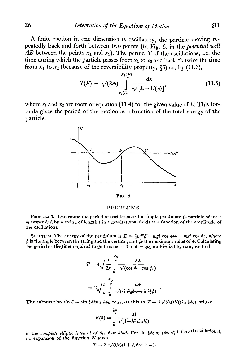
§11. Motion in one dimension
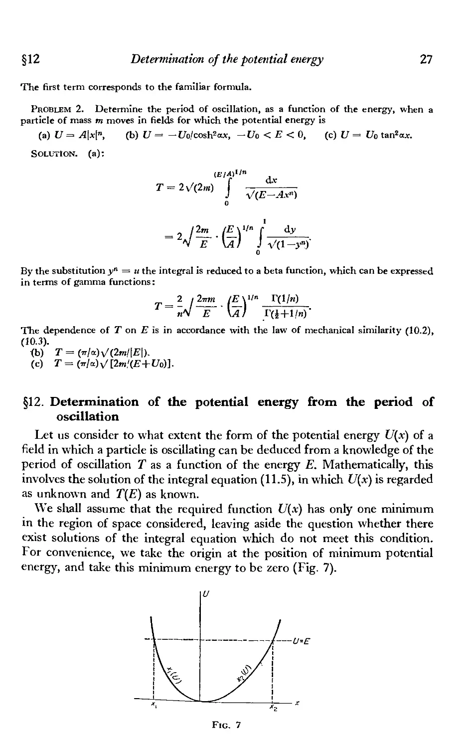
§12. Determination of the potential energy from the
oscillation
§13. The reduced mass
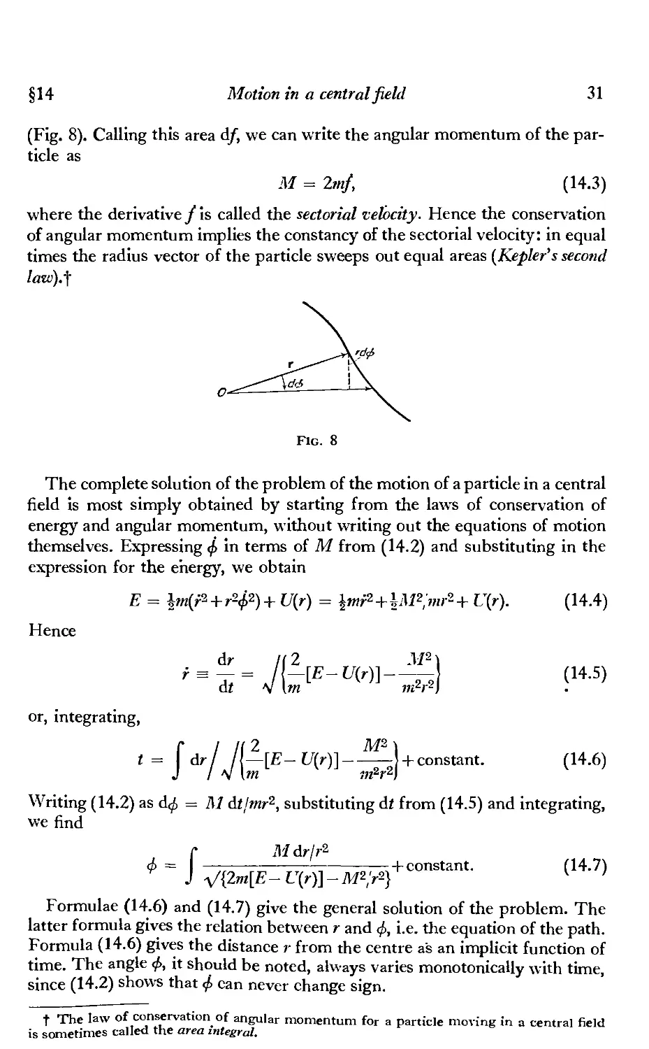
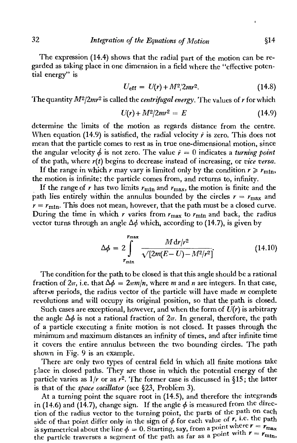
§14. Motion in a central field
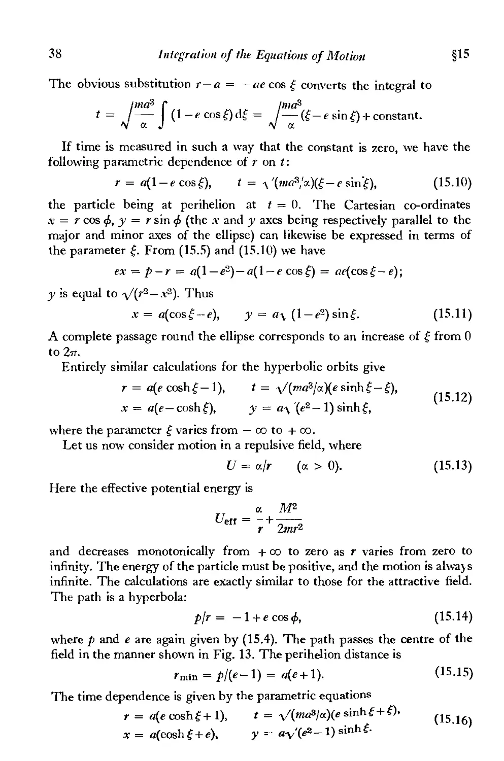
§15. Kepler's problem
13
15
16
18
22
OF MOTION
25
period of
27
29
30
35
IV. COLLISIONS BETWEEN PARTICLES
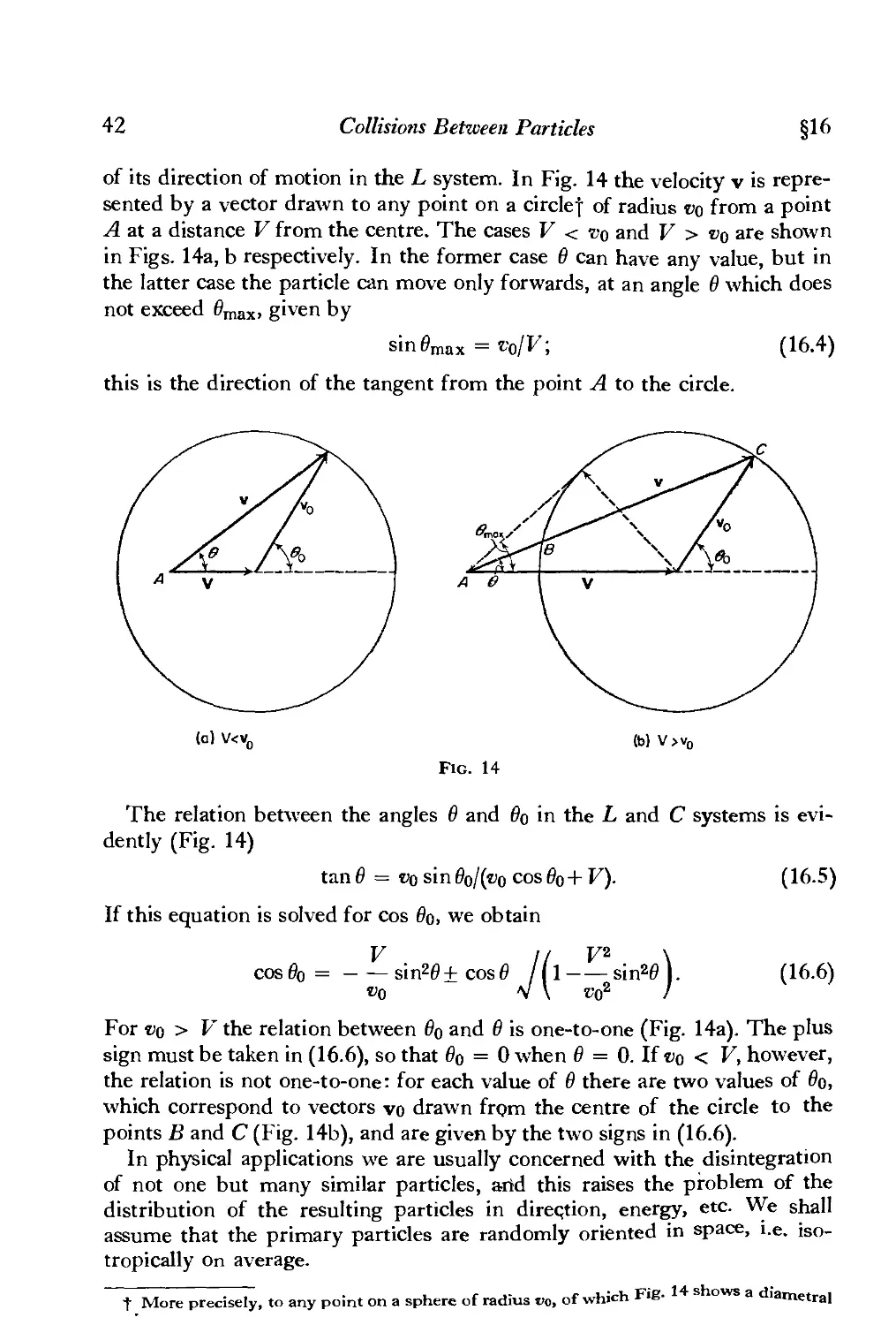
§16. Disintegration of particles 41
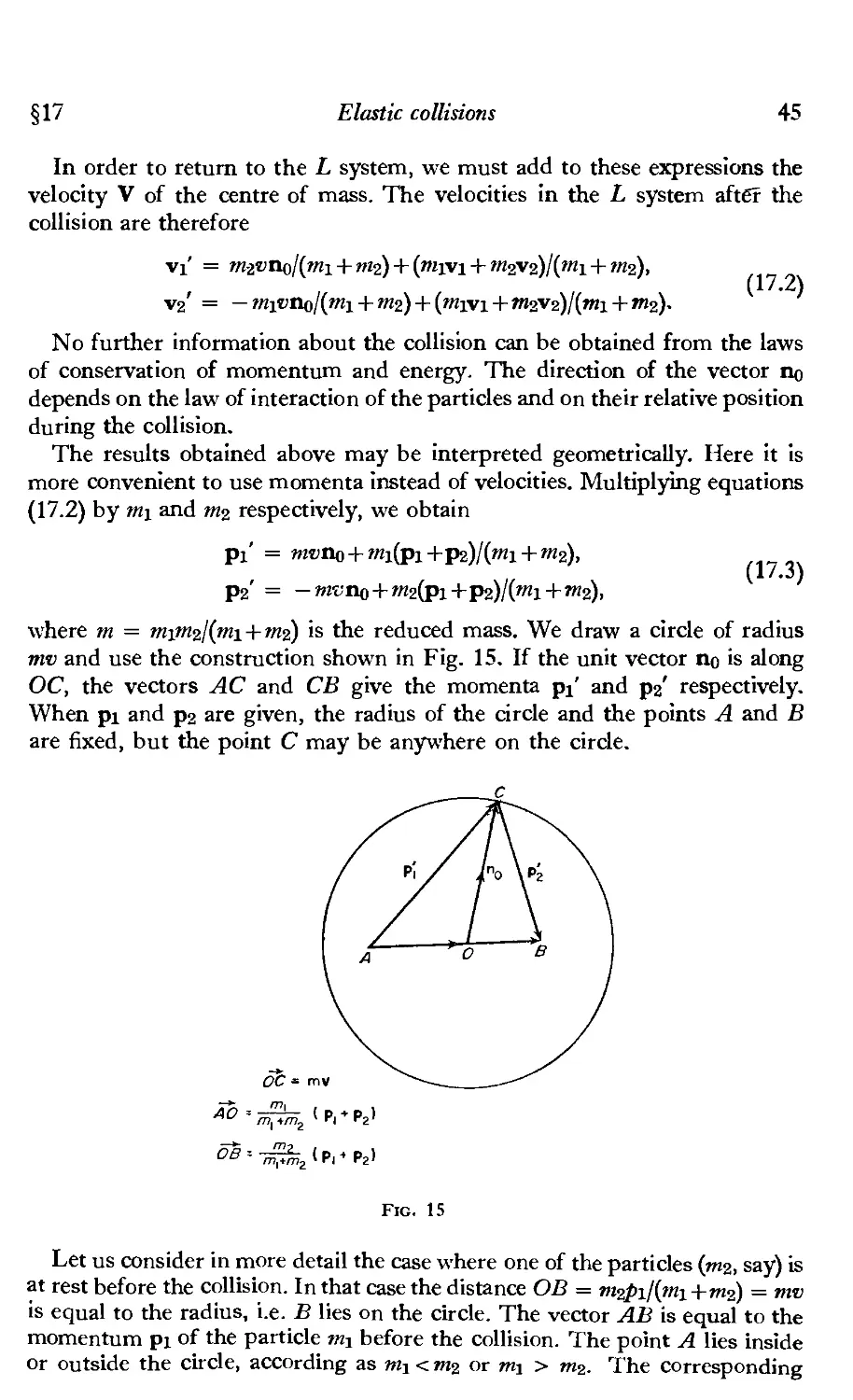
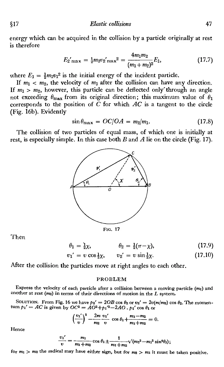
§17. Elastic collisions 44
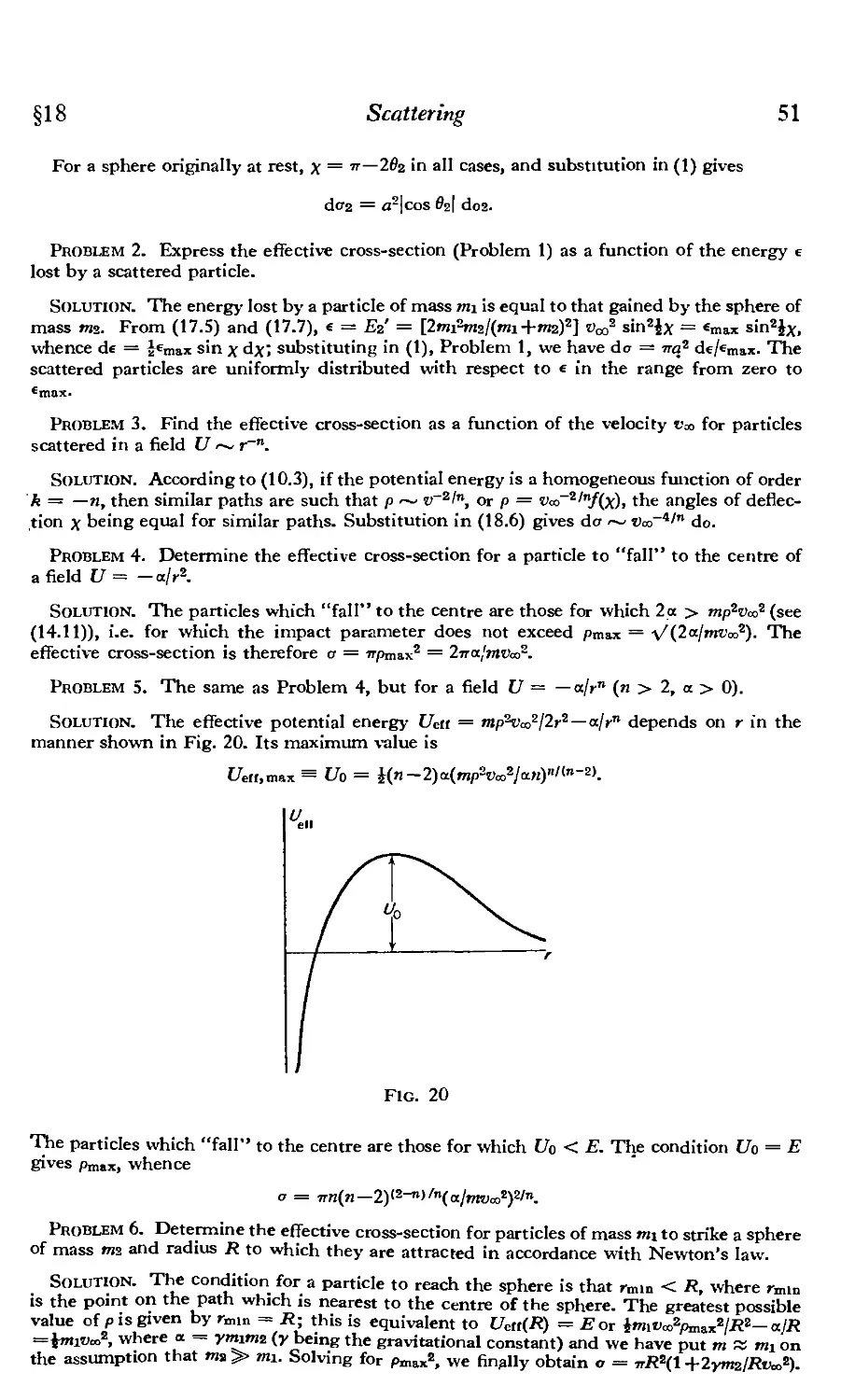
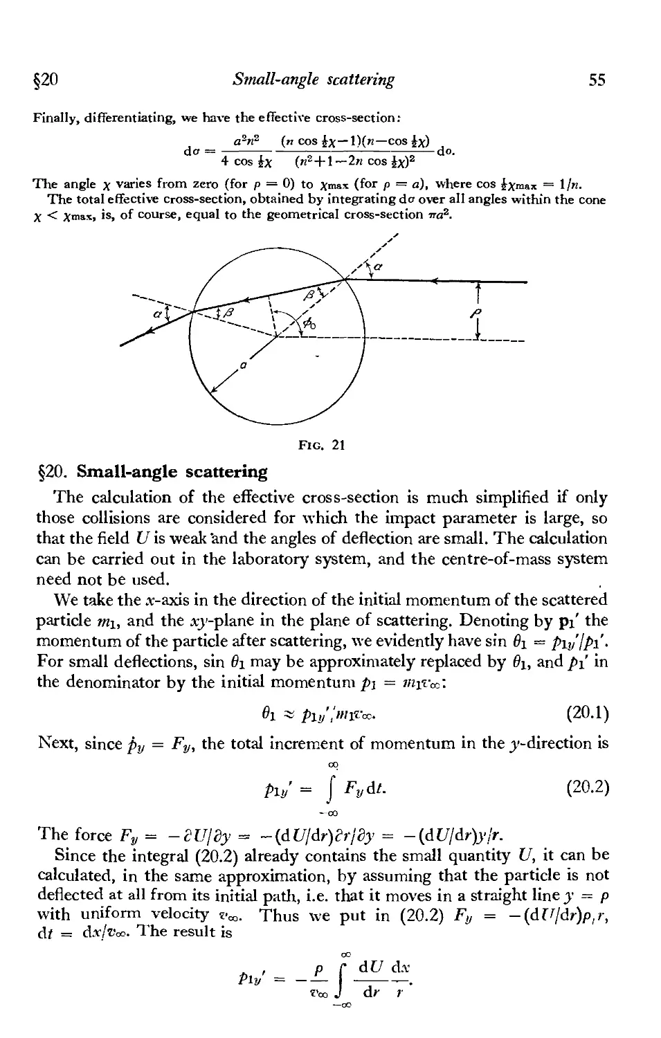
§18. Scattering 48
§19. Rutherford's formula 53
§20. Small-angle scattering 55
vi Contents
V. SMALL OSCILLATIONS
Page
§21. Free oscillations in one dimension 58
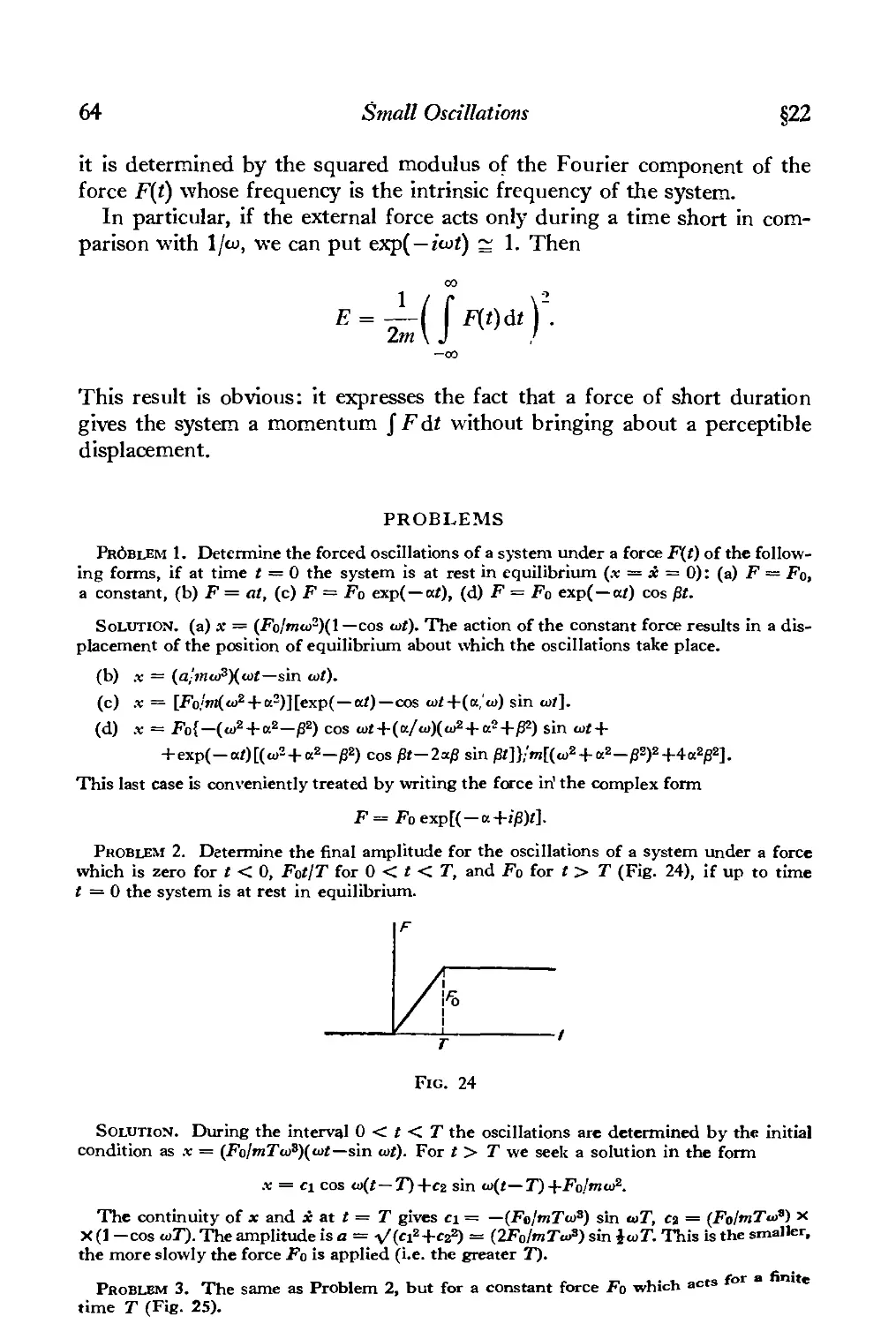
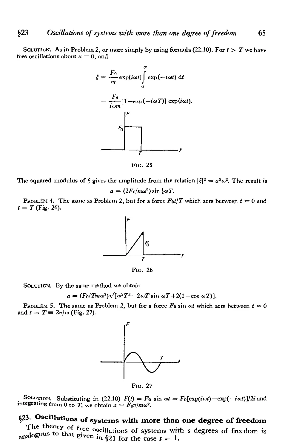
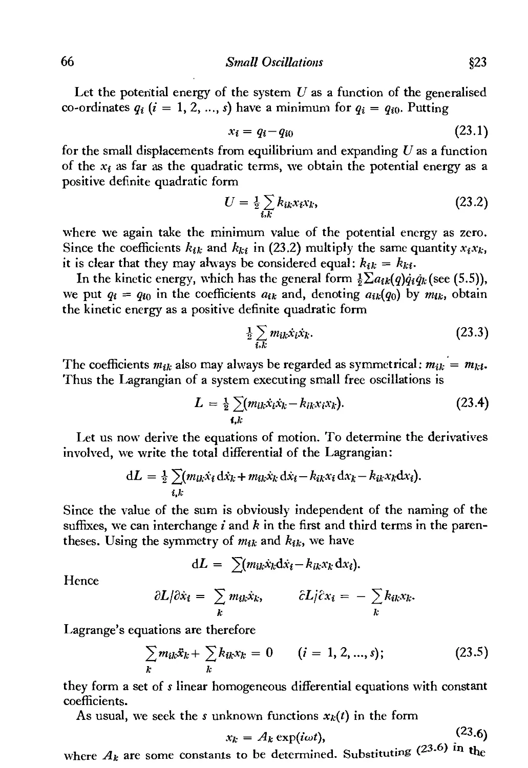
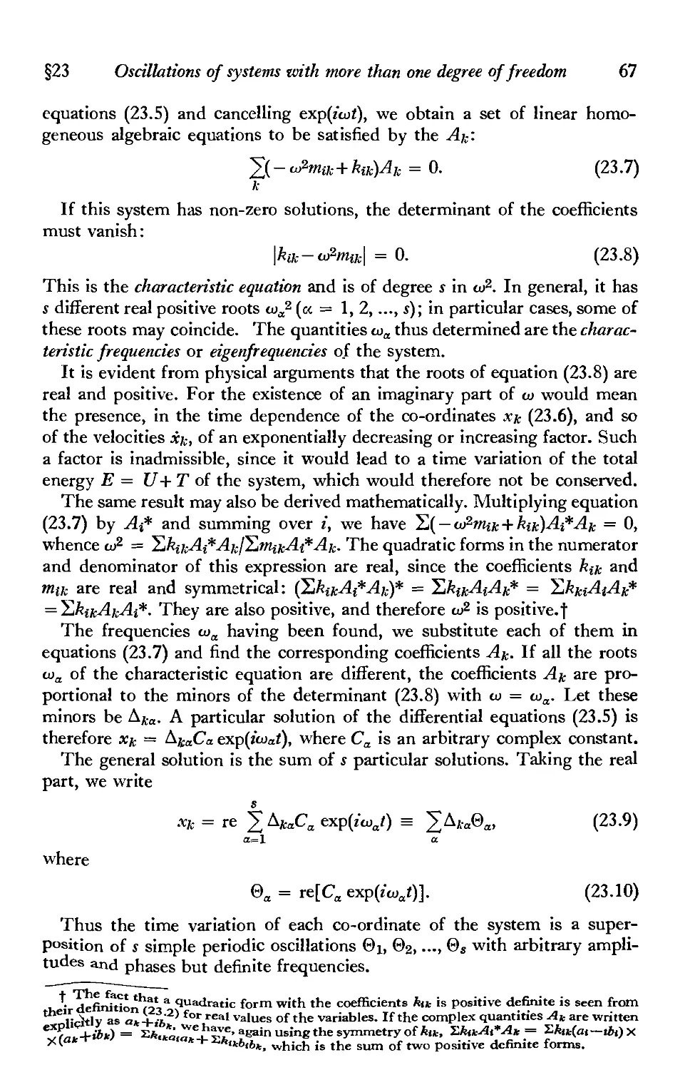
§22. Forced oscillations 61
§23. Oscillations of systems with more than one degree of freedom 65
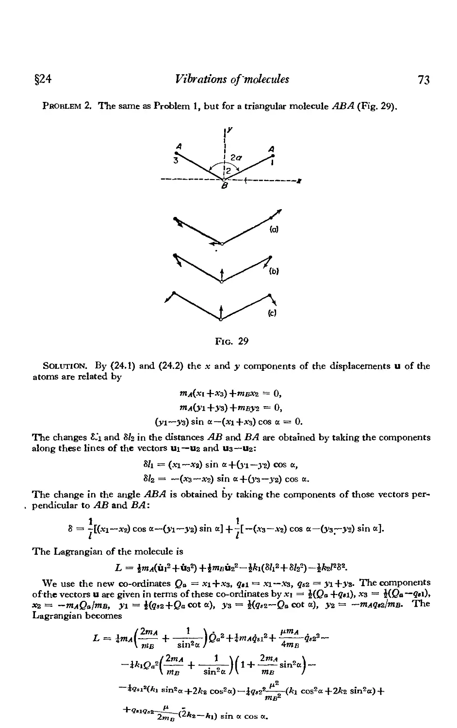
§24. Vibrations of molecules 70
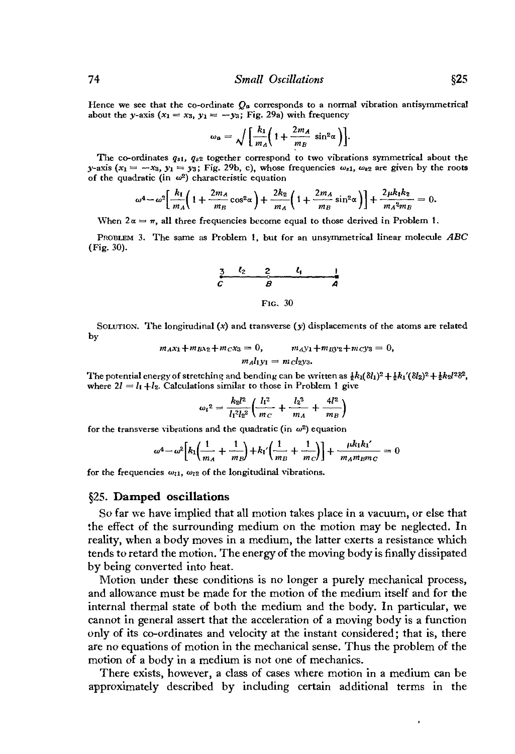
§25. Damped oscillations 74
§26. Forced oscillations under friction 77
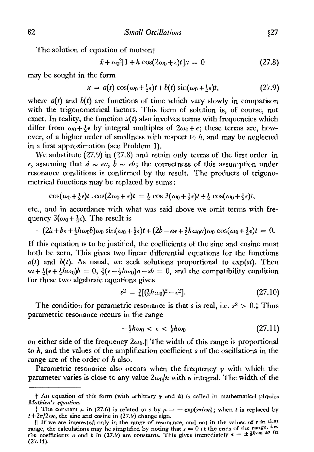
§27. Parametric resonance 80
§28. Anharmonic oscillations 84
§29. Resonance in non-linear oscillations 87
§30. Motion in a rapidly oscillating field 93
VI. MOTION OF A RIGID BODY
§31. Angular velocity 96
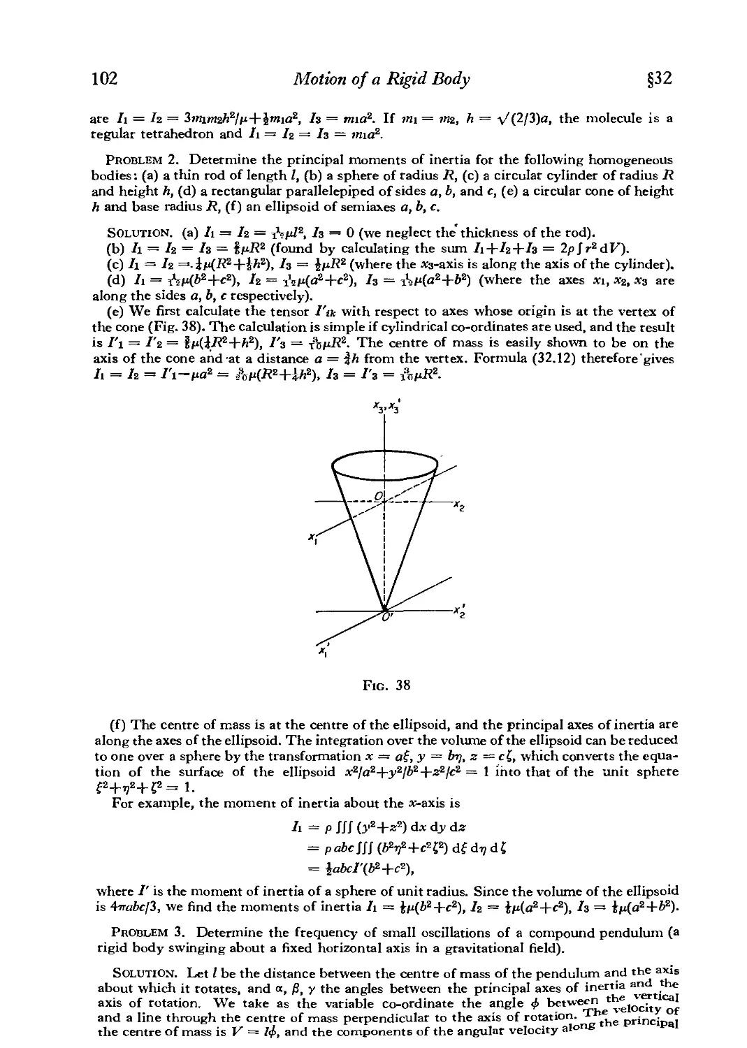
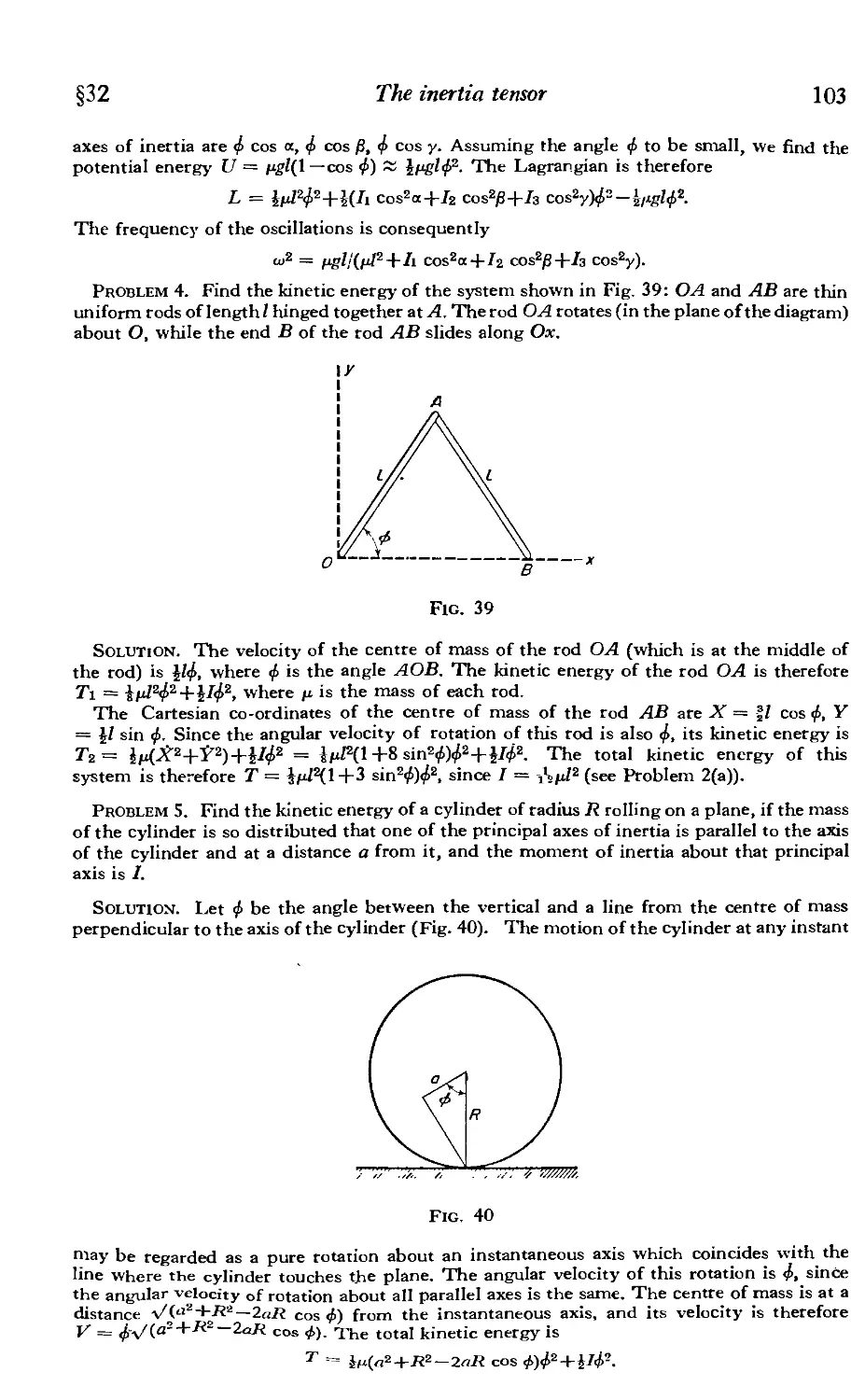
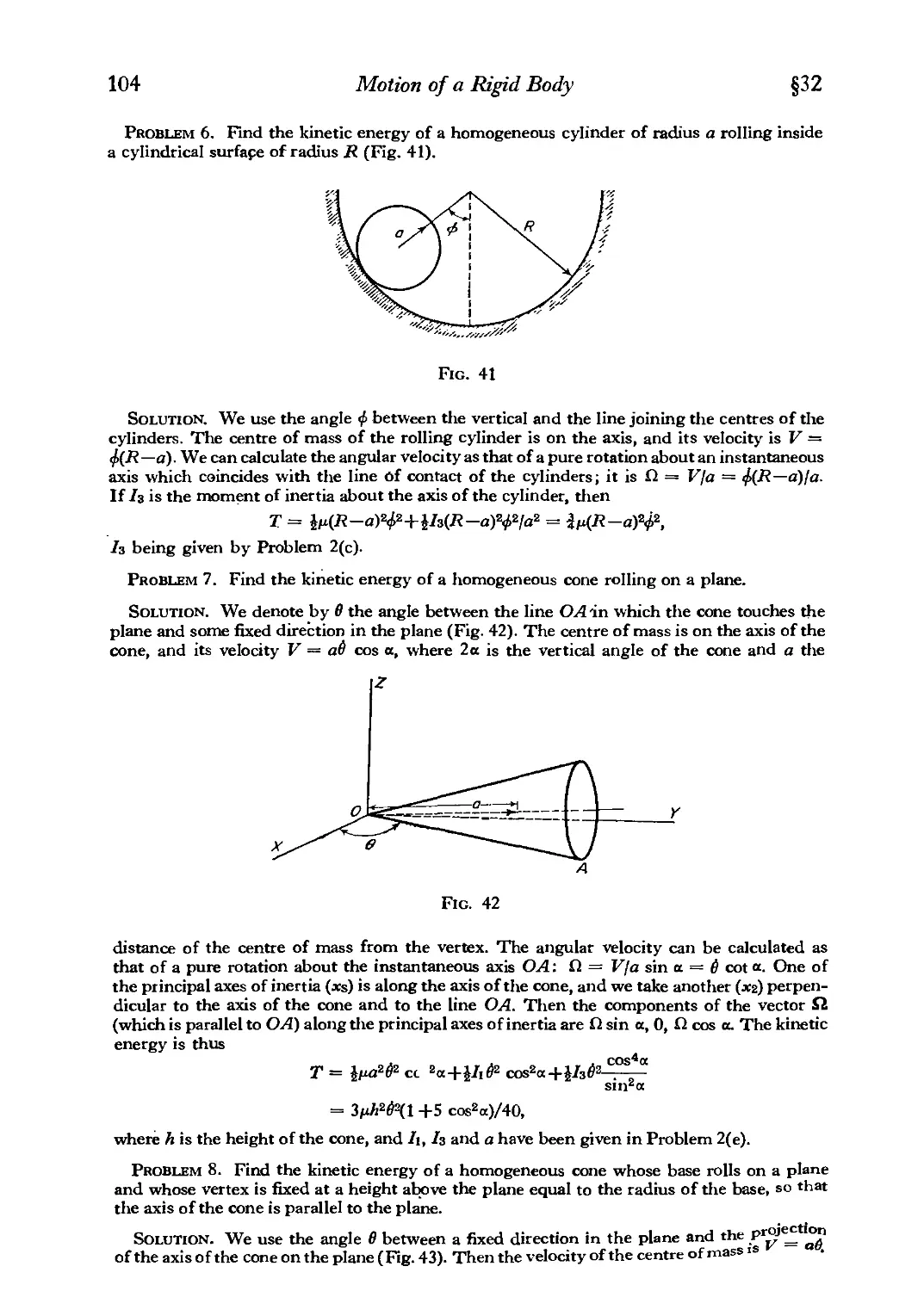
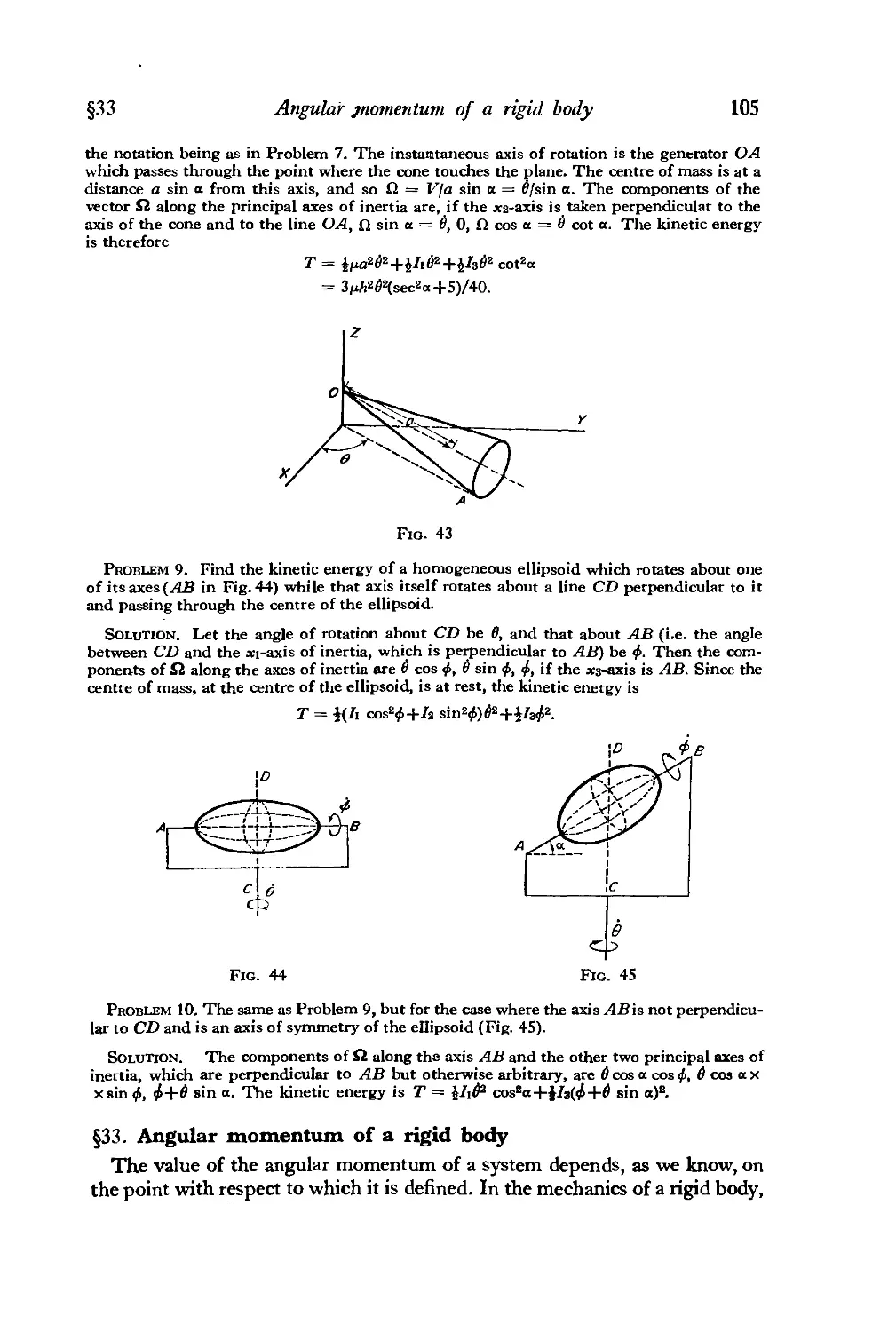
§32. The inertia tensor 98
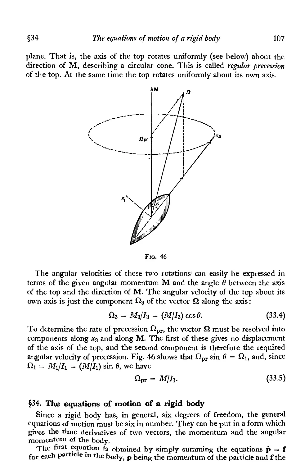
§33. Angular momentum of a rigid body 105
§34. The equations of motion of a rigid body 107
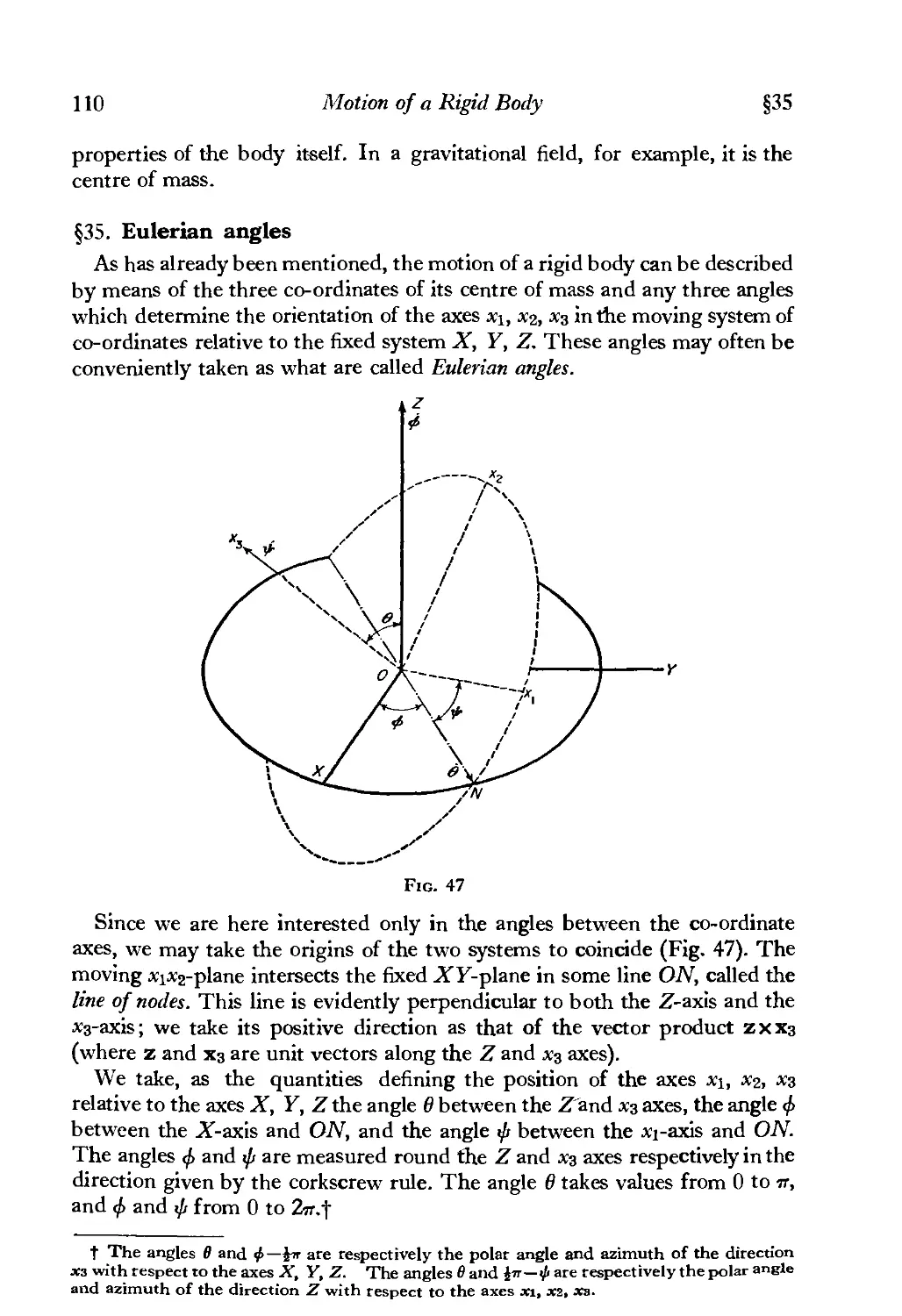
§35. Eulerian angles 110
§36. Euler's equations 114
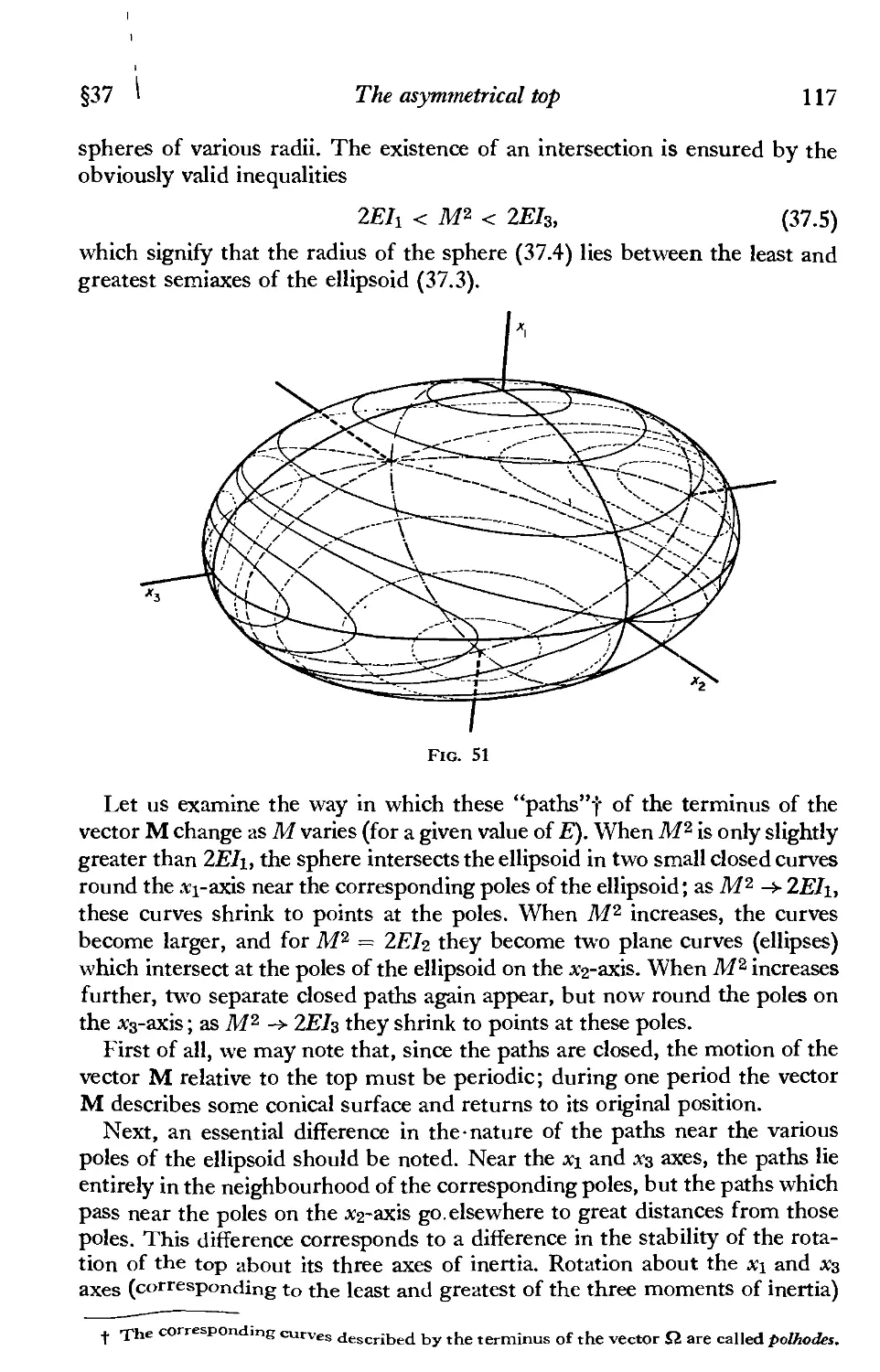
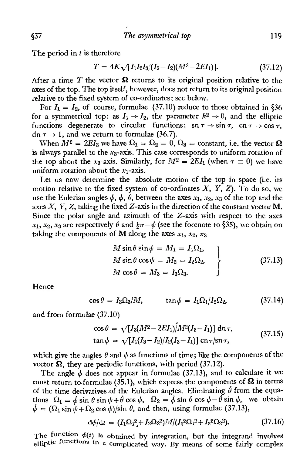
§37. The asymmetrical top 116
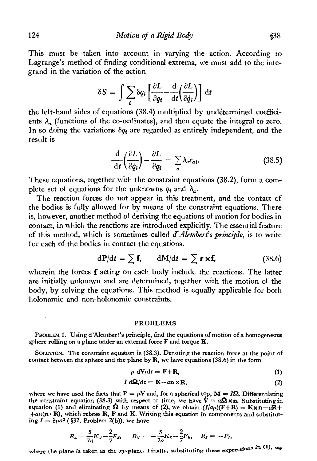
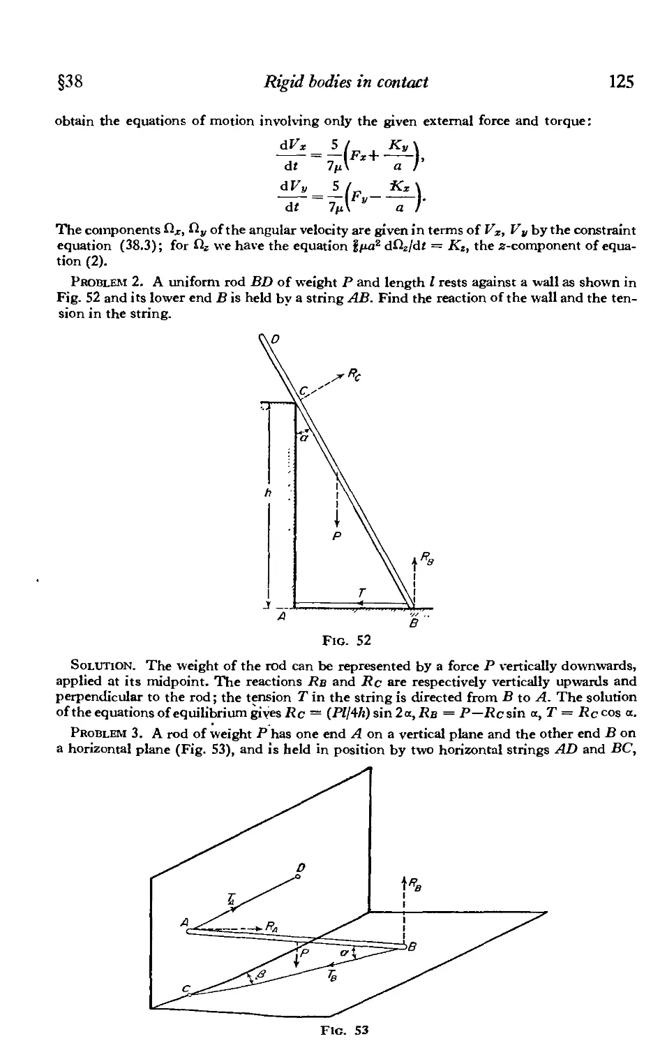
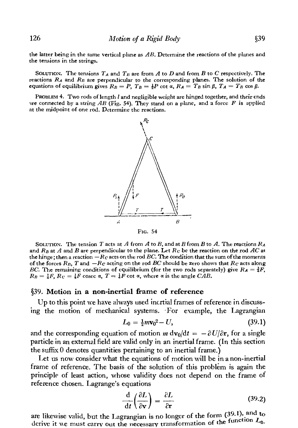
§38. Rigid bodies in contact 122
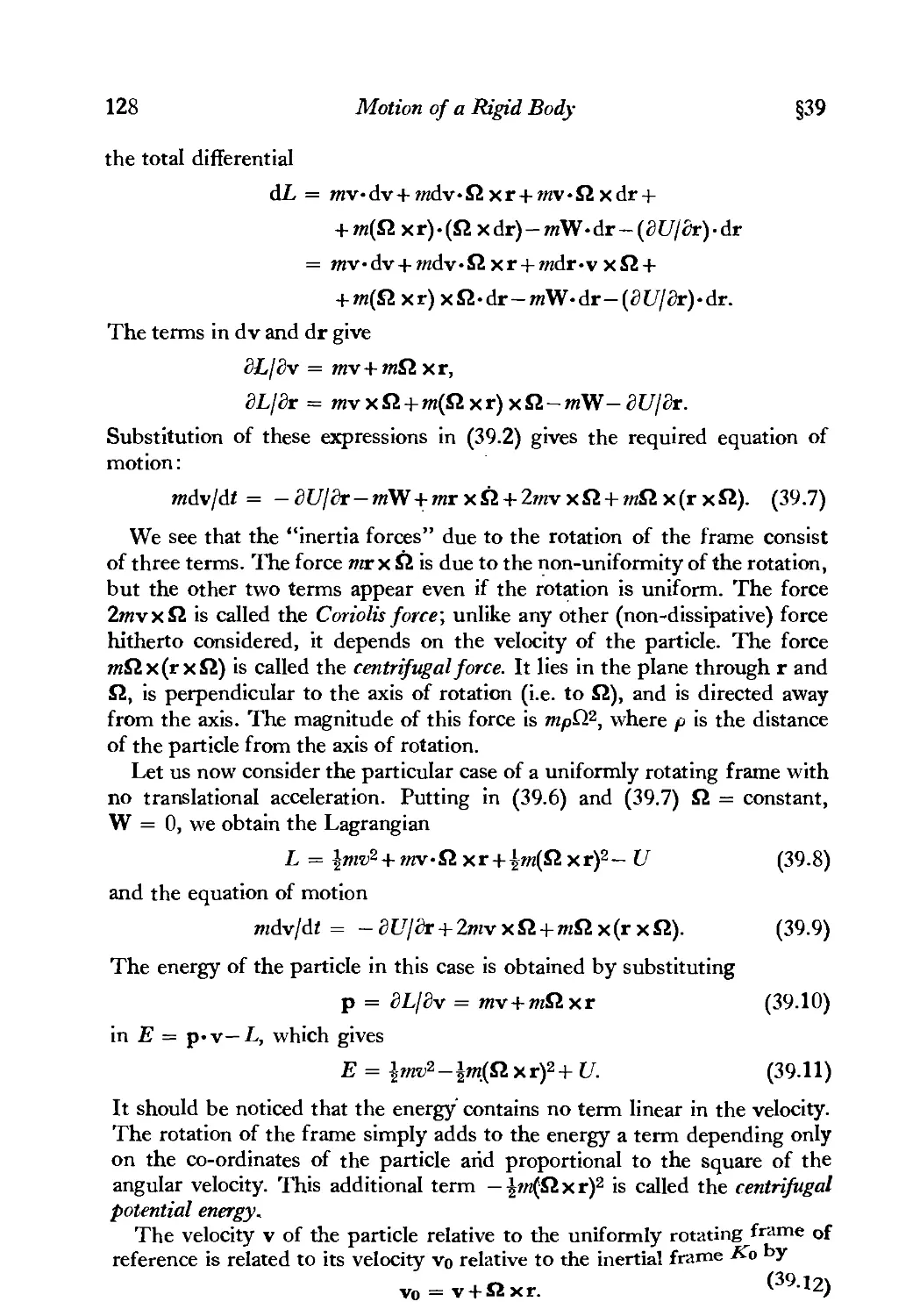
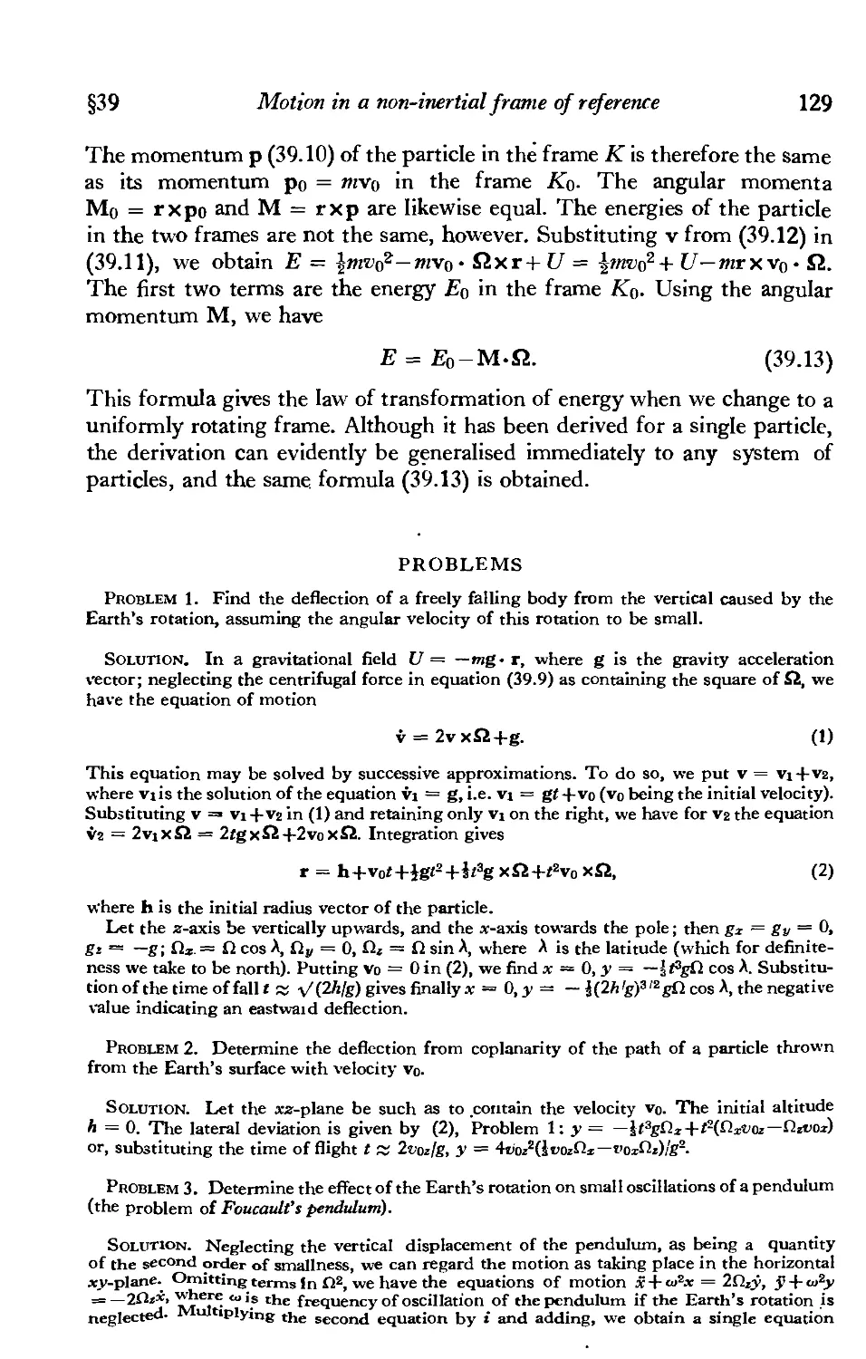
§39. Motion in a non-inertial frame of reference 126
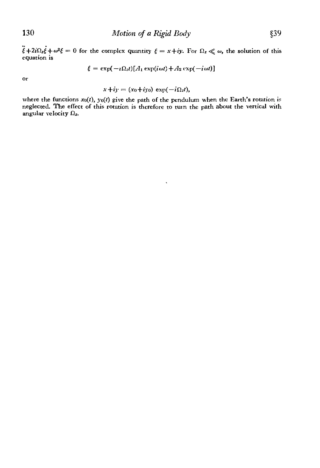
VII. THE CANONICAL EQUATIONS
§40. Hamilton's equations
§41. TheRouthian
§42. Poisson brackets
§43. The action as a function of the co-ordinates
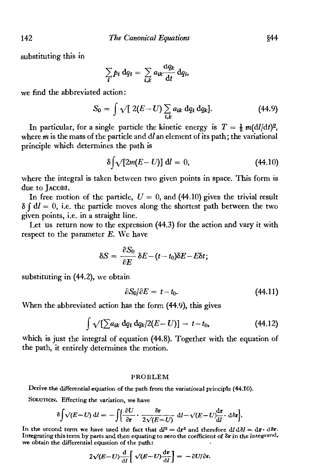
§44. Maupertuis' principle
§45. Canonical transformations
§46. Liouville's theorem
§47. The Hamilton-Jacobi equation
§48. Separation of the variables
§49. Adiabatic invariants
§50. Canonical variables
§51. Accuracy of conservation of the adiabatic invariant
§52. Conditionally periodic motion
Index
131
133
135
138
140
143
146
147
149
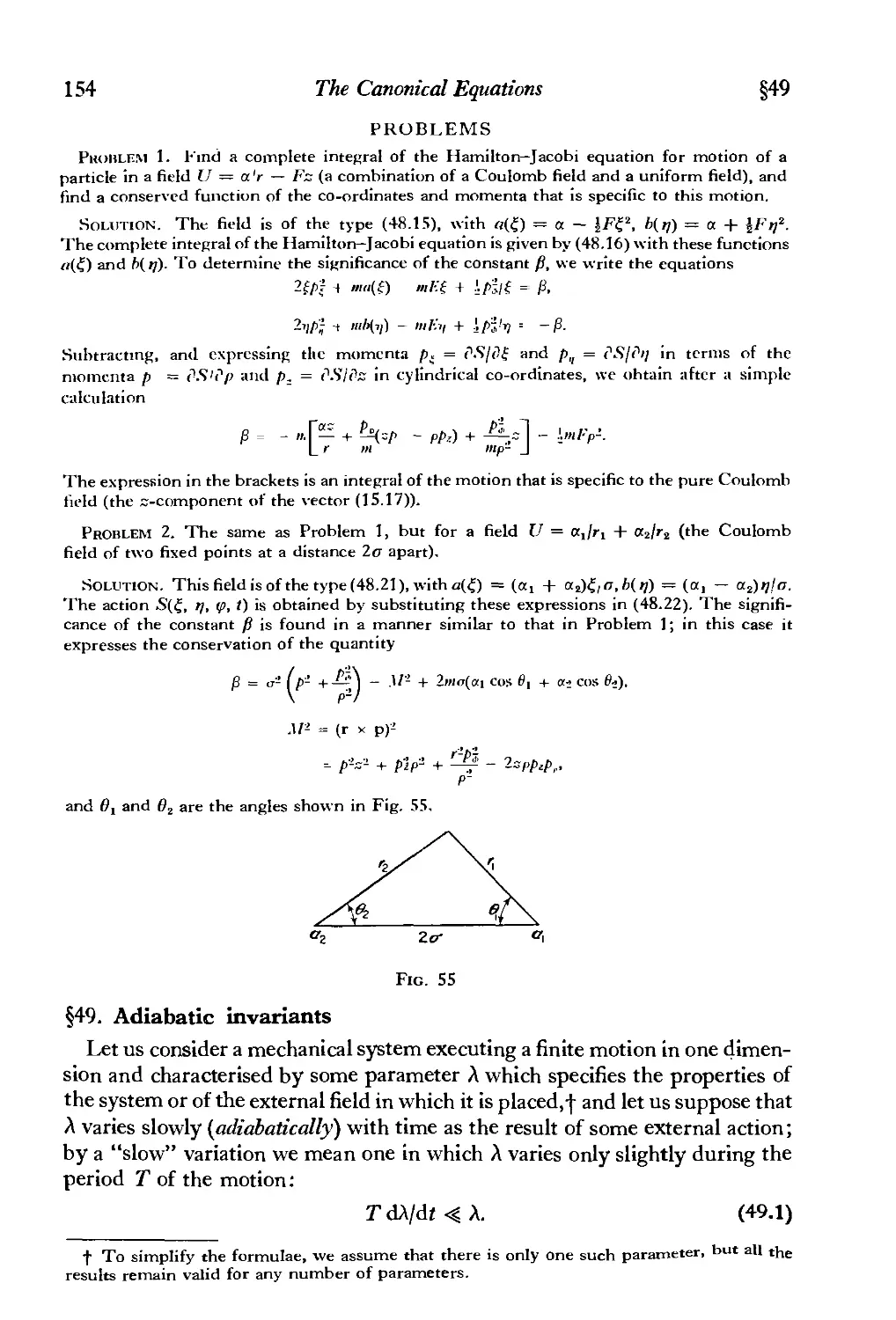
154
157
159
162
167
PREFACE TO THE THIRD ENGLISH EDITION
This book continues the series of English translations of the revised and
augmented volumes in the Course of Theoretical Physics, which have been
appearing in Russian since 1973. The English translations of volumes 2
(Classical Theory of Fields) and 3 (Quantum ^Mechanics) will shortly both
have been published. Unlike those two, the present volume 1 has not
required any considerable revision, as is to be expected in such a well-
established branch of theoretical physics as mechanics is. Only the final
sections, on adiabatic invariants, have been revised by L. P. Pitaevskii
and myself.
The Course of Theoretical Physics was initiated by Landau, my teacher
and friend. Our work together on these books began in the late 1930s and
continued until the tragic accident that befell him in 1962. Landau's work
in science was always such as to display his striving for clarity, his effort to
make simple what was complex and so to reveal the laws of nature in their
true simplicity and beauty. It was this aim which he sought to instil into his
pupils, and which has determined the character of the Course. I have tried
to maintain this spirit, so far as I was able, in the revisions that have had
to be made without Landau's participation. It has been my good fortune to
find a colleague for this work in L. P. Pitaevskii, a younger pupil of Landau's.
The present edition contains the biography of Landau which I wrote in
1969 for the posthumous Russian edition of his Collected Works. I should
like to hope that it will give the reader some slight idea of the personality of
that remarkable man.
The English translations of the Course were begun by Professor
M. Hamermesh in 1951 and continued by Dr. J. B. Sykes and his colleagues.
No praise can be too great for their attentive and careful work, which has
contributed so much to the success of our books in the English-speaking
world.
Institute of Physical Problems E. M. Lifshitz
I .S.S.R. Academy of Sciences
Moscow 1976
LEV DAVIDOVICH LANDAU A908-1968)f
Very little time has passed since the death of Lev Davidovich Landau on
1 April 1968, but fate wills that even now we view him at a distance, as it
were. From that distance we perceive more clearly not only his greatness as
a scientist, the significance of whose work becomes increasingly obvious
with time, but also that he was a great-hearted human being. He was
uncommonly just and benevolent. There is no doubt that therein lie the
roots of his popularity as a scientist and teacher, the roots of that genuine
love and esteem which his direct and indirect pupils felt for him and which
were manifested with such exceptional strength during the days of the
struggle to save his life following the terrible accident.
To him fell the tragic fate of dying twice. The first time it happened was
six years earlier on 7 January 1962 when on the icy road, en route from
Moscow to Dubna, his car skidded and collided with a lorry coming from
the opposite direction. The epic story of the subsequent struggle to save
his life is primarily a story of the selfless labour and skill of numerous
physicians and nurses. But it is also a story of a remarkable feat of solidarity.
The calamitous accident agitated the entire community of physicists,
arousing a spontaneous and instant response. The hospital in which Landau
lay unconscious became a centre to all those his students and colleagues -
who strove to make whatever contributions they could to help the physicians
in their desperate struggle to save Landau's life.
"Their feat of comradeship commenced on the very first day. Illustrious
scientists who, however, had no idea of medicine, academicians, correspond-
corresponding members of the scientific academies, doctors, candidates, men of the
same generation as the 54-year-old Landau as well as his pupils and their
still more youthful pupils - all volunteered to act as messengers, chauffeurs,
intermediaries, suppliers, secretaries, members of the watch and, lastly,
porters and labourers. Their spontaneously established headquarters was
located in the office of the Physician-in-Chief of Hospital No. 50 and it
became a round-the-clock organizational centre for an unconditional and
immediate implementation of any instruction of the attending physicians.
+ By E. M. I.ifshitz; written for the Russian edition of Landau's Collected Papers, and
first published in Russian in Uspekhi fisicheskikh nauk 97, 169-183, 1969. This translation
is by F. Bergman (first published in Soviet Physics Uspekhi 12, 135-143, 1969), with minor
modifications, and is reprinted by kind permission of the American Institute of Physics.
The reference numbers correspond to the numbering in the Collected Papers of L. D. Landau
(Pergamon Press, Oxford 1965).
x Lev Davidovich Landau
"Eighty-seven theoreticians and experimenters took part in this voluntary
rescue team. An alphabetical list of the telephone numbers and addresses of
any one and any institution with which contact might be needed at any
instant was compiled, and it contained 223 telephone numbers! It included
other hospitals, motor transport bases, airports, customs offices, pharmacies,
ministries, and the places at which consulting physicians could most likely
be reached.
"During the most tragic days when it seemed that 'Dau is dying' - and
there were at least four such days - 8-10 cars could be found waiting at
any time in front of the seven-storey hospital building. . . .
"When everything depended on the artificial respiration machine, on
12 January, a theoretician suggested that it should be immediately con-
constructed in the workshops of the Institute of Physical Problems. This was
unnecessary and naive, but how amazingly spontaneous! The physicists
obtained the machine from the Institute for the Study of Poliomyelitis
and carried it in their own hands to the ward where Landau was gasping
for breath. They saved their colleague, teacher, and friend.
"The story could be continued without limit. This was a real fraternity
of physicists. . . ."f
And so, Landau's life was saved. But when after three months he re-
regained consciousness, it was no longer the same man whom we had known.
He was not able to recover from all the consequences of his accident and
never again completely regained his abilities. The story of the six years
that followed is only a story of prolonged suffering and pain.
Lev Davidovich Landau was born on 22 January 1908 in Baku, in the
family of a petroleum engineer who worked on the Baku oil-fields. His
mother was a physician and at one time had engaged in scientific work on
physiology.
He completed his school course at the age of 13. Even then he already
was attracted by the exact sciences, and his mathematical ability manifested
itself very early. He studied mathematical analysis on his own and later he
used to say that he hardly remembere'd a time when he did not know
differentiation and integration.
His parents considered him too young to enter a university and for a
year he attended the Baku Economic Technicum. In 1922 he enrolled at
Baku University where he studied simultaneously in two departments:
Physico-mathematical and Chemical. Subsequently he did not continue
his chemical education but he remained interested in chemistry throughout
his life.
In 1924 Landau transferred to the Physics Department of Leningrad
t From D. Damn, "Comradeship", Literaturnaya Gazeta (Literary Gazette), 21 July 1962.
Lev Davidovich Landau x>
University. In Leningrad, the main centre of Soviet physics at that time,
he first made the acquaintance of genuine theoretical physics, which was
then going through a turbulent period. He devoted himself to its study with
all his youthful zeal and enthusiasm and worked so strenuously that often
he became so exhausted that at night he could not sleep, still turning over
formulae in his mind.
Later he used to describe how at that time he was amazed by the in-
incredible beauty of the general theory of relativity (sometimes he even
would declare that such a rapture on first making one's acquaintance with
this theory should be a characteristic of any born theoretical physicist).
He also described the state of ecstasy to which he was brought on reading
the articles by Heisenberg and Schrodinger signalling the birth of the new-
quantum mechanics. He said that he derived from them not only delight in
the true glamour of science but also an acute realization of the power of
the human genius, whose greatest triumph is that man is capable of appre-
apprehending things beyond the pale of his imagination. And of course, the
curvature of space-time and the uncertainty principle are precisely of this
kind.
In 1927 Landau graduated from the university and enrolled for post-
postgraduate study at the Leningrad Physicotechnical Institute where even
earlier, in 1926, he had been a part-time research student. These years
brought his first scientific publications. In 1926 he published a theory of
intensities in the spectra of diatomic molecules [l],f and as early as 1927,
a study of the problem of damping in quantum mechanics, which first
introduced a description of the state of a system with the aid of the density
matrix.
His fascination with physics and his first achievements as a scientist were,
however, at the time beclouded by a painful diffidence in his relations with
others. This trait caused him a great deal of suffering and at times - as he
himself confessed in later years - led him to despair. The changes which
occurred in him with the years and transformed him into a buoyant and
gregarious individual were largely a result of his characteristic self-discipline
and feeling of duty toward himself. These qualities, together with his sober
and self-critical mind, enabled him to train himself and to evolve into a
person with a rare ability - the ability to be happy. The same sobriety of
mind enabled him always to distinguish between what is of real value in
life and what is unimportant triviality, and thus also to retain his mental
equilibrium during the difficult moments which occurred in his life too.
In 1929, on an assignment from the People's Commissariat of Education,
Landau travelled abroad and for one and a half years worked in Denmark,
Great Britain and Switzerland. To him the most important part of his trip
was his stay in Copenhagen where, at the Institute of Theoretical Physics,
+ He did not know, however, at the time that these results had been already published a
year earlier by Honl and London.
xii Lev Davidovich Landau
theoretical physicists from all Europe gathered round the great Niels Bohr
and, during the famous seminars headed by Bohr, discussed all the basic
problems of the theoretical physics of the time. This scientific atmosphere,
enhanced by the charm of the personality of Bohr himself, decisively
influenced Landau in forming his own outlook on physics and subsequently
he always considered himself a disciple of Niels Bohr. He visited Copen-
Copenhagen two more times, in 1933 and 1934. Landau's sojourn abroad was
the occasion, in particular, of his work on the theory of the diamagnetism
of an electron gas [4] and the study of the limitations imposed on the
measurability of physical quantities in the relativistic quantum region (in
collaboration with Peierls) [6].
On his return to Leningrad in 1931 Landau worked in the Leningrad
Physicotechnical Institute and in 1932 he moved to Khar'kov, where he
became head of the Theoretical Division of the newly organized Ukrainian
Physicotechnical Institute, an offshoot of the Leningrad Institute. At the
same time he headed the Department of Theoretical Physics at the Physics
and Mechanics Faculty of the Khar'kov Mechanics and Machine Building
Institute and in 1935 he became Professor of General Physics at 'Khar'kov
University.
The Khar'kov period was for Landau a time of intense and varied
research activity.f It was there that he began his teaching career and estab-
established his own school of theoretical physics.
Twentieth-century theoretical physics is rich in illustrious names of
trail-blazing creators, and Landau was one of these creators. But his
influence on scientific progress was far from exhausted by his personal
contribution to it. He was not only an outstanding physicist but also a
genuinely outstanding educator, a born educator. In this respect one may
take the liberty of comparing Landau only to his own teacher - Niels Bohr.
The problems of the teaching of theoretical physics as well as of physics
as a whole had first attracted his interest while still quite a young man. It
was there, in Khar'kov, that he first began to work out programmes for the
"theoretical minimum" - programmes of the basic knowledge in theoretical
physics needed by experimental physicists and by those who wish to devote
themselves to professional research work in theoretical physics. In addition
to drafting these programmes, he gave lectures on theoretical physics to
the scientific staff at the Ukrainian Physicotechnical Institute as well as to
students of the Physics and Mechanics Faculty. Attracted by the ideas of
reorganizing instruction in physics as a whole, \ he accepted the Chair of
General Physics at Khar'kov State \ University \{and subsequently, after
t The extent of Landau's scientific activities at the time can be graspf d from the list of
studies he completed during the year 1936 alone: theory of second-order phase transitions
[29], theory of the intermediate state of superconductors [30], the transport equation in the
case of Coulomb interaction [24], the theory of unimolecular reactions L2JJ, properties of
metals at very low temperatures [25], theory of the dispersion and absorption of sound
[22, 28], theory of photoelectric effects in semiconductors [21]-
Lev Davidovich Landau xiii
the war, he continued to give lectures on general physics at the Physico-
technical Faculty of Moscow State University).
It was there also, in Khar'kov, that Landau had conceived the idea and
began to implement the programme for compiling a complete Course of
Theoretical Physics and Course of General Physics. All his life long, Landau
dreamed of writing books on physics at every level - from school textbooks
to a course of theoretical physics for specialists. In fact, by the time of his
fateful accident, nearly all the volumes of the Course of Theoretical Physics
and the first volumes of the Course of General Physics and Physics for
Everyone had been completed. He also had drafted plans for the compilation
of textbooks on mathematics for physicists, which should be "a guide to
action", should instruct in the practical applications of mathematics to
physics, and should be free of the rigours and complexities unnecessary to
this course. He did not have time to begin to translate this programme into
reality.
Landau always attached great importance to the mastering of mathemati-
mathematical techniques by the theoretical physicist. The degree of this mastery
should be such that, insofar as possible, mathematical complications would
not distract attention from the physical difficulties of the problem - at least
whenever standard mathematical techniques are concerned. This can be
achieved only by sufficient training. Yet experience shows that the current
style and programmes for university instruction in mathematics for physi-
physicists often do not ensure such training. Experience also shows that after a
physicist commences his independent research activity he finds the study
of mathematics too "boring".
Therefore, the first test which Landau gave to anyone who desired to
become one of his students was a quiz in mathematics in its "practical"
calculational aspects.f The successful applicant could then pass on to the
study of the seven successive sections of the programme for the "theoretical
minimum", which includes basic knowledge of all the domains of theoretical
physics, and subsequently take an appropriate examination. In Landau's
opinion, this basic knowledge should be mastered by any theoretician
regardless of his future specialization. Of course, he did not expect anyone
to be as universally well-versed in science as he himself. But he thus
manifested his belief in the integrity of theoretical physics as a single
science with unified methods.
At first Landau himself gave the examination for the "theoretical
minimum". Subsequently, after the number of applicants became too large,
this duty was shared with his closest associates. But Landau always re-
t The requirements were: ability to evaluate any indefinite integral that can be expressed
in terms of elementary functions and to solve any ordinary differential equation of the standard
type, knowledge of vector analysis and tensor algebra as well as of the principles of the theory
of functions of a complex variable (theory of residues, Laplace method). It was assumed that
such fields as tensor analysis and group theory would be studied together with the fields of
theoretical physics to which they apply.
xiv Lev Daridorich Landau
served for himself the first test, the first meeting with each new young
applicant. Anyone could meet him - it was sufficient to ring him up and
ask him for an interview.
Of course, not every one who began to study the "theoretical minimum"
had sufficient ability and persistence to complete it. Altogether, between
1934 and 1961, 43 persons passed this test. The effectiveness of this selec-
selection can be perceived from the following indicative facts alone: of these
persons 7 already have become members of the Academy of Sciences and
an additional 16, doctors of sciences.
In the spring of 1937 Landau moved to Moscow where he became head
of the Theoretical Division of the Institute of Physical Problems whichrhad
not long before been established under the direction of P. L. Kapitza.
There he remained to the end of his life; in this Institute, which became a
home to him, his varied activity reached its full flowering. It was there, in a
remarkable interaction with experimental research, that Landau created
what may be the outstanding accomplishment of his scientific life - the
theory of quantum fluids.
It was there also that he received the numerous outward manifestations
of the recognition of his contributions. In 1946 he was elected a full Member
of the USSR Academy of Sciences. He was awarded a number of orders
(including two Orders of Lenin) and the honorific title of Hero of Socialist
Labour - a reward for both his scientific accomplishments and his contribu-
contribution to the implementation of important practical State tasks. He was
awarded the State Prize three times and in 1962, the Lenin Prize. There
also was no lack of honorific awards from other countries. As far back as
1951 he was elected member of the Danish Royal Academy of Sciences
and in 1956, member of the Netherlands Royal Academy of Sciences. In
1959 he became honorary fellow of the British Institute of Physics and
Physical Society and in 1960, Foreign Member of the Royal Society of
Great Britain. In the same year he was elected to membership in the National
Academy of Sciences of the United States and the American Academy of
Arts and Sciences. In 1960 he became recipient of the F. London Prize
(United States) and of the Max Planck Medal (West Germany). Lastly, in
1962 he was awarded the Nobel Prize in Physics "for his pioneering theories
for condensed matter, especially liquid helium".
Landau's scientific influence was, of course, far from confined to his own
disciples. He was deeply democratic in his life as a scientist (and in his life
as a human being, for that matter; pomposity and deference to titles always
remained foreign to him). Anyone, regardless of his scientific merits and
title, could ask Landau for counsel and criticism (which were invariably
precise and clear), on one condition only: the question must be businesslike
instead of pertaining to what he detested most in science: empty philoso-
philosophizing or vapidity and futility cloaked in pseudo-scientific sophistries.
He had an acutely critical mind; this quality, along with his approach from
Lev Davidovich Landau
xv
the standpoint of profound physics, made discussion with him extremely
attractive and useful.
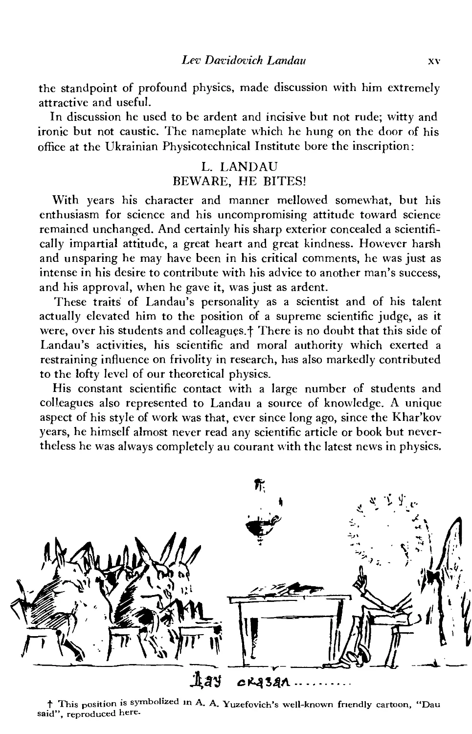
In discussion he used to be ardent and incisive but not rude; witty and
ironic but not caustic. The nameplate which he hung on the door of his
office at the Ukrainian Physicotechnical Institute bore the inscription:
L. LANDAU
BEWARE, HE BITES!
With years his character and manner mellowed somewhat, but his
enthusiasm for science and his uncompromising attitude toward science
remained unchanged. And certainly his sharp exterior concealed a scientifi-
scientifically impartial attitude, a great heart and great kindness. However harsh
and unsparing he may have been in his critical comments, he was just as
intense in his desire to contribute with his advice to another man's success,
and his approval, when he gave it, was just as ardent.
These traits of Landau's personality as a scientist and of his talent
actually elevated him to the position of a supreme scientific judge, as it
were, over his students and colleagues.f There is no doubt that this side of
Landau's activities, his scientific and moral authority which exerted a
restraining influence on frivolity in research, has also markedly contributed
to the lofty level of our theoretical physics.
His constant scientific contact with a large number of students and
colleagues also represented to Landau a source of knowledge. A unique
aspect of his style of work was that, ever since long ago, since the Khar'kov
years, he himself almost never read any scientific article or book but never-
nevertheless he was always completely au courant with the latest news in physics.
,. «!. 'i $. i-
t This position is symbolized in A. A. Yuzefovich's well-known friendly cartoon, "Dau
said", reproduced here.
xvi Lev Davidozich Landau
He derived this.knowledge from numerous discussions and from the papers
presented at the seminar held under his direction.
This seminar was held regularly once a week for nearly 30 years, and in
the last years its sessions became gatherings of theoretical physicists from
all Moscow. The presentation of papers at this seminar became a sacred
duty for all students and co-workers, and Landau himself was extremely
serious and thorough in selecting the material to be presented. He was
interested and equally competent in every aspect of physics and the partici-
participants in the seminar did not find it easy to follow his train of thought in
instantaneously switching from the discussion of, say, the properties of
"strange" particles to the discussion of the energy spectrum of electrons in
silicon. To Landau himself listening to the papers was never an empty
formality: he did not rest until the essence of a study was completely
elucidated and all traces of "philology" - unproved statements or proposi-
propositions made on the principle of "why might it not" - therein were eliminated.
As a result of such discussion and criticism many studies were condemned
as "pathology" and Landau completely lost interest in them. On the other
hand, articles that really contained new ideas or findings were included in
the so-called "gold fund" and remained in Landau's memory for ever.
In fact, usually it was sufficient for him to know just the guiding idea of
a study in order to reproduce all of its findings. As a rule, he found it easier
to obtain them on his own than to follow in detail the author's reasoning.
In this way he reproduced for himself and profoundly thought out most of
the basic results obtained in all the domains of theoretical physics, f This
probably also was the reason for his phenomenal ability to answer practically
any question concerning physics that might be asked of him.
Landau's scientific style was free of the - unfortunately fairly wide-
widespread - tendency to complicate simple things (often on the grounds of
generality and rigour which, however, usually turn out to be illusory). He
himself always strove towards the opposite - to simplify complex things, to
uncover in the most lucid manner the genuine simplicity of the laws under-
underlying the natural phenomena. This ability of his, this skill at "trivializing"
things as he himself used to say, was to him a matter of special pride.
The striving for simplicity and order was an inherent part of the structure
of Landau's mind. It manifested itself not only in serious matters but also
in semi-serious things as well as in his characteristic personal sense of
humour. J Thus, he liked to classify everyone, from women according to
the degree of their beauty, to theoretical physicists according to the signifi-
f Incidentally, this explains the absence of certain needed references in Landau's papers
which usually was not intentional. However, in some cases he could leave out a reference on
purpose, if he considered the question too trivial; and he did have his own rather high stan-
standards on that matter. . ,
J It is characteristic, however, that this trait was not a habit of Landau in nis, so to speak,
everyday outside life, in which he was not at all pedantically accurate and a zone or disorder"
would quite rapidly arise around him.
Lev Dmidmich Landau
Wll
• ч- *'
> Л- *
»■ ■
cance of their contribution to science. This last classification was based on a
logarithmic scale of five: thus, a second-class physicist supposedly accom-
accomplished 10 times as much as a third-class physicist ("pathological types"
were ranked in the fifth class). On this scale Einstein occupied the position \,
while Bohr, Heisenberg, Schrodinger, Dirac and certain others were
ranked in the first class. Landau modestly ranked himself for a long time
in class 2\ and it v\as only comparatively late in his life that he promoted
himself to the second class.
He always worked hard (never at j desk, usually reclining on j divan at
xviii Lev Davidovich Landau
home). The recognition of the results of one's work is to a greater or lesser
extent important to any scientist; it was, of course, also essential to Landau.
But it can still be said that he attached much less importance to questions of
priority than is ordinarily the case. And at any rate there is no doubt that
his drive for work was inherently motivated not by desire for fame but by
an inexhaustible curiosity and passion for exploring the laws of nature in
their large and small manifestations. He never omitted a chance to repeat
the elementary truth that one should never work for extraneous purposes,
work merely for the sake of making a great discovery, for then nothing
would be accomplished anyway.
The range of Landau's interests outside physics also was extremely wide.
In addition to the exact sciences he loved history and was well-versed in it.
He was also passionately interested in and deeply impressed by every genre
of fine arts, though with the exception of music (and ballet).
Those who had the good fortune to be his students and friends for many
years knew that our Dau, as his friends and comrades nicknamed himf, did
not grow old. In his company boredom vanished. The brightness of his
personality never grew dull and his scientific power remained strong. All
the more senseless and frightful was the accident which put an end to his
brilliant activity at its zenith.
Landau's articles, as a rule, display all the features of his characteristic
scientific style: clarity and lucidity of physical statement of problems, the
shortest and most elegant path towards their solution, no superfluities.
Even now, after many years, the greater part of his articles does not require
any revisions.
The brief review below is intended to provide only a tentative idea of the
abundance and diversity of Landau's work and to clarify to some extent
the place occupied by it in the history of physics, a place which may not
always be obvious to the contemporary reader.
A characteristic feature of Landau's scientific creativity is its almost
unprecedented breadth, which encompasses the whole of theoretical
physics, from hydrodynamics to the quantum field theory. In our century,
which is a century of increasingly narrow specialization, the scientific paths
of his students also have been gradually diverging, but Landau himself
unified them all, always retaining a truly astounding interest in everything.
It may be that in him physics has lost one of the last great universalists.
Even a cursory examination of the bibliography of Landau's works shows
that his life cannot be divided into any lengthy periods during which he
worked only in some one domain of physics. Hence also the survey of his
works is given not in chronological order but, insofar as possible, in thematic
t Landau himself liked to say that this name originated from the French spelling of his
name: Landau = L'ane Dau (the ass Dau).
Lev Daiidovich Landau xix
order. We shall begin with the works devoted to the general problems of
quantum mechanics.
These include, in the first place, several of his early works. In the course
of his studies of the radiation-damping problem he was the first to introduce
the concept of incomplete quantum-mechanical description accomplished
with the aid of quantities which were subsequently termed the density
matrix [2]. In this article the density matrix was introduced in its energy
representation.
Two articles [7, 9] are devoted to the calculation of the probabilities of
quasiclassical processes. The difficulty of this problem stems from the fact
that, by virtue of the exponential nature (with a large imaginary exponent)
of the quasiclassical wave functions, the integrand in the matrix elements
is a rapidly fluctuating quantity; this greatly complicates even an estimate
of the integral; in fact, until Landau's work all studies of problems of this
kind were erroneous. Landau was the first to provide a general method for
the calculation of quasiclassical matrix elements and he also applied it to
a number of specific processes.
In 1930 Landau (in collaboration with R. Peierls) published a detailed
study of the limitations imposed by relativistic requirements on the quantum-
mechanical description [6]; this article caused lively discussions at the time.
Its basic result lies in determining the limits of the possibility of measuring
the particle momentum within a finite time. This implied that in the rela-
relativistic quantum region it is not feasible to measure any dynamical variables
characterizing the particles in their interaction, and that the only measurable
quantities are" the momenta (and polarizations) of free particles. Therein
also lies the physical root of the difficulties that arise when methods of
conventional quantum mechanics, employing concepts which become
meaningless in the relativistic domain, are applied there. Landau returned
to this problem in his last published article [100], in which he expressed his
conviction that the ^-operators, as carriers of unobservable information,
and along with them the entire Hamiltonian method, should disappear
from a future theory.
One of the reasons for this conviction was the results of the research into
the foundations of quantum electrodynamics which Landau carried out
during 1954-1955 (in collaboration with A. A. Abrikosov, I. M. Khalatnikov
and I. Ya. Pomeranchuk) [78-81, 86]. These studies were based on the
concept of the point interaction as the limit of "smeared" interaction when
the smearing radius tends to zero. This made it possible to deal directly with
finite expressions. Further, it proved possible to carry out the summation
of the principal terms of the entire series of perturbation theory and this
led to the derivation of asymptotic expressions (for the case of large momen-
momenta) for the fundamental quantities of quantum electrodynamics - the Green
functions and the vertex part. These relations, in their own turn, were used
to derive the relationship between the true charge and mass of the electron,
xx Lev Davidovich Landau
on the one hand, and their "bare" values, on the other. Although these
calculations proceeded on the premise of smallness of the "bare" charge, it
was argued that the formula for the relation between true and bare charges
retains its validity regardless of the magnitude of the bare charge. Then
analysis of this formula shows that at the limit of point interaction the
true charge becomes zero - the theory is "nullified".j- (A review of the
pertinent questions is provided in the articles [84, 89]).
Only the future will show the extent of the validity of the programme
planned by Landau [100] for constructing a relativistic quantum field
theory. He himself was energetically working in this direction during the
last few years prior to his accident. As part of this programme, in particular,
he nad worked out a general method for determining the singularities of
the quantities that occur in the diagram technique of quantum field
theory [98].
In response to the discovery in 1956 of parity nonconservation in weak
interactions, Landau immediately proposed the theory of a neutrino with
fixed helicity ("two-component neutrino") [92]J, and also suggested the
principle of the conservation of "combined parity", as he termed the
combined application of spatial inversion and charge conjugation. Accord-
According to Landau, the symmetry of space would in this way be "saved" -
the asymmetry is transferred to the particles themselves. This principle
indeed proved to be more widely applicable than the law of parity conserva-
conservation. As is known, however, in recent years processes not conserving
combined parity have also been discovered; the meaning of this violation
is at present still unclear.
A 1937 study [31] by Landau pertains to nuclear physics. This study
represents a quantitative embodiment of the ideas proposed not long
before by Bohr: the nucleus is examined by methods of statistical physics
as a drop of "quantum fluid". It is noteworthy that this study did not make
use of any far-reaching model conceptions, contrary to the previous practice
of other investigators. In particular, the relationship between the mean
distance between the levels of the compound nucleus and the width of the
levels was established for the first time.
The absence of model conceptions is characteristic also of the theory of
proton-proton scattering developed by Landau (in collaboration with
Ya. A. Smorodinskii) [55]. The scattering cross-section in their study was
expressed in terms of parameters whose meaning is not restricted by any
specific assumptions concerning the particle interaction potential.
The study (in collaboration with Yu. B. Rumer) [36] of the cascade
t In connection with the search for a more rigorous proof of this statement, the article
[100] contains the assertion, characteristic of Landau, that "the brevity of lite does not allow
us the luxury of spending time on problems which will lead to no new results .
J Simultaneously and independently, this theory was proposed by saiam and by Lee
and Yang.
Lev Davidovich Landau xxi
theory of electron showers in cosmic rays is an example of technical
virtuosity; the physical foundations of this theory had been earlier formula-
formulated by a number of investigators, but a quantitative theory was essentially
lacking. That study provided the mathematical apparatus which became the
basis for all subsequent work in this domain. Landau himself took part in
the further refinement of the shower theory by contributing two more
articles, one on the particle angular distribution [43] and the other on
secondary showers [44].
Of ho smaller virtuosity was Landau's work dealing with the elaboration
of Fermi's idea of the statistical nature of multiple particle production in
collisions [74]. This study also represents a brilliant example of the metho-
methodological unity of theoretical physics in which the solution of a problem is
accomplished by using the methods from a seemingly completely different
domain. Landau showed that the process of multiple production includes
the stage of the expansion of a "cloud" whose dimensions are large com-
compared with the mean free path of particles in it; correspondingly, this stage
should be described by equations of relativistic hydrodynamics. The solu-
solution of these equations required a number of ingenious techniques as well
as a thorough analysis. Landau used to say that this study cost him more
effort than any other problem that he had ever solved.
Landau always willingly responded to the requests and needs of the
experimenters, e.g. by publishing the article [56] which established the
energy distribution of the ionization losses of fast particles during passage
through matter (previously only the theory of mean energy loss had existed).
Turning now to Landau's work on macroscopic physics, we begin with
several articles representing his contribution to the physics of
magnetism.
According to classical mechanics and statistics, a change in the pattern of
movement of free electrons in a magnetic field cannot result in the appear-
appearance of new magnetic properties of the system. Landau was the first to
elucidate the character of this motion in a magnetic field for the quantum
case, and to show that quantization completely changes the situation,
resulting in the appearance of diamagnetism of the free electron gas
("Landau diamagnetism" as this effect is now termed) [4]. The same study
qualitatively predicted the periodic dependence of the magnetic suscepti-
susceptibility on the intensity of the magnetic field when this intensity is high.
At the time A930) this phenomenon had not yet been observed by anyone,
and it was experimentally discovered onlv later (the De Haas-Van Alphen
effect); a quantitative theory of this effect was presented by Landau in a
later paper [38].
A short article published in 1933 [12] is of a significance greatly tran-
transcending the problem stated in its title - a possible explanation of the field
dependence of the magnetic susceptibility of a particular class of substances
xxii Lev Davidovich Landau
at low temperatures. This article was the first to introduce the concept of
antiferromagnetism (although it did not use this terni) as a special phase of
magnetic bodies differing in symmetry from the paramagnetic phase;
accordingly, the transition from one state to the other^must occur at a
rigorously definite point.f This article examined the particular model of a
layered antiferromagnet with a strong ferromagnetic coupling in each
layer and a weak antiferromagnetic coupling between the layers; a quantita-
quantitative investigation of this case was carried out and the characteristic features
of magnetic properties in the neighbourhood of the transition point were
established. The method employed here by Landau was based on ideas
which he subsequently elaborated in the general theory of second-order
phase transitions.
Another paper concerns the theory of ferromagnetism. The idea of the
structure of ferromagnetic bodies as consisting of elementary regions
spontaneously magnetized in various directions ("magnetic domains," as
trie modern term goes) was expressed by P. Weiss as early as in 1907.
However, there was no suitable approach to the question of the quantitative
theory of this structure until Landau (in collaboration with E. M. Lifshitz)
[18] showed in 1935 that this theory should be constructed on the basis
of thermodynamic considerations and determined the form and dimensions
of the domains for a typical case. The same study derived the macroscopic
equation of the motion of the domain magnetization vector and, with its
aid,-developed the principles of the theory of the dispersion of the magnetic
permeability of ferromagnets in an alternating magnetic field; in particular,
it predicted the effect now known as ferromagnetic resonance.
A short communication published in 1933 [10] expressed the idea of the
possibility of the "autolocalization" of an electron in a crystal lattice within
the potential well produced by virtue of the polarization effect of the electron
itself. This idea subsequently provided the basis for the so-called polaron
theory of the conductivity of ionic crystals. Landau himself returned once
more to these problems in a later study (in collaboration with S. I. Pekar)
[67] dealing with the derivation of the equations of motion of the polaron
in the external field.
Another short communication [14] reported on the results obtained by
Landau (in collaboration with G. Placzek) concerning the structure of the
Rayleigh scattering line in liquids or gases. As far back as the early 1920s
Brillouin and Mandel'shtam showed that, owing to scattering by sound
vibrations, this line must split into a doublet. Landau and Placzek drew
attention to the attendant necessity of the existence of scattering by entropy
t Roughly a year earlier Neel (whose work was unknown to Landau) had predicted the
possibility of existence of substances which, from the magnetic standpoint, consist of two
sublattices with opposite moments. Neel, however, did not assume that a special state of
matter is involved here, and instead he simply thought that a P"™"8^;*?™ ' P°»t,ve
exchange integral at low temperatures gradually turns into a structure consisting of several
magnetic sublattices.
Lev Daz'idwich Landau xxiii
fluctuations, not accompanied by any change in frequency; as a result, a
triplet should be observed instead of a doublet, f
Two of Landau's works pertain to plasma physics. One of these two
[24] was the first to derive the transport equation with allowance for Coulomb
interaction between particles; the slowness of decrease of these forces
rendered inapplicable in this case the conventional methods for constructing
transport equations. The other work [61], dealing with plasma oscillations,
showed that, even under conditions when collisions between particles in the
plasma can be disregarded, high-frequency oscillations will still attenuate
("Landau damping").%
His work to compile one of the successive volumes of the Course of
Theoretical Physics was to Landau a stimulus for a thorough study of
hydrodynamics. Characteristically, he independently pondered and derived
all the basic notions and results of this branch of science. His fresh and
original perception led, in particular, to a new approach to the problem of
the onset of turbulence and he elucidated the basic aspects of the process
of the gradual development of unsteady flow with increase in the Reynolds
number following the loss of stability by laminar motion and predicted
qualitatively various alternatives possible in this case [52]. On investigating
the qualitative properties of supersonic flow around bodies, he arrived at
the unexpected discovery that in supersonic flow there must exist far from
the body not one - as had been the conventional assumption - but two
shock waves, one following the other [60]. Even in such a "classical" field
as the jet theory he succeeded in finding a new and previously unnoticed
exact solution for an axially symmetric "inundated" jet of a viscous in-
incompressible fluid [51].
In Landau's scientific creative accomplishments an eminent position is
occupied - both from the standpoint of direct significance and in terms of
the consequent physical applications - by the theory of second-order phase
transitions [29]; a first outline of the ideas underlying this theory is already
contained in an earlier communication [17].|| The concept of phase transi-
transitions of various orders had first been introduced by Ehrenfest in a purely
formal manner, with respect to the order of the thermodynamic derivatives
which could undergo a discontinuity at the transition point. The question of
exactly which of these transitions can exist in reality, and what is their
f No detailed exposition of the conclusions and results of this study was ever published in
article form. It is partly presented in the book by Landau and Lifshitz, Electrodynamics of
Continuous Media, Pergamon, Oxford 1960, §96.
J It is interesting that this work was carried out by Landau as his response to the "philo-
"philology" present, in his opinion, in previous studies dealing with this subject (e.g., the unjustified
replacement of divergent integrals b> their principal values). It was to prove his Tightness
that he occupied himself with this question.
II Landau himself applied this theory to the scattering of X-rays by crystals [32] and - in
collaboration with I. M. Khalatnikov - to the absorption of sound in the neighbourhood of the
transition point [82].
xxiv Lev Dazidoztch Landau
physical nature, had remained open, and previous interpretations had been
fairly vague and unsubstantiated. Landau was the first to point to the
profound connection between the possibility of existence of a continuous
(in the sense of variation in the body's state) phase transition and the jump-
like (discontinuous) change in some symmetry property of the body at the
transition point. He also showed that far from just any change in symmetry
is possible at that transition point and provided a method which makes it
possible to determine the permissible types of change in symmetry. The
quantitative theory developed by Landau was based on the assumption of
the regularity of the expansion of thermodynamic quantities in the neigh-
neighbourhood of the transition point. It is now clear that such a theory, which
fails to allow for possible singularities of these quantities at the transition
point, does not reflect all the properties of phase transitions. The question
of the nature of these singularities was of great interest to Landau and
during the last years of his activity he worked a great deal on this difficult
problem without, however, succeedingin arrivingat any definite conclusions.
The phenomenological theory of superconductivity developed in 1950
by Landau (in collaboration with V. L. Ginzburg) [73] also was constructed
in the spirit of the theory of phase transitions; subsequently it became, in
particular, the basis for the theory of superconducting alloys. This theory
involves a number of variables and parameters whose meaning was not
completely clear at the time it was originally developed and became under-
understandable only after the appearance in 1957 of the microscopic theory of
superconductivity, which made possible a rigorous substantiation of the
Ginzburg-Landau equations and a determination of the region of their
applicability. In this connection, the story (recounted by V. L. Ginzburg)
of an erroneous statement contained in the original article by Landau and
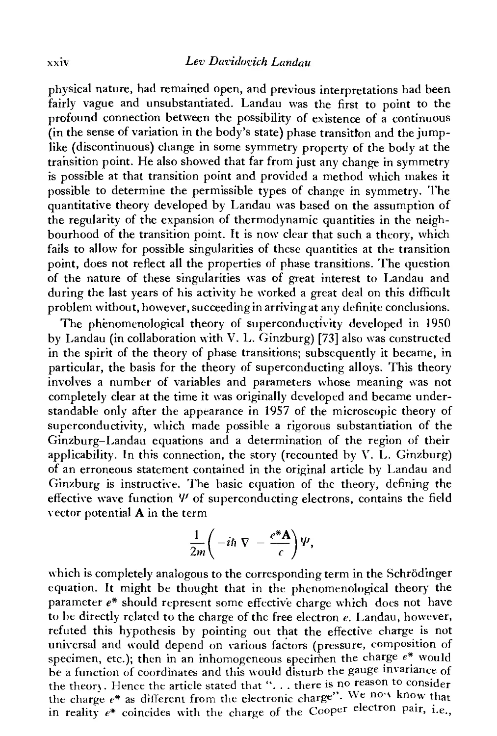
Ginzburg is instructive. The basic equation of the theory, defining the
effective wave function 4J of superconducting electrons, contains the field
vector potential A in the term
с J
which is completely analogous to the corresponding term in the Schrodinger
equation. It might be thought that in the phenomenological theory the
parameter e* should represent some effective charge which does not have
to be directly related to the charge of the free electron e. Landau, however,
refuted this hypothesis by pointing out that the effective charge is not
universal and would depend on various factors (pressure, composition of
specimen, etc.); then in an inhomogeneous specimen the charge e* would
be a function of coordinates and this would disturb the gauge invariance of
the theor\. Hence the article stated that ". . . there is no reason to consider
the charge e* as different from the electronic charge". We no-\ know that
in reality e* coincides with the charge of the Cooper electron pair, i.e.,
Lev Davidoz'ich Landau xxv
e* = 2e and not e. This value of e* could, of course, have been predicted
only on the basis of the idea of electron pairing which underlies the micro-
microscopic theory of superconductivity. But the value 2e is as universal as e and
hence Landau's argument in itself was valid.
Another of Landau's contributions to the physics of superconductivity
was to elucidate the nature of the so-called intermediate state. The concept
of this state was first introduced by Peierls and F. London A936) to account
for the observed fact that the transition to the superconducting state in a
magnetic field is gradual. Their theory was purely phenomenological,
however, and the question of the nature of the intermediate state had
remained open. Landau showed that this state is not a new state and that in
reality a superconductor in that state consists of successive thin layers of
normal and superconducting phases. In 1937 Landau [30] considered a
model in which these layers emerge to the surface of the specimen; using
an elegant and ingenious method he succeeded in completely determining
the shape and dimensions of the layers in such a model.f In 1938 he proposed
a new variant of the theory, according to which the layers repeatedly branch
out on emerging to the surface; such a structure should be thermodynami-
cally more favourable, given sufficiently large dimensions of the specimen.%
But the most significant contribution that physics owes to Landau is his
theory of quantum liquids. The significance of this new discipline at present
is steadily growing; there is no doubt that its development in recent decades
has produced a revolutionary effect on other domains of physics as well -
on solid-state physics and even on nuclear physics.
The superfluidity theory was created by Landau during 1940-1941 soon
after Kapitza's discovery towards the end of 1937 of this fundamental
property of helium II. Prior to it, the premises for understanding the
physical nature of the phase transition observed in liquid helium had been
essentially lacking and it is not surprising that the previous interpretations
of this phenomenon now seem even naive.|| The completeness with which
the theory of helium II had been constructed by Landau from the very
beginning is remarkable: already his first classic paper [46] on this subject
contained practically all the principal ideas of both the microscopic theory
of helium II and the macroscopic theory constructed on its basis - the
thermodynamics and hydrodynamics of this fluid.
Underlying Landau's theory is the concept of quasiparticles (elementary
excitations) constituting the energy spectrum of helium II. Landau was in
fact the first to pose the question of the energy spectrum of a macroscopic
t Landau himself wrote concerning this matter that "amazingly enough an exact determi-
determination of the shape of the layers proves to be possible" [30]
t A detailed description of this work was published in 1943 [49].
|{ Thus, Landau himself in his work on the theory of phase transitions [29] considered
whether helium II is a liquid crystal, even though he emphasized the dubiousness of this
assumption.
xxvi Lev Davidovich Landau
body in such a very general form, and it was he, too, who discovered the
nature of the spectrum for a quantum fluid of the type to which liquid
helium (He4 isotope) belongs - or, as it is now termed, of the Bose type.
In his 1941 work Landau assumed that the spectrum of elementary excita-
excitations consists of two branches: phonons, with a linear dependence of energy
£- on momentum p, and "rotons", with a quadratic dependence, separated
from the ground state by an energy gap. Subsequently he found that such
a form of spectrum is not satisfactory from the theoretical standpoint
(as it would be unstable) and careful analysis of the more complete and
exact experimental data that had by then become available led him in 1946
to establish the now famous spectrum containing only one branch in
which the "rotons" correspond to a minimum on the curve of fi(p)- The
macroscopic concepts of the theory of superfluidity are widely known.
Basically they reduce to the idea of two motions simultaneously occurring
in the fluid - "normal" motion and "superfluid" motion, which may be
visualized as motions of two "fluid components".! Normal motion is
accompanied by internal friction, as in conventional fluids. The determina-
determination of the viscosity coefficient represents a kinetic problem which requires
an analysis of the processes of the onset of an equilibrium in the "gas of
quasiparticles"; the principles of the theory of the viscosity of helium II
were developed by Landau (in collaboration with I. M. Khalatnikov) in
1949 [69, 70]. Lastly, yet another investigation (carried out in collaboration
with I. Ya. Pomeranchuk) [64] dealt with the problem of the behaviour of
extraneous atoms in helium; it was shown, in particular, that any atom of
this kind will become part of the "normal component" of the fluid regard-
regardless of whether the impurity substance itself does or does not display the
property of superfluidity - contrary to- the incorrect view previously held
in the literature.
The liquid isotope He3 is a quantum liquid of another type - the Fermi
type as it is now termed. Although its properties are not as.striking as the
properties of liquid He4, they are no less interesting from the standpoint of
basic theory. A theory of liquids of this kind was developed by Landau and
presented by him in three papers published during 1956-1958. The first two
of these [90, 91] established the nature of the energy spectrum of Fermi
liquids, considered their thermodynamic properties and established the
kinetic equation for the relaxation processes occurring in these liquids. His
study of the kinetic equation led Landau to predict a special type of vibra-
t Some of the ideas of the "two-component" macroscopic description of liquid helium
were introduced independently of Landau by L. Tisza (although without providing a clear
ПС1С II HIUUU^CU MiUC[JtlluciiliJ i_>i ijanuau uj li« ■» iai.a \_ui vnw—f-,-- . .
phvsical interpretation of them). His detailed article published in brance in 1У+О was>
owing to wartime conditions, not received in the USSR until 1943 and the bnef note of 1938
in the Comptes rendus of the Paris Academie des Sciences had unfortunately remained un-
unnoticed. A criticism of the quantitative aspects of Tisza's theory was provided b} Landau in
ng to wai
he Comp
ced. A ci
the article [66].
Lev Davidovich Landau xxvii
tional process in liquid He3 in the neighbourhood of absolute zero, which
he termed zeroth sound. The third paper [95] presented a rigorous micro-
microscopic substantiation of the transport equation, whose earlier derivation had
contained a number of intuitive assumptions.
Concluding this brief and far from complete survey, it only remains to be
repeated that to physicists there is no need to emphasize the significance of
Landau's contribution to theoretical physics. His accomplishments are of
lasting significance and will for ever remain part of science.
CHAPTER I
THE EQUATIONS OF MOTION
§1. Generalised co-ordinates
One of the fundamental concepts of mechanics is that of a particle.f By this
we mean a body whose dimensions may be neglected in describing its motion.
The possibility of so doing depends, of course, on the conditions of the prob-
problem concerned. For example, the planets may be regarded as particles in
considering their motion about the Sun, but not in considering their rotation
about their axes.
The position of a particle in space is defined by its radius vector r, whose
components are its Cartesian co-ordinates x, y, z. The derivative v = dr/df
of r with respect to the time t is called the velocity of the particle, and the
second derivative d2r/df2 is its acceleration. In what follows we shall, as is
customary, denote differentiation with respect to time by placing a dot above
alerter: v = f.
To define the position of a system of N particles in space, it is necessary to
specify N radius vectors, i.e. 3N co-ordinates. The number of independent
quantities which must be specified in order to define uniquely the position of
any system is called the number of degrees of freedom; here, this number is
ЗЛГ. These quantities need not be the Cartesian co-ordinates of the particles,
and the conditions of the problem may render some other choice of co-
coordinates more convenient. Any s quantities q\, qi, ...» qs which completely
define the position of a system with s degrees of freedom are called generalised
co-ordinates of the system, and the derivatives qi are called its generalised
velocities.
When the values of the generalised co-ordinates are specified, however,
the "mechanical state" of the system at the instant considered is not yet
determined in such a way that the position of the system at subsequent
instants can be predicted. For given values of the co-ordinates, the system
can have any velocities, and these affect the position of the system after an
infinitesimal time interval At.
If all the co-ordinates and velocities are simultaneously specified, it i3
known from experience that the state of the system is completely determined
and that its subsequent motion can, in principle, be calculated. Mathematic-
Mathematically, this means that, if all the co-ordinates q and velocities q are given at
some instant, the accelerations q at that instant are uniquely defined.i
t Sometimes called in Russian a material point.
% For brevity, we shall often conventionally denote by q the set of all the co-ordinates
i, 92 qs, and similarly by q the set of all the velocities.
1
2 The Equations of Motion §2
The relations between the accelerations, velocities and co-ordinates are
called the equations of motion. They are second-order differential equations
for the functions q(t), and their integration makes possible, in principle, the
determination of these functions and so of the path of the system.
§2. The principle of least action
The most general formulation of the law governing the motion of mech-
mechanical systems is the principle of least action or Hamilton's principle, according
to which every mechanical system is characterised by a definite function
L(qi, q2, ■■■, qs, ?i, ?2. •••. qs, t), or briefly L(q, q, t), and the motion of the
system is such that a certain condition is satisfied.
Let the system occupy, at the instants t\ and £2, positions defined by two
sets of values of the co-ordinates, cf^ and q^2\ Then the condition is that the
system moves between these positions in such a way that the integral
«2
S=JL(q,q,t)dt B.1)
takes the least possible value.f The function L is called the Lagrangian of
the system concerned, and the integral B.1) is called the action.
The fact that the Lagrangian contains only q and q, but not the higher
derivatives q, q, etc., expresses the result already mentioned, that the mech-
mechanical state of the system is completely defined when the co-ordinates and
velocities are given.
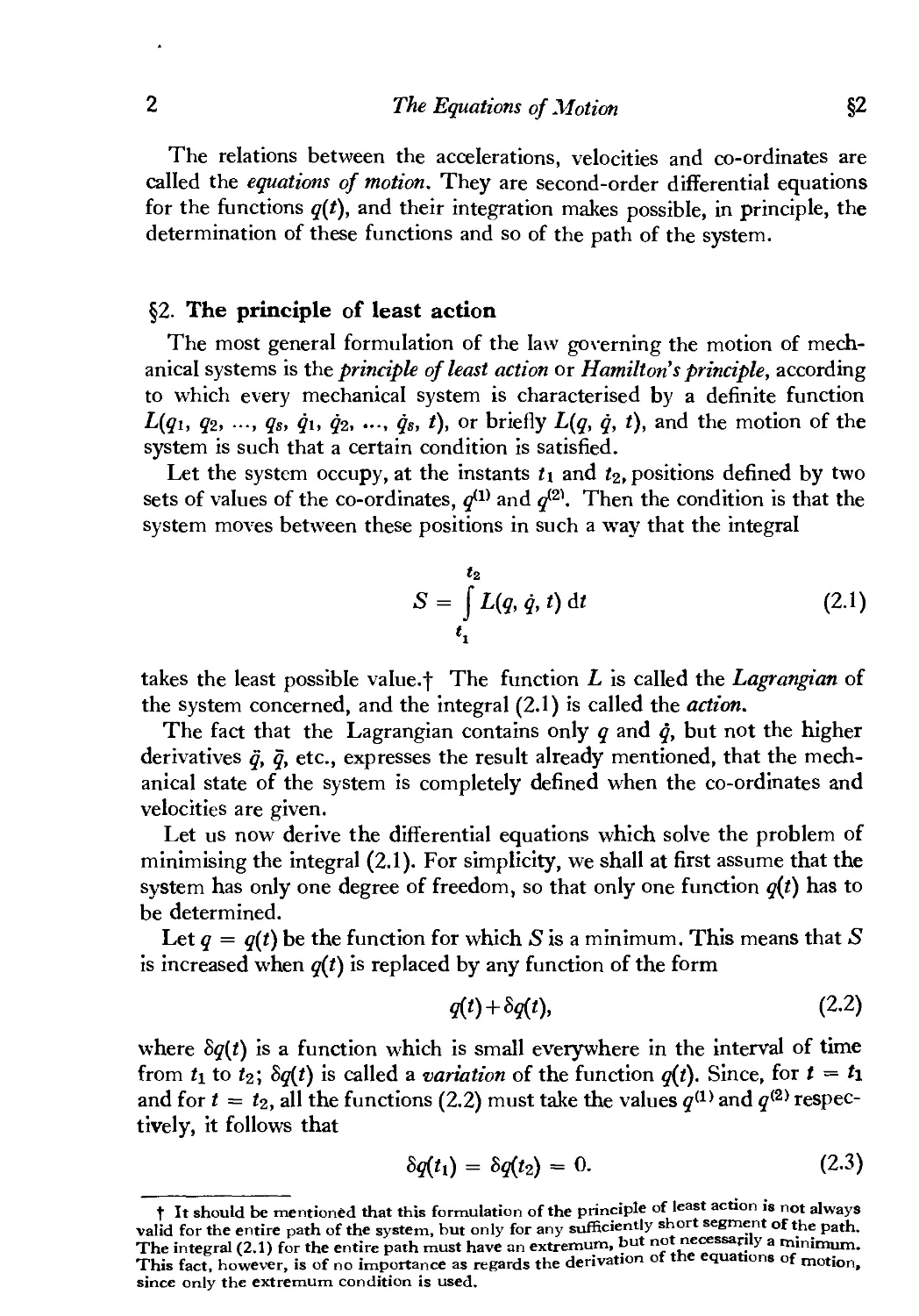
Let us now derive the differential equations which solve the problem of
minimising the integral B.1). For simplicity, we shall at first assume that the
system has only one degree of freedom, so that only one function q(t) has to
be determined.
Let q = q{t) be the function for which S is a minimum. This means that S
is increased when q(t) is replaced by any function of the form
q(t) + 8q(t), B.2)
where 8q(t) is a function which is small everywhere in the interval of time
from t\ to <2; bq(t) is called a variation of the function q(t). Since, for t = h
and for t = t2, all the functions B.2) must take the values qA) and qB) respec-
respectively, it follows that
= 0. B-3)
t It should be mentioned that this formulation of the principle of least action is not always
valid for the entire path of the system, but only for any sufficiently short segment of the path.
The integral B.1) for the entire path must have an extremum, but not necessarily a minimum.
This fact, however, is of no importance as regards the derivation ot tne equations of motion,
since only the extremum condition is used.
§2 The principle of least action 3
The change in 5 when q is replaced by q + 8q is
«2 <2
\ L(q+8q, q+8q, t) dt- J L(q, q, t) dt.
К h
When this difference is expanded in powers of bq and 8q in the integrand, the
leading terms are of the first order. The necessary condition for S to have a
minimumf is that these terms (called the first variation, or simply the varia-
variation, of the integral) should be zero. Thus the principle of least action may
be written in the form
«2
8S = 8 j L(q,q,t)dt = 0, B.4)
«i
or, effecting the variation,
r /8L 8L
J b^
Since 8q = d8qjdt, we obtain, on integrating the second term by parts,
\8L "l'z r/ 8L d 8L\
8S= — 8q\ + \(-—-—\Sqdt = O. B.5)
L 8q J «j J \ 8q dt 8q /
The conditions B.3) show that the integrated term in B.5) is zero. There
remains an integral which must vanish for all values of 8q. This can be so only
if the integrand is zero identically. Thus we have
d/8L\ 8L
dt\8q/ 8q
When the system has more than one degree of freedom, the s different
functions qi(t) must be varied independently in the principle of least action.
Wre then evidently obtain s equations of the form
di8L\ 8L
TbH ~ t— = 0 A=1,2,...,*). B.6)
dt\8qi/ 8qi
These are the required differential equations, called in mechanics Lagrange's
equations.% If the Lagrangian of a given mechanical system is known, the
equations B.6) give the relations between accelerations, velocities and co-
coordinates, i.e. they are the equations of motion of the system.
1" Or, in general, an extremum.
% In the calculus of variations they are Euler's equations for the formal problem of deter-
determining the extreme "of an integral of the form B.1).
4 The Equations of Motion §3
Mathematically, the equations B.6) constitute a set of s second-order
equations for s unknown functions qi(t). The general solution contains 2s
arbitrary constants. To determine these constants and thereby to define
uniquely the motion of the system, it is necessary to know the initial conditions
which specify the state of the system at some given instant, for example the
initial values of all the co-ordinates and velocities.
Let a mechanical system consist of two parts A and В which would, if
closed, have Lagrangians La and Lb respectively. Then, in the limit where
the distance between the parts becomes so large that the interaction between
them may be neglected, the Lagrangian of the whole system tends to the value
limL = La + Lb- B.7)
This additivity of the Lagrangian expresses the fact that the equations of mo-
motion of either of the two non-interacting parts cannot involve quantities per-
pertaining to the other part.
It is evident that the multiplication of the Lagrangian of a mechanical
system by an arbitrary constant has no effect on the equations of motion.
From this, it might seem, the following important property of arbitrariness
can be deduced: the Lagrangians of different isolated mechanical systems
may be multiplied by different arbitrary constants. The additive property,
however, removes this indefiniteness, since it admits only the simultaneous
multiplication of the Lagrangians of all the systems by the same constant.
This corresponds to the natural arbitrariness in the choice of the unit of mea-
measurement of the Lagrangian, a matter to which we shall return in §4.
One further general remark should be made. Let us consider two functions
L\q, q, t) and L(j, q, t), differing by the total derivative with respect to time
of some function/(f, t) of co-ordinates and time:
L'(q,q,t) = L(q,q,t) + ^-f(q,t). B.8)
at
The integrals B.1) calculated from these two functions are such that
*2 *2 *2
S' = JL'(q,q,t)dt = jL(?,9,0df+ J^df =
i.e. they differ by a quantity which gives zero on variation, so that the condi-
conditions 8S' = 0 and 8S = 0 are equivalent, and the form of the equations of
motion is unchanged. Thus the Lagrangian is denned only to within an
additive total time derivative of any function of co-ordinates and time.
§3. Galileo's relativity principle
In order to consider mechanical phenomena it is necessary to choose a
frame of reference. The laws of motion are in general different in form for
§3 Galileo's relativity principle 5
different frames of reference. When an arbitrary frame of reference is chosen,
it may happen that the laws governing even very simple phenomena become
very complex. The problem naturally arises of finding a frame of reference
in which the laws of mechanics take their simplest form.
If we were to choose an arbitrary frame of reference, space would be in-
homogeneous and anisotropic. This means that, even if a body interacted
with no other bodies, its various positions in space and its different orienta-
orientations would not be mechanically equivalent. The same would in general be
true of time, which would likewise be inhomogeneous; that is, different in-
instants would not be equivalent. Such properties of space and time would
evidently complicate the description of mechanical phenomena. For example,
a free body (i.e. one subject to no external action) could not remain at rest:
if its velocity were zero at some instant, it would begin to move in some direc-
direction at the next instant.
It is found, however, that a frame of reference can always be chosen in
which space is homogeneous and isotropic and time is homogeneous. This is
called an inertial frame. In particular, in such a frame a free body which is at
rest at some instant remains always at rest.
We can now draw some immediate inferences concerning the form of the
Lagrangian of a particle, moving freely, in an inertial frame of reference.
The homogeneity of space and time implies that the Lagrangian cannot con-
contain explicitly either the radius vector r of the particle or the time t, i.e. L
must be a function of the velocity v only. Since space is isotropic, the Lagran-
Lagrangian must also be independent of the direction of v, and is therefore a func-
function only of its magnitude, i.e. of v2 = v2:
L = L(v% C.1)
Since the Lagrangian is independent of r, we have BL/dr = 0, and so
Lagrange's equation isf
Affl - о
dl\8v) '
whence dL/8-v = constant. Since dLjd-v is a function of the velocity only, it
follows that
v = constant. C.2)
Thus we conclude that, in an inertial frame, any free motion takes place
with a velocity which is constant in both magnitude and direction. This is
the law of inertia.
If we consider, besides the inertial frame, another frame moving uniformly
in a straight line relative to the inertial frame, then the laws of free motion in
t The derivative of a scalar quantity with respect to a vector is defined as the vector whose
components are equal to the derivatives of the scalar with respect to the corresponding
components of the vector.
6 Thet Equations of Motion §4
the other frame will be the same as in the original frame: free motion takes
place with a constant velocity.
Experiment shows that not only are the laws of free motion the same in
the two frames, but the frames are entirely equivalent in all mechanical re-
respects. Thus there is not one but an infinity of inertial frames moving, relative
to one another, uniformly in a straight line. In all these frames the properties
of space and time are the same, and the laws of mechanics are the same. This
constitutes Galileo's relativity principle, one of the most important principles
of mechanics.
The above discussion indicates quite clearly that inertial frames of refer-
reference have special properties, by virtue of which they should, as a rule, be
used in the study of mechanical phenomena. In what follows, unless the con-
contrary is specifically stated, we shall consider only inertial frames.
The complete mechanical equivalence of the infinity of such frames shows
also that there is no "absolute" frame of reference which should be preferred
to other frames.
The co-ordinates r and r' of a given point in two different frames of refer-
reference К and K', of which the latter moves relative to the former with velocity
V, are related by
r = r' + \t. C.3)
Here it is understood that time is the same in the two frames:
* = *'. C.4)
The assumption that time is absolute is one of the foundations of classical
mechanics, f
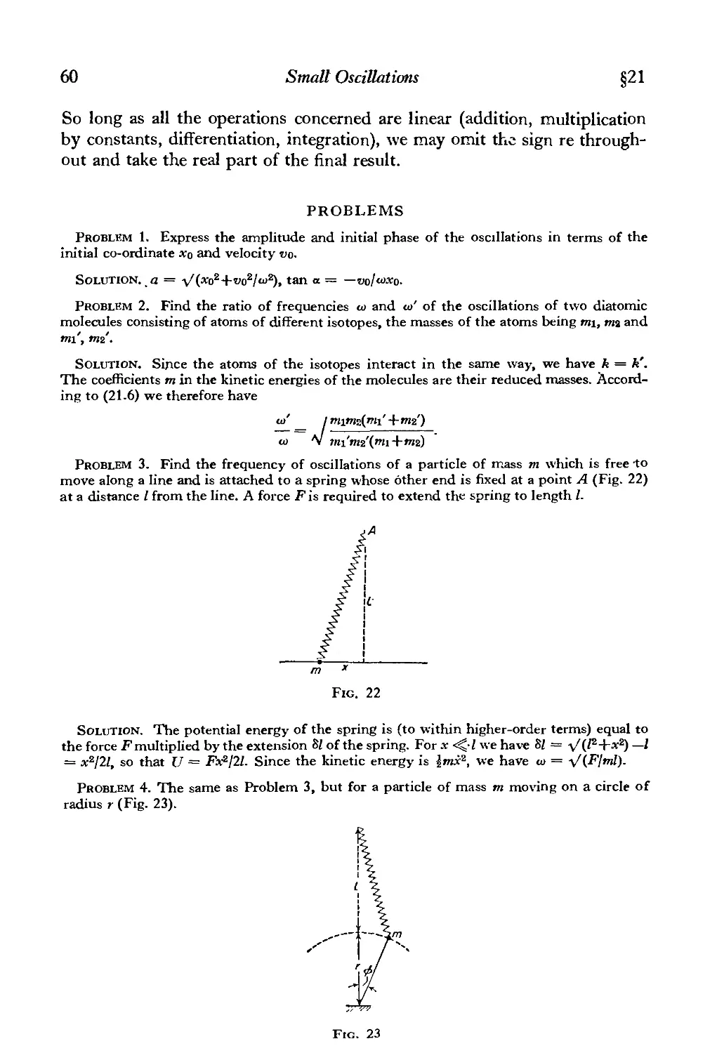
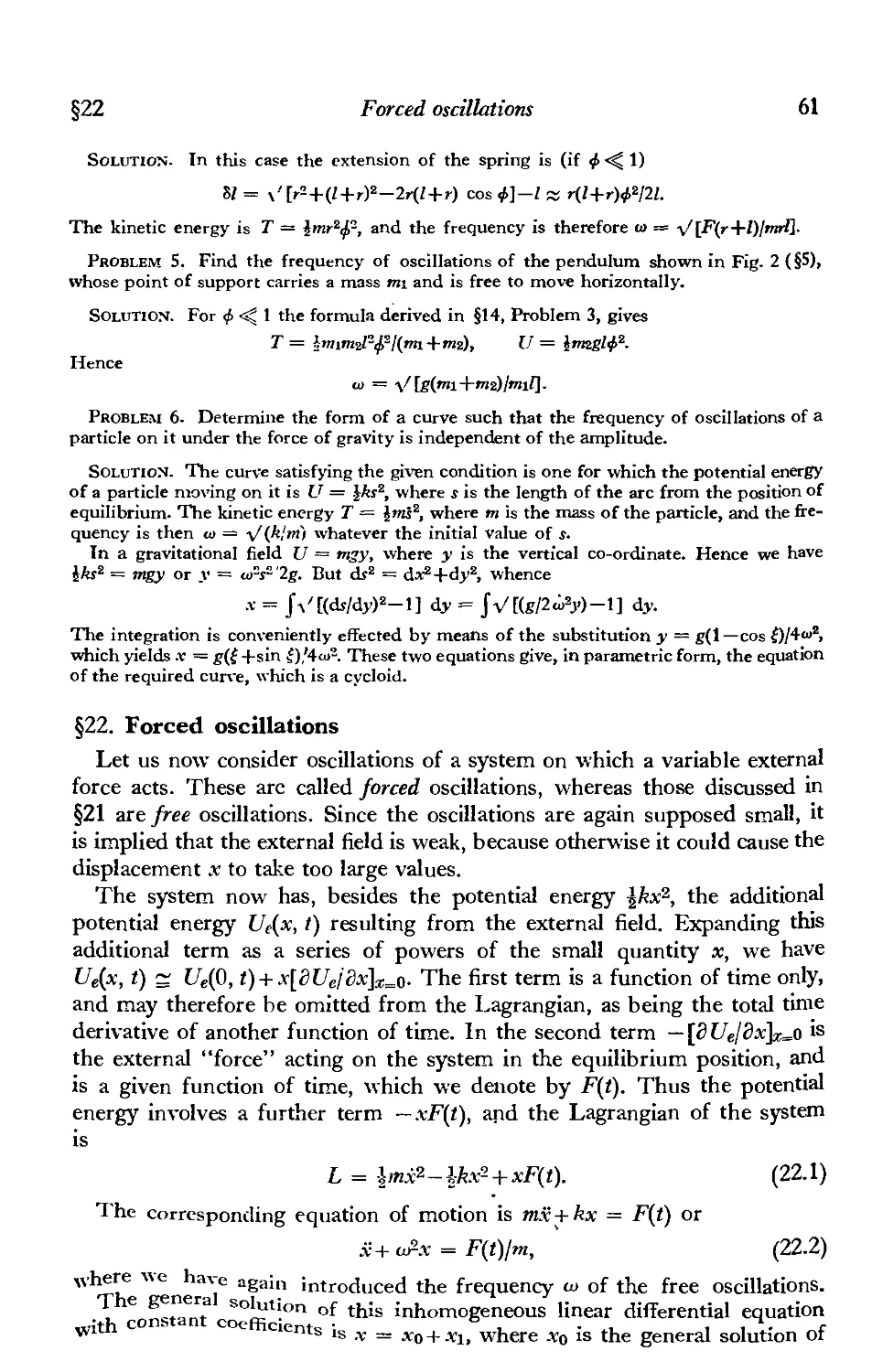
Formulae C.3) and C.4) are called a Galilean transformation. Galileo's
relativity principle can be formulated as asserting the invariance of the mech-
mechanical equations of motion under any such transformation.
§4. The Lagrangian for a free particle
Let us now go on to determine the form of the Lagrangian, and consider
first of all the simplest case, that of the free motion of a particle relative to
an inertial frame of reference. As we have already seen, the Lagrangian in
this case can depend only on the square of the velocity. To discover the form
of this dependence, we make use of Galileo's relativity principle. If an inertial
frame К is moving with an infinitesimal velocity e relative to another inertial
frame K', then v' = v+e. Since the equations of motion must have the same
form in every frame, the Lagrangian L(w2) must be converted by this trans-
transformation into a function L' which differs from £(w2), if at all, only by the
total time derivative of a function of co-ordinates and time (see the end of
§2).
t This assumption does not hold good in relativist» mechanics.
§4 The Lagrangian for a free particle 7
We have U = L(v'2) = L(v2 + 2v • e + e2). Expanding this expression in
powers of e and neglecting terms above the first order, we obtain
8L
2y.e.
cv2
The second term on the right of this equation is a total time derivative only
if it is a linear function of the velocity v. Hence dLJdv2 is independent of the
velocity, i.e. the Lagrangian is in this case proportional to the square of the
velocity, and we write it as
L = \mvL. D.1)
From the fact that a Lagrangian of this form satisfies Galileo's relativity
principle for an infinitesimal relative velocity, it follows at once that the
Lagrangian is invariant for a finite relative velocity V of the frames К and K'.
For
V = \mo'* = Ьп(м+ VJ =
or
V =
The second term is a total time derivative and may be omitted.
The quantity m which appears in the Lagrangian D.1) for a freely moving
particle is called the mass of the particle. The additive property of the Lagran-
Lagrangian shows that for a system of particles which do not interact we havef
L= B^»2- D-2)
It should be emphasised that the above definition of mass becomes mean-
meaningful only when the additive property is taken into account. As has been
mentioned in §2, the Lagrangian can always be multiplied by any constant
without affecting the equations of motion. As regards the function D.2), such
multiplication amounts to a change in the unit of mass; the ratios of the masses
of different particles remain unchanged thereby, and it is only these ratios
which are physically meaningful.
It is easy to see that the mass of a particle cannot be negative. For, according
to the principle of least action, the integral
2
5 = j %mvzdt,
l
has a minimum for the actual motion of the particle in space from point 1 to
point 2. If the mass were negative, the action integral would take arbitrarily
large negative values for a motion in which the particle rapidly left point 1
and rapidly approached point 2, and there would be no minimum.t
t We shall use the suffixes a, b, c, ... to distinguish the various particles, and i, k,l, ... to
distinguish the co-ordinates.
* The argument is not affected by the point mentioned in the first footnote to §2; for
tn < 0, the integral could not have a minimum even for a short segment of the path.
8 The Equations of Motion §5
It is useful to notice that
г.2 = (d//dfJ= (d/J(dfJ. D.3)
Hence, to obtain the Lagrangian, it is sufficient to find the square of the ele-
element of arc d/ in a given system of co-ordinates. In Cartesian co-ordinates,
for example, d/2 = dx2 + dy2 + dz2, and so
L = \т(х2+у2+&). D.4)
In cylindrical co-ordinates d/2 = dr2 + r2 d<j>2+ds2, whence
L = \m(r2+,fy+z2). D.5)
In spherical co-ordinates d/2 = dr* + r2 d02 + r2sin20 d<£2, and
L = \m(r2 + гФ + гЦ2 sin20). D.6)
§5. The Lagrangian for a system of particles
Let us now consider a system of particles which interact with one another
but with no other bodies. This is called a closed system. It is found that the
interaction between the particles can be described by adding to the Lagran-
Lagrangian D.2) for non-interacting particles a certain function of the co-ordinates,
which depends on the nature of the interaction, f Denoting this function
by — U, we have
L= 2lm^a2-U(rhr2,...), E.1)
where г„ is the radius vector of the ath. particle. This is the general form of
the Lagrangian for a closed system. The sum T = 2 imavaz is called the
kinetic energy, and U the potential energy, of the system. The significance
of these names is explained in §6.
The fact that the potential energy depends only on the positions of the
particles at a given instant shows that a change in the position of any particle
instantaneously affects all the other particles. We may say that the inter-
interactions are instantaneously propagated. The necessity for interactions in
classical mechanics to be of this type is closely related to the premises upon
which the subject is based, namely the absolute nature of time and Galileo's
relativity principle. If the propagation of interactions were not instantaneous,
but took place with a finite velocity, then that velocity would be different in
different frames of reference in relative motion, since the absoluteness of
time necessarily implies that the ordinary law of composition of velocities is
applicable to all phenomena. The laws of motion for interacting bodies would
then be different in different inertial frames, a result which would contradict
the relativity principle.
In §3 only the homogeneity of time has been spoken of. The form of the
Lagrangian E.1) shows that time is both homogeneous and isotropic, i.e. its
t This statement is valid in classical mechanics. Relativistic mechanics is not considered
in this book.
§5 The Lagrangian for a system of particles 9
properties are the same in both directions. For, if t is replaced by — t, the La-
Lagrangian is unchanged, and therefore so are the equations of motion. In other
words, if a given motion is possible in a system, then so is the reverse motion
(that is, the motion in which the system passes through the same states in
the reverse order). In this sense all motions which obey the laws of classical
mechanics are reversible.
Knowing the Lagrangian, we can derive (the equations.of motion:
d 8L dL
/5 2)
At 3va 8та
Substitution of E.1) gives
d* = -ги,!гт„. E.3)
In this form the equations of motion are called Newton's equations and form
the basis of the mechanics of a system of interacting particles. The vector
F = -BUIdta E.4)
which appears on the right-hand side of equation E.3) is called the force on
the flth particle. Like U, it depends only on the co-ordinates of the particles,
and not on their velocities. The equation E.3) therefore shows that the acceler-
acceleration vectors of the particles are likewise functions of their co-ordinates only.
The potential energy is defined only to within an additive constant, which
has no effect on the equations of motion. This is a particular case of the non-
uniqueness of the Lagrangian discussed at the end of §2. The most natural
and most usual way of choosing this constant is such that the potential energy
tends to zero as the distances between the particles tend to infinity.
If we use, to describe the motion, arbitrary generalised co-ordinates qt
instead of Cartesian co-ordinates, the following transformation is needed to
obtain the new Lagrangian:
28fa
-^-qn, etc.
Substituting these expressions in the function L = \Ъта{ха2 + ya2 + za2)- U,
we obtain the required Lagrangian in the form
- ЩЯ), E.5)
Lie
where the ащ are functions of the co-ordinates only. The kinetic energy in
generalised co-ordinates is still a quadratic function of the velocities, but it
may depend on the co-ordinates also.
Hitherto we have spoken only of closed systems. Let us now consider a
system A which is not closed and interacts with another system В executing
a given motion. In such a case we say that the system A moves in a given
external field (due to the system B). Since the equations of motion are obtained
10 The Equations of Motion §5
from the principle of least action by independently varying each of the co-
coordinates (i.e. by proceeding as if the remainder were given quantities), we
can find the Lagrangian La of the system A by using the Lagrangian L of
the whole system A + B and replacing the co-ordinates qв therein by given
functions of time.
Assuming that the system A + B is closed, we have L = Ta{qa-, 4a) +
+ Ts{qB, 4b) — UDa, Яв), where the first two terms are the kinetic energies of
the systems A and В and the third term is their combined potential energy.
Substituting for qs the given functions of time and omitting the term
T[qd.t), fs@] which depends on time only, and is therefore the total time
derivative of a function of time, we obtain La = Ta^a, $а)— Щ$а, ?в(')]-
Thus the motion of a system in an external field is described by a Lagrangian
of the usual type, the only difference being that the potential energy may
depend explicitly on time.
For example, when a single particle moves in an external field, the general
form of the Lagrangian is
L=bmP-U(r,t), E.6)
and the equation of motion is
mv = -dUjdr. E.7)
A field such that the same force F acts on a particle at any point in the field
is said to be uniform. The potential energy in such a field is evidently
[/= -Ft. E.8)
To conclude this section, we may make the following remarks concerning
the application of Lagrange's equations to various problems. It is often
necessary to deal with mechanical systems in which the interaction between
different bodies (or particles) takes the form of constraints, i.e. restrictions on
their relative position. In practice, such constraints are effected by means of
rods, strings, hinges and so on. This introduces a new factor into the problem,
in that the motion of the bodies results in friction at their points of contact,
and the problem in general ceases to be one of pure mechanics (see §25). In
many cases, however, the friction in the system is so slight that its effect on
the motion is entirely negligible. If the masses of the constraining elements of
the system are also negligible, the effect of the constraints is simply to reduce
the number of degrees of freedom s of the system to a value less than 7>N. To
determine the motion of the system, the Lagrangian E.5) can again be used,
with a set of independent generalised co-ordinates equal in number to the
actual degrees of freedom.
PROBLEMS
Find the Lagrangian for each of the following systems when placed in a uniform gravita-
gravitational field (acceleration g).
§5 The Lagrangian for a system of particles
Problem 1. A coplanar double pendulum (Fig. 1).
11
Fig. 1
Solution. We take as co-ordinates the angles 4>i and фг which the strings h and h make
with the vertical. Then we have, for the particle mi, Ti = Jmi/i2^i2, U = —migh cos $i. In
order to find the kinetic energy of the second particle, we express its Cartesian co-ordinates
X2, уг (with the origin at the point of support and the >-axis vertically downwards) in terms
of the angles 4>i and фг: хг "= li sin фг +& sin фг, уг = h cos фх -\-1г cos фг. Then we find
Тг =
Finally
L =
cos фг.
Problem 2. A simple pendulum of mass тг, with a mass mi at the point of support which
can move on a horizontal line lying in the plane in which тг moves (Fig. 2).
Fig. 2
Solution. Using the co-ordinate x of mi and the angle ф between the string and the
vertical, we have
L = J(mi+ma)x2+iTOB(^2+2K^ cos ^)+m2|r'cos ф.
Problem 3. A simple pendulum of mass m whose point of support (a) moves uniformly
on a vertical circle with constant frequency у (Fig. 3), (b) oscillates horizontally in the plane
of motion of the pendulum according to the law x = a cos yt, (c) oscillates vertically accord-
'ng to the law у = a cos yt.
Solution, (a) The co-ordinates of m are x = a cos yt+l sin ф, у = — a sin yt+l cos ф.
The Lagrangian is
L = lml*J?+mlay* smtf-yt)+mgl cos Ф;
here terms depending only on time have been omitted, together with the total time derivative
of mlay cos(^—yt).
12
The Equations of Motion
(b) The co-ordinates of m are x = a cos yt+l sin ф, у = I cos <f>. The Lagrangian is (omit-
(omitting total derivatives)
L = iml^+nday* cos yt sin ^+»<g/ cos ф.
(c) Similarly
i = 1т1гф2+т1ауг cos yf cos ф+mgl cos ^.
Fig. 3
Problem 4. The system shown in Fig. 4. The particle mz moves on a vertical axis and the
whole system rotates about this axis with a constant angular velocity fi.
Solution. Let в be the angle between one of the segments a and the vertical, and ф the
angle of rotation of the system about the axis; ф = Cl. For each particle mi, the infinitesimal
displacement is given by d/i2 = a2 d62+o2 sin2 в 6ф2. The distance of тг from the point
of support A is 2a cos 6, and so dlz = —2o sin 8 dfi. The Lagrangian is
L = mio2F2+fi2sin2e)+2»»2a262 sin2e+2(wi+ma)|ra cos 6.
CHAPTER II
CONSERVATION LAWS
§6. Energy
During the motion of a mechanical system, the 2s quantities qt and q{
(i = 1, 2,..., s) which specify the state of the system vary with time. There
exist, however, functions of these quantities whose values remain constant
during the motion, and depend only on the initial conditions. Such functions
are called integrals of the motion.
The number of independent integrals of the motion for a closed mechanical
system with s degrees of freedom is 2s— 1. This is evident from the following
simple arguments. The general solution of the equations of motion contains
2s arbitrary constants (see the discussion following equation B.6)). Since the
equations of motion for a closed system do not involve the time explicitly,
the choice of the origin of time is entirely arbitrary, and one of the arbitrary
constants in the solution of the equations can always be taken as an additive
constant Jo in the time. Eliminating t + to from the 2s functions qi = qt{t + to,
C\, Co,.... C2S-1), qi = qi{t + to, C\, Сг, .... C2s_i), we can express the 2s—\
arbitrary constants C\, C2,..., C2S-1 as functions of q and q, and these functions
will be integrals of the motion.
Not all integrals of the motion, however, are of equal importance in mech-
mechanics. There are some whose constancy is of profound significance, deriving
from the fundamental homogeneity and isotropy of space and time. The
quantities represented by such integrals of the motion are said to be conserved,
and have an important common property of being additive: their values for a
system composed of several parts whose interaction is negligible are equal
to the sums of their values for the individual parts.
It is to this additivity that the quantities concerned owe their especial
importance in mechanics. Let us suppose, for example, that two bodies
interact during a certain interval of time. Since each of the additive integrals
of the whole system is, both before and after the interaction, equal to the
sum of its values for the two bodies separately, the conservation laws for these
quantities immediately make possible various conclusions regarding the state
of the bodies after the interaction, if their states before the interaction are
known.
Let us consider first the conservation law resulting from the homogeneity
of time. By virtue of this homogeneity, the Lagrangian of a -' osed system
does not depend explicitly on time. The total time derivative of the Lagran-
Lagrangian can therefore be written
13
14 Conservation Laws §^
If L depended explicitly on time, a term dLJdt would have to be added on
the right-hand side. Replacing BL/dqi, in accordance with Lagrange's equa-
equations, by (djdt) dLjdqi, we obtain
d/BL\ ^ dL
2 a I cL\
or
Hence we see that the quantity
2BL
qt—r-L F.1)
i
remains constant during the motion of a closed system, i.e. it is an integral
of the motion; it is called the energy of the system. The additivity of the
energy follows immediately from that of the Lagrangian, since F.1) shows
that it is a linear function of the latter.
The law of conservation of energy is valid not only for closed systems, but
also for those in a constant external field (i.e. one independent of time): the
only property of the Lagrangian used in the above derivation, namely that
it does not involve the time explicitly, is still valid. Mechanical systems whose
energy is conserved are sometimes called conservative systems.
As we have seen in §5, the Lagrangian of a closed system (or one in a
constant field) is of the form L = T(q, q) — U(q), where Г is a quadratic
function of the velocities. Using Euler's theorem on homogeneous functions,
we have
2BL
dqt
dqt
Substituting this in F.1) gives
E=T(q,q)+U{q); F-2)
in Cartesian co-ordinates,
2,...). F-3)
§7 Momentum 15
Thus the energy of the system can be written as the sum of two quite different
terms: the kinetic energy, which depends on the velocities, and the potential
energy, which depends only on the co-ordinates of the particles.
§7. Momentum
A second conservation law follows from the homogeneity of space. By virtue
of this homogeneity, the mechanical properties of a closed system are un-
unchanged by any parallel displacement of the entire system in space. Let us
therefore consider an infinitesimal displacement e, and obtain the condition
for the Lagrangian to remain unchanged.
A parallel displacement is a transformation in which every particle in the
system is moved by the same amount, the radius vector r becoming r+e.
The change in L resulting from an infinitesimal change in the co-ordinates,
the velocities of the particles remaining fixed, is
Sra = e-> ,
a a
where the summation is over the particles in the system. Since с is arbitrary,
the condition 8L = 0 is equivalent to
^8Ll8ra = 0. G.1)
a
From Lagrange's equations E.2) we therefore have
2d 8L d ■t-n BL
. X _ о
dt d\a dt *-< dva
a a
Thus we conclude that, in a closed mechanical system, the vector
P s ^ SLlSva G.2)
remains constant during the motion; it is called the momentum of the system.
Differentiating the Lagrangian E.1), we find that the momentum is given in
terms of the velocities of the particles by
P= ]>>ava. G.3)
The additivity of the momentum is evident. Moreover, unlike the energy,
the momentum of the system is equal to the Sum of its values pa = mava for
the individual particles, whether or not the interaction between them can be
neglected.
The three components of the momentum vector are all conserved only in
the absence of an external field. The individual components may be conserved
even in the presence of a field, however, if the potential energy in the field does
not depend on all the Cartesian co-ordinates. The mechanical properties of
16 Conservation Laws §8
the system are evidently unchanged by a displacement along the axis of a
co-ordinate which does not appear in the potential energy, and so the corre-
corresponding component of the momentum is conserved. For example, in a uni-
uniform field in the г-direction, the x and у components of momentum are
conserved.
The equation G.1) has a simple physical meaning. The derivative
дЦдта = — dUJdra is the force Fa acting on the ath particle. Thus equation
G.1) signifies that the sum of the forces on all the particles in a closed system
is zero:
2Fo = 0. G.4)
a
In particular, for a system of only two particles, Fi + F-2 = 0: the force exerted
by the first particle on the second is equal in magnitude, and opposite in direc-
direction, to that exerted by the second particle on the first. This is the equality
of action and reaction (Newton's third law).
If the motion is described by generalised co-ordinates qu the derivatives
of the Lagrangian with respect to the generalised velocities
pt = dLjdqt G.5)
are called generalised momenta, and its derivatives with respect to the general-
generalised co-ordinates
Ft = BLIdqf G.6)
are called generalised forces. In this notation, Lagrange's equations are
Pi = Ft. G.7)
In Cartesian co-ordinates the generalised momenta are the components of the
vectors po. In general, however,- the p{ are linear homogeneous functions of
the generalised velocities qt, and do not reduce to products of mass and velo-
velocity.
PROBLEM
A particle of mass m moving with velocity Vi leaves a half-space in which its potential energy
is a constant U\ and enters another in which its potential energy is a different constant Г/г.
Determine the change in the direction of motion of the particle.
Solution. The potential energy is independent of the co-ordinates whose axes are parallel
to the plane separating the half-spaces. The component of momentum in that plane is
therefore conserved. Denoting by" 01 and 02 the angles between the normal to the plane and
the velocities Vi and V2 of the particle before and after passing the plane, we have vi sin 01
= vz sin 62. The relation between t'1 and г'2 is given by the law of conservation of energy,
and the result is
sin 01 /Г
sin 02 V L
1+ a
§8. Centre of mass
The momentum of a closed mechanical system has different values in
different (inertial) frames of reference. If a frame K' moves with velocity V
§8 Centre of mass 17
relative to another frame A', then the velocities vo' and va of the particles
relative to the two frames are such that va = va' + V. The momenta P and P'
in the two frames are therefore related by
p =
or
(8-1)
In particular, there is always a frame of reference K' in which the total
momentum is zero. Putting P' = 0 in (8.1), we find the velocity of this frame:
v = p/2m« = 2m»v«/2w«- (8-2)
If the total momentum of a mechanical system in a given frame of reference
is zero, it is said to be at rest relative to that frame. This is a natural generali-
generalisation of the term as applied to a particle. Similarly, the velocity V given by
(8.2) is the velocity of the "motion as a whole" of a mechanical system whose
momentum is not zero. Thus we see that the law of conservation of momen-
momentum makes possible a natural definition of rest and velocity, as applied to a
mechanical system as a whole.
Formula (8.2) shows that the relation between the momentum P and the
velocity V of the system is the same as that between the momentum and velo-
velocity of a single particle of mass [л = Цта, the sum of the masses of the particles
in the system. This result can be regarded as expressing the additivity of mass.
The right-hand side of formula (8.2) can be written as the total time deriva-
derivative of the expression
R = ]>>ere/ Jm,,. (8.3)
We can say that the velocity of the system as a whole is the rate of motion in
space of the point whose radius vector is (8.3). This point is called the centre
of mass of the system.
The law of conservation of momentum for a closed system can be formu-
formulated as stating that the centre of mass of the system moves uniformly in a
straight line. In this form it generalises the law of inertia derived in §3 for a
single free particle, whose "centre of mass" coincides with the particle itself.
In considering the mechanical properties of a closed system it is natural
to use a frame of reference in which the centre of mass is at rest. This elimi-
eliminates a uniform rectilinear motion of the system as a whole, but such motion
is of no interest.
The energy of a mechanical system which is at rest as a whole is usually
called its internal energy Et. This includes the kinetic energy of the relative
motion of the particles in the system and the potential energy of their inter-
interaction. The total energy of a system moving as a whole with velocity V can
be written
E = frVZ + Et. (8.4)
18 Conservation Laws §9
Although this formula is fairly obvious, we may give a direct proof of it.
The energies E and E' of a mechanical system in two frames of reference К
and K' are related by
= F + X-F+frV*. (8.5)
This formula gives the law of transformation of energy from one frame to
another, corresponding to formula (8.1) for momentum. If the centre of mass
is at rest in K', then P' = 0, E' = E(, and we have (8.4).
PROBLEM
Find the law of transformation of the action 5 from one inertial frame to another.
Solution. The Lagrangian is equal to the difference of the kinetic and potential energies,
and is evidently transformed in accordance with a formula analogous to (8.5):
Integrating this with respect to time, we obtain the required law of transformation of the
action:
where R' is the radius vector of the centre of mass in the frame K'.
§9. Angular momentum
Let us now derive the conservation law which follows from the isotropy of
space. This isotropy means that the mechanical properties of a closed system
do not vary when it is rotated as a whole in any manner in space. Let us there-
therefore consider an infinitesimal rotation of the system, and obtain the condition
for the Lagrangian to remain unchanged.
We shall use the vector 8ф of the infinitesimal rotation, whose magnitude
is the angle of rotation Ьф, and whose direction is that of the axis of rotation
(the direction of rotation being that of a right-handed screw driven along 8ф).
Let us find, first of all, the resulting increment in the radius vector from
an origin on the axis to any particle in the system undergoing rotation. The
linear displacement of the end of the radius vector is related to the angle by
|8r| = r sin в Ц (Fig. 5). The direction of 8r is perpendicular to the plane
of r and 8ф. Hence it is clear that
Sr = 5фхг. (9л)
Angular momentum
19
When the system is rotated, not only the radius vectors but also the velocities
of the particles change direction, and all vectors are transformed in the same
manner. The velocity increment relative to a fixed system of co-ordinates is
Sv = 8ф xv.
(9.2)
Ъф
Fig. 5
If these expressions are substituted in the condition that the Lagrangian is
unchanged by the rotation:
■^-n / 8L 8L \
8L = Z I^T" Вга + ^Г' Sv°) = °
a
and the derivative dLjdva replaced by pa, and 8Lj8ra by pa, the result is
2(ра'5фхго+ра.8фхго) = 0
a
or, permuting the factors and taking 8ф outside the sum,
d
dt
a a
Since 8ф is arbitrary, it follows that (d/d£) £га х po = 0, and we conclude
that the vector
M =
(9.3)
called the angular momentum or moment of momentum of the system, is con-
conserved in the motion of a closed system. Like the linear momentum, it is
additive, whether or not the particles in the system interact.
There are no other additive integrals of the motion. Thus every closed
system has seven such integrals: energy, three components of momentum,
and three components of angular momentum.
Since the definition of angular momentum involves the radius vectors of
the particles, its value depends in general on the choice of origin. The radius
20 Conservation Laws §9
vectors ro and ra' of a given point relative to origins at a distance a apart are
related by ro = ra' + a. Hence
м =
= M' + axP. (9.4)
It is seen from this formula that the angular momentum depends on the
choice of origin except when the system is at rest as a whole (i.e. P = 0).
This indeterminacy, of course, does not affect the law of conservation of
angular momentum, since momentum is also conserved in a closed system.
We may also derive a relation between the angular momenta in two inertial
frames of reference К and K\ of which the latter moves with velocity V
relative to the former. We shall suppose that the origins in the frames К and
K' coincide at a given instant. Then the radius vectors of the particles are the
same in the two frames, while their velocities are related by va = va' + V.
Hence we have
M = ~^viaraxva = ^inaXa xva'+ 2ma
The first sum on the right-hand side is the angular momentum M' in the
frame K'; using in the second sum the radius vector of the centre of mass
(8.3), we obtain
M = M' + fiRxV. (9.5)
This formula gives the law of transformation of angular momentum from one
frame to another, corresponding to formula (8.1) for momentum and (8.5)
for energy.
If the frame K' is that in which the system considered is at rest as a whole,
then V is the velocity of its centre of mass, /j\ its total momentum P relative
to K, and
M = M' + RxP. (9.6)
In other words, the angular momentum M of a mechanical system consists
of its "intrinsic angular momentum" in a frame in which it is at rest, and the
angular momentum R x P due to its motion as a whole.
Although the law of conservation of all three components of angular
momentum (relative to an arbitrary origin) is valid only for a closed system,
the law of conservation may hold in a more restricted form even for a system
in an external field. It is evident from the above derivation that the component
of angular momentum along an axis about which the field is symmetrical is
always conserved, for the mechanical properties of the system are unaltered
by any rotation about that axis. Here the angular momentum must, of
course, be denned relative to an origin lying on the axis.
§9 Angular momentum 21
The most important such case is that of a centrally symmetric field or central
field, i.e. one in which the potential energy depends only on the distance from
some particular point (the centre). It is evident that the component of angular
momentum along any axis passing through the centre is conserved in motion
in such a field. In other words, the angular momentum M is conserved pro-
provided that it is defined with respect to the centre of the field.
Another example is that of a homogeneous field in the г-direction; in such
a field, the component Mz of the_angtflar momentum is conserved, whichever
point is taken as the origin.
The component of angular momentum along any axis (say the г-axis) can
be found by differentiation of the Lagrangian:
where the co-ordinate ф is the angle of rotation about the л-axis. This is
evident from the above proof of the law of conservation of angular momentum,
but can also be proved directly. In cylindrical co-ordinates г, ф, z we have
(substituting xa = ra cos фа, ya = ra sin фа)
Мг = ^та{хауаУаа)
a
= ^тпгаЦа. (9.8)
a
The Lagrangian is, in terms of these co-ordinates,
and substitution of this in (9.7) gives (9.8).
PROBLEMS
Problem 1. Obtain expressions for the Cartesian components and the magnitude of the
angular momentum of a particle in cylindrical co-ordinates г, ф, z.
Solution. Mx = mfrz—zr) sin ф—mrzj, cos Ф,
My = —ni{rz—zr) cos ф—mrzi, sin ф,
Мг = тгЦ,
М- = nrr^
Problem 2. The same as Problem 1, but in spherical co-ordinates г, в, ф.
Solution. Mx = —тгЦб sin ф+ф sin в cos в cos Ф),
My = тг\в cos ф—i> sin в cos в sin ф),
Мг = mr2j, sin20,
М- = т2г*F-+фг sin2»).
Problem 3. Which components of momentum P and angular momentum M are conserved
in motion in the following fields?
(a) the field of an infinite homogeneous plane, (b) that of an infinite homogeneous cylinder,
(c) that of an infinite homogeneous prism, (d) that of two ppints, (e) that of an infinite homo-
homogeneous half-plane, (f) that of a homogeneous cone, (g) that of a homogeneous circular torus,
(h) that of an infinite homogeneous cylindrical helix.
22 Conservation Laws §Ю
Solution, (a) Px, Py, Mz (if the plane is the *y-plane), (b) Mz, Pz (if the axis of the
cylinder is the z-axis), (с) Рг (if the edges of the prism are parallel to the z-axis),
(d) Mz (if the line joining the points is the z-axis), (e) Py (if the edge of the half-
plane is the y-axis), (f) Mz (if the axis of the cone is the z-axis), (g) Mz (if the axis
of the torus is the z-axis), (h) the Lagrangian is unchanged by a rotation through an angle
8ф about the axis of the helix (let this be the z-axis) together with a translation through a
distance hbij>j2-n along the axis (h being the pitch of the helix). Hence SL = Sz BLl8z +
ф Щдф = H(hPzl2-n+Mz) = О, so that Mz+hPzlln = constant.
§10. Mechanical similarity
Multiplication of the Lagrangian by any constant cleany does not affect
the equations of motion. This fact (already mentioned in §2) makes possible,
in a number of important cases, some useful inferences concerning the pro-
properties of the motion, without the necessity of actually integrating the equa-
equations.
Such cases include those where the potential energy is a homogeneous
function of the co-ordinates, i.e. satisfies the condition
[/(arx, ar2,.... arra) = a*t/(ri, r2,..., rra), A0.1)
where a is any constant and k the degree of homogeneity of the function.
Let us carry out a transformation in which the co-ordinates are changed by
a factor a and the time by a factor j8: ro -> aro, t ~> j8f. Then all the velocities
vo = drajdt are changed by a factor a/j8, and the kinetic energy by a factor
a2//?2. The potential energy is multiplied by a*. If a and j8 are such that
a2//?2 = a*, i.e. j8 = a1"**, then the result of the transformation is to multiply
the Lagrangian by the constant factor a*, i.e. to leave the equations of motion
unaltered.
A change of all the co-ordinates of the particles by the same factor corre-
corresponds to the replacement of the paths of the particles by other paths, geometri-
geometrically similar but differing in size. Thus we conclude that, if the potential energy
of the system is a homogeneous function of degree k in the (Cartesian) co-
coordinates, the equations of motion permit a series of geometrically similar
paths, and the times of the motion between corresponding points are in the
ratio
fit = (I'llI-™, (Ю.2)
where /'// is the ratio of linear dimensions of the two paths. Not only the times
but also any mechanical quantities at corresponding points at corresponding
times are in a ratio which is a power of /'//■ For example, the velocities,
energies and angular momenta are such that
vjv (f/Q, E'/E =
^ The following are some examples of the foregoing.
As we shall see later, in small oscillations the potential energy is a quadratic
function of the co-ordinates (k = 2). From A0.2) we find that the period of
such oscillations is independent of their amplitude.
§10 Mechanical similarity 23
In a uniform field of force, the potential energy is a linear function of the
co-ordinates (see E.8)), i.e. k = 1. From A0.2) we have t'jt = y/(l'jl).
Hence, for example, it follows that, in fall under gravity, the time of fall is as
the square root of the initial altitude.
In the Newtonian attraction of two masses or the Coulomb interaction of
two charges, the potential energy is inversely proportional to the distance
apart, i.e. it is a homogeneous function of degree k= — 1. Then t'jt
— C/03'2' anc' we can state, for instance, that the square of the time of revolu-
revolution in the orbit is as the cube of the size of the orbit (Kepler's third law).
If the potential energy is a homogeneous function of the co-ordinates and
the motion takes place in a finite region of space, there is a very simple relation
between the time average values of the kinetic and potential energies, known
as the -cirial theorem.
Since the kinetic energy Г is a quadratic function of the velocities, we have
by Euler's theorem on homogeneous functions Y,\a'dTjd\a = 2T, or, put-
putting 8Tj8va = pO) the momentum,
it = 2po- vo = —( 2p«- r«)- 2r«- p«- A0-4)
a Ot и а
Let us average this equation with respect to time. The average value of any
function of time/(f) is defined as
1 Г
/= lim- \f(t)dt.
It is easy to see that, if/(*) is the time derivative dF(t)jdt of a bounded func-
function F(t), its mean value is zero. For
. 1 f dF
f = lim - dt = lim
T-*° rjdt T^ro
Let us assume that the system executes a motion in a finite region of space
and with finite velocities. Then 2po • ro is bounded, and the mean value of
the first term on the right-hand side of A0.4) is zero. In the second term we
replace pa by ~3Uj8ra in accordance with Newton's equations E.3), obtain-
obtaining!
A0.5)
a
If the potential energy is a homogeneous function of degree k in the radius
vectors ro, then by Euler's theorem equation A0.5) becomes the required
relation:
2T = kC. A0.6)
t The expression on the right of A0.5) is sometimes called the virial of the system.
24 Conservation Laws §10
Since T+ U = E = E, the relation A0.6) can also be expressed as
U = 2E,\k + 2), T = kE,l(k + 2), (Ю.7)
which express £7 and T in terms of the total energy of the-system.
~ In particular, for small oscillations (k = 2) we have T = U, i.e. the mean
values of the kinetic and potential energies are equal. For a Newtonian inter-
interaction (k = —lJT= —U, and E = — T, in accordance with the fact that,
in such an interaction, the motion takes place in a finite region of space only
if the total energy is negative (see §15).
PROBLEMS
Problem 1. Find the ratio of the times in the same path for particles having different
masses but the same potential energy.
Solution, t'jt = \/(m','m).
Problem 2. Find the ratio of the times in the same path for particles having the same mass
but potential energies differing by a constant factor.
Solution, t'lt = л/A//1/').
CHAPTER III
INTEGRATION OF THE EQUATIONS OF MOTION
§11. Motion in one dimension
The motion of a system having one degree of freedom is said to take place
in one dimension. The most general form of the Lagrangian of such a system
in fixed external conditions is
l = M<?)<?2- u(q), (ii.i)
where a(q) is some function of the generalised co-ordinate q. In particular,
if q is a Cartesian co-ordinate (x, say) then
Ь = \тх2-Щх). A1.2)
The equations of motion corresponding to these Lagrangians can be inte-
integrated in a general form. It is not even necessary to write down the equation
of motion; we can start from the first integral of this equation, which gives
the law of conservation of energy. For the Lagrangian A1.2) (e.g.) we have
\тхг-\- U{x) = E. This is a first-order differential equation, and can be inte-
integrated immediately. Since dx/df = д/{2[Е— U(x)]/?n}, it follows that
Г Ax
t = л/(\т) hconstant. (П.З)
The two arbitrary constants in the solution of the equations of motion are
here represented by die total energy E and the constant of integration.
Since the kinetic energy is essentially positive, the total energy always
exceeds the potential energy, i.e. the motion can take place only in those
regions of space where U(x) < E. For example, let the function U(x) be
of the form shown in Fig. 6 (p. 26). If we draw in the figure a horizontal
line corresponding to a given value of the total energy, we immediately find
the possible regions of motion. In the example of Fig. 6, the motion can
occur only in the range AB or in the range to the right of C.
The points at which the potential energy equals the total energy,
U[x) = E, A1.4)
give the limits of the motion. They are turning points, since the velocity there
is zero. If the region of the motion is bounded by two such points, then the
motion takes place in a finite region of space, and is said to be finite. If the
region of the motion is limited on only one side, or on neither, then the
motion is infinite and the particle goes to infinity.
25
26
Integration of the Equations of Motion
§11
A finite motion in one dimension is oscillatory, the particle moving re-
repeatedly back and forth between two points (in Fig. 6, in the potential well
AB between the points x\ and x?). The period T of the oscillations, i.e. the
time during which the particle passes from x\ to x% and back, "is twice the time
from xx to x2 (because of the reversibility property, §5) or, by A1.3),
T(E) =
2(E
С
J
(Jv;
A1.5)
where x± and xi are roots of equation A1.4) for the given value of E. This for—-
mula gives the period of the motion as a function of the total energy of the
particle.
■U=E
Fig. 6
PROBLEMS
Proble.ni 1. Determine the period of oscillations of a simple pendulum (a particle of mass
m suspended by a string of length /in a gravitational field) as a function of the amplitude of
the oscillations.
SOLUTION. The energy of the pendulum is E = bml2<j>2—mgl cos <£== — mgl cos ^o, where
ф is the angle fcetween the string and the vertical, and ^o the maximum value of <f>. Calculating
the peijiod as thVtime required to go from ф = 0 to ф = ^o, multiplied by four, we find
т =
V(cos ^—cos ^o)
The substitution sin f = sin J^/sin Ьфо converts this to T = 4\/(l/g)K(sin iфo), where
l-*2s;n^)
is the complete elliptic integral of the first kind. For sin 1фо
an expansion of the function К gives
Г = 2-nV(llgH- + М°г+ ■■■)■
(small oscillations),
§12 Determination of the potential energy
The first term corresponds to the familiar formula.
27
Problem 2. Determine the period of oscillation, as a function of the energy, when a
particle of mass m moves in fields for which the potential energy is
(a) U = A\x\", (b) U = -I/o/cosh2ccv, -I/o < E < 0, (c) U = Uo tan2a*.
Solution, (a):
= 2 /?!!L./^V/n[^^-
N E \A) J V(l->'")'
By the substitution yn = и the integral is reduced to a beta function, which can be expressed
in terms of gamma functions:
2-пт
(I)""
The dependence of T on E is in accordance with the law of mechanical similarity A0.2),
A0.3).
<b) T = (w/«)
(с) Г = (W«)
§12. Determination of the potential energy from the period of
oscillation
Let us consider to what extent the form of the potential energy U(x) of a
field in which a particle is oscillating can be deduced from a knowledge of the
period of oscillation Г as a function of the energy E. Mathematically, this
involves the solution of the integral equation A1.5), in which U(x) is regarded
as unknown and T[E) as known.
We shall assume that the required function U(x) has only one minimum
in the region of space considered, leaving aside the question whether there
exist solutions of the integral equation which do not meet this condition.
For convenience, we take the origin at the position of minimum potential
energy, and take this minimum energy to be zero (Fig. 7).
Fig. 7
28 Integration of the Equations of Motion §12
In the integral (П.5) we regard the co-ordinate x as a function of U. The
function x(U) is two-valued: each value of the potential energy corresponds
to two different values of x. Accordingly, the integral A1.5) must be divided
into two parts before replacing Ax by (dxjdU) dU: one from л: = л* to x = 0
and the other from x = 0 to x = x%. We shall write the function x(U) in
these two ranges as x = x\[U) and x = x-z[U) respectively.
The limits of integration with respect to U are evidently E and 0, so that
we have
Edx2{U) dU rdx^U) dU
Г dx-zOJ) dU Г
T(E) = л/Bm) —— + \'{2m)
K ' K ' J dU V(E-V) J
^/{ ) dU л/(£- V)
о i?
If both sides of this equation are divided by \/(ol— E), where a is a parameter,
and integrated with respect to E from 0 to a, the result is
T(E)dE f Г \dx2 dxi] dUdE
Г T{E)dE Г г rdx2
J V(«-^) = VBW) J J Ldt/
0 0 0
or, changing the order of integration,
J ■\/{a.~E) J laU dl/J J v[(a~
о о и
The integral over E is elementary; its value is тт. The integral over U is
thus trivial, and we have
С T(E)dE
0
since X2@) = xi@) = 0. Writing U in place of a, we obtain the final result:
= I . A2.1)
Thus the known function T(E) can be used to determine the difference
x£U)-Xi{U). The functions X2(U) and Xl(U) themselves remain indeter-
indeterminate. This means that there is not one but an infinity of curves V _ (J(x)
§13 The reduced mass 29
which give the prescribed dependence of period on energy, and differ in such
a way that the difference between the two values of x corresponding to each
value of U is the same for every curve.
The indeterminacy of the solution is removed if we impose the condition
that the curve U = U(x) must be symmetrical about the [/-axis, i.e. that
X2(U) = -xi(U) s x(U). In this case, formula A2.1) gives for x(U) the
unique expression
1 VrT(E)AE
, ' FV A2.2)
§13. The reduced mass
A complete general solution can be obtained for an extremely important
problem, that of the motion of a system consisting of two interacting particles
(the two-body problem).
As a first step towards the solution of this problem, we shall show how it
can be considerably simplified by separating the motion of the system into
the motion of the centre of mass and that of the particles relative to the centre
of mass.
The potential energy of the interaction of two particles depends only on
the distance between them, i.e. on the magnitude of the difference in their
radius vectors. The Lagrangian of such a system is therefore
L = 4fwi*i2+jjft2*22- t/fln-ral). A3.1)
Let r = n — гг be the relative position vector, and let the origin be at the
centre of mass, i.e. т+гх + то^ = О. These two equations give
rx = т2г!(т1 + п12), r2 = - »Jir, {ni\ + m2). A3-2)
Substitution in A3.1) gives
L = frn&-U(r), A3.3)
where
m = »ii;H2/'(»ii + »*2) A3-4)
is called the reduced mass. The function A3.3) is formally identical with the
Lagrangian of a particle of mass m moving in an external field U(r) which is
symmetrical about a fixed origin.
Thus the problem of the motion of two interacting particles is equivalent
to that of the motion of one particle in a given external field U(r). From the
solution r = r(t) of this problem, the paths rx = n(t) and r2 = r2(t) of the
two particles separately, relative to their common centre of mass, are obtained
by means of formulae A3.2).
30 Integration of the Equations of Motion §14
PROBLEM
A system consists of one particle of mass M and n particles with equal masses m. Eliminate
the motion of the centre of mass and so reduce the problem to one involving n particles.
Solution. Let R be the radius vector of the particle of mass M, and Ro (a = 1, 2, ..., n)
those of the particles of mass m. We put ro = Ro-R and take the origin to be at the centre
of mass: MR+7b!Ro = 0. Hence R = — («и//*)#£га, where /*==Л/ + nm\ Ra = R + rc.
Substitution in the Lagrangian L = i-l/R2 + J»n £RO2 — JJ gives
L = h
The potential energy depends only on the distances between the particles, and so can be
written as a function of the ro.
§14. Motion in a central field
On reducing the two-body problem to one of the motion of a single body,
we arrive at the problem of determining the motion of a single particle in an
external field such that its potential energy depends only on the distance r
from some fixed point. This is called a central field. The force acting on the
particle is F = ~8U{r)j£r = — (dtT,dr)r/r; its magnitude is likewise a func-
function of r only, and its direction is everywhere that of the radius vector.
As has already been shown in §9, the angular momentum of any system
relative to the centre of such a field is conserved. The angular momentum of a
single particle is M = r x p. Since M is perpendicular to r, the constancy of
M shows that, throughout the motion, the radius vector of the particle lies
in the plane perpendicular to M.
Thus the path of a particle in a central field lies in one plane. Using polar
co-ordinates г, ф in that plane, we can write the Lagrangian as
L=\r4fi + r*4?)-U(ryt A4.1)
see D.5). This function does not involve the co-ordinate ф explicitly. Any
generalised co-ordinate qi which does not appear explicitly in the Lagrangian
is said to be cyclic. Tor such a co-ordinate we have, by Lagrange's equation,
(ddf) dL'cqi = 3L:Bqi = 0, so that the corresponding generalised momen-
momentum pi = dLjcqi is an integral of the motion. This leads to a considerable
simplification of the problem of integrating the equations of motion when
there are cyclic co-ordinates.
In the present case, the generalised momentum p^ = тг2ф is the same as
the angular momentum Mz = -1/ (see (9.6)), and we return to the known law
of conservation of angular momentum:
M = тг-ф = constant. (H.2)
This law has a simple geometrical interpretation in the plane motion of a single
particle in a central field. The expression ir • гАф is the area of the sector
bounded by two neighbouring radius vectors and an element о е path
§14 Motion in a central field 31
(Fig. 8). Calling this area d/, we can write the angular momentum of the par-
particle as
M = 2?nf, A4.3)
where the derivative / is called the sectorial velocity. Hence the conservation
of angular momentum implies the constancy of the sectorial velocity: in equal
times the radius vector of the particle sweeps out equal areas {Kepler's second
Flo. 8
The complete solution of the problem of the motion of a particle in a central
field is most simply obtained by starting from the laws of conservation of
energy and angular momentum, without writing out the equations of motion
themselves. Expressing ф in terms of M from A4.2) and substituting in the
expression for the energy, we obtain
E = \т(г°- + гЦ2) + U[r) = \mr2 + Ш2>>2 + L\r). A4.4)
Hence
, * П^Е-иы-Щ (,4.5)
At V \m m2r2)
or, integrating,
Г I 1B M2\
t= \ Ar \—[E-U(r)] + constant. A4.6)
J / V [m m2r2i
Writing A4.2) as d^ = M Atjmr2, substituting At from A4.5) and integrating,
we find
r MArlr*
ф = h constant. A4.7)
Formulae A4.6) and A4.7) give the general solution of the problem. The
latter formula gives the relation between r and ф, i.e. the equation of the path.
Formula A4.6) gives the distance r from the centre as an implicit function of
time. The angle ф, it should be noted, always varies monotonically with time,
since A4.2) shows that ф can never change sign.
t The law of conservation of angular momentum for a particle moving in a central field
is sometimes called the area integral.
32 Integration ofthe Equations ofMotion §14
The expression A4.4) shows that the radial part of the motion can be re-
regarded as taking place in one dimension in a field where the "effective poten-
potential energy" is
A4.8)
The quantity M2[2mr2 is called the centrifugal energy. The values of r for which
U{r) + M2j2mr2 = E A4.9)
determine the limits of the motion as regards distance from the centre.
When equation A4.9) is satisfied, the radial velocity r is zero. This does not
mean that the particle comes to rest as in true one-dimensional motion, since
the angular velocity ф is not zero. The value f — 0 indicates a turni?ig point
of the path, where r{t) begins to decrease instead of increasing, or vice versa.
If the range in which r may vary is limited only by the condition r ^ rmin.
the motion is infinite: the particle comes from, and returns to, infinity.
If the range of r has two limits rmin and rmax, the motion is finite and the
path lies entirely within the annulus bounded by the circles r = rmax and
r = Tmin- This does not mean, however, that the path must be a closed curve.
During the time in which r varies from rmax to rm\n and back, the radius
vector turns through an angle Аф which, according to A4.7), is given by
Mdrli*
A4.10)
The condition for the path to be closed is that this angle should be a rational
fraction of 2tt, i.e. that Д^ = Ъпт\п, where m and n are integers. In that case,
after»/? periods, the radius vector of the particle will have made m complete
revolutions and will occupy its original position, so that the path is closed.
Such cases are exceptional, however, and when the form of U(r) is arbitrary
the angle Д^ is not a rational fraction of 2tt. In general, therefore, the path
of a particle executing a finite motion is not closed. It passes through the
minimum and maximum distances an infinity of times, and after infinite time
it covers the entire annulus between the two bounding circles. The path
shown in Fig. 9 is an example.
There are only two types of central field in which all finite motions take
place in closed paths. They are those in which the potential energy of the
particle varies as \jr or as r2. The former case is discussed in §15; the latter
is that of the space oscillator (see §23, Problem 3).
At a turning point the square root in A4.5), and therefore the integrands
in A4.6) and A4.7), change sign. If the angle ф is measured from the direc-
direction of the radius vector to the turning point, the parts of the path on each
side of that point differ only in the sign of ф for each value of r, i.e. the path
is symmetrical about the line ф = 0. Starting, say, from a point wh.^e^ ~ rmax
the particle traverses a segment of the path as far as a point wi r _ rmln>
§14
Motion in a central field
33
then follows a symmetrically placed segment to the next point where r — rmax,
and so on. Thus the entire path is obtained by repeating identical segments
forwards and backwards. This applies also to infinite paths, which consist of
two symmetrical branches extending from the turning point (r = гт\п) to
infinity.
Fig. 9
The presence of the centrifugal energy when M Ф 0, which becomes
infinite as 1/r2 when r -> 0, generally renders it impossible for the particle to
reach the centre of the field, even if the field is an attractive one. A "fall" of
the particle to the centre is possible only if the potential energy tends suffi-
sufficiently rapidly to — oo as r -> 0. From the inequality
irmr2 = E- 1]{г)-МЦ2тг2 > 0,
or r2U(r) + M2l2m < Er2, it follows that r can take values tending to zero
only if
[г2Щг)]гл < -Щ2т, A4.11)
i.e. U(r) must tend to — oo either as — a/r2 with a > M2[2m, or proportionally
to — ljrn with n > 2.
PROBLEMS
Problem 1. Integrate the equations of motion for a spherical pendulum (a particle of mass
m moving on the surface of a sphere of radius I in a gravitational field).
Solution. In spherical co-ordinates, with the origin at the centre of the sphere and the
polar axis vertically downwards, the Lagrangian of the pendulum is
cos в.
34 Integration of the Equations of Motion §14
The co-ordinate ф is cyclic, and hence the generalised momentum p., which is the same as the
z-component of angular momentum, is conserved:
ml-ф sin20 = MZ — constant. A)
The energy is
E = *т!-(в--+ф2 sinW)—mgl cos в
B)
= imFtP+lM.*'ml- sin2e~mgl cos 0.
Hence
Г d0
I . /Г1Г17 ГГ /3\"W— -f>l> V '
where the "effective potential energy" is
t/eff@) = hMz-'ml2 sin-e-m»l cos 0.
For the angle ф we find, using A),
Mt Г d0
Ф = f 41
ЫBт) Jsin2tf\'[£:-t/(e)]' V
The integrals C) and D) lead to elliptic integrals of the first and third kinds respectively.
The range of 0 in which the motion takes place is that «-here E > Uett, and its limits
are given by the equation E = [/err- This is a cubic equation for cos 0, having two roots
between —1 and +1; these define two circles of latitude on the sphere, between which the
path lies.
Problem 2. Integrate the equations of motion for a particle moving on the surface of a
cone (of vertical angle 2x) placed vertically and with vertex downwards in a gravitational
field.
Solution. In spherical co-ordinates, with the origin at the vertex of the cone and the
polar axis vertically upwards, the Lagrangian is Jm(rs +г2ф2 sin2cn)—mgr cos a. The co-
coordinate ф is cyclic, and Mz = тг2ф s'm-a. is again conserved. The energy is
E =
By the same method as in Problem 1, we find
f
J V{[£f7errC)]'«7
^ f *
VBm) sin2* J г2\'[Е-£Л.-гг
Mz2
\-mgr cos г.
a
2mr2 sin2 a
The condition E = Uett(r) is (if Mz ф 0) a cubic equation for r, having two positive roots;
these define two horizontal circles on the cone, between which the path lies.
Problem 3. Integrate the equations of motion for a pendulum of mass mz, with a mass mi
at the point of support which can move on a horizontal line lying in the plane in which nn
moves (Fig. 2, §5).
Solution. In the Lagrangian derived in §5, Problem 2, the co-ordinate x is cyclic. The
generalised momentum Pz, which is the horizontal component of the total momentum of the
system, is therefore conserved:
Px = (mi+mz)x+т?1ф cos ф ~ constant. A)
The system may always be taken to be at rest as a whole. Then the constant in A) ,s 2ero
and integration gives
(mi + mrfx+mzl sin ф = constant, B)
which expresses the fact that the centre of mass of the system does not m i n2ontally.
§15
Kepler's problem
35
Using A), we find the energy in the form
E =
cos2^ ) —rmgl cos <f>.
C)
Hence
-J-
u
E + ttlegl COS ф
Expressing the co-ordinates .V2 = x+l sin ф, у = I cos ф of the particle 7712 in terms of ф
by means of B), we find that its path is an arc of an ellipse with horizontal semi-
axis lmil(vn +7K2) and vertical semi-axis /. As thi -» со we return to the familiar simple pen-
pendulum, which moves in an arc of a circle.
§15. Kepler's problem
An important class of central fields is formed by those in which the poten-
potential energy is inversely proportional to r, and the force accordingly inversely
proportional to r2. They include the fields of Newtonian gravitational attrac-
attraction and of Coulomb electrostatic interaction; the latter may be either attrac-
attractive or repulsive.
Let us first consider an attractive field, where
и=-ф A5.1)
with a. a positive constant. The "effective" potential energy
АГ-
Uett = —
2mA
A5.2)
is of the form shown in Fig. 10. As r -> 0, Ueii tends to + oo, and as r -> oo
it tends to zero from negative values; for r = M2/ma it has a minimum value
[/efl.min= -mx*'2№. A5.3)
Fig. 10
It is seen at once from Fig. 10 that the motion is finite for E < 0 and infinite
for E > 0.
36
Integration of the Equations of Motion
§15
The shape of the path is obtained from the general formula A4.7)- Substi-
Substituting there Г = —o.r and effecting the elementary integration, we have
(Л//г)
о = cos 1
//
[ZwE +
V \ If2 /
—■ + constant.
A5.4)
Taking the origin of ф such that the constant is zero, and putting
p = .If2/»!*, e = VH +B£JJ2/iHa2)],
we can write the equation of the path as
pl'r = 1 + ccos^. A5.5)
This is the equation of a conic section with one focus at the origin; 2/> is called
the latiis rectum of the orbit and e the eccentricity. Our choice of the origin of ф
is seen from A5.5) to be such that the point where ф = 0 is the point nearest
to the origin (called the perihelion).
In the equivalent problem of two particles interacting according to the law
A5.1), the orbit of each particle is a conic section, with one focus at the centre
of mass of the two particles.
It is seen from A5.4) that, if E < 0, then the eccentricity e < 1, i.e. the
orbit is an ellipse (Fig. 11) and the motion is finite, in accordance with what
has been said earlier in this section. According to the formulae of analytical
geometry, the major and minor semi-axes of the ellipse are
a = p,'(l - ?-) = a/2|E|, b = p\/(\ - <?) = M, д 'B»i!£|).
A5.6)
Fig. 11
The least possible value of the energy is A5.3), and then e — 0, i.e. the ellipse
becomes a circle. It may be noted that the major axis of the ellipse depends
only on the energy of the particle, and not on its angular momentum. The
least and greatest distances from the centre of the field (the focus of the
ellipse) are
rmin = A'(l + e) = «0 - e)> 'мх = />,'(! - e) = «С1 + еУ A5.7)
These expressions, with a and e given by A5.6) and A5.4), ran, of course,
also be obtained directly as the roots of the equation Uett(.r) ~~ '
§15
Kepler's problem
37
The period T of revolution in an elliptical orbit is conveniently found by
using the law of conservation of angular momentum in the form of the area
integral A4.3). Integrating this equation with respect to time from zero to
T, we have 2mf = TM, where / is the area of the orbit. For an ellipse
/ = -nab, and by using the formulae A5.6) we find
T = 27ras/W{mh
= ™л\т12\Е\*). A5.8)
The proportionality between the square of the period and the cube of the
linear dimension of the orbit has already been demonstrated in §10. It may
also be noted that the period depends only on the energy of the particle.
For E > 0 the motion is infinite. If E > 0, the eccentricity e > 1, i.e. the
the path is a hyperbola with the origin as internal focus (Fig. 12). The dis-
distance of the perihelion from the focus is
rm.n =/>/(*+1) =«(«-!), A5-9)
where a = pj{e2- 1) = y.!2E is the "semi-axis" of the hyperbola.
Fig. 12
If E = 0, the eccentricity e = 1, and the particle moves in a parabola with
perihelion distance rmJn = \p- This case occurs if the particle starts from rest
at infinity.
The co-ordinates of the particle as functions of time in the orbit may be
found by means of the general formula A4.6). They may be represented in a
convenient parametric form as follows.
Let us first consider elliptical orbits. With a and e given by A5.6) and A5.4)
we can write the integral A4.6) for the time as
t = J^j —Tdr
rAr
У та г
a J
38 Integration of the Equations of Motion §15
The obvious substitution r — a= -aecos £ converts the integral to
/та3 Г inia3
t= / (l-ecosf)df = / (I-e sin Л + constant.
If time is measured in such a way that the constant is zero, we have the
following parametric dependence of ron(:
r= a(l — e cos£), t = \/(ma3'y.)(g—eung), A5.10)
the particle being at perihelion at 1= 0. The Cartesian co-ordinates
x = r cos ф, у = r sin ф (the x and у axes being respectively parallel to the
major and minor axes of the ellipse) can likewise be expressed in terms of
the parameter g. From A5.5) and A5.10) we have
ex = p — r = a[\ — e2) — йA — е cos£) = flf(cos£— e);
у is equal to -\/[r2—x2). Thus
x = a(cos£-e), у = ах A-е2) sinf. A5.11)
A complete passage round the ellipse corresponds to an increase of £ from 0
to 2-n.
Entirely similar calculations for the hyperbolic orbits give
r = e(ecosh£— 1), t = \/(ma31 <x)(es'mht; — g),
x = a(e— cosh£), у = a\ \e2— 1) sinh£,
where the parameter £ varies from — oo to + oo.
Let us now consider motion in a repulsive field, where
U = ot/г (a > 0). A5.13)
Here the effective potential energy is
a M2
and decreases monotonically from + oo to zero as r varies from zero to
infinity. The energy of the particle must be positive, and the motion is always
infinite. The calculations are exactly similar to those for the attractive field.
The path is a hyperbola:
pjr = -\+есовф, A5.14)
where p and e are again given by A5.4). The path passes the centre of the
field in the manner shown in Fig. 13. The perihelion distance is
fmin = />/(«-!)= «(«+!)• A5Л5)
The time dependence is given by the parametric equations
r = a(ecoshf+l), t = V(ma3l*)(esinhS + ^' A5.16)
-1) sinh f'
x = «(cosh f + e), у =■■ «v'(«2
§15
Kepler's problem
39
To conclude this section, we shall show that there is an integral of the mo-
motion which exists only in fields U = ajr (with either sign of a). It is easy to
verify by direct calculation that the quantity
vxM + ar/V A5.17)
is constant. For its total time derivative is v x M + av/r - ar(v • r)/r3 or,
since M = mrxv,
mr(v v) — wv(r- v) + av/r —ar(v r),V3.
Putting »iv = ar/r3 from the equation of motion, we find that this expression
vanishes.
Fig. 13
The direction of the conserved vector A5.17) is along the major axis from
the focus to the perihelion, and its magnitude is cue. This is most simply
seen by considering its value at perihelion.
It should be emphasised that the integral A5.17) of the motion, like M and
E, is a one-valued function of the state (position and velocity) of the particle.
We shall see in §50 that the existence of such a further one-valued integral
is due to the degeneracy of the motion.
PROBLEMS
Problem 1. Find the time dependence of the co-ordinates of a particle with energy E = 0
moving in a parabola in a field U = —a.jr.
Solution. In the integral
rdr
V[Ba/m)/—(M2,'»
we substitute r = МЦ1 +rf)l2ma. = Jp(l +v2), obtaining the following parametric form of
the required dependence:
' = */>(! +v2), t --
x = 4/41 ~v2), у = p-q.
40 Integration of the Equations of Motion §15
The parameter ij varies from —oo to +00.
Problem 2. Integrate the equations of motion for a particle in a central field
U = -ф2 (a > 0).
Solution. From formulae A4.6) and A4.7) we have, if ф and fare appropriately measured,
(b) for * > 0 and
(c) for ,, 0 and
In all three cases
In cases (b) and (c) the particle "falls" to the centre along a path which approaches the
origin as ф -*■ oo. The fall from a given value of r takes place in a finite time, namely
Problem 3. When a small correction &[/(/■) is added to the potential energy U = —air,
the paths of finite motion are no longer closed, and at each revolution the perihelion is dis-
displaced through a small angle 8^. Find 8^ when (a) 8[7 = /3/r2, (b) 8[7 = yjr3.
Solution. When r varies from гт\ч to i-max and back, the angle ф varies by an amount
A4.10), which we write as
in order to avoid the occurrence of spurious divergences. We put U = —a/r + 8[7, and
expand the integrand in powers of 8[7; the zero-order term in the expansion gives 2ir, and
the first-order term gives the required change 8^:
2mSUdr
\
where we have changed from the integration over r to one over ф, along the path of the "un-
"unperturbed" motion.
In case (a), the integration in A) is trivial: 8^ = —2-n$m\lVP = —2тгР/ар, where 2p A5.4)
is the latus rectum of the unperturbed ellipse. In case (b) r28[7 = yjr and, with l/rjgiven by
A5.5), we have 8^ = —6waym2/M4 = — 6*r/a/>2.
CHAPTER IV
COLLISIONS BETWEEN PARTICLES
§16. Disintegration of particles
In many cases the laws of conservation of momentum and energy alone can
be used to obtain important results concerning the properties of various mech-
mechanical processes. It should be noted that these properties are independent of
the particular type of interaction between the particles involved.
Let us consider a "spontaneous" disintegration (that is, one not due to
external forces) of a particle into two "constituent parts", i.e. into two other
particles which move independently after the disintegration.
This process is most simply described in a frame of reference in which the
particle is at rest before the disintegration. The law of conservation of momen-
momentum shows that the sum of the momenta of the two particles formed in the
disintegration is then zero; that is, the particles move apart with equal and
opposite momenta. The magnitude po of either momentum is given by the
law of conservation of energy:
here mi and m% are the masses of the particles, Ец and Ец their internal
energies, and Ei the internal energy of the original particle. If с is the "dis-
"disintegration energy", i.e. the difference
€ = Et-Eu-E2h A6.1)
which must obviously be positive, then
/1 1 \ ftJ
« = fco8(-+- )=~, A6-2)
\m\ ту 2m
which determines po; here m is the reduced mass of the two particles. The
velocities are »ю = po/m\, W20 = po/mz-
Let us now change to a frame of reference in which the primary particle
moves with velocity V before the break-up. This frame is usually called the
laboratory system, or L system, in contradistinction to the centre-of-mass
system, or С system, in which the total momentum is zero. Let us consider
one of the resulting particles, and let v and vo be its velocities in the L and
the С system-respectively. Evidently v = V + vo, or v -V = vo, and so
*<2 + V*- 2vV cos в = со2, A6.3)
where в is the angle at which this particle moves relative to the direction of
the velocity V- This equation gives the velocity of the particle as a function
42 Collisio?is Between Particles §16
of its direction of motion in the L system. In Fig. 14 the velocity v is repre-
represented by a vector drawn to any point on a circlej of radius vo from a point
A at я distance V from the centre. The cases V < г-о and V > vo are shown
in Figs. 14a, b respectively. In the former case 0 can have any value, but in
the latter case the particle can move only forwards, at an angle 0 which does
not exceed 0max, given by
sin0max = vo/V; A6.4)
this is the direction of the tangent from the point A to the circle.
a e
(b) V>v0
Fig. 14
The relation between the angles 0 and во in the L and С systems is evi-
evidently (Fig. 14)
tan0 = vo sin0o/(wo cos0o+ V). A6.5)
If this equation is solved for cos 0o, we obtain
V I/ Vй \
cos0o= sin20+cos0 /jl sin20). A6.6)
Vo V \ VO2 I
For vo > V the relation between 0o and 0 is one-to-one (Fig. 14a). The plus
sign must be taken in A6.6), so that 0o = 0 when 0 = 0. If vo < V, however,
the relation is not one-to-one: for each value of 0 there are two values of 0o,
which correspond to vectors vo drawn from the centre of the circle to the
points В and С (Fig. 14b), and are given by the two signs in A6.6).
In physical applications we are usually concerned with the disintegration
of not one but many similar particles, arid this raises the problem of the
distribution of the resulting particles in direction, energy, etc. We shall
assume that the primary particles are randomly oriented in space, i.e. iso-
tropically on average.
t More precisely, to any point on a sphere of radius г>о, of which Fig- s ows a diametral
§16 Disintegration of particles 43
In the С system, this problem is very easily solved: every resulting particle
(of a given kind) has the same energy, and their directions of motion are
isotropically distributed. The latter fact depends on the assumption that the
primary particles are randomly oriented, and can be expressed by saying
that the fraction of particles entering a solid angle element doo is proportional
to doo, ie. equal to doo/47r. The distribution with respect to the angle во is
obtained by putting doo = 27rsin во d0o, i.e. the corresponding fraction is
J-sin0od0o. (I6-7)
The corresponding distributions in the L system are obtained by an
appropriate transformation. For example, let us calculate the kinetic energy
distribution in the L system. Squaring the equation v = vo + V, we have
V2 = i;02+F2 + 2^0Fcos во, whence d(cos в0) = d(v2)/2v0V. Using the
kinetic energy T = |w»2, where m is m\ or тяг depending on which kind of
particle is under consideration, and substituting in A6.7), we find the re-
required distribution:
(l/2fKt-0F) AT, A6.8)
The kinetic energy can take values between rmin = \tn{vo — VJ and
^max = \m{vo+V)z. The particles are, according to A6.8), distributed
uniformly over this range.
When a particle disintegrates into more than two parts, the laws of con-
conservation of energy and momentum naturally allow considerably more free-
freedom as regards the velocities and directions of motion of the resulting particles.
In particular, the energies of these particles in the С system do not have
determinate values. There is, however, an upper limit to the kinetic energy
of any one of the resulting particles. To determine the limit, we consider
the system formed by all these particles except the one concerned (whose
mass is m\, say), and denote the "internal energy" of that system by £/.
Then the kinetic energy of the particle m\ is, by A6.1) and A6.2),
?io = po2l2mi = (M-mi)(Ei-Eii-Et')IM, where M is the mass of the
primary particle. It is evident that 7\o has its greatest possible value
when Ei is least. For this to be so, all the resulting particles except m\
must be moving with the same velocity. Then E{ is simply the sum of their
internal energies, and the difference Ег — Ец-Ei is the disintegration
energy с. Thus
7\0,max = (M-mi)ejM. A6.5)
PROBLEMS
Problem 1. Find the relation between the angles 0i, в2 (in the L system) after a disintegra-
disintegration into two particles.
Solution. In the С system, the corresponding angles are related by вы = тт — въо. Calling
#io simply во and using formula A6.5) for each of the two particles, we can put
V+via cos во = mo sin ft^ cot 8i, V—«20 cos во = via sin во cot 02- From these two
equations we must eliminate во. To do so, we first solve for cos во and sin во, and then
44 Collisions Between Particles §17
form the sum of their squares, which is unity. Since «ю/иго = mzlmi we have finally, using
A6.2),
(тог/пи) sin202+(mi/TO2) sina0i —2 sin 0i sin 0г 005(81+62)
*' sin2@t+02).
Problem 2. Find the angular distribution of the resulting particles in the L system.
Solution. When v0 > V, we substitute A6.6), with the plus sign of the radical, in A6.7),
obtaining
Г V 1 +(F2/»o2) cos 20 I
i sin 6 d0 2- cos 0+ K ' / , @ < 0 < *).
L vo v[l — (F^Mr) sina0] J
When 00 < F, both possible relations between 0o and 0 must be taken into account. Since,
when 0 increases, one -value of 0o increases and the other decreases, the difference (not the
sum) of the expressions d cos во with the two signs of the radical in A6.6) must be taken.
The result is
1 (уЬо^ cos 20
sin0d0 ,„* ' ' ■ ,„, (O«0«0ma*).
V [1 —(F2,foo2) sin20]
Problem 3. Determine the range of possible values of the angle в between the directions
of motion of the two resulting particles in the L system.
Solution. The angle в = 61+62, where 61 and 62 are the angles defined by formula A6.5)
(see Problem 1), and it is simplest to calculate the tangent of 8. A consideration of the extreme
of the resulting expression gives the following ranges of в, depending on the relative magni-
magnitudes of V, «io and V20 (for definiteness, we assume «20 > «10): 0 < в < it if ею < V < «го,
я— во < в < я- if V < «ю, 0 < в < 0о if V > «20. The value of в0 is given by
sin 0o= V(vw+V2o)l(V2+VioV2o).
§17. Elastic collisions
A collision between two particles is said to be elastic if it involves no change
in their internal state. Accordingly, when the law of conservation of energy
is applied to such a collision, the internal energy of the particles may be
neglected.
The collision is most simply described in a frame of reference in which the
centre of mass of the two particles is at rest (the С system). As in §16, we
distinguish by the suffix 0 the values of quantities in that system. The velo-
velocities of the particles before the collision are related to their velocities vi and
V2 in the laboratory system by vio = m$v\(m\-\-m<>), V20 = —mfy\{rn\ + m<>),
where v = vi—V2; see A3.2).
Because of the law of conservation of momentum, the momenta of the two
particles remain equal and opposite after the collision, and are also unchanged
in magnitude, by the law of conservation of energy. Thus, in the С system
the collision simply rotates the velocities, which remain opposite in direction
and unchanged in magnitude. If we denote by no a unit vector in the direc-
direction of the velocity of the particle vi\ after the collision, then the velocities
of the two particles after the collision (distinguished by primes) are
vio' = явдепо/От + жг), V20' - -wieno/(«i + ws)- A7.1)
§17 Elastic collisions 45
In order to return to the L system, we must add to these expressions the
velocity V of the centre of mass. The velocities in the L system after the
collision are therefore
vnol(mi + m2) + (mm + m2-v2)l{mx + т2)
No further information about the collision can be obtained from the laws
of conservation of momentum and energy. The direction of the vector no
depends on the law of interaction of the particles and on their relative position
during the collision.
The results obtained above may be interpreted geometrically. Here it is
more convenient to use momenta instead of velocities. Multiplying equations
A7.2) by mi and m2 respectively, we obtain
pi' = mvno + mi(pi+p2)l(mi + m2),
p2 = -mvno + m2(pi+p2)l{mi + m2),
where m = m\m2\{m\ + m2) is the reduced mass. We draw a circle of radius
mv and use the construction shown in Fig. 15. If the unit vector no is along
ОС, the vectors AC and CB give the momenta p^ and рг' respectively.
When pi and p2 are given, the radius of the circle and the points A and В
are fixed, but the point С may be anywhere on the circle.
ОС » mv
*° ^2 (Р| + Рг'
°~В '- iS&L ( Р, * Рг)
Fig. 15
Let us consider in more detail the case where one of the particles {m2, say) is
at rest before the collision. In that case the distance OB = m2pi/(mi+m2) = mv
is equal to the radius, i.e. В lies on the circle. The vector AB is equal to the
momentum pi of the particle tn\ before the collision. The point A lies inside
or outside the circle, according as ni\ < m2 or m\ > tn2. The corresponding
46
Collisions Between Particles
§17
diagrams are shown in Figs. 16a, b. The angles 6X and 62 in these diagrams
are the angles between the directions of motion after the collision and the
direction of impact (i.e. of px). The angle at the centre, denoted by x> which
gives the direction of no, is the angle through which the direction of motion
of mi is turned in the С system. It is evident from the figure that в\ and 62
can be expressed in terms of x by
m2
mi + m2 cos x
A7.4)
(о) Щ< mz
(b) m, >mz
AB-y>l ; АО/OB- m,/mz
Fig. 16
We may give also the formulae for the magnitudes of the velocities of the
two particles after the collision, likewise expressed in terms of x-
cos
mi + mz
)
v,
mi + m2
A7.5)
The sum 61 + 62 is the angle between the directions of motion of the
particles after the collision. Evidently 61 + 62 > \ъ if тг < m%, and 6\ + 64 < \n
if mi > m%.
When the two particles are moving afterwards in the same or in opposite
directions (head-on collision), we have x = ^ yt- ^е P°int С lies on the
diameter through A, and is on OA (Fig. 16b; pi' and p2' in the same direc-
direction) or on О A produced (Fig. 16a; pi' and p2' in opposite directions).
In this case the velocities after the collision are
mi-m2
v,
v2' =
2mi
A7.6)
This value of v2' has the greatest possible magnitude, and the maximum
§17 Elastic collisions 47
energy which can be acquired in the collision by a particle originally at rest
is therefore
4wiW/2
= |»2»2'max2 = ; -El, A7.7)
(ni + mJ
where E\ = \m\v^ is the initial energy of the incident particle.
If mi < in?,, the velocity of ni\ after the collision can have any direction.
If nix > mo,, however, this particle can be deflected only'through an angle
not exceeding 0max from its original direction; this maximum value of в\
corresponds to the position of С for which AC is a tangent to the circle
(Fig. 16b). Evidently
sinflmax = OCIOA = nizlnii. A7.8)
The collision of two particles of equal mass, of which one is initially at
rest, is especially simple. In this case both В and A lie on the circle (Fig. 17).
Fig. 17
Then
h = fo 62 = 4(тг-х), A7.9)
vi = wcos£x> V2 = iJsinlx- A7.10)
After the collision the particles move at right angles to each other.
PROBLEM
Express the velocity of each particle after a collision between a moving particle (mi) and
another at rest (тг) in terms of their directions of motion in the L system.
Solution. From Fig. 16 we have pz = 2OB cos Sz or vz' = 2v{mjtnz) cos Sz. The momen-
momentum pi' = AC is given by ОС2 = AOz+pi'z-2AO . pi cos 0i or
/ш'\2 2mm'
I 1 COS& +
\ v / mz v
tni—тг _
nti-\-tnz
Hence
vi mi 1
; cos 0i+ V(m22—mi2sin80j):
v mi+mz mi+mz
for mi > mz the radical may have either sign, but for тг > mi it must be taken positive.
48 Collisiom Between Particles §18
§18. Scattering
As already mentioned in §17, a complete calculation of the result of a
collision between two particles (i.e. the determination of the angle x) requires
the solution of the equations of motion for the particular law of interaction
involved.
We shall first consider the equivalent problem of the deflection of a single
particle of mass m moving in a field U(f) whose centre is at rest (and is at
the centre of mass of the two particles in the original problem).
As has been shown in §14, the path of a particle in a central field is sym-
symmetrical about a line from the centre to the nearest point in the orbit (OA
in Fig. 18). Hence the two asymptotes to the orbit make equal angles (фо,
say) with this line. The angle x through which the particle is deflected as it
passes the centre is seen from Fig. 18 to be
A8.1)
Fig. 18
The angle фо itself is given, according to A4.7), by
= Г (J4r^ __г A8 2)
'"mln
taken between the nearest approach to the centre and infinity. It should be
recalled that rmln is a zero of the radicand.
For an infinite motion, such as that considered here, it is convenient to
use instead of the constants E and M the velocity rm of the particle at infinity
and the impact parameter p. The latter is the length of the perpendicular
from the centre О to the direction of vm, i.e. the distance at which the particle
would pass the centre if there were no field of force (Fig. 18). The energy
and the angular momentum are given in terms of these quantities by
t. = imz'K,2, M = tnpcco, A8.3)
§18 Scattering 49
and formula A8.2) becomes
00
-J
A8.4)
Together with A8.1), this gives x as a function of p.
In physical applications we are usually concerned not with the deflection
of a single particle but with the scattering of a beam of identical particles
incident with uniform velocity voo on the scattering centre. The different
particles in the beam have different impact parameters and are therefore
scattered through different angles x. Let dN be the number of particles
scattered per unit time through angles between x and X + dy.. This number
itself is not suitable for describing the scattering process, since it is propor-
proportional to the density of the incident beam. We therefore use the ratio
d<j = dNjn, A8.5)
where и is the number of particles passing in unit time through unit area of
the beam cross-section (the beam being assumed uniform over its cross-
section). This ratio has the dimensions of area and is called the effective
scattering cross-section. It is entirely determined by the form of the scattering
field and is the most important characteristic of the scattering process.
We shall suppose that the relation between x ar>d p is one-to-one; this is
so if the angle of scattering is a monotonically decreasing function of the
impact parameter. In that case, only those particles whose impact parameters
lie between p(x) and p(X) + dp(x) are scattered at angles between x anc'
x+dx. The number of such particles is equal to the product of n and the
area between two circles of radii p and p + dp, i.e. dN = 2тгр dp . n. The
effective cross-section is therefore
da = 27rpdp. A8.6)
In order to find the dependence of da on the angle of scattering, we need
only rewrite A8.6) as
da = 27rp(x)|dp(x)/dx| dx. A8.7)
Here we use the modulus of the derivative dp/dx, since the derivative may
be (and usually is) negative, f Often do is referred to the solid angle element
do instead of the plane angle element dx. The solid angle between cones
with vertical angles x and x+dx is do = 2тг sinx dy. Hence we have from
A8.7)
sinXdx|
-I do. A8.8)
50 Collisions Between Particles §18
Returning now to the problem of the scattering of a beam of particles, not
by a fixed centre of force, but by other particles initially at rest, we can say
that A8.7) gives the effective cross-section as a function of the angle of
scattering in the centre-of-mass system. To find the corresponding expression
as a function of the scattering angle в in the laboratory system, we must
express x in A8.7) in terms of в by means of formulae A7.4). This gives
expressions for both the scattering cross-section for the incident beam of
particles (x in terms of 6{) and that for the particles initially at rest (x in terms
of 02).
PROBLEMS
Problem 1. Determine the effective cross-section for scattering of particles from a perfectly
rigid sphere of radius a (i.e. when the interaction is such that U = oo for r < a and U = 0
for r > a).
Solution. Since a particle moves freely outside the sphere and cannot penetrate into it,
the path consists of two straight lines symmetrical about the radius to the point where the
particle strikes, the sphere (Fig. 19). It is evident from Fig. 19 that
p = a sin ^o = a sin Myr~X) = a cos ix-
+
P
Fig. 19
Substituting in A8.7) or A8.8), we have
da = Jto2 sin x dx = \a2 do, A)
i.e. the scattering is isotropic in the С system. On integrating do- over all angles, we find that
the total cross-section a = то2, in accordance with the fact that the "impact area" which the
particle must strike in order to be scattered is simply the cross-sectional area of the sphere.
In order to change to the L system, x must be expressed in terms of 0i by A7.4). The
calculations are entirely similar to those of §16, Problem 2, on account of the formal resemb-
resemblance between formulae A7.4) and A6.5). For mi < tnz (where mi is the mass of the particle
and mi that of the sphere) we have
. ,f., , . o, 1 +("Ч1Ы2 cos 201 1
dtri = la2 2(mi/m2) cos0i+———-— . doi,
L V[l —(mijm2J sin20i] J
where doi = 2-n sin в\ d6i. If, on the other hand, mz < mi, then
' , 1 г 1 +(mi/m2J cos 20i
d iVdO1
V[()
For mi = m8, we have dai = a=|cos 0i| doi, which can also be obtained directly by sub-
substituting x = 201 from A7.9) in A).
§18
Scattering
51
For a sphere originally at rest, x = f—2вг in all cases, and substitution in A) gives
\ dos.
Problem 2. Express the effective cross-section (Problem 1) as a function of the energy e
lost by a scattered particle.
Solution. The energy lost by a particle of mass mi is equal to that gained by the sphere of
mass ms. From A7.5) and A7.7), e = Ег = [2mibn2l(mi+m2J] »co2 sin2ix = «max sin2ix,
whence de = J«max sin x dx; substituting in A), Problem 1, we have do = та2 de/«max. The
scattered particles are uniformly distributed with respect to « in the range from zero to
«max.
Problem 3. Find the effective cross-section as a function of the velocity e» for particles
scattered in a field U ~ Tn.
Solution. According to A0.3), if the potential energy is a homogeneous function of order
k = — n, then similar paths are such that p ~ Vzln, or p = »«T2/n/(x)> the angles of deflec-
deflection x being equal for similar paths. Substitution in A8.6) gives da ~ «<хГ4/п do.
Problem 4. Determine the effective cross-section for a particle to "fall" to the centre of
afield U= -a/r2.
Solution. The particles which "fall" to the centre are those for which 2a > mp2v<x,2 (see
A4.11)), i.e. for which the impact parameter does not exceed pmax = V{la-jmvx?). The
effective cross-section is therefore a = я-pmax2 = l-j
Problem 5. The same as Problem 4, but for a field U = — <x/i-n {n > 2, a > 0).
Solution. The effective potential energy Uett = mps»<x>2/2r2 — a/r" depends on r in the
manner shown in Fig. 20. Its maximum value is
Flc. 20
The particles which "fall" to the centre are those for which I/o < E. The condition I/o = E
gives pm»x, whence
о = T,n{n—2)B-")/п(а/тг)оогJ/".
Problem 6. Determine the effective cross-section for particles of mass tn\ to strike a sphere
of mass тг and radius R to which they are attracted in accordance with Newton's law.
Solution. The condition for a particle to reach the sphere is that /-min < R, where /-mm
is the point on the path which is nearest to the centre of the sphere. The greatest possible
value of p is given by гтщ = R; this is equivalent to Ueit(R) = Eor imiVa^pm^lR^—ajR
—\miv*?, where а — угттг (y being the gravitational constant) and we have put tn X mi on
the assumption that ma > mi. Solving for Pmax2, we finally obtain о = ttR*A +2ymzlRvxs).
52
Collisions Between Particles
§18
When am -> со the effective cross-section tends, of course, to the geometrical cross-section
of the sphere.
Problem 7. Deduce the form of a scattering field I/(r), given the effective cross-section
as a function of the angle of scattering for a given energy E. It is assumed that U(r) decreases
monotonically with r (a repulsive field), with 1/@) > E and Щ со) = 0 (О. В. Firsov 1953).
Solution. Integration of da with respect to the scattering angle gives, according to the
formula
IT
J (da/dx) dX = V,
A)
the square of the impact parameter, so that p(x) (and therefore x0>)) is known.
We put
Then formulae A8.1), A8.2) become
= г
V(xw*-s2) '
B)
C)
where зд(лг) is the root of the equation xto%so)— so2 = 0.
Equation C) is an integral equation for the function iv(s), and may be solved by a method
similar to that used in §12. Dividing both sides of C) by y/(a—x) and integrating with respect
to x from zero to a, we find
С
J
a a so(x)
7r~X(.x) dv Г Г
4»-*) = J J
ds dx
о о
so(a) a
_ Г Г dxds
~ J J v/[(m.2-^)(a-«)]
0 jcUo)
Jo(a)
j- dj
tt
J V,
or, integrating by parts on the left-hand side,
a
/a-J V(x-x)
d.v
This relation is differentiated with respect to a, and then Jo(«) is replaced by s simply;
accordingly a is replaced by szlzv2, and the result is, in differential form,
л/Г/-2/„»2\ vl "
V \\S {Ы ) AJ
This equation can be integrated immediately if the order of integration °^= Q^ ;
side is inverted. Since for s = 0 (i.e. r ->■ oo) we must have w =* * I ' '
^
§19 Rutherford's formula 53
on returning to the original variables r and p, the following two equivalent forms of the final
result:
со
w = expj - cosh~\plrw) (dx/dp) dp!
rw
Li f *<p)dp
This formula determines implicitly the function w{r) (and therefore !/(/•)) for all /• > тыт,
i.e. in the range of r which can be reached by a scattered particle of given energy E.
§19. Rutherford's formula
One of the most important applications of the formulae derived above is
to the scattering of charged particles in a Coulomb field. Putting in A8.4)
U = a/r and effecting the elementary integration, we obtain
= cos-
J>o = cos
whence p2 = (а2/т2т;го4) tan2<£o, or, putting фо = Ь{п~х) fr°m A8.1),
p2 = («2/^2^4) cot2ix. A9.1)
Differentiating this expression with respect to % and substituting in A8.7)
or A8.8) gives
da = 7r(a/W-co2Jcos|xdx/sin3^x A9-2)
or
da = (a/2wrcco2Jdo/sin^-x. A9.3)
This is Rutherford's formula. It may be noted that the effective cross-section
is independent of the sign of a, so that the result is equally valid for repulsive
and attractive Coulomb fields.
Formula A9.3) gives the effective cross-section in the frame of reference
in which the centre of mass of the colliding particles is at rest. The trans-
transformation to the laboratory system is effected by means of formulae A7.4).
For particles initially at rest we substitute x = ^ —202 in A9.2) and obtain
da2 = 2тг(а;'?йГоо2J sin 02 d02;'cos302
= (a/m7;oo2Jdo2/coE302. A9.4)
The same transformation for the incident particles leads, in general, to a very
complex formula, and we shall merely note two particular cases.
If the mass mz of the scattering particle is large compared with the mass
mi of the scattered particle, then x ~ #i and m x mi, so that
da! = (a/4EiJdoi/ein4i0i, A9.5)
where Ei — \m\Va? is the energy of the incident particle.
54 Collisions Between Particles §19
If the masses of the two particles are equal (m\ = тг, т = \m{), then by
A7.9) x = 20i, and substitution in A9.2) gives
da! = 27r(a/£'1Jcose1d01/sin301
= (a/£iJ cos 0X dd/sin^L A9.6)
If the particles are entirely identical, that which was initially at rest cannot
be distinguished after the collision. The total effective cross-section for all
particles is obtained by adding den and dcj2, and replacing 0i and 02 by their
common value 0:
Let us return to the general formula A9.2) and use it to determine the
distribution of the scattered particles with respect to the energy lost in the
collision. When the masses of the scattered (mi) and scattering {mo) particles
are arbitrary, the velocity acquired by the latter is given in terms of the angle
of scattering in the С system by e2' = \bnxl{m\-\-mo)~\i'm sin \x> see A7.5).
The energy acquired by mo, and lost by mi is therefore € = \то,-с<£г
= Bm2lm2)voo2 sin2-|x- Expressing sin \x m terms of € and substituting
in A9.2), we obtain
da = 277(a2W'cc2)dc/c2. A9.8)
This is the required formula: it gives the effective cross-section as a function
of the energy loss €, which takes values from zero to €max =
PROBLEMS
Problem 1. Find the effective cross-section for scattering in a field U = <x,V2 (a > 0).
Solution. The angle of deflection is
The effective cross-section is
do = —-— —^— ■ -^—.
mvx2 хЧ^—х)- sin*
Problem 2. Find the effective cross-section for scattering by a spherical "potential well"
of radius a and "depth" I/o (i.e. a field with U = 0 for r > a and U = — Uo for r < a).
Solution. The particle moves in a straight line which is "refracted" on entering and leav-
leaving the well. According to §7, Problem, the angle of incidence a and the angle of refraction
P (Fig. 21) are such that sin a'sin/3 = n, where n = \/(l +2Uo!mv<x>2). The angle of deflection
is x = 2(<x—/3). Hence
sin(a—ix) . . , 1
= cos ix~c°t * sin iy = —.
sin a n
Eliminating a from this equation and the relation a sin a = p, which is evident from the
diagram, we find the relation between p and x:
n- sin2 ix
P ~~ " «' + 1 —2я cos ix
§20 Small-angle scattering 55
Finally, differentiating, we have the effective cross-section:
a2n2 (n cos Jv—l)(n—cos £x)
da = : do.
4 cos ix (n2 + l~2n cos £xJ
The angle x varies from zero (for p = 0) to Xmax (for p = a), where cos Jxma* = !/«■
The total effective cross-section, obtained by integrating da over all angles within the cone
X < Xmax, 's. of course, equal to the geometrical cross-section то2.
I
Fig. 21
§20. Small-angle scattering
The calculation of the effective cross-section is much simplified if only
those collisions are considered for which the impact parameter is large, so
that the field U is weak 'and the angles of deflection are small. The calculation
can be carried out in the laboratory system, and the centre-of-mass system
need not be used.
We take the л-axis in the direction of the initial momentum of the scattered
particle mi, and the дгу-plane in the plane of scattering. Denoting by pi' the
momentum of the particle after scattering, we evidently have sin 6\ — piy'lpi'.
For small deflections, sin 0i may be approximately replaced by 6\, and p{ in
the denominator by the initial momentum pi = jtiiVcai
01 ^ puf'lmtvco. B0.1)
Next, since p'y = Fy, the total increment of momentum in the j-direction is
CO
fa'= \ FyAt. B0.2)
—CO
The force Fy = -ЩЪу - ~(AU\Ar)ir\dy = -{&U\&r)y\r.
Since the integral B0.2) already contains the small quantity U, it can be
calculated, in the same approximation, by assuming that the particle is not
deflected at all from its initial path, i.e. that it moves in a straight line у = p
with uniform velocity Voo. Thus we put in B0.2) Fy = -{AUldr)p,r,
dt = cLr/Coo. The result is
-if
56 Collisions Between Particles §20
Finally, we change the integration over x to one over r. Since, for a straight
path, r2 = x2+p2, when x varies from — oo to + oo, r varies from oo top
and back. The integral over x therefore becomes twice the integral over r
from p to oo, and dx = r drj\/[r2 — p2). The angle of scattering 6\ is thus
given by|
CO
2o r dU dr
and this is the form of the function 6\(j>) for small deflections. The effective
cross-section for scattering (in the L system) is obtained from A8.8) with в\
instead of x. where sin 6\ may now be replaced by 0i:
dfl,
6л
B0.4)
PROBLEMS
Problem 1. Derive formula B0.3) from A8.4).
Solution. In order to avoid spurious divergences, we write A8.4) in the form
S f IT. p2 2U
В r I г p2
Bp
rmln
and take as the upper limit some large finite quantity R, afterwards taking the value as R -*■ oo.
Since U is small, we expand the square root in powers of U, and approximately replace
rmin by p:
Г pdr В Г
= J 7-V(l-P2/r2) +TP}~
pdr 8 f U(r) dr
Bp .
P D
The first integral tends to Jtt as R -*■ oo. The second integral is integrated by parts, giving
Ю V(r2-p2) dU
В г
= тг-2фо = 2— -
Bp J
-dr
2p Г dU dr
mva2 J dr V(r2-p2) '
p
This is equivalent to B0.3).
Problem 2. Determine the effective cross-section for small-angle scattering in a field
U = air" (n > 0).
t If the above derivation is applied in the С system, the expression obtained for x 1S
same with m in place of mi, in accordance with the fact that the small angles «i an * re
related by (see A7.4)) fli = )
§20 Small-angle scattering 57
Solution. From B0.3) we have
OO
2pin г dr
2pin г dr
1 ~ tniVr? J rn + W(r2-pZ) '
p
The substitution p2jr2 = и converts the integral to a beta function, which can be expressed
in terms of gamma functions:
2W-" Щп + i)
mivr?pn Щп)
Expressing p in terms of 8i and substituting in B0.4), we obtain
-,2ln
L_f V-,ndoi.
CHAPTER V
SMALL OSCILLATIONS
§21. Free oscillations in one dimension
A very common form of motion of mechanical systems is what are called
small oscillations of a system about a position of stable equilibrium. We shall
consider first of all the simplest case, that of a system with only one degree
of freedom.
Stable equilibrium corresponds to a position of the system in which its
potential energy U(q) is a minimum. A movement away from this position
results in the setting up of a force — dUjdq which tends to return the system
to equilibrium. Let the equilibrium value of the generalised co-ordinate
q be qo. For small deviations from the equilibrium position, it is sufficient
to retain the first non-vanishing term in the expansion of the difference
U(q)— U(qo) in powers of q— qo. In general this is the second-order term:
U(q)— U(go) ^ \k(q— qoJ, where k is a positive coefficient, the value of the
second derivative U"(g) for q = qo. We shall measure the potential energy
from its minimum value, i.e. put U(go) = 0, and use the symbol
x=q-qp B1.1)
forthe deviation of the co-ordinate from its equilibrium value. Thus
U(x) = \kx*. B1.2)
The kinetic energy of a system with one degree of freedom is in general
of the form \a(q)q2 = ^a{q)x2. In the same approximation, it is sufficient to
replace the function a(q) by its value at q = qo. Putting for brevity! a(qd) = m,
we have the following expression for the Lagrangian of a system executing
small oscillations in one dimension:!
L = \mx"-\kx". B1.3)
The corresponding equation of motion is
mx + kx=0, B1.4)
or
* + аЯ« = 0, B1.5)
where
ы = v\kjm). B1.6)
t It should be noticed that m is the mass only if x is the Cartesian co-ordinate.
£ Such a system is often called a one-dimensional oscillator.
58
§21 Free oscillations in one dimension 59
Two independent solutions of the linear differential equation B1.5) are
cos cot and sin cot, and its general solution is therefore
x = c\ cos cot + c% sin cot. B1.7)
This expression can also be written
x = acos(o>f + a). B1.8)
Since cos(cot + ot) = cos cot cos a — sin a>£ sin a, a comparison with B1.7)
shows that the arbitrary constants a and a are related to c\ and c% by
a = V(ci2 + C22), tana = -c2/ci. B1.9)
Thus, near a position of stable equilibrium, a system executes harmonic
oscillations. The coefficient a of the periodic factor in B1.8) is called the
amplitude of the oscillations, and the argument of the cosine is their phase;
a is the initial value of the phase, and evidently depends on the choice of
the origin of time. The quantity со is called the angular frequency of the oscil-
oscillations ; in theoretical physics, however, it is usually called simply the fre-
frequency, and we shall use this name henceforward.
The frequency is a fundamental characteristic of the oscillations, and is
independent of the initial conditions of the motion. According to formula
B1.6) it is entirely determined by the properties of the mechanical system
itself. It should be emphasised, however, that this property of the frequency
depends on the assumption that the oscillations are small, and ceases to hold
in higher approximations. Mathematically, it depends on the fact that the
potential energy is a quadratic function of the co-ordinate."}"
The energy of a system executing small oscillations is E = %mx2 + %kx2
or, substituting B1.8),
E = ±тсАР. B1.10)
It is proportional to the square of the amplitude.
The time dependence of the co-ordinate of an oscillating system is often
conveniently represented as the real part of a complex expression:
x = re[A exp(itot)], B1.11)
where A is a complex constant; putting
Л = « exp(/a), B1.12)
we return to the expression B1.8). The constant A is called the complex
amplitude; its modulus is the ordinary amplitude, and its argument is the
initial phase.
The use of exponential factors is mathematically simpler than that of
trigonometrical ones because they are unchanged in form by differentiation.
j. It therefore does not h \л
order, i.e. и . , х„ . d good if the function V(x) has at jf = 0 a minimum of
ri'8her Vlth « > 2; see §11, Problem 2(a).
60 Small Oscillations §21
So long as all the operations concerned are linear (addition, multiplication
by constants, differentiation, integration), we may omit the sign re through-
throughout and take the real part of the final result.
PROBLEMS
Problem 1. Express the amplitude and initial phase of the oscillations in terms of the
initial co-ordinate xo and velocity vo.
Solution, a = \/(xo2+vo2lw2), tan a = —vol^xo.
Problem 2. Find the ratio of frequencies «o and a>' of the oscillations of two diatomic
molecules consisting of atoms of different isotopes, the masses of the atoms being mi, mi and
mi', тг'.
Solution. Since the atoms of the isotopes interact in the same way, we have k = k'.
The coefficients m in the kinetic energies of the molecules are their reduced masses. Accord-
According to B1.6) we therefore have
a) V nil'ffI2'('ni+TOg)
Problem 3. Find the frequency of oscillations of a particle of mass m which is free to
move along a line and is attached to a spring whose other end is fixed at a point A (Fig. 22)
at a distance I from the line. A force F is required to extend the spring to length I.
m *
Fig. 22
Solution. The potential energy of the spring is (to within higher-order terms) equal to
the force F multiplied by the extension S/of the spring. For x <^-/ we have S/ = -^(P+x2)— I
= x2/2l, so that U = Fx2j2l. Since the kinetic energy is imx2, we have w = -\J{Fjnd).
Problem 4. The same as Problem 3, but for a particle of mass m moving on a circle of
radius r (Fig. 23).
Fig. 23
§22 Forced oscillations 61
Solution. In this case the extension of the spring is (if ф <^ 1)
8/ = 4'[r2+(/ + rJ_2r(/ + r) cos ф]-1 ()ф
The kinetic energy is T — ЬпгЦ2, and the frequency is therefore ш = V[F(r+l)ltmi].
Problem 5. Find the frequency of oscillations of the pendulum shown in Fig. 2 (§5),
whose point of support carries a mass mi and is free to move horizontally.
Solution. For ф -^ 1 the formula derived in §14, Problem 3, gives
T = lwim2/2^2/(mi+m2), U =
Hence
<o = V[g(mi+m2)/mif|.
Problem 6. Determine the form of a curve such that the frequency of oscillations of a
particle on it under the force of gravity is independent of the amplitude.
Solution. The curve satisfying the given condition is one for which the potential energy
of a particle moving on it is U = \ksz, where s is the length of the arc from the position of
equilibrium. The kinetic energy T = Jmi2, where m is the mass of the particle, and the fre-
frequency is then w = V'(k!ni) whatever the initial value of s.
In a gravitational field U = tngy, where у is the vertical co-ordinate. Hence we have
iks2 = mgy or у = w-s2'2g. But ds2 = da^+dy2, whence
* = JV[(d*/dyJ-l] dy = JV[(*/2«i»y)-l] dy.
The integration is conveniently effected by means of the substitution у = g(l— cos $/4g>2,
which yields .v = g({ +sin £),'4шг. These two equations give, in parametric form, the equation
of the required сита, which is a cycloid.
§22. Forced oscillations
Let us now consider oscillations of a system on which a variable external
force acts. These arc called forced oscillations, whereas those discussed in
§21 are free oscillations. Since the oscillations are again supposed small, it
is implied that the external field is weak, because otherwise it could cause the
displacement x to take too large values.
The system now has, besides the potential energy %kx2, the additional
potential energy Ue(x, t) resulting from the external field. Expanding this
additional term as a series of powers of the small quantity x, we have
Ue(x, t) ~ Ue@, t) + x[8Uej8x]x=lo- The first term is a function of time only,
and may therefore be omitted from the Lagrangian, as being the total time
derivative of another function of time. In the second term — [d Uejdx^o is
the external "force" acting on the system in the equilibrium position, and
is a given function of time, which we denote by F(t). Thus the potential
energy involves a further term — xF(t), and the Lagrangian of the system
is
L = hnxz - Ш* + xF(t). B2.1)
The corresponding equation of motion is mx + kx = F{t) or
, B2.2)
^rv? e haT agaln introduced the frequency ш of the free oscillations.
The general solution of this inhomogeneous linear differential equation
with conbtant coefficients is x = Xq + Xu where Xo Is the general solutIon of
62 Small Oscillations §22
the corresponding homogeneous equation and x\ is a particular integral of
the inhomogeneous equation. In the present case xo represents the free
oscillations discussed in §21.
Let us consider a case of especial interest, where the external force is itself
a simple periodic function of time, of some frequency y:
F\t)=fcos(Yt+P). B2.3)
We seek a particular integral of equation B2.2) in the form x\ = b cos(yt + j8),
with the same periodic factor. Substitution in that equation gives
b = flm^uP — y2); adding the solution of the homogeneous equation, we
obtain the general integral in the form
x = a cos(iot + a) + [fjm(a^ - y2)] cos(y*+jS). B2.4)
The arbitrary constants a and a are found from the initial conditions.
Thus a system under the action of a periodic force executes a motion which
is a combination of two oscillations, one with the intrinsic frequency a> of
the system and one with the frequency у of the force.
The solution B2.4) is not valid when resonance occurs, i.e. when the fre-
frequency у of the external force is equal to the intrinsic frequency o> of the
system. To find the general solution of the equation of motion in this case,
we rewrite B2.4) as
x =
where a now has a different value. As у -> со, the second term is indetermin-
indeterminate, of the form 0/0. Resolving the indeterminacy by L'Hospital's rule, we
have
x = a cos(ojt +ot) + (fl2moj) t sin(tu* +jS). B2-5)
Thus the amplitude of oscillations in resonance increases linearly with the
time (until the oscillations are no longer small and the whole theory given
above becomes invalid).
Let us also ascertain the nature of small oscillations near resonance, when
у = vj + € with € a small quantity. We put the general solution in the com-
complex form
x = A exp(iwt) + В ехр[г(ш + e)t] = [A + В ex-p(iet)] exp(?W). B2.6)
Since the quantity A + B exp(iet) varies only slightly over the period 2ttJoj
of the factor exp(iwt), the motion near resonance may be regarded as small
oscillations of variable amplitude.| Denoting this amplitude by C, we have
С = \A + B exp(irf)|. Writing A and В in the form а ехр(га) and b exp(?jS)
respectively, we obtain
C2 = a2.+ bz + 2abcos(et + p-!x.). B2-7>
t The "constant" term in the phase of the oscillation also varies.
§22 Forced oscillations 63
Thus the amplitude varies periodically with frequency € between the limits
\a — b\ ^ С ^ a + b. This phenomenon is called beats.4- / '->
The equation of motion B2.2) can be integrated in a general form for an
arbitrary external force F(t). This is easily done by rewriting the equation
as
d 1
—(x + icox) — no(x + iu)x) = —F\t)
dt m
or
df/d/-iaif = F(t)jm, B2.8)
where
£ = x + icox B2.9)
is a complex quantity. Equation B2.8) is of the first order. Its solution when
the right-hand side is replaced by zero is £ = A exp(?W) with constant A.
As before, we seek a solution of the inhomogeneous equation in the form
£ = A(t) exp(icot), obtaining for the function A(t) the equation A(t)
= F(t) exp( — ivjt)jm. Integration gives the solution of B2.9):
t
£ = exp(iarf){ f —F(t) exp( - iu>t) dt + £0 j, B2.10)
о
where the constant of integration £o is the value of £ at the instant t = 0.
This is the required general solution; the function x(t) is given by the imagin-
imaginary part of B2.10), divided by cu.|
The energy of a system executing forced oscillations is naturally not con-
conserved, since the system gains energy from the source of the external field.
Let us determine the total energy transmitted to the system during all time,
assuming its initial energy to be zero. According to formula B2.10), with
the lower limit of integration — oo instead of zero and with £(— oo) = 0,
we have for t -> oo
The energy of the system is
E = ^m(x2 + oAv2) = Jiwlf p. B2.11)
Substituting |f(oo)[2, we obtain the energy transferred:
CO
1 I Г I2
E = F(t)exp(-iojt)dt\ ; Г22.12)
—CO
t The force f-(O must, of CO1,
I cour
se, be written in real form.
64 Small Oscillations §22
it is determined by the squared modulus of the Fourier component of the
force F(t) whose frequency is the intrinsic frequency of the system.
In particular, if the external force acts only during a time short in com-
comparison with 1/cu, we can put exp( — iwt) ~ 1. Then
This result is obvious: it expresses the fact that a force of short duration
gives the system a momentum J Fdt without bringing about a perceptible
displacement.
PROBLEMS
Pr6blem 1. Determine the forced oscillations of a system under a force F(t) of the follow-
following forms, if at time t = 0 the system is at rest in equilibrium (ж = x = 0): (a) F — Fo,
a constant, (b) F = at, (c) F = Fo exp( — at), (d) F = Fo exp(-at) cos /3f.
Solution, (а) я: = (Fojmur)(\ —cos iot). The action of the constant force results in a dis-
displacement of the position of equilibrium about which the oscillations take place.
(b) x = (a,'muP)(ii>t—sin uit).
(c) x — [Fo/m(w2 + a2)][exp(—at)—cos iot+(a,'io) sin iot].
(d) x = Fo{-(<o2 + a2-/32) cos wt+(а/ш)(ш2 + аг+Л sin wt +
+ exp(—a/)[(«>2 + a2—/32) cos /3f—2a/3 sin /3/]};'m[(«o2 + a2—/3sJ+4a2/32].
This last case is conveniently treated by writing the force iri the complex form
Problem 2. Determine the final amplitude for the oscillations of a system under a force
which is zero for t < 0, Fot/T for 0 < t < T, and Fo for t > T (Fig. 24), if up to time
t = 0 the system is at rest in equilibrium.
Fig. 24
Solution. During the interval 0 < t < T the oscillations are determined by the initial
condition as x = (FolmTws)(u>t—sm wt). For t > T we seek a solution in the form
x = ci cos a>(t—T)+C2 sin w(t— 7")+Fo/mw2.
The continuity of * and л at f = T gives ci = —(FejtnTw3) sin «uT, ca = (FolmTufi) x
X(l— cos шГ). The amplitude is a — л/^+сг2) = (IFo/mTw3) sin JoT. This is the smaller,
the more slowly the force Fo is applied (i.e. the greater T).
Problem 3. The same as Problem 2, but for a constant force Fo which acts for a ni e
time T (Fig. 25).
§23 Oscillations of systems with more than one degree of freedom 65
Solution. As in Problem 2, or more simply by using formula B2.10). For t > T we have
free oscillations about x = 0, and
ь = exp(iu)/) exp(—itot) dt
m J
!—exp(—iu>Ty] expd'co/).
F
Fig. 25
The squared modulus of f gives the amplitude from the relation |f |2 = a-u?. The result is
a = BFo!mio2) sin io>T.
Problem 4. The same as Problem 2, but for a force FotjT which acts between t = 0 and
f = T (Fig. 26).
Fig. 26
Solution. By the same method we obtain
a = (Foi<Тпш3)\'[ш-Т2-2<oT sin ш:Г+2A-со8 wT)].
Problem 5. The same as Problem 2, but for a force Fo sin cot which acts between t — 0
and f = T = 2тг/ш (Fig. 27).
Fig. 27
Solution. Substituting in B2.10) ДО = Fo sin «of = F0[exp(iW)—exp(—tW)]/2t and
integrating from 0 to Г, we obtain a = F/2
§23. Oscillations of systems with more than one degree of freedom
i ^,,«Тп^%°£ f^ee OSc'Hations of systems with j degrees of freedom is
analogous to that g.ven in §21 for the c'ase f = j.
66 Small Oscillations §23
Let the potential energy of the system U as a function of the generalised
co-ordinates qt (j = 1, 2, ..., s) have a minimum for qt = qi0. Putting
Xi=qi-qm B3.1)
for the small displacements from equilibrium and expanding U as a function
of the xf as far as the quadratic terms, we obtain the potential energy as a
positive definite quadratic form
5> B3.2)
where we again take the minimum value of the potential energy as zero.
Since the coefficients ]цк and kja in B3.2) multiply the same quantity хгхк,
it is clear that they may always be considered equal: kfk = ku-
In the kinetic energy, which has the general form \~^ацс{q)qtqk(see E.5)),
we put qt = qto in the coefficients ацс and, denoting anc{qo) by mac, obtain
the kinetic energy as a positive definite quadratic form
-l^mikxixk. B3.3)
i,k
The coefficients пцк also may always be regarded as symmetrical: пць = ты.
Thus the Lagrangian of a system executing small free oscillations is
L = \*2Jmlkxlxk-kikxiXi:). B3.4)
Let us now derive the equations of motion. To determine the derivatives
involved, we write the total differential of the Lagrangian:
AL = \ ^(miicXi dxk + тцсХк dxt - hm dxk - ku-xkdxi).
Since the value of the sum is obviously independent of the naming of the
suffixes, we can interchange i and k in the first and third terms in the paren-
parentheses. Using the symmetry of ntik and kuc, we have
Hence
dL/dxt = ^пцкХк, cLjcxi = -
к к
Lagrange's equations are therefore
2«***+ 2*«*fc = 0 (/ = 1, 2, ...,*); B3.5)
* к
they form a set of s linear homogeneous differential equations with constant
coefficients.
As usual, we seek the s unknown functions xt(t) in the form
xk = Ak exp(^f), .B3-6)
where Ak are some constants to be determined. Substituting ( " n the
§23 Oscillations of systems with more than one degree of freedom 67
equations B3.5) and cancelling exp(icot), we obtain a set of linear homo-
homogeneous algebraic equations to be satisfied by the Ak:
2( - <^mik+hk)Ak = 0. B3.7)
к
If this system has non-zero solutions, the determinant of the coefficients
must vanish:
\kik — io2mik\ = 0. B3.8)
This is the characteristic equation and is of degree s in o>2. In general, it has
s different real positive roots ioa2 (« = 1, 2,..., s); in particular cases, some of
these roots may coincide. The quantities coa thus determined are the charac-
characteristic frequencies or eigenfrequencies of the system.
It is evident from physical arguments that the roots of equation B3.8) are
real and positive. For the existence of an imaginary part of io would mean
the presence, in the time dependence of the co-ordinates xjc B3.6), and so
of the velocities xk, of an exponentially decreasing or increasing factor. Such
a factor is inadmissible, since it would lead to a time variation of the total
energy E = U+ T of the system, which would therefore not be conserved.
The same result may also be derived mathematically. Multiplying equation
B3.7) by Ai* and summing over i, we have S( — а>2тцс + кцс)Аг*А)с = 0,
whence со2 = HkikAi*AklHmncAi*Ak. The quadratic forms in the numerator
and denominator of this expression are real, since the coefficients кцс and
тцс are real and symmetrical: BjkncAi*Ak)* = ^ikucAfAic* = ХА^Л^Л^*
= ^EdkijcAkAi*. They are also positive, and therefore o>2 is positive, f
The frequencies ioa having been found, we substitute each of them in
equations B3.7) and find the corresponding coefficients Ajc. If all the roots
wa of the characteristic equation are different, the coefficients A/c are pro-
proportional to the minors of the determinant B3.8) with a> = a>a. Let these
minors be Aj,-a. A particular solution of the differential equations B3.5) is
therefore x/c = Дд^Са exp(ia>at), where Ca is an arbitrary complex constant.
The general solution is the sum of s particular solutions. Taking the real
part, we write
Xk = re 2 ^kaPa еХР(га)а0 = 2^*'"®"' B3.9)
а=1 а
where
0а = ге[Са exp(i«eO]- B3Л°)
Thus the time variation of each co-ordinate of the system is a super-
superposition of s simple periodic oscillations ©i, 02,..., ©« with arbitrary ampli-
amplitudes and phases but definite frequencies.
t • ИрЯшЧЬп1^'-,3 Quadratic form with the coefficients ktk is positive definite is seen from
their ~* - - -
expli
68 Small Oscillations §23
The question naturally arises whether the generalised co-ordinates can be
chosen in such a way that each of them executes only one simple oscillation.
The form of the general integral B3.9) points to the answer. For, regarding
the s equations B3.9) as a set of equations for s unknowns 0a, we can
express ©i, ©2, ..., 0S in terms of the co-ordinates x\, xo, ..., xs. The
quantities ©„ may therefore be regarded as new generalised co-ordinates,
called normal co-ordinates, and they execute simple periodic oscillations,
called normal oscillations of the system.
The normal co-ordinates ©„ are seen from their definition to satisfy the
equations
ёа+соаЩа = 0. B3.11)
This means that in normal co-ordinates the equations of motion become 5
independent equations. The acceleration in each normal co-ordinate depends
only on the value of that co-ordinate, and its time dependence is entirely
determined by the initial values of the co-ordinate and of the corresponding
velocity. In other words, the normal oscillations of the system are completely
independent.
It is evident that the Lagrangian expressed in terms of normal co-ordinates
is a sum of expressions each of which corresponds to oscillation in one dimen-
dimension with one of the frequencies a>a, i.e. it is of the form
L = B«-(®-2-«-20-2). B3Л2)
a
where the ma are positive constants. iMathematically, this means that the
transformation B3.9) simultaneously puts both quadratic forms—the kinetic
energy B3.3) and the potential energy B3.2)—in diagonal form.
The normal co-ordinates are usually chosen so as to make the coefficients
of the squared velocities in the Lagrangian equal to one-half. This can be
achieved by simply defining new normal co-ordinates Qx by
Oa = VmaQa. B3.13)
Then
The above discussion needs little alteration when some roots of the charac-
characteristic equation coincide. The general form B3.9), B3.10)-of the integral of
the equations of motion remains unchanged, with the same number 5 of
terms, and the only difference is that the coefficients A#a corresponding to
multiple roots are not the minors of the determinant, which in this case
vanish, f
t The impossibility of terms in the general integral which contain powers °^Дг£. that ^
well as the exponential factors is seen from the same argument as that which :s
frequencies are real: such terms would violate the law of conservation of епегв
§23 Oscillations of systems with more than one degree of freedom 69
Each multiple (or, as we say, degenerate) frequency corresponds to a number
of normal co-ordinates equal to its multiplicity, but the choice of these co-
coordinates is not unique. The normal co-ordinates with equal шя enter the
kinetic and potential energies as sums 2£)a2 and HiQaz which are transformed
in the same way, and they can be linearly transformed in any manner which
does not alter these sums of squares.
The normal co-ordinates are very easily found for three-dimensional oscil-
oscillations of a single particle in a constant external field. Taking the origin of
Cartesian co-ordinates at the point where the potential energy U(x,y, z) is
a minimum, we obtain this energy as a quadratic form in the variables x, y, z,
and the kinetic energy T = \m{x2 +У2 + zz) (where m is the mass of the
particle) does not depend on the orientation of the co-ordinate axes. We
therefore have only to reduce the potential energy to diagonal form by an
appropriate choice of axes. Then
L = ±m(x2+y2+z2)-i(kix2 + k2y2 + k3z2), B3.14)
and the normal oscillations take place in the x,y and z directions with fre-
frequencies cui = дДАх/тя), a>2 = -x/fclm), a>3 = \/(k3lm). In the particular
case of a central field (Ax = k^ = ks = k, U = \kr*) the three frequencies
are equal (see Problem 3).
The use of normal co-ordinates makes possible the reduction of a problem
of forced oscillations of a system with more than one degree of freedom to a
series of problems of forced oscillation in one dimension. The Lagrangian of
the system, including the variable external forces, is
L = U + 2ВД**> B3.15)
where Lo is the Lagrangian for free oscillations. Replacing the co-ordinates
x/c by normal co-ordinates, we have
Qa, B3.16)
a a
where we have put
/-@ =
к
The corresponding equations of motion
each involve only one unknown function Qa(t).
PROBLEMS
/' r1^1 e^Tcine 'be oscillations of a system with two degrees of freedom whose
c шо coud^k"*^*2^2^'"* <tWO identical one-dimensional systems of
y a" interaction — axy).
70 .Small Oscillations §24
Solution. The equations of motion are х+ин?х = ay, y + o>o2y = ax. The substitution
B3.6) gives
Л^ш^-ш2) = aAy, Л„(<оо2-со2) = aAx. A)
The characteristic equation is (wo2 — со2J = a2, whence «oj2 = coo2—a, сог2 = coo2+a. For
со = a>i, the equations A) give Ax = Av, and for со = <o2, Ax = —Av. Hence x =
(Qi+Qz)IV2, У = (Qi—{h)ly2, the coefficients 1/V2 resulting from the normalisation
of the normal co-ordinates as in equation B3.13).
For a <^ <o02 (weak coupling) we i have «o, ~ «o0|— Joc/co,,, co2 ~ «o0i+ i<x/co0. The
variation of x and у is in this case a superposition of two oscillations with almost equal
frequencies, i.e. beats of frequency co2 — со, = oc/co0 (see §22). The amplitude of у is a
minimum when that of x is a maximum, and vice versa.
Problem 2. Determine the small oscillations of a coplanar double pendulum (Fig. 1, §5).
Solution. For small oscillations (^1 <^ 1, фъ <^ 1), the Lagrangian derived in §5, Problem
1, becomes
L =
The equations of motion are
(т1+т2)/1$1+т2/2$2+(»л1+»л2)£^1 = 0, 1\ф +l2$2+g<f>z = 0.
Substitution of B3.6) gives
Ailmi+msXg—h^—AsaPtmls = 0, —Ailiw*+A2(g—lzo>2) = 0.
The roots of the characteristic equation are
«oi,22 = v-^rr{
2milih
As mi -*■ 00 the frequencies tend to the values \/{gIh) and \/{glh), corresponding to indepen-
independent oscillations of the two pendulums.
Problem 3. Find the path of a particle in a central field U = \kr2 (called a space oscillator).
Solution. As in any central field, the path lies in a plane, which we take as the л^-plane.
The variation of each co-ordinate x, у is a simple oscillation with the same frequency
o) = i/(klm): x = a cos(«of+a), y = b cos(«of-|-/3), or x = a cos ф, y = b cos(^ + S)
= b cos Scos ф—b sin S sin ф, where ф = «of+a, S = /3 — a. Solving for cos ф and sin ф and
equating the sum of their squares to unity, we find the equation of the path:
x2 y2 2xy
+ cos S = sm2S.
a2 № ab
This is an ellipse with its centre at the origin.t When S = 0 or ir, the path degenerates to a
segment of a straight line.
§24. Vibrations of molecules
If we have a system of interacting particles not in an external field, not all
of its degrees of freedom relate to oscillations. A typical example is that of
molecules. Besides motions in which the atoms oscillate about their positions
of equilibrium in the molecule, the whole molecule can execute translational
and rotational motions.
Three degrees of freedom correspond to translational motion, and in general
the same number to rotation, so that, of the Зя degrees of freedom of a mole-
molecule containing n atoms, Зя — 6 correspond to vibration. An exception is formed
t The fact that the path in a field with potential energy U = JAr2 is a closed curve has
already been mentioned in §14.
§24 Vibrations of molecules 71
by molecules in which the atoms are collinear, for which there are only two
rotational degrees of freedom (since rotation about the line of atoms is of no
significance), and therefore Зя — 5 vibrational degrees of freedom.
In solving a mechanical problem of molecular oscillations, it is convenient
to eliminate immediately the translational and rotational degrees of freedom.
The former can be removed by equating to zero the total momentum of the
molecule. Since this condition implies that the centre of mass of the molecule
is at rest, it can be expressed by saying that the three co-ordinates of the
centre of mass are constant. Putting ra = r0o + u0, where ro0 is the radius
vector of the equilibrium position of the ath atom, and uo its deviation from
this position, we have the condition Hmara = constant = ИтаГа0 or
= 0. B4.1)
To eliminate the rotation of the molecule, its total angular momentum
must be equated to zero. Since the angular momentum is not the total time
derivative of a function of the co-ordinates, the condition that it is zero can-
cannot in general be expressed by saying that some such function is zero. For
small oscillations, however, this can in fact be done. Putting again
ra = rao + un and neglecting small quantities of the second order in the
displacements uo, we can write the angular momentum of the molecule as
M = 2 mara y.va z 2 marao xuo = (d/df) 2 "№0 x uo-
The condition for this to be zero is therefore, in the same approximation,
0 = 0, B4.2)
in which the origin may be chosen arbitrarily.
The normal vibrations of the molecule may be classified according to the
corresponding motion of the atoms on the basis of a consideration of the sym-
symmetry of the equilibrium positions of the atoms in the molecule. There is
a general method of doing so, based on the use of group theory, which we
discuss elsewhere.f Here we shall consider only some elementary examples.
If all я atoms in a molecule lie in one plane, we can distinguish normal
vibrations in which the atoms remain in that plane from those where they
do not. The number of each kind is readily determined. Since, for motion
in a plane, there are 2я degrees of freedom, of which two are translational
and one rotational, the number of normal vibrations which leave the atoms
in the plane is 2я-3. The remaining (Зи-6)-Bи-3) = я-3 vibrational
degrees of freedom correspond to vibrations in which the atoms move out
°f the plane.
^or a linear molecule we can distinguish longitudinal vibrations, which
maintain the unear form) from vibrations which bring the atoms out of line
^^f011 °f n Particles in a line corresponds to n degrees of freedom,
js translational, the number of vibrations which leave the atoms
"""«, §100, Pcrgamun Press, Oxford 1976.
72 Small Oscillations §24
in line is n — 1. Since the total number of vibrational degrees of freedom of a
linear molecule is Зя —5, there are 2я —4 which bring the atoms out of line.
These 2я — 4 vibrations, however, correspond to only n — 2 different fre-
frequencies, since each such vibration can occur in two mutually pergeadicular
planes through the axis of the molecule. It is evident from syipmetry that
each such pair of normal vibrations have equal frequencies.
PROBLEMS!
Problem 1. Determine the frequencies of vibrations of a symmetrical linear triatornic
molecule ABA (Fig. 28). It is assumed that the potential energy of the molecule depends
only on the distances AB and BA and the angle ABA.
3
A
L
г
в
\
L
1
A
ft))
(d
Fig. 28
Solution. The longitudinal displacements xi, xz, xs of the atoms are related, according
to B4.1), by тл(х1+Хз)+твХ1 = 0. Using this, we eliminate x% from the Lagrangian of the
longitudinal motion
L = imA(x
and use new co-ordinates Qa — xi+xs, Qs = *i—дез. The result is
where /г = 2тл+тв is the mass of the molecule. Hence we see that Qa and Q, are normal
co-ordinates (not yet normalised). The co-ordinate Qa corresponds to a vibration anti-
symmetrical about the centre of the molecule (jci = хз; Fig. 28a), with frequency
wa = \Z(kinlmAtnB). The co-ordinate Qt corresponds to a symmetrical vibration (xi = — xs;
Fig. 28b), with frequency w«i = \/(kilmA).
The transverse displacements yi.yz, уз of the atoms are, according to B4.1) and B4.2),
related by тл(У1+уг)+тву2 = 0, yi = уз (a symmetrical bending of the molecule; Fig. 28c).
The potential energy of this vibration can be written as JfoPS2, where S is the deviation of the
angle ABA from the value t, given in terms of the displacements by S = [(yi —у2)+(Уз —ya)Vl-
Expressing у1,уг,уз in terms of S, we obtain the Lagrangian of the transverse motion:
L = imA(yi2+y32)+imBy22-ik2l2^
whence the frequency is w«2 = \7BЙ2/* 1тлтв)-
t Calculations of the vibrations of more complex molecules are given by M. V. Vol k^^
teIn, M. A. El'yashevich and B. I. Stepanov, Molecular Vibrations [KoUbaniya moiebuV)
Moscow 1949; G. HerzBerg, Molecular Spectra and Molecular Structure: Infra- and
Raman Spectra of Polyatomic Molecules, Van Nostrand, New York 1945.
§24 Vibrations of'molecules
Problem 2. The same as Problem 1, but for a triangular molecule ABA (Fig. 29).
73
(c)
Fig. 29
Solution. By B4.1) and B4.2) the x and у components of the displacements u of the
atoms are related by
= О,
тл(у1+уз) +тву2 = О,
(yi— J^)sin a—(jci4-xs)cos а = 0.
The changes £Ji and Sfe in the distances AB and ВЛ are obtained by taking the components
along these lines of the vectors щ—112 and из— иг:
S/i = (да — xi) sin a+(yi— j-г) cos a,
SI2 = — (as— xz) sin а+0'з—>'г) cos а.
The change in the angle ABA is obtained by taking the components of those vectors per-
perpendicular to AB and BA:
8 = -[(xi—X2) cos а~(у1~-уг) sin a] + y[— (.V3—.vs) cos a—(j>3— >s) sin a].
The Lagrangian of the molecule is
L = imA
We use the new co-ordinates Qa = xi+xs, 9«i = xi—xs, 9s2 = yi+ys- The components
ofthe vectors и are given in terms of these co-ordinates by xi = \(Qa +<7«i), *з = J(Qo —9«i).
Л2 = —тлОа/тв, yi = i(?j2+Qa cot a), y3 = J(?«a—Qa cot a), yz = —тлдгг/тв. The
Lagrangian becomes
1
sin2a
Лтв
sin
in2a)—
cos2a)
sm a cos a-
74 Small Oscillations §25
Hence we see that the co-ordinate Qa corresponds to a normal vibration antisymmetrical
about the >-axis (xi = хз, yi = — Уз; Fig. 29a) with frequency
VI mil
( + SIn a
mA\
The co-ordinates qs\, qsz together correspond to two vibrations symmetrical about the
>-axis (xi = — хз, yi = уз; Fig. 29b, c), whose frequencies a>,i, швг are given by the roots
of the quadratic (in wz) characteristic equation
. Л Ь\ 1, 2тА \ 2kz I 2тА . \1 2yk\ki
» — шЦ 1 Ц cosza Ы ( \-\ sinza ) N ■ = 0.
i.mA\ тв I тА \ тв 11 тАчпв
When 2a = -n, all three frequencies become equal to those derived in Problem 1.
Problem 3. The same as Problem 1, but for an unsymmetrical linear molecule ABC
(Fig. 30).
С В А
Fig. 30
Solution. The longitudinal {x) and transverse (y) displacements of the atoms are related
by
тАХ1+тв\2 + тсха = 0, тлух+твуг+тсуа = 0,
mAl\y\ = тскуа.
The potential energy of stretching and bending can be written as ifei(S/iJ4-Jfe1'(S/2)z
where 2/ = /i +'г- Calculations similar to those in Problem 1 give
h4z2 \ тс тл т
for the transverse vibrations and the quadratic (in <oz) equation
= 0
\mA тв/ \тв тс/1 тАтвтс
for the frequencies иц, wtz of the longitudinal vibrations.
§25. Damped oscillations
So far we have implied that all motion takes place in a vacuum, or else that
the effect of the surrounding medium on the motion may be neglected. In
reality, when a body moves in a medium, the latter exerts a resistance which
tends to retard the motion. The energy of the moving body is finally dissipated
by being converted into heat.
Motion under these conditions is no longer a purely mechanical process,
and allowance must be made for the motion of the medium itself and for the
internal thermal state of both the medium and the body. In particular, we
cannot in general assert that the acceleration of a moving body is a function
only of its co-ordinates and velocity at the instant considered; that is, there
are no equations of motion in the mechanical sense. Thus the problem of the
motion of a body in a medium is not one of mechanics.
There exists, however, a class of cases where motion in a medium can be
approximately described by including certain additional terms in the
§25 Damped oscillations 75
mechanical equations of motion. Such cases include oscillations with fre-
frequencies small compared with those of the dissipative processes in the
medium. When this condition is fulfilled we may regard the body as being
acted on by a force of friction which depends (for a given homogeneous
medium) only on its velocity.
If, in addition, this velocity is sufficiently small, then the frictional force
can be expanded in powers of the velocity. The zero-order term in the expan-
expansion is zero, since no friction acts on a body at rest, and so the first non-
vanishing term is proportional to the velocity. Thus the generalised frictional
force /fr acting on a system executing small oscillations in one dimension
(co-ordinate x) may be written fir = — ai, where a is a positive coefficient
and the minus sign indicates that the force acts in the direction opposite to
that of the velocity. Adding this force on the right-hand side of the equation
of motion, we obtain (see B1.4))
m'x = —kx — oLx. B5.1)
We divide this by m and put
kjm = too2, aim = 2Л; B5.2)
o>o is the frequency of free oscillations of the system in the absence of friction,
and Л is called the damping coefficient or damping decrement.^
Thus the equation is
x + ltec + orfx = 0. B5.3)
We again seek a solution x = exp(rt) and obtain r for the characteristic
equation r2 + 2Ar + tuo2 = 0, whence Г12 = — A +д/(А2 —tu02). The general
solution of equation B5.3) is
x = ci exp(rif) + c2 exp(r2*)-
Two cases must be distinguished. If Л < a>o, we have two complex con-
conjugate values of r. The general solution of the equation of motion can then
be written as
x = re
where A is an arbitrary complex constant, or as
x = a exp(-Af) cos(cot + a), B5.4)
with со = д/(а>о2 — A2) and a and a real constants. The motion described by
these formulae consists of damped oscillations. It may be regarded as being
harmonic oscillations of exponentially decreasing amplitude. The rate of
decrease of the amplitude is given by the exponent A, and the "frequency"
со is less than that of free oscillations in the absence of friction. For A <^ coo,
the difference between со and co0 is of the second order of smallness. The
decrease in frequency as a result of friction is to be expected, since friction
retards motion.
„„•„<* decrement" ^ product ЛГ (where T = 2ет/ш is the period) is called the logarithmic
76 Small Oscillations §25
If A -4 cuo, the amplitude of the damped oscillation is almost unchanged
during the period 2tt/w. It is then meaningful to consider the mean values
(over the period) of the squared co-ordinates and velocities, neglecting the
change in exp( — Xt) when taking the mean. These mean squares are evidently
proportional to exp( — 2Xt). Hence the mean energy of the system decreases
as
E = £Ьехр(-2Л*), B5.5)
where Eo is the initial value of the energy.
Next, let Л > cu0. Then the values of r are both real and negative. The
general form of the solution is
* = cxexpj-tA-V^-^M + ^expf-tA+^A2-^2)]^. B5.6)
We see that in this case, which occurs when the friction is sufficiently strong,
the motion consists of a decrease in \x\, i.e. an asymptotic approach (as t -> oo)
to the equilibrium position. This type of motion is called aperiodic damping.
Finally, in the special case where A = coq, the characteristic equation has
the double root r ~ — A. The general solution of the differential equation is
then
x = (cx + c2t) exp( - Xt). B5.7)
This is a special case of aperiodic damping.
For a system with more than one degree of freedom, the generalised
frictional forces corresponding to the co-ordinates Xi are linear functions of
the velocities, of the form
ftr.i = - 2 оч***> B5.8)
I:
From purely mechanical arguments we can draw no conclusions concerning
the symmetry properties of the coefficients а.цс as regards the suffixes i and
k, but the methods of statistical physicsf make it possible to demonstrate
that in all cases
a«fc = a*i- B5.9)
Hence the expressions B5.8) can be written as the derivatives
fir.t= -dFIBxt B5.10)
of the quadratic form
F = i2«»Mto B5.11)
a-
which is called the dissipative function.
The forces B5.10) must be added to the right-hand side of Lagrange's
equations:
A/^U— -— B5-i2)
dt\8xi/ 8xt дхг
t See Statistical Physics, part 1, § 121, Pergamon Press, Oxford 1980.
§26 Forced' oscillations under friction 77
The dissipative function itself has an important physical significance: it
gives the rate of dissipation of energy in the system. This is easily seen by
calculating the time derivative of the mechanical energy of the system. We
have
AE _ A /^. 8L \
At dt \£ * 8xi )
8F
Since F is a quadratic function of the velocities, Euler's theorem on homo-
homogeneous functions shows that the sum on the right-hand side is equal to 2F.
Thus
d£/d* = -IF, B5.13)
i.e. the rate of change of the energy of the system is twice the dissipative
function. Since dissipative processes lead to loss of energy, it follows that
F > 0, i.e. the quadratic form B5.11) is positive definite.
The equations of small oscillations under friction are obtained by adding
the forces B5.8) to the right-hand sides of equations B3.5):
^тцсхк+ ^kikxk = - ^оцкхк. B5.14)
к к к
Putting in these equations x/c = A/c exp(rt), we obtain, on cancelling exp(rt),
a set of linear algebraic equations for the constants A^:
^{mikr* + oLikr+ktk)Ak = 0. B5.15)
к
Equating to zero their determinant, we find the characteristic equation, which
determines the possible values of r:
\mikr2+0Likr + kik\ = 0. B5.16)
This is an equation in r of degree 2$. Since all the coefficients are real,
its roots are either real, or complex conjugate pairs. The real roots must be
negative, and the complex.roots must have negative real parts, since other-
otherwise the co-ordinates, velocities and energy of the system would increase
exponentially with time, whereas dissipative forces must lead to a decrease,
of the energy.
§26. Forced oscillations under friction
e. еогУ of forced oscillations under friction is entirely analogous to
dete^the'cafe o/°r os.cillations without friction. Here we shall consider
in a Periodic external force, which is of considerable interest.
78 Small Oscillations §26
Adding to the right-hand side of equation B5.1) an external force/cos yt
and dividing by m, we obtain the equation of motion:
x+2Xx+ to02x = (Jim) cos yt. B6.1)
The solution of this equation is more conveniently found in complex form,
and so we replace cos yt on the right by exp(zyf):
ic+ 2Xx+ojo2x = (fjm) exTp(iyt).
We seek a particular integral in the form x = В exp(iyt), obtaining for В
the value
В = flm(co0z -y* + 2iXy). B6.2)
Writing В = b exp(z'S), we have
b == //mVK^o2 - y2J + 4ЛУ], tan S = 2Лу/(у2 - too2). B6.3)
Finally, taking the real part of the expression В exp(z'yf) = b exp[i(yt + 8)],
we find the particular integral of equation B6.1); adding to this the general
solution of that equation with zero on the right-hand side (and taking for
definiteness the case too > A), we have
x = a exp( — Xt) cos(tof + a) + b cos(yt + S). B6.4)
The first term decreases exponentially with time, so that, after a sufficient
time, only the second term remains:
x = bcos(yt + 8). B6.5)
The expression B6.3) for the amplitude b of the forced oscillation increases
as у approaches too, but does not become infinite as it does in resonance
without friction. For a given amplitude / of the force, the amplitude of the
oscillations is greatest when у = д/(шо2 — 2Л2); for Л -4 too, this differs from
too only by a quantity of the second order of smallness.
Let us consider the range near resonance, putting у = too+e with e small,
and suppose also that Л -4 too. Then we can approximately put, in B6.2),
y2— too2 = (y+wo)(y— шо) ~ 2о>о€, 2г'Лу х 2i\a>o, so that
В = -//2т(€-гЛ)соо B6.6)
or
b =//2тсо0л/(*2 + Л2), tanS = A/€. B6.7)
A property of the phase difference S between the oscillation and the external
force is that it is always negative, i.e. the oscillation "lags behind" the force.
Far from resonance on the side у < too, 8 -> 0; on the side у > too, 8 -> — тт.
The change of S from zero to — тт takes place in a frequency range near too
which is narrow (of the order of Л in width); S passes through — \a when
у = too- In the absence of friction, the phase of the forced oscillation changes
discontinuously by тг at у = too (the second term in B2.4) changes sign);
when friction is allowed for, this discontinuity is smoothed out.
§26
Forced oscillations under friction
79
In steady motion, when the system executes the forced oscillations given
by B6.5), its energy remains unchanged. Energy is continually absorbed by
the system from the source of the external force and dissipated by friction.
Let I(y) be the mean amount of energy absorbed per unit time, which depends
on the frequency of the external force. By B5.13) we have I{y) = 2F, where
F is the average value (over the period of oscillation) of the dissipative func-
function. For motion in one dimension, the expression B5.11) for the dissipative
function becomes F = \olx2 — Xmx2. Substituting B6.5), we have
F =
B6.8)
The time average of the squared sine is \, so that
I{y) = hn№y\
Near resonance we have, on substituting the amplitude of the oscillation
from B6.7),
J(€) = /2A/4w(€2 + A2). B6.9)
This is called a dispersion-type frequency dependence of the absorption.
The half-width of the resonance curve (Fig. 31) is the value of |e| for which
I(e) is half its maximum value (e = 0). It is evident from B6.9) that in the
present case the half-width is just the damping coefficient A. The height of
the maximum is ДО) = /2/4mA, and is inversely proportional to A. Thus,
//7@)
-Л
Fig. 31
when the damping coefficient decreases, the resonance curve becomes more
peaked. The area under the curve, however, remains unchanged. This area
is given by the integral
= J
is
Since I(e) diminishes rapidly with increasing |e|, the region where \e
large is of no importance, and the lower limit may be replaced by — oo, and
I(e) taken to have the form given by B6.9). Then we have
00
1
4m
00
J €2 + A2~ 4m'
B6.10)
80 JSmall Oscillations §27
PROBLEM
Determine the forced oscillations due to an external force / = /o exp(af) cos yt in the
presence of friction.
Solution. We solve the complex equation of motion
x+2Xi+oi0-x = (fo/m) exp(af+iyt)
and then take the real part. The result is a forced oscillation of the form
x = b exp(af) cos(yt+8),
where
b =
tan 8 = -2у(а+Л)/(Шо2_у2+аг+2аА).
§27. Parametric resonance
There exist oscillatory systems which are not closed, but in which the
external action amounts only to a time variation of the parameters.f
The parameters of a one-dimensional system are the coefficients m and k
in the Lagrangian B1.3). If these are functions of time, the equation of
motion is
d
—(mx) + kx = 0. B7.1)
dt
We introduce instead of t a new independent variable т such that
dT = dtjm(t); this reduces the equation to
l
There is therefore no loss of generality in considering an equation of motion
of the form
= 0 B7.2)
obtained from B7.1) if m = constant.
The form of the function a>(t) is given by the conditions of the problem.
Let us assume that this function is periodic with some frequency у and period
T = 2тт/у. This means that oj(t + T) = w(t), and so the equation B7.2) is
invariant under the transformation t -> t+T. Hence, if x{t) is a solution of
the equation, so is x(t + T). That is, if xi(t) and x^{t) are two independent
integrals of equation B7.2), they must be transformed into linear combina-
combinations of themselves when t is replaced by t + T. It is possible} to choose xi
and xo in such a way that, when t -+t + T, they are simply multiplied by
t A simple example is that of a pendulum whose point of support executes a given periodic
motion in a vertical direction (see Problem 3).
X This choice is equivalent to reducing to diagonal form the matrix of the linear trans-
transformation of xi(t) and хг@, which involves the solution of the corresponding quadratic
secular equation. We shall suppose here that the roots of this equation do not coincide.
§27 Parametric resonance 81
constants: x\(t + T) = ftixi(t), x?(t + T) = /и2Л'г@- The most general functions
having this property are
*i@ = V4t/Tni{t), *a@ = /х2'/гП2@, B7.3)
where Ui(t), Hz{t) are purely periodic functions of time with period T.
The constants pi and ^2 in these functions must be related in a certain way.
Multiplying the equations xi + o£(t)xi = 0, X2 + o^(t)x2 = 0 by ад and #1
respectively and subtracting, we have xix-z — xoxi = d(xi^2 — xiX2)dt = 0, or
= constant. B7.4)
For any functions xi(t), xz{t) of the form B7.3), the expression on the left-
hand side of B7.4) is multiplied by fiifj^ when t is replaced by t + T. Hence
it is clear that, if equation B7.4) is to hold, we must have
/«/ад = 1. B7.5)
Further information about the constants щ, \ii can be obtained from the
fact that the coefficients in equation B7.2) are real. If x(t) is any integral of
such an equation, then the complex conjugate function x*(t) must also be
an integral. Hence it follows that щ, /хг must be the same as /щ*, /Х2*, i.e.
either щ = pz* or щ and /^2 are both real. In the former case, B7.5) gives
fii = 1//Ы]*, i.e. l/nil2 = |/Lt212 = 1: the constants [ц and /112 are of modulus
unity.
In the other case, two independent integrals of equation B7.2) are
Xl(t) = ц*1тЩ1)> «a@ = /*-"гП2@, B7.6)
with a positive or negative real value of fi (\[л\ ф 1). One of these functions
(xi or хг according as \^\ > 1 or \fi\ < 1) increases exponentially with time.
This means that the system at rest in equilibrium (# = 0) is unstable: any
deviation from this state, however small, is" sufficient to lead to a rapidly
increasing displacement #. This is called'parametric resonance.
It should be noticed that, when the initial values of л; and x are exactly
zero, they remain zero, unlike what happens in ordinary resonance (§22),
in which the displacement increases with time (proportionally to t) even from
initial values of zero.
Let us determine the conditions for parametric resonance to occur in the
important case where the function cj(t) differs only slightly from a constant
value a>o and is a simple periodic function:
= Ш02A + h cos yt), B7.7)
where the constant h <^ 1; we shall suppose h positive, as may always be
done by suitably choosing the origin of time. As we shall see below, para-
parametric resonance is strongest if the frequency of the function a>(t) is nearly
twice coo- Hence we ni.t o.u^
put у = 2w0 +1, where e ^
coo-
82 Small Oscillations §27
The solution of equation of motionf
x + tuo2[l + h cosBwo + e)*]-v = 0 B7.8)
may be sought in the form
x = a(t) cos(tu0 + ie)* + b(t) sin(a>0 + U)t, B7.9)
where a(f) and b(t) are functions of time which vary slowly in comparison
with the trigonometrical factors. This form of solution is, of course, not
exact. In reality, the function x(t) also involves terms with frequencies which
differ from шо+\е by integral multiples of 2a>o + €; these terms are, how-
however, of a higher order of smallness with respect to h, and may be neglected
in a first approximation (see Problem 1).
We substitute B7.9) in B7.8) and retain only terms of the first order in
€, assuming that a ~ ea, b ~ eb; the correctness of this assumption under
resonance conditions is confirmed by the result. The products of trigono-
trigonometrical functions may be replaced by sums:
COs(tu0+ |<:)£ .CosBtuo+f)< = i COS 3(tdo + ie)* + J COs(tuo + le)t,
etc., and in accordance with what was said above we omit terms with fre-
frequency 3(a>o + !«). The result is
b ,co£(a)o + ie)t = 0.
If this equation is to be justified, the coefficients of the sine and cosine must
both be zero. This gives two linear differential equations for the functions
a(t) and b(t). As usual, we seek solutions proportional to exp(rf). Then
sa + J(c + \hoj$> = 0, l(e — \h(x>o)a — sb = 0, and the compatibility condition
for these two algebraic equations gives
«3]. B7.10)
The condition for parametric resonance is that s is real, i.e. s2 > O.t Thus
parametric resonance occurs in the range
-ihw0 < e < i/iwo B7.11)
on either side of the frequency 2tuo.[| The width of this range is proportional
to h, and the values of the amplification coefficient s of the oscillations in the
range are of the order of h also.
Parametric resonance also occurs when the frequency у with which the
parameter varies is close to any value 2сио/я with я integral. The width of the
t An equation of this form (with arbitrary у and h) is called in mathematical physics
Mathieu's equation.
X The constant ц in B7.6) is related to s by ц = - ехр(«т/а>0); when t is replaced by
t-\-2-nj2wo, the sine and cosine in B7.9) change sign.
!| If we are interested only in the range of resonance, and not in the values of 5 in that
range, the calculations may be simplified by noting that 5 = 0 at the ends of the eie
the coefficients a and b in B7.9) are constants. This gives immediately « ± i
B7.11).
§27 Parametric resonance 83
resonance range (region of instability) decreases rapidly with increasing n,
however, namely as hn (see Problem 2, footnote). The amplification co-
coefficient of the oscillations also decreases.
The phenomenon of parametric resonance is maintained in the presence
of slight friction, but the region of instability becomes somewhat narrower.
As we have seen in §25, friction results in a damping of the amplitude of
oscillations as exp( — Xt). Hence the amplification of the oscillations in para-
parametric resonance is as exp[(s— X)t] with the positive s given by the solution
for the frictionless case, and the limit of the region of instability is given by
the equation s — \= 0. Thus, with s given by B7.10), we have for the resonance
range, instead of B7.11),
B7.12)
It should be noticed that resonance is now possible not for arbitrarily
small amplitudes h, but only when h exceeds a "threshold" value Лл. When
B7.12) holds, hk = 4A/tu0. It can be shown that, for resonance near the fre-
frequency 2сио/я, the threshold hk is proportional to A1/ra, i.e. it increases with n.
PROBLEMS
Problem 1. Obtain an expression correct as far as the term in A2 for the limits of the region
of instability for resonance near у = 2u>o-
Solution. We seek the solution of equation B7.8) in the form
x = ao cos(u)o+ie)'+^o sin(wo+Je)'+ai cos 3(u)o+ie)'+^i sin 3(wo+Je)<,
which includes terms of one higher order in h than B7.9). Since only the limits of the region
of instability are required, we treat the coefficients ao, bo, ai, 61 as constants in accordance
with the last footnote. Substituting in B7.8), we convert the products of trigonometrical
functions into sums and omit the terms of frequency 5(a>o+ie) in this approximation. The
result is
cos
sin 3(wo+lt)t = 0.
In the terms of frequency «>o + ie we retain terms of the second order of smallness, but in
those of frequency 3(u>o + ie) only the first-order terms. Each of the expressions in brackets
must separately vanish. The last two give a\ = Aao/16, 61 = M>o/16, and then the first two
give ш0е±й<оо2+1ег-А2шо2/32 = О.
Solving this as far as terms of order h\ we obtain the required limits of e:
t =
Problem 2. Determine the limits of the region of instability in resonance near у = o>o.
Solution. Putting у = wo+e, we obtain the equation of motion
ж + шо2[1 +h cos(wo+e)«]a: = 0.
Since the required limiting va,ues of e _ A2> we seek a solution in the form
ao соз(соо+£),+6о s-m(uo+e)t+ai cos 2(wo+*)<+*i sin 2(wo+e)t+ci,
84 Small Oscillations §28
which includes terms of the first two orders. To determine the limits of instability, we again
treat the coefficients as constants, obtaining
cos(u>o+e)f +
cos
sin 2(uH+e)f + [c1U)o2+l/jo)o2ao] = 0.
Hence a\ = ftao/6, 61 = Л60/6, a = — {hao, and the limits aret« = —5й2оH/24, с = h2a>0,:24.
Problem 3. Find the conditions for parametric resonance in small oscillations of a simple
pendulum whose point of support oscillates vertically.
Solution. The Lagrangian derived in §5, Problem 3(c), gives for small oscillations
(ф <^ 1) the equation of motion $ +wo2[l +Da/Z) cosBw0+f)«№ = °. where wo2 = g/l.
Hence we see that the parameter h is here represented by 4a//. The condition B7.11), for
example, becomes |e| < 2a\^(gll3).
§28. Anharmonic oscillations
The whole of the theory of small oscillations discussed above is based on
the expansion of the potential and kinetic energies of the system in terms of
the co-ordinates and velocities, retaining only the second-order terms. The
equations of motion are then linear, and in this approximation we speak of
linear oscillations. Although such an expansion is entirely legitimate when
the amplitude of the oscillations is sufficiently small, in higher approxima-
approximations (called anharmonic or non-linear oscillations) some minor but qualitatively
different properties of the motion appear.
Let us consider the expansion of the Lagrangian as far as the third-order
terms. In the potential energy there appear terms of degree three in the co-
coordinates xi, and in the kinetic energy terms containing products of velocities
and co-ordinates, of the form X{XjcXi. This difference from the previous
expression B3.3) is due to the retention of terms linear in x in the expansion
of the functions ацс(д). Thus the Lagrangian is of the form
L = l^
+ \ 2 niklXiX№ - $ 2 liklXiXkXi, B8.1)
i,k.l i,h\l
where щы, 1цм are further constant coefficients.
If we change from arbitrary co-ordinates X{ to the normal co-ordinates Oa
of the linear approximation, then, because this transformation is linear, the
third and fourth sums in B8.1) become similar sums with Qa and Qa in place
t Generally, the width Де of the region of instability in resonance near the frequency
2шо/к is given by
n result due to M. Bell (Proceedings of the Glasgow Matliematical Association 3, 1 .
§28 Anharmonic oscillations 85
of the co-ordinates xi and the velocities xi. Denoting the coefficients in these
new sums by Ха/Зу and iiapy, we have the Lagrangian in the form
2 KerQ&iQy-\ 2 ^yQaQfiQy B8.2)
We shall not pause to write out in their entirety the equations of motion
derived from this Lagrangian. The important feature of these equations is
that they are of the form
Qa+"a2Qa = Ш Q, Q), B8.3)
where fa are homogeneous functions, of degree two, of the co-ordinates Q
and their time derivatives.
Using the method of successive approximations, we seek a solution of
these equations in the form
\ B8.4)
where Q^ <^ Qaa), and the Q^ satisfy the "unperturbed" equations
Qza) + ^a2Qaa) = 0> l'e- ^еУ are ordinary harmonic oscillations:
B8.5)
Retaining only the second-order terms on the right-hand side of B8.3) in
the next approximation, we have for the QJ2) the equations
&B)+«v%B) = UQV, &>, Qv), B8.6)
where B8.5) is to be substituted on the right. This gives a set of inhomo-
geneous linear differential equations, in which the right-hand sides can be
represented as sums of simple periodic functions. For example,
cos(c«y + o^)
Thus the right-hand sides of equations B8.6) contain terms corresponding
to oscillations whose frequencies are the sums and differences of the eigen-
frequencies of the system. The solution of these equations must be sought
in a form involving similar periodic factors, and so we conclude that, in the
second approximation, additional oscillations with frequencies
aia + a>e, B8.7)
including the double frequencies 2ыа and the frequency zero (corresponding
to a constant displacement), are superposed on the normal oscillations of the
system. These are called combination frequencies. The corresponding ampli-
amplitudes are proportional to the products aaafi (or the squares aa2) of the cor-
corresponding normal amplitudes.
• Jof AerLPPrr°Ximations' When further terms are included in the expan-
S1OX? j-rr-,№r,«J?r?n^ian> combination frequencies occur which are the sums
and Q1"erences oi more tba * j с > i. i
л Ulan two со • and a further phenomenon also appears.
86 Small Oscillations §28
In the third approximation, the combination frequencies include some which
coincide with the original frequencies a>a(= cu^ + cu^ —сиД When the method
described above is used, the right-hand sides of the equations of motion there-
therefore include resonance terms, which lead to terms in the solution whose
amplitude increases with time. It is physically evident, however, that the
magnitude of the oscillations" cannot increase of itself in a closed system
with no external source of energy.
In reality, the fundamental frequencies coa in higher approximations are
not equal to their "unperturbed" values cua<0) which appear in the quadratic
expression for the potential energy. The increasing terms in the solution
arise from an expansion of the type
which is obviously not legitimate when t is sufficiently large.
In going to higher approximations, therefore, the method of successive
approximations must be modified so that the periodic factors in the solution
shall contain the exact and not approximate values of the frequencies. The
necessary changes in the frequencies are found by solving the equations and
requiring that resonance terms should not in fact appear.
We may illustrate this method by taking the example of anharmonic oscil-
oscillations in one dimension, and writing the Lagrangian in the form
L = 1тх2~\то^х2 - |max3 - \т^. B8.8)
The corresponding equation of motion is
x + шо2* = - ow2 - /S*3. B8.9)
We shall seek the solution as a series of successive approximations:
x = х^ + х^+х®), where
x<U= a cos cot, B8.10)
with the exact value of o>, which in turn we express as o> = ioq + o>A) + o>B) +
(The initial phase in л;A) can always be made zero by a suitable choice of the
origin of time.) The form B8.9) of the equation of motion is not the most
convenient, since, when B8.10) is substituted in B8.9), the left-hand side is
not exactly zero. We therefore rewrite it as
B8.11)
Putting x = a:Q> + a:B), a> = cuo + cuA) and omitting terms of above the
second order of smallness, we obtain for жB) the equation
= — о.ал cos'
= — ^эся2 — ^эся2 cos 2cot + 2a>oo)A)a cos cot.
The condition for the resonance term to be absent from the right-hand side
is simply cod) = 0, in agreement with the second approximation discussed
§29 Resonance in non-linear oscillatio7is 87
at the beginning of this section. Solving the inhomogeneous linear equation
in the usual way, we have
aa2 aa2
*®= — + ■ cos2wt. B8.12)
2a>o2 6a>o2
Putting in B8.11) л: = xa) + x<-2) + x®\ oj = oj0 + ojB>, we obtain the equa-
equation for х<Э)
> - fix™ + гиоы^х^
or, substituting on the right-hand side B8.10) and B8.12) and effecting a
simple transformation,
Г а2 .
= a3 Ш ■ • cos 3cot~
L бшо2 J
Г 5a2a2
+ a 2gj0gj<2> + —1аЩ cos ши
L 6oj02 J
Equating to zero the coefficient of the resonance term cos tut, we find the
correction to the fundamental frequency, which is proportional to the squared
amplitude of the oscillations:
(JLJfb B8.13)
„=(
The combination oscillation of the third order is
a3 / a2 \
sF> = —m
mcoslut. B8.14)
§29. Resonance in non-linear oscillations
When the anharmonic terms in forced oscillations of a system are taken
into account, the phenomena of resonance acquire new properties.
Adding to the right-hand side of equation B8.9) an external periodic force
of frequency y, we have
cu02x = (/» cosyt-xx--jS*3; B9.1)
here the frictional force, with damping coefficient A (assumed small) has also
been included. Strictly speaking, when non-linear terms are included in the
equation of free oscillations, the terms of higher order in the amplitude of
the external force (such as occur if it depends on the displacement #) should
also be included. We shall omit these terms merely to simplify the formulae;
they do not affect the qualitative results.
Let у = шо + е with e small, i.e. у be near the resonance value. To ascertain
^f C -^areue^is^Mi °f motlon> it is not necessary to consider equation B9.1)
if we so ows, In tjle i;near approximation, the amplitude b is given
88 Small Oscillations §29
near resonance, as a function of the amplitude / and frequency у of the
external force, by formula B6.7), which we write as
&2(€2 + Д2) = /2/4^2^2. B9.2)
The non-linearity of the oscillations results in the appearance of an ampli-
amplitude dependence of the eigenfrequency, which we write as
ио+кЬ2, B9.3)
the constant к being a definite function of the anharmonic coefficients (see
B8.13)). Accordingly, we replace co0 by cuo+ кЪ2 in formula B9.2) (or, more
precisely, in the small difference y — a>o). With y — ioo = «, the resulting
equation is
Щс - к&у + Л2] = /2/4m W B9.4)
or
Equation B9.4) is a cubic equation in b2, and its real roots give the ampli-
amplitude of the forced oscillations. Let us consider how this amplitude depends
on the frequency of the external force for a given amplitude / of that force.
When / is sufficiently small, the amplitude b is also small, so that powers
of b above the second may be neglected in B9.4), and we return to the form
of b(e) given by B9.2), represented by a symmetrical curve with a maximum
at the point € = 0 (Fig. 32a). As / increases, the curve changes its shape,
though at first it retains its single maximum, which moves to positive € if
к > 0 (Fig. 32b). At this stage only one of the three roots of equation B9.4)
is real.
When / reaches a certain value /# (to be determined below), however, the
nature of the curve changes. For all/ > /# there is a range of frequencies in
which equation B9.4) has three real roots, corresponding to the portion
BCDE in Fig. 32c.
The limits of this range are determined by the condition dbjde = oo which
holds at the points D and C. Differentiating equation B9.4) with respect to
€, we have
Hence the points D and С are determined by the simultaneous solution of
the equations
€2-4кЬ2е + Зк*Ь* + \2 = О B9.5)
and B9.4). The corresponding values of € are both positive. The greatest
amplitude is reached where db/de = 0. This gives € = кЪ2, and from B9.4)
we have
&max=//2ma,0A; <29-6)
this is the same as the maximum value given by B9.2).
§29
Resonance in non-linear oscillations
89
It may be shown (though we shall not pause to do so heref) that, of the
three real roots of equation B9.4), the middle one (represented by the dotted
part CD of the curve in Fig. 32c) corresponds to unstable oscillations of the
system: any action, no matter how slight, on a system in such a state causes
it to oscillate in a manner corresponding to the largest or smallest root (ВС
or DE). Thus only the branches ABC and DEF correspond to actual oscil-
oscillations of the system. A remarkable feature here is the existence of a range of
frequencies in which two different amplitudes of oscillation are possible. For
example, as the frequency of the external force gradually increases, the ampli-
amplitude of the forced oscillations increases along ABC. At С there is a dis-
discontinuity of the amplitude, which falls abruptly to the value corresponding
to E, afterwards decreasing along the curve EF as the frequency increases
further. If the frequency is now diminished, the amplitude of the forced
oscillations varies along FD, afterwards increasing discontinuously from D
to В and then decreasing along BA.
(o)
f+o
Fig. 32
To calculate the value of Д-, we notice that it is the value of / for which
the two roots of the quadratic equation in bs B9.5) coincide; for/ = /fc, the
section CD reduces to a point of inflection. Equating to zero the discriminant
The
totic
pelhi
eory of Non-Linear Oscillations, Hindustan Publishing Corporation
90 Small Oscillations §29
of B9.5), we find e2 = ЗЛ2, and the corresponding double root is кЬ2 = 2e/3.
Substitution of these values of b and € in B9.4) gives
- B9-7)
Besides the change in the nature of the phenomena of resonance at fre-
frequencies у x coo, the non-linearity of the oscillations leads also to new
resonances in which oscillations of frequency dose to o>o are excited by an
external force of frequency considerably different from o>o.
Let the frequency of the external force у x -|си0, i.e. у = \ю^ + е. In the
first (linear) approximation, it causes oscillations of the system with the same
frequency and with amplitude proportional to that of the force:
(see B2.4)). When the non-linear terms are included (second approximation),
these oscillations give rise to terms of frequency 2y x co0 on the right-hand
side of the equation of motion B9.1). Substituting лA) in the equation
using the cosine of the double angle and retaining only the resonance term
on the rigfyt-band side, we have
£2) + 2Ai<2> + wofc® + a*<2>2 + jSx®3 = - (8a/2/9mW) cos(cu0 + 2e)t.
B9.8)
This equation differs from B9.1) only in that the amplitude/ of the force is
replaced by an expression proportional to /2. This means that me resulting
resonance is of the same type as that considered above for frequencies
у x coo, but is less strong. The function b(e) is obtained by replacing / by
-8a/2/9mo>o4, and € by 2e, in B9.4):
B9.9)
Next, let the frequency of the external force be у = 2tuo + €. In the first
approximation, we have xA) = — (//3mo>o2) cosBo>o + e)t. On' substituting
x = xW + x®) in equation B9.1), we do not obtain terms representing an
external force in resonance such as occurred in the previous case. There is,
however, a parametric resonance resulting from the third-order term pro-
proportional to the product x^lx^K If only this is retained out of the non-linear
terms, the equation for a:B) is
or
[^ l2> = 0, B9.10)
i.e. an equation of the type B7.8) (including friction), which leads, as луе
have Seen, to an instability of the oscillations in a certain range of frequencies.
§29 Resonance in non-linear oscillations 91
This equation, however, does not suffice to determine the resulting ampli-
amplitude of the oscillations. The attainment of a finite amplitude involves non-
nonlinear effects, and to include these in the equation of motion we must retain
also the terms non-linear in л;B):
t. B9.11)
The problem can be considerably simplified by virtue of the following fact.
Putting on the right-hand side of B9.11) xi2) = b cos[(a>0 + ^€)t + &], where
b is the required amplitude of the resonance oscillations and S a constant
phase difference which is of no importance in what follows, and writing the
.product of cosines as a sum, we obtain a term (<xfb[3tnojo2) cos[(a>o + ^e)t — 8]
of the ordinary resonance type (with respect to the eigenfrequency o>o of the
system). The problem thus reduces to that considered at the beginning of
this section, namely ordinary resonance in a non-linear system, the only
differences being that the amplitude of the external force is here represented
by а/Ъ/Зсио2, and € is replaced by \e. Making this change in equation B9.4),
we have
Ъ2[(\е-кЪ2J + Щ = а.2р
Solving for b, we find the possible values of the amplitude:
b = 0, B9.12)
й /{/3J} B9.13)
к
1
B9.14)
Figure 33 shows the resulting dependence of b on € for к > 0; for к < 0
the curves are the reflections (in the 6-axis) of those shown. The points В
and С correspond to the values € = + \/{(a.fj3mcoo3J — 4Л2}. To the left of
B, only the value b = 0 is possible, i.e. there is no resonance, and oscillations
of frequency near io0 are not excited. Between В and С there are two roots,
b = 0(BC) and B9.13) (BE). Finally, to the right of С there are three roots
B9.12)-B9.14). Not all these, however, correspond to stable oscillations.
The value b = 0 is unstable on BC,*[ and it can also be shown that the middle
root B9.14) always gives instability. The unstable values of b are shown in
Fig. 33 by dashed lines.
Let us examine, for example, the behaviour of a system initially "at rest"t
as the frequency of the external force is gradually diminished. Until the point
This segment corresponds to the region of parametric resonance B7.12), and a com-
n°f (^91°) and B7.8) gives \h\ = 2a//3m«>o4. The condition |2<i//3m«>o3| > 4A for
d A h
rbtK ^ g
It shouldlT1'5'1011 can ех«* corresponds to A > hk.
. *nomena are аЫ^г^11*!? that °п1.у resonance phenomena are under consideration. If these
P, £requency y. n . t e system is not literally at rest, but executes small fc reed oscillations
92 Small Oscillations §29
С is reached, 6=0, but at С the state of the system passes discontinuously
to the branch EB. As € decreases further, the amplitude of the oscillations
decreases to zero at B. When the frequency increases again, the amplitude
increases along
, F
Fig. 33
The cases of resonance discussed above are the principal ones which may
occur in a non-linear oscillating system. In higher approximations, resonances
appear at other frequencies also. Strictly speaking, a resonance must occur
at every frequency у for which ny + ma>o = coo with n and m integers, i.e. for
every у = pojojq with p and q integers. As the degree of approximation
increases, however, the strength of the resonances, and the widths of the
frequency ranges in which they occur, decrease so rapidly that in practice
only the resonances at frequencies у к pioolq with small p and q can be ob-
observed.
PROBLEM
Determine the function 6(e) for resonance at frequencies у х 3<«o.
Solution. In the first approximation, эсA) = —(//8m<«o2) cosC<«o+f)'. For the second
approximation эсB) we have from B9.1) the equation
where only the term which gives the required resonance has been retained on the right-hand
side. Putting #'2' = b cos[(<«o+i£)£ + &] and taking the resonance term out of the product
of three cosines, we obtain on the right-hand side the expression
C/362//32m«>o2) cos[(«>o+J«f)f-28].
Hence it is evident that 6(f) is obtained by replacing/by 3/36У/32а)о2, and e by Jt, in
B9.4):
The roots of this equation are
' Зк 2k2 ~ W\ 3k 4k2
Fig. 34 shows a graph of the function 6@ for к > 0. Only the value 6 = 0 (the f-axis) and
the branch AB corresponds to stability. The point A corresponds to f* = 3Dk2As—
t It must be noticed, however, that all the formulae derived here are valid only w en the
amplitude * (and also «) is sufficiently small. In reality, the curves BE and CF mee , and at
their point of intersection the oscillation ceases; thereafter, 6 = 0.
§30 Motion in a rapidly oscillating field 93
it2 = Dк2Л2+Л2)/4к2Л. Oscillations exist only for * > f*. and then b > fo. Since the state
6 = 0 is always stable, an initial "push" is necessary in order to excite oscillations.
The formulae given above are valid only for small f. This condition is satisfied if A is small
and also the amplitude of the force is such that кЛ2/шо <^ A <^ kwo.
A\
Fig. 34
§30. Motion in a rapidly oscillating field
Let us consider the motion of a particle subject both to a time-independent
field of potential U and to a force
f = flCOS<x)t+f2Sincot C0.1)
which varies in time with a high frequency a> (/ь/г being functions of the
co-ordinates only). By a "high" frequency we mean one such that со > 1/T,
where T is the order of magnitude of the period of the motion which the
particle would execute in the field U alone. The magnitude of/ is not assumed
small in comparison with the forces due to the field U, but we shall assume
that the oscillation (denoted below by £) of the particle as a result of this
force is small.
To simplify the calculations, let us first consider motion in one dimension
in a field depending only on the space co-ordinate x. Then the equation of
motion of the particle isf
mx = -dUldx+f. C0.2)
It is evident, from the nature of the field in which the particle moves, that
it will traverse a smooth path and at the same time execute small oscillations
of frequency a> about that path. Accordingly, we represent the function x(t)
as a sum:
x(t) = X(t)+£(t), C0.3)
where £(<) corresponds to these small oscillations.
The mean value of the function g(t) over its period 2тг/си is zero, and the
function X(t) changes only slightly in that time. Denoting this average by a
bar, we therefore have x = X(t), i.e. X(t) describes the "smooth" motion of
sarily the mass of^h * ""^ not be Cartesian, and the coefficient m is therefore not neces-
in h/*'0'6 Пог nee<^ il be constant as has been assumed in C02) This
sarily th mass of^h ^
„ssumption, howeve/doe*'0'6' Пог nee<^ il be constant as has been assumed in C0.2). This
s not affect the final result (see the last footnote to this section).
94 Small Oscillations §30
the particle averaged over the rapid oscillations. We shall derive an equation
which determines the function X(t).^
Substituting C0.3) in C0.2) and expanding in powers of £ as far as the
first-order terms, we obtain
dU d2t/ 8f
^ +f{Xt)H C0.4)
dx dx2 'ч ' 8X
This equation involves both oscillatory and "smooth" terms, which must
evidently be separately equal. For the oscillating terms we can put simply
m£=f{X,t); C0.5)
the other terms contain the small factor £ and are therefore of a higher order
of smallness (but the derivative £ is proportional to the large quantity o>2
and so is not small). Integrating equation C0.5) with the function/given by
C0.1) (regarding X as a constant), we have
£ = —f\mu?-. C0.6)
Next, we average equation C0.4) with respect to time (in the sense discussed
above). Since the mean values of the first powers of/and £ are zero, the result
is
dU df dU 1 df
dX 8X dX rnofi 8X
which involves only the function X(t). This equation can be written
mX= -dUenldX, C0.7)
where the "effective potential energy" is defined as+
= [/+(/i2+/22)/4maA C0.8)
Comparing this expression with C0.6), we easily see that the term added to
U is just the mean kinetic energy of the oscillatory motion:
C0.9)
Thus the motion of the particle averaged over the oscillations is the same
as if the constant potential U were augmented by a constant quantity pro-
proportional to the squared amplitude of the variable field.
t The principle of this derivation is due to P. L. Kapitza A951). 30 ?
I By means of somewhat more lengthy calculations it is easy to show that formulae (. ■ j
and C0.8) remain valid even if m is a function of x.
§30 Motion in a rapidly oscillating field 95
The result can easily be generalised to the case of a system with any number
of degrees of freedom, described by generalised co-ordinates qj. The effective
potential energy is then given not by C0.8), but by
I
Ueii = U+
C0.10)
i,k
where the quantities a~\u, which are in general functions of the co-ordinates,
are the elements of the matrix inverse to the matrix of the coefficients щи in
the kinetic energy E.5) of the system.
PROBLEMS
Problem 1. Determine the positions of stable equilibrium of a pendulum whose point of
support oscillates vertically with a high frequency у (^> Vfe/0)-
Solution. From the Lagrangian derived in §5, Problem 3(c), we see that in this case the
variable force is / = —mlay2 cos yt sin ф (the quantity x being here represented by the angle
ф). The "effective potential energy" is therefore Uett = mgl\_— cos ф +(a2y2/4g/) sin2^]. The
positions of stable equilibrium correspond to the minima of this function. The vertically
downward position (ф = 0) is always stable. If the condition a2y2 > 2gl holds, the vertically
upward position (ф = да) is also stable.
Problem 2. The same as Problem 1, but for a pendulum whose point of support oscillates
horizontally.
Solution. From the Lagrangian derived in §5, Problem 3(b), we find / = mlay2 cos yt
cos Ф and С/еи = Mgl[—cos ^+(a2y2/4g/) cos2^]. If a2yz < 2gl, the position ф = 0 is stable.
If a2y2 > 2gl, on the other hand, the stable equilibrium position is given by cos ф = 2gljaiyi.
CHAPTER VI
MOTION OF A RIGID BODY
§31. Angular velocity
A rigid body may be defined in mechanics as a system of particles such that
the distances between the particles do not vary. This condition can, of course,
be satisfied only approximately by systems which actually exist in nature.
The majority of solid bodies, however, change so little in shape and size
under ordinary conditions that these changes may be entirely neglected in
considering the laws of motion of the body as a whole.
In what follows, we shall often simplify the derivations by regarding a
rigid body as a discrete set of particles, but this in no way invalidates the
assertion that solid bodies may usually be regarded in mechanics as continu-
continuous, and their internal structure disregarded. The passage from the formulae
which involve a summation over discrete particles to those for a continuous
body is effected by simply replacing the mass of each particle by the mass
p dV contained in a volume element dV (p being the density) and the sum-
summation by an integration over the volume of the body.
To describe the motion of a rigid body, we use two systems of co-ordinates:
a "fixed" (i.e. inertial) system XYZ, and a moving system xi = x, x2 = y,
xs = z which is supposed to be rigidly fixed in the body and to participate
in its motion. The origin of the moving system may conveniently be taken
to coincide with the centre of mass of the body.
The position of the body with respect to the fixed system of co-ordinates
is completely determined if the position of the moving system is specified.
Let the origin О of the moving system have the radius vector R (Fig. 35).
The orientation of the axes of that system relative to the fixed system is given
by three independent angles, which together with the three components of
the vector R make six co-ordinates. Thus a rigid body is a mechanical system
with six degrees of freedom.
Let us consider an arbitrary infinitesimal displacement of a rigid body.
It can be represented as the sum of two parts. One of these is an infinitesimal
translation of the body, whereby the centre of mass moves to its final position,
but the orientation of the axes of the moving system of co-ordinates is un-
unchanged. The other is an infinitesimal rotation about the centre of mass,
whereby the remainder of the body moves to its final position.
Let r be the radius vector of an arbitrary point P in a rigid body in the
moving system, and t the radius vector of the same point in the fixed system
(Fig. 35). Then the infinitesimal displacement dt of P consists of a ^P^06
ment dR, equal to that of the centre of mass, and a displacement
§31
Angular velocity
97
relative to the centre of mass resulting from a rotation through an infinitesimal
angle дф (see (9.1)): dt = dR + d<J>xr. Dividing this equation by the time
dt during which the displacement occurs, and puttingt
dr/d* = v,
we obtain the relation
dR/d* = V,
v = V + fixr.
d<J>/d* = SI,
C1.1)
C1.2)
Fig. 3S
The vector V is the velocity of the centre of mass of the body, and is also
the translational velocity of the body. The vector SI is called the angular
velocity of the rotation of the body; its direction, like that of d<J>, is along the
axis of rotation. Thus the velocity v of any point in the body relative to the
fixed system of co-ordinates can be expressed in terms of the translational
velocity of the body and its angular velocity of rotation.
It should be emphasised that, in deriving formula C1.2), no use has been
made of the fact that the origin is located at the centre of mass. The advan-
advantages of this choice of origin will become evident when we come to calculate
the energy of the moving body.
Let us now assume that the system of co-ordinates fixed in the body is
such that its origin is not at the centre of mass O, but at some point O' at
a distance a from O. Let the velocity of O' be V, and the angular velocity
of the new system of co-ordinates be SI'. We again consider some point P
in the body, and denote by r' its radius vector with respect to O'. Then
r=r' + a, and substitution in C1.2) gives v = V+fixa + fixr'. The
definition of V and SI' shows that v = V' + Sl'xr'. Hence it follows that
V = V + fixa, SI' = SI. C1.3)
The second of these equations is very important. We see that the angular
velocity of rotation, at any instant, of a system of co-ordinates fixed in
the body is independent of the particular system chosen. All such systems
velo^ r
all finite rotations.
ndin8.il should be noted that this way of expressing the angular
; the vector 8ф exists only for an infinitesimal rotation, and not
98 Motion of a Rigid Body §32
rotate with angular velocities SI which are equal in magnitude and parallel
in direction. This enables us to call SI the angular Telocity of the body. The
velocity of the translational motion, however, does not have this "absolute"
property.
It is seen from the first formula C1.3) that, if V and SI are, at any given
instant, perpendicular for some choice of the origin O, then V and SI' are
perpendicular for any other origin O'. Formula C1.2) shows that in this case
the velocities v of all points in the body are perpendicular to SI. It is then
always possible]" to choose an origin O' whose velocity V is zero, so that the
motion of the body at the instant considered is a pure rotation about an axis
through O'. This axis is called the instantaneous avis of rotation.%
In what follows we shall always suppose that the origin of the moving
system is taken to be at the centre of mass of the body, and so the axis of
rotation passes through the centre of mass. In general both the magnitude
and the direction of SI vary during the motion.
§32. The inertia tensor
To calculate the kinetic energy of a rigid body, we may consider it as a
discrete system of particles and put T = 2 brrv1, where the summation is
taken over all the particles in the body. Here, and in what follows, we simplify
the notation by omitting the suffix which denumerates the particles.
Substitution of C1.2) gives
T =^\m{\ + Slxrf =J^\mV* + J^m\ ■ Slx.r+^\m{Sly.rf.
The velocities V and Si. are the same for every point in the body. In the first
term, therefore, \VZ can be taken outside the summation sign, and Ymi is
just the mass of the body, which we denote by ц. In the second term we put
2?wV • Slxr = £wr • \xSl = \xSl ■ Y^rnr. Since we take the origin of the
moving system to be at the centre of mass, this term is zero, because Xwzr = 0.
Finally, in the third term we expand the squared vector product. The result
is
T = hfx J/2 +1 ^ т[№т* - (SI ■ rJ]. C2.1)
Thus the kinetic energy of a rigid body can be written as the sum of two
parts. The first term in C2.1) is the kinetic energy of the translational motion,
and is of the same form as if the whole mass of the body were concentrated
•it the centre of mass. The second term is the kinetic energy of the rotation
with angular velocity SI about an axis passing through the centre of mass.
It should be emphasised that this division of the kinetic energy into two parts
is possible only because the origin of the co-ordinate system fixed in the
body has been taken to be at its centre of mass.
t O' may, of course, lie outside the body.
t In the general case where V and П are not perpendicular, the origin may Ь^
as to make V and £2 parallel, i.e. so that the motion consists (at the instant in que
rotation about some axis together with a translation along that axis.
§32 The inertia tensor 99
We may rewrite the kinetic energy of rotation in tensor form, i.e. in terms
of the components^ Xi and Q$ of the vectors r and $2. We have
= \ 2 m(Q.pXiz
2 m(xi28ik-xixk).
Here we have used the identity Qj = 8ikQk, where 8ik is the unit tensor,
whose components are unity for i = k and zero for i Ф k. In terms of the
tensor
C2.2)
we have finally the following expression for the kinetic energy of a rigid
body:
T = ^У*+\11кпгпк. C2.3)
The Lagrangian for a rigid body is obtained from C2.3) by subtracting
the potential energy:
L = i^F2+У«А£>* - U. C2.4)
The potential energy is щ general a function of the six variables which define
the position of the rigid body, e.g. the three co-ordinates X, Y, Z of the
centre of mass and the three angles which specify the relative orientation of
the moving and fixed co-ordinate axes.
The tensor Iik is called the inertia tensor of the body. It is symmetrical,
i.e.
/* = hi, C2.5)
as is evident from the definition C2.2). For clarity, we may give its com-
components explicitly:
— > mxz
C2.6)
The components Ixx, Iyy, Izz are called the moments of inertia about the
corresponding axes.
The inertia tensor is evidently additive: the moments of inertia of a body
are the sums of those of its parts.
t In this chapter, the letters i, k, I are tensor suffixes and take the values 1, 2, 3. The
summation rule win always be used, i.e. summation signs are omitted, but summation over
thei ^a a e%,imm' 3 *s lmPlied whenever a suffix occurs twice in any expression. Such a suffix is
mv surWs caf ь аà exainple, A,Bt = A • B, At* = AiAi = A*, etc. It is obvious that
dUm~here jn the expressf^c611 Ьу аПУ °*ЬеГ Пкб suffixes> excePf ones which already appear
100 Motion of a Rigid Body §32
If the body is regarded as continuous, the sum in the definition C2.2)
becomes an integral over the volume of the body:
lac = / p(x?8u- ад) dV. C2.7)
Like any symmetrical tensor of rank two, the inertia tensor can be reduced
to diagonal form by an appropriate choice of the directions of the axes
Xi, #2, #з- These directions are called the principal axes of inertia, and the
corresponding values of the diagonal components of the tensor are called the
principal moments of inertia; we shall denote them by Д, /2, /3. When the
axes xi, X2, #3 are so chosen, the kinetic energy of rotation takes the very
simple form
C2.8)
None of the three principal moments of inertia can exceed the sum of the
other two. For instance,
Л + h = 2 m(x? + *22 + 2*з2) > 2 т№ + *з2) = h- C2.9)
A body whose three principal moments of inertia are all different is called
an asymmetrical top. If two are equal (Д — Io, Ф /3), we have a symmetrical
top. In this case the direction of one of the principal axes in the #i#2-plane
may be chosen arbitrarily. If all three principal moments of inertia are equal,
the body is called a spherical top, and the three axes of inertia may be chosen
arbitrarily as any three mutually perpendicular axes.
The determination of the principal axes of inertia is much simplified if
the body is symmetrical, for it is clear that the position of the centre of mass
and the directions of the principal axes must have the same symmetry as
the body. For example, if the body has a plane of symmetry, the centre of
mass must lie in that plane, which also contains two of the principal axes of
inertia, while the third is perpendicular to the plane. An obvious case of this
kind is a coplanar system of particles. Here there is a simple relation between
the three principal moments of inertia. If the plane of the system is taken as
the #i#2-plane, then #3 = 0 for every particle, and so I\ = Ewzx22, /2 = Yunx-p,
/3 = ljm(xi2 + X22), whence
/3 = /1+/2. C2.10)
If a body has an axis of symmetry of any order, the centre of mass must lie
on that axis, which is also one of the principal axes of inertia, while the other
two are perpendicular to it. If the axis is of order higher than the second,
the body is a symmetrical top. For any principal axis perpendicular to the
axis of symmetry can be turned through an angle different from 180° about the
latter, i.e. the choice of the perpendicular axes is not unique, and this can
happen only if the body is a symmetrical top.
A particular case here is a collinear system of particles. If the line of the
system is taken as the лз-axis, then xi = хг = 0 for every particle, an so
§32
The inertia tensor
101
two of the principal moments of inertia are equal and the third is zero:
/з = 0. C2.11)
Such a system is called a rotator. The characteristic property which distin-
distinguishes a rotator from other bodies is that it has only two, not three, rotational
degrees of freedom, corresponding to rotations about the xi and x% axes: it
is clearly meaningless to speak of the rotation of a straight line about itself.
Finally, we may note one further result concerning the calculation of the
inertia tensor. Although this tensor has been defined with respect to a system
of co-ordinates whose origin is at the centre of mass (as is necessary if the
fundamental formula C2.3) is to be valid), it may sometimes be more con-
conveniently found by first calculating a.similar tensor I'm = ljm(x'рЬ^ — x'&'к),
defined with respect to some other origin O'. If the distance OO' is repre-
represented by a vector a, then r = r' + a, xt = x't + af, since, by the definition
of O, ^jmx = 0, we have
I'ik = Iik+ti^ik-W*)- C2.12)
Using this formula, we can easily calculate 1цс if I'%k is known.
PROBLEMS
Problem 1. Determine the principal moments of inertia for the following types of mole-
molecule, regarded as systems of particles at fixed distances apart: (a) a molecule of collinear
atoms, (b) a triatomic molecule which is an isosceles triangle (Fig. 36), (c) a tetratomic
molecule which is an equilateral-based tetrahedron (Fig. 37).
mL_
Solution, (a)
™i
Fig. 36
0,
where tna is the mass of the ath atom, lab the dista'nce between the ath. and ith atoms, and
the summation includes one term for every pair of atoms in the molecule.
For a diatomic molecule there is only one term in the sum, and the result is obvious: it is
the product of the reduced mass of the two atoms and the square of the distance between
them: IY = I2 = mim2l2i\tni+tn2)-
(b) The centre of mass is on the axis of symmetry of the triangle, at a distance Xt =
from its base (Л being the height of the triangle). The moments of inertia are I\ = 2
h= imia2,1^ = /i+/s.
(c) The centre of mass is on the ax;s of symmetry of the tetrahedron, at a distance
^s = m2"IP m lts base (A being the height of the tetrahedron). The moments of inertia
102
Motion of a Rigid Body
§32
are Ii = h = 3mim2hzlti+lmia2, Л = тш2. If mi = mz, h = VB/3)a, the molecule is a
regular tetrahedron and /i = I2 = /з = mia2.
Problem 2. Determine the principal moments of inertia for the following homogeneous
bodies: (a) a thin rod of length /, (b) a sphere of radius R, (c) a circular cylinder of radius R
and height h, (d) a rectangular parallelepiped of sides a, b, and c, (e) a circular cone of height
h and base radius R, (f) an ellipsoid of semiaxes a, b, c.
Solution, (a) Ii = I2 = т\/Л2, h — 0 (we neglect the' thickness of the rod).
(b) h = h = /з = Ы?2 (found by calculating the sum Л+/2+/з = 2pJ>2dF).
(c) /i = /2 =-iK-R2+J''2). Л = hpR2 (where the жз-axis is along the axis of the cylinder).
(d) /i = A/462+c2), h = !V(a2+c2), /3 = i4Ke2+*2) (where the axes *i, x2, x3 are
along the sides a, b, с respectively).
(e) We first calculate the tensor I'tk with respect to axes whose origin is at the vertex of
the cone (Fig. 38). The calculation is simple if cylindrical co-ordinates are used, and the result
is I'i = Гг = fKii^+A2), /'з = A/iR2. The centre of mass is easily shown to be on the
axis of the cone and at a distance a = \h from the vertex. Formula C2.12) therefore gives
h = h = I'l-tM2 = fbKR2+if?). h = I'a = 1V-R2-
XX,
Fig. 38
(f) The centre of mass is at the centre of the ellipsoid, and the principal axes of inertia are
along the axes of the ellipsoid. The integration over the volume of the ellipsoid can be reduced
to one over a sphere by the transformation x = ai, у = br), z = c£, which converts the equa-
equation of the surface of the ellipsoid sc2/a2+y2/i2+22/c2 = 1 into that of the unit sphere
For example, the moment of inertia about the ж-axis is
Ii = P Ш Cv2+22) dx dy dz
= pabcjli (bV+^S2) df d, d£
where /' is the moment of inertia of a sphere of unit radius. Since the volume of the ellipsoid
is 4to*c/3, we find the moments of inertia Л = i/4*2+c2), h = t/^+e2), h = i/i(a2+i2).
Problem 3. Determine the frequency of small oscillations of a compound pendulum (a
rigid body swinging about a fixed horizontal axis in a gravitational field).
Solution. Let / be the distance between the centre of mass of the pendulum and the axis
about which it rotates, and a, /3, у the angles between the principal axes of inertia and the
axis of rotation. We take as the variable co-ordinate the angle ф between '^q^'^'
and a line through the centre of mass perpendicular to the axis of rotation. T Д^ principal
the centre of mass is V = 1ф, and the components of the angular velocity along
§32
The inertia tensor
103
axes of inertia are ф cos а, ф cos /3, ф cos y. Assuming the angle ф to be small, we find the
potential energy U = w?Z(l—cos ф) ~ Jw»Z^2. The Lagrangian is therefore
L = Ы¥2+£№ cos2a+/2 cos2/3+/3 cos2y)^=
The frequency of the oscillations is consequently
wi — Fg'/(f^2+-fr cos2a+/2 cos2/3+/3 cos2y).
Problem 4. Find the kinetic energy of the system shown in Fig. 39: О A and AB are thin
uniform rods of length / hinged together at A. The rod О A rotates (in the plane of the diagram)
about O, while the end В of the rod AB slides along Ox.
Fig. 39
Solution. The velocity of the centre of mass of the rod OA (which is at the middle of
the rod) is \1ф, where ф is the angle AOB. The kinetic energy of the rod OA is therefore
T\ = \у12ф2+\1ф2, where ц is the mass of each rod.
The Cartesian co-ordinates of the centre of mass of the rod AB are X = -JZ cos ф, Y
= JZ sin ф. Since the angular velocity of rotation of this rod is also ф, its kinetic energy is
7-2= ЫХ2+У2)+Щг = ilJKl +8 sin2^2+\1ф*. The total kinetic energy of this
system is therefore T = 4^1+3 sin2^2, since / = Л/J2 (see Problem 2(a)).
Problem S. Find the kinetic energy of a cylinder of radius R rolling on a plane, if the mass
of the cylinder is so distributed that one of the principal axes of inertia is parallel to the axis
of the cylinder and at a distance a from it, and the moment of inertia about that principal
axis is /.
Solution. Let ф be the angle between the vertical and a line from the centre of mass
perpendicular to the axis of the cylinder (Fig. 40). The motion of the cylinder at any instant
/. V W//////.
Fig. 40
may be regarded as a pure rotation about an instantaneous axis which coincides with the
line where the cylinder touches the plane. The angular velocity of this rotation is ф, since
the angular velocity of rotation about all parallel axes is the same. The centre of mass is at a
distance V(a2+/&—2aR cos ф) from the instantaneous axis, and its velocity is therefore
V = fiy/(a-+R°—2aR cos ф). The total kinetic energy is
— 2<7R cos
104
Motion of a Rigid Body
§32
Problem 6. Find the kinetic energy of a homogeneous cylinder of radius a rolling inside
a cylindrical surface of radius R (Fig. 41).
Solution. We use the angle ф between the vertical and the line joining the centres of the
cylinders. The centre of mass of the rolling cylinder is on the axis, and its velocity is V =
cj>(R—a). We can calculate the angular velocity as that of a pure rotation about an instantaneous
axis which coincides with the line of contact of the cylinders; it is Q = V/a = ф\Я—аIа.
If /з is the moment of inertia about the axis of the cylinder, then
T =
la being given by Problem 2(c).
Problem 7. Find the kinetic energy of a homogeneous cone rolling on a plane.
Solution. We denote by в the angle between the line ОЛ-in which the cone touches the
plane and some fixed direction in the plane (Fig. 42). The centre of mass is on the axis of the
cone, and its velocity V = аб cos a, where 2 a is the vertical angle of the cone and a the
Fig. 42
distance of the centre of mass from the vertex. The angular velocity can be calculated as
that of a pure rotation about the instantaneous axis OA: Cl = Vja sin a = 6 cot <*. One of
the principal axes of inertia (jcs) is along the axis of the cone, and we take another (лг) perpen-
perpendicular to the axis of the cone and to the line OA. Then the components of the vector SI
(which is parallel to OA) along the principal axes of inertia are Q sin a, 0, ft cos a. The kinetic
energy is thus
Г =
= ЗмЛ2^ +5 cos2a)/40,
where h is the height of the cone, and h, h and a have been given in Problem 2(e).
Problem 8. Find the kinetic energy of a homogeneous cone whose base rolls on a plane
and whose vertex is fixed at a height above the plane equal to the radius of the base, so that
the axis of the cone is parallel to the plane.
Solution. We use the angle в between a fixed direction in the plane and the .Pr£J<^ l°£
of the axis of the cone on the plane ( Fig. 43). Thenthe velocity of the centre of mass is
§33
Angular /nomentum of a rigid body
105
the notation being as in Problem 7. The instantaneous axis of rotation is the generator О А
which passes through the point where the cone touches the plane. The centre of mass is at a
distance a sin a. from this axis, and so fi= Vja sin a = p/sin a. The components of the
vector SI along the principal axes of inertia are, if the хг-axis is taken perpendicular to the
axis of the cone and to the line OA, Cl sin a = 6, 0, Cl cos a = 6 cot a. The kinetic energy
is therefore
T = lpeP6*+lli6*+lh6* cot2a
Fig. 43
Problem 9. Find the kinetic energy of a homogeneous ellipsoid which rotates about one
of its axes (AB in Fig. 44) while that axis itself rotates about a line CD perpendicular to it
and passing through the centre of the ellipsoid.
Solution. Let the angle of rotation about CD be 8, and that about AB (i.e. the angle
between CD and the j«-axis of inertia, which is perpendicular to AB) be ф. Then the com-
components of £2 along the axes of inertia are 6 cos ф, 6 sin ф, ф, if the хз-axis is AB. Since the
centre of mass, at the centre of the ellipsoid, is at rest, the kinetic energy is
T = Uli сов2ф+1г
\° c^tt?
Fig. 44
Fig. 45
Problem 10. The same as Problem 9, but for the case where the axis ^Bis not perpendicu-
perpendicular to CD and is an axis of symmetry of the ellipsoid (Fig. 45).
Solution. The components of £2 along the axis AB and the other two principal axes of
inertia, which are perpendicular to AB but otherwise arbitrary, are 6 cos a cos ф, 6 cos а ж
xsin ф, ф+6 sin a. The kinetic energy is T = J/itf2 cos2a+iI3(<f,+6 sin aJ.
§33. Angular momentum of a rigid body
The value of the angular momentum of a system depends, as we know, on
the point with respect to which it is defined. In the mechanics of a rigid body,
106 Motion of a Rigid Body §33
the most appropriate point to choose for this purpose is the origin of the
moving system of co-ordinates, i.e. the centre of mass of the body, and in
what follows we shall denote by M the angular momentum so defined.
According to formula (9.6), when the origin is taken at the centre of mass
of the body, the angular momentum M is equal to the "intrinsic" angular
momentum resulting from the motion relative to the centre of mass. In the
definition M = Smrxv we therefore replace vbyfixr:
or, in tensor notation,
Finally, using the definition C2.2) of the inertia tensor, we have
Mi = ia C3.1)
If the axes xi, #2, #3 are the same as the principal axes of inertia, formula
C3.1) gives
Mi = /iQi, M2 = /oQo, M3 = /3Пз- C3.2)
In particular, for a spherical top, where all three principal moments of inertia
are equal, we have simply
M = ISl, C3.3)
i.e. the angular momentum vector is proportional to, and in the same direc-
direction as, the angular velocity vector. For an, arbitrary body, however, the
vector M is not in general in the same direction as SI; this happens only
when the body is rotating about one of its principal axes of inertia.
Let us consider a rigid body moving freely, i.e. not subject to any external
forces. We suppose that any uniform translational motion, which is of no
interest, is removed, leaving a free rotation of the body.
As in any closed system, the angular momentum of the freely rotating body
is constant. For a spherical top the condition M = constant gives SI = con-
constant ; that is, the most general free rotation of a spherical top is a uniform
rotation about an axis fixed in space.
The case of a rotator is equally simple. Here also M = ISl, and the vector
SI is perpendicular to the axis of the rotator. Hence a free rotation of a rotator
is a uniform rotation in one plane about an axis perpendicular to that plane.
The law of conservation of angular momentum also suffices to determine
the more complex free rotation of a symmetrical top. Using the fact that the
principal axes of inertia x\, #2 (perpendicular to the axis of symmetry (#3)
of the top) may be chosen arbitrarily, we take the #2-axis perpendicular to
the plane containing the constant vector M and the instantaneous position
of the яз-axis. Then M2 = 0, and formulae C3.2) show that Q2 = 0. This
means that the directions of M, SI and the axis of the top are at every instant
in one plane (Fig. 46). Hence, in turn, it follows that the velocity v ^^
of every point on the axis of the top is at every instant perpendicul»r
§34
The equations of motion of a rigid body
107
plane. That is, the axis of the top rotates uniformly (see below) about the
direction of M, describing a circular cone. This is called regular precession
of the top. At the same time the top rotates uniformly about its own axis.
Fig. 46
The angular velocities of these two rotations' can easily be expressed in
terms of the given angular momentum M and the angle в between the axis
of the top and the direction of M. The angular velocity of the top about its
own axis is just the component П3 of the vector Si. along the axis:
fie = М3Д3 = (M//3) cos0. C3.4)
To determine the rate of precession Qpr, the vector SI must be resolved into
components along #3 and along M. The first of these gives no displacement
of the axis of the top, and the second component is therefore the required
angular velocity of precession. Fig. 46 shows that Clpi sin в = fii, and, since
Qi = M1//1 = (M//i) sin 0, we have
QPr = Mjh. C3.5)
§34. The equations of motion of a rigid body
Since a rigid body has, in general, six degrees of freedom, the general
equations of motion must be six in number. They can be put in a form which
gives the time derivatives of two vectors, the momentum and the angular
momentum of the body.
The first equation is obtained by simply summing the equations p = f
for each particle щ the body, p being the momentum of the particle and f the
108 Motion of a Rigid Body §34
force acting on it. In terms of the total momentum of the body P = Sp = /xV
and total force acting on it F = 2f, we have
dP/d* = F. C4.1)
Although F has been defined as the sum of all the forces f acting on the
various particles, including the forces due to other particles, F actually
includes only external forces: the forces of interaction between the particles
composing the body must cancel out, since if there are no external forces
the momentum of the body, like that of any closed system, must be conserved,
i.e. we must have F = 0.
If U is the potential energy of a rigid body in an external field, the force
F is obtained by differentiating U with respect to the co-ordinates of the
centre of mass of the body:
F = -8UJ8R. C4.2)
For, when the body undergoes a translation through a distance SR, the radius
vector t of every point in the body changes by SR, and so the change in the
potential energy is
&U = %(8UI8t) • Sr = SR • ^dU/dt = -SR 2 f = -F SR.
It may be noted that equation C4.1) can also be obtained as Lagrange's
equation for the co-ordinates of the centre of mass, {AjAt)dLjd\ = dLjdR,
with the Lagrangian C2.4), for which
8LI8V = цУ = P, SL/SR = -8UJ8R = F.
Let us now derive the second equation of motion, which gives the time
derivative of the angular momentum M. To simplify the derivation, it is
convenient to choose the "fixed" (inertial) frame of reference in such a way
that the centre of mass is at rest in that frame at the instant considered.
We have M = (d/dfJrxp = Sf xp + Srxp. Our choice of the frame of
reference (with V = 0) means that the value of f at the instant considered is
the same as v = i. Since the vectors v and p = mv are parallel, f xp = 0.
Replacing p by the force f, we have finally
dM/d* = K, C4.3)
where
K=2rxf. C4.4)
Since M has been defined as the angular momentum about the centre of
mass (see the beginning of §33), it is unchanged when we go from one inertial
frame to another. This is seen from formula (9.5) with R = 0. We can there-
therefore deduce that the equation of motion C4.3), though derived for a particular
frame of reference, is valid in any other inertial frame, by Galileo's relativity
principle.
The vector rxf is called the moment of the force f, and so К is the total
torque, i.e. the sum of the moments of all the forces acting on the bo y-
§34 The equations of motion of a rigid body 109
the total force F, the sum C4.4) need include only the external forces: by
the law of conservation of angular momentum, the sum of the moments of
the internal forces in a closed system must be zero.
The moment of a force, like the angular momentum, in general depends on
the choice of the origin about which it is defined. In C4.3) and C4.4) the
moments are defined with respect to the centre of mass of the body.
When the origin is moved a distance a, the new radius vector r' of each
point in the body is equal tor-a. Hence К = 5л:xf = Sr'xf+Saxf or
K=K' + axF. C4.5)
Hence we see, in particular, that the value of the torque is independent of
the choice of origin if the total force F = 0. In this case the body is said to
be acted on by a couple.
Equation C4.3) may be regarded as Lagrange's equation (djdt) 8LJ8SI
= dLj8<t> for the "rotational co-ordinates". Differentiating the Lagrangian
C2.4) with respect to the components of the vector SI, we obtain 8Lj8Q.i
= htP-k = M^ The change in the potential energy resulting from an
infinitesimal rotation S<J> of the body is Sf/= — Sf-St = — Ef-8<J>xr
= — 8<J> • £r x f = —K- 8<J>, whence
К = - 8и/8ф, C4.6)
so that 8Ц8ф = - 8Uj8$ = K.
Let us assume that the vectors F and К are perpendicular. Then a vector a
can always be found such that K' given by formula C4.5) is zero and
K = axF. C4.7)
The choice of a is not unique, since the addition to a of any vector parallel
to F does not affect equation C4.7). The condition К' = О thus gives a straight
line, not a point, in the moving system of co-ordinates. When К is perpendi-
perpendicular to F, the effect of all the applied forces can therefore be reduced to that
of a single force F acting along this line.
Such a case is that of a uniform field of force, in which the force on a particle
is f = eE, with E a constant vector characterising the field and e characterising
the properties of a particle with respect to the field.-]- Then F = ESe,
К = Ser x E. Assuming that Ее Ф 0, we define a radius vector ro such that
ro=2«/2>- C4.8)
Then the total torque is simply
К = r0 x F. C4.9)
Thus, when a rigid body moves in a uniform field, the effect of the field
reduces to the action of a single force F applied at the point whose radius
vector is C4.8). The position of this point is entirely determined by the
f For example, in a uniform electric field E is the field strength and e the charge; in a
uniform gravitational field E is the acceleration g due to gravity and e is the mass m.
по
Motion of a Rigid Body
§35
properties of the body itself. In a gravitational field, for example, it is the
centre of mass.
§35. Eulerian angles
As has already been mentioned, the motion of a rigid body can be described
by means of the three co-ordinates of its centre of mass and any three angles
which determine the orientation of the axes x\, #2, #3 in the moving system of
co-ordinates relative to the fixed system X, Y, Z. These angles may often be
conveniently taken as what are called Eulerian angles.
Fig. 47
Since we are here interested only in the angles between the co-ordinate
axes, we may take the origins of the two systems to coincide (Fig. 47). The
moving #i#2-plane intersects the fixed ХУ-plane in some line ON, called the
line of nodes. This line is evidently perpendicular to both the Z-axis and the
#3-axis; we take its positive direction as that of the vector product zxxg
(where z and X3 are unit vectors along the Z and #3 axes).
We take, as the quantities defining the position of the axes x\, #2, #3
relative to the axes X, Y, Z the angle в between the Z'and #3 axes, the angle ф
between the X-axis and ON, and the angle ф between the #i-axis and ON.
The angles ф and ф are measured round the Z and #3 axes respectively in the
direction given by the corkscrew rule. The angle в takes values from 0 to it,
and ф and ф from 0 to 2ir.f
t The angles в and Ф—Jir are respectively the polar angle and azimuth of the direction
хз with respect to the axes X, Y, Z. The angles в and i^—ф are respectively the polar angle
and azimuth of the direction Z with respect to the axes да, *2, хъ.
§35 Eulerian angles HI
Let us now express the components of the angular velocity vector SI along
the moving axes x\, xo, *з in terms of the Eulerian angles and their derivatives.
To do this, we must find the components along those axes of the angular
velocities в, ф, ф. The angular velocity в is along the line of nodes ON, and
its components are 6\ = 8 cos ф, во = — 6 sin ф, 0з = 0. The angular velo-
velocity ф is along the Z-axis; its component along the дгз-axis is <fa = <j> cos в, and
in the x\Xo-plane <j> sin в. Resolving the latter along the *i and xo axes, we
have <j>i = ф sin в sin ф, фо = ф sin в cos ф. Finally, the angular velocity ф
is along the #3-axis.
Collecting the components along each axis, we have
Q2 =<£sin0cos0-0sin0, C5.1)
Q3 = ф cosd + ф. I
If the axes x\, x%, #3 are taken to be the principal axes of inertia of the body,
the rotational kinetic energy in terms of the Eulerian angles is obtained by
substituting C5.1) in C2.8).
For a symmetrical top (/1 = 1гФ /з), a simple reduction gives
TYot = ШФ2 sin20 + №)+Щф cos в+4if. C5.2)
This expression can also be more simply obtained by using the fact that the
choice of directions of the principal axes x\, x% is arbitrary for a symmetrical
top. If the #1 axis is taken along the line of nodes ON, i.e. ф = 0, the compo-
components of the angular velocity are simply
Q: = в, п2=ф sin0, Q3 = ф сс&в + ф. C5.3)
As a simple example of the use of the Eulerian angles, we shall use them
to determine the free motion of a symmetrical top, already found in §33.
We take the Z-axis of the fixed system of co-ordinates in the direction of the
constant angular momentum M of the top. The #3-axis of the moving system
is along the axis of the top; let the #i-axis coincide with the line of nodes at
the instant considered. Then the components of the vector M are, by
formulae C5.3), Mx = l£lx = M M2 = /1^2 = h<j> sin в, M3 = /з^з
= 1э(ф cos в + ф). Since the #i-axis is perpendicular to the Z-axis, we have
Mi = 0, M2 = Msin в, M3 = Mcos в. Comparison gives
0 = 0, I4 = M, Н{фсо$в+ф) = Mcos0. C5.4)
The first of these equations gives в = constant, i.e. the angle between the
axis of the top and the direction of M is constant. The second equation gives
the angular velocity of precession <j> = M\I\, in agreement with C3.5).
Finally! the third equation gives the angular velocity with which the top
rotates about its own axis: Q3 = (M/I3) cos в.
112
Motion of a Rigid Body
§35
PROBLEMS
Problem 1. Reduce to quadratures the problem of the motion of a heavy symmetrical
top whose lowest point is fixed (Fig. 48).
Solution. We take the common origin of the moving and fixed systems of co-ordinates
at the fixed point О of the top, and the Z-axis vertical. The Lagrangian of the top in a gravita-
gravitational field is L = Uli+rfZ) @2 +^2 sin^B)+ 1ЫФ+Ф cos 0J-/^Z cos 0, where p. is the mass
of the top and I the distance from its fixed point to the centre of mass.
The co-ordinates ф and ф are cyclic. Hence we have two integrals of the motion:
рф = BL/гф = 1з(ф+ф cos в) = constant = Мз A)
РФ = ЩЪф= {1\ sin20+/3'cos20^+/3^ cos в = constant = Мг, B)
where /'i = Ii+fiP; the quantities рф and рф are the components of the rotational angular
momentum about О along the x3 and Z axes respectively. The energy
E =
sin20) +ШФ+Ф cos
cos в
is also conserved.
From equations A) and B) we find
ф = (Мг-Мз cos вI Гi sin20,
Мз Мг—Мз cos в
COS 6
I
h
Eliminating ф and ф from the energy C) by means of equations D) and E), we obtain
E' =
where
Мз2
C)
D)
E)
E' = E—
(Мг-Мз cos 0)s
F)
—ngl{l —cos в).
§35
Eulerian angles
113
Thus we have
V{2[E'-Uc№Vl'i}'
G)
this is an elliptic integral. The angles ф and ф are then expressed in terms of в by means of
integrals obtained from equations D) and E).
The range of variation of в during the motion is determined by the condition E' > I/err@).
The function I/errF) tends to infinity (if Мз Ф Мг) when в tends to 0 or -л, and has a minimum
between these values. Hence the equation E1 = I/err@) has two roots, which determine the
limiting values fli and ft> of the inclination of the axis of the top to the vertical.
When в varies from 61 to 62, the derivative <j> changes sign if and only if the difference
Мг — Ms cos в changes sign in that range of в. If it does not change sign, the axis of the top
precesses monotonically about the vertical, at the same time oscillating up and down. The
latter oscillation is called nutation; see Fig. 49a, where the curve shows the track of the axis
on the surface of a sphere whose centre is at the fixed point of the top. If ф does change sign,
the direction of precession is opposite on the two limiting circles, and so the axis of the top
describes loops as it moves round the vertical (Fig. 49b). Finally, if one of ft, ft> is a zero of
Мг—Л/з cos в, ф and 6 vanish together on the corresponding limiting circle, and the path
of the axis is of the kind shown in Pig. 49c.
(a)
@
Problem 2. Find the condition for the rotation of a top about a vertical axis to be stable.
Solution. For 6 = 0, the xs and Z axes coincide, so that Мз = Мг, Е' = 0. Rotation
about this axis is stable if в = 0 is a minimum of the function I/err@). For small в we have
I/err X (A/32/8/'i—l/JgQd2, whence the condition for stability is M32 > 41'i/jgl or П32
> W
Problem 3. Determine the motion of a top when the kinetic energy of its rotation about
its axis is large compared with its energy in the gravitational field (called a "fast" top).
Solution. In a first approximation, neglecting gravity, there is a free precession of the
axis of the top about the direction of the angular momentum M, corresponding in this case
to the nutation of the top; according to C3.S), the angular velocity of this precession is
In the next approximation, there is a slow precession of the angular momentum M about
the vertical (Fig. 50). To determine the rate of this precession, we average the exact equation
of motion C4.3) dM/d* = К over the nutation period. The moment of the force of gravity
on the top is K=MUi3Xg, where n3 is a unit vector along the axis of the top. It is evident
from symmetrytfiat the result of averaging К over the "nutation cone" is to replace пз by
its compo11' (МлМ) cos a £n tjjE direction of M, where a »s the angle between M and the
axis of the top. Thus we have dM/dt 0*//M)gxM cos a. This shows that the vector M
114 Motion of a Rigid Body
processes about the direction of g (i.e. the vertical) with a mean angular velocity
which is small compared with Sinu-
§36
B)
Fig. SO
In this approximation the quantities M and cos a in formulae A) and B) are constants,
although they are not exact integrals of the motion. To the same accuracy they are related
to the strictly conserved quantities E and Мз by Мз = M cos a,
§36. Euler's equations
The equations of motion given in §34 relate to the fixed system of co-
coordinates: the derivatives dVjdt and dM/df in equations C4.1) and C4.3)
are the rates of change of the vectors P and M with respect to that system.
The simplest relation between the components of the rotational angular
momentum M of a rigid body and the components of the angular velocity
occurs, however, in the moving system of co-ordinates whose axes are the
principal axes of inertia. In order to use this relation, we must first transform
the equations of motion to the moving co-ordinates x\, #2, л'з-
Let dA/d* be the rate of change of any vector A with respect to the fixed
system of co-ordinates. If the vector A does not change in the moving system,
its rate of change in the fixed system is due only to the rotation, so that
dA/dt = fix A; see §9, where it has been pointed out that formulae such as
(9.1) and (9.2) are valid for any vector. In the general case, the right-hand
side includes also the rate of change of the vector A with respect to the moving
system. Denoting this rate of change by d'A/df, we obtain
dA d'A
■+fflxA.
§36 Eider's equations 115
Using this general formula, we can immediately write equations C4.1) and
C4.3) in the form
d'P d'M
+flxP=F, + flxM=K. C6.2)
Since the differentiation with respect to time is here performed in the moving
system of co-ordinates, we can take the components of equations C6.2) along
the axes of that system, putting (d'Yjdt)x = dPijdt,..., (d'M/d*)i = dMx/d/,
..., where the suffixes 1, 2, 3 denote the components along the axes x%, x2, x3.
In the first equation we replace P by [л\, obtaining
C6.3)
If the axes xi, x2, x3 are the principal axes of inertia, we can put M\ = I\Q.\,
etc., in the second equation C6.2), obtaining
h dQi/d* + (I3 - 12)П2п3 = Къ
h dQ2/df + (h - h)Q3ui = K2, У C6.4)
I3 dQs/dt + (h - /i)fiifi2 = ^3. J
These are Eider's equations.
In free rotation, К = 0, so that Euler's equations become
dfii/d* + (J3 - h)n2n3lh = 0, 1
dQ2/df + (/1-/3)Q3O1//2 = 0, L C6.5)
dQ3/dt + (I2 - /i)QiQ2//3 = 0. J
As an example, let us apply these equations to the free rotation of a sym-
symmetrical top, which has already been discussed. Putting I\ = I2, we find from
the third equation Cl3 = 0, i.e. Q3 = constant. We then write the first two
equations as Ui = — cufi2, Cl2 = coQi, where
со = Q3(I3-h)lh C6.6)
is a constant. Multiplying the second equation by i and adding, we have
d(Q1 + in2)jdt = iai(Qi + ?fi2), so that Qi + Шг = Aexp(itot), where Л is a
constant, which may be made real by a suitable choice of the origin of time.
Thus
fii = A cos cut Q2 = A sin cot. C6.7)
116 Motion of or Rigid Body ■ §37
This result shows that the component of the angular velocity perpendicular
to the axis of the top rotates with an angular velocity a>, remaining of constant
magnitude A = д/(^12 + ^22)- Since the component Q3 along the axis of the
top is also constant, we conclude that the vector SI rotates uniformly with
angular velocity a> about the axis of the top, remaining unchanged in magni-
magnitude. On account of the relations Mi = h^i, Mi = /2^2, M3 = I3Q3 be-
between the components of SI and M, the angular momentum vector M evidently
executes a similar motion with respect to the axis of the top.
This description is naturally only a different view of the motion already
discussed in §33 and §35, where it was referred to the fixed system of co-
coordinates. In particular, the angular velocity of the vector M (the Z-axis in
Fig. 48, §35) about the #3-axis is, in terms of Eulerian angles, the same as
the angular velocity — ф. Using equations C5.4), we have
M cos в . /1 1 \
ф = — — <£COS0 = MCOS0 — ,
/3 \ ^з hi
or — ф = ^з(/3 — h)/Ii, in agreement with C6.6).
§37. The asymmetrical top
We shall now apply Euler's equations to the still more complex problem
of the free rotation of an asymmetrical top, for which all three moments of
inertia are different. We assume for definiteness that
h> h> h. C7.1)
Two integrals of Euler's equations are known already from the laws of
conservation of energy and angular momentum:
/2£>22 + №2 = 2E,
= M\
where the energy E and the magnitude M of the angular momentum are given
constants. These two equations, written in terms of the components of the
vector M, are
h h h
Л/12 + Mo2 + M32 = M2. C7.4)
From these equations we can already draw some conclusions concerning
the nature of the motion. To do so, we notice that equations C7.3) and C7.4),
regarded as involving co-ordinates Л/i, Л/9, M3, are respectively the equation
of an ellipsoid with semiaxes \/BEh), i/BEl2), \/BEI3) and that of a sphere
of radius Л/. When the vector M moves relative to the axes of inertia of the
top, its terminus moves along the line of intersection of these two surfaces.
Fig. 51 shows a number of such lines of intersection of an ellipSO1 with
§37
The asymmetrical top
117
spheres of various radii. The existence of an intersection is ensured by the
obviously valid inequalities
< M2 < 2Eh, C7.5)
which signify that the radius of the sphere C7.4) lies between the least and
greatest semiaxes of the ellipsoid C7.3).
Fig. 51
Let us examine the way in which these "paths"}- of the terminus of the
vector M change as M varies (for a given value of E). When M2 is only slightly
greater than 2EI\, the sphere intersects the ellipsoid in two small closed curves
round the xi-axis near the corresponding poles of the ellipsoid; as M2 -*- 2EIi,
these curves shrink to points at the poles. When M2 increases, the curves
become larger, and for M2 = 2EI% they become two plane curves (ellipses)
which intersect at the poles of the ellipsoid on the #2-axis. When M2 increases
further, two separate closed paths again appear, but now round the poles on
the #3-axis; as M2 -> 2Eh they shrink to points at these poles.
First of all, we may note that, since the paths are closed, the motion of the
vector M relative to the top must be periodic; during one period the vector
M describes some conical surface and returns to its original position.
Next, an essential difference in the nature of the paths near the various
poles of the ellipsoid should be noted. Near the xi and хз axes, the paths lie
entirely in the neighbourhood of the corresponding poles, but the paths which
pass near the poles on the #2-axis go.elsewhere to great distances from those
poles. This difference corresponds to a difference in the stability of the rota-
rotation of the top about its three axes of inertia. Rotation about the x\ and #3
axes (corresponding to the least and greatest of the three moments of inertia)
t The corresponding curves described by the terminus of the vector П are called polhodes.
118 Motion of a Rigid Body §37
is stable, in the sense that, if the top is made to deviate slightly from such a
state, the resulting motion is close to the original one. A rotation about the
#2-axis, however, is unstable: a small deviation is sufficient to give rise to a
motion which takes the top to positions far from its original one.
To determine the time dependence of the components of SI (or of the com-
components of M, which are proportional to those of SI) we use Euler's equations
C6.5). We express fii and Q3 in terms of Q2 by means of equations C7.2)
and C7.3):
fix* = [BEI3 - M2) - h{h - hWVHh - h),
h) (
and substitute in the second equation C6.5), obtaining
- Щ - h{h ~
x [(M2- 2Eh) - Щг- h)Q22]}lhV(hh). C7.7)
Integration of this equation gives the function *(O2) as an elliptic integral.
In reducing it to a standard form we shall suppose for definiteness that
M2 > 2EI2; if this inequality is reversed, the suffixes 1 and 3 are interchanged
in the following formulae. Using instead of t and Q2 the new variables
-ЩМ2-2Eh)lhI^},
s =
and defining a positive parameter k2 < 1 by
A2 = {h-h){2Eh-M*)l{h-h){M*-2Eh), C7.9)
we obtain
s
As
0
the origin of time being taken at an instant when fi2 = 0. YVben this integral
is inverted we have a Jacobian elliptic function s = snr, and this gives fi2
as a function of time; £i\{t) and ^(t) are algebraic functions of Q2(<) given
by C7.6). Using the definitions en т = y^(l - sn2r), dn т = v'(l - k2 sn2r),
we find
Q2 = V[BEh-M^lh(I3-h)]snr, C7.10)
Q3 = Vt(Af2-2E/i)//3(/3-/i)] dnr. '
These are periodic functions, and their period in the variable r is AK,
where К is a complete elliptic integral of the first kind:
K= f — =f^C711)
§37 The asymmetrical top 119
The period in t is therefore
T = 4tfV[Ws/(/3-/2)(M2-2£Ji)]. C7.12)
After a time T the vector SI returns to its original position relative to the
axes of the top. The top itself, however, does not return to its original position
relative to the fixed system of co-ordinates; see below.
For I\ = h, of course, formulae C7.10) reduce to those obtained in §36
for a symmetrical top: as I\ -> h, the parameter k2 -> 0, and the elliptic
functions degenerate to circular functions: sn r -> sin т, спт-> cos т,
dn т -> 1, and we return to formulae C6.7).
When M2 = 2EI3 we have Qi = Q2 = 0, Q3 = constant, i.e. the vector SI
is always parallel to the x3-axis. This case corresponds to uniform rotation of
the top about the #3-axis. Similarly, for M2 = 2EI\ (when т = 0) we have
uniform rotation about the ^i-axis.
Let us now determine the absolute motion of the top in space (i.e. its
motion relative to the fixed system of co-ordinates X, Y, Z). To do so, we
use the Eulerian angles ф, ф, в, between the axes x\, x2, хз of the top and the
axes X, Y, Z, taking the fixed Z-axis in the direction of the constant vector M.
Since the polar angle and azimuth of the Z-axis with respect to the axes
xi, #2) хз are respectively в and \тт — ф (see the footnote to §35), we obtain on
taking the components of M along the axes *i, X2, #з
n^ = Mi =
M sine cosф = M2 = hu2, \ C7.13)
Mcosfl = M3 = J3Q3. J
Hence
cos0 = /зОз/М, tan^ = /iQi//2Q2, C7.14)
and from formulae C7.10)
cos0 = V[h(M2-2EI1);'M2(I3~I1)] dnr,
tan ф = \/[h(h - h)/h{h—h)]cn т/sn т,
which give the angles в and ф as functions of time; like the components of the
vector SI, they are periodic functions, with period C7.12).
The angle ф does not appear in formulae C7.13), and to calculate it we
must return to formulae C5.1), which express the components of SI in terms
of the time derivatives of the Eulerian angles. Eliminating 6 from the equa-
equations Qx = ф sin в sin ф + в cos ф, Q2 = <j> sin в cos ф— 6 sin ф, we obtain
ф = (Q} sin ф + Q2 cos ^)/sin в, and then, using formulae C7.13),
cty/d* = (hQit + hnftMHWQf + Ifntf). C7.16)
The function <f,(t) is obtained by integration, but the integrand involves
elliptic functions in a complicated way. By means of some fairly complex
120 Motion of a Rigid Body §37
transformations, the integral can be expressed in terms of theta functions;
we shall not give the calculations,! but only the final result.
The function <j>(t) can be represented (apart from an arbitrary additive
constant) as a sum of two terms:
фA) = M*) + Mt), C7.17)
one of which is given by
exp[2i$i(£)] = &oil—•—kxI/&oi(—• + *'<* 11 C7.18)
where &01 is a theta function and a a real constant such that
snBioLK) = i'\Z[h(M2~2EIi)IIiBEl3~M2)]; C7.19)
К and Tare given by C7.11) and C7.12). The function on the right-hand side
of C7.18) is periodic, with period \T, so that <£i(<) varies by 2тг during a time
T. The second term in C7.17) is given by
1 T\/I ' <i. '/" \
Ut) = 2ntir, - = —--±--3r±. C7.20)
1 ZttIi ttI &oi(*a)
This function increases by 2тг during a time T'. Thus the motion in ф is a
combination of two periodic motions, one of the periods (T) being the same
as the period of variation of the angles ф and в, while the other (T") is incom-
incommensurable with T. This incommensurability has the result that the top does
not at any time return exactly to its original position.
PROBLEMS
Problem 1. Determine the free rotation of a top about an axis near the эсз-axis or the
*i-axis.
Solution. Let the хз-axis be near the direction of M. Then the components Mx and Ms
are small quantities, and the component Мз = M (apart from quantities of the second and
higher orders of smallness). To the same accuracy the first two Euler's equations C6.5) can
be written dMildt = ПоМгA -hlh), dM2/df = OoM(/s//i-l), where По = M\h. As
usual we seek solutions for Mx and Mz proportional to exp(jW), obtaining for the frequency w
WKtKs)]
The values of Mx and Ms are
Mx = MaJ(~-l\cosmt, M2 = MaJ(-j-i) sin tot, B)
where a is an arbitrary small constant. These formulae give the motion of the vector M
relative to the top. In Fig. SI, the terminus of the vector M describes, with frequency w,
a small ellipse about the pole on the жз-axis. .
To determine the absolute motion of the top jn space, we calculate its Eulerlan angles.
In the present case the angle в between the жз-axis 4nd the Z-axis (direction of M) is small,
t These are given by E. T. Whittaker, A Treatise on the Analytical Dynamics of Particles
and Rigid Bodies, 4th ed., Chapter VI, Dover, New York 1944.
§37 The asymmetrical top 121
and by formulae C7.14) tan ^ = M1IM2, &■ x 2A -cos в) = 2A -M3/M) x
substituting B), we obtain
tan ^ = v'[/i(/3— h)IHh—Л)] cot tut,
(y ""O si
To find ф, we note that, by the third formula C5.1), we have, for 8 <^ 1, По ~ П3
Hence
ф = iiof-Л D)
omitting an arbitrary constant of integration.
A clearer idea of the nature of the motion of the top is obtained if we consider the change
in direction of the three axes of inertia. Let щ,П2, пз be unit vectors along these axes. The
vectors ni and 112 rotate uniformly in the -У F-plane with frequency Po, and at the same time
execute small transverse oscillations with frequency w. These oscillations are given by the
Z-components of the vectors:
mz ~ M\[M — ay/(hlh—1) cos at,
mz ~ MzjM = aVihlli—l) sin tat.
For the vector пз we have, to the same accuracy, пзх х в sin ф, пзр х —в cos ф, этзг х 1.
(The polar angle and azimuth of Пз with respect to the axes X, Y, Z are в and ф—^п; see
the footnote to §35.) We also write, using formulae C7.13),
пзх = esin(£ht—<fi)
= в sin Clot cos ф—в cos Clot sin ф
= (M2/M) sin Clot—(MilM) cos Clot
= aj I— 11 sin Clot sin tat—aj I— —11 cos Clot cos tut
Similarly
From this we see that the motion of пз is a superposition of two rotations about the £-axis
with frequencies Clo+ ta.
Problem 2. Determine the free rotation of a top for which M2 = 2Eh.
Solution. This case corresponds to the movement of the terminus of M along a curve
through the pole on the зд-axis (Fig. 51). Equation C7.7) becomes ds/dr = 1—s*.
T = tVKis—Ii)(Is—Is)lliIs]Clo, » = Пг/По, where По = Mjh = 1E\M. Integration of
this equation and the use of formulae C7.6) gives
П1 = n0V[/2(/3-/3)//i(/3-/i)] sech t, .
Cl2 = Clo tanh т, J A)
Пз = noV[/2(/3-/i)//3(/s-/i)] sech r. '
To descrit» the absolute motion of the top, we use Eulerian angles, defining в as the angle
between the ;?~a?ls.(dlrfct'on of M) and the «2-axis (not the жз-axis as previously). In formulae
C7.14) and (•»'-*% which relate the components of the vector SI to the Eulerian angles, we
122 Motion of a Rigid Body §38
must cyclically permute the suffixes 1, 2, 3 to 3, 1, 2. Substitution of A) in these formulae
then gives cos в = tanh т, ф = fiot+constant, tan <p = \/[Ia(h — h)!Ii(l3—h)].
It is seen from these formulae that, as t -> oo, the vector SI asymptotically approaches the
эсг-axis, which itself asymptotically approaches the Z-axis.
§38. Rigid bodies in contact
The equations of motion C4.1) and C4.3) show that the conditions of
equilibrium for a rigid body can be written as the vanishing of the total force
and total torque on the body:
0. C8.1)
Here the summation is over all the external forces acting on the body, and r
is the radius vector of the "point of application"; the origin with respect to
which the torque is defined may be chosen arbitrarily, since if F = 0 the
value of К does not depend on this choice (see C4.5)).
If we have a system of rigid bodies in contact, the conditions C8.1) for
each body separately must hold in equilibrium. The forces considered must
include those exerted on each body by those with which it is in contact. These
forces at the points of contact are called reactions. It is obvious that the mutual
reactions of any two bodies are equal in magnitude and opposite in direction.
In general, both the magnitudes and the directions of the reactions are
found by solving simultaneously the equations of equilibrium C8.1) for all the
bodies. In some cases, however, their directions are given by the conditions
of the problem. For example, if two bodies can slide freely on each other, the
reaction between them is normal to the surface.
If two bodies in contact are in relative motion, dissipative forces of friction
arise, in addition to the reaction.
There are two possible types of motion of bodies in contact—sliding and
rolling. In sliding, the reaction is perpendicular to the surfaces in contact,
and the friction is tangential. Pure rolling, on the other hand, is characterised
by the fact that there is no relative motion of the bodies at the point of
contact; that is, a rolling body is at every instant as it were fixed to the point
of contact. The reaction may be in any direction, i.e. it need not be normal
to the surfaces in contact. The friction in rolling appears as an additional
torque which opposes rolling.
If the friction in sliding is negligibly small, the surfaces concerned are
said to be perfectly smooth. If, on the other hand, only pure rolling without
sliding is possible, and the friction in rolling can be neglected, the surfaces
are said to be perfectly rough.
In both these cases the frictional forces do not appear explicitly in the pro-
problem, which is therefore purely one of mechanics. If, on the other hand, the
properties of the friction play an essential part in determining the motion,
then the latter is not a purely mechanical process (cf. §25).
Contact between two bodies reduces the number of their degrees of freedom
as compared with the case of free motion. Hitherto, in discussing such
§38 Rigid bodies in contact 123
problems, we have taken this reduction into account by using co-ordinates
which correspond directly to the actual number of degrees of freedom. In
rolling, however, such a choice of co-ordinates may be impossible.
The condition imposed on the motion of rolling bodies is that the velocities
of the points in contact should be equal; for example, when a body rolls on a
fixed surface, the velocity of the point of contact must be zero. In the general
case, this condition is expressed by the equations of constraint, of the form
2 c-i4i = 0, C8.2)
i
where the caj are functions of the co-ordinates only, and the suffix a denumer-
ates the equations. If the left-hand sides of these equations are not the total
time derivatives of some functions-of the co-ordinates, the equations cannot
be integrated. In other words, they cannot be reduced to relations between the
co-ordinates only, which could be used to express the position of the bodies
in terms of fewer co-ordinates, corresponding to the actual number of degrees
of freedom. Such constraints are said to be non-holonomic, as opposed to
holonomic constraints, which impose relations between the co-ordinates only.
Let us consider, for example, the rolling of a sphere on a plane. As usual,
we denote by V the translational velocity (the velocity of the centre of the
sphere), and by SI the angular velocity of rotation. The velocity of the point
of contact with the plane is found by putting r = — en in the general formula
v = V + Яхг; a is the radius of the sphere and n a unit vector along the
normal to the plane. The required condition is that there should be no sliding
at the point of contact, i.e.
V-flflxn = 0. C8.3)
This cannot be integrated: although the velocity V is the total time derivative
of the radius vector of the centre of the sphere, the angular velocity is not in
general the total time derivative of any co-ordinate. The constraint C8.3) is
therefore non-holonomic. t
Since the equations of non-holonomic constraints cannot be used to reduce
the number of co-ordinates, when such constraints are present it is necessary
to use co-ordinates which are not all independent. To derive the correspond-
corresponding Lagrange's equations, we return to the principle of least action.
The existence of the constraints C8.2) places certain restrictions on the
possible values of the variations of the co-ordinates: multiplying equations
C8.2) by 8t, we find that the variations 8qt are not independent, but are
related by
2 *«|8» = 0. C8.4)
t It may be noted that the similar constraint in the rolling of a cylinder is holonomic. In
that case the axis of rotation has a fixed direction in space, and hence П = d^/d« is the total
derivative of the angle ф of rotation of the cylinder about its axis. The condition C8.3) can
therefore be integrated, and gives a relation between the angle ф and the co-ordinate of the
centre of mass.
124 Motion of a Rigid Body §38
This must be taken into account in varying the action. According to
Lagrange's method of finding conditional extrema, we must add to the inte-
integrand in the variation of the action
, . . ,8L
bS= >&/, - — U*
the left-hand sides of equations C8.4) multiplied by undetermined coeffici-
coefficients Xa (functions of the co-ordinates), and then equate the integral to zero.
In so doing the variations 8qi are regarded as entirely independent, and the
result is
d /8L\ 8L
dt\8qi/ 8qt
These equations, together with the constraint equations C8.2), form a com-
complete set of equations for the unknowns qi and Xa.
The reaction forces do not appear in this treatment, and the contact of
the bodies is fully allowed for by means of the constraint equations. There
is, however, another method of deriving the equations of motion for bodies in
contact, in which the reactions are introduced explicitly. The essential feature
of this method, which is sometimes called d'Alembert's principle, is to write
for each of the bodies in contact the equations.
dP/d* = J f. dM/d* = ^ r xf, C8.6)
wherein the forces f acting on each body include the reactions. The latter
are initially unknown and are determined, together with the motion of the
body, by solving the equations. This method is equally applicable for both
holonomic and non-holonomic constraints.
PROBLEMS
Problem 1. Using d'Alembert's principle, find the equations of motion of a homogeneous
sphere rolling on a plane under an external force F and torque K.
Solution. The constraint equation is C8.3). Denoting the reaction force at the point of
contact between the sphere and the plane by R, we have equations C8.6) in the form
V dV/dt = F+R, A)
/ dSijdt = K-an xR, B)
where we have used the facts that P = /*V and, for a spherical top, M = ISl. Differentiating
the constraint equation C8.3) with respect to time, we have V = a€lxn. Substituting in
equation A) and eliminating A by means of B), we obtain .(//a/i)(F-f-R) = Kxn-aR+
+an(n ■ R), which relates R, F and K. Writing this equation in components and substitut-
substituting / = ifiaz ( §32, Problem 2(b)), we have
5 2 5 2
Rx — —Ky— —Fx, Ry = — =~KX— —Fy, Rz = —Ft,
7a 7 7a 7
where the plane is taken as the jry-plane. Finally, substituting these express!»118 ж > we
§38
Rigid bodies in contact
125
obtain the equations of motion involving only the given external force and torque:
dVx 5
dt ly.
dVu 5
a
Kx
The components &x, &y of the angular velocity are given in terms of Vx, Vv by the constraint
equation C8.3); for Пг we have the equation f/кз2 d^/df = Кг, the г-component of equa-
equation B).
Problem 2. A uniform rod BD of weight P and length I rests against a wall as shown in
Fig. 52 and its lower end В is held by a string AB. Find the reaction of the wall and the ten-
tension in the string.
Fig. 52
Solution. The weight of the rod can be represented by a force P vertically downwards,
applied at its midpoint. The reactions Rb and Re are respectively vertically upwards and
perpendicular to the rod; the tension T in the string is directed from В to A. The solution
of the equations of equilibrium gives R с — (Pll4h) sin 2 a, Rb = P—Resin a, T = .Rccos a.
Problem 3. A rod of weight P has one end Л on a vertical plane and the other end В on
a horizontal plane (Fig. 53), and is held in position by two horizontal strings AD and ВС,
Fig. S3
126 Motion of a Rigid Body §39
the latter being in the same vertical plane as AB. Determine the reactions of the planes and
the tensions in the strings.
Solution. The tensions Та and Тв are from A to D and from В to С respectively. The
reactions Ra and Rb are perpendicular to the corresponding planes. The solution of the
equations of equilibrium gives Rb = P, Tb — hP cot a, Ra = Тв sin /3, Та = Тв cos /3.
Problem 4. Two rods of length / and negligible weight are hinged together, and their ends
ire connected by a string AB (Fig. 54). They stand on a plane, and a force F is applied
at the midpoint of one rod. Determine the reactions.
Solution. The tension T acts at A from A to B, and at В from В to A. The reactions Ra
and Rb at A and В are perpendicular to the plane. Let Re be the reaction on the rod AC at
the hinge; then a reaction —Re acts on the rod ВС. The condition that the sum of the moments
of the forces Rb, T and — Re acting on the rod ВС should be zero shows that Re acts along
ВС. The remaining conditions of equilibrium (for the two rods separately) give Ra = iF,
Rb = iF, Re = iF cosec a, T = iF cot a, where a is the angle CAB.
§39. Motion in a non-inertial frame of reference
Up to this point we have always used incrtial frames of reference in discuss-
discussing the motion of mechanical systems. For example, the Lagrangian
Lo = |mv02- U, C9.1)
and the corresponding equation of motion m dvo/df = —8U[8r, for a single
particle in an external field are valid only in an inertial frame. (In this section
the suffix 0 denotes quantities pertaining to an inertial frame.)
Let us now consider what the equations of motion will be in a non-inertial
frame of reference. The basis of the solution of this problem is again the
principle of least action, whose validity does not depend on the frame of
reference chosen. Lagrange's equations
±IB\ = d± C9.2)
dt\ 8v I dr
are likewise valid, but the Lagrangian is no longer of the form C9- ^.an to
derive it we must carrv out the necessary transformation of the lun o.
§39 Motion in a non-inertial frame of reference 127
This transformation is done in two steps. Let us first consider a frame of
reference K' which moves with a translational velocity \(t) relative to the
inertial frame Kq. The velocities vo and v' of a particle in the frames Ко and
K' respectively are related by
C9.3)
Substitution of this in C9.1) gives the Lagrangian in K':
L' = iiwv^ + iwv'-V + iiwVS- U.
Now \2(t) is a given function of time, and can be written as the total deriva-
derivative with respect to t of some other function; the third term in L' can there-
therefore be omitted. Next, v' = dr'/dt, where r' is the radius vector of the par-
particle in the frame K'. Hence
m\(t).v' = iiiV-dr'/d/ = d(mVT')/d*-if!r'-dV/d*.
Substituting in the Lagrangian and again omitting the total time derivative,
we have finally
L' = {mv'Z-mW(t)-r'- U, C9.4)
where W = dV/df is the translational acceleration of the frame K'.
The Lagrange's equation derived from C9.4) is
dv' 8 U
m = ■—mW(t). C9.5)
Thus an accelerated translational motion of a frame of reference is equivalent,
as regards its effect on the equations of motion of a particle, to the application
of a uniform field of force equal to the mass of the particle multiplied by the
acceleration W, in the direction opposite to this acceleration.
Let us now bring in a further frame of reference K, whose origin coincides
with that of K', but which rotates relative to K' with angular velocity Sl{t).
Thus К executes both a translational and a rotational motion relative to the
inertial frame Ко-
The velocity v' of the particle relative to K' is composed of its velocity v
relative to К and the velocity fixr of its rotation with K:\' = v+flxr
(since the radius vectors r and r' in the frames К and K' coincide). Substitut-
Substituting this in the Lagrangian C9.4), we obtain
L = imv2 + mv£lxr + lm(£lxrJ-inW-r- U. C9.6)
This is the general form of the Lagrangian of a particle in an arbitrary, not
necessarily inertial, frame of reference. The rotation of the frame leads to the
appearance in the Lagrangian of a term linear in the velocity of the particle.
To ся1си ate the derivatives appearing in Lagrange's equation, -we write
128 Motion of a Rigid Body §39
the total differential
AL = mv«dv+ mdv-Si. xr + mv'Sl xdr +
+ m{Sl xr)-(flxdr)-»iW.dr- (dUjdr)• dr
= mv-dv + mdv-Slxr + mdr-v xSl +
+ m(Slxr)xSl'dr-m\V'dr-(8Uldr)'dr.
The terms in dv and dr give
dLjdv = mv+m£l xr,
8L/8r = mv x SI + m(Sl x r) x Si - mW- dUjdx.
Substitution of these expressions in C9.2) gives the required equation of
motion:
mdv/dt = -8UI8r-mW+mrxSi + 2mvxSi + mSix(rxSi). C9.7)
We see that the "inertia forces" due to the rotation of the frame consist
of three terms. The force тс х Si is due to the non-uniformity of the rotation,
but the other two terms appear even if the rotation is uniform. The force
2mvxSl is called the Coriolis force; unlike any other (non-dissipative) force
hitherto considered, it depends on the velocity of the particle. The force
mSix(rxSi) is called the centrifugal force. It lies in the plane through r and
Si, is perpendicular to the axis of rotation (i.e. to SI), and is directed away
from the axis. The magnitude of this force is mpQ2, where p is the distance
of the particle from the axis of rotation.
Let us now consider the particular case of a uniformly rotating frame with
no translational acceleration. Putting in C9.6) and C9.7) SI = constant,
W = 0, we obtain the Lagrangian
L = imv2 + mv-Slxr + ^m{SlxrJ- U C9.8)
and the equation of motion
mdv/dt = -8UI8r + 2mvxSi + mSix{rxSl). C9.9)
The energy of the particle in this case is obtained by substituting
p = dLjdv = mv+mSlxr C9.10)
in E = p'V—L, which gives
E = I mv* - \m{Sl x rJ + U. C9.11)
It should be noticed that the energy contains no term linear in the velocity.
The rotation of the frame simply adds to the energy a term depending only
on the co-ordinates of the particle arid proportional to the square of the
angular velocity. This additional term — \m{Sl x rJ is called the centrifugal
potential energy.
The velocity v of the particle relative to the uniformly rotating frame of
reference is related to its velocity vo relative to the inertial frame Ко У
C9
§39 Motion in a non-inertial frame of reference 129
The momentum p C9.10) of the particle in the frame К is therefore the same
as its momentum p0 = mvo in the frame Ко- The angular momenta
Mo = rxpo and M = rxp are likewise equal. The energies of the particle
in the two frames are not the same, however. Substituting v from C9.12) in
C9.11), we obtain E = lmvo2-mvO' Slxr+U = \mv&+ U— mrxv0- SI.
The first two terms are the energy £0 in the frame Ко- Using the angular
momentum M, we have
E = Eo-M-Si. C9.13)
This formula gives the law of transformation of energy when we change to a
uniformly rotating frame. Although it has been derived for a single particle,
the derivation can evidently be generalised immediately to any system of
particles, and the same, formula C9.13) is obtained.
PROBLEMS
Problem 1. Find the deflection of a freely falling body from the vertical caused by the
Earth's rotation, assuming the angular velocity of this rotation to be small.
Solution. In a gravitational field U = —tng- r, where g is the gravity acceleration
vector; neglecting the centrifugal force in equation C9.9) as containing the square of Si, we
have the equation of motion
v = 2vx£i+g. A)
This equation may be solved by successive approximations. To do so, we put v = vi+V2,
where vi is the solution of the equation vi = g, i.e. vi = gt + vo (vo being the initial velocity).
Substituting v =» V1+V2 in A) and retaining only vi on the right, we have for V2 the equation
V2 = 2vix£i = 2fgx£i+2vox£i. Integration gives
г = b+v0t+igt2+it3g xSi+fivo xfl, B)
where h is the initial radius vector of the particle.
Let the z-axis be vertically upwards, and the зс-axis towards the pole; then gx = gy = 0,
gs — —g; Q.X- = Cl cos A, Clv = 0, Cli = Cl sin A, where A is the latitude (which for definite-
ness we take to be north). Putting Vo = 0 in B), we find x — 0, у = — ifigCl cos A. Substitu-
Substitution of the time of fall t x VBAfe) gives finally a: = 0, у — — |BA >gK '2gu cos A, the negative
value indicating an eastwaid deflection.
Problem 2. Determine the deflection from coplanarity of the path of a particle throw-n
from the Earth's surface with velocity vo.
Solution. Let the л-г-plane be such as to .contain the velocity vo. The initial altitude
h = 0. The lateral deviation is given by B), Problem \: у = —\fi{iH)
or, substituting the time of flight t x 2vozlg, у = 4vozKivoziix—v
Problem 3. Determine the effect of the Earth's rotation on small oscillations of a pendulum
(the problem of Foucault's pendulum).
Solution. Neglecting the vertical displacement of the pendulum, as being a quantity
of the second order of smallness, we can regard the motion as taking place in the horizontal
дсу-plane. Omitting terms in £22, we have the equations of motion x-\-cu2x = 2Clzy, y-\-oizy
= — 2OiX, ^"e. ы •» the frequency of oscillation of the pendulum if the Earth's rotation is
neglected- MultiplyIng the second equat;On by i and adding, we obtain a single equation
130 Motion of a Rigid Body §39
= о for the complex quantity £ = x+iy. For Clz <^ ш, the solution of this
equation is
£ = exp(— i
or
x+iy = (.vo+ij'o) exp(—i'DjO.
where the functions xo(t), yo(t) give the path of the pendulum when the Earth's rotation is
neglected. The effect of this rotation is therefore to turn the path about the vertical with
angular velocity Пг.
CHAPTER VII
THE CANONICAL EQUATIONS!
§40. Hamilton's equations
The formulation of the laws of mechanics in terms of the Lagrangian, and
of Lagrange's equations derived from it, presupposes that the mechanical
state of a system is described by specifying its generalised co-ordinates and
velocities. This is not the only possible mode of description, however. A
number of advantages, especially in the study of certain general problems of
mechanics, attach to a description in terms of the generalised co-ordinates
and momenta of the system. The question therefore arises of the form of
the equations of motion corresponding to that formulation of mechanics.
The passage from one set of independent variables to another can be
effected by means of what is called in matheinatics Legendre's transformation.
In the present case this transformation is as follows. The total differential
of the Lagrangian as a function of co-ordinates and velocities is
2
This expression may be written
dL=2ptdqt + Zptd4t, D0.1)
since the derivatives dLjdqi are, by definition, the generalised momenta, and
8Lj8qt = pi by Lagrange's equations. Writing the second term in D0.1) as
Hpi Aqi = А(Ърф) — Y*qt dpi, taking the differential d(Hpiqi) to the left-hand
side, and reversing the signs, we obtain from D0.1)
dB РФ ~L)= ~^Pi dqt +^qi dpi.
The argument of the differential is the energy of the system (cf. §6);
expressed in terms of co-ordinates and momenta, it is called the Hamilton's
function or Hamiltonian of the system:
it)=2piqi-L. D0.2)
t The reader may find useful the following table showing certain differences between the
nomenclature used in this book and that which is generally used in the English literature.
Here Elsezi'here
Principle of least action Hamilton's principle
M. , . . i Г Principle of least action
aupertuis principle < .,. . , . . ,
F F \Maupertuis' principle
Action Hamilton's principal function
Abbreviated action Action
—Translators.
131
132 The Canonical Equations §40
From the equation in differentials
d#= -2,pidqt + ZqiApi, D0.3)
in which the independent variables are the co-ordinates and momenta, we
have the equations
4i = cHtcpit pt=-8H[8qi. D0.4)
These are the required equations of motion in the variables p and q, and
are called Hamilton's equations. They form a set of 2s first-order differential
equations for the 2s unknown functions pi(t) and qt(t), replacing the s second-
order equations in the Lagrangian treatment. Because of their simplicity and
symmetry of form, they are also called canonical equations.
The total time derivative of the Hamiltonian is
AH cH
Substitution of qi and pi from equations D0.4) shows that the last two terms
cancel, and so
AHiAt = c-Hftt. D0.5)
In particular, if the Hamiltonian does not depend explicitly on time, then
AHjAt = 0, and we have the law of conservation of energy.
As well as the dynamical variables q, q or q, p, the Lagrangian and the
Hamiltonian involve various parameters which relate to the properties of the
mechanical system itself, or to the external forces on it. Let Л be one such
parameter. Regarding it as a variable, we have instead of D0.1)
AL = J Pi Aqi + 2 pi &q'i + (ЪЦдХ) АХ,
and D0.3) becomes
All = - v p\ dqi + Y qt Api - (ШдХ) АХ.
Hence
(сН.с\)РЛ = -(dLlcX)gtQ, D0.6)
which relates the derivatives of the Lagrangian and the Hamiltonian with
respect to the parameter A. The suffixes to the derivatives show the quantities
\vhich are to be kept constant in the differentiation.
This result can be put in another way. Let the Lagrangian be of the form
L = Lo+ L\ where L' is a smail correction to the function Lq. Then the
corresponding addition H' in the Ilatniltonian H =■ Hq + H' is related to L'
by
It may be noticed that, in transforming D0.1) into D0.3), we
include a term in dt to take account of a possible explicit timc-dcpe
§41 The Routhian 133
of the Lagrangian, since the time would there be only a parameter which
would not be involved in the transformation. Analogously to formula D0.6),
the partial time derivatives of L and H are related by
(8Hldt)PfQ = - (8LI8t)g>Q. D0.8)
PROBLEMS
Problem 1. Find the Hamiltonian for a single particle in Cartesian, cylindrical and
spherical Co-ordinates.
Solution. In Cartesian co-ordinates x, y, z,
^ +pS-) + U(x, v, z);
in cylindrical co-ordinates г, ф, zt
in spherical co-ordinates г, в, ф,
Problem 2. Find the Hamiltonian for a particle in a uniformly rotating frame of reference.
Solution. Expressing the velocity v in the energy C9.11) in terms of the momentum p
by C9.10), we have H = p^jlm-Sl' гхр + ГЛ
Problem 3. Find the Hamiltonian for a system comprising one particle of mass M and n
particles each of mass m, excluding the motion of the centre of mass (see §13, Problem).
Solution. The energy E is obtained from the Lagrangian found in §13, Problem, by
changing the sign of U. The generalised momenta are
pa =
= m\a —
Hence
/P. =
yv
(У Pa)
2M V-1 }
Va = Palm +
Substitution in E gives
H = — У PaZ -i (У Pa) + U.
a
§41. The Routhian
In some cases it is convenient, in changing to new variables, to replace
only some, and not all, of the generalised velocities by momenta. The trans-
transformation is entirely similar to that given in §40.
To simplify the formulae, let us at first suppose that there are only two
co-ordinates q and f, say, and transform from the variables q, f, £ f to
9, £> P> €> where p_ is the generalised momentum corresponding to the co-
coordinate q.
134 The Canonical Equations §42
The differential of the Lagrangian L(q, |, q, i) is
AL = £ (
whence
d(L-pq)=pdq-q<
If we define the Routhian as
Щ.Ч1Р1 £> £) = P4.~L, D1-1)
in which the velocity q is expressed in terms of the momentum p by means
of the equation/) = dLJdq, then its differential is
dR = -p dq + q dp-(8LI8£) А£-(8Ц8£) d(. D1.2)
Hence q = 8R/8p, p = -8Rjdq, D1.3)
8L\8£ = -8R\8£, 8Щ8£ = - 8R/81 D1.4)
Substituting these equations in the Lagrangian for the co-ordinate f, we have
d /8R\ dR
Thus the Routhian is a Hamiltonian with respect to the co-ordinate q
(equations D1.3)) and a Lagrangian with respect to the co-ordinate £ (equation
D1.5)).
According to the general definition the energy of the system is
E = q 8L/8q + i 8Ц8£-Ь = pq + i 8Ц8£-Ь.
In terms of the Routhian it is
E = R-£8Rldi, D1.6)
as we find by substituting D1.1) and D1.4).
The generalisation of the above formulae to the case of several co-ordinates
q and £ is evident.
The use of the Routhian may be convenient, in particular, when some of
the co-ordinates are cyclic. If the co-ordinates q are cyclic, they do not appear
in the Lagrangian, nor therefore in the Routhian, so that the latter is a func-
function of p, £ and £. The momenta p corresponding to cyclic co-ordinates are
constant, as follows also from the second equation D1.3), which in this sense
contains no new information. When the momenta p are replaced by their
given constant values, equations D1.5) (d/df) 8R(p, g, i)l8£ = 8R(p, |, g)jd£
become equations containing only the co-ordinates f, so that the cyclic co-
coordinates are entirely eliminated. If these equations are solved for the func-
functions £(<), substitution of the latter on the right-hand sides of the equations
q — 8R(p, i, i)j8p gives the functions q(t) by direct integration.
PROBLEM
Find the Routhian for a symmetrical top in an external field U(</>, в), eliminating the cyclic
co-ordinate ф (where ф, ф, в are Eulerian angles).
§42 Poisson brackets 135
Solution. The Lagrangian is L = J/'i@2+^2sin2e)+J/3(ii+^cos вJ-Щф, в); see
§35, Problem 1. The Routhian is
R = ръф-L =~-pi4 cos в-И'^Р+ф2 ятЩ + Щф, в);
the first term is a constant and may be omitted.
§42. Poisson brackets
Let/(/>, q, t) be some function of co-ordinates, momenta and time. Its
total time derivative is
Substitution of the values of q'jc апарк given by Hamilton's equations D0.4)
leads to the expression
dfldt = dfldt + [HJ], D2.1)
where
This expression is called the Poisson bracket of the quantities H and/.
Those functions of the dynamical variables which remain constant during
the motion of the system are, as we know, called integrals of the motion.
We see from D2.1) that the condition for the quantity/to be an integral of
the motion (d//d< = 0) can be written
dfl8t + [H,f] = 0. D2.3)
If the integral of the motion is not explicitly dependent on the time, then
[H,f] = 0, D2.4)
i.e. the Poisson bracket of the integral and the Hamiltonian must be zero.
For any two quantities/ and g, the Poisson bracket is defined analogously
to D2.2): „, „ a, „
K'i - Z-!-тЧг-г-• D2-5)
*-i\ dpk dqk dqk дрк I
К
The Poisson bracket has the following properties, which are easily derived
from its definition.
If the two functions are interchanged, the bracket changes sign; if one of
the functions is a constant c, the bracket is zero:
[/.*]= -\£,fl D2-6)
[/, c] = 0. D2.7)
Abo [fi+fbg] = Uug] + [fag]> D2-8)
[/1/2, g] = /i[/2, g] +Mfu g]- D2-9)
Taking the partial derivative of D2.5) with respect to time, we obtain
136 The Canonical Equations §42
If one of the functions / and g is one of the momenta or co-ordinates, the
Poisson bracket reduces to a partial derivative:
D2.12)
Formula D2.11), for example, may be obtained by putting £ = qk in D2.5);
the sum reduces to a single term, since 8qk\8qi = &ki and 8qkj8pi = 0. Put-
Putting in D2.11) and D2.12) the function/equal to qf and />< we have, in parti-
particular,
fe,«fc] = 0, [pi,/*] =0, [Pi,qk] = 8ik. D2.13)
The relation
[/. k. A]] + k, [A./]] + [A, [/, *]] = 0, D2.14)
known as Jacobi's identity, holds between the Poisson brackets formed from
three functions /, g and h. To prove it, we first note the following result.
According to the definition D2.5), the Poisson bracket [f,g] is a bilinear
homogeneous function of the first derivatives of / and g. Hence the bracket
[A. [/>£]]> f°r example, is a linear homogeneous function of the second
derivatives of/and g. The left-hand side of equation D2.14) is therefore a
linear homogeneous function of the second derivatives of all three functions
/ g and h. Let us collect the terms involving the second derivatives of /.
The first bracket contains no such terms, since it involves only the first
derivatives of/. The sum of the second and third brackets may be symboli-
symbolically written in terms of the linear differential operators D\ and D2, defined by
= к. ФЪ *Ш = [А, ф]. Then
к. [*./]]+[*. [/.*]] = к. [а,/]]-[а, к,/]]
It is easy to see that this combination of linear differential operators cannot
involve the second derivatives of/. The general form of the linear differential
operators is
Dl =
where gk and щ are arbitrary functions of the variables x\, #2,... • Then
82 ^-л di)i 8
., --„—.. 8xk 8xi
Kyi Kyi
aft г
Vk~ —,
CXk CXl
k,l k,l
and the difference of these,
§42 Poisson brackets 137
fyi % \ 8
t—1 \ CX]c CXic I 8xi
is again an operator involving only single differentiations. Thus the terms in
the second derivatives of/ on the left-hand side of equation D2.14) cancel
and, since the same is of course true of g and h, the whole expression is identi-
identically zero.
An important property of the Poisson bracket is that, if/ and g are two
integrals of the motion, their Poisson bracket is likewise an integral of the
motion:
[f,g] = constant. D2.15)
This is Poisson1 s theorem. The proof is very simple if/ and g do not depend
explicitly on the time. Putting h = H in Jacobi's identity, we obtain
Hence, if [H,g] = 0 and [H,f] = 0, then [H, [f,g]] = 0, which is the
required result.
If the integrals / and g of the motion are explicitly time-dependent, we
put, from D2.1),
Using formula D2.10) and expressing the bracket [H, [/, g]] in terms of two
others by means of Jacobi's identity, we find
d [ 8f 1 [ 8g\
D2.16)
which evidently proves Poisson's theorem.
Of course, Poisson's theorem does not always supply further integrals of
the motion, since there are only 2s— 1 of these (s being the number of degrees
of freedom). In some cases the result is trivial, the Poisson bracket being a
constant. In other cases the integral obtained is simply a function of the ori-
original integrals / and g. If neither of these two possibilities occurs, however,
then the Poisson bracket is a further integral of the motion.
PROBLEMS
Problem 1. Determine the Poisson brackets formed from the Cartesian components of
the momentum p and the angular momentum M = rxp of a particle.
Solution. Formula D2.12) gives \Mx, pv\ = —BMx\By = —B{ypt—zpy)IBy = —p,,
and similarly \MX, px] — 0, [Mx, pi] = pti- The remaining brackets are obtained by cyclically
permuting the suffixes x, y, z.
138 The Canonical Equations §43
Problem 2. Determine the Poisson brackets formed from the components of M.
Solution. A direct calculation from formula D2.5) gives [_MX, My] = —Мг, [My, Mz]
- -Mx, [Мг, Mx] = -My.
Since the momenta and co-ordinates of different particles are mutually independent variables,
it is easy to see that the formulae derived in Problems 1 and 2 are valid also for the total
momentum and angular momentum of any system of particles.
Problem 3. Show that [ф, Мг] = 0, where ф is any function, spherically symmetrical
about the origin, of the co-ordinates and momentum of a particle.
Solution. Such a function ф can depend on the components of the vectors г and p only
through the combinations r2, p2, r» p. Hence
гФ гФ
a(p- г)
and similarly for Вф/Вр. The required relation may be verified by direct calculation from
formula D2.5), using these formulae for the partial derivatives.
Problem 4. Show that [f, Мг] =fxn, where f is a vector function of the co-ordinates
and momentum of a particle, and n is a unit vector parallel to the z-axis.
Solution. An arbitrary vector f(r, p) may be written as f = гф1+рфг+г хрфз, where
$i, Ф2, Фз are scalar functions. The required relation may be verified by direct calculation
from formulae D2.9), D2.11), D2.12) and the formula of Problem 3.
§43. The action as a function of the co-ordinates
In formulating the principle of least action, we have considered the integral
ti
S=JLdt, D3.1)
ti
taken along a path between two given positions <?A) and <?B) which the system
occupies at given instants t\ and ti. In varying the action, we compared the
values of this integral for neighbouring paths with the same values of q(h)
and q(t-2). Only one of these paths corresponds to the actual motion, namely
the path for which the integral S has its minimum value.
Let us now consider another aspect of the concept of action, regarding S
as a quantity characterising the motion along the actual path, and compare
the values of S for paths having a common beginning at q(h) = qa\ but
passing through different points at time tz. In other words, we consider the
action integral for the true path as a function of the co-ordinates at the upper
limit of integration.
The change in the action from one path to a neighbouring path is given
(if there is one degree of freedom) by the expression B.5):
8L I'2 л/SL d 8L\ ,
\tl J\Bq dt dq) Ч
Bq dt dq
Since the paths of actual motion satisfy Lagrange's equations, the integral
in hS is zero. In the first term we put So(fx) = 0, and denote the value of
§43 The action as a function of the co-ordinates 139
Sqfo) by 8q simply. Replacing 8Lj8q by p, we have finally 8S = phq or, in
the general case of any number of degrees of freedom,
oS^ZPiSqi. D3.2)
i
From this relation it follows that the partial derivatives of the action with
respect to the co-ordinates are equal to the corresponding momenta:
8SISqt = Pi. D3.3)
The action may similarly be regarded as an explicit function of time, by
considering paths starting at a given instant t\ and at a given point qa\ and
ending at a given point <?B) at various times ti = t. The partial derivative
8Sj8t thus obtained may be found by an appropriate variation of the integral.
It is simpler, however, to use formula D3.3), proceeding as follows.
From the definition of the action, its total time derivative along the path is
dS/dt = L. D3.4)
Next, regarding S as a function of co-ordinates and time, in the sense des-
described above, and using formula D3.3), we have
dS 8S ^8S 8S
at 8t ^dqi dt
A comparison gives 8Sj8t = L — 2/ад or
8S,'8t= -H. D3.5)
Formulae D3.3) and D3.5) may be represented by the expression
dS= J.ptdqf-Hdt D3.6)
i
for the total differential of the action as a function of co-ordinates and time
at the upper limit of integration in D3.1). Let us now suppose that the co-
coordinates (and time) at the beginning of the motion, as well as at the end,
are variable. It is evident that the corresponding change in S will be given
by the difference of the expressions D3.6) for the beginning and end of the
path, i.e.
dS = 2/>гB) aqP-HM d№-2pia) dqia)+Ha\dtM. D3.7)
This relation shows that, whatever the external forces on the system during
its motion, its final state cannot be an arbitrary function of its initial state;
only those motions are possible for which the expression on the right-hand
side of equation D3.7) is a perfect differential. Thus the existence of the
principle ot least action, quite apart from any particular form of the Lagran-
gian, imposes certain restrictions on the range of possible motions. In parti-
particular, it is possible to derive a number of general properties, independent
of the external fields, for beams of particles diverging from given points in
140 The Canonical Equations §44
space. The study of these properties forms a part of the subject of geometrical
optics. I
It is of interest to note that Hamilton's equations can be formally derived
from the condition of minimum action in the form
S= jCZptuqt-Hdt), D3.8)
which follows from D3.6), if the co-ordinates and momenta are varied inde-
independently. Again assuming for simplicity that there is only one co-ordinate
and momentum, we write the variation of the action as
8S = | [8p dq+p d8q-{8Hj8q)8q dt-(dHj8p)8p dt].
An integration by parts in the second term gives
8S = j 8p{dq- {дЩдр) dt}+ [pSq]- j 8q{dp + {8HI8q) dt}.
At the limits of integration we must put 8q — 0, so that the integrated term
is zero. The remaining expression can be zero only if the two integrands
vanish separately, since the variations 8p and 8q are independent and arbitrary:
dq = (8HI8p) dt, dp = - (,8Hj8q) dt, which, after division by dt, are
Hamilton's equations.
§44. Maupertuis' principle
The motion ot a mechanical system is entirely determined by the principle
of least action: by solving the equations of motion which follow from that
principle, we can find both the form of the path and the position on the path
as a function of time.
If the problem is the more restricted one of determining only the path,
without reference to time, a simplified form of the principle of least action
may be used. We assume that the Lagrangian, and therefore the Hamilton-
ian, do not involve the time explicitly, so that the energy of the system is
conserved: H(p, q) = E = constant. According to the principle of least action,
the variation of the action, for given initial and final co-ordinates and times
(to and t, say), is zero. If, however, we allow a variation of the final time t,
the initial and final co-ordinates remaining fixed, we have (cf.D3.7))
SS= -H8t. D4.1)
We now compare, not all virtual motions of the system, but only those
which satisfy the law of conservation of energy. For such paths we can
replace H in D4.1) by a constant E, whieh gives
8S + E8t = 0. D4.2)
See The Classical Theory of Fields, Chapter 7, Pergamon Press, Oxford 197 •
§44 Maiipertuis' principle 141
Writing the action in the form D3.8) and again replacing H by E, w.e have
S= Г 2 Pt&fr -E(t- to)- D4.3)
J i
The first term in this expression,
J^>«i, D4-4)
is sometimes called the abbreviated action.
Substituting D4.3) in D4.2), we find that
SSo = 0. D4.5)
Thus the abbreviated action has a minimum with respect to all paths which
satisfy the law of conservation of energy and pass through the final point
at any instant. In order to use such a variational principle, the momenta
(and so the whole integrand in D4.4)) must be expressed in terms of the
co-ordinates q and their differentials dq. To do this, we use the definition of
momentum:
8 I Aq\
*-1ййМ) D4'6)
and the law of conservation of energy:
Expressing the differential At in terms of the co-ordinates q and their differen-
differentials Aq by means of D4.7) and substituting in D4.6), we have the momenta
in terms of q and Aq> with the energy E as a parameter. The variational prin-
principle so obtained determines the path of the system, and is usually called
Maiipertuis' principle, although its precise formulation is due to Euler and
Lagrange.
The above calculations may be carried out explicitly when the Lagrangian
takes its usual form E.5) as the difference of the kinetic and potential energies:
£ = 42 М
ik
The momenta are
pt =
and the energy is
i,k
The last equation gives
d/ = V&* dqt Aqkj2{E- £/)]; D4.8)
142 The Canonical Equations §44
substituting this in
i i,k ot
we find the abbreviated action:
So = f VI 2(E- U) 2 avc dqt dqk]. D4.9)
J i,k
In particular, for a single particle the kinetic energy is T = \ m{dljdtJ,
where m is the mass of the particle and d/ an element of its path; the variational
principle which determines the path is
8jV[2iw(£- Щ <U = 0, D4.10)
where the integral is taken between two given points in space. This form is
due to Jacobi.
In free motion of the particle, U = 0, and D4.10) gives the trivial result
S J d/ = 0, i.e. the particle moves along the shortest path between the two
given points, i.e. in a straight line.
Let us return now to the expression D4.3) for the action and vary it with
respect to the parameter E. We have
BSo
8S = —-8E-{t-to)8E-E8t;
BE
substituting in D4.2), we obtain
cSol8E=t-to. D4.11)
When the abbreviated action has the form D4.9), this gives
- U)] =t~t0, D4.12)
which is just the integral of equation D4.8). Together with the equation of
the path, it entirely determines the motion.
PROBLEM
Derive the differential equation of the path from the variational principle D4.10).
Solution. Effecting the variation, we have
In the second term we have used the fact that d/2 = dr2 and therefore d/dS/ = dr- dSr-
Integrating this term by parts and then equating to zero the coefficient of Sr in the integrand,
we obtain the differential equation of the path:
^] = -BUI Вт.
§45 Canonical transformations 143
Expanding the derivative on the left-hand side and putting the force F «= —BU/Sr gives
db/dl2 = [F-(F- t)t]l2(E-U),
where t = dr/d/ is a unit vector tangential to the path. The difference F—(F- t)t is the com-
component Fn of the force normal to the path. The derivative d?rldl2 — dt/d/ is known from
differential geometry to be n/R, where R is the radius of curvature of the path and n the unit
vector along the principal normal. Replacing E— U by inpJ, we have (tnv2IR)n = Fn, in
agreement with the familar expression for the normal acceleration in motion in a curved
path.
§45. Canonical transformations
The choice of the generalised co-ordinates q is subject to no restriction;
they may be any s quantities which uniquely define the position of the system
in space. The formal appearance of Lagrange's equations B.6) does not
depend on this choice, and in that-sense the equations may be said to be
invariant with respect to a transformation from the co-ordinates q\, qi, ...
to any other independent quantities Qi, Q2,.... The new co-ordinates Q are
functions of q, and we shall assume that they may explicitly depend on the
time, i.e. that the transformation is of the form
Qi = екв. о D5.1)
(sometimes called a point transformation).
Since Lagrange's equations are unchanged by the transformation D5.1),
Hamilton's equations D0.4) are also unchanged. The latter equations, how-
however, in fact allow a much wider range of transformations. This is, of course,
because in the Hamiltonian treatment the momenta p are variables inde-
independent of and on an equal footing with the co-ordinates q. Hence the trans-
transformation may be extended to include all the 2s independent variables p
and q:
Qi = Qi(p, q, t), Pi = Pi{p, q, t). D5.2)
This enlargement of the class of possible transformations is one of the im-
important advantages of the Hamiltonian treatment.
The equations of motion do 1 not, however, retain their canonical form
under all transformations of the form D5.2). Let us derive the conditions
which must be satisfied if the equations of motion in the new variables P, Q
are to be of the form
Qt = dH'l8Pt, Pt = -dH'ISQt D5.3)
with some Hamiltonian H'(P,Q). Among these transformations, there is a
particularly important class called canonical transformations.
The formulae for canonical transformations can be obtained as follows. It
has been shown at the end of §43 that Hamilton's equations can be derived
from the principle of least action in the form
0, D5.4)
144 The Canonical Equations §45
in which the variation is applied to all the co-ordinates and momenta inde-
independently. If the new variables P and Q also satisfy Hamilton's equations,
the principle of least action
b$&Pi&Qi-H'At) = Q D5.5)
must hold. The two forms D5.4) and D5.5) are certainly equivalent if their
integrands are the same apart from the total differential of some function F
of co-ordinates, momenta and time. The difference between the two integrals
is then a constant, namely the difference of the values of F at the limits of
integration, which does not affect the variation. Thus we will take
2pi<lqi-Hdt = ^PtAQi-H' dt + dF.
Transformations which satisfy this condition are said to be canonical.! Each
canonical transformation is characterised by a particular function F, called the
generating function of the transformation.
Writing this relation as
dF = 2 Pi Aqi-^ Pi A'Qi + (#' -H) dt, D5.6)
we see that
Pi = dF}dqu Pi = -dFjBQi, H' = H+dFjdt; D5.7)
here it is assumed that the generating function is given as a function of the
old and new co-ordinates and the time: F = F(q, Q, t). When F is known,
formulae D5.7) give the relation between p, q and P, Q as well as the new
Hamiltonian.
It may be convenient to express the generating function not in terms of the
variables q and Q but in terms of the old co-ordinates q and the new momenta
P. To derive the formulae for canonical transformations in this case, we must
effect the appropriate Legendre's transformation in D5.6), rewriting it as
The argument of the differential on the left-hand side, expressed in terms of
the variables q and P, is a new generating function Ф(д, Р, t), say. Thent
Pi=BOlBgt, Qt=dQ>ldPt, Н' = Н+сФ/ги 'D5.8)
We can similarly obtain the formulae for canonical transformations in-
involving generating functions Vvhich depend on the variables p and Q, or
pand P.
t The canonical form of the equations of motion is preserved not only by the canonical
transformations but also by transformations in which-the integrands in D5.4) and D5.5) differ by a
constant factor. An example is the transformation P, = ар„ Q, = q,, H' = aH, with any constant a.
t If the generating function is Ф = -/,(?, t)Pt, where the/,- are arbitrary functions, we
obtain a transformation in which the new co-ordinates are Qt =fs(q, t), i.e. are expressed
in terms of the old co-ordinates only (and not the momenta). This is a point transformation,
and is of course a particular canonical transformation.
§45 Canonical transformations 145
The relation between the two Hamiltonians is always of the same form:
the difference H' — H is the partial derivative of the generating function with
respect to time. In particular, if the generating function is independent of
time, then H' = H, i.e. the new Hamiltonian is obtained by simply substitut-
substituting for p,q'mH their values in terms of the new variables P, Q.
The wide range of the canonical transformations in the Hamiltonian treat-
treatment deprives the generalised co-ordinates and momenta of a considerable
part of their original meaning. Since the transformations D5.2) relate each
of the quantities P, Q to both the co-ordinates q and the momenta p, the
variables Q are no longer purely spatial co-ordinates, and the distinction
between Q and P becomes essentially one of nomenclature. This is very
clearly seen, for example, from the transformation^ Q{ = p{, P{ = — qh
which obviously does not affect the canonical form of the equations and
amounts simply to calling the co-ordinates momenta and vice versa.
On account of this arbitrariness of nomenclature, the variables p and q in
the Hamiltonian treatment are often called simply canonically conjugate
quantities. The conditions relating such quantities can be expressed in terms
of Poisson brackets. To do this, we shall first prove a general theorem on the
invariance of Poisson brackets with respect to canonical transformations.
Let [/> sip.Q be the Poisson bracket, for two quantities/ and g, in which
the differentiation is with respect to the variables p and q, and [/, g]p,Q that
in which the differentiation is with respect to P and Q. Then
[f,g]p.*=[f,g]p.Q- D5-9)
The truth of this statement can be seen by direct calculation, using the for-
formulae of the canonical transformation. It can also be demonstrated by the
following argument.
First of all, it may be noticed that the time appears as a parameter in the
canonical transformations D5.7) and D5.8). It is therefore sufficient to prove
D5.9) for quantities which do not depend explicitly on time. Let us now
formally regard g as the Hamiltonian of some fictitious system. Then, by
formula D2.1), [f,g]p>g = —dfldt. The derivative df/dt can depend only on
the properties of the motion of the fictitious system, and not on the particular
choice of variables. Hence the Poisson bracket [/, g] is unaltered by the
passage from one set of canonical variables to another.
Formulae D2.13) and D5.9) give
[Qi, Qk]p,Q = 0, [Pi, Pk]P,Q = 0, [Pu Qk]P,q = Stt. D5.10)
These are the conditions, written in terms of Poisson brackets, which must
be satisfied by the new variables if the transformation/), q -> P, Q is canonical.
It is of interest to observe that the change in the quantities p, q during the
motion may itself be regarded as a series of canonical transformations. The
meaning of this statement is as follows. Let qt, pt be the values of the canonical
Whose generating function is F =
146 The Canonical Equations §46
variables at time t, and qt+T, pt+T their values at another time t +т. The latter
are some functions of the former (and involve т as a parameter):
<2t+T = q(<2t,pt, t,r), pt+T =.p(qt,pt, t,r).
If these formulae are regarded as a transformation from the variables qt, pt
to qt+т, pt+T, then this transformation is canonical. This is evident from the
expression d5 = "L(pt+TAqt+T —ptdqt) —(Ht+T —Ht)dt for the differential of the
action S(qt+Tt qu t, т), taken along the true path, passing through the points q,
and qt+т at times t and t +т for a given т (cf. D3.7)). A comparison of this
formula with D5.6) shows that —S is the generating function of the trans-
transformation.
§46. Liouville's theorem
For the. geometrical interpretation of mechanical phenomena, use is often
made of phase space. This is a space of 2s dimensions, whose co-ordinate axes
correspond to the s generalised co-ordinates and s momenta of the system
concerned. Each point in phase space corresponds to a definite state of the
system. When the system moves, the point representing it describes a curve
called the phase path.
The product of differentials dP = dqi ... dqsdpi ... dps may be regarded
as an element of volume in phase space. Let us now consider the integral
J dP taken over some region of phase space, and representing the volume of
that region. We shall show that this integral is invariant with respect to
canonical transformations; that is, if the variables p, q are replaced by
P, Q by a canonical transformation, then the volumes of the corresponding
regions of the spaces of p, q and P, Q are equal:
j...jdql...dqsdp1...dps= j...jdQ1...dQsdP1...dPs. D6.1)
The transformation of variables in a multiple integral is effected by the
formula J... J dQi... dQs dPi... dPs = j... J Ddqi... dqs dpi... dps,
where
D = g(gb...,gs,Pb...,Ps) D6 2)
2(9b —i qs,pu —,ps)
is the Jacobian of the transformation. The proof of D6.1) therefore amounts
to proving that the Jacobian of every canonical transformation is unity:
D=\. D6.3)
We shall use a well-known property of Jacobians whereby they can be
treated somewhat like fractions. "Dividing numerator and denominator" by
е(9и ..-, qs, Pi, ..., Ps), we obtain
i, -, Qs, Pi, -, Ps) / d(gi,.... qs,Pu ...,/»«)
I
D
ЦЯЬ -, 4s, Pi, ..., Ps) I B(qi, ..., qs, Pi, ..., Ps)'
Another property of Jacobians is that, when the same quantities appear m
both the partial differentials, the Jacobian reduces to one in fewer variables,
§47 The Hamilton-Jacobi equation 147
in which these repeated quantities are regarded as constant in carrying out
the differentiations. Hence
й») /it*»)) D6.4)
рС) /) .
I d(qi, ..., qs) Jp=Constant/ l d{Pl, ..., Ps) /^constant
The Jacobian in the numerator is, by definition, a determinant of order s
whose element in the ith. row and Ath column is BQildq/c. Representing the
canonical transformation in terms of the generating function Ф(<?, P) as in
D5.8), we have dQijdqk = d^jdqkdPi. In the same way we find that the
г'А-element of the determinant in the denominator of D6.4) is d^jdqtdPk-
This means that the two determinants differ only by the interchange of rows
and columns; they are therefore equal, so that the ratio D6.4) is equal to
unity. This completes the proof.
Let us now suppose that each point in the region of phase space considered
moves in the course of time in accordance with the equations of motion of the
mechanical system. The region as a whole therefore moves also, but its volume
remains unchanged:
Г
dr = constant. D6.5)
This result, known as Liouville's theorem, follows at once from the invariance
of the volume in phase space under canonical transformations and from the
fact that the change inp and q during the motion may, as we showed at the end
of §45, be regarded as a canonical transformation.
In an entirely similar manner the integrals
in which the integration is over manifolds of two, four, etc. dimensions in
phase space, may be shown to be invariant.
§47. The Hamilton-Jacobi equation
In §43 the action has been considered as a function of co-ordinates and
time, and it has been shown that the partial derivative with respect to time
of this function S(q, t) is related to the Hamiltonian by
,t) = 0,
and its partial derivatives with respect to the co-ordinates are the momenta.
Accordingly replacing the momenta p in the Hamiltonian by the derivatives
dSjdq, we have the equation
~ + n(qi, .... qs;~, ..-, ^-;t)=0 D7.1)
8t \ cqi dqs 1
which must be satisfied by the function S(g, t). This first-order partial
differential equation is called the Hamilton-Jacobi equation.
148 The Canonical Equations §47
Like Lagrange's equations and the canonical equations, the Hamilton-
Jacobi equation is the basis of a general method of integrating the equations
of motion'.
Before describing this method, we should recall the fact that every first-
order partial differential equation has a solution depending on an arbitrary
function; such a solution is called the general integral of the equation. In
mechanical applications, the general integral of the Hamilton-Jacobi equation
is less important than a complete integral, which contains as many independent
arbitrary constants as there are independent variables.
The independent variables in the Hamilton-Jacobi equation are the time
and the co-ordinates. For a system with s degrees of freedom, therefore, a
complete integral of this equation must contain s + \ arbitrary constants.
Since the function S enters the equation only through its derivatives, one
of these constants is additive, so that a complete integral of the Hamilton-
Jacobi equation is
S = f(t, qh ..., qs; ob ..., <xs) + A, D7.2)
where oci, ..., <xs and A are arbitrary constants.f
Let us now ascertain the relation between a complete integral of the
Hamilton-Jacobi equation and the solution of the equations of motion which
is of interest. To do this, we effect a canonical transformation from the
variables q, p to new variables, taking the function f(t,q;a) as the
generating function, and the quantities oci, <X2,..., <xs as the new momenta.
Let the new co-ordinates be ft, ft,..., ft. Since the generating function
depends on the old co-ordinates and the new momenta, we use formulae
D5.8): рг = dfjdqi, ft = df/дсц, H' = H+dfjdt. But since the function/
satisfies the Hamilton-Jacobi equation, we see that the new Hamiltonian is
zero: H' = H+dfjdt = H+dS/dt = 0. Hence the canonical equations in
the new variables are &t = 0, /J< = 0, whence
a< = constant, ft = constant. D7.3)
By means of the s equations дДдщ = ft, the s co-ordinates q can be expressed
in terms of the time and the 2s constants a and ft This gives the general
integral of the equations of motion.
t Although the general integral of the Hamilton-Jacobi equation is not needed here, we
may show how it can be found from a complete integral. To do this, we regard A as an arbi-
arbitrary function of the remaining constants: 5 = /(/, 91, ...,9»; cei,..., a.,)-\-A{a.i,..., a»). Re-
Replacing the at by functions of co-ordinates and time given by the s conditions 8S/dat = 0,
we obtain the general integral in terms of the arbitrary function A(a.\,..., a»). For, when the
function 5 is obtained in this manner, we have
8S / BS\ W 8S \ £ock / cS
/ BS\ W 8S \ £ock = /
\ Sqi/a "|Лга*/0 cqi ~ \
\
Bqi \ Sqi/a "|Лга*/0 cqi \ Sqil*
The quantities (SS/8qf)a satisfy the Hamilton-Jacobi equation, since the fu"^"r°"ore sa?isf *
is assumed to be a complete integral of that equation. The quantities BSi'Sqi t У
§48 Separation of the variables 149
Thus the solution of the problem of the motion of a mechanical system by
the Hamilton-Jacobi method proceeds as follows. From the Hamiltonian,
we form the Hamilton-Jacob i equation, and find its complete integral D7.2).
Differentiating this with respect to the arbitrary constants a and equating
the derivatives to new constants /5, we obtain s algebraic equations
dSjdoii = ft, D7.4)
whose solution gives the co-ordinates q as functions of time and of the 2s
arbitrary constants. The momenta as functions of time may then be found
from the equations pi = dSjdqi.
If we have an incomplete integral of the Hamilton-Jacobi equation, depend-
depending on fewer than s arbitrary constants, it cannot give the general integral
of the equations of motion, but it can be used to simplify the finding of the
general integral. For example, if a function S involving one arbitrary con-
constant a is known, the relation dSjda. = constant gives one equation between
qi, ..., qs and t.
The Hamilton-Jacobi equation takes a somewhat simpler form if the func-
function H does not involve the time explicitly, i.e. if the system is conservative.
The time-dependence of the action is given by a term — Et:
S=S0(q)-Et D7.5)
(see §44), and substitution in D7.1) gives for the abbreviated action So(?)
the Hamilton-Jacobi equation in the form
8S0\
^ ) E. D7.6)
§48. Separation of the variables
In a number of important cases, a complete integral of the Hamilton-
Jacobi equation can be found by "separating the variables", a name given to
the following method.
Let us assume that some co-ordinate, q\ say, and the corresponding
derivative dS\bqx appear in the Hamilton-Jacobi equation only in some
combination <j>{q\, 8Sjdqi) which does not involve the other co-ordinates, time,
or derivatives, i.e. the equation is of the form
where qt denotes all the co-ordinates except
We seek a solution in the form of a sum:
S= S'(qitt)+Si(qi); D8.2)
150 The Canonical Equations §48
substituting this in equation D8.1), we obtain
Let us suppose that the solution D8.2) has been found. Then, when it is
substituted in equation D8.3), the latter must become an identity, valid (in
particular) for any value of the co-ordinate qlm When qi changes, only the
function ф is affected, and so, if equation D8.3) is an identity, ф must be a
constant. Thus equation D8.3) gives the two equations
tfgi, dSi/dei) = ai, D8.4)
Ф{#, t, dS'ldqu dS'ldt, ai} = 0, D8.5)
where ai is an arbitrary constant. The first of these is an ordinary differential
equation, and the function 5i(<?i) is obtained from it by simple integration.
The remaining partial differential equation D8.5) involves fewer independent
variables.
If we can successively separate in this way all the s co-ordinates and the
time, the finding of a complete integral of the Hamilton—Jacobi equation is
reduced to quadratures. For a conservative system we have in practice to
separate only s variables (the co-ordinates) in equation D7.6), and when this
separation is complete the required integral is
5=2 S^ik\ «i. «2, .... a,)-£(ai,.... a.s)t, D8.6)
к
where each of the functions Sjc depends on only one co-ordinate; the energy
E, as a function of the arbitrary constants ai,..., <xs, is obtained by substituting
So = 25^ in equation D7.6).
A particular case is the separation of a cyclic variable. A cyclic co-ordinate
§1 does not appear explicitly in the Hamiltonian, nor therefore in the Hamilton-
Jacobi equation. The function ф($\, dSjdqi) reduces to dSjdqx simply, and
from equation D8.4) we have simply 5X = a.\qi, so that
S= S\qut)+mi. D8.7)
The constant ai is just the constant value of the momentum pi = dSjdqx
corresponding to the cyclic co-ordinate.
The appearance of the time in the term — Et for a conservative system
corresponds to the separation of the "cyclic variable" t.
Thus all the cases previously considered of the simplification of the integra-
integration of the equations of motion by the use of cyclic variables are embraced
by the method of separating the variables in the Hamilton-Jacobi equation.
To those cases are added others in which the variables can be separated even
though they are not cyclic. The Hamilton-Jacobi treatment is consequently
the most powerful method of finding the general integral of the equations of
motion.
§48 Separation of the variables 151
To make the variables separable in the Hamilton—Jacobi equation the
co-ordinates must be appropriately chosen. We shall consider some examples
of separating the variables in different co-ordinates, which may be of
physical interest in connection with problems of the motion of a particle in
various external fields.
A) Spherical co-ordinates. In these co-ordinates (г, в, ф), the Hamiltonian is
and the variables can be separated if
where a(r), b(ff), с(ф) are arbitrary functions. The last term in this expression
for U is unlikely to be of physical interest, and we shall therefore take
U = a[r) + b{ff)lr2. D8.8)
In this case the Hamilton-Jacobi equation for the function 5o is
2 1 Г/ЭД)\2 I 1 /dS0\z
Since the co-ordinate ф is cyclic, we seek a solution in the form 5o
= рфф + Si(r) + S2{6), obtaining for the functions Si(r) andS г(#) the equations
1 /dSi\2 /S
1 -I +a(r)+—— = E.
2m \ Ar I K) 2mr2
Integration gives finally
S = -
j
+ fV{2m[E-a(r)]-PJr2}dr.
The arbitrary constants in D8.9) are рф, /S and E; on differentiating with
respect to these and equating the results to other constants, we have the
general solution of the equations of motion.
B) Parabolic co-ordinates. The passage from cylindrical co-ordinates
(here denoted by p, ф, z) to parabolic co-ordinates f, tj, ф is effected by the
formulae
* = Ш-п), p = V(£v)- D8-10)
The co-ordinates £ and ij take values from 0 to oo; the surfaces of constant
£ and v are easily seen to be two families of paraboloids of revolution, with
152 The- Canonical Equations §48
the г-axis as the axis of symmetry. The equations D8.10) can also be written,
in terms of
r = V(*2+p2) = Щ+v) D8.11)
(i.e. the radius in spherical co-ordinates), as
f = r + z, 7j = r-z. D8.12)
Let us now derive the Lagrangian of a particle in the co-ordinates £, tj, ф.
Differentiating the expressions D8.10) with respect to time and substituting
in the Lagrangian in cylindrical co-ordinates
L = i^
we obtain
L = lm(Z + V) ^-+-L + Jm^2 _ щг г), ф). D8.13)
The momenta are pi = \m{^^--^)i\Lpr, = 1т(€ + г)Iо1г)>Рф = ^^. and
the Hamiltonian is
m f + 7j zmf»j
The physically interesting cases of separable variables in these co-ordinates
correspond to a potential energy of the form
TJ a(^ + Kv) a{r + z) + b(r-z)
U = -iT— = _ . D8.15)
The equation for So is
2
Ш
The cyclic co-ordinate ф can be separated as a term/)^. Multiplying the equa-
equation by m(£ + tj) and rearranging, we then have
+ Zn^ ^+ mb{r])mEr] + ^ = 0.
Putting So = д^4 + Si(f) + 52(?j), we obtain the two equations
§48 Separation of the variables 153
integration of which gives finally
Here the arbitrary constants are рф, /5 and E.
C) Elliptic co-ordinates. These are £, tj, ф, defined by
P = <V[(f2-1)A - rF)l * = oft. D8.17)
The constant ст is a parameter of the transformation. The co-ordinate f takes
values from 1 to oo, and rj from —1 to +1. The definitions which are geo-
geometrically clearest^ are obtained in terms of the distances r\ and r% to points
Ax and Az on the я-axis for which z = ±a: r\
П =V[(z+a)Z + P2]- Substitution of D8.17) gives
8 щ
Transforming the Lagrangian from cylindrical to elliptic co-ordinates, we
find
Ч. Л- D8Л9)
The Hamiltonian is therefore
[(^2 l W2 M A2 /
H =
1
J
_,,2)
+ t/(f, ч, Ф). D8.20)
The physically interesting cases of separable variables correspond to a
potential energy
^2^2 nr\ \ 2 / \ 2 // v
where a(f) and i(?j) are arbitrary functions. The result of separating the
variables in the Hamilton—Jacobi equation is
D8.22)
f The surfaces of constant ( are the ellipsoids *2/o*f 2+p*/o2(f2—1) — 1, of which Ay and
At are the foci; the surfaces of constant tj are the hyperboloids »2/o*ij*—/^/«^(l — q>) -= 1,
also wi'h foci -"» and -<*«•
154 The Canonical Equations §49
PROBLEMS
Phohlem 1. Kind a complete integral of the Hamilton—Jacobi equation for motion of a
particle in a field U = a'r — Fz (a combination of a Coulomb field and a uniform field), and
find a conserved function of the co-ordinates and momenta that is specific to this motion.
Solution. The field is of the type D8.15), with fl(£) = a - \F1?, Kq) = a + £Fj/2.
The complete integral of the Hamilton—Jacobi equation is given by D8.16) with these functions
a(£.) and b(rj). To determine the significance of the constant /?, we write the equations
2fpt -i ma(£) ml-i + \рЫ = /3,
2i,p-- t «//.(,,) - ml.,, + i/>;'i) = -P.
Subtracting, and expressing the momenta p. = PS/dl; and ptl = PS/Pii in terms of the
momenta p = PSWp and />_ = PSIPz in cylindrical co-ordinates, we obtain after a simple
calculation
»ip-
The expression in the brackets is an integral of the motion that is specific to the pure Coulomb
field (the ^-component of the vector A5.17)).
Problem 2. The same as Problem 1, but for a field U = at/гг + a2lr2 (the Coulomb
field of two fixed points at a distance 2c apart).
Solution. This field is of the type D8.21), with a(£) = (a, + а2)£,о,Ь(ц) = (a, — a2)t)'o.
The action S(£, q, (p, t) is obtained by substituting these expressions in D8.22). The signifi-
significance of the constant /? is found in a manner similar to that in Problem 1; in this case it
expresses the conservation of the quantity
JS = a- (p- +—Л - М- + Ьпа(а\ cos #i + at cos в-,),
M2 = (r x p)-
- P~~~ + P'lp1 + г ~ ^-~PpzPr<
p-
and 6l and 02 are the angles shown in Fig. 55,
Fig. 55
§49. Adiabatic invariants
Let us consider a mechanical system executing a finite motion in one dimen-
dimension and characterised by some parameter Л which specifies the properties of
the system or of the external field in which it is placed, j- and let us suppose that
Л varies slowly {adiabatically) with time as the result of some external action;
by a "slow" variation we mean one in which Л varies only slightly during the
period T of the motion:
T dA/d* < X. D9.1)
t To simplify the formulae, we assume that there is only one such parameter, but all the
results remain valid for any number of parameters.
§49 Adiabatic invariants 155
If X were constant, the system would be closed and would execute a
strictly periodic motion with a constant energy E and a fixed period T[E).
When the parameter X is variable, the system is not closed and its energy is
not conserved. However, since X is assumed to vary only slowly, the rate of
change Ё of the energy will also be small. If this rate is averaged over the
period T and the "rapid" oscillations of its value are thereby smoothed out,
the resulting value Ё determines the rate of steady slow variation of the
energy of the system, and this rate will be proportional to the rate of change A
of the parameter. In other words, the slowly varying quantity E, taken in
this sense, will behave as some function of X. The dependence of E on X
can be expressed as the constancy of some combination of E and X. This
quantity, which remains constant during the motion of a system with slowly
varying parameters, is called an adiabatic invariant.
Let H(q, p; X) be the Hamiltonian of the system, which depends on the
parameter X. According to formula D0.5), the rate of change of the energy
of the system is
dF = Ш = dHdX 2
dt dt dX dt
The expression on the right depends not only on the slowly varying quantity
X but also on the rapidly varying quantities q and p. To ascertain the steady
variation of the energy we must, according to the above discussion, average
D9.2) over the period of the motion. Since X and therefore X vary only
slowly, we can take A outside the averaging:
^ 3)
dt dt dX'
and in the function дН/дХ being averaged we can regard only q and p, and
not X, as variable. In other words, the averaging is taken over the motion
which would occur if X remained constant.
The averaging may be explicitly written
ЁК = 1 [dJL
ex ~ t) ex
dt.
According to Hamilton's equation q = dHjdp, or dt = dq~[dHjdp). The
integration with respect to time can therefore be replaced by one with respect
to the co-ordinate, with the period T written as
т
T= j dt = j dq ~ (8H/8p); D9.4)
156 The Canonical Equations §49
here the § sign denotes an integration over the complete range of variation
("there and back") of the co-ordinate during the period.j- Thus D9.3) becomes
1гр)
dt dt § dql{8H/dp) ' ( ' )
As has already been mentioned, the integrations in this formula must be
taken over the path for a given constant value of Л. Along such a path the
Hamiltonian has a constant value E, and the momentum is a definite function
of the variable co-ordinate q and of the two independent constant parameters
E and Л. Putting therefore p = p(q; E, A) and differentiating with respect
to A the equation H(q,p,\) = E, we have dH\d\ + (dH\dp)(dp\d\) = 0, or
дЩдХ dp
га'
Substituting this in the numerator of D9.5) and writing the integrand in the
denominator as dpfdE, we obtain
dt
dp dE BpdA\
- _| ■
E dt dXdt
Finally, this may be written as
dlfdt = 0, D9.6)
where • r
/= jpdql27T, D9.7)
the integral being taken over the path for given E and A. This shows that, in
the approximation here considered, / remains constant when the parameter A
varies, i.e. / is an adiabatic invariant.
The quantity / is a function of the energy of the system (and of the para-
parameter X), The partial derivative with respect to energy determines the period
of the motion: from D9.4),
£dq=T D9.8)
dE J дЕ Ч '
t If the motion of the system is a rotation, and the co-ordinate q is an angle о jro ^ ion фг
the integration with respect to ф must be taken over a "complete rotation", >e- r to 2w.
§50 Canonical variables 157
or
dE/dl = ш, D9.9)
where ы = 2л/Т is the vibration frequency of the system.
The .integral D9.7) has a geometrical significance in terms of the phase
path of the system. In the case considered (one degree of freedom), the phase
space reduces to a two-dimensional space (i.e. a plane) with co-ordinates
p, q, and the phase path of a system executing a periodic motion is a closed
curve in the plane. The integral D9.7) taken round this curve is the area
enclosed. It can be written also as the area integral
/ = JJ dp dq/lx. D9.10)
As an example, let us determine the adiabatic invariant for a one-dimen-
one-dimensional oscillator. The Hamiltonian is
H = \р*\т + lmw2q2, D9.11)
where со is the eigenfrequency of the oscillator. The equation of the phase
path is given by the'law of conservation of energy H{p, q) = E. The path
is an ellipse with semi-axes \/BmE) and \/BEjmo}Z), and its area, divided
by 2л, is
/ = E\co. D9.12)
The adiabatic invariance of / signifies that, when the parameters of the
oscillator vary slowly, the energy is proportional to the frequency.
§50. Canonical variables
Now let the parameter Я be constant, so that the system in question is
closed. Let us effect a canonical transformation of the variables q and p,
taking / as the new "momentum". The generating function is the abbreviated
action 50, expressed as a function of q and /. For 50 is defined as the integral
taken for a given energy E and parameter Я. For a closed system, however,
/ is a function of the energy alone, and so 50 can equally well be written as a
function S0(q, I; Я), and the partial derivative {dS0/dq)E is the same as the
derivative (8S0ldq)j for constant /. Hence
p = dS0{q, I; X)ldq, E0.2)
corresponding to the first of the formulae D5.8) for a canonical transforma-
transformation. The second of these formulae gives the new "co-ordinate", which we
denote by zv:
zv = dSo(q, I; X)ldl. E0.3)
The variables I and zv are called canonical variables; I is called the action
variable and w the angle variable.
158 The Canonical Equations §50
Since the generating function So(q, I; A) does not depend explicitly on
time, the new Hamiltonian H' is just H expressed in terms of the new
variables. In other words, H' is the energy E[I), expressed as a function of
the action variable. Accordingly, Hamilton's equations in canonical variables
are
I = 0, tb = d£(/)/d/. E0.4)
The first of these shows that / is constant, as it should be; the energy is
constant, and / is so too. From the second equation we see that the angle
variable is a linear function of time:
AE
w = —t + constant = co(I)t + constant; E0.5)
it is the phase of the oscillations.
The action So(q, I) is a many-valued function of the co-ordinates. During
each period this function increases by
AS0 = 2ml, E0.6)
as is evident from E0.1) and the definition of / D9.7). During the same time
the angle variable increases by
Aw = A(dSoldI) = d(AS0)l8I = In. E0.7)
Conversely, if we express q and p, or any one-valued function F(q, p) of
them, in terms of the canonical variables, then they remain unchanged when
w increases by 2л (with / constant). That is, any one-valued function F(q, p),
when expressed in terms of the canonical variables, is a periodic function of w
with period Ътт.
The equations of motion can also be formulated in canonical variables for
a system that is not closed, in which the parameter X is time-dependent.
The transformation to these variables is again effected by formulae E0.2),
E0.3), with a generating function So given by the integral E0.1) and ex-
expressed in terms of the variable / given by the integral D9.7). The indefinite
integral E0.1) and the definite integral D9.7) are calculated as if the para-
parameter X(t) had a given fixed value; that is, S0(q, I; A(*)) is the previous
function with the constant X finally replaced by the specified function A(*).f
Since the generating function is now,- like the parameter X, an explicit
function of the time, the new Hamiltonian H' is different from the old one,
which was the energy E(I). According to the general formulae of the canonical
transformation D5.8), we have
H' = E(I; X) + dSofdt
= £(/; X) + AX, E0.8)
t It must be emphasised, however, that the function So thus determined is not * e rue
abbreviated action for a svstem with a time-dependent Hamiltonian.
§51 Accuracy of conservation of the adiabatic invariant 159
with the notation
Л = {dS0ldX)9j; E0.9)
here Л must be expressed in terms of / and w by E0.3) after the differentiation
with respect to A.
Hamilton's equations now become
*■> E0.10)
w = 8JL = O}{I;i) + (8A) x, Eo.il)
where ы = (dEjdI)x is the oscillation frequency, again calculated as if A were
constant.
PROBLEM
Write down the equations of motion in canonical variables for a harmonic oscillator (whose
Hamiltonian is D9.11)) with time-dependent frequency.
Solution. Since all the operations in E0.1)-E0.3) are for constant I (I being in this case
the frequency CO itself), the relation of q andp to zv has the same form as for constant frequency
with zv = cot:
IE . 2/ .
q = i Sin w = — sin vi,
\ ты - \ mio
p = \'BIvim) cos v>.
Hence
■$> = JP ^q = JP((q cw)Ito die = 2/ J cos2 w dm
and
Equations E0.10) and E0.11) then become
/ = —I(vj cj) cos 2гс, гс = ы + ((A;2си) sin 2w.
§51. Accuracy of conservation of the adiabatic invariant
The equation of motion in the form E0.10) allows a further proof that the
action variable is an adiabatic invariant.
The function S0(q, I; ?.) is not a single-valued function of q: when the
co-ordinate returns to its original value, So increases by an integral multiple
of 2nl. The derivative E0.9), however, is single-valued, since the differentia-
differentiation is at constant / and the increments of So disappear. The function Л, like
any single-valued function, is a periodic function when expressed in terms
of the angle variable w. The mean value, over the period, of the derivative
дЛ/dw of a periodic function is zero. Hence, on averaging E0.10) and taking
X outside the mean value (when Я varies only slowly), we have
/ = ~{8Aj8w)IX = 0, E1.1)
as was to be proved.
The equations of motion (SO-IO) and E0.11) enable us to consider the
160
The Canonical Equations
§51
accuracy with which the adiabatic invariant is conserved. The question may
be stated as follows: let the parameter A.(t) tend to constant limits A_ and Я+
as t -> — oo and t -> + oo; given the initial (t -> - oo) value /_ of the adiabatic
invariant, find the change in it, Д/ =/+—/_ as t -> + oo.
From E0.10),
E1.2)
As shown above, Л is a periodic function of zv, with period 2л; let us expand
it as a Fourier series
Л =
/=-oo
E1.3)
Since Л is real, the expansion coefficients are such that Л_, = Af. Hence
dzv
/=-00
E1.4)
When X is sufficiently small, w is positive (its sign being the same as that
of cu; see E0.11)), i.e. zv is a monotonic function of the time t. When we
change from integration over t to integration over zv in E1.2), the limits are
unaltered:
dzv dt Azv
E1.5)
Substituting E1.4), we can transform the integral by formally treating w
as a complex variable. We assume that the integrand has no singularities for
real w, and displace the path of integration off the real axis into the upper
half-plane of this complex variable. The contour is then "caught up" at the
singularities of the integrand, and forms loops round them, as shown
schematically in Fig. 56. Let w0 be the singularity nearest the real axis, i.e.
®
О
О wo
Fig. 56
§51 Accuracy of conservation of the adiabatic invariant 161
the one with the smallest (positive) imaginary part. The principal contribu-
contribution to the integral E1.5) comes from the neighbourhood of this point, and
each term in the series E1.4) gives a contribution containing a factor
exp( —/ im w0). Again retaining only the term with the negative exponent of
smallest magnitude (i.e. the term with / = 1), we findf
Д/ ~ exp(- im w0). E1.6)
Let t0 be the (complex) "instant" corresponding to the singularity w0:
w('o) = wo- ^n general> I'ol nas *Ье same order of magnitude as the charac-
characteristic time т of variation of the parameters of the system. J The order of
magnitude of the exponent in E1.6) is
imw0 ~«t ~ т/Т. E1.7)
Since we assume that т > T, this exponent is large. Thus the difference
/+ — /_ decreases exponentially as the rate of variation of the parameters
of the system decreases. ||
To determine zap in the first approximation with respect to Т/т (i.e.
retaining only the term ~(Г/т)~1 in the exponent), we can omit from E0.11)
the small term in X:
dzv/dt = ы(/, Щ), E1.8)
and the argument / of the function w(/, A) is taken to have a constant value,
say /_. Then
zv0 = I to(J, A@) d«; E1.9)
J
the lower limit may be taken as any real value of t, since it does not affect the
required imaginary part of wo.§
The integral E1.5) with zv from E1.8) (and with one term from the series
E1.4) as дЛ/dzv) becomes
J
l^L. E1.10)
Hence we see that the singularities that are in question as regards the nearest
to the real axis are the singularities (poles and branch points) of the functions
t In special cases it may happen that the expansion E1.4) does not include a term with
/ = l (see, for example, Problem i at the end of this section); in every case, we must take
the term with the lowest value of / present in the series.
X If the slowness of variation of the parameter X is expressed by its depending on t only
through a ratio £ = t\x with т large, then t„ = r£0, where £0 is a singularity of Л({) that is
independent of т.
|| Note that, if the initial and final values of X(t) are the same (Я+ = Я_), then not only
the difference Д/ but also the difference AE = E+ — E_ of the final and initial energies are
exponentially small; from D9.9), AE = CO AI in that case.
§ A ?,OIU S PIOOf ofthese statements, and a calculation of the coefficient of the exponential
in E'-6)l '5 8 Ьу A" A" SI»tskin, Soviet Physics JETP 18, 676, 1964.
162 The Canonical Equations §52
X(t) and \\vj[t). Here it should be remembered that the conclusion that Д/ is
exponentially small depends on the hypothesis that these functions have no
real singularities.
PROBLEMS
PROBLEM 1. Estimate Al for a harmonic oscillator with a frequency that varies slowly according to
„ о 1 + ae™
from a>_ = w0 for t = — со to w+ = \7««о for t = со (a > 0, ос <^«„).|
SOLUTION. Taking as the parameter Я the frequency w itself, we have
i-laf-f L_A
to \p~" -ha e " + IJ
This function has poles for e~at = —1 and e~at = —a. Calculating the integral Jo) df,
we find that the smallest value of im гс0 comes from one of the poles atB = —log (—a),
and is
im Wq — o)qn,a for a > 1,
For a harmonic oscillator, Л ~ sin 2zv (see §50, Problem), so that the series E1.3) reduces
to two terms (with / = + 2). Thus, for a harmonic oscillator,
Л/ ~ exp (— 2 im a0).
PROBLEM 2. A particle oscillates in a potential well. Determine how its energy varies under a
frictional force^= —OU with a small coefficient a (x being a Cartesian co-ordinate).
SOLUTION. We average B5.13) over the oscillation period, neglecting damping in the first
approximation. Then
---a» -~ v at-- -
1 Jo '
dE _
where /(£) is the adiabatic invariant and m the mass of the particle. Expressing the oscillation period
T in terms of / by D9.8) gives
d/ d£
—— — =
d£ d/
Integrating, we have
This formula implicitly determines E(t). For a harmonic oscillator, it becomes B5.5). The solution
is valid if a T\m« 1.
§52. Conditionally periodic motion
Let us consider a system with any number of degrees of freedom, executing
a motion finite in all the co-ordinates, and assume that the variables can be
completely separated in the Hamilton-Jacob i treatment. This means that,
t The harmonic nature of the oscillator is shown by the fact that the oscilla»0" frequency
is independent of the energy.
§52 Conditionally periodic motion 163
when the co-ordinates are appropriately chosen, the abbreviated action
can be written in the form
So =2 5i(««). E2.1)
г
as a sum of functions each depending on only one co-ordinate.
Since the generalised momenta are pi = dSojdqi = dSijdqt, each function
St can be written
St=jptdqt. E2.2)
These are many-valued functions. Since the motion is finite, each co-ordinate
can take values only in a finite range. When q% varies "there and back" in this
range, the action increases by
= ^Si = 2гг/г, E2.3)
where
It=jpt dqtftn, E2.4)
the integral being taken over the variation of q{ just mentioned f
Let us now effect a canonical transformation similar to that used in §50,
for the case of a single degree of freedom. The new variables are "action vari-
variables" It and "angle variables"
щ = aSbfe, l)jdh = 2 SSk(qk, l)jdh, E2.5)
к
where the generating function is again the action expressed as a function of
the co-ordinates and the Д. The equations of motion in these variables are
7, = 0, щ = dE(I)jdI,, which give
It = constant, E2.6)
tot = [BE(I)ldIf]t + constant. E2.7)
We also find, analogously to E0.7), that a variation "there and back" of
the co-ordinate qi corresponds to a change of 2лт in чю%:
Ащ = Ъп. E2.8)
In other words, the quantities zv^q, I) are many-valued functions of the co-
coordinates: when the latter vary and return to their original values, the wj
t It should be emphasised, however, that this refers to the formal variation of the co-
coordinate gt over the whole possible range of values, not to its variation during the period of
the actual motion as in the case of motion in one dimension. An actual finite motion of a
system with several degrees of freedom not only is not in general periodic as a whole, but
does not even involve a periodic time variation of each co-ordinate separately (see below).
164 The Canonical Equations §52
may vary by any integral multiple of Ъп. This property may also be formulated
as a property of the function wt(p, q), expressed in terms of the co-ordinates
and momenta, in the phase space of the system. Since the It, expressed in
terms of p and q, are one-valued functions, substitution of lt(p, q) in zv{(q, I)
gives a function wt(p, q) which may vary by any integral multiple of Ъп
(including zero) on passing round any closed path in phase space.
Hence it follows that any one-valued function-]- F(p, q) of the state of the
system, if expressed in terms of the canonical variables, is a periodic function
of the angle variables, and its period in each variable is 2тт. It can be expanded
as a multiple Fourier series:
F= 2 ■■■ 2 Ahh...i,exp[i(l1zv1+ ... +lsws)},
where h, h,..., ls are integers. Substituting the angle variables as functions
of time, we find that the time dependence of F is given by a sum of the form
oo oo / / fl]? £)]? \ \
F= У ... 2 4A...i. expU /x—+ ... +4— : E2.9)
I,—oo Z,=-co \ \ (I1 Cls/)
Each term in this sum is a periodic function of time, with frequency
ll(o1+ ... +lscos, E2.10)
which is a sum of integral multiples of the fundamental frequencies
ев,- = dEJdl{. E2.11)
Since the frequencies E2.10) are not in general commensurable, the sum
itself is not a periodic function, nor, in particular, are the co-ordinates q and
momenta p of the system.
Thus the motion of the system is in general not strictly periodic either as a
whole or in any co-ordinate. This means that, having passed through a given
state, the system does not return to that state in a finite time. We can say,
however, that in the course of a sufficient time the system passes arbitrarily
close to the given state. For this reason such a motion is said to be conditionally
periodic.
In certain particular cases, two or more of the fundamental frequencies
со,- are commensurable for arbitrary values of the /,-. This is called degeneracy,
and if all 5 frequencies are commensurable, the motion of the system is said
to be completely degenerate. In the latter case the motion is evidently periodic,
and the path of every particle is closed.
t Rotational co-ordinates ф (see the second footnote to §49) are not in one-to-one relation
with the state of the system, since the position of the latter is the same for all values of ф
differing by an integral multiple of Ъп. If the co-ordinates q include such angles, therefore,
these can appear in the function F(p, q) only in such expressions as cos ф and sin Ф, which
are in one-to-one relation with the state of the system.
§52 Conditionally periodic motion 165
The existence of degeneracy leads, first of all, to a reduction in the number
of independent quantities /j on which the energy of the system depends.
If two frequencies cui and сиг are such that
nxdEjdh = nzBE/Bh, E2.12)
where n\ and я2 are integers, then it follows that h and I2 appear in the energy
only as the sum яг/i + nilz.
A very important property of degenerate motion is the increase in the
number of one-valued integrals of the motion over their number for a general
non-degenerate system with the same number of degrees of freedom. In the
latter case, of the 2s— 1 integrals of the motion, only s functions of the state
of the system are one-valued; these may be, for example, the 5 quantities Ц.
The remaining s—l integrals may be written as differences
wtdEldh-WkdEjdlt. E2.13)
The constancy of these quantities follows immediately from formula E2.7),
but they are not one-valued functions of the state of the system, because the
angle variables are not one-valued.
When there is degeneracy, the situation is different. For example, the rela-
relation E2.12) shows that, although the integral
ТО]Я2 — wtfi\ E2.14)
is not one-valued^ it is so except for the addition of an arbitrary integral
multiple of Ътт. Hence we need only take a trigonometrical function of this
quantity to obtain a further one-valued integral of the motion.
An example of degeneracy is motion in a field U = — <xjr (see Problem).
There is consequently a further one-valued integral of the motion A5.17)
peculiar to this field, besides the two (since the motion is two-dimensional)
ordinary one-valued integrals, the angular momentum M and the energy E,
which hold for motion in any central field.
It may also be noted that the existence of further one-valued integrals
leads in turn to another property of degenerate motions: they allow a complete
separation of the variables for several (and not only onef) choices of the co-
coordinates. For the quantities U are one-valued integrals of the motion in
co-ordinates which allow separation of the variables. When degeneracy occurs,
the number of one-valued integrals exceeds s, and so the choice of those
which are the desired It is no longer unique.
As an example, we may again mention Keplerian motion, which allows
separation of the variables in both spherical and parabolic co-ordinates.
t We ignore such trivial dlanges jn the co-ordinates as qi' = $i'($i), qs
166 The Canonical Equations §52
In §49 it has been shown that, for finite motion in one dimension, the
action variable is an adiabatic invariant. This statement holds also for systems
with more than one degree of freedom. It can be proved, in the general case,
by a direct generalisation of the method given at the beginning of §51.
For a multi-dimensional system with a variable parameter X[t), the equa-
equations of motion in canonical variables give for the rate of variation of each
action variable It an expression analogous to E0.10):
li=~K E2-15)
OKI;
where, as before, Л = {dSojdK)j. This equation is to be averaged over a time
interval large compared with the fundamental periods of the system but
small compared with the time of variation of A(t). The quantity X is again
taken outside the mean value, and the derivatives dAjdw{ are averaged as
if the motion took place at constant A, as a conditionally periodic motion.
Then Л is a unique periodic function of the angle variables wit and the mean
values of its derivatives дЛ/dzv; are zero.
Finally, we may briefly discuss the properties of finite motion of closed
systems with 5 degrees of freedom in the most general case, where the vari-
variables in the Hamilton-Jacobi equation are not assumed to be separable.
The fundamental property of systems with separable variables is that the
integrals of the motion I{, whose number is equal to the number of degrees
of freedom, are one-valued. In the general case where the variables are not
separable, however, the one-valued integrals of the motion include only
those whose constancy is derived from the homogeneity and isotropy of space
and time, namely energy, momentum and angular momentum.
The phase path of the system traverses those regions of phase space which
are defined by the given constant values of the one-valued integrals of the
motion. For a system with separable variables and 5 one-valued integrals,
these conditions define an ^-dimensional manifold in phase space. During a
sufficient time, the path of the system passes arbitrarily close to every point
on this hypersurface.
In a system where the variables are not separable, however, the number
of one-valued integrals is less than s, and the phase path occupies, completely
or partly, a manifold of more than 5 dimensions in phase space.
In degenerate systems, ou the other hand, which have more than 5 integrals
of the motion, the phase path occupies a manifold of fewer than 5 dimensions.
If the Hamiltonian of the system differs only by small terms from one which
allows separation of the variables, then the properties of the motion are close
to those of a conditionally periodic motion, and the difference between the
two is of a much higher order of smallness than that of the additional terms in
the Hamiltonian.
§52 Conditionally periodic motion 167
PROBLEM
Calculate the action variables for elliptic motion in a field U = — ce/r.
Solution. In polar co-ordinates г, ф in the plane of the motion we have
Ъп J
о
mln
= -M+W(ml2\E\).
Hence the energy, expressed in terms of the action variables, is E = —ma2/2(/r+/^J. It
depends only on the sum 1г+1ф, and the motion is therefore degenerate; the two funda-
fundamental frequencies (in r and in Ф) coincide.
The parameters p and e of the orbit (see A5.4)) are related to Л and 1ф by
Since It and /^ are adiabatic invariants, when the coefficient a or the mass m varies slowb
the eccentricity of the orbit remains unchanged, while its dimensions vary in inverse propor-
tion to a and to m.
INDEX
Acceleration, 1
Action, 2, 138ff.
abbreviated, 141
variable, 157
Additivity of
angular momentum, 19
energy, 14
integrals of the motion, 13
Lagrangians, 4
mass, 17
momentum, 15
Adiabatic invariants, 155, 159rl., 165
Amplitude, 59
complex, 59
Angle variable, 157
Angular momentum, 19ff.
of rigid body, 105ff.
Angular velocity, 97f.
Area integral, 31n.
Beats, 63
Brackets, Poisson, 135ff.
Canonical equations (VII), 131ff.
Canonical transformation, 143ff.
Canonical variables, 157
Canonically conjugate quantities, 145
Central field, 21, 30
motion in, 30ff.
Centrally symmetric field, 21
Centre of field, 21
Centre of mass, 17
system, 41
Centrifugal force, 128
Centrifugal potential, 32, 128
Characteristic equation, 67
Characteristic frequencies, 67
Closed system, 8
Collisions between particles (IV), 41ff.
elastic, 44ff.
Combination frequencies, 85
Complete integral, 148
Conditionally periodic motion, 164
Conservation laws (II), 13ff.
Conservative systems, 14
Conserved quantities, 13
Constraints, 10
equations of, 123
holonomic, 123
Co-ordinates, 1
cyclic, 30
generalised, Iff.
normal, 68f.
Coriolis force, 128
Couple, 109
Cross-section, effective, for scattering,
49ff.
С system, 41
Cyclic co-ordinates, 30
d'Alembert's principle, 124
Damped oscillations, 74ff.
Damping
aperiodic, 76
coefficient, 75
decrement, 75
Degeneracy, 39, 69, 164f.
complete, 164
Degrees of freedom, 1
Disintegration of particles, 41ff.
Dispersion-type absorption, 79
Dissipative function, 76f.
Dummy suffix, 99n.
Eccentricity, 36
Eigenfrequencies, 67
Elastic collision, 44
Elliptic functions, 118f.
Elliptic integrals, 26, 118
Energy, 14, 25f.
centrifugal, 32, 128
internal, 17
kinetic, see Kinetic energy
potential, see Potential energy
Equations of motion (I), Iff.
canonical (VII), 131ff.
integration of (III), 25ff.
of rigid body, 107ff.
Eulerian angles, HOff.
Euler's equations, 115, 119
Finite motion, 25
Force, 9
generalised, 16
Foucault's pendulum, 129f.
Frame of reference, 4
inertial, 5f.
non-Inertial, 126ff.
Freedom, degrees of, 1
Frequency, 59
circular, 59
combination, 85
Friction, 75, 122
Galilean transformation, 6
Galileo's relativity principle» о
Index
169
General integral, 148
Generalised
co-ordinates, Iff.
forces, 16
momenta, 16
velocities, Iff.
Generating function, 144
Half-width, 79
Hamiltonian, 131f.
Hamilton-Jacobi equation, 147ff.
Hamilton's equations, 132
Hamilton's function, 131
Hamilton's principle, 2ff.
Holonomic constraint, 123
Impact parameter, 48
Inertia
law of, 5
moments of, 99ff.
principal, lOOff.
principal axes of, 100
tensor, 99
Inertial frames, 5f.
Infinite motion, 25
Instantaneous axis, 98
Integrals of the motion, 13, 135
Jacobi's identity, 136
Kepler's problem, 35ff.
Kepler's second law, 31
Kepler's third law, 23
Kinetic energy, 8, 15
of rigid body, 98f.
Laboratory system, 41
Lagrange's equations, 3f.
Lagrangian, 2ff.
for free motion, 5
of free particle, 6ff.
in non-inertial frame, 127
for one-dimensional motion, 25, 58
of rigid body, 99
for small oscillations, 58, 61, 66, 69, 84
of system of particles, 8ff.
of two bodies, 29
Latus rectum, 36
Least action, principle of, 2ff.
Legendre's transformation, 131
Liouville's theorem, 147
L system, 41
Mass, 7
additivity of, 17
centre of, 17
reduced, 29
Mathieu's equation, 82n.
Maupertuis Principle, 141
Mechanical similarity, 22ff.
Molecules, vibrations of, 70ff.
Moment
of force, 108
of inertia, 99ff.
principal, lOOff.
Momentum, 15f.
angular, see Angular momentum
generalised, 16
moment of, see Angular momentum
Multi-dimensional motion, 162ff.
Newton's equations, 9
Newton's third law, 16
Nodes, line of, 110
Non-holonomic constraint, 123
Normal co-ordinates, 68f.
Normal oscillations, 68
Nutation, 113
One-dimensional motion, 25ff., 58ff.
Oscillations, see Small oscillations
Oscillator
one-dimensional, 58n.
space, 32, 70
Particle, 1
Pendulums, llf., 26, 33ff., 61, 70, 95,
102f., 129f.
compound, 102f.
conical, 34
Foucault's, 129f.
spherical, 33f.
Perihelion, 36
movement of, 40
Phase, 59
path, 146
space, 146
Point transformation, 143
Poisson brackets, 135ff.
Poisson's theorem, 137
Polhodes, 117n.
Potential energy, 8, 15
centrifugal, 32, 128
effective, 32, 94
from period of oscillation, 27ff.
Potential well, 26, 54f.
Precession, regular, 107
Rapidly oscillating field, motion in, 93fl
Reactions, 122
Reduced mass, 29
Resonance, 62, 79
in non-linear Oscillations, 87ff-
parametric, 80ff.
Rest, system at, 17
Reversibility of motion, 9
170
Index
Rigid bodies, 96
angular momentum of, 105ff.
in contact, 122ff.
equations of motion of, 107ff.
motion of (VI), 96ff.
Rolling, 122
Rotator, 101, 106
Rough surface, 122
Routhian, 134f.
Rutherford's formula, 53f.
Scattering, 48ff.
cross-section, effective, 49ff.
Rutherford's formula for, 53f.
small-angle, 55ff.
Sectorial velocity, 31
Separation of variables, 149ff.
Similarity, mechanical, 22ff.
Sliding, 122
Small oscillations, 22, (V) 58ff.
anharmonic, 84ff.
damped, 74ff.
forced, 61ff., 77ff.
free, 58ff., 65ff.
linear, 84
non-linear, 84ff.
normal, 68
Smooth surface, 122
Space
homogeneity of, 5, 15
isotropy of, 5, 18
Space oscillator, 32, 70
Time
homogeneity of, 5, 13ff.
isotropy of, 8f.
Top
asymmetrical, 100, 116ff.
"fast", 113f.
spherical, 100, 106
symmetrical, 100, 106f., lllf.
Torque, 108
Turning points, 25, 32
Two-body problem, 29
Uniform field, 10
Variation, 2, 3
first, 3
Velocity, 1
angular, 97f.
sectorial, 31
translational, 97
Virial, 23n.
theorem, 23f.
Well, potential, 26, 54f.