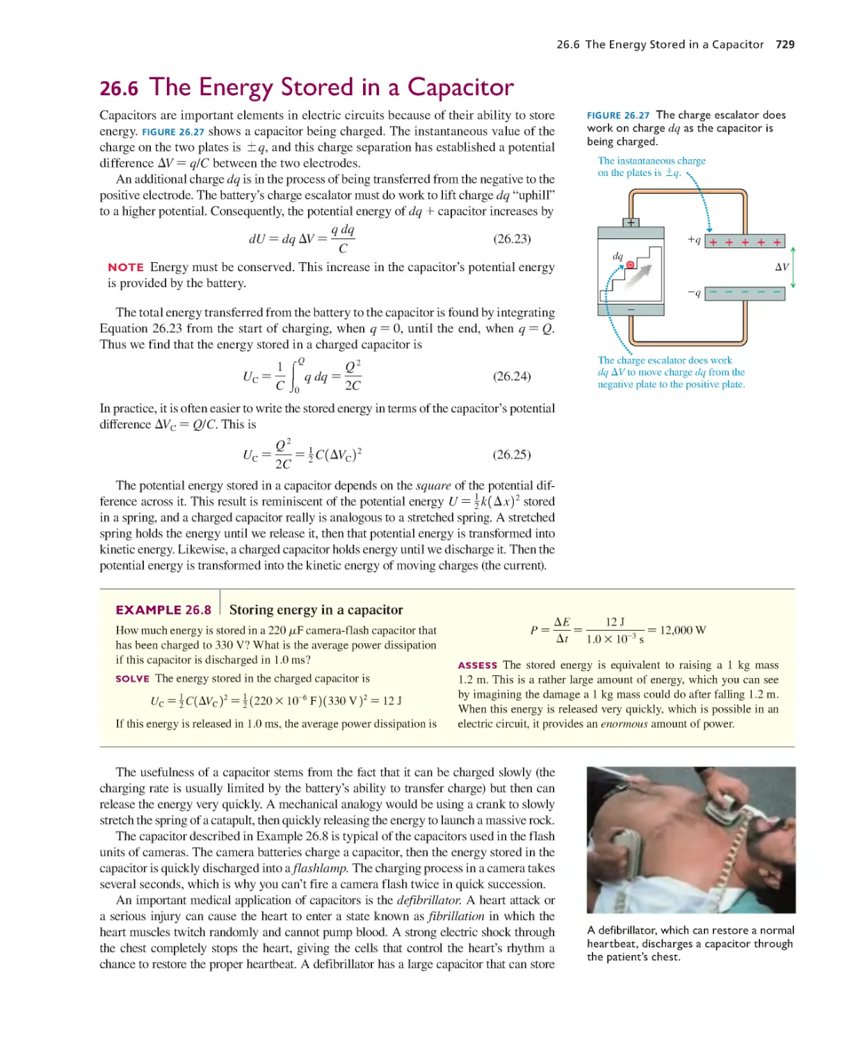
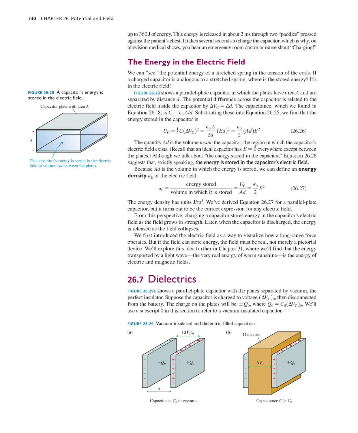
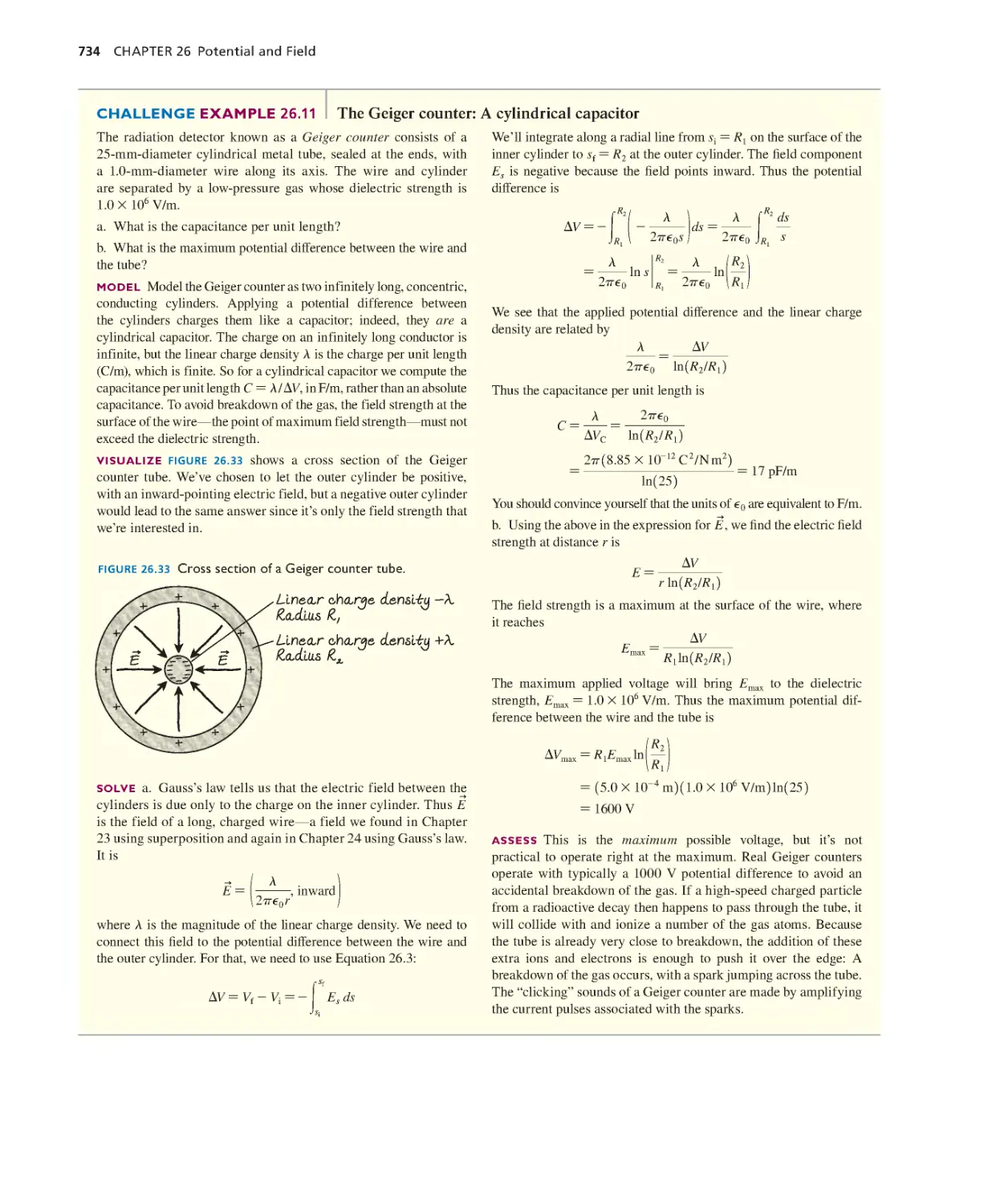
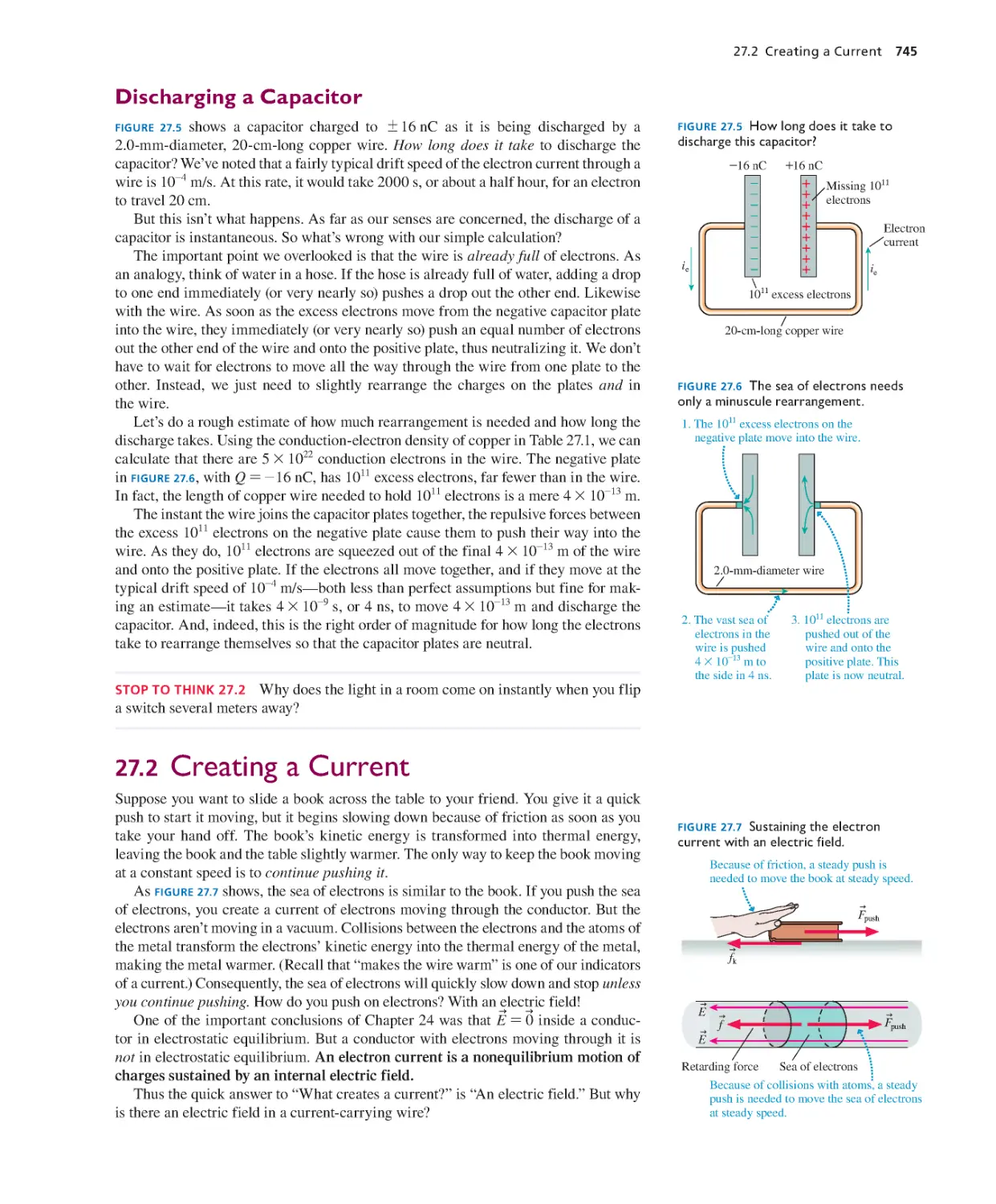
/


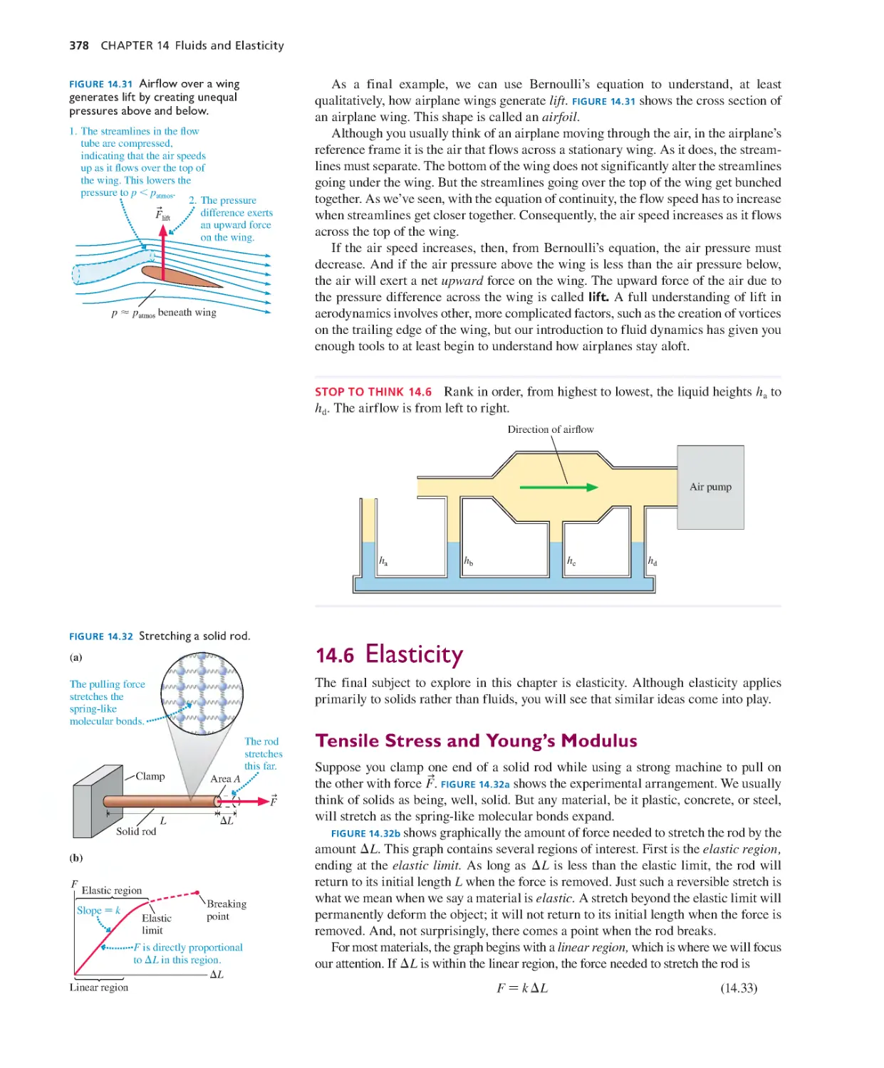


Текст
PHYSICS
FOR SCIENTISTS AND ENGINEERS A STRATEGIC APPROACH 4/E
RANDALL D. KNIGHT
WITH MODERN PHYSICS
PHYSICS
FOR SCIENTISTS AND ENGINEERS A STRATEGIC APPROACH 4/E
RANDALL D. KNIGHT
California Polytechnic State University
San Luis Obispo
with modern physics
Editor-in-Chief:
Jeanne Zalesky
Acquisitions Editor:
Darien Estes
Project Manager:
Martha Steele
Program Manager:
Katie Conley
Senior Development Editor:
Alice Houston, Ph.D.
Art Development Editors:
Alice Houston, Kim Brucker, and Margot Otway
Development Manager:
Cathy Murphy
Program and Project Management Team Lead:
Kristen Flathman
Production Management:
Rose Kernan
Compositor:
Cenveo® Publisher Services
Design Manager:
Mark Ong
Cover Designer:
John Walker
Illustrators:
Rolin Graphics
Rights & Permissions Project Manager:
Maya Gomez
Rights & Permissions Management:
Rachel Youdelman
Photo Researcher:
Eric Schrader
Manufacturing Buyer:
Maura Zaldivar-Garcia
Executive Marketing Manager:
Christy Lesko
Cover Photo Credit:
Thomas Vogel/Getty Images
Copyright © 2017, 2013 , 2008 , 2004 Pearson Education, Inc. All Rights Reserved. Printed in the United
States of America. This publication is protected by copyright, and permission should be obtained from the
publisher prior to any prohibited reproduction, storage in a retrieval system, or transmission in any form or
by any means, electronic, mechanical, photocopying, recording, or otherwise. For information regarding
permissions, request forms and the appropriate contacts within the Pearson Education Global Rights &
Permissions department, please visit www.pearsoned.com/permissions/.
Acknowledgements of third party content appear on page C-1, which constitutes an extension of this
copyright page.
PEARSON, ALWAYS LEARNING and MasteringPhysics® are exclusive trademarks in the U.S. and/or
other countries owned by Pearson Education, Inc. or its affiliates.
Unless otherwise indicated herein, any third-party trademarks that may appear in this work are the pro-
perty of their respective owners and any references to third-party trademarks, logos or other trade dress are
for demonstrative or descriptive purposes only. Such references are not intended to imply any sponsorship,
endorsement, authorization, or promotion of Pearson’s products by the owners of such marks, or any relation-
ship between the owner and Pearson Education, Inc. or its affiliates, authors, licensees or distributors.
Library of Congress Cataloging-in-Publication Data
Names: Knight, Randall Dewey, author.
Title: Physics for scientists and engineers : a strategic approach with
modern physics / Randall D. Knight, California Polytechnic State
University, San Luis Obispo.
Description: Fourth edition. | Boston : Pearson Education, Inc., [2015] |
?2017 | Includes bibliographical references and index.
Identifiers: LCCN 2015038869 | ISBN 9780133942651 | ISBN 0133942651
Subjects: LCSH: Physics--Textbooks. | Physics--Problems, exercises, etc.
Classification: LCC QC23.2 .K65 2015 | DDC 530--dc23 LC record
available at http://lccn.loc.gov/2015038869
ISBN 10: 0-133-94265-1; ISBN 13: 978-0-133-94265-1 (Extended edition)
ISBN 10: 0-134-08149-8; ISBN 13: 978-0-134-08149-6 (Standard edition)
ISBN 10: 0-134-39178-0; ISBN 13: 978-0-134-39178-6 (NASTA edition)
ISBN 10: 0-134-09250-3; ISBN 13: 978-0-134-09250-8 (Books A La Carte edition)
www.pearsonhighered.com
12345678910—V311—1817161514
About the Author
Randy Knight taught introductory physics for 32 years at Ohio State University
and California Polytechnic State University, where he is Professor Emeritus of
Physics. Professor Knight received a Ph.D. in physics from the University of
California, Berkeley and was a post-doctoral fellow at the Harvard-Smithsonian
Center for Astrophysics before joining the faculty at Ohio State University. It was at
Ohio State that he began to learn about the research in physics education that,
many years later, led to Five Easy Lessons: Strategies for Successful Physics
Teaching and this book, as well as College Physics: A Strategic Approach, co-
authored with Brian Jones and Stuart Field. Professor Knight’s research interests
are in the fields of laser spectroscopy and environmental science. When he’s not
in front of a computer, you can find Randy hiking, sea kayaking, playing the piano,
or spending time with his wife Sally and their five cats.
d
A research-driven approach,
fine-tuned for even greater
ease-of-use and student success
REVISED COVERAGE AND ORGANIZATION GIVE INSTRUCTORS
GREATER CHOICE AND FLEXIBILITY
NEW! CHAPTER ORGANIZATION allows instructors to
more easily present material as needed to complement labs, course
schedules, and different teaching styles. Work and energy are now
covered before momentum, oscillations are grouped with mechan-
ical waves, and optics appears after electricity and magnetism.
Unchanged is Knight’s unique approach of working from concrete
to abstract, using multiple representations, balancing qualitative
with quantitative, and addressing misconceptions.
NEW! MORE CALCULUS-BASED
PROBLEMS have been added, along with an
icon to make these easy to identify. The sig-
nificantly revised end-of-chapter problem sets,
extensively class-tested and both calibrated
and improved using MasteringPhysics® data,
expand the range of physics and math skills
students will use to solve problems.
60. || A clever engineer designs a “sprong” that obeys the force law
Fx=-q1x-xeq2
3
, whe re xeq is the equilibrium position of the
end of the sprong and q is the sprong consta nt. For simplicity,
we’llletxeq =0m.ThenFx = -qx
3
.
a. What are the units of q?
b. Find an expression for the potential energy of a stretched or
compressed sprong.
c. A sprong-loaded toy gun shoots a 20 g plastic ball. What
is the launch speed if the sprong constant is 40,000, with
the units you found in part a, and the sprong is compressed
10 cm? Assume the ba rrel is frictionless.
NEW! ADVANCED
TOPICS as optional sections
add even more f lexibility
for instructors’ individual
courses. Topics include rocket
propulsion, gyroscopes and
precession, the wave equation
(including for electromagnetic
waves), the speed of sound in gases, and more
details on the interference of light.
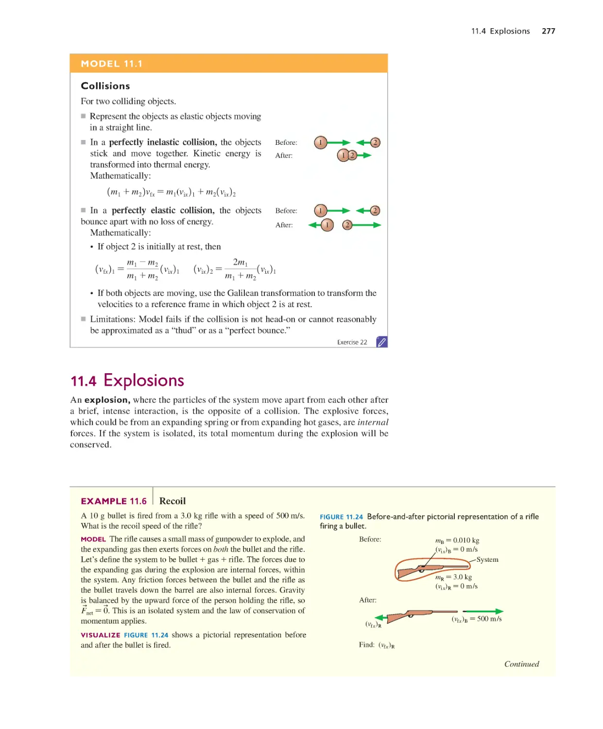
11.6 advanced topic Rocket Propulsion
Newton’s second law F
u
=ma
u
applies to objects whose mass does not change. That’s
an excellent assumption for balls and bicycles, but what about something like a rocket
that loses a significant amount of mass as its fuel is burned? Problems of varying
mass are solved with momentum rather than acceleration. We’ll look at one important
exa mple.
FIGURE 11.29 shows a rocket being propelled by the thrust of burning fuel but not
influenced by gravity or drag. Perhaps it is a rocket in deep space where gravity is very
weak in comparison to the rocket’s thrust. This may not be highly realistic, but ignoring
gravity allows us to understand the essentials of rocket propulsion without maki ng the
mat hematics too complicated. Rocket propulsion with gravity is a Challenge P roblem
in the end-of-chapter problems.
The system rocket + exhaust gases is an isolated system, so its total momentum is
conserved. The basic idea is simple: As exhaust gases are shot out the back, the rocket
“recoils” in the opposite direction. Putting this idea on a mathematical footing is fairly
st raightforward—it’s basically the same as a nalyzing a n explosion—but we have to be
extremely careful with signs.
We’ll use a before-and-after approach, as we do with all momentum problems. The
FIGURE 11. 2 9 A before-and-after pictorial
represent ation of a rocket burning a small
amount of fuel.
Before:
After:
Relative to rocket
m+dm
vex
mfuel
vx+dvx
m
vx
.
,
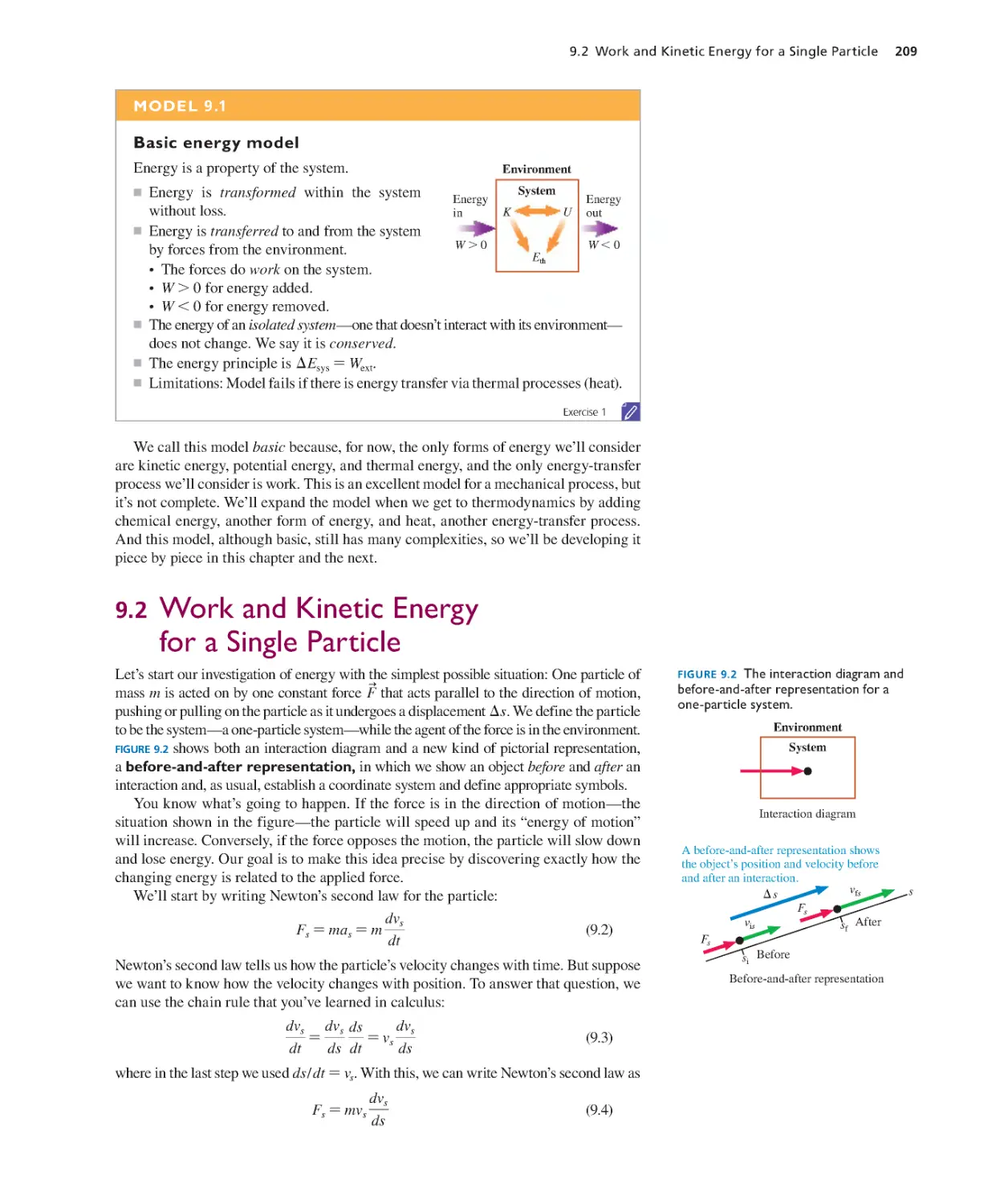
FIGURE 9 .1 A system-environment
perspective on energ y.
System
Environment
Environment
Heat
Work
Heat
Kinetic
Potential
Thermal
Chemical
Work
Energy removed
Energy added
Energy can be transformed
The system has energy Esys
Built from the ground up on physics education research and
crafted using key ideas from learning theory, Knight has set the
standard for effective and accessible pedagogical materials in
physics. In this fourth edition, Knight continues to refine and
expand the instructional techniques to take students further.
NEW AND UPDATED LEARNING TOOLS PROMOTE DEEPER AND
BETTER-CONNECTED UNDERSTANDING
NEW! MODEL BOXES enhance the text’s
emphasis on modeling—analyzing a complex,
real-world situation in terms of simple but
reasonable idealizations that can be applied
over and over in solving problems. These fun-
damental simplifications are developed in the
text and then deployed more explicitly in the
worked examples, helping students to recog-
nize when and how to use recurring models, a
key critical-thinking skill.
REVISED! ENHANCED
CHAPTER PREVIEWS,
based on the educational
psychology concept of an
“advance organizer,” have
been reconceived to address
the questions students are
most likely to ask themselves
while studying the material
for the first time. Questions
cover the impor tant ideas,
and provide a big-picture
overview of the chapter’s key
principles. Each chapter con-
cludes with the visual Chapter
Summary, consolidating and
structuring understanding.
a
u
Mathematically:
Limitations: Model fails if the particle’s
acceleration changes.
Model the object as a particle moving
in a straight line with constant acceleration.
For motion with constant acceleration.
v
u
Parabola
s
si
t
The slope is vs.
Horizontal line
as
0
t
The acceleration is constant.
Straight line
vs
vis
t
The slope is as.
vfs=vis+as∆t
vfs
2=vis
2+2as∆s
sf=si+vis∆t+ as1∆t22
1
2
Constant acceleration
MODEL 2.2
Exercise 16
MODEL 6.3
Friction
The friction force is parallel to the surface.
■ Static friction: Acts as needed to prevent motion.
Can have any magnitude up to fs max = ms n.
■ Kinetic friction: Opposes motion with fk = mk n.
■ Rolling friction: Opposes motion with fr = mr n.
■ Graphically:
Push or
pull
Friction
Motion is relative
to the surface.
f
Push or pull force
Static friction
increases to match
the push or pull.
Kinetic friction is constant
as the object moves.
Kinetic
Static
The object slips when static
friction reaches fs max.
Rest
Moving
fsmax = msn
mkn
0
152 CHAPTER 6 Dynamics I: Motion Along a Line
SUMMARY
The goal of Chapter 6 has been to learn to solve linear force-and-motion problems.
GENE RAL PRINCIPLES
Two Explanatory Models
An object on which there is
no net forceis in mechanical
equilibrium.
• Objects at rest.
• Objects moving with constant
velocity.
• Newton’s second law applies
with a
u
=0
u
.
An object on which the net force
is constant undergoes dynamics
with constant force.
• The object accelerates.
• The kinematic model is that of
constant acceleration.
• Newton’s second law applies.
A Problem-Solving Strategy
A four-part strategy applies to both equilibrium and
dynamics problems.
MODEL Make simplifying assumptions.
VISUA L IZE
• Translate words into symbols.
• Draw a sketch to define the situation.
• Draw a motion diagram.
• Identify forces.
• Draw a free-body diagram.
SOLVE Use Newton’s second law:
F
u
net=a
i
F
u
i=ma
u
“Read” the vectors from the fre e-body diagram. Use
kinematics to find velocities and positions.
ASSESS Is the result reasonable? Does it have correct
units and significant figures?
equilibrium model
constant-force model
flat-earth approximation
weight
co efficient of static friction, ms
coefficient of kinetic friction, mk
rolling friction
coefficient of rolling
friction, mr
drag coefficient, C
terminal speed, vterm
TERMS AND NOTATION
A falling object reaches
terminal speed
vterm =
B2mg
CrA
APPLICATIONS
Mass is an intrinsic property of an object that describes the object’s
inertia and, loosely speaking, its quantity of matter.
The weight of an object is the reading of a spring scale when the
object is at rest relative to the scale. Weight is the result of weigh-
ing. A n object’s weight depends on its mass, its acceleration, and the
strength of gravity. An object in free fall is weightless.
IMPORTANT CONCEPTS
Specific information about three important descriptive models:
Gravity F
u
G = 1mg, downward2
Friction f
u
s = 10 to ms n, direction as necessary to prevent motion2
fu
k = 1mkn, direction opposite the motion2
fu
r = 1mrn, direction opposite the motion2
Drag
F
u
drag = 11
2 CrAv2, direction opposite the motion2
Newton’s laws are vector
expressions. You must write
them out by components:
1Fnet2x =
aFx = max
1Fnet2y= aFy= may
The acceleration is zero in equi-
librium and also along an axis
perpendicular to the motion.
Fnet=0
u
u
a
u
Go back and forth
between these
steps as needed.
d
y
x
Fn et
u
F1
u
F3
u
F2
u
FG
Terminal speed is reached
when the drag force exactly
balances the gravitational
force: a = 0.
u
u
u
Fdrag
u
6
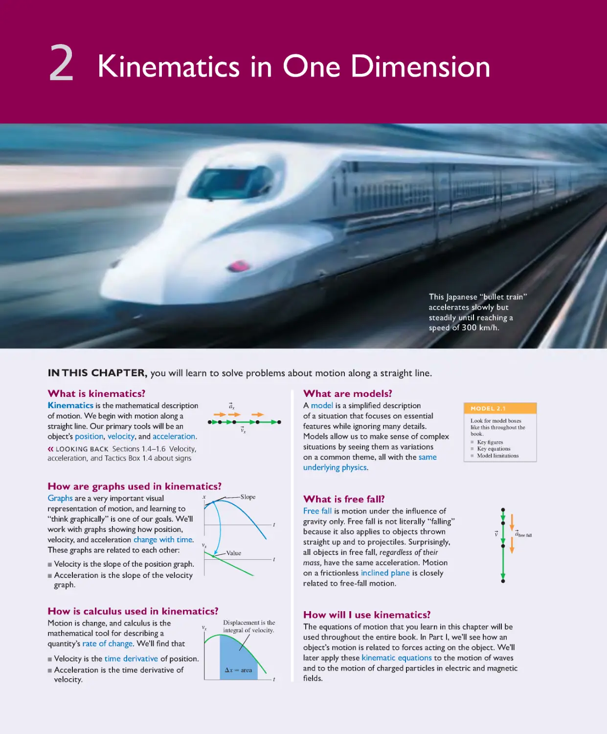
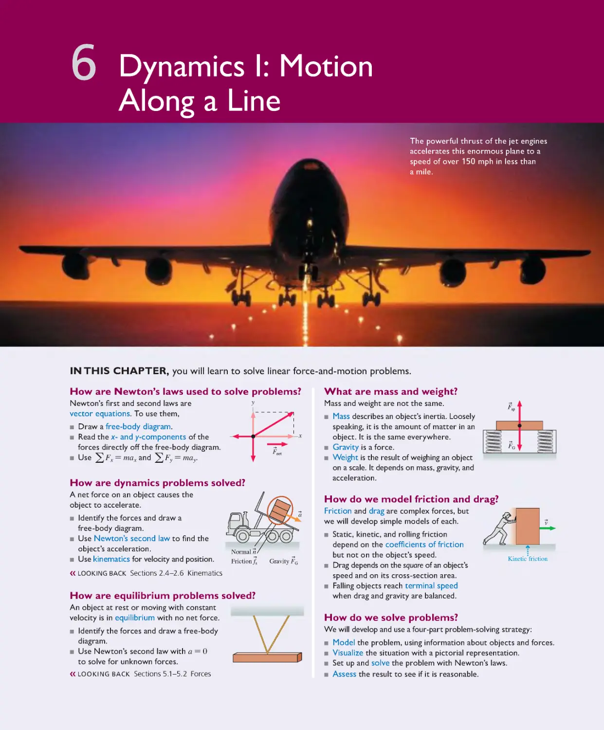
The powerful thrust of the jet engines
accelerates this enormous plane to a
speed of over 150 mph in less than
a mile.
Dynamics I: Motion
Along a Line
IN THIS CHAPTER, you will learn to solve linear force-and-motion problems.
How are Newton’s laws used to solve problems?
Newton’s i rst and second laws are
vector equations. To use them,
■ Draw a free-body diagram.
■ Read the x- and y-components of the
forces directly of the free-body diagram.
■UseaFx=maxandaFy=may.
How are dynamics problems solved?
A net force on an object causes the
object to accelerate.
■ Identify the forces and draw a
free-body diagram.
■ Use Newton’s second law to ind the
object’s acceleration.
■ Use kinematics for velocity and position.
❮❮ LOOKING BACK Sections 2.4 –2 .6 Kinematics
How are equilibrium problems solved?
An object at rest or moving with constant
velocity is in equilibrium with no net force.
■ Identify the forces and draw a free-body
diag ram .
■ UseNewton’s secondlawwith a = 0
to solve for unknown forces.
❮❮ LOOKING BACK Sections 5.1 –5 .2 Forces
What are mass and weight?
Mass and weight are not the same.
■ Mass describes an object’s inertia. Loosely
speaking , it is the amount of matter in an
object. It is the same everywhere.
■ Gravity is a force.
■ Weight is the result of weighing an object
on a scale. It depends on mass, gravity, and
acceleration.
How do we model friction and drag?
Friction and drag are complex forces, but
we will develop simple models of each.
■ Static, kinetic, and rolling friction
depend on the coefficients of friction
but not on the object’s speed.
■ Drag depends on the square of an object’s
speed and on its cross-section area.
■ Falling objects reach terminal speed
when drag and gravity are balan ced.
How do we solve problems?
We will develop and use a four-part problem-solving strategy:
■ Model the problem, using information about objects a nd forces.
■ Visualize the situation with a pictorial represent ation.
■ Set up and solve the problem with New ton’s laws.
■ Assess the result to see if it is reasonable.
Fnet
u
y
x
a
u
Fr ictio n fs
u
Normal n
u
Gravity FG
u
FG
u
Fsp
u
v
u
Kinetic friction
23,
.
3.
.
,
A STRUCTURED AND CONSISTENT APPROACH BUILDS
PROBLEM-SOLVING SKILLS AND CONFIDENCE
With a research-based 4-step problem-solving
framework used throughout the text , students
learn the importance of making assumptions
(in the MODEL step) and gathering informa-
tion and making sketches (in the VISUALIZE
step) before treating the problem mathemati-
cally (SOLVE) and then analyzing their results
(ASSESS).
The REVISED STUDENT WORKBOOK
is tightly integrated with the main text–allowing
students to practice skills from the text’s Tactics
Boxes, work through the steps of Problem-Solv-
ing Strategies, and assess the applicability of the
Models. The workbook is referenced throughout
the text with the icon
.
Detailed PROBLEM-SOLVING
STRATEGIES for different topics and
categories of problems (circular-motion
problems, calorimetr y problems, etc.)
are developed throughout, each one built
on the 4-step framework and carefully
illustrated in worked examples.
TACTICS BOXES give step-by-step procedures for
developing specific skills (drawing free-body diagrams,
using ray tracing, etc.).
PROBLEM-SOLVING STRATEGY 10.1
Energy-conservation problems
MODEL Deine the system so that there are no external forces or so that any
external forces do no work on the system. If there’s friction, bring both surfaces
into the system. Model objects as particles and springs as ideal.
VISUALIZE Draw a before-and-after pictorial representation and an energy bar
chart. A free-body diagram may be needed to visualize forces.
SOLVE If the system is both isolated and nondissipative, then the mechanical
energy is conserved:
Ki+Ui=Kf+Uf
where K is the total kinetic energy of all moving objects and U is the total
potential energy of all interactions within the system. If there’s friction, then
Ki+Ui=Kf+Uf+∆Eth
where the thermal energy increase due to friction is ∆Eth = fk ∆ s.
ASSESS Check that your result has correct units and signiicant igures, is
reasonable, and answers the question.
Exercise 14
TACTICS BOX 2 6 .1
Finding the potential from the electric field
●1 Draw a pictu re and identify the p oint at which you wish to find the potential.
Call this position f.
●2 Choose the zero point of the potential, often at ininity. Call this position i.
●3 Establish a coordinate axis from i to f along which you already know or can
easily determine the electric ield component Es.
●4 Carry out the integ ration of Equation 26.3 to find the potential.
Exercise 1
30-8 chapter 30 • Electromagnetic Induction
18. The graph shows how the magnetic field changes through
a rectangular loop of wire with resistance R. Draw a graph
of the current in the loop as a function of time. Let a
counterclockwise current be positive, a clockwise
current be negative.
a. What is the magnetic flux through the loop at t = 0?
b. Doesthisflux changebetweent = 0 and t = t1?
c. Is there an induced current in the loop between t = 0 and t = t1?
d. What is the magnetic flux through the loop at t = t2?
e. What is the change in f lux through the loop between t1 and t2?
f. What is the time interval between t1 and t2?
g. What is the magnitude of the induced emf between t1 and t2?
h. What is the magnitude of the induced current between t1 and t2?
i. Does the magnetic field point out of or into the loop?
j. Between t1 and t2, is the magnetic flux increasing or decreasing?
k. To oppose the change in the flux between t1 and t2, should the magnetic
field of the induced current point out of or into the loop?
l. Is the induced current between t1 and t2 positive or negative?
m. Does the flux through the loop change after t2?
n. Is there an induced current in the loop after t2?
o. Use all this information to draw a graph of the induced current. Add appropriate labels on the
vertical axis.
PSS
30.1
+U
s.
.
30 • Electromagnetic Induction
0?
0
?
0
?
?
?
?
?
?
t,
t,
t
?
?
THE ULTIMATE RESOURCE
BEFORE, DURING, AND AFTER CLASS
BEFORE CLASS
DURING CLASS
AFTER CLASS
NEW! INTERACTIVE PRELECTURE VIDEOS
address the rapidly growing movement toward pre-lecture
teaching and flipped classrooms. These whiteboard-style
animations provide an introduction to key topics with
embedded assessment to help students prepare and profes-
sors identify student misconceptions before lecture.
NEW! LEARNING CATALYTICSTM is an interactive
classroom tool that uses students’ devices to engage them in
more sophisticated tasks and thinking. Learning Catalytics
enables instructors to generate classroom discussion and
promote peer-to-peer learning to help students develop
critical-thinking skills. Instructors can take advantage of
real-time analytics to find out where students are struggling
and adjust their instructional strategy.
NEW! ENHANCED
END-OF-CHAPTER
QUESTIONS offer st u-
dents instructional suppor t
when and where they need
it, including links to the
eText, math remediation,
and wrong-answer feedback
for homework assignments.
ADAPTIVE FOLLOW-UPS
are personalized assignments
that pair Mastering’s powerful
content with Knewton’s adaptive
learning engine to provide
individualized help to students
before misconceptions take hold.
These adaptive follow-ups address
topics students struggled with on
assigned homework, including core
prerequisite topics.
NEW! DYNAMIC STUDY MODULES (DSMs) con-
tinuously assess students’ performance in real time to provide
personalized question and explanation content until students
master the module with confidence. The DSMs cover basic
math skills and key definitions and relationships for topics
across all of mechanics and electricity and magnetism.
MasteringPhysics
viii
Preface to the Instructor
This fourth edition of Physics for Scientists and Engineers: A
Strategic Approach continues to build on the research-driven
instructional techniques introduced in the irst edition and the
extensive feedback from thousands of users. From the begin-
ning, the objectives have been:
■ To produce a textbook that is more focused and coherent,
less encyclopedic.
■ To move key results from physics education research into
the classroom in a way that allows instructors to use a range
of teaching styles.
■ To provide a balance of quantitative reasoning and con-
ceptual understanding, with special attention to concepts
known to cause student diiculties.
■ To develop students’ problem-solving skills in a systematic
manner.
These goals and the rationale behind
them are discussed at length in the
Instructor’s Guide and in my small
paperback book, Five Easy Lessons:
Strategies for Successful Physics
Teaching. Please request a copy from
your local Pearson sales representa-
tive if it is of interest to you (ISBN
978-0-805-38702-5).
What’s New to This Edition
For this fourth edition, we continue to apply the best results
from educational research and to tailor them for this course and
its students. At the same time, the extensive feedback we’ve
received from both instructors and students has led to many
changes and improvements to the text, the igures, and the
end-of-chapter problems. These include:
■ Chapter ordering changes allow instructors to more easily
organize content as needed to accommodate labs, schedules,
and diferent teaching styles. Work and energy are now
covered before momentum, oscillations are grouped with
mechanical waves, and optics appears after electricity and
magnetism.
■ Addition of advanced topics as optional sections further
expands instructors’ options. Topics include rocket propul-
sion, gyroscopes, the wave equation (for mechanical and
electromagnetic waves), the speed of sound in gases, and
more details on the interference of light.
■ Model boxes enhance the text’s emphasis on modeling—
analyzing a complex, real-world situation in terms of simple
but reasonable idealizations that can be applied over and
over in solving problems. These fundamental simpliications
are developed in the text and then deployed more explicitly
in the worked examples, helping students to recognize when
and how to use recurring models.
■ Enhanced chapter previews have been redesigned, with
student input, to address the questions students are most
likely to ask themselves while studying the material for the
irst time. The previews provide a big-picture overview of
the chapter’s key principles.
■ Looking Back pointers enable students to look back at a
previous chapter when it’s important to review concepts.
Pointers provide the speciic section to consult at the exact
point in the text where they need to use this material.
■ Focused Part Overviews and Knowledge Structures con-
solidate understanding of groups of chapters and give a tighter
structure to the book as a whole. Reworked Knowledge Struc-
tures provide more targeted detail on overarching themes.
■ Updated visual program that has been enhanced by revis-
ing over 500 pieces of art to increase the focus on key ideas.
■ Significantly revised end-of-chapter problem sets in-
clude more challenging problems to expand the range of
physics and math skills students will use to solve problems.
A new icon for calculus-based problems has been added.
At the front of this book, you’ll ind an illustrated walkthrough
of the new pedagogical features in this fourth edition.
Textbook Organization
The 42-chapter extended edition (ISBN 978-0-133-94265-1 /
0-133-94265-1) of Physics for Scientists and Engineers is
intended for a three-semester course. Most of the 36-chapter
standard edition (ISBN 978-0 -134-08149-6 / 0-134-08149-8),
ending with relativity, can be covered in two semesters, although
the judicious omission of a few chapters will avoid rushing
through the material and give students more time to develop
their knowledge and skills.
The full textbook is divided into eight parts: Part I: Newton’s
Laws, Part II: Conservation Laws, Part III: Applications of
Newtonian Mechanics, Part IV: Oscillations and Waves, Part V:
Thermodynamics, Part VI: Electricity and Magnetism, Part VII:
Optics, and Part VIII: Relativity and Quantum Physics. Note
that covering the parts in this order is by no means essential.
Each topic is self-contained, and Parts III–VII can be rear-
ranged to suit an instructor’s needs. Part VII: Optics does need
to follow Part IV: Oscillations and Waves, but optics can be
taught either before or after electricity and magnetism.
There’s a growing sentiment that quantum physics is quickly
becoming the province of engineers, not just scientists, and
that even a two-semester course should include a reasonable
introduction to quantum ideas. The Instructor’s Guide outlines
Preface to the Instructor ix
a couple of routes through the book that allow most of the
quantum physics chapters to be included in a two-semester
course. I’ve written the book with the hope that an increasing
number of instructors will choose one of these routes.
■ Extended edition, with mode rn physics (ISBN 978-0 -133-
94265-1 / 0 -133 -94265 -1): Chapters 1–42 .
■ Standard edition (ISBN 978-0-134 -08149-6 / 0 -134-08149-8):
Chapters 1-36 .
■ Volume 1 (ISBN 978-0 -134 -11068 -4 / 0 -134 -11068 -4) covers
mech anics , wave s, and thermodynamics: Chapters 1 –21.
■ Volume 2 (ISBN 978-0 -134 -11066 -0 / 0 -134 -11066 -8)
cove r s e lectricity and magnetism and optics , pl us relativity:
Chapters 22–36 .
■ Volume 3 (ISBN 978-0 -134 -11065 -3 / 0 -134 -11065 -X) covers
rel ativity and quantum physics: Chapters 36 –42 .
The Student Workbook
A key component of Physics for Scientists and Engineers: A
Strategic Approach is the accompanying Student Workbook.
The workbook bridges the gap between textbook and home-
work problems by providing students the opportunity to learn
and practice skills prior to using those skills in quantitative
end-of-chapter problems, much as a musician practices tech-
nique separately from performance pieces. The workbook exer-
cises, which are keyed to each section of the textbook, focus on
developing speciic skills, ranging from identifying forces and
drawing free-body diagrams to interpreting wave functions.
The workbook exercises, which are
generally qualitative and/or graphical,
draw heavily upon the physics educa-
tion research literature. The exercises
deal with issues known to cause stu-
dent difficulties and employ tech-
niques that have proven to be effective
at overcoming those difficulties. New
to the fourth edition workbook are
exercises that provide guided practice
for the textbook’s Model boxes. The
workbook exercises can be used in class as part of an active-
learning teaching strategy, in recitation sections, or as assigned
homework. More information about effective use of the Student
Workbook can be found in the Instructor’s Guide.
ForceandMotion . CHAPTER5
9.
a. 2m
b. 0.5m
Usetriangles toshow fourpoints fortheobjectof
mass 2m, then drawalinethrough thepoints. Use
squares forthe objectof mass 0.5m.
10. A constant force applied to objectA causes Ato
accelerate at5 m/s2. The sameforceapplied to objectB
causes an accelerationof 3m/s2. Applied to objectC, it
causes an accelerationof 8m/s2.
a. Which objecthas thelargestmass?
b. Which object has the smallest mass?
c. Whatis theratioof mass Ato mass B?(mA/mB) =
11.Aconstant force applied to an object causes the object to accelerate at 10 m/s2. What will the
acceleration of this object beif
a. Theforceis doubled?
b. The massis doubled?
c. Theforceis doubled andthe mass is doubled?
d. Theforceis doubled andthe mass is halved?
12. Aconstantforceapplied to an objectcauses theobjectto accelerate at8 m/s2. Whatwillthe
acceleration of this object beif
a. Theforceis halved?
b. Themassis halved?
c. Theforceis halved and themass is halved?
d. Theforceis halved and themass is doubled?
13. Forcesare shown ontwo objects. Foreach:
a. Drawandlabelthe netforce vector.Do this righton thefigure.
b. Belowthe figure, draw and labeltheobject’sacceleration vector.
x
y
012
Force(rubberbands)
A
c
c
e
l
e
r
a
t
i
o
n
34
Thefigure shows an acceleration-versus -forcegraphfor
an objectofmass m. Datahavebeenplotted as individual
points, and aline has been drawnthroughthe points.
Draw and label, directly on thefigure, the acceleration-
versus-forcegraphsforobjects ofmass
Instructional Package
Physics for Scientists and Engineers: A Strategic Approach, fourth edition, provides an integrated teaching and learning package of support material
for students and instructors. NOTE For convenience, most instructor supplements can be downloaded from the “Instructor Resources” area of
MasteringPhysics® and the Instructor Resource Center (www.pearsonhighered.com/educator).
Name of Supplement
Print Online
Instructor
or Student
Supplement Description
MasteringPhysic s with Pearson eText
ISBN 0-134 -08313 -X
✓
Instructor
and Student
Supplement
This product features all of the resources of MasteringPhysics in addition
to the new Pearson eText 2.0 . Now available on smartphones and tablets,
Pearson eText 2.0 comprises the full text, including videos and other rich
media. Students can configure reading settings, including resizeable type and
night-reading mode, take notes, and highlight, bookmark, and search the text.
Instr uctor’s Solutions Manual
ISBN 0-134 -09246-5
✓
Instructor
Supplement
This comprehensive solutions manual contains complete solutions to all end-
of-chapter questions and problems. All problem solutions follow the Model/
Visualize/Solve/Assess problem-solving strategy used in the text.
Instr uctor’s Guide
ISBN 0-134 -09248-1
✓
Instructor
Supplement
Written by Randy Knight, this resource provides chapter-by-chapter creative
ideas and teaching tips for use in your class. It also contains an extensive
review of results of what has been learned from physics education research and
provides guidelines for using active-learning techniques in your classroom.
TestGen Test Bank
ISBN 0-134 -09245-7
✓
Instructor
Supplement
The Test Bank contains over 2,000 high-quality conceptual and multiple-choice
questions. Test files are provided in both TestGen® and Word format.
Instr uctor’s Re source DVD
ISBN 0-134 -09247-3
✓
✓
Instructor
Supplement
This cross-platform DVD includes an Image Library; editable content for Key
Equations, Problem-Solving Strategies, Math Relationship Boxes, Model Boxes,
and Tactic Boxes; PowerPoint Lecture Slides and Clicker Questions; Instructor’s
Guide, Instructor’s Solutions Manual; Solutions to Student Workbook exercises;
and PhET simulations.
Student Workbook
Extended (Ch 1–42) ISBN 0-134-08316 -4
Standard (Ch 1–36) ISBN 0-134-08315-6
Volume 1 (Ch 1–21) ISBN 0-134 -11064-1
Volume 2 (Ch 22–36) ISBN 0-134 -11063-3
Volume 3 (Ch 36–42) ISBN 0-134 -11060-9
✓
Student
Supplement
For a more detailed description of the Student Workbook, see page v.
x Preface to the Instructor
Acknowledgments
I have relied upon conversations with and, especially, the written
publications of many members of the physics education research
community. Those whose inluence can be seen in these pages
include Wendy Adams, the late Arnold Arons, Stuart Field,
Uri Ganiel, Ibrahim Halloun, Richard Hake, Ken Heller, Paula
Heron, David Hestenes, Brian Jones, the late Leonard Jossem,
Jill Larkin, Priscilla Laws, John Mallinckrodt, Kandiah
Manivannan, Richard Mayer, Lillian McDermott and members
of the Physics Education Research Group at the University of
Washington, David Meltzer, Edward “Joe” Redish, Fred Reif,
Jeffery Saul, Rachel Scherr, Bruce Sherwood, Josip Slisko, David
Sokoloff, Richard Steinberg, Ronald Thornton, Sheila Tobias,
Alan Van Heuleven, Carl Wieman, and Michael Wittmann. John
Rigden, founder and director of the Introductory University
Physics Project, provided the impetus that got me started down
this path. Early development of the materials was supported
by the National Science Foundation as the Physics for the Year
2000 project; their support is gratefully acknowledged.
I especially want to thank my editors, Jeanne Zalesky and
Becky Ruden, development editor Alice Houston, project
manager Martha Steele, art development editors Kim Brucker
and Margot Otway, and all the other staff at Pearson for their
enthusiasm and hard work on this project. Rose Kernan and
the team at Cenveo along with photo researcher Eric Schrader
get a good deal of the credit for making this complex project
all come together. Larry Smith, Larry Stookey, and Michael
Ottinger have done an outstanding job of checking the
solutions to every end-of-chapter problem and updating the
Instructor’s Solutions Manual. John Filaseta must be thanked
for carefully writing out the solutions to the Student Workbook
exercises, and Jason Harlow for putting together the Lecture
Slides. In addition to the reviewers and classroom testers
listed below, who gave invaluable feedback, I am particularly
grateful to Charlie Hibbard for his close scrutiny of every word
and figure.
Finally, I am endlessly grateful to my wife Sally for her
love, encouragement, and patience, and to our many cats, past
and present, who are always ready to suggest “Dinner time?”
when I’m in need of a phrase.
Randy Knight, September 2015
rknight@calpoly.edu
Reviewers and Classroom Testers
Gary B. Adams, Arizona State University
Ed Adelson, Ohio State University
Kyle Altmann, Elon University
Wayne R. Anderson, Sacramento City College
James H. Andrews, Youngstown State University
Kevin Ankoviak, Las Positas College
David Balogh, Fresno City College
Dewayne Beery, Bufalo State College
Joseph Bellina, Saint Mary’s College
James R. Benbrook, University of Houston
David Besson, University of Kansas
Matthew Block, California State University, Sacramento
Randy Bohn, University of Toledo
Richard A. Bone, Florida International University
Gregory Boutis, York College
Art Braundmeier, University of Southern Illinois,
Edwardsville
Carl Bromberg, Michigan State University
Meade Brooks, Collin College
Douglas Brown, Cabrillo College
Ronald Brown, California Polytechnic State University,
San Luis Obispo
Mike Broyles, Collin County Community College
Debra Burris, University of Central Arkansas
James Carolan, University of British Columbia
Michael Chapman, Georgia Tech University
Norbert Chencinski, College of Staten Island
Tonya Cofey, Appalachian State University
Kristi Concannon, King’s College
Desmond Cook, Old Dominion University
Sean Cordry, Northwestern College of Iowa
Robert L. Corey, South Dakota School of Mines
Michael Crescimanno, Youngstown State University
Dennis Crossley, University of Wisconsin–Sheboygan
Wei Cui, Purdue University
Robert J. Culbertson, Arizona State University
Danielle Dalafave, The College of New Jersey
Purna C. Das, Purdue University North Central
Chad Davies, Gordon College
William DeGrafenreid, California State
University–Sacramento
Dwain Desbien, Estrella Mountain Community College
John F. Devlin, University of Michigan, Dearborn
John DiBartolo, Polytechnic University
Alex Dickison, Seminole Community College
Chaden Djalali, University of South Carolina
Margaret Dobrowolska, University of Notre Dame
Sandra Doty, Denison University
Miles J. Dresser, Washington State University
Taner Edis, Truman State University
Charlotte Elster, Ohio University
Robert J. Endorf, University of Cincinnati
Tilahun Eneyew, Embry-Riddle Aeronautical University
F. Paul Esposito, University of Cincinnati
John Evans, Lee University
Harold T. Evensen, University of Wisconsin–Platteville
Michael R. Falvo, University of North Carolina
Abbas Faridi, Orange Coast College
Nail Fazleev, University of Texas–Arlington
Stuart Field, Colorado State University
Daniel Finley, University of New Mexico
Jane D. Flood, Muhlenberg College
Michael Franklin, Northwestern Michigan College
Preface to the Instructor xi
Jonathan Friedman, Amherst College
Thomas Furtak, Colorado School of Mines
Alina Gabryszewska-Kukawa, Delta State University
Lev Gasparov, University of North Florida
Richard Gass, University of Cincinnati
Delena Gatch, Georgia Southern University
J. David Gavenda, University of Texas, Austin
Stuart Gazes, University of Chicago
Katherine M. Gietzen, Southwest Missouri State
University
Robert Glosser, University of Texas, Dallas
William Golightly, University of California, Berkeley
Paul Gresser, University of Maryland
C. Frank Griin, University of Akron
John B. Gruber, San Jose State University
Thomas D. Gutierrez, California Polytechnic State University,
San Luis Obispo
Stephen Haas, University of Southern California
John Hamilton, University of Hawaii at Hilo
Jason Harlow, University of Toronto
Randy Harris, University of California, Davis
Nathan Harshman, American University
J. E. Hasbun, University of West Georgia
Nicole Herbots, Arizona State University
Jim Hetrick, University of Michigan–Dearborn
Scott Hildreth, Chabot College
David Hobbs, South Plains College
Laurent Hodges, Iowa State University
Mark Hollabaugh, Normandale Community College
Steven Hubbard, Lorain County Community College
John L. Hubisz, North Carolina State University
Shane Hutson, Vanderbilt University
George Igo, University of California, Los Angeles
David C. Ingram, Ohio University
Bob Jacobsen, University of California, Berkeley
Rong-Sheng Jin, Florida Institute of Technology
Marty Johnston, University of St. Thomas
Stanley T. Jones, University of Alabama
Darrell Judge, University of Southern California
Pawan Kahol, Missouri State University
Teruki Kamon, Texas A&M University
Richard Karas, California State University, San Marcos
Deborah Katz, U.S . Naval Academy
Miron Kaufman, Cleveland State University
Katherine Keilty, Kingwood College
Roman Kezerashvili, New York City College of Technology
Peter Kjeer, Bethany Lutheran College
M. Kotlarchyk, Rochester Institute of Technology
Fred Krauss, Delta College
Cagliyan Kurdak, University of Michigan
Fred Kuttner, University of California, Santa Cruz
H. Sarma Lakkaraju, San Jose State University
Darrell R. Lamm, Georgia Institute of Technology
Robert LaMontagne, Providence College
Eric T. Lane, University of Tennessee–Chattanooga
Alessandra Lanzara, University of California, Berkeley
Lee H. LaRue, Paris Junior College
Sen-Ben Liao, Massachusetts Institute of Technology
Dean Livelybrooks, University of Oregon
Chun-Min Lo, University of South Florida
Olga Lobban, Saint Mary’s University
Ramon Lopez, Florida Institute of Technology
Vaman M. Naik, University of Michigan, Dearborn
Kevin Mackay, Grove City College
Carl Maes, University of Arizona
Rizwan Mahmood, Slippery Rock University
Mani Manivannan, Missouri State University
Mark E. Mattson, James Madison University
Richard McCorkle, University of Rhode Island
James McDonald, University of Hartford
James McGuire, Tulane University
Stephen R. McNeil, Brigham Young University–Idaho
Theresa Moreau, Amherst College
Gary Morris, Rice University
Michael A. Morrison, University of Oklahoma
Richard Mowat, North Carolina State University
Eric Murray, Georgia Institute of Technology
Michael Murray, University of Kansas
Taha Mzoughi, Mississippi State University
Scott Nutter, Northern Kentucky University
Craig Ogilvie, Iowa State University
Benedict Y. Oh, University of Wisconsin
Martin Okafor, Georgia Perimeter College
Halina Opyrchal, New Jersey Institute of Technology
Derek Padilla, Santa Rosa Junior College
Yibin Pan, University of Wisconsin–Madison
Georgia Papaefthymiou, Villanova University
Peggy Perozzo, Mary Baldwin College
Brian K. Pickett, Purdue University, Calumet
Joe Pifer, Rutgers University
Dale Pleticha, Gordon College
Marie Plumb, Jamestown Community College
Robert Pompi, SUNY-Binghamton
David Potter, Austin Community College–Rio Grande
Campus
Chandra Prayaga, University of West Florida
Kenneth M. Purcell, University of Southern Indiana
Didarul Qadir, Central Michigan University
Steve Quon, Ventura College
Michael Read, College of the Siskiyous
Lawrence Rees, Brigham Young University
Richard J. Reimann, Boise State University
Michael Rodman, Spokane Falls Community College
Sharon Rosell, Central Washington University
Anthony Russo, Northwest Florida State College
Freddie Salsbury, Wake Forest University
Otto F. Sankey, Arizona State University
Jef Sanny, Loyola Marymount University
Rachel E. Scherr, University of Maryland
Carl Schneider, U.S . Naval Academy
xii Preface to the Instructor
Bruce Schumm, University of California, Santa Cruz
Bartlett M. Sheinberg, Houston Community College
Douglas Sherman, San Jose State University
Elizabeth H. Simmons, Boston University
Marlina Slamet, Sacred Heart University
Alan Slavin, Trent College
Alexander Raymond Small, California State Polytechnic
University, Pomona
Larry Smith, Snow College
William S. Smith, Boise State University
Paul Sokol, Pennsylvania State University
LTC Bryndol Sones, United States Military Academy
Chris Sorensen, Kansas State University
Brian Steinkamp, University of Southern Indiana
Anna and Ivan Stern, AW Tutor Center
Gay B. Stewart, University of Arkansas
Michael Strauss, University of Oklahoma
Chin-Che Tin, Auburn University
Christos Valiotis, Antelope Valley College
Andrew Vanture, Everett Community College
Arthur Viescas, Pennsylvania State University
Ernst D. Von Meerwall, University of Akron
Chris Vuille, Embry-Riddle Aeronautical University
Jerry Wagner, Rochester Institute of Technology
Robert Webb, Texas A&M University
Zodiac Webster, California State University,
San Bernardino
Robert Weidman, Michigan Technical University
Fred Weitfeldt, Tulane University
Gary Williams, University of California, Los Angeles
Lynda Williams, Santa Rosa Junior College
Jef Allen Winger, Mississippi State University
Carey Witkov, Broward Community College
Ronald Zammit, California Polytechnic State University,
San Luis Obispo
Darin T. Zimmerman, Pennsylvania State University,
Altoona
Fredy Zypman, Yeshiva University
Student Focus Groups
California Polytechnic State University, San Luis Obispo
Matthew Bailey
James Caudill
Andres Gonzalez
Mytch Johnson
California State University, Sacramento
Logan Allen
Andrew Fujikawa
Sagar Gupta
Marlene Juarez
Craig Kovac
Alissa McKown
Kenneth Mercado
Douglas Ostheimer
Ian Tabbada
James Womack
Santa Rosa Junior College
Kyle Doughty
Tacho Gardiner
Erik Gonzalez
Joseph Goodwin
Chelsea Irmer
Vatsal Pandya
Parth Parikh
Andrew Prosser
David Reynolds
Brian Swain
Grace Woods
Stanford University
Montserrat Cordero
Rylan Edlin
Michael Goodemote II
Stewart Isaacs
David LaFehr
Sergio Rebeles
Jack Takahashi
The most incomprehensible thing about the universe is that it is
comprehensible.
—Albert Einstein
The day I went into physics class it was death.
—Sylvia Plath, The Bell Jar
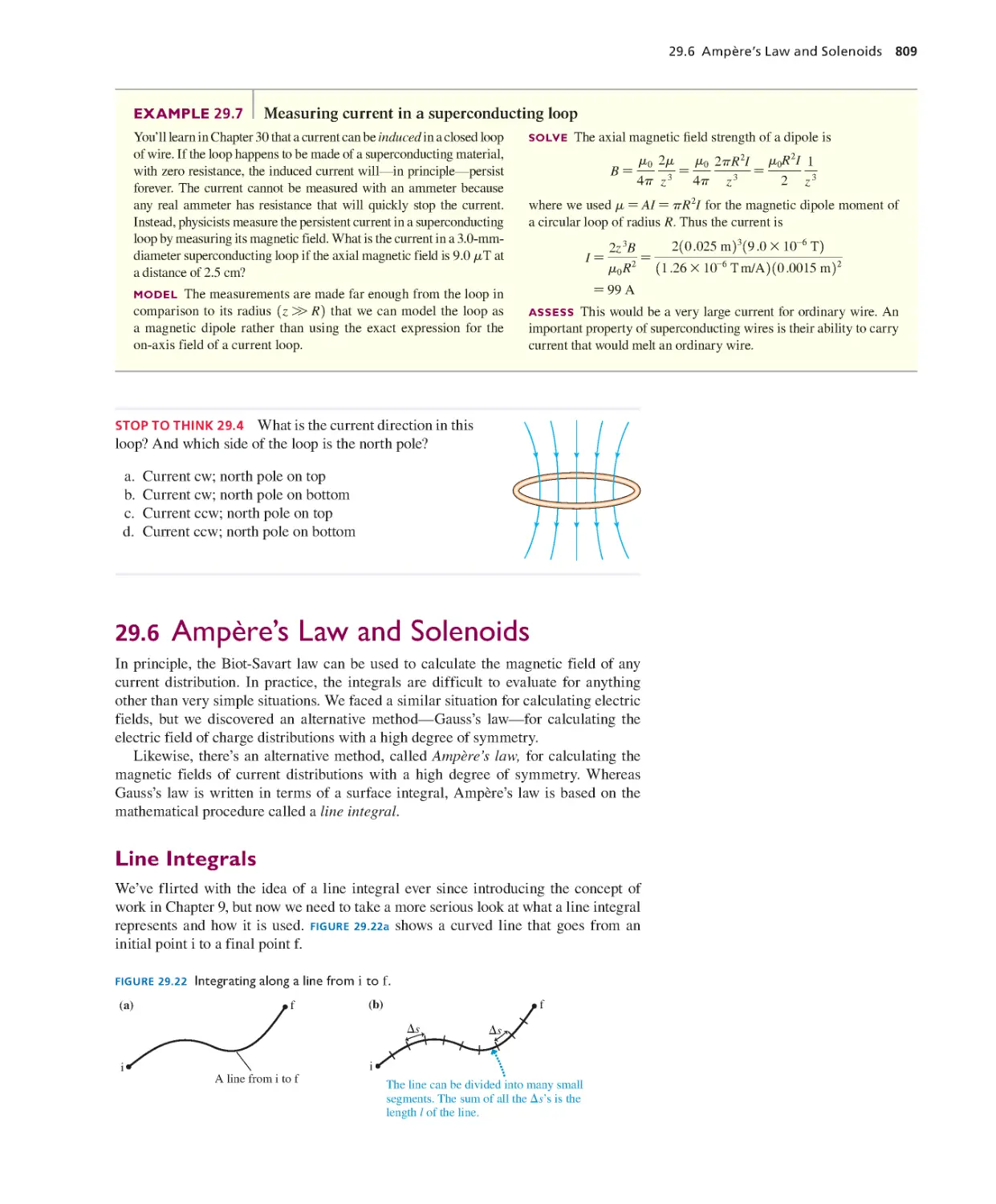
Let’s have a little chat before we start. A rather one-sided chat,
admittedly, because you can’t respond, but that’s OK. I’ve
talked with many of your fellow students over the years, so I
have a pretty good idea of what’s on your mind.
What’s your reaction to taking physics? Fear and loathing?
Uncertainty? Excitement? All the above? Let’s face it, physics
has a bit of an image problem on campus. You’ve probably heard
that it’s difficult, maybe impossible unless you’re an Einstein.
Things that you’ve heard, your experiences in other science
courses, and many other factors all color your expectations
about what this course is going to be like.
It’s true that there are many new ideas to be learned in physics
and that the course, like college courses in general, is going to be
much faster paced than science courses you had in high school.
I think it’s fair to say that it will be an intense course. But we
can avoid many potential problems and difficulties if we can
establish, here at the beginning, what this course is about and
what is expected of you—and of me!
Just what is physics, anyway? Physics is a way of think-
ing about the physical aspects of nature. Physics is not better
than art or biology or poetry or religion, which are also ways
to think about nature; it’s simply different. One of the things
this course will emphasize is that physics is a human endeavor.
The ideas presented in this book were not found in a cave or
conveyed to us by aliens; they were discovered and developed
by real people engaged in a struggle with real issues.
You might be surprised to hear that physics is not about
“facts.” Oh, not that facts are unimportant, but physics is far
more focused on discovering relationships and patterns than
on learning facts for their own sake.
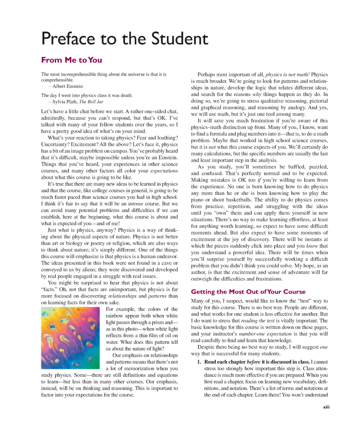
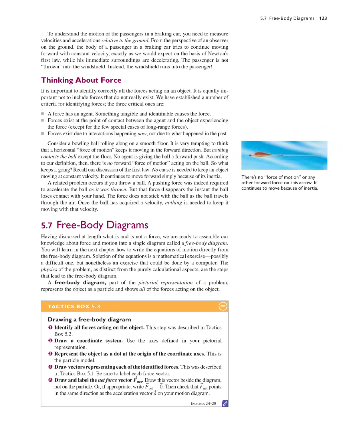
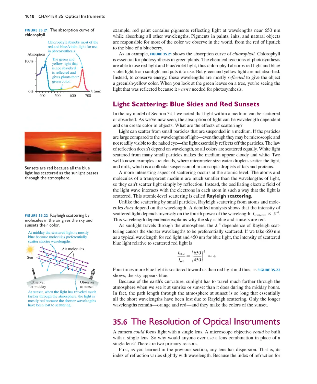
For example, the colors of the
rainbow appear both when white
light passes through a prism and—
as in this photo—when white light
ref lects from a thin film of oil on
water. What does this pattern tell
us about the nature of light?
Our emphasis on relationships
and patterns means that there’s not
a lot of memorization when you
study physics. Some—there are still definitions and equations
to learn—but less than in many other courses. Our emphasis,
instead, will be on thinking and reasoning. This is important to
factor into your expectations for the course.
Perhaps most important of all, physics is not math! Physics
is much broader. We’re going to look for patterns and relation-
ships in nature, develop the logic that relates different ideas,
and search for the reasons why things happen as they do. In
doing so, we’re going to stress qualitative reasoning, pictorial
and graphical reasoning, and reasoning by analogy. And yes,
we will use math, but it’s just one tool among many.
It will save you much frustration if you’re aware of this
physics–math distinction up front. Many of you, I know, want
to find a formula and plug numbers into it—that is, to do a math
problem. Maybe that worked in high school science courses,
but it is not what this course expects of you. We’ll certainly do
many calculations, but the specific numbers are usually the last
and least important step in the analysis.
As you study, you’ll sometimes be baffled, puzzled,
and confused. That’s perfectly normal and to be expected.
Making mistakes is OK too if you’re willing to learn from
the experience. No one is born knowing how to do physics
any more than he or she is born knowing how to play the
piano or shoot basketballs. The ability to do physics comes
from practice, repetition, and struggling with the ideas
until you “own” them and can apply them yourself in new
situations. There’s no way to make learning effortless, at least
for anything worth learning, so expect to have some difficult
moments ahead. But also expect to have some moments of
excitement at the joy of discovery. There will be instants at
which the pieces suddenly click into place and you know that
you understand a powerful idea. There will be times when
you’ll surprise yourself by successfully working a difficult
problem that you didn’t think you could solve. My hope, as an
author, is that the excitement and sense of adventure will far
outweigh the difficulties and frustrations.
Getting the Most Out of Your Course
Many of you, I suspect, would like to know the “best” way to
study for this course. There is no best way. People are diferent,
and what works for one student is less efective for another. But
I do want to stress that reading the text is vitally important. The
basic knowledge for this course is written down on these pages,
and your instructor’s number-one expectation is that you will
read carefully to ind and learn that knowledge.
Despite there being no best way to study, I will suggest one
way that is successful for many students.
1. Read each chapter before it is discussed in class. I cannot
stress too strongly how important this step is. Class atten-
dance is much more efective if you are prepared. When you
irst read a chapter, focus on learning new vocabulary, dei-
nitions, and notation. There’s a list of terms and notations at
the end of each chapter. Learn them! You won’t understand
Preface to the Student
From Me to You
xiii
xiv Preface to the Student
what’s being discussed or how the ideas are being used if
you don’t know what the terms and symbols mean.
2. Participate actively in class. Take notes, ask and answer
questions, and participate in discussion groups. There is
ample scientiic evidence that active participation is much
more efective for learning science than passive listening.
3. After class, go back for a careful re-reading of the
chapter. In your second reading, pay closer attention to
the details and the worked examples. Look for the logic
behind each example (I’ve highlighted this to make it
clear), not just at what formula is being used. And use the
textbook tools that are designed to help your learning, such
as the problem-solving strategies, the chapter summaries,
and the exercises in the Student Workbook.
4. Finally, apply what you have learned to the home-
work problems at the end of each chapter. I strongly
encourage you to form a study group with two or three
classmates. There’s good evidence that students who
study regularly with a group do better than the rugged
individualists who try to go it alone.
Did someone mention a
workbook? The companion Stu-
dent Workbook is a vital part of
the course. Its questions and ex-
ercises ask you to reason quali-
tatively, to use graphical infor-
mation, and to give explanations.
It is through these exercises that
you will learn what the concepts
mean and will practice the rea-
soning skills appropriate to the
chapter. You will then have ac-
quired the baseline knowledge
and confidence you need before turning to the end-of-chapter
homework problems. In sports or in music, you would never
think of performing before you practice, so why would you
want to do so in physics? The workbook is where you practice
and work on basic skills.
Many of you, I know, will be tempted to go straight to the
homework problems and then thumb through the text looking
for a formula that seems like it will work. That approach will
not succeed in this course, and it’s guaranteed to make you
frustrated and discouraged. Very few homework problems are
of the “plug and chug” variety where you simply put numbers
into a formula. To work the homework problems successfully,
you need a better study strategy—either the one outlined above
or your own—that helps you learn the concepts and the rela-
tionships between the ideas.
Getting the Most Out of Your Textbook
Your textbook provides many features designed to help you learn
the concepts of physics and solve problems more efectively.
■ TACTICS BOXES give step-by-step procedures for particu-
lar skills, such as interpreting graphs or drawing special
diagrams. Tactics Box steps are explicitly illustrated in sub-
sequent worked examples, and these are often the starting
point of a full Problem-Solving Strategy.
■ PROBLEM-SOLVING STRATEGIES are provided for each
broad class of problems—problems characteristic of a
chapter or group of chapters. The strategies follow a con-
sistent four-step approach to help you develop conidence
and proicient problem-solving skills: MODEL, VISUALIZE,
SOLVE, ASSESS.
■ Worked EXAMPLES illustrate good problem-solving practices
through the consistent use of the four-step problem-solving
approach The worked examples are often very detailed and
carefully lead you through the reasoning behind the solution
as well as the numerical calculations.
■ STOP TO THINK questions embedded in the chapter allow
you to quickly assess whether you’ve understood the main
idea of a section. A correct answer will give you conidence
to move on to the next section. An incorrect answer will
alert you to re-read the previous section.
■ Blue annotations on figures help you better understand what
the figure is showing.
They will help you to in-
terpret graphs; translate
between graphs, math,
and pictures; grasp dif-
ficult concepts through
a visual analogy; and de-
velop many other impor-
tant skills.
■ Schematic Chapter Summaries help you organize what you
have learned into a hierarchy, from general principles (top) to
applications (bottom). Side-by-side pictorial, graphical, tex-
tual, and mathematical representations are used to help you
translate between these key representations.
■ Each part of the book ends with a KNOWLEDGE STRUCTURE
designed to help you see the forest rather than just the trees.
Now that you know more about what is expected of you,
what can you expect of me? That’s a little trickier because the
book is already written! Nonetheless, the book was prepared
on the basis of what I think my students throughout the years
have expected—and wanted—from their physics textbook.
Further, I’ve listened to the extensive feedback I have received
from thousands of students like you, and their instructors, who
used the irst three editions of this book.
You should know that these course materials—the text and
the workbook—are based on extensive research about how stu-
dents learn physics and the challenges they face. The effective-
ness of many of the exercises has been demonstrated through
extensive class testing. I’ve written the book in an informal
style that I hope you will find appealing and that will encour-
age you to do the reading. And, finally, I have endeavored to
make clear not only that physics, as a technical body of knowl-
edge, is relevant to your profession but also that physics is an
exciting adventure of the human mind.
I hope you’ll enjoy the time we’re going to spend together.
I
The current in a wire is
the same at all points.
I = constant
xv
Detailed Contents
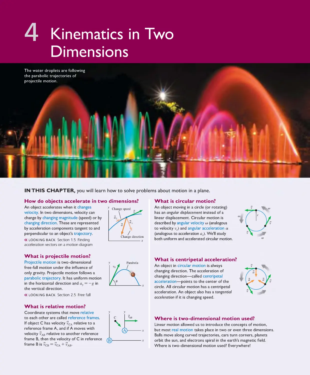
Chapter 4 Kinematics in Two Dimensions 80
4.1 Motion in Two Dimensions 81
4.2 Projectile Motion 85
4.3 Relative Motion 90
4.4 Uniform Circular Motion 92
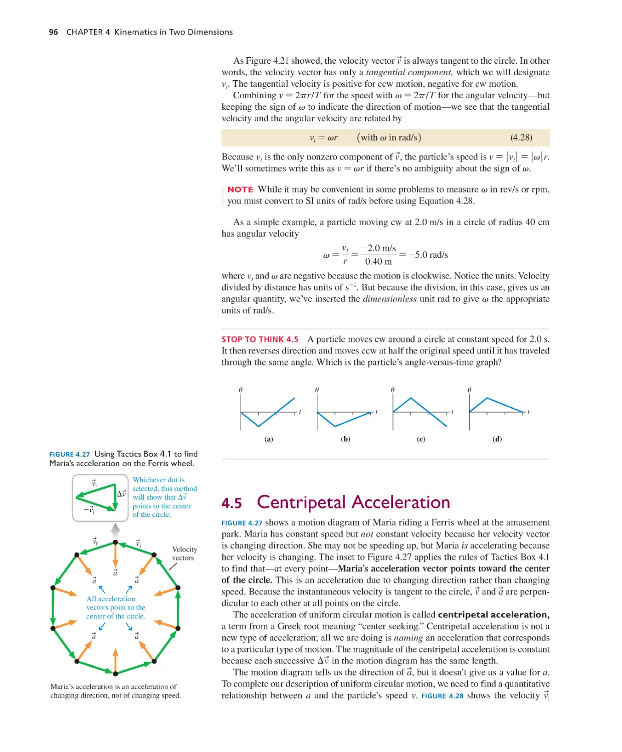
4.5 Centripetal Acceleration 96
4.6 Nonuniform Circular Motion 98
SUMMARY 103
QUESTIONS AND PROBLEMS 10 4
Chapter 5 Force and Motion 110
5.1 Force 111
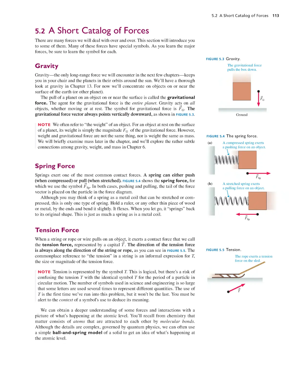
5.2 A Short Catalog of Forces 113
5.3 Identifying Forces 115
5.4 What Do Forces Do? 117
5.5 Newton’s Second Law 120
5.6 Newton’s First Law 121
5.7 Free-Body Diagrams 123
SUMMARY 126
QUESTIONS AND PROBLEMS 127
Chapter 6 Dynamics I: Motion Along a
Line 131
6.1 The Equilibrium Model 132
6.2 Using Newton’s Second Law 134
6.3 Mass, Weight, and Gravity 137
6.4 Friction 141
6.5 Drag 145
6.6 More Examples of Newton’s Second
Law 148
SUMMARY 152
QUESTIONS AND PROBLEMS 153
Chapter 7 Newton’s Third Law 159
7.1 Interacting Objects 160
7.2 Analyzing Interacting Objects 161
7.3 Newton’s Third Law 164
7.4 Ropes and Pulleys 169
7.5 Examples of Interacting-Object
Problems 172
SUMMARY 175
QUESTIONS AND PROBLEMS 176
Part I Newton’s Laws
OVERVIEW Why Things Change 1
Chapter 1 Concepts of Motion 2
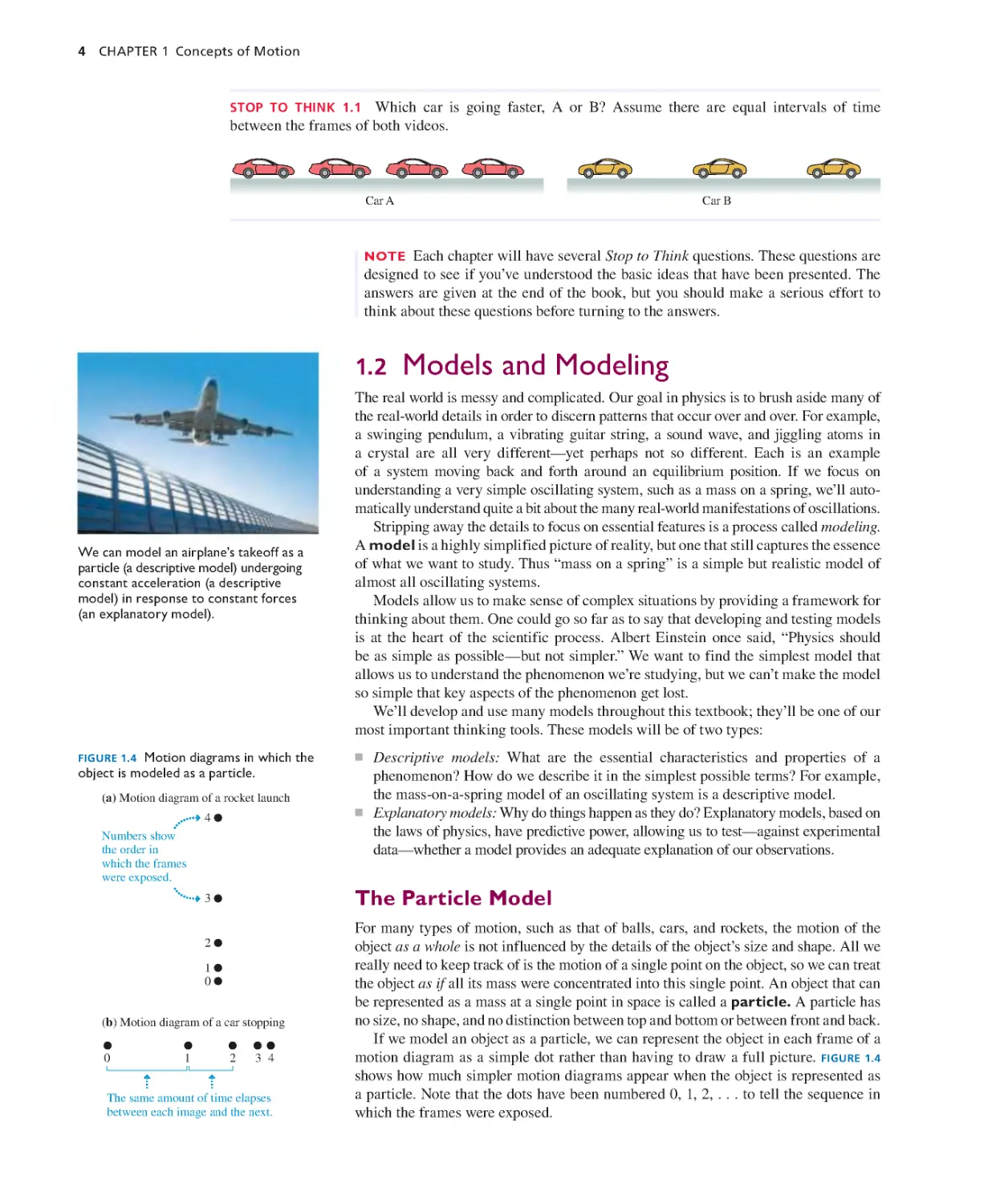
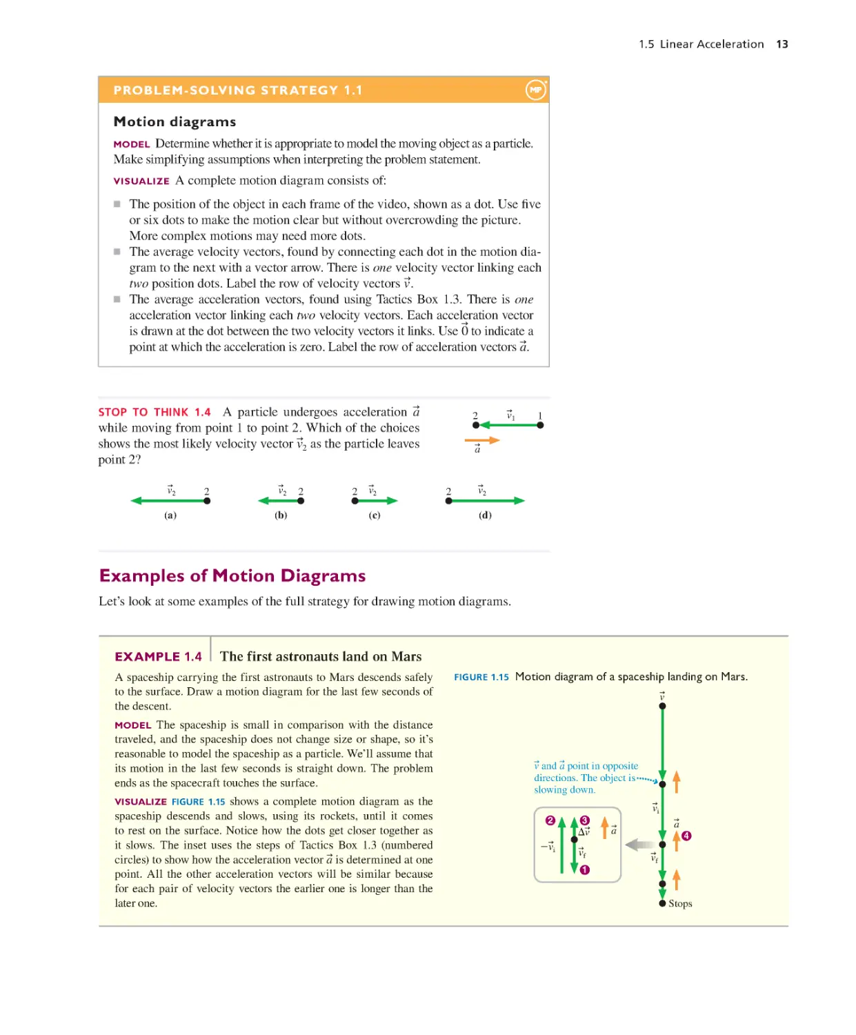
1.1 Motion Diagrams 3
1.2 Models and Modeling 4
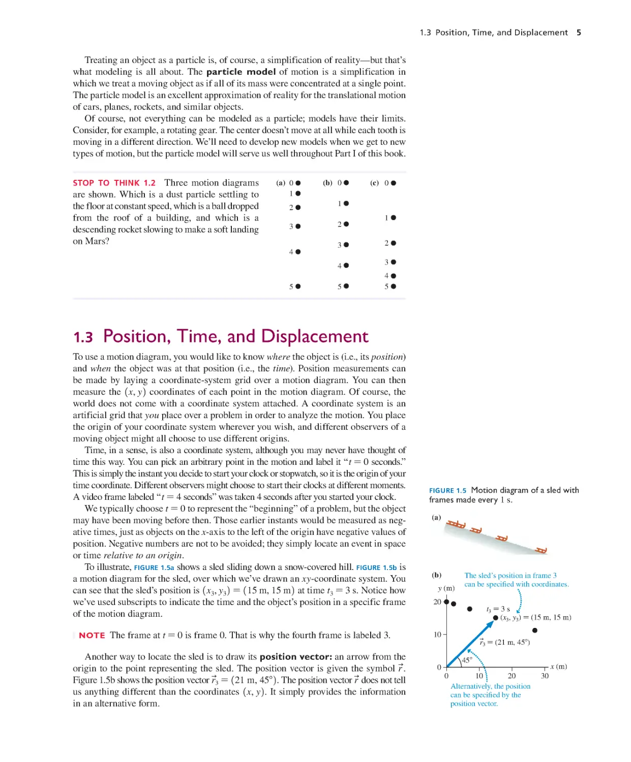
1.3 Position, Time, and Displacement 5
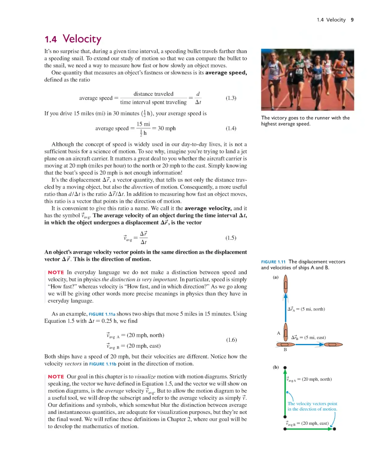
1.4 Velocity 9
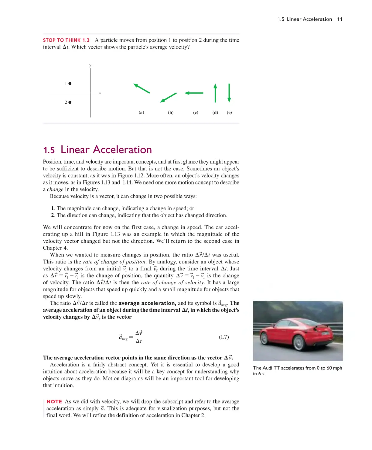
1.5 Linear Acceleration 11
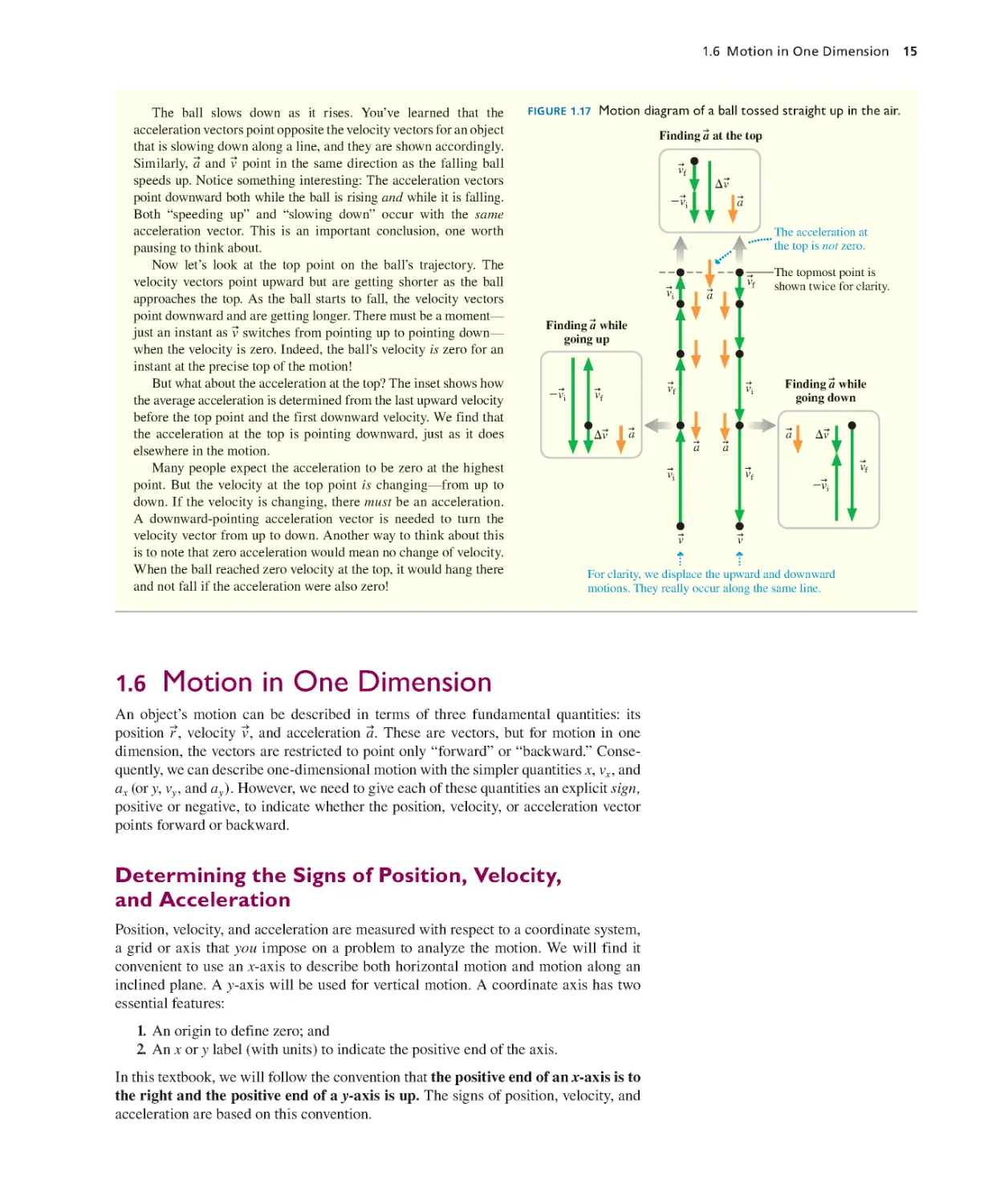
1.6 Motion in One Dimension 15
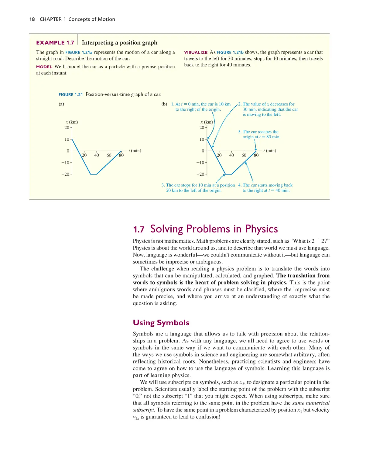
1.7 Solving Problems in Physics 18
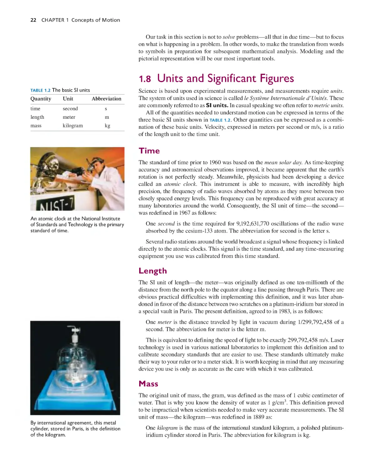
1.8 Unit and Significant Figures 22
SUMMARY 27
QUESTIONS AND PROBLEMS 28
Chapter 2 Kinematics in One Dimension 32
2 .1 Uniform Motion 33
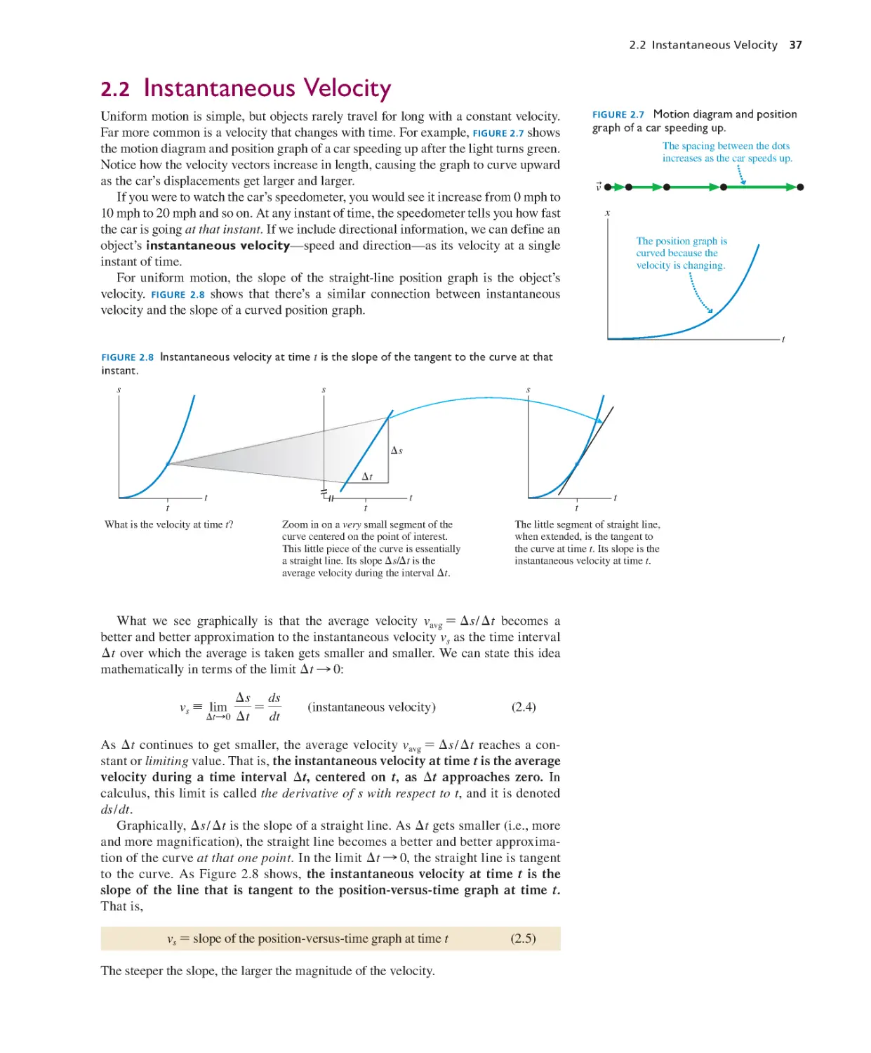
2.2 Instantaneous Velocity 37
2.3 Finding Position from Velocity 40
2.4 Motion with Constant Acceleration 43
2.5 Free Fall 49
2.6 Motion on an Inclined Plane 51
2.7 ADVANCED TOPIC Instantaneous
Acceleration 54
SUMMARY 57
QUESTIONS AND PROBLEMS 58
Chapter 3 Vectors and Coordinate Systems 65
3.1 Scalars and Vectors 66
3.2 Using Vectors 66
3.3 Coordinate Systems and Vector
Components 69
3.4 Unit Vectors and Vector Algebra 72
SUMMARY 76
QUESTIONS AND PROBLEMS 77
xvi Detailed Contents
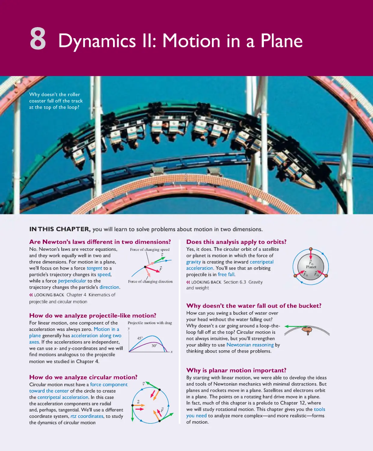
Chapter 8 Dynamics II: Motion in a Plane 182
8.1 Dynamics in Two Dimensions 183
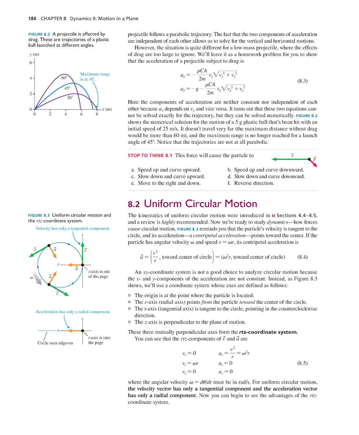
8.2 Uniform Circular Motion 184
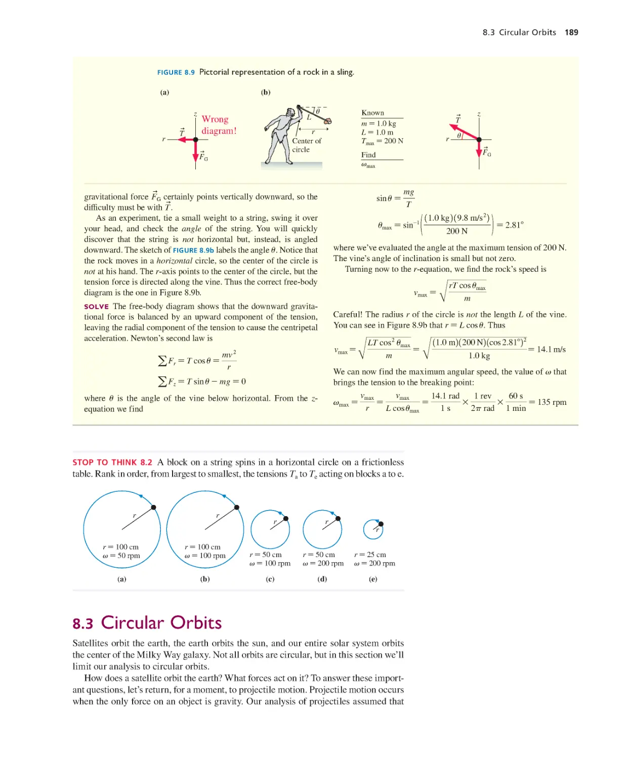
8.3 Circular Orbits 189
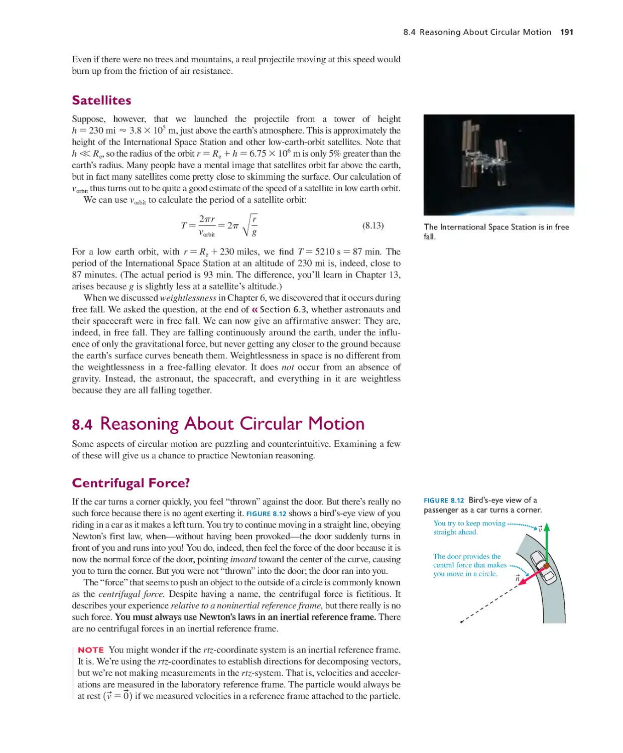
8.4 Reasoning About Circular Motion 191
8.5 Nonuniform Circular Motion 194
SUMMARY 197
QUESTIONS AND PROBLEMS 198
Part I Newton’s Laws 204
Part II Conservation Laws
OVERVIEW Why Some Things Don’t Change 205
Chapter 9 Work and Kinetic Energy 206
9.1 Energy Overview 207
9.2 Work and Kinetic Energy for a Single
Particle 209
9.3 Calculating the Work Done 213
9.4 Restoring Forces and the Work Done by
a Spring 219
9.5 Dissipative Forces and Thermal
Energy 221
9.6 Power 224
SUMMARY 226
QUESTIONS AND PROBLEMS 227
Chapter 10 Interactions and Potential
Energy 231
10.1 Potential Energy 232
10.2 Gravitational Potential Energy 233
10.3 Elastic Potential Energy 239
10.4 Conservation of Energy 242
10.5 Energy Diagrams 244
10.6 Force and Potential Energy 247
10.7 Conservative and Nonconservative
Forces 249
10.8 The Energy Principle Revisited 251
SUMMARY 254
QUESTIONS AND PROBLEMS 255
KNOWLEDGE
STRUCTURE
Chapter 11 Impulse and Momentum 261
11.1 Momentum and Impulse 262
11.2 Conservation of Momentum 266
11.3 Collisions 272
11.4 Explosions 277
11.5 Momentum in Two Dimensions 279
11.6 ADVANCED TOPIC Rocket Propulsion 281
SUMMARY 285
QUESTIONS AND PROBLEMS 286
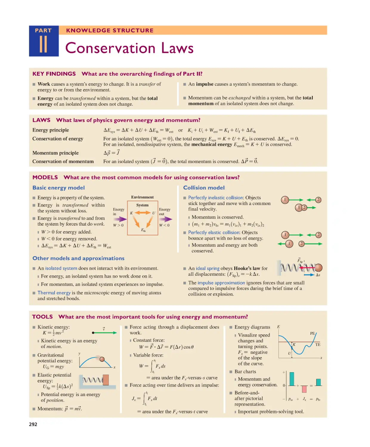
Part II Conservation Laws 292
Part III Applications of Newtonian
Mechanics
OVERVIEW Power Over Our Environment 293
KNOWLEDGE
STRUCTURE
Chapter 12 Rotation of a Rigid Body 294
12.1 Rotational Motion 295
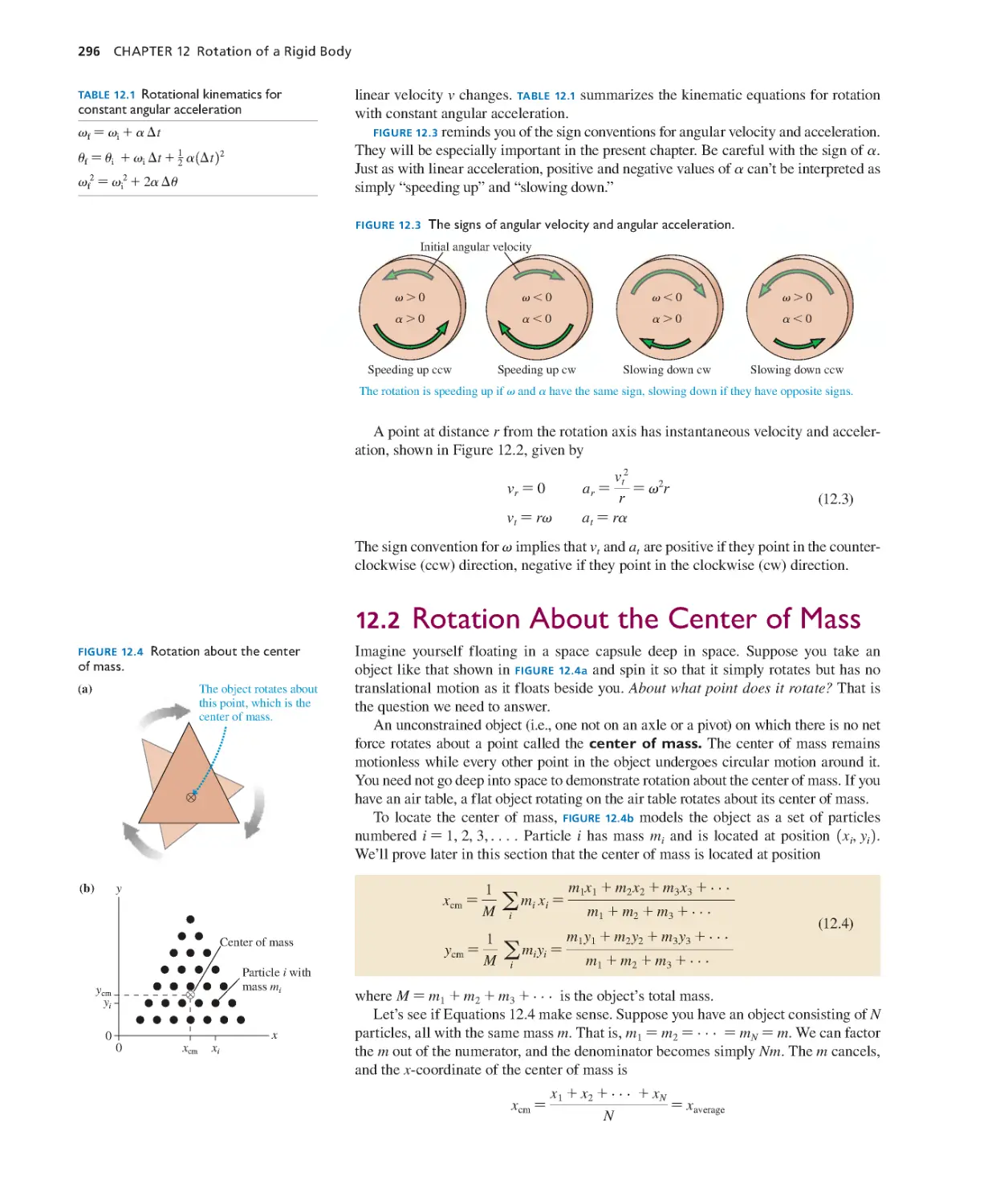
12.2 Rotation About the Center of Mass 296
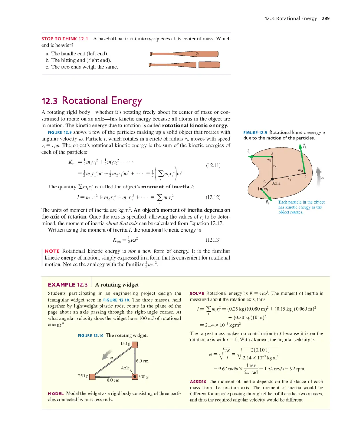
12.3 Rotational Energy 299
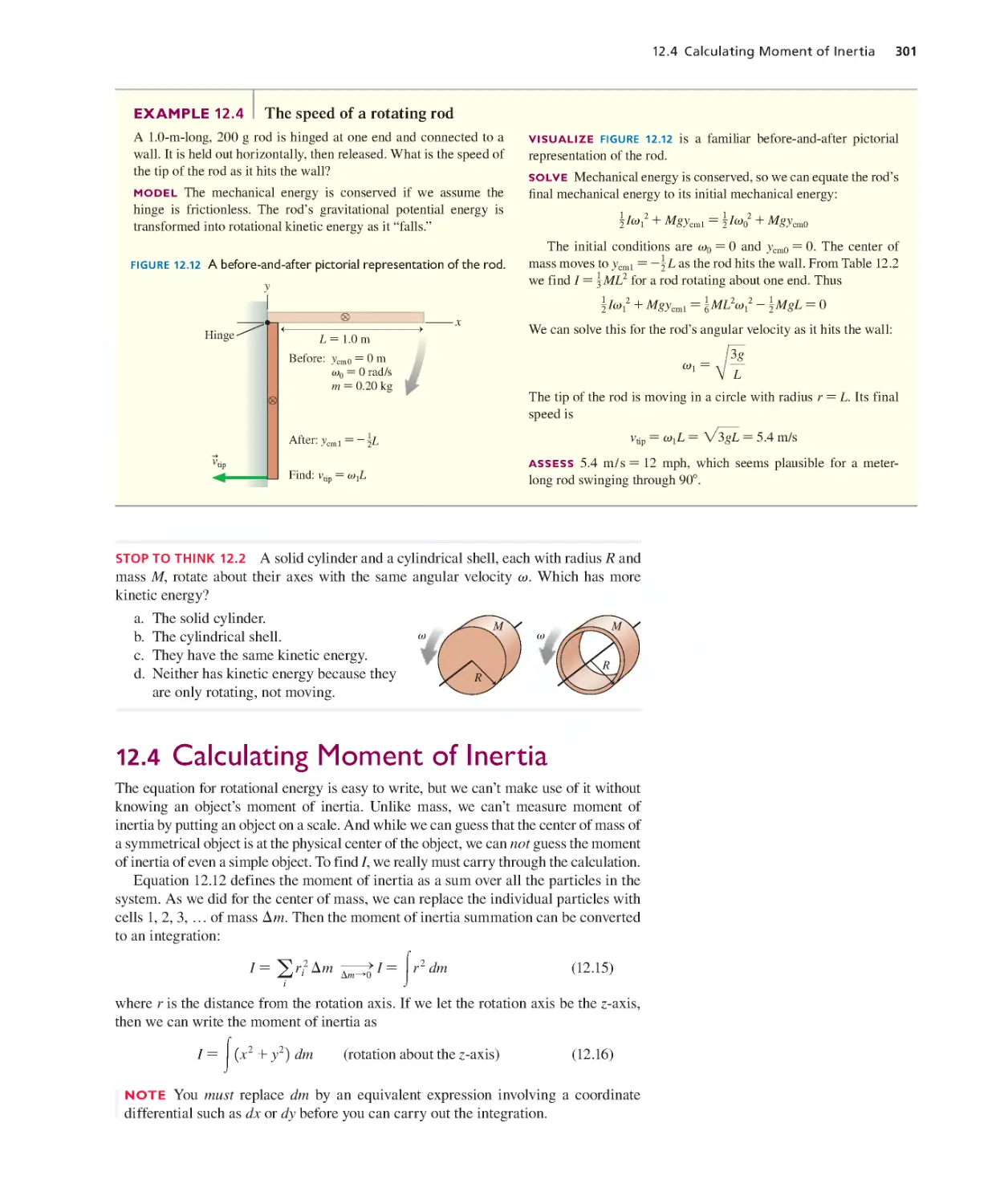
12.4 Calculating Moment of Inertia 301
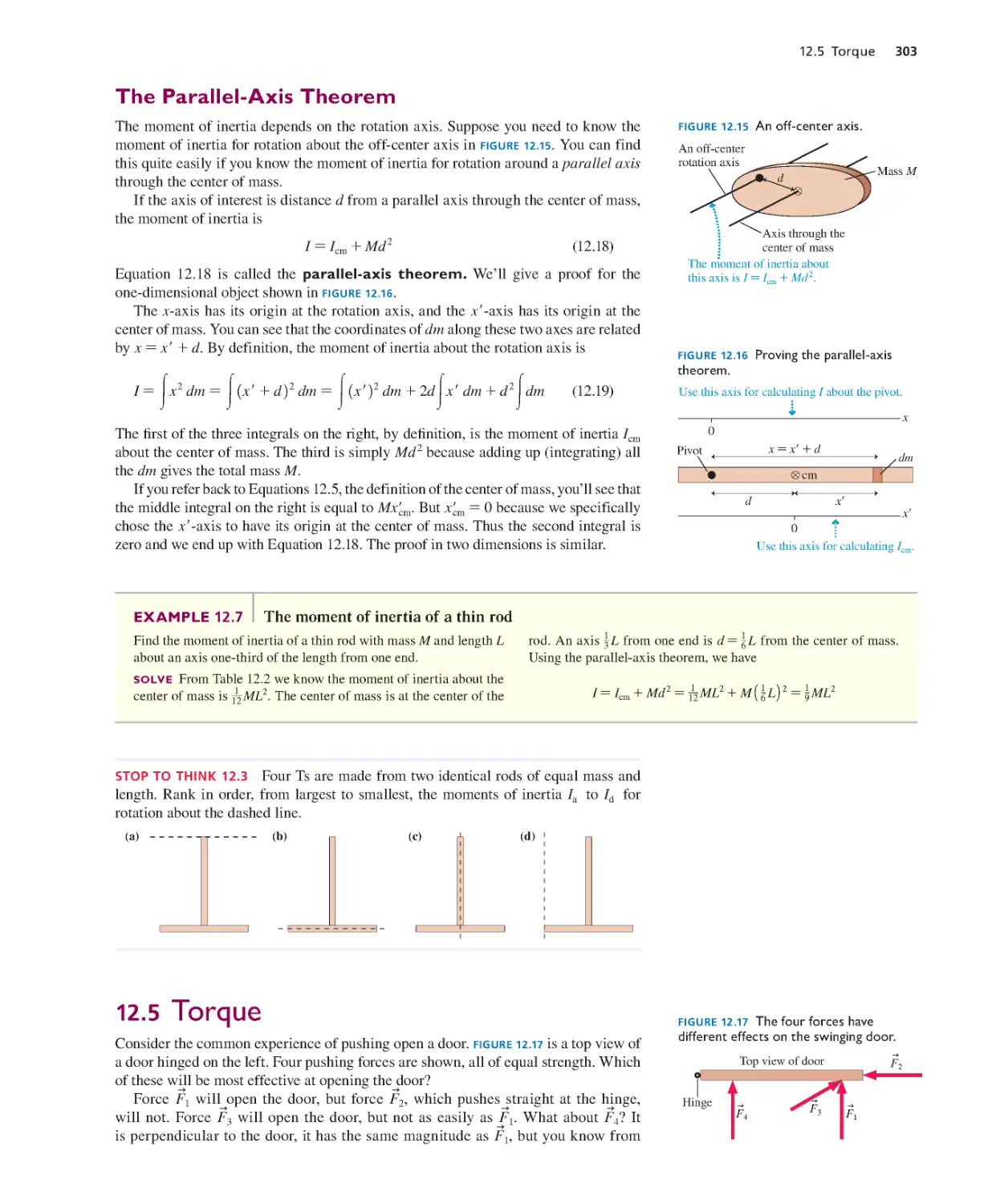
12.5 Torque 303
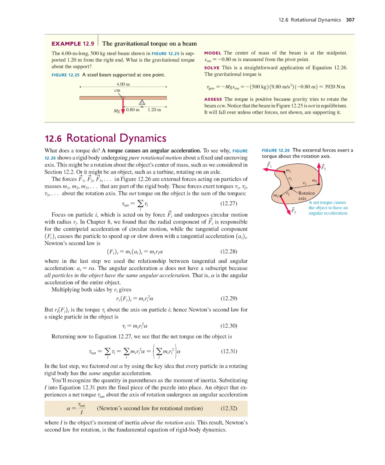
12.6 Rotational Dynamics 307
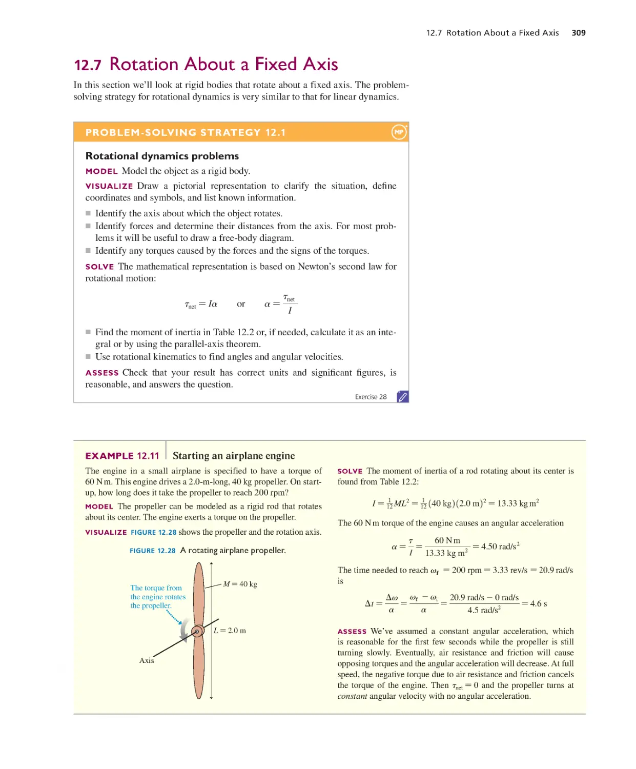
12.7 Rotation About a Fixed Axis 309
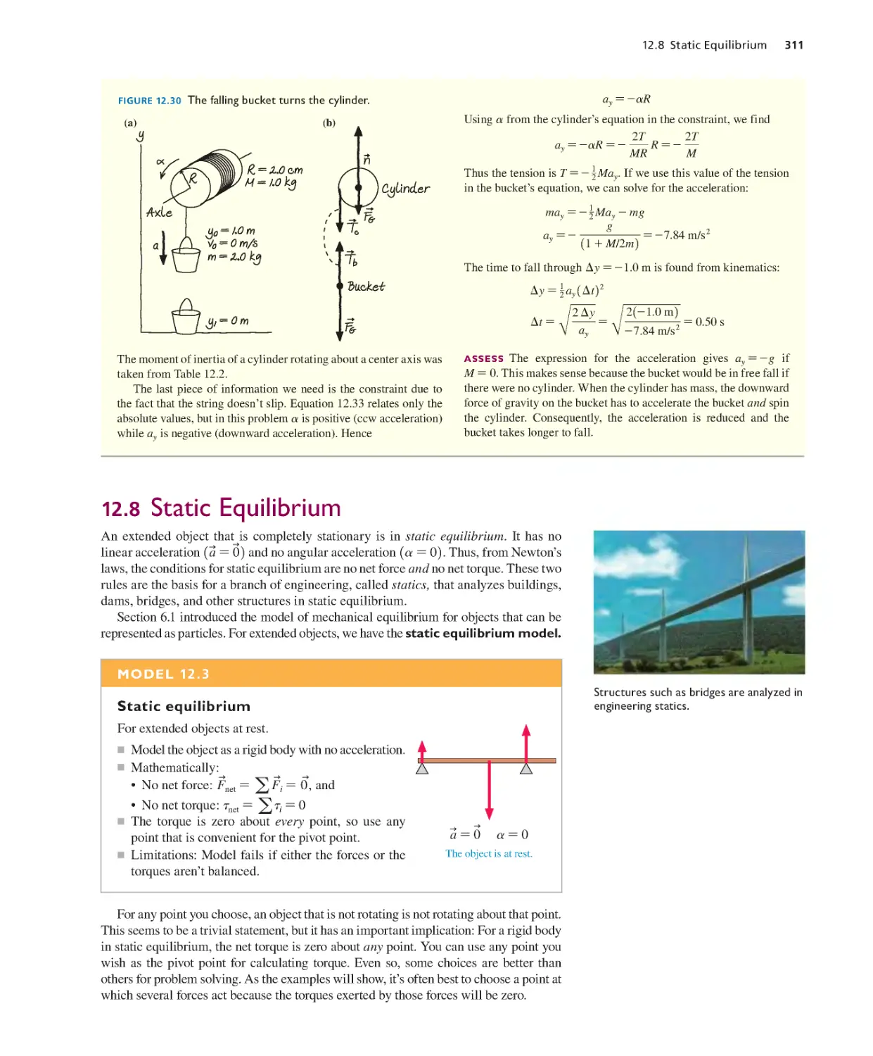
12.8 Static Equilibrium 311
12.9 Rolling Motion 314
12.10 The Vector Description of Rotational
Motion 317
12.11 Angular Momentum 320
12.12 ADVANCED TOPIC Precession of a
Gyroscope 324
SUMMARY 328
QUESTIONS AND PROBLEMS 339
Detailed Contents xvii
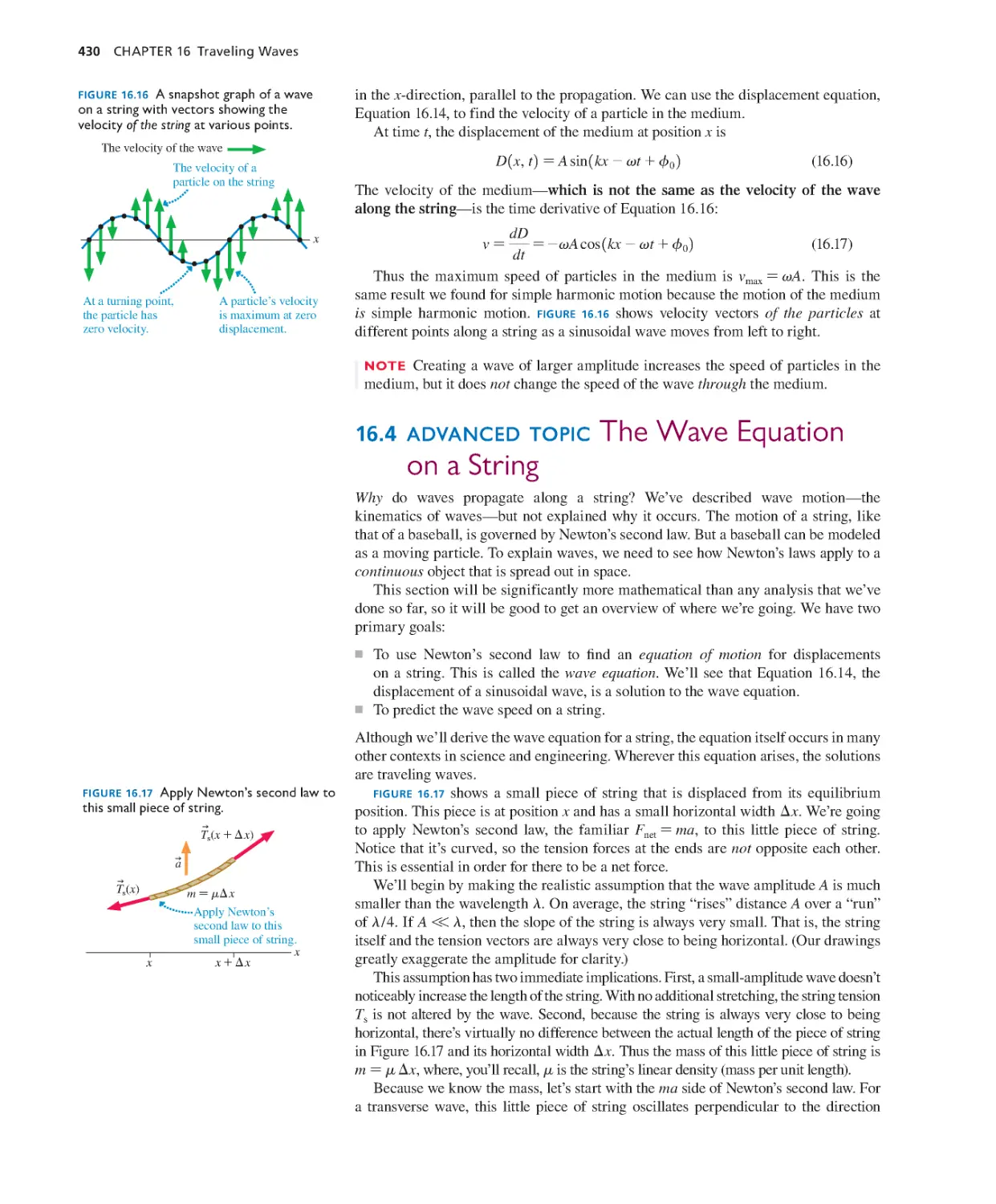
Chapter 16 Traveling Waves 420
16.1 The Wave Model 421
16.2 One-Dimensional Waves 423
16.3 Sinusoidal Waves 426
16.4 ADVANCED TOPIC The Wave Equation
on a String 430
16.5 Sound and Light 434
16.6 ADVANCED TOPIC The Wave Equation
in a Fluid 438
16.7 Waves in Two and Three
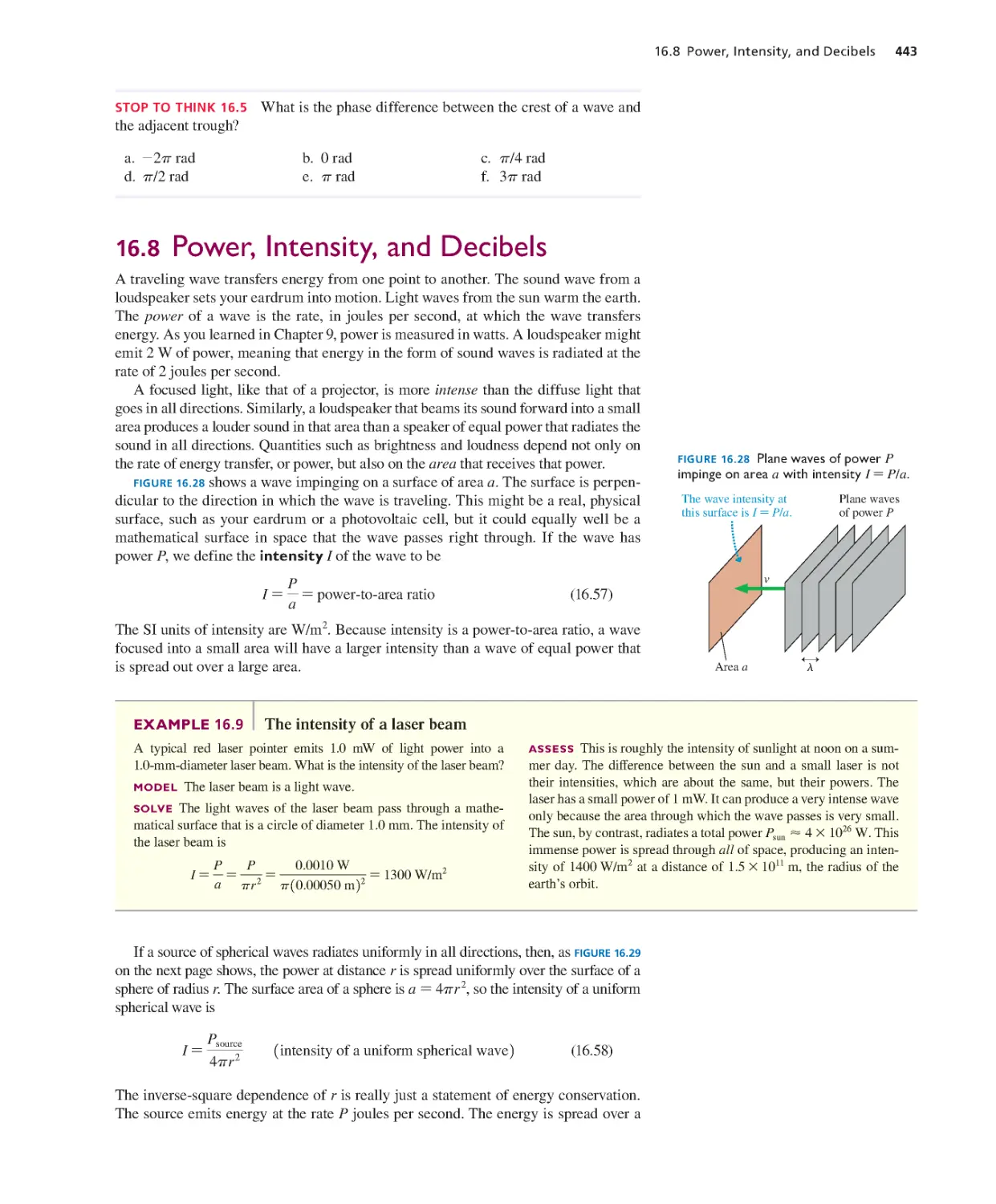
Dimensions 441
16.8 Power, Intensity, and Decibels 443
16.9 The Doppler Effect 445
SUMMARY 449
QUESTIONS AND PROBLEMS 450
Chapter 17 Superposition 455
17.1 The Principle of Superposition 456
17.2 Standing Waves 457
17.3 Standing Waves on a String 459
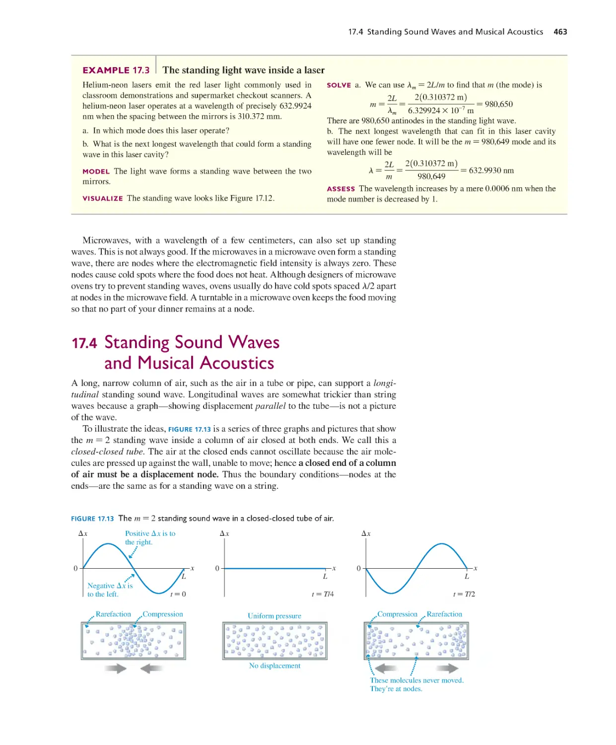
17.4 Standing Sound Waves and Musical
Acoustics 463
17.5 Interference in One Dimension 467
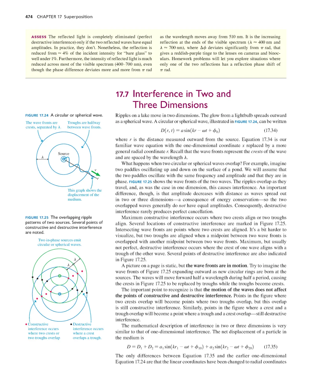
17.6 The Mathematics of Interference 471
17.7 Interference in Two and Three
Dimensions 474
17.8 Beats 477
SUMMARY 481
QUESTIONS AND PROBLEMS 482
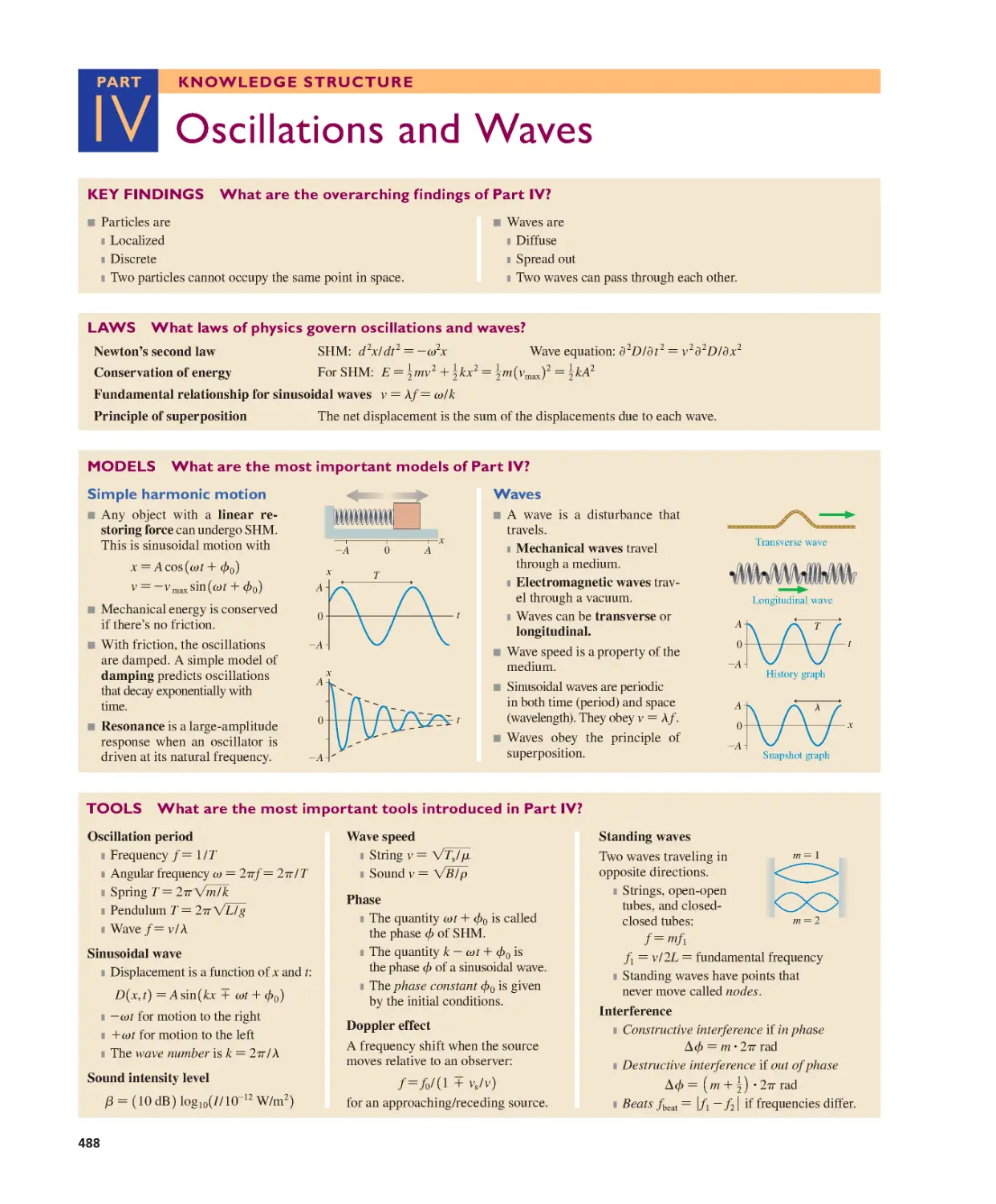
Part IV Oscillations and Waves 488
Part V Thermodynamics
OVERVIEW It’s All About Energy 489
Chapter 18 A Macroscopic Description of
Matter 490
18.1 Solids, Liquids, and Gases 491
18.2 Atoms and Moles 492
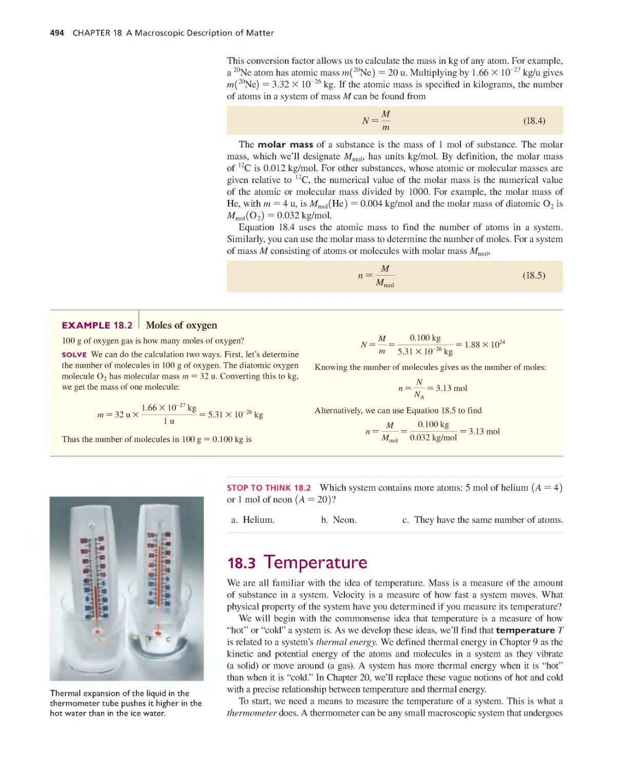
18.3 Temperature 494
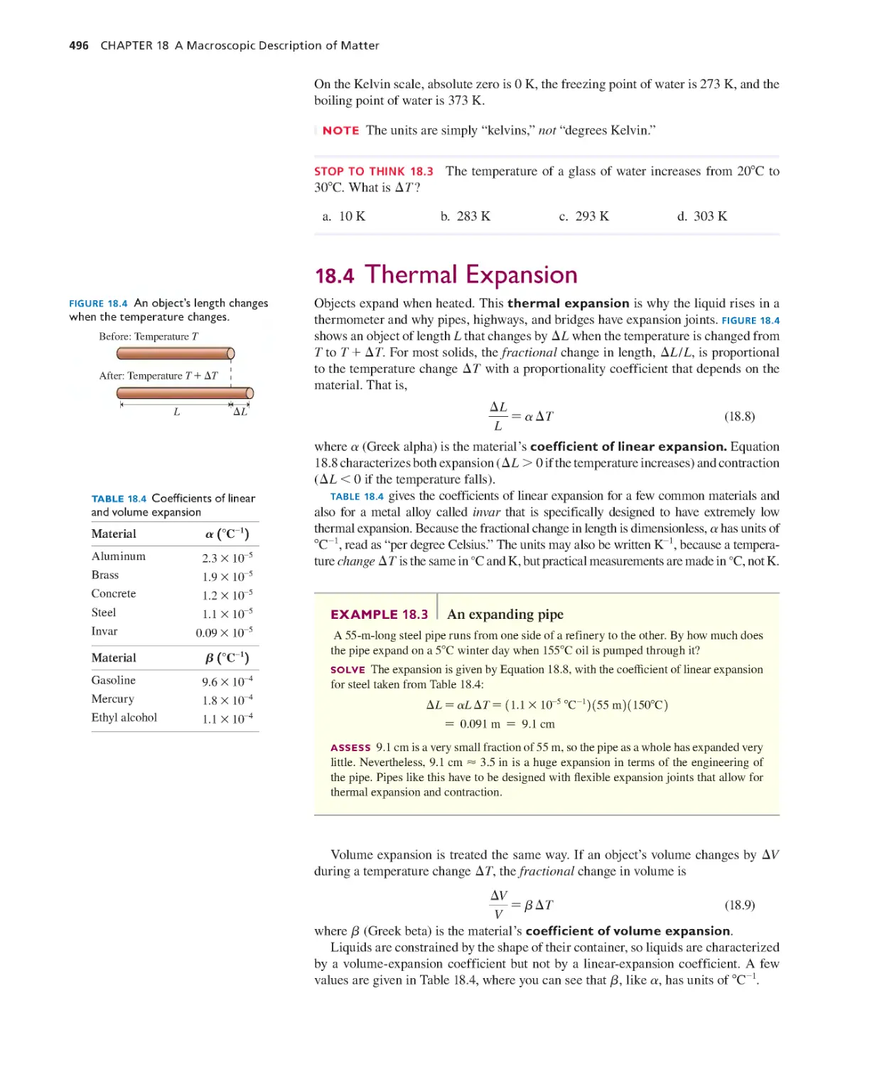
18.4 Thermal Expansion 496
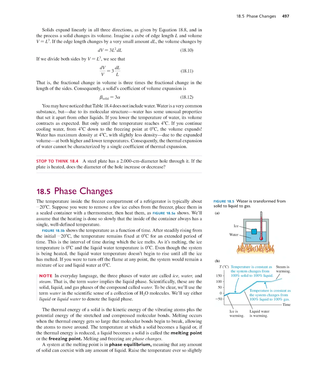
18.5 Phase Changes 497
18.6 Ideal Gases 499
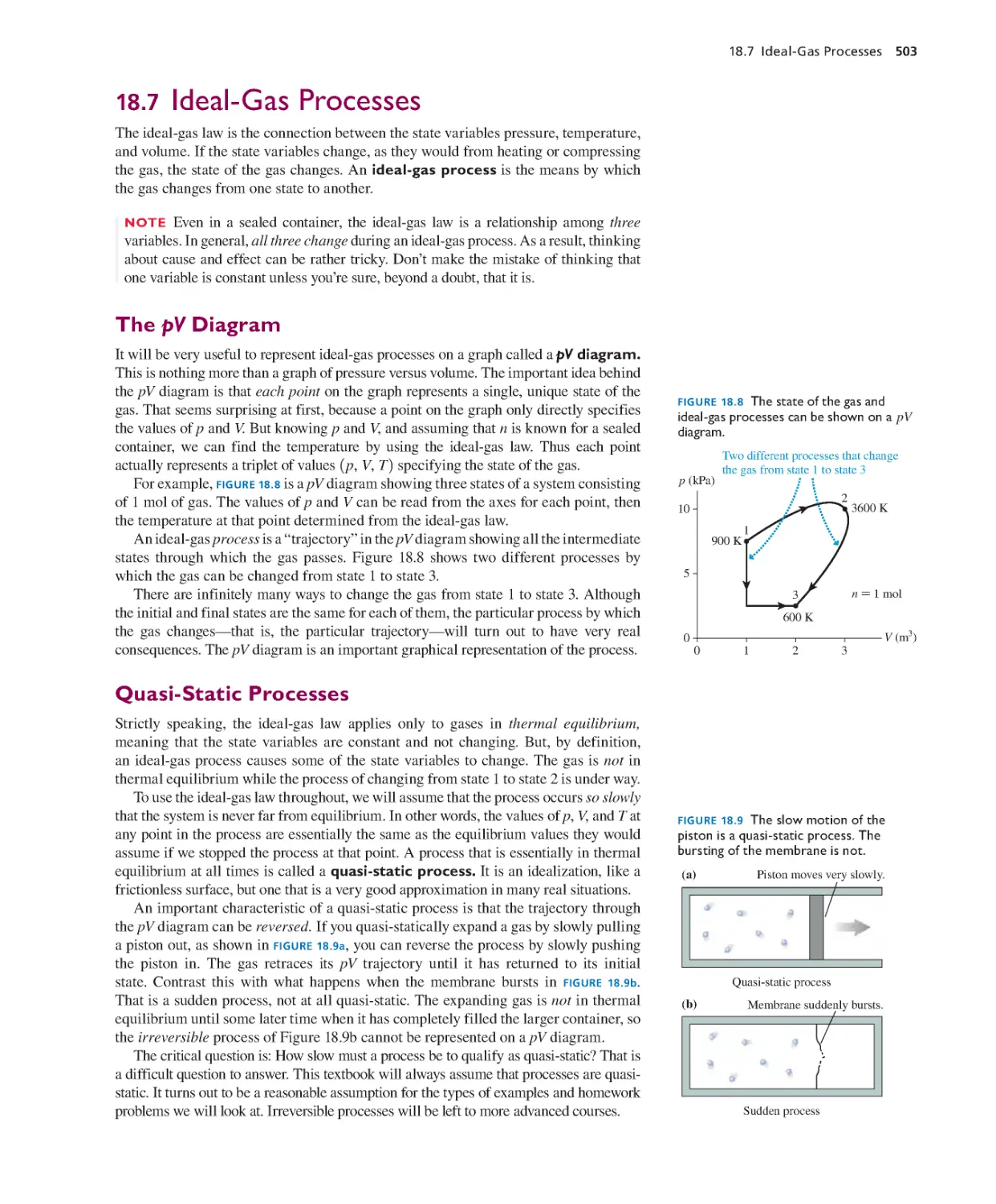
18.7 Ideal-Gas Processes 503
SUMMARY 509
QUESTIONS AND PROBLEMS 510
KNOWLEDGE
STRUCTURE
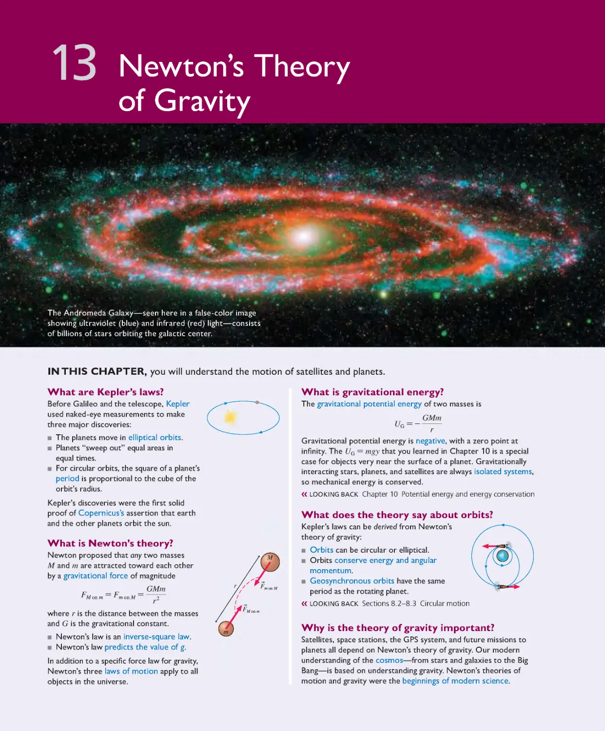
Chapter 13 Newton’s Theory of Gravity 336
13.1 A Little History 337
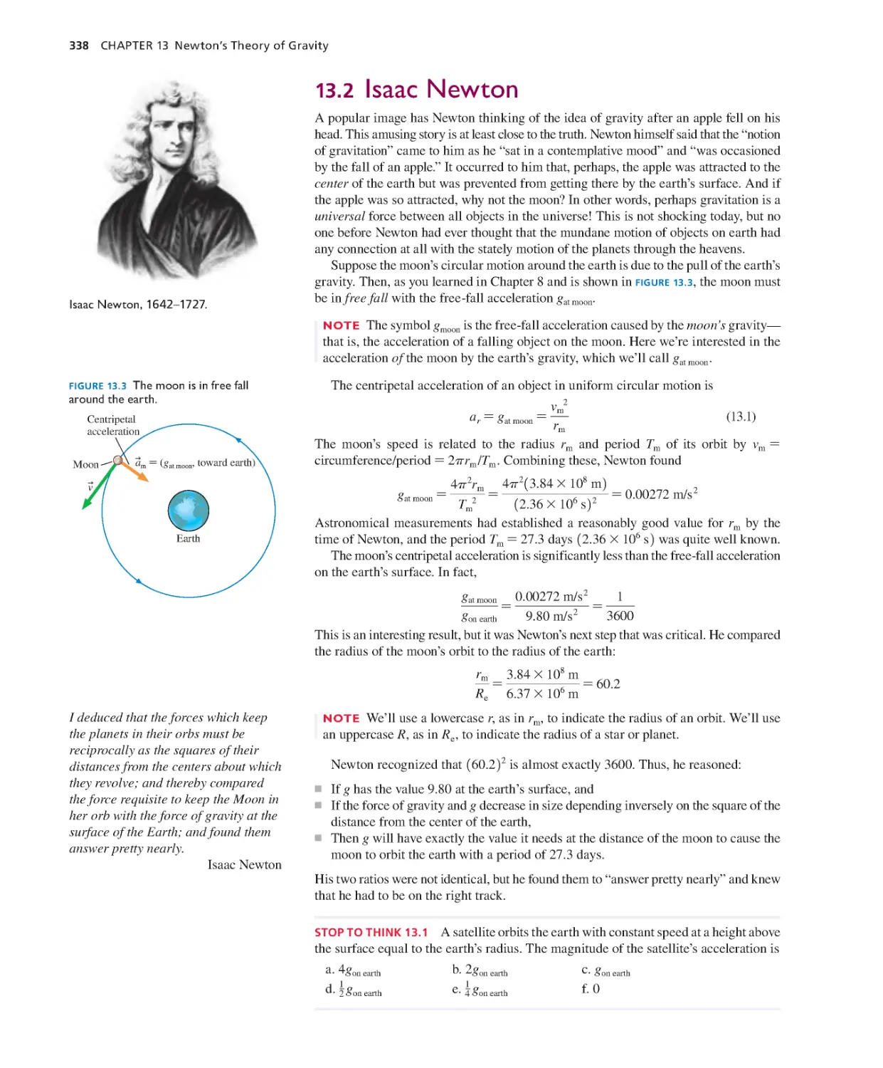
13.2 Isaac Newton 338
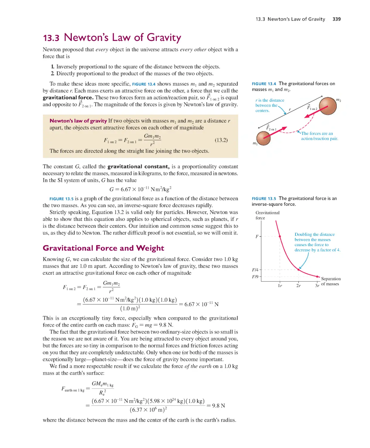
13.3 Newton’s Law of Gravity 339
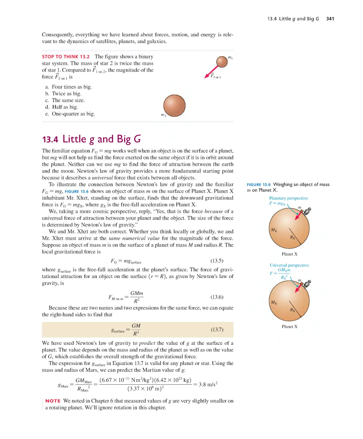
13.4 Little g and Big G 341
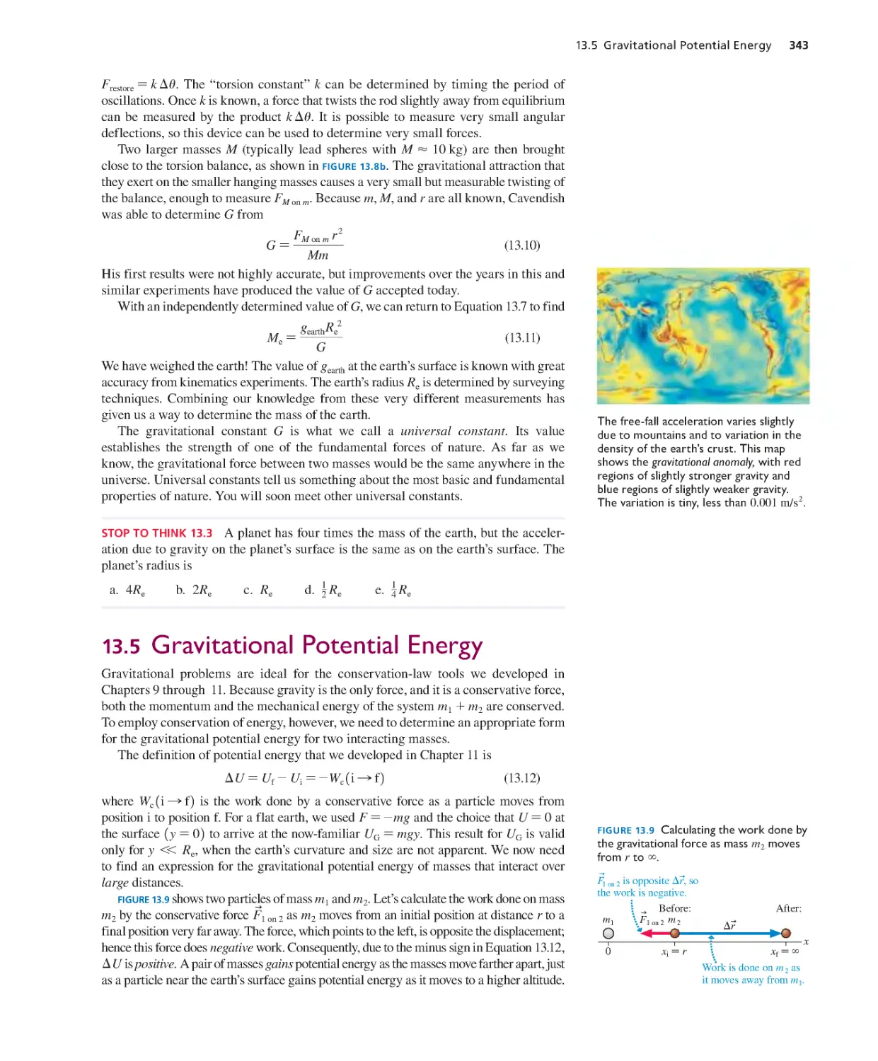
13.5 Gravitational Potential Energy 343
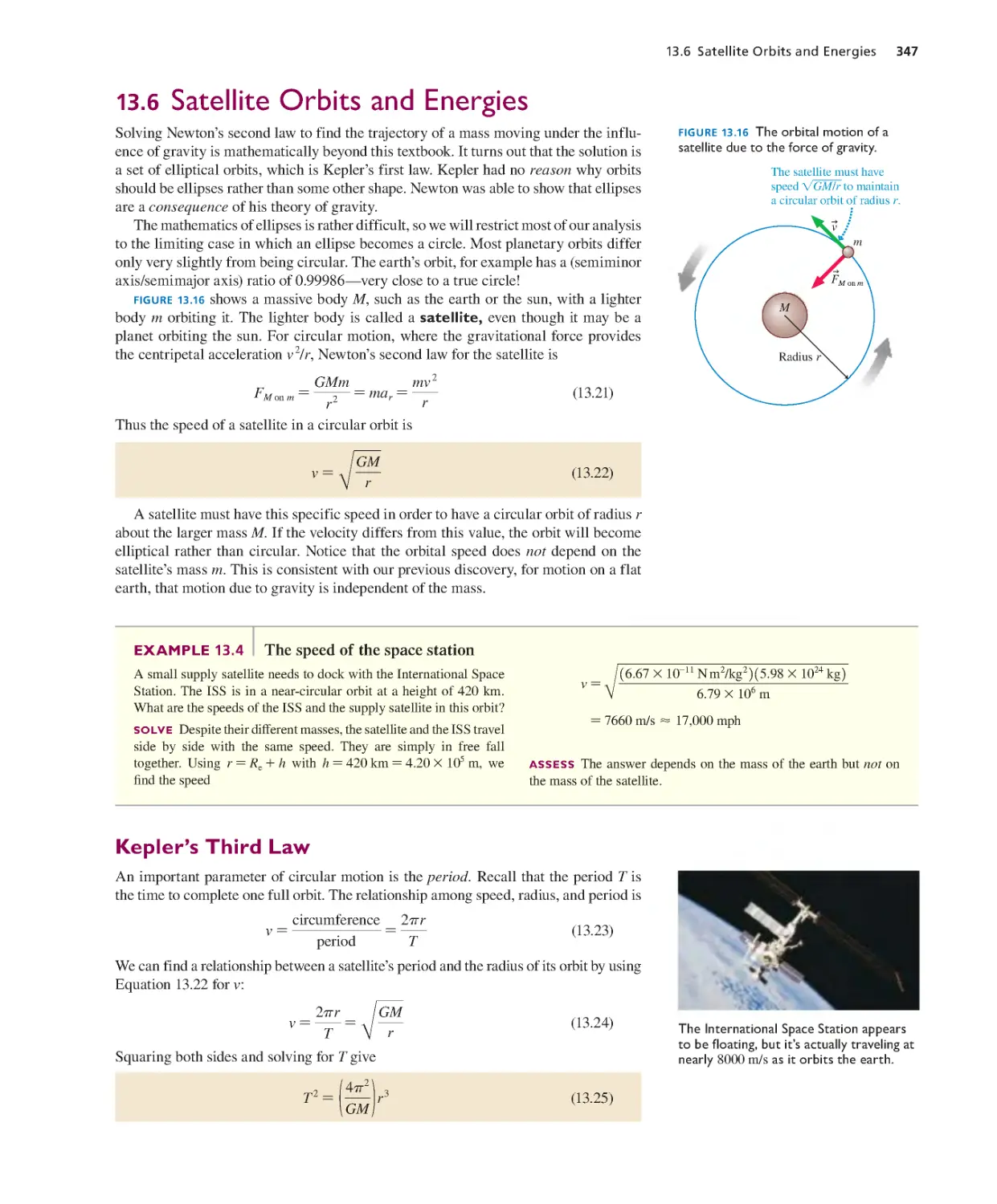
13.6 Satellite Orbits and Energies 347
SUMMARY 352
QUESTIONS AND PROBLEMS 353
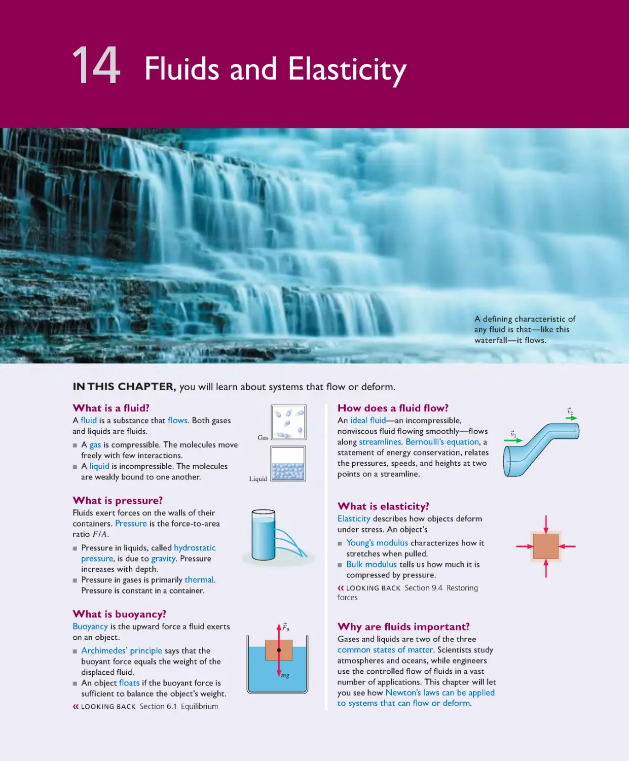
Chapter 14 Fluids and Elasticity 357
14.1 Fluids 358
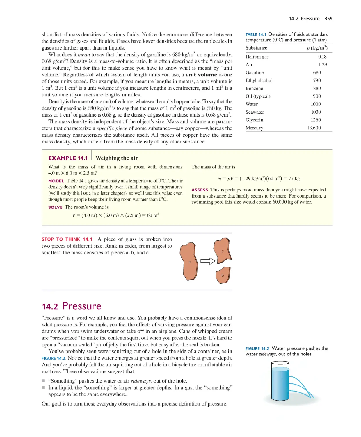
14.2 Pressure 359
14.3 Measuring and Using Pressure 365
14.4 Buoya ncy 369
14.5 Fluid Dynamics 373
14.6 Elasticity 378
SUMMARY 382
QUESTIONS AND PROBLEMS 383
Part III Applications of Newtonian
Mechanics 388
Part IV Oscillations and Waves
OVERVIEW The Wave Model 389
KNOWLEDGE
STRUCTURE
Chapter 15 Oscillations 390
15.1 Simple Harmonic Motion 391
15.2 SHM and Circular Motion 394
15.3 Energy in SHM 397
15.4 The Dynamics of SHM 399
15.5 Vertical Oscillations 402
15.6 The Pendulum 404
15.7 Damped Oscillations 408
15.8 Driven Oscillations and Resonance 411
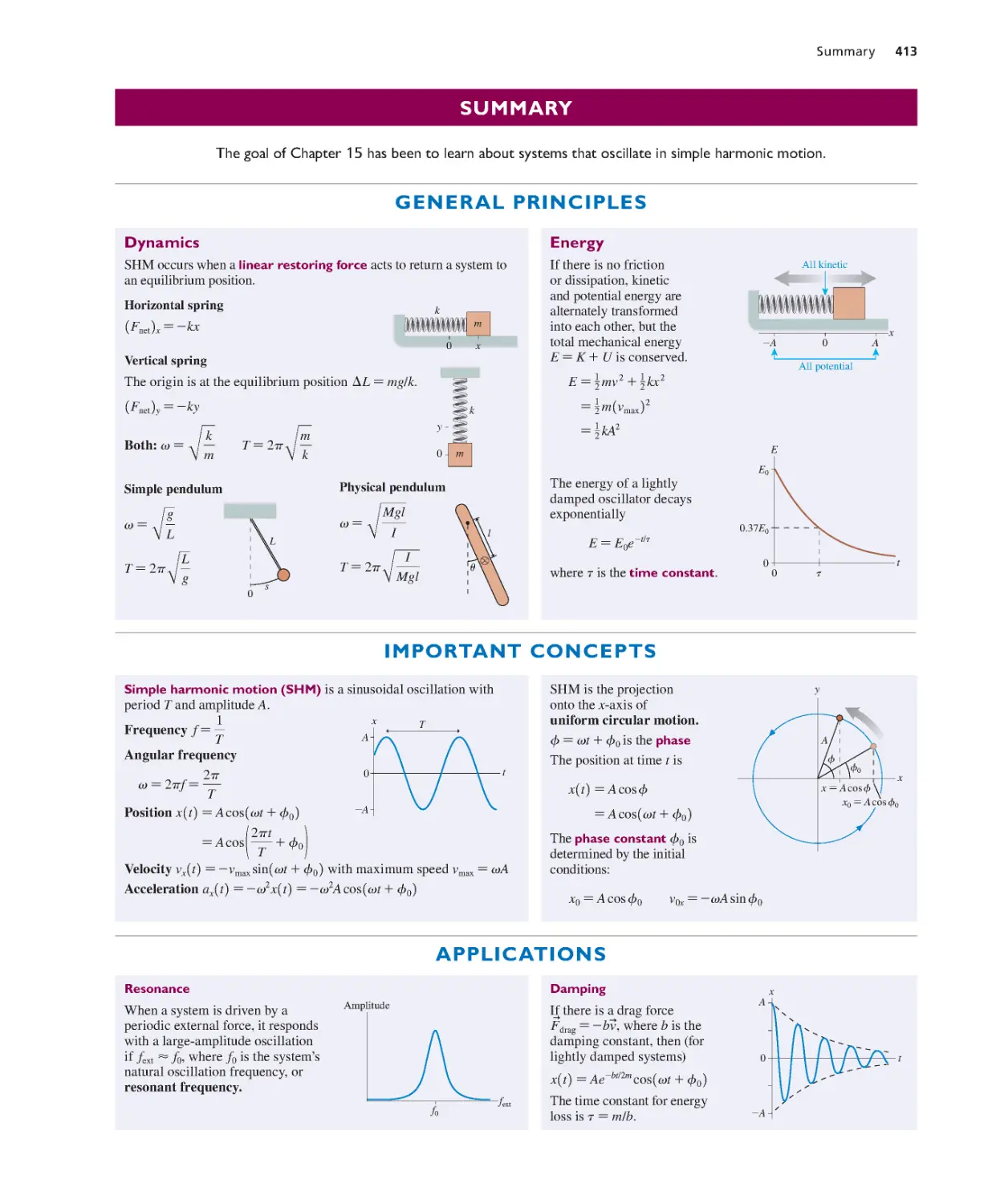
SUMMARY 413
QUESTIONS AND PROBLEMS 415
xviii Detailed Contents
Chapter 19 Work, Heat, and the First Law
of Thermodynamics 515
19.1 It’s All About Energy 516
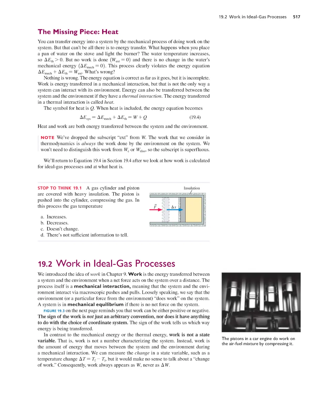
19.2 Work in Ideal-Gas Processes 517
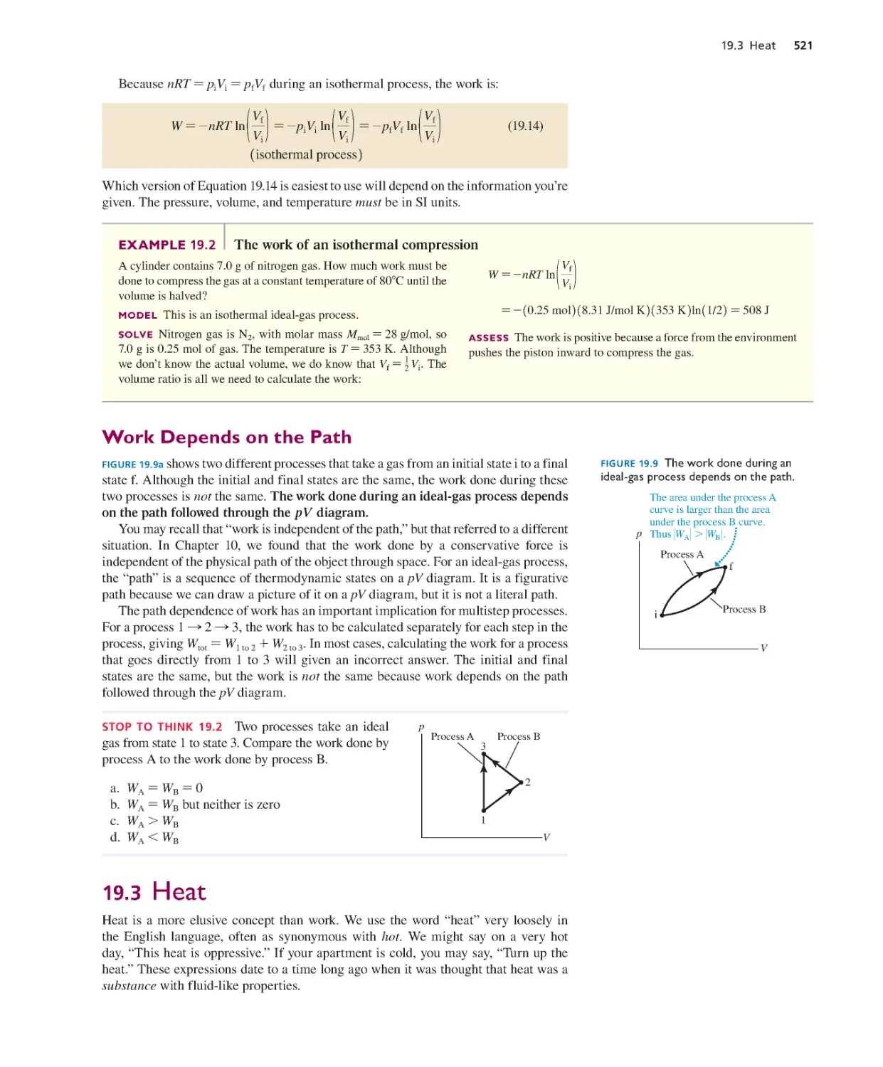
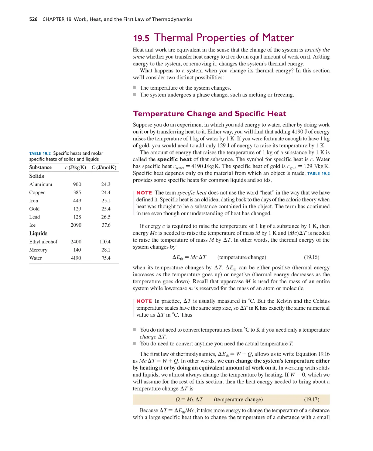
19.3 Heat 521
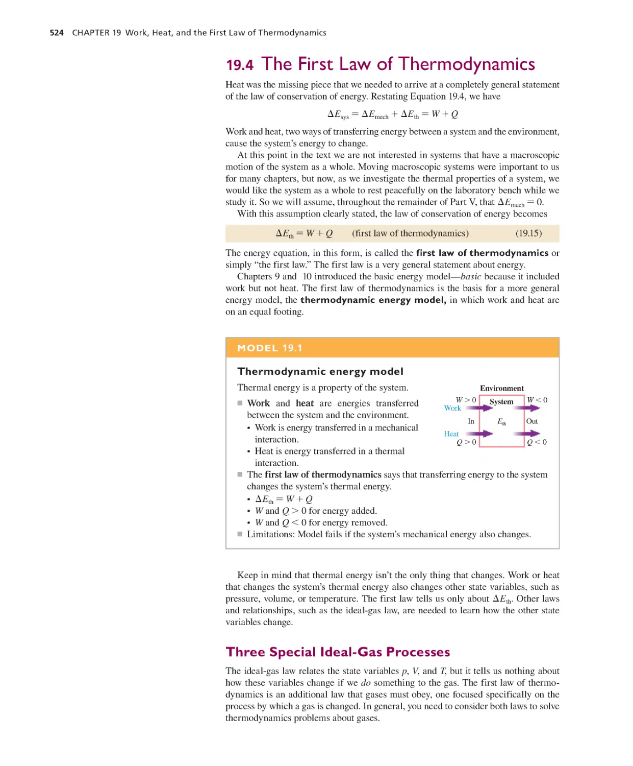
19.4 The First Law of Thermodynamics 524
19.5 Thermal Properties of Matter 526
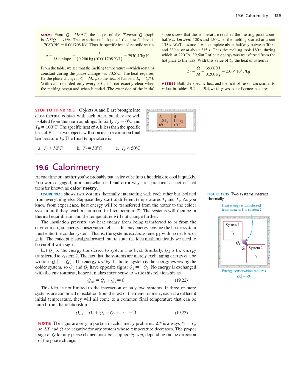
19.6 Calorimetry 529
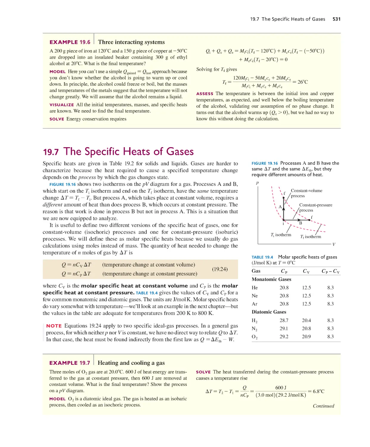
19.7 The Specific Heats of Gases 531
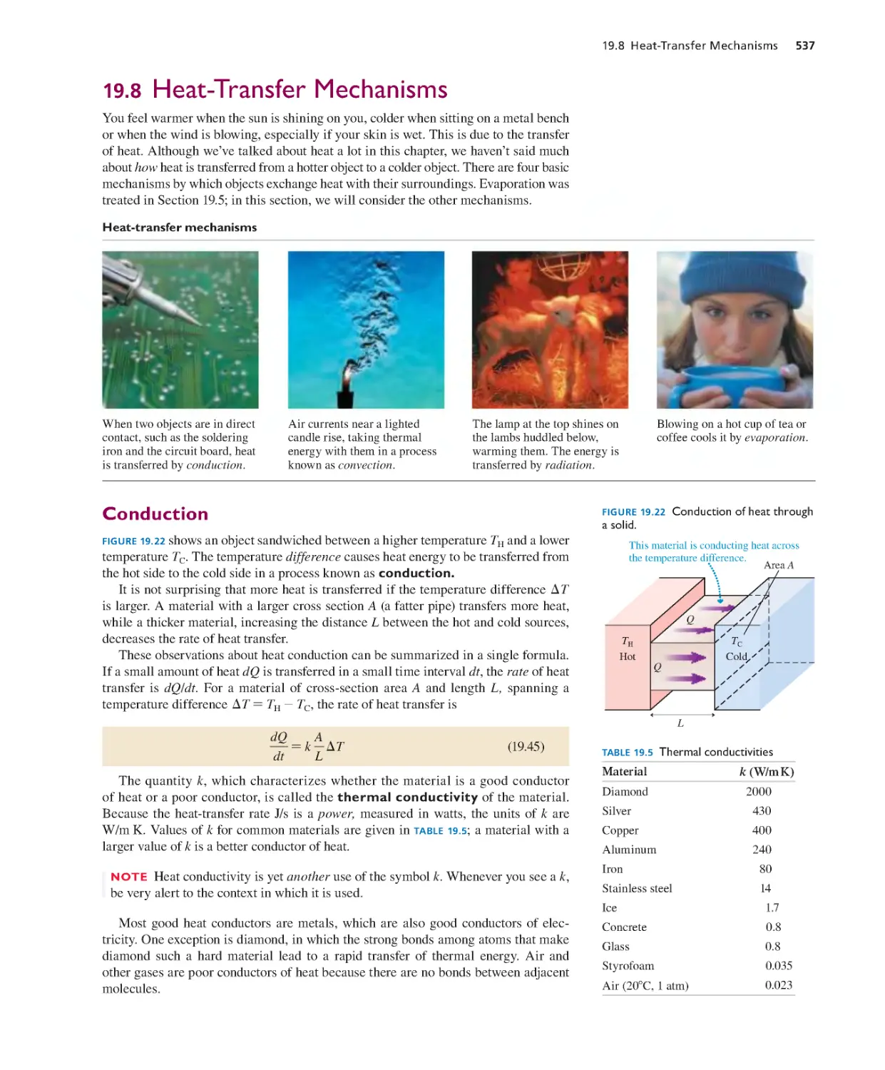
19.8 Heat-Transfer Mechanisms 537
SUMMARY 541
QUESTIONS AND PROBLEMS 542
Chapter 20 The Micro/Macro Connection 548
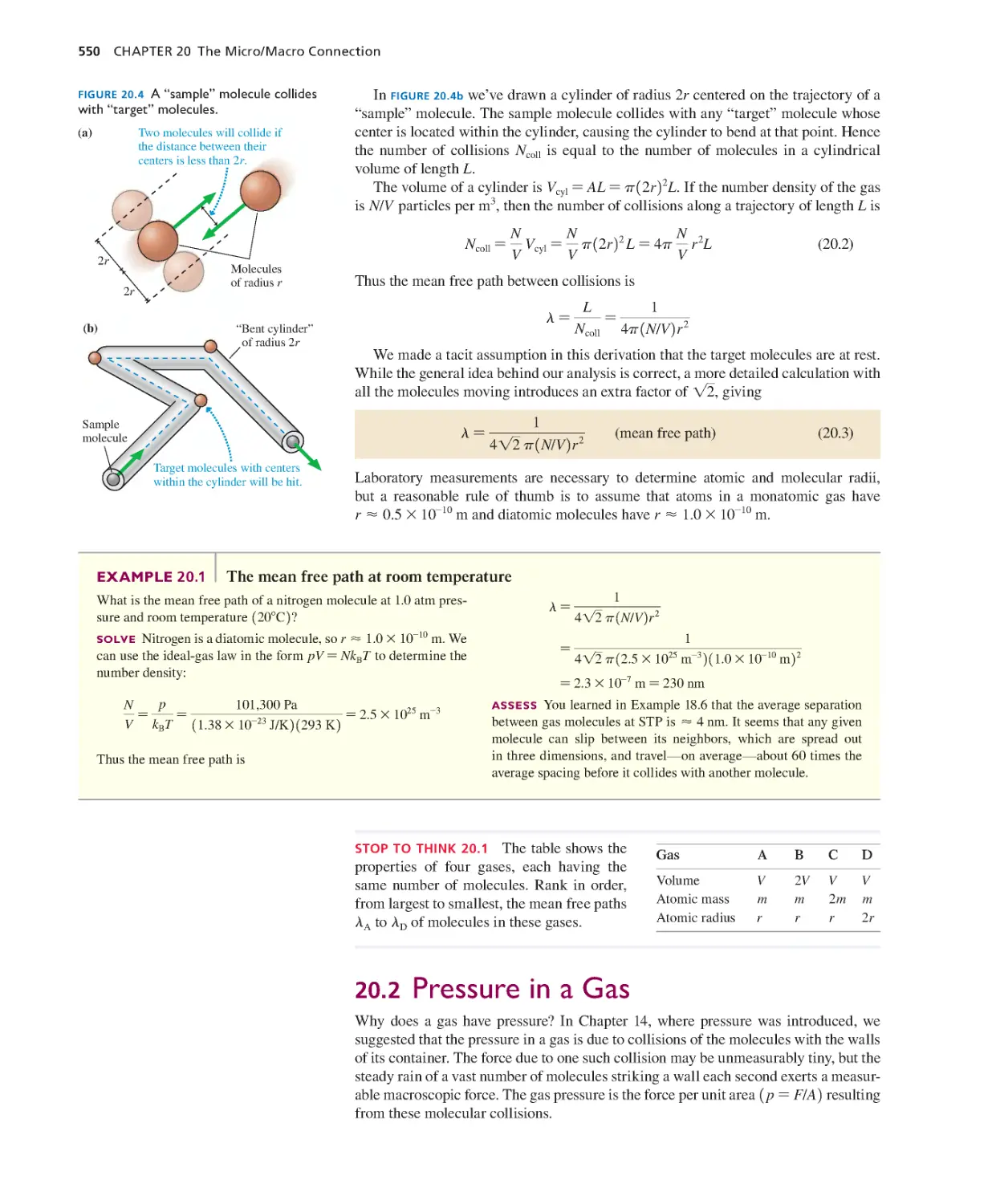
20.1 Molecular Speeds and Collisions 549
20.2 Pressure in a Gas 550
20.3 Temperature 553
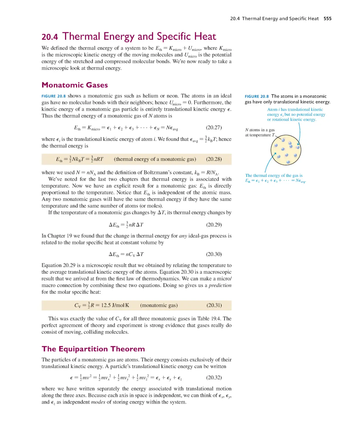
20.4 Thermal Energy and Specific Heat 555
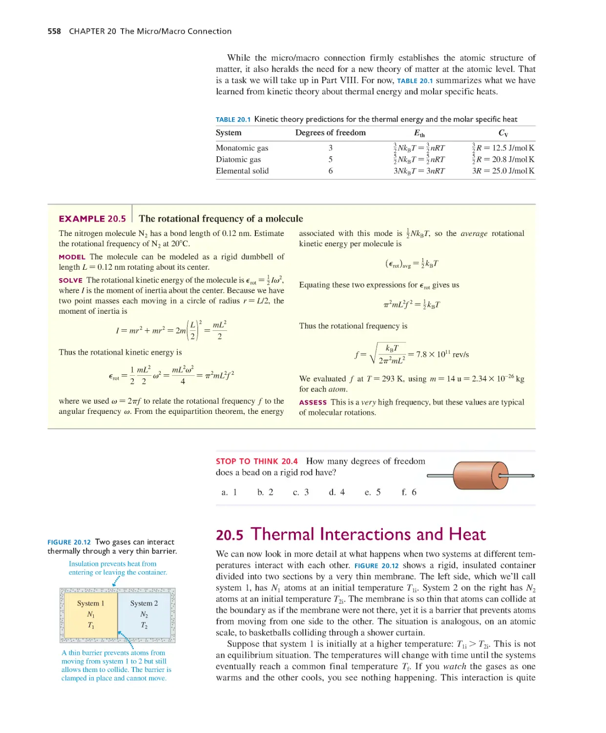
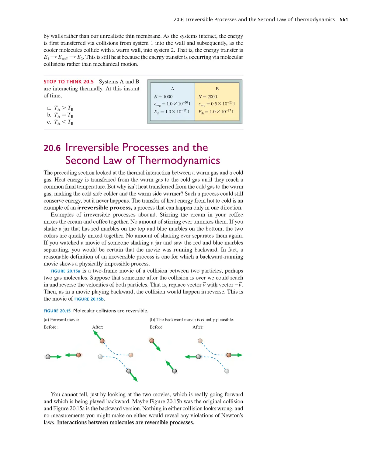
20.5 Thermal Interactions and Heat 558
20.6 Irreversible Processes and the Second
Law of Thermodynamics 561
SUMMARY 565
QUESTIONS AND PROBLEMS 566
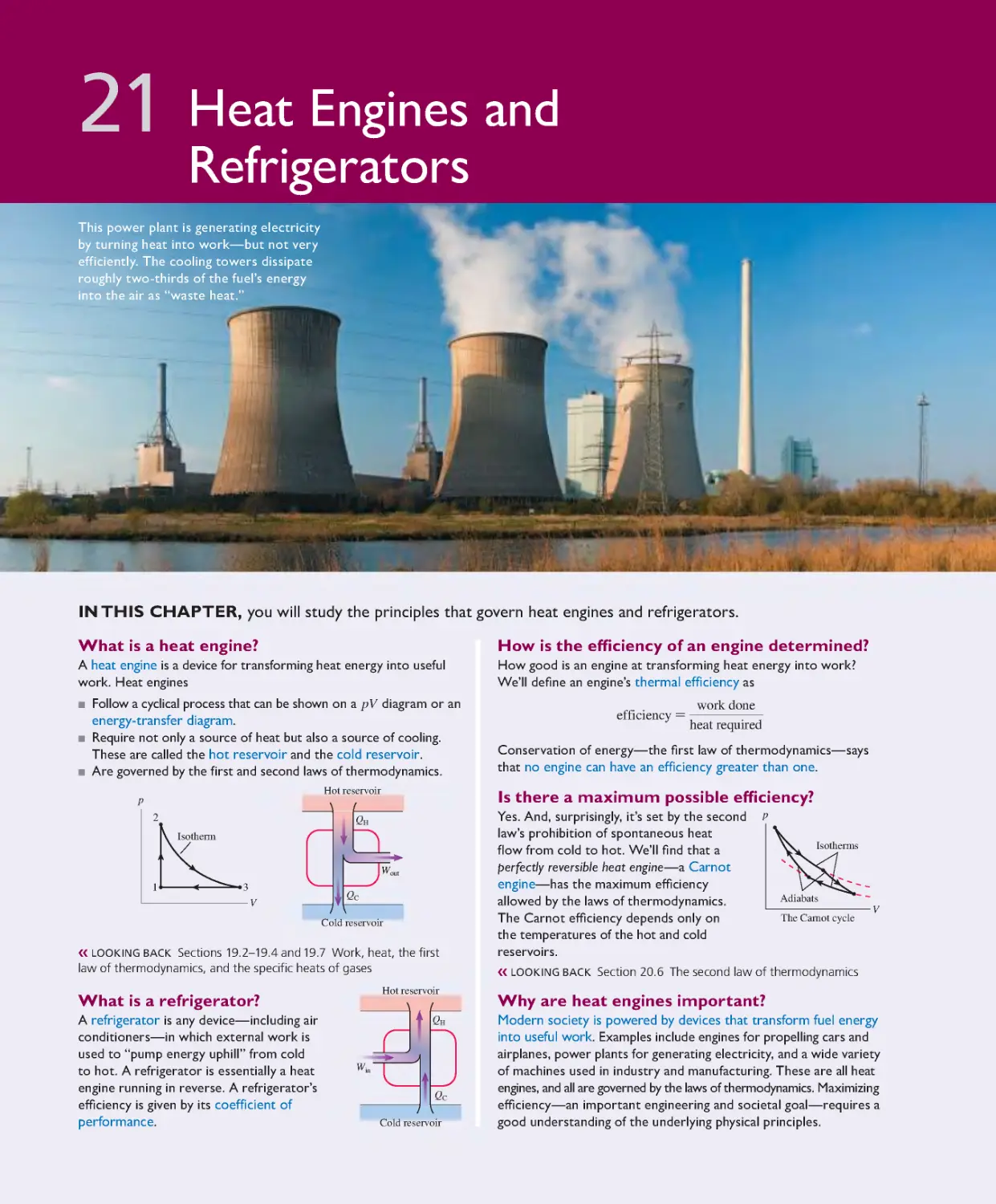
Chapter 21 Heat Engines and
Refrigerators 570
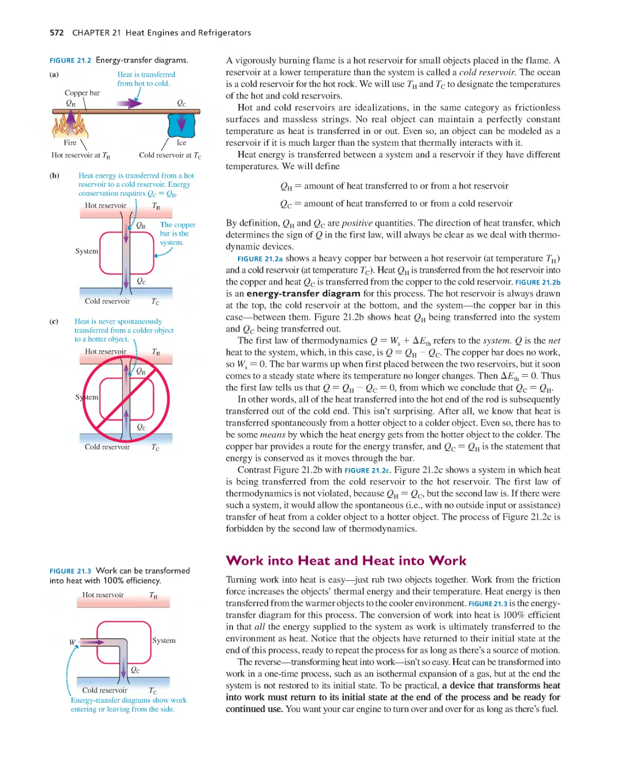
21.1 Turning Heat into Work 571
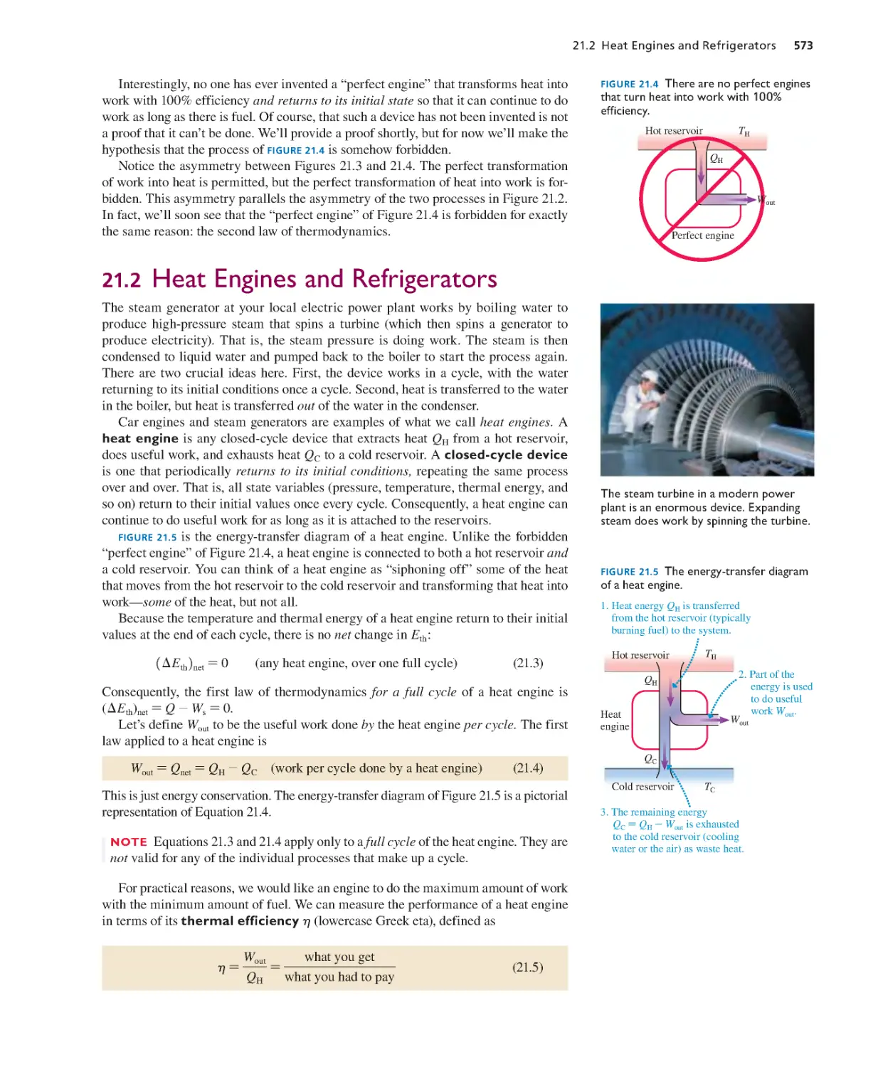
21.2 Heat Engines and Refrigerators 573
21.3 Ideal-Gas Heat Engines 578
21.4 Ideal-Gas Refrigerators 582
21.5 The Limits of Efficiency 584
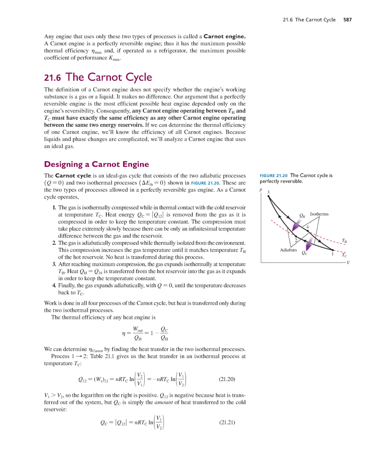
21.6 The Carnot Cycle 587
SUMMARY 592
QUESTIONS AND PROBLEMS 594
Part V Thermodynamics 600
Part VI Electricity and Magnetism
OVERVIEW Forces and Fields 601
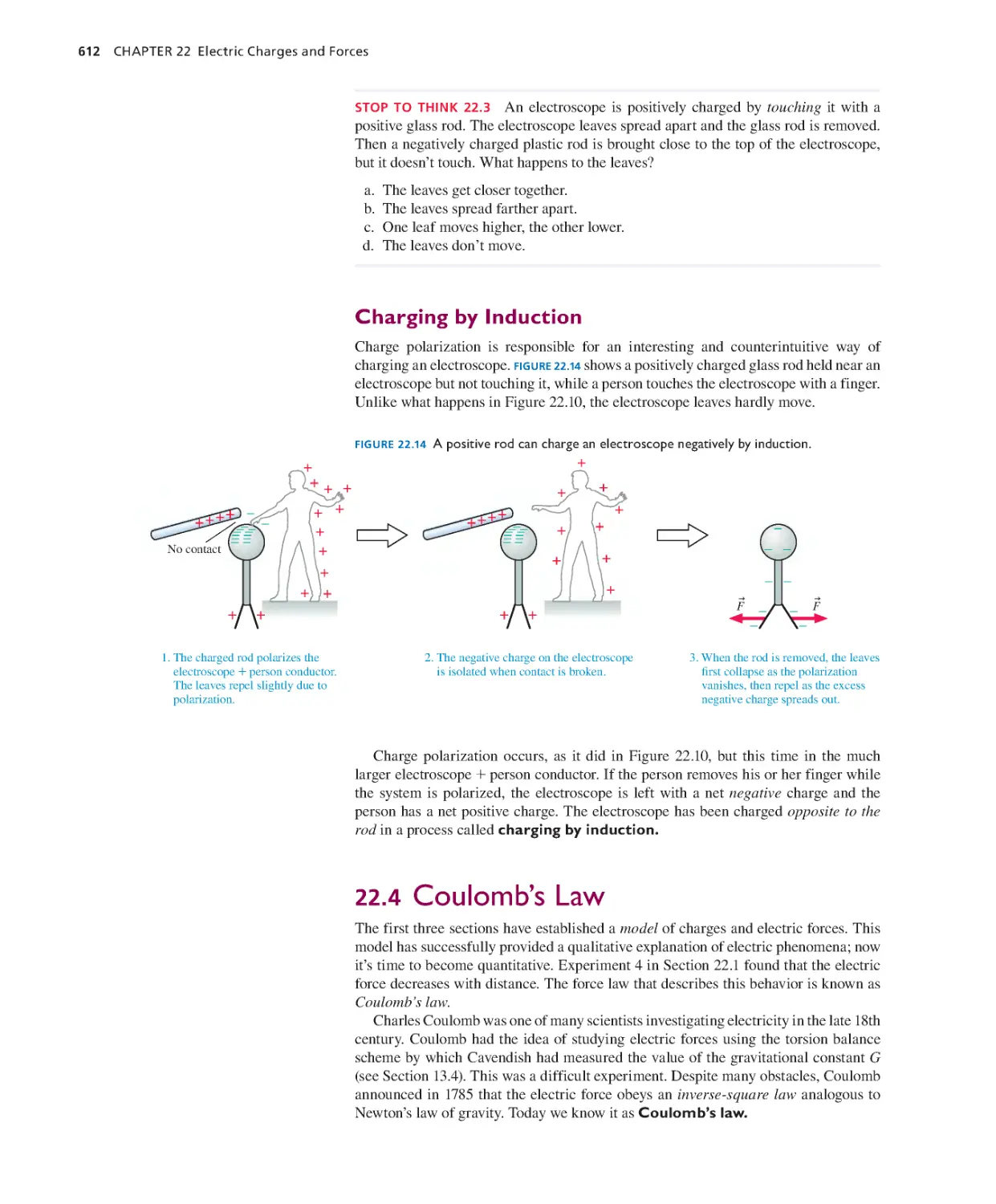
Chapter 22 Electric Charges and Forces 602
22.1 The Charge Model 603
22.2 Charge 606
22.3 Insulators and Conductors 608
22.4 Coulomb’s Law 612
22.5 The Electric Field 616
SUMMARY 622
QUESTIONS AND PROBLEMS 623
KNOWLEDGE
STRUCTURE
Chapter 23 The Electric Field 629
23.1 Electric Field Models 630
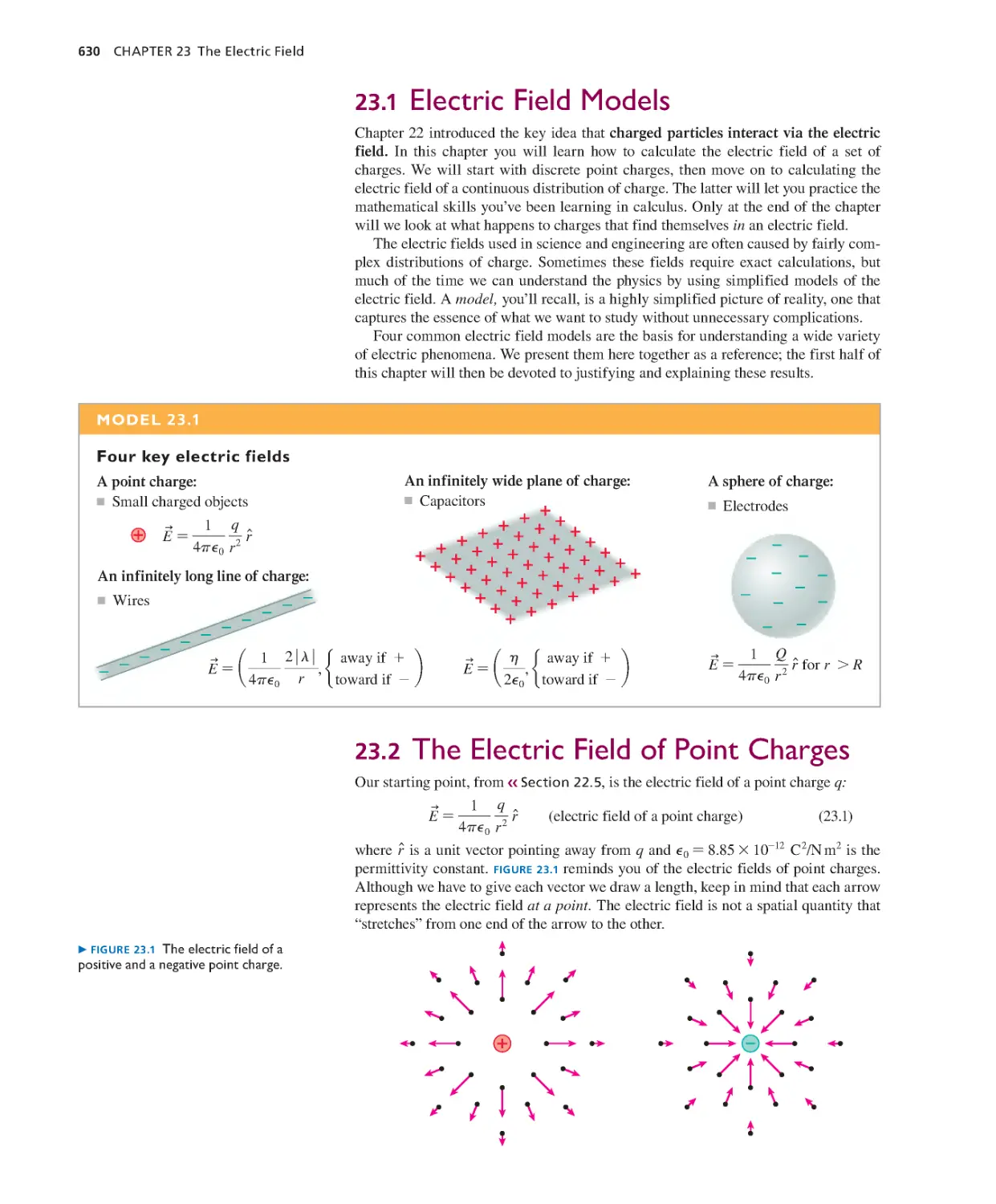
23.2 The Electric Field of Point Charges 630
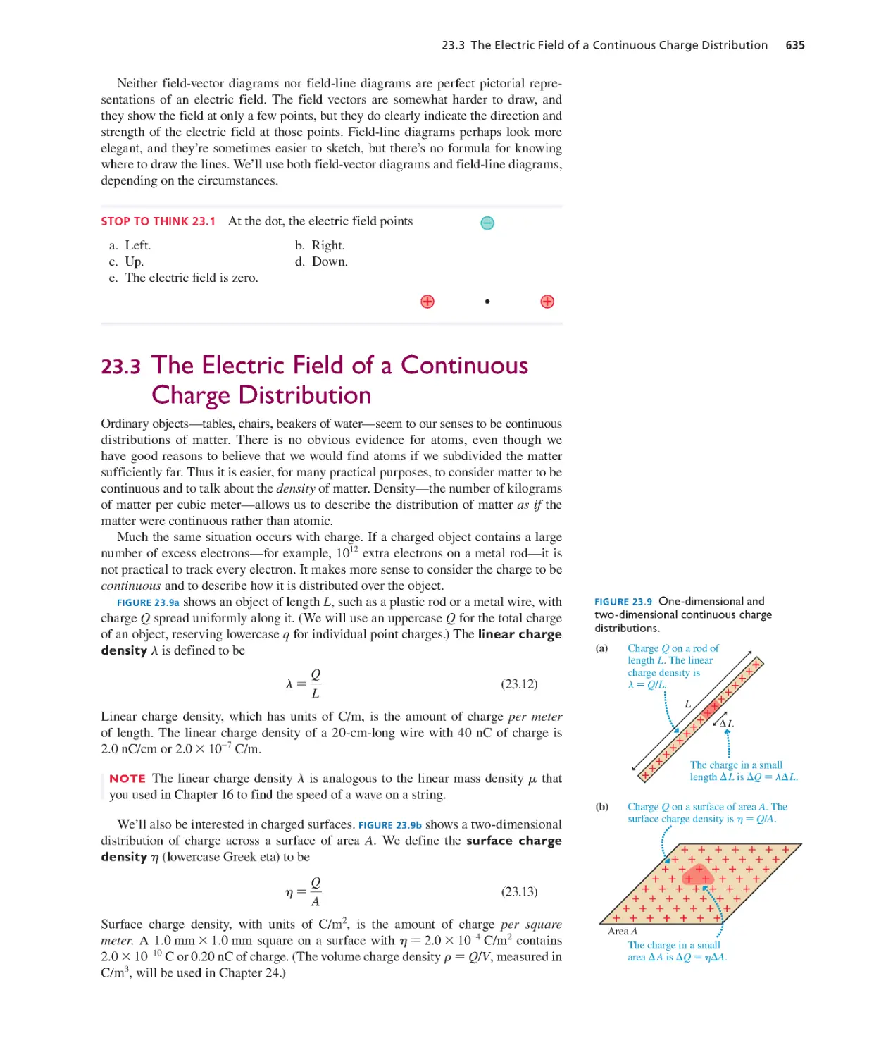
23.3 The Electric Field of a Continuous
Charge Distribution 635
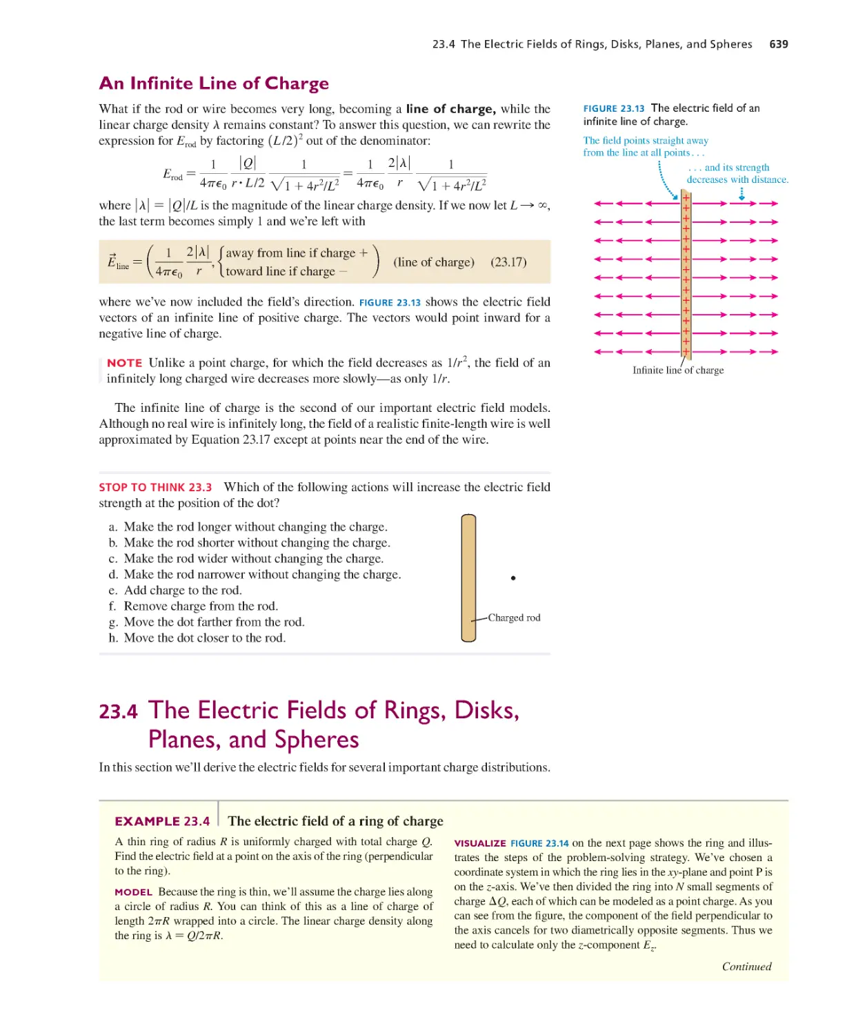
23.4 The Electric Fields of Rings, Disks,
Planes, and Spheres 639
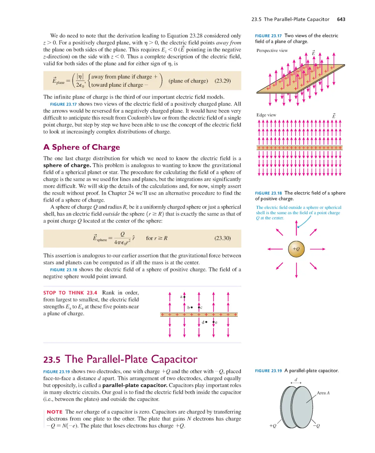
23.5 The Parallel-Plate Capacitor 643
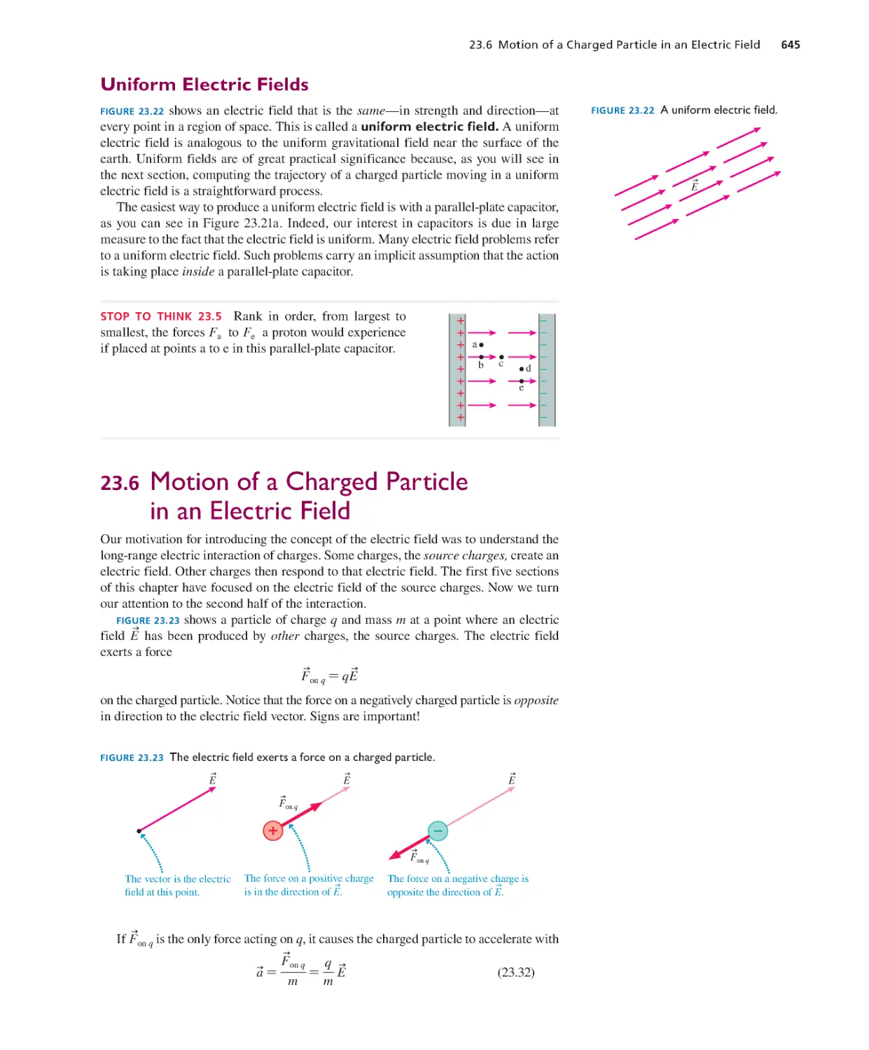
23.6 Motion of a Charged Particle in an
Electric Field 645
23.7 Motion of a Dipole in an Electric
Field 648
SUMMARY 6 51
QUESTIONS AND PROBLEMS 652
Chapter 24 Gauss’s Law 658
24.1 Symmetry 659
24.2 The Concept of Flux 661
24.3 Calculating Electric Flux 663
24.4 Gauss’s Law 669
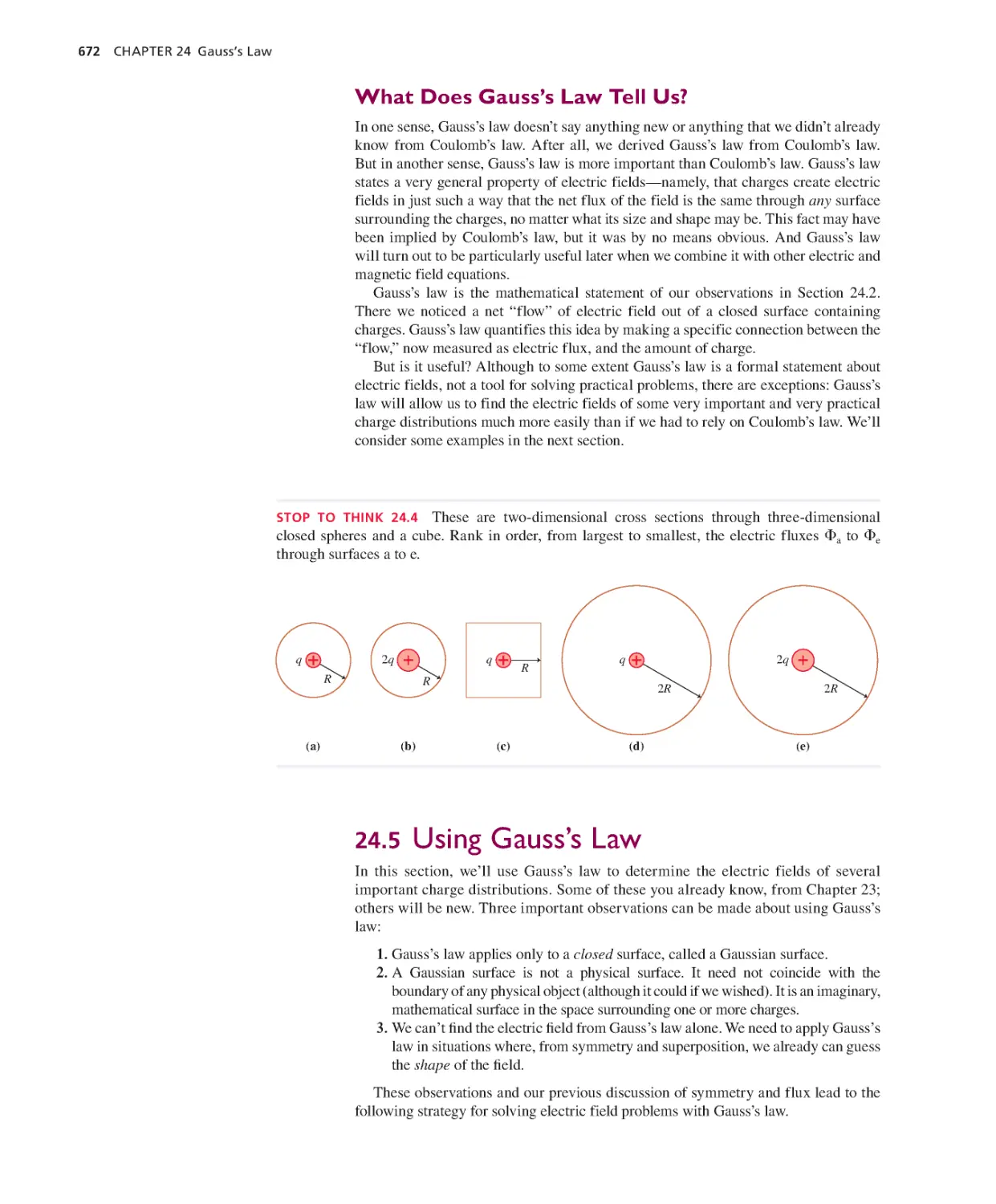
24.5 Using Gauss’s Law 672
24.6 Conductors in Electrostatic
Equilibrium 676
SUMMARY 680
QUESTIONS AND PROBLEMS 681
Chapter 25 The Electric Potential 687
25.1 Electric Potential Energy 688
25.2 The Potential Energy of Point
Charges 691
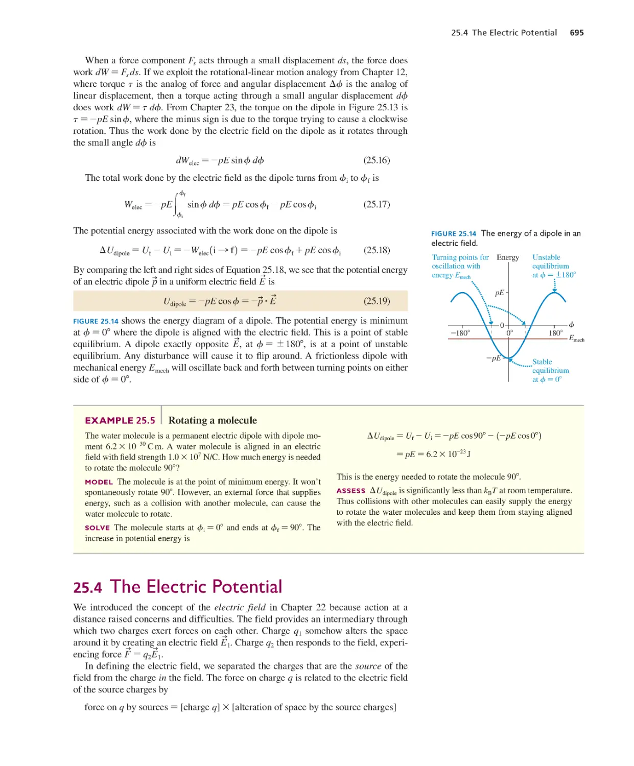
25.3 The Potential Energy of a Dipole 694
25.4 The Electric Potential 695
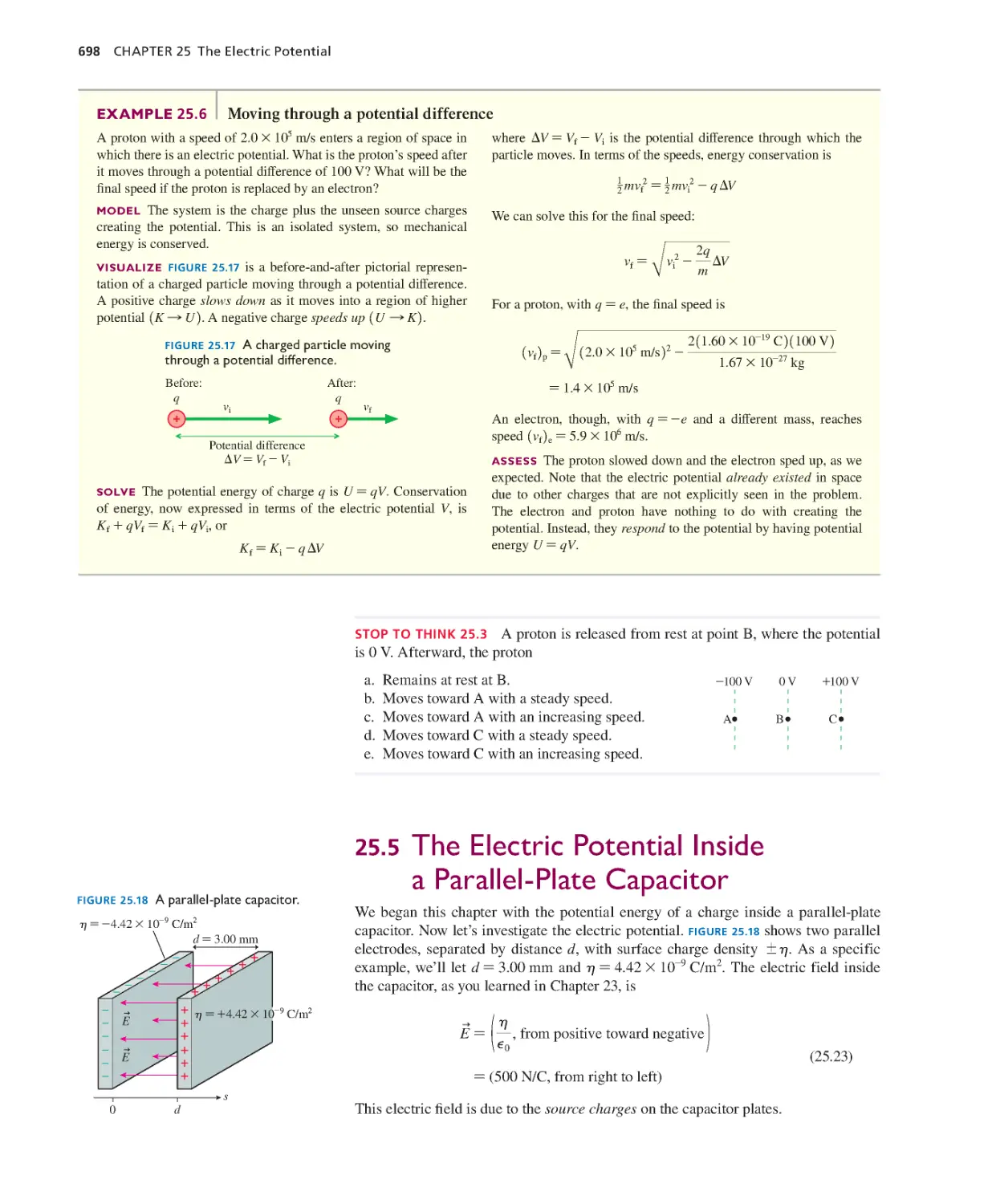
25.5 The Electric Potential Inside a Parallel-
Plate Capacitor 698
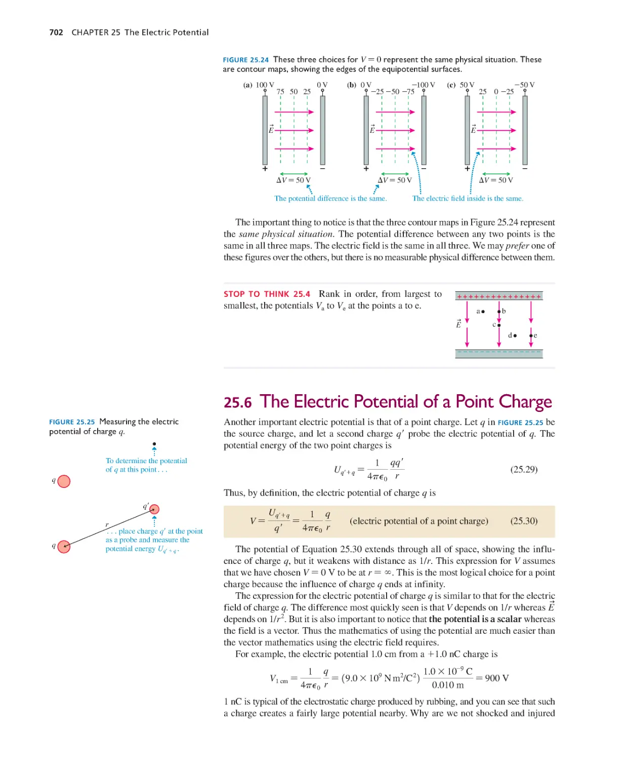
25.6 The Electric Potential of a Point
Charge 702
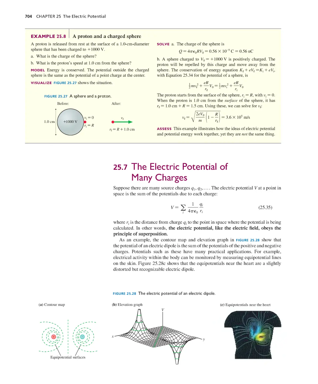
25.7 The Electric Potential of Many
Charges 704
SUMMARY 707
QUESTIONS AND PROBLEMS 708
Detailed Contents xix
Chapter 26 Potential and Field 714
26.1 Connecting Potential and Field 715
26.2 Finding the Electric Field from the
Potential 717
26.3 A Conductor in Electrostatic
Equilibrium 720
26.4 Sources of Electric Potential 722
26.5 Capacitance and Capacitors 724
26.6 The Energy Stored in a Capacitor 729
26.7 Dielectrics 730
SUMMARY 735
QUESTIONS AND PROBLEMS 736
Chapter 27 Current and Resistance 742
27.1 The Electron Cur rent 743
27.2 Creating a Current 745
27.3 Current and Current Density 749
27.4 Conductivity and Resistivity 753
27.5 Resistance and Ohm’s Law 755
SUMMARY 760
QUESTIONS AND PROBLEMS 761
Chapter 28 Fundamentals of Circuits 766
28.1 Circuit Elements and Diagrams 767
28.2 Kirchhoff’s Laws and the Basic Circuit 768
28.3 Energy and Power 771
28.4 Series Resistors 773
28.5 Real Batteries 775
28.6 Parallel Resistors 777
28.7 Resistor Circuits 780
28.8 Getting Grounded 782
28.9 RC Circuits 784
SUMMARY 788
QUESTIONS AND PROBLEMS 789
Chapter 29 The Magnetic Field 796
29.1 Magnetism 797
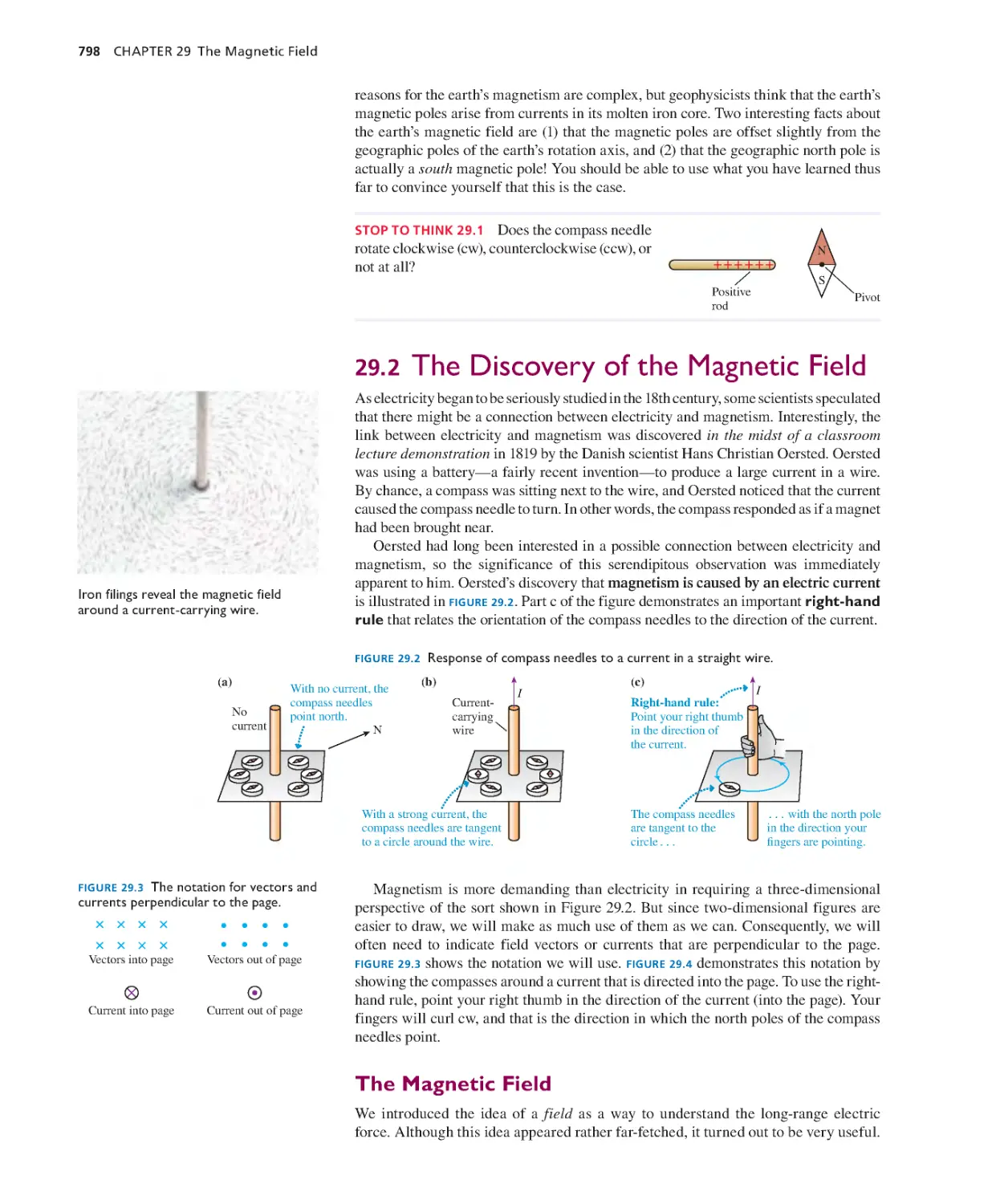
29.2 The Discovery of the Magnetic Field 798
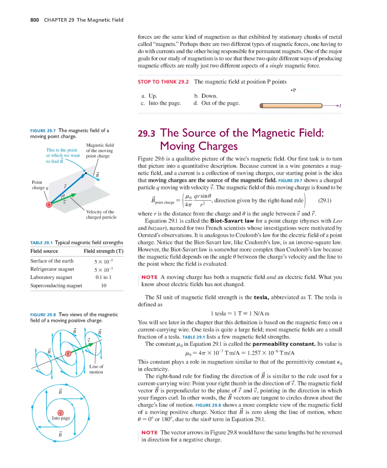
29.3 The Source of the Magnetic Field: Moving
Charges 800
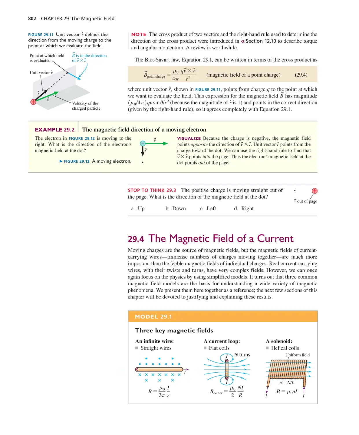
29.4 The Magnetic Field of a Current 802
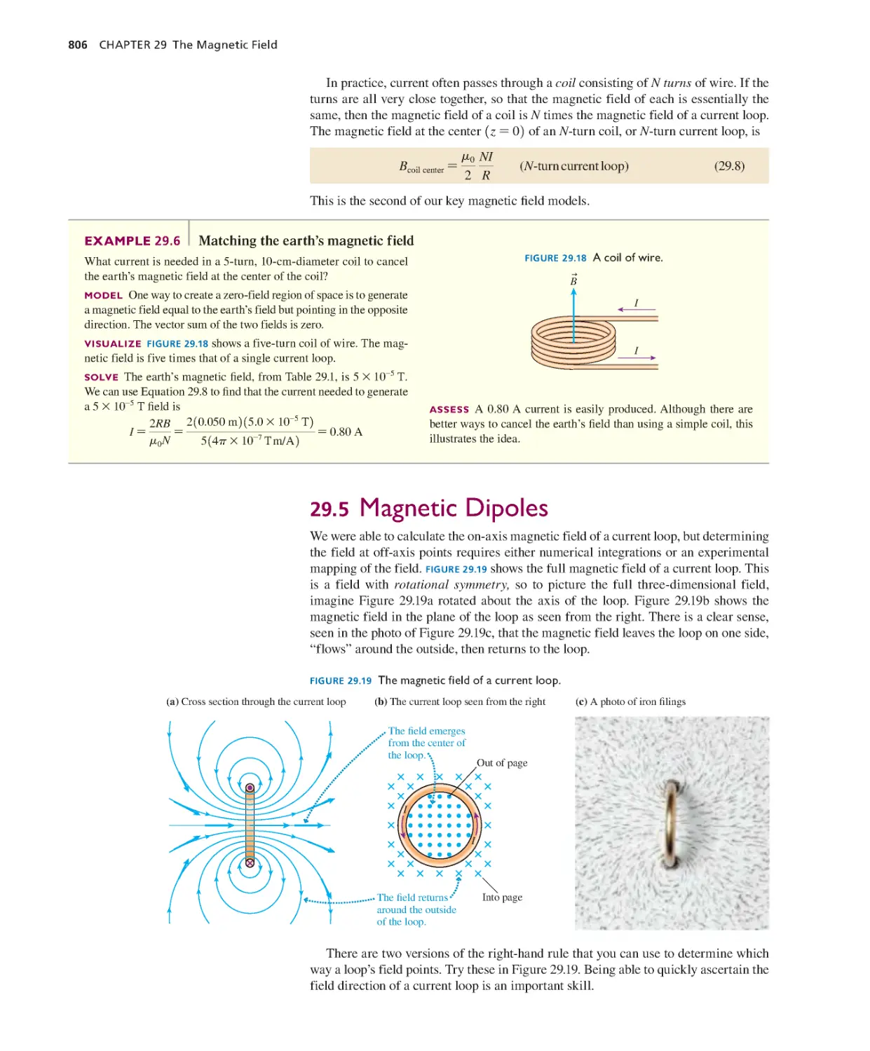
29.5 Magnetic Dipoles 806
29.6 Ampère’s Law and Solenoids 809
29.7 The Magnetic Force on a Moving
Charge 815
29.8 Magnetic Forces on Current-Car rying
Wires 820
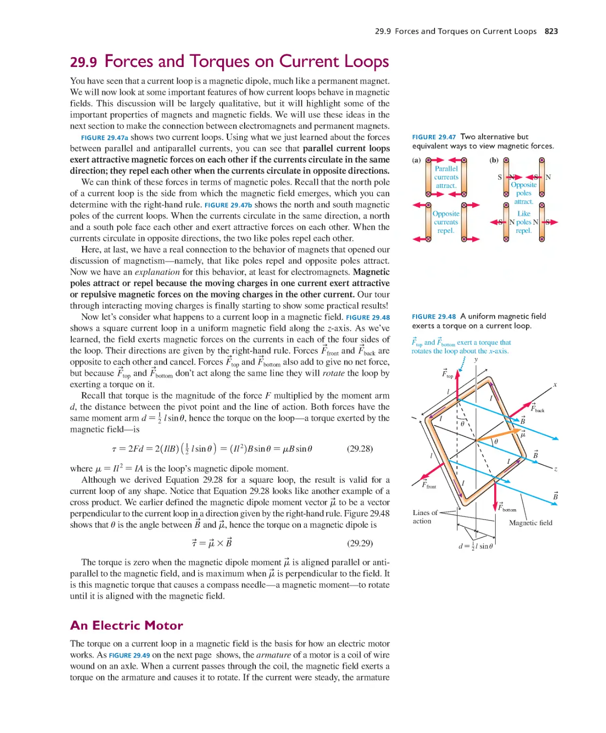
29.9 Forces and Torques on Current Loops 823
29.10 Magnetic Properties of Matter 824
SUMMARY 828
QUESTIONS AND PROBLEMS 829
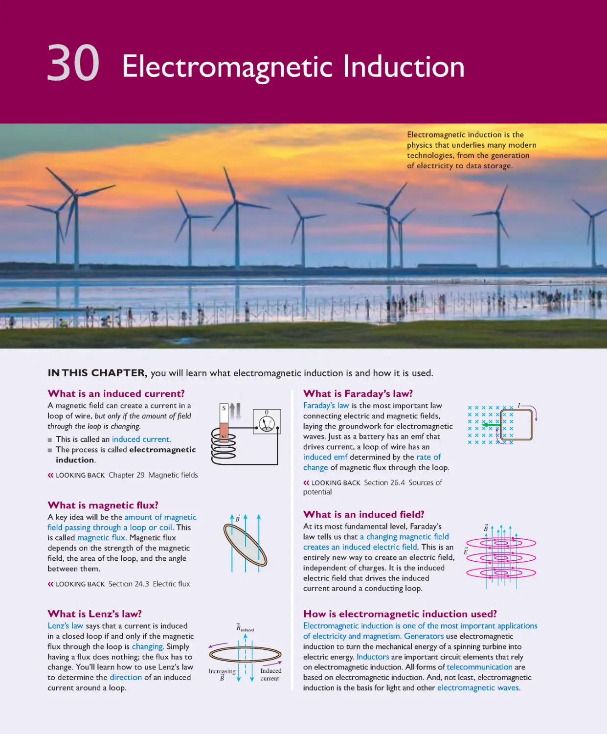
Chapter 30 Electromagnetic Induction 836
30.1 Induced Currents 837
30.2 Motional emf 838
30.3 Magnetic Flux 842
30.4 Lenz’s Law 845
30.5 Faraday’s Law 848
30.6 Induced Fields 852
30.7 Induced Currents: Three
Applications 855
30.8 Inductors 857
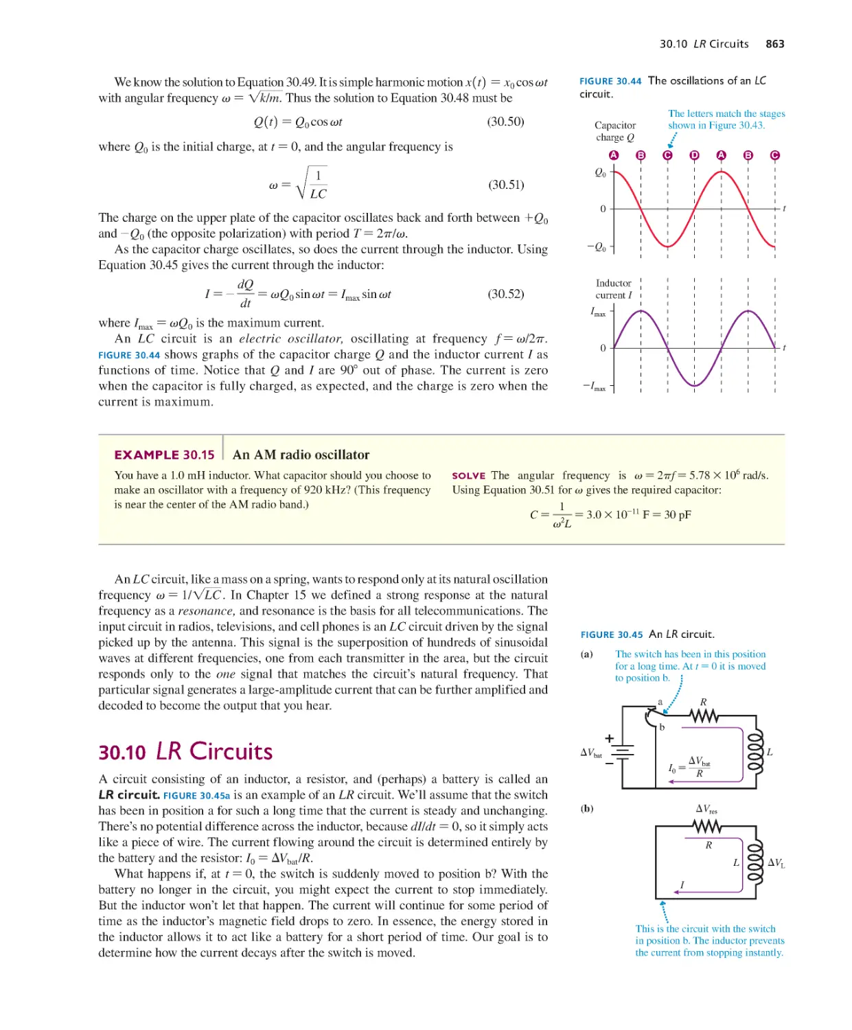
30.9 LC Circuits 861
30.10 LR Circuits 863
SUMMARY 867
QUESTIONS AND PROBLEMS 868
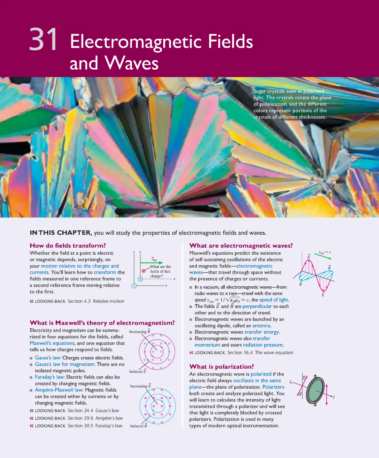
Chapter 31 Electromagnetic Fields and
Waves 876
31.1 E or B? It Depends on Your
Perspective 877
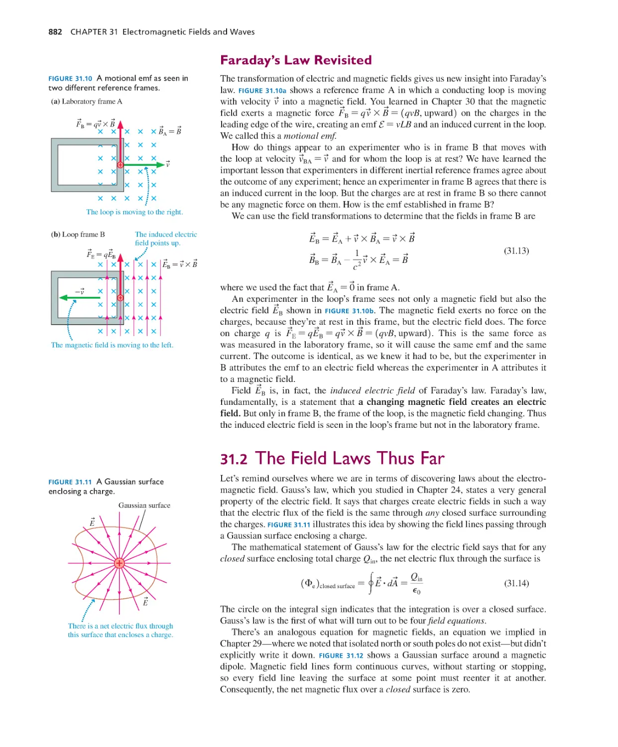
31.2 The Field Laws Thus Far 882
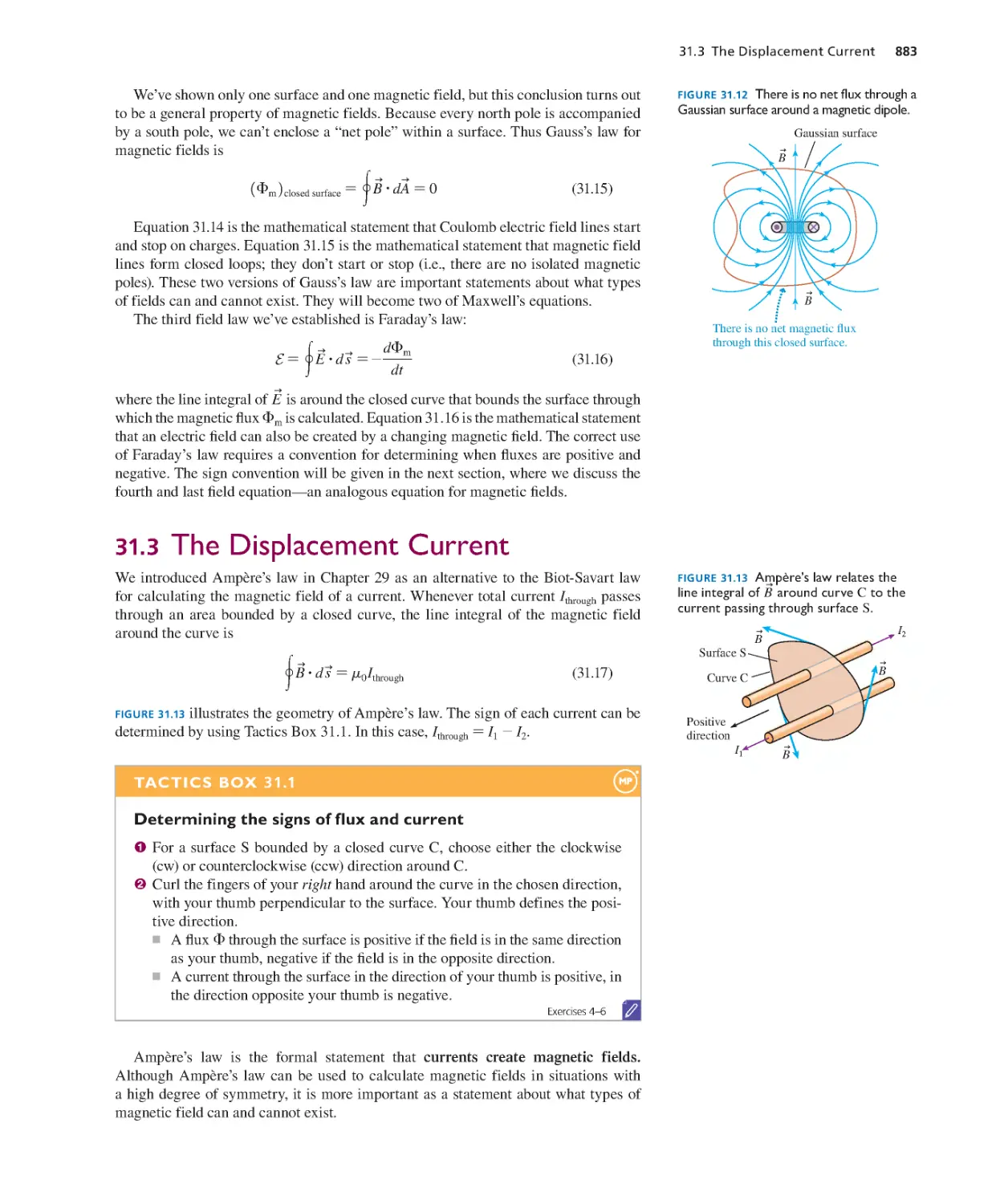
31.3 The Displacement Current 883
31.4 Maxwell’s Equations 886
31. 5 ADVANCED TOPIC Electromagnetic
Waves 888
31.6 Proper ties of Electromagnetic
Waves 893
31.7 Pola rization 896
SUMMARY 899
QUESTIONS AND PROBLEMS 900
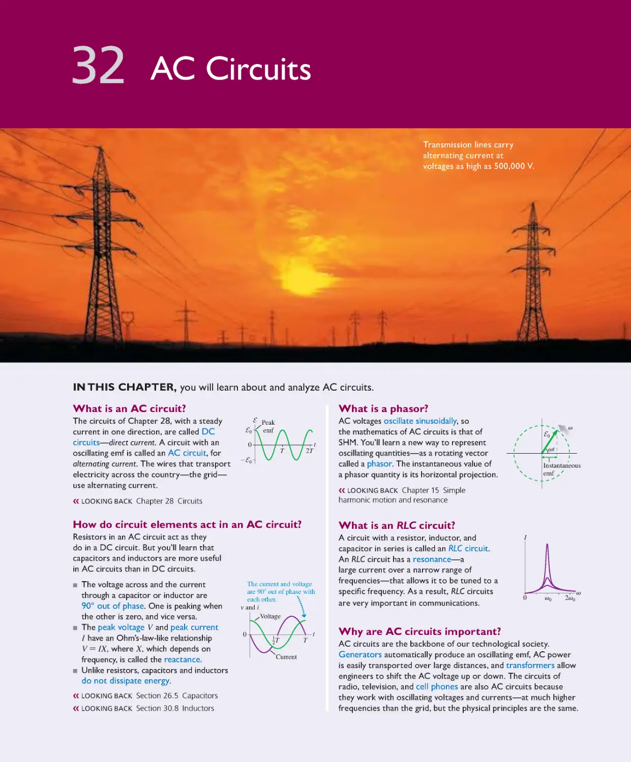
Chapter 32 AC Circuits 905
32.1 AC Sources and Phasors 906
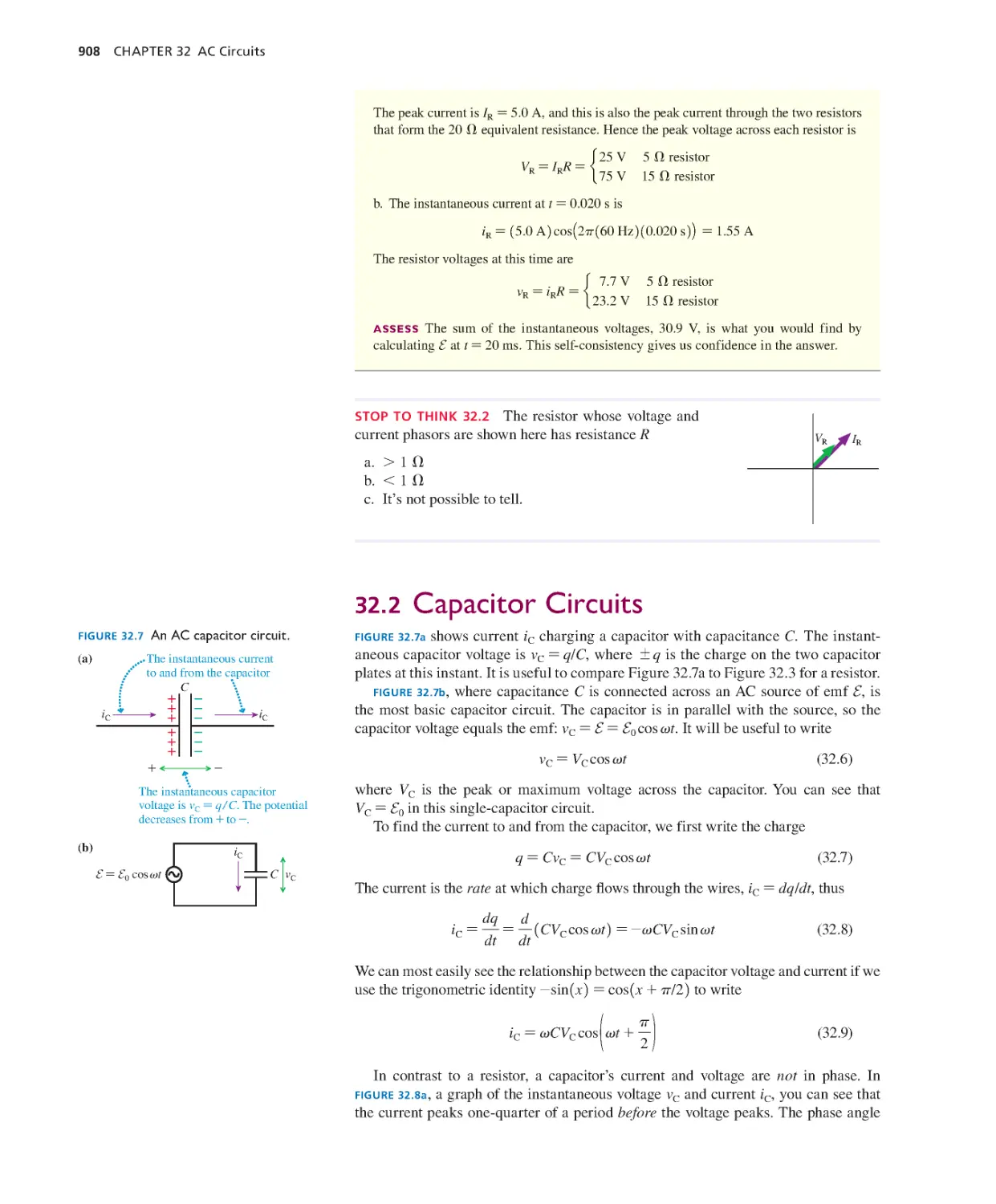
32.2 Capacitor Circuits 908
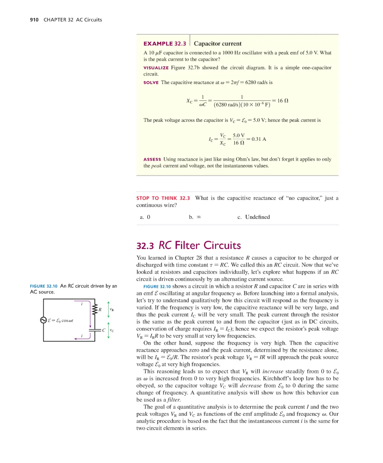
32.3 RC Filter Circuits 910
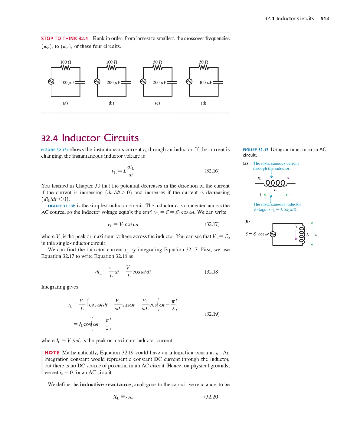
32.4 Inductor Circuits 913
32.5 The Series RLC Circuit 914
32.6 Power in AC Circuits 918
SUMMARY 922
QUESTIONS AND PROBLEMS 923
Part VI Electricity and Magnetism 928
KNOWLEDGE
STRUCTURE
xx Detailed Contents
Part VII Optics
OVERVIEW The Story of Light 929
Part VIII Relativity and Quantum
Physics
OVERVIEW Contemporary Physics 1021
Chapter 36 Relativity 1022
36.1 Relativity: What’s It All About? 1023
36.2 Galilean Relativity 1023
36.3 Einstein’s Principle of Relativity 1026
36.4 Events and Measurements 1029
36.5 The Relativity of Simultaneity 1032
36.6 Time Dilation 1035
36.7 Length Contraction 1039
36.8 The Lorentz Transformations 1043
36.9 Relativistic Momentum 1048
36.10 Relativistic Energy 1051
SUMMARY 1057
QUESTIONS AND PROBLEMS 1058
Chapter 37 The Foundations of Modern
Physics 1063
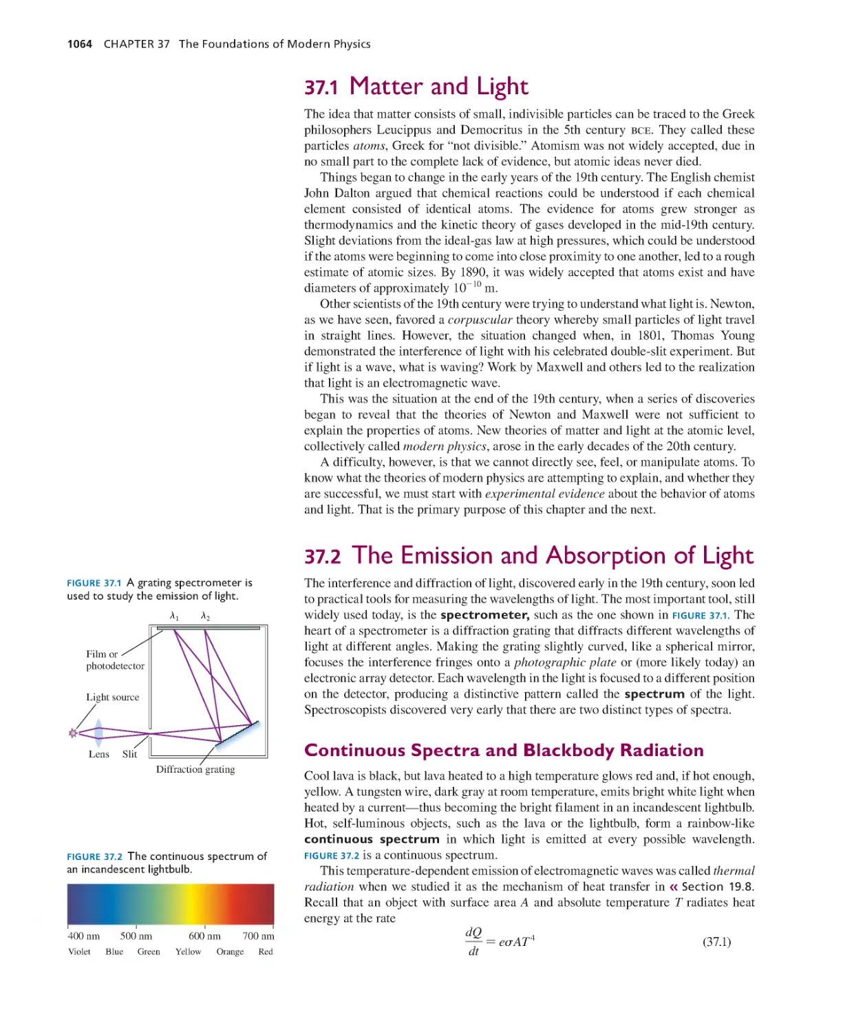
37.1 Matter and Light 1064
37.2 The Emission and Absorption of
Light 1064
37.3 Cathode Rays and X Rays 1067
37.4 The Discovery of the Electron 1069
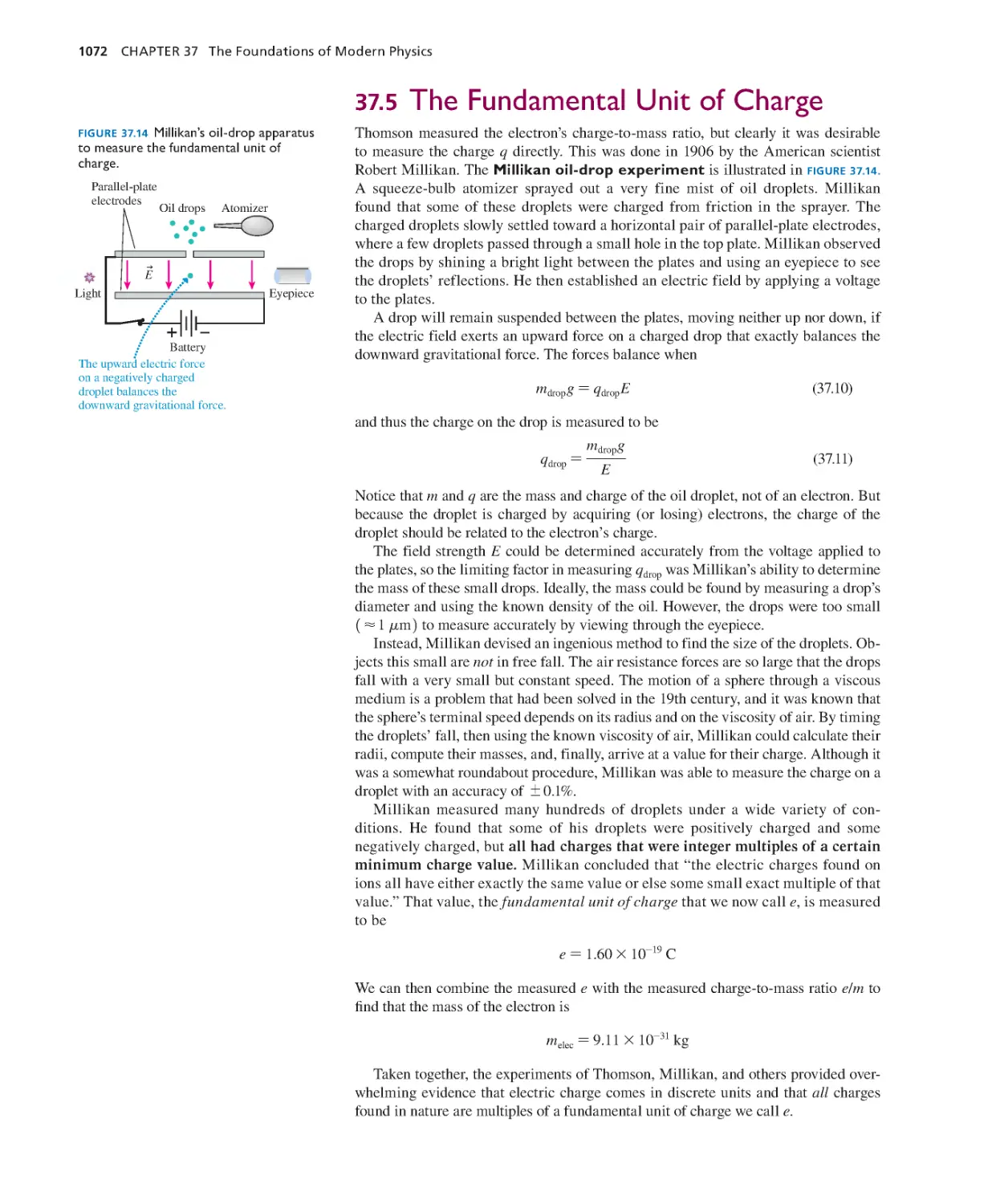
37.5 The Fundamental Unit of Charge 1072
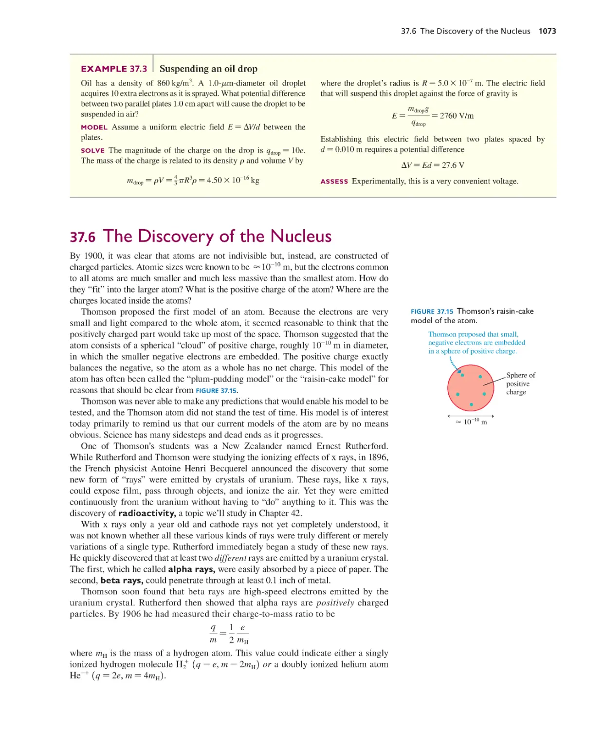
37.6 The Discovery of the Nucleus 1073
37.7 Into the Nucleus 1077
37.8 Classical Physics at the Limit 1079
SUMMARY 1080
QUESTIONS AND PROBLEMS 10 81
Chapter 38 Quantization 1085
38.1 The Photoelectric Effect 1086
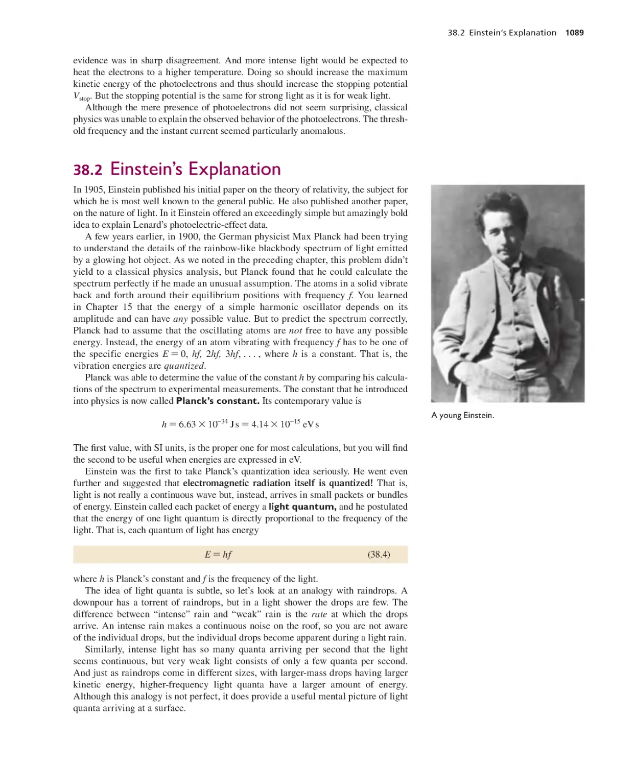
38.2 Einstein’s Explanation 1089
38.3 Photons 1092
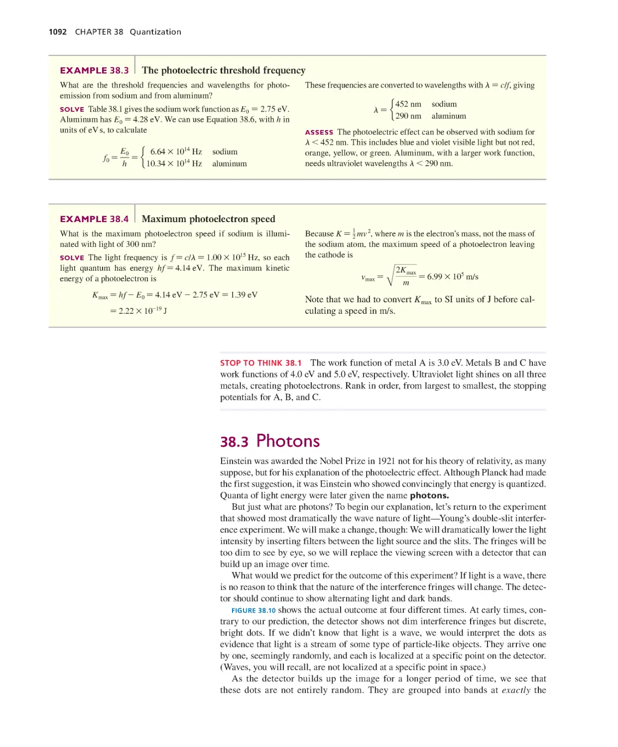
38.4 Matter Waves and Energy
Quantization 1096
38.5 Bohr’s Model of Atomic
Quantization 1099
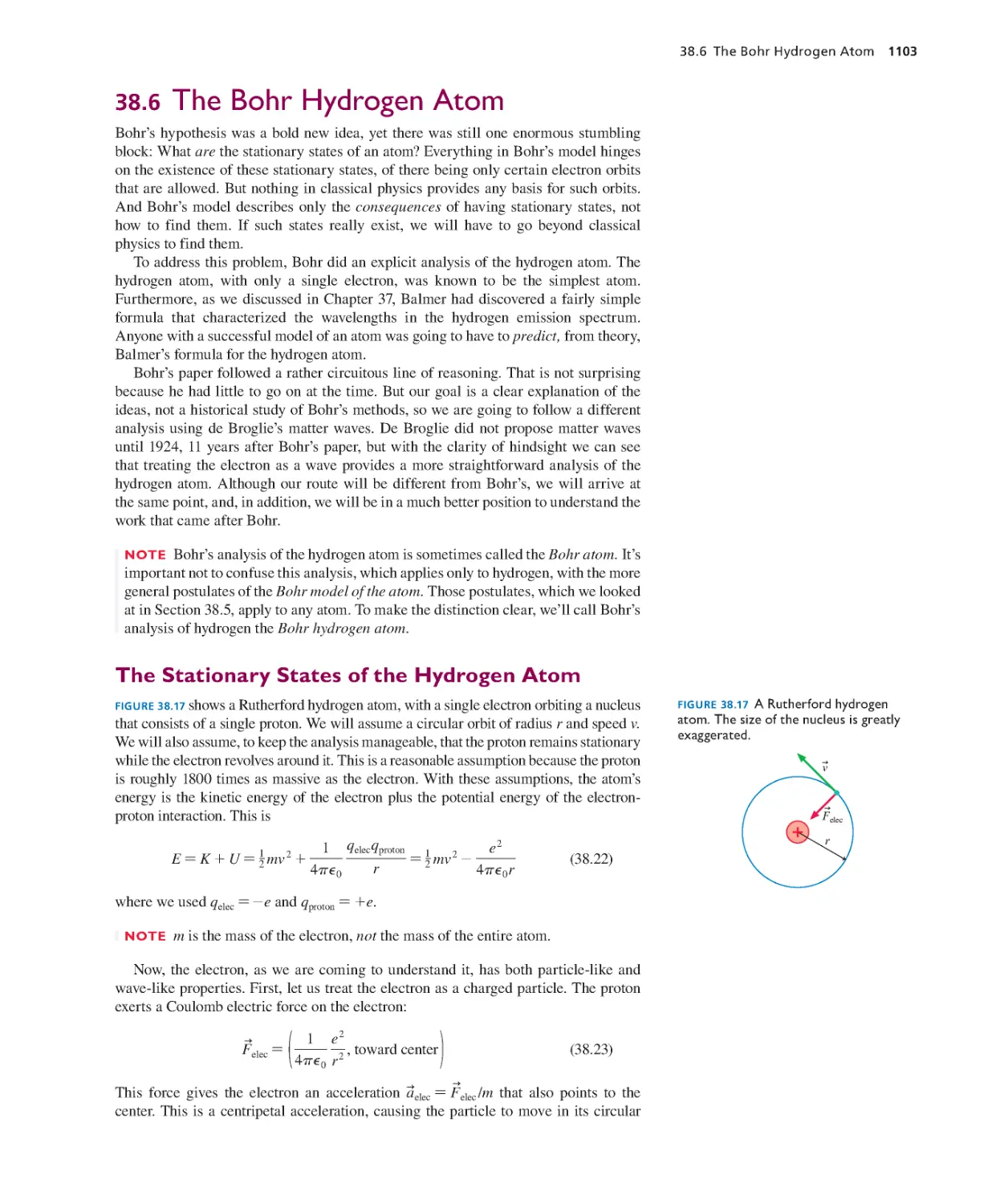
38.6 The Bohr Hydrogen Atom 1103
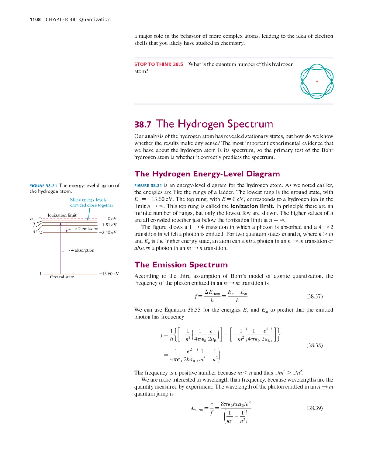
38.7 The Hydrogen Spectr um 1108
SUMMARY 1112
QUESTIONS AND PROBLEMS 1113
Chapter 33 Wave Optics 930
33.1 Models of Light 931
33.2 The Interference of Light 932
33.3 The Diffraction Grating 937
33.4 Single-Slit Diffraction 940
33.5 ADVANCED TOPIC A Closer Look at
Diffraction 944
33.6 Circular-Aperture Diffraction 947
33.7 The Wave Model of Light 948
33.8 Interferometers 950
SUMMARY 953
QUESTIONS AND PROBLEMS 954
Chapter 34 Ray Optics 960
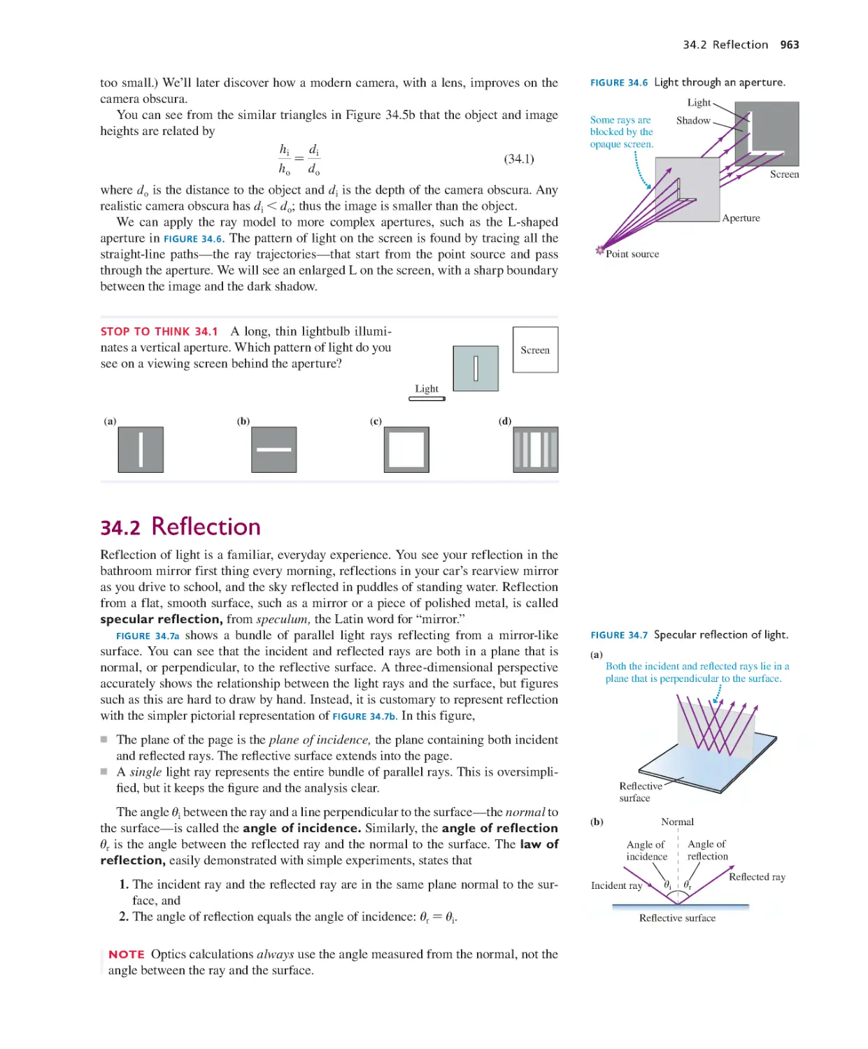
34.1 The Ray Model of Light 961
34.2 Reflection 963
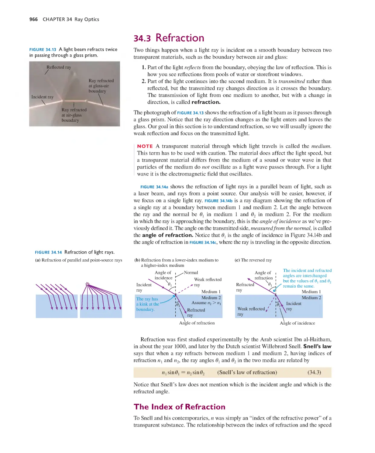
34.3 Refraction 966
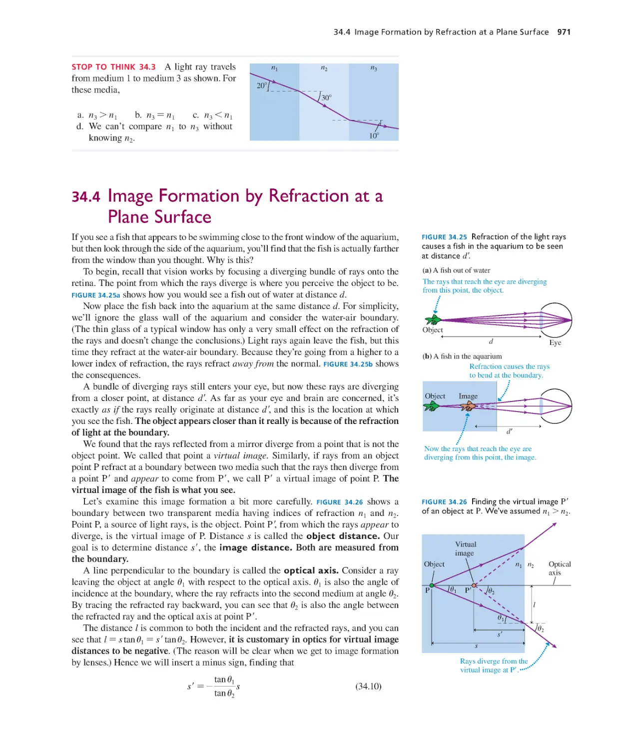
34.4 Image Formation by Refraction at a Plane
Surface 971
34.5 Thin Lenses: Ray Tracing 972
34.6 Thin Lenses: Refraction Theory 978
34.7 Image Formation with Spherical
Mirrors 983
SUMMARY 988
QUESTIONS AND PROBLEMS 989
Chapter 35 Optical Instruments 995
35.1 Lenses in Combination 996
35.2 The Camera 997
35.3 Vision 1001
35.4 Optical Systems That Magnify 1004
35.5 Color and Dispersion 1008
35.6 The Resolution of Optical
Instruments 1010
SUMMARY 1015
QUESTIONS AND PROBLEMS 1016
Part VII Optics 1020
KNOWLEDGE
STRUCTURE
Detailed Contents xxi
Chapter 39 Wave Functions and
Uncertainty 1118
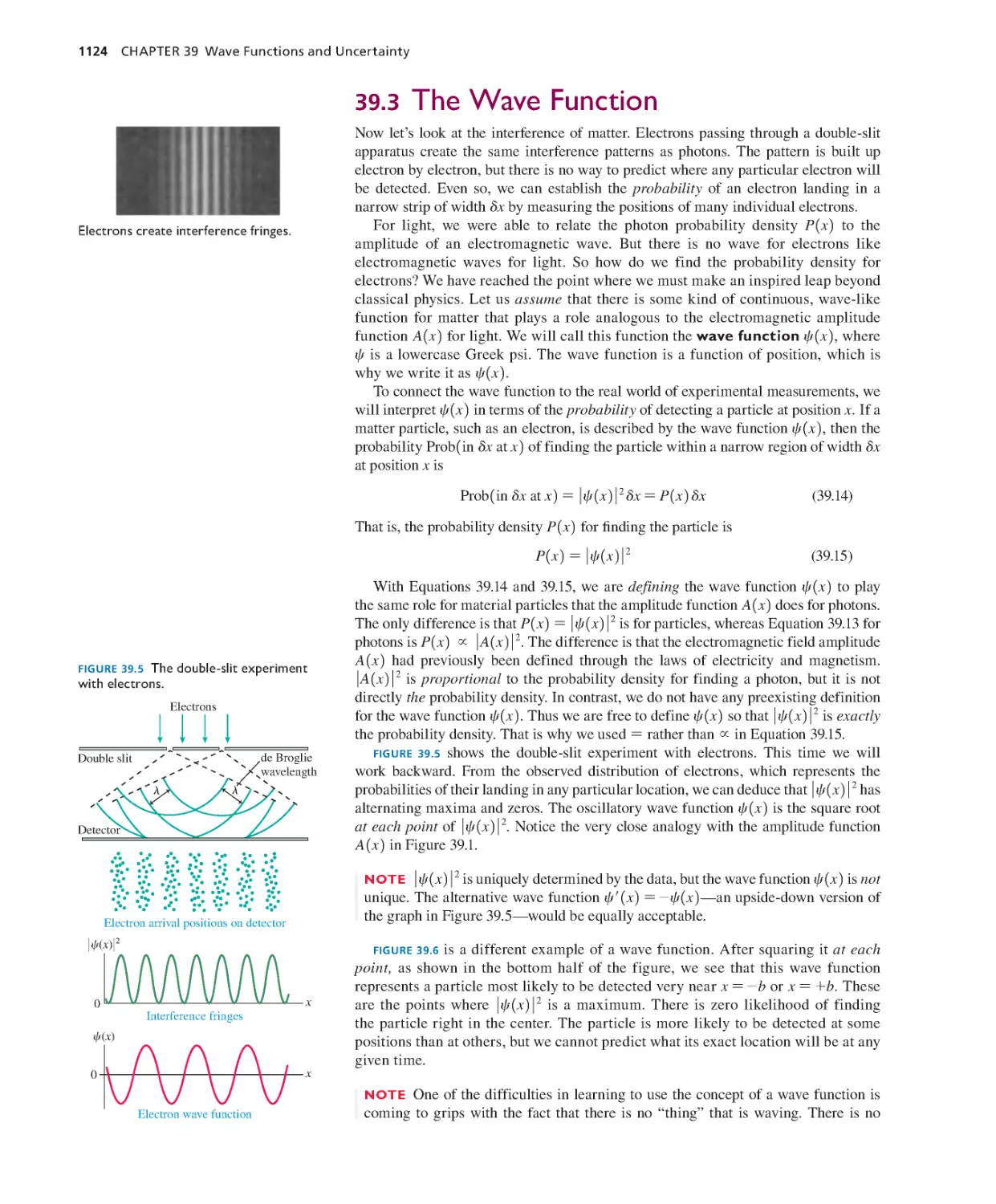
39.1 Waves, Particles, and the Double-Slit
Experiment 1119
39.2 Connecting the Wave and Photon
Views 1122
39.3 The Wave Function 1124
39.4 Normalization 1126
39.5 Wave Packets 1128
39.6 The Heisenberg Uncer tainty
Principle 1131
SUMMARY 1135
QUESTIONS AND PROBLEMS 1136
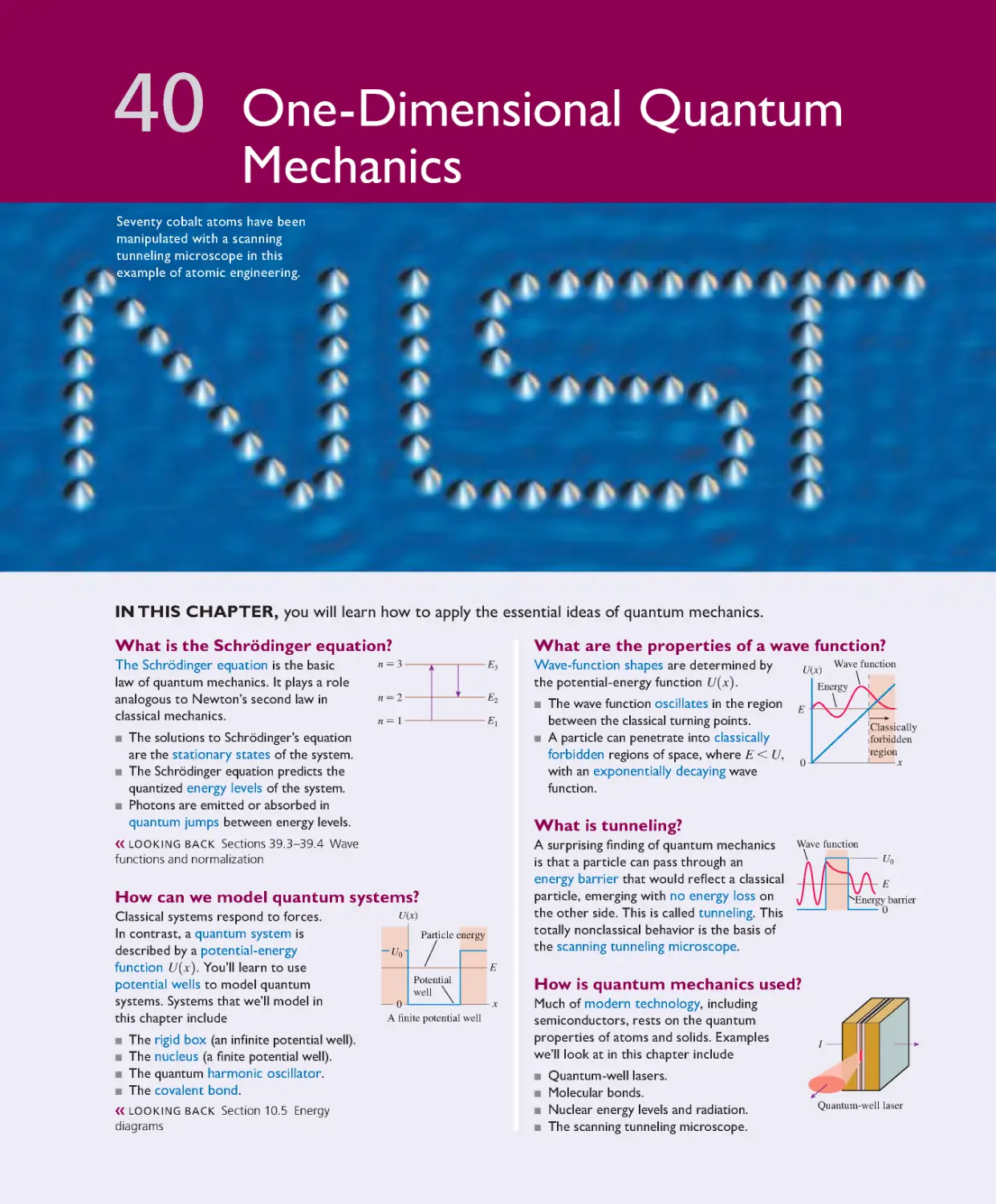
Chapter 40 One-Dimensional Quantum
Mechanics 1141
40.1 The Schrödinger Equation 1142
40.2 Solving the Schrödinger Equation 1145
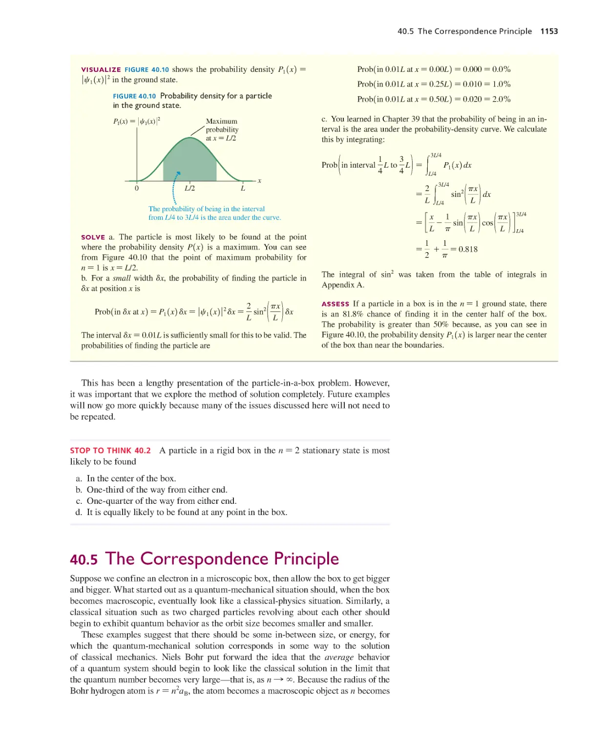
40.3 A Particle in a Rigid Box: Energies and
Wave Functions 1147
40.4 A Particle in a Rigid Box: Interpreting
the Solution 1150
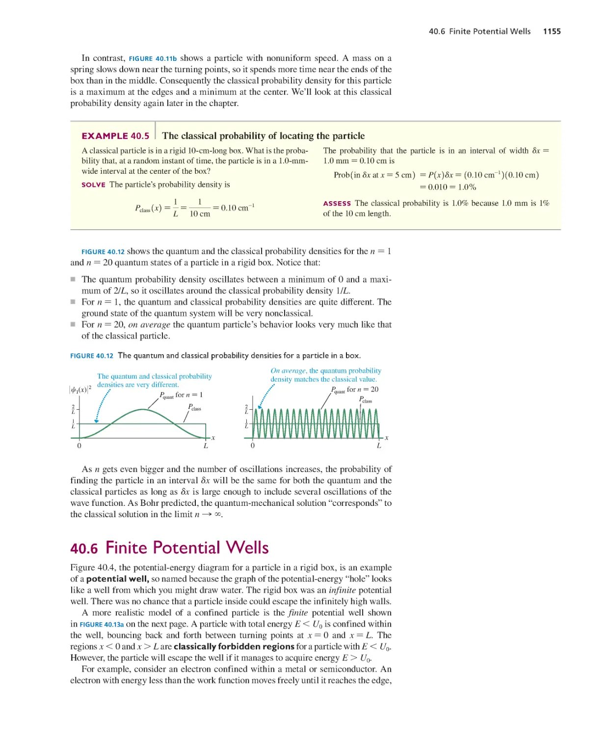
40.5 The Correspondence Principle 1153
40.6 Finite Potential Wells 1155
40.7 Wave-Function Shapes 1160
40.8 The Quantum Harmonic
Oscillator 1162
40.9 More Quantum Models 1165
40.10 Quantum-Mechanical Tunneling 1168
SUMMARY 1173
QUESTIONS AND PROBLEMS 1174
Chapter 41 Atomic Physics 1178
41.1 The Hydrogen Atom: Angular
Momentum and Energy 1179
41.2 The Hydrogen Atom: Wave Functions
and Probabilities 1182
41.3 The Electron’s Spin 1185
41.4 Multielectron Atoms 187
41.5 The Periodic Table of the Elements 1190
41.6 Excited States and Spectra 1193
41.7 Lifetimes of Excited States 1198
41.8 Stimulated Emission and Lasers 1200
SUMMARY 1205
QUESTIONS AND PROBLEMS 1206
Chapter 42 Nuclear Physics 1210
42.1 Nuclear Str ucture 1211
42.2 Nuclear Stability 1214
42.3 The Strong Force 1217
42.4 The Shell Model 1218
42.5 Radiation and Radioactivity 1220
42.6 Nuclear Decay Mechanisms 1225
42.7 Biological Applications of Nuclear
Physics 1230
SUMMARY 1234
QUESTIONS AND PROBLEMS 1235
Part VIII Relativity and Quantum
Physics 1240
Appendix A Mathematics Review A-1
Appendix B Periodic Table of Elements A- 4
Appendix C Atomic and Nuclear Data A-5
Answers to Stop to Think Questions and
Odd-Numbered Problems A-9
Credits C-1
Index I-1
KNOWLEDGE
STRUCTURE
This page intentionally left blank
OVERVIEW
Why Things Move
Each of the seven parts of this book opens with an overview to give you a
look ahead, a glimpse at where your journey will take you in the next few
chapters. It’s easy to lose sight of the big picture while you’re busy negotiating
the terrain of each chapter. In Part I, the big picture, in a word, is motion.
There are two big questions we must tackle:
■ How do we describe motion? It is easy to say that an object moves, but it’s
not obvious how we should measure or characterize the motion if we want
to analyze it mathematically. The mathematical description of motion is called
kinematics, and it is the subject matter of Chapters 1 through 4.
■ How do we explain motion? Why do objects have the particular motion
they do? Why, when you toss a ball upward, does it go up and then come
back down rather than keep going up? Are there “laws of nature” that allow
us to predict an object’s motion? The explanation of motion in terms of its
causes is called dynamics, and it is the topic of Chapters 5 through 8.
Two key ideas for answering these questions are force (the “cause”) and
acceleration (the “effect”). A variety of pictorial and graphical tools will be
developed in Chapters 1 through 5 to help you develop an intuition for the
connection between force and acceleration. You’ll then put this knowledge to
use in Chapters 5 through 8 as you analyze motion of increasing complexity.
Another important tool will be the use of models. Reality is extremely com-
plicated. We would never be able to develop a science if we had to keep track
of every little detail of every situation. A model is a simplified description of reality—
much as a model airplane is a simplified version of a real airplane—used to
reduce the complexity of a problem to the point where it can be analyzed and
understood. We will introduce several important models of motion, paying close
attention, especially in these earlier chapters, to where simplifying assumptions
are being made, and why.
The “laws of motion” were discovered by Isaac Newton roughly 350 years
ago, so the study of motion is hardly cutting-edge science. Nonetheless, it is
still extremely impor tant. Mechanics—the science of motion—is the basis for
much of engineering and applied science, and many of the ideas introduced
here will be needed later to understand things like the motion of waves and the
motion of electrons through circuits. Newton’s mechanics is the foundation of
much of contemporary science, thus we will start at the beginning.
Motion can be slow and steady, or fast and
sudden.This rocket, with its rapid acceleration,
is responding to forces exerted on it by thrust,
gravity, and the air.
Newton’s Laws
PART
I
1
IN THIS CHAPTER, you will learn the fundamental concepts of motion.
What is a chapter preview?
Each ch apter starts with an overview. Think of it as a roadm ap
to h elp you get orie nted and m ake the most of you r studying.
❮❮ LOOKING BACK A Looking Back reference tells you what material
from previous chapters is especially important for understanding the
new topic s. A quick review will help your learning. You will find
additional Looking Back reference s within the chapter, right at the
point they ’re needed.
Why do we need vectors?
Many of the quantities used to describe
motion, such as velocity, have both a
size and a direction. We use vectors to
rep re se nt these quantities. This chapter
introduces graphical techniques to add and
subtract vectors. Chapter 3 will explore
ve ctors in more detail.
Why are units and signiicant
igures important?
Scientists and engineers must communicate
their ideas to others. To do so, we have to
agre e ab out the units in which quantities
are me asured. In physics we use metric
units, called SI units. We also ne ed rule s
for telling others how accurately a quantity
is known. You will learn the rules for using
significant figures correctly.
Why is motion important?
The universe is in motion, from the smallest scale of electrons
and atoms to the large st scale of entire gala xie s. We’ll start with
the motion of everyday objects, such as cars and balls and people.
Later we’ll study the motions of waves, of atoms in gases, and of
electrons in circuits. Motion is the one theme that will be with us
from the i rst chapter to the last.
Concepts of Motion
Motion takes m any forms.
The ski jumpe r seen here is
an example of translational
motion.
INTHIS CHAPTER, you will learn the fundamental concepts of motion.
What is a chapter preview?
Each chapter starts with an overview. Think of itas aroadmap
to help you get oriented and make the most of your studying.
❮❮ LOOKING BACK ALookingBack referencetellsyou what material
from previous chaptersis especially important for understanding the
new topics. A quick review will help your learning. You will find
additional Looking Back references within the chapter, right at the
point they’re needed.
Why do we need vectors?
Many of the quantities used todescribe
motion, such as velocity, have both a
size and a direction. We use vectors to
represent these quantities. This chapter
introduces graphicaltechniques to add and
subtract vectors. Chapter 3 will explore
vectors in more detail.
Why are units and signiicant
igures important?
Scientists and engineers must communicate
their ideas to others. To do so, we have to
agree about the units in which quantities
are measured.In physics we use metric
units, called SI units. We also need rules
for telling others how accurately aquantity
is known. You will learn the rules for using
significant figures correctly.
Why is motion important?
The universe is in motion, from the smallest scale of electrons
and atoms to the largest scale of entire galaxies. We’ll start with
the motion of everyday objects, such as cars and balls and people.
Later we’ll studythe motions of waves, of atoms in gases, and of
electrons in circuits. Motion is the one theme that will be with us
from the irst chapter to the last.
What is motion?
Before solving motion problems, we must
learn to describe motion. We will use
■ Motion diagrams
■ Graphs
■ Pictures
Motion concepts introduced in this chapter
include position, velocity, and acceleration.
a
u
v
u
x0=v0x=t0=0
ax
x1
x
x0
Known
ax=2.0m/s2
Fin d
x1
A
u
A+B
u
u
B
u
0.00620 = 6.20 * 10
-3
What is motion?
Before solving motion problem s, we mu st
learn to describe motion. We will use
■ Motion diagrams
■ Graphs
■ Pictures
Motion concepts introduced in this chapter
include position, velocity, and acceleration.
a
u
v
u
x0=v0x=t0=0
ax
x1
x
x0
Known
ax=2.0m/s
2
Find
x1
A
u
A+B
u
u
B
u
0.00620 = 6.20 * 10-3
1.1 Motion Diagrams 3
1.1 Motion Diagrams
Motion is a theme that will appear in one form or another throughout this entire
book. Although we all have intuition about motion, based on our experiences, some
of the important aspects of motion turn out to be rather subtle. So rather than jumping
immediately into a lot of mathematics and calculations, this first chapter focuses on
visualizing motion and becoming familiar with the concepts needed to describe a
moving object. Our goal is to lay the foundations for understanding motion.
FIGURE 1.1 Four ba sic types of motion.
Linear motion
Circular motion
Projectile motion
Rotational motion
To begin, let’s define motion as the change of an object’s position with time. FIGURE 1.1
shows four basic types of motion that we will study in this book. The first three—
linear, circular, and projectile motion—in which the object moves through
space are called translational motion. The path along which the object moves,
whether straight or curved, is called the object’s trajector y. Rotational motion
is somewhat different because there’s movement but the object as a whole doesn’t
change position. We’ll defer rotational motion until later and, for now, focus on
translational motion.
Making a Motion Diagram
An easy way to study motion is to make a video of a moving object. A video camera,
as you probably know, takes images at a fixed rate, typically 30 ever y second. Each
separate image is called a frame. As an example, FIGURE 1.2 shows four frames from a
video of a car going past. Not surprisingly, the car is in a somewhat different position
in each frame.
Suppose we edit the video by layering the frames on top of each other, creating the
composite image shown in FIGURE 1.3. This edited image, showing an object’s position
at several equally spaced instants of time, is called a motion diagram. As the
examples below show, we can define concepts such as constant speed, speeding up,
and slowing down in terms of how an object appears in a motion diagram.
NoTE It’s important to keep the camera in a fixed position as the object moves by.
Don’t “pan” it to track the moving object.
FIGURE 1.2 Four fr am es from a video.
FIGURE 1.3 A motion diagr am of the car
shows all the fr ames simultaneously.
The same amount of time elapses
between each image and the next.
Examples of motion diagrams
Images that a re equally sp aced indicate an
object moving with constant speed .
An increasing distance between the images
shows that the object is speeding up.
A decreasing distance between the images
shows that the object is slowing down .
4 CHAPTER 1 Concepts of Motion
NoTE Each chapter will have several Stop to Think questions. These questions are
designed to see if you’ve understood the basic ideas that have been presented. The
answers are given at the end of the book, but you should make a serious effort to
think about these questions before turning to the answers.
1.2 Models and Modeling
The real world is messy and complicated. Our goal in physics is to brush aside many of
the real-world details in order to discern patterns that occur over and over. For example,
a swinging pendulum, a vibrating guitar string, a sound wave, and jiggling atoms in
a crystal are all very different—yet perhaps not so different. Each is an example
of a system moving back and forth around an equilibrium position. If we focus on
understanding a very simple oscillating system, such as a mass on a spring, we’ll auto-
matically understand quite a bit about the many real-world manifestations of oscillations.
Stripping away the details to focus on essential features is a process called modeling.
A model is a highly simplified picture of reality, but one that still captures the essence
of what we want to study. Thus “mass on a spring” is a simple but realistic model of
almost all oscillating systems.
Models allow us to make sense of complex situations by providing a framework for
thinking about them. One could go so far as to say that developing and testing models
is at the heart of the scientific process. Alber t Einstein once said, “Physics should
be as simple as possible—but not simpler.” We want to find the simplest model that
allows us to understand the phenomenon we’re studying, but we can’t make the model
so simple that key aspects of the phenomenon get lost.
We’ll develop and use many models throughout this textbook; they’ll be one of our
most important thinking tools. These models will be of two types:
■ Descriptive models: What are the essential characteristics and properties of a
phenomenon? How do we describe it in the simplest possible terms? For example,
the mass-on -a-spring model of an oscillating system is a descriptive model.
■ Explanatory models: Why do things happen as they do? Explanatory models, based on
the laws of physics, have predictive power, allowing us to test—against experimental
data—whether a model provides an adequate explanation of our observations.
The Particle Model
For many types of motion, such as that of balls, cars, and rockets, the motion of the
object as a whole is not influenced by the details of the object’s size and shape. All we
really need to keep track of is the motion of a single point on the object, so we can treat
the object as if all its mass were concentrated into this single point. An object that can
be represented as a mass at a single point in space is called a par ticle. A particle has
no size, no shape, and no distinction between top and bottom or between front and back.
If we model an object as a particle, we can represent the object in each frame of a
motion diagram as a simple dot rather than having to draw a full picture. FIGURE 1.4
shows how much simpler motion diagrams appear when the object is represented as
a particle. Note that the dots have been numbered 0, 1, 2, . . . to tell the sequence in
which the frames were exposed.
Car A
Car B
STOP TO THINK 1.1 Which car is going faster, A or B? Assume there are equal intervals of time
between the frames of both videos.
We can model an airplane’s take off as a
particle (a descriptive model) undergoing
constant acceleration (a descriptive
model) in respo nse to constant forces
(an explanatory model).
FIGURE 1.4 Motion diagr am s in which the
object is modeled as a particle.
0
1
2
3
(a) Motion diagram of a rocket launch
(b) Motion diagram of a car stopping
Numbers show
the order in
which the frames
were exposed.
4
0
The same amount of time elapses
between each image and the next.
1
234
1.3 Position, Time, and Displacement 5
Treating an object as a particle is, of course, a simplification of reality—but that’s
what modeling is all about. The par ticle model of motion is a simplification in
which we treat a moving object as if all of its mass were concentrated at a single point.
The particle model is an excellent approximation of reality for the translational motion
of cars, planes, rockets, and similar objects.
Of course, not everything can be modeled as a particle; models have their limits.
Consider, for example, a rotating gear. The center doesn’t move at all while each tooth is
moving in a different direction. We’ll need to develop new models when we get to new
types of motion, but the particle model will serve us well throughout Part I of this book.
STOP TO THINK 1.2 Three motion diagrams
are shown. Which is a dust particle settling to
the floor at constant speed, which is a ball dropped
from the roof of a building, and which is a
descending rocket slowing to make a soft landing
on Mars?
1.3 Position, Time, and Displacement
To use a motion diagram, you would like to know where the object is (i.e., its position)
and when the object was at that position (i.e., the time). Position measurements can
be made by laying a coordinate-system grid over a motion diagram. You can then
measure the 1x, y2 coordinates of each point in the motion diagram. Of course, the
world does not come with a coordinate system attached. A coordinate system is an
artificial grid that you place over a problem in order to analyze the motion. You place
the origin of your coordinate system wherever you wish, and different observers of a
moving object might all choose to use different origins.
Time, in a sense, is also a coordinate system, although you may never have thought of
time this way. You can pick an arbitrary point in the motion and label it ;t = 0 seconds.”
This is simply the instant you decide to start your clock or stopwatch, so it is the origin of your
time coordinate. Different observers might choose to start their clocks at different moments.
A video frame labeled ;t = 4 seconds” was taken 4 seconds after you started your clock.
We typically choose t = 0 to represent the “beginning” of a problem, but the object
may have been moving before then. Those earlier instants would be measured as neg-
ative times, just as objects on the x-axis to the left of the origin have negative values of
position. Negative numbers are not to be avoided; they simply locate an event in space
or time relative to an origin .
To illustrate, FIGURE 1.5a shows a sled sliding down a snow-covered hill. FIGURE 1.5b is
a motion diagram for the sled, over which we’ve drawn an xy-coordinate system. You
can see that the sled’s position is 1x3, y32 = 115 m, 15 m2 at time t3 = 3 s. Notice how
we’ve used subscripts to indicate the time and the object’s position in a specific frame
of the motion diagram.
NoTE The frame at t = 0 is frame 0. That is why the fourth frame is labeled 3.
Another way to locate the sled is to draw its position vector: an arrow from the
origin to the point representing the sled. The position vector is given the symbol r
u
.
Figure 1.5b shows the position vector r
u
3 = 121 m, 45°2. The position vector r
u
does not tell
us anything different than the coordinates 1x, y2. It simply provides the information
in an alternative form.
FIGURE 1.5 Motion diagram of a sled with
frames made every 1 s.
(a)
The sled’s position in frame 3
can be specified with coordinates.
Alternatively, the position
can be specified by the
position vector.
r3=(21m,45°)
(x3,y3)=(15m,15m)
t3=3s
u
(b)
45°
y (m)
x (m)
0
10
20
10
0
20
30
(a)
(c) 0
1
2
3
4
5
0
1
2
3
4
5
(b) 0
1
2
3
4
5
6 CHAPTER 1 Concepts of Motion
Scalars and Vectors
Some physical quantities, such as time, mass, and temperature, can be described com-
pletely by a single number with a unit. For example, the mass of an object is 6 kg and
its temperature is 30°C. A single number (with a unit) that describes a physical quantity
is called a scalar. A scalar can be positive, negative, or zero.
Many other quantities, however, have a directional aspect and cannot be described
by a single number. To describe the motion of a car, for example, you must specify
not only how fast it is moving, but also the direction in which it is moving. A quantity
having both a size (the “How far?” or “How fast?”) and a direction (the “Which way?”)
is called a vector. The size or length of a vector is called its magnitude. Vectors will
be studied thoroughly in Chapter 3, so all we need for now is a little basic information.
We indicate a vector by drawing an arrow over the letter that represents the quantity.
Thus r
u
and A
u
are symbols for vectors, whereas r and A, without the arrows, are symbols
for scalars. In handwritten work you must draw arrows over all symbols that represent
vectors. This may seem strange until you get used to it, but it is very important because
we will often use both r and r
u
, orbothAandA
u
, in the same problem, and they mean
different things! Note that the arrow over the symbol always points to the right, rega rdless
of which direction the actual vector points. Thus we write r
u
orA
u
, never r
z
orA
z
.
Displacement
We said that motion is the change in an object’s position with time, but how do we
show a change of position? A motion diagram is the perfect tool. FIGURE 1.6 is the
motion diagram of a sled sliding down a snow-covered hill. To show how the sled’s
position changes between, say, t3 = 3 s and t4 = 4 s, we draw a vector arrow between
the two dots of the motion diagram. This vector is the sled’s displacement, which
is given the symbol ∆ r
u
. T he Greek letter delta 1∆2 is used in math and science to
indicate the change in a quantity. In this case, as we’ll show, the displacement ∆ r
u
is
the change in an object’s position.
NoTE ∆r
u
is a single symbol. You cannot cancel out or remove the ∆ .
Notice how the sled’s position vector r
u
4 is a combination of its early position r
u
3 with
the displacement vector ∆r
u
. Infact,r
u
4 is the vector sum of the vectors r
u
3and∆r
u
. This
is written
r
u
4=r
u
3+∆r
u
(1.1)
Here we’re adding vector quantities, not numbers, and vector addition differs from
“regular” addition. We’ll explore vector addition more thoroughly in Chapter 3, but for
now you can add two vectors A
u
and B
u
with the three-step procedure shown in Tactics
Box 1.1 .
FIGURE 1.6 The sled undergoes a
displacement ∆r
u
from position r
u
3
to position r
u
4.
The sled’s displacement between
t3=3sandt4=4sisthevector
drawn from one postion to the next.
t3=3s
t4=4s
r4
u
r3
u
∆r
u
y (m)
x (m)
0
10
20
10
0
20
30
TACTICS BoX 1.1
Vector addition
1
2
3
ToaddBtoA:
Draw A.
Place the tail of
BatthetipofA.
Draw an arrow from
thetailofAtothe
tip of B. This is
vector A + B.
A+B
A
u
B
u
A
u
A
u
A
u
B
u
u
u
u
u
u
u
u
u
u
u
u
B
u
1.3 Position, Time, and Displacement 7
If you examine Figure 1.6, you’ll see that the steps of Tactics Box 1.1 are exactly
how r
u
3and∆r
u
are added to give r
u
4.
NoTE A vector is not tied to a particular location on the page. You can move a vector
around as long as you don’t change its length or the direction it points. Vector B
u
is
not changed by sliding it to where its tail is at the tip of A
u
.
Equation 1.1 told us that r
u
4=r
u
3+∆r
u
. T h is is easily rearranged to give a more pre-
cise definition of displacement: The displacement �r
u
of an object as it moves from
an initial position r
u
i to a final position r
u
fis
∆r
u
=r
u
f-r
u
i
(1.2)
Graphically, �r
u
is a vector arrow drawn from position r
u
i to position r
u
f.
NoTE To be more general, we’ve written Equation 1.2 in terms of an initial position
and a final position, indicated by subscripts i and f. We’ll frequently use i and f when
writing general equations, then use specific numbers or values, such as 3 and 4, when
work ing a problem.
This definition of ∆r
u
involves vector subtraction. With numbers, subtraction is the
same as the addition of a negative number. That is, 5 - 3 is the same as 5 + 1-32. Sim-
ilarly, we can use the rules for vector addition to find A
u
-
B
u
=A
u
+ 1-B
u
2 if we first
define what we mean by - B
u
. As FIGURE 1.7 shows, the negative of vector B
u
is a vector with
the same length but pointing in the opposite direction. This makes sense because
B
u
-
B
u
=B
u
+ 1-B
u
2=0
u
, where 0
u
, a vector with zero length, is called the zero vector.
FIGURE 1.7 The negative of a vector.
The zero vector 0 has no length.
B+(-B)=0becausethesum
returns to the starting point.
-B
u
u
B
u
u
u
u
Vector -B has the same length as
B but points in the opposite direction.
u
u
Place the tail of
- BatthetipofA.
Draw an arrow from
thetailofAtothe
tip of -B. This is
vector A - B.
A
u
u
u
u
A
u
A
u
A
u
B
u
To subtract B from A:
Draw A.
1
2
3
-B
A-B
u
u
u
u
-B
u
u
u
u
u
u
TACTICS BoX 1.2
Vector subtraction
FIGURE 1.8 uses the vector subtraction r ules of Tactics Box 1.2 to prove that the
displacement ∆ r
u
is simply the vector connecting the dots of a motion diagram.
rf
-r
i
f
i
Position
vectors
Origin
(a) Initial and final position vectors
Two dots of
a motion diagram
ri
f
i
Draw-ri atthe
tip of rf.
2
3Drawrf-ri
. This is ∆r.
1 Draw rf.
f
i
rf-ri
Finally, slide ∆ r back to the
motion diagram. It is a vector
fromdotitodotf.
(b) Procedure for finding the particle’s displacement vector ∆ r
u
u
-r
i
u
u
rf
u
rf
u
u
ri
u
ri
u
u
u
u
u
u
u
u
u
u
▼ FIGURE 1.8 Using ve ctor subtraction to
find ∆r
u
=r
u
f-r
u
i.
8 CHAPTER 1 Concepts of Motion
Motion Diagrams with Displacement Vectors
The first step in analyzing a motion diagram is to determine all of the displacement
vectors. As Figure 1.8 shows, the displacement vectors are simply the arrows connecting
each dot to the next. Label each ar row with a vector symbol ∆r
u
n, starting with n = 0.
FIGURE 1.9 shows the motion diagrams of Figure 1.4 redrawn to include the displacement
vectors. You do not need to show the position vectors.
NoTE When an object either starts from rest or ends at rest, the initial or final dots
are as close together as you can draw the displacement vector ar row connecting
them. In addition, just to be clear, you should write “Start” or “Stop” beside the
initial or final dot. It is impor tant to distinguish stopping from merely slowing down.
Now we can conclude, more precisely than before, that, as time proceeds:
■ An object is speeding up if its displacement vectors are increasing in length.
■ An object is slowing down if its displacement vectors are decreasing in length.
FIGURE 1.9 Motion diagrams with the
displacement vector s.
(a) Rocket launch
(b) Car stopping
Start
Stop
∆r3
∆r2
∆r1
∆r0
∆r1 ∆r2 ∆r3
u
u
u
u
∆r0
u
u
u
u
A stopwatch is used to measure a time
inter val.
EXAMPlE 1.1 | Headfirst into the snow
Alice is sliding along a smooth, icy road on her sled when she suddenly runs headfirst
into a large, very soft snowbank that gradually brings her to a halt. Draw a motion
diagra m for Alice. Show a nd label all displacement vectors.
MoDEl The details of Alice and the sled—their size, shape, color, and so on— a re not
releva nt to u nderstanding thei r overall motion. So we ca n model Alice and the sled as
one pa rticle.
VISuAlIzE FIGURE 1.10 shows a motion diagra m. The problem stat ement suggests that the
sled’s speed is very nearly constant until it hits the snowbank. Thus the displacement vectors
are of equal length as Alice slides along the icy road. She begins slowing when she hits the
snowbank , so the displacement vectors then get shorter until the sled stops. We’re told that her
stop is gradual, so we want the vector lengths to get shorter gradually rather than suddenly.
The displacement vectors
are getting shorter, so she’s
slowing down.
Stop
Hits snowbank
This is motion at constant speed
because the displacement vectors
are a constant length.
∆r0
∆r1
∆r2
∆r3
u
u
u
u
∆r4
u
∆r5
u
∆r6
u
FIGURE 1.10 The motion diagram of Alice and the sled.
x
Time Interval
It’s also useful to consider a change in time. For example, the clock readings of two frames
of film might be t1 and t2. The specific values are arbitrary because they are timed relative
to an arbitrary instant that you chose to call t = 0. But the time interval ∆t = t2 - t1 is not
arbitrary. It represents the elapsed time for the object to move from one position to the next.
The time interval �t ∙ tf ∙ ti measures the elapsed time as an object moves
from an initial position r
u
i at time ti to a final position r
u
f at time tf. The value of �t
is independent of the specific clock used to measure the times.
To summarize the main idea of this section, we have added coordinate systems
and clocks to our motion diagrams in order to measure when each frame was exposed
and where the object was located at that time. Different observers of the motion may
choose different coordinate systems and different clocks. However, all observers find
the same values for the displacements ∆ r
u
and the time intervals ∆ t because these are
independent of the specific coordinate system used to measure them.
1.4 Velocity 9
1.4 Velocity
It’s no sur prise that, during a given time interval, a speeding bullet travels farther than
a speeding snail. To extend our study of motion so that we can compare the bullet to
the snail, we need a way to measure how fast or how slowly an object moves.
One quantity that measures an object’s fastness or slowness is its average speed,
defined as the ratio
average speed =
distance traveled
time interval spent traveling
=
d
∆t
(1.3)
If you drive 15 miles (mi) in 30 minutes 1
1
2 h2, your average speed is
average speed =
15 mi
1
2h
= 30mph
(1.4)
Although the concept of speed is widely used in our day-to-day lives, it is not a
sufficient basis for a science of motion. To see why, imagine you’re trying to land a jet
plane on an aircraft carrier. It matters a great deal to you whether the aircraft carrier is
moving at 20 mph (miles per hour) to the north or 20 mph to the east. Simply knowing
that the boat’s speed is 20 mph is not enough information!
It’s the displacement ∆ r
u
, a vector quantity, that tells us not only the distance trav-
eled by a moving object, but also the direction of motion. Consequently, a more useful
ratio than d/∆t is the ratio ∆r
u
/∆t. In addition to measuring how fast an object moves,
this ratio is a vector that points in the direction of motion.
It is convenient to give this ratio a name. We call it the average velocity, and it
has the symbol v
u
avg. The average velocity of an object during the time interval � t,
in which the object undergoes a displacement �r
u
, is the vector
v
u
avg =
∆r
u
∆t
(1.5)
An object’s average velocity vector points in the same direction as the displacement
vector � r
u
. T his is the direction of motion.
NoTE In everyday language we do not make a distinction between speed and
velocity, but in physics the distinction is very important. In particular, speed is simply
“How fast?” whereas velocity is “How fast, and in which direction?” As we go along
we will be giving other words more precise meanings in physics than they have in
everyday language.
As an example, FIGURE 1.11a shows two ships that move 5 miles in 15 minutes. Using
Equation 1.5 with ∆t = 0.25 h, we find
v
u
avg A = (20 mph, north)
v
u
avg B = (20 mph, east)
(1.6)
Both ships have a speed of 20 mph, but their velocities are different. Notice how the
velocity vectors in FIGURE 1.11b point in the direction of motion.
NoTE Our goal in this chapter is to visualize motion with motion diagrams. Strictly
speaking, the vector we have defined in Equation 1.5, and the vector we will show on
motion diagrams, is the average velocity v
u
avg. But to allow the motion diagram to be
a useful tool, we will drop the subscript and refer to the average velocity as simply v
u
.
Our definitions and symbols, which somewhat blur the distinction between average
and instantaneous quantities, are adequate for visualization purposes, but they’re not
the final word. We will refine these definitions in Chapter 2, where our goal will be
to develop the mathematics of motion.
The victory goes to the runner with the
highest average speed.
FIGURE 1.11 The displacement vectors
and velocities of ships A and B.
vavg A = (20 mph, north)
u
(a)
vavg B = (20 mph, east)
(b)
A
B
∆rA = (5 mi, north)
∆rB = (5 mi, east)
The velocity vectors point
in the direction of motion.
u
u
u
10 CHAPTER 1 Concepts of Motion
Motion Diagrams with Velocity Vectors
The velocity vector points in the same direction as the displacement ∆ r
u
, and the
length of v
u
is directly proportional to the length of ∆ r
u
.
Consequently, the vectors
connecting each dot of a motion diagram to the next, which we previously labeled as
displacements, could equally well be identified as velocity vectors.
This idea is illustrated in FIGURE 1.12, which shows four frames from the motion
diagram of a tortoise racing a hare. The vectors connecting the dots are now labeled
as velocity vectors v
u
. T he length of a velocity vector represents the average speed
with which the object moves between the two points. Longer velocity vectors indicate
faster motion. You can see that the hare moves faster than the tortoise.
Notice that the hare’s velocity vectors do not change; each has the same length
and direction. We say the hare is moving with constant velocity. The tortoise is also
moving with its own constant velocity.
FIGURE 1.12 Motion diagr am of the
tor toise r acing the hare .
v1
u
v2
u
v0
u
v1
u
v2
u
v0
u
The length of each arrow represents
the average speed. The hare moves
faster than the tortoise.
These are average velocity vectors.
Hare
Tortoise
EXAMPlE 1.2 | Accelerating up a hill
The light turns green and a car accelerates, starting from rest, up a 20° hill. Draw a
motion diagra m showing the car’s velocity.
MoDEl Use the pa rticle model to represent the car as a dot.
VISuAlIzE The car’s motion takes place along a st raight line, but the line is neither
horizontal nor vertical. A motion diagra m should show the object moving with the
corre ct orientation —in this case, at a n angle of 20°. FIGURE 1.13 shows several f ra mes
of the motion diagram, where we see the car speeding up. The car starts from rest, so
the first arrow is drawn as short as possible and the first dot is labeled “Start.” The
displacement vectors have be en d rawn f rom each dot to the next, but then they are
identified a nd labeled as average velocity vectors v
u
.
v
u
This labels the whole row of
vectors as velocity vectors.
The velocity vectors
are getting longer, so
the car is speeding up.
Start
FIGURE 1.13 Motion diag ram of a car accele rating up a hill.
EXAMPlE 1.3 | A rolling soccer ball
Marcos kicks a soccer ball. It rolls along the ground u ntil stopped
by Jose. Draw a motion diagram of the ball.
MoDEl This example is typical of how ma ny problems in
science a nd engineering a re worded. The problem does not
give a clea r st atement of where the motion begins or ends. A re
we interested in the motion of the ball just during the time it is
rolling between Ma rcos a nd Jose? What about the motion as
Marcos kicks it (ball rapidly speeding up) or as Jose stops it
(ball rapidly slowing down)? The point is that you will often
be called on to make a reasonable interpretation of a problem
st atement. I n this problem, the det ails of kicking and stopping
the ball are complex. The motion of the ball across the ground
is easier to describe, and it’s a motion you might expect to lea rn
about in a physics cla ss. So ou r interpretation is that the motion
diagra m should sta rt as the ball leaves Ma rcos’s foot (ball
al ready moving) and should end the instant it touches Jose’s foot
(ball still moving). I n between, the ball will slow down a little. We
will model the ball as a pa rticle.
VISuAlIzE With this interpretation in mind, FIGURE 1.14 sh ows
the motion diag ram of the ball. Notice how, in cont rast to the car
of Figure 1.13, the ball is al ready moving as the motion diagra m
video begins. As before, the average velocity vectors a re found by
con necting the dots. You can se e that the average velo city vectors
get shorter as the ball slows. E ach v
u
is different, so this is not
consta nt-velocity motion.
FIGURE 1.14 Motion diagr am of a socce r ball rolling from
Marcos to Jose.
v
u
Marcos
Jose
The velocity vectors are gradually getting shorter.
1.5 Linear Acceleration 11
STOP TO THINK 1.3 A particle moves from position 1 to position 2 during the time
interval ∆t. Which vector shows the particle’s average velocity?
(e)
(d)
(c)
(b)
(a)
1
2
y
x
1.5 Linear Acceleration
Position, time, and velocity are important concepts, and at first glance they might appear
to be sufficient to describe motion. But that is not the case. Sometimes an object’s
velocity is constant, as it was in Figure 1.12 . More often, an object’s velocity changes
as it moves, as in Figures 1.13 and 1.14. We need one more motion concept to describe
a change in the velocity.
Because velocity is a vector, it can change in two possible ways:
1. The magnitude can change, indicating a change in speed; or
2. The direction can change, indicating that the object has changed direction.
We will concentrate for now on the first case, a change in speed. The car accel-
erating up a hill in Figure 1.13 was an example in which the magnitude of the
velocity vector changed but not the direction. We’ll return to the second case in
Chapter 4.
When we wanted to measure changes in position, the ratio ∆ r
u
/∆t was useful.
This ratio is the rate of change of position. By analogy, consider an object whose
velocity changes from an initial v
u
itoafinalv
u
f during the time interval ∆t. Just
as ∆r
u
=r
u
f-r
u
i is the change of position, the quantity ∆v
u
=v
u
f-v
u
i is the change
of velocity. The ratio ∆ v
u
/∆t is then the rate of change of velocity. It has a large
magnitude for objects that speed up quickly and a small magnitude for objects that
speed up slowly.
The ratio ∆ v
u
/∆t is called the average acceleration, and its symbol is a
u
avg. The
average acceleration of an object during the time interval �t, in which the object’s
velocity changes by �v
u
, is the vector
a
u
avg =
∆v
u
∆t
(1.7)
The average acceleration vector points in the same direction as the vector � v
u
.
Acceleration is a fairly abstract concept. Yet it is essential to develop a good
intuition about acceleration because it will be a key concept for understanding why
objects move as they do. Motion diagrams will be an impor tant tool for developing
that intuition.
NoTE As we did with velocity, we will drop the subscript and refer to the average
acceleration as simply a
u
.
This is adequate for visualization purposes, but not the
final word. We will refine the definition of acceleration in Chapter 2.
The Audi TT acceler ates from 0 to 60 mph
in6s.
12 CHAPTER 1 Concepts of Motion
Finding the Acceleration Vectors
on a Motion Diagram
Let’s look at how we can determine the average acceleration vector a
u
from a motion
diagram. From its definition, Equation 1.7, we see that a
u
points in the same direction
as ∆v
u
, the change of velocity. This critical idea is the basis for a technique to find a
u
.
Notice that the acceleration vector goes beside the middle dot, not beside the velocity
vectors. This is because each acceleration vector is determined by the difference
between the two velocity vectors on either side of a dot. The length of a
u
does not have
to be the exact length of ∆v
u
; it is the direction of a
u
that is most important.
The procedure of Tactics Box 1.3 can be repeated to find a
u
at each point in the
motion diagram. Note that we cannot determine a
u
at the first and last points because
we have only one velocity vector and can’t find ∆v
u
.
The Complete Motion Diagram
You’ve now seen several Tactics Boxes that help you accomplish specific tasks. Ta c t i c s
Boxes will appear in nearly every chapter in this book. We’ll also, where appropriate,
provide Problem-Solving Strategies.
TACTICS BoX 1.3
Finding the acceleration vector
a
u
1
2
3
4 Return to the original motion
diagram. Draw a vector at the
middle dot in the direction of
∆v; label it a. This is the average
acceleration at the midpoint
between vi and vf.
Draw the velocity vector vf.
To find the acceleration as the
velocity changes from vi to vf,
we must determine the change
of velocity ∆v = vf
-
vi.
vf
vi
vf
vf
-vi
vf
∆v
vf
vi
u
u
u
u
u
u
u
u
-vi
u
u
u
u
u
u
u
Draw∆v=vf
-
vi
=v
f + (-vi)
This is the direction of a.
u
u
u
u
u
u
Draw -vi at the tip of vf.
u
u
u
u
u
u
u
Exercises 21–24
Many Tactics Boxes will refer you to exercises in the
Student Workbook where you can practice the new skill.
1.5 Linear Acceleration 13
Examples of Motion Diagrams
Let’s look at some examples of the full strategy for drawing motion diagrams.
PRoBlEM-SolVING STRATEGY 1.1
Motion diagrams
MoDEl Determine whether it is appropriate to model the moving object as a particle.
Make simplifying assumptions when interpreting the problem statement.
VISuAlIzE A complete motion diagram consists of:
■ The position of the object in each frame of the video, shown as a dot. Use ive
or six dots to make the motion clear but without overcrowding the picture.
More complex motions may need more dots.
■ The average velocity vectors, found by connecting each dot in the motion dia-
gram to the next with a vector arrow. There is one velocity vector linking each
two position dots. Label the row of velocity vectors v
u
.
■ The average acceleration vectors, found using Tactics Box 1.3. There is one
acceleration vector linking each two velocity vectors. Each acceleration vector
is drawn at the dot between the two velocity vectors it links. Use 0
u
to indicate a
point at which the acceleration is zero. Label the row of acceleration vectors a
u
.
STOP TO THINK 1.4 A particle undergoes acceleration a
u
while moving from point 1 to point 2. Which of the choices
shows the most likely velocity vector v
u
2 as the particle leaves
poi nt 2?
a
u
v1
u
2
1
2
(a)
2
(c)
2
(d)
v2
2
(b)
u
v2
u
v2
u
v2
u
EXAMPlE 1.4 | The first astronauts land on Mars
A spaceship carrying the first astronauts to Ma rs descends safely
to the surface. Draw a motion diagra m for the last few seconds of
the descent.
MoDEl The spaceship is small i n compa rison with the distance
traveled, and the spaceship does not cha nge size or shap e, so it’s
reasonable to model the spaceship as a pa rticle. We’ll assume that
its motion in the la st few second s is st raight down. The problem
ends a s the spacecraft touches the surface.
VISuAlIzE FIGURE 1.15 shows a complete motion diag ram as the
spaceship descends a nd slows, usi ng its rockets, until it comes
to rest on the surface. Notice how the dots get closer together as
it slows. The inset uses the steps of Tactics Box 1.3 (numb ered
circles) to show how the acceleration vector a
u
is deter mined at one
point. All the other acceleration vectors will be si mila r because
for each pai r of velocity vectors the earlier one is longer than the
later one.
FIGURE 1.15 Motion diagr am of a space ship landing on M ars.
v and a point in opposite
directions. The object is
slowing down.
v
u
u
a
u
u
a
u
∆v
vi
u
-vi
u
vf
u
vf
u
Stops
1
2
3
4
u
x
14 CHAPTER 1 Concepts of Motion
Notice something interesting in Figures 1.15 and 1.16. Where the object is speeding
up, the acceleration and velocity vectors point in the same direction. Where the object
is slowing down, the acceleration and velocity vectors point in opposite directions.
These results are always true for motion in a straight line. For motion along a line:
■ An object is speeding up if and only if v
u
and a
u
point in the same direction.
■ An object is slowing down if and only if v
u
and a
u
point in opposite directions.
■ An object’s velocity is constant if and only if a
u
∙0
u
.
NoTE In everyday language, we use the word accelerate to mean “speed up” and
the word decelerate to mean “slow down.” But speeding up and slowing down are both
changes in the velocity and consequently, by our definition, both are accelerations.
In physics, acceleration refers to changing the velocity, no matter what the change
is, and not just to speeding up.
EXAMPlE 1.6 | Tossing a ball
Draw the motion diagra m of a ball tossed st raight up in the air.
MoDEl This problem calls for some interpretation. Should we
include the toss itself, or only the motion after the ball is released?
Should we include the ball hitting the g round? It appea rs that this
problem is really concerned with the ball’s motion through the air.
Consequently, we begin the motion diag ram at the insta nt that the
tosser releases the ball a nd end the diag ram at the inst ant the ball
hits the ground. We will consider neither the toss nor the impact.
And, of course, we will model the ball a s a pa rticle.
VISuAlIzE We have a slight difficulty here because the ball retraces
its route as it falls. A literal motion diag ra m would show the upward
motion and downwa rd motion on top of each other, leading to
conf usion. We ca n avoid this difficulty by horizontally sepa rating
the upward motion and downwa rd motion diagram s. This will not
affect our conclusions because it does not change a ny of the vectors.
FIGURE 1.17 shows the motion diagram d raw n this way. Notice that
the very top dot is shown twice— as the end point of the upward
motion and the beginning point of the downward motion.
FIGURE 1.16 Motion diagr am of a skier.
∆v=0
0
u
0
u
u
v
u
a
u
a
u
a
u
vi
u
vi
u
vf
u
vf
u
vf
u
vf
u
v and a point in the same direction.
The object is speeding up.
-vi
u
-vi
u
u
∆v
u
u
u
EXAMPlE 1.5 | Skiing through the woods
A skier glides along smooth, horizontal snow at consta nt speed, then spe eds up going
down a hill. Draw the skier’ motion diagra m.
MoDEl Model the skier as a pa rticle. It’s reasonable to assume that the downhill slope
is a straight line. Although the motion as a whole is not linear, we can treat the skier’s
motion as two sepa rate linear motions.
VISuAlIzE FIGURE 1.16 shows a complete motion diag ram of the skier. The dots are
equally spaced for the horizontal motion, indicating consta nt spe ed; then the dots get
farther apart as the skier speeds up going down the hill. The insets show how the average
acceleration ve ctor a
u
is determined for the horizontal motion and along the slope. All the
other acceleration vectors along the slope will be similar to the one shown b ecause each
velocity vector is longer than the preceding one. Notice that we’ve explicitly written 0
u
for the acceleration beside the dots where the velocity is consta nt. The acceleration at the
point where the direction changes will be considered in Chapter 4.
1.6 Motion in One Dimension 15
The ball slows down as it rises. You’ve learned that the
acceleration vectors point opposite the velocity vectors for a n object
that is slowing down along a line, a nd they a re shown accordingly.
Similarly, a
u
and v
u
point in the same direction as the falling ball
sp eeds up. Notice something interesting: The acceleration vectors
poi nt downward both while the ball is risi ng and while it is falling.
Both “speeding up” a nd “slowing down” o ccu r with the same
acceleration vector. This is an importa nt conclusion, one worth
pausing to think about.
Now let’s look at the top point on the ball’s trajectory. The
velocity vectors point upward but a re getting shorter as the ball
approaches the top. As the ball sta rts to fall, the velocity vectors
point downwa rd a nd a re getting longer. There must be a moment—
just a n instant as v
u
switches from p ointing up to p ointing down —
when the velocity is zero. I nde ed, the ball’s velo city is zero for an
inst ant at the precise top of the motion!
But what about the acceleration at the top? The inset shows how
the average acceleration is determined from the last upward velocity
before the top point and the fi rst downwa rd velocity. We find that
the acceleration at the top is p ointing downwa rd, just as it does
elsewhere in the motion.
Many pe ople expect the acceleration to be zero at the highest
point. But the velocity at the top p oint is changing—f rom up to
down. If the velocity is changing, there must be an acceleration.
A downwa rd-p ointing acceleration vector is needed to tu rn the
velocity vector from up to down. Another way to think about this
is to note that zero acceleration would mea n no change of velo city.
When the ball reached z ero velocity at the top, it would hang there
and not fall if the acceleration were also zero!
v
u
v
u
a
u
a
u
a
u
a
u
a
u
a
u
∆v
u
∆v
u
∆v
u
-vi
-vi
-vi
vf
u
vf
u
vf
u
vf
u
vf
u
vi
u
vi
u
vi
u
vf
u
Finding a while
going down
Finding a while
going up
u
u
For clarity, we displace the upward and downward
motions. They really occur along the same line.
The topmost point is
shown twice for clarity.
The acceleration at
the top is not zero.
Finding a at the top
u
u
u
u
FIGURE 1.17 Motion diagram of a ball tossed straight up in the air.
x
1.6 Motion in One Dimension
An object’s motion can be described in terms of three fundamental quantities: its
position r
u
, velocity v
u
, a nd acceleration a
u
.
These are vectors, but for motion in one
dimension, the vectors are restricted to point only “forward” or “backward.” Conse-
quently, we can describe one-dimensional motion with the simpler quantities x, vx , and
ax (or y, vy, and ay). However, we need to give each of these quantities an explicit sign,
positive or negative, to indicate whether the position, velocity, or acceleration vector
points forward or backward.
Determining the Signs of Position, Velocity,
and Acceleration
Position, velocity, and acceleration are measured with respect to a coordinate system,
a grid or axis that you impose on a problem to analyze the motion. We will find it
convenient to use an x-axis to describe both horizontal motion and motion along an
inclined plane. A y-axis will be used for vertical motion. A coordinate axis has two
essential features:
1. An origin to define zero; and
2. An x or y label (with units) to indicate the positive end of the axis.
In this textbook, we will follow the convention that the positive end of an x-axis is to
the right and the positive end of a y-axis is up. The signs of position, velocity, and
acceleration are based on this convention.
16 CHAPTER 1 Concepts of Motion
FIGURE 1.18 One of these objects is
spe eding up, the other slowing dow n , but
they both have a positive accele ration ax.
a
u
v
u
a
u
v
u
x
x70
vx60 ax70
0
x
x70
vx70 ax70
0
(a) Speeding up to the right
(b) Slowing down to the left
a
u
a
u
a
u
a
u
v
u
v
u
v
u
v
u
x
x70
y70
y60
Position to right of origin.
Position above origin.
Position below origin.
vy70
vy60
Direction of motion is up.
Direction of motion is down.
ay70
ay60
Acceleration vector points up. Acceleration vector points down.
Position to left of origin.
Direction of motion is to the right.
Direction of motion is to the left.
Acceleration vector points to the right.
Acceleration vector points to the left.
x60
vx70
vx60
ax70
ax60
0
y
0
y
0
x
0
The sign of position (x or y) tells us where an object is.
The sign of velocity (vx or vy) tells us which direction
the object is moving.
The sign of acceleration (ax or ay) tells us which way
the acceleration vector points, not whether the object
is speeding up or slowing down.
TACTICS BoX 1.4
Determining the sign of the position, velocity, and acceleration
Exercises 30–31
Acceleration is where things get a bit tricky. A natural tendency is to think that a
positive value of ax or ay describes an object that is speeding up while a negative value
describes an object that is slowing down (decelerating). However, this interpretation
does not work.
Acceleration is defined as a
u
avg=∆v
u
/∆t. The direction of a
u
can be determined by
using a motion diagram to find the direction of ∆v
u
. T he one-dimensional acceleration
ax (or ay) is then positive if the vector a
u
points to the right (or up), negative if a
u
points
to the left (or down).
FIGURE 1.18 shows that this method for determining the sign of a does not conform to
the simple idea of speeding up and slowing down. The object in Figure 1.18a has a positive
acceleration 1ax 7 02 not because it is speeding up but because the vector a
u
points in the
positive direction. Compare this with the motion diagram of Figure 1.18b. Here the object is
slowing down, but it still has a positive acceleration 1ax 7 02 because a
u
points to the right.
In the previous section, we found that an object is speeding up if v
u
and a
u
point in the
same direction, slowing down if they point in opposite directions. For one-dimensional
motion this rule becomes:
■ An object is speeding up if and only if vx and ax have the same sign.
■ An object is slowing down if and only if vx and ax have opposite signs.
■ An object’s velocity is constant if and only if ax = 0.
Notice how the first two of these rules are at work in Figure 1.18.
Position-versus-Time Graphs
FIGURE 1.19 is a motion diagram, made at 1 frame per minute, of a student walking to
school. You can see that she leaves home at a time we choose to call t = 0 min and
1.6 Motion in One Dimension 17
makes steady progress for a while. Beginning at t = 3 min there is a period where the
distance traveled during each time interval becomes less—perhaps she slowed down
to speak with a friend. Then she picks up the pace, and the distances within each interval
are longer.
Figure 1.19 includes a coordinate axis, and you can see that ever y dot in a motion
diagram occurs at a specific position. TABLE 1.1 shows the student’s positions at differ-
ent times as measured along this axis. For example, she is at position x = 120 m at
t=2min.
The motion diagram is one way to represent the student’s motion. Another is to
make a graph of the measurements in Table 1.1. FIGURE 1.20a is a graph of x versus t
for the student. The motion diagram tells us only where the student is at a few discrete
points of time, so this graph of the data shows only points, no lines.
NoTE A graph of “a versus b” means that a is graphed on the vertical axis and b
on the horizontal axis. Saying “graph a versus b” is really a shorthand way of saying
“graph a as a function of b.”
TABLE 1.1 Measured positions of a student
wal king to school
Time
t (min)
Position
x (m)
Time
t (min)
Position
x (m)
0
0
5
220
1
60
6
240
2
120
7
340
3
180
8
440
4
200
9
540
FIGURE 1.19 The motion diagr am of a stude nt w alking to school and a coordinate axis for
making measurements.
x (m)
0
100
1 frame per minute
200
300
400
500
t=0min
FIGURE 1.20 Position graphs of the stude nt’s motion.
t (min)
t (min)
x (m)
x (m)
0246810
600
400
200
0
0246810
600
400
200
0
(a)
(b)
Dots show the student’s position
at discrete instants of time.
A continuous line shows her
position at all instants of time.
However, common sense tells us the following. First, the student was somewhere
specific at all times. That is, there was never a time when she failed to have a well-defined
position, nor could she occupy two positions at one time. (As reasonable as this belief
appears to be, it will be severely questioned and found not entirely accurate when
we get to quantum physics!) Second, the student moved continuously through all
intervening points of space. She could not go from x = 100 m to x = 200 m without
passing through every point in between. It is thus quite reasonable to believe that
her motion can be shown as a continuous line passing through the measured points,
as shown in FIGURE 1.20b. A continuous line or curve showing an object’s position as
a function of time is called a position-versus-time graph or, sometimes, just a
position graph.
NoTE A graph is not a “picture” of the motion. The student is walking along a
straight line, but the graph itself is not a straight line. Further, we’ve graphed her
position on the vertical axis even though her motion is horizontal. Graphs are abstract
representations of motion. We will place significant emphasis on the process of
interpreting graphs, and many of the exercises and problems will give you a chance
to practice these skills.
18 CHAPTER 1 Concepts of Motion
1.7 Solving Problems in Physics
Physics is not mathematics. Math problems are clearly stated, such as “What is 2 + 2?<
Physics is about the world around us, and to describe that world we must use language.
Now, language is wonderful—we couldn’t communicate without it—but language can
sometimes be imprecise or ambiguous.
The challenge when reading a physics problem is to translate the words into
symbols that can be manipulated, calculated, and graphed. The translation from
words to symbols is the heart of problem solving in physics. This is the point
where ambiguous words and phrases must be clarified, where the imprecise must
be made precise, and where you arrive at an understanding of exactly what the
question is asking.
using Symbols
Symbols are a language that allows us to talk with precision about the relation-
ships in a problem. As with any language, we all need to agree to use words or
symbols in the same way if we want to communicate with each other. Many of
the ways we use symbols in science and engineering a re somewhat arbitra ry, often
reflecting historical roots. Nonetheless, practicing scientists and engineers have
come to agree on how to use the language of symbols. Learning this language is
part of learning physics.
We will use subscripts on symbols, such as x3, to designate a particular point in the
problem. Scientists usually label the starting point of the problem with the subscript
“0,” not the subscript “1” that you might expect. When using subscripts, make sure
that all symbols referring to the same point in the problem have the same numerical
subscript. To have the same point in a problem characterized by position x1 but velocity
v2x is guaranteed to lead to confusion!
EXAMPlE 1.7 | Interpreting a position graph
The g raph in FIGURE 1.21a represents the motion of a car along a
st raight road. Describe the motion of the car.
MoDEl We’ll model the car as a pa rticle with a pre cise position
at ea ch insta nt.
VISuAlIzE As FIGURE 1. 21b shows, the g raph represents a ca r that
travels to the left for 30 mi nutes, stops for 10 minutes, then travels
back to the right for 40 minutes.
x
FIGURE 1.21 Position-ver su s -time gr aph of a car.
t (min)
x (km)
20406080
(a)
20
10
0
-10
-20
t (min)
x (km)
20406080
(b)
20
10
0
-10
-20
1.Att=0min,thecaris10km
to the right of the origin.
5. The car reaches the
origin at t = 80 min.
4. The car starts moving back
totherightatt=40min.
2. The value of x decreases for
30 min, indicating that the car
is moving to the left.
3. The car stops for 10 min at a position
20 km to the left of the origin.
1.7 Solving Problems in Physics 19
Drawing Pictures
You may have been told that the first step in solving a physics problem is to “draw a
picture,” but perhaps you didn’t know why, or what to draw. The purpose of drawing a
picture is to aid you in the words-to-symbols translation. Complex problems have far
more information than you can keep in your head at one time. Think of a picture as a
“memory extension,” helping you organize and keep track of vital information.
Although any picture is better than none, there really is a method for drawing pictures
that will help you be a better problem solver. It is called the pictorial representation
of the problem. We’ll add other pictorial representations as we go along, but the following
procedure is appropriate for motion problems.
TACTICS BoX 1.5
Drawing a pictorial representation
●1 Draw a motion diagram. The motion diagram develops your intuition for
the motion.
●2 Establish a coordinate system. Select your axes and origin to match the
motion. For one-dimensional motion, you want either the x-axis or the y-axis
parallel to the motion. The coordinate system determines whether the signs
of v and a are positive or negative.
●3 Sketch the situation. Not just any sketch. Show the object at the beginning
of the motion, at the end, and at any point where the character of the motion
changes. Show the object, not just a dot, but very simple drawings are adequate.
●4 Define symbols. Use the sketch to define symbols representing quantities such
as position, velocity, acceleration, and time. Ever y variable used later in the
mathematical solution should be defined on the sketch. Some will have known
values, others are initially unknown, but all should be given symbolic names.
●5 List known information. Make a table of the quantities whose values you
can determine from the problem statement or that can be found quickly with
simple geometry or unit conversions. Some quantities are implied by the
problem, rather than explicitly given. Others are determined by your choice
of coordinate system.
●6 Identify the desired unknowns. What quantity or quantities will allow you
to answer the question? These should have been defined as symbols in step 4.
Don’t list every unknown, only the one or two needed to answer the question.
It’s not an overstatement to say that a well-done pictorial representation of the problem
will take you halfway to the solution. The following example illustrates how to construct
a pictorial representation for a problem that is typical of problems you will see in the
next few chapters.
EXAMPlE 1.8 | Drawing a pictorial representation
Draw a pictorial representation for the following problem: A rocket
sled accelerates horizont ally at 50 m/s
2
for 5.0 s, then coasts for
3.0 s. What is the tot al dist ance traveled?
VISuAlIzE FIGURE 1.22, on the next page, is the pictorial represen-
tation. The motion diagram shows an acceleration phase followed
by a coasting phase. Because the motion is horizontal, the appro -
priate coordinate system is an x-a xis. We’ve chosen to place the
origin at the sta rting point. The motion has a beginning, a n end,
and a point where the motion cha nges from accelerating to coasting,
and these are the three sled positions sketched in the figure. The
quantities x, vx , and t are needed at each of three points, so these
have been defined on the sketch and distinguished by subscripts.
Accelerations are associated with intervals between the points, so
on ly two accelerations are defined. Values for three quantities are
given in the problem stat ement, a lthough we need to use the motion
diagra m, where a
u
points to the right, a nd our choice of coordi nate
system to know that a0x = +50 m/s
2
rather than - 50 m/s
2
.
The
values x0 = 0 m and t0 = 0 s are choices we made when setting
up the coordinate system. The value v0x = 0 m/s is part of our
interpretation of the problem. Finally, we identify x2 as the quantity
that will answer the question. We now understa nd quite a bit about
the problem and would be ready to start a qua ntitative analysis.
Continued
20 CHAPTER 1 Concepts of Motion
A new building require s careful planning.
The architect’s visualization and dr awings
have to be complete before the detailed
procedures of construction get under
w ay. The same is true for solving
problems in physics.
We didn’t solve the problem; that is not the purpose of the pictorial representation.
The pictorial representation is a systematic way to go about interpreting a problem and
getting ready for a mathematical solution. Although this is a simple problem, and you
probably know how to solve it if you’ve taken physics before, you will soon be faced
with much more challenging problems. Learning good problem-solving skills at the
beginning, while the problems are easy, will make them second nature later when you
really need them.
Representations
A picture is one way to represent your knowledge of a situation. You could also
represent your knowledge using words, graphs, or equations. Each representation
of knowledge gives us a different perspective on the problem. The more tools you
have for thinking about a complex problem, the more likely you are to solve it.
There are four representations of knowledge that we will use over and over:
1. The verbal representation. A problem statement, in words, is a verbal representation
of knowledge. So is an explanation that you write.
2. The pictorial representation. The pictorial representation, which we’ve just
presented, is the most literal depiction of the situation.
3. The graphical representation. We will make extensive use of graphs.
4. The mathematical representation. Equations that can be used to find the numerical
values of specific quantities are the mathematical representation.
NoTE The mathematical representation is only one of many. Much of physics is
more about thinking and reasoning than it is about solving equations.
A Problem-Solving Strategy
One of the goals of this textbook is to help you learn a strategy for solving physics
problems. The purpose of a strategy is to guide you in the right direction with minimal
wasted effort. The four-part problem-solving strategy shown on the next page—Model,
Visualize, Solve, Assess—is based on using different representations of knowledge.
You will see this problem-solving strategy used consistently in the worked examples
throughout this textbook, and you should endeavor to apply it to your own problem solving.
Throughout this textbook we will emphasize the first two steps. They are the physics
of the problem, as opposed to the mathematics of solving the resulting equations. This
is not to say that those mathematical operations are always easy—in many cases they
are not. But our primary goal is to understand the physics.
x
FIGURE 1.22 A pictorial representation.
5
4
2
1
a
u
v
u
0
u
0
u
y
x
a0x
x0,v0x,t0
x1,v1x,t1
x2,v2x,t2
a1x
Sketch the situation.
Establish a
coordinate system.
Define symbols.
List known information.
Identify desired unknown.
Find
t0=0s
x2
a0x=50m/s
2
a1x=0m/s
2
t1=5.0s
t2=t1+3.0s=8.0s
Known
x0=0mv0x=0m/s
Draw a
motion diagram.
3
6
1.7 Solving Problems in Physics 21
Tex t b o o k illustrations are obviously more sophisticated than what you would draw
on your own paper. To show you a figure very much like what you should draw, the
final example of this section is in a “pencil sketch” style. We will include one or more
pencil-sketch examples in nearly every chapter to illustrate exactly what a good problem
solver would draw.
GENERAl PRoBlEM-SolVING STRATEGY
MoDEl It’s impossible to treat every detail of a situation. Simplify the situation
with a model that captures the essential features. For example, the object in a
mechanics problem is often represented as a par ticle.
VISuAlIzE This is where expert problem solvers put most of their effort.
■ Draw a pictorial representation. This helps you visualize important aspects
of the physics and assess the information you are given. It starts the process
of translating the problem into symbols.
■ Use a graphical representation if it is appropriate for the problem.
■ Go back and forth between these representations; they need not be done in
any particular order.
SolVE Only after modeling and visualizing are complete is it time to develop
a mathematical representation with specific equations that must be solved. All
symbols used here should have been defined in the pictorial representation.
ASSESS Is your result believable? Does it have proper units? Does it make sense?
EXAMPlE 1.9 | Launching a weather rocket
Use the fi rst two steps of the problem-solving strategy to analyze
the following problem: A small ro cket, such a s those used for mete -
orological mea su rements of the atmosphere, is launched vertically
with an acceleration of 30 m/s
2
. It runs out of fuel after 30 s. What
is its maximum altitude?
MoDEl We need to do some interpretation. Common sense tells us
that the rocket does not stop the instant it runs out of f uel. Instead ,
it continues upward , while slowing, until it reaches its maximu m
altitude. This second half of the motion, after running out of f uel, is
like the ball that was tossed upward in the first half of Example 1.6 .
Because the problem do es not ask ab out the rocket’s descent, we
conclude that the problem ends at the poi nt of ma ximu m altitude.
We’ll model the rocket as a pa rticle.
VISuAlIzE FIGURE 1.23 shows the pictorial r epresentation in
pencil-sketch style. The rocket is spe eding up during the fir st half of
the motion, so a
u
0 poi nts upward, i n the positive y-dire ction. Thus the
initial acceleration is a0y = 30 m/s
2
. During the second half, as the
rocket slows, a
u
1 points downwa rd. Thus a1y is a negative number.
This inform ation is included with the known information.
Although the velocity v2y wasn’t given in the problem statement, it
must—just like for the ball in Example 1.6 —be zero at the very top
of the trajectory. Last, we have identified y2 as the desired unk nown.
This, of course, is not the only unk nown in the problem, but it is the
one we a re specifically asked to find.
ASSESS If you’ve had a previous physics cla ss, you may be tempted
to assign a1y the value - 9 .8 m/s
2
, the free-fall acceleration.
However, that would be t rue only if there is no ai r resist ance
on the rocket. We will need to consider the forces acting on the
rocket duri ng the second half of its motion before we can deter-
m ine a value for a 1y. For now, a ll that we can safely conclude is
that a1y is n egative.
x
FIGURE 1.23 Pictorial repre se ntation for the rocket.
22 CHAPTER 1 Concepts of Motion
TABLE 1.2 The basic SI units
Quantity
Un it
Abbreviation
time
second
s
length
meter
m
ma ss
kilogra m
kg
An atomic clock at the N ational Institute
of Standards and Technology is the primary
standard of time .
Our task in this section is not to solve problems—all that in due time—but to focus
on what is happening in a problem. In other words, to make the translation from words
to symbols in preparation for subsequent mathematical analysis. Modeling and the
pictorial representation will be our most important tools.
1.8 Units and Significant Figures
Science is based upon experimental measurements, and measurements require units.
The system of units used in science is called le Système Internationale d’Unités. These
are commonly referred to as SI units. In casual speaking we often refer to metric units.
All of the quantities needed to understand motion can be expressed in terms of the
three basic SI units shown in TABLE 1.2 . Other quantities can be expressed as a combi-
nation of these basic units. Velocity, expressed in meters per second or m/s, is a ratio
of the length unit to the time unit.
Time
The standard of time prior to 1960 was based on the mean solar day. As time-keeping
accuracy and astronomical observations improved, it became apparent that the earth’s
rotation is not perfectly steady. Meanwhile, physicists had been developing a device
called an atomic clock. This instrument is able to measure, with incredibly high
precision, the frequency of radio waves absorbed by atoms as they move between two
closely spaced energy levels. This frequency can be reproduced with great accuracy at
many laboratories around the world. Consequently, the SI unit of time—the second—
was redefined in 1967 as follows:
One second is the time required for 9,192,631,770 oscillations of the radio wave
absorbed by the cesium-133 atom. The abbreviation for second is the letter s.
Several radio stations around the world broadcast a signal whose frequency is linked
directly to the atomic clocks. This signal is the time standard, and any time-measuring
equipment you use was calibrated from this time standard.
length
The SI unit of length—the meter—was originally defined as one ten-millionth of the
distance from the north pole to the equator along a line passing through Paris. There are
obvious practical difficulties with implementing this definition, and it was later aban-
doned in favor of the distance between two scratches on a platinum-iridium bar stored in
a special vault in Paris. The present definition, agreed to in 1983, is as follows:
One meter is the distance traveled by light in vacuum during 1/299,792,458 of a
second. The abbreviation for meter is the letter m.
This is equivalent to defining the speed of light to be exactly 299,792,458 m/s. Laser
technology is used in various national laboratories to implement this definition and to
calibrate secondary standards that are easier to use. These standards ultimately make
their way to your ruler or to a meter stick. It is worth keeping in mind that any measuring
device you use is only as accurate as the care with which it was calibrated.
Mass
The original unit of mass, the gram, was defined as the mass of 1 cubic centimeter of
water. That is why you know the density of water as 1 g/cm
3
. T h is definition proved
to be impractical when scientists needed to make very accurate measurements. The SI
unit of mass—the kilogram—was redefined in 1889 as:
One kilogram is the mass of the international standard kilogram, a polished platinum-
iridium cylinder stored in Paris. The abbreviation for kilogram is kg.
By inte rnational agree me nt, this metal
cylinder, sto red in Paris, is the definition
of the kilogram.
1.8 Units and Significant Figures 23
The kilogram is the only SI unit still defined by a manufactured object. Despite the
prefix kilo, it is the kilogram, not the gram, that is the SI unit.
using Prefixes
We will have many occasions to use lengths, times, and masses that are either much
less or much greater than the standards of 1 meter, 1 second, and 1 kilogram. We will
do so by using prefixes to denote various powers of 10. TABLE 1.3 lists the common
prefixes that will be used frequently throughout this book. Memorize it! Few things in
science are learned by rote memory, but this list is one of them. A more extensive list
of prefixes is shown inside the front cover of the book.
Although prefixes make it easier to talk about quantities, the SI units are meters,
seconds, and kilograms. Quantities given with prefixed units must be converted to
SI units before any calculations are done. Unit conversions are best done at the very
beginning of a problem, as part of the pictorial representation.
unit Conversions
Although SI units are our standard, we cannot entirely forget that the United States
still uses English units. Thus it remains important to be able to convert back and forth
between SI units and English units. TABLE 1.4 shows several frequently used conver-
sions, and these are worth memorizing if you do not already know them. While the
English system was originally based on the length of the king’s foot, it is interesting
to note that today the conversion 1 in = 2.54 cm is the definition of the inch. In other
words, the English system for lengths is now based on the meter!
There are various techniques for doing unit conversions. One effective method is to
write the conversion factor as a ratio equal to one. For example, using information in
Tables 1.3 and 1.4, we have
10-6
m
1mm
=1
and
2.54 cm
1in
=1
Because multiplying any expression by 1 does not change its value, these ratios are
easily used for conversions. To convert 3.5 mm to meters we compute
3.5mm*
10-6
m
1mm
= 3.5*10-6
m
Similarly, the conversion of 2 feet to meters is
2.00 ft *
12 in
1ft
*
2.54 cm
1in
*
10-2
m
1cm
= 0.610 m
Notice how units in the numerator and in the denominator cancel until only the desired
units remain at the end. You can continue this process of multiplying by 1 as many
times as necessary to complete all the conversions.
Assessment
As we get further into problem solving, you will need to decide whether or not the
answer to a problem “makes sense.” To determine this, at least until you have more
experience with SI units, you may need to convert from SI units back to the English
units in which you think. But this conversion does not need to be very accurate. For
example, if you are working a problem about automobile speeds and reach an answer
of 35 m/s, all you really want to know is whether or not this is a realistic speed for a
car. That requires a “quick and dirty” conversion, not a conversion of great accuracy.
TABLE 1.3 Common prefixes
Prefix
Power of 10 Abbreviation
giga-
109
G
mega-
106
M
kilo-
103
k
centi-
10-2
c
milli-
10-3
m
micro-
10-6
m
nano -
10-9
n
TABLE 1.4 Useful unit conversions
1in=2.54cm
1mi=1.609km
1 mph = 0.447 m/s
1m=39.37in
1km=0.621mi
1m/s=2.24mph
24 CHAPTER 1 Concepts of Motion
TABLE 1.5 shows several approximate conversion factors that can be used to assess
the answer to a problem. Using 1 m/s ≈ 2 mph, you find that 35 m/s is roughly 70 mph,
a reasonable speed for a car. But an answer of 350 m/s, which you might get after
making a calculation error, would be an unreasonable 700 mph. Practice with these
will allow you to develop intuition for metric units.
NoTE These approximate conversion factors are accurate to only one significant
figure. This is sufficient to assess the answer to a problem, but do not use the
conversion factors from Table 1.5 for converting English units to SI units at the start
of a problem. Use Table 1.4 .
Significant Figures
It is necessary to say a few words about a perennial source of difficulty: significant
figures. Mathematics is a subject where numbers and relationships can be as precise as
desired, but physics deals with a real world of ambiguity. It is important in science and
engineering to state clearly what you know about a situation—no less and, especially,
no more. Numbers provide one way to specify your knowledge.
If you report that a length has a value of 6.2 m, the implication is that the actual
value falls between 6.15 m and 6.25 m and thus rounds to 6.2 m. If that is the case,
then repor ting a value of simply 6 m is saying less than you know; you are withholding
information. On the other hand, to report the number as 6.213 m is wrong. Any person
reviewing your work—perhaps a client who hired you—would interpret the number
6.213 m as meaning that the actual length falls between 6.2125 m and 6.2135 m, thus
rounding to 6.213 m. In this case, you are claiming to have knowledge and information
that you do not really possess.
The way to state your knowledge precisely is through the proper use of significant
figures. You can think of a significant figure as being a digit that is reliably known. A
number such as 6.2 m has two significant figures because the next decimal place—the
one-hundredths—is not reliably known. As FIGURE 1.24 shows, the best way to determine
how many significant figures a number has is to write it in scientific notation.
TABLE 1.5 Approximate conversion
factors. Use these for assessment ,
not in proble m solving.
1cm≈
1
2in
10cm≈4in
1m≈1yard
1m≈3feet
1km≈0.6mile
1m/s≈2mph
FIGURE 1.24 Determining significant figures.
c
A trailing zero after the
decimal place is reliably
known. It is significant.
Leading zeros locate the decimal point.
They are not significant.
The number of significant
figures is the number of
digits when written in
scientific notation.
The number of significant figures
≠ the number of decimal places.
Changing units shifts the decimal
point but does not change the
number of significant figures.
0.00620 = 6.20 * 10-3
What about numbers like 320 m and 20 kg? Whole numbers with trailing zeros
are ambiguous unless written in scientific notation. Even so, writing 2.0 * 101 kg is
tedious, and few practicing scientists or engineers would do so. In this textbook, we’ll
adopt the rule that whole numbers always have at least two significant figures, even
if one of those is a trailing zero. By this rule, 320 m, 20 kg, and 8000 s each have two
significant figures, but 8050 s would have three.
Calculations with numbers follow the “weakest link” rule. The saying, which you prob-
ably know, is that “a chain is only as strong as its weakest link.” If nine out of ten links
in a chain can support a 1000 pound weight, that strength is meaningless if the tenth link
can support only 200 pounds. Nine out of the ten numbers used in a calculation might be
known with a precision of 0.01%; but if the tenth number is poorly known, with a precision
of only 10%, then the result of the calculation cannot possibly be more precise than 10%.
1.8 Units and Significant Figures 25
NoTE Be careful! Many calculators have a default setting that shows two decimal
places, such as 5.23. This is dangerous. If you need to calculate 5.23/58.5, you r
calculator will show 0.09 and it is all too easy to write that down as an answer. By
doing so, you have reduced a calculation of two numbers having three significant
figures to an answer with only one significant figure. The proper result of this division
is 0.0894 or 8.94 * 10-2
. You will avoid this error if you keep your calculator set to
display numbers in scientific notation with two decimal places.
TACTICS BoX 1.6
using significa nt figures
●1 When multiplying or dividing several numbers, or taking roots, the number
of significant figures in the answer should match the number of significant
figures of the least precisely known number used in the calculation.
●2 When adding or subtracting several numbers, the number of decimal places
in the answer should match the smallest number of decimal places of any
number used in the calculation.
●3 Exact numbers are perfectly known and do not affect the number of significant
figures an answer should have. Examples of exact numbers are the 2 and the
p in the formula C = 2pr for the circumference of a circle.
●4 It is acceptable to keep one or two extra digits during intermediate steps of a
calculation, to minimize rounding error, as long as the final answer is reported
with the proper number of significant figures.
●5 Examples and problems in this textbook will normally provide data to either two
or three significant figures, as is appropriate to the situation. The appropriate
number of significant figures for the answer is determined by the data
provided.
Exercises 38–39
Proper use of significant figures is part of the “culture” of science and engineering.
We will frequently emphasize these “cultural issues” because you must learn to speak
the same language as the natives if you wish to communicate effectively. Most
students know the rules of significant figures, having learned them in high school,
but many fail to apply them. It is important to understand the reasons for significant
figures and to get in the habit of using them properly.
EXAMPlE 1.1 0 | Using significant figures
An object consists of two pieces. The mass of one piece has been measu red to be 6.47 kg.
The volume of the second piece, which is made of aluminu m, has been measured to be
4.44 * 10-4
m
3
. A handbook lists the density of aluminu m as 2.7 * 103 kg/m3
. What is
the total mass of the object?
SolVE First, calculate the mass of the second piece:
m=14.44*10-4
m
3
212.7 * 103 kg/m32
= 1.199kg=1.2kg
The number of significant figures of a product must match that of the least precisely known
number, which is the two-significant-figure density of alumi num. Now add the two masses:
6.47 kg
+1.2 kg
7.7 kg
The sum is 7.67 kg, but the hu nd redths place is not reliable be cause the second mass has
no reliable infor mation about this digit. Thus we must round to the one decimal place of
the 1.2 kg. The best we can say, with reliability, is that the total mass is 7.7 kg.
x
26 CHAPTER 1 Concepts of Motion
TABLE 1.6 Some approximate lengths
Length (m)
Altitude of jet planes
10,000
Dist ance across ca mpus
1000
Length of a football field
100
Length of a classroom
10
Length of your arm
1
Width of a textbook
0.1
Length of a fingernail
0.01
TABLE 1.7 Some approximate masses
Mass (kg)
Small car
1000
Large human
100
Medium-si ze dog
10
Science textbook
1
Apple
0.1
Pencil
0.01
Raisin
0.001
orders of Magnitude and Estimating
Precise calculations are appropriate when we have precise data, but there are many
times when a very rough estimate is sufficient. Suppose you see a rock fall off a cliff
and would like to know how fast it was going when it hit the ground. By doing a
mental comparison with the speeds of familiar objects, such as cars and bicycles, you
might judge that the rock was traveling at “about” 20 mph.
This is a one-significant-figure estimate. With some luck, you can distinguish
20 mph from either 10 mph or 30 mph, but you cer tainly cannot distinguish 20 mph
from 21 mph. A one-significant-figure estimate or calculation, such as this, is called
an order-of-magnitude estimate. An order-of-magnitude estimate is indicated
by the symbol ∙ , which indicates even less precision than the “approximately equal”
symbol ≈ . You would say that the speed of the rock is v ∙ 20 mph.
A useful skill is to make reliable estimates on the basis of known information,
simple reasoning, and common sense. This is a skill that is acquired by practice.
Many chapters in this book will have homework problems that ask you to make order-
of-magnitude estimates. The following example is a typical estimation problem.
TABLES 1.6 and 1.7 have information that will be useful for doing estimates.
STOP TO THINK 1.5 Rank in order, from the most to the least, the number of
significant figures in the following numbers. For example, if b has more than c, c
has the same number as a, and a has more than d, you could give your answer as
b7c=a7d.
a. 82
b. 0 .0052
c. 0.430
d. 4.321 * 10-10
EXAMPlE 1.11 | Estimating a sprinter’s speed
Estimate the spe ed with which an Olympic sprinter crosses the finish line of the 100 m
dash.
SolVE We do ne ed one piece of infor mation, but it is a widely known piece of sports
trivia. That is, world-class sprinters run the 100 m dash in about 10 s. Their average
sp eed is vavg ≈ 1100 m2/110 s2 ≈ 10 m/s. But that’s on ly average. They go slower than
average at the beginning, and they cross the finish line at a spe ed fa ster than average.
How much fa ster? Twice as fa st, 20 m/s, would be ≈ 40 mph. Sprinters don’t seem
like they’re running as fast as a 40 mph car, so this probably is too fast. Let’s estimate
that their final sp eed is 50% faster than the average. Thus they cross the fi nish line at
v∙15m/s.
x
Summary 27
SuMMARY
The goal of Chapter 1 has been to learn the fundamental concepts of motion.
GENERAl STRATEGY
Motion Diagrams
• Help visualize motion.
• Provide a tool for finding acceleration vectors.
▶ These are the average velocity and acceleration vectors.
Problem Solving
MoDEl Make simplifying assumptions.
VISuAlIzE Use:
• Pictorial representation
• Graphical representation
SolVE Use a mathematical representation to find
nu mer ical answers.
ASSESS Does the answer have the proper units and
corre ct significant figures? Does it make sen se?
motion
translational motion
trajectory
motion diagram
model
particle
particle model
position vector, r
u
scalar
vector
displacement, ∆ r
u
zero vector, 0
u
time interval, ∆t
average speed
average velocity, v
u
average acceleration, a
u
position-versus-time graph
pictorial representation
representation of knowledge
SI units
significant figures
order-of-magnitude estimate
TERMS AND NoTATIoN
Significant figures are reliably known digits. The number of
significant figures for:
• Multiplication, division, powers is set by the value with the fewest
significant figures.
• Addition, subtraction is set by the value with the smallest number of
decimal places.
The appropriate number of significant figures in a calculation is
deter mined by the data provided.
APPlICATIoNS
For motion along a line:
• Speeding up: v
u
and a
u
point in the same direction, vx and ax
have the same sign.
• Slowing down: v
u
and a
u
point in opposite directions, vx a nd ax
have opposite signs.
• Const ant spe ed: a
u
=0
u
,ax=0.
Acceleration ax is positive if a
u
points right, negative if a
u
points
left. The sign of ax does not imply speeding up or slowing down.
IMPoRTANT CoNCEPTS
The particle model represents a moving object as if all its mass
were concentrated at a single point.
Pictorial Representation
-v0
u
v1
u
∆v
u
a
u
a
u
v1
u
v0
u
Dots show positions at
equal time intervals.
Velocity vectors go dot to dot.
The acceleration
vector points in the
direction of ∆v.
u
6
5
4
3
1
a
u
v
u
x0=v0x=t0=0
ax
x0, v0x, t0
x1, v1x, t1
x
0
Known
ax=2.0m/s2t1=2.0s
Find
x1
Draw a motion diagram.
Establish coordinates.
Sketch the situation.
Define symbols.
List knowns.
Identify desired
unknown.
2
Position locates an object with respect to a chosen coordinate
system. Cha nge in position is called displacement.
Velocity is the rate of change of the position vector r
u
.
Acceleration is the rate of change of the velocity vector v
u
.
An object has an acceleration if it
• Changes speed and/or
• Changes direction.
28 CHAPTER 1 Concepts of Motion
6. Deter mine the signs (positive, negative, or zero) of the p osition,
velocity, a nd acceleration for the pa rticle in FIGURE Q1.6.
CoNCEPTuAl QuESTIoNS
1. How ma ny significa nt figures does each of the following numbers
have?
a. 0.73
b. 7.30
c. 73
d. 0.073
2. How ma ny significa nt figures does each of the following numbers
have?
a. 290
b. 2.90 * 104
c. 0 .0029
d. 2.90
3. Is the particle in FIGURE Q1.3 speeding up? Slowing down? Or
can you tell? Explain.
4. Do es the object represented i n FIGURE Q1.4 have
a positive or negative value of a x? Explain.
5. Do es the object represented i n FIGURE Q1.5
have a positive or negative value of ay? Explain.
FIGURE Q1.3
FIGURE Q1.4
v
u
FIGURE Q1.5
v
u
FIGURE Q1.6
0
x
7. Deter mine the signs (positive, negative, or zero) of the p osition,
velocity, a nd acceleration for the pa rticle in FIGURE Q1.7.
FIGURE Q1.7
0
y
8. Deter mine the signs (positive, negative, or zero) of the p osition,
velocity, a nd acceleration for the pa rticle in FIGURE Q1.8.
FIGURE Q1.8
0
y
EXERCISES AND PRoBlEMS
Exercises
Section 1.1 Motion Diagrams
1. | A car skids to a halt to avoid hitting an object in the road.
Draw a basic motion diagra m, using the images from the video,
from the time the skid begins until the car is stopped.
2. | A rocket is launched straight up. D raw a basic motion diagram ,
using the images f rom the video, from the moment of liftoff until
the rocket is at an altitude of 500 m.
3. | You are watching a jet ski race. A racer speeds up from rest
to 70 mph in just a few seconds, then continues at a constant
speed. Dr aw a basic motion diagram of the jet ski, using images
from the video, f rom 10 s before reachi ng top speed until 10 s
afterward.
Section 1.2 Models and Modeling
4. | a. Write a pa rag raph describing the pa rticle model. What is it,
and why is it import ant?
b. Give two examples of situations, diferent from those
described in the text, for which the particle model is appropriate.
c. Give an example of a situation, diferent from those de-
scribed in the text, for which it would be inappropriate.
Section 1.3 Position, Time, and Displacement
Section 1.4 Velocity
5. | You drop a soccer ball from your third-story balcony. Use
the particle model to draw a motion diagram showing the ball’s
position and average velocity vectors from the time you release
the ball until the instant it touches the ground.
6. | A baseball player starts running to the left to catch the ball as
soon as the hit is made. Use the particle model to draw a motion
diagra m showing the position and average velocity vectors of the
player du ring the first few seconds of the run.
7. | A softball player slides into second ba se. Use the pa rticle
model to draw a motion diagram showing his position and his
average velocity vectors from the time he b egins to slide until he
reaches the base.
Section 1.5 Linear Acceleration
8. | a. FIGURE EX1.8 shows the fi rst three p oints of a motion
diag ram. Is the object’s average spe ed b etween points 1
and 2 greater than, less than, or equal to its average speed
between points 0 and 1? Explain how you can tell.
b. Use Tactics Box 1.3 to ind the average acceleration vector
at point 1. Draw the completed motion diagram, showing
the velocity vectors and acceleration vector.
FIGURE EX1.8
0
1
2
FIGURE EX1.9
2
3
4
1
0
9. | FIGURE EX1.9 shows five points of a motion diag ra m. Use
Tactics Box 1. 3 to find the average acceleration vectors at points
1, 2 , and 3. D raw the completed motion diagra m showing velocity
vectors a nd acceleration vectors.
Exercises and Problems 29
10. || FIGURE EX1.10 shows two dots of a motion diagram and vector
v
u
1. Copy this figure, then add dot 3 and the next velocity
vector v
u
2 i f the acceleration vector a
u
at dot 2 (a) points up and
(b) points down.
19. | Write a short description of the motion of a real object for
which FIGURE EX1.19 would b e a realistic position-versus-time
graph.
FIGURE EX1.10
v1
1
2
u
FIGURE EX1.11
2
3
v2
u
11. || FIGURE EX1.11 shows two dots of a motion diagram and vector
v
u
2. Copy this figure, then add dot 4 and the next velocity vector
v
u
3 if the acceleration vector a
u
at dot 3 (a) points right and (b)
poi nts left.
12. | A speed sk ater accelerates f rom rest and then keeps skating at
a const ant sp eed. Draw a complete motion diagra m of the sk ater.
13. | A car travels to the left at a steady speed for a few seconds,
then brakes for a stop sign. Draw a complete motion diag ram of
the car.
14. | A goose flies toward a pond. It lands on the water and slides
for some dist ance before it comes to a stop. Draw the motion
diagram of the goose, starting shortly before it hits the water and
assum ing the motion is entirely horizontal.
15. | You use a long rubber band to lau nch a paper wad straight up.
Draw a complete motion diagr am of the paper wad fr om the
moment you relea se the stretched r ubb er ba nd until the pap er
wad reaches its highest point.
16. | A roof tile falls straight down f rom a two -story building. It
lands in a swimming p ool and settles gently to the bottom. Draw
a complete motion diagra m of the tile.
17. | You r room mate d rops a tennis ball from a third-story balcony.
It hits the sidewalk and bounces as high as the second story.
Draw a complete motion diagram of the tennis ball f rom the
time it is released until it reaches the maximum height on its
bounce. Be sure to deter mi ne and show the acceler ation at the
lowest poi nt .
Section 1.6 Motion in One Dimension
18. || FIGURE EX1.18 shows the motion diagra m of a drag racer. The
camera took one frame every 2 s.
FIGURE EX1.18
v
u
1 frame every 2 s
x (m)
0
200
400
600
800
a. Measure the x-value of the racer at each dot. List your data in a
table similar to Table 1.1, showing each position and the time
at which it occurred.
b. Make a position-versus-time graph for the drag racer. Because
you have data only at certain instants, your graph should
consist of dots that are not connected together.
FIGURE EX1.19
300
200
100
0
x (m)
t (s)
0
200
400
600
20. | Write a short description of the motion of a real object for
which FIGURE EX1.20 would be a realistic position-versus-time
graph.
FIGURE EX1.20
120
80
40
0
x (mi)
t (h)
5
4
3
2
1
Section 1.7 Solving Problems in Physics
21. || Draw a pictorial representation for the following problem. Do
not solve the problem. The light turns green, a nd a bicyclist st a rts
forward with an acceleration of 1.5 m/s
2
. How far must she t ravel
to reach a speed of 7.5 m/s?
22. || Draw a pictorial representation for the following problem. Do
not solve the problem. What acceleration does a rocket need to
reach a speed of 200 m/s at a height of 1.0 km?
Section 1.8 Units and Significant Figures
23. | How many significant figures are there in the following
values?
a. 0.05 * 10-4
b. 0 .00340
c. 7.2*104
d. 103.00
24. || Convert the following to SI units:
a. 8.0in
b. 66 ft/s
c. 60 mph
d. 14 in2
25. | Convert the following to SI units:
a. 75in
b.3.45*106yr
c. 62 ft/day
d.2.2*104mi
2
26. || Usi ng the approxi mat e conver sion fact ors i n Table 1.5, convert
the following SI units to English units without usi ng you r calculator.
a.30cm
b. 25 m/s
c. 5km
d. 0.5 cm
27. | Using the approximate conversion factors in Table 1.5, convert
the following to SI units without usi ng your calculator.
a. 20ft
b.60mi
c. 60 mph
d.8in
30 CHAPTER 1 Concepts of Motion
28. | Comput e the following numbers, applying the significant figure
r ules adopted in this textbook.
a. 33.3 * 25.4
b. 33.3 - 25.4
c. 133.3
d. 333.3 , 25.4
29. | Perfor m the following calculations with the correct numb er of
significant figures.
a. 159.31 * 204.6
b. 5.1125 + 0.67 + 3.2
c. 7 .662 - 7.425
d. 16.5 / 3.45
30. | Estimate (don’t measure!) the length of a typical ca r. Give
your answer in both feet a nd meters. Briefly describe how you
a r rived at this estimate.
31. | Estimate the height of a telephone pole. Give you r answer in
both feet and meters. Briefly describ e how you arrived at this
estimate.
32. | Estimate the average speed with which the hair on your head
grows. Give your answer in both m/s and mm/hour. Briefly de-
scribe how you arrived at this estimate.
33. | Motor neurons in mammals transmit signals from the brain
to skeletal muscles at approximately 25 m/s. Estimate how long
in ms it takes a signal to get from your brain to your hand.
43. || David is driving a steady 30 m/s when he passes Tina, who
is sitting in her ca r at rest. Tina begins to accelerate at a steady
2.0 m/s
2
at the inst ant when David passes. How far does Tina
drive before passing David?
Problems 44 through 48 show a motion diagram. For each of these
problems, write a one or two sentence “story” about a real object
that has this motion diagram. Your stories should talk about people or
objects by name and say what they are doing. Problems 34 through 43
are examples of motion short stories.
44. |
FIGURE P1.44
a
u
v
u
Stop
Start
a
u
v
u
0
u
0
u
0
u
FIGURE P1.45
Start
a
u
v
u
FIGURE P1.46
45. |
46. |
47. |
FIGURE P1.47
a
u
a
u
a
u
v
u
v
u
Start
Stop
Same
point
48. |
FIGURE P1.48
a
u
v
u
0
u
Problems
For Problems 34 through 43, draw a complete pictorial representation.
Do not solve these problems or do any mathematics.
34. | A Porsche accelerates f rom a stoplight at 5.0 m/s
2
for five
seconds, then coasts for three more seconds. How far ha s it
traveled?
35. | A jet plane is cruising at 300 m/s when suddenly the pilot turns
the engines up to f ull throttle. After traveli ng 4.0 k m, the jet is
moving with a sp eed of 400 m/s. What is the jet’s acceleration as
it spe eds up?
36. | Sam is recklessly driving 60 mph in a 30 mph speed zone
when he suddenly sees the police. He steps on the brakes a nd
slows to 30 mph in three seconds, looking nonchalant as he passes
the officer. How far does he travel while braking?
37. | You would like to stick a wet spit wad on the ceiling, so you
toss it straight up with a speed of 10 m/s. How long does it take
to reach the ceiling, 3.0 m above?
38. | A speed skater moving across frictionless ice at 8.0 m/s hits
a 5.0 -m -wide patch of rough ice. She slows steadily, then con-
tinues on at 6.0 m /s. What is her acceleration on the rough ice?
39. | Sant a loses his footing a nd slides down a frictionless,
snowy roof that is tilted at a n a ngle of 30°. If Santa slides
10 m before reaching the edge, what is his spe ed as he leaves
the roof?
40. | A motorist is traveling at 20 m/s. He is 60 m from a stoplight
when he sees it turn yellow. His reaction time, before stepping on
the brake, is 0.50 s. What steady deceleration while braking will
bring him to a stop right at the light?
41. | A car traveling at 30 m/s runs out of gas while traveling up a
10° slope. How far up the hill will the car coast before starting to
roll back down?
42. || Ice hockey sta r Bruce Blades is 5.0 m from the blue line and
gliding toward it at a speed of 4.0 m/s. You are 20 m from the
blue line, directly behind Bruce. You want to pass the puck to
Bruce. With what spe ed should you shoot the puck down the
ice so that it reaches Bruce exactly as he crosses the blue line?
57. || The qua ntity called mass den sity is the mass p er unit volume
of a substance. What are the mass densities in SI units of the
following objects?
a. A 215 cm3 solid with a mass of 0.0179 kg.
b.95cm3ofaliquidwithamassof77g.
58. | FIGURE P1.58 shows a motion diagram of a car traveling down
a street. The camera took one frame every 10 s. A distance scale
is provided.
Problems 49 through 52 show a partial motion diagram. For each:
a. Complete the motion diagram by adding acceleration vectors.
b. Write a physics problem for which this is the correct mo-
tion diagram. Be imaginative! Don’t forget to include enough
information to make the problem complete and to state clearly
what is to be found.
c. Draw a pictorial representation for your problem.
49.
FIGURE P1.49
v
u
FIGURE P1.50
v
u
Stop
FIGURE P1.51
v
u
Stop
Top view of motion
in a horizontal plane
50.
51.
52.
FIGURE P1.52
vA
u
vB
u
Start
Start
53. | A reg ulation soccer field for i nter national play is a recta ngle
with a length between 100 m and 110 m and a width between
64 m and 75 m. What are the smallest and largest areas that the
field could be?
54. | As an a rchitect, you are designing a new house. A window
has a height between 140 cm and 150 cm and a width between
74 cm and 70 cm. What are the smallest a nd la rgest a reas that the
window could be?
55. || A 5.4 -cm-d ia meter cylinder has a length of 12.5 cm. What is
the cylinder’s volu me in SI units?
56. | An intravenous saline drip has 9.0 g of sodium chloride per
liter of water. By definition, 1 mL = 1 cm
3
.
Express the salt
concentration in kg/m3
.
v
u
x (m)
0
200
400
600
1 frame every 10 s
800
1000
1200
FIGURE P1.58
t (s)
10
0
20
0
10
20
30
40
30
x (m)
FIGURE P1.59
t (s)
8
4
0
16
12
0
15
30
20
y (m)
FIGURE P1.60
a. Measure the x-value of the car at each dot. Place your data in
a table, similar to Table 1.1, showing each position and the
instant of time at which it occurred.
b. Make a position-versus-time graph for the car. Because you
have data only at certain instants of time, your graph should
consist of dots that are not connected together.
59. | Write a short description of a real object for which FIGURE P1.59
would be a realistic position-versus-time graph.
60. | Write a short description of a real object for which FIGURE P1.60
would be a realistic position-versus-time graph.
Exercises and Problems 31
2
This Japanese “bullet train”
accelerates slowly but
ste adily until reaching a
speed of 300 km/h.
IN THIS CHAPTER, you will learn to solve problems about motion along a straight line.
What is kinematics?
Kinematics is the mathematical description
of m otion. We b egin with motion along a
straight line. Our primary tools will be an
o bj ec t ’s position, velocity, a nd acceleration.
❮❮ LOOKING BACK Sections 1.4 –1.6 Velocity,
acceleration, and Tactics Box 1.4 about signs
How are graphs used in kinematics?
Graphs are a very import ant visual
representation of motion, and learning to
“think gr aphically ” is one of our goals. We’ll
wor k with graphs showing how position,
velocity, and acceleration change with time.
These gr aphs are related to each other:
■ Velocity is the slope of the position gr aph.
■ Accele ration is the slope of the velocity
graph.
How is calculus used in kinematics?
Motion i s change, and calculus is the
mathematical tool for d escribing a
quantity’s rate of change. We’ll ind that
■ Velocity is the time derivative of position.
■ Accele ration is the time de rivative of
velocity.
What are models?
A model is a simpliied description
of a situation that focuses on essential
features while ignori ng many det ails.
Models allow us to make se nse of complex
situations by seei ng them as variations
on a common theme , all with the same
underlying physics.
What is free fall?
Free fall is motion unde r the inlue nce of
gravity only. Free fall is not literally “falling”
because it also applies to objects thrown
straight up and to p roje ctiles. Surprisingly,
all objects in fre e f all, r egardless of their
ma ss , h ave the same acceler ation. Motion
on a frictionle ss inclined plane is closely
re lated to fre e -fall motion.
How will I use kinematics?
The equations of motion that you learn i n this chapter will be
use d throughout the entire book . In Part I, we’ll see how an
object’s motion i s rel ated to forces acting on the object . We ’l l
later apply these kinematic equations to the motion of waves
a nd to the motion of charged particles in electric and magnetic
ields.
Kinematics in One Dimension
ax
u
vx
u
x
vx
t
t
Value
Slope
∆x = area
vx
t
Displacement is the
integral of velocity.
afree fall
u
v
u
MoDEl 2 .1
Look for model boxes
like this throughout the
book.
■ Key igures
■ Key equ ations
■ Model limitations
2.1 Uniform Motion 33
2 .1 Uniform Motion
The simplest possible motion is motion along a straight line at a constant, unvarying
speed. We call this uniform motion. Because velocity is the combination of speed
and direction, uniform motion is motion with constant velocity.
FIGURE 2.1 shows the motion diagram of an object in uniform motion. For example,
this might be you riding your bicycle along a straight line at a perfectly steady 5 m/s
( ≈ 10 mph). Notice how all the displacements are exactly the same; this is a charac-
teristic of uniform motion.
If we make a position-versus-time graph—remember that position is graphed on the
vertical axis—it’s a straight line. In fact, an alternative definition is that an object’s
motion is uniform if and only if its position-versus -time graph is a straight line.
❮❮ Section 1.4 defined an object’s average velocity as ∆r
u
/ ∆t. For one-dimensional
motion, this is simply ∆x/ ∆t (for horizontal motion) or ∆y/ ∆t (for vertical motion).
You can see in Figure 2.1 that ∆x and ∆t are, respectively, the “rise” and “run” of the
position graph. Because rise over run is the slope of a line,
vavg K
∆x
∆t
or
∆y
∆t
= slope of the position@versus@time graph
(2.1)
That is, the average velocity is the slope of the position-versus -time graph. Velocity
has units of “length per time,” such as “miles per hour.” The SI units of velocity are
meters per second, abbreviated m/s.
NoTE The symbol K in Equation 2.1 stands for “is defined as.” Th is is a stronger
statement than the two sides simply being equal.
The constant slope of a straight-line graph is another way to see that the velocity is
constant for uniform motion. There’s no real need to specify “average” for a velocity that
doesn’t change, so we will drop the subscript and refer to the average velocity as vx or vy.
An object’s speed v is how fast it’s going, independent of direction. This is simply
v =
vx
or v =
vy
, the magnitude or absolute value of the object’s velocity. Although
we will use speed from time to time, our mathematical analysis of motion is based
on velocity, not speed. The subscript in vx or vy is an essential part of the notation,
reminding us that, even in one dimension, the velocity is a vector.
FIGURE 2 .1 Motion diagr am and position
graph for uniform motion.
v
u
t
The position graph is a
straight line. Its slope
is ∆x/∆t.
The displacements between
successive frames are the same.
x
∆x
∆t
EXAMPlE 2 .1 | Relating a velocity graph to a position graph
FIGURE 2.2 is the position-versus-time graph of a ca r.
a. Draw the car’s velocity-versus-time graph.
b. Describe the car’s motion.
MoDEl Model the car as a particle, with a well-deined position at
each instant of time.
VISuAlIzE Figure 2.2 is the graphical representation.
SolVE a. The car’s position-versus-time graph is a sequence of
three straight lines. Each of these straight lines represents uniform
motion at a constant velocity. We can determine the car’s velocity
during each interval of time by measuring the slope of the line.
The position graph starts out sloping downward—a negative
slope. Although the car moves a distance of 4.0 m during the irst
2.0 s, its displacement is
∆x=xat2.0s-xat0.0s= -4.0m-0.0m= -4.0m
The time interval for this displacement is ∆t = 2.0 s, so the velocity
during this interval is
vx=
∆x
∆t
=
- 4.0m
2.0 s
= - 2.0m/s
Thecar’spositiondoesnotchangefromt=2stot=4s1∆x=02,
sovx =0.Finally,thedisplacementbetweent=4sandt=6sis
∆x = 10.0 m. Thus the velocity during this interval is
vx=
10.0 m
2.0 s
= 5.0 m/s
These velocities are shown on the velo city-versus-time graph of
FIGURE 2.3.
b. The car backs up for 2 s at 2.0 m/s, sits at rest for 2 s, then drives
forward at 5.0 m/s for at least 2 s. We can’t tell from the graph what
happensfort76s.
ASSESS The velocity graph and the position graph look completely
diferent. The value of the velocity graph at any instant of time
equals the slope of the position graph.
Continued
34 CHAPTER 2 Kinematics in One Dimension
Example 2.1 brought out several points that are wor th emphasizing.
TACTICS BoX 2 .1
Interpreting position-versus-time graphs
●1 Steeper slopes cor respond to faster speeds.
●2 Negative slopes correspond to negative velocities and, hence, to motion to the
left (or down).
●3 The slope is a ratio of intervals, ∆ x /∆t, not a ratio of coordinates. That is, the
slope is not simply x /t.
Exercises 1–3
NoTE We are distinguishing between the actual slope and the physically mean-
ingful slope. If you were to use a ruler to measure the rise and the run of the graph,
you could compute the actual slope of the line as drawn on the page. That is not the
slope to which we are referring when we equate the velocity with the slope of the
line. Instead, we find the physically meaningful slope by measuring the rise and run
using the scales along the axes. The “rise” ∆ x is some number of meters; the “run”
∆t is some number of seconds. The physically meaningful rise and run include units,
and the ratio of these units gives the units of the slope.
The Mathematics of uniform Motion
The physics of the motion is the same regardless of whether an object moves along
the x-axis, the y-axis, or any other straight line. Consequently, it will be convenient
to write equations for a “generic axis” that we will call the s-axis. The position of an
object will be represented by the symbol s and its velocity by vs.
NoTE In a specific problem you should use either x or y rather than s.
Consider an object in uniform motion along the s-axis with the linear position-versus-
time graph shown in FIGURE 2.4 . The object’s initial position is si at time ti. The term
initial position refers to the starting point of our analysis or the starting point in a
problem; the object may or may not have been in motion prior to ti. At a later time tf,
the ending point of our analysis, the object’s f inal position is sf.
The object’s velocity vs along the s-axis can be determined by finding the slope of
the graph:
vs=
rise
run
=
∆s
∆t
=
sf-si
tf-ti
(2.2)
sf
ti
tf
s
si
Initial
position
Final
position
∆t
∆s
t
The slope of the line is vs = ∆s/∆t.
We will use s as a generic label for position.
In practice, s could be either x or y.
FIGURE 2.4 The velocity is found from the
slop e of the position-versus -time gr aph .
6
4
2
0
-2
-4
1
3
5
2
4
6
x (m)
t (s)
Slope = -2.0 m/s
Slope = 5.0 m/s
Slope = 0 m/s
Slopes on the position
graph become values
on the velocity graph.
6
4
2
0
-2
1
3
5
2
4
6
vx (m /s)
t (s)
Value = -2.0 m/s
Value = 5.0 m/s
Value = 0 m/s
FIGURE 2.2 Position-versus -time graph.
FIGURE 2.3 The corresponding velocity-versus -time gr aph.
2.1 Uniform Motion 35
Equation 2.2 is easily rearranged to give
sf = si + vs ∆t (uniform motion)
(2.3)
Equation 2.3 tells us that the object’s position increases linearly as the elapsed time ∆ t
increases—exactly as we see in the straight-line position graph.
The uniform-Motion Model
Chapter 1 introduced a model as a simplified picture of reality, but one that still captures
the essence of what we want to study. When it comes to motion, few real objects move with
a precisely constant velocity. Even so, there are many cases in which it is quite reasonable
to model their motion as being uniform. That is, uniform motion is a very good approx-
imation of their actual, but more complex, motion. The uniform-motion model is a
coherent set of representations—words, pictures, graphs, and equations—that allows us to
explain an object’s motion and to predict where the object will be at a future instant of time.
vs = ∆s/∆t
sf=si+vs∆t
Straight line
s
si
t
The slope is vs.
Horizontal line
vs
vis
t
The velocity is constant.
Mathematically:
Limitations: Model fails if the particle has
a significant change of speed or direction.
Model the object as a particle moving
in a straight line at constant speed:
For motion with constant velocity.
v
u
Uniform motion
EXAMPlE 2.2 | Lunch in Cleveland?
Bob leaves home in Chicago at 9:00 a.m. and drives east at
60 mph. Susa n, 400 miles to the east in Pittsburgh, leaves at the same
time and travels west at 40 mph. Where will they meet for lunch?
MoDEl Here is a problem where, for the first time, we ca n really
put all four aspects of our problem-solving strategy into play.
To b egin, we’ll model Bob’s a nd Susa n’s ca rs as being in unifor m
motion. Their real motion is certai nly more complex, but over a
long drive it’s reasonable to approximate their motion as consta nt
sp eed along a straight line.
VISuAlIzE FIGURE 2.5 shows the pictorial representation. The
equal spacings of the dot s in the motion diagram i ndicat e that
the motion is unifor m. In evaluating the given infor mation, we
FIGURE 2.5 Pictorial repre se ntation for E xample 2.2.
Continued
MoDEl 2 .1
Exercise 4
36 CHAPTER 2 Kinematics in One Dimension
recognize that the starting time of 9:00 a.m . is not relevant to
the problem. Consequently, the initial time is chosen as si mply
t0 = 0 h. Bob and Susan are t raveling in opposite directions,
hence one of the velocities must be a negative number. We have
chosen a coordinate syst em i n which Bob st arts at the origin and
moves to the right (east) while Susan is moving to the left (west).
Thus Susan has the negative velocity. Notice how we’ve assigned
position, velocity, and time symbols t o each point in the motion.
Pay special att ention to how subscripts are used to distinguish
different poi nts in the problem and to distinguish Bob’s symbols
from Susan’s.
One purpose of the pictorial represent ation is to establish what
we need to find. Bob and Susan meet when they have the same
position at the same time t1. Thus we want to find 1x12B at the
time when 1x12B = (x1)S. Notice that 1x12B a nd 1x12S a re Bob’s a nd
S u s a n ’s positions , which are equal when they meet, not the dis-
tances they have t raveled.
SolVE The goal of the mathematical represent ation is to pro ceed
from the pictorial representation to a mathematical solution of the
problem. We can begin by using Equation 2.3 to find Bob’s and
Susan’s positions at time t1 when they meet:
1x12B = 1x02B + 1vx 2B1t1 - t02 = 1vx2B t1
1x12S = 1x02S + 1vx 2S1t1 - t02 = 1x02S + 1vx2S t1
Notice two things. First, we sta rted by writing the f ull statement of
Equation 2.3. Only then did we si mplify by dropping those ter ms
known to be zero. You’re less likely to make accidental errors if
you follow this procedure. Second , we replaced the generic symbol
s with the specific horizont al-position symbol x , a nd we replaced
the generic subscripts i a nd f with the sp ecific symbols 0 and 1
that we defined in the pictorial representation. This is also good
problem-solving tech nique.
The condition that Bob and Susa n me et is
1x12B = 1x 12S
By equating the right-hand sides of the above equations, we get
1vx2B t1 = 1x02S + 1vx2S t1
Solving for t1 we find that they meet at time
t1=
1x02S
1vx2B - 1vx2S
=
400 miles
60mph-1-402mph
= 4.0 hours
Finally, inserting this time back into the equation for 1x12B gives
1x12B = 160
miles
hour 2 * 14.0 hours2 = 240 miles
As noted in Chapter 1, this textbook will assume that all data
a re good to at least two significa nt figures, even when one of those
is a trailing zero. So 400 miles, 60 mph, and 40 mph each have two
significant figures, and consequently we’ve calculated results to
two significant figures.
While 240 miles is a number, it is not yet the answer to the
question. The phrase “240 miles” by itself does not say anything
mea ningful. Be cause this is the value of Bob’s position , and
Bob was d riving east, the answer to the question is, “ They meet
240 miles east of Chicago.”
ASSESS Before stopping, we should check whether or not this
answer se ems reasonable. We certainly expe cted an a nswer
between 0 miles and 400 miles. We also know that Bob is driving
faster than Susa n, so we expect that their meeting point will be
more than halfway from Chicago to Pittsbu rgh. Ou r assessment
tells us that 240 miles is a reasonable answer.
x
t (h)
x (mi)
0
2
4
6
400
300
200
100
0
Susan
Slope = - 40 mi/h
Bob
Bob and Susan
meet here.
Slope = 60 mi/h
FIGURE 2.6 Position-versus -time graphs
for Bob and Susan.
It is instructive to look at this example from a graphical perspective. FIGURE 2.6
shows position-versus-time graphs for Bob and Susan. Notice the negative
slope for Susan’s graph, indicating her negative velocity. The point of interest is
the intersection of the two lines; this is where Bob and Susan have the same
position at the same time. Our method of solution, in which we equated 1x12B a nd
1x12S, is really just solving the mathematical problem of finding the intersection
of two lines. This procedure is useful for many problems in which there are two
moving objects.
STOP TO THINK 2.1 Which position-versus-time
graph represents the motion shown in the motion
diagram?
v
u
x
0
t
x
(b)
0
t
t
t
x
x
x
(c)
(d)
(e)
t
x
(a)
0
0
0
0
2.2 Instantaneous Velocity 37
FIGURE 2.7 Motion diagram and position
graph of a car spe eding up.
v
u
t
x
The position graph is
curved because the
velocity is changing.
The spacing between the dots
increases as the car speeds up.
2.2 Instantaneous Velocity
Uniform motion is simple, but objects rarely travel for long with a constant velocity.
Far more common is a velocity that changes with time. For example, FIGURE 2.7 shows
the motion diagram and position graph of a car speeding up after the light turns green.
Notice how the velocity vectors increase in length, causing the graph to curve upward
as the car’s displacements get larger and larger.
If you were to watch the car’s speedometer, you would see it increase from 0 mph to
10 mph to 20 mph and so on. At any instant of time, the speedometer tells you how fast
the car is going at that instant. If we include directional information, we can define an
object’s instantaneous velocity—speed and direction—as its velocity at a single
instant of time.
For uniform motion, the slope of the straight-line position graph is the object’s
velocity. FIGURE 2.8 shows that there’s a similar connection between instantaneous
velocity and the slope of a curved position graph.
FIGURE 2.8 Instantaneou s velocity at time t is the slope of the tange nt to the curve at that
instant .
∆t
∆s
t
s
t
s
t
s
t
t
t
What is the velocity at time t?
Zoom in on a very small segment of the
curve centered on the point of interest.
This little piece of the curve is essentially
a straight line. Its slope ∆ s/∆t is the
average velocity during the interval ∆t.
The little segment of straight line,
when extended, is the tangent to
the curve at time t. Its slope is the
instantaneous velocity at time t.
What we see graphically is that the average velocity vavg = ∆ s/ ∆t becomes a
better and better approximation to the instantaneous velocity vs as the time interval
∆t over which the average is taken gets smaller and smaller. We can state this idea
mathematically in terms of the limit ∆t S 0:
vsKlim
∆tS0
∆s
∆t
=
ds
dt
(instantaneous velocity)
(2.4)
As ∆ t continues to get smaller, the average velocity vavg = ∆ s / ∆t reaches a con-
stant or limiting value. That is, the instantaneous velocity at time t is the average
velocity during a time interval ∆ t, centered on t, as ∆ t approaches zero. In
calculus, this limit is called the derivative of s with respect to t, and it is denoted
ds/dt.
Graphically, ∆ s / ∆t is the slope of a straight line. As ∆t gets smaller (i.e., more
and more magnification), the straight line becomes a better and better approxima-
tion of the curve at that one point. In the limit ∆t S 0, the straight line is tangent
to the curve. As Figure 2.8 shows, the instantaneous velocity at time t is the
slope of the line that is tangent to the position-versus-time graph at time t.
That is,
vs = slope of the position@versus@time graph at time t
(2.5)
The steeper the slope, the larger the magnitude of the velocity.
38 CHAPTER 2 Kinematics in One Dimension
A little Calculus: Derivatives
Calculus—invented simultaneously in England by Newton and in Germany by Leibniz—
is designed to deal with instantaneous quantities. In other words, it provides us with the
tools for evaluating limits such as the one in Equation 2.4.
The notation ds/dt is called the derivative of s with respect to t, and Equation 2.4
defines it as the limiting value of a ratio. As Figure 2.8 showed, ds / dt can be interpreted
graphically as the slope of the line that is tangent to the position graph.
The most common functions we will use in Parts I and II of this book are powers
and polynomials. Consider the function u1t2 = ct
n
, where c and n are constants. The
symbol u is a “dummy name” to represent any function of time, such as x1t2 or y1t2.
The following result is proven in calculus:
The derivative of u = ct
n
is
du
dt
= nct
n-1
(2.6)
For example, suppose the position of a particle as a function of time is s1t2 = 2t 2
m,
where t is in s. We can find the particle’s velocity vs = ds/ dt by using Equation 2.6
withc=2andn=2tocalculate
vs=
ds
dt
=2
#
2t2-1
=4t
This is an expression for the particle’s velocity as a function of time.
Scie ntists and e ngineers must use calculus
to calculate the orbits of satellites.
EXAMPlE 2.3 | Finding velocity from position graphically
FIGURE 2.9 shows the position-versus-time graph of an elevator.
a. At which labeled point or points does the elevator have the
least velocity?
b. At which point or points does the elevator have maximum velocity?
c. Sketch an approximate velocity-versus-time graph for the elevator.
MoDEl Model the elevator as a particle.
VISuAlIzE Figure 2.9 is the graphical representation.
SolVE a. At any instant, an object’s velocity is the slope of its
position graph. FIGURE 2.10a shows that the elevator has the least
velocity—no velocity at all!—at points A and C where the slope is
zero. At point A, the velocity is only instantaneously zero. At point
C, the elevator has actually stopped and remains at rest.
b. The elevator has maximum velocity at B, the point of steepest slope.
c. Although we cannot ind an exact velocity-versus-time graph, we
can see that the slope, and hence vy, is initially negative, becomes
zero at point A, rises to a maximum value at point B, decreases
back to zero a little before point C, then remains at zero thereafter.
Thus FIGURE 2 .10b shows, at least approximately, the elevator’s
velocity-versus-time graph.
ASSESS Once again, the shape of the velocity graph bears no
resemblance to the shape of the position graph. You must transfer
slope information from the position graph to value information on
the velocity graph.
FIGURE 2.9 Position-versus -time gr aph.
A
B
0
C
t
y
A
A
B
B
0
0
C
C
t
t
y Slope is maximum
at B. This is where
vy is maximum.
Slope is zero at A and C,
so the velocity is zero.
Slope is negative
beforeA,sovy60.
vy
(a)
(b)
FIGURE 2 .10 The velocity-versus -time graph is
found from the slope of the position g raph.
2.2 Instantaneous Velocity 39
FIGURE 2.11 shows the particle’s position and velocity graphs. It is critically important
to understand the relationship between these two graphs. The value of the velocity
graph at any instant of time, which we can read directly off the vertical axis, is the
slope of the position graph at that same time. This is illustrated at t = 3 s.
A value that doesn’t change with time, such as the position of an object at rest, can
be represented by the function u = c = constant. That is, the exponent of t n is n = 0.
You can see from Equation 2.6 that the derivative of a constant is zero. That is,
du
dt
= 0ifu=c =constant
(2.7)
This makes sense. The graph of the function u = c is simply a horizontal line. The
slope of a horizontal line—which is what the derivative du / dt measures—is zero.
The only other information we need about derivatives for now is how to evaluate
the derivative of the sum of two functions. Let u and w be two separate functions of
time. You will learn in calculus that
d
dt
1u+w2=
du
dt
+
dw
dt
(2.8)
That is, the derivative of a sum is the sum of the derivatives.
NoTE You may have learned in calculus to take the derivative dy/dx, where y is a
function of x. The derivatives we use in physics are the same; only the notation is
different. We’re interested in how quantities change with time, so our derivatives are
with respect to t instead of x.
40
20
0
20
16
12
8
4
0
0
1
2
3
4
0
1
2
3
4
s (m)
(a)
(b)
Position s = 2t2
Velocity vs = 4t
Slope = 12 m/s
Value = 12 m/s
t (s)
vs (m /s)
t (s)
FIGURE 2 .11 Position-ver sus -time gr aph
and the corresponding velocity-versus -
time gr aph.
EXAMPlE 2.4 | Using calculus to find the velocity
A particle’s position is given by the f unction x1t2 = 1- t
3
+3t2m,
wheretisins.
a. What are the particle’s position and velocity at t = 2 s?
b. Drawgraphsofxandvxduringtheinterval-3s...t...3s.
c. Draw a motion diagram to illustrate this motion.
SolVE
a. We can compute the position directly from the function x:
x1att=2s2= -1223+132122= -8+6= -2m
The velocity is vx = dx/dt. The function for x is the sum of two
polynomials, so
vx=
dx
dt
=
d
dt
1-t
3
+3t2=
d
dt
1-t
3
2+
d
dt
13t2
The irst derivative is a power with c = - 1 and n = 3; the second
hasc=3andn=1.UsingEquation2.6,wehave
vx = 1-3t2+32m/s
where t is in s. Evaluating the velocity at t = 2 s gives
vx1att=2s2= -31222+3= -9m/s
The negative sign indicates that the particle, at this instant of time,
ismoving totheleft at a speed of9 m/s.
b. FIGURE 2.12 shows the position graph and the velocity graph. You
can make graphs like these with a graphing calculator or graphing
software. The slope of the position-versus-time graph at t = 2 s is
- 9 m / s; this becomes the value that is graphed for the velocity at
t=2s.
FIGURE 2 .12 Position and velocity graphs.
x (m)
vx (m /s)
t (s)
t (s)
20
10
0
-10
-20
10
0
-10
-20
-2
0
2
-1
1
3
-2
0
2
-1
1
3
Slope= -9m/s
Value= -9m/s
Continued
40 CHAPTER 2 Kinematics in One Dimension
STOP TO THINK 2.2 Which velocity-versus-time graph goes with the position-versus-
time graph on the left?
2.3 Finding Position from Velocity
Equation 2.4 allows us to find the instantaneous velocity vs if we know the position
s as a function of time. But what about the reverse problem? Can we use the object’s
velocity to calculate its position at some future time t? Equation 2.3, sf = si + vs ∆ t,
does this for the case of uniform motion with a constant velocity. We need to find a
more general expression that is valid when vs is not constant.
FIGURE 2.14a is a velocity-versus-time graph for an object whose velocity varies with
time. Suppose we know the object’s position to be si at an initial time ti. Our goal is to
find its position sf at a later time tf.
Because we know how to handle constant velocities, using Equation 2.3, let’s
approximate the velocity function of Figure 2.14a as a series of constant-velocity steps
of width ∆t. This is illustrated in FIGURE 2.14b. During the first step, from time ti to
time ti + ∆ t, the velocity has the constant value 1vs21. The velocity during step k has
the constant value 1vs2k. Although the approximation shown in the figure is rather
rough, with only 11 steps, we can easily imagine that it could be made as accurate as
desired by having more and more ever-narrower steps.
The velocity during each step is constant (uniform motion), so we can apply
Equation 2.3 to each step. The object’s displacement ∆ s1 during the first step is simply
∆s1 = 1vs21 ∆t. The displacement during the second step ∆s2 = 1vs22 ∆t, and during step
k the displacement is ∆ sk = 1vs2k ∆ t.
s
vs
vs
vs
vs
t
t
t
t
t
(a)
(b)
(c)
(d)
FIGURE 2 .14 Approximating a velocity-
versus-time graph with a series of
constant-velocity steps.
tf
ti
tf
ti
vs
vs
The velocity varies
with time.
The velocity curve is
approximated by constant-
velocity steps of width ∆t.
S
t
e
p
1
S
t
e
p
k
S
t
e
p
N
t
t
∆t
(vs)k
(vs )1
(a)
(b)
c. Finally, we can interpret the graphs in Figure 2.12 to draw the
motion diagram shown in FIGURE 2.13.
■ Theparticleisinitiallytotherightoftheorigin1x 7 0att = -3 s2
butmovingtotheleft1vx 602.Itsspeedisslowing1v =
vx
is
decreasing2, so the velocity vector arrows are getting shorter.
■ Theparticlepassestheoriginx=0matt≈-1.5s,butitis
still moving to the left.
■ The position reaches a minimum at t = - 1 s; the particle is as
far left as it is going. The velocity is instantaneously vx = 0 m/s
as the particle reverses direction.
■ The particle moves back to the right between t = - 1 s and
t=1s1vx702.
■ The particle turns around again at t = 1 s and begins moving
back to the left 1vx 6 02. It keeps speeding up, then disappea rs
off to the left.
A point in the motion where a particle reverses direction is called a
turning point. It is a point where the velocity is instantaneously
zero while the position is a maximum or minimum. This particle
hastwoturningpoints,att= -1sandagainatt=+1s.Wewill
see many other examples of turning points.
x
FIGURE 2 .13 Motion diagram for Ex ample 2.4.
v
u
v
u
-20
-10
0
10
20
Turnatt=1s
Turnatt= -1s
Position at t = -3 s.
The particle is moving to
the left (vx 6 0) and slowing.
Positionatt=3s.
The particle is continuing
to speed up to the left.
The velocity is positive
betweent= -1sandt=1s.
x (m)
2.3 Finding Position from Velocity 41
The total displacement of the object between ti and tf can be approximated as the sum
of all the individual displacements during each of the N constant-velocity steps. That is,
∆s=sf-si≈∆s1+∆s2+g+∆sN=a
N
k=1
1vs2k ∆ t
(2.9)
where g (Greek sigma) is the symbol for summation. With a simple rearrangement,
the particle’s inal position is
sf≈si+a
N
k=1
1vs2k ∆t
(2.10)
Our goal was to use the object’s velocity to find its final position sf. Equation 2.10
nearly reaches that goal, but Equation 2.10 is only approximate because the con-
stant-velocity steps are only an approximation of the tr ue velocity graph. But if we
now let ∆t S 0, each step’s width approaches zero while the total number of steps N
approaches infinity. In this limit, the series of steps becomes a perfect replica of the
velocity-versus-time graph and Equation 2.10 becomes exact. Thus
sf=si+lim
∆tS0 a
N
k=1
1vs2k∆t=si+3
tf
ti
vs dt
(2.11)
The expression on the right is read, “the integral of vs dt from ti to tf.” E quation 2.11 is the
result that we were seeking. It allows us to predict an object’s position sf at a future time tf.
We can give Equation 2.11 an impor tant geometric interpretation. FIGURE 2.15 shows
step k in the approximation of the velocity graph as a tall, thin rectangle of height 1vs2k
and width ∆t. The product ∆sk = 1vs2k ∆t is the area 1base * height2 of this small
rectangle. The sum in Equation 2.11 adds up all of these rectangular areas to give the
total area enclosed between the t-axis and the tops of the steps. The limit of this sum
as ∆ t S 0 is the total area enclosed between the t-axis and the velocity curve. This is
called the “area under the curve.” T hus a graphical inter pretation of Equation 2.11 is
sf = si + area under the velocity curve vs between ti and tf
(2.12)
NoTE Wait a minute! The displacement ∆s = sf - si is a length. How can a length
equal an area? Recall earlier, when we found that the velocity is the slope of the
position graph, we made a distinction between the actual slope and the physically
meaningful slope? The same distinction applies here. We need to measure the
quantities we are using, vs and ∆t, by referring to the scales on the axes. ∆t is
some number of seconds while vs is some number of meters per second. When
these are multiplied together, the physically meaningful area has units of meters.
FIGURE 2 .15 The total displacement ∆s is
the “are a under the curve .”
vs
t
ti
tf
∆t
During step k, the product
∆sk = (vs)k ∆t is the area
of the shaded rectangle.
During the interval ti to tf,
the total displacement ∆s is
the “area under the curve.”
EXAMPlE 2.5 | The displacement during a drag race
FIGURE 2.16 shows the velo city-versus-time g raph of a drag racer.
How far does the racer move during the first 3.0 s?
MoDEl Model the drag racer as a particle with a well-deined position
at all times.
VISuAlIzE Figure 2.16 is the graphical representation.
SolVE The question “How far?” indicates that we need to ind a dis-
placement ∆ x rather than a position x. According to Equation 2.12,
thecar’sdisplacement∆x=xf -xibetweent=0sandt=3sis
theareaunderthecurvefromt=0stot=3s.Thecurveinthiscase
is an angled line, so the area is that of a triangle:
∆x=areaoftrianglebetweent=0sandt=3s
=
1
2 * base * height
=
1
2*3s*12m/s=18m
The drag racer moves 18 m during the irst 3 seconds.
ASSESS The “area” is a product of s with m/s, so ∆ x has the proper
units of m.
vx (m /s)
16
12
8
4
0
0
1
2
3
4
t (s)
The line is the function
vx =4tm/s.
The displacement
∆x is the area of the
shaded triangle.
FIGURE 2 .16 Velocity-ve rsu s -time gr aph for Ex ample 2.5.
x
42 CHAPTER 2 Kinematics in One Dimension
A little More Calculus: Integrals
Taking the derivative of a function is equivalent to finding the slope of a graph of the
function. Similarly, evaluating an integral is equivalent to finding the area under a
graph of the function. The graphical method is very impor tant for building intuition
about motion but is limited in its practical application. Just as derivatives of standard
functions can be evaluated and tabulated, so can integrals.
The integral in Equation 2.11 is called a definite integral because there are two
definite boundaries to the area we want to find. These boundaries are called the lower
1ti2 and upper 1tf2 limits of integration . For the important function u1t2 = ct
n
, the
essential result from calculus is that
3tf
ti
udt=3
tf
ti
ct
n
dt=
ct
n+1
n+1
`tf
ti
=
ctf
n+1
n+1
-
cti
n+1
n+1
1n ≠ -12 (2.13)
The vertical bar in the third step with subscript ti and superscript tf is a shorthand
notation from calculus that means—as seen in the last step—the integral evaluated
at the upper limit tf minus the integral evaluated at the lower limit ti. You also need to
know that for two functions u and w,
3tf
ti
1u+w2dt=3
tf
ti
udt+3
tf
ti
wdt
(2.14)
That is, the integral of a sum is equal to the sum of the integrals.
EXAMPlE 2.6 | Finding the turning point
FIGURE 2.17 is the velocity graph for a pa rticle that st arts at
xi=30mattimeti=0s.
a. Draw a motion diagram for the particle.
b. Where is the particle’s turning point?
c. At what time does the particle reach the origin?
VISuAlIzE The particle is initially 30 m to the right of the origin
and moving to the right 1vx 7 02 with a speed of 10 m/s. But vx is
decreasing, so the particle is slowing down. At t = 2 s the velocity,
just for an instant, is zero before becoming negative. This is the
turning point. The velocity is negative for t 7 2 s, so the particle
has reversed direction and moves back toward the origin. At some
later time, which we want to ind, the particle will pass x = 0 m.
SolVE a. FIGURE 2.18 shows the motion diagram. The distance scale
will be established in parts b and c but is shown here for convenience.
b. The particle reaches the turning point at t = 2 s. To learn where it
is at that time we need to ind the displacement during the irst two
seconds. We can do this by inding the area under the curve between
t=0sandt=2s:
x1att=2s2=xi+areaunderthecurvebetween0sand2s
= 30m+
1
212s-0s2110m/s-0m/s2
= 40m
The turning point is at x = 40 m.
c. The particle needs to move ∆ x = - 40 m to get from the turning
point to the origin. That is, the area under the curve from t = 2 s to
the desired time t needs to be - 40 m. Because the curve is below
the axis, with negative values of vx, the area to the right of t = 2 s
is a negative area. With a bit of geometry, you will ind that the
trianglewithabaseextendingfromt =2stot =6shasanareaof
- 40 m. Thus the particle reaches the origin at t = 6 s.
vx (m /s)
t (s)
10
0
-10
-20
2
4
6
FIGURE 2 .17 Velocity-ve rsus -time gr aph for the p article of
Example 2.6.
v
u
0m
t=6s
t=0s
Start at xi = 30 m Turning point
att=2s
10m
20m
30m
40m
x
FIGURE 2 .18 Motion diagr am for the particle whose velocity graph
w as shown in Figure 2 .17.
x
2.4 Motion with Constant Acceleration 43
2.4 Motion with Constant Acceleration
We need one more major concept to describe one-dimensional motion: acceleration.
Acceleration, as we noted in Chapter 1, is a rather abstract concept. Nonetheless,
acceleration is the linchpin of mechanics. We will see very shortly that Newton’s laws
relate the acceleration of an object to the forces that are exerted on it.
Let’s conduct a race between a Volkswagen Beetle and a Porsche to see which can
achieve a velocity of 30 m/s 1≈ 60 mph2 in the shortest time. Both cars are equipped
with computers that will record the speedometer reading 10 times each second. This
gives a nearly continuous record of the instantaneous velocity of each car. TABLE 2.1
shows some of the data. The velocity-versus-time graphs, based on these data, are
shown in FIGURE 2.19 on the next page.
How can we describe the difference in performance of the two cars? It is not that
one has a different velocity from the other; both achieve every velocity between 0 and
30 m/s. The distinction is how long it took each to change its velocity from 0 to 30 m/s.
The Porsche changed velocity quickly, in 6.0 s, while the VW needed 15 s to make
EXAMPlE 2.7 | Using calculus to find the position
Use calculus to solve Exa mple 2 .6.
SolVE Figure 2.17 is a linea r graph. Its “y-intercept” is se en to
be 10 m/s and its slope is - 5 1m/s2/s. Thus the velocity can be
described by the equation
vx = 110-5t2m/s
where t is in s. We can ind the position x at time t by using
Equation 2.11:
x=xi+3
t
0
vxdt=30m+3
t
0
110-5t2dt
=30m+3
t
0
10dt-3
t
0
5t dt
We used Equation 2.14 for the integ ral of a sum to get the final
expression. The first integral is a function of the form u = ct
n
with
c=10andn=0;thesecondisoftheformu=ct
n
withc=5and
n = 1. Using Equation 2.13, we have
3t
0
10dt=10t`
t
0
= 10#t -10#0 =10tm
and
3t
0
5tdt=
5
2t2`
t
0
=
5
2
#
t2
-
5
2
#
02
=
5
2t2m
Combining the pieces gives
x=130+10t-
5
2t22 m
This is a general result for the position at any time t.
The particle’s turning point occurs at t = 2 s, and its position
at that time is
x1att=2s2=30+1102122-
5
2 1222
= 40m
The time at which the pa rticle reaches the origin is found by setting
x=0m:
30+10t-
5
2t2
=0
This quadratic equation has two solutions: t = - 2 s or t = 6 s.
When we solve a quadratic equation, we ca nnot just a rbitrarily
select the root we wa nt. Instead , we must decide which is the
mea ning ful root. Here the negative root refers to a time before the
problem began, so the meaningful one is the positive root, t = 6 s.
ASSESS The results agree with the answers we found previously
from a g raphical solution.
x
vx (m/s)
x (m)
4
2
0
-2
10
5
0
-5
-10
10
5
0
-5
-10
10
5
0
-5
-10
10
5
0
-5
-10
t (s)
x (m)
t (s)
x (m)
t (s)
t (s)
x (m)
t (s)
(a)
(b)
(c)
(d)
510
510
510
510
5
10
STOP TO THINK 2.3 Which position-versus-time graph goes with the velocity-versus-time graph on
the left? The particle’s position at ti = 0 s is xi = - 10 m.
TABLE 2.1 Velocities of a Porsche and a
Volkswage n Beetle
t (s)
v Porsche (m /s)
vVW (m/s)
0.0
0.0
0.0
0.1
0.5
0.2
0.2
1.0
0.4
0.3
1.5
0.6
f
f
f
44 CHAPTER 2 Kinematics in One Dimension
the same velocity change. Because the Porsche had a velocity change ∆ vs = 30 m/ s
during a time interval ∆t = 6.0 s, the rate at which its velocity changed was
rate of velocity change =
∆vs
∆t
=
30m/s
6.0 s
= 5.0 1m/s2/s
(2.15)
Notice the units. They are units of “velocity per second.” A rate of velocity change
of 5.0 “meters per second per second” means that the velocity increases by 5.0 m/ s
during the first second, by another 5.0 m/ s during the next second, and so on. In fact,
the velocity will increase by 5.0 m / s during any second in which it is changing at the
rate of 5.0 1m/s2/s.
Chapter 1 introduced acceleration as “the rate of change of velocity.” T hat is,
acceleration measures how quickly or slowly an object’s velocity changes. In parallel
with our treatment of velocity, let’s define the average acceleration aavg during the
time interval ∆t to be
aavg K
∆vs
∆t
(average acceleration)
(2.16)
Equations 2.15 and 2.16 show that the Porsche had the rather large acceleration of
5.0 1m/s2/s.
Because ∆ vs and ∆t are the “rise” and “run” of a velocity-versus-time graph, we see
that aavg can be interpreted graphically as the slope of a straight-line velocity-versus-
time graph. In other words,
aavg = slope of the velocity@versus@time graph
(2.17)
Figure 2.19 uses this idea to show that the VW’s average acceleration is
aVW avg =
∆vs
∆t
=
10m/s
5.0 s
= 2.0 1m/s2/s
This is less than the acceleration of the Porsche, as expected.
An object whose velocity-versus-time graph is a straight-line graph has a steady
and unchanging acceleration. There’s no need to specify “average” if the acceleration
is constant, so we’ll use the symbol as as we discuss motion along the s-axis with
constant acceleration.
Signs and units
An important aspect of acceleration is its sign. Acceleration a
u
, like position r
u
and
velocity v
u
, is a vector. For motion in one dimension, the sign of ax (or ay) is positive if
the vector a
u
points to the right (or up), negative if it points to the left (or down). This
was illustrated in ❮❮ F igu r e 1.18 and the very important ❮❮ Tactics Box 1.4, which you
may wish to review. It’s particularly important to emphasize that positive and negative
values of as do not correspond to “speeding up” and “slowing down.”
Porsche
The Porsche reaches 30 m /s
in6s.TheVWtakes15s.
VW
vs (m /s)
30
20
10
0
0
5
10
15
t (s)
Slope = aPorsche avg = 5.0 (m /s)/s
Slope = aVW avg = 2.0 (m/s)/s
∆t=5.0s
∆vs=10m/s
FIGURE 2 .19 Velocity-versus-time graphs
for the Porsche and the V W Beetle.
EXAMPlE 2.8 | Relating acceleration to velocity
a. A bicyclist has a velocity of 6 m/s and a constant acceleration
of 2 1m/s2/s. What is her velocity 1 s later? 2 s later?
b. A bicyclist has a velocity of - 6 m / s and a constant acceleration
of 2 1m/s2/s. What is his velocity 1 s later? 2 s later?
SolVE
a. An acceleration of 2 1m / s2 / s means that the velocity increases
by 2 m/s every 1 s. If the bicyclist’s initial velocity is 6 m / s ,
then 1 s later her velocity will be 8 m/s. After 2 s, which is 1
additional second later, it will increase by another 2 m / s to
10 m/s. After 3 s it will be 12 m/s. Here a positive ax is causing
the bicyclist to speed up.
b. If the bicyclist’s initial velocity is a negative - 6 m / s but the
acceleration is a positive + 2 1m / s2 / s, then 1 s later his velocity will be
- 4 m/s.After2 sitwillbe -2 m/s, and so on. Inthiscase, a positive
a x is causing the object to slow down (decreasing speed v). This agrees
with the rule from Tactics Box 1.4: An object is slowing down if and
only if vx and a x have opposite signs.
x
2.4 Motion with Constant Acceleration 45
EXAMPlE 2.9 | Running the court
A basketball player sta rts at the left end of the court and moves
with the velocity shown i n FIGURE 2.20. Dr aw a motion diagram
and an acceleration-versus -time graph for the basketball player.
VISuAlIzE The velo city is positive (motion to the right) and
increasing for the first 6 s, so the velo city arrows in the motion
diagram are to the right and getting longer. From t = 6 s to 9 s the
motion is still to the right (vx is still positive), but the arrows a re
getting shorter because vx is decreasing. There’s a t ur ni ng point at
t=9s,whenvx = 0,andafterthatthemotionistotheleft(vxis
negative) a nd getting faster. The motion diag ram of FIGURE 2.21a
shows the velocity and the acceleration vectors.
SolVE Acceleration is the slope of the velocity graph. For the first
6 s, the slope has the consta nt value
ax=
∆vx
∆t
=
6.0 m/s
6.0 s
= 1.0 m/s
2
The velocity then decreases by 12 m/s during the 6 s interval from
t=6stot=12s,so
ax=
∆vx
∆t
=
- 12m/s
6.0 s
= -2.0m/s
2
The acceleration graph for these 12 s is shown in FIGURE 2.21b.
Notice that there is no change in the acceleration at t = 9 s, the
turning point.
ASSESS The sign of a x does not tell us whether the object is speed-
ing up or slowing down. The ba sketball player is slowing down
fromt=6stot=9s,thenspeedingupfromt=9stot=12s.
Nonetheless, his acceleration is negative during this entire interval
because his acceleration vector, as seen in the motion diagram, always
poi nts to the left.
FIGURE 2.20 Velocity-ve rsu s -time gr aph for the basketball playe r
of E xample 2.9.
6
3
0
-3
-6
3
6
9
12
t (s)
vx (m /s)
FIGURE 2. 21 Motion diagram and accele r ation gr aph for
Example 2 .9.
a
u
v
u
a
u
a
u
v
u
t=0s
Maximum speed
att=6s
Turning point
att=9s
t=12s
2
1
0
-1
-2
t (s)
ax (m/s
2
)
3
6
9
12
(a)
(b)
Each segment of the motion
has constant acceleration.
x
The Kinematic Equations of Constant Acceleration
Consider an object whose acceleration as remains constant during the time interval
∆t = tf - ti. At the beginning of this interval, at time ti, the object has initial velocity
vis and initial position si. Note that ti is often zero, but it does not have to be. We would
like to predict the object’s final position sf and final velocity vfs at time tf.
The object’s velocity is changing because the object is accelerating. FIGURE 2.22a
shows the acceleration-versus-time graph, a horizontal line between ti and tf. It is not
hard to find the object’s velocity vfs at a later time tf. By definition,
as=
∆vs
∆t
=
vfs - vis
∆t
(2.18)
which is easily rearranged to give
vfs=vis+as∆t
(2.19)
The velocity-versus-time graph, shown in FIGURE 2.22b, is a straight line that starts at
vis and has slope as.
Acceleration Constant acceleration as
Velocity
Constant slope = as
as
vfs
vis
0
0
∆t
as∆t
vis
ti
tf
∆t
ti
tf
t
t
Displacement ∆s is the area
under the curve, consisting of
a rectangle and a triangle.
(a)
(b)
FIGURE 2.22 Accele ration and velocity
graphs for constant accele ration.
NoTE It is customary to abbreviate the acceleration units (m/ s)/s as m/s
2
. For example,
the bicyclists in Example 2.8 had an acceleration of 2 m / s
2
. We will use this notation,
but keep in mind the meaning of the notation as “(meters per second) per second.”
46 CHAPTER 2 Kinematics in One Dimension
As you learned in the last section, the object’s final position is
sf = si + area under the velocity curve vs between ti and tf
(2.20)
The shaded area in Figure 2.22b can be subdivided into a rectangle of area vis ∆ t and
a triangle of area
1
2 1as ∆t21∆t2 =
1
2 as1∆t22
. Ad d ing these gives
sf=si+vis∆t+1
2 as1∆t22
(2.21)
where ∆t = tf - ti is the elapsed time. The quadratic dependence on ∆ t causes the
position-versus-time graph for constant-acceleration motion to have a parabolic shape,
as shown in Model 2.2 .
Equations 2.19 and 2.21 are two of the basic kinematic equations for motion with
constant acceleration. They allow us to predict an object’s position and velocity at a
future instant of time. We need one more equation to complete our set, a direct relation
between position and velocity. First use Equation 2.19 to write ∆t = 1vfs - vis2/as.
Substitute this into Equation 2.21, giving
sf=si+vis1
vfs - vis
as
2+1
2as1
vfs - vis
as
22
(2.22)
With a bit of algebra, this is rearranged to read
vfs
2
=v
is
2
+2as∆s
(2.23)
where ∆s = sf
-
si is the displacement (not the distance!). Equation 2.23 is the last of
the three kinematic equations for motion with constant acceleration.
The Constant-Acceleration Model
Few objects with changing velocity have a perfectly constant acceleration, but it is
often reasonable to model their acceleration as being constant. We do so by utilizing
the constant-acceleration model. Once again, a model is a set of words, pictures,
graphs, and equations that allows us to explain and predict an object’s motion.
a
u
Mathematically:
Limitations: Model fails if the particle’s
acceleration changes.
Model the object as a particle moving
in a straight line with constant acceleration.
For motion with constant acceleration.
v
u
Parabola
s
si
t
The slope is vs.
Horizontal line
as
0
t
The acceleration is constant.
Straight line
vs
vis
t
The slope is as.
vfs=vis+as∆t
vfs
2
= vis
2
+2as∆s
sf= si + vis∆t+ as1∆t22
1
2
Constant acceleration
MoDEl 2.2
In this text, we’ll usually model runners, cars, planes, and rockets as having con-
stant acceleration. Their actual acceleration is often more complicated (for example, a
car’s acceleration gradually decreases rather than remaining constant until full speed
is reached), but the mathematical complexity of dealing with realistic accelerations
would detract from the physics we’re trying to learn.
The constant-acceleration model is the basis for a problem-solving strategy.
Exercise 16
2.4 Motion with Constant Acceleration 47
NoTE You are strongly encouraged to solve problems on the Dynamics Worksheets
found at the back of the Student Workbook. These worksheets will help you use the
Problem-Solving Strategy and develop good problem-solving skills.
PRoBlEM-SolVING STRATEGY 2.1
Kinematics with constant acceleration
MoDEl Model the object as having constant acceleration.
VISuAlIzE Use different representations of the information in the problem.
■ Draw a pictorial representation. This helps you assess the information you
are given and starts the process of translating the problem into symbols.
■ Use a graphical representation if it is appropriate for the problem.
■ Go back and forth between these two representations as needed.
SolVE The mathematical representation is based on the three kinematic equations:
vfs =vis+as∆t
sf=si+vis∆t+1
2 as 1∆t22
vfs
2
=v
is
2
+2as∆s
■ Use x or y, as appropriate to the problem, rather than the generic s.
■ Replace i and f with numerical subscripts defined in the pictorial representation.
ASSESS Check that your result has the cor rect units and significant figures, is
reasonable, and answers the question.
EXAMPlE 2 .10 | The motion of a rocket sled
A rocket sled’s engines ire for 5.0 s, boosting the sled to a speed
of 250 m/s. The sled then deploys a braking parachute, slowing by
3.0 m/s per second until it stops. What is the total distance traveled?
MoDEl We’re not given the sled’s initial acceleration, while the
rockets a re fi ring, but rocket sleds a re a erodynamically shap ed to
minimiz e air resista nce a nd so it seems reasonable to model the
sled as a pa rticle undergoing consta nt acceleration.
VISuAlIzE FIGURE 2.23 shows the pictorial representation. We’ve
made the reasonable assu mptions that the sled sta rts from rest
and that the braking pa rachute is deployed just as the rocket burn
ends. There are three points of interest in this problem: the st art,
the cha nge from propulsion to braking, and the stop. Each of these
poi nts ha s be en assigned a position, velocity, and time. Notice
that we’ve replaced the generic subscripts i and f of the kinematic
equations with the numerical subscripts 0, 1, and 2. Accelerations
a re associated not with specific points in the motion but with the
intervals between the points, so acceleration a0x is the acceleration
between points 0 and 1 while acceleration a1x is the acceleration
between points 1 and 2. The acceleration vector a
u
1 points to the left,
so a1x is negative. The sled stops at the end point, so v2x = 0 m/s.
SolVE We k now how long the rocket burn lasts and the velocity
at the end of the bu rn. Because we’re mo deling the sled as having
un ifor m acceleration, we ca n use the first kinematic equation of
Problem-Solving Strategy 2.1 to write
v1x=v0x+a0x1t1-t02=a0xt1
We started with the complete equation, then simpliied by noting which
terms were zero. Solving for the boost-phase acceleration, we have
a0x =
v1x
t1
=
250 m/s
5.0 s
= 50m/s
2
Notice that we worked algebraically until the last step—a hallmark
of good problem-solving technique that minimizes the chances of
FIGURE 2.23 Pictorial rep re se ntation of the rocket sled.
Continued
48 CHAPTER 2 Kinematics in One Dimension
calculation errors. Also, in accord with the signiicant igure rules
of Chapter 1, 50 m/s
2
is considered to have two signiicant igures.
Now we have enough infor mation to find out how far the sled
travels while the rockets a re fi ring. The second kinematic equation
of Problem-Solving Strategy 2.1 is
x1=x0+v0x1t1-t02+1
2 a0x1t1 - t02
2
=
1
2a0xt1
2
=
1
2 150 m/s
2
215.0 s2
2
= 625m
The braking phase is a little diferent because we don’t know how
long it lasts. But we do know both the initial and inal velocities,
so we can use the third kinematic equation of Problem-Solving
Strategy 2.1:
v2x
2
= v1x
2
+2a1x∆x = v1x
2
+ 2a1x1x2 - x12
Notice that ∆x is not x 2; it’s the displacement 1x2 - x 12 during the
braking phase. We can now solve for x2:
x2=x1+
v2x
2
-
v1x
2
2a1x
= 625m+
0 - 1250 m/s2
2
21-3.0 m/s
2
2=11,000m
We kept three signiicant igures for x1 at an intermediate stage of the
calculation but rounded to two signiicant igures at the end.
ASSESS The total distance is 11 km ≈ 7 mi. That’s large but
believable. Using the approximate conversion factor 1 m/s ≈ 2 mph
from Table 1.5, we see that the top speed is ≈ 500 mph. It will take a
long distance for the sled to g radually stop from such a high speed.
EXAMPlE 2 .11 | A two-car race
Fred is driving his Volkswagen Beetle at a steady 20 m / s when he
passes Betty sitting at rest in her Porsche. Betty instantly begins accel-
erating at 5.0 m/s
2
. How far does Betty have to drive to overtake Fred?
MoDEl Model the VW as a pa rticle in uniform motion and the
Porsche a s a pa rticle with consta nt acceleration.
VISuAlIzE FIGURE 2.24 is the pictorial representation. Fred’s motion
diagra m is one of unifor m motion, while Betty’s shows unifor m accel-
eration. Fred is ahead in frames 1, 2, and 3, but Betty catches up with
him in frame 4. The coordinate system shows the cars with the same
position at the sta rt and at the end—but with the imp orta nt difference
that Betty’s Porsche has a n acceleration while Fred’s VW does not.
SolVE This problem is simila r to Example 2.2 , in which Bob
and Susa n met for lunch. As we did there, we wa nt to find Betty’s
position 1x 12B at the insta nt t1 when 1x12B = 1x 12F. We k now, from
the models of uniform motion and uniform acc eleration, that
Fred’s position g raph is a straight line but Betty’s is a pa rabola.
The position g raphs in Figure 2.24 show that we’re solving for the
intersection point of the line and the pa rabola.
Fred’s a nd Betty’s positions at t1 are
1x12F = 1x02F + 1v0x2F1t1 - t02 = 1v0x2F t1
1x12B = 1x02B + 1v0x2B1t1 - t02 + 1
2 1a0x2B1t1 - t02
2
=
1
2 1a0x2B t1
2
By equating these,
1v0x2F t1 =
1
2 1a0x2B t1
2
we can solve for the time when Betty passes Fred:
t13
1
2 1a0x2Bt1 - 1v0x2F4 = 0
t1=e
0s
21v0x2F / 1a0x2B = 8.0 s
Interestingly, there are two solutions. That’s not surprising, when you
think about it, because the line and the parabola of the position graphs
have two intersection points: when Fred irst passes Betty, and 8.0 s
later when Betty passes Fred. We’re interested in only the second of
these points. We can now use either of the distance equations to ind
1x12B = 1x12F = 160 m. Betty has to drive 160 m to overtake Fred.
ASSESS 16 0 m ≈ 160 yards. Because Betty starts from rest while
Fred is moving at 20 m/s ≈ 40 mph, needing 160 yards to catch him
seems reasonable.
NoTE The pu rp ose of the Assess step is not to prove that an
answer must be right but to r ule out a nswers that, with a little
thought, are clearly wrong.
FIGURE 2.24 Pictorial repre se ntation for Ex ample 2 .11 .
vF
u
vB
u
aB
u
0
1
2
3
4
01
2
3
4
x
0 (x0)F, (v0x )F, t0
(x1)F, (v1x)F, t1
x
0 (x0)B, (v0x )B, t0
(x1)B, (v1x)B, t1
Betty
Fred
Known
Find
(x0)F=0m(x0)B=0mt0=0s
(v0x)F = 20 m/s (v0x)B = 0 m/s
(a0x)B = 5.0 m/s
2
(v1x)F = 20 m/s
(x1)B at t1 when (x1)B = (x1)F
x
t
t0
t1
Betty
Fred
Betty passes Fred
at time t1.
2.5 Free Fall 49
STOP TO THINK 2.4 Which velocity-versus-time graph or graphs go with the
acceleration-versus-time graph on the left? The particle is initially moving to the right.
ax
vx
vx
vx
vx
0
0
0
0
0
t
t
t
t
t
(a)
(b)
(c)
(d)
2.5 Free Fall
The motion of an object moving under the influence of gravity only, and no other forces,
is called free fall. Strictly speaking, free fall occurs only in a vacuum, where there is no
air resistance. Fortunately, the effect of air resistance is small for “heavy objects,” so we’ll
make only a very slight error in treating these objects as if they were in free fall. For very
light objects, such as a feather, or for objects that fall through very large distances and gain
very high speeds, the effect of air resistance is not negligible. Motion with air resistance is
a problem we will study in Chapter 6. Until then, we will restrict our attention to “heavy
objects” and will make the reasonable assumption that falling objects are in free fall.
Galileo, in the 17th century, was the first to make detailed measurements of falling
objects. The story of Galileo dropping different weights from the leaning bell tower
at the cathedral in Pisa is well known, although historians cannot confirm its truth.
Based on his measurements, wherever they took place, Galileo developed a model for
motion in the absence of air resistance:
■ Two objects dropped from the same height will, if air resistance can be neglected,
hit the ground at the same time and with the same speed.
■ Consequently, any two objects in free fall, regardless of their mass, have the
same acceleration a
u
free fall.
FIGURE 2.25a shows the motion diagram of an object that was released from rest and
falls freely. FIGURE 2.25b shows the object’s velocity graph. The motion diagram and graph
are identical for a falling pebble and a falling boulder. The fact that the velocity graph is a
straight line tells us the motion is one of constant acceleration, and afree fall is found from
the slope of the graph. Careful measurements show that the value of a
u
free fall varies ever so
slightly at different places on the earth, due to the slightly nonspherical shape of the earth
and to the fact that the earth is rotating. A global average, at sea level, is
a
u
free fall = (9.80 m/s
2
, vertically downward)
(2.24)
Vertically downward means along a line toward the center of the earth.
The length, or magnitude, of a
u
free fall is known as the free-fall acceleration, and
it has the special symbol g:
g=9.80m/s
2
(free@fall acceleration)
Several points about free fall are worthy of note:
■ g, by deinition, is always positive. There will never be a problem that will use a
negative value for g. But, you say, objects fall when you release them rather than
rise, so how can g be positive?
■ g is not the acceleration afree fall, but simply its magnitude. Because we’ve chosen
the y-axis to point vertically upward, the downward acceleration vector a
u
free fall has
the one-dimensional acceleration
ay=afreefall = -g
(2.25)
It is ay that is negative, not g.
In a vacuum, the apple and feather fall at
the same rate and hit the ground at the
same time.
afree fall = slope
= -9.80m/s
2
(b)
vy (m /s)
t (s)
0
- 9.8
- 19.6
- 29.4
1
2
3
v
u
(a)
afree fall
u
FIGURE 2.25 Motion of an object in free
fall.
50 CHAPTER 2 Kinematics in One Dimension
■ We can model free fall as motion with constant acceleration, with ay = - g .
■ g is not called “gravity.” Gravity is a force, not an acceleration. The symbol g
recognizes the inluence of gravity, but g is the free-fall acceleration.
■ g=9.80m/s
2
only on earth. Other planets have diferent values of g. You will learn
in Chapter 13 how to determine g for other planets.
NoTE Despite the name, free fall is not restricted to objects that are literally falling.
Any object moving under the influence of gravity only, and no other forces, is in free
fall. This includes objects falling straight down, objects that have been tossed or shot
straight up, and projectile motion.
EXAMPlE 2.12 | A falling rock
A rock is dropped from the top of a 20-m-tall building. What is its
impact velocity?
MoDEl A rock is fairly heavy, and air resistance is probably not
a serious concern in a fall of only 20 m. It seems reasonable to
model the rock’s motion as free fall: constant acceleration with
ay=afreefall = -g.
VISuAlIzE FIGURE 2.26 shows the pictorial representation. We
have placed the origin at the ground, which makes y0 = 20 m.
Although the rock falls 20 m, it is important to notice that the
displacementis∆y=y1-y0= -20m.
SolVE In this problem we know the displacement but not the
time, which suggests that we use the third kinematic equation from
Problem-Solving Strategy 2.1:
v1y
2
= v0y
2
+2ay∆y= -2g∆y
We sta rted by writing the general equation, then noted that
v0y = 0 m/s and substituted ay = - g. Solving for v1y:
v1y = 2-2g∆y = 2-219.8 m/s
2
21-20m2 = {20m/s
Acommon error would be to say, “The rockfell20m, so ∆y = 20 m.”
That would have you trying to take the square root of a negative
number. As noted above, ∆y is a displacement, not a distance, and
inthiscase∆y= -20m.
The { sign indicate s that there are two mathematical solutions;
therefore, we have to use physical reasoning to choos e between them.
The rock does hit with a speed of 20 m/s, but the question asks for the
impact velo city. The velocity vector points down, so the sign of v1y is
negative. Thus the impact velocity is - 20 m/s.
ASSESS Is the answer reasonable? Well, 20 m is about 60 feet,
or about the height of a ive- or six-story building. Using 1 m / s ≈
2 mph, we see that 20 m / s ≈ 40 mph. That seems quite reasonable
for the speed of an object after falling ive or six stories. If we had
misplaced a decimal point, though, and found 2.0 m / s , we would
be suspicious that this was much too small after converting it
to≈4mph.
FIGURE 2.26 Pictorial representation of a f alling rock .
a
u
v
u
0
ay
y0, v0y, t0
y1, v1y, t1
y
Known
y0=20m
v0y=0m/s t0=0s
ay=-g=-9.80m/s
2
y1=0m
Find
v1y
Start
EXAMPlE 2 .13 | Finding the height of a leap
The springbok, an antelope found in
Africa, gets its name from its re-
markable jumping ability. When
startled, a springbok will leap
straight up into the air—a maneuver
called a “pronk.” A springbok goes
into a crouch to perform a pronk. It
then extends its legs forcefully, ac-
celerating at 35 m / s
2
for 0.70 m as
its legs straighten. Legs fully extended, it leaves the ground and
rises into the air. How high does it go?
MoDEl The springbok is changing shape as it leaps, so can we
reasonably model it as a particle? We can if we focus on the body
of the springbok, treating the expanding legs like external springs.
Initially, the body of the springbok is driven upward by its legs.
We’ll model this as a particle—the body—undergoing constant
acceleration. Once the springbok’s feet leave the ground, we’ll
model the motion of the springbok’s body as a particle in free fall.
2.6 Motion on an Inclined Plane 51
2.6 Motion on an Inclined Plane
FIGURE 2.28a shows a problem closely related to free fall: that of motion down a straight,
but frictionless, inclined plane, such as a skier going down a slope on frictionless snow.
What is the object’s acceleration? Although we’re not yet prepared to give a rigorous
derivation, we can deduce the acceleration with a plausibility argument.
FIGURE 2.28b shows the free-fall acceleration a
u
free fall the object would have if the
incline suddenly vanished. The free-fall acceleration points straight down. This vector
can be broken into two pieces: a vector a
u
‘ that is parallel to the incline and a vector a
u
#
that is perpendicular to the incline. The surface of the incline somehow “blocks” a
u
#,
through a process we will examine in Chapter 6, but a
u
‘ is unhindered. It is this piece
ofa
u
free fall , parallel to the incline, that accelerates the object.
By definition, the length, or magnitude, of a
u
free fall is g. Vector a
u
‘ is opposite angle u
(Greek theta), so the length, or magnitude, of a
u
‘ must be g sin u. Consequently, the
one-dimensional acceleration along the incline is
as = {gsinu
(2.26)
The correct sign depends on the direction in which the ramp is tilted. Examples will
illustrate.
Equation 2.26 makes sense. Suppose the plane is perfectly horizontal. If you place
an object on a horizontal surface, you expect it to stay at rest with no acceleration.
Equation 2.26 gives as = 0 when u = 0°, in agreement with our expectations. Now
suppose you tilt the plane until it becomes vertical, at u = 90°. Without friction, an
object would simply fall, in free fall, parallel to the vertical surface. Equation 2.26 gives
as = - g = afree fall when u = 90°, again in agreement with our expectations. Equation 2.26
gives the correct result in these limiting cases.
VISuAlIzE FIGURE 2.27 shows the pictorial representation. This
is a problem with a beginning point, an end point, and a point in
between where the nature of the motion changes. We’ve identiied
these points with subscripts 0, 1, and 2. The motion from 0 to 1
is a rapid upward acceleration until the springbok’s feet leave the
ground at 1. Even though the springbok is moving upward from 1
to 2, this is free-fall motion because the springbok is now moving
under the inluence of gravity only.
How do we put “How high?” into symbols? The clue is that
the very top p oint of the t rajectory is a turning point , a nd we’ve
seen that the instanta neous velocity at a t ur ning poi nt is v2y = 0.
This was not explicitly stated but is part of ou r interpretation of
the problem.
SolVE For the irst part of the motion, pushing of, we know a
displacement but not a time interval. We can use
v1y
2
= v0y
2
+ 2a0y∆y=2135m/s
2
210.70 m2 = 49 m2/s
2
v1y = 249 m2/s
2
= 7.0 m/s
The springbok leaves the ground with a velocity of 7.0 m / s . This is
the starting point for the problem of a projectile launched straight
up from the ground. One possible solution is to use the velocity
equation to ind how long it takes to reach maximum height, then
the position equation to calculate the maximum height. But that
takes two separate calculations. It is easier to make another use of
the velocity-displacement equation:
v2y
2
=0=v1y
2
+2a1y∆y=v1y
2
-
2g1y2 - y12
where now the acceleration is a1y = - g. Using y1 = 0, we can solve
for y2, the height of the leap:
y2=
v1y
2
2g
=
17.0 m/s2
2
219.80 m/s
2
2=2.5m
ASSESS 2.5 m is a bit over 8 feet, a remarkable vertical jump. But
these animals are known for their jumping ability, so the answer
seems reasonable. Note that it is especially important in a multipart
problem like this to use numerical subscripts to distinguish diferent
points in the motion.
FIGURE 2.27 Pictorial rep re se ntation of a startled springbok .
FIGURE 2.28 Accele ration on an inclined
plane.
a
u
v
u
Same angle
(b)
Angle of
incline
(a)
u
u
u
This piece of afree fall
accelerates the object
down the incline.
a‘
a#
afree fall
u
u
u
u
52 CHAPTER 2 Kinematics in One Dimension
EXAMPlE 2 .14 | Measuring acceleration
In the laboratory, a 2.00 -m-long track has been inclined as shown
in FIGURE 2.29. Your task is to measure the acceleration of a cart
on the ramp and to compare your result with what you might have
expected. You have available ive “photogates” that measure the
cart’s speed as it passes through. You place a gate every 30 cm from
a line you mark near the top of the track as the starting line. One
run generates the data shown in the table. The irst entry isn’t a
photogate, but it is a valid data point because you know the cart’s
speed is zero at the point where you release it.
Distance (cm) Speed (m/s)
0
0.00
30
0.75
60
1.15
90
1.38
120
1. 56
150
1.76
NoTE Physics is an experi ment al science. Our knowledge of
the universe is grounded i n observations and measurement s.
Consequently, some examples and homework problems
throughout this book will be based on data. Dat a-based
homework problems requi re the use of a spreadsheet , graphing
software, or a graphing calculat or i n which you can “fit” data
with a straight line.
MoDEl Model the cart as a particle.
VISuAlIzE FIGURE 2.30 shows the pictorial representation. The
track and axis are tilted at angle u = tan
-1
120.0 cm/180 cm2 = 6.34°.
This is motion on an inclined plane, so you might expect the cart’s
acceleration to be ax = g sinu = 1.08 m/s
2
.
SolVE In analyzing data, we want to use all the data. Further,
we almost always want to use graphs when we have a series of
measurements. We might start by graphing speed versus distance
traveled. This is shown in FIGURE 2.31a, where we’ve converted
distances to meters. As expected, speed increases with distance, but
the graph isn’t linear and that makes it hard to analyze.
Rather than proceeding by trial and er ror, let’s be guided by
t h e o r y. If the cart has constant acceleration—which we don’t yet
know and need to confirm—the third kinematic equation tells us
that velocity and displacement should be related by
vx
2
= v0x
2
+ 2ax∆x=2axx
The last step was based on starting from rest 1v0x = 02 at the origin
1∆x=x-x0=x2.
Rather than graphing vx versus x, supp ose we graph vx
2
versus x.
Ifwelety=vx
2
, the kinematic equation read s
y=2axx
Thisisintheformofalinearequation:y=mx+b,wheremisthe
slope and b is the y-intercept. In this case, m = 2ax and b = 0. So if
the cart really does have constant acceleration, a graph of vx
2
versus
x should be linear with a y-intercept of zero. This is a prediction
that we can test.
Thus our analysis has three steps:
1. Graph vx
2
versus x. If the graph is a straight line with a y-intercept
of zero (or very close to zero), then we can conclude that the cart
has constant acceleration on the ramp. If not, the acceleration
is not constant and we cannot use the kinematic equations for
constant acceleration.
2. If the graph has the correct shape, we can determine its slope m.
3. Because kinematics predicts m = 2ax, the acceleration must be
ax = m/2.
FIGURE 2.31b is the graph of vx
2
versus x. It does t urn out to be
a straight line with a y-intercept of zero, and this is the evidence
we need that the cart has a constant acceleration on the ramp. To
proceed, we want t o determine the slope by findi ng the straight
line that is the “best fit” to the data. This is a statistical technique,
justified i n a st atistics class, but one that is i mplement ed in
spreadsheet s and graphing calculators. The solid li ne in Figure
2.31b is the best-fit line for this dat a, and its equation is shown.
We see that the slope is m = 2.06m/s
2
. Slopes have units, a nd
the units come not from the fitting procedure but by looki ng at
the axes of the graph. Here the vertical axi s is velocity squa red,
with units of 1m / s2
2
, while the hori zont al axis is position,
measured in m. Thus the slope, rise over run, has units of m/s
2
.
Finally, we ca n determine that the cart’s acceleration was
ax=
m
2
= 1.03 m/s
2
This is about 5% less than the 1.08 m / s
2
we expected. Two pos-
sibilities come to mind. Perhaps the distances used to ind the tilt
angle weren’t measured accurately. Or, more likely, the cart rolls
with a small bit of friction. The predicted acceleration a x = g sin u
is for a frictionless inclined plane; any friction would decrease the
acceleration.
ASSESS The acceleration is just slightly less than predicted for a
frictionless incline, so the result is reasonable.
FIGURE 2.29 The experime ntal
setup.
180 cm
20.0 cm
Known
0
Find
x0=0m
t0=0s u=6.34°
v0x=0m/s
x0, v0x, t0
x,vx,t
x
ax
ax
u
FIGURE 2.30 The pictorial representation of the cart on
the track .
3.0
0.0
1.0
2.0
0.0 0.3 0.6 0.9
1.5
1.2
y=2.06x+0.00
Best-fit line
x (m)
1.5
2.0
0.0
0.5
1.0
0.0 0.3 0.6 0.9
1.5
1.2
(b)
vx
2
(m 2/s
2
)
(a)
vx (m /s)
x (m)
FIGURE 2.31 Graphs of velocity and of velo city squared.
2.6 Motion on an Inclined Plane 53
Thinking Graphically
A good way to solidify your intuitive understanding of motion is to consider the
problem of a hard, smooth ball rolling on a smooth track. The track is made up of
several straight segments connected together. Each segment may be either horizontal
or inclined. Your task is to analyze the ball’s motion graphically.
There are a small number of rules to follow:
1. Assume that the ball passes smoothly from one segment of the track to the next,
with no abrupt change of speed and without ever leaving the track.
2. The graphs have no numbers, but they should show the correct relationships. For
example, the position graph should be steeper in regions of higher speed.
3. The position s is the position measured along the track. Similarly, vs and as are
the velocity and acceleration parallel to the track.
EXAMPlE 2.15 | From track to graphs
Draw position, velocity, and acceleration graphs for the ball on the
smooth track of FIGURE 2.32.
VISuAlIzE It is often easiest to begin with the velocity. There is
no acceleration on the horizontal surface 1as = 0 if u = 0°2, so the
velocity remai ns const ant at v0s until the ball reaches the slope. The
slope is an inclined plane where the ball has const ant acceleration.
The velocity increases li nearly with time duri ng const ant-
acceler ation motion. The ball ret ur ns to const ant-velocity motion
after reachi ng the bottom horizont al s egment. The middle graph
of FIGURE 2.33 shows the velocity.
We can easily draw the acceleration graph. The acceleration
is zero while the ball is on the horizontal segments and has a
constant positive value on the slope. These acceler ations are
consistent with the slope of the velocity graph: zero slope, then
positive slope, then a retur n to zero. The acceleration cannot
really change instantly from
zer o to a nonzero value, but
the change can be so quick
thatwedonotseeitonthe
time scale of the graph. That
is what the ver tical dotted
lines i mply.
Finally, we need to find the
position-ver sus-time graph.
The position increa ses li nea rly
with time during the first
segment at const ant velocity.
It also does so during the third
segment of motion, but with
a ste eper slope to indicate a
faster velocity. In between,
while the acceleration is
nonz ero but consta nt, the
position graph has a pa rabolic shape. Notice that the pa rabolic se ction
blends smoothly into the st raight lines on either side. An abr upt cha nge
of slope (a “k ink”) would i ndicate a n abr upt cha nge in velocity and
would violate r ule 1.
v0s70
FIGURE 2.32 A ball rolling along a track .
s
vs
v0s
as
t
t
t
The position graph changes
smoothly, without kinks.
FIGURE 2.33 Motion gr aph s for
the ball in Example 2.15 .
EXAMPlE 2.16 | From graphs to track
FIGURE 2.34 shows a set of motion graphs for a ball moving on
a track. Draw a picture of the track and describe the ball ’s initial
condition. Each segment of the track is straight, but the segments
may be tilted.
VISuAlIzE The ball starts with initial velocity v0s 7 0 and
ma intains this velocity for awhile; there’s no acceleration. Thus the
ball must start out rolling to the right on a horizontal track. At the
end of the motion, the ball is again rolling on a horizontal track (no
acceleration, consta nt velocity), but it’s rolling to the left because vs
is negative. Further, the final speed 1 0 vs 0 2 is greater than the initial
sp eed. The middle section of the graph shows us what happ ens.
The ball sta rts slowing with consta nt acceleration (rolling uphill),
reaches a tu rning point 1s is maximum, vs = 02, then speeds up in
the opposite di rection (rolling downhill). This is still a negative
acceleration be cause the ball is speeding up in the negative
s
vs
v0s
as
t
t
t
0
0
0
FIGURE 2.34 Motion graphs
of a ball rolling on a track of
unknown shape.
Continued
54 CHAPTER 2 Kinematics in One Dimension
2.7 advanced topic Instantaneous
Acceleration
Although the constant-acceleration model is very useful, real moving objects only
rarely have constant acceleration. For example, FIGURE 2.36a is a realistic velocity-
versus-time graph for a car leaving a stop sign. The graph is not a straight line, so this
is not motion with constant acceleration.
We can define an instantaneous acceleration much as we defined the instantaneous
velocity. The instantaneous velocity at time t is the slope of the position-versus-time
graph at that time or, mathematically, the derivative of the position with respect to
time. By analogy: The instantaneous acceleration as is the slope of the line that
is tangent to the velocity-versus -time curve at time t. Mathematically, this is
as=
dvs
dt
= slope of the velocity@versus@time graph at time t
(2.27)
FIGURE 2.36b applies this idea by showing the car’s acceleration graph. At each instant of
time, the value of the car’s acceleration is the slope of its velocity graph. The initially
steep slope indicates a large initial acceleration. The acceleration decreases to zero as
the car reaches cruising speed.
The reverse problem—to find the velocity vs if we know the acceleration as at all
instants of time —is also important. Again, with analogy to velocity and position,
we have
vfs=vis+3
tf
ti
as dt
(2.28)
The graphical interpretation of Equation 2.28 is
vfs = vis + area under the acceleration curve as between ti and tf
(2.29)
s-d irection. It must roll fa rther downhill than it had rolled uphill
before reaching a horizontal se ction of track. FIGURE 2.35 sh ows
the t rack a nd the initial conditions that a re resp onsible for the
graphs of Figure 2.34.
v0s70
This track has a “switch.” A ball
moving to the right goes up the incline,
but a ball rolling downhill goes
straight through.
FIGURE 2.35 Track re sponsible fo r the motion
graphs of Figure 2.34.
(a)
(b)
(c)
(d)
(e)
as
as
as
as
as
t
t
t
t
t
STOP TO THINK 2.5 The ball rolls up the ramp, then back down. Which is the correct acceleration graph?
vx
t
The car speeds up from rest until
it reaches a steady cruising speed.
ax
t
The slope of the velocity
graph is the value of the
acceleration.
(a)
(b)
FIGURE 2.36 Velocity and accele ration
graphs of a car le aving a stop sign.
2.7 Advanced Topic: Instantaneous Acceleration 55
EXAMPlE 2 .17 | Finding velocity from acceleration
FIGURE 2.37 shows the acceleration graph for a particle with an
initial velocity of 10 m / s. What is the particle’s velocity at t = 8 s?
MoDEl We’re told this is the motion of a particle.
VISuAlIzE Figure 2.37 is a graphical representation of the motion.
SolVE The change in velocity is found as the area under the ac-
celeration curve:
vfs = vis + area under the acceleration curve as between ti and tf
Theareaunderthecurvebetweenti=0sandtf=8scanbesubdi-
videdintoarectangle10s...t...4s2andatriangle14s... t...8s2.
These areas are easily computed. Thus
vs1att=8s2 =10m/s+14(m/s)/s214s2
+1
2 14 (m/s)/s214 s2
= 34m/s
as (m/s
2
)
t (s)
246810
∆vs is the area
under the curve.
4
2
0
-2
FIGURE 2.37 Accele ration gr aph for Example 2 .17.
EXAMPlE 2 .18 | A realistic car acceleration
Starting from rest, a car takes T seconds to reach its cruising speed
vmax. A plausible expression for the velocity as a function of time is
vx1t2 = c
vmax 1
2t
T
-
t2
T22 t...T
vmax
tÚT
a. Demonstrate that this is a plausible function by drawing velocity
and acceleration graphs.
b. Find an expression for the distance traveled at time T in terms
of T and the maximum acceleration a max.
c. What are the maximum acceleration and the distance traveled
for a car that reaches a cruising speed of 15 m / s in 8.0 s?
MoDEl Model the car as a particle.
VISuAlIzE FIGURE 2.38a shows the velocity graph. It’s an inverted
parabola that reaches vmax at time T and then holds that value. From
the slope, we see that the acceleration should start at a maximum
value amax, steadily decrease until T, and be zero for t 7 T.
SolVE
a. We can ind an expression for ax by taking the derivative of vx.
Starting with t ... T, and using Equation 2.6 for the derivatives of
polynomials, we ind
ax=
dvx
dt
= vmax1
2
T
-
2t
T22 =
2vmax
T 11-
t
T2 = amax11 -
t
T2
where amax = 2vmax/T. For t Ú T, ax = 0.Altogether,
ax1t2 = c
amax11 -
t
T2 t...T
0
tÚT
This expression for the acceleration is graphed in FIGURE 2.38b. The
acceleration decreases linearly from amax to 0 as the car accelerates
from rest to its cruising speed.
b. To ind the position as a function of time, we need to integrate
the velocity (Equation 2.11) using Equation 2.13 for the integrals
of polynomials. At time T, when cruising speed is reached,
xT=x0+3
T
0
vxdt=0+
2vmax
T3
T
0
tdt -
vmax
T23
T
0
t2dt
=
2vmax
T
t2
2
`T
0
-
vmax
T2
t3
3
`T
0
= vmaxT -
1
3 vmaxT =
2
3 vmaxT
Recalling that amax = 2vmax / T, we can write the distance traveled as
xT=
2
3 vmaxT =
1
31
2vmax
T 2T2
=
1
3 amaxT
2
If the acceleration stayed constant, the distance would be
1
2aT
2
.
We have found a similar expression but, because the acceleration is
steadily decreasing, a smaller fraction in front.
c. With vmax = 15 m / s and T = 8.0 s, realistic values for city driving,
we ind
amax =
2vmax
T
=
2115 m/s2
8.0 s
= 3.75 m/s
2
xT=
1
3 amaxT
2
=
1
313.75m/s
2
218.0 s2
2
= 80m
ASSESS 80min8.0storeachacruisingspeedof15m/s ≈ 30mph
is very reasonable. This gives us good reason to believe that a car’s
initial acceleration is ≈
1
3g.
FIGURE 2.38 Velocity and acceleration graphs for Example 2 .18.
ax
t
T
0
vx
0
vmax
0
amax
t
T
0
(a)
(b)
56 CHAPTER 2 Kinematics in One Dimension
vs
t
0
A
B
C
STOP TO THINK 2.6 Rank in order, from most
positive to least positive, the accelerations at
points A to C.
a.aA7aB7aC
b.aC7aA7aB
c.aC7aB7aA
d.aB7aA7aC
CHAllENGE EXAMPlE 2 .19 | Rocketing along
A rocket sled accelerates along a long, horizontal rail. Starting from
rest, two rockets burn for 10 s, providing a constant acceleration.
One rocket then burns out, halving the acceleration, but the other
burns for an additional 5 s to boost the sled’s speed to 625 m/s. How
far has the sled traveled when the second rocket burns out?
MoDEl Model the rocket sled as a particle with constant acceleration.
VISuAlIzE FIGURE 2.39 shows the pictorial representation. This is
a two-part problem with a beginning, an end (the second rocket
burns out), and a point in between where the motion changes (the
irst rocket burns out).
SolVE The diiculty with this problem is that there’s not enough
information to completely analyze either the irst or the second
part of the motion. A successful solution will require combining
information about both parts of the motion, and that can be done
only by working algebraically, not worrying about numbers until
the end of the problem. A well-drawn pictorial representation and
clearly deined symbols are essential.
The first part of the motion, with both rockets firing, has accel-
eration a0x. The sled’s position and velocity when the first rocket
burns out are
x1=x0+v0x∆t+
1
2 a0x1∆t22
=
1
2a0xt1
2
v1x = v0x+a0x∆t=a0xt1
where we simpliied as much as possible by knowing that the sled
started from rest at the origin at t0 = 0 s. We can’t compute numerical
values, but these are valid algebraic expressions that we can carry
over to the second part of the motion.
From t1 to t2, the acceleration is a smaller a 1x. The velo city when
the second rocket burns out is
v2x=v1x+a1x∆t=a0xt1+a1x1t2-t12
where for v1x we used the algebraic result from the irst part of the
motion. Now we have enough information to complete the solution.
We know that the acceleration is halved when the irst rocket burns
out, so a1x =
1
2 a0x. Thus
v2x = 625m/s=a0x110s2+1
2 a0x15 s2 = 112.5 s2a0x
Solving, we ind a0x = 50 m/s
2
.
With the acceleration now known, we can calculate the position
and velo city when the first rocket burns out:
x1=
1
2a0xt1
2
=
1
2 150 m/s
2
2110 s2
2
= 2500m
v1x = a0xt1 = 150 m/s
2
2110 s2 = 500 m/s
Finally, the position when the second rocket burns out is
x2=x1+v1x∆t+
1
2 a1x1∆t22
= 2500m+1500m/s215s2+1
2 125 m/s
2
215 s2
2
= 5300m
The sled has traveled 5300 m when it reaches 625 m / s at the burnout
of the second rocket.
ASSESS 5300 m is 5.3 km, or roughly 3 miles. That’s a long way
to travel in 15 s! But the sled reaches incredibly high speeds. At the
inal speed of 625 m/s, over 1200 mph, the sled would travel nearly
10 km in 15 s. So 5.3 km in 15 s for the accelerating sled seems
reasonable.
FIGURE 2.39 The pictorial repre se ntation of the rocket sled.
Summary 57
SuMMARY
The goal of Chapter 2 has been to learn to solve problems about motion along a straight line.
GENERAl PRINCIPlES
Kinematics describes motion in terms of position, velocity, and acceleration.
General kinematic relationships are given mathematically by:
Instantaneous velocity
vs = ds/dt = slop e of position g raph
Instantaneous acceleration
as = dvs/dt = slope of velocity graph
Final position
sf=si+3
tf
ti
vsdt=si+e
area under the velocity
curve from ti to tf
Final velocity
vfs=vis+3
tf
ti
asdt=vis+e
area under the acceleration
curve from ti to tf
Solving Kinematics Problems
MoDEl Unifor m motion or consta nt acceleration.
VISuAlIzE Draw a pictorial representation.
SolVE
• Uniform motion sf = si + vs ∆t
• Constant acceleration vfs = vis + a s ∆t
sf=si+vs∆t+
1
2 as1∆t22
vfs
2
= vis
2
+2as∆s
ASSESS Is the result reasonable?
IMPoRTANT CoNCEPTS
Position, velocity, and acceleration are
related graphically.
• The slope of the position-versus-time
graph is the value on the velo city graph.
• The slope of the velocity graph is the
value on the acceleration graph.
• s is a maximum or minimum at a turning
point, and vs = 0.
s
vs
as
t
t
t
Turning
point
vs
Area
s
t
t
• Displacement is the area under the
velocity curve.
APPlICATIoNS
The sign of vs indicates the direction of motion.
• vs70ismotiontotherightorup.
• vs60ismotiontotheleftordown.
The sign of as indicates which way a
u
points, not whether the
object is sp eeding up or slowing down.
• as70ifa
u
points to the right or up.
• as60ifa
u
points to the left or down.
• The direction of a
u
is found with a motion diag ram.
An object is speeding up if and only if vs a nd as have the same sign.
An object is slowing dow n if and only if vs and as have opposite signs.
Free fall is constant-acceleration motion with
ay= -g = -9.80m/s
2
Motion on an inclined plane has as = {g sinu.
The sign depends on the direction of the tilt.
u
kinematics
u nifor m motion
average velocity, vavg
spe ed, v
initial position, si
final position, sf
un ifor m-motion model
insta nt aneous velocity, vs
turning point
average acceleration, a avg
consta nt-acceleration model
free fall
free-fall acceleration, g
inst antaneous acceleration, a s
TERMS AND NoTATIoN
58 CHAPTER 2 Kinematics in One Dimension
7. FIGURE Q2.7 shows the position-versus-time g raph for a moving
object. At which lettered poi nt or points:
a. Is the object moving the fastest?
b. Is the object moving to the left?
c. Is the object speeding up?
d. Is the object turning around?
CoNCEPTuAl QuESTIoNS
For Questions 1 through 3, interpret the position graph given in each
figure by writing a very short “story” of what is happening. Be cre-
ative! Have characters and situations! Simply saying that “a car moves
100 meters to the right” doesn’t qualify as a story. Your stories should
make specific reference to information you obtain from the graph, such
as distance moved or time elapsed.
1.
2.
t (min)
x (mi)
80
60
40
20
5
0
10
0
FIGURE Q2 .1
t (s)
x (m)
0
100
80
60
40
20
0246
10
8
FIGURE Q2 .2
t (s)
y (ft)
0
0
50
100
10
20
FIGURE Q2.3
3.
4. FIGURE Q2.4 shows a position-versus-time graph for the motion of
objects A and B as they move along the same axis.
a. At the instant t = 1 s, is the speed of A greater than, less than,
or equal to the speed of B? Explain.
b. Do objects A and B ever have the same speed? If so, at what
time or times? Explain.
t (s)
x
012345
A
B
FIGURE Q2.4
t (s)
x
012345
A
B
FIGURE Q2.5
5. FIGURE Q2.5 shows a position-versus-time g raph for the motion of
objects A and B as they move along the same axis.
a. At the instant t = 1 s, is the speed of A greater than, less than,
or equal to the speed of B? Explain.
b. Do objects A and B ever have the same speed? If so, at what
time or times? Explain.
6. FIGURE Q2.6 shows the position-versus-time graph for a moving
object. At which lettered point or points:
a. Is the object moving the slowest?
b. Is the object moving the fa stest?
c. Is the object at rest?
d. Is the object moving to the left?
FIGURE Q2.6
t
x
A
B
C
D
E
t
x
F
E
D
C
B
A
FIGURE Q2.7
1
A
B
6
1
6
FIGURE Q2.8
8. FIGURE Q2.8 shows six frames from the motion diagrams of two
moving cars, A and B.
a. Do the two cars ever have the same position at one inst ant of
time? If so, in which f rame number (or nu mbers)?
b. Do the two cars ever have the same velocity at one inst ant of
time? If so, between which two fra mes?
9. You’re driving along the highway at a steady speed of 60 mph when
another driver decides to pass you. At the moment when the front of
his car is exactly even with the front of your car, and you turn your
head to smile at him, do the two cars have equal velocities? Explain.
10. A bicycle is traveling east. Can its acceleration vector ever point
west? Explain.
11. (a) Give an example of a vertical motion with a positive velocity
and a negative acceleration. (b) Give an example of a vertical
motion with a negative velocity and a negative acceleration.
12. A ball is thrown straight up into the air. At each of the following
instants, is the magnitude of the ball ’s acceleration greater than g,
equal to g, less than g, or 0? Explain.
a. Just after leaving you r hand.
b. At the very top (maximum height).
c. Just before hitting the ground.
13. A rock is thrown (not dropped) straight dow n from a bridge into the
river below. At each of the following insta nts, is the magnitude of the
rock’s acceleration greater than g, equal to g, less than g, or 0? Explain.
a. Im mediately after bei ng relea sed.
b. Just before hitting the water.
14. FIGURE Q2.14 shows the velo city-versus-time g raph for a moving
object. At which lettered point or points:
a. Is the object speeding up?
b. Is the object slowing down?
c. Is the object moving to the left?
d. Is the object moving to the right?
0
A
B
C
t
vx
FIGURE Q2 .14
Exercises and Problems 59
EXERCISES AND PRoBlEMS
Exercises
Section 2.1 Uniform Motion
1. || Alan leaves L os A ngeles at 8:00 a.m . to d rive to San Francisco,
400 mi away. He travels at a steady 50 mph. Beth leaves Los
Angeles at 9:00 a.m . and drives a steady 60 mph.
a. Who gets to San Fra ncisco first?
b. How long does the first to arrive have to wait for the second?
2. || Julie d rives 100 mi to Grand mother’s house. On the way to
Grandmother’s, Julie d rives half the dista nce at 40 mph and half
the distance at 60 mph. On her return trip, she drives half the
time at 40 mph and half the time at 60 mph.
a. What is Julie’s average speed on the way to Gra nd mother’s
house?
b. What is her average speed on the return trip?
3. || Larry leaves home at 9:05 and runs at constant speed to the lamp-
post seen in FIGURE EX2.3. He reaches the la mppost at 9:07, i mmedi-
ately turns, and runs to the tree. Larry arrives at the tree at 9:10.
a. What is La r ry’s average velocity, in m/min, du ring each of
these two intervals?
b. What is La r ry’s average velocity for the entire run?
7. || FIGURE EX2.7 is a somewhat idealized graph of the velocity
of blood in the ascending aorta during one beat of the heart.
Approximately how far, in cm, does the blood move du ri ng one
beat?
FIGURE EX2.3
x (m)
0 200 400 600 800 1000 1200
FIGURE EX2.4
t (s)
x (m)
50
25
0
010203040
4. || FIGURE EX2.4 is the position-versus-time g raph of a jog-
ger.Whatisthejogger’svelocityatt=10s,att=25s,andat
t=35s?
Section 2.2 Instantaneous Velocity
Section 2.3 Finding Position from Velocity
5. | FIGURE EX2.5 shows the position graph of a pa rticle.
a. Draw the particle’s velocity graph for the interval 0 s ... t ... 4 s.
b. Does this particle have a turning point or points? If so, at what
time or times?
FIGURE EX2.5
t (s)
x (m)
0
0
10
20
1
2
3
4
FIGURE EX2.6
t (s)
4
0
-4
8
12
1
2
3
4
vx (m /s)
6.|| Aparticlestartsfromx0=10matt0=0sandmoveswith
the velocity graph shown in FIGURE EX2.6.
a. Does this pa rticle have a tu r ning point? If so, at what time?
b.Whatistheobject’spositionatt=2sand4s?
FIGURE EX2.7
t (s)
0.0
0.2
0.4
0.6
0.8
1.0
0.0
0.2
0.1
0.4
0.3
vy (m/s)
FIGURE EX2.8
t (s)
24681012
0
5
10
-5
-10
vx (m/s)
FIGURE EX2.9
t (s)
0
2
4
0
2
4
vx (m/s)
FIGURE EX2.11
t (s)
0
0
2
4
6
1
2
3
vx (m/s)
8. | FIGURE EX2.8 shows the velocity graph for a pa rticle having
initialpositionx0=0matt0=0s.Atwhattimeortimesisthe
particle found at x = 35 m?
10. || FIGURE EX2.7 showed the velocity graph of blood in the aorta.
What is the blood’s acceleration du ring each phase of the motion,
sp eeding up a nd slowing down?
11. || FIGURE EX2.11 shows the velocity graph of a pa rticle moving
along the x-axis. Its initial position is x0 = 2.0 m at t0 = 0 s. At
t = 2.0 s, what are the particle’s (a) position, (b) velocity, and (c)
acceleration?
Section 2.4 Motion with Constant Acceleration
9. || FIGURE EX2.9 shows the velocity graph of a pa rticle. Draw the
particle’s acceleration graph for the interval 0 s ... t ... 4 s.
60 CHAPTER 2 Kinematics in One Dimension
23. || When jumping, a f lea accelerat es at an astounding 1000 m/s
2
,
but over only the ver y short distance of 0.50 mm. If a flea jumps
str aight up, and i f ai r resist ance is neglected (a rather poor ap-
proxi mation i n this situation), how high does the f lea go?
24. || As a science project , you drop a wat ermelon off the top of
the Empire Stat e Building, 320 m above the sidewalk. It so
happens that Superma n flies by at the i nstant you release the
wat ermelon. Superman is headed st raight down with a speed
of 35 m /s. How fast is the watermelon goi ng when it passes
Superman?
25. ||| A rock is dropped from the top of a tall building. The rock’s
displacement in the last second before it hits the ground is 45%
of the entire dista nce it falls. How tall is the building?
Section 2.6 Motion on an Inclined Plane
26. || A sk ier is gliding along at 3.0 m/s on horizontal, f rictionless
snow. He suddenly sta rts down a 10° incline. His spe ed at the
bottom is 15 m/s.
a. What is the length of the incline?
b. How long does it take him to reach the bottom?
27. || A car traveling at 30 m/s runs out of gas while traveling up a
10° slope. How far up the hill will it coast before sta rting to roll
back down?
28. || Sant a loses his footing and slides down a f rictionless, snowy
roof that is tilted at a n angle of 30°. If Sant a slides 10 m before
reach ing the edge, what is his spe ed as he leaves the roof?
29. || A snowboarder glides down a 50-m -long, 15° hill. She then
glides horizontally for 10 m before reaching a 25° upward slope.
Assume the snow is f rictionless.
a. What is her velo city at the bottom of the hill?
b. How far can she travel up the 25° slope?
30. || A small child gives a plastic frog a big push at the bottom of
a sl ippery 2.0 -m -long, 1.0 -m-high ramp, sta rting it with a sp eed
of 5.0 m/s. What is the frog’s speed as it flies off the top of the
ramp?
Section 2.7 Instantaneous Acceleration
31. || FIGURE EX2.31 shows the acceleration-versus-time g raph of
a pa rticle moving along the x-a xis. Its initial velocity is v0x =
8.0 m/s at t0 = 0 s. What is the particle’s velocity at t = 4.0 s?
12. || FIGURE EX2.12 shows the velo city-versus-time g raph for a
particle moving along the x-ax is. Its initial position is x0 = 2.0 m
att0=0s.
a. What a re the pa rticle’s position, velocity, a nd acceleration at
t=1.0s?
b. What a re the pa rticle’s position, velocity, a nd acceleration at
t=3.0s?
FIGURE EX2.12
t (s)
2
0
1
0
2
3
4
4
vx (m/s)
13. | a. What const ant acceleration, in SI units, must a car have to
gofromzeroto60mphin10s?
b. How far has the car traveled when it reaches 60 mph? Give
your answer both in SI units and in feet.
14. || A jet plane is cruising at 300 m/s when suddenly the pilot
turns the engines up to f ull throttle. After traveling 4.0 k m, the
jet is moving with a speed of 400 m/s. What is the jet’s accelera-
tion, assum ing it to be a consta nt acceleration?
15. || a. How many days will it take a spaceship to accelerate to the
spe ed of light 13.0 * 108 m/s2 with the acceleration g?
b. How far will it travel du ring this interval?
c. What fraction of a light year is your a nswer to pa rt b? A light
year is the distance light travels in one yea r.
NoTE We know, from Einstein’s theory of relativity, that no ob-
ject can t ravel at the spe ed of light. So this problem, wh ile interest-
ing and instructive, is not realistic.
16. || When you sne eze, the air i n you r lungs accelerates from rest
to 150 km/h in approximately 0.50 s. What is the acceleration of
the air in m/s
2
?
17. || A speed skater moving to the left across frictionless ice at 8.0
m /s hits a 5.0 -m -wide patch of rough ice. She slows steadily, then
continues on at 6.0 m /s. What is her acceleration on the rough ice?
18. || A Porsche challenges a Honda to a 400 m race. Because the
Porsche’s acceleration of 3.5 m/s
2
is larger than the Honda’s
3.0 m/s
2
, the Honda gets a 1.0 s head start. Who wins? By how
many seconds?
19. || A ca r sta rts from rest at a stop sign. It accelerates at 4.0 m/s
2
for 6.0 s, coasts for 2.0 s, and then slows down at a rate of 3.0 m/s
2
for the next stop sign. How far apart are the stop signs?
Section 2.5 Free Fall
20. | Ball bearings are made by letting spherical drops of molten
metal fall inside a tall tower— called a shot tower —a nd solidify
as they fall.
a. If a bea ring needs 4.0 s to solidify enough for impact, how
high must the tower be?
b. What is the bea ring’s impact velocity?
21. || A student standing on the g round throws a ball straight up. The
ball leaves the student’s hand with a speed of 15 m/s when the hand
is 2.0 m above the g round. How long is the ball in the air before it
hits the ground? (The student moves her hand out of the way.)
22. || A rock is tossed st raight up from g round level with a sp eed of
20 m/s. When it returns, it falls into a hole 10 m deep.
a. What is the rock’s velocity as it hits the bottom of the hole?
b. How long is the rock in the air, from the insta nt it is released
until it hits the bottom of the hole?
FIGURE EX2.31
t (s)
0
2
4
0
2
4
ax (m/s
2
)
FIGURE EX2.32
t (s)
5
0
2
0
4
6
8
10
ax (m /s2)
32. || FIGURE EX2.32 shows the acceleration graph for a pa rticle
that sta rts from rest at t = 0 s. What is the particle’s velocity at
t=6s?
33. | A particle moving along the x-a xis has its position described by
thefunctionx=12t3+2t+12m,wheretisins.Att=2swhat
are the pa rticle’s (a) position, (b) velocity, and (c) acceleration?
Exercises and Problems 61
41. || A pa rticle’s acceleration is described by the fu nction
ax = 110-t2m/s
2
, where t is in s. Its initial conditions are
x0=0mandv0x=0m/satt=0s.
a . At what time is the velocity again zero?
b. What is the particle’s p osition at that time?
42. || A pa rticle’s velocity is given by the fu nction
vx = 12.0 m/s2sin1pt2,where t is in s.
a. What is the first time after t = 0 s when the particle reaches
a turning point?
b. What is the pa rticle’s acceleration at that time?
43. || A ball rolls along the smooth track shown in FIGURE P2.43.
Each segment of the track is straight, a nd the ball passes smoothly
from one seg ment to the next without changing speed or leaving
the track. Draw three ver tically stacked graphs showing posi-
tion, velo city, and acceleration versus time. Each graph should
have the same time axis, a nd the proportions of the g raph should
be qualitatively correct. Assume that the ball ha s enough spe ed
to reach the top.
34. || A particle moving along the x-a xis has its velo city described
by the fu nction vx = 2t 2 m/s, where t is in s. Its i nitial position is
x0=1matt0=0s.Att=1swhataretheparticle’s(a)position,
(b) velocity, a nd (c) acceleration?
35. | The position of a particle is given by the function
x=12t3
-
9t2+122m,wheretisins.
a. Atwhattimeortimesisvx = 0m/s?
b. What a re the pa rticle’s position and its acceleration at this time(s)?
36. || The position of a particle is given by the function
x=12t3
-
6t2+122m,wheretisins.
a. At what time does the pa rticle reach its minimum velocity?
What is 1vx2min?
b. At what time is the acceleration zero?
Problems
37. || Particles A, B, and C move along the x-axis. Particle C has
an initial velocity of 10 m/s. In FIGURE P2.37, the graph for A is a
position-versus-time graph; the g raph for B is a velo city-versus-
time g raph; the graph for C is a n acceleration-versus-time graph.
Find each particle’s velocity at t = 7.0 s.
FIGURE P2.37
t (s)
24
Particle A
68
t (s)
24
Particle B
68
t (s)
24
Particle C
68
vx (m /s)
0
-10
-20
-30
10
20
30
x (m)
0
-10
-20
-30
10
20
30
0
-10
-20
-30
10
20
30
ax (m/s2)
FIGURE P2.38
t (s)
1
2
3
4
y
0
38. | A block is suspended from a spring, pulled dow n, and released.
The block’s position-versus-time g raph is shown in FIGURE P2.38 .
a. At what times is the velocity zero? At what times is the velo c-
ity most positive? Most negative?
b. Draw a reasonable velocity-versus-time graph.
39. || A pa rticle’s velo city is described by the fu nction
vx=1t2
-
7t+102m/s,wheretisins.
a. At what times does the pa rticle reach its t ur ning points?
b. What is the particle’s acceleration at each of the turning points?
40. ||| A particle’s velo city is described by the f unction vx = k t 2 m/s,
where k is a constant and t is in s. The particle’s position at t0 = 0 s
isx0= -9.0m.Att1=3.0s,theparticleisatx1=9.0m.
Deter mine the value of the consta nt k. Be su re to include the
prop er u nits.
44. || Draw position, velo city, and a cceleration graphs for the ball
shown in FIGURE P2.44 . Se e Problem 43 for more infor mation.
v0s70
FIGURE P2.43
v0s=0
FIGURE P2.44
t
t
t
s
vs
as
0
0
0
FIGURE P2.45
t
t
t
s
vs
as
0
0
0
FIGURE P2.46
45. || FIGURE P2.45 shows a set of kinematic graphs for a ball rolling
on a track. All segments of the track a re st raight lines, but some
may be tilted. Draw a picture of the track and also indicate the
ball’s initial condition.
46. || FIGURE P2.46 shows a set of kinematic graphs for a ball rolling
on a track. All segments of the track a re st raight lines, but some
may be tilted. Draw a pictu re of the t rack a nd also indicate the
ball’s initial condition.
62 CHAPTER 2 Kinematics in One Dimension
47. || The takeoff speed for an Airbus A320 jetliner is 80 m/s. Ve-
locity dat a measured du ring takeoff a re as shown.
t 1s2
vx 1m/s2
0
0
10
23
20
46
30
69
a. Is the jetliner’s acceleration constant duri ng takeoff?
Explain.
b. At what time do the wheels leave the ground?
c. For safety reasons, in case of an aborted takeoff, the runway
must be three times the takeoff distance. Can an A320 take
off safely on a 2 .5 -mi-long r unway?
48. | You are driving to the grocery store at 20 m/s. You are 110 m
from an interse ction when the t raffic light turns red. Assu me
that your reaction time is 0.50 s and that your car brakes with
consta nt acceleration. What magnitude braking acceleration will
bring you to a stop exactly at the intersection?
49. || You’re driving down the highway late one night at 20 m/s
when a deer steps onto the road 35 m in front of you. Your reac-
tion time before stepping on the brakes is 0.50 s, a nd the maxi-
mum deceleration of your car is 10 m/s
2
.
a. How much dista nce is between you a nd the deer when you
come to a stop?
b. What is the maximum speed you could have and still not hit
the deer?
50. || Two cars are driving at the same constant speed on a
straight road, with car 1 in front of car 2. Ca r 1 suddenly starts
to brake with constant acceleration and stops in 10 m. At the
instant car 1 comes to a stop, car 2 begins to brake with the
sa me acceleration. It comes to a halt just as it reaches the back
of ca r 1. What was the separation between the cars before they
starting braking?
51. || You a re playing miniat ure golf at the golf course shown in
FIGURE P2.51 . Due to the fake plastic g rass, the ball decelerates at
1.0 m/s
2
when rolli ng horizontally and at 6.0 m/s
2
on the slope.
What is the slowest sp eed with which the ball ca n leave you r golf
club if you wish to make a hole in one?
54. || You are at a train station, standing next to the train at the front
of the first ca r. The train sta rts moving with constant accelera-
tion, and 5.0 s later the back of the fi rst ca r passes you. How long
does it take after the train sta rts moving until the back of the
seventh car passes you? All cars are the same length.
55. ||| A 200 kg weather rocket is loaded with 100 kg of fuel and
fired st raight up. It accelerates upward at 30 m/s
2
for 30 s, then
r uns out of f uel. Ignore any ai r resist ance effects.
a. What is the rocket’s max imum altitude?
b. How long is the rocket in the air before hitting the g rou nd?
56. ||| A 1000 kg weather rocket is launched straight up. The rocket
motor provides a const ant acceleration for 16 s, then the motor
stops. The rocket altitude 20 s after launch is 5100 m. You can
ignore any effects of ai r resista nce. What was the rocket’s accel-
eration du ring the first 16 s?
57. ||| A lead ball is dropped into a lake from a diving board 5.0 m
above the water. After entering the water, it sinks to the bottom
with a constant velocity equal to the velocity with which it hit the
water. The ball reaches the bottom 3.0 s after it is released. How
deep is the lake?
58. || A hotel elevator ascends 200 m with a maximum speed of
5.0 m/s. Its acceleration and deceleration both have a mag nitude
of 1.0 m/s
2
.
a. How far does the elevator move while accelerating to full
sp eed f rom rest?
b. How long does it take to make the complete trip from bottom
to top?
59. || A basketball player can jump to a height of 55 cm. How far
above the flo or can he ju mp in an elevator that is descending at a
consta nt 1.0 m/s?
60. || You are 9.0 m from the door of your bus, behind the bus, when
it pulls away with an acceleration of 1.0 m/s
2
. You insta ntly sta rt
r un ning towa rd the still-open door at 4.5 m/s.
a. How long does it take for you to reach the open door and
jump in?
b. What is the maximum time you can wait before starting to run
a nd still catch the bus?
61. || Ann and Carol are driving their cars along the same straight
road.Carolislocatedatx=2.4miatt=0handdrivesata
steady 36 mph. An n, who is traveling in the same direction, is
locatedatx=0.0miatt=0.50handdrivesatasteady50mph.
a. At what time does An n overt ake Ca rol?
b. What is their position at this instant?
c. Draw a p osition-versus-time graph showing the motion of
both Ann and Carol.
62. || Amir starts riding his bike up a 200-m-long slope at a speed
of 18 km/h, decelerating at 0.20 m/s
2
as he goes up. At the same
instant, Becky starts down from the top at a speed of 6.0 km/h,
accelerating at 0.40 m/s
2
as she goes down. How far has Amir
r idden when they pass?
63. || A very slippery block of ice slides down a smooth ramp tilted
at angle u. The ice is released from rest at vertical height h ab ove
the bottom of the ramp. Find a n expression for the spe ed of the
ice at the bottom.
64. || Bob is driving the getaway car after the big bank robbery. He’s
going 50 m/s when his headlights suddenly reveal a nail strip that
the cops have placed across the road 150 m in front of him. If Bob
ca n stop in time, he ca n throw the car into reverse and escape. But
if he crosses the nail strip, all his tires will go flat and he will be
caught. Bob’s reaction time before he ca n hit the brakes is 0.60 s, a nd
his ca r’s ma ximum dec eleration is 10 m/s
2
. Does Bob stop before or
after the nail strip? By what distance?
1.0 m
2.0 m
3.0 m
FIGURE P2.51
52. || The minimum stopping distance for a car traveling at a speed
of 30 m/s is 60 m, including the distance traveled during the
driver’s reaction time of 0.50 s. What is the minimum stopping
distance for the same car traveling at a speed of 40 m/s?
53. || A cheetah spots a Thomson’s gazelle, its prefer red prey, and
leaps into action, quickly accelerating to its top sp eed of 30 m/s,
the highest of any land animal. However, a cheetah can maintain
this extreme speed for only 15 s before having to let up. The
cheetah is 170 m from the gazelle as it reaches top speed, and the
gazelle sees the cheetah at just this insta nt. With negligible reac-
tion time, the ga zelle heads dire ctly away from the che et ah,
accelerating at 4.6 m/s
2
for 5.0 s, then running at constant speed.
Does the ga zelle escape? If so, by what distance is the gazelle in
front when the cheetah gives up?
Exercises and Problems 63
65. || One game at the amusement park has you push a puck up a
long, frictionless ramp. You win a stuffed animal if the puck, at
its highest point, comes to within 10 cm of the end of the ramp
without going off. You give the puck a push, releasing it with a
speed of 5.0 m/s when it is 8.5 m from the end of the ramp. The
puck’s spe ed after traveling 3.0 m is 4.0 m/s. How far is it from
the end when it stops?
66. || A motorist is driving at 20 m/s when she sees that a traffic
light 200 m ahead has just turned red. She knows that this light
stays red for 15 s, and she wants to reach the light just as it turns
green agai n. It takes her 1.0 s to step on the brakes and begin
slowing. What is her spe ed a s she reaches the light at the insta nt
it turns green?
67. || Nicole throws a ball straight up. Chad watches the ball from a
window 5.0 m above the point where Nicole released it. The ball
passes Chad on the way up, and it has a speed of 10 m /s as it passes
him on the way back down. How fast did Nicole throw the ball?
68. || David is driving a steady 30 m/s when he passes Tina, who
is sitting in her ca r at rest. Tina begins to accelerate at a steady
2.0 m/s
2
at the insta nt when David passes.
a. How far do es Tina d rive before passing David?
b. What is her speed as she passes him?
69. || A cat is sleeping on the f loor in the middle of a 3.0 -m-wide
room when a barking dog enters with a sp eed of 1.50 m/s. As the
dog enters, the cat (as only cats ca n do) immediately accelerates
at 0.85 m/s
2
towa rd an open window on the opposite side of the
room. The dog (all bark and no bite) is a bit startled by the cat and
begins to slow down at 0.10 m/s
2
as soon as it enters the room.
How far is the cat in front of the dog as it leaps through the win-
dow?
70. ||| Water drops fall from the edge of a roof at a steady rate. A fifth
drop sta rts to fall just as the first drop hits the ground. At this in-
stant, the second and third drops are exactly at the bottom and top
edges of a 1.00 -m -tall window. How high is the edge of the roof?
71. ||| I was driving along at 20 m/s, trying to change a CD and not
watching where I was going. When I looked up, I found myself
45 m from a railroad crossing. And wouldn’t you know it, a train
moving at 30 m/s was only 60 m from the crossing. In a split sec-
ond, I realized that the train was going to beat me to the crossing
a nd that I didn’t have enough dista nc e to stop. My only hope was
to accelerate enough to cross the track s before the t rain a r rived.
If my reaction time before sta rting to accelerate was 0.50 s, what
minimu m acceleration did my ca r ne ed for me to b e here today
writing these word s?
72. || As a n a stronaut visiting Planet X, you’re assigned to measure
the free-fall acceleration. Getting out your meter stick a nd stop
watch, you time the fall of a heavy ball f rom several heights.
Your data a re as follows:
Height (m)
Fall time (s)
0.0
0.00
1.0
0.54
2.0
0.72
3.0
0.91
4.0
1.01
5.0
1.17
Analyze these data to det er mine the f ree-fall acceleration on
Planet X. Your analysis method should i nvolve fitting a st raight line
to an appropriate graph, similar to the analysis in Example 2.14 .
73. || Your goal in laboratory is to launch a ball of mass m straight up
so that it reaches exactly height h above the top of the lau nching tube.
You and your lab partners will earn fewer points if the ball goes too
high or too low. The lau nch tub e uses compressed air to accelerate
the ball over a distance d, and you have a table of data telling you how
to set the ai r compressor to achieve a desi red acceleration. Find a n
expression for the acceleration that will earn you ma ximum points.
74. || When a 1984 Alfa Romeo Spider sports car accelerates at
the maximum possible rate, its motion du ring the first 20 s is
extremely well modeled by the simple equ ation
vx
2
=
2P
m
t
where P = 3.6 * 104 watts is the car’s power output, m = 1200 kg
is its mass, and vx is in m/s. That is, the square of the car’s velocity
increases linea rly with time.
a. Find an algebraic expression in terms of P, m, and t for the
ca r’s acceleration at time t.
b.Whatisthecar’sspeedatt=2sandt=10s?
c. Evaluate the acceleration at t = 2 s and t = 10 s.
75. || The two masses i n FIGURE P2.75 slide on frictionless wires.
They are connected by a pivoting rigid rod of length L. Prove that
v2x = - v1ytanu.
u
1
2
L
FIGURE P2.75
In Problem s 76 through 79, you are given the kinematic equation or
equations that a re used to solve a problem. For each of these, you are to:
a. Write a realistic problem for which this is the correct equation(s).
Be sure that the answer your problem requests is consistent with
the equation(s) given.
b. Draw the pictorial representation for your problem.
c. Finish the solution of the problem.
76.64m=0m+132m/s214s-0s2+1
2ax14s-0s2
2
77. 110 m/s2
2
= v0y
2
-
219.8 m/s
2
2110m-0m2
78. 10 m/s2
2
= 15 m/s2
2
-
219.8 m/s
2
21sin 10°21x1 - 0 m2
79.v1x = 0m/s+120m/s
2
215s-0s2
x1=0m+10m/s215s-0s2+1
2 120 m/s
2
215s-0s2
2
x2=x1+v1x110s-5s2
Challenge Problems
80. ||| A rocket is launched straight up with constant acceleration.
Four seconds after liftoff, a bolt falls off the side of the rocket. The
bolt hits the ground 6.0 s later. What was the rocket’s acceleration?
81. ||| Careful measu rements have been made of Olympic sprinters
in the 100 meter dash. A simple but reasonably accurate model
is that a sprinter accelerates at 3.6 m/s
2
for 3
1
3 s, then runs at con-
st ant velocity to the finish line.
a. What is the race time for a sprinter who follows this model?
b. A sprinter could r un a fa ster race by accelerating faster at the
beginning, thus reaching top spe ed sooner. If a sprinter’s top
sp eed is the same as in pa rt a, what acceleration would he
need to run the 100 meter dash in 9.9 s?
c. By what percent did the sprinter need to increase his acceler-
ation in order to decrease his time by 1%?
64 CHAPTER 2 Kinematics in One Dimension
82. ||| Careful measu rements have been made of Olympic sprinters
in the 100 meter d ash. A quite realistic model is that the sprint-
er’s velo city is given by
vx=a11-e
-bt
2
where t is in s, vx is in m/s, and the constants a and b are char-
acteristic of the sprinter. Sprinter Ca rl Lewis’s r un at the 1987
World Cha mpionships is modeled with a = 11.81 m/s and
b=0.6887s
-1
.
a. What was Lewis’s acceleration at t = 0 s, 2.00 s, and 4.00 s?
b. Find a n expression for the dista nce traveled at time t.
c. You r expression f rom pa rt b is a transcendental equation,
mean ing that you can’t solve it for t. However, it’s not hard to
use trial and error to find the time needed to travel a specific
dista nce. To the nearest 0.01 s, find the time L ewis needed to
sprint 100.0 m. His official time was 0.01 s more than your
answer, showing that this model is very good, but not perfect.
83. ||| A sprinter can accelerate with const ant acceleration for 4.0 s
before reaching top speed. He can run the 100 meter dash in 10.0 s.
What is his sp eed as he crosses the finish line?
84. ||| A rubber ball is shot straight up from the ground with speed v0.
Simultaneously, a se cond r ubber ball at height h directly above
the fi rst ball is dropped f rom rest.
a. At what height above the ground do the balls collide? Your an-
swer will be an algebraic expression in ter ms of h, v0, and g.
b. What is the maximum value of h for which a collision occurs
before the first ball falls back to the g rou nd?
c. For what value of h does the collision occur at the insta nt
when the first ball is at its highest point?
85. ||| The Starship Enterprise returns from warp drive to ordinary
space with a forward speed of 50 km/s. To the crew’s great sur-
prise, a Klingon ship is 100 km directly ahead, traveling in the
same di re ction at a mere 20 km/s. Without evasive action, the
Enterprise will overtake and collide with the Klingons i n just
slightly over 3.0 s. The Enterprise’s computers react insta ntly to
brake the ship. What magnitude acceleration does the Enterprise
need to just barely avoid a collision with the Klingon ship?
Assume the acceleration is consta nt.
Hint: Draw a position-versus-time graph showing the motions
of both the Enterprise and the Klingon ship. Let x0 = 0 km be
the location of the Enterprise as it ret ur ns from wa rp drive. How
do you show graphically the situation in which the collision is
“ba rely avoided”? Once you de cide what it look s like graphically,
express that situation mathematically.
3
IN THIS CHAPTER, you will learn how vectors are represented and used.
What is a vector?
A vector is a quantity with both a size—
its magnitude— and a direction. Vectors
you’ll meet in the next few chapters
include position, displacement , velocity,
acceleration, force, and momentum.
❮❮ LOOKING BACK Tactics Boxes 1.1 and 1.2
Vector addition and subtraction
How are vectors added and subtracted?
Vector s are added “tip to tail.” The order
of addition does not matter. To subtract
ve ctor s, turn the subtraction into addition
by writing A
u
-
B
u
=A
u
+ 1-B
u
2. The vector
-B
u
is the same length as B
u
but points in
the opposite direction.
What are unit vectors?
Unit vectors dei ne what we mean by
the + x@ and + y@directions in space.
■ A unit vector has m agnitude 1.
■ A unit vector has no units.
Unit vectors simply p oint .
What are components?
Components of vectors are the pieces of
ve ctors parallel to the coordinate axes —
in the directions of the unit vector s.
We write
E
u
= Exdn+Eyen
Compone nts simplify vector math.
How are components used?
Components let us do vector math with
algebr a, which is easie r and more precise
than adding and subtracting ve cto rs using
geometry and trigonometry. Multiplying
a vec tor by a number simply multiplies
all of the vector’s components by that
number.
Vectors and Coordinate
Systems
Wind has both a speed and a
direction, hence the motion
of the wind is described by a
vector.
Magnitude
Name
v
=
5
m
/
s
Direction
v
u
A
u
B
u
A+B
u
u
x
y
en
dn
E
u
Ey
Ex
en
dn
x
y
Components
C
u
=2A
u
+3B
u
means
Cx = 2Ax+3Bx
Cy=2Ay+3By
e
How will I use vectors?
Vectors appear everywhere in physics and engineering—from
velocities to electric ields and from forces to luid lows. The
tools and techniques you learn in this chapter will be used
throughout your studies and your profe ssional c aree r.
66 CHAPTER 3 Vectors and Coordinate Systems
3 .1 Scalars and Vectors
A quantity that is fully described by a single number (with units) is called a scalar.
Mass, temperature, volume and energy are all scalars. We will often use an algebraic
symbol to represent a scalar quantity. Thus m will represent mass, T temperature, V
volume, E energy, and so on.
Our universe has three dimensions, so some quantities also need a direction for a
full description. If you ask someone for directions to the post office, the reply “Go
three blocks” will not be very helpful. A full description might be, “Go three blocks
south.” A quantity having both a size and a direction is called a v e c t o r.
The mathematical term for the length, or size, of a vector is magnitude, so we can
also say that a vector is a quantity having a magnitude and a direction.
FIGURE 3.1 shows that the geometric representation of a vector is an arrow, with
the tail of the ar row (not its tip!) placed at the point where the measurement is made.
An arrow makes a natural representation of a vector because it inherently has both a
length and a direction. As you’ve already seen, we label vectors by drawing a small
arrow over the letter that represents the vector: r
u
for position, v
u
for velocity, a
u
for
acceleration.
NoTE Although the vector ar row is drawn across the page, from its tail to its tip,
this does not indicate that the vector “stretches” across this distance. Instead, the
vector arrow tells us the value of the vector quantity only at the one point where the
tail of the vector is placed.
The magnitude of a vector can be written using absolute value signs or, more
frequently, as the letter without the arrow. For example, the magnitude of the velocity
vectorinFigure3.1isv= 0v
u
0 = 5 m/s. This is the object’s speed. The magnitude of
the acceleration vector a
u
is written a. The magnitude of a vector is a scalar. Note
that magnitude of a vector cannot be a negative number; it must be positive or zero,
with appropriate units.
It is important to get in the habit of using the arrow symbol for vectors. If you omit
the vector ar row from the velocity vector v
u
and write only v, then you’re refer ring only
to the object’s speed, not its velocity. The symbols r
u
andr,orv
u
and v, do not represent
the same thing.
3.2 Using Vectors
Suppose Sam starts from his front door, walks across the street, and ends up 200 ft
to the northeast of where he started. Sam’s displacement, which we will label S
u
,is
shown in FIGURE 3.2a. T he displacement vector is a straight-line connection from his
initial to his final position, not necessarily his actual path.
To describe a vector we must specify both its magnitude and its direction. We can write
Sam’s displacement as S
u
= 1200 ft, northeast2. The magnitude of Sam’s displacement
isS=0S
u
0 = 200 ft, the distance between his initial and final points.
Sam’s next-door neighbor Bill also walks 200 ft to the northeast, starting from his
own front door. Bill’s displacement B
u
= 1200 ft, northeast2 has the same magnitude
and direction as Sam’s displacement S
u
. Because vectors are defined by their magni-
tude and direction, two vectors are equal if they have the same magnitude and
direction. Thus the two displacements in FIGURE 3.2b are equal to each other, and we
can write B
u
=S
u
.
NoTE A vector is unchanged if you move it to a different point on the page as long
as you don’t change its length or the direction it points.
FIGURE 3.1 The velocity vector v
u
has
both a magnitude and a direction.
Magnitude
of vector
Name of vector
v
=
5
m
/
s
Direction
of vector
The vector is drawn across
the page, but it represents
the particle’s velocity at
this one point.
v
u
FIGURE 3.2 Displacement vectors.
B
u
S
u
S
u
BandShavethe
same magnitude
and direction, so
B=S.
u
u
u
u
Sam’s actual path
(a)
(b)
Bill
Sam
Sam
Displacement is the
straight-line connection
from the initial to
the final position.
2
0
0
f
t
Sam’s
displacement
N
3.2 Using Vectors 67
Vector Addition
If you earn $50 on Saturday and $60 on Sunday, your net income for the weekend is
the sum of $50 and $60. With numbers, the word net implies addition. The same is
true with vectors. For example, FIGURE 3.3 shows the displacement of a hiker who first
hikes 4 miles to the east, then 3 miles to the north. The first leg of the hike is described by
the displacement A
u
= 14 mi, east2. The second leg of the hike has displacement
B
u
= 13mi, north2.Vector C
u
is the net displacement because it describes the net result
of the hiker’s first having displacement A
u
, then displacement B
u
.
The net displacement C
u
is an initial displacement A
u
plus a second displacement B
u
,or
C
u
=A
u
+B
u
(3.1)
The sum of two vectors is called the resultant vector. It’s not hard to show that vector
addition is commutative: A
u
+B
u
=B
u
+A
u
. T hat is, you can add vectors in any order you wish.
❮❮ Tactics Box 1.1 on page 6 showed the three-step procedure for adding two vectors,
and it’s highly recommended that you turn back for a quick review. T his tip-to-tail
method for adding vectors, which is used to find C
u
=A
u
+B
u
in Figure 3.3, is called
graphical addition. Any two vectors of the same type—two velocity vectors or two
force vectors—can be added in exactly the same way.
The graphical method for adding vectors is straightforward, but we need to do a little
geometry to come up with a complete description of the resultant vector C
u
. Vector C
u
of Figure 3.3 is defined by its magnitude C and by its direction. Because the three
vectors A
u
,B
u
, andC
u
form a right triangle, the magnitude, or length, of C
u
is given by
the Pythagorean theorem:
C=2A2+B2
= 214mi22+13mi22
= 5mi
(3.2)
Notice that Equation 3.2 uses the magnitudes A and B of the vectors A
u
and B
u
. The
angle u, which is used in Figure 3.3 to describe the direction of C
u
, is easily found for
a right triangle:
u=tan
-1
1B
A2=tan
-1
13 mi
4mi2=37°
(3.3)
Altogether, the hiker’s net displacement is C
u
=A
u
+B
u
= (5 mi, 37° north of east).
NoTE Vector mathematics makes extensive use of geometry and trigonometry.
Appendix A, at the end of this book, contains a brief review of these topics.
FIGURE 3.3 The net displacement C
u
re sulting from t wo displace ments A
u
and B
u
.
Start
Net displacement
Individual
displacements
End
4mi
3mi
N
uA
u
B
u
C
u
EXAMPlE 3 .1 | Using graphical addition to find a displacement
The bird’s net
displacement is
C=A+B.
A
u
B
u
C
u
u
u
u
f
End
Start
100 m
50m
45°
N
FIGURE 3.4 The bird’s ne t displa ce ment is C
u
=A
u
+B
u
.
A bird flies 100 m due east from a tree, then 50 m northwest (that
is, 45° nor th of west). What is the bird’s net displacement?
VISuAlIzE FIGURE 3.4 shows the two individual displacements,
which we’ve called A
u
and B
u
. The net displacement is the vector
sum C
u
=A
u
+B
u
, which is found graphically.
SolVE The two displacements are A
u
= 1100 m, east2 and B
u
=
150 m, northwest2. The net displacement C
u
=A
u
+B
u
is found
by drawing a ve ctor from the initial to the final position. But
describing C
u
is a bit trickier than the example of the hiker because
A
u
and B
u
are not at right angles. First, we can find the magnitude of
C
u
by using the law of cosines f rom trigonometry:
C2
=A
2
+B2
-
2AB cos 45°
= 1100 m2
2
+150m2
2
-
21100 m2150 m2 cos 45°
= 5430 m2
Thus C = 25430 m2
= 74m.Thenaseconduseofthelawof
cosines ca n determi ne a ngle f (the Greek letter phi):
B2
=A
2
+C2
-
2AC cos f
f=cos
-1
cA2+C2
-
B2
2AC
d= 29°
The bi rd’s net displacement is
C
u
= 174 m, 29° north of east2
x
68 CHAPTER 3 Vectors and Coordinate Systems
It is often convenient to draw two vectors with their tails together, as shown in
FIGURE 3.5a. To evaluate D
u
+E
u
, you could move vector E
u
over to where its tail is
onthetipofD
u
, then use the tip-to-tail rule of graphical addition. That gives vector
F=D
u
+E
u
in FIGURE 3.5b. Alternatively, FIGURE 3.5c shows that the vector sum D
u
+E
u
can be found as the diagonal of the parallelogram defined by D
u
and E
u
. Thismethod
for vector addition is called the parallelogram rule of vector addition.
▶ FIGURE 3.5 Two vectors ca n be
added using the tip-to-tail rule or
the par allelogr am rule.
D
u
D
u
D
u
E
u
E
u
E
u
(c)
(b)
(a)
WhatisD+E?
Parallelogram rule:
Find the diagonal of
the parallelogram
formed by D and E.
Tip-to-tail rule:
Slide the tail of E
tothetipofD.
F
=
D
+
E
F
=
D
+
E
u
u
u
u
u
u
u
u
u
u
u
u
Vector addition is easily extended to more than two vectors. FIGURE 3.6 shows the
path of a hiker moving from initial position 0 to position 1, then position 2, then
position 3, and finally arriving at position 4. These four segments are described by
displacement vectors D
u
1,D
u
2,D
u
3,andD
u
4. The hiker’s net displacement, an arrow from
position 0 to position 4, is the vector D
u
net. In this case,
D
u
net=D
u
1+D
u
2+D
u
3+D
u
4
(3.4)
The vector sum is found by using the tip-to-tail method three times in succession.
FIGURE 3.6 The net displacement after
four individual displacements.
Start
Net displacement
End
4
2
1
0
3
Dnet
D1
D4
D2
D3
u
u
u
u
u
More Vector Mathematics
In addition to adding vectors, we will need to subtract vectors (❮❮ Tactics Box 1.2 on
page 7), multiply vectors by scalars, and understand how to interpret the negative of a
vector. These operations are illustrated in FIGURE 3.7.
FIGURE 3.7 Working with vectors.
The length of B is “stretched”
by the factor c. That is, B = cA.
B=cA=(cA,u)
A=(A,u)
-A
-2A
Vector -A is
equal in magnitude
but opposite in
direction to A.
Multiplication by a scalar
The negative of a vector
Multiplication by a negative scalar
A-C
A-C
-C
-C
Parallelogram subtraction using - C
u
u
B points in the same direction as A.
Vector subtraction: What is A - C?
Write it as A + (-C) and add!
u
A
u
A
u
u
u
A
u
A
u
A
u
u
u
u
u
u
u
u
u
C
u
u
u
u
u
Tip-to-tail subtraction using - C
u
u
u
u
u
A+(-A)=0.Thetipof-A
returns to the starting point.
u
u
u
u
The zero vector 0 has zero length
u
u
u
STOP TO THINK 3.1 Which figure shows A
u
1+A
u
2+A
u
3?
(a)
(b)
(c)
(d)
(e)
A1
A3
A2
u
u
u
3.3 Coordinate Systems and Vector Components 69
STOP TO THINK 3.2 Which figure shows 2A
u
-
B
u
?
3.3 Coordinate Systems and
Vector Components
Vectors do not require a coordinate system. We can add and subtract vectors graphically,
and we will do so frequently to clarify our understanding of a situation. But the graphical
addition of vectors is not an especially good way to find quantitative results. In this
section we will introduce a coordinate representation of vectors that will be the basis
of an easier method for doing vector calculations.
Coordinate Systems
The world does not come with a coordinate system attached to it. A coordinate system
is an artificially imposed grid that you place on a problem in order to make quantitative
measurements. You are free to choose:
■ Where to place the origin, and
■ How to orient the axes.
Different problem solvers may choose to use different coordinate systems; that is
perfectly acceptable. However, some coordinate systems will make a problem easier
EXAMPlE 3.2 | Velocity and displacement
Carolyn drives her car north at 30 km/h for 1 hour, east at 60 km/h
for 2 hours, then north at 50 km/h for 1 hour. What is Carolyn’s net
displacement?
SolVE Chapter 1 defined average velo city as
v
u
=
∆r
u
∆t
so the displacement ∆r
u
during the time interval ∆t is ∆r
u
= 1∆t2v
u
.
This is multiplication of the vector v
u
by the scalar ∆t. Carolyn’s
velocity during the first hour is v
u
1 = 130 km/h, north2, so her
displacement during this interval is
∆r
u
1 = 11 hour2130 km/h, north2 = 130 km, north2
Similarly,
∆r
u
2 = 12 hours2160 km/h, east2 = 1120 km, east2
∆r
u
3 = 11 hour2150 km/h, north2 = 150 km, north2
In this case, mu ltiplication by a scalar changes not only the length
of the vector but also its units, from km/h to km. The direction,
however, is u nchanged. Carolyn’s net displacement is
∆r
u
net=∆r
u
1+∆r
u
2+∆r
u
3
This addition of the three vectors is shown in FIGURE 3.8, using the
tip-to -tail method. ∆ r
u
net st retches from Ca rolyn’s initial position to
her final position. The mag nitude of her net displacement is fou nd
using the Pythagorean theorem:
rnet = 21120 km2
2
+ 180 km2
2
= 144km
The direction of ∆r
u
net is described by angle u, which is
u=tan
-1
180km
120 km2 = 34°
Thus Ca rolyn’s net displacement is ∆ r
u
net = 1144 km, 34° north
of east2.
FIGURE 3.8 The net displaceme nt is the vect or sum
∆r
u
net=∆r
u
1+∆r
u
2+∆r
u
3.
u
80 km
120 km
Start
End
N
∆rnet
∆r3
∆r2
∆r1
u
u
u
u
x
A GPS uses satellite signals to find your
position in the earth’s coo rdinate system
with amazing accuracy.
A
u
B
u
(a)
(b)
(c)
(d)
(e)
70 CHAPTER 3 Vectors and Coordinate Systems
to solve. Part of our goal is to lear n how to choose an appropriate coordinate system
for each problem.
FIGURE 3.9 shows the xy-coordinate system we will use in this book. The placement
of the axes is not entirely arbitrary. By convention, the positive y-axis is located 90°
counterclockwise (ccw) from the positive x-axis. Figure 3.9 also identifies the four
quadrants of the coordinate system, I through IV.
Coordinate axes have a positive end and a negative end, separated by zero at the
origin where the two axes cross. When you draw a coordinate system, it is important
to label the axes. This is done by placing x and y labels at the positive ends of the axes,
as in Figure 3.9. The purpose of the labels is twofold:
■ To identify which axis is which, and
■ To identify the positive ends of the axes.
This will be important when you need to determine whether the quantities in a problem
should be assigned positive or negative values.
Component Vectors
FIGURE 3.10 shows a vector A
u
and an xy-coordinate system that we’ve chosen. Once the
directions of the axes are known, we can define two new vectors parallel to the axes
that we call the component vectors of A
u
.
You can see, using the parallelogram
rule, that A
u
is the vector sum of the two component vectors:
A
u
=A
u
x+A
u
y
(3.5)
In essence, we have broken vector A
u
into two perpendicular vectors that are parallel
to the coordinate axes. This process is called the decomposition of vector A
u
into its
component vectors.
NoTE It is not necessary for the tail of A
u
to be at the origin. All we need to know
is the orientation of the coordinate system so that we can draw A
u
xandA
u
y parallel
to the axes.
Components
You lear ned in Chapters 1 and 2 to give the kinematic variable vx a positive sign if the
velocity vector v
u
points toward the positive end of the x-axis, a negative sign if v
u
points in
the negative x-direction. We need to extend this idea to vectors in general.
Suppose vector A
u
has been decomposed into component vectors A
u
xandA
u
y parallel
to the coordinate axes. We can describe each component vector with a single number
called the component. The x-component and y-component of vector A
u
, denoted Ax
and Ay, are determined as follows:
FIGURE 3.9 A conventional xy- coordinate
system and the quadrants of the
xy -plane.
I
II
IV
III
y
x
90°
FIGURE 3.10 Component vectors A
u
x and
A
u
y are drawn parallel to the coordinate
axes such that A
u
=A
u
x+A
u
y.
x
y
The x-component
vector is parallel
to the x-axis.
The y-component
vector is parallel
to the y-axis.
A=Ax+Ay
Ay
A
Ax
u
u
u
u
u
u
TACTICS BOX 3.1
Determining the components of a vector
●1 The absolute value 0 Ax 0 of the x-component Ax is the magnitude of the
component vector A
u
x.
●2 The sign of Axis positive if A
u
x points in the positive x-direction (right), negative
ifA
u
x points in the negative x-direction (left).
●3 The y-component A y is determined similarly.
Exercises 10–18
In other words, the component Ax tells us two things: how big A
u
x is and, with its sign,
which end of the axis A
u
x points toward. FIGURE 3.11 shows three examples of determining
the components of a vector.
3.3 Coordinate Systems and Vector Components 71
NoTE Beware of the somewhat confusing terminology. A
u
xandA
u
y are called
component vectors, whereas Ax and Ay are simply called components. The components
Ax and Ay are just numbers (with units), so make sure you do not put arrow symbols
over the components.
We will frequently need to decompose a vector into its components. We will also
need to “reassemble” a vector from its components. In other words, we need to move
back and forth between the geometric and the component representations of a vector.
FIGURE 3.12 shows how this is done.
◀ FIGURE 3.12 Moving bet wee n the
geomet ric represent ation and the
component representation.
A
u
B
u
x
y
x
y
Ax=Acosu
Ay=Asinu
Bx=Bsinf
By= -Bcosf
B
f
u
A=2Ax
2
+Ay
2
B=2Bx
2
+By
2
A
The components of A are found from the
magnitude and direction.
u=tan
-1
1Ay /Ax2
f=tan
-1
1Bx/0By02
The angle is defined differently. In this
example, the magnitude and direction are
Minus signs must be inserted manually,
depending on the vector’s direction.
The magnitude and direction of A are found
from the components. In this example,
u
u
Each decomposition requires that you pay close attention to the direction in which
the vector points and the angles that are defined.
■ If a component vector points left (or down), you must manually insert a minus sign
in front of the component, as was done for By in Figure 3.12 .
■ The role of sines and cosines can be reversed, depending upon which angle is used
to deine the direction. Compare A x and Bx.
■ The angle used to deine direction is almost always between 0° and 90°, so you must
take the inverse tangent of a positive number. Use absolute values of the components,
as was done to ind angle f (Greek phi) in Figure 3.12 .
EXAMPlE 3.3 | Finding the components of an acceleration vector
Seen from above, a hum mi ngbird’s ac celeration is (6.0 m / s
2
, 30° south
of west). Find the x- and y-components of the acceleration vector a
u
.
VISuAlIzE It’s i mportant to draw ve cto r s . FIGURE 3.13 establishes
a map-like coordinate system with the x-a xis pointing east and the
y-ax is north. Ve ctor a
u
is then decomposed i nto components pa rallel
to the axes. Notice that the axes are “acceleration axes” with units of
acceleration, not xy-a xes, because we’re measur ing a n acceleration
vector.
▶ FIGURE 3.13 Decomposition of a
u
.
ay is negative.
ax is negative.
N
Continued
FIGURE 3.11 Deter mining the components of a vector.
Ay
Ax
A
u
u
u
x (m)
y (m)
1
1
-1
-2
234
-1
-2
2
3
Ax points in the positive
x-direction, so Ax = + 3 m.
Ay points in
the positive
y-direction, so
Ay=+2m.
u
u
By points in the
positive y-direction,
soBy=+2m.
Cx
Cy
C
u
u
u
u
x (m)
y (m)
1
-1
-2
234
-1
-2
2
3
x (m)
y (m)
1
1
-2
234
-1
-2
3
By
Bx
Bx points in the negative
x-direction, so Bx = - 2 m.
The x-component
ofCisCx=+4m.
The y-compo-
nentofCis
Cy= -3m.
B
u
u
u
u
u
u
72 CHAPTER 3 Vectors and Coordinate Systems
EXAMPlE 3.4 | Finding the direction of motion
FIGURE 3.14 shows a ca r’s velocity vector v
u
.
Determine the car’s
speed and direction of motion.
VISuAlIzE FIGURE 3.15 shows the comp onents vx a nd vy and de -
fines an angle u with which we can sp ecify the direction of motion.
SolVE We can read the components of v
u
directly from the axes:
vx = - 6.0 m/s and vy = 4.0 m/s. Notice that vx is negative. This is
enough infor mation to find the car’s speed v, which is the magnitude
ofv
u
:
v=2vx
2
+vy
2
= 21-6.0 m/s2
2
+ 14.0 m/s2
2
= 7.2 m/s
From trigonometry, a ngle u is
u=tan
-1
1vy
0vx02=tan
-1
14.0 m/s
6.0 m/s2 = 34°
The absolute value signs are necessary because vx is a negative
nu mber. The velocity vector v
u
can be written in terms of the speed
a nd the direction of motion as
v
u
= 17.2 m/s, 34° above the negative x@axis2
FIGURE 3.14 The velocity vector v
u
of Ex ample 3.4.
v
u
vx (m /s)
vy (m /s)
-2
-4
-6
2
4
FIGURE 3.15 Decomposition of v
u
.
-6
vx (m /s)
vy (m /s)
Direction u = tan
-1
1vy /0vx02
-2
-4
2
4
Magnitude
v=2vx
2
+vy
2
vy=4.0m/s
vx = -6.0m/s
u
x
STOP TO THINK 3.3 What are the x- and y-components C x and Cy of vector C
u
?
C
u
x (cm)
y (cm)
1
-3
-4
-1
-2
1
-1
2
FIGURE 3.16 The unit vectors in a nd jn.
x
y
1
1
2
2 The unit vectors have
magnitude 1, no units, and
point in the + x-direction
and + y-direction.
en
dn
SolVE The acceleration vector points to the left (negative x-direction)
and down (negative y-direction), so the comp onents a x a nd a y a re
both negative:
ax = -a cos30° = -16.0m/s
2
2cos30° = -5.2 m/s
2
ay= -a sin30° = -16.0m/s
2
2sin30° = -3.0 m/s
2
ASSESS The units of ax and ay are the same as the units of vector a
u
.
Notice that we had to insert the minus signs manually by observing
that the vector points left and down.
x
3.4 Unit Vectors and Vector Algebra
The vectors (1, + x-direction) and (1, + y-direction), shown in FIGURE 3.16, have some
interesting and useful properties. Each has a magnitude of 1, has no units, and is parallel
to a coordinate axis. A vector with these proper ties is called a unit vector. These unit
vectors have the special symbols
in K 11, positive x@direction2
jn K 11, positive y@direction2
The notation in (read “i hat”) and jn (read “j hat”) indicates a unit vector with a magnitude
of 1. Recall that the symbol K means “is defined as.”
Unit vectors establish the directions of the positive axes of the coordinate system.
Our choice of a coordinate system may be arbitrary, but once we decide to place a
coordinate system on a problem we need something to tell us “That direction is the
positive x-direction.” Th is is what the unit vectors do.
3.4 Unit Vectors and Vector Algebra 73
The unit vectors provide a useful way to write component vectors. The component
vector A
u
x is the piece of vector A
u
that is parallel to the x-axis. Similarly, A
u
y is parallel
to the y-axis. Because, by definition, the vector in points along the x-axis and jn points
along the y-axis, we can write
A
u
x=Axin
A
u
y=Ayjn
(3.6)
Equations 3.6 separate each component vector into a length and a direction. The full
decomposition of vector A
u
can then be written
A
u
=A
u
x+A
u
y=Axin+Ayjn
(3.7)
FIGURE 3.17 shows how the unit vectors and the components fit together to form vector A
u
.
NoTE In three dimensions, the unit vector along the + z@direction is called kn
, and
to describe vector A
u
we would include an additional component vector A
u
z=Azkn
.
FIGURE 3.17 The decomposition
of vector A
u
isAxin+Ayjn.
x
y
Unit vectors
identify the x-
and y-directions.
A=Axd+Aye
Ay=Aye
Ax=Axd
en
n
dn
n
n
n
u
u
u
Vector Ax d has length
Ax and points in the
direction of d.
n
n
EXAMPlE 3.5 | Run rabbit run!
A rabbit, escaping a fox, r uns 40.0° nor th of west at 10.0 m/s. A
coord inate system is established with the positive x-a x is to the east
and the positive y-a x is to the north. Write the rabbit’s velocity in
terms of components a nd u nit vectors.
VISuAlIzE FIGURE 3.18 shows the rabbit’s velocity vector a nd the
coord inate axes. We’re showing a velocity vector, so the axes are
labeled vx and vy rather than x and y.
SolVE 10.0 m/s is the rabbit’s speed , not its velo city. The velo city,
which includes directional information, is
v
u
= 110.0 m/s, 40.0° north of west2
Vector v
u
points to the left and up, so the components vx and vy
a re negative and positive, respectively. The components are
vx = -110.0m/s2cos40.0° = -7.66m/s
vy = +110.0 m/s2 sin 40.0° = 6.43 m/s
With vx a nd vy now known, the rabbit’s velo city vector is
v
u
= vxin + vyjn = 1-7.66in +6.43jn2 m/s
Notice that we’ve pulled the units to the end, rather than writing
them with each comp onent.
ASSESS Notice that the minus sign for vx was inserted ma nually.
Signs don’t occur automatically; you have to set them after
checking the vector’s direction.
FIGURE 3.18 The velocity vect or v
u
is decomposed into
components vx and vy .
v
u
vy = v sin40.0°
vx
vy
vx = -vcos40.0°
v=10.0m/s
40.0°
N
x
Vector Math
You learned in Section 3.2 how to add vectors graphically, but it is a tedious problem
in geometr y and trigonometry to find precise values for the magnitude and direction
of the resultant. The addition and subtraction of vectors become much easier if we use
components and unit vectors.
To see this, let’s evaluate the vector sum D
u
=A
u
+B
u
+C
u
. To begin, write this sum
in terms of the components of each vector:
D
u
=Dxin+Dyjn=A
u
+B
u
+C
u
= 1Axin +Ayjn2+1Bxin +Byjn2+1Cxin +Cyjn2
(3.8)
We can group together all the x-components and all the y-components on the right
side, in which case Equation 3.8 is
1Dx2in+1Dy2jn = 1Ax+Bx+Cx2in+1Ay+By+Cy2jn
(3.9)
Comparing the x- and y-components on the left and right sides of Equation 3.9, we find:
Dx=Ax+Bx+Cx
Dy=Ay+By+Cy
(3.10)
74 CHAPTER 3 Vectors and Coordinate Systems
Stated in words, Equation 3.10 says that we can perform vector addition by adding the
x-components of the individual vectors to give the x-component of the resultant and
by adding the y-components of the individual vectors to give the y-component of the
resultant. This method of vector addition is called algebraic addition.
EXAMPlE 3.6 | Using algebraic addition to find a displacement
Example 3.1 was about a bird that f lew 100 m to the east, then 50 m
to the northwest. Use the algebraic addition of vectors to find the
bird’s net displacement.
VISuAlIzE FIGURE 3.19 shows displacement vectors A
u
= 1100 m,
east2 and B
u
= (50 m, northwest). We d raw vectors tip-to-tail to
add them graphically, but it’s usua lly easier to d raw them all f rom
the origin if we are going to use algebraic addition.
SolVE To add the ve ctors algebraically we must know thei r com-
ponents. From the figure these are seen to be
A
u
= 100inm
B
u
= 1-50cos45°in + 50sin45°jn2 m = 1-35.3in + 35.3jn2 m
Notice that vector qua ntities must include units. Also notice, a s
you would expect from the figure, that B
u
has a negative x-component.
Adding A
u
and B
u
by components gives
C
u
=A
u
+B
u
= 100in m + 1-35.3in + 35.3jn2 m
= 1100m - 35.3 m2in + 135.3 m2jn = 164.7in + 35.3jn2 m
This would b e a perfectly acceptable a nswer for ma ny purposes.
However, we need to calculate the magnitude a nd di rection of C
u
if
we want to compa re this result to our earlier a nswer. The magnitude
ofC
u
is
C=2Cx
2
+Cy
2
= 2164.7 m2
2
+ 135.3 m2
2
= 74m
The angle f, a s defined in Figure 3.19, is
f=tan
-1
1Cy
0Cx02= tan
-1
135.3 m
64.7 m2 = 29°
Thus C
u
= 174 m, 29° north of west2, in perfe ct ag re ement with
Example 3.1.
FIGURE 3.19 The net displacement is C
u
=A
u
+B
u
.
x
y
A
u
B
u
C
u
f
100 m
50m
N
The net displacement C = A + B is drawn
according to the parallelogram rule.
u
u
u
x
FIGURE 3.20 A coordinat e syst em with
tilted axes.
u
x
y
C=Cxd+Cye
Cy
Cx
en
n
dn
n
u
u
The components of C are found
with respect to the tilted axes.
u
u
Unit vectors d and e
define the x- and y-axes .
n
n
Vector subtraction and the multiplication of a vector by a scalar, using components,
are very much like vector addition. To find R
u
=P
u
-
Q
u
we would compute
Rx=Px-Qx
Ry=Py-Qy
(3.11)
Similarly, T
u
=cS
u
would be
Tx=cSx
Ty=cSy
(3.12)
In other words, a vector equation is interpreted as meaning: Equate the x-components
on both sides of the equals sign, then equate the y-components, and then the z-components.
Vector notation allows us to write these three equations in a much more compact form.
Tilted Axes and Arbitrary Directions
As we’ve noted, the coordinate system is entirely your choice. It is a grid that you impose
on the problem in a manner that will make the problem easiest to solve. As you’ve
already seen in Chapter 2, it is often convenient to tilt the axes of the coordinate system,
such as those shown in FIGURE 3.20. The axes are perpendicular, and the y-axis is
oriented correctly with respect to the x-axis, so this is a legitimate coordinate system.
There is no requirement that the x-axis has to be horizontal.
Finding components with tilted axes is no harder than what we have done so far.
Vector C
u
in Figure 3.20 can be decomposed into C
u
= Cxin+Cyjn, whereCx = Ccosu
and Cy = C sinu. Note that the unit vectors in and jn correspond to the axes, not to
“horizontal” and “vertical,” so they are also tilted.
Tilted axes are useful if you need to determine component vectors “parallel to” and
“perpendicular to” an arbitrary line or surface. This is illustrated in the following example.
Challenge Example 75
EXAMPlE 3.7 | Muscle and bone
The deltoid—the rounded muscle across the top of your upper
arm—allows you to lift your arm away from your side. It does so
by pulling on a n attachment point on the humerus, the upp er a r m
bone, at an angle of 15° with respect to the humerus. If you hold
your arm at a n angle 30° below horizont al, the deltoid must pull
with a force of 720 N to support the weight of your arm, as shown
in FIGURE 3.21a. (You’ll lear n i n Chapter 5 that force is a ve ctor
quantity measured in u nits of newtons, abbreviated N.) What a re
the components of the muscle force pa rallel to and perpendicula r
to the bone?
VISuAlIzE FIGURE 3.21b shows a tilted coordinate system with
the x-a xis parallel to the humerus. The force F
u
is show n 15°
from the x-a xis. The component of force parallel to the bone,
which we can denote F‘ , is equivalent to the x-component:
F‘ = Fx. Similarly, the component of force perpendicular to the
boneisF# = Fy.
SolVE From the ge omet ry of Figure 3.21b, we see that
F‘ = F cos15° = 1720N2cos15° = 695N
F# = F sin15° = 1720N2sin15° = 186N
ASSESS The muscle pulls nearly parallel to the bone, so we expected
F‘ ≈ 720 N and F# V F‘. Thus our results seem reasonable.
FIGURE 3.21 Finding the compone nts of force pa rallel a nd
perpendicula r to the hume rus.
(a)
(b)
Deltoid muscle
Humerus
720 N
7
2
0
N
Shoulder
socket
30°
15°
30°
15°
F#
F‘
y
x
u
u
F
u
x
STOP TO THINK 3.4 Angle f that specifies the direction of
C
u
is given by
C
u
f
x
y
a. tan
-1
10Cx 0/Cy2
c. tan
-1
10Cx0/0Cy02
e. tan
-1
1Cy/0Cx02
b. tan
-1
1Cx/0Cy02
d. tan
-1
10Cy 0/Cx2
f. tan
-1
10Cy0/0Cx02
CHAllENGE EXAMPlE 3.8 | Finding the net force
FIGURE 3.22 shows three forces acting at one point. What is the net
force F
u
net=F
u
1+F
u
2+F
u
3?
VISuAlIzE Figure 3.22 shows the forces and a tilted co ordinate
system.
SolVE The vector equation F
u
net=F
u
1+F
u
2+F
u
3 is really two simul-
taneous equations:
1Fnet2x = F1x + F2x + F3x
1Fnet2y = F1y + F2y + F3y
The components of the forces are deter mi ned with respe ct to the
axes. Thus
F1x = F1cos45° = 150N2cos45° = 35N
F1y = F1sin45° = 150N2sin45° = 35N
F
u
2 is easier. It is pointing along the y-axis, so F2x = 0 N and
F2y = 20 N. To find the components of F
u
3, we need to recognize—
because F
u
3 poi nts st raight down —that the angle between F
u
3 and
the x-axis is 75°. Thus
F3x = F3cos75° = 157N2cos75° = 15N
F3y = -F3sin75° = -157N2sin75° = -55N
The minus sign in F3y is critical, and it appea rs not from some for mula
but because we recognized—from the figure—that the y-component
ofF
u
3, points in the - y -direction. Combining the pieces, we have
1Fnet2x = 35N+0N+15N=50N
1Fnet2y=35N+20N+1-55N2=0N
Thus the net force is F
u
net = 50in N. It points along the x-axis of the
tilted coordinate system.
ASSESS Notice that all work was done with reference to the axes
of the coordinate system, not with respect to vertical or horizont al.
FIGURE 3.22 Three forces.
45°
15°
F3
F2
F1
y
x
20N
50N
57N
u
u
u
x
76 CHAPTER 3 Vectors and Coordinate Systems
SuMMARY
The goals of Chapter 3 have been to learn how vectors are represented and used.
IMPoRTANT CoNCEPTS
A vector is a quantity described by both a magnitude and a direction.
unit Vectors
Unit vectors have mag nitude 1
a nd no u nits. Unit vectors in and jn
define the di rections of the x- and
y- axes .
scalar
vector
magnitude
resultant vector
graphical addition
zero vector, 0
u
quadrants
component vector
decomposition
component
unit vector, in or jn
algebraic addition
TERMS AND NoTATIoN
Working Algebraically
Vector calculations are done component by component: C
u
=2A
u
+B
u
means b
Cx=2Ax+Bx
Cy=2Ay+By
The magnitude of C
u
isthenC=2Cx
2
+Cy
2
a nd its dire ction is fou nd using tan
-1
.
uSING VECToRS
Working Graphically
Components
The component vectors are parallel to the x- and y-a xes:
A
u
=A
u
x+A
u
y=Axin+Ayjn
In the figure at the right, for exa mple:
Ax = Acosu A=2Ax
2
+Ay
2
Ay=Asinu u=tan
-1
1Ay/Ax2
▶ Minus signs need to b e included if the vector points
down or left.
The components Ax and Ay are
the mag nitudes of the component
vectors A
u
xandA
u
yandaplusor
minus sign to show whether the
component vector points towa rd
the positive end or the negative
end of the axis.
A
u
The vector
describes the
situation at
this point.
Direction
The length or magnitude is
denoted A. Magnitude is a scalar.
A
x
y
en
dn
u
x
y
x
y
Ax60
Ay70
Ax70
Ay70
Ax60
Ay60
Ax70
Ay60
Ay=Aye
Ax = Axdn
n
A
u
u
u
cA
A+B
A
u
A
u
A
u
A
u
u
u
B
u
u
A+B
u
u
B
u
B
u
B
u
A-B
-B
u
-B
u
u
u
Addition
Negative
Subtraction
Multiplication
Exercises and Problems 77
7. Can a vector have zero magnitude if one of its components is
nonzero? Explain.
8. Suppose two vectors have unequal magnitudes. Can their sum be
zero? Explain.
9. Are the following statements true or false? Explain your answer.
a. The mag nitude of a ve ctor can b e different in different coor-
dinate systems.
b. The di rection of a vector can be different in different coordinate
systems.
c. The components of a vector can be different in different
coordinate systems.
CoNCEPTuAl QuESTIoNS
1. Can the magnitude of the displacement vector be more than the
distance traveled? Less than the distance traveled? Explain.
2.IfC
u
=A
u
+B
u
, canC=A+B?CanC7A+B?Foreach,show
how or explain why not.
3.IfC
u
=A
u
+B
u
, canC=0?CanC60?Foreach,showhowor
explain why not.
4. Is it possible to add a scalar to a vector? If so, demonstrate. If not,
explain why not.
5. How would you deine the zero vector 0
u
?
6. Can a vector have a component equal to zero and still have
nonzero magnitude? Explain.
EXERCISES AND PRoBlEMS
Exercises
Section 3.1 Scalars and Vectors
Section 3.2 Using Vectors
1. | Trace the vectors in FIGURE EX3.1 onto your paper. Then find
(a) A
u
+B
u
and (b) A
u
-
B
u
.
8.| LetC
u
= 13.15 m, 15° above the negative x-axis) and D
u
=
125.6 m, 30° to the right of the negative y-axis2. Find the x- and
y-components of each vector.
9. | A runner is training for an upcoming marathon by running
around a 100-m -dia meter circular track at constant speed. Let a
coordinate system have its origin at the center of the circle with
the x-axis pointing east and the y-a xis north. The runner starts
at1x,y2=150m,0m2 and runs2.5timesaroundthetrackin a
clockwise direction. What is his displacement vector? Give your
answer as a m agnitude and direction.
Section 3.4 Unit Vectors and Vector Algebra
10. || Draw each of the following vectors, label an angle that speciies
the vector’s direction, then ind its magnitude and direction.
a.B
u
= -4.0in + 4.0jn
b.r
u
= 1-2.0in - 1.0jn2 cm
c.v
u
= 1-10in - 100jn2 m/s
d.a
u
= 120in + 10jn2 m/s
2
11. || Draw each of the following vectors, label a n a ngle that spe c-
ifies the vector’s direction, and then find the vector’s mag nitude
and direction.
a.A
u
= 3.0in + 7.0jn
b.a
u
= 1-2.0in + 4.5jn2 m/s
2
c.v
u
= 114in - 11j
n2 m/s
d.r
u
= 1-2.2in - 3.3jn2 m
12.|| LetA
u
= 2in+3jn,B
u
=2in-4j
n,andC
u
=A
u
+B
u
.
a. Write vector C
u
in component form.
b. Draw a coordinate system a nd on it show vectors A
u
,B
u
,andC
u
.
c. What are the magnitude and direction of vector C
u
?
13.| LetA
u
=4in-2j
n,B
u
= -3in+5jn,andC
u
=A
u
+B
u
.
a. Write vector C
u
in comp onent form.
b. Draw a co ordinate system a nd on it show vectors A
u
,B
u
,andC
u
.
c. What are the magnitude and direction of vector C
u
?
14.| LetA
u
=4in-2j
n,B
u
= -3in+5jn, andD
u
=A
u
-
B
u
.
a. Write vector D
u
in component form.
b. Draw a coordinate system a nd on it show ve ctors A
u
,B
u
, andD
u
.
c. What are the magnitude and direction of vector D
u
?
15.| LetA
u
=4in-2j
n,B
u
= -3in+5jn, andE
u
=2A
u
+3B
u
.
a. Write vector E
u
in component form.
b. Draw a coordinate system and on it show vectors A
u
,B
u
, andE
u
.
c. What are the magnitude and direction of vector E
u
?
FIGURE EX3 .1
A
u
B
u
2. | Trace the vectors in FIGURE EX3.2 onto you r paper. Then find
(a) A
u
+B
u
and (b) A
u
-
B
u
.
Section 3.3 Coordinate Systems and Vector Components
3. | a. What a re the x- and y-components
of vector E
u
shown in FIGURE EX3.3
in terms of the angle u and the
magnitude E?
b. For the same vector, what are the
x- and y-components in terms of
the angle f and the magnitude E?
4. || A velocity vector 40° below the positive x-axis has a y-compo-
nent of - 10 m/s. What is the value of its x-component?
5. | A position vector in the first quadra nt has an x-component of 6 m
and a magnitude of 10 m. What is the value of its y-component?
6. | Draw each of the following vectors. Then find its x- and y-
components.
a.a
u
= 13.5 m/s
2
, negative x@direction2
b.v
u
= 1440 m/s, 30° below the positive x@axis2
c.r
u
= 112 m, 40° above the positive x@axis2
7. || Draw each of the following vectors. Then find its x- and y-
component s.
a.v
u
= 17.5 m/s, 30° clockwise from the positive y@axis2
b.a
u
= 11.5 m/s
2
, 30° above the negative x@axis2
c.F
u
= 150.0 N, 36 .9° counterclockwise from the positive y@axis2
A
u
B
u
FIGURE EX3.2
FIGURE EX3.3
E
u
u
f
x
y
78 CHAPTER 3 Vectors and Coordinate Systems
16.| LetA
u
=4in-2j
n,B
u
= -3in+5jn, andF
u
=A
u
-
4B
u
.
a. Write vector F
u
in comp onent form.
b. Draw a coordinate system and on it show vectors A
u
,B
u
,andF
u
.
c. What a re the magnitude a nd direction of vector F
u
?
17.| LetE
u
= 2in+3jnandF
u
=2in-2j
n. Find the magnitude of
a.E
u
and F
u
b.E
u
+F
u
c.
-E
u
-
2F
u
18.| LetB
u
= (5.0 m, 30° counterclockwise from vertical). Find the
x- and y-components of B
u
in each of the two coordinate systems
shown in FIGURE EX3.18.
25. || FIGURE P3.25 shows vectors A
u
and B
u
. Find vector C
u
such that
A
u
+B
u
+C
u
=0
u
. Write your answer in component form .
26. ||| FIGURE P3.26 shows vectors A
u
and B
u
. FindD
u
=2A
u
+B
u
. Write
your answer in component form.
FIGURE EX3.18
x
x
y
y
30°
(a)
(b)
FIGURE EX3.19
N
30°
x
y
v = (100m/s,
south)
u
19. | What are the x- and y-components of the velocity vector shown
in FIGURE EX3.19?
20. || For the three vectors shown in FIGURE EX3.20, A
u
+B
u
+C
u
= 1jn.
What is vector B
u
?
a. Write B
u
in component form.
b. Write B
u
as a magnitude and a direction.
FIGURE EX3.20
A
u
B
u
C
u
x
y
4
3
21. | The magnetic field inside an instru ment is B
u
= 12.0in - 1.0jn2
T where B
u
represents the magnetic field vector a nd T stands for
tesla , the unit of the magnetic field. What a re the magnitude and
direction of the magnetic field?
Problems
22.|| LetA
u
= 13.0 m, 20° south of east2, B
u
= 12.0 m, north2, and
C
u
= 15.0 m, 70° south of west2.
a. Draw and label A
u
,B
u
,andC
u
with their tails at the origin. Use
a coord inate system with the x-a x is to the east.
b. Write A
u
,B
u
,andC
u
in comp onent form, using unit vectors.
c. Find the magnitude a nd the direction of D
u
=A
u
+B
u
+C
u
.
23. || The position of a particle as a function of time is given by
r
u
= 15.0in + 4.0jn2t2 m, where t is in seconds.
a. What is the particle’s distance from the origin at t = 0, 2, and
5s?
b. Find a n expression for the pa rticle’s velocity v
u
as a fu nction
of time.
c. What is the particle’s speed at t = 0,2, and5s?
24. || a. What is the angle f between vectors E
u
and F
u
in FIGURE P3.24?
b. Use geometry and trigonometry to determine the magnitude
a nd direction of G
u
=E
u
+F
u
.
c. Use components to deter mine the magnitude and direction of
G
u
=E
u
+F
u
.
FIGURE P3.24
E
u
F
u
f
x
y
1
1
-1
2
FIGURE P3.25
A
u
B
u
x
y
4m
3m
60°
20°
FIGURE P3.26
A
u
B
u
15°
15° 2m
4m
x
y
2 7. || Find a vector that points in the same direction as the vector
1in + jn2 and whose magnitude is 1.
28. || While vacationing in the mountains you do some hiking. In the
morning, your displacement is S
u
morning = 12000 m, east2 + 13000
m, north2 + 1200 m, vertical2. After lunch, your displacement is
S
u
afternoon = 11500 m, west2 + 12000 m, north2 - 1300 m, vertical2.
a. At the end of the hike, how much higher or lower are you
compa red to you r sta rting point?
b. What is the mag nitude of your net displacement for the day?
29. || The minute hand on a watch is 2.0 cm in length. What is the
displacement vector of the tip of the minute hand
a. From 8:00 to 8:20 a.m .?
b. From 8:00 to 9:00 a.m.?
30. || You go to an amusement park with your friend Betty, who
wants to ride the 30 -m -dia meter Fer ris wheel. She sta rts the ride
at the lowest point of a wheel that, as you face it, rotates counter-
clockwise. What is her displacement vector when the wheel has
rotated by an angle of 60°? Give your answer as a magnitude and
direction.
31. || Ruth sets out to visit her friend Ward, who lives 50 mi north
and 100 mi east of her. She starts by driving east, but after 30 mi
she comes to a detour that takes her 15 mi south before going east
again. She then drives east for 8 mi and runs out of gas, so Ward
flies there in his small plane to get her. What is Ward’s displace-
ment vector? Give you r answer (a) in component form , using a
coordinate system in which the y-ax is points north, and (b) as a
magnitude and direction.
32. | A ca nnon tilted upward at 30° fires a can nonball with a speed
of 100 m /s. What is the component of the cannonball’s velocity
parallel to the ground?
33. | You are fixing the roof of your house when a hammer breaks
loose and slides down. The roof m akes an angle of 35° with the
horizontal, a nd the ham mer is moving at 4.5 m /s when it reaches
the edge. What are the horizontal and vertical components of the
hammer’s velocity just as it leaves the roof?
34. | Jack and Jill ran up the hill at 3.0 m/s. The horizontal component
of Jill’s velocity vector was 2.5 m/s.
a. What was the angle of the hill?
b. What was the vertical comp onent of Jill’s velocity?
35. | A pine cone falls straight down from a pine tree growing on a
20° slope. The pine cone hits the ground with a speed of 10 m/s.
What is the component of the pine cone’s impact velocity (a) parallel
to the ground and (b) perpendicular to the ground?
36. | Kami is walking through the airport with her two -wheeled
suitcase. The suitcase handle is tilted 40° from vertical, and
Kami pulls parallel to the ha ndle with a force of 120 N. (Force is
measu red in newtons, abbreviated N.) What a re the horizontal and
vertical components of her applied force?
37. || Dee is on a swing in the playground. The chains are 2.5 m long,
and the tension in each chain is 450 N when Dee is 55 cm above
the lowest point of her swing. Tension is a vector dir ected along the
chai n, measured i n newtons, abbreviat ed N. What are the hori zon-
tal and vertical components of the tension at this poi nt in the swing?
38. || You r neighbor Paul has rented a tr uck with a loading ramp. The
ra mp is tilted upward at 25°, a nd Paul is pulling a la rge crate up the
ra mp with a rope that angles 10° above the ramp. If Paul pulls with
a force of 550 N, what a re the horizontal a nd vertical components
of his force? (Force is measured in newtons, abbreviated N.)
39. || Tom is climbi ng a 3.0 -m -long ladder that leans against a vertical
wall, contacting the wall 2.5 m above the g round. His weight of
680 N is a ve ctor p ointing vertically downward. (Weight is measured
in newtons, abbreviated N.) What are the components of Tom’s
weight parallel and perpendicula r to the ladder?
40. || The tre asure map in FIGURE P3.40 gives the following directions
to the buried treasure: “Start at the old oak tree, walk due north for
500 paces, then due ea st for 100 paces. Dig.” But when you a r rive,
you find an angry dragon just north of the tree. To avoid the dragon,
you set off along the yellow brick road at an angle 60° east of north.
After walking 300 paces you see an opening through the woods.
Which direction should you go, and how far, to reach the treasure?
42. || A flock of ducks is trying to migrate south for the winter, but
they keep being blown off course by a wind blowing from the west
at 6.0 m/s. A wise elder duck finally realizes that the solution is to
fly at an angle to the wind. If the ducks can fly at 8.0 m/s relative to
the air, what direction should they head in order to move directly
south?
43. || FIGURE P3.43 shows three ropes tied together in a k not. One
of your friends pulls on a rope with 3.0 units of force and another
pulls on a second rope with 5.0 units of force. How hard and in
what direction must you pull on the third rope to keep the k not
from moving?
FIGURE P3.40
Tree
Yellow brick road
Treasure
60°
N
41. ||| The bacterium E . coli is a single-cell orga nism that lives in the
gut of healthy animals, including humans. When grown in a uni-
form medium in the laboratory, these bacteria swim along zig-zag
paths at a constant sp eed of 20 mm/s. FIGURE P3.41 shows the
trajectory of an E . coli as it moves from point A to point E. What
are the magnitude and di rection of the bact erium’s aver age velocity
for the entire trip?
FIGURE P3.43
120°
5.0 units of force
3.0 units of force
Knot
?
FIGURE P3.44
20°
6.0 N
5.0 N
F2
F1
F3
u
u
F4
u
u
x
y
FIGURE P3.45
A
B
C
D
141 cm
100 cm
44. || Fou r forces a re exerted on the object show n in FIGURE P3.44 .
(Forces are measured in newtons, abbreviated N.) The net force on
the object is F
u
net=F
u
1+F
u
2+F
u
3+F
u
4=4.0inN.Whatare(a)F
u
3
and (b) F
u
4? Give you r answers in component form.
45. || FIGURE P3.45 shows four electric cha rges located at the corners
of a rectangle. Like cha rges, you will recall, repel each other while
opposite cha rges attract. Charge B exerts a repulsive force (directly
away from B) on cha rge A of 3.0 N. Cha rge C exerts an attractive
force (directly toward C) on charge A of 6.0 N. Finally, charge
D exerts a n attractive force of 2.0 N on charge A. Assuming that
forces are vectors, what are the magnitude and direction of the net
force F
u
net exerted on charge A?
Exercises and Problems 79
FIGURE P3.41
20406080100
A
B
C
D
E
x (mm)
-40
-20
0
20
40
y(mm)
4
IN THIS CHAPTER, you will learn how to solve problems about motion in a plane.
How do objects accelerate in two dimensions?
An object accel erates when it changes
velocity. In two dimensions, ve locity can
change by changing magnitude (speed) or by
changing direction. These are represented
by acceleration compone nt s ta ngent to and
perpendicular to an object’s trajectory.
❮❮ LOOKING BACK Section 1.5 Finding
acceleration vectors on a motion diagram
What is projectile motion?
Projectile motion is two- dimensional
free -fall motion unde r the inl uence of
only gr avity. Proje ctile motion follows a
parabolic trajectory. It has uniform motion
in the horizontal direction and ay = - g in
the vertical direction.
❮❮ LOOKING BACK Section 2.5 Free fall
What is relative motion?
Coordinate syste ms that move relative
to each other are called reference frames.
If object C has velocity v
u
CA re lative to a
reference frame A, and if A moves with
velocity v
u
AB relative to another refe rence
frame B, then the velocity of C in refere nce
frameBisv
u
CB=v
u
CA+v
u
AB.
What is circular motion?
An object moving in a circle (or rotating)
has an angular displacement inste ad of a
linear displacement. Circular motion is
described by angular velocity v (analogous
to velocity vs) and angular acceleration a
(analogo us to acceler ation a s). We’ll study
both uniform and acceler ated circular motion.
What is centripetal acceleration?
An object in circular motion is always
changing direction. The acceler ation of
changing direction— called centripetal
acceleration—points to the center of the
circle . All circular motion has a centripetal
acceler ation. An object also has a tangential
acceleration if it is changing spe ed.
Where is two-dimensional motion used?
Linear motion allowed u s to introduce the concepts of motion ,
but most real motion takes place in two or even three dimensions.
Balls move alo ng cur ved trajectories , cars tur n cor ners , p lanets
or bit the sun, and electrons spiral in the earth’s m agnetic ield.
Where is two-dimensional motion used? Every where!
Kinematics in Two
Dimensions
The water droplets are followi ng
the parabolic trajectories of
projectile motion.
A
y
y
x
B
x
C
vAB
u
y
Parabola
u
x
v0
a
u
v
u
u
a#
x
y Change speed
Change direction
a‘
u
a
u
v
u
a
u
v
u
a
u
v
u
v
u
v
u
v
u
r
v
v
v
4.1 Motion in Two Dimensions 81
4 .1 Motion in Two Dimensions
Motion diagrams are an important tool for visualizing motion, and we’ll continue to
use them, but we also need to develop a mathematical description of motion in two
dimensions. For convenience, we’ll say that any two-dimensional motion is in the
xy-plane regardless of whether the plane of motion is horizontal or vertical.
FIGURE 4.1 shows a particle moving along a curved path—its trajectory—in the xy-
plane. We can locate the particle in terms of its position vector r
u
= xin+yjn.
NoTE In Chapter 2 we made extensive use of position-versus-time graphs, either x
versus t or y versus t. Figure 4.1, like many of the graphs we’ll use in this chapter, is
a graph of y versus x. In other words, it’s an actual picture of the trajectory, not an
abstract representation of the motion.
FIGURE 4.2a shows the particle moving from position r
u
1 at time t1 to position r
u
2atalater
time t2 . The average velocity—pointing in the direction of the displacement ∆ r
u
—is
v
u
avg =
∆r
u
∆t
=
∆x
∆t
in+
∆y
∆t
jn
(4.1)
You learned in Chapter 2 that the instantaneous velocity is the limit of v
u
avgas∆tS0.
As ∆ t decreases, point 2 moves closer to point 1 until, as FIGURE 4.2b shows, the
displacement vector becomes tangent to the curve. Consequently, the instantaneous
velocity vector v
u
is tangent to the trajectory.
Mathematically, the limit of Equation 4.1 gives
v
u
= lim
∆tS0
∆r
u
∆t
=
dr
u
dt
=
dx
dt
in+
dy
dt
jn
(4.2)
We can also write the velocity vector in terms of its x- and y-components as
v
u
= vxdn + vyen
(4.3)
Comparing Equations 4.2 and 4.3, you can see that the velocity vector v
u
has x- and
y-components
vx=
dx
dt
and
vy=
dy
dt
(4.4)
That is, the x-component vx of the velocity vector is the rate dx/dt at which the particle’s
x-coordinate is changing. The y-component is similar.
FIGURE 4.2c illustrates another important feature of the velocity vector. If the vector’s
angle u is measured from the positive x-direction, the velocity vector components are
vx = vcosu
(4.5)
vy = vsinu
where
v=2vx
2
+vy
2
(4.6)
is the particle’s speed at that point. Speed is always a positive number (or zero), whereas
the components are signed quantities (i.e., they can be positive or negative) to convey
information about the direction of the velocity vector. Conversely, we can use the two
velocity components to determine the direction of motion:
u=tan
-1
1vy
vx
2
(4.7)
NoTE In Chapter 2, you lear ned that the value of the velocity is the slope of the
position-versus-time graph. Now we see that the direction of the velocity vector v
u
is the
tangent to the y-versus-x graph of the trajectory. FIGURE 4.3, on the next page, reminds
you that these two graphs use different interpretations of the tangent lines. The tangent
to the trajectory does not tell us anything about how fast the particle is moving.
r
=
x
d
+
y
e
u
x
y
Position vector
Trajectory
r
y
=
y
rx=x
The x- and y-components of r are simply x and y.
u
n
n
FIGURE 4.1 A particle m oving along a
trajectory in the xy-plane.
vavg
u
v
u
∆r
∆x
∆y
(a)
(b)
x
y
2
1
r1
x
y
(c)
2
2
2
1
As ∆t S 0, ∆r becomes
tangent to the curve at 1.
u
u
u
r2
u
The average velocity
points in the direction
of ∆r.
u
The instantaneous velocity v
is tangent to the
curve at 1.
u
x
y
vx=vcosu
Angle u describes the
direction of motion.
v
y
=
v
s
i
n
u
v
=
v
x
2
+
v
y
2
u
2
Thedisplacementis∆r = ∆xd + ∆ye
u
n
n
∆r
u
FIGURE 4 .2 The instantaneous velocity
vec tor is tange nt to the trajectory.
82 CHAPTER 4 Kinematics in Two Dimensions
v
u
The value of the
velocity is the slope
of the position graph.
The direction of the
velocity is tangent
to the trajectory.
x
y
t
s
Trajectory
Position-versus -time graph
FIGURE 4.3 Two different uses of tange nt lines.
EXAMPlE 4 .1 | Finding velocity
A sports ca r’s position on a winding road is given by
r
u
= 16.0t - 0.10t 2 + 0.00048t 32 in + 18.0t + 0.060t 2
-
0.00095t 32jn
where the y-axis points north, t is in s, and r is in m. What are the
car’s speed and direction at t = 120 s?
MoDEl Model the car as a particle.
SolVE Velocity is the derivative of position, so
vx=
dx
dt
= 6.0 - 210.10t) + 310.00048t 22
vy=
dy
dt
= 8.0 + 210.060t2 - 310.00095t22
Written as a vector, the velocity is
v
u
= 16.0 - 0 .20t + 0.00144t 22 in + 18.0 + 0.120t - 0 .00285t 22jn
wheretisinsandvisinm/s.Att=120s,wecancalculatev
u
=
12.7 in - 18.6jn2 m/s. The car’s speed at this instant is
v=2vx
2
+vy
2
= 212.7 m/s2
2
+ 1- 18.6 m/s2
2
= 19m/s
The velocity vector has a negative y-component, so the direction
of motion is to the right (east) and down (south). The angle below
the x-ax is is
u= tan
-1
1∙-18.6 m/s∙
2.7m/s 2=82°
So, at this inst ant, the car is headed 82° south of east at a speed of 19 m/s.
x
STOP TO THINK 4.1 During which time interval or intervals is the particle described
by these position graphs at rest? More than one may be cor rect.
a.0–1s
b.1–2s
c.2–3s
d.3–4s
Acceleration Graphically
In ❮❮ Section 1.5 we defined the average acceleration a
u
avg of a moving object to be
a
u
avg =
∆v
u
∆t
(4.8)
From its definition, we see that a
u
points in the same direction as ∆ v
u
, the change of
velocity. As an object moves, its velocity vector can change in two possible ways:
1. The magnitude of v
u
can change, indicating a change in speed, or
2. The direction of v
u
can change, indicating that the object has changed direction.
The kinematics of Chapter 2 considered only the acceleration due to changing
speed. Now it’s time to look at the acceleration associated with changing direction.
Tactics Box 4.1 shows how we can use the velocity vectors on a motion diagram to
determine the direction of the average acceleration vector. This is an extension of
Tactics Box 1.3, which showed how to find a
u
for one-dimensional motion.
1
0
0
0
3
2
4
t (s)
x
1
3
2
4
t (s)
y
0
4.1 Motion in Two Dimensions 83
Our everyday use of the word “accelerate” means “speed up.” The mathematical
definition of acceleration—the rate of change of velocity—also includes slowing
down, as you learned in Chapter 2, as well as changing direction. All these are motions
that change the velocity.
EXAMPlE 4.2 | Through the valley
A ball rolls down a long hill, through the valley, and back up the
other side. Draw a complete motion diagra m of the ball.
MoDEl Model the ball as a pa rticle.
VISuAlIzE FIGURE 4.4 is the motion diagra m. Where the particle
moves along a straight line, it speeds up if a
u
and v
u
point in
the same direction and slows dow n if a
u
and v
u
point in opposite
directions. This importa nt idea was the basis for the one-
dimensional kinematics we developed in Chapter 2. When the
direction of v
u
cha nges, as it does when the ball goes through the
valley, we need to use vector subtraction to find the direction of
∆v
u
and thus of a
u
. The procedure is shown at two points in the
motion diagram.
FIGURE 4.4 The motion diagram of the ball of Example 4.2 .
a
u
v
u
a
u
v
u
a
u
a is parallel to v.
Only speed is changing.
u
u
vi
u
vf
u
-vi
u
vf
u
∆v
u
∆v
u
-vi
u
vf
u
vi
u
vf
u
Both speed and direction are changing.
a has components parallel and perpendicular to v.
u
u
a is perpendicular to v.
Only direction is changing.
u
u
x
1
2
3
4
Draw the velocity vector vf.
u
a
u
vi
u
vf
u
-vi
u
vf
u
vi
u
vf
u
vf
u
-vi
u
vf
u
u
∆v
u
Return to the original motion
diagram. Draw a vector at the
middle point in the direction of
∆ v; label it a. This is the average
acceleration between vi and vf.
u
u
u
Draw -vi at the tip of vf.
u
u
To find the acceleration between
velocity vi and velocity vf:
u
u
Draw∆v=vf-vi
= vf+(-vi)
This is the direction of a.
u
u
u
u
u
u
TACTICS BoX 4 .1
Finding the acceleration vector
Exercises 1–4
84 CHAPTER 4 Kinematics in Two Dimensions
FIGURE 4.5 shows that an object’s acceleration vector can be decomposed into a
component parallel to the velocity—that is, parallel to the direction of motion—and
a component perpendicular to the velocity. a
u
‘ is the piece of the acceleration that
causes the object to change speed, speeding up if a
u
‘ points in the same direction as v
u
,
slowing down if they point in opposite directions. a
u
# is the piece of the acceleration
that causes the object to change direction. An object changing direction always has
a component of acceleration perpendicular to the direction of motion.
Looking back at Example 4.2 , we see that a
u
is parallel to v
u
on the straight portions
of the hill where only speed is changing. At the very bottom, where the ball’s direction
is changing but not its speed, a
u
is perpendicular to v
u
. T he acceleration is angled with
respect to velocity—having both parallel and perpendicular components—at those
points where both speed and direction are changing.
STOP TO THINK 4.2 This acceleration will cause the
particle to
a. Speed up and curve upward.
c. Slow down and curve upward.
e. Move to the right and down.
b. Speed up and curve downward.
d. Slow down and curve downward.
f. Reverse direction.
Acceleration Mathematically
In Tactics Box 4.1, the average acceleration is found from two velocity vectors separated
by the time interval ∆t. If we let ∆ t get smaller and smaller, the two velocity vectors
get closer and closer. In the limit ∆ t S 0, we have the instantaneous acceleration a
u
at the same point on the trajectory (and the same instant of time) as the instantaneous
velocity v
u
. Thisis shown in FIGURE 4.6.
By definition, the acceleration vector a
u
is the rate at which the velocity v
u
is chang-
ing at that instant. To show this, Figure 4.6a decomposes a
u
into components a
u
‘anda
u
#
that are parallel and perpendicular to the trajectory. As we just showed, a
u
‘ is associated
with a change of speed, and a
u
# is associated with a change of direction. Both kinds
of changes are accelerations. Notice that a
u
# always points toward the “inside” of the
curve because that is the direction in which v
u
is changing.
Although the parallel and perpendicular components of a
u
convey important ideas
about acceleration, it’s often more practical to write a
u
in terms of the x- and y-components
shown in Figure 4.6b. Because v
u
= vxin + vyjn, wefind
a
u
=axin+ayjn=
dv
u
dt
=
dvx
dt
in+
dvy
dt
jn
(4.9)
from which we see that
ax=
dvx
dt
and
ay=
dvy
dt
(4.10)
That is, the x-component of a
u
is the rate dvx /dt at which the x-component of velocity
is changing.
Notice that Figures 4.6a and 4.6b show the same acceleration vector; all that
differs is how we’ve chosen to decompose it. For motion with constant acceleration,
which includes projectile motion, the decomposition into x- and y-components is
most convenient. But we’ll find that the parallel and perpendicular components are
especially suited to an analysis of circular motion.
Constant Acceleration
If the acceleration a
u
= ax in + ay jn is constant, then the two components ax and ay are both
constant. In this case, everything you learned about constant-acceleration kinematics
in ❮❮ Section 2.4 carries over to two-dimensional motion.
a
u
v
u
FIGURE 4.5 Analy zing the acceleration
vector.
a#
a‘
a
u
u
u
This component of a is changing
the speed of the motion.
u
This component of a is changing
the direction of motion.
u
v
u
FIGURE 4.6 The instantaneous
acceleration a
u
.
v
u
x
y
Instantaneous
acceleration
Instantaneous velocity
(a) The parallel component is associated
with a change of speed.
The perpendicular
component is associated
with a change of direction.
a‘
a#
a
u
u
u
a
u
v
u
Instantaneous velocity
x
y
Instantaneous
acceleration
The x- and y-components
are mathematically more
convenient.
(b)
ax
ay
u
u
4.2 Projectile Motion 85
Consider a particle that moves with constant acceleration from an initial position
r
u
i = xi in + yijn, starting with initial velocity v
u
i = vix in + viy jn. Its position and velocity at
a final point f are
xf=xi+vix∆t+1
2 ax1∆t22
yf=yi+viy∆t+1
2 ay1∆t22
vfx=vix+ax∆t
vfy=viy+ay∆t
(4.11)
There are many quantities to keep track of in two-dimensional kinematics, making the
pictorial representation all the more important as a problem-solving tool.
NoTE For constant acceleration, the x-component of the motion and the y-component
of the motion are independent of each other. However, they remain connected
through the fact that ∆t must be the same for both.
EXAMPlE 4.3 | Plotting a spacecraft trajectory
In the distant futu re, a sma ll spacecraft is drifting “nor th”
through the galaxy at 680 m/s when it receives a command to
retur n to the sta rship. The pilot rotates the spacecraft until the
nose is pointed 25° nor th of east, then engages the ion engine. The
spacecraft accelerates at 75 m/s
2
. Plot the spacecraft’s trajectory for
the first 20 s.
MoDEl Model the spa cec raft as a pa rticle with const ant acceleration.
VISuAlIzE FIGURE 4.7 shows a pictorial representation in which
the y -a xis points north and the spacecraft st arts at the origin. Notice
that each point in the motion is labeled with two positions 1x and y2,
two velocity components 1vx and vy2, and the time t. This will be our
st anda rd labeling scheme for trajectory problems.
SolVE The acceleration vector has b oth x- and y- components;
their values have be en calculated in the pictorial representation. But
it is a constant acceleration, so we can write
x1=x0+v0x1t1-t02+1
2ax1t1 - t02
2
= 34.0 t1
2
m
y1=y0+v0y1t1-t02+1
2 ay1t1 - t02
2
= 680t1 + 15.8t1
2
m
where t1 is in s. Graphing software produces the trajectory shown in
FIGURE 4.8 . The trajectory is a parabola, which is characteristic of
two-dimensional motion with constant acceleration.
FIGURE 4.7 Pictorial representation of the spacecraft.
x
y
Known
x0=y0=0m v0x=0m/s v0y=680m/s
ay=(75m/s
2
)sin25° = 31.6 m/s
2
ax = (75m/s
2
)cos25° = 68.0 m/s
2
x1, y1, t1
v1x , v1y
x0, y0, t0
v0x, v0y
t0=0s t1=0sto20s
Find
x1 and y1
v0
u
25°
a
u
FIGURE 4.8 The spacecraft trajectory.
x (km)
y (km)
5
0
0
10
15
5
10
15
20
x
4.2 Projectile Motion
Baseballs and tennis balls flying through the air, Olympic divers, and daredevils shot
from cannons all exhibit what we call projectile motion . A projectile is an object
that moves in two dimensions under the influence of only gravity. Projectile motion
is an extension of the free-fall motion we studied in Chapter 2. We will continue to
neglect the influence of air resistance, leading to results that are a good approximation
of reality for relatively heavy objects moving relatively slowly over relatively short
distances. As we’ll see, projectiles in two dimensions follow a parabolic trajectory
like the one seen in FIGURE 4.9.
The start of a projectile’s motion, be it thrown by hand or shot from a gun, is called
the launch, and the angle u of the initial velocity v
u
0 above the horizontal (i.e., above
FIGURE 4.9 A parabolic trajectory.
The ball’s trajectory
between bounces is
a parabola.
86 CHAPTER 4 Kinematics in Two Dimensions
the x-axis) is called the launch angle. FIGURE 4.10 illustrates the relationship between
the initial velocity vector v
u
0 and the initial values of the components v0x and v0y. Yo u
can see that
v0x = v0cosu
(4.12)
v0y = v0sinu
where v0 is the initial speed.
NoTE A projectile launched at an angle below the horizontal (such as a ball thrown
downward from the roof of a building) has negative values for u and v0y . However,
the speed v0 is always positive.
Gravity acts downward, and we k now that objects released from rest fall straight
down, not sideways. Hence a projectile has no horizontal acceleration, while its vertical
acceleration is simply that of free fall. Thus
ax=0
(projectile motion)
(4.13)
ay=-g
In other words, the vertical component of acceleration ay is just the familiar ∙g of free
fall, while the horizontal component ax is zero. Projectiles are in free fall.
To see how these conditions influence the motion, FIGURE 4.11 shows a projectile
launched from 1x0, y02 = 10 m, 0 m2 with an initial velocity v
u
0 = 19.8in + 19.6jn2 m/s.
The value of vx never changes because there’s no horizontal acceleration, but vy decreases
by 9.8 m/s every second. This is what it means to accelerate at ay = - 9 .8 m/s
2
=
1- 9 .8 m/s2 per second.
You can see from Figure 4.11 that projectile motion is made up of two independent
motions: uniform motion at constant velocity in the horizontal direction and free-
fall motion in the vertical direction. The kinematic equations that describe these two
motions are simply Equations 4.11 with ax = 0 and ay = - g.
u
x
y
Launch angle
Parabolic
trajectory
I
n
i
t
i
a
l
s
p
e
e
d
v
0
v0x = v0 cosu
v
0
y
=
v
0
s
i
n
u
v0
u
FIGURE 4 .10 A proje ctile launched with
initial velocity v
u
0.
FIGURE 4 .11 The velocity and acceler ation
vectors of a projectile .
a
u
v
u
v
u
v
u
v
u
v
u
x
y
19.6
Velocity vectors are
shown every 1 s.
Values are in m/s.
- 19.6
9.8
9.8
9.8
ay= -9.8m/spers
9.8
9.8
9.8
- 9.8
When the particle returns
to its initial height, vy is
opposite its initial value.
vy decreases by
9.8 m/s every second.
vx is constant
throughout the motion.
EXAMPlE 4.4 | Don’t try this at home!
A stunt man drives a car off a 10.0 -m-high cliff at a speed of
20.0 m/s. How far does the car la nd from the base of the cliff?
MoDEl Model the car as a particle in free fall. Assume that the car
is moving horizontally as it leaves the cliff.
VISuAlIzE The pictorial representation, shown in FIGURE 4.12, is
very import ant because the number of quantities to ke ep track of is
quite large. We have chosen to put the origin at the base of the cliff.
The assumption that the car is moving horizont ally as it leaves the
cliffleadstov0x = v0andv0y=0m/s.
SolVE Each point on the trajectory has x- and y-components of
position, velocity, a nd acceleration but only one value of time. The
time needed to move horizontally to x1 is the same time needed to
fall vertically through dista nce y0. Although the horizontal and
vertical motions are independent, they are connected through the
time t. This is a critical observation for solving projectile motion
problems. The kinematics equations with ax = 0 and ay = - g are
x1=x0+v0x1t1-t02=v0t1
y1=0=y0+v0y1t1-t02-
1
2g1t1- t02
2
=y0-
1
2 gt1
2
We can use the vertical equation to deter mine the time t1 needed to
fall dist ance y0:
t1=
B2y0
g
=
B2110.0 m2
9.80 m/s
2 =1.43s
We then insert this expression for t into the horizontal equation to
find the dist ance traveled:
x1 = v0t1 = 120.0 m/s211.43s2 =28.6 m
ASSESS The cliff height is ≈ 33 ft and the initial speed is
v0 ≈ 40 mph.Traveling x1 = 29 m ≈ 95 ftbeforehitting theground
seem s reasonable.
x
a
u
x0, y0, t0
v0x, v0y
x1, y1, t1
v1x, v1y
0
0
x
y
Known
x0=0m v0y=0m/s t0=0s
y0=10.0m v0x=v0=20.0m/s
ax=0m/s
2
ay=-g y1=0m
Find
x1
v0
u
FIGURE 4 .12 Pictorial rep re se ntation for the car of Ex ample 4.4.
4.2 Projectile Motion 87
FIGURE 4 .13 A projectile laun ched
horizontally f alls in the same time as a
proje ctile that is rele ased from rest .
The x- and y-equations of Example 4.4 are parametric equations. It’s not hard to
eliminate t and write an expression for y as a function of x. From the x1 equation,
t1 = x1/v0 . Substituting this into the y1 equation, we find
y=y0-
g
2v0
2x
2
(4.14)
Thegraphofy=cx
2
is a parabola, so Equation 4.14 represents an inverted parabola
that starts from height y0. This proves, as we asserted previously, that a projectile
follows a parabolic trajectory.
Reasoning About Projectile Motion
Suppose a heavy ball is launched exactly horizontally at height h above a horizontal
field. At the exact instant that the ball is launched, a second ball is simply dropped
from height h. Which ball hits the ground first?
It may seem hard to believe, but—if air resistance is neglected—the balls hit the
ground simultaneously. They do so because the horizontal and ver tical components of
projectile motion are independent of each other. The initial horizontal velocity of the
first ball has no influence over its vertical motion. Neither ball has any initial motion
in the vertical direction, so both fall distance h in the same amount of time. You can
see this in FIGURE 4.13.
FIGURE 4.14a shows a useful way to think about the trajectory of a projectile. Without
gravity, a projectile would follow a straight line. Because of gravity, the particle at
time t has “fallen” a distance
1
2 gt 2 below this line. The separation grows as
1
2gt2
, giving
the trajector y its parabolic shape.
Use this idea to think about the following “classic” problem in physics:
A hungry bow-and-arrow hunter in the jungle wants to shoot down a coconut that
is hanging from the branch of a tree. He points his arrow directly at the coconut,
but as luck would have it, the coconut falls from the branch at the exact instant the
hunter releases the string. Does the arrow hit the coconut?
You might think that the arrow will miss the falling coconut, but it doesn’t. Al-
though the arrow travels ver y fast, it follows a slightly curved parabolic trajectory, not
a straight line. Had the coconut stayed on the tree, the arrow would have curved under
its target as gravity caused it to fall a distance
1
2 gt 2 below the straight line. But
1
2gt2is
also the distance the coconut falls while the arrow is in flight. Thus, as FIGURE 4.14b
shows, the arrow and the coconut fall the same distance and meet at the same point!
1
2
1
2
1
2
x
y
Trajectory
without
gravity
Actual trajectory
The distance between
the gravity-free trajectory
and the actual trajectory
grows as the particle
“falls” gt 2
.
gt2
(a)
(b)
Actual trajectory
of arrow
x
y
Trajectory
without gravity
gt2
1
2gt2
FIGURE 4 .14 A projectile follows a p ar abolic traje cto ry b ecau se it “falls” a distance
1
2gt2
below a str aight-line tr ajectory.
The Projectile Motion Model
Projectile motion is an ideal that’s rarely achieved by real objects. Nonetheless, the
projectile motion model is another important simplification of reality that we can
add to our growing list of models.
88 CHAPTER 4 Kinematics in Two Dimensions
A projectile follows a
parabolic trajectory.
Uniform motion in the horizontal
direction with vx = v0 cos u.
Mathematically:
Model the object as a particle launched
with speed v0 at angle u:
For motion under the influence of only gravity.
Constant acceleration in the vertical
direction with ay = - g .
Same ∆ t for both motions.
Limitations: Model fails if air resistance is significant.
u
x
y
Launch angle
Parabolic
trajectory
I
n
i
t
i
a
l
s
p
e
e
d
v
0
MoDEl 4 .1
Projectile motion
PRoBlEM-SolVING STRATEGY 4.1
Projectile motion problems
MoDEl Is it reasonable to ignore air resistance? If so, use the projectile motion
model.
VISuAlIzE Establish a coordinate system with the x-axis horizontal and the
y-axis vertical. Define symbols and identify what the problem is trying to find.
For a launch at angle u, the initial velocity components are vix = v0 cos u and
viy = v0sinu.
SolVE The acceleration is known: ax = 0 and ay = - g. Thus the problem is one
of two-dimensional kinematics. The kinematic equations are
Horizontal
Vertical
xf=xi+vix∆t
yf=yi+viy∆t-
1
2 g1∆t22
vfx = vix = constant
vfy=viy-g∆t
∆t is the same for the horizontal and vertical components of the motion. Find ∆t
from one component, then use that value for the other component.
ASSESS Check that your result has correct units and significant figures, is
reasonable, and answers the question.
EXAMPlE 4.5 | Jumping frog contest
Frogs, with their long, strong legs, a re excellent jumpers. And
thank s to the good folks of Calaveras County, Califor nia, who have
a ju mping frog contest every year i n honor of a Ma rk Twain story,
we have very good d ata on how far a deter mined f rog can jump.
High-spe ed camera s show that a go od jumper goes into a
crouch, then rapidly extends his legs by typically 15 cm du ring a
65 ms push off, leaving the ground at a 30° angle. How far does
this f rog leap?
MoDEl Model the push off as linea r motion with uniform acceler-
ation. A bullfrog is fai rly heavy and dense, so ignore ai r resista nce
and model the leap as proje ctile motion.
VISuAlIzE This is a two-part problem: linear acceleration followed
by proje ctile motion. A key observation is that the final velocity
for pushing off the ground becomes the initial velocity of the
projectile motion. FIGURE 4.15 shows a sepa rate pictorial repre-
sent ation for each part. Notice that we’ve used different co ordinate
systems for the two pa rts; co ordinate systems a re our choice, and
for each part of the motion we’ve chosen the coordinate system that
ma kes the problem ea siest to solve.
SolVE While pushing off, the frog travels 15 cm = 0.15 m in
65 ms = 0.065 s. We could find his speed at the end of pushing off
if we k new the acceleration. Because the i nitial velocity is zero,
Exercise 9
4.2 Projectile Motion 89
we can find the acceleration from the position-acceleration-time
kinematic equation:
x1=x0+v0x∆t+
1
2 ax 1∆t22
=
1
2 ax 1∆t22
ax=
2x1
1∆t22 =
210.15 m2
10.065 s2
2=71m/s
2
This is a substa ntial acceleration, but it doesn’t last long. At the end
of the 65 ms push off, the frog’s velocity is
v1x=v0x+ax∆t=171m/s
2
210.065 s) = 4.62 m/s
We’ll keep an extra significant figure here to avoid round-off error
in the second half of the problem.
The end of the push off is the beginning of the projectile
motion, so the second part of the problem is to find the dista nce
of a projectile lau nched with velocity v
u
0 = 14.62 m/s, 30°2. The
initial x- a nd y-components of the launch velocity are
v0x = v0cosu
v0y = v0sinu
The kinematic equations of projectile motion, with ax = 0 a nd
ay= -g,are
x1=x0+v0x∆t
y1=y0+v0y∆t-
1
2 g1∆t22
= 1v0 cos u2∆t
= 1v0sinu2∆t -
1
2 g1∆t22
We can find the time of flight from the vertical equation by setting
y1=0:
0=1v0sinu2∆t -
1
2 g1∆t22
= 1v0sinu -
1
2 g∆t2∆t
and thus
∆t=0
or
∆t=
2v0 sin u
g
Both are legitimate solutions. The first cor responds to the insta nt
wheny=0atthelaunch,thesecondtowheny=0asthefroghits
the g round. Clea rly, we want the second solution. Substituting this
expression for ∆t into the equation for x1 gives
x1 = 1v0cosu2
2v0 sin u
g
=
2v0
2
sinucosu
g
We can simplify this result with the trigonometric identity
2 sin u cos u = sin12u2. Thus the distance traveled by the frog is
x1=
v0
2
sin12u2
g
Using v0 = 4.62 m/s and u = 30°, we find that the frog leaps a dis-
tance of 1.9 m.
ASSESS 1.9 m is about 6 feet, or about 10 times the frog’s body
length. That’s pretty amazing, but true. Jumps of 2.2 m have been
recorded in the lab. A nd the Calaveras County record holder, Rosie
the Ribeter, covered 6.5 m—21 feet—in three jumps!
x
FIGURE 4 .15 Pictorial rep re se ntations of the jumping frog.
The distance a projectile travels is called its range. As Example 4.5 found, a projectile
that lands at the same elevation from which it was launched has
range =
v0
2
sin12u2
g
(4.15)
The maximum range occurs for u = 45°, where sin12u2 = 1. But there’s more that
we can learn from this equation. Because sin1180° - x2 = sin x, it follows that
sin12190° - u22 = sin12u2. Consequently, a projectile launched either at angle u or
at angle 190° - u2 will travel the same distance over level ground. FIGURE 4.16 shows
several trajectories of projectiles launched with the same initial speed.
NoTE Equation 4.15 is not a general result. It applies only in situations where the
projectile lands at the same elevation from which it was fired.
FIGURE 4 .16 Traje ctories of a projectile
launched at different angles with a sp eed
of 99 m/s.
x (m)
y (m)
200
0
100
0
400 600 800 1000
200
300
400
500
75°
60°
45°
30°
15°
Maximum range
is achieved at 45°.
Launch angles of u and
90° - u give the same range.
v0=99m/s
90 CHAPTER 4 Kinematics in Two Dimensions
STOP TO THINK 4.3 A 50 g marble rolls off a table and hits 2 m from the base of the
table. A 100 g marble rolls off the same table with the same speed. It lands at distance
a. Less than 1 m.
b.1m.
c. Between1mand2m.
d.2m.
e. Between2mand4m.
f.4m.
4.3 Relative Motion
FIGURE 4.17 shows Amy and Bill watching Carlos on his bicycle. According to Amy,
Carlos’s velocity is vx = 5 m/s. Bill sees the bicycle receding in his rearview mirror, in
the negative x-direction, getting 10 m farther away from him every second. According
to Bill, Carlos’s velocity is vx = - 10 m/s. Which is Carlos’s true velocity?
Velocity is not a concept that can be tr ue or false. Carlos’s velocity relative to Amy
is 1vx2CA = 5 m/s, where the subscript notation means “C relative to A.” Similarly,
Carlos’s velocity relative to Bill is 1vx2CB = - 10 m/s. These are both valid descriptions
of Carlos’s motion.
It’s not hard to see how to combine the velocities for one-dimensional motion:
(vx)CB = (vx)CA + (vx)AB
The first subscript is the
same on both sides.
The inner subscripts “cancel.”
The last subscript is the
same on both sides.
(4.16)
We’ll justify this relationship later in this section and then extend it to two-dimensional
motion.
Equation 4.16 tells us that the velocity of C relative to B is the velocity of C relative
to A plus the velocity of A relative to B. Note that
1vx2AB = - 1vx2BA
(4.17)
because if B is moving to the right relative to A, then A is moving to the left relative
to B. In Figure 4.17, Bill is moving to the right relative to Amy with 1vx2BA = 15 m/s,
so 1vx2AB = - 15 m/s. Knowing that Carlos’s velocity relative to Amy is 5 m/s, we
find that Carlos’s velocity relative to Bill is, as expected, 1vx2CB = 1vx2CA + 1vx2AB =
5m/s+1-152m/s= -10m/s.
FIGURE 4 .17 Velocities in Amy’s re fere nce
frame.
5 m/s
Carlos
Amy
15 m/s
Bill
Reference Frames
A coordinate system in which an experimenter (possibly with the assistance of helpers)
makes position and time measurements of physical events is called a reference
frame. In Figure 4.17, Amy and Bill each had their own reference frame (where they
were at rest) in which they measured Carlos’s velocity.
EXAMPlE 4.6 | A speeding bullet
The police are chasing a bank robber. While driving at 50 m/s, t hey
fire a bullet to shoot out a tire of his car. The police gun shoots
bullets at 300 m/s. What is the bullet’s speed as measured by a TV
camera c rew parked beside the road?
MoDEl Assume that all motion is in the positive x-di re ction. The
bullet is the object that is observed from both the police ca r a nd
the g round.
SolVE The bullet B’s velocity relative to the gun G is 1vx2BG =
300 m/s. The gu n, inside the car, is traveling relative to the TV crew
C at 1vx2GC = 50 m/s. We can combine these values to find that the
bullet’s velocity relative to the TV c rew on the ground is
1vx2BC = 1vx2BG + 1vx2GC = 300 m/s + 50 m/s = 350 m/s
ASSESS It should be no su rprise in this simple situation that we
simply add the velocities.
x
4.3 Relative Motion 91
More generally, FIGURE 4.18 shows two reference frames, A and B, and an object
C. It is assumed that the reference frames are moving with respect to each other. At
this instant of time, the position vector of C in reference frame A is r
u
CA, meaning “the
position of C relative to the origin of frame A.” Similarly, r
u
CB is the position vector of
C in reference frame B. Using vector addition, you can see that
r
u
CB=r
u
CA+r
u
AB
(4.18)
where r
u
AB locates the origin of A relative to the origin of B.
In general, object C is moving relative to both reference frames. To find its velocity
in each reference frame, take the time derivative of Equation 4.18:
dr
u
CB
dt
=
dr
u
CA
dt
+
dr
u
AB
dt
(4.19)
By definition, d r
u
/dt is a velocity. The first derivative is v
u
CB, the velocity of C relative to B.
Similarly, the second derivative is the velocity of C relative to A, v
u
CA. The last derivative is
slightly different because it doesn’t refer to object C. Instead, this is the velocity v
u
AB of ref-
erence frame A relative to reference frame B. As we noted in one dimension, v
u
AB=-v
u
BA.
Writing Equation 4.19 in terms of velocities, we have
v
u
CB=v
u
CA+v
u
AB
(4.20)
This relationship between velocities in different reference frames was recognized
by Galileo in his pioneering studies of motion, hence it is known as the Galilean
transformation of velocity. If you know an object’s velocity in one reference
frame, you can transform it into the velocity that would be measured in a different
reference frame. Just as in one dimension, the velocity of C relative to B is the velocity
of C relative to A plus the velocity of A relative to B, but you must add the velocities
as vectors for two-dimensional motion.
As we’ve seen, the Galilean velocity transformation is pretty much common sense
for one-dimensional motion. The real usefulness appears when an object travels in a
medium moving with respect to the earth. For example, a boat moves relative to the
water. What is the boat’s net motion if the water is a flowing river? Airplanes fly relative
to the air, but the air at high altitudes often f lows at high speed. Navigation of boats
and planes requires knowing both the motion of the vessel in the medium and the
motion of the medium relative to the earth.
A
y
x
B
y
x
Reference frame A
Reference frame B
C
rAB
rCB
rCA
Object C can be
located relative
toAortoB.
u
u
u
FIGURE 4 .18 Two refe re nce frame s.
EXAMPlE 4.7 | Flying to Cleveland I
Clevela nd is 300 miles east of Chicago. A plane leaves Chicago
flying due east at 500 mph. The pilot forgot to check the weather
and doesn’t know that the wind is blowing to the south at 50 mph.
What is the plane’s ground speed? Where is the plane 0.60 h later,
when the pilot expects to la nd in Clevela nd?
MoDEl Est ablish a coordinate system with the x-a x is pointing ea st
and the y-axis north. The plane P flies in the air, so its velocity rel-
ativetotheairAisv
u
PA = 500 in mph. Meanwhile, the air is moving
relative to the ground G at v
u
AG= -50jnmph.
SolVE The velo city equation v
u
PG=v
u
PA+v
u
AG is a vector-addition
e qu ation. FIGURE 4.19 shows g raphically what happ ens. Although
the nose of the plane points east, the wind carries the plane in a
direction somewhat south of ea st. The plane’s velocity relative to
the ground is
v
u
PG=v
u
PA+v
u
AG = 1500in - 50jn2 mph
The plane’s ground speed is
v = 21vx2PG
2
+ 1vy2PG
2
= 502 mph
After flying for 0.60 h at this velocity, the plane’s location (relative
to Chicago) is
x = 1vx2PG t = 1500 mph210.60 h2 = 300 mi
y = 1vy2PGt = 1-50 mph210.60 h2 = - 30 mi
The plane is 30 mi due south of Cleveland! Although the pilot
thought he was f lying to the east, his actual heading has been
tan
-1
150 mph/500 mph2 = tan
-1
10.102 = 5.71° south of east.
x
Chicago
Cleveland
vAG of air
vPG of plane
relative to ground
vPA of plane relative to air
u
u
u
FIGURE 4.19 The wind causes a plane flying due east in the air to
move to the southeast relative to the ground.
92 CHAPTER 4 Kinematics in Two Dimensions
STOP TO THINK 4.4 A plane traveling horizontally to the right at 100 m/s flies past
a helicopter that is going straight up at 20 m/s. From the helicopter’s perspective, the
plane’s direction and speed are
a. Right and up, less than 100 m/s.
b. Right and up, 100 m/s.
c. Right and up, more than 100 m/s.
d. Right and down, less than 100 m/s.
e. Right and down, 100 m/s.
f. Right and down, more than 100 m/s.
4.4 Uniform Circular Motion
FIGURE 4.21 shows a particle moving around a circle of radius r. The particle might be a
satellite in an orbit, a ball on the end of a string, or even just a dot painted on the side
of a rotating wheel. Circular motion is another example of motion in a plane, but it is
quite different from projectile motion.
To begin the study of circular motion, consider a particle that moves at
constant speed around a circle of radius r. This is called uniform circular
motion. Regardless of what the particle represents, its velocity vector v
u
is always
tangent to the circle. The particle’s speed v is constant, so vector v
u
is always the
same length.
The time interval it takes the particle to go around the circle once, completing
one revolution (abbreviated rev), is called the period of the motion. Period is repre-
sented by the symbol T. It’s easy to relate the particle’s period T to its speed v. For a
particle moving with constant speed, speed is simply distance/time. In one period,
the particle moves once around a circle of radius r and travels the circumference
2pr. Thus
v=
1 circumference
1 period
=
2pr
T
(4.21)
EXAMPlE 4.8 | Flying to Cleveland II
A wiser pilot flying from Chicago to Cleveland on the same d ay
plots a cou rse that will take her directly to Clevela nd. In which
direction does she fly the plane? How long does it take to reach
Clevela nd?
MoDEl Est ablish a coordinate system with the x-a x is pointing ea st
and the y-axis north. The air is moving relative to the ground at
v
u
AG= -50jnmph.
SolVE The objective of navigation is to move between two points
on the earth’s su rface. The wiser pilot, who k nows that the wind
will affect her plane, d raws the vector pictu re of FIGURE 4.20. Sh e
sees that she’ll need 1vy2PG = 0, in order to f ly due east to Clevela nd.
This will require tu rning the nose of the plane at an angle u
north of east, m ak ing v
u
PA = 1500cosuin + 500sinujn2 mph.
The velocity equation is v
u
PG=v
u
PA+v
u
AG. The desired heading is
found from setting the y -component of this equation to zero:
1vy2PG = 1vy2PA + 1vy2AG = 1500sinu - 502 mph = 0 mph
u=sin
-1
150 mph
500 mph2 = 5.74°
The plane’s velo city relative to the ground is then v
u
PG=
1500 mph2 * cos 5.74° in = 497 in mph. This is slightly slower than
the speed relative to the air. The time needed to fly to Cleveland at
this speed is
t=
300 mi
497 mph
= 0.604 h
It takes 0.004 h = 14 s longer to reach Cleveland than it would on
a d ay without wind.
ASSESS A boat crossing a river or an ocean current faces the same
difficulties. These are exactly the kind s of calculations perfor med
by pilots of b oats a nd planes as part of navigation.
x
u
Chicago
Cleveland
vAG of air
vPG of plane
relative to ground
vPA of plane relative to air
u
u
u
FIGURE 4.20 To tr avel due east in a south wind, a pilot has to point
the plane so mewhat to the northeast .
FIGURE 4.21 A par ticle in uniform
circular motion.
v
u
v
u
v
u
The velocity is tangent to the circle.
The velocity vectors are all the same length.
r
r
r
4.4 Uniform Circular Motion 93
Angular Position
Rather than using xy-coordinates, it will be more convenient to describe the position
of a particle in circular motion by its distance r from the center of the circle and
its angle u from the positive x-axis. This is shown in FIGURE 4.22 . The angle u is the
angular position of the particle.
We can distinguish a position above the x-axis from a position that is an equal
angle below the x-axis by defining u to be positive when measured counterclockwise
(ccw) from the positive x-axis. An angle measured clockwise (cw) from the positive
x-axis has a negative value. “Clockwise” and “counterclockwise” in circular motion
are analogous, respectively, to “left of the origin” and “right of the origin” in linear
motion, which we associated with negative and positive values of x. A particle 30°
below the positive x-axis is equally well described by either u = - 30° or u = + 330°.
We could also describe this particle by u =
11
12 rev, where revolutions are another way
to measure the angle.
Although degrees and revolutions are widely used measures of angle, mathemati-
cians and scientists usually find it more useful to measure the angle u in Figure 4.22
by using the arc length s that the particle travels along the edge of a circle of radius
r. We define the angular unit of radians such that
u1radians2 K
s
r
(4.22)
The radian, which is abbreviated rad, is the SI unit of angle. An angle of 1 rad has an
arc length s exactly equal to the radius r.
The arc length completely around a circle is the circle’s circumference 2pr. Thus
the angle of a full circle is
ufull circle =
2pr
r
= 2prad
This relationship is the basis for the well-known conversion factors
1rev=360°=2prad
As a simple example of converting between radians and degrees, let’s convert an angle
of 1 rad to degrees:
1rad=1rad*
360°
2p rad
= 57.3°
EXAMPlE 4.9 | A rotating crankshaft
A 4.0 -cm-diameter crankshaft turns at 2400 rpm (revolutions per minute). What is the
speed of a point on the surface of the crankshaft?
SolVE We need to deter mine the time it takes the crank shaft to make 1 rev. First, we
convert 2400 rpm to revolutions per second:
2400 rev
1 min
*
1 min
60s
= 40 rev/s
If the crankshaft turns 40 times in 1 s, the time for 1 rev is
T=
1
40
s=0.025s
Thus the speed of a point on the surface, where r = 2.0 cm = 0.020 m, is
v=
2pr
T
=
2p10.020 m2
0.025 s
= 5.0 m/s
x
u
r
s
Particle
Arc length
Center of
circular motion
x
y
This is the particle’s
angular position.
FIGURE 4.22 A par ticle’s position is
described by distan ce r and angle u.
Circular motion is one of the most
common types of motion.
94 CHAPTER 4 Kinematics in Two Dimensions
Thus a rough approximation is 1 rad ≈ 60°. We will often specify angles in degrees,
but keep in mind that the SI unit is the radian.
An important consequence of Equation 4.22 is that the arc length spanning
angle u is
s=ru 1withuinrad2
(4. 23)
This is a result that we will use often, but it is valid only if u is measured in radians
and not in degrees. This very simple relationship between angle and arc length is one
of the primary motivations for using radians.
NoTE Units of angle are often troublesome. Unlike the kilogram or the second, for
which we have standards, the radian is a defined unit. It’s really just a name to remind
us that we’re dealing with an angle. Consequently, the radian unit sometimes appears
or disappears without warning. This seems rather mysterious until you get used to it.
This textbook will call your attention to such behavior the first few times it occurs.
With a little practice, you’ll soon learn when the rad unit is needed and when it’s not.
Angular Velocity
FIGURE 4.23 shows a particle moving in a circle from an initial angular position ui at
time ti to a final angular position uf at a later time tf. The change ∆u = uf - ui is called
the angular displacement. We can measure the particle’s circular motion in terms
of the rate of change of u, just as we measured the particle’s linear motion in terms of
the rate of change of its position s.
In analogy with linear motion, let’s define the average angular velocity to be
average angular velocity K
∆u
∆t
(4.24)
As the time interval ∆t becomes very small, ∆t S 0, we arrive at the definition of the
instantaneous angular velocity:
vKlim
∆tS0
∆u
∆t
=
du
dt
1angular velocity2
(4.25)
The symbol v is a lowercase Greek omega, not an ordinary w. The SI unit of angular
velocity is rad/s, but °/s, rev/s, and rev/min are also common units. Revolutions per
minute is abbreviated rpm.
Angular velocity is the rate at which a particle’s angular position is changing as it
moves around a circle. A particle that starts from u = 0 rad with an angular velocity
of0.5rad/swillbeatangleu=0.5radafter1s,atu=1.0radafter2s,atu=1.5
rad after 3 s, and so on. Its angular position is increasing at the rate of 0.5 radian per
second. A particle moves with uniform circular motion if and only if its angular
velocity V is constant and unchanging.
Angular velocity, like the velocity vs of one-dimensional motion, can be positive or
negative. The signs shown in FIGURE 4.24 are based on the fact that u was defined to be
positive for a counterclockwise rotation. Because the definition v = du/dt for circular
motion parallels the definition vs = ds/dt for linear motion, the graphical relationships
we found between vs and s in Chapter 2 apply equally well to v and u:
v = slope of the u@versus@t graph at time t
uf = ui + area under the v@versus@t curve between ti and tf
(4.26)
= ui+v∆t
You will see many more instances where circular motion is analogous to linear motion
with angular variables replacing linear variables. Thus much of what you learned
about linear kinematics carries over to circular motion.
FIGURE 4.23 A particle moves with
angular velocity v.
v
r
Position
at time ti
x
y
Position at
timetf=ti+∆t
∆u
uf
ui
The particle has
an angular dis-
placement ∆u.
v is positive for a
counterclockwise
rotation.
v is negative for a
clockwise rotation.
FIGURE 4.24 Positive and negative angular
velocities.
4.4 Uniform Circular Motion 95
NoTE In physics, we nearly always want to give results as numerical values.
Example 4.9 had a p in the equation, but we used its numerical value to compute
v = 5.0 m/s. However, angles in radians are an exception to this rule. It’s okay to
leave a p in the value of u or v, and we have done so in Example 4.10.
Not surprisingly, the angular velocity v is closely related to the period and speed
of the motion. As a particle goes around a circle one time, its angular displacement
is ∆u = 2p rad during the interval ∆t = T. Thus, using the definition of angular
velocity, we find
0v0 =
2p rad
T
or
T=
2p rad
0v0
(4.27)
The period alone gives only the absolute value of 0 v 0 . You need to know the direction
of motion to determine the sign of v.
EXAMPlE 4 .10 | A graphical representation of circular motion
FIGURE 4.25 shows the angula r position of a pai nted dot on the
edge of a rot ating wheel. Desc ribe the wheel’s motion and draw a n
v@versus@t graph.
SolVE Although ci rcular motion seems to “sta rt over” every revo -
lution (every 2p rad), the ang ula r position u continues to increase.
u = 6p rad cor responds to three revolutions. This wheel makes
3 ccw rev (because u is getting more positive) in 3 s, immediately
reverses direction and makes 1 cw rev in 2 s, then stops at t = 5 s
and holds the position u = 4p rad. The angular velocity is found by
measuring the slope of the graph:
t=093s
slope = ∆u/∆t = 6p rad/3 s = 2p rad/s
t=395s
slope = ∆u/∆t= -2prad/2s = -prad/s
t75s
slope = ∆u/∆t = 0 rad/s
These results are shown as a n v@versus@t graph in FIGURE 4.26 .
For the first 3 s, the motion is unifor m ci rcular motion with v =
2p rad/s. The wheel then changes to a different u nifor m ci rcular
motion with v = - p rad/s for 2 s, then stops.
x
FIGURE 4.25 Angular p osition graph for the
wheel of Example 4.10.
1
3
6
5
2
0
4
2p
0
4p
6p
t (s)
u (rad)
-p
0
p
2p
v (rad /s)
1
3
6
5
2
4
t (s)
The value of v is the
slope of the angular
position graph.
FIGURE 4.26 v@versus -t graph for the wheel
of Example 4 .10.
EXAMPlE 4 .11 | At the roulette wheel
A small steel roulette ball rolls ccw a rou nd the inside of a 30 -cm-
diameter roulette wheel. The ball completes 2.0 rev in 1.20 s.
a. What is the ball ’s angular velocity?
b. What is the ball’s position at t = 2.0 s?Assume ui = 0.
MoDEl Model the ball as a pa rticle in unifor m ci rcular motion.
SolVE a. The period of the ball ’s motion, the time for 1 rev, is
T = 0.60 s. Angular velocity is positive for ccw motion, so
v=
2p rad
T
=
2p rad
0.60 s
= 10.47 rad/s
b. The ball starts at ui = 0 rad. After ∆t = 2.0 s, its position is
uf = 0 rad + 110.47 rad/s212.0 s2 = 20.94 rad
where we’ve kept an extra significant figure to avoid round-off
er ror. Although this is a mathematically acceptable answer, a n
observer would say that the ball is always located somewhere
between 0° and 360°. Thus it is common practice to subtract an
integer nu mber of 2p rad, representing the completed revolutions.
Because 20.94/2p = 3.333, we ca n write
uf=20.94rad=3.333*2prad
= 3*2prad+0.333*2prad
= 3*2prad+2.09rad
In other words, at t = 2.0 s the ball has completed 3 rev and is
2.09 rad = 120° i nto its fou rth revolution. An observer would say
that the ball’s position is uf = 120°.
x
96 CHAPTER 4 Kinematics in Two Dimensions
As Figure 4.21 showed, the velocity vector v
u
is always tangent to the circle. In other
words, the velocity vector has only a tangential component, which we will designate
vt. T he tangential velocity is positive for ccw motion, negative for cw motion.
Combining v = 2pr/T for the speed with v = 2p/T for the angular velocity—but
keeping the sign of v to indicate the direction of motion—we see that the tangential
velocity and the angular velocity are related by
vt=vr
1with v in rad/s2
(4.28)
Because vt is the only nonzero component of v
u
, theparticle’sspeedisv= 0vt0 =0v0r.
We’ll sometimes write this as v = vr if there’s no ambiguity about the sign of v.
NoTE While it may be convenient in some problems to measure v in rev/s or rpm,
you must convert to SI units of rad/s before using Equation 4.28.
As a simple example, a particle moving cw at 2.0 m/s in a circle of radius 40 cm
has angular velocity
v=
vt
r
=
- 2.0 m/s
0.40 m
= -5.0 rad/s
where vt and v are negative because the motion is clockwise. Notice the units. Velocity
divided by distance has units of s
-1
. But because the division, in this case, gives us an
angular quantity, we’ve inserted the dimensionless unit rad to give v the appropriate
units of rad/s.
STOP TO THINK 4.5 A particle moves cw around a circle at constant speed for 2.0 s.
It then reverses direction and moves ccw at half the original speed until it has traveled
through the same angle. Which is the particle’s angle-versus-time graph?
a
u
a
u
a
u
a
u
a
u
vi
u
-vi
u
vf
u
vf
u
All acceleration
vectors point to the
center of the circle.
Maria’s acceleration is an acceleration of
changing direction, not of changing speed.
Velocity
vectors
u
∆v
Whichever dot is
selected, this method
will show that ∆v
points to the center
of the circle.
u
FIGURE 4.27 Using Tactics Box 4 .1 to find
Maria’s acceleration on the Ferris wheel.
u
u
u
u
t
t
t
t
(a)
(b)
(c)
(d)
4.5 Centripetal Acceleration
FIGURE 4.27 shows a motion diagram of Maria riding a Ferris wheel at the amusement
park. Maria has constant speed but not constant velocity because her velocity vector
is changing direction. She may not be speeding up, but Maria is accelerating because
her velocity is changing. The inset to Figure 4.27 applies the rules of Tactics Box 4.1
to find that—at every point—Maria’s acceleration vector points toward the center
of the circle. This is an acceleration due to changing direction rather than changing
speed. Because the instantaneous velocity is tangent to the circle, v
u
and a
u
are perpen-
dicular to each other at all points on the circle.
The acceleration of uniform circular motion is called centripetal acceleration,
a term from a Greek root meaning “center seeking.” Centripetal acceleration is not a
new type of acceleration; all we are doing is naming an acceleration that cor responds
to a particular type of motion. The magnitude of the centripetal acceleration is constant
because each successive ∆ v
u
in the motion diagram has the same length.
The motion diagram tells us the direction of a
u
, but it doesn’t give us a value for a.
To complete our description of uniform circular motion, we need to find a quantitative
relationship between a and the particle’s speed v. FIGURE 4.28 shows the velocity v
u
i
4.5 Centripetal Acceleration 97
FIGURE 4.28 Finding the acceler ation of
circular motion.
vi
u
vf
u
vi
u
vf
u
These are the velocities
attimestandt+dt.
Same
angle
ds
du
du
r
u
dv is the arc of a circle
with arc length dv = v du.
dv
u
at one instant of motion and the velocity v
u
f an infinitesimal amount of time dt later.
During this small interval of time, the particle has moved through the infinitesimal
angle du and traveled distance ds = r du.
By definition, the acceleration is a
u
=dv
u
/dt. We can see from the inset to Figure 4.28
that dv
u
points toward the center of the circle—that is, a
u
is a centripetal acceleration.
To find the magnitude of a
u
, we can see from the isosceles triangle of velocity vectors
that, if du is in radians,
dv=0dv
u
0=vdu
(4. 29)
For uniform circular motion at constant speed, v = ds/dt = r du/dt and thus the time
to rotate through angle du is
dt=
rdu
v
(4.30)
Combining Equations 4.29 and 4.30, we see that the acceleration has magnitude
a=0a
u
0=0dv
u
0
dt
=
vdu
r du/v
=
v
2
r
In vector notation, we can write
a
u
=
1v
2
r
, toward center of circle2 (centripetal acceleration)
(4.31)
Using Equation 4.28, v = vr, we can also express the magnitude of the centripetal
acceleration in terms of the angular velocity v as
a=v
2
r
(4.32)
NoTE Centripetal acceleration is not a constant acceleration. The magnitude of the
centripetal acceleration is constant during uniform circular motion, but the direction
ofa
u
is constantly changing. Thus the constant-acceleration kinematics equations
of Chapter 2 do not apply to circular motion.
The uniform Circular Motion Model
The uniform circular motion model is especially important because it applies
not only to particles moving in circles but also to the uniform rotation of solid objects.
The velocity is tangent to the circle.
The acceleration points to the center.
The tangential velocity is vt = vr.
Mathematically:
Applies to a particle moving along a circular
trajectory at constant speed or to points on
a solid object rotating at a steady rate.
For motion with constant angular velocity v.
The centripetal acceleration is v
2
/rorv
2
r.
v and vt are positive for ccw rotation,
negative for cw rotation.
Limitations: Model fails if rotation isn’t steady.
a
u
a
u
a
u
r
v
u
v
u
v
u
v
Uniform circular motion
MoDEl 4.2
Exercise 20
98 CHAPTER 4 Kinematics in Two Dimensions
EXAMPlE 4 .12 | The acceleration of a Ferris wheel
A typical carnival Ferris wheel has a radius of 9.0 m and rotates
4.0 times per minute. What speed a nd acceleration do the riders
experience?
MoDEl Model the rider as a pa rticle in u niform circula r motion.
SolVE The period is T =
1
4 min = 15 s. From Equation 4.21, a
r ider’s spe ed is
v=
2pr
T
=
2p19.0 m2
15s
= 3.77 m/s
Consequently, the centripetal acceleration has magnitude
a=
v2
r
=
13.77 m/s2
2
9.0 m
= 1.6 m/s
2
ASSESS This was not intended to be a profound problem, merely
to illustrate how centripetal acceleration is computed. The acceler-
ation is enough to be noticed and make the ride interesting, but not
enough to be scary.
x
STOP TO THINK 4.6 Rank in order, from largest to smallest, the centripetal acceler-
ations aa to ae of particles a to e.
r
(a)
v
2r
(d)
v
2r
(e)
r
(c)
v
r
(b)
2v
2v
FIGURE 4.29 Circular motion with a
changing angular velocity.
v
v
The angular velocity is changing.
4.6 Nonuniform Circular Motion
A roller coaster car doing a loop-the-loop slows down as it goes up one side, speeds up as
it comes back down the other. The ball in a roulette wheel gradually slows until it stops.
Circular motion with a changing speed is called nonuniform circular motion. As
you’ll see, nonuniform circular motion is analogous to accelerated linear motion.
FIGURE 4.29 shows a point speeding up as it moves around a circle. This might be a
car speeding up around a curve or simply a point on a solid object that is rotating faster
and faster. The key feature of the motion is a changing angular velocity. For linear
motion, we defined acceleration as ax = dvx /dt. By analogy, let’s define the angular
acceleration a (Greek alpha) of a rotating object, or a point on the object, to be
aK
dv
dt
(angular acceleration)
(4. 33)
Angular acceleration is the rate at which the angular velocity v changes, just as linear
acceleration is the rate at which the linear velocity vx changes. The units of angular
acceleration are rad/s
2
.
For linear acceleration, you learned that ax and vx have the same sign when an object
is speeding up, opposite signs when it is slowing down. The same rule applies to circular
and rotational motion: v and a have the same sign when the rotation is speeding up,
opposite signs if it is slowing down. These ideas are illustrated in FIGURE 4.30 .
NoTE Be careful with the sign of a. You learned in Chapter 2 that positive and
negative values of the acceleration can’t be interpreted as simply “speeding up” and
“slowing down.” Similarly, positive and negative values of angular acceleration can’t
be interpreted as a rotation that is speeding up or slowing down.
4.6 Nonuniform Circular Motion 99
FIGURE 4.30 The signs of angular velo city and accele ration . Th e rotation is spe eding up if
v and a h ave the same sign, slowing down if they have opposite signs.
v70
a70
Speeding up ccw
v70
a60
Slowing down ccw
v60
a70
Slowing down cw
v60
a60
Speeding up cw
Initial angular velocity
Angular position, angular velocity, and angular acceleration are defined exactly
the same as linear position, velocity, and acceleration—simply starting with an
angular rather than a linear measurement of position. Consequently, the graphical
interpretation and the kinematic equations of circular/rotational motion with
constant angular acceleration are exactly the same as for linear motion with
constant acceleration. This is shown in the constant angular acceleration model
below. All the problem-solving techniques you learned in Chapter 2 for linear motion
carry over to circular and rotational motion.
Analogs:sSuvsSv asSa
Mathematically: The graphs and equations for this
circular/rotational motion are analogous to linear
motion with constant acceleration.
Applies to particles with
circular trajectories and
to rotating solid objects.
For motion with constant angular acceleration a.
Rotational kinematics
Linear kinematics
Constant angular acceleration
a
u
v
t
visthe
slope of u
aisthe
slope of v
v
vfs=vis+as∆t
sf = si + vis∆t+ as(∆t)2
vfs
2
=v
is
2
+2as∆s
1
2
vf=vi+a∆t
uf=ui+vi∆t+ a(∆t)2
vf
2
=vi
2
+ 2a∆u
1
2
t
t
MoDEl 4.3
EXAMPlE 4 .13 | A rotating wheel
FIGURE 4.31a is a g raph of a ng ula r velo city versus time for a rotating
wheel. Describe the motion and d raw a graph of ang ula r acceleration
versus time.
SolVE This is a wheel that sta rts from rest, gradually speed s up
counterclockwise until reaching top speed at t1, ma intains a consta nt
ang ula r velocity until t2, then g radu ally slows down u ntil stopping
at t3. The motion is always ccw because v is always positive. The
a ng ula r acceleration g raph of FIGURE 4.32b is based on the fact that
a is the slope of the v@versus@t graph.
Conversely, the initial linear increase of v can be seen as the
increasing area under the a@versus@t graph as t increases from 0 to
t1. The angular velocity doesn’t change from t1 to t2 when the area
under the a@versus@t is zero.
x
▶ FIGURE 4.31 v-ve rsus - t graph and the correspo nding
a-versus -t graph for a rotating wheel.
t
0
t1
t2
t3
Constant positive
slope, so a is positive.
Zero slope,
so a is zero.
Constant negative
slope, so a is negative.
t
0
t1
t2
t3
(a)
(b) a
v
100 CHAPTER 4 Kinematics in Two Dimensions
Tangential Acceleration
FIGURE 4.32 shows a particle in nonuniform circular motion. Any circular motion,
whether uniform or nonuniform, has a centripetal acceleration because the par ticle is
changing direction; this was the acceleration component a
u
# of Figure 4.6. As a vector
component, the centripetal acceleration, which points radially toward the center of the
circle, is the radial acceleration ar. T he expression ar = vt
2
/r=v
2
r is still valid in
nonuniform circular motion.
For a particle to speed up or slow down as it moves around a circle, it needs—
in addition to the centripetal acceleration—an acceleration parallel to the trajectory
or, equivalently, parallel to v
u
.
This is the acceleration component a
u
‘ associated
with changing speed. We’ll call this the tangential acceleration at because, like
the velocity vt , it is always tangent to the circle. Because of the tangential acceleration,
the acceleration vector a
u
of a particle in nonuniform circular motion does not
point toward the center of the circle. It points “ahead” of center for a particle that is
speeding up, as in Figure 4.32, but it would point “behind” center for a particle slowing
down. You can see from Figure 4.32 that the magnitude of the acceleration is
a=2ar
2
+at
2
(4.34)
If at is constant, then the arc length s traveled by the particle around the circle and the
ta ngential velocity vt are found from constant-acceleration kinematics:
sf=si+vit∆t+1
2 at1∆t22
(4.35)
vft=vit+at∆t
Because tangential acceleration is the rate at which the tangential velocity changes,
at = dvt /dt, and we already know that the tangential velocity is related to the angular
velocity by vt = vr, it follows that
at=
dvt
dt
=
d1vr2
dt
=
dv
dt
r=ar
(4.36)
Thus vt = vr and at = ar are analogous equations for the tangential velocity and
acceleration. In Example 4.14, where we found the fan to have angular acceleration
a = -0.25rad/s
2
, a blade tip 65 cm from the center would have tangential acceleration
at = ar = 1-0.25rad/s
2
210.65 m2 = - 0.16m/s
2
FIGURE 4.32 Acceler ation in nonuniform
circular motion.
a
u
at
ar
The radial or centripetal
acceleration causes the
particle to change direction.
The velocity is always tangent to the circle,
so the radial component vr is always zero.
The tangential acceleration
causes the particle to
change speed.
v
u
v
EXAMPlE 4.14 | A slowing fan
A ceiling fan spinning at 60 rpm coasts to a stop 25 s after being
turned off. How many revolutions does it make while stopping?
MoDEl Model the fan a s a rotating object with consta nt angula r
acceleration.
SolVE We don’t know which di re ction the fan is rotating, but the
fact that the rotation is slowing tells us that v and a have opposite
signs. We’ll a ssume that v is p ositive. We need to convert the i nitial
ang ula r velocity to SI units:
vi=60
rev
min
*
1 min
60s
*
2p rad
1 rev
= 6.28 rad/s
We can use the first rotational kinematics equation in Model 4.3 to
find the angula r acceleration:
a=
vf-vi
∆t
=
0 rad/s - 6.28 rad/s
25s
= -0.25rad/s
2
Then, from the second rotational kinematic equ ation, the ang ula r
displacement during these 25 s is
∆u=vi∆t+
1
2 a1∆t22
= 16.28 rad/s2125 s2 + 1
2 1-0.25 rad/s
2
2125 s2
2
= 78.9rad*
1 rev
2p rad
= 13rev
The kinematic equation returns an angle in rad, but the question
a sks for revolutions, so the last step was a unit conversion.
ASSESS Turni ng through 13 rev in 25 s while stopping seems reason-
able. Notice that the problem is solved just like the linear kinematics
problems you lear ned to solve in Chapter 2.
x
4.6 Nonuniform Circular Motion 101
STOP TO THINK 4.7 The fan blade is slowing down. What are
the signs of v and a?
a. v is positive and a is positive.
b. v is positive and a is negative.
c. v is negative and a is positive.
d. v is negative and a is negative.
EXAMPlE 4 .15 | Analyzing rotational data
You’ve be en assigned the task of measu ring the st a rt-up character-
istics of a large industrial motor. After several seconds, when the
motor has reached full speed, you know that the angular acceleration
will be zero, but you hypothesize that the angula r acceleration
may be const ant during the first couple of seconds a s the motor
speed increases. To find out, you attach a shaft encoder to the
3.0 -cm -diameter axle. A shaft encoder is a device that converts the
angular position of a shaft or axle to a signal that can be read by a
computer. After setting the computer prog ram to read four values a
second , you st a rt the motor and acqui re the following data:
Time (s)
Angle (°)
Time (s)
Angle (°)
0.00
0
1.00
267
0.25
16
1.25
428
0.50
69
1.50
620
0.75
161
a. Do the data support your hypothesis of a constant angular
acceleration? If so, what is the angular acceleration? If not, is the
angular acceleration increasing or decreasing with time?
b. A 76-cm -diameter blade is attached to the motor shaft. At what
time does the acceleration of the tip of the blade reach 10 m/s
2
?
MoDEl The axle is rotating with nonunifor m ci rcula r motion.
Model the tip of the blade as a particle.
VISuAlIzE FIGURE 4.33 shows that the blade tip has both a
tangential and a radial acceleration.
FIGURE 4.33 Pictorial represe ntation of the axle and blade .
best-fit line, found using a spreadshe et, gives a slop e of 274.6°/s
2
.
The units come not from the spreadsheet but by looking at the units
of rise 1°2 over run (s
2
because we’re graphing t 2 on the x-axis).
Thus the angula r acceleration is
a = 2m = 549.2°/s
2
*
p rad
180°
= 9.6 rad/s
2
where we used 180° = p rad to convert to SI units of rad/s
2
.
c. The magnitude of the linear acceleration is
a=2ar
2
+at
2
The ta ngential acceleration of the blade tip is
at=ar=19.6rad/s
2
210.38 m2 = 3.65 m/s
2
We were ca ref ul to use the blade’s radius, not its dia meter, and we
kept an extra significa nt figure to avoid rou nd- off er ror. The radial
(centripetal) acceleration increases as the rotation spe ed increases,
a nd the total acceleration reaches 10 m/s
2
when
ar=2a
2
-
at
2
= 2110 m/s
2
22
-
13.65 m/s
2
22
= 9.31 m/s
2
Radial acceleration is ar = v
2
r, so the corresponding angular
velocity is
v=
Aar
r
=
B9.31 m/s
2
0.38 m
= 4.95 rad/s
For constant a ng ular acceleration, v = at, so this ang ula r velocity
is achieved at
t=
v
a
=
4.95 rad/s
9.6 rad/s
2 =0.52s
Thus it takes 0.52 s for the acceleration of the blade tip to reach 10 m/s
2
.
ASSESS The acceleration at the tip of a long blade is likely to be large.
It seems plausible that the acceleration would reach 10 m/s
2
in≈0.5s.
t2(s
2
)
u (°)
1.0
0.5
0.0
0
1.5
2.0
2.5
200
100
400
300
700
600
500
y=274.6x+0.1
Best-fit line
FIGURE 4.34 Graph of u ve rsus t
2
for the motor shaft.
x
SolVE a. If the motor starts up with constant angular acceleration,
with ui = 0 and vi = 0 rad/s, the angle-time equation of rotation-
al kinematics is u =
1
2at
2
. This can be written as a linear equation
y=mx+bifweletu=yandt2
= x. That is, constant angular
acceleration predicts that a graph of u versus t
2
should be a straight
line with slope m =
1
2 a and y-intercept b = 0. We can test this.
FIGURE 4.34 is the graph of u versus t
2
, and it confirms our hypoth-
esis that the motor st art s up with const ant angular acceleration. The
102 CHAPTER 4 Kinematics in Two Dimensions
CHAllENGE EXAMPlE 4 .16 | Hit the target!
One day when you come into lab, you see a spring-loaded wheel that
ca n launch a ball straight up. To do so, you place the ball in a cup on
the rim of the wheel, turn the wheel to stretch the spring, then release.
The wheel rotates through an angle ∆u, then hits a stop when the cup
is level with the axle and pointing straight up. The cup stops, but the
ball flies out and keeps going. You’re told that the wheel has been
designed to have consta nt angular acceleration as it rotates through
∆u. The lab assignment is first to measure the wheel’s angula r
acceleration. Then the lab instructor is going to place a target at
height h above the point where the ball is launched. Your task will be
to launch the ball so that it just barely hits the ta rget.
a. Find an expression in terms of quantities that you can measure
for the angle ∆u that launches the ball at the correct speed.
b. Evaluate ∆u if the wheel ’s diameter is 62 cm, you’ve determined
that its angular acceleration is 200 rad/s
2
, themassoftheballis25g,
and the instructor places the target 190 cm above the launch point.
MoDEl Model the ball as a particle. It first undergoes ci rcular motion
that we’l l model as having const ant angular acceler ation. We’l l then
ignore ai r resist ance a nd model the vertical motion as free fall.
VISuAlIzE FIGURE 4.35 is a pictorial represent ation. This is a two -
part problem, with the speed at the end of the ang ula r acceleration
being the lau nch sp eed for the vertical motion. We’ve chosen to call
the wheel radius R and the target height h. These and the angular
acceleration a are considered “k nown” because we will measure
them, but we don’t have numerical values at this time.
SolVE
a. The circular motion problem and the vertical motion problem
are connected through the ball ’s speed: The inal speed of the
angular acceleration is the launch speed of the vertical motion. We
don’t know anything about time intervals, which suggests using
the kinematic equations that relate distance and acceleration (for
the vertical motion) and angle and angular acceleration (for the
circular motion). For the angular acceleration, with v0 = 0 rad/s,
v1
2
=v0
2
+ 2a∆u = 2a∆u
The final speed of the ball and cup, when the wheel hits the stop, is
v1 = v1R = R12a∆u
Thus the vertical-motion problem begins with the ball being shot
upward with velocity v1y = R 12a ∆u. How high does it go? The
highest point is the point where v2y = 0, so the free-fall equation is
v2y
2
=0=v1y
2
-
2g∆y=R
2#2a∆u-2gh
Rather than solve for height h, we ne ed to solve for the angle that
produces a given height. This is
∆u=
gh
aR
2
Once we’ve determined the properties of the wheel and then
measu red the height at which ou r inst ructor places the ta rget, we’ll
quickly be able to calculate the angle through which we should pull
back the wheel to launch the ball.
b. For the values given in the problem statement, ∆u = 0.969 rad =
56°. Don’t forget that equations involving angles need values in
radians and return values in radians.
ASSESS The angle needed to be less than 90° or else the ball
would fall out of the cup before launch. And an angle of only
a few degrees would seem suspiciously small. Thus 56° seems
to be reasonable. Notice that the mass was not needed in this
problem. Part of becoming a better problem solver is evaluating
the information you have to see what is relevant. Some homework
problems will help you develop this skill by providing information
that isn’t necessary.
FIGURE 4.35 Pictorial rep re se ntation of the ball lau ncher.
x
Summary 103
SuMMARY
The goal of Chapter 4 has been to learn how to solve problems about motion in a plane.
GENERAl PRINCIPlES
The instantaneous velocity
v
u
=dr
u
/dt
is a ve ctor tangent to the t rajectory.
The instantaneous acceleration is
a
u
=dv
u
/dt
a
u
‘, the component of a
u
parallel to v
u
, is responsible for change of
speed . a
u
#, the component of a
u
perpendicular to v
u
, is responsible
for change of direction.
Relative Motion
If object C moves relative to reference
frame A with velocity v
u
CA, then it moves
relative to a different reference frame B
with velocity
v
u
CB=v
u
CA+v
u
AB
where v
u
AB is the velocity of A relative
to B. This is the Galilean transformation
of velocity.
v
u
x
y
a‘
a#
a
u
u
u
A
y
x
B
y
x
Reference
frame A
Reference frame B
C
Object C moves relative
tobothAandB.
APPlICATIoNS
Kinematics in two dimensions
Ifa
u
is constant, then the x- and y-components of motion are
independent of each other.
xf=xi+vix∆t+
1
2 ax1∆t22
yf=yi+viy∆t+
1
2 ay1∆t22
vfx=vix+ax∆t
vfy=viy+ay∆t
Projectile motion is motion under the
inf luence of only gravity.
MoDEl Model as a particle launched with
sp eed v0 at angle u.
VISuAlIzE Use coordinates with the
x-a xis horizontal and the y-a xis vertical.
SolVE The horizontal motion is uniform with vx = v0 cos u. The
vertical motion is free fall with ay = - g. The x and y kinematic
equations have the same value for ∆t.
IMPoRTANT CoNCEPTS
uniform Circular Motion
Angular velocity v = du/dt.
vt and v are constant:
vt=vr
The centripetal acceleration points towa rd the
center of the circle:
a=
v2
r
=v
2
r
It cha nges the particle’s direction but not its speed.
Nonuniform Circular Motion
Angular acceleration a = dv/dt.
The radial acceleration
ar=
v2
r
=v
2
r
cha nges the particle’s d irection. The ta ngential component
at=ar
cha nges the particle’s spe ed.
a
u
v
u
v
a
u
v
u
v
ar
at
Circular motion kinematics
Period T =
2pr
v
=
2p
v
Angular position u =
s
r
Constant angular acceleration
vf=vi+a∆t
uf=ui+vi∆t+
1
2 a1∆t22
vf
2
=vi
2
+2a∆u
Circula r motion graphs and
kinematics are analogous to linea r motion
with constant acceleration.
Angle, angular velocity, and angular
acceleration are related graphically.
• The angular velocity is the slope of the
ang ular position graph.
• The angular acceleration is the slope of
the angula r velocity graph.
u
x
y
v0
u
The trajectory
is a parabola.
a
u
v
t
t
t
v
u
u
v
s
r
104 CHAPTER 4 Kinematics in Two Dimensions
9. An electromagnet on the ceiling of an airplane holds a steel ball.
When a button is pushed, the magnet releases the ball. The exper-
iment is irst done while the plane is parked on the ground, and the
point where the ball hits the loor is marked with an X. Then the
experiment is repeated while the plane is lying level at a steady
500 mph. Does the ball land slightly in front of the X (toward the
nose of the plane), on the X, or slightly behind the X (toward the
tail of the plane)? Explain.
10. Zack is driving past his house in FIGURE Q4.10. He wants to toss
his physics book out the window and have it land in his drive-
way. If he lets go of the book exactly as he passes the end of the
driveway, should he direct his throw outward and toward the front
of the car (throw 1), straight outward (throw 2), or outward and
toward the back of the car (throw 3)? Explain.
proj ectile
launch a ngle, u
projectile motion model
reference f rame
Galilean t ransfor mation
of velo city
un iform circula r motion
period, T
a ng ula r position, u
arc length, s
radians
a ng ula r displacement , ∆u
angula r velocity, v
centripetal acceleration
un ifor m ci rcula r motion
mo del
nonun ifor m ci rcular
motion
a ng ular acceleration, a
const ant a ngula r acceleration
model
rad ial acceleration, ar
tangential acceleration, a t
TERMS AND NoTATIoN
Which ball was thrown at a faster speed? Or were they thrown
with the same speed? Explain.
CoNCEPTuAl QuESTIoNS
1. a . At this instant, is the particle in FIGURE Q4.1 speeding up,
slowing down, or traveling at constant speed?
b. Is this particle curving to the right, curving to the left, or
traveling straight?
FIGURE Q 4 .1
a
u
v
u
FIGURE Q4.2
a
u
v
u
FIGURE Q4.8
5 m/s
1
2
FIGURE Q4.10
Zack
1
3
2
FIGURE Q4.11
Zack
Yvette
1
3
2
2. a . At this instant, is the particle in FIGURE Q4.2 speeding up,
slowing down, or traveling at constant speed?
b. Is this particle curving upward, curving downward, or
traveling straight?
3. Tarzan swings through the jungle by hanging from a vine.
a. Im mediately after stepping off a branch to swing over to
a nother tree, is Ta rza n’s acceleration a
u
zero or not zero? If not
zero, which way does it point? Explai n.
b. Answer the same question at the lowest point in Ta rza n’s
swing.
4. A projectile is launched at an angle of 30°.
a. Is there any point on the trajectory where v
u
and a
u
are parallel
to each other? If so, where?
b. Is there any point where v
u
and a
u
a re perpendicula r to each
other? If so, where?
5. For a projectile, which of the following quantities are constant
during the light: x, y, r, vx , vy, v, ax , ay? Which of these quantities
are zero throughout the light?
6. A cart that is rolling at constant velocity on a level table ires a
ball straight up.
a. When the ball comes back down, will it land in front of the
launchi ng tube, behi nd the launching tube, or d irectly in the
tube? Explain.
b. Will your answer change if the cart is accelerating in the
forward direction? If so, how?
7. A rock is thrown from a bridge at an angle 30° below horizontal.
Immediately after the rock is released, is the magnitude of its
acceleration greater than, less than, or equal to g? Explain.
8. Anita is running to the right at 5 m/s in FIGURE Q4.8. Balls 1
and 2 are thrown toward her by friends standing on the ground.
According to Anita, both balls are approaching her at 10 m/s.
11. In FIGURE Q4.11, Yvette and Zack are driving down the freeway
side by side with their windows down. Zack wants to toss his
physics book out the window and have it land in Yvette’s front
seat. Ignoring air resistance, should he direct his throw out-
ward and toward the front of the car (throw 1), straight outward
(throw 2), or outward and toward the back of the car (throw 3)?
Explain.
Exercises and Problems 105
5. || At this instant, the pa rticle is sp eeding up and
cur ving downwa rd. What is the direction of its
acceleration?
6. || A rocket-powered hockey puck moves on a horizont al f riction-
less table. FIGURE EX4.6 shows graphs of vx and vy, the x- and y- com-
ponents of the puck’s velocity. The puck st a rts at the origin.
a. In which direction is the puck moving at t = 2 s? Give your
answer as an a ngle from the x-a xis.
b. Howfarfromtheoriginisthepuckatt=5s?
14. FIGURE Q4.14 shows four rotating wheels. For each, determine the
signs1+or-2ofvanda.
12. In uniform circular motion, which of the following quantities are
constant: speed, instantaneous velocity, the tangential component
of velocity, the radial component of acceleration, the tangential
component of acceleration? Which of these quantities are zero
throughout the motion?
13. FIGURE Q4.13 shows three points on a
steadily rotating wheel.
a. Ra nk in order, from la rgest to small-
est, the angula r velocities v1, v2,
and v3 of these poi nts. Explain.
b. Rank in order, from largest to
smal lest, the speeds v1, v2, a nd v3 of
these points. Explai n.
FIGURE Q4.13
1
2
3
FIGURE Q4.14
Speeding
up
Slowing
down
Slowing
down
Speeding
up
(a)
(b)
(c)
(d)
FIGURE Q4.15
15. FIGURE Q4.15 shows a pendulum at one end
point of its arc.
a. At this poi nt, is v p ositive, negative, or
zero? Explain.
b. At this p oint, is a positive, negative, or
zero? Explain.
EXERCISES AND PRoBlEMS
Exercises
Section 4.1 Motion in Two Dimensions
Problems 1 and 2 show a partial motion diag ram. For each:
a. Complete the motion diag ra m by addi ng acceleration vectors.
b. Write a physics problem for which this is the correct motion
diagra m. Be imaginative! Don’t forget to include enough infor-
mation to make the problem complete and to state clea rly what
is to be found.
1.|
FIGURE EX4 .1
v
u
2.|
v
u
Top view of motion in
a horizontal plane
Circular arc
FIGURE EX4.2
Answer Problems 3 through 5 by choosing one
of the eight labeled acceleration vectors or se-
lecting option I: a
u
=0
u
.
3. || At this instant, the particle has steady
speed and is curving to the right. What is
the direction of its acceleration?
4. || At this instant, the pa rticle is speeding
up and curving upward. What is the di-
rection of its acceleration?
A.
E.
B.
C.
G.
D.
H.
F.
I.a=0
u
u
v
u
FIGURE EX4.3
v
u
FIGURE EX4.4
v
u
FIGURE EX4.5
FIGURE EX4.6
t (s)
vx (cm /s)
1
0
10
0
2345
20
30
40
t (s)
vy (cm/s)
1
0
10
0
2345
20
30
40
7. || A rocket-powered hockey puck moves on a horizontal fric-
tionless table. FIGURE EX4.7 shows g raphs of vx a nd vy, the x- and
y-components of the puck’s velo city. The puck sta rts at the origin.
What is the magnitude of the puck’s acceleration at t = 5 s?
FIGURE EX4.7
t (s)
vx (m/s)
10
-10
5
0
10
t (s)
vy (m/s)
10
-10
5
0
10
106 CHAPTER 4 Kinematics in Two Dimensions
8. || A particle’s trajectory is described by x = 1
1
2t3
-
2t22m and
y=1
1
2t2
-
2t2m, where t isin s.
a. What are the particle’s position and speed at t = 0 s and
t=4s?
b. What is the pa rticle’s di re ction of motion, measu red as an
anglefromthex-axis,att=0sandt=4s?
9. | A particle moving in the xy-plane has velocity v
u
=
12tin+13-t
2
2jn2 m/s, where t is in s. What is the pa rticle’s accel-
eration vector at t = 4 s?
10. || You have a remote-controlled car that has been programmed to
have velo cit y v
u
= 1-3tin+2t2jn2m/s,wheretisins.Att=0s,the
carisatr
u
0 = 13.0in + 2.0jn2 m . What are the car’s (a) position vector
and (b) acceleration vector at t = 2.0 s?
Section 4.2 Projectile Motion
11. || A ball thrown horizontally at 25 m/s travels a horizontal dis-
tance of 50 m before hitting the ground. From what height was the
ball throw n?
12. | A physics student on Planet Exidor throws a ball, and it follows
the parabolic trajectory show n in FIGURE EX4.12. The ball’s
positionisshownat1sintervalsuntilt=3s.Att=1s,theball’s
velocity is v
u
= 12.0in +2.0jn2m/s.
a. Determine the ball’s velocity at t = 0 s, 2 s, and 3 s.
b. What is the value of g on Planet Exidor?
c. What was the ball’s launch a ngle?
19. || When the moving sidewalk at the airport is broken, as it often
seems to be, it takes you 50 s to walk from your gate to baggage
claim. When it is working a nd you stand on the moving sidewalk
the entire way, without walking, it takes 75 s to travel the same dis-
tance. How long will it take you to travel from the gate to baggage
claim if you walk while riding on the moving sidewalk?
20. | Mary needs to row her boat across a 100-m -wide river that is
flowing to the east at a speed of 1.0 m/s. Mary can row with a
speed of 2.0 m/s.
a. If Mary points her boat due north, how far from her intended
landing spot will she be when she rea ches the opposite shore?
b. What is her sp eed with resp ect to the shore?
21. | A kayaker needs to paddle north across a 100-m -wide harbor.
The tide is going out, creating a tidal cur rent that flows to the east
at 2.0 m/s. The kayaker can paddle with a speed of 3.0 m/s.
a. In which direction should he paddle in order to t ravel straight
across the ha rbor?
b. How long will it take him to cross?
22. || Susan, driving north at 60 mph, a nd Trent, d riving east at
45 mph, a re approaching an intersection. What is Trent’s speed
relative to Susan’s reference frame?
Section 4.4 Uniform Circular Motion
23. || FIGURE EX4.23 shows the angular-velocity-versus-time graph
for a particle moving in a circle. How many revolutions does the
object make during the irst 4 s?
FIGURE EX4 .12
x
y
0s
1s
3s
2s
v = (2.0d + 2.0e) m/s
u
n
n
13. || A supply plane needs to drop a package of food to scientists
working on a glacier in G reenland. The plane flies 100 m above
the glacier at a speed of 150 m/s. How far short of the ta rget should
it drop the package?
14. || A rifle is aimed horizontally at a ta rget 50 m away. The bullet
hits the target 2.0 cm below the aim point.
a. What was the bullet’s f light time?
b. What was the bullet’s speed as it left the barrel?
15. || In the Olympic shotput event, an athlete throws the shot with an
initial speed of 12.0 m/s at a 40.0° a ngle from the horizontal. The
shot leaves her hand at a height of 1.80 m above the ground. How
far does the shot travel?
16. || On the Apollo 14 mission to the moon, astronaut Alan Shepard
hit a golf ball with a 6 iron. The free-fall acceleration on the moon
is 1/6 of its value on earth. Suppose he hit the ball with a speed of
25 m/s at an angle 30° above the horizontal.
a. How much fa rther did the ball travel on the moon than it
would have on ea rth?
b. For how much more time was the ball in flight?
17. ||| A baseball player friend of yours wa nts to determine his
pitching speed. You have him sta nd on a ledge and throw the ball
horizontally from an elevation 4.0 m above the g round. The ball
lands 25 m away. What is his pitching speed?
Section 4.3 Relative Motion
18. || A boat takes 3.0 hours to travel 30 km down a river, then
5.0 hours to return. How fast is the river lowing?
24. | FIGURE EX4.24 shows the angular-position-versus-time graph
for a pa rticle moving in a circle. What is the particle’s a ngular
velocityat(a)t=1s,(b)t=4s,and(c)t=7s?
25. || FIGURE EX4.25 shows the ang ular-velocity-versus-time graph
for a particle moving in a circle, starting from u0 = 0 rad at t = 0 s.
Draw the angular-position-versus-time graph. Include a n appropri-
ate scale on both axes.
FIGURE EX4.23
t (s)
1
0
2
3
4
v (rad/s)
10
20
0
FIGURE EX4.24
t (s)
2
4
6
8
u (rad)
0
-2p
2p
4p
FIGURE EX4.25
t (s)
2
4
6
8
v (rad/s)
0
10
20
-10
26. || The earth’s radius is about 4000 miles. Kampala, the capital
of Uganda, and Singapore are both nearly on the equator. The
distance between them is 5000 miles. The flight from Kampala
to Singapore takes 9.0 hours. What is the plane’s ang ular velocity
with respect to the earth’s surface? Give your answer in °/h.
2 7. | An old-fashioned single-play vinyl record rotates on a tu rntable
at 45 rpm. What a re (a) the angula r velocity in rad/s and (b) the
period of the motion?
Exercises and Problems 107
39. || A wheel initially rotating at
60 rpm experiences the angular
acceleration shown in FIGURE
EX4.39. What is the wheel’s angu-
lar velocity, in rpm, at t = 3.0 s?
28. || As the earth rotates, what is the speed of (a) a physics student
in Miami, Florida, at latitude 26°, and (b) a physics st udent in
Fai rbanks, Alaska, at latitude 65°? Ignore the revolution of the
earth around the sun. The radius of the earth is 6400 km.
29. | How fast must a plane ly along the earth’s equator so that the
sun stands still relative to the passengers? In which direction must
the plane ly, east to west or west to east? Give your answer in
both km/h and mph. The earth’s radius is 6400 km.
30. || A 3000-m -h igh mountain is located on the equator. How much
faster does a climber on top of the mountain move than a surfer at
a nearby beach? The earth’s radius is 6400 km.
Section 4.5 Centripetal Acceleration
31. | Peregrine falcons are k nown for their m aneuvering ability. In a
tight circula r turn, a falcon ca n attain a centripetal acceleration 1.5
times the free-fall acceleration. What is the radius of the turn if the
falcon is flying at 25 m /s?
32. | To withstand “g-forces” of up to 10 g’s, caused by suddenly
pulling out of a steep dive, fighter jet pilots train on a “human
centrifuge.” 10 g’s is an acceleration of 98 m/s
2
. If the length of the
centrifuge a rm is 12 m, at what speed is the rider moving when she
experiences 10 g’s?
33. || The radius of the earth’s very nearly circula r orbit around the
sun is 1.5 * 1011 m. Find the magnitude of the earth’s (a) velocity,
(b) angula r velocity, and (c) centripetal acceleration as it travels
around the sun. Assume a year of 365 days.
34. || A speck of dust on a spinni ng DVD has a cent ripet al accelera-
tion of 20 m/s
2
.
a. What is the acceleration of a different sp eck of dust that is
twice as far f rom the center of the disk?
b. What would be the acceleration of the first speck of dust if the
disk’s a ng ula r velocity was doubled?
35. || You r room mate is working on his bicycle and has the bike up-
side dow n. He spins the 60-cm -diameter wheel, a nd you notice
that a pebble stuck in the tread goes by three times every second.
What a re the pebble’s speed and acceleration?
Section 4.6 Nonuniform Circular Motion
36. | FIGURE EX4.36 shows the angular velocity graph of the crank-
shaft in a car. What is the crankshaft’s angular acceleration at
(a)t=1s,(b)t=3s,and(c)t=5s?
FIGURE EX4.36
t (s)
0
v (rad/s)
1234567
0
50
100
150
200
250
FIGURE EX4.37
t (s)
0
a (rad/s2)
1
2
3
4
0
1
2
3
4
5
3 7. || FIGURE EX4.37 shows the angula r acceleration graph of a tu rn-
table that sta rts from rest. What is the tur ntable’s angula r velocity
at(a)t=1s,(b)t=2s,and(c)t=3s?
38. || FIGURE EX4.38 shows the an-
gular-velocity-versus-time graph
for a particle moving in a circle.
How ma ny revolutions does the
object make during the first 4 s?
FIGURE EX4.38
t (s)
1
0
2
3
4
v (rad/s)
10
20
0
FIGURE EX4.39
t (s)
1
2
3
a (rad/s
2
)
2
4
0
0
40. || A 5.0 -m -diameter mer ry-go -round is initially turning with a
4.0 s period. It slows down and stops in 20 s.
a. Before slowing, what is the speed of a child on the rim?
b. How ma ny revolutions does the merry-go-rou nd make as it
stops?
41. || An electric fan goes from rest to 1800 rpm in 4.0 s. What is its
angula r acceler ation?
42. || A bicycle wheel is rotating at 50 rpm when the cyclist begins to
pedal harder, giving the wheel a consta nt ang ular acceleration of
0.50 rad/s
2
.
a. What is the wheel’s angular velocity, in rpm, 10 s later?
b. How many revolutions does the wheel make du ring this time?
43. || Starting from rest, a DVD steadily accelerates to 500 rpm in
1.0 s, rot ates at this ang ula r spe ed for 3.0 s, then steadily deceler-
ates to a halt in 2.0 s. How many revolutions does it make?
Problems
44. ||| A spaceship maneuvering near Planet Zeta is located at
r
u
= 1600 in - 400 jn + 200kn2 * 103 km, relative to the planet, and
traveling at v
u
= 9500 in m/s. It turns on its thruster engine and
accelerates with a
u
= 140in - 20kn2 m/s
2
for 35 min. What is the
spaceship’s position when the engine shuts of? Give your answer
as a position vector measured in km.
45. ||| A particle moving in the xy-plane has velocity v
u
0 = v0xin + v0yjn
at t = 0. It undergoes acceleration a
u
= btin - cvyjn, where b and c
are constants. Find a n expression for the pa rticle’s velocity at a
later time t.
46. || A projectile’s horizontal range over level ground is v0
2
sin 2u/g.
At what launch angle or angles will the projectile la nd at half of its
max imum possible ra nge?
4 7. || a. A projectile is launched with speed v0 and angle u. D erive an
expression for the projectile’s maximum height h.
b. A baseball is hit with a speed of 33.6 m/s. Calculate its
height and the dista nce t raveled if it is hit at a ngles of
30.0°, 45.0°, and 60.0°.
48. ||| A projectile is launched from ground level at a ngle u and speed
v0 into a headwind that causes a constant horizontal acceleration
of magnitude a opposite the direction of motion.
a. Find an expression in terms of a a nd g for the launch angle
that gives maximu m ra nge.
b. What is the angle for maximum range if a is 10% of g?
49. ||| A gray kangaroo ca n bound across level ground with each jump
ca rr ying it 10 m from the takeoff point. Typically the kangaroo
leaves the ground at a 20° a ngle. If this is so:
a. What is its takeoff speed?
b. What is its maximu m height above the g rou nd?
50. || A ball is thrown toward a cliff of height h with a speed of
30 m/s a nd an angle of 60° above horizontal. It lands on the edge
of the cliff 4.0 s later.
a. How high is the cliff?
b. What was the maximum height of the ball?
c. What is the ball’s impact speed?
108 CHAPTER 4 Kinematics in Two Dimensions
right of its first bounce. What is the ball’s rebound speed on its first
bounce?
51. || A tennis player hits a ball 2.0 m above the ground. The ball
leaves his racquet with a speed of 20.0 m/s at an a ngle 5.0° above
the horizontal. The horizontal distance to the net is 7.0 m, and the
net is 1.0 m high. Does the ball clea r the net? If so, by how much?
If not, by how much does it miss?
52. || You are ta rget shooting using a toy gun that fires a small ball at
a speed of 15 m/s. When the gun is fired at an angle of 30° above
horizontal, the ball hits the bull’s-eye of a ta rget at the same height
as the gun. Then the target distance is halved. At what angle must
you aim the gun to hit the bull’s-eye in its new position? (Mathe-
matically there are two solutions to this problem; the physically
reasonable answer is the smaller of the two.)
53. || A 35 g steel ball is held by a ceiling-mounted electromagnet
3.5 m above the floor. A compressed-air ca nnon sits on the floor,
4.0 m to one side of the point directly under the ball. When a
button is pressed, the ball drops a nd, simultaneously, the cannon
fires a 25 g plastic ball. The two balls collide 1.0 m above the floor.
What was the launch speed of the plastic ball?
54. || You are watching an archery tournament when you start won-
dering how fast an ar row is shot from the bow. Remembering your
physics, you ask one of the archers to shoot an ar row parallel to
the ground. You find the arrow stuck in the ground 60 m away,
mak ing a 3.0° angle with the ground. How fast was the arrow shot?
55. || You’re 6.0 m from one wall of the house seen in FIGURE P4.55.
You want to toss a ball to your friend who is 6.0 m from the oppo-
site wall. The throw and catch each occur 1.0 m above the g round.
a. What minimum sp eed will allow the ball to clea r the roof?
b. At what a ngle should you toss the ball?
FIGURE P4.55
6.0 m
1.0 m
3.0 m
6.0 m
6.0 m
45°
15°
6.0 m/s
3.0 m
d
FIGURE P4.56
56. || Sand moves without slipping at 6.0 m/s dow n a conveyer that
is tilted at 15°. The sand enters a pipe 3.0 m below the end of the
conveyer belt, as shown in FIGURE P4.56. What is the horizontal
distance d between the conveyer belt and the pipe?
57. || A stunt man drives a car at a speed of 20 m/s off a 30-m -high
cliff. The road leading to the cliff is inclined upward at a n angle of
20°.
a. How far from the base of the cliff does the car land?
b. What is the car’s impact spe ed?
58. ||| A javelin thrower standing at rest holds the center of the javelin
behind her head, then accelerates it through a distance of 70 cm as
she throws. She releases the javelin 2.0 m above the ground
traveling at a n a ngle of 30° above the horizontal. Top-rated javelin
throwers do throw at about a 30° angle, not the 45° you might have
expected, because the biomechanics of the arm allow them to
throw the javelin much faster at 30° than they would be able to at
45°. In this throw, the javelin hits the ground 62 m away. What was
the acceleration of the javelin du ring the throw? Assume that it has
a constant acceleration.
59. || A rubber ball is dropped onto a ramp that is tilted at 20°, as
shown in FIGURE P4.59. A bouncing ball obeys the “law of reflec-
tion,” which says that the ball leaves the surface at the same angle
it approached the surface. The ball’s next bounce is 3.0 m to the
FIGURE P4.59
20°
3.0 m
Ion
Acceleration plates
5.0 cm
1.5 m
Target
FIGURE P4.60
60. ||| You are asked to consult for the city’s research hospital, where
a group of doctors is investigating the bomba rd ment of ca ncer
tumors with high-energy ions. As FIGURE P4.60 shows, ions are
fired directly toward the center of the tumor at speeds of
5.0 * 106 m/s. To cover the entire tumor area, the ions are deflected
sideways by passing them between two cha rged metal plates that
accelerate the ions p erpendicula r to the di rection of their initial
motion. The acceleration region is 5.0 cm long, and the ends of the
acceleration plates are 1.5 m from the ta rget. What sideways accel-
eration is required to deflect a n ion 2.0 cm to one side?
61. || Ships A and B leave port together. For the next two hours, sh ip
A travels at 20 mph in a direction 30° west of north while ship B
travels 20° east of north at 25 mph.
a. What is the dista nc e between the two ships two hours after
they depa rt?
b. What is the speed of ship A as seen by ship B?
62. || While d riving north at 25 m/s du ring a rainstorm you notice
that the rain makes an angle of 38° with the vertical. While
driving back home moments later at the same speed but in the
opposite direction, you see that the rain is falling straight down.
From these observations, determine the speed and angle of the
ra indrops relative to the ground.
63. || You’ve been assigned the task of using a shaft encoder—a
device that measures the angle of a shaft or axle and provides a
signal to a computer— to a nalyze the rot ation of a n engine crank-
shaft under certain conditions. The table lists the crankshaft’s
angles over a 0.6 s interval.
Time (s)
Angle (rad)
0.0
0.0
0.1
2.0
0.2
3.2
0.3
4.3
0.4
5.3
0.5
6.1
0.6
7.0
Is the crankshaft rotating with uniform circular motion? If
so, what is its angular velocity in rpm? If not, is the angular
acceleration positive or negative?
64. || A circula r track has several concentric rings where people can
run at their leisure. Phil runs on the outermost track with radius rP
while Annie runs on an inner track with radius rA = 0.80rP. The
run ners sta rt side by side, along a radial line, and run at the same
speed in a counterclockwise direction. How many revolutions has
Annie made when A nnie’s and Phil’s velocity vectors point in
opposite directions for the first time?
Exercises and Problems 109
7 7. ||| A long string is w rapped around a 6.0 -cm -d iameter cylinder,
initially at rest, that is free to rotate on an axle. The string is then
pulled with a consta nt acceleration of 1.5 m/s
2
until 1.0 m of string
has been unwound. If the string unwinds without slipping, what is
the cylinder’s a ngular speed, in rpm, at this time?
In Problems 78 through 80 you are given the equations that are used to
solve a problem. For each of these, you a re to
a. Write a realistic problem for which these are the correct equations.
Be sure that the answer your problem requests is consistent with
the equations given.
b. Finish the solution of the problem, includi ng a pictorial repre-
sentation.
78.100m=0m+150cosum/s)t1
0m=0m+150sinum/s2t1-
1
2 19.80 m/s
2
2t1
2
79. vx = -16.0cos45°2 m/s + 3.0 m/s
vy = 16.0sin45°2m/s+0m/s
100m=vyt1,x1
= vxt1
80.2.5rad=0rad+vi110s2+111.5m/s
2
2/2150 m22110 s2
2
vf=vi+111.5m/s
2
2/150 m22110 s2
Challenge Problems
81. ||| In one contest at the county fair, seen in FIGURE CP4.81, a
spring-loaded plunger launches a ball at a speed of 3.0 m/s from
one corner of a smooth, lat board that is tilted up at a 20° angle. To
win, you must make the ball hit a small target at the adjacent corner,
2.50 m away. At what angle u should you tilt the ball launcher?
65. ||| A typical laboratory centrifuge rotates at 4000 rpm . Test tubes
have to be placed into a centrifuge very ca refully because of the
very large accelerations.
a. What is the acceleration at the end of a test tube that is 10 cm
from the axis of rotation?
b. For compa rison, what is the magnitude of the acceleration a
test tube would experience if d ropped from a height of 1.0 m
and stopped in a 1.0 -ms -long encounter with a ha rd f loor?
66. || Astronauts use a centrifuge to simulate the acceleration of a
rocket launch. The centrifuge takes 30 s to speed up from rest to its
top speed of 1 rotation every 1.3 s. The astronaut is strapped into a
seat 6.0 m from the axis.
a. What is the ast ronaut’s ta ngential acceleration du ring the first
30 s?
b. How ma ny g’s of acceleration does the astronaut experience
when the device is rotating at top sp eed? Each 9.8 m/s
2
of
acceleration is 1 g.
67. || Communications satellites are placed i n a circula r orbit where
they stay directly over a fixed point on the equator as the earth
rot ates. These are called geosynchronous orbits. The radius of
the earth is 6.37 * 106 m, a nd the altitude of a ge osynchronous
orbit is 3.58 * 107
m 1 ≈22,000 miles2. What are (a) the speed
a nd (b) the mag nitude of the acceleration of a satellite in a
geosynch ronous orbit?
68. || A computer hard disk 8.0 cm in diameter is initially at rest. A
small dot is painted on the edge of the disk. The disk accelerates
at 600 rad/s
2
for
1
2 s, then coasts at a steady angular velocity for
another
1
2s.
a. Whatisthespeedofthedotatt=1.0s?
b. Through how many revolutions has the disk turned?
69. || A high-speed drill rotating ccw at 2400 rpm comes to a halt in
2.5 s.
a. What is the magnitude of the d rill’s a ng ula r acceleration?
b. How many revolutions does it make as it stops?
70. || A turbine is spinning at 3800 rpm. Friction in the bearings is so
low that it takes 10 min to coast to a stop. How ma ny revolutions
does the tu rbine make while stopping?
71. || Your 64-cm -diameter car tire is rotating at 3.5 rev/s when
suddenly you press dow n hard on the accelerator. After traveling
200 m, the tire’s rotation has increased to 6.0 rev/s. What was the
tire’s a ngular acceleration? Give your a nswer in rad/s
2
.
72. || The angular velocity of a process control motor is
v=120-
1
2 t 22 rad/s, where t is in seconds.
a. At what time does the motor reverse direction?
b. Through what angle does the motor turn between t = 0 s and
the instant at which it reverses direction?
73. || A Fer ris wheel of radius R speeds up with angular acceleration
a sta rting from rest. Find a n expression for the (a) velocity and
(b) centripetal acceleration of a rider after the Fer ris wheel has
rotated through angle ∆u.
74. || A 6.0 -cm -diameter gea r rotates with angular velocity v =
12.0+1
2t22 rad/s, wheretisin seconds. At t = 4.0 s, what are:
a. The gea r’s a ngula r acceleration?
b. The tangential acceleration of a tooth on the gear?
75. || A painted tooth on a spinning gear has ang ular acceleration
a=120-t2rad/s
2
, where t is in s. Its initial a ngular velocity, at
t = 0 s, is 300 rpm. What is the tooth’s angular velocity in rpm at
t=20s?
76. ||| A car starts from rest on a curve with a radius of 120 m and accel-
erates t a ngentially at 1.0 m/s
2
. Through what angle will the car have
traveled when the mag nitude of its total acceleration is 2.0 m/s
2
?
FIGURE CP4.81
20°
Launch
Target
u
v0
u
FIGURE CP4.82
15°
20°
82. ||| An a rcher standing on a 15° slope shoots an ar row 20° above
the horizontal, as shown in FIGURE CP4.82 . How far dow n the slope
does the arrow hit if it is shot with a speed of 50 m/s from 1.75 m
above the ground?
83. ||| A skateboarder starts up a 1.0 -m-high, 30° ramp at a speed of
7.0 m/s. The skateboa rd wheels roll without friction. At the top
she leaves the ramp and sails through the air. How far from the
end of the ramp does the skateboa rder touch down?
84. ||| A cannon on a train car fires a projectile to the right with speed
v0, relative to the train, from a barrel elevated at angle u. The cannon
fires just as the train, which had been cruising to the right along a
level track with spe ed vtrain, begins to a ccelerate with acceleration
a, which ca n be either positive (spe eding up) or negative (slowing
down). Find a n expression for the angle at which the projectile
should be fi red so that it lands as fa r as possible from the cannon.
You can ignore the small height of the cannon above the track.
85. ||| A child in danger of drowning in a river is being carried down-
stream by a current that flows unifor mly with a speed of 2.0 m/s.
The child is 200 m from the shore and 1500 m upstream of the
boat dock from which the rescue tea m sets out. If their boat speed
is 8.0 m/s with respect to the water, at what angle from the shore
should the pilot leave the shore to go directly to the child?
5
These ice boats are a me morable
example of the connection
between force and motion.
Force and Motion
IN THIS CHAPTER, you will learn about the connection between force and motion.
What is a force?
The fundame ntal concept of mechanics
is force.
■ Aforceisapushorapull.
■ A force acts on an object.
■ A force req uires an agent.
■ A force is a vector.
How do we identify forces?
A force can be a contact force or a
long-range force.
■ Contact forces occur at points whe re
the environment touches the object.
■ Contact forces disappear the instant
contact is lost. Force s have no me mory.
■ Long- range forces i nclude g ravity and
magnetism.
How do we show forces?
Forces can b e displayed on a free-body
diagram. You’ll draw all forces — b oth
pushe s and pulls — as vec tors with
their tails on the particle . A well-dr awn
free -body diagram is an e sse ntial step
in solving problem s, as yo u’ll se e in the
next chapter.
What do forces do?
A net force causes an object to accelerate
with an acceleration directly proportional
to the size of the force. This is Newton’s
second law, the most important statem ent
in mechanics. For a p article of mass m,
a
u
=
1
m
F
u
net
❮❮ LOOKING BACK Sections 1.4 , 2.4 , and 3.2
Acceleration and vector addition
What is Newton’s irst law?
Newton’s first law— an o bject at rest stays at
rest and an object in motion continues moving at
co nstant speed in a str aight line if and o nly if the
net force on the object is zero —helps us deine
what a fo rce is. It is also the basis fo r identifying
the reference fr ames — c alled inertial reference
frames—in which Newton’s laws are valid.
What good are forces?
Kinematics describes how an object moves. For the more
import ant t ask s of k nowing why an object moves and being
a bl e to predict its position and orientation at a future time, we
have to know the forces acting on the object . Relating force to
motion is the subject of dynamics, and it is one of the most
import ant underpinnings of all science and engineering.
Gravity FG Normal force n
Thrust force Fthrust
u
u
u
n
u
x
y
Fthrust
Fnet
FG
u
u
u
0
1a
2a
3a
4a
01234
A
c
c
e
l
e
r
a
t
i
o
n
Force
FG
u
FSp
u
Fnet=0
u
u
5.1 Force 111
5 .1 Force
The two major issues that this chapter will examine are:
■ What is a force?
■ What is the connection between force and motion?
We begin with the irst of these questions in the table below.
What is a force?
Aforceisapushorapull.
Our commonsense idea of a force is that it is a push or a pull. We will refine this idea as we go along, but
it is an adequ ate sta rting point. Notice our careful choice of words: We refer to “a force,” rather than simply
“ force.” We want to think of a force as a very specific action, so that we can talk about a single force or
perhaps about two or three individual forces that we can clea rly distinguish. Hence the concrete idea of “a
force” acting on a n object.
A force acts on an object.
Implicit in our concept of force is that a force acts on an object. In other words, pushes a nd pulls are applied
to something—a n object. From the object’s perspective, it has a force exerted on it. Forces do not exist in
isolation from the object that experiences them.
A force requires an agent.
Every force has an agent, something that acts or exerts power. That is, a force has a specific, identifiable
cause. As you throw a ball, it is your ha nd, while in contact with the ball, that is the agent or the
cause of the force exerted on the ball. If a force is being exerted on a n object, you must be able to identify
a specific cause (i.e., the agent) of that force. Conversely, a force is not exerted on an object u nless
you can identify a specific cause or agent. Although this idea may seem to be stating the obvious, you
will find it to be a powerful tool for avoiding som e com mon misconceptions about what is and is not
a force.
A force i s a vector.
If you push an object, you ca n push either gently or very hard. Similarly, you can push either left or right, up
or down. To qua ntify a push, we need to spe cify both a mag nitude and a di rection. It should thus come as no
su r prise that force is a ve ctor. The general symbol for a force is the ve ctor symbol F
u
. The size or strength of
a force is its magnitude F.
A force can be either a contact force . . .
There are two basic classes of forces, depending on whether the agent touches the object or not.
Contact forces are forces that act on a n object by touchi ng it at a point of contact. The bat must touch the
ball to hit it. A stri ng must be tied to an object to pull it. The majority of forces that we will examine a re
contact forces.
. . . or a long-range force.
long-range forces are forces that act on a n object without physical contact. Magnetism is an example
of a long-ra nge force. You have undoubtedly held a magnet over a paper clip and seen the paper clip leap
up to the magnet. A coffee cup released f rom you r ha nd is pulled to the earth by the long-range force
of gravity.
Object
Agent
NoTE In the particle model, objects cannot exert forces on themselves. A force on an
object will always have an agent or cause external to the object. Now, there are certainly
objects that have internal forces (think of all the forces inside the engine of your car!),
but the particle model is not valid if you need to consider those internal forces. If you
are going to treat your car as a particle and look only at the overall motion of the car as
a whole, that motion will be a consequence of external forces acting on the car.
112 CHAPTER 5 Force and Motion
Force Vectors
We can use a simple diagram to visualize how forces are exerted on objects.
TACTICS BoX 5 .1
Drawing force vectors
Step 2 may seem contrary to what a “push” should do, but recall that moving a
vector does not change it as long as the length and angle do not change. The vector F
u
is the same regardless of whether the tail or the tip is placed on the particle. FIGURE 5.1
shows three examples of force vectors.
F
u
Model the object as a particle.
Draw the force vector as an arrow pointing in the proper
direction and with a length proportional to the size of the force.
Give the vector an appropriate label.
Place the tail of the force vector on the particle.
1
2
3
4
FIGURE 5.1 Three examples of forces and their vector representations.
The spring is the agent.
The rope is the agent.
Pushing force of spring
Earth is the agent.
Long-range
force of
gravity
Box
Box
Pulling force of rope
Box
FIGURE 5. 2 Two forces applied to a box.
Top view
of box
(a)
This is the
net force on
the box.
Pulling forces
of the ropes
Box
(b)
F1
Fnet=F1+F2
F2
u
u
u
u
u
Combining Forces
FIGURE 5.2a shows a box being pulled by two ropes, each exerting a force on the box.
How will the box respond? Experimentally, we find that when several forces F
u
1,F
u
2,
F
u
3, . . . are exerted on an object, they combine to form a net force given by the vector
sum of all the forces:
F
u
netKa
N
i=1
F
u
i=F
u
1+F
u
2+g+F
u
N
(5.1)
Recall that K is the symbol meaning “is deined as.” Mathematically, this summation
is called a superposition of forces. FIGURE 5.2b shows the net force on the box.
STOP TO THINK 5.1 Two of the three forces exerted on an object are shown. The net
force points to the left. Which is the missing third force?
(a)
F1
Two of the three
forces exerted on
an object
F2
F3
u
u
u
F3
u
(b)
(c)
F3
u
(d)
F3
u
5.2 A Short Catalog of Forces 113
5.2 A Short Catalog of Forces
There are many forces we will deal with over and over. This section will introduce you
to some of them. Many of these forces have special symbols. As you lear n the major
forces, be sure to learn the symbol for each.
Gravity
Gravity—the only long-range force we will encounter in the next few chapters—keeps
you in your chair and the planets in their orbits around the sun. We’ll have a thorough
look at gravity in Chapter 13. For now we’ll concentrate on objects on or near the
surface of the earth (or other planet).
The pull of a planet on an object on or near the surface is called the gravitational
force. The agent for the gravitational force is the entire planet. Gravity acts on all
objects, whether moving or at rest. The symbol for gravitational force is F
u
G. The
gravitational force vector always points vertically downward, as shown in FIGURE 5.3.
NoTE We often refer to “the weight” of an object. For an object at rest on the surface
of a planet, its weight is simply the magnitude FG of the gravitational force. However,
weight and gravitational force are not the same thing, nor is weight the same as mass.
We will briefly examine mass later in the chapter, and we’ll explore the rather subtle
connections among gravity, weight, and mass in Chapter 6.
Spring Force
Springs exert one of the most common contact forces. A spring can either push
(when compressed) or pull (when stretched). FIGURE 5.4 shows the spring force, for
which we use the symbol F
u
Sp. In both cases, pushing and pulling, the tail of the force
vector is placed on the particle in the force diagram.
Although you may think of a spring as a metal coil that can be stretched or com-
pressed, this is only one type of spring. Hold a ruler, or any other thin piece of wood
or metal, by the ends and bend it slightly. It flexes. When you let go, it “springs” back
to its original shape. This is just as much a spring as is a metal coil.
Tension Force
When a string or rope or wire pulls on an object, it exerts a contact force that we call
the tension force, represented by a capital T
u
. The direction of the tension force
is always along the direction of the string or rope, as you can see in FIGURE 5.5. The
commonplace reference to “the tension” in a string is an informal expression for T,
the size or magnitude of the tension force.
NoTE Tension is represented by the symbol T. This is logical, but there’s a risk of
confusing the tension T with the identical symbol T for the period of a particle in
circular motion. The number of symbols used in science and engineering is so large
that some letters are used several times to represent different quantities. The use of
T is the first time we’ve run into this problem, but it won’t be the last. You must be
alert to the context of a symbol’s use to deduce its meaning.
We can obtain a deeper understanding of some forces and interactions with a
picture of what’s happening at the atomic level. You’ll recall from chemistry that
matter consists of atoms that are attracted to each other by molecular bonds.
Although the details are complex, governed by quantum physics, we can often use
a simple ball-and-spring model of a solid to get an idea of what’s happening at
the atomic level.
FIGURE 5.3 Gravity.
Ground
The gravitational force
pulls the box down.
FG
u
FIGURE 5.4 The spring force .
(a)
A compressed spring exerts
a pushing force on an object.
FSp
u
FSp
(b)
A stretched spring exerts
a pulling force on an object.
u
FIGURE 5.5 Tension .
T
u
The rope exerts a tension
force on the sled.
114 CHAPTER 5 Force and Motion
In the case of tension, pulling on the ends of a string or rope stretches the spring-
like molecular bonds ever so slightly. What we call “tension” is then the net spring
force being exer ted by trillions and trillions of microscopic springs.
Normal Force
If you sit on a bed, the springs in the mattress compress and, as a consequence of the
compression, exert an upward force on you. Stiffer springs would show less compression
but still exert an upward force. The compression of extremely stiff springs might be
measurable only by sensitive instruments. Nonetheless, the springs would compress ever
so slightly and exert an upward spring force on you.
FIGURE 5.6 shows an object resting on top of a sturdy table. The table may not visibly
flex or sag, but—just as you do to the bed—the object compresses the spring-like
molecular bonds in the table. The size of the compression is ver y small, but it is not
zero. As a consequence, the compressed “molecular springs” push upward on the
object. We say that “the table” exerts the upward force, but it is important to under-
stand that the pushing is really done by molecular bonds.
We can extend this idea. Suppose you place your hand on a wall and lean against
it. Does the wall exert a force on your hand? As you lean, you compress the molecular
bonds in the wall and, as a consequence, they push outward against your hand. So the
answer is yes, the wall does exert a force on you.
The force the table surface exerts is vertical; the force the wall exerts is horizontal. In
all cases, the force exerted on an object that is pressing against a surface is in a direction
perpendicular to the surface. Mathematicians refer to a line that is perpendicular to a
surface as being normal to the surface. In keeping with this terminology, we define the
normal force as the force exerted perpendicular to a surface (the agent) against
an object that is pressing against the surface. The symbol for the normal force is n
u
.
We’re not using the word normal to imply that the force is an “ordinary” force or to
distinguish it from an “abnormal force.” A surface exerts a force perpendicular (i.e .,
normal) to itself as the molecular springs press outward. FIGURE 5.7 shows an object on
an inclined surface, a common situation.
In essence, the normal force is just a spring force, but one exerted by a vast number
of microscopic springs acting at once. The normal force is responsible for the “solid-
ness” of solids. It is what prevents you from passing right through the chair you are
sitting in and what causes the pain and the lump if you bang your head into a door.
Friction
Friction, like the normal force, is exerted by a surface. But whereas the normal force
is perpendicular to the surface, the friction force is always parallel to the surface. It
is useful to distinguish between two kinds of friction:
FIGURE 5.6 The table exerts an upward
force on the book .
The compressed
molecular bonds push
upward on the object.
n
u
FIGURE 5.7 The normal force .
n
u
The surface pushes outward
against the bottom of the frog.
MoDEl 5 .1
Ball-and-spring model of solids
Solids consist of atoms held together by molecular bonds.
■ Represent the solid as an array of balls connected
by springs.
■ Pulling on or pushing on a solid causes the bonds
to be stretched or compressed. Stretched or
compressed bonds exert spring forces .
■ There are an immense number of bonds. The force of one
bond is very tiny, but the combined force of all bonds can
be very large.
■ Limitations: Model fails for liquids and gases.
Ball-like
atoms
Spring-like bonds
5.3 Identifying Forces 115
■ Kinetic friction, denoted f
u
k, appears as an object slides across a surface. This is a
force that “opposes the motion,” meaning that the friction force vector f
u
k points in
a direction opposite the velocity vector v
u
(i.e ., “the motion”).
■ Static friction, denoted f
u
s, is the force that keeps an object “stuck” on a surface
and prevents its motion. Finding the direction of f
u
s is a little trickier than inding
itforf
u
k. Static friction points opposite the direction in which the object would move
if there were no friction. That is, it points in the direction necessary to prevent motion.
FIGURE 5.8 shows examples of kinetic and static friction.
NoTE A surface exerts a kinetic friction force when an object moves relative to the
surface. A package on a conveyor belt is in motion, but it does not experience a kinetic
friction force because it is not moving relative to the belt. So to be precise, we should say
that the kinetic friction force points opposite to an object’s motion relative to a surface.
Drag
Friction at a surface is one example of a resistive force, a force that opposes or resists
motion. Resistive forces are also experienced by objects moving through fluids—gases
and liquids. The resistive force of a fluid is called drag, with symbol F
u
drag. Drag, like
kinetic friction, points opposite the direction of motion. FIGURE 5.9 shows an example.
Drag can be a significant force for objects moving at high speeds or in dense
fluids. Hold your arm out the window as you ride in a car and feel how the air resistance
against it increases rapidly as the car’s speed increases. Drop a lightweight object into
a beaker of water and watch how slowly it settles to the bottom.
For objects that are heavy and compact, that move in air, and whose speed is not
too great, the drag force of air resistance is fairly small. To keep things as simple as
possible, you can neglect air resistance in all problems unless a problem explicitly
asks you to include it.
Thrust
A jet airplane obviously has a force that propels it forward during takeoff. Likewise for the
rocket being launched in FIGURE 5.10. This force, called thrust, occurs when a jet or rock-
et engine expels gas molecules at high speed. Thrust is a contact force, with the exhaust
gas being the agent that pushes on the engine. The process by which thrust is generated
is rather subtle, and we will postpone a full discussion until we study Newton’s third law
in Chapter 7. For now, we will treat thrust as a force opposite the direction in which the
exhaust gas is expelled. There’s no special symbol for thrust, so we will call it F
u
thrust.
Electric and Magnetic Forces
Electricity and magnetism, like gravity, exert long-range forces. We will study electric
and magnetic forces in detail in Part VI. For now, it is worth noting that the forces hold-
ing molecules together—the molecular bonds—are not actually tiny springs. Atoms and
molecules are made of charged particles— electrons and protons—and what we call a
molecular bond is really an electric force between these particles. So when we say that the
normal force and the tension force are due to “molecular springs,” or that friction is due
to atoms running into each other, what we’re really saying is that these forces, at the most
fundamental level, are actually electric forces between the charged particles in the atoms.
FIGURE 5.8 Kinetic and static friction.
v
u
Kinetic friction
opposes the motion.
fk
u
Static friction acts in the
direction that prevents slipping.
fs
u
FIGURE 5.9 Air resistance is an example
of dr ag.
v
u
Fdrag
u
Air resistance points opposite
the direction of motion.
FIGURE 5.10 Thrust force on a rocket .
Thrust force is exerted
on a rocket by exhaust
gases.
Fthrust
u
5.3 Identifying Forces
A typical physics problem describes an object that is being pushed and pulled in various
directions. Some forces are given explicitly; others are only implied. In order to proceed,
it is necessary to determine all the forces that act on the object. The procedure for identi-
fying forces will become part of the pictorial representation of the problem.
116 CHAPTER 5 Force and Motion
EXAMPlE 5 .1 | Forces on a bungee jumper
A bungee jumper has leapt of a bridge and is nearing the bottom of her fall. What forces are being exerted on the jumper?
VISuAlIzE
Identify the object of interest. Here the object is
the bungee jumper.
Draw a picture of the situation.
Draw a closed curve around the object.
Locate the points where other objects touch the
object of interest. Here the only point of contact
is where the cord attaches to her ankles.
Name and label each contact force. The force
exerted by the cord is a tension force.
Name and label long-range forces. Gravity
is the only one.
1
4
5
6
2
3
Gravity FG
Tension T
u
u
FIGURE 5.11 Forces on a bungee jumper.
NoTE You might have expected two friction forces and two normal forces in
Example 5.2 , one on each ski. Keep in mind, however, that we’re working within the
particle model, which represents the skier by a single point. A particle has only one
contact with the ground, so there is one normal force and one friction force.
TACTICS BoX 5.2
Identifying forces
●1 Identify the object of interest. This is the object you wish to study.
●2 Draw a picture of the situation. Show the object of interest and all other
objects—such as ropes, springs, or surfaces—that touch it.
●3 Draw a closed curve around the object. Only the object of interest is inside
the curve; everything else is outside.
●4 Locate every point on the boundary of this curve where other objects
touch the object of interest. These are the points where contact forces are
exerted on the object.
●5 Name and label each contact force acting on the object. There is at least
one force at each point of contact; there may be more than one. When neces-
sary, use subscripts to distinguish forces of the same type.
●6 Name and label each long-range force acting on the object. For now, the
only long-range force is the gravitational force.
Exercises 3–8
Force
Notation
General force
F
u
Gravitational force
F
u
G
Spring force
F
u
Sp
Tension
T
u
Normal force
n
u
Static friction
f
u
s
Kinetic friction
f
u
k
Drag
F
u
drag
Thrust
F
u
thrust
EXAMPlE 5.2 | Forces on a skier
A skier is being towed up a snow-covered hill by a tow rope. What forces are being exerted on the skier?
VISuAlIzE
Normal force n
Kinetic friction fk
Gravity FG
u
u
u
Identify the object of interest.
Here the object is the skier.
Draw a picture of
the situation.
Draw a closed curve
around the object.
Locate the points where other objects
touch the object of interest. Here the
rope and the ground touch the skier.
Name and label each contact force. The rope
exerts a tension force and the ground exerts
both a normal and a kinetic friction force.
Name and label long-range forces. Gravity
is the only one.
1
2
3
4
5
6
Tension T
u
FIGURE 5.12 Forces on a skier.
5.4 What Do Forces Do? 117
STOP TO THINK 5.2 You’ve just kicked a rock, and it is now sliding across the
ground 2 m in front of you. Which of these forces act on the rock? List all that apply.
a. Gravity, acting downward.
b. The normal force, acting upward.
c. The force of the kick, acting in the direction of motion.
d. Friction, acting opposite the direction of motion.
5.4 What Do Forces Do?
Having lear ned to identify forces, we ask the next question: How does an object move
when a force is exerted on it? The only way to answer this question is to do experiments.
Let’s conduct a “virtual experiment,” one you can easily visualize. Imagine using your
fingers to stretch a rubber band to a certain length—say 10 centimeters—that you can
measure with a ruler, as shown in FIGURE 5.14. You know that a stretched rubber band
exerts a force—a spring force—because your fingers feel the pull. Furthermore, this is
a reproducible force; the r ubber band exerts the same force every time you stretch it to
this length. We’ll call this the standard force F. Not sur prisingly, two identical rubber
bands exer t twice the pull of one rubber band, and N side-by-side rubber bands exert
N times the standard force: Fnet = NF.
Now attach one rubber band to a 1 kg block and stretch it to the standard length.
The object experiences the same force F as did your finger. The rubber band gives us a
way of applying a known and reproducible force to an object. Then imagine using the
rubber band to pull the block across a horizontal, frictionless table. (We can imagine
a frictionless table since this is a virtual experiment, but in practice you could nearly
eliminate friction by supporting the object on a cushion of air.)
If you stretch the rubber band and then release the object, the object moves toward
your hand. But as it does so, the rubber band gets shorter and the pulling force
decreases. To keep the pulling force constant, you must move your hand at just the
right speed to keep the length of the rubber band from changing! FIGURE 5.15a shows
the experiment being carried out. Once the motion is complete, you can use motion
diagrams and kinematics to analyze the object’s motion.
FIGURE 5 .14 A reproducible force.
F
u
Standard length
One rubber band
stretched the standard
length exerts the
standard force F.
Standard length
Two rubber bands
stretched the standard
length exert twice
the standard force.
2F
u
EXAMPlE 5.3 | Forces on a rocket
A rocket is being launched to place a new satellite in orbit.
Air resistance is not negligible. What forces are being
exerted on the rocket?
VISuAlIzE This drawing is much more like the sketch
you would make when identifying forces as part of solving
a problem.
▶ FIGURE 5.13 Forces on a rocket.
FIGURE 5 .15 Measuring the motion of a 1 kg block that is pulled with a consta nt force .
(a)
Pull
Rubber band
Maintain constant stretch.
Frictionless
surface
Motion diagram
a
u
v
u
5a1
4a1
3a1
2a1
1a1
0
A
c
c
e
l
e
r
a
t
i
o
n
0
1
2
3
Force (number of rubber bands)
4
5
Acceleration is directly
proportional to force.
(b)
118 CHAPTER 5 Force and Motion
MATHEMATICAl ASIDE
Proportionality and proportional reasoning
The concept of proportionality arises frequently in physics.
A quantity symbolized by u is proportional to another quantity
symbolized by v if
u=cv
where c (which might have units) is called the proportionality
constant. This relationship between u and v is often written
u∝v
where the symbol ∝ means “is proportional to.”
If v is doubled to 2v, then u doubles to c12v2 = 21cv2 = 2u.
In general, if v is changed by any factor f, then u changes
by the same factor. This is the essence of what we mean by
proportionality.
A graph of u versus v is a straight line passing through the
origin (i.e ., the vertical intercept is zero) with slope = c. Notice
that proportionality is a much more
speciic relationship between u
and v than mere linearity. The
linearequationu=cv+bhasa
straight-line graph, but it doesn’t
pass through the origin (unless b
happens to be zero) and doubling v
does not double u.
If u ∝ v, then u1 = cv1 and u2 = cv2. Dividing the second
equation by the irst, we ind
u2
u1
=
v2
v1
By working with ratios, we can deduce information about
u without needing to know the value of c. (This would not
be true if the relationship were merely linear.) This is called
propor tional reasoning.
Proportionality is not limited to being linearly proportional.
The graph on the left shows that u is clearly not proportional
to w. But a graph of u versus 1/w
2
is a straight line passing
through the origin; thus, in this case, u is proportional to 1/w
2
,
oru∝1/w
2
.
We would say that “u is proportional to the
inverse square of w.”
EXAMPlE u is proportional to the inverse square of w. By
what factor does u change if w is tripled?
SoluTIoN This is an opportunity for proportional reason-
ing; we don’t need to know the proportionality constant. If u
is proportional to 1/w
2
, then
u2
u1
=
1/w2
2
1/w1
2=
w1
2
w2
2=1
w1
w2
22
Tripling w, with w2 /w1 = 3, and thus w1 /w2 =
1
3, changes u to
u2=1
w1
w2
22u1=1
1
32
2
u1=
1
9
u1
Tripling w causes u to become
1
9 of its original value.
Many Student Workbook and end-of-chapter homework
questions will require proportional reasoning. It’s an import-
ant skill to learn.
The graph passes
through the origin.
u
v
The slope
is c.
u is proportional to v.
1
w2
u
Is not proportional
Is proportional
w
u
u is proportional to the inve rse square of w.
The first impor tant finding of this experiment is that an object pulled with a
constant force moves with a constant acceleration. That is, the answer to the question
What does a force do? is: A force causes an object to accelerate, and a constant force
produces a constant acceleration.
What happens if you increase the force by using several rubber bands? To find
out, use two rubber bands, then three rubber bands, then four, and so on. With N
rubber bands, the force on the block is NF. FIGURE 5.15b shows the results of this
experiment. You can see that doubling the force causes twice the acceleration,
tripling the force causes three times the acceleration, and so on. The graph reveals
our second important finding: The acceleration is directly proportional to the
force. This result can be written as
a=cF
(5.2)
where c, called the proportionality constant, is the slope of the graph.
5.4 What Do Forces Do? 119
TABLE 5.1 Approximate magnitude of
some typical forces
Force
Approximate
magnitude
(newtons)
Weight of a U.S. quarter
0.05
Weight of 1/4 cup suga r
0.5
Weight of a 1 pound object
5
Weight of a house cat
50
Weight of a 110 pound
person
500
Propulsion force of a ca r
5,000
Thrust force of a small
jet engine
50,000
FIGURE 5 .16 Accele ration is inve rsely
proportional to mass.
a1/2
0
a1
a1/4
A
c
c
e
l
e
r
a
t
i
o
n
0
1
2
3
Number of kilograms
4
The acceleration of
a1kgblockisa1.
The acceleration of a
2 kg block is half that
ofa1kgblock.
With 4 kg, the
acceleration is
1/4 as much.
The final question for our virtual experiment is: How does the acceleration depend
on the mass of the object being pulled? To find out, apply the same force—for example,
the standard force of one rubber band—to a 2 kg block, then a 3 kg block, and so on, and
for each measure the acceleration. Doing so gives you the results shown in FIGURE 5.16.
An object with twice the mass of the original block has only half the acceleration
when both are subjected to the same force.
Mathematically, the graph of Figure 5.16 is one of inverse proportionality. That
is, the acceleration is inversely proportional to the object’s mass. We can combine
these results—that the acceleration is directly proportional to the force applied and
inversely proportional to the object’s mass—into the single statement
a=
F
m
(5.3)
if we deine the basic unit of force as the force that causes a 1 kg mass to accelerate at
1 m/s
2
. That is,
1basicunitofforceK1kg*1
m
s
2=1
kgm
s
2
This basic unit of force is called a newton:
One newton is the force that causes a 1 kg mass to accelerate at 1 m/s
2
.
The
abbreviation for newton is N. Mathematically, 1 N = 1 kg m/s
2
.
TABLE 5.1 lists some typical forces. As you can see, “typical” forces on “typical” objects
are likely to be in the range 0.01–10,000 N.
Mass
We’ve been using the term mass without a clear definition. As we learned in Chapter
1, the SI unit of mass, the kilogram, is based on a particular metal block kept in a vault
in Paris. This suggests that mass is the amount of matter an object contains, and that
is certainly our everyday concept of mass. Now we see that a more precise way of
defining an object’s mass is in terms of its acceleration in response to a force. Figure
5.16 shows that an object with twice the amount of matter accelerates only half as
much in response to the same force. The more matter an object has, the more it resists
accelerating in response to a force. You’re familiar with this idea: Your car is much
harder to push than your bicycle. The tendency of an object to resist a change in its
velocity (i.e., to resist acceleration) is called iner tia. Consequently, the mass used
in Equation 5.3, a measure of an object’s resistance to changing its motion, is called
iner tial mass. We’ll meet a different concept of mass, gravitational mass, when we
study Newton’s law of gravity in Chapter 13.
STOP TO THINK 5.3 Two rubber bands stretched to the standard length cause an
object to accelerate at 2 m/s
2
. Suppose another object with twice the mass is pulled
by four rubber bands stretched to the standard length. The acceleration of this
second object is
a.1m/s
2
b.2m/s
2
c.4m/s
2
d.8m/s
2
e. 16 m/s
2
Hint: Use proportional reasoning.
120 CHAPTER 5 Force and Motion
5.5 Newton’s Second Law
Equation 5.3 is an important finding, but our experiment was limited to looking
at an object’s response to a single applied force. Realistically, an object is likely
to be subjected to several distinct forces F
u
1,F
u
2,F
u
3, . . . that may point in different
directions. What happens then? In that case, it is found experimentally that the
acceleration is determined by the net force.
Newton was the first to recognize the connection between force and motion. This
relationship is known today as Newton’s second law.
Newton’s second law An object of mass m subjected to forces F
u
1,F
u
2,F
u
3,...
will undergo an acceleration a
u
given by
a
u
=
F
u
net
m
(5.4)
where the net force F
u
net=F
u
1+F
u
2+F
u
3 + g is the vector sum of all forces
acting on the object. The acceleration vector a
u
points in the same direction as the
net force vector F
u
net.
The significance of Newton’s second law cannot be overstated. There was no reason
to suspect that there should be any simple relationship between force and acceleration.
Yet there it is, a simple but exceedingly powerful equation relating the two. The critical
idea is that an object accelerates in the direction of the net force vector F
u
net.
We can rewrite Newton’s second law in the form
F
u
net=ma
u
(5.5)
which is how you’ll see it presented in many textbooks. Equations 5.4 and 5.5 are
mathematically equivalent, but Equation 5.4 better describes the central idea of New-
tonian mechanics: A force applied to an object causes the object to accelerate.
It’s also worth noting that the object responds only to the forces acting on it at
this instant. The object has no memory of forces that may have been exerted at earlier
times. This idea is sometimes called Newton’s zeroth law.
NoTE Be careful not to think that one force “overcomes” the others to determine
the motion. Forces are not in competition with each other! It is F
u
net, the sum of all
the forces, that determines the acceleration a
u
.
As an example, FIGURE 5.17a shows a box being pulled by two ropes. The ropes
exert tension forces T
u
1andT
u
2 on the box. FIGURE 5.17b represents the box as a particle,
shows the forces acting on the box, and adds them graphically to find the net force
F
u
net. The box will accelerate in the direction of F
u
net with acceleration
a
u
=
F
u
net
m
=
T
u
1+T
u
2
m
NoTE The acceleration is not 1T1 + T22/m. You must add the forces as vectors, not
merely add their magnitudes as scalars.
Forces Are Interactions
There’s one more important aspect of forces. If you push against a door (the object) to
close it, the door pushes back against your hand (the agent). If a tow rope pulls on a car
(the object), the car pulls back on the rope (the agent). In general, if an agent exerts a force
on an object, the object exerts a force on the agent. We really need to think of a force as
an interaction between two objects. This idea is captured in Newton’s third law—that
for every action there is an equal but opposite reaction.
FIGURE 5 .17 Acceler ation of a pulled box .
a
u
Top view
of box
(a)
(b)
T2
The acceleration
is in the direction
of Fnet.
Fnet
u
u
u
T1
u
u
u
Two ropes exert tension
forces on a box. The net
force is the vector sum
of T1 and T2.
5.6 New ton’s First Law 121
Although the interaction perspective is a more exact way to view forces, it adds
complications that we would like to avoid for now. Our approach will be to start by
focusing on how a single object responds to forces exerted on it. Then, in Chapter 7,
we’ll return to Newton’s third law and the larger issue of how two or more objects
interact with each other.
STOP TO THINK 5.4 Three forces act on an object. In which direction does the object
accelerate?
5.6 Newton’s First Law
For 2000 years, scientists and philosophers thought that the “natural state” of an object
is to be at rest. An object at rest requires no explanation. A moving object, though, is
not in its natural state and thus requires an explanation: Why is this object moving?
What keeps it going?
Galileo, in around 1600, was one of the first scientists to carry out controlled
experiments. Many careful measurements in which he minimized the influence of
friction led Galileo to conclude that in the absence of friction or air resistance, a
moving object would continue to move along a straight line forever with no loss of
speed. In other words, the natural state of an object—its behavior if free of external
influences—is not rest but is uniform motion with constant velocity! “At rest” has
no special significance in Galileo’s view of motion; it is simply uniform motion that
happens to have v
u
=0
u
.
It was left to Newton to generalize this result, and today we call it Newton’s f irst
law of motion.
Newton’s first law An object that is at rest will remain at rest, or an object that
is moving will continue to move in a straight line with constant velocity, if and
only if the net force acting on the object is zero.
Newton’s first law is also known as the law of inertia. If an object is at rest, it has
a tendency to stay at rest. If it is moving, it has a tendency to continue moving with
the same velocity.
NoTE The first law refers to net force. An object can remain at rest, or can move in
a straight line with constant velocity, even though forces are exerted on it as long as
the net force is zero.
Notice the “if and only if” aspect of Newton’s first law. If an object is at rest or
moves with constant velocity, then we can conclude that there is no net force acting on
it. Conversely, if no net force is acting on it, we can conclude that the object will have
constant velocity, not just constant speed. The direction remains constant, too!
An object on which the net force is zero—and thus is either at rest or moving in a
straight line with constant velocity—is said to be in mechanical equilibrium. As
FIGURE 5.18 shows, objects in mechanical equilibrium have no acceleration: a
u
=0
u
.
a=0
v=0
An object at rest is in
equilibrium: Fnet = 0.
u
u
u
u
u
u
FIGURE 5.18 Two examples of mechanic al
equilibrium.
v
u
An object moving in a straight line at constant
velocity is also in equilibrium: Fnet = 0.
a=0
u
u
u
u
(a)
(e)
(d)
(c)
(b)
F1
F2
F3
a
u
a
u
a
u
a
u
a
u
u
u
u
122 CHAPTER 5 Force and Motion
What Good Is Newton’s First law?
So what causes an object to move? Newton’s first law says no cause is needed for an
object to move! Uniform motion is the object’s natural state. Nothing at all is required
for it to remain in that state. The proper question, according to Newton, is: What
causes an object to change its velocity? Newton, with Galileo’s help, also gave us the
a nswe r. A force is what causes an object to change its velocity.
The preceding paragraph contains the essence of Newtonian mechanics. This new per-
spective on motion, however, is often contrary to our common experience. We all know
perfectly well that you must keep pushing an object—exer ting a force on it—to keep it
moving. Newton is asking us to change our point of view and to consider motion from the
object’s perspective rather than from our personal perspective. As far as the object is con-
cerned, our push is just one of several forces acting on it. Others might include friction, air
resistance, or gravity. Only by knowing the net force can we determine the object’s motion.
Newton’s first law may seem to be merely a special case of Newton’s second law.
After all, the equation F
u
net=ma
u
tells us that an object moving with constant velocity
1a
u
=0
u
2hasF
u
net=0
u
.
The difficulty is that the second law assumes that we already
know what force is. The purpose of the first law is to identify a force as something
that disturbs a state of equilibrium. The second law then describes how the object
responds to this force. Thus from a logical perspective, the first law really is a separate
statement that must precede the second law. But this is a rather formal distinction.
From a pedagogical perspective it is better—as we have done—to use a commonsense
understanding of force and start with Newton’s second law.
Inertial Reference Frames
If a car stops suddenly, you may be “thrown” into the windshield if you’re not wearing your
seat belt. You have a ver y real forward acceleration relative to the car, but is there a force
pushing you forward? A force is a push or a pull caused by an identifiable agent in contact
with the object. Although you seem to be pushed forward, there’s no agent to do the pushing.
The difficulty—an acceleration without an apparent force— comes from using
an inappropriate reference frame. Your acceleration measured in a reference
frame attached to the car is not the same as your acceleration measured in a reference
frame attached to the ground. Newton’s second law says F
u
net=ma
u
.
But which a
u
?
Measured in which reference frame?
We define an inertial reference frame as a reference frame in which Newton’s
first law is valid. If a
u
=0
u
(an object is at rest or moving with constant velocity) only when
F
u
net=0
u
, then the reference frame in which a
u
is measured is an inertial reference frame.
Not all reference frames are inertial reference frames. FIGURE 5.19a shows a physics
student cruising at constant velocity in an airplane. If the student places a ball on the
floor, it stays there. There are no horizontal forces, and the ball remains at rest relative
to the airplane. That is, a
u
=0
u
in the airplane’s reference frame when F
u
net=0
u
. Newton’s
first law is satisfied, so this airplane is an inertial reference frame.
The physics student in FIGURE 5.19b conducts the same experiment during takeoff. He
carefully places the ball on the floor just as the airplane starts to accelerate down the
runway. You can imagine what happens. The ball rolls to the back of the plane as the
passengers are being pressed back into their seats. Nothing exerts a horizontal contact
force on the ball, yet the ball accelerates in the plane’s reference frame. This violates
Newton’s first law, so the plane is not an inertial reference frame during takeoff.
In the first example, the plane is traveling with constant velocity. In the second,
the plane is accelerating. Accelerating reference frames are not inertial reference
frames. Consequently, Newton’s laws are not valid in an accelerating reference frame.
The earth is not exactly an inertial reference frame because the earth rotates on
its axis and orbits the sun. However, the earth’s acceleration is so small that violations
of Newton’s laws can be measured only in very careful experiments. We will treat
the earth and laboratories attached to the earth as inertial reference frames, an
approximation that is exceedingly well justified.
This guy think s there’s a force hu rling him
into the windshield. Wh at a dummy!
FIGURE 5 .19 Reference frame s.
The ball stays in place; the airplane
is an inertial reference frame.
(a) Cruising at constant speed.
The ball accelerates toward the back even
though there are no horizontal forces; the
airplane is not an inertial reference frame.
(b) Accelerating during takeoff.
5.7 Free-Body Diagrams 123
To understand the motion of the passengers in a braking car, you need to measure
velocities and accelerations relative to the ground. From the perspective of an observer
on the ground, the body of a passenger in a braking car tries to continue moving
forward with constant velocity, exactly as we would expect on the basis of Newton’s
first law, while his immediate surroundings are decelerating. The passenger is not
“thrown” into the windshield. Instead, the windshield runs into the passenger!
Thinking About Force
It is important to identify correctly all the forces acting on an object. It is equally im-
portant not to include forces that do not really exist. We have established a number of
criteria for identifying forces; the three critical ones are:
■ A force has an agent. Something tangible and identiiable causes the force.
■ Forces exist at the point of contact between the agent and the object experiencing
the force (except for the few special cases of long-range forces).
■ Forces exist due to interactions happening now, not due to what happened in the past.
Consider a bowling ball rolling along on a smooth floor. It is very tempting to think
that a horizontal “force of motion” keeps it moving in the forward direction. But nothing
contacts the ball except the floor. No agent is giving the ball a forward push. According
to our definition, then, there is no forward “force of motion” acting on the ball. So what
keeps it going? Recall our discussion of the first law: No cause is needed to keep an object
moving at constant velocity. It continues to move forward simply because of its inertia.
A related problem occurs if you throw a ball. A pushing force was indeed required
to accelerate the ball as it was thrown. But that force disappears the instant the ball
loses contact with your hand. The force does not stick with the ball as the ball travels
through the air. Once the ball has acquired a velocity, nothing is needed to keep it
moving with that velocity.
5.7 Free-Body Diagrams
Having discussed at length what is and is not a force, we are ready to assemble our
knowledge about force and motion into a single diagram called a free-body diagram.
You will learn in the next chapter how to write the equations of motion directly from
the free-body diagram. Solution of the equations is a mathematical exercise—possibly
a difficult one, but nonetheless an exercise that could be done by a computer. The
physics of the problem, as distinct from the purely calculational aspects, are the steps
that lead to the free-body diagram.
A free-body diagram, part of the pictorial representation of a problem,
represents the object as a par ticle and shows all of the forces acting on the object.
There’s no “force of m otion” or any
other for w ard force on this arrow. It
continues to move because of inertia.
TACTICS BoX 5.3
Drawing a free-body diagram
●1 Identify all forces acting on the object. This step was described in Tactics
Box 5.2 .
●2 Draw a coordinate system. Use the axes defined in your pictorial
representation.
●3 Represent the object as a dot at the origin of the coordinate axes. This is
the particle model.
●4 Draw vectors representing each of the identified forces. This was described
in Tactics Box 5.1. Be sure to label each force vector.
●5 Draw and label the net force vector F
u
net. Draw this vector beside the diagram,
not on the particle. Or, if appropriate, write F
u
net=0
u
. Then checkthat F
u
net points
in the same direction as the acceleration vector a
u
on your motion diagram.
Exercises 24–29
124 CHAPTER 5 Force and Motion
ASSESS The motion diagram tells us that the acceleration is in the
positive x-direction. According to the rules of vector addition, this can
be true only if the upward-pointing n
u
and the downward-pointing F
u
G
are equal in magnitude and thus cancel each other. The vectors have
been drawn accordingly, and this leaves the net force vector pointing
toward the right, in agreement with a
u
from the motion diagram.
VISuAlIzE
EXAMPlE 5.5 | An ice block shoots across a frozen lake
Bobby straps a small model rocket to a block of ice and shoots it
across the smooth surface of a frozen lake. Friction is negligible.
Draw a pictorial representation of the block of ice.
MoDEl Model the block of ice as a particle. The pictorial representa-
tion consists of a motion diagram to determine a
u
, a force-identiication
picture, and a free-body diagram. The statement of the situation
implies that friction is negligible.
x
FIGURE 5.21 Pict orial repre se nt ation fo r a block of ice shooting a cross a frictionle ss froze n lake.
Force identification
Motion diagram
Free-body diagram
Check that Fnet points in the same direction as a.
u
u
EXAMPlE 5.4 | An elevator accelerates upward
An elevator, suspended by a cable, speeds up as it moves upward from the ground loor.
Identify the forces and draw a free-body diagram of the elevator.
MoDEl Model the elevator as a particle.
VISuAlIzE
ASSESS The coordinate axes, with a vertical y-axis, are the ones we would use in a pictorial
representation of the motion. The elevator is accelerating upward, so F
u
net must point upward.
For this to be true, the magnitude of T
u
must be larger than the magnitude of F
u
G. The diagram
has been drawn accordingly.
FIGURE 5.20 Free-body diagram of an elevator acceler ating upward.
Force identification
Identify all
forces acting
on the object.
1
Tension T
Gravity FG
u
u
T
u
Free-body diagram
Draw a coordinate
system.
Represent the
object as a dot
at the origin.
y
x
Draw vectors for
the identified forces.
2
3
4
5
FG
Fnet
Draw and label
Fnet beside the
diagram.
u
u
u
x
5.7 Free-Body Diagrams 125
Free-body diagrams will be our major tool for the next several chapters. Careful
practice with the workbook exercises and homework in this chapter will pay immediate
benefits in the next chapter. Indeed, it is not too much to assert that a problem is half
solved, or even more, when you complete the free-body diagram.
STOP TO THINK 5.5 An elevator suspended by a cable is moving upward and slowing
to a stop. Which free-body diagram is correct?
T
u
T
u
T
u
y
x
y
x
y
x
y
x
(a)
(b)
(c)
(d)
(e)
Fnet=0
Felevator
FG
FG
FG
FG
u
u
u
u
u
u
T
u
u
EXAMPlE 5.6 | A skier is pulled up a hill
A tow rope pulls a skier up a snow-covered hill at a constant speed.
Draw a pictorial representation of the skier.
MoDEl This is Example 5.2 again with the additional informa-
tion that the skier is moving at constant speed. The skier will be
modeled as a particle in mechanical equilibrium. If we were doing
a kinematics problem, the pictorial representation would use a tilted
coordinate system with the x-axis parallel to the slope, so we use
these same tilted coordinate axes for the free-body diagram.
VISuAlIzE
FIGURE 5.22 Pictorial representation for a skier being towed at a constant speed.
Force identification
Free-body diagram
Motion diagram
Check that Fnet points in the same direction as a.
Notice that the angle between
FG and the negative y-axis is
the same as the angle of
the incline.
u
u
u
ASSESS We have shown T
u
pulling parallel to the slope and f
u
k,
which opposes the direction of motion, pointing down the slope.
n
u
is perpendicular to the surface and thus along the y-axis. Finally,
and this is important, the gravitational force F
u
G is vertically down-
ward, not along the negative y-axis. In fact, you should convince
yourself from the geometry that the angle u between the F
u
G vector
and the negative y-axis is the same as the angle u of the incline
above the horizontal. The skier moves in a straight line with constant
speed, so a
u
=0
u
and, from Newton’s irst law, F
u
net=0
u
. Thus we
have drawn the vectors such that the y-component of F
u
G is equal
in magnitude to n
u
. S imilarly, T
u
must be large enough to match the
negative x-components of both f
u
kandF
u
G.
x
126 CHAPTER 5 Force and Motion
SuMMARY
The goal of Chapter 5 has been to learn about the connection between force and motion.
GENERAl PRINCIPlES
Newton’s First law
An object at rest will remain at rest, or an
object that is moving will continue to move
in a straight line with constant velocity, if
and only if the net force on the object is
zero.
The fi rst law tells us that no “cause” is needed
for motion. Unifor m motion is the “natu ral
state” of an object.
Newton’s Second law
An object with mass m has acceleration
a
u
=
1
m
F
u
net
where F
u
net=F
u
1+F
u
2+F
u
3+gisthevector
sum of all the individual forces acting on the object.
The second law tells us that a net force causes
a n object to accelerate. This is the connection
between force and motion.
v
u
Fnet=0
a=0
u
u
u
u
Newton’s laws are
valid only in inertial
reference frames.
a
u
v
u
Fnet
u
Newton’s zeroth law
An object responds only to forces
acting on it at this instant.
KEY SKIllS
Free-Body Diagrams
A free-body diagram represents the object
as a particle at the origin of a coordinate
system. Force vectors are drawn with their
tails on the particle. The net force vector is
drawn beside the diagram.
Identifying Forces
Forces are identified by locating the
points where other objects touch the object
of interest. These are points where contact
forces are exerted. In addition, objects with
mass feel a long-range gravitational force.
n
u
x
y
Fthrust
Fnet
FG
u
u
u
Thrust force Fthrust
Gravity FG Normal force n
u
u
u
mechanics
dynamics
force, F
u
agent
contact force
long-range force
net force, F
u
net
superposition of forces
gravitational force, F
u
G
spring force, F
u
Sp
tension force, T
u
ball-a nd-spring model
nor ma l force, n
u
friction, f
u
korf
u
s
drag, F
u
drag
thrust, F
u
thrust
proportionality
proportionality const ant
proportional reasoning
newton, N
inertia
inertial mass, m
Newton’s se cond law
Newton’s z eroth law
Newton’s third law
Newton’s fi rst law
mechanical equilibrium
inertial reference fra me
free-body diagram
TERMS AND NoTATIoN
IMPoRTANT CoNCEPTS
Acceleration is the link to kinematics.
From F
u
net, ind a
u
.
Froma,indvandx.
a
u
=0
u
is the condition for equilibrium.
An object at rest is in equilibrium.
So is an object with constant velocity.
Equilibrium occurs if and only if F
u
net=0
u
.
Force is a push or a pull on an object.
• Force is a vector, with a magnitude and a
direction.
• Force requires an agent.
• Force is either a contact force or a long-
ra nge fo rce.
Mass is the resistance of an
object to acceleration. It is an
intrinsic property of an object.
Mass is the inverse
of the slope. Larger
mass, smaller slope.
Force
A
c
c
e
l
e
r
a
t
i
o
n
Exercises and Problems 127
10. If a force is exerted on an object, is it possible for that object to be
moving with constant velocity? Explain.
11. Is the statement “An object always moves in the direction of the
net force acting on it” true or false? Explain.
12. Newton’s second law says F
u
net=ma
u
. Soisma
u
a force? Explain.
13. Is it possible for the friction force on an object to be in the direc-
tion of motion? If so, give an example. If not, why not?
14. Suppose you press your physics book against a wall hard enough
to keep it from moving. Does the friction force on the book point
(a) into the wall, (b) out of the wall, (c) up, (d) down, or (e) is
there no friction force? Explain.
15. FIGURE Q5.15 shows a hollow tube forming three-quarters of a
circle. It is lying lat on a table. A ball is shot through the tube at
high speed. As the ball emerges from the other end, does it follow
path A, path B, or path C? Explain.
CoNCEPTuAl QuESTIoNS
1. An elevator suspended by a cable is descending at constant ve-
locity. How many force vectors would be shown on a free-body
diagram? Name them.
2. A compressed spring is pushing a block across a rough horizontal
table. How many force vectors would be shown on a free-body
diagram? Name them.
3. A brick is falling from the roof of a three-story building. How many
force vectors would be shown on a free-body diagram? Name them.
4. In FIGURE Q5.4, block B is fall-
ing and dragging block A across
a table. How many force vectors
would be shown on a free-body
diagram of block A? Name them.
5. You toss a ball straight up in the air.
Immediately after you let go of it,
what force or forces are acting on
the ball? For each force you name, (a) state whether it is a contact
force or a long-range force and (b) identify the agent of the force.
6. A constant force applied to A causes A to accelerate at 5 m/s
2
.
The same force applied to B causes an acceleration of 3 m/s
2
.
Applied to C, it causes an acceleration of 8 m/s
2
.
a. Which object has the la rgest mass? Explain.
b. Which object has the smallest mass?
c. What is the ratio mA/mB of the mass of A to the mass of B?
7. An object experiencing a constant force accelerates at 10 m/s
2
.
What will the acceleration of this object be if
a. The force is doubled? Explai n.
b. The mass is doubled?
c. The force is doubled and the mass is doubled?
8. An object experiencing a constant force accelerates at 8 m/s
2
.
What will the acceleration of this object be if
a. The force is halved? Explain.
b. The mass is halved?
c. The force is halved and the mass is halved?
9. If an object is at rest, can you conclude that there are no forces
acting on it? Explain.
EXERCISES AND PRoBlEMS
Exercises
Section 5.3 Identifying Forces
1. | A car is pa rked on a steep hill. Identify the forces on the car.
2. | A chandelier hangs from a chain in the middle of a dining
room. Identify the forces on the chandelier.
3. | A baseball player is sliding into second base. Identify the forces
on the baseball player.
4. || A jet plane is speeding down the runway during takeoff. Air
resistance is not negligible. Identify the forces on the jet.
5. || An a rrow has just been shot from a bow and is now traveling
horizontally. Air resistance is not negligible. Identify the forces on
the arrow.
Section 5.4 What Do Forces Do?
6. | Two rubber bands cause an object to accelerate with accelera-
tion a. How many rubber bands are needed to cause an object with
half the mass to accelerate three times as quickly?
7. | Two rubber bands pulling on an object cause it to accelerate at
1.2 m/s
2
.
a. What will be the object’s acceleration if it is pulled by four
r ubber bands?
b. What will be the acceleration of two of these objects glued
together if they a re pulled by two rubb er ba nds?
A
B
FIGURE Q5.4
FIGURE Q5.15
View from above
A
B
C
FIGURE Q 5.16
16. Which, if either, of the basketballs in FIGURE Q5.16 are in equilib-
rium? Explain.
17. Which of the following are inertial reference frames? Explain.
a. A car driving at steady speed on a straight and level road.
b. A car driving at steady speed up a 10° incline.
c. A car speeding up after leaving a stop sign.
d. A car driving at steady speed around a curve.
128 CHAPTER 5 Force and Motion
8. || FIGURE EX5.8 shows acceleration-versus-force g raphs for two
objects pulled by rubber bands. What is the mass ratio m1/m2?
FIGURE EX5.8
1
2
0
1a1
2a1
3a1
4a1
5a1
0123456
Force (number of rubber bands)
A
c
c
e
l
e
r
a
t
i
o
n
FIGURE EX5.9
0
1a1
2a1
3a1
4a1
5a1
0123456
Force (number of rubber bands)
A
c
c
e
l
e
r
a
t
i
o
n
1
2
3
9. || FIGURE EX5.9 shows an acceleration-versus-for ce gr aph for three
objects pulled by rubber bands. The mass of object 2 is 0.20 kg.
What a re the masses of objects 1 and 3? Explai n you r reasoning.
10. || For an object sta rting from rest and accelerating with constant
acceleration, d istance traveled is proportional to the squa re of the
time. If an object travels 2.0 furlongs in the first 2.0 s, how far will
it travel in the first 4.0 s?
11. || You’ll learn in Chapter 25 that the potential energy of two elec-
tric cha rges is inversely proportional to the distance between them.
Two charges 30 nm apa rt have 1.0 J of potential energy. What is
their potential energy if they are 20 nm apart?
Section 5.5 Newton’s Second Law
12. | FIGURE EX5.12 shows an acceleration-versus-force graph for a 200
g object. What force values go in the blanks on the horizontal scale?
0
(a) ——
(b) ——
0
1
2
a (m/s
2
)
F (N)
FIGURE EX5.13
0
5
10
0
a (m/s
2
)
F (N)
(a) —— (b) ——
FIGURE EX5.12
0
5
10
15
0
100
300
200
a (m/s
2
)
m (g)
FIGURE EX5.14
0
1
2
3
4
0
50
100
a (m/s
2
)
F (N)
FIGURE EX5.15
13. | FIGURE EX5.13 shows an acceleration-versus-force graph for a
500 g object. What acceleration values go in the blanks on the
vertical scale?
14. || FIGURE EX5.14 shows the acceleration of objects of different
mass that experience the same force. What is the magnitude of the
force?
15. | FIGURE EX5.15 shows an object’s acceleration-versus-force
graph. What is the object’s ma ss?
16. | Based on the infor mation in Table 5.1, estimate
a. The weight of a laptop computer.
b. The propulsion force of a bicycle.
Section 5.6 Newton’s First Law
Exercises 17 through 19 show two of the three forces acting on an object
in equilibrium . Red raw the diagram, showing all three forces. Label the
third force F
u
3.
17. ||
18. ||
19. ||
FIGURE EX5.17
F2
F1
u
u
FIGURE EX5.18
F1
F2
u
u
FIGURE EX5.19
F1
F2
u
u
FIGURE P5.28
v
u
(a)
v
u
(b)
Exercises 23 through 27 describe a situation. For each, identify all
forces acting on the object a nd d raw a free-body diagra m of the object.
23. | A cat is sitting on a window sill.
24. | An ice hockey puck glides across frictionless ice.
25. | You r physics textbook is sliding across the table.
26. | A steel beam , suspended by a single cable, is being lowered by
a cra ne at a steadily decreasing speed.
2 7. | A jet plane is accelerating down the runway during takeoff.
Friction is negligible, but air resistance is not.
Problems
28. | Redraw the two motion
diagrams shown in FIGURE
P5.28, then draw a vector
beside each one to show
the direction of the net
force acting on the object.
Explain your reasoning.
Section 5.7 Free-Body Diagrams
Exercises 20 through 22 show a free-body diagra m. For each, write a
short description of a real object for which this would be the correct
free-body diag ram. Use Exa mples 5.4, 5.5, and 5.6 as exa mples of what
a description should be like.
20. |
T
u
y
x
FG
Fnet=0
u
u
u
FIGURE EX5.20
FIGURE EX5.21
y
x
FG
Fnet
Fthrust
u
u
Fdrag
u
u
21. |
FIGURE EX5.22
n
u
y
x
FG
fk
u
u
Fnet
u
22. |
Exercises and Problems 129
29. | A single force with x-component Fx acts on a 2.0 kg object as it
moves along the x-a xis. The object’s acceleration graph ( a x versus t)
is show n in FIGURE P5.29. Draw a graph of Fx versus t.
3
2
1
0
-1
1
2
3
4
ax (m/s
2
)
t (s)
FIGURE P5.29
1.5
1.0
0.5
0.0
- 0.5
1234
ax (m/s2)
t (s)
FIGURE P5.30
30. || A single force with x-component Fx acts on a 500 g object as it
moves along the x-a xis. The object’s acceleration graph ( a x versus t)
is show n in FIGURE P5.30. D raw a graph of Fx versus t.
31. | A single force with x-component Fx acts on a 2.0 kg object
as it moves along the x-axis. A graph of Fx versus t is shown in
FIGURE P5.31. Draw a n acceleration g raph ( a x versus t) for this
object.
FIGURE P5.31
3
2
1
0
-1
1
2
3
4
Fx (N)
t (s)
FIGURE P5.32
1.5
1.0
0.5
0.0
- 0.5
1234
Fx (N)
t (s)
32. || A single force with x-component Fx acts on a 500 g object
as it moves along the x-ax is. A graph of Fx versus t is shown in
FIGURE P5.32 . Draw an acceleration graph ( a x versus t) for this
object.
33. | A constant force is applied to an object, causing the object to
accelerate at 8.0 m/s
2
. What will the acceleration be if
a. The force is doubled?
b. The object’s mass is doubled?
c. The force a nd the object’s ma ss a re both doubled?
d. The force is doubled a nd the object’s mass is halved?
34. | A constant force is applied to an object, causing the object to
accelerate at 10 m/s
2
. What will the acceleration be if
a. The force is halved?
b. The object’s mass is halved?
c. The force and the object’s mass are both halved?
d. The force is halved and the object’s mass is doubled?
Problem s 35 through 40 show a free-body diag ram. For each:
a . Identify the direction of the acceleration vector a
u
and show it as
a vector next to you r diag ra m. Or, if appropriate, write a
u
=0
u
.
b. If possible, identify the direction of the velocity vector v
u
and
show it as a labeled vector.
c. Write a short description of a real object for which this is the
cor rect free-b ody diagra m. Use Examples 5.4, 5.5, a nd 5.6 as
mo dels of what a desc ription should be like.
35. |
36. |
FIGURE P5.35
n
u
y
x
Fthrust
FG
Fnet=0
u
u
u
u
Fdrag
u
FIGURE P5.36
n
u
T
u
y
x
fk
FG
Fnet
u
u
u
37. |
38. |
FIGURE P5.37
y
x
FG
u
FIGURE P5.38
x
y
fk
FSp
Fnet
FG
u
n
u
u
u
u
39. ||
40. ||
FIGURE P5.39
n
u
T
u
y
x
fk
Fnet
FG
u
u
u
FIGURE P5.40
y
x
Fnet
FG
fk
u
n
u
u
u
41. || In lab, you propel a ca rt with four known forces while using an
ultrasonic motion detector to measure the cart’s acceleration. Your
data a re as follows:
Force 1N2 Acceleration 1 m/s22
0.25
0.5
0.50
0.8
0.75
1.3
1.00
1.8
a. How should you graph these d ata so as to deter mine the mass
of the cart from the slope of the line? That is, what values
should you graph on the horizontal a xis and what on the
vertical axis?
b. Is there another d at a point that would be reasonable to add,
even though you made no measu rements? If so, what is it?
c. What is you r b est deter mination of the cart’s mass?
Problems 42 through 52 describe a situation. For each, d raw a motion
diagram , a force-identification diagram, a nd a free-body diagra m.
42. | An elevator, suspended by a single cable, has just left the tenth
loor and is speeding up as it descends toward the ground loor.
43. || A rocket is being launched straight up. Air resistance is not
negligible.
44. | A Styrofoam ball has just been shot straight up. Air resistance
is not negligible.
45. | You a re a rock climber going upward at a steady pace on a
vertical wall.
130 CHAPTER 5 Force and Motion
46. || You’ve slam med on the brakes and your car is skidding to a
stop while going down a 20° hill.
4 7. | You’ve just kicked a rock on the sidewalk and it is now sliding
along the concrete.
48. || You’ve jumped dow n from a platform. Your feet are touching
the ground and your k nees are flexing as you stop.
49. || You a re bungee jumping from a high bridge. You a re moving
downward while the bungee cord is stretching.
50. || You r friend went for a loop-the-loop ride at the amusement
park. Her car is upside down at the top of the loop.
51. || A spring-loaded gun shoots a plastic ball. The trigger has just
been pulled and the ball is starting to move down the barrel. The
barrel is horizontal.
52. || A person on a bridge throws a rock straight down toward the
water. The rock has just been released.
53. || The leaf hopper, cha mpion jumper of the insect world, can
jump straight up at 4 m/s
2
. The jump itself lasts a mere 1 ms before
the insect is clea r of the g round.
a. Draw a fre e-body diagra m of this mighty leaper while the
jump is taking place.
b. While the jump is taking place, is the force of the ground on
the leaf hopper g reater than, less than, or equal to the force of
gravity on the leaf hopp er? Explain.
54. || A bag of groceries is on the seat of your car as you stop for
a stop light. The bag does not slide. Draw a motion diagram , a
force-identification diagra m, and a free-body diagram for the bag.
55. || A heavy box is in the back of a tr uck. The truck is accelerating to
the right. Draw a motion diagram , a force-identification diag ram ,
and a free-body diagram for the box.
56. || If a car stops suddenly, you feel “thrown forwa rd.” We’d li ke
to underst and what happens to the passengers as a ca r stops.
Imagine yourself sitting on a very slippery bench inside a car.
This bench has no f riction, no seat back , a nd there’s nothing for
you to hold onto.
a. Draw a pictu re a nd identify all of the forces acting on you
as the car travels at a perfectly steady speed on level ground.
b. Draw your fre e-body diag ram. Is there a net force on you? If
so, i n which di rection?
c. Repeat parts a and b with the car slowing down.
d. Describe what happens to you a s the car slows down.
e. Use Newton’s laws to explai n why you seem to be “ thrown
forwa rd” as the car stops. Is there really a force pushing you
forward?
f. Suppose now that the bench is not slippery. As the car slows
down, you stay on the bench and don’t slide off. What force is
responsible for your deceleration? I n which di rection does this
force poi nt? Include a f ree-body diagram as par t of your answer.
57. || A r ubber ball bounces. We’d like to understa nd how the ball
bounces.
a. A rubber ball has been dropped and is bouncing off the
floor. Draw a motion diagram of the ball during the brief
time interval that it is in contact with the f loor. Show 4 or 5
frames as the ball compresses, then another 4 or 5 frames as it
expa nds. What is the direction of a
u
during each of these parts
of the motion?
b. Draw a picture of the ball in contact with the floor and identify
all forces acting on the ball.
c. Draw a f re e-body diagra m of the ball du ring its contact with
the ground. Is there a net force acting on the ball? If so, in
which direction?
d. Write a paragraph in which you describe what you learned
from parts a to c a nd in which you answer the question: How
does a ball bounce?
6
The powerful thrust of the jet engines
acceler ates this enormous plane to a
speed of over 150 mph in less than
a mile.
Dynamics I: Motion
Along a Line
IN THIS CHAPTER, you will learn to solve linear force-and-motion problems.
How are Newton’s laws used to solve problems?
Newton’s irst and se cond law s are
vector equations. To use them ,
■ Dr aw a free-body diagram.
■ Read the x- and y-components of the
forces directly of the free -b ody diagram.
■UseaFx=maxandaFy=may.
How are dynamics problems solved?
A net force on an object causes the
object to acceler ate .
■ Identify the forces and draw a
free -body diagram.
■ Use Newton’s second law to ind the
object’s acceleration.
■ U se kinematics for velocity and position.
❮❮ LOOKING BACK Sections 2.4 –2.6 Kinematics
How are equilibrium problems solved?
An object at re st or m oving with constant
ve locity is in equilibrium with no net force .
■ Identify the forces and draw a free-body
diagram.
■ Use Newton’s second law with a = 0
to solve for unk nown force s.
❮❮ LOOKING BACK Sections 5.1 –5 .2 Forces
What are mass and weight?
Mass and weight are not the same.
■ Mass describes an object’s inertia . Loosely
speaking, it is the amount of matter in an
object. It is the same everywhere.
■ Gravity is a force .
■ Weight is the result of weighing an object
on a scale. It depends o n mass , gravity, and
acceleration.
How do we model friction and drag?
Friction and drag are complex force s, but
we will develop simple models of e ach.
■ Static , kinetic , and rolling friction
depe nd on the coefficients of friction
but not o n the object’s spe ed.
■ Drag depends on the square of an object’s
speed and on its cross-se ction area.
■ Falling objects re ach terminal speed
wh en drag and gr avity are b alanced.
How do we solve problems?
We will develop and use a four-part problem-solving strategy:
■ Model the proble m , u sing inform ation about objects and fo rces.
■ Visualize the situation with a pictorial representation.
■ Set up and solve the proble m with Newton’s laws.
■ Assess the result to see if it is reasonable .
Fnet
u
y
x
a
u
Friction fs
u
Normal n
u
Gravity FG
u
FG
u
Fsp
u
v
u
Kinetic friction
132 CHAPTER 6 Dynamics I: Motion Along a Line
6 .1 The Equilibrium Model
Kinematics is a description of how an object moves. But our goal is deeper: We would
like an explanation for why an object moves as it does. Galileo and Newton discovered
that motion is determined by forces. In the absence of a net force, an object is at rest
or moves with constant velocity. Its acceleration is zero, and this is the basis for our
first explanatory model: the equilibrium model.
MoDEl 6 .1
Mechanical equilibrium
For objects on which the net force is zero.
■ Model the object as a particle with no acceleration.
• A particle at rest is in equilibrium.
• A particle moving in a straight line at constant
speed is also in equilibrium.
■ Mathematically: a
u
=0
u
in equilibrium; thus
• Newton’s second law is F
u
net=a
i
F
u
i=0
u
.
• The forces are “read” from the free-body diagram,
■ Limitations: Model fails if the forces aren’t balanced.
Newton’s laws are vector equations. The requirement for equilibrium, F
u
net=0
u
and
thus a
u
=0
u
, is a shorthand way of writing two simultaneous equations:
1Fnet2x =
ai
1Fi2x = 0 and 1Fnet2y = a
i
1Fi2y = 0
(6 .1)
In other words, the sum of all x-components and the sum of all y-components must
simultaneously be zero. Although real-world situations often have forces pointing
in three dimensions, thus requiring a third equation for the z-component of F
u
net, we
will restrict ourselves for now to problems that can be analyzed in two dimensions.
NoTE The equilibrium condition of Equations 6.1 applies only to particles, which
cannot rotate. Equilibrium of an extended object, which can rotate, requires an
additional condition that we will study in Chapter 12.
Equilibrium problems occur frequently. Let’s look at a couple of examples.
F1
u
F2
u
F3
u
a=0
u
u
Fnet=0
u
u
The object is at rest or
moves with constant
velocity.
The concept of equilibrium is e sse ntial
for the engineering analysis of stationary
objects such as b ridges.
EXAMPlE 6 .1 | Finding the force on the kneecap
Your kneecap (patella) is attached by a tendon to your quadriceps
muscle. This tendon pulls at a 10° angle relative to the femur, the bone
of your upper leg. The patella is also attached to your lower leg (tibia)
by a tendon that pulls parallel to the leg. To balance these forces, the
end of your femur pushes outward on the patella. Bending your knee
increases the tension in the tendons, and both have a tension of 60 N
when the knee is bent to make a 70° angle between the upper and lower
leg. What force does the femur exert on the kneecap in this position?
MoDEl Model the kneecap as a particle in equilibrium.
FIGURE 6 .1 Pictorial repre se ntation of the k nee cap in equilibrium .
F
u
y
x
Identify the patella
as the object.
There’s no
net force.
Establish a coordinate
system aligned with
the femur.
Femur
Quadriceps
10°
10°
70°
70°
Tendon
Femur push
Patella
Tibia
Three forces act
on the patella.
u
Name and label the
angle of the push.
T2
u
T1
u
Fnet=0
u
u
Known
T1=60N
T2=60N
Find
F
6.1 The Equilibrium Model 133
VISuAlIzE FIGURE 6.1 shows how to draw a pictorial representation.
We’ve chosen to align the x-axis with the femur. The three forces—
shown on the free-body diagram—are labeled T
u
1andT
u
2 for the tensions
and F
u
for the femur’s push. Notice that we’ve defined angle u to
indicate the direction of the femur’s force on the kneecap.
SolVE This is an equilibrium problem, with three forces on the
kneecap that must sum to zero. For a
u
=0
u
, Newton’s second law,
written in component form, is
1Fnet2x =
ai
1Fi2x=T1x+T2x+Fx=0
1Fnet2y = a
i
1Fi2y=T1y+T2y+Fy=0
NoTE You might have been tempted to write - T1x in the equation
since T
u
1 points to the left. But the net force, by deinition, is the sum
of all the individual forces. The fact that T
u
1 points to the left will
be taken into account when we evaluate the components.
The components of the force vectors ca n be evaluated di re ctly
from the f re e-body diag ram:
T1x = -T1cos10°
T1y = T1sin10°
T2x = -T2cos70°
T2y = - T2sin70°
Fx = Fcosu
Fy = Fsinu
This is where signs enter, with T1x being assigned a negative value
because T
u
1 points to the left. Simila rly, T
u
2 points both to the left
and down, so both T2x a nd T2y a re negative. With these components,
Newton’s se cond law becomes
- T1cos10° - T2cos70°+Fcosu =0
T1sin10° - T2sin70° + Fsinu =0
These are two simultaneous equations for the two unk nowns F a nd
u. We will encounter equations of this for m on many occasions,
so ma ke a note of the method of solution. First, rewrite the two
equations as
Fcosu =T1cos10° +T2cos70°
Fsinu = -T1sin10° + T2sin70°
Next, divide the second equ ation by the fi rst to elimi nate F:
Fsinu
Fcosu
= tanu=
- T1sin10° + T2sin70°
T1cos10° + T2cos70°
Then solve for u:
u=tan
-1
1-T1 sin10° + T2sin70°
T1cos10° + T2cos70°2
= tan
-1
1-160 N2 sin 10° + 160 N2 sin 70°
160N2cos10° + 160N2cos70° 2
= 30°
Finally, use u to find F:
F=
T1cos10° + T2cos70°
cos u
=
160N2cos10° + 160N2cos70°
cos 30°
= 92N
The question asked What force? and force is a vector, so we must
specify both the magnitude and the direction. With the knee in this
position, the femu r exerts a force F
u
= (92 N, 30° above the femur)
on the k neecap.
ASSESS The magnitude of the force would be 0 N if the leg were
straight, 120 N if the knee could be bent 180° so that the two tendons
pull in parallel. The knee is closer to fully bent than to straight, so
we would expect a femur force between 60 N and 120 N. Thus the
calculated magnitude of 92 N seems reasonable.
x
EXAMPlE 6.2 | Towing a car up a hill
A car with a weight of 15,000 N is being towed up a 20° slope at
constant velocity. Friction is negligible. The tow rope is rated at
6000 N maximum tension. Will it break?
MoDEl Model the car as a particle in equilibrium.
VISuAlIzE Part of our analysis of the problem statement is to deter-
mine which quantity or quantities allow us to answer the yes-or-no
question. In this case, we need to calculate the tension in the rope.
FIGURE 6.2 shows the pictorial representation. Note the similarities to
Examples 5.2 and 5.6 in Chapter 5, which you may want to review.
We noted in Chapter 5 that the weight of an object at rest is
the magnitude FG of the gravitational force acting on it, a nd that
infor mation has b een listed as k nown.
FIGURE 6.2 Pictorial representation of a car being towed up a hill.
n
u
u
u
y
x
Same
angle
Tension T
Normal force n
Gravity FG
FG
The coordinate system is chosen
with one axis parallel to the motion.
The normal force is
perpendicular to the surface.
Fnet=0
u
u
u
u
T
u
u
u
Known
u=20°
FG = 15,000 N
T
Find
Continued
134 CHAPTER 6 Dynamics I: Motion Along a Line
SolVE The free-body diagram shows forces T
u
,n
u
,andF
u
G acting on
the car. Newton’s second law with a
u
=0
u
is
1Fnet2x =
aFx=Tx+nx+1FG2x=0
1Fnet2y=aFy=Ty+ny+1FG2y=0
From here on, we’ll use gFx and gFy, without the label i, as a simple
shorthand notation to i ndicate that we’re adding all the x- component s
and all the y-components of the forces.
We can find the components directly from the f ree -body diagram:
Tx=T
Ty=0
nx=0
ny=n
1FG2x = -FGsinu 1FG2y = -FGcosu
NoTE The gravitational force has both x- and y-components
in this coordinate system, both of which are negative due to the
direction of the vector F
u
G. You’ll see this situation often, so be
sure you understand where 1FG2x and 1FG2y come from.
With these components, the second law becomes
T-FGsinu=0
n-FGcosu=0
The first of these can be rewritten as
T = FGsinu =115,000N2sin20° = 5100N
Because T 6 6000 N, we conclude that the rope will not break . It
turned out that we did not need the y-component equation in this
problem.
ASSESS Because there’s no friction, it would not take any tension
force to keep the car rolling along a horizontal surface 1u = 0°2. At
the other extreme, u = 90°, the tension force would need to equal
the car’s weight 1T = 15,000 N2 to lift the car straight up at constant
velocity. The tension force for a 20° slope should be somewhere in
between, and 5100 N is a little less than half the weight of the car.
That our result is reasonable doesn’t prove it’s right, but we have at
least ruled out careless errors that give unreasonable results.
x
6.2 Using Newton’s Second Law
The essence of Newtonian mechanics, introduced in ❮❮ Section 5.4, can be expressed
in two steps:
■ The forces acting on an object determine its acceleration a
u
=F
u
net/m.
■ The object’s trajectory can be determined by using a
u
in the equations of kinematics.
These two ideas are the basis of a problem-solving strategy.
PRoBlEM-SolVING STRATEGY 6 .1
Newtonian mechanics
MoDEl Model the object as a particle. Make other simpliications depending on
what kinds of forces are acting.
VISuAlIzE Draw a pictorial representation.
■ Show important points in the motion with a sketch, establish a coordinate
system, deine symbols, and identify what the problem is trying to ind.
■ Use a motion diagram to determine the object’s acceleration vector a
u
.
The
acceleration is zero for an object in equilibrium.
■ Identify all forces acting on the object at this instant and show them on a free-
body diagram.
■ It’s OK to go back and forth between these steps as you visualize the situation.
SolVE The mathematical representation is based on Newton’s second law:
F
u
net =
ai
F
u
i=ma
u
The forces are “read” directly from the free-body diagram. Depending on the
problem, either
■ Solve for the acceleration, then use kinematics to ind velocities and positions; or
■ Use kinematics to determine the acceleration, then solve for unknown forces.
ASSESS Check that your result has correct units and signiicant igures, is reasonable,
and answers the question.
Exercise 23
6.2 Using Newton’s Second Law 135
Newton’s second law is a vector equation. To apply the step labeled Solve, you must
write the second law as two simultaneous equations:
1Fnet2x =
aFx = max
1Fnet2y = aFy = may
(6.2)
The primary goal of this chapter is to illustrate the use of this strategy.
EXAMPlE 6.3 | Speed of a towed car
A 1500 kg car is pulled by a tow truck. The tension in the tow rope
is 2500 N, and a 200 N friction force opposes the motion. If the car
starts from rest, what is its speed after 5.0 seconds?
MoDEl Model the car as an accelerating particle. We’ll assume, as
part of our interpretation of the problem, that the road is horizontal
and that the direction of motion is to the right.
VISuAlIzE FIGURE 6.3 shows the pictorial representation. We’ve
established a coordinate system and deined symbols to represent
kinematic quantities. We’ve identiied the speed v1, rather than the
velocity v1x, as what we’re trying to ind.
SolVE We begin with Newton’s second law:
1Fnet2x =
aFx=Tx+fx+nx+1FG2x=max
1Fnet2y= aFy=Ty+fy+ny+1FG2y=may
All four forces acting on the car have been included in the vector
su m. The equations are perfectly general, with + signs eve r y-
where, because the fou r vectors a re added to give F
u
net. We can now
“read” the vector components from the free -body diag ra m:
Tx=+T
Ty=0
nx=0
ny=+n
fx=-f
fy=0 1FG2x=0 1FG2y=-FG
The signs, which we had to insert by hand, depend on which way
the vectors point. Substituting these i nto the second-law equations
and dividing by m give
ax=
1
m
1T-f2
=
1
1500 kg
12500N-200N2=1.53m/s
2
ay=
1
m
1n-FG2
NoTE Newton’s second law has allowed us to determine ax
exactly but has given only an algebraic expression for a y. However,
we know from the motion diagram that ay = 0! That is, the motion
is purely along the x-axis, so there is no acceleration along the
y-axis. The requirement ay = 0 allows us to conclude that n = FG.
Because ax is a constant 1.53 m/s
2
, we can finish by using
consta nt-acc eleration kinematics to find the velocity:
v1x=v0x+ax∆t
= 0+11.53m/s
2
215.0 s2 = 7.7 m/s
The problem asked for the speed after 5.0 s, which is v1 = 7.7 m/ s.
ASSESS 7.7 m / s ≈ 15 mph, a quite reasonable speed after 5 s of
acceleration.
x
FIGURE 6.3 Pictorial repre sent ation of a car being towed.
Sketch
Motion diagram and forces
Agrees
If all the forces acting on an object are constant, as in the last example, then the
object moves with constant acceleration and we can deploy the uniform-acceleration
model of kinetics. Now not all forces are constant—you will later meet forces that vary
with position or time—but in many situations it is reasonable to model the motion as
being due to constant forces. The constant-force model will be our most important
dynamics model for the next several chapters.
136 CHAPTER 6 Dynamics I: Motion Along a Line
MoDEl 6.2
Constant force
For objects on which the net force is constant.
■ Model the object as a particle with uniform acceleration.
• The particle accelerates in the direction of the net force.
■ Mathematically:
• Newton’s second law is F
u
net=a
i
F
u
i=ma
u
.
• Use the kinematics of constant acceleration.
■ Limitations: Model fails if the forces aren’t constant.
a
u
F1
u
F2
u
a=
u
m
Fnet
u
The object undergoes
uniform acceleration.
EXAMPlE 6.4 | Altitude of a rocket
A 500 g model rocket with a weight of 4.90 N is launched straight
up. The small rocket motor burns for 5.00 s and has a steady thrust
of 20.0 N. What maximum altitude does the rocket reach?
MoDEl We’ll model the rocket as a particle acted on by constant
forces by neglecting the velocity-dependent air resistance (rockets
have very aerodynamic shapes) and neglecting the mass loss of the
burned fuel.
VISuAlIzE The pictorial representation of FIGURE 6.4 inds that
this is a two-part problem. First, the rocket accelerates straight up.
Second, the rocket continues going up as it slows down, a free-fall
situation. The maximum altitude is at the end of the second part of
the motion.
SolVE We now know what the problem is asking, have established
relevant symbols and coordinates, and know what the forces are.
We begin the mathematical representation by writing Newton’s
second law, in component form, as the rocket accelerates upward.
The free-body diagram shows two forces, so
1Fnet2x =
aFx = 1Fthrust2x + 1FG2x = ma0x
1Fnet2y = a Fy = 1Fthrust2y + 1FG2y = ma0y
The fact that vector F
u
G points downward—a nd which m ight have
tempted you to use a m inus sign in the y-equation—will be taken
into account when we evaluate the components. None of the vectors
in this problem has an x-component, so only the y- component of the
second law is needed. We ca n use the free-body diagram to see that
1Fthrust2y = + Fthrust
1FG2y= -FG
FIGURE 6.4 Pictorial representation of a rocket launch.
a0y
a1y
y
Max altitude
0
y2, v2y, t2
y1, v1y, t1
y0, v0y, t0
Known
Find
y0=0m
v0y=0m/s
t0=0s
t1=5.00s
v2y = 0 (top)
y2
a1y= -9.80m/s
2
m=500g=0.500kg
FG=4.90N
Fthrust = 20.0 N
Gravity FG
Thrust Fthrust
u
u
a
u
a
u
v
u
y
x
After burnout
y
x
Before burnout
Stop
Fuel out
Start
Agrees
Agrees
Fnet
FG
Fthrust
FG
Fnet
u
u
u
u
u
6.3 Mass, Weight, and Gravity 137
6.3 Mass, Weight, and Gravity
Ordinary language does not make a large distinction between mass and weight.
However, these are separate and distinct concepts in science and engineering. We
need to understand how they differ, and how they’re related to gravity, if we’re going
to think clearly about force and motion.
Mass: An Intrinsic Property
Mass, you’ll recall from ❮❮ Sec tion 5.4, is a scalar quantity that describes an object’s
iner tia. Loosely speaking, it also describes the amount of matter in an object. Mass is
an intrinsic property of an object. It tells us something about the object, regardless
of where the object is, what it’s doing, or whatever forces may be acting on it.
A pan balance, shown in FIGURE 6.5, is a device for measuring mass. Although a
pan balance requires gravity to function, it does not depend on the strength of gravity.
Consequently, the pan balance would give the same result on another planet.
This is the point at which the dire ctional information about the
force vectors enters. The y -component of the second law is then
a0y =
1
m
1Fthrust - FG2
=
20.0N-4.90N
0.500 kg
= 30.2 m/s
2
Notice that we converted the mass to SI units of kilogra ms b efore
doing a ny calculations and that, be cause of the definition of the
newton, the division of newtons by kilog ra ms automatically gives
the correct SI units of acceleration.
The acceleration of the rocket is consta nt u ntil it runs out of
fuel, so we ca n use consta nt-a cceleration kinematics to find the
altitude and velocity at burnout 1∆t = t1 = 5.00 s2:
y1=y0+v0y∆t+
1
2 a0y 1∆t22
=
1
2 a0y 1∆t22
= 377m
v1y=v0y+a0y∆t=a0y∆t=151m/s
The only force on the rocket after burnout is gravity, so the second
part of the motion is free fall. We do not know how long it takes
to reach the top, but we do know that the final velocity is v2y = 0.
Consta nt-acceleration kinematics with a1y = - g gives
v2y
2
=0=v1y
2
-
2g∆y=v1y
2
-
2g1y2 - y12
which we can solve to find
y2=y1+
v1y
2
2g
= 377m+
1151 m/s2
2
219.80 m/s
2
2
= 1540m=1.54km
ASSESS The maximum altitude reached by this rocket is 1.54 km,
or just slightly under one mile. While this does not seem unreason-
able for a high-acceleration rocket, the neglect of air resistance was
probably not a terribly realistic assumption.
x
STOP TO THINK 6.1 A Martian lander is approaching the surface. It is slowing its
descent by firing its rocket motor. Which is the correct free-body diagram?
Descending
and slowing
(a) (b) (c) (d) (e)
FIGURE 6.5 A pan balance mea sures ma ss.
Pivot
Both pans are pulled down by the force of gravity.
Known
masses
The pans balance
when the masses
are equal.
Unknown
mass
u
FG
u
FG
If the two masses differ, the
beam will rotate about the pivot.
138 CHAPTER 6 Dynamics I: Motion Along a Line
Gravity: A Force
The idea of gravity has a long and interesting history intertwined with our evolving
ideas about the solar system. It was Newton who —along with discovering his three
laws of motion—first recognized that gravity is an attractive, long-range force
between any two objects.
FIGURE 6.6 shows two objects with masses m1 and m2 separated by distance r. Each
object pulls on the other with a force given by Newton’s law of gravity:
F1on2 =F2on1 =
Gm1 m2
r
2
1Newton>s law of gravity2
(6.3)
where G = 6.67 * 10-11
Nm
2
/kg2
, called the gravitational constant, is one of the basic
constants of nature. Notice that gravity is not a constant force—the force gets weaker
as the distance between the objects increases.
The gravitational force between two human-sized objects is minuscule, completely
insignificant in comparison with other forces. That’s why you’re not aware of being
tugged toward everything around you. Only when one or both objects are planet-sized
or larger does gravity become an important force. Indeed, Chapter 13 will explore in
detail the application of Newton’s law of gravity to the orbits of satellites and planets.
For objects moving near the surface of the earth (or other planet), things like balls
and cars and planes that we’ll be studying in the next few chapters, we can make
the flat-earth approximation shown in FIGURE 6.7. That is, if the object’s height
above the surface is very small in comparison with the size of the planet, then the curva-
ture of the surface is not noticeable and there’s virtually no difference between r and
the planet’s radius R. Consequently, a very good approximation for the gravitational
force of the planet on mass m is simply
F
u
G=F
u
planet on m =
1GMm
R2 , straight down 2 = 1mg, straight down2 (6.4)
The magnitude or size of the gravitational force is FG = mg, where the quantity g—a
property of the planet—is defined to be
g=
GM
R2
(6.5)
Also, the direction of the gravitational force defines what we mean by “straight down.”
But why did we choose to call it g, a symbol we’ve already used for free-fall accel-
eration? To see the connection, recall that free fall is motion under the influence of
gravity only. FIGURE 6.8 shows the free-body diagram of an object in free fall near the
surface of a planet. With F
u
net=F
u
G, Newton’s second law predicts the acceleration to be
a
u
free fall =
F
u
net
m
=
F
u
G
m
= 1g, straight down2
(6.6)
Because g is a property of the planet, independent of the object, all objects on the same
planet, regardless of mass, have the same free-fall acceleration. We introduced this
idea in Chapter 2 as an experimental discovery of Galileo, but now we see that the
mass independence of a
u
free fall is a prediction of Newton’s law of gravity.
But does Newton’s law predict the correct value, which we know from experiment to
beg=0afreefall0 =9.80m/s
2
? We can use the average radius 1Rearth = 6.37 * 106 m2
and mass 1Mearth = 5.98 * 1024 kg2 of the earth to calculate
gearth =
GMearth
1Rearth2
2=
16.67 * 10-11
Nm
2
/ kg2215.98 * 1024 kg2
16.37 * 106 m2
2
= 9.83 N/kg
You should convince yourself that N /kg is equivalent to m / s
2
, so gearth = 9.83 m/s
2
.
NoTE Astronomical data are provided inside the back cover of the book.
FIGURE 6.6 Newton’s law of gr avity.
F1on2
F2on1
u
u
r
r is the distance
between the
centers.
m1
m2
The forces are equal in
magnitude but opposite
in direction.
FIGURE 6.7 Gravity near the surface of a
planet.
m
r
Center of planet of mass M
hVR
FG
R
The surface of the
planet seems to be
flat for objects very
near the surface,
withhVR.
u
FIGURE 6.8 The free-body diagram of an
object in free f all.
x
y
FG
Gravity is the only
force acting on this
object, so Fnet = FG.
u
u
u
6.3 Mass, Weight, and Gravity 139
Newton’s prediction is very close, but it’s not quite right. The free-fall acceleration
would be 9.83 m/s
2
on a stationary earth, but, in reality, the earth is rotating on its
axis. The “missing” 0.03 m/s
2
is due to the earth’s rotation, a claim we’ll justify when
we study circular motion in Chapter 8. Because we’re on the outside of a rotating
sphere, rather like being on the outside edge of a merry-go-round, the effect of rotation
is to “weaken” gravity.
Strictly speaking, Newton’s laws of motion are not valid in an earth-based reference
frame because it is rotating and thus is not an inertial reference frame. Fortunately,
we can use Newton’s laws to analyze motion near the ear th’s surface, and we can use
FG = mg for the gravitational force if we use g = 0afreefall0 = 9.80 m/s
2
rather than
g = gearth. (This assertion is proved in more advanced classes.) In our rotating refer-
ence frame, F
u
G is the effective gravitational force, the true gravitational force given
by Newton’s law of gravity plus a small correction due to our rotation. This is the force
to show on free-body diagrams and use in calculations.
Weight: A Measurement
When you weigh yourself, you stand on a spring scale and compress a spring. The
reading of a spring scale, such as the one shown in FIGURE 6.9, is FSp, the magnitude of
the upward force the spring is exerting.
With that in mind, let’s define the weight of an object to be the reading FSp of a
calibrated spring scale when the object is at rest relative to the scale. That is, weight
is a measurement, the result of “weighing” an object. Because FSp is a force, weight
is measured in newtons.
If the object and scale in Figure 6.9 are stationary, then the object being weighed is
in equilibrium. F
u
net=0
u
only if the upward spring force exactly balances the downward
gravitational force of magnitude mg:
FSp=FG=mg
(6.7)
Because we defined weight as the reading FSp of a spring scale, the weight of a
stationary object is
w = mg 1weight of a stationary object2
(6.8)
Note that the scale does not “k now” the weight of the object. All it can do is to
measure how much its spring is compressed. On earth, a student with a mass of 70 kg
has weight w = 170 kg219.80 m / s
2
2 = 686 N because he compresses a spring until
the spring pushes upward with 686 N. On a different planet, with a different value for
g, the compression of the spring would be different and the student’s weight would
be different.
NoTE Mass and weight are not the same thing. Mass, in kg, is an intrinsic
property of an object; its value is unique and always the same. Weight, in N, depends
on the object’s mass, but it also depends on the situation—the strength of gravity
and, as we will see, whether or not the object is accelerating. Weight is not a property
of the object, and thus weight does not have a unique value.
Surprisingly, you cannot directly feel or sense gravity. Your sensation—how heavy
you feel—is due to contact forces pressing against you, forces that touch you and
activate nerve endings in your skin. As you read this, your sensation of weight is due
to the normal force exerted on you by the chair in which you are sitting. When you
stand, you feel the contact force of the floor pushing against your feet.
But recall the sensations you feel while accelerating. You feel “heavy” when an
elevator suddenly accelerates upward, but this sensation vanishes as soon as the elevator
reaches a steady speed. Your stomach seems to rise a little and you feel lighter than
normal as the upward-moving elevator brakes to a halt or a roller coaster goes over the
top. Has your weight actually changed?
FIGURE 6.9 A spring scale mea sures
weight.
The object is
compressing
the spring.
FSp
FG
u
u
140 CHAPTER 6 Dynamics I: Motion Along a Line
To answer this question, FIGURE 6.10 shows a man weighing himself on a spring
scale in an accelerating elevator. The only forces acting on the man are the upward
spring force of the scale and the downward gravitational force. This seems to be the
same situation as Figure 6.9, but there’s one big difference: The man is accelerating,
hence there must be a net force on the man in the direction of a
u
.
For the net force F
u
net to point upward, the magnitude of the spring force must be
greater than the magnitude of the gravitational force. That is, FSp 7 mg. Looking at the
free-body diagram in Figure 6.10, we see that the y-component of Newton’s second law is
1Fnet2y = 1FSp2y + 1FG2y = FSp - mg = may
(6.9)
where m is the man’s mass.
We defined weight as the reading Fsp of a calibrated spring scale when the object
is at rest relative to the scale. That is the case here as the scale and man accelerate
upward together. Thus the man’s weight as he accelerates vertically is
w=scalereadingFSp=mg+may=mg11+
ay
g2
(6.10)
If an object is either at rest or moving with constant velocity, then ay = 0 and w = mg.
That is, the weight of a stationary object is the magnitude of the (effective) gravitational
force acting on it. But its weight differs if it has a vertical acceleration.
Yo u do weigh more when accelerating upward 1ay 7 02 because the reading of a
scale—a weighing—increases. Similarly, your weight is less when the acceleration
vector a
u
points downward 1ay 6 02 because the scale reading goes down. Weight, as
we’ve defined it, corresponds to your sensation of heaviness or lightness.*
We found Equation 6.10 by considering a person in an accelerating elevator, but it
applies to any object with a vertical acceleration. Further, an object doesn’t really have
to be on a scale to have a weight; an object’s weight is the magnitude of the contact
force supporting it. It makes no difference whether this is the spring force of the scale
or simply the normal force of the floor.
NoTE Informally, we sometimes say “This object weighs such and such” or “The
weight of this object is . . . .” We’ll interpret these expressions as meaning mg,
the weight of an object of mass m at rest 1ay = 02 on the surface of the earth or
some other astronomical body.
Weightlessness
Suppose the elevator cable breaks and the elevator, along with the man and his scale,
plunges straight down in free fall! What will the scale read? When the free-fall accel-
eration ay = - g is used in Equation 6.10, we find w = 0. In other words, the man has
no weight!
Suppose, as the elevator falls, the man inside releases a ball from his hand. In the
absence of air resistance, as Galileo discovered, both the man and the ball would
fall at the same rate. From the man’s perspective, the ball would appear to “f loat”
beside him. Similarly, the scale would f loat beneath him and not press against his feet.
He is what we call weightless. Gravity is still pulling down on him—that’s why he’s
falling—but he has no sensation of weight as everything floats around him in free fall.
But isn’t this exactly what happens to astronauts orbiting the earth? If an astronaut
tries to stand on a scale, it does not exert any force against her feet and reads zero. She
is said to be weightless. But if the criterion to be weightless is to be in free fall, and if
astronauts orbiting the ear th are weightless, does this mean that they are in free fall?
This is a ver y interesting question to which we shall return in Chapter 8.
FIGURE 6.10 A man weighing himself in an
accelerating elevator.
a
u
Spring scale
The man feels heavier
than normal while
accelerating upward.
x
y
u
FSp
u
Fnet
u
FG
* Surprisingly, there is no universally agreed-upon deinition of weight. Some textbooks deine weight as
the gravitational force on an object, w
u
= (mg, down). In that case, the scale reading of an accelerating
object, and your sensation of weight, is often called apparent weight. This textbook prefers the deinition
of weight as being what a scale reads, the result of a weighing measurement.
Astron auts are weightless as they orbit
the earth.
6.4 Friction 141
6.4 Friction
Friction is absolutely essential for many things we do. Without friction you could not
walk, drive, or even sit down (you would slide right off the chair!). Although friction
is a complicated force, many aspects of friction can be described with a simple model.
Static Friction
❮❮ Sec tion 5.2 defined static friction f
u
s as the force on an object that keeps it from
slipping. FIGURE 6.11 shows a rope pulling on a box that, due to static friction, isn’t
moving. The box is in equilibrium, so the static friction force must exactly balance
the tension force:
fs=T
(6 .11)
To determine the direction of f
u
s, decide which way the object would move if there
were no friction. The static friction force f
u
s points in the opposite direction to prevent
the motion.
Unlike the gravitational force, which has the precise and unambiguous magnitude
FG = mg, the size of the static friction force depends on how hard you push or pull.
The harder the rope in Figure 6.11 pulls, the harder the floor pulls back. Reduce the
tension, and the static friction force will automatically be reduced to match. Static
friction acts in response to an applied force. FIGURE 6.12 illustrates this idea.
But there’s clearly a limit to how big fs can get. If you pull hard enough, the object
slips and starts to move. In other words, the static friction force has a maximum
possible size fs max.
■ An object remains at rest as long as fs 6 fs max.
■ The object slips when fs = fs max.
■ A static friction force fs 7 fs max is not physically possible.
Experiments with friction show that fs max is proportional to the magnitude of the
normal force. That is,
fsmax = msn
(6.12)
where the proportionality constant ms is called the coeff icient of static friction.
The coefficient is a dimensionless number that depends on the materials of which
the object and the surface are made. TABLE 6.1 on the next page shows some typical
coefficients of friction. It is to be emphasized that these are only approximate; the
exact value of the coefficient depends on the roughness, cleanliness, and dryness of
the surfaces.
NoTE The static friction force is not given by Equation 6.12; this equation is simply
the maximum possible static friction. The static friction force is not found with an
equation but by determining how much force is needed to maintain equilibrium.
Kinetic Friction
Once the box starts to slide, as in FIGURE 6.13, the static friction force is replaced by a
kinetic friction force f
u
k. Experiments show that kinetic friction, unlike static friction,
has a nearly constant magnitude. Furthermore, the size of the kinetic friction force
STOP TO THINK 6.2 An elevator that has descended from the 50th floor is coming to
a halt at the 1st f loor. As it does, your weight is
a. More than mg.
b. Less than mg.
c. Equal to mg.
d. Zero.
FIGURE 6 .11 Static friction keeps a n object
from slipping.
n
u
T
u
Object is
at rest.
The direction of static friction is opposite
to the pull, preventing motion.
u
u
Fnet=0
u
FG
u
fs
Pulling force
FIGURE 6 .12 Static friction act s in response
to an applied force.
fs max
c u ntil fs reaches fs max. Now, if T gets
any bigger, the object will start to move.
As T increases, fs grows c
fs
u
fs
u
fs
u
T
u
T
u
T
u
T is balanced by fs and
the box does not move.
u
u
FIGURE 6.13 The kinetic friction force is
opposite the direction of motion.
a
u
n
u
T
u
u
Fnet
u
FG
Object is
accelerating.
The direction of kinetic friction is
opposite to the motion.
Pulling force
fk
u
142 CHAPTER 6 Dynamics I: Motion Along a Line
is less than the maximum static friction, fk 6 fs max, which explains why it is easier
to keep the box moving than it was to start it moving. The direction of f
u
k is always
opposite to the direction in which an object slides across the surface.
The kinetic friction force is also proportional to the magnitude of the normal force:
fk=mkn
(6.13)
where mk is called the coeff icient of kinetic friction. Table 6.1 includes typical
values of mk. You can see that mk 6 ms, causing the kinetic friction to be less than the
maximum static friction.
Rolling Friction
If you slam on the brakes hard enough, your car tires slide against the road surface and
leave skid marks. This is kinetic friction. A wheel rolling on a surface also experiences
friction, but not kinetic friction. As FIGURE 6.14 shows, the portion of the wheel that
contacts the surface is stationary with respect to the surface, not sliding. The interaction
of this contact area with the surface causes rolling friction. The force of rolling
friction can be calculated in terms of a coefficient of rolling friction mr:
fr=mrn
(6.14)
Rolling friction acts very much like kinetic friction, but values of mr (see Table 6.1)
are much lower than values of mk. This is why it is easier to roll an object on wheels
than to slide it.
A Model of Friction
The friction equations are not “laws of nature” on a level with Newton’s laws. Instead,
they provide a reasonably accurate, but not perfect, description of how friction forces
act. That is, they are a model of friction. And because we characterize friction in terms
of constant forces, this model of friction meshes nicely with our model of dynamics
with constant force.
FIGURE 6 .14 Rolling friction is also
opposite the direction of motion
fr
u
The wheel is stationary across
the area of contact, not sliding.
Push or
pull
Friction
Motion is relative
to the surface.
f
Push or pull force
Static friction
increases to match
the push or pull.
Kinetic friction is constant
as the object moves.
Kinetic
Static
The object slips when static
friction reaches fs max.
Rest
Moving
fsmax = msn
mkn
0
MoDEl 6.3
Friction
The friction force is parallel to the surface.
■ Static friction: Acts as needed to prevent motion.
Can have any magnitude up to fs max = ms n.
■ Kinetic friction: Opposes motion with fk = mk n.
■ Rolling friction: Opposes motion with fr = mr n.
■ Graphically:
TABLE 6.1 Coefficients of friction
Materials
Static
Ms
Kinetic
Mk
Rolling
Mr
Rubber on
dry concrete 1.00
0.80
0.02
Rubber on
wet concrete 0.30 0.25
0.02
Steel on steel
(dry)
0.80 0.60
0.002
Steel on steel
(lubricat ed) 0.10
0.05
Wood on wood 0.50 0.20
Wood on snow 0.12
0.06
Ice on ice
0.10
0.03
6.4 Friction 143
STOP TO THINK 6.3 Rank in order, from largest to smallest, the sizes of the friction forces f
u
a tof
u
e in these 5 different situations.
The box and the floor are made of the same materials in all situations.
No
push
At rest
(a)
fa
u
Push
On the verge of slipping
(b)
fb
u
Push
Speeding up
(c)
fc
a
u
u
(d)
Push
Constant speed
fd
u
Push
Slowing down
(e)
fe
a
u
u
EXAMPlE 6.5 | How far does a box slide?
Carol pushes a 25 kg wood box across a wood loor at a steady
speed of 2.0 m / s. How much force does Carol exert on the box?
If she stops pushing, how far will the box slide before coming
to rest?
MoDEl This situation can be modeled as dynamics with constant
force—one of the forces being friction. Notice that this is a two-part
problem: irst while Carol is pushing the box, then as it slides after
she releases it.
VISuAlIzE This is a fairly complex situation, one that calls for
careful visualization. FIGURE 6.15 shows the pictorial representation
both while Carol pushes, when a
u
=0
u
, and after she stops. We’ve
placed x = 0 at the point where she stops pushing because this is the
point where the kinematics calculation for How far? will begin. No-
tice that each part of the motion needs its own free-body diagram.
The box is moving until the very instant that the problem ends, so
only kinetic friction is relevant.
SolVE We’ll start by inding how hard Carol has to push to keep
the box moving at a steady speed. The box is in equilibrium
1constant velocity, a
u
=0
u
2, and Newton’s second law is
aFx=Fpush-fk=0
aFy=n-FG=n-mg=0
where we’ve used FG = mg for the gravitational force. The negative
sign occurs in the first equation because f
u
k points to the left and
thus the component is negative: 1 fk2x = - fk. Similarly, 1FG2y = - FG
because the gravitational force vector—with magnitude mg—poi nts
down. In addition to Newton’s laws, we also have ou r model of
kinetic friction:
fk=mkn
Altogether we have three simultaneous equations in the three
unknowns Fpush, fk, a nd n. Fort unately, these equations are easy
to solve. The y-component of Newton’s se cond law tells us that
n = mg. We can then find the friction force to be
fk = mkmg
We substitute this into the x- component of the second law, giving
Fpush = fk = mkmg
= 10.202125 kg219.80 m / s
2
2=49N
Carol pushes this ha rd to keep the box moving at a steady speed.
The box is not in equilibrium after Ca rol stops pushing it. O ur
strategy for the second half of the problem is to use Newton’s
second law to find the acceleration, then use constant-acceleration
kinematics to find how far the box moves before stopping. We k now
FIGURE 6 .15 Pictorial repre se ntation of a box sliding across a floor.
The coefficient of friction
is found in Table 6.1 .
Continued
144 CHAPTER 6 Dynamics I: Motion Along a Line
from the motion diagra m that a y = 0. Newton’s se cond law, applied
to the second f re e-body diag ram of Figure 6.15, is
aFx=-fk=max
aFy=n-mg=may=0
We also have our model of friction,
fk=mkn
We see from the y-component equation that n = mg, a nd thus
fk = mk mg. Using this in the x-component equation gives
max = -fk= -mkmg
This is ea sily solved to find the box’s acceleration:
ax = -mkg = -10.20219.80 m/s
2
2= -1.96m/s
2
The acceleration comp onent ax is negative b ecause the acceleration
vector a
u
points to the left, as we see from the motion diag ram.
Now we a re left with a problem of constant-acceleration kine-
matics. We a re interested in a dista nce, rather than a time interval,
so the easiest way to pro ceed is
v1x
2
=0=v0x
2
+2ax∆x=v0x
2
+ 2axx1
from which the dista nce that the box slides is
x1=
- v0x
2
2ax
=
- 12.0 m/s2
2
21-1.96 m/s
2
2=1.0m
ASSESS Carol was pushing at 2 m / s ≈ 4 mph, which is fairly fast.
The box slides 1.0 m, which is slightly over 3 feet. That sounds
reasonable.
x
NoTE Example 6.5 needed both the horizontal and the vertical components of the
second law even though the motion was entirely horizontal. This need is typical
when friction is involved because we must find the normal force before we can evaluate
the friction force.
EXAMPlE 6.6 | Dumping a file cabinet
A 50 kg steel ile cabinet is in the back of a dump truck. The truck’s
bed, also made of steel, is slowly tilted. What is the size of the static
friction force on the cabinet when the bed is tilted 20°? At what
angle will the ile cabinet begin to slide?
MoDEl Model the ile cabinet as a particle in equilibrium. We’ll
also use the model of static friction. The ile cabinet will slip when
the static friction force reaches its maximum value fs max.
VISuAlIzE FIGURE 6.16 shows the pictorial representation when the
truck bed is tilted at angle u. We can make the analysis easier if we
tilt the coordinate system to match the bed of the truck.
SolVE The ile cabinet is in equilibrium. Newton’s second law is
1Fnet2x =
aFx = nx+1FG2x+1fs2x = 0
1Fnet2y= aFy=ny+1FG2y+1fs2y=0
From the free-body diag ram we see that fs has only a negative
x-component a nd that n has only a p ositive y- component. The g rav-
itational force vector ca n be written F
u
G = +FGsinu in - FGcosujn,
soF
u
G ha s both x- a nd y- comp onents in this coordinate system.
Thus the second law becomes
aFx = FGsinu-fs = mgsinu-fs = 0
aFy=n-FGcosu=n-mgcosu=0
where we’ve used FG = mg.
You might be tempted to solve the y-component equation for
n, then to use Equ ation 6.12 to calculate the st atic friction force
as ms n. But Equation 6.12 does not say fs = Ms n. Equation 6.12
gives only the maximu m possible st atic f riction force fs max, the
poi nt at which the object slips. I n nea rly all situations, the act ual
static f riction force is less than fs max. In this problem, we ca n use
the x-component equ ation —which tells us that static friction has to
exa ctly bala nce the component of the g ravitational force along the
incline —to fi nd the size of the static friction force:
fs = mgsinu = 150kg219.80 m/s
2
2 sin 20°
= 170N
FIGURE 6 .16 The pictorial represe nt ation of a file cabinet in a tilted d ump truck .
u
Normal n
Friction fs
u
u
Gravity FG
u
y
x
fswhereu=20°
u where cabinet slips
Known
Find
u
u
ms=0.80m=50kg
mk = 0.60
FG
fs
The coefficients of
friction are found in
Table 6.1 .
To prevent slipping, static
friction must point up the slope.
u
n
u
u
x
6.5 Drag 145
Causes of Friction
It is worth a brief pause to look at the causes of friction. All surfaces, even those
quite smooth to the touch, are very rough on a microscopic scale. When two objects
are placed in contact, they do not make a smooth fit. Instead, as FIGURE 6.17 shows,
the high points on one surface become jammed against the high points on the other
surface, while the low points are not in contact at all. The amount of contact depends
on how hard the surfaces are pushed together, which is why friction forces are
propor tional to n.
At the points of actual contact, the atoms in the two materials are pressed closely
together and molecular bonds are established between them. These bonds are the “cause”
of the static friction force. For an object to slip, you must push it hard enough to break
these molecular bonds between the surfaces. Once they are broken, and the two surfaces
are sliding against each other, there are still attractive forces between the atoms on the
opposing surfaces as the high points of the materials push past each other. However, the
atoms move past each other so quickly that they do not have time to establish the tight
bonds of static friction. That is why the kinetic friction force is smaller. Friction can be
minimized with lubrication, a very thin film of liquid between the surfaces that allows
them to “float” past each other with many fewer points in actual contact.
6.5 Drag
The air exerts a drag force on objects as they move through the air. You experience
drag forces every day as you jog, bicycle, ski, or drive your car. The drag force F
u
drag
■ Is opposite in direction to v
u
.
■ Increases in magnitude as the object’s speed increases.
FIGURE 6.18 illustrates the drag force.
Drag is a more complex force than ordinary friction because drag depends on the
object’s speed. Drag also depends on the object’s shape and on the density of the medium
through which it moves. Fortunately, we can use a fairly simple model of drag if the
following three conditions are met:
■ The object is moving through the air near the earth’s surface.
■ The object’s size (diameter) is between a few millimeters and a few meters.
■ The object’s speed is less than a few hundred meters per second.
These conditions are usually satisfied for balls, people, cars, and many other objects in
our everyday world. Under these conditions, the drag force on an object moving with
speed v can be written
F
u
drag=1
1
2 CrAv
2
, direction opposite the motion2
(6.15)
Slipping o ccu rs when the static friction reaches its maxi mum value
fs=fsmax=msn
From the y- component of Newton’s law we see that n = mg cos u.
Consequently,
fsmax = msmgcosu
Substituting this into the x-component of the first law gives
mgsinu -msmgcosu =0
The mg in both terms cancels, and we find
sin u
cos u
= tanu=ms
u=tan
-1
ms=tan
-1
10.802 = 39°
ASSESS Steel doesn’t slide all that well on unlubricated steel, so a
fairly large angle is not surprising. The answer seems reasonable.
NoTE A common error is to use simply n = mg. Be sure to eval-
uate the normal force within the context of each specific problem.
In this example, n = mg cos u.
x
FIGURE 6 .17 An atomic- level view of
friction.
Two surfaces
in contact
Very few points
are actually
in contact.
Molecular bonds form
between the two
materials. These bonds
have to be broken
as the object slides.
FIGURE 6.18 The drag force on a high-
sp eed motorcyclist is significant.
Fdrag
u
146 CHAPTER 6 Dynamics I: Motion Along a Line
The symbols in Equation 6.15 are:
■ A is the cross-section area of the object as it “faces into the wind,” as illustrated in
FIGURE 6.19.
■ r is the density of the air, which is 1.3 kg/m
3
at atmospheric pressure and 0°C, a
common reference point of pressure and temperature.
■ C is the drag coefficient. It is smaller for aerodynamically shaped objects, larger
for objects presenting a lat face to the wind. Figure 6.19 gives approximate values
for a sphere and two cylinders. C is dimensionless; it has no units.
Notice that the drag force is proportional to the square of the object’s speed. So drag
is not a constant force (unless v is constant) and you cannot use constant-acceleration
kinematics.
This model of drag fails for objects that are ver y small (such as dust particles), very
fast (such as bullets), or that move in liquids (such as water). Motion in a liquid will
be considered in Challenge Problems 6.76 and 6.77, but otherwise we’ll leave these
situations to more advanced textbooks.
FIGURE 6 .19 Cross-se ction areas for objects of different shape .
A falling sphere
C≈0.5
The cross section is
an equatorial circle.
A=pr
2
r
A cylinder falling end down
C≈0.8
r
A=pr
2
The cross section
is a circle.
A cylinder falling side down
C≈1.1
The cross section
is a rectangle.
A=2rL
2r
L
EXAMPlE 6.7 | Air resistance compared to rolling friction
The proile of a typical 1500 kg passenger car, as seen from the
front, is 1.6 m wide and 1.4 m high. Aerodynamic body shaping
gives a drag coeicient of 0.35. At what speed does the magnitude
of the drag equal the magnitude of the rolling friction?
MoDEl Model the car as a particle. Use the models of rolling friction
and drag. Note that this is not a constant-force situation.
VISuAlIzE FIGURE 6.20 shows the car and a free-body diagram. A
full pictorial representation is not needed because we won’t be do-
ing any kinematics calculations.
SolVE Drag is less than friction at low speeds, where air resistance
is negligible. But drag increases as v increases, so there will be a
speed at which the two forces are equal in size. Above this speed,
drag is more important than rolling friction.
There’s no motion and no acceleration in the vertical di rection,
so we can see from the free-body diagram that n = FG = mg. Thus
fr = mr mg. Equating friction and drag, we have
1
2CrAv2
= mrmg
Solving for v, we find
v=
B2mr mg
CrA
=
C 210.02211500 kg219.80 m / s
2
2
10.35211.3 kg/m32 11.4 m * 1.6 m2
= 24m/s
where the value of mr for rubber on concrete was taken from
Table 6.1.
ASSESS 24 m / s is approximately 50 mph, a reasonable result. This
calculation shows that we can reasonably ignore air resistance for
car speeds less than 30 or 40 mph. Calculations that neglect drag
will be increasingly inaccurate as speeds go above 50 mph.
FIGURE 6.20 A car experie nces both rolling friction and d rag.
v
u
Car’s cross-
section area A
Drag due to air
resistance
Rolling friction
due to road
Propulsion due to
car engine
n
u
y
x
fr
FG
u
u
Fdrag
u
Fprop
u
x
6.5 Drag 147
Terminal Speed
The drag force increases as an object falls and gains speed. If the object falls far
enough, it will eventually reach a speed, shown in FIGURE 6.21, at which Fdrag = FG. That
is, the drag force will be equal and opposite to the gravitational force. The net force
at this speed is F
u
net=0
u
, so there is no further acceleration and the object falls with a
constant speed. The speed at which the exact balance between the upward drag force
and the downward gravitational force causes an object to fall without acceleration is
called the terminal speed vterm. Once an object has reached terminal speed, it will
continue falling at that speed until it hits the ground.
It’s not hard to compute the terminal speed. It is the speed, by definition, at which
Fdrag = FG or, equivalently,
1
2 CrAv
2
= mg. This speed is
vterm =
B2mg
CrA
(6.16)
A more massive object has a larger terminal speed than a less massive object of equal
size and shape. A 10-cm -diameter lead ball, with a mass of 6 kg, has a terminal speed
of 160 m / s, while a 10-cm-diameter Styrofoam ball, with a mass of 50 g, has a terminal
speed of only 15 m/s.
A popular use of Equation 6.16 is to find the terminal speed of a skydiver. A
skydiver is rather like the cylinder of Figure 6.19 falling “side down,” for which we
see thatC ≈ 1.1.Atypical skydiver is1.8 mlong and0.40m wide1A = 0.72 m
2
2 and
has a mass of 75 kg. His terminal speed is
vterm =
B2mg
CrA
=
C 2175 kg219.8 m/s
2
2
11.1211.3 kg/m
3
210.72 m
2
2=38m/s
This is roughly 90 mph. A higher speed can be reached by falling feet first or head
first, which reduces the area A and the drag coefficient.
Although we’ve focused our analysis on objects moving vertically, the same ideas
apply to objects moving horizontally. If an object is thrown or shot horizontally, F
u
drag
causes the object to slow down. An airplane reaches its maximum speed, which is
analogous to the terminal speed, when the drag is equal and opposite to the thr ust:
Fdrag = Fthrust. The net force is then zero and the plane cannot go any faster. The
maximum speed of a passenger jet is about 550 mph.
FIGURE 6.21 An object falling at terminal
speed.
Terminal speed is
reached when the
drag force exactly
balances the
gravitational force:
a=0.
u
u
Fdrag
u
u
FG
STOP TO THINK 6.4 The terminal speed of a Styrofoam ball is 15 m / s. Suppose a Styrofoam ball is shot straight down from a high
tower with an initial speed of 30 m / s. Which velocity graph is correct?
t
0
vy (m /s)
-30
(a)
t
0
-30
vy (m /s)
(b)
t
0
-30
vy (m /s)
(c)
t
0
-30
vy (m /s)
(d)
t
0
-30
vy (m /s)
(e)
148 CHAPTER 6 Dynamics I: Motion Along a Line
6.6 More Examples of Newton’s
Second Law
We will finish this chapter with four additional examples in which we use the problem-
solving strategy in more complex scenarios.
EXAMPlE 6.8 | Stopping distances
A 1500 kg car is traveling at a speed of 30 m / s when the driver
slams on the brakes and skids to a halt. Determine the stopping
distance if the car is traveling up a 10° slope, down a 10° slope, or
on a level road.
MoDEl Model the car’s motion as dynamics with constant force
and use the model of kinetic friction. We want to solve the problem
only once, not three separate times, so we’ll leave the slope angle u
unspeciied until the end.
VISuAlIzE FIGURE 6.22 shows the pictorial representation. We’ve
shown the car sliding uphill, but these representations work equally
well for a level or downhill slide if we let u be zero or negative,
respectively. We’ve used a tilted coordinate system so that the motion
is along one of the axes. We’ve assumed that the car is traveling to the
right, although the problem didn’t state this. You could equally well
make the opposite assumption, but you would have to be careful with
negative values of x and vx. The car skids to a halt, so we’ve taken the
coeicient of kinetic friction for rubber on concrete from Table 6.1.
SolVE Newton’s second law and the model of kinetic friction are
aFx = nx+1FG2x+1fk2x
= -mgsinu-fk=max
aFy=ny+1FG2y+1fk2y
=n-mgcosu=may=0
fk=mkn
We’ve written these equ ations by “reading” the motion diagra m
and the free -body diag ram. Notice that both comp onents of the
gravitational force vector F
u
G are negative. ay = 0 because the mo-
tion is entirely along the x-a xis.
The second equation gives n = mg cos u. Using this i n the
friction model, we find fk = mk mg cos u. I nserting this result back
into the first equation then gives
max = -mgsinu -mkmgcosu
= -mg1sinu + mkcosu2
ax = -g1sinu+mkcosu2
This is a consta nt acceleration. Consta nt-acceleration ki nematics
gives
v1x
2
=0=v0x
2
+2ax1x1-x02=v0x
2
+ 2axx1
which we can solve for the stopping dista nce x1:
x1=-
v0x
2
2ax
=
v0x
2
2g1sinu + mkcosu2
Notice how the minus sign i n the expression for ax c anc eled the minus
sign in the expression for x 1. Evaluating our result at the three
different angles gives the stopping distances:
x1=c
48m u=10°
uphill
57m u=0°
level
75m u= -10° downhill
The implications are clear about the da nger of d riving downhill
too fast!
ASSESS 30 m/s ≈ 60 mph and 57 m ≈ 180 feet on a level surface.
This is similar to the stopping distances you learned when you got
your driver’s license, so the results seem reasonable. Additional
conirmation comes from noting that the expression for ax becomes
- gsinu if mk = 0. This is what you learned in Chapter 2 for the
acceleration on a frictionless inclined plane.
FIGURE 6.22 Pictorial repre se ntation of a skidding ca r.
This representation works for a downhill
slide if we let u be negative.
x
6.6 More Examples of New ton’s Second Law 149
EXAMPlE 6.9 | Measuring the tension pulling a cart
Your instructor has set up a lecture demonstration in which a 250 g
cart can roll along a level, 2.00 -m-long track while its velocity is
measured with a motion detector. First, the instructor simply gives
the cart a push and measures its velocity as it rolls down the track.
The data below show that the cart slows slightly before reaching the
end of the track. Then, as FIGURE 6.23 shows, the instructor attaches a
string to the cart and uses a falling weight to pull the cart. She then
asks you to determine the tension in the string. For extra credit, ind
the coeicient of rolling friction.
Time (s)
Rolled velocity (m/s)
Pulled velocity (m/s)
0.00
1.20
0.00
0.25
1.17
0.36
0.50
1.15
0.80
0 .75
1.12
1.21
1.00
1.08
1. 52
1.25
1.04
1.93
1.50
1.02
2.33
MoDEl Model the cart as a particle acted on by constant forces.
VISuAlIzE The cart changes velocity—it accelerates—when both
pulled and rolled. Consequently, there must be a net force for
both motions. For rolling, force identiication inds that the only
horizontal force is rolling friction, a force that opposes the motion
and slows the cart. There is no “force of motion” or “force of the
hand” because the hand is no longer in contact with the cart. (Recall
Newton’s “zeroth law”: The cart responds only to forces applied at
this instant.) Pulling adds a tension force in the direction of motion.
The two free-body diagrams are shown in FIGURE 6.24.
SolVE The cart’s acceleration when pulled, which we can ind from
the velocity data, will allow us to ind the net force. Isolating the tension
force will require knowing the friction force, but we can determine that
from the rolling motion. For the rolling motion, Newton’s second law
can be written by “reading” the free-body diagram on the left:
aFx=1fr2x=-fr=max=maroll
aFy=ny+1FG2y=n-mg=0
Make su re you understand where the signs come from a nd how we
used our k nowledge that a
u
has only an x-component, which we called
a roll. The magnitude of the friction force, which is all we’ll need to
determine the tension, is found from the x-component equation:
fr = - maroll = - m * slope of the rolling@velocity graph
But we’l l need to do a bit more analysis to get the coefficient of
rolling friction. The y -component equation tells us that n = mg.
Using this in the model of rolling friction, fr = mr n = mr mg, we see
that the coefficient of rolli ng friction is
mr=
fr
mg
The x-component equation of Newton’s se cond law when the
cart is pulled is
aFx=T+1fr2x =T -fr=max =mapulled
Thus the tension that we seek is
T = fr + mapulled = fr + m * slope of the pulled@velocity graph
FIGURE 6.25 shows the graphs of the velocity data. The accelerations
a re the slopes of these lines, and from the equations of the best-fit
lines we find aroll = - 0.124 m/s
2
and apulled = 1.55 m/s
2
. Thus the
friction force is
fr = -maroll = - 10.25 kg21-0.124 m/s
2
2=0.031N
Knowing this, we find that the string tension pulling the cart is
T = fr + mapulled = 0.031 N + 10.25 kg211.55 m/s
2
2=0.42N
and the coefficient of rolling friction is
mr=
fr
mg
=
0.031 N
10.25 kg219.80 m / s
2
2 = 0.013
ASSESS The coeicient of rolling friction is very small, but it’s
similar to the values in Table 6.1 and thus believable. That gives
us conidence that our value for the tension is also correct. It’s
reasonable that the tension needed to accelerate the cart is small
because the cart is light and there’s very little friction.
FIGURE 6.23 The experimental arrangement.
Falling weight
Motion detector
250 g cart
FIGURE 6.24 Pictorial representations of the cart.
n
u
n
u
T
u
y
Rolling
x
fr
Fnet
FG
y
Pulled
x
fr
Fnet
FG
u
u
u
u
u
u
FIGURE 6. 25 The velocity graphs of the rolling and pulled motion.
The slopes of these g raphs are the cart ’s a cceler ation.
Best-fit lines
Rolling
y= -0.124x+1.20
Pulled
y=1.55x+0.01
t (s)
v (m/s)
0.25 0 .50 0.75 1.00 1.25 1 .50
0.00
0.0
0.5
1.0
1.5
2.0
2.5
x
150 CHAPTER 6 Dynamics I: Motion Along a Line
The mathematical representation of this last example was quite straightforward.
The challenge was in the analysis that preceded the mathematics—that is, in the
physics of the problem rather than the mathematics. It is here that our analysis tools—
motion diagrams, force identification, and free-body diagrams—prove their value.
EXAMPlE 6 .10 | Make sure the cargo doesn’t slide
A100kgboxofdimensions50cm*50cm*50cmisintheback
of a latbed truck. The coeicients of friction between the box and
the bed of the truck are ms = 0.40 and mk = 0.20. What is the
maximum acceleration the truck can have without the box slipping?
MoDEl This is a somewhat diferent problem from any we have
looked at thus far. Let the box, which we’ll model as a particle, be
the object of interest. It contacts other objects only where it touches
the truck bed, so only the truck can exert contact forces on the box.
If the box does not slip, then there is no motion of the box relative
to the truck and the box must accelerate with the truck: a box = atruck.
As the box accelerates, it must, according to Newton’s second law,
have a net force acting on it. But from what?
Imagine, for a moment, that the tr uck bed is f rictionless. The
box would slide backward (as seen in the tr uck’s reference fra me)
as the tr uck accelerates. The force that prevents sliding is static
friction, so the t ruck must exert a static friction force on the b ox
to “pull” the box along with it and prevent the box from sliding
relative to the tru ck .
VISuAlIzE This situation is shown in FIGURE 6.26. There is only
one horizontal force on the box, f
u
s , and it points in the forward
direction to accelerate the box. Notice that we’re solving the
problem with the ground as our reference frame. Newton’s laws
are not valid in the accelerating truck because it is not an inertial
reference frame.
SolVE Newton’s second law, which we can “read” from the free-
body diagram, is
aFx=fs=max
aFy=n-FG=n-mg=may=0
Now, static friction, you will recall, can be any value between 0
and fs max. If the tr uck accelerates slowly, so that the box doesn’t
slip, then fs 6 fs max. However, we’re i nterested in the acceleration
a max at which the box begins to slip. This is the acceleration at
which fs reaches its maximu m possible value
fs=fsmax=msn
The y- equation of the second law a nd the friction model combine
to give fs max = ms mg. Substituting this into the x-equation, and
noting that ax is now amax, we find
amax =
fs max
m
= msg =3.9m/s
2
The tr uck must keep its acceleration less than 3.9 m / s
2
if slipping
is to be avoided.
ASSESS 3.9 m/s
2
is about one-third of g. You may have noticed that
items in a car or truck are likely to tip over when you start or stop,
but they slide only if you really loor it and accelerate very quickly.
So this answer seems reasonable. Notice that neither the dimensions
of the crate nor mk was needed. Real-world situations rarely have
exactly the information you need, no more and no less. Many prob-
lems in this textbook will require you to assess the information in the
problem statement in order to learn which is relevant to the solution.
x
CHAllENGE EXAMPlE 6 .11 | Acceleration from a variable force
Force Fx = c sin1pt/T2, where c and T are constants, is applied to
an object of mass m that moves on a horizontal, frictionless surface.
The object is at rest at the origin at t = 0.
a. Find an expression for the object’s velocity. Graph your result
for0...t...T.
b. What is the maximum velocity of a 500 g object if c = 2.5 N
andT=1.0s?
MoDEl Model the object as a particle. But we cannot use the
constant-force model or constant-acceleration kinematics.
VISuAlIzE The sine function is 0 at t = 0 and again at t = T, when
the value of the argument is p rad. Over the interval 0 ... t ... T, the
force grows from 0 to c and then returns to 0, always pointing in the
positive x-direction. FIGURE 6.27 shows a graph of the force and a
pictorial representation.
FIGURE 6.26 Pictorial representation for the box in a flatbed truck.
Known
m=100kg
Boxdimensions50cm*50cm*50cm
ms=0.40 mk=0.20
Acceleration at which box slips
Find
n
u
x
y
fs
Fnet
FG
Gravity FG
Normal n
Static friction fs
u
u
u
u
u
u
Challenge Example 151
SolVE The object’s acceleration increases between 0 and T / 2
as the force increases. You might expect the object to slow down
between T/2 and T as the force decreases. However, there’s still a
net force in the positive x-direction, so there must be an acceleration
in the positive x-direction. The object continues to speed up, only
more slowly as the acceleration decreases. Maximum velocity is
reached at t = T.
a. This is not constant-acceleration motion, so we cannot use the
familiar equations of constant-acceleration kinematics. Instead,
we must use the deinition of acceleration as the rate of change—
the time derivative—of velocity. With no friction, we need only
the x-component equation of Newton’s second law:
ax=
dvx
dt
=
Fnet
m
=
c
m
sin 1
pt
T2
First we rewrite this as
dvx =
c
m
sin 1
pt
T 2dt
Then we integrate both sides from the initial conditions 1vx =
v0x = 0att=t0=02totheinalconditions1vxatthelatertimet2:
3vx
0
dvx =
c
m3
t
0
sin 1
pt
T 2dt
The fraction c / m is a constant that we could take outside the integral.
The integral on the right side is of the form
3sin1bx2dx = -
1
b
cos 1bx2
Using this, and integrating both sides of the equation, we ind
vx`
vx
0
=vx-0=-
cT
pm
cos 1
pt
T 2`t
0
=-
cT
pm
1cos 1
pt
T2-12
Simplifying, we ind the object’s velocity at time t is
vx=
cT
pm11-cos1
pt
T22
This expression is graphed in FIGURE 6.28 , where we see that, as
predicted, maximum velocity is reached at t = T.
b. Maximum velocity, at t = T, is
vmax =
cT
pm
11- cosp2 =
2cT
pm
=
212.5 N211.0 s2
p10.50 kg2
= 3.2 m/s
ASSESS A steady 2.5 N force would cause a 0.5 kg object to
accelerate at 5 m / s
2
and reach a speed of5m/sin 1 s. A variable
force with a maximum of 2.5 N will produce less acceleration, so a
top speed of 3.2 m / s seems reasonable.
FIGURE 6.27 Pictorial repre sent ation for a va riable force.
FIGURE 6.28 The object’s velocity as a function of time.
x
152 CHAPTER 6 Dynamics I: Motion Along a Line
SuMMARY
The goal of Chapter 6 has been to learn to solve linear force-and-motion problems.
GENERAl PRINCIPlES
Two Explanatory Models
An object on which there is
no net force is in mechanical
equilibrium.
• Objects at rest.
• Object s moving with const ant
velocity.
• Newton’s second law applies
with a
u
=0
u
.
An object on which the net force
is constant undergoes dynamics
with constant force.
• The object acceler at es.
• The kinematic model is that of
consta nt acceleration.
• Newton’s second law applies.
A Problem-Solving Strategy
A four-part strategy applies to both equilibrium and
dynamics problems.
MoDEl Make simplifying assumptions.
VISuAlIzE
• Translate words into symbols.
• Draw a sketch to define the situation.
• Draw a motion diagram.
• Identify forces.
• Draw a free-body diagram.
SolVE Use Newton’s second law:
F
u
net =
ai
F
u
i=ma
u
“Read” the vectors f rom the f ree-body diagram. Use
kinematics to find velocities and positions.
ASSESS Is the result reasonable? Does it have correct
units and significant figures?
Fnet=0
u
u
a
u
Go back and forth
between these
steps as needed.
d
IMPoRTANT CoNCEPTS
Specific information about three important descriptive models:
Gravity F
u
G = 1mg, downward2
Friction f
u
s = 10 to ms n, direction as necessary to prevent motion2
f
u
k = 1mk n, direction opposite the motion2
f
u
r = 1mr n, direction opposite the motion2
Drag
F
u
drag=1
1
2CrAv2
, direction opposite the motion 2
Newton’s laws a re vector
expressions. You must write
them out by components:
1Fnet2x =
aFx = max
1Fnet2y = aFy = may
The acceleration is zero in equi-
librium and also along an axis
perpendicular to the motion.
y
x
Fnet
u
F1
u
F3
u
F2
u
A falling object reaches
terminal speed
vterm =
B2mg
CrA
APPlICATIoNS
Mass is an intrinsic property of an object that describes the object’s
inertia and, loosely speaking, its quantity of matter.
The weight of an object is the reading of a spring scale when the
object is at rest relative to the scale. Weight is the result of weigh-
ing. A n object’s weight depends on its mass, its acceleration, and the
strength of gravity. A n object in free fall is weightless.
FG
Terminal speed is reached
when the drag force exactly
balances the gravitational
force: a = 0.
u
u
u
Fdrag
u
equilibrium model
const ant-force model
f lat-ea r th approximation
weight
coefficient of static friction, ms
coefficient of kinetic friction, mk
rolling friction
coeff icient of rolling
friction, mr
drag coefficient, C
terminal speed, vterm
TERMS AND NoTATIoN
Conceptual Questions 153
11. An astronaut orbiting the earth is handed two balls that have
identical outward appearances. However, one is hollow while the
other is illed with lead. How can the astronaut determine which
is which? Cutting or altering the balls is not allowed.
12. A hand presses down on the book in FIGURE Q6.12. Is the normal
force of the table on the book larger than, smaller than, or equal
to mg?
CoNCEPTuAl QuESTIoNS
1. Are the objects described here in equilibriu m while at rest, in
equilibrium while in motion, or not in equilibrium at all? Explain.
a. A 200 pound barbell is held over your head.
b. A girder is lifted at constant speed by a crane.
c. A girder is being lowered into place. It is slowing down.
d. A jet plane has reached its cruising sp eed a nd altitude.
e. A box in the back of a truck doesn’t slide as the truck stops.
2. A ball tossed straight up has v = 0 at its highest point. Is it in
equilibrium? Explain.
3. Kat, Matt, and Nat are arguing about why a physics book on a
table doesn’t fall. According to Kat, “Gravity pulls down on it, but
the table is in the way so it can’t fall.” “Nonsense,” says Matt. “An
upward force simply overcomes the downward force to prevent it
from falling.” “But what about Newton’s irst law?” counters Nat.
“It’s not moving, so there can’t be any forces acting on it.” None
of the statements is exactly correct. Who comes closest, and how
would you change his or her statement to make it correct?
4. If you know all of the forces acting on a moving object, can you
tell the direction the object is moving? If yes, explain how. If no,
give an example.
5. An elevator, hanging from a single cable, moves upward at constant
speed. Friction and air resistance are negligible. Is the tension in
the cable greater than, less than, or equal to the gravitational force
on the elevator? Explain. Include a free-body diagram as part of
your explanation.
6. An elevator, hanging from a single cable, moves downward and is
slowing. Friction and air resistance are negligible. Is the tension
in the cable greater than, less than, or equal to the gravitational
force on the elevator? Explain. Include a free-body diagram as
part of your explanation.
7. Are the following statements true or false? Explain.
a. The mass of a n object depends on its lo cation.
b. The weight of a n object dep ends on its location.
c. Mass a nd weight describe the same thing in different u nits.
8. An astronaut takes his bathroom scale to the moon and then stands
on it. Is the reading of the scale his weight? Explain.
9. The four balls in FIGURE Q6.9 have been thrown straight up. They
have the same size, but diferent masses. Air resistance is negligible.
Rank in order, from largest to smallest, the magnitude of the net
force acting on each ball. Some may be equal. Give your answer
intheforma7b7c=dandexplainyourranking.
3 m/s
c
4m/s
b
5m/s
a
3 m/s
300 g
300 g
200 g
400 g
d
FIGURE Q6.9
10. Suppose you attempt to pour out 100 g of salt, using a pan balance
for measurements, while in a rocket accelerating upward. Will
the quantity of salt be too much, too little, or the correct amount?
Explain.
FIGURE Q 6.12
Book of mass m
13. Boxes A and B in FIGURE Q6.13 both remain at rest. Is the friction
force on A larger than, smaller than, or equal to the friction force
on B? Explain.
FIGURE Q6.13
30N
ms=0.4
A
20 kg
30N
ms=0.5
B
10 kg
14. Suppose you push a hockey puck of mass m across frictionless ice
for 1.0 s, starting from rest, giving the puck speed v after traveling
distance d. If you repeat the experiment with a puck of mass 2m,
pushing with the same force,
a. How long will you have to push for the puck to reach the same
sp eed v?
b. How long will you have to push for the puck to travel the same
dista nce d?
15. A block pushed along the loor with velocity v0x slides a distance
d after the pushing force is removed.
a. If the mass of the block is doubled but its initial velocity is not
cha nged, what distance does the block slide before stopping?
b. If the initial velocity is doubled to 2v0x but the mass is not
cha nged, what dista nce does the block slide before stopping?
16. A crate of fragile dishes is in the back of a pickup truck. The truck
accelerates north from a stop sign, and the crate moves without
slipping. Does the friction force on the crate point north or south?
Or is the friction force zero? Explain.
17. Five balls move through the air as shown in FIGURE Q6.17. All
ive have the same size and shape. Air resistance is not negligible.
Rank in order, from largest to smallest, the magnitudes of the
accelerations aa to a e. Some may be equal. Give your answer in
theforma7b=c7d7eandexplainyourranking.
a
50g
Just released
vy=0
b
100 g
Just released
vy=0
c
50g
d
100 g
e
50g
vy=20m/s
vy=-20m/s vy= -20m/s
FIGURE Q 6 .17
154 CHAPTER 6 Dynamics I: Motion Along a Line
EXERCISES AND PRoBlEMS
Exercises
Section 6.1 The Equilibrium Model
1. || The three ropes in FIGURE EX6.1 are tied to a small, very light
r ing. Two of these ropes are a nchored to walls at right angles
with the tensions shown in the figure. What a re the magnitude
a nd d irection of the tension T
u
3 in the third rope?
9. | The forces in FIGURE EX6.9 act on a 2.0 kg object. What a re
the values of ax and a y, the x- and y-components of the object’s
acceleration?
FIGURE EX6.1
0.60 m
0.80 m
T2=80N
T1=50N
T3
u
2. | The three ropes in FIGURE EX6.2 a re tied to a small, very light
ring. Two of the ropes a re anchored to walls at right angles, and the
third rope pulls as shown. What are T1 and T2, the magnitudes of
the tension forces in the first two ropes?
FIGURE EX6.2
30°
Rope 2
Rope 1
100 N
3. | A football coach sits on a sled while two of his players build
their strength by dragging the sled across the field with ropes. The
friction force on the sled is 1000 N, the players have equal pulls,
and the angle between the two ropes is 20°. How hard must each
player pull to d rag the coach at a steady 2.0 m / s?
4. || A 20 kg loudspeaker is suspended 2.0 m below the ceiling by
two 3.0 -m -long cables that angle outward at equal a ngles. What is
the tension in the cables?
5. | A 65 kg gymnast wedges himself between two closely spaced
vertical walls by pressing his hands a nd feet against the walls.
What is the magnitude of the friction force on each hand and foot?
Assume they a re all equal.
6. || A constr uction worker with a weight of 850 N stands on a roof
that is sloped at 20°. What is the magnitude of the normal force of
the roof on the worker?
7. || In a n electricity experiment, a 1.0 g plastic ball is suspended on
a 60-cm -long string and given an electric charge. A cha rged rod
brought near the ball exerts a horizontal electrical force F
u
elec on it,
causing the ball to swing out to a 20° angle and remain there.
a. What is the magnitude of F
u
elec?
b. What is the tension in the string?
Section 6.2 Using Newton’s Second Law
8. | The forces in FIGURE EX6.8 act on a 2.0 kg object. What are
the values of a x and ay, the x- and y-components of the object’s
acceleration?
FIGURE EX6.8
y
x
3.0 N
3.0 N
2.0 N
4.0 N
y
x
3.0 N
2.82 N
1.0 N
5.0 N
20°
FIGURE EX6.9
FIGURE EX6.10
vx (m/s)
t (s)
12
6
0
02
4
6
8
11. || FIGURE EX6.11 shows the force acting on a 2.0 kg object as it
moves along the x-axis. The object is at rest at the origin at t = 0 s.
What a re its acceleration and velocity at t = 6 s?
FIGURE EX6.11
t (s)
0
Fx (N)
-2
2
2
4
6
4
12. | A horizontal rope is tied to a 50 kg box on frictionless ice. What
is the tension in the rope if:
a. The box is at rest?
b. The box moves at a steady 5.0 m/s?
c. Theboxhasvx = 5.0m/sandax = 5.0m/s
2
?
13. | A 50 kg box hangs from a rope. What is the tension in the rope if:
a. The box is at rest?
b. The box moves up at a steady 5.0 m/s?
c. Theboxhas vy = 5.0 m/s andis speeding up at5.0 m/s
2
?
d. The box has vy = 5.0 m/s and is slowing down at 5.0 m/s
2
?
10. | FIGURE EX6.10 shows the velocity graph of a 2.0 kg object as it
moves along the x-axis. What is the net force acting on this object
att=1s?At4s?At7s?
Exercises and Problems 155
14. | A 2 .0 * 107 kg train applies its brakes with the intent of slow-
ing down at a 1.2 m/s
2
rate. What magnitude force must its brakes
provide?
15. || A 8.0 * 104 kg spaceship is at rest in deep space. Its thrusters
provide a force of 1200 kN. The spaceship fires its thrusters for
20 s, then coasts for 12 km. How long does it take the spaceship to
coast this dista nce?
16. || The position of a 2.0 kg mass is given by x = 12t3
-
3t22 m,
where t is in seconds. What is the net horizontal force on the mass
at(a)t=0sand(b)t=1s?
Section 6.3 Mass, Weight, and Gravity
17.| Awomanhasamassof55kg.
a. What is her weight while standing on ea rth?
b. What are her mass and her weight on Mars, where g =
3.76 m/s
2
?
18. | It takes the elevator in a skyscraper 4.0 s to reach its cruising
speed of 10 m / s. A 60 kg passenger gets aboard on the ground
floor. What is the passenger’s weight
a. Before the elevator sta rts moving?
b. While the elevator is sp eeding up?
c. After the elevator reaches its cruising spe ed?
19. || Zach, whose mass is 80 kg, is in an elevator descending at
10 m/s. The elevator takes 3.0 s to brake to a stop at the first floor.
a. What is Z ach’s weight before the elevator sta rts braking?
b. What is Z ach’s weight while the elevator is braking?
20. || FIGURE EX6.20 shows the velocity graph of a 75 kg passenger in
an elevator. What is the passenger’s weight at t = 1 s? At 5 s? At 9 s?
26. || A 10 kg crate is placed on a horizontal conveyor belt. The
materials are such that ms = 0.5 and mk = 0.3.
a. Draw a free-body diagram showing all the forces on the crate
if the conveyer belt runs at consta nt speed.
b. Draw a free-body diagram showing all the forces on the crate
if the conveyer belt is sp eeding up.
c. What is the maximu m acceleration the b elt can have without
the crate slipping?
2 7. || Bob is pulling a 30 kg filing cabinet with a force of 200 N,
but the filing cabinet refuses to move. The coefficient of static
friction between the filing cabinet and the floor is 0.80. What is
the magnitude of the friction force on the filing cabinet?
28. || A rubber-wheeled 50 kg cart rolls down a 15° concrete incline.
What is the cart’s acceleration if rolling friction is (a) neglected
and (b) included?
29. || A 4000 kg truck is parked on a 15° slope. How big is the friction
force on the truck? The coefficient of static friction between the
tires and the road is 0.90.
30.| A1500kgcarskidstoahaltonawetroadwheremk=0.50.
How fast was the car traveling if it leaves 65-m -long skid marks?
31. || A 50,000 kg locomotive is traveling at 10 m / s when its engine
and brakes both fail. How far will the locomotive roll before it
comes to a stop? A ssume the track is level.
32. || You and your friend Peter are putting new shingles on a roof
pitched at 25°. You’re sitting on the very top of the roof when Peter,
who is at the edge of the roof directly below you, 5.0 m away, asks
you for the box of nails. Rather than carry the 2.5 kg box of nails
down to Peter, you decide to give the box a push a nd have it slide
down to him. If the coefficient of kinetic friction between the box
and the roof is 0.55, with what speed should you push the box to
have it gently come to rest right at the edge of the roof?
33. || An Airbus A320 jetliner has a takeoff mass of 75,000 kg. It
reaches its takeoff speed of 82 m / s (180 mph) in 35 s. What is the
thrust of the engines? You can neglect air resistance but not rolling
friction.
Section 6.5 Drag
34. || A medium-sized jet has a 3.8 -m-diameter fuselage and a loaded
mass of 85,000 kg. The drag on an airplane is primarily due to
the cylindrical fuselage, and aerodynamic shaping gives it a
drag coeicient of 0.37. How much thrust must the jet’s engines
provide to cruise at 230 m/s at an altitude where the air density is
1.0 kg/m3?
35. ||| A 75 kg skydiver can be modeled as a rectangula r “box” with
dimensions 20 cm * 40 cm * 180 cm. What is his terminal speed
if he falls feet first? Use 0.8 for the drag coefficient.
36. ||| A 6.5 -cm -diameter ball has a terminal speed of 26 m/ s. What
is the ball’s mass?
Problems
37. || A 2 .0 kg object initially at rest at the origin is subjected to the
time-varying force shown in FIGURE P6.37. What is the object’s
velocityatt=4s?
vy (m/s)
t (s)
8
4
0
0246810
FIGURE EX6.20
21. | What thrust does a 200 g model rocket need in order to have a
vertical acceleration of 10 m / s
2
a. On earth?
b. On the moon, where g = 1.62 m/s
2
?
22. || A 20,000 kg rocket has a rocket motor that generates 3.0 * 105 N
of thrust. Assume no air resistance.
a. What is the rocket’s initial upward acceleration?
b. At an altitude of 5000 m the rocket’s acceleration has increased
to 6.0 m/s
2
. What mass of fuel has it burned?
23. || The earth is 1.50 * 1011 m from the sun. The earth’s mass is
5.98 * 1024 kg, while the mass of the sun is 1.99 * 1030 kg. What
is earth’s acceleration toward the sun?
Section 6.4 Friction
24. | Bonnie and Clyde are sliding a 300 kg bank safe across the
loor to their getaway car. The safe slides with a constant speed
if Clyde pushes from behind with 385 N of force while Bonnie
pulls forward on a rope with 350 N of force. What is the safe’s
coeicient of kinetic friction on the bank loor?
25. | A stubbor n, 120 kg mule sits down and refuses to move. To drag
the mule to the ba rn, the exasperated far mer ties a rope around
the mule and pulls with his maximum force of 800 N. The coef-
ficients of friction between the mule and the g round are ms = 0.8
and mk = 0.5. Is the farmer able to move the mule?
Fx (N)
t (s)
6
3
0
0
4
3
2
1
FIGURE P6.37
156 CHAPTER 6 Dynamics I: Motion Along a Line
Fx (N)
t (s)
10
5
0
0
6
4
2
FIGURE P6.38
38. || A 5.0 kg object initially at rest at the origin is subjected to the
time-varying force shown in FIGURE P6.38. What is the object’s
velocityatt=6s?
20° 30°
Rope 1
Rope 2
FIGURE P6.39
39. || The 1000 kg steel beam in FIGURE P6.39 is supported by two
ropes. What is the tension in each?
40. || Henry, whose mass is 95 kg, sta nds on a bathroom scale in an
elevator. The scale reads 830 N for the first 3.0 s after the elevator
starts moving, then 930 N for the next 3.0 s. What is the elevator’s
velocity 6.0 s after starting?
41. || An accident victim with a broken
leg is being placed in traction. The
patient wears a special boot with a
pulley attached to the sole. The foot
and boot together have a mass of 4.0
kg, and the doctor has decided to
hang a 6.0 kg mass from the rope.
The boot is held suspended by the
ropes, as shown in FIGURE P6.41,
and does not touch the bed.
a. Deter mi ne the amount of tension
in the rope by using Newton’s
laws to a nalyze the hanging mass.
b. The net traction force ne eds to pull straight out on the leg.
What is the proper a ngle u for the upper rop e?
c. What is the net traction force pulling on the leg?
Hint: If the pulleys a re frictionless, which we will assume, the
tension in the rope is constant from one end to the other.
42. || Seat belts and air bags save lives by reducing the forces exerted
on the d river and passengers in an automobile collision. Ca rs a re
designed with a “cr umple zone” in the front of the car. In the event
of an impact, the passenger compartment decelerates over a
distance of about 1 m as the front of the car crumples. A n occupant
restrained by seat belts and air bags decelerates with the car. By
contrast, an un restrained occupant keeps moving forwa rd with no
loss of speed (Newton’s first law!) until hitting the dashboard or
windshield. These are unyielding surfaces, and the unfortunate
occupa nt then decelerates over a dista nce of only about 5 mm.
a. A 60 kg person is in a head-on collision. The car’s speed at
impact is 15 m / s. E stimate the net force on the person if he or
she is wea ring a seat belt and if the air bag deploys.
b. Estimate the net force that ultimately stops the p erson if he or
she is not restrained by a seat belt or ai r bag.
u
6.0 kg
15°
4.0 kg
FIGURE P6.41
43. || The piston of a machine exert s
a constant force on a ball as it
moves horizontally through a dis-
tance of 15 cm. You use a motion
detector to measure the speed of
five different balls as they come
off the piston; the data are show n
in the table. Use theory to find
two qua ntities that, when graphed,
should give a straight line. Then use the g raph to find the size of
the piston’s force.
44. ||| Compressed air is used to fire a 50 g ball vertically upward
from a 1.0 -m -tall tube. The air exerts an upward force of 2.0 N on
the ball as long as it is in the tube. How high does the ball go above
the top of the tube?
45. || a. A rocket of m ass m is launched straight up with thrust F
u
thrust.
Find an expression for the rocket’s speed at height h if air
resistance is neglected.
b. The motor of a 350 g model rocket generates 9.5 N thrust.
If air resistance can be neglected, what will be the rocket’s
speed as it reaches a height of 85 m?
46. || A rifle with a barrel length of 60 cm fires a 10 g bullet with a
horizontal speed of 400 m / s. The bullet strikes a block of wood
and penetrates to a depth of 12 cm.
a. What resistive force (assu med to be consta nt) does the wood
exert on the bullet?
b. How long does it take the bullet to come to rest?
47. || A truck with a heavy load has a total mass of 7500 kg. It is
climbing a 15° incline at a steady 15 m / s when, unfortunately, the
poorly secured load falls off! Immediately after losing the load,
the truck begins to accelerate at 1.5 m / s
2
. What was the mass of
the load? Ignore rolling friction.
48. || An object of mass m is at rest at the top of a smooth slope of
height h and length L. The coefficient of kinetic f riction between
the object a nd the surface, mk, is small enough that the object will
slide down the slope after being given a very small push to get it
sta rted. Find an expression for the object’s speed at the bottom of
the slope.
49. || Sam, whose mass is 75 kg, takes off across level snow on his
jet-powered skis. The skis have a thrust of 200 N and a coefficient
of kinetic friction on snow of 0.10. Unfortunately, the skis r un out
of fuel after only 10 s.
a. What is Sa m’s top speed?
b. How far has Sam traveled when he finally coasts to a stop?
50. || A baggage handler dr ops your 10 kg suitcase onto a conveyor
belt running at 2.0 m/s. The materials are such that ms = 0.50
and mk = 0.30. How far is your suitcase d ragged before it is riding
smoothly on the belt?
51. || A 2 .0 kg wood block is launched up a wooden ramp that is
inclined at a 30° angle. The block’s initial speed is 10 m / s.
a. What vertical height does the block reach above its sta rting point?
b. What speed does it have when it slides back down to its
starting point?
52. || It’s a snowy day and you’re pulling a friend along a level road
on a sled. You’ve both been taking physics, so she asks what you
think the coefficient of friction between the sled and the snow is.
You’ve been walking at a steady 1.5 m / s, and the rope pulls up on
the sled at a 30° angle. You estimate that the mass of the sled, with
your friend on it, is 60 kg and that you’re pulling with a force of
75 N. What answer will you give?
Mass (g) Speed (m/s)
200
9.4
400
6.3
600
5.2
800
4.9
1000
4.0
Exercises and Problems 157
53. || A large box of mass M is pulled across a horizontal, frictionless
surface by a horizontal rope with tension T. A sm all box of mass
m sits on top of the la rge box. The coefficients of static and kinetic
friction between the two boxes are ms and mk, respectively. Find an
expression for the maximum tension Tmax for which the small box
rides on top of the large box without slipping.
54. || A large box of mass M is moving on a horizontal surface at
speed v0. A small box of mass m sits on top of the large box. The
coefficients of static and kinetic friction between the two boxes a re
ms and mk, respectively. Find a n expression for the shortest distance
dmin in which the la rge box can stop without the small box slipping.
55. || You’re driving along at 25 m / s with your aunt’s valuable an-
tiques in the back of your pickup truck when suddenly you see a
giant hole in the road 55 m ahead of you. Fortunately, your foot is
right beside the brake a nd your reaction time is zero!
a. Can you stop the truck before it falls into the hole?
b. If your answer to part a is yes, can you stop without the
antiques sliding and being damaged? Thei r coefficients of
friction are ms = 0.60 and mk = 0.30.
Hint: You’re not trying to stop in the shortest possible dista nce.
What’s your best strategy for avoiding damage to the antiques?
56. || The 2.0 kg wood box in FIGURE P6.56 slides down a ve rtical wood
wall while you push on it at a 45° angle. What magnitude of force
should you apply to cause the box t o slide down at a constant speed?
61. || Astronauts in space “weigh” themselves by oscillating on a
spring. Suppose the position of an oscillating 75 kg astronaut is
given by x = 10.30 m2 sin1(p rad/s) * t2, where t is in s. What
force does the spring exert on the astronaut at (a) t = 1.0 s and
(b) 1.5 s? Note that the angle of the sine function is in radians.
62. || A particle of m ass m moving along the x-axis experiences the
net force Fx = ct, where c is a consta nt. The pa rticle has velocity
v0x at t = 0. Find an algebraic expression for the pa rticle’s velocity
vx at a later time t.
63.|| Att=0,anobjectofmassmisatrestatx=0onahorizontal,
frictionless su rface. A horizontal force Fx = F011 - t/T2, which
decreases from F0 at t = 0 to zero at t = T, is exerted on the object.
Find an expression for the object’s (a) velocity and (b) position at
time T.
64.|| Att=0,anobjectofmassmisatrestatx=0onahori-
zontal, frictionless surface. Starting at t = 0, a horizontal force
Fx=F0e
- t/T
is exerted on the object.
a. Find a nd graph an expression for the object’s velocity at an
a rbitrary later time t.
b. What is the object’s velocity after a very long time has elapsed?
65. ||| Large objects have inertia and tend to keep moving—Newton’s
first law. Life is very different for small microorganism s that swim
through wat er. For them, drag forces are so large that they inst antly
stop, without coasting, if they cease their swimming motion. To
swim at constant speed, they must exert a constant propulsion
force by rotating corkscrew-like flagella or beating hair-like cilia.
The quadratic model of d rag of Equation 6.15 fails for very sm all
particles. Instead, a small object moving in a liquid experiences a
linear drag force, F
u
drag = (bv, direction opposite the motion),
where b is a constant. For a sphere of radius R, the d rag constant
can be shown to be b = 6phR, where h is the viscosity of the liquid.
Water at 20°C has viscosity 1.0 * 10-3
N s/m
2
.
a. A parameciu m is about 100 mm long. If it’s modeled as a
sphere, how much propulsion force must it exert to swim at a
typical speed of 1.0 m m/s? How about the propulsion force of
a 2.0 @mm@diameter E . coli bacteriu m swimming at 30 mm / s?
b. The propulsion forces are very small, but so are the organ-
isms. To judge whether the propulsion force is la rge or small
relative to the organism, compute the acceleration that the
propulsion force could give each organism if there were no
drag. The density of both organisms is the same as that of
water, 1000 kg/m3
.
66. ||| A 60 kg skater is gliding across frictionless ice at 4.0 m/s. Air
resista nce is not negligible. You ca n model the skater as a 170-cm-t all,
36-cm -diameter cylinder. What is the skater’s speed 2.0 s later?
67. ||| Very small objects, such as dust particles, exp erience a linear
drag force, F
u
drag = (bv, di re ction opposite the motion), where b is
a consta nt. That is, the quadratic model of d rag of Equation 6.15
fails for very small particles. For a sphere of radius R, the drag
con sta nt can be shown to be b = 6phR, where h is the viscosity
of the gas.
a. Find a n expression for the terminal spe ed vterm of a spherical
particle of radius R and mass m falling through a gas of
viscosity h.
b. Suppose a gust of wind has ca rried a 50@mm@diameter dust
particle to a height of 300 m. If the wind suddenly stops, how
long will it take the dust particle to settle back to the g rou nd?
Dust has a density of 2700 kg/m3
, the viscosity of 25°C air is
2.0 * 10-5
N s/m
2
, and you can assume that the falling dust
particle rea ches terminal sp eed almost insta ntly.
FIGURE P6.56
45°
2.0 kg
Fpush
u
30°
12N
1.0 kg
FIGURE P6.57
58. || A p erson with compromised pinch
st rength in his fingers ca n exert a force
of only 6.0 N to either side of a pinch-
held object, such as the book shown in
FIGURE P6.58. What is the heaviest book
he can hold vertically before it slips out
of h is fingers? The coefficient of static
friction between his fingers and the book
cover is 0.80.
59. || A ball is shot from a compressed-a ir g un at twice its terminal
speed.
a. What is the ball’s initial acceleration, as a multiple of g, if it
is shot st raight up?
b. What is the ball’s i nitial acceleration, as a multiple of g, if it is
shot straight down?
60. ||| Starting from rest, a 2500 kg helicopter accelerates straight
up at a consta nt 2.0 m/s
2
. What is the helicopter’s height at the
moment its blades a re providing an upward force of 26 kN? The
helicopter can be modeled as a 2.6 -m -diameter sphere.
FIGURE P6.58
57. || A 1.0 kg wood block is pressed against a vertical wood wall by
the 12 N force shown in FIGURE P6.57. If the block is initially at
rest, will it move upward, move dow nwa rd, or stay at rest?
158 CHAPTER 6 Dynamics I: Motion Along a Line
68.
75. ||| FIGURE CP6.75 sh ows a n
accelerom eter, a device for
measu ring the horizontal accel-
eration of ca rs and airplanes. A
ball is free to roll on a parabolic
track described by the equation
y=x
2
, wherebothxandyare
in meters. A scale along the bot-
tom is used to measure the ball’s
horizontal position x.
a. Find a n expression that allows you to use a measured position
x (in m) to compute the acceleration ax (in m / s
2
). (For example,
a x = 3x is a possible expression.)
b. What is the acceleration if x = 20 cm?
76. ||| An object moving in a liquid experiences a linear drag
force: F
u
drag = (bv, direction opposite the motion), where b is a
consta nt called the drag coefficient. For a sphere of radius R, the
drag consta nt can be computed as b = 6phR, where h is the viscosity
of the liquid.
a. Find an algebraic expression for vx1t2, the x-component of
velocity as a f unction of time, for a spherical particle of radius
R and mass m that is shot horizontally with initial sp eed v0
through a liquid of viscosity h.
b. Water at 20°C has viscosity h = 1.0 * 10-3
N s/m
2
. Suppose a
4.0 - cm -dia meter, 33 g ball is shot horizontally into a ta nk of
20°C water. How long will it take for the horizontal spe ed to
decrease to 50% of its initial value?
7 7. ||| An object moving in a liquid experiences a linear drag
force: F
u
drag = (bv, direction opposite the motion), where b is a
consta nt called the drag coefficient . For a sphere of radius R,
the drag constant can be computed as b = 6phR, where h is the
viscosity of the liquid.
a. Use what you’ve lea rned i n calculus to prove that
ax=vx
dvx
dx
b. Find a n algebraic expression for vx1x2, the x- component of
velocity as a fu nction of distance t raveled, for a spherical
particle of radius R a nd mass m that is shot horizontally with
initial speed v0 through a liquid of viscosity h.
c. Water at 20°C has viscosity h = 1.0 * 10- 3
N s/m
2
. Supp ose
a 1.0 -cm-d ia meter, 1.0 g marble is shot horizontally into a
tank of 20°C water at 10 cm/ s. How far will it travel before
stopping?
78. ||| An object with cross section A is shot horizontally across
frictionless ice. Its initial velocity is v0x at t0 = 0 s. Air resistance
is not negligible.
a. Show that the velo city at time t is given by the expression
vx=
v0x
1 + CrAv0x t/2m
b. A 1.6 -m-wide, 1.4 -m -h igh, 1500 kg car with a d rag coefficient
of 0.35 hits a very slick patch of ice while going 20 m/ s. If
friction is neglected, how long will it take until the car’s spe ed
drops to 10 m/s? To 5 m/s?
c. Assess whether or not it is reasonable to neglect kinetic
friction.
FIGURE P6.68
y
x
9.8 N
9.8 N
20N
4.9 N
FIGURE P6.69
y
x
15,000 N
12,000 N
14,500 N
15°
69.
In P roblems 70 through 72 you are given the dynamics equations that
are used to solve a problem. For each of these, you a re to
a. Write a realistic problem for which these are the correct equations.
b. Draw the f re e-body diag ram and the pictorial representation for
your problem.
c. Finish the solution of the problem.
70.
- 0.80n = 11500 kg2ax
n - 11500 kg219.80 m/s
2
2=0
71. T
-
0.20n - 120 kg219.80 m / s
2
2 sin 20°
= 120 kg212.0 m/s
2
2
n - 120 kg219.80 m/s
2
2cos20° = 0
72.1100N2cos30° - fk=120kg2ax
n + 1100N2sin30° - 120kg219.80 m/s
2
2=0
fk = 0.20n
Challenge Problems
73.||| Ablockofmassmisatrestattheoriginatt=0.Itispushed
with constant force F0 from x = 0 to x = L across a horizontal
surface whose coeicient of kinetic friction is mk = m011 - x/L2.
That is, the coeicient of friction decreases from m0 at x = 0 to
zeroatx=L.
a. Use what you’ve lea rned i n calculus to prove that
ax=vx
dvx
dx
b. Find an expression for the block’s speed as it reaches position L .
74. ||| A spring-loaded toy gun exerts a variable for ce on a plastic ball as
the spring expands. Consider a hori zont al spri ng and a ball of mass
m whose position when bar ely touchi ng a fully expanded spring is
x = 0. The ball is pushed to the left, compressing the spring. Yo u’l l
learn in Chapter 9 that the spring force on the ball, when the ball
is at position x (which is negative), can be written as 1FSp2x = - kx,
where k is called the spring const ant. The minus sign is needed to
make the x- component of the force positive. Suppose the ball is
initially pushed to x0 = - L, then released and shot to the r ight.
a. Use what you’ve lea rned i n calculus to prove that
ax=vx
dvx
dx
b. Find an expression, in terms of m, k, and L, for the speed of
the ball as it comes off the spring at x = 0.
0m
0.5 m
- 0.5m
y=x
2
FIGURE CP6.75
Problems 68 and 69 show a free-body diagram. For each:
a. Write a realistic dynamics problem for which this is the correct
free-b ody diag ra m. You r problem should a sk a question that can
be answered with a value of position or velo city (such as “How
far? ” or “How fast?”), a nd should give sufficient information to
a llow a solution.
b. Solve your problem!
7
The hammer and nail are interacting.
The forces of the hammer on the nail
and the nail on the hammer are an
action/reaction pair of forces.
Newton’s Third Law
IN THIS CHAPTER, you will use Newton’s third law to understand how objects interact.
What is an interaction?
All forces are interactions in which objects
exert forces on each other. If A pushes on
B, then B pushes back on A. These two
forces form an action/reaction pair of
forces. O ne can’t exist without the other.
❮❮ LOOKING BACK Section 5.5 Forces,
interactions, and Newton’s second law
What is an interaction diagram?
We will often analyze a probl em by deining
a system—the objects of interest— and the
larger environment that acts on the system .
An interaction diagram is a key visual tool
for identifying action/reaction forces of
interaction inside the system and external
forces from agents i n the envi ronme nt .
How do we model ropes and pulleys?
A common way that two objects interact
is to be conne cted via a rope or cable or
string. Pulleys change the direction of the
tension forces. We will often model
■ Rope s and strings as massless;
■ P ulleys as ma ssless and frictionless.
The objects’ accelerations are constrained
to h ave the same magnitude.
What is Newton’s third law?
Newton’s third law governs interactions:
■ Every force is a member of an action/
reaction pair.
■ The two members of a pair act on
different objects.
■ The two members of a pair are equal in
magnitude but opposite in direction.
How is New ton’s third law used?
The dynamics problem-solving strategy
of Chapter 6 is still our primary tool.
■ Draw a free-body diagram for each object.
■ Identify and show action/reaction pairs.
■ Use Newton’s second law for each object .
■ Relate forces with Newton’s third law.
❮❮ LOOKING BACK Section 6.2 Problem-
Solving Strategy 6.1
Why is Newton’s third law important?
We started our study of dynamics with only the irst two of
Newton’s laws in order to pr actice identifying and using forces . B ut
objects in the real world don’t exist in isolation — they interact with
e ac h other. Newton’s third law gives us a much more complete view
of mechanics. The third law is also an essential tool in the pr actical
application of physic s to problems in engineering and technology.
System
C
A
B
External
forces
Environment
Inter-
actions
A
Action/reaction pair
B
FBonA
FAonB
u
u
B
A
aA
u
aB
u
y
x
y
x
n
u
TConR
u
TRonC
u
Fhand
u
FG
u
160 CHAPTER 7 Newton’s Third Law
7.1 Interacting Objects
FIGURE 7.1 shows a hammer hitting a nail. The hammer exerts a force on the nail as it
drives the nail forward. At the same time, the nail exerts a force on the hammer. If
you’re not sure that it does, imagine hitting the nail with a glass hammer. It’s the force
of the nail on the hammer that would cause the glass to shatter.
In fact, any time an object A pushes or pulls on another object B, B pushes or pulls
back on A. When you pull someone with a rope in a tug-of-war, that person pulls
back on you. Your chair pushes up on you (the normal force) as you push down on the
chair. These are examples of an interaction, the mutual influence of two objects
on each other.
To be more specific, if object A exerts a force F
u
A on B on object B, then object B
exerts a force F
u
B on A on object A. This pair of forces, shown in FIGURE 7.2, is called an
action/reaction pair. Two objects interact by exerting an action/reaction pair of
forces on each other. Notice the very explicit subscripts on the force vectors. The first
letter is the agent; the second letter is the object on which the force acts. F
u
AonBisa
force exerted by A on B.
NoTE The name “action/reaction pair” is somewhat misleading. The forces occur
simultaneously, and we cannot say which is the “action” and which the “reaction.”
An action/reaction pair of forces exists as a pair, or not at all.
The hammer and nail interact through contact forces. Does the same idea hold true
for long-range forces such as gravity? Newton was the first to realize that it does. His
evidence was the tides. Astronomers had known since antiquity that the tides depend
on the phase of the moon, but Newton was the first to understand that tides are the
ocean’s response to the gravitational pull of the moon on the earth.
objects, Systems, and the Environment
Chapters 5 and 6 considered forces acting on a single object that we modeled as a par-
ticle. FIGURE 7.3a shows a diagrammatic representation of single-particle dynamics.
We can use Newton’s second law, a
u
=F
u
net/m, to determine the particle’s acceleration.
We now want to extend the particle model to situations in which two or more objects,
each represented as a particle, interact with each other. For example, FIGURE 7. 3b shows
three objects interacting via action/reaction pairs of forces. The forces can be given
labels such as F
u
AonBandF
u
B on A. How do these particles move?
We will often be interested in the motion of some of the objects, say objects A and
B, but not of others. For example, objects A and B might be the hammer and the nail,
while object C is the earth. The earth interacts with both the hammer and the nail via
gravity, but in a practical sense the earth remains “at rest” while the hammer and nail
move. Let’s define the system as those objects whose motion we want to analyze and
the environment as objects external to the system.
FIGURE 7.3c is a new kind of diagram, an interaction diagram, in which we’ve
enclosed the objects of the system in a box and represented interactions as lines
FIGURE 7.1 The ha mmer and nail are
interacting with each other.
The force of the nail
on the hammer
The force of the
hammer on the nail
FIGURE 7. 2 An action/reaction pair of
forces.
A
Action/reaction pair
B
FBonA
FAonB
u
u
FIGURE 7. 3 Single-particle dynamics and a model of interacting objects.
Each line represents an interaction
via an action/reaction pair of forces.
This is a force diagram.
This is an interaction diagram.
A
Isolated
object
Objects
(a) Single-particle dynamics
(b) Interacting objects
(c) System and environment
Forces acting
on the object
C
A
B
System
C
A
B
External
forces
Environment
Internal
interactions
F1
F2
F3
u
u
u
7.2 Analyzing Interacting Objects 161
connecting objects. This is a rather abstract, schematic diagram, but it captures the
essence of the interactions. Notice that interactions with objects in the environment are
called external forces. For the hammer and nail, the gravitational force on each—an
interaction with the earth—is an external force.
NoTE Ever y force is one member of an action/reaction pair, so there is no such thing
as a true “external force.” What we call an external force is simply an interaction
between an object of interest, one we’ve chosen to place inside the system, and an
object whose motion is not of interest.
7. 2 Analyzing Interacting Objects
The bat and the ball are inte racting with
each other.
We’ll illustrate these ideas with two concrete examples. The first example will be
much longer than usual because we’ll go carefully through all the steps in the reasoning.
TACTICS BoX 7.1
Analyzing interacting objects
●1 Represent each object as a circle with a name and label. Place each in the
cor rect position relative to other objects. The surface of the earth (label S;
contact forces) and the entire earth (label EE; long-range forces) should be
considered separate objects.
●2 Identify interactions. Draw one connecting line between relevant circles to
represent each interaction.
■ Every interaction line connects two and only two objects.
■ A surface can have two interactions: friction (parallel to the surface) and
a normal force (perpendicular to the surface).
■ The entire earth interacts only by the long-range gravitational force.
●3 Identify the system. Identify the objects of interest; draw and label a box
enclosing them. This completes the interaction diagram.
●4 Draw a free-body diagram for each object in the system. Include only the
forces acting on each object, not forces exerted by the object.
■ Every interaction line crossing the system boundary is one external force
acting on an object. The usual symbols, such as n
u
and T
u
can be used.
■ Every interaction line within the system represents an action/reaction pair
of forces. There is one force vector on each of the objects, and these forces
point in opposite directions. Use labels like F
u
AonBandF
u
BonA.
■ Connect the two action/reaction forces—which must be on diferent free-
body diagrams—with a dashed line.
Exercises 1–7
EXAMPlE 7.1 | Pushing a crate
FIGURE 7.4 shows a person pushing a large crate across a rough
surface. Identify all interactions, show them on an interaction
diagram, then draw free-body diagrams of the person and the crate.
VISuAlIzE The interaction diagram of FIGURE 7.5 on the next page
starts by representing every object as a circle in the correct position
but separated from all other objects. The person and the crate are
obvious objects. The earth is also an object that both exerts and
experiences forces, but it’s necessary to distinguish between the
surface, which exerts contact forces, and the entire earth, which
exerts the long-range gravitational force.
Figure 7.5 also identifies the va rious interactions. Some, like
the pushing interaction between the person a nd the crate, a re fairly
FIGURE 7. 4 A person pushe s a crate across a rough floor.
Continued
162 CHAPTER 7 Newton’s Third Law
Propulsion
The friction force f
u
P (force of surface on person) is an example of propulsion. It is
the force that a system with an internal source of energy uses to drive itself forward.
Propulsion is an important feature not only of walking or running but also of the
forward motion of cars, jets, and rockets. Propulsion is somewhat counterintuitive, so
it is worth a closer look.
If you try to walk across a frictionless floor, your foot slips and slides backward.
In order for you to walk, the floor needs to have friction so that your foot sticks to
the floor as you straighten your leg, moving your body forward. The friction that
prevents slipping is static friction. Static friction, you will recall, acts in the direction
that prevents slipping. The static friction force f
u
P has to point in the for ward direction
to prevent your foot from slipping backward. It is this forward-directed static friction
force that propels you forward! The force of your foot on the floor, the other half of
the action/reaction pair, is in the opposite direction.
The distinction between you and the crate is that you have an internal source of
energy that allows you to straighten your leg by pushing backward against the surface.
obvious. The interactions with the earth are a little trickier. Grav-
ity, a long-ra nge force, is a n i nteraction between each object a nd
the earth as a whole. Friction forces a nd nor mal forces are contact
interactions between each object and the earth’s su rfa ce. These
a re two different interactions, so two interaction lines con nect
the crate to the surface a nd the p erson to the surface. Finally, we’ve
enclosed the person and crate in a b ox labeled System. These are
the objects whose motion we wish to analyze.
NoTE Interactions are between two diferent objects. None of
the interactions are between an object and itself.
We can now draw free-body diagram s for the object s i n the
system , the crate a nd the person. FIGURE 7.6 cor rectly locates
the crat e’s free-body diagram to the right of the person’s
free-body diag ram. For each, three int eraction li nes cross the
system boundary and thus represent exter nal forces. These are
the gravitational force from the entire earth, the upward normal
force from the surface, and a friction force from the surface. We
can use familiar labels such as n
u
Pandf
u
C, but it’s very important
to distinguish different forces with subscripts. T h e r e ’s n o w
more than one normal force. If you call both si mply n
u
, you’re
almost certain to make mistakes when you start writing out the
second-law equations.
The directions of the normal forces and the g ravitational forces
a re clear, but we have to be ca reful with friction. Friction force
f
u
C is kinetic f riction of the crate sliding ac ross the surface, so it
poi nts left, opp osite the motion. But what about friction between
the p erson and the surface? It is tempting to draw force f
u
P p oint-
ing to the left. After all, friction forces a re supp osed to be in the
direction opposite the motion. But if we did so, the person would
have two forces to the left, F
u
ConP and f
u
P, and none to the right,
causing the p erson to accelerate backward! That is clearly not what
happ ens, so what is wrong?
Imagine pushing a crate to the right across lo ose sa nd. Each
time you take a step, you tend to kick the sand to the left, behind
you. Thus friction force f
u
P on S , the force of the person pushing
against the earth’s sur face, is to the left. I n reaction, the force of the
ea rth’s sur face against the person is a friction force to the right . It is
force f
u
S on P , which we’ve shortened to f
u
P , that causes the person to
accelerate in the forwa rd di rection. Fu rther, as we’ll d iscuss more
below, this is a static friction force; your fo ot is planted on the
ground, not sliding across the surface.
Finally, we have one internal interaction. The crate is pushed
with force F
u
PonC.IfApushesorpulls onB,thenBpushesorpulls
back on A, so the reaction to force F
u
PonCisF
u
C on P , the crate pushing
back against the person’s ha nds. Force F
u
PonCisaforceexertedon
the crate, so it’s shown on the crate’s f ree-body diagra m. Force
F
u
C on P is exerted on the person, so it is drawn on the person’s
free-body diag ra m. The two forces of an action/reaction pair
never occur on the same free-body diagram. We’ve connected
forces F
u
PonCandF
u
C on P with a dashed line to show that they are an
action/reaction pair.
x
FIGURE 7. 5 The interaction diagram.
System
Push
Friction
Friction
Normal
Gravity
Gravity
S
EE
P
P = Person
C = Crate
S = Surface
EE = Entire earth
C
1
2
3
FIGURE 7.6 Free-body diagrams of the person and the crate.
x
y
x
y
u
nP
Similar forces
are distinguished
by subscripts.
Action/reaction pair
between the two systems
Crate
Person
u
FConP
u
(FG)P
u
(FG)C
u
fC
u
fP
4
nC
u
FPonC
u
7.2 Analyzing Interacting Objects 163
EXAMPlE 7.2 | Towing a car
A tow truck uses a rope to pull a car along a horizontal road, as
shown in FIGURE 7.8. Identify all interactions, show them on an
interaction diagram, then draw free-body diagrams of each object
in the system.
VISuAlIzE The i nteraction diagra m of FIGURE 7.9 represents the
objects as sepa rate circles, but with the correct relative positions.
The rop e is shown as a sepa rate object. Ma ny of the interactions
a re identical to those in Exa mple 7.1. The system—the objects in
motion— consists of the tr uck, the rope, a nd the car.
The three objects in the system require three free-body
diagram s, show n in FIGURE 7.10. Gravity, friction, and normal
forces at the surface are all interactions that cross the system
boundary and are shown as external forces. The car is an
inert object rolling along. It would slow and stop if the rope
were cut, so the surface must exert a rolling friction force f
u
Cto
the left. The tr uck , however, has a n internal source of energy.
The truck’s d rive wheels push the grou nd to the left with force
f
u
T on S. In reaction, the ground propels the tr uck forward, to the
right, with force f
u
T.
We next need to identify the forces between the car, the tr uck ,
and the rop e. The rope pulls on the car with a tension force T
u
RonC.
You might be tempted to put the reaction force on the tr uck b ecause
we say that “the truck pulls the car,” but the truck is not in contact
FIGURE 7.8 A truck towing a car.
System
Friction
Friction
Normal
Pull
Pull
Gravity
Gravity
Gravity
S
EE
C
C=Car
R=Rope
T = Truck
S = Surface
EE = Entire earth
T
R
FIGURE 7. 9 The interaction diagram.
x
y
x
y
Rope
Car
x
y
Truck
The rope has to sag in
order for the forces
to balance.
This is the propulsion force
pushing the truck forward. It
is a static friction force.
fT
nC
TRonC
TConR
TRonT
(FG)R
(FG)C
u
fC
u
u
nT
u
u
u
(FG)T
u
u
u
TTonR
u
u
FIGURE 7.10 Free-body diagrams of Example 7.2 .
In essence, you walk by pushing the ear th away from you. The earth’s surface responds
by pushing you forward. These are static friction forces. In contrast, all the crate can
do is slide, so kinetic friction opposes the motion of the crate.
FIGURE 7.7 shows how propulsion works. A car uses its motor to spin the tires,
causing the tires to push backward against the ground. This is why dirt and gravel
are kicked backward, not forward. The earth’s surface responds by pushing the car
forward. These are also static friction forces. The tire is rolling, but the bottom
of the tire, where it contacts the road, is instantaneously at rest. If it weren’t, you
would leave one giant skid mark as you drove and would burn off the tread within
a few miles.
The person pushes backward
against the earth.
The earth pushes forward
on the person.
The car pushes backward
against the earth.
The earth pushes forward
on the car.
The rocket pushes the hot
gases backward.
The gases push the rocket
forward.
Static friction
Static friction
Thrust
FIGURE 7.7 Examples of p ropulsion.
Continued
164 CHAPTER 7 Newton’s Third Law
with the car. The tr uck pulls on the rope, then the rope pulls on
the car. Thus the reaction to T
u
RonCisaforceontherope:T
u
ConR.
These are an action /reaction pair. At the other end , T
u
TonR and
T
u
R on T are also an action/reaction pair.
NoTE Drawing an interaction diagram helps you avoid mistakes
because it shows very clearly what is interacting with what.
Notice that the tension forces of the rope ca nnot be horizontal. If
they were, the rope’s free-body diagram would show a net downward
force, because of its weight, and the rope would accelerate dow nwa rd.
The tension forces T
u
TonRandT
u
C on R have to a ngle slightly upward to
bala nce the gravitational force, so any real rope has to sag at least a
little in the center.
ASSESS Make su re you avoid the common error of considering n
u
and F
u
G to be an action/reaction pair. These are both forces on the
same object, whereas the two forces of a n action/reaction pai r are
always on two different objects that a re interacting with each other.
The normal and gravitational forces a re often equal in magnitude,
as they are in this example, but that doesn’t make them an action/
reaction pair of forces.
x
7. 3 Newton’s Third Law
Newton was the first to recognize how the two members of an action/reaction pair of
forces are related to each other. Today we know this as Newton’s third law:
Newton’s third law Every force occurs as one member of an action/reaction
pair of forces.
■ The two members of an action/reaction pair act on two diferent objects.
■ The two members of an action/reaction pair are equal in magnitude but
opposite in direction: F
u
AonB= -F
u
BonA.
We deduced most of the third law in Section 7.2 . There we found that the two
members of an action/reaction pair are always opposite in direction (see Figures 7.6
and 7.10). According to the third law, this will always be true. But the most significant
portion of the third law, which is by no means obvious, is that the two members of
an action/reaction pair have equal magnitudes. That is, FA on B = FB on A. This is the
quantitative relationship that will allow you to solve problems of interacting objects.
Newton’s third law is frequently stated as “For every action there is an equal but
opposite reaction.” Wh ile this is indeed a catchy phrase, it lacks the preciseness of
our preferred version. In par ticular, it fails to capture an essential feature of action/
reaction pairs—that they each act on a different object.
NoTE Newton’s third law extends and completes our concept of force. We can
now recognize force as an interaction between objects rather than as some “thing”
with an independent existence of its own. The concept of an interaction will become
increasingly important as we begin to study the laws of energy and momentum.
Reasoning with Newton’s Third law
Newton’s third law is easy to state but harder to grasp. For example, consider what
happens when you release a ball. Not surprisingly, it falls down. But if the ball and the
earth exert equal and opposite forces on each other, as Newton’s third law alleges, why
doesn’t the ear th “fall up” to meet the ball?
y
x
x
Rope
Crate
y
FG
Fhand
TRonC
TConR
fk
u
n
u
u
u
u
u
STOP TO THINK 7.1 A rope of negligible
mass pulls a crate across the floor. The
rope and crate are the system; the hand
pulling the rope is part of the environment.
What, if anything, is wrong with the free-
body diagrams?
7.3 New ton’s Third Law 165
The key to understanding this and many similar puzzles is that the forces are
equal but the accelerations are not. Equal causes can produce very unequal effects.
FIGURE 7.11 shows equal-magnitude forces on the ball and the earth. The force on ball
B is simply the gravitational force of Chapter 6:
F
u
earth on ball = 1F
u
G2B = - mBgjn
( 7.1)
where mB is the mass of the ball. According to Newton’s second law, this force gives
the ball an acceleration
a
u
B=
1F
u
G2B
mB
= -gjn
(7.2)
This is just the familiar free-fall acceleration.
According to Newton’s third law, the ball pulls up on the earth with force F
u
ball on earth.
Because F
u
earth on ball and F
u
ball on earth are an action/reaction pair, F
u
ball on earth must be equal
in magnitude and opposite in direction to F
u
earth on ball. That is,
F
u
ballonearth= -F
u
earthonball = -1F
u
G2B = + mBgjn
(7.3)
Using this result in Newton’s second law, we ind the upward acceleration of the earth
as a whole is
a
u
E=
F
u
ball on earth
mE
=
mBgjn
mE
=
1mBmE2gjn
(7.4)
The upward acceleration of the earth is less than the downward acceleration of
the ball by the factor mB/mE. If we assume a 1 kg ball, we can estimate the magnitude
ofa
u
E:
a
u
E=
F
u
ball on earth
mE
=
mBgjn
mE
=
1mBmE2gjn
With this incredibly small acceleration, it would take the earth 8 * 1015
years,
approximately 500,000 times the age of the universe, to reach a speed of 1 mph! So
we certainly would not expect to see or feel the earth “fall up” after we drop a ball.
NoTE Newton’s third law equates the size of two forces, not two accelerations.
The acceleration continues to depend on the mass, as Newton’s second law states.
In an interaction between two objects of different mass, the lighter mass will
do essentially all of the accelerating even though the forces exerted on the two
objects are equal.
The earth pulls
on the ball.
The ball pulls
equally hard
on the earth.
Fearth on ball
Fball on earth
u
u
FIGURE 7.11 The action/reaction forces of
a ball and the ear th are equal in magnitude .
EXAMPlE 7. 3 | The forces on accelerating boxes
The hand shown in FIGURE 7.12 pushes boxes A and B to the right
across a frictionless table. The mass of B is larger than the mass of A.
a. Draw free-body diagrams of A, B, and the hand H, showing only
the horizontal forces. Connect action/reaction pairs with dashed lines.
b. Rank in order, from largest to smallest, the horizontal forces
shown on your free-body diagrams.
VISuAlIzE a. The hand H pushes on box A, and A pushes back
onH.ThusF
u
HonAandF
u
A on H are an action/reaction pair. Similarly,
A pushes on B and B pushes back on A. The hand H does not
touch box B, so there is no interaction between them. There
is no friction. FIGURE 7.13 on the next page shows ive horizontal
forces and identiies two action/reaction pairs. Notice that each
force is shown on the free-body diagram of the object that it acts on.
b. AccordingtoNewton’s thirdlaw, FAonH = FHonA andFAonB =
FB on A. But the third law is not our only tool. The boxes are acceler-
ating to the right, because there’s no friction, so Newton’s second law
tells us that box A must have a net force to the right. Consequently,
FH on A 7 FB on A. Similarly, Farm on H 7 FA on H is needed to accelerate
the hand. Thus
FarmonH7FAonH =FHonA7FBonA =FAonB
Continued
FIGURE 7.12 Hand H pushes boxes A and B.
a
u
Frictionless surface
H
A
B
mB7mA
166 CHAPTER 7 Newton’s Third Law
Acceleration Constraints
Newton’s third law is one quantitative relationship you can use to solve problems of
interacting objects. In addition, we frequently have other information about the motion
in a problem. For example, if two objects A and B move together, their accelera-
tions are constrained to be equal: a
u
A=a
u
B. A well-defined relationship between the
accelerations of two or more objects is called an acceleration constraint. It is an
independent piece of information that can help solve a problem.
In practice, we’ll express acceleration constraints in terms of the x- and y-
components of a
u
. Consider the car being towed in FIGURE 7.14 . This is one-dimensional
motion, so we can write the acceleration constraint as
aCx=aTx=ax
Because the accelerations of both objects are equal, we can drop the subscripts C and
T and call both of them ax.
Don’t assume the accelerations of A and B will always have the same sign.
Consider blocks A and B in FIGURE 7.15. The blocks are connected by a string, so they
are constrained to move together and their accelerations have equal magnitudes. But
A has a positive acceleration (to the right) in the x-direction while B has a negative
acceleration (downward) in the y-direction. Thus the acceleration constraint is
aAx=-a
By
This relationship does not say that aAx is a negative number. It is simply a relational
statement, saying that aAx is 1- 12 times whatever aBy happens to be. The acceleration
aBy in Figure 7.15 is a negative number, so aAx is positive. In some problems, the signs
of aAx and aBy may not be known until the problem is solved, but the relationship is
known from the beginning.
STOP TO THINK 7.2 A small car is pushing a
larger truck that has a dead battery. The mass
of the truck is larger than the mass of the car.
Which of the following statements is true?
a. The car exerts a force on the truck, but the truck doesn’t exert a force on the car.
b. The car exerts a larger force on the truck than the truck exerts on the car.
c. The car exerts the same amount of force on the truck as the truck exerts on the car.
d. The truck exerts a larger force on the car than the car exerts on the truck.
e. The truck exerts a force on the car, but the car doesn’t exert a force on the truck.
a
u
The rope is under tension.
aT
aC
u
u
FIGURE 7.14 The car and the truck have
the same acceler ation.
A
String
B
Pulley
aA
aB
u
u
The accelerations have
the same magnitude.
FIGURE 7.15 The string constrains the two
objects to acceler ate together.
ASSESS You might have expected FA on B to be larger than FH on A
because mB 7 mA. It’s true that the net force on B is larger than
the net force on A, but we have to reason more closely to judge
the individual forces. Notice how we used both the second a nd the
third laws to a nswer this question.
x
FIGURE 7.13 The free-body diagrams, showing only the horizontal forces.
x
y
x
y
A
H
x
y
B
FAonH
FBonA
FHonA
Fnet
FAonB
Fnet
u
Farm on H
u
u
u
u
u
u
Fnet
u
7.3 New ton’s Third Law 167
A Revised Strategy for Interacting-objects Problems
Problems of interacting objects can be solved with a few modifications to the problem-
solving strategy we developed in ❮❮ Section 6.2.
PRoBlEM-SolVING STRATEGY 7.1
Interacting-objects problems
MoDEl Identify which objects are part of the system and which are part of the
environment. Make simplifying assumptions.
VISuAlIzE Draw a pictorial representation.
■ Show important points in the motion with a sketch. You may want to give
each object a separate coordinate system. Deine symbols, list acceleration
constraints, and identify what the problem is trying to ind.
■ Draw an interaction diagram to identify the forces on each object and all
action/reaction pairs.
■ Draw a separate free-body diagram for each object showing only the forces
acting on that object, not forces exerted by the object. Connect the force
vectors of action/reaction pairs with dashed lines.
SolVE Use Newton’s second and third laws.
■ Write the equations of Newton’s second law for each object, using the force
information from the free-body diagrams.
■ Equate the magnitudes of action/reaction pairs.
■ Include the acceleration constraints, the friction model, and other quantitative
information relevant to the problem.
■ Solve for the acceleration, then use kinematics to ind velocities and positions.
ASSESS Check that your result has the correct units and signiicant igures, is
reasonable, and answers the question.
You might be puzzled that the Solve step calls for the use of the third law to equate
just the magnitudes of action/reaction forces. What about the “opposite in direction” part
of the third law? You have already used it! Your free-body diagrams should show the
two members of an action/reaction pair to be opposite in direction, and that information
will have been utilized in writing the second-law equations. Because the directional
information has already been used, all that is left is the magnitude information.
EXAMPlE 7. 4 | Keep the crate from sliding
You and a friend have just loaded a 200 kg crate illed with
priceless art objects into the back of a 2000 kg truck. As you
press down on the accelerator, force F
u
surface on truck propels the
truck forward. To keep things simple, call this just F
u
T. What is
the maximum magnitude F
u
T can have without the crate sliding?
The static and kinetic coeicients of friction between the crate
and the bed of the truck are 0.80 and 0.30 . Rolling friction of the
truck is negligible.
MoDEl The crate and the truck are separate objects that form
the system. We’ll model them as particles. The earth and the road
su r face a re pa rt of the environment.
VISuAlIzE The sketch i n FIGURE 7.16 on the next page establish-
es a coord inate system, lists the k nown infor mation, and —new
to problems of interacting objects —identifies the acceleration
constraint. As long as the crate doesn’t slip, it must accelerate with
the tr uck. Both accelerations are in the p ositive x-di re ction, so the
acceleration constraint in this problem is aCx = aTx = a x.
The interaction diagra m of Figure 7.16 shows the crate interact-
ing twice with the tr uck— a friction force pa rallel to the surface of
the truck bed and a normal force perpendicular to this surface. The
truck interacts si mila rly with the road surface, but notice that the
crate do es not interact with the g round; there’s no contact between
them. The two interactions within the system a re each a n action/
reaction pair, so this is a total of four forces. You can also see
four exter nal forces crossi ng the system bou nd ary, so the free -body
diag rams should show a total of eight forces.
Continued
168 CHAPTER 7 Newton’s Third Law
Finally, the interaction information is transferred to the free-body
diagrams, where we see friction between the crate and truck as an
action/reaction pai r and the normal forces (the tr uck pushes up on the
cr ate, the crat e pushes down on the tr uck) as another action/reaction
pai r. It’s easy to overlook forces such as f
u
C on T, but you won’t make
this mistake if you first identify action/reaction pairs on an interaction
diagram. Note that f
u
ConTandf
u
T on C a re static f riction forces because
they a re forces that prevent slipping; force f
u
T on C must point forward
to prevent the crate from sliding out the back of the truck.
SolVE Now we’re ready to w rite Newton’s second law. For the crate:
a1Foncrate2x = fTonC = mCaCx = mCax
a1Foncrate2y=nTonC -1FG2C=nTonC -mCg=0
For the t ruck:
a1Fontruck2x = FT -fConT = mTaTx = mTax
a1Fontruck2y=nT-1FG2T-nConT
=nT-mTg-nConT=0
Be sure you agree with all the signs, which are based on the free-body
diagrams. The net force in the y-direction is zero because there’s no
motion in the y-direction. It may seem like a lot of efort to write all
the subscripts, but it is very important in problems with more than
one object.
Notice that we’ve already used the acceleration constraint
aCx = aTx = ax. Another important piece of information is Newton’s
thirdlaw, whichtells usthat fConT =fTonC and nConT = nTonC.
Finally, we know that the maximum value of FT will occur when
the st atic friction on the crate reaches its maximu m value:
fTonC =fsmax = msnTonC
The friction depends on the normal force on the crate, not the
normal force on the truck.
Now we can assemble all the pieces. From the y -equation of the
crate, nTonC = mCg.Thus
fTonC =msnTonC =msmCg
Using this in the x-equation of the crate, we ind that the acceleration is
ax=
fTonC
mC
= msg
This is the crate’s maximum acceleration without slipping. Now use
this acceleration and the fact that fConT = fTonC = msmCg in the
x-equation of the truck to ind
FT-fConT=FT-msmCg=mTax=mTmsg
Solving for FT, we ind the maximum propulsion without the crate
sliding is
1FT2max = ms1mT + mC2g
= 10.80212200 kg219.80 m/s
2
2=17,000N
ASSESS This is a hard result to assess. Few of us have any intu-
ition about the size of forces that propel cars and trucks. Even so,
the fact that the forwa rd force on the tr uck is a significant fraction
(80,) of the combined weight of the t ruck and the crate se ems
plausible. We might have been suspicious if FT had been only a tiny
fraction of the weight or much greater than the weight.
As you can see, there are many equations and many pieces of
infor mation to keep track of when solving a problem of interacting
objects. These problems a re not inherently harder than the problems
you lea rned to solve in Chapter 6, but they do require a high level of
orga nization. Using the systematic approach of the problem-solving
strategy will help you solve similar problems successfully.
x
FIGURE 7.16 Pictorial represent ation of the crate and truck in E xample 7. 4 .
C
x
y
y
x
Known
mT=2000kg
mC=200kg
ms = 0.80
mk = 0.30
Acceleration
constraint
Find
(FT)max without
slipping
aCx=aTx=ax
y
x
Sketch
Free-body diagrams
T
Interaction diagram
C
T
S
EE
System
Crate
Truck
Friction
Normal
Gravity
aC
aT
FT
nTonC
nT
nConT
fConT
fTonC
(FG)C
(FG)T
FT
u
u
u
u
u
u
u
u
u
u
u
STOP TO THINK 7.3 Boxes A and B are sliding to
the right across a frictionless table. The hand H is
slowing them down. The mass of A is larger than the
mass of B. Rank in order, from largest to smallest,
the horizontal forces on A, B, and H.
a. FBonH =FHonB =FAonB =FBonA
b. FBonH =FHonB7FAonB =FBonA
c. FBonH =FHonB6FAonB =FBonA
d.FHonB =FHonA7FAonB
v
u
Frictionless surface
H
B
A
Slowing
mA7mB
g
g
7.4 Ropes and Pulleys 169
7. 4 Ropes and Pulleys
Many objects are connected by strings, ropes, cables, and so on. In single-particle
dynamics, we defined tension as the force exerted on an object by a rope or string.
Now we need to think more carefully about the string itself. Just what do we mean
when we talk about the tension “in” a string?
Tension Revisited
FIGURE 7.17 shows a heavy safe hanging from a rope, placing the rope under tension. If
you cut the rope, the safe and the lower portion of the rope will fall. Thus there must
be a force within the rope by which the upper portion of the rope pulls upward on the
lower portion to prevent it from falling.
Chapter 5 introduced an atomic-level model in which tension is due to the stretch-
ing of spring-like molecular bonds within the rope. Stretched springs exer t pulling
forces, and the combined pulling force of billions of stretched molecular springs in a
string or rope is what we call tension.
An important aspect of tension is that it pulls equally in both directions. To gain a
mental picture, imagine holding your arms outstretched and having two friends pull on
them. You’ll remain at rest—but “in tension”—as long as they pull with equal strength
in opposite directions. But if one lets go, analogous to the breaking of molecular bonds
if a rope breaks or is cut, you’ll f ly off in the other direction!
Safe
Stretched
molecular
bonds
Tension forces pull
in both directions.
FIGURE 7.17 Tension force s within the
rope are due to stretching the spring -like
molecular bonds.
EXAMPlE 7. 5 | Pulling a rope
FIGURE 7.18a shows a student pulling horizontally with a 100 N
force on a rope that is attached to a wall. In FIGURE 7.18b, two
students in a tug-of-war pull on opposite ends of a rope with 100 N
each. Is the tension in the second rope larger than, smaller than, or
the same as that in the irst rope?
SolVE Surely pulli ng on a rope f rom both ends causes more
tension than pulling on one end. Right? Before jumping to conclu-
sions, let’s a nalyze the situation caref ully.
FIGURE 7.19a shows the first student, the rope, a nd the wall a s
sepa rate, interacting objects. Force F
u
S on R is the student pulling on
the rope, so it has magnitude 100 N. Forces F
u
SonRandF
u
RonS are
an a ction/rea ction pair and must have equal mag nitudes. Si mila rly
for forces F
u
WonRandF
u
R on W. Finally, be cause the rope is in static
equilibrium, force F
u
W on R has to balance force F
u
SonR.Thus
FRonW =FWonR =FSonR =FRonS =100N
The irst and third equalities are Newton’s third law; the second
equality is Newton’s irst law for the rope.
Forces F
u
RonSandF
u
R on W a re the pulli ng forces exerted by the
rope and are what we mean by “the tension in the rope.” Thus the
tension in the first rope is 100 N.
FIGURE 7.19b rep eats the analysis for the rop e pulled by two
students. Each student pulls with 100 N, so FS1 on R = 100 N and
FS2 on R = 100 N. Just as before, there are two action/reaction pairs
and the rope is in static equilibrium. Thus
FRonS2 =FS2onR =FS1onR =FRonS1 =100N
The tension in the rope—the pulling forces F
u
RonS1andF
u
R on S2—is
still 100 N!
You may have assumed that the st udent on the right in Figure
7.18b is doing something to the rope that the wall in Figure 7.18a
does not do. But ou r analysis find s that the wall, just like the
student, pulls to the right with 100 N. The rope doesn’t ca re wheth-
er it’s pulled by a wall or a ha nd. It exp eriences the same forces in
both cases, so the rop e’s tension is the same in both.
ASSESS Ropes a nd strings exert forces at both ends. The force with
which they pull—and thus the force pulling on them at each end—is
the tension in the rope. Tension is not the sum of the pulling forces.
FIGURE 7.18 Which rope ha s a larger tension?
(a)
T=?
Rope 1
100 N
(b)
T=?
Rope 2
100 N
100 N
x
FIGURE 7.19 Analysis of tension forces.
Student
(a)
Wall
100 N pull
The rope is in
equilibrium.
FSonR
u
FRonW
u
FWonR
u
FRonS
u
Student 1
u
FRonS1
Student 2
100 N pull
u
FS1onR
u
FS2onR
u
FRonS2
(b)
The rope is in
equilibrium.
170 CHAPTER 7 Newton’s Third Law
STOP TO THINK 7.4 All three 50 kg blocks are at
rest. Is the tension in rope 2 greater than, less than,
or equal to the tension in rope 1?
The Massless String Approximation
The tension is constant throughout a rope that is in equilibrium, but what happens if
the rope is accelerating? For example, FIGURE 7.20a shows two connected blocks being
pulled by force F
u
. Is the string’s tension at the right end, where it pulls back on B, the
same as the tension at the left end, where it pulls on A?
FIGURE 7.20b shows the horizontal forces acting on the blocks and the string. The
only horizontal forces acting on the string are T
u
AonSandT
u
B on S, so Newton’s second
law for the string is
1Fnet2x = TBonS -TAonS =mSax
(7.5)
where mS is the mass of the string. If the string is accelerating, then the tensions at the
two ends can not be the same. The tension at the “front” of the string must be greater
than the tension at the “back” in order to accelerate the string!
Often in physics and engineering problems the mass of the string or rope is
much less than the masses of the objects that it connects. In such cases, we can
adopt the massless string approximation. In the limit mS S 0, Equation 7.5
becomes
TBonS =TAonS
(massless string approximation)
(7.6)
In other words, the tension in a massless string is constant. This is nice, but it isn’t
the primary justification for the massless string approximation.
Look again at Figure 7.20b. If TB on S = TA on S, then
T
u
SonA = -T
u
SonB
(7.7)
That is, the force on block A is equal and opposite to the force on block B. Forces
T
u
SonA andT
u
S on B act as if they are an action/reaction pair of forces. Thus we can
draw the simpliied diagram of FIGURE 7.21 in which the string is missing and blocks
A and B interact directly with each other through forces that we can call T
u
AonBand
T
u
BonA.
In other words, if objects A and B interact with each other through a massless
string, we can omit the string and treat forces F
u
AonBandF
u
BonAasiftheyarean
action/reaction pair. This is not literally true because A and B are not in contact.
Nonetheless, all a massless string does is transmit a force from A to B without chang-
ing the magnitude of that force. This is the real significance of the massless string
approximation.
NoTE For problems in this book, you can assume that any strings or ropes are
massless unless the problem explicitly states otherwise. The simplified view of
Figure 7.21 is appropriate under these conditions. But if the string has a mass, it must
be treated as a separate object.
50 kg
50 kg
50 kg
2
2
1
F
u
F
u
A
B
(a)
A
String S
B
(b)
TSonB
TBonS
TAonS
TSonA
u
u
u
u
FIGURE 7. 2 0 Tension pulls for w ard on
block A, back w ard on block B.
A
B
This pair of forces acts as if
it were an action/reaction pair.
We can omit the string if
we assume it is massless.
as if
F
u
TAonB
u
TBonA
u
FIGURE 7. 21 The massless string
approximation allow s objects A and B to
act as if they are directly int eracting.
7.4 Ropes and Pulleys 171
Pulleys
Strings and ropes often pass over pulleys. The application might be as simple as
lifting a heavy weight or as complex as the inter nal cable-and-pulley arrangement that
precisely moves a robot arm.
FIGURE 7.24a shows a simple situation in which block B, as it falls, drags block A
across a table. As the string moves, static friction between the string and pulley causes
the pulley to turn. If we assume that
■ The string and the pulley are both massless, and
■ There is no friction where the pulley turns on its axle,
then no net force is needed to accelerate the string or turn the pulley. Thus the tension in
a massless string remains constant as it passes over a massless, frictionless pulley.
Because of this, we can draw the simplified free-body diagram of FIGURE 7.24b, in
which the string and pulley are omitted. Forces T
u
AonBandT
u
BonAactasiftheyarean
action/reaction pair, even though they are not opposite in direction because the tension
force gets “turned” by the pulley.
EXAMPlE 7. 6 | Comparing two tensions
Blocks A and B in FIGURE 7.22 are connected by massless string
2 and pulled across a frictionless table by massless string 1. B has
a larger mass than A. Is the tension in string 2 larger than, smaller
than, or equal to the tension in string 1?
MoDEl The massless st ring approximation allows us to treat A
and B as if they interact directly with each other. The blocks a re
accelerating because there’s a force to the right and no friction.
SolVE B has a larger mass, so it may be tempting to conclude that
string 2, which pulls B, has a greater tension than string 1, which
pulls A. The flaw in this reasoning is that Newton’s second law tells
us only about the net force. The net force on B is la rger than the net
force on A, but the net force on A is not just the tension T
u
1inthe
forward direction. The tension in string 2 also pulls backward on A!
FIGURE 7.23 shows the horizontal forces in this frictionless
situation. Be cause the stri ng is massless, forces T
u
AonBandT
u
BonA
act a s if they are a n action/reaction pai r.
From Newton’s third law,
TAonB =TBonA =T2
where T2 is the tension in string 2. From Newton’s second law, the
net force on A is
1FAnet2x=T1-TBonA=T1-T2=mAaAx
The net force on A is the diference in tensions. The blocks are
accelerating to the right, making aAx 7 0, so
T17T2
The tension in string 2 is smaller than the tension in string 1.
ASSESS This is not a n int uitively obvious result. A ca reful st udy of
the reasoni ng in this example is worthwhile. An alternative analysis
would note that T
u
1 acceler ates both blocks, of c ombined ma ss
1mA + mB2, whereas T
u
2 a ccelerat es only block B. Thus st ring 1 must
have the la rger t ension.
x
FIGURE 7. 2 2 Block s A and B are pulled across a frictionless table
by massless strings.
B
2
1
A
mB7mA
T1
u
FIGURE 7. 23 The horizont al forces on block s A and B.
x
y
y
B
A
as if
TAonB
TBonA
T1
u
u
u
◀ FIGURE 7.24 Blocks A and B are
connec ted by a string that passes
over a pulley.
fk
u
nA
u
TAonB
u
TBonA
u
TSonB
u
TSonA
u
(a)
B
A
x
y
x
y
A
B
A massless string and a
massless, frictionless
pulley
(b)
as if
(FG)A
u
(FG)B
u
172 CHAPTER 7 Newton’s Third Law
STOP TO THINK 7.5 In Figure 7.24, on the previous page, is the tension in the string
greater than, less than, or equal to the gravitational force acting on block B?
7. 5 Examples of Interacting-Objects
Problems
We will conclude this chapter with three extended examples. Although the mathemat-
ics will be more involved than in any of our work up to this point, we will continue
to emphasize the reasoning one uses in approaching problems such as these. The
solutions will be based on Problem-Solving Strategy 7.1. In fact, these problems are
now reaching such a level of complexity that, for all practical purposes, it becomes
impossible to work them unless you are following a well-planned strategy. Our earlier
emphasis on forces and free-body diagrams will now really begin to pay off!
EXAMPlE 7. 7 | Placing a leg in traction
Serious fractures of the leg often need a stretching force to keep
contracting leg muscles from forcing the broken bones together
too hard. This is done using traction, an arrangement of a rope, a
weight, and pulleys as shown in FIGURE 7.25. The rope must make
the same angle on both sides of the pulley so that the net force on
the leg is horizontal, but the angle can be adjusted to control the
amount of traction. The doctor has speciied 50 N of traction for
this patient with a 4.2 kg hanging mass. What is the proper angle?
MoDEl Model the leg and the weight as particles. The other point
where forces are applied is the pulley attached to the patient’s foot,
which we’ll treat as a separate object. We’ll assume massless ropes
and a massless, frictionless pulley.
VISuAlIzE FIGURE 7.26 shows three free-body diagrams. Forces
T
u
P1andT
u
P2 are the tension forces of the rope as it pulls on the pulley.
The pulley is in equilibrium, so these forces are balanced by F
u
LonP,
which forms an action/reaction pair with the 50 N traction force
F
u
P on L. Our model of the rope and pulley makes the tension force
constant, TP1 = TP2 = TW, so we’ll call it simply T.
SolVE The x-component equation of Newton’s second law for the
pulley is
a1FonP2x = TP1cosu+TP2cosu-FLonP
= 2Tcosu-FLonP =0
4.2 kg
u
u
FIGURE 7.25 A leg in traction.
FIGURE 7. 26 The free-body diagr ams.
x
TP2
TP1
FLonP
FPonL
u
u
y
x
(FG)W
TW
y
Pulley
Weight
as if
x
Fbody on leg
y
Leg
u
u
u
u
u
u
u
TACTICS BoX 7. 2
Working with ropes and pulleys
For massless ropes or strings and massless, frictionless pulleys:
■ If a force pulls on one end of a rope, the tension in the rope equals the
magnitude of the pulling force.
■ If two objects are connected by a rope, the tension is the same at both ends.
■ If the rope passes over a pulley, the tension in the rope is unafected.
Exercises 17–22
7.5 Examples of Interacting-Objects Problems 173
Thus the correct angle for the ropes is
u= cos
-1
1FLonP
2T2
Weknow, fromNewton’s thirdlaw, thatFLonP =FPonL =50N.
We can determine the tension force by analyzing the weight. It also
is in equilibrium, so the upward tension force exactly balances the
downward gravitational force:
T = 1FG2W = mWg = 14.2 kg219.80 m/s
2
2=41N
Thus the proper angle is
u= cos
-1
150N
2141 N22 = 52°
ASSESS The traction force would approach 82 N if angle u
approached zero because the two ropes would pull in parallel.
Conversely, the traction would approach 0 N if u approached
90°. The desired traction is roughly midway between these two
extremes, so an angle near 45° seems reasonable.
x
x
EXAMPlE 7.8 | The show must go on!
A 200 kg set used in a play is stored in the loft above the stage.
The rope holding the set passes up and over a pulley, then is tied
backstage. The director tells a 100 kg stagehand to lower the set.
When he unties the rope, the set falls and the unfortunate man is
hoisted into the loft. What is the stagehand’s acceleration?
MoDEl The system is the stagehand M and the set S, which we
will model as particles. Assume a massless rope and a massless,
frictionless pulley.
VISuAlIzE FIGURE 7.27 shows the pictorial representation. The
man’s acceleration aMy is positive, while the set’s acceleration
aSy is negative. These two accelerations have the same magnitude
because the two objects are connected by a rope, but they have
opposite signs. Thus the acceleration constraint is aSy = - a My.
Forces T
u
MonSandT
u
S on M are not literally an action/reaction pair,
but they act as if they are because the rope is massless and the
pulley is massless and frictionless. Notice that the pulley has
“turned” the tension force so that T
u
MonSandT
u
S on M are parallel
to each other rather than opposite, as members of a true action/
reaction pair would have to be.
SolVE Newton’s second law for the man and the set is
a1FonM2y=TSonM -mMg=mMaMy
a1FonS2y =TMonS -mSg =mSaSy= -m
S aMy
Only the y-e quations are needed. Notice that we used the accelera-
tion constraint in the last step. Newton’s third law is
TMonS =TSonM =T
where we can drop the subscripts and call the tension simply T.
With this substitution, the two second-law equations can be written
T-mMg=mMaMy
T-mSg= -mSaMy
These are simultaneous equations in the two unknowns T and a My.
We can eliminate T by subtracting the second equation from the
irst to give
1mS - mM2g = 1mS + mM2aMy
Finally, we can solve for the hapless stagehand’s acceleration:
aMy =
mS-mM
mS+mM
g=
100 kg
300 kg
9.80 m/s
2
= 3.27 m/s
2
This is also the acceleration with which the set falls. If the rope’s
tension was needed, we could now ind it from T = mM aMy + mM g.
ASSESS If the stagehand weren’t holding on, the set would fall
with free-fall acceleration g. The stagehand acts as a counterweight
to reduce the acceleration.
y
x
M
Sketch
S
Rope R
Known
mM=100kg
mS=200kg
Acceleration
constraint
Find
aMy
aSy = -aMy
aM
aS
u
u
FIGURE 7. 2 7 Pictorial represent ation for Ex ample 7. 8 .
TSonM
TMonS
(FG)S
(FG)M
u
u
u
u
y
Free-body diagrams
Interaction diagram
y
as if
M
S
M
R
EE
S
Pull
Pull
Gravity
Gravity
x
174 CHAPTER 7 Newton’s Third Law
CHAllENGE EXAMPlE 7.9 | A not-so -clever bank robbery
Bank robbers have pushed a 1000 kg safe to a second-story loor-to-
ceiling window. They plan to break the window, then lower the safe
3.0 m to their truck. Not being too clever, they stack up 500 kg of
furniture, tie a rope between the safe and the furniture, and place the
rope over a pulley. Then they push the safe out the window. What
is the safe’s speed when it hits the truck? The coeicient of kinetic
friction between the furniture and the loor is 0.50.
MoDEl This is a continuation of the situation that we analyzed
in Figures 7.15 and 7.24, which are worth reviewing. The system
is the safe S and the furniture F, which we will model as particles.
We will assume a massless rope and a massless, frictionless pulley.
VISuAlIzE The safe and the furniture are tied together, so their
accelerations have the same magnitude. The safe has a y-component
of acceleration aSy that is negative because the safe accelerates in
the negative y-direction. The furniture has an x-component a Fx that
is positive. Thus the acceleration constraint is
aFx = -aSy
The free-body diagrams shown in FIGURE 7.28 are modeled after
Figure 7.24 but now include a kinetic friction force on the furniture.
Forces T
u
FonSandT
u
S on F act as if they are an action/reaction pair, so
they have been connected with a dashed line.
SolVE We can write Newton’s second law directly from the free-
body diagrams. For the furniture,
a1FonF2x = TSonF -fk=T -fk=mFaFx = -mFaSy
a1FonF2y=n -mFg=0
And for the safe,
a1FonS2y = T -mSg=mSaSy
Notice how we used the acceleration constraint in the irst
equation. We also went ahead and made use of Newton’s third law:
TF on S = TS on F = T. We have one additional piece of information,
the model of kinetic friction:
fk=mkn=mkmFg
where we used the y-equation of the furniture to deduce that n = mF g.
Substitute this result for fk into the x-equation of the furniture, then
rewrite the furniture’s x-equation and the safe’s y-equation:
T-mkmFg= -mFaSy
T-mSg=mSaSy
We have succeeded in reducing ou r k nowledge to two simul-
taneous equations in the two unk nowns aSy a nd T. Subtract the
second equation f rom the first to eliminate T:
1mS - mkmF2g= -1mS+ mF2aSy
Finally, solve for the safe’s acceleration:
aSy=-
1mS - mkmF
mS+mF
2g
=-
11000 kg - 10.5021500 kg2
1000kg+500kg 29.80m/s
2
= -4.9m/s
2
Now we need to calculate the kinematics of the falling safe. Because
the time of the fall is not known or needed, we can use
v1y
2
= v0y
2
+2aSy∆y=0+2aSy1y1-y02= -2aSyy0
v1 = 2-2aSy y0 = 2-21-4.9 m/s
2
213.0 m2 = 5.4 m/s
ASSESS The value of v1y is negative, but we only needed to ind
the speed so we took the absolute value. This is about 12 mph,
so it seems unlikely that the truck will survive the impact of the
1000 kg safe!
x
Sketch
Free-body diagrams
Interaction diagram
FIGURE 7. 28 Pict orial represent ation for Challenge Exa mple 7. 9 .
Summary 175
APPlICATIoNS
Acceleration constraints
Objects that are constrained
to move together must have
accelerations of equal
magnitude: a A = aB.
This must be expressed in
terms of components, such
asaAx = -aBy.
Strings and pulleys
The tension in a string or rope pulls in both
directions. The tension is constant in a string
if the string is:
• Massless, or
• In equilibrium
Objects connected by massless st rings
passing over massless, frictionless pulleys
act as if they interact via an action/reaction
pair of forces.
B
A
aA
u
aB
u
A
B
TBonS
TAonS
TSonA
TSonB
u
u
u
u
B
A
as if
TBonA
TAonB
u
u
TERMS AND NoTATIoN
interaction
action/reaction pair
system
environment
interaction diagram
external force
propulsion
Newton’s third law
acceleration constraint
massless string approximation
SuMMARY
The goal of Chapter 7 has been to use Newton’s third law to understand how objects interact.
GENERAl PRINCIPlES
Newton’s Third law
Every force occurs as one member of an action/reaction pair of
forces. The two members of an action/reaction pair:
• Act on two different objects.
• Are equal in magnitude but opposite in direction:
F
u
AonB=-F
u
BonA
Solving Interacting-objects Problems
MoDEl Identify which objects form the system.
VISuAlIzE Draw a pictorial representation.
• Define symbols and coordinates.
• Identify acceleration constraints.
• Draw an interaction diag ra m.
• Draw a sepa rate free-body diagra m for each object.
• Connect action/reaction pairs with dashed lines.
SolVE Write Newton’s second law for each object.
• Use the free-body diagrams.
• Equate the magnitudes of action/reaction pairs.
• Include acceleration constraints and friction.
ASSESS Is the result reasonable?
A
Action/reaction pair
B
FBonA
FAonB
u
u
Interaction diagram
IMPoRTANT CoNCEPTS
objects, systems, and the environment
Objects whose motion is of interest are the system.
Objects whose motion is not of interest form the environment.
The objects of i nterest interact with the environment, but those
interactions can b e considered exter nal forces.
System
C
A
B
External
forces
Environment
Internal
interactions
176 CHAPTER 7 Newton’s Third Law
12. FIGURE Q7.12 shows two masses at rest. The string is massless and
the pullies are frictionless. The spring scale reads in kg. What is
the reading of the scale?
CoNCEPTuAl QuESTIoNS
1. You find yourself in the middle of a frozen lake with a surface so
slippery 1ms = mk = 02 you cannot walk . However, you happen
to have several rocks in your po cket. The ice is extremely hard. It
can not be chipped , and the rocks slip on it just as much as your
feet do. Can you think of a way to get to shore? Use pictures,
forces, a nd Newton’s laws to explain you r reasoni ng.
2. How does a sprinter sprint? What is the forward force on a
sprinter as she accelerates? Where does that force come from?
Your explanation should include an interaction diagram and a
free-body diagram.
3. How does a rocket take of? What is the upward force on it?
Your explanation should include an interaction diagram and
free-body diagrams of the rocket and of the parcel of gas being
exhausted.
4. How do basketball players jump straight up into the air? Your
explanation should include an interaction diagram and a free-body
diagram.
5. A mosquito collides head-on with a car traveling 60 mph. Is the
force of the mosquito on the car larger than, smaller than, or equal
to the force of the car on the mosquito? Explain.
6. A mosquito collides head-on with a car traveling 60 mph. Is the
magnitude of the mosquito’s acceleration larger than, smaller
than, or equal to the magnitude of the car’s acceleration? Explain.
7. A small car is pushing a large truck. They are speeding up. Is the
force of the truck on the car larger than, smaller than, or equal to
the force of the car on the truck?
8. A very smart 3-year-old child is given a wagon for her birthday.
She refuses to use it. “After all,” she says, “Newton’s third law
says that no matter how hard I pull, the wagon will exert an equal
but opposite force on me. So I will never be able to get it to move
forward.” What would you say to her in reply?
9. Teams red and blue are having a tug-of-war. According to
Newton’s third law, the force with which the red team pulls on the
blue team exactly equals the force with which the blue team pulls
on the red team. How can one team ever win? Explain.
10. Will hanging a magnet in front of the iron cart in FIGURE Q7.10
make it go? Explain.
11. FIGURE Q7.11 shows two masses at rest. The string is massless and
the pulley is frictionless. The spring scale reads in kg. What is the
reading of the scale?
FIGURE Q 7.10
N
S
FIGURE Q7.11
5kg
5kg
5kg
5kg
FIGURE Q7.12
FIGURE Q7.13
Hand
B
A
FIGURE Q7.14
1kg
A
B 1kg
FIGURE Q7.15
10N
A
Case a
A
10N
tension
Case b
13. The hand in FIGURE Q7.13 is pushing on the back of block A.
Blocks A and B, with mB 7 mA, are connected by a massless
string and slide on a frictionless surface. Is the force of the string
on B larger than, smaller than, or equal to the force of the hand
on A? Explain.
14. Blocks A and B in FIGURE Q7.14 are connected by a massless
string over a massless, frictionless pulley. The blocks have just
been released from rest. Will the pulley rotate clockwise, counter-
clockwise, or not at all? Explain.
15. In case a in FIGURE Q7.15, block A is accelerated across a
frictionless table by a hanging 10 N weight (1.02 kg). In
case b, block A is accelerated across a frictionless table by a
steady 10 N tension in the string. The string is massless, and
the pulley is massless and frictionless. Is A’s acceleration in
case b greater than, less than, or equal to its acceleration in
case a? Explain.
Exercises and Problems 177
9.|| Blockswithmassesof1kg,2kg,and3kgarelinedupina
row on a f rictionless table. All three are pushed forward by a
12 N force applied to the 1 kg block .
a. How much force does the 2 kg block exert on the 3 kg block?
b. How much force do es the 2 kg block exert on the 1 kg block?
10. | A 3000 kg meteorite falls toward the earth. What is the mag-
n itude of the earth’s acceleration just before impact? The earth’s
mass is 5.98 * 1024 kg.
11. | The foot of a 55 kg sprinter is on the ground for 0.25 s while
her body accelerates f rom rest to 2.0 m/s.
a. Is the friction between her foot a nd the g rou nd static f riction
or k i netic f riction?
b. What is the magnitude of the f riction force?
12. || A steel cable lying flat on the floor drags a 20 kg block across
a horizontal, frictionless floor. A 100 N force applied to the cable
causes the block to reach a speed of 4.0 m/s in a dist ance of 2.0 m.
What is the mass of the cable?
13. || An 80 kg spac ewalki ng astronaut pushes off a 640 kg satellite,
exer ting a 100 N force for the 0.50 s it takes him to str aighten his
arms. How far apart are the astronaut and the satellite after 1.0 min?
14. || The sled dog in FIGURE EX7.14 drags sleds A and B across the
snow. The coefficient of friction between the sleds a nd the snow
is 0.10. If the tension in rope 1 is 150 N, what is the tension in
rope 2?
EXERCISES AND PRoBlEMS
Exercises
Section 7.2 Analyzing Interacting Objects
For Exercises 1 through 5:
a. Draw a n interaction diagra m.
b. Identify the “system” on you r interaction diag ram.
c. Draw a f ree-body diagra m for each object in the system. Use
dashed li nes to connect members of a n action/reaction pair.
1. | A soccer ball and a bowling ball have a head- on collision at
this insta nt. Rolling friction is negligible.
2. | A weightlifter stands up at constant speed from a squatting
position while holding a heavy barbell across his shoulders.
3. | A steel cable with mass is lifting a girder. The girder is speeding
up.
4. || Block A in FIGURE EX7.4 is heavier than block B and is sliding
down the incline. All surfaces have friction. The rope is massless,
and the massless pulley turns on frictionless bearings. The rope
and the pulley are among the interacting objects, but you’ll have to
decide if they’re part of the system.
FIGURE EX 7.4
FIGURE EX7.5
A
B
A
B
5. || Block A in FIGURE EX7.5 is sliding down the incline. The rope
is massless, a nd the massless pulley turns on frictionless bea rings,
but the surface is not frictionless. The rope and the pulley a re
among the interacting objects, but you’ll have to decide if they’re
part of the system.
Section 7.3 Newton’s Third Law
6. | a. How much force does an 80 kg astronaut exert on his chair
while sitting at rest on the launch pad?
b. How much force does the astronaut exert on his chai r while
accelerating straight up at 10 m/s
2
?
7. | Block B in FIGURE EX7.7
rests on a surfac e for which the
static and kinetic coefficient s
of f riction are 0.60 and 0.40,
respe ctively. The ropes a re ma ss-
less. What is the maxi mum ma ss
of block A for which the system
remains in equilibrium?
8. || A 1000 kg car pushes a 2000 kg truck that has a dead battery.
When the d river steps on the accelerator, the d rive wheels of
the car push against the ground with a force of 4500 N. Rolling
friction can be neglected.
a. What is the magnitude of the force of the car on the t ruck?
b. What is the magnitude of the force of the truck on the car?
FIGURE EX7.7
45°
90°
B
20 kg
A
FIGURE E X 7.14
1
2
100 kg
A
80 kg
B
FIGURE E X 7.17
60 kg
100 kg
FIGURE E X 7.16
A
Rope 1
Rope 2
B
F
u
17. || What is the tension i n the rop e of FIGURE EX7.17?
15. || Two-thirds of the weight of a 1500 kg car rests on the drive
wheels. What is the maximu m acceleration of this car on a con-
crete surface?
Section 7.4 Ropes and Pulleys
16. || FIGURE EX7.16 shows two 1.0 kg blocks connected by a rope.
A second rope hangs beneath the lower block. Both ropes have
a mass of 250 g. The entire assembly is accelerated upward at
3.0 m/s
2
by force F
u
.
a. What is F?
b. What is the tension at the top end of rope 1?
c. What is the tension at the bottom end of rope 1?
d. What is the tension at the top end of rope 2?
178 CHAPTER 7 Newton’s Third Law
Problems
26. || FIGURE P7.26 shows two strong magnets on opposite sides of a
small table. The long-range attractive force between the magnets
keeps the lower magnet in place.
a. Draw an interaction diag ra m and d raw free-body diagra ms
for both magnets a nd the table. Use d ashed lines to conne ct
the members of a n action /reaction pair.
b. The lower mag net is bei ng pulled upward agai nst the bottom
of the table. Supp ose that each magnet’s weight is 2.0 N and
that the mag netic force of the lower mag net on the upp er
mag net is 6.0 N. How hard do es the lower magnet push
against the table?
18. || A 2.0 -m-long, 500 g rope pulls a 10 kg block of ice across
a horizontal, frictionless surface. The block accelerates at
2.0 m/s
2
. How much forc e pulls forwa rd on (a) the ice, (b) the
rop e? Assume that the rope is perfectly horizontal.
19. | A woman living in a third-story apartment is moving out. Rather
than carrying everything down the st air s, she decides to pack her
belongings i nto cr ates, att ach a f rictionless pulley to her balcony
rai li ng, and lower the crates by rope. How hard must she pull on the
hori zont al end of the rope to lower a 25 kg crate at steady speed?
20. || Two blocks a re attached to opposite ends of a massless rope
that goes over a massless, frictionless, stationary pulley. One of
the block s, with a mass of 6.0 kg, accelerates downwa rd at
3
4g.
What is the mass of the other blo ck?
21. || The cable cars in San
Francisco a re pulled along
thei r t racks by an underground
steel cable that moves along at
9.5 mph. The cable is driven by
large motors at a central power
station and extends, via an
intricate pulley arrangement, for
seve ral miles beneath the city
stre ets. The length of a cable
stretches by up to 100 ft during
its lifetime. To keep the tension
consta nt, the cable pa sses a round
a 1.5 -m -diameter “ tensioning pulley” that rolls ba ck a nd forth on
ra ils, a s shown i n FIGURE EX7.21. A 2000 kg block is attached to the
tensioning pulley’s cart, via a rope and pulley, and is suspended in
a deep hole. What is the tension in the cable car’s cable?
22. || A 2 .0 kg rope hangs from the ceiling. What is the tension at
the midpoint of the rop e?
23. || A mobile at the art museum has
a 2.0 kg steel cat and a 4.0 kg steel
dog susp ended from a lightweight
cable, as shown in FIGURE EX7.23.
It is found that u1 = 20° when
the center rope is adjusted to be
perfectly horizontal. What are the
tension and the angle of rope 3?
24. || The 1.0 kg block in FIGURE EX7.24 is tied to the wall with a
rop e. It sits on top of the 2.0 kg block. The lower block is pulled
to the right with a tension force of 20 N. The coefficient of kinetic
friction at both the lower a nd upper surfaces of the 2.0 kg block is
mk = 0.40.
a. What is the tension in the rope attached to the wall?
b. What is the acceleration of the 2.0 kg block?
FIGURE EX7.21
2000 kg
1.5 m
Cable
Rail
FIGURE EX 7.23
1
3
4.0 kg
2.0 kg
2
u1
u3
FIGURE EX7.24
1.0 kg
20N
2.0 kg
FIGURE EX7.25
m
100 kg
1.0 m
Lower magnet
Table
Upper magnet
FIGURE P7.26
200 g
A
600 g
6.0 N
400 g
B
FIGURE P7.27
2 7. || FIGURE P7.27 shows a 6.0 N force pushing two gliders along
an a ir track. The 200 g spring between the gliders is compressed.
How much force does the spring exert on (a) glider A and (b) glider
B? The spring is firmly attached to the gliders, a nd it does not sag.
28. || A rope of length L and mass m is suspended from the ceiling.
Find a n expression for the tension in the rope at position y,
measured upward f rom the free end of the rope.
29. || While driving to work last year, I was holding my coffee mug
in my left hand while changing the CD with my right hand. Then
the cell phone rang, so I placed the mug on the flat part of my dash-
board. Then, believe it or not, a deer ran out of the woods and on
to the road right in front of me. Fortunately, my reaction time was
zero,andIwasabletostopfromaspeedof20m/sinamere50m,
just barely avoiding the deer. Later t est s reve aled that the static and
kinetic coefficients of friction of the coffee mug on the dash are 0.50
a nd 0.30, respe ctively; the coffe e a nd mug had a mass of 0.50 kg;
and the mass of the deer was 120 kg. Did my coffee mug slide?
30. || A Federation sta rship 12.0 * 106 kg2 uses its tr actor beam
to pull a shuttlecraft 12.0 * 104 kg2 aboard f rom a dist ance
of 10 km away. The tr actor beam exert s a const ant force of
4.0 * 104 N on the shuttlecraft. Both spacecraft are i nitially at
rest. How far does the sta rship move as it pulls the shuttlecraft
aboard?
31. || You r forehead can withst and a force of about 6.0 kN before
fractu ri ng, while your cheekbone can withstand only about 1.3
kN. Suppose a 140 g baseball traveling at 30 m/s strikes your
head a nd stops in 1.5 ms.
a. What is the magnitude of the force that stops the baseball?
b. What force does the baseball exert on your head? Explain.
c. Are you in danger of a fracture if the ball hits you in the fore-
head? On the cheek?
32.|| Bob,whohasamassof75kg,canthrowa500grockwitha
speed of 30 m/s. The distance through which his hand moves as
he accelerates the rock f rom rest u ntil he releases it is 1.0 m.
a. What constant force must Bob exert on the rock to throw it
with this sp eed?
b. If Bob is sta nding on frictionless ice, what is his recoil speed
after relea sing the rock?
25. || The 100 kg block in FIGURE EX7.25 takes 6.0 s to reach the
floor after being released from rest. What is the mass of the block
on the left? The pulley is massless and frictionless.
Exercises and Problems 179
34. ||| The two blo cks in FIGURE P7.34 are sliding down the incline.
What is the tension in the massless string?
35. || The coefficient of static f riction is 0.60 between the two
blocks in FIGURE P7.35. The coefficient of kinetic friction be-
tween the lower block and the f loor is 0.20. Force F
u
causes both
blocks to cross a distance of 5.0 m, starting from rest. What is
the least amount of time i n which this motion can be completed
without the top block sliding on the lower block?
33. ||| Two packages at UPS sta rt sliding down the 20° ramp shown
in FIGURE P7.33. Pa ckage A has a mass of 5.0 kg and a coefficient
of friction of 0.20. Package B has a mass of 10 kg and a coeffi-
cient of f riction of 0.15. How long does it take package A to reach
the bottom?
20°
2.0 m
A
B
FIGURE P7.33
1.0 kg
2.0 kg
20°
mk = 0.20
mk = 0.10
FIGURE P7.34
F
u
4.0 kg
3.0 kg
FIGURE P7.35
m
Massless, fric-
tionless pulley
Massless string
M
FIGURE P7.36
36. ||| The block of mass M in FIGURE P7.36 slides on a f rictionless
su r face. Find a n expression for the tension in the string.
37. || The 10.2 kg block in FIGURE P7.37 is held in place by a force
applied to a rope passi ng over two massless, frictionless pulleys.
Find the tensions T1 to T5 a nd the magnitude of force F
u
.
FIGURE P7.37
F
u
T5
T1
T2
T4
T3
10.2 kg
FIGURE P7.38
1.0 kg
3.0 kg
2.0 kg
2.0 kg
m
20°
FIGURE P7.39
40. || A 4.0 kg box is on a frictionless 35° slope and is connected via a
massless string over a massless, frictionless pulley to a hanging 2.0
kg weight. The picture for this situation is similar to FIGURE P7.39.
a. What is the tension in the st ring if the 4.0 kg box is held in
place, so that it cannot move?
b. If the box is then released, which way will it move on the slope?
c. What is the tension in the st ring once the box b egins to move?
41. || The 1.0 kg physics book in
FIGURE P7.41 is connected by
a string to a 500 g coffee cup.
The book is given a push up the
slope a nd released with a sp eed
of 3.0 m/s. The coefficients
of friction are ms = 0.50 and
mk = 0.20.
a. How far does the book slide?
b. At the highest point, does the
book stick to the slop e, or does
it slide back down?
42. || The 2000 kg cable car shown in FIGURE P7.42 descends a
200-m -h igh hill. In addition to its brakes, the cable ca r controls
its speed by pulli ng an 1800 kg counterweight up the other side
of the hill. The rolling friction of both the cable car and the coun-
terweight are negligible.
a. How much braking force
does the cable car need to de-
scend at consta nt sp eed?
b. One day the brakes fail just as
the cable ca r leaves the top on
its dow nward journey. What is
the runaway car’s speed at the bottom of the hill?
43. || The cent ury-old ascensores i n Valparaiso, Chi le, are
pict uresque cable cars built on stilts to keep the passenger
compart ment s level as they go up and down the st eep hillsides.
As FIGURE P7.43 shows, one ca r ascends as the other descends.
The cars use a two-cable a rra ngement to compensate for
friction; one cable passi ng a round a large pulley connects the
ca rs, the second is pulled by a small motor. Suppose the mass
of both cars (with passengers) is 1500 kg, the coefficient of
rol l ing friction is 0.020, and the cars move at constant speed.
What is the t ension in (a) the connecting cable and (b) the cable
to the motor?
v
u
20°
FIGURE P 7. 41
30°
200 m
Counterweight
20°
FIGURE P7.42
38. || The coefficient of kinetic f riction between the 2.0 kg block in
FIGURE P7.38 and the table is 0.30 . What is the acceleration of the
2.0 kg block?
39. ||| FIGURE P7.39 shows a block of mass m resting on a 20° slope.
The block has coefficients of friction ms = 0.80 and mk = 0.50
with the surface. It is connected via a massless string over a
ma ssless, frictionless pulley to a ha nging block of mass 2.0 kg.
a. What is the minimum mass m that will stick and not slip?
b. If this minimum mass is nudged ever so slightly, it will sta rt
being pulled up the incline. What acceleration will it have?
35°
Pulley
Motor
FIGURE P7.43
180 CHAPTER 7 Newton’s Third Law
FIGURE P7.45
F
u
m1
m2
u
FIGURE P7.49
Problems 51 and 52 show the free-body diagrams of two interacting
systems. For each of these, you a re to
a. Write a realistic problem for which these are the correct free-
body diag rams. Be su re that the answer you r problem requests is
consistent with the diag rams shown.
b. Finish the solution of the problem.
51.
52.
x
y
x
y
7.0 N
7.0 N
19.6 N
9.8 N
9.8 N
29.4 N
21.0 N
9.8 N
FIGURE P7.51
x
y
x
y
19.6 N
19.6 N
9.80 N
9.80 N
9.80 N
2.94 N
F
F
FIGURE P7.52
Challenge Problems
53. ||| The lower block in FIGURE CP7.53 is pulled on by a rope with a
tension force of 20 N. The coeicient of kinetic friction between
the lower block and the surface is 0.30 . The coeicient of kinetic
friction between the lower block and the upper block is also 0.30 .
What is the acceleration of the 2.0 kg block?
1.0 kg
2.0 kg
20N
FIGURE C P7.53
m2
m1
Frictionless
FIGURE CP7.54
3.0 kg
1.0 kg
Frictionless
FIGURE CP7.55
44. || A 3200 kg helicopter is flying horizontally. A 250 kg crate is
suspended from the helicopter by a massless cable that is constantly
20° from vertical. What propulsion force F
u
prop is being provided
by the helicopter’s rotor? Air resistance can be ignored. Give your
answer in component form in a coordinate system where in poi nts
in the direction of motion and jn p oi nt s upwa rd.
45. || A house painter uses the chair-and-
pulley a r rangement of FIGURE P7.45 to
lift himself up the side of a house. The
painter’s m ass is 70 kg and the chair’s
mass is 10 kg. With what force must he
pull dow n on the rope in order to acceler-
ate upward at 0.20 m/s
2
?
46. || A long, 1.0 kg rope hangs f rom a supp ort that breaks, causing
the rope to fall, if the pull exceeds 40 N. A student team has built
a 2.0 kg robot “mouse” that r uns up a nd down the rope. What
max imum acceleration can the robot have — both magnitude and
direction —without the rop e falling?
47. || A 50-cm-diameter, 400 g beach ball is dropped with a 4.0 mg
a nt riding on the top. The ball experiences air resista nce, but the
a nt does not. What is the magnitude of the normal force exerted
on the ant when the ball’s speed is 2.0 m/s?
48. || A 70 kg tightrope walker stands at the center of a rope. The
rope supports are 10 m apart and the rope sags 10° at each end.
The tightrope walker crouches down, then leaps st raight up with
an acceler ation of 8.0 m/s
2
to catch a passing trapeze. What is the
tension i n the rope as he jumps?
49. || Find an expression for the magnitude of the horizont al force
F in FIGURE P7.49 for which m1 do es not slip either up or down
along the wedge. All surfaces a re frictionless.
50. || A rocket burns fuel at a rate of 5.0 kg/s, exp elling the exhaust
gases at a speed of 4.0 km/s relative to the rocket. We would like
to find the thrust of the rocket engine.
a. Model the fuel bu r ning as a steady ejection of small pellets,
each with the small mass ∆ m. Suppose it takes a short time ∆ t
to accelerate a pellet (at constant acceleration) to the exhaust
sp eed vex. Further, suppose the rocket is clamped down so that
it can’t recoil. Find an expression for the mag nitude of the
force that one pellet exerts on the rocket during the short time
while the pellet is b eing expelled.
b. If the rocket is moving, vex is no longer the pellet’s speed through
space but it is still the pellet’s speed relative to the rocket. By
considering the limiting case of ∆ m and ∆ t approaching zero,
in which case the rocket is now burning fuel continuously,
calculate the rocket thrust for the values given above.
55. ||| What is the acceleration of the 3.0 kg block in FIGURE CP7.55
across the f rictionless table?
Hint: Think ca refully about the acceleration constraint.
54. ||| In FIGURE CP7.54, find a n expression for the acceleration of
m1. The pulleys a re massless a nd frictionless.
Hint: Think ca refully about the acceleration constraint.
Exercises and Problems 181
56. ||| A 40-cm- diameter, 50-cm -tall, 15 kg hollow cylinder is
placed on top of a 40-cm -diameter, 30 -cm -tall, 100 kg cylinder of
solid alumi num, then the two are sent sliding across f rictionless
ice. The st atic and kinetic coefficients of friction between the
cylinders a re 0.45 and 0.25, resp ectively. Air resista nce can not
be neglected. What is the maxi mum speed the cylinders ca n have
without the top cylinder sliding off?
57. ||| FIGURE CP7.57 shows a 200 g hamster sitting on an 800 g
wedge-shaped block. The blo ck, in tu rn, rests on a spring scale.
An ext ra-f ine lubricating oil having ms = mk = 0 is sprayed on
the top surface of the blo ck, causing the ha mster to slide down.
Friction between the block and the scale is la rge enough that the
block does not slip on the scale. What does the scale read, in
grams, as the ha mster slides down?
Scale
40°
FIGURE C P7.57
58. ||| FIGURE CP7.58 shows three
hanging masses con ne cted
by massless st rings over two
ma ssless, frictionless pulleys.
a. Find the acceleration con-
straint for this system. It is
a single equation relating
a1y, a2y, and a3y.
Hint: yA isn’t constant.
b. Find a n expression for the
tension in st ring A.
Hint: You should be able
to write four second-law
equations. These, plus the
acceleration constraint,
are ive equations in ive
unknowns.
c. Suppose: m1=2.5kg, m2 = 1.5kg, and m3=4.0kg.Find
the acceleration of each.
d. The 4.0 kg mass would app ear to be in equilibriu m. Explain
why it accelerates.
FIGURE CP7.58
B
A
Length LB
m1
y1
y2
y3
yB
yA
m2
m3
Length LA
8
Why doesn’t the rolle r
coaster fall off the track
at the top of the loop?
Dynamics II: Motion in a Plane
IN THIS CHAPTER, you will learn to solve problems about motion in two dimensions.
Are New ton’s laws diferent in two dimensions?
No. New ton’s laws are vector eq uations ,
and they work eq ually well in two and
three dimensions. For motion in a plane,
we’ll focu s o n how a force tangent to a
particle’s traje ctory change s its speed,
w hile a force perpendicular to the
trajectory changes the p article’s direction.
❮❮ LOOKING BACK Chapter 4 Kinematics of
projectile and circular motion
How do we analyze projectile-like motion?
For linear motion, one component of the
acceleration was alw ays ze ro. Motion in a
plane generally h as acceleration along two
axes. If the accele rations are independent,
we can use x- and y-coordinates and we will
ind motions analogous to the projectile
motion we studied in Chapter 4.
How do we analyze circular motion?
Circular motion must have a force component
toward the center of the circle to create
the centripetal acceleration. In this case
the acceleration component s are radial
and, perhaps, tangential. We’ll use a diferent
coordinate system , rtz coordinates, to study
the dyna mi cs of circula r motion
Does this analysis apply to orbits?
Yes , it does. Th e circular orbit of a satellite
or planet is motion in which the force of
gravity is creating the inw ard centripetal
acceleration. You’ll se e that an o rbiting
proje ctile is in free fall.
❮❮ LOOKING BACK Section 6.3 Gravity
and weight
Why doesn’t the water fall out of the bucket?
How can you swing a bucket of water over
your head without the water falling out?
Why doesn’t a car going around a loop-the-
loop f all of at the top? Circular motion is
no t alw ays intuitive , but you’ll stre ngthen
your ability to use Newtonian reasoning by
thinking about some of these problem s.
Why is planar motion important?
By starting with linear motion , we we re able to develop the ideas
and tools of Newto nian me chanics with minim al distr actions. But
planes and rockets move in a plane . Satellites and ele ctrons orbit
in a plane . The points on a rotating hard drive m ove in a plane.
In fact, much of this chapter is a prelude to Chapter 12, where
we will study rotational motion. This chapter gives you the tools
you need to analy ze more comple x— and m ore re alistic — forms
of motion.
v
u
F
u
Force of changing speed
Force of changing direction
Projectile motion with drag
y
45°
30°
x
a
u
v
u
F
u
u
u
u
Planet
FG
FG FG
8.1 Dynamics in Two Dimensions 183
8 .1 Dynamics in Two Dimensions
Newton’s second law, a
u
=F
u
net /m, determines an object’s acceleration; it makes no
distinction between linear motion and two-dimensional motion in a plane. We began
with motion along a line, in order to focus on the essential physics, but now we turn
our attention to the motion of projectiles, satellites, and other objects that move in two
dimensions. We’ll continue to follow ❮❮ Problem-Solving Strategy 6.1, which is well
worth a review, but we’ll find that we need to think carefully about the appropriate
coordinate system for each problem.
Projectile Motion
We found in Chapter 6 that the gravitational force on an object near the surface of a
planet is F
u
G = (mg, down). For a coordinate system with a vertical y-axis,
F
u
G= -mgjn
(8 .1)
Consequently, from Newton’s second law, the acceleration is
ax=
1FG2x
m
=0
ay=
1FG2y
m
=-g
(8.2)
Equations 8.2 justify the analysis of projectile motion in ❮❮ Section 4.2—a downward
acceleration ay = - g with no horizontal acceleration—where we found that a drag-free
EXAMPlE 8 .1 | Rocketing in the wind
A small rocket for gathering weather data has a mass of 30 kg
and generates 1500 N of thrust. On a windy day, the wind exerts a
20 N horizontal force on the rocket. If the rocket is launched
st raight up, what is the shape of its t rajectory, and by how much
has it been def lected sideways when it reaches a height of 1.0 k m?
Because the rocket goes much higher than this, assume there’s no
significant mass loss du ring the first 1.0 k m of f light.
MoDEl Model the rocket as a particle. We need to ind the function
y1x2 describing the curve the rocket follows. Because rockets have
aerodynamic shapes, we’ll assume no vertical air resistance.
VISuAlIzE FIGURE 8.1 shows a pictorial representation. We’ve
chosen a coordinate system with a vertical y-axis. Three forces act
on the rocket: two vertical and one horizontal.
SolVE In this problem, the vertical and horizontal forces are
independent of each other. Newton’s second law is
ax=
1Fnet2x
m
=
Fwind
m
ay=
1Fnet2y
m
=
Fthrust - mg
m
The prima ry difference from the linear-motion problems you’ve
been solving is that the rocket accelerates along both axes. However,
both accelerations are consta nt, so we can use kinem atics to find
x=
1
2 ax 1∆t22
=
Fwind
2m
1∆t22
y=
1
2 ay 1∆t22
=
Fthrust - mg
2m
1∆t22
where we used the fact that all initial positions and velocities are
zero. From the x-equation, 1∆t22
= 2mx/Fwind. Substituting this
into the y- equation, we find
y1x2=1
Fthrust - mg
Fwind
2x
This is the equation of the rocket’s trajectory. It is a linea r equation.
Somewhat surprisingly, given that the rocket has both vertical and
horizontal accelerations, its traje ctory is a straight line. We can
rearrange this result to find the deflection at height y:
x=1
Fwind
Fthrust - mg2 y
From the data provided, we can calculate a deflection of 17 m at a
height of 1000 m.
ASSESS The solution depended on the fact that the time parameter
∆t is the same for both components of the motion.
x
FIGURE 8 .1 Pictorial repre se ntation of the rocket launch.
Fwind
u
Fthrust
y
x
FG
0
0
x
y
Known
Deflection
xi=yi=0m
vix=viy=0m/s
yf=1000m
m=30kg
Fthrust = 1500 N
Fwind =20N
Find
xf
xf
yf
u
u
184 CHAPTER 8 Dynamics II: Motion in a Plane
projectile follows a parabolic trajectory. The fact that the two components of acceleration
are independent of each other allows us to solve for the vertical and horizontal motions.
However, the situation is quite different for a low-mass projectile, where the effects
of drag are too large to ignore. We’ll leave it as a homework problem for you to show
that the acceleration of a projectile subject to drag is
ax=-
rCA
2m
vx 2vx
2
+vy
2
ay=-g
-
rCA
2m
vy 2vx
2
+vy
2
(8.3)
Here the components of acceleration are neither constant nor independent of each
other because ax depends on vy and vice versa. It turns out that these two equations can-
not be solved exactly for the trajectory, but they can be solved numerically. FIGURE 8.2
shows the numerical solution for the motion of a 5 g plastic ball that’s been hit with an
initial speed of 25 m/s. It doesn’t travel ver y far (the maximum distance without drag
would be more than 60 m), and the maximum range is no longer reached for a launch
angle of 45°. Notice that the trajectories are not at all parabolic.
STOP TO THINK 8.1 This force will cause the particle to
a. Speed up and curve upward.
b. Speed up and curve downward.
c. Slow down and curve upward.
d. Slow down and curve downward.
e. Move to the right and down.
f. Reverse direction.
8.2 Uniform Circular Motion
The kinematics of uniform circular motion were introduced in ❮❮ Sections 4.4 – 4 .5,
and a review is highly recommended. Now we’re ready to study dynamics—how forc es
cause circular motion. FIGURE 8.3 reminds you that the particle’s velocity is tangent to the
circle, and its acceleration—a centripetal acceleration—points toward the center. If the
particle has angular velocity v and speed v = vr, its centripetal acceleration is
a
u
=
1v
2
r
, toward center of circle2 = (v
2
r, toward center of circle)
(8.4)
An xy-coordinate system is not a good choice to analyze circular motion because
the x- and y-components of the acceleration are not constant. Instead, as Figure 8.3
shows, we’ll use a coordinate system whose axes are defined as follows:
■ The origin is at the point where the particle is located.
■ The r-axis (radial axis) points from the particle toward the center of the circle.
■ The t-axis (tangential axis) is tangent to the circle, pointing in the counterclockwise
direction.
■ The z-axis is perpendicular to the plane of motion.
These three mutually perpendicular axes form the rtz-coordinate system.
You can see that the rtz-components of v
u
and a
u
are
vr=0
ar=
v
2
r
=v
2
r
vt=vr
at=0
(8.5)
vz=0
az=0
where the angular velocity v = du/dt must be in rad/s. For uniform circular motion,
the velocity vector has only a tangential component and the acceleration vector
has only a radial component. Now you can begin to see the advantages of the rtz-
coordinate system.
FIGURE 8.3 Uniform circular motion and
the rtz-coordinate system.
a
u
a
u
a
u
v
u
v
u
v
u
v
z-axis is out
of the page
t-axis is into
the page
r
t
z
r
Velocity has only a tangential component.
Acceleration has only a radial component.
Circle seen edge-on
FIGURE 8.2 A proje ctile is affected by
drag. The se are trajectories of a plastic
ball launched at different angles.
x (m)
y (m)
0
2
4
6
0
2
4
6
8
60°
45°
30°
Maximum range
is at 30°.
v
u
F
u
8.2 Uniform Circular Motion 185
NoTE Recall that v and vt are positive for a counterclockwise (ccw) rotation, nega-
tive for a clockwise (cw) rotation. The particle’s speed is v = vt .
Dynamics of uniform Circular Motion
A particle in uniform circular motion is clearly not traveling at constant velocity in a
straight line. Consequently, according to Newton’s first law, the particle must have a net
force acting on it. We’ve already determined the acceleration of a particle in uniform
circular motion—the centripetal acceleration of Equation 8.4 . Newton’s second law tells
us exactly how much net force is needed to cause this acceleration:
F
u
net=ma
u
=
1mv
2
r
, toward center of circle2
(8.6)
In other words, a particle of mass m moving at constant speed v around a circle of radius
r must have a net force of magnitude mv
2
/r pointing toward the center of the circle.
Without such a force, the particle would move off in a straight line tangent to the circle.
FIGURE 8.4 shows the net force F
u
net acting on a particle as it undergoes uniform
circular motion. You can see that F
u
net, like a
u
, points along the radial axis of the rtz-
coordinate system, toward the center of the circle. The tangential and perpendicular
components of F
u
net are zero.
NoTE The force described by Equation 8.6 is not a new force. The force itself must
have an identifiable agent and will be one of our familiar forces, such as tension,
friction, or the normal force. Equation 8.6 simply tells us how the force needs to
act—how strongly and in which direction—to cause the par ticle to move with speed
v in a circle of radius r.
The usefulness of the rtz-coordinate system becomes apparent when we write
Newton’s second law, Equation 8.6, in terms of the r-, t-, and z-components:
1Fnet2r =
aFr=mar=
mv
2
r
=mv
2
r
1Fnet2t =
aFt=mat=0
(8.7)
1Fnet2z =
aFz=maz=0
For uniform circular motion, the sum of the forces along the t-axis and along the
z-axis must equal zero, and the sum of the forces along the r-axis must equal mar,
where ar is the centripetal acceleration.
On banked curves, the normal force
of the road assists in providing the
centripetal acceleration of the turn.
EXAMPlE 8.2 | Spinning in a circle
An energetic father places his 20 kg child on a 5.0 kg cart to which
a 2 .0 -m-long rope is att ached. He then hold s the end of the rope
and spins the cart and child around in a circle, keeping the rope
parallel to the ground. If the tension in the rope is 100 N, how many
revolutions per minute (rpm) does the cart make? Rolling friction
between the cart’s wheels a nd the ground is negligible.
MoDEl Model the child in the cart as a particle in uniform circular
motion.
VISuAlIzE FIGURE 8.5 on the next page shows the pictorial
representation. A circular-motion problem usually does not have
starting and ending points like a projectile problem, so numerical
subscripts such as x1 or y2 are usually not needed. Here we need
to deine the cart’s speed v and the radius r of the circle. Further, a
motion diagram is not needed for uniform circular motion because
we already know the acceleration a
u
points to the center of the circle.
The essential part of the pictorial representation is the free-body
diagram. For uniform circular motion we’ll draw the free-body
diagram in the rz-plane, looking at the edge of the circle, because
this is the plane of the forces. The contact forces acting on the cart
are the normal force of the ground and the tension force of the rope.
The normal force is perpendicular to the plane of the motion and thus
in the z-direction. The direction of T
u
is determined by the statement
that the rope is parallel to the ground. In addition, there is the long-
range gravitational force F
u
G.
SolVE We deined the r-axis to point toward the center of the circle,
soT
u
points in the positive r-direction and has r-component Tr = T.
FIGURE 8.4 The net force points in the
r adial direction, toward the center of the
circle.
t
v
u
v
u
v
u
v
Fnet
u
Fnet
u
Fnet
u
u
With no force, the particle would continue
moving in the direction of v.
z-axis is out
of the page
r
Continued
186 CHAPTER 8 Dynamics II: Motion in a Plane
Newton’s second law, using the rtz-components of Equations 8.7, is
aFr=T=
mv
2
r
aFz=n-mg=0
We’ve taken the r- a nd z-components of the forces directly from
the free-body diagram, as you learned to do in Chapter 6. Then
we ’v e explicitly equated the sums to ar = v
2
/randaz=0.Thisis
the ba sic strategy for all uniform ci rcula r-motion problems. From
the z-equation we can find that n = mg. This would be useful if
we needed to deter mine a f riction force, but it’s not needed in this
problem. From the r-e quation, the speed of the cart is
v=
BrT
m
=
B12.0 m21100 N2
25 kg
= 2.83 m/s
The cart’s angula r velocity is then fou nd f rom Equations 8.5:
v=
vt
r
=
v
r
=
2.83 m/s
2.0 m
= 1.41 rad/s
This is another case where we i nserted the radian unit because v is
specifically an angular velocity. Finally, we need to convert v to r pm:
v=
1.41 rad
1s
*
1 rev
2p rad
*
60s
1 min
= 14rpm
ASSESS 14 rpm corresponds to a period T ≈ 4 s. This result is
reasonable.
x
FIGURE 8.5 Pictorial repre se ntation of a cart spinning in a circle .
The Central-Force Model
A force that is always directed toward the same point is called a central force. The
tension in the rope of the last example is a central force, as is the gravitational force
acting on an orbiting satellite. An object acted on by an attractive central force can
undergo uniform circular motion around the central point. More complicated trajec-
tories can occur in some situations—such as satellites following elliptical orbits—but
for now we’ll focus on circular motion, or motion with constant r. This central-force
model is another important model of motion.
MoDEl 8 .1
Central force with constant r
For objects on which a constant net force points
toward a central point.
■ Model the object as a par ticle.
■ The force causes a centripetal acceleration.
• The motion is uniform circular motion.
■ Mathematically:
• Newton’s second law is
F
u
net=1
mv
2
r
or mv
2
r, toward center 2
• Use the kinematics of uniform circular motion.
■ Limitations: Model fails if the force has a tangential component or if r changes.
Exercise 10
v
u
v
u
v
u
F
u
F
u
F
u
v
v
v
The object undergoes
uniform circular motion.
Let’s look at more examples of the central-force model in action.
8.2 Uniform Circular Motion 187
EXAMPlE 8.3 | Turning the corner I
What is the maximum speed with which a 1500 kg car can make a
left turn around a curve of radius 50 m on a level (unbanked) road
without sliding?
MoDEl The car doesn’t complete a full circle, but it is in uniform
circular motion for a quarter of a circle while turning. We can model
the car as a particle subject to a central force. Assume that rolling
friction is negligible.
VISuAlIzE FIGURE 8.6 shows the pictorial representation. The issue
we must address is how a car turns a corner. What force or forces
cause the direction of the velocity vector to change? Imagine driving
on a completely frictionless road, such as a very icy road. You would
not be able to turn a corner. Turning the steering wheel would be of
no use; the car would slide straight ahead, in accordance with both
Newton’s irst law and the experience of anyone who has ever driven
on ice! So it must be friction that somehow allows the car to turn.
Figure 8.6 shows the top view of a tire as it turns a corner. If the
road surface were frictionless, the tire would slide straight ahead.
The force that prevents an object from sliding across a surface is
static friction. Static friction f
u
s pushes sideways on the tire, toward
the center of the circle. How do we know the direction is sideways? If
f
u
s had a component either parallel to v
u
or opposite to v
u
, it would
cause the car to speed up or slow down. Because the car changes
direction but not speed, static friction must be perpendicular to v
u
.
f
u
s causes the centripetal acceleration of circular motion around the
curve, and thus the free-body diagram, drawn from behind the car,
shows the static friction force pointing toward the center of the circle.
SolVE The maximum turning speed is reached when the static
friction force reaches its maximum fs max = msn. If the car enters the
curve at a speed higher than the maximum, static friction will not
be large enough to provide the necessary centripetal acceleration
and the car will slide.
The static friction force points in the positive r-direction, so its
radial component is simply the magnitude of the vector: 1fs2r = fs.
Newton’s second law in the rtz-coordinate system is
aFr=fs=
mv
2
r
aFz=n-mg=0
The only difference from Example 8.2 is that the tension force to-
ward the center has been replaced by a static f riction force toward
the center. From the radial equation, the spe ed is
v=
Brfs
m
The speed will be a maximum when fs reaches its maximum value:
fs=fsmax=msn=msmg
where we used n = mg from the z-equation. At that point,
vmax =
Brfs max
m
= 2msrg
= 211.02150 m219.80 m/s
2
2=22m/s
where the coefficient of st atic friction was taken from Table 6.1.
ASSESS 22 m/s ≈ 45 mph, a reasonable answer for how fast
a car can take an unbanked curve. Notice that the car’s mass
canceled out and that the inal equation for vmax is quite simple.
This is another example of why it pays to work algebraically until
the very end.
FIGURE 8.6 Pictorial repre sentation of a car turning a corn er.
Known
Top view
of car
Find
m=1500kg
r=50m
ms=1.0
vmax
r
r
z
fs
fs
This force prevents
the tire from
slipping sideways.
Rear view
of car
Top view
of tire
fs
FG
Fnet
u
u
u
n
u
v
u
v
u
u
u
x
Because ms depends on road conditions, the maximum safe speed through turns can
vary dramatically. Wet roads, in particular, lower the value of ms and thus lower the speed
of turns. Icy conditions a re even worse. The corner you turn every day at 45 mph will
require a speed of no more than 15 mph if the coefficient of static friction drops to 0.1.
EXAMPlE 8.4 | Turning the corner II
A highway curve of radius 70 m is banked at a 15° angle. At
what speed v0 can a car t ake this curve without assistance f rom
friction?
MoDEl Model the car as a particle subject to a central force.
VISuAlIzE Having just discussed the role of friction in turning
corners, it is perhaps surprising to suggest that the same turn can
also be accomplished without friction. Example 8.3 considered a
level roadway, but real highway curves are banked by being tilted
Continued
188 CHAPTER 8 Dynamics II: Motion in a Plane
It’s interesting to explore what happens at other speeds on a banked curve. FIGURE 8.8
shows that the car will need to rely on both the banking and friction if it takes the
curve at a speed faster or slower than v0.
EXAMPlE 8.5 | A rock in a sling
A Stone Age hu nter places a 1.0 kg rock in a sling and swings it in
a horizontal ci rcle a rou nd his head on a 1.0 -m-long vine. If the vine
breaks at a tension of 200 N, what is the maximum angular speed,
in rpm, with which he can swing the rock?
MoDEl Model the rock as a particle in uniform circular motion.
VISuAlIzE This problem appears, at irst, to be essentially the
same as Example 8.2, where the father spun his child around on
a rope. However, the lack of a normal force from a supporting
surface makes a big diference. In this case, the only contact force
on the rock is the tension in the vine. Because the rock moves in a
horizontal circle, you may be tempted to draw a free-body diagram
like FIGURE 8.9a , where T
u
is directed along the r-axis. You will
quickly run into trouble, however, because this diagram has a net
force in the z-direction and it is impossible to satisfy g Fz = 0. The
FIGURE 8.8 Free -body diagr am s for a car going around a banked cur ve at sp eeds slower and f aste r than the friction-
free speed v0.
Speedv7v0
r
z
Static friction must point downhill:
A faster speed requires a larger net
force toward the center. The radial
component of static friction adds to
nr to allow the car to make the turn.
Speedv6v0
r
z
Static friction must point uphill:
Without a static friction force up the
slope, a slow-moving car would slide
down the incline!
Road surface
Road surface
fs
fs
FG
Fnet
Fnet
FG
u
n
u
u
u
u
n
u
u
u
up at the outside edge of the curve. The angle is modest on ordinary
highways, but it can be quite large on high-speed racetracks. The
purpose of banking becomes clear if you look at the free-body
diagram in FIGURE 8.7. The normal force n
u
is perpendicular to the
road, so tilting the road causes n
u
to have a component toward the
center of the circle. The radial component nr is the central force
that causes the centripetal acceleration needed to turn the car.
Notice that we are not using a tilted coordinate system, although
this looks rather like an inclined-plane problem. The center of the
circle is in the same horizontal plane as the car, and for circular-
motion problems we need the r-axis to pass through the center.
Tilted axes are for linear motion along an incline.
SolVE Without friction, n r = n sin u is the only component of
force in the radial direction. It is this inward component of the
normal force on the car that causes it to turn the corner. Newton’s
second law is
aFr=nsinu=
mv0
2
r
aFz=ncosu-mg=0
where u is the angle at which the road is banked and we’ve
assumed that the car is t raveling at the cor rect speed v0. F rom
the z-e qu ation,
n=
mg
cos u
Substituting this into the r-e quation and solving for v0 give
mg
cos u
sinu=mgtanu=
mv0
2
r
v0=2rgtanu=14m/s
ASSESS This is ≈ 28 mph, a reasonable speed. Only at this very
speciic speed can the turn be negotiated without reliance on friction
forces.
FIGURE 8.7 Pictorial rep re se ntation of a car on a banked cur ve.
r
r
r
z
Top view
Road
surface
Rear view
Known
Find
r=70m
u=15°
v0
u
u
u
FG
Fnet
The r-axis points
toward the center
of the circle.
n
u
v
u
u
u
x
8.3 Circular Orbits 189
8.3 Circular Orbits
Satellites orbit the earth, the earth orbits the sun, and our entire solar system orbits
the center of the Milky Way galaxy. Not all orbits are circular, but in this section we’ll
limit our analysis to circular orbits.
How does a satellite orbit the earth? What forces act on it? To answer these impor t-
ant questions, let’s return, for a moment, to projectile motion. Projectile motion occurs
when the only force on an object is gravity. Our analysis of projectiles assumed that
gravitational force F
u
G certainly points vertically downward, so the
diiculty must be with T
u
.
As an experiment, tie a small weight to a string, swing it over
your head, and check the angle of the string. You will quickly
discover that the string is not horizontal but, instead, is angled
downward. The sketch of FIGURE 8.9b labels the angle u. Notice that
the rock moves in a horizontal circle, so the center of the circle is
not at his hand. The r-axis points to the center of the circle, but the
tension force is directed along the vine. Thus the correct free-body
diagram is the one in Figure 8.9b.
SolVE The free-body diagram shows that the downward gravita-
tional force is balanced by an upward component of the tension,
leaving the radial component of the tension to cause the centripetal
acceleration. Newton’s second law is
aFr=Tcosu=
mv
2
r
aFz=Tsinu-mg=0
where u is the angle of the vine below horizont al. From the z-
equation we find
sinu =
mg
T
umax = sin
-1
111.0 kg219.8 m/s
2
2
200 N
2= 2.81°
where we’ve evaluated the angle at the maxi mum tension of 200 N.
The vine’s a ngle of inclination is small but not zero.
Turning now to the r-equation, we ind the rock’s speed is
vmax =
BrT cos umax
m
Careful! The radius r of the circle is not the length L of the vine.
You can see in Figure 8.9b that r = L cos u. Thus
vmax =
BLT cos2 umax
m
=
B11.0 m21200 N21cos 2.81°2
2
1.0 kg
= 14.1 m/s
We can now find the maximum angular speed, the value of v that
brings the tension to the breaking point:
vmax =
vmax
r
=
vmax
L cos umax
=
14.1 rad
1s
*
1 rev
2p rad
*
60s
1 min
= 135 rpm
FIGURE 8.9 Pictorial represe ntation of a rock in a sling.
r
z
Wrong
diagram!
(a)
FG
u
T
u
L
r
Center of
circle
(b)
Known
Find
m=1.0kg
Tmax = 200N
L=1.0m
vmax
r
z
u
u
FG
u
T
u
x
STOP TO THINK 8.2 A block on a string spins in a horizontal circle on a frictionless
table. Rank in order, from largest to smallest, the tensions Ta to Te acting on blocks a to e.
(a)
(b)
(c)
(d)
(e)
r
r=100cm
v=50rpm
r=25cm
v=200rpm
r
r
r
r
r=100cm
v=100rpm
r=50cm
v=100rpm
r=50cm
v=200rpm
190 CHAPTER 8 Dynamics II: Motion in a Plane
the earth is flat and that the acceleration due to gravity is everywhere straight down.
This is an acceptable approximation for projectiles of limited range, such as baseballs
or cannon balls, but there comes a point where we can no longer ignore the curvature
of the earth.
FIGURE 8.10 shows a perfectly smooth, spherical, airless planet with one tower of
height h. A projectile is launched from this tower parallel to the ground 1u = 0°2
with speed v0. If v0 is very small, as in trajectory A, the “f lat-earth approximation” is
valid and the problem is identical to Example 8.4 in which a car drove off a cliff. The
projectile simply falls to the ground along a parabolic trajectory.
As the initial speed v0 is increased, the projectile begins to notice that the ground
is curving out from beneath it. It is falling the entire time, always getting closer to
the ground, but the distance that the projectile travels before finally reaching the
ground—that is, its range—increases because the projectile must “catch up” with the
ground that is curving away from it. Trajectories B and C are of this type. The actual
calculation of these trajectories is beyond the scope of this textbook, but you should
be able to understand the factors that influence the trajectory.
If the launch speed v0 is sufficiently large, there comes a point where the curve of
the trajectory and the curve of the earth are parallel. In this case, the projectile “falls”
but it never gets any closer to the ground! This is the situation for trajectory D. A
closed trajector y around a planet or star, such as trajectory D, is called an orbit.
The most important point of this qualitative analysis is that an orbiting projectile is
in free fall. This is, admittedly, a strange idea, but one worth careful thought. An orbit-
ing projectile is really no different from a thrown baseball or a car driving off a cliff. The
only force acting on it is gravity, but its tangential velocity is so large that the curvature
of its trajectory matches the curvature of the earth. When this happens, the projectile
“falls” under the influence of gravity but never gets any closer to the surface.
In the flat-earth approximation, shown in FIGURE 8.11a, the gravitational force acting
on an object of mass m is
F
u
G = (mg, vertically downward) (flat@earth approximation)
(8.8)
But since stars and planets are actually spherical (or very close to it), the “real” force
of gravity acting on an object is directed toward the center of the planet, as shown in
FIGURE 8.11b. In this case the gravitational force is
F
u
G = (mg, toward center)
(spherical planet)
(8.9)
That is, gravity is a central force causing the centripetal acceleration of uniform
circular motion. Thus the gravitational force causes the object in Figure 8.11b to have
acceleration
a
u
=
F
u
net
m
= (g, toward center)
(8.10)
An object moving in a circle of radius r at speed vorbit will have this centripetal
acceleration if
ar=
1vorbit2
2
r
=g
(8 .11)
That is, if an object moves parallel to the surface with the speed
vorbit = 1rg
(8.12)
then the free-fall acceleration is exactly the centripetal acceleration needed for a circular
orbit of radius r. An object with any other speed will not follow a circular orbit.
The earth’s radius is r = Re = 6.37 * 106 m. (A table of useful astronomical data is
inside the back cover of this book.) The orbital speed of a projectile just skimming the
surface of an airless, bald earth is
vorbit = 2rg = 216.37 * 106 m219.80 m/s
2
2 = 7900 m/s ≈ 16,000 mph
FIGURE 8 .10 Proje ctiles being launched
at increasing spe eds from height h on a
smooth, airless planet.
Projectile motion
The ground is
curving away from
the projectile.
This projectile “falls” all
the way around the planet
because the curvature of
its trajectory matches
the planet’s curvature.
A
B
C
D
h
Planet
Parabolic
trajectory
(a)
Flat-earth approximation
FG
FG
FG
u
u
u
Planet
Circular orbit
(b)
Spherical planet
FG
FG
FG
u
u
u
FIGURE 8 .11 The “real” gravitational force
is always directed toward the cente r of
the planet.
8.4 Reasoning About Circular Motion 191
The Inte rnational Space Station is in free
fall.
Even if there were no trees and mountains, a real projectile moving at this speed would
burn up from the friction of air resistance.
Satellites
Suppose, however, that we launched the projectile from a tower of height
h = 230 mi ≈ 3.8 * 105 m, just above the ea rth’s atmosphere. This is approximately the
height of the International Space Station and other low-earth-orbit satellites. Note that
hVRe,sotheradiusoftheorbitr = Re+h=6.75*106misonly5%greaterthanthe
earth’s radius. Many people have a mental image that satellites orbit far above the earth,
but in fact many satellites come pretty close to skimming the surface. Our calculation of
vorbit thus turns out to be quite a good estimate of the speed of a satellite in low earth orbit.
We can use vorbit to calculate the period of a satellite orbit:
T=
2pr
vorbit
=2p
Ar
g
(8.13)
Foralowearthorbit,withr=Re+230miles, we indT=5210s=87min. The
period of the International Space Station at an altitude of 230 mi is, indeed, close to
87 minutes. (The actual period is 93 min. The diference, you’ll learn in Chapter 13,
arises because g is slightly less at a satellite’s altitude.)
When we discussed weightlessness in Chapter 6, we discovered that it occurs during
free fall. We asked the question, at the end of ❮❮ Section 6.3, whether astronauts and
their spacecraft were in free fall. We can now give an affirmative answer: They are,
indeed, in free fall. They are falling continuously around the earth, under the influ-
ence of only the gravitational force, but never getting any closer to the ground because
the earth’s surface curves beneath them. Weightlessness in space is no different from
the weightlessness in a free-falling elevator. It does not occur from an absence of
gravity. Instead, the astronaut, the spacecraft, and everything in it are weightless
because they are all falling together.
8.4 Reasoning About Circular Motion
Some aspects of circular motion are puzzling and counterintuitive. Examining a few
of these will give us a chance to practice Newtonian reasoning.
Centrifugal Force?
If the car turns a corner quickly, you feel “thrown” against the door. But there’s really no
such force because there is no agent exerting it. FIGURE 8.12 shows a bird’s-eye view of you
riding in a car as it makes a left turn. You try to continue moving in a straight line, obeying
Newton’s first law, when—without having been provoked—the door suddenly turns in
front of you and runs into you! You do, indeed, then feel the force of the door because it is
now the normal force of the door, pointing inward toward the center of the curve, causing
you to turn the corner. But you were not “thrown” into the door; the door ran into you.
The “force” that seems to push an object to the outside of a circle is commonly known
as the centrifugal force. Despite having a name, the centrifugal force is fictitious. It
describes your experience relative to a noninertial reference frame, but there really is no
such force. You must always use Newton’s laws in an inertial reference frame. There
are no centrifugal forces in an inertial reference frame.
NoTE You might wonder if the rtz-coordinate system is an inertial reference frame.
It is. We’re using the rtz-coordinates to establish directions for decomposing vectors,
but we’re not making measurements in the rtz-system. That is, velocities and acceler-
ations are measured in the laboratory reference frame. The particle would always be
at rest 1v
u
=0
u
2 if we measured velocities in a reference frame attached to the particle.
n
u
v
u
The door provides the
central force that makes
you move in a circle.
You try to keep moving
straight ahead.
FIGURE 8.12 Bird’s-eye view of a
passenger as a car turns a corne r.
192 CHAPTER 8 Dynamics II: Motion in a Plane
Gravity on a Rotating Earth
There is one small problem with the admonition that you must use Newton’s laws in an
iner tial reference frame: A reference frame attached to the ground isn’t truly inertial
because of the earth’s rotation. Fortunately, we can make a simple correction that
allows us to continue using Newton’s laws on the earth’s surface.
FIGURE 8.13 shows an object being weighed by a spring scale on the ear th’s equator.
An observer hovering above the north pole sees two forces on the object: the gravi-
tational force F
u
M on m, given by Newton’s law of gravity, and the outward spring force
F
u
Sp. The object moves in a circle as the earth rotates, so Newton’s second law is
aFr=FMonm-FSp=mv
2
R
where v is the angular speed of the rotating earth. The spring-scale reading
FSp=FMonm-mv
2
R is less than it would be on a nonrotating earth.
The blow-up in Figure 8.13 shows how we see things in a noninertial, flat-earth
reference frame. For us the object is at rest, in equilibrium, hence the upward
spring force must be exactly balanced by a downward gravitational force F
u
G. Thus
FSp = FG.
Now both we and the hovering, inertial observer see the same reading on the scale.
If FSp is the same for both of us, then
FG=FMonm-mv
2
R
(8.14)
In other words, force F
u
G—what we called the efective gravitational force in
Chapter 6—is slightly less than the true gravitational force F
u
M on m because of
the earth’s rotation. In essence, mv
2
R is the centrifugal force, a ictitious force
trying—from our perspective in a noninertial reference frame—to “throw” us of the
rotating platform. There really is no such force, but—this is the important point—we
can continue to use Newton’s laws in our rotating reference frame if we pretend
there is.
Because FG = mg for an object at rest, the effect of the centrifugal term in
Equation 8.14 is to make g a little smaller than it would be on a nonrotating earth:
g=
FG
m
=
FMonm-mv
2
R
m
=
GM
R2 -v
2
R=gearth-v
2
R
(8.15)
We calculated gearth = 9.83 m/s
2
in Chapter 6. Using v = 1 rev/day (which must be
converted to SI units) and R = 6370 km, we ind v
2
R = 0.033 m/s
2
at the equator.
Thus the free-fall acceleration—what we actually measure in our rotating reference
frame—is about 9.80 m/s
2
, exactly what we measure in the laboratory.
Things are a little more complicated at other latitudes, but the bottom line is that we
can safely use Newton’s laws in our rotating, noninertial reference frame on the earth’s
surface if we calculate the gravitational force—as we’ve been doing—as FG = mg
with g the measured free-fall value, a value that compensates for our rotation, rather
than the purely gravitational gearth.
Why Does the Water Stay in the Bucket?
If you swing a bucket of water over your head quickly, the water stays in, but you’ll get
a shower if you swing too slowly. Why? We’ll answer this question by starting with an
equivalent situation, a roller coaster doing a loop-the-loop.
FIGURE 8.14 shows a roller-coaster car going around a vertical loop-the-loop of
radius r. Why doesn’t the car fall off at the top of the circle? Now, motion in a vertical
circle is not uniform circular motion; the car slows down as it goes up one side
and speeds up as it comes back down the other. But at the very top and very bot-
tom points, only the car’s direction is changing, not its speed, so at those points the
acceleration is purely centripetal. Thus there must be a net force toward the center
of the circle.
Object on equator
Spring scale
North pole
Earth
R
FMonm
Scale
m
FSp
Fnet=0
The object is in
equilibrium in our
reference frame on
the rotating earth.
The object is in circular motion on a rotating
earth, so there is a net force toward the center.
Fnet
Mass M
u
u
u
FG
u
u
u
FIGURE 8 .13 The earth’s rot ation affe cts
the measured value of g.
r
r
The r-axis
points toward
the center.
r
vtop
vbot
n
Fnet
FG
n
Fnet
FG
u
u
u
u
u
u
u
u
FIGURE 8.14 A roller-coaster car going
around a loop-the-loop.
8.4 Reasoning About Circular Motion 193
First consider the very bottom of the loop. To have a net force toward the center—
upward at this point—requires n 7 FG. The normal force has to exceed the gravita-
tional force to provide the net force needed to “turn the corner” at the bottom of the
circle. This is why you “feel heavy” at the bottom of the circle or at the bottom of a
valley on a roller coaster.
We can analyze the situation quantitatively by writing the r-component of Newton’s
second law. At the bottom of the circle, with the r-axis pointing upward, we have
aFr=nr+1FG2r=n-mg=mar=
m1vbot2
2
r
(8.16)
From Equation 8.16 we ind
n=mg+
m1vbot2
2
r
(8.17)
The normal force at the bottom is larger than mg.
Things are a little trickier as the roller-coaster car crosses the top of the loop.
Whereas the normal force of the track pushes up when the car is at the bottom of the
ci rcle, it presses down when the car is at the top and the track is above the car. Think
about the free-body diagram to make sure you agree.
The car is still moving in a circle, so there must be a net force toward the center of
the circle. The r-axis, which points toward the center of the circle, now points down-
ward. Consequently, both forces have positive components. Newton’s second law at
the top of the circle is
aFr=nr+1FG2r=n+mg=
m1vtop2
2
r
(8.18)
Thus at the top the normal force of the track on the car is
n=
m1vtop2
2
r
-
mg
(8.19)
The normal force at the top can exceed mg if vtop is large enough. Our interest,
however, is in what happens as the car goes slower and slower. As vtop decreases, there
comes a point when n reaches zero. “No normal force” means “no contact,” so at that
speed, the track is not pushing against the car. Instead, the car is able to complete the
circle because gravity alone provides sufficient centripetal acceleration.
The speed at which n = 0 is called the critical speed vc:
vc=
Armg
m
= 2rg
(8.20)
The critical speed is the slowest speed at which the car can complete the circle.
Equation 8.19 would give a negative value for n if v 6 vc, but that is physically
impossible. The track can push against the wheels of the car 1n 7 02, but it can’t pull
on them. If v 6 vc, the car cannot turn the full loop but, instead, comes of the track and
becomes a projectile! FIGURE 8.15 summarizes our reasoning.
Water stays in a bucket swung over your head for the same reason: Circular
motion requires a net force toward the center of the circle. At the top of the circle—
if you swing the bucket fast enough—the bucket adds to the force of gravity by
pushing down on the water, just like the downward normal force of the track on the
roller-coaster car. As long as the bucket is pushing against the water, the bucket and
the water are in contact and thus the water is “in” the bucket. As you swing slower
and slower, requiring the water to have less and less centripetal acceleration, the
bucket-on-water normal force decreases until it becomes zero at the critical speed.
At the critical speed, gravity alone provides sufficient centripetal acceleration.
Below the critical speed, gravity provides too much downward force for circular
motion, so the water leaves the bucket and becomes a projectile following a parabolic
trajectory toward your head!
v7vc
The normal force adds to gravity
to make a large enough force for
the car to turn the circle.
vc
At vc, gravity alone is enough
force for the car to turn the
circle. n = 0 at the top point.
v6vc
The gravitational force is
too large for the car to stay
in the circle!
Parabolic trajectory
Normal force
became zero here.
FG
FG
FG
n
u
u
u
u
u
u
FIGURE 8 .15 A roller- coa ster car at the
top of the loop.
194 CHAPTER 8 Dynamics II: Motion in a Plane
8.5 Nonuniform Circular Motion
Many interesting examples of circular motion involve objects whose speed changes.
As we’ve already noted, a roller-coaster car doing a loop-the-loop slows down as it
goes up one side, speeds up as it comes back down the other side. Circular motion with
a changing speed is called nonuniform circular motion.
FIGURE 8.16 shows a particle moving in a circle of radius r. In addition to a radial force
component—required for all circular motion—this particle experiences a tangential
force component 1Fnet2t and hence a tangential acceleration
at=
dvt
dt
(8.21)
Now vt is the particle’s velocity around the circle, with speed v =
vt
, so a tangential
force component causes the particle to change speed. That is, the particle is undergo-
ing nonuniform circular motion. Note that 1Fnet2t, like vt, is positive when ccw, nega-
tive when cw.
Force and acceleration are still related to each other through Newton’s second law:
1Fnet2r =
aFr=mar=
mvt
2
r
=mv
2
r
1Fnet2t =
aFt = mat
(8.22)
1Fnet2z =
aFz=0
If the tangential force is constant, you can apply what you know about constant-
acceleration kinematics to solve for vt at a later time.
NoTE Equations 8.22 differ from Equations 8.7 for uniform circular motion only in
the fact that at is no longer zero.
STOP TO THINK 8.3 An out-of-gas car is
rolling over the top of a hill at speed v. At
this instant,
a.n7FG
b.n6FG
c.n=FG
d. We can’t tell about n without
knowing v.
n
u
v
u
FG
u
The radial force
causes the centripetal
acceleration ar.
The tangential
force causes
the tangential
acceleration at.
r-axis
t-axis
(Fnet)r
(Fnet)t
Fnet
u
FIGURE 8.16 Net force F
u
net is applied to a
particle moving in a circle.
EXAMPlE 8.6 | Sliding out of the curve
A 1500 kg car drives around a f lat, 50-m -dia meter track,
sta rting from rest. The drive wheels supply a small but steady
525 N force in the forward di rection. The coefficient of static
friction between the car tires and the road is 0.90. How many
revolutions of the track have been m ade when the car slides out
of the curve?
MoDEl Model the car as a particle in nonuniform circular motion.
Assume that rolling friction and air resistance can be neglected.
VISuAlIzE FIGURE 8.17 shows a pictorial representation. As in
earlier examples, it’s static friction, perpendicular to the tires, that
causes the centripetal acceleration of circular motion. The propulsion
force is a tangential force. For the irst time, we need a free-body
diagram showing forces in three dimensions.
vt
u
r
Known
Find
∆u
r=50m m=1500kg
ms = 0.90 Fwheels = 525 N
n
u
r
z
t
FG
fs
u
u
Fwheels
u
FIGURE 8 .17 Pictorial repre se ntation of a
car speeding up around a circle.
8.5 Nonuniform Circular Motion 195
SolVE At slow speeds, static friction in the radial direction keeps
the car moving in a circle. But there’s an upper limit to the size of
the static friction force, and the car will begin to slide out of the
curve when that limit is reached. The r-component of Newton’s
second law is
aFr=fs=
mvt
2
r
That is, static friction increases proportional to vt
2
until the car
reaches a velocity vmax at which the static friction is fs max.
Recall that the maximum possible static friction is fs max = ms n.
We can ind the normal force from the z-component of Newton’s
second law:
aFz=n-FG=0
Thus n = FG = mg and fs max = msmg. Combining these two equa-
tions, we se e that the mass cancels and we have
vmax
2
= msrg
How far does the car have to travel to reach this speed? We can
find the car’s t angential acceleration f rom the t-component of the
second law: at = Fwheels/m. This is a constant acceleration, so we
can use constant-acceleration kinematics. L et s measure the dis-
tance around the circle—the arc length. Thus, because the initial
velocity is v0 = 0, we have
vt
2
=v0
2
+2ass =2ass =
2sFwheels
m
You’ll recall that the angula r displacement, measured in radia ns,
is ∆u = s/r. So when the car reaches velocity vt, it has revolved
through an angle
∆u=
s
r
=
mvt
2
2rFwheels
Using the maximum spe ed before slidi ng, we fi nd that the car
slides out of the curve after revolving through an angle
∆umax =
mvmax
2
2rFwheels
=
m
2rFwheels
*msrg=
ms mg
2Fwheels
For the car in this problem,
∆umax =
10.90211500 kg219.80 m/s
2
2
21525 N2
= 12.6rad*
1 rev
2p rad
= 2.0 rev
It completes 2 .0 revolutions b efore it st arts to slide.
ASSESS A 525 N force on a 1500 kg car causes a tangential accel-
eration of at ≈ 0.3 m/s
2
. That’s a quite modest acceleration, so it
seems reasonable that the car would complete 2 rev before gaining
enough speed to start sliding.
x
We’ve come a long way since our first dynamics problems in Chapter 6, but our
basic strategy has not changed.
PRoBlEM-SolVING STRATEGY 8.1
Circular-motion problems
MoDEl Model the object as a particle and make other simplifying assumptions.
VISuAlIzE Draw a pictorial representation. Use rtz-coordinates.
■ Establish a coordinate system with the r-axis pointing toward the center of
the circle.
■ Show important points in the motion on a sketch. Deine symbols and identify
what the problem is trying to ind.
■ Identify the forces and show them on a free-body diagram.
SolVE Newton’s second law is
1Fnet2r =
aFr=mar=
mvt
2
r
=mv
2
r
1Fnet2t =
aFt = mat
1Fnet2z =
aFz=0
■ Determine the force components from the free-body diagram. Be careful with
signs.
■ The tangential acceleration for uniform circular motion is at = 0.
■ Solve for the acceleration, then use kinematics to ind velocities and positions.
ASSESS Check that your result has the correct units and signiicant igures, is
reasonable, and answers the question.
Exercise 11
196 CHAPTER 8 Dynamics II: Motion in a Plane
STOP TO THINK 8.4 A ball on a string is swung in
a vertical circle. The string happens to break when it
is parallel to the ground and the ball is moving up.
Which trajectory does the ball follow?
a
b
c
d
String
breaks
CHAllENGE EXAMPlE 8.7 | Swinging on two strings
The 250 g ball shown in FIGURE 8.18 revolves in a horizontal plane
as the vertical shaft spins. What is the critical angular speed, in
rpm, that the shaft must exceed to keep both strings taut?
MoDEl Model the ball as a particle in uniform circular motion. For
both strings to be straight, as shown, both must be under tension. If
the angular speed is slowly decreased, eventually the lower string
will go slack and the ball will sag. The critical angular speed vc is
the angular speed at which the tension in the lower string reaches
zero. We need to ind an expression for the tension in the lower
string, then determine when that tension becomes zero.
VISuAlIzE FIGURE 8.19 is the ball ’s free-body diagram with the
r-axis pointing toward the center of the circle. The ball is acted on
by two tension forces, at equal angles above and below horizontal,
and by gravity. The free-body diagram is similar to Example 8.5,
the rock in the sling, but with an additional tension force.
SolVE This is uniform circular motion, so we need to consider
only the r- and z-components of Newton’s second law. All the infor-
mation is on the free-body diagram, where we see that gravity has
only a z-component but the tensions have both r- and z-components.
The two equations are
aFr = Ttopcosu+Tbotcosu=mv
2
r
aFz=Ttopsinu-Tbotsinu-mg=0
Factoring out the cos u and sin u terms, we have two si multaneous
equations:
Ttop + Tbot =
mv
2
r
cos u
Ttop - Tbot =
mg
sin u
Subtracting the second equation from the first will eliminate Ttop:
2Tbot =
mv
2
r
cos u
-
mg
sin u
and thus
Tbot =
m
21
v
2
r
cos u
-
g
sinu2
You can see that this expression be comes negative —a physically
impossible situation—if v is too small. The angular speed at which
the tension reaches zero —the critical angula r speed—is fou nd by
setting the expression in parentheses equal to zero. This gives
vc=
Ag
rtanu
For our situation,
r=211.0m2
2
-
10.50 m2
2
= 0.866 m
u=sin
-1
310.50 m2/11.0 m2 4 = 30°
Thus the critical angular speed is
vc=
B 9.80 m/s
2
10.866 m2tan 30°
= 4.40 rad/s
Converting to rpm:
vc = 4.40 rad/s *
1 rev
2p rad
*
60s
1 min
= 42rpm
ASSESS vc is the minimum angular speed needed to keep both strings
taut. For a ball attached to meter-long strings, 42 rpm—a bit less than
1 revolution per second—seems plausible. Your intuition probably
suggests that the bottom string wouldn’t be taut if the shaft spun at only
a few rpm, and hundreds of rpm seems much too high. Remember that
the goal of Assess is not to prove that an answer is correct but to rule
out answers that, with a little thought, are clearly wrong.
FIGURE 8 .18 A ball revolving on two strings.
0.50 m
1.0 m
1.0 m
0.50 m
FIGURE 8 .19 Free -body diagram of the ball.
x
Summary 197
SuMMARY
The goal of Chapter 8 has been to learn to solve problems about motion in two dimensions.
GENERAl PRINCIPlES
Newton’s Second law
Expressed in x- and y-component form:
1Fnet2x =
aFx = max
1Fnet2y = aFy = may
Expressed in rtz-component form:
1Fnet2r =
aFr=mar=
mvt
2
r
=mv
2
r
1Fnet2t =
aFt=b
0 uniform circular motion
ma t nonuniform circular motion
1Fnet2z =
aFz=0
uniform Circular Motion
• Speed is constant.
•F
u
net points towa rd the center of the
ci r cle.
• The centripetal acceleration a
u
points
toward the center of the circle. It
changes the particle’s direction but
not its speed.
Nonuniform Circular Motion
• Speed changes.
•F
u
net and a
u
have both radial and tangential components.
• The radial component cha nges the particle’s
direction.
• The tangential component changes the particle’s
speed.
v
u
v
u
v
u
Fnet
u
Fnet
u
Fnet
u
v
v
u
v
u
v
u
Fnet
u
Fnet
u
Fnet
u
APPlICATIoNS
orbits
An object acted on only by gravity has a
circular orbit of radius r if its speed is
v=2rg
The object is in free fall.
Circular motion on surfaces
Circular motion requires
a net force pointing to the
center. n must be 7 0 for
the object to be in contact
with a surface.
FG
FG
FG
u
u
u
n
u
n
u
Fnet
FG
FG
Fnet
u
u
u
u
TERMS AND NoTATIoN
r tz- co ord inate system
central force
central-force model
or bit
IMPoRTANT CoNCEPTS
rtz-coordinates
• The r-a xis points toward the
center of the circle.
• The t-axis is tangent,
pointing counterclockwise.
Projectile motion
• With no drag, the x- and y-components of
a cceleration are i ndependent. The t rajectory
is a pa rabola.
• With drag, the trajectory is not a parabola.
Maximum range is achieved for an angle
less than 45°.
v
u
z-axis is out
of the page
Plane of motion
r
t
Projectile motion with drag
y
45°
30°
x
198 CHAPTER 8 Dynamics II: Motion in a Plane
5. FIGURE Q8.5 shows two balls of
equal ma ss moving in vertical
circles. Is the tension in stri ng A
greater than, less than, or equal
to the tension in string B if the
balls t ravel over the top of the ci rcle
(a) with equal speed and (b) with
equal a ngula r velocity?
6. Ramon and Sally are observing a toy car speed up as it goes
around a circular track. Ramon says, “The car’s speeding up, so
there must be a net force parallel to the track.” “I don’t think so,”
replies Sally. “It’s moving in a circle, a nd that requires centripetal
acceleration. The net force has to point to the center of the ci rcle.”
Do you ag re e with Ramon, Sally, or neither? E xplain.
7. A jet plane is f lying on a level course at constant speed. The
engines are at full throttle.
a. What is the net force on the plane? Explain.
b. Draw a free-body diagram of the plane as seen from the side
with the plane flying to the right. Name (don’t just label) any
and all forces shown on you r diag ram.
c. Airplanes bank when they turn. Draw a free-body diagram of
the plane as seen from behind as it makes a right turn.
d. Why do planes bank as they turn? Explain.
8. A small proje ctile is lau nched parallel to the g round at height
h = 1 m with sufficient sp eed to orbit a completely smooth,
a irless planet. A bug rides inside a small hole inside the projectile.
Is the bug weightless? Explain.
9. You can swing a ball on a string in a vertical circle if you swing
it fast enough. But if you swing too slowly, the string goes slack
as the ball nea rs the top. Explain why there’s a minimum sp eed
to ke ep the ball moving in a circle.
10. A golfer st arts with the club over her head and swings it to
reach maximu m speed a s it contacts the ball. Halfway through
her swing, when the golf club is parallel to the ground, does
the acceleration vector of the club head point (a) straight
down, (b) parallel to the g rou nd, approximately towa rd the
golfer’s shoulders, (c) approximately towa rd the golfer’s feet, or
(d) toward a point above the golfer’s head? Explai n.
CoNCEPTuAl QuESTIoNS
1. I n uniform ci rcula r motion, which of the following a re consta nt:
spe ed, velocity, a ngula r velocity, cent ripet al acc ele ration, magnitude
of the net force?
2. A ca r runs out of gas while driving down a hill. It rolls through
the valley a nd starts up the other side. At the very bottom of the
valley, which of the free-body diagra ms in FIGURE Q8.2 is correct?
The car is moving to the right, and drag and rolling friction are
negligible.
FIGURE Q8.2
v
u
(a) (b) (c) (d) (e) (f)
FIGURE Q8.3
2r
r
b
c
a
m
2m
m
v
v
2r
r
d
2m
v
v
FIGURE Q8.5
m
2r
r
m
B
A
3. FIGURE Q8.3 is a bird’s-eye view of particles on st ri ngs moving
in horizontal circles on a tabletop. All are moving at the same
speed. Rank in order, from largest t o smallest, the t ensions Ta
toTd.Giveyouranswerintheforma7b=c7dandexplain
your ranking.
4. Tarza n swings through the jungle on a massless vine. At the low-
est point of his swing, is the tension in the vine g reater than, less
than, or equal to the gravitational force on Ta rzan? Explai n.
2. || A 500 g model rocket is on a cart that is rolling to the right
at a speed of 3.0 m/s. The rocket engine, when it is fired, exerts
an 8.0 N vertical thrust on the rocket. Your goal is to have the
rocket pass through a small horizontal hoop that is 20 m above
the ground. At what horizontal distance left of the hoop should
you launch?
3. || A 4 .0 * 1010 kg asteroid is heading directly towa rd the center
of the earth at a steady 20 km/s. To save the planet, ast ronauts
st rap a giant ro cket to the asteroid perpendicular to its direction
of travel. The rocket generates 5.0 * 109 N of thrust. The rocket
is fired when the asteroid is 4.0 * 106 km away from earth. You
can ignore the earth’s gravitational force on the asteroid a nd their
rot ation about the sun.
EXERCISES AND PRoBlEMS
Problems labeled integrate material from earlier chapters.
Exercises
Section 8.1 Dynamics in Two Dimensions
1. || As a science fair project, you want to launch an 800 g model
rocket st raight up and hit a horizontally moving target as it
passes 30 m above the launch point. The rocket engine provides
a constant thrust of 15.0 N. The target is approaching at a speed
of 15 m/s. At what horizont al dista nce between the ta rget a nd the
rocket should you launch?
Exercises and Problems 199
a. If the mission fails, how ma ny hours is it until the asteroid
impacts the earth?
b. The radius of the earth is 6400 km. By what minimum angle
must the asteroid be def lected to just miss the earth?
c. What is the actual angle of defle ction if the rocket fires at full
thrust for 300 s before running out of fuel?
4. || A 55 kg astronaut who weighs 180 N on a distant planet is
pondering whether she ca n leap over a 3.5 -m -wide chasm with-
out falling in. If she leaps at a 15° a ngle, what initial speed does
she need to clea r the chasm?
Section 8.2 Uniform Circular Motion
5. | A 1500 kg car drives around a flat 200-m-diameter circular
track at 25 m/s. What a re the mag nitude and direction of the net
force on the car? What causes this force?
6. | A 1500 kg car takes a 50-m-radius unbanked curve at 15 m/s.
What is the size of the friction force on the car?
7. || A 200 g block on a 50-cm-long string swings in a circle on a
horizontal, f rictionless table at 75 rpm.
a. What is the speed of the block?
b. What is the tension in the string?
8. || In the Bohr model of the hydrogen atom, an electron 1mass
m=9.1*10-31
kg2 orbits a proton at a dista nce of 5.3 * 10-11
m.
The proton pulls on the electron with an electric force of
8.2 * 10-8
N. How ma ny revolutions per second does the electron
make?
9. | Suppose the moon were held in its orbit not by gravity but by a
ma ssless cable attached to the center of the earth. What would be
the tension in the cable? Use the table of a stronomical d ata inside
the back cover of the book.
10. || A highway curve of radius 500 m is designed for t raffic
moving at a speed of 90 km/h. What is the correct banking
angle of the road?
11. || It is proposed that futu re space stations create a n a rtificial
gravity by rot ating. Suppose a space station is const ructed as a
1000-m -dia meter cylinder that rotates about its axis. The inside
su r face is the deck of the space station. What rotation period will
provide “nor ma l” gravity?
12. || A 5.0 g coin is placed 15 cm from the center of a turntable.
The coin has st atic and ki netic coefficients of f riction with the
turntable surface of ms = 0.80 and mk = 0.50. The turntable very
slowly speeds up to 60 rpm. Does the coin slide off?
13. || Mass m1 on the f rictionless t able
of FIGURE EX8.13 is connected by a
string through a hole in the table to
a ha nging mass m2. With what spe ed
must m1 rotate in a circle of radius r if
m2 is to remain ha nging at rest?
17. || Communications satellites are placed in circula r orbits where
they stay directly over a fixed point on the equator as the earth
rot ates. These are called geosynchronous orbits. The altitude of
a geosynch ronous orbit is 3.58 * 107
m ( ≈ 22,000 miles).
a. What is the period of a satellite in a ge osynch ronous orbit?
b. Find the value of g at this altitude.
c. What is the weight of a 2000 kg satellite in a geosynch ronous
orbit?
Section 8.4 Reasoning About Circular Motion
18.| Acardrivesoverthetopofahillthathasaradiusof50m.
What maximum speed ca n the car have at the top without flying
off the road?
19. || The weight of passengers on a roller coaster increases by 50%
as the car goes through a dip with a 30 m radius of curvature.
What is the car’s speed at the bottom of the dip?
20. || A roller coaster ca r crosses the top of a circula r loop-the-loop
at twice the critical spe ed. What is the ratio of the normal force
to the gravitational force?
21. || The normal force equals the magnitude of the gravitational
force as a roller coaster ca r crosses the top of a 40-m -d ia meter
loop-the-loop. What is the car’s speed at the top?
22. || A student has 65-cm-long arms. What is the minimum angu-
lar velo city (in rpm) for swinging a bucket of water in a vertical
circle without spilling a ny? The distance from the handle to the
bottom of the bucket is 35 cm.
23. | While at the county fair, you decide to ride the Ferris wheel.
Having eaten too ma ny candy apples and elephant ea rs, you fi nd
the motion somewhat unpleasant. To t ake you r mind off your
stomach, you wonder about the motion of the ride. You estimate
the radius of the big wheel to be 15 m, and you use your watch to
find that each loop a round takes 25 s.
a. What a re you r speed and the magnitude of your acceleration?
b. What is the ratio of your weight at the top of the ride to your
weight while st andi ng on the g rou nd?
c. What is the ratio of your weight at the bottom of the ride to
your weight while standing on the g rou nd?
24. || A 500 g ball swings in a vertical circle at the end of a 1.5 -m -long
string. When the ball is at the bottom of the circle, the tension in
the string is 15 N. What is the speed of the ball at that point?
25. || A 500 g ball moves in a vertical circle on a 102-cm -long string.
If the speed at the top is 4.0 m/s, then the speed at the bottom will
be 7.5 m/s. (You’ll lear n how to show this in Chapter 10.)
a. What is the gravitational force acting on the ball?
b. What is the tension in the string when the ball is at the top?
c. What is the tension in the string when the ball is at the bottom?
26.|| Aheavyballwithaweightof100N1m=10.2kg2ishung
from the ceiling of a lectu re hall on a 4.5 -m-long rope. The ball is
pulled to one side a nd released to swing as a p endulu m, reaching
a sp eed of 5.5 m/s as it passes through the lowest point. What is
the tension in the rope at that point?
Section 8.5 Nonuniform Circular Motion
2 7. || A toy train rolls a round a horizontal 1.0 -m- dia meter track.
The coefficient of rolli ng friction is 0.10. How long does it take
the train to stop if it’s released with an angular speed of 30 rpm?
28. || A new ca r is tested on a 200-m -diameter track. If the car speeds
up at a steady 1.5 m/s
2
, how long after sta rting is the magnitude of
its centripetal acceleration equal to the tangential acceleration?
m1
m2
r
FIGURE EX8.13
Section 8.3 Circular Orbits
14. | A satellite orbiting the moon very near the surface has a period of
110 mi n. What is f re e-fall ac celeration on the surface of the moon?
15. || What is fre e-fall acceleration toward the sun at the distance of the
ear th’s orbit? Astronomical data a re inside the back cover of the book.
16. || A 9.4 * 1021 kg moon orbits a dista nt planet in a ci rcular orbit of
radius 1.5 * 108 m. It experiences a 1.1 * 1019 N gravitational pull
from the planet. What is the moon’s orbital period in earth days?
200 CHAPTER 8 Dynamics II: Motion in a Plane
29. || An 85,000 kg stunt plane perfor ms a loop -the-loop, flying in
a 260-m-diameter vertical circle. At the point where the plane is
flying straight down, its speed is 55 m/s and it is speeding up at a
rate of 12 m/s per second.
a. What is the magnitude of the net force on the plane? You can
neglect air resistance.
b. What angle does the net force make with the horizontal? Let
an angle above horizontal b e positive and an angle b elow
horizontal be negative.
30. || Three cars are driving at 25 m/s along the road shown in
FIGURE EX8.30. Car B is at the bottom of a hill and car C is at the
top. Both hills have a 200 m radius of curvatu re. Suppose each
car suddenly brakes hard and starts to skid. What is the tangen-
tial acceleration (i.e., the acceleration pa rallel to the road) of ea ch
car? Assume mk = 1.0.
3 7. || A 500 g model ro cket is resting horizont ally at the top edge
of a 40-m-high wall when it is accidentally bumped. The bump
pushes it off the edge with a horizontal speed of 0.5 m/s a nd at
the same time causes the engine to ignite. When the engine fires,
it exerts a constant 20 N horizontal thrust away from the wall.
a. How far from the base of the wall does the rocket land?
b. Describe the rocket’s tr ajectory as it travels to the ground.
38. || A 2.0 kg projectile with initial velocity v
u
= 8.0 in m/s experi-
ences the variable force F
u
= -2.0tin+4.0t2jnN,wheretisins.
a. What is the projectile’s speed at t = 2.0 s?
b. At what insta nt of time is the projectile moving pa rallel to
the y-axis?
39. || A 75 kg man weighs himself at the north pole and at the equator.
Which scale reading is higher? By how much? Assume the earth is
spherical.
40. || A concrete highway curve of radius 70 m is banked at a 15°
angle. What is the maximum speed with which a 1500 kg rubber-
tired ca r can take this curve without sliding?
41. || a . An object of mass m swings in a horizontal circle on a
string of length L that tilts downwa rd at angle u. Find an
expression for the angula r velocity v.
b. A student ties a 500 g rock to a 1.0 -m -long string a nd swings
it around her head in a horizontal circle. At what a ngular
speed, in rpm , does the string tilt dow n at a 10° angle?
42. ||| You’ve taken your neighbor’s you ng child to the carnival
to ride the rides. She wants to ride The Ro cket. Eight rocket-
shap ed ca rs ha ng by chains from the outside edge of a la rge
steel disk. A vertical axle through the center of the ride turns the
disk , causing the cars to revolve in a ci rcle. You’ve just finished
taking physics, so you decide to figure out the speed of the cars
while you wait. You estimate that the disk is 5 m in dia meter a nd
the chains are 6 m long. The ride takes 10 s to reach full speed,
then the cars swing out until the chains a re 20° from vertical.
What is the cars’ spe ed?
43. || A 4 .4 -cm-diameter, 24 g plastic ball is attached to a 1.2 -m -long
string and swung in a vertical circle. The ball’s speed is 6.1 m/s at
the p oint where it is moving straight up. What is the magnitude of
the net force on the ball? Air resist ance is not negligible.
44. || A charged particle of mass m moving with speed v in a plane
perpendicula r to a magnetic field experiences a force F
u
=
1qvB, perpendicular to v
u
2, where q is the amount of charge and
B is the magnetic field st rength. Because the force is always
perpendicula r to the pa rticle’s velocity, the particle undergoes
un iform circula r motion. Find a n expression for the p eriod of the
motion. Gravity can be neglected.
45. ||| Two wires are tied to the 2.0 kg sphere shown in FIGURE P8.45.
The sphere revolves in a horizontal ci rcle at const ant spe ed.
a. For what speed is the tension the same in both wires?
b. What is the tension?
FIGURE EX8.30
v
u
v
u
v
u
B
C
r=200m
r=200m
A
Problems
31. || Derive Equations 8.3 for the acceleration of a projectile
subject to d rag.
32. || A 100 g bead slides along a frictionless wire with the parabolic
shapey=12m
-1
2x2
.
a. Find a n expression for a y, the vertical component of accel-
eration, in terms of x, vx, and ax.
Hint: Use the basic definitions of velo city and acceleration.
b. Suppose the b ead is released at some negative value of x and
has a speed of 2.3 m/s as it passes through the lowest point of
the pa rabola. What is the net force on the bead at this insta nt?
Write you r a nswer in component form.
33. || Space scientists have a la rge test chamber from which all the
a ir ca n be evacuated a nd in which they ca n create a horizontal
un iform electric field. The electric field exerts a consta nt hor-
izontal force on a cha rged object. A 15 g cha rged proje ctile is
launched with a sp eed of 6.0 m/s at a n angle 35° above the hori-
zontal. It lands 2.9 m in front of the launcher. What is the magni-
tude of the electric force on the proje ctile?
34. || A 5000 kg interceptor rocket is launched at an angle of 44.7 °.
The thrust of the rocket motor is 140,700 N.
a. Find a n equation y(x) that describes the rocket’s t rajectory.
b. What is the shape of the t rajectory?
c. At what elevation does the rocket reach the sp eed of sou nd ,
330 m/s?
35. || A motor cycle daredevil plans to ride up a 2.0 -m-high, 20° ra mp,
sai l across a 10-m -wide pool filled with hungry cr ocodiles, and
land at ground level on the other side. He has done this st unt many
times and appr oaches it with confidence. Unfort unat ely, the motor-
cycle engine dies just as he starts up the ramp. He is going 11 m/s
at that instant, and the rolling friction of his rubber tires (coefficient
0.02) is not negligible. Does he survive, or does he become croco-
dile food? Justify your answer by calculating the dist ance he t ravels
through the air after leaving the end of the ramp.
36. ||| A rocket-powered hockey puck has a thrust of 2.0 N and a
tot al mass of 1.0 kg. It is released from rest on a frictionless table,
4.0 m from the edge of a 2.0 m drop. The front of the rocket is
pointed directly towa rd the edge. How far does the puck land
from the base of the t able?
FIGURE P8.45
1.0 m
60°
60°
Exercises and Problems 201
46. ||| Two wires are tied to the 300 g
sphere shown in FIGURE P8.46. The
sphere revolves in a horizont al cir-
cle at a const ant speed of 7.5 m/s.
What is the tension in each of the
wires?
51. || In a n a musement park ride called The Roundup, passengers
st and inside a 16-m -diameter rotating ring. After the ring has
acquired sufficient speed, it tilts into a vertical plane, as shown
in FIGURE P8.51.
a. Suppose the ring rotates once every 4.5 s. If a rider’s mass is
55 kg, with how much force does the ring push on her at the
top of the ride? At the bottom?
b. What is the longest rotation p eriod of the wheel that will
prevent the riders from falling off at the top?
FIGURE P8.46
0.50 m
1.0 m
1.0 m
0.50 m
FIGURE P8.47
Point of
support
L
r
m
FIGURE P8.48
v
u
5.0 cm
FIGURE P8.51
Rotation
axis
47. || A conical pendulum is formed by attaching a ball of mass m to
a string of length L, then allowing the ball to move in a horizontal
circle of radius r. FIGURE P8.47 shows that the st ring traces out the
su r face of a cone, hence the name.
a. Find a n expression for the tension T in the string.
b. Find a n expression for the ball’s angula r sp eed v.
c. What are the tension and angular speed (in rpm)fora 500g ball
swinging in a 20-cm-radius circle at the end of a 1.0 -m -long
string?
48. || The 10 mg bead in FIGURE P8.48 is free to slide on a friction-
less wire loop. The loop rotates about a vertical axis with ang ula r
velocity v. If v is less than some critical value vc, the bead sits at
the bottom of the spinning loop. When v 7 vc, the bead moves
out to some a ngle u.
a. What is vc in rpm for the loop shown in the figure?
b.Atwhatvalueofv,inrpm,isu=30°?
49. ||| In a n old-fashioned a musement park ride, passengers st and
inside a 5.0 -m- dia meter hollow steel cylinder with their backs
against the wall. The cylinder b egins to rotate about a vertical
ax is. Then the f loor on which the passengers a re standing sud-
denly drops away! If all goes well, the passengers will “stick ” to
the wall a nd not slide. Clothing has a static coefficient of f riction
against steel in the range 0.60 to 1.0 and a kinetic coefficient in
the range 0.40 to 0.70. A sign next to the entra nce says “No chil-
dren under 30 kg allowed.” What is the minimum angular speed,
in rpm, for which the ride is safe?
50. || The ultracentrifuge is an important tool for sepa rating and an-
alyzing proteins. Because of the enormous centripetal accelera-
tions, the centrifuge must be carefully balanced, with each sample
matched by a sample of identical mass on the opposite side. Any
difference in the masses of opposing samples creates a net force on
the shaft of the rotor, potentially leading to a catastrophic failure of
the apparatus. Suppose a scientist makes a slight error in sample
preparation and one sample has a mass 10 mg larger than the op-
posing sample. If the samples are 12 cm from the axis of the rotor
and the ultracentrifuge spins at 70,000 rpm, what is the mag nitude
of the net force on the rotor due to the unbalanced sa mples?
54. ||| FIGURE P8.54 shows a small block of mass m slidi ng ar ound the
inside of an L-shaped track of radius r. The bottom of the track is
frictionless; the coefficient of kinetic friction between the block
and the wall of the track is mk. The block’s speed is v0 at t0 = 0.
Find an expression for the block’s speed at a later time t.
55. || The physics of ci rcula r motion sets an upper li mit to the
speed of human walking. (If you need to go fast er, your gait
changes from a walk to a run.) If you take a few steps and watch
what’s happening, you’l l see that your body pivots i n cir cular
motion over your forward foot as you bri ng your rear foot for-
ward for the next step. As you do so, the normal force of the
ground on your foot decreases and your body tries to “l ift off ”
from the ground.
a. A person’s center of mass is very near the hips, at the top of
the legs. Model a person as a particle of mass m at the top of a
leg of length L. Find an expression for the person’s ma ximu m
walking sp eed vmax.
b. Evaluate you r expression for the maximum walking speed of
a 70 kg person with a typical leg length of 70 cm. G ive your
answer in both m /s and mph, then comment, based on your
experience, as to whether this is a reasonable result. A “normal”
walking speed is about 3 mph.
FIGURE P8.53
FIGURE P8.54
Bottom is
frictionless
52. || Suppose you swing a ball of mass m in a vertical circle on a
st ring of length L. As you probably know from experience, there
is a minimu m ang ula r velocity vmin you must maintain if you
want the ball to complete the full circle without the st ring going
slack at the top.
a. Find a n expression for vmin.
b. Evaluate vmin in rpm for a 65 g ball tied to a 1.0 -m-long string.
53. || A 30 g ball rolls around a 40-cm-diameter L-shaped track,
shown in FIGURE P8.53, at 60 rpm. What is the mag nitude of the
net force that the track exerts on the ball? Rolling friction can be
neglected.
Hint: The track exerts more than one force on the ball.
202 CHAPTER 8 Dynamics II: Motion in a Plane
67. ||| In the absence of air resista nce, a projectile that lands at the
elevation f rom which it was lau nched achieves maximum range
when launched at a 45° a ngle. Suppose a projectile of mass m is
launched with sp eed v0 into a headwind that exerts a consta nt,
horizontal reta rding force F
u
wind = - Fwind in.
a. Find an expression for the angle at which the range is m aximum .
b. By what percentage is the maximum range of a 0.50 kg ball
reduced if Fwind = 0.60 N?
61. ||| A 1500 kg car starts from rest and drives around a flat
50-m- dia meter circula r t rack. The forwa rd force provided by the
car’s drive wheels is a constant 1000 N.
a. What a re the magnitude a nd di rection of the car’s acceleration
at t = 10 s? Give the direction as an angle from the r-axis.
b. If the car has rubber tires and the track is concrete, at what
time does the car begin to slide out of the circle?
62. ||| A 500 g steel block rotates on a steel table while attached to a
2.0 -m -long massless rod. Compressed air fed through the rod is
ejected from a nozzle on the back of the block, exer ting a thrust
force of 3.5 N. The nozzle is 70° from the radial line, as shown in
FIGURE P8.62 . The block sta rts from rest.
a. What is the block’s angula r velocity after 10 rev?
b. What is the tension in the rod after 10 rev?
57. || A 60 g ball is tied to the end of a 50-cm-long string and
swung in a vertical ci rcle. The center of the ci rcle, as shown in
FIGURE P8.57, is 150 cm above the floor. The ball is swung at the
minimu m speed necessa ry to make it over the top without the
st ring going slack. If the stri ng is released at the insta nt the ball
is at the top of the loop, how far to the right does the ball hit the
ground?
58. || Elm Street has a pronounced dip at the bottom of a steep
hill before goi ng back uphill on the other side. You r science
teacher has asked everyone in the class to measure the radius of
cur vatu re of the dip. Some of your classmates a re using su rvey-
ing equipment, but you decide to base you r measurement on what
you’ve lea r ned in physics. To do so, you sit on a spring scale,
drive through the dip at different speeds, and for each speed
record the scale’s rea ding as you pa ss through the bottom of the
dip. Your dat a are as follows:
Speed (m/s)
Scale reading (N)
5
599
10
625
15
674
20
756
25
834
Sitting on the scale while the car is parked gives a reading of
588 N. Analyze you r data, using a g raph, to deter mine the dip’s
radius of curvature.
59. || A 100 g ball on a 60-cm-long string is swung in a vertical
circle ab out a point 200 cm above the f loor. The string suddenly
breaks when it is parallel to the ground and the ball is moving
upward. The ball reaches a height 600 cm above the floor. What
was the tension in the string an instant before it broke?
60. || Scientists design a new particle accelerator in which pro-
tons 1mass 1.7 * 10-27
kg2 follow a circula r trajectory given by
r
u
= ccos1kt22in + csin1kt22jn, where c = 5.0m and k =8.0*
104 rad/s
2
are constants and t is the elapsed time.
a. What is the radius of the circle?
b. What is the proton’s speed at t = 3.0 s?
c. What is the force on the proton at t = 3.0 s? Give your answer
in component form.
FIGURE P8.56
200 cm
60 cm
Knife
FIGURE P8.57
50 cm
150 cm
FIGURE P8.62
70°
Pivot
Rod
2.0 m
Air
63. ||| A 2.0 kg ball swings in a vertical circle on the end of an
80-cm -long string. The tension in the string is 20 N when its
angle f rom the highest point on the circle is u = 30°.
a. What is the ball’s speed when u = 30°?
b. What a re the magnitude a nd direction of the ball’s accelera-
tion when u = 30°?
In Problems 64 and 65 you are given the equation used to solve a
problem. For each of these, you are to
a. Write a realistic problem for which this is the correct equation. Be
sure that the answer your problem requests is consistent with the
equation given.
b. Finish the solution of the problem.
64. 60 N = 10.30 kg2v
2
10.50 m2
65. 11500 kg219.8 m/s
2
2-11,760N= 11500kg2v2/1200m2
Challenge Problems
66. ||| Sam (75 kg) takes off up a 50-m -h igh, 10° frictionless slope on
his jet-powered skis. The skis have a thrust of 200 N. He keeps
his skis tilted at 10° after becoming airborne, as shown in FIG-
URE CP8.66 . How far does Sam land from the base of the cliff?
56. || A 100 g ball on a 60-cm-long string is swung in a vertical
circle about a point 200 cm above the floor. The tension in the
string when the ball is at the very bottom of the circle is 5.0 N. A
very sha rp knife is suddenly inserted, as shown i n FIGURE P8.56,
to cut the string directly below the point of support. How far to
the right of where the string was cut does the ball hit the floor?
FIGURE CP8.66
10°
10°
50m
Start
Exercises and Problems 203
68. ||| The father of Example 8.2 stands at the summit of a conical
hill as he spins his 20 kg child around on a 5.0 kg cart with a
2.0 -m -long rope. The sides of the hill are inclined at 20°. He
again keeps the rope pa rallel to the ground, and friction is negli-
gible. What rope tension will allow the cart to spin with the same
14 rpm it had i n the example?
69. ||| A small bead slides a round a horizontal circle at height y
inside the cone shown in FIGURE CP8.69. Find a n expression for
the bead’s speed in terms of a, h, y, and g.
70. ||| A 500 g steel block rotates on a steel table while attached to a
1.2 -m-long hollow tub e a s shown in FIGURE CP8.70. Compressed
a ir fed through the tube and ejected from a nozzle on the back of
the block exerts a thrust force of 4.0 N perpendicula r to the tube.
The maximum tension the t ube can withsta nd without breaking
is 50 N. If the block sta rts f rom rest, how ma ny revolutions does
it make before the tube breaks?
71. ||| If a vertical cylinder of water (or a ny other liquid) rotates
about its axis, as shown in FIGURE CP8.71, the surface forms a
smooth curve. Assu ming that the water rot ates as a unit (i.e.,
all the water rotates with the same angular velocity), show that
the shape of the surface is a parabola described by the equation
z=1v
2
/2g2r2
.
Hint: Each particle of water on the surface is subject to only
two forces: gravity and the normal force due to the water
under neath it. The normal force, as always, act s perpendicula r
to the surface.
FIGURE CP8.69
h
y
a
FIGURE CP8.70
Pivot
Tube
1.2 m
Air
FIGURE CP8.71
Surface
Rotation axis
Water
204
KNoWlEDGE STRuCTuRE
1
PART
Newton’s Laws
lAWS What laws of physics govern motion?
Newton’s first law
An object will remain at rest or will continue to move with constant velocity if and only if F
u
net=0
u
.
The object is in mechanical equilibrium.
Newton’s second law
F
u
net=ma
u
A net force on an object causes the object to accelerate.
Newton’s third law
F
u
AonB= -F
u
B on A For every action, there is an equal but opposite reaction.
Constant force/uniform acceleration
■ Model the object as a particle.
❚ Acceleration is in the direction of
the net force and is constant.
■ Mathematically:
❚ Newton’s second law is
F
u
net =
ai
F
u
i=ma
u
❚ Use xy-coordinates.
❚ Constant-acceleration kinematics:
vfs=vis+as∆t
sf=si+vis∆t+1
2 as1∆t22
vfs
2
= vis
2
+2as∆s
■ Special cases:
❚ Uniform motion: as = 0. The displacement graph is a straight
line with slope vs.
❚ Projectile motion: The only force is gravity. Horizontal motion
is uniform; vertical motion has constant ay = - g .
Central force/uniform circular motion
■ Model the object as a particle.
❚ The force causes a constant centripetal
acceleration. The particle moves around a
circle at constant speed and with constant
angular velocity.
■ Mathematically: Newton's second law is
❚F
u
net = (mv
2
/rormv
2
r, toward the center)
❚ Use rtz-coordinates.
❚ Uniform-circular-motion kinematics:
❚ The tangential velocity is vt = vr.
❚ The centripetal acceleration is v
2
/rorv
2
r.
❚ v and vt are positive for a ccw rotation,
negative for a cw rotation.
■ General case: Acceler ated circular/rotational motion.
Ang ula r acceleration is contant.
vf=vi+a∆t
uf=ui+vi∆t+
1
2 a 1∆t22
vf
2
=vi
2
+2a∆u
These equations are
analogous to constant-
acceleration kinematics.
MoDElS What are the most common models for applying the laws of physics to moving objects?
a
u
F1
u
F2
u
Parabola
si
s
t
Horizontal line
as
0
t
The acceleration is constant.
Straight line
vis
vs
t
The slope is as .
The slope is vs.
a
u
r
v
u
F
u
v
KEY FINDINGS What are the overarching findings of Part I?
■ Kinematics is the description of motion.
Motion can be described
❚ Visually ❚ Graphically ❚ Mathematically
■ Forces cause objects to change their motion —that is,
to accelerate.
■ Objects interact by exerting equ al but opposite forces
on each other.
ToolS What are the most important tools for analyzing the physics of motion?
■ Calculus and graphical analysis
vs = ds/dt = slope of the position graph
as = dvs/dt = slope of the velocity graph
vfs=vis+3
tf
ti
as dt = vis + area under acceleration curve
sf=si+3
tf
ti
vs dt = si + area under the velocity curve
■ The particle model and motion
diag rams
■ Vectors
■ Free-body
diag rams
■ Interaction
diag rams
a
u
v
u
C
A
System
External
forces
Environment
Internal
interactions
B
n
u
x
y
Fpush
u
Fnet
u
FG
u
A
u
B
u
A+B
u
u
Energy is the lifeblood of modern society.
These photovoltaic panels transform solar
energ y into electrical energy and, unavoidably,
increased thermal energy.
oVERVIEW
Why Some Things Don’t Change
Part I of this textbook was about change. One particular type of change—
motion— is gover ned by Newton’s second law. Although Newton’s second law
is a very powerful statement, it isn’t the whole story. Par t II will now focus on
things that stay the same as other things around them change.
Consider, for example, an explosive chemical reaction taking place inside a
closed, sealed box. No matter how violent the explosion, the total mass of the
products—the final mass Mf —is the same as the initial mass Mi of the reac-
tants. In other words, matter cannot be created or destroyed, only rearranged.
This is an important and powerful statement about nature.
A quantity that stays the same throughout an interaction is said to be con-
served. The most important such quantity is energy. If a system of interacting
objects is isolated—an important qualification—then the energy of the system
never changes no matter how complex the interactions. This description of
how nature behaves, called the law of conservation of energy, is perhaps the
most important physical law ever discovered.
But what is energy? How do you determine the energy of a system? These
are not easy questions. Energy is an abstract idea, not as tangible or easy to
picture as mass or force. Our modern concept of energy wasn’t fully formu-
lated until the middle of the 19th century, two hundred years after Newton,
when the relationship between energy and heat was finally understood. That
is a topic we will take up in Part V, where the concept of energy will be found
to be the basis of thermodynamics. But all that in due time. In Part II we will
be content to introduce the concept of energy and show how energy can be a
useful problem-solving tool. We’ll also meet another quantity—momentum—
that is conserved under the proper circumstances.
Conservation laws give us a new and different perspective on motion. This
is not insignificant. You’ve seen optical illusions where a figure appears first
one way, then another, even though the information has not changed. Likewise
with motion. Some situations are most easily analyzed from the perspective of
Newton’s laws; others make more sense from a conservation-law perspective.
An important goal of Part II is to learn which is better for a given problem.
Conservation Laws
II
PART
9 Work and Kinetic Energy
IN THIS CHAPTER, you will begin your study of how energy is transferred and transformed.
How should we think about energy?
Chapters 9 and 10 will develop the basic
energy model, a powe rful set of ideas for
using en ergy. A key distinction is betwee n
the system, which has energy, and the
environment. Energy can b e transferred
betwee n the syste m and the environm ent
or transformed within the system.
❮❮ LOOKING BACK Section 7.1 Interacting objects
What are some important forms of energy?
Three important forms of ene rgy:
■ Potential energy is energy associated
w ith an object’s position.
■ Kinetic energy is energy associated with
an object’s motion.
■ Thermal energy is the energy of the
random motion of atoms within an object.
Energy is measured in joules.
What is work?
A process that changes the energy of a
system by mechanical means—pu shing or
pulling on it—is called work.
Work W is done when a force pushes or
pulls a particle through a displace me nt,
thus changing the particle’s kinetic energy.
What laws govern energy?
Working with energy is very much
like accounting: A syste m’s ene rg y E
ch ange s by the amount of work done
o n the system . The m athematical
statement of this idea is called the
energy principle:
∆Esys = Wext
What is power?
Power is the rate at which energy is
transferred or transformed. For m achines,
power is the rate at which they do work.
For electricity, powe r is the rate at which
electric energy is transformed into heat,
sound, or light. Power is me asured in
watts, where 1 watt is a rate of 1 joule
per second.
Why is energy important?
Energy is one of the most important concepts in scie nce ,
engineering, and society. S ome would s ay it is the most
important. All life depe nds on e ne rgy, transformed from solar
energy to chemical energy to us. Society depends on energy,
from industry and transportation to he ating and cooling our
buildings . Using e nergy wisely and eiciently is a key concer n
of the 21st century.
The bow may be very contemporary,
but it’s still the bow string doing work
on the arrow that makes the arrow fly.
System
Environment
Transfers
Transformations
Energy
Potential energy
Kinetic energy
F
u
F
u
∆r
Force does work on
the particle
u
Esys
Wext
Wext
System
Environment
In
Out
100 W
9.1 Energy Overview 207
9.1 Energy Overview
Energy. It’s a word you hear all the time, and everyone has some sense of what energy
means. Moving objects have energy; energy is the ability to make things happen;
energy is associated with heat and with electricity; we’re constantly told to conserve
energy; living organisms need energy; and engineers harness energy to do useful
things. Some scientists consider the law of conservation of energy to be the most
important of all the laws of nature. But all that in due time—first we have to start
with the basic ideas.
Just what is energy? The concept of energy has grown and changed with time, and
it is not easy to define in a general way just what energy is. Rather than starting with
a formal definition, we’re going to let the concept of energy expand slowly over the
course of several chapters. Our goal is to understand the characteristics of energy,
how energy is used, and how energy is transformed from one form into another. It’s a
complex story, so we’ll take it step by step until all the pieces are in place.
The Energy Principle
❮❮ Section 7.1 introduced interaction diagrams and the very important distinction
between the system, those objects whose motion and interactions we wish to
analyze, and the environment, objects external to the system but exer ting forces
on the system. The most important step in an energy analysis is to clearly define the
system. Why? Because energy is not some disembodied, ethereal substance; it’s the
energy of something. Specifically, it’s the energy of a system.
FIGURE 9.1 illustrates the idea pictorially. The system has energy, the system energy,
which we’ll designate Esys. T here are many kinds or forms of energy: kinetic energy K,
potential energy U, thermal energy Eth, chemical energy, and so on. We’ll introduce
these one by one as we go along. Within the system, energy can be transfor med
without loss. Chemical energy can be transfor med into kinetic energy, which is then
transformed into thermal energy. As long as the system is not interacting with the
environment, the total energy of the system is unchanged. You’ll recognize this idea
as an initial statement of the law of conservation of energy.
But systems often do interact with their environment. Those interactions change
the energy of the system, either increasing it (energy added) or decreasing it (energy
removed). We say that interactions with the environment transfer energy into or
out of the system. Interestingly, there are only two ways to transfer energy. One is
by mechanical means, using forces to push and pull on the system. A process that
Some important forms of energy
Kinetic energy K
Potential energy U
Thermal energy Eth
Kinetic energy is the energy of motion.
All moving objects have kinetic energy.
The more massive an object or the faster
it moves, the la rger its kinetic energy.
Potential energy is stored energy associated
with an object’s position. The roller coaster’s
gravitational potential energy depend s on
its height above the ground.
Thermal energy is the sum of the micro-
scopic kinetic and potential energies
of all the atoms and bonds that make up
the object. An object has more thermal
energy when hot than when cold.
FIGURE 9.1 A system-environment
perspective on energy.
System
Environment
Environment
Heat
Work
Heat
Kinetic
Potential
Thermal
Chemical
Work
Energy removed
Energy added
Energy can be transformed
The system has energy Esys
208 CHAPTER 9 Work and Kinetic Energy
transfers energy to or from a system by mechanical means is called work, with the
symbol W. We’ll have a lot to say about work in this chapter. The second is by thermal
means when the environment is hotter or colder than the system. A process that transfers
energy to or from a system by thermal means is called heat. We’ll defer a discussion of
heat until Chapter 18, but we wanted to mention it now in order to gain an overview
of what the energy stor y is all about.
Some energy transfers ...
... a nd transformations
Putting a shot
System: The shot
Transfer: W S K
The athlete (the environment)
does work pushing the shot to
give it kinetic energy.
A falling diver
System: The diver and the earth
Transformation: U S K
The diver is speeding up as
gravitational potential energy is
transformed into kinetic energy.
Pulling a slingshot
System: The slingshot
Transfer: W S U
The boy (the environment) does
work by stretchi ng the rubb er
band to give it potential energy.
A speeding meteor
System: The meteor and the air
Transformation: K S E th
The meteor and the air get hot
enough to glow as the meteor’s
kinetic energy is tra nsfor med into
thermal energy.
The key ideas are energy transfer between the environment and the system and
energy transformation within the system. This is much like what happens with
money. You may have several accounts at the bank—perhaps a checking account and a
couple of savings accounts. You can move money back and forth between the accounts,
thus transforming it without changing the total amount of money. Of course, you can
also transfer money into or out of your accounts by making deposits or withdrawals.
If we treat a withdrawal as a negative deposit—which is exactly what accountants do—
simple accounting tells you that
∆1balance2 = net deposit
That is, the change in your bank balance is simply the sum of all your deposits.
Energy accounting works the same way. Transformations of energy within the
system move the energy around but don’t change the total energy of the system.
Change occurs only when there’s a transfer of energy between the system and the
environment. If we treat incoming energy as a positive transfer and outgoing energy
as a negative transfer, and with work being the only energy-transfer process that we
consider for now, we can write
∆Esys = Wext
(9.1)
where the subscript on W refers to external work done by the environment. This very
simple looking statement, which is just a statement of energy accounting, is called the
energy principle. But don’t let the simplicity fool you; this will turn out to be an
incredibly powerful tool for analyzing physical situations and solving problems.
The Basic Energy Model
We’ll complete our energy overview—a roadmap of the next two chapters—with the
basic energy model.
9.2 Work and Kinetic Energy for a Single Particle 209
We call this model basic because, for now, the only forms of energy we’ll consider
are kinetic energy, potential energy, and thermal energy, and the only energy-transfer
process we’ll consider is work. This is an excellent model for a mechanical process, but
it’s not complete. We’ll expand the model when we get to thermodynamics by adding
chemical energy, another form of energy, and heat, another energy-transfer process.
And this model, although basic, still has many complexities, so we’ll be developing it
piece by piece in this chapter and the next.
9.2 Work and Kinetic Energy
for a Single Particle
Let’s start our investigation of energy with the simplest possible situation: One particle of
mass m is acted on by one constant force F
u
that acts parallel to the direction of motion,
pushing or pulling on the particle as it undergoes a displacement ∆s. We define the particle
to be the system—a one -particle system—while the agent of the force is in the environment.
FIGURE 9.2 shows both an interaction diagram and a new kind of pictorial representation,
a before-and-after representation, in which we show an object before and after an
interaction and, as usual, establish a coordinate system and define appropriate symbols.
You know what’s going to happen. If the force is in the direction of motion—the
situation shown in the figure—the particle will speed up and its “energy of motion”
will increase. Conversely, if the force opposes the motion, the particle will slow down
and lose energy. Our goal is to make this idea precise by discovering exactly how the
changing energy is related to the applied force.
We’ll start by writing Newton’s second law for the particle:
Fs=mas=m
dvs
dt
(9.2)
Newton’s second law tells us how the particle’s velocity changes with time. But suppose
we want to k now how the velocity changes with position. To answer that question, we
can use the chain rule that you’ve learned in calculus:
dvs
dt
=
dvs
ds
ds
dt
=vs
dvs
ds
(9.3)
where in the last step we used ds/dt = vs. With this, we can write Newton’s second law as
Fs=mvs
dvs
ds
(9.4)
MoDEl 9 .1
Basic energy model
Energy is a property of the system.
■ Energy is transformed within the system
without loss.
■ Energy is transferred to and from the system
by forces from the environment.
• The forces do work on the system.
• W 7 0 for energy added.
• W 6 0 for energy removed.
■ The energy of an isolated system —one that doesn’t interact with its environment—
does not change. We say it is conserved.
■ The energy principle is ∆Esys = Wext.
■ Limitations: Model fails if there is energy transfer via thermal processes (heat).
Exercise 1
Eth
K
U
System
Environment
Energy
out
Energy
in
W60
W70
FIGURE 9.2 The intera ction diagr am and
before -and-after repre sent ation for a
one-particle system.
Fs
Before
After
Before-and-after representation
Interaction diagram
Fs
vis
sf
si
s
vfs
A before-and-after representation shows
the object’s position and velocity before
and after an interaction.
Environment
System
∆s
210 CHAPTER 9 Work and Kinetic Energy
Now we have an alternative version of Newton’s second law in terms of the rate of
change of velocity with position.
To use Equation 9.4, we first rewrite it as
mvsdvs = Fsds
(9.5)
Now we can integrate. This is going to be a definite integral over just the motion
shown in the before-and-after representation. That is, the right side will be an integral
over position s from the initial position si to the final position sf. The left side will be
an integral over velocity vs, and its limits have to match the limits of the right-hand
integral: from vis at si to vfs at sf. Thus we have
3vfs
vis
mvs dvs =
3sf
si
Fs ds
(9.6)
We have two integrals to examine, and we’ll do them one by one. We can start with the
integral on the left, which is of the form 1 x dx. Factoring out m, which is a constant, we find
m
3vfs
vis
vsdvs=mc
1
2vs
2
dvfs
vis
=
1
2 mvfs
2
-
1
2 mvis
2
= ∆11
2mv
2
2=∆K
(9.7)
You’ll notice that we dropped the subscript s in the next-to-last step. vs is a vector
component, with a sign to indicate direction, but the sign makes no difference after vs
is squared. All that matters is the particle’s speed v.
The last step in Equation 9.7 introduces a new quantity
K=
1
2mv
2
(kinetic energy)
(9.8)
which is called the kinetic energy of the particle. Kinetic energy is energy of motion.
It depends on the particle’s mass and speed but not on its position. Furthermore, kinetic
energy is a property or characteristic of the system. So what we’ve calculated with the
left-hand integral is ∆K = K f - K i, the change in the system’s kinetic energy as the
force pushes the particle through the displacement ∆ s. ∆K is positive if the particle
speeds up (gain of kinetic energy), negative if it slows down (loss of kinetic energy).
NoTE By its definition, kinetic energy can never be negative. Finding a negative value
for K while solving a problem is an indication that you’ve made a mistake somewhere.
The unit of kinetic energy is mass multiplied by velocity squared. In SI units, this
iskgm
2
/s
2
. Because energy is so important, the unit of energy is given its own name,
the joule. We define
1joule=1J=1kgm
2
/s
2
All other forms of energy are also measured in joules.
To give you an idea about the size of a joule, consider a 0.5 kg mass ( ≈1 lb on
earth) moving at 4 m/s ( ≈ 10 mph). Its kinetic energy is
K=
1
2mv
2
=
1
210.5 kg214 m/s2
2
=4J
This suggests that everyday objects moving at ordinary speeds will have energies
from a fraction of a joule up to, perhaps, a few thousand joules. A r unning person has
K ≈ 1000 J, while a high-speed truck might have K ≈ 106 J.
NoTE Yo u must have masses in kilograms and velocities in m/s before doing energy
calculations.
STOPTOTHINK9.1 A1000kgcarhasaspeedof20m/s.A2000kgtruckhasa
speed of 10 m/s. Which has more kinetic energy?
a. The car.
b. The truck.
c. Their kinetic energies are the same.
9.2 Work and Kinetic Energy for a Single Particle 211
Work
Now let’s turn to the integral on the right-hand side of Equation 9.6 . This integral is
telling us by how much the kinetic energy changes due to the force. That is, it is the
energy transferred to or from the system by the force. Earlier we said that a process
that transfers energy to or from a system by mechanical means—by forces—is called
work. So the integral on the right-hand side of Equation 9.6 must be the work W done
by force F
u
.
Having identified the left side of Equation 9.6 with the changing kinetic energy
of the system and the right side with the work done on the system, we can rewrite
Equation 9.6 as
∆K=Kf-Ki=W
(Energy principle for a one-particle system)
Amount of work done
by an external force
Change in the system’s
kinetic energy
Final kinetic energy
Initial kinetic energy
(9.9)
This is our first version of the energy principle. Notice that it’s a cause-and-effect
statement: The work done on a one-particle system causes the system’s kinetic
energy to change.
We’ll study work thoroughly in the next section, but for now we’re considering only
the simplest case of a constant force parallel to the direction of motion (the s-axis). A
constant force can be factored out of the integral, giving
W=3
sf
si
Fsds=Fs3
sf
si
ds=Fss`
sf
si
= Fs1sf - si2
= Fs∆s
(9.10)
The unit of work, that of force multiplied by distance, is the N m. Recall that
1N=1kgm/s
2
. Thus
1Nm=11kgm/s
2
2m=1kgm
2
/s
2
=1J
Thus the unit of work is really the unit of energy. This is consistent with the idea that
work is a transfer of energy. Rather than use N m, we will measure work in joules.
EXAMPlE 9 .1 | Firing a cannonball
A 5.0 kg cannonball is ired straight up at 35 m/s. What is its speed
after rising 45 m?
MoDEl Let the system consist of only the cannonball, which we
model as a particle. Assume that air resistance is negligible.
VISuAlIzE FIGURE 9.3 is a before-and-after pictorial representation.
Because before-and-after representations are usually simpler than
the pictorial representation used in dynamics problems, you can
include known information right on the diagram instead of making
a Known table.
SolVE It isn’t necessary to use work and energy to solve this
problem. You could solve it as a free-fall problem. Or you might
have previously learned to solve problems like this using potential
energy, a topic we’ll take up in the next chapter. But using work and
energy emphasizes how these two key ideas are related, and it gives
us a simple example of the problem-solving process before we get
to more complex problems. The energy principle is ∆K = W, where
work is done by the force of gravity. The cannonball is rising, so its
displacement ∆y is positive. But the force vector points down, with
component Fy = - mg. Thus gravity does work
W=Fy∆y= -mg∆y= -15.0kg219.80m/s
2
2145m2= -2210J
as the cannonball rises 45 m. A negative work means that the
system is losing energy, which is what we expe ct a s the cannonball
slows .
Continued
FG
u
FG
u
vi=35m/s
vf
5.0 kg
Before:
yi=0m
Find: vf
After:
yf=45m
y
Gravity does work
on the cannonball.
FIGURE 9.3 Before-and-after representation of the cannonball.
212 CHAPTER 9 Work and Kinetic Energy
Signs of Work
Work can be either positive or negative, but some care is needed to get the sign right
when calculating work. The key is to remember that work is an energy transfer. If the
force causes the particle to speed up, then the work done by that force is positive. Sim-
ilarly, negative work means that the force is causing the object to slow and lose energy.
The sign of W is not determined by the direction the force vector points. That’s only
half the issue. The displacement ∆s also has a sign, so you have to consider both the
force direction and the displacement direction. As FIGURE 9.4 shows, work is positive
when the force acts in the direction of the displacement (causing the par ticle to
speed up). Similarly, work is negative when force and displacement are in opposite
directions (causing the particle to slow). And there’s no work at all 1W = 02 if the
particle doesn’t move!
STOP TO THINK 9.2 A rock falls to the bottom of a deep canyon. Is the work done on
the rock by gravity positive, negative, or zero?
Extending the Model
Our initial model has been of a single particle acted on by a constant force parallel to
the displacement. We can easily make some straightforward extensions of this model
to slightly more complex—and interesting—situations:
■ Force perpendicular to the displacement: A force parallel to a particle’s displace-
ment causes the particle to speed up or slow down, changing its energy. But a force
perpendicular to the displacement does not change the particle’s speed; it is neither
speeding up nor slowing down. Its energy is not changing, so no work is being done
on it. A force perpendicular to the displacement does no work.
■ Multiple forces: If multiple forces act on a system, their works add. That is, ∆K = Wtot,
where the total work done is
Wtot=W1+W2+W3+g
(9.11)
■ Multiparticle systems: If a system has more than one particle, the system’s energy
is the total kinetic energy of all the particles:
Esys=Ktot=K1+K2+K3+g
(9.12)
Ktot is truly a system energy, not the energy of any one particle. How does K tot cha nge
when work is done? You can see from its definition that ∆Ktot is the sum of all the
individual kinetic-energy changes, and each of those changes is the work done on that
particular particle. Thus
∆Ktot = Wtot
(9.13)
where now Wtot is the total work done on all the par ticles in the system.
NoTE You might expect Wtot = 1Fnet2s ∆s, where F
u
net is the net work on the system.
This is tr ue for a one-particle system (if all the forces are constant), but in general
it is not true for a multiparticle system because each particle undergoes a different
displacement. You must find the work done on each particle, then sum those to find
the total work done on the system.
The cannonball’s change of kinetic energy is ∆K = Kf - Ki.
The initial kinetic energy is
Ki=
1
2 mvi
2
=
1
215.0 kg2135 m/s2
2
= 3060J
Using the energy principle, we find the final kinetic energy to be
Kf=Ki+W=3060J-2210J=850J.Then
vf=
B2Kf
m
=
B21850 J2
5.0 kg
= 18m/s
ASSESS 35 m/s ≈ 70 mph. A cannonball ired upward at that speed
is going to go fairly high. To have lost half its speed at a height of
45 m ≈ 150 ft seems reasonable.
FIGURE 9.4 How to determine the sign
of W.
F
u
F
u
F
u
F
u
Speeds up
Slows down
Work is positive when the force acts in
the same direction as the displacement.
Work is negative when the force and
displacement are in opposite directions.
Work is zero if the particle doesn’t
move (no displacement).
∆s
∆s
vi
u
vi
u
vf
u
vf
u
F
u
F
u
F
u
F
u
F
u
∆s
∆s
vi
u
vi
u
vf
u
vf
u
9.3 Calculating the Work Done 213
STOP TO THINK 9.3 Two equal-mass pucks on fric-
tionless ice are pushed toward each other by two equal
but opposite forces. Is the total work positive, negative,
or zero?
9.3 Calculating the Work Done
Section 9.2 introduced two key ideas: (1) a system has energy and (2) work is a mechanical
process that changes the system’s energy. Now we’re ready to look more closely at how
to calculate the work done in different situations. Although we’ll be focusing on the
mathematical techniques of calculating work, it’s important to keep in mind that our
real goal is to learn how the energy of a system changes when forces are applied to it.
“Work” is a common word in the English language, with many meanings. Work
might refer to physical exertion, to your job or occupation, or even to a work of art.
But set aside those ideas about work because they are not what work means in physics.
Work, as we’ll use the word, is a process. Specifically, it is a process that changes a
system’s energy by mechanical means—pushing or pulling on it with forces. We say
that work transfers energy between the environment and the system.
Equation 9.6 defined work as
W=3
sf
si
Fs ds
(work done by force F
u
as a particle is displaced from si to sf )
(9.14)
where, to remind you, Fs is the component of F
u
in the direction of motion (the s-direction).
We began by looking at a force that was parallel to the displacement, but such a
restriction is not required because any force component perpendicular to the motion
does no work. Equation 9.14 is, in fact, a general definition of work.
We’ll start by lear ning how to calculate work for constant forces, and we’ll introduce
a new mathematical idea, the dot product of two vectors, that will allow us to write the
work in a compact notation. Then we’ll consider the work done by a variable force that
changes as the particle moves.
Constant Force
FIGURE 9.5 shows a par ticle moving in a straight line. A constant force F
u
, which makes
an angle u with respect to the particle’s displacement ∆ r
u
, acts on the particle throughout
its motion. We’ve established an s-axis in the direction of motion, and you can see
that the force component along the direction of motion is Fs = F cos u. According to
Equation 9.14, the work done on the particle by this force is
W=3
sf
si
Fsds=
3sf
si
Fcosu ds
(9.15)
Both F and cos u are constant, so they can be taken outside the integral. Thus
W=Fcosu3
sf
si
ds= Fcosu1sf- si2
(9.16)
Now si and sf are specific to this coordinate system, but their difference sf - si is ∆r, the
magnitude of the particle’s displacement vector. Thus we can write more generally, inde-
pendent of any specific coordinate system, that the work done by the constant force F
u
is
W = F1∆r2 cos u (work done by a constant force)
(9.17)
where u is the angle between the force and the par ticle’s displacement ∆ r
u
.
NoTE You may have learned in an earlier physics course that work is “force times
distance.” Th is is not the definition of work, merely a special case. Work is “force
times distance” only if the force is constant and parallel to the displacement 1u = 0°2.
FIGURE 9.5 Work being done by a
constant force.
F
u
F
u
u
u
∆r
Fs
Fs
A constant force acts on
the particle as it moves.
s
si
sf
Fs is the component of F in the
direction of motion. It causes the
particle to speed up or slow down.
u
u
214 CHAPTER 9 Work and Kinetic Energy
NoTE The sign of W depends on the angle between the force vector and the displace-
ment vector, not on the coordinate axes. A force to the left does positive work if it
pushes a particle to the left (the force and the displacement are in the same direction)
even though the force component Fx is negative. Think about whether the force is trying
to increase the particle’s speed 1W 7 02 or decrease the particle’s speed 1W 6 02.
EXAMPlE 9.2 | Pulling a suitcase
A strap inclined upward at a 45° angle pulls a suitcase 100 m
through the airport. The tension in the strap is 20 N. How much
work does the tension force do on the suitcase?
MoDEl Let the system consist of only the suitcase, which we model
as a particle.
VISuAlIzE FIGURE 9.6 is a before-and-after pictorial representation.
SolVE The motion is along the x-axis, so in this case ∆ r = ∆ x. We
can use Equation 9.17 to ind that the tension does work:
W=T1∆x2cosu =120N21100m2cos45° = 1400J
ASSESS Because a person pulls the strap, we would say informally
that the person does 1400 J of work on the suitcase.
FIGURE 9.6 Pictorial represent ation of the suitcase.
T
u
T
u
xi
x
xf
∆x=100m
Before:
After:
45°
45°
TACTICS BoX 9.1
Calculating the work done by a constant force
Force and displacement
u
Work W
Sign of W Energy transfer
F
u
F
u
∆r
u
vi
vf
u
u
0°
F1∆r2
+
Energy is transfer red into the system.
The particle speeds up. K increases.
u
F
u
F
u
∆r
u
vi
u
vf
u
6 90°
F1∆r2cosu
+
u
F
u
F
u
∆r
u
vi
u
vf
u
90°
0
0
No energy is transferred.
Speed and K are constant.
u
F
u
F
u
∆r
u
vi
u
vf
u
7 90°
F1∆r2cosu
−
Energy is transfer red out of the system.
The particle slows down. K decreases.
Exercises 3–9
u
F
u
F
u
∆r
u
vi
u
vf
u
180°
−F1∆r2
−
x
According to the basic energy model, work can be either positive or negative to
indicate energy transfer into or out of the system. The quantities F and ∆ r a re always
positive, so the sign of W is determined entirely by the angle U between the force F
u
and the displacement Δ r
u
.
9.3 Calculating the Work Done 215
STOP TO THINK 9.4 A crane uses a single cable to lower a steel girder into place. The
girder moves with constant speed. The cable tension does work WT and gravity does
work WG. Which statement is true?
a. WT is positive and WG is positive.
b. WT is positive and WG is negative.
c. WT is negative and WG is p ositive.
d. WT is negative and WG is negative.
e. WT and WG are both zero.
Work as a Dot Product of Two Vectors
There’s something different about the quantity F1∆r2cos u in E q u at ion 9.17. We’ve
spent many chapters adding vectors, but this is the first time we’ve multiplied two
vectors. Multiplying vectors is not like multiplying scalars. In fact, there is more than
one way to multiply vectors. We will introduce one way now, the dot product.
FIGURE 9.8 shows two vectors, A
u
and B
u
, with angle a between them. We define the
dot product of A
u
and B
u
as
A
u
#
B
u
= ABcosa
(9.18)
A dot product must have the dot symbol · between the vectors. The notation A
u
B
u
,
without the dot, is not the same thing as A
u
#
B
u
.
The dot product is also called the
scalar product because the value is a scalar. Later, when we need it, we’ll introduce
a dif ferent way to multiply vectors called the cross product.
The dot product of two vectors depends on the orientation of the vectors. FIGURE 9.9
shows five different situations, including the three “special cases” where a = 0°, 90°,
and 180°.
EXAMPlE 9.3 | Launching a rocket
A 150,000 kg rocket is launched straight up. The rocket motor
generates a thrust of 4.0 * 106 N. What is the rocket’s speed at a
height of 500 m?
MoDEl Let the system consist of only the rocket, which we model
as a particle. Thrust and gravity are constant forces that do work
on the rocket. We’ll ignore air resistance and any slight mass loss.
VISuAlIzE FIGURE 9.7 shows a before-and-after representation and
a free-body diagram.
SolVE We can solve this problem with the energy principle,
∆K = Wtot. Both forces do work on the rocket. The thrust is in the
direction of motion, with u = 0°, and thus
Wthrust = Fthrust1∆r2 = 14.0 * 106 N21500 m2 = 2.00 * 109 J
The g ravitational force points dow nwa rd, opposite the displacement
∆r
u
, so u = 180°. Thus the work done by gravity is
Wgrav = - FG1∆r2 = - mg1∆r2
= - 11.5 * 105 kg219.8 m/s
2
21500m2= -0.74*109J
The work done by the thrust is positive. By itself, the thrust would
cause the rocket to speed up. The work done by gravity is negative,
not because F
u
G poi nts down but because F
u
G is opposite the dis-
placement. By itself, g ravity would cause the rocket to slow down.
The energy principle, using Ki = 0, is
∆K=
1
2 mv1
2
-
0=Wtot =Wthrust+Wgrav = 1.26*109J
Solving for the speed , we find
v1=
B2Wtot
m
= 130 m/s
ASSESS The total work is positive, meaning that energy is transferred
to the rocket. In response, the rocket speeds up.
FIGURE 9.7 Before -and-after repre sent ation and free -body
diag ram of a rocket launch.
Fthrust
FG
x
y
y
0
After:
y1=500m
v1
Before:
y0=0m
v0=0m/s
Find: v1
u
u
x
FIGURE 9.8 Vectors A
u
and B
u
, with angle a
between them.
A
u
B
u
a
216 CHAPTER 9 Work and Kinetic Energy
NoTE The dot product of a vector with itself is well defined. If B
u
=A
u
(i.e ., B
u
isa
copy of A
u
),thena=0°.ThusA
u
#
A
u
=A
2
.
A#B60
A#B = -AB
A
u
A
u
u
u
B
u
B
u
u
u
a690°
a790°
a=90°
a=180°
A#B =AB
A#B70
a=0
A#B =0
A
u
A
u
A
u
u
u
u
B
u
B
u
B
u
u
u
u
FIGURE 9.9 The dot product A
u
#
B
u
as a ranges from 0° to 180°.
EXAMPlE 9.4 | Calculating a dot product
Compute the dot product of the two ve ctors in
FIGURE 9.10.
SolVE The angle between the vectors is a = 30°, so
A
u
#
B
u
= AB cos a = 132142cos 30° = 10.4
FIGURE 9.10 Vectors A
u
and
B
u
of Exa mple 9.4 .
A
u
B
u
30°
3
4
x
Like vector addition and subtraction, calculating the dot product of two vectors is
often performed most easily using vector components. FIGURE 9.11 reminds you of the unit
vector s in and jn that point in the positive x-direction and positive y-direction. The two
unit vectors are perpendicular to each other, so their dot product is in
#
jn = 0. Furthermore,
because the magnitudes of in and jn are 1, in
#
in=1andjn
#
jn=1.
In terms of components, we can write the dot product of vectors A
u
and B
u
as
A
u
#
B
u
= 1Axin+Ayjn2
#
1Bxin +Byjn2
Multiplying this out, and using the results for the dot products of the unit vectors:
A
u
#
B
u
= AxBxin
#
in + 1AxBy + AyBx2in
#
jn + AyByjn
#
jn
= AxBx + AyBy
(9.19)
That is, the dot product is the sum of the products of the components.
FIGURE 9 .11 The unit vectors in a nd jn.
en
n
dn
a=90°,sod#e =0
n
x
y
Magnitude = 1
EXAMPlE 9.5 | Calculating a dot product using components
Compute the dot product of A
u
= 3in+3jn and
B
u
=4in-j
n.
SolVE FIGURE 9.12 shows vectors A
u
and B
u
.We
could calculate the dot product by irst doing the
geometry needed to ind the angle between the
vectors and then using Equation 9.18. But calcu-
lating the dot product from the vector components
is much easier. It is
A
u
#
B
u
= AxBx+AyBy = 132142+1321-12=9
FIGURE 9.12 Vectors A
u
and B
u
.
A
u
B
u
1
x
y
1
0
345
-1
2
3
x
Looking at E quat ion 9.17 , the work done by a constant force, you should recognize
that it is the dot product of the force vector and the displacement vector:
W=F
u
#
∆r
u
(work done by a constant force)
(9.20)
This definition of work is valid for a constant force.
9.3 Calculating the Work Done 217
NoTE While in the midst of the mathematics of calculating work, do not lose sight
of what the energy principle is all about. It is a statement about energy transfer:
Work causes a particle’s kinetic energy to either increase or decrease.
STOP TO THINK 9.5 Which force does the most work as a par ticle undergoes
displacement ∆ r
u
?
a. The 10 N force.
b. The 8 N force.
c. The 6 N force.
d. They all do the same amount of work.
zero-Work Situations
There are three common situations where no work is done. The most obvious is when
the object doesn’t move 1∆s = 02. If you were to hold a 200 lb weight over your head,
you might break out in a sweat and your arms would tire. You might feel that you had
done a lot of work, but you would have done zero work in the physics sense because
the weight was not displaced and thus you transferred no energy to it. A force acting
on a particle does no work unless the particle is displaced.
FIGURE 9.14 shows a particle moving in uniform circular motion. As you learned in
Chapter 8, uniform circular motion requires a force pointing toward the center of the
circle. How much work does this force do?
Zero! You can see that the force is everywhere perpendicular to the small displacement
ds
u
, so the dot product is zero and the force does no work on the particle. This shouldn’t be
surprising. The particle’s speed, and hence its kinetic energy, doesn’t change in uniform
circular motion, so no energy is transferred to or from the system. A force everywhere
perpendicular to the motion does no work. The friction force on a car turning a corner
does no work. Neither does the tension force when a ball on a string is in circular motion.
Last, consider the roller skater in FIGURE 9.15 who straightens her arms and pushes
off from a wall. She applies a force to the wall and thus, by Newton’s third law, the
wall applies a force F
u
W on S to her. How much work does this force do?
Surprisingly, zero. The reason is subtle but worth discussing because it gives
us insight into how energy is transferred and transformed. The skater differs from
suitcases and rockets in two important ways. First, the skater, as she extends her arms,
EXAMPlE 9.6 | Calculating work using the dot product
A 70 kg skier is gliding at 2.0 m/s when he starts down a very slippery
50-m-long, 10° slope. What is his speed at the bottom?
MoDEl Model the skier as a particle and interpret “very slippery”
to mean frictionless. Use the energy principle to ind his inal speed.
VISuAlIzE FIGURE 9.13 shows a pictorial representation.
SolVE The only forces on the skier are F
u
Gandn
u
. The normal force
is perpendicular to the motion and thus does no work. The work
done by gravity is easily calculated as a dot product:
W=F
u
G
#
∆r
u
= mg1∆r2cos a
= 170 kg219.8 m/s
2
2150 m2cos 80° = 5960 J
Notice that the angle between the ve ctors is 80°, not 10°. Then, from
the energy principle, we find
∆K=
1
2 mv1
2
-
1
2 mv0
2
=W
v1=
Bv0
2
+
2W
m
=
B12.0 m/s2
2
+
215960 J2
70 kg
= 13m/s
FIGURE 9.13 Pict orial represent ation of the skier.
n
u
∆r=50m
90°
Before:
x0=0m
v0=2.0m/s
m=70kg
v1
x
10°
After:
Find:
x1=50m
v1
FG
a=80°
u
x
60°
10N
6N
8N
∆r
u
∆r
u
∆r
u
FIGURE 9.14 A perpe ndicular force d oes
no work .
F
u
F
u
s
The force is everywhere perpendicular to
the displacement, so it does no work.
ds
u
ds
u
FIGURE 9.15 Does the wall do work on
the skater?
How much work does
this force do as she pushes
away from the wall?
FSonW
u
FWonS
u
218 CHAPTER 9 Work and Kinetic Energy
is a deformable object. We cannot use the particle model for a deformable object.
Second, the skater has an internal source of energy. Because she’s a living object, she
has an internal store of chemical energy that is available through metabolic processes.
Although the skater’s center of mass is displaced, the palms of her hands—where the
force is exerted— are not. The particles on which force FW on S acts have no displacement,
and we’ve just seen that there’s no work without displacement. The force acts, but the
force doesn’t push any physical thing through a displacement. Hence no work is done.
But the skater indisputably gains kinetic energy. How? Recall, from the energy
overview that started this chapter, that the full energy principle is ∆Esys = Wext. A system
can gain kinetic energy without any work being done if it can transform some other
energy into kinetic energy. In this case, the skater transforms chemical energy into
kinetic energy. The same is true if you jump straight up from the ground. The ground
applies an upward force to your feet, but that force does no work because the point
of application—the soles of your feet—has no displacement while you’re jumping.
Instead, your increased kinetic energy comes via a decrease in your body’s chemical
energy. A brick cannot jump or push off from a wall because it cannot deform and has
no usable source of internal energy.
STOP TO THINK 9.6 A car accelerates smoothly away from a stop sign. Is the work
done on the car positive, negative, or zero?
Variable Force
We’ve learned how to calculate the work done on an object by a constant force, but what
about a force that changes as the object moves? Equation 9.14, the definition of work,
is all we need:
W=3
sf
si
Fs ds = area under the force@versus@position graph
(work done by a variable force)
(9.21)
The integral sums up the small amounts of work Fs ds done in each step along the
trajector y. The only new feature, because Fs now varies with position, is that we
cannot take Fs outside the integral. We must evaluate the integral either geometrically
by finding the area under the curve (which we’ll do in the next example) or by actually
doing the integration (which we’ll do in the next section).
EXAMPlE 9.7 | Using work to find the speed of a car
A 1500 kg car is towed, starting from rest. FIGURE 9.16 shows the
tension force in the tow rope as the car travels from x = 0 m to
x = 200 m. What is the car’s speed after being pulled 200 m?
MoDEl Let the system consist of only the car, which we model as a
particle. We’ll neglect rolling friction. Two vertical forces, the normal
force and gravity, are perpendicular to the motion and thus do no work.
SolVE We can solve this problem with the energy principle,
∆K=Kf - Ki = W,whereWistheworkdonebythetensionforce,
but the force is not constant so we have to use the full deinition of
work as an integral. In this case, we can do the integral graphically:
W=3
200 m
0m
Tx dx
= area under the force curve from 0 m to 200 m
=
1
215000 N21200 m2 = 500,000 J
The initial kinetic energy is zero, so the final kinetic energy is simply
the energy transfer red to the system by the work of the tension:
Kf = W = 500,000 J. Then, from the definition of kinetic energy,
vf=
B2Kf
m
=
B21500,000 J2
1500 kg
= 26m/s
ASSESS 26 m/s ≈ 55 mph is a reasonable inal speed after being
towed 200 m.
FIGURE 9.16 Force -versus - position graph for a ca r.
x (m)
Tx (N)
0
0
100
200
2500
5000
x
9.4 Restoring Forces and the Work Done by a Spring 219
9.4 Restoring Forces and the Work
Done by a Spring
If you stretch a rubber band, a force tries to pull the rubber band back to its equilibrium,
or unstretched, length. A force that restores a system to an equilibrium position is
called a restoring force. Objects that exert restoring forces are called elastic. The
most basic examples of elasticity are things like springs and rubber bands, but other
examples of elasticity and restoring forces abound. For example, the steel beams flex
slightly as you drive your car over a bridge, but they are restored to equilibrium after
your car passes by. Nearly everything that stretches, compresses, f lexes, bends, or
twists exhibits a restoring force and can be called elastic.
We didn’t introduce restoring forces in Part I of this textbook because we didn’t
have the mathematical tools to deal with them. But now—using work and energy—we
do. We’re going to use a simple spring as our model of elasticity. Suppose you have a
spring whose equilibrium length is L 0. This is the length of the spring when it is
neither pushing nor pulling. If you stretch (or compress) the spring, how hard does it
pull (or push) back? Measurements show that
■ The force is opposite the displacement. This is what we mean by a restoring force.
■ If you don’t stretch or compress the spring too much, the force is proportional to the
displacement from equilibrium. The farther you push or pull, the larger the force.
FIGURE 9.17 shows a spring along a generic s-axis exerting force F
u
Sp. Notice that seq
is the position, or coordinate, of the free end of the spring, not the spring’s equilibrium
length L 0. When the spring is stretched, the spring displacement ∆ s = s - seq
is positive while 1FSp2s, the s-component of the restoring force, is negative. Similarly,
compressing the spring makes ∆ s 6 0 and 1FSp2s 7 0. The graph of force versus
displacement is a straight line with negative slope, showing that the spring force is
propor tional to but opposite the displacement.
The equation of the straight-line graph passing through the origin is
1FSp2s = - k ∆s (Hooke’s law)
(9.22)
The minus sign is the mathematical indication of a restoring force, and the constant
k—the absolute value of the slope of the line—is called the spring constant of the
spring. The units of the spring constant are N/m. This relationship between the force
and displacement of a spring was discovered by Rober t Hooke, a contemporary (and
sometimes bitter rival) of Newton. Hooke’s law is not a true “law of nature,” in
the sense that Newton’s laws are, but is actually just a model of a restoring force. It
works well for small displacements from equilibrium, but Hooke’s law will fail for any
real spring that is compressed or stretched too far. A hypothetical massless spring for
which Hooke’s law is true at all displacements is called an ideal spring.
NoTE The force does not depend on the spring’s physical length L but, instead, on
the displacement ∆ s of the end of the spring.
The spring constant k is a property that characterizes a spring, just as mass m
characterizes a particle. For a given spring, k is a constant—it does not change as
the spring is stretched or compressed. If k is large, it takes a large pull to cause a
significant stretch, and we call the spring a “stiff ” spring. A spring with small k can
be stretched with very little force, and we call it a “soft” spring.
NoTE In an earlier physics course, you may have lear ned Hooke’s law as FSp = - kx
rather than as - k ∆s. This can be misleading, and it is a common source of errors.
The restoring force is - kx only if the coordinate system in the problem is chosen
such that the origin is at the equilibrium position of the free end of the spring. That
is, x = ∆s only if xeq = 0. This choice of origin is often made, but in some problems
it will be more convenient to locate the origin of the coordinate system elsewhere.
FIGURE 9.17 Prope rties of a spring.
s
seq
Unstretched
Stretched
Compressed
(FSp)s = 0
(FSp)s 6 0
(FSp)s
(FSp)s 7 0
The sign of (FSp)s is
always opposite the
sign of ∆s.
Slope= -k
∆s
∆s70
∆s60
L0
220 CHAPTER 9 Work and Kinetic Energy
EXAMPlE 9.8 | Pull until it slips
FIGURE 9.18 shows a spring attached to a 2.0 kg block. The other end
of the spring is pulled by a motorized toy train that moves forward
at 5.0 cm/s. The spring constant is 50 N/m, and the coeicient of
static friction between the block and the surface is 0.60. The spring
is at its equilibrium length at t = 0 s when the train starts to move.
When does the block slip?
MoDEl Model the block as a particle
and the spring as an ideal spring
obeying Hooke’s law.
VISuAlIzE FIGURE 9.19 is a free-body
diagram for the block.
SolVE Recall that the tension in a
massless string pulls equally at both
ends of the string. The same is true
for the spring force: It pulls (or pushes) equally at both ends. This is
the key to solving the problem. As the right end of the spring moves,
stretching the spring, the spring pulls backward on the train and
forward on the block with equal strength. As the spring stretches,
the static friction force on the block increases in magnitude to keep
the block at rest. The block is in static equilibrium, so
a1Fnet2x=1FSp2x+1fs2x=FSp-fs=0
where FSp is the magnitude of the spring force. The magnitude is
FSp = k ∆x, where ∆x = vx t is the distance the train has moved.
Thus
fs=FSp=k∆x
The block slips when the static friction force reaches its maximu m
value fs max = msn = ms mg. This occurs when the train has moved
∆x=
fs max
k
=
msmg
k
=
10.60212.0 kg219.80 m / s
2
2
50 N/m
= 0.235m=23.5cm
The time at which the block slips is
t=
∆x
vx
=
23.5 cm
5.0 cm/s
= 4.7s
FIGURE 9.18 A toy train stretches the spring until the block slips.
5.0 cm /s
2.0 kg
FIGURE 9.19 The free -body
diagr am.
n
u
y
x
FG
FSp
fs
u
u
u
The slip can range from a few ce ntimeters
in a relatively sm all e arthquake to sever al
meters in a very large earthquake.
x
This example illustrates a class of motion called stick-slip motion. Once the block
slips, it will shoot forward some distance, then stop and stick again. As the train
continues, there will be a recurring sequence of stick, slip, stick, slip, stick. . . .
Ear thquakes are an important example of stick-slip motion. The large tectonic plates
making up the earth’s crust are attempting to slide past each other, but friction causes
the edges of the plates to stick together. You may think of rocks as rigid and brittle,
but large masses of rock are somewhat elastic and can be “stretched.” Eventually the
elastic force of the deformed rocks exceeds the friction force between the plates. An
earthquake occurs as the plates slip and lurch forward. Once the tension is released,
the plates stick together again and the process starts all over.
STOP TO THINK 9.7 The graph shows the force
magnitude versus displacement for three springs.
Rank in order, from largest to smallest, the spring
constants ka, kb, and kc.
Work Done by Springs
The primary goal of this section is to calculate the work done by a spring. FIGURE 9.20
shows a spring acting on an object as it moves from si to sf. The spring force on the object
varies as the object moves, but we can calculate the spring’s work by using Equation 9.21
for a variable force. Hooke’s law for the spring is 1FSp2s = - k ∆s = - k1s - seq2. Thus
W=3
sf
si
1FSp2sds= -k3
sf
si
1s-seq2ds
(9.23)
FSp
∆s
c
b
a
9.5 Dissipative Forces and Thermal Energy 221
This is an integration best carried out with a change of variables. Define u = s - seq,
in which case ds = du. This changes the integrand from 1s - seq2ds to u du. When we
change variables, we also have to change the integration limits. At the lower limit,
where s = si, the new variable u is si - seq = ∆si. The lower limit becomes the initial
displacement. Similarly, s = sf makes u = sf - seq = ∆ sf at the upper limit. With these
changes, the integral is
W= -k3
∆sf
∆si
uds=-
1
2ku
2
`∆sf
∆si
=-
1
2 k1∆sf2
2
+1
2 k1∆si2
2
(9.2 4)
With a small rearrangement of the right side, we see that the work done by a spring is
W=-1
1
2 k1∆sf2
2
-
1
2 k1∆si2
2
2 (work done by a spring)
(9.25)
Because the displacements are squared, it makes no difference whether the initial and
final displacements are stretches or compressions.
The work done by a spring is energy transferred to the object by the force of the
spring. We can use this—and the energy principle—to solve problems that we were
unable to solve with a direct application of Newton’s laws.
FIGURE 9.20 The spring d oes work on
the object .
si
k
k
Equilibrium
position
seq
s
∆si
∆sf
Before:
After:
sf
FSp
u
EXAMPlE 9.9 | Using the energy principle for a spring
The “pincube machine” was an ill-fated predecessor of the pinball
machine. A 100 g cube is launched by pulling a spring back 12 cm
and releasing it. The spring’s spring constant is 65 N/m. What is the
cube’s launch speed as it leaves the spring? Assume that the surface
is frictionless.
MoDEl Let the system consist of only the cube, which we model
as a particle. Two vertical forces, the normal force and gravity,
are perpendicular to the cube’s displacement, and we’ve seen that
perpendicular forces do no work. Only the spring force does work.
VISuAlIzE FIGURE 9.21 is a before-and-after pictorial representation
in which, for horizontal motion, we’ve replaced the generic s-axis
with an x-axis. Notice that for problem solving we use numerical
subscripts in place of the generic i and f.
SolVE We can solve this problem with the energy principle,
∆K=K1-K0=W,whereWistheworkdonebythespring.The
initial displacement is ∆ x0 = - 0.12 m. The cube will separate from
the spring when the spring has expanded back to its equilibrium
length, so the inal displacement is ∆ x1 = 0 m. From Equation 9.25,
the spring does work
W=-1
1
2 k1∆x12
2
-
1
2 k1∆x02
2
2=
1
2165 N/m21- 0.12 m2
2
-
0
= 0.468 J
The initial kinetic energy is zero, so the final kinetic energy is
simply the energy transfer red to the system by the work of the
spring: K1 = W = 0.468 J. Then, from the definition of kinetic
energy,
v1=
B2K1
m
=
B210.468 J2
0.10 kg
= 3.1 m/s
ASSESS 3.1 m/s ≈ 6 mph seems a reasonable inal speed for a small,
spring-launched cube.
FIGURE 9.21 Pictorial repre sent ation of the pincube machine.
x
∆x=12cm
m=0.10kg
k=65N/m
Before:∆x0 = -0.12 m
v0=0m/s
x0
After:∆x1=0m
Find: v1
v1
Equilibrium
position
0
FSp
u
x
STOP TO THINK 9.8 A block is attached to a spring,
the spring is stretched, and the block is released at the
position shown. As the block moves to the right, is the
work done by the wall positive, negative, or zero?
9.5 Dissipative Forces and Thermal Energy
Suppose you drag a heavy sofa across the floor at a steady speed. You are doing work,
but the sofa is not gaining kinetic energy. And when you stop pulling, the sofa almost
instantly stops moving. Where is the energy going that you’re adding to the system?
And what happens to the sofa’s kinetic energy when you stop pulling?
Frictionless 0
222 CHAPTER 9 Work and Kinetic Energy
You know that rubbing things together raises their temperature, in extreme cases
making them hot enough to start a fire. As the sofa slides across the floor, friction causes
the bottom of the sofa and the floor to get hotter. An increasing temperature is associated
with increasing thermal energy, so in this situation the work done by pulling is increasing
the system’s thermal energy instead of its kinetic energy. Our goal in this section is to
understand what thermal energy is and how it is related to dissipative forces.
Energy at the Microscopic level
FIGURE 9.22 shows two different perspectives of an object. In the macrophysics
perspective of Fig ure 9.22 a you see an object of mass m moving as a whole with
velocity vobj. As a consequence of its motion, the object has macroscopic kinetic energy
Kmacro =
1
2 mvobj
2
.
NoTE You recognize the prefix micro, meaning “small.” You may not be familiar
with macro, which means “large.” Everyday objects, which consist of vast numbers of
particle-like atoms, are macroscopic objects. We will use the term macrophysics
to refer to the motion and dynamics of an object as a whole and microphysics to
refer to the motions of atoms within an object.
Figure 9.22b is a microphysics view of the same object, where now we see a system
of particles. Each of these atoms is jiggling about and has kinetic energy. As the
atoms move, they stretch and compress the spring-like bonds between them. We’l l
study potential energy in Chapter 10, but you’ll recall from the energy overview at
the beginning of this chapter that potential energy is stored energy. Stretched and
compressed springs store energy, so the bonds have potential energy.
The kinetic energy of one atom is exceedingly small, but there are enormous numbers
of atoms in a macroscopic object. The total kinetic energy of all the atoms is what
we call the microscopic kinetic energy, K micro. The total potential energy of all the
bonds is the microscopic potential energy, Umicro. T hese energies are distinct from the
macroscopic energy of the object as a whole.
The combined microscopic kinetic and potential energy of the atoms—the energy of
the jiggling atoms and stretching bonds—is called the thermal energy of the system:
Eth = Kmicro + Umicro
(9.26)
This energy is hidden from view in our macrophysics perspective, but it is quite real.
We will discover later, when we reach thermodynamics, that the thermal energy is
related to the temperature of the system. Raising the temperature causes the atoms
to move faster and the bonds to stretch more, giving the system more thermal energy.
With the inclusion of thermal energy, the system has both macroscopic kinetic
energy and thermal energy: Esys = K + Eth. K is understood to be the total macroscopic
kinetic energy; we’ll use the subscript “macro” only if there’s a need to distinguish
macroscopic energy from microscopic energy. With this, the energy principle becomes
∆Esys= ∆K+∆Eth=Wext
(9.27)
Work done on the system might increase the system’s kinetic energy, its thermal energy,
or both. Or, in the absence of work, kinetic energy can be transformed into thermal
energy as long as the total energy change is zero. Recognizing thermal energy greatly
expands the range of problems we can analyze with the energy principle.
NoTE The microscopic energy of atoms is not called “heat.” As we’ve already seen,
heat is a process, similar to work, for transferring energy between the system and the
environment. We’ll have a lot more to say about heat in future chapters. For the time
being we want to use the correct term “thermal energy” to describe the random, thermal
motions of the atoms in a system. If the temperature of a system goes up (i.e., it gets
hotter), it is because the system’s thermal energy has increased.
FIGURE 9.22 Two perspectives of motion
and energy.
m
(a) The macroscopic motion of
the system as a whole
vobj
u
Molecular bonds stretch
and compress; each has
potential energy.
Atoms in motion;
each has kinetic energy.
(b) The microscopic motion of
the atoms inside
9.5 Dissipative Forces and Thermal Energy 223
Dissipative Forces
Forces such as friction and drag cause the macroscopic kinetic energy of a system to
be dissipated as thermal energy. Hence these are called dissipative forces. FIGURE 9.23
shows how microscopic interactions are responsible for transforming macroscopic
kinetic energy into thermal energy when two objects slide against each other. Because
friction causes both objects to get warmer, with increased thermal energy, we must
define the system to include both objects whose temperature changes—both the
sofa and the floor.
For example, FIGURE 9.24 shows a box being pulled at constant speed across a
horizontal surface with friction. As you can imagine, both the surface and the box are
getting warmer—increasing thermal energy—but the kinetic energy is not changing.
If we define the system to be box + surface, then the increasing thermal energy of the
system is entirely due to the work being done on the system by tension in the rope:
∆Eth = Wtension.
The work done by tension in pulling the box through distance ∆s is simply
Wtension = T ∆s; thus ∆Eth = T ∆s. Because the box is moving with constant velocity,
and thus no net force, the tension force has to exactly balance the friction force:
T = fk. Consequently, the increase in thermal energy due to the dissipative force of
friction is
∆Eth = fk∆s
(9.28)
Notice that the increase in thermal energy is directly propor tional to the total distance
of sliding. Dissipative forces always increase the thermal energy; they never
decrease it.
You might wonder why we didn’t simply calculate the work done by friction.
The rather subtle reason is that work is defined only for forces acting on a particle.
There is work being done on individual atoms at the boundary as they are pulled
this way and that, but we would need a detailed knowledge of atomic-level friction
forces to calculate this work. The friction force f
u
k is an average force on the object
as a whole; it is not a force on any particular particle, so we cannot use it to calculate
work. Furthermore, increasing thermal energy is not an energy transfer—the definition
of work—from the box to the surface or from the surface to the box; both the box
and the surface are gaining thermal energy. The techniques used to calculate the
work done on a particle cannot be used to calculate the work done by dissipative
forces .
NoTE The considerations that led to Equation 9.28 allow us to calculate the total
increase in thermal energy of the entire system, but we cannot determine what fraction
of ∆Eth goes to the box and what fraction goes to the surface.
FIGURE 9.23 Motion with friction le ads to
thermal energy.
Motion
The potential energy
is transformed into
kinetic energy when
the bonds break.
The spring-like bonds
stretch and store
potential energy.
Atoms at the interface
push and pull on each
other.
FIGURE 9.24 Work d one by tension is
dissipated as thermal energy.
T
u
∆s
fk
System
u
Work done by tension increases the thermal
energy of the box and the surface.
The system is the box
plus the surface.
EXAMPlE 9 .10 | Increasing kinetic and thermal energy
A rope with 30 N of tension pulls a 10 kg crate 3.0 m across a
horizontal loor, starting from rest. The coeicient of friction
between the crate and the loor is 0.20. What is the increase in
thermal energy? What is the crate’s inal speed?
MoDEl Let the system consist of both the crate and the loor. The
tension in the rope does work on the system, but the vertical normal
force and gravitational force do not.
SolVE The energy principle, Equation 9.27, is ∆K + ∆Eth = Wext.
The friction force on an object moving on a horizontal surface
is fk = mkn = mkmg, so the increase in thermal energy, given by
Equation 9.28, is
∆Eth = fk∆s = mkmg∆s
= 10.202110 kg219.80 m/s 2213.0 m2 = 59 J
ThetensionforcedoesworkWext = T∆s =130N213.0m2 =90J.
59 J of this goes to increasing the thermal energy, so ∆K = 31 J is the
crate’s change of kinetic energy. Because Ki = 0 J, Kf = ∆K = 31 J.
Using the definition of kinetic energy, we find that the crate’s final
sp eed is
vf=
B2Kf
m
=
B2131 J2
10 kg
= 2.5 m/s
ASSESS The thermal energy of the crate and loor increases by 59 J.
We cannot determine ∆Eth for the crate (or loor) alone.
x
224 CHAPTER 9 Work and Kinetic Energy
9.6 Power
Work is a transfer of energy between the environment and a system. In many situations
we would like to know how quickly the energy is transfer red. Does the force act quickly
and transfer the energy very rapidly, or is it a slow and lazy transfer of energy? If you
need to buy a motor to lift 1000 kg of bricks up 20 m, it makes a big difference whether
themotorhastodothisin30sor30min!
The question How quickly? implies that we are talking about a rate. For example,
the velocity of an object—how quickly it is moving—is the rate of change of position.
So when we raise the issue of how quickly the energy is transferred, we are talking
about the rate of transfer of energy. The rate at which energy is transfer red or trans-
formed is called the power P, and it is defined as
P=
dEsys
dt
(9.29)
The unit of power is the watt, which is defined as 1 watt = 1 W = 1 J/s. Common
prefixes used with power are mW (milliwatts), kW (kilowatts), and MW (megawatts).
For example, the rope in Example 9.10 pulled with a tension of 30 N and, by doing
work, transferred 90 J of energy to the system. If it took 10 s to drag the crate 3.0 m,
then energy was being transferred at the rate of 9 J/s. We would say that whatever was
supplying this energy—whether a human or a motor—has a “power output” of 9 W.
The idea of power as a rate of energy transfer applies no matter what the form of
e n e r g y. FIGURE 9.25 shows three examples of the idea of power. For now, we want to focus
primarily on work as the source of energy transfer. Within this more limited scope, power
is simply the rate of doing work: P = dW/dt. If a particle moves through a small displace-
ment dr
u
while acted on by force F
u
, the force does a small amount of work dW given by
dW=F
u
#
dr
u
Dividing both sides by dt, to give a rate of change, yields
dW
dt
=F
u
#
dr
u
dt
But dr
u
/ dt is the velocity v
u
, so we can write the power as
P=F
u
#
v
u
= Fv cosu
(9.30)
In other words, the power delivered to a particle by a force acting on it is the dot product of
the force and the particle’s velocity. These ideas will become clearer with some examples.
The E nglish unit of power is the
horsepowe r. The conver sio n facto r
to watts is
1horsepower=1hp=746W
Many common appliances, such as
motors, are rated in hp.
FIGURE 9.25 Examples of power.
Lightbulb
Electric energy
light
and thermal energy at 100 J/s
100 W
Athlete
Chemical energy of glucose
and fat
mechanical
energy at ≈350 J/s ≈ hp
1
2
1
2
hp
Gas furnace
Chemical energy of gas
thermal energy at 20,000 J/s
20 kW
EXAMPlE 9 .11 | Power output of a motor
A factory uses a motor and a cable to drag a 300 kg machine to
the proper place on the factory f loor. What power must the motor
supply to d rag the machine at a spe ed of 0.50 m/s? The coefficient
of friction between the machine a nd the flo or is 0.60.
SolVE The force applied by the motor, through the cable, is the
tension force T
u
. This force does work on the machine with power
P = Tv. The machine is in equilibrium, because the motion is at
constant velocity, hence the tension in the rope balances the friction
and is
T=fk=mkmg
The motor’s power output is
P=Tv=mkmgv=882W
x
EXAMPlE 9.12 | Power output of a car engine
A 1500 kg car has a front proile that is 1.6 m wide by 1.4 m high and
a drag coeicient of 0.50. The coeicient of rolling friction is 0.02.
What power must the engine provide to drive at a steady 30 m/s ( ≈65
mph) if 25% of the power is “lost” before reaching the drive wheels?
SolVE The net force on a car moving at a steady speed is zero. The
motion is opposed both by rolling friction and by air resistance. The
forward force on the car F
u
car (recall that this is really F
u
ground on car, a
reaction to the drive wheels pushing backward on the ground with
F
u
car on ground) exactly balances the two opposing forces:
Fcar = fr + Fdrag
where F
u
drag is the drag due to the air. Using the results of Chapter 6,
where both rolling friction and d rag were introduced , this be comes
Challenge Example 225
CHAllENGE EXAMPlE 9.13 | Stopping a brick
A 25.0 -cm-long spring stands vertically on the ground, with its
lower end secured in a base. A 1.5 kg brick is held 40 cm directly
above the spring and dropped onto the spring. The spring compresses
to a length of 17.0 cm before starting to launch the brick back upward.
What is the spring’s spring constant?
MoDEl Let the system consist of only the brick, which is modeled
as a particle. Assume that the spring is ideal. Both gravity and, after
contact, the spring do work on the brick.
VISuAlIzE FIGURE 9.26 is a before-and-after pictorial representation.
We’ve chosen to place the origin of the y-axis at the equilibrium
position of the spring’s upper end. The length of the spring is not
relevant, but the diference between its before and after lengths—8.0
cm—is the spring’s maximum compression. The point of maximum
compression is a turning point for the brick, as it reverses direction
and starts moving back up, so the brick’s instantaneous velocity is zero.
SolVE At irst, this seems like a two-part problem: free fall until
hitting the spring, then deceleration as the spring compresses. But
by using the energy principle, ∆Esys = ∆K = Wtot = WG + WSp,
wecandoitinone
step. Interestingly,
∆K = 0 because the
brick is instanta-
neously at rest at the
beginning and again at
the point of maximum
spring compression.
Consequently,Wtot = 0.
That’s not a diiculty
because gravity does
positive work (the
downward gravita-
tional force is in the
direction of the brick’s
displacement) while
the spring does negative work (the upward spring force is opposite
the displacement).
The work done by gravity is
WG = 1FG2y ∆ybrick = - mg ∆ybrick
where ∆ybrick is the brick’s total displacement. The negative sign
comes from 1FG2y = - mg, but WG is positive because ∆ybrick =
y1 - y0 = - 0 .48 m is also negative. It may seem strange that
calculating the work done by gravity is so simple when the brick
irst accelerates, then slows quickly after hitting the spring. But
work depends on only the displacement, not how fast or slow the
object is moving.
We have t o be ca reful with the spring because its displacement is
not the same as the brick’s displacement. The spring begins compressing
only when contact is made, so ∆ySp 0 = 0 m at the instant the brick is
released. The work done by the spring then continues until maximum
compression, when the spri ng’s displacement is ∆ySp 1 = - 0.080 m.
The work done by the spri ng, Equation 9.25, is thus
WSp=-1
1
2 k1∆ySp 12
2
-
1
2 k1∆ySp 02
2
2=-
1
2 k1∆ySp 12
2
With this infor mation about the two work s, the energy principle is
∆K=0 =WG+WSp= -mg∆ybrick -
1
2 k1∆ySp 12
2
Solving for the spring consta nt gives
k=-
2mg ∆ybrick
1∆ySp 12
2=-
211.5 kg219.80 m/s
2
21-0.48 m2
1- 0.080 m2
2
= 2200 N/m
ASSESS 2200 N/m is a fairly large spring constant, but that’s to be
expected for a spring that’s going to stop a falling ≈ 3 pound brick.
The complexity of this problem was not the math, which was fairly
simple, but the reasoning. It’s a good illustration of how to apply
energy reasoning to other problems.
STOP TO THINK 9.9 Four students run up the stairs in the time shown. Rank in order,
from largest to smallest, their power outputs Pa to Pd.
10m
(a)
∆t=10s
80 kg
(b)
80 kg
∆t=8s
64 kg
∆t=8s
(c)
20m
80 kg
∆t=25s
(d)
Fcar=mrmg+1
2CrAv2
= 294N+655N=949N
Here A = 11.6 m2 * 11.4 m2 is the front cross-section area of the
car, and we used 1.3 kg/m3 as the density of air. The power requi red
to push the car forward at 30 m/s is
Pcar = Fcarv =1949N2130m/s2=28,500W=38hp
This is the power needed at the d rive wheels to push the car against
the dissipative forces of friction and air resista nce. The power output
of the engine is la rger because some energy is used to run the water
pump, the power steering, and other accessories. In addition, energy
is lost to friction in the drive train. If 25% of the power is lost (a typical
value), leading to Pcar = 0.75Pengine, the engine’s power output is
Pengine =
Pcar
0.75
= 38,000W=51hp
ASSESS Automobile engines are typically rated at ≈ 200 hp. Most
of that power is reserved for fast acceleration and climbing hills.
FIGURE 9.26 Pictorial represent ation
of the brick and spring.
x
x
226 CHAPTER 9 Work and Kinetic Energy
Dot product
A
u
#
B
u
= ABcosu =AxBx +AyBy
SuMMARY
The goal of Chapter 9 has been to begin your study of how energy is transferred and transformed.
GENERAl PRINCIPlES
Basic Energy Model
• Energy is a property of the system.
• Energy is transform ed within the
syst em without loss.
• Energy is transfer red to and from the
system by forces that do work W.
• W 7 0 for energy added.
• W 6 0 for energy removed.
The Energy Principle
Doing work on a system changes the system energy:
∆Esys = Wext
For systems containi ng only particles, no interactions,
Esys = K + Eth. All forces are external forces, so
∆K+∆Eth=Wtot
where Wtot is the total work done on all particles.
energ y
system
environment
system energy, E sys
work, W
heat
energ y transfer
energy transfor mation
energy principle
basic energy model
before-and-a fter representation
kinetic energy, K
joule, J
dot product
sca la r product
restoring force
elastic
equilibrium length, L 0
spring displacement, Δs
spring constant, k
Hooke’s law
ideal spring
m acr ophysics
m icrophysics
thermal energy, Eth
dissipative force
power, P
watt, W
TERMS AND NoTATIoN
Powe r is the rate at which energy is tra nsfer red or transformed:
P = dEsys/dt
For a pa rticle with velocity v
u
, the power delivered to the pa rticle by
force F
u
isP=F
u
#
v
u
= Fvcosu.
APPlICATIoNS
Hooke’s law
The restoring force of an ideal spring is
1FSp2s = -k∆s
where k is the spring constant and ∆s is the
displacement of the end of the spring from
equilibrium.
IMPoRTANT CoNCEPTS
Kinetic energy is an energy of motion: K =
1
2mv
2
Potential energy is stored energy.
Thermal energy is the microscopic energy of moving atoms and
stretched bonds.
The work done by a force on a particle as it moves from si to sf is
W=3
sf
si
Fs ds = area under the force curve
The work done by a consta nt force is
W=F
u
#
∆r
u
The work done by a spring is
W=-1
1
2 k1∆sf2
2
-
1
2 k1∆si2
2
2
where ∆ s is the displacement of the end of the spring.
Eth
K
U
System
Environment
Energy
out
Energy
in
W60
W70
∆s
FSp
u
u
A
u
B
u
Dissipative forces, such as friction and drag, transfor m macroscopic
energy into thermal energy. For friction:
∆Eth = fk∆s
Exercises and Problems 227
8. You need to raise a heavy block by pulling it with a massless rope.
You can either (a) pull the block straight up height h, or (b) pull it
up a long, frictionless plane inclined at a 15° angle until its height
has increased by h. Assume you will move the block at constant
speed either way. Will you do more work in case a or case b? Or is
the work the same in both cases? Explain.
9. A ball on a string travels once a round a circle with a circumference
of 2.0 m. The tension in the string is 5.0 N. How much work is done
by tension?
10. A sprinter accelerates from rest. Is the work done on the sprinter
positive, negative, or zero? Explain.
11. A spring has an unstretched length of 10 cm. It exerts a restoring
force F when stretched to a length of 11 cm.
a. For what length of the spring is its restoring force 3F?
b. At what compressed length is the restoring force 2F?
12. The left end of a spring is attached to a wall. When Bob pulls on
the right end with a 200 N force, he stretches the spring by 20 cm.
The same spring is then used for a tug-of-war between Bob a nd
Carlos. Each pulls on his end of the spring with a 200 N force.
How far does the spring stretch? Explain.
13. The driver of a car traveling at 60 mph slam s on the brakes, a nd
the car skids to a halt. What happened to the kinetic energy the car
had just before stopping?
14. The motor of a crane uses power P to lift a steel beam. By what
factor must the motor’s power increase to lift the bea m twice as
high in half the time?
CoNCEPTuAl QuESTIoNS
1. If a pa rticle’s speed increases by a factor of 3, by what factor does
its kinetic energy cha nge?
2. Pa rticle A has half the mass and eight times the kinetic energy of
particle B. What is the speed ratio vA / vB?
3. A n elevator held by a single cable is ascending but slowing down.
Is the work done by tension positive, negative, or zero? What about
the work done by gravity? Explain.
4. The rope in FIGURE Q9.4 pulls the box
to the left across a rough surface. Is the
work done by tension positive, negative,
or zero? Explain.
5. A 0.2 kg plastic cart and a 20 kg lead cart both roll without friction
on a horizontal surface. Equal forces are used to push both carts
forward a distance of 1 m, starting from rest. After traveling 1 m,
is the kinetic energy of the plastic cart greater than, less than, or
equal to the kinetic energy of the lead cart? Explain.
6. A particle moving to the left is slowed by a force pushing to the
right. Is the work done on the pa rticle positive or negative? Or is
there not enough infor mation to tell? Explain.
7. A pa rticle moves in a vertical
plane along the closed path seen
in FIGURE Q9.7, starting at A
and eventually returning to its
starting point. Is the work done
by gravity positive, negative, or
zero? Explain.
FIGURE Q9.4
Up
A
FIGURE Q9.7
8. || FIGURE EX9.8 is the kinetic-energy g raph for a 2.0 kg object
moving along the x-axis. Determine the work done on the object
during each of the four intervals AB, BC, CD, and DE.
EXERCISES AND PRoBlEMS
Problems labeled
integrate material from earlier chapters.
Exercises
Section 9.2 Work and Kinetic Energy for a Single Particle
1. | Which has the larger kinetic energy, a 10 g bullet fired at
500 m/s or a 75 kg student running at 5.5 m/s?
2. || At what speed does a 1000 kg compact car have the same kinetic
energy as a 20,000 kg truck going 25 km/h?
3. || A mother has fou r times the mass of her young son. Both are
run ning with the same kinetic energy. What is the ratio vson /vmother
of thei r speeds?
4. | A horizontal rope with 15 N tension drags a 25 kg box 2.0 m
to the left across a horizontal su rface. How much work is done by
(a) tension and (b) gravity?
5. | A 25 kg box sliding to the left across a horizontal su rface is
brought to a halt in a distance of 35 cm by a horizontal rope pulling
to the right with 15 N tension. How much work is done by (a) tension
and (b) gravity?
6. | A 2.0 kg book is lying on a 0.75-m-high table. You pick it up
and place it on a bookshelf 2.25 m above the floor.
a. How much work does gravity do on the book?
b. How much work does your ha nd do on the bo ok?
7. || A 20 g particle is moving to the left at 30 m/s. A force on the
particle causes it to move the the right at 30 m/s. How much work
is done by the force?
FIGURE EX9.8
B
A
CDE
t
K (J)
2
0
4
9. | You throw a 5.5 g coin straight down at 4.0 m/s from a
35-m -high bridge.
a. How much work do es gravity do as the coin falls to the water
below?
b. What is the speed of the coin just as it hits the water?
10. || The cable of a crane is lifting a 750 kg girder. The girder
increases its speed from 0.25 m/s to 0.75 m /s in a distance of 3.5 m.
a. How much work is done by gravity?
b. How much work is done by tension?
Section 9.3 Calculating the Work Done
11. | Evaluate the dot product A
u
#
B
u
if
a.A
u
=4in-2j
n andB
u
= -2in - 3jn.
b.A
u
= -4in+2jnandB
u
= 2in+4jn.
228 CHAPTER 9 Work and Kinetic Energy
12. | Evaluate the dot product A
u
#
B
u
if
a.A
u
= 3in+4jnandB
u
=2in-6jn.
b.A
u
=3in-2j
n andB
u
= 6in+4jn.
13. | What is the angle u between vectors A
u
and B
u
in each part of
Exercise 12?
14. | Evaluate the dot product of the three pairs of vectors in
FIGURE EX9.14 .
22. || A 2 .0 kg particle moving along the x-a xis experiences the
force shown in FIGURE EX9.22 . The particle’s velocity is 4.0 m/s at
x=0m.Whatisitsvelocityatx=2mandx=4m?
23. || A pa rticle moving on the x-axis experiences a force given by
Fx=qx
2
, where q is a constant. How much work is done on the
particleasitmovesfromx=0tox=d?
24.||A150gparticleatx=0ismovingat2.00m/sinthe
+ x-direction. As it moves, it experiences a force given by
Fx = 10.250 N2 sin 1x / 2.00 m2 . What is the particle’s speed when
it reaches x = 3.14 m?
Section 9.4 Restoring Forces and the Work Done by a Spring
25. | A horizontal spring with spring const ant 750 N/m is attached
to a wall. An athlete presses against the free end of the spring,
compressing it 5.0 cm. How hard is the athlete pushing?
26. | A 35-cm -long vertical spring has one end fixed on the f loor.
Placing a 2.2 kg physics textbook on the spring compresses it to a
length of 29 cm. What is the spring constant?
2 7. || A 10-cm -long spring is attached to the ceiling. When a 2.0 kg
mass is hung from it, the spring stretches to a length of 15 cm.
a. What is the spring const ant?
b. How long is the spring when a 3.0 kg mass is suspended from it?
28. || A 60 kg student is standing atop a spring in an elevator as it
accelerates upward at 3.0 m/s
2
. The spring constant is 2500 N/m.
By how much is the spring compressed?
29. || A 5.0 kg mass hanging from a spring scale is
slowly lowered onto a vertical spring, as show n
in FIGURE EX9.29 . The scale reads in newtons.
a. What does the spring scale read just before
the mass touches the lower spring?
b. The scale reads 20 N when the lower
spring has been compressed by 2.0 cm.
What is the value of the spring consta nt for
the lower spring?
c. At what compression will the scale read
zero?
30. || A horizontal spring with spring constant 85 N/m extends
outward from a wall just above floor level. A 1.5 kg box
slid ing across a frictionless f loor hits the end of the spri ng and
compresses it 6.5 cm before the spring expa nds and shoots the
box back out. How fast was the box going when it hit the spring?
Section 9.5 Dissipative Forces and Thermal Energy
31. | One mole 16.02 * 1023 atoms2 of helium atoms in the gas
phase has 3700 J of microscopic kinetic energy at room tempera-
ture. If we assume that all atoms move with the same speed, what
is that speed? The mass of a helium atom is 6.68 * 10-27
kg.
A
u
B
u
5
(a)
3
40°
C
u
D
u
2
(b)
3
140°
E
u
F
u
3
4
90°
(c)
FIGURE EX9.14
15. | Evaluate the dot product of the three pairs of vectors in
FIGURE EX9.15 .
(a)
A
u
B
u
2
4
110°
C
u
D
u
(b)
5
4
(c)
E
u
F
u
4
3
30°
FIGURE EX9.15
16. || A 25 kg air compressor is dragged up a rough incline from
r
u
1=11.3in+1.3jn2mtor
u
2 = 18.3 in + 2.9jn2 m, where the y-axis
is vertical. How much work does gravity do on the compressor
during this displacement?
17. || A 45 g bug is hovering in the air. A gust of wind exerts a force
F
u
= 14.0in - 6.0jn2 * 10-2
N on the bug.
a. How much work is done by the wind as the bug u ndergoes
displacement ∆r
u
= 12.0in - 2.0jn) m?
b. What is the bug’s speed at the end of this displacement? Assume
that the sp eed is due entirely to the wind.
18. || The two ropes seen in FIGURE EX9.18 are used to lower a 255 kg
piano 5.00 m from a second-story window to the ground. How
much work is done by each of the three forces?
60°
45°
1295 N
1830 N
2500 N
T1
T2
FG
u
u
u
FIGURE EX9.18
v
u
20°
660 N
600 N
410 N
30°
T1
T3
T2
u
u
u
FIGURE EX9.19
19. || The three ropes shown in the bird’s-eye view of FIGURE EX9.19
are used to d rag a crate 3.0 m across the floor. How much work is
done by each of the three forces?
20. | FIGURE EX9.20 is the force-versus-position g raph for a pa rticle
moving along the x-ax is. Deter mine the work done on the pa rticle
during each of the three intervals 0–1 m, 1–2 m, and 2–3 m.
x (m)
Fx (N)
0
-4
-2
2
4
1
2
3
FIGURE EX9.20
21. || A 500 g particle moving along the x-axis experiences the
force show n in FIGURE EX9.21. The particle’s velocity is 2.0 m/s at
x=0m.Whatisitsvelocityatx=3m?
FIGURE EX9.21
x (m)
Fx(N)
1
0
5
23
0
10
15
Scale
FIGURE EX9.29
x (m)
Fx (N)
0
-10
10
1234
FIGURE EX9.22
Exercises and Problems 229
32. | A 55 kg softball player slides i nto sec ond base, generating 950 J
of thermal energy in her legs and the ground. How fast was she
running?
33. || A baggage handler throws a 15 kg suitcase along the floor of
an air plane luggage compart ment with a speed of 1.2 m/s. The
su itcase slides 2.0 m before stopping. Use work a nd energy to
find the suitcase’s co eff icient of kinetic friction on the floor.
34. ||| An 8.0 kg crate is pulled 5.0 m up a 30° incline by a rope a ngled
18° above the incline. The tension in the rope is 120 N, a nd the
crate’s coeff icient of kinetic friction on the incline is 0.25.
a. How much work is done by tension, by gravity, and by the
nor mal force?
b. What is the increase in thermal energy of the crate and incline?
35. || Justin, with a mass of 30 kg, is going down an 8.0 -m -high water
slide. He sta rts at rest, a nd his speed at the bottom is 11 m/s. How
much thermal energy is created by friction during his descent?
Section 9.6 Power
36. | a. How much work does an elevator motor do to lift a 1000 kg
elevator a height of 100 m?
b. How much power must the motor supply to do this in 50 s
at const ant spe ed?
37. | a. How much work must you do to push a 10 kg block of steel
across a steel table at a steady speed of 1.0 m/s for 3.0 s?
b. What is your p ower output while doing so?
38. || How much energy is consumed by (a) a 1.2 kW hair d ryer used
for10minand(b)a10Wnightlightleftonfor24h?
39. | At midday, solar energy strikes the earth with an intensity of
about 1 kW/m2
. What is the area of a sola r collector that could
collect 150 MJ of energy in 1 h? This is roughly the energy content
of 1 gallon of gasoline.
40. ||| A 50 kg sprinter, starting from rest, runs 50 m in 7.0 s at
consta nt acceleration.
a. What is the magnitude of the horizontal force acting on the
sprinter?
b. What is the sprinter’s power output at 2.0 s, 4.0 s, and 6.0 s?
41. || A 70 kg human sprinter ca n accelerate from rest to 10 m/s in
3.0 s. Du ring the same time interval, a 30 kg greyhound can go
from rest to 20 m/s. What is the average power output of each?
Average power over a time interval ∆t is ∆E/∆t.
42. || The human heart pumps the average adult’s 6.0 L 16000 cm32
of blood through the body every minute. The heart must do work
to overcome frictional forces that resist blood flow. The average
adult blood pressure is 1.3 * 104 N/m2
.
a. How much work does the heart do to move the 6.0 L of blood
completely through the body?
b. What power output must the hea rt have to do this task once
a minute?
Hint: When the hea rt cont racts, it applies force to the blood.
Pressure is force/a rea. Model the ci rculatory system as a single
closed tube, with cross-se ction area A a nd volume V = 6.0 L,
filled with blood to which the heart applies a force.
Problems
43. || A 1000 kg elevator accelerates upward at 1.0 m/s
2
for 10 m,
starting from rest.
a. How much work does g ravity do on the elevator?
b. How much work do es the tension in the elevator cable do on
the elevat or?
c. What is the elevator’s k inetic energy after traveli ng 10 m?
44. || a. Starting from rest, a crate of mass m is pushed up a fric-
tionless slope of a ngle u by a horizontal force of magni-
tude F. Use work and energy to find an expression for the
crate’s speed v when it is at height h above the bottom of
the slope.
b. Doug uses a 25 N horizontal force to push a 5.0 kg crate
up a 2.0@m@high, 20° frictionless slope. What is the sp eed
of the crate at the top of the slope?
45. ||| Susan’s 10 kg baby brother Paul sits on a mat. Susan pulls the
mat across the floor using a rope that is angled 30° above the floor.
The tension is a constant 30 N and the coefficient of friction is
0.20. Use work and energy to find Paul’s speed after being pulled
3.0 m.
46. || A particle of mass m moving along the x-a x is has ve-
locity vx = v0 sin 1px /2L2. How much work is done on the
particleasitmoves(a)fromx=0tox=Land(b)fromx=0
tox=2L?
4 7. | A ball shot straight up with kinetic energy K0 reaches height
h. What height will it reach if the initial kinetic energy is
doubled?
48. || A pile driver lifts a 250 kg weight and then lets it fall onto the
end of a steel pipe that needs to be driven into the ground. A fall of
1.5 m drives the pipe in 35 cm. What is the average force exerted
on the pipe?
49. || A 50 kg ice skater is gliding along the ice, heading due nor th
at 4.0 m/s. The ice has a small coefficient of static friction, to
prevent the skater from slipping sideways, but mk = 0. Suddenly,
a wind from the northeast exerts a force of 4.0 N on the sk ater.
a. Use work a nd energy to find the skater’s sp eed after gliding
100 m in this wind.
b. What is the minimu m value of ms that allows her to continue
moving straight north?
50. | You’re f ishing from a t all pier and have just caught a 1.5 kg
fish. As it breaks the surface, essentially at rest, the tension in
the vertical fishing line is 16 N. Use work and energy to find the
fish’s upward sp eed after you’ve lifted it 2.0 m.
51. || Hooke’s law describes an ideal spring. Many real springs a re
better described by the restoring force 1FSp2s = - k ∆s - q 1∆s2
3
,
where q is a constant. Consider a spring with k = 250 N/m and
q=800N/m3
.
a. How much work must you do to compress this spring 15 cm?
Note that, by Newton’s third law, the work you do on the
spring is the negative of the work done by the spring.
b. By what percent has the cubic ter m increased the work over
what would be needed to compress a n ideal spring?
Hint: Let the spring lie along the s-axis with the equilibrium
positionoftheendofthespringats=0.Then∆s=s.
52. || The force acting on a particle is Fx = F0e
- x/L
. How much work
does this force do as the pa rticle moves along the x-axis from
x=0tox=L?
53. || The gravitational attraction between two objects with masses
m1 and m2, separated by dista nce x, is F = Gm1m2 / x
2
, whereGis
the gravitational consta nt.
a. How much work is done by gravity when the separation
changes from x1 to x2? Assume x2 6 x1.
b. If one mass is much greater than the other, the larger mass
stays essentially at rest while the smaller mass moves toward
it. Suppose a 1.5 * 1013 kg comet is passing the orbit of Mars,
heading straight for the sun at a speed of 3.5 * 104 m/s .
What will its speed be when it crosses the orbit of Mercury?
Astronomical data are given in the tables at the back of the
book, and G = 6.67 * 10-11
Nm2/kg2
.
230 CHAPTER 9 Work and Kinetic Energy
54. || An electric dipole consists of two equal but opposite electric
cha rge s, + q and - q, separated by a small distance d. If another
cha rge Q is dista nce x from the center of the dipole, in the plane
perpendicular to the line between +q and -q, and if x W d, the
dipole exerts an electric force F = KqQd/x3 on charge Q, where
K is a constant. How much work does the electric force do if
cha rge Q moves from dista nce x 1 to distance x2?
55.|| A50grockisplacedina
slingshot and the rubber band
is stretched. The magnitude of
the force of the rubber band
on the rock is shown by the
graph in FIGURE P9.55 . The
rubber band is stretched 30 cm
and then released. What is the
speed of the rock?
63.|| Afarmerusesatractortopulla150kgbaleofhayupa15°
incline to the bar n at a steady 5.0 km /h. The coefficient of kinetic
friction between the bale a nd the ramp is 0.45. What is the tractor’s
power output?
64. || A Porsche 944 Turbo has a rated engine power of 217 hp. 30%
of the power is lost in the drive train, and 70% reaches the wheels.
The total mass of the car and driver is 1480 kg, and two-thirds of
the weight is over the drive wheels.
a. What is the maximu m acceleration of the Porsche on a
concrete su rfac e where ms = 1.00?
Hint: What force pushes the car forwa rd?
b. If the Porsche accelerates at amax, what is its sp eed when it
reaches ma ximum power output?
c. How long does it take the Porsche to reach the maximu m
power output?
65. || Astronomers using a 2.0 -m- diameter telescope observe a
dist ant super nova— an exploding st ar. The telescope’s detector
records 9.1 * 10-11
J of light energy during the first 10 s. It’s
known that this type of super nova has a visible-l ight power
output of 5.0 * 1037
W for the first 10 s of the explosion. How
dist ant is the super nova? Give you r answer in light years, where
one light year is the distance light travels in one year. The speed
of lightis3.0 *108m/s.
66. || Six dogs pull a two-person sled with a total mass of 220 kg.
The coefficient of kinetic friction between the sled and the snow is
0.080. The sled accelerates at 0.75 m/s
2
until it reaches a cruising
speed of 12 km /h. What is the team’s (a) ma ximum power
output during the acceleration phase and (b) power output during
the cruising phase?
In P roblems 67 through 69 you are given the equation(s) used to solve
a problem. For each of these, you a re to
a. Write a realistic problem for which this is the correct equation(s).
b. Draw a pictorial representation.
c. Finish the solution of the problem.
67.
1
2 12.0 kg214.0 m/s2
2
+0
+ 10.15212.0 kg219.8 m/s
2
212.0m2=0+0+T12.0m2
68. Fpush - 10.202130 kg219.8 m/s
2
2=0
75 W = Fpushv
69. T - 11500 kg219.8 m/s
2
2 = 11500 kg211.0 m/s
2
2
P = T12.0 m/s2
Challenge Problems
70. ||| A 12 kg weather rocket generates a thrust of 200 N. The
rocket, pointing upward, is clamped to the top of a vertical spring.
The bottom of the spring, whose spring constant is 550 N/m, is
anchored to the g round.
a. Initially, before the engine is ignited , the rocket sits at rest on
top of the spring. How much is the spri ng compressed?
b. After the engine is ignited, what is the rocket’s sp eed when
the spring has st retched 40 cm?
71. ||| A ga rdener pushes a 12 kg lawnmower whose ha ndle is tilted
up 37° above horizontal. The lawn mower’s coefficient of rolling
friction is 0.15. How much power does the ga rdener have to supply
to push the lawnmower at a consta nt speed of 1.2 m/s? Assume his
push is pa rallel to the handle.
72. ||| A uniform solid ba r with mass m and length L rotates with
angular velocity v about an axle at one end of the bar. What is the
bar’s kinetic energy?
30
20
10
0
60
40
20
x (cm)
FSp (N)
FIGURE P9.55
56. || When a 65 kg cheerleader stands on a vertical spring, the spring
compresses by 5.5 cm. When a second cheerleader stands on the
shoulders of the first, the spring compresses an additional 4.5 cm.
What is the mass of the second cheerleader?
57. || Two identical horizontal springs are attached to opposite sides
of a box that sits on a frictionless table. The outer ends of the springs
are clamped while the springs are at their equilibrium lengths.
Then a 2 .0 N force applied to the box, parallel to the springs,
compresses one spring by 3.0 cm while stretching the other by
the same amount. What is the spri ng const ant of the springs?
58. || A spring of equilibrium length L 1 and spring constant k1 hangs
from the ceiling. Mass m1 is suspended from its lower end. Then a
second spring, with equilibrium length L 2 and spring constant k2,
is hung from the bottom of m1. Mass m2 is suspended from this
second spring. How far is m2 below the ceiling?
59. || A horizontal spring with spring constant 250 N/m is com-
pressed by 12 cm and then used to launch a 250 g box across the
floor. The coefficient of kinetic friction between the box and the
floor is 0.23. What is the box’s launch speed?
60. | A 90 kg firefighter needs to climb the stairs of a 20-m -tall
building while carrying a 40 kg backpack filled with gear. How
much power does he need to reach the top in 55 s?
61. || A hydroelectric power plant uses spinning turbines to transform
the kinetic energy of moving water into electric energy with 80%
efficiency. That is, 80% of the kinetic energy becomes electric
energy. A small hydroelectric plant at the base of a da m generates
50 MW of electric power when the falling water has a speed of
18 m/s. What is the water flow rate—kilograms of water per
se cond—through the turbines?
62. ||| When you ride a bicycle at constant speed, nea rly all the energy
you expend goes into the work you do against the drag force of the
air. Model a cyclist as having cross-section area 0.45 m2 and, be-
cause the human body is not aerodynamically shaped, a d rag coef-
ficient of 0.90.
a. What is the cyclist’s p ower output while riding at a steady
7.3 m/s 116 mph2?
b. Metabolic power is the rate at which your body “bur ns” fuel
to power your activities. For ma ny activities, you r body is
roughly 25% efficient at converting the chemical energy of
food into mechanical energy. What is the cyclist’s met abolic
power while cycling at 7.3 m/s?
c. The food calorie is equivalent to 4190 J. How many calories
does the cyclist burn if he rides over level ground at 7.3 m/s
for1h?
10
These windmills are
transforming the kinetic
energy of the wind into
elect ric energy.
Interactions and Potential
Energy
IN THIS CHAPTER, you will develop a better understanding of energy and its conservation.
How do interactions afect energy?
We continue our investigation of energy
by all owing interactions to be part of the
system, rather than external forces. You
will learn that inte ractions can store energy
within the system. Further, this interaction
energy can be tr ansformed— via the
interaction forces— into kinetic energy.
What is potential energy?
Inter action energ y is usually called potential
energy. There are many kinds of potential
energ y, each associated with position.
■ Gravitational potential energy changes
with height.
■ Elastic potential energy changes with
stretching.
❮❮ LOOKING BACK Section 9.1 Energy overview
When is energy conserved?
■ I f a syste m is isolated, its total energy is
conser ved.
■ If a system both is isolated and has no
dissipative forces, its mechanical energy,
K + U, is conserved.
Energy bar charts are a tool for visualizing
energ y conser vation.
What is an energy diagram?
An energy diagram is a gr aphical
representation of how the energy of a
particle changes as it moves . Turning points
o ccur where the total energy line crosses the
potential -energ y curve. And potential- energ y
minima are points of stable equilibrium.
How is force related to potential energy?
Only ce rtain types of fo rces, called
conservative forces, are associated with
a pote ntial e ne rgy. For these force s,
■ The work done change s the pote ntial
energyby∆U= -W.
■ Force is the negative of the slope of the
potential-energ y cur ve.
Where are we now in our study of energy?
Energy is a big topic, not one that can be presented in a si ngl e
chapter. Chapters 9 a nd 10 are primarily about mechanical energy
a nd the mechanical transfer of energy via work. A nd we’ve touched
on thermal ene rgy be cause it’s unavoidable in re alistic mechanical
systems with friction. These are rel ated by the energy principle:
∆Esys = ∆K+∆U+∆Eth=Wext
Part V of this book , Thermodynamics, will expand our energy ideas
to include heat and a d eeper underst anding of thermal e ne rgy. The n
we’ll add another form of energy—electric energy—in P art VI.
Environment
System
The interaction is
part of the system.
x
y
0
+
Ki Ui
Uf
=
+
+
=
+
+
Kf
E
0
x
Total energy
Potential energy
U
s
Fs = -slope
232 CHAPTER 10 Interactions and Potential Energy
10 .1 Potential Energy
If you press a ball against a spring and release it, the ball shoots forward. It certainly
seems like the spring had a supply of stored energy that was transferred to the ball.
Or imagine tossing the ball straight up. Where does its kinetic energy go as it slows?
And from where does it acquire kinetic energy as it falls? There’s again a sense that
the energy is stored somewhere as the ball rises, then released as the ball falls. But is
energy really stored? And if so, where? And how? Answering these questions is key to
expanding our understanding of the basic energy model.
Chapter 9 emphasized the importance of the system and the environment. The sys-
tem has energy Esys, and forces from the environment—external forces—change the
system’s energy by doing work on the system. In Chapter 9, we considered only systems
of particles, and all forces originated in the environment. But that’s not the only way to
define the system. What happens if we bring some of the interactions inside the system?
FIGURE 10.1 shows two particle-like objects A and B that interact with each other
and nothing else. For example, these might be two objects connected by a spring, two
masses exerting gravitational forces on each other, or two charged particles exerting
electric forces on each other. Regardless of what the interaction is, this is an action/
reaction pair of forces that obeys Newton’s third law. There are two ways to define
a system.
System 1 has been chosen to consist of only the two particles; the forces are external
forces. This is exactly the analysis we did in Chapter 9, so we know that the energy
principle for system 1 is
∆Esys1=∆Ktot=Wext=WA+WB
(10.1)
where Ktot is the combined kinetic energies of A and B. Work WA is the work done on
AbyforceF
u
B on A, and similarly WB is the work done on B by force F
u
AonB.Thework
of these two forces changes the system’s kinetic energy.
Now consider the same two particles but with a different choice of system, system 2,
where we’ve included the interaction within the system. It’s important to recognize
that a system is not a physical thing. It’s an analysis tool that we can define however we
wish, and our choice doesn’t change the behavior of physical objects. Objects A and
B are oblivious to our choice of system, so ∆Ktot for system 2 is exactly the same as
for system 1. But Wext has changed. System 2 has no external forces to transfer energy
to or from the system, so Wext = 0. Consequently, the energy principle for system 2 is
∆Esys2 =Wext =0
(10.2)
Now the fact that ∆Esys 1 ≠ ∆Esys 2 is not an issue; after all, they are different systems.
But we know that system 2 has a changing kinetic energy, so how can ∆Esys 2 = 0?
Because system 2 has an interaction inside the system that system 1 lacks, let’s
postulate that system 2 has an additional form of energy associated with the interac-
tion. That is, system 1 has Esys 1 = K tot, because par ticles have only k inetic energy, but
system 2 has Esys 2 = K tot + U, where U, called potential energy, is the energy of
the interaction.
If this is true, we can combine ∆Esys 2 = 0, from Equation 10.2, with our knowledge
of ∆Ktot from Equation 10.1 to write
∆Esys2 =∆Ktot+∆U=1WA+WB2+∆U=0
(10.3)
That is, system 2 can have ∆Esys = 0 if it has a potential energy that changes by
∆U= -1WA+WB2= -Wint
(10.4)
where Wint is the total work done inside the system by the interaction forces.
Equation 10.3 tells us that the system’s kinetic energy can increase 1∆K 7 02 if its
potential energy decreases 1∆U 6 02 by the same amount. In effect, the interaction
stores energy inside the system with the potential to be converted to kinetic energy
(or, in other situations, thermal energy)—hence the name potential energy. This
FIGURE 10.1 Two choice s of the system
and the environment .
System 2:
System 1:
A
B
A
B
Action/reaction
pair of forces
A
B
A–B interaction
FAonB
u
FBonA
u
External forces do work on the system.
The interaction is part of the system.
10.2 Gravitational Potential Energy 233
idea will become more concrete as we start looking at specific examples. And, since
we postulated the existence of an energy associated with interactions, we’ll need to
investigate the types of interactions for which this is true.
NoTE Kinetic energy is the energy of an object. In contrast, potential energy is the
energy of an interaction. You can say “The ball has kinetic energy” but not “The ball
has potential energy.” We’ll look at the best way to describe potential energy when
we get to specific examples.
Systems Matter
When solving a problem, you get to define the system. But your choice has consequences!
Esys is the energy of the system, so a different system will have a different energy.
Similarly, Wext is the work done on the system by forces originating in the environment,
and that will depend on the boundary between the system and the environment.
In Figure 10.1, system 1 is a restricted system of just the particles, so system 1 has
only kinetic energy. All the interaction forces are external forces that do work. Thus
system 1 obeys
∆Esys= ∆Ktot=WA+WB
System 2 includes the interaction, so system 2 has both kinetic and potential energy.
But the choice of the system boundary means that no work is done by external forces.
So for system 2,
∆Esys = ∆Ktot+∆U=0
Both mathematical statements are true because they refer to diferent systems. Notice
that, for system 2, kinetic energy can be transformed into potential energy, or vice
versa, but the total energy of the system does not change. This is our irst glimpse of
the idea of conservation of energy.
The point to remember is that any choice of system is acceptable, but you can’t
mix and match. You can define the system so that you have to calculate work, or you
can define the system where you use potential energy, but using both work and potential
energy is incorrect because it double counts the contribution of the interaction. Thus the
most critical step in an energy analysis is to clearly define the system you’re working with.
10.2 Gravitational Potential Energy
We’ll start our exploration of potential energy with gravitational potential energy,
the interaction energy associated with the gravitational interaction between two masses.
The symbol for gravitational potential energy is UG. We’ll restrict ourselves to the “f lat-
earth approximation” FG = - mgjn. T he gravitational potential energy of two astronomical
bodies will be taken up in Chapter 13.
FIGURE 10.2 shows a ball of mass m moving upward from an initial vertical position
yi to a final vertical position yf. The earth exerts force F
u
E on B on the ball and, by Newton’s
third law, the ball exerts an equal-but-opposite force F
u
BonEontheearth.
We could define the system to consist of only the ball, in which case the force of
gravity is an external force that does work on the ball, changing its kinetic energy.
We did exactly this in Chapter 9. Now let’s define the system to be ball + earth. This
brings the interaction inside the system, so (ignoring any gravitational forces from
distant astronomical bodies) there’s no external work. Instead, we have an energy of
interaction—the gravitational potential energy—described by Equation 10.4:
∆UG= -1WB+WE2
(10.5)
where WB is the work gravity does on the ball and WE is the work gravity does on the
earth. The latter, practically speaking, is zero. F
u
EonB andF
u
B on E have equal magni-
tudes, by Newton’s third law, but the earth’s displacement is completely insigniicant
FIGURE 10.2 The ball + earth system has
a gr avitational potential energy.
yf
yi
y
m
System
Environment
∆y
FEonB
u
FEonB
u
FBonE
u
234 CHAPTER 10 Interactions and Potential Energy
compared to the ball ’s displacement. Because work is a product of force and displace-
ment, the work done on the earth is essentially zero and we can write
∆UG= -WB
(10.6)
You lear ned in Chapter 9 to compute the work of gravity on the ball: WB =
1FG2y∆y = - mg ∆y. So if the ball changes its vertical position by ∆y, the gravitational
potential energy changes by
∆UG=-WB=mg∆y
(10.7)
Notice that increasing the ball ’s height 1∆y 7 02 increases the gravitational potential
energy 1∆UG 7 02, as we would expect.
Our energy analysis has given us an expression for ∆UG, the change in potential
energy, but not an expression for UG itself. If we write out what the ∆ in Equation 10.7
means—final value minus initial value—we have
UGf-UGi=mgyf-mgyi
(10.8)
Consequently, we define the gravitational potential energy to be
UG = mgy (gravitational potential energy)
(10.9)
Notice that gravitational potential energy is an energy of position. It depends on the
object’s position but not on its speed. You should convince yourself that the units of
mass times acceleration times position are joules, the unit of energy.
STOP TO THINK 10.1 Rank in order, from largest to
smallest, the gravitational potential energies of balls
atod.
a
b
c
d
v=0
EXAMPlE 1 0 .1 | Launching a pebble
Rafael uses a slingshot to shoot a 25 g pebble straight up at 17 m/s.
How high does the pebble go?
MoDEl Let the system consist of both the earth and the pebble,
which we model as a particle. Assume that air resistance is
negligible. There are no external forces to do work, but the system
does have gravitational potential energy.
VISuAlIzE FIGURE 10.3 is a before-and-after pictorial represen-
tation. The before-and-after representation will continue to be our
primary visualization tool.
SolVE The energy principle for the pebble + earth system is
∆Esys= ∆K+∆UG=Wext=0
That is, the system energy does not cha nge at all. Instead, ki netic
energy is tra nsformed into potential energy without loss inside the
system. In pri nciple, the kinetic energy is that of the ball plus the
kinetic energy of the earth. But as we just noted , the enormous
ma ss difference mea ns that the earth is effectively at rest while the
pebble does all the moving, so the only kinetic energy we need to
consider is that of the p ebble. Thus we have
0=∆K+∆UG=1
1
2 mv1
2
-
1
2 mv0
2
2 + 1mgy1 - mgy02
We k now that v1 = 0 m/s, and we chose a coordinate system in
which y0 = 0 m, so we’re left with
y1=
v0
2
2g
=
117 m/s2
2
219.80 m/s
2
2=15m
The answer did not depend on the pebble’s mass, which is not
su r prising after our earlier practice with free -fall problems.
ASSESS A height of 15 m ≈ 45 ft seems reasonable for a slingshot.
FIGURE 10.3 Picto rial rep resentation of the pebble + earth system.
0
y
System
Before:
y0=0m
v0=17m/s
m=0.025kg
After:
y1
v1=0m/s
Find: y1
x
10.2 Gravitational Potential Energy 235
The zero of Potential Energy
Our expression for the gravitational potential energy UG = mgy seems straightfor-
ward. But you might notice, on further reflection, that the value of UG depends on
where you choose to put the origin of your coordinate system. Consider FIGURE 10.4,
where Amber and Carlos are attempting to determine the potential energy when a 1 kg
rock is 1 m above the ground. Amber chooses to put the origin of her coordinate system
on the ground, measures yrock = 1 m, and quickly computes UG = mgy = 9.8 J . Carlos,
on the other hand, read Chapter 1 very carefully and recalls that it is entirely up to him
where to locate the origin of his coordinate system. So he places his origin next to the
rock, measures yrock = 0 m, and declares that UG = mgy = 0 J!
How can the potential energy have two different values? The source of this apparent
difficulty comes from our inter pretation of Equation 10.7. Our energy analysis found
that the potential energy changes by ∆UG = mg1yf - yi2. Our claim that UG = mgy is
consistent with this finding, but so also would be a claim that UG = mgy + C, where
C is any constant.
In other words, potential energy does not have a uniquely defined value. Adding or
subtracting the same constant from all potential energies in a problem has no physical
consequences because our analysis uses only ∆UG, the change in the potential energy,
never the actual value of UG. In practice, we work with potential energies by setting a
reference point or reference level where UG = 0. This is the zero of potential energy.
Where you place the reference point is entirely up to you; it makes no difference as long
as every potential energy in the problem uses the same reference point. For gravitational
potential energy, we choose the reference level by placing the origin of the y-axis at that
point. Where y = 0, UG = 0. In Figure 10.4, Amber has placed her zero of potential
energy at the ground, whereas Carlos has set a reference level 1 m above the ground. Either
is perfectly acceptable as long as Amber and Carlos use their reference levels consistently.
But what happens when the rock falls? When it gets to the ground, Amber measures
y=0mandcomputesUG=0J.Noproblem.ButCarlosmeasuresy= -1mandthus
computes UG = - 9 .8 J. A negative potential energy may seem surprising, but it’s not
wrong; it simply means that the potential energy is less than at the reference point. The
potential energy with the rock on the ground is certainly less than when the rock was
1 m above the ground, so for Carlos—with an elevated reference level—the potential
energy is negative. The important point is that both Amber and Carlos agree that the
gravitational potential energy changes by ∆UG = - 9.8 J as the rock falls.
Energy Bar Charts
If an object of mass m interacts with the earth (or other astronomical body) and there
are no other forces, the energy principle for the object + earth system, Equation 10.3, is
∆K+∆UG=1Kf-Ki2+1UGf-UGi2=0
(10.10)
We can rewrite this as
Ki+UGi=Kf+UGf
(10.11)
The quantity Emech = K tot + Uint, the total macroscopic kinetic and potential energy, is
called the mechanical energy of the system. Equation 10.11 is telling us that—in this
situation—the mechanical energy does not change as the object undergoes vertical
motion. Whatever initial mechanical energy the system had before the vertical motion, it has
exactly the same mechanical energy after the motion. Kinetic energy may be transformed
into potential energy during the motion, or vice versa, but their sum remains unchanged.
A quantity that is unchanged during an interaction is said to be conserved, and
Equation 10.11 is our first statement of the law of conservation of energy. Now this
is a highly restricted situation: only the gravitational force, no other forces, and only
vertical motion. We’ll explore energy conservation thoroughly later in this chapter and
see to what extent these restrictions can be lifted, but we’re already beginning to see
the power of thinking about mechanical systems in terms of energy.
FIGURE 10.4 Amber and Carlos u se
different coordinate syste ms to
determine the gravitational potential
energy.
Amber’s coordinate
system
1kg
rock
1m
UG=9.8J
UG=0J
0m
0m
-1m
Carlos’s coordinate
system
236 CHAPTER 10 Interactions and Potential Energy
Equation 10.11, which is really just energy accounting, can be represented graphi-
cally with an energy bar chart. For example, FIGURE 10.5 is a bar chart showing how
energy is transformed when a ball is tossed straight up. Kinetic energy is gradually
transformed into potential energy as the ball rises, then potential energy is transformed
into kinetic energy as it falls, but the combined height of the bars does not change.
That is, the mechanical energy of the ball + earth system is conserved.
UG=0
UG=0
K=0
As it falls, the ball loses
potential energy and gains
kinetic energy.
As it rises, the ball
loses kinetic energy and
gains potential energy.
KUG
KUG
KUG
KUG
KUG
The sum K + UG remains constant.
FIGURE 10.5 Energy bar ch arts for a ball tossed into the air.
NoTE Most bar charts have no numbers. Their purpose is to think about the relative
changes—what’s increasing, what’s decreasing, and what remains constant; there’s
no significance to how tall a bar is.
EXAMPlE 10.2 | Dropping a watermelon
A 5.0 kg water melon is d ropped fr om a third-story balcony, 11 m
above the str eet . Unfor tunately, the wat er depa rtment forgot to replace
the cover on a manhole, and the watermelon falls into a 3.0 -m -deep
hole. How fast is the wat er melon going when it hits bottom?
MoDEl Let the system consist of both the earth and the watermelon,
which we model as a particle. Assume that air resistance is negligible.
There are no external forces, and the motion is vertical, so the system’s
mechanical energy is conserved.
VISuAlIzE FIGURE 10.6 shows both a before-and-after picto-
rial representation and an energy bar chart. Initially the system
has gravitational potential energy but no kinetic energy. Potential
energy is transformed into kinetic energy as the watermelon falls.
Our choice of the y-axis origin has placed the zero of potential
energy at ground level, so the potential energy is negative when the
watermelon reaches the bottom of the hole. Even so, the combined
height of the two bars has not changed.
SolVE The energy principle for the watermelon + earth system,
written as a conservation statement, is
Ki+UGi=0+mgy0=Kf+UGf=
1
2 mv1
2
+ mgy1
Solving for the impact sp eed , we find
v1 = 22g1y0 - y12
= 2219.80 m/s
2
2111.0 m - 1 -3.0 m22
= 17m/s
ASSESS A speed of 17 m/s ≈ 35 mph seems reasonable for the
watermelon after falling ≈ 4 stories. In thinking about this problem,
you might be concerned that, once below ground level, potential
energy continues being transformed into kinetic energy even though
the potential energy is “less than none.” Keep in mind that the actual
value of U is not relevant because we can place the zero of potential
energy anywhere we wish, so a negative potential energy is just a
number with no implication that it’s “less than none.” There’s no
“storehouse” of potential energy that might run dry. As long as the
interaction acts, potential energy can continue being transformed
into kinetic energy.
FIGURE 10.6 Pictorial repre se ntation and e nergy bar ch art of the
watermelon + earth system.
0
y0
y1
y
System
Before:
y0=11m
v0=0m/s
m=5.0kg
After:
y1=-3.0m
v1
Find: v1
The combined height of the
two bars is unchanged.
0
+
-
Ki UGi
UGf
+
=
+
Kf
+
+
=
x
10.2 Gravitational Potential Energy 237
FIGURE 10.7 Gravity does work on a
particle moving at an angle.
f
i
FG
u
u
∆r
FG= -mge
u
n
∆yen
∆x dn
FIGURE 10.8 For motion on any
frictionless surface, only the vertical
displacement ∆y affects the energy.
Frictionless
∆y
n
u
n
u
FG
u
FG
u
The normal force is always
perpendicular to the motion.
It does no work.
Digging Deeper into Gravitational Potential Energy
The concept of gravitational potential energy would be of little interest or use if it
applied only to vertical free fall. Let’s begin to expand the idea. FIGURE 10.7 shows a
particle of mass m moving at an angle while acted on by gravity. How much work does
gravity do?
Gravity is a constant force. In Chapter 9 you learned that, in general, the work done
byaconstantforceisW=F
u
#
∆r
u
. IfwewritebothF
u
Gand∆r
u
in terms of compo-
nents, and use the Chapter 9 result for calculating the dot product with components,
we find that the work done by gravity is
Wbygrav = F
u
G
#
∆r
u
= 1FG2x1∆rx2 + 1FG2y1∆ry2 = 0 + 1- mg21∆y2
= -mg∆y
(10.12)
Because F
u
G has no x-component, the work depends only on the vertical displacement ∆y.
Consequently, the change in gravitational potential energy depends only on an
object’s vertical displacement. This is true not only for motion along a straight line,
as in Figure 10.7, but also for motion along a curved trajectory because a curve can be
represented as the limit of a very large number of very short straight-line segments.
For example, FIGURE 10.8 shows an object sliding down a curved, frictionless
surface. The change in gravitational potential energy of the object + ea rth system
depends only on ∆y, the distance the object descends, not on the shape of the curve.
But now there’s an additional force—the normal force of the surface. Does this
force affect the system’s energy? No! The normal force is always perpendicular
to the box’s instantaneous displacement, and you learned in Chapter 9 that forces
perpendicular to the displacement do no work. Forces always perpendicular to
the motion do not affect the system’s energy. They can be ignored during an
energy analysis.
STOP TO THINK 10.2 Two identical projectiles
are fired with the same speed but at different angles.
Neglect air resistance. At the elevation shown as a
dashed line,
a. The speed of A is greater than the speed of B.
b. ThespeedofAisthesameasthespeedofB.
c. The speed of A is less than the speed of B.
x
y
A
B
EXAMPlE 10.3 | The speed of a sled
Christine runs forward with her sled at 2.0 m/s. She hops onto the
sled at the top of a 5.0 -m-high, very slippery slope. What is her
sp eed at the bottom?
MoDEl Let the system consist of the earth and the sled, which
we model as a particle. Because the slope is “very slippery,” we’ll
assume that friction is negligible. The slope exerts a normal force
on the sled, but it is always perpendicular to the motion and does
not afect the energy.
VISuAlIzE FIGURE 10.9a shows a before-and-after pictorial rep-
resentation. We are not told the angle of the slope, or even if it is a
straight slope, but the change in potential energy depends only on
the vertical distance Christine descends and not on the shape of the
hill. FIGURE 10.9b is an energy bar chart in which we see an initial
(a)
(b)
FIGURE 10.9 Pictorial represe ntation and e nergy bar ch art of the
sled + earth system.
Continued
238 CHAPTER 10 Interactions and Potential Energy
kinetic and potential energy being transformed into entirely kinetic
energy as Christine goes down the slope.
SolVE The energy analysis is just like in Example 10.2; the fact
that the object is moving on a curved surface hasn’t changed any-
thing. The energy principle, written as a conservation statement, is
Ki+UGi=
1
2 mv0
2
+ mgy0
= Kf+UGf=
1
2 mv1
2
+0
Her spe ed at the bottom is
v1=2v0
2
+ 2gy0
= 212.0 m/s2
2
+ 219.80 m/s
2
215.0 m2
= 10m/s
ASSESS 10m/s≈20mphisfastbutbelievablefora5m≈15ft
descent.
x
STOP TO THINK 10.3 A small child slides
down the four frictionless slides a–d . Each
has the same height. Rank in order, from
largest to smallest, her speeds va to vd at the
bottom.
Motion with Gravity and Friction
What if there’s friction? You learned in ❮❮ Sec tion 9.5 that friction increases the
thermal energy of the system—defined to include both objects—by ∆Eth = fk ∆ s.
For a system with both gravitational potential energy and friction, the energy
principle becomes
∆K+∆UG+∆Eth=0
(10.13)
or, equivalently,
Ki+UGi=Kf+UGf+∆Eth
(10.14)
Mechanical energy K + UG is not conserved if there is friction. Because ∆Eth 7 0
(friction always makes surfaces hotter, never cooler), the final mechanical energy is
less than the initial mechanical energy. That is, some fraction of the initial kinetic and
potential energy is transformed into thermal energy during the motion. Friction causes
objects to slow down, and motion ceases when all the mechanical energy has been
transformed into thermal energy. Mechanical energy is conserved only when there are
no dissipative forces and thus ∆Eth = 0.
NoTE We can write the energy principle in terms of initial and final values of the
kinetic energy and the potential energy, but not the thermal energy. Objects always
have thermal energy—the atoms are constantly in motion—but we have no way to
know how much. All we can calculate is the change in thermal energy.
Although mechanical energy is not conserved, the system’s energy is. Equation
10.13 tells us that the sum of kinetic, potential, and thermal energy—the energy of the
system— does not change as the object moves on a surface with friction. The initial
mechanical energy does not disappear; it’s merely transformed into an equal amount
of thermal energy.
a
b
c
d
h
EXAMPlE 10.4 | Skateboarding up a ramp
During the skateb oa rd finals, Isabella encounters a 6.0 -m -long, 15°
upward ra mp. Isab ella’s mass, including the skateboa rd, is 55 kg,
and the coefficient of rolling friction between her wheels and the
ramp is 0.025. With what spe ed must she sta rt up the ramp to reach
the top at 2.5 m/s? What percent age of her mechanical energy is
“lost” to friction?
10.3 Elastic Potential Energy 239
MoDEl Let the system consist of the earth (including the ramp)
and Isabella on the skateboard.
VISuAlIzE FIGURE 10.10 shows a before-and-after pictorial
representation.
SolVE Isabella’s kinetic energy is transformed into potential energy
as she gains height, but some of her kinetic energy is also transformed
into increased thermal energy of her wheels and the ramp because of
rolling friction. The energy principle including friction is
Ki+UGi=
1
2 mv0
2
+0
= Kf+UGf+∆Eth=
1
2 mv1
2
+mgy1+fr∆s
where we’ve used rolling friction fr rather than the kinetic f riction
of sliding. Rolling friction is fr = mr n, a nd recall—from Chapter 6
— that the normal force of an object on a slope is n = mgcosu.
(Draw a free -body diag ram if you’re not su re.) Thus
1
2 mv0
2
=
1
2 mv1
2
+ mgy1 + mrmg∆scosu
The mass cancels. Solving for Isabella’s speed at the bottom of the
ramp, we find
v0=2v1
2
+ 2gy1 + 2mrg∆scosu =6.3 m/s
Isabella’s initial mechanical energy is entirely kinetic energy:
K0=
1
2 mv0
2
= 1090 J. The thermal energy of the ramp and her
wheels increases by ∆Eth = mrmg ∆scosu = 78 J. Thus the per-
centage of me cha nical energy transfor med into thermal energy as
Isabella ascend s the ramp is
78J
1090 J
*100=7.2,
This energy is not t ruly lost—it’s still in the system—but it’s no
longer available for motion.
ASSESS The ramp is 1.55 m ≈ 5 ft high. Starting up the ramp
at 6.3 m/s≈12 mph in order to reach the top at 2.5 m/s≈5 mph
seems reasonable.
FIGURE 10.10 Pictorial represe ntation of Isabella on the ramp.
Before:
y0=0m
v0
m=55kg
Find: v0
After:
y1=1.55m
v1=2.5m/s
∆y = (6.0 m)sin15°
=1.55m
mr = 0.025
15°
6.0 m
0
y
v1
u
v0
u
x
STOP TO THINK 10.4 A skier glides down a gentle slope at constant speed. What
energy transformation is tak ing place?
a.UGSK
b.UGSK+Eth
c. UGSEth
d.KSEth
e. No energy transformation is occurring.
10.3 Elastic Potential Energy
Much of what you’ve just learned about gravitational potential energy car ries over to
the elastic potential energy of a spring. FIGURE 10.11 shows a spring exerting a force
on a block while the block moves on a frictionless, horizontal surface. In Chapter 9,
we analyzed this problem by defining the system to consist of only the block, and
we calculated the work of the spring on the block. Now let’s define the system to be
block + spring + wall. That is, the system is the spring and the objects connected by
the spring. The surface and the earth exert forces on the block—the normal force and
gravity—but those forces are always perpendicular to the displacement and do not
transfer any energy to the system.
We’ll assume the spring to be massless, so it has no kinetic energy. Instead, the
spring is the interaction between the block and the wall. Because the interaction is in-
side the system, it has an interaction energy, the elastic potential energy, given by
∆USp= -1WB+WW2
(10.15)
where WB is the work the spring does on the block and WW is the work done on the
wall. But the wall is rigid and has no displacement, so WW = 0 and thus ∆USp = - WB.
We calculated the work done by an ideal spring—one that produces a linear restoring
force for all displacement—in ❮❮ Sec tion 9.4. If the block moves from an initial position
Frictionless
System
k
The system is the spring and the
objects the spring is attached to.
FIGURE 10.11 The block + spring + wall
syste m has an elastic potential ene rgy.
240 CHAPTER 10 Interactions and Potential Energy
si, where the spring’s displacement is ∆si = si - seq, to a final position sf with displacement
∆sf = sf - seq, the spring does work
WB=-1
1
2 k 1∆sf2
2
-
1
2 k 1∆si2
2
2
(10.16)
With the minus sign of Equation 10.15, we have
∆USp=Uf-Ui=-WB=
1
2 k 1∆sf2
2
-
1
2 k1∆si2
2
(10.17)
Thus the elastic potential energy is
USp =
1
2k1∆s2
2
(elastic potential energy)
(10.18)
where ∆ s is the displacement of the spring from its equilibrium length. Elastic potential
energy, like gravitational potential energy, is an energy of position. It depends on where
the block is, not on how fast the block is moving. Although we derived Equation 10.18
for a spring, it applies to any linear restoring force if k is the appropriate “spring constant”
for that force.
The energy principle for a system with elastic potential energy and no external
interactions is either ∆Esys = ∆K + ∆USp = 0 or, recognizing that mechanical energy
is again conserved,
Ki+USpi=Kf+USpf
(10.19)
EXAMPlE 10.5 | An air-track glider compresses a spring
In a laboratory experiment , your instr uctor challenges you to figure
out how fast a 500 g air-track glider is traveling when it collides with
a horizontal spring attached to the end of the track. He pushes the
glider, and you notice that the spring compresses 2.7 cm before the
glider rebounds. After discussi ng the situation with your lab partners,
you decide to hang the spri ng on a hook and suspend the glider from
the bottom end of the spring. This stretches the spring by 3.5 cm.
Based on your measur ements, how fast was the glider moving?
MoDEl Let the system consist of the track, the spring, and the
glider. The spring is inside the system, so the elastic interaction will
be treated as a potential energy. Gravity and the normal force of the
track on the glider are perpendicular to the glider’s displacement, so
they do no work and do not enter into an energy analysis. An air track
is essentially frictionless, and there are no other external forces.
VISuAlIzE FIGURE 10.12 shows a before-and-after pictorial rep-
resentation of the collision, an energy bar chart, and a free-body
diagram of the suspended glider.
SolVE The glider’s kinetic energy is gradually transformed into
elastic potential energy as it compresses the spring. The point of
maximum compression—After in Figure 10.12 —is a turning point
in the motion. The velocity is instantaneously zero, the glider’s
kinetic energy is zero, and thus—as the bar chart shows—all the
energy has been transformed into potential energy. The spring will
expand and cause the glider to rebound, but that’s not part of this
problem. The energy principle with elastic potential energy, in
conservation form, is
Ki+USpi=
1
2 mv0
2
+0=Kf+USpf=0+1
2 k 1∆x12
2
where we utilized ou r k nowledge that the initial elastic potential
energy a nd the final kinetic energy, at the tu r ning p oint, a re zero.
Solving for the glider’s initial speed, we find
v0=
Ak
m
∆x1
FIGURE 10.12 Picto rial repre sentation of the exp erime nt.
FSp
u
FG
u
∆y= -0.035m
u
v0
k
k
System
Before:
m=0.50kg
After:
∆x0=0m
∆x1 = 0.027 m
v1=0m/s
0
+
-
Ki USpi
USp f
+
=
+
Kf
+
+
=
Find: v0
10.3 Elastic Potential Energy 241
Including Gravity
Now that we see how the basic energy model works, it’s easy to extend it to new
situations. If a problem has both a spring and a vertical displacement, we define the
system so that both the gravitational interaction and the elastic interaction are inside
the system. Then we have both elastic and gravitational potential energy. That is,
U=UG+USp
(10.20)
You have to be careful with the energy accounting because there are more ways that
energy can be transformed, but nothing fundamental has changed by having two
potential energies rather than one.
And we know how to include the increased thermal energy if there’s friction. Thus
for a system that has gravitational interactions, elastic interactions, and friction, but no
external forces that do work, the energy principle is
∆Esys= ∆K+∆UG+∆USp+∆Eth=0
(10. 21)
or, in conservation form,
Ki+UGi+USpi=Kf+UGf+USpf+∆Eth
(10.22)
This is looking a bit more complex as we have more and more energies to keep
track of, but the message of Equations 10.21 and 10.22 is both simple and profound:
For a system that has no other interactions with its environment, the total energy
of the system does not change. It can be transformed in many ways by the interac-
tions, but the total does not change.
It was at this point that you and your lab partners realized you
needed to determine the spring constant k. One way to do so is
to measure the stretch caused by a suspended mass. The hang-
ing glider is in equilibrium with no net force, and the free-body
diag ra m shows that the upward spring force exactly bala nces the
downwa rd gravitational force. From Hooke’s law, the magnitude
of the spring force is FSp = k∆y . Thus Newton’s first law for the
susp ended glider is
FSp=k∆y=FG=mg
from which the spri ng’s spring const ant is
k=
mg
∆y
=
10.50 kg219.80 m/s
2
2
0.035 m
= 140 N/m
Knowing k, you can now find that the glider’s speed was
v0=
Ak
m
∆x1 =
A140 N/m
0.50 kg
10.027 m2 = 0.45 m/s
ASSESS A speed of ≈ 0.5 m/s is typical for gliders on an air track.
x
EXAMPlE 10.6 | A spring-launched block
Your lab assignment for the week is to devise an innovative method
to deter mine the spring consta nt of a spring. You se e several small
blocks of different ma ss lying a round, so you de cide to measu re
how high the compressed spring will launch each of the blo cks.
You and your lab partners realize that you need to compress the
spring the same amount each time, so that only the mass is varying,
and you choose to use a compression of 4.0 cm. You decide to
measure height from the point on the compressed spring at which
the blo ck is released. Fou r launches generate the data in the t able:
Mass (g)
Height (m)
50
2.07
100
1.11
150
0.65
200
0.51
What value will you report for the spring const ant?
MoDEl Let the system consist of the earth, the block, the spring,
and the loor, so there will be two potential energies. There’s no
friction and we’ll assume no drag; hence the mechanical energy of
this system is conserved. Model the spring as ideal.
VISuAlIzE FIGURE 10.13 shows a pictorial representation, includ-
ing an energy bar chart. We’ve chosen to place the origin of the
FIGURE 10.13 Picto rial representation of the experiment .
Continued
242 CHAPTER 10 Interactions and Potential Energy
STOP TO THINK 10.5 A spring-loaded pop gun shoots a plastic ball with a speed of
4 m/s. If the spring is compressed twice as far, the ball’s speed will be
a.2m/s
b.4m/s
c. 8m/s
d. 16 m/s
10.4 Conservation of Energy
One of the most powerful statements in physics is the law of conservation of energy:
law of conservation of energy The total energy Esys = Emech + Eth of an iso-
lated system is a constant. The kinetic, potential, and thermal energy within the
system can be transformed into each other, but their sum cannot change. Further,
the mechanical energy Emech = K + U is conserved if the system is both isolated
and nondissipative.
The key is that energy is conserved for an isolated system, a system that does not
exchange energy with its environment either because it has no interactions with the
environment or because those interactions do no work. FIGURE 10.15 shows our basic
energy model for an isolated system.
It Depends on the System
As significant as the law of conservation of energy is, it’s critical to notice that the law
does not say “Energy is always conserved.” The law of conservation of energy refers to
the energy of a system—hence our emphasis on systems in Chapters 9 and 10. Energy is
FIGURE 10.15 The basic energy model for
an isolated system.
Eth
∆Esys = 0
K
U
System
The system’s
total energy Esys
is conserved.
Energy can still
be transformed
within the system.
The system
is isolated
from the
environment.
coordinate system at the point of launch. The projectile reaches
height y1 = h, at which point v1 = 0 m/s.
SolVE You might think we would need to ind the block’s speed
as it leaves the spring. That would be true if we were solving this
problem with Newton’s laws of motion. But with an energy analysis,
we can compare the system’s pre-launch energy to its energy when
the block reaches its highest point, completely bypassing the launch
speed. The block certainly has kinetic energy during the motion,
but the net energy transfer, shown on the energy bar chart, is from
elastic potential energy to gravitational potential energy.
With both elastic and gravitational potential energy included,
the energy principle is
Ki+UGi+USpi=0+0+1
2 k 1∆y02
2
= Kf+UGf+USpf=0+mgy1+0
The block travels to position y1, but the end of the spring does not! Be
ca reful in spring problem s not to mistake the position of an object for
the position of the end of the spring; sometimes they are the same,
but not always. Here the final elastic potential energy is that of an
empty, unstretched spring: zero. Solving for the height, we find
y1=h=
k1∆y02
2
2mg
=
k 1∆y02
2
2g
*
1
m
The first expression is cor rect as a n algebraic expression, but here
we want to use the result to analyze an experiment in which we
measure h as m is varied. By isolating the mass term, we see that
plotting h versus 1 / m (that is, using 1 / m as the x-va riable) should
yield a straight line with slop e k 1∆y02
2
/ 2g.
FIGURE 10.14 is a graph of h versus 1 / m, with masses fi rst converted
to kg. The graph is linear and the best-fit line has a y-intercept very
near zero, con fi rming ou r a nalysis of the situation. The exp erimen-
tally deter mined slop e is 0.105 m kg, with the units determined by
rise over ru n. Thus the experimental value of the spri ng const ant is
k=
2g
1∆y02
2 *slope=1290N/m
ASSESS 1290 N/m is a reasonably stif spring, but that’s to be
expected if you’re launching blocks a meter or more into the air.
y=0.105x - 0.005
1/m (kg-1
)
0.0
h (m)
0
Best-fit line
0.5
1.0
1.5
2.0
2.5
5
10
15
20
25
FIGURE 10 .14 Graph of the block height versus the inverse of its mass.
x
10.4 Conservation of Energy 243
conserved for some choices of system, but not others. For example, energy is conserved
for a projectile moving near the earth if you define the system to be projectile + earth,
but not if you define the system to be only the projectile.
In addition, the law of conservation of energy comes with an important qualifi-
cation: Is the system isolated? Energy is certainly not conserved if an external force
does work on the system. Thus the answer to the question “Is energy conserved?” is
“It depends on the system.”
A Strategy for Energy Problems
This is a good place to summarize the problem-solving strategy we’ve been develop-
ing for using the law of conservation of energy.
EXAMPlE 10.7 | The speed of a pendulum
A pendulu m is created by attaching one end of a 78-cm -long string
to the ceiling and tying a 150 g steel ball to the other end. The ball
is pulled back u ntil the string is 60° from vertical, then released.
What is the speed of the ball at its lowest point?
MoDEl Let the system consist of the earth and the ball. The tension
force, like a normal force, is always perpendicular to the motion
and does no work, so this is an isolated system with no friction. Its
mechanical energy is conserved.
VISuAlIzE FIGURE 10.16 shows a before-and-after pictorial
representation, where we’ve placed the zero of potential energy
at the lowest point of the ball ’s swing. Trigonometry is needed to
determine the ball ’s initial height.
SolVE Conservation of mechanical energy is
Ki+UGi=0+mgy0=Kf+UGf=
1
2 mv1
2
+0
Thus the ball’s speed at the bottom is
v1 = 22gy0 = 2219.80 m/s
2
210.39 m2 = 2.8 m/s
The speed is exactly the same as if the ball had simply fallen 0.39 m.
ASSESS To solve this problem directly from Newton’s laws of
motion requires advanced mathematics because of the complex way
the net force changes with angle. But we can solve it in one line
with an energy analysis!
FIGURE 10 .16 Picto rial representation of a pe ndulum .
L=0.78m
Before:
y0=0.39m
v0=0m/s
m=0.15kg
After:
y1=0m
v1
Find: v1
L cos 60°
L-Lcos60° = 0.39m
60°
v1
u
T
u
T
u
y0
y10
y
m
∆y
FG
u
FG
u
x
PRoBlEM-SolVING STRATEGY 10.1
Energy-conservation problems
MoDEl Deine the system so that there are no external forces or so that any
external forces do no work on the system. If there’s friction, bring both surfaces
into the system. Model objects as particles and springs as ideal.
VISuAlIzE Draw a before-and-after pictorial representation and an energy bar
chart. A free-body diagram may be needed to visualize forces.
SolVE If the system is both isolated and nondissipative, then the mechanical
energy is conserved:
Ki+Ui=Kf+Uf
where K is the total kinetic energy of all moving objects and U is the total
potential energy of all interactions within the system. If there’s friction, then
Ki+Ui=Kf+Uf+∆Eth
where the thermal energy increase due to friction is ∆Eth = fk ∆ s.
ASSESS Check that your result has correct units and signiicant igures, is
reasonable, and answers the question.
Exercise 14
244 CHAPTER 10 Interactions and Potential Energy
Where Is Potential Energy?
Kinetic energy is the energy of a moving object. The basic energy model says that
kinetic energy can be transformed into potential energy without loss, but where is the
potential energy? If energy is real, not just an accounting fiction, what is it that has
potential energy?
Potential energy is stored in fields. We’ve not yet introduced fields in this textbook,
although we’ll have a lot to say about electric and magnetic fields in later chapters. Even
so, you’ve no doubt heard of magnetic fields and gravitational fields. Our modern under-
standing of the fundamental forces of nature, the long-range forces such as gravitational
and electric forces, is that they are mediated by fields. How do two masses exert forces
on each other through empty space? Or two electric charges? Through their fields!
When two masses move apart, the gravitational field changes to a new configuration
that can store more energy. Thus the phrase “kinetic energy is transformed into
gravitational potential energy” really means that the energy of a moving object is
transformed into the energy of the gravitational field. At a later time, the field’s energy
can be transformed back into k inetic energy. The same holds true for the energy of
charges and electric fields, a topic we’ll take up in Part VII.
What about elastic potential energy? Remember that all solids, including springs,
are held together by molecular bonds. Although quantum physics is needed for
a complete understanding of bonds, they are essentially electric forces between
neighboring atoms. When a solid is placed under tension, a vast number of molecular
bonds stretch just a little and more energy is stored in their electric fields. What we
call elastic potential energy at the macroscopic level is really energy stored in the
electric fields of molecular bonds.
The theory of field energy is an advanced topic in physics. Nonetheless, this brief
discussion helps complete our picture of what energy is and how it’s associated with
physical objects.
10.5 Energy Diagrams
Potential energy is an energy of position. The gravitational potential energy depends
on the height of an object, and the elastic potential energy depends on a spring’s
displacement. Other potential energies you will meet in the future will depend in
some way on position. Functions of position are easy to represent as graphs. A graph
showing a system’s potential energy and total energy as a function of position is called
an energy diagram. Energy diagrams allow you to visualize motion based on
energy considerations.
FIGURE 10.17 is the energy diagram of a particle in free fall. The gravitational
potential energy UG = mgy is graphed as a line through the origin with slope mg. The
potential-energy curve is labeled PE. The line labeled TE is the total energy line,
E = K + UG. It is horizontal because mechanical energy is conserved, meaning that
the object’s mechanical energy E has the same value at every position.
Suppose the particle is at position y1. By definition, the distance from the axis to the
potential-energy curve is the system’s potential energy UG1 at that position. Because
K1 = E - UG1, the distance between the potential-energy curve and the total energy
line is the particle’s kinetic energy.
The four-frame “movie” of FIGURE 10.18 illustrates how an energy diagram is used
to visualize motion. The first frame shows a particle projected upward from ya = 0
with kinetic energy Ka. Initially the energy is entirely kinetic, with UGa = 0. A pictorial
representation and an energy bar chart help to illustrate what the energy diagram is
showi ng.
In the second frame, the particle has gained height but lost speed. The potential
energy UGb is larger, and the distance K b between the potential-energy curve and the
total energy line is less. The particle continues rising and slowing until, in the third
frame, it reaches the y-value where the total energy line crosses the potential-energy
y
Energy
Potential energy (PE)
E=K+UG
UG=mgy
y1
y2
K and UG change as the particle moves from
y1 to y2, but their sum is always E.
UG1
UG2
K1
K2
Total energy (TE)
FIGURE 10.17 The energy diagram of a
particle in free fall.
10.5 Energy Diagrams 245
curve. This point, where K = 0 and the energy is entirely potential, is a turning point
where the particle reverses direction. Finally, we see the particle speeding up as it falls.
A particle with this amount of total energy would need negative kinetic energy to be
to the right of the point, at yc, where the total energy line crosses the potential-energy
cur ve. Negative K is not physically possible, so the particle cannot be at positions
with U 7 E. Now, it’s certainly true that you could make the particle reach a larger
value of y simply by throwing it harder. But that would increase E and move the total
energy line higher.
NoTE It’s important to realize that the TE line is under your control. If you project
an object with a different speed, or drop it from a different height, you’re giving it a
different total energy. You can give the object different initial conditions and use the
energy diagram to explore how it will move with that amount of total energy.
FIGURE 10.19 shows the energy diagram of a mass on a horizontal spring, where x
has been measured from the wall where the spring is attached. The equilibrium length
of the spring is L0 and the displacement of the end of the spring is ∆x = x - L0, so
the spring’s potential energy is USp =
1
2 k1∆x2
2
=
1
2k1x - L02
2
.
The potential-energy
curve, a graph of USp versus x, is a parabola centered at the equilibrium position. You
can’t change the PE curve—it’s determined by the spring constant—but you can set
the TE to any height you wish simply by stretching the spring to the proper length. The
figure shows one possible TE line.
If you pull the mass out to position xR and release it, the initial mechanical energy
is entirely potential. As the restoring force of the spring pulls the mass to the left, the
kinetic energy increases as the potential energy decreases. The mass has maximum
speed at x = L 0, where USp = 0, and then it slows down as the spring starts to compress.
You should be able to visualize that xL, where the PE curve crosses the TE line, is a
turning point. It’s the point of maximum compression where the mass instantaneously
has K = 0. The mass will reverse direction, speed up until x = L 0, then slow down until
reaching xR, where it started. This is another turning point, so it will reverse direction
again and start the process over. In other words, the mass will oscillate back and forth
between the left and right turning points at xL and xR where the TE line crosses the PE
cur ve. We’ll study oscillations in Chapter 15, but we can already see from the energy
diagram that a mass on a spring undergoes oscillatory motion.
FIGURE 10.18 A four-frame movie of a particle in free f all.
Ka UGa
PE
TE
Energy
y
ya=0
vc=0
y
ya=0
va
100% KE
100% PE
Turning point
Kb UGb
PE
TE
Energy
y
yb
y
yb
vb
Kc UGc
PE
TE
Energy
y
yc
y
yc
Kd UGd
PE
TE
Energy
y
yd
y
yd
vd
S
K
U
S
UK
FIGURE 10.19 The energy diagram of a
mass on a horizontal spring.
The height of the TE line
is determined by how far
you stretch or compress
the spring.
The PE curve is
a parabola
determined by
the spring
constant.
Energy
PE
TE
x
xL
xR
L0
246 CHAPTER 10 Interactions and Potential Energy
FIGURE 10.20 applies these ideas to a more general energy diagram. We don’t know
how this potential energy was created, but we can visualize the motion of a particle
in a system that has this potential energy. Suppose the particle is released from rest at
position x1. How will it then move?
The initial conditions are K = 0 at x1, hence the TE line must cross the PE curve at
this point. The particle cannot move to the left, because that would require K 6 0, so it
begins to move toward the right. We see from the energy diagram that U decreases from
x1 to x2, so the particle is speeding up as potential energy is transformed into kinetic
energy. The particle then slows down from x2 to x3 as it goes up the “potential-energy
hill,” increasing U at the expense of K. The particle doesn’t stop at x3 because it still
has kinetic energy. It speeds up from x3 to x4 (K increasing as U decreases), reaching
its maximum speed at x4, then slows down between x4 and x5. Position x5 is a turning
point, a point where the TE line crosses the PE curve. The particle is instantaneously at
rest, then reverses direction. The particle will oscillate back and forth between x1 and x5,
following the pattern of slowing down and speeding up that we’ve outlined.
Equilibrium Positions
Positions x2, x3, and x4 in Figure 10.20, where the potential energy has a local minimum
or maximum, are special positions. Consider a particle with the total energy E2 show n
in FIGURE 10.21. The particle can be at rest at x2, with K = 0, but it cannot move away
from x2. In other words, a particle with energy E2 is in equilibrium at x2. If you disturb
the particle, giving it a small kinetic energy and a total energy just slightly larger than
E2, the particle will undergo a very small oscillation centered on x2, like a marble
in the bottom of a bowl. An equilibrium for which small disturbances cause small
oscillations is called a point of stable equilibrium. You should recognize that any
minimum in the PE curve is a point of stable equilibrium. Position x4 is also a point of
stable equilibrium, in this case for a par ticle with E = 0.
Figure 10.21 also shows a particle with energy E3 that is tangent to the curve at
x3. If a particle is placed exactly at x3, it will stay there at rest 1K = 02. But if you
disturb the particle at x3, giving it an energy only slightly more than E3, it will speed
up as it moves away from x3. This is like trying to balance a marble on top of a hill.
The slightest displacement will cause the marble to roll down the hill. A point of
equilibrium for which a small disturbance causes the particle to move away is called
a point of unstable equilibrium. Any maximum in the PE curve, such as x3, is a
point of unstable equilibrium.
We can summarize these lessons as follows:
FIGURE 10.20 A more general energy
diagram.
Energy
PE
TE=E1
Speeds
up
Speeds
up
Slows
down
Slows
down
x
x4
x1
x3
x5
x2
Point of
maximum
speed
Turning
point
Particle starts from rest.
FIGURE 10.21 Points of stable and
unstable equilibrium.
Energy
PE
x
TE=E3
TE=E2
x4
x3
x2
Stable
Stable
Unstable
TACTICS BoX 10 .1
Interpreting an energy diagram
●1 The distance from the axis to the PE curve is the par ticle’s potential energy.
The distance from the PE curve to the TE line is its kinetic energy. These are
transformed as the position changes, causing the particle to speed up or slow
down, but the sum K + U doesn’t change.
●2 A point where the TE line crosses the PE curve is a turning point. The parti-
cle reverses direction.
●3 The particle cannot be at a point where the PE curve is above the TE line.
●4 The PE curve is determined by the properties of the system—mass, spring
constant, and the like. You cannot change the PE curve. However, you can
raise or lower the TE line simply by changing the initial conditions to give
the particle more or less total energy.
●5 A minimum in the PE curve is a point of stable equilibrium. A maximum in
the PE curve is a point of unstable equilibrium.
Exercises 15–17
10.6 Force and Potential Energy 247
10.6 Force and Potential Energy
As you’ve seen, we can find the energy of an interaction—potential energy—by
calculating the work the interaction force does inside the system. Can we reverse
this procedure? That is, if we know a system’s potential energy, can we find the
interaction force?
We defined the change in potential energy to be ∆U = - Wint. Suppose that an
object undergoes a ver y small displacement ∆ s, so small that the interaction force F
u
is essentially constant. The work done by a constant force is W = Fs ∆ s, where Fs is
the force component parallel to the displacement. During this small displacement, the
system’s potential energy changes by
∆U= -Wint = -Fs∆s
(10.23)
EXAMPlE 10.8 | Balancing a mass on a spring
A spring of length L 0 and spring constant k is standing on one end.
A block of mass m is placed on the spring, compressing it. What is
the length of the compressed spring?
MoDEl Assume an ideal spring obeying Hooke’s law. The block
+ earth + spring system has both gravitational potential energy
UG and elastic potential energy USp. The block sitting on top of
the spring is at a point of stable equilibrium (small disturbances
cause the block to oscillate slightly around the equilibrium
position), so we can solve this problem by looking at the energy
diagram.
VISuAlIzE FIGURE 10.22a is a pictorial representation. We’ve used
a coordinate system with the origin at ground level, so the displace-
ment ofthespringisy -L0.
SolVE FIGURE 10.22b shows the two potential energies separately
and also shows the total potential energy:
Utot =UG+USp
= mgy+1
2k1y-L02
2
The equilibrium position (the mi nimum of Utot ) has shifted f rom
L 0 to a smaller value of y, closer to the ground. We can find the
equilibrium by locating the position of the minimum in the PE
curve. You know from calculus that the minimum of a function is
at the point where the derivative (or slope) is zero. The derivative
of Utot is
dUtot
dy
= mg+k1y-L02
The derivative is zero at the point yeq, so we can easily find
mg+k1yeq -L02=0
yeq=L0-
mg
k
The block compresses the spring by the length mg/k from its original
length L0, giving it a new equilibrium length L 0 - mg/k.
FIGURE 10.22 The block + earth + spring system has both
gravitational and elastic potential energy.
L0
yeq
0
y
Before
After
Compressed
(a)
Energy
y
L0
yeq
Utot
UG
USp
Original
equilibrium
New equilibrium of
compressed spring
(b)
x
E (J)
x (m)
0
5
4
3
2
1
0
7
1
4
6
2
5
3
STOP TO THINK 10.6 A particle with
the potential energy shown in the graph
is moving to the right. It has 1 J of kinetic
energy at x = 1 m. Where is the particle’s
turning point?
248 CHAPTER 10 Interactions and Potential Energy
which we can rewrite as
Fs= -
∆U
∆s
(10.2 4)
In the limit ∆s S 0, the force on the object is
Fs=lim
∆sS01-
∆U
∆s2= -
dU
ds
(10.25)
That is, the interaction force on an object is the negative of the derivative of the
potential energy with respect to position.
Graphically, as FIGURE 10.23 shows, force is the negative of the slope, at position s,
of the potential-energy curve in an energy diagram:
Fs= -
dU
ds
= the negative of the slope of the PE curve at s
(10.26)
In practice, of course, we’ll usually use either Fx = - dU/ dx or Fy = - dU /dy. Thus
■ A positive slope corresponds to a negative force: to the left or downward.
■ A negative slope corresponds to a positive force: to the right or upward.
■ The steeper the slope, the larger the force.
As an example, consider the elastic potential energy USp =
1
2 kx 2 for a horizontal
spring with xeq = 0 so that ∆x = x. FIGURE 10.24a shows that the potential-energy curve
is a parabola, with changing slope. If an object attached to the spring is at position x,
the force on the object is
Fx= -
dUSp
dx
=-
d
dx
112kx22 = -kx
This is just Hooke’s law for an ideal spring, with the minus sign indicating that
Hooke’s law is a restoring force. FIGURE 10.24b is a graph of force versus x. At
each position x, the value of the force is equal to the negative of the slope of the
PE curve.
We already knew Hooke’s law, of course, so the point of this particular exercise
was to illustrate the meaning of Equation 10.26. But if we had not known the force,
we see that it’s possible to find the force from the PE curve. For example, you’ll learn
in Part VIII that FIGURE 10.25a is a possible potential-energy function for a charged
particle, one that we could create with suitably shaped electrodes. What force does
the par ticle experience in this region of space? We find out by measuring the slope of
the PE curve. The result is shown in FIGURE 10.25b. On the left side of this region of
space 1x 6 2 m2, a negative slope, and thus a positive value of Fx, mea ns that the force
pushes the particle to the right. A negative force on the right side 1x 7 3 m2 tells us
that Fx pushes the particle to the left. And there’s no force at all in the center. This is a
restoring force because a particle tr ying to leave this region is pushed back toward the
center, but it’s not a linear restoring force like that of a spring.
FIGURE 10.23 Relating force to the PE
curve.
s
U
Fs is the negative of the
slope of the potential-
energy curve.
FIGURE 10.24 Elastic p ote ntial ene rgy and
force gr aphs.
(a)
(b)
0
The value of the force is the
negative of the slope of the
potential energy curve.
x
U
x
Fx
FIGURE 10.25 A potential-energy curve
and the associated force cur ve .
(a)
Negative
slope
Zero
slope
Positive
slope
U
x (m)
0
1
2
3
4
5
(b) Fx
x (m)
0
1
2
3
4
5
EXAMPlE 10.9 | Finding equilibrium positions
A system’s p otential energy is given by U1x2 = 12x 3
-
3x22 J,
where x is a particle’s position in m. Where are the equilibrium
positions for this system, and a re they stable or unst able equilibria?
SolVE You learned in Chapter 6 that a particle in equilibrium
has F
u
net=0
u
. Then, in the previous section, you learned that the
maxima and minima of the PE curve are points of equilibrium.
10.7 Conservative and Nonconservative Forces 249
These may seem to be two diferent criteria for equilibrium, but
actually they are identical. The interaction force on the particle
is Fx = - dU / dx. The force is zero—equilibrium—at positions
where the derivative is zero. But you’ve learned in calculus
that positions where the derivative of a function is zero are the
maxima and minima of the function. At either a maximum or
minimum of the PE curve, the slope is zero and hence the force
is zero.
For this potential-energy function,
Fx= -
dU
dx
= 1-6x
2
+6x2N
when x is in m. The force is zero—minima or maxima of U—when
6 xeq
2
= 6 xeq. This has two solutions:
xeq=0m and xeq=1m
These are positions of equilibrium, where a pa rticle at rest will
remain at rest. But how do we know if these are positions of stable
equilibrium or unstable equilibrium?
A minimum in the PE curve is a stable equilibrium. Recall, from
calculus, that a minimum of a function has a irst derivative equal to
zero and a second derivative that’s positive. Similarly, a maximum
of a function has a irst derivative equal to zero and a second deriv-
ative that’s negative. The second derivative of U is
d2U
dx2 =
d
dx
16x2
-
6x2 =112x -62N/m
The second derivative evaluated at x = 0 m is - 6 N/m 6 0, so
x=0misamaximumofthePEcurve.Atx=1m,thesecond
derivative is +6 N/m > 0, hence a minimum in the PE curve. Thus
this system has an unstable equilibrium if the particle is at x = 0 m
and a stable equilibrium if it is at x = 1 m. There’s a force on the
particle at all other p ositions.
x
10.7 Conservative and Nonconservative
Forces
A system in which particles interact gravitationally or elastically or, as we’ll discover
later, electrically has a potential energy. But do all forces have potential energies?
Is there a “tension potential energy” or a “friction potential energy”? If not, what’s
special about the gravitational and elastic forces? What conditions must an interaction
satisfy to have an associated potential energy?
FIGURE 10.26 shows a particle that can move from point A to point B along two
possible paths while a force F
u
acts on it. In general, the force experienced along path 1
is not the same as the force experienced along path 2. The force changes the particle’s
speed, so the particle’s kinetic energy when it arrives at B differs from the kinetic
energy it had when it left A.
Let’s assume that there is a potential energy U associated with force F
u
just as
the gravitational potential energy UG = mgy is associated with the gravitational force
F
u
G = - mgjn. What restrictions does this assumption place on F
u
? There are three steps
in the logic:
1. Potential energy is an energy of position. U depends only on where the particle
is, not on how it got there. The system has one value of potential energy when
the particle is at A, a diferent value when the particle is at B. Thus the change in
potential energy, ∆U = UB - UA, is the same whether the particle moves along
path 1 or path 2.
F
u
F
u
Path 1
B
A
Path 2
Potential energy UB
Potential energy UA
The particle can move
along either path from
AtoB.
The force does work on the particle
as it moves from A to B, changing
the particle’s kinetic energy.
FIGURE 10.26 A particle can move from A
to B along either of two paths.
x (m)
U (J)
1
0
1
0
234
2
3
4
STOP TO THINK 10.7 A particle moves along the x-axis
with the potential energy shown. The x-component of the
forceontheparticlewhenitisatx=4mis
a.4N
b.2N
c. 1N
d.
-4
N
e.
-2
N
f.
-1
N
250 CHAPTER 10 Interactions and Potential Energy
2. Potential energy is transformed into kinetic energy, with ∆K = - ∆U. If ∆U
is independent of the path followed, then ∆K is also independent of the
path. The particle has the same kinetic energy at B no matter which path it
follows.
3. According to the energy principle, the change in a particle’s kinetic energy is
equal to the work done on the particle by force F
u
. That is, ∆K = W. Because ∆K
is independent of the path followed, it must be the case that the work done
by force F
u
as the particle moves from A to B is independent of the path
followed.
A force for which the work done on a particle as it moves from an initial to a
final position is independent of the path followed is called a conservative force.
The importance of conservative forces is that a potential energy can be associated
with any conservative force. Specifically, the potential-energy difference between an
initial position i and a final position f is
∆U= -Wc1iSf2
(10.27)
where the notation Wc1i S f2 is the work done by a conservative force as the particle
moves along any path from i to f. Equation 10.27 is a general deinition of the potential
energy associated with a conservative force.
A force for which we can define a potential energy is called conservative because
the mechanical energy K + U is conserved for a system in which this is the only
interaction. We’ve already shown that the gravitational force is a conservative force
by showing that ∆UG depends only on the vertical displacement, not on the path
followed; hence mechanical energy is conserved when two masses interact gravita-
tionally. Similarly, mechanical energy is conserved for a mass on a spring—an elastic
interaction—if there are no other forces. Conservative forces do not contribute to any
loss of mechanical energy.
Nonconservative Forces
A characteristic of a conservative force is that an object returning to its starting
point will return with no loss of kinetic energy because ∆U = 0 if the initial and
final points are the same. If a ball is tossed into the air, energy is transformed from
kinetic into potential and back such that the ball’s kinetic energy is unchanged when
it returns to its initial height. The same is true for a puck sliding up and back down
a frictionless slope.
But not all forces are conservative forces. If the slope has friction, then the
puck returns with less kinetic energy. Part of its kinetic energy is transformed into
gravitational potential energy as it slides up, but part is transformed into some other
form of energy—thermal energy—that lacks the “potential” to be transformed
back into kinetic energy. A force for which we cannot define a potential energy is
called a nonconservative force. Friction and drag, which transform mechanical
energy into thermal energy, are nonconservative forces, so there is no “friction
potential energy.”
Similarly, forces like tension and thrust are nonconservative. If you pull an object
with a rope, the work done by tension is proportional to the distance traveled. More
work is done along a longer path between two points than along a shorter path, so
tension fails the “Work is independent of the path followed” test and does not have a
potential energy.
All in all, most forces are not conservative forces. Gravitational forces, linear
restoring forces, and, later, electric forces turn out to be fairly special because they are
among the few forces for which we can define a potential energy. Fortunately, these
are some of the most important forces in nature, so the energy principle is powerful
and useful despite there being only a small number of conservative forces.
10.8 The Energy Principle Revisited 251
10.8 The Energy Principle Revisited
We opened Chapter 9 by introducing the energy principle—basically a statement
of energy accounting—but noted that we would need to develop many new ideas
to make sense of energy. We’ve now explored kinetic energy, potential energy,
work, conservative and nonconservative forces, and much more. It’s time to return
to the basic energy model and start pulling together the many ideas introduced in
Chapters 9 and 10.
FIGURE 10. 27 shows a system of three objects that interact with each other and are acted
on by external forces from the environment. These forces cause the system’s kinetic
energy K to change. By how much? Kinetic energy is energy of motion, and the kinetic
energy would be the same if we had defined the system—as we did in Chapter 9 — to
consist of only the objects, not the interactions. Thus ∆K = Wtot = Wc + Wnc, where in
the second step we’ve divided the total work done by all forces into the work Wc done
by conservative forces and the work Wnc done by nonconservative forces.
Now let’s make a further distinction by dividing the nonconservative forces into
dissipative forces and external forces. Dissipative forces, like friction and drag, transform
mechanical energy into thermal energy.
To illustrate what we mean by an external force, suppose you pick up a box at rest
on the floor and place it at rest on a table. The box + earth system gains gravitational
potential energy, but ∆K = 0 and ∆Eth = 0. So where did the energy come from? Or
consider pulling the box across the table with a string. The box gains kinetic energy
and possibly thermal energy, but not by transforming potential energy. The force of
your hand and the tension of the string are forces that “reach in” from the environment
to change the system. Thus they are external forces. They are nonconservative forces,
with no potential energy, but they change the system’s mechanical energy rather than
its thermal energy.
With this distinction, the system’s change in kinetic energy is
∆K=Wtot=Wc+Wnc=Wc+Wdiss+Wext
(10.28)
When we bring the conservative interactions inside the system, the work done by conser-
vative forces becomes potential energy: Wc = - ∆U. And, as we learned in Chapter 9,
the work done by dissipative forces becomes thermal energy: Wdiss = - ∆Eth. With
these substitutions, Equation 10.28 becomes
∆K= -∆U-∆Eth+Wext
(10.29)
Separating energy terms from the work, we can write Equation 10.29 as
∆K+∆U+∆Eth=∆Emech+∆Eth=∆Esys=Wext
(10.30)
where Esys = K + U + Eth = Emech + Eth is the energy of the system. Equation 10.30,
the energy principle but with all the terms now deined, is our most general statement
about how the energy of a mechanical system changes.
In Section 10.4 we defined an isolated system as a system that does not exchange
energy with its environment. That is, an isolated system is one on which no work
is done by external forces: Wext = 0. Thus an immediate conclusion from Equation
10.30 is that the total energy Esys of an isolated system is conserved. If, in addition,
the system is nondissipative (i.e., no friction forces), then ∆Eth = 0. In that case, the
mechanical energy Emech is conserved. You’ll recognize this as the law of conservation
of energy from Section 10.4 . The law of conservation of energy is one of the most
powerful statements in physics.
FIGURE 10.28 reproduces the basic energy model of Chapter 9. Now you can see that
this is a pictorial representation of Equation 10.30. E sys, the total energy of the system,
changes only if exter nal forces transfer energy into or out of the system by doing work
on the system. The kinetic, potential, and thermal energies within the system can be
Work done by
forces from the
environment is
external work Wext.
Interaction forces can
be either conservative
or dissipative. These
do work Wc and Wdiss.
Environment
System
Fext
Fext
u
u
FIGURE 10.27 A system with both intern al
interactions and external forces.
FIGURE 10.28 The basic energy model.
Eth
∆Esys = Wext
K
U
System
Work done
on system
Wext70
Energy in
Energy out
Work done
by system
Wext60
Energy is
transferred
to (and from)
the system.
Energy is
transformed
within the system.
Environment
252 CHAPTER 10 Interactions and Potential Energy
CHAllENGE EXAMPlE 10.11 | A spring workout
An exercise machine at the gym ha s a 5.0 kg weight attached to one
end of a horizontal spring with spring constant 80 N/m. The other end
of the spring is anchored to a wall. When a woman working out on
the machine pushes her a r ms forwa rd, a ca ble stretches the spring by
dragging the weight along a t rack with a coefficient of ki netic f riction
of 0.30. What is the woma n’s power output at the moment when the
weight has moved 50 cm if the cable tension is a const a nt 100 N?
MoDEl This is a complex situation, but one that we can analyze.
First, identify the weight, the spring, the wall, and the track as the
system. We need to have the track inside the system because friction
increases the temperature of both the weight and the track. The
tension in the cable is an external force. The work Wext done by the
cable’s tension transfers energy into the system, causing K, USp, and
Eth all to increase.
transformed into each other by forces within the system. And Esys is conserved in the
absence of interactions with the environment.
Energy Bar Charts Expanded
Energy bar charts can now be expanded to include the thermal energy and the work
done by external forces. The energy principle, Equation 10.30, can be rewritten as
Ki+Ui+Wext=Kf+Uf+∆Eth
(10.31)
The initial mechanical energy 1Ki + Ui2 plus any energy added to or removed from
the system 1Wext2 becomes, without loss, the inal mechanical energy 1Kf + Uf2 plus
any increase in the system’s thermal energy 1∆Eth2. Remember that we have no way
to determine Eth i or Eth f, only the change in thermal energy. ∆Eth is always positive
when the system contains dissipative forces.
EXAMPlE 10.10 | Hauling up supplies
A mountain climber uses a rope to drag a bag of supplies up a slope
at consta nt spe ed. Show the energy transfers a nd transfor mations
on an energ y bar cha rt.
MoDEl Let the system consist of the earth, the bag of supplies,
and the slope.
SolVE The tension in the rope is an external force that does work
on the bag of supplies. This is an energy transfer into the system. The
bag has kinetic energy, but it moves at a steady speed and so K is not
changing. Instead, the energy transfer into the system increases both
gravitational potential energy (the bag is gaining height) and thermal
energy (the bag and the slope are getting warmer due to friction). The
overall process is Wext S U + Eth. This is shown in FIGURE 10.29 .
FIGURE 10.29 The energy bar chart for
Example 10.10.
0
Ki Ui Wext
Uf ∆Eth
Kf
+
-
+
=
+
+
+
+
=
+
+
+
x
STOP TO THINK 10.8 A weight attached to a rope is released from rest. As the weight
falls, picking up speed, the rope spins a generator that causes a lightbulb to glow.
Define the system to be the weight and the earth. In this situation,
a. U S K + Wext. Emech is not conserved but Esys is.
b. U + Wext S K. Both Emech and Esys are conserved.
c. U S K + Eth. Emech is not conserved but Esys is.
d. U S K + Wext. Neither Emech nor Esys is conserved.
e. Wext S K + U. Emech is not conserved but Esys is.
Challenge Example 253
(a)
(b)
FIGURE 10.30 Pictorial repre sentation and e ne rgy bar chart for Challenge Ex ample 1 0 .11 .
VISuAlIzE FIGURE 10.30 a is a before-and-after pictorial represen-
tation. The energy transfers and transformations are shown in the
energy bar chart of FIGURE 10.30b.
SolVE You learned in ❮❮ Section 9.6 that power is the rate at which
work is done and that the power delivered by force F
u
to an object
moving with velocity v
u
isP=F
u
#
v
u
. Here the tension T
u
pulls parallel
to the weight’s velocity, so the power being supplied when the weight
has velocity v
u
is P = Tv. We know the cable’s tension, so we need
to use energy considerations to ind the weight’s speed v1 after the
spring has been stretched to ∆ x 1 = 50 cm.
TheenergyprincipleKi+Ui+Wext = Kf+Uf+∆Ethis
1
2 mv0
2
+1
2 k1∆x02
2
+Wext =
1
2 mv1
2
+1
2 k1∆ x12
2
+ ∆Eth
The initial displacement is ∆x0 = 0 m and we know that v0 = 0 m/s,
so the energy principle simplifies to
1
2 mv1
2
=Wext-
1
2 k1∆x12
2
-
∆Eth
The exter nal work done by the cable’s tension is
Wext = T∆r= 1100N210.50m2 = 50.0J
From Chapter 9, the increase in thermal energy due to f riction is
∆Eth = fk∆r = mkmg∆r
= 10.30215.0 kg219.80 m/s
2
210.50 m2 = 7.4 J
Solving for the sp eed v1, when the spring’s displacement is ∆ x1 =
50cm = 0.50m,wehave
v1=
B21Wext -
1
2 k1∆ x12
2
-
∆Eth2
m
= 3.6 m/s
The power being supplied at this inst ant to keep st retching the
spring is
P=Tv1=1100N213.6m/s2=360W
ASSESS The work done by the cable’s tension is energy transferred
to the system. Part of the energy increases the speed of the weight,
part increases the potential energy stored in the spring, and part
is transformed into increased thermal energy, thus increasing the
temperature. We had to bring all these energy ideas together to
solve this problem.
x
254 CHAPTER 10 Interactions and Potential Energy
SuMMARY
The goal of Chapter 10 has been to develop a better understanding of energy and its conservation.
GENERAl PRINCIPlES
The Energy Principle Revisited
• Energy is transform ed within the syst em.
• Energy is transferred to and
from the system by work W.
Two variations of the energy principle are
∆Esys = ∆K+∆U+∆Eth=Wext
Ki+Ui+Wext =Kf+Uf+∆Eth
Solving Energy Problems
MoDEl Define the system.
VISuAlIzE Draw a before -a nd-after pictorial
representation and an energy bar cha rt.
SolVE Use the energy principle:
Ki+Ui+Wext=Kf+Uf+∆Eth
ASSESS Is the result reasonable?
Eth
K
U
System
Environment
Energy
out
Energy
in
W60
W70
IMPoRTANT CoNCEPTS
Potential energy, or i nt eraction energy, is energy stored inside
a system via interaction forces. The energy is stored in fields.
• Potential energy is associated only with conservative forces
for which the work done is independent of the path.
• Wo rk Wint by the interaction forces causes ∆U = - Wint.
• Force Fs = - dU / ds = - (slope of the potential energy curve).
• Potential energy is an energy of the system, not an energy of a
speciic object.
Energy diagrams show the potential- energy curve PE and the total
mechanical energy line TE.
• From the axis to the curve is U. From the
curve to the TE line is K.
• Turning points occur where the TE
line crosses the PE curve.
• Minima and maxima in the PE curve
are, respectively, positions of stable and
unstable equilibrium.
Energy
x
PE
TE
U
K
Energy bar charts show the energy principle in graphical form.
APPlICATIoNS
Gravitational potential energy is an
energy of the earth + object system:
UG=mgy
Elastic potential energy is an energy
of the spring + attached objects system:
USp =
1
2 k1∆s2
2
x
y
0
+
+
=
-
Ki Ui
+
Wext
Kf Uf
++
+
=
+
+ +∆Eth
potential energy, U
gravitational potential energy, UG
zero of potential energy
mecha nical energy, E mech
energy bar chart
elastic potential energy, USp
law of conservation of energy
isolated system
energ y diag ram
stable equilibrium
unstable equilibrium
conser vative force
nonconser vative force
TERMS AND NoTATIoN
law of Conservation of Energy
• Isolated system: Wext = 0. The total system energy Esys = K + U + Eth is conserved. ∆Esys = 0.
• Isolated, nondissipative system: Wext = 0 and Wdiss = 0. The mechanical energy Emech = K + U is conserved: K i + Ui = K f + Uf .
Basic energy model
Exercises and Problems 255
Section 10.2 Gravitational Potential Energy
3. | The lowest point in Death Valley is 85 m below sea level. The
su mmit of nea rby Mt. Whitney has an elevation of 4420 m. What
is the cha nge in potential energy when an energetic 65 kg hiker
makes it from the floor of Death Valley to the top of Mt. Whitney?
4. | a. What is the kinetic energy of a 1500 kg car traveling at a
speed of 30 m/s (≈65 mph)?
b. From what height would the car have to be d ropp ed to have
this same amount of kinetic energy just before impact?
5. | a. With what minimum speed must you toss a 100 g ball
straight up to just touch the 10-m -high roof of the
gymnasium if you release the ball 1.5 m above the ground?
Solve this problem using energy.
b. With what sp eed does the ball hit the ground?
EXERCISES AND PRoBlEMS
Problem s lab eled
integrate material f rom earlier chapters.
Exercises
Section 10.1 Potential Energy
1. | Object A is stationary while objects B and C are in motion.
ForcesfromobjectAdo10JofworkonobjectBand–5Jof
work on object C. Forces from the environment do 4 J of work
onobjectBand8JofworkonobjectC.ObjectsBandCdo
not interact. What are ∆Ktot and ∆Uint if (a) objects A, B, and C
a re defined as sepa rate systems a nd (b) one system is defined to
include objects A, B, and C a nd thei r interactions?
2.| Asystemoftwoobjectshas∆Ktot = 7Jand∆Uint = -5J.
a. How much work is done by interaction forces?
b. How much work is done by exter nal forces?
b. Does this pa rticle
have a tu rning point or
points in the range of
x covered by the g raph?
If so, where?
c. If E is cha nged appro-
priately, cou ld the pa r-
ticle remain at rest at
any point or points in the range of x covered by the graph? If
so, where?
9. A compressed spring launches a block up an incli ne. Which
objects should be included within the system in order to make a n
energy a nalysis as ea sy as possible?
10. A pro cess occu rs in which a system’s potential energy decreases
while the system does work on the environment. Does the
system’s k inetic energy increase, decrease, or stay the same? Or
is there not enough information to tell? Explain.
11. A process occu rs in which a system’s potential energy increases
while the environment does work on the system. Do es the sys-
tem’s k inetic energy increase, decrease, or st ay the same? Or is
there not enough infor mation to tell? Explain.
12. FIGURE Q10.12 is the energy bar cha rt for a firefighter sliding
down a fi re pole from the second floor to the g rou nd. Let the
system consist of the firefighter, the pole, and the earth. What a re
the bar heights of Wext, Kf, and UGf?
CoNCEPTuAl QuESTIoNS
1. Upon what basic qua ntity does kinetic energy depend? Upon
what basic qua ntity does potential energy depend?
2. Ca n kinetic energy ever be negative? Can g ravitational potential
energy ever b e negative? For each, give a plausible reason for
your answer without making use of a ny equations.
3. A roller- coa ster ca r rolls down a f rictionless track, reach ing
speed v0 at the bottom. If you want the car to go twice as fast at
the bottom, by what factor must you increase the height of the
track? Explain.
4. The three balls in FIGURE Q10.4, which have equal masses, are
fired with equal speeds from the same height above the ground.
Rank in order, from largest to smallest, their speeds va, vb, and vc
as they hit the ground. Explain.
FIGURE Q10.4
Ball a
Ball c
Ball b
FIGURE Q10.5
a
k
Compressed d
b
k
Stretched d
c
2k
Stretched d
d
k
Stretched 2d
FIGURE Q10.8
E
0
0
x (m)
PE
TE
12345678
5. Ra nk in order, from most to least, the elastic potential energy
1USp2a to 1USp2d stored in the springs of FIGURE Q10.5 . Explai n.
6. A spring is compressed 1.0 cm. How far must you compress a
spring with twice the spring consta nt to store the same amount
of energy?
7. A spring gun shoots out a plastic ball at speed v0. The spring is
then compressed twice the dista nce it was on the first shot. By
what factor is the ball’s sp eed increased? Explai n.
8. A pa rticle with the potential energy shown in FIGURE Q10.8 is
moving to the right at x = 5 m with total energy E.
a. At what value or values of x is this particle’s speed a ma ximum?
FIGURE Q10.12
+
=
Ki UGi
+
Wext
+
UGf
+
+
=
+
+ +∆Eth
Kf
0
2
4
E (J)
?
??
13. a . If the force on a particle at some point in space is zero, must its
potential energy also be z ero at that poi nt? Explain.
b. If the potential energy of a particle at some point in space is
zero, must the force on it also b e zero at that point? Explai n.
256 CHAPTER 10 Interactions and Potential Energy
6. | What height does a frictionless playground slide ne ed so that
a 35 kg child reaches the bottom at a speed of 4.5 m/s?
7. | A 55 kg skateboa rder wants to just make it to the upper edge
of a “quarter pipe,” a track that is one-quarter of a circle with a
radius of 3.0 m. What sp eed does he need at the bottom?
8. | What minimum speed does a 100 g puck need to make it to
the top of a 3.0 -m-long, 20° frictionless ramp?
9. || A pendulum is made by tying a 500 g ball to a 75-cm -long
st ring. The pendulu m is pulled 30° to one side, then relea sed.
What is the ball’s spe ed at the lowest point of its trajectory?
10. || A 20 kg child is on a swing that hangs from 3.0 -m-long chains.
What is her maximum speed if she swings out to a 45° angle?
11. || A 1500 kg car traveling at 10 m/s suddenly runs out of gas
while approaching the valley shown in FIGURE EX10.11. The alert
driver immediately puts the car in neut ral so that it will roll.
What will be the car’s spe ed a s it coasts into the gas station on
the other side of the valley?
21. || The elastic energy stored in you r tendons ca n contribute up to
35, of your energy needs when running. Sports scientists find
that (on average) the k ne e extensor tendons in sprinters stretch
41 mm while those of nonathletes st retch only 33 mm. The
spring consta nt of the tendon is the same for both groups,
33 N/mm. What is the difference in ma ximu m stored energy
between the sprinters and the nonathletes?
22. || The spring in FIGURE EX10.22a is compressed by ∆x. It
launches the block across a f rictionless surface with speed v0.
The two springs in FIGURE EX10.22b are identical to the spring of
Figure EX10.22a. They are compressed by the same ∆x and used
to launch the same block. What is the blo ck’s sp eed now?
15m
Gas station
10m
FIGURE EX10.11
∆x
xeq
(a)
∆x
xeq
(b)
FIGURE EX10.22
∆x
xeq
(a)
∆x
2xeq
(b)
Identical springs
FIGURE EX10.23
6
5
4
3
2
1
0
01234567
x (m)
U (J)
FIGURE EX10. 24
U (J)
5
4
3
2
1
0
A
B
C
D
x
FIGURE EX10.25
12. | The maximum energy a bone can absorb without breaking is
su r prisingly small. Experimental data show that the leg bones of
a healthy, 60 kg human can absorb about 200 J. From what max-
imum height could a 60 kg person ju mp and land rigidly upright
on both feet without breaki ng his legs? Assu me that all energy is
absorbed by the leg bones in a rigid landing.
13. || A cannon tilted up at a 30° angle fires a cannon ball at 80 m/s
from atop a 10 -m-high fortress wall. What is the ball’s i mpact
sp eed on the g rou nd below?
14. || In a hydroelectric dam, water falls 25 m and then spins a tur-
bine to generate ele ct ricity.
a. What is ∆UG of 1.0 kg of water?
b. Suppose the da m is 80% efficient at converting the water’s
potential energy to ele ct rical energy. How many kilogra ms of
water must pass through the tu rbines each second to generate
50 MW of electricity? This is a typical value for a small
hydroelectric dam.
Section 10.3 Elastic Potential Energy
15. | How far must you stretch a spring with k = 1000 N/m to store
200 J of energy?
16. || A stretched spring stores 2.0 J of energy. How much energy
will be stored if the spring is st retched three times as far?
17. | A student places her 500 g physics book on a frictionless t a-
ble. She pushes the b ook against a spring, compressi ng the spring
by 4.0 cm, then releases the book . What is the book’s speed as it
slides away? The spri ng const ant is 1250 N/m.
18. | A block sliding along a horizontal frictionless surface with
sp eed v collides with a spri ng a nd compresses it by 2.0 cm. What
will be the compression if the same blo ck collides with the spring
at a speed of 2v?
19. | A 10 kg runaway grocery cart runs into a spring with spring
consta nt 250 N/m and compresses it by 60 cm. What was the
sp eed of the cart just before it hit the spring?
20. || As a 15,000 kg jet plane lands on an aircraft carrier, its tail
hook snags a cable to slow it down. The cable is att ached to a
spring with spring constant 60,000 N/m. If the spring st retches
30 m to stop the plane, what was the plane’s la nding sp eed?
23. ||| The spring in FIGURE EX10.23a is compressed by ∆x. It
launches the block across a f rictionless surface with speed v0.
The two spri ngs in FIGURE EX10.23b are identical to the spring
of Figure EX10.23a. They a re compressed the same total ∆x and
used to launch the same block. What is the blo ck’s sp eed now?
Section 10.4 Conservation of Energy
Section 10.5 Energy Diagrams
24. || FIGURE EX10.24 is the potential-energy diagram for a 20 g
particle that is released from rest at x = 1.0 m.
a. Will the pa rticle move to the right or to the left?
b. What is the pa rticle’s ma ximu m sp eed? At what position does
it have this spe ed?
c. Where are the tu rning points of the motion?
25. || FIGURE EX10.25 is the potential-energy diagram for a 500 g
particle that is relea sed from rest at A. What are the pa rticle’s
speeds at B, C, and D?
Exercises and Problems 257
26. || In FIGURE EX10.26, what is the maximum speed of a 2.0 g
particle that oscillates between x = 2.0 mm and x = 8.0 mm?
34. || FIGURE EX10.34 shows the potential energy of a system in
which a pa rticle moves along the x-a xis. Draw a g raph of the
force Fx as a function of position x.
x (cm)
U (J)
10
0
203040
0
10
FIGURE EX10.30
y (m)
U (J)
1
0
2345
0
60
FIGURE EX10.31
x
U (J)
0
1m
0
2
FIGURE EX10.34
x (m)
y (m)
1
0
1
23
0
2
3
4
A
B
D
C
FIGURE EX10.35
27. | a. In FIGURE EX10.27, what minimum speed does a 100 g par-
ticle need at point A to reach poi nt B?
b. What minimum speed does a 100 g particle need at point
B to reach point A?
28. || FIGURE EX10.28 shows the potential energy of a 500 g particle
as it moves along the x-ax is. Supp ose the pa rticle’s mechanical
energy is 12 J.
a. Where are the particle’s t ur ning points?
b. What is the particle’s speed when it is at x = 4.0 m?
c. What is the pa rticle’s ma ximu m sp eed? At what position or
positions does this occur?
d. Suppose the particle’s energ y is lowered to 4.0 J. Ca n the
particleeverbeatx=2.0m?Atx=4.0m?
29. || In FIGURE EX10.28, what is the maximu m speed a 200 g particle
couldhaveatx=2.0mandneverreachx=6.0m?
Section 10.6 Force and Potential Energy
30. || A system in which only one pa rticle ca n move has the poten-
tial energy shown in FIGURE EX10.30 . What is the x-component of
the force on the particle at x = 5, 15, and 25 cm?
FIGURE EX10.26
U (J)
5
4
3
2
1
0
0
246
8
x (mm)
FIGURE EX10.27
U (J)
5
4
3
2
1
0
A
B
x
FIGURE EX10.28
16
12
8
4
0
U (J)
x (m)
0
2
4
6
8
31. || A system in which only one pa rticle ca n move has the poten-
tial energy shown in FIGURE EX10.31. What is the y-component of
theforceontheparticleaty=0.5mand4m?
32. || A pa rticle moving along the y-a x is is in a system with poten-
tial energy U = 4y
3
J, where y is in m. What is the y-component
oftheforceontheparticleaty=0m,1m,and2m?
33. || A pa rticle moving along the x-a xis is in a system with poten-
tial energy U = 10/x J, where x is in m. What is the x-component
oftheforceontheparticleatx=2m,5m,and8m?
+
=
Ki Ui
+
Wext
+
Uf
+
+
=
+
+ +∆Eth
Kf
0
1
2
3
4
E (J)
?
FIGURE EX10.38
FIGURE EX10.39
+
=
Ki Ui
+
Wext
+
Uf
+
+
=
+
+
+ ∆Eth
Kf
0
1
2
3
4
E (J)
?
Section 10.7 Conservative and Nonconservative Forces
35. | A particle moves from A to D in FIGURE EX10.35 while expe-
r iencing force F
u
= 16in + 8jn2 N. How much work does the force
do if the pa rticle follows path (a) ABD, (b) ACD, and (c) AD? Is
this a conservative force? Explain.
36. | A force does work on a 50 g particle as the particle moves along
the following st raight paths in the xy-plane: 25 J from 10 m, 0 m2
to15m,0m2;35Jfrom10m,0m2to10m,5m2;–5Jfrom
15m,0m2to15m,5m2;–15Jfrom10m,5m2to15m,5m2;
and20Jfrom10m,0m2to15m,5m2.
a. Is this a conservative force?
b. If the zero of potential energy is at the origin, what is the po-
tential energy at 15 m, 5 m2?
Section 10.8 The Energy Principle Revisited
37. | A system loses 400 J of potential energy. In the process, it
does 400 J of work on the environment and the thermal energy
increases by 100 J. Show this process on a n energy bar cha rt.
38. | What is the final kinetic energy of the system for the pro cess
shown in FIGURE EX10.38?
39. | How much work is done by the environment in the process
shown in FIGURE EX10.39? Is energy transferred from the envi-
ron ment to the system or f rom the system to the environment?
40. || A cable with 20.0 N of tension pulls straight up on a 1.50 kg
block that is initially at rest. What is the blo ck’s spe ed after being
lifted 2.00 m? Solve this problem using work and energy.
258 CHAPTER 10 Interactions and Potential Energy
Problems
41. || A very slippery ice cube slides in a vertical plane around the
inside of a smooth, 20-cm- diameter horizontal pipe. The ice
cube’s speed at the bottom of the circle is 3.0 m/s. What is the
ice cube’s speed at the top?
42. || A 50 g ice cube can slide up and down a frictionless 30° slope.
At the bottom, a spring with spring consta nt 25 N/m is com-
pressed 10 cm and used to launch the ice cube up the slope. How
high does it go above its sta rting point?
43. || You have been hi red to design a spring-launched roller coaster
that will carry two passengers per car. The car goes up a 10-m -high
hill, then desc ends 15 m to the t rack’s lowest poi nt. You’ve
deter mined that the spring ca n be compressed a ma ximum of 2.0
m and that a loaded car will have a maximum mass of 400 kg. For
sa fety reasons, the spring consta nt should be 10% la rger than the
minimum needed for the car to just make it over the top.
a. What spring consta nt should you specify?
b. What is the maximum speed of a 350 kg car if the spring is
compressed the full amou nt?
44. || It’s been a great day of new, frictionless snow. Julie sta rts at
the top of the 60° slope shown in FIGURE P10.44 . At the bottom, a
circular arc carries her through a 90° turn, and she then launches
off a 3.0 -m -h igh ramp. How far horizont ally is her touchdown
point from the end of the ramp?
49. || A horizontal spring with spring consta nt 100 N/m is com-
pressed 20 cm and used to launch a 2.5 kg box across a frictionless,
horizontal surface. After the box travels some distance, the surface
becomes rough. The coefficient of kinetic friction of the box on
the surface is 0.15. Use work and energy to find how far the box
slides across the rough surface before stopping.
50. || Truck brakes can fail if they get too hot. In some mountain-
ous a reas, ra mps of loose gravel a re const r ucted to stop ru naway
trucks that have lost their brakes. The combination of a slight
upward slope a nd a la rge coefficient of rolling resist ance as the
truck tires sink into the gravel brings the truck safely to a halt.
Suppose a gravel ramp slop es upward at 6.0° and the coefficient
of rolling friction is 0.40. Use work a nd energy to find the length
of a ramp that will stop a 15,000 kg truck that enters the ramp at
35 m/s (≈ 75 mph).
51. || A freight company uses a compressed spring to sho ot 2.0 kg
packages up a 1.0 -m -h igh frictionless ra mp into a t ruck, as
FIGURE P10.51 shows. The spring constant is 500 N/m and the
spring is compressed 30 cm.
a. What is the speed of the package when it reaches the truck?
b. A ca reless worker spills his sod a on the ramp. This creates a
50 -cm-long sticky spot with a coefficient of kinetic f riction
0.30 . Will the next package make it into the t ruck?
90°
60°
25m
3.0 m
FIGURE P10.44
45. || A block of ma ss m slides down a frictionless track, then
a rou nd the i nside of a circula r loop -the -loop of radius R. From
what minimum height h must the block st art to make it around
without falling off? Give your a nswer as a multiple of R.
46. ||| A 1000 kg safe is 2.0 m above a heavy-duty spring when
the rop e holding the safe breaks. The safe hits the spring and
compresses it 50 cm. What is the spring constant of the spring?
47. ||| You have a ball of unknown mass, a spring with spring con-
st ant 950 N/m, a nd a meter stick. You use va rious compressions
of the spring to launch the ball vertically, then use the meter stick
to measure the ball’s max imu m height above the launch point.
Your data a re as follows:
Compression (cm) Height (cm)
2.0
32
3.0
65
4.0
115
5.0
189
Use an appropriate graph of the data to determine the ball’s mass.
48. || Sam, whose mass is 75 kg, straps on his skis and starts down
a 50-m-h igh, 20° frictionless slop e. A strong headwind exerts
a horizontal force of 200 N on him as he skies. Use work and
energy to fi nd Sa m’s spe ed at the bottom.
52. || Use work and energy to find an expression for the sp eed of
the block in FIGURE P10.52 just before it hits the floor if (a) the
coeff icient of kinetic friction for the block on the t able is mk and
(b) the table is frictionless.
53. || a. A 50 g ice cube can slide without friction up and down a
30° slope. The ice cube is pressed against a spring at the
bottom of the slop e, compressi ng the spring 10 cm. The
spring consta nt is 25 N/m. When the ice cube is relea sed ,
what total distance will it travel up the slope before
reversing direction?
b. The ice cube is replaced by a 50 g plastic cube whose
coeff icient of ki netic friction is 0.20. How far will the
plastic cube travel up the slope? Use work and energy.
54. || The spring shown in FIGURE P10.54 is compressed 50 cm and
used to lau nch a 100 kg physics student. The track is f rictionless
until it sta rts up the incline. The student’s coeff icient of kinetic
friction on the 30° incline is 0.15.
a. What is the student’s speed just after losing contact with the
spring?
b. How far up the incline does the student go?
1.0 m
50-cm -long
sticky spot
FIGURE P10.51
h
M
m
mk
FIGURE P10.52
k = 80,000 N/m
m=100kg
10m
30°
FIGURE P10.54
Exercises and Problems 259
55. ||| P rotons and neut rons (together called nu cleons) a re held
together in the nucleus of a n atom by a force called the stro ng
force. At very small sepa rations, the strong force between two
nucle ons is la rger than the repulsive electrical force between two
protons— hence its name. But the strong force quickly weakens
as the dist ance b etween the protons increases. A well-established
model for the potential energy of two nucleons interacting via the
st rong force is
U=U031-e
- x/x04
where x is the distance b etween the centers of the two nucle-
ons, x0 is a constant having the value x0 = 2.0 * 10-15
m, and
U0=6.0*10-11
J.
Quant um effects are essential for a proper underst anding
of nucleons, but let us i nnocently consider two neut rons as
if they were small, hard, elect rically neut ral spheres of mass
1.67 * 10-27
kg and dia meter 1.0 * 10-15
m. Suppo se you hold
two neut rons 5.0 * 10-15
m apart , measured between their
centers, then release them. What is the speed of each neutron
as they crash together? Keep in mi nd that both neutr ons are
movi ng.
56. || A 2 .6 kg block is attached to a horizontal rope that exerts a
variable force Fx = 120 - 5x2 N, where x is in m. The coefficient
of k inetic friction between the block and the flo or is 0.25.
Initially the block is at rest at x = 0 m. What is the block’s speed
when it has been pulled to x = 4.0 m?
57. || A system has potential energy
U1x2 = x + sin112 rad/m2x2
asaparticlemovesovertherange0m...x...pm.
a. Where are the equilibrium positions in this range?
b. For each, is it a p oint of st able or unst able equilibriu m?
58. || A particle that can move along the x-axis is part of a system
with potential energy
U1x2 =
A
x
2-
B
x
where A and B are positive consta nts.
a. Where are the particle’s e quilibriu m p ositions?
b. For each, is it a p oint of st able or unst able equilibriu m?
59. || A 100 g particle experiences the one- dimensional, conser vative
force Fx shown in FIGURE P10.59.
a. What are the units of q?
b. Find a n expression for the p otential energy of a st retched or
compressed sprong.
c. A sprong-loaded toy g un shoots a 20 g plastic ball. What
is the launch speed if the sprong constant is 40,000, with
the units you found in pa rt a , and the sprong is compressed
10 cm? Assume the ba r rel is f rictionless.
61. || The potential energy for a pa rticle that can move along the
x-axisisU =Ax
2
+ B sin1px /L2, where A, B, and L are constants.
Whatistheforceontheparticleat(a)x=0,(b)x=L/2,and(c)
x=L?
62. || A particle that can move along the x-axis experiences an
int eraction force Fx = 13x 2
-
5x2N, where xisin m. Find an
expression for the system’s potential energy.
63. || An object moving in the xy-plane is subjected to the force
F
u
=12xyin+x
2
jn2N,wherexandyareinm.
a. The pa rticle moves from the origin to the point with coordinates
1a, b2 by moving first along the x-a xis to 1a, 02, then parallel to
the y-a xis. How much work does the force do?
b. The pa rticle moves from the origin to the point with coordinates
1a, b2 by moving first along the y-axis to 10, b2, then parallel to
the x-a xis. How much work does the force do?
c. Is this a conservative force?
64. || An object moving in the xy-plane is subjected to the force
F
u
= 12xyin+3yjn2N,wherexandyareinm.
a. The particle moves from the origin to the point with coordinates
1a, b2 by moving first along the x-axis to 1a, 02, then parallel to
the y-axis. How much work does the for ce do?
b. The particle moves from the origin to the point with coordinates
1a, b2 by moving first along the y-axis to 10, b2, then parallel to
the x-axis. How much work does the force do?
c. Is this a conservative force?
65. Wr ite a realistic problem for which the energy bar char t shown in
FIGURE P10.65 cor rectly shows the energy at the beginning and end
of the problem.
FIGURE P10.59
x (m)
Fx (N)
0
-10
-20
12345
=
=
40
20
0
-20
Ki UGi USpi
UGf
+
+
++
+
+
+ +USpf
Kf
E (J)
FIGURE P10.65
In Problems 66 through 68 you are given the equation used to solve a
problem. For each of these, you are to
a. Write a realistic problem for which this is the correct equation.
b. Draw the b efore -a nd-after pictorial representation.
c. Finish the solution of the problem.
66.
1
2 11500 kg215.0 m/s2
2
+ 11500 kg219.80 m/s
2
2110 m2
=
1
2 11500 kg2vi
2
+ 11500 kg219.80 m/s
2
210 m2
67.
1
2 10.20 kg212.0 m/s2
2
+1
2k10m2
2
=
1
2 10.20 kg210 m/s2
2
+1
2 k1-0.15 m2
2
68.
1
2 10.50 kg2vf
2
+ 10.50 kg219.80 m/s
2
210 m2
+1
2 1400 N/m210 m2
2
=
1
2 10.50 kg210 m/s2
2
+ 10.50 kg219.80 m/s
2
211- 0 .10 m2 sin 30°2
+1
2 1400 N/m21- 0 .10 m2
2
a. Let the zero of potential energy be at x = 0 m. What is the
potential energy at x = 1.0, 2.0, 3.0, and 4.0 m?
Hint: Use the deinition of potential energy and the geometric
interpretation of work.
b. Suppose the particle is shot to the right from x = 1.0 m with a
speed of 25 m/s. Where is its turning point?
60. || A clever engineer designs a “sprong” that obeys the force law
Fx=-q1x-xeq2
3
, where x eq is the equilibrium position of the
end of the sprong a nd q is the sprong constant. For simplicity,
we’llletxeq =0m.ThenFx = -qx
3
.
260 CHAPTER 10 Interactions and Potential Energy
Challenge Problems
69. ||| A pendulum is formed from a small ball of mass m on a string
of length L. As FIGURE CP10.69 shows, a peg is height h = L /3
above the p endulum’s lowest point. From what minimum a ngle u
must the pendulum be released i n order for the ball to go over the
top of the peg without the stri ng going slack?
72. ||| A 10 kg box slides 4.0 m down the frictionless ramp shown
in FIGURE CP10.72, then collides with a spri ng whose spri ng
consta nt is 250 N/m.
a. What is the maximu m compression of the spring?
b. At what compression of the spring does the box have its
maximum speed?
4.0 m
30°
FIGURE CP10.72
200 g
2.0 m
d
45°
FIGURE CP10.73
fR
FIGURE CP10.74
u
Peg
h=L/3
L
FIGURE CP10.69
70. ||| In a physics lab experiment, a compressed spring launches
a 20 g metal ball at a 30° angle. Compressing the spring 20 cm
causes the ball to hit the floor 1.5 m below the point at which it
leaves the spring after t raveling 5.0 m horizontally. What is the
spring consta nt?
71. ||| It’s your bi rthday, a nd to celebrate you’re going to make your
first bungee jump. You stand on a bridge 100 m above a raging
r iver and attach a 30 -m-long bungee cord to your har ness. A
bungee cord, for practical purposes, is just a long spring, a nd this
cord has a spri ng consta nt of 40 N/m. Assume that your mass
is 80 kg. After a long hesitation, you dive off the bridge. How
far are you above the water when the cord reaches its maximu m
elongation?
73. ||| The spring in FIGURE CP10.73 has a spring constant of
1000 N/m. It is compressed 15 cm, then launches a 200 g block.
The horizontal su rface is frictionless, but the blo ck’s coef ficient
of k inetic f riction on the incline is 0.20. What distance d do es the
block sail through the ai r?
74. ||| A sled starts from rest at the top of the frictionless, hemi-
spherical, snow- covered hill shown in FIGURE CP10.74 .
a. Find a n expression for the sled’s sp eed when it is at angle f.
b. Use Newton’s laws to find the maximum speed the sled can
have at a ngle f without leaving the surface.
c. At what angle fmax does the sled “fly off” the hill?
11
An expl oding firework is a dram atic
event . Nonetheless, the explosion
obeys some simple l aws of physic s.
Impulse and Momentum
IN THIS CHAPTER, you will learn to use the concepts of impulse and momentum.
What is momentum?
An object’s momentum is the produ ct
of its mass and velocity. An object can
have a large mom entum by having
a large m ass or a large velocity.
Momentum is a vector, and it is
esp ecially important to pay atte ntion to
the signs of the compone nts of m ome ntum .
What is impulse?
A force of short duration is an impulsive
force. The impulse Jx that this force
delivers to an object is the area under
the force-versus -time graph. For time-
dependent forces, impulse and momentum
are often more useful than Newton’s laws.
How are impulse and momentum related?
Working with momentum is similar to
working with energy. It’s important to
cle arly deine the system. The momentum
principle says that a system’s mome ntu m
changes when an impulse is delivered:
∆px=Jx
A momentum bar chart, similar to an
en erg y bar chart , shows this principle
graphically.
❮❮ LOOKING BACK Section 9.1 Energy overview
Is momentum conserved?
The tot al mome ntum of an isolated
system is conserved. The particles of
an isolated system interact with each
other but not with the environment.
Regardle ss of how inten se the
inte r actions are , the final momentum
equals the initial momentum.
❮❮ LOOKING BACK Section 10.4 Energy conser vation
How does momentum apply to collisions?
One important application of momentum
conser v ation is the study of collisions.
■ In a totally inelastic collision, the
o bjects stick together. Mo mentum
is conserved.
■ In a perfectly elastic collision, the
objects bounce apart. Both momentum
and e ne rgy are conse r ved.
Where else is momentum used?
This chapter looks at two other important
applications of momentum conser vation:
■ An explosion is a short interaction that
drive s two o r more objects apart .
2
1
■ In rocket propulsion the object’s m ass is
changing continuously.
Large mass
Large velocity
Same momentum:
Fx
t
Impulse = area
∆t
+
=
+
=
pix
Jx
pfx
0
+
-
System
Interactions
Environment
12
1
2
1
2
1
2
262 CHAPTER 11 Impulse and Momentum
11.1 Momentum and Impulse
A collision is a short-duration interaction between two objects. The collision between
a tennis ball and a racket, or a baseball and a bat, may seem instantaneous to your eye,
but that is a limitation of your perception. A high -speed photograph reveals that the
side of the ball is significantly f lattened during the collision. It takes time to compress
the ball, and more time for the ball to re-expand as it leaves the racket or bat.
The duration of a collision depends on the materials from which the objects are
made, but 1 to 10 ms (0.001 to 0.010 s) is fairly typical. This is the time during which
the two objects are in contact with each other. The harder the objects, the shorter the
contact time. A collision between two steel balls lasts less than 200 microseconds.
FIGURE 11.1 shows an object colliding with a wall. The object approaches with an
initial horizontal velocity vix, experiences a force of duration ∆ t, and leaves with final
velocity vfx. Notice that the object, as in the photo above, deforms during the collision.
A particle cannot be deformed, so we cannot model colliding objects as particles.
Instead, we model a colliding object as an elastic object that compresses and then
expands, much like a spring. Indeed, that’s exactly what happens during a collision
at the microscopic level: Molecular bonds compress, store elastic potential energy,
then transform some or all of that potential energy back into the kinetic energy of the
rebounding object. We’ll examine the energy issues of collisions later in this chapter.
The force of a collision is usually very large in comparison to other forces exerted
on the object. A large force exerted for a small interval of time is called an impulsive
force. The graph of Figure 11.1 shows how a typical impulsive force behaves, rapidly
growing to a maximum at the instant of maximum compression, then decreasing back
to zero. The force is zero before contact begins and after contact ends. Because an
impulsive force is a function of time, we will write it as Fx1t2.
NoTE Both vx and Fx are components of vectors and thus have signs indicating
which way the vectors point.
We can use Newton’s second law to find how the object’s velocity changes as a result
of the collision. Acceleration in one dimension is ax = dvx /dt, so the second law is
max=m
dvx
dt
= Fx1t2
After multiplying both sides by dt, we can write the second law as
mdvx = Fx1t2dt
(11.1)
The force is nonzero only during an interval of time from ti to tf = ti + ∆t, so let’s
integrate Equation 11.1 over this interval. The velocity changes from vix to vfx during
the collision; thus
m
3vf
vi
dvx=mvfx-mvix=
3tf
ti
Fx1t2 dt
(11.2)
We need some new tools to help us make sense of Equation 11.2 .
Momentum
The product of a particle’s mass and velocity is called the momentum of the particle:
momentum = p
u
Kmv
u
(11.3)
Momentum, like velocity, is a vector. The units of momentum are kg m/s. The plural
of “momentum” is “momenta,” from its Latin origin.
The momentum vector p
u
is parallel to the velocity vector v
u
. FIGURE 11.2 shows that
p
u
, like any vector, can be decomposed into x- and y-components. Equation 11.3, which
is a vector equation, is a shorthand way to write the simultaneous equations
px=mvx
py=mvy
A tennis ball collides with a racket . Notice
that the left side of the ball is flattened.
vix
vfx
Before:
During:
After:
Fx (t)
Fx (t)
Fmax
0
t
Contact begins
Contact ends
Duration of
collision ∆t
Instant of maximum
compression
The object approaches c
ccollidesfor∆tc
c a nd then rebounds.
C
o
m
p
r
e
s
s
i
o
n
E
x
p
a
n
s
i
o
n
FIGURE 11.1 A collision.
FIGURE 11. 2 The momentum p
u
can be
decomposed into x@ and y@components.
v
u
m
Momentum is a vector pointing in the
same direction as the object’s velocity.
py
px
p
u
u
u
11.1 Momentum and Impulse 263
NoTE One of the most common errors in momentum problems is a failure to use the
appropriate signs. The momentum component px has the same sign as vx. Momentum
is negative for a particle moving to the left (on the x-axis) or down (on the y-a xis).
An object can have a large momentum by having either a small mass but a large velocity
or a small velocity but a large mass. For example, a 5.5 kg (12 lb) bowling ball rolling
at a modest 2 m/s has momentum of magnitude p = 15.5 kg212 m/s2 = 11 kg m/s.
This is almost exactly the same momentum as a 9 g bullet fired from a high-speed
rifle at 1200 m/s.
Newton actually formulated his second law in terms of momentum rather than
acceleration:
F
u
=ma
u
=m
dv
u
dt
=
d1mv
u
2
dt
=
dp
u
dt
(11.4)
This statement of the second law, saying that force is the rate of change of momentum,
is more general than our earlier version F
u
=ma
u
. It allows for the possibility that the
mass of the object might change, such as a rocket that is losing mass as it bur ns fuel.
Returning to Equation 11.2, you can see that mvix and mvfx are pix and pfx, the
x-component of the particle’s momentum before and after the collision. Further,
pfx - pix is ∆px, the change in the particle’s momentum. In terms of momentum,
Equation 11.2 is
∆px=pfx-pix=
3tf
ti
Fx1t2 dt
(11.5)
Now we need to examine the right-hand side of Equation 11.5.
Impulse
Equation 11.5 tells us that the particle’s change in momentum is related to the time
integral of the force. Let’s define a quantity Jx called the impulse to be
impulse = Jx K
3tf
ti
Fx1t2 dt
= area under the Fx1t2 curve between ti and tf
(11.6)
Strictly speaking, impulse has units of N s, but you should be able to show that N s are
equivalent to kg m/s, the units of momentum.
The interpretation of the integral in Equation 11.6 as an area under a curve is
especially important. FIGURE 11.3a portrays the impulse graphically. Because the force
changes in a complicated way during a collision, it is often useful to describe the
collision in terms of an average force Favg. As FIGURE 11.3b shows, Favg is the height of
a rectangle that has the same area, and thus the same impulse, as the real force curve.
The impulse exer ted during the collision is
Jx=Favg∆t
(11.7 )
Equation 11.2, which we found by integrating Newton’s second law, can now be rewritten
in terms of impulse and momentum as
∆px = Jx (momentum principle)
(11. 8)
This result, called the momentum principle, says that an impulse delivered to an
object causes the object’s momentum to change. The momentum pfx “after” an
interaction, such as a collision or an explosion, is equal to the momentum pix “ before”
the interaction plus the impulse that arises from the interaction:
pfx=pix+Jx
(11.9)
FIGURE 11. 3 Looking at the impulse
graphically.
Fx
Fmax
Object has
momentum pix
Object has
momentum pfx
0
t
(a)
Fx
Favg
Same duration ∆t
The area under the rectangle
of height Favg is the same as
the area in part (a).
0
t
(b)
Impulse Jx is the area
under the force curve.
264 CHAPTER 11 Impulse and Momentum
FIGURE 11.4 illustrates the momentum principle for a rubber ball bouncing off a wall.
Notice the signs; they are very impor tant. The ball is initially traveling toward the
right, so vix and pix are positive. After the bounce, vfx and pfx are negative. The force
on the ball is toward the left, so Fx is also negative. The graphs show how the force and
the momentum change with time.
Although the interaction is very complex, the impulse—the area under the force
graph—is all we need to know to find the ball’s velocity as it rebounds from the wall.
The final momentum is
pfx = pix + Jx = pix + area under the force curve
(11.10)
and the final velocity is vfx = pfx /m. In this example, the area has a negative value.
An Analogy with the Energy Principle
You’ve probably noticed that there is a similarity between the momentum principle
and the energy principle of Chapters 9 and 10. For a system of one object acted on
by a force:
energy principle:
∆K=W =3
xf
xi
Fx dx
momentum principle: ∆px = Jx =
3
tf
ti
Fx dt
(11.11)
In both cases, a force acting on an object changes the state of the system. If the force
acts over the spatial interval from xi to xf, it does work that changes the object’s kinetic
energy. If the force acts over a time interval from ti to tf, it delivers an impulse that
changes the object’s momentum. FIGURE 11.5 shows that the geometric inter pretation of
work as the area under the F-versus-x graph parallels an interpretation of impulse as
the area under the F-versus-t graph.
FIGURE 11. 4 The momentum principle
helps us und erst and a rubber ball
bouncing off a w all.
t
t
Jx = area
under curve
Maximum
compression
Contact
begins
Contact ends
vix70
pix
pfx
vfx60
Fx
px
0
Before:
After:
0
∆px=Jx
The wall delivers an impulse to the ball.
The impulse changes the ball’s momentum.
F
u
FIGURE 11.5 Impulse and work are both the area under a force curve, but it’s very important
to know what the horizontal axis is.
x (m)
Fx (N)
Work W is the area under a
force-versus -position graph.
t (s)
Fx (N)
Impulse Jx is the area under a
force-versus -time graph.
This does not mean that a force either creates an impulse or does work but does
not do both. Quite the contrary. A force acting on a particle both creates an impulse
and does work, changing both the momentum and the kinetic energy of the particle.
Whether you use the energy principle or the momentum principle depends on the
question you are trying to answer.
In fact, we can express the kinetic energy in terms of momentum as
K=
1
2mv
2
=
1mv2
2
2m
=
p2
2m
(11.12)
You cannot change a particle’s kinetic energy without also changing its momentum.
11.1 Momentum and Impulse 265
Solving Impulse and Momentum Problems
Impulse and momentum problems, like energy problems, relate the situation before
an interaction to the situation afterward. Consequently, the before-and-after pictorial
representation remains our primary visualization tool. Let’s look at an example.
FIGURE 11.6 A momentum bar chart.
0
+
+
=
+
=
-
pix
Jx
pfx
Initially the ball is moving to the right.
Then it’s hit to the left.
It rebounds to the left
with no loss of speed.
STOP TO THINK 11.1 The cart’s change of momentum is
a.
- 30kgm/s
b.
- 20kgm/s
c. 0 kgm/s
d. 10kgm/s
e. 20kgm/s
f. 30kgm/s
2 m/s
Before:
After:
10 kg
1 m/s
EXAMPlE 11.1 | Hitting a baseball
A 150 g baseball is thrown
with a speed of 20 m/s. It is
hit straight back toward the
pitcher at a speed of 40 m/s.
The interaction force be-
tween the ball and the bat is
shown in FIGURE 11.7. What
maximum force Fmax does the
bat exert on the ball? What is
the average force of the bat
on the ball?
MoDEl Model the baseball as an elastic object and the interaction
as a collision.
VISuAlIzE FIGURE 11.8 is a before-and-after pictorial representation.
Because Fx is positive (a force to the right), we know the ball was
initially moving toward the left and is hit back toward the right.
Thus we converted the statements about speeds into information
about velocities, with vix negative.
SolVE The momentum principle is
∆px = Jx = area under the force curve
We k now the velo cities before and after the collision, so we can
calculate the ball’s momenta:
pix = mvix = 10.15 kg21-20 m/s2 = - 3.0 kgm/s
pfx = mvfx = 10.15 kg2140 m/s2 = 6.0 kg m/s
FIGURE 11.7 The interaction force
between the baseball and the bat .
Fx
Fmax
0
3.0 ms
t
FIGURE 11. 8 A before -and-a fter pictorial repre sent ation.
Initially the ball is moving to the left.
Then it’s hit to the right.
It rebounds to the right
at a higher speed.
0
+
+
=
+
=
-
pix
Jx
pfx
vix = -20m/s
x
vfx=40m/s
m=0.15kg
0
Before:
After:
Fmax and Favg
Find:
x
Momentum Bar Charts
The momentum principle tells us that impulse transfers momentum to an object.
If an object has 2 kg m/s of momentum, a 1 kg m/s impulse delivered to the object
increases its momentum to 3 kg m/s. That is, pfx = pix + Jx.
Just as we did with energy, we can represent this “momentum accounting” with a
momentum bar chart. For example, the bar chart of FIGURE 11.6 represents the ball
colliding with a wall in Figure 11.4. Momentum bar charts are a tool for visualizing
an interaction.
NoTE The vertical scale of a momentum bar chart has no numbers; it can be
adjusted to match any problem. However, be sure that all bars in a given problem use
a consistent scale.
Continued
266 CHAPTER 11 Impulse and Momentum
FIGURE 11.9 A collision between two
objects.
(vix)1 (vix)2
Before
During
After
The forces
during the
collision are an
action/reaction
pair.
(vfx)2
(vfx)1
1
1
2
2
1
2
F2on1
F1on2
u
u
Other forces often act on an object during a collision or other brief interaction.
In Example 11.1, for instance, the baseball is also acted on by gravity. Usually these
other forces are much smaller than the interaction forces. The 1.5 N weight of the ball
is vastly less than the 6000 N force of the bat on the ball. We can reasonably neglect
these small forces during the brief time of the impulsive force by using what is called
the impulse approximation.
When we use the impulse approximation, pix and pfx (a nd vix and vfx) are the
momenta (and velocities) immediately before and immediately after the collision. For
example, the velocities in Example 11.1 are those of the ball just before and after it
collides with the bat. We could then do a follow-up problem, including gravity and
drag, to find the ball’s speed a second later as the second baseman catches it. We’ll
look at some two-part examples later in the chapter.
STOP TO THINK 11.2 A 10 g rubber ball and a 10 g clay ball are thrown at a wall
with equal speeds. The rubber ball bounces, the clay ball sticks. Which ball delivers a
larger impulse to the wall?
a. The clay ball delivers a larger impulse because it sticks.
b. The rubber ball delivers a larger impulse because it bounces.
c. They deliver equal impulses because they have equal momenta.
d. Neither delivers an impulse to the wall because the wall doesn’t move.
11. 2 Conservation of Momentum
The momentum principle was derived from Newton’s second law and is really just an
alter native way of looking at single-particle dynamics. To discover the real power of
momentum for problem solving, we need also to invoke Newton’s third law, which will
lead us to one of the most important principles in physics: conservation of momentum.
FIGURE 11.9 shows two objects with initial velocities 1vix21 and 1vix22. The objects
collide, then bounce apart with final velocities 1vfx21 and 1vfx22. The forces during the
collision, as the objects are interacting, are the action/reaction pair F
u
1on2andF
u
2on1.For
now, we’ll continue to assume that the motion is one dimensional along the x-axis.
NoTE The notation, with all the subscripts, may seem excessive. But there are two
objects, and each has an initial and a final velocity, so we need to distinguish among
four different velocities.
Newton’s second law for each object during the collision is
d1px21
dt
= 1Fx22on1
d1px22
dt
= 1Fx21on2 = -1Fx22on1
(11.13)
We made explicit use of Newton’s third law in the second equation.
Thus the change in momentum is
∆px = pfx - pix = 9.0kgm/s
The force curve is a tria ngle with height Fmax a nd width 3.0 ms. The
a rea under the curve is
Jx=area=
1
2 1Fmax210.0030 s2 = 1Fmax210.0015 s2
Using this infor mation in the momentum principle, we have
9.0 kg m /s = 1Fmax210.0015 s2
Thus the maximum force is
Fmax =
9.0 kg m/s
0.0015 s
= 6000N
The average force, which depends on the collision duration
∆t = 0.0030 s, has the smaller value:
Favg =
Jx
∆t
=
∆px
∆t
=
9.0 kg m/s
0.0030 s
= 3000N
ASSESS Fmax is a large force, but quite typical of the impulsive forces
during collisions. The main thing to focus on is our new perspective:
An impulse changes the momentum of an object.
x
11.2 Conservation of Momentum 267
Although Equations 11.13 are for two different objects, suppose—just to see what
happens—we were to add these two equations. If we do, we find that
d1px21
dt
+
d1px22
dt
=
d
dt
c1px21 + 1px22d = 1Fx22 on 1 + 1-1Fx22 on 12 = 0 (11.14)
If the time derivative of the quantity 1px21 + 1px22 is zero, it must be the case that
1px21 + 1px22 = constant
(11.15)
Equation 11.15 is a conservation law! If 1px21 + 1px22 is a constant, then the sum of the
momenta after the collision equals the sum of the momenta before the collision. That is,
1pfx21 + 1pfx22 = 1pix21 + 1pix22
(11.16 )
Furthermore, this equality is independent of the interaction force. We don’t need to
know anything about F
u
1on2andF
u
2 on 1 to make use of Equation 11.16.
As an example, FIGURE 11.10 is a before-and-after pictorial representation of two
equal-mass train cars colliding and coupling. Equation 11.16 relates the momenta of
the cars after the collision to their momenta before the collision:
m1 1vfx21 + m2 1vfx22 = m1 1vix21 + m2 1vix22
Initially, car 1 is moving with velocity 1vix21 = vi while car 2 is at rest. Afterward, they
roll together with the common final velocity vf. Furthermore, m1
=m
2=m.Withthis
information, the momentum equation is
mvf+mvf=mvi+0
The mass cancels, and we find that the train cars’ final velocity is vf =
1
2 vi. That is,
we can predict that the final speed is exactly half the initial speed of car 1 without
knowing anything about the complex interaction between the two cars as they collide.
FIGURE 11.10 Two colliding train cars.
Before:
(vix)1 = vi
(vix)2 = 0
m2=m
m
m
m1=m
(vfx)1 = (vfx)2 = vf
After:
Fext on 2
F1on2
F2on1
F3on1
F1on3
F2on3
Fext on 3
F3on2
2
1
System
External
force
External
force
3
u
u
u
u
u
u
u
u
FIGURE 11.11 A system of particles.
Systems of Particles
Equation 11.16 illustrates the idea of a conservation law for momentum, but it was
derived for the specific case of two particles colliding in one dimension. Our goal
is to develop a more general law of conservation of momentum, a law that will be
valid in three dimensions and that will work for any type of interaction. The next few
paragraphs are fairly mathematical, so you might want to begin by looking ahead to
Equations 11.24 and the statement of the law of conservation of momentum to see
where we’re heading.
Our study of energy in the last two chapters has emphasized the importance of
having a clearly defined system. The same is true for momentum. Consider a system
consisting of N particles. FIGURE 11.11 shows a simple case where N = 3, but N could
be anything. The particles might be large entities (cars, baseballs, etc.), or they might
be the microscopic atoms in a gas. We can identify each particle by an identification
number k. Every particle in the system interacts with every other particle via action/
reaction pairs of forces F
u
jonkandF
u
k on j. In addition, ever y particle is subjected to
possible external forces F
u
ext on k from agents outside the system.
If particle k has velocity v
u
k, its momentum is p
u
k=mkv
u
k. We define the total
momentum P
u
of the system as the vector sum
P
u
= total momentum = p
u
1+p
u
2+p
u
3+g+p
u
N=a
N
k=1
p
u
k
(11.17 )
That is the total momentum of the system is the vector sum of the individual momenta.
268 CHAPTER 11 Impulse and Momentum
The total mom entum of the rocket +
gases system is conser ved, so the rocket
acce le rate s for w ard as the gases are
expelled backward.
The time derivative of P
u
tells us how the total momentum of the system changes
with time:
dP
u
dt
=
ak
dp
u
k
dt
=
ak
F
u
k
(11.18)
where we used Newton’s second law for each particle in the form F
u
k=dp
u
k /dt, which
was Equation 11.4 .
The net force acting on particle k can be divided into external forces, from outside
the system, and interaction forces due to all the other particles in the system:
F
u
k=a
j≠k
F
u
jonk+F
u
extonk
(11.19)
The restriction j ≠ k expresses the fact that particle k does not exer t a force on itself. Using
this in Equation 11.18 gives the rate of change of the total momentum P
u
of the system:
dP
u
dt
=
aka
j≠k
F
u
jonk+a
k
F
u
extonk
(11.2 0)
The double sum on F
u
j on k adds ever y interaction force within the system. But the
interaction forces come in action/reaction pairs, with F
u
konj= -F
u
jonk, so F
u
konj+
F
u
jonk=0
u
.
Consequently, the sum of all the interaction forces is zero. As a result,
Equation 11.20 becomes
dP
u
dt
=
ak
F
u
extonk=F
u
net
(11.21)
where F
u
net is the net force exerted on the system by agents outside the system. But
this is just Newton’s second law written for the system as a whole! That is, the rate of
change of the total momentum of the system is equal to the net force applied to
the system.
Equation 11.21 has two very important implications. First, we can analyze the
motion of the system as a whole without needing to consider interaction forces between
the particles that make up the system. In fact, we have been using this idea all along
as an assumption of the particle model. When we treat cars and rocks and baseballs as
particles, we assume that the internal forces between the atoms—the forces that hold
the object together— do not affect the motion of the object as a whole. Now we have
justified that assumption.
Isolated Systems
The second implication of Equation 11.21, and the more important one from the
perspective of this chapter, applies to an isolated system. In Chapter 10, we defined
an isolated system as one that is not influenced or altered by external forces from the
environment. For momentum, that means a system on which the net external force is
zero: F
u
net=0
u
. T hat is, an isolated system is one on which there are no external forces
or for which the external forces are balanced and add to zero.
For an isolated system, Equation 11.21 is simply
dP
u
dt
=0
u
(isolated system)
(11.22)
In other words, the total momentum of an isolated system does not change. The total
momentum P
u
remains constant, regardless of whatever interactions are going on inside
the system. The impor tance of this result is sufficient to elevate it to a law of nature,
alongside Newton’s laws.
11.2 Conservation of Momentum 269
law of conservation of momentum The total momentum P
u
of an isolated
system is a constant. Interactions within the system do not change the system’s
total momentum. Mathematically, the law of conservation of momentum is
P
u
f=P
u
i
(11.23)
The total momentum after an interaction is equal to the total momentum before the
interaction. Because Equation 11.23 is a vector equation, the equality is true for each
of the components of the momentum vector. That is,
1pfx21 + 1pfx22 + 1pfx23 + g = 1pix21 + 1pix22 + 1pix23 + g
1pfy21 + 1pfy22 + 1pfy23 + g = 1piy21 + 1piy22 + 1piy23 + g
(11.2 4)
The x-equation is an extension of Equation 11.16 to N interacting particles.
NoTE It is worth emphasizing the critical role of Newton’s third law. The law of
conservation of momentum is a direct consequence of the fact that interactions
within an isolated system are action/reaction pairs.
EXAMPlE 11. 2 | A glider collision
A 250 g air-track glider is pushed across a level track toward a
500 g glider that is at rest. FIGURE 11.12 shows a position-versus-time
graph of the 250 g glider as recorded by a motion detector. Best-it
lines have been found. What is the speed of the 500 g glider after
the collision?
MoDEl Let the system be the two gliders. The gliders interact
with each other, but the external forces (normal force and gravity)
balance to make F
u
net=0
u
. Thus the gliders form an isolated system
and their total momentum is conserved.
VISuAlIzE FIGURE 11.13 is a before-and-after pictorial representa-
tion. The graph of Figure 11.12 tells us that the 250 g glider initially
moves to the right, collides at t = 1.0 s, then rebounds to the left
(decreasing x). Note that the best-it lines are written as a generic
y = c , which is what you would see in data-analysis software.
SolVE Conservation of momentum for this one-dimensional problem
requires that the inal momentum equal the initial momentum:
Pfx = Pix. In terms of the individual components, conservation of
momentum is
1pfx21 + 1pfx22 = 1pix21 + 1pix22
Each momentum is mvx, so conservation of momentum in terms of
velocities is
m11vfx21 + m21vfx22 = m11vix21 + m21vix22 = m11vix21
where, in the last step, we used 1vix22 = 0 for the 500 g glider. Solving
for the heavier glider’s final velocity gives
1vfx22 =
m1
m2
31vix21 - 1vfx214
From Chapter 2 kinematics, the velocities of the 250 g glider b efore
and after the collision a re the slop es of the position-versus-time
graph. Refer ring to Figure 11.12 , we see that 1vix21 = 0.75 m/s and
1vfx21 = - 0 .21 m/s. The latter is negative b ecause the rebou nd
motion is to the left. Thus
1vfx22 =
250 g
500 g
30.75 m/s - 1-0.21 m/s24 = 0.48 m/s
The 500 g glider moves away from the collision at 0.48 m/s.
ASSESS The 500 g glider has twice the mass of the glider that
was pushed, so a somewhat smaller speed seems reasonable. Paying
attention to the signs—which are positive and which negative—was
very important for reaching a correct answer. We didn’t convert the
masses to kilograms because only the mass ratio of 0.50 was needed.
y=0.75x+0.20
y= -0.21x+1.06
1.5
t (s)
0.0
0.5
1.0
2.0
0.8
1.0
0.6
0.4
0.2
0.0
Best-fit lines
x (m)
FIGURE 11.12 Position graph of the 250 g glider.
FIGURE 11.13 Before-and-after representation of a collision.
(vix)1
(vix)2 = 0
(vfx )1
(vfx)2
Before:
System
After:
Find: (vfx )2
m1=250g
m2=500g
x
1
1
2
2
x
270 CHAPTER 11 Impulse and Momentum
EXAMPlE 11. 3 | Rolling away
Bob sees a stationary cart 8.0 m in front of him. He decides to
run to the cart as fast as he can, jump on, and roll down the street.
Bobhasamassof75kgandthecart’smassis25kg.IfBob
accelerates at a steady 1.0 m/s
2
, what is the cart’s speed just after
Bob jumps on?
MoDEl This is a two-part problem. First Bob accelerates across
the ground. Then Bob lands on and sticks to the cart, a “collision”
between Bob and the cart. The interaction forces between Bob and
the cart (i.e ., friction) act only over the fraction of a second it takes
Bob’s feet to become stuck to the cart. Using the impulse approx-
imation allows the system Bob + cart to be treated as an isolated
system during the brief interval of the “collision,” and thus the
total momentum of Bob + cart is conserved during this interaction.
But the system Bob + cart is not an isolated system for the entire
problem because Bob’s initial acceleration has nothing to do with
the cart.
VISuAlIzE Our strategy is to divide the problem into an
acceleration part, which we can analyze using kinematics, and a
collision part, which we can analyze with momentum conservation.
The pictorial representation of FIGURE 11.14 includes information
about both parts. Notice that Bob’s velocity 1v1x2B at the end of his
run is his “before” velocity for the collision.
SolVE The irst part of the mathematical representation is kine-
matics. We don’t know how long Bob accelerates, but we do know
his acceleration and the distance. Thus
1v1x2B
2
= 1v0x2B
2
+2ax∆x=2axx1
His velo city after accelerating for 8.0 m is
1v1x2B = 22axx1 = 4.0 m/s
The second part of the problem, the collision, uses conser vation
of moment um: P2x = P1x. E quation 11.24 is
mB 1v2x2B + mC 1v2x2C = mB 1v1x2B + mC1v1x2C = mB 1v1x2B
where we’ve used 1v1x2C = 0 m/s be cause the cart sta rts at rest. In
this problem, Bob a nd the cart move together at the end with a
com mon velocity, so we can replace b oth 1v2x2B a nd 1v2x2C with
simply v2x. Solving for v2x, we find
v2x =
mB
mB+mC
1v1x2B =
75 kg
100 kg
*4.0m/s=3.0m/s
The cart’s speed is 3.0 m/s immediately after Bob jumps on.
A Strategy for Conservation of Momentum
Problems
PRoBlEM-SolVING STRATEGY 11.1
Conservation of momentum
MoDEl Clearly define the system.
■ If possible, choose a system that is isolated 1F
u
net=0
u
2 or within which the
interactions are suiciently short and intense that you can ignore external
forces for the duration of the interaction (the impulse approximation).
Momentum is conserved.
■ If it’s not possible to choose an isolated system, try to divide the problem
into parts such that momentum is conserved during one segment of the
motion. Other segments of the motion can be analyzed using Newton’s laws
or conservation of energy.
VISuAlIzE Draw a before-and-after pictorial representation. Define symbols
that will be used in the problem, list known values, and identify what you’re
trying to find.
SolVE The mathematical representation is based on the law of conservation of
momentum: P
u
f=P
u
i. In component form, this is
1pfx21 + 1pfx22 + 1pfx23 + g = 1pix21 + 1pix22 + 1pix23 + g
1pfy21 + 1pfy22 + 1pfy23 + g = 1piy21 + 1piy22 + 1piy23 + g
ASSESS Check that your result has correct units and significant figures, is reasonable,
and answers the question.
Exercise 17
11.2 Conservation of Momentum 271
Notice how easy this was! No forces, no acceleration constraints, no simultaneous
equations. Why didn’t we think of this before? Conservation laws are indeed powerful,
but they can answer only certain questions. Had we wanted to know how far Bob
slid across the cart before sticking to it, how long the slide took, or what the cart’s
acceleration was during the collision, we would not have been able to answer such
questions on the basis of the conservation law. There is a price to pay for finding a
simple connection between before and after, and that price is the loss of information
about the details of the interaction. If we are satisfied with knowing only about before
and after, then conservation laws are a simple and straightforward way to proceed. But
many problems do require us to understand the interaction, and for these there is no
avoiding Newton’s laws.
It Depends on the System
The first step in the problem-solving strategy asks you to clearly define the system.
The goal is to choose a system whose momentum will be conserved. Even then, it is
the total momentum of the system that is conserved, not the momenta of the individual
objects within the system.
As an example, consider what happens if you drop a r ubber ball and let it bounce off
a hard floor. Is momentum conserved? You might be tempted to answer yes because
the ball’s rebound speed is very nearly equal to its impact speed. But there are two
er rors in this reasoning.
First, momentum depends on velocity, not speed. The ball’s velocity and momentum
change sign during the collision. Even if their magnitudes are equal, the ball’s momentum
after the collision is not equal to its momentum before the collision.
But more important, we haven’t defined the system. The momentum of what?
Whether or not momentum is conserved depends on the system. FIGURE 11.15 shows
two different choices of systems. In Figure 11.15a, where the ball itself is chosen as the
system, the gravitational force of the earth on the ball is an external force. This force
causes the ball to accelerate toward the earth, changing the ball’s momentum. When
the ball hits, the force of the floor on the ball is also an external force. The impulse of
F
u
floor on ball changes the ball’s momentum from “down” to “up” as the ball bounces. The
momentum of this system is most definitely not conserved.
Figure 11.15b shows a different choice. Here the system is ball + earth. Now the
gravitational forces and the impulsive forces of the collision are interactions within
the system. This is an isolated system, so the total momentum P
u
=p
u
ball+p
u
earth is
conserved.
In fact, the total momentum (in this reference frame) is P
u
=0
u
because both the
ball and the earth are initially at rest. The ball accelerates toward the earth after you
release it, while the earth—due to Newton’s third law—accelerates toward the ball in
such a way that their individual momenta are always equal but opposite.
FIGURE 11.14 Pictorial representation of Bob and the cart.
x
x0=0m
(v0x)B = 0 m/s
x1=8.0m
(v1x )B
(v1x)C = 0 m/s
(v2x)B = (v2x)C = v2x
Find: v2 x
mC=25kg
mB=75kg
System
System
ax=1.0m/s
2
Before:
After:
0m
8m
x
FIGURE 11.15 Whether or not momentum
is conserved as a ball falls to earth
depends on your choice of the syste m.
System = ball
(a)
External force.
Impulse changes the
ball’s momentum.
FEonB
FBonE
u
u
Interaction forces
within an isolated
system. The
system’s total
momentum
is conserved.
System = ball + earth
(b)
FBonE
u
FEonB
u
272 CHAPTER 11 Impulse and Momentum
FIGURE 11.16 An inelastic collision.
After:
Combined
massm1+m2
m1
m2
Common final
velocity
They stick and move together.
Two objects approach and collide.
Before:
(vix)1
(vix)2
vfx
12
1
2
Why don’t we notice the earth “leaping up” toward us each time we drop something?
Because of the earth’s enormous mass relative to everyday objects—roughly 1025
times larger. Momentum is the product of mass and velocity, so the earth would need
an “upward” speed of only about 10–25
m/s to match the momentum of a typical falling
object. At that speed, it would take 300 million years for the earth to move the diameter
of an atom! The earth does, indeed, have a momentum equal and opposite to that of
the ball, but we’ll never notice it.
STOP TO THINK 11.3 Objects A and C
are made of different materials, with dif-
ferent “springiness,” but they have the
same mass and are initially at rest. When
ball B collides with object A, the ball ends
up at rest. When ball B is thrown with the
same speed and collides with object C,
the ball rebounds to the left. Compare the
velocities of A and C after the collisions. Is
vA greater than, equal to, or less than vC ?
11. 3 Collisions
Collisions can have different possible outcomes. A rubber ball dropped on the floor
bounces, but a ball of clay sticks to the floor without bouncing. A golf club hitting a
golf ball causes the ball to rebound away from the club, but a bullet striking a block of
wood embeds itself in the block.
Inelastic Collisions
A collision in which the two objects stick together and move with a common final
velocity is called a perfectly inelastic collision. The clay hitting the floor and
the bullet embedding itself in the wood are examples of perfectly inelastic collisions.
Other examples include railroad cars coupling together upon impact and dar ts hitting
a dart board. As FIGURE 11.16 shows, the key to analyzing a perfectly inelastic collision
is the fact that the two objects have a common final velocity.
A system consisting of the two colliding objects is isolated, so its total momentum
is conserved. However, mechanical energy is not conserved because some of the initial
kinetic energy is transformed into thermal energy during the collision.
B
Before:
After:
mA=mC
vA
vC
v=0
A
B
C
C
A
EXAMPlE 11. 4 | An inelastic glider collision
In a laboratory experiment, a 200 g air-track glider and a 400 g
air-track glider are pushed toward each other from opposite
ends of the track. The gliders have Velcro tabs on the front and
will stick together when they collide. The 200 g glider is pushed
with an initial speed of 3.0 m/s. The collision causes it to reverse
direction at 0.40 m/s. What was the initial speed of the 400 g
glider?
MoDEl Deine the system to be the two gliders. This is an isolated
system, so its total momentum is conserved in the collision. The
gliders stick together, so this is a perfectly inelastic collision.
VISuAlIzE FIGURE 11.17 shows a pictorial representation. We’ve
chosen to let the 200 g glider (glider 1) start out moving to the right,
so 1vix21 is a positive 3.0 m/s. The gliders move to the left after the
collision, so their common inal velocity is vfx = - 0 .40 m/s.
11.3 Collisions 273
SolVE The law of conservation of momentum, Pfx = Pix, is
1m1 + m22vfx = m1 1vix21 + m21vix22
where we made use of the fact that the combined mass m1 + m2
moves together after the collision. We ca n easily solve for the initial
velocity of the 400 g glider:
1vix22 =
1m1 + m22vfx - m1 1vix21
m2
=
10.60 kg21- 0.40 m/s2 - 10.20 kg213.0 m/s2
0.40 kg
= -2.1m/s
The negative sign indicates that the 400 g glider sta rted out moving
to the left. The initial speed of the glider, which we were asked to
find, is 2.1 m/s.
(vix)1 = 3.0 m/s
vfx = -0.40m/s
(vix)2
m1+m2
Before:
After:
System
Find: (vix)2
m1=200g
m2=400g
x
1
2
1
2
FIGURE 11.17 The before - and -a fter pictorial repre sent ation of an
inelastic collision.
x
EXAMPlE 11. 5 | A ballistic pendulum
A 10 g bullet is ired into a 1200 g wood block hanging from a
150-cm-long string. The bullet embeds itself into the block, and the
block then swings out to an angle of 40°. What was the speed of the
bullet? (This is called a ballistic pendulum.)
MoDEl This is a two-part problem. Part one, the impact of the
bullet on the block, is an inelastic collision. For this part, we deine
the system to be bullet + block. Momentum is conserved, but
mechanical energy is not because some of the energy is transformed
into thermal energy. For part two, the subsequent swing, mechanical
energy is conserved for the system bullet + block + earth (there’s
no friction). The total momentum is conserved, including the
momentum of the earth, but that’s not helpful. The momentum of
the block with the bullet—which is all that we can calculate—is not
conserved because the block is acted on by the external forces of
tension and gravity.
VISuAlIzE FIGURE 11.18 is a pictorial representation in which
we’ve identiied before-and-after quantities for both the collision
and the swing.
SolVE The momentum conservation equation Pf = Pi applied to
the inelastic collision gives
1mW + mB2v1x = mW 1v0x2W + mB 1v0x2B
The wood block is initially at rest, with 1v0x2W = 0, so the bullet’s
velocity is
1v0x2B =
mW+mB
mB
v1x
where v1x is the velocity of the block + bullet immediately after the
collision, as the p endulu m begins to swing. If we can deter mine v1x
from an analysis of the swing, then we will be able to calculate the
speed of the bullet. Turning our attention to the swing, the energy
conservation equation Kf + UGf = Ki + UGi is
1
2 1mW + mB2v2
2
+1mW+mB2gy2=
1
2 1mW + mB2v1
2
+ 1mW + mB2gy1
We used the total mass 1mW + mB2 of the block and embedded bul-
let, but notice that it cancels out. We also d ropp ed the x-subscript
on v1 b ecause for energy calculations we need only sp eed, not
velocity. The speed is zero at the top of the swing 1v2 = 02, and
we’ve defined the y-axis such that y1 = 0 m. Thus
v1 = 22gy2
The initial speed is found simply from the maximum height of the
swing. You ca n see from the geometry of Figure 11.18 that
y2=L -Lcosu=L11-cosu2=0.351m
With this, the i nitial velo city of the p endulum, im mediately after
the collision, is
v1x = v1 = 22gy2 = 2219.80 m/s
2
210.351 m2 = 2.62 m/s
Having found v1x from an energy analysis of the swing, we ca n now
calculate that the speed of the bullet was
1v0x2B =
mW+mB
mB
v1x =
1.210 kg
0.010 kg
*2.62m/s=320m/s
ASSESS It would have been very diicult to solve this problem
using Newton’s laws, but it yielded to a straightforward analysis
based on the concepts of momentum and energy.
y2
u=40°
y1=0m
v2=0m/s
L=1.50m
Lcosu
L
mB = 0.010 kg
mW=1.20kg
(v0x)W = 0 m/s
(v0x)B
Collision / Momentum
Swing / Energy
Find: (v0x )B
v1
u
FIGURE 11.18 A ballistic pe nd ulum is used to measure the speed
of a bullet .
x
274 CHAPTER 11 Impulse and Momentum
FIGURE 11.19 A perfectly elastic collision.
1
Ki
Before:
2
1
During:
2
1
After:
2
Kf=Ki
(vix)1
(vfx)1 (vfx)2
Energy is stored in
compressed bonds,
then released as the
bonds re-expand.
After
Before
v1
v2
vf
2
1
12
STOP TO THINK 11.4 The two particles are both moving to the right. Particle 1
catches up with particle 2 and collides with it. The particles stick together and continue
on with velocity vf. Which of these statements is true?
a. vf is greater than v1.
b.vf=v1
c. vf is greater than v2 but less than v1.
d.vf=v2
e. vf is less than v2.
f. Can’t tell without knowing the masses.
A perfe ctly elastic collision conse r ve s
both momentum and mechanical energy.
Elastic Collisions
In an inelastic collision, some of the mechanical energy is dissipated inside the objects
as thermal energy and not all of the kinetic energy is recovered. We’re now interested
in “perfect bounce” collisions in which kinetic energy is stored as elastic potential
energy in compressed molecular bonds, and then all of the stored energy is trans-
formed back into the post-collision kinetic energy of the objects. A collision in which
mechanical energy is conserved is called a perfectly elastic collision. A perfectly
elastic collision is an idealization, like a frictionless surface, but collisions between
two very hard objects, such as two billiard balls or two steel balls, come close to being
perfectly elastic.
FIGURE 11.19 shows a head-on, perfectly elastic collision of a ball of mass m1, havi ng
initial velocity 1vix21, with a ball of mass m2 that is initially at rest. The balls’ velocities
after the collision are 1vfx21 and 1vfx22. These are velocities, not speeds, and have signs.
Ball 1, in particular, might bounce backward and have a negative value for 1vfx21.
The collision must obey two conservation laws: conservation of momentum (obeyed in
any collision) and conservation of mechanical energy (because the collision is perfectly
elastic). Although the energy is transformed into potential energy during the collision,
the mechanical energy before and after the collision is purely kinetic energy. Thus
momentum conservation:
m11vfx21 + m21vfx22 = m11vix21 (11.25)
energy conservation:
1
2 m1 1vfx21
2
+1
2 m2 1vfx22
2
=
1
2 m1 1vix21
2
(11.26)
Momentum conservation alone is not sufficient to analyze the collision because there
are two unknowns: the two final velocities. Energy conservation provides the addi-
tional information that we need. Isolating 1vfx21 in Equation 11.25 gives
1vfx21 = 1vix21 -
m2
m1
1vfx22
(11.27)
We substitute this into Equation 11.26:
1
2 m1 c1vix21 -
m2
m1
1vfx22 d
2
+1
2 m2 1vfx22
2
=
1
2 m1 1vix21
2
With a bit of algebra, this can be rearranged to give
1vfx22 c11 +
m2
m1
21vfx22 - 21vix21 d = 0
(11.2 8)
One possible solution to this equation is seen to be 1vfx22 = 0. However, this solution
is of no interest; it is the case where ball 1 misses ball 2. The other solution is
1vfx22 =
2m1
m1+m2
1vix21
which, finally, can be substituted back into Equation 11.27 to yield 1vfx21. The complete
solution is
11.3 Collisions 275
1vfx21 =
m1-m2
m1+m2
1vix21 1vfx22 =
2m1
m1+m2
1vix21
(11. 29)
(perfectly elastic collision with ball 2 initially at rest)
Equations 11.29 allow us to compute the final velocity of each ball. These equations are
a little difficult to interpret, so let us look at the three special cases shown in FIGURE 11. 20 .
Case a: m1 = m2. This is the case of one billiard ball striking another of equal mass.
For this case, Equations 11.29 give
vf1=0
vf2 = vi1
Case b: m1 W m2. This is the case of a bowling ball running into a Ping-Pong ball.
We do not want an exact solution here, but an approximate solution for the limiting
case that m1 S ∞ . Equations 11.29 in this limit give
vf1 ≈ vi1
vf2 ≈ 2vi1
Case c: m1 V m2. Now we have the reverse case of a Ping-Pong ball colliding with
a bowling ball. Here we are interested in the limit m1 S 0, in which case Equations
11.29 become
vf1≈-vi1
vf2≈0
These cases agree well with our expectations and give us confidence that Equations
11.29 accurately describe a perfectly elastic collision.
using Reference Frames
Equations 11.29 assumed that ball 2 was at rest prior to the collision. Suppose, however,
you need to analyze the perfectly elastic collision that is just about to take place in
FIGURE 11.21. What are the direction and speed of each ball after the collision? You could
solve the simultaneous momentum and energy equations, but the mathematics becomes
quite messy when both balls have an initial velocity. Fortunately, there’s an easier way.
You already know the answer—Equations 11.29—when ball 2 is initially at rest. And
in Chapter 4 you learned the Galilean transformation of velocity. This transformation
relates an object’s velocity as measured in one reference frame to its velocity in a differ-
ent reference frame that moves with respect to the first. The Galilean transformation
provides an elegant and straightforward way to analyze the collision of Figure 11.21.
FIGURE 11. 20 Three special elastic
collisions.
1
2
2
1
2
2
1
1
2
2
1
1
Casea:m1 =m2
Caseb:m1Wm2
Casec:m1Vm2
Ball 1 stops. Ball 2 goes forward with vf2 = vi1.
Ball 1 hardly slows down. Ball 2 is knocked
forward at vf 2 ≈ 2vi1.
Ball 1 bounces off ball 2 with almost no loss
of speed. Ball 2 hardly moves.
TACTICS BoX 11.1
Analyzing elastic collisions
●1 Use the Galilean transformation to transform the initial velocities of balls 1
and 2 from the “lab frame” to a reference frame in which ball 2 is at rest.
●2 Use Equations 11.29 to determine the outcome of the collision in the frame
where ball 2 is initially at rest.
●3 Transform the final velocities back to the “lab frame.”
FIGURE 11.22a on the next page shows the situation, just before the collision, in the
lab frame L. Ball 1 has initial velocity 1vix21L = 2.0 m/s. Recall from Chapter 4 that
the subscript notation means “velocity of ball 1 relative to the lab frame L.” Because
ball 2 is moving to the left, it has 1vix22L = - 3 .0 m/s. We would like to observe the
collision from a reference frame in which ball 2 is at rest. That will be true if we
choose a moving reference frame M that travels alongside ball 2 with the same velocity:
1vx2ML = -3.0 m/s.
FIGURE 11.21 A perfectly elastic collision
in which both balls have a n initial velocity.
m1=200g
2.0 m/s
1
2
3.0 m/s
m2=100g
276 CHAPTER 11 Impulse and Momentum
FIGURE 11. 2 3 The post-collision velocities
in the lab fra me.
(vfx)1L = -1.3 m/s (vfx)2L = 3.7 m/s
1
2
We first need to transform the balls’ velocities from the lab frame to the moving ref-
erence frame. From Chapter 4, the Galilean transformation of velocity for an object O is
1vx2OM = 1vx2OL + 1vx2LM
(11.30)
That is, O’s velocity in reference frame M is its velocity in reference frame L plus the
velocity of frame L relative to frame M. Because reference frame M is moving to the
left relative to L with 1vx2ML = - 3 .0 m/s, reference frame L is moving to the right
relative to M with 1vx2LM = + 3.0 m/s. Applying the transformation to the two initial
velocities gives
1vix21M = 1vix21L + 1vx2LM = 2.0 m/s + 3.0 m/s = 5.0 m/s
1vix22M=1vix22L+1vx2LM= -3.0m/s+3.0m/s=0m/s
(11. 31)
1vix22M = 0 m/s, as expected, because we chose a moving reference frame in which
ball 2 would be at rest.
FIGURE 11.22b now shows a situation—with ball 2 initially at rest—in which we can
use Equations 11.29 to find the post-collision velocities in frame M:
1vfx21M =
m1-m2
m1+m2
1vix21M = 1.7 m/s
1vfx22M =
2m1
m1+m2
1vix21M = 6.7 m/s
(11.32)
Reference frame M hasn’t changed—it’s still moving to the left in the lab frame at
3.0 m/s—but the collision has changed both balls’ velocities in frame M.
To finish, we need to transform the post-collision velocities in frame M back to the
lab frame L. We can do so with another application of the Galilean transformation:
1vfx21L = 1vfx21M + 1vx2ML = 1.7 m/s + 1-3.0 m/s2 = -1.3 m/s
1vfx22L = 1vfx22M + 1vx2ML = 6.7 m/s + 1-3 .0 m/s2 = 3.7 m/s
(11.33)
FIGURE 11.23 shows the outcome of the collision in the lab frame. It’s not hard to confirm
that these final velocities do, indeed, conserve both momentum and energy.
Two Collision Models
No collision is perfectly elastic, although collisions between two very hard objects
(metal spheres) or between two springs (such as a collision on an air track) come close.
Collisions can be perfectly inelastic, although many real-world inelastic collisions
exhibit a small residual bounce. Thus perfectly elastic and perfectly inelastic collisions
are models of collisions in which we simplify reality in order to gain understanding
without getting bogged down in the messy details of real collisions.
FIGURE 11. 2 2 The collision se en in t wo refere nce fra mes: the lab frame L a nd a moving
frame M in which ball 2 is initially at rest .
(a)
y
x
1
2
y
x
(vx)ML = - 3.0 m/s
The collision seen
in the lab frame L.
Frame M moves
with ball 2.
(vix)1L = 2.0 m/s
(vix)2L = - 3.0 m/s
L
M
(b)
y
x
1
2
The collision seen
in moving frame M.
(vix)1M = 5.0 m/s
(vix)2M = 0 m/s
Ball2isat
rest in M.
M
11.4 Explosions 277
11. 4 Explosions
An explosion, where the particles of the system move apart from each other after
a brief, intense interaction, is the opposite of a collision. The explosive forces,
which could be from an expanding spring or from expanding hot gases, are internal
forces. If the system is isolated, its total momentum during the explosion will be
conserved.
EXAMPlE 11.6 | Recoil
A 10 g bullet is ired from a 3.0 kg rile with a speed of 500 m/s.
What is the recoil speed of the rile?
MoDEl The rile causes a small mass of gunpowder to explode, and
the expanding gas then exerts forces on both the bullet and the rile.
Let’s deine the system to be bullet + gas + rifle. The forces due to
the expanding gas during the explosion are internal forces, within
the system. Any friction forces between the bullet and the rile as
the bullet travels down the barrel are also internal forces. Gravity
is balanced by the upward force of the person holding the rile, so
F
u
net=0
u
. This is an isolated system and the law of conservation of
momentum applies.
VISuAlIzE FIGURE 11.24 shows a pictorial representation before
and after the bullet is ired.
Continued
MoDEl 11.1
Collisions
For two colliding objects.
■ Represent the objects as elastic objects moving
in a straight line.
■ In a perfectly inelastic collision, the objects
stick and move together. Kinetic energy is
transformed into thermal energy.
Mathematically:
1m1 + m22vfx = m1(vix21 + m21vix22
■ In a perfectly elastic collision, the objects
bounce apart with no loss of energy.
Mathematically:
• If object 2 is initially at rest, then
1vfx21 =
m1-m2
m1+m2
1vix21 1vix22 =
2m1
m1+m2
1vix21
• If both objects are moving, use the Galilean transformation to transform the
velocities to a reference frame in which object 2 is at rest.
■ Limitations: Model fails if the collision is not head-on or cannot reasonably
be approximated as a “thud” or as a “perfect bounce.”
Exercise 22
Before:
After:
12
1
2
FIGURE 11.24 Before-and-after pictorial representation of a rifle
firing a bullet .
(vix)R = 0 m/s
(vfx)B = 500 m/s
(vfx)R
mR=3.0kg
(vix)B = 0 m/s
mB = 0.010 kg
System
Before:
After:
Find: (vfx)R
Before:
After:
1
2
1
2
278 CHAPTER 11 Impulse and Momentum
We would not know where to begin to solve a problem such as this using Newton’s
laws. But Example 11.6 is a simple problem when approached from the before-and-after
perspective of a conservation law. The selection of bullet + gas + rifle as “the system”
was the critical step. For momentum conservation to be a useful principle, we had
to select a system in which the complicated forces due to expanding gas and friction
were all internal forces. The rifle by itself is not an isolated system, so its momentum
is not conserved.
EXAMPlE 11.7 | Radioactivity
A 238U uranium nucleus is radioactive. It spontaneously disintegrates
into a small fragment that is ejected with a measured speed of
1.50 * 107
m/s and a “daughter nucleus” that recoils with a measured
speed of 2.56 * 105 m/s. What are the atomic masses of the ejected
fragment and the daughter nucleus?
MoDEl The notation 238U indicates the isotope of uranium with an
atomic mass of 238 u, where u is the abbreviation for the atomic mass
unit. The nucleus contains 92 protons (uranium is atomic number
92) and 146 neutrons. The disintegration of a nucleus is, in essence,
an explosion. Only internal nuclear forces are involved, so the total
momentum is conserved in the decay.
VISuAlIzE FIGURE 11.25 shows the pictorial representation. The
mass of the daughter nucleus is m1 and that of the ejected fragment
is m2 . Notice that we converted the speed information to velocity
information, giving 1vfx21 and 1vfx22 opposite signs.
SolVE The nucleus was initially at rest, hence the total momentum
is zero. The momentum after the decay is still zero if the two pieces
ly apart in opposite directions with momenta equal in magnitude
but opposite in sign. That is,
Pfx = m11vfx21 + m21vfx22 = Pix = 0
Although we k now both final velocities, this is not enough infor-
mation to find the two unk nown masses. However, we also have
another conservation law, conservation of mass, that requi res
m1+m2=238u
Combining these two conservation laws gives
m1 1vfx21 + 1238 u - m121vfx22 = 0
The mass of the daughter nucleus is
m1=
1vfx22
1vfx22 - 1vfx21
*238u
=
1.50 * 107
m/s
11.50 * 107
-
1-2.56 * 10522 m/s
*238u=234u
With m1 k nown, the mass of the ejected fragment is m2 =
238-m1 =4u.
ASSESS All we learn from a momentum analysis is the masses.
Chemical analysis shows that the daughter nucleus is the element
thorium, atomic number 90, with two fewer protons than uranium.
The ejected fragment carried away two protons as part of its mass
of 4 u, so it must be a particle with two protons and two neutrons.
This is the nucleus of a helium atom,
4
He, which in nuclear physics
is called an alpha particle a. Thus the radioactive decay of
238
U can
be written as 238U S 234
Th+a.
SolVE The x-component of the total momentum is Px = 1 px2B +
1 px2R + 1 px2gas. Everything is at rest before the trigger is pulled,
so the initial momentum is zero. After the trigger is pulled, the
momentum of the expanding gas is the sum of the momenta of all
the molecules in the gas. For every molecule moving in the forward
direction with velocity v and momentum mv there is, on average,
another molecule moving in the opposite direction with velocity - v
and thus momentum - mv. When the values are summed over the
enormous number of molecules in the gas, we will be left with
pgas ≈ 0. In addition, the mass of the gas is much less than that
of the rile or bullet. For both reasons, we can reasonably neglect
the momentum of the gas. The law of conservation of m om entum
is thus
Pfx = mB1vfx2B + mR1vfx2R = Pix = 0
Solving for the rifle’s velo city, we find
1vfx2R = -
mB
mR
1vfx2B = -
0.010 kg
3.0 kg
*500m/s= -1.7m/s
The minus sign indicates that the rifle’s recoil is to the left. The
recoil speed is 1.7 m/s.
x
FIGURE 11.25 Before-and-after pictorial representation of the
decay of a
238
U nucleus.
Before:
After:
Find:
m1
m1 and m2
m2
(vfx)1 = -2.56 * 105m/s
(vfx)2 = 1.50 * 107 m/s
vix=0m/s
m=238u
238
U
1
2
x
11.5 Momentum in Two Dimensions 279
FIGURE 11. 26 Rocket propulsion is an
example of conser vation of momentum.
Before:
After:
The total momentum is
zero, so the rocket goes
forward as the gases
are ejected backward.
Fuel on
board
Ejected
exhaust
gases
pR
pG
Pf=pR+pG=0
Pi=0
u
u
u
u
u
u
u
u
Collisions and explosions often involve
motion in two dimensions.
Much the same reasoning explains how a rocket or jet aircraft accelerates. FIGURE 11. 2 6
shows a rocket with a parcel of fuel on board. Burning conver ts the fuel to hot gases
that are expelled from the rocket motor. If we choose rocket + gases to be the system,
the burning and expulsion are both internal forces. There are no other forces, so the
total momentum of the rocket + gases system must be conserved. The rocket gains
forward velocity and momentum as the exhaust gases are shot out the back, but the
total momentum of the system remains zero.
Section 11.6 looks at rocket propulsion in more detail, but even without the details
you should be able to understand that jet and rocket propulsion is a consequence of
momentum conservation.
STOP TO THINK 11.5 An explosion in a rigid pipe shoots out three pieces. A 6 g
piece comes out the right end. A 4 g piece comes out the left end with twice the speed
of the 6 g piece. From which end, left or right, does the third piece emerge?
11. 5 Momentum in Two Dimensions
The law of conservation of momentum P
u
f=P
u
i is not restricted to motion along a line.
Many interesting examples of collisions and explosions involve motion in a plane, and
for these both the magnitude and the direction of the total momentum vector are
unchanged. The total momentum is the vector sum of the individual momenta, so the
total momentum is conserved only if each component is conserved:
1pfx21 + 1pfx22 + 1pfx23 + g = 1pix21 + 1pix22 + 1pix23 + g
1pfy21 + 1pfy22 + 1pfy23 + g = 1piy21 + 1piy22 + 1piy23 + g
(11. 3 4)
Let’s look at some examples of momentum conservation in two dimensions.
EXAMPlE 11. 8 | A peregrine falcon strike
Peregrine falcons often grab their prey from above while both
falcon and prey are in light. A 0.80 kg falcon, lying at 18 m/s,
swoops down at a 45° angle from behind a 0.36 kg pigeon lying
horizontally at 9.0 m/s. What are the speed and direction of the
falcon (now holding the pigeon) immediately after impact?
MoDEl The two birds, modeled as particles, are the system. This is
a perfectly inelastic collision because after the collision the falcon
and pigeon move at a common inal velocity. The birds are not a
perfectly isolated system because of external forces of the air, but
during the brief collision the external impulse delivered by the air
resistance will be negligible. Within this approximation, the total
momentum of the falcon + pigeon system is conserved during the
collision.
VISuAlIzE FIGURE 11.27 is a before-and-after pictorial representa-
tion. We’ve used angle f to label the post-collision direction.
SolVE The initial velocity components of the falcon are
1vix2F = vF cos u and 1viy2F = - vF sin u. The pigeon’s initial veloc-
ity is entirely along the x-axis. After the collision, when the falcon
and pigeon have the common velocity v
u
f, the components are
vfx = vf cos f and vfy = - vf sin f. Conservation of momentum in two
dimensions requires conservation of both the x- and y-components
of momentum. This gives two conservation equations:
1mF + mP2vfx = 1mF + mP2vfcosf
= mF1vix2F + mP1vix2P = mFvF cos u + mPvP
1mF + mP2vfy = -1mF + mP2vfsinf
= mF1viy2F + mP1viy2P = - mFvF sin u
FIGURE 11. 27 Pictorial represent ation of a falcon catching
a pigeon.
Continued
280 CHAPTER 11 Impulse and Momentum
The unk nowns a re vf and f. Dividing both equations by the total
mass gives
vfcosf =
mFvF cos u + mPvP
mF+mP
= 11.6 m/s
vfsinf =
mFvF sin u
mF+mP
= 8.78 m/s
We can eliminate vf by dividing the second equation by the fi rst
to give
vfsinf
vfcosf
=tanf=
8.78 m/s
11.6 m/s
= 0.757
f= tan
-1
10.7572 = 37°
Then vf = 111.6 m/s2/cos137°2 = 15 m/s. Im mediately after i mpa ct,
the falcon, with its meal, is traveling at 15 m/s at an a ngle 37° below
the horizontal.
ASSESS It makes sense that the falcon would slow down after grab-
bing the slower-moving pigeon. And Figure 11.27 tells us that the
total momentum is at an angle between 0° (the pigeon’s momentum)
and 45° (the falcon’s momentum). Thus our answer seems reasonable.
EXAMPlE 11.9 | A three-piece explosion
A 10.0 g projectile is traveling east at 2.0 m/s when it suddenly
explodes into three pieces. A 3.0 g fragment is shot due west at
10 m/s while another 3.0 g fragment travels 40° north of east at
12 m/s. What are the speed and direction of the third fragment?
MoDEl Although many complex forces are involved in the explosion,
they are all internal to the system. There are no external forces, so
this is an isolated system and its total momentum is conserved.
VISuAlIzE FIGURE 11.28 shows a before-and-after pictorial
representation. We’ll use uppercase M and V to distinguish the
initial object from the three pieces into which it explodes.
SolVE The system is the initial object and the subsequent three
pieces. Conservation of momentum requires
m1 1vfx21 + m21vfx22 + m31vfx23 = MVix
m1 1vfy21 + m21vfy22 + m31vfy23 = MViy
Conservation of mass i mplies that
m3=M-m1
-
m2=4.0g
Neither the original object nor m2 has any momentum along the
y-axis. We can use Figure 11.28 to write out the x- and y-components
ofv
u
1andv
u
3, leadi ng to
m1v1cos40° - m2v2 + m3v3cosu =MV
m1v1sin40° - m3v3sinu = 0
where we used 1vfx22 = - v2 because m2 is moving in the negative
x-d irection. I nserting known values i n these equ ations gives us
- 2.42+4v3cosu=20
23.14 -4v3sinu =0
We can leave the masses in gra ms in this situation because the
conversion factor to kilogra ms app ears on both sides of the
equation and thus cancels out. To solve, fi rst use the second equ a-
tion to write v3 = 5.79/sin u. Substitute this result into the first
equation, noting that cos u/sin u = 1/tan u, to get
- 2.42+41
5.79
sinu2cosu = -2.42 +
23.14
tan u
=20
Now solve for u:
tanu =
23.14
20 + 2.42
= 1.03
u=tan
-1
11.032 = 45.8°
Finally, use this result in the earlier expression for v3 to find
v3=
5.79
sin 45.8°
= 8.1 m/s
The third fragment, with a mass of 4.0 g, is shot 46° south of east
at a speed of 8.1 m/s.
x
FIGURE 11.28 Before-and-after pictorial representation of the
three-piece explosion.
x
STOP TO THINK 11.6 An object trav-
eling to the right with p
u
= 2inkgm/s
suddenly explodes into two pieces.
Piece 1 has the momentum p
u
1 shown in
the figure. What is the momentum p
u
2of
the second piece?
11.6 advanced topic Rocket Propulsion
Newton’s second law F
u
=ma
u
applies to objects whose mass does not change. That’s
an excellent assumption for balls and bicycles, but what about something like a rocket
that loses a significant amount of mass as its fuel is burned? Problems of varying
mass are solved with momentum rather than acceleration. We’ll look at one important
exa mple.
FIGURE 11.29 shows a rocket being propelled by the thrust of burning fuel but not
influenced by gravity or drag. Perhaps it is a rocket in deep space where gravity is very
weak in comparison to the rocket’s thr ust. This may not be highly realistic, but ignoring
gravity allows us to understand the essentials of rocket propulsion without making the
mathematics too complicated. Rocket propulsion with gravity is a Challenge Problem
in the end-of-chapter problems.
The system rocket + exhaust gases is an isolated system, so its total momentum is
conserved. The basic idea is simple: As exhaust gases are shot out the back, the rocket
“re coils” in the opposite direction. Putting this idea on a mathematical footing is fairly
straightforward—it’s basically the same as analyzing an explosion—but we have to be
extremely careful with signs.
We’ll use a before-and-after approach, as we do with all momentum problems. The
Before state is a rocket of mass m (including all onboard fuel) moving with velocity
vx and having initial momentum Pix = mvx. During a small interval of time dt, the
rocket burns a small mass of fuel mfuel and expels the resulting gases from the back of
the rocket at an exhaust speed vex relative to the rocket. That is, a space cadet on the
rocket sees the gases leaving the rocket at speed vex regardless of how fast the rocket
is traveling through space.
After this little packet of burned fuel has been ejected, the rocket has new velocity
vx + dvx and new mass m + dm. Now you’re probably thinking that this can’t be right;
the rocket loses mass rather than gaining mass. But that’s our understanding of the
physical situation. The mathematical analysis knows only that the mass changes, not
whether it increases or decreases. Saying that the mass is m + dm at time t + dt is a
formal statement that the mass has changed, and that’s how analysis of change is done
in calculus. The fact that the rocket’s mass is decreasing means that dm has a negative
value. That is, the minus goes with the value of dm, not with the statement that the
mass has changed.
After the gas has been ejected, both the rocket and the gas have momentum.
Conservation of momentum tells us that
Pfx = mrocket1vx2rocket + mfuel1vx2fuel = Pix = mvx
(11.35)
The mass of this little packet of bur ned fuel is the mass lost by the rocket: mfuel = - dm.
Mathematically, the minus sign tells us that the mass of the burned fuel (the gases) and
the rocket mass are changing in opposite directions. Physically, we know that dm 6 0,
so the exhaust gases have a positive mass.
a
b
c
e
d
0
2
-2
py (kg m/s)
px(kgm/s)
2
f.p2=0
u
u
p1
u
0
2
-2
py(kgm/s)
FIGURE 11. 2 9 A before-and-after pictorial
re pre sent ation of a rocket burning a sm all
amount of fuel.
Before:
After:
Relative to rocket
m+dm
vex
mfuel
vx+dvx
m
vx
11.6 Advanced Topic: Rocket Propulsion 281
282 CHAPTER 11 Impulse and Momentum
The gases are ejected toward the left at speed vex relative to the rocket. If the rocket’s
velocity is vx, then the gas’s velocity through space is vx - vex. W hen we assemble all
these pieces of information, the momentum conservation equation is
1m + dm21vx + dvx2 + 1-dm21vx - vex2 = mvx
(11.36)
Multiplying this out gives
mvx+vxdm+mdvx+dmdvx - vxdm+vexdm=mvx
(11.37)
You can see that several terms cancel, leading to m dvx + vex dm + dmdvx = 0. We can
drop the third term; it is the product of two infinitesimal terms and thus is negligible
compared to the first two terms. With one final algebraic rearrangement, we’re left with
dvx = -vex
dm
m
(11.3 8)
Remember that dm is negative—it’s the mass lost by the rocket when a small amount of
fuel is burned—and so dvx is positive. Physically, Equation 11.38 is telling us the amount
by which the rocket’s velocity increases when it burns a small amount of fuel. Not sur-
prisingly, a lighter rocket (smaller m) gains more velocity than a heavier rocket (larger m).
There are a couple of ways to use Equation 11.38. First, divide both sides by the small
interval of time dt in which the fuel is burned, which will make this a rate equation:
dvx
dt
=
- vex dm/dt
m
=
vexR
m
(11.39)
where R = dm/dt is the rate—in kg/s—at which fuel is burned. The fuel burn rate
is reasonably constant for most rocket engines.
The left side of Equation 11.39 is the rocket’s acceleration: ax = dvx / dt. Thus from
Newton’s second law, ax = Fx / m, the numerator on the right side of Equation 11.39
must be a force. This is the thrust of the rocket engine:
Fthrust = vexR
(11.40)
So Equation 11.39 is just Newton’s second law, a = Fthrust / m, for the instantaneous
acceleration, which will change as the rocket’s mass m changes. But now we know
how the thrust force is related to physical properties of the rocket engine.
Returning to Equation 11.38, we can find out how the rocket’s velocity changes as
fuel is burned by integrating. Suppose the rocket starts from rest 1vx = 02 with mass
m0 = mR + mF0, where mR is the mass of the empty rocket and mF0 is the initial mass
of the fuel. At a later time, when the mass has been reduced to m, the velocity is v.
Integrating between this Before and After, we find
3v
0
dvx=v=-vex3
m
m0
dm
m
= -vexlnm`
m
m0
(11.41)
where ln m is the natural logarithm (logarithm with base e) of m. Evaluating this
between the limits, and using the properties of logarithms, gives
- vexlnm`
m
m0
= -vex1lnm- lnm02= -vexln1
m
m0
2= vex ln1
m0
m 2 (11.42)
Thus the rocket’s velocity when its mass has decreased to m is
v=vexln1
m0
m2
(11.43)
Initially, when m = m0
, v = 0 because ln 1 = 0. The maximum speed occurs when
the fuel is completely gone and m = mR
. Thisis
vmax = vex ln1
mR+mF0
mR
2
(11.4 4)
Notice that the rocket speed can exceed vex if the fuel-mass-to-rocket-mass ratio is
large enough. Also, because vmax is greatly improved by reducing mR, we can see
why rockets that need enough speed to go into orbit are usually multistage rockets,
dropping off the mass of the lower stages when their fuel is depleted.
EXAMPlE 11.10 | Firing a rocket
Sounding rockets are small rockets used to gather weather data and
do atmospheric research. One of the most popular sounding rockets
has been the fairly small (10-in-diameter, 16-ft-long) Black Brant
III. It is loaded with 210 kg of fuel, has a launch mass of 290 kg, and
generates 49 kN of thrust for 9.0 s. What would be the maximum
speed of a Black Brant III if launched from rest in deep space?
MoDEl We deine the system to be the rocket and its exhaust gases.
This is an isolated system, its total momentum is conserved, and the
rocket’s maximum speed is given by Equation 11.44.
SolVE We’re given mF0 = 210 kg. Knowing that the launch mass
is 290 kg, we can deduce that the mass of the empty rocket is
mR = 80 kg. Because the rocket burns 210 kg of fuel in 9.0 s, the
fuel burn rate is
R=
210 kg
9.0 s
= 23.3 kg/s
Knowing the burn rate and the thrust, we can use Equation 11.40 to
calculate the exhaust velocity:
vex =
Fthrust
R
=
49,000 N
23.3 kg/s
= 2100 m/s
Thus the rocket’s ma ximu m speed in deep space would b e
vmax = vex ln1
mR+mF0
mR
2= 12100 m/s2ln1
290 kg
80kg2=2700m/s
ASSESS An actual sounding rocket doesn’t reach this speed because
it’s afected both by gravity and by drag. Even so, the rocket’s accel-
eration is so large that gravity plays a fairly minor role. A Black Brant
III launched into the earth’s atmosphere achieves a maximum speed
of 2100 m/s and, because it continues to coast upward long after the
fuel is exhausted, reaches a maximum altitude of 175 km (105 mi).
CHAllENGE EXAMPlE 11.11 | A rebounding pendulum
A 200 g steel ball hangs on a 1.0 -m -long string. The ball is pulled
sideways so that the string is at a 45° angle, then released. At the
very bottom of its swing the ball strikes a 500 g steel paperweight
that is resting on a frictionless table. To what angle does the ball
rebound?
MoDEl We can divide this problem into three parts. First the ball
swings down as a pendulum. Second, the ball and paperweight
have a collision. Steel balls bounce of each other very well, so we
will model the collision as perfectly elastic. Third, the ball, after
it bounces of the paperweight, swings back up as a pendulum.
For Parts 1 and 3, we deine the system as the ball and the earth.
This is an isolated, nondissipative system, so its mechanical energy
is conserved. In Part 2, let the system consist of the ball and the
paperweight, which have a perfectly elastic collision.
VISuAlIzE FIGURE 11.30 shows four distinct moments of time: as
the ball is released, an instant before the collision, an instant after
the collision but before the ball and paperweight have had time
to move, and as the ball reaches its highest point on the rebound.
Call the ball A and the paperweight B, so mA
= 0.20 kg and
mB = 0.50 kg.
x
Challenge Example 283
FIGURE 11. 3 0 Four moment s in the collision of a pendulum with a paper weight.
Find: u3
0
L=1.0m
mB=500g
u0=45°
mA=200g
A
y
(v0)A = 0 m/s
(y0)A = L(1 - cos u0)
(v3)A = 0 m/s
(y3)A = L(1 - cos u3)
(v1)A = (v1x)A
(y1)A = 0
(v1x)B = 0 m/s
A
(v2x)B
(v2x)A
AB
A
B
B
Part 1: Conservation of energy
Part 2: Perfectly elastic collision
Part 3: Conservation of energy
u3
Continued
284 CHAPTER 11 Impulse and Momentum
SolVE Part 1: The irst part involves the ball only. Its initial height is
1y02A=L -Lcosu0=L11-cosu02=0.293m
We can use conservation of me cha nical energy to find the ball’s
velocity at the bottom, just before impa ct on the paperweight:
1
2 mA1v12A
2
+ mAg1y12A =
1
2 mA 1v02A
2
+ mA g1y02A
We k now 1v02A = 0. Solving for the velocity at the bottom, where
1y12A = 0, gives
1v12A = 22g1y02A = 2.40 m/s
Part 2: The ball a nd pap erweight undergo a perfe ctly elastic col-
lision in which the paperweight is initially at rest. These are the
cond itions for which Equations 11.29 were derived. The velo cities
immediately after the collision, prior to a ny further motion, a re
1v2x2A =
mA-mB
mA+mB
1v1x2A = -1.03 m/s
1v2x2B =
2mA
mA+mB
1v1x2A = + 1.37 m/s
The ball rebounds towa rd the left with a sp eed of 1.03 m /s while
the pap erweight moves to the right at 1.37 m/s. Kinetic energy has
been conserved (you might want to check this), but it is now sha red
between the ball a nd the paperweight.
Part 3: Now the ball is a pendulum with an initial speed of
1.03 m/s. Mechanical energy is again conserved, so we can find its
ma xi mum height at the point where 1v32A = 0:
1
2 mA 1v32A
2
+ mAg1y32A =
1
2 mA 1v22A
2
+ mA g1y22A
Solving for the maximum height gives
1y32A =
1v22A
2
2g
= 0.0541 m
The height 1y32A is related to angle u3 by 1y32A = L11 - cos u32.
This can be solved to find the angle of rebound:
u3=cos
-1
11-
1y32A
L 2=19°
The paperweight speeds away at 1.37 m/s and the ball rebounds to
an a ngle of 19°.
ASSESS The ball and the paperweight aren’t hugely diferent in
mass, so we expect the ball to transfer a signiicant fraction of its
energy to the paperweight when they collide. Thus a rebound to
roughly half the initial angle seems reasonable.
x
Summary 285
SuMMARY
The goals of Chapter 11 have been to learn to use the concepts of impulse and momentum.
GENERAl PRINCIPlES
law of Conservation of Momentum
The total momentum P
u
=p
u
1+p
u
2+gofanisolatedsystemisa
constant. Thus
P
u
f=P
u
i
Newton’s Second law
In terms of momentum, Newton’s second law is
F
u
=
dp
u
dt
Solving Momentum Conservation Problems
MoDEl Choose an isolated system or a system that is isolated
during at least part of the problem.
VISuAlIzE Draw a pictorial representation of the system b efore
and after the interaction.
SolVE Write the law of conservation of moment um i n ter ms of
vector components:
1pfx21 + 1pfx22 + g = 1pix21 + 1pix22 + g
1pfy21 + 1pfy22 + g = 1piy21 + 1piy22 + g
ASSESS Is the result reasonable?
collision
impulsive force
momentu m, p
u
impulse, Jx
momentum pri nciple
momentum bar cha rt
impulse approximation
tot al moment um, P
u
law of conservation of moment um
perfectly inelastic collision
perfectly elastic collision
explosion
TERMS AND NoTATIoN
Two dimensions The same ideas
apply in two dimensions. Both the
x- and y- components of P
u
must
be conserved. This gives two
simultaneous equations to solve.
Rockets The momentu m of the exhaust-gas + rocket system is
conserved. Thrust is the product of the exhaust spe ed a nd the rate
at which fuel is burned.
APPlICATIoNS
Collisions In a perfectly inelastic
collision, two objects stick together and
move with a common final velocity. In a
perfectly elastic collision, they bounce
apart and conserve mechanical energy as
well as momentum.
Explosions Two or more objects f ly apart
from each other. Their total momentum is
conser ved.
IMPoRTANT CoNCEPTS
Momentum p
u
=mv
u
Impulse Jx =
3tf
ti
Fx 1t2 dt = area under force curve
Impulse and momentum a re
related by the momentum
principle
∆px=Jx
The impulse delivered to an object causes the object’s
momentum to change. This is an alternative statement
of Newton’s second law.
Momentum bar charts display the
momentum principle pfx = pix + Jx in
graphical form.
v
u
p
u
m
Fx
t
Impulse = area
∆t
+
+
+
-
=
=
pix
Jx
pfx
0
System A g roup of interacting pa rticles.
Isolated system A system on which there are no
external forces or the net external force is zero.
12
1
2
1
2
1
2
1
2
3
1
1
2
2
286 CHAPTER 11 Impulse and Momentum
than the steel block.” “I think the bounce is an important factor,”
replies Carlos. “The steel block will be faster because the bullet
bounces of it and goes back the other direction.” Which of these
three do you agree with, and why?
7. It feels better to catch a hard ball while wearing a padded glove
than to catch it bare handed. Use the ideas of this chapter to
explain why.
8. Automobiles are designed with “crumple zones” intended to
collapse in a collision. Use the ideas of this chapter to explain why.
9. A golf club continues forward after hitting the golf ball. Is
momentum conserved in the collision? Explain, making sure you
are careful to identify “the system.”
10. Suppose a rubber ball collides head-on with a more massive steel
ball traveling in the opposite direction with equal speed. Which
ball, if either, receives the larger impulse? Explain.
11. Two particles collide, one of which was initially moving and the
other initially at rest.
a. Is it possible for both particles to be at rest after the collision?
Give an example in which this happens, or explain why it
can’t happen.
b. Is it possible for one particle to be at rest after the collision?
Give an example in which this happens, or explain why it
can’t happen.
12. Two ice skaters, Paula and Ricardo, push of from each other.
Ricardo weighs more than Paula.
a. Which skater, if either, has the greater momentu m after the
push-off? Explain.
b. Which skater, if either, has the greater speed after the push-
off? Explain.
13. Two balls of clay of known masses hang from the ceiling on
massless strings of equal length. They barely touch when both
hang at rest. One ball is pulled back until its string is at 45°, then
released. It swings down, collides with the second ball, and they
stick together. To determine the angle to which the balls swing
on the opposite side, would you invoke (a) conservation of
momentum, (b) conservation of mechanical energy, (c) both, (d)
either but not both, or (e) these laws alone are not suicient to ind
the angle? Explain.
CoNCEPTuAl QuESTIoNS
1. Rank in order, from largest to smallest, the momenta 1px2a to 1px2e
of the objects in FIGURE Q11.1.
4. || What is the impulse on a 3.0 kg particle that experiences the
force shown in FIGURE EX11.4?
EXERCISES AND PRoBlEMS
Problems labeled
integrate material from earlier chapters.
Exercises
Section 11.1 Momentum and Impulse
1. | At what speed do a bicycle and its rider, with a combined mass
of 100 kg, have the same momentum as a 1500 kg car traveling at
5.0 m /s?
2. | What is the magnitude of the momentum of
a. A 3000 kg truck traveling at 15 m/s?
b. A 200 g baseball thrown at 40 m/s?
3. || What impulse does the force shown in FIGURE EX11.3 exert on
a 250 g particle?
FIGURE Q11.1
20g
1 m/s
20g
2 m/s
10g
2 m/s
10g
1 m/s
0.1 m/s
a
b
c
d
200 g
e
2. A 2 kg object is moving to the right with a speed of 1 m/s when it
experiences an impulse of 4 N s. What are the object’s speed and
direction after the impulse?
3. A 2 kg object is moving to the right with a speed of 1 m/s when
it experiences an impulse of - 4 N s. What are the object’s speed
and direction after the impulse?
4. A 0.2 kg plastic cart and a 20 kg lead cart can both roll without
friction on a horizontal surface. Equal forces are used to push
both carts forward for a time of 1 s, starting from rest. After the
force is removed at t = 1 s, is the momentum of the plastic cart
greater than, less than, or equal to the momentum of the lead cart?
Explain.
5. A 0.2 kg plastic cart and a 20 kg lead cart can both roll without
friction on a horizontal surface. Equal forces are used to push
both carts forward for a distance of 1 m, starting from rest. After
traveling 1 m, is the momentum of the plastic cart greater than,
less than, or equal to the momentum of the lead cart? Explain.
6. Angie, Brad, and Carlos are discussing a physics problem in
which two identical bullets are ired with equal speeds at equal-
mass wood and steel blocks resting on a frictionless table. One
bullet bounces of the steel block while the second becomes
embedded in the wood block. “All the masses and speeds are the
same,” says Angie, “so I think the blocks will have equal speeds
after the collisions.” “But what about momentum?” asks Brad.
“The bullet hitting the wood block transfers all its momentum and
energy to the block, so the wood block should end up going faster
0
0
2
4
6
t (ms)
1000
Fx (N)
FIGURE EX11. 3
FIGURE EX11.4
10
t (ms)
2
0
468
12
2000
1500
1000
500
0
Fx (N)
Exercises and Problems 287
Section 11.2 Conservation of Momentum
14. | A 5000 kg open train car is rolling on frictionless rails at
22 m/s when it starts pouring rain. A few minutes later, the car’s
speed is 20 m/s. What mass of water has collected in the car?
15. | A 10,000 kg railroad car is rolling at 2.0 m/s when a 4000 kg
load of gravel is suddenly dropped in. What is the car’s speed just
a fter the gravel is loaded?
16. || A 10-m -long glider with a mass of 680 kg (including the pas-
sengers) is gliding horizontally through the air at 30 m/s when a
60 kg skydiver drops out by releasing his grip on the glider. What
is the glider’s velocity just after the skydiver lets go?
17. | Three identical train ca rs, coupled together, are rolling east at
speed v0. A fourth car traveling east at 2v0 catches up with the
three and couples to make a four-ca r train. A moment later, the
train cars hit a fifth car that was at rest on the tracks, and it couples
to make a five-car train. What is the speed of the five-car train?
Section 11.3 Collisions
18. | A 300 g bird lying along at 6.0 m/s sees a 10 g insect heading
straight toward it at a speed of 30 m/s. The bird opens its mouth
wide and enjoys a nice lunch. What is the bird’s speed immediately
after swallowing?
19. | The parking brake on a 2000 kg Cadillac has failed, and it is
r ol l ing slowly, at 1.0 mph, toward a group of small childr en. Seei ng
the situation, you realize you have just enough time to d rive your
1000 kg Volkswagen head-on into the Cadillac and save the
child ren. With what speed should you impact the Cadillac to bring
it to a halt?
20. | A 1500 kg car is rolling at 2.0 m/s. You would like to stop the
car by firing a 10 kg blob of sticky clay at it. How fast should you
fire the clay?
10. | A sled slides along a horizontal surface on which the coeffi-
cient of kinetic friction is 0.25. Its velocity at point A is 8.0 m/s
a nd at point B is 5.0 m/s. Use the momentum principle to find how
long the sled takes to travel from A to B.
11. | Far in space, where gravity
is negligible, a 425 kg rocket
traveling at 75 m/s fires its
engines. FIGURE EX11.11 shows
the thrust force as a function of
time. The mass lost by the rocket
during these 30 s is negligible.
a. What impulse does the
engine impa rt to the rocket?
b. At what time does the rocket reach its maximum spe ed? What
is the maximum sp eed?
5. || In FIGURE EX11.5, what value of Fmax gives an impulse of 6.0 Ns?
FIGURE EX11.5
Fx
Fmax
0
0
246810
t (ms)
FIGURE EX11.6
+
=
+
=
6
4
2
0
-2
-4
pix
Jx
kgm/s
?
pfx
6. || FIGURE EX11.6 is an incomplete momentum bar cha rt for a
collision that lasts 10 ms. What are the magnitude a nd direction of
the average collision force exerted on the object?
7. || FIGURE EX11.7 is an incomplete momentum bar chart for a 50 g
particle that experiences an impulse lasting 10 ms. What were the
speed and direction of the particle before the impulse?
FIGURE EX11.7
6
4
2
0
-2
-4
+
=
+
=
pix
Jx
kgm/s
?
pfx
Fx(N)
2
0
-2
1.0 s
t (s)
FIGURE EX11.8
8. | A 2.0 kg object is moving to the right with a speed of 1.0 m/s
when it experiences the force show n in FIGURE EX11.8 . What are
the object’s speed a nd direction after the force ends?
9. | A 2.0 kg object is moving to the right with a speed of 1.0 m/s
when it experiences the force shown in FIGURE EX11.9. What are
the object’s speed a nd direction after the force ends?
FIGURE EX11.9
Fx (N)
8
0
-8
0.50 s
t (s)
0
1000
0
10
20
30
Fx(N)
t (s)
FIGURE E X11.11
12. || A 600 g air-track glider collides with a spring at one end of
the track. FIGURE EX11.12 shows the glider’s velocity and the
force exerted on the glider by the spring. How long is the glider in
contact with the spring?
3
0
-3
vx (m/s)
t (s)
36
0
Fx(N)
t (s)
∆t
FIGURE E X11.12
13. || A 250 g ball collides with a wall. FIGURE EX11.13 show s the
ball’s velocity and the force exerted on the ball by the wall. What
is vfx, the ball’s rebound velocity?
FIGURE E X11.13
Fx (N)
500
0
8.0 ms
t
vx (m /s)
vfx
0
-10
t
288 CHAPTER 11 Impulse and Momentum
33. || A 20 g ball of clay traveling east at 3.0 m/s collides with a 30 g
ball of clay traveling north at 2.0 m/s. What a re the speed a nd the
direction of the resulting 50 g ball of clay? Give you r a nswer as an
angle north of east.
34. || At the center of a 50-m -diameter circular ice rink, a 75 kg skater
traveling north at 2.5 m/s collides with and holds on to a 60 kg
skater who had been heading west at 3.5 m /s.
a. How long will it take them to glide to the edge of the rink?
b. Where will they reach it? Give you r answer as a n a ngle north
of west.
Section 11.6 Rocket Propulsion
35. || A small rocket with 15 kN thrust burns 250 kg of fuel in 30 s.
What is the exhaust speed of the hot gases?
36. || A rocket in deep space has an empty mass of 150 kg and
exhausts the hot gases of burned fuel at 2500 m/s. What mass of
fuel is needed to reach a top speed of 4000 m/s?
3 7. || A rocket in deep space has an exhaust-gas speed of 2000 m/s.
When the rocket is fully loaded, the mass of the fuel is five times
the mass of the empty rocket. What is the rocket’s speed when half
the fuel has been bur ned?
Problems
38. || A tennis player swings her 1000 g racket with a speed of
10 m/s. She hits a 60 g tennis ball that was approaching her at a
speed of 20 m /s. The ball rebounds at 40 m/s.
a. How fast is her racket moving immediately after the i mpact?
You can ignore the interaction of the racket with her ha nd for
the brief du ration of the collision.
b. If the tennis ball and racket are in contact for 10 ms, what is
the average force that the racket exerts on the ball? How does
this compa re to the g ravitational force on the ball?
21. || Fred (mass 60 kg) is running with the football at a speed of
6.0 m /s when he is met head-on by Brutus (mass 120 kg), who
is moving at 4.0 m/s. Brutus grabs Fred in a tight grip, and
they fall to the ground. Which way do they slide, and how far?
The coefficient of kinetic friction between football uniforms and
Astroturf is 0.30.
22. || A 50 g marble moving at 2.0 m/s strikes a 20 g marble at
rest. What is the speed of each marble i m mediately after the
coll ision?
23. | A proton is traveling to the right at 2.0 * 107
m/s. It has a head-
on perfectly elastic collision with a carbon atom. The mass of the
ca rbon atom is 12 times the mass of the proton. What a re the speed
and direction of each after the collision?
24. || A 50 g ball of clay traveling at speed v0 hits and sticks to a 1.0
kg brick sitting at rest on a frictionless su rface.
a. What is the speed of the brick after the collision?
b. What percentage of the mechanical energy is lost in this
collision?
25. || A package of m ass m is released from rest at a wa rehouse
loading dock and slides down the 3.0 -m -high, frictionless chute of
FIGURE EX11.25 to a waiting truck. Unfortunately, the truck d river
went on a break without having removed the previous package, of
mass 2m, from the bottom of the chute.
a. Suppose the packages stick together. What is their common
sp eed after the collision?
b. Suppose the collision between the packages is perfectly
elastic. To what height does the package of mass m rebound?
FIGURE EX11.25
3.0 m
m
2m
Section 11.4 Explosions
26. | A 50 kg archer, standing on frictionless ice, shoots a 100 g arrow
at a speed of 100 m/s. What is the recoil speed of the archer?
2 7. || A 70.0 kg football player is gliding across very smooth ice at
2.00 m/s. He throws a 0.450 kg football straight forwa rd. What
is the player’s speed afterward if the ball is thrown at
a. 15.0 m/s relative to the ground?
b. 15.0 m/s relative to the player?
28. || Da n is gliding on his skateboa rd at 4.0 m/s. He suddenly
jumps backward off the skateboard, kicking the skateboard for-
ward at 8.0 m/s. How fast is Dan going as his feet hit the ground?
Dan’s mass is 50 kg and the skateb oa rd’s mass is 5.0 kg.
29. | Two ice skaters, with masses of 50 kg and 75 kg, are at the
center of a 60-m-diameter circular rink. The skaters push off
against each other and glide to opposite edges of the ri nk. If the
heavier skater reaches the edge in 20 s, how long does the lighter
sk ater take to reach the edge?
30. | A ball of mass m and another ball of mass 3m are placed inside
a smooth metal tube with a massless spring compressed between
them. When the spri ng is released, the heavier ball f lies out of
one end of the t ube with speed v0. With what sp eed does the
lighter ball emerge f rom the other end?
Section 11.5 Momentum in Two Dimensions
31. || Two particles collide and bounce apart. FIGURE EX11.31 shows
the initial momenta of both and the inal momentum of particle
2. What is the inal momentum of particle 1? Write your answer
using unit vectors.
-4
-2
2
4
px (kg m/s)
py (kg m/s)
2
-2
(pi)2
(pf)2
(pi)1
u
u
u
FIGURE EX11. 31
32. || A n object at rest explodes into three fragments. FIGURE EX11.32
shows the moment um ve ctors of two of the f rag ments. What is
the momentu m of the third fragment? Write you r answer usi ng
unit vectors.
FIGURE EX11.32
py(kgm/s)
px(kg m/s)
2
-2
2
0
p1
p2
u
u
39. || A 60 g tennis ball with an
initial speed of 32 m/s hits a
wall a nd rebou nds with the
sa me sp eed. FIGURE P11.39
shows the force of the wall on
the ball du ring the collision.
What is the value of Fmax, the
maximum value of the contact force during the collision?
40. || A 500 g cart is released from rest 1.00 m from the bottom of a
frictionless, 30.0° ramp. The cart rolls dow n the ramp a nd bounces
off a r ubber block at the bottom. FIGURE P11.40 shows the force
during the collision. After the cart bounces, how far does it roll
back up the ramp?
Exercises and Problems 289
45. || Most geologists believe that the dinosaurs became extinct
65 million years ago when a large comet or asteroid struck the
ear th, throwing up so much dust that the sun was blocked out for
a period of many months. Suppose an asteroid with a diameter of
2.0 km and a mass of 1.0 * 1013 kg hits the earth 16.0 * 1024 kg2
with an impact speed of 4.0 * 104 m/s.
a. What is the earth’s recoil speed after such a collision? (Use a
reference fra me in which the earth was initially at rest.)
b. What percentage is this of the earth’s speed around the sun?
The earth orbits the sun at a distance of 1.5 * 1011 m.
46. || Squids rely on jet propulsion to move around. A 1.50 kg squid
(including the mass of water inside the squid) drifting at 0.40 m /s
suddenly ejects 0.10 kg of water to get itself moving at 2.50 m/s. If
drag is ignored over the small interval of time needed to expel the
water (the impulse approximation), what is the water’s ejection
speed relative to the squid?
47. || A firecracker in a coconut blows the coconut into three pieces.
Two pieces of equal mass f ly off south and west, perpendicular to
each other, at speed v0. The third piece has twice the mass as the
other two. What are the speed and direction of the third piece?
Give the direction as an angle east of north.
48. || One billiard ball is shot east at 2.0 m/s. A second, identical
billiard ball is shot west at 1.0 m /s. The balls have a glancing
collision, not a head-on collision, deflecting the second ball by 90°
and sending it north at 1.41 m/s. What are the speed a nd direction
of the first ball after the collision? Give the direction as an angle
south of east.
49.|| a. AbulletofmassmisfiredintoablockofmassMthatisat
rest. The block, with the bullet embedded, slides distance
d across a horizontal su rface. The coefficient of kinetic
friction is mk. Find an expression for the bullet’s speed vbullet.
b. What is the speed of a 10 g bullet that, when fired into
a 10 kg stationary wood block, causes the block to slide
5.0 cm across a wood table?
50. || You are part of a search-and-
rescue mission that has been
called out to look for a lost
explorer. You’ve found the
m issing explorer, but, as FIGURE
P11. 50 shows, you’re sepa rated
from him by a 200-m-h igh cliff
a nd a 30 -m -wide raging river.
To save his life, you need to get
a 5.0 kg pack age of emergency
supplies across the river.
Unfort unately, you can’t throw
the package hard enough to
make it across. Fort unately, you
happen to have a 1.0 kg rocket
int ended for launching f lares. Impr ovising quickly, you att ach
a sharpened stick to the front of the rocket, so that it will im-
pale itself i nto the package of supplies, then fi re the rocket
at ground level towa rd the supplies. What minimu m speed
must the rocket have just before i mpact in order to save the
explorer’s life?
51. || An object at rest on a f lat, horizont al su rface explodes into
two fragments, one seven times as massive as the other. The
heavier fragment slides 8.2 m before stopping. How far do es
the lighter f rag ment slide? Assume that both fragments have the
same coeff icient of kinetic friction.
Fx
Fmax
0
0
2
4
6
t (ms)
FIGURE P11.39
Fx(N)
200
0
26.7 ms
t (ms)
FIGURE P11.40
FIGURE P11.41
Fx
Fmax
0
5.0 ms
t (ms)
FIGURE P11.44
0.75
t (s)
0.0
0.25
y= -0.41x+0.53
300 g
200 g
y=0.53x+0.42
0.50
1.00
0.8
1.0
0.6
0.4
0.2
0.0
Best-fit lines
x (m)
41. ||| A 200 g ball is dropped from a height of 2.0 m, bounces on
a ha rd floor, and rebounds to a height of 1.5 m. FIGURE P11.41
shows the impulse received from the floor. What maximum force
does the floor exert on the ball?
42. || The flowers of the bunchber ry plant op en with astonishing
force and speed , causing the pollen g rains to be eje cted out of the
flower in a mere 0.30 ms at an acceleration of 2.5 * 104 m/s
2
.If
the acceleration is consta nt, what impulse is delivered to a pollen
grain with a mass of 1.0 * 10-7
g?
43.| Aparticleofmassmisatrestatt=0.Itsmomentumfort70
is given by px = 6t 2 kg m/s, where t is in s. Find an expression for
Fx 1t2, the force exerted on the particle as a function of time.
44. || Air-track gliders with masses 300 g, 400 g, and 200 g are lined
up and held in place with lightweight springs compressed between
them. All three are released at once. The 200 g glider flies off to
the right while the 300 g glider goes left. Their position-ver sus-time
graphs, as measu red by motion detectors, are shown in FIGURE P11.44.
What are the direction (right or left) and speed of the 400 g glider
that was in the middle?
Package
200 m
30m
Explorer
FIGURE P11.50
290 CHAPTER 11 Impulse and Momentum
52. || A 1500 kg weather rocket accelerates upward at 10 m /s
2
.It
explodes 2.0 s after liftoff a nd break s i nto two fragments, one
twice as massive as the other. Photos reveal that the lighter frag-
ment traveled straight up a nd reached a ma ximum height of 530
m. What were the spe ed and di re ction of the heavier frag ment
just after the explosion?
53. || I n a ballistics test, a 25 g bullet t raveling horizontally at
1200 m/s goes through a 30-cm-thick 350 kg stationary target
and emerges with a speed of 900 m/s. The target is free to slide
on a smooth horizontal su rfac e. What is the ta rget’s spe ed just
after the bullet emerges?
54. || Two 500 g blocks of wood are 2.0 m apart on a frictionless
table. A 10 g bullet is fired at 400 m /s toward the blocks. It passes
all the way through the fi rst block, then emb eds itself in the sec-
ond blo ck. The speed of the first block immediately afterwa rd
is 6.0 m/s. What is the speed of the second block after the bullet
stops in it?
55. ||| A 100 g granite cube slides down a 40° frictionless ramp.
At the bottom, just as it exits onto a horizontal table, it collides
with a 200 g steel cube at rest. How high above the table should
the granite cube be released to give the steel cube a speed of
150 cm/s?
56. ||| You have been asked to design a “ballistic spring system” to
measure the speed of bullets. A spring whose spring constant is
k is suspended from the ceiling. A block of mass M hangs f rom
the spring. A bullet of m ass m is fired vertically upward into the
bottom of the block and stops in the block. The spring’s ma ximum
compression d is measured.
a. Find an expression for the bullet’s speed vB in ter ms of m, M,
k, and d.
b. What was the speed of a 10 g bullet if the block’s mass is 2.0 kg
a nd if the spring, with k = 50 N/m, was compressed by 45 cm?
57. || In FIGURE P11.57, a block of mass
m slides along a frictionless track
with speed vm. It collides with a
stationary block of mass M. Find an
expression for the mini mum value
of vm that will allow the second
block to ci rcle the loop -the-loop
without falli ng off if the collision is
(a) perfectly inelastic or (b) perfectly ela stic.
58. || The stoplight had just cha nged and a 2000 kg Cadillac had
entered the interse ction, heading north at 3.0 m/s, when it was
str uck by a 1000 kg eastbound Volkswagen. The cars st uck
together and slid to a halt, leaving skid ma rks a ngled 35° nor th
of east. How fast was the Volkswagen goi ng just before the
impact?
59. || Ann (mass 50 kg) is standing at the left end of a 15-m -long,
500 kg cart that has frictionless wheels and rolls on a frictionless
track. Initially both Ann and the cart are at rest. Suddenly, Ann
starts running along the cart at a speed of 5.0 m/s relative to the
cart. How far will Ann have run relative to the ground when she
reaches the right end of the cart?
60. ||| Force Fx = 110 N2 sin12pt/4.0 s2 is exerted on a 250 g parti-
cle during the interval 0 s ... t ... 2.0 s. If the particle starts from
rest, what is its speed at t = 2.0 s?
61.||| A500gparticlehasvelocityvx = -5.0m/satt= -2s.Force
Fx=14-t
2
2 N, where t is in s, is exerted on the particle between
t= -2sandt=2s.Thisforceincreasesfrom0Natt= -2sto
4Natt=0sandthenbackto0Natt=2s.Whatistheparticle’s
velocityatt=2s?
m
vm
M
R
FIGURE P11.57
62. || A 30 ton rail car and a 90 ton rail car, initially at rest, are
connected together with a giant but massless compressed spring
between them. When released, the 30 ton car is pushed away at a
speed of 4.0 m/s relative to the 90 ton car. What is the speed of the
30 ton car relative to the ground?
63. ||| A 20 g ball is fired horizontally with speed v0 toward a 100 g ball
hanging motionless f rom a 1.0 -m -long st ring. The balls u ndergo
a head-on, perfectly el astic collision, a fter which the 100 g ball
swings out to a maximum angle umax = 50°. What was v0?
64. || A 100 g ball moving to the right at 4.0 m/s catches up and col-
lides with a 400 g ball that is moving to the right at 1.0 m/s. If the
collision is perfectly elastic, what are the speed and direction of
each ball after the collision?
65. || A 100 g ball moving to the right at 4.0 m /s collides head-on
with a 200 g ball that is moving to the left at 3.0 m/s.
a. If the collision is p erfectly elastic, what are the spe ed and di-
rection of each ball after the collision?
b. If the collision is perfectly inelastic, what a re the speed and
direction of the combined balls after the collision?
66. || Old naval ships fired 10 kg cannon balls from a 200 kg cannon.
It was very importa nt to stop the recoil of the cannon, since other-
wise the heavy cannon would go careening across the deck of the
ship. In one design, a large spring with spring constant 20,000 N/m
was placed behind the cannon. The other end of the spring braced
against a post that was firmly anchored to the ship’s frame. What
was the speed of the cannon ball if the spring compressed 50 cm
when the cannon was fired?
67. || A proton (mass 1 u) is shot toward an unknown target nucleus
at a speed of 2.50 * 106 m /s. The proton rebounds with its speed
reduced by 25% while the ta rget nucleus acquires a speed of
3.12 * 105 m/s. What is the mass, in atomic mass units, of the
target nucleus?
68. || The nucleus of the polonium isotope
214
Po (m ass 214 u) is radio-
active and decays by emitting an alpha particle (a helium nucleus
with mass 4 u). Laboratory experiments measure the speed of the
alpha particle to be 1.92 * 107
m /s. Assuming the polonium nu-
cleus was initially at rest, what is the recoil speed of the nucleus
that rem ains after the decay?
69. || A neutron is a n electrically neutral subatomic pa rticle
with a mass just slightly greater than that of a proton. A free
neutron is radioactive and decays after a few minutes into other
subatomic particles. I n one experiment, a neutron at rest was
observed to decay into a proton 1mass 1.67 * 10-27
kg2 and an
ele ct ron 1mass 9.11 * 10- 31
kg2. The proton a nd electron were
shot out back-to -back. The proton spe ed was measured to be
1.0 * 105 m/s and the electron speed was 3.0 * 107
m/s. No other
decay products were detected.
a. Did momentum seem to b e conserved in the de cay of this neutron?
NoTE Experi ments such a s this were fi rst perfor med in the
1930s and se emed to indicate a failu re of the law of conser-
vation of moment um. In 1933, Wolfgang Pauli postulated that
the neutron might have a third de cay product that is virtu ally
impossible to detect. Even so, it can carry away just enough
moment um to keep the total momentu m conserved. This
proposed particle wa s named the neutrino, m ean ing “little
neutral one.” Neutrinos were, indeed, discovered nea rly 20
years later.
b. If a neutrino wa s emitted in the above neutron decay, in which
direction did it travel? Explain you r reasoning.
c. How much momentum did this neutrino “ca rr y away” with it?
Exercises and Problems 291
70. || A 20 g ball of clay traveling east at 2.0 m/s collides with a 30 g
ball of clay traveling 30° south of west at 1.0 m/s. What a re the
speed and direction of the resulting 50 g blob of clay?
71. || FIGURE P11.71 shows a collision between three balls of clay.
The three hit simultaneously and stick together. What are the
speed and direction of the resulting blob of clay?
45°
40g
4.0 m/s
3.0 m/s
2.0 m/s
30g
20g
FIGURE P11.71
Challenge Problems
79. ||| A 1000 kg cart is rolling to the right at 5.0 m/s. A 70 kg man
is standing on the right end of the cart. What is the speed of the
cart if the man suddenly starts running to the left with a speed of
10 m/s relative to the cart?
80. ||| A spaceship of mass 2.0 * 106 kg is cruising at a speed of
5.0 * 106 m/s when the antimatter reactor fails, blowing the ship
into three pieces. One section, having a mass of 5.0 * 105 kg, is
blown straight backward with a speed of 2.0 * 106 m/s. A second
piece, with mass 8.0 * 105 kg, continues forward at 1.0 * 106 m/s.
What a re the direction and speed of the third piece?
81. ||| A 20 kg wood ball hangs from a 2.0 -m -long wire. The maxi-
mum tension the wire can withstand without breaking is 400 N.
A 1.0 kg projectile traveling horizontally hits and embeds itself in
the wood ball. What is the greatest speed this projectile can have
without causing the wire to break?
82. ||| A two -stage ro cket is t raveling at 1200 m/s with respect to the
ea r th when the fi rst st age r uns out of f uel. Explosive b olts release the
first stage and push it backward with a speed of 35 m/s relative to the
second stage. The fi rst stage is three times as massive as the second
stage. What is the sp eed of the second stage after the separation?
83. ||| The ai r-tr ack cart s i n FIGURE CP11.83 are sliding to the right
at 1.0 m /s. The spring between them has a spring constant of
120 N/m and is compressed 4.0 cm. The carts slide past a fla me
that burns through the string holding them together. Afterwa rd,
what are the speed and direction of each cart?
String holding carts together
300 g
1.0 m/s
100 g
FIGURE P11.83
72. || A 2100 kg truck is t raveling east through an i ntersection at
2.0 m /s when it is hit simultaneously from the side and the rear.
(Some p eople have all the luck!) One car is a 1200 kg compact
traveling north at 5.0 m/s. The other is a 1500 kg midsize t rav-
eling east at 10 m/s. The three vehicles b ecome enta ngled and
slide as one body. What a re their spe ed and direction just after
the collision?
73. || A rocket in deep space has an empty mass of 150 kg and
exhausts the hot gases of burned fuel at 2500 m/s. It is loaded with
600 kg of fuel, which it burns in 30 s. What is the rocket’s speed
10 s, 20 s, and 30 s after launch?
74. || a. To underst and why rockets often have multiple st ages,
first consider a single-st age rocket with an empty mass
of 200 kg, 800 kg of fuel, and a 2000 m/s exhaust speed.
If fired i n deep space, what is the rocket’s max imum
speed?
b. Now divide the rocket into two stages, each with an empty
mass of 100 kg, 400 kg of fuel, and a 2000 m/s exhaust
sp eed. The first stage is released after it runs out of fuel.
What is the top speed of the second stage? You’ll ne ed to
consider how the equ ation for vmax should be altered when
a ro cket is not st arting from rest.
In Problem s 75 through 78 you are given the equation(s) used to solve a
problem. For each of these, you are to
a. Write a realistic problem for which this is the correct equation(s).
b. Finish the solution of the problem, including a pictorial
represent ation.
75. 10.10 kg2140 m/s2 - 10.10 kg21- 30 m/s2 =
1
2 11400 N2∆t
76. 1600 g214.0 m/s2 = 1400 g213.0 m/s2 + 1200 g21vix22
7 7. 13000 kg2vfx = 12000 kg215.0 m /s2 + 11000 kg21- 4.0 m/s2
78. 10.10 kg + 0.20 kg2v1x = 10.10 kg213.0 m/s2
1
2 10.30 kg210 m/s2
2
+1
2 13.0 N/m21∆x22
2
=
1
2 10.30 kg21v1x2
2
+1
2 13.0 N/m210 m2
2
84. ||| Section 11.6 found a n equation for vmax of a rocket fired in deep
space. What is vmax for a rocket fired vertically from the surface of
an airless planet with free-fall acceleration g? Referring to Section
11.6, you can write an equation for ∆Py, the change of momentum
in the vertical direction, in terms of dm and dvy. ∆Py is no longer
zero because now gravity delivers an impulse. Rewrite the mo -
mentum equation by including the impulse due to gravity during
the time dt during which the mass changes by dm. Pay attention
to signs! Your equation will have three differentials, but two are
related through the fuel burn rate R. Use this relationship—again
pay attention to signs; m is decreasing—to w rite your equation in
terms of dm and dvy. Then integrate to find a modified expression
for vmax at the instant all the fuel has been bur ned.
a. What is vmax for a vertical launch from an airless planet? Your
answer will be in terms of mR, the empty rocket mass; mF0, the
initial fuel mass; vex, the exhaust speed; R, the fuel bur n rate; a nd g.
b. A rocket with a total mass of 330,000 kg when fully loaded burns
all 280,000 kg of fuel in 250 s. The engines generate 4.1 MN
of thrust. What is this rocket’s speed at the instant all the fuel
has been burned if it is launched in deep space? If it is launched
vertically from the earth?
KNoWlEDGE STRuCTuRE
KEY FINDINGS What are the overarching findings of Part II?
■ Wo rk causes a system’s energy to change. It is a tran sfer of
energy to or from the environment.
■ Energy can be transformed within a system, but the total
energy of a n isolated system do es not cha nge.
■ An impulse causes a system’s momentum to cha nge.
■ Momentum can b e exchanged within a system, but the total
momentum of a n isolated system do es not cha nge.
l AWS What laws of physics govern energy and momentum?
Energy principle
∆Esys= ∆K+∆U+∆Eth=Wext or Ki+Ui+Wext=Kf+Uf+∆Eth
Conservation of energy
For an isolated system 1Wext = 02, the total energy Esys = K + U + Eth is conserved. ∆Esys = 0.
For an isolated, nondissipative system, the mechanical energy Emech = K + U is conserved.
Momentum principle
∆p
u
=J
u
Conservation of momentum For an isolated system 1J
u
=0
u
2, the total momentum is conserved. ∆P
u
=0
u
.
II
PART
Conservation Laws
MoDElS What are the most common models for using conservation laws?
Basic energy model
■ Energy is a property of the system.
■ Energy is transformed within
the system without loss.
■ Energy is transferred to and from
the syst em by forces that do work.
❚ W 7 0 for energy added.
❚ W 6 0 for energy removed.
❚ ∆Esys= ∆K+∆U+∆Eth=Wext
Collision model
■ Perfectly inela stic collision: Objects
stick together and move with a common
final velo city.
❚ Momentum is conserved.
❚ 1m1 + m22vfx = m11vix21 + m21vix22
■ Perfectly ela stic collision: Objects
bounce apart with no loss of energy.
❚ Momentum and energy are both
conserved.
other models and approximations
■ An isolated system do es not interact with its environment.
❚ For energy, an isolated system has no work done on it.
❚ For momentum, an isolated system experiences no impulse.
■ Thermal energy is the mic roscopic energy of moving atoms
a nd st retched bonds.
■ An ideal spring obeys Hooke’s law for
a ll displacements: 1FSp2s = - k ∆s.
■ The impulse approximation ignores forces that a re small
compa red to impulsive forces during the brief time of a
collision or explosion.
Eth
K
U
System
Environment
Energy
out
Energy
in
W60
W70
12
1
2
FSp
u
∆s
ToolS What are the most important tools for using energy and momentum?
■ Energy diagrams
❚ Visualize speed
changes and
turning points.
Fx = negative
of the slope
of the curve.
■ Bar charts
❚ Momentum and
energy conservation.
■ Before -a nd-
after pictorial
representation.
❚ Important problem-solving tool.
■ Kinetic energy:
K=
1
2mv
2
❚ Kinetic energy is an energy
of motion.
■ Gravitational
potential energy:
UG=mgy
■ Elastic potential
energ y:
USp =
1
2 k1∆s2
2
❚ Potential energy is an energy
of position.
■ Momentum : p
u
=mv
u
.
■ Force acting through a displacement does
work.
❚ Constant force:
W=F
u
#
∆r
u
= F1∆r2 cos u
❚ Variable force:
W=3
sf
si
Fs ds
= area under the Fs@versus@s curve
■ Force acting over time delivers an impulse:
Jx=
3tf
ti
Fx dt
= area under the Fx@versus@t curve
v
u
x
y
E
x
PE
TE
U
K
+
=
+
=
pix
Jx
pfx
0
+
-
1
2
1
2
292
oVERVIEW
Power Over Our Environment
Early humans had to endure whatever nature provided. Only within the last
few thousand years have agriculture and technology provided some level of
control over the environment. And it has been a mere couple of centuries since
machines, and later electronics, began to do much of our work and provide us
with “creature comforts.”
It’s no coincidence that machines began to appear about a century after
Galileo, Newton, and others ignited what we now call the scientific revolution.
The machines and other devices we take for granted today are direct conse-
quences of scientific k nowledge and the scientific method.
Parts I and II have established Newton’s theory of motion, the foundation of
modern science. Most of the applications will be developed in other science and
engineering courses, but we’re now in a good position to examine a few of the
more practical aspects of Newtonian mechanics.
Our goal for Part III is to apply our newfound theory to three important
topics:
■ Rotation. Rotation is a very impor tant form of motion, but to understand
rotational motion we’ll need to introduce a new model—the rigid-body
model. We’ll then be able to study rolling wheels and spinning space
stations. Rotation will also lead to the law of conservation of angular
momentum.
■ Gravity. By adding one more law, Newton’s law of gravity, we’ll be able
to understand much about the physics of the space station, communication
satellites, the solar system, and interplanetary travel.
■ Fluids. Liquids and gases flow. Surprisingly, it takes no new physics to
understand the basic mechanical properties of fluids. By applying our
understanding of force, we’ll be able to understand what pressure is, how a
steel ship can float, and how f luids flow through pipes.
Newton’s laws of motion and the conservation laws, especially conservation of
energy, will be the tools that allow us to analyze and understand a variety of
interesting and practical applications.
Applications of Newtonian Mechanics
III
PART
A hurricane is a fluid—the air—moving on a rotating
sphere—the earth—under the influence of gravity.
Understanding hurricanes is very much an application of
Newtonian mechanics.
12
Not all motion can be
described as that of a particle.
Rot ation requires the idea of
an extended object.
Rotation of a Rigid Body
IN THIS CHAPTER, you will learn to understand and apply the physics of rotation.
What is a rigid body?
An object wh ose size and shape don’t
change as it moves is called a rigid body.
A rigid body is ch ar acterized by its
moment of inertia I, which is the
ro tational equivalent of mass. We’ll
co nsider
■ Rotation about an a xle .
■ Rolling without slipping.
❮❮ LOOKING BACK Section 6.1 Equilibrium
What is torque?
Torque is the te nde ncy or ability of a force
to rotate an object about a pivot point.
You’ll learn that torque depends on both
the force and whe re the force is applied.
A longe r wre nch provides a large r torque .
What does torque do?
Torque is to rotation what force is to linear
motion . Torque t causes an object to have
angular acceleration. New ton’s second law
for rotation is a = t / I. Much of rotational
dynamics will look f amiliar because it is
analogous to linear dynamics.
❮❮ LOOKING BACK Section 6.2 New ton ’s
se cond law
What is angular momentum?
Angular momentum is to rotation wh at
m ome ntum is to linear motion . Angular
m ome ntum is an object’s tenden cy to “keep
rotating.” Angular momentum L
u
is a vector
pointing along the rotation axis. You’ll use
angular mom entum to unde rstand the
precession of a spinning top or gyroscope.
What is conser ved in rotational motion?
The mechanical e nergy of a rotating object
include s its rotational kinetic energy
1
2Iv
2
.
This is analogous to linear kinetic energy.
■ Mechanical energy is conserved for
frictionless, rotating syste ms.
■ Angular mome ntum is conser ved for
isolated systems.
❮❮ LOOKING BACK Section 10.4 Conservation of
energy; Section 11.2 Conservation of momentum
Why is rigid-body motion important?
The world is full of rot ating object s, from windmill turbines to the
g yroscopes used in navigation. The wheels on your bicycle or car
roll without slipping. Scientist s investigate rotating molecules and
rot ating g ala xies. No understanding of motion is complete without
understanding rotational motion, and this chapter will develop the
tools you need . We’ll also expand our und erst anding of equilibrium
by explori ng the conditions und er which objects don’t rotate .
F
u
a
L
u
vi=0
vf
12.1 Rotational Motion 295
12 .1 Rotational Motion
Thus far, our study of motion has focused almost exclusively on the particle model,
in which an object is represented as a mass at a single point in space. As we expand
our study of motion to rotation, we need to consider extended objects whose size and
shape do matter. Thus this chapter will be based on the rigid-body model:
FIGURE 12.1 illustrates the three basic types of motion of a rigid body: translational
motion, rotational motion, and combination motion.
Bonds are rigid,
massless rods.
Atoms are
particles.
FIGURE 12 .1 Three basic types of motion of a rigid body.
Translational motion:
The object as a whole
moves along a trajectory
but does not rotate.
Rotational motion:
The object rotates about a
fixed point. Every point on
the object moves in a circle.
Combination motion:
An object rotates as it
moves along a trajectory.
Parabolic trajectory
Brief Review of Rotational Kinematics
Rotation is an extension of circular motion, so we begin with a brief summary of
Chapter 4. A review of ❮❮ Sections 4.4 – 4 .6 is highly recommended. FIGURE 12.2
shows a wheel rotating on an axle. Its angular velocity
v=
du
dt
(12.1)
is the rate at which the wheel rotates. The SI units of v are radians per second (rad/s),
but revolutions per second (rev/s) and revolutions per minute (rpm) are frequently
used. Notice that all points have equal angular velocities, so we can refer to the angular
velocity v of the wheel.
If the wheel is speeding up or slowing down, its angular acceleration is
a=
dv
dt
(12.2)
The units of angular acceleration are rad/s
2
. Angular acceleration is the rate at which
the angular velocity v changes, just as the linear acceleration is the rate at which the
FIGURE 12.2 Rotational motion.
v
Axle
vt
ar
at
Every point on the wheel rotates
with the same angular velocity v.
All points have a
tangential velocity and
a radial (centripetal)
acceleration. They have a
tangential acceleration if the
wheel has angular acceleration.
Exercise 1
MoDEl 12.1
Rigid-body model
A rigid body is an extended object whose size
and shape do not change as it moves.
■ Particle-like atoms are held together by rigid
massless rods.
■ A rigid body cannot be stretched, compressed,
or deformed. All points on the body have the
same angular velocity and angular acceleration.
■ Limitations: Model fails if an object changes
shape or is deformed.
296 CHAPTER 12 Rotation of a Rigid Body
linear velocity v changes. TABLE 12.1 summarizes the kinematic equations for rotation
with constant angular acceleration.
FIGURE 12.3 reminds you of the sign conventions for angular velocity and acceleration.
They will be especially important in the present chapter. Be careful with the sign of a.
Just as with linear acceleration, positive and negative values of a can’t be interpreted as
simply “speeding up” and “slowing down.”
TABLE 12.1 Rotational kinematics for
const ant a ngular accele ration
vf=vi+a∆t
uf=ui+vi∆t+
1
2 a1∆t22
vf
2
=vi
2
+2a∆u
FIGURE 12.3 The signs of angular velocity and angular accele ration.
v70
a70
Speeding up ccw
v70
a60
Slowing down ccw
v60
a70
Slowing down cw
v60
a60
Speeding up cw
Initial angular velocity
The rotation is speeding up if v and a have the same sign, slowing down if they have opposite signs.
A point at distance r from the rotation axis has instantaneous velocity and acceler-
ation, shown in Figure 12.2, given by
vr=0
ar=
vt
2
r
=v
2
r
vt=rv
at=ra
(12.3)
The sign convention for v implies that vt and at are positive if they point in the counter-
clockwise (ccw) direction, negative if they point in the clockwise (cw) direction.
12 .2 Rotation About the Center of Mass
Imagine yourself floating in a space capsule deep in space. Suppose you take an
object like that shown in FIGURE 12.4a and spin it so that it simply rotates but has no
translational motion as it floats beside you. About what point does it rotate? That is
the question we need to answer.
An unconstrained object (i.e., one not on an axle or a pivot) on which there is no net
force rotates about a point called the center of mass. The center of mass remains
motionless while every other point in the object undergoes circular motion around it.
You need not go deep into space to demonstrate rotation about the center of mass. If you
have an air table, a f lat object rotating on the air table rotates about its center of mass.
To locate the center of mass, FIGURE 12.4b models the object as a set of particles
numbered i = 1, 2, 3, c . Particle i has mass mi and is located at position 1xi, yi2.
We’ll prove later in this section that the center of mass is located at position
xcm =
1
Ma
i
mixi=
m1x1+m2x2+m3x3+g
m1+m2+m3+g
ycm =
1
Ma
i
miyi =
m1y1+m2y2+m3y3+g
m1+m2+m3+g
(12.4)
whereM=m1+m2+m3+gistheobject’stotalmass.
Let’s see if Equations 12.4 make sense. Suppose you have an object consisting of N
particles, all with the same mass m. That is, m1 = m2 = g = mN = m. We can factor
the m out of the numerator, and the denominator becomes simply Nm. The m cancels,
and the x-coordinate of the center of mass is
xcm =
x1+x2+g+xN
N
= xaverage
FIGURE 12.4 Rotation about the center
of m ass.
⊗
The object rotates about
this point, which is the
center of mass.
(a)
x
Center of mass
Particle i with
mass mi
y
ycm
yi
0
0
xcm xi
(b)
⊗
12.2 Rotation About the Center of Mass 297
In this case, xcm is simply the average x-coordinate of all the particles. Likewise, ycm
will be the average of all the y-coordinates.
This does make sense! If the par ticle masses are all the same, the center of mass
should be at the center of the object. And the “center of the object” is the average
position of all the particles. To allow for unequal masses, Equations 12.4 are called
weighted averages. Particles of higher mass count more than par ticles of lower mass,
but the basic idea remains the same. The center of mass is the mass-weighted center
of the object.
EXAMPlE 12 .1 | The center of mass of a barbell
A barbell consists of a 500 g ball and a 2.0 kg ball connected by a
ma ssless 50-cm-long rod.
a. Where is the center of mass?
b. What is the speed of each ball if they rotate about the center of
mass at 40 rpm?
MoDEl Model the barbell as a rigid body.
VISuAlIzE FIGURE 12.5 shows the two masses. We’ve chosen a
coordinate system in which the masses are on the x-axis with the
2.0 kg mass at the origin.
SolVE a. We can use Equations 12.4 to calculate that the center
of mass is
xcm =
m1x1 + m2x2
m1+m2
=
12.0 kg2 10.0 m2 + 10.50 kg2 10.50 m2
2.0kg+0.50kg
= 0.10m
ycm = 0 because all the masses are on the x-axis. The center of mass
is 20% of the way from the 2.0 kg ball to the 0.50 kg ball.
b. Each ball rotates about the center of mass. The radii of the circles are
r1 = 0.10 m and r2 = 0.40 m. The tangential velocities are 1vi2t = ri v,
but this equation requires v to be in rad/s. The conversion is
v=40
rev
min
*
1 min
60s
*
2p rad
1 rev
= 4.19 rad/s
Consequently,
1v12t = r1v = 10.10 m214.19 rad/s2 = 0.42 m/s
1v22t = r2v = 10.40 m214.19 rad/s2 = 1.68 m/s
ASSESS The center of mass is closer to the heavier ball than to
the lighter ball. We expected this because xcm is a mass-weighted
average of the positions. But the lighter mass moves faster because
it is farther from the rotation axis.
x
FIGURE 12.5 Finding the center of mass.
Finding the Center of Mass by Integration
For any realistic object, carrying out the summations of Equations 12.4 over all the
atoms in the object is not practical. Instead, as FIGURE 12.6 shows, we can divide an
extended object into many small cells or boxes, each with the same very small mass
∆m. We will number the cells 1, 2, 3, ... , just as we did the particles. Cell i has coor-
dinates 1xi, yi2 and mass mi = ∆m. The center-of-mass coordinates are then
xcm =
1
Ma
i
xi ∆m
and ycm =
1
Ma
i
yi ∆m
Now, as you might expect, we’ll let the cells become smaller and smaller, with the
total number increasing. As each cell becomes ininitesimally small, we can replace
∆m with dm and the sum by an integral. Then
xcm =
1
M3xdm
and ycm =
1
M3ydm
(12.5)
Equations 12.5 are a formal definition of the center of mass, but they are not
ready to integrate in this form. First, integrals are carried out over coordinates, not
over masses. Before we can integrate, we must replace dm by an equivalent expression
involving a coordinate differential such as dx or dy. Second, no limits of integration
have been specified. The procedure for using Equations 12.5 is best shown with an
exa mple.
FIGURE 12.6 Calculating the center of
mass of an extended object.
v1
Divide the extended object into
many small cells of mass ∆m.
y
yi
xi
x
Cell i
298 CHAPTER 12 Rotation of a Rigid Body
NoTE For any symmetrical object of uniform density, the center of mass is at the
physical center of the object.
To see where the center-of-mass equations come from, FIGURE 12.8 shows an object
rotating about its center of mass. Particle i is moving in a circle, so it must have a
centripetal acceleration. Acceleration requires a force, and this force is due to tension in
the molecular bonds that hold the object together. Force T
u
i on particle i has magnitude
Ti = mi1ai2r = miriv
2
(12.6)
where we used Equation 12.3 for ar. All points in a rigid rotating object have the same
angular velocity, so v doesn’t need a subscript.
At every instant of time, the internal tension forces are all paired as action/reaction
forces, equal in magnitude but opposite in direction, so the sum of all the tension forces
must be zero. That is, g T
u
i=0
u
. T he x-component of this sum is
ai
1Ti2x =
ai
Ticosui=a
i
1miriv22 cos ui = 0
(12.7)
You can see from Figure 12.8 that cos ui = 1xcm - x i2/ri. Thus
ai
1Ti2x =
ai
1miriv22
xcm-xi
ri
=
1ai mixcm -
ai mixi2 v
2
= 0 (12.8)
This equation will be true if the term in parentheses is zero. xcm is a constant, so we can
bring it outside the summation to write
ai mixcm -
aimixi= 1aimi2xcm -
aimixi=Mxcm-
ai mixi = 0 (12.9)
where we used the fact that g mi is simply the object’s total mass M. Solving for xcm,
we ind the x-coordinate of the object’s center of mass to be
xcm =
1
Ma
i
mixi =
m1x1+m2x2+m3x3+g
m1+m2+m3+g
(12.10)
This was Equation 12.4. The y-equation is found similarly.
EXAMPlE 12.2 | The center of mass of a rod
Find the center of mass of a thin, uniform rod of length L and mass
M. Use this result to find the ta ngential acceleration of one tip of
a 1.60-m-long rod that rot ates about its center of mass with an
ang ula r acceleration of 6.0 rad/s
2
.
VISuAlIzE FIGURE 12.7 shows the rod. We’ve chosen a coordinate
system such that the rod lies along the x-a xis from 0 to L . Because
the rod is “thin,” we’ll assume that ycm = 0.
SolVE Our fi rst task is to find xcm, which lies somewhere on the
x-ax is. To do this, we divide the rod into many small cells of mass
dm. One such cell, at position x, is shown. The cell’s width is dx.
Because the rod is u niform , the mass of this little cell is the same
fraction of the tot al mass M that dx is of the total length L. That is,
dm
M
=
dx
L
Consequently, we can express dm in ter ms of the coordi nate
differential dx as
dm=
M
L
dx
NoTE The change of variables from dm to the diferential of a
coordinate is the key step in calculating the center of mass.
With this expression for dm, E quation 12.5 for xcm becomes
xcm =
1
M1
M
L 3xdx2 =
1
L3
L
0
xdx
where in the la st step we’ve noted that sum ming “all the mass in
the rod” means integrating from x = 0 to x = L. This is a straight-
forward integral to carry out, giving
xcm =
1
L
cx2
2
dL
0
=
1
L
cL2
2
-
0d=
1
2L
The center of mass is at the center of the rod, as you probably
guessed. For a 1.60-m-long rod , each tip of the rod rotates in a
circle with r =
1
2 L = 0.80 m. The ta ngential acceleration, the rate
at which the tip is spe eding up, is
at = ra = 10.80 m216.0 rad/s
2
2=4.8m/s
2
x
FIGURE 12.7 Finding the cente r of m ass of a long, thin rod.
y
x
x
0
L
dx
A small cell of width dx at position
x has mass dm = (M/L)dx.
FIGURE 12.8 Finding the center of mass.
v
x
y
xi
ycm
yi
Particle i
xcm
Ti
mi
ri
Center of mass.
The object
rotates around
this point.
Force causing
the centripetal
acceleration of
particle i
ui
⊗
u
12.3 Rotational Energy 299
⊗
STOP TO THINK 12.1 A baseball bat is cut into two pieces at its center of mass. Which
end is heavier?
a. The handle end (left end).
b. The hitting end (right end).
c. The two ends weigh the same.
12.3 Rotational Energy
A rotating rigid body—whether it’s rotating freely about its center of mass or con-
strained to rotate on an axle—has kinetic energy because all atoms in the object are
in motion. The kinetic energy due to rotation is called rotational kinetic energy.
FIGURE 12.9 shows a few of the particles making up a solid object that rotates with
angula r velocity v. Pa rticle i, which rotates in a circle of radius ri, moves with speed
vi = ri v. The object’s rotational kinetic energy is the sum of the kinetic energies of
each of the particles:
Krot =
1
2 m1v1
2
+1
2 m2v2
2
+g
=
1
2 m1r1
2
v
2
+1
2 m2r2
2
v
2
+g=
1
2 1ai miri22v
2
(12 .11)
The quantity g miri
2
is called the object’s moment of inertia I:
I=m1r1
2
+ m2r2
2
+ m3r3
2
+g=
ai miri2
(12.12)
The units of moment of inertia are kg m
2
. An object’s moment of inertia depends on
the axis of rotation. Once the axis is speciied, allowing the values of ri to be deter-
mined, the moment of inertia about that axis can be calculated from Equation 12.12 .
Written using the moment of inertia I, the rotational kinetic energy is
Krot =
1
2 Iv2
(12 .13)
NoTE Rotational kinetic energy is not a new form of energy. It is the familiar
kinetic energy of motion, simply expressed in a form that is convenient for rotational
motion. Notice the analogy with the familiar
1
2mv
2
.
FIGURE 12.9 Rotational kinetic energy is
due to the motion of the particles.
v
v2
v1
3
2
Axle
1
r1
r2
m2
m3
m1
r3
Each particle in the object
has kinetic energy as the
object rotates.
v3
u
u
u
EXAMPlE 12.3 | A rotating widget
Students pa rticipating in an engineeri ng project design the
triangular widget seen i n FIGURE 12.10. The three masses, held
together by lightweight plastic rods, rot at e in the plane of the
page about an axle passi ng through the right-angle corner. At
what angular velocity does the widget have 100 mJ of rotational
en erg y?
MoDEl Model the widget as a rigid body consisting of three parti-
cles connected by massless rods.
SolVE Rotational energy is K =
1
2Iv
2
.
The moment of inertia is
measured about the rotation axis, thus
I=a
i
mi ri
2
= 10.25 kg210.080 m2
2
+ 10.15 kg210.060 m2
2
+ 10.30 kg210 m2
2
= 2.14 * 10-3
kg m2
The largest mass makes no contribution to I because it is on the
rotation axis with r = 0. With I known, the angular velocity is
v=
B2K
I
=
B 210.10 J2
2.14 * 10-3
kg m2
= 9.67 rad/s *
1 rev
2p rad
= 1.54 rev/s = 92 rpm
ASSESS The moment of inertia depends on the distance of each
mass from the rotation axis. The moment of inertia would be
diferent for an axle passing through either of the other two masses,
and thus the required angular velocity would be diferent.
v
250 g
300 g
150 g
Axle
8.0 cm
6.0 cm
FIGURE 12 .10 The rotating widget .
x
300 CHAPTER 12 Rotation of a Rigid Body
Before rushing to calculate moments of inertia, let’s get a better understanding
of the meaning. First, notice that moment of inertia is the rotational equivalent
of mass. It plays the same role in Equation 12.13 as mass m in the now-
familiar K =
1
2mv
2
. Recall that the quantity we call mass was actually defined as the
inertial mass. Objects with larger mass have a larger inertia, meaning that they’re
harder to accelerate. Similarly, an object with a larger moment of inertia is harder
to rotate. The fact that moment of inertia retains the word “inertia” reminds us
of this.
Consider the two wheels shown in FIGURE 12.11. They have the same total mass M
and the same radius R. As you probably know from experience, it’s much easier to spin
the wheel whose mass is concentrated at the center than to spin the one whose mass is
concentrated around the rim. This is because having the mass near the center (smaller
values of ri) lowers the moment of iner tia.
Moments of inertia for many solid objects are tabulated and found online. You
would need to compute I yourself only for an object of unusual shape. TABLE 12.2 is
a short list of common moments of inertia. We’ll see in the next section where these
come from, but do notice how I depends on the rotation axis.
FIGURE 12.11 Moment of inertia depends
on both the mass and how the mass is
distributed.
Equal
mass
Axis
Axis
Smaller moment
of inertia, easier
to spin
Larger moment
of inertia, harder
to spin
Mass concentrated
at the center
Mass concentrated
around the rim
R
R
TABLE 12.2 Moments of inertia of objects with uniform density
Object and axis
Picture
I
Object and axis
Picture
I
Thin rod,
about center
1
12 ML2
Cylinder or disk,
about center
1
2 MR2
Thin rod,
about end
1
3 ML2
Cylind rical hoop,
about center
MR2
Plane or slab,
about center
1
12 Ma2
Solid sphere, about
diameter
2
5 MR2
Plane or slab,
about edge
1
3 Ma2
Spherical shell,
about diameter
2
3 MR2
L
L
a
b
a
b
R
R
R
R
If the rotation axis is not through the center of mass, then rotation may cause
the center of mass to move up or down. In that case, the object’s gravitational
potential energy UG = Mgycm will change. If there are no dissipative forces (i.e.,
if the axle is frictionless) and if no work is done by external forces, then the
mechanical energy
Emech=Krot+UG=
1
2 Iv2 + Mgycm
(12.14)
is a conserved quantity.
12.4 Calculating Moment of Inertia 301
EXAMPlE 12.4 | The speed of a rotating rod
A 1.0 -m -long, 200 g rod is hinged at one end and connected to a
wall. It is held out horizontally, then released. What is the speed of
the tip of the rod as it hits the wall?
MoDEl The mechanical energy is conserved if we assume the
hinge is frictionless. The rod’s gravitational potential energy is
transformed into rotational kinetic energy as it “falls.”
VISuAlIzE FIGURE 12.12 is a familiar before-and-after pictorial
representation of the rod.
SolVE Mechanical energy is conserved, so we can equate the rod’s
inal mechanical energy to its initial mechanical energy:
1
2 Iv1
2
+ Mgycm1 =
1
2 Iv0
2
+ Mgycm0
The initial conditions are v0 = 0 and ycm0 = 0. The center of
mass moves to ycm1 = -
1
2 L as the rod hits the wall. From Table 12 .2
wefindI=
1
3 ML2 for a rod rotating about one end. Thus
1
2 Iv1
2
+ Mgycm1 =
1
6 ML2
v1
2
-
1
2MgL=0
We can solve this for the rod’s angular velocity as it hits the wall:
v1=
B3g
L
The tip of the rod is moving in a circle with radius r = L. Its final
sp eed is
vtip=v1L=23gL=5.4m/s
ASSESS 5.4 m / s = 12 mph, which seems plausible for a meter-
long rod swinging through 90°.
vtip
u
Hinge
x
y
L=1.0m
Before: ycm0 = 0 m
v0=0rad/s
m=0.20kg
After: ycm1 = - L
Find: vtip = v1L
1
2
⊗
⊗
FIGURE 12.12 A befo re-and -after pictorial representation of the rod.
x
12 .4 Calculating Moment of Inertia
The equation for rotational energy is easy to write, but we can’t make use of it without
knowing an object’s moment of inertia. Unlike mass, we can’t measure moment of
inertia by putting an object on a scale. And while we can guess that the center of mass of
a symmetrical object is at the physical center of the object, we can not guess the moment
of inertia of even a simple object. To find I, we really must carry through the calculation.
Equation 12.12 defines the moment of inertia as a sum over all the particles in the
system. As we did for the center of mass, we can replace the individual particles with
cells 1, 2, 3, ... of mass ∆m. Then the moment of inertia summation can be converted
to an integration:
I=a
i
ri
2
∆m ∆mS0
"
I=3
r
2
dm
(12 .15)
where r is the distance from the rotation axis. If we let the rotation axis be the z-axis,
then we can write the moment of inertia as
I = 31x2 + y22 dm (rotation about the z@axis)
(12 .16)
NoTE Yo u must replace dm by an equivalent expression involving a coordinate
differential such as dx or dy before you can car ry out the integration.
R
R
v
v
M
M
STOP TO THINK 12.2 A solid cylinder and a cylindrical shell, each with radius R and
mass M, rotate about their axes with the same angular velocity v. Which has more
kinetic energy?
a. The solid cylinder.
b. The cylindrical shell.
c. They have the same kinetic energy.
d. Neither has kinetic energy because they
are only rotating, not moving.
302 CHAPTER 12 Rotation of a Rigid Body
You can use any coordinate system to calculate the coordinates xcm and ycm of the
center of mass. But the moment of inertia is defined for rotation about a particular
axis, and r is measured from that axis. Thus the coordinate system used for moment-
of-inertia calculations must have its origin at the pivot point.
EXAMPlE 12.5 | Moment of inertia of a rod about a pivot at one end
Find the moment of inertia of a thin, un ifor m rod of length L and
ma ss M that rotates about a pivot at one end.
MoDEl An object’s moment of inertia depends on the axis of rota-
tion. In this case, the rotation axis is at the end of the rod.
VISuAlIzE FIGURE 12.13 deines an x-axis with the origin at the
pivot point.
SolVE Because the rod is thin, we can assume that y ≈ 0 for all
points on the rod. Thus
I=3
x
2
dm
The small amount of mass dm in the small length dx is dm =
1M/L2 dx, as we found i n Exa mple 12.2. The rod ext ends from
x=0tox=L,sothemomentofinertiaaboutoneendis
Iend =
M
L3
L
0
x
2
dx=
M
L
cx3
3
dL
0
=
1
3 ML2
ASSESS The moment of inertia involves a product of the total mass
M with the square of a length, in this case L. All moments of inertia
have a similar form, although the fraction in front will vary. This is
the result shown earlier in Table 12.2 .
x
x
0
L
dx
A small cell of width dx at position
x has mass dm = (M/L)dx.
Pivot
point
FIGURE 12.13 Setting up the integral to find the moment of
inertia of a rod.
x
EXAMPlE 12.6 | Moment of inertia of a circular disk about an axis through the center
Find the moment of inertia of a circular disk of radius R and mass
M that rotates on an a xis passing through its center.
VISuAlIzE FIGURE 12.14 shows the disk and deines distance r
from the axis.
SolVE This is a situation of great practical importance. To solve
this problem, we need to use a two-dimensional integration scheme
that you learned in calculus. Rather than dividing the disk into little
boxes, let’s divide it into narrow rings of mass dm. Figure 12.14
shows one such ring, of radius r and width dr. Let dA represent the
area of this ring. The mass dm in this ring is the same fraction of the
total mass M as dA is of the total area A. That is,
dm
M
=
dA
A
Thus the mass in the small area dA is
dm=
M
A
dA
This is the reasoning we used to find the center of mass of the rod
in Exa mple 12 .2, on ly now we’re using it in two dimensions.
ThetotalareaofthediskisA=pR
2
, butwhatisdA?Ifwe
imagine unrolling the little ring, it would form a long, thin rectangle
of length 2pr and height dr. Thus the area of this little ring is
dA = 2pr dr. With this information we can write
dm=
M
pR
212prdr2=
2M
R2rdr
Now we have a n expression for dm in ter ms of a co ordinate
differential dr, so we can proceed to carry out the integration for I.
Usi ng Equation 12.15, we find
Idisk =
3r2dm=
3r21
2M
R2rdr2=
2M
R23
R
0
r
3
dr
where in the la st step we have used the fact that the disk extends
from r = 0 to r = R. Performing the integration gives
Idisk =
2M
R2c
r
4
4
dR
0
=
1
2 MR2
ASSESS Once again, the moment of inertia involves a product of
the total mass M with the square of a length, in this case R.
FIGURE 12.14 Setting up the integral to find the moment of
inertia of a disk.
A narrow ring of width dr has mass
dm = (M/A)dA. Its area is dA = width
* circumference = 2pr dr.
x
If a complex object can be divided into simpler pieces 1, 2, 3, c whose moments
of inertia I1, I2, I3 c are already known, the moment of inertia of the entire object is
Iobject=I1+I2+I3+g
(12.17)
12.5 Torque 303
The Parallel-Axis Theorem
The moment of inertia depends on the rotation axis. Suppose you need to know the
moment of inertia for rotation about the off-center axis in FIGURE 12.15. You can find
this quite easily if you know the moment of inertia for rotation around a parallel axis
through the center of mass.
If the axis of interest is distance d from a parallel axis through the center of mass,
the moment of inertia is
I=Icm+Md2
(12.18)
Equation 12.18 is called the parallel-axis theorem. We’ll give a proof for the
one-dimensional object shown in FIGURE 12.16.
The x-axis has its origin at the rotation axis, and the x′@axis has its origin at the
center of mass. You can see that the coordinates of dm along these two axes are related
by x = x ′ + d. By definition, the moment of inertia about the rotation axis is
I=3
x
2
dm=
31x′+d22dm=
31x ′2
2
dm+2d3x′dm+d2
3dm (12.19)
The irst of the three integrals on the right, by deinition, is the moment of inertia Icm
about the center of mass. The third is simply Md 2 because adding up (integrating) all
the dm gives the total mass M.
If you refer back to Equations 12.5, the definition of the center of mass, you’ll see that
the middle integral on the right is equal to Mx
=
cm. But x
=
cm = 0 because we specifically
chose the x′-axis to have its origin at the center of mass. Thus the second integral is
zero and we end up with Equation 12.18. The proof in two dimensions is similar.
FIGURE 12.15 An off-center axis.
An off-center
rotation axis
Axis through the
center of mass
The moment of inertia about
thisaxisisI=Icm+Md2
.
Mass M
d
⊗
FIGURE 12 .16 Proving the parallel-ax is
theorem.
x
x′
x=x′+d
0
dm
Pivot
0
d
x′
Use this axis for calculating I about the pivot.
Use this axis for calculating Icm.
cm
⊗
EXAMPlE 12.7 | The moment of inertia of a thin rod
Find the moment of inertia of a thin rod with mass M and length L
about a n axis one-third of the length from one end.
SolVE From Table 12.2 we k now the moment of inertia about the
center of mass is
1
12 ML2
. The center of mass is at the center of the
rod. An axis
1
3Lfromoneendisd=
1
6 L from the center of mass.
Using the pa rallel-ax is theorem, we have
I=Icm+Md2
=
1
12ML2+M11
6L22
=
1
9 ML2
x
STOP TO THINK 12.3 Four Ts are made from two identical rods of equal mass and
length. Rank in order, from largest to smallest, the moments of inertia Ia to Id for
rotation about the dashed line.
(a)
(b)
(c)
(d)
12 .5 Torque
Consider the common experience of pushing open a door. FIGURE 12.17 is a top view of
a door hinged on the left. Four pushing forces are shown, all of equal strength. Which
of these will be most effective at opening the door?
Force F
u
1 will open the door, but force F
u
2, which pushes straight at the hinge,
will not. Force F
u
3 will open the door, but not as easily as F
u
1. What about F
u
4? It
is perpendicular to the door, it has the same magnitude as F
u
1, but you know from
F2
F1
F4
Hinge
Top view of door
F3
u
u
u
u
FIGURE 12 .17 The four force s have
different effects on the swinging door.
304 CHAPTER 12 Rotation of a Rigid Body
experience that pushing close to the hinge is not as effective as pushing at the
outer edge of the door.
The ability of a force to cause a rotation depends on three factors:
1. The magnitude F of the force.
2. The distance r from the point of application to the pivot.
3. The angle at which the force is applied.
We can incorporate these three factors into a single quantity called the torque.
FIGURE 12.18 shows a force F
u
trying to rotate the wrench and nut about a pivot point—
the axis about which the nut will rotate. We say that this force exerts a torque t
(Greek tau), which we define as
t K rFsinf
(12.20)
Torque depends on the three properties we just listed: the magnitude of the force, its
distance from the pivot, and its angle. Loosely speaking, t measures the “efectiveness”
of the force at causing an object to rotate about a pivot. Torque is the rotational
equivalent of force.
NoTE Angle f is measured counterclockwise from the dashed line that extends
outward along the radial line. This is consistent with our sign convention for the
angular position u.
The SI units of torque are newton-meters, abbreviated N m. Although we deined
1 N m = 1 J during our study of energy, torque is not an energy-related quantity and so
we do not use joules as a measure of torque.
Torque, like force, has a sign. A torque that tries to rotate the object in a ccw direction
is positive while a negative torque gives a cw rotation. FIGURE 12.19 summarizes the
signs. Notice that a force pushing straight toward the pivot or pulling straight out from
the pivot exerts no torque.
FIGURE 12 .18 Force F
u
exerts a torque
ab out the pivot point.
F
u
u
f
r
Pivot
point
Point where
force is applied
Rigid body
y
x
Angle f is measured
ccw from the radial line.
F exerts a torque
about the pivot point.
r is measured from the pivot to the
point where the force is applied.
u
FIGURE 12 .19 Signs and strengths of the torque .
Pivot point
Point where
force is applied
Radial line
Pushing straight at the pivot exerts
zero torque.
Maximum positive torque for a force
perpendicular to the radial line
A positive torque tries to rotate the
object ccw about the pivot.
Pulling straight out from the pivot
exerts zero torque.
A negative torque tries to rotate
the object cw about the pivot.
Maximum negative torque for a force
perpendicular to the radial line
Your foot exerts a torque that rotates
the crank.
NoTE Torque differs from force in a very important way. Torque is calculated
or measured about a pivot point. To say that a torque is 20 N m is meaningless.
You need to say that the torque is 20 N m about a particular point. Torque can be
calculated about any pivot point, but its value depends on the point chosen because
this choice determines r and f.
Returning to the door of Figure 12.17, you can see that F
u
1 is most effective at
opening the door because F
u
1 exerts the largest torque about the pivot point. F
u
3 has
equal magnitude, but it is applied at an angle less than 90° and thus exerts less torque.
F
u
2, pushing straight at the hinge with f = 0°, exerts no torque at all. And F
u
4, with a
smaller value for r, exerts less torque than F
u
1.
12.5 Torque 305
Interpreting Torque
Torque can be interpreted from two perspectives, as shown in FIGURE 12.20. First, the
quant ity F sin f is the tangential force component Ft. Consequently, the torque is
t=rFt
(12.21)
In other words, torque is the product of r with the force component Ft that is tangent
to the circular path followed by this point on the wrench. This interpretation makes
sense because the radial component of F
u
points straight at the pivot point and cannot
exert a torque.
A second perspective, widely used in applications, is based on the idea of a moment
arm. Figure 12.20 shows the line of action, the line along which the force acts.
The minimum distance between the pivot point and the line of action—the length of
a line drawn perpendicular to the line of action—is called the moment arm (o r
the lever arm) d. Because sin1180° - f2= sinf, it is easy to see that d = r sinf.
Thus the torque rF sin f can also be written
0t0 =dF
(12.22)
NoTE Equation 12.22 gives only 0 t 0 , the magnitude of the torque; the sign has to be
supplied by observing the direction in which the torque acts.
FIGURE 12.20 Two useful interpretations
of the torque.
F
u
f
r
y
x
Ft = Fsinf
Moment
arm d
Line of
action
1. Torque is due to the tangential
component of force: t = rFt.
2. Torque is the force multiplied
by the moment arm: 0 t0 = dF.
EXAMPlE 12.8 | Applying a torque
Luis uses a 20-cm -long wrench to turn a nut. The wrench handle is
tilted 30° above the hori zontal, a nd Luis pulls straight down on the end
with a forc e of 100 N. How much torque does Luis exert on the nut?
VISuAlIzE FIGURE 12.21 shows the situation. The angle is a nega-
tive f = - 120° b ecause it is clockwise from the radial line.
SolVE The tangential component of the force is
Ft=Fsinf= -86.6N
According to our sign convention, Ft is negative be cause it points
in a cw direction. The torque, from Equation 12.21, is
t=rFt = 10.20m21-86.6N2= -17 Nm
Alternatively, Figure 12.21 has d rawn the line of action by
extending the force vector forward and backward. The moment arm ,
the distance between the pivot point and the line of action, is
d=rsin160°2 =0.17m
Inserting the moment ar m in Equ ation 12 .22 gives
0t0 =dF=10.17m21100N2=17Nm
The torque acts to give a cw rotation, so we insert a minus sign to
end up with
t=-17Nm
ASSESS The la rgest possible torque, if Luis pulled perpendicular
to the 20- cm-long wrench, would have a mag nitude of 20 N m.
Pulling at an a ngle will reduce this, so 17 N m is a reasonable
answer.
FIGURE 12.21 A wrench being used to turn a nut.
Ft
r=20cm
Moment arm d
30°
Luis’s pull (100 N)
Line of action
f = -120°
x
STOP TO THINK 12.4 Rank in order, from largest to smallest, the five torques ta to te. The rods all have
the same length and are pivoted at the dot.
2N
2N
4N
2N
4N
45°
(a)
(b)
(c)
(d)
(e)
306 CHAPTER 12 Rotation of a Rigid Body
Net Torque
FIGURE 12.22 shows the forces acting on the crankset of a bicycle. The crankset is free
to rotate about the axle, but the axle prevents it from having any translational motion
relative to the bike frame. It does so by exerting force F
u
axle on the crankset to balance
the other forces and keep F
u
net=0
u
.
Forces F
u
1,F
u
2,F
u
3, c exert torques t1, t2, t3, c on the crankset, but F
u
axle does
not exert a torque because it is applied at the pivot point and has zero moment
arm. Thus the net torque about the axle is the sum of the torques due to the applied
forces:
tnet=t1+t2+t3+g
=
ai ti
(12.23)
Gravitational Torque
Gravity exerts a torque on many objects. If the object in FIGURE 12.23 is released, a
torque due to gravity will cause it to rotate around the axle. To calculate the torque
about the axle, we start with the fact that gravity acts on every particle in the object,
exerting a downward force of magnitude Fi = mi g on particle i. The magnitude of the
gravitational torque on particle i is 0 ti0 = di mig, where di is the moment arm. But we
need to be careful with signs.
A moment arm must be a positive number because it’s a distance. If we establish
a coordinate system with the origin at the axle, then you can see from Figure 12.23a
that the moment arm di of particle i is 0 xi0 . A particle to the right of the axle
(positive xi ) experiences a negative torque because gravity tries to rotate this particle
in a clockwise direction. Similarly, a particle to the left of the axle (negative xi)
has a positive torque. The torque is opposite in sign to xi, so we can get the sign
right by writing
ti= -ximig= -1mixi2g
(12.2 4)
The net torque due to gravity is found by summing Equation 12.24 over all particles:
tgrav =
aiti=a
i
1-mixig2= -
1ai mixi2g
(12.25)
But according to the deinition of center of mass, Equations 12.4, g mi xi = Mxcm. Thus
the torque due to gravity is
tgrav = - Mgxcm
(12.26)
where xcm is the position of the center of mass relative to the axis of rotation.
Equation 12.26 has the simple interpretation shown in Figure 12.23b. Mg is the
net gravitational force on the entire object, and xcm is the moment arm between the
rotation axis and the center of mass. The gravitational torque on an extended object of
mass M is equivalent to the torque of a single force vector F
u
G= -Mgjnactingatthe
object’s center of mass.
In other words, the gravitational torque is found by treating the object as if all its
mass were concentrated at the center of mass. This is the basis for the well-known
technique of finding an object’s center of mass by balancing it. An object will balance
on a pivot, as shown in FIGURE 12.24, only if the center of mass is directly above the
pivot point. If the pivot is not under the center of mass, the gravitational torque will
cause the object to rotate.
NoTE The point at which gravity acts is also called the center of gravity. As long
as gravity is uniform over the object—always true for earthbound objects—there’s
no difference between center of mass and center of gravity.
FIGURE 12.22 The forces exert a net
torque about the pivot point.
F1
u
Faxle
u
F2
u
F3
u
F4
u
The axle exerts a force on the
crank to keep Fnet = 0. This
force does not exert a torque.
u
u
Axle
FIGURE 12 .23 Gravitational torque.
x1
xcm
x2
0
x
xcm
0
x
Gravity exerts a
positive torque
on particle 1.
d2
d1
Moment arms
Axle
Axle
Moment arm
m1g
m2g
The net torque due to gravity is
found by pretending the object’s
entire mass is at the center of mass.
Mg
(b)
(a)
Gravity exerts a
negative torque
on particle 2.
cm
cm
⊗
⊗
FIGURE 12.24 An object balances on a
pivot that is directly under the center
of m ass.
The line of action passes
through the pivot.
Pivot
Mg
⊗
12.6 Rotational Dynamics 307
12 .6 Rotational Dynamics
What does a torque do? A torque causes an angular acceleration. To see why, FIGURE
12 .26 shows a rigid body undergoing pure rotational motion about a fixed and unmoving
axis. This might be a rotation about the object’s center of mass, such as we considered in
Section 12.2 . Or it might be an object, such as a turbine, rotating on an axle.
The forces F
u
1,F
u
2,F
u
3, c in Figure 12.26 are external forces acting on particles of
masses m1, m2, m3, c that are part of the rigid body. These forces exert torques t1, t2,
t3, c about the rotation axis. The net torque on the object is the sum of the torques:
tnet=a
i
ti
(12.27)
Focus on particle i, which is acted on by force F
u
i and undergoes circular motion
with radius ri. In Chapter 8, we found that the radial component of F
u
i is responsible
for the centripetal acceleration of circular motion, while the tangential component
1Fi2t causes the particle to speed up or slow down with a tangential acceleration 1ai2t.
Newton’s second law is
1Fi2t = mi1ai2t = miria
(12 .28)
where in the last step we used the relationship between tangential and angular
acceleration: at = ra. The angular acceleration a does not have a subscript because
all particles in the object have the same angular acceleration. That is, a is the angular
acceleration of the entire object.
Multiplying both sides by ri gives
ri1Fi2t = miri
2
a
(12.29)
But ri1Fi2t is the torque ti about the axis on particle i; hence Newton’s second law for
a single particle in the object is
ti = miri
2
a
(12 .30)
Returning now to Equation 12.27, we see that the net torque on the object is
tnet =
aiti=a
i
mi ri
2
a = 1ai miri22a
(12.31)
In the last step, we factored out a by using the key idea that every particle in a rotating
rigid body has the same angular acceleration.
You’ll recognize the quantity in parentheses as the moment of inertia. Substituting
I into Equation 12.31 puts the final piece of the puzzle into place. An object that ex-
periences a net torque tnet about the axis of rotation undergoes an angular acceleration
a=
tnet
I
(Newton >s second law for rotational motion)
(12.32)
where I is the object’s moment of inertia about the rotation axis. This result, Newton’s
second law for rotation, is the fundamental equation of rigid-body dynamics.
EXAMPlE 12.9 | The gravitational torque on a beam
The 4.00 -m-long, 500 kg steel beam shown in FIGURE 12.25 is sup-
ported 1.20 m from the right end. What is the g ravitational torque
about the support?
MoDEl The center of mass of the beam is at the midpoint.
xcm = - 0.80 m is measured from the pivot point.
SolVE This is a straightforward application of Equation 12.26.
The gravitational torque is
tgrav = - Mgxcm = - 1500 kg2 19.80 m/s
2
21-0.80 m2 = 3920Nm
ASSESS The torque is positive because gravity tries to rot ate the
beam ccw. Notice that the bea m in Figure 12.25 is not in equilibrium.
It will fall over unless other forces, not shown, a re supporting it.
FIGURE 12.25 A steel beam supported at one point.
⊗
Mg 0.80m 1.20m
4.00 m
cm
x
FIGURE 12.26 The external forces exert a
torque about the rotation axis.
F3
F1
F2
u
u
u
Rotation
axis
A net torque causes
the object to have an
angular acceleration.
r1
m1
m2
m3
r3
r2
308 CHAPTER 12 Rotation of a Rigid Body
In practice we often write tnet = Ia, but Equation 12.32 better conveys the idea that
torque is the cause of angular acceleration. In the absence of a net torque 1tnet = 02,
the object either does not rotate 1v = 02 or rotates with constant a ngula r velocity
1v = constant2.
TABLE 12.3 summarizes the analogies between linear and rotational dynamics.
TABLE 12.3 Rotational and linear dynamics
Rotational dynamics
Linear dynamics
torque (N m)
tnet
force (N)
F
u
net
moment of inertia (kg m2)
I
ma ss (kg)
m
a ng ular acceleration (rad/s
2
)a
acceleration (m/s
2
)a
u
second law
a = tnet/I
second law
a
u
=F
u
net /m
EXAMPlE 12 .10 | Rotating rockets
Far out in space, a 100,000 kg rocket and a 200,000 kg rocket are
docked at opposite ends of a motionless 90 -m -long con ne cting
tunnel. The tunnel is rigid and its mass is much less than that of
either rocket. The rockets sta rt thei r engines simultaneously, each
generating 50,000 N of thrust in opp osite directions. What is the
st ructu re’s a ng ula r velocity after 30 s?
MoDEl The entire structure can be modeled as two masses at the
ends of a massless, rigid rod. There’s no net force, so the structure does
not undergo translational motion, but the thrusts do create torques that
will give the structure angular acceleration and cause it to rotate. We’ll
assume the thrust forces are perpendicular to the connecting tunnel.
This is an unconstrained rotation, so the structure will rotate about its
center of mass.
VISuAlIzE FIGURE 12.27 shows the rockets and deines distances
r1 and r2 from the center of mass.
SolVE Our strategy will be to use Newton’s second law to ind
the angular acceleration, followed by rotational kinematics to ind
v. We’ll need to determine the moment of inertia, and that requires
knowing the distances of the two rockets from the rotation axis. As
we did in Example 12.1, we choose a coordinate system in which the
masses are on the x-axis and in which m1 is at the origin. Then
xcm =
m1x1 + m2x2
m1+m2
=
1100,000 kg2 10 m2 + 1200,000 kg2 190 m2
100,000 kg + 200,000 kg
= 60m
The structure’s center of mass is r1 = 60 m from the 100,000 kg
rocket and r2 = 30 m from the 200,000 kg rocket. The moment of
inertia about the center of mass is
I=m1r1
2
+ m2r2
2
= 540,000,000 kg m2
The two rocket thrusts exert net torque
tnet = r1F1 + r2F2 = 160 m2150,000 N2 + 130 m2150,000 N2
= 4,500,000 Nm
With I and tnet now known, we can use Newton’s second law to
find the ang ular acceleration:
a=
t
I
=
4,500,000 N m
540,000,000 kg m2 = 0.00833 rad/s
2
After 30 se conds, the str uctu re’s a ng ula r velo city is
v=a∆t=0.25rad/s
FIGURE 12.27 The thrusts exert a torque on the structure.
⊗
xcm
x2=90m
x
x1=0
F2 = 50,000 N
m2 = 200,000 kg
F1 = 50,000 N
m1 = 100,000 kg
r2
r1
F2
9
0
m
t
u
n
n
e
l
cm
F1
u
u
x
STOP TO THINK 12.5 Rank in order, from largest to smallest, the angular accelerations aa to ad.
2m
(a)
2kg
2kg
1N
1N
4m
2kg
(d)
2kg
1N
1N
2m
(b)
2kg
2N
2N
2kg
2m
(c)
4kg
1N
1N
4kg
12.7 Rotation About a Fixed Axis 309
12 .7 Rotation About a Fixed Axis
In this section we’ll look at rigid bodies that rotate about a fixed axis. The problem-
solving strategy for rotational dynamics is very similar to that for linear dynamics.
PRoBlEM-SolVING STRATEGY 12 .1
Rotational dynamics problems
MoDEl Model the object as a rigid body.
VISuAlIzE Draw a pictorial representation to clarify the situation, deine
coordinates and symbols, and list known information.
■ Identify the axis about which the object rotates.
■ Identify forces and determine their distances from the axis. For most prob-
lems it will be useful to draw a free-body diagram.
■ Identify any torques caused by the forces and the signs of the torques.
S o lV E The mathematical representation is based on Newton’s second law for
rotational motion:
tnet = Ia
or
a=
tnet
I
■ Find the moment of inertia in Table 12.2 or, if needed, calculate it as an inte-
gral or by using the parallel-axis theorem.
■ Use rotational kinematics to find angles and angular velocities.
ASSESS Check that your result has correct units and signiicant igures, is
reasonable, and answers the question.
Exercise 28
EXAMPlE 12 .11 | Starting an airplane engine
The engine in a small airplane is specified to have a torque of
60 N m. This engine drives a 2.0 -m -long, 40 kg propeller. On start-
up, how long does it take the propeller to reach 200 rpm?
MoDEl The propeller can be modeled as a rigid rod that rotates
about its center. The engine exerts a torque on the propeller.
VISuAlIzE FIGURE 12.28 shows the propeller and the rotation axis.
SolVE The moment of inertia of a rod rotating about its center is
found from Table 12.2:
I=
1
12 ML2
=
1
12 140 kg212.0 m2
2
= 13.33 kg m2
The 60 N m torque of the engine causes an angula r acceleration
a=
t
I
=
60Nm
13.33 kg m2 = 4.50 rad/s
2
The time needed to reach vf = 200 rpm = 3.33 rev/s = 20.9 rad/s
is
∆t=
∆v
a
=
vf-vi
a
=
20.9 rad/s - 0 rad/s
4.5 rad/s
2
= 4.6s
ASSESS We’ve assumed a constant angular acceleration, which
is reasonable for the irst few seconds while the propeller is still
turning slowly. Eventually, air resistance and friction will cause
opposing torques and the angular acceleration will decrease. At full
speed, the negative torque due to air resistance and friction cancels
the torque of the engine. Then tnet = 0 and the propeller turns at
constant angular velocity with no angular acceleration.
Axis
L=2.0m
M=40kg
The torque from
the engine rotates
the propeller.
FIGURE 12. 28 A rotating airplane p rop elle r.
x
310 CHAPTER 12 Rotation of a Rigid Body
Constraints Due to Ropes and Pulleys
Many important applications of rotational dynamics involve objects, such as pulleys,
that are connected via ropes or belts to other objects. FIGURE 12.29 shows a rope passing
over a pulley and connected to an object in linear motion. If the rope does not slip as the
pulley rotates, then the rope’s speed vrope must exactly match the speed of the rim of the
pulley, which is vrim = 0 v 0 R. If the pulley has an angular acceleration, the rope’s accel-
eration arope must match the tangential acceleration of the rim of the pulley, at = 0 a 0 R.
The object attached to the other end of the rope has the same speed and acceleration
as the rope. Consequently, an object connected to a pulley of radius R by a rope that
does not slip must obey the constraints
vobj=0v0R
(motion constraints for a nonslipping rope) (12.33)
aobj= 0a0R
These constraints are very similar to the acceleration constraints introduced in Chapter 7
for two objects connected by a string or rope.
NoTE The constraints are given as magnitudes. Specific problems will need to introduce
signs that depend on the direction of motion and on the choice of coordinate system.
The Constant-Torque Model
If all the torques exerted on an object are constant, the object rotates with constant
angular acceleration. Even if the torques aren’t perfectly constant, there are many
situations where it’s reasonable to model them as if they were. The constant-torque
model, analogous to the constant-force model of Section 6.2, is the most important
model of rotational dynamics.
FIGURE 12. 29 The rope’s motion must
match the motion of the rim of the pull ey.
vobj=0v0R
R
The motion of the
object must match
the motion of the
rim.
aobj=0a0R
Nonslipping rope
v
F1
u
F2
u
a
tnet
I
a=
The object has constant
angular acceleration.
MoDEl 12.2
Constant torque
For objects on which the net torque is constant.
■ Model the object as a rigid body with constant angular
acceleration.
■ Take into account constraints due to ropes and pulleys.
■ Mathematically:
• Newton’s second law is tnet = Ia.
• Use the kinematics of constant angular acceleration.
■ Limitations: Model fails if the torque isn’t constant.
EXAMPlE 12.12 | Lowering a bucket
A 2.0 kg bucket is attached to a massless string that is wrapped around
a 1.0 kg, 4.0 -cm -d ia meter cylinder, as shown in FIGURE 12.30a. The
cylinder rotates on a n axle through the center. The bucket is released
from rest 1.0 m above the floor. How long does it take to reach the f loor?
MoDEl Assume the st ring does not slip.
VISuAlIzE FIGURE 12.30b shows the free-body diagram for the
cylinder and the bucket. The string tension exerts an upward force
on the bucket a nd a downward force on the outer edge of the cylinder.
The string is massless, so these two tension forces act as if they a re
an action/reaction pair: Tb = Tc = T.
SolVE Newton’s se cond law applied to the linea r motion of the
bucket is
may=T-mg
where, as usua l, the y-ax is points upward. What about the cylinder?
The only torque comes from the stri ng tension. The moment a r m
for the tension is d = R, a nd the torque is positive because the string
turns the cylinder ccw. Thus tstring = TR and Newton’s se cond law
for the rotational motion is
a=
tnet
I
=
TR
1
2 MR2
=
2T
MR
12.8 Static Equilibrium 311
12 .8 Static Equilibrium
An extended object that is completely stationary is in static equilibrium. It has no
linear acceleration 1a
u
=0
u
2 and no angular acceleration 1a = 02. Thus, from Newton’s
laws, the conditions for static equilibrium are no net force and no net torque. These two
rules are the basis for a branch of engineering, called statics, that analyzes buildings,
dams, bridges, and other structures in static equilibrium.
Section 6.1 introduced the model of mechanical equilibrium for objects that can be
represented as particles. For extended objects, we have the static equilibrium model.
The moment of inertia of a cylinder rot ating about a center a xis was
taken f rom Table 12.2 .
The last piece of information we need is the constraint due to
the fact that the string doesn’t slip. Equation 12.33 relates only the
absolute values, but in this problem a is positive (ccw acceleration)
while ay is negative (downward acceleration). Hence
ay=-aR
Usi ng a from the cylinder’s equation in the constraint, we fi nd
ay=-aR=-
2T
MR
R=-
2T
M
Thus the tension is T = -
1
2 May. If we use this value of the tension
in the bucket’s equation, we can solve for the acceleration:
may=-
1
2May - mg
ay=-
g
11 + M/2m2
= -7.84m/s
2
The time to fall through ∆y = - 1 .0 m is found from kinematics:
∆y=
1
2 ay1∆t22
∆t=
B2 ∆y
ay
=
B21-1.0 m2
- 7.84m/s
2 =0.50s
ASSESS The expression for the acceleration gives ay = - g if
M = 0. This makes sense because the bucket would be in free fall if
there were no cylinder. When the cylinder has ma ss, the downwa rd
force of gravity on the bucket has to accelerate the bucket and spin
the cylinder. Consequently, the acceleration is reduced a nd the
bucket takes longer to fall.
(a)
(b)
FIGURE 12.30 The falling b ucket tu rns the cylinder.
x
Structures such as bridges are analy zed in
engineering statics.
MoDEl 12.3
Static equilibrium
For extended objects at rest.
■ Model the object as a rigid body with no acceleration.
■ Mathematically:
• No net force: F
u
net=aF
u
i=0
u
, and
• No net torque: tnet =
ati=0
■ The torque is zero about every point, so use any
point that is convenient for the pivot point.
■ Limitations: Model fails if either the forces or the
torques aren’t balanced.
a=0
u
a=0
u
The object is at rest.
For any point you choose, an object that is not rotating is not rotating about that point.
This seems to be a trivial statement, but it has an important implication: For a rigid body
in static equilibrium, the net torque is zero about any point. You can use any point you
wish as the pivot point for calculating torque. Even so, some choices are better than
others for problem solving. As the examples will show, it’s often best to choose a point at
which several forces act because the torques exerted by those forces will be zero.
312 CHAPTER 12 Rotation of a Rigid Body
EXAMPlE 12 .14 | Walking the plank
Adrienne (50 kg) and Bo (90 kg) are playing on a 100 kg rigid plank
resting on the supports se en in FIGURE 12.33. If Adrienne sta nds on the
left end, can Bo walk all the way to the right end without the plank
tipping over? If not, how far can he get past the support on the right?
MoDEl Model the plank as a uniform rigid body with its center of
mass at the center.
VISuAlIzE FIGURE 12.34 shows the forces acting on the plank.
Both supports exert upward forces. n
u
Aandn
u
B are the normal forces
of Adrienne’s and Bo’s feet pushing down on the board.
SolVE Because the plank is resting on the supports, not held down,
forces n
u
1andn
u
2 must point upward. (The supports could pull down
if the plank were nailed to them, but that’s not the case here.) Force
n
u
1 will decrease as Bo moves to the right, and the tipping point
occurs when n1 = 0. The plank remains in static equilibrium right
up to the tipping point, so both the net force and the net torque on it
are zero. The force equation is
aFy=n1+n2-nA
-
nB-Mg
=n1+n2-mAg-mBg-Mg=0
Adrienne is at rest, with zero net force, so her downwa rd force on
the board, an action/reaction pai r with the upward normal force
of the board on her, equals her weight: nA = mA g. Bo’s center of
2.0 m
3.0 m
4.0 m
FIGURE 12.33 Adrienne and Bo on the plank .
EXAMPlE 12.13 | Lifting weights
Weightlifting can exert ext remely large forces on the body’s joi nts
and tendons. In the strict curl event, a st andi ng athlete uses both
arms to lift a barbell by moving only his forearms, which pivot
at the elbows. The record weight lifted in the strict curl is over
200 pounds (about 900 N). FIGURE 12.31 shows the arm bones
and the biceps, the main lifting muscle when the forearm is
horizontal. What is the tension in the tendon connecting the
biceps muscle t o the bone while a 900 N barbell is held st ationary
in this position?
MoDEl Model the arm as two rigid rods connected by a hinge.
We’ll ignore the arm’s weight because it is so much less than that
of the barbell. Although the tendon pulls at a slight angle, it is close
enough to vertical that we’ll treat it as such.
VISuAlIzE FIGURE 12.32 shows the forces acting on our simpliied
model of the forearm. The biceps pulls the forearm up against the
upper arm at the elbow, so the force F
u
elbow on the forearm at the
elbow—a force due to the upper arm—is a downward force.
SolVE Static equilibrium requires both the net force and the net
torque on the forearm to be zero. Only the y-component of force is
relevant, and setting it to zero gives a irst equation:
aFy = Ftendon - Felbow - Fbarbell = 0
Because each a rm supports half the weight of the ba rbell, Fbarbell =
450 N. We don’t know either Ftendon or Felbow, nor does the force
equation give us enough infor mation to find them. But the fact that
the net torque also must be zero gives us that ext ra i nformation.
The torque is zero about every point, so we ca n cho ose a ny point
we wish to calculate the torque. The elbow joint is a convenient
poi nt because force F
u
elbow exer t s no torque about this poi nt; its mo-
ment arm is zero. Thus the torque equation is
tnet = dtendon Ftendon - darmFbarbell = 0
The tension i n the tendon tries to rotate the arm ccw, so it produces
a positive torque. Simila rly, the torque due to the ba rbell is negative.
We can solve the torque equation for Ftendon to fi nd
Ftendon = Fbarbell
darm
dtendon
= 1450 N2
35 cm
4.0 cm
= 3900N
ASSESS The short distance dtendon from the tendon to the elbow
joint means that the force supplied by the biceps has to be very
large to counter the torque generated by a force applied at the
opposite end of the forearm. Although we ended up not needing
the force equation in this problem, we could now use it to calculate
that the force exerted at the elbow is Felbow = 3450 N. These large
forces can easily damage the tendon or the elbow.
FIGURE 12.31 An arm holding a barbell.
Lifting muscle
(biceps)
4.0 cm
35 cm
FIGURE 12.32 A pictorial represe ntation of the force s involved.
Fbarbell
These forces cause
torques about the elbow.
darm
dtendon
Known
dtendon = 4.0 cm
darm
=35cm
Fbarbell = 450 N
Find
Ftendon
Ftendon
Felbow
u
u
u
x
12.8 Static Equilibrium 313
ma ss oscillates up a nd down a s he walks, so he’s not in equilibrium
and, strictly speaking, nB ∙ mBg. But we’ll assume that he edges
out onto the board slowly, with minimal bouncing, in which case
n B = mB g is a reasonable approximation.
We can again choose any point we wish for calculating torque.
Let’s use the support on the left. Adrienne and the support on the
right exert positive torques about this point; the other forces exert
negative torques. Force n
u
1 exerts no torque because it acts at the
pivot point. Thus the torque equation is
tnet =dAmAg-dBmBg-dMMg+d2n2=0
At the tipping point, where n1 = 0, the force equation gives n2 =
1mA + mB + M2g. Substituting this into the torque equation and
then solving for Bo’s p osition give
dB=
dAmA-dMM+d21mA+mB+M2
mB
= 6.3m
Bo doesn’t quite make it to the end. The plank tips when he’s
6.3 m pa st the left support, our pivot point, a nd thus 3.3 m past the
support on the right.
ASSESS We could have solved this problem somewhat more simply
had we chosen the support on the right for calculating the torques.
However, you might not recognize the “best” point for calculating
the torques in a problem. The point of this example is that it doesn’t
matter which point you choose.
Calculate torques
about this point.
FIGURE 12.34 A pictorial representation of the fo rces o n the plank.
x
EXAMPlE 12 .15 | Will the ladder slip?
A 3.0 -m -long ladder lea ns agai nst a frictionless wall at a n a ngle
of 60°. What is the minimum value of ms , the coefficient of static
friction with the ground, that prevents the ladder from slipping?
MoDEl The ladder is a rigid rod of length L. To not slip, it must
be in both translational equilibrium 1F
u
net=0
u
2 and rotational equi-
librium 1tnet = 02.
VISuAlIzE FIGURE 12.35 shows the ladder and the forces acting on it.
SolVE The x- and y-components of F
u
net=0
u
are
aFx=n2-fs=0
aFy=n1
-
Mg=0
The net torque is zero ab out a ny poi nt, so which should we choose?
The bottom corner of the ladder is a good choice b ecause two
forces pass through this point and have no torque about it. The
torque about the bottom cor ner is
tnet=d1FG-d2n2=
1
21Lcos60°2Mg-1Lsin60°2n2 = 0
The signs are based on the observation that F
u
G would cause the
ladder to rotate ccw while n
u
2 would cause it to rotate cw. All
together, we have three equations in the three unknowns n1, n2, and
fs. If we solve the third for n2,
n2=
1
2 1L cos 60°2Mg
L sin 60°
=
Mg
2 tan 60°
we can then substitute this into the first to find
fs=
Mg
2 tan 60°
Our model of friction is fs ... fs max = msn1. We can find n1 from the
second equation: n1 = Mg. Using this, the model of st atic f riction
tells us that
fs ... msMg
Comparing these two expressions for fs, we see that ms must
obey
msÚ
1
2 tan 60°
= 0.29
Thus the minimum value of the coefficient of static friction is 0.29.
ASSESS You know from experience that you can lean a ladder or
other object against a wall if the ground is “rough,” but it slips if the
surface is too smooth. 0 .29 is a “medium” value for the coeicient
of static friction, which is reasonable.
FIGURE 12.35 A ladde r in total equilibrium .
⊗
Center
of mass
Static friction
prevents slipping.
Gravity acts at
the center of mass.
fs
n1
n2
d2
FG
d1
L=3.0m
60°
tnet = 0 about
this point.
u
u
u
u
x
314 CHAPTER 12 Rotation of a Rigid Body
Balance and Stability
If you tilt a box up on one edge by a small amount and let go, it falls back down. If you
tilt it too much, it falls over. And if you tilt “just right,” you can get the box to balance
on its edge. What determines these three possible outcomes?
FIGURE 12.36 illustrates the idea with a car, but the results are general and apply
in many situations. As long as the object’s center of mass remains over the base of
support, torque due to gravity will rotate the object back to its equilibrium position.
FIGURE 12.36 Stability dep ends on the position of the cente r of mass.
The torque due to gravity
will bring the car back down
as long as the center of mass
is above the base of support.
The vehicle is at the critical
angle uc when its center of
mass is exactly over the pivot.
Base of
support
Base of
support
h
t/2
(a)
(b)
(c)
uc
uc
Pivot
Now the center of mass is
outside the base of support.
Torque due to gravity will
cause the car to roll over.
⊗
⊗
⊗
This dance r balances en pointe by having
her center of mass directly over her toes,
her base of support.
A critical angle uc is reached when the center of mass is directly over the pivot
point. This is the point of balance, with no net torque. For vehicles, the distance
between the tires is called the track width t. If the height of the center of mass is h, you
can see from Figure 12.36b that the critical angle is
uc=tan
-1
1t
2h2
For passenger cars with h ≈ 0.33t, the critical angle is uc ≈ 57°. But for a sport
utility vehicle (SUV) with h ≈ 0.47t, a higher center of mass, the critical angle is
only uc ≈ 47°. Various automobile safety groups have determined that a vehicle with
uc 7 50° is unlikely to roll over in an accident. A rollover becomes increasingly likely
when uc is reduced below 50°. The general rule is that a wider base of support and/or
a lower center of mass improve stability.
STOP TO THINK 12.6 What does the scale read?
a. 500N
b. 1000 N
c. 2000 N
d. 4000 N
1000 N
Massless rod
Scale
FIGURE 12.37 The tr ajectories of the
center of a wheel and of a point on
the rim are seen in a time-exposure
photogr aph.
Path of wheel rim
Path of center of wheel
12 .9 Rolling Motion
Rolling is a combination motion in which an object rotates about an axis that is moving
along a straight-line trajectory. For example, FIGURE 12.37 is a time-exposure photo of a
rolling wheel with one lightbulb on the axis and a second lightbulb at the edge. The axis
light moves straight ahead, but the edge light moves along a curve. Let’s see if we can
understand this interesting motion. We’ll consider only objects that roll without slipping.
FIGURE 12.38 shows a round object—a wheel or a sphere—that rolls forward exactly
one revolution. The point that had been on the bottom follows the curve you saw in
Figure 12.37 to the top and back to the bottom. Because the object doesn’t slip, the
center of mass moves forward exactly one circumference: ∆ xcm = 2pR.
We can also write the distance traveled in terms of the velocity of the center
of mass: ∆ xcm = vcm ∆t. But ∆t, the time it takes the object to make one complete
revolution, is nothing other than the rotation period T. In other words, ∆ xcm = vcmT.
12.9 Rolling Motion 315
◀ FIGURE 12.38 An object rolling through
one revolution.
R
R
Path followed by
the point on the rim
Object rolls one revolution
without slipping.
∆xcm = vcm∆t=2pR
vcm
vcm
vcm
u
u
u
FIGURE 12.39 The motion of a particle in
the rolling object.
⊗
ri
rcm
ri,rel
Particle i
(a)
cm
Position of particle
i relative to the
center of mass
Center-of-mass position
u
u
u
x
y
⊗
R
Point P
(b)
Translational velocity
of point P
Rotational velocity
of point P
The sum of the two
velocities is zero. Point P
is instantaneously at rest.
vcm=Rv
vi,rel = - Rv
v
x
y
These two expressions for ∆ xcm come from two perspectives on the motion: one
looking at the rotation and the other looking at the translation of the center of mass.
But it’s the same distance no matter how you look at it, so these two expressions must
be equal. Consequently,
∆xcm = 2pR = vcmT
(12 .34)
If we divide by T, we can write the center-of-mass velocity as
vcm =
2p
T
R
(12.35)
But 2p/T is the angular velocity v, as you learned in Chapter 4, leading to
vcm=Rv
(12 .36)
Equation 12.36 is the rolling constraint, the basic link between translation and
rotation for objects that roll without slipping.
Let’s look carefully at a particle in the rolling object. As FIGURE 12.39a shows,
the position vector r
u
i for particle i is the vector sum r
u
i=r
u
cm+r
u
i, rel. Taking the time
derivative of this equation, we can write the velocity of particle i as
v
u
i=v
u
cm+v
u
i, rel
(12.37)
In other words, the velocity of particle i can be divided into two parts: the velocity v
u
cm
of the object as a whole plus the velocity v
u
i, rel of particle i relative to the center of mass
(i.e., the velocity that particle i would have if the object were only rotating and had no
translational motion).
FIGURE 12.39b applies this idea to point P at the very bottom of the rolling object, the
point of contact between the object and the surface. This point is moving around the
center of the object at angular velocity v, so vi, rel = - Rv. The negative sign indicates
that the motion is cw. At the same time, the center-of-mass velocity, Equation 12.36, is
vcm = Rv. Adding these, we find that the velocity of point P, the lowest point, is vi = 0.
In other words, the point on the bottom of a rolling object is instantaneously at rest.
Although this seems surprising, it is really what we mean by “rolling without
slipping.” I f the bottom point had a velocity, it would be moving horizontally relative
to the surface. In other words, it would be slipping or sliding across the surface. To
roll without slipping, the bottom point, the point touching the surface, must be at rest.
FIGURE 12.40 shows how the velocity vectors at the top, center, and bottom of a
rotating wheel are found by adding the rotational velocity vectors to the center-of-
mass velocity. You can see that vbottom = 0 and that vtop = 2Rv = 2vcm.
FIGURE 12.40 Rolling without slipping is a combination of translation and rotation.
⊗
⊗
⊗
Translation
Rotation
+
=
+
=
Rolling
vcm
vcm
vcm
-Rv
0
v=vcm=Rv
v=2vcm=2Rv
v=0
Rv
316 CHAPTER 12 Rotation of a Rigid Body
Kinetic Energy of a Rolling object
We found earlier that the rotational kinetic energy of a rigid body in pure rotational
motion is K rot =
1
2Iv
2
. Now we would like to find the kinetic energy of an object that
rolls without slipping, a combination of rotational and translation motion.
We begin with the observation that the bottom point in FIGURE 12.41 is instanta-
neously at rest. Consequently, we can think of an axis through P as an instantaneous
axis of rotation. The idea of an instantaneous axis of rotation seems a little far-fetched,
but it is confirmed by looking at the instantaneous velocities of the center point and
the top point. We found these in Figure 12.40 and they are shown again in Figure
12.41. They are exactly what you would expect as the tangential velocity vt = rv for
rotation about P at distances R and 2R.
From this perspective, the object’s motion is pure rotation about point P. Thus the
kinetic energy is that of pure rotation:
K = KrotationaboutP =
1
2IPv
2
(12.38)
IP is the moment of inertia for rotation about point P. We can use the parallel-axis
theorem to write IP in terms of the moment of iner tia Icm about the center of mass.
Point P is displaced by distance d = R; thus
IP=Icm+MR2
Using this expression in Equation 12.38 gives us the kinetic energy:
K=
1
2 Icmv
2
+1
2 M1Rv2
2
(12.39)
We know from the rolling constraint that Rv is the center-of-mass velocity vcm.
Thus the kinetic energy of a rolling object is
Krolling =
1
2 Icmv
2
+1
2 Mvcm
2
= Krot+Kcm
(12.4 0)
In other words, the rolling motion of a rigid body can be described as a translation
of the center of mass (with kinetic energy Kcm) plus a rotation about the center of
mass (with kinetic energy Krot).
The Great Downhill Race
FIGURE 12.42 shows a contest in which a sphere, a cylinder, and a circular hoop, all of
mass M and radius R, are placed at height h on a slope of angle u. All three are released
from rest at the same instant of time and roll down the ramp without slipping. To make
things more interesting, they are joined by a particle of mass M that slides down the
ramp without friction. Which one will win the race to the bottom of the hill? Does
rotation affect the outcome?
An object’s initial gravitational potential energy is transformed into kinetic
energy as it rolls (or slides, in the case of the particle). The kinetic energy, as we
just discovered, is a combination of translational and rotational kinetic energy. If we
choose the bottom of the ramp as the zero point of potential energy, the statement of
energy conservation Kf = Ui can be written
1
2 Icmv
2
+1
2 Mvcm
2
= Mgh
(12.41)
The translational and rotational velocities are related by v = vcm/R. In addition, notice
from Table 12.2 that the moments of inertia of all the objects can be written in the form
Icm = cMR
2
(12.42)
where c is a constant that depends on the object’s geometry. For example, c =
2
5fora
sphere but c = 1 for a circular hoop. Even the particle can be represented by c = 0,
which eliminates the rotational kinetic energy.
With this information, Equation 12.41 becomes
1
2 1cMR
2
2avcm
R
b2
+1
2 Mvcm
2
=
1
2 M11 + c2vcm
2
= Mgh
⊗
v
Instantaneous rotation
about point P
v=Rv
v=2Rv
P
Point P, which is instantaneously at rest,
is the pivot point for the entire object.
FIGURE 12.41 Rolling motion is an
instantaneou s rotation about point P.
u
Particle
Sphere
Cylinder
All mass M
Radius R
h
Hoop
FIGURE 12.42 Which will win the dow nhill
r ace?
12.10 The Vector Description of Rotational Motion 317
Thus the inishing speed of an object with I = cMR
2
is
vcm =
B 2gh
1+c
(12.43)
The final speed is independent of both M and R, but it does depend on the shape
of the rolling object. The particle, with the smallest value of c, will finish with the
highest speed, while the circular hoop, with the largest c, will be the slowest. In other
words, the rolling aspect of the motion does matter!
We can use Equation 12.43 to find the acceleration acm of the center of mass. The
objects move through distance ∆ x = h/sin u, so we can use constant-acceleration
kinematics to find
vcm
2
= 2acm ∆x
acm =
vcm
2
2∆x
=
2gh/11 + c2
2h/sin u
=
gsinu
1+c
(12.4 4)
Recall, from Chapter 2, that aparticle = g sin u is the acceleration of a particle sliding
down a frictionless incline. We can use this fact to write Equation 12.44 in an interesting
form:
acm =
aparticle
1+c
(12.45)
This analysis leads us to the conclusion that the acceleration of a rolling object
is less—in some cases significantly less—than the acceleration of a particle. The
reason is that the energy has to be shared between translational kinetic energy and
rotational kinetic energy. A particle, by contrast, can put all its energy into translational
kinetic energy.
FIGURE 12.43 shows the results of the race. The simple particle wins by a fairly wide
margin. Of the solid objects, the sphere has the largest acceleration. Even so, its accel-
eration is only 71% the acceleration of a particle. The acceleration of the circular hoop,
which comes in last, is a mere 50% that of a particle.
NoTE The objects having the largest acceleration are those whose mass is most
concentrated near the center. Placing the mass far from the center, as in the hoop,
increases the moment of inertia. Thus it requires a larger effort to get a hoop rolling
than to get a sphere of equal mass rolling.
12 .10 The Vector Description
of Rotational Motion
Rotation about a fixed axis, such as an axle, can be described in terms of a scalar angular
velocity v and a scalar torque t, using a plus or minus sign to indicate the direction of
rotation. This is very much analogous to the one-dimensional kinematics of Chapter 2.
For more general rotational motion, angular velocity, torque, and other quantities must
be treated as vectors. We won’t go into much detail because the subject rapidly gets very
complicated, but we will sketch some important basic ideas.
The Angular Velocity Vector
FIGURE 12.44 shows a rotating rigid body. We can define an angular velocity vector v
u
as follows:
■ The magnitude of v
u
is the object’s angular velocity v.
■v
u
points along the axis of rotation in the direction given by the right-hand rule
illustrated in Figure 12.44 .
FIGURE 12.43 And the winner is ...
Particle
Solid sphere
c=
acm = aparticle
= 0.71aparticle
c=
acm = aparticle
= 0 .67aparticle
c=1
acm = aparticle
= 0.50aparticle
c=0
a = aparticle
1
2
Solid cylinder
Circular hoop
3
4
2
5
5
7
1
2
1
2
2
3
v
u
Rotation axis
1. Using your right hand,
curl your fingers in the
direction of rotation
with your thumb along
the rotation axis.
2. Your thumb is
then pointing in
the direction of v.
u
FIGURE 12 .4 4 The angular velocity vector
v
u
is found using the right-h and rule .
318 CHAPTER 12 Rotation of a Rigid Body
If the object rotates in the xy-plane, the vector v
u
points along the z-axis. The scalar
angula r velocity v = vt /r that we’ve been using is now seen to be vz, the z-component
of the vector v
u
. You should convince yourself that the sign convention for v (positive
for ccw rotation, negative for cw rotation) is equivalent to having the vector v
u
pointing
in the positive z-direction or the negative z-direction.
The Cross Product of Two Vectors
We defined the torque exerted by force F
u
tobet=rFsinf.ThequantityFisthe
magnitude of the force vector F
u
, a nd the distance r is really the magnitude of the position
vector r
u
. Hence torque looks very much like a product of the two vectors r
u
and F
u
.
Previously, in conjunction with the definition of work, we introduced the dot prod-
uct of two vectors: A
u
#
B
u
= AB cos a, where a is the angle between the vectors. t =
rF sin f is a different way of multiplying vectors that depends on the sine of the angle
between them.
FIGURE 12.45 shows two vectors, A
u
and B
u
, with angle a between them. We define the
cross product of A
u
and B
u
as the vector
A
u
*B
u
K ( AB sin a, in the direction given by the right@hand rule) (12.46)
The symbol * between the vectors is required to indicate a cross product. The cross
product is also called the vector product because the result is a vector.
The right-hand rule, which specifies the direction of A
u
*B
u
, can be stated in
three different but equivalent ways:
using the right-hand rule
Spread your right thumb and index inger
apart by angle a. Bend your middle inger
so that it is perpendicular to your thumb
and index inger. Orient your hand so that
your thumb points in the direction of A
u
and your index inger in the direction of B
u
.
Your middle inger now points in the direc-
tion of A
u
*B
u
.
Make a loose ist with your right hand with
your thumb extended outward. Orient your
hand so that your thumb is perpendicular
to the plane of A
u
and B
u
and your ingers
are curling from the line of vector A
u
toward
the line of vector B
u
. Your thumb now
points in the direction of A
u
*B
u
.
Imagine using a screwdriver to turn the slot
in the head of a screw from the direction of
A
u
to the direction of B
u
. The screw will move
either “in” or “out.” The direction in which
the screw moves is the direction of A
u
*B
u
.
These methods are easier to demonstrate than to describe in words! Your instructor
will show you how they work. Some individuals find one method of thinking about
the direction of the cross product easier than the others, but they all work, and you’ll
soon find the method that works best for you.
Referring back to Figure 12.45, you should use the right-hand rule to convince
yourself that the cross product A
u
*B
u
is a vector that points upward, perpendicular
to the plane of A
u
and B
u
.
FIGURE 12.46 shows that the cross product, like the
dot product, depends on the angle between the two vectors. Notice the two special
cases: A
u
*B
u
=0
u
when a = 0° (parallel vectors) and A
u
*B
u
has its maximum
magnitude AB when a = 90° (perpendicular vectors).
FIGURE 12.45 The cross product A
u
*B
u
,
is a vector pe rpe ndicular to the plane of
vectors A
u
and B
u
.
a
The cross product is
perpendicular to the plane.
A*B
PlaneofAandB
A
u
u
u
B
u
u
u
A
u
B
u
A*B
u
u
A*B
A
u
u
B
u
u
A
u
B
u
A*B
u
u
12.10 The Vector Description of Rotational Motion 319
The cross product has three important properties:
1. The product A
u
*B
u
is not equal to the product B
u
*A
u
. That is, the cross product
does not obey the commutative rule ab = ba that you know from arithmetic.
In fact, you can see from the right-hand rule that the product B
u
*A
u
points in
exactly the opposite direction from A
u
*B
u
. Thus, as FIGURE 12.48a shows,
B
u
*A
u
=-A
u
*B
u
2. In a right-handed coordinate system, which is the standard coordinate system
of science and engineering, the z-axis is oriented relative to the xy-plane such
that the unit vectors obey in * jn = k
n
.
This is shown in FIGURE 12.48b. You can
also see from this figure that jn * kn
= inandkn*in= jn.
3. The derivative of a cross product is
d
dt
1A
u
*B
u
2=
dA
u
dt
*B
u
+A
u
*
dB
u
dt
(12.47)
Torque
Now let’s return to torque. As a concrete example, FIGURE 12.49 on the next page shows
a long wrench being used to loosen the nuts holding a car wheel on. We’ve established
a right-handed coordinate system with its origin at the nut, so force F
u
exerts a torque
about the origin. Let’s define a torque vector
t
u
Kr
u
*F
u
(12.48)
If we place the vector tails together in order to use the right-hand rule, we see that the
torque vector is perpendicular to the plane of r
u
and F
u
. The angle between the vectors is
f, so the magnitude of the torqueis t = rF0sinf0.
FIGURE 12.46 The magnitude of the cross-product ve cto r increases from 0 to AB as a
increases from 0° to 90°.
A
u
A
u
B
u
The cross product is
maximum when A and
B are perpendicular.
u
u
A
u
B
u
B
u
1
2
The cross product is
always perpendicular
totheplaneofAandB.
a=0°
a=90°
Length = AB
Length = AB
a=30°
A*B
u
u
A*B
u
u
A*B=0
u
u
u
u
u
As a increases from
0° to 90°, the length
of A * B increases.
u
u
The cross product is
zero when A and B
are parallel.
u
u
EXAMPlE 12 .16 | Calculating a cross product
FIGURE 12.47 shows ve ctors C
u
and D
u
in the plane of the page. What
is the cross product E
u
=C
u
*D
u
?
SolVE The angle between the two vectors is a = 110°. Conse-
quently, the magnitude of the cross product is
E=CDsina= 12m211m2sin1110°2 =1.88m
2
The direction of E
u
is given by the right-ha nd r ule. To cu rl your
right fingers from C
u
toD
u
, you have to point your thumb into the
page. Alternatively, if you tur ned a screwdriver f rom C
u
toD
u
you
would b e driving a screw into the page. Thus
E
u
= (1.88 m
2
, into page)
ASSESS Notice that E
u
has units of m
2
.
FIGURE 12.47 Vectors C
u
and D
u
.
C
u
D
u
20°
2m
1m
x
FIGURE 12.48 Properties of the cross
product.
A
u
B
u
u
u
A*B
B*A= -A*B
u
u
u
u
B*A
u
u
(a)
(b)
y
x
z
d*e=k
e*k=d
k*d=e
n
n
n
en
n
n
n
dn
n
n
n
kn
320 CHAPTER 12 Rotation of a Rigid Body
You can see that the scalar torque t = rF sin f we’ve been using is really the
component along the rotation axis—in this case tx— of the vector t
u
. Thisisthebasis
for our earlier sign convention for t. In Figure 12.49, where the force causes a ccw
rotation, the torque vector points in the positive x-direction, and thus tx is positive.
FIGURE 12.49 The torque vector.
t=r*F
The force vector is redrawn
with its tail on the tail of r.
Force F exerts
a torque.
This is a right-handed
coordinate system.
The torque vector is perpendicular
totheplaneofrandF.
x
z
y
r
u
u
u
F
u
u
F
u
f
f
u
u
u
u
12 .11 Angular Momentum
FIGURE 12.51 shows a particle that, at this instant, is located at position r
u
and is moving
with momentum p
u
=mv
u
. Together, r
u
and p
u
define the plane of motion . We define the
particle’s angular momentum L
u
relative to the origin to be the vector
L
u
Kr
u
*p
u
= (mrv sin b , direction of right@hand rule)
(12.49)
Because of the cross product, the angular momentum vector is perpendicular to the
plane of motion. The units of angular momentum are kg m
2
/s.
NoTE Angular momentum is the rotational equivalent of linear momentum in
much the same way that torque is the rotational equivalent of force. Notice that the
vector definitions are parallel: t
u
Kr
u
*F
u
and L
u
Kr
u
*p
u
.
EXAMPlE 12 .17 | Wrench torque revisited
Example 12.8 found the torque that Luis exerts on a nut by pulling
on the end of a wrench. What is the torque vector?
VISuAlIzE FIGURE 12.50 shows the position vector r
u
, drawn from
the pivot point to the point where the force is applied. The figure
also red raws the force ve ctor F
u
at the pivot point, not because force
is applied there but because it’s ea siest to use the right-hand r ule if
the vectors a re drawn with thei r tails together.
SolVE We already know the mag nitude of the torque, 17 N m,
from Exa mple 12.8 . Now we need to apply the right-hand rule. If
you place your right thumb along r
u
and your index finger along
F
u
, which is somewhat awkward, you’ll see that your middle fin-
ger points into the page. Alternatively, ma ke a loose fist of your
right hand, then orient your fist so that your fingers curl from r
u
toward F
u
. Doing so requires you r thumb to point into the page.
Using either method, we conclude that
t
u
= (17 N m, into page)
FIGURE 12.50 Calculating the torque vector.
r
u
F
u
F
u
f
The torque vector
points into the page.
The force vector is redrawn
at the pivot point in order
to use the right-hand rule.
x
12.11 Angular Momentum 321
Angular momentum, like torque, is about the point from which r
u
is measured. A
different origin would yield a different angular momentum. Angular momentum is
especially simple for a particle in circular motion. As FIGURE 12.52 shows, the angle b
between p
u
(or v
u
)andr
u
is always 90° if we make the obvious choice of measuring r
u
from the center of the circle. For motion in the xy-plane, the angular momentum vector
L
u
—which must be perpendicular to the plane of motion—is entirely along the z-axis:
Lz = mrvt
(particle in circular motion)
(12.50)
where vt is the tangential component of velocity. Our sign convention for vt makes L z,
like v, positive for a ccw rotation, negative for a cw rotation.
In Chapter 11, we found that Newton’s second law for a particle can be written
F
u
net=dp
u
/dt. There’s a similar connection between torque and angular momentum. To
show this, we take the time derivative of L
u
:
dL
u
dt
=
d
dt
1r
u
*p
u
2=
dr
u
dt
*p
u
+r
u
*
dp
u
dt
=v
u
*p
u
+r
u
*F
u
net
(12.51)
where we used Equation 12.47 for the derivative of a cross product. We also used the
deinitions v
u
=dr
u
/dt and F
u
net=dp
u
/dt.
Vectors v
u
and p
u
are parallel, and the cross product of two parallel vectors is 0
u
. Thus
the first term in Equation 12.51 vanishes. The second term r
u
*F
u
net is the net torque,
t
u
net=t
u
1+t
u
2+g, sowearriveat
dL
u
dt
=t
u
net
(12.52)
Equation 12.52, which says a net torque causes the particle’s angular momentum to
change, is the rotational equivalent of dp
u
/dt=F
u
net.
Angular Momentum of a Rigid Body
Equation 12.52 is the angular momentum of a single particle. The angular momentum
of a rigid body composed of particles with individual angular momenta L
u
1,L
u
2,L
u
3,c
is the vector sum
L
u
=L
u
1+L
u
2+L
u
3+g=
ai
L
u
i
(12.53)
We can combine Equations 12.52 and 12.53 to find the rate of change of the system’s
angular momentum:
dL
u
dt
=
ai
dL
u
i
dt
=
ait
u
i=t
u
net
(12.54)
Because any internal forces are action/reaction pairs of forces, acting with the same
strength in opposite directions, the net torque due to internal forces is zero. Thus the
r
u
Vectors r and p define
the plane of motion.
u
u
u
p=mv
u
b
y
Particle of mass m
x
z
The momentum at this
instant makes angle b with r.
u
FIGURE 12.51 The angular mo mentum vector L
u
.
Plane of motion
The vector tails
are placed together
to determine the
cross product.
The angular momentum
vector is perpendicular
to the plane of motion.
y
x
z
r
u
p
u
b
L=r*p
u
u
u
FIGURE 12.52 Angular mom entum of
circular motion.
r
u
v
u
x
y
Vector L points
out of the page.
u
b=90°
322 CHAPTER 12 Rotation of a Rigid Body
only forces that contribute to the net torque are external forces exerted on the system
by the environment.
For a system of particles, the rate of change of the system’s angular momentum
is the net torque on the system. Equation 12.54 is analogous to the Chapter 11 result
dP
u
/dt=F
u
net, which says that the rate of change of a system’s total linear momentum
is the net force on the system.
Conservation of Angular Momentum
A net torque on a rigid body causes its angular momentum to change. Conversely,
the angular momentum does not change—it is conserved—for a system with no net
torque. This is the basis of the law of conservation of angular momentum.
law of conservation of angular momentum The angular momentum L
u
of an
isolated system 1t
u
net=0
u
2 is conserved. The final angular momentum L
u
f is equal
to the initial angular momentum L
u
i. Both the magnitude and the direction of L
u
are unchanged.
EXAMPLE 12.18 | An expanding rod
Two equal masses are at the ends of a massless 50-cm -long rod.
The rod spins at 2.0 rev/s about an axis through its midpoint.
Suddenly, a compressed gas expands the rod out to a length of
160 cm. What is the rot ation f requency after the expansion?
MODEL The forces push outward from the pivot a nd exert no
torques. Thus the system’s angula r momentu m is conserved.
VISUALIZE FIGURE 12.53 is a before-a nd-a fter pictorial represen-
tation. The ang ular momentu m vectors L
u
iandL
u
f are perpendicular
to the plane of motion.
SOLVE The particles are moving in circles, so each has angular
momentum L = mrvt = mr
2
v=
1
4ml
2
v, whereweusedr=
1
2l.
Thus the initial angular momentum of the system is
Li=
1
4 mli
2
vi+
1
4 mli
2
vi=
1
2 mli
2
vi
Simila rly, the ang ula r momentum after the expa nsion is L f =
1
2mlf
2
vf. Ang ula r moment um is conserved as the rod expa nds, thus
1
2 mlf
2
vf=
1
2 mli
2
vi
Solving for vf, we find
vf=1
li
lf
22
vi=1
50 cm
160 cm2
2
12.0 rev/s2 = 0.20 rev/s
ASSESS The values of the masses weren’t needed. All that matters
is the ratio of the lengths.
FIGURE 12.53 The system before and after the rod expands.
Lf
u
Li=L1i+L2i
p2i
p2f
1
2
vi=2rev/s
vf
li=50cm
Before:
2
1
lf=160cm
After:
Rotation axis
p1i
p1f
u
u
u
u
u
u
u
x
Angular Momentum and Angular Velocity
The analogy between linear and rotational motion has been so consistent that you might
expect one more. The Chapter 9 result P
u
=Mv
u
, which we can now write as Mv
u
cm because
it is translational motion of the object as a whole, might give us reason to anticipate
that angular momentum and angular velocity are related by L
u
=Iv
u
. Unfortunately, the
analogy breaks down here. For an arbitrarily shaped object, the angular momentum
12.11 Angular Momentum 323
vector and the angular velocity vector don’t necessarily point in the same direction. The
general relationship between L
u
and v
u
is beyond the scope of this text.
The good news is that the analogy does continue to hold in two important situations:
the rotation of a symmetrical object about the symmetry axis and the rotation of any
object about a fixed axle. For example, the axis of a cylinder or disk is a symmetry axis,
as is any diameter through a sphere. In these two situations, the angular momentum
and angular velocity are related by
L
u
=Iv
u
(rotation about a fixed axle or axis of symmetry)
(12.55)
This relationship is shown for a spinning disk in FIGURE 12.54 . Equation 12.55 is partic-
ularly important for applying the law of conservation of angular momentum.
If an object’s angular momentum is conserved, its angular speed is inversely
proportional to its moment of inertia. The rotation of the rod in Example 12.18 slowed
dramatically as it expanded because its moment of inertia increased. Similarly, the ice
skater in FIGURE 12.55 uses her moment of iner tia to control her spin. She spins faster if
she pulls in her arms, decreasing her moment of inertia. Similarly, extending her arms
increases her moment of inertia, and her angular velocity drops until she can skate out
of the spin. It’s all a matter of conserving angular momentum.
TABLE 12.4 summarizes the analogies between linear and angular quantities.
FIGURE 12.54 The angular mome ntu m
ve ctor about an axis of symm etry.
L=Iv
v
u
u
Symmetry
axis
Angular velocity and angular
momentum vectors point along
the rotation axis in the direction
determined by the right-hand rule.
u
FIGURE 12.55 An ice skater’s rotation
speed depends on her moment of inertia.
Large moment of inertia; slow spin
Small moment of inertia; fast spin
TABLE 12.4 Angula r and linear momentum and energy
Angular motion
Linear motion
Krot =
1
2Iv
2
Kcm =
1
2 Mvcm
2
L
u
=Iv
u
*
P
u
=Mv
u
cm
dL
u
/dt=t
u
net
dP
u
/dt=F
u
net
The angular momentum of a system is
conser ved if there is no net torque.
The linear momentum of a system is
conserved if there is no net force.
*Rotation about a n axis of sym metry.
EXAMPlE 12 .19 | Two interacting disks
A 20-cm -diameter, 2.0 kg solid disk is rotating at 200 rpm. A
20-cm -diameter, 1.0 kg circular loop is d ropp ed straight down
onto the rotating disk . Friction causes the lo op to accelerate until
it is “riding” on the disk. What is the final angular velocity of the
combined system?
MoDEl The friction between the two objects creates torques that
speed up the loop and slow down the disk. But these torques are
internal to the combined disk + loop system, so tnet = 0 and the
total a ngula r momentu m of the disk + loop system is conserved.
VISuAlIzE FIGURE 12.56 is a before-a nd-a fter pictorial represent a-
tion. I nitially only the disk is rotating, at a ngula r velocity v
u
i. The
rotation is about a n a xis of symmetry, so the angula r momentum
L
u
=Iv
u
is parallel to v
u
. At the end of the problem, v
u
disk=v
u
loop =v
u
f.
SolVE Both angula r momentum ve ctors point along the rot ation
ax is. Conservation of a ng ula r momentum tells us that the mag ni-
tude of L
u
is unchanged. Thus
Lf = Idiskvf + Iloopvf = Li = Idiskvi
Solving for vf gives
vf=
Idisk
Idisk + Iloop
vi
The moments of inertia for a disk and a loop can be found in
Table 12.2 , leading to
vf=
1
2 Mdisk R
2
1
2 Mdisk R
2
+ Mloop R
2
vi=100rpm
ASSESS The angula r velocity has been reduced to half its initial
value, which se ems reasonable.
After:
vf
Lf
Li
Mloop = 1.0 kg
Mdisk = 2.0 kg
Symmetry axis
Before:
vi=200rpm
20 cm
FIGURE 12.56 The circular loop drops onto the rotating disk .
x
324 CHAPTER 12 Rotation of a Rigid Body
12.12 advanced topic Precession
of a Gyroscope
Rotating objects can exhibit surprising and unexpected behaviors. For example, a common
lecture demonstration makes use of a bicycle wheel with two handles along the axis. The
wheel is spun, then handed to an unsuspecting student who is asked to turn the spinning
wheel 90°. Surprisingly, this is very hard to do. The reason is that the angular momentum
is a vector, so the wheel’s rotation axis—the direction of L
u
— is highly resistant to change.
If the wheel is spinning fast, a large torque is required to turn the wheel’s axis.
We’ll look at a related example: the precession of a gyroscope. A gyroscope—
whether it’s a toy or a precision instrument used for navigation—is a rapidly spinning
wheel or disk whose axis of rotation can assume any orientation. As it spins, it has
angular momentum L
u
=Iv
u
along the rotation axis. A navigation gyroscope is mounted
in gimbals that allow it to spin with virtually no torque from the environment. Once
its axis is pointed north, conservation of angular momentum will ensure that the axis
continues to point north no matter how the ship or plane moves.
We want to consider a horizontal gyroscope, with the disk spinning in a vertical plane,
that is supported at only one end of its axle, as shown in FIGURE 12.57. You would expect
it to simply fall over—but it doesn’t. Instead, the axle remains horizontal, parallel to the
ground, while the entire gyroscope slowly rotates in a horizontal plane. This steady change
in the orientation of the rotation axis is called precession, and we say that the gyroscope
precesses about its point of support. The precession frequency Ω (capital Greek
omega) is much less than the disk’s rotation frequency v. Note that Ω, like v, is in rad/s.
You might object that angular momentum is not conserved during precession. This
is true. The magnitude of L
u
is constant, but its direction is changing. However, angular
momentum is conserved only for an isolated system, one on which there is no net
torque. The spinning gyroscope is not an isolated system because gravity is exerting
a torque on it. Indeed, understanding the relationship between the gravitational torque
and the angular momentum is the key to understanding why the gyroscope precesses.
FIGURE 12.58a shows a gyroscope that is not spinning. When released, it most definitely
falls over by rotating about the point of support until the disk hits the table. Because the
motion is rotation, rather than the translational motion of a gyroscope that is simply
dropped, we can analyze it using the concepts of torque and angular momentum.
There are two forces acting on the gyroscope: gravity pulling downward at the disk’s
center of mass (we’ll assume that the axle is massless) and the normal force of the support
pushing upward. The normal force exerts no torque about the pivot point because it acts
at the pivot point, so the net torque on the gyroscope is entirely a gravitational torque:
t
u
=r
u
*F
u
G=Mgdin
(12.56)
STOP TO THINK 12.7 Two buckets spin around
in a horizontal circle on frictionless bearings.
Suddenly, it starts to rain. As a result,
a. The buckets continue to rotate at constant
angular velocity because the rain is falling
vertically while the buckets move in a horizontal plane.
b. The buckets continue to rotate at constant angular velocity because the total
mechanical energy of the bucket + rain system is conserved.
c. The buckets speed up because the potential energy of the rain is transformed
into kinetic energy.
d. The buckets slow down because the angular momentum of the bucket + rain
system is conserved.
e. Bothaandb.
f. None of the above.
FIGURE 12.57 A spinning gyroscope
precesses in a ho rizontal plane .
The gyroscope precesses around a
horizontal circle at frequency Ω.
The gyroscope spins with angular velocity v.
Ω
v
v
L
u
L
u
L
u
12.12 Advanced Topic: Precession of a Gyroscope 325
whered= r
u
is the distance from the pivot to the center of the disk. To evaluate the
cross product, we redrew F
u
G at the pivot and established a coordinate system with
the z-axis along the axle. Vectors r
u
and F
u
G are perpendicular 1sin a = 12, and by using
the right-hand rule we see that t
u
points along the x-axis.
We found in the previous section that a torque causes the angular momentum to
change. In particular,
dL
u
dt
=t
u
(12.57)
So in a small interval of time dt, the torque causes the gyroscope’s angular momentum
about the point of support to change by dL
u
=t
u
dt.
FIGURE 12.58b shows graphically what happens. Initially, when the gyroscope is first
released, L
u
=0
u
. A fter a small interval of time, the gyroscope acquires a small amount
of angular momentum dL
u
in the direction of t
u
, the in direction. An angular momentum
along the x-axis means that the gyroscope is rotating in the yz-plane—which is exactly
what it does as it starts to fall. During the next interval of time, L
u
increases a bit more
in the dn direction, and then a bit more. This is what we expect as the falling gyroscope
picks up speed, increasing its angular momentum.
Now the magnitude of t
u
does not remain constant—the angle between r
u
and
F
u
G changes as the gyroscope falls, changing the cross product—so integrating
Equation 12.57 symbolically is very difficult. Nonetheless, the direction of t
u
is always
the dn direction, so we can see that the angular momentum keeps increasing in the
dn direction as the gyroscope falls.
What’s different about a spinning gyroscope that causes it to precess rather
than fall? In FIGURE 12.59a we’ve again just released the gyroscope, its axle is again
along the z-axis, but now it’s spinning with angular velocity v
u
= vkn
. Consequently,
the gyroscope has initial angular momentum L
u
=Iv
u
= Iv kn along the z-axis. The torque
is exactly as we calculated above, and that torque again causes the angular momentum
to change by dL
u
=t
u
dt. The only difference is that the gyroscope starts with initial
angular momentum—but that makes all the difference.
FIGURE 12.59b, looking down from above, shows the initial angular momentum L
u
.A
very small time interval dt after we release the gyroscope, its angular momentum will
have changed to L
u
+dL
u
.
The small change in angular momentum, dL
u
, is parallel to
the torque and thus perpendicular to the spinning gyroscope’s angular momentum L
u
.
Because we’re adding vectors, not scalars, the “new” angular momentum has rotated to a
new position but not increased in magnitude. So during dt, the angular momentum—and
thus the entire gyroscope—rotates through a small angle df in the horizontal plane.
The torque vector is always perpendicular to the axle, and thus dL
u
is always
perpendicular to L
u
.
With each subsequent time interval dt, the gyroscope rotates
through another small angle df while the magnitude of the angular momentum (and
hence the disk’s angular velocity v) is unchanged. The gyroscope is precessing in the
horizontal plane!
You’ve encountered a similar situation previously. If a ball is initially at rest,
pulling on it with a string causes the ball to accelerate (increasing v
u
) in the direction
of the pull. That is, v
u
increases in magnitude but doesn’t change direction. But if a ball
on a string is in uniform circular motion, a force directed to the center—the string
tension—has a very different effect. d v
u
points toward the center, because that’s the
direction of the centripetal acceleration, but now d v
u
is perpendicular to v
u
.
Adding
them as vectors to get v
u
+dv
u
changes the direction of the velocity vector but not
its magnitude. Then, as now, having an initial vector (v
u
orL
u
) leads to very different
behavior than not having an initial vector.
The small horizontal rotation df is a small piece of the precession. Because it
occurs during the small time interval dt, the rate of horizontal rotation—the precession
frequency—is
Ω=
df
dt
(12.58)
FIGURE 12.58 The gravitational torque on a
no nspinning gy roscope c auses it to fall over.
(b)
(a)
n
u
t
u
r
u
FG
u
FG
u
L
u
L
u
L
u
L
u
L
u
0
u
The angular momentum increases
in the direction of the torque.
The initial angular
momentum is zero.
The gyroscope falls.
dL
u
dL
u
dL
u
dL
u
dL
u
d
x
z
y
The torque is
perpendicular to r.
u
FIGURE 12.59 For a spinning gyroscope ,
the gr avitational torque ch ange s the
direction b ut n ot the magnitude of the
angular momentum.
View
from
above
L
u
L
u
L
u
(a)
(b)
n
u
t
u
r
u
FG
u
The angular momentum
changes direction but
not magnitude.
The gyroscope precesses.
dL
u
dL
u
df
dL
u
dL
u
x
y
The torque hasn’t
changed.
v
d
dL is always
perpendicular to L.
u
u
326 CHAPTER 12 Rotation of a Rigid Body
In Figure 12.59b the small length dL is the arc length spanned by df, hence df = dL/ L
and the precession frequency is
Ω=
dL/L
dt
=
dL/dt
L
(12 .59)
From Equations 12.56 and 12.57, dL/ dt = t = Mgd. Fur ther, the gyroscope’s
angular momentum has magnitude L = Iv, where I is the moment of inertia of the disk
rotating about the axle. Thus the precession frequency of the gyroscope—in rad/s—is
Ω=
Mgd
Iv
(12.6 0)
Because the spin angular velocity v is in the denominator, a very rapidly spinning
gyroscope precesses very slowly. As the gyroscope runs down, due to any little bit of
friction, it begins to precess faster and faster.
We have made one tacit assumption. As the gyroscope precesses, the precessional
motion has its own angular momentum along the vertical axis. The gyroscope’s
angular momentum L
u
is not simply the angular momentum of the spinning disk, as we
assumed, but the vector sum L
u
spin+L
u
precess. As long as the gyroscope precesses slowly,
with Ω V v, the precessional angular momentum is ver y small compared to the spin
angular momentum and our assumption is well justified. But toward the end of the
gyroscope’s motion, as v decreases and Ω increases, our model of precession breaks
down and the gyroscope’s motion becomes more complex.
CHAllENGE EXAMPlE 12.21 | The ballistic pendulum revisited
A 2.0 kg block hangs from the end of a 1.5 kg,1.0 @m@long rod,
together for ming a pendulum that swings from a frictionless pivot
at the top end of the rod. A 10 g bullet is fired horizontally into the
block, where it stick s, causing the p endulu m to swing out to a 30°
angle. What was the speed of the bullet?
MoDEl Model the rod as a uniform rod that can rotate around
one end, a nd assu me the block is small enough to model as a
particle. There are no exter nal torques on the bullet + block + rod
system, so a ng ula r moment um is conserved i n the inelastic
collision. Fu rther, the mecha nical energy of the system is con-
ser ved after (but not duri ng) the collision as the pendulum swings
outward.
VISuAlIzE FIGURE 12.60 is a pictorial representation. This is a
two -pa rt problem, so we’ve sepa rated the collision’s before -a nd-
after from the pendulum swing’s before-and-after. The end of the
collision is the beginning of the swing.
SolVE This is a ballistic pendulum. E x a m ple 11. 5 considered a
simpler ballistic pendulu m with a mass on a st ring, rather than on
EXAMPlE 12.20 | A precessing gyroscope
A gyroscope used in a le ct ure demonstration consists of a 120 g,
7.0 -cm- diameter solid disk that rotates on a lightweight axle.
From the center of the disk to the end of the axle is 5.0 cm. When
spu n, placed on a stand, a nd released, the gyroscop e is observed
to precess with a period of 1.0 s. How fast, in rpm, is it spinning?
SolVE The precession frequency is given by Equation 12.60. The
moment of inertia of a disk of mass M and radius R about an axis
through its center is I =
1
2 MR2
. Inserting this into Equation 12 .60,
we see that the precession frequency
Ω=
Mgd
Iv
=
Mgd
1
2MR2
v
=
2gd
vR
2
is actually indep endent of the gy roscope’s mass. Solving for v
gives
v=
2gd
ΩR2
A precession period of 1.0 s cor responds to the pre cession f re-
quency
Ω=
2p rad
1.0 s
= 6.28 rad/s
Thus the gyroscope’s spin angula r velocity is
v=
219.80 m/s
2
210.050 m2
16.28 rad/s210 .035 m2
2 = 127 rad/s
Converting to rpm gives
v=127rad/s*
1 rev
2p rad
*
60s
1 min
= 1200 rpm
ASSESS 1200 rpm is 20 rev/s. That se ems reasonable for a spinning
top or gy roscope. And Ω V v, so our precession model of the
gyroscope is valid.
x
a rod, and a review of that example is highly recommended. The
key to both is that a different conservation law applies to each part
of the problem.
Angular momentum is conserved in the collision, thus L 1 = L 0.
Before the collision, the angular momentum—which we’ll measure
about the pendulum’s pivot point—is entirely that of the bullet.
The angular momentum of a particle is L = mrv sin b . An instant before
the collision, just as the bullet reaches the block, r = d and, because v
u
is perpendicular to r
u
at that instant, b = 90°. Thus L 0 = mbdv0b. (This
is the magnitude of the angular momentum; from the right-hand rule,
the angular momentum vector points out of the page.)
An instant after the collision, but before the pendulum has had
time to move, the rod has angular velocity v1 and the block, with the
embedded bullet, is moving in a circle with speed v1 = v1r = v1d.
The angular momentum of the block + bullet system is that of a par-
ticle, still with b = 90°, while that of the rod—an object rotating on
a ixed axle—is Irodv1. Thus the post-collision angular momentum is
L1=1mB+mb2v1r+Irodv1=1mB+mb2d2
v1+
1
3 mRd
2
v1
The moment of inertia of the rod was taken from Table 12.2 .
Equating the before-and-after angular momenta, then solving
for v0b, gives
mbdv0b = 1mB + mb2d2
v1+
1
3 mRd
2
v1
v0b =
mB+mb+
1
3mR
mb
dv1 = 251dv1
Once we k now v1, which we’ll find from energy conservation i n
the swing, we’ll be able to compute the bullet’s spe ed.
Mecha nical energy is conserved during the swing, but you must
be caref ul to include all the energies. The kinetic energy has two
components: the tra nslational kinetic energy of the block + bullet
system a nd the rotational kinetic energy of the rod. The gravitational
potential energy also has two comp onents: the potential energy of
the block + bullet system and the potential energy of the rod. The
latter cha nges b ecause the center of mass moves upward as the rod
swings. Thus the energy conservation st atement is
1
2 1mB + mb2v2
2
+1
2 Irod v2
2
+ 1mB + mb2gy2 + mRgycm2 =
1
2 1mB + mb2v1
2
+1
2 Irod v1
2
+ 1mB + mb2gy1 + mR gycm1
Although this look s very complicated, you should convince you r-
self that we’ve done nothing more than add up two ki netic energies
a nd two potential energies before a nd after the swing.
Weknowthatv2=0andv2 =0attheendoftheswing,andthat
v1 = dv1 at the beginning. We also know the moment of inertia of
a rod pivoted at one end. Combining the potential energy terms and
using∆y=yf-yi,wethushave
1
21mB+mb+
1
3mR2d2
v1
2
= 1mB + mb2g∆y+mRg∆ycm
We see from Figure 12 .60 that the block , at its highest point, is
dista nce d cos u below the pivot. It started dista nce d below the pivot,
so the bullet + block system gained height ∆y = d - d cos u =
d11 - cos u2. The rod’s center of m ass sta rted distance d/2
below the pivot a nd rises only half as much as the block, so
∆ycm =
1
2 d11 - cos u2. With these, the energy equation becomes
1
21mB+mb+
1
3mR2d2
v1
2
=1mB+mb+
1
2 mR2gd11 - cos u2
We can now solve for v1:
v1=
CmB+mb+
1
2mR
mB+mb+
1
3mR
2g11- cosu2
d
= 1.70 rad/s
a nd with that
v0b = 251dv1 = 430 m/s
ASSESS 430 m/s seems a reasonable sp eed for a bullet. This was a
challenging problem, but one that you can solve if you fo cus on the
problem-solving strategies — d rawing a caref ul pictorial represen-
tation, defining the system, a nd thinking about which conservation
laws apply—rather than hunting for the “r ight” equation.
⊗
⊗
y2
v2=0rad/s
v2=0m/s
u=30°
∆y
∆ycm
y1
d=1.0m
mR=1.5kg
v1=dv1
v1
dcosu
mb = 0.010 kg
v0b
mB=2.0kg
v0B=0m/s
Collision: Angular momentum
Swing: Mechanical energy
Find: v0b
FIGURE 12.60 Picto rial repre sentation of the bullet hitting the
pendulum.
x
Challenge Example 327
328 CHAPTER 12 Rotation of a Rigid Body
SuMMARY
The goal of Chapter 12 has been to understand and apply the physics of rotation.
GENERAl PRINCIPlES
Solving Rotational Dynamics Problems
MoDEl Model the object as a rigid body.
VISuAlIzE Draw a pictorial representation.
SolVE Use Newton’s second law for rotational motion:
a=
tnet
I
Use rot ational kinematics to find angles and a ng ular velo cities.
ASSESS Is the result reasonable?
Conservation laws
Energy is conserved for an isolated system.
• PurerotationE=Krot+UG=
1
2Iv
2
+ Mgycm
• RollingE=Krot+Kcm+UG=
1
2Iv
2
+1
2 Mvcm
2
+ Mgycm
Angular momentum is conserved if t
u
net=0
u
.
• Particle L
u
=r
u
*p
u
• Rotation about a symmetry axis or ixed axle L
u
=Iv
u
r igid-body model
rigid body
translational motion
rotational motion
combination motion
center of mass
rotational kinetic energy, K rot
moment of inertia, I
parallel-ax is theorem
torque, t
line of action
moment arm, d
const ant-torque model
static equilibrium model
rolling constraint
cross product
vector product
r ight-ha nd r ule
angular momentum, L
u
law of conservation of angula r
momentu m
gyroscope
precession
precession frequency
TERMS AND NoTATIoN
IMPoRTANT CoNCEPTS
Torque is the rotational
equivalent of force:
t=rFsinf=rFt=dF
The vector description
of torque is
t
u
=r
u
*F
u
Vector description of rotation
Angula r velocity v
u
poi nts along the rotation
a xis in the di rection of the right-hand r ule.
For a rigid body rotating about a fixed axle or
an axis of symmetry, the angular momentum
isL
u
=Iv
u
.
Newton’s se cond law is
dL
u
dt
=t
u
net.
A system of particles on which there is no net force undergoes
unconstrained rotation about the center of mass:
xcm =
1
M3xdm
ycm =
1
M3ydm
The gravitational torque on a body can be found by treating the body
as a particle with all the mass M concentrated at the center of mass.
The moment of inertia
I=a
i
mi ri
2
=
3r2 dm
is the rotational equivalent of mass. The moment of i nertia dep ends
on how the mass is distributed around the axis. If Icm is known, I
about a parallel axis distance d away is given by the parallel-axis
theorem:I = Icm + Md2
.
F
u
f
x
Line of
action
Moment arm
r
d
y
r
u
t
u
F
u
u
L
u
v
Axis
APPlICATIoNS
Rigid-body model
• Size and shape do not
change as the object
m oves.
• The object is modeled as
particle-like atoms con-
nected by massless, rigid rods.
Rigid-body equilibrium
An object is in total
equilibrium only if
both F
u
net=0
u
and
t
u
net=0
u
.
Rolling motion
For an object that rolls
without slipping
vcm=Rv
K=Krot+Kcm
No rotational
or translational
motion
v
vcm
R
u
Conceptual Questions 329
9. A student gives a quick push
toaballattheendofamass-
less, r igid rod, as shown in
FIGURE Q12.9, c au sing the
ball to rotate clockwise in a
horizontal circle . The rod ’s
pivot is frictionles s.
a. As the st udent is pushing,
is the torque about the
pivot positive, negative,
or zero?
b. After the push has ended,
does the ball’s angular velocity (i) steadily increase; (ii) increase
for awhile, then hold steady; (iii) hold steady; (iv) decrease for
awhile, then hold steady; or (v) steadily decrease? Explain.
c. Right after the push has ended, is the torque positive, negative,
or zero?
10. Ra nk in order, from la rgest to smallest, the ang ula r accelerations
aa to ad in FIGURE Q12.10. Explain.
CoNCEPTuAl QuESTIoNS
1. Is the center of mass of the dumbbell in FIGURE Q12.1 at point a ,
b, or c? Explain.
a
b
c
FIGURE Q12.1
v
v
R
m2
m1
FIGURE Q12.2
1
2
1
3
v
r
r
2r
2v
a
b
c
v
FIGURE Q12.3
F
u
F
u
F
u
L/4
L/4
L/4
L/4
tc
td
ta
tb
tf
te
2F
2F
u
u
F
u
u
u
FIGURE Q12.8
Pivot
Push
Top view
FIGURE Q12.9
F
u
F
u
2m
r
b
2r
c
m
2r
d
2m
m
r
a
2F
2F
u
u
FIGURE Q12.10
1
2
va
vb= va
ra
m
m
rb=2ra
b
a
FIGURE Q12.13
2. If the ang ula r velocity v is held const ant, by what factor must R
cha nge to double the rotational kinetic energy of the du mbbell in
FIGURE Q12.2?
3. FIGURE Q12.3 shows three rot ating disk s, a ll of equal mass. Rank
in order, from la rgest to smallest, their rotational kinetic energies
Ka to Kc.
4. Must a n object be rotating to have a moment of inertia? Explain.
5. The moment of inertia of a uniform rod about an axis through its
center is
1
12 mL
2
. The moment of inertia about an axis at one end
is
1
3mL
2
. Explain why the moment of inertia is la rger about the
end than about the center.
6. You have two solid ste el spheres. Sphere 2 has twice the radius of
sphere 1. By what factor does the moment of inertia I2 of sphere
2 exceed the moment of inertia I1 of sphere 1?
7. The professor hands you two spheres. They have the same mass,
the same radius, a nd the same exterior surface. The professor
claims that one is a solid sphere and the other is hollow. Ca n you
deter mine which is which without cutting them open? If so, how?
If not, why not?
8. Six forces a re applied to the door in FIGURE Q12.8. Ra nk in order,
from la rgest to smallest, the si x torques ta to tf about the hinge
on the left. Explain.
FIGURE Q12.11
11. The solid cylinder a nd cylind rical
shell in FIGURE Q12.11 have the
same mass, same rad ius, and turn
on frictionless, horizontal a xles.
(The cylind rical shell has light-
weight spokes con necting the
shell to the axle.) A rope is wrap -
ped around each cylinder and tied
to a block. The blocks have the same mass and are held the same
height above the ground. Both blocks a re released si multaneously.
Which hits the ground first? Or is it a tie? Explain.
12. A diver in the pike position (legs st raight, hands on ankles)
usua lly makes only one or one-and-a -half rotations. To make two
or three rotations, the diver goes into a tuck position (knees bent,
body curled up tight). Why?
13. Is the angular momentum of disk a in FIGURE Q12.13 larger
than, smaller than , or equal to the angula r moment um of disk
b? Explain.
330 CHAPTER 12 Rotation of a Rigid Body
11. || The three 200 g masses in FIGURE
E X12 .11 a re conne cted by massless,
r igid rods.
a. What is the t riangle’s moment of
inertia about the axis through the
cent er?
b. What is the t riangle’s k inetic
energy if it rotates about the axis
at 5.0 rev/s?
12. || A drum major twirls a 96-cm-long, 400 g baton about its cen-
ter of mass at 100 rpm. What is the baton’s rotational kinetic
energy?
Section 12.4 Calculating Moment of Inertia
13. || The four masses shown in
FIGURE EX12.13 are connected
by massless, r igid rods.
a. Find the coordinates of the
center of ma ss.
b. Find the moment of inertia
about an axis that passes
through mass A and is per-
pendicular to the page.
14. || The four masses shown in FIGURE EX12.13 are connected by
ma ssless, rigid rods.
a. Find the coordinates of the center of mass.
b. Find the moment of inertia about a diagonal axis that passes
through masses B and D.
15. | The three masses shown in
FIGURE EX12.15 a re conne cted
by massless, r igid rods.
a. Find the coordinates of the
center of ma ss.
b. Find the moment of inertia
about a n a xis that passes
through mass A and is per-
pendicular to the page.
c. Find the moment of inertia
about a n a xis that passes
through masses B and C.
16. || A 12 -cm-diameter CD has a mass of 21 g. What is the CD’s
moment of inertia for rot ation about a p erp endicula r a xis (a)
through its center a nd (b) through the edge of the disk?
17. || A 25 kg solid door is 220 cm tall, 91 cm wide. What is the door’s
moment of i nertia for (a) rot ation on its hinges a nd (b) rot ation about
a vertical axis inside the door, 15 cm from one edge?
Section 12.5 Torque
18 . || In FIGURE EX12.18, what
is the net torque ab out the
axle?
EXERCISES AND PRoBlEMS
Problem s lab eled
integrate material f rom earlier chapters.
Exercises
Section 12.1 Rotational Motion
1. || A high-speed drill reaches 2000 rpm in 0.50 s.
a. What is the drill’s a ngula r acceleration?
b. Through how many revolutions does it turn during this first
0.50 s?
2. || A skater holds her a rms outst retched as she spins at 180 rpm.
What is the speed of her hands if they are 140 cm apart?
3. || A ceiling fan with 80-cm -diameter blades is turning at 60 rpm.
Suppose the fa n coasts to a stop 25 s after being turned off.
a. Whatisthespeedofthetipofablade10safterthefanis
turned off?
b. Through how many revolutions does the fan turn while
stopping?
4. ||| An 18-cm -long bicycle crank arm, with a pedal at one end, is
attached to a 20 -cm-d ia meter sprocket, the toothed disk a round
which the chain moves. A cyclist riding this bike increases her
pedaling rate from 60 rpm to 90 rpm in 10 s.
a. What is the tangential acceleration of the ped al?
b. What length of chain passes over the top of the spro cket
during this interval?
Section 12.2 Rotation About the Center of Mass
5. | How far from the center of the earth is the center of mass of
the earth + moon system? Data for the earth and moon can be
found inside the back cover of the bo ok.
6. | The three masses show n in FIGURE EX12.6 a re conne cted by
massless, r igid rods. What a re the coordi nates of the cente r of mass?
7. | The three masses shown in FIGURE EX12.7 a re con nected by
massless, r igid rods. What a re the coordi nates of the cente r of mass?
8. || A 100 g ball and a 200 g ball are connected by a 30-cm-long,
massless, r igid rod. The balls rotate about thei r center of mass at
120 rpm. What is the speed of the 100 g ball?
Section 12.3 Rotational Energy
9. || A thin, 100 g disk with a diameter of 8.0 cm rotates about an
axis through its center with 0.15 J of kinetic energy. What is the
speed of a point on the rim?
10. || What is the rotational kinetic energy of the earth? Assume the
earth is a uniform sphere. Data for the earth can be found inside
the back cover of the book.
FIGURE EX12.6
x
y
10 cm
10 cm
A
C
B
100 g
300 g
200 g
FIGURE EX12.7
x
y
10 cm
12 cm
300 g
C
A
B
100 g
200 g
FIGURE E X12 .11
40 cm
Axis
40 cm
40 cm
60°
60°
FIGURE EX12.13
x
y
8cm
10 cm
A
D
100 g
300 g
200 g
200 g
C
B
FIGURE EX12.18
30N
4.0 cm
20N
FIGURE E X12 .15
x
y
10 cm
10 cm
B
C
100 g
200 g
100 g
A
12 cm
Exercises and Problems 331
19. || In FIGURE EX12.19, what magni-
tude force provides 5.0 N m net torque
about the axle?
28. || A 4.0 kg, 36- cm-d ia meter metal disk, initially at rest, can
rotate on an axle along its axis. A steady 5.0 N tangential force
is applied to the edge of the disk. What is the disk’s angular
velocity, i n rpm, 4.0 s later?
Section 12.8 Static Equilibrium
29. | The two objects in FIGURE EX12.29 a re balanced on the pivot.
What is dista nce d?
FIGURE EX12.19
10 cm
10 cm
F
u
-F
u
FIGURE EX12.20
20N
30N
20N
30N
y
x
5.0
cm
5.0
cm
45°
20. || The 20-cm- diameter disk in FIGURE EX12.20 ca n rotate on an
ax le through its center. What is the net torque about the axle?
21. || The axle in FIGURE EX12.21 is half the distance from the center
to the rim. What is the net torque about the axle?
22. || A 4.0 -m-long, 500 kg steel bea m extends horizont ally from
the point where it has be en b olted to the framework of a new
building u nder constr uction. A 70 kg constr uction worker st ands
at the far end of the beam. What is the magnitude of the torque
about the bolt due to the worker and the weight of the b eam?
23. || An athlete at the gym holds a 3.0 kg steel ball in his hand. His
arm is 70 cm long and has a mass of 3.8 kg, with the center of mass
at 40% of the arm length. What is the magnitude of the torque
about his shoulder due to the ball a nd the weight of his ar m if he
holds his arm
a. Straight out to his side, parallel to the floor?
b. Straight, but 45° below horizontal?
Section 12.6 Rotational Dynamics
Section 12.7 Rotation About a Fixed Axis
24. | An object’s moment of inertia is 2.0 kg m2
. Its ang ular veloci-
ty is inc reasing at the rate of 4.0 rad/s per second. What is the net
torque on the object?
25. || An object whose moment of
inertia is 4.0 kg m2 experiences the
torque shown in FIGURE EX12.25.
What is the object’s angular veloc-
ity at t = 3.0 s? Assume it starts
from rest.
26. ||| A 1.0 kg ball and a 2.0 kg ball are connected by a 1.0 -m-long
r igid, massless rod. The rod is rotating cw about its center of
mass at 20 rpm. What net torque will bring the balls to a halt
in 5.0 s?
2 7. || Starting from rest, a 12-cm- diameter compact disk takes 3.0 s
to reach its operating angular velocity of 2000 rpm. Assume that
the ang ula r acceleration is con sta nt. The disk’s moment of inertia
is 2.5 * 10-5
kg m2
.
a. How much net torque is applied to the disk?
b. How many revolutions does it make before reaching full speed?
FIGURE EX12.21
15 kg
5.0 kg
30 cm
10 kg
FIGURE EX12.25
2
3
t (s)
0
t (Nm)
1
0
2
1
FIGURE EX12.29
2.0 m
1.0 m
1.0 kg
d
4.0 kg
FIGURE EX12.30
2.0 m
1.0 m
Massless
40N
F1
u
F2
u
FIGURE EX12.31 Support 1
3.0 m
2.0 m
Support 2
FIGURE EX12.32
2.0 m
d
2.0 m
30. || The object shown in FIGURE EX12.30 is in equilibrium. What
a re the magnitudes of F
u
1andF
u
2?
31. || The 3.0 -m -long, 100 kg rigid beam of FIGURE EX12.31 is
supported at each end. An 80 kg student sta nds 2.0 m from
support 1. How much upward force do es each support exert on
the beam?
32. || A 5.0 kg cat and a 2.0 kg bowl of tuna fish are at opposite ends
of the 4.0 -m-long seesaw of FIGURE EX12.32. How far to the left
of the pivot must a 4.0 kg cat st and to keep the seesaw balanced?
Section 12.9 Rolling Motion
33. || A car tire is 60 cm in diameter. The car is traveling at a speed
of 20 m/s.
a. What is the tire’s a ngula r velocity, in rpm?
b. What is the speed of a point at the top edge of the tire?
c. What is the spe ed of a point at the bottom edge of the tire?
34. || A 500 g, 8.0 -cm -diameter can is filled with uniform, dense
food. It rolls across the floor at 1.0 m/s. What is the can’s k inetic
energy?
35. || An 8.0 -cm- dia meter, 400 g solid sphere is released from rest
at the top of a 2.1-m -long, 25° incline. It rolls, without slipping,
to the bottom.
a. What is the sphere’s ang ula r velocity at the bottom of the
incline?
b. What fraction of its kinetic energy is rotational?
36. || A solid sphere of radius R is placed at a height of 30 cm on a 15°
slope. It is released and rolls, without slipping, to the bottom. From
what height should a circula r hoop of radius R be released on the
same slope in order to equal the sphere’s speed at the bottom?
332 CHAPTER 12 Rotation of a Rigid Body
Section 12.10 The Vector Description of Rotational Motion
37. | Evaluate the cross products A
u
*B
u
and C
u
*D
u
.
Section 12.12 Precession of a Gyroscope
47. || A 75 g, 6.0 -cm -diameter solid spherical top is spun at 1200
r pm on a n axle that extends 1.0 cm past the edge of the sphere.
The tip of the axle is placed on a support. What is the top’s
precession frequency in rpm?
48. || A toy gyroscope has a ring of mass M and radius R attached
to the axle by lightweight spokes. The end of the axle is distance
R from the center of the ring. The gyroscope is spun at angular
velocity v, then the end of the axle is placed on a support that
al lows the gy roscope to precess.
a. Find an expression for the precession frequency Ω in ter ms
ofM,R,v,andg.
b. A 120 g, 8.0 -cm-diameter gyroscope is spun at 1000 rpm and
allowed to pre cess. What is the precession period?
Problems
49. || A 300 g ball and a 600 g ball are connected by a 40-cm -long
massless, rigid rod. The str uctu re rotates about its center of mass
at 100 rpm. What is its rotational kinetic energy?
50. || An 800 g steel plate has the shap e of the isosceles triangle
shown in FIGURE P12.50. What a re the x- and y- co ord inates of the
center of mass?
Hint: Divide the triangle into vertical strips of width dx, then
relate the mass dm of a strip at position x to the values of x and dx.
FIGURE EX12.37
A
u
B
u
C
u
D
u
45°
6
4
(a)
6
4
(b)
38. | Evaluate the cross products A
u
*B
u
and C
u
*D
u
.
39. | Vector A
u
=3in+jnandvectorB
u
=3in-2jn+2kn
.
What is
the cross product A
u
*B
u
?
40. || Force F
u
= -10jnNisexertedonaparticleatr
u
= 15in+5jn2m.
What is the torque on the pa rticle about the origin?
41. || A 1.3 kg ball on the end of a lightweight rod is located at
1x, y2 = 13.0 m, 2.0 m2, where the y-axis is vertical. The other
end of the rodis attached to a pivot at 1x,y2=10m,3.0m2.
What is the torque about the pivot? Write you r a nswer using unit
vectors.
Section 12.11 Angular Momentum
42. || What are the magnitude and
direction of the angula r momentu m
relative to the origin of the 200 g
particle in FIGURE EX12.42?
FIGURE EX12.38
A
u
B
u
C
u
D
u
45°
6
5
(a)
90°
6
4
(b)
FIGURE EX12.42
x
y
2.0 m
1.0 m
3.0 m/s
200 g
45°
43. || What is the ang ula r momentu m vector of the 2.0 kg, 4.0 -cm-
diameter rotating disk in FIGURE EX12.43?
44. || What is the angular momentum vector of the 500 g rotating
bar in FIGURE EX12.44?
45. || How fast, in rpm, would a 5.0 kg, 22-cm- diameter bowling
ball have to spin to have an a ngula r momentu m of 0.23 kg m2/s?
46. || A 2.0 kg, 20-cm -dia meter tur ntable rotates at 100 rpm on
frictionless bea rings. Two 500 g blocks fall f rom above, hit the
turntable simultaneously at opposite ends of a diameter, a nd stick.
What is the turntable’s angular velocity, in rpm, just after this event?
y
x
z
600 rpm
FIGURE EX12.43
FIGURE EX12 .4 4
x
2.0 m
120 rpm
y
FIGURE P12.50
x
y
20 cm
30 cm
FIGURE P12.51
m1
m2
Rod of
mass M
Rotation axis
L
L
L
1
2
1
4
1
4
51. || Determine the moment of inertia about the axis of the object
shown in FIGURE P12.51.
52. || What is the moment of inertia of a 2.0 kg, 20-cm -diameter
disk for rot ation about an axis (a) through the center, a nd
(b) through the edge of the disk?
53. || Calculate by direct integ ration the moment of inertia for a thin
rod of mass M and length L about an axis located distance d from
one end. Confir m that your answer agrees with Table 12 .2 when
d=0andwhend=L/2.
54. || Calculat e the moment
of inertia of the recta ngular
plate in FIGURE P12.54 for ro -
tation about a perpendicular
axis through the center.
FIGURE P12.54
L
L
Rotation axis
55. || a. A disk of mass M and radius R has a hole of radius r centered
on the axis. Calculat e the moment of i nertia of the disk.
b. Confirm that your answer agrees with Table 12.2 when
r=0andwhenr=R.
c. A 4.0 -cm -d iameter disk with a 3.0 -cm -diameter hole rolls
dow n a 50-cm -long, 20° ramp. What is its speed at the
bottom? What percent is this of the speed of a pa rticle
sliding dow n a frictionless ramp?
Exercises and Problems 333
56. ||| Consider a solid cone of radius R, height H, and mass M. The
volume of a cone is
1
3 pHR
2
.
a. What is the dista nce from the ap ex (the point) to the center
of mass?
b. What is the moment of inertia for rotation about the axis of
the cone?
Hint: The moment of inertia can be calculated as the sum of the
moments of i nertia of lots of small pieces.
57. || A person’s center of mass is easily found by having the per-
son l ie on a reaction board . A horizont al, 2.5-m -long, 6.1 kg
reaction board i s supported only at the ends, with one end rest-
ing on a scale and the other on a pivot. A 60 kg woman lies on
the reaction board with her feet over the pivot . The scale reads
25 kg. What is the dist ance from the woman’s feet to her center
of mass?
58. || A 3.0 -m-long ladder, a s shown in Figure 12 .35, lea ns against
a f rictionless wall. The coefficient of static f riction b etween the
ladder and the floor is 0.40. What is the minimum angle the
ladder can make with the f loor without slipping?
59. || In FIGURE P12.59, an 80 kg
constr uction worker sits down
2.0mfromtheendofa1450kg
steel beam to eat his lunch.
What is the tension in the cable?
60. || A 40 kg, 5.0 -m-long beam is supported by, but not attached
to, the two posts in FIGURE P12.60. A 20 kg boy starts walking
along the beam. How close can he get to the right end of the beam
without it falling over?
63. || A piece of moder n sculpture consists of an 8.0 -m-long, 150 kg
st ainless ste el bar passing diamet rically through a 50 kg copp er
sphere. The center of the sphere is 2.0 m from one end of the ba r.
To be mou nted for display, the ba r is oriented vertically, with the
copper sphere at the lower end, then tilted 35° from vertical a nd
held in place by one horizontal ste el cable attached to the ba r
2.0 m from the top end. What is the tension in the cable?
64. ||| Flywheels a re la rge, massive wheels used to store ener-
gy. They can be spun up slowly, then the wheel’s energy can
be released quickly to accomplish a task that demand s high
power. An industrial flywheel has a 1.5 m diameter and a mass of
250 kg. Its maximum angular velocity is 1200 rpm.
a. A motor spins up the flywheel with a constant torque of 50 N m.
How long does it take the flywheel to reach top speed?
b. How much energy is stored in the flywheel?
c. The flywheel is discon nected from the motor a nd con nected
to a machine to which it will deliver energy. Half the energy
stored in the flywheel is delivered in 2.0 s. What is the average
power delivered to the machine?
d. How much torque does the f lywheel exert on the machine?
65. || Block s of mass m1 and m2 a re connected by a massless stri ng
that passes over the pulley in FIGURE P12.65. The pulley turns on
frictionless bea rings. Mass m1 slides on a horizontal, f rictionless
su r face. Mass m2 is released while the blocks a re at rest.
a. Assume the pulley is massless. Find the acceleration of m1 and
the tension in the string. This is a Chapter 7 review problem.
b. Suppose the pulley has mass mp a nd radius R. Find the
acceleration of m1 and the tensions in the upper a nd lower
portions of the string. Verify that your answers agree with part
aifyousetmp = 0.
FIGURE P12.59
6.0 m
30°
Cable
FIGURE P12.60
3.0 m
FIGURE P12 .61
d
L
61. || You r ta sk in a science contest is to stack fou r identical uni-
form bricks, each of length L, so that the top brick is as far to the
r ight as p ossible without the stack falling over. Is it possible, as
FIGURE P12.61 shows, to stack the brick s such that no part of the
top brick is over the table? Answer this question by determini ng
the maximum possible value of d.
62. || A 120-cm-wide sign hangs from a
5.0 kg, 200 -cm-long p ole. A cable of
negligible mass supports the end of the
rod as shown in FIGURE P12.62 . What
is the maximum mass of the sign if the
ma x imum tension in the cable without
breaking is 300 N?
FIGURE P12.62
80 cm
200 cm
250 cm
Cable
FIGURE P12.65
m2
m1
FIGURE P12.66
v
Brake
Rotation (rpm) Time (s)
1500
19
1800
22
2100
25
2400
30
2700
34
66. || The 2.0 kg, 30 -cm- dia meter disk in FIGURE P12.66 is spinning
at 300 rpm. How much friction force must the brake apply to the
rim to bring the disk to a halt in 3.0 s?
67. || A 30-cm- diameter, 1.2 kg solid turntable rot ates on a
1.2 -cm-diameter, 450 g shaft at a constant 33 rpm. When you hit
the stop switch, a brake pad presses against the shaft and brings
the t ur nt able to a halt in 15 seconds. How much friction force
does the brake pad apply to the shaft?
68. || Your engineering team has been assigned the task of measur-
ing the properties of a new jet-engine turbine. You’ve previously
determined that the turbine’s moment of inertia is 2.6 kg m2
. The
next job is to measure the frictional torque of the bea rings. You r
plan is to run the turbine up to a predetermined rotation speed,
cut the power, and time how long it
takes the turbine to reduce its rota-
tion speed by 50,. Your data a re
given in the table. D raw a n appro-
priate graph of the d at a and, from
the slope of the best-fit line, deter-
mi ne the frictional torque.
334 CHAPTER 12 Rotation of a Rigid Body
69. || A hollow sphere is rolling along a horizontal floor at 5.0 m/s
when it comes to a 30° incline. How far up the incline does it roll
before reversing direction?
70. || A 750 g disk and a 760 g ring, both 15 cm in diameter, are
rolling along a horizont al su rface at 1.5 m/s when they encou nter
a 15° slope. How far up the slope does each travel before rolling
back down?
71. ||| A cylinder of radius R, length L, and mass M is released from rest
on a slope inclined at angle u. It is oriented to roll straight down the
slope. If the slope were frictionless, the cylinder would slide dow n
the slope without rot ating. What minimum coefficient of static
friction is ne eded for the cylinder to roll down without slipping?
72. || The 5.0 kg, 60-cm-diameter disk in
FIGURE P12.72 rotates on a n a xle pa ssing
through one edge. The axle is parallel to
the floor. The cylinder is held with the
center of mass at the same height as the
ax le, then released.
a. What is the cylinder’s initial a ng ular
acceleration?
b. What is the cylinder’s angula r velocity when it is di re ctly
below the axle?
73. || A thin, unifor m rod of length L and mass M is placed vertically
on a horizontal table. If tilted ever so slightly, the rod will fall over.
a. What is the speed of the center of mass just as the rod hits the
table if there’s so much friction that the bottom tip of the rod
does not slide?
b. What is the speed of the center of mass just as the rod hits the
table if the t able is frictionless?
74. || A long, thin rod of mass M and length L is standing straight
up on a table. Its lower end rot ates on a frictionless pivot. A very
slight push causes the rod to fall over. As it hits the table, what
a re (a) the angula r velocity and (b) the spe ed of the tip of the rod?
75. ||| The marble rolls down the track shown in FIGURE P12.75 and
around a loop-the-loop of radius R. The marble has mass m and
radius r. What minimum height h must the t rack have for the
ma rble to make it around the loop-the-loop without falling off?
78. ||| A 10 g bullet traveling at 400 m/s strikes a 10 kg, 1.0 -m-wide
door at the edge opposite the hinge. The bullet embeds itself in
the door, causing the door to swing open. What is the angular
velocity of the door just after impa ct?
79. || A 200 g, 40- cm -diameter tur ntable rot ates on f rictionless bea r-
ings at 60 rpm. A 20 g block sits at the center of the turntable. A
compressed spring shoot s the block radially outward along a f ric-
tionless groove in the surface of the tur ntable. What is the t ur nt able’s
rotation angula r velocity when the block rea ches the outer edge?
80. || Luc, who is 1.80 m tall and weighs 950 N, is standing at the
cent er of a playground mer ry-go-round with his arms ext ended,
holdi ng a 4.0 kg dumbbell i n each hand. The merr y-go-round can
be modeled as a 4.0 -m -diameter disk with a weight of 1500 N.
Luc’s body can be modeled as a unifor m 40- cm - diameter
cylinder with massless ar ms extendi ng to hands that are 85 cm
from his cent er. The mer ry-go-round is coasting at a steady
35 rpm when Luc brings his hands in to his chest. Afterward,
what is the angular velocity, in rpm, of the merry-go-round?
81. ||| A mer ry-go -round is a common piece of playg round equip-
ment. A 3.0 -m -diameter mer ry-go -rou nd with a mass of 250 kg
is spinning at 20 rpm. John runs tangent to the merry-go-round
at 5.0 m/s, in the same direction that it is turning, and jumps
onto the outer edge. John’s mass is 30 kg. What is the merry-go-
rou nd’s angula r velocity, in rpm, after John jumps on?
82. ||| A 45 kg figure skater is spinning on the toes of her skates
at 1.0 rev/s. Her arms are outstretched as far as they will go. In
this orientation, the sk ater can be modeled as a cylind rical torso
(40 kg, 20 cm average diameter, 160 cm tall) plus two rod-like
a rms (2.5 kg each, 66 cm long) attached to the outside of the
torso. The sk ater then raises her a rms st raight above her head,
where she app ea rs to be a 45 kg, 20-cm- diameter, 200-cm-tall
cylinder. What is her new angula r velocity, i n rev/s?
83. ||| Du ring most of its lifetime, a sta r maintains a n equilibriu m size
in which the inward force of gravity on each atom is balanced by an
outward pressure force due to the heat of the nuclea r reactions i n the
core. But after all the hydrogen “f uel” is con su med by nuclea r fusion,
the pressu re force d rops a nd the sta r u ndergoes a gravitational col-
lapse u ntil it becomes a neutron star. I n a neutron st ar, the ele ct rons
a nd protons of the atoms a re squeezed together by gravity until they
fuse into neut rons. Neutron sta rs spin very rapidly and emit intense
pulses of radio a nd light waves, one pulse per rotation. These “puls-
ing stars” were discovered in the 1960s and are called pulsars.
a. A star withthemass1M=2.0*1030kg2and size1R=
7.0 * 108 m2 of our sun rotates once every 30 days. After
undergoing gravitational collapse, the star form s a pulsa r that
is observed by astronomers to emit radio pulses every 0.10 s.
By treating the neutron star as a solid sphere, deduce its radius.
b. What is the speed of a point on the equator of the neutron star?
Your answers will be somewhat too large because a star cannot
be accurately modeled as a solid sphere. Even so, you will
be able to show that a star, whose mass is 106 larger than the
earth’s, can be compressed by gravitational forces to a size
smaller than a typical state in the United States!
FIGURE P12.72
⊗
60 cm
Axle
FIGURE P12.75
h
R
Mass m, radius r
FIGURE P12.76
1
2R
Radius r
T
u
FIGURE P12.77
Planet
a
c
b
9000 km
30,000 km
24,000 km
va
u
76. || The sphere of mass M and radius R in FIGURE P12.76 is rigidly
attached to a thin rod of radius r that passes through the sphere
at dista nce
1
2 R from the center. A st ring wrapp ed a round the rod
pulls with tension T. Find a n expression for the sphere’s a ng ular
acceleration. The rod’s moment of inertia is negligible.
7 7. || A satellite follows the elliptical orbit shown in FIGURE P12.77.
The only force on the satellite is the gravitational attraction of the
planet. The satellite’s sp eed at point a is 8000 m/s.
a. Does the satellite experience a ny torque about the center of
the planet? Explain.
b. What is the satellite’s speed at point b?
c. What is the satellite’s speed at point c?
Exercises and Problems 335
84. || The earth’s rotation axis, which is tilted 23.5° from the plane
of the earth’s orbit, today p oints to Pola ris, the north sta r. But
Polaris has not always been the north star because the earth,
like a spinning gy roscope, precesses. That is, a line extending
along the earth’s rotation axis traces out a 23.5° cone as the earth
precesses with a period of 26,000 years. This occurs because the
ea rth is not a perfect sphere. It has an equatorial b ulge, which
allows both the moon and the sun to exert a gravitational torque
on the earth. Ou r expression for the pre cession frequency of a
gyroscope can be written Ω = t /Iv. Although we derived this
equation for a spe cific situation, it’s a valid result, differing by
at most a consta nt close to 1, for the precession of a ny rotating
object. What is the average gravitational torque on the earth due
to the moon and the sun?
Challenge Problems
85. ||| The bunchber ry flower has the fastest-moving pa rts ever
observed in a plant. Initially, the stamens are held by the petals in
a bent position, storing elastic energy like a coiled spring. When
the p et als release, the tips of the sta men act like medieval
catapults, f lipping through a 60° a ngle in just 0.30 ms to lau nch
pollen from anther sacs at thei r ends. The hu ma n eye just sees a
burst of pollen; only high-spe ed photography reveals the details.
As FIGURE CP12.85 shows, we ca n model the stamen tip as a
1.0 @mm@long, 10 mg rigid rod with a 10 mg anther sac at the end.
Although oversi mplifying, we’ll assume a consta nt a ng ular
acceleration.
a. How large is the “st raightening torque”?
b. What is the speed of the anther sac as it releases its pollen?
86. ||| The two blocks in FIGURE CP12.86
a re con nected by a massless rope that
passes over a pulley. The pulley is 12
cm in diameter and has a mass of 2.0
kg. As the pulley turns, friction at
the axle exerts a torque of magnitude
0.50 N m. If the blocks are released
from rest, how long does it take the
4.0 kg block to reach the floor?
FIGURE CP12.85
1.0 mm
Stamen
Initial configuration
Final configuration
Anther sac
Pollen
Pollen
60°
FIGURE CP12.86
1.0 m
4.0 kg
2.0 kg
FIGURE CP12 .88
FIGURE CP12.89
u
m
M
d
v0
87. ||| A rod of length L and mass M has a nonuniform mass distribu-
tion. The linear mass density (mass per length) is l = cx
2
, where
x is measured from the center of the rod and c is a constant.
a. What are the units of c?
b. Find a n expression for c in terms of L and M.
c. Find a n expression in ter ms of L and M for the moment of
inertia of the rod for rotation about a n a xis through the center.
88. ||| In FIGURE CP12.88, a 200 g toy car is placed on a nar row
60-cm -diameter track with wheel grooves that keep the car going
in a circle. The 1.0 kg track is free to turn on a frictionless, vertical
axis. The spokes have negligible mass. After the car’s switch is
turned on, it soon reaches a steady speed of 0.75 m/s relative to the
track. What then is the track’s angula r velocity, in rpm?
89. ||| FIGURE CP12.89 shows a cub e of mass m slidi ng without fric-
tion at spe ed v0. It undergoes a perfectly elastic collision with
thebottomtipofarodoflengthdandmassM=2m.Therodis
pivoted about a frictionless a xle through its center, a nd initially it
hangs straight down a nd is at rest. What is the cube’s velocity—
both speed and direction— after the collision?
90. ||| A 75 g, 30 -cm -long rod hangs vertically on a frictionless,
horizontal axle pa ssing through its center. A 10 g ball of clay
traveling horizontally at 2.5 m/s hits and sticks to the very
bottom tip of the rod. To what ma xi mum a ngle, measured from
vertical, does the rod (with the attached ball of clay) rotate?
IN THIS CHAPTER, you will understand the motion of satellites and planets.
What are Kepler’s laws?
Before G alileo and the telescope , Kepler
used naked -eye m easurem ents to m ake
three major discoveries:
■ T he planets move in elliptical orbits.
■ Planets “sweep out” equal areas in
equal times.
■ For ci rcular orbits, the square of a pl anet’s
period is proportional to the cube of the
orbit’s radius.
Keple r’s discoveries we re the irst solid
proof of Copernicus’s asser tion that e arth
and the other planets orbit the sun.
What is New ton’s theory?
Newton proposed that any two masses
M and m are attr acted toward e ach other
by a gravitational force of magnitude
FMonm=FmonM=
GMm
r
2
where r is the distance between the masses
and G is the gr avitational constant.
■ New ton’s law is an inverse-square law.
■ N ewton’s law predicts the value of g.
In addition t o a speciic force law for gravity,
Newton’s three laws of motion apply to all
objects in the univer se .
What is gravitational energy?
The gravitational potential energy of two masses is
UG=-
GMm
r
Gravitational potential ene rgy is negative, w ith a zero point at
ininity. The UG = mgy that you learned in Chapter 10 is a special
case for objects ve ry near the surface of a planet. Gravitationally
intera cting st ars, planets, a nd satellites are always isolated systems,
so mechanical energy is conserved.
❮❮ LOOKING BACK Chapter 10 Potential energy and energy conser vation
What does the theory say about orbits?
Kepler ’s law s can b e derived from New ton’s
theor y of gr avity:
■ Orbits can be circular or elliptical.
■ Orbits conserve energy and angular
momentum.
■ Geosynchronous orbits have the same
peri od as the rotating pl anet .
❮❮ LOOKING BACK Sections 8.2 –8 .3 Circular motion
Why is the theory of gravity important?
Satellites, space stations, the GPS syste m , and future missions to
planets all depend on New ton’s theory of gravity. O ur modern
unde rstanding of the cosmos—from stars and galaxie s to the Big
Bang—is based on unde rstanding gravity. New ton’s theories of
m otion and gr avity were the beginnings of modern science.
The Andromeda Galaxy—seen here in a false-color image
showing ultraviolet (blue) and infr ared (red) light— consist s
of billions of st ars orbiting the g alactic center.
13 Newton’s Theory
of Gravity
m
M
r
FmonM
u
FMonm
u
13.1 A Little History 337
13 .1 A Little History
The study of the structure of the universe is called cosmology. The ancient Greeks
developed a cosmological model, with the earth at the center of the universe while the
moon, the sun, the planets, and the stars were points of light turning about the earth
on large “celestial spheres.” T his viewpoint was further expanded by the second-century
Egyptian astronomer Ptolemy (the P is silent). He developed an elaborate mathematical
model of the solar system that quite accurately predicted the complex planetary
motions.
Then, in 1543, the medieval world was turned on its head with the publication of
Nicholas Copernicus’s De Revolutionibus. Copernicus argued that it is not the earth at
rest in the center of the universe—it is the sun! Furthermore, Copernicus asserted that
all of the planets revolve about the sun (hence his title) in circular orbits.
Tycho and Kepler
The greatest medieval astronomer was Tycho Brahe. For 30 years, from 1570 to 1600,
Tycho compiled the most accurate astronomical observations the world had known.
The invention of the telescope was still to come, but Tycho developed ingenious
mechanical sighting devices that allowed him to determine the positions of stars and
planets in the sky with unprecedented accuracy.
Tycho had a young mathematical assistant named Johannes Kepler. Kepler had
become one of the first outspoken defenders of Copernicus, and his goal was to
find evidence for circular planetary orbits in Tycho’s records. To appreciate the
difficulty of this task, keep in mind that Kepler was working before the development
of graphs or of calculus—and certainly before calculators! His mathematical tools
were algebra, geometry, and trigonometry, and he was faced with thousands upon
thousands of individual observations of planetary positions measured as angles
above the horizon.
Many years of work led Kepler to discover that the orbits are not circles, as
Copernicus claimed, but ellipses. Furthermore, the speed of a planet is not constant
but varies as it moves around the ellipse.
Kepler’s laws, as we call them today, state that
1. Planets move in elliptical orbits, with the sun at one focus of the ellipse.
2. A line drawn between the sun and a planet sweeps out equal areas during equal
intervals of time.
3. The square of a planet’s orbital period is proportional to the cube of the semimajor-
axis length.
FIGURE 13.1a shows that an ellipse has two foci (plural of focus), and the sun occupies
one of these. The long axis of the ellipse is the major axis, and half the length of this
axis is called the semimajor-axis length . As the planet moves, a line drawn from the
sun to the planet “sweeps out” an area. FIGURE 13.1b shows two such areas. Kepler’s
discovery that the areas are equal for equal ∆t implies that the planet moves faster
when near the sun, slower when farther away.
All the planets except Mercury have elliptical orbits that are only very slightly
distorted circles. As FIGURE 13.2 shows, a circle is an ellipse in which the two foci move
to the center, effectively making one focus, and the semimajor-axis length becomes
the radius. Because the mathematics of ellipses is difficult, this chapter will focus on
circular orbits.
Kepler published the first two of his laws in 1609, the same year in which Galileo
first turned a telescope to the heavens. Through his telescope Galileo could see
moons orbiting Jupiter, just as Copernicus had suggested the planets orbit the sun.
He could see that Venus has phases, like the moon, which implied its orbital motion
about the sun. By the time of Galileo’s death in 1642, the Copernican revolution
was complete.
FIGURE 13 .1 The elliptical orbit of a planet
about the sun.
Minor axis
Semimajor-axis length
Semiminor-
axis
length
Sun
Foci
Major axis
The planet moves in an
elliptical orbit with the
sun at one focus.
Planet
(a)
The line between the sun
and the planet sweeps out
equal areas during equal
intervals of time.
Slower
Faster
(b)
FIGURE 13.2 A circular orbit is a special
case of a n elliptical orbit.
Kepler’s second law:
Equal areas in equal times
imply the speed is constant.
The motion is uniform
circular motion.
Kepler’s third law: The
square of the period is
proportional to r 3
.
Kepler’s first law:
The sun is at
the center.
Sun
Circular orbit
r
338 CHAPTER 13 Newton’s Theory of Gravity
13.2 Isaac Newton
A popular image has Newton thinking of the idea of gravity after an apple fell on his
head. This amusing story is at least close to the truth. Newton himself said that the “notion
of gravitation” came to him as he “sat in a contemplative mood” and “was occasioned
by the fall of an apple.” It occurred to him that, perhaps, the apple was attracted to the
center of the earth but was prevented from getting there by the earth’s surface. And if
the apple was so attracted, why not the moon? In other words, perhaps gravitation is a
universal force between all objects in the universe! This is not shocking today, but no
one before Newton had ever thought that the mundane motion of objects on earth had
any connection at all with the stately motion of the planets through the heavens.
Suppose the moon’s circular motion around the earth is due to the pull of the earth’s
gravity. Then, as you learned in Chapter 8 and is shown in FIGURE 13.3, the moon must
be in free fall with the free-fall acceleration gat moon.
NoTE The symbol gmoon is the free-fall acceleration caused by the m o o n’s g ravity—
that is, the acceleration of a falling object on the moon. Here we’re interested in the
acceleration of the moon by the earth’s gravity, which we’ll call gat moon .
The centripetal acceleration of an object in uniform circular motion is
ar=gatmoon=
vm
2
rm
(13.1)
The moon’s speed is related to the radius rm and period Tm of its orbit by vm =
circumference/period = 2prm /Tm . Combining these, Newton found
gat moon =
4p2rm
Tm
2=
4p213.84 * 108
m2
12.36 * 106 s2
2 = 0.00272 m/s
2
Astronomical measurements had established a reasonably good value for rm by the
time of Newton, and the period Tm = 27.3 days 12.36 * 106 s2 was quite well known.
The moon’s centripetal acceleration is significantly less than the free-fall acceleration
on the earth’s surface. In fact,
gat moon
gon earth
=
0.00272 m/s
2
9.80 m/s
2=
1
3600
This is an interesting result, but it was Newton’s next step that was critical. He compared
the radius of the moon’s orbit to the radius of the earth:
rm
Re
=
3.84 * 108
m
6.37*106m
= 60.2
NoTE We’ll use a lowercase r, as in rm, to indicate the radius of an orbit. We’ll use
an uppercase R, as in Re , to indicate the radius of a star or planet.
Newton recognized that 160.222 is almost exactly 3600. Thus, he reasoned:
■ If g has the value 9.80 at the earth’s surface, and
■ If the force of gravity and g decrease in size depending inversely on the square of the
distance from the center of the earth,
■ Then g will have exactly the value it needs at the distance of the moon to cause the
moon to orbit the earth with a period of 27.3 days.
His two ratios were not identical, but he found them to “answer pretty nearly” and knew
that he had to be on the right track.
STOP TO THINK 13.1 A satellite orbits the ear th with constant speed at a height above
the surface equal to the earth’s radius. The magnitude of the satellite’s acceleration is
a. 4gon earth
b. 2gon earth
c. gon earth
d.
1
2 gon earth
e.
1
4 gon earth
f.0
Isaac Newton, 1642–1727.
FIGURE 13.3 The moon is in free fall
around the earth.
v
u
am = (gat moon, toward earth)
Moon
Centripetal
acceleration
Earth
u
I deduced that the forces which keep
the planets in their orbs must be
reciprocally as the squares of their
distances from the centers about which
they revolve; and thereby compared
the force requisite to keep the Moon in
her orb with the force of gravity at the
surface of the Earth; and found them
answer pretty nearly.
Isaac Newton
13.3 Newton’s Law of Gravity 339
13.3 Newton’s Law of Gravity
Newton proposed that ever y object in the universe attracts ever y other object with a
force that is
1. Inversely proportional to the square of the distance between the objects.
2. Directly proportional to the product of the masses of the two objects.
To make these ideas more specific, FIGURE 13.4 shows masses m1 and m2 separated
by distance r. Each mass exerts an attractive force on the other, a force that we call the
gravitational force. These two forces form an action/reaction pair, so F
u
1on2isequal
and opposite to F
u
2 on 1. The magnitude of the forces is given by Newton’s law of gravity.
Newton’s law of gravity If two objects with masses m1 and m2 are a distance r
apart, the objects exert attractive forces on each other of magnitude
F1on2 =F2on1 =
Gm1m2
r
2
(13.2)
The forces are directed along the straight line joining the two objects.
The constant G, called the gravitational constant, is a proportionality constant
necessary to relate the masses, measured in kilograms, to the force, measured in newtons.
In the SI system of units, G has the value
G=6.67*10-11
Nm
2
/kg2
FIGURE 13.5 is a graph of the gravitational force as a function of the distance between
the two masses. As you can see, an inverse-square force decreases rapidly.
Strictly speaking, Equation 13.2 is valid only for particles. However, Newton was
able to show that this equation also applies to spherical objects, such as planets, if r
is the distance between their centers. Our intuition and common sense suggest this to
us, as they did to Newton. The rather difficult proof is not essential, so we will omit it.
Gravitational Force and Weight
K nowing G, we can calculate the size of the gravitational force. Consider two 1.0 kg
masses that are 1.0 m apart. According to Newton’s law of gravity, these two masses
exer t an attractive gravitational force on each other of magnitude
F1on2 =F2on1 =
Gm1m2
r
2
=
16.67 * 10-11
Nm
2
/kg2211.0 kg211.0 kg2
11.0 m2
2
= 6.67 * 10-11
N
This is an exceptionally tiny force, especially when compared to the gravitational
force of the entire earth on each mass: FG = mg = 9.8 N.
The fact that the gravitational force between two ordinary-size objects is so small is
the reason we are not aware of it. You are being attracted to every object around you,
but the forces are so tiny in comparison to the normal forces and friction forces acting
on you that they are completely undetectable. Only when one (or both) of the masses is
exceptionally large—planet-size— does the force of gravity become important.
We find a more respectable result if we calculate the force of the earth on a 1.0 kg
mass at the earth’s surface:
Fearthon1kg=
GMem1 kg
Re
2
=
16.67 * 10-11
Nm
2
/kg2215.98 * 1024 kg211.0 kg2
16.37 * 106 m2
2
= 9.8N
where the distance between the mass and the center of the earth is the earth’s radius.
FIGURE 13.4 The gravitational force s on
masses m1 a nd m2.
r
r is the distance
between the
centers.
The forces are an
action /reaction pair.
m1
m2
F1on2
F2on1
u
u
FIGURE 13.5 The g ravitational force is an
inverse -squa re force .
1r
F
F/4
F/9
Gravitational
force
Separation
of masses
2r
3r
Doubling the distance
between the masses
causes the force to
decrease by a factor of 4.
340 CHAPTER 13 Newton’s Theory of Gravity
The earth’s mass Me and radius Re were taken from Table 13.2 in Section 13.6. This
table, which is also printed inside the back cover of the book, contains astronomical
data that will be used for examples and homework.
The force Fearth on 1 kg = 9.8 N is exactly the weight of a stationary 1.0 kg mass:
FG = mg = 9.8 N. Is this a coincidence? Of course not. Weight—the upward force of
a spring scale—exactly balances the downward gravitational force, so numerically
they must be equal.
Although weak, gravity is a long-range force. No matter how far apart two objects
may be, there is a gravitational attraction between them given by Equation 13.2 .
Consequently, gravity is the most ubiquitous force in the universe. It not only keeps your
feet on the ground, it also keeps the earth orbiting the sun, the solar system orbiting the
center of the Milky Way galaxy, and the entire Milky Way galaxy performing an intricate
orbital dance with other galaxies making up what is called the “local cluster” of galaxies.
The Principle of Equivalence
Newton’s law of gravity depends on a rather curious assumption. The concept of mass
was introduced in Chapter 5 by considering the relationship between force and accel-
eration. The inertial mass of an object, which is the mass that appears in Newton’s
second law, is found by measuring the object’s acceleration a in response to force F:
minert = inertial mass =
F
a
(13.3)
Gravity plays no role in this definition of mass.
The quantities m1 and m2 in Newton’s law of gravity are being used in a very different
way. Masses m1 and m2 gover n the strength of the gravitational attraction between two
objects. The mass used in Newton’s law of gravity is called the gravitational mass.
The gravitational mass of an object can be determined by measuring the attractive
force exerted on it by another mass M a distance r away:
mgrav = gravitational mass =
r
2
FMonm
GM
(13.4)
Acceleration does not enter into the definition of the gravitational mass.
These are two very different concepts of mass. Yet Newton, in his theory of gravity,
asserts that the inertial mass in his second law is the very same mass that governs
the strength of the gravitational attraction between two objects. The assertion that
mgrav = minert is called the principle of equivalence. It says that inertial mass is
equivalent to gravitational mass.
As a hypothesis about nature, the principle of equivalence is subject to experimental
verification or disproof. Many exceptionally clever experiments have looked for any
difference between the gravitational mass and the inertial mass, and they have shown
that any difference, if it exists at all, is less than 10 parts in a trillion! As far as we know
today, the gravitational mass and the inertial mass are exactly the same thing.
But why should a quantity associated with the dynamics of motion, relating force
to acceleration, have anything at all to do with the gravitational attraction? This is a
question that intrigued Einstein and eventually led to his general theory of relativity, the
theory about curved spacetime and black holes. General relativity is beyond the scope
of this textbook, but it explains the principle of equivalence as a property of space itself.
Newton’s Theory of Gravity
Newton’s theory of gravity is more than just Equation 13.2 . The theory of gravity
consists of:
1. A specific force law for gravity, given by Equation 13.2, and
2. The principle of equivalence, and
3. An assertion that Newton’s three laws of motion are universally applicable. These
laws are as valid for heavenly bodies, the planets and stars, as for earthly objects.
A galaxy of ≈ 1011 stars spanning a
distance greater than 100,000 light
years.
The dynamics of stellar motions, spanning
many thousands of light years, are governed
by Newton’s law of gravity.
13.4 Little g and Big G 341
Consequently, everything we have learned about forces, motion, and energy is rele-
vant to the dynamics of satellites, planets, and galaxies.
STOP TO THINK 13.2 The figure shows a binary
star system. The mass of star 2 is twice the mass
of star 1. Compared to F
u
1 on 2 , the magnitude of the
force F
u
2on1is
a. Four times as big.
b. Twice as big.
c. The same size.
d. Half as big.
e. One-quarter as big.
13.4 Little g and Big G
The familiar equation FG = mg works well when an object is on the surface of a planet,
but mg will not help us find the force exerted on the same object if it is in orbit around
the planet. Neither can we use mg to find the force of attraction between the earth
and the moon. Newton’s law of gravity provides a more fundamental star ting point
because it describes a universal force that exists between all objects.
To illustrate the connection between Newton’s law of gravity and the familiar
FG = mg, FIGURE 13.6 shows an object of mass m on the surface of Planet X. Planet X
inhabitant Mr. Xhzt, standing on the surface, finds that the downward gravitational
force is FG = mgX, where gX is the free-fall acceleration on Planet X.
We, taking a more cosmic perspective, reply, “Yes, that is the force because of a
universal force of attraction between your planet and the object. The size of the force
is determined by Newton’s law of gravity.”
We and Mr. Xhzt are both cor rect. Whether you think locally or globally, we and
Mr. Xhzt must ar rive at the same numerical value for the magnitude of the force.
Suppose an object of mass m is on the surface of a planet of mass M and radius R. The
local gravitational force is
FG = mgsurface
(13.5)
where gsurface is the free-fall acceleration at the planet’s surface. The force of gravi-
tational attraction for an object on the surface 1r = R2, as given by Newton’s law of
gravity, is
FMonm=
GMm
R2
(13.6)
Because these are two names and two expressions for the same force, we can equate
the right-hand sides to find that
gsurface =
GM
R2
(13.7)
We have used Newton’s law of gravity to predict the value of g at the surface of a
planet. The value depends on the mass and radius of the planet as well as on the value
of G, which establishes the overall strength of the gravitational force.
The expression for gsurface in Equation 13.7 is valid for any planet or star. Using the
mass and radius of Mars, we can predict the Martian value of g:
gMars =
GMMars
RMars
2=
16.67 * 10-11
Nm
2
/kg2216.42 * 1023 kg2
13.37 * 106 m2
2
= 3.8 m/s
2
NoTE We noted in Chapter 6 that measured values of g are ver y slightly smaller on
a rotating planet. We’ll ignore rotation in this chapter.
m2
m1
F2on1
u
FIGURE 13.6 Weighing an object of mass
m on Planet X.
RX
Planet X
MX
m
Planetary perspective:
F=mgX
RX
Planet X
MX
Universal perspective:
GMXm
RX
2
m
F=
342 CHAPTER 13 Newton’s Theory of Gravity
Decrease of g with Distance
Equation 13.7 gives gsurface at the surface of a planet. More generally, imagine an object
of mass m at distance r 7 R from the center of a planet. Further, suppose that gravity
from the planet is the only force acting on the object. Then its acceleration, the free-
fall acceleration, is given by Newton’s second law:
g=
FMonm
m
=
GM
r
2
(13.8)
This more general result agrees with Equation 13.7 if r = R, but it allows us to determine
the “local” free-fall acceleration at distances r 7 R. Equation 13.8 expresses Newton’s dis-
covery, with regard to the moon, that g decreases inversely with the square of the distance.
FIGURE 13.7 shows a satellite orbiting at height h above the earth’s surface. Its distance
from the center of the earth is r = Re + h. Most people have a mental image that
satellites orbit “far” from the earth, but in reality h is typically 200 miles ≈ 3 * 105 m,
while Re = 6.37 * 106 m. Thus the satellite is barely “skimming” the earth at a height
only about 5% of the earth’s radius!
The value of g at height h above the earth (i.e., above sea level) is
g=
GMe
1Re+h22=
GMe
Re
2
11 + h/Re2
2=
gearth
11 + h/Re2
2
(13.9)
where gearth = 9.83 m/s
2
is the value calculated from Equation 13.7 for h = 0 on a
nonrotating earth. TABLE 13.1 shows the value of g evaluated at several values of h.
FIGURE 13.7 A satellite orbits the earth at
height h.
Earth
Satellite
Re
r
h
Me
h is typically very
small compared
with Re.
TABLE 13.1 Vari ation of g with height above the ground
Height h
Example
g (m/s2)
0m
ground
9.83
4500 m
Mt. Whitney
9.82
10,000 m
jet airplane
9.80
300,000 m
space station
8.90
35,900,000 m
com mun ications satellite
0.22
NoTE The free-fall acceleration of a satellite such as the space station is only slightly
less than the ground-level value. An object in orbit is not “weightless” because there
is no gravity in space but because it is in free fall, as you learned in Chapter 8.
Weighing the Earth
We can predict g if we know the earth’s mass. But how do we know the value of Me? We
cannot place the earth on a giant pan balance, so how is its mass known? Furthermore,
how do we know the value of G?
Newton did not know the value of G. He could say that the gravitational force is
proportional to the product m1 m2 and inversely proportional to r
2
, but he had no means
of knowing the value of the proportionality constant.
Determining G requires a direct measurement of the gravitational force between
two known masses at a known separation. The small size of the gravitational force
between ordinary-size objects makes this quite a feat. Yet the English scientist Henry
Cavendish came up with an ingenious way of doing so with a device called a torsion
balance. Two fairly small masses m, typically about 10 g, are placed on the ends of
a lightweight rod. The rod is hung from a thin fiber, as shown in FIGURE 13.8a , and
allowed to reach equilibrium.
If the rod is then rotated slightly and released, a restoring force will return it to
equilibrium. This is analogous to displacing a spring from equilibrium, and in fact
the restoring force and the angle of displacement obey a version of Hooke’s law:
FIGURE 13.8 Cavendish’s experiment to
measure G.
The force needed to rotate
the rod by ∆u is k∆u.
The gravitational
force causes the
fiber to twist.
Fiber
Rod with small masses
(a)
(b)
Lead sphere
Gravitational
forces
r
m
m
M
M
∆u
13.5 Gravitational Potential Energy 343
Frestore = k ∆u. The “torsion constant” k can be determined by timing the period of
oscillations. Once k is known, a force that twists the rod slightly away from equilibrium
can be measured by the product k ∆u. It is possible to measure very small angular
deflections, so this device can be used to determine very small forces.
Two larger masses M (typically lead spheres with M ≈ 10 kg) are then brought
close to the torsion balance, as shown in FIGURE 13.8b. The gravitational attraction that
they exert on the smaller hanging masses causes a very small but measurable twisting of
the balance, enough to measure FM on m. Because m, M, and r are all known, Cavendish
was able to determine G from
G=
FMonmr
2
Mm
(13.10)
His first results were not highly accurate, but improvements over the years in this and
similar experiments have produced the value of G accepted today.
With an independently determined value of G, we can return to Equation 13.7 to find
Me=
gearth Re
2
G
(13.11)
We have weighed the earth! The value of gearth at the earth’s surface is known with great
accuracy from kinematics experiments. The earth’s radius Re is determined by surveying
techniques. Combining our knowledge from these very different measurements has
given us a way to determine the mass of the earth.
The gravitational constant G is what we call a universal constant. Its value
establishes the strength of one of the fundamental forces of nature. As far as we
know, the gravitational force between two masses would be the same anywhere in the
universe. Universal constants tell us something about the most basic and fundamental
properties of nature. You will soon meet other universal constants.
STOP TO THINK 13.3 A planet has four times the mass of the earth, but the acceler-
ation due to gravity on the planet’s surface is the same as on the earth’s surface. The
planet’s radius is
a. 4Re
b. 2Re
c. Re
d.
1
2Re
e.
1
4Re
13.5 Gravitational Potential Energy
Gravitational problems are ideal for the conservation-law tools we developed in
Chapters 9 through 11. Because gravity is the only force, and it is a conservative force,
both the momentum and the mechanical energy of the system m1 + m2 are conserved.
To employ conservation of energy, however, we need to determine an appropriate form
for the gravitational potential energy for two interacting masses.
The definition of potential energy that we developed in Chapter 11 is
∆U=Uf-Ui= -Wc1iSf2
(13.12)
where Wc1i S f2 is the work done by a conservative force as a particle moves from
position i to position f. For a flat earth, we used F = - mg and the choice that U = 0 at
the surface 1y = 02 to arrive at the now-familiar UG = mgy. This result for UG is valid
only for y V Re, when the earth’s curvature and size are not apparent. We now need
to find an expression for the gravitational potential energy of masses that interact over
large distances.
FIGURE 13.9 shows two particles of mass m1 and m2. Let’s calculate the work done on mass
m2 by the conservative force F
u
1 on 2 as m2 moves from an initial position at distance r to a
final position very far away. The force, which points to the left, is opposite the displacement;
hence this force does negative work. Consequently, due to the minus sign in Equation 13.12 ,
∆U is positive. A pair of masses gains potential energy as the masses move farther apart, just
as a particle near the earth’s surface gains potential energy as it moves to a higher altitude.
The fre e -fall accele ration varies slightly
due to m ountains and to variation in the
density of the earth’s cru st. This map
show s the gravitational anomaly, with red
re gions of slightly stronge r gr avity and
blue regions of slightly weake r gravity.
The variation is tiny, less than 0.001 m/s
2
.
FIGURE 13.9 Calculating the work done by
the g ravitational force as ma ss m2 move s
fromrto∞.
∆r
u
u
Workisdone on m2 as
it moves away from m1.
x
m1
m2
xf=∞
xi=r
0
Before:
After:
F1on2
F1 on 2 is opposite ∆r, so
the work is negative.
u
u
344 CHAPTER 13 Newton’s Theory of Gravity
We can establish a coordinate system with m1 at the origin and m2 moving along the
x-axis. The gravitational force is a variable force, so we need the full definition of work:
W1iSf2=3
xf
xi
Fx dx
(13.13)
F
u
1 on 2 points toward the left, so its x-component is 1F1 on 22x = - Gm1m2/x
2
. Asmassm2
moves from xi = r to xf = ∞ , the potential energy changes by
∆U=Uat∞ -Uatr=-
3∞
r
1F1on22xdx= -
3∞
r
1- Gm1 m2
x
2
2dx
= +Gm1m23
∞
r
dx
x
2=-
Gm1m2
x
`∞
r
=
Gm1m2
r
(13.14)
NoTE We chose to integrate along the x-axis, but the fact that gravity is a conserva-
tive force means that ∆U will have this value if m2 moves from r to ∞ along any path.
To proceed further, we need to choose the point where U = 0. We would like our choice
to be valid for any star or planet, regardless of its mass and radius. This will be the case if
we set U = 0 at the point where the interaction between the masses vanishes. According
to Newton’s law of gravity, the strength of the interaction is zero only when r = ∞ . Tw o
masses infinitely far apart will have no tendency, or potential, to move together, so we
will choose to place the zero point of potential energy at r = ∞ . That is, Uat ∞ = 0.
This choice gives us the gravitational potential energy of masses m1 and m2:
UG=-
Gm1m2
r
(13.15)
This is the potential energy of masses m1 and m2 when their centers are separated by
distance r. FIGURE 13.10 is a graph of UG as a function of the distance r between the
masses. Notice that it asymptotically approaches 0 as r S ∞ .
NoTE Although Equation 13.15 looks rather similar to Newton’s law of gravity, it
depends only on 1/r, not on 1/r 2
.
It may seem disturbing that the potential energy is negative, but we encountered
similar situations in Chapter 10. All a negative potential energy means is that the potential
energy of the two masses at separation r is less than their potential energy at infinite
separation. Only the change in U has physical significance, and the change will be the
same no matter where we place the zero of potential energy.
To illustrate, suppose two masses a distance r1 apart are released from rest. How will
they move? From a force perspective, you would note that each mass experiences an
attractive force and accelerates toward the other. The energy perspective of FIGURE 13.11
tells the same thing. By moving toward smaller r (that is, r1 S r2), the system loses
potential energy and gains kinetic energy while conserving Emech . The system is “falling
downhill,” although in a more general sense than we think about on a flat earth.
FIGURE 13 .10 The gr avitational potential-
energy curve.
Uapproaches-∞ as r S0,
but this is not physically
significant because two
objects can’t occupy the
same point.
r
U approaches 0
asrS∞.
0
UG
FIGURE 13.11 Two masses gain kinetic
energy as their separation decreases.
The kinetic energy K is
the distance from the
potential-energy curve
to the total energy line.
The system loses potential energy
and gains kinetic energy.
r
0
PE
TE
Energy
Before
After
K
r2
r1
EXAMPlE 13.1 | Crashing into the sun
Suppose the earth suddenly came to a halt and ceased revolving
around the sun. The gravitational force would then pull it directly
into the sun. What would be the earth’s speed as it crashed?
MoDEl Model the earth and the sun as spherical masses. This is an
isolated system, so its mechanical energy is conserved.
VISuAlIzE FIGURE 13.12 is a before-and-after pictorial representa-
tion for this gruesome cosmic event. The “crash” occurs as the earth
touches the sun, at which point the distance between their centers
is r2 = R s + Re . The initial separation r1 is the radius of the earth’s
orbit about the sun, not the radius of the earth.
FIGURE 13.12 Before - and- a fter pictorial repre sent ation of the
earth crashing into the sun (not to scale).
v1=0m/s
v2
Rs
Re
r1=1.50*1011m
r2=Rs+Re=7.02*108m
Before:
After:
Earth
Sun
13.5 Gravitational Potential Energy 345
The Flat-Earth Approximation
How does Equation 13.15 for the gravitational potential energy relate to our previous
use of UG = mgy on a flat earth? FIGURE 13.14 shows an object of mass m located at
height y above the surface of the earth. The object’s distance from the ear th’s center is
r = Re + y and its gravitational potential energy is
UG=-
GMem
r
=-
GMem
Re+y
=-
GMe m
Re11 + y/Re2
(13.16)
where, in the last step, we factored Re out of the denominator.
Suppose the object is very close to the earth’s surface 1y V Re2. In that case, the
ratio y/Re V 1. There is an approximation you will learn about in calculus, called the
binomial approximation, that says
11+x2
n
≈1+nx
ifxV1
(13.17)
As an illustration, you can easily use your calculator to find that 1/1.01 = 0.9901, to
four significant figures. But suppose you wrote 1.01 = 1 + 0.01. You could then use
the binomial approximation to calculate
1
1.01
=
1
1+0.01
= 11 + 0.012-1
≈ 1 + 1-1210.012 = 0.9900
You can see that the approximate answer is off by only 0.01%.
SolVE Strictly speaking, the kinetic energy is the sum
K = Kearth + Ksun. However, the sun is so much more massive than the
earth that the lightweight earth does almost all of the moving. It is a
reasonable approximation to consider the sun as remaining at rest.
In that case, the energy conservation equation K2 + U2 = K 1 + U1 is
1
2 Mev2
2
-
GMs Me
Rs+Re
=0-
GMs Me
r1
This is easily solved for the earth’s speed at impact. Using data from
Table 13.2, we find
v2=
B2GMs 1
1
Rs+Re
-
1
r1
2= 6.13 * 105 m/s
ASSESS The earth would be really lying along at over 1 million
miles per hour as it crashed into the sun! It is worth noting
that we do not have the mathematical tools to solve this problem
using Newton’s second law because the acceleration is not
constant. But the solution is straightforward when we use energy
conservation.
x
EXAMPlE 13.2 | Escape speed
A 1000 kg rocket is ired straight away from the surface of the earth.
What speed does the rocket need to “escape” from the gravitational
pull of the earth and never return? Assume a nonrotating earth.
MoDEl In a simple universe, consisting of only the earth and the
rocket, an insuicient launch speed will cause the rocket eventually
to fall back to earth. Once the rocket inally slows to a halt, gravity
will ever so slowly pull it back. The only way the rocket can escape
is to never stop 1v = 02 and thus never have a turning point! That
is, the rocket must continue moving away from the earth forever.
The minimum launch speed for escape, which is called the escape
speed, will cause the rocket to stop 1v = 02 only as it reaches
r = ∞. Now ∞, of course, is not a “place,” so a statement like this
means that we want the rocket’s speed to approach v = 0 asymptot-
icallyasrS ∞.
VISuAlIzE FIGURE 13.13 is a before-and-after pictorial represen-
tation.
SolVE Energy conservation K2 + U2 = K1 + U1 is
0+0=
1
2 mv1
2
-
GMe m
Re
where we used the fact that both the kinetic and potential energy
are zero at r = ∞. Thus the escape speed is
vescape = v1 =
B2GMe
Re
= 11,200 m/s ≈ 25,000 mph
ASSESS It is diicult to assess the answer to a problem with which
we have no direct experience, although we certainly expected
the escape speed to be very large. Notice that the problem was
mathematically easy; the diiculty was deciding how to interpret
it. That is why—as you have now seen many times—the “physics”
of a problem consists of thinking, interpreting, and modeling. We
will see variations on this problem in the future, with both gravity
and electricity, so you might want to review the reasoning involved.
FIGURE 13.13 Pictorial repre sent ation of a rocket launched with
suf ficie nt spe ed to escape the earth’s g ravity.
x
FIGURE 13.14 Gravity on a flat earth.
Re
UG=mgy
y
m
yVRe
r=Re+y
Earth
For a spherical earth:
We can treat the earth
asflatifyVRe:
m
UG=-
GMe m
Re+y
346 CHAPTER 13 Newton’s Theory of Gravity
If we call y/Re = x in Equation 13.16 and use the binomial approximation, with
n= -1,wefind
UG1ifyVRe2≈-
GMem
Re
11-
y
Re
2=-
GMe m
Re
+m1
GMe
Re
2 2y (13.18)
Now the first term is just the gravitational potential energy U0 when the object is at
ground level 1y = 02. In the second term, you can recognize GMe/Re
2
= gearth from the
definition of g in Equation 13.7. Thus we can write Equation 13.18 as
UG1ify V Re2 =U0+ mgearthy
(13.19)
Although we chose UG to be zero when r = ∞, we are always free to change our
minds. If we change the zero point of potential energy to be U0 = 0 at the surface,
which is the choice we made in Chapter 10, then Equation 13.19 becomes
UG1if y V Re2 = mgearthy
(13.20)
We can sleep easier knowing that Equation 13.15 for the gravitational potential energy
is consistent with our earlier “f lat-earth” expression for the potential energy.
EXAMPlE 13.3 | The speed of a satellite
A less-than-successful inventor wants to launch small satellites into
orbit by launching them straight up from the surface of the earth at
very high speed.
a. With what speed should he launch the satellite if it is to have a
speed of 500 m/s at a height of 400 km? Ignore air resistance.
b. By what percentage would your answer be in error if you used a
lat-earth approximation?
MoDEl Mecha nical energy is conserved if we ignore d rag.
VISuAlIzE FIGURE 13.15 shows a pictorial representation.
SolVE a. Although the height is exaggerated in the igure,
400 km = 400,000 m is high enough that we cannot ignore
the earth’s spherical shape. The energy conservation equation
K2+U2=K1+U1is
1
2 mv2
2
-
GMe m
Re+y2
=
1
2 mv1
2
-
GMe m
Re+y1
where we’ve written the distance between the satellite and the
earth’s center as r = R e + y. The initial height is y1 = 0. Notice
that the satellite mass m cancels and is not needed. Solving for the
launch speed, we have
v1=
Bv2
2
+ 2GMe1
1
Re
-
1
Re+y2
2= 2770 m/s
This is about 6000 mph, much less than the escape speed.
b. The calculation is the same in the lat-earth approximation except
that we use UG = mgy. Thus
1
2 mv2
2
+mgy2=
1
2 mv1
2
+ mgy1
v1=2v2
2
+ 2gy2 = 2840 m/s
The lat-earth value of 2840 m/s is 70 m/s too big. The error, as a
percentage of the correct 2770 m/s, is
error =
70
2770
*100=2.5,
ASSESS The true speed is less than the flat-earth approximation
because the force of gravity decreases with height. L aunching a
ro cket against a dec reasing force takes less effort than it would
with the flat-earth force of mg at all heights.
FIGURE 13 .15 Pictorial represent ation of a satellite launched
straight up.
Re
y2=400km
v2=500m/s
y1=0km
v1
r2=Re+y2
r1=Re
Earth
Before:
After:
y
0
x
STOP TO THINK 13.4 Rank in order, from largest to
smallest, the absolute values of the gravitational potential
energies of these pairs of masses. The numbers give the
relative masses and distances.
m1=4
m2=4
r=4
r=1
r=2
r=4
r=8
(e)
m1=1
m2=4
(d)
m1=1
m2=1
(c)
m1=1
m2=1
(b)
m1=2
m2=2
(a)
13.6 Satellite Orbits and Energies 347
13.6 Satellite Orbits and Energies
Solving Newton’s second law to find the trajector y of a mass moving under the influ-
ence of gravity is mathematically beyond this textbook. It turns out that the solution is
a set of elliptical orbits, which is Kepler’s first law. Kepler had no reason why orbits
should be ellipses rather than some other shape. Newton was able to show that ellipses
are a consequence of his theory of gravity.
The mathematics of ellipses is rather difficult, so we will restrict most of our analysis
to the limiting case in which an ellipse becomes a circle. Most planetar y orbits differ
only very slightly from being circular. The earth’s orbit, for example has a (semiminor
axis/semimajor axis) ratio of 0.99986—very close to a true circle!
FIGURE 13.16 shows a massive body M, such as the earth or the sun, with a lighter
body m orbiting it. The lighter body is called a satellite, even though it may be a
planet orbiting the sun. For circular motion, where the gravitational force provides
the centripetal acceleration v
2
/r, Newton’s second law for the satellite is
FMonm=
GMm
r
2 =mar=
mv
2
r
(13.21)
Thus the speed of a satellite in a circular orbit is
v=
BGM
r
(13.22)
A satellite must have this specific speed in order to have a circular orbit of radius r
about the larger mass M. If the velocity differs from this value, the orbit will become
elliptical rather than circular. Notice that the orbital speed does not depend on the
satellite’s mass m. This is consistent with our previous discovery, for motion on a flat
earth, that motion due to gravity is independent of the mass.
FIGURE 13 .16 The orbital motion of a
satellite due to the force of gr avity.
The satellite must have
speed 1GM/r to maintain
a circular orbit of radius r.
v
u
Radius r
M
m
FMonm
u
The Inte rnational Space Station appe ars
to b e flo ating, but it’s actually traveling at
nearly 8000 m/s as it orbits the earth.
EXAMPlE 13.4 | The speed of the space station
A small supply satellite needs to dock with the International Space
Station. The ISS is in a near-circular orbit at a height of 420 km.
What are the speeds of the ISS and the supply satellite in this orbit?
SolVE Despite their diferent masses, the satellite and the ISS travel
side by side with the same speed. They are simply in free fall
together. Using r=Re+hwithh=420km=4.20*105m, we
ind the speed
v=
B16.67 * 10-11
N m2/kg2215.98 * 1024 kg2
6.79*106m
= 7660 m/s ≈ 17,000 mph
ASSESS The answer depends on the mass of the earth but not on
the mass of the satellite.
x
Kepler’s Third law
An important parameter of circular motion is the period. Recall that the period T is
the time to complete one full orbit. The relationship among speed, radius, and period is
v=
circumference
period
=
2pr
T
(13.23)
We can find a relationship between a satellite’s period and the radius of its orbit by using
Equation 13.22 for v:
v=
2pr
T
=
BGM
r
(13.2 4)
Squaring both sides and solving for T give
T2
=
14p2
GM2r3
(13.25)
348 CHAPTER 13 Newton’s Theory of Gravity
In other words, the square of the period is proportional to the cube of the radius. This
is Kepler’s third law. You can see that Kepler’s third law is a direct consequence of
Newton’s law of gravity.
TABLE 13.2 contains astronomical information about the solar system. We can use
these data to check the validity of Equation 13.25. FIGURE 13.17 is a graph of log T
versus log r for all the planets in Table 13.2 except Mercury. Notice that the scales
on each axis are increasing logarithmically—by factors of 10—rather than linearly.
(Also, the vertical axis has converted T to the SI units of s.) As you can see, the graph
is a straight line with a best-fit equation
logT=1.500logr-9.264
Taking the logarithm of both sides of Equation 13.25, and using the logarithm properties
log a
n
= nlogaandlog1ab2=loga+logb,wehave
logT=
3
2logr+
1
2 log1
4p2
GM2
In other words, theory predicts that the slope of a log T@versus@log r graph should be
exactly 3
2. As Figure 13.17 shows, the solar-system data agree to an impressive four
significant figures. A homework problem will let you use the y-intercept of the graph
to determine the mass of the sun.
TABLE 13.2 Useful astronomical dat a
Planetary
body
Mean distance
from sun (m)
Period
(years)
Mass
(kg)
Mean radius
(m)
Sun
—
—
1.99 * 1030
6.96 * 108
Moon
3.84 * 108
*
27.3 days
7.36 * 1022
1.74 * 106
Mercury
5.79 * 1010
0.2 41
3.18 * 1023
2.43 * 106
Venus
1.08 * 1011
0.615
4.88 * 1024
6.06 * 106
Earth
1.50 * 1011
1.00
5.98 * 1024
6.37 * 106
Mars
2.28 * 1011
1.88
6.42 * 1023
3.37 * 106
Jupiter
7.78 * 1011
11. 9
1.90 * 1027
6.99 * 107
Saturn
1.43 * 1012
29.5
5.68 * 1026
5.85 * 107
Uranus
2.87 * 1012
84.0
8.68 * 1025
2.33 * 107
Neptune
4.50 * 1012
165
1.03 * 1026
2.21 * 107
*Dista nce f rom earth.
FIGURE 13 .17 The graph of log T versus
log r for the planetary data of Table 13.2 .
Neptune
The best-fit straight line is
logT=1.500logr-9.264.
Uranus
Saturn
Mars
Jupiter
Earth
Venus
Distance from sun r (m)
Period T (s)
1011
107
1012
1013
108
109
1010
A particularly interesting application of Equation 13.25 is to communications
satellites that are in geosynchronous orbits above the earth. These satellites have
a period of 24 h = 86,400 s, making their orbital motion synchronous with the earth’s
rotation. As a result, a satellite in such an orbit appears to remain stationary over one
point on the ear th’s equator. Equation 13.25 allows us to compute the radius of an orbit
with this period:
rgeo=Re+hgeo= c1GM
4p22T2d
1/3
= c116.67 * 10-11
Nm
2
/kg2215.98 * 1024 kg2
4p2
2186,400 s2
2
d1/3
= 4.225 * 107
m
The height of the orbit is
hgeo=rgeo-Re=3.59*107
m = 35,900 km ≈ 22,300 mi
NoTE When you use Equation 13.25, the period must be in SI units of s.
13.6 Satellite Orbits and Energies 349
Geosynchronous orbits are much higher than the low-earth orbits used by the space
station and remote-sensing satellites, where h ≈ 300 km. Communications satellites
in geosynchronous orbits were first proposed in 1948 by science fiction writer Ar thur
C. Clarke, 10 years before the first ar tificial satellite of any type!
EXAMPlE 13.5 | Extrasolar planets
In recent years, astronomers have discovered thousands of planets
orbiting nearby stars. These are called extrasolar planets. Suppose a
planet is observed to have a 1200 day period as it orbits a star at the
same distance that Jupiter is from the sun. What is the mass of the star
in solar masses? (1 solar mass is deined to be the mass of the sun.)
SolVE Here “day” mea ns ea r th days, as used by astronomers
to measure the period. Thus the planet’s period in SI units is
T = 1200 days = 1.037 * 108 s. The orbital radius is that of Jupiter,
which we can find in Table 13.2 to be r = 7.78 * 1011 m. Solving
Equation 13.25 for the mass of the sta r gives
M=
4p
2
r
3
GT2 =2.59*1031kg*
1 solar mass
1.99 * 1030 kg
= 13 solar masses
ASSESS This is a la rge, but not extraordina ry, sta r.
x
STOP TO THINK 13.5 Two planets orbit a star. Planet 1 has orbital radius r1 and planet
2 has r2 = 4r1. Planet 1 orbits with period T1. Planet 2 orbits with period
a.T2=8T1
b.T2=4T1
c.T2=2T1
d.T2=
1
2T1
e.T2=
1
4T1
f.T2=
1
8T1
Kepler’s Second law
FIGURE 13.18a shows a planet moving in an elliptical orbit. In Chapter 12 we defined a
particle’s angular momentum to be
L=mrvsinb
(13.26)
where b is the angle between r
u
and v
u
. For a circular orbit, where b is always 90°, this
reduces to simply L = mrv.
The only force on the satellite, the gravitational force, points directly toward the
star or planet that the satellite is orbiting and exerts no torque; thus the satellite’s
angular momentum is conserved as it orbits.
The satellite moves forward a small distance ∆ s = v ∆t during the small interval of
time ∆t. This motion defines the triangle of area ∆ A shown in FIGURE 13.18b. ∆ A is the
area “swept out” by the satellite during ∆t. You can see that the height of the triangle
is h = ∆s sin b, so the triangle’s area is
∆A=
1
2 *base*height=
1
2*r*∆ssinb=
1
2rvsinb∆t
(13.27)
The rate at which the area is swept out by the satellite as it moves is
∆A
∆t
=
1
2rvsinb =
mrv sin b
2m
=
L
2m
(13.28)
The angular momentum L is conserved, so it has the same value at ever y point in the
orbit. Consequently, the rate at which the area is swept out by the satellite is constant.
This is Kepler’s second law, which says that a line drawn between the sun and a planet
sweeps out equal areas during equal intervals of time. We see that Kepler’s second law
is a consequence of the conservation of angular momentum.
Another consequence of angular momentum is that the orbital speed is constant
only for a circular orbit. Consider the “ends” of an elliptical orbit, where r is a mini-
mum or maximum. At these points, b = 90° and thus L = mrv. Because L is constant,
the satellite’s speed at the farthest point must be less than its speed at the nearest point.
In general, a satellite slows as r increases, then speeds up as r decreases, to keep its
angular momentum (and its energy) constant.
FIGURE 13 .18 Angular momentum is
conser ved for a planet in an elliptical
orbit.
b
Sun
(a)
The gravitational force points straight
at the sun and exerts no torque.
v
u
F
u
h=∆ssinb
∆s=v∆t
r
Area ∆ A is swept
out during ∆t.
(b)
Sun
b
350 CHAPTER 13 Newton’s Theory of Gravity
Kepler’s laws summarize observational data about the motions of the planets. They
were an outstanding achievement, but they did not form a theory. Newton put forward
a theory, a specific set of relationships between force and motion that allows any
motion to be understood and calculated. Newton’s theory of gravity has allowed us
to deduce Kepler’s laws and, thus, to understand them at a more fundamental level.
orbital Energetics
Let us conclude this chapter by thinking about the energetics of orbital motion. We
found, with Equation 13.24, that a satellite in a circular orbit must have v
2
= GM/r.
A satellite’s speed is determined entirely by the size of its orbit. The satellite’s kinetic
energy is thus
K=
1
2mv
2
=
GMm
2r
(13.29)
But - GMm/r is the potential energy, UG, so
K=-
1
2UG
(13.30)
This is an interesting result. In all our earlier examples, the kinetic and potential
energy were two independent parameters. In contrast, a satellite can move in a circular
orbit only if there is a very specific relationship between K and U. It is not that K and U
have to have this relationship, but if they do not, the trajectory will be elliptical rather
than circular.
Equation 13.30 gives us the mechanical energy of a satellite in a circular orbit:
Emech=K+UG=
1
2UG
(13.31)
The gravitational potential energy is negative, hence the total mechanical energy is
also negative. Negative total energy is characteristic of a bound system, a system in
which the satellite is bound to the central mass by the gravitational force and cannot
get away. The total energy of an unbound system must be Ú 0 because the satellite
can reach infinity, where U = 0, while still having kinetic energy. A negative value of
Emech tells us that the satellite is unable to escape the central mass.
FIGURE 13.19 shows the energies of a satellite in a circular orbit as a function of the
orbit’s radius. Notice how Emech =
1
2 UG . This figure can help us understand the ener-
getics of transferring a satellite from one orbit to another. Suppose a satellite is in an
orbit of radius r1 and we’d like it to be in a larger orbit of radius r2. The kinetic energy
at r2 is less than at r1 (the satellite moves more slowly in the larger orbit), but you can
see that the total energy increases as r increases. Consequently, transferring a satellite
to a larger orbit requires a net energy increase ∆ E 7 0. Where does this increase of
energy come from?
Artificial satellites are raised to higher orbits by firing their rocket motors to create
a forward thrust. This force does work on the satellite, and the energy principle of
Chapter 10 tells us that this work increases the satellite’s energy by ∆Emech = Wext .
Thus the energy to “lift” a satellite into a higher orbit comes from the chemical energy
stored in the rocket fuel.
FIGURE 13 .19 The kinetic, p otential, and
total energy of a satellite in a circular
orbit.
1
2
∆E
Potential energy UG
Kinetic energy K
Total energy
E=K+UG= UG
r
0
Energy
r1
r2
Energy ∆ E must be added to move
a satellite from an orbit with radius
r1 to radius r2.
EXAMPlE 13.6 | Raising a satellite
How much work must be done to boost a 1000 kg communications satellite from a low earth
orbit with h = 300 km to a geosynchronous orbit?
SolVE The required work is Wext = ∆Emech , and from Equation 13.31 we see that
∆Emech =
1
2 ∆UG. The initial orbit has radius rlow = Re + h = 6.67 * 106 m. We earlier
found the radius of a geosynch ronous orbit to be 4.22 * 107
m. Thus
Wext = ∆Emech =
1
2∆UG=
1
21-GMem21
1
rgeo
-
1
rlow
2=2.52*1010J
ASSESS It takes a lot of energy to bo ost satellites to high orbits!
x
Challenge Example 351
You might think that the way to get a satellite into a larger orbit would be to point
the thrusters toward the earth and blast outward. That would work fine if the satellite
were initially at rest and moved straight out along a linear trajectory. But an orbiting
satellite is already moving and has significant inertia. A force directed straight outward
would change the satellite’s velocity vector in that direction but would not cause it to
move along that line. (Remember all those earlier motion diagrams for motion along
curved trajectories.) In addition, a force directed outward would be almost at right
angles to the motion and would do essentially zero work. Navigating in space is not as
easy as it appears in Star Wars!
To move the satellite in FIGURE 13.20 from the orbit with radius r1 to the larger
circular orbit of radius r2, the thrusters are turned on at point 1 to apply a brief forward
thrust force in the direction of motion, tangent to the circle. This force does a significant
amount of work because the force is parallel to the displacement, so the satellite quickly
gains kinetic energy 1∆K 7 02. But ∆UG = 0 because the satellite does not have
time to change its distance from the earth during a thrust of short duration. With the
kinetic energy increased, but not the potential energy, the satellite no longer meets
the requirement K = -
1
2 UG for a circular orbit. Instead, it goes into an elliptical orbit.
In the elliptical orbit, the satellite moves “uphill” toward point 2 by transforming
kinetic energy into potential energy. At point 2, the satellite has arrived at the desired
distance from earth and has the “right” value of the potential energy, but its kinetic
energy is now less than needed for a circular orbit. (The analysis is more complex
than we want to pursue here. It will be left for a homework Challenge Problem.) If no
action is taken, the satellite will continue on its elliptical orbit and “fall” back to point 1.
But another for ward thrust at point 2 increases its kinetic energy, without changing
UG , until the kinetic energy reaches the value K = -
1
2 UG required for a circular orbit.
Presto! The second burn kicks the satellite into the desired circular orbit of radius
r2. The work Wext = ∆Emech is the total work done in both burns. It takes a more
extended analysis to see how the work has to be divided between the two burns, but
even without those details you now have enough knowledge about orbits and energy to
understand the ideas that are involved.
CHAllENGE EXAMPlE 13.7 | A binary star system
Astronomers discover a binary star system with a period of 90 days.
Both stars have a mass twice that of the sun. How far apart are the
two stars?
MoDEl Model the st ars a s spherical masses exerting gravitational
forces on each other.
VISuAlIzE An isolated system rotates arou nd its center of ma ss.
FIGURE 13.21 shows the orbits and the forces. If r is the dista nce
of each sta r to the center of mass— the radius of that sta r’s orbit—
then the distance between the stars is d = 2r.
SolVE Star 2 has only one force acting on it, F
u
1 on 2, and that force
has to provide the cent ripetal acceleration v
2
/r of circula r motion.
Newton’s second law for st a r 2 is
F1on2 =
GM1M2
d2
=
GM2
4r2 =Mar=
Mv2
r
where we used M1 = M2 = M. The equation for star 1 is identical.
The sta r’s spe ed is related to the p eriod a nd the circumference of
its orbit by v = 2pr/T. With this, the force equation becomes
GM2
4r2 =
4p
2
Mr
T2
Solving for r g ives
r=c
GMT 2
16p
2d
1/3
=c
16.67 * 10-11
N m2/kg2212 * 1.99 * 1030 kg217.78 * 106 s2
2
16p
2
d1/3
= 4.67*1010 m
The distance between the stars is d = 2r = 9.3 * 1010 m.
ASSESS The result is in the range of sola r-system dist ances and
thus is reasonable.
FIGURE 13.20 Transferring a satellite to a
larger circular orbit.
Elliptical
transfer
orbit
Desired orbit
Initial orbit
2
1
r1
r2
Kinetic energy is
transformed into
potential energy
as the rocket
moves “uphill.”
Firing the rocket tangentially
to the circle here moves the
satellite into the elliptical orbit.
A second firing here transfers
it to the larger circular orbit.
Fthrust
Fthrust
u
u
FIGURE 13.21 The binary star system.
The distance between the stars is 2r.
Both stars revolve around
the center of mass in an
orbit with radius r.
x
352 CHAPTER 13 Newton’s Theory of Gravity
SuMMARY
The goal of Chapter 13 has been to understand the motion of satellites and planets.
GENERAl PRINCIPlES
Newton’s Theory of Gravity
1. Two objects with masses M and m a distance r apart exert attractive
gravitational forces on each other of magnitude
FMonm=FmonM=
GMm
r
2
where the gravitational constant is G = 6.67 * 10-11
N m2/kg2
.
Gravity is an inverse-square force.
2. Gravitational mass and inertial mass are equivalent.
3. Newton’s three laws of motion apply to all objects in the universe.
cosmology
Kepler’s laws
gravitational force
Newton’s law of gravity
gravitational const ant, G
gravitational mass
principle of equivalence
Newton’s theory of gravity
escape speed
satellite
geosy nch ronous orbit
bound system
TERMS AND NoTATIoN
To move a satellite to
a la rger orbit:
• Forward thrust to
move to an elliptical
transfer orbit
• A second forward
thrust to move to the
new circular orbit
APPlICATIoNS
For a planet of mass M and radius R:
• Free-fall acceleration on the surface is gsurface =
GM
R2
• Escape speed is vescape =
B2GM
R
• Radius of a geosynchronous orbit is rgeo =
1GM
4p
2T
2
21/3
IMPoRTANT CoNCEPTS
orbital motion of a planet (or satellite) is described by Kepler’s laws:
1. Orbits are ellipses with the sun
(or planet) at one focus.
2. A line between the sun and the
planet sweeps out equal areas
during equal intervals of time.
3. The square of the planet’s period
T is proportional to the cube of
the orbit’s semimajor axis.
Circular orbits are a special case of an ellipse. For a circular orbit around
a mass M,
v=
BGM
r
and T2
=
14p
2
GM2r3
Conser vation of angular momentum
The angular momentum L = mrv sin b remains constant
throughout the orbit. Kepler’s second law is a consequence
of this law.
m
M
r
FmonM
FMonm
The forces are an
action /reaction pair.
u
u
v
u
b
r
M
m
Swept-out
area
Semimajor axis
orbital energetics
A satellite’s m echanical energy Emech = K + UG is conserved,
where the gravitational potential energy is
UG=-
GMm
r
For circular orbits, K = -
1
2UGandEmech =
1
2 UG. Negative
total energy is cha racteristic of a bound system.
v
u
R
M
rgeo
Exercises and Problems 353
8. The escape speed from Planet X is 10,000 m/s. Planet Y has the
same radius as Planet X but is twice as dense. What is the escape
speed from Planet Y?
9. The mass of Jupiter is 300 times the mass of the earth.
Jupiter orbits the sun with TJupiter = 11.9 yr in an orbit with
rJupiter = 5.2rearth. Suppose the earth could be moved to the dis-
tance of Jupiter and placed in a circular orbit around the sun.
Which of the following describes the earth’s new period?
Explain.
a.1yr
b. Between 1 yr and 11.9 yr
c. 11.9 yr
d. More than 11.9 yr
e. It would depend on the earth’s speed.
f. It’s impossible for a planet of ea rth’s mass to orbit at the
dista nce of Jupiter.
10. Satellites in near-earth orbit experience a very slight drag due to
the extremely thin upper atmosphere. These satellites slowly but
surely spiral inward, where they inally burn up as they reach the
thicker lower levels of the atmosphere. The radius decreases so
slowly that you can consider the satellite to have a circular orbit
at all times. As a satellite spirals inward, does it speed up, slow
down, or maintain the same speed? Explain.
CoNCEPTuAl QuESTIoNS
1. Is the earth’s g ravitational force on the sun la rger than, smaller
than, or equal to the sun’s g ravitational force on the earth? Explain.
2. The gravitational force of a star on orbiting planet 1 is F1. Planet 2,
which is twice as massive as planet 1 and orbits at twice the dis-
tance from the star, experiences gravitational force F2. What is
the ratio F1/F2?
3. A 1000 kg satellite and a 2000 kg satellite follow exactly the same
orbit around the earth.
a. What is the ratio F1/F2 of the gravitational force on the first
satellite to that on the second satellite?
b. What is the ratio a1/a2 of the acceleration of the first satellite
to that of the second satellite?
4. How far away from the earth must an orbiting spacecraft be for
the astronauts inside to be weightless? Explain.
5. A space station astronaut is working outside the station as it orbits
the earth. If he drops a hammer, will it fall to earth? Explain why
or why not.
6. The free-fall acceleration at the surface of planet 1 is 20 m/s
2
. The
radius and the mass of planet 2 are twice those of planet 1. What
is g on planet 2?
7. Why is the gravitational potential energy of two masses negative?
Note that saying “because that’s what the equation gives” is not
an explanation.
EXERCISES AND PRoBlEMS
Problems labeled integrate material from earlier chapters.
Exercises
Section 13.3 Newton’s Law of Gravity
1. | What is the ratio of the sun’s g ravitational force on you to the
ea rth’s g ravitational force on you?
2. || What is the ratio of the sun’s gravitational force on the moon to
the earth’s gravitational force on the moon?
3. || The centers of a 10 kg lead ball and a 100 g lead ball are sepa-
rated by 10 cm.
a. What gravitational force does each exert on the other?
b. What is the ratio of this g ravitational force to the gravitational
force of the earth on the 100 g ball?
4. | What is the force of attraction between a 50 kg woman and a 70
kg man sitting 1.0 m apa rt?
5. || The Inter national Space Station orbits 300 k m above the sur-
face of the earth. What is the gravitational force on a 1.0 kg sphere
inside the International Space Station?
6. || Two 65 kg astronauts leave earth in a spacecraft, sitting 1.0 m
apart. How far are they from the center of the earth when the grav-
itational force between them is as strong as the gravitational force
of the earth on one of the astronauts?
7. || A20kgsphereisattheoriginanda10kgsphereisatx = 20cm.
At what position on the x-ax is could you place a small mass such
that the net gravitational force on it due to the spheres is zero?
Section 13.4 Little g and Big G
8. | a. What is the free-fall acceleration at the surface of the sun?
b. What is the f ree-fall acceleration towa rd the sun at the dis-
tance of the earth?
9. || What is the free-fall acceleration at the surface of (a) the moon
and (b) Jupiter?
10. || A sensitive gravimeter at a mountain observatory finds that
the free-fall acceleration is 0.0075 m/s
2
less than that at sea level.
What is the observatory’s a ltitude?
11. | Satur n’s moon Titan has a mass of 1.35 * 1023 kg and a radius
of 2580 km. What is the free-fall acceleration on Titan?
12. || A newly discovered planet has a radius twice as la rge as earth’s
and a mass five times as la rge. What is the free-fall acceleration on
its surface?
13. | Suppose we could shrink the earth without changing its mass.
At what fraction of its current radius would the free-fall accelera-
tion at the surface be three times its present value?
14. || Planet Z is 10,000 k m in diameter. The free-fall acceleration on
Planet Z is 8.0 m/s
2
.
a. What is the mass of Planet Z?
b. What is the free -fall acceleration 10,000 k m above Planet Z’s
north pole?
Section 13.5 Gravitational Potential Energy
15. | An astronaut on ea rth can throw a ball straight up to a height of
15 m. How high can he throw the ball on Mars?
16. || What is the escape speed from Jupiter?
17. || A rocket is launched straight up from the earth’s surface at a
speed of 15,000 m/s. What is its speed when it is very far away
from the earth?
18. | A space station orbits the sun at the same distance as the earth
but on the opposite side of the sun. A sm all probe is fired away
from the station. What minimum speed does the probe need to
escape the solar system?
354 CHAPTER 13 Newton’s Theory of Gravity
19. || A proposed space elevator would consist of a cable stretching
from the earth’s surface to a satellite, orbiting far in space, that
would keep the cable taut. A motorized climber could slowly carry
rockets to the top, where they could be launched away from the
earth using much less energy. What would be the escape speed for
a craft launched from a space elevator at a height of 36,000 k m?
Ignore the earth’s rotation.
20. || Nothing can escape the event horizon of a black hole, not even
light. You can think of the event horizon as being the distance
from a black hole at which the escape speed is the speed of light,
3.00 * 108 m/s, ma king all escape impossible. What is the radius
of the event horizon for a black hole with a mass 5.0 times the mass
of the sun? This distance is called the Schwarzschild radius.
21. || You have been visiting a dista nt planet. Your measu rements
have determined that the planet’s mass is twice that of earth but
the free-fall acceleration at the surface is only one-fourth as large.
a. What is the planet’s rad ius?
b. To get back to earth, you need to escape the planet. What mi n-
imum sp eed does your rocket need?
22. || Two meteoroids a re heading for earth. Their speeds as they
cross the moon’s orbit are 2.0 km/s.
a. The first meteoroid is heading straight for earth. What is its
sp eed of i mpact?
b. The second misses the earth by 5000 km. What is its speed at
its closest poi nt?
23. || A binary star system has two stars, each with the same mass
as our sun, sepa rated by 1.0 * 1012 m. A comet is very far away
and essentially at rest. Slowly but surely, gravity pulls the comet
toward the sta rs. Suppose the comet travels along a trajectory that
passes through the midpoint between the two sta rs. What is the
comet’s speed at the midpoint?
Section 13.6 Satellite Orbits and Energies
24. || The asteroid belt circles the sun between the orbits of Mars and
Jupiter. O ne asteroid has a period of 5.0 ea rth years. What a re the
asteroid’s orbital radius and speed?
25. || You are the science officer on a visit to a distant solar system.
Prior to la nding on a planet you measure its diameter to be
1.8 * 107
m a nd its rotation period to be 22.3 hours. You have
previously deter mined that the planet orbits 2.2 * 1011 m f ro m its
star with a period of 402 earth days. O nce on the surface you find
that the free-fall acceleration is 12.2 m/s
2
. What is the mass of
(a) the planet and (b) the sta r?
26. || Three sat ellites orbit a planet of radius R , as shown in FIG-
URE EX13.26 . Satellites S1 and S3 have mass m. Satellite S2 has mass
2m. Satellite S1 orbits in 250 minutes and the force on S 1 is 10,000 N.
a. What are the periods of S2 and S3?
b. What are the forces on S2 and S3?
c. What is the kinetic-energy ratio K1/K3 for S1 and S3?
28. || A new planet is discovered orbiting the sta r Vega in a circular
orbit. The planet takes 55 ea rth years to complete one orbit around
the sta r. Vega’s m ass is 2.1 times the sun’s mass. What is the radius
of the planet’s orbit? Give you r answer as a multiple of the radius
of the earth’s orbit.
29. || A sm all moon orbits its planet in a circular orbit at a speed of
7.5 km/s. It takes 28 hours to complete one full orbit. What is the
mass of the planet?
30. || An earth satellite moves in a circular orbit at a speed of 5500 m/s.
What is its orbital period?
31. || What are the speed and altitude of a geosynch ronous satellite
orbiting M ars? Ma rs rotates on its axis once every 24.8 hours.
32. || a. At what height above the earth is the free -fall acceleration
10% of its value at the surface?
b. What is the spe ed of a satellite orbiting at that height?
33. || In 2000, NASA placed a satellite in orbit around an asteroid.
Consider a spherical asteroid with a mass of 1.0 * 1016 kg and a
radius of 8.8 k m.
a. What is the speed of a satellite orbiting 5.0 k m above the surface?
b. What is the escape speed from the asteroid?
34. || Pluto moves in a fairly elliptical orbit around the sun. Pluto’s
speed at its closest approach of 4.43 * 109 km is 6.12 km/s. What
is Pluto’s speed at the most distant point in its orbit, where it is
7.30 * 109 km from the sun?
Problems
35. || FIGURE P13.35 shows three masses. What a re the magnitude
and the direction of the net gravitational force on (a) the 20.0 kg
mass and (b) the 5.0 kg mass? Give the direction as an angle cw or
ccw from the y-ax is.
FIGURE EX13.26
R2R
3R
S1
m
S3
m
S2
2m
FIGURE P13.35
x
y
5.0 kg
20 cm
20.0 kg
10.0 kg
10 cm
36. || What are the magnitude a nd direction of the net gravitational
force on the 20.0 kg mass in FIGURE P13.36?
3 7. || What is the total gravitational potential energy of the three
masses in FIGURE P13.35?
38. || What is the total gravitational potential energy of the three
masses in FIGURE P13.36?
39. || Two spherical objects have a combined mass of 150 kg. The
gravitational attraction between them is 8.00 * 10-6
N when their
centers are 20 cm apa rt. What is the mass of each?
40. ||| Two 100 kg lead spheres are suspended from 100-m -long
massless cables. The tops of the cables have been ca refully
anchored exactly 1 m apa rt. By how much is the distance between
the centers of the spheres less than 1 m?
41. || A rogue black hole with a mass 12 times the mass of the sun
drifts into the sola r system on a collision course with earth. How
far is the black hole from the center of the earth when objects on
the earth’s surface begin to lift into the air and “fall” up into the
black hole? Give your answer as a multiple of the earth’s radius.
FIGURE P13.36
x
y
10.0 kg
10.0 kg
20.0 cm
20.0 kg
5.0 cm
5.0 cm
2 7. || A satellite orbits the sun with a period of 1.0 day. What is the
radius of its orbit?
Exercises and Problems 355
42. ||| An object of mass m is d ropped from height h above a planet of
mass M and radius R. Find an expression for the object’s speed as
it hits the ground.
43. ||| A projectile is shot straight up from the earth’s surface at a
speed of 10,000 km/h. How high does it go?
44. || The unexplored planet Alpha Centauri III has a radius of
7.0 * 106 m. A visiting astronaut drops a rock, from rest, into a
100-m -deep crevasse. She records that it takes 6.0 s for the rock to
reach the bottom. What is the mass of Alpha Centauri III?
45. || An astronaut circling the earth at an altitude of 400 km is horri-
fied to discover that a cloud of space debris is moving in the exact
same orbit as his spacecraft, but in the opposite direction. The as-
tronaut detects the debris when it is 25 km away. How much time
does he have to fire his rockets and change orbits?
46. || Suppose that on earth you can jump straight up a distance of 45
cm. Asteroids are made of material with mass density 2800 kg/m3
.
What is the maximum dia meter of a spherical asteroid from which
you could escape by jumping?
4 7. ||| A rog ue band of colonists on the moon declares wa r a nd
prepares to use a catapult to launch la rge boulders at the earth.
Assume that the boulders are launched from the point on the moon
nearest the earth. For this problem you can ignore the rotation of
the two bodies and the orbiting of the moon.
a. What is the minimum speed with which a boulder must be
launched to reach the earth?
Hint: The minimum speed is not the escape speed. You need
to analyze a three-body system.
b. Ignoring air resistance, what is the impact speed on earth of a
boulder launched at this minimu m speed?
48. ||| Two spherical asteroids have the same radius R. Asteroid 1
has mass M and asteroid 2 has mass 2M. The two asteroids are
released from rest with distance 10R between their centers. What
is the speed of each asteroid just before they collide?
Hint: You will need to use two conservation laws.
49. || A starship is circling a distant planet of radius R. The astronauts
find that the free-fall acceleration at their altitude is half the value
at the planet’s su r face. How far above the surface are they orbiting?
Your answer will be a multiple of R.
50. ||| The two stars in a bina ry star system have m asses 2.0 * 1030 kg
and 6.0 * 1030 kg. They are separated by 2.0 * 1012 m. What are
a. The system’s rotation period, in yea rs?
b. The speed of each star?
51. ||| A 4000 kg lunar lander is in orbit 50 km above the surface of
the moon. It needs to move out to a 300 -k m-high orbit in order to
link up with the mother ship that will take the astronauts home.
How much work must the thrusters do?
52. ||| The 75,000 kg space shuttle used to fly in a 250-k m-high circula r
orbit. It needed to reach a 610-k m-high circula r orbit to service the
Hubble Space Telescope. How much energy was required to boost
it to the new orbit?
53. ||| How much energy would be required to move the earth into a
circular orbit with a radius 1.0 km la rger than its current radius?
54. || NASA would like to place a satellite in orbit around the moon
such that the satellite always remains in the same position over the
lunar surface. What is the satellite’s a ltitude?
55. || In 2014, the European Space Agency placed a satellite in orbit
a round comet 67P/Churyumov-G erasi menko and then la nded a probe
on the surface. The actual orbit was elliptical, but we’ll approximate it
as a 50-km-diameter circular orbit with a period of 11 days.
a. What was the satellite’s orbital spe ed a round the comet?
(Both the comet and the satellite are orbiting the sun at a much
higher speed.)
b. What is the mass of the comet?
c. The lander was pushed from the satellite, toward the comet, at
a speed of 70 cm/s, and it then fell—taking about 7 hours—to
the surface. What was its la nding spe ed? The comet’s shape is
irreg ula r, but on average it has a diameter of 3.6 km.
56. || A satellite orbiting the earth is directly over a point on the equa-
tor at 12:00 midnight every two days. It is not over that point at a ny
time in between. What is the radius of the satellite’s orbit?
57. ||| FIGURE P13.57 shows two planets of
mass m orbiting a sta r of mass M. The
planets are in the same orbit, with radius
r, but a re always at opposite ends of a
diameter. Find an exact expression for
the orbital period T.
Hint: Each planet feels two forces.
58. || Figure 13.17 showed a graph of log T versus log r for the planeta ry
data given in Table 13.2. Such a graph is called a log-l og graph.
The scales in Figure 13.17 a re logarithmic, not linear, meaning
that each division along the axis corresponds to a factor o f 10
increase in the value. Strictly speaking, the “correct” labels on the
y-axis should be 7, 8, 9, and 10 because these are the loga rithms of
107
, c ,1010
.
a. Consider two quantities u and v that are related by the expression
vp
=Cu
q
, where C is a constant. The exponents p and q are
not necessa rily integers. Defi ne x = log u and y = log v. Find
an expression for y in ter ms of x.
b. What shape will a g raph of y versus x have? Explai n.
c. What slope will a graph of y versus x have? Explain.
d. Use the experimentally deter mined “best-fit” line i n Figure 13.17
to find the mass of the sun.
59. || Large stars can explode as they finish bu rning their nuclear
fuel, causing a super nova . The explosion blows away the outer
layers of the star. According to Newton’s third law, the forces that
push the outer layers away have reaction forces that are inwardly
directed on the core of the sta r. These forces compress the core
and can cause the core to undergo a gravitational collapse. The
gravitational forces keep pulling all the matter together tighter and
tighter, cr ush ing atoms out of existence. Under these ext reme
conditions, a proton and an electron can be squeezed together to
form a neutron. If the collapse is halted when the neutrons all come
into contact with each other, the result is an object called a neutron
star, an entire star consisting of solid nuclear m atter. Many neutron
stars rotate about their axis with a period of ≈ 1 s and, as they do
so, send out a pulse of electrom agnetic waves once a second. These
stars were discovered in the 1960s and are called pulsars.
a. Consider a neutron sta r with a mass equal to the sun, a radius
of 10 km, and a rotation period of 1.0 s. What is the speed of
a point on the equator of the star?
b. What is g at the surface of this neutron star?
c. A stationary 1.0 kg mass has a weight on earth of 9.8 N. What
would be its weight on the star?
d. How many revolutions per minute a re made by a satellite
orbiting 1.0 k m ab ove the surface?
e. What is the radius of a ge osynchronous orbit?
60. || The solar system is 25,000 light years from the center of ou r
Milky Way gala xy. O ne light year is the distance light travels in
one yea r at a speed of 3.0 * 108 m/s. Ast ronomers have det er mined
that the sola r system is orbiting the center of the galaxy at a speed
of 230 km/s.
a. Assu ming the orbit is ci rcula r, what is the period of the sola r
system’s orbit? Give you r answer in yea rs.
FIGURE P13.57
r
m
m
r
M
356 CHAPTER 13 Newton’s Theory of Gravity
b. Our sola r system was formed roughly 5 billion yea rs ago.
How many orbits ha s it completed?
c. The gravitational force on the sola r system is the net force
due to all the matter inside ou r orbit. Most of that matter is
concentrated nea r the center of the gala xy. Assume that the
matter has a spherical distribution, like a giant star. What is
the approximate mass of the galactic center?
d. Assume that the sun is a typical star with a typical mass. If
galactic matter is made up of sta rs, approximately how many
stars are in the center of the galaxy?
Astronomers have spent many years trying to determine how
many stars there are in the Milky Way. The number of stars seems
to be only about 10% of what you found in part d. In other words,
about 90% of the mass of the galaxy appears to be in some form
other than stars. This is called the dark matter of the universe. No
one knows what the dark matter is. This is one of the outstanding
scientific questions of our day.
61. || Three stars, each with the mass of our sun, form an equilateral
tria ngle with sides 1.0 * 1012 m long. (This triangle would just
about fit within the orbit of Jupiter.) The triangle has to rotate,
because otherwise the sta rs would crash together in the center.
What is the period of rotation?
62. || Comets move around the sun in very elliptical orbits. At its
closet approach, in 1986, Comet Halley was 8.79 * 107 km from
the sun and moving with a speed of 54.6 km/s. What was the
comet’s speed when it crossed Neptune’s orbit in 2006?
63. ||| A 55,000 kg space capsule is in a 28,000 -k m-diameter circula r
orbit around the moon. A brief but intense firing of its engine in
the forwa rd direction suddenly decreases its speed by 50%. This
causes the space capsule to go into an elliptical orbit. What a re the
space capsule’s (a) maximum and (b) minimum distances from the
center of the moon in its new orbit?
Hint: You will need to use two conservation laws.
In Problems 64 through 66 you are given the equation(s) used to
solve a problem. For each of these, you are to
a. Write a realistic problem for which this is the correct equation(s).
b. Draw a pictorial representation.
c. Finish the solution of the problem.
64.
16.67 * 10-11
N m2/kg2215.68 * 1026 kg2
r
2
=
16.67 * 10-11
N m2/kg2215.98 * 1024 kg2
16.37 * 106 m2
2
65.
16.67 * 10-11
N m2/kg2215.98 * 1024 kg211000 kg2
r
2
=
11000 kg211997 m/s2
2
r
66.
1
2 1100 kg2v2
2
-
16.67 * 10- 11
N m2/kg 2217.36 * 1022 kg21100 kg2
1.74*106m
=0-
16.67 * 10- 11
N m2/kg2217.36 * 1022 kg21100 kg2
3.48*106m
Challenge Problems
67. ||| Two Jupiter-size planets are released from rest 1.0 * 1011 m
apart. What a re their speeds as they crash together?
68. ||| A satellite in a circular orbit of radius r has period T. A satellite
in a nearby orbit with radius r + ∆r, where ∆r V r, has the very
slightly different period T + ∆T.
a. Show that
∆T
T
=
3
2
∆r
r
b. Two earth satellites are in parallel orbits with radii 6700 km
and 6701 km. One day they pass each other, 1 km apart, along
a l ine radially outward from the earth. How long will it be
until they are again 1 km apart?
69. ||| While visiting Planet Physics, you toss a rock straight up at
11 m/s and catch it 2.5 s later. While you visit the surface, you r
cruise ship orbits at an altitude equal to the planet’s radius every
230 min. What are the (a) m ass and (b) radius of Planet Physics?
70. ||| A moon lander is orbiting the moon at a n altitude of 1000 km.
By what percentage must it decrease its speed so as to just graze
the moon’s surface one-half period later?
71. ||| Let’s look in more detail at
how a satellite is moved from
one circula r orbit to another.
FIGURE CP13.71 sh ows two
circula r orbits, of radii r1 and
r2, and an elliptical orbit that
connects them. Points 1 a nd 2
are at the ends of the semimajor
ax is of the ellipse.
a. A satellite moving along
the elliptical orbit has to
satisfy two conservation
laws. Use these two laws to prove that the velocities at points
1and2are
v=
1=
B2GM1r2/r12
r1+r2
and
v=
2=
B2GM1r1/r22
r1+r2
The prime indicates that these are the velocities on the elliptical
orbit. Both reduce to Equation 13.22 if r1 = r2
=r.
b. Consider a 1000 kg communications satellite that need s to be
boosted from an orbit 300 km above the earth to a geosy n-
chronous orbit 35,900 k m above the earth. Find the velocity v1
on the i nner circula r orbit and the velocity v =
1 at the low point
on the elliptical orbit that spans the two circula r orbits.
c. How much work must the rocket motor do to transfer the sat-
ell ite f rom the circula r orbit to the elliptical orbit?
d. Now find the velocity v =
2 at the high point of the elliptical orbit
a nd the velocity v2 of the outer ci rcular orbit.
e. How much work must the rocket motor do to t ransfer the sat-
ellite f rom the elliptical orbit to the outer ci rcular orbit?
f. Compute the total work done a nd compa re your a nswer to the
result of Example 13.6 .
72. ||| FIGURE CP13.72 shows a particle of mass m at distance x from
the center of a very thin cylinder of mass M and length L. The
particle is outside the cylinder, so x 7 L/2.
a. Calculat e the gravitational potential energy of these two masses.
b. Use what you k now about the relationship between force a nd
potential energy to find the mag nitude of the gravitational
force on m when it is at position x.
r2
r1
2
1
Transfer
ellipse
Outer
orbit
Inner
orbit
FIGURE CP13.71
FIGURE C P13.72
x
x
M
L
y
m
14
A defining characte ristic of
any f luid is that—like this
waterfall—it flows.
Fluids and Elasticity
IN THIS CHAPTER, you will learn about systems that flow or deform.
What is a fluid?
A fluid is a substan ce that flows. Both gases
and liquids are luids.
■ A gas is comp re ssible. The mole cule s move
freely with few inte ractions.
■ A liquid is incompressible . The molecules
a re weak ly bound to one another.
What is pressure?
Fluids exert forces on the walls of their
containers . Pressure is the force -to -are a
ratio F/A.
■ Pressure in liquids, called hydrostatic
pressure, is due to gravity. Pre ssu re
increases with depth.
■ P ressure in g ase s is primarily thermal.
Pressure is constant in a container.
What is buoyancy?
Buoyancy is the upw ard force a luid exerts
on an object.
■ Archimedes’ principle says that the
buoyant force eq uals the weight of the
displaced fluid.
■ An object floats if the buoyant force is
suf ficie nt to balance the object’s we ight.
❮❮ LOOKING BACK Section 6.1 Equilibrium
How does a fluid flow?
An ideal fluid— an incompressible ,
nonviscous luid lowing smoothly—lows
alo ng streamlines. Bernoulli’s equation, a
state ment of e nergy co nse r vation , relates
the pressures, speeds, and heights at two
points on a stre amline .
What is elasticity?
Elasticity describes how objects deform
u nde r stress. An object’s
■ Young’s modulus characte rize s how it
stretches when pulled.
■ Bulk modulus tells u s how much it is
co mpressed by pressure.
❮❮ LOOKING BACK Section 9.4 Re storing
forces
Why are fluids important?
Gases and liquids are two of the three
common states of matter. Scie ntists study
atm ospheres and oce ans , w hile engineers
u se the controlled low of luids in a vast
nu mbe r of applications. This ch apter will let
you see how Newton’s laws can be applied
to systems that can flow or deform.
Gas
Liquid
mg
FB
u
v2
u
v1
u
358 CHAPTER 14 Fluids and Elasticity
14 .1 Fluids
Quite simply, a fluid is a substance that f lows. Because they flow, f luids take the
shape of their container rather than retaining a shape of their own. You may think that
gases and liquids are quite different, but both are fluids, and their similarities are often
more important than their differences.
The detailed behavior of gases and, especially, liquids can be complex. Fortunately,
the essential characteristics of gases and liquids are captured in simple molecular models
that are related to the ball-and-spring model of solids that we presented in ❮❮ Section 5.2.
MoDEl 14 .1
Molecular model of gases and liquids
Gases and liquids are luids—they low and exert pressure.
■ Gases
• Molecules move freely through space.
• Molecules do not interact except for occasional
collisions with each other or the walls.
• Molecules are far apart, so a gas is compressible.
■ liquids
• Molecules are weakly bound and stay close together.
• A liquid is incompressible because the molecules
can’t get any closer.
• Weak bonds allow the molecules to move around.
A gas fills the container.
A liquid has a surface.
Volume and Density
One important parameter that characterizes a macroscopic system is its volume V, the
amount of space the system occupies. The SI unit of volume is m
3
. Nonetheless, both
cm
3
and, to some extent, liters (L) are widely used metric units of volume. In most
cases, you must conver t these to m
3
before doing calculations.
Whileitistruethat1m=100cm,itisnottruethat1m
3
= 100cm
3
. F IGURE 14.1
shows that the volume conversion factor is 1 m
3
= 106cm
3
.
A liter is 1000 cm
3
,so
1m
3
= 103L.Amilliliter(1mL)isthesameas1cm
3
.
A system is also characterized by its density. Suppose you have several blocks
of copper, each of different size. Each block has a different mass m and a different
volume V. Nonetheless, all the blocks are copper, so there should be some quantity
that has the same value for all the blocks, telling us, “This is copper, not some other
material.” The most important such parameter is the ratio of mass to volume, which
we call the mass density r (lowercase Greek rho):
r=
m
V
(mass density)
(14.1)
Conversely, an object of density r has mass m = rV.
The SI units of mass density are kg/m
3
. Nonetheless, units of g/cm
3
are widely used.
You need to convert these to SI units before doing most calculations. You must convert
both the grams to kilograms and the cubic centimeters to cubic meters. The net result
is the conversion factor
1 g/cm
3
= 1000 kg/m
3
The mass density is usually called simply “the density” if there is no danger of con-
fusion. However, we will meet other types of density as we go along, and sometimes
it is important to be explicit about which density you are using. TABLE 14 .1 provides a
FIGURE 14.1 There are 106 cm3 in 1 m
3
.
Subdividethe1m*1m*1mcubeinto
little cubes 1 cm on a side. You will get
100 subdivisions along each edge.
1m
1m
1m
100 cm down
100 cm deep
100 cm across
1 cm3
Thereare100*100*100=10
6
little
1 cm3 cubes in the big 1 m3 cube.
1m3
14.2 Pressure 359
short list of mass densities of various luids. Notice the enormous diference between
the densities of gases and liquids. Gases have lower densities because the molecules in
gases are farther apart than in liquids.
What does it mean to say that the density of gasoline is 680 kg/m
3
or, e quiva lently,
0.68 g/cm
3
? Density is a mass-to-volume ratio. It is often described as the “mass per
unit volume,” but for this to make sense you have to know what is meant by “unit
volume.” Regardless of which system of length units you use, a unit volume is one
of those units cubed. For example, if you measure lengths in meters, a unit volume is
1m
3
. But1cm
3
is a unit volume if you measure lengths in centimeters, and 1 mi
3
isa
unit volume if you measure lengths in miles.
Density is the mass of one unit of volume, whatever the units happen to be. To say that the
density of gasoline is 680 kg/m
3
istosaythatthemassof1m
3
of gasoline is 680 kg. The
massof1cm
3
of gasoline is 0.68 g, so the density of gasoline in those units is 0.68 g/cm
3
.
The mass density is independent of the object’s size. Mass and volume are param-
eters that characterize a specific piece of some substance—say copper—whereas the
mass density characterizes the substance itself. All pieces of copper have the same
mass density, which differs from the mass density of any other substance.
TABLE 14.1 Densities of fluids at st andard
temperature (0°C) and pressure (1 at m)
Substance
r (kg/m3)
Helium gas
0.18
Air
1. 29
Gasoline
680
Ethyl alcohol
790
Benzene
880
Oil (typical)
900
Water
1000
Seawater
1030
Glycerin
1260
Mercury
13,600
EXAMPlE 14 .1 | Weighing the air
What is the mass of air in a living room with dimensions
4.0m*6.0m*2.5m?
MoDEl Table 14.1 gives air density at a temper at ure of 0°C. The ai r
density doesn’t vary significantly over a small range of temperat ures
(we’l l study this issue in a lat er chapter), so we’l l use this value even
though most people keep thei r living r oom war mer than 0°C.
SolVE The room’s volu me is
V=14.0m2*16.0m2*12.5m2=60m3
The mass of the air is
m=rV=11.29kg/m32160m32=77kg
ASSESS This is perhaps more mass than you might have expected
from a substance that hardly seems to be there. For comparison, a
swimming pool this size would contain 60,000 kg of water.
x
14.2 Pressure
“Pressure” is a word we all know and use. You probably have a commonsense idea of
what pressure is. For example, you feel the effects of varying pressure against your ear-
drums when you swim underwater or take off in an airplane. Cans of whipped cream
are “pressurized” to make the contents squirt out when you press the nozzle. It’s hard to
open a “vacuum sealed” jar of jelly the first time, but easy after the seal is broken.
You’ve probably seen water squirting out of a hole in the side of a container, as in
FIGURE 14.2. Notice that the water emerges at greater speed from a hole at greater depth.
And you’ve probably felt the air squirting out of a hole in a bicycle tire or inflatable air
mattress. These observations suggest that
■ “Something” pushes the water or air sideways, out of the hole.
■ In a liquid, the “something” is larger at greater depths. In a gas, the “something”
appears to be the same everywhere.
Our goal is to turn these everyday observations into a precise deinition of pressure.
STOP TO THINK 14.1 A piece of glass is broken into
two pieces of different size. Rank in order, from largest to
smallest, the mass densities of pieces a, b, and c.
a
b
c
FIGURE 14.2 Wate r pressure pushe s the
w ate r sideways, out of the hole s.
360 CHAPTER 14 Fluids and Elasticity
FIGURE 14.3 shows a f luid—either a liquid or a gas—pressing against a small area
A with force F
u
. Th is is the force that pushes the fluid out of a hole. In the absence of
a hole, F
u
pushes against the wall of the container. Let’s define the pressure at this
point in the fluid to be the ratio of the force to the area on which the force is exerted:
p=
F
A
(14.2)
Notice that pressure is a scalar, not a vector. You can see, from Equation 14.2, that a
luid exerts a force of magnitude
F=pA
(14.3)
on a surface of area A. The force is perpendicular to the surface.
NoTE Pressure itself is not a force, even though we sometimes talk informally
about “the force exerted by the pressure.” The correct statement is that the fluid
exerts a force on a surface.
From its definition, pressure has units of N/m
2
. T he SI unit of pressure is the pascal,
defined as
1pascal=1PaK1N/m
2
This unit is named for the 17th-century French scientist Blaise Pascal, who was
one of the irst to study luids. Large pressures are often given in kilopascals, where
1kPa=1000Pa.
Equation 14.2 is the basis for the simple pressure-measuring device shown in
FIGURE 14.4a. Because the spring constant k and the area A are known, we can determine
the pressure by measuring the compression of the spring. Once we’ve built such a
device, we can place it in various liquids and gases to learn about pressure. FIGURE 14.4b
shows what we can learn from a series of simple experiments.
FIGURE 14.3 The fluid presses again st are a
A with force F
u
.
F
u
F
u
A
A
The fluid pushes with
force F against area A.
u
FIGURE 14.4 Learning about pressure.
1.
2.
3.
There is pressure everywhere in a fluid, not
just at the bottom or at the walls of the container.
The pressure at one point in the fluid is the
same whether you point the pressure-measuring
device up, down, or sideways. The fluid pushes
up, down, and sideways with equal strength.
In a liquid, the pressure increases with depth
below the surface. In a gas, the pressure is nearly
the same at all points (at least in laboratory-size
containers).
(b) Pressure-measuring device in fluid
(a)
Piston attached to spring
Vacuum; no fluid
force is exerted on
the piston from
this side.
1.
2.
3.
The fluid exerts force F on a
piston with surface area A.
The force compresses the spring.
Because the spring constant k is
known, we can use the spring’s
compression to find F.
Because A is known, we can
find the pressure from p = F/A.
u
The first statement in Figure 14.4b is especially important. Pressure exists at all points
within a fluid, not just at the walls of the container. You may recall that tension exists
at all points in a string, not only at its ends where it is tied to an object. We understood
tension as the different parts of the string pulling against each other. Pressure is an
analogous idea, except that the different parts of a fluid are pushing against each other.
Causes of Pressure
Gases and liquids are both f luids, but they have some important differences. Liquids
are nearly incompressible; gases are highly compressible. The molecules in a liquid
attract each other via molecular bonds; the molecules in a gas do not interact other
than through occasional collisions. These differences affect how we think about
pressure in gases and liquids.
14.2 Pressure 361
Imagine that you have two sealed jars, each containing a small amount of mercury
and nothing else. All the air has been removed from the jars. Suppose you take the two
jars into orbit on the space station, where they are weightless. One jar you keep cool,
so that the mercury is a liquid. The other you heat until the mercury becomes a gas.
What can we say about the pressure in these two jars?
As FIGURE 14.5 shows, molecular bonds hold the liquid mercury together. It might
quiver like Jello, but it remains a cohesive drop floating in the center of the jar. The
liquid drop exerts no forces on the walls, so there’s no pressure in the jar containing
the liquid. (If we actually did this experiment, a very small fraction of the mercury
would be in the vapor phase and create what is called vapor pressure.)
The gas is different. The gas molecules collide with the wall of the container, and
each bounce exer ts a force on the wall. The force from any one collision is incredibly
small, but there are an extraordinarily large number of collisions every second. These
collisions cause the gas to have a pressure. We will do the calculation in Chapter 20.
FIGURE 14.6 shows the jars back on earth. Because of gravity, the liquid now fills
the bottom of the jar and exerts a force on the bottom and the sides. Liquid mercury
is incompressible, so the volume of liquid in Figure 14.6 is the same as in Figure 14.5.
There is still no pressure on the top of the jar (other than the very small vapor pressure).
At first glance, the situation in the gas-filled jar seems unchanged from Figure 14.5.
However, the earth’s gravitational pull causes the gas density to be slightly more
at the bottom of the jar than at the top. Because the pressure due to collisions is
proportional to the density, the pressure is slightly larger at the bottom of the jar
than at the top.
Thus there appear to be two contributions to the pressure in a container of fluid:
1. A gravitational contribution that arises from gravity pulling down on the luid.
Because a luid can low, forces are exerted on both the bottom and sides of the
container. The gravitational contribution depends on the strength of the gravita-
tional force.
2. A thermal contribution due to the collisions of freely moving gas molecules
with the walls. The thermal contribution depends on the absolute temperature of
the gas.
A detailed analysis inds that these two contributions are not entirely independent of
each other, but the distinction is useful for a basic understanding of pressure. Let’s see
how these two contributions apply to diferent situations.
Pressure in Gases
The pressure in a laboratory-size container of gas is due almost entirely to the ther-
mal contribution. A container would have to be ≈ 100 m tall for gravity to cause the
pressure at the top to be even 1% less than the pressure at the bottom. Laboratory-size
containers are much less than 100 m tall, so we can quite reasonably assume that p has
the same value at all points in a laboratory-size container of gas.
Decreasing the number of molecules in a container decreases the gas pressure
simply because there are fewer collisions with the walls. If a container is completely
empty, with no atoms or molecules, then the pressure is p = 0 Pa. This is a perfect
vacuum . No perfect vacuum exists in nature, not even in the most remote depths of
outer space, because it is impossible to completely remove every atom from a region
of space. In practice, a vacuum is an enclosed space in which p V 1 atm. Using
p = 0 Pa is then a very good approximation.
Atmospheric Pressure
The earth’s atmosphere is not a laboratory-size container. The height of the atmos-
phere is such that the gravitational contribution to pressure is important. As FIGURE 14.7
shows, the density of air slowly decreases with increasing height until approaching
FIGURE 14.5 A liquid and a gas in a
weightless environment .
Nothing is touching
the wall. There is no
pressure.
Molecules collide with
the wall and exert forces.
There is pressure.
Liquid
Gas
FIGURE 14.6 Gravity affe cts the pre ssu re
of the fluids.
Gravity has little
effect on the pressure
of the gas.
Liquid
Gas
As gravity pulls down,
the liquid exerts a force
on the bottom and
sides of its container.
Slightly less density
and pressure at the top
FIGURE 14.7 The pressure and density
decrease with increasing height in the
atmosphere.
Walls of an
imaginary
container
Air
Space
The density and
pressure approach
zero in outer space.
Because of gravity,
the density and
pressure decrease
with increasing height.
The air’s density and
pressure are greatest
at the earth’s surface.
3.
2.
1.
Earth
362 CHAPTER 14 Fluids and Elasticity
zero in the vacuum of space. Consequently, the pressure of the air, what we call the
atmospheric pressure patmos , decreases with height. The air pressure is less in Denver
than in Miami.
The atmospheric pressure at sea level varies slightly with the weather, but the
global average sea-level pressure is 101,300 Pa. Consequently, we define the standard
atmosphere as
1 standard atmosphere = 1 atm K 101,300 Pa = 101.3 kPa
The standard atmosphere, usually referred to simply as “atmospheres,” is a commonly
used unit of pressure. But it is not an SI unit, so you must convert atmospheres to pas-
cals before doing most calculations with pressure.
NoTE Unless you happen to live right at sea level, the atmospheric pressure around
you is somewhat less than 1 atm. Pressure experiments use a barometer to determine
the actual atmospheric pressure. For simplicity, this textbook will always assume
that the pressure of the air is patmos = 1 atm unless stated otherwise.
Given that the pressure of the air at sea level is 101.3 kPa, you might wonder why
the weight of the air doesn’t crush your forearm when you rest it on a table. Your
forearm has a surface area of ≈ 200 cm
2
= 0.02m
2
, so the force of the air pressing
against it is ≈ 2000 N ( ≈ 450 pounds). How can you even lift your arm?
The reason, as FIGURE 14.8 shows, is that a f luid exerts pressure forces in all
directions. There is a downward force of ≈ 2000 N on your forearm, but the air
underneath your arm exerts an upward force of the same magnitude. The net force
is very close to zero. (To be accurate, there is a net upward force called the buoyant
force. We’ll study buoyancy in Section 14.4. The buoyant force of the air is usually
too small to notice.)
But, you say, there isn’t any air under my arm if I rest it on a table. Actually, there
is. There would be a vacuum under your arm if there were no air. Imagine placing
your arm on the top of a large vacuum cleaner suction tube. What happens? You feel
a downward force as the vacuum cleaner “tries to suck your arm in.” However, the
downward force you feel is not a pulling force from the vacuum cleaner. It is the
pushing force of the air above your arm when the air beneath your arm is removed
and cannot push back. Air molecules do not have hooks! They have no ability to
“pull” on your arm. The air can only push.
Vacuum cleaners, suction cups, and other similar devices are powerful examples
of how strong atmospheric pressure forces can be if the air is removed from one side
of an object so as to produce an unbalanced force. The fact that we are surrounded by
the fluid allows us to move around in the air, just as we swim underwater, oblivious
of these strong forces.
FIGURE 14.8 Pressure forces in a fluid
push with equal strength in all directions.
The forces of a fluid
push in all directions.
EXAMPlE 14.2 | A suction cup
A 10.0 -cm- dia meter suction cup is pushed against a smooth ceil-
ing. What is the maximum mass of an object that can be suspended
from the suction cup without pulli ng it off the ceiling? The mass of
the suction cup is negligible.
MoDEl Pushing the suction cup against the ceiling pushes the ai r
out. We’ll assu me that the volume enclosed between the suction
cup and the ceiling is a perfect vacuum with p = 0 Pa. We’ll also
assu me that the pressure in the room is 1 atm.
VISuAlIzE FIGURE 14.9 shows a free -body diagra m of the suction
cup st uck to the ceiling. The downward nor mal force of the ceiling
is distributed a rou nd the rim of the suction cup, but in the particle
model we can show this as a single force vector.
FIGURE 14.9 A suction cup is held to the ceiling
by air pre ssure pu shing upw ard on the bottom .
n
u
x
y
Object
Normal
force of
ceiling
Gravitational
force
Fair
u
FG
u
Fnet=0
u
u
14.2 Pressure 363
Pressure in liquids
Gravity causes a liquid to fill the bottom of a container. Thus it’s not surprising that
the pressure in a liquid is due almost entirely to the gravitational contribution. We’d
like to determine the pressure at depth d below the surface of the liquid. We will
assume that the liquid is at rest; f lowing liquids will be considered later in this chapter.
The shaded cylinder of liquid in FIGURE 14.10 extends from the surface to depth d.
This cylinder, like the rest of the liquid, is in static equilibrium with F
u
net=0
u
. Three
forces act on this cylinder: the gravitational force mg on the liquid in the cylinder, a
downward force p0 A due to the pressure p0 at the surface of the liquid, and an upward
force pA due to the liquid beneath the cylinder pushing up on the bottom of the cylin-
der. This third force is a consequence of our earlier observation that different parts of
a f luid push against each other. Pressure p, which is what we’re trying to find, is the
pressure at the bottom of the cylinder.
The upward force balances the two downward forces, so
pA=p0A+mg
(14.4)
The liquid is a cylinder of cross-section area A and height d. Its volume is V = Ad and
its mass is m = rV = rAd. Substituting this expression for the mass of the liquid into
Equation 14.4, we ind that the area A cancels from all terms. The pressure at depth d
in a liquid is
p = p0 + rgd (hydrostatic pressure at depth d)
(14. 5)
where r is the liquid’s density. Because the luid is at rest, the pressure given by Equa-
tion 14.5 is called the hydrostatic pressure. The fact that g appears in Equation 14.5
reminds us that this is a gravitational contribution to the pressure.
As expected, p = p0 at the surface, where d = 0. Pressure p0 is often due to the air
or other gas above the liquid. p0 = 1 atm = 101.3 kPa for a liquid that is open to the
air. However, p0 can also be the pressure due to a piston or a closed surface pushing
down on the top of the liquid.
NoTE Equation 14.5 assumes that the liquid is incompressible; that is, its density
r doesn’t increase with depth. This is an excellent assumption for liquids, but not a
good one for a gas, which is compressible.
FIGURE 14 .10 Measuring the pressure at
depth d in a liquid.
d
p0A
Pressure p0
at the surface
pA
Whatever is above the liquid pushes
down on the top of the cylinder.
The liquid beneath the
cylinder pushes up.
Pressure at depth d is p.
This cylinder
of liquid
(depth d,
cross-section
area A, mass
m) is in static
equilibrium.
Liquid of
density r
x
y
mg
p0A
pA
Free-body diagram
of the column
of liquid
Fnet=0
u
u
SolVE The suction cup remains stuck to the ceiling, in static equi-
librium, as long as Fair = n + FG. The magnitude of the upward
force exerted by the ai r is
Fair= pA =ppr
2
= 1101,300 Pa2p10.050 m2
2
= 796N
There is no downward force from the air in this case because there
is no air inside the cup. I nc reasing the hanging mass decreases
the normal force n by an equal amount. The maximum weight has
been reached when n is reduced to zero. Thus
1FG2max = mg=Fair = 796N
m=
796 N
g
= 81kg
ASSESS The suction cup can support a mass of up to 81 kg if all
the air is pushed out, leaving a p erfect vacuum inside. A real suc-
tion cup won’t achieve a perfect vacuum, but suction cups ca n hold
substa ntial weight.
x
EXAMPlE 14.3 | The pressure on a submarine
A submarine cruises at a depth of 300 m. What is the pressure at
this depth? Give the answer in b oth pascals a nd atmospheres.
SolVE The density of seawater, from Table 14.1, is r = 1030 kg/m3
.
The pressure at depth d = 300 m is found from Equation 14.5 to be
p=p0+rgd=1.013*105Pa
+ 11030 kg/m3219.80 m/s
2
21300m2=3.13*106Pa
Converting the answer to atmospheres gives
p=3.13*106Pa*
1 atm
1.013 * 105 Pa
= 30.9 atm
ASSESS The pressu re deep in the ocean is very large. Windows
on submersibles must be very thick to withst and the la rge forces.
x
364 CHAPTER 14 Fluids and Elasticity
The hydrostatic pressure in a liquid depends only on the depth and the pressure at
the surface. This observation has some important implications. FIGURE 14.11a shows two
connected tubes. It’s certainly true that the larger volume of liquid in the wide tube weighs
more than the liquid in the narrow tube. You might think that this extra weight would push
the liquid in the narrow tube higher than in the wide tube. But it doesn’t. If d1 were larger
than d2, then, according to the hydrostatic pressure equation, the pressure at the bottom of
the narrow tube would be higher than the pressure at the bottom of the wide tube. This pres-
sure difference would cause the liquid to flow from right to left until the heights were equal.
Thus a first conclusion: A connected liquid in hydrostatic equilibrium rises to
the same height in all open regions of the container.
FIGURE 14.11b shows two connected tubes of different shape. The conical tube holds
more liquid above the dotted line, so you might think that p1 7 p2. But it isn’t. Both
points are at the same depth, thus p1 = p2. If p1 were larger than p2, the pressure at
the bottom of the left tube would be larger than the pressure at the bottom of the right
tube. This would cause the liquid to f low until the pressures were equal.
Thus a second conclusion: The pressure is the same at all points on a horizontal
line through a connected liquid in hydrostatic equilibrium.
NoTE Both of these conclusions are restricted to liquids in hydrostatic equilibrium.
The situation is different for flowing fluids, as we’ll see later in the chapter.
FIGURE 14 .11 Some properties of a liquid
in hydrostatic equilibrium are not what
you might expect.
d1
d2
Is this possible?
(a)
Isp17p2?
(b)
p1
p2
1
2
We can draw one more conclusion from the hydrostatic pressure equation p = p0 + rgd.
If we change the pressure p0 at the surface to p1, the pressure at depth d becomes
p′ = p1 + rgd. The change in pressure ∆p = p1 - p0 is the same at all points in the fluid,
independent of the size or shape of the container. This idea, that a change in the pressure
at one point in an incompressible fluid appears undiminished at all points in the fluid,
was first recognized by Blaise Pascal and is called Pascal’s principle.
For example, if we compressed the air above the open tube in Example 14.4 to a
pressure of 1.5 atm, an increase of 0.5 atm, the pressure at the top of the closed tube
would increase to 1.56 atm. Pascal’s principle is the basis for hydraulic systems, as
we’ll see in the next section.
EXAMPlE 14.4 | Pressure in a closed tube
Water fills the tube shown
in FIGURE 14.12. What is
the pressure at the top of
the closed tube?
MoDEl This is a liquid
in hydrostatic equilib-
rium. The closed tube
is not an open region
of the container, so the
water ca n not rise to an
equal height. Neverthe -
less, the pressure is still the same at all points on a horizontal line.
In pa rticula r, the pressu re at the top of the closed tube equals the
pressure in the op en tube at the height of the da shed line. Assume
p0 = 1.00 atm.
SolVE A point 40 cm above the bottom of the open tube is at a
depth of 60 cm. The pressure at this depth is
p=p0+rgd
= 1.013 * 105 Pa + 11000 kg/m3219.80 m/s
2
210.60 m2
= 1.072*105Pa=1.06atm
This is the pressu re at the top of the closed tube.
ASSESS The water in the open tube pushes the water in the closed
tube up agai nst the top of the tube, which is why the pressu re is
greater than 1 atm.
FIGURE 14.12 A water-filled tube.
Closed
40 cm
100 cm
x
STOP TO THINK 14.2 Water is slowly poured into the container until the water level
has risen into tubes A, B, and C. The water doesn’t overf low from any of the tubes.
How do the water depths in the three columns compare to each other?
a.dA7dB7dC
b.dA6dB6dC
c.dA=dB=dC
d.dA=dC7dB
e. dA=dC6dB
Water
A
B
C
14.3 Measuring and Using Pressure 365
14.3 Measuring and Using Pressure
The pressure in a fluid is measured with a pressure gauge. The fluid pushes against
some sort of spring, and the spring’s displacement is registered by a pointer on a dial.
Many pressure gauges, such as tire gauges and the gauges on air tanks, measure
not the actual or absolute pressure p but what is called gauge pressure. The gauge
pressure, denoted pg, is the pressure in excess of 1 atm. That is,
pg=p-1atm
(14.6)
You must add 1 atm = 101.3 kPa to the reading of a pressure gauge to ind the absolute
pressure p that you need for doing most science or engineering calculations: p = pg + 1 atm.
EXAMPlE 14.5 | An underwater pressure gauge
An underwater pressu re gauge reads 60 kPa. What is its depth?
MoDEl The gauge reads gauge pressure, not absolute pressure.
SolVE The hydrostatic pressure at depth d, with p0 = 1 atm, is
p = 1 atm + rgd. Thus the gauge pressure is
pg=p -1atm=11atm+rgd2-1atm=rgd
The ter m rgd is the pressu re in excess of atmospheric pressu re and
thus is the gauge pressu re. Solving for d, we find
d=
60,000 Pa
11000 kg/m3219.80 m/s
2
2=6.1m
x
A tire -pressure gauge re ads the gauge
pressure pg , not the ab solute pressure p.
FIGURE 14.13 A manometer is used to
measure gas pressure.
3
2
1
12
p1
p2
h
Draw a
picture.
This is an open surface,
sop0=1atm.
This is a surface
covered by a gas,
so p0 = pgas.
Points1and2areona
horizontal line, so p1 = p2.
Gas at
pressure
pgas
Liquid,
density r
Solving Hydrostatic Problems
We now have enough information to formulate a set of rules for thinking about hydro-
static problems.
TACTICS BoX 14 .1
Hydrostatics
●1 Draw a picture. Show open surfaces, pistons, boundaries, and other features
that affect pressure. Include height and area measurements and fluid densities.
Identify the points at which you need to find the pressure.
●2 Determine the pressure at surfaces.
■ Surface open to the air: p0 = patmos, usually 1 atm.
■ Surface covered by a gas: p0 = pgas.
■ Closed surface: p = F/A, where F is the force the surface, such as a piston,
exerts on the luid.
●3 Use horizontal lines. Pressure in a connected f luid is the same at any point
along a horizontal line.
●4 Allow for gauge pressure. Pressure gauges read pg = p - 1 atm.
●5 Use the hydrostatic pressure equation. p = p0 + rgd.
Exercises 4–13
Manometers and Barometers
Gas pressure is sometimes measured with a device called a m an om et er. A manometer,
shown in FIGURE 14.13, is a U-shaped tube connected to the gas at one end and open to
the air at the other end. The tube is filled with a liquid—usually mercury— of density
r. The liquid is in static equilibrium. A scale allows the user to measure the height h
of the right side above the left side.
Steps 1–3 from Tactics Box 14.1 lead to the conclusion that the pressures p1 and
p2 must be equal. Pressure p1, at the surface on the left, is simply the gas pressure:
p1 = pgas . Pressure p2 is the hydrostatic pressure at depth d = h in the liquid on the
right: p2 = 1 atm + rgh. Equating these two pressures gives
pgas=1atm+rgh
(14.7)
366 CHAPTER 14 Fluids and Elasticity
Figure 14.13 assumed pgas 7 1 atm, so the right side of the liquid is higher than the
left. Equation 14.7 is also valid for pgas 6 1 atm if the distance of the right side below
the left side is considered to be a negative value of h.
EXAMPlE 14.6 | Using a manometer
The pressu re of a gas cell is measured with a mercury m anometer. The mercury is 36.2 cm
higher in the outside a r m than in the arm connected to the gas cell.
a. What is the gas pressure?
b. What is the reading of a pressure gauge attached to the gas cell?
SolVE a. From Table 14.1, the density of mercury is r = 13,600 kg/m3
. Equation 14.7
with h = 0.362 m gives
pgas = 1atm+rgh=149.5kPa
We had to change 1 atm to 101,300 Pa before adding. Converting the result to atmospheres,
we have pgas = 1.476 atm.
b. The pressure gauge reads gauge pressure: pg = p - 1 atm = 0.476 atm or 48.2 kPa.
Another important pressure-measuring instrument is the barom eter, which is used
to measure the atmospheric pressure patmos. F IGURE 14.14 a shows a glass tube, sealed at
the bottom, that has been completely filled with a liquid. If we temporarily seal the
top end, we can invert the tube and place it in a beaker of the same liquid. When the
temporary seal is removed, some, but not all, of the liquid runs out, leaving a liquid
column in the tube that is a height h above the surface of the liquid in the beaker. This
device, shown in FIGURE 14.14b, is a barometer. What does it measure? And why doesn’t
all the liquid in the tube run out?
We can analyze the barometer much as we did the manometer. Points 1 and 2 in
Figure 14.14b are on a horizontal line drawn even with the surface of the liquid. The
liquid is in hydrostatic equilibrium, so the pressure at these two points must be equal.
Liquid runs out of the tube only until a balance is reached between the pressure at the
base of the tube and the pressure of the air.
You can think of a barometer as rather like a seesaw. If the pressure of the
atmosphere increases, it presses down on the liquid in the beaker. This forces liquid
up the tube until the pressures at points 1 and 2 are equal. If the atmospheric pressure
falls, liquid has to f low out of the tube to keep the pressures equal at these two points.
The pressure at point 2 is the pressure due to the weight of the liquid in the tube plus the
pressure of the gas above the liquid. But in this case there is no gas above the liquid! Because
the tube had been completely full of liquid when it was inverted, the space left behind when
the liquid ran out is a vacuum (ignoring a very slight vapor pressure of the liquid, negligible
except in extremely precise measurements). Thus pressure p2 is simply p2 = rgh.
Equating p1 and p2 gives
patmos = rgh
(14.8)
Thus we can measure the atmosphere’s pressure by measuring the height of the liquid
column in a barometer.
The average air pressure at sea level causes a column of mercury in a mercury barometer
to stand 760 mm above the surface. Knowing that the density of mercury is 13,600 kg/m
3
(a t 0°C), we can use Equation 14.8 to find that the average atmospheric pressure is
patmos = rHg gh = 113,600 kg/m
3
219.80 m/s
2
210.760 m2
= 1.013*105Pa=101.3kPa
This is the value given earlier as “one standard atmosphere.”
The barometric pressure varies slightly from day to day as the weather changes.
Weather systems are called high-pressure systems or low-pressure systems, depending
on whether the local sea-level pressure is higher or lower than one standard atmosphere.
Higher pressure is usually associated with fair weather, while lower pressure portends rain.
x
FIGURE 14.14 A barometer.
(a) Seal and invert tube.
(b)
1
Vacuum
(zero pressure)
2
h
Liquid, density r
p2=rgh
p1 = patmos
14.3 Measuring and Using Pressure 367
Pressure units
In practice, pressure is measured in several different units. This plethora of units and
abbreviations has arisen historically as scientists and engineers working on different
subjects (liquids, high-pressure gases, low-pressure gases, weather, etc.) developed
what seemed to them the most convenient units. These units continue in use through
tradition, so it is necessary to become familiar with conver ting back and forth between
them. TABLE 14 .2 gives the basic conversions.
TABLE 14.2 Pressure units
Unit
Abbreviation
Conversion to 1 atm
Uses
pascal
Pa
101.3 kPa
SIunit:1Pa=1N/m2
atmosphere
atm
1 atm
general
mill imeters
of mercury
mmofHg
760mmofHg
gases and ba rometric
pressure
inches of
mercu r y
in
29.92 in
baromet ric pressu re in
U.S. weather forecasting
pounds per
squ are inch
psi
14.7 psi
engineering a nd industry
Blood Pressure
The last time you had a medical checkup, the doctor may have told you something like
“Your blood pressure is 120 over 80.” What does that mean?
About every 0.8 s, assuming a pulse rate of 75 beats per minute, your heart “beats.”
The heart muscles contract and push blood out into your aorta. This contraction, like
squeezing a balloon, raises the pressure in your heart. The pressure increase, in accor-
dance with Pascal’s principle, is transmitted through all your arteries.
FIGURE 14.15 is a pressure graph showing how blood pressure changes during one
cycle of the heartbeat. The medical condition of high blood pressure usually means
that your resting systolic pressure is higher than necessary for blood circulation.
The high pressure causes undue stress and strain on your entire circulatory system,
often leading to serious medical problems. Low blood pressure can cause you to get
dizzy if you stand up quickly because the pressure isn’t adequate to pump the blood
up to your brain.
Blood pressure is measured with a cuff that goes a round your arm. The doc-
tor or nurse pressurizes the cuff, places a stethoscope over the artery in your arm,
then slowly releases the pressure while watching a pressure gauge. Initially, the cuff
squeezes the artery shut and cuts off the blood flow. When the cuff pressure drops
below the systolic pressure, the pressure pulse during each beat of your heart forces
the artery open briefly and a squirt of blood goes through. You can feel this, and the
doctor or nurse records the pressure when she hears the blood start to flow. This is
your systolic pressure.
This pulsing of the blood through your arter y lasts until the cuff pressure reaches
the diastolic pressure. Then the artery remains open continuously and the blood flows
smoothly. This transition is easily heard in the stethoscope, and the doctor or nurse
records your diastolic pressure.
Blood pressure is measured in millimeters of mercury. And it is a gauge pressure,
the pressure in excess of 1 atm. A fairly typical blood pressure of a healthy young adult
is 120/80, meaning that the systolic pressure is pg = 120 mm of Hg (absolute pressure
p = 880 mm of Hg) and the diastolic pressure is 80 mm of Hg.
The Hydraulic lift
The use of pressurized liquids to do useful work is a technology known as hydraulics.
Pascal’s principle is the fundamental idea underlying hydraulic devices. If you increase
the pressure at one point in a liquid by pushing a piston in, that pressure increase is
FIGURE 14 .15 Blood p re ssure during one
cycle of a heartbeat.
t (s)
Blood pressure
(mm of Hg)
0.2
0
40
0
0.4 0.6 0.8
80
120
Heart is
contracting.
The peak pressure is
called systolic pressure.
It is the first number in
blood-pressure readings.
The base pressure is
called diastolic pressure.
It is the second number
in blood-pressure readings.
368 CHAPTER 14 Fluids and Elasticity
transmitted to all points in the liquid. A second piston at some other point in the fluid
can then push outward and do useful work.
The brake system in your car is a hydraulic system. Stepping on the brake pushes
a piston into the master brake cylinder and increases the pressure in the brake fluid.
The fluid itself hardly moves, but the pressure increase is transmitted to the four
wheels where it pushes the brake pads against the spinning brake disk. You’ve used a
pressurized liquid to achieve the useful goal of stopping your car.
One advantage of hydraulic systems over simple mechanical linkages is the possi-
bility of force multiplication. To see how this works, we’ll analyze a hydraulic lift,
such as the one that lifts your car at the repair shop. FIGURE 14.16a shows force F
u
2, due
to the weight of the car, pressing down on a liquid via a piston of area A 2. A much
smaller force F
u
1 presses down on a piston of area A1. Can this system possibly be in
equilibrium?
As you now know, the hydrostatic pressure is the same at all points along a
horizontal line through a fluid. Consider the line passing through the liquid/piston
interface on the left in Figure 14.16a. Pressures p1 and p2 must be equal, thus
p0+
F1
A1
= p0+
F2
A2
+ rgh
(14.9)
The atmosphere presses equally on both sides, so p0 cancels. The system is in static
equilibrium if
F2=
A2
A1
F1 - rghA2
(14.10)
NoTE Force F
u
2 is the force of the heavy object pushing down on the liquid.
According to Newton’s third law, the liquid pushes up on the object with a force of
equal magnitude. Thus F2 in Equation 14.10 is the “lifting force.”
Suppose we need to lift the car higher. If piston 1 is pushed down distance d1,
as in FIGURE 14.16b, it displaces volume V1 = A 1d1 of liquid. Because the liquid is
incompressible, V1 must equal the volume V2 = A2d2 added beneath piston 2 as it rises
distance d2. That is,
d2=
d1
A2/A1
(14.11)
The distance is divided by the same factor as that by which force is multiplied. A small
force may be able to support a heavy weight, but you have to push the small piston a
large distance to raise the heavy weight by a small amount.
This conclusion is really just a statement of energy conservation. Work is done
on the liquid by a small force pushing the liquid through a large displacement. Work
is done by the liquid when it lifts the heavy weight through a small distance. A full
analysis must consider the fact that the gravitational potential energy of the liquid is
also changing, so we can’t simply equate the output work to the input work, but you
can see that energy considerations require piston 1 to move far ther than piston 2.
FIGURE 14 .16 A hydraulic lift.
F1
u
F2
u
h
1
2
Density r
Area A1
(a)
Area A2
Pressure p1 is due to
atmospheric pressure
p0 plus pressure F1/A1,
due to F1.
Pressure p2 is p0 plus
F2 /A2 plus rgh from
the liquid column of
height h.
u
Down d1
Up d2
Volume
V1 = A1d1
Volume
V2 = A2d2
Because the fluid
is incompressible,
A1d1 = A2d2.
(b)
EXAMPlE 14.7 | Lifting a car
The hydraulic lift at a car repair shop is filled with oil. The car rests on a 25-cm -diameter
piston. To lift the car, compressed air is used to push down on a 6.0 -cm-d ia meter piston.
What does the pressure gauge read when a 1300 kg car is 2.0 m above the compressed-a ir
piston?
MoDEl Assume that the oil is incompressible. Its density, from Table 14.1, is 900 kg/m3
.
SolVE F2 is the weight of the car pressing dow n on the piston: F2 = mg = 12,700 N. The
piston areas are A1 = p10.030 m2
2
= 0.00283 m2 and A2 = p10.125 m2
2
= 0.0491 m2
.
The force required to hold the car at height h = 2.0 m is found by solving Equation 14.10
for F1:
14.4 Buoyancy 369
14.4 Buoyancy
A rock, as you k now, sinks like a rock. Wood floats on the surface of a lake. A penny
with a mass of a few grams sinks, but a massive steel aircraft carrier floats. How can
we understand these diverse phenomena?
An air mattress floats effortlessly on the surface of a swimming pool. But if you’ve ever
tried to push an air mattress underwater, you know it is nearly impossible. As you push
down, the water pushes up. This net upward force of a fluid is called the buoyant force.
The basic reason for the buoyant force is easy to understand. FIGURE 14.17 shows a
cylinder submerged in a liquid. The pressure in the liquid increases with depth, so the
pressure at the bottom of the cylinder is larger than at the top. Both cylinder ends have
equal area, so force F
u
up is larger than force F
u
down . (Remember that pressure forces
push in all directions.) Consequently, the pressure in the liquid exer ts a net upward
force on the cylinder of magnitude Fnet = Fup - Fdown . Th is is the buoyant force.
The submerged cylinder illustrates the idea in a simple way, but the result is not
limited to cylinders or to liquids. Suppose we isolate a parcel of fluid of arbitrary shape
and volume by drawing an imaginary boundary around it, as shown in FIGURE 14.18a
on the next page. This parcel is in static equilibrium. Consequently, the gravitational
force pulling down on the parcel must be balanced by an upward force. The upward force,
which is exerted on this parcel of fluid by the surrounding fluid, is the buoyant force
F
u
B . The buoyant force matches the weight of the fluid: FB = mg.
Imagine that we could somehow remove this parcel of fluid and instantaneously
replace it with an object of exactly the same shape and size, as shown in FIGURE 14.18b.
Because the buoyant force is exerted by the surrounding fluid, and the surrounding
F1=
A1
A2
F2 + rghA1
=
0.00283 m2
0.0491 m2 * 12,700 N + 1900 kg/m3219.8 m/s
2
212.0 m210.00283 m22
= 782N
The pressu re applied to the fluid by the compressed-ai r piston is
F1
A1
=
782 N
0.00283m2 =2.76*105Pa=2.7atm
This is the pressure in excess of atmospheric pressu re, which is what a pressure gauge
measures, so the gauge reads, depending on its units, 276 kPa or 2.7 atm.
ASSESS 782 N is roughly the weight of a n average adult man. The multiplication factor
A2/A1 = 17 makes it quite easy for this much force to lift the car.
x
STOP TO THINK 14.3 Rank in order, from largest to smallest, the magnitudes of the
forces F
u
a,F
u
b,andF
u
c required to balance the masses. The masses are in kilograms,
the three smaller cylinders have the same diameter, and the four larger cylinders have
the same diameter.
Fa
u
Fb
u
Fc
u
600
600
600
1000
FIGURE 14 .17 The buoyant force arise s
because the fluid pressure at the b ottom
of the cylinder is large r than at the top.
Fup
Fnet = FB
Increasing
pressure
Fup 7 Fdown because the pressure
increases with depth. Hence the
fluid exerts a net upward force.
The net force of the fluid on the
cylinder is the buoyant force FB.
Fdown
u
u
u
u
u
370 CHAPTER 14 Fluids and Elasticity
fluid hasn’t changed, the buoyant force on this new object is exactly the same as the
buoyant force on the parcel of fluid that we removed.
When an object (or a portion of an object) is immersed in a fluid, it displaces fluid
that would otherwise fill that region of space. This fluid is called the displaced fluid.
The displaced fluid’s volume is exactly the volume of the por tion of the object that
is immersed in the fluid. Figure 14.18 leads us to conclude that the magnitude of the
upward buoyant force matches the weight of this displaced fluid.
This idea was first recognized by the ancient Greek mathematician and scientist
Archimedes, perhaps the greatest scientist of antiquity, and today we know it as
Archimedes’ principle.
Archimedes’ principle A fluid exerts an upward buoyant force F
u
B on an object
immersed in or f loating on the fluid. The magnitude of the buoyant force equals
the weight of the fluid displaced by the object.
Suppose the luid has density rf and the object displaces volume Vf of luid. The mass
of the displaced luid is mf = rfVf and so its weight is mf g = rfVfg. Thus Archimedes’
principle in equation form is
FB = rfVfg
(14.12)
NOTE It is important to distinguish the density and volume of the displaced fluid
from the density and volume of the object. To do so, we’ll use subscript f for the fluid
and o for the object.
FIGURE 14 .18 The buoyant force .
These are equal
because the parcel is
in static equilibrium.
Imaginary boundary
around a parcel of fluid
(a)
FB
u
FG
u
FB
u
Real object with same size and
shape as the parcel of fluid
(b)
The buoyant force on the object is the
same as on the parcel of fluid because
the surrounding fluid has not changed.
Float or Sink?
If you hold an object underwater and then release it, it floats to the surface, sinks, or
remains “hanging” in the water. How can we predict which it will do? The net force
on the object an instant after you release it is F
u
net = 1FB - mog2kn
. W hether it heads for
the surface or the bottom depends on whether the buoyant force FB is larger or smaller
than the object’s weight mo g.
The magnitude of the buoyant force is rfVfg. The weight of a uniform object, such
as a block of steel, is simply roVog. But a compound object, such as a scuba diver, may
have pieces of varying density. If we define the average density to be ravg = mo /Vo ,
the weight of a compound object is ravg Vog.
EXAMPLE 14.8 | Holding a block of wood underwater
A10cm*10cm*10cmblockofwoodwithdensity700kg/m3
is held u nderwater by a string tied to the bottom of the container.
What is the tension in the st ring?
MODEL The buoyant force is given by Archimedes’ principle.
VISUALIZE FIGURE 14.19 shows the forces acting on the wood.
SOLVE The block is in equilibrium, so
aFy=FB-T
-
mog =0
Thus the tension is T = FB - mog. The mass of the block is
mo = roVo , and the buoyant force, given by Equation 14.12, is
FB = rfVfg. Thus
T=rfVfg-roVog =1rf-ro2Vog
where we’ve used the fact that Vf = Vo for a completely submerged
object. The volume is Vo = 1000 cm3
= 1.0*10-3
m
3
, and hence
the tension in the string is
T = 111000 kg/m32 - 1700 kg/m322
* 11.0 * 10-3
m
3
219.8 m/s
2
2=2.9N
ASSESS The tension depends on the diference in densities. The
tension would vanish if the wood density matched the water density.
FB
u
FG
u
T
u
Block
of wood
String
The buoyant
force pushes up
on the block.
FIGURE 14 .19 The force s acting on the subme rged wood.
x
14.4 Buoyancy 371
Comparing rfVfg to ravg Vog, and noting that Vf = Vo for an object that is fully
submerged, we see that an object f loats or sinks depending on whether the fluid den-
sity rf is larger or smaller than the object’s average density ravg . If the densities are
equal, the object is in static equilibrium and hangs motionless. This is called neutral
buoyancy. These conditions are summarized in Tactics Box 14.2 .
TACTICS BoX 14.2
Finding whether an object floats or sinks
1
FB
u
Object sinks
mog
ravg 7 rf
2
FB
u
Object floats
mog
ravg 6 rf
FB
u
Neutral buoyancy
mog
3
ravg = rf
An object sinks if it weighs more than the
luid it displaces—that is, if its average
density is greater than the density of the
luid.
An object loats on the surface if it
weighs less than the luid it displaces—
that is, if its average density is less than
the density of the luid.
An object hangs motionless if it
weighs exactly the same as the luid it
displaces—that is, if its average den-
sity equals the density of the luid.
Exercises 14–18
As an example, steel is denser than water, so a chunk of steel sinks. Oil is less
dense than water, so oil f loats on water. Fish use swim bladders filled with air and
scuba divers use weighted belts to adjust their average density to match the density of
water. Both are examples of neutral buoyancy.
If you release a block of wood underwater, the net upward force causes the block to
shoot to the surface. Then what? Let’s begin with a uniform object such as the block
shown in FIGURE 14.20. This object contains nothing tricky, like indentations or voids.
Because it’s f loating, it must be the case that ro 6 rf.
Now that the object is floating, it’s in static equilibrium. The upward buoyant force,
given by Archimedes’ principle, exactly balances the downward weight of the object.
That is,
FB=rfVfg=mog=roVog
(14.13)
In this case, the volume of the displaced luid is not the same as the volume of the
object. In fact, we can see from Equation 14.13 that the volume of luid displaced by a
loating object of uniform density is
Vf=
ro
rf
Vo6Vo
(14.14)
You’ve often heard it said that “90% of an iceberg is underwater.” Equation 14.14 is
the basis for that statement. Most icebergs break of glaciers and are fresh-water ice
with a density of 917 kg/m
3
. The density of seawater is 1030 kg/m
3
. Thus
Vf=
917 kg/m
3
1030 kg/m
3 Vo = 0.89Vo
Vf, the displaced water, is the volume of the iceberg that is underwater. You can see
that, indeed, 89% of the volume of an iceberg is underwater.
NoTE Equation 14.14 applies only to uniform objects. It does not apply to boats,
hollow spheres, or other objects of nonuniform composition.
FIGURE 14.20 A floating object is in static
equilibrium.
FB
u
An object of density ro and volume Vo
is floating on a fluid of density rf.
The submerged volume of the object is
equal to the volume Vf of displaced fluid.
Fluid
density rf
mog
About 90% of an iceberg is underwater.
372 CHAPTER 14 Fluids and Elasticity
Boats
We’ll conclude by designing a boat. FIGURE 14.22 is a physicist’s idea of a boat. Four
massless but rigid walls are attached to a solid steel plate of mass mo and area A. As
the steel plate settles down into the water, the sides allow the boat to displace a volume
of water much larger than that displaced by the steel alone. The boat will f loat if the
weight of the displaced water equals the weight of the boat.
In terms of density, the boat will float if ravg 6 rf. If the sides of the boat are height
h, the boat’s volume is Vo = Ah and its average density is ravg = mo /Vo = mo/Ah. The
boat will f loat if
ravg =
mo
Ah
6rf
(14.15)
Thus the minimum height of the sides, a height that would allow the boat to loat
(in perfectly still water!) with water right up to the rails, is
hmin =
mo
rfA
(14.16)
As a quick example, a 5 m * 10 m steel “barge” with a 2-cm-thick loor has an area of
50m
2
and a mass of 7900 kg. The minimum height of the massless walls, as given by
Equation 14.16, is 16 cm.
Real ships and boats are more complicated, but the same idea holds true. Whether
it’s made of concrete, steel, or lead, a boat will float if its geometry allows it to
displace enough water to equal the weight of the boat.
STOP TO THINK 14.4 An ice cube is floating in a glass of water that is filled entirely
to the brim. When the ice cube melts, the water level will
a. Fall.
b. Stay the same, right at the brim.
c. Rise, causing the water to spill.
EXAMPlE 14.9 | Measuring the density of an unknown liquid
You need to determine the density of an unknown liquid. You
notice that a block floats in this liquid with 4.6 cm of the side of the
block submerged. When the block is placed i n water, it also f loats
but with 5.8 cm submerged. What is the density of the unk nown
liquid?
MoDEl The block is a n object of u nifor m composition.
VISuAlIzE FIGURE 14.21 shows the block and defines the cross-
section area A and submerged lengths h u in the unk nown liquid
and h w in water.
SolVE The block is f loating, so Equation 14.14 applies. The block
displaces volume Vu = Ahu of the unknown liquid. Thus
Vu=Ahu=
ro
ru
Vo
Simila rly, the block displaces volume Vw = Ahw of the water, lead-
ing to
Vw=Ahw=
ro
rw
Vo
Because there are two f luids, we’ve used subscripts w for water
and u for the unknown in place of the fluid subscript f. The product
roVo appea rs in both equations; hence
ruAhu = rwAhw
The area A cancels, and the density of the unknown liquid is
ru=
hw
hu
rw=
5.8 cm
4.6 cm
* 1000 kg/m3
= 1260 kg/m3
ASSESS Comparison with Table 14.1 shows that the unk nown
liquid is likely to be glyceri n.
FIGURE 14.21 More of the block is subme rged in wate r than in
an unk now n liquid.
x
Solid bottom of
mass mo and area A
Sides of
height h
Massless, rigid walls
FIGURE 14.22 A physicist’s boat.
14.5 Fluid Dynamics 373
14.5 Fluid Dynamics
The wind blowing through your hair, a white-water river, and oil gushing from an oil
well are examples of fluids in motion. We’ve focused thus far on fluid statics, but it’s
time to turn our attention to fluid dynamics.
Fluid flow is a complex subject. Many aspects, especially turbulence and the
formation of eddies, are still not well understood and are areas of current science
and engineering research. We will avoid these difficulties by using a simplified
model. The ideal-fluid model provides a good, though not perfect, description of
fluid flow in many situations. It captures the essence of fluid flow while eliminating
unnecessary details.
FIGURE 14.23 Rising sm oke changes from
laminar flow to turbulent flow.
Turbulent
flow
Laminar
flow
The rising smoke in the photograph of FIGURE 14.23 begins as laminar flow, recog-
nizable by the smooth contours, but at some point undergoes a transition to turbulent
flow. A laminar-to-turbulent transition is not uncommon in fluid flow. The ideal-fluid
model can be applied to the laminar flow, but not to the turbulent flow.
The Equation of Continuity
FIGURE 14.24a shows smoke being used to help engineers visualize the airflow around
a car in a wind tunnel. The smoothness of the flow tells us this is laminar flow. But
notice also how the individual smoke trails retain their identity. They don’t cross or get
mixed together. Each smoke trail represents a streamline in the fluid. FIGURE 14.24b
illustrates three impor tant properties of streamlines.
FIGURE 14.24 Particles in an ideal fluid move along streamlines.
Streamline
(a)
v
u
1. Streamlines never cross.
2. Fluid particle velocity is
tangent to the streamline.
3. The speed is higher where the
streamlines are closer together.
(b)
MoDEl 14.2
Ideal fluid
Applies to liquids and gases. A luid can be considered ideal if
■ The fluid is incompressible.
■ The fluid is nonviscous.
• Viscosity, a luid’s resistance to low, is analogous to kinetic friction.
• Nonviscous low is analogous to friction-free motion.
■ The flow is laminar.
• laminar flow occurs when the luid velocity at each point in the luid is
constant. The low is smooth; it doesn’t change or luctuate.
■ Limitations: The model fails if
• the luid has signiicant viscosity.
• the low is turbulent rather than laminar.
Exercise 20
374 CHAPTER 14 Fluids and Elasticity
A key observation is that the flow speed changes as the streamlines get closer
together or farther apart. In FIGURE 14.25, where an ideal fluid flows through a tube,
the streamlines get closer together as the tube gets narrower, so the flow speed must
increase. To understand quantitatively how the speed changes, focus on the shaded
volume of fluid as it moves through the tube.
An ideal fluid is incompressible, so this shaded portion of the fluid moves forward
without changing volume. If the flow speed on the left side of the tube is v1, then
during a time interval ∆t the shaded fluid moves forward distance ∆x1 = v1 ∆t and
“vacates” volume V1 = A1 ∆x1 = A1v1 ∆t. (New fluid moves in to fill this volume, but
we’re focusing on the shaded portion of the fluid.) On the right side of the tube, where
the flow speed is v2, the shaded fluid moves forward distance ∆x2 = v2 ∆t and occu-
pies a new volume V2 = A2 ∆x2 = A2v2 ∆t. These two volumes must be equal, leading
to the conclusion that
v1A1 = v2A2
(14.17)
Equation 14.17 is called the equation of continuity, and it is one of two
important equations for the flow of an ideal fluid. The equation of continuity says
that flow is faster in narrower parts of a tube, slower in wider parts. Yo u ’r e
familiar with this conclusion from many everyday observations. For example,
water is shot from the narrow nozzle in FIGURE 14.26 much faster than it’s f lowing
through the wider hose.
The quantity
Q=vA
(14.18)
is called the volume flow rate. The SI units of Q are m
3
/s, although in practice
Q may be measured in cm
3
/s, liters per minute, or, in the United States, gallons per
minute. Another way to express the meaning of the equation of continuity is to say that
the volume flow rate is constant at all points in a tube.
FIGURE 14.25 The flow speed changes as
a tube’s cross-se ction area change s.
Before:
After:
Cross-section
area A1
Cross-section
area A2
v1
u
v2
u
Streamlines are converging,
so the speed is increasing.
The fluid is incompressible,
so the two shaded volumes
are the same.
The new volume V2 occupied on
the right must match the volume
V1 vacated on the left.
V1
∆x1
∆x2
V2
FIGURE 14.26 Narrowing the cross
se ction incre ase s the wate r’s sp eed.
?
1
10
2
Flows in cm
3
/s
8
4
STOP TO THINK 14.5 The figure shows
volume flow rates (in cm
3
/s) for all but one
tube. What is the volume flow rate through
the unmarked tube? Is the flow direction in
or out?
EXAMPlE 14 .10 | River rafting
A 20-m-wide, 4.0 -m-deep river with a triangular cross section
flows at a lazy 1.0 m/s. As it makes its way to the sea, the river
enters a gorge where rocky walls confine it to a width of 4.0 m and
a depth of 6.0 m, again with a triangular cross section. What is the
r iver’s volume flow rate? And what is its speed through the gorge?
MoDEl Model the f lowing river as an ideal fluid.
SolVE A triang ula r river cross section of width w and depth d has
cross-se ction area A =
1
2 wd. In the first part of the river,
A1=
1
2120m214.0 m2 = 40m2
and thus the river’s flow rate is
Q= v1A1 = 11.0 m/s2140m22 =40m3/s
The volume flow rate is the same at all points along the river,
including the gorge. The gorge has cross-section area
A2=
1
214.0 m216.0 m2 = 12 m
2
Thus the river’s speed through the gorge is
v2=
Q
A2
=
40 m3/s
12m2 =3.3m/s
ASSESS A river speed of 3.3 m/s, or about 7 mph, is typical of
a Class III whitewater-ra fting river. For a 6 -m- de ep river, some
whitewater a nd waves on the surface don’t greatly affect our
assumption of smooth f low through a perfe ctly tria ng ular cross
section.
x
14.5 Fluid Dynamics 375
Bernoulli’s Equation
The equation of continuity is one of two important relationships for ideal fluids.
The other is a statement of energy conservation. The general statement of the energy
principle that you learned in Chapter 10 is
∆K+∆U=Wext
(14.19)
where Wext is the work done by any external forces.
Let’s see how this applies to the fluid flowing through the tube of FIGURE 14.27. This
is the situation we considered in Figure 14.25, but now the tube changes height. The
more darkly shaded volume of fluid is the system to which we will apply Equation
14.19. Work is done on this system by pressure forces from the surrounding fluid in the
tube. The unseen fluid to the left of our system exer ts force F
u
1 = 1p1A1, to the right2,
where p1 is the fluid pressure at this point in the tube and A 1 is the cross-section area.
During a small time interval ∆t, this force pushes the fluid through displacement
∆r
u
1 = 1∆x1, to the right2 and does work
W1=F
u
1
#
∆r
u
1 = F1∆x1 = 1p1A12∆x1 = p11A1∆x12 = p1V
(14. 20)
The A1 and ∆x1 enter the equation from diferent terms, but they conveniently combine
to give V = A 1 ∆ x1, the volume “vacated” by the shaded luid as it’s pushed forward.
The situation is much the same on the right edge of the system, where the sur-
rounding fluid exer ts a pressure force F
u
2 = 1p2 A2, to the left2. However, force F
u
2is
opposite the displacement ∆ r
u
2, which introduces a minus sign into the dot product for
the work, giving
W2=F
u
2
#
∆r
u
2 = -F2∆x2 = -1p2A22∆x2 = -p21A2∆x22 = -p2V (14.21)
Because the luid is incompressible, the volume V = A 2 ∆x2 “gained” on the right side
is exactly the same as that lost on the left. Altogether, the work done on the system by
the surrounding luid is
Wext=W1+W2=1p1-p22V
(14. 22)
The work depends on the pressure diference p1 - p2.
Now let’s see what happens to the system’s potential and kinetic energy. Most of the
system does not change during time interval ∆t; it’s f luid at the same height moving
at the same speed. All we need to consider are the volumes V at the two ends. On the
right, the system gains kinetic and gravitational potential energy as the fluid moves
into volume V. Simultaneously, the system loses kinetic and gravitational potential
energy on the left as f luid vacates volume V.
The mass of fluid in volume V is m = rV, where r is the fluid density. Thus the net
change in the system’s gravitational potential energy during ∆t is
∆UG = mgy2 - mgy1 = rVgy2 - rVgy1
(14. 23)
Similarly, the system’s change in kinetic energy is
∆K=
1
2 mv2
2
-
1
2 mv1
2
=
1
2 rVv2
2
-
1
2 rVv1
2
(14.2 4)
Combining Equations 14.22, 14.23, and 14.24 gives us the energy equation for the
luid in the low tube:
1
2 rVv2
2
-
1
2 rVv1
2
+rVgy2-rVgy1=p1V-p2V
(14. 25)
The volume V cancels out of all the terms. Regrouping terms, we have
p1+
1
2 rv1
2
+rgy1=p2+
1
2 rv2
2
+ rgy2
(14.26)
Equation 14.26 is called Bernoulli’s equation. It is named for the 18th-century
Swiss scientist Daniel Bernoulli, who made some of the earliest studies of luid
dynamics.
FIGURE 14.27 Energy analysis of fluid flow
through a tube .
F1
u
F1
u
F2
u
F2
u
Before:
After:
Area A1
Area A2
v2
u
v1
u
Follow the shaded
mass of fluid as it
moves.
K and UG don’t change.
KandUG
decrease.
KandUG
increase.
∆x1
∆x2
y2
y1
y
376 CHAPTER 14 Fluids and Elasticity
Bernoulli’s equation is really nothing more than a statement about work and energy.
It is sometimes useful to express Bernoulli’s equation in the alternative form
p+1
2rv
2
+ rgy = constant
(14. 27)
This version of Bernoulli ’s equation tells us that the quantity p + 1
2rv
2
+ rgy remains
constant along a streamline.
NoTE Using Bernoulli’s equation is very much like using the law of conservation
of energy. Rather than identifying a “before” and “after,” you want to identify two
points on a streamline. As the following examples show, Bernoulli’s equation is often
used in conjunction with the equation of continuity.
EXAMPlE 14 .11 | An irrigation system
Water flows through the pipes shown in FIGURE 14.28. The water’s
sp eed through the lower pipe is 5.0 m/s a nd a pressure gauge read s
75 kPa. What is the reading of the pressure gauge on the upp er
pipe?
MoDEl Treat the water as a n ideal f luid ob eying Bernoulli’s equa-
tion. Consider a streamline con necting poi nt 1 in the lower pipe
with point 2 in the upper pipe.
SolVE Bernoulli’s equation, Equation 14.26, relates the pressure,
fluid speed, and heights at points 1 and 2. It is easily solved for the
pressure p2 at point 2:
p2=p1+
1
2 rv1
2
-
1
2 rv2
2
+ rgy1 - rgy2
= p1+
1
2 r1v1
2
-
v2
2
2+rg1y1- y22
All quantities on the right are known except v2, and that is where
the equ ation of continuity will be useful. The cross-section areas
and water speed s at points 1 and 2 are related by
v1A1 = v2A2
from which we find
v2=
A1
A2
v1=
r1
2
r2
2v1=
10.030 m2
2
10.020 m2
2 15.0 m/s2 = 11.25 m/s
The pressure at point 1 is p1=75kPa+1atm=176,300Pa.
We can now use the above expression for p2 to calculate
p2 = 105,900 Pa. This is the absolute pressure; the pressure gauge
on the upp er pipe will read
p2=105,900Pa-1atm=4.6kPa
ASSESS Reducing the pipe size decreases the pressu re be cause it
ma kes v2 7 v1. Gaining elevation also reduces the pressu re.
FIGURE 14.28 The water pipes of an irrigation syste m.
v2
75 kPa
1
2
2.0 m
4.0 cm
5.0 m/s
6.0 cm
?
x
EXAMPlE 14 .12 | Hydroelectric power
Small hydroelectric plants in the mount ains sometimes bring the
water f rom a reservoi r down to the p ower plant through enclosed
tubes. In one such plant, the 100-cm -diameter intake tube in the
base of the dam is 50 m below the reservoir surface. The water
drops 200 m through the tube before flowing into the turbine
through a 50- cm -diameter nozzle.
a. What is the water speed into the turbine?
b. By how much does the inlet pressure difer from the hydrostatic
pressure at that depth?
MoDEl Treat the water as a n ideal f luid ob eying Bernoulli’s equa-
tion. Consider a streamline that begins at the surface of the reservoir
and ends at the exit of the nozzle. The pressure at the surface is
p1 = patmos and v1 ≈ 0 m/s. The water discharges into air, so
p3 = patmos at the exit.
VISuAlIzE FIGURE 14.29 is a pictorial representation of the situation.
3
1
200
0
50 cm
250
y (m)
Dam
100 cm
Streamline
Turbine
2
FIGURE 14.29 Picto rial representation of the
water flow to a hydroelectric plant.
14.5 Fluid Dynamics 377
Two Applications
The speed of a flowing gas is often measured with a device called a Venturi tube.
Venturi tubes measure gas speeds in environments as different as chemistry laborato-
ries, wind tunnels, and jet engines.
FIGURE 14.30 shows gas flowing through a tube that changes from cross-section area
A1 to area A2. A U-shaped glass tube containing liquid of density rliq connects the two
segments of the flow tube. When gas flows through the horizontal tube, the liquid
stands height h higher in the side of the U tube connected to the narrow segment of the
flow tube.
Figure 14.30 shows how a Venturi tube works. We can make this analysis quantitative
and determine the gas-f low speed from the liquid height h. Two pieces of information
we have to work with are Bernoulli’s equation
p1+
1
2 rv1
2
+rgy1=p2+
1
2 rv2
2
+ rgy2
(14.28)
and the equation of continuity
v2A2 = v1A1
(14. 29)
In addition, the hydrostatic equation for the liquid tells us that the pressure p2 above
the right tube difers from the pressure p1 above the left tube by rliqgh. That is,
p2=p1-rliqgh
(14.30)
First we use Equations 14.29 and 14.30 to eliminate v2 and p2 in Bernoulli’s equation:
p1+
1
2 rv1
2
= 1p1-rliqgh2+1
2r1
A1
A2
22
v1
2
(14.31)
The potential energy terms have disappeared because y1 = y2 for a horizontal tube.
Equation 14.31 can now be solved for v1, then v2 is obtained from Equation 14.29.
We’ll skip a few algebraic steps and go right to the result:
v1=A2B
2rliqgh
r1A1
2
-
A2
2
2
v2=A1B
2rliqgh
r1A1
2
-
A2
2
2
(14.32)
Equations 14.32 are reasonably accurate as long as the low speeds are much less than
the speed of sound, about 340 m/s. The Venturi tube is an example of the power of
Bernoulli ’s equation.
FIGURE 14.30 A Venturi tube me asure s
gas-flow speeds.
h
Gas of density r
Liquid of
density rliq
Pressure p2
Area A2
Pressure p1
Area A1
2. The U tube acts like a manometer.
The liquid level is higher on the side
where the pressure is lower.
1. As the gas flows into a smaller
cross section, it speeds up
(equation of continuity). As it
speeds up, the pressure decreases
(Bernoulli’s equation).
v2
u
v1
u
SolVE a. Bernoulli ’s equation, with v1 = 0 m/s and y3 = 0 m, is
patmos + rgy1 = patmos +
1
2 rv3
2
The power plant is in the mountains, where patmos 6 1 atm, but
patmos occurs on both sides of Bernoulli ’s equation and cancels.
Solving for v3 gives
v3 = 22gy1 = 2219.80 m/s
2
21250 m2 = 70 m/s
b. You might expect the pressure p2 at the intake to be the hydrostatic
pressure patmos + rgd at depth d. But the water is flowing into the
intake tube, so it’s not in static equilibrium. We can ind the intake
speed v2 from the equation of continuity:
v2=
A3
A2
v3=
r3
2
r2
2 22gy1
The intake is along the streamline between points 1 and 3, so we can
apply Bernoulli ’s equation to points 1 and 2:
patmos+rgy1=p2+
1
2 rv2
2
+ rgy2
Solving this equation for p2, and noting that y1 - y2 = d, we ind
p2=patmos+rg1y1-y22-
1
2 rv2
2
= patmos+rgd-
1
2r1
r3
r2
24
12gy12
= pstatic - rgy11
r3
r2
24
The intake pressure is less than hydrostatic pressure by the amount
rgy1 1
r3
r2
24
= 153,000 Pa = 1.5 atm
ASSESS The water’s exit speed from the nozzle is the same as if
it fell 250 m from the surface of the reservoi r. This isn’t surprising
because we’ve assu med a nonviscous (i.e., frictionless) liquid.
“Real” water would have less speed but still f low very fast.
x
378 CHAPTER 14 Fluids and Elasticity
As a final example, we can use Bernoulli’s equation to understand, at least
qualitatively, how airplane wings generate lift. FIGURE 14.31 shows the cross section of
an airplane wing. This shape is called an airfoil.
Although you usually think of an airplane moving through the air, in the airplane’s
reference frame it is the air that f lows across a stationary wing. As it does, the stream-
lines must separate. The bottom of the wing does not significantly alter the streamlines
going under the wing. But the streamlines going over the top of the wing get bunched
together. As we’ve seen, with the equation of continuity, the flow speed has to increase
when streamlines get closer together. Consequently, the air speed increases as it flows
across the top of the wing.
If the air speed increases, then, from Bernoulli’s equation, the air pressure must
decrease. And if the air pressure above the wing is less than the air pressure below,
the air will exert a net upward force on the wing. The upward force of the air due to
the pressure difference across the wing is called lift. A full understanding of lift in
aerodynamics involves other, more complicated factors, such as the creation of vortices
on the trailing edge of the wing, but our introduction to f luid dynamics has given you
enough tools to at least begin to understand how airplanes stay aloft.
FIGURE 14.31 Airflow over a wing
generate s lift by creating unequal
pressures above and below.
p ≈ patmos beneath wing
1. The streamlines in the flow
tube are compressed,
indicating that the air speeds
up as it flows over the top of
the wing. This lowers the
pressure to p 6 patmos.
2. The pressure
difference exerts
an upward force
on the wing.
Flift
u
STOP TO THINK 14.6 Rank in order, from highest to lowest, the liquid heights ha to
hd. The airflow is from left to right.
Direction of airflow
Air pump
ha
hb
hc
hd
14.6 Elasticity
The final subject to explore in this chapter is elasticity. Although elasticity applies
primarily to solids rather than fluids, you will see that similar ideas come into play.
Tensile Stress and Young’s Modulus
Suppose you clamp one end of a solid rod while using a strong machine to pull on
the other with force F
u
. F IGURE 14.32a shows the experimental arrangement. We usually
think of solids as being, well, solid. But any material, be it plastic, concrete, or steel,
will stretch as the spring-like molecular bonds expand.
FIGURE 14.32b shows graphically the amount of force needed to stretch the rod by the
amount ∆L. This graph contains several regions of interest. First is the elastic region,
ending at the elastic limit. As long as ∆L is less than the elastic limit, the rod will
return to its initial length L when the force is removed. Just such a reversible stretch is
what we mean when we say a material is elastic. A stretch beyond the elastic limit will
permanently deform the object; it will not return to its initial length when the force is
removed. And, not surprisingly, there comes a point when the rod breaks.
For most materials, the graph begins with a linear region, which is where we will focus
our attention. If ∆L is within the linear region, the force needed to stretch the rod is
F=k∆L
(14. 33)
∆L
Elastic
limit
Breaking
point
Linear region
Elastic region
F is directly proportional
to ∆L in this region.
Slope = k
F
(b)
F
u
L
Area A
∆L
Clamp
Solid rod
The pulling force
stretches the
spring-like
molecular bonds.
The rod
stretches
this far.
(a)
FIGURE 14.32 Stretching a solid rod.
14.6 Elasticity 379
where k is the slope of the graph. You’ll recognize Equation 14.33 as none other than
Hooke’s law.
The difficulty with Equation 14.33 is that the proportionality constant k depends
both on the composition of the rod—whether it is, say, steel or aluminum—and on
the rod’s length and cross-section area. It would be useful to characterize the elastic
properties of steel in general, or aluminum in general, without needing to know the
dimensions of a specific rod.
We can meet this goal by thinking about Hooke’s law at the atomic scale. The
elasticity of a material is directly related to the spring constant of the molecular bonds
between neighboring atoms. As FIGURE 14.33 shows, the force pulling each bond is
propor tional to the quantity F/A. This force causes each bond to stretch by an amount
proportional to ∆L/L. We don’t know what the proportionality constants are, but we
don’t need to. Hooke’s law applied to a molecular bond tells us that the force pulling
on a bond is proportional to the amount that the bond stretches. Thus F/A must be
propor tional to ∆L/L. We can write their proportionality as
F
A
=Y
∆L
L
(14.34)
The proportionality constant Y is called Young’s modulus. It is directly related to
the spring constant of the molecular bonds, so it depends on the material from which
the object is made but not on the object’s geometry.
A comparison of Equations 14.33 and 14.34 shows that Young’s modulus can be
written as Y = kL/A. This is not a definition of Young’s modulus but simply an expres-
sion for making an experimental determination of the value of Young’s modulus. This
k is the spring constant of the rod seen in Figure 14.32. It is a quantity easily measured
in the laboratory.
The quantity F/A, where A is the cross-section area, is called tensile stress.
Notice that it is essentially the same definition as pressure. Even so, tensile stress
differs in that the stress is applied in a particular direction whereas pressure forces
are exerted in all directions. Another difference is that stress is measured in N/m
2
rather than pascals. The quantity ∆L/L, the fractional increase in the length, is
called strain. Strain is dimensionless. The numerical values of strain are always
very small because solids cannot be stretched very much before reaching the
breaking point.
With these definitions, Equation 14.34 can be written
stress = Y * strain
(14.35)
Because strain is dimensionless, Young’s modulus Y has the same dimensions as
stress, namely N/m
2
. TABLE 14 .3 gives values of Young’s modulus for several common
materials. Large values of Y characterize materials that are stiff and rigid. “Softer”
materials, at least relatively speaking, have smaller values of Y. You can see that steel
has a larger Young’s modulus than aluminum.
TABLE 14.3 Elastic properties of various material s
Substance
Young’s modulus
(N/m2)
Bulk modulus
(N/m2)
Steel
20 * 1010
16 * 1010
Copper
11 * 1010
14 * 1010
Aluminum
7*1010
7*1010
Concrete
3*1010
–
Wood (Douglas fir)
1*1010
–
Plastic (polystyrene)
0.3 * 1010
–
Mercury
–
3*1010
Water
–
0.2 * 1010
FIGURE 14.33 A mate rial’s elasticity is
directly related to the sp ring constant of
the molecular bonds.
Length L
Area A
The number of bonds is proportional
to area A. If the rod is pulled with
force F, the force pulling on each bond
is proportional to F/A.
The number of bonds along the rod
is proportional to length L. If the
rod stretches by ∆ L, the stretch of
each bond is proportional to ∆ L /L.
Concrete i s a widely used building material
because it is relatively inexpensi ve and,
with its large Young’s modulus, it has
tremendous compressional strength.
380 CHAPTER 14 Fluids and Elasticity
We introduced Young’s modulus by considering how materials stretch. But Equation
14.35 and Young’s modulus also apply to the compression of materials. Compression is
particularly important in engineering applications, where beams, columns, and support
foundations are compressed by the load they bear. Concrete is often compressed, as in
columns that support highway overpasses, but rarely stretched.
NoTE Whether the rod is stretched or compressed, Equation 14.35 is valid only
in the linear region of the graph in Figure 14.32b. The breaking point is usually
well outside the linear region, so you can’t use Young’s modulus to compute the
maximum possible stretch or compression.
EXAMPlE 14 .13 | Stretching a wire
A 2.0 -m -long, 1.0 -m m -diameter wire is suspended from the ceiling.
Hanging a 4.5 kg mass from the wire stretches the wire’s length by
1.0 m m. What is Young’s modulus for this wire? Can you identify
the material?
MoDEl The ha nging mass creates tensile stress in the wire.
SolVE The force pulling on the wire, which is simply the weight
of the ha nging mass, produces tensile stress
F
A
=
mg
pr
2=
14.5 kg219.80 m/s
2
2
p10.0005 m2
2
= 5.6*107N/m2
The resulting stretch of 1.0 mm is a strain of ∆L/L =
11.0 mm2/12000 mm2 = 5.0 * 10-4
. Thus Young’s modulus for the
wire is
Y=
F/A
∆L/L
= 11*1010N/m2
Refer ring to Table 14.3, we see that the wire is made of copper.
x
EXAMPlE 14.14 | Compressing a sphere
A 1.00 -m -diameter solid steel sphere is lowered to a depth of 10,000
m in a deep ocea n trench. By how much does its diameter sh rink?
MoDEl The water pressu re applies a volume stress to the sphere.
SolVE The water pressu re at d = 10,000 m is
p=p0+rgd=1.01*108Pa
where we used the density of seawater. The bulk modulus of
steel, taken f rom Table 14.3, is 16 * 1010 N/m2
. Thus the volume
strain is
∆V
V
=-
p
B
=-
1.01 * 108 Pa
16*1010Pa
= -6.3*10-4
FIGURE 14.34 An object is comp re ssed
by pressure force s pushing equally on all
sides.
F
u
F
u
F
u
F
u
F
u
F
u
Cube with
cross-section
area A
Volume Stress and the Bulk Modulus
Young’s modulus characterizes the response of an object to being pulled in one
direction. FIGURE 14.34 shows an object being squeezed in all directions. For example,
objects under water are squeezed from all sides by the water pressure. The force per
unit area F/A applied to all surfaces of an object is called the volume stress. Because
the force pushes equally on all sides, the volume stress (unlike the tensile stress) really
is the same as pressure p.
No material is perfectly rigid. A volume stress applied to an object compresses
its volume slightly. The volume strain is defined as ∆V/V. The volume strain is a
negative number because the volume stress decreases the volume.
Volume stress, or pressure, is linearly proportional to the volume strain, much as
the tensile stress is linearly proportional to the strain in a rod. That is,
F
A
=p=-B
∆V
V
(14.36)
where B is called the bulk modulus. The negative sign in Equation 14.36 ensures
that the pressure is a positive number. Table 14.3 gives values of the bulk modulus for
several materials. Smaller values of B correspond to materials that are more easily
compressed. Both solids and liquids can be compressed and thus have a bulk modulus,
whereas Young’s modulus applies only to solids.
Challenge Example 381
The volume of a sphere is V =
4
3pr
3
.
If the radius cha nges by
the infinitesimal a mount dr, we ca n use calculus to find that the
volu me cha nges by
dV=
4
3 pd1r32 =
4
3p*3r2dr=4pr
2
dr
Thus ∆V = 4pr
2
∆r is a quite good approximation for very small
cha nges in the sphere’s ra dius and volu me. Using this, the volume
st rain is
∆V
V
=
4pr
2
∆r
4
3pr
3
=
3∆r
r
= - 6.3*10-4
Solving for ∆r gives ∆r = -1.05 * 10-4
m= -0.105mm. The
diameter cha nges by twice this, de creasing 0.21 mm.
ASSESS The im mense pressure of the deep ocea n causes only
a tiny cha nge i n the sphere’s diameter. You can see that treating
solids a nd liquids as incompressible is an excellent approximation
under nea rly all circu msta nces.
x
CHAllENGE EXAMPlE 14 .15 | Draining a cone
A conical tank of radius R and height H, pointed end down, is full of
water. A small hole of radius r is opened at the bottom of the tank,
with r V R so that the tank drains slowly. Find an expression for
the time T it takes to drain the ta nk completely.
MoDEl Model the water as a n ideal f luid. We can use Ber noulli’s
equation to relate the flow speed from the hole to the height of the
water in the cone.
VISuAlIzE FIGURE 14.35 is a pictorial represent ation. Because the
tank d rains slowly, we’ve a ssumed that the water velocity at the
top surface is always very close to zero: v1 = 0. The pressure at
the surface is p1 = patmos. The water discharges into air, so we also
have p2 = patmos at the exit.
SolVE As the ta nk drains, the water height y decreases from H
to 0. If we can find an expression for dy/dt, the rate at which the
water height cha nges, we’ll be able to find T by integ rating from
“full tank” at t = 0 to “empty tank” at t = T. Our starting point is
the rate at which water flows out of the hole at the bottom—the
volume flow rate Q = v2A2 = pr
2
v2, where v2 is the exit speed.
The volume of water inside the tank is changing at the rate
dVwater
dt
=-Q=-pr
2
v2
where the minus sign shows that the volume is decreasing with time.
We need to relate both Vwater and v2 to the height y of the
water surface. The volume of a cone is V =
1
3 * base * height, so
the cone of water has volume Vwater =
1
3 pr1
2
y. Based on the similar
triangles in Figure 14.35, r1/R = y/H. Thus r1 = 1R/H2y and
Vwater =
pR
2
3H2y
3
Taking the time derivative, we find
dVwater
dt
=
d
dt
cpR
2
3H2 y
3
d=
pR
2
H2y
2dy
dt
This relates the rate at which the volu me changes to the rate at
which the height changes.
We can next relate v2 to the water height y by using Bernoulli ’s
equation to connect the conditions at the surface (point 1) to condi-
tions at the exit (point 2):
p1+
1
2 rv1
2
+rgy1=p2+
1
2 rv2
2
+ rgy2
With p1=p2,v1=0,y1=y,andy2=0 atthebottom, Bernoulli’s
equation simpliies to rgy =
1
2 rv2
2
. Thus the exit speed of the water is
v2 = 12gy
The exit spe ed de creases as the water height drops because the
pressure at the bottom is less.
With this infor mation, ou r equation for the rate at which the
volume is changing becomes
dVwater
dt
=
pR
2
H2y
2dy
dt
= -pr
2
v2=-pr
2
22gy
In prepa ration for integration, we ne ed to get all the y’s on one side
of the equation and dt on the other. Rea rra nging gives
dt= -
R2
r
2
H2 22g
y3/2 dy
We need to integrate this from the beginning, with y = H at t = 0,
tothemomentthetankisempty,withy=0att=T:
3T
0
dt=T=-
R2
r
2
H222g3
0
H
y3/2 dy =
R2
r
2
H222g3
H
0
y3/2 dy
The minus sign was eliminated by reversing the integration limits.
Perfor ming the integration gives us the desired result for the time
to drain the tank:
T=
R2
r
2
H222g3
H
0
y3/2 dy =
R2
r
2
H2 22g
c2
5
y5/2 d
H
0
=
2
5
R2
r
2B
H
2g
ASSESS Making the t ank la rger by increasi ng R or H increases
the time needed to d rain. Making the hole at the bottom la rger—a
larger value of r—decreases the time. These are as we would have
exp ected, giving us confidence in ou r result.
FIGURE 14.35 Pictorial representation of water dr aining from a tank .
x
382 CHAPTER 14 Fluids and Elasticity
SuMMARY
The goal of Chapter 14 has been to learn about systems that flow or deform.
GENERAl PRINCIPlES
Fluid Statics
Gases
• Freely moving particles
• Compressible
• P ressure prima rily thermal
• Pressure is constant in a
laboratory-size container
liquids
• Loosely bound particles
• Incompressible
• P ressure prima rily gravitational
• Hydrostatic pressure at depth d
isp=p0+rgd
Fluid Dynamics
Ideal-fluid model
• Incompressible
• Nonviscous
• Smooth, la mina r flow
Equation of continuity
v1A1 = v2A2
Bernoulli ’s equation
p1+
1
2 rv1
2
+rgy1=p2+
1
2 rv2
2
+ rgy2
Bernoulli’s equation is a statement of energy conservation.
IMPoRTANT CoNCEPTS
Density r = m/V, where m is mass and V is volume.
Pressure p = F/A, where F is the magnitude of the f luid force and A
is the area on which the force acts.
• P ressure exists at all points in a fluid.
• P ressure pushes equally in all directions.
• P ressure is constant along a horizontal line.
• Gaugepressureispg = p -1atm.
APPlICATIoNS
Buoyancy is the upward force of a fluid on an
object.
Archimedes’ principle
The mag nitude of the buoya nt force equals the
weight of the f luid displaced by the object.
Sink
ravg7rf FB6mog
Rise to surface
ravg6rf FB7mog
Neutrally buoyant
ravg=rf FB=mog
Elasticity describes the defor mation of
solids a nd liquids under stress.
TERMS AND NoTATIoN
fluid
gas
liquid
ma ss density, r
unit volume
pressure, p
pascal, Pa
vacuum
st anda rd atmosphere, atm
hydrostatic pressu re
Pascal’s principle
gauge pressu re, pg
hydraulics
buoya nt force
displaced f luid
Archimedes’ principle
average density, ravg
neutral buoya ncy
ideal-fluid model
viscosity
laminar flow
st rea mli ne
equation of continuity
volume flow rate, Q
Bernoulli’s equation
Venturi tube
lift
Young’s modulus, Y
tensile stress
strain
volume stress
volume strain
bulk modulus, B
Density
r
A1
p1
p2
A2
v2
u
v1
u
The fluid moves
along streamlines.
y2
y1
y
F
u
L
A
∆L
Linear stretch and
compression
(F/A) = Y (∆L/L)
Tensile stress
Young’s modulus
Strain
p = -B(∆V/V)
Bulk modulus Volume strain
Volume compression
mog
rf
FB
u
Exercises and Problems 383
7. Blocks a, b, and c in FIGURE Q14.7
have the same volume. Rank in
order, from largest to smallest,
the sizes of the buoyant forces
Fa, Fb,andFcona,b,andc.
Explain.
CoNCEPTuAl QuESTIoNS
1. An object has density r.
a. Suppose each of the object’s three dimensions is increased by a
factor of 2 without changing the material of which the object is
made. Will the density change? If so, by what factor? Explain.
b. Suppose each of the object’s three dimensions is increased
by a factor of 2 without cha nging the object’s ma ss. Will the
density change? If so, by what factor? Explain.
2. Rank in order, from largest to
smallest, the pressures at a, b, and
c in FIGURE Q14.2. Explain.
3. Rank in order, from largest to smallest, the pressures at d, e, and f
in FIGURE Q14.2. Explain.
4. FIGURE Q14.4 shows two rectan-
gular tanks, A and B, full of water.
They have equal depths and equal
thicknesses (the dimension into
the page) but diferent widths.
a. Compa re the forces the water
exerts on the bottoms of the
tanks. Is FA larger than, smaller than, or equal to FB? Explain.
b. Compa re the forces the water exerts on the sides of the ta nks.
Is FA larger than, smaller than, or equal to FB? Explain.
5. In FIGURE Q14.5, is pA larger than, smaller than, or equal to pB?
Explain.
is half that of cylinder A, and cylinder B is filled with glycerin. What
is the ratio of the fluid mass in cylinder B to that in cylinder A?
3. || a. 50 g of gasoline are mixed with 50 g of water. What is the
average density of the mixtu re?
b. 50 cm3 of gasoli ne are mixed with 50 cm3 of water. What
is the average density of the mixtu re?
4. || A 6.0 m * 12.0 m swimming pool slopes linearly from a 1.0 m
depth at one end to a 3.0 m depth at the other. What is the mass
of water in the pool?
EXERCISES AND PRoBlEMS
Problems labeled
integrate material from earlier chapters.
Exercises
Section 14.1 Fluids
1. || What is the volume in mL of 55 g of a liquid with density
1100 kg/m3?
2. | Cylinders A and B have equal heights. Cylinder A is filled with
helium gas at 1.0 at m pressure a nd 0°C. The diameter of cylinder B
FIGURE Q14.2
a
d
b
e
c
f
FIGURE Q14.4
A
Sides B
FIGURE Q14.7
a
50g
b
40g
c
50g
FIGURE Q14.9
A
B
FIGURE Q14.10
Liquid
a
b
c
FIGURE Q14.5
A
B
a
b
c
FIGURE Q14.6
6. Rank in order, from largest to smallest, the densities of blocks a,
b, and c in FIGURE Q14.6. Explain.
FIGURE Q14.11
Wind
10. Gas lows through the pipe of FIGURE Q14.10. You can’t see into
the pipe to know how the inner diameter changes. Rank in order,
from largest to smallest, the gas speeds va , vb , and vc at points a,
b, and c. Explain.
11. Wind blows over the house in FIGURE
Q14.11 . A window on the ground loor is
open. Is there an airlow through the house?
If so, does the air low in the window and
out the chimney, or in the chimney and out
the window? Explain.
12. A 2000 N force stretches a wire by 1 mm. A second wire of the
same material is twice as long and has twice the diameter. How
much force is needed to stretch it by 1 mm? Explain.
13. A wire is stretched right to the breaking point by a 5000 N force.
A longer wire made of the same material has the same diameter.
Is the force that will stretch it right to the breaking point larger
than, smaller than, or equal to 5000 N? Explain.
8. Blocks a, b, and c in FIGURE Q14.7 have the same density. Rank in
order, from largest to smallest, the sizes of the buoyant forces Fa ,
Fb, and Fc on a, b, and c. Explain.
9. The two identical beakers in FIGURE Q14.9 are illed to the same
height with water. Beaker B has a plastic sphere loating in it.
Which beaker, with all its contents, weighs more? Or are they
equal? Explain.
384 CHAPTER 14 Fluids and Elasticity
Section 14.2 Pressure
5. || A 1.0 -m- diameter vat of liquid is 2.0 m deep. The pressure at
the bottom of the vat is 1.3 atm. What is the mass of the liquid in
the vat?
6. | The deepest point in the ocean is 11 km below sea level, deeper
than Mt. Everest is tall. What is the pressure in atmospheres at
this depth?
7. | A 3.0 -cm -diameter tube is held upright and filled to the top
with mercury. The mercury pressu re at the bottom of the tube —
the pressu re in exc ess of atmospheric pressure —is 50 kPa. How
tall is the tube?
8. || a. What volume of water has the same mass as 8.0 m
3
of ethyl
a lcohol?
b. If this volume of water is in a cubic tank, what is the pres-
sure at the bottom?
9. || A 50-cm-thick layer of oil floats on a 120-cm -thick layer of
water. What is the pressu re at the bottom of the water layer?
10. || A research submarine has a 20- cm - diameter window
8.0 cm thick. The manufactur er says the window can withst and
forces up to 1.0 * 106 N. What is the submarine’s maximum
safe depth? The pressure i nside the submarine is maint ained
at 1.0 atm.
11. || A 20-cm- dia meter circula r cover is placed over a 10-cm-
diameter hole that leads into a n evacuated chamb er. The pressure
in the cha mber is 20 kPa. How much force is required to pull the
cover off?
12. || The container shown in
FIGURE EX14.12 is filled with oil.
It is open to the at mosphere on
the left.
a. What is the pressu re at point
A?
b. What is the pressu re differ-
ence between p oints A a nd
B? Between poi nts A and C?
Section 14.3 Measuring and Using Pressure
13. | What is the height of a water barometer at atmospheric
pressure?
14. || What is the mi nimum hose diameter of an ideal vacuum cleaner
that could lift a 10 kg (22 lb) dog off the floor?
15. || How far must a 2.0 - cm-d ia meter piston be pushed down into
one cylinder of a hydraulic lift to raise a n 8.0 -cm- diameter piston
by 20 cm?
Section 14.4 Buoyancy
16. | A 6.00 -cm -diameter sphere with a mass of 89.3 g is neutrally
buoyant in a liquid. Identify the liquid.
17.|| A2.0cm*2.0cm*6.0cmblockfloatsin waterwithits
long a xis vertical. The length of the block above water is 2 .0 cm.
What is the block’s mass density?
18. || Astronauts visiting a new planet find a lake filled with an
un k nown liquid. They have with them a plastic cube, 6.0 cm
on each side, with a density of 840 kg/m3
. First they weigh the
cube with a spring scale, measur ing a weight of 21 N. Then they
float the cube in the lake and find that two-thirds of the cube is
submerged. At what depth in the lake will the pressu re b e twice
the atmospheric pressure of 85 kPa?
19. || A sphere completely submerged in water is tethered to the
bottom with a stri ng. The tension in the string is one-third the
weight of the sphere. What is the density of the sphere?
20. || A 5.0 kg rock whose density is 4800 kg/m3 is susp ended by a
st ring such that half of the rock’s volume is under water. What is
the tension in the string?
21. || What is the tension of the st ring in FIGURE EX14.21?
FIGURE EX14.12
100
75
50
25
0
y (cm)
C
B
A
100cm3of
aluminum, density
rAl = 2700 kg/m 3
Ethyl alcohol
FIGURE EX14 .21
22. || A 10-cm -diameter, 20-cm -tall steel cylinder (rsteel =
7900 kg/m3) floats in mercu ry. The axis of the cylinder is
perpendicular to the surface. What length of steel is ab ove the
sur face?
23. | You need to determine the density of a ceramic statue. If
you suspend it from a spring scale, the scale reads 28.4 N .
If you then lower the statue into a tub of water, so that it is
complet ely submerged, the scale reads 17.0 N. What is the
st at ue’s density?
24. || Styrofoa m has a density of 150 kg/m3
. What is the maximum
mass that can hang without sinking from a 50-cm-diameter
Styrofoam sphere in water? Assu me the volu me of the mass is
negligible compa red to that of the sphere.
25. || You a nd your f riends a re playing in the swimming pool with
a 60-cm- dia meter beach ball. How much force would be ne eded
to push the ball completely under water?
Section 14.5 Fluid Dynamics
26. | Water f lows through a 2.5 -cm -diameter hose at 3.0 m /s.
How long, in minutes, will it take to fill a 600 L child’s wading
pool?
2 7. || A long horizont al tube ha s a square cross section with sides of
width L. A fluid moves through the tube with speed v0. The tube
then changes to a circular cross section with diameter L. What is
the fluid’s speed in the circular part of the tube?
28. || A 1.0 -cm -diamet er pipe widens t o 2.0 cm, then narrows to
5.0 m m. Liquid flows through the fi rst segment at a speed of
4.0 m/s.
a. What is the spe ed in the second and third seg ments?
b. What is the volume flow rate through the pipe?
29. | A bucket is filled with water to a height of 23 cm, then a plug
is removed from a 4.0 -mm-diameter hole in the bottom of the
bucket. As the wat er begins to pour out of the hole, how fast is
it moving?
30. || What does the top pressu re gauge read in FIGURE EX14.30?
2.0 m/s
200 kPa
3.0 m/s
10m
Oil
?
FIGURE EX14.30
Exercises and Problems 385
31. ||| A 2 .0 mL syringe has an inner diameter of 6.0 mm, a needle
inner diameter of 0.25 mm, a nd a plunger pad diameter (where
you place your finger) of 1.2 cm. A nu rse uses the sy ringe
to inject medicine into a patient whose blood pressure is 140/100.
a. What is the minimum force the nurse needs to apply to the
syringe?
b. The nurse empties the syringe in 2.0 s. What is the flow speed
of the medicine through the needle?
Section 14.6 Elasticity
32. | A 70 kg mountain climber dangling in a crevasse stretches
a 50 -m-long, 1.0 -cm- diameter rop e by 8.0 cm. What is You ng’s
modulus for the rope?
33. || An 80-cm-long, 1.0 -mm-diameter steel guitar string must be
tightened to a tension of 2000 N by turning the tuning screws. By
how much is the st ring stretched?
34. || A 3.0 -m-tall, 50- cm -d ia meter concrete column supports a
200,000 kg load. By how much is the colum n compressed?
35. || a. What is the pressure at a depth of 5000 m in the ocean?
b. What is the fractional volu me change ∆V/V of seawater at
this pressure?
c. What is the density of seawater at this pressu re?
36. || A large 10,000 L aquarium is supported by four wood
posts (Douglas fir) at the corners. Each post has a squa re
4.0 cm * 4.0 cm cross section and is 80 cm tall. By how much is
each post compressed by the weight of the aqua rium?
37. || A 5.0 -m -diameter solid aluminum sphere is launched into space.
By how much does its dia met er inc rease? Give your a nswer i n mm.
Problems
38. || a. In FIGURE P14.38, how much force do es the f luid exert on
the end of the cylinder at A?
b. How much force does the f luid exert on the end of the
cylinder at B?
40. || Postural hypotension is the occurrence of low systolic blood
pressure when a person sta nds up too quickly from a reclini ng
position. A brain blood pressure lower than 90 mm of Hg can
cause fainting or lightheadedness. In a healthy adult, the
automatic const riction and expa nsion of blood vessels keep the
brain blood pressure const ant while posture is cha nging, but
disease or aging ca n weaken this resp onse. If the blood pressure
in your brain is 118 mm of Hg while lying down, what would it
be when you st and up if this automatic response failed? Assume
your brain is 40 cm from your heart and the density of blood is
1060 kg/m3
.
41. || A friend asks you how much pressure is in your car tires.
You k now that the tire manufact urer recommends 30 psi,
but it’s been a while since you’ve checked. You can’t find
a tire gauge in the car, but you do find the owner’s manual
a nd a ruler. Fortunately, you’ve just finished taking physics, so
you tell your friend, “I don’t know, but I can figure it out.” From
the owner’s ma nual you find that the car’s mass is 1500 kg. It
seems reasonable to assume that each tire supports one-fourth of
the weight. With the ruler you find that the tires are 15 cm wide
and the flattened segment of the tire in contact with the road is
13 cm long. What a nswer—in psi—will you give you r friend?
42. || a. The 70 kg student in FIGURE P14.42 balances a 1200 kg
elephant on a hydraulic lift. What is the diameter of the
piston the student is sta nding on?
b. When a second student joins the first, the piston sinks
35 cm. What is the second student’s mass?
A
20 cm
60 cm
100 cm
4.0 cm
B
Oil
10 kg floating piston
FIGURE P14.38
60 cm
FIGURE P14.39
70 kg
Oil
1200 kg
2.0 m
FIGURE P14.42
FIGURE P14.45
100 m
39. | The two 60-cm -diameter cylinders in FIGURE P14.39, closed at
one end, open at the other, a re joi ned to form a si ngle cylinder,
then the air inside is removed.
a. How much force do es the atmosphere exert on the flat end of
each cylinder?
b. Suppose one cylinder is bolted to a stu rdy ceiling. How ma ny
100 kg football players would ne ed to hang from the lower
cylinder to pull the two cylinders apa rt?
43. ||| A 55 kg cheerleader uses an oil-filled hydraulic lift to hold four
110 kg football players at a height of 1.0 m. If her piston is 16 cm in
diameter, what is the diameter of the football players’ piston?
44. || A U-shaped tube, open to the air on both ends, contains
mercury. Water is poured into the left arm until the water column
is 10.0 cm de ep. How far upward from its initial position does
the mercury in the right arm rise?
45. || Geologists place tiltmeters on the sides of volcanoes to
measure the displacement of the surface as magma moves inside
the volca no. Although most tiltmeters today a re electronic, the
traditional tiltmeter, used for de cades, consisted of two or more
water-f illed metal cans placed some distance apa rt a nd con nected
by a hose. FIGURE P14.45 shows two such ca ns, each having a window
to measure the water height. Suppose the cans are placed so that
the water level in both is initially at the 5.0 cm ma rk. A week later,
the water level in can 2 is at the 6.5 cm mark.
a. Did can 2 move up or down relative to can 1? By what distance?
b. Where is the water level now in can 1?
386 CHAPTER 14 Fluids and Elasticity
55. ||| A plastic “boat” with a 25 cm2 squ are cross section f loats in
a l iquid. One by one, you place 50 g masses inside the boat and
measure how far the boat extends below the surface. Your data
a re as follows:
Mass added (g)
Depth (cm)
50
2.9
100
5.0
150
6.6
200
8.6
Draw an appropriate graph of the data and, from the slope and
intercept of the best-it line, determine the mass of the boat and
the density of the liquid.
56.||| A355mLsodacanis6.2cmindiameterandhasamassof20g.
Such a soda can half full of water is loating upright in water.
What length of the can is above the water level?
57. || A nuclear power plant draws 3.0 * 106 L/min of cooling water
from the ocean. If the water is drawn in through two parallel,
3.0 -m- diameter pipes, what is the water speed in each pipe?
58. || a. A liquid of density r flows at speed v0 through a horizontal
pipe that expands smoothly from dia meter d0 to a la rger
diameter d1. The pressure in the narrower section is p0.
Find a n expression for the pressure p1 in the wider section.
b. A pressure gauge reads 50 kPa as water flows at 10.0 m/s
through a 16.8 @cm@diameter horizont al pipe. What is the
read ing of a pressure gauge after the pipe has expa nded to
20.0 cm in diameter?
59. ||| A tree loses water to the air by the process of transpiration at
the rate of 110 g/h. This water is replaced by the upward flow of
sap through vessels in the trunk. If the trunk contains 2000
vessels, each 100 mm in dia meter, what is the upward spe ed of
the sap in each vessel? The density of tree sap is 1040 kg/m3
.
60. || Water flows from the pipe shown i n FIGURE P14.60 with a
sp eed of 4.0 m/s.
a. What is the water pressure as it exits into the air?
b. What is the height h of the standing column of water?
46. || Glycerin is poured into a n open U-shaped tub e until the height
in both sides is 20 cm. Ethyl alcohol is then poured into one a r m
until the height of the alcohol column is 20 cm. The two liquids
do not mix. What is the difference in height between the top sur-
face of the glycerin and the top su rface of the alcohol?
4 7. || An aqua rium of length L, width (front to back) W, and depth
D is filled to the top with liquid of density r.
a. Find a n expression for the force of the liquid on the bottom of
the aquarium.
b. Find an expression for the force of the liquid on the front
window of the aquarium.
c. Evalu ate the forces for a 100-cm-long, 35-cm-wide, 40-cm -
deep aqua riu m filled with water.
48. || It’s possible to use the ideal-gas law to show that the density of
the earth’s atmosphere decreases exp onentially with height. That
is, r = r0 exp(- z/z0), where z is the height ab ove sea level, r0 is
the density at sea level (you can use the Table 14.1 value), a nd z0
is called the scale h eight of the atmosphere.
a. Determine the value of z0.
Hint: What is the weight of a column of air?
b. What is the density of the air i n Denver, at an elevation of
1600 m? What percent of sea-level density is this?
49. || The average density of the body of a fish is 1080 kg/m3
.To
keep from sinking, a fish increases its volume by inf lating an
inter nal air bladder, k nown as a swim bladder, with ai r. By what
percent must the fish increase its volume to be neutrally buoya nt
in fresh water? The density of air at 20°C is 1.19 kg/m3
.
50. || A cylinder with cross-section area A floats with its long axis
vertical in a liquid of density r.
a. P ressing down on the cylinder pushes it deep er into the liquid.
Find an expression for the force ne eded to push the cylinder
dista nce x deeper into the liquid a nd hold it there.
b. A 4.0 -cm -diameter cylinder floats in water. How much work
must be done to push the cylinder 10 cm deeper into the water?
51. || A less- dense liquid of density r1 f loats on top of a more- dense
liquid of density r2. A unifor m cylinder of length l and density
r, with r1 6 r 6 r2, floats at the interface with its long axis
vertical. What fraction of the length is in the more -dense liquid?
52. || A 30- cm -t all, 4.0 -cm -diameter plastic tube has a sealed
bottom. 250 g of lead pellets are poured into the bottom of the
tube, whose mass is 30 g, then the t ube is lowered into a liquid.
The tube f loats with 5.0 cm extending above the surface. What is
the density of the liquid?
53. || One d ay when you come into physics lab you fi nd several
plastic hemispheres f loating like boats in a ta nk of fresh water.
Each lab group is challenged to deter mine the heaviest ro ck that
can be placed in the bottom of a plastic boat without si nki ng it.
You get one try. Sinking the boat gets you no points, and the
max imum numb er of poi nts goes to the group that ca n place the
heaviest rock without sinking. You begin by measuring one of
the hemispheres, finding that it has a mass of 21 g and a diameter
of 8.0 cm. What is the mass of the heaviest ro ck that, in perfe ctly
still water, won’t sink the plastic boat?
54. ||| A spring with spring constant 35 N/m is attached to the ceiling,
and a 5.0 -cm -diameter, 1.0 kg metal cylinder is attached to its lower
end. The cylinder is held so that the spring is neither stretched nor
compressed, then a tank of water is placed under neath with the
surface of the water just touching the bottom of the cylinder. When
released, the cylinder will oscillate a few times but, da mped by the
wat er, quickly reach an equilibrium position. When i n equilibrium,
what length of the cylinder is submerged?
61. || The 1.0 -m-tall cylinder in FIGURE P14.61 cont ains ai r at a
pressure of 1 atm. A very thin, f rictionless piston of negligible
mass is placed at the top of the cylinder, to prevent any air from
escaping, then mercury is slowly poured into the cylinder u ntil
no more ca n be added without the cylinder overf lowing. What is
the height h of the colum n of compressed air?
Hint: Boyle’s law, which you learned in chemistry, says p1V1 = p2V2
for a gas compressed at constant temperature, which we will
assume to be the case.
62. ||| Water f lowing out of a 16-mm -diameter faucet fills a 2.0 L
bottle in 10 s. At what dist ance b elow the fauc et has the water
stream narrowed to 10 mm diameter?
4.0 m/s
4.0 m
5.0 cm2
Open
h
10 cm2
FIGURE P14.60
1.0 m
h
Air
Hg
Thin piston of
negligible mass
FIGURE P14.61
Exercises and Problems 387
63. || Water from a vertical pipe emerges as a 10- cm -d ia meter
cylinder and falls straight down 7.5 m i nto a bucket. The water
exits the pipe with a spe ed of 2.0 m/s. What is the dia meter of the
colum n of water as it hits the bucket?
64. || A 2.0 -m -d iameter vertical cylinder, open at the top, is filled
with ethyl alcohol to the 2.5 m m ark. A worker pulls a plug from a
hole 55 cm from the bottom, causing the fluid level to begin drop-
ping at a rate of 3.4 mm/min. What is the diameter of the hole?
65. | A hurricane wind blows across a 6.0 m * 15.0 m flat roof at a
sp eed of 130 km/h.
a. Is the ai r pressure ab ove the roof higher or lower than the
pressure inside the house? E xplain.
b. What is the pressu re difference?
c. How much force is exerted on the roof? If the roof cannot
withsta nd this much force, will it “blow in” or “blow out”?
66. ||| Air flows through the t ube shown in FIGURE P14.66 at a rate of
1200 cm3/s. Assume that air is an ideal fluid. What is the height
h of mercury in the right side of the U-tube?
Suppose a relaxed disk is 4.0 cm in diameter and 5.0 mm thick.
If a disk in the lower spine supports half the weight of a 66 kg
person, by how ma ny mm do es the disk compress?
Challenge Problems
71. ||| Thebottomofasteel“boat”isa5.0m*10m*2.0cmpiece
of steel (rsteel = 7900 kg/m3). The sides are made of 0.50-cm-
thick ste el. What minimum height must the sides have for this
boat to f loat in p erfectly calm water?
72. ||| The ta nk shown in FIGURE CP14.72 is completely filled with a
liquid of density r. The right face is not permanently attached to
the tank but, instead, is held against a r ubber seal by the tension
in a spring. To prevent leakage, the spring must both pull with
su fficient strength and prevent a torque f rom pushing the bottom
of the right face out.
a. What minimu m spring tension is needed?
b. If the spring has the minimum tension, at what height d from
the bottom must it be attached?
2.0 cm
h
Hg
1200 cm3/s
4.0 mm
FIGURE P14.66
1.0 cm
Hg
1
10 cm
Air
2
2.0 mm
FIGURE P14.67
67. || Air f lows through the tub e shown in FIGURE P14.67. Assume
that air is an ideal fluid.
a. What are the air speeds v1 and v2 at points 1 and 2?
b. What is the volume f low rate?
68. || A water tank of height h has a small hole at height y. The water
is replenished to keep h from changing. The water squirting from
the hole has range x. The range approaches zero as y S 0 because
the water squirts right onto the ground. The range also approaches
zero as y S h be cause the horizontal velo city becomes zero.
Thus there must be some height y between 0 and h for which the
range is a ma ximum.
a. Find a n algebraic expression for the f low speed v with which
the water exits the hole at height y.
b. Find an algebraic expression for the range of a pa rticle shot
horizontally from height y with sp eed v.
c. Combine your expressions from parts a and b. Then find the
maximum range xmax and the height y of the hole. “Real”
water won’t achieve quite this range because of viscosity, but
it will be close.
69. ||| a. A cylindrical tank of radius R, filled to the top with a
liquid, has a small hole in the side, of radius r, at dista nc e d
below the surfa ce. Find a n expression for the volu me f low
rate through the hole.
b. A 4.0 -mm-diameter hole is 1.0 m below the surface of
a 2.0 -m-diameter tank of water. What is the rate, in
mm /min, at which the water level will initially drop if the
water is not replenished?
70. || There is a disk of cartilage between each pair of vertebrae in
your spine. You ng’s modulus for ca rtilage is 1.0 * 106 N/m2
.
FIGURE CP14.72
Rubber seal
d
w
h
FIGURE CP14.73
h
l
FIGURE CP14.74
Oil
Oil
Brake pad
Piston
Rotating
disk
73. ||| In FIGURE CP14.73, a cone of density ro a nd total height l f loats
in a liquid of density rf . The height of the cone above the liquid is
h. What is the ratio h/l of the exposed height to the total height?
74. ||| Disk brakes, such as those in your
ca r, op erate by using pressu rized oil
to push outward on a piston. The pis-
ton, in tu rn, presses brake pads against
a spinning rotor or wheel, as seen
in FIGURE CP14.74. Consider a 15 kg
industrial grinding wheel, 26 cm in
diameter, spinning at 900 rpm. The
brake pads a re actuated by 2.0 -cm-
diameter pistons, a nd they cont act the wheel a n average distance
12 cm f rom the axis. If the coefficient of kinetic friction between
the brake pad a nd the wheel is 0.60, what oil pressure is ne eded
to stop the wheel in 5.0 s?
75. ||| In addition to the buoya nt force, an object moving in a liquid
experiences a linear drag force F
u
drag = (bv, direction opposite the
motion), where b is a constant. For a sphere of radius R, the drag
consta nt can be shown to be b = 6phR, where h is the viscosity
of the liquid. Consider a sphere of radius R and density r that is
released from rest at the surface of a liquid with density rf.
a. Find an expression in terms of R, h, g, and the densities for the
s p h e r e ’s terminal speed vterm as it falls through the liquid.
b. Solve Newton’s second law to fi nd an expression for vy1t2, the
sphere’s vertical velocity as a fu nction of time as it falls. Pay
caref ul attention to signs!
c. Water at 20°C has viscosity h = 1.0 * 10-3
Pa s. Aluminum
has density 2700 kg/m3
.
If a 3.0 -m m -diameter aluminum
pellet is dropped into water, what is its ter minal speed, a nd
how long does it take to reach 90% of its term inal speed?
KNoWlEDGE STRuCTuRE
KEY FINDINGS What are the overarching findings of Part III?
■ Newton’s laws of motion together with the conservation laws
for energy and momentu m for m what is called Newtonian
mechanics. Pa rt III has introduced relatively little new physics
and instead ha s focused on applying Newtonian mecha nics to
new situations.
■ Rotational motion is a nalogous to linea r motion.
■ With Newton’s law of gravity, we can use Newtonian me cha nics
to understand the motions of satellites and planets.
■ Liquids a nd gases cannot be modeled as particles. Even so, f luids
still obey Newtonia n laws of statics and motion.
1II
PART
Applications of Newtonian Mechanics
ToolS What are the most important tools introduced in Par t III?
Fluids
■ Pressure p = F/A exists at all points
in a fluid.
❚ Gas pressure is primarily thermal.
❚ Liquid pressure is primarily
gravitational.
❚ Hydrostatic pressure at depth d:
p=p0+rgd
■ Archimedes’ principle says that the
upward buoya nt force equals the weight
of the displaced liquid.
❚ An object f loats if its average density
is less than the f luid density.
■ Equation of continuity: v1 A 1 = v2 A 2
❚ Relates two points on a streamline.
❚ v is the flow speed.
❚ A is the cross-section area.
Rotation
■ Rotational/linear a nalogs:
Moment of inertia I Mass m
Torque t
Force F
Angula r ac celeration a Acceleration a
Ang ula r momentum L
u
Moment um p
u
■ Rotational kinetic energy: K =
1
2Iv
2
■ Torque:t=rFsinf=rF‘=dF
❚ d is the moment arm or lever arm.
❚ Vector torque is t
u
=r
u
*F
u
.
■ Angular momentum: L
u
=Iv
u
■ Rolling motion:
❚ Rolling without slipping: vcm = Rv
❚K=Kcm+Krot
Gravity
■ Newton’s theory of gravity predicts
Kepler’s three observational laws. We
can summarize them as:
❚ Planets and satellites move in elliptical
orbits.
❚ Angular momentum is conserved.
❚ For circular orbits, the square of the
period is proportional to the cube of the
orbit’s radius.
■ Gravitational potential energy:
UG=-
GMm
r
❚ The potential energy is negative with a
zero at infinity
❚ Escape speed is the minimum speed
needed to reach infinity.
lAWS What laws of physics govern these applications?
Newton’s second law for rotation
A net torque causes an extended object to have angular acceleration: tnet = Ia
Conservation of angular momentum For an isolated system 1tnet = 02, the total angular momentum is conserved: ∆ L
u
=0
u
.
Newton’s law of gravity
The attractive force between two objects separated by r is Fm on M = FM on m =
GMm
r
2.
Bernoulli’s equation
For two points along a streamline of a lowing luid, p1 +
1
2 rv1
2
+rgy1=p2+
1
2 rv2
2
+ rgy2.
Rotation models
■ A rigid body is an extended object
whose size a nd shape do not change.
❚ Particle-like atoms held together by
bonds that are massless, rigid rods.
■ A rigid body that experiences a constant
torque undergoes constant angula r
acceleration.
❚ Obeys Newton’s second law
for rotation.
■ An extended object is in static
equilibrium if and only if there are
no net force and no net torque.
Fluid models
■ A gas fills its container.
❚ Molecules move freely.
❚ Molecules are far apart.
❚ A gas is compressible.
■ A liquid has a well-defined surface.
❚ Molecules are loosely bound.
❚ Molecules are close together.
❚ A liquid is incompressible.
■ An ideal f luid obeys Ber noulli’s equation.
❚ Incompressible
❚ Nonviscous
❚ Smooth, laminar f low
MoDElS What are the most impor tant models of Par t III?
a
388
The song of a humpback whale can travel
hundreds of kilometers underwater. This graph
uses a procedure called wavelet analysis to
study the frequency structure of a humpback
whale song.
oVERVIEW
The Wave Model
Parts I–III of this text have been primarily about the physics of particles.
You’ve seen that systems ranging from balls and rockets to planets can be
thought of as particles or as systems of particles. A particle is one of the two
fundamental models of classical physics. The other, to which we now turn our
attention, is a wave.
Waves are ubiquitous in nature. Familiar examples include
■ Undulating ripples on a pond.
■ The swaying ground of an earthquake.
■ A vibrating guitar string.
■ The sweet sound of a flute.
■ The colors of the rainbow.
The physics of oscillations and waves is the subject of Part IV. The most
basic oscillation, called simple harmonic motion, is still the motion of a particle.
But oscillators are the sources of waves, and the mathematical description of
oscillation will car ry over to the mathematical description of waves.
A wave, in contrast with a par ticle, is diffuse, spread out, not to be found
at a single point in space. We will star t with waves traveling outward through
some medium, like the spreading ripples after a pebble hits a pool of water.
These are called traveling waves. An investigation of what happens when
waves travel through each other will lead us to standing waves, which are
essential for understanding phenomena ranging from those as common as
musical instruments to as complex as lasers and the electrons in atoms. We’ll
also study one of the most important defining characteristics of waves—their
ability to exhibit interference.
Our exploration of wave phenomena will call upon sound waves, light
waves, and vibrating strings for examples, but our goal will be to emphasize
the unity and coherence that are common to all types of waves. Later, in
Part VII, we will devote three chapters to light and optics, perhaps the most
important application of waves. Although light is an electromagnetic wave,
your understanding of those chapters will depend on nothing more than the
“waviness” of light. If you wish, you can proceed to those chapters immedi-
ately after finishing Part IV. The electromagnetic aspects of light waves will
be taken up in Chapter 31.
Oscillations and Waves
IV
PART
IN THIS CHAPTER, you will learn about systems that oscillate in simple harmonic motion.
What are oscillations?
Oscillatory motion is a repetitive motion
back and forth around an eq uilibrium
position. We’ll describe oscillations in
terms of their amplitude, period, and
frequency. The most imp ortant
oscillation is simple harmonic motion
(SHM), w here the p osition and velocity
graphs are sinusoidal.
What things undergo SHM?
The prototype of SHM is a mass oscillating
on a spring. Lessons le arned from this
syste m apply to all SHM.
■ A pendulum is a classic example of SHM.
■ Any system with a linear restoring force
undergoes SHM.
❮❮ LOOKING BACK Section 9.4 Restoring forces
How is SHM related to circular motion?
The projection of uniform circular motion
onto a line oscillate s ba ck and forth in SHM.
■ T his link to circular motion will help us
develop the mathematics of SHM .
■ A phase constant, b ased on the angle on
a circle, will describe the initial conditions.
❮❮ LOOKING BACK Section 4.4 Circular motion
Is energy conserved in SHM?
If there is no friction or other dissipative
force, the mechanical energy of an oscillating
system is conserved. Energy is transformed
back and forth betwe en kinetic and
potential e ne rgy. Ene rgy conse r vation is
an important problem-solving strategy.
❮❮ LOOKING BACK Sections 10.3 –10.5 Elastic
potential energy and energy diagrams
What if there’s friction?
If there’s dissipation , the syste m “run s
down.” This is called a damped oscillation.
The oscillation amplitude undergoes
exponential decay. But the amplitude can
grow very large whe n an oscillato ry system
is driven at its natural f reque ncy. This is
called resonance.
Why is SHM important?
Simple harmonic motion is one of the most common and important
motions in science and engineering.
■ O scillations and vibrations occur in m ech anical, electrical,
che mical, and atomic syste ms. Under standing how a syste m
m ight oscillate is an imp ortant part of e ngineering design .
■ More complex oscillations can be understood in terms of SHM.
■ Oscillations are the sources of waves, which we’ll study in the
next t wo chapters.
15 Oscillations
A pendulum swinging
back and forth is one of the most
common example s of simple harmonic motion.
t
0
x
T
A
-A
0
A
x
-A
0
-A
A
x
-A
A
0
Energy
E=K+U
K
U
t
x
0
-A
A
15.1 Simple Harmonic Motion 391
15 .1 Simple Harmonic Motion
One of the most common and important types of motion is oscillatory motion—
a repetitive motion back and forth around an equilibrium position. Swinging
chandeliers, vibrating guitar strings, the electrons in cell phone circuits, and even
atoms in solids are all undergoing oscillatory motion. In addition, oscillations are the
sources of waves, our subject in the following two chapters. Oscillations play a major
role in all fields of science and engineering.
FIGURE 15.1 shows position-versus-time graphs for two different oscillating systems.
The shape of the graph depends on the details of the oscillator, but all oscillators have
two things in common:
1. The oscillations take place around an equilibrium position.
2. The motion is periodic, repeating at regular intervals of time.
The time to complete one full cycle, or one oscillation, is called the period of the
oscillation. Period is represented by the symbol T.
A system can oscillate in many ways, but the most fundamental oscillation is the
smooth sinusoidal oscillation (i.e., li ke a sine or cosine) of Figure 15.1. This sinusoidal
oscillation is called simple harmonic motion, abbreviated SHM. You’ll learn in
more advanced courses that any oscillation can be represented as a sum of sinusoidal
oscillations, so SHM is the basis for understanding all oscillator y motion.
The prototype of simple harmonic motion is a mass oscillating on a spring. FIGURE 15.2
shows an air-track glider attached to a spring. If the glider is pulled out a few centi-
meters and released, it oscillates back and forth. The graph shows an actual air-track
measurement in which the glider’s position was recorded 20 times per second. This
is a position-versus-time graph that has been rotated 90° from its usual orientation to
match the motion of the glider. You can see that it’s a sinusoidal oscillation—simple
harmonic motion.
As Figures 15.1 and 15.2 show, an oscillator moves back and forth between x = - A
and x = + A, where A, the amplitude of the motion, is the maximum displacement
from equilibrium. Notice that the amplitude is the distance from the axis to a maximum
or minimum, not the distance from the minimum to the maximum.
Period and amplitude are two important characteristics of oscillatory motion. A
third is the frequency, f, which is the number of cycles or oscillations completed
per second. If one cycle takes T seconds, the oscillator can complete 1 / T cycles each
second. That is, period and frequency are inverses of each other:
f=
1
T
or T=
1
f
(15.1)
The units of frequency are hertz, abbreviated Hz, named in honor of the German
physicist Heinrich Hertz, who produced the first artificially generated radio waves in
1887. By definition,
1Hz K1cyclepersecond=1s
-1
We will often deal with very rapid oscillations and make use of the units shown in
TABLE 15.1. For example, electrons oscillating back and forth at 101 MHz in an FM
radiocircuithaveanoscillationperiodT = 1/1101 * 106 Hz2 = 9.9 * 10-9
s = 9.9ns.
NoTE Uppercase and lowercase letters are important. 1 MHz is 1 megahertz =
106 Hz, but 1 mHz is 1 millihertz = 10-3
Hz!
Kinematics of Simple Harmonic Motion
We’ll start by describing simple harmonic motion mathematically—that is, with
kinematics. Then in Section 15.4 we’ll take up the dynamics of how forces cause
simple harmonic motion.
t
Position
Period T
The oscillation takes
place around an
equilibrium position.
-A
0
A
t
Position
T
This oscillation
is sinusoidal.
-A
0
A
FIGURE 15.1 Examples of oscillatory
motion.
Air track
Oscillation
x
t
0
-A
A
A
A
x is measured from
the equilibrium
position.
Turning
point
The motion is
sinusoidal.
Maximum distance from equilibrium is A.
The point on the
object that is
measured
FIGURE 15. 2 A prototype simple-
harmonic-motion experiment.
TABLE 15.1 Units of frequency
Frequency
Period
103Hz=1kilohertz=1kHz
1ms
106Hz=1megahertz=1MHz 1μs
109Hz=1gigahertz=1GHz
1ns
392 CHAP TER 15 Oscillations
FIGURE 15.3 shows a SHM position graph—such as the one generated by the air-track
glider—in its “normal” position. For the moment we’ll assume that the oscillator starts
at maximum displacement 1x = + A2 at t = 0. Also shown is the oscillator’s velocity-
versus-time graph, which we can deduce from the slope of the position graph.
■ The instantaneous velocity is zero at the instants when x = { A because the slope
of the position graph is zero. These are the turning points in the motion.
■ The position graph has maximum slope when x = 0, so these are points of maximum
speed. When x = 0 with a positive slope—maximum speed to the right—the
instantaneous velocity is vx = + vmax, where vmax is the amplitude of the velocity
curve. Similarly, vx = - vmax when x = 0 with a negative slope—maximum speed
to the left.
Although these are empirical observations (we don’t yet have any “theory” of
oscillation), we can see that the position graph, with a maximum at t = 0, is a cosine
function with amplitude A and period T. We can write this as
x1t2 = Acosa
2pt
T
b
(15.2)
where the notation x1t2 indicates that x is a function of time t.
NoTE The arguments of sine and cosine functions are in radians. This will be true
throughout our study of oscillations and waves. Be sure to set your calculator to
radian mode before doing calculations.
Becausecos10rad2=cos12prad2=1,wecanseethatx=Aatt=0andagainat
t = T. In other words, this is a cosine function with amplitude A and period T. Notice
that x passes through zero at t =
1
4Tandt=
3
4 T because cos 1
1
2p2 =cos1
3
2p2 =0.
We can write Equation 15.2 in two alternative forms. First, because the oscillation
frequency is f = 1/T, we can write
x1t2 = A cos12pft2
(15.3)
Second, recall from Chapter 4 that a particle in circular motion has angular velocity
v that is related to the period by v = 2p/T, where v is in rad/s. For oscillations and
waves, v is called the angular frequency. We can write the position in terms of v as
x1t2 = A cos1vt2
(15.4)
Most of our work with oscillations and waves will be in terms of the angular frequency.
Now that we’ve defined f = 1/T, we see that v, f, and T are related by
v 1inrad/s2 =
2p
T
= 2pf 1in Hz2
(15.5)
Be careful! Both f and v are frequencies, but they’re not the same and they’re not
interchangeable. Frequency f is the true frequency, in cycles per second, and it’s always
measured in Hz. Angular frequency v is useful because it’s related to the angle of the
cosine function and, as you’ll learn in the next section, to a circular-motion analog of
SHM, but it’s always in rad/s.
Just as the position graph is a cosine function, you can see that the velocity graph
in Figu re 15.3 is an “upside-down” sine function with the same period. We can write
the velocity function as
vx1t2 = - vmaxsina
2pt
T
b
(15.6)
where the minus sign inverts the graph. This function is zero at t = 0 and again at
t=T.
NoTE vmax is the maximum speed and thus is a positive number.
t
Velocity vx
0
T
2T
- vmax
vmax
t
Position x
0
T
2T
-A
A
T
vx(t) = - vmax sin vt
T
x(t) = Acosvt
The speed is zero
whenx={A.
The speed is max-
imumwhenx=0.
FIGURE 15.3 Position and velocity graphs
for simple h armonic motion.
15.1 Simple Harmonic Motion 393
We deduced Equation 15.6 from the experimental results, but we could equally
well find it from the position function of Equation 15.2 . After all, velocity is the time
derivative of position. TABLE 15 .2 reminds you of the derivatives of the sine and cosine
functions. Using the derivative of the position function, we find
vx1t2 =
dx
dt
=-
2pA
T
sin1
2pt
T 2= -2pfAsin12pft2= -vAsinvt
(15.7)
Comparing Equation 15.7, the mathematical definition of velocity, to Equation 15.6 ,
the empirical description, we see that the maximum speed of an oscillation is
vmax =
2pA
T
= 2pfA=vA
(15.8)
Not sur prisingly, the object has a greater maximum speed if you stretch the spring
farther and give the oscillation a larger amplitude.
TABLE 15.2 Deri vatives of sine and cosine
functions
d
dt
1asin1bt + c22 = + ab cos1bt + c2
d
dt
1acos1bt + c22 = - ab sin1bt + c2
EXAMPlE 15 .1 | A system in simple harmonic motion
An air-track glider is attached to a spring, pulled 20.0 cm to the
right, and released at t = 0 s. It makes 15 oscillations in 10.0 s.
a. What is the period of oscillation?
b. What is the object’s maximum speed?
c. What are the position and velocity at t = 0.800 s?
MoDEl An object oscillating on a spring is in SHM.
SolVE a. The oscillation frequency is
f=
15 oscillations
10.0 s
= 1.50 oscillations/s = 1.50 Hz
Thus the period is T = 1/f = 0.667 s.
b. The oscillation amplitude is A = 0.200 m. Thus
vmax =
2pA
T
=
2p10.200 m2
0.667 s
= 1.88 m/s
c. The object starts at x = + A at t = 0 s. This is exactly the oscillation
described by Equations 15.2 and 15.6 . The position at t = 0.800 s is
x=Acos1
2pt
T 2=10.200m2cos1
2p10.800 s2
0.667 s 2
= 10.200 m2 cos17.54 rad2 = 0.0625 m = 6.25 cm
The velocity at this instant of time is
vx = -vmaxsin1
2pt
T 2 = -11.88 m/s2sin1
2p10.800 s2
0.667 s 2
= - 11.88 m/s2 sin17.54 rad2 = - 1.79 m/s = - 179 cm/s
At t = 0.800 s, which is slightly more than one period, the object
is 6.25 cm to the right of equilibrium and moving to the left at
179 cm/s. Notice the use of radians in the calculations.
x
EXAMPlE 15.2 | Finding the time
A mass oscillating in simple harmonic motion starts at x = A and
has period T. At what time, as a fraction of T, does the object irst
pass through x =
1
2A?
SolVE Figure 15.3 showed that the object passes through the
equilibrium position x = 0 at t =
1
4 T. This is one-quarter of the
tot al distance in one -qua rter of a period. You might exp ect it to
take
1
8T to reach
1
2 A, but this is not the case because the SHM
graphisnotlinearbetweenx=Aandx=0.Weneedtouse
x1t2 = A cos12pt/T2. First, we write the equation with x =
1
2A:
x=
A
2
= Acos1
2pt
T2
Then we solve for the time at which this position is reached:
t=
T
2p
cos
-1
1122 =
T
2p
p
3
=
1
6T
ASSESS The motion is slow at the b eginning and then sp eeds up,
soittakeslongertomovefromx=Atox=
1
2A than itdoes to
move from x =
1
2 A to x = 0. Notice that the answer is independent
of the amplitude A.
x
STOP TO THINK 15.1 An object moves with simple harmonic motion. If the amplitude
and the period are both doubled, the object’s maximum speed is
a. Quadrupled.
b. Doubled.
c. Unchanged.
d. Halved.
e. Quartered.
394 CHAP TER 15 Oscillations
15. 2 SHM and Circular Motion
The graphs of Figure 15.3 and the position function x1t2 = A cos vt are for an
oscillation in which the object just happened to be at x0 = A at t = 0. But you will
recall that t = 0 is an arbitrary choice, the instant of time when you or someone else
starts a stopwatch. What if you had started the stopwatch when the object was at
x0 = - A, or when the object was somewhere in the middle of an oscillation? In other
words, what if the oscillator had different initial conditions? The position graph would
still show an oscillation, but neither Figure 15.3 nor x1t2 = A cos vt would describe
the motion cor rectly.
To lear n how to describe the oscillation for other initial conditions it will help
to turn to a topic you studied in Chapter 4— circular motion. There’s a very close
connection between simple harmonic motion and circular motion.
Imagine you have a turntable with a small ball glued to the edge. FIGURE 15.4a shows
how to make a “shadow movie” of the ball by projecting a light past the ball and onto
a screen. The ball’s shadow oscillates back and forth as the turntable rotates. This
is certainly periodic motion, with the same period as the turntable, but is it simple
harmonic motion?
To find out, you could place a real object on a real spring directly below the shadow,
as shown in FIGURE 15.4b. If you did so, and if you adjusted the turntable to have the
same period as the spring, you would find that the shadow’s motion exactly matches
the simple harmonic motion of the object on the spring. Uniform circular motion
projected onto one dimension is simple harmonic motion.
To understand this, consider the particle in FIGURE 15.5. It is in uniform circular
motion, moving counterclockwise in a circle with radius A. As in Chapter 4, we can
locate the particle by the angle f measured counterclockwise (ccw) from the x-axis.
Projecting the ball’s shadow onto a screen in Figure 15.4 is equivalent to observing
just the x-component of the particle’s motion. Figure 15.5 shows that the x-component,
when the par ticle is at angle f, is
x = Acosf
(15.9)
Recall that the par ticle’s angular velocity, in rad /s, is
v=
df
dt
(15.10)
This is the rate at which the angle f is increasing. If the particle starts from f0 = 0 at
t=0,itsangleatalatertimetissimply
f=vt
(15.11)
As f increases, the particle’s x-component is
x1t2=Acosvt
(15.12)
This is identical to Equation 15.4 for the position of a mass on a spring! Thus the
x-component of a particle in uniform circular motion is simple harmonic motion.
NoTE When used to describe oscillatory motion, v is called the angular frequency
rather than the angular velocity. The angular frequency of an oscillator has the same
numerical value, in rad/s, as the angular velocity of the corresponding par ticle in
circular motion.
The names and units can be a bit confusing until you get used to them. It may help
to notice that cycle and oscillation are not true units. Unlike the “standard meter” or the
“standard kilogram,” to which you could compare a length or a mass, there is no “stan-
dard cycle” to which you can compare an oscillation. Cycles and oscillations are simply
counted events. Thus the frequency f has units of hertz, where 1 Hz = 1 s
-1
. Wemay
say “cycles per second” just to be clear, but the actual units are only “per second.”
(a)
Light from projector
Screen
Shadow
Oscillation of ball’s shadow
Ball
Circular
motion
of ball
Turntable
Simple harmonic motion of block
(b)
FIGURE 15.4 A proje ction of the circular
m otion of a rotating ball matches the
simple harm onic motion of an object on
a spring.
x
y
-A
A
A
v
v
The x-component of
the particle’s position
describes the position
of the ball’s shadow.
Acosf
Acosf
Particle in uniform
circular motion
f
x
0
-A
A
FIGURE 15.5 A particle in uniform circular
motion with radius A and ang ula r velocity v.
15.2 SHM and Circular Motion 395
The radian is the SI unit of angle. However, the radian is a defined unit. Further, its
definition as a ratio of two lengths 1u = s/r2 makes it a pure number without dimensions.
As we noted in Chapter 4, the unit of angle, be it radians or degrees, is really just a
name to remind us that we’re dealing with an angle. The 2p in the equation v = 2pf
(and in similar situations), which is stated without units, means 2p rad/cycle. When
multiplied by the frequency f in cycles/s, it gives the frequency in rad/s. That is why,
in this context, v is called the angular frequency.
NoTE Hertz is specifically “cycles per second” or “oscillations per second.” It is
used for f but not for v. We’ll always be careful to use rad/s for v, but you should be
aware that many books give the units of v as simply s
-1
.
Initial Conditions: The Phase Constant
Now we’re ready to consider the issue of other initial conditions. The par ticle in Figu re 15.5
started at f0 = 0. This was equivalent to an oscillator starting at the far right edge,
x0 = A. FIGURE 15.6 shows a more general situation in which the initial angle f0 can
have any value. The angle at a later time t is then
f=vt+f0
(15.13)
In this case, the particle’s projection onto the x-axis at time t is
x1t2 = A cos1vt + f02
(15.14)
If E qua t i on 15.14 describes the particle’s projection, then it must also be the position
of an oscillator in simple harmonic motion. The oscillator’s velocity vx is found by
taking the derivative dx/dt. The resulting equations,
x1t2 = A cos1vt + f02
vx1t2= -vAsin1vt+f02 = -vmaxsin1vt+f02
(15.15)
are the two primary kinematic equations of simple harmonic motion.
The quantity f = vt + f0, which steadily increases with time, is called the phase
of the oscillation. The phase is simply the angle of the circular-motion particle whose
shadow matches the oscillator. The constant f0 is called the phase constant. It is
determined by the initial conditions of the oscillator.
To see what the phase constant means, set t = 0 in Equations 15.15:
x0 = Acosf0
v0x = -vAsinf0
(15.16)
The position x0 and velocity v0x at t = 0 are the initial conditions. Different values of
the phase constant correspond to different starting points on the circle and thus
to different initial conditions.
The cosine function of Figure 15.3 and the equation x1t2 = A cos vt are for an oscillation
with f0 = 0 rad. You can see from Equations 15.16 that f0 = 0 rad implies x0 = A and
v0 = 0. That is, the particle starts from rest at the point of maximum displacement.
FIGURE 15.7, on the next page, illustrates these ideas by looking at three values of the
phase constant: f0 = p/3 rad 160°2, - p/3 rad 1- 60°2, and p rad 1180°2. Notice that
f0 = p/3 rad and f0 = - p/3 rad have the same starting position, x0 =
1
2A.Thisisaprop-
erty of the cosine function in Equation 15.16. But these are not the same initial conditions.
In one case the oscillator starts at
1
2 A while moving to the left, in the other case it starts at
1
2A
while moving to the right. You can distinguish between the two by visualizing the motion.
All values of the phase constant f0 between 0 and p rad cor respond to a particle in
the upper half of the circle and moving to the left. Thus v0x is negative. All values of
the phase constant f0 between p and 2p rad (or, as they are usually stated, between
- p and 0 rad) have the particle in the lower half of the circle and moving to the right.
Thus v0x is positive. If you’re told that the oscillator is at x =
1
2 A and moving to the
right at t = 0, then the phase constant must be f0 = - p/3 rad, not +p/3 rad.
x
y
-A
A
A
v
v
Acosf
x0=Acosf0
Initial position of
particle at t = 0
The initial x-component of the
particle’s position can be anywhere
between -A and A, depending on f0.
Angle at time t is
f=vt+f0.
f0
f
FIGURE 15.6 A particle in uniform circular
motion with initial angle f 0.
396 CHAP TER 15 Oscillations
x
y
x
y
x
y
t=0
A
t
x
A
0
T
-A
t
vx
vmax
0
T
- vmax
x
A
-A
0
t=0
t
x
A
0
T
-A
t
vx
vmax
0
T
- vmax
x
A
-A
0
t=0
f0=p
f0=
f0=p/3rad
f0= -p/3rad
f0=prad
t
x
A
0
T
-A
t
vx
vmax
0
T
- vmax
x
A
-A
0
-A
A
A
A
A
A
Initial conditions
Amplitude unchanged
Period unchanged
Different initial conditions
1
2
1
2
1
2
p
3
f0=-
p
3
1
2
FIGURE 15.7 Different initial conditions are d escribed by different values of the ph ase consta nt .
EXAMPlE 15.3 | Using the initial conditions
An object on a spring oscillates with a period of 0.80 s and an
amplitude of 10 cm. At t = 0 s, it is 5.0 cm to the left of equilibrium
and moving to the left. What are its position and direction of motion
att=2.0s?
MoDEl An object oscillating on a spring is in si mple ha r monic
motion.
SolVE We can find the phase constant f0 from the initial condition
x0 = - 5.0 cm = Acosf0. Thisconditiongives
f0=cos
-1
1x0
A2=cos
-1
1-
1
22={
2
3prad ={120°
Because the oscillator is moving to the left at t = 0, it is in the
upper half of the ci rcula r-motion diag ra m a nd must have a phase
constant between 0 and p rad. Thus f0 is
2
3 p rad. The angular
frequency is
v=
2p
T
=
2p
0.80 s
= 7.85 rad/s
Thus the object’s position at time t = 2.0 s is
x1t2 = A cos1vt + f02
= 110 cm2 cos117.85 rad /s212.0 s2 + 2
3p2
= 110 cm2 cos117.8 rad2 = 5.0 cm
The object is now 5.0 cm to the right of equilibrium. But which way
is it moving? There are two ways to find out. The direct way is to
calculate the velocity at t = 2.0 s:
vx = -vAsin1vt+f02=+68cm/s
The velocity is positive, so the motion is to the right. Alternatively,
we could note that the phase at t = 2.0 s is f = 17.8 rad. Dividing
by p, you can see that
f=17.8rad=5.67prad=14p+1.67p2rad
The 4p rad represents two complete revolutions. The “extra”
phase of 1.67p rad falls between p and 2p rad, so the particle in
the circula r-motion diagra m is i n the lower half of the circle a nd
moving to the right.
x
NoTE The inverse-cosine function cos
-1
is a two-valued function. Your calculator
returns a single value, an angle between 0 rad and p rad. But the negative of this
angle is also a solution. As Example 15.3 demonstrates, you must use additional
information to choose between them.
15.3 Energy in SHM 397
STOP TO THINK 15.2 The figure
shows four oscillators at t = 0.
Which one has the phase constant
f0 = p/4 rad?
15.3 Energy in SHM
We’ve begun to develop the mathematical language of simple harmonic motion, but
thus far we haven’t included any physics. We’ve made no mention of the mass of the
object or the spring constant of the spring. An energy analysis, using the tools of
Chapter 10, is a good starting place.
FIGURE 15.8 shows an object oscillating on a spring, our prototype of simple harmonic
motion. Now we’ll specify that the object has mass m, the spring has spring constant
k, and the motion takes place on a frictionless surface. You learned in Chapter 10 that
the elastic potential energy when the object is at position x is USp =
1
2 k1∆x2
2
, where
∆x = x - xeq is the displacement from the equilibrium position xeq. In this chapter
we’ll always use a coordinate system in which xeq = 0, making ∆x = x. There’s no
chance for confusion with gravitational potential energy, so we can omit the subscript
Sp and write the elastic potential energy as
U=
1
2kx
2
(15.17)
Thus the mechanical energy of an object oscillating on a spring is
E=K+U=
1
2mv
2
+1
2 kx2
(15.18)
The lower portion of Figu re 15.8 is an energy diagram, showing the parabolic
potential-energy curve U =
1
2 kx2
and the kinetic energy K = E - U. Recall that a
particle oscillates between the turning points where the total energy line E crosses
the potential-energy curve. The left turning point is at x = - A, and the right turning
point is at x = + A. To go beyond these points would require a negative kinetic energy,
which is physically impossible.
You can see that the particle has purely potential energy at x = t A and purely
kinetic energy as it passes through the equilibrium point at x = 0. At maximum
displacement, with x = { A and v = 0, the energy is
E1atx={A2=U =
1
2kA
2
(15.19)
Atx=0,wherev= {vmax, theenergyis
E1atx=02=K =
1
2 m1vmax2
2
(15.20)
The system’s mechanical energy is conserved because the surface is frictionless
and there are no external forces, so the energy at maximum displacement and the
energy at maximum speed, Equations 15.19 and 15.20, must be equal. That is
1
2 m1vmax2
2
=
1
2kA
2
(15.21)
(a)
(b)
(c)
(d)
x (mm)
-100
-71
100
71
0
-A
A
v
u
x
-A
A
x
0
x
-A
A
0
Energy
Potential
energy U
Kinetic
energy K
Turning
point
Total
energy
E
m
k
Energy is transformed between
kinetic and potential, but the total
mechanical energy E doesn’t change.
Energy here is
purely kinetic.
Energy here is purely potential.
FIGURE 15.8 Energy transformations
during SHM .
398 CHAP TER 15 Oscillations
Thus the maximum speed is related to the amplitude by
vmax =
Ak
m
A
(15.22)
This is a relationship based on the physics of the situation.
Earlier, using kinematics, we found that
vmax =
2pA
T
= 2pfA=vA
(15.23)
Comparing Equations 15.22 and 15.23, we see that frequency and period of an oscillating
spring are determined by the spring constant k and the object’s mass m:
v=
Ak
m
f=
1
2pA
k
m
T=2p
Am
k
(15.2 4)
These three expressions are really only one equation. They say the same thing, but
each expresses it in slightly different terms.
Equations 15.24 tell us that the period and frequency are related to the object’s mass
m and the spring constant k. It is perhaps surprising, but the period and frequency
do not depend on the amplitude A. A small oscillation and a large oscillation have
the same period.
Conservation of Energy
Because energy is conserved, we can combine Equations 15.18, 15.19, and 15.20 to write
E=
1
2mv
2
+1
2kx
2
=
1
2kA
2
=
1
2 m1vmax2
2
(conservation of energy) (15.25)
Any pair of these expressions may be useful, depending on the known information.
For example, you can use the amplitude A to find the speed at any point x by combin-
ing the first and second expressions for E. The speed v at position x is
v=
Bk
m
1A2
-
x
2
2=v2A2
-
x
2
(15.26)
FIGURE 15.9 shows graphically how the kinetic and potential energy change with
time. They both oscillate but remain positive because x and v are squared. Energy is
continuously being transformed back and forth between the kinetic energy of the moving
block and the stored potential energy of the spring, but their sum remains constant.
Notice that K and U both oscillate twice each period; make sure you understand why.
The total mechanical
energy E is constant.
Kinetic energy
Potential energy
t
Energy
T
t
Position
0
0
FIGURE 15.9 Kinetic energy, potential
energy, and the total mechanical energy
for simple harmonic motion.
EXAMPlE 15.4 | Using conservation of energy
A 500 g block on a spring is pulled a distance of 20 cm and released.
The subsequent oscillations are measured to have a period of 0.80 s.
a. At what position or positions is the block’s speed 1.0 m/s?
b. What is the spring constant?
MoDEl The motion is SHM. E nergy is conserved.
SolVE a . The block starts from the point of maximum displacement,
whereE=U =
1
2 kA2
. At a later time, when the position is x and
the speed is v, energy conservation requires
1
2mv
2
+1
2 kx2
=
1
2 kA2
Solving for x, we ind
x=
BA2
-
mv
2
k
=
BA2
-
1v
v
22
where we used k/m = v
2
from Equation 15.24. The angular fre-
quency is easily found from the period: v = 2p/T = 7.85 rad/s.
Thus
x=
B10.20 m2
2
-
1 1.0 m/s
7.85 rad/s 2
2
= {0.15m= {15cm
There are two positions because the block has this speed on either
side of equilibrium.
b. Although part a did not require that we know the spring constant,
it is straightforward to ind from Equation 15.24:
T=2p
Am
k
k=
4p
2
m
T2=
4p
2
10.50 kg2
10.80 s2
2 =31N/m
x
15.4 The Dynamics of SHM 399
STOP TO THINK 15.3 The four
springs shown here have been
compressed from their equilibrium
position at x = 0 cm. When re-
leased, the attached mass will start
to oscillate. Rank in order, from
highest to lowest, the maximum
speeds of the masses.
15.4 The Dynamics of SHM
Our analysis thus far has been based on the experimental observation that the oscillation
of a spring “looks” sinusoidal. It’s time to look at force and acceleration and to see that
Newton’s second law predicts sinusoidal motion.
A motion diagram will help us visualize the object’s acceleration. FIGURE 15.10
shows one cycle of the motion, separating motion to the left and motion to the right
to make the diagram clear. As you can see, the object’s velocity is large as it passes
through the equilibrium point at x = 0, but v
u
is not changing at that point. Acceleration
measures the change of the velocity; hence a
u
=0
u
atx=0.
1
2
(a)
(b)
(c)
(d)
x (cm)
-20
-15
-10
-5
0
4m
4m
2m
m
k
k
k
k
a
u
a
u
a
u
a
u
a
u
a
u
v
u
v
u
v
u
v
u
x
0
-A
A
To the right
Same
point
Same
point
Equilibrium
To the left
a=0
u
u
a=0
u
u
FIGURE 15 .10 Motion diagra m of simple harmonic motion. The left and right motions are
se parated ve rtically for clarity but re ally occur along the same line .
In contrast, the velocity is changing rapidly at the turning points. At the right turn-
ing point, v
u
changes from a right-pointing vector to a left-pointing vector. Thus the
acceleration a
u
at the right turning point is large and to the left. In one-dimensional
motion, the acceleration component ax has a large negative value at the right turning
point. Similarly, the acceleration a
u
at the left turning point is large and to the right.
Consequently, a x has a large positive value at the left turning point.
Our motion-diagram analysis suggests that the acceleration ax is most positive
when the displacement is most negative, most negative when the displacement is a
maximum, and zero when x = 0. This is confirmed by taking the derivative of the
velocity:
ax=
dvx
dt
=
d
dt
1-vAsinvt2 = -v
2
Acosvt
(15.27)
then graphing it.
FIGURE 15.11 shows the position graph that we started with in Fig ure 15.3 and the
cor responding acceleration graph. Comparing the two, you can see that the acceleration
t
Acceleration ax
0
T
2T
- amax
amax
t
Position x
0
T
2T
-A
A
amin = -v
2
Awhenx=+A
amax=v
2
Awhenx=-A
T
FIGURE 15 .11 Position and acceleration
graphs for an oscillating spring. We’ve
chosen f0 = 0.
400 CHAP TER 15 Oscillations
graph looks like an upside-down position graph. In fact, because x = A cos vt,
Equation 15.27 for the acceleration can be written
ax=-v
2
x
(15.28)
That is, the acceleration is proportional to the negative of the displacement. The
acceleration is, indeed, most positive when the displacement is most negative and is
most negative when the displacement is most positive.
Recall that the acceleration is related to the net force by Newton’s second law.
Consider again our prototype mass on a spring, shown in FIGURE 15.12. This is the simplest
possible oscillation, with no distractions due to friction or gravitational forces. We will
assume the spring itself to be massless.
You learned in Chapter 9 that the spring force is given by Hooke’s law:
1FSp2x = -k∆x
(15.29)
The minus sign indicates that the spring force is a restoring force, a force that always
points back toward the equilibrium position. If we place the origin of the coordinate
system at the equilibrium position, as we’ve done throughout this chapter, then ∆ x = x
and Hooke’s law is simply 1FSp2x = - kx.
The x-component of Newton’s second law for the object attached to the spring is
1Fnet2x = 1FSp2x = - kx = max
(15.30)
Equation 15.30 is easily rearranged to read
ax=-
k
m
x
(15.31)
You can see that Equation 15.31 is identical to Equation 15.28 if the system oscillates
with angular frequency v = 1k/m. We previously found this expression for v from
an energy analysis. Our experimental observation that the acceleration is proportional
to the negative of the displacement is exactly what Hooke’s law would lead us to
expect. That’s the good news.
The bad news is that ax is not a constant. As the object’s position changes, so does
the acceleration. Nearly all of our kinematic tools have been based on constant ac-
celeration. We can’t use those tools to analyze oscillations, so we must go back to the
very definition of acceleration:
ax=
dvx
dt
=
d2x
dt2
Acceleration is the second derivative of position with respect to time. If we use this
definition in Equation 15.31, it becomes
d2x
dt2=-
k
m
x (equation of motion for a mass on a spring)
(15.32)
Equation 15.32, which is called the equation of motion, is a second-order differential
equation. Unlike other equations we’ve dealt with, Equation 15.32 cannot be solved by
direct integration. We’ll need to take a different approach.
Solving the Equation of Motion
The solution to an algebraic equation such as x
2
= 4 is a number. The solution to a
differential equation is a function. The x in Equat ion 15.32 is really x1t2, the position
as a function of time. The solution to this equation is a function x1t2 whose second
derivative is the function itself multiplied by 1- k/m2.
One important property of differential equations that you will learn about in math
is that the solutions are unique. That is, there is only one solution to Equation 15.32
that satisfies the initial conditions. If we were able to guess a solution, the uniqueness
property would tell us that we had found the only solution. That might seem a rather
Spring
constant k
Oscillation
m
x
0x
-A
A
FSp
u
FIGURE 15 .12 The prototype of simple
harmonic motion: a mass oscillating on
a horizontal spring without friction .
15.4 The Dynamics of SHM 401
strange way to solve equations, but in fact differential equations are frequently solved
by using your knowledge of what the solution needs to look like to guess an appropriate
function. Let us give it a try!
We know from experimental evidence that the oscillatory motion of a spring
appears to be sinusoidal. Let us guess that the solution to Equ ation 15.32 should have
the functional form
x1t2 = A cos1vt + f02
(15.33)
where A, v, and f0 are unspecified constants that we can adjust to any values that
might be necessary to satisfy the differential equation.
If you were to guess that a solution to the algebraic equation x
2
=4isx=2,you
would verify your guess by substituting it into the original equation to see if it works.
We need to do the same thing here: Substitute our guess for x1t2 into Equation 15.32
to see if, for an appropriate choice of the three constants, it works. To do so, we need
the second derivative of x1t2. That is straightforward:
x1t2 = A cos1vt + f02
dx
dt
= -vAsin1vt+f02
(15.34)
d2x
dt2=-v
2
A cos1vt + f02
If we now substitute the first and third of Equations 15.34 into Equation 15.32, we find
-v
2
Acos1vt + f02 = -
k
m
A cos1vt + f02
(15.35)
Equation 15.35 will be tr ue at all instants of time if and only if v
2
= k/m. There do
not seem to be any restrictions on the two constants A and f0—they are determined
by the initial conditions.
So we have found—by guessing!—that the solution to the equation of motion for a
mass oscillating on a spring is
x1t2 = A cos1vt + f02
(15.36)
where the angular frequency
v=2pf=B
k
m
(15.37)
is determined by the mass and the spring constant.
NoTE Once again we see that the oscillation frequency is independent of the
amplitude A.
Equations 15.36 and 15.37 seem somewhat anticlimactic because we’ve been using
these results for the last several pages. But keep in mind that we had been assuming
x = A cos vt simply because the experimental observations “looked” like a cosine
function. We’ve now justified that assumption by showing that Equation 15.36 really is
the solution to Newton’s second law for a mass on a spring. The theory of oscillation,
based on Hooke’s law for a spring and Newton’s second law, is in good agreement
with the experimental observations.
An optical technique called
interferometry reve als the bell-like
vibrations of a wine glass.
EXAMPlE 15.5 | Analyzing an oscillator
At t = 0 s, a 500 g block oscillating on a spring is observed moving
to the right at x = 15 cm. It reaches a maximum displacement of
25cmatt=0.30s.
a. Draw a position-versus-time graph for one cycle of the motion.
b. What is the maximum force on the block, and what is the irst
time at which this occurs?
Continued
402 CHAP TER 15 Oscillations
MoDEl The motion is simple ha r monic motion.
SolVE a. The position equation of the block is x1t2 = A cos1vt +
f02. We know that the amplitude is A = 0.25 m and that
x 0 = 0.15 m. From these two pieces of information we obtain the
phase constant:
f0=cos
-1
1x0
A2=cos
-1
10.602 = { 0.927 rad
The object is initially moving to the right, which tells us that
the phase constant must be between - p and 0 rad. Thus f 0 =
- 0 .927 rad. The block reaches its maximum displacement xmax = A
at time t = 0.30 s. At that instant of time
xmax= A =Acos1vt+f02
This equation can be true only if cos1vt + f02 = 1, which requires
vt+f0=0.Thus
v=
-f0
t
=
- 1-0.927rad2
0.30 s
= 3.09 rad/s
Now that we know v, it is straightforward to compute the period:
T=
2p
v
= 2.0s
FIGURE 15.13 graphs x1t2 = 125 cm2 cos13.09 t - 0.9272, where t is
ins,fromt=0stot=2.0s.
b. We found the acceleration of SHM to be ax = - v
2
x, so the
force on the block at position x is Fx = - mv
2
x. The force will be a
maximum, Fmax = mv
2
A, when x reaches its minimum displacement
x= -A.Fortheblock,
Fmax = 10.50 kg213.09 rad/s2
2
10.25m2=1.2N
This occurs exactly half a p eriod (1.0 s) after the block reaches its
ma xi mum displacement, thus at t = 1.3 s.
ASSESS A 2 s p eriod is a modest oscillation, so we don’t exp ect
the block’s acceleration to be extreme. A ma ximu m force of 1.2 N
on a 0.5 kg block causes a maximum acceleration of 2.4 m/s
2
,
which seems reasonable.
x (cm)
0.5
0.3
1.0
1.5
2.0
20
10
0
-10
-20
T=2.0s
t (s)
FIGURE 15.13 Position -versus -time graph
for the oscillator of Example 15.5 .
x
STOP TO THINK 15.4 This is the position graph of a mass on a spring. What can you
say about the velocity and the force at the instant indicated by the dashed line?
a. Velocity positive; force to the right.
b. Velocity negative; force to the right.
c. Velocity zero; force to the right.
d. Velocity positive; force to the left.
e. Velocity negative; force to the left.
f. Velocity zero; force to the left.
g. Velocity and force both zero.
15.5 Vertical Oscillations
We have focused our analysis on a horizontally oscillating spring. But the typical
demonstration you’ll see in class is a mass bobbing up and down on a spring hung
vertically from a support. Is it safe to assume that a vertical oscillation has the same
mathematical description as a horizontal oscillation? Or does the additional force of
gravity change the motion? Let us look at this more carefully.
FIGURE 15.14 shows a block of mass m hanging from a spring of spring constant k.
An important fact to notice is that the equilibrium position of the block is not where
the spring is at its unstretched length. At the equilibrium position of the block, where
it hangs motionless, the spring has stretched by ∆L.
Finding ∆L is an equilibrium problem in which the upward spring force balances
the downward gravitational force on the block. The y-component of the spring force
is given by Hooke’s law:
1FSp2y = -k∆y= +k∆L
(15.38)
t
x
0
-A
A
Unstretched
spring
∆L
k
m
The block hanging
at rest has stretched
the spring by ∆L.
FSp
u
FG
u
FIGURE 15.14 Gravity st ret che s the spring.
15.5 Vertical Oscillations 403
Equation 15.38 makes a distinction between ∆L, which is simply a distance and is
a positive number, and the displacement ∆y. The block is displaced downward, so
∆y = - ∆L. Newton’s first law for the block in equilibrium is
1Fnet2y=1FSp2y+1FG2y=k∆L-mg=0
(15.39)
from which we can find
∆L=
mg
k
(15.40)
This is the distance the spring stretches when the block is attached to it.
Let the block oscillate around this equilibrium position, as shown in FIGURE 15.15.
We’ve now placed the origin of the y-axis at the block’s equilibrium position in order to
be consistent with our analyses of oscillations throughout this chapter. If the block moves
upward, as the figure shows, the spring gets shorter compared to its equilibrium length,
but the spring is still stretched compared to its unstretched length in Figure 15.14. When
the block is at position y, the spring is stretched by an amount ∆L - y and hence exerts
an upward spring force FSp = k1∆L - y2. The net force on the block at this point is
1Fnet2y=1FSp2y+1FG2y=k1∆L-y2-mg=1k∆L-mg2-ky (15.41)
But k ∆L - mg is zero, from Equation 15.40, so the net force on the block is simply
1Fnet2y = - ky
(15.42)
Equation 15.42 for vertical oscillations is exactly the same as Equation 15.30 for
horizontal oscillations, where we found 1Fnet2x = - kx. That is, the restoring force for
vertical oscillations is identical to the restoring force for horizontal oscillations. The
role of gravity is to determine where the equilibrium position is, but it doesn’t affect
the oscillatory motion around the equilibrium position.
Because the net force is the same, Newton’s second law has exactly the same
oscillatory solution:
y1t2 = A cos1vt + f02
(15.43)
with, again, v = 1k/m. The vertical oscillations of a mass on a spring are the
same simple harmonic motion as those of a block on a horizontal spring. This is
an important finding because it was not obvious that the motion would still be simple
harmonic motion when gravity was included.
EXAMPlE 15.6 | Bungee oscillations
An 83 kg student hangs from a bungee cord with spring constant
270 N/m. The student is pulled down to a point where the cord is
5.0 m longer than its unstretched length, then released. Where is the
student, and what is his velocity 2.0 s later?
MoDEl A bungee cord can be modeled as a spring. Vertical oscil-
lations on the bungee cord are SHM.
VISuAlIzE FIGURE 15.16 shows the situation.
SolVE Although the cord is stretched by 5.0 m when the student
is released, this is not the amplitude of the oscillation. Oscillations
occur around the equilibrium position, so we have to begin by
inding the equilibrium point where the student hangs motionless.
The cord stretch at equilibrium is given by Equation 15.40:
∆L=
mg
k
= 3.0m
Stretching the cord 5.0 m pulls the student 2.0 m below the equi-
librium point, so A = 2.0 m. That is, the student oscillates with
amplitude A = 2.0 m about a point 3.0 m beneath the bungee cord’s
original end point. The student’s position as a fu nction of time, as
measured f rom the equilibrium position, is
y1t2 = 12.0 m2 cos1vt + f02
where v = 1k/m = 1.80 rad/s.
Continued
The bungee cord is
modeled as a spring.
FIGURE 15 .16 A stud ent on a bungee cord oscillates about the
equilibrium position.
Block’s
equilibrium
position
0
y
-A
A
m
m
Spring
stretched
by∆L-y
Spring
stretched
by ∆L
Oscillation around the
equilibrium position
is symmetrical.
FSp
u
Fnet
u
FG
u
FIGURE 15.15 The block oscillates around
the equilibrium p osition.
404 CHAP TER 15 Oscillations
15.6 The Pendulum
Now let’s look at another very common oscillator: a pendulum. FIGURE 15.17a shows a
mass m attached to a string of length L and free to swing back and forth. The pendulum’s
position can be described by the arc of length s, which is zero when the pendulum
hangs straight down. Because angles are measured ccw, s and u are positive when the
pendulum is to the right of center, negative when it is to the left.
Two forces are acting on the mass: the string tension T
u
and gravity F
u
G.Aswedid
with circular motion, it will be useful to divide the forces into tangential components,
parallel to the motion, and radial components parallel to the string. These are shown
on the free-body diagram of FIGURE 15.17b.
Newton’s second law for the tangential component, parallel to the motion, is
1Fnet2 t =
aFt=1FG2t= -mgsinu=mat
(15.4 4)
Usingat=d
2
s/dt 2 for acceleration “around” the circle, and noting that the mass cancels,
we can write Equation 15.44 as
d2
s
dt2 = -gsinu
(15.45)
This is the equation of motion for an oscillating pendulum. The sine function makes
this equation more complicated than the equation of motion for an oscillating spring.
The Small-Angle Approximation
Suppose we restrict the pendulum’s oscillations to small angles of less than about 10°.
This restriction allows us to make use of an interesting and important piece of geometry.
FIGURE 15.18 shows an angle u and a circular arc of length s = ru. A right triangle
has been constructed by dropping a perpendicular from the top of the arc to the axis.
The height of the triangle is h = r sin u. Suppose that the angle u is “small,” which, in
practice, means u V 1 rad. In that case there is very little difference between h and s.
Ifh≈ s,thenrsinu≈ ru.Itfollowsthat
sinu≈u if uV1rad
The result that sin u ≈ u for small angles is called the small-angle approximation.
We can similarly note that l ≈ r for small angles. Because l = r cos u, it follows that
cosu≈1 if uV1rad
Finally, we can take the ratio of sine and cosine to find tan u ≈ sinu ≈ u. We will
have other occasions to use the small-angle approximation throughout the remainder
of this text.
NoTE The small-angle approximation is valid only if angle u is in radians!
How small does u have to be to justify using the small-angle approximation? It’s
easy to use your calculator to find that the small-angle approximation is good to three
significant figures, an error of ... 0.1,, up to angles of ≈ 0.10 rad 1 ≈5°2. In practice,
we will use the approximation up to about 10°, but for angles any larger it rapidly loses
validity and produces unacceptable results.
The initial condition
y0=Acosf0=-A
requires the phase constant to be f0 = p rad. At t = 2.0 s the student’s
position and velocity are
y = 12.0 m2 cos111.80 rad/s212.0 s2 + p rad2 = 1.8 m
vy= -vAsin1vt+f02= -1.6m/s
The st udent is 1.8 m above the equilibrium position, or 1.2 m below
the original end of the cord. Because his velocity is negative, he’s
passed through the highest point a nd is heading down.
x
0
uandsare
negative on
the left.
uandsare
positive on
the right.
Arc length
L
s
m
(a)
u
Center
of circle
Tangential
axis
t
The tension has
only a radial
component.
The gravitational force
has a tangential
component - mg sin u.
(b)
u
u
(FG)t
(FG)r
FG
u
T
u
FIGURE 15 .17 Pendulum motion
s=ru
h=rsinu
l=rcosu
r
u
FIGURE 15 .18 The ge omet rical ba sis of the
small-angle approximation.
15.6 The Pendulum 405
If we restrict the pendulum to u 6 10°, we can use sin u ≈ u. In that case, Equa-
tion 15.44 for the net force on the mass is
1Fnet2t = -mgsinu≈ -mgu= -
mg
L
s
where, in the last step, we used the fact that angle u is related to the arc length by u = s/L.
Then the equation of motion becomes
d2
s
dt2 =
1Fnet2t
m
=-
g
L
s
(15.46)
This is exactly the same as Equation 15.32 for a mass oscillating on a spring. The
names are different, with x replaced by s and k/m by g/L, but that does not make it a
different equation.
Because we know the solution to the spring problem, we can immediately write the
solution to the pendulum problem just by changing variables and constants:
s1t2 = A cos1vt + f02
or
u1t2 = umax cos1vt + f02
(15.47)
The angular frequency
v=2pf=A
g
L
(15.48)
is determined by the length of the string. The pendulum is interesting in that the
frequency, and hence the period, is independent of the mass. It depends only on the
length of the pendulum. The amplitude A and the phase constant f0 are determined by
the initial conditions, just as they were for an oscillating spring.
EXAMPlE 15.7 | The maximum angle of a pendulum
A 300 g mass on a 30-cm-long string oscillates as a pendulum. It
has a speed of 0.25 m/s as it passes through the lowest point. What
maximum angle does the pendulum reach?
MoDEl Assume that the angle remains small, in which case the
motion is simple har monic motion.
SolVE The angula r frequency of the pendulum is
v=
Bg
L
=
B9.8 m/s
2
0.30 m
= 5.72 rad/s
The speed at the lowest point is vmax = vA, so the amplitude is
A=smax=
vmax
v
=
0.25 m/s
5.72 rad/s
= 0.0437 m
The maximum angle, at the maximum arc length smax, is
umax =
smax
L
=
0.0437 m
0.30 m
= 0.146 rad = 8.3°
ASSESS Because the maximum angle is less than 10°, ou r a nalysis
based on the small-a ngle approximation is reasonable.
EXAMPlE 15.8 | The gravimeter
Deposits of minerals and ore can alter the local value of the free-
fall acceleration because they tend to be denser than surrounding
rocks. Geologists use a gravimeter—an instrument that accurately
measures the local free-fall acceleration—to search for ore
deposits. One of the simplest gravimeters is a pendulum. To achieve
the highest accuracy, a stopwatch is used to time 100 oscillations
of a pendulum of diferent lengths. At one location in the ield, a
geologist makes the following measurements:
What is the local value of g?
MoDEl Assume the oscillation angle is small, in which case the
motion is simple har monic motion with a period independent of
the mass of the pendulum. Because the data are known to four
significant figures ({1 mm on the length and {0.1 s on the timing,
both of which a re easily achievable), we expect to deter mine g to
four significant figures.
SolVE From Equation 15.48, using f = 1/T, we fi nd
T2
=
12p
AL
g2
2
=
4p
2
g
L
That is, the squa re of a pendulum’s period is proportional to its
length. Con sequently, a graph of T 2 versus L should be a straight
line passing through the origin with slop e 4p
2
/g. We can use the
Continued
x
Length (m)
Time (s)
0.500
141.7
1.000
200.6
1.500
2 45.8
2.000
283.5
406 CHAP TER 15 Oscillations
The Simple-Harmonic-Motion Model
You can begin to see how, in a sense, we have solved all simple-harmonic-motion
problems once we have solved the problem of the horizontal spring. The restoring force
of a spring, FSp = - kx, is directly proportional to the displacement x from equilibrium.
The pendulum’s restoring force, in the small-angle approximation, is directly
proportional to the displacement s. A restoring force that is directly proportional to
the displacement from equilibrium is called a linear restoring force. For any linear
restoring force, the equation of motion is identical to the spring equation (other than
perhaps using different symbols). Consequently, any system with a linear restoring
force will undergo simple harmonic motion around the equilibrium position.
This is why an oscillating spring is the prototype of SHM. Everything that we
learn about an oscillating spring can be applied to the oscillations of any other linear
restoring force, ranging from the vibration of airplane wings to the motion of electrons
in electric circuits.
experimentally measured slope to deter mine g. FIGURE 15.19 is a
graph of the d ata, with the period found by dividing the measured
time by 100.
As expected, the graph is a straight line passing through the
origin. The slope of the best-fit line is 4.021 s2/m. Consequently,
g=
4p
2
slope
=
4p
2
4.021 s 2/m
= 9.818 m/s
2
ASSESS The fact that the graph is linear and passes through the
origin confi rms our model of the situation. Had this not been
the case, we would have had to conclude either that our model of
the pendulum as a simple, sma ll-a ngle pendulu m was not valid
or that our measu rements were bad. This is a n importa nt reason
for having multiple d at a points rather than usi ng only one length.
Best-fit line
y = 4.021x + 0.001
2
0
4
6
8
T2(s
2
)
L (m)
0.5
0.0
1.0
1.5
2.0
FIGURE 15 .19 Graph of the square of the
pendulum’s period ver sus its le ng th.
x
MoDEl 15 .1
Simple harmonic motion
For any system with a restoring force that’s
linear or can be well approximated as linear.
■ Motion is SHM around the equilibrium position.
■ Frequency and period are independent of the
a mplit ude.
■ Mathematically:
• For an appropriate position variable u, the
equation of motion can be written
d2u/dt2
= -Cu
where C is a collection of constants.
• The angular frequency is v = 1C.
• The position and velocity are
u = Acos1vt+f02 vu = -vmaxsin1vt+f02
where A and f0 are determined by the initial conditions.
• Mechanical energy is conserved.
■ Limitations: Model fails if the restoring force deviates significantly from linear.
0
A
x
-A
t
0
u
T
A
-A
Exercise 22
15.6 The Pendulum 407
The Physical Pendulum
A mass on a string is often called a simple pendulum. But you can also make a pendulum
from any solid object that swings back and forth on a pivot under the influence of
gravity. This is called a physical pendulum.
FIGURE 15.20 shows a physical pendulum of mass M for which the distance between
the pivot and the center of mass is l. The moment arm of the gravitational force acting
at the center of mass is d = l sin u, so the gravitational torque is
t= -Mgd= -Mglsinu
The torque is negative because, for positive u, it’s causing a clockwise rotation. If we
restrict the angle to being small 1u 6 10°2, as we did for the simple pendulum, we can
use the small-angle approximation to write
t= -Mglu
(15.49)
Gravity exerts a linear restoring torque on the pendulum—that is, the torque is directly
proportional to the angular displacement u—so we expect the physical pendulum to
undergo SHM.
From Chapter 12, Newton’s second law for rotational motion is
a=
d2u
dt2 =
t
I
where I is the object’s moment of inertia about the pivot point. Using Equation 15.49
for the torque, we find
d2u
dt2 =
- Mgl
I
u
(15.50)
The equation of motion is of the form d
2
u/dt2
= - C u, so the model for simple harmonic
motion tells us that the motion is SHM with angular frequency
v=2pf=B
Mgl
I
(15.51)
It appears that the frequency depends on the mass of the pendulum, but recall that
the moment of inertia is directly proportional to M. Thus M cancels and the frequency
of a physical pendulum, like that of a simple pendulum, is independent of mass.
Mg
d
l
u⊗
Distance from
pivot to center of
mass
Moment arm of
gravitational torque
FIGURE 15.20 A physical pendulum.
EXAMPlE 15.9 | A swinging leg as a pendulum
A student in a biomechanics lab measures the length of his leg,
from hip to heel, to be 0.90 m. What is the frequency of the pendu-
lum motion of the student’s leg? What is the period?
MoDEl We can model a human leg r easonably well as a rod of
unifor m cross section, pivoted at one end (the hip) to for m a physical
pendulum. For small-a ngle oscillations it will undergo SHM. The center
of mass of a uniform leg is at the midpoint, so l = L /2.
SolVE The moment of inertia of a rod pivoted about one end is
I=
1
3 ML2
, so the pendulum frequency is
f=
1
2pB
Mgl
I
=
1
2pB
Mg1L /22
ML2/3
=
1
2pB
3g
2L
= 0.64 Hz
The corresponding period is T = 1/f = 1.6 s. Notice that we didn’t
need to k now the mass.
ASSESS As you walk, you r legs do swing as physical pendulu ms
as you bring them forward. The frequency is fixed by the length
of your legs and thei r dist ribution of ma ss; it doesn’t depend on
amplitude. Consequently, you don’t increase you r walking sp eed
by taking more rapid steps— changing the frequency is difficult.
You si mply take longer st rides, changing the amplitude but not the
frequency.
x
STOP TO THINK 15.5 One person swings on a swing and finds that the period is 3.0 s. A
second person of equal mass joins him. With two people swinging, the period is
a.6.0s
b. 7 3.0 s but not necessarily 6.0 s
c.3.0s
d. 6 3.0 s but not necessarily 1.5 s
e.1.5s
f. Can’t tell without knowing the length
408 CHAP TER 15 Oscillations
15.7 Damped Oscillations
A pendulum left to itself gradually slows down and stops. The sound of a ringing bell
gradually dies away. All real oscillators do run down—some very slowly but others
quite quickly—as friction or other dissipative forces transform their mechanical energy
into the thermal energy of the oscillator and its environment. An oscillation that runs
down and stops is called a damped oscillation.
There are many possible reasons for the dissipation of energy, such as air resistance,
friction, and internal forces within a metal spring as it flexes. The forces involved
in dissipation are complex, but a simple linear drag model gives a quite accurate
description of most damped oscillations. That is, we’ll assume a drag force that
depends linearly on the velocity as
F
u
drag = -bv
u
(model of the drag force)
(15.52)
where the minus sign is the mathematical statement that the force is always opposite
in direction to the velocity in order to slow the object.
The damping constant b depends in a complicated way on the shape of the
object and on the viscosity of the air or other medium in which the particle moves.
The damping constant plays the same role in our model of drag that the coefficient of
friction does in our model of friction.
The units of b need to be such that they will give units of force when multiplied
by units of velocity. As you can confirm, these units are kg/s. A value b = 0 kg/s
cor responds to the limiting case of no resistance, in which case the mechanical energy
is conserved. A typical value of b for a spring or a pendulum in air is ... 0.10 kg/s.
Objects moving in a liquid can have significantly larger values of b.
FIGURE 15.21 shows a mass oscillating on a spring in the presence of a drag force.
With the drag included, Newton’s second law is
1Fnet2x = 1FSp2x + 1Fdrag2x = - kx - bvx = max
(15.53)
Usingvx=dx/dtandax=d
2
x/dt2
, we can write Equation 15.53 as
d2x
dt2 +
b
m
dx
dt
+
k
m
x=0
(15.54)
Equation 15.54 is the equation of motion of a damped oscillator. If you compare it to
Equation 15.32, the equation of motion for a block on a frictionless surface, you’ll see
that it differs by the inclusion of the term involving dx/dt.
Equation 15.54 is another second-order differential equation. We will simply asser t
(and, as a homework problem, you can confirm) that the solution is
x1t2 = Ae
- bt/2m
cos1vt + f02 (damped oscillator)
(15.55)
where the angular frequency is given by
v=
Bk
m
-
b2
4m2 =
Bv02
-
b2
4m2
(15.56)
Here v0 = 1k/m is the angular frequency of an undamped oscillator 1b = 02. The
constant e is the base of natural logarithms, so e
- bt/2m
is an exponential function.
Because e
0
= 1, Equation 15.55 reduces to our previous x1t2 = A cos1vt + f02 when
b = 0. This makes sense and gives us confidence in Equation 15.55.
lightly Damped oscillators
A lightly damped oscillator, which oscillates many times before stopping, is one
for which b/2m V v0. In that case, v ≈ v0 is a good approximation. That is, light
damping does not affect the oscillation frequency.
FIGURE 15.22 is a graph of the position x1t2 for a lightly damped oscillator, as given
by Equation 15.55. To keep things simple, we’ve assumed that the phase constant is
The shock abso rbe rs in cars and truck s
are he avily damped springs. Th e vehicle’s
ver tical m otion , after hitting a rock or a
pothole , is a damped oscillation .
v
u
Spring
constant k
m
FSp
u
Fdrag
u
FIGURE 15.21 An oscillating m ass in the
presence of a drag force.
t
x
0
-A
A
A is the initial amplitude.
The envelope of the
amplitude decays
exponentially:
xmax = Ae
- bt/2m
FIGURE 15.22 Position-versus -time graph
for a lightly damped oscillator.
15.7 Damped Oscillations 409
zero. Notice that the term Ae
- bt/2m
, which is shown by the dashed line, acts as a slowly
varying amplitude:
xmax1t2 = Ae
- bt/2m
(15.57)
where A is the initial amplitude, at t = 0. The oscillation keeps bumping up against
this line, slowly dying out with time.
A slowly changing line that provides a border to a rapid oscillation is called the
envelope of the oscillations. In this case, the oscillations have an exponentially
decaying envelope. Make sure you study Figure 15.22 long enough to see how both
the oscillations and the decaying amplitude are related to Equation 15.55.
Changing the amount of damping, by changing the value of b, affects how quickly
the oscillations decay. FIGURE 15.23 shows just the envelope xmax1t2 for several oscillators
that are identical except for the value of the damping constant b. (You need to imagine
a rapid oscillation within each envelope, as in Figure 15.22 .) Increasing b causes the
oscillations to damp more quickly, while decreasing b makes them last longer.
t (s)
Amplitude
0
A
0
20
40
60
Envelope from
Figure 15.22
Energy is conserved.
b=0kg/s
b = 0.03 kg/s
b=0.1kg/s
b=0.3kg/s
Larger b, more damping.
Smaller b,
less damping.
FIGURE 15.23 Oscillation envelopes for
several values of b, mass 1.0 kg.
MATHEMATICAl ASIDE
Exponential decay
Exponential decay occurs in a vast number of physical
systems of importance in science and engineering. Mechan-
ical vibrations, electric circuits, and nuclear radioactivity all
exhibit exponential decay.
The mathematical analysis of physical systems frequently
leads to solutions of the form
u=Ae
- v/v0
= A exp1- v/v02
where exp is the exponential function. The number
e = 2.71828 c is the base of natural logarithms in the same
way that 10 is the base of ordinary logarithms.
A graph of u illustrates what we mean by exponential
decay.Itstartswithu=Aatv=0(becausee
0
=1)and
then steadily decays, asymptotically approaching zero.
The quantity v0 is called the decay constant. When v = v0,
u=e
-1
A=0.37A.Whenv=2v0,u =e
-2
A = 0.13A.
The decay constant v0 must have the same units as v.
If v represents position, then v0 is a length; if v represents
time, then v0 is a time interval. In a specific situation, v0
is often called the decay length or the decay time. It is the
length or time in which the quantity decays to 37% of its
initial value.
No matter what the process is or what u represents, a
quantity that decays exponentially decays to 37% of its
initial value when one decay constant has passed. Thus
exponential decay is a universal behavior. The decay curve
always looks exactly like the figure shown here. Once
you’ve lea rned the properties of exponential decay, you’ll
immediately know how to apply this knowledge to a new
situation.
u starts at A.
u decays to 37% of
its initial value at v = v0.
u decays to 13% of its
initial value at v = 2v0.
0
e
-2
A
e
-1
A
A
v
u
0
v0
2v0
The mechanical energy of a damped oscillator is not conserved because of the drag
force. We previously found the energy of an undamped oscillator to be E =
1
2kA
2
. This
is still valid for a lightly damped oscillator if we replace A with the slowly decaying
amplitude xmax. Thus
E1t2 =
1
2 k1xmax2
2
=
1
2 k1Ae
- bt/2m
22
=
1
2kA
2
e
- bt/m
(15.58)
Here A is the initial amplitude, so
1
2kA
2
is the initial energy, which we call E0. L e t ’s
define the time constant t (also called the decay constant or the decay time) to be
t=
m
b
(15.59)
410 CHAP TER 15 Oscillations
Because b has units of kg/s, t has units of seconds. With this, we can write the energy
decay as
E1t2 = E0e
- t/t
(15.60)
In other words, a lightly damped oscillator’s mechanical energy decays exponentially
with time constant t.
As FIGURE 15.24 shows, the time constant is the amount of time needed for the
energy to decay to e
-1
, or 37%, of its initial value. We say that the time constant
t measures the “characteristic time” during which the energy of the oscillation is
dissipated. Roughly two-thirds of the initial energy is gone after one time constant has
elapsed, and nearly 90% has dissipated after two time constants have gone by.
For practical purposes, we can speak of the time constant as the lifetime of the
oscillation—about how long it lasts. Mathematically, there is never a time when the
oscillation is “over.” The decay approaches zero asymptotically, but it never gets
there in any finite time. The best we can do is define a characteristic time when the
motion is “almost over,” and that is what the time constant t does.
t
Energy
t=t
0.13E0
0
0
0.37E0
E0
t=2t
The energy has decreased to
37% of its initial value at t = t.
FIGURE 15.24 Energy decay of a lightly
damped oscillator.
EXAMPlE 15 .1 0 | A damped pendulum
A 500 g mass swings on a 60-cm-string as a pendulum. The ampli-
tude is observed to decay to half its initial value after 35 oscillations.
a. What is the time constant for this oscillator?
b. At what time will the energy have decayed to half its initial value?
MoDEl The motion is a da mped oscillation.
SolVE a. The initial amplitude at t = 0 is xmax = A. After 35
oscillations the amplitude is xmax =
1
2 A. The period of the pendulum is
T=2p
AL
g
=2p
A0.60m
9.8 m/s
2=1.55s
so 35 oscillations have occurred at t = 54.2 s.
The amplitude of oscillation at time t is given by Equation 15.57:
x max1t2 = Ae
- bt/2m
=Ae
- t/2t
. In this case,
1
2A=Ae
- 154.2 s2/2t
Notice that we do not need to know A itself because it cancels out.
To solve for t, we take the natural logarithm of both sides of the
equation:
ln1
1
22= -ln2=lne
- 154.2 s2/2t
=-
54.2 s
2t
This is easily rearranged to give
t=
54.2 s
2ln2
= 39s
If desired, we could now determine the damping constant to be
b = m/t = 0.013 kg/s.
b. The energy at time t is given by
E1t2 = E0e
- t/t
The time at which an exponential decay is reduced to
1
2 E0, half
its initial value, has a special name. It is called the half-life and
given the symbol t1/2. The concept of the half-life is widely used
in applications such as radioactive decay. To relate t1/2 to t, we
irst write
E1att=t1/22=
1
2E0= E0e
- t1/2 /t
The E 0 cancels, giving
1
2=e
- t1/2 /t
Again, we take the natural logarithm of both sides:
ln1
1
22= -ln2=lne
- t1/2 /t
= - t1/2/t
Finally, we solve for t1/2:
t1/2= tln2=0.693t
This result that t1/2 is 69% of t is valid for any exponential decay. In
this particular problem, half the energy is gone at
t1/2 = 10.6932139 s2 = 27 s
ASSESS The oscillator loses energy faster than it loses amplitude.
This is what we should expect because the energy depends on the
square of the amplitude.
x
STOP TO THINK 15.6 Rank in order, from largest to smallest, the time constants ta to
td of the decays shown in the figure. All the graphs have the same scale.
t
E
t
E
t
E
t
E
(a)
(b)
(c)
(d)
15.8 Driven Oscillations and Resonance 411
15.8 Driven Oscillations and Resonance
Thus far we have focused on the free oscillations of an isolated system. Some initial
disturbance displaces the system from equilibrium, and it then oscillates freely until
its energy is dissipated. These are very important situations, but they do not exhaust
the possibilities. Another important situation is an oscillator that is subjected to a
periodic external force. Its motion is called a driven oscillation.
A simple example of a driven oscillation is pushing a child on a swing, where your
push is a periodic external force applied to the swing. A more complex example is a car
driving over a series of equally spaced bumps. Each bump causes a periodic upward
force on the car’s shock absorbers, which are big, heavily damped springs. The elec-
tromagnetic coil on the back of a loudspeaker cone provides a periodic magnetic force
to drive the cone back and forth, causing it to send out sound waves. Air turbulence
moving across the wings of an aircraft can exer t periodic forces on the wings and
other aerodynamic surfaces, causing them to vibrate if they are not properly designed.
As these examples suggest, driven oscillations have many important applications.
However, driven oscillations are a mathematically complex subject. We will simply
hint at some of the results, saving the details for more advanced classes.
Consider an oscillating system that, when left to itself, oscillates at a frequency f0.
We will call this the natural frequency of the oscillator. The natural frequency for
a mass on a spring is 1k /m /2p, but it might be given by some other expression
for another type of oscillator. Regardless of the expression, f0 is simply the frequency
of the system if it is displaced from equilibrium and released.
Suppose that this system is subjected to a periodic external force of frequency fext.
This frequency, which is called the driving frequency, is completely independent
of the oscillator’s natural frequency f0. Somebody or something in the environment
selects the frequency fext of the external force, causing the force to push on the system
fext times every second.
Although it is possible to solve Newton’s second law with an external driving
force, we will be content to look at a graphical representation of the solution. The
most important result is that the oscillation amplitude depends very sensitively on the
frequency fext of the driving force. The response to the driving frequency is shown
in FIGURE 15.25 for a system with m = 1.0 kg, a natural frequency f0 = 2.0 Hz, and a
damping constant b = 0.20 kg/s. This graph of amplitude versus driving frequency,
called the response curve, occurs in many different applications.
When the driving frequency is substantially different from the oscillator’s natural
frequency, at the right and left edges of Figure 15.25, the system oscillates but
the amplitude is very small. The system simply does not respond well to a driving
frequency that differs much from f0. As the driving frequency gets closer and closer
to the natural frequency, the amplitude of the oscillation rises dramatically. After
all, f0 is the frequency at which the system “wants” to oscillate, so it is quite happy
to respond to a driving frequency near f0. Hence the amplitude reaches a maximum
when the driving frequency exactly matches the system’s natural frequency: fext = f0.
The amplitude can become exceedingly large when the frequencies match,
especially if the damping constant is very small. FIGURE 15.26 shows the same oscillator
with three different values of the damping constant. There’s very little response if the
damping constant is increased to 0.80 kg/s, but the amplitude for fext = f0 becomes
very large when the damping constant is reduced to 0.08 kg/s. This large-amplitude
response to a driving force whose frequency matches the natural frequency of the
system is a phenomenon called resonance. The condition for resonance is
fext = f0 (resonance condition)
(15.61)
Within the context of driven oscillations, the natural frequency f0 is often called the
resonance frequency.
An important feature of Figure 15.26 is how the amplitude and width of the
resonance depend on the damping constant. A heavily damped system responds fairly
fext (Hz)
Amplitude
1
2
3
Maximum amplitude
when fext = f0.
Amplitude is small
when fext differs
substantially from f0.
Natural frequency f0
FIGURE 15.25 The response curve of a
driven oscillator at freque ncies ne ar its
natur al frequency of 2.0 Hz .
fext (Hz)
Amplitude
1
2
3
b = 0.08 kg/s
b = 0.20 kg/s
b = 0.80 kg/s
f0=2.0Hz
A lightly damped system
has a very tall and very
narrow response curve.
A heavily damped
system has little
response.
FIGURE 15.26 The resonance amplitude
becomes higher and na rrower a s the
damping constant decreases.
412 CHAP TER 15 Oscillations
little, even at resonance, but it responds to a wide range of driving frequencies. Very
lightly damped systems can reach exceptionally high amplitudes, but notice that the
range of frequencies to which the system responds becomes narrower and narrower
as b decreases.
This allows us to understand why a few singers can break crystal goblets but not
inexpensive, everyday glasses. An inexpensive glass gives a “thud” when tapped, but a
fine crystal goblet “rings” for several seconds. In physics terms, the goblet has a much
longer time constant than the glass. That, in turn, implies that the goblet is ver y lightly
damped while the ordinary glass is heavily damped (because the internal forces within
the glass are not those of a high-quality crystal structure).
The singer causes a sound wave to impinge on the goblet, exerting a small driving
force at the frequency of the note she is singing. If the singer’s frequency matches the
natural frequency of the goblet—resonance! Only the lightly damped goblet, like the
top curve in Figure 15.26, can reach amplitudes large enough to shatter. The restric-
tion, though, is that its natural frequency has to be matched very precisely. The sound
also has to be very loud.
A singer o r m usical instrume nt c an
shatter a crystal goblet by matching the
goblet’s natural oscillation frequency.
CHAllENGE EXAMPlE 15.11 | A swinging pendulum
A pendulum consists of a massless, rigid rod with a mass at one
end. The other end is pivoted on a frictionless pivot so that the rod
can rotate in a complete circle. The pendulum is inverted, with the
mass directly above the pivot point, then released. The speed of the
mass as it passes through the lowest point is 5.0 m/s. If the pendu-
lum later undergoes small-amplitude oscillations at the bottom of
the arc, what will its frequency be?
MoDEl This is a simple pendulum because the rod is massless.
However, our analysis of a pendulum used the small-angle approx-
imation. It applies only to the small-amplitude oscillations at the
end, not to the pendulum swinging down from the inverted position.
Fortunately, energy is conserved throughout, so we can analyze the
big swing using conservation of mechanical energy.
VISuAlIzE FIGURE 15.27 is a pictorial representation of the pen-
dulum swinging down from the inverted position. The pendulum
length is L, so the initial height is 2L.
SolVE The frequency of a simple pendulum is f = 1g/L /2p.
We’re not given L, but we can ind it by analyzing the pendu-
lum’s swing down from an inverted position. Mechanical energy is
conserved, and the only potential energy is gravitational potential
energy. Conservation of mechanical energy Kf + UGf = K i + UGi,
with UG = mgy, is
1
2 mvf
2
+mgyf=
1
2 mvi
2
+ mgyi
The mass cancels, which is good since we don’t know it, and two
terms are zero. Thus
1
2vf
2
= g12L2 = 2gL
Solving for L, we find
L=
vf
2
4g
=
15.0 m/s2
2
419.80 m/s
2
2=0.638m
Now we can calculate the f requency:
f=
1
2pB
g
L
=
1
2pB
9.80 m/s
2
0.638 m
= 0.62 Hz
ASSESS The frequency corresponds to a period of about 1.5 s,
which seems reasonable.
FIGURE 15.27 Before -a nd- after pictorial repre sent ation of the
pendulum swinging d ow n from an inverted position.
x
Summary 413
SuMMARY
The goal of Chapter 15 has been to learn about systems that oscillate in simple harmonic motion.
GENERAl PRINCIPlES
Dynamics
SHM occurs when a linear restoring force acts to retu rn a system to
an equilibrium position.
Horizontal spring
1Fnet2x = - kx
Vertical spring
The origin is at the equilibrium position ∆L = mg/k.
1Fnet2y = - ky
Both: v =
Bk
m
T=2p
Bm
k
Simple pendulum
v=
Ag
L
T=2p
AL
g
Energy
If there is no friction
or dissipation, kinetic
and potential energy are
alternately transformed
into each other, but the
total mechanical energy
E=K+Uisconserved.
E=
1
2mv
2
+1
2kx2
=
1
2 m1vmax2
2
=
1
2 kA2
The energy of a lightly
damp ed oscillator de cays
exponentially
E=E0e
- t/t
where t is the time constant.
Damping
If there is a drag force
F
u
drag = -bv
u
, wherebisthe
damping consta nt, then (for
lightly damped systems)
x1t2 = Ae
- bt/2m
cos1vt + f02
The time constant for energy
lossist=m/b.
APPlICATIoNS
Resonance
When a system is d riven by a
periodic exter nal force, it responds
with a la rge-a mplitude oscillation
if fext ≈ f0, where f0 is the system’s
natural oscillation frequency, or
resonant frequency.
IMPoRTANT CoNCEPTS
Simple harmonic motion (SHM) is a sinusoidal oscillation with
period T and amplitude A.
Frequency f =
1
T
Angular frequency
v=2pf=
2p
T
Position x1t2 = A cos1vt + f02
= Acos1
2pt
T
+ f02
Velocity vx1t2 = - vmax sin1vt + f02 with maximum speed vmax = vA
Acceleration ax1t2 = - v
2
x1t2= -v
2
A cos1vt + f02
SHM is the proje ction
onto the x-a xis of
uniform circular motion.
f= vt+f0isthephase
The position at time t is
x1t2 = Acosf
= Acos1vt+f02
The phase constant f0 is
determined by the initial
conditions:
x0=Acosf0
v0x = -vAsinf0
k
m
0
x
y
k
0m
0
L
s
l
u
⊗
0
All potential
All kinetic
A
x
-A
t
E
0
0
0.37E0
E0
t
Physical pendulum
v=
BMgl
I
T=2p
A IMgl
t
0
x
T
A
-A
x
y
A
x = Acosf
x0 = Acosf0
f0
f
Amplitude
fext
f0
t
x
0
-A
A
414 CHAP TER 15 Oscillations
oscillatory motion
period, T
simple ha rmonic motion,
SHM
amplitude, A
frequency, f
hertz, Hz
angular frequency, v
phase, f
phase consta nt, f 0
restoring force
equation of motion
sm a ll-a ngle approxi mation
linear restoring force
damped oscillation
damping constant, b
envelop e
exponential decay
time const ant, t
half-life, t1/2
driven oscillation
natu ral frequency, f0
driving frequency, fext
resp onse curve
resona nce
resona nce frequency, f0
TERMS AND NoTATIoN
7. A block oscillating on a spring has a maximum speed of 20 cm/s.
What will the block’s maximum speed be if the total energy is
doubled? Explain.
8. The solid disk and circular hoop in FIGURE Q15.8 have the same
radius and the same mass. Each can swing back and forth as a
pendulum from a pivot at the top edge. Which, if either, has the
larger period of oscillation?
CoNCEPTuAl QuESTIoNS
1. A block oscillating on a spring has period T = 2 s. What is the
period if:
a. The block’s mass is doubled? Explain. Note that you do not
know the value of either m or k, so do not assume any partic-
ular values for them. The requi red a nalysis involves thinking
about ratios.
b. The value of the spring constant is quad r upled?
c. The oscillation amplitude is doubled while m and k a re
unchanged?
2. A pendulum on Planet X, where the value of g is unknown, oscil-
lates with a period T = 2 s. What is the period of this pendulum if:
a. Its mass is doubled? Explain. Note that you do not know the
value of m, L , or g, so do not assume any specific values. The
required a nalysis i nvolves thinking about ratios.
b. Its length is doubled?
c. Its oscillation amplitude is doubled?
3. FIGURE Q15.3 shows a position-
versus-time graph for a particle
in SHM. What are (a) the ampli-
tude A, (b) the angular frequency
v, and (c) the phase constant f0?
4. FIGURE Q15.4 shows a position-versus-time graph for a particle
in SHM.
a. What is the phase constant f0? Explain.
b. What is the phase of the particle at each of the three numbered
points on the g raph?
10
0
-10
2
4
t (s)
x (cm)
FIGURE Q15.3
x
t
0
A
-A
1
3
2
FIGURE Q15.4
5. Equation 15.25 states that
1
2 kA2
=
1
2 m1vmax)
2
.
What does this
mean? Write a couple of sentences explaining how to interpret
this equation.
6. A block oscillating on a spring has an amplitude of 20 cm. What
will the amplitude be if the total energy is doubled? Explain.
9. FIGURE Q15.9 shows the potential-energy diagram and the total
energy line of a particle oscillating on a spring.
a. What is the spring’s equilibrium length?
b. Where are the tu rning points of the motion? Explai n.
c. What is the particle’s ma ximu m kinetic energy?
d. What will be the turning points if the particle’s total energy
is doubled?
10. Suppose the damping constant b of an oscillator increases.
a. Is the medium more resistive or less resistive?
b. Do the oscillations d amp out more quickly or less quickly?
c. Is the time constant t i ncreased or dec reased?
11. a . Describe the diference between t and T. Don’t just name them;
say what is diferent about the physical concepts they represent.
b. Describe the difference between t a nd t1/2.
12. What is the diference between the driving frequency and the natural
frequency of an oscillator?
FIGURE Q15.8
TE
PE
x (cm)
12
16
20
24
28
Energy (J)
20
15
10
5
0
FIGURE Q15.9
Exercises and Problems 415
9. || An object in simple harmonic motion has an amplitude of
4.0 cm, a frequency of 2.0 Hz, and a phase constant of 2p/3 rad.
Draw a position graph showing two cycles of the motion.
10. || An object in simple harmonic motion has an amplitude of 8.0 cm,
a frequency of 0.25 Hz, and a phase constant of - p/2 rad. Draw
a position graph showing two cycles of the motion.
11. | An object in simple harmonic motion has amplitude 4.0 cm
and frequency 4.0 Hz, and at t = 0 s it passes through the equi-
librium point moving to the right. Write the function x1t2 that
describes the object’s position.
12. | An object in simple harmonic motion has amplitude 8.0 cm
and frequency 0.50 Hz. At t = 0 s it has its most negative position.
Write the function x1t2 that describes the object’s position.
13. || An air-track glider attached to a spring oscillates with a period
of 1.5 s. At t = 0 s the glider is 5.00 cm left of the equilibrium
position and moving to the right at 36.3 cm/s.
a. What is the phase consta nt?
b.Whatisthephaseatt=0s,0.5s,1.0s,and1.5s?
Section 15.3 Energy in SHM
Section 15.4 The Dynamics of SHM
14. | A block attached to a spring with unknown spring constant
oscillates with a period of 2.0 s. What is the period if
a. The mass is doubled?
b. The mass is halved?
c. The amplitude is doubled?
d. The spring constant is doubled?
Parts a to d are independent questions, each referring to the
initial situation.
15. || A 200 g air-track glider is attached to a spring. The glider is
pushed in 10 cm and released. A student with a stopwatch inds
that 10 oscillations take 12.0 s. What is the spring constant?
16. || A 200 g mass attached to a horizontal spring oscillates at a
frequencyof2.0Hz.Att=0s,themassisatx=5.0cmandhas
vx = - 30 cm/s. Determine:
a. The period.
b. The ang ula r frequency.
c. The amplitude.
d. The phase constant.
e. The maximum speed.
f. The maximum acceleration.
g. The total energy.
h. The position at t = 0.40 s.
17. || The position of a 50 g oscillating mass is given by x1t2 =
12.0 cm2 cos110 t - p/42, where t is in s. Determine:
a. The amplitude.
b. The period.
c. The spring consta nt.
d. The phase consta nt.
e. The initial conditions.
f. The maximum speed.
g. The total energy.
h. The velocity at t = 0.40 s.
18. || A 1 .0 kg block is attached to a spring with spring constant
16 N/m. While the block is sitting at rest, a student hits it with a
hammer and almost instantaneously gives it a speed of 40 cm/s.
What are
a. The amplitude of the subsequent oscillations?
b. The block’s spe ed at the point where x =
1
2A?
19. || A student is bouncing on a tra mpoline. At her highest point, her
feet a re 55 cm above the tra mpoline. When she lands, the trampo-
line sags 15 cm before propelling her back up. For how long is she
in contact with the trampoline?
EXERCISES AND PRoBlEMS
Problems labeled integrate material from earlier chapters.
Exercises
Section 15.1 Simple Harmonic Motion
1. | An air-track glider attached to a spring oscillates between the
10 cm mark and the 60 cm mark on the track. The glider com-
pletes 10 oscillations in 33 s. What are the (a) period, (b) frequency,
(c) angula r frequency, (d) amplitude, and (e) ma ximu m spe ed of
the glider?
2. || An air-track glider is attached to a spring. The glider is pulled
to the right and released from rest at t = 0 s. It then oscillates with
a period of 2.0 s and a maximum speed of 40 cm/s.
a. What is the amplitude of the oscillation?
b. What is the glider’s position at t = 0.25 s?
3. | When a guitar string plays the note “A,” the string vibrates at
440 Hz. What is the period of the vibration?
4. || An object in SHM oscillates with a period of 4.0 s and an
amplitude of 10 cm. How long does the object take to move from
x=0.0cmtox=6.0cm?
Section 15.2 SHM and Circular Motion
5. | What are the (a) amplitude, (b) frequency, and (c) phase constant
of the oscillation shown in FIGURE EX15.5?
6. || What are the (a) amplitude, (b) frequency, and (c) phase constant
of the oscillation shown in FIGURE EX15.6?
7. || FIGURE EX15.7 is the position-versus-time graph of a particle in
simple harmonic motion.
a. What is the phase consta nt?
b.Whatisthevelocityatt=0s?
c. What is vmax?
t (s)
0
x (cm)
5
10
-10
-5
1234
FIGURE EX15.6
8. || FIGURE EX15.8 is the velocity-versus-time graph of a particle in
simple harmonic motion.
a. What is the amplitude of the oscillation?
b. What is the phase consta nt?
c. Whatisthepositionatt=0s?
t (s)
0
x (cm)
5
10
-10
-5
1234
FIGURE EX15.7
t (s)
0
vx (cm/s)
30
60
-60
-30
36912
FIGURE EX15.8
t (s)
0
x (cm)
10
20
-20
-10
24
68
FIGURE EX15.5
416 CHAP TER 15 Oscillations
20. || FIGURE EX15.20 is a kinetic-energy graph of a mass oscillating
on a very long horizontal spring. What is the spring constant?
Section 15.7 Damped Oscillations
Section 15.8 Driven Oscillations and Resonance
32. | A 2 .0 g spider is dangling at the end of a silk thread. You can
make the spider bounce up and down on the thread by tapping
lightly on his feet with a pencil. You soon discover that you can
give the spider the largest amplitude on his little bungee cord if
you tap exactly once every second. What is the spring constant of
the silk thread?
33. || The amplitude of an oscillator decreases to 36.8% of its initial
value in 10.0 s. What is the value of the time constant?
34. || In a science museum, a 110 kg brass pendulum bob swings
at the end of a 15.0 -m -long wire. The pendulum is started at ex-
actly 8:00 a.m. every morning by pulling it 1.5 m to the side and
releasing it. Because of its compact shape and smooth surface,
the pendulum’s damping constant is only 0.010 kg/s. At exactly
12:00 noon, how many oscillations will the pendulum have com-
pleted and what is its amplitude?
35. | Vision is blurred if the head is vibrated at 29 Hz because the
vibrations are resonant with the natural frequency of the eyeball
in its socket. If the mass of the eyeball is 7.5 g, a typical value,
what is the efective spring constant of the musculature that holds
the eyeball in the socket?
36. || A 350 g mass on a 45-cm-long string is released at an angle
of 4.5° from vertical. It has a damping constant of 0.010 kg/s. After
25 s, (a) how many oscillations has it completed and (b) how much
energy has been lost?
Problems
37. || The motion of a particle is given by x1t2 = 125 cm2cos110 t2,
where t is in s. What is the irst time at which the kinetic energy is
twice the potential energy?
38. || a. When the displacement of a mass on a spring is
1
2 A, what
fraction of the energy is kinetic energy and what fraction is
potential energy?
b. At what displacement, as a fraction of A, is the energy half
k inetic and half potential?
39. || For a particle in simple harmonic motion, show that vmax =
1p/22vavg, where vavg is the average speed during one cycle of the
motion.
40. || A 100 g block attached to a spring with spring constant 2.5 N/m
oscillates horizontally on a frictionless table. Its velocity is 20 cm/s
whenx= -5.0cm.
a. What is the amplitude of oscillation?
b. What is the block’s ma ximu m acceleration?
c. What is the block’s position when the acceleration is
maximum?
d. What is the speed of the block when x = 3.0 cm?
41. || A 0.300 kg oscillator has a speed of 95.4 cm/s when its
displacement is 3.00 cm and 71.4 cm/s when its displacement is
6.00 cm. What is the oscillator’s maximum speed?
42. || An ultrasonic transducer, of the type used in medical ultra-
sound imaging, is a very thin disk (m = 0.10 g) driven back and
forth in SHM at 1.0 MHz by an electromagnetic coil.
a. The maximum restoring force that can be applied to the disk
without breaking it is 40,000 N. What is the maximum oscil-
lation amplitude that won’t r upture the disk?
b. What is the disk’s max imum sp eed at this amplitude?
x (m)
1
4
8
0
K (J)
2
-2
-1
FIGURE EX15.20
Section 15.5 Vertical Oscillations
21. | A spring is hanging from the ceiling. Attaching a 500 g
physics book to the spring causes it to stretch 20 cm in order to
come to equilibrium.
a. What is the spring const ant?
b. From equilibrium, the book is pulled down 10 cm and re-
leased. What is the period of oscillation?
c. What is the book’s maximum speed?
22. || A spring with spring constant 15 N/m hangs from the ceil-
ing. A ball is attached to the spring and allowed to come to rest.
It is then pulled down 6.0 cm and released. If the ball makes
30 oscillations in 20 s, what are its (a) mass and (b) maximum
speed?
23. || A spring is hung from the ceiling. When a block is attached
to its end, it stretches 2.0 cm before reaching its new equilibrium
length. The block is then pulled down slightly and released. What
is the frequency of oscillation?
Section 15.6 The Pendulum
24. | A grandfather clock ticks each time the pendulum passes
through the lowest point. If the pendulum is modeled as a sim-
ple pendulum, how long must it be for the ticks to occur once a
second?
25. || A 200 g ball is tied to a string. It is pulled to an angle of 8.0°
and released to swing as a pendulum. A student with a stopwatch
inds that 10 oscillations take 12 s. How long is the string?
26. | A mass on a string of unknown length oscillates as a pendulum
with a period of 4.0 s. What is the period if
a. The mass is doubled?
b. The string length is doubled?
c. The string length is halved?
d. The amplitude is doubled?
Parts a to d are independent questions, each referring to the initial
situation.
2 7. | What is the length of a pendulum whose period on the moon
matches the period of a 2.0 -m -long pendulum on the earth?
28. | What is the period of a 1.0 -m -long pendulum on (a) the earth
and (b) Venus?
29. | Astronauts on the first trip to Mars take along a pendulum that
has a period on earth of 1.50 s. The period on Mars turns out to be
2.45 s. What is the free-fall acceleration on Mars?
30. ||| A 100 g mass on a 1.0-m-long string is pulled 8.0° to one side
and released. How long does it take for the pendulum to reach
4.0° on the opposite side?
31. || A uniform steel bar swings from a pivot at one end with a period
of 1.2 s. How long is the bar?
Exercises and Problems 417
44. || Your lab instructor has asked you to measure a spring constant
using a dynamic method—letting it oscillate—rather than a static
method of stretching it. You and your lab partner suspend the
spring from a hook, hang diferent masses on the lower end, and
start them oscillating. One of you uses a meter stick to measure
the amplitude, the other uses a stopwatch to time 10 oscillations.
Your data are as follows:
Mass (g)
Amplitude (cm) T i me (s)
100
6.5
7.8
150
5.5
9.8
200
6.0
10.9
250
3.5
12 .4
Use the best-fit line of an appropriate graph to determine the spring
constant.
45. || A 5.0 kg block hangs from a spring with spring constant
2000 N/m. The block is pulled down 5.0 cm from the equilibrium
position and given an initial velocity of 1.0 m/s back toward equi-
librium. What are the (a) frequency, (b) amplitude, and (c) total
mechanical energy of the motion?
46. ||| A 200 g block hangs from a spring with spring constant 10 N/m.
At t = 0 s the block is 20 cm below the equilibrium point and
moving upward with a speed of 100 cm/s. What are the block’s
a. Oscillation f requency?
b. Dista nce from equilibriu m when the sp eed is 50 cm/s?
c. Distance from equilibrium at t = 1.0 s?
47. || A block hangs in equilibrium from a vertical spring. When a
second identical block is added, the original block sags by 5.0 cm.
What is the oscillation frequency of the two-block system?
48. || A 75 kg student jumps off a bridge with a 12-m-long bungee
cord tied to his feet. The massless bungee cord has a spring
consta nt of 430 N/m.
a. How far below the bridge is the st udent’s lowest poi nt?
b. How long does it take the student to reach his lowest point?
You can assume that the bungee cord exerts no force until it
begins to stretch.
49. || Scientists are measu ring the properties of a newly discovered
elastic material. They create a 1.5 -m -long, 1.6 -m m -diameter cord,
attach an 850 g mass to the lower end, then pull the mass down
2.5 m m and release it. Their high-speed video camera records 36
oscillations in 2.0 s. What is Young’s modulus of the material?
50. ||| A mass hanging from a spring oscillates with a period of 0.35 s.
Suppose the mass and spring a re sw ung in a horizontal circle, with
the free end of the spring at the pivot. What rotation frequency, in
rpm, will cause the spring’s length to stretch by 15%?
51. || A compact car has a mass of 1200 kg. Assume that the car has
one spring on each wheel, that the springs are identical, and that
the mass is equally distributed over the four springs.
a. What is the spring const ant of each spring if the empty car
bounces up a nd down 2 .0 times each se cond?
b. What will be the car’s oscillation frequency while carrying
four 70 kg passengers?
52. || The two blocks in FIGURE P15.52 oscillate on a frictionless su r-
face with a period of 1.5 s. The upper block just begins to slip
when the amplitude is increased to 40 cm. What is the coefficient
of static friction between the two blocks?
43. || Astronauts in space cannot weigh themselves by standing on a
bathroom scale. Instead, they determine their mass by oscillating
on a large spring. Suppose an astronaut attaches one end of a large
spring to her belt and the other end to a hook on the wall of the
space capsule. A fellow astronaut then pulls her away from the
wall and releases her. The spring’s length as a function of time is
shown in FIGURE P15.43.
a. What is her mass if the spring const ant is 240 N/m?
b. What is her speed when the spring’s length is 1.2 m?
t (s)
0.0
3
0
6
L (m)
0.2
0.4
0.6
0.8
1.0
1.2
1.4
FIGURE P15.43
FIGURE P15.52
53. || A 1.00 kg block is attached to a horizontal spring with spring
consta nt 2500 N/m. The block is at rest on a frictionless surface. A
10 g bullet is fired into the block, in the face opposite the spring,
and sticks. What was the bullet’s speed if the subsequent oscilla-
tions have an amplitude of 10.0 cm?
54. ||| It has recently become possible to “weigh” DNA molecules
by measuring the inluence of their mass on a nano-oscillator.
FIGURE P15.54 shows a thin rectangular cantilever etched out of
silicon (density 2300 kg/m3 ) with a small gold dot (not visible)
at the end. If pulled down and released, the end of the cantilever
vibrates with SHM, moving up and down like a diving board after
a jump. When bathed with DNA molecules whose ends have been
modiied to bind with gold, one or more molecules may attach to
the gold dot. The addition of their mass causes a very slight—but
measurable—decrease in the oscillation frequency.
4000 nm
400 nm
Thickness = 100 nm
FIGURE P15.54
A vibrating cantilever of mass M can be modeled as a block of
mass
1
3 M attached to a spring. (The factor of
1
3 arises from the mo-
ment of inertia of a bar pivoted at one end.) Neither the mass nor
the spring constant can be determined very accurately— perhaps
to only two signiicant igures—but the oscillation frequency can
be measured with very high precision simply by counting the os-
cillations. In one experiment, the cantilever was initially vibrating
at exactly 12 MHz. Attachment of a DNA molecule caused the
frequency to decrease by 50 Hz. What was the mass of the DNA?
55. || It is said that Galileo discovered a basic principle of the pendu-
lum—that the period is independent of the amplitude—by using
his pulse to time the period of swinging lamps in the cathedral
as they swayed in the breeze. Suppose that one oscillation of a
swinging lamp takes 5.5 s.
a. How long is the lamp chain?
b. What maximum speed does the lamp have if its maximum
angle from vertical is 3.0°?
418 CHAP TER 15 Oscillations
56. || Orangutans can move by brachiation, swinging like a pendu-
lum beneath successive handholds. If an orangutan has arms that
are 0.90 m long and repeatedly swings to a 20° angle, taking one
swing after another, estimate its speed of forward motion in m/s.
While this is somewhat beyond the range of validity of the
small-angle approximation, the standard results for a pendulum
are adequate for making an estimate.
57. || The pendulum show n in FIGURE P15.57
is pulled to a 10° angle on the left side and
released.
a. What is the period of this pendulum?
b. What is the pendulum’s ma ximum angle
on the right side?
64. || A penny rides on top of a piston as it undergoes vertical sim-
ple har monic motion with an amplitude of 4.0 cm. If the f requen-
cy is low, the penny rides up and dow n without difficulty. If the
frequency is steadily increased, there comes a point at which the
penny leaves the surface.
a. At what point in the cycle does the pen ny first lose cont act
with the piston?
b. What is the maximum frequency for which the pen ny just
barely remains in place for the full cycle?
65. || On your irst trip to Planet X you happen to take along a 200 g
mass, a 40-cm-long spring, a meter stick, and a stopwatch. You’re
curious about the free-fall acceleration on Planet X, where ordinary
tasks seem easier than on earth, but you can’t ind this information
in your Visitor’s Guide. One night you suspend the spring from
the ceiling in your room and hang the mass from it. You ind that
the mass stretches the spring by 31.2 cm. You then pull the mass
down 10.0 cm and release it. With the stopwatch you ind that 10
oscillations take 14.5 s. Based on this information, what is g?
66. ||| Suppose a large spherical object, such as a planet, with radius R
and mass M has a narrow tunnel passi ng diamet rically through it. A
particle of mass m is inside the tunnel at a distance x ... R from the
center. It can be shown that the net gravitational force on the pa rticle is
due entirely to the sphere of mass with radius r ... x; there is no net
gravitational force from the mass in the spherical shell with r 7 x.
a. Find an expression for the gravitational force on the pa rticle,
assum ing the object has unifor m density. You r expression will
be in terms of x, R, m, M, and any necessary constants.
b. You should have fou nd that the gravitational force is a linear
restoring force. Consequently, in the absence of ai r resist ance,
objects in the tun nel will oscillate with SHM. Suppose a n in-
trepid astronaut exploring a 150-k m- diameter, 3.5 * 1018 kg
asteroid discovers a tu nnel through the center. If she jumps
into the hole, how long will it take her to fall all the way
through the asteroid a nd emerge on the other side?
67. || The 15 g head of a bobble-head doll oscillates in SHM at a
frequency of 4.0 Hz.
a. What is the spring constant of the spring on which the head
is mounted?
b. The amplitude of the head’s oscil lations decreases to 0.5 cm
in 4.0 s. What is the head’s da mping const ant?
68. || An oscillator with a mass of 500 g and a period of 0.50 s has
an amplitude that decreases by 2.0% during each complete oscil-
lation. If the initial amplitude is 10 cm, what will be the amplitude
after 25 oscillations?
69. ||| A spring with spring constant 15.0 N/m hangs from the ceiling.
A 500 g ball is attached to the spring and allowed to come to
rest. It is then pulled down 6.0 cm and released. What is the time
constant if the ball ’s amplitude has decreased to 3.0 cm after
30 oscillations?
70. ||| A captive James Bond is strapped to a table beneath a huge
pendulum made of a 2.0 -m-diameter uniform circular metal blade
rigidly attached, at its top edge, to a 6.0 -m-long, massless rod.
The pendulum is set swinging with a 10° amplitude when its lower
edge is 3.0 m above the prisoner, then the table slowly starts as-
cending at 1.0 mm/s. After 25 minutes, the pendulum’s amplitude
has decreased to 7.0°. Fortunately, the prisoner is freed with a
mere 30 s to spare. What was the speed of the lower edge of the
blade as it passed over him for the last time?
71. || A 250 g air-track glider is attached to a spring with spring
constant 4.0 N/m. The damping constant due to air resistance is
0.015 kg/s. The glider is pulled out 20 cm from equilibrium and
released. How many oscillations will it make during the time in
which the amplitude decays to e
-1
of its initial value?
12 cm
12 cm
Peg
FIGURE P15.57
58. || A uniform rod of mass M and length L swings as a pendulum
on a pivot at distance L /4 from one end of the rod. Find an expres-
sion for the frequency f of small-a ngle oscillations.
59. || Interestingly, there have been several studies using cadavers to
determine the moments of inertia of human body parts, informa-
tion that is important in biomechanics. In one study, the center of
mass of a 5.0 kg lower leg was found to be 18 cm from the knee.
When the leg was allowed to pivot at the knee and swing freely as
a pendulum, the oscillation frequency was 1.6 Hz. What was the
moment of inertia of the lower leg about the knee joint?
60. || A 500 g air-track glider attached to a spring with spring con-
st ant 10 N/m is sitting at rest on a frictionless air track. A 250 g
glider is pushed toward it from the fa r end of the track at a speed of
120 cm/s. It collides with and sticks to the 500 g glider. What are
the amplitude and period of the subsequent oscillations?
61. || A 200 g block attached to a horizontal spring is oscillating with
an amplitude of 2.0 cm and a frequency of 2.0 Hz. Just as it passes
through the equilibrium point, moving to the right, a sharp blow
directed to the left exerts a 20 N force for 1.0 ms. What are the new
(a) frequency and (b) amplitude?
62. || FIGURE P15.62 is a top view of an object of mass m connected
between two stretched rubber bands of length L. The object rests
on a frictionless surface. At equilibrium, the tension in each rub-
ber band is T. Find an expression for the frequency of oscilla-
tions perpendicular to the rubber bands. Assume the amplitude is
suiciently small that the magnitude of the tension in the rubber
bands is essentially unchanged as the mass oscillates.
Rubber bands
L
L
FIGURE P15.62
63. || A molecular bond can be modeled as a spring between two
atoms that vibrate with simple har monic motion. FIGURE P15.63
shows an SHM approximation for the potential energy of an HCl
molecule. Because the chlorine atom is so much more massive
than the hydrogen atom , it is reasonable to assume that the hy-
drogen atom 1m = 1.67 * 10-27
kg2 vibrates back and forth while
the chlorine atom remains at rest. Use the graph to estimate the
vibrational frequency of the HCl molecule.
0.08 0.10 0.12 0.14 0.16
Bond length (nm)
Potential energy (J)
4 * 10-19
3 * 10-19
2 * 10-19
1 * 10-19
FIGURE P15.63
Exercises and Problems 419
72. || A 200 g oscillator in a vacuum chamber has a frequency of 2.0
Hz. When air is admitted, the oscillation decreases to 60% of its
initial amplitude in 50 s. How many oscillations will have been
completed when the amplitude is 30% of its initial value?
73. || Prove that the expression for x1t2 in Equation 15.55 is a solu-
tion to the equation of motion for a damped oscillator, Equation
15.54, if and only if the angular frequency v is given by the ex-
pression in Equation 15.56 .
74. || A block on a frictionless table is connected as shown in
FIGURE P15.74 to two springs having spring constants k 1 and k 2.
Show that the block’s oscillation frequency is given by
f=2f12+f2
2
where f1 and f2 are the frequencies at which it would oscillate if
attached to spring 1 or spring 2 alone.
77. ||| A solid sphere of mass M and radius R
is suspended from a thin rod, as shown in
FIGURE CP15.77. The sphere can swing back
and forth at the bottom of the rod. Find an
expression for the frequency f of small-
angle oscillations.
78. ||| A uniform rod of length L oscillates as a pendulum about a
pivot that is a distance x from the center.
a. For what value of x, in terms of L, is the oscillation p eriod a
minimum?
b. What is the minimu m oscillation period of a 15 kg, 1.0 -m -long
steel ba r?
79. ||| A spring is standing upright on a table with its bottom end
fastened to the table. A block is dropped from a height 3.0 cm
above the top of the spring. The block sticks to the top end of the
spring and then oscillates with an amplitude of 10 cm. What is the
oscillation frequency?
80. ||| The analysis of a simple pendulum assumed that the mass
was a particle, with no size. A realistic pendulum is a small,
uniform sphere of mass M and radius R at the end of a massless
string, with L being the distance from the pivot to the center of
the sphere.
a. Find a n expression for the period of this pendulu m.
b.Suppose M=25g,R =1.0cm,andL=1.0m, typical val-
ues for a real pendulum. What is the ratio Treal /Tsimple, where
Treal is you r expression from pa rt a and Tsimple is the expression
derived in this chapter?
81. ||| FIGURE CP15.81 shows a 200 g
uniform rod pivoted at one end.
The other end is attached to a hori-
zontal spring. The spring is neither
stretched nor compressed when the
rod hangs straight down. What is
the rod’s oscillation period? You can
assume that the rod’s angle from
vertical is always small.
75. || A block on a frictionless table is connected as shown in
FIGURE P15.75 to two springs having spring constants k 1 and k 2.
Find an expression for the block’s oscillation frequency f in
terms of the frequencies f1 and f2 at which it would oscillate if
attached to spring 1 or spring 2 alone.
Axle
k=3.0N/m
20 cm
FIGURE CP15.81
k1
m
k2
FIGURE P15.74
k1
k2
m
FIGURE P15.75
Challenge Problems
76. ||| A 15@cm@long, 200 g rod is pivoted at one end. A 20 g ball of
clay is stuck on the other end. What is the period if the rod and
clay swing as a pendulum?
Pivot
R
FIGURE CP15.77
This surfer is “catching a
wave.” At the same time, he’s
seeing light waves and he aring
sound waves.
16 Traveling Waves
IN THIS CHAPTER, you will learn the basic properties of traveling waves.
What is a wave?
A wave is a disturbance tr aveling
through a m edium . In a transverse wave,
the displacement is perpendicular to
the direction of travel. In a longitudinal
wave, the displacement is parallel to the
direction of travel.
What are some wave properties?
A wave is characte rized by:
■ Wave speed: How f ast it travels
through the medium.
■ Wavelength: The distance between
two neighboring crests.
■ Frequency: The number of oscillations
per second.
■ Amplitude: The m aximum displacement.
❮❮ LOOKING BACK Sections 15.1–15 . 2 Properties of
simple harmonic motion
Are sound and light waves?
Yes! Very important waves.
■ Sound waves are longitudinal waves.
■ Light waves are transverse waves.
The colors of visible light correspond to
diferent wavelengths.
Do waves carry energy?
They do. The rate at which a wave delivers
energy to a surface is the intensity of
the wave. For sound waves, we’ll use a
logarithmic decibel scale to characte rize
the loudness of a sound.
What is the Doppler efect?
The frequency and wavelength of a
w ave are shif ted if there is relative
motion betwee n the source and the
observer of the waves. This is called the
Doppler effect. It explains why the pitch
of an ambulance siren drops as it races
past you.
How will I use waves?
Waves are literally everywhere. Commu nications syste m s
from radios to cell phone s to ibe r optics use waves. Sonar
and r adar and m edical ultrasound use w ave s. Mu sic and m usical
instrume nts are all about w ave s. Waves are pre sent in the oceans ,
the atmosphere, and the earth. This chapter and the next will
allow you to understand and work with a wide variety of w aves
that you may meet in your career.
v
v
Transverse wave
Longitudinal wave
v
A
-A
0
x
Wavelength l
Visible light
Wavelength (nm)
700
600 500
400
ll
Intensity is decreasing
Reduced
wavelength
Increased
wavelength
16.1 An Introduction to Waves 421
16 .1 An Introduction to Waves
From sound and light to ocean waves and seismic waves, we’re surrounded by waves.
Understanding musical instr uments, cell phones, or lasers requires a knowledge of
waves. With this chapter we shift our focus from the particle model to a new wave
model that emphasizes those aspects of wave behavior common to all waves.
The wave model is built around the idea of a traveling wave, which is an orga-
nized disturbance traveling with a well-defined wave speed. We’ll begin our study of
traveling waves by looking at two distinct wave motions.
Two types of traveling waves
A transverse wave
Motion of wave at speed v
Up/down
Displacement
A transverse wave is a wave in which the displacement is
perpendicular to the direction in which the wave travels. For exa mple, a
wave t ravels along a stri ng in a horizontal direction while the particles
that make up the st ring oscillate vertically. Electromag netic waves
a re also transverse waves be cause the ele ct romag netic fields oscillate
perpendicula r to the direction in which the wave travels.
A longitudinal wave
Motion of wave at speed v
Push/pull
Displacement
In a longitudinal wave, the particles in the medium a re displaced
parallel to the direction in which the wave travels. Here we see a chain
of masses con nected by springs. If you give the first mass in the chain
a sharp push, a disturba nce travels down the chain by compressing and
expa nding the springs. Sound waves in gases and liquids a re the most well
know n examples of longitudinal waves.
We can also classify waves on the basis of what is “waving”:
1. Mechanical waves travel only within a material medium, such as air or water.
Two familiar mechanical waves are sound waves and water waves.
2. Electromagnetic waves, from radio waves to visible light to x rays, are a
self-sustaining oscillation of the electromagnetic field. Electromagnetic waves
require no material medium and can travel through a vacuum.
The medium of a mechanical wave is the substance through or along which the
wave moves. For example, the medium of a water wave is the water, the medium of
a sound wave is the air, and the medium of a wave on a stretched string is the string.
A medium must be elastic. That is, a restoring force of some sort brings the medium
back to equilibrium after it has been displaced or disturbed. The tension in a stretched
string pulls the string back straight after you pluck it. Gravity restores the level surface
of a lake after the wave generated by a boat has passed by.
As a wave passes through a medium, the atoms of the medium—we’ll simply
call them the particles of the medium—are displaced from equilibrium. This is a
disturbance of the medium. The water ripples of FIGURE 16.1 are a disturbance of the
water’s surface. A pulse traveling down a string is a disturbance, as are the wake of a
boat and the sonic boom created by a jet traveling faster than the speed of sound. The
disturbance of a wave is an organized motion of the particles in the medium, in
contrast to the random molecular motions of thermal energy.
Wave Speed
A wave disturbance is created by a source. The source of a wave might be a rock
thrown into water, your hand plucking a stretched string, or an oscillating loudspeaker
cone pushing on the air. Once created, the disturbance travels outward through the
medium at the wave speed v. This is the speed with which a ripple moves across the
water or a pulse travels down a string.
FIGURE 16.1 Ripples on a pond are a
traveling w ave.
The disturbance is the rippling
of the water’s surface.
The water is the medium.
422 CHAPTER 16 Traveling Waves
NoTE The disturbance propagates through the medium, but the medium as a whole
does not move! The ripples on the pond (the disturbance) move outward from the
splash of the rock, but there is no outward f low of water from the splash. A wave
transfers energy, but it does not transfer any material or substance outward from
the source.
As an example, we’ll prove in Section 16.4 that the wave speed on a string stretched
with tension Ts is
vstring =
BTs
m
(wave speed on a stretched string)
(16 .1)
where m is the string’s linear density, its mass-to-length ratio:
m=
m
L
(16.2)
The SI unit of linear density is kg/m. A fat string has a larger value of m than a skinny
string made of the same material. Similarly, a steel wire has a larger value of m than
a plastic string of the same diameter. We’ll assume that strings are uniform, meaning
the linear density is the same everywhere along the length of the string.
NoTE The subscript s on the symbol Ts for the string’s tension distinguishes it from
the symbol T for the period of oscillation.
Equation 16.1 is the wave speed, not the wave velocity, so vstring always has a positive
value. Ever y point on a wave travels with this speed. You can increase the wave speed
either by increasing the string’s tension (make it tighter) or by decreasing the string’s
linear density (make it skinnier).
This seque nce of photogr aph s shows a
w ave pulse tr aveling along a spring.
EXAMPlE 16 .1 | Measuring the linear density
A 2.00 -m -long metal wire is att ached to a motion sensor, stretched
horizontally to a pulley 1.50 m away, then connected to a 2.00 kg
hanging mass that provides tension. A mecha nical pick plucks a
horizontal segment of wire right at the pulley, creating a small
wave pulse that travels along the wire. The plucking motion sta rts
a timer that is stopp ed by the motion sensor when the pulse reaches
the end of the wire. What is the wire’s linea r density if the pulse
takes 18.0 ms to travel the length of the wire?
MoDEl Model the pulse as a traveling wave a nd the pulley as
frictionless.
VISuAlIzE FIGURE 16.2 is a pictorial representation. The free-body
diagra m is for the ha nging mass.
SolVE The wave speed on a wire is deter mined by the wire’s
linear density m and tension Ts. By measu ring the wave speed and
the tension, we can determine the linea r density. The hanging mass
is in equilibrium, with no net force, so we see from the free-body
diag ram that the tension throughout the wire (because the pulley
is frictionless) is Ts = FG = Mg = 19.6 N. Because the wave pulse
travels 1.50 m in 18.0 ms, its speed is
v=
1.50 m
0.0180 s
= 83.3 m/s
Thus, from Equation 16.1, the wire’s linea r density is
m=
Ts
v2=
19.6 N
183.3 m/s2
2=2.82*10-3
kg/m = 2.82 g/m
Linear densities of st rings a re often stated i n g/m, a lthough these
a re not SI units. You must use kg/m in a ny calculations.
ASSESS A meter of thin wire is likely to have a mass of a few
grams, so a linea r density of a few g/m is reasonable. Note that the
total length of the wire wa s not releva nt.
FIGURE 16.2 A wave pulse on a wire.
The wave speed on a string is a property of the string—its tension and linear
density. In general, the wave speed is a property of the medium. The wave speed
depends on the restoring forces within the medium but not at all on the shape or size
of the pulse, how the pulse was generated, or how far it has traveled.
16.2 One-Dimensional Waves 423
STOP TO THINK 16.1 Which of the following actions would make a pulse travel
faster along a stretched string? More than one answer may be cor rect. If so, give all
that are correct.
a. Move your hand up and down more quickly as you generate the pulse.
b. Move your hand up and down a larger distance as you generate the pulse.
c. Use a heavier string of the same length, under the same tension.
d. Use a lighter string of the same length, under the same tension.
e. Stretch the string tighter to increase the tension.
f. Loosen the string to decrease the tension.
g. Put more force into the wave.
16.2 One-Dimensional Waves
To understand waves we must deal with functions of two variables. Until now, we
have been concerned with quantities that depend only on time, such as x1t2 or v1t2.
Functions of the one variable t are appropriate for a particle because a particle is only
in one place at a time, but a wave is not localized. It is spread out through space at each
instant of time. To describe a wave mathematically requires a function that specifies
not only an instant of time (when) but also a point in space (where).
Rather than leaping into mathematics, we will start by thinking about waves graphi-
cally. Consider the wave pulse shown moving along a stretched string in FIGURE 16.3.
(We will consider somewhat artificial triangular and square-shaped pulses in this
section to make clea r where the edges of the pulse are.) The graph shows the
string’s displacement ∆y at a particular instant of time t1 as a function of position
x along the string. This is a “snapshot” of the wave, much like what you might
make with a camera whose shutter is opened briefly at t1. A graph that shows the
wave’s displacement as a function of position at a single instant of time is called a
snapshot graph. For a wave on a string, a snapshot graph is literally a picture of
the wave at this instant.
FIGURE 16.4 shows a sequence of snapshot graphs as the wave of Figure 16.3
continues to move. These are like successive frames from a video. Notice that the
wave pulse moves forward distance ∆ x = v ∆t during the time interval ∆t. That is, the
wave moves with constant speed.
A snapshot graph tells only half the story. It tells us where the wave is and
how it varies with position, but only at one instant of time. It gives us no informa-
tion about how the wave changes with time. As a different way of portraying the
wave, suppose we follow the dot marked on the string in Figu re 16.4 and produce
a graph showing how the displacement of this dot changes with time. The result,
shown in FIGURE 16.5, is a displacement-versus-time graph at a single position in
space. A graph that shows the wave’s displacement as a function of time at a single
position in space is called a history graph. It tells the history of that particular
point in the medium.
FIGURE 16.3 A snapshot graph of a wave
pulse on a string.
∆y
This is a graph of the string’s
displacement as a function of
position at time t1.
x
This is a wave pulse traveling
along a string. Wave speed v
Trailing edge
Leading edge
FIGURE 16.4 A sequence of snapshot
graphs show s the wave in m otion.
Wave at
time t1
The wave moves horizontally,
but a string particle moves
only vertically.
The wave moves
∆x = v∆tduring
time ∆t.
The wave moves
forward without
changing shape.
t2
t1
x1
x
x
x
x1
x1
t3
∆y
∆y
∆y
∆x=v∆t
∆x=v∆t
FIGURE 16.5 A history graph for the dot
on the string in Figure 16.4 .
∆y The string’s displacement as a
function of time at position x1
t
Later times
Earlier times
Trailing edge
Leading edge
x
t
Wave
travel
Greater
distances
Later
times
(0, 0)
FIGURE 16.6 An alternative lo ok at a
traveling w ave.
424 CHAPTER 16 Traveling Waves
You might think we have made a mistake; the graph of Figure 16.5 is reversed
compared to Figure 16.4. It is not a mistake, but it requires careful thought to see why.
As the wave moves toward the dot, the steep leading edge causes the dot to rise
quickly. On the displacement-versus-time graph, earlier times (smaller values of t) are
to the left and later times (larger t) to the right. Thus the leading edge of the wave is
on the left side of the Figure 16.5 history graph. As you move to the right on Figure
16.5 you see the slowly falling trailing edge of the wave as it moves past the dot at
later times.
The snapshot graph of Figure 16.3 and the history graph of Figure 16.5 portray
complementary information. The snapshot graph tells us how things look throughout
all of space, but at only one instant of time. The history graph tells us how things
look at all times, but at only one position in space. We need them both to have the full
story of the wave. An alternative representation of the wave is the series of graphs in
FIGURE 16.6, where we can get a clearer sense of the wave moving forward. But graphs
like these are essentially impossible to draw by hand, so it is necessary to move back
and forth between snapshot graphs and history graphs.
EXAMPlE 16.2 | Finding a history graph from a snapshot graph
FIGURE 16.7 is a snapshot graph at t = 0 s of a wave moving to the
r ight at a speed of 2.0 m/s. Draw a history g raph for the position
x=8.0m.
MoDEl This is a wave traveling at constant speed. The pulse
moves 2.0 m to the right every second.
VISuAlIzE The snapshot graph of Figure 16.7 shows the wave at all
points on the x-axis at t = 0 s. You can see that nothing is happening at
x = 8.0 m at this instant of time because the wave has not yet reached
x = 8.0m.Infact,att=0stheleadingedgeofthewaveisstill4.0m
away from x = 8.0 m. Because the wave is traveling at 2.0 m/s, it will
take 2.0 s for the leading edge to reach x = 8.0 m. Thus the history
graphforx=8.0mwillbezerountilt=2.0s.Theirstpartofthe
wave causes a downward displacement of the medium, so immedi-
ately after t = 2.0 s the displacement at x = 8.0 m will be negative.
The negative portion of the wave pulse is 2.0 m wide and takes 1.0 s
topassx=8.0m,sothemidpointofthepulsereachesx=8.0mat
t = 3.0 s. The positive portion takes another 1.0 s to go past, so the
trailing edge of the pulse arrives at t = 4.0 s. You could also note that
the trailing edge was initially 8.0 m away from x = 8.0 m and needed
4.0 s to travel that distance at 2.0 m/s. The displacement at x = 8.0 m
returns to zero at t = 4.0 s and remains zero for all later times. This
information is all portrayed on the history graph of FIGURE 16.8.
FIGURE 16.7 A snapshot graph at t = 0 s.
∆y (mm)
2
-2
-2
2
4
6
8
10
2.0 m/s
Snapshot graph at t = 0 s
x (m)
FIGURE 16.8 The corresponding history graph at x = 8.0 m.
∆y (mm)
2
-2
-1
1
2
3
4
5
History graph at x = 8.0 m
t (s)
x
2
6
10
Thewaveatx=4.0m
4
0
8
12
t (s)
∆y (cm)
1
2
6
10
4
0
8
12
∆y (cm)
t (s)
1
2
6
10
4
8
12
∆y (cm)
t (s)
1
2
6
10
4
8
12
t (s)
∆y (cm)
1
(b)
(c)
(d)
0
0
2
6
10
4
0
8
12
∆y (cm)
t (s)
1
(a)
STOP TO THINK 16.2 The graph at the right is the history graph at x = 4.0 m of a
wave traveling to the right at a speed of 2.0 m/s. Which is the history graph of this
waveatx=0m?
16.2 One-Dimensional Waves 425
longitudinal Waves
For a wave on a string, a transverse wave, the snapshot graph is literally a picture of the
wave. Not so for a longitudinal wave, where the par ticles in the medium are displaced
parallel to the direction in which the wave is traveling. Thus the displacement is ∆ x
rather than ∆y, and a snapshot graph is a graph of ∆x versus x.
FIGURE 16.9a is a snapshot graph of a longitudinal wave, such as a sound wave. It’s
purposefully drawn to have the same shape as the string wave in Example 16.2 . Without
practice, it’s not clear what this graph tells us about the particles in the medium.
FIGURE 16.9 Visualizing a longitudinal wave.
-1
1
2
4
6
8
10
x (cm)
∆x (cm)
Snapshot graph of a longitudinal wave at t1 = 0 s
1.0 cm /s
(a)
1. Draw a series of equally spaced vertical lines to represent
the equilibrium positions of particles before the wave arrives.
2. Use information from the graph to displace the particles
in the medium to the right or left.
3. The wave propagates to the right at 1.0 cm/s.
t1=0s
t2=1s
Equilibrium
t3=2s
(b)
To help you find out, FIGURE 16.9b provides a tool for visualizing longitudinal waves.
In the second row, we’ve used information from the graph to displace the particles in
the medium to the right or to the left of their equilibrium positions. For example, the
particle at x = 1.0 cm has been displaced 0.5 cm to the right because the snapshot
graph shows ∆x = 0.5 cm at x = 1.0 cm. We now have a picture of the longitudinal
wave pulse at t1 = 0 s. You can see that the medium is compressed to higher density
at the center of the pulse and, to compensate, expanded to lower density at the leading
and trailing edges. Two more lines show the medium at t2 = 1 s and t3 = 2 s so that
you can see the wave propagating through the medium at 1.0 cm/s.
The Displacement
A traveling wave causes the particles of the medium to be displaced from their
equilibrium positions. Because one of our goals is to develop a mathematical
representation to describe all types of waves, we’ll use the generic symbol D to
stand for the displacement of a wave of any type. But what do we mean by a
“particle” in the medium? And what about electromagnetic waves, for which there
is no medium?
For a string, where the atoms stay fixed relative to each other, you can think
of either the atoms themselves or very small segments of the string as being the
particles of the medium. D is then the perpendicular displacement ∆y of a point
on the string. For a sound wave, D is the longitudinal displacement ∆ x of a small
volume of fluid. For any other mechanical wave, D is the appropriate displacement.
Even electromagnetic waves can be described within the same mathematical
representation if D is interpreted as a yet-undefined electromagnetic field strength,
a “displacement” in a more abstract sense as an electromagnetic wave passes
through a region of space.
You’ve probably see n or participated
in “ the wave” at a sporting event . The
wave moves a round the stadium , but
the people (the medium) simply undergo
sm all displacements from their equilibrium
positions.
426 CHAPTER 16 Traveling Waves
Because the displacement of a particle in the medium depends both on where the
particle is (position x) and on when you observe it (time t), D must be a function of the
two variables x and t. That is,
D1x, t2 = the displacement at time t of a particle at position x
The values of both variables—where and when—must be speciied before you can
evaluate the displacement D.
16.3 Sinusoidal Waves
A wave source that oscillates with simple harmonic motion (SHM) generates a
sinusoidal wave. For example, a loudspeaker cone that oscillates in SHM radiates a
sinusoidal sound wave. The sinusoidal electromagnetic waves broadcast by television
and FM radio stations are generated by electrons oscillating back and for th in
the antenna wire with SHM. The frequency f of the wave is the frequency of the
oscillating source.
FIGURE 16.10 shows a sinusoidal wave moving through a medium. To understand
how this wave propagates, let’s look at history and snapshot graphs. FIGURE 16.11a is a
histor y graph, showing the displacement of the medium at one point in space. Each
particle in the medium undergoes simple harmonic motion with frequency f, so this
graph of SHM is identical to the graphs you learned to work with in Chapter 15.
The period of the wave, shown on the graph, is the time interval for one cycle of the
motion. The period is related to the wave frequency f by
T=
1
f
(16.3)
exactly as in simple harmonic motion. The amplitude A of the wave is the maximum
value of the displacement. The crests of the wave have displacement Dcrest = A and the
troughs have displacement Dtrough = - A.
FIGURE 16 .11 History and snapshot graph s for a sinusoidal w ave .
(a) A history graph at one point in space
(b) A snapshot graph at one instant of time
D
D
A
-A
A
-A
Period T
Amplitude
Wavelength l Crest Wave
speed v
Trough
t
x
Displacement versus time is only half the story. FIGURE 16.11b shows a snapshot
graph for the same wave at one instant in time. Here we see the wave stretched out in
space, moving to the right with speed v. An important characteristic of a sinusoidal
wave is that it is periodic in space as well as in time. As you move from left to right
along the “frozen” wave in the snapshot graph, the disturbance repeats itself over and
over. The distance spanned by one cycle of the motion is called the wavelength of
the wave. Wavelength is symbolized by l (lowercase Greek lambda) and, because it is
a length, it is measured in units of meters. The wavelength is shown in Figure 16.11b
as the distance between two crests, but it could equally well be the distance between
two troughs.
NoTE Wavelength is the spatial analog of period. The period T is the time in which
the disturbance at a single point in space repeats itself. The wavelength l is the
distance in which the disturbance at one instant of time repeats itself.
x
t
(0, 0)
Wave
travel
Greater
distances
Later
times
The wave crests move with
steady speed toward larger
values of x at later times t.
FIGURE 16 .10 A sinusoidal w ave m oving
along the x-axis.
16.3 Sinusoidal Waves 427
The Fundamental Relationship for Sinusoidal Waves
There is an important relationship between the wavelength and the period of a wave.
FIGURE 16.12 shows this relationship through five snapshot graphs of a sinusoidal
wave at time increments of one-quarter of the period T. One full period has elapsed
between the first graph and the last, which you can see by observing the motion at
a fixed point on the x-axis. Each point in the medium has undergone exactly one
complete oscillation.
The critical observation is that the wave crest marked by an arrow has moved one
full wavelength between the first graph and the last. That is, during a time interval
of exactly one period T, each crest of a sinusoidal wave travels forward a distance
of exactly one wavelength L. Because speed is distance divided by time, the wave
speed must be
v=
distance
time
=
l
T
(16.4)
Because f = 1/T, it is customary to write Equation 16.4 in the form
v=lf
(16.5)
Although Equation 16.5 has no special name, it is the fundamental relationship for
periodic waves. When using it, keep in mind the physical meaning that a wave moves
forward a distance of one wavelength during a time interval of one period.
NoTE Wavelength and period are defined only for periodic waves, so Equations
16.4 and 16.5 apply only to periodic waves. A wave pulse has a wave speed, but it
doesn’t have a wavelength or a period. Hence Equations 16.4 and 16.5 cannot be
applied to wave pulses.
Because the wave speed is a property of the medium while the wave frequency is a
property of the oscillating source, it is often useful to write Equation 16.5 as
l=
v
f=
property of the medium
property of the source
(16.6)
The wavelength is a consequence of a wave of frequency f traveling through a
medium in which the wave speed is v.
STOP TO THINK 16.3 What is the frequency of this traveling wave?
a. 0.1 Hz
b. 0.2 Hz
c.2Hz
d.5Hz
e. 10Hz
f. 500 Hz
The Mathematics of Sinusoidal Waves
FIGURE 16.13 on the next page shows a snapshot graph at t = 0 of a sinusoidal wave. The
sinusoidal function that describes the displacement of this wave is
D1x, t = 02=Asin12p
x
l
+ f02
(16.7)
x (m)
x (m)
x (m)
x (m)
x (m)
t=0
t=T
A
D
This crest is moving to the right.
v
0
-A
A
0
-A
A
0
-A
A
0
-A
A
0
-A
l
2l
l
2l
l
l
2l
l
2l
l
2l
During a time interval of exactly
one period, the crest has moved
forward exactly one wavelength.
1
4T
t=
1
2T
t=
3
4T
t=
FIGURE 16.12 A series of snapshot graphs
at time increments of one-quarter of the
period T .
A
D
x (m)
-A
10
20
Travels left
at 50 m/s
428 CHAPTER 16 Traveling Waves
where the notation D1x, t = 02 means that we’ve frozen the time at t = 0 to make the
displacement a function of only x. The term f0 is a phase constant that characterizes
the initial conditions. (We’ll return to the phase constant momentarily.)
The function of Equation 16.7 is periodic with period l. We can see this by writing
D1x+ l2=Asin12p
1x+l2
l
+f02 =Asin12p
x
l
+f0+2prad2
= A sin12p
x
l
+f02=D1x2
where we used the fact that sin1a + 2p rad2 = sin a. In other words, the disturbance
created by the wave at x + l is exactly the same as the disturbance at x.
The next step is to set the wave in motion. We can do this by replacing x in Equation
16.7 with x - vt. To see why this works, recall that the wave moves distance vt during
time t. In other words, whatever displacement the wave has at position x at time t, the
wave must have had that same displacement at position x - vt at the earlier time t = 0.
Mathematically, this idea can be captured by writing
D1x,t2=D1x-vt,t =02
(16.8)
Make sure you understand how this statement describes a wave moving in the positive
x-direction at speed v.
This is what we were looking for. D1x, t2 is the general function describing the
traveling wave. It’s found by taking the function that describes the wave at t = 0—
the function of Equation 16.7 —and replacing x with x - vt. Thus the displacement
equation of a sinusoidal wave traveling in the positive x-direction at speed v is
D1x, t2 = A sin12p
x-vt
l
+ f02 = A sin12p1
x
l
-
t
T2+f02
(16.9)
In the last step we used v = lf = l/T to write v/l = 1/T. The function of Equation 16.9
is not only periodic in space with period l, it is also periodic in time with period T.
Thatis,D1x,t+T2=D1x,t2.
It will be useful to introduce two new quantities. First, recall from simple harmonic
motion the angular frequency
v=2pf=
2p
T
(16.10)
The units of v are rad/s, although many textbooks use simply s
-1
.
You can see that v is 2p times the reciprocal of the period in time. This suggests
that we define an analogous quantity, called the wave number k, that is 2p times the
reciprocal of the period in space:
k=
2p
l
(16 .11)
The units of k are rad/m, although many textbooks use simply m
-1
.
NoTE The wave number k is not a spring constant, even though it uses the same
symbol. This is a most unfortunate use of symbols, but every major textbook and
professional tradition uses the same symbol k for these two very different meanings,
so we have little choice but to follow along.
We can use the fundamental relationship v = lf to find an analogous relationship
between v and k:
v=lf=
2p
k
v
2p
=
v
k
(16.12)
x
l
D
A
-A
x
x
x+l
x+2l
D(x,t =0)=Asin12p +f02
Snapshot graph at t = 0
f0 is the phase
constant.
The wave is “frozen”
att=0.
FIGURE 16.13 A sinusoidal wave.
16.3 Sinusoidal Waves 429
which is usually written
v=vk
(16.13)
Equation 16.13 contains no new information. It is a variation of Equation 16.5, but one
that is convenient when working with k and v.
If we use the definitions of Equations 16.10 and 16.11, Equation 16.9 for the dis-
placement can be written
D1x,t2=Asin1kx-vt+f02
(sinusoidal wave traveling in the positive x@direction)
(16.14)
A sinusoidal wave traveling in the negative x-direction is A sin1kx + vt + f02. Equa-
tion 16.14 is graphed versus x and t in FIGURE 16.14.
You learned in ❮❮ Section 15. 2 that the initial conditions of an oscillator can
be characterized by a phase constant. The same is true for a sinusoidal wave. At
1x, t2 = 10 m, 0 s2 Equation 16.14 becomes
D10m,0s2=Asinf0
(16.15)
Diferent values of f0 describe diferent initial conditions for the wave.
The Velocity of a Particle in the Medium
As a sinusoidal wave travels along the x-axis with speed v, the particles of the medium
oscillate back and forth in SHM. For a transverse wave, such as a wave on a string, the
oscillation is in the y-direction. For a longitudinal sound wave, the particles oscillate
EXAMPlE 16.3 | Analyzing a sinusoidal wave
A sinusoidal wave with an amplitude of 1.00 cm and a frequency
of 100 Hz travels at 200 m/s in the positive x-direction. At t = 0 s,
thepointx=1.00misonacrestofthewave.
a. Determine the values of A, v, l, k, f, v, T, and f0 for this wave.
b. Write the equation for the wave’s displacement as it travels.
c. Drawasnapshotgraphofthewaveatt=0s.
VISuAlIzE The snapshot graph will be sinusoidal, but we must do
some numerical a nalysis b efore we k now how to d raw it.
SolVE a. There are several numerical values associated with a
sinusoidal traveling wave, but they are not all independent. From
the problem statement itself we learn that
A=1.00cm
v=200m/s f=100Hz
We can then ind:
l=v/f=2.00m
k=2p/l=prad/mor3.14rad/m
v=2pf=628rad/s
T=1/f=0.0100s=10.0ms
The phase constant f0 is determined by the initial conditions.
We know that a wave crest, with displacement D = A, is passing
x0=1.00matt0=0s.Equation16.14atx0andt0is
D1x0, t02 = A = Asin3k11.00 m2 +f04
This equation is true only if sin3k11.00 m2 + f04 = 1, which
requires
k11.00m2+f0=
p
2
rad
Solving for the phase constant gives
f0=
p
2
rad - 1p rad/m211.00 m2 = -
p
2
rad
b. With the information gleaned from part a, the wave’s
displacement is
D1x,t2=1.00cm*
sin 313.14 rad/m2x - 1628 rad/s2t - p/2 rad 4
Notice that we included units with A, k, v, and f0.
c.Weknowthatx=1.00misawavecrestatt=0sandthat
the wavelength is l = 2.00 m. Because the origin is l/2 away
from the crest at x = 1.00 m, we expect to ind a wave trough
at x = 0. This is conirmed by calculating D10 m, 0 s2 =
11.00 cm2 sin1- p/2 rad2 = - 1 .00 cm. FIGURE 16.15 is a snapshot
graph that portrays this information.
FIGURE 16 .15 A snapshot graph at t = 0 s of the sinusoidal w ave
of Example 16.3 .
1
0
-1
1
2
3
4
5
x (m)
D (cm)
Att=0s
v=200m/s
l=2.00m
x
FIGURE 16 .14 Interp reting the equation
of a sinusoidal traveling w ave .
D
D
A
-A
A
-A
T
l
t
x
Ifxisfixed,D(x1,t)=Asin(kx1-vt+f0)
gives a sinusoidal history graph at one
point in space, x1. It repeats every T s.
Iftisfixed,D(x,t1)=Asin(kx-vt1+f0)
gives a sinusoidal snapshot graph at one
instant of time, t1. It repeats every l m.
History graph at x1
Snapshot graph at t1
430 CHAPTER 16 Traveling Waves
in the x-direction, parallel to the propagation. We can use the displacement equation,
Equation 16.14, to find the velocity of a particle in the medium.
At time t, the displacement of the medium at position x is
D1x,t2=Asin1kx-vt+f02
(16.16)
The velocity of the medium—which is not the same as the velocity of the wave
along the string—is the time derivative of Equation 16.16:
v=
dD
dt
= -vAcos1kx-vt+f02
(16.17)
Thus the maximum speed of particles in the medium is vmax = vA. This is the
same result we fou nd for simple harmonic motion because the motion of the medium
is simple harmonic motion. FIGURE 16.16 shows velocity vectors of the particles at
different points along a string as a sinusoidal wave moves from left to right.
NoTE Creating a wave of larger amplitude increases the speed of particles in the
medium, but it does not change the speed of the wave through the medium.
16.4 advanced topic The Wave Equation
on a String
Why do waves propagate along a string? We’ve described wave motion—the
kinematics of waves—but not explained why it occurs. The motion of a string, like
that of a baseball, is governed by Newton’s second law. But a baseball can be modeled
as a moving par ticle. To explain waves, we need to see how Newton’s laws apply to a
continuous object that is spread out in space.
This section will be significantly more mathematical than any analysis that we’ve
done so far, so it will be good to get an overview of where we’re going. We have two
primary goals:
■ To use Newton’s second law to ind an equation of motion for displacements
on a string. This is called the wave equation. We’ll see that Equation 16.14, the
displacement of a sinusoidal wave, is a solution to the wave equation.
■ To predict the wave speed on a string.
Although we’ll derive the wave equation for a string, the equation itself occurs in many
other contexts in science and engineering. Wherever this equation arises, the solutions
are traveling waves.
FIGURE 16.17 shows a small piece of string that is displaced from its equilibrium
position. This piece is at position x and has a small horizontal width ∆x. We’re going
to apply Newton’s second law, the familiar Fnet = ma, to this little piece of string.
Notice that it’s curved, so the tension forces at the ends are not opposite each other.
This is essential in order for there to be a net force.
We’ll begin by making the realistic assumption that the wave amplitude A is much
smaller than the wavelength l. On average, the string “rises” distance A over a “run”
of l/4. If A V l, then the slope of the string is always very small. That is, the string
itself and the tension vectors are always very close to being horizontal. (Our drawings
greatly exaggerate the amplitude for clarity.)
This assumption has two immediate implications. First, a small-amplitude wave doesn’t
noticeably increase the length of the string. With no additional stretching, the string tension
Ts is not altered by the wave. Second, because the string is always very close to being
horizontal, there’s virtually no difference between the actual length of the piece of string
in Figure 16.17 and its horizontal width ∆x. Thus the mass of this little piece of string is
m = m ∆x, where, you’ll recall, m is the string’s linear density (mass per unit length).
Because we know the mass, let’s start with the ma side of Newton’s second law. For
a transverse wave, this little piece of string oscillates perpendicular to the direction
FIGURE 16.16 A snapshot graph of a w ave
on a string with vectors showing the
velocity of the string at vario us points.
The velocity of a
particle on the string
At a turning point,
the particle has
zero velocity.
A particle’s velocity
is maximum at zero
displacement.
x
The velocity of the wave
Apply Newton’s
second law to this
small piece of string.
x
x
m=m∆x
x+∆x
a
u
Ts(x)
u
Ts(x + ∆x)
u
FIGURE 16 .17 Apply Newton’s se cond law to
this small piece of string.
16.4 Advanced Topic: The Wave Equation on a String 431
of wave propagation. For wave motion along the x-axis, the string accelerates in the
y-direction. If we had only this little piece of string, not an entire string, we would model
it as a particle and write its acceleration as ay = dvy / dt = d
2
y/dt2
. T he acceleration of a
particle, as you’ve learned, is the second derivative of its position with respect to time.
But the string isn’t a particle. At any instant of time, different pieces of the string
have different accelerations. To find the acceleration at a specific point on the string,
we want to know how the displacement varies with t at that specific value of x. Or,
because the displacement D1x, t2 is a function of two variables, we want to know the
rate at which D1x, t2 changes with respect to t at a specific value of x. In multivariable
calculus, the rate of change of a function with respect to one variable while all other
variables are held fixed is called a partial derivative. Par tial, because by holding
other variables constant we’re only partially examining the many ways in which the
function could change.
Par tial derivatives have a special notation, using a “curly d.” T he velocity of our
little piece of string is written
vy=
0D
0t
(16.18)
and its acceleration is
ay=
02D
0t2
(16.19)
Don’t panic if you’ve not reached partial derivatives in calculus. They are evaluated
exactly like regular derivatives, but the partial-derivative notation means “treat all the
other variables as if they were constants.” Using the partial derivative, we find the first
half of Newton’s second law for our little piece of string is
may = m∆x
02D
0t2
(16.20)
Now we can turn our attention to finding the net force on this little piece of string.
The type of analysis we’re going to do may be new to you, but it is widely used in more
advanced science and engineering courses. FIGURE 16.18 shows our little piece of the
string, this time with the tension forces—one at each end of the string—resolved into
x- and y-components.
Strictly speaking, the tension force Ts is tangent to the string. However, our small-
amplitude assumption, requiring this piece of string to be almost horizontal, means
there is virtually no distinction between Ts and its horizontal component. (This is the
small-angle approximation cos u ≈ 1 if u V 1 rad.) Thus we’ve identified the two
horizontal components as Ts. Because they are equal but opposite, the net horizontal
force is zero. This has to be tr ue because each piece of this transverse wave accelerates
only in the y-direction.
The net force on this little piece of string in the transverse direction (the y-direction) is
Fnety=Ty1x+∆x2+Ty1x2
(16.21)
The notation Ty1x2 means “the y-component of the string tension at position x on the
string.” And we’re adding, not subtracting, because this is a formal statement that the
net force is the sum of all forces.
You can see, from the force triangle in Figure 16.18, that the ratio Ty1x + ∆ x2 / Ts—
rise over run—is the slope of the string at position x + ∆x. This is a key part of
the analysis, so make sure you understand it. The slope is the derivative of the
string’s displacement with respect to x at this specific instant of time. We’re holding
t constant while looking at the spatial variation of the string, so this is another
partial derivative:
string slope =
0D
0x
(16.22)
FIGURE 16.18 Finding the net force on the
string.
Slope = rise/run
x
x
Ty(x)
Ty(x + ∆x)
x+∆x
Ts
Ts
432 CHAPTER 16 Traveling Waves
At the right end of this little piece of string, at position x + ∆x, the y-component
of the tension is
Ty1x+∆x2=1slopeatx+∆x2*Ts =Ts
0D
0x
`x+∆x
(16.23)
where the subscript on the partial derivative means to evaluate the slope at x + ∆x. The
same analysis holds at the left end, position x, with one change: Because Ts points toward
the left, a “negative run,” the ratio Ty1x2 /Ts is the negative of the string slope. Thus
Ty1x2= -1slopeatx2*Ts = -Ts
0D
0x
`x
(16.24)
Combining Equations 16.23 and 16.24, we find that the net force on this little piece
of string is
Fnety=Ty1x+∆x2+Ty1x2=Tsc
0D
0x
`x+ ∆x
-
0D
0x
`xd
(16.25)
If this little piece of string were straight, the two slopes would be the same and there
would be no net force. As we noted above, the string has to have a curvature to have
a net force.
We’re almost done. We know the net force on this little piece of string (Equation
16.25) and we know its mass and acceleration (Equation 16.20). Because Fnet y = may,
we can equate these two results:
Tsc
0D
0x
`x+∆x
-
0D
0x
`xd =m∆x
02D
0t2
(16.26)
Dividing by m ∆x, we have
02D
0t2 =
Ts
m
*
0D
0x
`x+ ∆x
-
0D
0x
`x
∆x
(16.27)
Recall, from calculus, that the derivative of the function f1x2 is defined as
df
dx
= lim
∆xS0
cf1x + ∆x2 - f1x2
∆x
d
This is exactly what we have on the right side of Equation 16.27 if we let the width
of our little piece of string approach zero: ∆ x S 0. The function for which we’re
evaluating the diference between x + ∆ x and x is the partial derivative 0 D/ 0 x, and the
derivative of a derivative is a second derivative.
Thus in the limit ∆ x S 0, Equation 16.27 becomes
02D
0t2 =
Ts
m
02D
0 x 2 (wave equation for a string)
(16.28)
Equation 16.28 is the wave equation for a string. It’s really Newton’s second law in
disguise, but written for a continuous object where the displacement is a function of
both position and time. Just like Newton’s second law for a particle, it governs the
dynamics of motion on a string.
Traveling Wave Solutions
The equation of motion for a simple harmonic oscillator turned out to be a second-
order differential equation. Although there are systematic ways to solve differential
equations, we noted that—because solutions are unique—we can sometimes use what
we know about a situation to guess the solution. The same is tr ue for Equation 16.28,
16.4 Advanced Topic: The Wave Equation on a String 433
which is a partial differential equation. We have reason to think that sinusoidal waves
can travel on stretched strings, so let’s guess that a solution to Equation 16.28 is
D1x,t2=Asin1kx-vt+f02
(16.29)
where the minus sign gives a wave traveling in the +x-direction and—from Equation
16.13—the wave speed is v = v/k.
To evaluate this possible solution we need its second partial derivatives. With respect
to position we have
0D
0x
= kAcos1kx-vt+f02
02D
0x2 =
0
0x1
0D
0x2=-k
2
Asin1kx - vt + f02
(16. 30)
and with respect to time we have
0D
0t
= -vAcos1kx-vt+f02
02D
0t2 =
0
0t1
0D
0t2=-v
2
Asin1kx - vt + f02
(16 .31)
Substituting the second partial derivatives into the wave equation, Equation 16.28, gives
-v
2
Asin1kx-vt+f02=
Ts
m
1-k
2
Asin1kx - vt + f022
(16.32)
This will be true only if
v
2
=
Ts
m
k2
(16. 33)
But v/k is the wave speed v, so what we’ve found is that the sinusoidal wave of Equa-
tion 16.l is a solution to the wave equation, but only if the wave travels with speed
v=
v
k
=
BTs
m
(16.34)
You should be able to convince yourself that we would have arrived at the same
result if we had started with D1x, t2 = A sin1kx + vt + f02 for a wave traveling in
the –x -direction.
Let’s summarize. We used Newton’s second law for a small piece of the string to
come up with an equation for the dynamics of motion on a string. We then showed
that a solution to this equation is a sinusoidal traveling wave, and we made a specific
prediction for the wave speed in terms of two properties or characteristics of the string:
its tension and its mass density. Thus the answer to the question with which we started
this section—why do waves propagate along a string—is that wave motion is simply a
consequence of Newton’s second law, the relationship between force and acceleration,
when applied to a continuous object.
With Equation 16.9 in hand, we can write Equation 16.28 as
02D
0t2=v
20
2
D
0 x 2 (the general wave equation)
(16.35)
We derived Equation 16.28 speciically for a string, but any physical system that obeys
Equation 16.35 for some type of displacement D will have sinusoidal waves traveling
with speed v. Equation 16.35 is called the wave equation, and it occurs over and
over in science and engineering. We will see it again in this chapter in our analysis of
sound waves. And much later, in Chapter 31, we’ll discover that electromagnetic ields
also obey this equation. Thus electromagnetic waves exist, and we’ll be able to predict
that all electromagnetic waves, regardless of wavelength, travel through vacuum with
the same speed—the speed of light.
434 CHAPTER 16 Traveling Waves
16.5 Sound and Light
Although there are many kinds of waves in nature, two are especially significant for
us as humans. These are sound waves and light waves, the basis of hearing and seeing.
Sound Waves
We usually think of sound waves traveling in air, but sound can travel through any
gas, through liquids, and even through solids. FIGURE 16.19 shows a loudspeaker cone
vibrating back and forth in a fluid such as air or water. Each time the cone moves
forward, it collides with the molecules and pushes them closer together. A half cycle
later, as the cone moves backward, the fluid has room to expand and the density
decreases a little. These regions of higher and lower density (and thus higher and lower
pressure) are called compressions and rarefactions.
This periodic sequence of compressions and rarefactions travels outward from
the loudspeaker as a longitudinal sound wave. When the wave reaches your ear, the
oscillating pressure causes your eardrum to vibrate. These vibrations are transferred
into your inner ear and perceived as sound.
The speed of sound waves depends on the compressibility of the medium. As TABLE 16.1
shows, the speed is faster in liquids and solids (relatively incompressible) than in gases
(highly compressible). For sound waves in air, the speed at temperature T (in °C) is
vsound in air = 331 m/s *
BT1°C2 + 273
273
(16. 36)
We’ll derive this result in Section 16.6 , but recall from chemistry that adding 273 to
a Celsius temperature converts it to an absolute temperature in kelvins. The speed of
sound increases with increasing temperature but, interestingly, does not depend on the
air pressure. For air at room temperature (20°C),
vsound in air = 343 m/s 1sound speed in air at 20°C2
EXAMPlE 16.4 | Generating a sinusoidal wave
A very long string with m = 2.0 g/m is stretched along the x-axis
withatensionof5.0N.Atx=0mitistiedtoa100Hzsimple
harmonic oscillator that vibrates perpendicula r to the string with
an amplitude of 2.0 m m. The oscillator is at its maximum positive
displacement at t = 0 s.
a. Write the displacement equation for the traveling wave on the string.
b. At t = 5.0 ms, what is the string’s displacement at a point 2.7 m
from the oscillator?
MoDEl The oscillator generates a sinusoidal traveli ng wave on a
st ring. The displacement of the wave has to match the displacement
of the oscillator at x = 0 m.
SolVE a. The equation for the displacement is
D1x,t2=Asin1kx-vt+f02
with A, k, v, and f0 to be determined. The wave amplitude is the
same as the amplitude of the oscillator that generates the wave,
so A = 2.0 mm. The oscillator has its maximum displacement
yosc=A =2.0mmatt=0s,thus
D10m,0s2=Asin1f02=A
This requires the phase constant to be f 0 = p/2 rad. The wave’s
frequency is f = 100 Hz, the frequency of the source; therefore
the angular frequency is v = 2pf = 200p rad/s. We still need
k = 2p/l, but we do not know the wavelength. However, we have
enough information to determine the wave speed, and we can then
useeitherl=v/fork=v/v.Thespeedis
v=
BTs
m
=
A5.0N
0.0020 kg/m
= 50m/s
Usingv,weindl=0.50mandk=2p/l=4prad/m.Thusthe
wave’s displacement equation is
D1x,t2=12.0mm2*
sin 3 2p112.0 m
-1
2x-1100s
-1
2t2 + p/2 rad4
Notice that we have separated out the 2p. This step is not essential,
but for some problems it makes subsequent steps easier.
b. The wave’s displacement at t = 5.0 ms = 0.0050 s is
D1x, t = 5.0 ms2 = 12.0 mm2sin14px - p rad + p/2 rad2
= 12.0 mm2 sin14px - p/2 rad2
At x = 2.7 m (calculator set to radians!), the displacement is
D12.7 m, 5.0 ms2 = 1.6 mm
x
FIGURE 16.19 A sound wave is a sequence
of compressions and rarefactions.
Loudspeaker
Rarefaction Compression
Molecules
Individual molecules oscillate back and forth.
As they do so, the compressions propagate
forward at speed vsound. Compressions are
regions of higher pressure, so a sound wave
is a pressure wave.
l
vsound
TABlE 16.1 The speed of sound
Medium
Speed (m/s)
Air (0°C)
331
Air (20°C)
343
Heliu m (0°C)
970
Ethyl alcohol
1170
Water (20°C)
1480
Granite
6000
Aluminum
6420
16.5 Sound and Light 435
This is the value you should use when solving problems unless you’re given
temperature information.
A speed of 343 m/s is high, but not extraordinarily so. A distance as small as 100 m
is enough to notice a slight delay between when you see something, such as a person
hammering a nail, and when you hear it. The time required for sound to travel 1 km
is t = 11000 m2/1343 m/s2 ≈ 3 s. You may have learned to estimate the distance to a
bolt of lightning by timing the number of seconds between when you see the flash and
when you hear the thunder. Because sound takes 3 s to travel 1 km, the time divided
by 3 gives the distance in kilometers. Or, in English units, the time divided by 5 gives
the distance in miles.
Your ears are able to detect sound waves with frequencies between roughly 20 Hz
and 20,000 Hz, or 20 kHz. You can use the fundamental relationship vsound = lf to
calculate that a 20 Hz sound wave has a 17-m-long wavelength, while the wavelength
of a 20 kHz note is a mere 17 mm. Low frequencies are perceived as “low-pitch”
bass notes, while high frequencies are heard as “high-pitch” treble notes. Your high-
frequency range of hearing can deteriorate with age (10 kHz is the average upper limit
at age 65) or as a result of exposure to very loud sounds.
Sound waves exist at frequencies well above 20 kHz, even though humans can’t hear
them. These are called ultrasonic frequencies. Oscillators vibrating at frequencies of
many MHz generate the ultrasonic waves used in ultrasound medical imaging. A 3
MHz wave traveling through water (which is basically what your body is) at a sound
speed of 1480 m/s has a wavelength of about 0.5 mm. It is this very small wavelength
that allows ultrasound to image very small objects. We’ll see why when we study
diffraction in Chapter 33.
Electromagnetic Waves
A light wave is an electromagnetic wave, a self-sustaining oscillation of the
electromagnetic field. Other electromagnetic waves, such as radio waves, microwaves,
and ultraviolet light, have the same physical characteristics as light waves even though we
cannot sense them with our eyes. It is easy to demonstrate that light will pass unaffected
through a container from which all the air has been removed, and light reaches us from
distant stars through the vacuum of interstellar space. Such observations raise interesting
but difficult questions. If light can travel through a region in which there is no matter,
then what is the medium of a light wave? What is it that is waving?
It took scientists over 50 years, most of the 19th century, to answer this question. We
will examine the answers in more detail in Chapter 31 after we introduce the ideas of
electric and magnetic fields. For now we can say that light waves are a “self-sustaining
oscillation of the electromagnetic field.” That is, the displacement D is an electric or
magnetic field. Being self-sustaining means that electromagnetic waves require no
material medium in order to travel; hence electromagnetic waves are not mechanical
waves. Fortunately, we can learn about the wave properties of light without having to
understand electromagnetic fields.
It was predicted theoretically in the late 19th century, and has been subsequently
confirmed, that all electromagnetic waves travel through vacuum with the same speed,
called the speed of light. The value of the speed of light is
vlight = c = 299,792,458 m/s 1electromagnetic wave speed in vacuum2
where the special symbol c is used to designate the speed of light. (This is the c in
Einstein’s famous formula E = mc
2
. ) Now this is really moving—about one million
times faster than the speed of sound in air!
NoTEc=3.00*108
m/s is the appropriate value to use in calculations.
The wavelengths of light are extremely small. You will learn in Chapter 33
how these wavelengths are determined, but for now we will note that visible light
This ultrasound image is an example of
using high-frequency sound wave s to “se e”
within the human body.
436 CHAPTER 16 Traveling Waves
is an electromagnetic wave with a wavelength (in air) in the range of roughly
400 nm 1400 * 10-9
m2to700nm1700*10-9
m2. Each wavelength is perceived as
a different color, with the longer wavelengths seen as orange or red light and the
shorter wavelengths seen as blue or violet light. A prism is able to spread the different
wavelengths apart, from which we learn that “white light” is all the colors, or wave-
lengths, combined. The spread of colors seen with a prism, or seen in a rainbow, is
called the visible spectrum.
If the wavelengths of light are unbelievably small, the oscillation frequencies are
unbelievably large. The frequency for a 600 nm wavelength of light (orange) is
f=
v
l
=
3.00 * 108
m/s
600 * 10-9
m
= 5.00*1014Hz
The frequencies of light waves are roughly a factor of a trillion 110122 higher than
sound frequencies.
Electromagnetic waves exist at many frequencies other than the rather limited range
that our eyes detect. One of the major technological advances of the 20th century was
learning to generate and detect electromagnetic waves at many frequencies, ranging from
low-frequency radio waves to the extraordinarily high frequencies of x rays. FIGURE 16.20
shows that the visible spectrum is a small slice of the much broader electromagnetic
spectrum.
White light passing through a prism is
spread out into a band of color s called
the visible spectrum.
FIGURE 16.20 The electromagn etic spectrum fro m 106 Hz to 1018 Hz.
106
AM radio FM radio/TV
Microwaves
Infrared
Ultraviolet
Visible light
X rays
108
1010
1012
1014
700nm 600nm 500nm 400nm
1016
1018
300
3
0.03
3*10-4
3*10-6
3*10-8
3 * 10-10
Increasing frequency (Hz)
Increasing wavelength (m)
EXAMPlE 16.5 | Traveling at the speed of light
A satellite exploring Jupiter tra nsmits data to the earth as a radio
wave with a frequency of 200 MHz. What is the wavelength of the
ele ct romag netic wave, and how long does it take the signal to t ravel
800 million kilometers from Jupiter to the earth?
SolVE Radio waves a re sinusoidal elect rom agnetic waves traveling
with speed c. Thus
l=
c
f=
3.00 * 108 m/s
2.00 * 108 Hz
= 1.5m
Thetimeneededtotravel800*106km=8.0*1011mis
∆t=
∆x
c
=
8.0*1011m
3.00 * 108 m/s
= 2700s=45min
x
The Index of Refraction
Light waves travel with speed c in a vacuum, but they slow down as they pass through
transparent materials such as water or glass or even, to a very slight extent, air. The
slowdown is a consequence of interactions between the electromagnetic field of the
wave and the electrons in the material. The speed of light in a material is characterized
by the material’s index of refraction n, defined as
n=
speed of light in a vacuum
speed of light in the material
=
c
v
(16.37)
The index of refraction of a material is always greater than 1 because v 6 c. A vacuum
has n = 1 exactly. TABLE 16.2 shows the index of refraction for several materials. You
can see that liquids and solids have larger indices of refraction than gases.
TABlE 16.2 Typical indices of refraction
Material
Index of refraction
Vacuum
1 exactly
Air
1.0003
Water
1.33
Glass
1.50
Diamond
2.42
16.5 Sound and Light 437
NoTE An accurate value for the index of refraction of air is relevant only in very
precise measurements. We will assume nair = 1.00 in this text.
If the speed of a light wave changes as it enters into a transparent material, such as
glass, what happens to the light’s frequency and wavelength? Because v = lf, either l
or f or both have to change when v cha nges.
As an analogy, think of a sound wave in the air as it impinges on the surface of
a pool of water. As the air oscillates back and forth, it periodically pushes on the
surface of the water. These pushes generate the compressions of the sound wave that
continues on into the water. Because each push of the air causes one compression of
the water, the frequency of the sound wave in the water must be exactly the same as
the frequency of the sound wave in the air. In other words, the frequency of a wave
is the frequency of the source. It does not change as the wave moves from one
medium to another.
The same is true for electromagnetic waves; the frequency does not change as the
wave moves from one material to another.
FIGURE 16.21 shows a light wave passing through a transparent material with index of
refraction n. As the wave travels through vacuum it has wavelength lvac and frequency
fvac such that lvac fvac = c. In the material, lmat fmat = v = c/n. The frequency does not
change as the wave enters 1 fmat = fvac2, so the wavelength must. The wavelength in the
material is
lmat =
v
fmat
=
c
nfmat
=
c
nfvac
=
lvac
n
(16.38)
The wavelength in the transparent material is less than the wavelength in vacu-
um. This makes sense. Suppose a marching band is marching at one step per second
at a speed of 1 m/s. Suddenly they slow their speed to
1
2 m/s but maintain their
march at one step per second. The only way to go slower while marching at the
same pace is to take smaller steps. W hen a light wave enters a material, the only
way it can go slower while oscillating at the same frequency is to have a smaller
wavelength.
FIGURE 16.21 Light passing through
a transpare nt material with inde x of
refr action n.
A transparent material in which
light travels slower, at speed v = c/n
Vacuumn=1
Index n
n=1
l = lvac/n
lvac
The wavelength inside the
material decreases, but the
frequency doesn’t change.
EXAMPlE 16.6 | Light traveling through glass
Orange light with a wavelength of 600 nm is incident upon a
1.00 -m m-thick glass microscope slide.
a. What is the light speed in the glass?
b. How many wavelengths of the light are inside the slide?
SolVE a. From Table 16.2 we see that the index of refraction of
glass is n glass = 1.50. Thus the speed of light in glass is
vglass =
c
nglass
=
3.00 * 108 m/s
1.50
= 2.00*108m/s
b. The wavelength inside the glass is
lglass =
lvac
n glass
=
600 nm
1.50
= 400nm=4.00*10-7
m
N wavelengths span a distance d = Nl, so the number of wave-
lengths in d = 1.00 mm is
N=
d
l
=
1.00 * 10-3
m
4.00 * 10-7
m
= 2500
ASSESS The fact that 2500 wavelengths fit within 1 m m shows
how small the wavelengths of light are.
x
na
nb
nc
STOP TO THINK 16.4 A light
wave travels from left to right
through three transparent mate-
rials of equal thickness. Rank in
order, from largest to smallest, the
indices of refraction na, nb, and nc.
438 CHAPTER 16 Traveling Waves
The Wave Model
We introduced the concept of a wave model at the beginning of this chapter. Now
we’re in a position to articulate what this means.
MoDEl 16 .1
The wave model
A wave is an organized disturbance that travels.
■ Two classes of waves:
• Mechanical waves travel through a medium.
• Electromagnetic waves travel through vacuum.
■ Two types of waves:
• Transverse waves are displaced perpendicular to
the direction in which the wave travels.
• Longitudinal waves are displaced parallel to the
direction in which the wave travels.
■ The wave speed is a property of the medium.
■ Sinusoidal waves are periodic in both time (period)
and space (wavelength).
• The wave frequency is the oscillation frequency
of the source.
• The fundamental relationship for periodic waves
is v = lf. This says that wave moves forward one
wavelength during one period.
A
-A
0
T
t
History graph
Transverse wave
A
-A
0
l
x
Snapshot graph
Longitudinal wave
16.6 advanced topic The Wave Equation
in a Fluid
In Section 16.4 we used Newton’s second law to show that traveling waves can propagate
on a stretched string and to predict the wave speed in terms of properties of the string. Now
we wish to do the same for sound waves—longitudinal waves propagating through a fluid.
A sound wave is a sequence of compressions and rarefactions in which the fluid is
alternately compressed and expanded. A substance’s compressibility is characterized
by its bulk modulus B, which you met in ❮❮ Section 14 .6 when we looked at the elastic
properties of materials. If excess pressure p is applied to an object of volume V, then
the fractional change in volume—the fraction by which it’s compressed—is
∆V
V
=-
p
B
(16. 39)
The minus sign indicates that the volume decreases when pressure is applied. Gases
are much more compressible than liquids, so gases have much smaller values of B than
liquids.
Let’s apply this to a fluid—either a liquid or a gas. FIGURE 16.22 shows a small
cylindrical piece of fluid with equilibrium pressure p0 located between positions x
and x + ∆x. The initial length and volume of this little piece of fluid are Li = ∆ x
and Vi = aLi = a∆x. Noticethatweusea for areainthischaptersothatthereisno
conf lict with A for amplitude. Suppose the pressure changes to p0 + p. The volume
of this little piece of fluid will either decrease (compression) or increase (expansion),
depending on whether p is positive or negative.
The volume changes only if the ends of the cylinder undergo different displace-
ments. (Equal displacements would shift the cylinder but not change its volume.) In
Before:
After:
x
x+∆x
x
x+∆x
Area a
Li
p0
p0+p
Lf
D(x)
D(x + ∆x)
FIGURE 16.22 An element of fluid changes
volume as the pre ssure change s.
16.6 Advanced Topic: The Wave Equation in a Fluid 439
the bottom half of Figure 16.22 we see that the left end of the cylinder has undergone
displacement D1x, t2 while the displacement at the right end is D1x + ∆ x, t2. Now the
cylinder has length
Lf=Li+1D1x+∆x,t2-D1x,t22
(16.4 0)
and consequently its volume has changed by
∆V=a1Lf-Li2=a1D1x+∆x,t2-D1x,t22
(16.41)
Substituting both the initial volume and the volume change into Equation 16.39, we have
∆V
V
=
a1D1x + ∆x, t2 - D1x, t22
a∆x
=-
p
B
(16.42)
After canceling the a, you can see that, just as in Section 16.4, we’re left—in the limit
∆x S 0—with the deinition of the derivative of D with respect to x. It is again a
partial derivative because we’re holding the variable t constant. Thus we ind that the
luid pressure (or, to be exact, the pressure deviation from p0) at position x is related to
the displacement of the medium by
p1x,t2= -B
0D
0x
(16.43)
The pressure depends on how rapidly the luid’s displacement changes with position.
We anticipate that we’ll discover sinusoidal sound waves later in this section, so a
displacement wave of amplitude A,
D1x,t2=Asin1kx-vt+f02
(16.4 4)
is associated with a pressure wave
p1x,t2= -B
0D
0x
= -kBAcos1kx-vt+f02
= -pmaxcos1kx-vt+f02
(16.45)
The pressure amplitude, or maximum pressure, is
pmax = kBA=
2pfBA
vsound
(16.46)
where we used v = 2pf = vk (Equation 16.13) in the last step to write the result in terms
of the wave’s speed and frequency. In other words, a sound wave is not just a traveling
wave of molecular displacement. A sound wave is also a traveling pressure wave.
As an example, a quite loud 100 decibel, 500 Hz sound wave in air has a pressure
amplitude of 2 Pa. That is, the pressure varies around atmospheric pressure by {2 Pa.
You can use Equation 16.46 and Bair = 1.42 * 105 Pa to find that the amplitude of the
oscillating air molecules is a microscopic 1.5 mm.
FIGURE 16.23 uses Equations 16.44 and 16.45 to draw snapshot graphs of displacement
and pressure for a sound wave propagating to the right. Positive displacement pushes
molecules to the right while negative displacement pushes them to the left, so molecules
pile up (a compression) at points where the displacement is changing from positive to
negative. These are the points where the displacement has the most negative slope and
thus, from Equation 16.43, the greatest pressure.
In general, the pressure wave has a maximum or minimum at points where the
displacement wave is zero, and vice versa. This observation will help us understand
standing sound waves in Chapter 17.
Predicting the Speed of Sound
Let’s return to our small, cylindrical piece of fluid and this time, in FIGURE 16.24 on the
next page, apply Newton’s second law to it. The fluid pressure at position x is p1x, t2,
FIGURE 16.23 Snap sh ot graphs of the
sound displacement and pressure.
x
p
0
- pmax
pmax
x
v
v
v
D
0
Compression
Rarefaction
-A
A
l
Pressure maxima and minima
occur at displacement zeros.
440 CHAPTER 16 Traveling Waves
and this pressure pushes the cylinder to the right with force ap1x, t2. At the same time,
the fluid at position x + ∆x has pressure p1x + ∆x, t2, and it pushes the cylinder to the
left with force ap1x + ∆ x, t2. The net force is
Fnetx = ap1x,t2-ap1x+∆x,t2= -a1p1x+∆x,t2-p1x,t22 (16.47)
The minus sign arises because the pressure forces push in opposite directions.
Newton’s second law is Fnet x = max. The cylinder’s mass is m = rV = ra ∆x, where
r is the fluid density. (Don’t confuse area a with acceleration ax!) The acceleration,
just as in our analysis of a string, is the second partial derivative of displacement with
respect to time. Thus the second law for our little cylinder of fluid is
Fnetx= -a1p1x+∆x,t2-p1x,t22=max=ra∆x
02D
0t2
(16.48)
The area a cancels, and a slight rearrangement gives
02D
0t2=-
1
r
p1x+∆x,t2-p1x,t2
∆x
S-
1
r
0p
0x
(16.49)
where, once again, we have a derivative in the limit ∆ x S 0.
Fortunately, we already found, in Equation 16.43, that p = - B 0D /0 x. Substituting this
for p in Equation 16.49 gives
02D
0t2 =
B
r
02D
0x2
(16.50)
Equation 16.50 is a wave equation! Just as in our analysis of a string, applying
Newton’s second law to a small piece of the medium has led to a wave equation. We’ve
already shown that a sinusoidal traveling wave, Equation 16.44, is a solution, so we
don’t need to prove it again. Further, by comparing Equation 16.50 to the general
wave equation, Equation 16.35, we can predict the speed of sound in a luid:
vsound =
ABr
(16.51)
TABLE 16.3 gives values of the bulk modulus for several common luids.
TABlE 16.3 Bulk moduli of common fluids
Medium
B (Pa)
Mercury (20°C)
2.85 * 1010
Water (20°C)
2.18 * 109
Ethyl alcohol (20°C)
1.06 * 109
Heliu m (0°C, 1 atm)
1.688 * 105
Air (0°C, 1 atm)
1.418 * 105
EXAMPlE 16.7 | The speed of sound in water
Predict the speed of sou nd in water at 20°C.
SolVE From Table 16.3, the bulk modulus of water at 20°C is
2.18 * 109 Pa. The density of water is usually given as 1000 kg/m3
,
but this is at 4°C. To three significant figures, the density at 20°C
is 998 kg/m3
. Thus we predict
vsound =
B2.18 * 109 Pa
998 kg/m3 = 1480 m/s
This is exactly the value given earlier in Table 16.1.
x
For gases, both B and r are propor tional to the pressure, so their ratio is indepen-
dent of pressure. At 0°C and 1 atm, the density of air is r0 = 1.292 kg/m
3
. Thus the
speed of sound in air at 0°C is
vsound in air =
BB0
r0
=
B1.418 * 105 Pa
1.292 kg/m
3 = 331 m/s 1at 0°C2 (16.52)
exactly as shown in Table 16.1 .
You can use the ideal-gas law to show that the density (at constant pressure) of a gas
is inversely proportional to its absolute temperature T in kelvins. If the density at 0°C
and 1 atm is r0, then the density at temperature T is
rT=r0
273
T1K2
=r0
273
T1°C2 + 273
(16. 53)
FIGURE 16.24 Fluid pressure exerts a net
force on the cylinde r.
x
x+∆x
Area a
V=A∆x
p(x)
p(x + ∆x)
16.7 Waves in Two and Three Dimensions 441
where we used 0°C = 273 K to convert kelvin to °C. Thus a general expression for the
speed of sound in air is
vsound in air =
BBr
=
BB0
r0
T1°C2 + 273
273
= 331m/s *
BT1°C2 + 273
273
(16.54)
This was the expression given without proof in Section 16.5. Now we see that it comes
from the wave equation for sound with a little help from the ideal-gas law.
16.7 Waves in Two and Three Dimensions
Suppose you were to take a photograph of ripples spreading on a pond. If you mark
the location of the crests on the photo, your picture would look like FIGURE 16.25a. T he
lines that locate the crests are called wave fronts, and they are spaced precisely
one wavelength apart. The diagram shows only a single instant of time, but you can
imagine a movie in which you would see the wave fronts moving outward from the
source at speed v. A wave like this is called a circular wave. It is a two-dimensional
wave that spreads across a surface.
Although the wave fronts are circles, you would hardly notice the curvature if you
observed a small section of the wave front very, very far away from the source. The wave
fronts would appear to be parallel lines, still spaced one wavelength apart and traveling at
speed v. A good example is an ocean wave reaching a beach. Ocean waves are generated
by storms and wind far out at sea, hundreds or thousands of miles away. By the time they
reach the beach where you are working on your tan, the crests appear to be straight lines.
An aerial view of the ocean would show a wave diagram like FIGURE 16.25b.
Many waves of interest, such as sound waves or light waves, move in three
dimensions. For example, loudspeakers and lightbulbs emit spherical waves. That
is, the crests of the wave form a series of concentric spherical shells separated by
the wavelength l. In essence, the waves are three-dimensional ripples. It will still be
useful to draw wave-front diagrams such as Figure 16.25, but now the circles are slices
through the spherical shells locating the wave crests.
If you observe a spherical wave very, very far from its source, the small piece of
the wave front that you can see is a little patch on the surface of a ver y large sphere.
If the radius of the sphere is sufficiently large, you will not notice the curvature and
this little patch of the wave front appears to be a plane. FIGURE 16.26 illustrates the idea
of a plane wave.
To visualize a plane wave, imagine standing on the x-axis facing a sound wave as
it comes toward you from a very distant loudspeaker. Sound is a longitudinal wave, so
the par ticles of medium oscillate toward you and away from you. If you were to locate
all of the particles that, at one instant of time, were at their maximum displacement
toward you, they would all be located in a plane perpendicular to the travel direction.
This is one of the wave fronts in Figure 16.26, and all the particles in this plane are
doing exactly the same thing at that instant of time. This plane is moving toward you at
speed v. There is another plane one wavelength behind it where the molecules are also
at maximum displacement, yet another two wavelengths behind the first, and so on.
Because a plane wave’s displacement depends on x but not on y or z, the displace-
ment function D1x, t2 describes a plane wave just as readily as it does a one-dimensional
wave. Once you specify a value for x, the displacement is the same at every point in the
yz-plane that slices the x-axis at that value (i.e., one of the planes shown in Figure 16.26).
NoTE There are no perfect plane waves in nature, but many waves of practical
interest can be modeled as plane waves.
We can describe a circular wave or a spherical wave by changing the mathematical
description from D1x, t2 to D1r, t2, where r is the radial distance measured outward
from the source. Then the displacement of the medium will be the same at every point
FIGURE 16.25 The wave fronts of a
circular or sphe rical w ave .
Source
Wave fronts are the crests of the wave.
They are spaced one wavelength apart.
The circular wave fronts move
outward from the source at speed v.
v
v
v
v
lll
(a)
Very far away from
the source, small
sections of the wave
fronts appear to be
straight lines.
v
v
l
l
l
(b)
FIGURE 16.26 A plane wave.
D
v
x
Very far from the source, small segments of
spherical wave fronts appear to be planes. The
wave is cresting at every point in these planes.
l
l
442 CHAPTER 16 Traveling Waves
on a spherical surface. In particular, a sinusoidal spherical wave with wave number k
and angular frequency v is written
D1r,t2=A1r2sin1kr - vt+f02
(16.55)
Other than the change of x to r, the only diference is that the amplitude is now a func-
tion of r. A one-dimensional wave propagates with no change in the wave amplitude.
But circular and spherical waves spread out to ill larger and larger volumes of space.
To conserve energy, an issue we’ll look at later in the chapter, the wave’s amplitude
has to decrease with increasing distance r. This is why sound and light decrease in
intensity as you get farther from the source. We don’t need to specify exactly how the
amplitude decreases with distance, but you should be aware that it does.
Phase and Phase Difference
❮❮ Section 15 . 2 introduced the concept of phase for an oscillator in simple harmonic
motion. Phase is also important for waves. The phase of a sinusoidal wave, denoted
f, is the quantity 1kx - vt + f02. Phase will be an important concept in Chapter 17,
where we will explore the consequences of adding various waves together. For now, we
can note that the wave fronts seen in Figures 16.25 and 16.26 are “surfaces of constant
phase.” To see this, write the displacement as simply D1x, t2 = A sin f. Because each
point on a wave front has the same displacement, the phase must be the same at every
point.
It will be useful to know the phase difference ∆f between two different points on
a sinusoidal wave. FIGURE 16.27 shows two points on a sinusoidal wave at time t. The
phase difference between these points is
∆f=f2-f1=1kx2-vt+f02-1kx1-vt+f02
=k1x2-x12=k∆x=2p
∆x
l
(16.56)
That is, the phase difference between two points on a wave depends on only the
ratio of their separation Δx to the wavelength L. For example, two points on a wave
separated by ∆x =
1
2 l have a phase diference ∆f = p rad.
An important consequence of Equation 16.56 is that the phase difference between
two adjacent wave fronts is ΔF = 2P rad. This follows from the fact that two
adjacent wave fronts are separated by ∆x = l. This is an important idea. Moving
from one crest of the wave to the next corresponds to changing the distance by l and
changing the phase by 2p rad.
FIGURE 16.27 The ph ase difference
between two points on a wave.
∆f=2p .
∆x
l
D
The phase of the
wave at this point is
f1=kx1-vt+f0.
The phase of the
wave at this point is
f2=kx2-vt+f0.
x1
x2
x
The phase difference
between these points is
l
∆x
EXAMPlE 16.8 | The phase difference between two points on a sound wave
A 100 Hz sound wave t ravels with a wave speed of 343 m/s.
a. What is the phase diference between two points 60.0 cm apart
along the direction the wave is traveling?
b. How far apart are two points whose phase difers by 90°?
MoDEl Treat the wave as a plane wave traveling in the positive
x-d irection.
SolVE a. The phase diference between two points is
∆f=2p
∆x
l
In this case, ∆ x = 60.0 cm = 0.600 m. The wavelength is
l=
v
f=
343 m/s
100 Hz
= 3.43m
and thus
∆f=2p
0.600 m
3.43 m
= 0.350p rad = 63.0°
b. A phase diference ∆f = 90° is p/2 rad. This will be the phase
diference between two points when ∆ x/l =
1
4,orwhen∆x=l/4.
Here,withl=3.43m,∆x=85.8cm.
ASSESS The phase difference increases as ∆ x increases, so we
expect the answer to part b to be larger than 60 cm.
x
16.8 Power, Intensity, and Decibels 443
16.8 Power, Intensity, and Decibels
A traveling wave transfers energy from one point to another. The sound wave from a
loudspeaker sets your eardr um into motion. Light waves from the sun warm the earth.
The power of a wave is the rate, in joules per second, at which the wave transfers
energ y. As you learned in Chapter 9, power is measured in watts. A loudspeaker might
emit 2 W of power, meaning that energy in the form of sound waves is radiated at the
rate of 2 joules per second.
A focused light, like that of a projector, is more intense than the diffuse light that
goes in all directions. Similarly, a loudspeaker that beams its sound forward into a small
area produces a louder sound in that area than a speaker of equal power that radiates the
sound in all directions. Quantities such as brightness and loudness depend not only on
the rate of energy transfer, or power, but also on the area that receives that power.
FIGURE 16.28 shows a wave impinging on a surface of area a. The surface is perpen-
dicular to the direction in which the wave is traveling. This might be a real, physical
surface, such as your eardrum or a photovoltaic cell, but it could equally well be a
mathematical surface in space that the wave passes right through. If the wave has
power P, we define the intensity I of the wave to be
I=
P
a
= power@to@area ratio
(16.57)
The SI units of intensity are W/m
2
. Because intensity is a power-to-area ratio, a wave
focused into a small area will have a larger intensity than a wave of equal power that
is spread out over a large area.
STOP TO THINK 16.5 What is the phase difference between the crest of a wave and
the adjacent trough?
a.
- 2prad
b.0rad
c. p/4 rad
d. p/2 rad
e. prad
f. 3p rad
FIGURE 16.28 Plane waves of power P
impinge on area a with inten sity I = P/a.
v
Area a
l
The wave intensity at
this surface is I = P/a.
Plane waves
of power P
EXAMPlE 16.9 | The intensity of a laser beam
A typical red laser pointer emits 1.0 mW of light power into a
1.0 -m m -diameter la ser be am. What is the intensity of the laser bea m?
MoDEl The laser beam is a light wave.
SolVE The light waves of the laser beam pass through a mathe-
matical surface that is a circle of diameter 1.0 mm. The intensity of
the laser beam is
I=
P
a
=
P
pr
2=
0.0010 W
p10.00050 m2
2 = 1300 W/m2
ASSESS This is roughly the intensity of sunlight at noon on a sum-
mer day. The diference between the sun and a small laser is not
their intensities, which are about the same, but their powers. The
laser has a small power of 1 mW. It can produce a very intense wave
only because the area through which the wave passes is very small.
The sun, by contrast, radiates a total power Psun ≈ 4 * 1026 W. This
immense power is spread through all of space, producing an inten-
sity of 1400 W/m2 at a distance of 1.5 * 1011 m, the radius of the
earth’s orbit.
x
If a source of spherical waves radiates uniformly in all directions, then, as FIGURE 16.29
on the next page shows, the power at distance r is spread uniformly over the surface of a
sphere of radius r. The surface area of a sphere is a = 4pr
2
, so the intensity of a uniform
spherical wave is
I=
Psource
4pr2
1intensity of a uniform spherical wave2
(16.58)
The inverse-square dependence of r is really just a statement of energy conservation.
The source emits energy at the rate P joules per second. The energy is spread over a
444 CHAPTER 16 Traveling Waves
larger and larger area as the wave moves outward. Consequently, the energy per unit
area must decrease in proportion to the surface area of a sphere.
If the intensity at distance r1 is I1 = Psource /4pr1
2
and the intensity at r2 is
I2 = Psource /4pr2
2
, then you can see that the intensity ratio is
I1
I2
=
r2
2
r1
2
(16.59)
You can use Equation 16.59 to compare the intensities at two distances from a source
without needing to know the power of the source.
NoTE Wave intensities are strongly affected by reflections and absorption.
Equations 16.58 and 16.59 apply to situations such as the light from a star or the
sound from a firework exploding high in the air. Indoor sound does not obey a simple
inverse-square law because of the many reflecting surfaces.
For a sinusoidal wave, each par ticle in the medium oscillates back and forth in
simple harmonic motion. You learned in Chapter 15 that a particle in SHM with
amplitude A has energy E =
1
2kA
2
, where k is the spring constant of the medium,
not the wave number. It is this oscillatory energy of the medium that is transferred,
particle to particle, as the wave moves through the medium.
Because a wave’s intensity is proportional to the rate at which energy is transferred
through the medium, and because the oscillatory energy in the medium is proportional
to the square of the amplitude, we can infer that
I∝A
2
(16.6 0)
That is, the intensity of a wave is proportional to the square of its amplitude. If you
double the amplitude of a wave, you increase its intensity by a factor of 4.
Sound Intensity level
Human hearing spans an extremely wide range of intensities, from the threshold of
hearing at ≈ 1 * 10-12
W/m
2
(at midrange frequencies) to the threshold of pain at
≈ 10W/m
2
.
If we want to make a scale of loudness, it’s convenient and logical to
place the zero of our scale at the threshold of hearing. To do so, we define the sound
intensity level, expressed in decibels (d B), a s
b = 110 dB2 log101
I
I0
2
(16.61)
where I0 = 1.0 * 10-12
W/m
2
. The symbol b is the Greek letter beta. Notice that b is
computed as a base-10 logarithm, not a natural logarithm.
The decibel is named after Alexander Graham Bell, inventor of the telephone.
Sound intensity level is actually dimensionless because it’s formed from the ratio of
two intensities, so decibels are just a name to remind us that we’re dealing with an
int ensity level rather than a true intensity.
Right at the threshold of hearing, where I = I0, the sound intensity level is
b = 110 dB2 log101
I0
I0
2=110 dB2 log10112 = 0 dB
Note that 0 dB doesn’t mean no sound; it means that, for most people, no sound is
heard. Dogs have more sensitive hearing than humans, and most dogs can easily
perceive a 0 dB sound. The sound intensity level at the pain threshold is
b = 110 dB2 log101
10 W/m
2
10-12
W/m
22 =110 dB2 log10110132 = 130 dB
The major point to notice is that the sound intensity level increases by 10 dB
each time the actual intensity increases by a factor of 10. For example, the sound
FIGURE 16.29 A source emitting uniform
spherical waves.
Source with
power Psource
Intensity I1 at
distance r1
Intensity I2 at
distance r2
The energy from the source
is spread uniformly over a
spherical surface of area 4pr
2
.
r1
r2
16.9 The Doppler Effect 445
intensity level increases from 70 dB to 80 dB when the sound intensity increases
from 10-5
W/m
2
to 10-4
W/m
2
. Perception experiments find that sound is perceived as
“twice as loud” when the intensity increases by a factor of 10. In terms of decibels, we
can say that the perceived loudness of a sound doubles with each increase in the sound
intensity level by 10 dB.
TABLE 16.4 gives the sound intensity levels for a number of sounds. Although 130
dB is the threshold of pain, quieter sounds can damage your hearing. A fairly short
exposure to 120 dB can cause damage to the hair cells in the ear, but lengthy exposure
to sound intensity levels of over 85 dB can produce damage as well.
TABlE 16.4 Sound intensity levels of
common sounds
Sound
B (dB)
Threshold of hearing
0
Person breathing, at 3 m
10
A whisper, at 1 m
20
Quiet room
30
Outdoors, no traffic
40
Quiet restaurant
50
Normal conversation, at 1 m
60
Busy traffic
70
Vacuum cleaner, for user
80
Niagara Falls, at viewpoint
90
Snowblower, at 2 m
100
Stereo, at ma ximum volume
110
Rock concert
120
Threshold of pain
130
Loudest football stadium
140
STOP TO THINK 16.6 Four trumpet players are playing the same note. If three of
them suddenly stop, the sound intensity level decreases by
a. 40dB
b. 12dB
c. 6dB
d.4dB
16.9 The Doppler Effect
Our final topic for this chapter is an interesting effect that occurs when you are in
motion relative to a wave source. It is called the Doppler effect. You’ve likely noticed
that the pitch of an ambulance’s siren drops as it goes past you. Why?
FIGURE 16.30a on the next page shows a source of sound waves moving away from
Pablo and toward Nancy at a steady speed vs. The subscript s indicates that this is the
speed of the source, not the speed of the waves. The source is emitting sound waves of
frequency f0 as it travels. The figure is a motion diagram showing the position of the
source at times t = 0, T, 2T, and 3T, where T = 1/f0 is the period of the waves.
Nancy measures the frequency of the wave emitted by the approaching source to
be f+ . At the same time, Pablo measures the frequency of the wave emitted by the
receding source to be f-
. Our task is to relate f+ and f- to the source frequency f0 and
speed vs.
After a wave crest leaves the source, its motion is governed by the properties of
the medium. That is, the motion of the source cannot affect a wave that has already
been emitted. Thus each circular wave front in FIGURE 16.30b is centered on the point
from which it was emitted. The wave crest from point 3 was emitted just as this figure
was made, but it hasn’t yet had time to travel any distance.
EXAMPlE 1 6 .10 | Blender noise
The blender maki ng a smoothie pr oduces a sound i ntensity level of 83 dB. What is
the intensity of the sound? What will the sound int ensity level be if a second blender
is turned on?
SolVE We can solve Equation 16.61 for the sound intensity, finding I = I0 * 10 b/10 dB
.
Here we used the fact that 10 raised to a power is an “antilogarithm.” In this case,
I=11.0*10-12
W/m22 * 108.3
= 2.0*10-4
W/m2
A second blender doubles the sound power a nd thus raises the intensity to I =
4.0 * 10-4
W/m2
. The new sou nd i ntensity level is
b = 110 dB2 log101
4.0 * 10-4
W/m2
1.0 * 10-12
W/m22 = 86 dB
ASSESS In general, doubling the act ual sound i ntensity increases the decibel level by 3 dB.
x
446 CHAPTER 16 Traveling Waves
The wave crests are bunched up in the direction the source is moving, stretched
out behind it. The distance between one crest and the next is one wavelength,
so the wavelength l+ Nancy measures is less than the wavelength l0 = v/f0 that
would be emitted if the source were at rest. Similarly, l
-
behind the source is
larger than l0.
These crests move through the medium at the wave speed v. Consequently, the fre-
quency f+ = v/l+ detected by the observer whom the source is approaching is higher
than the frequency f0 emitted by the source. Similarly, f
-
= v/l- detected behind the
source is lower than frequency f0. This change of frequency when a source moves
relative to an observer is called the Doppler effect.
The distance labeled d in Figure 16.30b is the difference between how far the wave
has moved and how far the source has moved at time t = 3T. These distances are
∆xwave = vt = 3vT
∆xsource = vst = 3vsT
(16.62)
The distance d spans three wavelengths; thus the wavelength of the wave emitted by
an approaching source is
l+=
d
3
=
∆xwave - ∆ xsource
3
=
3vT - 3vsT
3
=1v-vs2T
(16.63)
You can see that our arbitrary choice of three periods was not relevant because the
3 cancels. The frequency detected in Nancy’s direction is
f+=
v
l+
=
v
1v - vs2T
=
v
1v - vs2f0
(16.6 4)
where f0 = 1/T is the frequency of the source and is the frequency you would detect
if the source were at rest. We’ll ind it convenient to write the detected frequency as
f+=
f0
1-vs/v
(Doppler effect for an approaching source)
f-=
f0
1+vs/v
(Doppler effect for a receding source)
(16.65)
Proof of the second version, for the frequency f- of a receding source, is similar. You
can see that f+ 7 f0 in front of the source, because the denominator is less than 1, and
f- 6 f0 behind the source.
FIGURE 16.30 A motion diagram showing the wave fronts emitted by a source as it moves to the right at speed vs.
Distance d
vs
Pablo sees the source
receding at speed vs.
Nancy sees the source
approaching at speed vs.
Nancy
The dots are the positions of the
sourceatt=0,T,2T,and3T.
The source emits frequency f0.
Pablo
(a) Motion of the source
0123
Pablo detects
frequency f-
.
(b) Snapshot at time 3T
Nancy detects
frequency f+ .
Crest 2 was emitted at t = 2T.
The wave front is a circle
centered on point 2.
Crest 1 was emitted at t = T.
The wave front is a circle
centered on point 1.
Crest 0 was emitted at t = 0.
The wave front is a circle
centered on point 0.
0123
3l0
2l0
l0
Behind the source,
the wavelength is
expanded to l -
.
In front of the source,
the wavelength is
compressed to l+ .
l-
l+
Doppler we ather radar uses the Doppler
shift of reflected radar signals to me asu re
wind sp eeds and thus better gauge the
severity of a storm .
16.9 The Doppler Effect 447
A Stationary Source and a Moving observer
Suppose the police car in Example 16.11 is at rest while you drive toward it at 34.3 m/s.
You might think that this is equivalent to having the police car move toward you at
34.3 m/s, but it isn’t. Mechanical waves move through a medium, and the Doppler
effect depends not just on how the source and the observer move with respect to each
other but also on how they move with respect to the medium. We’ll omit the proof,
but it’s not hard to show that the frequencies heard by an observer moving at speed vo
relative to a stationary source emitting frequency f0 are
f+ = 11 + vo /v2 f0 (observer approaching a source)
f- = 11 - vo /v2 f0 (observer receding from a source)
(16.66)
A quick calculation shows that the frequency of the police siren as you approach it at
34.3 m/s is 545 Hz, not the 550 Hz you heard as it approached you at 34.3 m/s.
The Doppler Effect for light Waves
The Doppler effect is observed for all types of waves, not just sound waves. If a source
of light waves is receding from you, the wavelength l- that you detect is longer than
the wavelength l0 emitted by the source.
Although the reason for the Doppler shift for light is the same as for sound waves,
there is one fundamental difference. We derived Equations 16.65 for the Doppler-
shifted frequencies by measuring the wave speed v relative to the medium. For
electromagnetic waves in empty space, there is no medium. Consequently, we need to
turn to Einstein’s theory of relativity to determine the frequency of light waves from a
moving source. The result, which we state without proof, is
l-=
B1 + vs/c
1-vs/c
l0 (receding source)
l+=
B1 - vs/c
1+vs/c
l0 (approaching source)
(16.67)
Here vs is the speed of the source relative to the observer.
The light waves from a receding source are shifted to longer wavelengths 1l- 7 l02.
Because the longest visible wavelengths are perceived as the color red, the light from a
receding source is red shifted. That is not to say that the light is red, simply that its
wavelength is shifted toward the red end of the spectrum. If l0 = 470 nm (blue) light
emitted by a rapidly receding source is detected at l- = 520 nm (green), we would
say that the light has been red shifted. Similarly, light from an approaching source
is blue shifted, meaning that the detected wavelengths are shorter than the emitted
wavelengths 1l+ 6 l02 and thus are shifted toward the blue end of the spectrum.
EXAMPlE 1 6 .11 | How fast are the police traveling?
A police si ren has a frequency of 550 Hz as the police car
approaches you, 450 Hz after it has passed you and is receding.
How fast are the p olice t raveling? The temperature is 20°C.
MoDEl The siren’s frequency is altered by the Doppler efect. The
frequency is f+ as the car approaches and f- as it moves away.
SolVE To ind vs, we rewrite Equations 16.65 as
f0 = 11 + vs/v2f-
f0 = 11 - vs/v2f+
We subtract the second equ ation f rom the fi rst, giving
0=f-
-
f++
vs
v
1f- + f+2
This is easily solved to give
vs=
f+-f
-
f++f-
v=
100 Hz
1000 Hz
*343m/s=34.3m/s
ASSESS If you now solve for the siren frequency when at rest,
you will ind f0 = 495 Hz. Surprisingly, the at-rest frequency is not
halfway between f- and f+.
x
448 CHAPTER 16 Traveling Waves
EXAMPlE 1 6 .12 | Measuring the velocity of a galaxy
Hydrogen atoms in the laboratory emit red light with wavelength
656 nm. In the light from a distant galaxy, this “spectral line” is observed
at 691 nm. What is the speed of this galaxy relative to the earth?
MoDEl The observed wavelength is longer than the wavelength
em itted by atoms at rest with respect to the observer (i.e., red shifted), so
we are looking at light emitted from a galaxy that is receding from us.
SolVE Squaring the expression for l - i n Equations 16.67 and
solving for vs g ive
vs=
1l- /l02
2
-
1
1l- /l02
2
+1
c
=
1691 nm/656 nm2
2
-
1
1691 nm/656 nm2
2
+1
c
= 0.052c = 1.56 * 107
m/s
ASSESS The galaxy is moving away from the earth at about 5% of
the sp eed of light!
x
FIGURE 16.31 A Hubble Space Tele scope
picture of a quasar.
In the 1920s, an analysis of the red shifts of many galaxies led the astronomer Edwin
Hubble to the conclusion that the galaxies of the universe are all moving apart from each
other. Extrapolating backward in time must bring us to a point when all the matter of the
universe—and even space itself, according to the theory of relativity—began rushing out
of a primordial fireball. Many observations and measurements since have given support to
the idea that the universe began in a Big Bang about 14 billion years ago.
As an example, FIGURE 16.31 is a Hubble Space Telescope picture of a quasar, short
for quasistellar object. Quasars are extraordinarily powerful sources of light and radio
waves. The light reaching us from quasars is highly red shifted, corresponding in some
cases to objects that are moving away from us at greater than 90% of the speed of light.
Astronomers have determined that some quasars are 10 to 12 billion light years away
from the earth, hence the light we see was emitted when the universe was only about 25%
of its present age. Today, the red shifts of distant quasars and supernovae (exploding stars)
are being used to refine our understanding of the structure and evolution of the universe.
STOP TO THINK 16.7 Amy and Zack are both listening to the source of sound waves
that is moving to the right. Compare the frequencies each hears.
a. fAmy 7 fZack
b. fAmy = fZack
c. fAmy 6 fZack
Amy
Zack
10 m/s 10 m/s
10 m/s
f0
CHAllENGE EXAMPlE 16 .13 | Decreasing the sound
The loudspeaker on a homecoming float—mounted on a pole —is
stuck playing an an noying 210 Hz tone. When the speaker is 10 m
away, you measure the sound to be a loud 95 dB at 208 Hz. How long
will it take for the sound intensity level to d rop to a tolerable 55 dB?
MoDEl The source is on a pole, so model the sound waves as uni-
form spherical waves. Assu me a temperatu re of 20°C.
SolVE The 208 Hz f requency you measure is less than the 210 Hz
frequency that was emitted, so the float must be moving away from
you. The Doppler effect for a receding source is
f-=
f0
1+vs/v
We can solve this to find the speed of the float:
vs=
1f0
f-
-
12v=1
210 Hz
208 Hz
-
12*343m/s=3.3m/s
The sound intensity of a spherical wave decreases with the
inverse squ are of the dista nce f rom the source. A sound i nten-
sity level b corresponds to an intensity I = I0 * 10 b/10 dB
, where
I0=1.0*10-12
W/m2
. At the initial 95 dB, the intensity is
I1=I0*109.5
= 3.2*10-3
W/m2
At the desired 55 dB, the intensity will have d ropped to
I2=I0*105.5
= 3.2*10-7
W/m2
The intensity ratio is related to the dista nces by
I1
I2
=
r2
2
r1
2
Thus the sound will have dropped to 55 dB when the dist ance to
the sp eaker is
r2=
BI1
I2
r1=2104*10m = 1000m
The float has to travel ∆x = 990 m, which will take
∆t=
∆x
vs
=
990 m
3.3 m/s
= 300s = 5.0min
ASSESS To drop the sound intensity level by 40 dB requi res
decreasing the intensity by a factor of 104
. And with the i ntensity
dep ending on the inverse squa re of the dista nce, that requi res
increasing the dist ance by a factor of 100. Floats don’t move very
fast—3.3 m/s is about 7 mph—so nee ding several minutes to t ravel
the ≈ 1000 m seems reasonable.
x
Summary 449
Sinusoidal waves a re periodic in b oth time (period T ) and space
(wavelength l2:
D1x, t2 = A sin32p1x/l - t/T2 + f04
= Asin1kx-vt+f02
where A is the amplitude, k = 2p/l is the wave nu mber,
v = 2pf = 2p/T is the angular frequency, and f0 is the
phase constant that describes initial conditions.
The fu nd amental relationship for any sinusoid al wave is v = lf.
IMPoRTANT CoNCEPTS
The displacement D of a wave is a function of both position
(where) and time (when).
• A snapshot graph shows the
wave’s displacement as a
function of position at a single
insta nt of time.
• A history graph shows the
wave’s displacement as a
function of time at a single
point in space.
For a tra nsverse wave on a st ring, the snapshot graph is a pictu re of
the wave. The displacement of a longitudinal wave is pa rallel to the
motion; thus the snapshot graph of a longitudinal sound wave is not
a picture of the wave.
SuMMARY
The goal of Chapter 16 has been to learn the basic properties of traveling waves.
GENERAl PRINCIPlES
The Wave Model
This model is based on the idea of a traveling wave, which is an organized disturbance
traveling at a well-defined wave speed v.
• In transverse waves the displacement is
perpendicular to the direction in which the
wave tr avels.
• In longitudinal waves the particles of the
medium are displaced parallel to the direction
in which the wave travels.
A wave transfers e ne rg y, but no m aterial or substance is tra nsferred outward from
the source.
Two basic classes of waves:
• Mechanical waves travel through a material
med ium such as water or air.
• Electromagnetic waves require no material
medium and can travel through a vacuum.
For mechanical waves, such as sou nd waves
a nd waves on st rings, the speed of the wave
is a property of the medium. Speed does not
depend on the size or shap e of the wave.
v
v
v
D
x
D
t
A
-A
0
l
x
One-dimensional waves
ll
Wave fronts
Two- and three-dimensional waves
The Doppler effect occurs when a wave source and detector are
moving with respect to each other: the frequency dete cted differs
from the frequency f0 emitted.
Approaching source
Observer approaching a source
f+=
f0
1-vs/v
f+ = 11 + vo/v2f0
Receding source
Observer receding from a source
f-
=
f0
1+vs/v
f- = 11 - vo/v2f0
The Doppler effect for light uses a result derived from the theory
of relativity.
APPlICATIoNS
• String (transverse): v = 1Ts /m
• Sound (longitudinal): v = 1B/r = 343 m/s in 20°C air
• Light (transverse): v = c/n, where c = 3.00 * 108 m/s is the
speed of light in a vacuum and n is the material ’s index of
refraction
The wave intensity is the power-to-area ratio: I = P/a
For a circula r or spherical wave: I = Psource /4pr
2
The sound intensity level is
b = 110 dB2 log 101I/1.0 * 10-12
W/m22
450 CHAPTER 16 Traveling Waves
wave model
traveling wave
transverse wave
longitudinal wave
mecha nical wave
electromagnetic wave
med ium
dist urbance
wave speed, v
linear density, m
snapshot graph
history g raph
leading edge
traili ng edge
sinusoid al wave
amplitude, A
wavelength, l
wave nu mber, k
partial derivative
wave equation
compression
ra refaction
ele ct romag netic spe ct ru m
index of refraction, n
wave f ront
circular wave
spherical wave
plane wave
phase, f
intensity, I
sound intensity level, b
decibels
Doppler effect
red shifted
blue shifted
TERMS AND NoTATIoN
8. FIGURE Q16.8 is a snapshot graph of a sinusoidal wave at t = 1.0 s.
What is the phase constant of this wave?
9. FIGURE Q16.9 shows the wave
fronts of a circular wave. What
is the phase difference between
(a) points A and B, (b) points C
and D, and (c) points E and F?
10. Sound wave A delivers 2 J of energy in 2 s. Sound wave B delivers
10 J of energy in 5 s. Sound wave C delivers 2 mJ of energy in
1 ms. Rank in order, from largest to smallest, the sound powers
PA, PB, and PC of these three sound waves. Explain.
11. One physics professor talking produces a sound intensity level
of 52 dB. It’s a frightening idea, but what would be the sound
intensity level of 100 physics professors talking simultaneously?
12.Youarestandingatx=0m,
listening to a sound that is
emitted at frequency f0. The
graph of FIGURE Q16.12 shows
the frequency you hear during a
4-second interval. Which of the
following describes the sound
source? Explain your choice.
A. It moves from left to right
andpassesyouatt=2s.
B. It moves from right to left and passes you at t = 2 s.
C. It moves towa rd you but doesn’t reach you. It then reverses
direction at t = 2 s.
D. It moves away from you until t = 2 s. It then reverses direction
a nd moves towa rd you but doesn’t reach you.
CoNCEPTuAl QuESTIoNS
1. The three wave pulses in FIGURE Q 16 .1
travel along the same stretched string.
Rank in order, from largest to smallest,
their wave speeds va, vb, and vc. Explain.
2. A wave pulse travels along a stretched string at a speed of
200 cm/s. What will be the speed if:
a. The string’s tension is doubled?
b. The string’s mass is quad r upled (but its length is uncha nged)?
c. The string’s length is quad r upled (but its mass is uncha nged)?
Note: Each part is i ndependent and refers to changes made to
the original string.
3. FIGURE Q16.3 is a history graph
showing the displacement
as a function of time at one
point on a string. Did the
displacement at this point
reach its maximum of 2 mm
before or after the interval of
time when the displacement
was a constant 1 mm?
4. FIGURE Q16.4 shows a snapshot graph and a history graph for a
wave pulse on a stretched string. They describe the same wave
from two perspectives.
a. In which direction is the wave traveling? Explain.
b. What is the speed of this wave?
FIGURE Q16.1
va
vb
vc
FIGURE Q16.8
x (m)
D
0
1234
1m/s
Snapshot graph at t = 1.0 s
FIGURE Q16.3
D (mm)
2
1
0.00
0.04
0.08
t (s)
FIGURE Q16.4
x (cm)
Snapshot at t = 0.01 s
-6
-2
D
-4
Historyatx=2cm
t (s)
D
0.02
0.06
0.04
FIGURE Q16.7
x (m)
D (cm)
-4
-2
4
2
48121620
Snapshot graph at t = 0 s
24 m/s
FIGURE Q16.9
D
F
B
C
A
E
FIGURE Q16.12
t (s)
f
f0
01234
5. Rank in order, from largest to smallest, the wavelengths la,
lb, and lc for sound waves having frequencies fa = 100 Hz,
fb = 1000 Hz, and fc = 10,000 Hz. Explain.
6. A sound wave with wavelength l0 and frequency f0 moves into
a new medium in which the speed of sound is v1 = 2v0. What are
the new wavelength l1 and frequency f1? Explain.
7. What are the amplitude, wavelength, frequency, and phase con-
stant of the traveling wave in FIGURE Q16.7?
Exercises and Problems 451
11. | A wave travels with speed 200 m/s. Its wave number is
1.5 rad/m. What are its (a) wavelength and (b) frequency?
12. | The displacement of a wave traveling in the negative y-direction
isD1y,t2=15.2cm2sin15.5y+72t2,whereyisinmandtisins.
What are the (a) frequency, (b) wavelength, and (c) speed of this wave?
13. | The displacement of a wave traveling in the positive x-direction is
D1x,t2=13.5cm2sin12.7x -124t2,wherexisinmandtisins.
What are the (a) frequency, (b) wavelength, and (c) speed of this wave?
14. || What are the amplitude, frequency, and wavelength of the
wave in FIGURE EX16.14?
EXERCISES AND PRoBlEMS
Problems labeled
integrate material from earlier chapters.
Exercises
Section 16.1 An Introduction to Waves
1. | The wave speed on a string under tension is 200 m/s. What is
the speed if the tension is halved?
2. | The wave speed on a string is 150 m/s when the tension is 75 N.
What tension will give a speed of 180 m/s?
3. || A 25 g string is under 20 N of tension. A pulse travels the
length of the string in 50 ms. How long is the string?
Section 16.2 One-Dimensional Waves
4.|| DrawthehistorygraphD1x=4.0m,t2atx=4.0mforthe
wave shown in FIGURE EX16.4.
t (s)
D (cm)
-6
-3
6
3
0.2 0.4 0.6 0.8 1.0
Historygraphatx=0m
Wave traveling left at 2.0 m /s
FIGURE EX16.14
x (m)
D (cm)
1
1
23
567
-1
-1
1.0 m/s
Snapshotgraphofawaveatt=2s
4
FIGURE EX16.4
FIGURE EX16.5
x (m)
D (cm)
1
1
234567
-1
-1
1.0 m/s
Snapshotgraphofawaveatt=0s
FIGURE EX16.6
t (s)
D (cm)
1
1
23456
-1
-2
-1
Historygraphofawaveatx=2m
Wave moving to the right at 1.0 m /s
FIGURE EX16.7
t (s)
D (cm)
1
1
234
6
-1
-2
-1
Historygraphofawaveatx=0m
Wave moving to the left at 1.0 m /s
5
5.|| DrawthehistorygraphD1x=0m,t2atx=0mforthewave
shown in FIGURE EX16.5.
6.|| DrawthesnapshotgraphD1x,t =0s2att=0sforthewave
shown in FIGURE EX16.6.
7.|| DrawthesnapshotgraphD1x,t =1.0s2att=1.0sforthe
wave shown in FIGURE EX16.7.
8. || FIGURE EX16.8 is a picture at t = 0 s of the particles in a me-
dium as a longitudinal wave is passing through. The equilibrium
spacing between the particles is 1.0 cm. Draw the snapshot graph
D1x,t=0s2ofthiswaveatt=0s.
x (cm)
0
2
4
6
8
10
FIGURE EX16.8
x (cm)
∆x(cm)
2
0
0.5
46810
0
FIGURE EX16.9
9. || FIGURE EX16.9 is the snapshot graph at t = 0 s of a longitudinal
wave. Draw the corresponding picture of the particle positions, as
was done in Figure 16.9b. Let the equilibrium spacing between
the particles be 1.0 cm.
Section 16.4 The Wave Equation on a String
15. || Show that the displacement D1x, t2 = cx
2
+ dt2
, where c and
d are constants, is a solution to the wave equation. Then find an
expression in terms of c and d for the wave speed.
16. || Show that the displacement D1x, t2 = ln1ax + bt2, where a
and b are constants, is a solution to the wave equation. Then find
an expression in terms of a and b for the wave speed.
Section 16.5 Sound and Light
17. || a. What is the wavelength of a 2.0 MHz ultrasound wave
traveling through alu minum?
b. What frequency of electromagnetic wave would have the
same wavelength as the ultrasound wave of part a?
18. | a. What is the f requency of a n elect romagnetic wave with a
wavelength of 20 cm?
b. What would be the wavelength of a sound wave i n water with
the same f requency as the elect romagnetic wave of part a?
19. | a. What is the frequency of blue light that has a wavelength of
450 nm?
b. What is the f requency of red light that has a wavelength
of 650 nm?
c. What is the index of refraction of a material in which the
red-light wavelength is 450 nm?
20. | a. An FM radio station broadcasts at a frequency of
101.3 MHz. What is the wavelength?
b. What is the frequency of a sound sou rce that produces the
same wavelength in 20°C ai r?
21. | a. Telephone signals a re often transmitted over long dista nces
by microwaves. What is the frequency of microwave
rad iation with a wavelength of 3.0 cm?
b. Microwave signals a re bea med between two mount aintops
50 km apart. How long does it take a signal to travel from
one mountaintop to the other?
22. || A hammer taps on the end of a 4.00 -m -long metal bar at room
temperature. A microphone at the other end of the bar picks up
two pulses of sound, one that travels through the metal and one
that travels through the air. The pulses are separated in time by
9.00 ms. What is the speed of sound in this metal?
Section 16.3 Sinusoidal Waves
10. | A wave has angular frequency 30 rad/s and wavelength 2.0 m.
What are its (a) wave number and (b) wave speed?
452 CHAPTER 16 Traveling Waves
38. | What are the sound intensity levels for sound waves of
intensity (a) 3.0 * 10- 6
W/m2 and (b) 3.0 * 10-2
W/m2?
39. || A loudspeaker on a tall pole broadcasts sound waves equally
in all directions. What is the speaker’s power output if the sound
intensity level is 90 dB at a distance of 20 m?
40. || The sound intensity level 5.0 m from a large power saw is 100
dB. At what distance will the sound be a more tolerable 80 dB?
Section 16.9 The Doppler Effect
41. | A friend of yours is loudly singing a single note at 400 Hz
while racing toward you at 25.0 m/s on a day when the speed of
sound is 340 m/s.
a. What frequency do you hea r?
b. What frequency does your friend hea r if you suddenly sta rt
singing at 400 Hz?
42. | An opera singer in a convertible sings a note at 600 Hz while cruis-
ing down the highway at 90 km/h. What is the frequency heard by
a. A person sta nding beside the road in front of the car?
b. A person on the ground behind the car?
43. || A bat locates insects by emitting ultrasonic “chirps” and then
listening for echoes from the bugs. Suppose a bat chirp has a
frequency of 25 kHz. How fast would the bat have to f ly, and in what
direction, for you to just barely be able to hear the chirp at 20 kHz?
44. || A mother hawk screeches as she dives at you. You recall from
biology that female hawks screech at 800 Hz, but you hear the
screech at 900 Hz. How fast is the hawk approaching?
Problems
45. || FIGURE P16.45 is a history graph at x = 0 m of a wave traveling
in the positive x-direction at 4.0 m/s.
a. What is the wavelength?
b. What is the phase constant of the wave?
c. Write the displacement equation for this wave.
23. | Cell phone conversations are transmitted by high-frequency radio
waves. Suppose the signal has wavelength 35 cm while traveling
through air. What are the (a) frequency and (b) wavelength as the
signal travels through 3-mm-thick window glass into your room?
24. || a. How long does it take light to travel through a 3.0 -mm-
thick piece of window glass?
b. Through what thick ness of water could light travel in the
sa me a mount of time?
25. | A light wave has a 670 nm wavelength in air. Its wavelength in a
transparent solid is 420 nm.
a. What is the speed of light in this solid?
b. What is the light’s f requency in the solid?
26. | A 440 Hz sound wave in 20°C air propagates into the water
of a swimming pool. What are the wave’s (a) frequency and
(b) wavelength in the water?
Section 16.6 The Wave Equation in a Fluid
27. | What is the speed of sound in air (a) on a cold winter day
in Minnesota when the temperature is –25°F, and (b) on a hot
summer day in Death Valley when the temperature is 125°F?
28. | The density of mercury is 13,600 kg/m3
. What is the speed of
sound in mercury at 20°C?
Section 16.7 Waves in Two and Three Dimensions
29. | A circular wave travels outward from the origin. At one in-
stantoftime,thephaseat r1=20cmis0 rad andthephaseat
r2 = 80 cm is 3p rad. What is the wavelength of the wave?
30. || A spherical wave with a wavelength of 2.0 m is emitted from
the origin. At one instant of time, the phase at r = 4.0 m is p rad.
Atthatinstant,whatisthephaseatr=3.5mandatr=4.5m?
31. || A loudspeaker at the origin emits a 120 Hz tone on a day when the
speed of sound is 340 m/s. The phase difference between two points
on the x-axis is 5.5 rad. What is the distance between these two points?
32. || A sound source is located somewhere along the x-axis. Ex-
periments show that the same wave front simultaneously reaches
listenersatx= -7.0mandx=+3.0m.
a. What is the x-coord inate of the source?
b. A third listener is positioned along the p ositive y-a xis. What
is her y -coord inate if the same wave f ront rea ches her at the
sa me insta nt it does the first two listeners?
Section 16.8 Power, Intensity, and Decibels
33. || A sound wave with intensity 2.0 * 10-3
W/m2 is perceived to
be modestly loud. Your eardrum is 6.0 mm in diameter. How
much energy will be transferred to your eardrum while listening
to this sound for 1.0 min?
34. || The intensity of electromagnetic waves from the sun is
1.4 kW/m2 just above the earth’s atmosphere. Eighty percent of
this reaches the surface at noon on a clear summer day. Suppose you
think of your back as a 30 cm * 50 cm rectangle. How many joules
of solar energy fall on your back as you work on your tan for 1.0 h?
35. || A concert loudspeaker suspended high above the ground emits
35 W of sound power. A small microphone with a 1.0 cm
2
area is
50 m from the speaker.
a. What is the sound intensity at the position of the microphone?
b. How much sound energy impinges on the microphone each second?
36. || During takeoff, the sound intensity level of a jet engine is
140 dB at a distance of 30 m. What is the sound intensity level at
a distance of 1.0 km?
37. | The sun emits electromagnetic waves with a power of
4.0 * 1026 W. Determine the intensity of electromagnetic waves from
the sun just outside the atmospheres of Venus, the earth, and Mars.
FIGURE P16.45
t (s)
D (mm)
-2
2
1
0.2
- 0.1
0.4 0.5
0.1
0.3
Historygraphatx=0m
Wave traveling right at 4.0 m/s
FIGURE P16.46
x (m)
D (mm)
-1
1
2
4
6
Snapshot graph at t = 0 s
v
FIGURE P16.47
String 1
4.0 m
String 2
Knot
L1
L2
46.|| FIGUREP16.46isasnapshotgraphatt=0sofa5.0Hzwave
traveling to the left.
a. What is the wave speed?
b. What is the phase const ant of the wave?
c. Write the displacement equation for this wave.
47. | String 1 in FIGURE P16.47 has
linear density 2.0 g/m and string
2 has linear density 4.0 g/m.
A student sends pulses in both
directions by quickly pulling up
on the knot, then releasing it.
What should the string lengths L 1 and L 2 be if the pulses are to
reach the ends of the strings simultaneously?
48. || Oil explorers set off explosives to make loud sounds, then listen
for the echoes from underground oil deposits. Geologists suspect
that there is oil under 500-m -deep Lake Physics. It’s known that
Lake Physics is carved out of a granite basin. Explorers detect a
weak echo 0.94 s after exploding dynamite at the lake surface. If it’s
really oil, how deep will they have to drill into the granite to reach it?
Exercises and Problems 453
49. || One cue your hearing system uses to localize a sound (i.e., to
tell where a sound is coming from) is the slight difference in the
arrival times of the sound at your ears. Your ears are spaced
approximately 20 cm apart. Consider a sound source 5.0 m from
the center of your head along a line 45° to your right. What is the
difference in arrival times? Give your answer in microseconds.
Hint: You are looking for the diference between two numbers that
are nearly the same. What does this near equality imply about the
necessary precision during intermediate stages of the calculation?
50. || A helium-neon laser beam has a wavelength in air of 633 nm. It
takes 1.38 ns for the light to travel through 30 cm of an unknown
liquid. What is the wavelength of the laser beam in the liquid?
51. || Earthquakes are essentially sound waves—called seismic
waves—traveling through the earth. Because the earth is solid,
it can support both longitudinal and transverse seismic waves.
The speed of longitudinal waves, called P waves, is 8000 m/s.
Transverse waves, called S waves, travel at a slower 4500 m/s.
A seismograph records the two waves from a distant earthquake.
If the S wave arrives 2.0 min after the P wave, how far away was
the earthquake? You can assume that the waves travel in straight
lines, although actual seismic waves follow more complex routes.
52. || Helium (density 0.18 kg/m3 at 0°C and 1 atm pressure)
remains a gas until the extraordinarily low temperature of 4.2 K.
What is the speed of sound in helium at 5 K?
53. || A 20.0 -cm-long, 10.0 -cm-diameter cylinder with a piston at
one end contains 1.34 kg of an unknown liquid. Using the piston
to compress the length of the liquid by 1.00 mm increases the
pressure by 41.0 atm. What is the speed of sound in the liquid?
54. || A sound wave is described by D1y, t2 = 10.0200 mm2 *
sin 318.96 rad/m2y + 13140 rad/s2t + p/4 rad4 , where y is in m
andtisins.
a. In what direction is this wave t raveling?
b. Along which axis is the air oscillating?
c. What are the wavelength, the wave speed, a nd the period of
oscillation?
55. || A wave on a string is described by D1x, t2 = 13.0 cm2 *
sin32p1x/12.4 m2 + t/10.20 s2 + 124, where xisin m and tisin s.
a. In what direction is this wave t raveling?
b. What are the wave speed, the frequency, and the wave number?
c. At t = 0.50 s, what is the displacement of the string at
x=0.20m?
56. || A wave on a string is described by D1x, t2 = 12.00 cm2 *
sin 3112.57 rad/m2x - 1638 rad/s2t4 , where x is in m and t in s.
The linear density of the string is 5.00 g/m. What are
a. The string tension?
b. The maximum displacement of a point on the string?
c. The maximum speed of a point on the string?
57. || FIGURE P16.57 shows a snapshot graph of a wave traveling
to the right along a string at 45 m/s. At this instant, what is the
velocity of points 1, 2, and 3 on the string?
58. ||| FIGURE P16.58 shows two masses hanging from a ste el wire.
The mass of the wire is 60.0 g. A wave pulse travels along the
wire from point 1 to point 2 in 24.0 ms. What is mass m?
59. || A wire is made by welding
together two metals having diffe-
rent densities. FIGURE P16.59
shows a 2.00-m -long section of
wire centered on the junction,
but the wire extends much farther in both directions. The wire is
placed under 2250 N tension, then a 1500 Hz wave with an amplitude
of 3.00 mm is sent down the wire. How many wavelengths (complete
cycles) of the wave are in this 2.00-m -long section of the wire?
60. || The string in FIGURE P16.60 has linear
density m. Find a n expression i n ter ms of
M, m, and u for the speed of waves on the
string.
61. || A string that is under 50.0 N of tension has linear density
5.0 g/m. A sinusoidal wave with amplitude 3.0 cm and wavelength
2.0 m travels along the string. What is the maximum speed of a
particle on the string?
62. || The G string on a guitar is a 0.46-mm -diameter steel string
with a linea r density of 1.3 g/m. When the string is properly
tuned to 196 Hz, the wave speed on the string is 250 m/s. Tuning
is done by turning the tuning screw, which slowly tightens— and
st retches —the string. By how ma ny mm does a 75-cm-long G
st ring st retch when it’s fi rst tuned?
63. || A sinusoidal wave travels along a stretched string. A particle on the
string has a maximum speed of 2.0 m/s and a maximum acceleration
of 200 m/s
2
. What are the frequency and amplitude of the wave?
64. ||| Is the displacement D1x, t2 = 10.10 - 0.10x 2 + xt - 2.5t 22 m,
where x is in m and t is in s, a possible traveling wave? If so, what
is the wave speed?
65. ||| Is the displacement D1x, t2 = 13.0 mm2 e
i12.0x + 8.0t + 5.02
, where
xisinm,tisins,andi=1-1,apossibletravelingwave?Ifso,
what is the wave speed? Complex exponentials are often used to
represent waves in more advanced treatments.
66. || An AM radio station broadcasts with a power of 25 kW at a
frequency of 920 kHz. Estimate the intensity of the radio wave at
a point 10 km from the broadcast antenna.
67. || LASIK eye surgery uses pulses of laser light to shave off tissue
from the cornea, reshaping it. A typical LASIK laser emits a
1.0 -mm -diameter laser beam with a wavelength of 193 nm. Each
laser pulse lasts 15 ns and contains 1.0 mJ of light energy.
a. What is the power of one laser pulse?
b. Du ring the very brief time of the pulse, what is the intensity
of the light wave?
68. || The sound intensity 50 m from a wailing tornado siren is
0.10 W/m2
.
a. What is the intensity at 1000 m?
b. The weakest intensity likely to b e hea rd over background
noise is ≈ 1 mW/m2
.
Estimate the maximum distance at
which the siren can be heard.
69. || A distant star system is discovered in which a planet with
twice the radius of the earth and rotating 3.0 times as fast as the
earth orbits a star with a total power output of 6.8 * 1029 W.
a. If the sta r’s rad ius is 6.0 times that of the sun, what is the
electromag netic wave inten sity at the surface? Astronomers
call this the surface flux. Ast ronomical data are provided
inside the back cover of the bo ok.
b. Every planet-d ay (one rotation), the planet rec eives 9.4 * 1022 J
of energy. What is the planet’s d ista nce from its st ar? Give
your answer in astronomical units (AU), where 1 AU is the
dista nce of the earth from the sun.
FIGURE P16.57
x
D (cm)
13
2
30 cm
45 m/s
2
0
-2
FIGURE P16.58
m
m
40°
40°
4.0 m
2.0 m
2.0 m
1
2
1.00 m
2250 N
m1=9.00g/m m2=25.0g/m
2250 N
1.00 m
FIGURE P16.59
FIGURE P16.60
u
M
Frictionless
454 CHAPTER 16 Traveling Waves
70. || A compact sound source radiates 25 W of sound energy
uniformly in all directions. What is the ratio of the sound intensity
at a distance of 1.0 m to that at 5.0 m in (a) a two-dimensional
universe, (b) our normal three-dimensional universe, and (c) a
hypothetical four-dimensional universe?
71. || A loudspeaker, mounted on a tall pole, is engineered to emit
75% of its sound energy into the forward hemisphere, 25%
toward the back. You measure an 85 dB sound intensity level
when standing 3.5 m in front of and 2.5 m below the speaker.
What is the speaker’s power output?
72. || Your ears are sensitive to differences in pitch, but they are not
very sensitive to differences in intensity. You are not capable of
detecting a difference in sound intensity level of less than 1 dB.
By what factor does the sound intensity increase if the sound
intensity level increases from 60 dB to 61 dB?
73. || The intensity of a sound source is described by an inverse-
square law only if the source is very small (a point source) and
only if the waves can travel unimpeded in all directions. For an
extended source or in a situation where obstacles absorb or ref lect
the waves, the intensity at distance r can often be expressed as
I = cPsource /r
x
, where c is a constant and the exponent x—which
would be 2 for an ideal
spherical wave—depends
on the situation. In one
such situation, you use a
sound meter to measure
the sound intensity level
at different distances
from a source, acquiring
the data in the table. Use
the best-it line of an appropriate graph to determine the exponent
x that characterizes this sound source.
74. || A physi cs professor demonstrate s the Doppler effe ct by tying a
600 Hz sound generator to a 1.0 -m -long rope a nd whirli ng it a round
her head in a horizontal circle at 100 rpm. What are the highest and
lowest frequencies hea rd by a st udent in the cla ssroom?
75. || An avant-garde composer wants to use the Doppler effect
in his new opera. As the soprano sings, he wants a large bat
to f ly toward her from the back of the stage. The bat will be
outfitted with a microphone to pick up the singer’s voice and a
loudspeaker to rebroadcast the sound toward the audience. The
composer wants the sound the audience hears from the bat to be,
in musical terms, one half-step higher in frequency than the note
they are hearing from the singer. Two notes a half-step apart have
a frequency ratio of 21/12
= 1.059. With what speed must the bat
f ly toward the singer?
76. ||| A loudspeaker on a pole is radiating 100 W of sound energy in all
directions. You are walking directly toward the speaker at 0.80 m/s.
When you are 20 m away, what are (a) the sound intensity level and
(b) the rate (dB/s) at which the sound intensity level is increasing?
Hint: Use the chain rule and the relationship log 10 x = ln x / ln 10.
77. || Show that the Doppler frequency f- of a receding source is
f-
= f0/11 + vs/v2.
78. | A starship approaches its home planet at a speed of 0.10c. When
it is 54 * 106 km away, it uses its green laser beam 1l = 540 nm2
to signal its approach.
a. How long does the signal take to travel to the home planet?
b. At what wavelength is the signal dete cted on the home planet?
79. | Wavelengths of light from a distant galaxy are found to be
0.50% longer than the corresponding wavelengths measured in a
terrestrial laboratory. Is the galaxy approaching or receding from
the earth? At what speed?
80. | You have just been pulled over for running a red light, and
the police officer has informed you that the fine will be $250. In
desperation, you suddenly recall an idea that your physics pro-
fessor recently discussed in class. In your calmest voice, you tell
the officer that the laws of physics prevented you from knowing
that the light was red. In fact, as you drove toward it, the light was
Doppler shifted to where it appeared green to you. “OK,” says the
officer, “Then I’ll ticket you for speeding. The fine is $1 for every
1 km/h over the posted speed limit of 50 km/h.< How big is your
fine? Use 650 nm as the wavelength of red light and 540 nm as the
wavelength of green light.
Challenge Problems
81. ||| One way to monitor global warming is to measure the average
temperature of the ocean. Researchers are doing this by measuring
the time it takes sound pulses to travel underwater over large
distances. At a depth of 1000 m, where ocean temperatures hold
steady near 4°C, the average sound speed is 1480 m/s. It’s known
from laboratory measurements that the sound speed increases
4.0 m/s for every 1.0°C increase in temperature. In one experiment,
where sounds generated near California are detected in the South
Pacific, the sound waves travel 8000 km. If the smallest time
change that can be reliably detected is 1.0 s, what is the smallest
change in average temperature that can be measured?
82. ||| A rope of mass m and length L hangs from a ceiling.
a. Show that the wave spe ed on the rop e a dista nce y above the
lower end is v = 1gy.
b. Show that the time for a pulse to travel the length of the string
is ∆t = 22L/g.
83. ||| A communications truck with a 44-cm-diameter dish receiver
on the roof starts out 10 km from its base station. It drives directly
away from the base station at 50 km/h for 1.0 h, keeping the re-
ceiver pointed at the base station. The base station antenna broad-
casts continuously with 2.5 kW of power, radiated uniformly in
all directions. How much electromagnetic energy does the truck’s
dish receive during that 1.0 h?
84. ||| Some modern optical devic-
es are made with glass whose
index of refraction changes
with distance from the front
surface. FIGURE CP16.84 shows
the index of refraction as a
function of the distance into
a slab of glass of thickness L.
The index of refraction increas-
es linearly from n1 at the front
surface to n 2 at the rear surface.
a. Find a n expression for the
time light takes to travel through this piece of glass.
b. Evalu ate you r expression for a 1.0 -cm -thick piece of glass for
which n1 = 1.50 and n2 = 1.60.
85. ||| A water wave is a shallow-water wave if the water depth d is less
than ≈ l/10. It is shown in hydrodynamics that the speed of a shal-
low-water wave is v = 1gd, so waves slow down as they move into
shallower water. Ocean waves, with wavelengths of typically 100 m,
are shallow-water waves when the water depth is less than ≈ 10 m.
Consider a beach where the depth increases linearly with distance
from the shore until reaching a depth of 5.0 m at a distance of 100 m.
How long does it take a wave to move the last 100 m to the shore?
Assume that the waves are so small that they don’t break before
reaching the shore.
FIGURE CP16.8 4
Distance
Index of
refraction n
L
0
1
0
n1
n2
Dista nc e (m) Intensity level (dB)
1
100
3
93
10
85
30
78
100
70
IN THIS CHAPTER, you will understand and use the ideas of superposition.
What is superposition?
Waves can pass through each other.
When they do, their displaceme nts add
together at e ach point. This is called the
principle of superposition. It is a property
of waves but not of particles.
❮❮ LOOKING BACK Sections 16.1–16.4
Properties of traveling w aves
What is a standing wave?
A standing wave is created whe n two
w aves travel in opp osite directions
betwee n two boundarie s.
■ Standing w aves have well-defined
patterns called modes.
■ S ome points on the wave , called
nodes, d o not oscillate at all.
How are standing waves related to music?
The note s played by musical instrum ents
are standing w ave s.
■ G uitars have string standing w ave s.
■ Flutes have pressure st anding w aves.
Changing the length of a standing
wave changes its frequency and the
note played.
❮❮ LOOKING BACK Section 16.5 Sound w aves
What is interference?
When two sources emit waves with the
same w avele ngth, the overlapped w aves
cre ate an interference pattern.
■ Constructive interference (red) occurs
where waves add to produce a wave
with a larger amplitude.
■ Destructive interference (black) occurs
w he re waves cancel .
What are beats?
The superposition of two waves with
slightly diferent frequencies produces
a loud-soft-loud-soft modulation of
the inte nsity called beats. Be ats h ave
important applications in m usic ,
ultrasonics, and telecommunications.
Why is superposition important?
Supe rposition and standing wave s occur often in the world
around us, e specially when there are relections. Musical
instruments, microwave systems, and lasers all d epe nd on st anding
w aves. Standing w ave s are also impor tant for large structure s
such as b uildings and b ridges. Supe rposition of light waves causes
inte rference , w hich is used in electro-optic devices and precision
measuring techniques.
17 Superposition
This swirl of colors is due to a very
thin layer of oil. Oil is clea r. The col ors
ari se from the interference of reflected
light waves.
Mode 2
Mode 1
Displacement
Pressure
D
Loud
Loud
Soft
Soft
0
t
456 CHAP TER 17 Superposition
17.1 The Principle of Superposition
FIGURE 17.1a shows two baseball players, Alan and Bill, at batting practice. Unfortunately,
someone has turned the pitching machines so that pitching machine A throws baseballs
toward Bill while machine B throws toward Alan. If two baseballs are launched at the
same time, and with the same speed, they collide at the crossing point. Two particles
cannot occupy the same point of space at the same time.
Pitching machines
Alan
Bill
The balls collide
and bounce apart.
(a)
A
B
Alan
Bill
The waves pass
through each other.
Loudspeakers
(b)
A
B
FIGURE 17.1 Unlike particle s, t wo waves ca n pass directly through each other.
But waves, unlike particles, can pass directly through each other. In FIGURE 17.1b
Alan and Bill are listening to the stereo system in the locker room after practice.
Because both hear the music quite well, the sound wave that travels from loudspeaker
A toward Bill must pass through the wave traveling from loudspeaker B toward Alan.
What happens to the medium at a point where two waves are present simultane-
ously? If wave 1 displaces a particle in the medium by D1 and wave 2 simultaneously
displaces it by D2, the net displacement of the particle is simply D1 + D2. This is a very
impor tant idea because it tells us how to combine waves. It is known as the principle
of superposition.
Principle of superposition When two or more waves are simultaneously present
at a single point in space, the displacement of the medium at that point is the sum
of the displacements due to each individual wave.
Mathematically, the net displacement of a particle in the medium is
Dnet=D1+D2+g =
ai
Di
(17.1)
where Di is the displacement that would be caused by wave i alone. We will make the
simplifying assumption that the displacements of the individual waves are along the
same line so that we can add displacements as scalars rather than vectors.
To use the principle of superposition you must know the displacement caused by each
wave if traveling alone. Then you go through the medium point by point and add the
displacements due to each wave at that point to find the net displacement at that point.
To illustrate, FIGURE 17.2 shows snapshot graphs taken 1 s apart of two waves traveling
at the same speed (1 m/s) in opposite directions. The principle of superposition comes
into play wherever the waves overlap. The solid line is the sum at each point of the two
displacements at that point. This is the displacement that you would actually observe
as the two waves pass through each other.
Notice how two overlapping positive displacements add to give a displacement
twice that of the individual waves. This is called constructive interference. Similarly,
destructive interference is occurring at the points where positive and negative displacements
add to give a superposition with zero displacement. We will defer the main discussion
until later in this chapter, but you can already see that interference is a consequence
of superposition.
x (m)
0
2
4
6
8
x (m)
0
2
4
6
8
x (m)
0
2
4
6
8
x (m)
0
2
4
6
8
x (m)
0
2
4
6
8
The waves emerge unchanged.
Constructive
interference
Destructive
interference
Two waves approach
1 m/s
1 m/s
1 m/s
1m/s
t=0s
1s
2s
3s
4s
FIGURE 17. 2 The superposition of two
waves a s they pa ss through each other.
17.2 Standing Waves 457
x (m)
2
0
468101214161820
1 m/s
1 m/s
Approaching waves at t = 0 s
x (m)
8
6
101214
(a)
x (m)
8
6
101214
(b)
x (m)
8
6
101214
(c)
x (m)
8
6
101214
(d)
STOP TO THINK 17.1 Two pulses on a string approach each other at
speedsof1m/s.Whatistheshapeofthestringatt=6s?
1
8
1
8
2
8
3
8
4
8
5
8
6
8
7
8
2
8
3
8
4
8
5
8
6
8
7
8
t=T
t=T
t=T
t=T
t=T
t=T
t=T
t=T
t=0
The blue wave is the
superposition of the
red and green waves.
At this time the waves exactly
overlap and the superposition
has a maximum amplitude.
At this time a crest of the red
wave meets a trough of the
green wave. The waves cancel.
The superposition again reaches
a maximum amplitude.
The waves again overlap
and cancel.
At this time the superposition
hastheformithadatt=0.
(b)
t=T
t=T
t=T
t=T
t=T
t=T
t=T
t=T
t=0
The superposition is a standing wave with
the same wavelength as the original waves.
(c)
l
A string is carrying two waves moving in opposite directions.
(a)
Antinode
Node
The red wave is
traveling to the right.
The green wave is
traveling to the left.
FIGURE 17. 4 The superposition of two sinusoidal waves traveling in opposite directions.
17. 2 Standing Waves
FIGURE 17.3 is a time-lapse photograph of a standing wave on a vibrating string. It’s
not obvious from the photograph, but this is actually a superposition of two waves. To
understand this, consider two sinusoidal waves with the same frequency, wavelength,
and amplitude traveling in opposite directions. For example, FIGURE 17.4a shows two
waves on a string, and FIGURE 17.4b shows nine snapshot graphs, at intervals of
1
8T.The
dots identify two of the crests to help you visualize the wave movement.
At each point, the net displacement—the superposition—is found by adding the
red displacement and the green displacement. FIGURE 17.4c shows the result. It is the
wave you would actually observe. The blue dot shows that the blue wave is moving
neither right nor left. The wave of Figure 17.4 c is called a standing wave because
the crests and troughs “stand in place” as the wave oscillates.
FIGURE 17. 3 A vibrating string is an example
of a standing wave.
458 CHAP TER 17 Superposition
Nodes and Antinodes
FIGURE 17.5a has collapsed the nine graphs of Figure 17.4b into a single graphical
representation of a standing wave. Compare this to the Figure 17.3 photograph of
a vibrating string. A striking feature of a standing-wave pattern is the existence of
nodes, points that never move! The nodes are spaced L/2 apart. Halfway between
the nodes are the points where the particles in the medium oscillate with maximum
displacement. These points of maximum amplitude are called antinodes, and you
can see that they are also spaced l/2 apart.
It seems surprising and counterintuitive that some particles in the medium have no
motion at all. To understand this, look closely at the two traveling waves in Figure 17.4a.
You will see that the nodes occur at points where at every instant of time the displace-
ments of the two traveling waves have equal magnitudes but opposite signs. That is,
nodes are points of destructive interference where the net displacement is always zero. In
contrast, antinodes are points of constructive interference where two displacements of the
same sign always add to give a net displacement larger than that of the individual waves.
In Chapter 16 you learned that the intensity of a wave is proportional to the square
of the amplitude: I ∝ A
2
. You can see in FIGURE 17.5b that maximum intensity occurs
at the antinodes and that the intensity is zero at the nodes. If this is a sound wave,
the loudness is maximum at the antinodes and zero at the nodes. A standing light
wave is bright at the antinodes, dark at the nodes. The key idea is that the intensity is
maximum at points of constructive interference and zero at points of destructive
interference.
The Mathematics of Standing Waves
A sinusoidal wave traveling to the right along the x-axis with angular frequency
v = 2pf, wave number k = 2p/l, and amplitude a is
DR = asin1kx - vt2
(17.2)
An equivalent wave traveling to the left is
DL=asin1kx+vt2
(17.3)
We previously used the symbol A for the wave amplitude, but here we will use a
lowercase a to represent the amplitude of each individual wave and reserve A for the
amplitude of the net wave.
According to the principle of superposition, the net displacement of the medium
when both waves are present is the sum of DR and DL:
D1x,t2=DR+DL=asin1kx-vt2+asin1kx+vt2
(17.4)
We can simplify Equation 17.4 by using the trigonometric identity
sin1a{b2= sinacosb{cosasinb
Doing so gives
D1x, t2 = a1sinkxcosvt - coskxsinvt2 + a1sinkxcosvt + coskxsinvt2
= 12asinkx2cosvt
(17.5)
It is useful to write Equation 17.5 as
D1x, t2 = A1x2 cos vt
(17.6)
where the amplitude function A1x2 is defined as
A1x2 = 2asinkx
(17.7 )
The amplitude reaches a maximum value Amax = 2a at points where sin kx = 1.
The displacement D1x, t2 given by Equation 17.6 is neither a function of x - vt
nor a function of x + vt; hence it is not a traveling wave. Instead, the cos vt term in
1
2
3
2
Nodes
Antinodes
x
I
2l
l/2
0
The intensity is zero at the nodes.
The intensity is maximum
at the antinodes.
Nodes are spaced l/2 apart.
l
l
l
Imax
x
D
0
0
A
-A
(a)
(b)
FIGURE 17. 5 The int ensity of a st anding
wave is maximum at the antinodes, zero
at the node s.
This photograph shows the Tacom a
Narrows suspension bridge on the day in
1940 when it experienced a wind-induced
standing-w ave oscillation that led to its
co llapse . T he red line shows the original
line of the de ck of the bridge . You can
cle arly see the large amplitude of the
oscillation and the node at the cente r
of the span.
17.3 Standing Waves on a String 459
Equation 17.6 describes a medium in which each point oscillates in simple harmonic
motion with frequency f = v/2p. The function A1x2 = 2a sin kx gives the amplitude
of the oscillation for a particle at position x.
FIGURE 17.6 graphs Equation 17.6 at several different instants of time. Notice that
the graphs are identical to those of Figure 17.5a, showing us that Equation 17.6 is the
mathematical description of a standing wave.
The nodes of the standing wave are the points at which the amplitude is zero. They
are located at positions x for which
A1x2 =2asinkx = 0
(17.8)
The sine function is zero if the angle is an integer multiple of p rad, so Equation 17.8
is satisfied if
kxm =
2pxm
l
=mp
m=0,1,2,3,c
(17.9)
Thus the position xm of the mth node is
xm=m
l
2
m=0,1,2,3,c
(17.10)
You can see that the spacing between two adjacent nodes is l/2, in agreement with
Figure 17.5b. The nodes are not spaced by l, as you might have expected.
D
0
The oscillation amplitude
changes with position.
Whent=0,cosvt=1.
Thus the outer curve is the
amplitude function A(x).
2a
-2a
x
FIGURE 17.6 The net displacement resulting
from two counter-propagating sinusoidal
waves .
EXAMPlE 17.1 | Node spacing on a string
A very long string has a linear density of 5.0 g/m and is stretched
with a tension of 8.0 N. 100 Hz waves with amplitudes of 2.0 mm
a re generated at the ends of the stri ng.
a. What is the node spacing along the resulting standing wave?
b. What is the maximum displacement of the string?
MoDEl Two counter-propagating waves of equal frequency create
a st anding wave.
VISuAlIzE The st andi ng wave will look like Figure 17.5a.
SolVE a. The speed of the waves on the string is
v=
BTs
m
=
B8.0N
0.0050 kg/m
= 40m/s
and the wavelength is
l=
v
f=
40 m/s
100 Hz
= 0.40m=40cm
Thus the spacing between adjacent nodes is l/2 = 20 cm.
b. The maximum displacement is A max = 2a = 4.0 mm.
x
17. 3 Standing Waves on a String
Wiggling both ends of a very long string is not a practical way to generate standing
waves. Instead, as in the photograph in Figu re 17. 3 , standing waves are usually seen on a
string that is fixed at both ends. To understand why this condition causes standing waves,
we need to examine what happens when a traveling wave encounters a discontinuity.
FIGURE 17.7a shows a discontinuity between a string with a larger linear density and
one with a smaller linear density. The tension is the same in both strings, so the wave
speed is slower on the left, faster on the right. Whenever a wave encounters a disconti-
nuity, some of the wave’s energy is transmitted forward and some is reflected.
(a)
Discontinuity where the
wave speed increases
Before:
After:
String with faster
wave speed
String with slower
wave speed
(b)
Discontinuity where the
wave speed decreases
The reflected pulse is inverted.
Before:
After:
(c)
The reflected pulse is inverted
and its amplitude is unchanged.
Boundary
Before:
After:
FIGURE 17.7 A wave refle cts whe n it encounters a discontinuity or a bound ary.
460 CHAP TER 17 Superposition
Light waves exhibit an analogous behavior when they encounter a piece of glass.
Most of the light wave’s energy is transmitted through the glass, which is why glass
is transparent, but a small amount of energy is reflected. That is how you see your
ref lection dimly in a storefront window.
In FIGURE 17.7b, an incident wave encounters a discontinuity at which the wave
speed decreases. In this case, the reflected pulse is inverted. A positive displacement
of the incident wave becomes a negative displacement of the reflected wave. Because
sin1f + p2 = - sin f, we say that the reflected wave has a phase change of p upon
reflection. This aspect of reflection will be important later in the chapter when we
look at the interference of light waves.
The wave in FIGURE 17.7c ref lects from a boundary. This is like Figure 17.7b in the
limit that the string on the right becomes infinitely massive. Thus the reflection in
Figure 17.7c looks like that of Figure 17.7b with one exception: Because there is no
transmitted wave, all the wave’s energy is reflected. Hence the amplitude of a wave
reflected from a boundary is unchanged.
Creating Standing Waves
FIGURE 17.8 shows a string of length L tied at x = 0 and x = L. If you wiggle the string
in the middle, sinusoidal waves travel outward in both directions and soon reach the
boundaries. Because the speed of a reflected wave does not change, the wavelength
and frequency of a reflected sinusoidal wave are unchanged. Consequently, ref lections
at the ends of the string cause two waves of equal amplitude and wavelength to travel
in opposite directions along the string. As we’ve just seen, these are the conditions that
cause a standing wave!
To connect the mathematical analysis of standing waves in Section 17.2 with
the physical reality of a string tied down at the ends, we need to impose boundary
conditions. A boundary condition is a mathematical statement of any constraint
that must be obeyed at the boundary or edge of a medium. Because the string is tied
down at the ends, the displacements at x = 0 and x = L must be zero at all times. Thus
the standing-wave boundary conditions are D1x = 0, t2 = 0 and D1x = L, t2 = 0. Stated
another way, we require nodes at both ends of the string.
We found that the displacement of a standing wave is D1x, t2 = 12a sin kx2 cos vt.
This equation already satisfies the boundary condition D1x = 0, t2 = 0. That is, the
origin has already been located at a node. The second boundary condition, at x = L,
requires D1x = L, t2 = 0. This condition will be met at all times if
2a sin kL = 0 (boundary condition at x = L)
(17.11)
Equation 17.11 will be true if sin kL = 0, which in turn requires
kL=
2pL
l
=mp
m=1,2,3,4,c
(17.12)
kL must be a multiple of mp, but m = 0 is excluded because L can’t be zero.
For a string of fixed length L, the only quantity in Equation 17.12 that can vary is
l. That is, the boundary condition is satisfied only if the wavelength has one of the
values
lm=
2L
m
m=1,2,3,4,c
(17.13)
A standing wave can exist on the string only if its wavelength is one of the values
given by Equation 17.13. The mth possible wavelength lm = 2L/m is just the right size
so that its mth node is located at the end of the string (at x = L).
NoTE Other wavelengths, which would be perfectly acceptable wavelengths for a
traveling wave, cannot exist as a standing wave of length L because they cannot meet
the boundary conditions requiring a node at each end of the string.
The reflected waves travel
through each other. This
creates a standing wave.
Wiggle the string in the middle.
x=0
x=L
FIGURE 17.8 Reflections at the two
bounda ries cau se a st anding w ave on
the string.
17.3 Standing Waves on a String 461
If standing waves are possible only for certain wavelengths, then only a few specific
oscillation frequencies are allowed. Because lf = v for a sinusoidal wave, the oscillation
frequency corresponding to wavelength lm is
fm=
v
lm
=
v
2L/m
=m
v
2L
m=1,2,3,4,c
(17.14)
The lowest allowed frequency
f1=
v
2L
(fundamental frequency)
(17.15 )
which cor responds to wavelength l1 = 2L, is called the fundamental frequency
of the string. The allowed frequencies can be written in terms of the fundamental
frequency as
fm=mf1
m=1,2,3,4,c
(17.16 )
The allowed standing-wave frequencies are all integer multiples of the fundamental
frequency. The higher-frequency standing waves are called harmonics, with the
m = 2 wave at frequency f2 called the second harmonic, the m = 3 wave called the
third harmonic, and so on.
FIGURE 17.9 graphs the first four possible standing waves on a string of fixed length
L. These possible standing waves are called the modes of the string, or sometimes
the normal modes. Each mode, numbered by the integer m, has a unique wavelength
and frequency. Keep in mind that these drawings simply show the envelope, or outer
edge, of the oscillations. The string is continuously oscillating at all positions between
these edges, as we showed in more detail in Figure 17.5a.
There are three things to note about the modes of a string.
1. m is the number of antinodes on the standing wave, not the number of nodes.
You can tell a string’s mode of oscillation by counting the number of antinodes.
2.Thefundamentalmode,withm=1,hasl1=2L,notl1=L.Onlyhalfofa
wavelength is contained between the boundaries, a direct consequence of the
fact that the spacing between nodes is l/2.
3. The frequencies of the normal modes form a series: f1, 2f1, 3f1, 4f1, c . T he
fundamental frequency f1 can be found as the difference between the frequencies
of any two adjacent modes. That is, f1 = ∆f = fm+1 - fm.
m=4
m=3
m=2
m=1
2L
1
v
2L
l1=
f1=
2L
2
v
2L
l2=
f2=2
2L
3
v
2L
f3=3
l3=
2L
4
v
2L
f4=4
l4=
L
FIGURE 17.9 The first four mode s for
standing waves on a string of length L.
EXAMPlE 17. 2 | Measuring g
Standi ng-wave frequencies can
be measured very accu rately.
Consequently, standing waves are
often used in experiments to make
accurate measu rements of other
quantities. One such experiment,
shown in FIGURE 17.10, uses stand-
ing waves to measu re the fre e-fall
acceleration g. A heavy mass is
suspended from a 1.65 -m-long,
5.85 g steel wire; then an oscillat-
ing magnetic field (because steel
is mag netic) is used to excite the
m = 3 standing wave on the wire.
Measuring the f requency for
different masses yield s the data
given in the t able. Analyze these
data to determine the lo cal value
of g.
MoDEl The ha nging mass creates tension in the wire. This
establishes the wave sp eed along the wire and thus the frequencies
of st anding waves. Masses of a few kg might stretch the wire a mm
or so, but that doesn’t cha nge the length L until the third decimal
place. The mass of the wire itself is insignificant in compa rison
to that of the hanging mass. We’ll be justified in determining g to
three significant figures.
SolVE The f requency of the third ha rmonic is
f3=
3
2
v
L
The wave speed on the wire is
v=
BTs
m
=
BMg
m/L
=
BMgL
m
where Mg is the weight of the hanging mass, a nd thus the tension
in the wire, while m is the mass of the wire. Combining these two
equations, we have
Continued
Mass (kg)
f3 (Hz)
2.00
68
4.00
97
6.00
117
8.00
135
10.00
152
Electro-
magnet
M
L
FIGURE 17.10 An experiment
to measure g.
462 CHAP TER 17 Superposition
Standing Electromagnetic Waves
Because electromagnetic waves are transverse waves, a standing electromagnetic
wave is very much like a standing wave on a string. Standing electromagnetic waves
can be established between two parallel mirrors that ref lect light back and forth. The
mirrors are boundaries, analogous to the boundaries at the ends of a string. In fact,
this is exactly how a laser operates. The two facing mirrors in FIGURE 17.12 form what
is called a laser cavity.
Because the mirrors act like the points to which a string is tied, the light wave must
have a node at the surface of each mirror. One of the mirrors is only partially reflec-
tive, to allow some light to escape and form the laser beam, but this doesn’t affect the
boundary condition.
Because the boundary conditions are the same, Equations 17.13 and 17.14 for lm
and fm apply to a laser just as they do to a vibrating string. The primary difference is
the size of the wavelength. A typical laser cavity has a length L ≈ 30 cm, and visible
light has a wavelength l ≈ 600 nm. The standing light wave in a laser cavity has a
mode number m that is approximately
m=
2L
l
≈
2*0.30m
6.00 * 10-7
m
= 1,000,000
In other words, the standing light wave inside a laser cavity has approximately one million
antinodes! This is a consequence of the very shor t wavelength of light.
f3=
3
2B
Mg
mL
=
3
2A
g
mL
2M
Squaring both sides gives
f32
=
9g
4mL
M
A graph of the squa re of the st andi ng-wave frequency versus mass
M should be a straight line pa ssing through the origin with slope
9g/4mL. We ca n use the exp erimental slop e to determine g.
FIGURE 17.11 is a g raph of f3
2
versus M. The slope of the best-fit
line is 2289 kg-1
s
-2
, from which we find
g=slope*
4mL
9
= 2289 kg-1
s
-2
*
410.00585 kg211.65 m2
9
= 9.82 m/s
2
ASSESS The fact that the g raph is linea r a nd passes through the
origin confir ms ou r model. This is an importa nt reason for having
multiple data points rather than using only one mass.
Best-fit line
y=2289x+77
f32 (s
-2
)
M (kg)
2
4
6
8
10
0
10,000
15,000
20,000
25,000
0
5,000
FIGURE 17.11 Graph of the data.
x
Original standing wave
STOP TO THINK 17.2 A standing wave on a string vibrates as shown
at the right. Suppose the string tension is quadrupled while the frequency
and the length of the string are held constant. Which standing-wave
pattern is produced?
(a)
(b)
(c)
(d)
Full reflector
Standing light wave
Laser cavity
Laser
beam
Partial reflector
FIGURE 17.12 A laser cont ains a sta nding
light wave bet wee n two par allel mirrors.
17.4 Standing Sound Waves and Musical Acoustics 463
Microwaves, with a wavelength of a few centimeters, can also set up standing
waves. This is not always good. If the microwaves in a microwave oven form a standing
wave, there are nodes where the electromagnetic field intensity is always zero. These
nodes cause cold spots where the food does not heat. Although designers of microwave
ovens try to prevent standing waves, ovens usually do have cold spots spaced l/2 apart
at nodes in the microwave field. A turntable in a microwave oven keeps the food moving
so that no part of your dinner remains at a node.
17. 4 Standing Sound Waves
and Musical Acoustics
A long, narrow column of air, such as the air in a tube or pipe, can support a longi-
tudinal standing sound wave. Longitudinal waves are somewhat trickier than string
waves because a graph—showing displacement parallel to the tube—is not a picture
of the wave.
To illustrate the ideas, FIGURE 17.13 is a series of three graphs and pictures that show
the m = 2 standing wave inside a column of air closed at both ends. We call this a
closed-closed tube. The air at the closed ends cannot oscillate because the air mole-
cules are pressed up against the wall, unable to move; hence a closed end of a column
of air must be a displacement node. Thus the boundary conditions—nodes at the
ends—are the same as for a standing wave on a string.
EXAMPlE 17. 3 | The standing light wave inside a laser
Heliu m-neon lasers emit the red laser light commonly used in
cla ssroom demonstrations and super ma rket checkout sca nners. A
heliu m-neon laser op erates at a wavelength of precisely 632.9924
n m when the spacing between the mir rors is 310.372 mm.
a. In which mode does this laser operate?
b. What is the next longest wavelength that could form a standing
wave in this laser cavity?
MoDEl The light wave for ms a sta nding wave b etween the two
m i rrors.
VISuAlIzE The st andi ng wave look s like Figure 17.1 2 .
SolVE a. We can use lm = 2L/m to ind that m (the mode) is
m=
2L
lm
=
210.310372 m2
6.329924 * 10-7
m
= 980,650
There are 980,650 antinodes in the standing light wave.
b. The next longest wavelength that can fit in this laser cavity
will have one fewer node. It will be the m = 980,649 mode and its
wavelength will be
l=
2L
m
=
210.310372 m2
980,649
= 632.9930 nm
ASSESS The wavelength increases by a mere 0.0006 nm when the
mode number is de creased by 1.
x
Positive ∆ x is to
the right.
Negative ∆ x is
to the left.
∆x
t=0
0
0
0
These molecules never moved.
They’re at nodes.
x
L
Uniform pressure
No displacement
∆x
t=T/4
t=T/2
x
L
Compression
∆x
Rarefaction
x
L
Compression Rarefaction
FIGURE 17.13 The m = 2 st anding sound wave in a closed - closed tube of air.
464 CHAP TER 17 Superposition
Although the graph looks familiar, it is now a graph of longitudinal displacement.
At t = 0, positive displacements in the left half and negative displacements in the right
half cause all the air molecules to converge at the center of the tube. The density and
pressure rise at the center and fall at the ends—a compression and rarefaction in the
term inology of Chapter 16. A half cycle later, the molecules have r ushed to the ends
of the tube. Now the pressure is maximum at the ends, minimum in the center. Try to
visualize the air molecules sloshing back and forth this way.
FIGURE 17.14 combines these illustrations into a single picture showing where the
molecules are oscillating (antinodes) and where they’re not (nodes). A graph of the
displacement ∆ x looks just like the m = 2 graph of a standing wave on a string. Because
the boundary conditions are the same, the possible wavelengths and frequencies of
standing waves in a closed-closed tube are the same as for a string of the same length.
It is often useful to think of sound as a pressure wave rather than a displacement wave,
and the bottom graph in Figure 17.14 shows the m = 2 pressure standing wave in a closed-
closed tube. Notice that the pressure is oscillating a round patmos, its equilibrium value.
We showed in ❮❮ Section 16.6 that the pressure in a sound wave is minimum or maximum
at points where the displacement is zero, and vice versa. Consequently, the nodes and
antinodes of the pressure wave are interchanged with those of the displacement
wave. You can see in Figure 17.13 that the gas molecules are alternately pushed up against
the ends of the tube, then pulled away, causing the pressure at the closed ends to oscillate
with maximum amplitude—an antinode—at a point where the displacement is a node.
L
The closed end is a displacement
node and a pressure antinode.
Air molecules undergo longitudinal
oscillations. This is a displacement
antinode and a pressure node.
x
∆x
L
N
A
N
A
N
A
N
A
N
A
x
p
0
L
The displacement and pressure nodes
and antinodes are interchanged.
The pressure is oscillating around
atmospheric pressure patmos.
FIGURE 17.14 The m = 2 longitudinal
standing wave can be represented as a
displace ment w ave or a s a pressure w ave.
EXAMPlE 17. 4 | Singing in the shower
A shower stall is 2.45 m (8 ft) tall. For what frequencies less than 500 Hz are there standing
sou nd waves in the shower stall?
MoDEl The shower stall, to a irst approximation, is a column of air 2.45 m long. It is
closed at the ends by the ceiling and loor. Assume a 20°C speed of sound.
VISuAlIzE A standing sound wave will have nodes at the ceiling and the loor. The
m = 2 mode will look like Figure 17.14 rotated 90°.
SolVE The fundamental frequency for a standing sound wave in this air column is
f1=
v
2L
=
343 m/s
212.45 m2
= 70Hz
The possible sta nding-wave f requencies a re integer multiples of the f unda ment al fre-
quency. These are 70 Hz, 140 Hz, 210 Hz, 280 Hz, 350 Hz, 420 Hz, and 490 Hz.
ASSESS The many possible standing waves in a shower cause the sound to resonate, which
helps explain why some people like to sing in the shower. Our approximation of the shower
stall as a one-dimensional tube is actually a bit too simplistic. A three-dimensional analysis
would ind additional modes, making the “sound spectrum” even richer.
x
Tubes with openings
Air columns closed at both ends are of limited interest unless, as in Example 17.4, you
are inside the column. Columns of air that emit sound are open at one or both ends.
Many musical instruments fit this description. For example, a f lute is a tube of air
open at both ends. The flutist blows across one end to create a standing wave inside the
tube, and a note of that frequency is emitted from both ends of the flute. (The blown
end of a flute is open on the side, rather than across the tube. That is necessary for
practical reasons of how f lutes are played, but from a physics perspective this is the
“end” of the tube because it opens the tube to the atmosphere.) A trumpet, however, is
open at the bell end but is closed by the player’s lips at the other end.
You saw earlier that a wave is partially transmitted and partially reflected at a
discontinuity. When a sound wave traveling through a tube of air reaches an open end,
some of the wave’s energy is transmitted out of the tube to become the sound that you
hear and some portion of the wave is reflected back into the tube. These reflections,
17.4 Standing Sound Waves and Musical Acoustics 465
analogous to the reflection of a string wave from a boundary, allow standing sound
waves to exist in a tube of air that is open at one or both ends.
Not sur prisingly, the boundary condition at the open end of a column of air is not
the same as the boundary condition at a closed end. The air pressure at the open end of
a tube is constrained to match the atmospheric pressure of the surrounding air. Conse-
quently, the open end of a tube must be a pressure node. Because pressure nodes and
antinodes are interchanged with those of the displacement wave, an open end of an
air column is required to be a displacement antinode. (A careful analysis shows that
the antinode is actually just outside the open end, but for our purposes we’ll assume
the antinode is exactly at the open end.)
L
m=1
m=2
m=3
(a) Closed-closed
Displacement
Pressure
m=1
m=2
m=3
L
(b) Open-open
Displacement
Pressure
(c) Open-closed
Displacement
Pressure
m=1
m=3
m=5
L
FIGURE 17.15 The first three sta nding sound w ave m od es in colum ns of air with different
boundary conditions.
lm=
2L
m
fm=m
v
2L
= mf1
m=1,2,3,4,c
(open@open or closed@closed tube)
(17.17)
The open-closed tube is different. The fundamental mode has only one-quarter
of a wavelength in a tube of length L; hence the m = 1 wavelength is l1 = 4L. This
is twice the l1 wavelength of an open-open or a closed-closed tube. Consequently, the
fundamental frequency of an open-closed tube is half that of an open-open or a
closed-closed tube of the same length. It will be left as a homework problem for you to
show that the possible wavelengths and frequencies of an open-closed tube of length L are
lm=
4L
m
fm=m
v
4L
= mf1
m=1,3,5,7,c
(open@closed tube)
(17.18)
Notice that m in Equation 17.18 takes on only odd values.
FIGURE 17.15 shows displacement and pressure graphs of the first three standing-wave
modes of a tube closed at both ends (a closed-closed tube), a tube open at both ends (an
open-open tube), and a tube open at one end but closed at the other (an open-closed tube),
all with the same length L. Notice the pressure and displacement boundary conditions.
The standing wave in the open-open tube looks like the closed-closed tube except that
the positions of the nodes and antinodes are interchanged. In both cases there are m
half-wavelength segments between the ends; thus the wavelengths and frequencies of an
open-open tube and a closed-closed tube are the same as those of a string tied at both ends:
466 CHAP TER 17 Superposition
STOP TO THINK 17.3 An open-open tube of air supports standing waves at frequencies
of 300 Hz and 400 Hz and at no frequencies between these two. The second harmonic
of this tube has frequency
a. 100 Hz
b. 200 Hz
c. 400 Hz
d. 600 Hz
e. 800 Hz
Musical Instruments
An important application of standing waves is to musical instruments. Instruments such
as the guitar, the piano, and the violin have strings fixed at the ends and tightened to
create tension. A disturbance generated on the string by plucking, strik ing, or bowing
it creates a standing wave on the string.
The fundamental frequency of a vibrating string is
f1=
v
2L
=
1
2LB
Ts
m
where Ts is the tension in the string and m is its linear density. The fundamental
frequency is the musical note you hear when the string is sounded. Increasing the
tension in the string raises the fundamental frequency, which is how stringed
instruments are tuned.
NoTE v is the wave speed on the string, not the speed of sound in air.
For the guitar or the violin, the strings are all the same length and under approxi-
mately the same tension. Were that not the case, the neck of the instrument would tend
to twist toward the side of higher tension. The strings have different frequencies
because they differ in linear density: The lower-pitched strings are “fat” while the
higher-pitched strings are “skinny.” Th is difference changes the frequency by changing
the wave speed. Small adjustments are then made in the tension to bring each string
to the exact desired frequency. Once the instrument is tuned, you play it by using your
fingertips to alter the effective length of the string. As you shorten the string’s length,
the frequency and pitch go up.
A piano covers a much wider range of frequencies than a guitar or violin. This
range cannot be produced by changing only the linear densities of the strings. The
high end would have strings too thin to use without breaking, and the low end would
have solid rods rather than flexible wires! So a piano is tuned through a combination
of changing the linear density and the length of the strings. The bass note strings are
not only fatter, they are also longer.
EXAMPlE 17. 5 | Resonances of the ear canal
The eardrum, which transmits sound vibrations to the sensory or-
gans of the inner ear, lies at the end of the ear canal. For adults,
the ear canal is about 2.5 cm in length. What frequency standing
waves can occur in the ear canal that are within the range of
human hearing? The speed of sound in the warm air of the ear
canal is 350 m/s.
MoDEl The ear canal is open to the air at one end, closed by the
eardrum at the other. We can model it as an open-closed tube. The
standing waves will be those of Figure 17.15c .
SolVE The lowest standing-wave frequency is the fu nd amental
frequency for a 2 .5 -cm-long op en- closed tube:
f1=
v
4L
=
350 m/s
410.025 m2
= 3500 Hz
Standing waves also occur at the ha r monics, but a n open-closed
tube has only odd harmonics. These are
f3=3f1=10,500Hz
f5=5f1=17,500Hz
Higher har monics are beyond the range of human heari ng, as
discussed i n Section 16.5.
ASSESS The ear canal is short, so we exp ected the sta nding-wave
frequencies to be relatively high. The air i n your ea r ca nal resp onds
rea dily to sounds at these f requencies—what we call a reson an ce
of the ear canal—and transmits theses sounds to the eardrum.
Consequently, your ea r actually is slightly more sensitive to sounds
with frequencies a round 3500 Hz and 10,500 Hz than to sounds
at nea rby frequencies.
x
The strings on a harp vibrate as standing
waves. Their frequencies determine the
notes that you hear.
17.5 Interference in One Dimension 467
With a wind instr ument, blowing into the mouthpiece creates a standing sound
wave inside a tube of air. The player changes the notes by using her fingers to cover
holes or open valves, changing the length of the tube and thus its frequency. The fact
that the holes are on the side makes very little difference; the first open hole becomes
an antinode because the air is free to oscillate in and out of the opening.
A wind instr ument’s frequency depends on the speed of sound inside the instru-
ment. But the speed of sound depends on the temperature of the air. When a wind
player first blows into the instr ument, the air inside star ts to rise in temperature. This
increases the sound speed, which in turn raises the instr ument’s frequency for each
note until the air temperature reaches a steady state. Consequently, wind players must
“warm up” before tuning their instrument.
Many wind instruments have a “buzzer” at one end of the tube, such as a vibrating
reed on a saxophone or vibrating lips on a trombone. Buzzers generate a continuous
range of frequencies rather than single notes, which is why they sound like a “squawk”
if you play on just the mouthpiece without the rest of the instrument. When a buzzer is
connected to the body of the instrument, most of those frequencies cause no response
of the air molecules. But the frequency from the buzzer that matches the fundamental
frequency of the instrument causes the buildup of a large-amplitude response at just
that frequency—a standing-wave resonance. This is the energy input that generates
and sustains the musical note.
EXAMPlE 17. 6 | Flutes and clarinets
A clarinet is 66.0 cm long. A lute is nearly the same length, with
63.6 cm between the hole the player blows across and the end of
the lute. What are the frequencies of the lowest note and the next
higher harmonic on a lute and on a clarinet? The speed of sound in
warm air is 350 m/s.
MoDEl The flute is an open-open tube, open at the end as well
as at the hole the player blows ac ross. A cla rinet is an op en-closed
tube because the player’s lips and the reed seal the tube at the
upper end.
SolVE The lowest frequency is the fu nd amental f requency. For
the f lute, a n open-open tube, this is
f1=
v
2L
=
350 m/s
210.636 m2
= 275Hz
The clarinet, an open-closed tube, has
f1=
v
4L
=
350 m/s
410.660 m2
= 133Hz
The next higher harmonic on the lute’s open-open tube is m = 2
with frequency f2 = 2 f1 = 550 Hz. An open-closed tube has only
odd harmonics, so the next higher harmonic of the clarinet is
f3=3f1=399Hz.
ASSESS The cla rinet plays a much lower not e than the f lute—
musically, about a n octave lower—b ecause it is an open-closed
tube. It’s worth noting that neither of our f unda mental frequencies
is exactly correct because our op en- op en a nd open-closed tube
models a re a bit too si mplified to adequately describe a real i nstr u ment.
However, both calculated frequencies a re close because our models
do capture the essence of the physics.
x
A vibrating string plays the musical note corresponding to the fundamental frequency
f1, so stringed instruments must use several strings to obtain a reasonable range of
notes. In contrast, wind instruments can sound at the second or third harmonic of the
tube of air 1 f2 or f32. These higher frequencies are sounded by overblowing (f lut es,
brass instr uments) or with keys that open small holes to encourage the formation of
an antinode at that point (clarinets, saxophones). The controlled use of these higher
harmonics gives wind instruments a wide range of notes.
17. 5 Interference in One Dimension
One of the most basic characteristics of waves is the ability of two waves to combine
into a single wave whose displacement is given by the principle of superposition. The
pattern resulting from the superposition of two waves is often called inter ference. A
standing wave is the interference pattern produced when two waves of equal frequency
travel in opposite directions. In this section we will look at the interference of two
waves traveling in the same direction.
468 CHAP TER 17 Superposition
FIGURE 17.16a shows two light waves impinging on a partially silvered mirror. Such
a mirror partially transmits and partially reflects each wave, causing two overlapped
light waves to travel along the x-axis to the right of the mirror. Or consider the two
loudspeakers in FIGURE 17.16b. The sound wave from loudspeaker 2 passes just to the
side of loudspeaker 1; hence two overlapped sound waves travel to the right along
the x-axis. We want to find out what happens when two overlapped waves travel in the
same direction along the same axis.
Figure 17.16b shows a point on the x-axis where the overlapped waves are detected,
either by your ear or by a microphone. This point is distance x1 from loudspeaker 1
and distance x2 from loudspeaker 2. (We will use loudspeakers and sound waves for
most of our examples, but our analysis is valid for any wave.) What is the amplitude of
the combined waves at this point?
Throughout this section, we will assume that the waves are sinusoidal, have the
same frequency and amplitude, and travel to the right along the x-axis. Thus we
can write the displacements of the two waves as
D11x1,t2= asin1kx1 - vt+f102 = asinf1
D21x2,t2= asin1kx2 - vt+f202 = asinf2
(17.19)
where f1 and f2 are the phases of the waves. Both waves have the same wave number
k = 2p/l and the same angular frequency v = 2pf.
The phase constants f10 and f20 are characteristics of the sources, not the medium.
FIGURE 17.17 shows snapshot graphs at t = 0 of waves emitted by three sources with
phase constants f0 = 0 rad, f0 = p/2 rad, and f0 = p rad. You can see that the phase
constant tells us what the source is doing at t = 0. For example, a loudspeaker
at its center position and moving backward at t = 0 has f0 = 0 rad. Looking back
at Figure 17.16b, you can see that loudspeaker 1 has phase constant f10 = 0 rad and
loudspeaker 2 has f20 = p rad.
NoTE We will often consider identical sources, by which we mean that f20 = f10.
That is, the sources oscillate in phase.
Let’s examine overlapped waves graphically before diving into the mathematics.
FIGURE 17.18 shows two important situations. In part a, the crests of the two waves are
aligned as they travel along the x-axis. In part b, the crests of one wave align with the
troughs of the other wave. The graphs and the wave fronts are slightly displaced from
each other so that you can see what each wave is doing, but the physical situation is
one in which the waves are traveling on top of each other.
The two waves of Figure 17.18a have the same displacement at every point:
D11x2 = D21x2. Two waves that are aligned crest to crest and trough to trough are
said to be in phase. Waves that are in phase march along “in step” with each other.
When we combine two in-phase waves, using the principle of superposition, the
net displacement at each point is twice the displacement of each individual wave. The
superposition of two waves to create a traveling wave with an amplitude larger than
either individual wave is called constructive interference. When the waves are
exactly in phase, giving A = 2a, we have maximum constructive interference.
Laser
Laser
Partially
silvered
mirror
(a) Two overlapped light waves
Speaker 2
(b) Two overlapped sound waves
Speaker 1
Point of detection
x2
x1
FIGURE 17.16 Two overlapped w ave s t ravel along the x-axis.
x
D
l
a
0
2l
-a
(a)Snapshotgraphatt=0forf0 =0rad
When this crest was emitted,
a quarter-cycle ago, the speaker
cone was all the way forward.
Now this speaker cone, at x = 0,
is centered and moving backward.
v
x
D
l
a
0
2l
-a
This speaker cone is
all the way forward.
v
(b)Snapshotgraphatt=0forf0 =p/2rad
x
D
l
a
0
2l
-a
This speaker cone is centered
and moving forward.
When this trough was emitted,
a quarter-cycle ago, the speaker
cone was all the way back.
v
(c)Snapshotgraphatt=0forf0 =prad
FIGURE 17.17 Waves from three sources
having phase const ants f 0 = 0 rad,
f0=p/2rad,andf0=prad.
17.5 Interference in One Dimension 469
In Figure 17.18b, where the crests of one wave align with the troughs of the other,
the waves march along “out of step” with D11x2 = - D21x2 at every point. Two waves
that are aligned crest to trough are said to be 180° out of phase or, more generally,
just out of phase. A superposition of two waves to create a wave with an amplitude
smaller than either individual wave is called destructive interference. In this
case, because D1 = - D2, the net displacement is zero at every point along the axis.
The combination of two waves that cancel each other to give no wave is called perfect
destructive interference.
NoTE Perfect destructive interference occurs only if the two waves have exactly
equal amplitudes, as we’re assuming. A 180° phase difference always produces maximum
destructive interference, but the cancellation won’t be perfect if there is any difference
in the amplitudes.
The Phase Difference
To understand interference, we need to focus on the phases of the two waves, which are
f1=kx1-vt+f10
f2=kx2-vt+f20
(17.2 0)
The difference between the two phases f1 and f2, called the phase difference ∆f, is
∆f=f2-f1=1kx2-vt+f202-1kx1-vt+f102
= k1x2 - x12+1f20 - f102
(17.21)
=2p
∆x
l
+ ∆f0
You can see that there are two contributions to the phase difference. ∆ x = x2
-
x1,
the distance between the two sources, is called path-length difference. It is the
extra distance traveled by wave 2 on the way to the point where the two waves are
combined. ∆f0 = f20 - f10 is the inherent phase difference between the sources.
The condition of being in phase, where crests are aligned with crests and troughs
with troughs, is ∆f = 0, 2p, 4p, or any integer multiple of 2p rad. Thus the condition
for maximum constr uctive interference is
Maximum constructive interference:
∆f=2p
∆x
l
+∆f0=m
#
2p rad
m=0,1,2,3,c
(17.2 2)
For identical sources, which have ∆f0 = 0 rad, maximum constructive interference
occurs when ∆ x = ml. That is, two identical sources produce maximum constructive
interference when the path-length difference is an integer number of wavelengths.
FIGURE 17.19 shows two identical sources (i.e., the two loudspeakers are doing the
same thing at the same time), so ∆f0 = 0 rad. The path-length difference ∆ x is the extra
distance traveled by the wave from loudspeaker 2 before it combines with loudspeaker
1. In this case, ∆ x = l. Because a wave moves forward exactly one wavelength during
one period, loudspeaker 1 emits a crest exactly as a crest of wave 2 passes by. The two
waves are “in step,” with ∆f = 2p rad, so the two waves interfere constructively to
produce a wave of amplitude 2a.
Maximum destructive interference, where the crests of one wave are aligned
with the troughs of the other, occurs when two waves are out of phase, meaning that
∆f = p, 3p, 5p, or any odd multiple of p rad. Thus the condition for maximum
destructive interference is
Maximum destructive interference:
∆f=2p
∆x
l
+∆f0=1m+
1
22#2prad
m=0,1,2,3,c
(17.2 3)
(a) Maximum constructive interference
Wave 1
2
1
Wave 2
These two waves are in phase.
Their crests are aligned.
Their superposition produces a
traveling wave with amplitude 2a.
l
x
D
+2a
0
-2a
v
v
v
(b) Perfect destructive interference
Wave 1
2
1
Wave 2
These two waves are out of phase.
The crests of one wave are aligned
with the troughs of the other.
Their superposition produces a
wave with zero amplitude.
x
D
+2a
0
-2a
l
FIGURE 17.18 Interference of two waves
traveling along the x-axis.
Speaker 2
Identical sources
∆f0=0
∆x=l
Path-length
difference
Speaker 1
v
v
This crest is emitted as a crest
from speaker 2 passes by.
The two waves are in
phase (∆f = 2p rad) and
interfere constructively.
FIGURE 17.19 Two identical sources one
wavelength ap art.
470 CHAP TER 17 Superposition
For identical sources, which have ∆f0 = 0 rad, maximum destructive interference
occurs when ∆x = 1m+
1
22l. That is, two identical sources produce maximum
destructive interference when the path-length difference is a half-integer number
of wavelengths.
Two waves can be out of phase because the sources are located at different positions,
because the sources themselves are out of phase, or because of a combination of these
two. FIGURE 17.20 illustrates these ideas by showing three different ways in which two
waves interfere destructively. Each of these three arrangements creates waves with
∆f=prad.
(a) The sources are out of phase.
2
∆f0=prad
1
∆x=0
1
2
(b) Identical sources are separated by half a
wavelength.
2
∆f0=0rad
1
∆x= l
1
4
(c) The sources are both separated and
partially out of phase.
2
1
∆x= l
p
2
∆f0 = rad
FIGURE 17. 2 0 Destructive interference three ways.
NoTE Don’t confuse the phase difference of the waves 1∆f2 with the phase differ-
ence of the sources 1∆f02. It is ∆f, the phase difference of the waves, that governs
interference.
EXAMPlE 17. 7 | Interference between two sound waves
You are standing in front of two side-by-side loudspeakers playing
sounds of the same frequency. Initially there is almost no sound at
all. Then one of the speakers is moved slowly away from you. The
sound intensity increases as the separation between the speakers
increases, reaching a maximum when the speakers are 0.75 m
apart. Then, as the speaker continues to move, the intensity starts to
decrease. What is the distance between the speakers when the sound
intensity is again a minimum?
MoDEl The cha nging sound intensity is due to the interference of
two overlapped sound waves.
VISuAlIzE Moving one speaker relative to the other cha nges the
phase difference between the waves.
SolVE A mi nimu m sound intensity implies that the two sound
waves a re interfering destr uctively. I nitially the loudspeakers a re
side by side, so the situation is as shown in Figure 17. 2 0 a with
∆x = 0 and ∆f0 = p rad. That is, the speakers themselves are out
of phase. Moving one of the sp eakers does not cha nge ∆f0, but it
does cha nge the path-length difference ∆ x a nd thus increases the
overall phase difference ∆f. Constr uctive interference, causing
ma x imum intensity, is reached when
∆f=2p
∆x
l
+∆f0=2p
∆x
l
+p=2prad
where we used m = 1 because this is the first separation giving
constr uctive interference. The sp eaker sepa ration at which this
occurs is ∆ x = l/2. This is the situation shown in FIGURE 17.21.
Because ∆ x = 0.75 m is l/2, the sound’s wavelength is
l = 1.50 m. The next point of destr uctive interference, with m = 1,
occurs when
∆f=2p
∆x
l
+∆f0=2p
∆x
l
+p=3prad
Thus the dista nce b etween the speakers when the sound i ntensity
is again a minimum is
∆x=l =1.50m
ASSESS A sepa ration of l gives constr uctive interference for two
identical speakers 1∆f0 = 02. Here the phase difference of p rad
between the speakers (one is pushing forwa rd as the other pulls
back) gives dest ructive interference at this sepa ration.
1
2
The sources are out of phase, ∆f0 = p rad.
The sources are separated
by half a wavelength.
As a result, the
waves are in phase.
2
1
∆x= l
FIGURE 17. 21 Two out- of-pha se sources gene rate w ave s that are
in phase if the sources are one half-w avele ngth ap art .
x
17.6 The Mathematics of Interference 471
17. 6 The Mathematics of Interference
Let’s look more closely at the superposition of two waves. As two waves of equal
amplitude and frequency travel together along the x-axis, the net displacement of the
medium is
D=D1+D2 =asin1kx1-vt+f102+asin1kx2-vt+f202
= asinf1+ asinf2
(17.2 4)
where the phases f1 and f2 were defined in Equations 17.20.
A useful trigonometric identity is
sina + sinb =2cos3
1
21a - b24sin3
1
21a + b24
(17.25)
This identity is certainly not obvious, although it is easily proven by working back-
ward from the right side. We can use this identity to write the net displacement of
Equation 17.24 as
D=c2acos1
∆f
2 2dsin1kxavg - vt + 1f02avg2
(17.26)
where ∆f = f2 - f1 is the phase difference between the two waves, exactly as in
Equation 17.21. xavg = 1x1 + x22/2 is the average distance to the two sources and
1f02avg = 1f10 + f202/2 is the average phase constant of the sources.
The sine term shows that the superposition of the two waves is still a traveling
wave. An observer would see a sinusoidal wave moving along the x-axis with the same
wavelength and frequency as the original waves.
But how big is this wave compared to the two original waves? They each had
amplitude a, but the amplitude of their superposition is
A= `2acos1
∆f
22`
(17.27)
where we have used an absolute value sign because amplitudes must be positive.
Depending upon the phase difference of the two waves, the amplitude of their
superposition can be anywhere from zero (perfect destr uctive interference) to 2a
(maximum constructive interference).
The amplitude has its maximum value A = 2a if cos1∆f/22 = {1. This occurs
when
∆f=m
#
2p (maximum amplitude A = 2a)
(17.2 8)
where m is an integer. Similarly, the amplitude is zero if cos1∆f/22 = 0, which occurs
when
∆f=1m+
1
2 2 # 2p (minimum amplitude A = 0)
(17. 29)
Equations 17.28 and 17.29 are identical to the conditions of Equations 17.22 and 17.2 3
for constructive and destructive interference. We initially found these conditions by
1.0 m
l=2.0m
l=2.0m
1
2
STOP TO THINK 17.4 Two loudspeakers emit waves with l = 2.0 m. Speaker 2 is
1.0 m in front of speaker 1. What, if anything, can be done to cause constructive
interference between the two waves?
a. Move speaker 1 forward (to the right) 1.0 m.
b. Move speaker 1 forward (to the right) 0.5 m.
c. Move speaker 1 backward (to the left) 0.5 m.
d. Move speaker 1 backward (to the left) 1.0 m.
e. Nothing. The situation shown already causes constructive interference.
f. Constructive interference is not possible for any placement of the speakers.
x
a
0
-a
For ∆f = 40°, the interference is constructive
but not maximum constructive.
For ∆f = 160°, the interference is destructive
but not perfect destructive.
x
x
a
0
-a
a
0
-a
∆f=90°
∆f=40°
A = 1.41a
A = 1.88a
∆f = 160°
A = 0.35a
FIGURE 17. 2 2 The int erfere nce of two
waves for three different values of the
phase difference.
472 CHAP TER 17 Superposition
considering the alignment of the crests and troughs. Now we have confirmed them
with an algebraic addition of the waves.
It is entirely possible, of course, that the two waves are neither exactly in phase
nor exactly out of phase. Equation 17.27 allows us to calculate the amplitude of the
superposition for any value of the phase difference. As an example, FIGURE 17.22 on
the previous page shows the calculated interference of two waves that differ in phase
by 40°, by 90°, and by 160°.
EXAMPlE 17. 8 | More interference of sound waves
Two loudspeakers emit 500 Hz sound waves with an amplitude
of 0.10 mm. Speaker 2 is 1.00 m behind speaker 1, and the phase
difference b etween the sp eakers is 90°. What is the amplitude of
the sound wave at a point 2.00 m in front of speaker 1?
MoDEl The amplitude is determined by the interference of the two
waves. Assume that the speed of sound has a room-temperature
120°C2 value of 343 m/s.
SolVE The amplitude of the sound wave is
A = 02a cos1∆f/220
where a = 0.10 mm and the phase difference between the waves is
∆f=f2-f1=2p
∆x
l
+ ∆f0
The sound’s wavelength is
l=
v
f=
343 m/s
500 Hz
= 0.686 m
Distances x1 = 2.00 m and x2 = 3.00 m are measured from the
speakers, so the path-length difference is ∆ x = 1.00 m. We ’r e
given that the inherent phase difference between the speakers is
∆f0 = p/2 rad. Thus the phase difference at the observation point is
∆f=2p
∆x
l
+∆f0=2p
1.00 m
0.686 m
+
p
2
rad = 10.73 rad
and the amplitude of the wave at this p oint is
A= `2acos1
∆f
2 2`=`10.200mm2cos1
10.73
2 2`= 0.121 mm
ASSESS The interference is constructive because A 7 a, but less
than maximum constructive interference.
x
Application: Thin-Film optical Coatings
The shimmering colors of soap bubbles and oil slicks, as seen in the photo at the
beginning of the chapter, are due to the interference of light waves. In fact, the idea
of light-wave interference in one dimension has an important application in the optics
industr y, namely the use of thin-f ilm optical coatings. These films, less than 1 mm
110-6
m2 thick, are placed on glass surfaces, such as lenses, to control reflections from
the glass. Antireflection coatings on the lenses in cameras, microscopes, and other
optical equipment are examples of thin-film coatings.
FIGURE 17.23 shows a light wave of wavelength l approaching a piece of glass that
has been coated with a transparent film of thickness d whose index of refraction is n.
The air-film boundary is a discontinuity at which the wave speed suddenly decreases,
and you saw earlier, in Figure 17.7, that a discontinuity causes a reflection. Most of the
light is transmitted into the film, but a little bit is reflected.
Furthermore, you saw in Figure 17.7 that the wave ref lected from a discontinuity at
which the speed decreases is inverted with respect to the incident wave. For a sinusoidal
wave, which we’re now assuming, the inversion is represented mathematically as a
phase shift of p rad. The speed of a light wave decreases when it enters a material with
a larger index of refraction. Thus a light wave that reflects from a boundary at which
the index of refraction increases has a phase shift of P rad. There is no phase shift
for the reflection from a boundary at which the index of refraction decreases. The
ref lection in Figure 17.23 is from a boundary between air 1nair = 1.002 and a transparent
film with nfilm 7 nair, so the reflected wave is inverted due to the phase shift of p rad.
When the transmitted wave reaches the glass, most of it continues on into the glass
but a portion is reflected back to the left. We’ll assume that the index of refraction of
the glass is larger than that of the film, nglass 7 nfilm, so this reflection also has a phase
shift of p rad. This second reflection, after traveling back through the film, passes
back into the air. There are now two equal-frequency reflected waves traveling to the
left, and these waves will interfere. If the two ref lected waves are in phase, they will
interfere constructively to cause a strong reflection. If the two ref lected waves are out of
1. Incident wave
approaches
the first surface.
4. The two reflected
waves are overlapped
and interfere.
Glass
Thin film
Index n
d
lf
l
Air
2. Part of the wave reflects back
with a phase shift of p rad, part
continues on into the film.
3. Part of the transmitted wave
reflects at the second surface,
part continues on into the glass.
FIGURE 17. 2 3 The t wo reflections, one
from the coating and one from the gla ss,
interfere.
17.6 The Mathematics of Interference 473
phase, they will interfere destructively to cause a weak reflection or, if their amplitudes
are equal, no reflection at all.
This suggests practical uses for thin-film optical coatings. The reflections from
glass surfaces, even if weak, are often undesirable. For example, ref lections degrade
the performance of optical equipment. These reflections can be eliminated by coating
the glass with a film whose thickness is chosen to cause destructive interference of the
two ref lected waves. This is an antireflection coating.
The amplitude of the reflected light depends on the phase difference between the
two ref lected waves. This phase difference is
∆f=f2-f1=1kx2+f20+prad2-1kx1+f10+prad2
=2p
∆x
lf
+ ∆f0
(17. 3 0)
where we explicitly included the reflection phase shift of each wave. In this case, because
both waves had a phase shift of p rad, the reflection phase shifts cancel.
The wavelength lf is the wavelength in the film because that’s where the path-length
difference ∆ x occurs. You learned in Chapter 16 that the wavelength in a transparent
material with index of refraction n is lf = l/n, where the unsubscripted l is the wave-
length in vacuum or air. That is, l is the wavelength that we measure on “our ” side of
the air-film boundary.
The path-length difference between the two waves is ∆ x = 2d because wave 2 travels
through the film twice before rejoining wave 1. The two waves have a common origin—
the initial division of the incident wave at the front surface of the film—so the inherent
phase difference is ∆f0 = 0. Thus the phase difference of the two ref lected waves is
∆f=2p
2d
l/n
=2p
2nd
l
(17.31)
The interference is constructive, causing a strong reflection, when ∆f = m
#
2p rad.
So when both reflected waves have a phase shift of p rad, constr uctive interference
occurs for wavelengths
lC=
2nd
m
m=1,2,3,c
(constructive interference)
(17.32)
You will notice that m starts with 1, rather than 0, in order to give meaningful results.
Destructive interference, with minimum reflection, requires ∆f = 1m -
1
22#2prad.
This—again, when both waves have a phase shift of p rad— occurs for wavelengths
lD=
2nd
m-
1
2
m=1,2,3,c
(destructive interference) (17. 33)
We’ve used m -
1
2, rather than m +
1
2, so that m can start with 1 to match the condition
for constructive interference.
NoTE The exact condition for constructive or destructive interference is satisfied
for only a few discrete wavelengths l. Nonetheless, ref lections are strongly enhanced
(nearly constr uctive interference) for a range of wavelengths near lC. Likewise, there
is a range of wavelengths near lD for which the reflection is nearly canceled.
Antireflection coatings use the
interference of light waves to nearly
elimin ate refle ctions from glass su rfaces.
EXAMPlE 17. 9 | Designing an antireflection coating
Mag nesium f luoride (MgF2) is used as a n antireflection coating
on lenses. The index of refraction of MgF2 is 1.39. What is the
thinnest film of MgF2 that works as an a ntirefle ction coating at
l = 510 nm, near the center of the visible spectrum?
MoDEl Refle ction is minimiz ed if the two reflected waves inter-
fere destr uctively.
SolVE The film thick nesses that cause dest ructive interference at
wavelength l are
d=1m-
1
22
l
2n
The thinnest film has m = 1. Its thickness is
d=
l
4n
=
510 nm
411.392
= 92nm
The film thick ness is significantly less than the wavelength of visible
light!
Continued
474 CHAP TER 17 Superposition
17.7 Interference in Two and
Three Dimensions
Ripples on a lake move in two dimensions. The glow from a lightbulb spreads outward
as a spherical wave. A circular or spherical wave, illustrated in FIGURE 17.24, can be written
D1r,t2=asin1kr-vt+f02
(17.3 4)
where r is the distance measured outward from the source. Equation 17.34 is our
familiar wave equation with the one-dimensional coordinate x replaced by a more
general radial coordinate r. Recall that the wave fronts represent the crests of the wave
and are spaced by the wavelength l.
What happens when two circular or spherical waves overlap? For example, imagine
two paddles oscillating up and down on the surface of a pond. We will assume that
the two paddles oscillate with the same frequency and amplitude and that they are in
phase. FIGURE 17.25 shows the wave fronts of the two waves. The ripples overlap as they
travel, and, as was the case in one dimension, this causes interference. An important
difference, though, is that amplitude decreases with distance as waves spread out
in two or three dimensions—a consequence of energy conservation—so the two
overlapped waves generally do not have equal amplitudes. Consequently, destructive
interference rarely produces perfect cancellation.
Maximum constr uctive interference occurs where two crests align or two troughs
align. Several locations of constructive interference are marked in Figure 17.2 5.
Intersecting wave fronts are points where two crests are aligned. It’s a bit harder to
visualize, but two troughs are aligned when a midpoint between two wave fronts is
overlapped with another midpoint between two wave fronts. Maximum, but usually
not perfect, destructive interference occurs where the crest of one wave aligns with a
trough of the other wave. Several points of destructive interference are also indicated
in Figure 17.25.
A picture on a page is static, but the wave fronts are in motion. Try to imagine the
wave fronts of Figure 17.25 expanding outward as new circular rings are born at the
sources. The waves will move forward half a wavelength during half a period, causing
the crests in Figure 17.25 to be replaced by troughs while the troughs become crests.
The important point to recognize is that the motion of the waves does not affect
the points of constructive and destructive interference. Points in the figure where
two crests overlap will become points where two troughs overlap, but this overlap
is still constructive interference. Similarly, points in the figure where a crest and a
trough overlap will become a point where a trough and a crest overlap—still destructive
interference.
The mathematical description of interference in two or three dimensions is very
similar to that of one-dimensional interference. The net displacement of a particle in
the medium is
D=D1+D2=a1sin1kr1-vt+f102+a2sin1kr2-vt+f202 (17.35)
The only differences between Equation 17.35 and the earlier one-dimensional
Equation 17.24 are that the linear coordinates have been changed to radial coordinates
ASSESS The reflected light is completely eliminated (perfect
dest r uctive interferenc e) only if the two ref le cted waves have equal
a mplitudes. In practice, they don’t. Nonetheless, the ref lection is
reduced from ≈ 4% of the incid ent intensity for “ ba re glass” to
well u nder 1%. Furthermore, the intensity of reflected light is much
reduced across most of the visible spectrum (400–700 nm), even
though the phase difference deviates more a nd more f rom p rad
as the wavelength moves away from 510 nm. It is the i ncreasing
reflection at the ends of the visible spectrum (l ≈ 400 nm and
l ≈ 700 nm), where ∆f deviates significa ntly from p rad, that
gives a reddish-pu rple tinge to the lenses on ca meras and binoc-
ula rs. Homework problems will let you explore situations where
only one of the two ref lections has a reflection phase shift of
p rad.
x
The wave fronts are
crests, separated by l.
Troughs are halfway
between wave fronts.
Source
r
v
This graph shows the
displacement of the
medium.
l
FIGURE 17. 2 4 A circular or spherical wave.
Two in-phase sources emit
circular or spherical waves.
Constructive
interference occurs
where two crests or
two troughs overlap
Destructive
interference occurs
where a crest
overlaps a trough.
l
l
FIGURE 17. 2 5 The overlapping ripple
patterns of two sources. S ever al point s of
constructive and destructive interference
are noted.
17.7 Interference in Two and Three Dimensions 475
and we’ve allowed the amplitudes to differ. These changes do not affect the phase
difference, which, with x replaced by r, is now
∆f=2p
∆r
l
+ ∆f0
(17.36)
The term 2p1∆r/l2 is the phase difference that arises when the waves travel different
distances from the sources to the point at which they combine. ∆ r itself is the path-length
difference. As before, ∆f0 is any inherent phase difference of the sources themselves.
Maximum constructive interference occurs, just as in one dimension, at those points
where cos1∆f/22 = {1. Similarly, maximum destructive interference occurs at points
where cos1∆f/22 = 0. The conditions for constructive and destructive interference are
Maximum constructive interference:
∆f=2p
∆r
l
+∆f0=m
#
2p
m=0,1,2,c
(17.37)
Maximum destructive interference:
∆f=2p
∆r
l
+∆f0=1m+
1
22#2p
Identical Sources
For two identical sources (i.e., sources that oscillate in phase with ∆f0 = 0), the
conditions for constructive and destructive interference are simple:
Constructive:
∆r=ml
(identical sources)
(17.3 8)
Destructive:
∆r=1m+
1
22l
The waves from two identical sources interfere constructively at points where
the path-length difference is an integer number of wavelengths because, for these
values of ∆r, crests are aligned with crests and troughs with troughs. The waves
interfere destructively at points where the path-length difference is a half-integer
number of wavelengths because, for these values of ∆r, crests are aligned with
troughs. These two statements are the essence of interference.
NoTE Equation 17.38 applies only if the sources are in phase. If the sources are
not in phase, you must use the more general Equation 17.37 to locate the points of
constr uctive and destructive interference.
Wave fronts are spaced exactly one wavelength apart; hence we can measure the
distances r1 and r2 simply by counting the rings in the wave-front pattern. In FIGURE 17.26,
which is based on Figure 17.25, point A is distance r1 = 3l from the first source and
r2 = 2l from the second. The path-length difference is ∆rA = 1l, the condition for the
maximum constructive interference of identical sources. Point B has ∆ rB =
1
2l,soitis
a point of maximum destr uctive interference.
NoTE Interference is determined by ∆r, the path-length difference, rather than by
r1 or r2.
STOP TO THINK 17.5 The interference at point C in Figure 17. 2 6 is
a. Maximum constructive.
b. Constructive, but less than maximum.
c. Maximum destr uctive.
d. Destructive, but less than maximum.
e. There is no interference at point C.
Two overlapping w ate r w aves create an
interference pattern.
1
2
AtA,∆rA=l,sothisisapoint
of constructive interference.
C
A
2l
2.5l
3l
3l
B
AtB,∆rB= l,sothisisapoint
of destructive interference.
FIGURE 17. 2 6 For identical source s, the
path-length difference ∆ r determines
whether the interference at a particular
point is constructive or destructive.
476 CHAP TER 17 Superposition
We can now locate the points of maximum constructive interference by drawing a
line through all the points at which ∆r = 0, another line through all the points at which
∆r = l, and so on. These lines, shown in red in FIGURE 17.27, are called antinodal
lines. They are analogous to the antinodes of a standing wave, hence the name. An
antinode is a point of maximum constructive interference; for circular waves, oscillation
at maximum amplitude occurs along a continuous line. Similarly, destructive interfer-
ence occurs along lines called nodal lines. The amplitude is a minimum along a nodal
line, usually close to zero, just as it is at a node in a standing-wave pattern.
3
2
3
2
1
2
1
2
Antinodal lines, constructive
interference, oscillation with
maximum amplitude. Intensity
is at its maximum value.
∆r= l
∆r=l
∆r=l
∆r=2l
∆r=2l
∆r=0
∆r= l
∆r= l
∆r= l
Nodal lines, destructive
interference, oscillation with
minimum amplitude. Intensity
is close to zero.
FIGURE 17. 27 The points of constructive and de st ructive interference f all along antinod al a nd
nodal lines.
A Problem-Solving Strategy for Interference Problems
The information in this section is the basis of a strategy for solving interference
problems. This strategy applies equally well to interference in one dimension if you
use ∆ x instead of ∆r.
PRoBlEM-SolVING STRATEGY 17.1
Interference of two waves
MoDEl Model the waves as linear, circular, or spherical.
VISuAlIzE Draw a picture showing the sources of the waves and the point
where the waves interfere. Give relevant dimensions. Identify the distances r1
and r2 from the sources to the point. Note any phase diference ∆f0 between the
two sources.
SolVE The interference depends on the path-length diference ∆ r = r2 - r1 and
the source phase diference ∆f0.
Constructive: ∆f = 2p
∆r
l
+∆f0=m
#
2p
Destructive:
∆f=2p
∆r
l
+∆f0=1m+
1
22#2p
m=0,1,2,c
For identical sources 1∆f0 = 02, the interference is maximum constructive if
∆r = ml, maximum destructive if ∆r = 1m +
1
22l.
ASSESS Check that your result has correct units and signiicant igures, is reasonable,
and answers the question.
Exercise 18
17.8 Beats 477
EXAMPlE 17.1 0 | Two-dimensional interference between two loudspeakers
Two loudspeakers in a plane are 2.0 m apart and in phase with
each other. Both emit 700 Hz sound waves into a room where the
spe ed of sound is 341 m/s. A listener stands 5.0 m in front of the
loudspeakers and 2.0 m to one side of the center. Is the interference
at this point maximum constructive, maximum destructive, or in
between? How will the situation difer if the loudspeakers are out
of phase?
MoDEl The two sp eakers a re sources of in-phase, spherical
waves. The overlap of these waves causes interference.
VISuAlIzE FIGURE 17.28 shows the loudsp eakers a nd defi nes the
dist ances r1 a nd r2 to the point of observation. The figure includes
dimensions and notes that ∆f0 = 0 rad.
SolVE It’s not r1 and r2 that matter, but the difference ∆ r between
them. From the geometry of the figure we can calculate that
r1 = 215.0 m2
2
+ 11.0 m2
2
= 5.10m
r2 = 215.0 m2
2
+ 13.0 m2
2
= 5.83m
Thus the path-length difference is ∆r = r2 - r1 = 0.73 m. The wave-
length of the sound waves is
l=
v
f=
341 m/s
700 Hz
= 0.487 m
In terms of wavelengths, the path-length difference is
∆r/l = 1.50, or
∆r=
3
2l
Because the sources are in phase 1∆f0 = 02, this is the
cond ition for destructive interference. If the sources were out of
phase 1∆f0 = p rad2, then the phase difference of the waves at the
listener would be
∆f=2p
∆r
l
+∆f0=2p1
3
22+prad=4prad
This is an integer multiple of 2p rad, so in this case the interference
would b e co nstru ctive.
ASSESS Both the path-length difference and any inherent phase
difference of the sources must be considered when evaluating
interference.
FIGURE 17. 28 Pictorial represent ation of the inte rfe rence
between two loudspeakers.
x
STOP TO THINK 17.6 These two loud-
speakers are in phase. They emit equal-
amplitude sound waves with a wavelength
of 1.0 m. At the point indicated, is the
interference
maximum
constructive,
maximum destructive, or something in
between?
17. 8 Beats
Thus far we have looked at the superposition of sources having the same wavelength and
frequency. We can also use the principle of superposition to investigate a phenomenon
that is easily demonstrated with two sources of slightly different frequency.
If you listen to two sounds with very different frequencies, such as a high note and
a low note, you hear two distinct tones. But if the frequency difference is very small,
just one or two hertz, then you hear a single tone whose intensity is modulated once or
twice every second. That is, the sound goes up and down in volume, loud, soft, loud,
soft, ... , making a distinctive sound pattern called beats.
Consider two sinusoidal waves traveling along the x-axis with angular frequencies
v1 = 2pf1 and v2 = 2pf2. The two waves are
D1 = asin1k1x - v1t+f102
D2=asin1k2x-v2t+f202
(17.39)
8.5 m
9.5 m
l=1.0m
l=1.0m
478 CHAP TER 17 Superposition
where the subscripts 1 and 2 indicate that the frequencies, wave numbers, and phase
constants of the two waves may be different.
To simplify the analysis, let’s make several assumptions:
1. The two waves have the same amplitude a,
2. A detector, such as your ear, is located at the origin 1x = 02,
3. The two sources are in phase 1f10 = f202, and
4. The source phases happen to be f10 = f20 = p rad.
None of these assumptions is essential to the outcome. All could be otherwise and we
would still come to basically the same conclusion, but the mathematics would be far
messier. Making these assumptions allows us to emphasize the physics with the least
amount of mathematics.
With these assumptions, the two waves as they reach the detector at x = 0 are
D1 = asin1-v1t+p2 = asinv1t
D2 = asin1-v2t+p2 = asinv2t
(17.4 0)
where we’ve used the trigonometric identity sin1p - u2 = sin u. The principle of
superposition tells us that the net displacement of the medium at the detector is the
sum of the displacements of the individual waves. Thus
D=D1+D2=a1sinv1t+sinv2t2
(17.41)
Earlier, for interference, we used the trigonometric identity
sina + sinb =2cos3
1
21a - b24sin3
1
21a + b24
We can use this identity again to write Equation 17.41 as
D=2acos3
1
21v1 - v22t4 sin3
1
21v1 + v22t4
= 32a cos1vmod t24 sin1vavgt2
(17.42)
where vavg =
1
21v1 + v22 is the average angular frequency and vmod =
1
2v1-v2is
called the modulation frequency. We’ve used the absolute value because the modulation
depends only on the frequency difference between the sources, not on which has the
larger frequency.
We are interested in the situation when the two frequencies are very nearly equal:
v1 ≈ v2. In that case, vavg hardly differs from either v1 or v2 while vmod is very near
to—but not exactly—zero. When vmod is very small, the term cos(vmodt) oscillates
ver y slowly. We have grouped it with the 2a term because, together, they provide a
slowly changing “amplitude” for the rapid oscillation at frequency vavg.
FIGURE 17.29 is a history graph of the wave at the detector 1x = 02. It shows the
oscillation of the air against your eardrum at frequency favg = vavg /2p =
1
21f1 + f22.
This oscillation determines the note you hear; it differs little from the two notes at
frequencies f1 and f2. We are especially interested in the time-dependent amplitude,
shown as a dashed line, that is given by the term 2a cos1vmod t2. This periodically varying
amplitude is called a modulation of the wave, which is where vmod gets its name.
As the amplitude rises and falls, the sound alternates as loud, soft, loud, soft, and
so on. But that is exactly what you hear when you listen to beats! The alternating loud
and soft sounds arise from the two waves being alternately in phase and out of phase,
causing constructive and then destructive interference.
Imagine two people walking side by side at just slightly different paces. Initially
both of their right feet hit the ground together, but after a while they get out of step.
A little bit later they are back in step and the process alternates. The sound waves are
doing the same. Initially the crests of each wave, of amplitude a, ar rive together at
your ear and the net displacement is doubled to 2a. But after a while the two waves,
being of slightly different frequency, get out of step and a crest of one arrives with a
2a
-2a
D
Loud
Loud Soft
Loud
Soft
Loud
Soft
0
The medium oscillates
rapidly at frequency favg.
The amplitude is slowly
modulated as 2a cos (vmod t).
t
FIGURE 17.29 Beats are caused by the
supe rposition of two waves of ne arly
identical frequency.
17.8 Beats 479
trough of the other. When this happens, the two waves cancel each other to give a net
displacement of zero. This process alternates over and over, loud and soft.
Notice, in Figure 17.29, that the sound intensity rises and falls twice during one cycle
of the modulation envelope. Each “loud-soft-loud” is one beat, so the beat frequency
fbeat, which is the number of beats per second, is twice the modulation frequency
fmod = vmod /2p. From the above definition of vmod, the beat frequency is
fbeat = 2fmod = 2
vmod
2p
=2
#
1
2
av1
2p
-
v2
2p
b=f1-f2
(17.43)
The beat frequency is simply the difference between the two individual frequencies.
EXAMPlE 17.11 | Detecting bats with beats
The little brown bat is a common species in North America. It
emits echolocation pulses at a f requency of 40 kHz, well above the
range of human hea ring. To allow researchers to “hea r” these bats,
the bat detector shown in FIGURE 17.30 combines the bat’s sou nd
wave at frequency f1 with a wave of frequency f2 from a t unable
oscil lator. The resulting beat frequency is then amplified a nd sent
to a loudspeaker. To what frequency should the tu nable oscillator
be set to produce an audible beat frequency of 3 kHz?
SolVE Combining two waves with diferent frequencies gives a
beat frequency
fbeat = f1 - f2
A beat frequency will be generated at 3 kHz if the oscillator
frequency and the bat frequency differ by 3 kHz. An oscillator
frequency of either 37 kHz or 43 kHz will work nicely.
ASSESS The electronic circuitry of radios, televisions, and cell
phones makes extensive use of mixers to generate diference
frequencies.
0f1 - f20
f2
The mixer combines the signal from
the bat with a sinusoidal wave from an
oscillator. The result is a modulated wave.
The filter extracts the
beat frequency, which
is sent to the speaker.
Mixer
Filter
Tunable
oscillator
Speaker
f1
Microphone
FIGURE 17. 3 0 The ope ration of a bat detect or.
x
Beats aren’t limited to sound waves. FIGURE 17.31 shows a graphical example of
beats. Two “fences” of slightly different frequencies are superimposed on each other.
The difference in the two frequencies is two lines per inch. You can confirm, with a
ruler, that the figure has two “beats” per inch, in agreement with Equation 17.43.
Beats are important in many other situations. For example, you have probably seen
movies where rotating wheels seem to turn slowly backward. Why is this? Suppose the
movie camera is shooting at 30 frames per second but the wheel is rotating 32 times
per second. The combination of the two produces a “beat” of 2 Hz, meaning that the
wheel appears to rotate only twice per second. The same is true if the wheel is rotating
28 times per second, but in this case, where the wheel frequency slightly lags the camera
frequency, it appears to rotate backward twice per second!
STOP TO THINK 17.7 You hear three beats per second when two sound tones are
generated. The frequency of one tone is 610 Hz. The frequency of the other is
a. 604 Hz
b. 607 Hz
c. 613 Hz
d. 616 Hz
e. Either a or d.
f. Either b or c.
27 lines per inch
25 lines per inch
The visual beat frequency
is fbeat = 2 per inch.
FIGURE 17. 31 A graphical e xample of
beats.
480 CHAP TER 17 Superposition
CHAllENGE EXAMPlE 17.12 | An airplane landing system
Your firm has been hired to design a system that allows airplane
pilots to make inst r ument landi ngs in rain or fog. You’ve decided
to place two radio transmitters 50 m apart on either side of the
r unway. These two t ransmitters will broadcast the same f requency,
but out of phase with each other. This will cause a nodal line to
extend straight off the end of the runway. As long as the airplane’s
receiver is silent, the pilot knows she’s d irectly in line with the
runway. If she drifts to one side or the other, the radio will pick up
a signal a nd sound a war ning beep. To have sufficient accuracy, the
first intensity maxima need to be 60 m on either side of the nodal
line at a dist ance of 3.0 k m. What frequency should you sp ecify for
the transmitters?
MoDEl The two transmitters are sources of out-of-phase, circular
waves. The overlap of these waves produces an interference pattern.
VISuAlIzE For out-of-phase sources, the center line—with zero
path-length diference—is a nodal line of maximum destructive
interference because the two signals always arrive out of phase.
FIGU R E 17. 32 shows the nodal line, extending straight of the runway,
and the irst antinodal line—the points of maximum constructive
interference—on either side. Comparing this to Figure 17.27, where
the two sources were in phase, you can see that the nodal and
antinodal lines have been reversed.
SolVE Point P, 60 m to the side at a distance of 3000 m, needs to
be a point of maximum constructive interference. The distances are
r1 = 213000 m2
2
+160m-25m2
2
= 3000.204 m
r2 = 213000 m2
2
+160m+25m2
2
= 3001.204 m
We needed to keep several extra significant figures because we’re
looking for the difference between two numbers that a re al most the
sa me. The path-length difference at P is
∆r=r2-r1=1.000m
We k now, for out- of-phase tra nsmitters, that the phase difference
of the sources is ∆f0 = p rad. The first maximum will occur
where the phase difference b etween the waves is ∆f = 1
#
2p rad.
Thus the condition that we must satisfy at P is
∆f=2prad=2p
∆r
l
+prad
Solving for l, we find
l=2∆r=2.00m
Consequently, the required f requency is
f=
c
l
=
3.00 * 108 m/s
2.00 m
= 1.50*108Hz=150MHz
ASSESS 150 MHz is slightly higher than the frequencies of FM
radio 1 ≈ 100 MHz2 but is well within the radio frequency range.
Notice that the condition to be satisied at P is that the path-length
diference must be
1
2 l. This makes sense. A path-length diference
of
1
2 l contributes p rad to the phase diference. When combined
with the p rad from the out-of-phase sources, the total phase difer-
ence of 2p rad creates constructive interference.
FIGURE 17. 32 Pictorial repre sent ation of the landing system .
x
Summary 481
SuMMARY
The goal of Chapter 17 has been to understand and use the idea of superposition.
GENERAl PRINCIPlES
Principle of Superposition
The displacement of a medium when more than one wave is present is the sum at each
point of the displacements due to each individual wave.
Beats (loud-soft-loud-soft modulations of intensity) occur when
two waves of slightly different frequency are superimposed.
The beat frequency between waves of f requencies f1 a nd f2 is
fbeat = f1 - f2
APPlICATIoNS
Boundary conditions
Strings, ele ct romag netic waves, a nd sound waves in closed- closed
tubes must have nodes at both ends:
lm=
2L
m
fm=m
v
2L
= mf1
m=1,2,3,c.
The frequencies and wavelengths are the same for a sound wave in an
open-open tube, which has a ntinodes at both ends.
A sound wave in a n open-closed tube must have a node at the closed
end but an antinode at the open end. This leads to
lm=
4L
m
fm=m
v
4L
= mf1
m=1,3,5,7,c.
IMPoRTANT CoNCEPTS
Standing Waves
Standing waves are due to the superposition of two
traveling waves moving in opposite directions.
The amplitude at position x is
A1x2 = 2asinkx
where a is the ampli-
tude of each wave.
The boundary
cond itions deter mine
which standing-wave
frequencies a nd
wavelengths are
al lowed. The allowed
st anding waves a re
modes of the system.
Solving Interference Problems
Maximum constructive interference
occurs where crests a re aligned with
crests and troughs with troughs. The
waves are in phase.
Maximum destructive interference
occurs where crests a re aligned with
troughs. The waves a re out of phase.
MoDEl Model the wave a s linear,
circula r, or spherical.
VISuAlIzE Find dist ances to the sources.
SolVE Interference dep ends on the
phase difference ∆f between the waves:
Constructive: ∆f = 2p
∆r
l
+∆f0=m
#
2p
Destructive: ∆f = 2p
∆r
l
+∆f0=1m+
1
22#2p
∆r is the path-length difference of the two waves, and ∆f0 is any phase
difference b etween the sources. For identical (in-phase) sou rces:
Constructive: ∆ r = ml
Destructive: ∆r = 1m +
1
22l
ASSESS Is the result reasonable?
1
2
Node spacing is l.
Antinodes
Nodes
m=3
Standing waves on a string
m=2
m=1
Antinodal lines, maximum
constructive interference.
Nodal lines, maximum
destructive interference.
D
Loud
Soft
0
Loud
Soft
Soft
t
482 CHAP TER 17 Superposition
principle of superposition
standing wave
node
antinode
a mplitude function, A(x)
bound a ry condition
fund amental f requency, f1
harmonic
mode
interference
in phase
constr uctive interference
out of phase
dest ructive interference
phase difference, ∆f
path-length difference, ∆ x
or ∆r
thin-film optical coating
antinodal line
nod al line
beats
modulation
beat frequency, fbeat
TERMS AND NoTATIoN
7. In music, two notes are said to be an octave apart when one note
is exactly twice the frequency of the other. Suppose you have a
guitar string playing frequency f0. To increase the frequency by
an octave, to 2 f0, by what factor would you have to (a) increase
the tension or (b) decrease the length?
8. FIGURE Q17.8 is a snapshot graph of two plane waves passing
through a region of space. Each wave has a 2.0 mm amplitude
and the same wavelength. What is the net displacement of the
medium at points a, b, and c?
CoNCEPTuAl QuESTIoNS
1. FIGURE Q17.1 shows a st andi ng
wave oscillating on a string at
frequency f0.
a. What mode (m-value) is this?
b. How many a ntinodes will there be if the frequency is doubled
to 2f0?
2. If you take snapshots of a standing wave on a string, there are
certain instants when the string is totally lat. What has happened
to the energy of the wave at those instants?
3. FIGURE Q17. 3 shows the displace-
ment of a standing sound wave in
a 32-cm-long horizontal tube of
air open at both ends.
a. What mode (m-value) is this?
b. Are the air mole cules moving
horizontally or vertically? Explain.
c. At what dista nces from the left end of the tube do the mole-
cu les oscillate with maximu m a mplitude?
d. At what distances from the left end of the tube does the air
pressure oscillate with maximu m a mplitude?
4. An organ pipe is tuned to exactly 384 Hz when the room tem-
perature is 20°C. If the room temperature later increases to 22°C,
does the pipe’s frequency increase, decrease, or stay the same?
Explain.
5. If you pour liquid into a tall, narrow glass, you may hear sound
with a steadily rising pitch. What is the source of the sound? And
why does the pitch rise as the glass ills?
6. A lute illed with helium will, until the helium escapes, play
notes at a much higher pitch than normal. Why?
2. | FIGURE EX17.2 is a snapshot graph at t = 0 s of two waves
approaching each other at 1.0 m/s. Draw six snapshot graphs,
stacked vertically, showing the string at 1 s intervals from t = 1 s
tot=6s.
EXERCISES AND PRoBlEMS
Problems labeled integrate material from earlier chapters.
Exercises
Section 17.1 The Principle of Superposition
1. | FIGURE EX17.1 is a snapshot
graphatt=0softwowaves
approaching each other at
1.0 m/s. Draw six snapshot
graphs, stacked vertically,
showing the string at 1 s inter-
valsfromt=1stot=6s.
FIGURE Q17.1
x (cm)
D
32
0
FIGURE Q17. 3
a
b
c
Wave 1
Wave 2
FIGURE Q17. 8
9. FIGURE Q17.9 shows the circular waves emitted by two in-phase
sources. Are a, b, and c points of maximum constructive interference,
maximum destructive interference, or in between?
10. A trumpet player hears 5 beats per second when she plays a note
and simultaneously sounds a 440 Hz tuning fork. After pulling
her tuning valve out to slightly increase the length of her trumpet,
she hears 3 beats per second against the tuning fork. Was her initial
frequency 435 Hz or 445 Hz? Explain.
a
b
c
1
2
FIGURE Q17. 9
x (m)
1
0
-1
1.0 m/s
1.0 m/s
2
10
4
8
6
D(cm)att=0s
FIGURE EX17.1
x (m)
1
0
-1
1.0 m/s
1.0 m/s
2
10
4
8
6
D(cm)att=0s
FIGURE EX17.2
Exercises and Problems 483
Section 17.2 Standing Waves
Section 17.3 Standing Waves on a String
4. || FIGURE EX17.4 is a snapshot graph at t = 0 s of two waves mov-
ing to the right at 1.0 m/s. The string is ixed at x = 8.0 m. Draw
four snapshot graphs, stacked vertically, showing the string at
t=2,4,6,and8s.
10. | The two highest-pitch strings on a violin are tuned to 440 Hz
(the A string) and 659 Hz (the E string). What is the ratio of the
mass of the A string to that of the E string? Violin strings are all
the same length and under essentially the same tension.
11. || A heavy piece of hanging sculpture is suspended by a 90 -cm -
long, 5.0 g steel wire. When the wind blows hard, the wire hums
at its fundamental frequency of 80 Hz. What is the mass of the
sculpture?
12. | A carbon dioxide laser is an infrared laser. A CO2 laser with
a cavity length of 53.00 cm oscillates in the m = 100,000 mode.
What are the wavelength and frequency of the laser beam?
13. | Microwaves pass through a
small hole into the “microwave
cavity” of FIGURE EX17.13. What
frequencies between 10 GHz
and 20 GHz will create standing
waves in the cavity?
Section 17.4 Standing Sound Waves and Musical Acoustics
14. | What are the three longest wavelengths for standing sound
waves in a 121-cm-long tube that is (a) open at both ends and
(b) open at one end, closed at the other?
15. | FIGUR E EX17.15 shows a standing sound wave in an 80-cm-long
tube. The tube is illed with an unknown gas. What is the speed of
sound in this gas?
x (m)
1
0
2
(a)
(b)
10
4
8
6
D (cm)
x (m)
1
0
1.0 m/s
1.0 m/s
2
0
10
4
8
6
D(cm)att=0s
0
FIGURE EX17.3
50 cm
FIGURE EX17.5
FIGURE EX17.6
FIGURE EX17.7
3. || FIGURE EX17.3a is a snapshot graph at t = 0 s of two waves
approaching each other at 1.0 m/s. At what time was the snapshot
graph in FIGURE EX17.3b taken?
1
2
3
0
-1
-2
-3
1.0 m/s
2
4
D(cm)att=0s
1.0 m/s
8
3
1
7
6
5
x (m)
FIGURE EX17.4
5. || FIGUR E EX17.5 shows a standing wave oscillating at 100 Hz on
a string. What is the wave speed?
6. || FIGURE EX17.6 shows a standing wave on a 2.0 -m -long string
that has been ixed at both ends and tightened until the wave
speed is 40 m/s. What is the frequency?
7. | FIGURE EX17.7 shows a stand-
ing wave on a string that is
oscillating at 100 Hz.
a. How many antinodes will
there be if the frequency is
increased to 200 Hz?
b. If the tension is increased by a factor of 4, at what frequency
will the string continue to oscillate a s a sta nding wave that
looks like the one in the figure?
8. | a. What are the three longest wavelengths for standing waves
on a 240-cm -long string that is fixed at both ends?
b. If the frequency of the second-longest wavelength is 50 Hz,
what is the frequency of the third-longest wavelength?
9. | Standing waves on a 1.0 -m-long string that is ixed at both
ends are seen at successive frequencies of 36 Hz and 48 Hz.
a. What a re the funda mental f requency a nd the wave speed?
b. Draw the sta nding-wave pattern when the string oscillates at
48 Hz.
10 cm
Microwaves
FIGURE EX17.13
f=500Hz
Molecule
80 cm
FIGURE EX17.15
16. | The fundamental frequency of an open-open tube is 1500 Hz
when the tube is illed with 0°C helium. What is its frequency
when illed with 0°C air?
17. | We can make a simple model of the human vocal tract as an
open-closed tube extending from the opening of the mouth to the
diaphragm. What is the length of this tube if its fundamental fre-
quency equals a typical speech frequency of 250 Hz? The speed
of sound in the warm air is 350 m/s.
18. || The lowest note on a grand piano has a frequency of 27.5 Hz.
The entire string is 2.00 m long and has a mass of 400 g. The
vibrating section of the string is 1.90 m long. What tension is
needed to tune this string properly?
19. | A bass clarinet can be modeled as a 120-cm-long open-closed
tube. A bass clarinet player starts playing in a 20°C room, but
soon the air inside the clarinet warms to where the speed of sound
is 352 m/s. Does the fundamental frequency increase or decrease?
By how much?
20. || A violin string is 30 cm long. It sounds the musical note A
(440 Hz) when played without ingering. How far from the end of
the string should you place your inger to play the note C (523 Hz)?
21. | A longitudinal standing wave can be created in a long, thin alu-
minum rod by stroking the rod with very dry ingers. This is often
done as a physics demonstration, creating a high-pitched, very
annoying whine. From a wave perspective, the standing wave is
equivalent to a sound standing wave in an open-open tube. As
FIGURE EX17.21 shows, both ends of the rod are antinodes. What
is the fundamental frequency of a 2.0 -m-long aluminum rod?
Aluminum rod
FIGURE EX17.21
484 CHAP TER 17 Superposition
29. || Two in-phase loudspeakers, which emit sound in all directions,
are sitting side by side. One of them is moved sideways by 3.0 m,
then forward by 4.0 m. Afterward, constructive interference is
observed
1
4 and
3
4 of the distance between the speakers along the
line that joins them. What is the maximum possible wavelength
of the sound waves?
30. || Two in-phase speakers 2.0 m apart in a plane are emitting 1800 Hz
sound waves into a room where the speed of sound is 340 m/s. Is
the point 4.0 m in front of one of the speakers, perpendicular to the
plane of the speakers, a point of maximum constructive interference,
maximum destructive interference, or something in between?
31. || Two out-of-phase radio antennas at x = { 300 m on the
x-axis are emitting 3.0 MHz radio waves. Is the point 1x, y2 =
1300 m, 800 m2 a point of maximum constructive interference,
maximum destructive interference, or something in between?
Section 17.8 Beats
32. | Two strings are adjusted to vibrate at exactly 200 Hz. Then the
tension in one string is increased slightly. Afterward, three beats
per second are heard when the strings vibrate at the same time.
What is the new frequency of the string that was tightened?
33. | A lute player hears four beats per second when she compares
her note to a 523 Hz tuning fork (the note C). She can match the
frequency of the tuning fork by pulling out the “tuning joint” to
lengthen her lute slightly. What was her initial frequency?
34. | Traditional Indonesian music uses an ensemble called a
gamelan that is based on tuned percussion instruments somewhat
like gongs. In Bali, the gongs are often grouped in pairs that are
slightly out of tune with each other. When both are played at once,
the beat frequency lends a distinctive vibrating quality to the
music. Suppose a pair of gongs are tuned to produce notes at 151 Hz
and 155 Hz. How many beats are heard if the gongs are struck
together and both ring for 2.5 s?
35. || Two microwave signals of nearly equal wavelengths can gener-
ate a beat frequency if both are directed onto the same microwave
detector. In an experiment, the beat frequency is 100 MHz. One
microwave generator is set to emit microwaves with a wavelength
of 1.250 cm. If the second generator emits the longer wavelength,
what is that wavelength?
Problems
36. | A 2.0-m-long string vibrates at its second-harmonic frequency
with a maximum amplitude of 2.0 cm. One end of the string is at
x = 0 cm. Find the oscillation amplitude at x = 10, 20, 30, 40,
and 50 cm.
37. || A string vibrates at its third-harmonic frequency. The amplitude
at a point 30 cm from one end is half the maximum amplitude.
How long is the string?
38. || Tendons are, essentially, elastic cords stretched between two
ixed ends. As such, they can support standing waves. A woman
has a 20-cm -long Achilles tendon—connecting the heel to a mus-
cle in the calf—with a cross-section area of 90 mm
2
. The density
of tendon tissue is 1100 kg/m3
. For a reasonable tension of 500 N,
what will be the fundamental frequency of her Achilles tendon?
39. || Biologists think that some spiders “tune” strands of their web
to give enhanced response at frequencies corresponding to those
at which desirable prey might struggle. Orb spider web silk has a
typical diameter of 20 mm, and spider silk has a density of
Section 17.5 Interference in One Dimension
Section 17.6 The Mathematics of Interference
22. | Two loudspeakers emit sound waves along the x-axis. The
sound has maximum intensity when the speakers are 20 cm apart.
The sound intensity decreases as the distance between the speakers
is increased, reaching zero at a separation of 60 cm.
a. What is the wavelength of the sound?
b. If the dista nce between the speakers continues to i ncrease, at
what sepa ration will the sound intensity again be a ma ximum?
23. || Two loudspeakers in a 20°C room emit 686 Hz sound waves
along the x-axis.
a. If the speakers are in phase, what is the smallest dista nce be-
tween the speakers for which the interference of the sound
waves is maximu m dest ructive?
b. If the speakers are out of phase, what is the smallest distance
between the speakers for which the interference of the sound
waves is ma ximu m const ructive?
24. | Noise-canceling headphones are an application of destructive
interference. Each side of the headphones uses a microphone to
pick up noise, delays it slightly, then rebroadcasts the noise next
to your ear where it can interfere with the incoming sound wave
of the noise. Suppose you are sitting 1.8 m from an annoying,
110 Hz buzzing sound. What is the minimum headphone delay, in
ms, that will cancel this noise?
25. | What is the thinnest ilm of MgF2 1n = 1.392 on glass that
produces a strong relection for orange light with a wavelength of
600 nm?
26. || A very thin oil ilm 1n = 1.252 loats on water 1n = 1.332.
What is the thinnest ilm that produces a strong relection for
green light with a wavelength of 500 nm?
Section 17.7 Interference in Two and Three Dimensions
27. || FIGUR E EX17.27 shows the circular wave fronts emitted by two
wave sources.
a. Are these sources in phase or out of phase? E xplain.
b. Make a table with rows labeled P, Q, and R and columns
labeled r1, r2
, ∆r, and C/D. Fill in the table for points P, Q, and
R, giving the distances as multiples of l and indicating, with a
C or a D, whether the interference at that point is constr uctive
or destr uctive.
P
Q
R
1
2
FIGURE EX17. 27
P
Q
R
1
2
FIGURE EX17.28
28. || FIGURE EX17.28 shows the circular wave fronts emitted by two
wave sources.
a. Are these sources in phase or out of phase? E xplain.
b. Make a table with rows labeled P, Q, and R and columns
labeled r1, r2, ∆ r, and C/D. Fill in the table for points P, Q,
and R, giving the dista nces as multiples of l and indicating,
with a C or a D, whether the interference at that point is
constr uctive or destr uctive.
Exercises and Problems 485
1300 kg/m3
. To have a fundamental frequency at 100 Hz, to what
tension must a spider adjust a 12-cm-long strand of silk?
40. || A particularly beautiful note reaching your ear from a rare
Stradivarius violin has a wavelength of 39.1 cm. The room is
slightly warm, so the speed of sound is 344 m/s. If the string’s
linear density is 0.600 g/m and the tension is 150 N, how long is
the vibrating section of the violin string?
41. || A violinist places her inger so that the vibrating section of
a 1.0 g/m string has a length of 30 cm, then she draws her bow
across it. A listener nearby in a 20°C room hears a note with a
wavelength of 40 cm. What is the tension in the string?
42. || A steel wire is used to stretch the spring of FIGURE P17.42. A n
oscillating magnetic field drives the steel wire back and forth. A
standing wave with three antinodes is created when the spring is
stretched 8.0 cm. What stretch of the spring produces a standing
wave with two antinodes?
Steel wire
Pull
Spring
FIGURE P17.42
43. || Astronauts visiting Planet X have a 250-cm-long string
whose mass is 5.00 g. They tie the string to a support, stretch
it horizontally over a pulley 2.00 m away, and hang a 4.00 kg
mass on the free end. Then the astronauts begin to excite stand-
ing waves on the horizontal portion of the string. Their data are
as follows:
m
Frequency (Hz)
1
31
2
66
3
95
4
130
5
162
Use the best-it line of an appropriate graph to determine the value
of g, the free-fall acceleration on Planet X.
44. || A 75 g bungee cord has an equilibrium length of 1.20 m. The
cord is stretched to a length of 1.80 m, then vibrated at 20 Hz. This
produces a standing wave with two antinodes. What is the spring
consta nt of the bungee cord?
45. || A metal wire under tension T0 vibrates at its fundamental
frequency. For what tension will the second-harmonic frequency
be the same as the fundamental frequency at tension T0?
46. ||| In a laboratory experiment, one end of a horizontal string is tied
to a support while the other end passes over a frictionless pulley
and is tied to a 1.5 kg sphere. Students deter mine the frequencies
of standing waves on the horizontal segment of the string, then
they raise a beaker of water until the hanging 1.5 kg sphere is
completely submerged. The frequency of the fifth harmonic with
the sphere submerged exactly matches the frequency of the third
harmonic before the sphere was submerged. What is the diameter
of the sphere?
4 7. ||| A vibrating sta nding wave on a string radiates a sound wave
with intensity proportional to the square of the standing-wave
amplitude. When a piano key is struck and held dow n, so that the
string continues to vibrate, the sound level decreases by 8.0 dB in
1.0 s. What is the string’s damping time constant t?
48. || What is the fundamental frequency of the steel wire in
FIGURE P17.48?
8.0 kg
2.0 m
4.0 kg bar
75 g steel wire
45°
FIGURE P17.4 8
49. || The two strings in FIGURE P17.49 are of equal length and are
being driven at equal frequencies. The linear density of the left
string is 5.0 g/m. What is the linear density of the right string?
Stretched spring
FIGURE P17.49
50. || Western music uses a musical scale with equal tempera-
ment tuning, which means that any two adjacent notes have the
same frequency ratio r. That is, notes n and n + 1 are related by
fn + 1 = r fn for all n. In this system, the frequency doubles every 12
notes—an interval called an octave.
a. What is the value of r?
b. Orchestras tune to the note A, which has a frequency of
440 Hz. What is the frequency of the next note of the scale
(called A-sharp)?
51. || An open-open organ pipe is 78.0 cm long. An open-closed
pipe has a fundamental frequency equal to the third harmonic of
the open-open pipe. How long is the open-closed pipe?
52. || Deep-sea divers often breathe a mixture of helium and oxygen
to avoid getting the “bends” from breathing high-pressure nitro-
gen. The helium has the side efect of making the divers’ voices
sound odd. Although your vocal tract can be roughly described as
an open-closed tube, the way you hold your mouth and position
your lips greatly afects the standing-wave frequencies of the vo-
cal tract. This is what allows diferent vowels to sound diferent.
The “ee” sound is made by shaping your vocal tract to have stand-
ing-wave frequencies at, normally, 270 Hz and 2300 Hz. What
will these frequencies be for a helium-oxygen mixture in which
the speed of sound at body temperature is 750 m/s? The speed of
sound in air at body temperature is 350 m/s.
53. || In 1866, the German scientist Adolph Kundt developed a
technique for accurately measuring the speed of sound in var-
ious gases. A long glass tube, known today as a Kundt’s tube,
has a vibrating piston at one end and is closed at the other. Very
inely ground particles of cork are sprinkled in the bottom of
the tube before the piston is inserted. As the vibrating piston is
slowly moved forward, there are a few positions that cause the
cork particles to collect in small, regularly spaced piles along
the bottom. FIGURE P17.53
shows an experiment in
which the tube is illed
with pure oxygen and the
piston is driven at 400 Hz.
What is the speed of sound
in oxygen?
400 Hz
Glass
tube
Piles of cork
particles
123 cm
Piston
FIGURE P17.53
486 CHAP TER 17 Superposition
63. || A sheet of glass is coated with a 500-nm-thick layer of oil
1n = 1.422.
a. For what visible wavelengths of light do the refle cted waves
interfere const ructively?
b. For what visible wavelengths of light do the refle cted waves
interfere dest r uctively?
c. What is the color of ref lected light? What is the color of trans-
mitted light?
64. || A manufacturing irm has hired your company, Acoustical Con-
sulting, to help with a problem. Their employees are complaining
about the annoying hum from a piece of machinery. Using a fre-
quency meter, you quickly determine that the machine emits a rather
loud sound at 1200 Hz. After investigating, you tell the owner that
you cannot solve the problem entirely, but you can at least improve
the situation by eliminating relections of this sound from the walls.
You propose to do this by installing mesh screens in front of the
walls. A portion of the sound will relect from the mesh; the rest will
pass through the mesh and relect from the wall. How far should the
mesh be placed in front of the wall for this scheme to work?
65. || A soap bubble is essentially a very thin ilm of water 1n =
1.332 surrounded by air. The colors that you see in soap bubbles
are produced by interference.
a. Derive an expression for the wavelengths lC for which con-
str uctive interference causes a strong reflection from a soap
bubble of thick ness d.
Hint: Think about the relection phase shifts at both boundaries.
b. What visible wavelengths of light are strongly ref lected from
a 390 -n m-thick soap bubble? What color would such a soap
bubble appea r to be?
66. || Engineers are testing a new thin-ilm coating whose index of re-
fraction is less than that of glass. They deposit a 560-nm-thick layer on
glass, then shine lasers on it. A red laser with a wavelength of 640 nm
has no relection at all, but a violet laser with a wavelength of 400 nm
has a maximum relection. How the coating behaves at other wave-
lengths is unknown. What is the coating’s index of refraction?
67. || Scientists are testing a transparent material whose in-
dex of refraction for visible light varies with wavelength as
n=30.0nm
1/2
/ l1/2
, where l is in nm. If a 295-nm-thick coating
is placed on glass 1n = 1.502 for what visible wavelengths will
the relected light have maximum constructive interference?
68. || You are standing 2.5 m
directly in front of one of the
two loudspeakers shown in
FIGURE P17.68. They are 3.0
m apart and both are playing a
686 Hz tone in phase. As you
begin to walk directly away
from the speaker, at what dis-
tances from the speaker do you
hear a minimum sound intensity?
The room temperature is 20°C.
69. || Two loudspeakers in a plane, 5.0 m apart, are playing the same
frequency. If you stand 12.0 m in front of the plane of the speak-
ers, centered between them, you hear a sound of maximum in-
tensity. As you walk parallel to the plane of the speakers, staying
12.0 m in front of them, you irst hear a minimum of sound inten-
sity when you are directly in front of one of the speakers. What is
the frequency of the sound? Assume a sound speed of 340 m/s.
70. || Two identical loudspeakers separated by distance ∆ x each
emit sound waves of wavelength l and amplitude a along the
x-axis. What is the minimum value of the ratio ∆ x/l for which
the amplitude of their superposition is also a?
54. || The 40-cm -long tube of FIG-
URE P 17. 5 4 has a 40-cm-long insert
that can be pulled in and out. A vi-
brating tuning fork is held next to the
tube. As the insert is slowly pulled
out, the sound from the tuning fork
creates standing waves in the tube
when the total length L is 42.5 cm, 56.7 cm, and 70.9 cm. What is
the frequency of the tuning fork? Assume vsound = 343 m/s.
55. || A 1.0 -m-tall vertical tube is illed with 20°C water. A tuning
fork vibrating at 580 Hz is held just over the top of the tube as the
water is slowly drained from the bottom. At what water heights,
measured from the bottom of the tube, will there be a standing
wave in the tube above the water?
56. ||| A 44-cm -diameter water tank is illed with 35 cm of water. A
3.0 -mm-diameter spigot at the very bottom of the tank is opened
and water begins to low out. The water falls into a 2.0-cm -diameter,
40-cm -tall glass cylinder. As the water falls and creates noise, res-
onance causes the column of air in the cylinder to produce a tone
at the column’s fundamental frequency. What are (a) the frequency
and (b) the rate at which the frequency is changing (Hz/s) when the
cylinder has been illing for 4.0 s? You can assume that the height
of the water in the tank does not appreciably change in 4.0 s.
57. || A 25-cm-long wire with a linear density of 20 g/m passes
across the open end of an 85-cm-long open-closed tube of air. If
the wire, which is ixed at both ends, vibrates at its fundamental
frequency, the sound wave it generates excites the second vibra-
tional mode of the tube of air. What is the tension in the wire?
Assume vsound = 340 m/s.
58. || An old mining tunnel disappears into a hillside. You would like
to know how long the tunnel is, but it’s too dangerous to go inside.
Recalling your recent physics class, you decide to try setting up
standing-wave resonances inside the tunnel. Using your subsonic
ampliier and loudspeaker, you ind resonances at 4.5 Hz and 6.3 Hz,
and at no frequencies between these. It’s rather chilly inside the
tunnel, so you estimate the sound speed to be 335 m/s. Based on
your measurements, how far is it to the end of the tunnel?
59. || Two in-phase loudspeakers emit identical 1000 Hz sound
waves along the x-axis. What distance should one speaker be placed
behind the other for the sound to have an amplitude 1.5 times that
of each speaker alone?
60. || Analyze the standing sound waves in an open-closed tube to
show that the possible wavelengths and frequencies are given by
Equation 17.18.
61. || Two loudspeakers emit sound waves of the same frequency
along the x-axis. The amplitude of each wave is a. The sound
intensity is minimum when speaker 2 is 10 cm behind speaker 1.
The intensity increases as speaker 2 is moved forward and irst
reaches maximum, with amplitude 2a, when it is 30 cm in front
of speaker 1. What is
a. The wavelength of the sound?
b. The phase difference between the two loudspeakers?
c. The amplitude of the sound (as a multiple of a) if the speakers
a re placed side by side?
62. || Two loudspeakers emit sound waves along the x-axis. A lis-
tener in front of both speakers hears a maximum sound intensity
when speaker 2 is at the origin and speaker 1 is at x = 0.50 m. If
speaker 1 is slowly moved forward, the sound intensity decreases
and then increases, reaching another maximum when speaker 1 is
atx=0.90m.
a. What is the frequency of the sound? Assume vsound = 340 m/s.
b. What is the phase difference between the speakers?
40 cm
L
40 cm
FIGURE P17.54
Walk
3.0 m
2.5 m
FIGURE P17.68
Exercises and Problems 487
78. ||| As the captain of the scientiic team sent to Planet Physics, one
of your tasks is to measure g. You have a long, thin wire labeled
1.00 g/m and a 1.25 kg weight. You have your accurate space ca-
det chronometer but, unfortunately, you seem to have forgotten a
meter stick. Undeterred, you irst ind the midpoint of the wire by
folding it in half. You then attach one end of the wire to the wall
of your laboratory, stretch it horizontally to pass over a pulley at
the midpoint of the wire, then tie the 1.25 kg weight to the end
hanging over the pulley. By vibrating the wire, and measuring
time with your chronometer, you ind that the wire’s second-
harmonic frequency is 100 Hz. Next, with the 1.25 kg weight still
tied to one end of the wire, you attach the other end to the ceiling
to make a pendulum. You ind that the pendulum requires 314 s to
complete 100 oscillations. Pulling out your trusty calculator, you
get to work. What value of g will you report back to headquarters?
79. ||| When mass M is tied to the bottom of a long, thin wire sus-
pended from the ceiling, the wire’s second-harmonic frequency is
200 Hz. Adding an additional 1.0 kg to the hanging mass increases
the second-harmonic frequency to 245 Hz. What is M?
80. ||| Ultrasound has many medical applications, one of which is to mon-
itor fetal heartbeats by relecting ultrasound of a fetus in the womb.
a. Consider an object moving at speed vo toward a n at-rest source
that is emitting sound waves of f requency f0. Show that the
ref lected wave (i.e., the echo) that ret ur ns to the source has a
Doppler-sh ifted frequency
fecho =
1v+vo
v-vo
2f0
where v is the speed of sound in the medium.
b. Suppose the object’s speed is much less than the wave spe ed:
vo V v. Then fecho ≈ f0, a nd a microphone that is sensitive to
these f requencies will detect a beat frequency if it listens to
f0 and fecho si multaneously. Use the binomial approximation
and other appropriate approximations to show that the b eat
frequency is fbeat ≈ 12vo/v2 f0.
c. The ref lection of 2.40 MHz ultrasound waves from the surface
of a fetus’s beating heart is combined with the 2.40 MHz wave
to produce a beat frequency that reaches a m aximum of 65 Hz.
What is the maximum spe ed of the surface of the hea rt? The
speed of ultrasound waves within the body is 1540 m/s.
d. Supp ose the surface of the heart moves in simple ha rmonic motion
at 90 beats/min. What is the amplitude in m m of the hea rtbeat?
81. ||| A water wave is called a deep-water wave if the water’s depth
is more than one-quarter of the wavelength. Unlike the waves
we’ve considered in this chapter, the speed of a deep-water wave
depends on its wavelength:
v=
Bgl2p
Longer wavelengths travel faster. Let’s apply this to standing waves.
Consider a diving pool that is 5.0 m deep and 10.0 m wide. Stand-
ing water waves can set up across the width of the pool. Because
water sloshes up and down at the sides of the pool, the boundary
conditions require antinodes at x = 0 and x = L. Thus a standing
water wave resembles a standing sound wave in an open-open tube.
a. What a re the wavelengths of the first three sta nding-wave
modes for water in the pool? Do they satisfy the condition for
bei ng deep -wat er waves?
b. What a re the wave speed s for each of these waves?
c. Derive a gener al expression for the f requencies fm of the possible
sta nding waves. You r expression should be in terms of m, g, and L.
d. What a re the oscillation periods of the first three sta nding wave
modes?
71. || The three identical loudspeakers
in FIGURE P17.71 play a 170 Hz tone
in a room where the speed of sound
is 340 m/s. You are standing 4.0 m
in front of the middle speaker. At
this point, the amplitude of the wave
from each speaker is a.
a. What is the amplitude at this
poi nt?
b. How far must speaker 2 be moved
to the left to produce a ma ximum
amplitude at the point where you
are standing?
c. When the amplitude is ma ximum,
by what factor is the sound inten-
sity great er than the sound int ensity from a si ngle speaker?
72. | Piano tuners tune pianos by listening to the beats between the
harmonics of two diferent strings. When properly tuned, the note
A should have a frequency of 440 Hz and the note E should be
at 659 Hz.
a. What is the f requency difference between the third ha rmonic
of the A and the second harmonic of the E?
b. A tuner first tunes the A string very precisely by matching it to
a 440 Hz tuning fork. She then strikes the A and E strings si-
multaneously and listens for beats between the har monics. What
beat frequency indicates that the E st ri ng is properly tuned?
c. The tuner starts with the tension in the E string a little low,
then tightens it. What is the f requency of the E string when
she hea rs fou r beats per se cond?
73. || A lutist assembles her lute in a room where the speed of
sound is 342 m/s. When she plays the note A, it is in perfect tune
with a 440 Hz tuning fork. After a few minutes, the air inside her
lute has warmed to where the speed of sound is 346 m/s.
a. How many beats per second will she hea r if she now plays the
note A as the tu ning fork is sounded?
b. How far does she need to extend the “tuning joint” of her flute
to be in tune with the tuning fork?
74. || You have two small, identical boxes that generate 440 Hz
notes. While holding one, you drop the other from a 20-m-high
balcony. How many beats will you hear before the falling box hits
the ground? You can ignore air resistance.
75. || Two loudspeakers emit 400 Hz notes. One speaker sits on the
ground. The other speaker is in the back of a pickup truck. You
hear eight beats per second as the truck drives away from you.
What is the truck’s speed?
Challenge Problems
76. ||| Two radio antennas are separated by 2.0 m. Both broadcast
identical 750 MHz waves. If you walk around the antennas in a
circle of radius 10 m, how many maxima will you detect?
77. ||| A 280 Hz sound wave is
directed into one end of the
trombone slide seen in FIG-
URE CP17.77 . A microphone
is placed at the other end to
record the intensity of sound
waves that are transmitted
through the tube. The straight
sides of the slide are 80 cm in length and 10 cm apart with a
semicircular bend at the end. For what slide extensions s will the
microphone detect a maximum of sound intensity?
3.0 m
4.0 m
3.0 m
1
2
3
FIGURE P17.71
80 cm
80 cm
10 cm
s
FIGURE C P17.77
KNoWlEDGE STRuCTuRE
KEY FINDINGS What are the overarching findings of Part IV?
■ Particles are
❚ Localized
❚ Discrete
❚ Two particles cannot occupy the same point in space.
■ Waves are
❚ Diffuse
❚ Spread out
❚ Two waves can pass through each other.
1V
PART
Oscillations and Waves
l AWS What laws of physics govern oscillations and waves?
Newton’s second law
SHM: d
2
x/dt2
=-v
2
x
Wave equation: 0
2
D/0t2
=v
2
02D/0x2
Conservation of energy
ForSHM: E=
1
2mv
2
+1
2 kx2
=
1
2 m1vmax2
2
=
1
2 kA2
Fundamental relationship for sinusoidal waves v = l f = v / k
Principle of superposition
The net displacement is the sum of the displacements due to each wave.
MoDElS What are the most impor tant models of Par t IV?
Simple harmonic motion
■ Any object with a linear re-
storing force can undergo SHM.
This is sinusoidal motion with
x=Acos1vt+f02
v= -vmaxsin1vt+f02
■ Mechanical energy is conserved
if there’s no friction.
■ With friction, the oscillations
are damped. A simple model of
damping predicts oscillations
that decay exponentially with
time.
■ Resonance is a la rge -a mplitude
response when an oscillator is
driven at its nat ural f requency.
Waves
■ A wave is a disturbance that
travels.
❚ Mechanical waves travel
through a medium.
❚ Electromagnetic waves trav-
el through a vacuum.
❚ Waves can be transverse or
longitudinal.
■ Wave speed is a property of the
m ediu m.
■ Sinusoidal waves a re periodic
in both time (period) and space
(wavelength). They obey v = l f .
■ Waves obey the principle of
superposition.
0
A
x
-A
x
T
0
A
-A
t
t
x
0
-A
A
Transverse wave
Longitudinal wave
A
-A
0
T
t
History graph
A
-A
0
l
Snapshot graph
x
ToolS What are the most important tools introduced in Part IV?
Standing waves
Two waves t raveling in
opposite directions.
❚ Strings, open-open
tubes, and closed-
closed tubes:
f=mf1
f1 = v / 2L = fundamental frequency
❚ Standing waves have points that
never move called nodes.
Interference
❚ Constructive interference if in phase
∆f=m
#
2p rad
❚ Destructive interference if out of phase
∆f=1m+
1
22#2prad
❚ Beats fbeat = ∙ f1 - f2 ∙ if frequencies differ.
Oscillation period
❚ Frequency f = 1/T
❚ Angular frequency v = 2pf = 2p/T
❚ Spring T = 2p1m/k
❚ Pendulum T = 2p1L/g
❚Wavef=v/l
Sinusoidal wave
❚ Displacement is a function of x and t:
D1x,t2=Asin1kx|vt+f02
❚ - vt for motion to the right
❚ + vt for motion to the left
❚ The wave number is k = 2p/l
Sound intensity level
b = 110 dB2 log101I/10-12
W/m22
Wave speed
❚ String v = 1Ts/m
❚Soundv=1B/r
Phase
❚ The quantity v t + f0 is called
the phase f of SHM.
❚ Thequantityk-vt+f0is
the phase f of a sinusoidal wave.
❚ The phase constant f0 is given
by the initial conditions.
Doppler effect
A frequency shift when the source
moves relative to an observer:
f=f0/11| vs/v2
for an approaching/receding sou rce.
m=1
m=2
488
oVERVIEW
It’s All About Energy
Thermodynamics—the science of energy in its broadest context—arose hand
in hand with the industrial revolution as the systematic study of converting heat
energy into mechanical motion and work. Hence the name thermo + dynamics.
Indeed, the analysis of engines and generators of various kinds remains the
focus of engineering thermodynamics. But thermodynamics, as a science, now
extends to all forms of energy conversions, including those involving living
organisms. For example:
■ Engines convert the energy of a fuel into the mechanical energy of moving
pistons, gears, and wheels.
■ Fuel cells convert chemical energy into electrical energy.
■ Photovolt aic cells convert the electromagnetic energy of light into electrical
energy.
■ Lasers convert electrical energy into the electromagnetic energy of light.
■ Organisms conver t the chemical energy of food into a variety of other forms
of energy, including kinetic energy, sound energy, and thermal energy.
The major goals of Part V are to understand both how energy transformations
such as these take place and how efficient they are. We’ll discover that the laws
of thermodynamics place limits on the efficiency of energy transformations,
and understanding these limits is essential for analyzing the very real energy
needs of society in the 21st century.
Our ultimate destination in Par t V is an understanding of the thermodynamics
of heat engines. A heat engine is a device, such as a power plant or an internal
combustion engine, that transforms heat energy into useful work. These are the
devices that power our modern society.
Understanding how to transform heat into work will be a significant
achievement, but we first have many steps to take along the way. We need to
understand the concepts of temperature and pressure. We need to learn about
the properties of solids, liquids, and gases. Most important, we need to expand
our view of energy to include heat, the energy that is transfer red between two
systems at different temperatures.
At a deeper level, we need to see how these concepts are connected to the
underlying microphysics of randomly moving molecules. We will find that
the familiar concepts of thermodynamics, such as temperature and pressure, have
their roots in atomic-level motion and collisions. This micro/macro connection
will lead to the second law of thermodynamics, one of the most subtle but also
one of the most profound and far-reaching statements in physics.
Only after all these steps have been taken will we be able to analyze a real
heat engine. It is an ambitious goal, but one we can achieve.
Thermodynamics
V
PART
Smoke particles allow us to visualize convection, one of the ways in
which heat is transferred from one place to another .
18
The phrase “solid as a rock ” is
cast in doubt when rocks melt,
as they do in this flowing lava .
A Macroscopic Description
of Matter
IN THIS CHAPTER, you will learn some of the characteristics of macroscopic systems.
What are the phases of matter?
Most materials can exist as a solid, a liquid, or a gas. Th ese are
the most com mon phases of matter.
Starting with this ch apter and continuing through Par t V you will
co me to unde rstand that the macroscopic properties of matte r,
such as volum e , den sity, pressure , and temper atu re , can of ten be
understood in term s of the microscopic motions of their ato ms
and molecules. This micro/macro connection is an important part
of our m ode rn under standing of matter.
❮❮ LOOKING BACK Sections 14.1–14 .3 Fluids and pressure
What is temperature?
You’re familiar with temper atu re , but wh at
does it actually me asure? We’ll start with
the simple idea that temper atu re me asures
“hotness” and “coldne ss,” b ut we’ll come
to recognize that temperature measures a
system’s thermal energy. We’ll study the
well-known fact that objects expand or
co ntr act whe n the temper ature ch ange s.
What is an ideal gas?
We’ll model a gas as con sisting of tiny,
hard sphe res that occasion ally collide but
otherwise do not interact with each other.
This ideal gas obeys a law relating four
state variable s— the ideal-gas law:
pV=nRT
You will use the ideal-gas law to an aly ze
what happens when a gas changes state.
What is an ideal-gas process?
Heating or compressing a gas is a process
that change s the state of the gas. An
ideal-gas process can be show n as a
traje cto ry through a pV diagram. We’ll
study three basic proce sse s:
■ Constant-volume process
■ Constant-pressure process
■ Constant-temperature process
Why are macroscopic properties important?
Physicists, chemists, biologists, and engineers all work with
matter at the macroscopic level. Eve rything from b asic scie nce
to engineering de sign depe nds on k nowing how mate rials re spond
when they are heated, compressed, melted, or otherwise changed
by factor s in their e nvironme nt. Changing states of m atte r unde rlie
devices r anging fro m car e ngines to power plants to space cr aft.
Solid
Liquid
Gas
Before
After
p
n,V,T
p
V
1
2
18.1 Solids, Liquids, and Gases 491
18 .1 Solids, Liquids, and Gases
In Part V we will study the properties of matter itself, as opposed to the motion of
matter. We will focus on a macroscopic description of large quantities of matter. Even
so, part of our modern understanding of matter is that macroscopic properties, such
as pressure and temperature, have their basis in the microscopic motions of atoms and
molecules, and we’ll spend some time exploring this micro/macro connection.
As you k now, each of the elements and most compounds can exist as a solid, liquid,
or gas—the three most common phases of matter. The change between liquid and
solid (freezing or melting) or between liquid and gas (boiling or condensing) is called
a phase change. Water is the only substance for which all three phases—ice, liquid,
and steam—are everyday occurrences.
NoTE This use of the word “phase” has no relationship at all to the phase or phase
constant of simple harmonic motion and waves.
MoDEl 18 .1
Solids, liquids, and gases
Atoms vibrate around
equilibrium positions.
Atoms are held close together
by weak molecular bonds, but
they can slide around each other.
Atoms are far apart and travel
freely through space except for
occasional collisions.
Freeze
Melt
Condense
Boil
Liquid
Solid
Gas
A solid is a rigid macroscopic system
consisting of particle-like atoms connected
by spring-like molecular bonds. Solids are
nearly incompressible, which tells us that
the atoms in a solid are just about as close
together as they can get.
The solid shown here is a crystal,
meaning that the atoms are arranged
in a periodic array. Elements and many
compounds have a crystal structure in
their solid phase.
A liquid is a system in which the mole-
cules are loosely held together by weak
molecular bonds. The bonds are strong
enough that the molecules never get far
apart but not strong enough to prevent the
molecules from sliding around each other.
A liquid is more complicated than
either a solid or a gas. Like a solid, a
liquid is nearly incompressible. Like a
gas, a liquid lows and deforms to it the
shape of its container.
A gas is a system in which each
molecule moves through space as a
free, noninteracting particle until, on
occasion, it collides with another mol-
ecule or with the wall of the container.
A gas is a fluid. A gas is also highly
compressible, which tells us that there
is lots of space between the molecules.
Gases are fairly simple macroscopic
systems; hence many of our examples
in Part V will be based on gases.
State Variables
The parameters used to characterize or describe a macroscopic system are known as
state variables because, taken all together, they describe the state of the macroscopic
system. You met some state variables in earlier chapters: volume, pressure, mass, mass
density, and thermal energy. We’ll soon introduce several new state variables.
One impor tant state variable, the mass density, is defined as the ratio of two other
state variables:
r=
M
V
(mass density)
(18 .1)
In this chapter we’ll use an uppercase M for the system mass and a lowercase m for the
mass of an atom. TABLE 18.1 is a short list of mass densities.
A system is said to be in thermal equilibrium if its state variables are constant
and not changing. As an example, a gas is in thermal equilibrium if it has been left
undisturbed long enough for p, V, and T to reach steady values.
TABlE 18.1 Densities of materials
Substance
R (kg/m3)
Air at STP*
1.29
Ethyl alcohol
790
Water (solid)
920
Water (liquid)
1000
Aluminum
2700
Copper
8920
Gold
19,300
Iron
7870
Lead
11,300
Mercury
13,600
Sil icon
2330
*T=0°C,p =1atm
492 CHAPTER 18 A Macroscopic Description of Matter
STOP TO THINK 18.1 The pressure in a system is measured to be 60 kPa. At a later
time the pressure is 40 kPa. The value of ∆p is
a. 60 kPa
b. 40 kPa
c. 20 kPa
d.
- 20kPa
18.2 Atoms and Moles
The mass of a macroscopic system is directly related to the total number of atoms or
molecules in the system, denoted N. Because N is determined simply by counting,
it is a number with no units. A typical macroscopic system has N ∼ 1025
atoms, an
incredibly large number.
The symbol ∼ , if you are not familiar with it, stands for “has the order of magni-
tude.” It means that the number is known only to within a factor of 10 or so. The
statement N ∼ 1025
, which is read “N is of order 1025
,” implies that N is somewhere in
the range 1024 to 1026
. It is far less precise than the “approximately equal” symbol ≈ .
Saying N ∼ 1025
gives us a rough idea of how large N is and allows us to know that it
differs significantly from 105 or even 1015
.
It is often useful to know the number of atoms or molecules per cubic meter in a
system. We call this quantity the number density. It characterizes how densely the
atoms are packed together within the system. In an N-atom system that fills volume V,
the number density is
N
V
(number density)
(18.2)
The SI units of number density are m
-3
.
The number density of atoms in a solid is
(N/V)solid ∼ 1029
m
-3
.
The number density of a gas depends on the pressure, but is
usually less than 1027
m
-3
.
As FIGURE 18.1 shows, the value of N/V in a uniform
system is independent of the volume V. That is, the number density is the same
whether you look at the whole system or just a portion of it.
NoTE While we might say “There are 100 tennis balls per cubic meter,” or “There
are 1029
atoms per cubic meter,” tennis balls and atoms are not units. The units of
N/V are simply m
-3
.
Atomic Mass and Atomic Mass Number
You will recall from chemistry that atoms of different elements have different masses.
The mass of an atom is determined primarily by its most massive constituents, the
protons and neutrons in its nucleus. The sum of the number of protons and neutrons is
called the atomic mass number A:
A = number of protons + number of neutrons
A, which by deinition is an integer, is written as a leading superscript on the atomic
symbol. For example, the common isotope of hydrogen, with one proton and no
neutrons, is
1
H. The “heavy hydrogen” isotope called deuterium, which includes
FIGURE 18.1 The number density of a
uniform syste m is indep endent of the
volume.
In half the room, we find
5000 balls in 50 m
3
:
N/V = 5000/50 m
3
=100m
-3
In one-tenth of the room, we
find 1000 balls in 10 m
3
:
N/V = 1000/10 m
3
=100m
-3
A 100 m3 room contains 10,000 tennis balls.
The number density of balls in the room is
N/V = 10 ,000/100 m
3
=100m
-3
EXAMPlE 18.1 | The mass of a lead pipe
A project on which you are working uses a cylindrical lead pipe
with outer a nd in ner dia meters of 4.0 cm a nd 3.5 cm, resp ectively,
and a length of 50 cm. What is its mass?
SolVE The mass density of lead is rlead = 11,300 kg/m3
. The vol-
ume of a circular cylinder of length l is V = pr
2
l. In this case we
nee d to find the volume of the outer cylinder, of radius r2, minus
the volume of air in the inner cylinder, of radius r1. The volume of
the pipe is
V=pr2
2
l-pr1
2
l=p1r2
2
-
r1
2
2l=1.47*10-4
m
3
Hence the pipe’s ma ss is
M=rleadV=1.7kg
x
18.2 Atoms and Moles 493
one neutron, is
2
H. The primary isotope of carbon, with six protons (which makes it
carbon) and six neutrons, is
12
C. The radioactive isotope
14
C, used for carbon dating of
archeological inds, contains six protons and eight neutrons.
The atomic mass scale is established by defining the mass of
12
C to be exactly
12 u, where u is the symbol for the atomic mass unit. That is, m1
12
C2=12u.
The atomic mass of any other atom is its mass relative to
12
C. For example, careful
experiments with hydrogen find that the mass ratio m1
1
H2/m1
12
C2 is 1.0078/12. Thus
the atomic mass of hydrogen is m1
1
H2 = 1.0078 u.
The numerical value of the atomic mass of
1
H is close to, but not exactly, its
atomic mass number A = 1. For our purposes, it will be sufficient to overlook the
slight difference and use the integer atomic mass numbers as the values of the
atomic mass. That is, we’ll use m1
1
H2=1u, m1
4
He2=4u,andm1
16
O2 =16 u.
For molecules, the molecular mass is the sum of the atomic masses of the atoms
forming the molecule. Thus the molecular mass of O2, the constituent of oxygen gas,
ism1O22=32u.
NoTE An element’s atomic mass number is not the same as its atomic number. The
atomic number, the element’s position in the periodic table, is the number of protons
in the nucleus.
TABLE 18.2 shows the atomic mass numbers of some of the elements that we’ll use
for examples and homework problems. A complete periodic table of the elements,
including atomic masses, is found in Appendix B.
Moles and Molar Mass
One way to specify the amount of substance in a macroscopic system is to give its
mass. Another is to measure the amount of substance in moles. By definition, one
mole of matter, be it solid, liquid, or gas, is the amount of substance containing as
many basic particles as there are atoms in 0.012 kg 112 g2 of
12
C. Many ingenious
experiments have determined that there are 6.02 * 1023
atoms in 0.012 kg of
12
C, so
we can say that 1 mole of substance, abbreviated 1 mol, is 6.02 * 1023 basic particles.
The basic particle depends on the substance. Helium is a monatomic gas, meaning
that the basic particle is the helium atom. Thus 6.02 * 1023 helium atoms are 1 mol of
helium. But oxygen gas is a diatomic gas because the basic particle is the two-atom
diatom ic molecule O 2. 1 mol of oxygen gas contains 6.02 * 1023 molecules of O2 and
thus2*6.02*1023
oxygen atoms. TABLE 18.3 lists the monatomic and diatomic gases
that we will use for examples and homework problems.
The number of basic particles per mole of substance is called Avogadro’s number,
NA. The value of Avogadro’s number is
NA=6.02*1023
mol
-1
Despite its name, Avogadro’s number is not simply “a number”; it has units. Because there
are NA particles per mole, the number of moles in a substance containing N basic particles is
n=
N
NA
(moles of substance)
(18.3)
Avogadro’s number allows us to determine atomic masses in kilograms. Knowing
that NA
12
C atoms have a mass of 0.012 kg, the mass of one
12
C atom must be
m1
12
C2=
0.012 kg
6.02 * 1023 = 1.993 * 10-26
kg
We deined the atomic mass scale such that m1
12
C2 = 12 u. Thus the conversion factor
between atomic mass units and kilograms is
1u=
m1
12
C2
12
= 1.66 * 10-27
kg
One mole of helium , sulfur, coppe r, and
mercury.
TABlE 18.2 Some atomic mass numbers
Element
A
1
H Hydrogen
1
4
He Helium
4
12
C Carbon
12
14
N Nitrogen
14
16
O Oxygen
16
20
Ne Neon
20
27
Al Aluminum
27
40
Ar A rgon
40
207
Pb Lead
207
TABlE 18.3 Monatomic a nd diatomic g ase s
Monatomic
Diatomic
He Hel ium
H2 Hydrogen
Ne Neon
N2 Nitrogen
Ar A rgon
O2 Oxygen
494 CHAPTER 18 A Macroscopic Description of Matter
This conversion factor allows us to calculate the mass in kg of any atom. For example,
a
20
Ne atom has atomic mass m1
20
Ne2 = 20 u. Multiplying by 1.66 * 10-27
kg/u gives
m1
20
Ne2 = 3.32 * 10-26
kg. If the atomic mass is speciied in kilograms, the number
of atoms in a system of mass M can be found from
N=
M
m
(18.4)
The molar mass of a substance is the mass of 1 mol of substance. The molar
mass, which we’ll designate Mmol, has units kg/mol. By definition, the molar mass
of
12
C is 0.012 kg/mol. For other substances, whose atomic or molecular masses are
given relative to
12
C, the numerical value of the molar mass is the numerical value
of the atomic or molecular mass divided by 1000. For example, the molar mass of
He, with m = 4 u, is Mmol1He2 = 0.004 kg/mol and the molar mass of diatomic O2 is
Mmol1O22 = 0.032 kg/mol.
Equation 18.4 uses the atomic mass to find the number of atoms in a system.
Similarly, you can use the molar mass to determine the number of moles. For a system
of mass M consisting of atoms or molecules with molar mass Mmol,
n=
M
Mmol
(18.5)
EXAMPlE 18.2 | Moles of oxygen
100 g of oxygen gas is how many moles of oxygen?
SolVE We can do the calculation two ways. First, let’s determine
the number of mole cules in 100 g of oxygen. The diatomic oxygen
molecule O2 has molecular mass m = 32 u. Converting this to kg,
we get the mass of one molecule:
m=32u*
1.66 * 10-27
kg
1u
= 5.31 * 10-26
kg
Thus the number of molecules in 100 g = 0.100 kg is
N=
M
m
=
0.100 kg
5.31 * 10- 26
kg
= 1.88 * 1024
Knowing the number of molecules gives us the number of moles:
n=
N
NA
= 3.13 mol
Alternatively, we ca n use Equation 18.5 to find
n=
M
Mmol
=
0.100 kg
0.032 kg/mol
= 3.13 mol
x
18.3 Temperature
We are all familiar with the idea of temperature. Mass is a measure of the amount
of substance in a system. Velocity is a measure of how fast a system moves. What
physical property of the system have you determined if you measure its temperature?
We will begin with the commonsense idea that temperature is a measure of how
“hot ” or “cold” a system is. As we develop these ideas, we’ll find that temperature T
is related to a system’s thermal energy. We defined thermal energy in Chapter 9 as the
kinetic and potential energy of the atoms and molecules in a system as they vibrate
(a solid) or move around (a gas). A system has more thermal energy when it is “hot”
than when it is “cold.” In Chapter 20, we’ll replace these vague notions of hot and cold
with a precise relationship between temperature and thermal energy.
To start, we need a means to measure the temperature of a system. This is what a
thermometer does. A thermometer can be any small macroscopic system that undergoes
STOP TO THINK 18.2 Which system contains more atoms: 5 mol of helium 1A = 42
or1molofneon1A=202?
b. Neon.
a. Helium.
Thermal expansion of the liquid in the
thermometer tube pushes it higher in the
hot water than in the ice water.
c. They have the same number of atoms.
18.3 Temperature 495
a measurable change as it exchanges thermal energy with its surroundings. It is placed in
contact with a larger system whose temperature it will measure. In a common glass-tube
thermometer, for example, a small volume of mercury or alcohol expands or contracts
when placed in contact with a “hot” or “cold” object. The object’s temperature is deter-
mined by the length of the column of liquid.
A thermometer needs a temperature scale to be a useful measuring device. In 1742,
the Swedish astronomer Anders Celsius sealed mercury into a small capillary tube
and observed how it moved up and down the tube as the temperature changed. He se-
lected two temperatures that anyone could reproduce, the freezing and boiling points
of pure water, and labeled them 0 and 100. He then marked off the glass tube into one
hundred equal intervals between these two reference points. By doing so, he invented
the temperature scale that we today call the Celsius scale. The units of the Celsius
temperature scale are “degrees Celsius,” which we abbreviate °C. Note that the degree
symbol ° is part of the unit, not part of the number.
The Fahrenheit scale, still widely used in the United States, is related to the Celsius
scale by
TF=
9
5TC+32°
(18.6)
FIGURE 18.2 shows several temperatures measured on the Celsius and Fahrenheit scales
and also on the Kelvin scale.
Absolute zero and Absolute Temperature
Any physical property that changes with temperature can be used as a thermome-
ter. In practice, the most useful thermometers have a physical property that changes
linearly with temperature. One of the most important scientific thermometers is the
constant-volume gas thermometer shown in FIGURE 18.3a. Th is thermometer
depends on the fact that the absolute pressure (not the gauge pressure) of a gas in a
sealed container increases linearly as the temperature increases.
A gas thermometer is first calibrated by recording the pressure at two reference tem-
peratures, such as the boiling and freezing points of water. These two points are plotted on
a pressure-versus-temperature graph and a straight line is drawn through them. The gas
bulb is then brought into contact with the system whose temperature is to be measured.
The pressure is measured, then the corresponding temperature is read off the graph.
FIGURE 18.3b shows the pressure-temperature relationship for three different gases.
Notice two important things about this graph.
1. There is a linear relationship between temperature and pressure.
2. All gases extrapolate to zero pressure at the same temperature: T0 = - 273°C.
No gas actually gets that cold without condensing, although helium comes very
close, but it is surprising that you get the same zero-pressure temperature for any
gas and any starting pressure.
The pressure in a gas is due to collisions of the molecules with each other and the
walls of the container. A pressure of zero would mean that all motion, and thus all
collisions, had ceased. If there were no atomic motion, the system’s thermal energy
would be zero. The temperature at which all motion would cease, and at which
Eth = 0, is called absolute zero. Because temperature is related to thermal energy,
absolute zero is the lowest temperature that has physical meaning. We see from the
gas-thermometer data that T0 = - 273°C.
It is useful to have a temperature scale with the zero point at absolute zero. Such
a temperature scale is called an absolute temperature scale. Any system
whose temperature is measured on an absolute scale will have T 7 0. The absolute
temperature scale having the same unit size as the Celsius scale is called the Kelvin
scale. It is the SI scale of temperature. The units of the Kelvin scale are kelvins,
abbreviated as K. The conversion between the Celsius scale and the Kelvin scale is
TK=TC+273
(18.7)
FIGURE 18.2 Temperatures measured
with different scales.
Water boils
1
8
0
°
F
°F
Room temperature
Water freezes
Nitrogen boils
Absolute zero
CO2 sublimates
Normal body temp
212
68
32
-321
- 460
-109
99
1
0
0
°
C
°C
100
20
0
-196
-273
-78
37
1
0
0
K
K
373
293
273
77
0
195
310
FIGURE 18.3 The pressure in a constant-
volume gas thermomete r extr ap olate s to
zero at T0 = - 273°C.
Pressure gauge reading
absolute pressure
Rigid
gas-filled
sphere
T
System whose
temperature is
to be measured
(a)
(b)
Condensation
points
T (°C)
Gas 3
Gas 2
Gas 1
p
100
-100
-200
- 300
T0 = -273°C
0
Each gas thermometer
is calibrated at 0°C
and 100°C.
496 CHAPTER 18 A Macroscopic Description of Matter
On the Kelvin scale, absolute zero is 0 K, the freezing point of water is 273 K, and the
boiling point of water is 373 K.
NoTE The units are simply “kelvins,” not “degrees Kelvin.”
STOP TO THINK 18.3 The temperature of a glass of water increases from 20°C to
30°C. What is ∆T?
a. 10K
b. 283K
c. 293K
d.303K
18.4 Thermal Expansion
Objects expand when heated. This thermal expansion is why the liquid rises in a
thermometer and why pipes, highways, and bridges have expansion joints. FIGURE 18.4
shows an object of length L that changes by ∆L when the temperature is changed from
T to T + ∆T. For most solids, the fractional change in length, ∆L/L, is proportional
to the temperature change ∆T with a propor tionality coefficient that depends on the
material. That is,
∆L
L
= a∆T
(18.8)
where a (Greek alpha) is the material ’s coefficient of linear expansion. Equation
18.8 characterizes both expansion (∆L 7 0 if the temperature increases) and contraction
(∆L 6 0 if the temperature falls).
TABLE 18.4 gives the coefficients of linear expansion for a few common materials and
also for a metal alloy called invar that is specifically designed to have extremely low
thermal expansion. Because the fractional change in length is dimensionless, a has units of
°C
-1
, read as “per degree Celsius.” The units may also be written K
-1
, because a tempera-
ture change ∆T is the same in °C and K, but practical measurements are made in °C, not K.
FIGURE 18.4 An object’s length changes
w hen the temper ature changes.
Before: Temperature T
After: Temperature T + ∆T
L
∆L
TABlE 18.4 Coefficients of linear
and volume expansion
Material
A 1°C
-1
2
Aluminum
2.3 * 10-5
Brass
1.9 * 10-5
Concrete
1.2 * 10-5
Steel
1.1 * 10-5
Invar
0.09 * 10-5
Material
B 1°C
-1
2
Gasoline
9.6 * 10-4
Mercury
1.8 * 10-4
Ethyl alcohol
1.1 * 10-4
Volume expansion is treated the same way. If an object’s volume changes by ∆V
during a temperature change ∆T, the fractional change in volume is
∆V
V
= b∆T
(18.9)
where b (Greek beta) is the material ’s coeff icient of volume expansion.
Liquids are constrained by the shape of their container, so liquids are characterized
by a volume-expansion coefficient but not by a linear-expansion coefficient. A few
values are given in Table 18.4, where you can see that b, like a, has units of °C
-1
.
EXAMPlE 18.3 | An expanding pipe
A 55-m-long steel pipe runs from one side of a refinery to the other. By how much does
the pipe expand on a 5°C winter d ay when 155°C oil is pumped through it?
SolVE The expansion is given by Equation 18.8, with the coeicient of linear expansion
for steel taken from Table 18.4:
∆L=aL∆T=11.1*10-5
°C
-1
2155 m21150°C2
= 0.091m = 9.1cm
ASSESS 9.1 cm is a very small fraction of 55 m, so the pipe as a whole has expanded very
little. Nevertheless, 9.1 cm ≈ 3.5 in is a huge expansion in terms of the engineering of
the pipe. Pipes like this have to be designed with lexible expansion joints that allow for
thermal expansion and contraction.
x
18.5 Phase Changes 497
Solids expand linearly in all three directions, as given by Equation 18.8, and in
the process a solid changes its volume. Imagine a cube of edge length L and volume
V=L
3
. I f the edge length changes by a ver y small amount dL, the volume changes by
dV = 3L2dL
(18.10)
IfwedividebothsidesbyV=L
3
, we see that
dV
V
=3
dL
L
(18 .11)
That is, the fractional change in volume is three times the fractional change in the
length of the sides. Consequently, a solid’s coeicient of volume expansion is
bsolid = 3a
(18.12)
You may have noticed that Table 18.4 does not include water. Water is a very common
substance, but—due to its molecular structure—water has some unusual properties
that set it apart from other liquids. If you lower the temperature of water, its volume
contracts as expected. But only until the temperature reaches 4°C . If you continue
cooling water, from 4°C down to the freezing point at 0°C, the volume expands!
Water has maximum density at 4°C , with slightly less density—due to the expanded
volume—at both higher and lower temperatures. Consequently, the thermal expansion
of water cannot be characterized by a single coefficient of thermal expansion.
STOP TO THINK 18.4 A steel plate has a 2.000 -cm-diameter hole through it. If the
plate is heated, does the diameter of the hole increase or decrease?
18.5 Phase Changes
The temperature inside the freezer compartment of a refrigerator is typically about
- 20°C. Suppose you were to remove a few ice cubes from the freezer, place them in
a sealed container with a thermometer, then heat them, as FIGURE 18.5a shows. We’ll
assume that the heating is done so slowly that the inside of the container always has a
single, well-defined temperat ure.
FIGURE 18.5b shows the temperature as a function of time. After steadily rising from
the initial - 20°C, the temperature remains fixed at 0°C for an extended period of
time. This is the interval of time during which the ice melts. As it’s melting, the ice
temperature is 0°C and the liquid water temperature is 0°C. Even though the system
is being heated, the liquid water temperature doesn’t begin to rise until all the ice
has melted. If you were to turn off the flame at any point, the system would remain a
mixture of ice and liquid water at 0°C.
NoTE In everyday language, the three phases of water are called ice, water, and
steam. That is, the term water implies the liquid phase. Scientifically, these are the
solid, liquid, and gas phases of the compound called water. To be clear, we’ll use the
term water in the scientific sense of a collection of H2O molecules. We’ll say either
liquid or liquid water to denote the liquid phase.
The thermal energy of a solid is the kinetic energy of the vibrating atoms plus the
potential energy of the stretched and compressed molecular bonds. Melting occurs
when the thermal energy gets so large that molecular bonds begin to break, allowing
the atoms to move around. The temperature at which a solid becomes a liquid or, if
the thermal energy is reduced, a liquid becomes a solid is called the melting point
or the freezing point. Melting and freezing are phase changes.
A system at the melting point is in phase equilibrium, meaning that any amount
of solid can coexist with any amount of liquid. Raise the temperature ever so slightly
FIGURE 18.5 Wate r is transfo rmed from
solid to liquid to gas.
Ice
Water
Time
Ice is
warming.
Liquid water
is warming.
T (°C)
150
100
50
0
-50
Temperature is constant as
the system changes from
100% solid to 100% liquid.
Temperature is constant as
the system changes from
100% liquid to 100% gas.
Steam is
warming.
(b)
(a)
498 CHAPTER 18 A Macroscopic Description of Matter
and the entire system becomes liquid. Lower it slightly and it all becomes solid. But
exactly at the melting point the system has no tendency to move one way or the other.
That is why the temperature remains constant at the melting point until the phase
change is complete.
You can see the same thing happening in Figure 18.5b at 100°C, the boiling point.
This is a phase equilibrium between the liquid phase and the gas phase, and any
amount of liquid can coexist with any amount of gas at this temperature. Above this
temperature, the thermal energy is too large for bonds to be established between
molecules, so the system is a gas. If the thermal energy is reduced, the molecules
begin to bond with each other and stick together. In other words, the gas condenses
into a liquid. The temperature at which a gas becomes a liquid or, if the thermal
energy is increased, a liquid becomes a gas is called the condensation point or the
boiling point.
NoTE Liquid water becomes solid ice at 0°C, but that doesn’t mean the temperature
of ice is always 0°C. Ice reaches the temperature of its surroundings. If the air
temperature in a freezer is - 20°C, then the ice temperature is - 20°C. Likewise,
steam can be heated to temperatures above 100°C. That doesn’t happen when you
boil water on the stove because the steam escapes, but steam can be heated far above
100°C in a sealed container.
Phase Diagrams
A phase diagram is used to show how the phases and phase changes of a substance
vary with both temperature and pressure. FIGURE 18.6 shows the phase diagrams for
water and carbon dioxide. You can see that each diagram is divided into three regions
corresponding to the solid, liquid, and gas phases. The boundary lines separating
the regions indicate the phase transitions. The system is in phase equilibrium at a
pressure-temperature point that falls on one of these lines.
Phase diagrams contain a great deal of information. Notice on the water phase
diagram that the dashed line at p = 1 atm crosses the solid-liquid boundary at 0°C
and the liquid-gas boundary at 100°C. These well-known melting and boiling point
temperatures of water apply only at standard atmospheric pressure. You can see that
in Denver, where patmos 6 1 atm, water melts at slightly above 0°C and boils at a
temperature below 100°C. A pressure cooker works by allowing the pressure inside
to exceed 1 atm. This raises the boiling point, so foods that are in boiling water are at
a temperature above 100°C and cook faster.
Crossing the solid-liquid boundary cor responds to melting or freezing while
crossing the liquid-gas boundary corresponds to boiling or condensing. But there’s
another possibility—crossing the solid-gas boundary. The phase change in which a
solid becomes a gas is called sublimation. It is not an everyday experience with
water, but you probably are familiar with the sublimation of dry ice. Dry ice is solid
carbon dioxide. You can see on the carbon dioxide phase diagram that the dashed line
at p = 1 atm crosses the solid-gas boundary, rather than the solid-liquid boundary, at
T = - 78°C. This is the sublimation temperature of dry ice.
Liquid carbon dioxide does exist, but only at pressures greater than 5 atm and
temperatures greater than - 56°C. A CO2 fire extinguisher contains liquid carbon
dioxide under high pressure. (You can hear the liquid slosh if you shake a CO 2 fire
extinguisher.)
One important difference between the water and carbon dioxide phase diagrams is
the slope of the solid-liquid boundary. For most substances, the solid phase is denser
than the liquid phase and the liquid is denser than the gas. Pressurizing the substance
compresses it and increases the density. If you start compressing CO2 gas at room
temperature, thus moving upward through the phase diagram along a vertical line,
you’ll first condense it to a liquid and eventually, if you keep compressing, change it
into a solid.
FIGURE 18.6 Phase diagr am s (not to scale)
for wate r and carb on dioxide.
T (°C)
p (atm)
1
-78
Carbon dioxide
-56
31
5
73
T (°C)
p (atm)
SOLID
LIQUID
Critical
point
GAS
SOLID
LIQUID
GAS
0.006
0
Water
0.01 100 374
1
218
Boil
Triple
point
Condense
Sublimate
Melt
Freeze
Triple
point
Critical
point
Solid and liquid
are in phase
equilibrium.
Liquid and gas
are in phase
equilibrium.
18.6 Ideal Gases 499
Water is a very unusual substance in that the density of ice is less than the density
of liquid water. That is why ice floats. If you compress ice, making it denser, you
eventually cause a phase transition in which the ice turns to liquid water! Consequently,
the solid-liquid boundary for water slopes to the left.
The liquid-gas boundary ends at a point called the critical point. Below the
critical point, liquid and gas are clearly distinct and there is a phase change if you
go from one to the other. But there is no clear distinction between liquid and gas at
pressures or temperatures above the critical point. The system is a fluid, but it can be
varied continuously between high density and low density without a phase change.
The final point of interest on the phase diagram is the triple point where the
phase boundaries meet. Two phases are in phase equilibrium along the boundaries.
The triple point is the one value of temperature and pressure for which all three phases
can coexist in phase equilibrium. That is, any amounts of solid, liquid, and gas can
happily coexist at the triple point. For water, the triple point occurs at T3 = 0.01°C and
p3 = 0.006 atm.
The significance of the triple point of water is its connection to the Kelvin
temperature scale. The Celsius scale required two reference points, the boiling and
melting points of water. We can now see that these are not very satisfactory reference
points because their values vary as the pressure changes. In contrast, there’s only one
temperature at which ice, liquid water, and water vapor will coexist in equilibrium.
If you produce this equilibrium in the laboratory, then you know the system is at the
triple-point temperature.
The triple-point temperature of water is an ideal reference point, hence the Kelvin
temperature scale is defined to be a linear temperature scale starting from 0 K at
absolute zero and passing through 273.16 K at the triple point of water. Because
T3 = 0.01°C, absolute zero on the Celsius scale is T0 = - 273.15°C.
NoTE To be consistent with our use of significant figures, T0 = - 273 K is the
appropriate value to use in calculations unless you know other temperatures with an
accuracy of better than 1°C.
STOP TO THINK 18.5 For which is there a sublimation temperature that is higher
than a melting temperature?
a. Water
b. Carbon dioxide
c. Both
d. Neither
18.6 Ideal Gases
We noted earlier in the chapter that solids and liquids are nearly incompressible, an
observation suggesting that atoms are fairly hard and cannot be pressed together once
they come into contact with each other. Based on this observation, suppose we were
to model atoms as “hard spheres” that do not interact except for occasional elastic
collisions when two atoms come into contact and bounce apart.
This is a model of an atom—what we might call the ideal atom—because it ignores
the weak attractive interactions that hold liquids and solids together. A gas of these
noninteracting atoms is called an ideal gas. It is a gas of small, hard, randomly moving
atoms that bounce off each other and the walls of their container but otherwise do not
interact. The ideal gas is a somewhat simplified description of a real gas, but experiments
show that the ideal-gas model is quite good for real gases if two conditions are met:
1. The density is low (i.e ., the atoms occupy a volume much smaller than that of
the container), and
2. The temperature is well above the condensation point.
If the density gets too high, or the temperature too low, then the attractive forces
between the atoms begin to play an important role and our model, which ignores
Food takes longe r to cook at high
altitudes because the boiling point of
w ate r is less than 100°C.
500 CHAPTER 18 A Macroscopic Description of Matter
those attractive forces, fails. These are the forces that are responsible, under the right
conditions, for the gas condensing into a liquid.
We’ve been using the term “atoms,” but many gases, as you know, consist of
molecules rather than atoms. Only helium, neon, argon, and the other iner t elements
in the far-right column of the periodic table of the elements form monatomic
gases. Hydrogen (H2), nitrogen (N2), and oxygen (O2) are diatomic gases. As far as
translational motion is concerned, the ideal-gas model does not distinguish between a
monatomic gas and a diatomic gas; both are considered as simply small, hard spheres.
Hence the terms “atoms” and “molecules” can be used interchangeably to mean the
basic constituents of the gas.
The Ideal-Gas law
Section 18.1 introduced the idea of state variables, those parameters that describe the
state of a macroscopic system. The state variables for an ideal gas are the volume V of
its container, the number of moles n of the gas present in the container, the temperature
T of the gas and its container, and the pressure p that the gas exer ts on the walls of the
container. These four state parameters are not independent of each other. If you change
the value of one—by, say, raising the temperature—then one or more of the others will
change as well. Each change of the parameters is a change of state of the system.
Experiments during the 17th and 18th centuries found a very specific relationship
between the four state variables. Suppose you change the state of a gas, by heating it
or compressing it or doing something else to it, and measure p, V, n, and T. Repeat this
many times, changing the state of the gas each time, until you have a large table of p,
V, n, and T values.
Then make a graph on which you plot pV, the product of the pressure and volume,
on the vertical axis and nT, the product of the number of moles and temperature (in
kelvins), on the horizontal axis. The very surprising result is that for any gas, whether
it is hydrogen or helium or oxygen or methane, you get exactly the same graph, the
linear graph shown in FIGURE 18.7. In other words, nothing about the graph indicates
what gas was used because all gases give the same result.
NoTE No real gas could extend to nT = 0 because it would condense. But an ideal
gas never condenses because the only interactions among the molecules are hard-
sphere collisions.
As you can see, there is a very clear proportionality between the quantity pV and
the quantity nT. If we designate the slope of the line in this graph as R, then we can
write the relationship as
pV=R*1nT2
It is customary to write this relationship in a slightly diferent form, namely
pV = nRT (ideal@gas law)
(18.13)
Equation 18.13 is the ideal-gas law. The ideal-gas law is a relationship among
the four state variables—p, V, n, and T—that characterize a gas in thermal
equilibrium.
The constant R, which is determined experimentally as the slope of the graph in
Figure 18.7, is called the universal gas constant. Its value, in SI units, is
R = 8.31J/molK
The units of R seem puzzling. The denominator mol K is clear because R multiplies nT.
But what about the joules? The left side of the ideal-gas law, pV, has units
Pam
3
=
N
m
2m
3
= Nm = joules
The product pV has units of joules, as shown on the vertical axis in Figure 18.7.
FIGURE 18.7 A graph of pV versus nT for
an ideal gas.
nT (mol K)
pV (J)
1
0
8.31
0
2
16.62
The graph of pV versus nT
is a straight line with slope
R = 8.31 J/mol K.
18.6 Ideal Gases 501
NoTE You perhaps lear ned in chemistry to work gas problems using units of
atmospheres and liters. To do so, you had a different numerical value of R expressed
in those units. In physics, however, we always work gas problems in SI units.
Pressures must be in Pa, volumes in m
3
, and temperatures in K.
The surprising fact, and one worth commenting upon, is that all gases have the
same graph and the same value of R. There is no obvious reason a very simple atomic
gas such as helium should have the same slope as a more complex gas such as methane
1CH42. Nonetheless, both tur n out to have the same value for R. The ideal-gas law,
within its limits of validity, describes all gases with a single value of the constant R.
EXAMPlE 18.4 | Calculating a gas pressure
100 g of oxygen gas is distilled into an evacu ated 600 cm3 container.
What is the gas pressu re at a temperatu re of 150°C?
MoDEl The gas can be treated as an ideal gas. Oxygen is a
diatomic gas of O 2 molecules.
SolVE From the ideal-ga s law, the pressu re is p = nRT/V. In Exa mple
18.2 we calculated the number of moles in 100 g of O2 and found
n = 3.13 mol. Ga s problems typically involve several conversions to
get quantities i nto the proper units, and this example is no exception.
The SI units of V and T are m3 and K, respectively, thus
V = 1600 cm321
1m
100 cm2
3
= 6.00 * 10-4
m
3
T=1150+2732K=423K
With this infor mation, the pressure is
p=
nRT
V
=
13.13 mol218.31 J/mol K21423 K2
6.00 * 10-4
m
3
= 1.83*107Pa=181atm
x
In this text we will consider only gases in sealed containers. The number of moles
(and number of molecules) will not change during a problem. In that case,
pV
T
= nR = constant
(18.14)
If the gas is initially in state i, characterized by the state variables pi, Vi, and Ti, and at
some later time in a inal state f, the state variables for these two states are related by
pfVf
Tf
=
piVi
Ti
(ideal gas in a sealed container)
(18.15)
This before-and-after relationship between the two states, reminiscent of a conserva-
tion law, will be valuable for many problems.
EXAMPlE 18.5 | Calculating a gas temperature
A cylinder of gas is at 0°C. A piston compresses the gas to half its
original volume and three times its original pressure. What is the
final gas temp eratu re?
MoDEl Treat the gas a s a n ideal gas in a sealed container.
SolVE The before-a nd-a fter relationship of Equation 18.15 can be
written
T2=T1
p2
p1
V2
V1
In this problem, the compression of the gas results in V2 /V1 =
1
2
and p2/p1 = 3. The initial temperature is T1 = 0°C = 273 K. With
this infor mation,
T2=273K*3*1
2=409K=136°C
ASSESS We did not need to know actual values of the pressure and
volume, just the ratios by which they cha nge.
x
We will often want to refer to the number of molecules N in a gas rather than the
number of moles n. This is an easy change to make. Because n = N/NA, the ideal-gas
lawintermsofNis
pV=nRT=
N
NA
RT=N
R
NA
T
(18.16)
502 CHAPTER 18 A Macroscopic Description of Matter
R/NA, the ratio of two known constants, is known as Boltzmann’s constant kB:
kB=
R
NA
= 1.38 * 10-23
J/K
The subscript B distinguishes Boltzmann’s constant from a spring constant or other
uses of the symbol k.
Ludwig Boltzmann was an Austrian physicist who did some of the pioneering work
in statistical physics during the mid-19th century. Boltzmann’s constant kB can be
thought of as the “gas constant per molecule,” whereas R is the “gas constant per
mole.” With this definition, the ideal-gas law in terms of N is
pV = NkBT (ideal@gas law)
(18.17)
Equations 18.13 and 18.17 are both the ideal-gas law, just expressed in terms of
diferent state variables.
Recall that the number density (molecules per m
3
) was defined as N/V. A re-
arrangement of Equation 18.17 gives the number density as
N
V
=
p
kBT
(18.18)
This is a useful consequence of the ideal-gas law, but keep in mind that the pressure
must be in SI units of pascals and the temperature must be in SI units of kelvins.
EXAMPlE 18.6 | The distance between molecules
“Stand ard temperatu re a nd pressure,” abbreviated S T P, a re
T = 0°C and p = 1 atm. Estimate the average dista nce between
gas molecules at STP.
MoDEl Consider the gas to be an ideal gas.
SolVE Supp ose a container of volu me V holds N mole cules at STP.
How do we estimate the dista nce between them? Imagine placing
a n imaginary sphere around each molecule, separating it from its
neighbors. This divides the total volume V into N little spheres
of volume vi, where i = 1 to N. The spheres of two neighboring
molecules touch each other, li ke a crate f ull of Ping-Pong balls
of somewhat different sizes all touching their neighbors, so the
dista nce b etween two molecules is the sum of the radii of thei r
two spheres. Each of these spheres is somewhat different, but a
reasonable estimate of the distance between mole cules would be
twice the average radius of a sphere.
The average volume of one of these little spheres is
vavg =
V
N
=
1
N/V
That is, the average volume per molecule (m
3
per mole cule)
is the i nver se of the number density, the number of molecules
per m3
.
This is not the volume of the molecule itself, which is
much smaller, but the average volume of space that each molecule
can clai m as its own. We can use Equation 18.18 to calculat e the
nu mb er den sity:
N
V
=
p
kBT
=
1.01 * 105 Pa
11.38 * 10-23
J/K21273 K2
= 2.69 * 1025 molecules/m
3
where we used the definition of STP in SI units. Thus the average
volu me per molecule is
vavg =
1
N/V
= 3.72 * 10-26
m
3
The volume of a sphere is
4
3pr
3
, so the average radius of a sphere is
ravg=1
3
4p
vavg 2
1/3
= 2.1*10-9
m=2.1nm
The average distance b etween two mole cules, with their spheres
touching, is twice ravg. Thus
average distance = 2ravg ≈ 4 nm
This is a simple estimate, so we’ve given the answer with only one
significant figure.
ASSESS One of the assumptions of the ideal-gas model is that atom s
or molecules a re “fa r apa rt” in comparison to the sizes of atoms and
molecules. Chemistry experiments find that sm all molecules, such
as N2 and O2, are roughly 0.3 nm in diameter. For a gas at STP,
we see that the average distance between molecules is more than
10 times the size of a molecule. Thus the ideal-gas model works very
well for a gas at STP.
x
STOP TO THINK 18.6 You have two containers of equal volume. One is full of helium
gas. The other holds an equal mass of nitrogen gas. Both gases have the same pressure.
How does the temperature of the helium compare to the temperature of the nitrogen?
a. Thelium 7 Tnitrogen
b. Thelium = Tnitrogen
c. Thelium 6 Tnitrogen
18.7 Ideal-Gas Processes 503
18.7 Ideal-Gas Processes
The ideal-gas law is the connection between the state variables pressure, temperature,
and volume. If the state variables change, as they would from heating or compressing
the gas, the state of the gas changes. An ideal-gas process is the means by which
the gas changes from one state to another.
NoTE Even in a sealed container, the ideal-gas law is a relationship among three
variables. In general, all three change during an ideal-gas process. As a result, thinking
about cause and effect can be rather tricky. Don’t make the mistake of thinking that
one variable is constant unless you’re sure, beyond a doubt, that it is.
The pV Diagram
It will be very useful to represent ideal-gas processes on a graph called a pV diagram.
This is nothing more than a graph of pressure versus volume. The important idea behind
the pV diagram is that each point on the graph represents a single, unique state of the
gas. That seems surprising at first, because a point on the graph only directly specifies
the values of p and V. But knowing p and V, and assuming that n is known for a sealed
container, we can find the temperature by using the ideal-gas law. Thus each point
actually represents a triplet of values 1p, V, T2 specifying the state of the gas.
For example, FIGURE 18.8 is a pV diagram showing three states of a system consisting
of 1 mol of gas. The values of p and V can be read from the axes for each point, then
the temperature at that point determined from the ideal-gas law.
An ideal-gas process is a “trajectory” in the pV diagram showing all the intermediate
states through which the gas passes. Figure 18.8 shows two different processes by
which the gas can be changed from state 1 to state 3.
There are infinitely many ways to change the gas from state 1 to state 3. Although
the initial and final states are the same for each of them, the particular process by which
the gas changes—that is, the particular trajectory—will turn out to have very real
consequences. The pV diagram is an important graphical representation of the process.
Quasi-Static Processes
Strictly speaking, the ideal-gas law applies only to gases in thermal equilibrium,
meaning that the state variables are constant and not changing. But, by definition,
an ideal-gas process causes some of the state variables to change. The gas is not in
thermal equilibrium while the process of changing from state 1 to state 2 is under way.
To use the ideal-gas law throughout, we will assume that the process occurs so slowly
that the system is never far from equilibrium. In other words, the values of p, V, and T at
any point in the process are essentially the same as the equilibrium values they would
assume if we stopped the process at that point. A process that is essentially in thermal
equilibrium at all times is called a quasi-static process. It is an idealization, like a
frictionless surface, but one that is a very good approximation in many real situations.
An important characteristic of a quasi-static process is that the trajectory through
the pV diagram can be reversed. If you quasi-statically expand a gas by slowly pulling
a piston out, as shown in FIGURE 18.9a, you can reverse the process by slowly pushing
the piston in. The gas retraces its pV trajectory until it has returned to its initial
state. Contrast this with what happens when the membrane bursts in FIGURE 18.9b.
That is a sudden process, not at all quasi-static. The expanding gas is not in thermal
equilibrium until some later time when it has completely filled the larger container, so
the irreversible process of Figure 18.9b cannot be represented on a pV diagram.
The critical question is: How slow must a process be to qualify as quasi-static? That is
a difficult question to answer. This textbook will always assume that processes are quasi-
static. It turns out to be a reasonable assumption for the types of examples and homework
problems we will look at. Irreversible processes will be left to more advanced courses.
FIGURE 18.8 The state of the gas and
ideal-gas processes can be shown on a pV
diagram.
V (m3)
p (kPa)
1
0
5
0
2
3
10
1
3
2
900 K
n=1mol
600 K
3600 K
Two different processes that change
the gas from state 1 to state 3
FIGURE 18.9 The slow motion of the
piston is a qu asi-static proce ss. The
bursting of the membrane is not.
(a)
(b)
Quasi-static process
Membrane suddenly bursts.
Piston moves very slowly.
Sudden process
504 CHAPTER 18 A Macroscopic Description of Matter
Constant-Volume Process
Many important gas processes take place in a container of constant, unchanging
volume. A constant-volume process is called an isochoric process, where iso is
a prefix meaning “constant” or “equal” while choric is from a Greek root meaning
“volume.” An isochoric process is one for which
Vf=Vi
(18.19)
For example, suppose that you have a gas in the closed, rigid container shown in
FIGURE 18.10a. Warming the gas with a Bunsen burner will raise its pressure without
changing its volume. This process is shown as the vertical line 1 S 2 on the pV dia-
gram of FIGURE 18.10b. A constant-volume cooling, by placing the container on a block of
ice, would lower the pressure and be represented as the vertical line from 2 to 1. Any
isochoric process appears on a pV diagram as a vertical line.
FIGURE 18 .10 A constant-volume (isochoric) process.
(a) p1
V1
Before
Constant-
volume
container
p2
After
V2=V1
(b)
V
p
p1
V
p2
1
2
An isochoric
process appears
on a pV diagram
as a vertical line.
0
0
EXAMPlE 18.7 | A constant-volume gas thermometer
A constant-volume gas thermometer is placed in contact with a
reference cell containing water at the triple point. After reach-
ing equilibrium, the gas pressure is recorded as 55.78 kPa. The
thermometer is then placed in contact with a sample of unknown
temperature. After the thermometer reaches a new equilibrium ,
the gas pressu re is 65.12 kPa. What is the temperature of this
sample?
MoDEl The thermometer’s volume doesn’t cha nge, so this is an
isochoric process.
SolVE The temperat ure at the triple point of water is
T1 = 0.01°C = 273.16 K. The ideal-gas law for a closed system
is p2V2 /T2 = p1V1/T1. The volume doesn’t change, so V2/V1 = 1.
Thus
T2=T1
V2
V1
p2
p1
=T1
p2
p1
= 1273.16 K2
65.12 kPa
55.78 kPa
= 318.90 K = 45.75°C
The temp erat ure must be in kelvins to do this calculation, a lthough
it is common to convert the final a nswer to °C. The fact that the
pressures were given to four significa nt figures justified using
TK = TC + 273.15 rather than the usual TC + 273.
ASSESS T2 7 T1, which we expe cted from the increase in pressu re.
x
Constant-Pressure Process
Other gas processes take place at a constant, unchanging pressure. A constant-
pressure process is called an isobaric process, where baric is from the same root as
“barometer” and means “pressure.” An isobaric process is one for which
pf=pi
(18.2 0)
FIGURE 18.11a shows one method of changing the state of a gas while keeping the
pressure constant. A cylinder of gas has a tight-fitting piston of mass M that can slide
up and down but seals the container so that no atoms enter or escape. As the free-
body diagram of FIGURE 18.11b shows, the piston and the air press down with force
patmos A + Mg while the gas inside pushes up with force pgas A. In equilibrium, the gas
pressure inside the cylinder is
pgas = patmos +
Mg
A
(18.21)
18.7 Ideal-Gas Processes 505
In other words, the gas pressure is determined by the requirement that the gas must
support both the mass of the piston and the air pressing inward. This pressure is
independent of the temperature of the gas or the height of the piston, so it stays
constant as long as M is unchanged.
If the cylinder is warmed, the gas will expand and push the piston up. But the
pressure, determined by mass M, will not change. This process is shown on the
pV diagram of FIGURE 18.11c as the horizontal line 1 S 2. We call this an isobaric
expansion. An isobaric compression occurs if the gas is cooled, lowering the piston.
Any isobaric process appears on a pV diagram as a horizontal line.
FIGURE 18 .11 A constant-pressure (isobaric) process.
(a)
Before
After
The piston’s mass maintains a
constant pressure in the cylinder.
V1
V2
M
M
Area A
(b)
pgasA
patmosA
Mg
Piston
(c)
V
p
p
V1
V2
1
2
An isobaric process appears on
a pV diagram as a horizontal line.
0
0
EXAMPlE 18.8 | Comparing pressure
The two cylinders in FIGURE 18.12 contain ideal gases at 20°C.
Each cylinder is sealed by a frictionless piston of mass M.
a. How does the pressure of gas 2 compare to that of gas 1? Is it
larger, smaller, or the same?
b. Suppose gas 2 is warmed to 80°C. Describe what happens to the
pressure and volume.
MoDEl Treat the gases as ideal gases.
SolVE a. The pressure in the gas is determined by the requirement
that the piston be in mechanical equilibrium. The pressure of the
gas inside pushes up on the piston; the air pressure and the weight
of the piston press down. The gas pressure p = patmos + Mg/A
depends on the mass of the piston, but not at all on how high the
piston is or what type of gas is inside the cylinder. Thus both pres-
sures are the same.
b. Neither does the pressure depend on temperature. Warming
the gas increases the temperature, but the pressure—determined
by the mass and area of the piston—is unchanged. Because
pV/T = constant, and p is constant, it must be true that
V/T = constant. As T increases, the volume V also must increase to
keep V/T unchanged. In other words, increasing the gas temperature
causes the volume to expand—the piston goes up—but with no
change in pressure. This is an isobaric process.
FIGURE 18.12 Compare the pressures of the two gases.
M
M
Gas 1
20°C
Gas 2
20°C
x
EXAMPlE 18.9 | Identifying a gas
Your lab assista nt distilled 50 g of a gas
into a cylinder, but he left without writing
down what kind of gas it is. The cylinder has
a pressu re reg ulator that adjusts a piston to
keep the pressu re at a consta nt 2.00 atm. To
identify the ga s, you measu re the cylinder
volu me at several different temp eratu res,
acquiring the data shown at the right. What
is the gas?
MoDEl The pressu re doesn’t cha nge, so heating the gas is an iso -
baric process.
SolVE The ideal-gas law is pV = nRT. Writing this as
V=
nR
p
T
we see that a g raph of V versus T should be a straight line pa ssing
through the origin. Further, we ca n use the slope of the graph,
nR/p, to measure the number of moles of gas, and from that we can
identify the gas by deter mining its mola r mass.
FIGURE 18.13 on the next page is a g raph of the d at a, with
the volumes a nd temperatures converted to SI units of m
3
(1 m3
= 1000 L) and kelvins. The y-i ntercept of the graph is
T (°C)
V (L)
-50
11. 6
0
14.0
50
16.2
100
19.4
150
21.8
Continued
506 CHAPTER 18 A Macroscopic Description of Matter
Constant-Temperature Process
The last process we wish to look at for now is one that takes place at a constant
temperature. A constant-temperature process is called an isothermal process. An
isothermal process is one for which Tf = Ti. Because pV = nRT, a constant-temperature
process in a closed system (constant n) is one for which the product pV doesn’t change.
Thus
pfVf = piVi
(18.22)
in an isothermal process.
One possible isothermal process is illustrated in FIGURE 18.14a , where a piston is
being pushed down to compress a gas. If the piston is pushed slowly, then heat energy
transfer through the walls of the cylinder keeps the gas at the same temperature as the
sur rounding liquid. This is an isothermal compression. The reverse process, with the
piston slowly pulled out, would be an isothermal expansion.
Representing an isothermal process on the pV diagram is a little more complicated
than the two previous processes because both p and V change. As long as T remains
fixed, we have the relationship
p=
nRT
V
=
constant
V
(18.23)
The inverse relationship between p and V causes the graph of an isothermal
process to be a hyperbola. As one state variable goes up, the other goes down.
The process shown as 1 S 2 in FIGURE 18.14b represents the isothermal compression
shown in Figure 18.14a. An isothermal expansion would move in the opposite direction
along the hyperbola.
essentially zero, con fir mi ng the behavior of the gas a s ideal, and
the slope of the best-fit line is 5.16 * 10-5
m
3
/K. The number of
moles of gas is
n=
p
R
* slope =
2 * 101,300 Pa
8.31 J/mol K
* 5.16 * 10-5
m
3
/K = 1.26 mol
From this, the molar mass is
M=
0.050 kg
1.26 mol
= 0.040 kg/mol
Thus the atomic mass is 40 u, identifying the gas as argon.
ASSESS The atomic mass is that of a well-k nown gas, which gives
us con fidence in the result.
FIGURE 18.13 A graph of the gas volume versus its
temperature.
y=5.16*10-5
x-6.68*10-5
T (K)
Best-fit line
0
V (m3)
0.005
0.010
0.015
0.020
0.025
0
100 200 300 400 500
x
STOP TO THINK 18.7 Two cylinders of equal diameter contain the same number of
moles of the same ideal gas. Each cylinder is sealed by a frictionless piston. To have
the same pressure in both cylinders, which piston would you use in cylinder 2?
80°C
M
20°C
Cylinder 2
Piston a
Ma6M
Piston b
Mb=M
Piston c
Mc7M
Cylinder 1
Piston not
shown
FIGURE 18 .14 A constant-temper ature
(isothermal) process .
(a)
Push
Constant T
Constant T
V1
Before
V2
After
(b)
V
p
p1
V2
V1
p2
1
2
An isothermal process
appears on a pV diagram
as a hyperbola.
0
0
Increasing
temperature
Isotherms
(c)
V
p
T1T2T3T4
18.7 Ideal-Gas Processes 507
The location of the hyperbola depends on the value of T. A lower-temperature
process is represented by a hyperbola closer to the origin than a higher-temperature
process. FIGURE 18.14c shows four hyperbolas representing the temperatures T1 to
T4, where T4 7 T3 7 T2 7 T1. These are called isotherms. A gas undergoing an
isothermal process moves along the isother m of the appropriate temperature.
EXAMPlE 1 8 .1 0 | Compressing air in the lungs
An ocean snorkeler takes a deep breath at the surface, fill-
ing his lungs with 4.0 L of air. He then descends to a depth of
5.0 m. At this depth, what is the volume of air in the snorkeler’s
lungs?
MoDEl At the surface, the pressure in the lungs is 1.00 atm.
Because the body cannot sustain la rge pressure differences between
inside a nd outside, the air pressu re in the lungs rises—a nd the
volume decreases—to match the surrounding water pressure as he
descends.
SolVE The ideal-gas law for a sealed container is
V2=
p1
p2
T2
T1
V1
Air is quickly warmed to body temp erat ure as it enters through the
nose a nd mouth, a nd it remains at body temp eratu re as the snor-
keler dives, so T2/T1 = 1. We know p1 = 1.00 atm = 101,300 Pa at
the surface. We can find p2 from the hydrost atic pressu re equation,
using the density of seawater:
p2 = p1 + rgd = 101,300 Pa + 11030 kg/m3219.80 m/s
2
215.0 m2
= 151,800 Pa
With this, the volume of the lungs at a depth of 5.0 m is
V2=
101,300 Pa
151,800 Pa
*1*4.0L=2.7L
ASSESS The air inside you r lungs does compress —significantly—
as you dive below the surface.
x
EXAMPlE 1 8 .11 | A multistep process
A gas at 2.0 atm pressu re a nd a temperatu re of 200°C is first
expa nded isothermally until its volume has doubled. It then
undergoes a n isobaric compression u ntil it retu rns to its original
volume. First show this process on a pV diagram. Then find the
final temperat ure (in °C) and pressure.
MoDEl The final state of the isothermal expa nsion is the initial
st ate for an isoba ric compression.
VISuAlIzE FIGURE 18.15 shows the process. As the gas expa nd s
isothermally, it moves downwa rd along a n isotherm until it reaches
volu me V2 = 2V1. The gas is then compressed at consta nt pressure
p2 until its final volume V3 equ als its original volu me V1. State 3
is on an isotherm closer to the origin, so we expect to find T3 6 T1.
SolVE T2/T1 = 1 during the isothermal expansion a nd V2 = 2V1,
so the pressure at point 2 is
p2=p1
T2
T1
V1
V2
=p1
V1
2V1
=
1
2p1=1.0atm
We have p3 /p2 = 1 during the isobaric compression and
V3=V1=
1
2V2,so
T3=T2
p3
p2
V3
V2
=T2
1
2V2
V2
=
1
2T2=236.5K= -36.5°C
where we converted T2 to 473 K before doing calculations and then
converted T3 back to °C. The final state, with T3 = - 36.5°C and
p3 = 1.0 atm, is one in which both the pressure a nd the absolute tem-
perature are half their original values.
FIGURE 18.15 A pV diagram for the process of Example 18 .11 .
V
p (atm)
V1=V3
T3
T1
0
1
0
V2=2V1
2
2
3
1
Isotherms
The gas expands isothermally
from1to2c
c then is compressed
isobarically from 2 to 3.
x
STOP TO THINK 18.8 What is the ratio T2 /T1 for this process?
a.
1
4
b.
1
2
c. 1 (no change)
d.2
e.4
f. There’s not enough information to tell.
V
p
1
0
2
0
2
4
1
3
1
2
508 CHAPTER 18 A Macroscopic Description of Matter
CHAllENGE EXAMPlE 18 .12 | Depressing a piston
A large, 50.0 -cm -diamet er met al cylinder filled with ai r supports
a 20.0 kg pist on that ca n slide up and down without friction.
The piston is 100.0 cm above the bottom when the t emperat ure
is 20°C. An 80.0 kg st udent then st ands on the piston. After
several mi nut es have elapsed, by how much has the pist on been
depressed?
MoDEl The met al walls of the cylinder a re a go od thermal
conductor, so a fter several minutes the gas temperatu re — even if
it initially cha nged—will retur n to room temp eratu re. The final
temperature matches the initial temperatu re. Assume that the
atmospheric pressu re is 1 atm.
VISuAlIzE FIGURE 18.16 shows the cylinder b efore a nd after the
student stands on it. The volume of the cylinder is V = Ah, and
only h changes.
SolVE The ideal-gas law for a sealed container is
p2Ah2
T2
=
p1Ah1
T1
Because T2 = T1, the final height of the piston is
h2=
p1
p2
h1
The pressure of the gas is determined by the mass of the piston
(and anything on the piston) and the pressure of the air above. In
equilibrium,
p=patmos+
Mg
A
=e
1.023 * 105 Pa
piston only
1.063 * 105 Pa
piston and student
where we usedpatmos = 1atm=1.013*105Pa andA=pr
2
=
0.196 m2
. The final height of the piston is
h2=
1.023 * 105 Pa
1.063 * 105 Pa
*100.0cm=96.2cm
The question, however, was by how much the piston is depressed.
Thisish1-h2=3.8cm.
ASSESS Neither the piston nor the st udent increases the gas pres-
sure to much above 1 atm, so it’s not surprising that the added
weight of the student doesn’t push the piston down very far.
FIGURE 18 .16 The student co mpresses the gas.
x
Summary 509
SuMMARY
The goal of Chapter 18 has been to learn some of the characteristics of macroscopic systems.
GENERAl PRINCIPlES
Three Common Phases of Matter
Solid
Rigid, definite shape.
Nearly incompressible.
liquid Molecules loosely held
together by molecular bonds,
but able to move around.
Nearly incompressible.
Gas
Molecules moving freely
through space.
Compressible.
The different phases exist
for different conditions of
temperature T and pressure p.
The boundaries separating the
regions of a phase diagram are
lines of phase equilibrium. Any
amounts of the two phases can
coexist in equilibrium. The
triple point is the one value
of temperature and pressure
at which all three phases can
coexist in equilibrium.
T
p
SOLID
LIQUID
GAS
Triple point
Boiling/
condensation
point
Melting/
freezing
point
IMPoRTANT CoNCEPTS
Ideal-Gas Model
• Atoms and molecules are small, hard
spheres that travel freely through
space except for occasional collisions
with each other or the walls.
• The model is valid when the density
is low and the temperature well above
the condensation point.
Counting atoms and moles
A macroscopic sample of matter consists of N atoms (or
molecules), each of ma ss m (t h e atomic or molecular mass):
N=
M
m
Alternatively, we ca n state that the sample
consists of n moles:
n=
N
NA
or
M
Mmol
where NA = 6.02 * 1023 mol
-1
is Avogadro’s number.
The molar mass Mmol, in kg/mol, is the numerical value of the
atomic or molecular mass in u divided by 1000. The atomic
or mole cula r mass, in atomic mass units u, is well approximated
by the atomic mass number A. The atomic mass unit is
1u=1.66*10-27
kg
The number density of the sample is
N
V
.
Ideal-Gas law
The state variables of an ideal gas are related by the ideal-gas law
pV=nRT or pV=NkBT
where R = 8.31 J/mol K is the universal gas constant and
kB = 1.38 * 10-23
J/K is Boltzmann’s constant. p, V, and T must
beinSIunitsofPa,m
3
, andK.
For a gas in a sealed container, with constant n:
p2V2
T2
=
p1V1
T1
Volume V
Mass M
Three basic gas processes
pV diagram
Ideal-gas processes a re shown a s
trajectories through the pV diagra m.
1. Isochoric, or constant volume
2. Isobaric, or constant pressure
3. Isothermal, or constant temperature
APPlICATIoNS
Temperature scales
The Kelvin scale has absolute zero at T0 = 0 K and the triple point of
water at T3 = 273.16 K.
TK=TC+273
Thermal expansion
For a temperatu re cha nge ∆T,
∆L/L= a∆T ∆V/V=b∆T
Forasolid,b =3a.
1
2
3
p
V
510 CHAPTER 18 A Macroscopic Description of Matter
TERMS AND NoTATIoN
9. A gas is in a sealed container. By what factor does the gas pres-
sure change if:
a. The volume is doubled a nd the temp erat ure is tripled?
b. The volume is halved and the temperatu re is tripled?
10. A gas undergoes the process shown in FIGURE Q18.10. By what
factor does the temperature change?
CoNCEPTuAl QuESTIoNS
1. Rank in order, from highest to lowest, the temperatures
T1=0K,T2=0°C,andT3=0°F.
2. The sample in an experiment is initially at 10°C. If the sample’s
temperature is doubled, what is the new temperature in °C?
3. a . Is there a highest temperature at which ice can exist? If so,
what is it? If not, why not?
b. Is there a lowest temperatu re at which water vapor ca n exist?
If so, what is it? If not, why not?
4. The cylinder in FIGURE Q18.4 is divided into two compartments
by a frictionless piston that can slide back and forth. If the piston
is in equilibrium, is the pressure on the left side greater than, less
than, or equal to the pressure on the right? Explain.
FIGURE Q18.4
80°C
20°C
Piston
5. A gas is in a sealed container. By what factor does the gas tem-
perature change if:
a. The volume is doubled a nd the pressu re is t ripled?
b. The volume is halved and the pressure is tripled?
6. A gas is in a sealed container. The gas pressure is tripled and the
temperature is doubled.
a. Does the number of moles of gas in the container increase,
decrease, or stay the same?
b. By what factor does the number density of the gas increase?
7. An aquanaut lives in an underwater apartment 100 m beneath the
surface of the ocean. Compare the freezing and boiling points of
water in the aquanaut’s apartment to their values at the surface.
Are they higher, lower, or the same? Explain.
8. a . A sample of water vapor in an enclosed cylinder has an ini-
tial pressure of 500 Pa at an initial temperature of - 0 .01°C.
A piston squeezes the sample smaller and smaller, without
limit. Describe what happens to the water as the squeezing
progresses.
b. Repeat part a if the initial temp eratu re is 0.03°C warmer.
FIGURE Q18.10
V
p
0
0
FIGURE Q18.11
V
p (atm)
0
2
0
FIGURE Q18.12
V
a
b
c
p
0
0
11. The temperature increases from 300 K to 1200 K as a gas un-
dergoes the process shown in FIGURE Q18.11. What is the inal
pressure?
12. A student is asked to sketch a pV diagram for a gas that goes
through a cycle consisting of (a) an isobaric expansion, (b) a
constant-volume reduction in temperature, and (c) an isothermal
process that returns the gas to its initial state. The student draws
the diagram shown in FIGURE Q18.12. What, if anything, is wrong
with the student’s diagram?
m icro/mac ro con nection
phase
phase change
sol id
crystal
liquid
gas
state variable
thermal equilibrium
numb er density, N/V
atomic mass number, A
atomic m ass
atomic mass unit, u
mole cula r mass
mole, n
monatomic gas
diatomic gas
Avogad ro’s number, NA
molar mass, Mmol
temperat ure, T
consta nt-volume ga s
thermometer
absolute zero, T0
absolute temperature scale
thermal expansion
co eff icient of linea r expa nsion, a
co eff icient of volu me expa nsion, b
melting point
freezing p oint
phase equilibrium
condensation point
boili ng point
phase diagra m
sublim ation
critical point
triple point
ideal gas
ideal-gas law
un iversal gas consta nt, R
Boltzmann’s consta nt, k B
STP
ideal-gas pro cess
pV diagram
quasi-static process
isochoric process
isoba ric process
isothermal process
isotherm
Exercises and Problems 511
17. | A 60.00 L fuel tank is filled with gasoline on a –10°C day, then
rolled into a storage shed where the temperature is 20°C. If the
tank is not vented, what minimum volume needs to be left empty
at filling time so that the tank doesn’t rupture as it warms?
18. || What is the temperature in °F and the pressure in Pa at the
triple point of (a) water and (b) carbon dioxide?
Section 18.6 Ideal Gases
19. | A cylinder contains nitrogen gas. A piston compresses the gas
to half its initial volume. Afterward,
a. Has the mass density of the gas changed? If so, by what factor?
If not, why not?
b. Has the number of moles of gas changed? If so, by what factor?
If not, why not?
20. | 3.0 mol of gas at a temperature of - 120°C fills a 2.0 L
container. What is the gas pressure?
21. || A rigid container holds 2.0 mol of gas at a pressure of 1.0 atm
and a temperature of 30°C.
a. What is the contai ner’s volume?
b. What is the pressu re if the temperat ure is raised to 130°C?
22. || A gas at 100°C fills volume V0. If the pressure is held constant,
what is the volume if (a) the Celsius temperature is doubled and
(b) the Kelvin temperature is doubled?
23. || The total lung capacity of a typical adult is 5.0 L. Approximately
20% of the air is oxygen. At sea level and at a body temperature of
37°C, how many oxygen molecules do the lungs contain at the end
of a strong inhalation?
24. ||| A 20-cm -diameter cylinder that is 40 cm long contains 50 g of
oxygen gas at 20°C.
a. How many moles of oxygen are in the cylinder?
b. How many oxygen molecules a re in the cylinder?
c. What is the numb er density of the oxygen?
d. What is the reading of a pressure gauge att ached to the t ank?
25. | The solar corona is a very hot atmosphere surrounding the visible
surface of the sun. X-ray emissions from the corona show that its tem-
perature is about 2 * 106 K. The gas pressure in the corona is about
0.03 Pa. Estimate the number density of particles in the solar corona.
26. || A gas at temperature T0 and atmospheric pressure fills a cyl-
inder. The gas is transferred to a new cylinder with three times
the volume, after which the pressure is half the original pressure.
What is the new temperature of the gas?
Section 18.7 Ideal-Gas Processes
27. | A gas with initial state variables p1, V1, and T1 expands iso-
thermally until V2 = 2V1. What are (a) T2 and (b) p2?
28. | A gas with initial state variables p1, V1, and T1 is cooled in an
isochoric process until p2 =
1
3 p1. What are (a) V2 and (b) T2?
29. || A rigid, hollow sphere is submerged in boiling water in a room
where the air pressure is 1.0 atm. The sphere has an open valve
with its inlet just above the water level. After a long period of time
has elapsed, the valve is closed. What will be the pressure inside
the sphere if it is then placed in (a) a mixture of ice and water and
(b) an insulated box filled with dry ice?
30. | A rigid container holds hydrogen gas at a pressure of 3.0 atm
and a temperature of 20°C. What will the pressure be if the tem-
perature is lowered to - 20°C?
EXERCISES AND PRoBlEMS
Problems labeled
integrate material from earlier chapters.
Exercises
Section 18.1 Solids, Liquids, and Gases
1. || What volume of water has the same mass as 100 cm3 of gold?
2. | The nucleus of a uranium atom has a diameter of 1.5 * 10- 14
m
and a mass of 4.0 * 10-25
kg. What is the density of the nucleus?
3. || What is the diameter of a copper sphere that has the same mass
asa10cm*10cm*10cmcubeofaluminum?
4. || A hollow aluminum sphere with outer diameter 10.0 cm has a
mass of 690 g. What is the sphere’s inner diameter?
Section 18.2 Atoms and Moles
5.|| Howmanymolesareina2.0cm*2.0cm*2.0cmcubeof
copper?
6.|| Howmanyatomsareina2.0cm*2.0cm*2.0cmcubeof
aluminum?
7. || What is the number density of (a) aluminum and (b) lead?
8. || An element in its solid phase has mass density 1750 kg/m3
and number density 4.39 * 1028 atoms/m
3
. What is the element’s
atomic mass number?
9. || 1.0 mol of gold is shaped into a sphere. What is the sphere’s
diameter?
10. || What volume of aluminum has the same number of atoms as
10 cm3 of mercury?
Section 18.3 Temperature
11. | The lowest and highest natural temperatures ever recorded on
earth are - 129°F in Antarctica and 134°F in Death Valley. What
are these temperatures in °C and in K?
12. || At what temperature does the numerical value in °F match the
numerical value in °C?
13. || A demented scientist creates a new temperature scale, the “Z
scale.” He decides to call the boiling point of nitrogen 0°Z and the
melting point of iron 1000°Z.
a. What is the boiling point of water on the Z scale?
b. Convert 500°Z to degrees Celsius a nd to kelvins.
Section 18.4 Thermal Expansion
Section 18.5 Phase Changes
14. | A concrete bridge is built of 325-cm-long concrete slabs with
an expansion joint between them. The slabs just touch on a 115°F
day, the hottest day for which the bridge is designed. What is the
gap between the slabs when the temperature is 0°F?
15. | A surveyor has a steel measuring tape that is calibrated to be
100.000 m long (i.e., accurate to {1 mm) at 20°C. If she mea-
sures the distance between two stakes to be 65.175 m on a 3°C
day, does she need to add or subtract a correction factor to get the
true distance? How large, in mm, is the correction factor?
16. | Two students each build a piece of scientific equipment that
uses a 655-mm-long metal rod. One student uses a brass rod, the
other an invar rod. If the temperature increases by 5.0°C, how
much more does the brass rod expand than the invar rod?
512 CHAPTER 18 A Macroscopic Description of Matter
31. || A 24 -cm-diameter vertical cylinder is sealed at the top by a
frictionless 20 kg piston. The piston is 84 cm above the bottom
when the gas temperature is 303°C. The air above the piston is at
1.00 atm pressure.
a. What is the gas pressu re inside the cylinder?
b. What will the height of the piston be if the temperatu re is
lowered to 15°C?
32. || 0.10 mol of argon gas is admitted to an evacuated 50 cm3
container at 20°C. The gas then undergoes an isochoric heating to
a temperature of 300°C.
a. What is the final pressure of the gas?
b. Show the process on a pV diag ram. I nclude a prop er scale on
both axes.
33. | 0.10 mol of argon gas is admitted to an evacuated 50 cm3
container at 20°C. The gas then undergoes an isobaric heating to
a temperature of 300°C.
a. What is the final volume of the gas?
b. Show the process on a pV diag ram. I nclude a prop er scale on
both axes.
34. || 0.10 mol of argon gas is admitted to an evacuated 50 cm3
container at 20°C. The gas then undergoes an isothermal
expansion to a volume of 200 cm3
.
a. What is the final pressure of the gas?
b. Show the process on a pV diag ram. I nclude a prop er scale on
both axes.
35. | 0.0040 mol of gas undergoes the process shown in FIG-
URE EX18.35.
a. What type of process is this?
b. What a re the initial a nd final temp eratu res in °C?
38. | 0.0050 mol of gas undergoes the process 1 S 2 S 3 shown in
FIGURE P16.38 . What are (a) temperature T1, (b) pressure p2, and
(c) volume V3?
p (atm)
1
1
0
0 100 200 300
3
2
2
V (cm3)
FIGURE EX18.35
p (atm)
1
1
0
0 100 200 300
3
2
2
V (cm3)
FIGURE EX18.36
36. || A gas with an initial temperature of 900°C undergoes the pro-
cess shown in FIGURE EX18.36.
a. What type of process is this?
b. What is the final temperature in °C?
c. How many moles of gas are there?
37. | 0.020 mol of gas undergoes the process shown in FIG-
URE EX18.37.
a. What type of process is this?
b. What is the final temperatu re in °C?
c. What is the final volume V2?
FIGURE EX18.37
p (atm)
2
1
0
0
V2
400
3
2
V (cm3)
1
p (atm)
p2
2
1
0
0
300
200
100
V (cm3)
V3
T2=2926K
T3=2438K
1
2
3
FIGURE P16.38
39. || An ideal gas starts with pressure p1 and volume V1. Draw
a pV diagram showing the process in which the gas undergoes
an isochoric process that doubles the pressure, then an isobaric
process that doubles the volume, followed by an isothermal
process that doubles the volume again. Label each of the three
processes.
40. || An ideal gas starts with pressure p1 and volume V1. Draw a
pV diagram showing the process in which the gas undergoes an
isothermal process during which the volume is halved, then an
isochoric process during which the pressure is halved, followed
by an isobaric process during which the volume is doubled. Label
each of the three processes.
Problems
41. || The atomic mass number of copper is A = 64. Assume that
atoms in solid copper form a cubic crystal lattice. To envision
this, imagine that you place atoms at the centers of tiny sugar
cubes, then stack the little sugar cubes to form a big cube. If
you dissolve the sugar, the atoms left behind are in a cubic
crystal lattice. What is the smallest distance between two
copper atoms?
42. || The molecular mass of water (H2O) is A = 18. How many pro-
tons are there in 1.0 L of liquid water?
43. | A brass ring with inner diameter 2.00 cm and outer diameter
3.00 cm needs to fit over a 2.00 -cm-diameter steel rod, but at 20°C
the hole through the brass ring is 50 mm too small in diameter. To
what temperature, in °C, must the rod and ring be heated so that
the ring just barely slips over the rod?
44. || A 15°C, 2 .0 -cm-diameter aluminum bar just barely slips be-
tween two rigid steel walls 10.0 cm apart. If the bar is warmed to
25°C, how much force does it exert on each wall?
45. || The semiconductor industry manufactures integrated circuits
in large vacuum chambers where the pressure is 1.0 * 10-10
mm
of Hg.
a. What fraction is this of atmospheric pressu re?
b. At T = 20°C, how many molecules a re i n a cylindrical cha mber
40 cm in diameter and 30 cm tall?
46. ||| A 6.0 -cm -dia meter, 10-cm -long cylinder contains 100 mg
of oxygen (O 2) at a pressure less than 1 atm. The cap on one
end of the cylinder is held in place only by the pressu re of
the air. One day when the atmospheric pressure is 100 kPa, it
takes a 184 N force to pull the cap off. What is the tempera-
ture of the gas?
47. || A nebula—a region of the galaxy where new stars are
forming—contains a very tenuous gas with 100 atoms/cm
3
. This
gas is heated to 7500 K by ultraviolet radiation from nearby stars.
What is the gas pressure in atm?
Exercises and Problems 513
48. || On average, each person in the industrialized world is
responsible for the emission of 10,000 kg of carbon dioxide
(CO2) every year. This includes CO 2 that you generate directly, by
burning fossil fuels to operate your car or your furnace, as well as
CO 2 generated on your behalf by electric generating stations and
manufacturing plants. CO 2 is a greenhouse gas that contributes to
global warming. If you were to store your yearly CO2 emissions
in a cube at STP, how long would each edge of the cube be?
49. || To determine the mass of neon contained in a rigid, 2 .0 L
cylinder, you va ry the cylinder’s temp eratu re while recording the
reading of a pressu re gauge. You r data a re as follows:
Temperature (°C)
Pressure gauge (atm)
100
6.52
150
7.80
200
8.83
250
9.59
Use the best-it line of an appropriate graph to determine the mass
of the neon.
50. || The 3.0 -m-long pipe in FIG-
URE P18.50 is closed at the top
end. It is slowly pushed straight
down into the water until the
top end of the pipe is level with
the water’s surface. What is the
length L of the trapped volume
of air?
56. || The mercury ma nometer shown in FIGURE P18.56 is attached
to a gas cell. The mercury height h is 120 mm when the cell is
placed in a n ice-water mixture. The mercury height drops to
30 mm when the device is carried into an industrial freezer.
What is the freezer temperatu re?
Hint: The right tube of the manometer is much narrower than the
left tube. What reasonable assumption can you make about the gas
volume?
Before
After
3.0 m
L
FIGURE P18.50
51. || A diving bell is a 3.0 -m -tall cylinder closed at the upper end
but open at the lower end. The temperature of the air in the bell is
20°C. The bell is lowered into the ocean until its lower end is 100
m deep. The temperature at that depth is 10°C.
a. How high does the water rise in the bell after enough time has
passed for the air inside to reach thermal equilibrium?
b. A compressed-air hose from the surface is used to expel all
the water from the bell. What mini mum air pressure is ne eded
to do this?
52. || An electric generating plant boils water to produce high-
pressure steam. The steam spins a turbine that is connected to the
generator.
a. How many liters of water must be boiled to fill a 5.0 m
3
boiler
with 50 atm of stea m at 400°C?
b. The steam has d ropped to 2 .0 atm pressure at 150°C as it exits
the tu rbine. How much volume do es it now occupy?
53. || On a cool morning, when the temperature is 15°C, you measure
the pressure in your car tires to be 30 psi. After driving 20 mi on
the freeway, the temperature of your tires is 45°C. What pressure
will your tire gauge now show?
54. || The air temperature and pressure in a laboratory are 20°C and
1.0 atm. A 1 .0 L container is open to the air. The container is
then sealed and placed in a bath of boiling water. After reaching
thermal equilibrium, the container is opened. How many moles of
air escape?
55. || 10,000 cm
3
of 200°C steam at a pressure of 20 atm is cooled
until it condenses. What is the volume of the liquid water? Give
your answer in cm
3
.
57. || The U-shaped tube in FIGURE P18.57 has a total length of 1.0
m. It is open at one end, closed at the other, and is initially filled with
a ir at 20°C a nd 1.0 at m pressure. Mercury is poured slowly into the
open end without letting any air escape, thus compressing the air.
This is continued until the open side of the t ube is completely filled
with mercury. What is the length L of the column of mercury?
58. || The 50 kg circular piston shown
in FIGURE P18.58 f loats on 0.12 mol
of compressed air.
a. What is the piston height h if
the temperature is 30°C?
b. How far does the piston move
if the temperat ure is increased
by 100°C?
FIGURE P18.58
50 kg
1 atm
30°C
10 cm
h
FIGURE P18.56
h
Gas cell
FIGURE P18.57
L
Air
Hg
Open
Closed
59. || A diver 50 m deep in 10°C fresh water exhales a 1.0 -cm-
diameter bubble. What is the bubble’s diameter just a s it reaches
the surface of the lake, where the water temperature is 20°C?
Hint: Assume that the air bubble is always in thermal equilibrium
with the surrounding water.
60.| 8.0gofheliumgasfollowstheprocess1S2S3shownin
FIGURE P18.60. Find the values of V1, V3, p2, and T3.
61. || FIGURE P18.61 shows two different processes by which 1.0 g
of nitrogen gas moves from state 1 to state 2. The temperature of
state 1 is 25°C. What are (a) pressure p1 and (b) temperatures (in
°C) T2, T3, and T4?
p
0.5p1
p1
1.5p1
2.0p1
0
1
2
3
4
0
150
100
50
V (cm3)
FIGURE P18.61
p
2 atm
Isothermal
p2
0
0
V1
V3
V
1
2
657°C
37°C
3
FIGURE P18.60
514 CHAPTER 18 A Macroscopic Description of Matter
62. || FIGURE P18.62 shows two different processes by which 80 mol
of gas move from state 1 to state 2. The dashed line is an isotherm.
a. What is the temp erat ure of the isothermal process?
b. What maximum temperature is reached along the straight-
line process?
69.V2=
1400 + 2732 K
150+2732K
*1*200cm3
70. 12.0 * 101,300 Pa21100 * 10-6
m
3
2 = n18.31 J/mol K2T1
n=
0.12 g
20 g/mol
T2=
200 cm3
100cm3*1*T1
Challenge Problems
71. ||| An inf lated bicycle inner tube is 2.2 cm in diameter and 200 cm
in circumference. A small leak causes the gauge pressure to de-
crease from 110 psi to 80 psi on a day when the temperature is
20°C. What mass of air is lost? Assume the air is pure nitrogen.
72. ||| The cylinder in FIGURE CP18.72 has a moveable piston attached
to a spring. The cylinder’s cross-section area is 10 cm2
, it contains
0.0040 mol of gas, and the spring constant is 1500 N/m. At 20°C
the spring is neither compressed nor stretched. How far is the
spring compressed if the gas temperature is raised to 100°C?
p (kPa)
100
200
0
0
3
2
1
V (m3)
1
2
Isotherm
FIGURE P18.62
p
p2
p1
0
0
V
V2
V1
2
1
FIGURE P18.63
63. || 4.0 g of oxygen gas, starting at 820°C, follow the process
1 S 2 shown in FIGURE P18.63. What is temperature T2 (in °C)?
64. || 10 g of dry ice (solid CO2) is placed in a 10,000 cm
3
container,
then all the air is quickly pumped out and the container sealed. The
container is warmed to 0°C, a temperature at which CO 2 is a gas.
a. What is the gas pressu re? Give your a nswer in atm.
The gas then undergoes an isothermal compression until the pres-
sure is 3.0 atm, immediately followed by an isobaric compression
until the volume is 1000 cm3
.
b. What is the final temperatu re of the gas (in °C)?
c. Show the process on a pV diag ram.
65. || A container of gas at 2.0 atm pressure and 127°C is com-
pressed at constant temperature until the volume is halved. It is
then further compressed at constant pressure until the volume is
halved again.
a. What a re the final pressure and temperatu re of the gas?
b. Show this process on a pV diagram.
66. || Five grams of nitrogen gas at an initial pressure of 3.0 atm
and at 20°C undergo an isobaric expansion until the volume has
tripled.
a. What is the gas volu me after the expa nsion?
b. What is the gas temperatu re after the expansion (in °C)?
The gas pressure is then decreased at constant volume until the
original temperature is reached.
c. What is the gas pressu re after the decrease?
Finally, the gas is isothermally compressed until it returns to its
initial volume.
d. What is the final gas pressure?
e. Show the full three-step process on a pV diagra m. Use appro-
priate scales on b oth axes.
In Problems 67 through 70 you are given the equation(s) used to solve
a problem. For each of these, you are to
a. Write a realistic problem for which this is the correct equation(s).
b. Draw a pV diagra m.
c. Finish the solution of the problem.
67.p2=
300 cm3
100cm3 *1*2atm
68.1T2+2732K=
200 kPa
500 kPa
*1*1400+2732K
73. ||| Containers A and B in FIGURE CP18.73 hold the same gas. The
volume of B is four times the volume of A. The two containers
are connected by a thin tube (negligible volume) and a valve that
is closed. The gas in A is at 300 K and pressure of 1.0 * 105 Pa.
The gas in B is at 400 K and pressure of 5.0 * 105 Pa. Heaters
will maintain the temperatures of A and B even after the valve is
opened. After the valve is opened, gas will f low one way or the
other until A and B have equal pressure. What is this final pressure?
74. ||| The closed cylinder of FIGURE CP18.74 has a tight-fitting but
frictionless piston of mass M. The piston is in equilibrium when
the left chamber has pressure p0 and length L 0 while the spring on
the right is compressed by ∆L.
a. Whatis∆Lintermsofp0,L0,A,M,andk?
b. Suppose the piston is moved a small dista nce x to the right.
Find a n expression for the net force (Fx)net on the piston. As-
sume all motions are slow enough for the gas to remain at the
sa me temp eratu re as its surroundings.
c. If released, the piston will oscillate a round the equilibriu m
position. Assu ming x V L 0 find a n expression for the oscillation
period T.
Hint: Use the binomial approximation.
1500 N/m
A=10cm
2
FIGURE CP18.72
A
300 K
Valve
B
400 K
FIGURE CP18.73
Mass M
Area A
Compressed ∆L
p0
p=0
k
L0
FIGURE C P18.74
IN THIS CHAPTER, you will learn and apply the first law of thermodynamics.
What is the first law of thermodynamics?
The first law of thermodynamics is a very
general statement about energy and its
co nse r vation. A system’s thermal e ne rgy
changes if energy is t ransferred into or out
of the system as work or as heat. That is,
∆Eth=W+Q
❮❮ LOOKING BACK Sections 10.4 and 10.8
Conservation of energy
How is work done on a gas?
Work W is the transfer of energy in a
mechanical interaction when forces push
or pull. Work is done on a gas by changing
its volume.
■ W 7 0 (energy added) in a compression.
■ W 6 0 (energy extracted) in an expansion.
❮❮ LOOKING BACK Sections 9.2–9.3 Work
What is heat?
Heat Q is the transfer of energy in a
thermal interaction whe n the syste m
and its enviro nme nt are at diferent
temperatures.
■ Q 7 0 (energy added) when the
environment is hotter than the system.
■ Q 6 0 (energy extracted) when the
syst em is hott er than the environme nt .
How is heat transferred?
Heat energy can be transferred between
a system and its environm ent by
■ Conduction
■ Convection
■ Radiation
■ Evaporation
What are some thermal
properties of matter?
Heat can cause either a temperature
change or a phase change. A m ate rial’s
respon se to he at is gove rned by its
speciic heat, its heat of fusion, its heat of
vaporization , and its thermal conductivity.
These are thermal properties of m atte r.
An impor tant application is calorimetry—
determining the inal temperature when
two or more system s inter act thermally.
Why is the first law important?
The irst law of thermodynamics is a very ge ne ral statem ent that
energy cannot be created or destroyed— mere ly moved from
one place to another. Much of the machinery of moder n society,
from autom obile engines to ele ctric powe r plants to spacecr aft,
depends on and is an application of the irst law. We’ll look at
some of these applications in more detail in Chapter 21.
19 Work, Heat, and the First
Law of Thermodynamics
Eth
W70
Q70
W60
Q60
System
Environment
In
Out
Fext
u
T
Hot
Heat
conduction
Q
Cold
Q
T1
T2
This false-color thermal image—
an infrared photo—shows the hotter
and cooler parts of the anvil.
516 CHAPTER 19 Work, Heat, and the First Law of Thermodynamics
19 .1 It’s All About Energy
In ❮❮ Section 10.8 we wrote the energy principle as
∆K=Wc+Wdiss+Wext
(19.1)
Recall that energy is about systems and their interactions. Equation 19.1 tells us that the
kinetic energy of a system of particles is changed when forces do work on the particles
by pushing or pulling them through a distance. Here
1. Wc is the work done by conservative forces. This work can be represented as a
change in the system’s potential energy: ∆U = - Wc.
2. Wdiss is the work done by friction-like dissipative forces within the system. This
work increases the system’s thermal energy: ∆Eth = - Wdiss.
3. Wext is the work done by external forces that originate in the environment. The
push of a piston rod would be an external force.
With these definitions, Equation 19.1 becomes
∆K+∆U+∆Eth=Wext
(19.2)
The system’s mechanical energy was defined as Emech = K + U. FIGURE 19.1 reminds
you that the mechanical energy is the macroscopic energy of the system as a whole,
while Eth is the microscopic energy of the atoms and molecules within the system.
This led to our final energy statement of Chapter 10:
∆Esys = ∆Emech + ∆Eth = Wext
(19.3)
Thus the total energy of an isolated system, for which Wext = 0, is constant.
The emphasis in Chapters 9 and 10 was on isolated systems. There we were interested
in learning how kinetic and potential energy were transformed into each other and,
where there is friction, into thermal energy. Now we want to focus on how energy is
transferred between the system and its environment when Wext is not zero.
NoTE Strictly speaking, E q u ation 19.3 should use the internal energy Eint rather
than the thermal energy Eth, where Eint = Eth + Echem + Enuc + g includes all the
various kinds of energies that can be stored inside a system. This textbook will
focus on simple thermodynamics systems in which the internal energy is entirely
thermal: Eint = E th. We’ll leave other forms of internal energy to more advanced
courses.
Energy Transfer
Doing work on a system can have very different consequences. FIGURE 19.2a shows an
object being lifted at steady speed by a rope. The rope’s tension is an external force
doing work Wext on the system. In this case, the energy transferred into the system
goes entirely to increasing the system’s macroscopic potential energy Ugrav, part of the
mechanical energy. The energy-transfer process Wext S E mech is shown graphically in
the energy bar chart of Figure 19.2a.
Contrast this with FIGURE 19.2b, where the same rope with the same tension now
drags the object at steady speed across a rough surface. The tension does the same
amount of work, but the mechanical energy does not change. Instead, friction increases
the thermal energy of the object + surface system. The energy-transfer process
Wext S Eth is shown in the energy bar chart of Figure 19.2b.
The point of this example is that the energy transferred to a system can go entirely
to the system’s mechanical energy, entirely to its thermal energy, or (imagine dragging
the object up an incline) some combination of the two. The energy isn’t lost, but where
it ends up depends on the circumstances.
v
u
Esys = Emech + Eth
The microscopic energy
of the atoms and molecules
is the system’s thermal
energy Eth.
The macroscopic energy of
the system as a whole is its
mechanical energy Emech.
FIGURE 19.1 The total energy of a system.
v
u
T
u
0
+
=
Ki Ui
+
Wext
+
Uf
+
+
=
+
+
+
Kf
∆Eth
The tension does
work on the system.
Energy transferred to the system goes
entirely to mechanical energy.
Lift at steady speed
(a)
v
u
T
u
0
+
=
Ki Ui
+
Wext
+
Uf
+
+
=
+
+
+
Kf
∆Eth
Energy transferred to the system goes
entirely to thermal energy.
The tension does
work on the system.
Drag at steady speed
(b)
FIGURE 19.2 The work done by tension
can have very different consequence s.
19.2 Work in Ideal-Gas Processes 517
The Missing Piece: Heat
You can transfer energy into a system by the mechanical process of doing work on the
system. But that can’t be all there is to energy transfer. What happens when you place
a pan of water on the stove and light the burner? The water temperature increases,
so ∆Eth 7 0. But no work is done 1Wext = 02 and there is no change in the water’s
mechanical energy 1∆Emech = 02. This process clearly violates the energy equation
∆Emech + ∆Eth = Wext. What’s wrong?
Nothing is wrong. The energy equation is correct as far as it goes, but it is incomplete.
Work is energy transferred in a mechanical interaction, but that is not the only way a
system can interact with its environment. Energy can also be transferred between the
system and the environment if they have a ther mal interaction. The energy transferred
in a thermal interaction is called heat.
The symbol for heat is Q. When heat is included, the energy equation becomes
∆Esys= ∆Emech+∆Eth=W+Q
(19.4)
Heat and work are both energy transferred between the system and the environment.
NoTE We’ve dropped the subscript “ext” from W. The work that we consider in
thermodynamics is always the work done by the environment on the system. We
won’t need to distinguish this work from Wc or Wdiss, so the subscript is superfluous.
We’ll return to Equation 19.4 in Section 19.4 after we look at how work is calculated
for ideal-gas processes and at what heat is.
F
u
∆x
Insulation
STOP TO THINK 19.1 A gas cylinder and piston
are covered with heavy insulation. The piston is
pushed into the cylinder, compressing the gas. In
this process the gas temperature
a. Increases.
b. Decreases.
c. Doesn’t change.
d. There’s not suicient information to tell.
19.2 Work in Ideal-Gas Processes
We introduced the idea of work in Chapter 9. Wo rk is the energy transferred between
a system and the environment when a net force acts on the system over a distance. The
process itself is a mechanical interaction, meaning that the system and the envi-
ronment interact via macroscopic pushes and pulls. Loosely speaking, we say that the
environment (or a particular force from the environment) “does work” on the system.
A system is in mechanical equilibrium if there is no net force on the system.
FIGURE 19.3 on the next page reminds you that work can be either positive or negative.
The sign of the work is not just an arbitrary convention, nor does it have anything
to do with the choice of coordinate system. The sign of the work tells us which way
energy is being transfer red.
In contrast to the mechanical energy or the thermal energy, work is not a state
variable. That is, work is not a number characterizing the system. Instead, work is
the amount of energy that moves between the system and the environment during
a mechanical interaction. We can measure the change in a state variable, such as a
temperature change ∆T = Tf - Ti, but it would make no sense to talk about a “change
of work.” Consequently, work always appears as W, never as ∆W.
The pistons in a car e ngine do work on
the air-fuel mixture by co mpressing it.
518 CHAPTER 19 Work, Heat, and the First Law of Thermodynamics
You learned in ❮❮ Section 9.3 how to calculate work. The small amount of work dW
done by force F
u
as a system moves through the small displacement d s
u
isdW=F
u
#
ds
u
.
If we restrict ourselves to situations where F
u
is either parallel or opposite to d s
u
, then
the total work done on the system as it moves from si to sf is
W=3
sf
si
Fs ds
(19.5)
Let’s apply this definition to calculate the work done when a gas is expanded or
compressed. FIGURE 19.4a shows a gas of pressure p whose volume can be changed by
a moving piston. The system is the gas in the cylinder, which exer ts a force F
u
gas of
magnitude pA on the left side of the piston. To prevent the pressure from blowing the
piston out of the cylinder, there must be an equal but opposite external force F
u
ext pushing
on the right side of the piston. In practice, this would likely be the force exerted by a
piston rod. Using the coordinate system of Figure 19.4a, we have
1Fext2x = - 1Fgas2x = - pA
(19.6)
Suppose the piston moves a small distance dx, as shown in FIGURE 19.4b. As it does
so, the external force (i.e., the environment) does work
dWext = 1Fext2xdx = -pAdx
(19.7)
If dx is positive (expanding gas), then dWext is negative. This is to be expected because
the force is opposite the displacement. dWext is positive if the gas is slightly compressed
1dx 6 02.
If the piston moves dx, the gas volume changes by dV = A dx. Thus the work is
dWext = -pdV
(19.8)
If we allow the gas to change in a slow, quasi-static process from an initial volume Vi
to a final volume Vf, the total work done by the environment is found by integrating
Equation 19.8:
Wext=-
3Vf
Vi
p dV (work done on a gas)
(19.9)
Equation 19.9 is a key result of thermodynamics. Although we used a cylinder to derive
it, it turns out to be true for a container of any shape.
NoTE The pressure of a gas usually changes as the gas expands or contracts.
Consequently, p is not a constant that can be brought outside the integral. You need to
know how the pressure changes with volume before you can carry out the integration.
What is this work done on? Not, as you might think, the piston. Work is an energy
transfer, but the piston’s energy is not changing. It is in equilibrium, with equal forces
exerted on both faces. Further, the motion of the piston is very slow—it’s a quasi-static
process—so the piston has negligible kinetic energy. The piston is merely a movable
boundary of the gas, so the work is done by the environment on the gas. When a
gas expands or contracts, energy is transferred between the gas and the environment.
v
u
v
u
F
u
F
u
Before
After
Before
After
Work is positive when the force
is in the direction of motion.
The force causes the object to speed up.
Energy is transferred from the
environment to the system.
Work is negative when the force
is opposite to the motion.
The force causes the object to slow down.
Energy is transferred from the system to
the environment.
FIGURE 19.3 The sign of work.
Pressure p
(a)
Piston area A
x
0
Fext
u
Fgas
u
The gas pushes
with force Fgas.
u
To keep the piston in place,
an external force must be
equal and opposite to Fgas.
u
dx
(b)
As the piston moves dx, the
external force does work (Fext)x dx
on the gas.
The volume changes by dV = A dx
as the piston moves dx.
Fext
u
FIGURE 19.4 The extern al force d oes
work on the g as as the piston moves.
19.2 Work in Ideal-Gas Processes 519
We could also look at the moving piston from the perspective of the gas. The gas is
exerting a force on the piston as it’s displaced, so the gas does work Wgas. In fact, because
F
u
gas=-F
u
ext, the work done by the gas is Wgas = - Wext. This is really just another way
of saying that there’s no net work done on the piston. However, the work that appears
in the energy principle, and now in the laws of thermodynamics, is Wext, the work done
by the environment—either positive or negative— on the system, and that is the work
that will appear (without a subscript) in our equations.
But some care is needed. Both the environment and the gas do work, with opposite
signs. It is not an either-or situation. When a gas is compressed, it is often said that
“Work isdone on thegas.” Thisis a situation with Wext 7 0 and Wgas 6 0.When agas
expands, it is often said that “Work is done by the gas.” But this doesn’t mean that
Wext = 0! It simply means that Wgas 7 0 and so, in this case, you would use Wext 6 0.
We can give the work done on a gas a nice geometric interpretation. You learned in
Chapter 18 how to represent an ideal-gas process as a curve in the pV diagram. FIGURE 19.5
shows that the work done on a gas is the negative of the area under the pV curve as the
volume changes from Vi to Vf. That is,
W = the negative of the area under the pV curve between Vi and Vf
Figure 19.5a shows a process in which a gas expands from Vi to a larger volume Vf.
The area under the curve is positive, so the environment does a negative amount of
work on an expanding gas. Figure 19.5b shows a process in which a gas is compressed
to a smaller volume. This one is a little trickier because we have to integrate “backward”
along the V@axis. You learned in calculus that integrating from a larger limit to a smaller
limit gives a negative result, so the area in Figure 19.5b is a negative area. Consequently,
as the minus sign in Equation 19.9 indicates, the environment does positive work on
a gas to compress it.
Expanding gas (Vf 7 Vi):
Integration direction to right;
Area under pV curve positive;
Environment does negative work.
(a)
p
V
Integration direction
i
f
W= -area
Vf
Vi
Compressed gas (Vf 6 Vi):
Integration direction to left;
Area under pV curve negative;
Environment does positive work.
(b)
p
V
Integration direction
f
i
W= -area
Vi
Vf
FIGURE 19.5 The work done on a gas is
the neg ative of the area under the curve.
EXAMPlE 19 .1 | The work done on an expanding gas
How much work is done in the ideal-gas process of FIGURE 19.6?
MoDEl The work done on a gas is the negative of the area under the pV curve. The gas
is expanding, so we expect the work to be negative.
SolVE As Figure 19.6 shows, the area under the curve can be divided into two rectangles
and a triangle. Volumes must be converted to SI units of m
3
. The total area under the curve
is 250 J, so the work done on the gas as it expands is
W= -(areaunderthepVcurve)= -250J
ASSESS We noted previously that the product Pa m3 is equivalent to joules. The work
is negative, as expected, because the external force pushing on the piston is opposite the
direction of the piston’s displacement.
1
2
V (cm3)
p (kPa)
1500
1000
500
0
0
100
200
300
(500 * 10-6
m
3
)(300,000 Pa) = 150 J
(500 * 10-6
m
3
)(100,000 Pa) = 50 J
f
i
(500 * 10-6
m
3
)(200,000 Pa) = 50 J
FIGURE 19.6 The ideal-g a s process of Ex ample 19.1 .
x
520 CHAPTER 19 Work, Heat, and the First Law of Thermodynamics
Equation 19.9 is the basis for a problem-solving strategy.
PRoBlEM-SolVING STRATEGY 19.1
Work in ideal-gas processes
MoDEl Model the gas as ideal and the process as quasi-static.
VISuAlIzE Show the process on a pV diagram. Note whether it happens to be
one of the basic gas processes: isochoric, isobaric, or isothermal.
SolVE Calculate the work as the area under the pV curve either geometrically or
by carrying out the integration:
WorkdoneonthegasW= -
3Vf
Vi
p dV = - (area under pV curve)
ASSESS Check your signs.
■ W 7 0 when the gas is compressed. Energy is transferred from the environment
to the gas.
■ W 6 0 when the gas expands. Energy is transferred from the gas to the environment.
■ No work is done if the volume doesn’t change. W = 0.
Exercise 4
Isochoric Process
The isochoric process in FIGURE 19.7a is one in which the volume does not change.
Consequently,
W = 0 (isochoric process)
(19.10)
An isochoric process is the only ideal-gas process in which no work is done.
Isobaric Process
FIGURE 19.7b shows an isobaric process in which the volume changes from Vi to Vf. The
rectangular area under the curve is p ∆V, so the work done during this process is
W = - p ∆V (isobaric process)
(19.11)
where ∆V = Vf - Vi. ∆V is positive if the gas expands 1Vf 7 Vi2, so W is negative. ∆V
is negative if the gas is compressed 1Vf 6 Vi2, making W positive.
Isothermal Process
FIGURE 19.8 shows an isothermal process. Here we need to know the pressure as a function
of volume before we can integrate Equation 19.9. From the ideal-gas law, p = nRT/V.
Thus the work on the gas as the volume changes from Vi to Vf is
W=-
3Vf
Vi
pdV= -
3Vf
Vi
nRT
V
dV= -nRT3
Vf
Vi
dV
V
(19.12)
where we could take the T outside the integral because temperature is constant during
an isothermal process. This is a straightforward integration, giving
W= -nRT3
Vf
Vi
dV
V
= -nRTlnV`
Vf
Vi
= -nRT1lnVf-lnVi2= -nRTln1
Vf
Vi
2
(19.13)
For an isochoric process,
the area under the pV
curve is zero. No work
is done.
(a)
(b)
p
V
f
i
Vi=Vf
For an isobaric process,
the area is p∆V. The work
done on the gas is - p∆V.
p
p
V
i
f
∆V
pi
pf
Vf
Vi
FIGURE 19.7 Calculating the work done
during ideal-gas processes.
Isotherm for
temperature T
For an isothermal process,
the work done on the gas is
the negative of the area
under the hyperbola.
p
V
i
f
Vf
Vi
pi
pf
FIGURE 19.8 An isothermal process.
19.3 Heat 521
Because nRT = piVi = pfVf during an isothermal process, the work is:
W= -nRTln1
Vf
Vi
2= - piVi ln1
Vf
Vi
2= - pfVf ln1
Vf
Vi
2
1isothermal process2
(19.14)
Which version of Equation 19.14 is easiest to use will depend on the information you’re
given. The pressure, volume, and temperature must be in SI units.
EXAMPlE 19.2 | The work of an isothermal compression
A cylinder contains 7.0 g of nitrogen gas. How much work must be
done to compress the gas at a constant temperature of 80°C until the
volume is halved?
MoDEl This is a n isothermal ideal-gas process.
SolVE Nitrogen gas is N2, with mola r mass Mmol = 28 g/mol, so
7.0 g is 0.25 mol of gas. The temperature is T = 353 K. Although
we don’t know the actual volume, we do know that Vf =
1
2 Vi. The
volu me ratio is all we need to calculate the work:
W= -nRTln1
Vf
Vi
2
= - 10.25 mol218.31 J/mol K21353 K2ln11/22 = 508 J
ASSESS The work is positive because a force from the environment
pushes the piston inward to compress the gas.
x
Work Depends on the Path
FIGURE 19.9a shows two different processes that take a gas from an initial state i to a final
state f. Although the initial and final states are the same, the work done during these
two processes is not the same. The work done during an ideal-gas process depends
on the path followed through the pV diagram.
You may recall that “work is independent of the path,” but that referred to a different
situation. In Chapter 10, we found that the work done by a conservative force is
independent of the physical path of the object through space. For an ideal-gas process,
the “path” is a sequence of thermodynamic states on a pV diagram. It is a figurative
path because we can draw a picture of it on a pV diagram, but it is not a literal path.
The path dependence of work has an important implication for multistep processes.
For a process 1 S 2 S 3, the work has to be calculated separately for each step in the
process, giving Wtot = W1 to 2 + W2 to 3. In most cases, calculating the work for a process
that goes directly from 1 to 3 will given an incorrect answer. The initial and final
states are the same, but the work is not the same because work depends on the path
followed through the pV diagram.
V
p
f
Process A
Process B
i
The area under the process A
curve is larger than the area
under the process B curve.
Thus 0WA0 70WB0.
FIGURE 19.9 The work done d uring an
ideal-gas process depends on the path.
Process A
Process B
1
3
2
V
p
STOP TO THINK 19.2 Two processes take an ideal
gas from state 1 to state 3. Compare the work done by
process A to the work done by process B.
a.WA=WB=0
b. WA = WB but neither is zero
c. WA7WB
d.WA6WB
19.3 Heat
Heat is a more elusive concept than work. We use the word “heat” very loosely in
the English language, often as synonymous with hot. We might say on a ver y hot
day, “This heat is oppressive.” I f your apartment is cold, you may say, “Turn up the
heat.” These expressions date to a time long ago when it was thought that heat was a
substance with fluid-like properties.
522 CHAPTER 19 Work, Heat, and the First Law of Thermodynamics
Our concept of heat changed with the work of British physicist James Joule in the
1840s. Joule was the first to carry out careful experiments to learn how it is that
systems change their temperature. Using experiments like those shown in FIGURE 19.10,
Joule found that you can raise the temperature of a beaker of water by two entirely
different means:
1. Heating it with a f lame, or
2. Doing work on it with a rapidly spinning paddle wheel.
The final state of the water is exactly the same in both cases. This implies that heat
and work are essentially equivalent. In other words, heat is not a substance. Instead,
heat is energy. Heat and work, which previously had been regarded as two completely
different phenomena, were now seen to be simply two different ways of transfer ring
energy to or from a system.
Thermal Interactions
To be specific, heat is the energy transferred between a system and the environment as
a consequence of a temperature difference between them. Unlike a mechanical interaction
in which work is done, heat requires no macroscopic motion of the system. Instead
(we’ll look at the details in Chapter 20), energy is transferred when the faster molecules
in the hotter object collide with the slower molecules in the cooler object. On average,
these collisions cause the faster molecules to lose energy and the slower molecules to
gain energy. The net result is that energy is transferred from the hotter object to the
colder object. The process itself, whereby energy is transferred between the system and
the environment via atomic-level collisions, is called a thermal interaction.
When you place a pan of water on the stove, heat is the energy transfer red from the
hotter flame to the cooler water. If you place the water in a freezer, heat is the energy
transferred from the warmer water to the colder air in the freezer. A system is in thermal
equilibrium with the environment, or two systems are in thermal equilibrium with
each other, if there is no temperature difference.
Like work, heat is not a state variable. That is, heat is not a property of the system.
Instead, heat is the amount of energy that moves between the system and the environment
during a thermal interaction. It would not be meaningful to talk about a “change of
heat.” Thus heat appears in the energy equation simply as a value Q, never as ∆Q.
FIGURE 19.11 shows how to interpret the sign of Q.
NoTE For both heat and work, a positive value indicates energy being transferred
from the environment to the system. TABLE 19.1 summarizes the similarities and
differences between work and heat.
Water
The flame heats the
water. The temperature
increases.
The paddle does work
on the water. The
temperature increases.
FIGURE 19 .10 Joule’s experiments to show
the equivale nce of heat a nd work .
Q70
Tenv 7 Tsys
System
Q60
Tsys 7 Tenv
System
Q=0
Tsys = Tenv
System
(a) Positive heat
(b) Negative heat
(c) Thermal equilibrium
FIGURE 19 .11 The sign of he at .
TABLE 19.1 Understanding work and he at
Work
Heat
Interaction:
Mechanical
Thermal
Requires:
Force and displacement
Temperature difference
Process:
Macroscopic pushes a nd pulls
Microscopic collisions
Positive value:
W70whenagasis
compressed. Energy is
transfer red in.
Q 7 0 when the environment is
at a higher temperat ure than the
system . Energy is t ra nsfer red in.
Negative value:
W 6 0 when a gas expands.
Energy is t ransfer red out.
Q60whenthesystemisat
a higher temperatu re than
the environment. Energy is
transfer red out.
Equilibrium:
A system is in mechanical
equilibriu m when there is
no net force or torque on it.
A system is in thermal
equilibrium when it is at
the same temp eratu re as the
environment.
19.3 Heat 523
units of Heat
Heat is energy transferred between the system and the environment. Consequently,
the SI unit of heat is the joule. Historically, before the connection between heat and
work had been recognized, a unit for measuring heat, the calorie, had been defined as
1 calorie = 1 cal = the quantity of heat needed to change the
temperature of 1 g of water by 1°C
Once Joule established that heat is energy, it was apparent that the calorie is really a
unit of energy. In today’s SI units, the conversion is
1cal=4.186J
The calorie you know in relation to food is not the same as the heat calorie. The
food calorie, abbreviated Cal with a capital C, is
1foodcalorie=1Cal=1000cal=1kcal=4186J
We will not use calories in this textbook, but there are some fields of science and
engineering where calories are still widely used. All the calculations you learn to do
with joules can equally well be done with calories.
Heat, Temperature, and Thermal Energy
It is important to distinguish among heat, temperature, and thermal energy. These
three ideas are related, but the distinctions among them are cr ucial. In brief,
■ Thermal energy is an energy of the system due to the motion of its atoms and mole-
cules and the stretching/compressing of spring-like molecular bonds. It is a form of
energy. Thermal energy is a state variable, and it makes sense to talk about how Eth
changes during a process. The system’s thermal energy continues to exist even if
the system is isolated and not interacting thermally with its environment.
■ Heat is energy transferred between the system and the environment as they interact.
Heat is not a particular form of energy, nor is it a state variable. It makes no sense
to talk about how heat changes. Q = 0 if a system does not interact thermally with
its environment. Heat may cause the system’s thermal energy to change, but that
doesn’t make heat and thermal energy the same.
■ Temperature is a state variable that quantiies the “hotness” or “coldness” of a system.
We haven’t yet given a precise deinition of temperature, but it is related to the
thermal energy per molecule. A temperature diference is a requirement for a
thermal interaction in which heat energy is transferred between the system and the
environment.
It is especially important not to associate an observed temperature increase with
heat. Heating a system is one way to change its temperature, but, as Joule showed,
not the only way. You can also change the system’s temperature by doing work on the
system or, as is the case with friction, transforming mechanical energy into thermal
e n e r g y. Observing the system tells us nothing about the process by which energy
enters or leaves the system.
STOP TO THINK 19.3 Which one or more of the following processes involves heat?
a. The brakes in your car get hot when you stop.
b. A steel block is held over a candle.
c. You push a rigid cylinder of gas across a frictionless surface.
d. You push a piston into a cylinder of gas, increasing the temperature of the gas.
e. You place a cylinder of gas in hot water. The gas expands, causing a piston to
rise and lift a weight. The temperature of the gas does not change.
Heat is the energy transferred in a thermal
interaction.
524 CHAPTER 19 Work, Heat, and the First Law of Thermodynamics
19.4 The First Law of Thermodynamics
Heat was the missing piece that we needed to arrive at a completely general statement
of the law of conservation of energy. Restating Equation 19.4, we have
∆Esys= ∆Emech+∆Eth=W+Q
Work and heat, two ways of transferring energy between a system and the environment,
cause the system’s energy to change.
At this point in the text we are not interested in systems that have a macroscopic
motion of the system as a whole. Moving macroscopic systems were important to us
for many chapters, but now, as we investigate the thermal properties of a system, we
would like the system as a whole to rest peacefully on the laboratory bench while we
study it. So we will assume, throughout the remainder of Part V, that ∆Emech = 0.
With this assumption clearly stated, the law of conservation of energy becomes
∆Eth = W + Q (first law of thermodynamics)
(19.15)
The energy equation, in this form, is called the first law of thermodynamics or
simply “the first law.” T he first law is a very general statement about energy.
Chapters 9 and 10 introduced the basic energy model—basic because it included
work but not heat. The first law of thermodynamics is the basis for a more general
energy model, the thermodynamic energy model, in which work and heat are
on an equal footing.
Eth
W70
Q70
W60
Q60
System
Environment
In
Out
Work
Heat
MoDEl 19.1
Thermodynamic energy model
Thermal energy is a property of the system.
■ Wo rk and heat are energies transferred
between the system and the environment.
• Work is energy transferred in a mechanical
interaction.
• Heat is energy transferred in a thermal
interaction.
■ The first law of thermodynamics says that transferring energy to the system
changes the system’s thermal energy.
• ∆Eth=W+Q
• WandQ70forenergyadded.
• W and Q 6 0 for energy removed.
■ Limitations: Model fails if the system’s mechanical energy also changes.
Keep in mind that thermal energy isn’t the only thing that changes. Work or heat
that changes the system’s thermal energy also changes other state variables, such as
pressure, volume, or temperature. The first law tells us only about ∆Eth. Other laws
and relationships, such as the ideal-gas law, are needed to learn how the other state
va riables cha nge.
Three Special Ideal-Gas Processes
The ideal-gas law relates the state variables p, V, and T, but it tells us nothing about
how these variables change if we do something to the gas. The first law of thermo-
dynamics is an additional law that gases must obey, one focused specifically on the
process by which a gas is changed. In general, you need to consider both laws to solve
thermodynamics problems about gases.
19.4 The First Law of Thermodynamics 525
There are three ideal-gas processes in which one of the three terms in the first law—
∆Eth, W, or Q—is zero:
■ Isothermal process 1∆Eth = 0 2 : If the temperature of a gas doesn’t change, neither
does its thermal energy. In this case, the irst law is W + Q = 0. For example, a
gas can be compressed 1W 7 02 without a temperature increase if all the energy
is returned to the environment as heat (Q 6 0 for heat energy leaving the system).
An isothermal process exchanges work and heat (one entering the system, the other
leaving) without changing the gas temperature. But pressure and volume do change.
Equation 19.14 for the work done in an isothermal process, together with the ide-
al-gas law, will allow you to calculate what happens to p and V. FIGURE 19.12a shows
an energy bar chart for an isothermal process.
■ Isochoric process 1 W = 0 2 : We saw in Section 19.2 that work is done on (or by)
a gas when its volume changes. An isochoric process has ∆V = 0; thus no work is
done and the irst law can be written ∆Eth = Q. This is a process in which the system
is mechanically isolated from its environment. Heating (or cooling) the gas increases
(or decreases) its thermal energy, so the temperature goes up (or down). You’ll learn
later in this chapter how to calculate the temperature change ∆T. After using the irst
law to ind ∆T, then you can use the ideal-gas law to calculate the pressure change.
FIGURE 19.12b is an energy bar chart for a cooling process that lowers the temperature.
■ Adiabatic process 1 Q = 0 2 : A process in which no heat is transferred—perhaps the
system is extremely well insulated—is called an adiabatic process. The system
is thermally isolated from its environment. With Q = 0, the irst law is ∆Eth = W.
But just because there’s no heat does not mean that the temperature remains constant.
Compressing an insulated gas—a mechanical interaction with W 7 0—raises its
temperature! Similarly, an adiabatic expansion (one with no heat exchanged) lowers
the gas temperature. Q = 0 does not mean ∆T = 0. We’ll examine adiabatic
processes and their pV curves later in the chapter, but notice that all three state
variables p, V, and T change during an adiabatic process. FIGURE 19.12c is an energy
bar chart for an adiabatic process with an increasing temperature.
(a) Isothermal process: ∆Eth = 0
0
+
-
+
=
+
Eth f
=
Q
W
+
+
Eth i
Energy that enters the system
as heat leaves as work. The
thermal energy is unchanged.
(b) Isochoric process: W = 0
0
+
-
+
=
+
Eth f
=
Q
W
+
+
Eth i
Thermal energy has decreased
by the amount of energy that
left the system as heat.
(c) Adiabatic process: Q = 0
0
+
-
+
=
+
Eth f
=
Q
W
+
+
Eth i
Energy that enters the system as
work increases the thermal energy
— a nd thus the temperature.
FIGURE 19.12 First-law bar charts for three special ideal-gas processes.
STOP TO THINK 19.4 Which first-law bar chart describes the process shown in the pV diag ram? p
i
f
V
(a)
0
+
-
+
=
+
Eth f
=
Q
W
+
+
Eth i
(b)
0
+
-
+
=
+
Eth f
=
Q
W
+
+
Eth i
(c)
0
+
-
+
=
+
Eth f
=
Q
W
+
+
Eth i
(d)
0
+
-
+
=
+
Eth f
=
Q
W
+
+
Eth i
526 CHAPTER 19 Work, Heat, and the First Law of Thermodynamics
19.5 Thermal Properties of Matter
Heat and work are equivalent in the sense that the change of the system is exactly the
same whether you transfer heat energy to it or do an equal amount of work on it. Adding
energy to the system, or removing it, changes the system’s thermal energy.
What happens to a system when you change its thermal energy? In this section
we’ll consider two distinct possibilities:
■ The temperature of the system changes.
■ The system undergoes a phase change, such as melting or freezing.
Temperature Change and Specific Heat
Suppose you do an experiment in which you add energy to water, either by doing work
on it or by transferring heat to it. Either way, you will find that adding 4190 J of energy
raises the temperature of 1 kg of water by 1 K. If you were fortunate enough to have 1 kg
of gold, you would need to add only 129 J of energy to raise its temperature by 1 K.
The amount of energy that raises the temperature of 1 kg of a substance by 1 K is
called the specific heat of that substance. The symbol for specific heat is c. Water
has specific heat cwater = 4190 J/kg K. The specific heat of gold is cgold = 129 J/kg K.
Specific heat depends only on the material from which an object is made. TABLE 19.2
provides some specific heats for common liquids and solids.
NoTE The term specific heat does not use the word “heat” in the way that we have
defined it. Specific heat is an old idea, dating back to the days of the caloric theory when
heat was thought to be a substance contained in the object. The term has continued
in use even though our understanding of heat has changed.
If energy c is required to raise the temperature of 1 kg of a substance by 1 K, then
energy Mc is needed to raise the temperature of mass M by 1 K and (Mc)∆T is needed
to raise the temperature of mass M by ∆T. In other words, the thermal energy of the
system changes by
∆Eth = Mc ∆T (temperature change)
(19.16)
when its temperature changes by ∆T. ∆Eth can be either positive (thermal energy
increases as the temperature goes up) or negative (thermal energy decreases as the
temperature goes down). Recall that uppercase M is used for the mass of an entire
system while lowercase m is reserved for the mass of an atom or molecule.
NoTE In practice, ∆T is usually measured in °C. But the Kelvin and the Celsius
temperature scales have the same step size, so ∆T in K has exactly the same numerical
value as ∆T in °C. Thus
■ You do not need to convert temperatures from °C to K if you need only a temperature
change ∆T.
■ You do need to convert anytime you need the actual temperature T.
The first law of thermodynamics, ∆Eth = W + Q, allows us to write Equation 19.16
as Mc ∆T = W + Q. In other words, we can change the system’s temperature either
by heating it or by doing an equivalent amount of work on it. In working with solids
and liquids, we almost always change the temperature by heating. If W = 0, which we
will assume for the rest of this section, then the heat energy needed to bring about a
temperature change ∆T is
Q = Mc ∆T (temperature change)
(19.17)
Because ∆T = ∆Eth /Mc, it takes more energy to change the temperature of a substance
with a large specific heat than to change the temperature of a substance with a small
TABLE 19.2 Specific heats and molar
specific heat s of solids and liquids
Substance
c (J/kgK) C(J/molK)
Solids
Aluminum
900
24.3
Copper
385
24.4
Iron
449
25.1
Gold
129
25.4
Lead
128
26.5
Ice
2090
37.6
Liquids
Ethyl alcohol
2400
110.4
Mercury
140
28.1
Water
419 0
75.4
19.5 Thermal Properties of Matter 527
specific heat. You can think of specific heat as measuring the thermal inertia of a
substance. Metals, with small specific heats, warm up and cool down quickly. A piece
of aluminum foil can be safely held within seconds of removing it from a hot oven.
Water, with a very large specific heat, is slow to warm up and slow to cool down. This
is fortunate for us. The large thermal inertia of water is essential for the biological
processes of life. We wouldn’t be here studying physics if water had a small specific heat!
EXAMPlE 19.3 | Running a fever
A 70 kg student catches the lu, and his body temperature increas-
es from 37.0°C 198.6°F2 to 39.0°C 1102.2°F2. How much energy
is required to raise his body’s temperature? The speciic heat of
a mammalian body is 3400 J/kg K, nearly that of water because
mammals are mostly water.
MoDEl Energy is supplied by the chemical reactions of the body’s
metabolism. These exothermic reactions t ransfer heat to the body.
Normal m etabolism provides enough heat energy to offset energy
losses (radiation, evaporation, etc.) while maintaining a nor mal
body temper at ure of 37°C. We need to calculat e the additional energy
needed to raise the body’s temp erat ure by 2.0°C, or 2.0 K.
SolVE The necessary heat energy is
Q=Mc∆T=170kg213400J/kgK212.0K2=4.8*105J
ASSESS This appears to be a lot of energy, but a joule is actually a
very small a mount of energy. It is only 110 Cal, approximately the
energy gained by eating an apple.
x
The molar specific heat is the amount of energy that raises the temperature of
1 mol of a substance by 1 K. We’ll use an uppercase C for the molar specific heat. The
heat energy needed to bring about a temperature change ∆T of n moles of substance is
Q= nC∆T
(19.18)
Molar specific heats are listed in Table 19.2 . Look at the five elemental solids (excluding
ice). All have C very near 25 J/mol K. If we were to expand the table, we would find
that most elemental solids have C ≈ 25 J/mol K. This can’t be a coincidence, but what
is it telling us? This is a puzzle we will address in Chapter 20, where we will explore
thermal energy at the atomic level.
Phase Change and Heat of Transformation
Suppose you start with a system in its solid phase and heat it at a steady rate. FIGURE 19.13,
which you saw in Chapter 18, shows how the system’s temperature changes. At first, the
temperature increases linearly. This is not hard to understand because Equation 19.17
can be written
slope of the T@versus@Q graph =
∆T
Q=
1
Mc
(19.19)
The slope of the graph depends inversely on the system’s specific heat. A constant
specific heat implies a constant slope and thus a linear graph. In fact, you can measure
c from such a graph.
NoTE The different slopes indicate that the solid, liquid, and gas phases of a substance
have different specific heats.
But there are times, shown as horizontal line segments, during which heat is being
transferred to the system but the temperature isn’t changing. These are phase changes.
The thermal energy continues to increase during a phase change, but the additional
energy goes into breaking molecular bonds rather than speeding up the molecules.
A phase change is characterized by a change in thermal energy without a change
in temperature.
The amount of heat energy that causes 1 kg of a substance to undergo a phase
change is called the heat of transformation of that substance. For example, labo-
ratory experiments show that 333,000 J of heat are needed to melt 1 kg of ice at 0°C.
T
Cumulative heat added
Solid
Tb
Tm
Liquid
Boiling
Gas
Melting
Slope =
The system’s thermal energy is
increasing as heat energy is added,
but it’s causing a phase change
rather than a temperature change.
∆T
Q
FIGURE 19 .13 The tempe rature of a
system that is heated at a steady rate.
528 CHAPTER 19 Work, Heat, and the First Law of Thermodynamics
EXAMPlE 19.4 | Melting wax
An insulated jar containing 200 g of solid candle wax is placed on a
hot plate that supplies heat energy to the wax at the rate of 220 J/s. The
wax temperature is measured every 30 s, yielding the following data:
What are the specific heat of the solid wax, the melting point, a nd
the wax’s heat of fusion?
MoDEl The wax is in an insulated jar, so assume that heat loss to
the environment is negligible.
VISuAlIzE Heat energy is being supplied at the rate of 220 J/s,
so the total heat energy that has been tra nsfer red into the wa x at
time t is Q = 220t J. FIGURE 19.14 shows the temperatu re g raphed
against the cumulative heat Q, although notice that the horizontal
axis is in kJ, not J. The initial linear slope corresponds to raising
the wa x’s temperatu re to the melting poi nt. Temp eratu re remains
consta nt during a phase cha nge, even though the sample is still
being heated , so the horizont al section of the g raph is when the
wax is melting. The temperatu re increase at the end shows that the
temperat ure of the liquid wax is beginning to rise after melting is
com plete.
The symbol for heat of transformation is L. The heat required for the entire system of
mass M to undergo a phase change is
Q = ML (phase change)
(19.2 0)
Heat of transformation is a generic term that refers to any phase change. Two specific
heats of transformation are the heat of fusion L f, the heat of transformation between
a solid and a liquid, and the heat of vaporization L v, the heat of transformation
between a liquid and a gas. The heat needed for these phase changes is
Q=b
{ ML f melt/freeze
{ ML v boil/condense
(19.21)
where the { indicates that heat must be added to the system during melting or boiling
but removed from the system during freezing or condensing. You must explicitly include
the minus sign when it is needed.
TABLE 19.3 gives the heats of transformation of a few substances. Notice that the
heat of vaporization is always much larger than the heat of fusion. We can understand
this. Melting breaks just enough molecular bonds to allow the system to lose rigidity
and f low. Even so, the molecules in a liquid remain close together and loosely bonded.
Vaporization breaks all bonds completely and sends the molecules flying apar t. This
process requires a larger increase in the thermal energy and thus a larger quantity of heat.
Lava — molten rock— undergoe s a phase
change whe n it contacts the much colder
water. This is one way in which new
islands are fo rmed.
TABLE 19.3 Melting/boiling tempe rature s and heat s of transform ation
Substance
Tm (°C)
Lf (J/kg)
Tb (°C)
Lv (J/kg)
Nitrogen (N2)
- 210
0.26 * 105
- 196
1.99 * 105
Ethyl alcohol
- 114
1.09 * 105
78
8.79 * 105
Mercury
-39
0.11 * 105
357
2.96 * 105
Water
0
3.33 * 105
100
22.6 * 105
Lead
328
0.25 * 105
175 0
8.58 * 105
T (°C)
Q (kJ)
Solid
60
40
20
0
80
60
40
20
0
80
Liquid
Best-fit line
y = 1.708x + 20.2
Melting
FIGURE 19.14 The heating cur ve of the wa x.
T i me (s) Temperature (°C) Ti m e (s) Temperature (°C)
0
20.0
180
70.5
30
31.7
210
70.5
60
42.2
240
70.6
90
55.0
270
70.5
120
64.7
300
70.4
150
70.4
330
74.5
19.6 Calorimetry 529
SolVE From Q = Mc ∆T, the slope of the T@versus@Q graph
is ∆T/Q = 1/Mc. The experiment al slope of the best-fit line is
1.708°C/kJ = 0.001708 K/J. Thus the specific heat of the solid wax is
c=
1
M * slope
=
1
10.200 kg210.001708 K / J2
= 2930 J/kg K
From the table, we see that the melting temperature—which remains
consta nt during the phase cha nge —is 70.5°C. The heat required
forthephasechangeisQ =MLf,sotheheatoffusionisLf = Q/M.
With data recorded only every 30 s, it’s not exactly clea r when
the melting bega n a nd when it ended. The extension of the initial
slope shows that the temp erat ure reached the melting point about
halfway between 120 s and 150 s, so the melting st arted at about
135 s. We’ll assu me it was complete about halfway between 300 s
and 330 s, or at about 315 s. Thus the melting took 180 s, during
which, at 220 J/s, 39,600 J of heat energy was tra nsfer red f rom the
hot plate to the wax. With this value of Q, the heat of fusion is
Lf=
Q
M
=
39,600 J
0.200 kg
= 2.0*105J/kg
ASSESS Both the spe cific heat a nd the heat of fusion a re simila r to
values in Tables 19.2 a nd 19.3 , which gives us confidenc e in our results.
x
STOP TO THINK 19.5 Objects A and B are brought into
close thermal contact with each other, but they are well
isolated from their surroundings. Initially TA = 0°C and
TB = 100°C. The specific heat of A is less than the specific
heat of B. The two objects will soon reach a common final
temperature Tf. The final temperature is
a. Tf750°C
b.Tf=50°C
c. Tf650°C
19.6 Calorimetry
At one time or another you’ve probably put an ice cube into a hot drink to cool it quickly.
You were engaged, in a somewhat trial-and-error way, in a practical aspect of heat
transfer known as calorimetry.
FIGURE 19.15 shows two systems thermally interacting with each other but isolated
from ever ything else. Suppose they start at different temperatures T1 and T2. As you
know from experience, heat energy will be transferred from the hotter to the colder
system until they reach a common final temperature Tf. The systems will then be in
thermal equilibrium and the temperature will not change further.
The insulation prevents any heat energy from being transferred to or from the
environment, so energy conservation tells us that any energy leaving the hotter system
must enter the colder system. That is, the systems exchange energy with no net loss or
gain. The concept is straightforward, but to state the idea mathematically we need to
be careful with signs.
Let Q1 be the energy transferred to system 1 as heat. Similarly, Q2 is the energy
transferred to system 2. The fact that the systems are merely exchanging energy can be
written 0 Q10 = 0 Q20 . The energy lost by the hotter system is the energy gained by the
colder system, so Q1 and Q2 have opposite signs: Q1 = - Q2. No energy is exchanged
with the environment, hence it makes more sense to write this relationship as
Qnet=Q1+Q2=0
(19.22)
This idea is not limited to the interaction of only two systems. If three or more
systems are combined in isolation from the rest of their environment, each at a different
initial temperature, they will all come to a common final temperature that can be
found from the relationship
Qnet=Q1+Q2+Q3+g = 0
(19.23)
NoTE The signs are very important in calorimetry problems. ∆T is always Tf - Ti,
so ∆T and Q are negative for any system whose temperature decreases. The proper
sign of Q for any phase change must be supplied by you, depending on the direction
of the phase change.
A
1.0 kg
0°C
B
1.0 kg
100°C
System 1
T1
Q1
Q2 System 2
T2
Heat energy is transferred
from system 1 to system 2.
Energy conservation requires
0Q10 =0Q20
FIGURE 19 .15 Two systems inter act
thermally.
530 CHAPTER 19 Work, Heat, and the First Law of Thermodynamics
NoTE You may have lear ned to solve calorimetry problems in other courses
by writing Qgained = Qlost. That is, by balancing heat gained with heat lost. That
approach works in simple problems, but it has two drawbacks. First, you often have
to “fudge” the signs to make them work. Second, and more serious, you can’t extend
this approach to a problem with three or more interacting systems. Using Qnet = 0 is
much preferred.
PRoBlEM-SolVING STRATEGY 19.2
Calorimetry problems
MoDEl Model the systems as interacting with each other but isolated from the
larger environment.
VISuAlIzE List known information and identify what you need to ind. Convert
all quantities to SI units.
SolVE The mathematical representation, a statement of energy conservation, is
Qnet=Q1+Q2+g
=0
■ For systems that undergo a temperature change, Q = Mc1Tf - Ti2. Be sure to
have the temperatures Ti and Tf in the correct order.
■ For systems that undergo a phase change, Q = { ML. Supply the correct sign
by observing whether energy enters or leaves the system.
■ Some systems may undergo a temperature change and a phase change. Treat
the changes separately. The heat energy is Q = Q∆T + Qphase.
ASSESS Is the inal temperature in the middle? Tf that is higher or lower than all
initial temperatures is an indication that something is wrong, usually a sign error.
Exercise 15
EXAMPlE 19.5 | Calorimetry with a phase change
Your 500 mL soda is at 20°C, room temperature, so you add 100 g
of ice from the - 20°C freezer. Does all the ice melt? If so, what is
the inal temperature? If not, what fraction of the ice melts? Assume
that you have a well-insulated cup.
MoDEl We have a thermal interaction between the soda, which
is essentially water, and the ice. We need to distinguish between
three possible outcomes. If all the ice melts, then Tf 7 0°C. It’s also
possible that the soda will cool to 0°C before all the ice has melted,
leaving the ice and liquid in equilibrium at 0°C. A third possibility is
that the soda will freeze solid before the ice warms up to 0°C. That
seems unlikely here, but there are situations, such as the pouring of
molten metal out of furnaces, when all the liquid does solidify. We
need to distinguish between these before knowing how to proceed.
VISuAlIzE All the initial temperatures, masses, and speciic
heats are known. The inal temperature of the combined soda + ice
system is unknown.
SolVE Let’s irst calculate the heat needed to melt all the ice and
leave it as liquid water at 0°C. To do so, we must warm the ice
to 0°C, then change it to water. The heat input for this two-stage
process is
Qmelt = Mici120 K2 + MiL f = 37,500 J
where L f is the heat of fusion of water. It is used as a positive
quantity because we must add heat to melt the ice. Next, let’s
calculate how much heat energy will leave the soda if it cools all
thewayto0°C.ThevolumeisV=500mL=5.00*10-4
m
3
and
thus the mass is Ms = rV = 0.500 kg. The heat loss is
Qcool = Mscw1-20 K2 = - 41,900 J
where ∆T = - 20 K because the temperature decreases. Because
0 Qcool 0 7 Qmelt, the soda has sufficient energy to melt all the ic e. Hence
the final state will be all liquid at Tf 7 0. (Had we found 0 Qcool 0 6 Qmelt,
then the final state would have been an ice-liquid mixture at 0°C.)
Energy conservation requi res Qice + Qsoda = 0. The heat Qice
consists of three ter ms: war ming the ice to 0°C, melting the ice to
water at 0°C, then war ming the 0°C water to Tf. The mass will still
be Mi in the last of these steps be cause it is the “ice system,” but we
need to use the sp ecific heat of liquid water. Thus
Qice + Qsoda = 3Mici120 K2 + MiL f + Micw1Tf - 0°C24
+ Mscw1Tf - 20°C2 = 0
We’ve already done pa rt of the calculation, allowing us to write
37,500 J + Micw1Tf - 0°C2 + Mscw1Tf - 20°C2 = 0
Solving for Tf g ives
Tf=
20Ms cw - 37,500
Micw + Mscw
= 1.7°C
ASSESS As expected, the soda has been cooled to nearly the
freezing point.
x
19.7 The Specific Heats of Gases 531
19.7 The Specific Heats of Gases
Specific heats are given in Table 19.2 for solids and liquids. Gases are harder to
characterize because the heat required to cause a specified temperature change
depends on the process by which the gas changes state.
FIGURE 19.16 shows two isotherms on the pV diagram for a gas. Processes A and B,
which start on the Ti isotherm and end on the Tf isotherm, have the same temperature
change ∆T = Tf - Ti. But process A, which takes place at constant volume, requires a
different amount of heat than does process B, which occurs at constant pressure. The
reason is that work is done in process B but not in process A. This is a situation that
we are now equipped to analyze.
It is useful to define two different versions of the specific heat of gases, one for
constant-volume (isochoric) processes and one for constant-pressure (isobaric)
processes. We will define these as molar specific heats because we usually do gas
calculations using moles instead of mass. The quantity of heat needed to change the
temperature of n moles of gas by ∆T is
Q = nC V ∆T (temperature change at constant volume)
Q = nC P ∆T (temperature change at constant pressure)
(19.2 4)
where CV is the molar specific heat at constant volume and CP is the molar
specific heat at constant pressure. TABLE 19.4 gives the values of CV and CP for a
few common monatomic and diatomic gases. The units are J/mol K. Molar specific heats
do vary somewhat with temperature—we’ll look at an example in the next chapter—but
the values in the table are adequate for temperatures from 200 K to 800 K.
NoTE Equations 19.24 apply to two specific ideal-gas processes. In a general gas
process, for which neither p nor V is constant, we have no direct way to relate Q to ∆T.
In that case, the heat must be found indirectly from the first law as Q = ∆Eth - W.
EXAMPlE 19.6 | Three interacting systems
A200gpieceofiron at120°C and a150 gpieceof copper at -50°C
are dropped into an insulated beaker containing 300 g of ethyl
alcohol at 20°C. What is the inal temperature?
MoDEl Here you can’t use a simple Qgained = Qlost approach because
you don’t know whether the alcohol is going to warm up or cool
down. In principle, the alcohol could freeze or boil, but the masses
and temperatures of the metals suggest that the temperature will not
change greatly. We will assume that the alcohol remains a liquid.
VISuAlIzE All the initial temperatures, masses, and speciic heats
are known. We need to ind the inal temperature.
SolVE Energy conservation requires
Qi + Qc + Qe = Mici1Tf - 120°C2 + Mccc1Tf - 1-50°C22
+ Mece1Tf - 20°C2 = 0
Solving for Tf g ives
Tf=
120Mici - 50Mc cc + 20Mece
Mici + Mccc + Mece
= 26°C
ASSESS The temperature is between the initial iron and copper
temperatures, as expected, and well below the boiling temperature
of the alcohol, validating our assumption of no phase change. It
turns out that the alcohol warms up 1Qe 7 02, but we had no way to
know this without doing the calculation.
x
p
V
Ti isotherm Tf isotherm
i
A
B
Constant-volume
process
Constant-pressure
process
f
f
FIGURE 19 .16 Processes A and B have the
same ∆T and the same ∆Eth, but they
require different amounts of heat.
TABLE 19.4 Mol ar specific heats of g ases
(J/molK)atT=0°C
Gas
CP
CV
CP–CV
Monatomic Gases
He
20.8
12 .5
8.3
Ne
20.8
12 .5
8.3
Ar
20.8
12 .5
8.3
Diatomic Gases
H2
28.7
20.4
8.3
N2
2 9.1
20.8
8.3
O2
29.2
2 0.9
8.3
EXAMPlE 19.7 | Heating and cooling a gas
Three moles of O 2 gas are at 20.0°C. 600 J of heat energy are trans-
ferred to the gas at constant pressure, then 600 J are removed at
constant volume. What is the inal temperature? Show the process
on a pV diagram.
MoDEl O 2 is a diatomic ideal gas. The gas is heated as an isobaric
process, then cooled as an isochoric process.
SolVE The heat transferred during the constant-pressure process
causes a temperature rise
∆T=T2-T1=
Q
nCP
=
600 J
13.0 mol2129.2 J/mol K2
= 6.8°C
Continued
532 CHAPTER 19 Work, Heat, and the First Law of Thermodynamics
CP and CV
You may have noticed two curious features in Table 19.4. First, the molar specific
heats of monatomic gases are all alike. And the molar specific heats of diatomic gases,
while different from monatomic gases, are again very nearly alike. We saw a similar
feature in Table 19.2 for the molar specific heats of solids. Second, the difference
CP - CV = 8.3 J/mol K is the same in every case. And, most puzzling of all, the value
of CP - CV appears to be equal to the universal gas constant R! Why should this be?
The relationship between CV and CP hinges on one crucial idea: ∆Eth, the change
in the thermal energy of a gas, is the same for any two processes that have the
same ∆T. The thermal energy of a gas is associated with temperature, so any process
that changes the gas temperature from Ti to Tf has the same ∆Eth as any other process
that goes from Ti to Tf. Furthermore, the first law ∆Eth = Q + W tells us that a gas
cannot distinguish between heat and work. The system’s thermal energy changes in
response to energy added to or removed from the system, but the response of the gas is
the same whether you heat the system, do work on the system, or do some combination
of both. Thus any two processes that change the thermal energy of the gas by ∆Eth
will cause the same temperature change ∆T.
where CP for oxygen was taken f rom Table 19.4. Heating leaves the
gas at temperature T2 = T1 + ∆T = 26.8°C. The temperature then
falls as heat is removed during the consta nt-volu me process:
∆T=T3-T2=
Q
nCV
=
- 600J
13.0 mol2120.9 J/mol K2
= - 9.5°C
We used a n egative value for Q because heat energy is transfer red
from the gas to the environment. The final temperatu re of the ga s
is T3 = T2 + ∆T = 17.3°C. FIGURE 19.17 shows the process on a pV
diagra m. The ga s expands (moves horizont ally on the diagra m) as
heat is added , then cools at consta nt volu me (moves vertically on
the diagra m) a s heat is removed.
ASSESS The inal temperature is lower than the initial temperature
because C P 7 CV.
p
V
1
2
3
17.3°C
20.0°C
26.8°C
FIGURE 19.17 The pV diagram for
Example 19.7.
x
EXAMPlE 19.8 | Calorimetry with a gas and a solid
The interior volume of a 200 g hollow aluminum box is 800 cm
3
.
The box contains nitrogen gas at STP. A 20 cm3 block of copper
at a temperature of 300°C is placed inside the box, then the box is
sealed. What is the inal temperature?
MoDEl This example has three interacting systems: the aluminum
box, the nitrogen gas, and the copper block. They must all come to
a common inal temperature Tf.
VISuAlIzE The box and gas have the same initial temperature:
TAl = TN2 = 0°C. The box doesn’t change size, so this is a constant-
volume process. The inal temperature is unknown.
SolVE Although one of the systems is now a gas, the calorimetry
equation Qnet = QAl + QN2 + QCu = 0 is still appropriate. In this
case,
Qnet = mAl cAl1Tf - TAl2 + nN2CV1Tf - TN22
+mCucCu1Tf-TCu2 =0
Notice that we used masses a nd spe cific heats for the solids but
moles and the mola r specific heat for the gas. We used C V because
this is a constant-volume pro cess. Solving for Tf gives
Tf=
mAl cAlTAl + n N2CVTN2 + mCu cCuTCu
mAlcAl + nN2CV + mCucCu
The specific heat values are found in Tables 19.2 a nd 19.4. The mass
of the copper is
mCu = rCuVCu = 18920 kg/cm32120 * 10-6
m
3
2=0.178kg
The number of moles of the gas is found from the ideal-gas
law, usi ng the initial conditions. Notice that inserting the copp er
block displaces 20 cm3 of gas; hence the gas volume is only
V=780cm3
= 7.80 * 10-4
m
3
. Thus
nN2 =
pV
RT
= 0.0348 mol
Computing the final temperatu re gives Tf = 83°C.
x
19.7 The Specific Heats of Gases 533
With that in mind, look back at Figure 19.16. Both gas processes have the same ∆T,
so both have the same value of ∆Eth. Process A is an isochoric process in which no
work is done (the piston doesn’t move), so the first law for this process is
1∆Eth2A=W+Q=0+Qconstvol =nCV∆T
(19.25)
Process B is an isobaric process. You learned earlier that the work done on the gas
during an isobaric process is W = - p ∆V. Thus
1∆Eth2B=W+Q= -p∆V+Qconstpress = -p∆V+nCP∆T
(19.26)
1∆Eth2B = 1∆Eth2A because both have the same ∆T, so we can equate the right sides of
Equations 19.25 and 19.26:
- p∆V+nCP∆T= nCV∆T
(19.27)
For the final step, we can use the ideal-gas law pV = nRT to relate ∆V and ∆T
during process B. For any gas process,
∆1pV2 = ∆1nRT2
(19.28)
For a constant-pressure process, where p is constant, Equation 19.28 becomes
p∆V= nR∆T
(19.29)
Substituting this expression for p ∆V into Equation 19.27 gives
- nR∆T+nCP∆T= nCV∆T
(19.30)
The n ∆T cancels, and we are left with
CP=CV+R
(19.31)
This result, which applies to all ideal gases, is exactly what we see in the data of
Table 19.4 .
But that’s not the only conclusion we can draw. Equation 19.25 found that
∆Eth = nCV ∆T for a constant-volume process. But we had just noted that ∆Eth is the
same for all gas processes that have the same ∆T. Consequently, this expression for
∆Eth is equally true for any other process. That is
∆Eth = nC V ∆T (any ideal@gas process)
(19.32)
Compare this result to Equations 19.24. We first made a distinction between constant-
volume and constant-pressure processes, but now we’re saying that Equation 19.32 is
true for any process. Are we contradicting ourselves? No, the difference lies in what
you need to calculate.
■ The change in thermal energy when the temperature changes by ∆T is the same for
any process. That’s Equation 19.32.
■ The heat required to bring about the temperature change depends on what the
process is. That’s Equations 19.24 . An isobaric process requires more heat than an
isochoric process that produces the same ∆T.
The reason for the difference is seen by writing the first law as Q = ∆Eth - W. In
an isochoric process, where W = 0, all the heat input is used to increase the gas
temperature. But in an isobaric process, some of the energy that enters the system as
heat then leaves the system as work 1W 6 02 done by the expanding gas. Thus more
heat is needed to produce the same ∆T.
Heat Depends on the Path
Consider the two ideal-gas processes shown in FIGURE 19.18. Even though the initial and
final states are the same, the heat added during these two processes is not the same.
Wecanusethefirstlaw∆Eth =W+Qtoseewhy.
p
V
f
Process A
Process B
i
Vi
pi
Vf
pf
FIGURE 19 .18 Is the heat input along these
two paths the same or different?
534 CHAPTER 19 Work, Heat, and the First Law of Thermodynamics
The thermal energy is a state variable. That is, its value depends on the state of the
gas, not the process by which the gas arrived at that state. Thus ∆Eth = Eth f - Eth i
is the same for both processes. If ∆Eth is the same for processes A and B, then
WA+QA=WB+QB.
You learned in Section 19.2 that the work done during an ideal-gas process depends
on the path in the pV diagram. There’s more area under the process B curve, so
0WB0 7 0 WA 0 . Both values of W are negative because the gas expands, so WB is more
negative than WA. Consequently, WA + QA can equal WB + QB only if QB 7 QA. The
heat added or removed during an ideal-gas process depends on the path followed
through the pV diagram.
Adiabatic Processes
Section 19.4 introduced the idea of an adiabatic process, a process in which no
heat energy is transferred 1Q = 02. FIGURE 19.19 compares an adiabatic process with
isothermal and isochoric processes. We’re now prepared to look at adiabatic processes
in more detail.
In practice, there are two ways that an adiabatic process can come about. First, a
gas cylinder can be completely surrounded by thermal insulation, such as thick pieces
of Styrofoam. The environment can interact mechanically with the gas by pushing or
pulling on the insulated piston, but there is no thermal interaction.
Second, the gas can be expanded or compressed very rapidly in what we call an
adiabatic expansion or an adiabatic compression. In a rapid process there is essen-
tially no time for heat to be transfer red between the gas and the environment. We’ve
already alluded to the idea that heat is transfer red via atomic-level collisions. These
collisions take time. If you stick one end of a copper rod into a f lame, the other end
will eventually get too hot to hold—but not instantly. Some amount of time is required
for heat to be transferred from one end to the other. A process that takes place faster
than the heat can be transferred is adiabatic.
NoTE You may recall reading in Chapter 18 that we are going to study only quasi-
static processes, processes that proceed slowly enough to remain essentially in equilibrium
at all times. Now we’re proposing to study processes that take place very rapidly.
Isn’t this a contradiction? Yes, to some extent it is. What we need to establish are the
appropriate time scales. How slow must a process go to be quasi-static? How fast
must it go to be adiabatic? These types of calculations must be deferred to a more
advanced course. It tur ns out—fortunately!—that many practical applications, such
as the compression strokes in gasoline and diesel engines, are fast enough to be
adiabatic yet slow enough to still be considered quasi-static.
For an adiabatic process, with Q = 0, the first law of thermodynamics is ∆Eth = W.
Compressing a gas adiabatically 1W 7 02 increases the thermal energy. Thus an
adiabatic compression raises the temperature of a gas. A gas that expands adiabatically
1W 6 02 gets colder as its thermal energy decreases. Thus an adiabatic expansion
lowers the temperature of a gas. You can use an adiabatic process to change the gas
temperature without using heat!
The work done in an adiabatic process goes entirely to changing the thermal energy
of the gas. But we just found that ∆Eth = nCV ∆T for any process. Thus
W = nCV ∆T (adiabatic process)
(19.33)
Equation 19.33 joins with the equations we derived earlier for the work done in isochoric,
isobaric, and isothermal processes.
Gas processes can be represented as trajectories in the pV diagram. For example,
a gas moves along a hyperbola during an isothermal process. How does an adiabatic
process appear in a pV diagram? The result is more important than the derivation,
An isothermal
process has ∆Eth = 0,
soW= -Q.
∆Eth=W+Q
An isochoric
process has W = 0,
so∆Eth=Q.
An adiabatic process
hasQ=0,so∆Eth=W.
FIGURE 19.19 The relationship of three
import ant processes t o the first law of
thermodynamics.
19.7 The Specific Heats of Gases 535
which is a bit tedious, so we’ll begin with the answer and then, at the end of this section,
show where it comes from.
First, we define the specific heat ratio g (lowercase Greek gamma) to be
g=
CP
CV
=b
1.67 monatomic gas
1.40 diatomic gas
(19.34)
The specific heat ratio has many uses in thermodynamics. Notice that g is dimensionless.
An adiabatic process is one in which
pVg
= constant
or
pfVf
g
= piVi
g
(19.35)
This is similar to the isothermal pV = constant, but somewhat more complex due to
the exponent g.
The curves found by graphing p = constant/V g
are called adiabats. In FIGURE 19.20
you see that the two adiabats are steeper than the hyperbolic isotherms. An adiabatic
process moves along an adiabat in the same way that an isothermal process moves
along an isotherm. You can see that the temperature falls during an adiabatic expansion
and rises during an adiabatic compression.
If we use the ideal-gas-law expression p = nRT/V in the adiabatic equation pV g
=
constant, we see that TV g-1
is also constant during an adiabatic process. Thus another
useful equation for adiabatic processes is
TfVf
g-1
= TiVi
g-1
(19.36)
p
V
T2
T1
Adiabats
Temperature rises
during an adiabatic
compression.
Temperature falls
during an adiabatic
expansion.
Isotherms
FIGURE 19.20 An adiab atic p rocess moves
along pV curves called adiabats.
EXAMPlE 19.9 | An adiabatic compression
Air containing gasoline vapor is admitted into the cylinder of an
internal combustion engine at 1.00 atm pressure and 30°C. The
piston rapidly compresses the gas from 500 cm3 to 50 cm3
,acom-
pression ratio of 10.
a. What are the inal temperature and pressure of the gas?
b. Show the compression process on a pV diagram.
c. How much work is done to compress the gas?
MoDEl The compression is rapid, with insufficient time for heat to
be tr ansfer red from the gas to the environment, so we will model it as
an adiabatic compression. We’ll treat the gas as if it were 100% air.
SolVE a. We know the initial pressure and volume, and we know
the volume after the compression. For an adiabatic process, where
pVg
remains constant, the inal pressure is
pf=pi1
Vi
Vf
2g
= 11.00 atm211021.40
= 25.1 atm
Air is a mixture of N2 and O 2, diatomic gases, so we used g = 1.40.
We can now ind the temperature by using the ideal-gas law:
Tf=Ti
pf
pi
Vf
Vi
= 1303 K2125.121
1
102=761K=488°C
Temperature must be in kelvins for doing gas calculations such as
these.
b. FIGURE 19.21 shows the pV diagram. The 30°C and 488°C
isotherms are included to show how the temperature changes during
the process.
c. TheworkdoneisW = nCV∆T,with∆T=458K.Thenumber
of moles is found from the ideal-gas law and the initial conditions:
n=
piVi
RTi
= 0.0201 mol
Thus the work done to compress the gas is
W = nCV ∆T = 10.0201 mol2120.8 J/mol K21458 K2 = 192 J
ASSESS The temperatu re rises d ra matically during the compres-
sion stroke of an engine. But the higher temperatu re has nothing to
do with heat! The temperature and thermal energy of the gas are
increased not by heating the gas but by doing work on it. This is
an i mportant idea to understa nd.
p (atm)
V (cm3)
488°C
30°C
500
i
f
50
1
25
FIGURE 19.21 The adiabatic compression of the g as in an internal
combustion engine.
x
536 CHAPTER 19 Work, Heat, and the First Law of Thermodynamics
Proof of Equation 19.35
Now let’s see where Equation 19.35 comes from. Consider an adiabatic process in
which an infinitesimal amount of work dW done on a gas causes an infinitesimal
change in the thermal energy. For an adiabatic process, with dQ = 0, the first law of
thermodynamics is
dEth = dW
(19.37)
We can use Equation 19.32, which is valid for any gas process, to write dEth =
nC V dT. Earlier in the chapter we found that the work done during a small volume
change is dW = - p dV. With these substitutions, Equation 19.37 becomes
nCVdT= -pdV
(19.38)
The ideal-gas law can now be used to write p = nRT/V. The n cancels, and the C V can
be moved to the other side of the equation to give
dT
T
=-
R
CV
dV
V
(19.39)
We’re going to integrate Equation 19.39, but anticipating the need for g = CP/CV
wecanfirstusethefactthatCP=CV+Rtowrite
R
CV
=
CP-CV
CV
=
CP
CV
-
1=g -1
(19.4 0)
Now we integrate Equation 19.39 from the initial state i to the final state f:
3Tf
Ti
dT
T
= -1g-123
Vf
Vi
dV
V
(19.41)
Carrying out the integration gives
ln1
Tf
Ti
2= ln1
Vi
Vf
2g- 1
(19.42)
where we used the logarithm properties log a - log b = log1a/b2 and c log a = log1a
c
2.
Taking the exponential of both sides now gives
1Tf
Ti
2=1
Vi
Vf
2g-1
TfVf
g-1
= TiVi
g-1
(19.43)
This was Equation 19.36. Writing T = pV/nR and canceling 1/nR from both sides of
the equation give Equation 19.35:
pfVf
g
= piVi
g
(19.4 4)
This was a lengthy derivation, but it is good practice at seeing how the ideal-gas
law and the first law of thermodynamics can work together to yield results of great
impor tance.
p
V
i
f
B
A
STOP TO THINK 19.6 For the two processes
shown, which of the following is tr ue:
a.QA7QB
b.QA=QB
c. QA6QB
19.8 Heat-Transfer Mechanisms 537
19.8 Heat-Transfer Mechanisms
You feel warmer when the sun is shining on you, colder when sitting on a metal bench
or when the wind is blowing, especially if your skin is wet. This is due to the transfer
of heat. Although we’ve talked about heat a lot in this chapter, we haven’t said much
about how heat is transferred from a hotter object to a colder object. There are four basic
mechanisms by which objects exchange heat with their surroundings. Evaporation was
treated in Section 19.5; in this section, we will consider the other mechanisms.
Heat-transfer mechanisms
When two objects are in direct
cont act, such as the soldering
iron and the circuit board, heat
is tra nsfer red by conduction.
Air currents near a lighted
candle rise, taking thermal
energ y with them in a process
known as convection.
The lamp at the top shines on
the lambs huddled b elow,
warming them. The energy is
transfer red by radiation.
Blowing on a hot cup of tea or
coffee cools it by evaporation.
Conduction
FIGURE 19.22 shows an object sandwiched between a higher temperature TH and a lower
temperature TC. The temperature difference causes heat energy to be transferred from
the hot side to the cold side in a process known as conduction.
It is not surprising that more heat is transferred if the temperature difference ∆T
is larger. A material with a larger cross section A (a fatter pipe) transfers more heat,
while a thicker material, increasing the distance L between the hot and cold sources,
decreases the rate of heat transfer.
These observations about heat conduction can be summarized in a single formula.
If a small amount of heat dQ is transferred in a small time interval dt, the rate of heat
transfer is dQ/dt. For a material of cross-section area A and length L, spanning a
temperature difference ∆T = TH - TC, the rate of heat transfer is
dQ
dt
=k
A
L
∆T
(19.45)
The quantity k, which characterizes whether the material is a good conductor
of heat or a poor conductor, is called the thermal conductivity of the material.
Because the heat-transfer rate J/s is a p ower, measured in watts, the units of k are
W/m K. Values of k for common materials are given in TABLE 19.5; a material with a
larger value of k is a better conductor of heat.
NoTE Heat conductivity is yet another use of the symbol k. Whenever you see a k,
be very alert to the context in which it is used.
Most good heat conductors are metals, which are also good conductors of elec-
tricity. One exception is diamond, in which the strong bonds among atoms that make
diamond such a hard material lead to a rapid transfer of thermal energy. Air and
other gases are poor conductors of heat because there are no bonds between adjacent
molecules.
This material is conducting heat across
the temperature difference.
TH
Hot
Q
Q
TC
L
Cold
Area A
FIGURE 19.22 Conduction of heat through
a solid.
TABLE 19.5 Thermal conductivities
Material
k (W/m K)
Diamond
2000
Silver
430
Copper
400
Aluminum
240
Iron
80
Stainless steel
14
Ice
1.7
Concrete
0.8
Glass
0.8
Styrofoam
0.035
Air (20°C, 1 atm)
0.023
538 CHAPTER 19 Work, Heat, and the First Law of Thermodynamics
Some of our perceptions of hot and cold have more to do with thermal conductivity
than with temperature. For example, a metal chair feels colder to your bare skin than a
wooden chair not because it has a lower temperature—both are at room temperature—
but because it has a much larger thermal conductivity that conducts heat away from
your body at a much higher rate.
EXAMPlE 19.10 | Keeping a freezer cold
A 1.8 -m-wide by 1.0 -m-tall by 0.65-m-deep home freezer is in-
sulated with 5.0 -cm-thick Styrofoam insulation. At what rate must
the compressor remove heat from the freezer to keep the inside at
- 20°C in a room where the air temperature is 25°C?
MoDEl Heat is tra nsferred through each of the six sides by
c on duction. The compressor must remove heat at the same rate it
enters to maintain a steady temperature inside. The heat conduction
is deter mined prima rily by the thick i nsulation, so we’ll neglect the
thin in ner a nd outer panels.
SolVE Each of the six sides is a slab of Styrofoam with cross-section
area Ai and thickness L = 5.0 cm. The total rate of heat transfer is
dQ
dt
=
a
6
i=1
k
Ai
L
∆T=
k∆T
La
6
i=1
Ai=
k∆T
L
Atotal
The total surface area is
Atotal =2*11.8m*1.0m+1.8m*0.65m
+1.0m*0.65m2=7.24m
2
Using k = 0.035 W/mK from Table 19.5, we find
dQ
dt
=
k∆T
L
Atotal =
10.035 W/m K2145 K217.24 m
2
2
0.050 m
= 230W
Heat enters the freezer through the walls at the rate 230 J/s; thus the
compressor must remove 230 J of heat energy every se cond to keep
the temperature at - 20°C.
ASSESS We’ll lea rn in Chapter 19 how the compressor does this
and how much work it must do. A typical freezer uses electric energy
at a rate of about 150 W, so our resu lt seems reasonable.
x
Convection
Air is a poor conductor of heat, but thermal energy is easily transferred through air,
water, and other fluids because the air and water can flow. A pan of water on the stove
is heated at the bottom. This heated water expands, becomes less dense than the water
above it, and thus rises to the surface, while cooler, denser water sinks to take its place.
The same thing happens to air. This transfer of thermal energy by the motion of a
fluid—the well-known idea that “heat rises”—is called convection.
Convection is usually the main mechanism for heat transfer in fluid systems. On
a small scale, convection mixes the pan of water that you heat on the stove; on a
large scale, convection is responsible for making the wind blow and ocean currents
circulate. Air is a very poor thermal conductor, but it is very effective at transferring
energy by convection. To use air for thermal insulation, it is necessary to trap the air in
small pockets to limit convection. And that’s exactly what feathers, fur, double-paned
windows, and fiberglass insulation do. Convection is much more rapid in water than
in air, which is why people can die of hypothermia in 68°F (20°C) water but can live
quite happily in 68°F a i r.
Because convection involves the often-turbulent motion of fluids, there is no simple
equation for energy transfer by convection. Our description must remain qualitative.
Radiation
The sun radiates energy to earth through the vacuum of space. Similarly, you feel the
warmth from the glowing red coals in a fireplace.
All objects emit energy in the form of radiation, electromagnetic waves generated
by oscillating electric charges in the atoms that form the object. These waves transfer
energy from the object that emits the radiation to the object that absorbs it. Electro-
magnetic waves carry energy from the sun; this energy is absorbed when sunlight falls
Warm water (colored) moves
by convection.
19.8 Heat-Transfer Mechanisms 539
on your skin, warming you by increasing your thermal energy. Your skin also emits
electromagnetic radiation, helping to keep your body cool by decreasing your thermal
energy. Radiation is a significant part of the energy balance that keeps your body at
the proper temperature.
NoTE The word “radiation” comes from “radiate,” meaning “to beam.” Radiation
can refer to x rays or to the radioactive decay of nuclei, but it also can refer simply to
light and other forms of electromagnetic waves that “beam” from an object. Here we
are using this second meaning of the term.
You are familiar with radiation from objects hot enough to glow “red hot” or, at a
high enough temperature, “white hot.” The sun is simply a very hot ball of glowing
gas, and the white light from an incandescent lightbulb is radiation emitted by a thin
wire filament heated to a very high temperature by an electric cur rent. Objects at low-
er temperatures also radiate, but at infrared wavelengths. You can’t see this radiation
(although you can sometimes feel it), but infrared-sensitive detectors can measure it
and are used to make thermal images.
The energy radiated by an object depends strongly on temperature. If a small
amount of heat energy dQ is radiated during a small time interval dt by an object with
surface area A and absolute temperature T, the rate of heat transfer is found to be
dQ
dt
= esAT4
(19.46)
Because the rate of energy transfer is power 11 J/s = 1 W2, dQ/dt is often called the
radiated power. Notice the very strong four th-power dependence on temperature.
Doubling the absolute temperature of an object increases the radiated power by a
factor of 16!
The parameter e in Equation 19.46 is the emissivity of the surface, a measure of
how effectively it radiates. The value of e ranges from 0 to 1. s is a constant, known
as the Stefan-Boltzmann constant, with the value
s=5.67*10-8
W/m
2
K4
NoTE Just as in the ideal-gas law, the temperature in Equation 19.46 must be in
kelvins.
Objects not only emit radiation, they also absorb radiation emitted by their
sur roundings. Suppose an object at temperature T is surrounded by an environment at
temperature T0. The net rate at which the object radiates heat energy—that is, radiation
emitted minus radiation absorbed—is
dQnet
dt
= esA1T 4
-
T0
4
2
(19.47)
This makes sense. An object should have no net radiation if it’s in thermal equilibrium
1T = T02 with its surroundings.
Notice that the emissivity e appears for absorption as well as emission; good emit-
ters are also good absorbers. A perfect absorber 1e = 12, one absorbing all light and
radiation impinging on it but ref lecting none, would appear completely black. Thus a
perfect absorber is sometimes called a black body. But a perfect absorber would also
be a perfect emitter, so thermal radiation from an ideal emitter is called black-body
radiation. It seems strange that black objects are perfect emitters, but think of black
charcoal glowing bright red in a fire. At room temperature, it “glows” equally bright
with infrared.
This satellite image shows r adiation
emitted by the ocean waters off the
east coast of the United States. You can
clearly see the warm waters of the Gulf
Stream , a large -scale convection that
transfers heat to northern latitudes.
540 CHAPTER 19 Work, Heat, and the First Law of Thermodynamics
EXAMPlE 19 .11 | Taking the sun’s temperature
The radius of the sun is 6.96 * 108 m. At the distance of the
earth, 1.50 * 1011 m, the intensity of solar radiation (measured by
satellites above the atmosphere) is 1370 W/m2
. What is the tem-
perature of the sun’s surface?
MoDEl Assume the sun to be an ideal radiator with e = 1.
SolVE The total power radiated by the sun is the power per m
2
multiplied by the surface a rea of a sphere extending to the earth:
P=
1370 W
1m2 *4p11.50*1011m2
2
= 3.87*1026W
That is, the sun radiates energy at the rate dQ/dt = 3.87 * 1026 J/s.
That’s a lot of power! This energy is radiated from the surface of a
sphere of radius R S. Using this information in Equation 19.46, we
find that the sun’s su rface temperatu re is
T=c
dQ/dt
es14pRS
2
2d
1/4
=c
3.87 * 1026 W
11215.67 * 10-8
W/m2 K
4
24p16.96 * 108 m2
2d
1/4
= 5790K
ASSESS This temperatu re is confir med by measurements of the
sola r sp ectr um, a topic we’ll explore in Pa rt VIII.
x
Thermal radiation plays a prominent role in climate and global warming. The earth
as a whole is in thermal equilibrium. Consequently, it must radiate back into space
exactly as much energy as it receives from the sun. The incoming radiation from the
hot sun is mostly visible light. The earth’s atmosphere is transparent to visible light,
so this radiation reaches the surface and is absorbed. The cooler earth radiates infrared
radiation, but the atmosphere is not completely transparent to infrared. Some compo-
nents of the atmosphere, notably water vapor and carbon dioxide, are strong absorbers
of infrared radiation. They hinder the emission of radiation and, rather like a blanket,
keep the earth’s surface warmer than it would be without these gases in the atmosphere.
The greenhouse effect, as it’s called, is a natural part of the earth’s climate. The
earth would be much colder and mostly frozen were it not for naturally occurring carbon
dioxide in the atmosphere. But carbon dioxide also results from the burning of fossil
fuels, and human activities since the beginning of the industrial revolution have increased
the atmospheric concentration of carbon dioxide by nearly 50%. This human contribution
has amplified the greenhouse effect and is the primary cause of global warming.
STOP TO THINK 19.7 Suppose you are an astronaut in space, hard at work in your
sealed spacesuit. The only way that you can transfer excess heat to the environment is by
a. Conduction.
b. Convection.
c. Radiation.
d. Evaporation.
CHAllENGE EXAMPlE 19 .12 | Boiling water
400 mL of water is poured into a covered 8.0 @cm@diameter, 150 g
glass beaker with a 2.0 @mm @thick bottom; then the beaker is placed
on a 400°C hot plate. Once the water reaches the boiling point, how
long will it take to boil away all the water?
MoDEl The bottom of the b eaker is a heat- conducting material
transfer ring heat energy from the 400°C hot plate to the 100°C
boiling water. The temp eratu re of both the water a nd the beaker
rema ins constant until the water has boiled away. We’ll assu me
that heat losses due to conve ction and radiation are negligible, in
which case the heat energy entering the system is used entirely
for the phase cha nge of the water. The beaker’s mass isn’t relevant
because its temperatu re isn’t changing.
SolVE The heat energy requi red to boil mass M of water is
Q=MLv
where L v = 2.26 * 106 J/kg is the heat of vaporization. The heat
energy transferred through the bottom of the beaker during a time
interval ∆t is
Q=k
A
L
∆T ∆t
where k = 0.80 W/m K is the thermal conductivity of glass. Because
the heat t ra nsfer red by conduction is used entirely for boiling the
water, we can combine these two expressions:
k
A
L
∆T∆t=MLv
and then solve for ∆t:
∆t=
MLLv
kA∆T
=
10.40 kg210.0020 m212.26 * 106 J/kg2
10.80 W/m K210.0050 m221300 K2
= 1500s=25min
We used the density of water to find that M = 400 g = 0.40 kg and
calculated A = pr
2
= 0.0050 m2 as the area through which heat
conduction occurs.
ASSESS 400 mL is roughly 2 cups, a small hot plate ca n bring
2 cups of water to a boil in 5 min or so, and boiling the water away
takes quite a bit longer than bringing it to a boil. 25 min is a slight
u nderestimate since we neglected energy losses due to convection
a nd radiation, but it seems reasonable. A stove could boil the water
away much faster b ecause the bu r ner temperatu re (gas f la me or
red-hot heating coil) is much higher.
x
Summary 541
SuMMARY
The goal of Chapter 19 has been to learn and apply the first law of thermodynamics.
GENERAl PRINCIPlES
First law of Thermodynamics
∆Eth=W+Q
The first law is a general statement
of energy conservation.
Work W and heat Q depend on the
process by which the system is
cha nged.
Energy
Thermal energy E th Microscopic energy of moving molecules
and stretched molecular bonds. ∆Eth depends on the initial/final
states but is independent of the process.
Work W Energy transfer red to the system by forces in a
mechanical interaction.
Heat Q Energy transferred to the system via atomic-level
collisions in a thermal interaction.
SuMMARY oF BASIC GAS PRoCESSES
Process
Definition
Stays constant
Work
Heat
Isochoric
∆V=0
V and p/T
W=0
Q= nCV∆T
Isoba ric
∆p=0
p and V/T
W= -p∆V
Q= nCP∆T
Isothermal
∆T=0
TandpV
W= -nRTln1Vf/Vi2
∆Eth=0
Adiabatic
Q=0
pVg
W=∆Eth
Q=0
All gas processes
Firstlaw∆Eth =W+Q=nCV∆T
Ideal-gas law pV = nRT
An adiabatic process has Q = 0. Gases
move along an adiabat for which
pVg
= constant, where g = CP/CV is
the specific heat ratio. A n adiabatic
process changes the temperature of the
gas without heating it.
Solving Calorimetry Problems
When two or more systems interact thermally, they come to a
common final temperature determined by
Qnet=Q1+Q2+g=0
IMPoRTANT CoNCEPTS
Solving Problems of Work on an Ideal Gas
The work done on a gas is
W=-
3Vf
Vi
pdV
= - (area under the pV curve)
The heat of transformation L is the energy needed to cause 1 kg
of substance to undergo a phase change
Q={ML
The specific heat c of a substance is the energy needed to raise the
temperature of 1 kg by 1 K:
Q=Mc∆T
The molar specific heat C is the energy needed to raise the
temperature of 1 mol by 1 K:
Q=nC∆T
The mola r spe cific heat of gases depends on the process by which
the temperatu re is changed:
CV = mola r spe cific heat at constant volume
CP = CV + R = molar specific heat at constant pressure
Eth
W70
Q70
W60
Q60
System
Environment
Energy in
Energy out
Work
Heat
V
p
i
f
V
p
Adiabat
Isotherms
Heat is transfer red by conduction, convection, radiation, and
evaporation.
Conduction: dQ/dt = 1kA/L2∆T
Radiation: dQ/dt = esAT 4
542 CHAPTER 19 Work, Heat, and the First Law of Thermodynamics
work, W
mecha nical interaction
mechanical equilibrium
heat, Q
thermal interaction
thermal equilibrium
first law of thermodynamics
thermodynamic energy model
ad iabatic pro cess
specific heat, c
mola r spe cific heat, C
heat of transfor mation, L
heat of fusion, L f
heat of vaporization, L v
calorimetry
molar specific heat at consta nt
volume, CV
molar specific heat at consta nt
pressure, CP
spe cific heat ratio, g
adiabat
conduction
thermal conductivity, k
convection
radiation
emissivity, e
black body
black-body radiation
greenhouse effect
TERMS AND NoTATIoN
9. The gas cylinder in FIGURE Q19.9 is a rigid container that is well
insulated except for the bottom surface, which is in contact with a
block of ice. The initial gas temperature is 7 0°C.
a. During the pro cess that o ccu rs until the gas reaches a new
equilibrium, are (i) ∆T, (ii) W, a nd (iii) Q greater than, less
than, or equal to zero? Explain.
b. Draw a pV diagra m showing the process.
10. The gas cylinder in FIGURE Q19.10 is well
insulated except for the bottom surface,
which is in contact with a block of ice.
The piston can slide without friction. The
initial gas temperature is 7 0°C.
a. During the process that occurs until
the gas reaches a new equilibrium, a re
(i) ∆T, (ii) W, and (iii) Q greater than,
less than, or equal to zero? Explain.
b. Draw a pV diag ram showing the
process.
11. The gas cylinder in FIGURE Q19.11 is well insulated on all sides.
The piston can slide without friction. Many small masses on
top of the piston are removed one by one until the total mass is
reduced by 50%.
a. During this process, are (i) ∆T, (ii) W, and (iii) Q greater than,
less than, or equal to zero? Explain.
b. Draw a pV diagra m showing the process.
CoNCEPTuAl QuESTIoNS
1. When a space capsule returns to earth, its surfaces get very hot
as it passes through the atmosphere at high sp eed. Ha s the space
capsule be en heated? If so, what was the source of the heat? If
not, why is it hot?
2. Do (a) temperature, (b) heat, and (c) thermal energy describe a
property of a system, an interaction of the system with its envi-
ronment, or both? Explain.
3. Two containers hold equal masses of nitrogen gas at equal
temperatures. You supply 10 J of heat to container A while not
allowing its volume to change, and you supply 10 J of heat to
container B while not allowing its pressure to change. Afterward,
is temperature TA greater than, less than, or equal to TB? Explain.
4. You need to raise the temperature of a gas by 10°C. To use the
least amount of heat energy, should you heat the gas at constant
pressure or at constant volume? Explain.
5. Why is the molar speciic heat of a gas at constant pressure larger
than the molar speciic heat at constant volume?
6. FIGURE Q19.6 shows an adiabatic process.
a. Is the final temperature higher than, lower than, or equal to
the initial temp eratu re?
b. Is a ny heat energy added to or removed f rom the system in
this process? Explain.
V
p
i
f
Vi
Vf
pf
pi
FIGURE Q19.6
V
f
B
A
i
p
FIGURE Q19.7
7. FIGURE Q19.7 shows two diferent processes taking an ideal gas
from state i to state f. Is the work done on the gas in process A
greater than, less than, or equal to the work done in process B?
Explain.
8. FIGURE Q19.8 shows two diferent processes taking an ideal gas
from state i to state f.
a. Is the temperature change ∆T during process A larger than,
sma ller than, or equal to the cha nge during process B? Explain.
b. Is the heat energy added du ri ng process A g reater than, less
than, or equal to the heat added during pro cess B? E xplain.
p
V
i
f
B
A
FIGURE Q19.8
Ice
Gas
FIGURE Q19.9
Ice
Gas
FIGURE Q19.10
Gas
FIGURE Q19.11
Exercises and Problems 543
EXERCISES AND PRoBlEMS
Problem s lab eled
integ rate material from ea rlier chapters.
Exercises
Section 19.1 It’s All About Energy
Section 19.2 Work in Ideal-Gas Processes
1. || How much work is done on the gas in the process shown in
FIGURE EX19.1?
8. | Draw a irst-law bar chart (see Figure 19.12) for the gas process
in FIGURE EX19.8.
p (kPa)
V (cm3)
i
f
0
100
0
200 300
200
400
FIGURE EX19.1
p (kPa)
V (cm3)
i
f
0
100
0
200 300
200
400
FIGURE EX19.2
2. || How much work is done on the gas in the process shown in
FIGURE EX19.2?
3. || 80 J of work are done on the gas in the process shown in
FIGURE EX19.3. What is V1 in cm
3
?
V
0
V1
0
2V1 3V1
200
300
100
p (kPa)
FIGURE EX19.3
4. || A 2000 cm3 container holds 0.10 mol of helium gas at 300°C.
How much work must be done to compress the gas to 1000 cm3 at
(a) constant pressure and (b) constant temperature?
5. || 500 J of work must be done to compress a gas to half its initial
volume at constant temperature. How much work must be done to
compress the gas by a factor of 10, starting from its initial volume?
Section 19.3 Heat
Section 19.4 The First Law of Thermodynamics
6. | Draw a irst-law bar chart (see Figure 19.12) for the gas process
in FIGURE EX19.6.
p
V
f
i
FIGURE EX19.6
p
V
f
i
FIGURE EX19.7
7. | Draw a irst-law bar chart (see Figure 19.12) for the gas process
in FIGURE EX19.7.
f
i
V
p
Adiabat
Isotherms
FIGURE EX19.8
p
V
Isotherm
i
f
FIGURE EX19.9
9. | Draw a irst-law bar chart (see Figure 19.12) for the gas pro-
cess in FIGURE EX19.9.
10. | A gas is compressed from 600 cm3 to 200 cm3 at a constant
pressure of 400 kPa. At the same time, 100 J of heat energy is
transferred out of the gas. What is the change in thermal energy
of the gas during this process?
11. | 500 J of work are done on a system in a process that decreases
the system’s thermal energy by 200 J. How much heat energy is
transferred to or from the system?
Section 19.5 Thermal Properties of Matter
12. || How much heat energy must be added to a 6.0-cm -diameter
copper sphere to raise its temperature from - 50°C to 150°C?
13. || A rapidly spinning paddle wheel raises the temperature of 200 mL
of water from 21°C to 25°C. How much (a) heat is transferred and
(b) work is done in this process?
14. | a. 100 J of heat energy are transferred to 20 g of mercury. By
how much does the temperatu re increase?
b. How much heat is needed to raise the temperatu re of 20 g
of water by the same amount?
15. || How much heat is needed to change 20 g of mercury at 20°C
into mercury vapor at the boiling point?
16. || What is the maximum mass of ethyl alcohol you could boil
with 1000 J of heat, starting from 20°C?
17. | One way you keep from overheating is by perspiring.
Evaporation—a phase change—requires heat, and the heat energy
is removed from your body. Evaporation is much like boiling,
only water’s heat of vaporization at 35°C is a somewhat larger
24 * 105 J/kg because at lower temperatures more energy is re-
quired to break the molecular bonds. Very strenuous activity can
cause an adult human to produce 30 g of perspiration per minute.
If all the perspiration evaporates, rather than dripping of, at what
rate (in J/s) is it possible to exhaust heat by perspiring?
18. | A scientist whose scale is broken but who has a working
2.5 kW heating coil and a thermometer decides to improvise
to determine the mass of a block of aluminum she has recently
acquired. She heats the aluminum for 30 s and inds that its
temperature increases from 20°C to 35°C. What is the mass of the
aluminum?
19. || Two cars collide head-on while each is traveling at 80 km /h.
Suppose all their kinetic energy is transfor med into the thermal
energy of the w recks. What is the temperatu re increase of each
ca r? You can assume that each ca r’s specific heat is that of iron.
544 CHAPTER 19 Work, Heat, and the First Law of Thermodynamics
Section 19.6 Calorimetry
21. || 30 g of copper pellets are removed from a 300°C oven and im-
mediately dropped into 100 mL of water at 20°C in an insulated
cup. What will the new water temperature be?
22. | A 750 g aluminum pan is removed from the stove and plunged
into a sink illed with 10.0 L of water at 20.0°C. The water tem-
perature quickly rises to 24.0°C. What was the initial temperature
ofthepanin°Candin°F?
23. || A 50.0 g thermometer is used to measure the temperature of
200 mL of water. The speciic heat of the thermometer, which
is mostly glass, is 750 J/kg K, and it reads 20.0°C while lying
on the table. After being completely immersed in the water, the
thermometer’s reading stabilizes at 71.2°C. What was the actual
water temperature before it was measured?
24. || A 500 g metal sphere is heated to 300°C, then dropped into a
beaker containing 300 cm3 of mercury at 20.0°C. A short time later
the mercury temperature stabilizes at 99.0°C. Identify the metal.
25. ||| A 65 cm3 block of iron is removed from an 800°C furnace and
immediately dropped into 200 mL of 20°C water. What fraction
of the water boils away?
Section 19.7 The Specific Heats of Gases
26. | A container holds 1.0 g of argon at a pressure of 8.0 atm.
a. How much heat is required to increase the temperatu re by
100°C at const ant volume?
b. How much will the temp erat ure increase if this amount of
heat energy is tra nsfer red to the ga s at consta nt pressure?
27. || A container holds 1.0 g of oxygen at a pressure of 8.0 atm.
a. How much heat is required to inc rease the temperatu re by
100°C at const ant pressure?
b. How much will the temp erat ure increase if this amount of
heat energy is tra nsfer red to the ga s at consta nt volume?
28. | The volume of a gas is halved during an adiabatic compression
that increases the pressure by a factor of 2.5 .
a. What is the specific heat ratio g?
b. By what factor does the temperature increase?
29. || A gas cylinder holds 0.10 mol of O 2 at 150°C and a pressure
of 3.0 atm. The gas expands adiabatically until the pressure is
halved. What are the inal (a) volume and (b) temperature?
30. || A gas cylinder holds 0.10 mol of O 2 at 150°C and a pressure
of 3.0 atm. The gas expands adiabatically until the volume is dou-
bled. What are the inal (a) pressure and (b) temperature?
31. || 0.10 mol of nitrogen gas follow the two processes shown in
FIGURE EX19.31. How much heat is required for each?
32. || A monatomic gas follows the process 1 S 2 S 3 shown in
FIGURE EX19.32. How much heat is needed for (a) process 1 S 2
and (b) process 2 S 3?
Section 19.8 Heat-Transfer Mechanisms
33. | The ends of a 20-cm-long, 2.0 -cm-diameter rod are maintained
at 0°C and 100°C by immersion in an ice-water bath and boiling
water. Heat is conducted through the rod at 4.5 * 104 J per hour.
Of what material is the rod made?
34. || A 10 m * 14 m house is built on a 12-cm-thick concrete slab.
What is the heat-loss rate through the slab if the ground tempera-
ture is 5°C while the interior of the house is 22°C?
35. | You are boiling pasta and absentmindedly grab a copper stir-
ring spoon rather than your wooden spoon. The copper spoon has
a 20 mm * 1.5 mm rectangular cross section, and the distance
from the boiling water to your 35°C hand is 18 cm. How long
does it take the spoon to transfer 25 J of energy to your hand?
36. || What maximum power can be radiated by a 10-cm -diameter
solid lead sphere? Assume an emissivity of 1.
37. ||| Radiation from the head is a major source of heat loss from the
human body. Model a head as a 20-cm-diameter, 20-cm -tall
cylinder with a lat top. If the body’s surface temperature is 35°C,
what is the net rate of heat loss on a chilly 5°C day? All skin,
regardless of color, is efectively black in the infrared where the
radiation occurs, so use an emissivity of 0.95.
Problems
38. || A 5.0 g ice cube at - 20°C is in a rigid, sealed container from
which all the air has been evacuated. How much heat is re-
quired to change this ice cube into steam at 200°C? Steam has
CV = 1500 J/kgK and CP = 1960 J/kgK.
39. || A 5.0-m-diameter garden pond is 30 cm deep. Solar energy is
incident on the pond at an average rate of 400 W/m2
. If the water
absorbs all the solar energy and does not exchange energy with its sur-
roundings, how many hours will it take to warm from 15°C to 25°C?
40. || The burner on an electric stove has a power output of 2.0 kW.
A 750 g stainless steel teakettle is illed with 20°C water and
placed on the already hot burner. If it takes 3.0 min for the water
to reach a boil, what volume of water, in cm
3
, was in the kettle?
Stainless steel is mostly iron, so you can assume its speciic heat
is that of iron.
41. || When air is inhaled, it quickly becomes saturated with water
vapor as it passes through the moist airways. Consequently, an
adult human exhales about 25 mg of evaporated water with each
breath. Evaporation—a phase change—requires heat, and the
heat energy is removed from your body. Evaporation is much like
boiling, only water’s heat of vaporization at 35°C is a somewhat
larger 24 * 105 J/kg because at lower temperatures more energy
is required to break the molecular bonds. At 12 breaths/min, on a
20. || An experiment measures the temperature of a 500 g substance
while steadily supplying heat to it. FIGURE EX19.20 shows the
results of the experiment. What are the (a) speciic heat of the
solid phase, (b) speciic heat of the liquid phase, (c) melting and
boiling temperatures, and (d) heats of fusion and vaporization?
Q (kJ)
T (°C)
-40
-20
0
20
40
60
80
40
80 120 160 200
FIGURE EX19.20
p (atm)
V (cm3)
2000
1000
3000
2
1
3
i
i
A
B
f
f
0
0
FIGURE EX19.31
p (atm)
V (cm3)
200
100
100°C isotherm
300
2
1
3
0
0
1
2
3
FIGURE EX19.32
Exercises and Problems 545
dry day when the inhaled air has almost no water content, what is
the body’s rate of energy loss (in J/s) due to exhaled water? (For
comparison, the energy loss from radiation, usually the largest
loss on a cool day, is about 100 J/s.)
42. || 512 g of an unknown metal at a temperature of 15°C is dropped
into a 100 g aluminum container holding 325 g of water at 98°C.
A short time later, the container of water and metal stabilizes at a
new temperature of 78°C. Identify the metal.
43. || A 150 L 1 ≈ 40 gal2 electric hot-water tank has a 5.0 kW heater.
How many minutes will it take to raise the water temperature
from 65°F to 140°F?
44. || The speciic heat of most solids is nearly constant over a wide
temperature range. Not so for diamond. Between 200 K and 600 K,
the speciic heat of diamond is reasonably well described by
c = 2.8T - 350 J/kg K, where T is in K. For gemstone diamonds,
1 carat = 200 mg. How much heat energy is needed to raise the
temperature of a 3.5 carat diamond from - 50°C to 250°C?
45. || A lava low is threatening to engulf a small town. A 400-m -wide,
35-cm -thick tongue of 1200°C lava is advancing at the rate of 1.0 m
per minute. The mayor devises a plan to stop the lava in its tracks by
lying in large quantities of 20°C water and dousing it. The lava has
density 2500 kg/m3
, speciic heat 1100 J/kg K, melting temperature
800°C, and heat of fusion 4.0 * 105 J/kg. How many liters of wa-
ter per minute, at a minimum, will be needed to save the town?
46. || Suppose you take and hold a deep breath on a chilly day, inhaling
3.0Lofairat0°Cand1atm.
a. How much heat must your body supply to wa r m the air to your
inter nal body temperatu re of 37°C?
b. By how much does the air’s volume increase as it warms?
47. || Your 300 mL cup of cofee is too hot to drink when served at
90°C. What is the mass of an ice cube, taken from a - 20°C freezer,
that will cool your cofee to a pleasant 60°C?
48. || A typical nuclear reactor generates 1000 MW (1000 MJ/s) of
electrical energy. In doing so, it produces 2000 MW of “waste
heat” that must be removed from the reactor to keep it from melt-
ing down. Many reactors are sited next to large bodies of water so
that they can use the water for cooling. Consider a reactor where
the intake water is at 18°C. State regulations limit the temperature
of the output water to 30°C so as not to harm aquatic organisms.
How many liters of cooling water have to be pumped through the
reactor each minute?
49. ||| 2.0 mol of gas are at 30°C and a pressure of 1.5 atm. How
much work must be done on the gas to compress it to one third
of its initial volume at (a) constant temperature and (b) constant
pressure? (c) Show both processes on a single pV diagram.
50. ||| A 6.0 -cm-diameter cylinder of nitrogen gas has a 4.0 -cm-thick
movable copper piston. The cylinder is oriented vertically, as
shown in FIGURE P19.50, and the air above the piston is evacuated.
When the gas temperature is 20°C, the
piston loats 20 cm above the bottom of
the cylinder.
a. What is the gas pressu re?
b. How many gas molecules are in the
cylinder?
Then 2.0 J of heat energy a re transfer red
to the gas.
c. What is the new equilibriu m tempera-
ture of the gas?
d. What is the final height of the piston?
e. How much work is done on the gas as
the piston rises?
51. || A 560 kg concrete table needs to be supported at the four
corners by compressed-air cylinders. Each cylinder is 25 cm in
diameter and has a 1.20 m initial length when the pressure inside
is 1.0 atm. A hoist lowers the table very slowly, compressing the
cylinders while allowing them to stay in thermal equilibrium with
their surroundings. How much work has been done on the gas of
the four cylinders when the table reaches its equilibrium position?
52. || An ideal-gas process is described by p = cV
1/2
, wherecisa
constant.
a. Find an expression for the work done on the gas in this process
as the volu me cha nges from V1 to V2.
b. 0.033 mol of gas at an initial temperatu re of 150°C is com-
pressed, using this pro cess, from 300 cm
3
to 200 cm3
.
How
much work is done on the ga s?
c. What is the final temperatu re of the gas in °C?
53. || A 10-cm-diameter cylinder contains argon gas at 10 atm pres-
sure and a temperature of 50°C. A piston can slide in and out
of the cylinder. The cylinder’s initial length is 20 cm. 2500 J of
heat are transferred to the gas, causing the gas to expand at con-
stant pressure. What are (a) the inal temperature and (b) the inal
length of the cylinder?
54. ||| A cube 20 cm on each side contains 3.0 g of helium at 20°C.
1000 J of heat energy are transferred to this gas. What are (a) the
inal pressure if the process is at constant volume and (b) the inal
volume if the process is at constant pressure? (c) Show and label
both processes on a single pV diagram.
55. || An 8.0 -cm-diameter, well-insulated vertical cylinder contain-
ing nitrogen gas is sealed at the top by a 5.1 kg frictionless piston.
The air pressure above the piston is 100 kPa.
a. What is the gas pressu re i nside the cylinder?
b. Initially, the piston height above the bottom of the cylinder is
26 cm. What will be the piston height if an additional 3.5 kg
a re placed on top of the piston?
56. || n moles of an ideal gas at temperature T1 and volume V1 ex-
pand isothermally until the volume has doubled. In terms of n, T1,
and V1, what are (a) the inal temperature, (b) the work done on
the gas, and (c) the heat energy transferred to the gas?
57. ||| 5.0 g of nitrogen gas at 20°C and an initial pressure of 3.0 atm
undergo an isobaric expansion until the volume has tripled.
a. What a re the gas volu me and temperatu re after the expansion?
b. How much heat energy is tra nsferred to the gas to cause this
expansion?
The ga s pressu re is then decreased at consta nt volu me u ntil the
original temperatu re is reached.
c. What is the gas pressu re after the decrease?
d. What a mount of heat energy is t ransfer red f rom the gas as its
pressure decreases?
e. Show the total process on a pV diagram . P rovide an appropriate
sca le on both axes.
58. || 0.10 mol of nitrogen gas follow the two processes shown in
FIGURE P19.58. How much heat is required for each?
Vacuum
Piston
N2
6.0 cm
20 cm
FIGURE P19.50
p (atm)
V (cm3)
2000
1000
3000
2
1
3
i
i
Isotherm
f
Adiabat
0
0
FIGURE P19.58
546 CHAPTER 19 Work, Heat, and the First Law of Thermodynamics
59. ||| You come into lab one day and ind a well-insulated 2000 mL
thermos bottle containing 500 mL of boiling liquid nitrogen. The
remainder of the thermos has nitrogen gas at a pressure of 1.0
atm. The gas and liquid are in thermal equilibrium. While waiting
for lab to start, you notice a piece of iron on the table with “197 g”
written on it. Just for fun, you drop the iron into the thermos and
seal the cap tightly so that no gas can escape. After a few seconds
have passed, what is the pressure inside the thermos? The density
of liquid nitrogen is 810 kg/m3
.
60. ||| Your laboratory assignment for the week is to measure the spe-
ciic heat ratio g of carbon dioxide. The gas is contained in a cyl-
inder with a movable piston and a thermometer. When the piston
is withdrawn as far as possible, the cylinder’s length is 20 cm. You
decide to push the piston in very rapidly by various amounts and,
for each push, to measure the temperature of the carbon dioxide.
Before each push, you withdraw the piston all the way and wait
several minutes for the gas to come to the room temperature of
21°C. Your data are as follows:
Push (cm)
Temperature (°C)
5
35
10
68
13
110
15
150
Use the best-fit line of a n appropriate g raph to deter mine g for
ca rbon dioxide.
61. || Two cylinders each contain 0.10 mol of a diatomic gas at
300 K and a pressure of 3.0 atm. Cylinder A expands isothermally
and cylinder B expands adiabatically until the pressure of each is
1.0 atm.
a. What a re the final temp eratu re and volume of each?
b. Show both processes on a single pV diagra m. Use an appropri-
ate scale on both axes.
62. ||| FIGURE P19.62 shows a thermodynamic process followed by
120 mg of helium.
a. Determine the pressu re (in atm), temp eratu re (in °C), and
volume (in cm3) of the gas at points 1, 2, and 3. Put your results
in a table for easy reading.
b. How much work is done on the gas during each of the three
segments?
c. How much heat energy is transferred to or from the gas during
each of the three segments?
64. || 14 g of nitrogen gas at STP are adiabatically compressed to
a pressure of 20 atm. What are (a) the inal temperature, (b) the
work done on the gas, (c) the heat transfer to the gas, and (d) the
compression ratio Vmax/Vmin ? (e) Show the process on a pV dia-
gram, using proper scales on both axes.
65. || 14 g of nitrogen gas at STP are pressurized in an isochoric
process to a pressure of 20 atm. What are (a) the inal tempera-
ture, (b) the work done on the gas, (c) the heat transfer to the gas,
and (d) the pressure ratio pmax/pmin ? (e) Show the process on a
pV diagram, using proper scales on both axes.
66. || A cylinder with a movable piston contains n moles of gas at
a temperature higher than that of the surrounding environment.
An external force on the piston keeps the pressure constant while
the gas cools as ∆T = 1∆T20e
- t/t
, where ∆T is the temperature
diference between the gas and the environment, 1∆T20 is the
initial temperature diference, and t is the time constant.
a. Find an expression for the rate at which the environment does
work on the gas. Recall that the rate of doing work is power.
b. What power is initially supplied by the environment if 0.15 mol
of gas are initially 12°C warmer than the surroundings and
cool with a time constant of 60 s?
67. || When strong winds rapidly carry air down from mountains
to a lower elevation, the air has no time to exchange heat with
its surroundings. The air is compressed as the pressure rises, and
its temperature can increase dramatically. These warm winds
are called Chinook winds in the Rocky Mountains and Santa
Ana winds in California. Suppose the air temperature high in the
mountains behind Los Angeles is 0°C at an elevation where the
air pressure is 60 kPa. What will the air temperature be, in °C and
°F, when the Santa Ana winds have carried this air down to an
elevation near sea level where the air pressure is 100 kPa?
68. || You would like to put a solar hot water system on your roof,
but you’re not sure it’s feasible. A reference book on solar
energy shows that the ground-level solar intensity in your city
is 800 W/m2 for at least 5 hours a day throughout most of the
year. Assuming that a completely black collector plate loses
energy only by radiation, and that the air temperature is 20°C,
what is the equilibrium temperature of a collector plate directly
facing the sun? Note that while a plate has two sides, only the side
facing the sun will radiate because the opposite side will be well
insulated.
69. || A cubical box 20 cm on a side is constructed from 1.2 -cm-
thick concrete panels. A 100 W lightbulb is sealed inside the box.
What is the air temperature inside the box when the light is on if
the surrounding air temperature is 20°C?
70. || A cylindrical copper rod and an iron rod with exactly the same
dimensions are welded together end to end. The outside end of the
copper rod is held at 100°C, and the outside end of the iron rod
is held at 0°C. What is the temperature at the midpoint where the
rods are joined together?
71. ||| Most stars are main-sequence stars, a group of stars for which
size, mass, surface temperature, and radiated power are closely
related. The sun, for instance, is a yellow main-sequence star with
a surface temperature of 5800 K. For a main-sequence star whose
mass M is more than twice that of the sun, the total radiated power,
relative to the sun, is approximately P / Psun = 1.51M / Msun2
3.5
. The
star Regulus A is a bluish main-sequence star with mass 3.8Msun
and radius 3.1Rsun. What is the surface temperature of Regulus A?
72. ||| A satellite to relect radar is a 2.0 -m-diameter, 2.0-mm-thick
spherical copper shell. While orbiting the earth, the satellite
absorbs sunlight and is warmed to 50°C. When it passes into the
p
V
1000 cm3
Isotherm
V3
5p1
p1
1
3
2
133°C
FIGURE P19.62
63. || Two containers of a diatomic gas have the same initial conditions.
One container, heated at constant pressure, has a temperature in-
crease of 20°C. The other container receives the same quantity
of heat energy, but at constant volume. What is its temperature
increase?
Exercises and Problems 547
earth’s shadow, the satellite radiates energy to deep space. The
temperature of deep space is actually 3 K, as a result of the Big
Bang 14 billion years ago, but it is so much colder than the satel-
lite that you can assume a deep-space temperature of 0 K. If the
satellite’s emissivity is 0.75, to what temperature, in °C, will it
drop during the 45 minutes it takes to move through the earth’s
shadow?
73. || The sun’s intensity at the distance of the earth is 1370 W/m2
.
30% of this energy is relected by water and clouds; 70% is
absorbed. What would be the earth’s average temperature (in °C)
if the earth had no atmosphere? The emissivity of the surface is
very close to 1. (The actual average temperature of the earth, about
15°C, is higher than your calculation because of the greenhouse
efect.)
In P roblems 74 through 76 you are given the equation used to solve a
problem. For each of these, you are to
a. Write a realistic problem for which this is the correct equation.
b. Finish the solution of the problem.
74. 50 J = - n18.31 J/mol K21350 K2ln 1
1
32
75. 1200 * 10-6
m
3
2113,600 kg/m32
* 1140 J/kg K2190°C - 15°C2
+ 10.50 kg21449 J/kg K2190°C - Ti2 = 0
76. 110 atm2V2
1.40
= 11.0 atm2V1
1.40
Challenge Problems
77. ||| 10 g of aluminum at 200°C and 20 g of copper are dropped
into 50 cm3 of ethyl alcohol at 15°C. The temperature quickly
comes to 25°C. What was the initial temperature of the copper?
78. ||| A beaker with a metal bottom is illed with 20 g of water at
20°C. It is brought into good thermal contact with a 4000 cm3
container holding 0.40 mol of a monatomic gas at 10 atm pres-
sure. Both containers are well insulated from their surroundings.
Gas
Water
Insulation
Thin metal
FIGURE CP19.78
p (atm)
V (cm3)
200
100
300
4
2
0
0
i
f
FIGURE CP19.79
79. ||| FIGURE CP19.79 shows a thermodynamic process followed by
0.015 mol of hydrogen. How much heat energy is transferred to
the gas?
80. ||| One cylinder in the diesel engine of a truck has an initial
volume of 600 cm3
. Air is admitted to the cylinder at 30°C and
a pressure of 1.0 atm. The piston rod then does 400 J of work
to rapidly compress the air. What are its inal temperature and
volume?
81. ||| 0.020 mol of a diatomic gas, with initial temperature 20°C,
are compressed from 1500 cm3 to 500 cm3 in a process in which
pV2
= constant. How much heat energy is added during this
process?
82. ||| A monatomic gas ills the left end of the cylinder in
FIGURE CP19.82. At 300 K, the gas cylinder length is 10.0 cm and
the spring is compressed by 2.0 cm. How much heat energy must
be added to the gas to expand the cylinder length to 16.0 cm?
8.0 cm
2
Vacuum
2000 N/m
L
FIGURE CP19.82
What is the gas pressure after a long time has elapsed? You can
assume that the containers themselves are nearly massless and do
not afect the outcome.
20
Heating the air in a hot-air
balloon increa ses the thermal
energ y of the molecules. This
causes the gas to expand,
loweri ng its de nsity and
allowing it to float in the
coole r surrounding air.
The Micro/Macro Connection
IN THIS CHAPTER, you will see how macroscopic proper ties depend on the motion of atoms.
What is the micro/macro connection?
We’ve discovered seve ral pu zzle s in the last two chapters:
■ Why does the ideal-gas law work for every gas?
■ Why is the molar speciic heat the same for every monatomic
gas? And for every diatomic gas? And for every elemental solid?
■ Just what does tempe rature actually me asure?
We can resolve these puzzles and underst and many properties of
macroscopic systems by studying the microscopic behavior of the
system’s ato ms and molecules. T his is the micro/macro connection.
❮❮ LOOKING BACK Sections 19.3 –19.5 Heat, the first law, and
specific heats
Why do gases have pressure?
Gases h ave pressure due to the collisions of the
molecules with the walls of the containe r. We’ll
ind that we can calculate an ave rage molecular
speed, the root-mean -square speed, by relating
the ideal-gas law to a microscopic calculation of
the gas pressure.
What is temperature?
At a microscopic level, temperature
m easures the average translational kinetic
e ne rgy of m oving atoms and mole cules.
We will use this discovery to explain why
all mon atomic (and diatomic) gases have
e xactly the same molar speciic he at.
❮❮ LOOKING BACK Section 19.7 The specific
heats of gases
How do interacting systems reach equilibrium?
Tw o thermally interacting systems reach
a co mmon inal temper ature bec ause they
exchange energy via collisions. On aver age,
more -energetic ato ms transfer energy to
less- energetic ato ms until both systems have
the same average translational kinetic energy.
What is the second law of thermodynamics?
The second law of thermodynamics governs how syste ms evolve
in time. One statement of the second law is that heat energy
is tr an sfe rred spontan eously from a hotter syste m to a colder
system , but never from colde r to hotter. Heat transfer is an
irreversible process. The con cept of entropy will help u s see that
irreversible proce sse s occur be cau se som e m acroscopic state s are
vastly more likely to occur than others.
Macro
Gas
p,T,V
N, P, Eth
Micro
Molecules
Q
Hotter
Colder
20.1 Molecular Speeds and Collisions 549
2 0 .1 Molecular Speeds and Collisions
If matter really consists of atoms and molecules, then the macroscopic properties
of matter, such as temperature, pressure, and specific heat, ought to be related to
the microscopic motion of those atoms and molecules. Our goal in this chapter is to
explore this micro/macro connection. Let’s begin by looking at a gas. Do all molecules
in the gas move with the same speed, or is there a range of speeds?
FIGURE 20.1 shows an experiment to measure the speeds of molecules in a gas. The
two rotating disks form a velocity selector. Once every revolution, the slot in the first
disk allows a small pulse of molecules to pass through. By the time these molecules
reach the second disk, the slots have rotated. The molecules can pass through the
second slot and be detected only if they have exactly the right speed v = L/∆t to
travel between the two disks during time interval ∆t it takes the axle to complete
one revolution. Molecules having any other speed are blocked by the second disk.
By changing the rotation speed of the axle, this apparatus can measure how many
molecules have each of many possible speeds.
FIGURE 20.2 shows the results for nitrogen gas (N2) at T = 20°C. The data are
presented in the form of a histogram, a bar chart in which the height of each bar
tells how many (or, in this case, what percentage) of the molecules have a speed in the
range of speeds shown below the bar. For example, 16% of the molecules have speeds
in the range from 600 m/s to 700 m/s. All the bars sum to 100%, showing that this
histogram describes all of the molecules leaving the source.
It turns out that the molecules have what is called a distribution of speeds, ranging
from as low as ≈ 100 m/s to as high as ≈ 1200 m/s. But not all speeds are equally
likely; there is a most likely speed of ≈ 550 m/s. This is really fast, ≈ 1200 mph!
Changing the temperature or changing to a different gas changes the most likely speed,
as we’ll learn later in the chapter, but it does not change the shape of the distribution.
If you were to repeat the experiment, you would again find the most likely speed
to be ≈ 550 m/s and that 16% of the molecules have speeds between 600 m/s and
700 m/s. This is an important lesson. Although a gas consists of a vast number
of molecules, each moving randomly, averages, such as the average number of
molecules in the speed range 600 to 700 m/s, have precise, predictable values. The
micro/macro connection is built on the idea that the macroscopic properties of a
system, such as temperature or pressure, are related to the average behavior of
the atoms and molecules.
Mean Free Path
Imagine someone opening a bottle of strong perfume a few feet away from you. If
molecular speeds are hundreds of meters per second, you might expect to smell the
perfume almost instantly. But that isn’t what happens. As you know, it takes many
seconds for the molecules to diffuse across the room. Let’s see why this is.
FIGURE 20.3 shows a “movie” of one molecule. Instead of zipping along in a straight
line, as it would in a vacuum, the molecule follows a convoluted zig-zag path in which
it frequently collides with other molecules. A question we could ask is: What is the
average distance between collisions? If a molecule has Ncoll collisions as it travels
distance L, the average distance between collisions, which is called the mean free
path l (lowercase Greek lambda), is
l=
L
Ncoll
(20.1)
FIGURE 20.4a on the next page shows two molecules approaching each other. We
will assume that the molecules are spherical and of radius r. We will also continue the
ideal-gas assumption that the molecules undergo hard-sphere collisions, like billiard
balls. In that case, the molecules will collide if the distance between their centers is
less than 2r. They will miss if the distance is greater than 2r.
FIGURE 20.1 An experiment to measure
the speeds of molecules in a gas.
Source of
molecules
Molecular beam Velocity
selector
Detector
Axle
L
Only molecules with speed L /∆t reach the detector.
A vacuum inside prevents
molecules from colliding.
The axle rotates
once every ∆t s.
FIGURE 20.2 The distribution of molecular
speeds in a sample of nitrogen gas.
N2 molecules
at 20°C
16% of the molecules
have speeds between
600 m/s and 700 m/s.
Most
likely
speed
%of
molecules
Speed range (m/s)
0
-
1
0
0
1
0
0
-
2
0
0
2
0
0
-
3
0
0
3
0
0
-
4
0
0
4
0
0
-
5
0
0
5
0
0
-
6
0
0
6
0
0
-
7
0
0
7
0
0
-
8
0
0
8
0
0
-
9
0
0
9
0
0
-
1
0
0
0
1
0
0
0
-
1
1
0
0
1
1
0
0
-
1
2
0
0
20
15
10
5
0
FIGURE 20.3 A single molecule follow s a
zig-z ag path through a gas .
Initial
position
Later
position
The molecule changes
direction and speed
with each collision.
It moves freely
between collisions.
550 CHAPTER 20 The Micro/Macro Connection
In FIGURE 20.4b we’ve drawn a cylinder of radius 2r centered on the trajectory of a
“sample” molecule. The sample molecule collides with any “target” molecule whose
center is located within the cylinder, causing the cylinder to bend at that point. Hence
the number of collisions Ncoll is equal to the number of molecules in a cylindrical
volume of length L.
The volume of a cylinder is Vcyl = AL = p12r2
2
L. If the number density of the gas
is N/V particles per m
3
, then the number of collisions along a trajectory of length L is
Ncoll =
N
V
Vcyl =
N
V
p12r2
2
L=4p
N
V
r
2
L
(20.2)
Thus the mean free path between collisions is
l=
L
Ncoll
=
1
4p1N/V2r2
We made a tacit assumption in this derivation that the target molecules are at rest.
While the general idea behind our analysis is correct, a more detailed calculation with
all the molecules moving introduces an extra factor of 12, givi ng
l=
1
4 12 p1N/V2r2 (mean free path)
(20.3)
Laboratory measurements are necessary to determine atomic and molecular radii,
but a reasonable rule of thumb is to assume that atoms in a monatomic gas have
r≈0.5*10-10
m and diatomic molecules have r ≈ 1.0 * 10-10
m.
FIGURE 20.4 A “sam ple” molecule collides
with “target” molecules.
2r
Molecules
of radius r
(a)
2r
Two molecules will collide if
the distance between their
centers is less than 2r.
Sample
molecule
(b)
“Bent cylinder”
of radius 2r
Target molecules with centers
within the cylinder will be hit.
STOP TO THINK 20.1 The table shows the
properties of four gases, each having the
same number of molecules. Rank in order,
from largest to smallest, the mean free paths
lA to lD of molecules in these gases.
Gas
ABCD
Volume
V
2VVV
Atomic m ass
m
m
2mm
Atomic radius
r
r
r
2r
EXAMPlE 2 0 .1 | The mean free path at room temperature
What is the mean free path of a nitrogen mole cule at 1.0 atm pres-
su re and room temperatu re 120°C2?
SolVE Nitrogen is a diatomic molecule, so r ≈ 1.0 * 10-10
m. We
can use the ideal-gas law in the form pV = NkBT to determine the
nu mber density:
N
V
=
p
kBT
=
101,300 Pa
11.38 * 10-23
J/K21293 K2
= 2.5*1025m
-3
Thus the mean free path is
l=
1
4 12 p1N/V2r 2
=
1
412 p12.5 * 1025 m
-3
211.0 * 10- 10
m2
2
= 2.3*10-7
m=230nm
ASSESS You learned in E x a mple 18.6 that the average separation
between gas molecules at STP is ≈ 4 nm. It seems that any given
mole cule ca n slip between its neighbors, which are spread out
in three dimensions, a nd travel— on average —about 60 times the
average spacing before it collides with another molecule.
x
20.2 Pressure in a Gas
Why does a gas have pressure? In Chapter 14, where pressure was introduced, we
suggested that the pressure in a gas is due to collisions of the molecules with the walls
of its container. The force due to one such collision may be unmeasurably tiny, but the
steady rain of a vast number of molecules striking a wall each second exerts a measur-
able macroscopic force. The gas pressure is the force per unit area 1 p = F/A2 resulting
from these molecular collisions.
20.2 Pressure in a Gas 551
Our task in this section is to calculate the pressure by doing the appropriate averaging
over molecular motions and collisions. This task can be divided into three main pieces:
1. Calculate the momentum change of a single molecule during a collision.
2. Find the force due to all collisions.
3. Introduce an appropriate average speed.
Force Due to Collisions
FIGURE 20.5 shows a molecule with an x-component of velocity vx having a perfectly
elastic collision with a wall and rebounding with its velocity changed to - vx. T h is one
molecule has a momentum change
∆px = m1-vx2 -mvx = -2mvx
(20.4)
Suppose there are Ncoll collisions with the wall during a small interval of time ∆t.
Further, suppose that all the molecules have the same speed. (This latter assumption isn’t
really necessary, and we’ll soon remove this constraint, but it helps us focus on the physics
without getting lost in the math.) Then the total momentum change of the gas during ∆t is
∆Px = Ncoll ∆px = - 2Ncoll mvx
(20.5)
You lear ned in Section 11.1 that the momentum principle can be written as
∆Px = 1Favg2x∆t
(20.6)
Thus the average force of the wall on the gas is
1Fon gas2x =
∆Px
∆t
=-
2Ncoll mvx
∆t
(20.7)
Equation 20.7 has a negative sign because, as we’ve set it up, the collision force of the
wall on the gas molecules is to the left. But Newton’s third law is 1Fon gas2x = - 1Fon wall2x,
so the force on the wall due to these collisions is
1Fon wall2x =
2Ncoll mvx
∆t
(20.8)
We need to determine how many collisions occur during ∆t. Assume that ∆ t is
smaller than the mean time between collisions, so no collisions alter the molecular
speeds during this interval. FIGURE 20.6 has shaded a volume of the gas of length
∆x = vx ∆t. Every one of the molecules in this shaded region that is moving to the
right will reach and collide with the wall during ∆t. Molecules outside this region will
not reach the wall and will not collide.
The shaded region has volume A ∆x, where A is the area of the wall. If the
gas has number density N/V, the number of molecules in the shaded region is
1N/V2A ∆ x = 1N/V2Avx ∆t. But only half these molecules are moving to the right, so
the number of collisions during ∆t is
Ncoll =
1
2
N
V
Avx ∆t
(20.9)
Substituting Equation 20.9 into Equation 20.8, we see that ∆ t cancels and that the
force of the molecules on the wall is
Fon wall =
N
V
mvx
2
A
(20.10)
Notice that this expression for Fon wall does not depend on any details of the collisions.
We can relax the assumption that all molecules have the same speed by replacing
the squared velocity vx
2
in Equation 20.10 with its average value. That is,
Fon wall =
N
V
m1vx
2
2avg A
(20.11)
where 1vx
2
2avg is the quantity vx
2
averaged over all the molecules in the container.
FIGURE 20.5 A molecule colliding with the
wall exerts an impulse on it.
x
y
-vx
vx
Wall of
area A
Before:
After:
Collision
FIGURE 20.6 Deter mining the rate of
co llisions.
∆x=v
x
∆t
Area A
Only molecules moving to the right in the
shaded region will hit the wall during ∆t.
552 CHAPTER 20 The Micro/Macro Connection
The Root-Mean-Square Speed
We need to be somewhat careful when averaging velocities. The velocity component
vx has a sign. At any instant of time, half the molecules in a container move to the right
and have positive vx while the other half move to the left and have negative vx. Thus the
average velocity is 1vx2avg = 0. If this weren’t tr ue, the entire container of gas would
move away!
The speed of a molecule is v = 1vx
2
+vy
2
+vz
2
21/2
. T hus the average of the speed
squared is
1v
2
2avg = 1vx
2
+vy
2
+vz
2
2avg = 1vx
2
2avg + 1vy
2
2avg + 1vz
2
2avg
(20.12)
The square root of 1v
2
2avg is called the root-mean -square speed vrms:
vrms = 21v
2
2avg
(root@mean @square speed)
(20.13)
This is usually called the rms speed. You can remember its deinition by noting that its
name is the opposite of the sequence of operations: First you square all the speeds, then
you average the squares (ind the mean), then you take the square root. Because the
square root “undoes” the square, vrms must, in some sense, give an average speed.
NoTE We could compute a tr ue average speed vavg, but that calculation is difficult.
More important, the root-mean -square speed tends to arise naturally in many scien-
tific and engineering calculations. It turns out that vrms differs from vavg by less than
10%, so for practical purposes we can interpret vrms as being essentially the average
speed of a molecule in a gas.
There’s nothing special about the x-axis. The coordinate system is something that
we impose on the problem, so on average it must be the case that
1vx
2
2avg = 1vy
2
2avg = 1vz
2
2avg
(20.14)
Hence we can use Equation 20.12 and the deinition of vrms to write
vrms
2
= 1vx
2
2avg + 1vy
2
2avg + 1vz
2
2avg = 31vx
2
2avg
(20.15)
Consequently, 1vx
2
2avg is
1vx
2
2avg =
1
3 vrms
2
(20.16)
Using this result in Equation 20.11 gives us the net force on the wall of the container:
Fon wall =
1
3
N
V
mvrms
2
A
(20.17)
Thus the pressure on the wall of the container due to all the molecular collisions is
p=
Fon wall
A
=
1
3
N
V
mvrms
2
(20.18)
We have met our goal. Equation 20.18 expresses the macroscopic pressure in terms of
the microscopic physics. The pressure depends on the number density of molecules in
the container and on how fast, on average, the molecules are moving.
EXAMPlE 20.2 | The rms speed of helium atoms
A container holds helium at a pressure of 200 kPa and a temperature
of 60.0°C. What is the rms speed of the helium atom s?
SolVE The rms speed can be found from the pressure and the number
density. Using the ideal-gas law gives us the number density:
N
V
=
p
kBT
=
200,000 Pa
11.38 * 10-23
J/K21333 K2
= 4.35*1025m
-3
Themassofaheliumatomism=4u=6.64*10-27
kg. Thus
vrms =
B3p
1N/V2m
= 1440 m/s
ASSESS We found in Chapter 17 that the spe ed of sou nd in heliu m
is roughly 1000 m/s. I ndividual atoms probably move somewhat
faster than a wave f ront, so 1440 m/s seems quite reasonable.
x
20.3 Temperature 553
20.3 Temperature
A molecule of mass m and velocity v has translational kinetic energy
P=
1
2mv
2
(20.19)
We’ll use P (lowercase Greek epsilon) to distinguish the energy of a molecule from the
system energy E. Thus the average translational kinetic energy is
Pavg = average translational kinetic energy of a molecule
=
1
2 m1v
2
2avg =
1
2 mvrms
2
(20.20)
We’ve included the word “translational” to distinguish P from rotational kinetic energy,
which we will consider later in this chapter.
We can write the gas pressure, Equation 20.18, in terms of the average translational
kinetic energy as
p=
2
3
N
V
112 mvrms
2
2=
2
3
N
V
Pavg
(20.21)
The pressure is directly proportional to the average molecular translational kinetic
energy. This makes sense. More-energetic molecules will hit the walls harder as they
bounce and thus exert more force on the walls.
It’s instructive to write Equation 20.21 as
pV=
2
3 NPavg
(20.22)
We know, from the ideal-gas law, that
pV = NkBT
(20.23)
Comparing these two equations, we reach the signiicant conclusion that the average
translational kinetic energy per molecule is
Pavg =
3
2 kBT (average translational kinetic energy)
(20.24)
where the temperature T is in kelvins. For example, the average translational kinetic
energy of a molecule at room temperature 120°C2 is
Pavg =
3
2 11.38 * 10-23
J/K21293 K2 = 6.1 * 10-21
J
NoTE A molecule’s average translational kinetic energy depends only on the tem-
perature, not on the molecule’s mass. If two gases have the same temperature, their
molecules have the same average translational kinetic energy.
Equation 20.24 is especially satisfying because it finally gives real meaning to the
concept of temperature. Writing it as
T=
2
3kB
Pavg
(20.25)
we can see that, for a gas, this thing we call temperature measures the average
translational kinetic energy. A higher temperature corresponds to a larger value of
Pavg and thus to higher molecular speeds. This concept of temperature also gives mean-
ing to absolute zero as the temperature at which Pavg = 0 and all molecular motion
STOP TO THINK 20.2 The speed of ever y molecule in a gas is suddenly increased by
a factor of 4. As a result, vrms increases by a factor of
a. 2.
b. 6 4 but not necessarily 2.
c. 4.
d. 7 4 but not necessarily 16.
e. 16.
f. vrms doesn’t change.
554 CHAPTER 20 The Micro/Macro Connection
ceases. (Quantum efects at very low temperatures prevent the motions from actually
stopping, but our classical theory predicts that they would.) FIGURE 20.7 summarizes
what we’ve learned thus far about the micro/macro connection.
We can now justify our assumption that molecular collisions are perfectly elastic.
Suppose they were not. If kinetic energy was lost in collisions, the average translational
kinetic energy Pavg of the gas would decrease and we would see a steadily decreasing
temperature. But that doesn’t happen. The temperature of an isolated system remains
constant, indicating that Pavg is not changing with time. Consequently, the collisions
must be perfectly elastic.
FIGURE 20.7 The micro/m acro con nection
for pressure and tempe rature .
Macro
A container of
an ideal gas
Micro
N molecules of gas with
number density N/V
The average translational
kinetic energy of a
molecule is
Pavg = mvrms
2
=
kBT.
Pressure, p =
Pavg
Temperature, T =
Pavg
2
3
N
V
1
2
3
2
2
3kB
EXAMPlE 20.3 | Total microscopic kinetic energy
What is the total translational kinetic energy of the molecules in 1.0 mol of gas at STP?
SolVE The average translational kinetic energy of each molecule is
Pavg =
3
2kBT =
3
2 11.38 * 10-23
J/K21273 K2
= 5.65 * 10-21
J
1.0 mol of gas contai ns NA molecules; hence the total ki netic energy is
Kmicro = NAPavg = 3400 J
ASSESS The energy of any one molecule is incredibly small. Nonetheless, a macroscopic
system has substantial thermal energy because it consists of an incredibly large number
of molecules.
x
By definition, Pavg =
1
2 mvrms
2
.
Using the ideal-gas law, we found Pavg =
3
2 kBT. By
equating these expressions we find that the rms speed of molecules in a gas is
vrms =
B3kBT
m
(20.26)
The rms speed depends on the square root of the temperature and inversely on the
square root of the molecular mass. For example, room-temperature nitrogen (molecular
mass 28 u) has rms speed
vrms =
B311.38 * 10-23
J/K21293 K2
2811.66 * 10-27
kg2
= 509 m/s
This is in excellent agreement with the experimental results of Figure 20.2 .
EXAMPlE 20.4 | Mean time between collisions
Estimate the mean time b etween collisions for a nitrogen molecule
at 1.0 atm pressu re a nd room temperatu re 120°C2.
MoDEl Because vrms is essentially the average molecular speed,
the mean time between collisions is simply the time needed to travel
distance l, the mean free path, at speed vrms.
SolVE We found l = 2.3 * 10-7
m in Example 20.1 and vrms =
509 m/s above. Thus the mean time between collisions is
1∆t2avg =
l
vrms
=
2.3 * 10-7
m
509 m/s
= 4.5 * 10-10
s
ASSESS The air molecules around us move very fast, they collide
with their neighbors about two billion times every second, and
they manage to move, on average, only about 230 nm between
collisions.
x
STOP TO THINK 20.3 The speed of ever y molecule in a gas is suddenly increased by
a factor of 4. As a result, the temperature T increases by a factor of
a. 2.
b. 6 4 but not necessarily 2.
c. 4.
d. 7 4 but not necessarily 16.
e. 16.
f. T doesn’t change.
20.4 Thermal Energy and Specific Heat 555
20.4 Thermal Energy and Specific Heat
We defined the thermal energy of a system to be Eth = K micro + Umicro, where K micro
is the microscopic kinetic energy of the moving molecules and Umicro is the potential
energy of the stretched and compressed molecular bonds. We’re now ready to take a
microscopic look at thermal energy.
Monatomic Gases
FIGURE 20.8 shows a monatomic gas such as helium or neon. The atoms in an ideal
gas have no molecular bonds with their neighbors; hence Umicro = 0. Furthermore, the
kinetic energy of a monatomic gas particle is entirely translational kinetic energy P.
Thus the thermal energy of a monatomic gas of N atoms is
Eth=Kmicro=P1+P2+P3+g+PN=NPavg
(20.27)
where Pi is the translational kinetic energy of atom i. We found that Pavg =
3
2 kBT; hence
the thermal energy is
Eth =
3
2NkBT =
3
2 nRT (thermal energy of a monatomic gas) (20.28)
where we used N = nNA and the deinition of Boltzmann’s constant, kB = R/NA.
We’ve noted for the last two chapters that thermal energy is associated with
temperature. Now we have an explicit result for a monatomic gas: Eth is directly
proportional to the temperature. Notice that Eth is independent of the atomic mass.
Any two monatomic gases will have the same thermal energy if they have the same
temperature and the same number of atoms (or moles).
If the temperature of a monatomic gas changes by ∆T, its thermal energy changes by
∆Eth =
3
2nR∆T
(20.29)
In Chapter 19 we found that the change in thermal energy for any ideal-gas process is
related to the molar speciic heat at constant volume by
∆Eth = nCV∆T
(20.30)
Equation 20.29 is a microscopic result that we obtained by relating the temperature to
the average translational kinetic energy of the atoms. Equation 20.30 is a macroscopic
result that we arrived at from the irst law of thermodynamics. We can make a micro/
macro connection by combining these two equations. Doing so gives us a prediction
for the molar speciic heat:
CV=
3
2 R = 12.5 J/mol K (monatomic gas)
(20.31)
This was exactly the value of CV for all three monatomic gases in Table 19.4 . The
perfect agreement of theory and experiment is strong evidence that gases really do
consist of moving, colliding molecules.
The Equipartition Theorem
The particles of a monatomic gas are atoms. Their energy consists exclusively of their
translational kinetic energy. A particle’s translational kinetic energy can be written
P=
1
2mv
2
=
1
2 mvx
2
+1
2 mvy
2
+1
2 mvz
2
=Px+Py+Pz
(20.32)
where we have written separately the energy associated with translational motion
along the three axes. Because each axis in space is independent, we can think of Px, Py,
and Pz as independent modes of storing energy within the system.
FIGURE 20.8 The atoms in a m onatomic
gas have only translational kinetic energy.
Natomsinagas
at temperature T
Atom i has translational kinetic
energy Pi but no potential energy
or rotational kinetic energy.
The thermal energy of the gas is
Eth=P1+P2+P3+g=NPavg.
556 CHAPTER 20 The Micro/Macro Connection
Other systems have additional modes of energy storage. For example,
■ Two atoms joined by a spring-like molecular bond can vibrate back and forth. Both
kinetic and potential energy are associated with this vibration.
■ A diatomic molecule, in addition to translational kinetic energy, has rotational
kinetic energy if it rotates end-over-end like a dumbbell.
We deine the number of degrees of freedom as the number of distinct and
independent modes of energy storage. A monatomic gas has three degrees of freedom,
the three modes of translational kinetic energy. Systems that can vibrate or rotate have
more degrees of freedom.
An important result of statistical physics says that the energy in a system is
distributed so that all modes of energy storage have equal amounts of energy. This
conclusion is known as the equipartition theorem, meaning that the energy is equally
divided. The proof is beyond what we can do in this textbook, so we will state the
theorem without proof:
Equipartition theorem The thermal energy of a system of particles is equally
divided among all the possible degrees of freedom. For a system of N particles
at temperature T, the energy stored in each mode (each degree of freedom) is
1
2 NkBT or, in terms of moles,
1
2 nRT.
A monatomic gas has three degrees of freedom and thus, as we found above,
Eth =
3
2 NkBT.
Solids
FIGURE 20.9 reminds you of our “bedspring model” of a solid with particle-like atoms
connected by a lattice of spring-like molecular bonds. How many degrees of freedom
does a solid have? Three degrees of freedom are associated with the kinetic energy,
just as in a monatomic gas. In addition, the molecular bonds can be compressed or
stretched independently along the x-, y-, a nd z-axes. Three additional degrees of
freedom are associated with these three modes of potential energy. Altogether, a solid
has six degrees of freedom.
The energy stored in each of these six degrees of freedom is
1
2 NkBT. The thermal
energy of a solid is the total energy stored in all six modes, or
Eth = 3NkBT = 3nRT (thermal energy of a solid)
(20.33)
We can use this result to predict the molar speciic heat of a solid. If the temperature
changes by ∆T, then the thermal energy changes by
∆Eth = 3nR ∆T
(20.34)
In Chapter 19 we deined the molar speciic heat of a solid such that
∆Eth = nC∆T
(20.35)
By comparing Equations 20.34 and 20.35 we can predict that the molar speciic heat
of a solid is
C = 3R = 25.0 J/mol K (solid)
(20.36)
Not bad. The five elemental solids in Tabl e 19.2 had molar specific heats
clustered right around 25 J/mol K. They ranged from 24.3 J/mol K for aluminum
to 26.5 J/mol K for lead. There are two reasons the agreement between theory and
experiment isn’t quite as perfect as it was for monatomic gases. First, our simple
FIGURE 20.9 A simple model of a solid.
x
z
y
Each atom has microscopic translational
kinetic energy and microscopic potential
energy along all three axes.
20.4 Thermal Energy and Specific Heat 557
bedspring model of a solid isn’t quite as accurate as our model of a monatomic gas.
Second, quantum effects are beginning to make their appearance. More on this
shortly. Nonetheless, our ability to predict C to within a few percent from a simple
model of a solid is further evidence for the atomic structure of matter.
Diatomic Molecules
Diatomic molecules are a bigger challenge. How many degrees of freedom does a
diatomic molecule have? FIGURE 20.10 shows a diatomic molecule, such as molecular
nitrogen N2, oriented along the x-axis. Three degrees of freedom are associated with
the molecule’s translational kinetic energy. The molecule can have a dumbbell-like
end-over-end rotation about either the y-axis or the z-axis. It can also rotate about its own
axis. These are three rotational degrees of freedom. The two atoms can also vibrate back
and forth, stretching and compressing the molecular bond. This vibrational motion has
both kinetic and potential energy—thus two more degrees of freedom.
Altogether, then, a diatomic molecule has eight degrees of freedom, and we
would expect the thermal energy of a gas of diatomic molecules to be Eth = 4kBT.
The analysis we followed for a monatomic gas would then lead to the prediction
CV = 4R = 33.2 J/mol K. As compelling as this reasoning seems to be, this is not the
experimental value of CV that was reported for diatomic gases in Tabl e 19.4 . Instead,
we found CV = 20.8 J/molK.
Why should a theory that works so well for monatomic gases and solids fail so
miserably for diatomic molecules? To see what’s going on, notice that 20.8 J/mol K =
5
2 R. A monatomic gas, with three degrees of freedom, has CV =
3
2 R. A solid, with six
degrees of freedom, has C = 3R. A diatomic gas would have C V =
5
2Rifithadfive
degrees of freedom, not eight.
This discrepancy was a major conundrum as statistical physics developed in
the late 19th century. Although it was not recognized as such at the time, we are
here seeing our first evidence for the breakdown of classical Newtonian physics.
Classically, a diatomic molecule has eight degrees of freedom. The equipartition
theorem doesn’t distinguish between them; all eight should have the same energy. But
atoms and molecules are not classical particles. It took the development of quantum
theory in the 1920s to accurately cha racterize the behavior of atoms and molecules.
We don’t yet have the tools needed to see why, but quantum effects prevent three
of the modes—the two vibrational modes and the rotation of the molecule about its
own axis—from being active at room temperature.
FIGURE 20.11 shows CV as a function of temperature for hydrogen gas. CV is right
at
5
2 R for temperatures from ≈ 200 K up to ≈ 800 K. But at very low temperatures
CV drops to the monatomic-gas value
3
2 R. The two rotational modes become “frozen
out” and the nonrotating molecule has only translational kinetic energy. Quantum
physics can explain this, but not Newtonian physics. You can also see that the two
vibrational modes do become active at very high temperatures, where CV rises to
7
2 R. Thus the real answer to What’s wrong? is that Newtonian physics is not the
right physics for describing atoms and molecules. We are somewhat fortunate that
Newtonian physics is adequate to understand monatomic gases and solids, at least
at room temperature.
Accepting the quantum result that a diatomic gas has only five degrees of freedom
at commonly used temperatures (the translational degrees of freedom and the two
end-over-end rotations), we find
Eth =
5
2NkBT =
5
2 nRT
(diatomic gases)
CV=
5
2R = 20.8J/molK
(20.37)
A diatomic gas has more thermal energy than a monatomic gas at the same temperature
because the molecules have rotational as well as translational kinetic energy.
FIGURE 20.10 A diatomic molecule can
rotate or vibrate.
x
z
y
Rotation about the z-axis
z
x
y
Rotation about the y-axis
z
x
y
Rotation about the x-axis
z
x
y
Vibration along the x-axis
CV (J/mol K)
T (K)
Translation
Vibration
Rotation
10
100
1000 10,000
0
10
20
30
7
2
5
2
3
2
R
R
R
The temperature
scale is logarithmic.
FIGURE 20 .11 Hydroge n molar spe cific
heat at constant volume as a function of
temperature.
558 CHAPTER 20 The Micro/Macro Connection
20.5 Thermal Interactions and Heat
We can now look in more detail at what happens when two systems at different tem-
peratures interact with each other. FIGURE 20.12 shows a rigid, insulated container
divided into two sections by a very thin membrane. The left side, which we’ll call
system 1, has N1 atoms at an initial temperature T1i. System 2 on the right has N2
atoms at an initial temperature T2i. The membrane is so thin that atoms can collide at
the boundary as if the membrane were not there, yet it is a barrier that prevents atoms
from moving from one side to the other. The situation is analogous, on an atomic
scale, to basketballs colliding through a shower curtain.
Suppose that system 1 is initially at a higher temperature: T1i 7 T2i. This is not
an equilibrium situation. The temperatures will change with time until the systems
eventually reach a common final temperature Tf. If you watch the gases as one
warms and the other cools, you see nothing happening. This interaction is quite
TABLE 20.1 Kinetic theory predictions for the thermal e nergy and the mola r specific he at
System
Degrees of freedom
Eth
CV
Monatomic gas
3
3
2NkBT =
3
2 nRT
3
2R = 12.5J/molK
Diatomic gas
5
5
2NkBT =
5
2 nRT
5
2R = 20.8J/molK
Element al solid
6
3NkBT = 3nRT
3R = 25.0 J/mol K
EXAMPlE 20.5 | The rotational frequency of a molecule
The nitrogen molecule N2 ha s a bond length of 0.12 n m. Estimate
the rotational frequency of N2 at 20°C.
MoDEl The mole cule can b e modeled as a rigid dumbbell of
length L = 0.12 nm rotating about its center.
SolVE The rotational kinetic energy of the mole cule is Prot =
1
2Iv
2
,
where I is the moment of inertia about the center. Because we have
two point masses each moving in a circle of radius r = L/2, the
moment of inertia is
I=mr
2
+ mr2
= 2m1
L
22
2
=
mL
2
2
Thus the rotational kinetic energy is
Prot =
1
2
mL
2
2
v
2
=
mL
2
v
2
4
=p
2
mL
2
f2
where we used v = 2pf to relate the rotational frequency f to the
ang ula r f requency v. From the equipartition theorem, the energy
associated with this mode is
1
2 NkBT, so the average rotational
kinetic energy per molecule is
1Prot2avg =
1
2 kBT
Equating these two expressions for Prot gives us
p
2
mL
2
f2
=
1
2 kBT
Thus the rotational frequency is
f=B
kBT
2p
2
mL
2 =7.8*1011rev/s
WeevaluatedfatT=293K,usingm=14u=2.34*10-26
kg
for each atom .
ASSESS This is a very high frequency, but these values a re typical
of molecula r rotations.
x
STOP TO THINK 20.4 How many degrees of freedom
does a bead on a rigid rod have?
a.1
b.2
c.3
d.4
e.5
f.6
FIGURE 20.12 Two gases can interact
thermally through a ve ry thin barrie r.
Insulation prevents heat from
entering or leaving the container.
System 1
N1
T1
System 2
N2
T2
A thin barrier prevents atoms from
moving from system 1 to 2 but still
allows them to collide. The barrier is
clamped in place and cannot move.
While the micro/macro connection firmly establishes the atomic structure of
matter, it also heralds the need for a new theory of matter at the atomic level. That
is a task we will take up in Part VIII. For now, TABLE 20.1 summarizes what we have
learned from kinetic theory about thermal energy and molar specific heats.
20.5 Thermal Interactions and Heat 559
different from a mechanical interaction in which, for example, you might see a
piston move from one side toward the other. The only way in which the gases can
interact is via molecular collisions at the boundary. This is a thermal interaction,
and our goal is to understand how thermal interactions bring the systems to thermal
equilibrium.
System 1 and system 2 begin with thermal energies
E1i =
3
2 N1kBT1i =
3
2 n1RT1i
E2i =
3
2 N2kBT2i =
3
2 n2RT2i
(20.38)
We’ve written the energies for monatomic gases; you could do the same calculation if
one or both of the gases is diatomic by replacing the
3
2 with
5
2. Notice that we’ve omitted
the subscript “th” to keep the notation manageable.
The total energy of the combined systems is Etot = E1i + E2i. As systems 1 and 2
interact, their individual thermal energies E1 and E2 can change but their sum Etot
remains constant. The system will have reached thermal equilibrium when the individual
thermal energies reach final values E1f and E2f that no longer change.
The Systems Exchange Energy
FIGURE 20.13 shows a fast atom and a slow atom approaching the barrier from opposite
sides. They undergo a perfectly elastic collision at the barrier. Although no net energy
is lost in a perfectly elastic collision, in most such collisions the more-energetic atom
loses energy while the less-energetic atom gains energy. In other words, there’s an
energy transfer from the more-energetic atom’s side to the less-energetic atom’s side.
The average translational kinetic energy per atom is directly proportional to the
temperature: Pavg =
3
2 kBT. Because T1i 7 T2i, the atoms in system 1 are, on average,
more energetic than the atoms in system 2. Thus on average the collisions transfer
energy from system 1 to system 2. Not in every collision: sometimes a fast atom in
system 2 collides with a slow atom in system 1, transferring energy from 2 to 1. But
the net energy transfer, from all collisions, is from the warmer system 1 to the cooler
system 2. In other words, heat is the energy transferred via collisions between the
more-energetic (warmer) atoms on one side and the less-energetic (cooler) atoms
on the other.
How do the systems “know” when they’ve reached thermal equilibrium? Energy
transfer continues until the atoms on both sides of the barrier have the same average
translational kinetic energy. Once the average translational kinetic energies are the
same, there is no tendency for energy to f low in either direction. This is the state of
thermal equilibrium, so the condition for thermal equilibrium is
1P12avg = 1P22avg
(thermal equilibrium)
(20.39)
where, as before, P is the translational kinetic energy of an atom.
Because the average energies are directly proportional to the final temperatures,
Pavg =
3
2 kBTf, thermal equilibrium is characterized by the macroscopic condition
T1f = T2f = Tf (thermal equilibrium)
(20.40)
In other words, two thermally interacting systems reach a common inal temperature
because they exchange energy via collisions until the atoms on each side have, on
average, equal translational kinetic energies. This is a very important idea.
Equation 20.40 can be used to determine the equilibrium thermal energies. Because
these are monatomic gases, E th = NPavg. Thus the equilibrium condition 1P12avg =
1P22avg = 1Ptot2avg implies
E1f
N1
=
E2f
N2
=
Etot
N1+N2
(20.41)
FIGURE 20 .13 On average , collisions
transfe r en ergy from more -e nergetic
atoms to le ss- ene rgetic atom s.
Fast
Slow
Elastic collision
Gains energy
Loses energy
Thin barrier
Energy transfer
560 CHAPTER 20 The Micro/Macro Connection
from which we can conclude
E1f =
N1
N1+N2
Etot =
n1
n1+n2
Etot
E2f =
N2
N1+N2
Etot =
n2
n1+n2
Etot
(20.42)
where in the last step we used moles rather than molecules.
Notice that E1f + E2f = Etot, verifying that energy has been conserved even while
being redistributed between the systems.
No work is done on either system because the barrier has no macroscopic
displacement, so the first law of thermodynamics is
Q1=∆E1=E1f-E1i
Q2=∆E2=E2f-E2i
(20.43)
As a homework problem you can show that Q1 = - Q2, as required by energy
conservation. That is, the heat lost by one system is gained by the other. 0 Q1 0 is the
quantity of heat that is transfer red from the warmer gas to the cooler gas during the
thermal interaction.
NoTE In general, the equilibrium thermal energies of the system are not equal.
That is, E1f ≠ E2f. They will be equal only if N1 = N2. Equilibrium is reached when
the average translational kinetic energies in the two systems are equal—that is,
when 1P12avg = 1P22avg, not when E1f = E2f. The distinction is important. FIGURE 20.14
summarizes these ideas.
FIGURE 20 .14 Equilibriu m is re ached when
the atoms on each side have, on average,
equal energies.
Thermal equilibrium occurs when
the systems have the same average
translational kinetic energy and thus
the same temperature.
In general, the thermal
energies E1f and E2f are
not equal.
T1i
E1i
(P1)avg
T2i
E2i
(P2)avg
Tf
E1f
Pavg
Tf
E2f
Pavg
Collisions transfer energy from the
warmer system to the cooler system
as more-energetic atoms lose energy
to less-energetic atoms.
The main idea of this section is that two systems reach a common final temperature
not by magic or by a prearranged agreement but simply from the energy exchange of
vast numbers of molecular collisions. Real interacting systems, of course, are separated
EXAMPlE 20.6 | A thermal interaction
A sealed, insulated container has 2.0 g of heliu m at an initial
temperature of 300 K on one side of a barrier and 10.0 g of argon at
an initial temperatu re of 600 K on the other side.
a. How much heat energy is transferred, and in which direction?
b. What is the inal temperature?
MoDEl The systems sta rt with different temperat ures, so they
are not in thermal equilibrium. Energy will be transferred via
collisions from the argon to the heliu m until both systems have the
same average molecular energy.
SolVE a. Let the helium be system 1. Helium has molar mass
Mmol = 0.004 kg/mol, so n1 = M/Mmol = 0.50 mol. Similarly, argon
has Mmol = 0.040 kg/mol, so n2
= 0.25 mol. The initial thermal
energies of the two monatomic gases are
E1i =
3
2n1RT1i = 225R=1870J
E2i =
3
2n2RT2i = 225R=1870J
The systems start with equal thermal energies, but they are
not in thermal equilibrium. The total energy is E tot = 3740 J.
In equilibrium, this energy is distributed between the two
systems as
E1f =
n1
n1+n2
Etot =
0.50
0.75
*3740J=2493J
E2f =
n2
n1+n2
Etot =
0.25
0.75
*3740J=1247J
The heat entering or leaving each system is
Q1=QHe=E1f-E1i=623J
Q2=QAr=E2f-E2i=-623J
The helium and the argon interact thermally via collisions at the
boundary, causing 623 J of heat to be transferred from the warmer
argon to the cooler helium.
b. These are constant-volume processes, thus Q = nC V ∆T.
CV=
3
2 R for monatomic gases, so the temperature changes are
∆THe =
QHe
3
2nR
=
623 J
1.510.50 mol218.31 J/mol K2
= 100K
∆TAr =
QAr
3
2nR
=
- 623J
1.510.25 mol218.31 J/mol K2
= -200K
Both gases reach the common inal temperature Tf = 400 K.
ASSESS E1f = 2E2f because there are twice as many atoms in
system 1.
x
20.6 Irreversible Processes and the Second Law of Thermodynamics 561
by walls rather than our unrealistic thin membrane. As the systems interact, the energy
is first transferred via collisions from system 1 into the wall and subsequently, as the
cooler molecules collide with a warm wall, into system 2. That is, the energy transfer is
E1 S E wall S E2. This is still heat because the energy transfer is occurring via molecular
collisions rather than mechanical motion.
STOP TO THINK 20.5 Systems A and B
are interacting thermally. At this instant
of time,
a. TA7TB
b.TA=TB
c. TA6TB
20.6 Irreversible Processes and the
Second Law of Thermodynamics
The preceding section looked at the thermal interaction between a warm gas and a cold
gas. Heat energy is transferred from the warm gas to the cold gas until they reach a
common final temperature. But why isn’t heat transferred from the cold gas to the warm
gas, making the cold side colder and the warm side warmer? Such a process could still
conserve energy, but it never happens. The transfer of heat energy from hot to cold is an
example of an irreversible process, a process that can happen only in one direction.
Examples of irreversible processes abound. Stirring the cream in your coffee
mixes the cream and coffee together. No amount of stirring ever unmixes them. If you
shake a jar that has red marbles on the top and blue marbles on the bottom, the two
colors are quickly mixed together. No amount of shaking ever separates them again.
If you watched a movie of someone shaking a jar and saw the red and blue marbles
separating, you would be cer tain that the movie was r unning backward. In fact, a
reasonable definition of an irreversible process is one for which a backward-running
movie shows a physically impossible process.
FIGURE 20.15a is a two-frame movie of a collision between two particles, perhaps
two gas molecules. Suppose that sometime after the collision is over we could reach
in and reverse the velocities of both particles. That is, replace vector v
u
with vector - v
u
.
Then, as in a movie playing backward, the collision would happen in reverse. This is
the movie of FIGURE 20.15b.
N=1000
A
Eth = 1.0 * 10-17
J
Pavg = 1.0 * 10-20
J
N=2000
B
Eth = 1.0 * 10-17
J
Pavg = 0.5 * 10-20
J
FIGURE 20 .15 Molecular collisions are reversible.
Before:
After:
Before:
After:
(b) The backward movie is equally plausible.
(a) Forward movie
You cannot tell, just by looking at the two movies, which is really going forward
and which is being played backward. Maybe Figure 20.15b was the original collision
and Figure 20.15a is the backward version. Nothing in either collision looks wrong, and
no measurements you might make on either would reveal any violations of Newton’s
laws. Interactions between molecules are reversible processes.
562 CHAPTER 20 The Micro/Macro Connection
Contrast this with the two-frame car crash movies in FIGURE 20.16. Past and future
are clearly distinct in an ir reversible process, and the backward movie of Figure 20.16b
is obviously wrong. But what has been violated in the backward movie? To have the
crumpled car spring away from the wall would not violate any laws of physics we
have so far discovered. It would simply require transforming the thermal energy
of the car and wall back into the macroscopic center-of-mass energy of the car as
a whole.
The paradox stems from our assertion that macroscopic phenomena can be
understood on the basis of microscopic molecular motions. If the microscopic motions
are all reversible, how can the macroscopic phenomena end up being irreversible? If
reversible collisions can cause heat to be transferred from hot to cold, why do they
never cause heat to be transfer red from cold to hot? There must be another law of
physics preventing it. The law we seek must, in some sense, be able to distinguish the
past from the future.
Which Way to Equilibrium?
Stated another way, how do two systems initially at different temperatures “know”
which way to go to reach equilibrium? Perhaps an analogy will help.
FIGURE 20.17 shows two boxes, numbered 1 and 2, containing identical balls. Box 1
starts with more balls than box 2, so N1i 7 N2i. Once every second, one ball is chosen
at random and moved to the other box. This is a reversible process because a ball can
move from box 2 to box 1 just as easily as from box 1 to box 2. What do you expect to
see if you retur n several hours later?
Because balls are chosen at random, and because N1i 7 N2i, it’s initially more likely
that a ball will move from box 1 to box 2 than from box 2 to box 1. Sometimes a ball
will move “backward” from box 2 to box 1, but overall there’s a net movement of balls
from box 1 to box 2. The system will evolve until N1 ≈ N2. This is a stable situation—
equilibrium!—with an equal number of balls moving in both directions.
But couldn’t it go the other way, with N1 getting even larger while N2 decreases? In
principle, any possible ar rangement of the balls is possible in the same way that any
number of heads are possible if you throw N coins in the air and let them fall. If you
throw four coins, the odds are 1 in 2
4
, or 1 in 16, of getting four heads. With four balls,
the odds are 1 in 16 that, at a randomly chosen instant of time, you would find N1 = 4.
You wouldn’t find that to be terribly surprising.
With 10 balls, the probability that N1 = 10 is 0.5
10
≈ 1/1000. With 100 balls, the
probability that N1 = 100 has dropped to ≈ 10-30
. W ith 1020 balls, the odds of finding
all of them, or even most of them, in one box are so staggeringly small that it’s safe to
say it will “never” happen. Although each transfer is reversible, the statistics of large
numbers make it overwhelmingly more likely that the system will evolve toward a
state in which N1 ≈ N2 than toward a state in which N1 + N2.
The balls in our analogy represent energy. The total energy, like the total number
of balls, is conserved, but molecular collisions can move energy between system 1 and
system 2. Each collision is reversible, just as likely to transfer energy from 1 to 2 as from
2 to 1. But if 1P1i2avg 7 1P2i2avg, and if we’re dealing with two macroscopic systems where
N71020
, then it’s overwhelmingly likely that the net result of many, many collisions
will be to transfer energy from system 1 to system 2 until 1P1f2avg = 1P2f2avg—in other
words, for heat energy to be transferred from hot to cold.
The system reaches thermal equilibrium not by any plan or by outside intervention,
but simply because equilibrium is the most probable state in which to be. It is
possible that the system will move away from equilibrium, with heat moving from
cold to hot, but remotely improbable in any realistic system. The consequence of a
vast number of random events is that the system evolves in one direction, toward
equilibrium, and not the other. Reversible microscopic events lead to irreversible
macroscopic behavior because some macroscopic states are vastly more probable
than others.
FIGURE 20 .16 A car crash is irreversible .
Before:
(a) Forward movie
(b) The backward movie is physically impossible.
Before:
After:
After:
FIGURE 20 .17 Two interacting systems.
Balls are chosen at r andom and moved to
the other box.
Balls are chosen at random
and moved from one box
to the other.
Box 1
N1 balls
Box 2
N2 balls
Tossing all he ads, while not impossible , is
ex tre mely unlikely, and the probability of
doing so r apidly decreases as the numbe r
of coins incre ase s.
20.6 Irreversible Processes and the Second Law of Thermodynamics 563
order, Disorder, and Entropy
FIGURE 20.18 shows three different systems. At the top is a group of atoms arranged in a
crystal-like lattice. This is a highly ordered and nonrandom system, with each atom’s
position precisely specified. Contrast this with the system on the bottom, where there
is no order at all. The position of every atom was assigned entirely at random.
It is extremely improbable that the atoms in a container would spontaneously
arrange themselves into the ordered pattern of the top picture. In a system of, say,
1020
atoms, the probability of this happening is similar to the probability that 1020
tossed coins will all be heads. We can safely say that it will never happen. By
contrast, there are a vast number of arrangements like the one on the bottom that
randomly fill the container.
The middle picture of Figu re 20.18 is an in-between situation. This situation might
arise as a solid melts. The positions of the atoms are clearly not completely random,
so the system preserves some degree of order. This in-between situation is more likely
to occur spontaneously than the highly ordered lattice on the top, but is less likely to
occur than the completely random system on the bottom.
Scientists and engineers use a state variable called entropy to measure the
probability that a macroscopic state will occur spontaneously. The ordered lattice,
which has a very small probability of spontaneous occurrence, has a very low entropy.
The entropy of the randomly filled container is high. The entropy of the middle picture
is somewhere in between. It is often said that entropy measures the amount of disorder
in a system. The entropy in Figure 20.18 increases as you move from the ordered
system on the top to the disordered system on the bottom.
Similarly, two thermally interacting systems with different temperatures have a low
entropy. These systems are ordered in the sense that the faster atoms are on one side
of the barrier, the slower atoms on the other. The most random possible distribution
of energy, and hence the least ordered system, cor responds to the situation where the
two systems are in thermal equilibrium with equal temperatures. Entropy increases as
two systems with initially different temperatures move toward equilibrium. Entropy
would decrease if heat energy moved from cold to hot, making the hot system hotter
and the cold system colder.
Entropy can be calculated, but we’ll leave that to more advanced courses. For
our purposes, the concept of entropy as a measure of the disorder in a system, or
of the probability that a macroscopic state will occur, is more important than a
numerical value.
The Second law of Thermodynamics
The fact that macroscopic systems evolve irreversibly toward equilibrium is a
statement about nature that is not contained in any of the laws of physics we have
encountered. It is, in fact, a new law of physics, one known as the second law of
thermodynamics.
The formal statement of the second law of thermodynamics is given in terms of
entropy:
Second law, formal statement The entropy of an isolated system (or group of
systems) never decreases. The entropy either increases, until the system reaches
equilibrium, or, if the system began in equilibrium, stays the same.
The qualiier “isolated” is most important. We can order the system by reaching
in from the outside, perhaps using tiny tweezers to place the atoms in a lattice.
Similarly, we can transfer heat from cold to hot by using a refrigerator. The second
law is about what a system can or cannot do spontaneously, on its own, without
outside intervention.
FIGURE 20 .18 Ordered and disordered
systems.
Increasing order
Decreasing entropy
Decreasing probability
Increasing randomness
Increasing entropy
Increasing probability
564 CHAPTER 20 The Micro/Macro Connection
The second law of thermodynamics tells us that an isolated system evolves such that
■ Order turns into disorder and randomness.
■ Information is lost rather than gained.
■ The system “runs down.”
An isolated system never spontaneously generates order out of randomness. It is not
that the system “knows” about order or randomness, but rather that there are vastly
more states corresponding to randomness than there are corresponding to order. As
collisions occur at the microscopic level, the laws of probability dictate that the system
will, on average, move inexorably toward the most probable and thus most random
macroscopic state.
The second law of thermodynamics is often stated in several equivalent but more
informal versions. One of these, and the one most relevant to our discussion, is
Second law, informal statement #1 When two systems at different tempera-
tures interact, heat energy is transferred spontaneously from the hotter to the
colder system, never from the colder to the hotter.
This version of the second law will be used in Chapter 21 to understand the
thermodynamics of engines.
The second law of thermodynamics is an independent statement about nature,
separate from the first law. The first law is a precise statement about energy
conservation. The second law, by contrast, is a probabilistic statement, based on the
statistics of very large numbers. While it is conceivable that heat could spontaneously
move from cold to hot, it will never occur in any realistic macroscopic system.
The irreversible evolution from less-likely macroscopic states to more-likely
macroscopic states is what gives us a macroscopic direction of time. Stirring blends
your coffee and cream; it never unmixes them. Friction causes an object to stop while
increasing its thermal energy; the random atomic motions of thermal energy never
spontaneously organize themselves into a macroscopic motion of the entire object.
A plant in a sealed jar dies and decomposes to carbon and various gases; the gases
and carbon never spontaneously assemble themselves into a f lower. These are all
examples of ir reversible processes. They each show a clear direction of time, a distinct
difference between past and future.
Thus another statement of the second law is
Second law, informal statement #2 The time direction in which the entropy
of an isolated macroscopic system increases is “the future.”
Establishing the “arrow of time” is one of the most profound implications of the second
law of thermodynamics.
STOP TO THINK 20.6 Two identical boxes each contain 1,000,000 molecules. In box
A, 750,000 molecules happen to be in the left half of the box while 250,000 are in the
right half. In box B, 499,900 molecules happen to be in the left half of the box while
500,100 are in the right half. At this instant of time,
a. The entropy of box A is larger than the entropy of box B.
b. The entropy of box A is equal to the entropy of box B.
c. The entropy of box A is smaller than the entropy of box B.
Summary 565
SuMMARY
The goal of Chapter 20 has been to see how macroscopic properties depend on the motion of atoms.
GENERAl PRINCIPlES
The micro/macro connection relates the macroscopic properties of a system to the motion and collisions of its atoms and molecules.
The Equipartition Theorem
Tells us how collisions distribute the energy in the system.
The energy stored in each mode of the system (each degree
of freedom) is
1
2 NkBT or, in terms of moles,
1
2 nRT.
The Second law of Thermodynamics
Tells us how collisions move a system toward equilibrium.
The entropy of a n isolated system ca n only increase or, in
equilibrium, stay the same.
• O rder turns into disorder and random ness.
• Systems r u n down.
• Heat energy is transferred spontaneously from a hotter to a
colder system, never from colder to hotter.
IMPoRTANT CoNCEPTS
Pressure is due to the force of the
molecules colliding with the walls:
p=
1
3
N
V
mvrms
2
=
2
3
N
V
Pavg
The average translational kinetic energy of a molecule is
Pavg =
3
2 kBT. The temperature of the gas T = 2Pavg/3kB
measures the average tra nslational ki netic energy.
Entropy measures the probability
that a macroscopic state will occur or,
equivalently, the amount of disorder
in a system.
The thermal energy of a system is
Eth = translational kinetic energy + rotational
kinetic energy + vibrational energy
• Monatomic gas
Eth =
3
2NkBT =
3
2 nRT
• Diatomic gas
Eth =
5
2NkBT =
5
2 nRT
• Elemental solid
Eth = 3NkBT = 3nRT
Heat is energy transfer red via
coll isions f rom more -energetic
molecules on one side to less-
energetic molecules on the other.
Equilibrium is reached when
1P12avg = 1P22avg, which implies
T1f = T2f.
Increasing entropy
Q
Molar specif ic heats ca n be predicted from the thermal energy
because ∆Eth = nC ∆T.
• Monatomic gas CV =
3
2R
• Diatomic gas
CV=
5
2R
• Elemental solid C = 3R
APPlICATIoNS
The root-mean -square speed vrms is the square root of the
average of the squares of the molecular speeds:
vrms = 21v 22avg
For molecules of mass m at temperat ure T, vrms =
B3kBT
m
TERMS AND NoTATIoN
histogra m
mea n free path, l
ro ot-mean -squa re sp eed, vrms
deg re es of freedom
e quipartition theorem
irreversible process
ent ropy
second law of thermodynamics
566 CHAPTER 20 The Micro/Macro Connection
b. Would the mola r sp ecific heat at consta nt volu me change? If
so, by what factor? If not, why not?
8. The two containers of gas in FIGURE Q20.8 are in good thermal
contact with each other but well insulated from the environment. They
have been in contact for a long time and are in thermal equilibrium.
a. Is vrms of heliu m greater than, less than, or equal to vrms of
a rgon? Explain.
b. Do es the helium have more thermal energy, less thermal
energy, or the same amount of thermal energy as the argon?
Explain.
CoNCEPTuAl QuESTIoNS
1. Solids and liquids resist being compressed. They are not totally
incompressible, but it takes large forces to compress them even
slightly. If it is true that matter consists of atoms, what can you
infer about the microscopic nature of solids and liquids from their
incompressibility?
2. Gases, in contrast with solids and liquids, are very compressible.
What can you infer from this observation about the microscopic
nature of gases?
3. The density of air at STP is about
1
1000 the density of water. How
does the average distance between air molecules compare to the
average distance between water molecules? Explain.
4. The mean free path of molecules in a gas is 200 nm.
a. What will be the mean f ree path if the pressu re is doubled
while the temperat ure is held consta nt?
b. What will be the mean free path if the absolute temperat ure is
doubled while the pressure is held consta nt?
5. If the pressure of a gas is really due to the random collisions of
molecules with the walls of the container, why do pressure gauges—
even very sensitive ones—give perfectly steady readings? Shouldn’t
the gauge be continually jiggling and luctuating? Explain.
6. Suppose you could suddenly increase the speed of every mole-
culeinagasbyafactorof2.
a. Would the rms speed of the mole cules increase by a factor of
21/2
,2,or2
2
? Explain.
b. Would the gas pressure increase by a factor of 21/2
,2,or2
2
?
Explain.
7. Suppose you could suddenly increase the speed of every mole-
culeinagasbyafactorof2.
a. Would the temperat ure of the gas inc rease by a factor of 21/2
,
2,or2
2
? Explain.
6. || A lottery machine uses blowing air to keep 2000 Ping-Pong
balls bouncing around inside a 1.0 m * 1.0 m * 1.0 m box. The
diameter of a Ping-Pong ball is 3.0 cm. What is the mean free path
between collisions? Give your answer in cm.
7. | For a monatomic gas, what is the ratio of the volume per atom
1V/N2 to the volume of an atom when the mean free path is ten
times the atomic diameter?
Section 20.2 Pressure in a Gas
8. || The molecules in a six-particle gas have velocities
v
u
1 = 120in - 30jn2 m/s
v
u
4=30inm/s
v
u
2 = 140in + 70jn2 m/s
v
u
5 = 140in - 40jn2 m/s
v
u
3 = 1-80in + 20jn2 m/s
v
u
6 = 1-50in - 20jn2 m/s
Calculate (a) v
u
avg, (b) vavg, and (c) vrms.
9. | Eleven molecules have speeds 15, 16, 17, ... , 25 m/s. Calcu-
late (a) vavg and (b) vrms.
EXERCISES AND PRoBlEMS
Problems labeled
integrate material from earlier chapters.
Exercises
Section 20.1 Molecular Speeds and Collisions
1. || The number density of an ideal gas at STP is called the
Loschmidt number. Calculate the Loschmidt number.
2.|| A1.0m*1.0m*1.0mcubeofnitrogengasisat20°Cand
1.0 atm. Estimate the number of molecules in the cube with a
speed between 700 m/s and 1000 m/s.
3. || At what pressure will the mean free path in room-temperature
120°C2 nitrogen be 1.0 m?
4. ||| Integrated circuits are manufactured in vacuum chambers in
which the air pressure is 1.0 * 10- 10
mm of Hg. What are (a) the
number density and (b) the mean free path of a molecule? Assume
T = 20°C.
5. | The mean free path of a molecule in a gas is 300 nm. What
will the mean free path be if the gas temperature is doubled at
(a) constant volume and (b) constant pressure?
FIGURE Q20.8
0.1 mol He
0.2 mol Ar
9. Suppose you place an ice cube in a beaker of room-temperature
water, then seal them in a rigid, well-insulated container. No
energy can enter or leave the container.
a. If you open the container an hour later, will you find a beaker
of water slightly cooler than room temperatu re, or a la rge ice
cube and some 100°C steam?
b. Finding a large ice cube and some 100°C stea m would not
violate the first law of thermodynamics. W = 0 J and Q = 0 J
because the container is sealed, and ∆Eth = 0 J because
the increase in thermal energy of the water molecules that
became stea m is offset by the decrease in thermal energy
of the water molecules that tu rned to ice. E nergy would be
conser ved, yet we never see a n outcome like this. Why not?
Exercises and Problems 567
10. | FIGURE EX20.10 is a histogram showing the speeds of the mol-
ecules in a very small gas. What are (a) the most probable speed,
(b) the average speed, and (c) the rms speed?
Section 20.4 Thermal Energy and Specific Heat
26. || A 10 g sample of neon gas has 1700 J of thermal energy. Esti-
mate the average speed of a neon atom.
27. || The rms speed of the atoms in a 2.0 g sample of helium gas is
700 m/s. What is the thermal energy of the gas?
28.|| A6.0m*8.0m*3.0mroomcontainsairat20°C.Whatis
the room’s thermal energy?
29. | The thermal energy of 1.0 mol of a substance is increased by
1.0 J. What is the temperature change if the system is (a) a mona-
tomic gas, (b) a diatomic gas, and (c) a solid?
30. || What is the thermal energy of 100 cm3 of aluminum at 100°C?
31. | 1 .0 mol of a monatomic gas interacts thermally with 1.0 mol
of an elemental solid. The gas temperature decreases by 50°C at
constant volume. What is the temperature change of the solid?
32. || A cylinder of nitrogen gas has a volume of 15,000 cm
3
and a
pressure of 100 atm.
a. What is the thermal energy of this gas at room temperature
120°C2?
b. What is the mean free path in the gas?
c. The valve is opened and the gas is allowed to expa nd slowly
a nd isothermally until it reaches a pressu re of 1.0 atm. What
is the change in the thermal energy of the gas?
33. || A rigid container holds 0.20 g of hydrogen gas. How much
heat is needed to change the temperature of the gas
a. From50Kto100K?
b. From250Kto300K?
c. From 2250 K to 2300 K?
Section 20.5 Thermal Interactions and Heat
34. | 2.0 mol of monatomic gas A initially has 5000 J of thermal en-
ergy. It interacts with 3.0 mol of monatomic gas B, which initially
has 8000 J of thermal energy.
a. Which gas has the higher i nitial temperature?
b. What is the final thermal energy of each gas?
35. ||| 4.0 mol of monatomic gas A interacts with 3.0 mol of monatomic
gas B. Gas A initially has 9000 J of thermal energy, but in the process
of coming to thermal equilibrium it transfers 1000 J of heat energy to
gas B. How much thermal energy did gas B have initially?
Section 20.6 Irreversible Processes and the Second Law of
Thermodynamics
36. || Two containers hold several balls. Once a second, one of the
balls is chosen at random and switched to the other container.
After a long time has passed, you record the number of balls in
each container every second. In 10,000 s, you find 80 times when
all the balls were in one container (either one) and the other con-
tainer was empty.
a. How many balls a re there?
b. What is the most likely numb er of balls to be found i n one of
the containers?
Problems
37. || The pressure inside a tank of neon is 150 atm. The temperature
is 25°C. On average, how many atomic diameters does a neon
atom move between collisions?
38. ||| From what height must an oxygen molecule fall in a vacuu m
so that its ki netic energy at the bottom equals the average energy
of a n oxygen molecule at 300 K?
FIGURE EX20.10
v (m/s)
0
N
1
2
3
4
2468
11. || The number density in a container of neon gas is 5.00 *
1025 m
-3
. The atoms are moving with an rms speed of 660 m/s.
What are (a) the temperature and (b) the pressure inside the
container?
12. ||| At 100°C the rms speed of nitrogen molecules is 576 m/s.
Nitrogen at 100°C and a pressure of 2.0 atm is held in a container
with a 10 cm * 10 cm square wall. Estimate the rate of molecular
collisions (collisions/s) on this wall.
13. || A cylinder contains gas at a pressure of 2.0 atm and a number
density of 4.2 * 1025 m
-3
. The rms speed of the atoms is 660 m/s.
Identify the gas.
Section 20.3 Temperature
14. | A gas consists of a mixture of neon and argon. The rms speed
of the neon atoms is 400 m/s. What is the rms speed of the argon
atoms?
15. || What are the rms speeds of (a) argon atoms and (b) hydrogen
molecules at 800°C?
16. || 1 .5 m/s is a typical walking speed. At what temperature
(in °C) would nitrogen molecules have an rms speed of 1.5 m/s?
17. || At what temperature (in °C) do hydrogen molecules have the
same rms speed as nitrogen molecules at 100°C?
18. | The rms speed of molecules in a gas is 600 m/s. What will be
the rms speed if the gas pressure and volume are both halved?
19. || By what factor does the rms speed of a molecule change if the
temperature is increased from 10°C to 1000°C?
20. || Atoms can be “cooled” to incredibly low temperatures by
letting them interact with a laser beam. Various novel quantum
phenomena appear at these temperatures. What is the rms speed of
cesium atoms that have been cooled to a temperature of 100 nK?
21. | At STP, what is the total translational kinetic energy of the
molecules in 1.0 mol of (a) hydrogen, (b) helium, and (c) oxygen?
22. | Suppose you double the temperature of a gas at constant
volume. Do the following change? If so, by what factor?
a. The average t ranslational kinetic energy of a molecule.
b. The rms speed of a molecule.
c. The mean free path.
23. || During a physics experiment, helium gas is cooled to a
temperature of 10 K at a pressure of 0.10 atm. What are (a) the
mean free path in the gas, (b) the rms speed of the atoms, and
(c) the average energy per atom?
24. | What are (a) the average kinetic energy and (b) the rms speed
of a proton in the center of the sun, where the temperature is
2.0*107K?
25. || The atmosphere of the sun consists mostly of hydrogen atoms
(not molecules) at a temperature of 6000 K. What are (a) the
average translational kinetic energy per atom and (b) the rms
speed of the atoms?
568 CHAPTER 20 The Micro/Macro Connection
39. || Dust particles are ≈ 10 mm in diameter. They are pulverized
rock, with r ≈ 2500 kg/m3
. If you treat dust as an ideal gas, what
is the rms speed of a dust particle at 20°C?
40. || A mad engineer builds a cube, 2.5 m on a side, in which
6.2 -cm-diameter rubber balls are constantly sent f lying in random
directions by vibrating walls. He will award a prize to anyone
who can figure out how many balls are in the cube without
entering it or taking out any of the balls. You decide to shoot
6.2 -cm-diameter plastic balls into the cube, through a small hole,
to see how far they get before colliding with a rubber ball. After
many shots, you find they travel an average distance of 1.8 m.
How many rubber balls do you think are in the cube?
41. || Photons of light scatter off molecules, and the distance you can
see through a gas is proportional to the mean free path of photons
through the gas. Photons are not gas molecules, so the mean free
path of a photon is not given by Equation 20.3, but its dependence
on the number density of the gas and on the molecular radius is
the same. Suppose you are in a smoggy city and can barely see
buildings 500 m away.
a. How far would you be able to see if all the molecules around
you suddenly doubled in volume?
b. How far would you be able to se e if the temperatu re suddenly
rose from 20°C to a blazing hot 1500°C with the pressure
unchanged?
42. || Interstellar space, far from any stars, is filled with a very low
density of hydrogen atoms (H, not H2 ) . The number density is about
1 atom/cm
3
and the temperature is about 3 K.
a. Estimate the pressure in interstella r spa ce. Give your a nswer
in Pa and in atm.
b. What is the rms speed of the atoms?
c. WhatistheedgelengthLofanL*L*Lcubeofgaswith1.0J
of thermal energy?
43. || You are watching a science fiction movie in which the hero
shrinks down to the size of an atom and fights villains while
jumping from air molecule to air molecule. In one scene, the hero’s
molecule is about to crash head-on into the molecule on which a
villain is riding. The villain’s molecule is initially 50 molecular
radii away and, in the movie, it takes 3.5 s for the molecules to
collide. Estimate the air temperature required for this to be possible.
Assume the molecules are nitrogen molecules, each traveling at the
rms speed. Is this a plausible temperature for air?
44. ||| a. Find an expression for the vrms of gas molecules in ter ms of
p, V, and the total mass of the gas M.
b. A gas cylinder has a piston at one end that is moving
outward at sp eed vpiston during an isobaric expansion of
the gas. Find a n expression for the rate at which vrms is
changing in ter ms of vpiston, the instanta neous value of vrms,
and the instantaneous value L of the length of the cylinder.
c. A cylind rical sa mple cha mber has a piston moving outward
at 0.50 m/s during an isobaric expansion. The rms speed
of the gas molecules is 450 m/s at the insta nt the chamber
length is 1.5 m. At what rate is vrms cha nging?
45. || Equation 20.3 is the mean free path of a particle through a gas
of identical particles of equal radius. An electron can be thought
of as a point particle with zero radius.
a. Find an expression for the mean free path of an electron
through a gas.
b. Elect rons t ravel 3 k m through the Stanford Linear Accelera-
tor. I n order for scattering losses to b e negligible, the pressure
inside the accelerator t ube must be reduced to the point where
the mean free path is at least 50 km. What is the maximum
possible pressu re inside the accelerator tube, a ssumi ng
T = 20°C? Give your answer in both Pa and atm.
46. || Uranium has two naturally occurring isotopes.
238
Uhasa
natural abundance of 99.3% and
235
U has an abundance of 0.7% .
It is the rarer 235U that is needed for nuclear reactors. The isotopes
are separated by forming uranium hexafluoride, UF6, which
is a gas, then allowing it to diffuse through a series of porous
membranes. 235
UF6 has a slightly larger rms speed than 238UF6
and diffuses slightly faster. Many repetitions of this procedure
gradually separate the two isotopes. What is the ratio of the rms
speed of
235
UF6 to that of
238
UF6?
47. || On earth, STP is based on the average atmospheric pressure
at the surface and on a phase change of water that occurs at an
easily produced temperature, being only slightly cooler than
the average air temperature. The atmosphere of Venus is almost
entirely carbon dioxide 1CO22, the pressure at the surface is
a staggering 93 atm, and the average temperature is 470°C.
Venusian scientists, if they existed, would certainly use the
surface pressure as part of their definition of STP. To complete
the definition, they would seek a phase change that occurs near
the average temperature. Conveniently, the melting point of the
element tellurium is 450°C. What are (a) the rms speed and
(b) the mean free path of carbon dioxide molecules at Venusian
STP based on this phase change in tellurium? The radius of a
CO 2 molecule is 1.5 * 10-10
m.
48. ||| 5.0 * 1023 nitrogen molecules collide with a 10 cm2 wall
each second. Assume that the molecules all travel with a speed
of 400 m/s and strike the wall head-on . What is the pressure on
the wall?
49. ||| A 10 cm * 10 cm * 10 cm box contains 0.010 mol of nitrogen
at 20°C. What is the rate of collisions (collisions/s) on one wall of
the box?
50. || FIGURE P20.50 shows the thermal energy of 0.14 mol of gas as
a function of temperature. What is C V for this gas?
FIGURE P20.50
T (°C)
Eth (J)
1892
1492
1092
0
200
100
0
51. || A 100 cm3 box contains helium at a pressure of 2.0 atm and
a temperature of 100°C. It is placed in thermal contact with a
200 cm3 box containing argon at a pressure of 4.0 atm and a
temperature of 400°C.
a. What is the initial thermal energy of each gas?
b. What is the final thermal energy of each gas?
c. How much heat energy is transfer red, a nd in which di rection?
d. What is the final temp eratu re?
e. What is the final pressure in each box?
52. || 2 .0 g of helium at an initial temperature of 300 K interacts
thermally with 8.0 g of oxygen at an initial temperature of 600 K.
a. What is the initial thermal energy of each gas?
b. What is the final thermal energy of each gas?
c. How much heat energy is tran sfer red , a nd in which direction?
d. What is the final temp eratu re?
53. || A gas of 1.0 * 1020 atoms or molecules has 1.0 J of thermal
energy. Its molar specific heat at constant pressure is 20.8 J/mol K.
What is the temperature of the gas?
Exercises and Problems 569
54. || Scientists studying the behavior of hydrogen at low tempera-
tures need to lower the temperature of 0.50 mol of hydrogen gas
from 300 K to 30 K. How much thermal energy must they remove
from the gas?
55. || A water molecule has its three atoms arranged in a “V” shape,
so it has rotational kinetic energy around any of three mutually
perpendicular axes. However, like diatomic molecules, its
vibrational modes are not active at temperatures below 1000 K.
What is the thermal energy of 2.0 mol of steam at a temperature
of 160°C?
56. || A monatomic gas and a diatomic gas have equal numbers of
moles and equal temperatures. Both are heated at constant pressure
until their volume doubles. What is the ratio Qdiatomic /Qmonatomic?
57. || In the discussion following Equation 20.43 it was said that
Q1 = - Q2. Prove that this is so.
58. || A monatomic gas is adiabatically compressed to
1
8 of its initial
volume. Does each of the following qua ntities cha nge? If so, does
it increase or decrease, a nd by what factor? If not, why not?
a. The rms speed.
b. The mean free path.
c. The thermal energy of the gas.
d. The mola r specific heat at consta nt volume.
59. || n moles of a diatomic gas with CV =
5
2 R has initial pressure pi
and volume Vi. The gas undergoes a process in which the pressure
is directly proportional to the volume until the rms speed of the
molecules has doubled.
a. Show this process on a pV diagram.
b. How much heat does this process requi re? Give your a nswer
in terms of n, pi, and Vi.
60. || The 2010 Nobel Prize in Physics was awarded for the
discovery of graphene, a two-dimensional form of carbon in
which the atoms form a two-dimensional crystal-lattice sheet
only one atom thick. Predict the molar specific heat of graphene.
Give your answer as a multiple of R.
61. ||| The rms speed of the molecules in 1.0 g of hydrogen gas is
1800 m/s.
a. What is the total translational kinetic energy of the gas
molecules?
b. What is the thermal energy of the gas?
c. 500 J of work are done to compress the gas while, in the same
process, 1200 J of heat energy are tra nsfer red from the gas
to the environment. Afterwa rd , what is the rms sp eed of the
molecules?
62. || At what temperature does the rms speed of (a) a nitrogen
molecule and (b) a hydrogen mole cule equal the escape sp eed
from the earth’s su rfac e? (c) You’ll f ind that these temperatu res
are very high, so you might think that the earth’s gravity could
easily contain both gases. But not all molecules move with vrms.
There is a distribution of speeds, a nd a small percentage of
molecules have sp eeds several times vrms. Bit by bit, a gas ca n
slowly leak out of the atmosphere as its fastest molecules escape.
A reasonable rule of thumb is that the earth’s g ravity can contain
a ga s only if the average tra nslational kinetic energy p er molecule
is less than 1% of the kinetic energy needed to escape. Use this
r ule to show why the earth’s atmosphere contains nitrogen but not
hydrogen, even though hydrogen is the most abunda nt element in
the universe.
63. || n 1 moles of a monatomic gas and n2 moles of a diatomic gas
are mixed together in a container.
a. Derive an expression for the mola r specific heat at consta nt
volume of the mixt ure.
b. Show that your expression has the expected behavior if
n1S0orn2S0.
64.|| A1.0kgballisatrestonthefloorina2.0m*2.0m*2.0m
room of air at STP. Air is 80% nitrogen 1N22 and 20% oxygen
1O22 by volume.
a. What is the thermal energy of the air in the room?
b. What fraction of the thermal energy would have to be con-
veyed to the ball for it to be sp onta neously launched to a
height of 1.0 m?
c. By how much would the air temperat ure have to decrease to
launch the ball?
d. Your answer to part c is so small as to be unnoticeable, yet
this event never happens. Why not?
Challenge Problems
65. ||| An experiment you’re designing needs a gas with g = 1.50.
You recall from your physics class that no individual gas has
this value, but it occurs to you that you could produce a gas with
g = 1.50 by mixing together a monatomic gas and a diatomic gas.
What fraction of the molecules need to be monatomic?
66. ||| Consider a container like that shown in Figure 20.12, with n1
moles of a monatomic gas on one side and n2 moles of a diatomic
gas on the other. The monatomic gas has initial temperature T1i.
The diatomic gas has initial temperature T2i.
a. Show that the equilibrium thermal energies are
E1f =
3n1
3n1 + 5n2
1E1i + E2i2
E2f =
5n2
3n1 + 5n2
1E1i + E2i2
b. Show that the equilibrium temperature is
Tf=
3n1T1i + 5n2T2i
3n1 + 5n2
c. 2 .0 g of helium at an initial temperature of 300 K interacts
thermally with 8.0 g of oxygen at a n initial temperatu re of
600 K. What is the final temperatu re? How much heat energy
is t ransfer red, and in which di re ction?
IN THIS CHAPTER, you will study the principles that govern heat engines and refrigerators.
What is a heat engine?
A heat engine is a device for tr ansforming he at ene rg y into useful
work. Heat engines
■ F ollow a cyclical process that can be shown o n a pV diagram or an
energy-transfer diagram.
■ Require not only a source of heat but also a source of cooling.
These are called the hot reservoir and the cold reservoir.
■ A re governed by the first and second l aws of thermodynamics.
How is the eiciency of an engine determined?
How good is an engine at transforming heat energy into work?
We’ll deine an e ngine’s thermal efficiency as
efficiency =
work done
heat required
Conservation of e nergy— the irst law of thermodyn amics— says
that no engine can have an efficiency greater than one.
Is there a maximum possible eiciency?
Yes. And, surprisingly, it’s set by the second
law ’s prohibition of sp ontane ous he at
low from cold to hot. We’ll ind that a
perfectly reversible heat engine — a Carnot
engine—h as the maximum eicien cy
allowed by the laws of thermodynamics.
The Carnot eiciency depends only on
the temperatures of the hot and cold
reservoirs.
❮❮ LOOKING BACK Section 20.6 The second law of thermodynamic s
Why are heat engines important?
Modern society is powered by devices that transform fuel energy
into useful work. Examples includ e engines for propelling cars and
airplane s, powe r plant s for ge nerating ele ctricity, and a wide variety
of m achines used in indu stry and m anufacturing. These are all heat
engines , and all are gover ned by the laws of thermodynamics . M a xi mi zi ng
eiciency—an important engineering and societal goal—requires a
good unde rstanding of the unde rlying physical p rinciples.
21 Heat Engines and
Refrigerators
This power plant is ge nerating el ectricity
by turning heat into work—but not very
efficie ntly. The cooling towers dissipate
roughly two -thirds of the fuel’s energ y
into the air as “waste heat.”
V
p
1
3
2
Isotherm
Hot reservoir
Cold reservoir
QH
QC
Wout
Hot reservoir
Cold reservoir
QH
QC
Win
p
V
Isotherms
Adiabats
The Carnot cycle
❮❮ LOOKING BACK Sections 19.2–19. 4 and 19.7 Work, heat, the first
law of thermodynamic s, and the specific heats of gases
What is a refrigerator?
A refrigerator is any device — including air
co nditioners— in which e xtern al work is
used to “pump e nergy uphill” from cold
to hot. A refrigerator is e sse ntially a he at
en gine running in reverse . A refrigerator’s
e icie ncy is given by its coefficient of
performance.
21.1 Turning Heat into Work 571
21.1 Turning Heat into Work
Thermodynamics is the branch of physics that studies the transformation of energy.
Many practical devices are designed to transform energy from one form, such as the
heat from burning fuel, into another, such as work. Chapters 19 and 20 established two
laws of thermodynamics that any such device must obey:
First law Energy is conserved; that is, ∆Eth = W + Q.
Second law Most macroscopic processes are irreversible. In particular, heat
energy is transferred spontaneously from a hotter system to a colder system but
never from a colder system to a hotter system.
Our goal in this chapter is to discover what these two laws, especially the second law,
imply about devices that turn heat into work. In particular:
■ How does a practical device transform heat into work?
■ What are the limitations and restrictions on these energy transformations?
Work Done by the System
The work W in the first law is the work done on the system by exter nal forces from the
environment. However, it makes more sense in “practical thermodynamics” to use the
work done by the system. For example, you want to know how much useful work you
can obtain from an expanding gas. The work done by the system is called Ws.
Work done by the environment and work done by the system are not mutually
exclusive. In fact, they are very simply related by Ws = - W . In FIGURE 21.1, force F
u
gas
due to the gas pressure does work when the piston moves. This is Ws, the work done
by the system. At the same time, some object in the environment, such as a piston rod,
must be pushing inward with force F
u
ext=-F
u
gas to keep the gas pressure from blowing
the piston out. This force does the work W on the system, work that you’ve learned is
the negative of the area under the pV curve of the process.
Because the forces are equal but opposite, we see that
Ws = -W =theareaunderthepVcurve
(21.1)
When a gas expands and pushes the piston out, transferring energy out of the system,
we say “the system does work on the environment.” Wh ile this may seem to imply
that the environment is doing no work on the system, all the phrase means is that Ws
is positive and W is negative.
Similarly, “the environment does work on the system” means that W 7 0 (energy
is transferred into the system) and thus Ws 6 0. Whether we use W or Ws is a matter
of convenience. They are always opposite to each other rather than one being zero.
The first law of thermodynamics ∆Eth = W + Q can be written in terms of Ws as
Q=Ws+∆Eth
(first law of thermodynamics)
(21.2)
Any energy transferred into a system as heat is either used to do work or stored
within the system as an increased thermal energy.
Energy-Transfer Diagrams
Suppose you drop a hot rock into the ocean. Heat is transferred from the rock to
the ocean until the rock and ocean are at the same temperature. Although the ocean
warms up ever so slightly, ∆Tocean is so small as to be completely insignificant. For all
practical purposes, the ocean is infinite and unchangeable.
An energy reservoir is an object or a part of the environment so large that its
temperature does not change when heat is transferred between the system and the
reservoir. A reservoir at a higher temperature than the system is called a hot reservoir.
Fgas
Fext
The external force does
work W = -Fext∆x.
∆x
(a)
i
f
The system does work Ws = Fgas ∆ x.
Ws = -W becauseFgas = -Fext.
u
u
u
u
(b) p
i
f
V
Vi
Vf
Ws is the area
under the pV curve.
FIGURE 21.1 Forces F
u
gas and F
u
ext both do
work a s the piston move s.
572 CHAPTER 21 Heat Engines and Refrigerators
A vigorously burning flame is a hot reservoir for small objects placed in the flame. A
reservoir at a lower temperature than the system is called a cold reservoir. The ocean
is a cold reservoir for the hot rock. We will use TH and TC to designate the temperatures
of the hot and cold reservoirs.
Hot and cold reservoirs are idealizations, in the same category as frictionless
surfaces and massless strings. No real object can maintain a perfectly constant
temperature as heat is transferred in or out. Even so, an object can be modeled as a
reservoir if it is much larger than the system that thermally interacts with it.
Heat energy is transfer red between a system and a reservoir if they have different
temperatures. We will define
QH = amount of heat transferred to or from a hot reservoir
QC = amount of heat transferred to or from a cold reservoir
By definition, QH and QC are positive quantities. The direction of heat transfer, which
determines the sign of Q in the first law, will always be clear as we deal with thermo-
dynamic devices.
FIGURE 21.2a shows a heavy copper bar between a hot reservoir (at temperature TH )
and a cold reservoir (at temperature TC). Heat QH is transferred from the hot reservoir into
the copper and heat QC is transferred from the copper to the cold reservoir. FIGURE 21.2b
is an energy-transfer diagram for this process. The hot reservoir is always drawn
at the top, the cold reservoir at the bottom, and the system—the copper bar in this
case—between them. Figure 21.2b shows heat QH being transfer red into the system
and QC being transferred out.
The first law of thermodynamics Q = Ws + ∆Eth refers to the system. Q is the net
heat to the system, which, in this case, is Q = QH - QC. The copper bar does no work,
so Ws = 0. The bar warms up when first placed between the two reservoirs, but it soon
comes to a steady state where its temperature no longer changes. Then ∆Eth = 0. Thus
the first law tells us that Q = QH - QC = 0, from which we conclude that QC = QH.
In other words, all of the heat transferred into the hot end of the rod is subsequently
transferred out of the cold end. This isn’t surprising. After all, we know that heat is
transferred spontaneously from a hotter object to a colder object. Even so, there has to
be some means by which the heat energy gets from the hotter object to the colder. The
copper bar provides a route for the energy transfer, and QC = QH is the statement that
energy is conserved as it moves through the bar.
Contrast Figure 21.2b with FIGURE 21.2c. Figure 21.2c shows a system in which heat
is being transferred from the cold reservoir to the hot reservoir. The first law of
thermodynamics is not violated, because QH = QC, but the second law is. If there were
such a system, it would allow the spontaneous (i.e., with no outside input or assistance)
transfer of heat from a colder object to a hotter object. The process of Figure 21.2c is
forbidden by the second law of thermodynamics.
Work into Heat and Heat into Work
Turning work into heat is easy—just rub two objects together. Work from the friction
force increases the objects’ thermal energy and their temperature. Heat energy is then
transferred from the warmer objects to the cooler environment. FIGURE 21. 3 is the energy-
transfer diagram for this process. The conversion of work into heat is 100% efficient
in that all the energy supplied to the system as work is ultimately transfer red to the
environment as heat. Notice that the objects have returned to their initial state at the
end of this process, ready to repeat the process for as long as there’s a source of motion.
The reverse—transforming heat into work—isn’t so easy. Heat can be transformed into
work in a one-time process, such as an isothermal expansion of a gas, but at the end the
system is not restored to its initial state. To be practical, a device that transforms heat
into work must return to its initial state at the end of the process and be ready for
continued use. You want your car engine to turn over and over for as long as there’s fuel.
(a)
Fire
Hot reservoir at TH
Copper bar
Heat is transferred
from hot to cold.
Cold reservoir at TC
Ice
QH
QC
(b)
System
Hot reservoir
Cold reservoir
TC
TH
QH
QC
The copper
bar is the
system.
Heat energy is transferred from a hot
reservoir to a cold reservoir. Energy
conservation requires QC = QH.
(c)
Hot reservoir
Cold reservoir
TC
TH
QH
QC
Heat is never spontaneously
transferred from a colder object
to a hotter object.
System
FIGURE 21.2 Energy-tr ansfer diagrams.
System
Hot reservoir
Cold reservoir
TC
TH
QC
W
Energy-transfer diagrams show work
entering or leaving from the side.
FIGURE 21.3 Work can be transformed
into heat with 100% efficiency.
21.2 Heat Engines and Refrigerators 573
Interestingly, no one has ever invented a “perfect engine” that transforms heat into
work with 100% efficiency and returns to its initial state so that it can continue to do
work as long as there is fuel. Of course, that such a device has not been invented is not
a proof that it can’t be done. We’ll provide a proof shortly, but for now we’ll make the
hypothesis that the process of FIGURE 21.4 is somehow forbidden.
Notice the asymmetry between Figures 21.3 and 21.4. The perfect transformation
of work into heat is permitted, but the perfect transformation of heat into work is for-
bidden. This asymmetry parallels the asymmetry of the two processes in Figure 21.2 .
In fact, we’ll soon see that the “perfect engine” of Figure 21.4 is forbidden for exactly
the same reason: the second law of thermodynamics.
21.2 Heat Engines and Refrigerators
The steam generator at your local electric power plant works by boiling water to
produce high-pressure steam that spins a turbine (which then spins a generator to
produce electricity). That is, the steam pressure is doing work. The steam is then
condensed to liquid water and pumped back to the boiler to start the process again.
There are two cr ucial ideas here. First, the device works in a cycle, with the water
returning to its initial conditions once a cycle. Second, heat is transferred to the water
in the boiler, but heat is transfer red out of the water in the condenser.
Car engines and steam generators are examples of what we call heat engines. A
heat engine is any closed-cycle device that extracts heat QH from a hot reservoir,
does useful work, and exhausts heat QC to a cold reservoir. A closed-cycle device
is one that periodically returns to its initial conditions, repeating the same process
over and over. That is, all state variables (pressure, temperature, thermal energy, and
so on) return to their initial values once every cycle. Consequently, a heat engine can
continue to do useful work for as long as it is attached to the reservoirs.
FIGURE 21.5 is the energy-transfer diagram of a heat engine. Unlike the forbidden
“perfect engine” of Figure 21.4, a heat engine is connected to both a hot reservoir and
a cold reservoir. You can think of a heat engine as “siphoning off” some of the heat
that moves from the hot reservoir to the cold reservoir and transforming that heat into
work—some of the heat, but not all.
Because the temperature and thermal energy of a heat engine return to their initial
values at the end of each cycle, there is no net change in Eth :
1∆Eth2net = 0 (any heat engine, over one full cycle)
(21.3)
Consequently, the first law of thermodynamics for a full cycle of a heat engine is
(∆Eth)net =Q -Ws = 0.
Let’s define Wout to be the useful work done by the heat engine per cycle. The first
law applied to a heat engine is
Wout = Qnet = QH - QC (work per cycle done by a heat engine)
(21.4)
This is just energy conservation. The energy-transfer diagram of Figure 21.5 is a pictorial
representation of Equation 21.4 .
NoTE Equations 21.3 and 21.4 apply only to a full cycle of the heat engine. They are
not valid for any of the individual processes that make up a cycle.
For practical reasons, we would like an engine to do the maximum amount of work
with the minimum amount of fuel. We can measure the performance of a heat engine
in terms of its thermal efficiency h (lowercase Greek eta), defined as
h=
Wout
QH
=
what you get
what you had to pay
(21.5)
Hot reservoir
Perfect engine
TH
QH
Wout
FIGURE 21.4 There are no perfect e ngines
that t urn he at into work with 10 0%
efficiency.
The steam turbine in a modern power
plant is an enormous device. Expanding
steam does work by spinning the turbine.
Hot reservoir
Heat
engine
Cold reservoir
TC
TH
QH
QC
Wout
1. Heat energy QH is transferred
from the hot reservoir (typically
burning fuel) to the system.
2. Part of the
energy is used
to do useful
work Wout.
3. The remaining energy
QC = QH - Wout is exhausted
to the cold reservoir (cooling
water or the air) as waste heat.
FIGURE 21.5 The energy-tr ansfer diagram
of a heat engine.
574 CHAPTER 21 Heat Engines and Refrigerators
Using Equation 21.4 for Wout, we can also write the thermal efficiency as
h=1 -
QC
QH
(21.6)
FIGURE 21.6 illustrates the idea of thermal efficiency.
A perfect heat engine would have hperfect = 1. That is, it would be 100% efficient at
converting heat from the hot reservoir (the burning fuel) into work. You can see from
Equation 21.6 that a perfect engine would have no exhaust 1QC = 02 and would not
need a cold reservoir. Figure 21.4 has already suggested that there are no perfect heat
engines, that an engine with h = 1 is impossible. A heat engine must exhaust waste
heat to a cold reservoir. It is energy that was extracted from the hot reservoir but not
transformed to useful work.
Practical heat engines, such as car engines and steam generators, have thermal ef-
ficiencies in the range h ≈ 0.1 9 0 .5 . This is not large. Can a clever designer do better,
or is this some kind of physical limitation?
Hot reservoir
Heat
engine
Cold reservoir
TC
TH
QH is what
you pay.
QC=(1-h)QH
is the energy that
wasn’t used.
Wout = hQH is
what you get.
FIGURE 21.6 h is the fraction of heat
ene rg y that is tra nsformed into
useful work.
100 J
(a)
60J
TC
TH
Wout
200 J
(b)
160 J
TC
TH
Wout
90J
(c)
60J
TC
TH
Wout
90J
(d)
40J
TC
TH
Wout
STOP TO THINK 21.1 Rank in order, from largest to smallest, the work Wout performed
by these four heat engines.
A Heat-Engine Example
To illustrate how these ideas actually work, FIGURE 21.7 shows a simple engine that
converts heat into the work of lifting mass M.
(a) Heat is transferred
into the gas from
the burning fuel.
(b) The gas does work
by lifting the mass
in an isobaric
expansion.
(c) The piston is locked and
the mass is removed.
The heat is turned off.
(d) The gas cools back to
room temperature at
constant volume. Then
the piston is unlocked.
(e) A steadily increasing external force
steadily raises the pressure in an
isothermal compression until the
initial pressure has been restored.
Fext
u
Heat
in
Isobaric heating and expansion
Heat
out
Constant-volume cooling
Isothermal compression
Pin
M
M
M
FIGURE 21.7 A simple he at engine tra nsforms he at int o work .
The net effect of this multistep process is to convert some of the fuel’s energy into
the useful work of lifting the mass. There has been no net change in the gas, which
has returned to its initial pressure, volume, and temperature at the end of step (e). We
can start the whole process over again and continue lifting masses (doing work) as
long as we have fuel.
21.2 Heat Engines and Refrigerators 575
FIGURE 21.8 shows the heat-engine process on a pV diagram. It is a closed cycle
because the gas returns to its initial conditions. No work is done during the isochoric
process, and, as you can see from the areas under the curve, the work done by the
gas to lift the mass is greater than the work the environment must do on the gas
to recompress it. Thus this heat engine, by burning fuel, does net work per cycle:
Wnet = Wlift - Wext = 1Ws21S2 + 1Ws23S1.
Notice that the cyclical process of Figure 21.8 involves two cooling processes in
which heat is transferred from the gas to the environment. Heat energy is transferred
from hotter objects to colder objects, so the system must be connected to a cold reservoir
with TC 6 Tgas during these two processes. A key to understanding heat engines is that
they require both a heat source (burning fuel) and a heat sink (cooling water, the air,
or something at a lower temperature than the system).
V
p
QH
QC
QC
Isotherm
The mass is lifted in
an isobaric expansion.
An external force compresses the
gas back to its initial conditions.
Mass removed
The gas
undergoes
constant-
volume
cooling.
1
2
3
FIGURE 21.8 The closed - cycle pV diagram
for the he at engine of Figure 21.7.
EXAMPlE 21.1 | Analyzing a heat engine I
Analyze the heat engine of FIGURE 21.9 to determine (a) the net
work done per cycle, (b) the engine’s thermal eiciency, and
(c) the engine’s power output if it runs at 600 rpm. Assume the gas
is monatomic.
MoDEl The gas follows a closed cycle consisting of three distinct
processes, each of which was st udied i n Chapters 18 and 19. For
each of the three we need to determine the work done and the heat
transferred.
SolVE To begin, we can use the i nitial conditions at state 1 and
the ideal-gas law to determine the number of moles of gas:
n=
p1V1
RT1
=
1200 * 103 Pa212.0 * 10-4
m
3
2
18.31 J/mol K21300 K2
= 0.0160 mol
Process 1 S 2: The work done by the gas in the isobaric
expa nsion is
1Ws212 = p∆V = 1200 * 103Pa2116.0 - 2.02 * 10-4
m
3
2=80J
We can use the ideal-ga s law at const ant pressure to fi nd
T2 = 1V2/V12T1 = 3T1 = 900 K. The heat transfer during a constant-
pressure process is
Q12 = nCP∆T
= 10.0160 mol2120.8 J/mol K21900 K - 300 K2 = 200 J
where we used CP =
5
2 R for a monatomic ideal gas.
Process 2 S 3: No work is done in an isochoric process, so
1Ws223 = 0. The temperature drops back to 300 K, so the heat
transfer, with CV =
3
2R,is
Q23=nCV∆T
= 10.0160 mol2112.5 J/mol K21300 K - 900 K2 = - 120 J
Process 3 S 1: The gas retur ns to its initial state with volume V1.
The work done by the gas during an isothermal process is
1Ws231 = nRT ln 1
V1
V3
2
= 10.0160 mol218.31 J/mol K21300 K2 ln 1
1
32= -44J
Ws is negative b ecause the environment does work on the gas to
compress it. An isothermal process has ∆Eth = 0 a nd hence, from
the fi rst law,
Q31=1Ws231= -44J
Q is negative be cause the ga s must be cooled as it is compressed to
keep the temperat ure consta nt.
a. The net work done by the engine during one cycle is
Wout = 1Ws212 + 1Ws223 + 1Ws231 = 36 J
As a consistency check, notice that the net heat transfer is
Qnet =Q12+Q23+Q31=36J
Equation 21.4 told us that a heat engine must have Wout = Qnet, and
we see that it does.
b. The eiciency depends not on the net heat transfer but on the
heat QH transferred into the engine from the lame. Heat enters during
process 1 S 2, where Q is positive, and exits during processes
2S3and3S1,whereQisnegative.Thus
QH=Q12=200J
QC= 0Q230 +0Q310 =164J
NoticethatQH-QC=36J=Wout. Inthisheat engine, 200Jof
heat from the hot reservoir does 36 J of useful work. Thus the thermal
eiciency is
h=
Wout
QH
=
36J
200 J
= 0.18 or 18,
This heat engine is far from being a perfect engine!
V (cm3)
p (kPa)
300 K isotherm
1
2
3
200
200
100
400
600
0
0
FIGURE 21.9 The heat engine of Example 21.1 .
Continued
576 CHAPTER 21 Heat Engines and Refrigerators
Let’s think about this example a bit more before going on. We’ve said that a heat
engine operates between a hot reservoir and a cold reservoir. Figure 21.9 doesn’t
explicitly show the reservoirs. Nonetheless, we know that heat is transferred from a
hotter object to a colder object. Heat QH is transferred into the system during process
1 S 2 as the gas warms from 300 K to 900 K. For this to be true, the hot-reservoir
temperature TH must be Ú 900 K. Likewise, heat QC is transferred from the system to
the cold reservoir as the temperature drops from 900 K to 300 K in process 2 S 3. For
this to be true, the cold-reservoir temperature TC must be ... 300 K.
So, while we really don’t know what the reservoirs are or their exact temperatures,
we can say with certainty that the hot-reservoir temperature TH must exceed the highest
temperature reached by the system and the cold-reservoir temperature TC must be less
than the coldest system temperature.
Refrigerators
Your house or apartment has a refrigerator. Very likely it has an air conditioner. The
purpose of these devices is to make air that is cooler than its environment even colder.
The first does so by blowing hot air out into a warm room, the second by blowing it
out to the hot outdoors. You’ve probably felt the hot air exhausted by an air conditioner
compressor or coming out from beneath the refrigerator.
At first glance, a refrigerator or air conditioner may seem to violate the second law of
thermodynamics. After all, doesn’t the second law forbid heat from being transferred
from a colder object to a hotter object? Not quite: The second law says that heat is
not spontaneously transferred from a colder to a hotter object. A refrigerator or air
conditioner requires electric power to operate. They do cause heat to be transferred
from cold to hot, but the transfer is “assisted” rather than spontaneous.
A refrigerator is any closed-cycle device that uses external work Win to remove
heat QC from a cold reservoir and exhaust heat QH to a hot reservoir. FIGURE 21.10 is the
energy-transfer diagram of a refrigerator. The cold reservoir is the air inside the refrig-
erator or the air inside your house on a summer day. To keep the air cold, in the face of
inevitable “heat leaks,” the refrigerator or air conditioner compressor continuously
removes heat from the cold reservoir and exhausts heat into the room or outdoors. You can
think of a refrigerator as “pumping heat uphill,” much as a water pump lifts water uphill.
Because a refrigerator, like a heat engine, is a cyclical device, ∆Eth = 0. Conservation
of energy requires
QH=QC+Win
(21.7)
To move energy from a colder to a hotter reservoir, a refrigerator must exhaust more
heat to the outside than it removes from the inside. This has significant implications
for whether or not you can cool a room by leaving the refrigerator door open.
The thermal efficiency of a heat engine was defined as “what you get (useful work
Wout)< versus “what you had to pay (fuel to supply QH ) .< By analogy, we define the
coefficient of performance K of a refrigerator to be
K=
QC
Win
=
what you get
what you had to pay
(21.8)
What you get, in this case, is the removal of heat from the cold reservoir. But you
have to pay the electric company for the work needed to run the refrigerator. A better
c. An engine running at 600 rpm goes through 10 cycles per second.
The power output is the work done per second:
Pout = (work per cycle) * (cycles per second)
= 360J/s=360W
ASSESS Although we did n’t need Qnet, verifying that Qnet = Wout
was a check of self-consistency. Heat-engine analysis requires many
calculations and offers many opportunities to get signs wrong. How-
ever, there are a sufficient number of self-consistency checks so that
you can almost always spot calculational errors if you check for them .
x
This air conditioner tr ansfe rs he at e ne rgy
from the cool indoors to the hot exterior.
Refrigerator
Hot reservoir
Cold reservoir
TC
TH
QH
QC
Win
The amount of heat exhausted to the hot
reservoir is larger than the amount of heat
extracted from the cold reservoir.
External work is used to remove heat
from a cold reservoir and exhaust heat
to a hot reservoir.
FIGURE 21.10 The energy-transfer diagr am
of a refrigerator.
21.2 Heat Engines and Refrigerators 577
refrigerator will require less work to remove a given amount of heat, thus having a
larger coefficient of performance.
A perfect refrigerator would require no work 1Win = 02 and would have Kperfect = ∞ .
But if Figure 21.10 had no work input, it would look like Figure 21.2c. That device was
forbidden by the second law of thermodynamics because, with no work input, heat would
move spontaneously from cold to hot.
We noted in Chapter 20 that the second law of thermodynamics can be stated
several different but equivalent ways. We can now give a third informal statement:
Second law, informal statement #3 There are no perfect refrigerators with
coefficient of performance K = ∞.
Any real refrigerator or air conditioner must use work to move energy from the cold
reservoir to the hot reservoir, hence K 6 ∞.
No Perfect Heat Engines
We hypothesized above that there are no perfect heat engines—that is, no heat engines
like the one shown in Figure 21.4 with QC = 0 and h = 1. Now we’re ready to prove
this hypothesis. FIGURE 21.11 shows a hot reservoir at temperature TH and a cold reservoir
at temperature TC. An ordinary refrigerator, one that obeys all the laws of physics, is
operating between these two reservoirs.
Refrigerator
Hot reservoir
Cold reservoir
TC
TH
QH2
QC
Win
Perfect
engine
Perfect engine
Refrigerator
Heat transfer from
cold to hot with no
outside assistance
QH1
Wout
QH
QC
=
=
+
◀ FIGURE 21.11 A perfect engine
driving an ordinary refrigerat or would
be able to violate the second law of
thermodynamics.
Suppose we had a perfect heat engine, one that takes in heat QH from the high-
temperature reservoir and transforms that energy entirely into work Wout. I f we had
such a heat engine, we could use its output to provide the work input to the refrigerator.
The two devices combined have no connection to the external world. That is, there’s
no net input or net output of work.
If we built a box around the heat engine and refrigerator, so that you couldn’t see
what was inside, the only thing you would observe is heat being transferred with no
outside assistance from the cold reservoir to the hot reservoir. But a spontaneous or
unassisted transfer of heat from a colder to a hotter object is exactly what the second
law of thermodynamics forbids. Consequently, our assumption of a perfect heat engine
must be wrong. Hence another statement of the second law of thermodynamics is:
Second law, informal statement #4 There are no perfect heat engines with
efficiency h = 1.
Any real heat engine must exhaust waste heat QC to a cold reservoir.
STOP TO THINK 21.2 It’s a hot day and your air conditioner is broken. Your roommate
says, “Let’s open the refrigerator door and cool this place off.” Will this work?
a. Yes.
b. No.
c. It might, but it will depend on how hot the room is.
578 CHAPTER 21 Heat Engines and Refrigerators
21.3 Ideal-Gas Heat Engines
We will focus on heat engines that use a gas as the working substance. The gasoline
or diesel engine in your car is an engine that alternately compresses and expands a
gaseous fuel-air mixture. A discussion of engines such as steam generators that rely
on phase changes will be deferred to more advanced courses.
A gas heat engine can be represented by a closed-cycle trajector y in the pV dia-
gram, such as the one shown in FIGURE 21.12a . Th is observation leads to an important
geometric interpretation of the work done by the system during one full cycle. You
learned in Section 21.1 that the work done by the system is the area under the curve of
a pV trajectory. As FIGURE 21.12b shows, the net work done during a full cycle is
Wout = Wexpand - 0 Wcompress 0 = area inside the closed curve
(21.9)
V
Vmin
Vmax
p
V
p
V
Vmin
Vmax
Wout
p
(a)
V
Vmin
Wexpand 7 0
Wcompress 6 0
Vmax
p
(b)
A typical heat-engine cycle
As the gas expands,
the work Wexpand done
by the gas is positive.
As the gas is compressed,
the work Wcompress done by
the gas is negative.
The net work done by the
gas is the area enclosed
within the curve.
+
=
FIGURE 21.12 The work Wout d one by the syste m during one full cycle is the area enclosed
within the curve.
You can see that the net work done by a gas heat engine during one full cycle is
the area enclosed by the pV curve for the cycle. A thermodynamic cycle with a larger
enclosed area does more work than one with a smaller enclosed area. Notice that the
gas must go around the pV trajectory in a clockwise direction for Wout to be positive.
We’ll see later that a refrigerator uses a counterclockwise (ccw) cycle.
Ideal-Gas Summary
We’ve learned a lot about ideal gases in the last three chapters. All gas processes
obey the ideal-gas law pV = nRT and the first law of thermodynamics ∆Eth = Q - Ws.
TABLE 21.1 summarizes the results for specific gas processes. This table shows Ws, the
work done by the system, so the signs are opposite those in Chapter 19.
TABLE 21.1 Summary of ideal -g as processes
Process
Gas law
Work Ws
Heat Q
Thermal energy
Isochoric
pi/Ti = pf/Tf
0
nCV ∆T
∆Eth=Q
Isoba ric
Vi/Ti = Vf/Tf
p∆V
nCP ∆T
∆Eth=Q-Ws
Isothermal
piVi = pfVf
nRT ln1Vf /Vi2
Q=Ws
∆Eth=0
pV ln1Vf /Vi2
Adiabatic
piVi
g
= pfVf
g
1pfVf - piVi2/11 - g2 0
∆Eth= -Ws
TiVi
g-1
= TfVf
g-1
- nCV∆T
Any
piVi /Ti = pfVf /Tf area under cu rve
∆Eth = nCV ∆T
There is one entry in this table that you haven’t seen before. The expression
Ws=
pfVf - piVi
1-g
(work in an adiabatic process)
(21.10)
21.3 Ideal-Gas Heat Engines 579
for the work done in an adiabatic process follows from writing Ws = - ∆Eth = - nCV ∆T,
which you learned in Chapter 19, then using ∆T = ∆1pV2/nR and the definition of g.
The proof will be left for a homework problem.
You learned in Chapter 20 that the thermal energy of an ideal gas depends only on
its temperature. TABLE 21.2 lists the thermal energy, molar specific heats, and specific
heat ratio g = CP/CV for monatomic and diatomic gases.
A Strategy for Heat-Engine Problems
The engine of Example 21.1 was not a realistic heat engine, but it did illustrate the kinds
of reasoning and computations involved in the analysis of a heat engine.
PRoBlEM-SolVING STRATEGY 21.1
Heat-engine problems
MoDEl Identify each process in the cycle.
VISuAlIzE Draw the pV diagram of the cycle.
SolVE There are several steps in the mathematical analysis.
■ Use the ideal-gas law to complete your knowledge of n, p, V, and T at one
point in the cycle.
■ Use the ideal-gas law and equations for speciic gas processes to determine p,
V, and T at the beginning and end of each process.
■ Calculate Q, Ws, and ∆Eth for each process.
■ Find Wout by adding Ws for each process in the cycle. If the geometry is simple,
you can conirm this value by inding the area enclosed within the pV curve.
■ Add just the positive values of Q to ind QH.
■ Verify that 1∆Eth2net = 0. This is a self-consistency check to verify that you
haven’t made any mistakes.
■ Calculate the thermal eiciency h and any other quantities you need to complete
the solution.
ASSESS Is 1∆Eth2net = 0? Do all the signs of Ws and Q make sense? Does h have
a reasonable value? Have you answered the question?
TABLE 21.2 Prope rties of monatomic and
diatomic g ases
Monatomic
Diatomic
Eth
3
2 nRT
5
2 nRT
CV
3
2R
5
2R
CP
5
2R
7
2R
g
5
3=1.67
7
5=1.40
EXAMPlE 21.2 | Analyzing a heat engine II
A heat engine with a diatomic gas as the working substance uses
the closed cycle shown in FIGURE 21.13. How much work does this
engine do per cycle, and what is its thermal eiciency?
MoDEl Processes 1 S 2 and 3 S 4 are isobaric. Processes 2 S 3
and 4 S 1 are isochoric.
VISuAlIzE The pV diag ram has al ready been drawn.
SolVE We k now the pressure, volu me, and temperat ure at st ate 4.
The number of moles of gas in the heat engine is
n=
p4V4
RT4
=
1101,300 Pa211.0 m
3
2
18.31 J/mol K21300 K2
= 40.6 mol
p/T = constant during a n isochoric process a nd V/T = constant
during an isobaric process. These allow us to find that T1 = T3 =
900 K and T2 = 2700 K. This completes our k nowledge of the state
variables at all four corners of the diag ram.
Process 1 S 2 is an isoba ric expansion, so
1Ws212 = p ∆V = 13.0 * 101,300 Pa212.0 m
3
2=6.08*105J
V (m3)
p (atm)
1
0
1
0
1
2
3
4
3
3
300 K isotherm
FIGURE 21.13 The pV diagr am for the he at engine of
Example 21.2 .
Continued
580 CHAPTER 21 Heat Engines and Refrigerators
We noted in Example 21.1 that a heat engine’s hot-reservoir temperature TH must
exceed the highest temperature reached by the system and the cold-reservoir temperature
TC must be less than the coldest system temperature. Although we don’t know what
the reservoirs are in Example 21.2, we can be sure that TH 7 2700 K and TC 6 300 K.
x
where we converted the pressu re to pascals. The heat transfer during
an isoba ric expa nsion is
Q12 = nC P ∆T = 140.6 mol2129.1 J/mol K211800 K2
= 21.27*105J
where CP =
7
2 R for a diatomic gas. Then, using the fi rst law,
∆E12=Q12-1Ws212=15.19*105J
Process 2 S 3 is an isochoric process, so (Ws)23 = 0 and
∆E23=Q23=nCV∆T= -15.19*105J
Notice that ∆T is negative.
Process 3 S 4 is an isobaric compression. Now ∆V is negative,
so
1Ws234=p∆V= -2.03*105J
and
Q34=nCP∆T= -7.09*105J
Then∆Eth=Q34-1Ws234= -5.06*105J.
Process 4 S 1 is another constant-volume pro cess, so again
1Ws241 = 0 and
∆E41=Q41=nCV∆T=5.06*105J
The results of all four processes are shown in TABLE 21.3 . The
net results for Wout, Qnet, and 1∆Eth2net are found by summing the
columns. As expected, Wout = Qnet and 1∆Eth2net = 0.
The work done during one cycle is Wout = 4.05 * 105 J.
Heat enters the system f rom the hot reservoir during processes
1 S 2 and 4 S 1, where Q is positive. Summing these gives
QH = 26.33 * 105 J. Thus the thermal efficiency of this engine is
h=
Wout
QH
=
4.05*105J
26.33 * 105 J
= 0.15=15,
ASSESS The verification that Wout = Qnet and 1∆Eth2net = 0 gives
us g reat confidence that we did n’t make any calculational er rors.
This engine may not seem very efficient, but h is quite typical of
ma ny real engines.
TABLE 21.3 Energy transfers in E xample 21. 2 . All energies * 105 J
Process
Ws
Q
�Eth
1S2
6.08
21.27
15.19
2S3
0
- 15.19
- 15.19
3S4
- 2.03
- 7.09
- 5.06
4S1
0
5.0 6
5.06
Net
4.05
4.05
0
p (Pa)
V (m3)
0
0
0.1
0.2
20,000
40,000
QC
QC
QH=4000J
STOP TO THINK 21.3 What is the thermal efficiency of this heat engine?
a. 0.10
b. 0.50
c. 0.25
d.4
e. Can’t tell without knowing QC
The Brayton Cycle
The heat engines of Examples 21.1 and 21.2 have been educational but not realistic.
As an example of a more realistic heat engine we’ll look at the thermodynamic cycle
known as the Brayton cycle. It is a reasonable model of a gas turbine engine. Gas
turbines are used for electric power generation and as the basis for jet engines in aircraft
and rockets. The Otto cycle, which describes the gasoline internal combustion engine,
and the Diesel cycle, which, not sur prisingly, describes the diesel engine, will be the
subject of homework problems.
FIGURE 21.14a is a schematic look at a gas turbine engine, and FIGURE 21.14b is the
cor responding pV diagram. To begin the Brayton cycle, air at an initial pressure p1
is rapidly compressed in a compressor. This is an adiabatic process, with Q = 0,
A jet engine uses a modified Brayton cycle.
21.3 Ideal-Gas Heat Engines 581
because there is no time for heat to be exchanged with the sur roundings. Recall that
an adiabatic compression raises the temperature of a gas by doing work on it, not by
heating it, so the air leaving the compressor is very hot.
The hot gas flows into a combustion chamber. Fuel is continuously admitted to the
combustion chamber where it mixes with the hot gas and is ignited, transferring heat to
the gas at constant pressure and raising the gas temperature yet further. The high-pressure
gas then expands, spinning a turbine that does some form of useful work. This adiabatic
expansion, with Q = 0, drops the temperature and pressure of the gas. The pressure at
the end of the expansion through the turbine is back to p1, but the gas is still quite hot.
The gas completes the cycle by flowing through a device called a heat exchanger
that transfers heat energy to a cooling fluid. Large power plants are often sited on rivers
or oceans in order to use the water for the cooling fluid in the heat exchanger.
This thermodynamic cycle, called a Brayton cycle, has two adiabatic processes—
the compression and the expansion through the turbine—plus a constant-pressure
heating and a constant-pressure cooling. There’s no heat transfer during the adiabatic
processes. The hot-reservoir temperature must be TH Ú T3 for heat to be transferred
into the gas during process 2 S 3. Similarly, the heat exchanger will remove heat
from the gas only if TC ... T1.
The thermal efficiency of any heat engine is
h=
Wout
QH
=1-
QC
QH
Heat is transferred into the gas only during process 2 S 3. This is an isobaric process,
so QH = nCP ∆T = nCP1T3 - T22. Similarly, heat is transferred out only during the
isobaric process 4 S 1.
We have to be careful with signs. Q41 is negative because the temperature decreases,
but QC was defined as the amount of heat exchanged with the cold reservoir, a positive
quantity. Thus
QC= 0Q410 =0nCP1T1- T420=nCP1T4-T12
(21.11)
With these expressions for QH and QC , the thermal efficiency is
hBrayton = 1 -
T4-T1
T3-T2
(21.12)
This expression isn’t useful unless we compute all four temperatures. For tunately, we
can cast Equation 21.12 into a more useful form.
You learned in Chapter 19 that pVg
= constant during an adiabatic process, where
g = CP/C V is the specific heat ratio. If we use V = nRT/p from the ideal-gas law,
Vg
= 1nR2gT
g
p-g
. 1nR2g is a constant, so we can write pVg
= constant as
p11-g2
Tg
= constant
(21.13)
Equation 21.13 is a pressure-temperature relationship for an adiabatic process. Because
1T g2
1/g
= T, we can simplify Equation 21.13 by raising both sides to the power 1/g.
Doing so gives
p11-g2/gT = constant
(21.14)
during an adiabatic process.
Process 1 S 2 is an adiabatic process; hence
p1
11-g2/gT1 = p2
11-g2/gT2
(21.15)
Isolating T1 gives
T1=
p2
11-g2/g
p1
11-g2/g T2 = 1
p2
p12
11-g2/g
T2=1
pmax
pmin
211-g2/g
T2
(21.16)
If we define the pressure ratio rp as rp = pmax/pmin , then T1 and T2 are related by
T1=rp
(1-g)/gT2
(21.17)
Combustion
chamber
Com-
pressor
Heat
exchanger
Turbine
3
2
Fuel
4
1
Cooling water
Wout
QC
QH
(a)
(b)
p (atm)
V (m3)
Vmin
pmin
pmax
Vmax
1
2
3
Combustion
Cooling
Adiabatic
expansion
Adiabatic
compression
4
QC
QH
FIGURE 21.14 A gas turbine engine follows
a B rayton cycle .
582 CHAPTER 21 Heat Engines and Refrigerators
The algebra of getting to Equation 21.17 was a bit tricky, but the final result is fairly simple.
Process 3 S 4 is also an adiabatic process. The same reasoning leads to
T4=rp
11-g2/gT3
(21.18)
If we substitute these expressions for T1 and T4 into Equation 21.12 , the efficiency is
hB=1-
T4-T1
T3-T2
=1-
rp
11-g2/gT3 - rp
11-g2/gT2
T3-T2
=1-
rp
11-g2/g1T3 - T22
T3-T2
=1-rp
11-g2/g
Remarkably, all the temperatures cancel and we’re left with an expression that depends
only on the pressure ratio. Noting that 11 - g2 is negative, we can make one final change
and write
hB=1-
1
rp
1g-12/g
(21.19)
FIGURE 21.15 is a graph of the efficiency of the Brayton cycle as a function of the pressure
ratio, assuming g = 1.40 for a diatomic gas such as air.
21.4 Ideal-Gas Refrigerators
Suppose we were to operate a Brayton heat engine backward, going ccw rather than
cw in the pV diagram. FIGURE 21.16a (which you should compare to Figure 21.14a)
shows a device for doing this. FIGURE 21.16b is its pV diagram, and FIGURE 21.16c is the
energy-transfer diagram. Starting from point 4, the gas is adiabatically compressed to
increase its temperature and pressure. It then flows through a high-temperature heat
exchanger where the gas cools at constant pressure from temperature T3 to T2. The gas
then expands adiabatically, leaving it significantly colder at T1 than it started at T4. It
completes the cycle by flowing through a low-temperature heat exchanger, where it
warms back to its starting temperature.
Suppose that the low-temperature heat exchanger is a closed container of air
sur rounding a pipe through which the engine’s cold gas is flowing. The heat-exchange
process 1 S 4 cools the air in the container as it warms the gas flowing through the
pipe. If you were to place eggs and milk inside this closed container, you would call
it a refrigerator!
Going around a closed pV cycle in a ccw direction reverses the sign of W for each
process in the cycle. Consequently, the area inside the curve of Figure 21.16b is Win,
the work done on the system. Here work is used to extract heat QC from the cold
reservoir and exhaust a larger amount of heat QH = QC + Win to the hot reservoir. But
where, in this situation, are the energy reservoirs?
Understanding a refrigerator is a little harder than understanding a heat engine. The
key is to remember that heat is always transferred from a hotter object to a colder
object. In particular,
■ The gas in a refrigerator can extract heat QC from the cold reservoir only if the gas
temperature is lower than the cold-reservoir temperature TC. Heat energy is then
transferred from the cold reservoir into the colder gas.
■ The gas in a refrigerator can exhaust heat QH to the hot reservoir only if the gas
temperature is higher than the hot-reservoir temperature TH. Heat energy is then
transferred from the warmer gas into the hot reservoir.
These two requirements place severe constraints on the thermodynamics of a
refrigerator. Because there is no reservoir colder than TC, the gas cannot reach a
temperature lower than TC by heat exchange. The gas in a refrigerator must use an
adiabatic expansion 1Q = 02 to lower the temperature below TC. Likewise, a gas
refrigerator requires an adiabatic compression to raise the gas temperature above TH.
hBrayton
rp
0
10%
70%
60%
50%
40%
30%
20%
051015202530
The efficiency first grows quickly
as the pressure ratio is increased,
reaching ≈ 50% at rp = 10, then
levels off.
FIGURE 21.15 The efficie ncy of a B rayton
c ycle as a function of the pres sure r atio rp.
High-T heat
exchanger
Expander
Low-T heat
exchanger
Cooled side
Com-
pressor
3
2
4
1
Win
QC
QH
(a)
Min T
Max T
(b)
p
V
1
2
3
High-T heat exchanger cools gas.
Low-T heat exchanger
warms gas and cools
the “refrigerator.”
Adiabatic
compression
Adiabatic
expansion
4
QC
QH
Refrigerator
Hot reservoir
Cold reservoir
TC
TH
QH
QC
Win
(c)
FIGURE 21.16 A refrigerat or that ext ract s
heat from the cold reser voir and exh austs
heat t o the hot reser voir.
21.4 Ideal-Gas Refrigerators 583
EXAMPlE 21.3 | Analyzing a refrigerator
A refrigerator using helium gas operates on a reversed Brayton
cycle with a pressure ratio of 5.0 . Prior to compression, the gas
occupies 100 cm3 at a pressure of 150 kPa and a temperature of
- 23°C. Its volume at the end of the expansion is 80 cm
3
. What are
the refrigerator’s coeicient of performance and its power input if it
operates at 60 cycles per second?
MoDEl The Brayton cycle has two adiabatic processes and two
isobaric processes. The work per cycle needed to run the refrigerator
is Win = QH - QC ; hence we can determine both the coeicient of
performance and the power requirements from QH and QC. Heat
energy is transferred only during the two isobaric processes.
VISuAlIzE FIGURE 21.17 shows the pV cycle. We know from the
pressure ratio of 5.0 that the maximum pressure is 750 kPa. Neither
V2 nor V3 is known.
SolVE To calculate heat we’re going to need the temperatures at
the four corners of the cycle. First, we can use the conditions of
state 4 to ind the number of moles of helium:
n=
p4V4
RT4
= 0.00722 mol
Process 1 S 4 is isoba ric; hence temperature T1 is
T1=
V1
V4
T4=10.8021250K2=200K= -73°C
With Equation 21.14 we fou nd that the quantity p11-g2/g
T re-
ma ins consta nt during a n adiabatic process. Helium is a monatomic
gas withg=
5
3, so 11-g2/g= -
2
5 = - 0.40. For the adiabatic
compression 4 S 3,
p3
- 0.40
T3=p4
-0.40
T4
Solving for T3 g ives
T3=1
p4
p3
2-0.40
T4=1
1
52
- 0.40
1250K2=476K=203°C
The same analysis applied to the 2 S 1 adiabatic expa nsion gives
T2=1
p1
p2
2-0.40
T1=1
1
52
- 0.40
1200K2=381K=108°C
NowwecanuseCP=
5
2 R = 20.8 J/mol K for a monatomic gas to
compute the heat transfers:
QH = 0Q320 = nCP1T3 - T22
= 10.00722 mol2120.8 J/mol K2195 K2 = 14.3 J
QC = 0Q140 = nCP1T4 - T12
= 10.00722 mol2120.8 J/mol K2150 K2 = 7.5 J
Thus the work input to the refrigerator is Win = QH - QC = 6.8 J.
During each cycle, 6.8 J of work are done on the gas to extract 7.5
J of heat from the cold reservoi r. Then 14.3 J of heat a re exhausted
into the hot reservoir.
The refrigerator’s co eff icient of perfor ma nce is
K=
QC
Win
=
7.5 J
6.8 J
= 1.1
The power input ne eded to run the refrigerator is
Pin = 6.8
J
cycle
*60
cycles
s
= 410
J
s
= 410W
ASSESS These are fairly realistic values for a kitchen refrigerator.
You pay your electric company for providing the work Win that oper-
ates the refrigerator. The cold reservoir is the freezer compartment.
The cold temperature TC must be higher than T4 1TC 7 - 23°C2 in
order for heat to be transferred from the cold reservoir to the gas. A
typical freezer temperature is - 15°C, so this condition is satisied.
The hot reservoir is the air in the room. The back and underside of a
refrigerator have heat-exchanger coils where the hot gas, after com-
pression, transfers heat to the air. The hot temperature TH must be
less than T2 1TH 6 108°C2 in order for heat to be transferred from
the gas to the air. An air temperature ≈ 25°C under a refrigerator
satisies this condition.
p (kPa)
V (cm3)
100
80
60
1
2
3
4
- 23°C =250K
40
20
750
600
450
300
150
0
0
QC
QH
FIGURE 21.17 A Brayton - cycle refrigerator.
x
STOP TO THINK 21.4 What, if anything, is
wrong with this refrigerator?
Refrigerator
Hot reservoir
Cold reservoir
TC
TH
30J
40J
10J
584 CHAPTER 21 Heat Engines and Refrigerators
21.5 The Limits of Efficiency
Thermodynamics has its historical roots in the development of the steam engine and
other machines of the early industrial revolution. Early steam engines, built on the
basis of experience rather than scientific understanding, were not very efficient at
converting fuel energy into work. The first major theoretical analysis of heat engines
was published by the French engineer Sadi Carnot in 1824. The question that Carnot
raised was: Can we make a heat engine whose thermal efficiency h approaches 1, or is
there an upper limit hmax that cannot be exceeded? To frame the question more clearly,
imagine we have a hot reservoir at temperature TH and a cold reservoir at TC. What is
the most efficient heat engine (maximum h) that can operate between these two energy
reservoirs? Similarly, what is the most efficient refrigerator (maximum K) that can
operate between the two reservoirs?
We just saw that a refrigerator is, in some sense, a heat engine running backward.
We might thus suspect that the most efficient heat engine is related to the most efficient
refrigerator. Suppose we have a heat engine that we can turn into a refrigerator by
reversing the direction of operation, thus changing the direction of the energy transfers,
and with no other changes. In particular, the heat engine and the refrigerator operate
between the same two energy reservoirs at temperatures TH and TC.
FIGURE 21.18a shows such a heat engine and its corresponding refrigerator. Notice
that the refrigerator has exactly the same work and heat transfer as the heat engine,
only in the opposite directions. A device that can be operated as either a heat
engine or a refrigerator between the same two energy reservoirs and with the same
energy transfers, with only their direction changed, is called a perfectly reversible
engine. A perfectly reversible engine is an idealization, as was the concept of a
perfectly elastic collision. Nonetheless, it will allow us to establish limits that no real
engine can exceed.
Everyone knows that heat can produce
motion. That it possesses vast motive
power no one can doubt, in these days
when the steam engine is everywhere
so well known. c Notwithstanding
the satisfactory condition to which they
have been brought today, their theory
is very little understood . The question
has often been raised whether the
motive power of heat is unbounded , or
whether the possible improvements in
steam engines have an assignable limit.
Sadi Carnot
+
=
=
QH
QC
Win
Hot reservoir
Cold reservoir
Perfectly reversible
heat engine
Perfectly reversible
refrigerator
Perfectly reversible
heat engine
Perfectly reversible
refrigerator
TC
TH
QH
Same
Same
QC
Wout
(a)
(b)
TC
TH
QH
QC
QC
Win
No work done and
no heat transferred
QH
Wout
QH=0
QC=0
Wout=0
FIGURE 21.18 If a perfectly reversible he at engine is used to ope rate a pe rfe ctly reversible
re frigerat or, the t wo d evices exactly cancel each other.
Suppose we have a perfectly reversible heat engine and a perfectly reversible
refrigerator (the same device r unning backward) operating between a hot reservoir at
temperature TH and a cold reservoir at temperature TC. Because the work Win needed
to operate the refrigerator is exactly the same as the useful work Wout done by the heat
engine, we can use the heat engine, as shown in FIGURE 21.18b, to drive the refrigerator.
The heat QC the engine exhausts to the cold reservoir is exactly the same as the
heat QC the refrigerator extracts from the cold reservoir. Similarly, the heat QH the
engine extracts from the hot reservoir matches the heat QH the refrigerator exhausts
to the hot reservoir. Consequently, there is no net heat transfer in either direction. The
refrigerator exactly replaces all the heat energy that had been transfer red out of the hot
reservoir by the heat engine.
21.5 The Limits of Efficiency 585
You may want to compare the reasoning used here with the reasoning we used
with Figure 21.11. There we tried to use the output of a “perfect” heat engine to r un a
refrigerator but did not succeed.
A Perfectly Reversible Engine Has
Maximum Efficiency
Now we’ve arrived at the critical step in the reasoning. Suppose I claim to have a heat
engine that can operate between temperatures TH and TC with more efficiency than a
perfectly reversible engine. FIGURE 21.19 shows the output of this heat engine operating
the same perfectly reversible refrigerator that we used in Figure 21.18b.
+
=
=
Superefficient
heat engine
Perfectly reversible
refrigerator
TC
TH
QH
QC
6QC
Win
Heat transfer
from cold to hot
6QH
Wout
FIGURE 21.19 A heat e ngine more efficient than a perfectly reversible engine could be used
to violat e the second law of thermodynamics.
Recall that the thermal efficiency and the work of a heat engine are
h=
Wout
QH
and
Wout=QH-QC
If the new heat engine is more efficient than the perfectly reversible engine it
replaces, it needs less heat QH from the hot reservoir to perform the same work
Wout. If QH is less while Wout is the same, then QC must also be less. That is, the
new heat engine exhausts less heat to the cold reservoir than does the perfectly
reversible heat engine.
When this new heat engine drives the perfectly reversible refrigerator, the heat it
exhausts to the cold reservoir is less than the heat extracted from the cold reservoir
by the refrigerator. Similarly, this engine extracts less heat from the hot reservoir than
the refrigerator exhausts. Thus the net result of using this superefficient heat engine
to operate a perfectly reversible refrigerator is that heat is transferred from the cold
reservoir to the hot reservoir without outside assistance.
But this can’t happen. It would violate the second law of thermodynamics. Hence
we have to conclude that no heat engine operating between reservoirs at temperatures
TH and TC can be more efficient than a perfectly reversible engine. This very important
conclusion is another version of the second law:
Second law, informal statement #5 No heat engine operating between reser-
voirs at temperatures TH and TC can be more efficient than a perfectly reversible
engine operating between these temperatures.
586 CHAPTER 21 Heat Engines and Refrigerators
The answer to our question “Is there a maximum h that cannot be exceeded?” is
a clear Yes! The maximum possible efficiency hmax is that of a perfectly reversible
engine. Because the perfectly reversible engine is an idealization, any real engine will
have an efficiency less than hmax.
A similar argument shows that no refrigerator can be more efficient than a perfectly
reversible refrigerator. If we had such a refrigerator, and if we ran it with the output
of a perfectly reversible heat engine, we could transfer heat from cold to hot with no
outside assistance. Thus:
Second law, informal statement #6 No refrigerator operating between reser-
voirs at temperatures TH and TC can have a coefficient of performance larger than
that of a perfectly reversible refrigerator operating between these temperatures.
Conditions for a Perfectly Reversible Engine
This argument tells us that hmax a nd Kmax exist, but it doesn’t tell us what they are. Our
final task will be to “design” and analyze a perfectly reversible engine. Under what
conditions is an engine reversible?
An engine transfers energy by both mechanical and thermal interactions. Mechanical
interactions are pushes and pulls. The environment does work on the system, trans-
ferring energy into the system by pushing in on a piston. The system transfers energy
back to the environment by pushing out on the piston.
The energy transferred by a moving piston is perfectly reversible, returning the
system to its initial state, with no change of temperature or pressure, only if the motion
is frictionless. The slightest bit of friction will prevent the mechanical transfer of
energy from being perfectly reversible.
The circumstances under which heat transfer can be completely reversed aren’t
quite so obvious. After all, Chapter 20 emphasized the irreversible nature of heat
transfer. If objects A and B are in thermal contact, with TA 7 TB, then heat energy
is transferred from A to B. But the second law of thermodynamics prohibits a heat
transfer from B back to A. Heat transfer through a temperature difference is an
irreversible process.
But suppose TA = TB. With no temperature difference, any heat that is transferred
from A to B can, at a later time, be transferred from B back to A. This transfer wouldn’t
violate the second law, which prohibits only heat transfer from a colder object to a
hotter object. Now you might object, and rightly so, that heat c a n’t move from A to
B if they are at the same temperature because heat, by definition, is the energy
transferred between two objects at different temperatures.
This is true, but consider a heat engine in which, during one part of the cycle,
TH = Tengine + dT. That is, the hot reservoir is only infinitesimally hotter than the engine.
Heat QH can be transferred to the heat engine, but very slowly. If you later, with a reversed
cycle, try to make the heat move from the engine back to the hot reservoir, the second
law will prevent you from doing so with perfect precision. But, because the temperature
difference is infinitesimal, you’ll be missing only an infinitesimal amount of heat. You
can transfer heat reversibly in the limit dT S 0 (making this an isothermal process), but
you must be prepared to spend an infinite amount of time doing so. Similarly, the engine
can reversibly exchange heat with a cold reservoir at temperature TC = Tengine - dT.
Thus the thermal transfer of energy is reversible if the heat is transferred infinitely
slowly in an isothermal process. This is an idealization, but so are completely frictionless
processes. Nonetheless, we can now say that a perfectly reversible engine must use
only two types of processes:
1. Frictionless mechanical interactions with no heat transfer 1Q = 02, and
2. Thermal interactions in which heat is transferred in an isothermal process
1∆Eth = 02.
21.6 The Carnot Cycle 587
Any engine that uses only these two types of processes is called a Carnot engine.
A Carnot engine is a perfectly reversible engine; thus it has the maximum possible
thermal efficiency hmax a nd, if operated as a refrigerator, the maximum possible
coefficient of performance K max.
21.6 The Carnot Cycle
The definition of a Carnot engine does not specify whether the engine’s working
substance is a gas or a liquid. It makes no difference. Our argument that a perfectly
reversible engine is the most efficient possible heat engine depended only on the
engine’s reversibility. Consequently, any Carnot engine operating between TH and
TC must have exactly the same efficiency as any other Carnot engine operating
between the same two energy reservoirs. If we can determine the thermal efficiency
of one Ca rnot engine, we’ll know the efficiency of all Carnot engines. Because
liquids and phase changes are complicated, we’ll analyze a Carnot engine that uses
an ideal gas.
Designing a Carnot Engine
The Carnot cycle is an ideal-gas cycle that consists of the two adiabatic processes
1Q = 02 and two isothermal processes 1∆Eth = 02 shown in FIGURE 21.20. These are
the two types of processes allowed in a perfectly reversible gas engine. As a Carnot
cycle operates,
1. The gas is isothermally compressed while in thermal contact with the cold reservoir
at temperature TC. Heat energy QC = 0 Q12 0 is removed from the gas as it is
compressed in order to keep the temperature constant. The compression must
take place extremely slowly because there can be only an infinitesimal temperature
difference between the gas and the reservoir.
2. The gas is adiabatically compressed while thermally isolated from the environment.
This compression increases the gas temperature until it matches temperature TH
of the hot reservoir. No heat is transferred during this process.
3. After reaching maximum compression, the gas expands isothermally at temperature
TH. Heat QH = Q34 is transferred from the hot reservoir into the gas as it expands
in order to keep the temperature constant.
4. Finally, the gas expands adiabatically, with Q = 0, until the temperature decreases
back to TC.
Work is done in all four processes of the Carnot cycle, but heat is transferred only during
the two isothermal processes.
The thermal efficiency of any heat engine is
h=
Wout
QH
=1-
QC
QH
We can determine h Carnot by f inding the heat transfer in the two isothermal processes.
Process 1 S 2: Table 21.1 gives us the heat transfer in an isothermal process at
temperature TC:
Q12 = (Ws)12 = nRTC ln1
V2
V1
2= - nRTC ln1
V1
V2
2 (21.20)
V1 7 V2, so the logarithm on the right is positive. Q12 is negative because heat is trans-
ferred out of the system, but QC is simply the amount of heat transferred to the cold
reservoir:
QC = 0Q120 = nRTCln1
V1
V2
2
(21.21)
p
V
1
2
3
4
TH
QH
QC
TC
Isotherms
Adiabats
FIGURE 21.20 The Carnot cycle is
perfectly reversible .
588 CHAPTER 21 Heat Engines and Refrigerators
Process 3 S 4: Similarly, the heat transferred in the isothermal expansion at
temperature TH is
QH=Q34=1Ws234=nRTHln1
V4
V3
2
(21.22)
Thus the thermal efficiency of the Carnot cycle is
hCarnot = 1 -
QC
QH
=1-
TC ln1V1/V22
TH ln1V4/V32
(21.23)
We can simplify this expression. During the two adiabatic processes,
TCV2
g-1
= THV3
g-1
and TCV1
g-1
= THV4
g-1
(21.2 4)
An algebraic rearrangement gives
V2=V31
TH
TC
21/1g-12
and
V1=V41
TH
TC
21/1g-12
(21.25)
from which it follows that
V1
V2
=
V4
V3
(21.26)
Consequently, the two logarithms in Equation 21.23 cancel and we’re left with the
result that the thermal efficiency of a Carnot engine operating between a hot reservoir
at temperature TH and a cold reservoir at temperature TC is
hCarnot = 1 -
TC
TH
(Carnot thermal efficiency)
21.27
This remarkably simple result, an efficiency that depends only on the ratio of the
temperatures of the hot and cold reservoirs, is Carnot’s legacy to thermodynamics.
NoTE Temperatures TH and TC are absolute temperatures.
EXAMPlE 21.4 | A Carnot engine
A Carnot engine is cooled by water at TC = 10°C. What temperature
must be maintained in the hot reservoir of the engine to have a thermal
eiciency of 70%?
MoDEl The efficiency of a Car not engine depends only on the
temperatures of the hot and cold reservoirs.
SolVE The thermal efficiency hCarnot = 1 - TC /TH can be rearranged
to give
TH=
TC
1 - hCarnot
= 943K=670°C
where we used TC = 283 K.
ASSESS A “real” engine would need a higher temperature than
this to provide 70% efficiency because no real engine will match
the Ca r not efficiency.
x
EXAMPlE 21.5 | A real engine
The heat engine of Example 21.2 had a highest temperature of
2700 K, a lowest temperature of 300 K, and a thermal eiciency of
15%. What is the eiciency of a Carnot engine operating between
these two temperatures?
SolVE The Ca rnot efficiency is
hCarnot = 1 -
TC
TH
=1-
300 K
2700 K
= 0.89 =89,
ASSESS The thermodynamic cycle used in Exa mple 21.2 doesn’t
come anywhere close to the Ca rnot efficiency.
x
21.6 The Carnot Cycle 589
The Maximum Efficiency
In Section 21.2 we tried to invent a perfect engine with h = 1 and QC = 0. We found
that we could not do so without violating the second law, so no engine can have h = 1.
However, that example didn’t rule out an engine with h = 0.9999 . Further analysis has
now shown that no heat engine operating between energy reservoirs at temperatures
TH and TC can be more efficient than a perfectly reversible engine operating between
these temperatures.
We’ve now reached the endpoint of this line of reasoning by establishing an exact
result for the thermal efficiency of a perfectly reversible engine, the Car not engine. We
can summarize our conclusions:
Second law, informal statement #7 No heat engine operating between energy
reservoirs at temperatures TH and TC can exceed the Carnot efficiency
hCarnot = 1 -
TC
TH
As Example 21.5 showed, real engines usually fall well short of the Carnot limit.
We also found that no refrigerator can exceed the coefficient of performance of
a perfectly reversible refrigerator. We’ll leave the proof as a homework problem, but
an analysis very similar to that above shows that the coefficient of performance of a
Carnot refrigerator is
KCarnot =
TC
TH-TC
(Carnot coefficient of performance)
(21.28)
Thus we can state:
Second law, informal statement #8 No refrigerator operating between energy
reservoirs at temperatures TH and TC can exceed the Carnot coefficient of
performance
KCarnot =
TC
TH-TC
EXAMPlE 21.6 | Brayton versus Carnot
The Brayton-cycle refrigerator of Example 21.3 had coeicient of performance K = 1.1 .
Compare this to the limit set by the second law of thermodynamics.
SolVE Example 21.3 fou nd that the reservoi r temperatu res had to be TC Ú 250 K and
TH ... 381 K. A Carnot refrigerator operating between 250 K and 381 K has
KCarnot =
TC
TH-TC
=
250 K
381K-250K
= 1.9
ASSESS This is the minimum value of KCarnot. It will be even higher if TC 7 250 K or
TH 6 381 K. The coefficient of performa nce of the reasonably realistic refrigerator of
Exa mple 21.3 is less than 60% of the limiting value.
x
Statements # 7 and #8 of the second law are a major result of this chapter, one with
profound implications. The efficiency limit of a heat engine is set by the temperatures
of the hot and cold reservoirs. High efficiency requires TC /TH V 1 and thus TH W TC.
However, practical realities often prevent TH from being significantly larger than TC,
in which case the engine cannot possibly have a large efficiency. This limit on the
efficiency of heat engines is a consequence of the second law of thermodynamics.
590 CHAPTER 21 Heat Engines and Refrigerators
Hot reservoir
Heat
engine
Cold reservoir TC = 300 K
TH=600K
100 J
40J
60J
STOP TO THINK 21.5 Could this heat engine
be built?
a. Yes.
b. No.
c. It’s impossible to tell
without knowing what
kind of cycle it uses.
CHAllENGE EXAMPlE 21.8 | Calculating efficiency
A heat engine using a monatomic ideal gas goes through the
following closed cycle:
■ Isochoric heating until the pressure is doubled.
■ Isothermal expansion until the pressure is restored to its initial value.
■ Isobaric compression until the volume is restored to its initial value.
What is the thermal efficiency of this heat engine? What would be
the thermal efficiency of a Ca r not engine operating between the
highest and lowest temp erat ures rea ched by this engine?
MoDEl The cycle consists of three familia r processes; we’ll need
to analyze each. The amount of work and heat will depend on the
quantity of gas, which we don’t know, but efficiency is a work-to -
heat ratio that is indep endent of the amount of gas.
VISuAlIzE FIGURE 21.21 shows the cycle. The initial pressure,
volu me, a nd temperatu re a re p, V, and T. The isochoric process
increases the pressu re to 2p and , because the ratio p/T is constant
in an isochoric process, inc reases the temperat ure to 2T. The
isothermal expansion is along the 2T isotherm. The product pV is
consta nt in an isothermal process, so the volume doubles to 2V as
the pressure ret ur ns to p.
FIGURE 21.21 The pV cycle of the heat engine.
EXAMPlE 21.7 | Generating electricity
An electric power plant boils water to produce high-pressure steam
at 400°C. The high-pressure steam spins a turbine as it expands,
then the turbine spins the generator. The steam is then condensed
back to water in an ocean-cooled heat exchanger at 25°C. What
is the maximum possible eiciency with which heat energy can be
converted to electric energy?
MoDEl The maximum possible efficiency is that of a Car not en-
gine operating between these temperatures.
SolVE The Car not efficiency depends on absolute temperat ures,
sowemustuseTH=400°C =673KandTC=25°C =298K.Then
hmax=1-
298
673
= 0.56 =56,
ASSESS This is a n upper limit. Real coal-, oil-, gas-, and nuclea r-
heated stea m generators actually op erate at ≈ 35, thermal
eff iciency, converting only ab out one-third of the f uel energy to
electric energy while exhausting about two -thirds of the energy
to the environment as wa ste heat. (The heat source has nothing
to do with the efficiency. All it does is boil water.) Not much ca n
be done to alter the low-temperatu re li mit. The high-temperature
limit is deter mined by the maximu m temperature a nd pressure
the boiler a nd turbine ca n withsta nd. The efficiency of electricity
generation is far less than most people i magine, but it is an unavoid-
able consequence of the second law of thermodynamics.
x
A limit on the efficiency of heat engines was not expected. We are used to think-
ing in terms of energy conservation, so it comes as no surprise that we cannot make
an engine with h 7 1. But the limits a rising from the second law were not anticipat-
ed, nor are they obvious. Nonetheless, they are a very real fact of life and a very real
constraint on any practical device. No one has ever invented a machine that exceeds
the second-law limits, and we have seen that the maximum efficiency for realistic
engines is surprisingly low.
Challenge Example 591
SolVE We k now, symbolically, the st ate va riables at each corner of
the pV diagra m. That is sufficient for calculating Ws, Q, and ∆Eth.
Process 1 S 2: An isochoric process has Ws = 0 and
Q=∆Eth = nCV∆T=
3
2 nRT
where we used CV =
3
2Rforamonatomicgasand∆T = 2T -T = T.
Process 2 S 3: An isothermal process has ∆Eth = 0 and
Q=Ws = nR12T2lna
2V
V
b= 12 ln 22nRT
Here we used the Table 21.1 result for the work done in an isothermal
process.
Process 3 S 1: The work done by the gas is the area under
the curve, which is negative because ∆V = V - 2V = - V in the
compression:
Ws=area=p∆V=-pV=-nRT
We used the ideal-gas law in the last step to express the result
in terms of n and T. The heat transfer is also negative because
∆T=T -2T= -T:
Q=nCP∆T= -
5
2 nRT
where we used CP =
5
2 R for a monatomic gas. Based on the first
law,∆Eth=Q-Ws= -
3
2 nRT.
Summing over the three processes, we see that 1∆Eth2net = 0,
as expected, a nd
Wout = 12ln2-12nRT
Heat energy is supplied to the gas 1Q 7 02 in processes 1 S 2 and
2S3,so
QH=12ln2+3
22nRT
Thus the thermal efficiency of this heat engine is
h=
Wout
QH
=
12ln2-12nRT
12ln2+3
22nRT
= 0.134 = 13.4,
A Ca rnot engine would be able to operate between a high tempe rature
TH = 2T and a low temperature TC = T. Its efficiency would be
hCarnot = 1 -
TC
TH
=1-
T
2T
= 0.500 = 50.0,
ASSESS As we a nticipated , the thermal efficiency depend s on the
shape of the pV cycle but not on the qua ntity of gas or even on the
values of p, V, or T. The heat engine’s 13.4% efficiency is consider ably
less than the 50% maxi mum possible efficiency set by the second
law of thermodynamics.
x
592 CHAPTER 21 Heat Engines and Refrigerators
SuMMARY
The goal of Chapter 21 has been to study the principles that govern heat engines and refrigerators.
GENERAl PRINCIPlES
Heat Engines
Devices that transform heat into work. They require two energy
reservoirs at different temperatures.
Thermal efficiency
h=
Wout
QH
=
what you get
what you pay
Refrigerators
Devices that use work to transfer heat from a colder object to a
hotter object.
Coefficient of performance
K=
QC
Win
=
what you get
what you pay
To analyze a heat engine or refrigerator:
MoDEl Identify each process in the cycle.
VISuAlIzE Draw the pV diagra m of the cycle.
SolVE There are several steps:
• Determine p, V, and T at the beginning and
end of each process.
• Calculate ∆Eth, Ws, and Q for each process.
• Determine Win or Wout, QH, a nd QC.
• Calculate h = Wout /QH or K = QC/Win.
ASSESS Verify 1∆Eth2net = 0.
Check signs.
APPlICATIoNS
IMPoRTANT CoNCEPTS
A perfectly reversible engine (a Carnot engine) can be operated as either a
heat engine or a refrigerator between the same two energy reservoirs by
reversing the cycle and with no other changes.
• A Carnot heat engine has the maximum possible thermal efficiency of a ny
heat engine operating between TH and TC:
hCarnot = 1 -
TC
TH
• A Carnot refrigerator has the
maximum possible coeicient of
performance of any refrigerator
operating between TH and TC:
KCarnot =
TC
TH-TC
The Carnot cycle for a gas engine
consist s of two isothermal processes
and two adiabatic processes.
An energy reser voir is a pa rt of the environ-
ment so la rge in compa rison to the system that its
temperature doesn’t change as the system extracts
heat energy from or exhausts heat energy to the
reservoir. All heat engines and refrigerators oper-
ate between two energy reservoirs at different
temperatures TH and TC.
Cyclical process
(∆Eth)net = 0
QC
QH
Useful work done
Wout=QH-QC
Hot reservoir
Energy in
TH
TC
Cold reservoir
Unused energy is
exhausted as waste heat.
Second-law limit:
h...1-
TC
TH
Cyclical process
(∆Eth)net = 0
QC
QH
Work must be done
to transfer energy
from cold to hot.
Hot reservoir
Energy
QH=QC+Win
is exhausted to
the hot reservoir.
TH
TC
Cold reservoir
Heat energy is
extracted from
the cold reservoir.
Win
Second-law limit:
K...
TC
TH-TC
TC
TH
p
V
1
2
3
4
Isotherms
Adiabats
The work Ws done by the
system has the opposite
sign to the work done on
the system.
Ws = area under pV curve
V
p
Vi
Vf
Ws = area
Conceptual Questions 593
thermodynamics
energ y reservoir
energ y-tra nsfer diag ram
heat engine
closed- cycle device
thermal efficiency, h
waste heat
refrigerator
coeff icient of perfor mance, K
heat exchanger
pressure ratio, rp
perfectly reversible engine
Carnot engine
Carnot cycle
TERMS AND NoTATIoN
5. Rank in order, from largest to smallest, the thermal eiciencies
h1 to h4 of the four heat engines in FIGURE Q21.5. Explain.
CoNCEPTuAl QuESTIoNS
1. In going from i to f in each of the three processes of FIGURE
Q21.1, is work done by the system 1W 6 0, Ws 7 02, is work done
onthesystem1W70,Ws602,orisnonetworkdone?
V
f
i
f
i
i
f
p
(a)
V
p
(b)
V
p
(c)
FIGURE Q21.1
2. Rank in order, from largest to smallest, the amount of work
1Ws21 to (Ws)4 done by the gas in each of the cycles shown in
FIGURE Q21.2 . Explain.
1
2
3
4
V
p
V
p
V
p
V
p
FIGURE Q21. 2
3. Could you have a heat engine with h 7 1? Explain.
4. FIGURE Q21.4 shows the pV
diagram of a heat engine.
During which stage or stages
is (a) heat added to the gas,
(b) heat removed from the
gas, (c) work done on the gas,
and (d) work done by the gas?
p1
p2
V1
V2
p
V
Stage 1
Stage 3
Stage 2
Isotherm
FIGURE Q21.4
1
6J
10J
4J
Hot reservoir
Cold reservoir
2
60J
100 J
40J
Hot reservoir
Cold reservoir
3
4J
10J
6J
Hot reservoir
Cold reservoir
4
94J
100 J
6J
Hot reservoir
Cold reservoir
FIGURE Q21.5
6. FIGURE Q21.6 shows the thermodynamic cycles of two heat
engines. Which heat engine has the larger thermal eiciency? Or
are they the same? Explain.
V1
V2
V
V
p2
p1
p
p
Engine 1
V1
V2
p2
p1
Engine 2
FIGURE Q21.6
7. A heat engine satisies Wout = Qnet. Why is there no ∆Eth term in
this relationship?
8. Do the energy-transfer diagrams in FIGURE Q21.8 represent
possible heat engines? If not, what is wrong?
(a)
10J
10J
5J
Hot reservoir
Cold reservoir
600 K
300 K
(b)
6J
10J
4J
Hot reservoir
Cold reservoir
600 K
300 K
(c)
4J
10J
6J
Hot reservoir
Cold reservoir
600 K
300 K
FIGURE Q21.8
594 CHAPTER 21 Heat Engines and Refrigerators
9. Do the energy-transfer diagrams in FIGURE Q21.9 represent possi-
ble refrigerators? If not, what is wrong?
10. It gets pretty hot in your apartment. In browsing the Internet, you
ind a company selling small “room air conditioners.” You place
the air conditioner on the loor, plug it in, and—the advertisement
says—it will lower the room temperature up to 10°F. Should you
order one? Explain.
11. The irst and second laws of thermodynamics are sometimes stated
as “You can’t win” and “You can’t even break even.” Do these
sayings accurately characterize the laws of thermodynamics as
applied to heat engines? Why or why not?
(b)
30J
10J
20J
Hot reservoir
Cold reservoir
600 K
300 K
(c)
30J
20J
10J
Hot reservoir
Cold reservoir
600 K
300 K
(a)
10J
10J
20J
Hot reservoir
Cold reservoir
600 K
300 K
FIGURE Q21.9
EXERCISES AND PRoBlEMS
Problems labeled integrate material from earlier chapters.
Exercises
Section 21.1 Turning Heat into Work
Section 21.2 Heat Engines and Refrigerators
1. || A heat engine does 200 J of work per cycle while exhausting
400 J of waste heat. What is the engine’s thermal efficiency?
2. | A heat engine with a thermal eiciency of 40% does 100 J
of work per cycle. How much heat is (a) extracted from the hot
reservoir and (b) exhausted to the cold reservoir per cycle?
3. | A heat engine extracts 55 kJ of heat from the hot reservoir
each cycle and exhausts 40 kJ of heat. What are (a) the thermal
eiciency and (b) the work done per cycle?
4. | 50 J of work are done per cycle on a refrigerator with a coei-
cient of performance of 4.0 . How much heat is (a) extracted from
the cold reservoir and (b) exhausted to the hot reservoir per cycle?
5. || A refrigerator requires 200 J of work and exhausts 600 J
of heat per cycle. What is the refrigerator’s coeicient of
performance?
6. || A 32%-eicient electric power plant produces 900 MW of
electric power and discharges waste heat into 20°C ocean wa-
ter. Suppose the waste heat could be used to heat homes during
the winter instead of being discharged into the ocean. A typical
American house requires an average of 20 kW for heating. How
many homes could be heated with the waste heat of this one
power plant?
7. || The power output of a car engine running at 2400 rpm is
500 kW. How much (a) work is done and (b) heat is exhausted
per cycle if the engine’s thermal eiciency is 20%? Give your
answers in kJ.
8. || 1.0 L of 20°C water is placed in a refrigerator. The refrigerator’s
motor must supply an extra 8.0 W of power to chill the water to
5°C in 1.0 h . What is the refrigerator’s coeff icient of perfor mance?
Section 21.3 Ideal-Gas Heat Engines
Section 21.4 Ideal-Gas Refrigerators
9. || The cycle of FIGURE EX21.9 consists of three processes. Make
a table with rows labeled A–C and columns labeled ∆Eth, Ws, and
Q. Fill each box in the table with +, - , or 0 to indicate whether
the quantity increases, decreases, or stays the same during that
process.
10. || The cycle of FIGURE EX21.10 consists of four processes. Make a
table with rows labeled A to D and columns labeled ∆Eth , Ws , and
Q. Fill each box in the table with + , - , or 0 to indicate whether the
quantity increases, decreases, or stays the same during that process.
11. || How much work is done per cycle by a gas following the pV
trajectory of FIGURE EX21.11?
V
p
A
C
Isotherm
B
Adiabat
FIGURE EX21.9
V
p
A
B
Isotherm
C
D
Adiabat
FIGURE EX21.10
V (cm3)
p (atm)
200
0
1
400 600
2
0
3
FIGURE EX21.11
12. || A gas following the pV trajectory of FIGURE EX21.12 does 60 J
of work per cycle. What is pmax?
13. || What are (a) Wout and QH and (b) the thermal eiciency for the
heat engine shown in FIGURE EX21.13?
V (cm3)
p (kPa)
200
0
100
400 600 800
0
pmax
FIGURE EX21.12
V (cm3)
p (kPa)
100
0
200
200
0
400
Q= -90J
Q= -25J
FIGURE EX21.13
114 J
V (cm3)
p (kPa)
100
0
200
200
0
400
FIGURE EX21.14
14. || What are (a) Wout and QH and (b) the thermal eiciency for the
heat engine shown in FIGURE EX21.14?
Exercises and Problems 595
16. || How much heat is exhausted to the cold reservoir by the heat
engine shown in FIGURE EX21.16?
17. || A heat engine uses a diatomic gas in a Brayton cycle. What is
the engine’s thermal eiciency if the gas volume is halved during
the adiabatic compression?
18. | At what pressure ratio does a Brayton cycle using a monatomic
gas have an eiciency of 50%?
19. || The coeicient of performance of a refrigerator is 6.0 . The re-
frigerator’s compressor uses 115 W of electric power and is 95%
eicient at converting electric power into work. What are (a) the
rate at which heat energy is removed from inside the refrigerator
and (b) the rate at which heat energy is exhausted into the room?
20. || What are (a) the heat ex-
tracted from the cold reservoir
and (b) the coeicient of per-
formance for the refrigerator
shown in FIGURE EX21.20?
21. || An air conditioner removes 5.0 * 105 J/min of heat from a
house and exhausts 8.0 * 105 J/min to the hot outdoors.
a. How much power does the ai r conditioner’s compressor requi re?
b. What is the air conditioner’s coefficient of perfor ma nce?
Section 21.5 The Limits of Efficiency
Section 21.6 The Carnot Cycle
22. | Which, if any, of the heat engines in FIGURE EX21.22 violate
(a) the irst law of thermodynamics or (b) the second law of ther-
modynamics? Explain.
24. || At what cold-reservoir temperature (in °C) would a Car-
not engine with a hot-reservoir temperature of 427°C have an
eiciency of 60%?
25. || A heat engine does 10 J of work and exhausts 15 J of waste
heat during each cycle.
a. What is the engine’s thermal efficiency?
b. If the cold-reservoir temperature is 20°C, what is the minimum
possible temp eratu re in °C of the hot reservoir?
26. || a. A heat engine does 200 J of work per cycle while exhaust-
ing 600 J of heat to the cold reservoir. What is the engine’s
thermal eiciency?
b. A Carnot engine with a hot-reser voi r temperatu re of 400°C
has the same thermal efficiency. What is the cold-reser voir
temp eratu re in °C?
27. | A Carnot engine operating between energy reservoirs at tem-
peratures 300 K and 500 K produces a power output of 1000 W.
What are (a) the thermal eiciency of this engine, (b) the rate of
heat input, in W, and (c) the rate of heat output, in W?
28. || A Carnot engine whose hot-reservoir temperature is 400°C
has a thermal eiciency of 40%. By how many degrees should
the temperature of the cold reservoir be decreased to raise the
engine’s eiciency to 60%?
29. || The ideal gas in a Carnot engine extracts 1000 J of heat energy
during the isothermal expansion at 300°C. How much heat energy
is exhausted during the isothermal compression at 50°C?
30. || A heat engine operating between energy reservoirs at 20°C and
600°C has 30% of the maximum possible eiciency. How much
energy must this engine extract from the hot reservoir to do 1000 J
of work?
31. || A heat engine operating between a hot reservoir at 500°C and a
cold reservoir at 0°C is 60% as eicient as a Carnot engine. If this
heat engine and the Carnot engine do the same amount of work,
what is the ratio QH/1QH2Carnot ?
32. || A Carnot refrigerator operating between - 20°C and + 20°C
extracts heat from the cold reservoir at the rate 200 J/s. What are
(a) the coeicient of performance of this refrigerator, (b) the rate
at which work is done on the refrigerator, and (c) the rate at which
heat is exhausted to the hot side?
V (cm3)
p (kPa)
0
100
600
400
200
200
0
300
180 J
100 J
FIGURE EX21.15
V (cm3)
p (kPa)
300
0
100
600
200
0
300
225 J
90J
FIGURE EX21.16
15. || What are (a) the thermal eiciency and (b) the heat extracted f rom
the hot reservoir for the heat engine shown in FIGURE EX21.15?
Adiabats
105 J
Ws = -119J
Ws=78J
V
p
FIGURE EX21.20
Heat
engine
200 J
300 J
100 J
Hot reservoir
TH=600K
TC=300K
Cold reservoir
(c)
Heat
engine
200 J
500 J
300 J
Hot reservoir
TH=600K
TC=300K
Cold reservoir
(a)
Heat
engine
200 J
500 J
200 J
Hot reservoir
TH=600K
TC=300K
Cold reservoir
(b)
FIGURE EX21.22
23. | Which, if any, of the refrigerators in FIGURE EX21.23 violate (a)
the irst law of thermodynamics or (b) the second law of thermo-
dynamics? Explain.
Refrigerator
40J
60J
20J
Hot reservoir
TH=400K
TC=300K
Cold reservoir
(a)
Refrigerator
30J
40J
20J
Hot reservoir
TH=400K
TC=300K
Cold reservoir
(c)
Refrigerator
40J
50J
10J
Hot reservoir
TH=400K
TC=300K
Cold reservoir
(b)
FIGURE EX21.23
596 CHAPTER 21 Heat Engines and Refrigerators
33. || The coeicient of performance of a refrigerator is 5.0 . The
compressor uses 10 J of energy per cycle.
a. How much heat energy is exhausted per cycle?
b. If the hot-reservoir temp erat ure is 27°C, what is the lowest
possible temp eratu re in °C of the cold reservoir?
34. || A Carnot heat engine with thermal eiciency
1
3 is run backward
as a Carnot refrigerator. What is the refrigerator’s coeicient of
performance?
Problems
35. || FIGURE P21.35 shows a heat engine going through one cycle.
The gas is diatomic. The masses are such that when the pin is
removed, in steps 3 and 6, the piston does not move.
a. Draw the pV diag ram for this heat engine.
b. How much work is done per cycle?
c. What is this engine’s thermal efficiency?
40. || Prove that the coeicient of performance of a Carnot refriger-
ator is K Carnot = TC /1TH - TC2.
41. ||| An ideal refrigerator utilizes a Ca rnot cycle operating between
0°C and 25°C. To turn 10 kg of liquid water at 0°C into 10 kg of ice
at 0°C, (a) how much heat is exhausted into the room and (b) how
much energy must be supplied to the refrigerator?
42. || A freezer with a coefficient of perform ance 30% that of a Ca r-
not refrigerator keeps the inside temperature at - 22°C in a 25°C
room. 3.0 L of water at 20°C are placed in the freezer. How long
does it take for the water to freeze if the freezer’s compressor does
work at the rate of 200 W while the water is freezing?
43. | There has long been an interest in using the vast quantities of
thermal energy in the oceans to run heat engines. A heat engine
needs a temperature diference, a hot side and a cold side. Conve-
niently, the ocean surface waters are warmer than the deep ocean
waters. Suppose you build a loating power plant in the tropics
where the surface water temperature is ≈ 30°C. This would be
the hot reservoir of the engine. For the cold reservoir, water would
be pumped up from the ocean bottom where it is always ≈ 5°C.
What is the maximum possible eiciency of such a power plant?
44. || A Carnot heat engine operates between reservoirs at 182°C and
0°C. If the engine ext racts 25 J of energy from the hot reservoi r
per cycle, how m any cycles will it take to lift a 10 kg mass a height
of10m?
45. || A Carnot engine operates between temperatures of 5°C and
500°C. The output is used to run a Carnot refrigerator operating
between - 5°C and 25°C. How many joules of heat energy does
the refrigerator exhaust into the room for each joule of heat energy
used by the heat engine?
46. | FIGURE P21.46 shows a Carnot heat engine driving a Carnot
refrigerator.
a. Determine Q2, Q3, and Q4.
b. Is Q3 greater than, less than, or equal to Q1?
c. Do these two devices, when operated together in this way,
violate the second law?
Locking
pin
1. Start.
5. Cool to 1.0 atm. 6. Remove pin.
Continue cooling
to50cm
3
.
7. Insert pin.
Add mass.
Start again.
2. Heat to 3 atm.
3. Remove pin.
Continue heating
to 100 cm3.
4. Insert pin.
Remove mass.
50 cm3
1.0 atm
20°C
100 cm3
3.0 atm
Ice
Ice
Remove
Add
FIGURE P21.35
36. || The engine that powers a crane bu rns fuel at a flame tempera-
ture of 2000°C. It is cooled by 20°C air. The crane lifts a 2000 kg
steel girder 30 m upward. How much heat energy is transfer red to
the engine by burning fuel if the engine is 40% as efficient as a
Carnot engine?
3 7. || A heat engine with 50% of the Car not efficiency operates be-
tween reservoirs at 20°C a nd 200°C. The engine inputs heat ener-
gy at a n average rate of 63 W while compressing a spring 22 cm in
0.50 s. What is the spring constant?
38. || Prove that the work done in an adiabatic process i S f is
Ws = 1pfVf - piVi2/11 - g2.
39. || A Carnot refrigerator operat es between reservoi rs at - 20°C
and 50°C in a 25°C room. The refrigerator is a 40 cm * 40 cm *
40 cm box. Five of the walls are perfect insulators, but the sixth is a
1.0 - cm -thick piece of stainless steel. What electric power does
the refrigerator require to maintai n the inside temperatu re at
– 20°C?
Carnot
heat
engine
Wout
Win
600 K
300 K
Carnot
refrigerator
500 K
400 K
Q2
Q4
Q1=1000J
Q3
FIGURE P21.46
47. ||| A Carnot heat engine and an ordinary refrigerator with coef-
icient of performance 2.00 operate between reservoirs at 350 K
and 250 K. The work done by the Carnot heat engine drives the
refrigerator. If the heat engine extracts 10.0 J of energy from the
hot reservoir, how much energy does the refrigerator exhaust to
the hot reservoir?
48. || A heat engine running backward is called a refrigerator if its
purpose is to extract heat from a cold reservoir. The same engine
running backward is called a heat pump if its purpose is to ex-
haust warm air into the hot reservoir. Heat pumps are widely used
for home heating. You can think of a heat pump as a refrigera-
tor that is cooling the already cold outdoors and, with its exhaust
heat QH, warming the indoors. Perhaps this seems a little silly, but
Exercises and Problems 597
consider the following. Electricity can be directly used to heat a
home by passing an electric current through a heating coil. This
is a direct, 100% conversion of work to heat. That is, 15 kW of
electric power (generated by doing work at the rate of 15 kJ/s at
the power plant) produces heat energy inside the home at a rate of
15 kJ/s. Suppose that the neighbor’s home has a heat pump with
a coeicient of performance of 5.0, a realistic value. Note that
“what you get” with a heat pump is heat delivered, QH, so a heat
pump’s coeicient of performance is deined as K = QH / Win.
a. How much electric power (in kW) does the heat pump use to
deliver 15 kJ/s of heat energy to the house?
b. An average price for electricity is about 40 MJ per dolla r. A
furnace or heat pump will run typically 250 hours per month
during the winter. What does one month’s heating cost in the
home with a 15 kW electric heater and in the home of the
neighbor who uses a heat pump?
49. || A car’s internal combustion engine can be modeled as a heat
engine operating between a combustion temperature of 1500°C
and an air temperature of 20°C with 30% of the Carnot eiciency.
The heat of combustion of gasoline is 47 kJ/g. What mass of
gasoline is burned to accelerate a 1500 kg car from rest to a speed
of 30 m/s?
50. || Consider a 1.0 MW power plant (this is the useful output in the
form of electric energy) that operates between 30°C and 450°C
at 65% of the Carnot eiciency. This is enough electric energy
for about 750 homes. One way to use energy more eiciently
would be to use the 30°C “waste” energy to heat the homes rath-
er than releasing that heat energy into the environment. This is
called cogeneration, and it is used in some parts of Europe
but rarely in the United States. The average home uses 70 GJ of
energy per year for heating. For estimating purposes, assume that
all the power plant’s exhaust energy can be transported to homes
without loss and that home heating takes place at a steady rate
for half a year each year. How many homes could be heated by
the power plant?
51. || A typical coal-ired power plant burns 300 metric tons of
coal every hour to generate 750 MW of electricity. 1 metric
ton = 1000 kg. The density of coal is 1500 kg/m3 and its heat of
combustion is 28 MJ/kg. Assume that all heat is transferred from
the fuel to the boiler and that all the work done in spinning the
turbine is transformed into electric energy.
a. Supposethecoalispiledupina10m*10mroom.Howtall
must the pile be to operate the plant for one day?
b. What is the power plant’s thermal efficiency?
52. || A nuclea r power plant generates 3000 MW of heat energy from
nuclear reactions in the reactor’s core. This energy is used to boil
water a nd produce high-pressure steam at 300°C. The steam spins
a turbine, which produces 1000 MW of electric power, then the
steam is condensed and the water is cooled to 25°C before starting
the cycle again.
a. What is the maxi mum possible thermal efficiency of the
power plant?
b. What is the plant’s actual efficiency?
c. Cooling water f rom a river f lows through the condenser (the
low-temp eratu re heat exchanger) at the rate of 1.2 * 108 L/h
( ≈ 30 million gallons p er hour). If the river water enters the
condenser at 18°C, what is its exit temp erat ure?
53. || The electric output of a power plant is 750 MW. Cooling water
flows through the power plant at the rate 1.0 * 108 L/h. The cool-
ing water enters the plant at 16°C and exits at 27°C. What is the
power plant’s thermal efficiency?
54. || Engineers testing the eiciency of an electric generator gradu-
ally vary the temperature of the hot steam used to power it while
leaving the temperature of the cooling water at a constant 20°C.
They ind that the generator’s eiciency increases at a rate of
3.5 * 10-4
K-1
at steam temperatures near 300°C. What is the ratio
of the generator’s eiciency to the eiciency of a Carnot engine?
55. || A heat engine using 1.0 mol of a monatomic gas follows the
cycle shown in FIGURE P21.55. 3750 J of heat energy is transferred
to the gas during process 1 S 2.
a. Determine Ws, Q, and ∆Eth for each of the four processes in
this cycle. Display your results in a table.
b. What is the thermal efficiency of this heat engine?
V
p (kPa)
Vmin
0
300
Vmax = 2Vmin
0
pmax
3750 J
1
4
2
3
T1=300K
FIGURE P21.55
56. || A heat engine using a diatomic gas follows the cycle shown in
FIGURE P21.56. Its temperature at point 1 is 20°C.
a. Determine Ws, Q, and ∆Eth for each of the three processes in
this cycle. Display your results in a table.
b. What is the thermal efficiency of this heat engine?
c. What is the power output of the engine if it runs at 500 rpm?
57. || FIGURE P21.57 shows the cycle for a heat engine that uses a gas
having g = 1.25. The initial temperature is T1 = 300 K, and this
engine operates at 20 cycles per second.
a. What is the power output of the engine?
b. What is the engine’s thermal efficiency?
V (cm3)
p (atm)
0
0.5
10203040
1.0
0
1.5
1
3
2
FIGURE P21.56
58. || A heat engine using a monatomic gas follows the cycle shown
in FIGURE P21.58.
a. Find Ws, Q, and ∆Eth for each process in the cycle. Display
your results in a t able.
b. What is the thermal efficiency of this heat engine?
59. || A heat engine uses a di-
atomic gas that follows the pV
cycle in FIGURE P21.59.
a. Determine the pressu re,
volume, and temperatu re at
poi nt 2.
b. Determine ∆Eth, Ws, and
Q for each of the three pro-
cesses. P ut your results in a
table for easy reading.
c. How much work does this engine do per cycle and what is its
thermal efficiency?
V (cm3)
p (atm)
200
0
1
400 600
0
pmax
1
3
2
Isotherm
FIGURE P21.57
V (cm3)
p (kPa)
200
0
100
400 600
0
pmax
2
1
3
600 K
Adiabat
FIGURE P21.58
V (cm3)
p (kPa)
0
100
400
2000
4000
0
1
2
3
Adiabat
300 K
isotherm
FIGURE P21.59
598 CHAPTER 21 Heat Engines and Refrigerators
60. || FIGURE P21.60 is the pV diagram of Example 21.2 , but now the
device is operated in reverse.
a. Du ring which processes is heat transfer red into the ga s?
b. Is this QH, heat extracted from a hot reservoi r, or QC, heat
ext racted from a cold reservoir? Explain.
c. Determine the values of QH and QC.
Hint: The calculations have been done i n Example 21.2 a nd do
not need to b e repeated. I nstead, you ne ed to deter mine which
processes now cont ribute to QH a nd which to QC.
d. Is the area inside the curve Win or Wout ? What is its value?
e. The device is now being op erated in a ccw cycle. Is it a ref rig-
erator? Explain.
V (m3)
p (atm)
0
3
2
1
0
3
2
1
1
2
4
3
300 K
2700 K
FIGURE P21.60
V (cm3)
p (kPa)
1000
0
Vmax
0
500
400
300
200
100
1
3
2
Adiabat
FIGURE P21.63
61. || A heat engine using 120 mg of helium as the working sub-
stance follows the cycle shown in FIGURE P21.61.
a. Determine the pressu re, temp eratu re, and volu me of the gas
at points 1, 2, and 3.
b. What is the engine’s thermal efficiency?
c. What is the maximu m possible efficiency of a heat engine that
operates between Tmax and Tmin ?
62. ||| The heat engine shown in FIGURE P21.62 uses 2.0 mol of a
monatomic gas as the working substance.
a. Determine T1, T2, a nd T3.
b. Make a table that shows ∆Eth, Ws, and Q for each of the three
processes.
c. What is the engine’s thermal efficiency?
■ Isothermal expansion to 4000 cm3
.
■ Isochoric cooling to 300 K.
■ Isothermal compression to 2000 cm3
.
■ Isochoric heating to 600 K.
How much work does this engine do per cycle a nd what is its
thermal efficiency?
In Problems 65 through 68 you are given the equation(s) used to solve a
problem. For each of these, you are to
a. Write a realistic problem for which this is the correct equ ation(s).
b. Finish the solution of the problem.
65. 0.80 = 1 - 10°C + 2732/1TH + 2732
66. 4.0 = QC /Win
QH=100J
67. 0.20=1 -QC/QH
Wout=QH-QC=20J
68. 400kJ=
1
2 1pmax - 100 kPa213.0 m
3
-
1.0 m
3
2
Challenge Problems
69. ||| 100 mL of water at 15°C is placed in the freezer compartment of
a refrigerator with a coefficient of performance of 4.0. How much
heat energy is exhausted into the room as the water is changed to
ice at -15°C?
70. ||| FIGURE CP21.70 shows two insulated compartments separated
by a thin wall. The left side contains 0.060 mol of helium at an
initial temperature of 600 K and the right side contains 0.030 mol
of helium at an initial temperature of 300 K. The compartment
on the right is attached to a vertical cylinder, above which the air
pressure is 1.0 atm. A 10-cm-diameter, 2.0 kg piston can slide
without friction up and down the cylinder. Neither the cylinder
diameter nor the volumes of the compartments are known.
a. What is the final temperatu re?
b. How much heat is transfer red from the left side to the right side?
c. How high is the piston lifted due to this heat transfer?
d. What fraction of the heat is converted into work?
V (m3)
p (kPa)
0.025
0
200
0.050
0
600
400
1
3
2
FIGURE P21.62
V (cm3)
p (atm)
1000
0
Vmax
0
5
4
3
2
11
3
2
Isotherm
FIGURE P21.61
System 1
0.060 mol He
600 K
2.0 kg piston
System 2
0.030 mol He
300 K
FIGURE CP21.70
Adiabats
- 23°C
- 73°C
V (cm3)
p (kPa)
0
0
150
20406080100
FIGURE CP21.71
63. || The heat engine shown in FIGURE P21.63 uses 0.020 mol of a
diatomic gas as the working substance.
a. Determine T1, T2, a nd T3.
b. Make a table that shows ∆Eth, Ws, and Q for each of the three
processes.
c. What is the engine’s thermal efficiency?
64. ||| A heat engine with 0.20 mol of a monatomic ideal gas initially
ills a 2000 cm3 cylinder at 600 K. The gas goes through the
following closed cycle:
71. ||| A refrigerator using helium gas operates on the reversed cycle
shown in FIGURE CP21.71. What are the refrigerator’s (a) coei-
cient of performance and (b) power input if it operates at 60 cycles
per second?
Exercises and Problems 599
72. ||| A heat engine using a diatomic ideal gas goes through the
following closed cycle:
■ Isothermal compression until the volume is halved.
■ Isoba ric expa nsion u ntil the volume is restored to its initial
value.
■ Isochoric co oling u ntil the pressure is restored to its initial
value.
What are the thermal efficiencies of (a) this heat engine
and (b) a Car not engine operating between the highest and
lowest temperat ures reached by this engine?
73. ||| The gasoline engine in your car can be modeled as the Otto
cycle shown in FIGURE CP21.73. A fuel-air mixture is sprayed into
the cylinder at point 1, where the piston is at its farthest distance
from the spark plug. This mixture is compressed as the piston
moves toward the spark plug during the adiabatic compression
stroke. The spark plug ires at point 2, releasing heat energy that
had been stored in the gasoline. The fuel burns so quickly that the
piston doesn’t have time to move, so the heating is an isochoric
process. The hot, high-pressure gas then pushes the piston out-
ward during the power stroke. Finally, an exhaust value opens to
allow the gas temperature and pressure to drop back to their initial
values before starting the cycle over again.
b. Use the adiabatic connection between T1 and T2 and also be-
tween T3 and T4 to show that the thermal efficiency of the
Otto cycle is
h=1 -
1
r
1g-12
where r = Vmax /Vmin is the engine’s compression ratio.
c. Graph h versus r out to r = 30 for a diatomic gas.
74. ||| FIGURE CP21.74 shows the Diesel cycle. It is similar to the Otto
cycle (see Problem 21.73), but there are two important diferenc-
es. First, the fuel is not admitted until the air is fully compressed at
point 2. Because of the high temperature at the end of an adiabatic
compression, the fuel begins to burn spontaneously. (There are no
spark plugs in a diesel engine!) Second, combustion takes place
more slowly, with fuel continuing to be injected. This makes the
ignition stage a constant-pressure process. The cycle shown, for
one cylinder of a diesel engine, has a displacement Vmax - Vmin of
1000 cm3 and a compression ratio r = Vmax/Vmin = 21. These are
typical values for a diesel truck. The engine operates with intake
air 1g = 1.402 at 25°C and 1.0 atm pressure. The quantity of fuel
injected into the cylinder has a heat of combustion of 1000 J.
V
p (atm)
Vmin
1
Vmax
pmax
QC
QH
2
3
4
1
Ignition
Power stroke
Compression stroke
Exhaust
FIGURE CP21.73
a. Analyze the Otto cycle and show that the work done per cycle is
Wout =
nR
1-g
1T2-T1+T4-T32
a. Find p, V, and T at each of the four corners of the cycle.
Display your results in a table.
b. What is the net work done by the cylinder during one full cycle?
c. What is the thermal efficiency of this engine?
d. What is the power output in kW and horsepower 11 hp =
746 W2 of an eight- cylinder diesel engine runni ng at 2400 rpm?
V (cm3)
p (atm)
50
1
1050
pmax
QC
QH
2
3
4
Ignition
Adiabats
Exhaust
1
FIGURE CP21.74
KNoWlEDGE STRuCTuRE
KEY FINDINGS What are the overarching findings of Part V?
Thermodynamics is an expanded view of systems and energy.
■ A system exchanges energy with its environment via both work
a nd heat. These are energy transfers.
■ In a heat engine, heat energy is transformed into useful work
when a system follows a cyclical process.
■ Some pro cesses a re irreversible. A reversible Carnot engine is a
heat engine with the maximu m possible efficiency.
■ Many macroscopic thermal properties of materials can be under-
stood in ter ms of the motions of atoms and molecules.
l AWS What laws of physics govern thermodynamics?
First law of thermodynamics
Energy is conserved: ∆Eth = W + Q.
Second law of thermodynamics
Heat is not sp onta neously transfer red f rom a colder object to a hotter object.
Ideal-gas law
pV=nRTorpV=NkBT
Equipartition theorem
The energy stored in each deg re e of freedom is
1
2 NkBT or
1
2 nRT.
V
PART
Thermodynamics
Thermodynamic energy model
■ Work and heat are energies trans-
ferred between the system and the
environment.
❚ Work is a mechanical interaction.
❚ Heat is a thermal interaction.
■ Transfer ring energy cha nges the
system's thermal energy as given
bythefirstlaw:∆Eth=W+Q.
Ideal-gas model
■ For low densities and temperat ures not too close to the condensation
point, a ll gases, rega rdless of comp osition, obey the ideal-gas law
with the same value of the gas const ant R.
Phases of matter
■ Solid: Rigid, defi nite shap e,
nea rly incompressible.
■ Liquid: Fluid, takes shape of
container, nearly incomp ressible.
■ Gas: Non-interacting pa rticles,
highly compressible.
Carnot engine
■ A perfe ctly reversible heat engine has the maximum possible
efficiency of any heat engine op erating between TH and TC.
■ The efficiency depends only on the reservoir temperatures, not on
any details of the engine: hCarnot = 1 - TC/TH.
MoDElS What are the most impor tant models of Par t V?
ToolS What are the most important tools introduced in Part V?
Heat engines and refrigerators
Heat engines and ref rigerators require both
a hot reservoir and a cold reservoir.
❚ A heat engine trans-
forms heat energy from
a hot reservoir into
work while exhaust-
ing energy to the cold
reservoir.
❚ A refrigerator uses
external work to
“pump” heat energy
from a cold reservoir
to the hot reservoir.
❚ A Carnot engine is the
best possible engine or
refrigerator.
pV diagrams
show
❚ States
❚ Processes
Four fundamental gas processes
❚Isochoric:∆V=0andW=0
❚ Isobaric: ∆p = 0
❚ Isothermal: ∆T = 0 and ∆Eth = 0
❚ Adiabatic: Q = 0
Work in gas processes
❚ Theworkdoneonagasis
W=-
3Vf
Vi
pdV
= - area under the pV curve
❚ For a closed cycle, the work done by
a gas is Ws = area enclosed.
Heat and thermal energy
❚ Heat is energy transferred in a thermal
process when there is a temperature
difference.
❚ Thermal energy is the microscopic
energy of moving atoms.
❚ Heat, thermal energy, and temperature
are related but not the same.
Heat is transferred by
❚ Conduction
❚ Convection
❚ Radiation
❚ Evaporation
Heating and cooling
❚ The heat energy needed for a tem-
perature change is Q = mc ∆T or
Q= nC∆T.
❚ For thermally isolated systems
Qnet=Q1+Q2+g=0
Eth
W70
Q70
W60
Q60
System
Environment
In
Out
p1
V2
V1
p2
1
2
p
V
600
Hot reservoir
Cold reservoir
QH
QC
Wout
Hot reservoir
QH
QC
Win
Cold reservoir
oVERVIEW
Forces and Fields
Amber, or fossilized tree resin, has long been prized for its beauty. It has been
known since antiquity that a piece of amber rubbed with fur can attract feathers
or straw—seemingly magical powers to a pre-scientific society. It was also
known to the ancient Greeks that certain stones from the region they called
Magnesia could pick up pieces of iron. It is from these humble beginnings that
we today have high-speed computers, lasers, and magnetic resonance imaging
as well as such mundane modern-day miracles as the lightbulb.
The basic phenomena of electricity and magnetism are not as familiar as
those of mechanics. You have spent your entire life exerting forces on objects
and watching them move, but your experience with electricity and magnetism
is probably much more limited. We will deal with this lack of experience by
placing a large emphasis on the phenomena of electricity and magnetism.
We will begin by looking in detail at electric charge and the process of
charging an object. It is easy to make systematic observations of how charges
behave, and we will consider the forces between charges and how charges
behave in different materials. Similarly, we will begin our study of magnetism
by observing how magnets stick to some metals but not others and how
magnets affect compass needles. But our most important observation will be
that an electric current affects a compass needle in exactly the same way as a
magnet. This observation, suggesting a close connection between electricity and
magnetism, will eventually lead us to the discovery of electromagnetic waves.
Our goal in Part VI is to develop a theory to explain the phenomena of
electricity and magnetism. The linchpin of our theory will be the entirely new
concept of a field. Electricity and magnetism are about the long-range interac-
tions of charges, both static charges and moving charges, and the field concept
will help us understand how these interactions take place. We will want to
know how fields are created by charges and how charges, in return, respond
to the fields. Bit by bit, we will assemble a theory—based on the new concepts
of electric and magnetic fields—that will allow us to understand, explain, and
predict a wide range of electromagnetic behavior.
The story of electricity and magnetism is vast. The 19th-century formulation
of the theory of electromagnetism, which led to sweeping revolutions in science
and technology, has been called by no less than Einstein “the most important
event in physics since Newton's time.” Not surprisingly, all we can do in this
text is develop some of the basic ideas and concepts, leaving many details and
applications to later courses. Even so, our study of electricity and magnetism will
explore some of the most exciting and important topics in physics.
Electricity and Magnetism
VI
PART
These bright loops above the surface of the sun—called coronal loops—are an
extremely hot gas (>106 K) of charged particles moving along field lines of the
sun’s magnetic field.
22
Electricity is one of the
fundamental force s of
nature. Lightning is a vivid
manifestation of electric
charges and forces.
Electric Charges and Forces
IN THIS CHAPTER, you will learn that electric phenomena are based on charges, forces, and fields.
What is electric charge?
Electric phenomena depend on charge.
■ There are two kinds of charge, called
positive and negative.
■ Electrons and protons—the constituents
of atoms—are the basic charges of
ordinary matter.
■ Charging is the transfer of ele ctrons from
one object to another.
How do charges behave?
Charges have well-established behaviors:
■ Two charges of the same kind repel; two
opposite charges attract.
■ Small neutral objects are attracted to a
charge of either sign.
■ Charge can be transferred from one
object to another.
■ Charge is conserved.
What are conductors and insulators?
There are two classe s of materials with
very diferent electrical properties:
■ Conductors are mate rials through or
alo ng which charge moves e asily.
■ Insulators are mate ri als on or in which
charge is immobile.
What is Coulomb’s law?
Coulomb’s law is the fundame ntal law for
the electric force between two charged
particle s. Coulomb’s law, like Ne wton’s law
of gr avity, is an inverse-square law: The
e le ctric force is inve rsely proportional to
the square of the distance betwe en ch arge s.
❮❮ LOOKING BACK Sections 3.2–3.4 Vector addition
❮❮ LOOKING BACK Sections 13.2 –13. 4 Gravity
What is an electric field?
How is a long-r ange force transmitted from
one charge to another? We’ll d evelop the
idea that charges cre ate an electric ield , and
the electric field of one charge is the agent
that exerts a force on another charge . That
is, charges interact via electric fields. The
e lectric ield is prese nt at all point s in space.
Why are electric charges important?
Compute rs, ce ll phones, and optical iber communications may
seem to have little in common with the fact that you can get a shock
w he n you touch a doorknob after walking across a carpet . But
the physics of electric charges— how object s get charged and how
charge s interact with each other— is the found ation for all modern
electronic devices and communications technology. Electricity
and magnetism is a very large and very important topic, and it starts
w ith simple obse rvations of electric charges and forces.
Charged rod
Paper
Electron
Nucleus
Proton
Conductor
Insulator
F
u
F
u
F
u
F
u
22.1 The Charge Model 603
2 2 .1 The Charge Model
You can receive a mildly unpleasant shock and produce a little spark if you touch
a metal doork nob after walking across a carpet. Vigorously brushing your freshly
washed hair makes all the hairs fly apart. A plastic comb that you’ve run through your
hair will pick up bits of paper and other small objects, but a metal comb won’t.
The common factor in these observations is that two objects are rubbed together.
Why should rubbing an object cause forces and sparks? What k ind of forces are these?
Why do metallic objects behave differently from nonmetallic? These are the questions
with which we begin our study of electricity.
Our first goal is to develop a model for understanding electric phenomena in terms
of charges and forces. We will later use our contemporary knowledge of atoms to un-
derstand electricity on a microscopic level, but the basic concepts of electricity make
no reference to atoms or electrons. The theory of electricity was well established long
before the electron was discovered.
Experimenting with Charges
Let us enter a laborator y where we can make observations of electric phenomena. The
major tools in the lab are plastic, glass, and metal rods; pieces of wool and silk; and
small metal spheres on wood stands. Let’s see what we can learn with these tools.
Discovering electricity I
Experiment 1
Experiment 2
Experiment 3
Experiment 4
Plastic
Plastic
Rods that haven’t
been rubbed
Plastic rubbed
with wool
Plastic
rubbed
with
wool
Glass rubbed
with silk
Increased distance
Take a plastic rod that has been
undist urbed for a long p eriod
of time and hang it by a thread.
Pick up another undist urbed
plastic rod and bring it close to
the ha nging rod. Nothing hap-
pens to either rod.
Rub both plastic rods with
wool. Now the hanging rod
tries to move away from the
handheld rod when you bring
the two close together. Two
glass rods r ubbed with silk
also r epel each other.
Bring a glass rod that has been
rubbed with silk close to a hang-
ing plastic rod that has been
r ubbed with wool. These two
rods attract each other.
Further observations show that:
■ These forces a re g reater for
rods that have been r ubbed
more vigorously.
■ The st rength of the forces
decreases as the sepa ration
between the rods increa ses.
No forces were observed in Experiment 1. We will say that the original objects
are neutral. Rubbing the rods (Experiments 2 and 3) somehow causes forces to be
exerted between them. We will call the rubbing process charging and say that a
rubbed rod is charged . For now, these are simply descriptive terms. The terms don’t
tell us anything about the process itself.
Experiments 2 and 3 show that there is a long-range repulsive force, requiring
no contact, between two identical objects that have been charged in the same wa y.
Furthermore, Experiment 4 shows that the force between two charged objects depends
on the distance between them. This is the first long-range force we’ve encountered
since gravity was introduced in Chapter 5. It is also the first time we’ve observed a
repulsive force, so right away we see that new ideas will be needed to understand
electricity.
Experiment 3 is a puzzle. Two rods seem to have been charged in the same way, by
rubbing, but these two rods attract each other rather than repel. Why does the outcome
of Experiment 3 differ from that of Experiment 2? Back to the lab.
604 CHAPTER 22 Electric Charges and Forces
Our first set of experiments found that charged objects exert forces on each other.
The forces are sometimes attractive, sometimes repulsive. Experiments 5 and 6 show
that there is an attractive force between a charged object and a neutral (uncha rged)
object. This discovery presents us with a problem: How can we tell if an object is
charged or neutral? Because of the attractive force between a charged and a neutral
object, simply observing an electric force does not imply that an object is charged.
However, an important characteristic of any charged object appears to be that a
charged object picks up small pieces of paper. This behavior provides a straightfor-
ward test to answer the question, Is this object charged? An object that passes the test
by picking up paper is charged; an object that fails the test is neutral.
These observations let us tentatively advance the first stages of a charge model.
A comb rubbed through your hair pick s
up small pieces of paper.
MoDEl 22.1
Charge model, part I
1. Frictional forces, such as rubbing, add something called charge to an object
or remove it from the object. The process itself is called charging. More
vigorous rubbing produces a larger quantity of charge.
2. There are two and only two kinds of charge. For now we will call these “plastic
charge” and “glass charge.” Other objects can sometimes be charged by
rubbing, but the charge they receive is either “plastic charge” or “glass charge.”
3. Tw o like charges (plastic/plastic or glass/glass) exert repulsive forces on
each other. Two opposite charges (plastic/glass) attract each other.
4. The force between two charges is a long-range force. The size of the force
increases as the quantity of charge increases and decreases as the distance
between the charges increases.
5. Neutral objects have an equal mixture of both “plastic charge” and “glass
charge.” The rubbing process somehow manages to separate the two.
Postulate 2 is based on Experiment 8. If an object is charged (i.e., picks up paper), it
always attracts one charged rod and repels the other. That is, it acts either “like plastic”
or “like glass.” I f there were a third kind of charge, different from the first two, an
Discovering electricity II
Experiment 5
Experiment 6
Experiment 7
Experiment 8
Charged rod
Paper
Charged plastic rod
Neutral rod
Charged plastic rod
Wool used to
rub plastic
Charged
object
Charged
plastic
rod
Charged
glass
rod
Hold a cha rged (i.e ., r ubbed)
plastic rod over small pieces
of paper. The pieces of pap er
leap up and stick to the rod. A
charged glass rod does the same.
However, a neutral rod ha s no
effect on the pieces of paper.
Hang cha rged plastic and glass
rods. Both are attracted to a neu-
tral (i.e ., unr ubbed) plastic rod.
Both are also attracted to a neutral
glass rod. I n fact, the cha rged rods
a re at tr acted to any neutr al object ,
such as a finger or a piece of paper.
Rub a ha nging plastic rod with
wool a nd then hold the wo ol
close to the rod. The rod is
wea k ly attracted to the wool.
The plastic rod is repelled by a
piece of silk that has been used
to rub glass.
Further exp eriments show that
there appea r to be no objects
that, a fter being r ubbed, pick up
pieces of pap er a nd attract both
the cha rged plastic and glass
ro ds.
22.1 The Charge Model 605
object with that charge should pick up paper and attract both the charged plastic and
glass rods. No such objects have ever been found.
The basis for postulate 5 is the observation in Experiment 7 that a charged plastic
rod is attracted to the wool used to rub it but repelled by silk that has rubbed glass. It
appears that rubbing glass causes the silk to acquire “plastic charge.” The easiest way
to explain this is to hypothesize that the silk starts out with equal amounts of “glass
charge” and “plastic charge” and that the rubbing somehow transfers “glass charge”
from the silk to the rod. This leaves an excess of “glass charge” on the rod and an
excess of “plastic charge” on the silk.
While the charge model is consistent with the observations, it is by no means
proved. We still have some large unexplained puzzles, such as why charged objects
exert attractive forces on neutral objects.
Electric Properties of Materials
We still need to clarify how different types of materials respond to charges.
Our final set of experiments has shown that
■ Charge can be transferred from one object to another, but only when the objects
touch. Contact is required. Removing charge from an object, which you can do by
touching it, is called discharging.
■ There are two types or classes of materials with very diferent electric properties.
We call these conductors and insulators.
Experiment 12, in which a metal rod is used, is in sharp contrast to Experiment 11.
Charge somehow moves through or along a metal rod, from one sphere to the other,
but remains fixed in place on a plastic or glass rod. Let us define conductors as
those materials through or along which charge easily moves and insulators as those
materials on or in which charges remain immobile. Glass and plastic are insulators;
metal is a conductor.
Discovering electricity III
Metal
Charged
plastic
The metal
sphere acquires
“plastic charge.”
Experiment 9
Charge a plastic rod by rubbi ng it with wool. Touch a neutral metal sphere with the
rubbed area of the rod. The metal sphere then picks up small pieces of paper and repels
a charged , ha nging plastic rod. The metal sphere appea rs to have acquired “plastic
charge.”
Paper
Rod that had
been charged
Experiment 10
Charge a plastic rod, then run you r finger along it. After you’ve done so, the rod no
longer pick s up small pieces of pap er or rep els a charged , ha nging plastic rod. Simi-
larly, the metal sphere of Experiment 9 no longer repels the plastic rod after you touch
it with your finger.
Metal
Metal
Charged
plastic
Plastic rod
This sphere
remains
neutral.
Experiment 11
Place two metal spheres close together with a plastic rod con necting them. Cha rge a
second plastic rod, by rubbing, and touch it to one of the metal spheres. Afterwa rd ,
the met al sphere that was touched pick s up small pieces of paper a nd rep els a cha rged,
hanging plastic rod. The other metal sphere does neither.
Metal
Metal
Charged
plastic
Metal rod
This sphere
acquires
“plastic
charge.”
Experiment 12
Repeat Exp eriment 11 with a met al rod con necting the two metal spheres. Touch one
metal sphere with a cha rged plastic rod. Afterwa rd, both metal spheres pick up small
pieces of paper and repel a cha rged, hanging plastic rod.
606 CHAPTER 22 Electric Charges and Forces
This information lets us add two more postulates to our charge model:
MoDEl 22.1
Charge model, part II
6. There are two types of materials. Conductors are materials through or along
which charge easily moves. Insulators are materials on or in which charges
remain ixed in place.
7. Charge can be transferred from one object to another by contact.
NoTE Both insulators and conductors can be charged. They differ in the mobility
of the charge.
We have by no means exhausted the number of experiments and observations we
might try. Early scientific investigators were faced with all of these results, plus many
others. How should we make sense of it all? The charge model seems promising, but
certainly not proven. We have not yet explained how charged objects exert attractive
forces on neutral objects, nor have we explained what charge is, how it is transferred,
or why it moves through some objects but not others. Nonetheless, we will take
advantage of our historical hindsight and continue to pursue this model. Homework
problems will let you practice using the model to explain other observations.
EXAMPlE 2 2 .1 | Transferring charge
In Experiment 12, touching one met al sphere with a cha rged plas-
tic rod caused a second met al sphere to become charged with the
same type of cha rge as the rod. Use the postulates of the cha rge
model to explain this.
SolVE We need the following postulates from the cha rge model:
7. Charge is transferred upon contact.
6. Metal is a conductor, and charge moves through a conductor
3. Like charges repel.
The plastic rod was cha rged by rubbing with wool. The cha rge
doesn’t move around on the rod, because it is an insulator, but some
of the “plastic cha rge” is tra nsfer red to the metal upon contact.
Once in the metal, which is a conductor, the cha rges a re free to
move a round. Fu rthermore, be cause like cha rges repel, these
plastic charges quickly move as fa r apa rt a s they possibly can.
Some move through the connecting metal rod to the second sphere.
Consequently, the second sphere acqui res “plastic cha rge.”
x
STOP TO THINK 22.1 To determine if an object has “glass charge,” you need to
a. See if the object attracts a charged plastic rod.
b. See if the object repels a charged glass rod.
c. Dobothaandb.
d.Doeitheraorb.
22.2 Charge
As you probably know, the modern names for the two types of charge are positive
charge and negative charge. You may be surprised to learn that the names were
coined by Benjamin Franklin.
So what is positive and what is negative? It’s entirely up to us! Franklin established the
convention that a glass rod that has been rubbed with silk is positively charged. That’s
it. Any other object that repels a charged glass rod is also positively charged. Any charged
object that attracts a charged glass rod is negatively charged. Thus a plastic rod rubbed
with wool is negative. It was only long afterward, with the discovery of electrons and
protons, that electrons were found to be attracted to a charged glass rod while protons were
repelled. Thus by convention electrons have a negative charge and protons a positive charge.
22.2 Charge 607
Atoms and Electricity
Now let’s fast forward to the 21st century. The theory of electricity was developed
without knowledge of atoms, but there is no reason for us to continue to overlook
this important part of our contemporary perspective. FIGURE 22.1 shows that an atom
consists of a very small and dense nucleus (diameter ∼ 10-14
m) surrounded by much
less massive orbiting electrons. The electron orbital frequencies are so enormous
(∼ 1015
revolutions per second) that the electrons seem to form an electron cloud of
diameter ∼ 10-10
m, a factor 104 larger than the nucleus.
Experiments at the end of the 19th century revealed that electrons are particles with
both mass and a negative charge. The nucleus is a composite str ucture consisting of
protons, positively charged particles, and neutral neutrons. The atom is held together
by the attractive electric force between the positive nucleus and the negative electrons.
One of the most impor tant discoveries is that charge, like mass, is an inherent
property of electrons and protons. It’s no more possible to have an electron without
charge than it is to have an electron without mass. As far as we know today, electrons
and protons have charges of opposite sign but exactly equal magnitude. (Very careful
experiments have never found any difference.) This atomic-level unit of charge, called
the fundamental unit of charge, is represented by the symbol e. TABLE 22.1 shows
the masses and charges of protons and electrons. We need to define a unit of charge,
which we will do in Section 22.4, before we can specify how much charge e is.
The Micro/Macro Connection
Electrons and protons are the basic charges of ordinary matter. Consequently,
the various observations we made in Section 22.1 need to be explained in terms of
electrons and protons.
NoTE Electrons and protons are particles of matter. Their motion is governed by
Newton’s laws. Electrons can move from one object to another when the objects are in
contact, but neither electrons nor protons can leap through the air from one object to
another. An object does not become charged simply from being close to a charged object.
Charge is represented by the symbol q (or sometimes Q). A macroscopic object,
such as a plastic rod, has charge
q=Npe-Nee=1Np-Ne2e
(22.1)
where Np and Ne are the number of protons and electrons contained in the object. An
object with an equal number of protons and electrons has no net cha rge (i.e., q = 0)
and is said to be electrically neutral.
NoTE Neutral does not mean “no charges” but, instead, no net charge.
A charged object has an unequal number of protons and electrons. An object is
positively charged if Np 7 Ne. It is negatively charged if Np 6 Ne. Notice that an
object’s charge is always an integer multiple of e. That is, the amount of charge on
an object varies by small but discrete steps, not continuously. This is called charge
quantization.
In practice, objects acquire a positive charge not by gaining protons, as you might
expect, but by losing electrons. Protons are extremely tightly bound within the nucleus
and cannot be added to or removed from atoms. Electrons, on the other hand, are
bound rather loosely and can be removed without great difficulty. The process of
removing an electron from the electron cloud of an atom is called ionization. An
atom that is missing an electron is called a positive ion. Its net charge is q = + e.
Some atoms can accommodate an extra electron and thus become a negative ion
with net charge q = - e . A saltwater solution is a good example. When table salt (the
chemical sodium chloride, NaCl) dissolves, it separates into positive sodium ions Na
+
and negative chlorine ions Cl-
. F IGURE 22.2 shows positive and negative ions.
The nucleus, exaggerated for
clarity, contains positive protons.
The electron cloud is negatively charged.
∼10
-10
m
FIGURE 22.1 An atom.
TABLE 22.1 Protons and electrons
Particle
Mass (kg)
Charge
Proton
1.67 * 10-27
+e
Elect ron
9.11 * 10-31
-e
FIGURE 22.2 Positive and negative ions.
Positive ion
Negative ion
The atom has gained
one electron, giving it
a net negative charge.
The atom has lost one
electron, giving it a
net positive charge.
608 CHAPTER 22 Electric Charges and Forces
All the charging processes we observed in Section 22.1 involved rubbing and
friction. The forces of friction cause molecular bonds at the surface to break as the
two materials slide past each other. Molecules are electrically neutral, but FIGURE 22.3
shows that molecular ions can be created when one of the bonds in a large molecule is
broken. The positive molecular ions remain on one material and the negative ions on
the other, so one of the objects being rubbed ends up with a net positive charge and the
other with a net negative charge. This is the way in which a plastic rod is charged by
rubbing with wool or a comb is charged by passing through your hair.
Charge Conservation and Charge Diagrams
One of the most impor tant discoveries about charge is the law of conservation of
charge: Charge is neither created nor destroyed. Charge can be transferred from one
object to another as electrons and ions move about, but the total amount of charge
remains constant. For example, charging a plastic rod by rubbing it with wool transfers
electrons from the wool to the plastic as the molecular bonds break. The wool is left
with a positive charge equal in magnitude but opposite in sign to the negative charge
of the rod: qwool = - qplastic. T he net charge remains zero.
Diagrams are going to be an important tool for understanding and explaining
charges and the forces on charged objects. As you begin to use diagrams, it will be
impor tant to make explicit use of charge conservation. The net number of plusses and
minuses drawn on your diagrams should not change as you show them moving around.
FIGURE 22.3 Charging by friction usually
cre ates mole cular ions as bonds are
broken.
Electrically
neutral
molecule
Positive
molecular
ion
Negative
molecular
ion
Atoms
Bond
Friction
These bonds were
broken by friction.
This half of the
molecule lost an
electron.
This half of the
molecule gained an
extra electron.
FIGURE 22.4 A microscopic look at
insulators and conductors.
Valence electrons form
a “sea of electrons.”
Insulator
Metal
Positive
ion cores
Nucleus
Valence electrons
are tightly bound.
Core electrons
Valence electrons
(a)
Proton
(b)
Electron
(c)
17 protons
19 electrons
(e)
Glass ball missing
3 electrons
(d)
1,000 ,000 protons
1,000 ,000 electrons
STOP TO THINK 22.2 Rank in order, from most positive to most negative, the charges
qa to qe of these five systems.
22.3 Insulators and Conductors
You have seen that there are two classes of materials as defined by their electrical
properties: insulators and conductors. FIGURE 22.4 looks inside an insulator and a
metallic conductor. The electrons in the insulator are all tightly bound to the positive
nuclei and not free to move around. Charging an insulator by friction leaves patches of
molecular ions on the surface, but these patches are immobile.
In metals, the outer atomic electrons (called the valence electrons in chemistry) are
only weakly bound to the nuclei. As the atoms come together to form a solid, these
outer electrons become detached from their parent nuclei and are free to wander about
through the entire solid. The solid as a whole remains electrically neutral, because
we have not added or removed any electrons, but the electrons are now rather like a
negatively charged gas or liquid—what physicists like to call a sea of electrons—
permeating an array of positively charged ion cores.
The primary consequence of this structure is that electrons in a metal are highly
mobile. They can quickly and easily move through the metal in response to electric
forces. The motion of charges through a material is what we will later call a current,
and the charges that physically move are called the charge carriers. The charge
carriers in metals are electrons.
Metals aren’t the only conductors. Ionic solutions, such as salt water, are also good
conductors. But the charge carriers in an ionic solution are the ions, not electrons.
We’ll focus on metallic conductors because of their importance in applications of
electricity.
22.3 Insulators and Conductors 609
EXAMPlE 22.2 | Charging an electroscope
Many electricity demonstrations are carried out with the help of
an electroscope like the one shown in FIGURE 22.7. Touching the
sphere at the top of a n electroscope with a cha rged plastic rod
causes the leaves to fly apart and remain hanging at an angle. Use
cha rge diagra ms to explain why.
MoDEl We’ll use the cha rge model a nd the model of a conductor
as a material through which electrons move.
VISuAlIzE FIGURE 22.8 on the next page uses a series of cha rge
diagra ms to show the cha rging of an electroscope.
Charging
Insulators are often charged by rubbing. The charge diagrams of FIGURE 22.5 show that
the charges on the rod are on the surface and that charge is conserved. The charge can
be transferred to another object upon contact, but it doesn’t move around on the rod.
FIGURE 22.6 A condu ctor is charged by
co ntact with a charged plastic rod.
Charge is
transferred to the
metal upon contact.
These charges
repel each other.
Charge spreads
over the surface
of the metal.
Plastic
Metal
Very
fast
FIGURE 22.5 An insulating rod is ch arged by rubbing.
Plastic
Wool
Rub the plastic rod
with a piece of wool.
The positive charge on the wool is
equal to the negative charge on the rod.
Negative charges are immobile
on the rod’s surface.
This end is
still neutral.
FIGURE 22.7 A charged electroscope.
Metal sphere
Metal post
Very thin
gold leaves
Glass box to
isolate gold leaves
Charging the
electroscope
causes the gold
leaves to repel
each other.
Metals usually cannot be charged by rubbing, but Experiment 9 showed that a
metal sphere can be charged by contact with a charged plastic rod. FIGURE 22.6 gives a
pictorial explanation. An essential idea is that the electrons in a conductor are free to
move. Once charge is transferred to the metal, repulsive forces between the negative
charges cause the electrons to move apart from each other.
Note that the newly added electrons do not themselves need to move to the far cor-
ners of the metal. Because of the repulsive forces, the newcomers simply “shove” the
entire electron sea a little to the side. The electron sea takes an extremely short time
to adjust itself to the presence of the added charge, typically less than 10-9
s. For all
practical purposes, a conductor responds instantaneously to the addition or removal
of cha rge.
Other than this ver y brief interval during which the electron sea is adjusting, the
charges in an isolated conductor are in static equilibrium. That is, the charges are
at rest (i.e., static) and there is no net force on any charge. This condition is called
electrostatic equilibrium. If there were a net force on one of the charges, it would
quickly move to an equilibrium point at which the force was zero.
Electrostatic equilibrium has an important consequence:
In an isolated conductor, any excess charge is located on the surface of the
conductor.
To see this, suppose there were an excess electron in the interior of an isolated con-
ductor. The extra electron would upset the electrical neutrality of the interior and exert
forces on nearby electrons, causing them to move. But their motion would violate the
assumption of static equilibrium, so we’re forced to conclude that there cannot be any
excess electrons in the interior. Any excess electrons push each other apart until they’re
all on the surface.
Continued
610 CHAPTER 22 Electric Charges and Forces
Discharging
The human body consists largely of salt water. Pure water is not a terribly
good conductor, but salt water, with its Na
+
and Cl- ions, is. Consequently, and
occasionally tragically, humans are reasonably good conductors. This fact allows us
to understand how it is that touching a charged object discharges it, as we observed
in Experiment 10. As FIGURE 22.9 shows, the net effect of touching a charged metal
is that it and the conducting human together become a much larger conductor
than the metal alone. Any excess charge that was initially confined to the metal
can now spread over the larger metal + human conductor. This may not entirely
discharge the metal, but in typical circumstances, where the human is much larger
than the metal, the residual charge remaining on the metal is much reduced from
the original charge. The metal, for most practical purposes, is discharged. In
essence, two conductors in contact “share” the charge that was originally on just
one of them.
Moist air is a conductor, although a rather poor one. Charged objects in air slowly
lose their charge as the object shares its charge with the air. The earth itself is a giant
conductor because of its water, moist soil, and a variety of ions. Any object that is
physically connected to the earth through a conductor is said to be grounded. The
effect of being grounded is that the object shares any excess charge it has with the
entire earth! But the earth is so enormous that any conductor attached to the earth will
be completely discharged.
The purpose of grounding objects, such as circuits and appliances, is to prevent the
buildup of any charge on the objects. The third prong on appliances and electronics
that have a three-prong plug is the ground connection. The building wiring physically
connects that third wire deep into the ground somewhere just outside the building,
often by attaching it to a metal water pipe that goes underground.
Charge Polarization
One observation from Section 22.1 still needs an explanation. How do charged
objects exer t an attractive force on a neutral object? To begin answering this question,
FIGURE 22.10 shows a positively charged rod held close to —but not touching—a neutral
electroscope. The leaves move apart and stay apart as long as you hold the rod near,
but they quickly collapse when it is removed.
The charged rod doesn’t touch the electroscope, so no charge is added or removed.
Instead, the metal’s sea of electrons is attracted to the positive rod and shifts slightly
to create an excess of negative charge on the side near the rod. The far side of the
electroscope now has a deficit of electrons—an excess positive charge. We say that
FIGURE 22.8 The proce ss by which an ele ctroscope is charged.
Plastic
Electroscope
Very fast
1. Negative charges (i.e ., elec-
trons) are transferred from
the rod to the metal sphere
upon contact.
2. Metal is a conductor.
Therefore charge very quickly
spreads throughout the entire
electroscope.
3. Like charges repel. The
negatively charged leaves exert
repulsive forces on each other,
causing them to spread apart.
F
u
F
u
x
FIGURE 22.9 Touching a ch arged m etal
discharges it.
Metal
Charges spread
through the
metal + human
system. Very
little charge is
left on the metal.
The metal
is positively
charged
Touch
FIGURE 2 2 .10 A charged rod held close
to an ele ctroscope cause s the le aves to
repel each other.
The electroscope is polarized by
the charged rod. The sea of electrons
shifts toward the positive rod.
Although the net charge on the electroscope
is still zero, the leaves have excess positive
charge and repel each other.
22.3 Insulators and Conductors 611
the electroscope has been polarized. Charge polarization is a slight separation of
the positive and negative charges in a neutral object. Because there’s no net charge, the
electron sea quickly readjusts when the rod is removed.
Why don’t all the electrons r ush to the side near the positive charge? Once the
electron sea shifts slightly, the stationary positive ions begin to exert a force, a restoring
force, pulling the electrons back to the right. The equilibrium position for the sea of
electrons shifts just enough that the forces due to the exter nal charge and the positive
ions are in balance. In practice, the displacement of the electron sea is usually less
than 10
–15
m!
Charge polarization is the key to understanding how a charged object exer ts an
attractive force on a neutral object. FIGURE 22.11 shows a positively charged rod near
a neutral piece of metal. Because the electric force decreases with distance, the
attractive force on the electrons at the top surface is slightly greater than the
repulsive force on the ions at the bottom. The net force toward the charged rod is
called a polarization force. The polarization force arises because the charges in the
metal are separated, not because the rod and metal are oppositely charged.
A negatively charged rod would push the electron sea slightly away, polarizing the
metal to have a positive upper surface charge and a negative lower surface charge.
Once again, these are the conditions for the charge to exert a net attractive force on
the metal. Thus our charge model explains how a charged object of either sign attracts
neutral pieces of metal.
The Electric Dipole
Polarizing a conductor is one thing, but why does a charged rod pick up paper, which
is an insulator? Consider what happens when we bring a positive charge near an atom.
As FIGURE 22.12 shows, the charge polarizes the atom. The electron cloud doesn’t move
far, because the force from the positive nucleus pulls it back, but the center of positive
charge and the center of negative charge are now slightly separated.
FIGURE 2 2 .11 The polariz ation force o n a
neu tr al piece of metal is due to the slight
charge separ ation.
Fneg
u
Fnet
u
Fpos
u
1. The charged rod polarizes
the neutral metal.
2. The nearby negative charge is attracted
to the rod more strongly than the
distant positive charge is repelled,
resulting in a net upward force.
FIGURE 22.12 A neutral atom is polarized by and attracted toward an external charge.
External
charge
Atom
The external charge attracts the
atom’s negative charge, pulling the
negative charge slightly toward it.
The atom’s negative charge is closer to the
external charge than its positive charge, so the
atom is attracted toward the external charge.
Fpos
u
Fnet
u
Fneg
u
FIGURE 2 2 .13 The ato ms in an insulator
are p olarized by an exte rnal charge .
External
charge
Electric dipoles
Insulator
Net force
Two opposite charges with a slight separation between them form what is called an
electric dipole. (The actual distortion from a perfect sphere is minuscule, nothing
like the distortion shown in the figure.) The attractive force on the dipole’s near end
slightly exceeds the repulsive force on its far end because the near end is closer to the
external charge. The net force, an attractive force between the charge and the atom, is
another example of a polarization force.
An insulator has no sea of electrons to shift if an external charge is brought close.
Instead, as FIGURE 22.13 shows, all the individual atoms inside the insulator become
polarized. The polarization force acting on each atom produces a net polarization
force toward the external charge. This solves the puzzle. A charged rod picks up pieces
of paper by
■ Polarizing the atoms in the paper,
■ Then exerting an attractive polarization force on each atom.
This is important. Make sure you understand all the steps in the reasoning.
612 CHAPTER 22 Electric Charges and Forces
Charging by Induction
Charge polarization is responsible for an interesting and counterintuitive way of
charging an electroscope. FIGURE 22.14 shows a positively charged glass rod held near an
electroscope but not touching it, while a person touches the electroscope with a finger.
Unlike what happens in Figure 22.10, the electroscope leaves hardly move.
FIGURE 2 2 .14 A positive rod can charge an electroscope n egatively by induction .
F
u
F
u
No contact
1. The charged rod polarizes the
electroscope + person conductor.
The leaves repel slightly due to
polarization.
2. The negative charge on the electroscope
is isolated when contact is broken.
3. When the rod is removed, the leaves
first collapse as the polarization
vanishes, then repel as the excess
negative charge spreads out.
Charge polarization occurs, as it did in Figure 22.10, but this time in the much
larger electroscope + person conductor. If the person removes his or her finger while
the system is polarized, the electroscope is left with a net negative charge and the
person has a net positive charge. The electroscope has been charged opposite to the
rod in a process called charging by induction.
22.4 Coulomb’s Law
The first three sections have established a model of charges and electric forces. This
model has successfully provided a qualitative explanation of electric phenomena; now
it’s time to become quantitative. Experiment 4 in Section 22.1 found that the electric
force decreases with distance. The force law that describes this behavior is known as
Coulomb’s law.
Charles Coulomb was one of many scientists investigating electricity in the late 18th
centur y. Coulomb had the idea of studying electric forces using the torsion balance
scheme by which Cavendish had measured the value of the gravitational constant G
(s ee Section 13.4). This was a difficult experiment. Despite many obstacles, Coulomb
announced in 1785 that the electric force obeys an inverse-square law a nalogous to
Newton’s law of gravity. Today we know it as Coulomb’s law.
STOP TO THINK 22.3 An electroscope is positively charged by touching it with a
positive glass rod. The electroscope leaves spread apar t and the glass rod is removed.
Then a negatively charged plastic rod is brought close to the top of the electroscope,
but it doesn’t touch. What happens to the leaves?
a. The leaves get closer together.
b. The leaves spread farther apart.
c. One leaf moves higher, the other lower.
d. The leaves don’t move.
22.4 Coulomb’s Law 613
We sometimes speak of the “force between charge q1 and charge q2,” but keep in
mind that we are really dealing with charged objects that also have a mass, a size, and
other properties. Charge is not some disembodied entity that exists apart from matter.
Coulomb’s law describes the force between charged particles, which are also called
point charges. A charged particle, which is an extension of the particle model we
used in Part I, has a mass and a charge but has no size.
Coulomb’s law looks much like Newton’s law of gravity, but there is one important
difference: The charge q can be either positive or negative. Consequently, the absolute
value signs in Equation 22.2 are especially important. The first part of Coulomb’s law
gives only the magnitude of the force, which is always positive. The direction must
be determined from the second part of the law. FIGURE 22.15 shows the forces between
different combinations of positive and negative charges.
units of Charge
Coulomb had no unit of charge, so he was unable to determine a value for K,
whose numerical value depends on the units of both charge and distance. The SI
unit of charge, the coulomb (C), is derived from the SI unit of current, so we’l l
have to await the study of current in Chapter 27 before giving a precise definition.
For now we’ll note that the fundamental unit of charge e has been measured to
have the value
e=1.60*10-19
C
This is a very small amount of charge. Stated another way, 1 C is the net charge of
roughly 6.25 * 1018 protons.
NoTE The amount of charge produced by friction is typically in the range 1 nC
110-9
C2 to 100 nC. This is an excess or deficit of 1010 to 1012
electrons.
Once the unit of charge is established, torsion balance experiments such as Cou-
lomb’s can be used to measure the electrostatic constant K. In SI units
K=8.99*109Nm
2
/C2
ItiscustomarytoroundthistoK =9.0*109Nm
2
/C2 for all but extremely precise
calculations, and we will do so.
Surprisingly, we will find that Coulomb’s law is not explicitly used in much of the
theory of electricity. While it is the basic force law, most of our future discussion and
calculations will be of things called fields and potentials. It turns out that we can make
many future equations easier to use if we rewrite Coulomb’s law in a somewhat more
complicated way. Let’s define a new constant, called the permittivity constant P0
(pronounced “epsilon zero” or “epsilon naught”), as
P0=
1
4pK
= 8.85 * 10-12
C2/Nm
2
Coulomb’s law
1. If two charged particles having charges q1 and q2 are a distance r apart, the
particles exert forces on each other of magnitude
F1on2 =F2on1 =
K0q100q20
r
2
(22.2)
where K is called the electrostatic constant. These forces are an action/
reaction pair, equal in magnitude and opposite in direction.
2. The forces are directed along the line joining the two particles. The forces are
repulsive for two like charges and attractive for two opposite charges.
FIGURE 2 2 .15 Attractive and repulsive
forces b etwe en ch arged particle s.
u
Two
positive
charges
Two
negative
charges
Opposite
charges
r
F1on2
q1
q2
q1
q2
q1
q2
F2on1
u
F2on1
u
F1on2
u
F1on2
u
F2on1
u
614 CHAPTER 22 Electric Charges and Forces
Rewriting Coulomb’s law in terms of P0 g ives us
F=
1
4pP0
0q100q20
r
2
(22.3)
It will be easiest when using Coulomb’s law directly to use the electrostatic constant K.
However, in later chapters we will switch to the second version with P0.
using Coulomb’s law
Coulomb’s law is a force law, and forces are vectors. It has been many chapters since
we made much use of vectors and vector addition, but these mathematical techniques
will be essential in our study of electricity and magnetism.
There are two important observations regarding Coulomb’s law:
1. Coulomb’s law applies only to point charges. A point charge is an idealized
material object with charge and mass but with no size or extension. For practical
purposes, two charged objects can be modeled as point charges if they are much
smaller than the separation between them.
2. Electric forces, like other forces, can be superimposed. If multiple charges
1, 2, 3, ... are present, the net electric force on charge j due to all other charges is
F
u
net=F
u
1onj+F
u
2onj+F
u
3onj+g
(22.4)
where each of the F
u
i on j is given by Equation 22.2 or 22.3 .
These conditions are the basis of a strategy for using Coulomb’s law to solve elec-
trostatic force problems.
PRoBlEM-SolVING STRATEGY 2 2 .1
Electrostatic forces and Coulomb’s law
MoDEl Identify point charges or model objects as point charges.
VISuAlIzE Use a pictorial representation to establish a coordinate system,
show the positions of the charges, show the force vectors on the charges, define
distances and angles, and identify what the problem is trying to find. This is the
process of translating words to symbols.
SolVE The mathematical representation is based on Coulomb’s law:
F1on2 =F2on1 =
K0q100q20
r
2
■ Show the directions of the forces—repulsive for like charges, attractive for
opposite charges—on the pictorial representation.
■ When possible, do graphical vector addition on the pictorial representation.
While not exact, it tells you the type of answer you should expect.
■ Write each force vector in terms of its x- and y-components, then add the
components to ind the net force. Use the pictorial representation to determine
which components are positive and which are negative.
ASSESS Check that your result has correct units and significant figures, is reason-
able, and answers the question.
Exercise 26
EXAMPlE 22.3 | Lifting a glass bead
A small plastic sphere cha rged to -10 nC is held 1.0 cm above a
small glass bead at rest on a table. The bead has a mass of 15 mg and a
cha rge of + 10 nC. Will the glass bead “leap up” to the plastic sphere?
MoDEl Model the plastic sphere and glass bead a s p oint cha rges.
VISuAlIzE FIGURE 22.16 establishes a y-axis, identifies the plastic
sphere as q1 and the glass bead as q2, and shows a free-body diagram .
22.4 Coulomb’s Law 615
SolVE If F1 on 2 is less than the gravitational force FG = mbeadg,
then the bead will remain at rest on the table with F
u
1on2+F
u
G+
n
u
=0
u
.
But if F1 on 2 is greater than mbeadg, the glass bead will
accelerat e upward from the t able. Usi ng the values provided, we
have
F1on2 =
K∙q100q2∙
r
2
=
19.0 * 109 Nm2/C
2
2110 * 10-9C2110 * 10-9C2
10.010 m2
2
= 9.0*10-3
N
FG=mbeadg=1.5*10-4
N
F1 on 2 exceeds mbeadg by a factor of 60, so the glass bead will leap
upward.
ASSESS The values used in this example are realistic for spheres
≈ 2 mm in diameter. In general, as in this example, ele ct ric forc es
a re significantly larger than gravitational forces. Consequently, we
can neglect gravity when working electric-force problems unless
the pa rticles are fairly massive.
FIGURE 22.16 A pictorial representation of the charges
and forces.
n
u
Plastic
Glass
F1on2
q1=-10nC
q2=+10nC
y
1.0 cm
0
FG
u
u
x
EXAMPlE 22.4 | The point of zero force
Two positively cha rged particles q1 and q2 = 3q1 are 10.0 cm apa rt
on the x-axis. Where (other than at infinity) could a third charge q3
be placed so as to experience no net force?
MoDEl Model the cha rged particles as p oint cha rges.
VISuAlIzE FIGURE 22.17 establishes a coordinate system with q1
at the origin and q2 at x = d. We have no information about the
sign of q3, so appa rently the p osition we’re lo oking for will work
for either sign. Suppose q3 is off the x-axis, such as at point A. The
two repulsive (or attractive) electric forces on q3 can not possibly
add to zero, so q3 must be somewhere on the x-a xis. At point B,
outside the two charges, the two forces on q3 will always be in
the same direction and, again, cannot add to zero. The only possi-
ble location is at point C, on the x-a xis between the cha rges where
the two forces are in opposite directions.
SolVE The mathematical problem is to fi nd the position for
which the forces F
u
1on3andF
u
2 on 3 are equal in magnitude. If q3 is
distance x from q1, it is distance d - x from q2. The magnitudes
of the forces are
F1on3 =
Kq10q30
r13
2=
Kq10q30
x
2
F2on3 =
Kq20q30
r23
2=
K13q12 0 q3 0
1d-x2
2
Charges q1 a nd q2 are positive and do not ne ed absolute value signs.
Equating the two forces gives
Kq10q30
x
2
=
3Kq10q30
1d-x2
2
The term Kq1 0 q3 0 cancels. Multiplying by x21d - x2
2
gives
1d-x2
2
=3x
2
which can b e rea r ra nged into the quad ratic equation
2x2+2dx-d
2
=2x
2
+20x-100=0
where we used d = 10 cm and x is in cm. The solutions to this
equation are
x = +3.66 cm and -13.66 cm
Both are points where the magnitudes of the two forces are equal,
but x = - 13.66 cm is a point where the magnitudes are equal
while the directions are the same. The solution we want, which is
between the cha rges, is x = 3.66 cm. Thus the point to place q3 is
3.66 cm from q1 along the line joining q1 and q2.
ASSESS q1 is smaller than q2, so we expect the point at which the
forces bala nce to be closer to q1 than to q2. The solution seems
reasonable. Note that the problem statement has no coordinates, so
; x = 3.66 cm< is not an acceptable a nswer. You need to describe
the position relative to q1 a nd q2.
FIGURE 2 2 .17 A picto rial representation of the charges
and forces .
q1
q2B
0
x
d=10cm
F1on3
F1on3
F1on3
F2on3
F2on3
F2on3
A
C
u
u
u
u
u
u
Only if q3 is somewhere along the line between
q1 and q2 can the forces add to zero.
x
616 CHAPTER 22 Electric Charges and Forces
STOP TO THINK 22.4 Charged spheres A and B exert repulsive
forces on each other. qA = 4qB. Which statement is true?
a. FAonB7FBonA
b. FAonB =FBonA
c. FAonB6FBonA
B
A
EXAMPlE 22.5 | Three charges
Three charged particles with q1 = - 50 nC,
q2 = +50nC,andq3 = +30nCareplaced
on the corners of the 5.0 cm * 10.0 cm
rect a ngle shown in FIGURE 22.18. What is
the net force on cha rge q3 due to the other
two cha rges? Give your a nswer both in
component form and as a magnitude a nd
direction.
MoDEl Model the cha rged particles as
point charges.
VISuAlIzE The pictorial representation of FIGURE 22.19 establishes
a coordinate system. q1 and q3 are opposite charges, so force vector
F
u
1 on 3 is an attractive force toward q1. q2 and q3 are like charges,
so force vector F
u
2 on 3 is a repulsive force away from q2. q1 and q2
have equal m agnitudes, but F
u
2 on 3 has been draw n shorter than F
u
1on3
because q2 is farther from q3. Vector addition has been used to draw
the net force vector F
u
3 and to define its angle f.
SolVE The question ask s for a force, so our a nswer will be the
vector su m F
u
3=F
u
1on3+F
u
2on3.WeneedtowriteF
u
1on3andF
u
2on3
in component form. The magnitude of force F
u
1on3 can befound
using Coulomb’s law:
F1on3 =
K0q100q30
r13
2
=
19.0 * 109 N m2/C
2
2150 * 10-9 C2130 * 10-9 C2
10.100 m2
2
= 1.35 * 10-3
N
where we used r13 = 10.0 cm.
The pictorial represent ation shows that F
u
1 on 3 points downwa rd ,
in the negative y-direction , so
F
u
1on3 = -1.35*10-3
jnN
To calculate F
u
2 on 3 we first need the distance r23 between the charges:
r23 = 215.0 cm2
2
+ 110.0 cm2
2
= 11.2 cm
The magnitude of F
u
2on3isthus
F2on3 =
K0q200q30
r23
2
=
19.0 * 109 N m2/C
2
2150 * 10-9 C2130 * 10-9 C2
10.112 m2
2
= 1.08 * 10-3
N
This is only a magnitude. The vector F
u
2on3is
F
u
2on3 = -F2on3cosuin+F2on3sinujn
where angle u is defined in the figure and the signs (negative
x-component, positive y- component) were deter mi ned from the
pictorial represent ation. From the geometry of the recta ngle,
u=tan
-1
110.0 cm
5.0cm2=tan
-1
12.02 = 63.4°
Thus F
u
2on3 = 1-4.83in + 9.66jn2 *10-4
N.NowwecanaddF
u
1on3
and F
u
2on3tofind
F
u
3=F
u
1on3+F
u
2on3 = 1-4.83in - 3.84jn2 * 10-4
N
This would b e an acceptable answer for ma ny problems, but
sometimes we need the net force as a magnitude a nd direction.
With angle f as defined in the figure, these are
F3 = 2F3x
2
+ F3y
2
= 6.2*10-4
N
f=tan
-1
` F3y
F3x
`= 38°
Thus F
u
3=16.2*10-4
N, 38° below the negative x-axis).
ASSESS The forces a re not large, but they are typical of electro-
static forces. Even so, you’ll soon see that these forces ca n produce
very large accelerations be cause the masses of the charged objects
are usually very small.
FIGURE 22.18 The
three charges .
q3=+30nC
q1=-50nC
q2=+50nC
5.0 cm
10.0 cm
FIGURE 22 .19 A pictorial
re pre se ntation of the
charges and forces.
x
22.5 The Electric Field
Electric and magnetic forces, like gravity, are long-range forces; no contact is required
for one charged particle to exert a force on another. But this raises some troubling issues.
For example, consider the charged particles A and B in FIGURE 22.20. If A suddenly starts
22.5 The Electric Field 617
moving, as shown by the arrow, the force vector on B must pivot to follow A. Does
this happen instantly? Or is there some delay between when A moves and when the force
F
u
A on B responds?
Neither Coulomb’s law nor Newton’s law of gravity is dependent on time, so the answer
from the perspective of Newtonian physics has to be “instantly.” Yet most scientists
found this troubling. What if A is 100,000 light years from B? Will B respond instantly
to an event 100,000 light years away? The idea of instantaneous transmission of forces
had become unbelievable to most scientists by the beginning of the 19th century. But if
there is a delay, how long is it? How does the information to “change force” get sent from
A to B? These were the issues when a young Michael Faraday appeared on the scene.
Michael Faraday is one of the most interesting figures in the history of science.
Because of the late age at which he started his education—he was a teenager—he
never became fluent in mathematics. In place of equations, Faraday’s brilliant and
insightful mind developed many ingenious pictorial methods for thinking about and
describing physical phenomena. By far the most important of these was the field.
The Concept of a Field
Faraday was particularly impressed with the pattern that iron filings make when
sprinkled around a magnet, as seen in FIGURE 22.21. The pattern’s regularity and the
curved lines suggested to Faraday that the space itself around the magnet is filled
with some kind of magnetic influence. Perhaps the magnet in some way alters the
space around it. In this view, a piece of iron near the magnet responds not directly to
the magnet but, instead, to the alteration of space caused by the magnet. This space
alteration, whatever it is, is the mechanism by which the long-range force is exerted.
FIGURE 22.22 illustrates Faraday’s idea. The Newtonian view was that A and B interact
directly. In Faraday’s view, A first alters or modifies the space around it, and particle B
then comes along and interacts with this altered space. The alteration of space becomes
the agent by which A and B interact. Furthermore, this alteration could easily be imagined
to take a finite time to propagate outward from A, perhaps in a wave-like fashion. If A
changes, B responds only when the new alteration of space reaches it. The interaction
between B and this alteration of space is a local interaction, rather like a contact force.
Faraday’s idea came to be called a field. The term “field,” which comes from math-
ematics, describes a function that assigns a vector to every point in space. When used in
physics, a field conveys the idea that the physical entity exists at every point in space. That
is, indeed, what Faraday was suggesting about how long-range forces operate. The charge
makes an alteration everywhere in space. Other charges then respond to the alteration at
their position. The alteration of the space around a mass is called the gravitational field.
Similarly, the space around a charge is altered to create the electric field.
NoTE The concept of a field is in sharp contrast to the concept of a particle. A
particle exists at one point in space. The purpose of Newton’s laws of motion is to
determine how the particle moves from point to point along a trajector y. A field
exists simultaneously at all points in space.
Faraday’s idea was not taken seriously at first; it seemed too vague and nonmathe-
matical to scientists steeped in the Newtonian tradition of par ticles and forces. But the
significance of the concept of field grew as electromagnetic theory developed during
the first half of the 19th century. What seemed at first a pictorial “gimmick” came to
be seen as more and more essential for understanding electric and magnetic forces.
The Field Model
The basic idea is that the electric field is the agent that exerts an electric force on
a charged particle. Or, if you prefer, that charged particles interact via the electric
field. We postulate:
FIGURE 22.20 If ch arge A m ove s, how
long does it take the force vector on B
to resp ond?
A
B
Original FA on B
FA on B after
charge A moves
u
u
FIGURE 22.22 New ton’s and Faraday’s
ideas about long-r ange forces.
In the Newtonian view, A
exerts a force directly on B.
In Faraday’s view, A alters
the space around it. (The wavy
lines are poetic license. We
don’t know what the alteration
looks like.)
Particle B then responds to
the altered space. The altered
space is the agent that exerts
the force on B.
A
A
B
B
Ffield on B
FAonB
u
u
FIGURE 22.21 Iron filings sp rinkled around
the ends of a magnet suggest that the
influe nce of the magn et extends into the
space around it.
618 CHAPTER 22 Electric Charges and Forces
1. Some set of charges, which we call the source charges, alters the space
around them by creating an electric ield E
u
at all points in space.
2. A separate charge q in the electric ield experiences force F
u
=qE
u
exerted by
the field. The force on a positive charge is in the direction of E
u
;theforceona
negative charge is directed opposite to E
u
.
Thus the source charges exert an electric force on q through the electric ield that
they’ve created.
We can learn about the electric field by measuring the force on a probe charge q.
If, as in FIGURE 22.23a, we place a probe charge at position (x, y, z) and measure force
F
u
on q, then the electric field at that point is
E
u
1x,y,z2=
F
u
onqat1x,y,z2
q
(22.5)
We’r e defining the electric field as a force-to-charge ratio; hence the units of electric
field are newtons per coulomb, or N/C. The magnitude E of the electric field is called
the electric field strength.
It is important to recognize that probe charge q allows us to observe the field, but q is
not responsible for creating the field. The field was already there, created by the source
charges. FIGURE 22.23b shows the field at this point in space after probe charge q has been re-
moved. You could imagine “mapping out” the field by moving charge q all through space.
Because q appears in Equation 22.5, you might think that the electric field depends
on the size of the charge used to probe it. It doesn’t. Coulomb’s law tells us that F
u
onq
is proportional to q, so the electric field defined in Equation 22.5 is independent of the
charge that probes it. The electric field depends only on the source charges that create it.
We can summarize these important ideas with the field model of charge interactions:
FIGURE 22.23 Charge q is a p robe of the
electric field.
Position (x, y, z)
(a)
Fon q
u
If the probe charge feels
an electric force c
q
c then there’s an electric field
at this point in space.
(b)
E
u
MoDEl 22.2
Electric field
Charges interact via the electric ield.
■ The electric force on a charge is exerted by
the electric ield.
■ The electric ield is created by other charges,
the source charges.
• The electric force is a vector.
• The ield exists at all points in space.
• A charge does not feel its own ield.
■ If the electric ield at a point in space is E
u
, a particle with charge q experiences
an electric force F
u
onq=qE
u
.
• The force on a positive charge is in the direction of the ield.
• The force on a negative charge is opposite the direction of the ield.
EXAMPlE 22.6 | Electric forces in a cell
Every cell in you r body is electrically active i n va rious ways.
For example, nerve propagation occurs when la rge ele ct ric field s
in the cell membra nes of neurons cause ions to move through
the cell walls. The field st rength in a typical cell membra ne is
1.0 * 107 N/C. What is the magnitude of the electric force on a
singly cha rged calcium ion?
MoDEl The ion is a point cha rge in a n electric field. A
singly cha rged ion is missing one electron and has net charge
q=+e.
SolVE A cha rged particle in a n electric field experiences an
electric force F
u
onq=qE
u
. In this case, the magnitude of the force is
F=eE=11.6*10-19C211.0*107N/C2=1.6*10-12
N
ASSESS This may seem like a n incredibly tiny force, but it is
applied to a particle with mass m ∼ 10-26
kg. The ion would have
an un imaginable acceleration 1F/m ∼ 1014 m/s
2
2 were it not for
resistive forces a s it moves through the membrane. Even so, a n ion
can cross the cell wall in less than 1 ms.
x
22.5 The Electric Field 619
The Electric Field of a Point Charge
We will begin to put the definition of the electric field to full use in the next chapter.
For now, to develop the ideas, we will determine the electric field of a single point
charge q. FIGURE 22.24a shows charge q and a point in space at which we would like to
know the electric field. To do so, we use a second charge q′ as a probe of the electric field.
For the moment, assume both charges are positive. The force on q ′, which is repul-
sive and directed straight away from q, is given by Coulomb’s law:
F
u
on q′
=
1 14pP0
qq′
r
2,awayfromq2
(22.6)
It’s customary to use 1/4pP0 rather than K for ield calculations. Equation 22.5 deined the
electric ield in terms of the force on a probe charge; thus the electric ield at this point is
E
u
=
F
u
on q′
q′
=
1 14pP0
q
r
2, away from q2
(22.7)
The electric field is shown in FIGURE 22.24b.
NoTE The expression for the electric field is similar to Coulomb’s law. To distin-
guish the two, remember that Coulomb’s law has a product of two charges in the
numerator. It describes the force between two charges. The electric field has a single
charge in the numerator. It is the field of a charge.
If we calculate the field at a sufficient number of points in space, we can draw a
field diagram such as the one shown in FIGURE 22.25. Notice that the field vectors
all point straight away from charge q. Also notice how quickly the arrows decrease in
length due to the inverse-square dependence on r.
Keep these three important points in mind when using field diagrams:
1. The diagram is just a representative sample of electric ield vectors. The ield
exists at all the other points. A well-drawn diagram can tell you fairly well what
the ield would be like at a neighboring point.
2. The arrow indicates the direction and the strength of the electric ield at the point
to which it is attached—that is, at the point where the tail of the vector is placed. In
this chapter, we indicate the point at which the electric ield is measured with a dot.
The length of any vector is signiicant only relative to the lengths of other vectors.
3. Although we have to draw a vector across the page, from one point to another,
an electric ield vector is not a spatial quantity. It does not “stretch” from one
point to another. Each vector represents the electric ield at one point in space.
unit Vector Notation
Equation 22.7 is precise, but it’s not terribly convenient. Furthermore, what happens if
the source charge q is negative? We need a more concise notation to write the electric
field, a notation that will allow q to be either positive or negative.
The basic need is to express “away from q” in mathematical notation. “Away from
q” is a direction in space. To guide us, recall that we already have a notation for
FIGURE 22.25 The electric field of a
positive point charge.
FIGURE 22.24 Charge q′ is used to probe
the ele ctric field of point charge q.
Fon q′
3. The electric field is
E = Fon q′/q′
It is a vector in the
direction of Fon q′
.
E
u
u
1. Use q′ to probe the
field at this point.
2. Measure the
force on q′.
q
q′
r
q
u
u
u
(a)
(b)
STOP TO THINK 22.5 An electron is placed at the position marked by the dot. The
force on the electron is
a. Zero.
b. To the right.
c. To the left.
d. There’s not enough information to tell.
E
u
E
u
E
u
E
u
620 CHAPTER 22 Electric Charges and Forces
expressing certain directions—namely, the unit vectors in, jn, and kn
. For example, unit
vector in means “in the direction of the positive x-axis.” With a minus sign, - in means
“in the direction of the negative x-axis.” Unit vectors, with a magnitude of 1 and no
units, provide purely directional information.
With this in mind, let’s define the unit vector rn to be a vector of length 1 that points
from the origin to a point of interest. Unit vector rn provides no information at all about
the distance to the point; it merely specifies the direction.
FIGURE 22.26 shows unit vectors rn1, rn2, and rn3 pointing toward points 1, 2 , and 3.
Unlike in and jn, u nit vector rn does not have a fixed direction. Instead, unit vector rn
specifies the direction “straight outward from this point.” But that’s just what we need
to describe the electric field vector, which is shown at points 1, 2, and 3 due to a pos-
itive charge at the origin. No matter which point you choose, the electric field at that
point is “straight outward” from the charge. In other words, the electric field E
u
points
in the direction of the unit vector rn.
With this notation, the electric field at distance r from a point charge q is
E
u
=
1
4pP0
q
r
2rn
(electric field of a point charge)
(22.8)
where rn is the unit vector from the charge toward the point at which we want to know
the ield. Equation 22.8 is identical to Equation 22.7, but written in a notation in which
the unit vector rn expresses the idea “away from q.”
Equation 22.8 works equally well if q is negative. A negative sign in front of a vector
simply reverses its direction, so the unit vector - r
n points toward charge q. FIGURE 22.27
shows the electric field of a negative point charge. It looks like the electric field of a positive
point charge except that the vectors point inward, toward the charge, instead of outward.
We’ll end this chapter with three examples of the electric field of a point charge.
Chapter 23 will expand these ideas to the electric fields of multiple charges and of
extended objects.
FIGURE 22.27 The electric field of a
negative point charge.
EXAMPlE 22.7 | Calculating the electric field
A -1 .0 nC charged particle is located at the origin. Points 1, 2 ,
and 3 have (x, y) coordinates (1 cm, 0 cm), (0 cm, 1 cm), and
(1 cm, 1 cm), respe ctively. Deter mine the electric field E
u
at these
points, then show the vectors on a n electric field diag ram.
MoDEl The electric field is that of a negative point cha rge.
VISuAlIzE The electric field points st raight toward the origin. It
will be weaker at (1 cm, 1 cm), which is farther from the cha rge.
SolVE The electric field is
E
u
=
1
4pP0
q
r
2rn
whereq= -1.0nC= -1.0*10-9C.Thedistanceris1.0cm=
0.010mforpoints1 and2and112 *1.0cm2=0.0141mfor
point 3. The magnitude of E
u
at the three points is
E1=E2=
1
4pP0
0q0
r1
2
=
19.0 * 109 N m2/C
2
211.0 * 10-9 C2
10.010 m2
2
= 90,000 N/C
E3=
1
4pP0
0q0
r3
2
=
19.0*109Nm2/C
2
211.0 * 10-9 C2
10.0141 m2
2
= 45,000 N/C
Because q is negative, the field at each of these positions points dire ctly
at cha rge q. The ele ct ric field vectors, i n component form, a re
E
u
1 = -90,000in N/C
E
u
2 = - 90,000jn N/C
E
u
3 = -E3cos45°in - E3sin45°jn = 1-31,800in - 31,800jn2N/C
These vectors are shown on the electric field diag ra m of
FIGURE 22.28.
FIGURE 22.28 The electric field diagram
of a - 1 .0 nC charged particle.
x
FIGURE 22.26 Using the unit vector rn.
The unit vectors specify
the directions to the points.
r1
r3
n
n
r2n
E3
E1
E2
3
1
2
Electric field at point 1
is in the direction of r1.
n
n
u
u
E2 is in the direction of r2.
u
u
Challenge Example 621
EXAMPlE 22.8 | The electric field of a proton
The ele ct ron in a hydrogen atom orbits the proton at a radius of
0.053 nm.
a. What is the proton’s electric ield strength at the position of
the electron?
b. What is the magnitude of the electric force on the electron?
SolVE a. The proton’s charge is q = e. Its electric ield strength at
the distance of the electron is
E=
1
4pP0
e
r
2=
1
4pP0
1.6 * 10-19 C
15.3 * 10-11
m2
2 =5.1*1011N/C
Note how large this ield is compared to the ield of Example 22.7.
b. We could use Coulomb’s law to ind the force on the electron,
but the whole point of knowing the electric ield is that we can use
it directly to ind the force on a charge in the ield. The magnitude
of the force on the electron is
Fonelec = 0qe0Eofproton
= 11.60 * 10-19 C215.1 * 1011 N/C2
= 8.2*10-8
N
x
STOP TO THINK 22.6 Rank in order, from largest to smallest, the electric field strengths
EatoEdatpointsatod.
r
q
a
r
2q
b
2r
q
c
2r
2q
d
CHAllENGE EXAMPlE 22.9 | A charge in static equilibrium
A horizontal electric field causes the cha rged ball in FIGURE 22.29
to hang at a 15° angle, as show n. The spring is plastic, so it doesn’t
discharge the ball, and in its equilibrium position the spring extends
only to the vertical dashed line. What is the electric field strength?
MoDEl Model the ball as a point cha rge in static equilibriu m. The
electric force on the ball is F
u
E=qE
u
.
The charge is positive, so
the force is in the same direction as the field.
VISuAlIzE FIGURE 22.30 is a free-body diagra m for the ball.
SolVE The ball is in equilibrium, so the net force on the ball
must be zero. With the field applied, the spring is stretched by
∆x=Lsinu=10.60m21sin15°2 =0.16m,whereListhestring
length, and exerts a pulling force FSp = k ∆x to the left.
Newton’s f irst law, with a
u
=0
u
for equilibrium, is
aFx=FE-FSp-Tsinu=0
aFy=Tcosu-FG=Tcosu-mg=0
From the y -equation,
T=
mg
cos u
The x- equation is then
qE-k∆x-mgtanu=0
We can solve this for the electric field strength:
E=
mgtanu+k∆x
q
=
10.0030 kg219.8 m/s
2
2 tan 15° + 10.050 N/m210.16 m2
20*10-9C
= 7.9*105N/C
ASSESS We don’t yet have a way of judging whether this is a
reasonable field strength, but we’ll see in the next chapter that this
is typical of the ele ct ric field strength near an object that has been
cha rged by rubbing.
x
FIGURE 22.29 A charged ball
hanging in static equilibrium.
3.0g,20nC
60 cm
0.050 N/m
15°
E
u
FIGURE 22.30 The free -b ody
diagram.
622 CHAPTER 22 Electric Charges and Forces
SuMMARY
The goal of Chapter 22 has been to learn that electric phenomena are based on charges, forces, and fields.
GENERAl PRINCIPlES
Coulomb’s law
The forces between two charged particles q1 and q2 separated by distance r are
F1on2 =F2on1 =
K0q100q20
r
2
The forces a re repulsive for two like cha rges, attractive for two opp osite cha rges.
To solve electrost atic force problems:
MoDEl Model objects as poi nt cha rges.
VISuAlIzE Draw a pictu re showing cha rges and force vectors.
q1
q2
r
F2on1
F1on2
1
2
u
u
IMPoRTANT CoNCEPTS
The Charge Model
There are two kinds of charge, positive and negative.
• Fundamental cha rges are protons and electrons, with charge { e
where e = 1.60 * 10-19 C.
• Objects a re cha rged by adding or removing electrons.
• The amount of charge is q = 1Np - Ne2e.
• An object with an equal numb er of protons and ele ct rons is neutral,
mea n ing no net charge.
Charged objects exert electric forces on each other.
• Like cha rges repel, opposite cha rges attract.
• The force increases as the cha rge increases.
• The force decreases as the distance increases.
There are two types of material, insulators and
conductors.
• Charge remains fixed in or on an insulator.
• Charge moves easily through or along conductors.
• Charge is transfer red by contact between objects.
Charged objects attract neutral objects.
• Charge pola rizes metal by shifting the electron sea.
• Charge pola rizes atoms, creating electric dipoles.
• The polarization force is always an attractive force.
The Field Model
Charges interact with each other via the electric field E
u
.
• Charge A alters the space around it by creating
an electric field.
• The ield is the agent that exerts a force. The force on
charge qB is F
u
onB=qBE
u
.
An electric field is identified and mea su red in ter ms of the
force on a probe charge q:
E
u
=F
u
on q/q
• The electric field exists at all points in space.
• An electric ield vector shows the ield only at one point,
the point at the tail of the vector.
The electric field of a point charge is
E
u
=
1
4pP0
q
r
2rn
Unit vector rn indicates “away from q.”
Fon B
B
A
A
u
External
charge
Electric
dipoles
Net force
SolVE Use Coulomb’s law a nd the vector addition
of forces.
ASSESS Is the result reasonable?
Conceptual Questions 623
TERMS AND NoTATIoN
neutral
cha rging
cha rge model
charge, q or Q
like charges
opposite cha rges
discha rging
conductor
insulator
electron cloud
funda mental u nit of charge, e
cha rge quantization
ionization
law of conservation of cha rge
sea of electrons
ion core
cu r rent
cha rge car rier
electrostatic equilibrium
grounded
cha rge polarization
pola rization force
electric dipole
cha rging by induction
Coulomb’s law
electrostatic const ant, K
point cha rge
coulomb, C
permittivity constant, P0
field
electric field, E
u
source cha rge
electric field strength, E
field model
field diagram
10. A negatively charged electroscope has separated leaves.
a. Suppose you bring a negatively cha rged rod close to the top
of the electroscop e, but not touching. How will the leaves
respond? Use both cha rge diagra ms a nd words to explain.
b. How will the leaves respond if you bring a positively cha rged
rod close to the top of the electroscope, but not touching? Use
both charge diagra ms and words to explain.
11. Metal spheres A and B in FIGURE Q22.11 are initially neutral and
are touching. A positively charged rod is brought near A, but not
touching. Is A now positive, negative, or neutral? Use both charge
diagrams and words to explain.
CoNCEPTuAl QuESTIoNS
1. Can an insulator be charged? If so, how would you charge an
insulator? If not, why not?
2. Can a conductor be charged? If so, how would you charge a con-
ductor? If not, why not?
3. Four lightweight balls A, B, C, and D are suspended by threads.
Ball A has been touched by a plastic rod that was rubbed with
wool. When the balls are brought close together, without touch-
ing, the following observations are made:
• Balls B, C, and D are attracted to ball A.
• Balls B and D have no effect on each other.
• Ball B is attracted to ball C.
What are the charge states (glass, plastic, or neutral) of balls A,
B, C, and D? Explain.
4. Charged plastic and glass rods hang by threads.
a. An object repels the plastic rod. Ca n you predict what it will
do to the glass rod? If so, what? If not, why not?
b. A different object attracts the plastic rod. Ca n you predict
what it will do to the glass rod? If so, what? If not, why not?
5. A lightweight metal ball hangs by a thread. When a charged rod
is held near, the ball moves toward the rod, touches the rod, then
quickly “lies away” from the rod. Explain this behavior.
6. A plastic balloon that has been rubbed with wool will stick to a
wall. Can you conclude that the wall is charged? If so, where does
the charge come from? If not, why does the balloon stick?
7. Suppose there exists a third type of charge in addition to the two
types we’ve called glass and plastic. Call this third type X charge.
What experiment or series of experiments would you use to test
whether an object has X charge? State clearly how each possible
outcome of the experiments is to be interpreted.
8. The two oppositely charged metal spheres in FIGURE Q22.8 have
equal quantities of charge. They are brought into contact with a
neutral metal rod. What is the inal charge state of each sphere
and of the rod? Use both charge diagrams and words to explain.
Metal
A
B
FIGURE Q22.8
Touch
A
B
FIGURE Q22.9
A
B
FIGURE Q22.11
Finger
FIGURE Q22.12
FIGURE Q22.13
F
u
F
u
A
B
A
B
?
?
FIGURE Q22.14
12. If you bring your inger near a lightweight, negatively charged
hanging ball, the ball swings over toward your inger as shown
in FIGURE Q22.12. Use charge diagrams and words to explain this
observation.
13. Reproduce FIGURE Q22.13 on your paper. Then draw a dot (or
dots) on the igure to show the position (or positions) where an
electron would experience no net force.
14. Charges A and B in FIGURE
Q2 2 .14 are equal. Each charge
exerts a force on the other of
magnitude F. Suppose the
charge of B is increased by a
factor of 4, but everything else
is unchanged. In terms of F, (a) what is the magnitude of the force
on A, and (b) what is the magnitude of the force on B?
15. The electric force on a charged particle in an electric ield is F.
What will be the force if the particle’s charge is tripled and the
electric ield strength is halved?
9. Metal sphere A in FIGURE Q22.9 has 4 units of negative charge and
metal sphere B has 2 units of positive charge. The two spheres
are brought into contact. What is the inal charge state of each
sphere? Explain.
624 CHAPTER 22 Electric Charges and Forces
charges of exactly equal magnitude. Use charge diagrams to explain
your procedure.
12. || You have two neutral metal spheres on wood stands. Devise a
procedure for charging the spheres so that they will have opposite
charges of exactly equal magnitude. Use charge diagrams to
explain your procedure.
Section 22.4 Coulomb’s Law
13. | Two 1.0 kg masses are 1.0 m apart (center to center) on a fric-
tionless table. Each has + 10 mC of cha rge.
a. What is the magnitude of the elect ric force on one of the masses?
b. What is the initial acceleration of this mass if it is relea sed and
allowed to move?
14. || Two small plastic spheres each have a mass of 2.0 g and a charge
of - 50.0 nC. They a re placed 2.0 cm apa rt (center to center).
a. What is the magnitude of the electric force on each sphere?
b. By what factor is the electric force on a sphere la rger than its
weight?
15. || A small glass bead has been charged to + 20 nC. A small metal
ball bearing 1.0 cm above the bead feels a 0.018 N downward
electric force. What is the charge on the ball bearing?
16. | Two protons are 2.0 f m apa rt.
a. What is the magnitude of the electric force on one proton due
to the other proton?
b. What is the magnitude of the gravitational force on one proton
due to the other proton?
c. What is the ratio of the electric force to the gravitational force?
17. || What is the net electric force on charge A in FIGURE EX22.17?
EXERCISES AND PRoBlEMS
Problems labeled
integrate material from earlier chapters.
Exercises
Section 22.1 The Charge Model
Section 22.2 Charge
1. | A glass rod is charged to + 8.0 nC by rubbing.
a. Have ele ct rons been removed from the rod or protons added?
b. How many electrons have b een removed or protons added?
2. | A plastic rod is charged to - 12 nC by rubbing.
a. Have ele ct rons been added to the rod or protons removed?
b. How many electrons have b een added or protons removed?
3. | A plastic rod that has been charged to - 15 nC touches a metal
sphere. Afterward, the rod’s charge is - 10 nC.
a. What kind of charged particle was tra nsfer red between the
rod and the sphere, and in which direction? That is, did it
move from the rod to the sphere or from the sphere to the rod?
b. How many cha rged particles were transfer red?
4. | A glass rod that has been charged to + 12 nC touches a metal
sphere. Afterward, the rod’s charge is + 8.0 nC.
a. What kind of charged particle was tra nsfer red between the
rod and the sphere, and in which direction? That is, did it
move from the rod to the sphere or from the sphere to the rod?
b. How many cha rged particles were transfer red?
5. || What is the total charge of all the electrons in 1.0 L of liquid
water?
6. || What mass of aluminum has a total nuclear charge of 1.0 C?
Aluminu m has atomic nu mber 13.
7. | A chemical reaction takes place among 3 molecular ions that have
each lost 2 electrons, 2 molecular ions that have each gained 3 elec-
trons, and 1 molecular ion that has gained 2 electrons. The products
of the reaction are two neutral molecules and multiple molecular ions
that each have a charge of magnitude e. How many molecular ions
are produced, and are they charged positively or negatively?
8. | A linear accelerator uses alternating electric fields to acceler-
ate electrons to close to the speed of light. A small number of the
electrons collide with a target, but a large majority pass through
the target and impact a beam dump at the end of the accelerator.
In one experiment the beam dump measured charge accumulating
at a rate of - 2 .0 nC/s. How many electrons traveled down the
accelerator during the 2.0 h run?
Section 22.3 Insulators and Conductors
9. | Figure 22.8 showed how an electroscope becomes negatively
charged. The leaves will also repel each other if you touch the
electroscope with a positively charged glass rod. Use a series
of charge diagrams to explain what happens and why the leaves
repel each other.
10. | Two neutral metal spheres on wood stands are touching. A
negatively charged rod is held directly above the top of the left
sphere, not quite touching it. While the rod is there, the right
sphere is moved so that the spheres no longer touch. Then the rod
is withdrawn. Afterward, what is the charge state of each sphere?
Use charge diagrams to explain your answer.
11. || You have two neutral metal spheres on wood stands. Devise
a procedure for charging the spheres so that they will have like
FIGURE EX22.17
1.0 cm
1.0 nC
-1.0 nC
4.0 nC
A
B
C
1.0 cm
1.0 nC
-2.0nC
2.0 nC
A
B
C
2.0 cm
1.0 cm
FIGURE EX22.18
18. || What is the net electric force on charge B in FIGURE EX22.18?
19. || What is the force F
u
on the 1.0 nC charge in FIGURE EX22.19?
Give your answer as a magnitude and a direction.
FIGURE EX22.19
2.0 nC
2.0 nC
1.0 nC
1.0 cm
1.0 cm
1.0 cm
60° 60°
FIGURE EX22.20
2.0 nC
-2.0nC
1.0 nC
1.0 cm
1.0 cm
1.0 cm
60° 60°
20. || What is the force F
u
on the 1.0 nC charge in FIGURE EX22.20?
Give your answer as a magnitude and a direction.
Exercises and Problems 625
21. | Object A, which has been charged to + 4.0 nC, is at the or-
igin. Object B, which has been charged to - 8 .0 nC, is at
1x, y2 = 10.0 cm, 2.0 cm2. Determine the electric force on each
object. Write each force vector in component form.
22. | A small plastic bead has been cha rged to - 15 nC. What are
the mag nitude a nd direction of the acceleration of (a) a proton
and (b) an electron that is 1.0 cm from the center of the bead?
23. | A2.0gplasticbead chargedto -4.0 nC and a4.0gglassbead
charged to +8.0 nC are 2.0 cm apart and free to move. What are
the accelerations of (a) the plastic b ead and (b) the glass b ead?
24.|| Twopositivepointchargesqand4qareatx=0andx=L,
respectively, and free to move. A third charge is placed so that the
entire three-charge system is in static equilibrium. What are the
magnitude, sign, and x-coordinate of the third charge?
25. || A massless spring is attached to a support at one end and has a
2.0 mC charge glued to the other end. A -4.0 mC charge is slowly
brought near. The spring has st retched 1.2 cm when the cha rges
a re 2.6 cm apa rt. What is the spring constant of the spring?
Section 22.5 The Electric Field
26. | What are the strength and direction of the electric field 1.0 mm
from (a) a proton and (b) an electron?
27. || Theelectricfield at apointinspaceis E
u
= 1400in + 100jn2N/C.
a. What is the electric force on a proton at this p oint? Give your
answer in component form.
b. What is the electric force on an electron at this point? Give
your answer in component form.
c. What is the magnitude of the proton’s acceleration?
d. What is the magnitude of the electron’s acceleration?
28. | What are the strength and direction of the electric field 4.0 cm
from a small plastic bead that has been charged to - 8 .0 nC?
29. || What magnitude charge creates a 1.0 N/C electric field at a
point 1.0 m away?
30. || What are the strength and direction of an electric field that will
balance the weight of a 1.0 g plastic sphere that has been charged
to -3.0 nC?
31. || The electric field 2.0 cm from a small object points away from
the object with a strength of 270,000 N/C. What is the object’s
charge?
32. || A + 12 nC charge is located at the origin.
a. What a re the electric fields at the positions 1x, y2 =
15.0 cm, 0 cm2, (-5.0 cm, 5.0 cm), and 1-5.0 cm, - 5.0 cm2?
Write each ele ct ric field vector in component form.
b. Draw a field diag ram showing the electric field vectors at
these points.
33. || A –12 nC charge is located at 1x, y2 = 11.0 cm, 0 cm2. What
are the electric fields at the positions 1x, y2 = 15.0 cm, 0 cm2,
1- 5 .0 cm, 0 cm2, and 10 cm, 5.0 cm2? Write each electric field
vector in component form.
34. | A 0.10 g honeybee acquires a charge of + 23 pC while f lying.
a. The earth’s electric field near the surface is typically (100
N/C, downwa rd). What is the ratio of the electric force on the
bee to the be e’s weight?
b. What ele ct ric field (strength and direction) would allow the
bee to ha ng suspended in the ai r?
Problems
35. || Pen nies today a re copper-covered zinc, but older pen nies a re
3.1 g of solid copper. What a re the total positive cha rge and total
negative charge in a solid copper penny that is electrically neutral?
36. || Two 1.0 g spheres are cha rged equally and placed 2.0 cm
apart. When released, they begin to accelerate at 150 m/s
2
. What
is the magnitude of the cha rge on each sphere?
37. || The nucleus of a
125
Xe atom (an isotop e of the element xenon
with mass 125 u) is 6.0 fm in diameter. It has 54 protons a nd
charge q = +54e.
a. What is the electric force on a proton 2.0 fm from the surface
of the nucleus?
b. What is the proton’s acceleration?
Hint: Treat the spherical nucleus as a point charge.
38. || A Van de Graaff generator is a device that accumulates
electrons on a large metal sphere until the large amount of charge
causes sparks. As you’ll learn in Chapter 23, the electric field
of a charged sphere is exactly the same as if the charge were a
point charge at the center of the sphere. Suppose that a 25-cm-
diameter sphere has accumulated 1.0 * 1013 extra electrons and
that a small ball 50 cm from the edge of the sphere feels the force
F
u
= 19.2 * 10-4
N, away from sphere2. What is the charge on
the ball?
39. || A smart phone charger delivers charge to the phone, in the
form of electrons, at a rate of –0 .75 C/s. How many electrons are
delivered to the phone during 30 min of charging?
40. || Objects A and B are both positively cha rged. Both have a
massof100g,butAhastwicethechargeofB.WhenAandB
are placed 10 cm apart, B experiences an electric force of 0.45 N.
a. What is the charge on A?
b. If the objects are released, what is the initial acceleration of A?
41. || What is the force F
u
on the - 10 nC charge in FIGURE P22.41?
Give your answer as a magnitude and an angle measured cw or
ccw (specify which) from the + x@axis.
42. || What is the force F
u
on the - 10 nC charge in FIGURE P22.42?
Give your answer as a magnitude and an angle measured cw or
ccw (specify which) from the + x@axis.
43. || What is the force F
u
on the 5.0 nC charge in FIGURE P22.43?
Give your answer as a magnitude and an angle measured cw or
ccw (specify which) from the + x@axis.
FIGURE P22.41
- 15nC
5.0 nC
-10nC
1.0 cm
3.0 cm
FIGURE P22.42
10 nC
8.0 nC
-10nC
1.0 cm
3.0 cm
FIGURE P22.43
5.0 nC
10 nC
- 5.0nC
4.0 cm
3.0 cm
FIGURE P22.44
2.0 nC
- 2.0nC
2.0 nC
-1.0 nC
- 2.0nC
1.0 cm
1.0 cm
44. || What is the force F
u
on the −1 .0 nC charge in the middle of
FIGURE P22.44 due to the four other charges? Give your answer in
component form.
626 CHAPTER 22 Electric Charges and Forces
45. || What is the force F
u
on the 1.0 nC charge at the bottom in
FIGURE P22.45? Give your answer in component form.
54. || In a simple model of the hydrogen atom, the electron moves
in a circula r orbit of radius 0.053 nm around a st ationary proton.
How many revolutions per second do es the electron make?
55. || You have two small, 2.0 g balls that have been given equal but
opposite charges, but you don’t know the magnitude of the charge. To
find out, you place the balls distance d apart on a slippery horizontal
surface, release them, and use a motion detector to measure the initial
acceleration of one of the balls toward the other. After repeating this
for several different separation distances, your data are as follows:
Distance (cm)
Acceleration (m/s2)
2.0
0 .74
3.0
0.30
4.0
0.19
5.0
0.10
Use an appropriate graph of the data to determine the magnitude
of the charge.
56. || A 2.0 g metal cube and a 4.0 g metal cube are 6.0 cm apart,
measured between thei r centers, on a hori zontal surfac e. For both,
the coefficient of st atic f riction is 0.65. Both cubes, initially neut ral,
are charged at a rate of 7.0 nC/s. How long after charging begins
does one cube begin to slide away? Which cube moves first?
57. || Space explorers discover a n 8.7 * 1017
kg asteroid that
happens to have a positive charge of 4400 C. They would like to
place their 3.3 * 105 kg spaceship in orbit around the asteroid.
Interestingly, the sola r wind has given thei r spaceship a cha rge
of –1.2 C. What sp eed must their spaceship have to achieve a
7500-k m-diameter circula r orbit?
58. || Two equal point charges 2.5 cm apart, both initially neutral,
are being charged at the rate of 5.0 nC/s. At what rate (N/s) is the
force between them increasing 1.0 s after charging begins?
59. || You have a lightweight spri ng whose unst retched length is
4.0 cm. First, you attach one end of the spring to the ceiling and
hang a 1.0 g mass from it. This stretches the spring to a length of
5.0 cm. You then attach two small plastic beads to the opposite ends
of the spring, lay the spri ng on a f rictionless table, and give each
plastic bead the same cha rge. This st retches the spri ng to a length of
4.5 cm. What is the magnitude of the charge (in nC) on each bead?
60. || An elect ric dipole consists of two opposite cha rges { q sep-
arated by a small distance s. The product p = qs is called the
dipole moment. FIGURE P22.60 shows an electric dipole perpen-
dicular to an elect ric field E
u
.
Find an expression in terms of
p and E for the magnitude of the torque that the electric field
exer ts on the dipole.
46. || What is the force F
u
on the 1.0 nC charge at the bottom in
FIGURE P22.46? Give your answer in component form.
47. ||| A +2.0 nC charge is at the origin and a -4.0 nC charge is at
x=1.0cm.
a. At what x- coord inate could you place a proton so that it would
exp erience no net force?
b. Would the net force be zero for a n electron placed at the same
position? Explain.
48. || The net force on the 1.0 nC charge in FIGURE P22.48 is zero.
What is q?
49. || Charge q2 in FIGURE P22.49 is in equilibrium. What is q1?
50. || A positive point charge Q is located at x = a and a negative
point charge - Q is at x = - a. A positive charge q can be placed
anywhere on the y-axis. Find an expression for 1Fnet2x, the x-
component of the net force on q.
51. || FIGURE P22.51 shows four charges at the corners of a square of
side L. What is the magnitude of the net force on q?
52. || FIGURE P22.52 shows three charges and the net force on charge
- q.ChargeQissomemultiple a ofq.What is a?
53. ||| Suppose the magnitude of the proton charge differs from the
magnitude of the electron charge by a mere 1 part in 109.
a. What would be the force between two 2 .0 -mm -diameter cop-
per spheres 1.0 cm apa rt? Assume that each copp er atom has
an equal number of electrons and protons.
b. Would this amount of force be detectable? What ca n you con-
clude from the fact that no such forces a re observed?
FIGURE P22.48
3.0 cm
2.0 nC
1.0 nC
q
2.0 nC
3.0 cm
4.0 cm
2.0 cm
FIGURE P22.49
10 cm
q1
q2
5.0 nC
10 cm
FIGURE P22.51
-Q
4Q
q
-Q
L
L
FIGURE P22.52
Q=aq
45°
L
-q
q
2L
FIGURE P22.45
1.0 nC
2.0 nC
2.0 nC
- 6.0nC
5.0 cm
5.0 cm
45°
45°
FIGURE P22.46
1.0 nC
2.0 nC
- 2.0nC
- 6.0nC
5.0 cm
5.0 cm 45° 45°
FIGURE P22.60
E
u
q
s
-q
Electric dipole
61. || You sometimes create a spark when you touch a doork nob after
shuffling your feet on a ca rpet. Why? The air always has a few
free electrons that have been kicked out of atoms by cosmic rays.
If an electric field is present, a free electron is accelerated until it
collides with an air molecule. Most such collisions are elastic, so
the electron collides, accelerates, collides, accelerates, a nd so on,
gradually gaining speed. But if the electron’s k inetic energy just
before a collision is 2.0 * 10-18
J or more, it has sufficient energy
to kick an electron out of the molecule it hits. Where there was one
free electron, now there are two! Each of these can then accelerate,
Exercises and Problems 627
hit a molecule, and k ick out another electron. Then there will
be fou r free electrons. In other words, as FIGURE P22.61 shows ,
a su fficiently strong ele ct ric field causes a “chain reaction” of
electron production. This is called a breakdown of the air. The
cur rent of moving electrons is what gives you the shock, a nd a
spa rk is generated when the electrons recombine with the positive
ions and give off excess energy a s a bu rst of light.
a. The average dist ance b etween ionizing collisions is 2.0 mm.
(The electron’s mea n free path is less than this, but most colli-
sions are elastic collisions in which the ele ct ron bounces with
no loss of energy.) What acceleration must an electron have to
gain 2.0 * 10-18
J of kinetic energy in this dista nce?
b. What force must act on an electron to give it the acceleration
found in part a?
c. What strength electric field will exert this much force on a n
electron? This is the breakdown field strength . Note: The
measured breakdown field strength is a little less than your
calculated value be cause ou r model of the pro cess is a bit too
simple. Even so, you r calculated value is close.
d. Suppose a f ree elect ron in ai r is 1.0 cm away from a point cha rge.
What minimum charge is needed to cause a breakdown and cre-
ate a spark as the electron moves toward the point charge?
65. ||| A 10.0 nC charge is located at position 1x, y2 = 11.0 cm,
2.0 cm2. At what 1x, y2 position(s) is the electric field
a.
- 2 25,000 in N/C?
b. 1161,000 in + 80,500 jn2 N/C?
c. 121,600 in - 28,800 jn2 N/C?
66. || Three 1.0 nC charges are
placed as shown in FIGURE
P22.66. Each of these charges
creates an electric field E
u
ata
point 3.0 cm in front of the
middle charge.
a. What are the three fields
E
u
1,E
u
2,andE
u
3 created by
the three charges? Write your answer for each as a vector in
component form.
b. Do you think that electric fields ob ey a principle of super-
position? That is, is there a “net field” at this point given by
E
u
net=E
u
1+E
u
2+E
u
3? Use what you lea r ned in this chapter
and previously in our study of forces to argue why this is or
is not true.
c. Ifitistrue,whatisE
u
net?
67. || An electric field E
u
= 100,000 in N/C causes the 5.0 g point
cha rge in FIGURE P22.67 to hang at a 20° angle. What is the
cha rge on the ball?
FIGURE P22.61
Electron knocked
from first atom
Electrons
Original electron
Atoms
2.0 mm
Breakdown of the air
63. || What are the electric fields at points 1, 2, and 3 in FIGURE P22.63?
Give your answer in component form.
62. || Two 5.0 g point charges on
1.0 -m -long threads repel each other
after being charged to + 100 nC, as
shown in FIGURE P22.62. What is
the angle u? You can assume that u
is a small angle.
FIGURE P22.62
100 nC
5.0 g
5.0 g
1.0 m
1.0 m
100 nC
u
u
q2=1.0nC
q1=1.0nC
q3=1.0nC
1.0 cm
1.0 cm
3.0 cm
FIGURE P22.66
64. || What are the electric fields at points 1, 2, and 3 in FIGURE P22.64?
Give your answer in component form.
68. || An electric field E
u
= 200,000 in N/C causes the point charge
in FIGURE P25.68 to hang at an angle. What is u?
In Problems 69 through 72 you are given the equation(s) used to solve
a problem. For each of these,
a. Write a realistic problem for which this is the correct equation(s).
b. Finish the solution of the problem.
69.
19.0 * 109 N m2/C
2
2*N*11.60*10-19C2
11.0 * 10-6
m2
2
= 1.5*106N/C
70.
19.0 * 109 N m2/C
2
2q2
10.0150 m2
2
= 0.020 N
71.
19.0 * 109 N m2/C
2
2115 * 10-9 C2
r
2
= 54,000 N/C
72.aFx=2*
19.0 * 109 N m2/C
2
211.0 * 10-9 C2q
110.020 m2/sin 30°2
2
* cos 30°
= 5.0*10-5
N
aFy=0N
FIGURE P22.67
E
u
5.0 g
q
20°
FIGURE P22.68
E
u
u
2.0 g
25 nC
FIGURE P22.63
-10nC
4.0 cm
3.0 cm
1
2
3
FIGURE P22.64
1.0 cm
2.0 cm
5.0 nC
2.0 cm
3
2
1
628 CHAPTER 22 Electric Charges and Forces
Challenge Problems
73. ||| Two 3.0 g point charges on 1.0 -m-long threads repel each
other after being equally charged, as shown in FIGURE CP22.73.
What is the magnitude of the charge q?
FIGURE CP22.73
q
3.0 g
3.0 g
1.0 m
1.0 m
q
20° 20°
74. ||| Three 3.0 g balls are tied to 80-cm-long threads and hung from
a single fixed point. Each of the balls is given the same charge q.
At equilibrium, the three balls form an equilateral triangle in a
horizontal plane with 20 cm sides. What is q?
75. ||| The identical small spheres shown in FIGURE CP22.75 are
charged to + 100 nC and - 100 nC. They hang as shown in a
100,000 N/C electric field. What is the mass of each sphere?
76. ||| The force on the - 1 .0 nC charge is as shown in FIGURE
CP22.76. What is the magnitude of this force?
Q
r
s
-q
q
FIGURE CP22.77
77. ||| In Section 22.3 we claimed that a charged object exerts a net
attractive force on an electric dipole. Let’s investigate this. FIGURE
CP22.77 shows a permanent electric dipole consisting of charges
+ q and - q separated by the fixed distance s. Charge + Q is dis-
tance r from the center of the dipole. We’ll assume, as is usually
the case in practice, that s V r.
a. Write an expression for the net force exerted on the dipole by
charge +Q.
b. Is this force toward +Q or away from + Q? Explain.
c. Use the binomial approximation 11 + x2
-n
≈1-nxif
x V 1 to show that your expression from part a can be writ-
ten Fnet = 2KqQs/r
3
.
d. How ca n a n electric force have a n inverse- cube dep endence?
Doesn’t Coulomb’s law say that the electric force dep ends on
the inverse squa re of the distance? Explain.
FIGURE CP22.75
E
u
100 nC
-100nC
50 cm
50 cm
10°
10°
FIGURE CP22.76
F
u
-1.0 nC
60°
30°
q
10 nC
5.0 cm
IN THIS CHAPTER, you will learn how to calculate and use the electric field.
Where do electric fields come from?
Electric ields are cre ated by charges.
■ Electric fields add. Th e field due to
seve ral p oint charges is the sum of
the fields due to e ach charge .
■ Electric fields are vectors. Summing
e le ctric fields is ve ctor addition.
■ Two equal but opposite charges
form an electric dipole.
■ Electric fields can be represented
by electric field vectors or electric
field lines.
❮❮ LOOKING BACK Section 22.5 The ele ctric field of a point charge
What if the charge is continuous?
For macroscopic charged objects, like rods
or disk s, we can think of the charge as
having a continuous distribution.
■ A charged object is characte rized by
its charge density—the charge pe r
length, area, or volume.
■ We’ll divide objects into small
point charge -like pieces ∆Q.
■ T he summ ation of their electric
fields will become an integral.
■ We’ll calculate the electric f ields of
charged rods, loops, disks, and planes.
What fields are especially important?
We will develop and u se fou r important electric field models.
What is a parallel-plate capacitor?
Two parallel co nducting plate s with eq ual but
opp osite charges form a parallel-plate capacitor.
You’ll learn that the electric i eld betwee n the
plates is a uniform electric field, the same at
eve r y point. Capacitors are also impo rtant
e le me nts of circuits, as you’ll see in Chapter 26 .
How do charges respond to fields?
Electric ields e xer t forces on charges.
■ Charged particles accelerate.
Acceleration depe nds on the
charge-to-mass ratio.
■ A charged particle in a uniform field
follows a parabolic trajectory.
■ A dipole in an electric field feels a torque
that aligns the dipole with the field.
❮❮ LOOKING BACK Section 4.2 Proje ctiles
23 The Electric Field
In a plasma ball, electrons follow
the electric field lines out ward
from the center el ectrode . The
streamers appear where gas atoms
emit light after the high- speed
ele ctrons collide with them.
Field of a dipole
L
Total charge Q
Linear charge
density l = Q/L
∆Q
Point charge
Line of charge
Plane of charge
Sphere of charge
E
u
630 CHAPTER 23 The Electric Field
2 3 .1 Electric Field Models
Chapter 22 introduced the key idea that charged particles interact via the electric
field. In this chapter you will learn how to calculate the electric field of a set of
charges. We will start with discrete point charges, then move on to calculating the
electric field of a continuous distribution of charge. The latter will let you practice the
mathematical skills you’ve been learning in calculus. Only at the end of the chapter
will we look at what happens to charges that find themselves in an electric field.
The electric fields used in science and engineering are often caused by fairly com-
plex distributions of charge. Sometimes these fields require exact calculations, but
much of the time we can understand the physics by using simplified models of the
electric field. A model, you’ll recall, is a highly simplified picture of reality, one that
captures the essence of what we want to study without unnecessary complications.
Four common electric field models are the basis for understanding a wide variety
of electric phenomena. We present them here together as a reference; the first half of
this chapter will then be devoted to justifying and explaining these results.
23.2 The Electric Field of Point Charges
Our starting point, from ❮❮ Sec tion 22.5, is the electric field of a point charge q:
E
u
=
1
4pP0
q
r
2rn
(electric field of a point charge)
(23.1)
where rn is a unit vector pointing away from q and P0 = 8.85 * 10-12
C2/Nm
2
is the
permittivity const ant. FIGURE 23.1 reminds you of the electric fields of point charges.
Although we have to give each vector we draw a length, keep in mind that each arrow
represents the electric field at a point. The electric field is not a spatial quantity that
“stretches” from one end of the ar row to the other.
MoDEl 23.1
Four key electric fields
A point charge:
■ Small cha rged objects
E
u
=
1
4pP0
q
r
2rn
A sphere of charge:
■ Electrodes
An infinitely long line of charge:
■ Wires
E
u
=a
1
4pP0
2∙l∙
r
,e
away if +
toward if -
bE
u
=a
h
2P0
,e
away if +
toward if -
bE
u
=
1
4pP0
Q
r
2rnforr 7R
An infinitely wide plane of charge:
■ Capacitors
▶ FIGURE 23.1 The electric field of a
positive and a negative point charge.
23.2 The Electric Field of Point Charges 631
Multiple Point Charges
What happens if there is more than one charge? The electric field was defined as
E
u
=F
u
onq/q,whereF
u
on q is the electric force on charge q. Forces add as vectors, so the
net force on q due to a group of point charges is the vector sum
F
u
onq=F
u
1onq+F
u
2onq+g
Consequently, the net electric field due to a group of point charges is
E
u
net =
F
u
onq
q
=
F
u
1onq
q
+
F
u
2onq
q
+g=E
u
1+E
u
2+g=
ai
E
u
i
(23.2)
where E
u
i is the field from point charge i. That is, the net electric field is the vector
sum of the electric fields due to each charge. In other words, electric fields obey the
principle of superposition .
Thus vector addition is the key to electric field calculations.
PRoBlEM-SolVING STRATEGY 2 3 .1
The electric field of multiple point charges
MoDEl Model charged objects as point charges.
VISuAlIzE For the pictorial representation:
■ Establish a coordinate system and show the locations of the charges.
■ Identify the point P at which you want to calculate the electric field.
■ Draw the electric field of each charge at P.
■ Use symmetry to determine if any components of E
u
net are zero.
SolVE The mathematical representation is E
u
net=gE
u
i.
■ For each charge, determine its distance from P and the angle of E
u
i from the axes.
■ Calculate the field strength of each charge’s electric field.
■ Write each vector E
u
i in component form.
■ Sum the vector components to determine E
u
net.
ASSESS Check that your result has correct units and significant figures, is rea-
sonable (see TABLE 23.1), and agrees with any known limiting cases.
TABLE 23.1 Typical elect ric field strengths
Field location
Field strength
(N/C)
Inside a cu r rent-
carrying wire
10-3
9 10-1
Near the earth’s
sur face
102
9 104
Near objects cha rged
by rubbing
103
9 106
Elect ric breakdown in
a ir, causing a spa rk
3*106
Inside an atom
1011
EXAMPlE 2 3 .1 | The electric field of three equal point charges
Three equal point charges q are located on the y-axis at y = 0 and at
y = { d. What is the electric ield at a point on the x-axis?
MoDEl This problem is a step along the way to understanding
the electric field of a cha rged wire. We’ll assu me that q is posi-
tive when d rawing pictu res, but the solution should allow for the
possibility that q is negative. The question does not ask about a ny
sp ecific point, so we will be looking for a sy mbolic expression in
terms of the unsp ecified position x.
VISuAlIzE FIGURE 23.2 shows the cha rges, the coordinate sys-
tem, and the three electric field vectors E
u
1,E
u
2,andE
u
3. Each of
these fields points away from its source cha rge b ecause of the
assu mption that q is p ositive. We need to find the vector su m
E
u
net=E
u
1+E
u
2+E
u
3.
Before r ushing into a calculation, we can make our t ask
much easier by first thinking qualitatively about the situation. For
example, the fields E
u
1,E
u
2,andE
u
3 all lie in the xy-plane, hence we
can conclude without a ny calculations that 1Enet2z = 0. Next, look
at the y- components of the fields. The fields E
u
1andE
u
3 have equal
mag nitudes and a re tilted away from the x-a xis by the same angle
u. Consequently, the y -components of E
u
1andE
u
3 will cancel when
added. E
u
2 has no y-component, so we can conclude that 1Enet2y = 0.
The only component we need to calculate is 1Enet2x.
Continued
This is the point at which we
will calculate the electric field.
FIGURE 23.2 Calculating the electric field
of three equal point charges.
632 CHAPTER 23 The Electric Field
SolVE We’re ready to calculate. The x-component of the ield is
1Enet2x = 1E12x + 1E22x + 1E32x = 21E12x + 1E22x
where we used the fact that ields E
u
1andE
u
3 have equal x-compo-
nents. Vector E
u
2 has only the x-component
1E22x=E2=
1
4pP0
q2
r2
2=
1
4pP0
q
x
2
where r2 = x is the distance from q2 to the point at which we are
calculating the ield. Vector E
u
1 is at angle u from the x-axis, so its
x-component is
1E12x = E1cosu =
1
4pP0
q1
r1
2cosu
where r1 is the distance from q1. This expression for (E1)x is correct,
but it is not yet suicient. Both the distance r1 and the angle u vary
with the position x and need to be expressed as functions of x. From
the Pythagorean theorem, r1 = 1x
2
+ d22
1/2
. Thus
cosu =
x
r1
=
x
1x2 + d22
1/2
By combining these pieces, we see that 1E12x is
1E12x =
1
4pP0
q
x
2
+d2
x
1x2 + d22
1/2 =
1
4pP0
xq
1x2 + d22
3/2
This expression is a bit complex, but notice that the dimensions
of x/1x2 + d22
3/2
are 1/m2
, as they must be for the ield of a point
charge. Checking dimensions is a good way to verify that you haven’t
made algebra errors.
We can now combine 1E12x and 1E22x to write
1Enet2x = 21E12x + 1E22x =
q
4pP0
c1
x
2+
2x
1x2 + d22
3/2 d
The other two components of E
u
net are zero, hence the electric ield
of the three charges at a point on the x-axis is
E
u
net =
q
4pP0
c1
x
2+
2x
1x2 + d22
3/2din
ASSESS This is the electric ield only at points on the x-axis.
Furthermore, this expression is valid only for x 7 0. The electric
ield to the left of the charges points in the opposite direction,
but our expression doesn’t change sign for negative x. (This is a
consequence of how we wrote (E2)x.) We would need to modify
this expression to use it for negative values of x. The good news,
though, is that our expression is valid for both positive and negative
q. A negative value of q makes 1Enet2x negative, which would be an
electric ield pointing to the left, toward the negative charges.
x
limiting Cases
There are two cases for which we know what the result should be. First, let x become
really small. As the point in Figure 23.2 approaches the origin, the fields E
u
1andE
u
3
become opposite to each other and cancel. Thus as x S 0, the field should be that of
the single point charge q at the origin, a field we already know. Is it? Notice that
lim
xS0
2x
1x2 + d22
3/2=0
(23.3)
Thus Enet S q/4pP0 x
2
as x S 0, the expected field of a single point charge.
Now consider the opposite situation, where x becomes extremely large. From very
far away, the three source charges will seem to merge into a single charge of size
3q, just as three very distant lightbulbs appear to be a single light. Thus the field for
x W d should be that of a point charge 3q. Is it?
The field is zero in the limit x S ∞. That doesn’t tell us much, so we don’t want
to go that far away. We simply want x to be very large in comparison to the spacing
d between the source charges. If x W d, then the denominator of the second term of
E
u
net is well approximated by 1x2 + d22
3/2
≈1x
2
23/2
=x
3
. Thus
lim
xWd
c1
x
2+
2x
1x2 + d22
3/2d =
1
x
2+
2x
x
3=
3
x
2
(23.4)
Consequently, the net electric field far from the source charges is
E
u
net1xWd2=
1
4pP0
13q2
x
2in
(23.5)
As expected, this is the field of a point charge 3q. These checks of limiting cases provide
confidence in the result of the calculation.
FIGURE 23.3 is a graph of the field strength Enet for the three charges of Example 23.1.
Although we don’t have any numerical values, we can specify x as a multiple of the
charge separation d. Notice how the graph matches the field of a single point charge
when x V d and matches the field of a point charge 3q when x W d.
x
Enet
Electric field of
point charge 3q
Electric field of
point charge q
2d
d
0
3d
4d
0
The electric field matches
that of a single point charge
qwhenxVd.
The electric field matches
that of point charge 3q
whenxWd.
FIGURE 23.3 The elect ric field streng th
along a line perpe ndicular to three equ al
point charges.
23.2 The Electric Field of Point Charges 633
The Electric Field of a Dipole
Two equal but opposite charges separated by a small distance form an electric dipole.
FIGURE 23.4 shows two examples. In a permanent electric dipole, such as the water
molecule, the oppositely charged particles maintain a small permanent separation. We
can also create an electric dipole, as you learned in Chapter 22, by polarizing a neutral
atom with an external electric field. This is an induced electric dipole.
FIGURE 23.5 shows that we can represent an electric dipole, whether permanent or
induced, by two opposite charges { q separated by the small distance s. The dipole has zero
net charge, but it does have an electric field. Consider a point on the positive y-axis. This
point is slightly closer to + q than to - q, so the fields of the two charges do not cancel. You
can see in the figure that E
u
dipole points in the positive y-direction. Similarly, vector addition
shows that E
u
dipole points in the negative y-direction at points along the x-axis.
Let’s calculate the electric field of a dipole at a point on the axis of the dipole. This
is the y-axis in Figure 23.5. The point is distance r+ = y - s/2 from the positive charge
and r- = y + s/2 from the negative charge. The net electric field at this point has only
a y-component, and the sum of the fields of the two point charges gives
1Edipole2y = 1E+2y + 1E-2y =
1
4pP0
q
1y-
1
2s2
2
+
1
4pP0
1- q2
1y+1
2s2
2
=
q
4pP0
c1
1y-
1
2s2
2
-
1
1y+1
2s2
2
d (23.6)
Combining the two terms over a common denominator, we find
1Edipole2y =
q
4pP0
c 2ys
1y-
1
2s2
2
1y+1
2s2
2
d (23.7)
We omitted some of the algebraic steps, but be sure you can do this yourself. Some of
the homework problems will require similar algebra.
In practice, we almost always observe the electric field of a dipole at distances
y W s—that is, for distances much larger than the charge separation. In such cases, the
denominator can be approximated 1y -
1
2s2
2
1y+1
2s2
2
≈y
4
. With this approximation,
Equation 23.7 becomes
1Edipole2y ≈
1
4pP0
2qs
y3
(23.8)
It is useful to define the dipole moment p
u
, shown in FIGURE 23.6, as the vector
p
u
= (qs, from the negative to the positive charge)
(23.9)
The direction of p
u
identifies the orientation of the dipole, and the dipole-moment
magnitude p = qs determines the electric field strength. The SI units of the dipole
moment are C m.
We can use the dipole moment to write a succinct expression for the electric field
at a point on the axis of a dipole:
E
u
dipole ≈
1
4pP0
2p
u
r
3
(on the axis of an electric dipole)
(23.10)
where r is the distance measured from the center of the dipole. We’ve switched from y to r
because we’ve now specified that Equation 23.10 is valid only along the axis of the dipole.
Notice that the electric field along the axis points in the direction of the dipole moment p
u
.
A homework problem will let you calculate the electric field in the plane that
bisects the dipole. This is the field shown on the x-axis in Figure 23.5, but it could equally
well be the field on the z-axis as it comes out of the page. The field, for r W s, is
E
u
dipole ≈ -
1
4pP0
p
u
r
3
(bisecting plane)
(23.11)
This dipole is induced, or stretched, by
the electric field acting on the + and -
charges.
A water molecule is a permanent dipole
because the negative electrons spend
more time with the oxygen atom.
O
H
H
E
u
E
u
FIGURE 23.4 Permanent and induced
electric dipoles.
E+
u
E-
u
Edipole
u
E+
u
E-
u
Edipole
u
x
y
s
A dipole
has no net
charge.
-q
+q
The dipole electric field
at this point is in the
positive y-direction.
The dipole electric field
at this point is in the
negative y-direction.
u
u
E+7E-
because the
+ charge is
closer.
FIGURE 23.5 The dipole electric field at
two point s.
-q
+q
s
The dipole moment p is a
vector pointing from the
negative to the positive
charge with magnitude qs.
p
u
u
FIGURE 23.6 The dipole moment.
634 CHAPTER 23 The Electric Field
This field is opposite to p
u
, and it is only half the strength of the on-axis field at the same
distance.
NoTE Do these inverse-cube equations violate Coulomb’s law? Not at all. Coulomb’s
law describes the force between two point charges, and from Coulomb’s law we
found that the electric field of a point charge varies with the inverse square of the
distance. But a dipole is not a point charge. The field of a dipole decreases more
rapidly than that of a point charge, which is to be expected because the dipole is,
after all, electrically neutral.
EXAMPlE 23.2 | The electric field of a water molecule
The water molecule H2O has a permanent dipole moment of
magnitude 6.2 * 10-30
C m. What is the electric ield strength
1.0 nm from a water molecule at a point on the dipole’s axis?
MoDElThesizeofamoleculeis ≈0.1nm.ThusrWs,andwe
can use Equation 23.10 for the on-axis electric ield of the molecule’s
dipole moment.
SolVE The on-axis electric ield strength at r = 1.0 nm is
E≈
1
4pP0
2p
r
3 = 19.0*109Nm2/C
2
2 216.2 * 10-30
Cm2
11.0 * 10-9
m2
3
= 1.1*108N/C
ASSESS By referring to Table 23.1 you can see that the ield strength
is “strong” compared to our everyday experience with charged
objects but “weak” compared to the electric ield inside the atoms
themselves. This seems reasonable.
x
Electric Field lines
We can’t see the electric field. Consequently, we need pictorial tools to help us visu-
alize it in a region of space. One method, introduced in Chapter 22, is to picture the
electric field by drawing electric field vectors at various points in space.
Another common way to picture the field is to draw electric field lines. As
FIGURE 23.7 shows,
■ Electric ield lines are continuous curves tangent to the electric ield vectors.
■ Closely spaced ield lines indicate a greater ield strength; widely spaced ield
lines indicate a smaller ield strength.
■ Electric ield lines start on positive charges and end on negative charges.
■ Electric ield lines never cross.
The third bullet point follows from the fact that electric fields are created by charge.
However, we will have to modify this idea in Chapter 30 when we find another way
to create an electric field.
FIGURE 23.8 shows three electric fields represented by electric field lines. Notice that
the electric field of a dipole points in the direction of p
u
(left to right) on both sides of
the dipole, but points opposite to p
u
in the bisecting plane.
Field line
The field vectors are
tangent to the field lines.
Field vector
FIGURE 23.7 Electric field lines.
(c)
(b)
(a)
Field vectors
FIGURE 23.8 The ele ctric field lines of (a) a positive point charge , (b) a negative point cha rge ,
and (c) a dipole .
23.3 The Electric Field of a Continuous Charge Distribution 635
Neither field-vector diagrams nor field-line diagrams are perfect pictorial repre-
sentations of an electric field. The field vectors are somewhat harder to draw, and
they show the field at only a few points, but they do clearly indicate the direction and
strength of the electric field at those points. Field-line diagrams perhaps look more
elegant, and they’re sometimes easier to sketch, but there’s no formula for knowing
where to draw the lines. We’ll use both field-vector diagrams and field-line diagrams,
depending on the circumstances.
STOP TO THINK 23.1 At the dot, the electric field points
a. Left.
b. Right.
c. Up.
d. Down.
e. The electric ield is zero.
23.3 The Electric Field of a Continuous
Charge Distribution
Ordinary objects—tables, chairs, beakers of water—seem to our senses to be continuous
distributions of matter. There is no obvious evidence for atoms, even though we
have good reasons to believe that we would find atoms if we subdivided the matter
sufficiently far. Thus it is easier, for many practical purposes, to consider matter to be
continuous and to talk about the density of matter. Density—the number of kilograms
of matter per cubic meter—allows us to describe the distribution of matter as if the
matter were continuous rather than atomic.
Much the same situation occurs with charge. If a charged object contains a large
number of excess electrons—for example, 1012
extra electrons on a metal rod—it is
not practical to track ever y electron. It makes more sense to consider the charge to be
continuous and to describe how it is distributed over the object.
FIGURE 23.9a shows an object of length L, such as a plastic rod or a metal wire, with
cha rge Q spread uniformly along it. (We will use an uppercase Q for the total charge
of an object, reserving lowercase q for individual point charges.) The linear charge
density l is defined to be
l=
Q
L
(23.12)
Linear charge density, which has units of C/m, is the amount of charge per meter
of length. The linear charge density of a 20-cm-long wire with 40 nC of charge is
2.0 nC/cm or 2.0 * 10-7
C/m.
NoTE The linear charge density l is analogous to the linear mass density m that
you used in Chapter 16 to find the speed of a wave on a string.
We’ll also be interested in charged surfaces. FIGURE 23.9b shows a two-dimensional
distribution of charge across a surface of area A. We define the surface charge
density h (lowercase Greek eta) to be
h=
Q
A
(23.13)
Surface charge density, with units of C/m
2
, is the amount of charge per square
meter. A1.0mm*1.0mmsquareonasurfacewithh=2.0*10-4
C/m
2
contains
2.0 * 10-10
C or 0.20 nC of charge. (The volume charge density r = Q/V, measured in
C/m
3
, will be used in Chapter 24.)
(a) ChargeQonarodof
length L. The linear
charge density is
l=Q/L.
The charge in a small
length ∆L is ∆Q = l∆L.
L
∆L
(b) Charge Q on a surface of area A. The
surface charge density is h = Q/A.
The charge in a small
area∆Ais∆Q=h∆A.
Area A
FIGURE 23.9 One-dimensional and
two -dimensional continuous charge
distributions.
636 CHAPTER 23 The Electric Field
Figure 23.9 and the definitions of Equations 23.12 and 23.13 assume that the object
is uniformly charged, meaning that the charges are evenly spread over the object.
We will assume objects are uniformly charged unless noted otherwise.
NoTE Some textbooks represent the surface charge density with the symbol s.
Because s is also used to represent conductivity, an idea we’ll introduce in Chapter 27,
we’ve selected a different symbol for surface charge density.
ha
hb
hc
STOP TO THINK 23.2 A piece of plastic is uniformly charged with surface
charge density ha . T he plastic is then broken into a large piece with surface
charge density hb and a small piece with surface charge density hc . Rank in
order, from largest to smallest, the surface charge densities ha to hc .
Integration Is Summation
Calculating the electric field of a continuous charge distribution usually requires setting
up and evaluating integrals—a skill you’ve been learning in calculus. It is common
to think that “an integral is the area under a curve,” an idea we used in our study of
kinematics.
But integration is much more than a tool for finding areas. More generally, integration
is summation. That is, an integral is a sophisticated way to add an infinite number of
infinitesimally small pieces. The area under a curve happens to be a special case in
which you’re summing the small areas y1x2dx of an infinite number of tall, narrow
boxes, but the idea of integration as summation has many other applications.
Suppose, for example, that a charged object is divided into a large number
of small pieces numbered i = 1, 2, 3, c, N having small quantities of charge
∆Q1, ∆Q2, ∆Q3, c, ∆QN. Figure 23.9 showed small pieces of charge for a charged
rod and a charged sheet, but the object could have any shape. The total charge on the
object is found by summing all the small charges:
Q=a
N
i=1
∆Qi
(23.14)
If we now let ∆Qi S 0 and N S ∞, then we define the integral:
Q= lim
∆QS0 a
N
i=1
∆Qi= 3
object
dQ
(23.15)
That is, integration is the summing of an infinite number of infinitesimally small
pieces of charge. This use of integration has nothing to do with the area under a curve.
Although Equation 23.15 is a formal statement of “add up all the little pieces,” it’s
not yet an expression that can actually be integrated with the tools of calculus. Integrals
are carried out over coordinates, such as dx or dy, and we also need coordinates to
specify what is meant by “integrate over the object.” Th is is where densities come in.
Suppose we want to find the total charge of a thin, charged rod of length L. First, we
establish an x-axis with the origin at one end of the rod, as shown in FIGURE 23.10. Then
we divide the rod into lots of tiny segments of length dx. Each of these little segments
has a charge dQ, and the total charge on the rod is the sum of all the dQ values—that’s
what Equation 23.15 is saying. Now the critical step: The rod has some linear charge
density l. Consequently, the charge of a small segment of the rod is dQ = l dx. Densities
are the link between quantities and coordinates. Finally, “integrate over the rod”
means to integrate from x = 0 to x = L. Thus the total charge on the rod is
Q=3
rod
dQ=3
L
0
ldx
(23.16)
L
0
Total charge Q
The rod’s linear charge
density is l.
The charge in a small
length dx is dQ = ldx.
dx
x
FIGURE 23.10 Setting up an integral to
calculat e the charge on a rod.
23.3 The Electric Field of a Continuous Charge Distribution 637
Now we have an expression that can be integrated. If l is constant, as it is for a uni-
formly charged rod, we can take it outside the integral to find Q = lL. But we could
also use Equation 23.16 for a nonuniformly charged rod where l is some function of x.
This discussion reveals two key ideas that will be needed for calculating electric fields:
■ Integration is the tool for summing a vast number of small pieces.
■ Density is the connection between quantities and coordinates.
A Problem-Solving Strategy
Our goal is to find the electric field of a continuous distribution of charge, such as a
charged rod or a charged disk. We have two basic tools to work with:
■ The electric ield of a point charge, and
■ The principle of superposition.
We can apply these tools with a three-step strategy:
1. Divide the total charge Q into many small point-like charges ∆Q.
2. Use our knowledge of the electric field of a point charge to find the electric field
of each ∆Q.
3. Calculate the net field E
u
net by summing the fields of all the ∆Q.
As you’ve no doubt guessed, we’ll let the sum become an integral.
We will go step by step through several examples to illustrate the procedures. However,
we first need to f lesh out the steps of the problem-solving strategy. The aim of this
problem-solving strategy is to break a difficult problem down into small steps that are
individually manageable.
PRoBlEM-SolVING STRATEGY 23.2
The electric field of a continuous distribution of charge
MoDEl Model the charge distribution as a simple shape.
VISuAlIzE For the pictorial representation:
■ Draw a picture, establish a coordinate system, and identify the point P at
which you want to calculate the electric field.
■ Divide the total charge Q into small pieces of charge ∆Q, using shapes for
which you already know how to determine E
u
. Thisis often, but not always, a
division into point charges.
■ Draw the electric field vector at P for one or two small pieces of charge. This
will help you identify distances and angles that need to be calculated.
SolVE The mathematical representation is E
u
net=gE
u
i.
■ Write an algebraic expression for each of the three components of E
u
(unless
you are sure one or more is zero) at point P. Let the 1x, y, z2 coordinates of the
point remain variables.
■ Replace the small charge ∆Q with an equivalent expression involving a charge
density and a coordinate, such as dx. This is the critical step in making the
transition from a sum to an integral because you need a coordinate to serve
as the integration variable.
■ Express all angles and distances in terms of the coordinates.
■ Let the sum become an integral. The integration limits for this variable must
“cover” the entire charged object.
ASSESS Check that your result is consistent with any limits for which you know
what the field should be.
Exercise 16
638 CHAPTER 23 The Electric Field
EXAMPlE 23.3 | The electric field of a line of charge
FIGURE 23.11 shows a thin, uniformly charged rod of length L with
total charge Q. Find the electric ield strength at radial distance r in
the plane that bisects the rod.
MoDEl The rod is thin, so we’ll assume the charge lies along a
line and forms what we call a line of charge. The rod’s linear charge
density is l = Q/L.
VISuAlIzE FIGURE 23.12 illustrates the steps of the problem-solving
strategy. We’ve chosen a coordinate system in which the rod lies
along the y-axis and point P, in the bisecting plane, is on the x-axis.
We’ve then divided the rod into N small segments of charge ∆Q,
each of which is small enough to model as a point charge. For every
∆Q in the bottom half of the wire with a ield that points to the right
and up, there’s a matching ∆Q in the top half whose ield points to the
right and down. The y-components of these two ields cancel, hence
the net electric ield on the x-axis points straight away from the
rod. The only component we need to calculate is E x. (This is the same
reasoning on the basis of symmetry that we used in Example 23.1 .)
SolVE Each of the little segments of charge can be modeled as a
point charge. We know the electric ield of a point charge, so we
can write the x-component of E
u
i, the electric ield of segment i, as
1Ei2x = Ei cosui =
1
4pP0
∆Q
ri
2 cosui
where ri is the distance from charge i to point P. You can see from
the igure that ri = 1yi
2
+ r22
1/2
and cos ui = r/ri = r/1yi
2
+ r22
1/2
.
With these, 1Ei2x is
1Ei2x =
1
4pP0
∆Q
yi
2
+r2
r
2yi
2
+r2
=
1
4pP0
r∆Q
1yi
2
+ r22
3/2
Compare this result to the very similar calculation we did in
Example 23.1 . If we now sum this expression over all the charge
segments, the net x-component of the electric ield is
Ex=
a
N
i=1
1Ei2x =
1
4pP0
a
N
i=1
r∆Q
1yi
2
+ r22
3/2
This is the same superposition we did for the N = 3 case in Exam-
ple 23.1. The only diference is that we have now written the result
as an explicit summation so that N can have any value. We want to
let N S ∞ and to replace the sum with an integral, but we can’t
integrate over Q; it’s not a geometric quantity. This is where the
linear charge density enters. The quantity of charge in each segment
is related to its length ∆y by ∆Q = l ∆y = 1Q/L2∆y. In terms of
the linear charge density, the electric ield is
Ex=
Q/L
4pP0
a
N
i=1
r∆y
1yi
2
+ r22
3/2
Now we’re ready to let the sum become an integral. If we let
N S ∞, then each segment becomes an ininitesimal length
∆y S dy while the discrete position variable yi becomes the contin-
uous integration variable y. The sum from i = 1 at the bottom end
of the line of charge to i = N at the top end will be replaced with
anintegralfromy= -L/2toy=+L/2.ThusinthelimitNS∞,
Ex=
Q/L
4pP0
3L/2
- L/2
rdy
1y2+r
2
23/2
This is a standard integral that you have learned to do in calculus
and that can be found in Appendix A. Note that r is a constant as far
as this integral is concerned. Integrating gives
Ex=
Q/L
4pP0
y
r2y2+r
2
`L/2
- L/2
=
Q/L
4pP0
c L/2
r 21L/222+r
2
-
- L/2
r21-L/222+r
2
d
=
1
4pP0
Q
r2r
2
+ 1L /222
Because E x is the only component of the ield, the electric ield
strength Erod at distance r from the center of a charged rod is
Erod =
1
4pP0
0Q0
r2r
2
+ 1L/222
The ield strength must be positive, so we added absolute value
signs to Q to allow for the possibility that the charge could be
negative. The only restriction is to remember that this is the electric
ield at a point in the plane that bisects the rod.
ASSESS Suppose we are at a point very far from the rod. If r W L,
the length of the rod is not relevant and the rod appears to be a
point charge Q in the distance. Thus in the limiting case r W L,
we expect the rod’s electric ield to be that of a point charge. If
r W L, the square root becomes 1r
2
+ 1L/2222
1/2
≈1r
2
21/2
=rand
the electric ield strength at distance r becomes E rod ≈ Q/4pP0r
2
,
the ield of a point charge. The fact that our expression of Erod has
the correct limiting behavior gives us conidence that we haven’t
made any mistakes in its derivation.
L
r
Total charge Q
What is the electric
field at this point?
The linear charge
density is l = Q/L.
FIGURE 23 .11 A thin, uniformly charged rod.
Draw field vectors at P to establish distances
and angles. Note how the y-components from
symmetrically opposed charge segments cancel.
Divide the rod into N small segments
of length ∆y and charge ∆Q = l∆y.
FIGURE 23.12 Calculating the electric field of a line of charge.
x
23.4 The Electric Fields of Rings, Disks, Planes, and Spheres 639
An Infinite line of Charge
What if the rod or wire becomes very long, becoming a line of charge, while the
linear charge density l remains constant? To answer this question, we can rewrite the
expression for Erod by factoring 1L /222
out of the denominator:
Erod =
1
4pP0
0Q0
r#L/2
1
21 + 4r2/L2
=
1
4pP0
20l0
r
1
21 + 4r2/L2
where 0 l0 = 0Q0/L is the magnitude of the linear charge density. If we now let L S ∞,
the last term becomes simply 1 and we’re left with
E
u
line=a
1
4pP0
2∙l∙
r
,e
away from line if charge +
toward line if charge -
b (line of charge) (23.17)
where we’ve now included the field’s direction. FIGURE 23.13 shows the electric field
vectors of an infinite line of positive charge. The vectors would point inward for a
negative line of charge.
NoTE Unlike a point charge, for which the field decreases as 1/r2
, the field of an
infinitely long charged wire decreases more slowly—as only 1/r.
The infinite line of charge is the second of our important electric field models.
Although no real wire is infinitely long, the field of a realistic finite-length wire is well
approximated by Equation 23.17 except at points near the end of the wire.
STOP TO THINK 23.3 Which of the following actions will increase the electric field
strength at the position of the dot?
a. Make the rod longer without changing the charge.
b. Make the rod shorter without changing the charge.
c. Make the rod wider without changing the charge.
d. Make the rod narrower without changing the charge.
e. Add charge to the rod.
f. Remove charge from the rod.
g. Move the dot farther from the rod.
h. Move the dot closer to the rod.
23.4 The Electric Fields of Rings, Disks,
Planes, and Spheres
In this section we’ll derive the electric fields for several important charge distributions.
Infinite line of charge
The field points straight away
from the line at all points c
c a nd its strength
decreases with distance.
FIGURE 2 3.13 The ele ctric field of an
infinite line of charge.
Charged rod
EXAMPlE 23.4 | The electric field of a ring of charge
A thin ring of radius R is uniformly charged with total charge Q.
Find the electric ield at a point on the axis of the ring (perpendicular
to the ring).
MoDEl Because the ring is thin, we’ll assume the charge lies along
a circle of radius R. You can think of this as a line of charge of
length 2pR wrapped into a circle. The linear charge density along
the ring is l = Q/2pR.
VISuAlIzE FIGURE 23.14 on the next page shows the ring and illus-
trates the steps of the problem-solving strategy. We’ve chosen a
coordinate system in which the ring lies in the xy-plane and point P is
on the z-axis. We’ve then divided the ring into N small segments of
charge ∆Q, each of which can be modeled as a point charge. As you
can see from the igure, the component of the ield perpendicular to
the axis cancels for two diametrically opposite segments. Thus we
need to calculate only the z-component Ez.
Continued
640 CHAPTER 23 The Electric Field
FIGURE 23.15 shows two representations of the on-axis electric field of a positively
charged ring. Figure 23.15a shows that the electric field vectors point away from the
ring, increasing in length until reaching a maximum when 0 z 0 ≈ R, then decreasing.
The graph of 1Ering2z in Figure 23.15b confirms that the field strength has a maximum
on either side of the ring. Notice that the electric field at the center of the ring is zero,
even though this point is surrounded by charge. You might want to spend a minute
thinking about why this has to be the case.
A Disk of Charge
FIGURE 23.16 shows a disk of radius R that is uniformly charged with charge Q. This is
a mathematical disk, with no thickness, and its surface charge density is
h=
Q
A
=
Q
pR
2
(23.18)
We would like to calculate the on-axis electric field of this disk. Our problem-solving
strategy tells us to divide a continuous charge into segments for which we already know
how to find E
u
. Because we now know the on-axis electric field of a ring of charge, let’s
divide the disk into N very narrow rings of radius r and width ∆r. One such ring, with
radius ri and charge ∆Qi, is shown.
We need to be careful with notation. The R in Example 23.4 was the radius of
the ring. Now we have many rings, and the radius of ring i is ri. Similarly, Q was the
charge on the ring. Now the charge on ring i is ∆Qi, a small fraction of the total charge
on the disk. With these changes, the electric field of ring i, with radius ri, is
1Ei2z =
1
4pP0
z ∆Qi
1z2+ri
2
23/2
(23.19)
The on-axis electric field of the charged disk is the sum of the electric fields of all
of the rings:
1Edisk2z =
a
N
i=1
1Ei2z =
z
4pP0
a
N
i=1
∆Qi
1z2+ri
2
23/2
(23.20)
SolVE The z-component of the electric ield due to segment i is
1Ei2z = Ei cosui =
1
4pP0
∆Q
ri
2 cosui
You can see from the igure that every segment of the ring, independent
of i, has
ri=2z2+R2
cosui =
z
ri
=
z
2z2+R2
Consequently, the ield of segment i is
1Ei2z =
1
4pP0
∆Q
z2+R2
z
2z2+R2
=
1
4pP0
z
1z2 + R22
3/2 ∆Q
The net electric ield is found by summing 1Ei2z due to all N segments:
Ez=
a
N
i=1
1Ei2z =
1
4pP0
z
1z2 + R22
3/2 a
N
i=1
∆Q
We were able to bring all terms involving z to the front because z is
a constant as far as the summation is concerned. Surprisingly, we
don’t need to convert the sum to an integral to complete this calcu-
lation. The sum of all the ∆Q around the ring is simply the ring’s
total charge, g ∆Q = Q, hence the ield on the axis is
1Ering2z =
1
4pP0
zQ
1z2 + R22
3/2
This expression is valid for both positive and negative z (i.e ., on
either side of the ring) and for both positive and negative charge.
ASSESS It will be left as a homework problem to show that this
result gives the expected limit when z W R.
P
ui
ri
ui
z
z
y
x
R
Segment i
with charge
∆Q
Divide the ring into segments.
The field perpendicular
to the axis cancels for
two diametrically
opposed segments.
Ei
u
FIGURE 2 3 .14 Calculating the on-a xis electric field of a ring of charge.
x
(a)
Maximum
field strength
The field is zero
in the center.
z
(Ering )z
-R
-2R
R
2R
(b)
FIGURE 23.15 The on-axis electric field of
a ring of cha rge.
23.4 The Electric Fields of Rings, Disks, Planes, and Spheres 641
The critical step, as always, is to relate ∆Q to a coordinate. Because we now have a
surface, rather than a line, the charge in ring i is ∆Q = h ∆Ai, where ∆Ai is the area
of ring i. We can find ∆Ai, as you’ve learned to do in calculus, by “unrolling” the ring
to form a narrow rectangle of length 2pri and height ∆r. Thus the area of ring i is
∆Ai = 2pri ∆ r and the charge is ∆Qi = 2phri ∆ r. With this substitution, Equation 23.20
becomes
1Edisk2z =
hz
2P0
a
N
i=1
ri ∆r
1z2+ri
2
23/2
(23.21)
As N S ∞ , ∆r S dr and the sum becomes an integral. Adding all the rings means
integrating from r = 0 to r = R; thus
1Edisk2z =
hz
2P0
3R
0
rdr
1z2+r
2
23/2
(23.22)
All that remains is to carry out the integration. This is straightforward if we make
the variable change u = z
2
+r2
. Thendu =2rdror,equivalently,rdr=
1
2du.Atthe
lower integration limit r = 0, our new variable is u = z
2
. Attheupperlimitr = R,thenew
variable is u = z
2
+R2
.
NoTE When changing variables in a definite integral, you must also change the limits
of integration.
With this variable change the integral becomes
1Edisk2z =
hz
2P0
1
23
z2 +R2
z2
du
u
3/2 =
hz
4P0
-2
u
1/2 `
z2+R2
z2
=
hz
2P0
c1
z
-
1
2z2+R2
d (23.23)
If we multiply through by z, the on-axis electric field of a charged disk with surface charge
density h = Q/pR
2
is
1Edisk2z =
h
2P0
c1-
z
2z2+R2
d
(23.24)
NoTE This expression is valid only for z 7 0. The field for z 6 0 has the same
magnitude but points in the opposite direction.
limiting Cases
It’s a bit difficult to see what Equation 23.24 is telling us, so let’s compare it to what we
already know. First, you can see that the quantity in square brackets is dimensionless.
The surface charge density h = Q/A has the same units as q/r2
, so h/2P0 has the same
units as q/4pP0 r
2
. Th is tells us that h/2P0 really is an electric field.
Next, let’s move very far away from the disk. At distance z W R, the disk appears
to be a point charge Q in the distance and the field of the disk should approach that
of a point charge. If we let z S ∞ in Equation 23.24, so that z2 + R2
≈z
2
, we find
1Edisk2z S 0. This is true, but not quite what we wanted. We need to let z be very large
in comparison to R, but not so large as to make Edisk vanish. That requires a little more
care in taking the limit.
We can cast Equation 23.24 into a somewhat more useful form by factoring the z
2
out of the square root to give
1Edisk2z =
h
2P0
c1-
1
21 + R2/z2
d
(23.25)
Now R
2
/z2
V 1 if z W R, so the second term in the square brackets is of the form
11+x2
-1/2
where x V 1. We can then use the binomial approximation
11+x2
n
≈ 1 + nx if x V 1 (binomial approximation)
z
2pri
Area ∆Ai = 2pri ∆r
∆r
∆r
Field due
to ring i
Ring i with radius ri and
area ∆ Ai. If we unroll the
ring it looks as shown below.
z
R
ri
Disk with
radius R and
charge Q
The charge of
the ring is ∆Qi.
Ei
u
FIGURE 23 .16 Calculating the on -axis field
of a charged disk.
642 CHAPTER 23 The Electric Field
to simplify the expression in square brackets:
1-
1
21 + R2/z2
= 1 -11+R2/z22
-1/2
≈1 -11+1-
1
22
R2
z22 =
R2
2z2
(23.26)
This is a good approximation when z W R. Substituting this approximation into
Equation 23.25, we find that the electric field of the disk for z W R is
1Edisk2z ≈
h
2P0
R2
2z2 =
Q/pR
2
4P0
R2
z2=
1
4pP0
Q
z2
ifzWR
(23.27)
This is, indeed, the field of a point charge Q, giving us confidence in Equation 23.24
for the on-axis electric field of a disk of charge.
EXAMPlE 23.5 | The electric field of a charged disk
A 10-cm-diameter plastic disk is charged uniformly with an extra
1011 electrons. What is the electric ield 1.0 mm above the surface
at a point near the center?
MoDEl Model the plastic disk as a uniformly charged disk. We are
seeking the on-axis electric ield. Because the charge is negative,
the ield will point toward the disk.
SolVE The total charge on the plastic square is Q = N1- e) =
- 1.60 * 10-8
C. The surface charge density is
h=
Q
A
=
Q
pR
2=
- 1.60 * 10-8
C
p10.050 m2
2 = -2.04*10-6
C/m2
The electric ield at z = 0.0010 m, given by Equation 23.25, is
Ez=
h
2P0
c1-
1
21+R2/z2
d= -1.1*105N/C
The minus sign indicates that the ield points toward, rather than
away from, the disk. As a vector,
E
u
= 11.1 * 105 N/C, toward the disk2
ASSESS The total charge, - 16 nC, is typical of the amount of
charge produced on a small plastic object by rubbing or friction.
Thus 105 N/C is a typical electric ield strength near an object that
has been charged by rubbing.
x
A Plane of Charge
Many electronic devices use charged, flat surfaces—disks, squares, rectangles, and
so on—to steer electrons along the proper paths. These charged surfaces are called
electrodes. Although any real electrode is finite in extent, we can often model an
electrode as an infinite plane of charge. As long as the distance z to the electrode
is small in comparison to the distance to the edges, we can reasonably treat the edges
as if they are infinitely far away.
The electric field of a plane of charge is found from the on-axis field of a charged
disk by letting the radius R S ∞. That is, a disk with infinite radius is an infinite
plane. From Equation 23.24, we see that the electric field of a plane of charge with
surface charge density h is
Eplane =
h
2P0
= constant
(23.28)
This is a simple result, but what does it tell us? First, the field strength is directly
proportional to the charge density h: more charge, bigger field. Second, and more
interesting, the field strength is the same at all points in space, independent of the
distance z. The field strength 1000 m from the plane is the same as the field strength
1 mm from the plane.
How can this be? It seems that the field should get weaker as you move away from
the plane of charge. But remember that we are dealing with an infinite plane of charge.
What does it mean to be “close to” or “far from” an infinite object? For a disk of finite
radius R, whether a point at distance z is “close to” or “far from” the disk is a comparison
ofztoR.Ifz V R,thepointisclosetothedisk.Ifz W R,thepointisfarfromthe
disk. But as R S ∞, we have no scale for distinguishing near and far. In essence, ever y
point in space is “close to” a disk of infinite radius.
No real plane is infinite in extent, but we can interpret Equation 23.28 as saying
that the field of a surface of charge, regardless of its shape, is a constant h/2P0 for those
points whose distance z to the surface is much smaller than their distance to the edge.
23.5 The Parallel-Plate Capacitor 643
We do need to note that the derivation leading to Equation 23.28 considered only
z 7 0. For a positively charged plane, with h 7 0, the electric field points away from
the plane on both sides of the plane. This requires Ez 6 0 (E
u
pointing in the negative
z-direction) on the side with z 6 0. Thus a complete description of the electric field,
valid for both sides of the plane and for either sign of h, is
E
u
plane = a ∙h∙
2P0
,e
away from plane if charge +
toward plane if charge -
b (plane of charge) (23.29)
The infinite plane of charge is the third of our important electric field models.
FIGURE 23.17 shows two views of the electric field of a positively charged plane. All
the arrows would be reversed for a negatively charged plane. It would have been very
difficult to anticipate this result from Coulomb’s law or from the electric field of a single
point charge, but step by step we have been able to use the concept of the electric field
to look at increasingly complex distributions of charge.
A Sphere of Charge
The one last charge distribution for which we need to know the electric field is a
sphere of charge. This problem is analogous to wanting to know the gravitational
field of a spherical planet or star. The procedure for calculating the field of a sphere of
charge is the same as we used for lines and planes, but the integrations are significantly
more difficult. We will skip the details of the calculations and, for now, simply assert
the result without proof. In Chapter 24 we’ll use an alternative procedure to find the
field of a sphere of charge.
A sphere of charge Q and radius R, be it a uniformly charged sphere or just a spherical
shell, has an electric field outside the sphere 1r Ú R2 that is exactly the same as that of
a point charge Q located at the center of the sphere:
E
u
sphere =
Q
4pP0r
2rn
forrÚR
(23.30)
This asser tion is analogous to our earlier assertion that the gravitational force between
stars and planets can be computed as if all the mass is at the center.
FIGURE 23.18 shows the electric field of a sphere of positive charge. The field of a
negative sphere would point inward.
E
u
Perspective view
E
u
Edge view
FIGURE 23 .17 Two views of the elect ric
field of a plane of charge.
+Q
The electric field outside a sphere or spherical
shell is the same as the field of a point charge
Q at the center.
FIGURE 23.18 The electric field of a sphere
of positive charge.
c
a
b
d
e
STOP TO THINK 23.4 Rank in order,
from largest to smallest, the electric field
strengths Ea to Ee at these five points near
a plane of charge.
23.5 The Parallel-Plate Capacitor
FIGURE 23.19 shows two electrodes, one with charge + Q and the other with - Q, placed
face-to-face a distance d apart. This arrangement of two electrodes, charged equally
but oppositely, is called a parallel-plate capacitor. Capacitors play important roles
in many electric circuits. Our goal is to find the electric field both inside the capacitor
(i.e., between the plates) and outside the capacitor.
NoTE The net charge of a capacitor is zero. Capacitors are charged by transferring
electrons from one plate to the other. The plate that gains N electrons has charge
- Q = N1- e). The plate that loses electrons has charge + Q.
d
Area A
+Q
-Q
FIGURE 23 .19 A parallel-plate capacitor.
644 CHAPTER 23 The Electric Field
FIGURE 23.20 is an enlarged view of the capacitor plates, seen from the side. Because
opposite charges attract, all of the charge is on the inner surfaces of the two plates.
Thus the inner surfaces of the plates can be modeled as two planes of charge with
equal but opposite surface charge densities. As you can see from the figure, at all
points in space the electric field E
u
+ of the positive plate points away from the plane of
positive charges. Similarly, the field E
u
-
of the negative plate everywhere points toward
the plane of negative charges.
NoTE You might think the right capacitor plate would somehow “block” the electric
field created by the positive plate and prevent the presence of an E
u
+ field to the right
of the capacitor. To see that it doesn’t, consider an analogous situation with gravity.
The strength of gravity above a table is the same as its strength below it. Just as the
table doesn’t block the ear th’s gravitational field, intervening matter or charges do
not alter or block an object’s electric field.
Outside the capacitor, E
u
+andE
u
-
point in opposite directions and, because the
field of a plane of charge is independent of the distance from the plane, have equal
magnitudes. Consequently, the fields E
u
+andE
u
-
add to zero outside the capacitor
plates. There’s no electric field outside an ideal parallel-plate capacitor.
Inside the capacitor, between the electrodes, field E
u
+ points from positive to negative
and has magnitude h/ 2P0 = Q/ 2P0A, where A is the surface area of each electrode.
Field E
u
-
also points from positive to negative and also has magnitude Q/ 2P0 A, so
the inside field E
u
++E
u
-
is twice that of a plane of charge. Thus the electric field of a
parallel-plate capacitor is
E
u
capacitor = •a Q
P0A
, from positive to negativeb inside
0
u
outside
(23.31)
FIGURE 23.21a shows the electric field—this time using field lines—of an ideal
parallel-plate capacitor. Now, it’s true that no real capacitor is infinite in extent, but the
ideal parallel-plate capacitor is a very good approximation for all but the most precise
calculations as long as the electrode separation d is much smaller than the electrodes’
size. FIGURE 23.21b shows that the interior field of a real capacitor is virtually identical
to that of an ideal capacitor but that the exterior field isn’t quite zero. This weak field
outside the capacitor is called the fringe field. We will keep things simple by always
assuming the plates are very close together and using Equation 23.31 for the field inside
a parallel-plate capacitor.
NoTE The shape of the electrodes—circular or square or any other shape—is not
relevant as long as the electrodes are very close together.
d
Enet=0
Inside the capacitor,
E+ and E- are parallel,
so the net field is large.
The capacitor’s charge resides on the
inner surfaces as planes of charge.
Outside the capacitor,
E+ and E- are opposite,
so the net field is zero.
Edge view
of electrodes
Enet
u
u
E+
u
E+
u
E-
u
E+
u
E-
u
E-
u
u
u
u
u
u
Enet=0
u
u
FIGURE 23.20 The elect ric field s inside and
out side a parallel-plate cap acitor.
The field is uniform
(a) Ideal capacitor—edge view
(b) Real capacitor—edge view
FIGURE 23.21 Ideal versus real capacitors.
EXAMPlE 23.6 | The electric field inside a capacitor
Two 1.0 cm * 2.0 cm rectangular electrodes are 1.0 mm apart.
What charge must be placed on each electrode to create a uniform
electric ield of strength 2.0 * 106 N/C? How many electrons must
be moved from one electrode to the other to accomplish this?
MoDEl The electrodes can be modeled as an ideal parallel-plate
capacitor because the spacing between them is much smaller than
their lateral dimensions.
SolVE The electric ield strength inside the capacitor is E = Q/P0A.
Thus the charge to produce a ield of strength E is
Q = 18.85 * 10-12
C2/N m2212.0 * 10-4
m
2
212.0 * 106 N/C2
= 3.5*10-9C=3.5nC
The positive plate must be charged to + 3.5 nC and the negative
plate to - 3 .5 nC. In practice, the plates are charged by using a
battery to move electrons from one plate to the other. The number
of electrons in 3.5 nC is
N=
Q
e
=
3.5*10-9C
1.60 * 10- 19 C/electron
= 2.2 * 1010 electrons
Thus 2.2 * 1010 electrons are moved from one electrode to the other.
Note that the capacitor as a whole has no net charge.
ASSESS The plate spacing does not enter the result. As long as the
spacing is much smaller than the plate dimensions, as is true in this
example, the ield is independent of the spacing.
x
23.6 Motion of a Charged Particle in an Electric Field 645
uniform Electric Fields
FIGURE 23.22 shows an electric field that is the same—in strength and direction—at
every point in a region of space. This is called a uniform electric field. A uniform
electric field is analogous to the uniform gravitational field near the surface of the
earth. Uniform fields are of great practical significance because, as you will see in
the next section, computing the trajectory of a charged particle moving in a uniform
electric field is a straightforward process.
The easiest way to produce a uniform electric field is with a parallel-plate capacitor,
as you can see in Figure 23.21a. Indeed, our interest in capacitors is due in la rge
measure to the fact that the electric field is uniform. Many electric field problems refer
to a uniform electric field. Such problems car ry an implicit assumption that the action
is taking place inside a parallel-plate capacitor.
E
u
FIGURE 23.22 A uniform ele ctric field.
a
bcd
e
STOP TO THINK 23.5 Rank in order, from largest to
smallest, the forces Fa to Fe a proton would experience
if placed at points a to e in this parallel-plate capacitor.
23.6 Motion of a Charged Particle
in an Electric Field
Our motivation for introducing the concept of the electric field was to understand the
long-range electric interaction of charges. Some charges, the source charges, create an
electric field. Other charges then respond to that electric field. The first five sections
of this chapter have focused on the electric field of the source charges. Now we turn
our attention to the second half of the interaction.
FIGURE 23.23 shows a particle of charge q and mass m at a point where an electric
field E
u
has been produced by other charges, the source charges. The electric field
exerts a force
F
u
onq=qE
u
on the charged particle. Notice that the force on a negatively charged particle is opposite
in direction to the electric field vector. Signs are important!
E
u
E
u
E
u
The vector is the electric
field at this point.
Fon q
Fon q
The force on a negative charge is
opposite the direction of E.
The force on a positive charge
is in the direction of E.
u
u
u
u
FIGURE 23.23 The elect ric field exerts a force on a charged pa rticle .
IfF
u
on q is the only force acting on q, it causes the charged particle to accelerate with
a
u
=
F
u
onq
m
=
q
m
E
u
(23.32)
646 CHAPTER 23 The Electric Field
This acceleration is the response of the charged particle to the source charges that
created the electric field. The ratio q/m is especially important for the dynamics of
charged-par ticle motion. It is called the charge-to-mass ratio. Tw o equal cha rges,
say a proton and a Na
+
ion, will experience equal forces F
u
=qE
u
if placed at the same
point in an electric field, but their accelerations will be different because they have
different masses and thus different charge-to-mass ratios. Two particles with different
charges and masses but with the same charge-to-mass ratio will undergo the same
acceleration and follow the same trajectory.
Motion in a uniform Field
The motion of a charged particle in a uniform electric field is especially important for
its basic simplicity and because of its many valuable applications. A uniform field is
constant at all points— constant in both magnitude and direction—within the region
of space where the charged particle is moving. It follows, from Equation 23.32, that
a charged particle in a uniform electric field will move with constant acceleration.
The magnitude of the acceleration is
a=
qE
m
= constant
(23.33)
where E is the electric field strength, and the direction of a
u
is parallel or antiparallel to
E
u
, depending on the sign of q.
Identifying the motion of a charged particle in a uniform field as being one of
constant acceleration brings into play all the kinematic machinery that we developed
in Chapters 2 and 4 for constant-acceleration motion. The basic trajectory of a charged
particle in a uniform field is a parabola, analogous to the projectile motion of a mass in
the near-earth uniform gravitational field. In the special case of a charged particle moving
parallel to the electric field vectors, the motion is one-dimensional, analogous to the
one-dimensional vertical motion of a mass tossed straight up or falling straight down.
NoTE The gravitational acceleration a
u
grav always points straight down. The electric
field acceleration a
u
elec can point in any direction. You must determine the electric
field E
u
in order to learn the direction of a
u
.
The technique of gel electrophoresis uses
an electric field to measure “DN A
fingerprints.” DNA fragments are
charged, and fragments with different
charge -to -m ass r atios are separated
by the field.
EXAMPlE 23.7 | An electron moving across a capacitor
Two 6.0-cm -diameter electrodes are spaced 5.0 mm apart. They are
charged by transferring 1.0 * 1011 electrons from one electrode to
the other. An electron is released from rest just above the surface of
the negative electrode. How long does it take the electron to cross to
the positive electrode? What is its speed as it collides with the posi-
tive electrode? Assume the space between the electrodes is a vacuum.
MoDEl The electrodes form a parallel-plate capacitor. The charges
on the electrodes cannot escape, but any additional charges between
the capacitor plates will be accelerated by the electric ield. The
electric ield inside a parallel-plate capacitor is a uniform ield, so
the electron will have constant acceleration.
VISuAlIzE FIGURE 23.24 shows an edge view of the capacitor and
the electron. The force on the negative electron is opposite the
electric ield, so the electron is repelled by the negative electrode as
it accelerates across the gap of width d.
SolVE The electrodes are not point charges, so we cannot use
Coulomb’s law to ind the force on the electron. Instead, we must
analyze the electron’s motion in terms of the electric ield inside the
capacitor. The ield is the agent that exerts the force on the electron,
causing it to accelerate. The electric ield strength inside a parallel-
plate capacitor with charge Q = Ne is
E=
h
P0
=
Q
P0A
=
Ne
P0pR
2 = 639,000 N/C
a
u
E
u
d=5.0mm
2R=6.0cm
The capacitor was charged by transferring 1011 electrons
from the right electrode to the left electrode.
Electron
+Q
-Q
FIGURE 23.24 An electron accele rate s across a capacitor (plate
separation exagger ated).
23.6 Motion of a Charged Particle in an Electric Field 647
Parallel electrodes such as those in Example 23.7 are often used to accelerate
charged particles. If the positive plate has a small hole in the center, a beam of elect rons
will pass through the hole and emerge with a speed of 3.3 * 107
m/s. This is the basic
idea of the electron gun used until quite recently in cathode-ray tube (CRT) devices
such as televisions and computer display terminals. (A negatively charged electrode is
called a cathode, so the physicists who first learned to produce electron beams in the
late 19th century called them cathode rays.)
The electron’s acceleration in this ield is
a=
eE
m
= 1.1*1017
m/s
2
where we used the electron mass m = 9.11 * 10-31
kg. This is an
enormous acceleration compared to accelerations we’re familiar with
for macroscopic objects. We can use one-dimensional kinematics,
with xi = 0 and vi = 0, to ind the time required for the electron
to cross the capacitor:
xf=d=
1
2 a1∆t22
∆t=
A2d
a
= 3.0 * 10-10
s=0.30ns
The electron’s speed as it reaches the positive electrode is
v=a∆t=3.3*107
m/s
ASSESS We used e rather than - e to ind the acceleration because
we already knew the direction; we needed only the magnitude. The
electron’s speed, after traveling a mere 5 mm, is approximately
10% the speed of light.
EXAMPlE 23.8 | Deflecting an electron beam
An electron gun creates a beam of electrons moving horizontally
with a speed of 3.3 * 107
m/s. The electrons enter a 2.0 -cm-long
gap between two parallel electrodes where the electric ield is
E
u
= (5.0 * 104 N/C, down). In which direction, and by what angle,
is the electron beam delected by these electrodes?
MoDEl The electric ield between the electrodes is uniform.
Assume that the electric ield outside the electrodes is zero.
VISuAlIzE FIGURE 23.25 shows an electron moving through the
electric ield. The electric ield points down, so the force on the
(negative) electrons is upward. The electrons will follow a parabolic
trajectory, analogous to that of a ball thrown horizontally, except
that the electrons “fall up” rather than down.
SolVE This is a two-dimensional motion problem. The electron
enters the capacitor with velocity vector v
u
0=v0xin=3.3*107
in m/s
and leaves with velocity v
u
1 = v1x in + v1y jn. The electron’s angle of
travel upon leaving the electric ield is
u=tan
-1
1v1y
v1x
2
This is the deflection angle. To ind u we must compute the inal
velocity vector v
u
1.
There is no horizontal force on the electron, so v1x =
v0x = 3.3*107
m/s. The electron’s upward acceleration has
magnitude
a=
eE
m
=
11.60 * 10-19 C215.0 * 104 N/C2
9.11 * 10-31
kg
= 8.78 * 1015 m/s
2
We can use the fact that the horizontal velocity is constant to
determine the time interval ∆t needed to travel length 2.0 cm:
∆t=
L
v0x
=
0.020 m
3.3 * 107
m/s
= 6.06 * 10-10
s
Vertical acceleration will occur during this time interval, resulting
in a inal vertical velocity
v1y=v0y+a∆t=5.3*106m/s
The electron’s velocity as it leaves the capacitor is thus
v
u
1=13.3*107
in+5.3*106jn2m/s
and the delection angle u is
u=tan
-1
1v1y
v1x
2= 9.1°
ASSESS We know that the electron beam in a cathode-ray tube can
be delected enough to cover the screen, so a delection angle of 9°
seems reasonable. Our neglect of the gravitational force is seen to
be justiied because the acceleration of the electrons is enormous in
comparison to the free-fall acceleration g.
x
v1
v0
E = (5.0 * 104 N/C, down)
L=2.0cm
u
Deflection plates
u
u
u
FIGURE 23.25 The deflection of an ele ctron be am in a uniform
electric field.
x
648 CHAPTER 23 The Electric Field
By using two sets of deflection plates—one for vertical deflection and one for
horizontal—a cathode-ray tube could steer the electrons to any point on the screen.
Electrons striking a phosphor coating on the inside of the screen would then make a
dot of light.
Parabolic
trajectory
(a)
(b)
(c)
(d)
(e)
STOP TO THINK 23.6 Which electric field is responsible for the proton’s trajectory?
23.7 Motion of a Dipole in
an Electric Field
Let us conclude this chapter by retur ning to one of the more striking puzzles we faced
when making the observations at the beginning of Chapter 22. There you found that
charged objects of either sign exert forces on neutral objects, such as when a comb
used to brush your hair picks up pieces of paper. Our qualitative understanding of the
polarization force was that it required two steps:
■ The charge polarizes the neutral object, creating an induced electric dipole.
■ The charge then exerts an attractive force on the near end of the dipole that is slightly
stronger than the repulsive force on the far end.
We are now in a position to make that understanding more quantitative.
Dipoles in a uniform Field
FIGURE 23.26a shows an electric dipole in a uniform external electric field E
u
that has
been created by source charges we do not see. That is, E
u
is not the field of the dipole
but, instead, is a field to which the dipole is responding. In this case, because the field
is uniform, the dipole is presumably inside an unseen parallel-plate capacitor.
The net force on the dipole is the sum of the forces on the two charges forming
the dipole. Because the charges { q are equal in magnitude but opposite in sign, the two
forces F
u
+=+qE
u
and F
u
-
= -qE
u
are also equal but opposite. Thus the net force on
the dipole is
F
u
net=F
u
++F
u
-
=0
u
(23.34)
There is no net force on a dipole in a uniform electric field.
There may be no net force, but the electric field does affect the dipole. Because the
two forces in Figure 23.26a are in opposite directions but not aligned with each other,
the electric field exerts a torque on the dipole and causes the dipole to rotate.
The torque rotates the dipole until it is aligned with the electric field, as shown in
FIGURE 23.26b. In this position, the dipole experiences not only no net force but also
no torque. Thus Figure 23.26b represents the equilibrium position for a dipole in a
uniform electric field. Notice that the positive end of the dipole is in the direction in
which E
u
points.
FIGURE 23.27 shows a sample of permanent dipoles, such as water molecules, in an
external electric field. All the dipoles rotate until they are aligned with the electric
field. This is the mechanism by which the sample becomes polarized . Once the dipoles
are aligned, there is an excess of positive charge at one end of the sample and an excess
of negative charge at the other end. The excess charges at the ends of the sample are
the basis of the polarization forces we discussed in Section 22.3.
E
u
E
u
F+
F-
(a)
The electric field exerts
a torque on this dipole.
u
u
F-
F+
(b)
This dipole is in equilibrium.
E
u
u
u
FIGURE 23.26 A dipole in a uniform
electric field.
E
u
E
u
The dipoles align with the electric field.
Excess negative charge
on this surface
Excess positive charge
on this surface
FIGURE 23.27 A sample of permanent
dipoles is polarized in an ele ctric field.
23.7 Motion of a Dipole in an Electric Field 649
It’s not hard to calculate the torque. Recall from Chapter 12 that the magnitude of
a torque is the product of the force and the moment arm. FIGURE 23.28 shows that there
are two forces of the same magnitude 1F+ = F- = qE2, each with the same moment
arm1d=
1
2 s sin u2. Thus the torque on the dipole is
t=2*dF+=211
2ssinu21qE2 = pEsinu
(23.35)
where p = qs was our definition of the dipole moment. The torque is zero when the
dipole is aligned with the field, making u = 0.
Also recall from Chapter 12 that the torque can be written in a compact mathemat-
ical form as the cross product between two vectors. The terms p and E in Equation
23.35 are the magnitudes of vectors, and u is the angle between them. Thus in vector
notation, the torque exerted on a dipole moment p
u
by an electric field E
u
is
t
u
=p
u
*E
u
(23.36)
The torque is greatest when p
u
is perpendicular to E
u
, zero when p
u
is aligned with or
opposite to E
u
.
F+
F-
E
u
u
u
ssinu
d=
1
2
u
s
Line of action
Moment arm
-q
+q
1
2ssinu
d=
p
u
Intermsofvectors,t =p*E.
u
u
u
FIGURE 23.28 The torque on a dipole .
EXAMPlE 23.9 | The angular acceleration of a dipole dumbbell
Two 1.0 g balls are connected by a 2.0 -cm -long insulating rod
of negligible mass. One ball has a charge of + 10 nC, the other a
charge of - 10 nC. The rod is held in a 1.0 * 104 N/C uniform electric
ield at an angle of 30° with respect to the ield, then released. What
is its initial angular acceleration?
MoDEl The two oppositely charged balls form an electric dipole.
The electric ield exerts a torque on the dipole, causing an angular
acceleration.
VISuAlIzE FIGURE 23.29 shows the dipole in the electric ield.
SolVE The dipole moment is p = qs = 11.0 * 10-8
C2*
10.020 m2 = 2.0 * 10-10
C m. The torque exerted on the dipole
moment by the electric ield is
t = pEsinu =12.0 *10-10
C m211.0 * 104 N/C2 sin 30°
= 1.0*10-6
Nm
You learned in Chapter 12 that a torque causes an angular acceleration
a = t/I, where I is the moment of inertia. The dipole rotates about
its center of mass, which is at the center of the rod, so the moment
of inertia is
I=m1r1
2
+ m2r2
2
= 2m1
1
2s2
2
=
1
2 ms2
= 2.0*10-7
kg m2
Thus the rod’s angular acceleration is
a=
t
I
=
1.0 * 10-6
Nm
2.0 * 10-7
kgm2 = 5.0 rad/s
2
ASSESS This value of a is the initial angular acceleration, when
the rod is irst released. The torque and the angular acceleration will
decrease as the rod rotates toward alignment with E
u
.
p
u
s=2.0cm
1.0 g
+10 nC
1.0 g
-10nC
E=1.0*104N/C
30°
FIGURE 23.29 The dipole of E xample 23.9.
x
Dipoles in a Nonuniform Field
Suppose that a dipole is placed in a nonuniform electric field, one in which the
field strength changes with position. For example, FIGURE 23.30 shows a dipole in the
nonuniform field of a point charge. The first response of the dipole is to rotate until it
is aligned with the field, with the dipole’s positive end pointing in the same direction
as the field. Now, however, there is a slight difference between the forces acting on
the two ends of the dipole. This difference occurs because the electric field, which
depends on the distance from the point charge, is stronger at the end of the dipole
nearest the charge. This causes a net force to be exerted on the dipole.
Which way does the force point? Once the dipole is aligned, the leftward attractive
force on its negative end is slightly stronger than the rightward repulsive force on its
positive end. This causes a net force toward the point charge.
In fact, for any nonuniform electric field, the net force on a dipole is toward the
direction of the strongest field. Because any finite-size charged object, such as a charged
rod or a charged disk, has a field strength that increases as you get closer to the object,
we can conclude that a dipole will experience a net force toward any charged object.
E
u
E
u
Fnet
u
FIGURE 23.30 An aligned dipole is dr aw n
toward a point charge .
650 CHAPTER 23 The Electric Field
EXAMPlE 23 .10 | The force on a water molecule
The water molecule H 2O has a permanent dipole moment of
magnitude 6.2 * 10-30
C m. A water molecule is located 10 nm
from a Na
+
ion in a saltwater solution. What force does the ion
exert on the water molecule?
VISuAlIzE FIGURE 23.31 shows the ion and the dipole. The forces
are an action/reaction pair.
SolVE A Na
+
ion has charge q = + e. The electric ield of the ion
aligns the water’s dipole moment and exerts a net force on it. We
could calculate the net force on the dipole as the small diference
between the attractive force on its negative end and the repulsive
force on its positive end. Alternatively, we know from Newton’s
third law that the force F
u
dipole on ion has the same magnitude as the
force F
u
ion on dipole that we are seeking. We calculated the on-axis ield
of a dipole in Section 23.2. An ion of charge q = e will experience a
force of magnitude F = qEdipole = eE dipole when placed in that ield.
The dipole’s electric ield, which we found in Equation 23.10, is
Edipole =
1
4pP0
2p
r
3
The force on the ion at distance r = 1.0 * 10-8
mis
Fdipole on ion = eEdipole =
1
4pP0
2ep
r
3 =1.8*10-14
N
Thus the force on the water molecule is Fion on dipole = 1.8 * 10-14
N.
ASSESS While 1.8 * 10-14
N may seem like a very small force, it is
≈ 1011 times larger than the size of the earth’s gravitational force on
these atomic particles. Forces such as these cause water molecules
to cluster around any ions that are in solution. This clustering plays
an important role in the microscopic physics of solutions studied in
chemistry and biochemistry.
Fdipole on ion
Fion on dipole
r=10nm
Na
+
ion
Water molecule
u
u
FIGURE 23.31 The inter action between
an ion and a permanent dipole.
x
CHAllENGE EXAMPlE 2 3 .11 | An orbiting proton
In a vacuum chamber, a proton orbits a 1.0 -cm-diameter metal
ball 1.0 mm above the surface with a period of 1.0 ms. What is the
charge on the ball?
MoDEl Model the ball as a charged sphere. The electric ield of a
charged sphere is the same as that of a point charge at the center,
so the radius of the ball is irrelevant. Assume that the gravitational
force on the proton is extremely small compared to the electric force
and can be neglected.
VISuAlIzE FIGURE 23.32 shows the orbit and the force on the
proton.
SolVE The ball must be negative, with an inward electric ield
exerting an inward electric force on the positive proton. This is
exactly the necessary condition for uniform circular motion. Recall
from Chapter 8 that Newton’s second law for uniform circular
motion is 1Fnet2r = mv
2
/r. Here the only radial force has magnitude
Felec = eE, so the proton will move in a circular orbit if
eE=
mv
2
r
The electric ield strength of a sphere of charge Q at distance r is
E=Q/4pP0r
2
. From Chapter 4, orbital speed and period are related
by v = circumference/period = 2pr/T. With these substitutions,
Newton’s second law becomes
eQ
4pP0 r
2=
4p
2
m
T2r
Solving for Q, we ind
Q=
16p
3
P0 mr
3
eT
2
= 9.9 * 10-12
C
where we used r = 6.0 mm as the radius of the proton’s orbit. Q
is the magnitude of the charge on the ball. Including the sign, we
have
Qball = - 9.9 * 10-12
C
ASSESS This is not a lot of charge, but it shouldn’t take much
charge to afect the motion of something as light as a proton.
FIGURE 23.32 An orbiting proton.
x
Summary 651
SuMMARY
The goal of Chapter 23 has been to learn how to calculate and use the electric field.
GENERAl PRINCIPlES
Sources of E
u
Electric fields are created by charges.
Multiple point charges
MoDEl Model objects as poi nt cha rges.
VISuAlIzE Establish a coordinate system a nd d raw field vectors.
SolVE Use superposition: E
u
=E
u
1+E
u
2+E
u
3+g
Continu ous dist ribution of charge
MoDEl Model objects as simple shap es.
VISuAlIzE
• Est ablish a coordi nat e system.
• Divide the cha rge into small segments ∆Q.
• Draw a ield vector for one or two pieces of charge.
SolVE
• Find the field of each ∆Q.
• Write E
u
as the sum of the fields of all ∆Q. Don’t forget that it’s a
vector sum; use components.
• Use the cha rge density 1l or h2 to replace ∆Q with an integration
coordinate, then integrate.
Consequences of E
u
The electric field exerts a force
on a charged particle:
F
u
=qE
u
The force causes acceleration:
a
u
= 1q/m2E
u
Trajectories of cha rged particles are calculated with kinematics.
The electric field exerts a torque on
a d ipole:
t = pEsinu
The torque tends to align the
dipoles with the field.
In a nonunifor m electric field, a
dipole has a net force in the direction
of increasi ng field strength.
APPlICATIoNS
Four Key Electric Field Models
Point charge with charge q
E
u
=
1
4pP0
q
r
2rn
Infinite line of charge with linear charge
density l
E
u
line=a
1
4pP0
2 ∙l∙
r
,e
away if +
toward if -
b
Infinite plane of charge with surface charge
density h
E
u
plane = a ∙h∙
2P0
,e
away if +
toward if -
b
Sphere of charge with total cha rge Q
SameasapointchargeQforr7R
Electric dipole
The ele ct ric dipole moment is
p
u
= (qs, from negative to positive)
Field on axis: E
u
=
1
4pP0
2p
u
r
3
Field in bisecting plane: E
u
=-
1
4pP0
p
u
r
3
Parallel-plate capacitor
The electric field inside an ideal
capacitor is a uniform electric field:
E
u
=
1h
P0
, from positive to negative2
E
u
E
u
F
u
F
u
E
u
E
u
E
u
F
u
R
p
u
s
-q
+q
E
u
652 CHAPTER 23 The Electric Field
dipole moment, p
u
electric field line
linear cha rge density, l
su rface cha rge density, h
uniformly charged
line of cha rge
electrode
plane of charge
sphere of cha rge
parallel-plate capacitor
fringe field
u niform ele ct ric field
charge -to-mass ratio, q/m
TERMS AND NoTATIoN
7. The irregularly shaped area of charge in
FIGURE Q23.7 has surface charge density
hi. Each dimension (x and y) of the area
is reduced by a factor of 3.163.
a. What is the ratio hf /hi, where hf is
the final su rface cha rge density?
b. An electron is very far from the
area. What is the ratio Ff /Fi of the
ele ct ric force on the ele ct ron after the area is reduced to the
force before the area was reduced?
8. A circular disk has surface charge density 8 nC/cm
2
. What will
the surface charge density be if the radius of the disk is doubled?
9. A sphere of radius R has charge Q. The electric ield strength at
distance r 7 R is Ei. What is the ratio Ef/Ei of the inal to initial
electric ield strengths if (a) Q is halved, (b) R is halved, and (c) r
is halved (but is still 7 R)? Each part changes only one quantity;
the other quantities have their initial values.
10. The ball in FIGURE Q23.10 is suspended from a large, uniformly
charged positive plate. It swings with period T. If the ball is
discharged, will the period increase, decrease, or stay the same?
Explain.
CoNCEPTuAl QuESTIoNS
1. You’ve been a ssigned the task of determining the magnitude and
direction of the electric field at a point in space. Give a step -by-
step procedu re of how you will do so. List a ny objects you will
use, any measu rements you will make, and any calculations you
will need to perform. Make sure that your measurements do not
dist urb the charges that a re creating the field.
2. Reproduce FIGURE Q23.2 on your paper. For each part, draw a dot
or dots on the igure to show any position or positions (other than
ininity) where E
u
=0
u
.
(a)
(b)
FIGURE Q23.2
3. Rank in order, from largest to smallest, the electric ield strengths
E1 to E 4 at points 1 to 4 in FIGURE Q23.3. Explain.
1
2
4
3
FIGURE Q23.3
FIGURE Q23.4
4. A small segment of wire in FIGURE Q23.4 contains 10 nC of charge.
a. The segment is shrunk to one-third of its original length.
What is the ratio lf/li, where li and lf are the initial and
final linea r cha rge densities?
b. A proton is very far from the wire. What is the ratio Ff /Fi of
the electric force on the proton after the segment is shrunk to
the force b efore the seg ment was sh r unk?
c. Suppose the original segment of wire is stretched to 10 times
its original length. How much cha rge must be added to the
wire to keep the li nea r charge density uncha nged?
5. An electron experiences a force of magnitude F when it is 1 cm
from a very long, charged wire with linear charge density l. If the
charge density is doubled, at what distance from the wire will a
proton experience a force of the same magnitude F?
6. FIGURE Q23.6 shows a hollow
soda straw that has been uni-
formly charged with positive
charge. What is the electric
ield at the center (inside) of the
straw? Explain.
Inside straw
FIGURE Q23.6
FIGURE Q23.7
Mass m
Charge q
FIGURE Q23.10
5
4
3
2
1
FIGURE Q23.11
11. Rank in order, from largest to smallest, the electric ield strengths
E1 to E 5 at the ive points in FIGURE Q23.11. Explain.
12. A parallel-plate capacitor consists of two square plates, size
L * L, separated by distance d. The plates are given charge { Q.
What is the ratio E f /Ei of the inal to initial electric ield strengths
if (a) Q is doubled, (b) L is doubled, and (c) d is doubled? Each
part changes only one quantity; the other quantities have their
initial values.
13. A small object is released at point 3 in the center of the capacitor
in FIGURE Q23.11. For each situation, does the object move to the
right, to the left, or remain in place? If it moves, does it accelerate
or move at constant speed?
a. A p ositive object is relea sed from rest.
b. A neut ral but pola rizable object is released from rest.
c. A negative object is released from rest.
Exercises and Problems 653
6. || An electric dipole is formed from { 1.0 nC charges spaced
2.0 mm apart. The dipole is at the origin, oriented along the
x-axis. What is the electric ield strength at the points (a)
1x,y2=110cm,0cm2and(b)1x,y2=10cm,10cm2?
7. || An electret is similar to a magnet, but rather than being
permanently magnetized, it has a permanent electric dipole
moment. Suppose a small electret with electric dipole moment
1.0 * 10-7
C m is 25 cm from a small ball charged to +25 nC,
with the ball on the axis of the electric dipole. What is the magni-
tude of the electric force on the ball?
Section 23.3 The Electric Field of a Continuous Charge Distribution
8. || The electric ield strength 10.0 cm from a very long charged
wire is 2000 N/C. What is the electric ield strength 5.0 cm from
the wire?
9. || A 10-cm -long thin glass rod uniformly charged to + 10 nC
and a 10-cm -long thin plastic rod uniformly charged to - 10 nC
are placed side by side, 4.0 cm apart. What are the electric ield
strengths E 1 to E 3 at distances 1.0 cm, 2.0 cm, and 3.0 cm from the
glass rod along the line connecting the midpoints of the two rods?
10. || Two 10-cm-long thin glass rods uniformly charged to + 10 nC
are placed side by side, 4.0 cm apart. What are the electric ield
strengths E1 to E3 at distances 1.0 cm, 2.0 cm, and 3.0 cm to the
right of the rod on the left along the line connecting the midpoints
of the two rods?
11. || A small glass bead charged to + 6.0 nC is in the plane that bisects
a thin, uniformly charged, 10-cm -long glass rod and is 4.0 cm
from the rod’s center. The bead is repelled from the rod with a
force of 840 mN. What is the total charge on the rod?
12. ||| The electric ield 5.0 cm from a very long charged wire is
(2000 N/C, toward the wire). What is the charge (in nC) on a
1.0 -cm-long segment of the wire?
13. ||| A 12 -cm-long thin rod has the nonuniform charge density
l1x2 = 12.0 nC/cm2e
- ∙x∙/16.0 cm2
, where x is measured from the
center of the rod. What is the total charge on the rod?
Hint: This exercise requires a n integ ration. Think about how to
handle the absolute value sign.
Section 23.4 The Electric Fields of Rings, Disks, Planes,
and Spheres
14. || Two 10-cm-diameter charged rings face each other, 20 cm
apart. The left ring is charged to - 20 nC and the right ring is
charged to + 20 nC.
a. What is the electric field E
u
, both magnitude and di re ction, at
the midpoint between the two rings?
b. What is the force on a proton at the midpoint?
EXERCISES AND PRoBlEMS
Problems labeled
integrate material from earlier chapters.
Exercises
Section 23.2 The Electric Field of Point Charges
1. || What are the strength and direction of the electric field at the
position i ndicated by the dot in FIGURE EX23.1? Specify the di re ction
as a n angle above or below horizontal.
14. A proton and an electron are released from rest in the center of
a capacitor.
a. Is the force ratio Fp/Fe greater than 1, less than 1, or equal to
1? Explain.
b. Is the acceleration ratio ap /ae g reater than 1, less than 1, or
equal to 1? Explain.
15. Three charges are placed at the corners
of the triangle in FIGURE Q23.15. The + +
charge has twice the quantity of charge
of the two - charges; the net charge is
zero. Is the triangle in equilibrium? If so,
explain why. If not, draw the equilibrium
orientation.
FIGURE Q23.15
5.0 cm
5.0 cm
5.0 cm
3.0 nC
3.0 nC
FIGURE EX23.1
5.0 cm
10 cm
3.0 nC
6.0 nC
FIGURE EX23.2
5.0 cm
5.0 cm
5.0 cm
3.0 nC
- 3.0nC
FIGURE EX23.3
5.0 cm
10 cm
3.0 nC
- 6.0nC
FIGURE EX23.4
2. || What are the strength and direction of the electric ield at the
position indicated by the dot in FIGURE EX23.2? Specify the direction
as an angle above or below horizontal.
3. || What are the strength and direction of the electric ield at the
position indicated by the dot in FIGURE EX23.3? Specify the direction
as an angle above or below horizontal.
4. || What are the strength and direction of the electric ield at the
position indicated by the dot in FIGURE EX23.4? Specify the direc-
tion as an angle above or below horizontal.
5. || An electric dipole is formed from two charges, { q, spaced
1.0 cm apart. The dipole is at the origin, oriented along the y-axis.
The electric ield strength at the point 1x, y2 = 10 cm, 10 cm2 is
360 N/C.
a. What is the charge q? Give your answer in nC.
b. What is the electric field strength at the point 1x, y2 =
110 cm, 0 cm2?
654 CHAPTER 23 The Electric Field
15. || Two 10-cm-diameter charged rings face each other, 20 cm
apart. Both rings are charged to + 20 nC. What is the electric ield
strength at (a) the midpoint between the two rings and (b) the
center of the left ring?
16. || Two 10-cm-diameter charged disks face each other, 20 cm
apart. The left disk is charged to - 50 nC and the right disk is
charged to + 50 nC.
a. What is the electric field E
u
, both magnitude and di re ction, at
the midpoint between the two disks?
b. What is the force F
u
on a -1.0 nC charge placed at the
m idpoi nt?
17. || The electric ield strength 2.0 cm from the surface of a
10-cm-diameter metal ball is 50,000 N/C. What is the charge
(in nC) on the ball?
18. || A 20 cm * 20 cm horizontal metal electrode is uniformly
charged to + 80 nC. What is the electric ield strength 2.0 mm
above the center of the electrode?
19. || Two 2.0 -cm-diameter insulating spheres have a 6.0 cm space
between them. One sphere is charged to + 10 nC, the other
to - 15 nC. What is the electric ield strength at the midpoint
between the two spheres?
20. || You’ve hung two very large
sheets of plastic facing each
other with distance d between
them, as shown in FIGURE EX23.20.
By rubbing them with wool and
silk, you’ve managed to give
one sheet a uniform surface
charge density h1 = - h0 and
the other a uniform surface
charge density h2 = + 3h0. What
are the electric ield vectors at
points 1, 2, and 3?
21. | A 2.0 m * 4.0 m lat carpet acquires a uniformly distributed
charge of - 10 mC after you and your friends walk across it several
times. A 2 .5 mg dust particle is suspended in midair just above the
center of the carpet. What is the charge on the dust particle?
Section 23.5 The Parallel-Plate Capacitor
22. || Two circular disks spaced 0.50 mm apart form a parallel-plate
capacitor. Transferring 3.0 * 109 electrons from one disk to the
other causes the electric ield strength to be 2.0 * 105 N/C. What
are the diameters of the disks?
23. || A parallel-plate capacitor is formed from two 6.0 -cm-diameter
electrodes spaced 2.0 mm apart. The electric ield strength inside
the capacitor is 1.0 * 106 N/C. What is the charge (in nC) on each
electrode?
24. ||| Air “breaks down” when the electric ield strength reaches
3.0 * 106 N/C, causing a spark. A parallel-plate capacitor is made
from two 4.0 cm * 4.0 cm electrodes. How many electrons must
be transferred from one electrode to the other to create a spark
between the electrodes?
25. || Two parallel plates 1.0 cm apart are equally and oppositely
charged. An electron is released from rest at the surface of the
negative plate and simultaneously a proton is released from rest at
the surface of the positive plate. How far from the negative plate
is the point at which the electron and proton pass each other?
Section 23.6 Motion of a Charged Particle in an Electric Field
26. || Two 2.0 -cm-diameter disks face each other, 1.0 mm apart.
They are charged to { 10 nC.
a. What is the electric field st rength between the disks?
b. A proton is shot from the negative disk towa rd the positive
disk. What launch speed must the proton have to just barely
rea ch the positive disk?
27. | Honeybees acquire a charge while lying due to friction with
the air. A 100 mg bee with a charge of + 23 pC experiences an
electric force in the earth’s electric ield, which is typically 100 N/C,
directed downward.
a. What is the ratio of the electric force on the be e to the bee’s
weight?
b. What electric field strength and di re ction would allow the bee
to hang suspended in the air?
28. || An electron traveling parallel to a uniform electric ield in-
creases its speed from 2.0 * 107
m/sto4.0*107
m/s over a dis-
tance of 1.2 cm. What is the electric ield strength?
29. || The surface charge density on an ininite charged plane is
- 2.0*10-6
C/m2
. A proton is shot straight away from the plane
at 2.0 * 106 m/s. How far does the proton travel before reaching
its turning point?
30. || An electron in a vacuum chamber is ired with a speed of
8300 km/s toward a large, uniformly charged plate 75 cm away.
The electron reaches a closest distance of 15 cm before being
repelled. What is the plate’s surface charge density?
31. ||| A 1 .0-mm-diameter oil droplet (density 900 kg/m3) is nega-
tively charged with the addition of 25 extra electrons. It is released
from rest 2.0 mm from a very wide plane of positive charge, after
which it accelerates toward the plane and collides with a speed of
3.5 m/s. What is the surface charge density of the plane?
Section 23.7 Motion of a Dipole in an Electric Field
32. | The permanent electric dipole moment of the water molecule
1H2O2 is 6.2 * 10-30
C m. What is the maximum possible torque
on a water molecule in a 5.0 * 108 N/C electric ield?
33. || A point charge Q is distance r from a dipole consisting of
charges { q separated by distance s. The dipole is initially
oriented so that Q is in the plane bisecting the dipole. Immediately
after the dipole is released, what are (a) the magnitude of the force
and (b) the magnitude of the torque on the dipole? You can assume
rWs.
34. || An ammonia molecule (NH3) has a permanent electric dipole
moment 5.0 * 10-30
C m. A proton is 2.0 nm from the molecule
in the plane that bisects the dipole. What is the electric force of
the molecule on the proton?
Problems
35. || What are the strength and direction of the electric ield at the
position indicated by the dot in FIGURE P23.35? Give your answer
(a) in component form and (b) as a magnitude and angle mea-
sured cw or ccw (specify which) from the positive x-axis.
d
1
2
3
h1=-h0
h2=3h0
FIGURE EX23.20
2.0 cm
4.0 cm
5.0 nC
10 nC
- 5.0nC
FIGURE P23.35
2.0 cm
4.0 cm
10 nC
10 nC
- 5.0nC
FIGURE P23.36
Exercises and Problems 655
36. || What are the strength and direction of the electric ield at the
position indicated by the dot in FIGURE P23.36? Give your answer
(a) in component form and (b) as a magnitude and angle mea-
sured cw or ccw (specify which) from the positive x-axis.
37. || What are the strength and direction of the electric ield at the
position indicated by the dot in FIGURE P23.37? Give your answer
(a) in component form and (b) as a magnitude and angle mea-
sured cw or ccw (specify which) from the positive x-axis.
44. || FIGURE P23.44 shows a thin rod of length L with total charge
Q. Find an expression for the electric ield E
u
at point P. Give your
answer in component form.
45. || Show that the on-axis electric ield of a ring of charge has the
expected behavior when z V R and when z W R.
46. || A ring of radius R has total charge Q.
a. At what dista nce along the z-ax is is the electric field strength
a maximum?
b. What is the electric field st rength at this point?
47. || Charge Q is uniformly distributed along a thin, f lexible rod
of length L. The rod is then bent into the semicircle shown in
FIGURE P23.47.
a. Find a n expression for the ele ct ric field E
u
at the center of the
semici rcle.
Hint: A small piece of arc length ∆s spans a small angle
∆u = ∆s/R, where R is the radius.
b. Evaluate the field strength if L = 10 cm and Q = 30 nC.
3.0 cm
5.0 cm
-10 nC
10 nC
- 5.0nC
FIGURE P23.37
L
L
-Q
4Q
-Q
P
FIGURE P23.38
38. || FIGURE P23.38 shows three charges at the corners of a square.
Write the electric ield at point P in component form.
39. || Charges -q and +2q in FIGURE P23.39 are located at x = {a.
Determine the electric ield at points 1 to 4. Write each ield in
component form.
40. || Derive Equation 23.11 for the ield E
u
dipole in the plane that
bisects an electric dipole.
41. || FIGURE P23.41 is a cross section of two ininite lines of charge
that extend out of the page. Both have linear charge density l.
Find an expression for the electric ield strength E at height y
above the midpoint between the lines.
Lines of charge
coming out of the page
y
d
FIGURE P23.41
Lines of charge
coming out of the page
y
d
FIGURE P23.42
42. ||| FIGURE P23.42 is a cross section of two ininite lines of charge
that extend out of the page. The linear charge densities are { l.
Find an expression for the electric ield strength E at height y
above the midpoint between the lines.
43. || FIGURE P23.43 shows a thin rod of length L with total charge Q.
a. Find an expression for the electric field strength at point P on
the axis of the rod at distance r from the center.
b. Verify that your expression has the exp ected behavior if
rWL.
c. EvaluateEatr=3.0cmifL=5.0cmandQ=3.0nC.
L
r
P
FIGURE P23.43
L
x
P
x
y
FIGURE P23.44
Center
L
FIGURE P23.47
u
x
y
R
FIGURE P23.48
48. || A plastic rod with linear charge density l is bent into the
quarter circle shown in FIGURE P23.48. We want to ind the electric
ield at the origin.
a. Write expressions for the x- and y- components of the electric
field at the origin due to a small piece of charge at angle u.
b. Write, but do not evaluate, definite integrals for the x- and
y-components of the net ele ct ric field at the origin.
c. Evalu ate the integ rals and write E
u
net in component form.
49. || An ininite plane of charge with surface charge density
3.2 mC/m2 has a 20-cm-diameter circular hole cut out of it. What
is the electric ield strength directly over the center of the hole at
a distance of 12 cm?
Hint: Can you create this charge distribution as a superposition
of cha rge distributions for which you k now the electric field?
50. || A sphere of radius R and surface charge density h is positioned
with its center distance 2R from an ininite plane with surface
charge density h. At what distance from the plane, along a line
toward the center of the sphere, is the electric ield zero?
x
y
+2q
a
2a
-q
-2a
-a
-2a
2a1
2
3
4
FIGURE P23.39
656 CHAPTER 23 The Electric Field
51. || A parallel-plate capacitor has 2.0 cm * 2.0 cm electrodes with
surface charge densities { 1.0 * 10 - 6
C/m2
. A proton traveling
parallel to the electrodes at 1.0 * 106 m/s enters the center of
the gap between them. By what distance has the proton been
delected sideways when it reaches the far edge of the capacitor?
Assume the ield is uniform inside the capacitor and zero outside
the capacitor.
52. || An electron is launched at a 45° angle and a speed of
5.0 * 106 m/s from the positive plate of the parallel-plate capacitor
shown in FIGURE P23.52. The electron lands 4.0 cm away.
a. What is the electric field st rength inside the capacitor?
b. What is the smallest possible spacing between the plates?
force of the wire on the plastic rod will shoot it away. Suppose
you can uniformly charge the plastic stirrer to 10 nC and that the
linear charge density of the long wire is 1.0 * 10- 7
C/m. What is
the net electric force on the plastic stirrer if the end closest to the
wire is 2.0 cm away?
Hint: The stirrer cannot be modeled as a point cha rge; a n inte-
gration is required.
57. ||| The combustion of fossil fuels produces micron-sized particles
of soot, one of the major components of air pollution. The termi-
nal speeds of these particles are extremely small, so they remain
suspended in air for very long periods of time. Furthermore, very
small particles almost always acquire small amounts of charge
from cosmic rays and various atmospheric efects, so their motion
is inluenced not only by gravity but also by the earth’s weak elec-
tric ield. Consider a small spherical particle of radius r, density r,
and charge q. A small sphere moving with speed v experiences a
drag force Fdrag = 6phrv, where h is the viscosity of the air. (This
difers from the drag force you learned in Chapter 6 because there
we considered macroscopic rather than microscopic objects.)
a. A pa rticle falling at its ter minal speed vterm is in equilibrium
with no net force. Write Newton’s first law for this pa rticle
falling in the presence of a d ownward electric field of strength
E, then solve to find an expression for vterm.
b. Soot is primarily carbon, and carbon in the form of graph-
ite has a density of 2200 kg/m3
.
In the absence of an
electric field, what is the terminal speed in mm/s of a
1.0 - mm- dia meter graphite pa rticle? The viscosity of air at
20°C is 1.8 * 10-5
kg/m s.
c. The earth’s electric field is typically (150 N/C, downwa rd).
In this field, what is the terminal speed in mm/s of a 1.0 -
mm- diameter g raphite pa rticle that has acquired 250 extra
electrons?
58. || A 2 .0 -mm-diameter glass sphere has a charge of + 1.0 nC.
What speed does an electron need to orbit the sphere 1.0 mm
above the surface?
59. || In a classical model of the hydrogen atom, the electron orbits
the proton in a circular orbit of radius 0.053 nm. What is the or-
bital frequency? The proton is so much more massive than the
electron that you can assume the proton is at rest.
60. || An electric ield can induce an electric dipole in a neutral
atom or molecule by pushing the positive and negative charges in
opposite directions. The dipole moment of an induced dipole is
directly proportional to the electric ield. That is, p
u
=aE
u
, where
a is called the polarizability of the molecule. A bigger ield
stretches the molecule farther and causes a larger dipole moment.
a. What are the units of a?
b. An ion with charge q is distance r from a molecule with polar-
izability a. Find an expression for the force F
u
ion on dipole.
61. || Show that an ininite line of charge with linear charge density
l exerts an attractive force on an electric dipole with magnitude
F = 2lp/4pP0r
2
.
Assume that r, the distance from the line, is
much larger than the charge separation in the dipole.
62. ||| The ozone molecule O 3 has a permanent dipole moment of
1.8 * 10-30
C m. Although the molecule is very slightly bent—
which is why it has a dipole moment—it can be modeled as a
uniform rod of length 2.5 * 10-10
m with the dipole moment per-
pendicular to the axis of the rod. Suppose an ozone molecule is
in a 5000 N/C uniform electric ield. In equilibrium, the dipole
moment is aligned with the electric ield. But if the molecule is
rotated by a small angle and released, it will oscillate back and forth
in simple harmonic motion. What is the frequency f of oscillation?
4.0 cm
v0
45°
u
FIGURE P23.52
v0
u
2.0 cm
45°
FIGURE P23.53
53. ||| The two parallel plates in FIGURE P23.53 are 2.0 cm apart and
the electric ield strength between them is 1.0 * 104 N/C. An
electron is launched at a 45° angle from the positive plate. What
is the maximum initial speed v0 the electron can have without
hitting the negative plate?
54. || A problem of practical interest
is to make a beam of electrons turn
a 90° corner. This can be done with
the parallel-plate capacitor shown
in FIGURE P23.54. An electron with
kinetic energy 3.0 * 10-17
J enters
through a small hole in the bottom
plate of the capacitor.
a. Should the bottom plate be cha rged
positive or negative relative to the
top plate if you want the electron
to turn to the right? Explain.
b. What st rength electric field is needed if the electron is to
emerge from an exit hole 1.0 cm away from the entra nce hole,
traveling at right angles to its original di re ction?
Hint: The difficulty of this problem depends on how you choose
your coordinate system.
c. What minimu m separation dmin must the capacitor plates
have?
55. ||| A positron is an elementary particle identical to an electron
except that its charge is + e. An electron and a positron can rotate
about their center of mass as if they were a dumbbell connected
by a massless rod. What is the orbital frequency for an electron
and a positron 1.0 nm apart?
56. ||| Your physics assignment
istoigureoutawaytouse
electricity to launch a small
6.0 -cm-long plastic drink
stirrer. You decide that you’ll
charge the little plastic rod by
rubbing it with fur, then hold
it near a long, charged wire,
as shown in FIGURE P23.56.
When you let go, the electric
Electrons
d
FIGURE P23.54
6.0 cm
Plastic stirrer
2.0 cm
l=1.0*10-7
C/m
FIGURE P23.56
Exercises and Problems 657
In P roblems 63 through 66 you are given the equation(s) used to solve
a problem. For each of these
a. Write a realistic problem for which this is the correct equation(s).
b. Finish the solution of the problem.
63. 19.0 * 109 N m2/C
2
2
12.0*10-9C2s
10.025 m2
3 =1150N/C
64. 19.0 * 109 N m2/C
2
2
212.0 * 10-7
C/m2
r
= 25,000 N/C
65.
h
2P0
c1-
z
2z2+R2
d=
1
2
h
2P0
66. 2.0 * 1012 m/s
2
=
11.60 * 10-19 C2E
11.67 * 10-27
kg2
E=
Q
18.85 * 10-12
C2/N m2210.020 m2
2
Challenge Problems
67. ||| A rod of length L lies along the y-axis with its center at the
origin. The rod has a nonuniform linear charge density l = a 0 y 0 ,
where a is a constant with the units C/m
2
.
a. Draw a graph of l versus y over the length of the rod.
b. Determine the constant a in terms of L and the rod’s total
cha rge Q.
c. Find the ele ct ric field st rength of the rod at dista nce x on the
x-ax is.
68. ||| a. An infinitely long sheet of charge of width L lies i n the xy-
plane between x = - L /2 and x = L /2. The surface charge
density is h. Derive an expression for the electric field E
u
at
height z above the centerli ne of the she et.
b. Verify that your expression has the exp ected behavior if
zVLandifzWL.
c. Draw a graph of field strength E versus z.
69. ||| a. An infinitely long sheet of cha rge of width L lies in the xy-
plane between x = - L /2 and x = L /2. The surface charge
density is h. Derive an expression for the electric field E
u
a long the x-ax is for points outside the she et 1x 7 L /22.
b. Verify that your expression has the exp ected behavior if
xWL.
Hint:ln11+u2≈uifuV1.
c. Draw a graph of field strength E versus x for x 7 L /2.
70. ||| A thin cylindrical shell of radius R and length L, like a soda
straw, is uniformly charged with surface charge density h. What is
the electric ield strength at the center of one end of the cylinder?
71. ||| One type of ink-jet printer, called an electrostatic ink-jet printer,
forms the letters by using delecting electrodes to steer charged
ink drops up and down vertically as the ink jet sweeps horizon-
tally across the page. The ink jet forms 30@mm@diameter drops of
ink, charges them by spraying 800,000 electrons on the surface,
and shoots them toward the page at a speed of 20 m/s. Along the
way, the drops pass through two horizontal, parallel electrodes
that are 6.0 mm long, 4.0 mm wide, and spaced 1.0 mm apart.
The distance from the center of the electrodes to the paper is 2.0
cm. To form the tallest letters, which have a height of 6.0 mm,
the drops need to be delected upward (or downward) by 3.0 mm.
What electric ield strength is needed between the electrodes to
achieve this delection? Ink, which consists of dye particles sus-
pended in alcohol, has a density of 800 kg/m3
.
72. ||| A proton orbits a long charged wire, making 1.0 * 106 revo-
lutions per second. The radius of the orbit is 1.0 cm. What is the
wire’s linear charge density?
73. ||| You have a summer intern position with a company that
designs and builds nanomachines. An engineer with the company is
designing a microscopic oscillator to help keep time, and you’ve
been assigned to help him analyze the design. He wants to place
a negative charge at the center of a very small, positively charged
metal ring. His claim is that the negative charge will undergo
simple harmonic motion at a frequency determined by the amount
of charge on the ring.
a. Consider a negative cha rge nea r the center of a positive-
ly cha rged ring centered on the z-a xis. Show that there is a
restoring force on the cha rge if it moves along the z-ax is but
stays close to the center of the ring. That is, show there’s a
force that tries to keep the charge at z = 0.
b. Show that for small oscillations, with amplitude V R, a par-
ticle of mass m with charge -q undergoes simple harmonic
motion with frequency
f=
1
2pB
qQ
4pP0mR
3
R and Q are the radius and charge of the ring.
c. Evalu ate the oscillation frequency for an ele ct ron at the center
of a 2.0 @mm@diameter ring cha rged to 1.0 * 10-13
C.
24
An electri c field image of
blood pl asma from healthy
blood. The wire in the cente r
creates the electric field.
Variations i n the shape and
color of the pattern ca n give
early wa rning of c ancer.
Gauss’s Law
IN THIS CHAPTER, you will learn about and apply Gauss’s law.
What is Gauss’s law?
Gauss’s law is a ge ne ral statem ent ab out
the nature of electric ields. It is more
fundam ental than Coulomb’s law and is the
irst of what we will late r call Maxwell’s
equations, the gove rning equations of
electricity and magnetism.
Gauss’s law says that the electric flux
through a closed surface is proportional
to the amount of charge Qin e nclosed
within the surf ace. This seemingly abstr act
state me nt will be the b asis of a power ful
strategy for i nding the ele ctric ields
of charge distributions that have a high
degree of symmetry.
❮❮ LOOKING BACK Section 22.5 The ele ctric
field of a point charge Section 23.2 Electric
field lines
What good is symmetry?
For charge distributions with a high deg ree
of symmetry, the symmetry of the elect ric
ield must match the symmetry of the
charge distribution. Important symmetries
are planar symmetry, cylindrical symmetry,
and spherical symmetry. The concept of
symmetry plays an import ant rol e in math
and science.
What is electric flux?
The amount of electric ield p assing
through a surface is called the electric flux.
Electric lux is analogous to the amount of
air or w ater lowing through a loop. You
w ill learn to calculate the lux through open
and closed surfaces.
❮❮ LOOKING BACK Section 9.3 Vector dot
products
How is Gauss’s law used?
Gauss’s l aw is easier to use than
superposition for inding the electric
ield both inside and outside of charged
s pheres, cy linders , and pl anes. To use
Gauss’s l aw, you c alculate the electric lux
through a Gaussian surface surrounding
the charge. This will turn out to be much
e asier than it sounds!
What can we learn about conductors?
Gauss’s law can be used to establish seve ral
prope rties of conductors in electrostatic
equilibrium. In particular :
■ Any excess charge is all on the surface .
■ The interior electric field is zero.
■ The external field is perpendicular to the
surface.
E
u
E
u
Qin
E
u
E
u
E
u
Gaussian
surface
Cylindrical
symmetry
E=0
u
u
E
u
24.1 Symmetry 659
24.1 Symmetry
To continue our exploration of electric fields, suppose we knew only two things:
1. The ield points away from positive charges, toward negative charges, and
2. An electric ield exerts a force on a charged particle.
From this information alone, what can we deduce about the electric ield of the
ininitely long charged cylinder shown in FIGURE 24.1?
We don’t know if the cylinder’s diameter is large or small. We don’t know if the
charge density is the same at the outer edge as along the axis. All we know is that the
charge is positive and the charge distribution has cylindrical symmetry. We say that
a charge distribution is symmetric if there is a group of geometric transformations
that don’t cause any physical change.
To make this idea concrete, suppose you close your eyes while a friend transforms
a charge distribution in one of the following three ways. He or she can
■ Translate (that is, displace) the charge parallel to an axis,
■ Rotate the charge about an axis, or
■ Reflect the charge in a mirror.
When you open your eyes, will you be able to tell if the charge distribution has been
changed? You might tell by observing a visual difference in the distribution. Or the
results of an experiment with charged particles could reveal that the distribution has
changed. If nothing you can see or do reveals any change, then we say that the charge
distribution is symmetric under that particular transformation.
FIGURE 24.2 shows that the charge distribution of Figure 24.1 is symmetric with
respect to
■ Translation parallel to the cylinder axis. Shifting an ininitely long cylinder by 1 mm
or 1000 m makes no noticeable or measurable change.
■ Rotation by any angle about the cylinder axis. Turning a cylinder about its axis by
1° or 100° makes no detectable change.
■ Relections in any plane containing or perpendicular to the cylinder axis. Exchanging
top and bottom, front and back, or left and right makes no detectable change.
A charge distribution that is symmetric under these three groups of geometric
transformations is said to be cylindrically symmetric. Other charge distributions have
other types of symmetries. Some charge distributions have no symmetry at all.
Our interest in symmetry can be summed up in a single statement:
The symmetry of the electric field must match the symmetry of the charge
distribution.
If this were not true, you could use the electric ield to test whether the charge
distribution had undergone a transformation.
Now we’re ready to see what we can learn about the electric field in Figure 24.1.
Could the field look like FIGURE 24.3a? (Imagine this picture rotated about the axis.)
That is, is this a possible field? This field looks the same if it’s translated parallel to the
FIGURE 24 .1 A charge distribution with
cylindrical symmetry.
Infinitely long
charged cylinder
FIGURE 24.2 Transformations that don’t
change an infinite cylinde r of charge .
Rotation
about the
axis
Translation
parallel to
the axis
Reflection
perpendicular
to the axis
Reflection
in plane
containing
the axis
Original
cylinder
FIGURE 24.3 Could the field of a cylindrical charge distribution look like this?
E
u
E
u
Reflection plane
(a) Is this a possible electric field of an infinitely
long charged cylinder? Suppose the charge and
the field are reflected in a plane perpendicular
to the axis.
Reflect
E
u
E
u
(b) The charge distribution is not changed by the
reflection, but the field is. This field doesn’t
match the symmetry of the cylinder, so the
cylinder’s field can’t look like this.
660 CHAPTER 24 Gauss’s Law
cylinder axis, if up and down are exchanged by reflecting the field in a plane coming
out of the page, or if you rotate the cylinder about its axis.
But the proposed field fails one test: ref lection in a plane perpendicular to the axis,
a ref lection that exchanges left and right. This reflection, which would not make any
change in the charge distribution itself, produces the field shown in FIGURE 24.3b. This
change in the field is detectable because a positively charged particle would now have
a component of motion to the left instead of to the right.
The field of Figure 24.3a, which makes a distinction between left and right, is
not cylindrically symmetric and thus is not a possible field. In general, the electric
field of a cylindrically symmetric charge distribution cannot have a component
parallel to the cylinder axis.
Well then, what about the electric field shown in FIGURE 24.4a? Here we’re looking
down the axis of the cylinder. The electric field vectors are restricted to planes
perpendicular to the cylinder and thus do not have any component parallel to the
cylinder axis. This field is symmetric for rotations about the axis, but it’s not symmetric
for a reflection in a plane containing the axis.
The field of FIGURE 24.4b, after this reflection, is easily distinguishable from the
field of Figure 24.4a. Thus the electric field of a cylindrically symmetric charge
distribution cannot have a component tangent to the circular cross section.
FIGURE 24.5 shows the only remaining possible field shape. The electric field is
radial, pointing straight out from the cylinder like the bristles on a bottle brush. This
is the one electric field shape matching the symmetry of the charge distribution.
FIGURE 24.5 This is the only shape for the electric field that matches the symmetry of the
charge distribution.
E
u
E
u
Side view
E
u
E
u
End view
FIGURE 24.4 Or might the field of a
cy lindric al charge distribution lo ok like this?
E
u
E
u
(a)
The charge distribution
is not changed by
reflecting it in a plane
containing the axis.
Reflection plane
Reflect
End view
of cylinder
E
u
E
u
(b)
This field is changed.
It doesn’t match
the symmetry of
the cylinder, so the
field can’t look
like this.
What Good Is Symmetry?
Given how little we assumed about Figure 24.1—that the charge distribution is
cylindrically symmetric and that electric fields point away from positive charges—
we’ve been able to deduce a great deal about the electric field. In particular, we’ve
deduced the shape of the electric field.
Now, shape is not everything. We’ve learned nothing about the strength of the field
or how strength changes with distance. Is E constant? Does it decrease like 1/r or 1/r2?
We don’t yet have a complete description of the field, but knowing what shape the field
has to have will make finding the field strength a much easier task.
That’s the good of symmetry. Symmetry arguments allow us to rule out many
conceivable field shapes as simply being incompatible with the symmetry of the
charge distribution. Knowing what doesn’t happen, or can’t happen, is often as useful
as knowing what does happen. By the process of elimination, we’re led to the one
and only shape the field can possibly have. Reasoning on the basis of symmetr y is a
sometimes subtle but always powerful means of reasoning.
Three Fundamental Symmetries
Three fundamental symmetries appear frequently in electrostatics. The first row of
FIGURE 24.6 shows the simplest form of each symmetry. The second row shows a more
complex, but more realistic, situation with the same symmetry.
24.2 The Concept of Flux 661
NoTE Figures must be finite in extent, but the planes and cylinders in Figure 24.6
are assumed to be infinite.
Objects do exist that are extremely close to being perfect spheres, but no real
cylinder or plane can be infinite in extent. Even so, the fields of infinite planes and
cylinders are good models for the fields of finite planes and cylinders at points not too
close to an edge or an end. The fields that we’ll study in this chapter, even if idealized,
have many important applications.
FIGURE 24.6 Three fundamental symmetries.
Planar symmetry
Basic
symmetry:
The field is
perpendicular
to the plane.
Infinite
plane
Cylindrical symmetry
The field is radial
toward or away
from the axis.
Infinite
cylinder
Spherical symmetry
The field is radial
toward or away
from the center.
More
complex
example:
Infinite parallel-plate capacitor
Coaxial cylinders
Concentric spheres
24.2 The Concept of Flux
FIGURE 24.7a on the next page shows an opaque box sur rounding a region of space. We
can’t see what’s in the box, but there’s an electric field vector coming out of each face
of the box. Can you figure out what’s in the box?
(a)
(b)
STOP TO THINK 24.1 A uniformly charged rod has a finite length
L. The rod is symmetric under rotations about the axis and under
ref lection in any plane containing the axis. It is not symmetric under
translations or under reflections in a plane perpendicular to the axis
unless that plane bisects the rod. Which field shape or shapes match
the symmetry of the rod?
(c)
(d)
(e)
662 CHAPTER 24 Gauss’s Law
Of course you can. Because electric fields point away from positive charges, it
seems clear that the box contains a positive charge or charges. Similarly, the box in
FIGURE 24.7b certainly contains a negative charge.
What can we tell about the box in FIGURE 24.7c? The electric field points into the
box on the left. An equal electric field points out on the right. An electric field passes
through the box, but we see no evidence there’s any charge (or at least any net charge)
inside the box. These examples suggest that the electric field as it passes into, out of,
or through the box is in some way connected to the charge within the box.
To explore this idea, suppose we sur round a region of space with a closed surface,
a surface that divides space into distinct inside and outside regions. Within the context
of electrostatics, a closed surface through which an electric field passes is called a
Gaussian surface, named after the 19th-century mathematician Karl Gauss. This is
an imaginary, mathematical surface, not a physical surface, although it might coincide
with a physical surface. For example, FIGURE 24.8a shows a spherical Gaussian surface
sur rounding a charge.
A closed surface must, of necessity, be a surface in three dimensions. But three-
dimensional pictures are hard to draw, so we’ll often look at two-dimensional cross
sections through a Gaussian surface, such as the one shown in FIGURE 24.8b. Now we
can tell from the spherical symmetry of the electric field vectors poking through the
surface that the positive charge inside must be spherically symmetric and centered at
the center of the sphere.
FIGURE 24 .7 Although we can’t see into the boxes , the ele ctric fields passing through the
faces tell us something about what’s in them.
E
u
Opaque
box
The field is coming
out of each face of
the box. There must
be a positive charge
in the box.
(a)
E
u
The field is going
into each face of the
box. There must be
a negative charge in
the box.
(b)
E
u
E
u
(c) A field passing
through the box
implies there’s
no net charge
in the box.
FIGURE 24.8 Gaussian surf ace
surrou nding a ch arge . A two -dimensional
cross section is usually easie r to dr aw.
E
u
E
u
(a)
A Gaussian surface
is a closed surface
around a charge.
E
u
E
u
(b)
A two-dimensional
cross section through
a spherical Gaussian
surface is easier to draw.
FIGURE 24.9 A Gaussian surf ace is most useful when it matches the shape of the field.
E
u
E
u
Cylindrical Gaussian
surface
(a)
E
u
E
u
E
u
E
u
Two-dimensional cross sections
of a Gaussian surface
Top
Side
(b)
A Gaussian surface is most useful when it matches the shape and symmetry of
the field. For example, FIGURE 24.9a shows a cylindrical Gaussian surface—a closed
cylinder—sur rounding some kind of cylindrical charge distribution, such as a charged
wi re. FIGURE 24.9b simplifies the drawing by showing two-dimensional end and side
views. Because the Gaussian surface matches the symmetry of the charge distribution,
the electric field is everywhere perpendicular to the side wall and no field passes
through the top and bottom surfaces.
For contrast, consider the spherical surface in FIGURE 24.10. This is also a Gauss-
ian surface, and the protruding electric field tells us there’s a positive charge in-
side. It might be a point charge located on the left side, but we can’t really say. A
Gaussian surface that doesn’t match the symmetry of the charge distribution isn’t
terribly useful.
These examples lead us to two conclusions:
FIGURE 24 .10 Not every surface is useful
for le arning about charge .
E
u
E
u
A Gaussian surface
that doesn’t match
the symmetry of the
electric field isn’t
very useful.
24.3 Calculating Electric Flux 663
1. The electric ield, in some sense, “lows” out of a closed surface surrounding a region
of space containing a net positive charge and into a closed surface surrounding a net
negative charge. The electric ield may low through a closed surface surrounding a
region of space in which there is no net charge, but the net flow is zero.
2. The electric ield pattern through the surface is particularly simple if the closed
surface matches the symmetry of the charge distribution inside.
The electric field doesn’t really flow like a fluid, but the metaphor is a useful one. The
Latin word for flow is flux, and the amount of electric field passing through a surface
is called the electric flux. Our first conclusions, stated in terms of electric flux, are
■ There is an outward lux through a closed surface around a net positive charge.
■ There is an inward lux through a closed surface around a net negative charge.
■ There is no net lux through a closed surface around a region of space in which
there is no net charge.
This chapter has been entirely qualitative thus far as we’ve established pictorially
what we mean by symmetry, flux, and the fact that the electric flux through a closed
surface has something to do with the charge inside. In the next two sections you’ll
learn how to calculate the electric flux through a surface and how the flux is related
to the enclosed charge. That relationship, Gauss’s law, will allow us to determine the
electric fields of some interesting and useful charge distributions.
a. A positive charge.
b. A negative cha rge.
c. No charge.
d. A net positive charge.
e. A net negative charge.
f. No net charge.
STOP TO THINK 24.2 This box contains
24.3 Calculating Electric Flux
Let’s start with a brief overview of where this section will take us. We’ll begin with
a definition of flux that is easy to understand, then we’ll turn that simple definition
into a formidable-looking integral. We need the integral because the simple definition
applies only to uniform electric fields and flat surfaces. Those are good starting points,
but we’ll soon need to calculate the flux of nonuniform fields through curved surfaces.
Mathematically, the flux of a nonuniform field through a curved surface is described
by a special kind of integral called a surface integral. It’s quite possible that you have
not yet encountered surface integrals in your calculus course, and the “novelty factor”
contributes to making this integral look worse than it really is. We will emphasize
over and over the idea that an integral is just a fancy way of doing a sum, in this case
the sum of the small amounts of flux through many small pieces of a surface.
The good news is that every surface integral we need to evaluate in this chapter, or that
you will need to evaluate for the homework problems, is either zero or is so easy that you
will be able to do it in your head. This seems like an astounding claim, but you will soon
see it is true. The key will be to make effective use of the symmetry of the electric field.
The Basic Definition of Flux
Imagine holding a rectangular wire loop of area A in front of a fan. As FIGURE 24.11 on the
next page shows, the volume of air flowing through the loop each second depends on the
angle between the loop and the direction of flow. The flow is maximum through a loop
that is perpendicular to the airflow; no air goes through the same loop if it lies parallel
to the flow.
664 CHAPTER 24 Gauss’s Law
FIGURE 24 .11 The amount of air flowing through a loop depends on the angle bet wee n v
u
and nn.
v
u
nn
Loop
Air
flow
(a)
The air flowing through the
loop is maximum when u = 0°.
nn
v
u
Unit vector
normal to loop
(b)
No air flows through
the loop when u = 90°.
nn
v
u
u
u
u
v‘
v#
(c) The loop is
tilted by angle u.
v# = vcosuisthecomponentofthe
air velocity perpendicular to the loop.
The flow direction is identified by the velocity vector v
u
. We can identify the loop’s
orientation by defining a unit vector nn normal to the plane of the loop. Angle u is then
the angle between v
u
and nn . T he loop per pendicular to the flow in Figure 24.11a has
u = 0°; the loop parallel to the flow in Figure 24.11b has u = 90°. You can think of u
as the angle by which a loop has been tilted away from perpendicular.
NoTE A surface has two sides, so nn could point either way. We’ll choose the side
that makes u ... 90°.
You can see from Figure 24.11c that the velocity vector v
u
can be decomposed into
components v# = v cos u perpendicular to the loop and v‘ = v sinu parallel to the loop.
Only the perpendicular component v# carries air through the loop. Consequently, the
volume of air flowing through the loop each second is
volume of air per second (m
3
/s) = v#A = vAcosu
(24.1)
u = 0° is the orientation for maximum low through the loop, as expected, and no air
lows through the loop if it is tilted 90°.
An electric field doesn’t f low in a literal sense, but we can apply the same idea to
an electric field passing through a surface. FIGURE 24.12 shows a surface of area A in
a uniform electric field E
u
. Unit vector nn is normal to the surface, and u is the angle
between nn and E
u
. Only the component E# = E cos u passes through the surface.
With this in mind, and using Equation 24.1 as an analog, let’s define the electric
flux Φe (uppercase Greek phi) as
Φe = E#A = EAcosu
(24.2)
The electric lux measures the amount of electric ield passing through a surface of
area A if the normal to the surface is tilted at angle u from the ield.
Equation 24.2 looks very much like a vector dot product: E
u
#
A
u
= EAcosu.Forthis
idea to work, let’s define an area vector A
u
= Ann to be a vector in the direction of
nn — that is, perpendicular to the surface—with a magnitude A equal to the area of the
surface. Vector A
u
has units of m
2
. F IGURE 24.13a shows two area vectors.
FIGURE 24 .12 An electric field passing
through a surf ace.
nn
E
u
u
u
u
E‘
E#
Surface
of area A
Normal to
surface
E# = E cos u is the component
of the electric field that passes
through the surface.
u is the angle
between n and E.
n
u
FIGURE 24.13 The electric flux can be defined in terms of the area vector A
u
.
A
u
A
u
Area A
Area A
(a)
Area vector A is
perpendicular to
the surface. The
magnitude of A is
the surface area A.
u
u
A
u
E
u
u
(b)
The electric flux
through the surface
isΦe=E
#
A.
u
u
FIGURE 24.13b shows an electric field passing through a surface of area A. The angle
between vectors A
u
and E
u
is the same angle used in Equation 24.2 to define the electric
flux, so Equation 24.2 really is a dot product. We can define the electric flux more
concisely as
24.3 Calculating Electric Flux 665
Φe=E
u
#
A
u
(electric flux of a constant electric field)
(24.3)
Writing the flux as a dot product helps make clear how angle u is defined: u is the
angle between the electric field and a line perpendicular to the plane of the surface.
NoTE Figure 24.13b shows a circular area, but the shape of the surface is not
relevant. However, Equation 24.3 is restricted to a constant electric field passing
through a planar surface.
The Electric Flux of a Nonuniform Electric Field
Our initial definition of the electric flux assumed that the electric field E
u
was constant over
the surface. How should we calculate the electric flux if E
u
varies from point to point on the
surface? We can answer this question by returning to the analogy of air flowing through
a loop. Suppose the airflow varies from point to point. We can still find the total volume
of air passing through the loop each second by dividing the loop into many small areas,
finding the flow through each small area, then adding them. Similarly, the electric flux
through a surface can be calculated as the sum of the fluxes through smaller pieces
of the surface. Because flux is a scalar, adding fluxes is easier than adding electric fields.
FIGURE 24.14 shows a surface in a nonuniform electric field. Imagine dividing the
surface into many small pieces of area dA. Each little area has an area vector dA
u
perpendicular to the surface. Two of the little pieces are shown in the figure. The
electric fluxes through these two pieces differ because the electric fields are different.
Consider the small piece i where the electric field is E
u
i. The small electric flux dΦi
through area 1dA
u
2i is
dΦi=E
u
i
#
1dA
u
2i
(24.4)
The lux through every other little piece of the surface is found the same way. The total
electric lux through the entire surface is then the sum of the luxes through each of
the small areas:
Φe=
ai
dΦi=a
i
E
u
i
#
1dA
u
2i
(24.5)
Now let’s go to the limit dA
u
SdA
u
. T hat is, the little areas become infinitesimally
small, and there are infinitely many of them. Then the sum becomes an integral, and
the electric flux through the surface is
Φe=
3surface
E
u
#
dA
u
(24.6)
The integral in Equation 24.6 is called a surface integral.
FIGURE 24 .14 A surf ace in a nonuniform
electric field.
Piece j
Piece i
(dA)i
u
(dA)j
u
Ej
u
Ei
u
The total area A can be divided
into many small pieces of area dA.
E may be different at each piece.
u
EXAMPlE 2 4 .1 | The electric flux inside a parallel-plate capacitor
Tw o 100 cm2 pa rallel electrodes a re spaced 2.0 cm apart. One is
charged to +5.0 nC, the other to -5.0 nC.A 1.0 cm * 1.0 cm sur-
face between the electrodes is tilted to where its normal makes a
45° a ngle with the electric field. What is the electric flux through
this surface?
MoDEl Assume the surface is lo cated near the center of the ca-
pacitor where the electric field is uniform. The electric flux doesn’t
depend on the shape of the surface.
VISuAlIzE The surface is squ are, rather than ci rcula r, but other-
wise the situation looks like Figure 24.13b.
SolVE In Chapter 23, we found the ele ct ric field inside a parallel-
plate capacitor to be
E=
Q
P0 Aplates
=
5.0*10-9C
18.85 * 10-12
C2/N m2211.0 * 10-2
m
2
2
= 5.65*104N/C
A1.0cm*1.0cmsurfacehasA=1.0*10-4
m
2
. The electric lux
through this surface is
Φe=E
u
#
A
u
= EAcosu
= 15.65 * 104 N/C211.0 * 10-4
m
2
2 cos 45°
= 4.0Nm2/C
ASSESS The units of electric flux are the product of electric field
and area units: N m
2
/C.
x
666 CHAPTER 24 Gauss’s Law
Equation 24.6 may look rather frightening if you haven’t seen surface integrals
before. Despite its appearance, a surface integral is no more complicated than integrals
you know from calculus. After all, what does 1 f (x) dx really mean? This expression
is a shor thand way to say “Divide the x-axis into many little segments of length dx,
evaluate the function f 1x2 in each of them, then add up f 1x2 dx for all the segments
along the line.” The integral in Equation 24.6 differs only in that we’re dividing a
surface into little pieces instead of a line into little segments. In particular, we’re
summing the fluxes through a vast number of very tiny pieces.
You may be thinking, “OK, I understand the idea, but I don’t know what to do.
In calculus, I learned formulas for evaluating integrals such as 1 x
2
dx.HowdoI
evaluate a surface integral?” This is a good question. We’ll deal with evaluation
shortly, and it will turn out that the surface integrals in electrostatics are quite easy
to evaluate. But don’t confuse evaluating the integral with understanding what the
integral means. The surface integral in Equation 24.6 is simply a shorthand notation
for the summation of the electric fluxes through a vast number of very tiny pieces
of a surface.
The electric field might be different at every point on the surface, but suppose it
isn’t. That is, suppose a flat surface is in a uniform electric field E
u
.
A field that is
the same at every single point on a surface is a constant as far as the integration of
Equat ion 24.6 is concerned, so we can take it outside the integral. In that case,
Φe=
3surface
E
u
#
dA
u
=
3surface
EcosudA=Ecosu 3
surface
dA
(24.7)
The integral that remains in Equation 24.7 tells us to add up all the little areas into
which the full surface was subdivided. But the sum of all the little areas is simply the
area of the surface:
3surface
dA=A
(24.8)
This idea—that the surface integral of dA is the area of the surface—is one we’ll use
to evaluate most of the surface integrals of electrostatics. If we substitute Equation
24.8 into Equation 24.7, we find that the electric flux in a uniform electric field is
Φe = EAcosu. We already knew this, from Equation 24.2, but it was important to
see that the surface integral of Equation 24.6 gives the cor rect result for the case of a
uniform electric field.
The Flux Through a Curved Surface
Most of the Gaussian surfaces we considered in the last section were curved surfaces.
FIGURE 24.15 shows an electric field passing through a curved surface. How do we find
the electric flux through this surface? Just as we did for a flat surface!
Divide the surface into many small pieces of area dA. For each, define the area
vector dA
u
perpendicular to the surface at that point. Compared to Figure 24.14,
the only difference that the curvature of the surface makes is that the dA
u
are no longer
parallel to each other. Find the small electric flux dΦi = E
u
i
#
1dA
u
2i through each little
area, then add them all up. The result, once again, is
Φe=
3surface
E
u
#
dA
u
(24.9)
We assumed , in deriving this expression the first time, that the surface was flat and
that all the dA
u
were parallel to each other. But that assumption wasn’t necessary. The
meaning of Equation 24.9 —a summation of the fluxes through a vast number of very
tiny pieces—is unchanged if the pieces lie on a curved surface.
FIGURE 24 .15 A curved surface in an
electric field.
Curved surface
of total area A
(dA)i
u
Ei
u
The flux through
this little piece is
dΦi=Ei
#
(dA)i.
u
u
24.3 Calculating Electric Flux 667
We seem to be getting more and more complex, using surface integrals first
for nonuniform fields and now for curved surfaces. But consider the two situations
shown in FIGURE 24.16. The electric field E
u
in Figure 24.16a is ever ywhere tangent, or
parallel, to the curved surface. We don’t need to know the magnitude of E
u
to recognize
that E
u
#
dA
u
is zero at every point on the surface because E
u
is perpendicular to dA
u
at
every point. Thus Φe = 0. A tangent electric field never pokes through the surface, so
it has no flux through the surface.
The electric field in Figure 24.16b is everywhere perpendicular to the surface and
has the same magnitude E at every point. E
u
differs in direction at different points on
a curved surface, but at any particular point E
u
is parallel to dA
u
and E
u
#
dA
u
is simply
E dA. In this case,
Φe=
3surface
E
u
#
dA
u
=
3surface
EdA=E 3
surface
dA=EA
(24.10)
As we evaluated the integral, the fact that E has the same magnitude at every point on
the surface allowed us to bring the constant value outside the integral. We then used
the fact that the integral of dA over the surface is the surface area A.
We can summarize these two situations with a Tactics Box.
FIGURE 24 .16 Electric fields that are
everywhere tangent to or everywhere
perpendicular to a curved surface.
E
u
(a)
Area A
E is everywhere tangent
to the surface. The flux
is zero.
u
E
u
(b)
Area A
E is everywhere
perpendicular to the
surface and has the same
magnitude at each point.
The flux is EA.
u
TACTICS BoX 2 4 .1
Evaluating surface integrals
●1 If the electric field is everywhere tangent to a surface, the electric flux
through the surface is Φe = 0.
●2 If the electric field is ever ywhere perpendicular to a surface and has the
same magnitude E at every point, the electric flux through the surface is
Φe=EA.
These two results will be of immeasurable value for using Gauss’s law because
ever y flux we’ll need to calculate will be one of these situations. This is the basis for
our earlier claim that the evaluation of surface integrals is not going to be difficult.
The Electric Flux Through a Closed Surface
Our final step, to calculate the electric flux through a closed surface such as a box, a
cylinder, or a sphere, requires nothing new. We’ve already learned how to calculate
the electric flux through flat and curved surfaces, and a closed surface is nothing more
than a surface that happens to be closed.
However, the mathematical notation for the surface integral over a closed surface
differs slightly from what we’ve been using. It is customary to use a little circle on
the integral sign to indicate that the surface integral is to be performed over a closed
surface. With this notation, the electric flux through a closed surface is
Φe=
CE
u
#
dA
u
(2 4.11)
Only the notation has changed. The electric lux is still the summation of the luxes
through a vast number of tiny pieces, pieces that now cover a closed surface.
NoTE A closed surface has a distinct inside and outside. The area vector dA
u
is
defined to always point toward the outside. This removes an ambiguity that was
present for a single surface, where dA
u
could point to either side.
Now we’re ready to calculate the flux through a closed surface.
668 CHAPTER 24 Gauss’s Law
TACTICS BoX 24.2
Finding the flux through a closed sur face
●1 Choose a Gaussian surface made up of pieces that are everywhere tangent to
the electric field or everywhere perpendicular to the electric field.
●2 Use Tactics Box 24.1 to evaluate the surface integrals over these surfaces,
then add the results.
Exercise 10
EXAMPlE 24.2 | Calculating the electric flux through a closed cylinder
A cha rge distribution with cylind rical sym metry has created the
electric field E
u
= E01r
2
/r0
2
2rn, where E 0 and r0 a re constants and
where unit vector rn lies in the xy-plane. Calculate the electric f lux
through a closed cylinder of length L and radius R that is centered
along the z-a x is.
MoDEl The electric field extends radially outward f rom the z-ax is
with cylindrical symmetry. The z-component is Ez = 0. The cylin-
der is a Gaussia n surface.
VISuAlIzE FIGURE 24.17a is a view of the electric field looking
along the z-ax is. The field strength increases with increasing radial
dist ance, and it’s sym metric about the z-ax is. FIGURE 24.17b is the
closed Gaussian su rface for which we need to calculate the ele ct ric
flux. We ca n place the cylinder anywhere along the z-a xis because
the ele ct ric field extends forever in that direction.
SolVE To calculate the f lux, we divide the closed cylinder into
three surfaces: the top, the bottom, a nd the cylindrical wall. The
electric field is ta ngent to the surface at every point on the top and
bottom surfaces. Hence, according to step 1 in Tactics Box 24.1,
the flu x through those two surfaces is zero. For the cylindrical
wall, the electric field is perpendicular to the surface at every point
and has the constant magnitude E = E 01R2/r0
2
2 at every point on
the surface. Thus, from step 2 in Tactics Box 24.1,
Φwall = EA wall
If we add the three pieces, the net lux through the closed surface is
Φe=
CE
u
#
dA
u
= Φtop+Φbottom+Φwall =0+0+EAwall
= EA wall
We’ve evaluated the surface integral, using the two steps in
Tactics Box 24.1, and there was nothing to it! To inish, all we
need to recall is that the surface area of a cylindrical wall is
circumference * height, or A wall = 2pRL. Thus
Φe=
1E0
R2
r0
2212pRL2 =
2pLR
3
r0
2E0
ASSESS LR 3/r0
2
has units of m
2
, an area, so this expression for
Φe has units of N m2/C. These are the correct units for electric
flux, giving us confidence in our a nswer. Notice the i mportant role
played by symmetry. The electric field was perpendicular to the
wall and of const ant value at every p oint on the wall because the
Gaussia n su rface had the same symmet ry as the charge distribu-
tion. We would not have b een able to evaluate the surface i nteg ral
in such an easy way for a surface of a ny other shape. Symmet ry is
the key.
FIGURE 2 4 .17 The ele ctric field and the closed surface through
w hich we will calculate the ele ctric flu x.
L
(b)
y
x
z
Radius R
Gaussian
surface
There is no field
through the end.
The field is
everywhere
perpendicular
to the wall.
Electric field, looking
along the z-axis
(a)
x
y
x
STOP TO THINK 24.3 The total electric flux
through this box is
a. 0Nm
2
/C
b.1Nm
2
/C
c.2Nm
2
/C
d.4Nm
2
/C
e. 6Nm
2
/C
f. 8Nm
2
/C
Plane of charge
Cross section of a
1m*1m*1mbox
E=(1N/C,up)
u
E = (1 N/C, down)
u
24.4 Gauss’s Law 669
24.4 Gauss’s Law
The last section was long, but knowing how to calculate the electric flux through a
closed surface is essential for the main topic of this chapter: Gauss’s law. Gauss’s law
is equivalent to Coulomb’s law for static charges, although Gauss’s law will look very
different.
The purpose of learning Gauss’s law is twofold:
■ Gauss’s law allows the electric ields of some continuous distributions of charge to
be found much more easily than does Coulomb’s law.
■ Gauss’s law is valid for moving charges, but Coulomb’s law is not (although it’s a
very good approximation for velocities that are much less than the speed of light).
Thus Gauss’s law is ultimately a more fundamental statement about electric ields
than is Coulomb’s law.
Let’s start with Coulomb’s law for the electric field of a point charge. FIGURE 24.18
shows a spherical Gaussian surface of radius r centered on a positive charge q. Keep in
mind that this is an imaginary, mathematical surface, not a physical surface. There is
a net f lux through this surface because the electric field points outward at every point
on the surface. To evaluate the flux, given formally by the surface integral of Equation
24.11, notice that the electric field is perpendicular to the surface at every point on the
surface and, from Coulomb’s law, it has the same magnitude E = q/4pP0r
2
at every
point on the surface. This simple situation arises because the Gaussian surface has
the same symmetry as the electric field.
Thus we know, without having to do any hard work, that the flux integral is
Φe=
CE
u
#
dA
u
= EAsphere
(24.12)
The surface area of a sphere of radius r is A sphere = 4pr
2
.
If we use A sphere and the
Coulomb-law expression for E in Equation 24.12, we ind that the electric lux through
the spherical surface is
Φe=
q
4pP0r
2 4pr
2
=
q
P0
(24.13)
You should examine the logic of this calculation closely. We really did evaluate the
surface integral of Equation 24.11, although it may appear, at first, as if we didn’t do much.
The integral was easily evaluated, we reiterate for emphasis, because the closed surface
on which we performed the integration matched the symmetry of the charge distribution.
NoTE We found Equation 24.13 for a positive charge, but it applies equally to
negative charges. According to Equation 24.13, Φe is negative if q is negative. And
that’s what we would expect from the basic definition of flux, E
u
#
A
u
. T he electric field
of a negative charge points inward, while the area vector of a closed surface points
outward, making the dot product negative.
Electric Flux Is Independent of Surface Shape
and Radius
Notice something interesting about Equation 24.13. The electric flux depends on the
amount of charge but not on the radius of the sphere. Although this may seem a bit
surprising, it’s really a direct consequence of what we mean by f lux. Think of the fluid
analogy with which we introduced the term “f lux.” I f f luid flows outward from a central
point, all the fluid crossing a small-radius spherical surface will, at some later time,
cross a large-radius spherical surface. No fluid is lost along the way, and no new f luid is
created. Similarly, the point charge in FIGURE 24.19 is the only source of electric field.
Every electric field line passing through a small-radius spherical surface also passes
through a large-radius spherical surface. Hence the electric flux is independent of r.
FIGURE 24 .18 A spherical G aussian
sur face surrounding a point ch arge .
E
u
E
u
Point charge q
r
Cross section of a Gaussian sphere of
radius r. This is a mathematical surface,
not a physical surface.
The electric field is everywhere
perpendicular to the surface and has
the same magnitude at every point.
FIGURE 24 .19 The electric flux is the
same through every sphere cente red on a
point charge.
Every field line passes through the smaller
and the larger sphere. The flux through the
two spheres is the same.
670 CHAPTER 24 Gauss’s Law
NoTE This argument hinges on the fact that Coulomb’s law is an inverse-square
force law. The electric field strength, which is proportional to 1/r2
, decreases
with distance. But the surface area, which increases in proportion to r
2
, exactly
compensates for this decrease. Consequently, the electric flux of a point charge
through a spherical surface is independent of the radius of the sphere.
This conclusion about the flux has an extremely important generalization. FIGURE 24.20a
shows a point charge and a closed Gaussian surface of arbitrary shape and dimensions. All
we know is that the charge is inside the surface. What is the electric flux through this
arbitrary surface?
One way to answer the question is to approximate the surface as a patchwork of
spherical and radial pieces. The spherical pieces are centered on the charge and the
radial pieces lie along lines extending outward from the charge. (Figure 24.20 is a
two-dimensional drawing so you need to imagine these arcs as actually being pieces
of a spherical shell.) The figure, of necessity, shows fairly large pieces that don’t match
the actual surface all that well. However, we can make this approximation as good as
we want by letting the pieces become sufficiently small.
The electric field is everywhere tangent to the radial pieces. Hence the electric flux
through the radial pieces is zero. The spherical pieces, although at varying distances
from the charge, form a complete sphere. That is, any line drawn radially outward
from the charge will pass through exactly one spherical piece, and no radial lines can
avoid passing through a spherical piece. You could even imagine, as FIGURE 24.20b
shows, sliding the spherical pieces in and out without changing the angle they subtend
until they come together to form a complete sphere.
Consequently, the electric flux through these spherical pieces that, when assembled,
form a complete sphere must be exactly the same as the flux q/P0 through a spherical
Gaussian surface. In other words, the flux through any closed surface surrounding
a point charge q is
Φe=
CE
u
#
dA
u
=
q
P0
(24.14)
This surprisingly simple result is a consequence of the fact that Coulomb’s law is an
inverse-square force law. Even so, the reasoning that got us to Equation 24.14 is rather
subtle and well worth reviewing.
Charge outside the Surface
The closed surface shown in FIGURE 24.21a has a point charge q outside the surface but
no charges inside. Now what can we say about the flux? By approximating this surface
with spherical and radial pieces centered on the charge, as we did in Figure 24.20,
we can reassemble the surface into the equivalent surface of FIGURE 24.21b. This closed
FIGURE 24.20 An arbitrary Gaussian
sur face can be app roximated with
sphe rical and r adial pieces.
(a)
Point charge
The spherical pieces are
centered on the charge.
Gaussian surface
of arbitrary shape
The radial pieces are along lines
extending out from the charge.
There’s no flux through these.
(b)
The spherical pieces can
slide in or out to form
a complete sphere. Hence
the flux through the
pieces is the same as
the flux through a sphere.
FIGURE 24 .21 A point charge outside a Gaussian surface .
E
u
Point charge
outside surface
Closed
surface
(a)
The flux is negative
on some pieces of
the surface.
Approximating this surface with spherical
and radial pieces allows it to be reassembled
as the surface in part (b) that has the same flux.
The flux is positive
on some pieces of
the surface.
A
u
A
u
E
u
Two-dimensional
cross section
The fluxes through these surfaces are
equal but opposite. The net flux is zero.
(b)
A is opposite to E, so
the flux is negative.
u
u
A is parallel to E, so
the flux is positive.
u
u
24.4 Gauss’s Law 671
surface consists of sections of two spherical shells, and it is equivalent in the sense
that the electric flux through this surface is the same as the electric flux through the
original surface of Figure 24.21a.
If the electric field were a f luid flowing outward from the charge, all the fluid
entering the closed region through the first spherical surface would later exit the
region through the second spherical surface. There is no net flow into or out of the
closed region. Similarly, ever y electric field line entering this closed volume through
one spherical surface exits through the other spherical surface.
Mathematically, the electric fluxes through the two spherical surfaces have the
same magnitude because Φe is independent of r. But they have opposite signs because
the outward-pointing area vector A
u
is parallel to E
u
on one surface but opposite to E
u
on the other. The sum of the fluxes through the two surfaces is zero, and we are led to
the conclusion that the net electric flux is zero through a closed surface that does
not contain any net charge. Charges outside the surface do not produce a net f lux
through the surface.
This isn’t to say that the flux through a small piece of the surface is zero. In fact,
as Figure 24.21a shows, nearly every piece of the surface has an electric field either
entering or leaving and thus has a nonzero flux. But some of these are positive and
some are negative. When summed over the entire surface, the positive and negative
contributions exactly cancel to give no net f lux.
Multiple Charges
Finally, consider an arbitrary Gaussian surface and a group of charges q1, q2, q3, c
such as those shown in FIGURE 24.22 . What is the net electric flux through the surface?
By definition, the net flux is
Φe=
CE
u
#
dA
u
From the principle of superposition, the electric ield is E
u
=E
u
1+E
u
2+E
u
3+g,
where E
u
1,E
u
2,E
u
3, c are the ields of the individual charges. Thus the lux is
Φe=
CE
u
1
#
dA
u
+CE
u
2
#
dA
u
+CE
u
3
#
dA
u
+g
= Φ1+Φ2+Φ3+g
(24.15)
where Φ1, Φ2, Φ3, c are the luxes through the Gaussian surface due to the individual
charges. That is, the net lux is the sum of the luxes due to individual charges. But we
know what those are: q/P0 for the charges inside the surface and zero for the charges
outside. Thus
Φe=
1q1
P0
+
q2
P0
+g+
qi
P0
for all charges inside the surface2
+ 10 + 0 + g + 0 for all charges outside the surface2
(24.16)
We define
Qin = q1 + q2 + g + qi for all charges inside the surface
(24.17)
as the total charge enclosed within the surface. With this deinition, we can write our
result for the net electric lux in a very neat and compact fashion. For any closed
surface enclosing total charge Qin, the net electric lux through the surface is
Φe=
CE
u
#
dA
u
=
Qin
P0
(24.18)
This result for the electric flux is known as Gauss’s law.
FIGURE 24.22 Charges b oth inside and
outside a G au ssian sur face.
Two-dimensional
cross section of a
Gaussian surface
The fluxes due to charges
inside the surface add.
q1
q2
q3
Total charge
inside is Qin.
The fluxes due to charges
outside the surface are all zero.
672 CHAPTER 24 Gauss’s Law
What Does Gauss’s law Tell us?
In one sense, Gauss’s law doesn’t say anything new or anything that we didn’t already
know from Coulomb’s law. After all, we derived Gauss’s law from Coulomb’s law.
But in another sense, Gauss’s law is more important than Coulomb’s law. Gauss’s law
states a very general property of electric fields—namely, that charges create electric
fields in just such a way that the net flux of the field is the same through any surface
sur rounding the charges, no matter what its size and shape may be. This fact may have
been implied by Coulomb’s law, but it was by no means obvious. And Gauss’s law
will turn out to be par ticularly useful later when we combine it with other electric and
magnetic field equations.
Gauss’s law is the mathematical statement of our observations in Section 24.2 .
There we noticed a net “flow” of electric field out of a closed surface containing
charges. Gauss’s law quantifies this idea by making a specific connection between the
“f low,” now measured as electric flux, and the amount of charge.
But is it useful? Although to some extent Gauss’s law is a formal statement about
electric fields, not a tool for solving practical problems, there are exceptions: Gauss’s
law will allow us to find the electric fields of some very important and very practical
charge distributions much more easily than if we had to rely on Coulomb’s law. We’ll
consider some examples in the next section.
STOP TO THINK 24.4 These are two-dimensional cross sections through three-dimensional
closed spheres and a cube. Rank in order, from largest to smallest, the electric fluxes Φa to Φe
through surfaces a to e.
(a)
(b)
(c)
(d)
(e)
q
R
q
2R
2R
q
R
2q
2q
R
24.5 Using Gauss’s Law
In this section, we’ll use Gauss’s law to determine the electric fields of several
important charge distributions. Some of these you already know, from Chapter 23;
others will be new. Three important observations can be made about using Gauss’s
law:
1. Gauss’s law applies only to a closed surface, called a Gaussian surface.
2. A Gaussian surface is not a physical surface. It need not coincide with the
boundary of any physical object (although it could if we wished). It is an imaginary,
mathematical surface in the space surrounding one or more charges.
3. We can’t ind the electric ield from Gauss’s law alone. We need to apply Gauss’s
law in situations where, from symmetry and superposition, we already can guess
the shape of the ield.
These observations and our previous discussion of symmetr y and flux lead to the
following strategy for solving electric field problems with Gauss’s law.
24.5 Using Gauss’s Law 673
PRoBlEM-SolVING STRATEGY 2 4 .1
Gauss’s law
MoDEl Model the charge distribution as a distribution with symmetr y.
VISuAlIzE Draw a picture of the charge distribution.
■ Determine the symmetry of its electric ield.
■ Choose and draw a Gaussian surface with the same symmetry.
■ You need not enclose all the charge within the Gaussian surface.
■ Be sure every part of the Gaussian surface is either tangent to or perpendicular
to the electric ield.
SolVE The mathematical representation is based on Gauss’s law
Φe=
CE
u
#
dA
u
=
Qin
P0
■ Use Tactics Boxes 24.1 and 24.2 to evaluate the surface integral.
ASSESS Check that your result has correct units and significant figures, is reasonable,
and answers the question.
Exercise 19
EXAMPlE 24.3 | Outside a sphere of charge
In Chapter 23 we asserted, without proof, that the electric field
outside a sphere of total cha rge Q is the same as the field of a point
cha rge Q at the center. Use Gauss’s law to prove this result.
MoDEl The charge dist ribution within the sphere need not be uni-
form (i.e., the charge density might increase or decrease with r), but it
must have spherical sym metr y in order for us to use Gauss’s law. We
will assume that it does.
VISuAlIzE FIGURE 24.23 shows a sphere of cha rge Q and radius
R.WewanttofindE
u
outside this sphere, for dista nces r 7 R. The
spherical symmetry of the charge distribution tells us that the electric
field must point radially outward f rom the sphere. Although Gauss’s
law is tr ue for a ny surface sur rounding the cha rged sphere, it is usef ul
only if we choose a Gaussia n surface to match the spherical symmetry
of the cha rge distribution and the field. Thus a spherical surface of
radius r 7 R concentric with the cha rged sphere will be our Gaussia n
sur fa ce. Because this surface sur rounds the entire sphere of cha rge,
the enclosed cha rge is si mply Qin = Q.
SolVE Gauss’s law is
Φe=
CE
u
#
dA
u
=
Qin
P0
=
Q
P0
To calculate the lux, notice that the electric ield is everywhere
perpendicular to the spherical surface. And although we don’t know
the electric ield magnitude E, spherical symmetry dictates that E
must have the same value at all points equally distant from the cen-
ter of the sphere. Thus we have the simple result that the net lux
through the Gaussian surface is
Φe = EAsphere = 4pr
2
E
where we used the fact that the surface area of a sphere is
A sphere = 4pr
2
. With this result for the lux, Gauss’s law is
4pr
2
E=
Q
P0
Thus the electric ield at distance r outside a sphere of charge is
Eoutside =
1
4pP0
Q
r
2
Or in vector form, making use of the fact that E
u
is radially outward,
E
u
outside =
1
4pP0
Q
r
2rn
where rn is a radial unit vector.
ASSESS The field is exactly that of a point cha rge Q, which is what
we wanted to show.
FIGURE 24.23 A sphe rical G aussian surf ace su rrou nding a
sph ere of charge .
dA
u
dA
u
dA
u
E
u
E
u
E
u
R
r
Gaussian
surface
Sphere of
total charge Q
E is everywhere
perpendicular to
the surface.
u
x
674 CHAPTER 24 Gauss’s Law
The derivation of the electric field of a sphere of charge depended crucially on a proper
choice of the Gaussian surface. We would not have been able to evaluate the flux integral
so simply for any other choice of surface. It’s worth noting that the result of Example 24.3
can also be proven by the superposition of point-charge fields, but it requires a difficult
three-dimensional integral and about a page of algebra. We obtained the answer using
Gauss’s law in just a few lines. Where Gauss’s law works, it works extremely wel l! Howev-
er, it works only in situations, such as this, with a very high degree of symmetry.
EXAMPlE 24.5 | The electric field of a long, charged wire
In Chapter 23, we used sup erposition to find the electric field
of a long, cha rged wire with linear cha rge density l 1C/m2. It
was not a n easy derivation. Find the electric field using
Gauss’s law.
MoDEl A long, charged wire can be modeled as a n infinitely long
line of charge.
VISuAlIzE FIGURE 24.26 shows a n infinitely long line of charge.
We can use the symmetry of the situation to see that the only
EXAMPlE 24.4 | Inside a sphere of charge
What is the electric field inside a unifor mly cha rged sphere?
MoDEl We haven’t considered a situation like this before. To be -
gin, we don’t know if the field st rength is increasing or decreasing
as we move outward f rom the center of the sphere. But the field
inside must have spherical sy mmetry. That is, the field must point
radially inwa rd or outward, and the field strength can depend only
on r. This is sufficient infor mation to solve the problem because it
al lows us to choose a Gaussia n su rface.
VISuAlIzE FIGURE 24.24 shows a spherical Gaussian su rface with
radius r ... R inside, a nd concentric with, the sphere of cha rge. This
su r face matches the symmet ry of the cha rge distribution, hence
E
u
is perpendicular to this surface and the field strength E has the
same value at all points on the surface.
SolVE The flu x integral is identical to that of Example 24.3:
Φe = EAsphere = 4pr
2
E
Consequently, Gauss’s law is
Φe=4pr
2
E=
Qin
P0
The diference between this example and Example 24.3 is that Qin is
no longer the total charge of the sphere. Instead, Qin is the amount
of charge inside the Gaussian sphere of radius r. Because the charge
distribution is uniform, the volume charge density is
r=
Q
VR
=
Q
4
3pR
3
The charge enclosed in a sphere of radius r is thus
Qin=rVr=
1Q
4
3pR
32143 pr
3
2=
r
3
R3Q
The amount of enclosed charge increases with the cube of the dis-
tance r from the center and, as expected, Qin = Q if r = R. With this
expression for Qin, Gauss’s law is
4pr
2
E=
1r3/R 32Q
P0
Thus the electric ield at radius r inside a uniformly charged sphere is
Einside =
1
4pP0
Q
R3r
The electric ield strength inside the sphere increases linearly with
the distance r from the center.
ASSESS The field inside a nd the field outside a sphere of cha rge
match at the boundary of the sphere, r = R, where both give
E = Q/4pP0R
2
.
In other words, the field strength is continuous
as we cross the bounda ry of the sphere. These results are shown
graphically in FIGURE 24.25.
FIGURE 24.25 The electric field strength of a
u niform sphere of ch arge of radius R.
Q
4pP0 R
2
r
0
0
R
E
R
The field inside the sphere
increases linearly with distance.
The field outside the
sphere decreases as 1/r
2
.
FIGURE 24.24 A sphe rical G aussian surf ace in side a
uniform sphere of charge.
R
r
Gaussian surface inside
the sphere of charge
Sphere of
total charge Q
x
24.5 Using Gauss’s Law 675
Example 24.5, for the electric field of a long, charged wire, contains a subtle but
impor tant idea, one that often occurs when using Gauss’s law. The Gaussian cylinder
of length L encloses only some of the wire’s charge. The pieces of the charged wire
outside the cylinder are not enclosed by the Gaussian surface and consequently do not
contribute anything to the net f lux. Even so, they are essential to the use of Gauss’s
law because it takes the entire charged wire to produce an electric field with cylindri-
cal symmetry. In other words, the charge outside the cylinder may not contribute to
the flux, but it affects the shape of the electric field. Our ability to write Φe = EAcyl
depended on knowing that E is the same at every point on the wall of the cylinder.
That would not be true for a charged wire of finite length, so we cannot use Gauss’s
law to find the electric field of a finite-length charged wire.
EXAMPlE 24.6 | The electric field of a plane of charge
Use Gauss’s law to find the electric field of an infinite plane of
cha rge with surfa ce cha rge density h 1C/m22.
MoDEl A unifor mly cha rged flat electrode ca n be modeled as an
infinite plane of charge.
VISuAlIzE FIGURE 24.27 on the next page sh ows a u nifor mly
charged plane with surface charge density h. We will assume
that the plane extends i nfi nitely far in all dir ections, although
we obviously have to show “edges” i n our d rawing. The planar
sym metry allows the electric field to poi nt only str aight toward
or away from the plane. With this in mind, choose as a Gaussian
sur face a cylinder with length L and faces of area A cent ered on
the plane of cha rge. Although we’ve drawn them as ci rcular, the
shape of the faces is not relevant.
SolVE The ele ct ric field is perpendicula r to both faces of the
cylinder, so the total f lux through both faces is Φfaces = 2EA. (The
fluxes add rather than cancel b ecause the area vector A
u
points
possible shape of the electric field is to point straight into or out
from the wire, rather like the bristles on a bottle br ush. The shape
of the field suggests that we choose ou r Gaussia n su rface to be a
cylinder of radius r and length L, centered on the wire. Because
Gauss’s law refers to closed su rfaces, we must include the ends of
the cylinder as pa rt of the surface.
SolVE Gauss’s law is
Φe=
CE
u
#
dA
u
=
Qin
P0
where Qin is the charge inside the closed cylinder. We have two tasks:
to evaluate the lux integral, and to determine how much charge is
inside the closed surface. The wire has linear charge density l, so
the amount of charge inside a cylinder of length L is simply
Qin=lL
Finding the net lux is just as straightforward. We can divide the
lux through the entire closed surface into the lux through each
end plus the lux through the cylindrical wall. The electric ield E
u
,
pointing straight out from the wire, is tangent to the end surfaces at
every point. Thus the lux through these two surfaces is zero. On the
wall, E
u
is perpendicular to the surface and has the same strength E
at every point. Thus
Φe = Φtop+Φbottom+Φwall =0+0+EAcyl=2prLE
where we used A cyl = 2prL as the surface area of a cylindrical
wall of radius r and length L. Once again, the proper choice of the
Gaussian surface reduces the lux integral merely to inding a sur-
face area. With these expressions for Qin and Φe, Gauss’s law is
Φe=2prLE=
Qin
P0
=
lL
P0
Thus the electric ield at distance r from a long, charged wire is
Ewire =
l
2pP0r
ASSESS This ag rees exactly with the result of the more complex
derivation in Chapter 23. Notice that the result does not depend on
our choice of L. A Gaussian surface is an imaginary device, not a
physical object. We needed a finite-length cylinder to do the f lux
calculation, but the ele ct ric field of a n infinitely long wire can’t
dep end on the length of an imaginary cylinder.
FIGURE 24.26 A Gaussian surf ace around a charged
wire.
The field is tangent to
the surface on the ends.
The flux is zero.
The field is perpendicular to
the surface on the cylinder wall.
x
676 CHAPTER 24 Gauss’s Law
The plane of charge is an especially good example of how powerful Gauss’s law
can be. Finding the electric field of a plane of charge via superposition was a difficult
and tedious derivation. With Gauss’s law, once you see how to apply it, the problem is
simple enough to solve in your head!
You might wonder, then, why we bothered with superposition at all. The reason is
that Gauss’s law, powerful though it may be, is effective only in a limited number of
situations where the field is highly symmetric. Superposition always works, even if the
derivation is messy, because superposition goes directly back to the fields of individu-
al point charges. It’s good to use Gauss’s law when you can, but superposition is often
the only way to attack real-world charge distributions.
STOP TO THINK 24.5 Which Gaussian surface would allow you to use Gauss’s law
to calculate the electric field outside a uniformly charged cube?
a. A sphere whose center coincides with the center of the charged cube
b. A cube whose center coincides with the center of the charged cube and that has
parallel faces
c. Eitheraorb
d. Neither a nor b
24.6 Conductors in Electrostatic
Equilibrium
Consider a charged conductor, such as a charged metal electrode, in electrostatic
equilibrium. That is, there is no current through the conductor and the charges are
all stationary. One very important conclusion is that the electric field is zero at all
points within a conductor in electrostatic equilibrium. That is, E
u
in=0
u
.
If this
weren’t true, the electric field would cause the charge carriers to move and thus
violate the assumption that all the charges are at rest. Let’s use Gauss’s law to see
what else we can learn.
outward on each face.) There’s no flux through the wall of the
cylinder be cause the field vectors a re ta ngent to the wall. Thus the
net f lux is simply
Φe=2EA
The charge inside the cylinder is the charge contained in area A of
the plane. This is
Qin=hA
With these expressions for Qin and Φe, Gauss’s law is
Φe = 2EA=
Qin
P0
=
hA
P0
Thus the electric ield of an ininite charged plane is
Eplane =
h
2P0
This agrees with the result in Chapter 23.
ASSESS This is another example of a Gaussian surface enclosing
on ly some of the charge. Most of the plane’s cha rge is outside the
Gaussia n su rface a nd does not cont ribute to the f lux, but it does
affect the shape of the field. We would n’t have planar symmet ry,
with the electric field exactly perp endicula r to the plane, without
all the rest of the cha rge on the plane.
FIGURE 24.27 The Gaussian surface extends to
both sides of a plane of charge.
dA
u
E
u
E
u
L
Infinite plane of charge
Gaussian surface
Area A
dA
u
x
24.6 Conductors in Electrostatic Equilibrium 677
At the Surface of a Conductor
FIGURE 24.28 shows a Gaussian surface just barely inside the physical surface of a
conductor that’s in electrostatic equilibrium. The electric field is zero at all points
within the conductor, hence the electric flux Φe through this Gaussian surface must
be zero. But if Φe = 0, Gauss’s law tells us that Qin = 0. That is, there’s no net charge
within this surface. There are charges— electrons and positive ions—but no net cha rge.
If there’s no net charge in the interior of a conductor in electrostatic equilibrium,
then all the excess charge on a charged conductor resides on the exterior surface
of the conductor. Any charges added to a conductor quickly spread across the surface
until reaching positions of electrostatic equilibrium, but there is no net charge within
the conductor.
There may be no electric field within a charged conductor, but the presence of
net charge requires an exterior electric field in the space outside the conductor.
FIGURE 24.29 shows that the electric field right at the surface of the conductor has
to be perpendicular to the surface. To see that this is so, suppose E
u
surface had a
component tangent to the surface. This component of E
u
surface would exert a force on
the surface charges and cause a surface cur rent, thus violating the assumption that
all charges are at rest. The only exterior electric field consistent with electrostatic
equilibrium is one that is perpendicular to the surface.
We can use Gauss’s law to relate the field strength at the surface to the charge
density on the surface. FIGURE 24.30 shows a small Gaussian cylinder with faces very
slightly above and below the surface of a charged conductor. The charge inside this
Gaussian cylinder is hA, where h is the surface charge density at this point on the
conductor. There’s a f lux Φ = AEsurface through the outside face of this cylinder
but, unlike Example 24.6 for the plane of charge, no f lux through the inside face
because E
u
in=0
u
within the conductor. Furthermore, there’s no f lux through the wall
of the cylinder because E
u
surface is perpendicular to the surface. Thus the net flux is
Φe = AEsurface. Gauss’s law is
Φe = AEsurface =
Qin
P0
=
hA
P0
(24.19)
from which we can conclude that the electric ield at the surface of a charged conductor is
E
u
surface =
1h
P0
, perpendicular to surface2
(24.20)
In general, the surface charge density h is not constant on the surface of a conductor
but depends on the shape of the conductor. If we can determine h, by either calculating
it or measuring it, then Equation 24.20 tells us the electric field at that point on the
surface. Alternatively, we can use Equation 24.20 to deduce the charge density on the
conductor’s surface if we know the electric field just outside the conductor.
Charges and Fields Within a Conductor
FIGURE 24.31 shows a charged conductor with a hole inside. Can there be charge
on this interior surface? To find out, we place a Gaussian surface around the hole,
infinitesimally close but entirely within the conductor. The electric flux Φe through
this Gaussian surface is zero because the electric field is zero everywhere inside the
conductor. Thus we must conclude that Qin = 0. There’s no net charge inside this
Gaussian surface and thus no charge on the surface of the hole. Any excess charge
resides on the exterior surface of the conductor, not on any interior surfaces.
Furthermore, because there’s no electric field inside the conductor and no charge
inside the hole, the electric field inside the hole must also be zero. This conclusion has
an important practical application. For example, suppose we need to exclude the electric
field from the region in FIGURE 24.32a on the next page enclosed within dashed lines. We
can do so by surrounding this region with the neutral conducting box of FIGURE 24.32b.
FIGURE 24.28 A Gaussian surface just
inside a conductor ’s sur face.
The flux through the Gaussian surface
is zero. Hence all the excess charge
must be on the surface.
The electric field inside is zero.
E=0
u
u
FIGURE 24.29 The ele ctric field at the
sur face of a charged conductor.
E
u
Surface charge
The electric field at the
surface is perpendicular
to the surface.
E=0
u
u
FIGURE 24.30 A Gaussian surface extending
through the sur face has a flux only through
the outer f ace .
A
u
E
u
Surface charge
density h
Gaussian
surface
The electric field is perpendicular
to the surface.
E=0
u
u
FIGURE 24.31 A Gaussian su rface
surrou nding a hole inside a conductor.
The flux through the Gaussian surface is
zero. There’s no net charge inside, hence
no charge on this interior surface.
A hollow completely
enclosed by the conductor
E=0
u
u
678 CHAPTER 24 Gauss’s Law
FIGURE 24.32 The electric field can be excluded from a region of space by
surro unding it with a conducting box .
E
u
Parallel-plate capacitor
(a)
We want to exclude the
electric field from this region.
(b) The conducting box has been polarized
and has induced surface charges.
The electric field is perpendicular
to all conducting surfaces.
E=0
u
u
This region of space is now a hole inside a conductor, thus the interior electric field
is zero. The use of a conducting box to exclude electric fields from a region of space is
called screening. Solid metal walls are ideal, but in practice wire screen or wire mesh—
sometimes called a Faraday cage—provides sufficient screening for all but the most
sensitive applications. The price we pay is that the exterior field is now very complicated.
Finally, FIGURE 24.33 shows a charge q inside a hole within a neutral conductor.
The electric field within the conductor is still zero, hence the electric flux through the
Gaussian surface is zero. But Φe = 0 requires Qin = 0. Consequently, the charge inside
the hole attracts an equal charge of opposite sign, and charge - q now lines the inner
surface of the hole.
The conductor as a whole is neutral, so moving - q to the surface of the hole must
leave + q behind somewhere else. Where is it? It can’t be in the interior of the con-
ductor, as we’ve seen, and that leaves only the exterior surface. In essence, an internal
charge polarizes the conductor just as an external charge would. Net charge - q moves
to the inner surface and net charge + q is left behind on the exterior surface.
In summary, conductors in electrostatic equilibrium have the properties described
in Tactics Box 24.3.
FIGURE 24.33 A charge in the hole cau se s
a ne t ch arge on the inte rior and e xterior
sur faces.
Neutral
conductor
Point
charge q
The flux through the Gaussian surface is zero,
hence there’s no net charge inside this surface.
There must be charge - q on the inside
surface to balance point charge q.
The outer surface must have charge + q
so that the conductor remains neutral.
E=0
u
u
TACTICS BoX 24.3
Finding the electric field of a conductor in electrostatic
equilibrium
●1 The electric field is zero at all points within the volume of the conductor.
●2 Any excess charge resides entirely on the exterior surface.
●3 The external electric field at the surface of a charged conductor is perpen-
dicular to the surface and of magnitude h/P0, where h is the surface charge
density at that point.
●4 The electric field is zero inside any hole within a conductor unless there is a
charge in the hole.
Exercises 20–24
EXAMPlE 24.7 | The electric field at the surface of a charged metal sphere
A 2.0 -cm-diameter brass sphere has been given a charge of 2.0 nC.
What is the electric field strength at the surface?
MoDEl Brass is a conductor. The excess cha rge resides on the
su r face.
VISuAlIzE The cha rge distribution has spherical sym metry. The
electric field points radially outward f rom the surface.
SolVE We can solve this problem in two ways. One uses the fact
that a sphere, because of its complete symmet ry, is the one shape
Challenge Example 679
for which any excess cha rge will spread out to a u niform surface
cha rge density. Thus
h=
q
A sphere
=
q
4pR
2=
2.0*10-9C
4p10.010 m2
2=1.59*10-6
C/m2
From Equation 24.20, we know the electric ield at the surface has
strength
Esurface =
h
P0
=
1.59 * 10-6
C/m2
8.85 * 10-12
C2/Nm2 = 1.8 * 105N/C
Alternatively, we could have used the result, obtained earlier in the
chapter, that the electric ield strength outside a sphere of charge Q
is Eoutside = Qin/14pP0r
2
2.ButQin=qand,atthesurface,r =R.
Thus
Esurface =
1
4pP0
q
R2 = 19.0*109Nm2/C
2
22.0*10-9C
10.010 m2
2
= 1.8*105N/C
As we can see, both methods lead to the same result.
x
CHAllENGE EXAMPlE 24.8 | The electric field of a slab of charge
An infi nite slab of cha rge of thick ness 2 a is centered in the xy-
plane. The charge density is r = r011 - 0 z0 /a2. Find the electric
field st rengths i nside a nd outside this slab of cha rge.
MoDEl The charge density is not uniform. Starting at r0 in the
xy-plane, it decreases linearly with dista nce above and below the
xy-plane until reaching zero at z = { a, the edges of the slab.
VISuAlIzE FIGURE 24.34 shows an edge view of the slab of cha rge
and, a s Gaussia n surfaces, side viwews of two cylinders with
cross-se ction area A. By symmetry, the ele ct ric field must point
away from the xy-plane; the field can not have a n x- or y-component.
SolVE Gauss’s law is
Φe=
CE
u
#
dA
u
=
Qin
P0
With symmetry, inding the net lux is straightforward. The elec-
tric ield is perpendicular to the faces of the cylinders and pointing
outward, so the total lux through the faces is Φfaces = 2EA, where
E may depend on distance z. The ield is parallel to the walls of the
cylinders, so Φwall = 0. Thus the net lux is simply
Φe=2EA
Because the charge density is not uniform, we need to integrate
to ind Qin, the charge inside the cylinder. We can slice the cylinder
into small slabs of ininitesimal thickness dz and volume dV = A dz.
Figure 24.34 shows one such little slab at distance z from the xy-
plane. The charge in this little slab is
dq=rdV=r011-
z
a2Adz
where we assumed that z is positive. Because the charge is sym-
metric about z = 0, we can avoid diiculties with the absolute value
sign in the charge density by integrating from 0 and multiplying by
2. For the Gaussian cylinder that ends inside the slab of charge, at
distance z, the total charge inside is
Qin =
3dq=23
z
0
r011 -
z
a2Adz
= 2r0Acz`
0
z
-
1
2a
z2`
0
z
d
= 2r0Az11 -
z
2a2
Gauss’s law inside the slab is then
Φe = 2Einside A =
Qin
P0
=
2r0 Az
P0
11-
z
2a2
The area A cancels, as it must because it was an arbitrary choice,
leaving
Einside =
r0z
P0
11-
z
2a2
The ield strength is zero at z = 0, then increases as z increases.
This expression is valid only above the xy-plane, for z 7 0, but the
ield strength is symmetric on the other side.
For the Gaussian cylinder that extends outside the slab of charge,
theintegralforQhastoendatz=a.Thus
Qin = 2r0Aa11 -
a
2a2 = r0Aa
independent of distance z. With this, Gauss’s law gives
Eoutside =
Qin
2P0 A
=
r0a
2P0
This matches E inside at the surface, z = a, so the ield is continuous
as it crosses the boundary.
ASSESS Outside a sphere of charge, the field is the same as that of
a point cha rge at the center. Si mila rly, the field outside a n infinite
slab of charge should be the same as that of an infinite charged
plane. We found, by integration, that the total charge in an area A
of the slab is Q = r0 Aa. If we squished this charge into a plane, the
su rface cha rge density would be h = Q/A = r0 a. Thus our expres-
sion for E outside could be written h/2P0, which matches the field we
found in Example 24.6 for a plane of charge.
FIGURE 24.34 Two cylindrical G aussian surf ace s for an infinite
slab of charge .
x
680 CHAPTER 24 Gauss’s Law
SuMMARY
The goal of Chapter 24 has been to learn about and apply Gauss’s law.
GENERAl PRINCIPlES
Gauss’s law
For any closed surface enclosing net charge Qin, the net electric f lux through the surface is
Φe=
CE
u
#
dA
u
=
Qin
P0
The ele ctric flux Φe is the same for any closed su rface enclosing cha rge Qin.
To solve electric field problems with Gauss’s law:
MoDEl Model the cha rge distribution as one with sym metry.
VISuAlIzE Draw a pictu re of the cha rge distribution.
Draw a Gaussia n surface with the same symmet ry a s the
electric field, every part of which is either tangent to or
perpendicular to the electric field.
Symmetry
The symmetry of the electric field must
match the symmetry of the
charge distribution.
In practice, Φe is computable only if
the sym metry of the Gaussia n surface
matches the symmet ry of the cha rge
dist ribution.
SolVE Apply Gauss’s law and
Tactics Boxes 24.1 a nd 24.2 to
evaluate the surface i nteg ral.
ASSESS Is the result reasonable?
IMPoRTANT CoNCEPTS
Charge creates the electric field that is
responsible for the electric f lux.
Surface integrals calculate the f lux by summing the flu xes
through many small pieces of the surface:
Φe=
aE
u
#
dA
u
S
3E
u
#
dA
u
Two important situations:
If the electric field is everywhere
tangent to the surface, then
Φe=0
If the electric field is everywhere
perpendicula r to the surface and has
the same strength E at all points, then
Φe=EA
Flux is the amount of electric field
passing through a surface of area A:
Φe=E
u
#
A
u
where A
u
is the area vector.
For closed surfaces:
A net flux in or out indicates that
the surface encloses a net cha rge.
Field lines through but with no net
flux mean that the surface encloses
no net cha rge.
Charges outside the surface
contribute to the electric field, but
they don’t contribute to the flux.
Qin is the sum of all enclosed
charges. This charge contributes
to the flux.
Gaussian surface
A
u
E
u
u
E
u
dA
u
APPlICATIoNS
Conductors in electrostatic equilibrium
• The electric field is zero at all points within the conductor.
• Any excess cha rge resides entirely on the exterior su rface.
• The external electric field is perpendicular to the surface and of magnitude h/P0, where h is the surface charge
density.
• The electric ield is zero inside any hole within a conductor unless there is a charge in the hole.
E
u
E=0
u
u
Conceptual Questions 681
TERMS AND NoTATIoN
symmetric
Gaussian surface
electric f lux, Φe
area vector, A
u
surface integral
Gauss’s law
screeni ng
6. What is the electric lux through each of the surfaces A to E in
FIGURE Q24.6? Give each answer as a multiple of q/P0.
CoNCEPTuAl QuESTIoNS
1. Suppose you have the uniformly charged cube
in FIGURE Q24.1. Can you use symmetry alone
to deduce the shape of the cube’s electric ield?
If so, sketch and describe the ield shape. If
not, why not?
2. FIGURE Q24.2 shows cross sections of three-dimensional closed
surfaces. They have a lat top and bottom surface above and below
the plane of the page. However, the electric ield is everywhere
parallel to the page, so there is no lux through the top or bottom
surface. The electric ield is uniform over each face of the surface.
For each, does the surface enclose a net positive charge, a net
negative charge, or no net charge? Explain.
FIGURE Q24 .1
FIGURE Q24.2
(a)
10 N/C
10 N/C
10 N/C
10 N/C
(b)
10 N/C
10 N/C
10 N/C
(c)
10 N/C
10 N/C
10 N/C
3. The square and circle in FIGURE Q24.3 are in the same uniform
ield. The diameter of the circle equals the edge length of the square.
Is Φsquare larger than, smaller than, or equal to Φcircle? Explain.
FIGURE Q24.3
1
2
FIGURE Q24.4
4. In FIGURE Q24.4, where the ield is uniform, is the magnitude of
Φ1 larger than, smaller than, or equal to the magnitude of Φ2?
Explain.
5. What is the electric lux through each of the surfaces in FIGURE
Q24.5? Give each answer as a multiple of q/P0.
FIGURE Q24.5
(a)
q
q
q
(b)
q
q
q
-q
-q
-q
-q
-q
-q
(c)
q
q
q
FIGURE Q24.6
-3q
-q
q
3q
E
A
B
C
D
12
Initial
Final
3
FIGURE Q24.7
7. The charged balloon in FIGURE
Q24.7 expands as it is blown up,
increasing in size from the initial
to inal diameters shown. Do the
electric ield strengths at points
1, 2, and 3 increase, decrease,
or stay the same? Explain your
reasoning for each.
8. The two spheres in FIGURE Q24.8 on the next page surround equal
charges. Three students are discussing the situation.
Student 1: The luxes through spheres A and B are equal because
they enclose equal charges.
Student 2: But the electric ield on sphere B is weaker than the
electric ield on sphere A. The lux depends on the electric ield
strength, so the lux through A is larger than the lux through B.
682 CHAPTER 24 Gauss’s Law
9. The sphere and ellipsoid in FIGURE Q24.9 surround equal charges.
Four students are discussing the situation.
Student 1: The luxes through A and B are equal because the
average radius is the same.
Student 2: I agree that the luxes are equal, but that’s because
they enclose equal charges.
Student 3: The electric ield is not perpendicular to the surface for
B, and that makes the lux through B less than the lux through A.
Student 4: I don’t think that Gauss’s law even applies to a
situation like B, so we can’t compare the luxes through A and B.
A
B
q
q
FIGURE Q24.8
Student 3: I thought we learned that lux was about surface area.
Sphere B is larger than sphere A, so I think the lux through B is
larger than the lux through A.
Which of these students, if any, do you agree with? Explain.
2r
A
B
q
r
q
r
1
2
FIGURE Q24.9
10. A small, metal sphere hangs by an
insulating thread within the larger,
hollow conducting sphere of FIGURE
Q2 4 .10. A conducting wire extends
from the small sphere through, but not
touching, a small hole in the hollow
sphere. A charged rod is used to transfer
positive charge to the protruding wire.
After the charged rod has touched
the wire and been removed, are the
following surfaces positive, negative,
or not charged? Explain.
a. The small sphere.
b. The inner su rface of the hollow sphere.
c. The outer su rfac e of the hollow sphere.
Wire
FIGURE Q24.10
Section 24.2 The Concept of Flux
4. | The electric field is constant over each face of the cube shown
in FIGURE EX24.4. Does the box contain positive charge, negative
charge, or no charge? Explain.
EXERCISES AND PRoBlEMS
Problems labeled
integrate material from earlier chapters.
Exercises
Section 24.1 Symmetry
1. | FIGURE EX24.1 shows two cross sections of two infinitely long
coaxial cylinders. The inner cylinder has a positive charge, the
outer cylinder has an equal negative charge. Draw this figure on
your paper, then draw electric field vectors showing the shape of
the electric field.
End view
Side view
FIGURE EX24.1
FIGURE EX24.2
FIGURE EX24.3
15
20
10
15
Field strengths
in N/C
20
15
FIGURE EX24.4
5
20
10
15
Field strengths
in N/C
10
10
FIGURE EX24.5
2. | FIGURE EX24.2 shows a cross section of two concentric spheres.
The inner sphere has a negative charge. The outer sphere has a
positive charge larger in magnitude than the charge on the inner
sphere. Draw this figure on your paper, then draw electric field
vectors showing the shape of the electric field.
3. | FIGURE EX24.3 shows a cross section of two infinite parallel
planes of charge. Draw this figure on your paper, then draw elec-
tric field vectors showing the shape of the electric field.
15
20
10
20
Field strengths
in N/C
10
FIGURE EX24.6
5. | The electric field is constant over each face of the cube shown
in FIGURE EX24.5. Does the box contain positive charge, negative
charge, or no charge? Explain.
6. | The cube in FIGURE EX24.6
contains negative charge. The
electric field is constant over
each face of the cube. Does
the missing electric field vec-
tor on the front face point in
or out? What strength must
this field exceed?
Which of these students, if any, do you agree with? Explain.
Exercises and Problems 683
7. | The cube in FIGURE EX24.7 contains negative charge. The elec-
tric field is constant over each face of the cube. Does the miss-
ing electric field vector on the front face point in or out? What
strength must this field exceed?
15. || A 1.0 cm * 1.0 cm * 1.0 cm box with its edges aligned with
the xyz-axes is in the electric field E
u
= 1350x + 1502 in N/C,
where x is in meters. What is the net electric f lux through the box?
16. | What is the net electric f lux through the two cylinders shown
in FIGURE EX24.16? Give your answer in terms of R and E.
15
20
10
20
Field strengths
in N/C
10
FIGURE EX24.7
15
15
10
20
Field strengths
in N/C
15
FIGURE EX24.8
8. | The cube in FIGURE EX24.8 contains no net charge. The elec-
tric field is constant over each face of the cube. Does the missing
electric field vector on the front face point in or out? What is the
field strength?
Section 24.3 Calculating Electric Flux
9. || What is the electric f lux through the surface shown in
FIGURE EX24.9?
E
u
nn
30°
15cm*15cm
n
180 N/C
FIGURE EX24.9
E
u
nn
30°
200 N/C
10cm*10cm
FIGURE EX24.10
E
u
nn
60°
10cm*20cm
FIGURE EX24.11
E
u
E
u
(a)
2R
(b)
2R
FIGURE EX24.16
10. || What is the electric f lux through the surface shown in
FIGURE EX24.10?
11. || The electric f lux through the surface shown in FIGURE EX24.11
is 25 N m2/C. What is the electric field strength?
12. || A 2.0 cm * 3.0 cm rectangle lies in the xy-plane. What is the
magnitude of the electric f lux through the rectangle if
a.E
u
= 1100in - 200kn2 N/C?
b.E
u
= 1100in - 200jn2 N/C?
13. || A 2 .0 cm * 3.0 cm rectangle lies in the xz-plane. What is the
magnitude of the electric f lux through the rectangle if
a.E
u
= 1100in - 200kn2 N/C?
b.E
u
= 1100in - 200jn2 N/C?
14. || A 3.0-cm -diameter circle lies in the xz-plane in a region where
the electric field is E
u
= 11500 in + 1500jn - 1500kn2 N/C. What is
the electric f lux through the circle?
Section 24.4 Gauss’s Law
Section 24.5 Using Gauss’s Law
17. | FIGURE EX24.17 shows three charges. Draw these charges on
your paper four times. Then draw two-dimensional cross sections
of three-dimensional closed surfaces through which the electric
f lux is (a) 2q/P0, (b) q/P0, (c) 0, and (d) 5q/P0.
2q
-2q
3q
FIGURE EX24.17
2q
2q
-q
FIGURE EX24 .18
18. | FIGURE EX24.18 shows three charges. Draw these charges on
your paper four times. Then draw two-dimensional cross sections
of three-dimensional closed surfaces through which the electric
f lux is (a) - q/P0, (b) q/P0, (c) 3q/P0, and (d) 4q/P0.
19. | FIGURE EX24.19 shows three Gaussian surfaces and the electric
f lux through each. What are the three charges q1, q2, and q3?
q1
q2
q3
ΦA = -q/P0 ΦC = -2q/P0
ΦB = 3q/P0
FIGURE EX24.19
+100 nC
-1 nC (inside)
FIGURE EX24.20
+100 nC +1 nC (inside) -100 nC
FIGURE EX24.21
20. || What is the net electric f lux through the torus (i.e., doughnut
shape) of FIGURE EX24.20?
21. || What is the net electric f lux through the cylinder of FIGURE
EX24.21?
684 CHAPTER 24 Gauss’s Law
22. || The net electric f lux through an octahedron is - 1000 N m2/C.
How much charge is enclosed within the octahedron?
23. || 55.3 million excess electrons are inside a closed surface. What
is the net electric f lux through the surface?
Section 24.6 Conductors in Electrostatic Equilibrium
24. | A spark occurs at the tip of a metal needle if the electric field
strength exceeds 3.0 * 106 N/C, the field strength at which air
breaks down. What is the minimum surface charge density for
producing a spark?
25. || The electric field strength just above one face of a copper
penny is 2000 N/C. What is the surface charge density on this
face of the penny?
26. | The conducting box in FIGURE EX24.26 has been given an
excess negative charge. The surface density of excess electrons at
the center of the top surface is 5.0 * 1010 electrons/m
2
. What are
the electric field strengths E 1 to E 3 at points 1 to 3?
31. || A tetrahedron has an equilateral triangle base with 20-cm-long
edges and three equilateral triangle sides. The base is parallel to
the ground, and a vertical uniform electric field of strength 200
N/C passes upward through the tetrahedron.
a. What is the electric flux through the base?
b. What is the electric flux through each of the three sides?
32.| Chargesq1= -4Qandq2=+2Qarelocatedatx= -a and
x = + a, respectively. What is the net electric f lux through a
sphere of radius 2a centered (a) at the origin and (b) at x = 2a?
33.|| A10nCchargeisatthecenterofa2.0m*2.0m*2.0m
cube. What is the electric f lux through the top surface of the cube?
34. || A spherically symmetric charge distribution produces the elec-
tric field E
u
= 15000r 22rn N/C, where r is in m.
a. What is the electric field strength at r = 20 cm?
b. What is the electric flu x through a 40- cm -diameter spherical
su r face that is concentric with the cha rge distribution?
c. How much cha rge is inside this 40-cm- dia meter spherical
surface?
35. || A neutral conductor contains a hollow cavity in which there is
a + 100 nC point charge. A charged rod then transfers - 50 nC to
the conductor. Afterward, what is the charge (a) on the inner wall
of the cavity, and (b) on the exterior surface of the conductor?
36. || A hollow metal sphere has inner radius a and outer radius b.
The hollow sphere has charge + 2Q. A point charge + Q sits at the
center of the hollow sphere.
a. Determine the electric fields in the three regions r ... a,
a6r6b,andrÚb.
b. How much charge is on the inside su rface of the hollow
sphere? On the exterior surface?
37. ||| A 20-cm-radius ball is uniformly charged to 80 nC.
a. What is the ball’s volume cha rge density 1C/m32?
b. How much charge is enclosed by spheres of radii 5, 10, and
20 cm?
c. What is the electric field strength at poi nts 5, 10, and 20 cm
from the center?
38. ||| FIGURE P24.38 shows a solid metal sphere at the center of a
hollow metal sphere. What is the total charge on (a) the exterior of
the inner sphere, (b) the inside surface of the hollow sphere, and
(c) the exterior surface of the hollow sphere?
3
2
1
FIGURE EX24.26
Closed surface
Q
FIGURE EX24.27
27. || FIGURE EX24.27 shows a hollow cavity within a neutral conduc-
tor. A point charge Q is inside the cavity. What is the net electric f lux
through the closed surface that surrounds the conductor?
28. | A thin, horizontal, 10-cm-diameter copper plate is charged to
3.5 nC. If the electrons are uniformly distributed on the surface,
what are the strength and direction of the electric field
a. 0.1 mm above the center of the top su rface of the plate?
b. at the plate’s center of mass?
c. 0.1 mm below the center of the bottom su rface of the plate?
Problems
29. || Find the electric f luxes Φ1 to Φ5 through surfaces 1 to 5 in
FIGURE P24.29.
E
u
400 N/C
30°
2.0 m
4.0 m
5
1
4
3
2
FIGURE P24.29
E
u
500 N/C
30°
Top view of a
3.0cm*3.0cm*3.0cmcube
1
4
2
3
FIGURE P24.30
30. | FIGURE P24.30 shows four sides of a 3.0 cm * 3.0 cm * 3.0 cm
cube.
a. What are the electric fluxes Φ1 to Φ4 through sides 1 to 4?
b. What is the net flux through these four sides?
E
u
E
u
8cm
17 cm
10 cm
15 cm
15,000 N/C 15,000 N/C
Conducting
spheres
5cm
FIGURE P24.38
39. || The earth has a vertical electric field at the surface, pointing
down, that averages 100 N/C. This field is maintained by various
atmospheric processes, including lightning. What is the excess
charge on the surface of the earth?
40. || Figure 24.32b showed a conducting box inside a parallel-plate
capacitor. The electric field inside the box is E
u
=0
u
. Suppose the
surface charge on the exterior of the box could be frozen. Draw
a picture of the electric field inside the box after the box, with its
frozen charge, is removed from the capacitor.
Hint: Superposition.
Exercises and Problems 685
41. || A hollow metal sphere has 6 cm and 10 cm inner and outer
radii, respectively. The surface charge density on the inside
surface is - 100 nC/m
2
. The surface charge density on the exterior
surface is + 100 nC/m
2
. What are the strength and direction of the
electric field at points 4, 8, and 12 cm from the center?
42. || A positive point charge q sits at the center of a hollow spherical
shell. The shell, with radius R and negligible thickness, has net
charge - 2q . Find an expression for the electric field strength (a)
inside the sphere, r 6 R, and (b) outside the sphere, r 7 R. In
what direction does the electric field point in each case?
43. || Find the electric field inside and outside a hollow plastic ball
of radius R that has charge Q uniformly distributed on its outer
surface.
44. || A uniformly charged ball of radius a and charge - Q is at the
center of a hollow metal shell with inner radius b and outer radius
c. The hollow sphere has net charge + 2Q. Determine the electric
fieldstrengthinthefourregionsr...a,a6r6b,b...r...c,and
r7c.
45. | The three parallel planes of charge shown in FIGURE P24.45
have surface charge densities -
1
2h,h,and-
1
2 h. Find the electric
fields E
u
1toE
u
4inregions1to4.
the cylinder, r 6 R, and (b) outside the cylinder, r 7 R. In what
direction does the electric field point in each of the cases?
50. || A very long, uniformly charged cylinder has radius R and linear
charge density l. Find the cylinder’s electric field strength (a) outside
the cylinder, r Ú R, and (b) inside the cylinder, r ... R. (c) Show that
your answers to parts a and b match at the boundary, r = R.
51. || The electric field must be zero inside a conductor in electrostatic
equilibrium, but not inside an insulator. It turns out that we can still
apply Gauss’s law to a Gaussian surface that is entirely within an
insulator by replacing the right-hand side of Gauss’s law, Qin / P0,
with Qin / P, where P is the permittivity of the material. (Technically,
P0 is called the vacuum permittivity.) Suppose that a 50 nC point
charge is surrounded by a thin, 32-cm -diameter spherical rubber
shell and that the electric field strength inside the rubber shell is
2500 N/C. What is the permittivity of rubber?
52. || The electric field must be zero inside a conductor in
electrostatic equilibrium, but not inside an insulator. It turns out
that we can still apply Gauss’s law to a Gaussian surface that is
entirely within an insulator by replacing the right-hand side of
Gauss’s law, Qin / P0, with Qin / P, where P is the permittivity of
the material. (Technically, P0 is called the vacuum permittivity.)
Suppose a long, straight wire with linear charge density 250 nC/m
is covered with insulation whose permittivity is 2.5P0. What is the
electric field strength at a point inside the insulation that is 1.5
mm from the axis of the wire?
53. ||| A long cylinder with radius b and volume charge density r
has a spherical hole with radius a 6 b centered on the axis of the
cylinder. What is the electric field strength inside the hole at radial
distance r 6 a in a plane that is perpendicular to the cylinder
through the center of the hole?
Hint: Can you create this charge distribution as a superposition
of charge distributions for which you can use Gauss’s law to ind
the electric ield?
54. || A spherical shell has inner radius R in and outer radius Rout. The
shell contains total charge Q, uniformly distributed. The interior
of the shell is empty of charge and matter.
a. Find the electric field strength outside the shell, r Ú Rout.
b. Find the electric field strength in the interior of the shell,
r...Rin.
c. Find the electric field strength within the shell, Rin ... r ... Rout.
d. Show that your solutions match at both the inner a nd outer
boundaries.
55. ||| An early model of the atom, proposed by Rutherford after his
discovery of the atomic nucleus, had a positive point charge + Ze
(the nucleus) at the center of a sphere of radius R with uniformly
distributed negative charge - Ze. Z is the atomic number, the
number of protons in the nucleus and the number of electrons in
the negative sphere.
a. Show that the electric field strength inside this atom is
Ein =
Ze
4pP0
11
r
2-
r
R32
b. What is E at the surface of the atom? Is this the expected val-
ue? Explain.
c. AuraniumatomhasZ=92andR=0.10nm.Whatisthe
electric field strength at r =
1
2R?
56. || Newton’s law of gravity and Coulomb’s law are both inverse-
square laws. Consequently, there should be a “Gauss’s law for
gravity.”
a. The electric field was defined as E
u
=F
u
on q/q, and we used this
to find the electric field of a point charge. Using analogous
reasoning, what is the gravitational field g
u
of a point mass?
1
2
3
4
h
-
h
-
h
1
2
1
2
FIGURE P24.45
46. || An infinite slab of charge of thickness 2z0 lies in the xy-
plane between z = - z0 and z = + z0. The volume charge density
r 1C/m32 is a constant.
a. Use Gauss’s law to find an expression for the electric field
strength inside the slab 1-z0 ... z ... z02.
b. Find an expression for the electric field strength above the
slab 1z Ú z02.
c. DrawagraphofEfromz=0toz=3z0.
47. || FIGURE P24.47 shows an infinitely wide conductor parallel
to and distance d from an infinitely wide plane of charge with
surface charge density h. What are the electric fields E
u
1toE
u
4in
regions 1 to 4?
1
2
4
3
d
Surface charge density h
Conductor
FIGURE P24 .47
1
2
4
5
3
l
Q1=Q
Q2=2Q
a
b
c
d
FIGURE P24.48
48. || FIGURE P24.48 shows two very large slabs of metal that are
parallel and distance l apart. The top and bottom of each slab
has surface area A. The thickness of each slab is so small in
comparison to its lateral dimensions that the surface area around
the sides is negligible. Metal 1 has total charge Q1 = Q and metal 2
has total charge Q2 = 2Q. Assume Q is positive. In terms of Q
and A, determine
a. The electric field strengths E1 to E5 in regions 1 to 5.
b. The surface charge densities ha to hd on the four surfaces a
to d.
49. || A long, thin straight wire with linear charge density l runs
down the center of a thin, hollow metal cylinder of radius R.
The cylinder has a net linear charge density 2l. Assume l is
positive. Find expressions for the electric field strength (a) inside
686 CHAPTER 24 Gauss’s Law
Write you r answer using the unit vector rn, but be careful with
signs; the gravitational force between two “li ke masses” is
attractive, not repulsive.
b. What is Gauss’s law for g ravity, the g ravitational equivalent
of Equation 24.18? Use ΦG for the g ravitational f lux, g
u
for the
gravitational field , a nd Min for the enclosed mass.
c. A spherical planet is discovered with mass M, radius R, and
a mass density that varies with radius as r = r011 - r / 2R2,
where r0 is the density at the center. Determine r0 in ter ms
ofMandR.
Hint: Divide the planet into ininitesimal shells of thickness dr,
then sum (i.e ., integrate) their masses.
d. Find an expression for the g ravitational field strength inside
the planet at distance r 6 R.
Challenge Problems
57. ||| All examples of Gauss’s law have used highly symmetric
surfaces where the f lux integral is either zero or EA. Yet we’ve
claimed that the net Φe = Qin /P0 is independent of the surface.
This is worth checking. FIGURE CP24.57 shows a cube of edge
length L centered on a long thin wire with linear charge density l.
The f lux through one face of the cube is not simply EA because, in
this case, the electric field varies in both strength and direction. But
you can calculate the f lux by actually doing the f lux integral.
58. ||| An infinite cylinder of radius R has a linear charge density l.
The volume charge density 1C/m32 within the cylinder 1r ... R2 is
r1r2 = rr0 /R, where r0 is a constant to be determined.
a. Draw a graph of r versus x for a n x-a xis that crosses the cylinder
perpendicular to the cylinder axis. Let x range from - 2R to 2R.
b. The charge within a small volumedVisdq = r dV. The integral
of r dV over a cylinder of length L is the total charge Q = lL
within the cylinder. Use this fact to show that r0 = 3l/2pR
2
.
Hint: Let dV be a cylindrical shell of length L, radius r, and thick-
ness d r. What is the volume of such a shell?
c. Use Gauss’s law to find an expression for the ele ct ric field
strength E inside the cylinder, r ... R, in terms of l and R.
d. Does you r expression have the expected value at the surface,
r = R? Explain.
59. ||| A sphere of radius R has total charge Q. The volume charge
density (C/m3) within the sphere is r(r) = C/r
2
, whereCisacon-
stant to be determined.
a. The charge within a small volume dV is dq = r dV. The integral
of r dV over the entire volume of the sphere is the total charge
Q. Use this fact to determine the constant C in terms of Q and R.
Hint: Let dV be a spherical shell of radius r and thickness d r.
What is the volume of such a shell?
b. Use Gauss’s law to find an expression for the ele ct ric field
strength E inside the sphere, r ... R, in terms of Q and R.
c. Does you r expression have the expected value at the surface,
r = R? Explain.
60. ||| A sphere of radius R has total charge Q. The volume charge
density (C/m3) within the sphere is
r=r011-
r
R2
This charge density decreases linearly from r0 at the center to
zero at the edge of the sphere.
a. Show that r0 = 3Q/pR
3
.
b. Show that the ele ct ric field inside the sphere p oints radially
outward with magnitude
E=
Qr
4pP0 R
314-3
r
R2
c. Show that your result of part b has the expected value at r = R.
61. ||| A spherical ball of charge has radius R and total charge Q. The
electric field strength inside the ball 1r ... R2 is E1r2 = r
4
Emax/R4
.
a. WhatisEmaxintermsofQandR?
b. Find a n expression for the volu me cha rge density r1r2 inside
the ball as a function of r.
c. Verify that your cha rge density gives the total cha rge Q when
integrated over the volu me of the ball.
y
x
Linear charge
density l
L
dy
z
dA
u
FIGURE CP24.57
a. Consider the face pa rallel to the yz-plane. Define area dA
u
asa
strip of width dy and height L with the vector pointing in the
x-d irection. One such st rip is located at position y. Use the
known electric field of a wire to calculate the electric flux
dΦ through this little area. Your expression should be written
in ter ms of y, which is a va riable, and various const ants. It
should not explicitly contain a ny angles.
b. Now integrate dΦ to find the total f lux through this face.
c. Finally, show that the net f lux through the cube is Φe = Qin /P0.
IN THIS CHAPTER, you will learn to use the electric potential and electric potential energy.
What is electric potential energy?
Recall that potential energy is an interaction
energy. Charged particles that interact via
the electric force have electric potential
energy U. You’ll le arn that there’s a close
analogy with gravitational potential energy.
❮❮ LOOKING BACK Section 10.1 Potential energy
❮❮ LOOKING BACK Section 10.5 Energy diagrams
What is the electric potential?
You’ve seen that source ch arges create a n
electric ield. Source charges also c reate an
electric potential. The elect ric pote ntial V
■ Exists everywhere in space.
■ Is a scalar.
■ Causes charges to have potential energy.
■ Is measured in volts.
What potentials are especially important?
We’ll calculate the ele ctric potential of
four important charge dist ributions: a point
charge, a charged sphere, a ring of charge,
and a parallel-plate capacitor. Finding the
potential of a continuous charge distribution
is similar to calculating ele ctric ields, but
e asier be cause p ote ntial is a scalar.
❮❮ LOOKING BACK Section 23.3 The electric field
How is potential represented?
Electric potential is a fairly abstract idea, so it
w ill be important to visualize how the ele ctric
potential varies in space . O ne w ay of doing so is
with equipotential surfaces. These are mathematical
sur face s, not physical surface s, with the same
value of the pote ntial V at every point .
How is electric potential used?
A charged particle q in an electric
potential V has electric potential
energyU=qV.
■ Charged particles accelerate as they
m ove through a potential difference.
■ Mechanical energy is conserved:
Kf+qVf=Ki+qVi
❮❮ LOOKING BACK Section 10.4 Energy conservation
Why is energy important in electricity?
Energy allow s things to happe n. You w ant your lights to light, your
compute r to compute , and your music to play. All these req uire
energ y— electric energy. This is the irst of two chapters that
explore electric energy and its connection to electric forces and
fields. You’ll then be p repared to unde rstand electric circuits—
w hich are all about how energy is transformed and transferred
from sources, such as batte rie s, to devices that utilize and
dissipate the energy.
25 The Electric Potential
City lights seen from space show
where millions of lightbulbs are
transforming electric energy into
light and thermal energy.
System
Interactions
Electric potential
0V
100 V
25
75 50
Potential of a point charge
0V
500 V
688 CHAPTER 25 The Electric Potential
2 5 .1 Electric Potential Energy
We started our study of electricity with electric forces and fields. But in electricity, just
as in mechanics, energy is also a powerful idea. This chapter and the next will explore
how energy is used in electricity, introduce the important concept of electric potential,
and lay the groundwork for our upcoming study of electric circuits.
It’s been many chapters since we dealt much with work and energy, but these ideas
will now be essential to our story. Consequently, the Looking Back recommendations
in the chapter preview are especially important. You will recall that a s y s t e m ’s
mechanical energy Emech = K + U is conserved for particles that interact with each other
via conservative forces, where K and U are the kinetic and potential energy. That is,
∆Emech =∆K+∆U=0
(25.1)
We need to be careful with notation because we are now using E to represent the electric
ield strength. To avoid confusion, we will represent mechanical energy either as the
sum K + U or as Emech, with an explicit subscript.
NoTE Recall that for any X, the change in X is ∆X = Xfinal - Xinitial.
A key idea of Chapters 9 and 10 was that energy is the energy of a system, and
clearly defining the system is crucial. Kinetic energy K =
1
2mv
2
is a system’s energy
of motion. For a multiparticle system, K is the sum of the kinetic energies of each
particle in the system.
Potential energy U is the interaction energy of the system. Suppose the particles of
the system move from some initial set of positions i to final positions f. As the particles
move, the action/reaction pairs of forces between the particles—the interaction forces—
do work and the system’s potential energy changes. In ❮❮ Section 10.1 we defined the
change in potential energy to be
∆U = - Winteraction1i S f2
(25.2)
where the notation means the work done by the interaction forces as the coniguration
changes from i to f. This rather abstract deinition will make more sense when we see
speciic applications.
Recall that work is done when a force acts on a particle as it is being displaced. In
❮❮ Section 9.3 you learned that a constant force F
u
does work
W=F
u
#
∆r
u
= F∆rcosu
(25.3)
as the particle undergoes displacement ∆ r
u
, where u is the angle between the two vectors.
FIGURE 25.1 reminds you of the three special cases u = 0°, 90°, and 180°.
NoTE Work is not the oft-remembered “force times distance.” Work is force times
distance only in the one very special case in which the force is both constant and
parallel to the displacement.
If the force is not constant, we can calculate the work by dividing the path into
many small segments of length dx, finding the work done in each segment, and then
summing (i.e., integrating) from the start of the path to the end. The work done in one
such segment is dW = F1x2 cos u dx, where F1x) indicates that the force is a function
of position x. Thus the work done on the particle as it moves from xi to xf is
W=3
xf
xi
F1x2 cos u dx
(25.4)
Fi na l ly, recall that a conservative force is one for which the work done on a particle
as it moves from position i to position f is independent of the path followed. We’ll
assert for now, and prove later, that the electric force is a conservative force, and thus
we can define an electric potential energy.
F
u
F
u
F
u
F
u
F
u
F
u
i
f
u=180°
W= -F∆r
u=0°
W=F∆r
u=90°
W=0
i
f
i
f
∆r
u
∆r
u
The particle undergoes
displacement ∆r.
u
∆r
u
FIGURE 25 .1 The work done by a const ant
force .
25.1 Electric Potential Energy 689
A Gravitational Analogy
Gravity, like electricity, is a long-range force. Much as we defined the electric field
E
u
=F
u
on q /q, we can also define a gravitational field—the agent that exerts gravitational
forces on masses—as F
u
on m/m. But F
u
onm=mg
u
near the earth’s surface; thus the familiar
g
u
= 19.80 N/kg, down2 is really the gravitational field! Notice how we’ve written the
units of g
u
as N/kg, but you can easily show that N/kg = m/s
2
. T he gravitational field
near the earth’s surface is a uniform field in the downward direction.
FIGURE 25.2 shows a particle of mass m falling in the gravitational field. The gravitational
force is in the same direction as the par ticle’s displacement, so the gravitational field
does a positive amount of work on the par ticle. The gravitational force is constant,
hence the work done by the gravitational field is
WG = FG∆rcos0° = mg0yf - yi0 = mgyi - mgyf
(25.5)
We have to be careful with signs because ∆ r, the magnitude of the displacement vector,
must be a positive number.
Now we can see how the definition of ∆U in Equation 25.2 makes sense. The
change in gravitational potential energy is
∆UG=Uf-Ui= -WG1iSf2=mgyf-mgyi
(25.6)
Comparing the initial and inal terms on the two sides of the equation, we see that the
gravitational potential energy near the earth is the familiar quantity
UG=U0+mgy
(25.7)
where U0 is the value of UG at y = 0. We usually choose U0 = 0, in which case
UG = mgy, but such a choice is not necessary.
A uniform Electric Field
FIGURE 25.3 shows a charged particle inside a parallel-plate capacitor with electrode
spacing d. This is a uniform electric field, and the situation looks very much like
Figure 25.2 for a mass in a uniform gravitational field. The one difference is that g
u
always points down whereas the positive-to-negative electric field can point in any
direction. To deal with this, let’s define a coordinate axis s that points from the negative
plate, which we define to be s = 0, toward the positive plate. The electric field E
u
then points in the negative s-direction, just as the gravitational field g
u
points in the
negative y-direction. This s-axis, which is valid no matter how the capacitor is oriented,
is analogous to the y-axis used for gravitational potential energy.
A positive charge q inside the capacitor speeds up and gains kinetic energy as it
“falls” toward the negative plate. Is the charge losing potential energy as it gains kinetic
energy? Indeed it is, and the calculation of the potential energy is just like the calculation
of gravitational potential energy. The electric field exerts a constant force F = qE on the
charge in the direction of motion; thus the work done on the charge by the electric field is
Welec = F∆rcos0° = qE0sf - si0 =qEsi - qEsf
(25.8)
where we again have to be careful with the signs because sf 6 si.
The work done by the electric field causes the electric potential energy to change by
∆Uelec = Uf-Ui= -Welec1iSf2=qEsf-qEsi
(25.9)
Comparing the initial and inal terms on the two sides of the equation, we see that the
electric potential energy of charge q in a uniform electric ield is
Uelec=U0+qEs
(25.10)
where s is measured from the negative plate and U0 is the potential energy at the
negative plate 1s = 02. It will often be convenient to choose U0 = 0, but the choice has
no physical consequences because it doesn’t afect ∆Uelec. Equation 25.10 was derived
with the assumption that q is positive, but it is valid for either sign of q.
0
y
yf
yi
u
FG
Gravitational
field
The gravitational field does
work on the particle.
The net force on the particle is down.
It gains kinetic energy (i.e ., speeds up)
as it loses potential energy.
g
u
g
u
g
u
∆r
u
FG
u
FIGURE 25.2 Potential energy is
transformed into kinetic energ y a s a
particle move s in a g ravitational field .
E
u
E
u
F
u
F
u
Electric field
0
sf
si
d
s
The electric field does work on the particle.
The particle is “falling” in the direction of E.
u
∆r
u
FIGURE 25.3 The elect ric field doe s work
on the charged particle.
690 CHAPTER 25 The Electric Potential
NoTE Although Equation 25.10 is sometimes called “the potential energy of charge
q,” it is really the potential energy of the charge + capacitor system.
FIGURE 25.4 shows positive and negative charged particles moving inside a parallel-
plate capacitor. For a positive charge, Uelec decreases and K increases as the charge
moves toward the negative plate (decreasing s). Thus a positive charge is going “downhill”
if it moves in the direction of the electric field. A positive charge moving opposite the
field direction is going “uphill,” slowing as it transforms kinetic energy into electric
potential energy.
E
u
v
u
v
u
Slowing down
Speeding up
For a positive charge,
the field direction is
“downhill.” Potential
energy decreases as the
charge speeds up.
For a negative charge,
the field direction is
“uphill.” Potential
energy increases as the
charge slows.
UcKT
UTKc
E
u
v
u
v
u
UcKT
UTKc
FIGURE 25.4 A cha rged particle exchange s kinetic and pot ential e nergy as it moves in an
electric field.
If we choose U0 = 0, so that potential energy is zero at the negative plate, then a
negative charged par ticle has negative potential energy. You learned in Chapter 10 that
there’s nothing wrong with negative potential energy—it’s simply less than the potential
energy at some arbitrarily chosen reference location. The more important point, from
Equation 25.10, is that the potential energy increases (becomes less negative) as a
negative charge moves toward the negative plate. A negative charge moving in the
field direction is going “uphill,” transforming kinetic energy into electric potential
energy as it slows.
FIGURE 25.5 is an energy diagram for a positively charged particle in an electric field.
Recall that an energy diagram is a graphical representation of how kinetic and potential
energies are transformed as a particle moves. For positive q, the electric potential
energy given by Equation 25.10 increases linearly from 0 at the negative plate (with
U0 = 0) to qEd at the positive plate. The total mechanical energy—which is under
your control—is constant. If Emech 6 qEd, as shown here, a positively charged particle
projected from the negative plate will gradually slow (transforming kinetic energy
into potential energy) until it reaches a turning point where Uelec = E mech. But if you
project the particle with greater speed, such that Emech 7 qEd, it will be able to cross
the gap to collide with the positive plate.
s
smax
0
0
Energy
Emech
Uelec
qEd
U
K
Kinetic and potential
energy are transformed
into each other.
The particle reaches
a turning point when
Uelec = Emech.
Mechanical energy
is constant.
FIGURE 25.5 The energ y diag ra m for a
positively ch arged pa rticle in a uniform
electric field.
EXAMPlE 2 5 .1 | Conservation of energy
A 2.0 cm * 2.0 cm pa rallel-plate capacitor with a 2.0 m m spacing
is charged to { 1.0 nC. First a proton and then an electron are
released f rom rest at the midpoint of the capacitor.
a. What is each particle’s energy?
b. What is each particle’s speed as it reaches the plate?
MoDEl The mecha nical energy is conserved. A pa rallel-plate
capacitor ha s a unifor m electric field.
VISuAlIzE FIGURE 25.6 is a before-and-a fter pictorial represen-
tation, as you learned to draw in Part II. Each particle is released
from rest 1K = 02 and moves “downhill” towa rd lower p otential
energy. Thus the proton moves towa rd the negative plate, the ele ctron
towa rd the positive plate.
-1.0nC
+1.0 nC
2.0 cm
*
2.0 cm
After:
After:
Before:
0
si=
d=2.0mm
s
sf of electron
sf of proton
d1
2
FIGURE 25.6 A proton and an elect ron in a capacitor.
25.2 The Potential Energy of Point Charges 691
SolVE a. The s -a xis was defined to p oint from the negative
towa rd the p ositive plate of the capacitor. Both cha rged particles
have si =
1
2 d, where d = 2.0 mm is the plate separation. If we let
U0 = 0, defining the negative plate as ou r zero- energy reference
point, then the proton 1q = e2 has energy
Emechp=Ki+Ui=0+eE11
2d2
while the electron 1q = - e2 has
Emeche=Ki+Ui=0 -eE11
2d2
The elect ric field inside the pa r allel-plate capa citor, from
Chapter 23, is
E=
Q
P0A
= 2.82*105N/C
Thus the pa rticles’ energies can be calculated to be
Emech p = 4.5 * 10-17
JandEmeche = -4.5*10-17
J
Notice that the electron’s mecha nical energy is negative.
b. Conservation of mechanical energy requi res K f + Uf =
Ki + Ui = E mech. The proton collides with the negative plate, so
Uf = 0, and the final kinetic energy is Kf =
1
2 mpvf
2
= Emechp. Thus
the proton’s impact speed is
1vf2p =
B2Emech p
mp
= 2.3*105m/s
Simila rly, the ele ct ron collides with the positive plate, where
Uf = qEd = - eEd = 2Emech e. Thus energy conservation for the
electron is
Kf=
1
2 mevf
2
= Emeche-Uf=Emeche -2Emeche= -Emeche
We found the electron’s mecha nical energy to be negative, so K f is
positive. The electron reaches the positive plate with speed
1vf2e =
B-2Emech e
me
= 1.0*107
m/s
ASSESS Even though both particles have mechanical energy with
the same mag nitude, the electron has a much greater final spe ed
due to its much smaller mass.
x
STOP TO THINK 25.1 A glass rod is
positively charged. The figure shows
an end view of the rod. A negatively
charged particle moves in a circular arc
around the glass rod. Is the work done
on the charged particle by the rod’s
electric field positive, negative, or zero?
25.2 The Potential Energy of Point Charges
FIGURE 25.7a shows two charges q1 and q2, which we will assume to be like charges.
These two charges interact, and the energy of their interaction can be found by
calculating the work done by the electric field of q1 on q2 as q2 moves from position
xi to position xf. We’ll assume that q1 has been glued down and is unable to move, as
shown in FIGURE 25.7b.
The force is entirely in the direction of motion, so cos u = 1. Thus
Welec =
3xf
xi
F1on2dx=
3xf
xi
Kq1q2
x
2 dx=Kq1q2
-1
x
`xfxi
=-
Kq1q2
xf
+
Kq1q2
xi
(25.11)
The potential energy of the two charges is related to the work done by
∆Uelec = Uf-Ui= -Welec1iSf2=
Kq1q2
xf
-
Kq1q2
xi
(25.12)
By comparing the left and right sides of the equation we see that the potential energy
of the two-point-charge system is
Uelec =
Kq1q2
x
(25.13)
End view of
charged rod
Motion of negatively
charged particle
F
u
q1
q2
q1
Fixed in
position
q2
xi
0
xf
x
(a)
(b)
The electric field of q1 does work
onq2asq2movesfromxitoxf.
Like charges exert repulsive forces.
The force changes
with distance.
∆r
u
F2on1
u
F1on2
u
FIGURE 25.7 The inte raction bet we en t wo
point charges.
692 CHAPTER 25 The Electric Potential
We could include a constant U0, as we did in Equation 25.10, for the potential energy
of a charge in a uniform electric ield, but it is customary to set U0 = 0.
We chose to integrate along the x-axis for convenience, but all that matters is the
distance between the cha rges. Thus a general expression for the electric potential
energy is
Uelec =
Kq1q2
r
=
1
4pP0
q1q2
r
(two point charges)
(25.14)
This is explicitly the energy of the system, not the energy of just q1 or q2.
NoTE The electric potential energy of two point charges looks almost the same
as the force between the charges. The difference is the r in the denominator of the
potential energy compared to the r
2
in Coulomb’s law.
Three important points need to be noted:
■ The choice U0 = 0 is equivalent to saying that the potential energy of two charged
particles is zero only when they are ininitely far apart. This makes sense because
two charged particles cease interacting only when they are ininitely far apart.
■ We derived Equation 25.14 for two like charges, but it is equally valid for two
opposite charges. The potential energy of two like charges is positive and of two
opposite charges is negative.
■ Because the electric ield outside a sphere of charge is the same as that of a point
charge at the center, Equation 25.14 is also the electric potential energy of two
charged spheres. Distance r is the distance between their centers.
Charged-Particle Interactions
FIGURE 25.8a shows the potential-energy curve—a hyperbola—for two like charges as
a function of the distance r between them. Also shown is the total energy line for two
charged particles shot toward each other with equal but opposite momenta.
You can see that the total energy line crosses the potential-energy curve at
rmin. T his is a turning point. The two charges gradually slow down, because of the
repulsive force between them, until the distance separating them is rmin. At this
point, the kinetic energy is zero and both particles are instantaneously at rest. Both
then reverse direction and move apart, speeding up as they go. rmin is the distance
of closest approach.
Two opposite charges are a little trickier because of the negative energies. Negative
total energies seem troubling at first, but they characterize bound systems. FIGURE 25.8b
shows two oppositely charged particles shot apar t from each other with equal but
opposite momenta. If Emech 6 0, as shown, then their total energy line crosses the
potential-energy curve at rmax. T hat is, the particles slow down, lose kinetic energy,
reverse directions at maximum separation rmax, a nd then “fall” back together. They
cannot escape from each other. Although moving in three dimensions rather than one,
the electron and proton of a hydrogen atom are a realistic example of a bound system,
and their mechanical energy is negative.
Two oppositely charged particles can escape from each other if Emech 7 0. They’ll
slow down, but eventually the potential energy vanishes and the particles still have
kinetic energy. The threshold condition for escape is Emech = 0, which will allow the
particles to reach infinite separation 1U S 02 at infinitesimally slow speed 1K S 02.
The initial speed that gives Emech = 0 is called the escape speed.
NoTE Real particles can’t be infinitely far apart, but because Uelec decreases with
distance, there comes a point when Uelec = 0 is an excellent approximation. Two
charged particles for which Uelec ≈ 0 are sometimes described as “far apart” or
“ far away.”
Closest approach for
two like charges
Emech
Uelec
r
rmin
ri
rf = rmin
Kf=0
Ki
ri
0
0
Energy
(a) Like charges
Emech
Uelec
r
(b) Opposite charges
rmax
ri
rf = rmax
ri
0
0
Energy
Maximum separation of
two opposite charges
Before:
After:
Before:
After:
Kf=0
Ki
FIGURE 25.8 The potential-energy
diagr ams for t wo like charge s and two
opposite charges.
25.2 The Potential Energy of Point Charges 693
The Electric Force Is a Conservative Force
Potential energy can be defined only if the force is conservative, meaning that the work
done on the particle as it moves from position i to position f is independent of the path
followed between i and f. FIGURE 25.9 demonstrates that electric force is indeed conservative.
F
u
i
f
i
f
i
f
The electric force is a central force. As a result,
zero work is done as q2 moves along a circular
arc because the force is perpendicular to the
displacement.
Approximate the path using circular arcs
and radial lines centered on q1.
q1
q1
q1
Consider an alternative path for
q2tomovefromitof.
All the work is done along the radial line
segments, which are equivalent to a straight
line from i to f. This is the work that was
calculated in Equation 25.11 .
q2
FIGURE 25.9 The work done on q2 is independent of the path from i to f.
EXAMPlE 25.2 | Approaching a charged sphere
A proton is ired from far away at a 1.0 -mm-diameter glass sphere
that has been charged to + 100 nC. What initial speed must the
proton have to just reach the surface of the glass?
MoDEl Energy is conserved. The glass sphere can be modeled as a
charged particle, so the potential energy is that of two point charges.
The glass is so much more massive than the proton that it remains
at rest as the proton moves. The proton starts “far away,” which we
interpret as suiciently far to make Ui ≈ 0.
VISuAlIzE FIGURE 25.10 shows the before-and-after pictorial repre-
sentation. To “just reach” the glass sphere means that the proton comes
to rest, vf = 0, as it reaches rf = 0.50 mm, the radius of the sphere.
SolVE Conservation of energy Kf + Uf = Ki + Ui is
0+
Kqpqsphere
rf
=
1
2 mvi
2
+0
The proton charge is qp = e. With this, we can solve for the proton’s
initial speed:
vi=
B2Keqsphere
mrf
= 1.86*107
m/s
vi
rf=R
vf=0
ri≈∞soUi=0
Before:
After:
R
FIGURE 25.10 A proton approaching a glass sphere.
x
EXAMPlE 25.3 | Escape speed
An interaction between two elementary particles causes an electron
and a positron (a positive electron) to be shot out back to back with
equal speeds. What minimum speed must each have when they are
100 fm apart in order to escape each other?
MoDEl Energy is conserved. The particles end “far apart,” which
we interpret as suiciently far to make Uf ≈ 0.
VISuAlIzE FIGURE 25.11 shows the before-and-after pictorial
representation. The minimum speed to escape is the speed that
allows the particles to reach rf = ∞ with vf = 0.
SolVE Uelec is the potential energy of the electron + positron
system. Similarly, K is the total kinetic energy of the system.
The electron and the positron, with equal masses and equal
speeds, have equal kinetic energies. Conservation of energy
Kf+Uf=Ki+Uiis
0+0+0=
1
2 mvi
2
+1
2 mvi
2
+
Kqe qp
ri
= mvi
2
-
Ke2
ri
Usingri=100fm=1.0*10-13
m, we can calculate the minimum
initial speed to be
vi=
BKe2
mri
= 5.0*107
m/s
ASSESS vi is a little more than 10% the speed of light, just about
the limit of what a “classical” calculation can predict. We would
need to use the theory of relativity if vi were any larger.
FIGURE 25.11 An electron and a positron flying apart.
x
694 CHAPTER 25 The Electric Potential
Multiple Point Charges
If more than two charges are present, their potential energy is the sum of the potential
energies due to all pairs of charges:
Uelec =
ai6j
Kqi qj
rij
(25.15)
where rij is the distance between qi and qj. The summation contains the i 6 j restriction
to ensure that each pair of charges is counted only once.
NoTE For energy conservation problems, it’s necessary to calculate only the potential
energy for those pairs of charges for which the distance rij changes. The potential energy
of any pair that doesn’t move is an additive constant with no physical consequences.
EXAMPlE 25.4 | Launching an electron
Three electrons are spaced 1.0 mm apart along a vertical line. The
outer two electrons are ixed in position.
a. Is the center electron at a point of stable or unstable equilibrium?
b. If the center electron is displaced horizontally by a small distance,
what will its speed be when it is very far away?
MoDEl Energy is conserved. The outer two electrons don’t move,
so we don’t need to include the potential energy of their interaction.
VISuAlIzE FIGURE 25.12 shows the situation.
SolVE a. The center electron is in equilibrium exactly in the center
because the two electric forces on it balance. But if it moves a
little to the right or left, no matter how little, then the horizontal
components of the forces from both outer electrons will push the
center electron farther away. This is an unstable equilibrium for
horizontal displacements, like being on the top of a hill.
b. A small displacement will cause the electron to move away. If
the displacement is only ininitesimal, the initial conditions are
1r122i = 1r232i = 1.0 mm and vi = 0. “Far away” is interpreted as
rf S ∞ , where Uf ≈ 0. There are now two terms in the potential
energy, so conservation of energy Kf + Uf = K i + Ui gives
1
2 mvf
2
+0+0=0+c
Kq1q2
1r122i
+
Kq2q3
1r232i
d
=c
Ke2
1r122i
+
Ke2
1r232i
d
This is easily solved to give
vf=
B2
m
cKe2
1r122i
+
Ke2
1r232i
d= 1000 m/s
(r12)i = 1.0 mm
vi=0
vf
1
2
3
(r23)i = 1.0 mm
(r12)f ≈ ∞
(r23)f ≈ ∞
Before:
After:
FIGURE 2 5.12 Three electrons.
x
25.3 The Potential Energy of a Dipole
The electric dipole has been our model for understanding how charged objects interact
with neutral objects. In Chapter 23 we found that an electric field exerts a torque on a
dipole. We can complete the picture by calculating the potential energy of an electric
dipole in a uniform electric field.
FIGURE 25.13 shows a dipole in an electric field E
u
. Recall that the dipole moment p
u
is
a vector that points from - q to q with magnitude p = qs. The forces F
u
+andF
u
-
exert
a torque on the dipole, but now we’re interested in calculating the work done by these
forces as the dipole rotates from angle fi to angle ff.
r
(a)
r
(b)
2r
(c)
2r
(d)
STOP TO THINK 25.2 Rank in order, from largest to smallest, the potential energies Ua to
Ud of these four pairs of charges. Each + symbol represents the same amount of charge.
p
u
E
u
E
u
F+
u
F-
u
s
f
The electric forces exert
a torque on the dipole.
FIGURE 25 .13 The ele ctric field does work
as a dipole rot ate s.
25.4 The Electric Potential 695
When a force component Fs acts through a small displacement ds, the force does
work dW = Fs ds. If we exploit the rotational-linear motion analogy from Chapter 12,
where torque t is the analog of force and angular displacement ∆f is the analog of
linear displacement, then a torque acting through a small angular displacement df
does work dW = t df. From Chapter 23, the torque on the dipole in Figure 25.13 is
t = - pE sin f, where the minus sign is due to the torque trying to cause a clockwise
rotation. Thus the work done by the electric field on the dipole as it rotates through
the small angle df is
dWelec = - pE sinfdf
(25.16)
The total work done by the electric ield as the dipole turns from fi to ff is
Welec = - pE3
ff
fi
sinfdf = pE cosff - pE cosfi
(25.17)
The potential energy associated with the work done on the dipole is
∆Udipole = Uf-Ui= -Welec1iSf2= -pEcosff+pEcosfi (25.18)
By comparing the left and right sides of Equation 25.18, we see that the potential energy
of an electric dipole p
u
in a uniform electric ield E
u
is
Udipole = -pEcosf= -p
u
#
E
u
(25.19)
FIGURE 25.14 shows the energy diagram of a dipole. The potential energy is minimum
at f = 0° where the dipole is aligned with the electric ield. This is a point of stable
equilibrium. A dipole exactly opposite E
u
, at f = {180°, is at a point of unstable
equilibrium. Any disturbance will cause it to lip around. A frictionless dipole with
mechanical energy Emech will oscillate back and forth between turning points on either
sideoff=0°.
pE
-pE
-180°
180°
0°
0
f
Energy
Emech
Stable
equilibrium
atf=0°
Unstable
equilibrium
atf={180°
Turning points for
oscillation with
energy Emech
FIGURE 25.14 The energy of a dipole in an
electric field.
EXAMPlE 25.5 | Rotating a molecule
The water molecule is a permanent electric dipole with dipole mo-
ment 6.2 * 10-30
C m. A water molecule is aligned in an electric
ield with ield strength 1.0 * 107 N/C. How much energy is needed
to rotate the molecule 90°?
MoDEl The molecule is at the point of minimum energy. It won’t
spontaneously rotate 90°. However, an external force that supplies
energy, such as a collision with another molecule, can cause the
water molecule to rotate.
SolVE The molecule starts at fi = 0° and ends at ff = 90°. The
increase in potential energy is
∆Udipole = Uf - Ui = -pEcos90° - 1-pEcos0°2
= pE=6.2*10-23
J
This is the energy needed to rotate the molecule 90°.
ASSESS ∆Udipole is signiicantly less than kBT at room temperature.
Thus collisions with other molecules can easily supply the energy
to rotate the water molecules and keep them from staying aligned
with the electric ield.
x
25.4 The Electric Potential
We introduced the concept of the electric field in Chapter 22 because action at a
distance raised concerns and difficulties. The field provides an intermediary through
which two charges exert forces on each other. Charge q1 somehow alters the space
around it by creating an electric field E
u
1. Charge q2 then responds to the field, experi-
encing force F
u
= q2E
u
1.
In defining the electric field, we separated the charges that are the source of the
field from the charge in the field. The force on charge q is related to the electric field
of the source charges by
force on q by sources = [charge q] * [alteration of space by the source charges]
696 CHAPTER 25 The Electric Potential
Let’s try a similar procedure for the potential energy. The electric potential energy is
due to the interaction of charge q with other charges, so let’s write
potential energy of q + sources
= [charge q] * [ potential for interaction with the source charges]
FIGURE 25.15 shows this idea schematically.
In analogy with the electric field, we will define the electric potential V (or, for
brevity, just the potential) as
VK
Uq + sources
q
(25.20)
Charge q is used as a probe to determine the electric potential, but the value of V
is independent of q. The electric potential, like the electric ield, is a property
of the source charges. And, like the electric ield, the electric potential ills the
space around the source charges. It is there whether or not another charge is there to
experience it.
In practice, we’re usually more interested in knowing the potential energy if a charge
q happens to be at a point in space where the electric potential of the source charges is
V. Turning Equation 25.20 around, we see that the electric potential energy is
Uq + sources = qV
(25.21)
Once the potential has been determined, it’s very easy to ind the potential energy.
The unit of electric potential is the joule per coulomb, which is called the volt V:
1volt=1V K1J/C
This unit is named for Alessandro Volta, who invented the electric battery in the year
1800. Microvolts (mV), millivolts (mV), and kilovolts (kV) are commonly used units.
NoTE Once again, commonly used symbols are in conflict. The symbol V is widely
used to represent volume, and now we’re introducing the same symbol to represent
potential. To make matters more confusing, V is the abbreviation for volts. In printed
text, V for potential is italicized and V for volts is not, but you can’t make such a
distinction in handwritten work. This is not a pleasant state of affairs, but these are
the commonly accepted symbols. It’s incumbent upon you to be especially alert to
the context in which a symbol is used.
using the Electric Potential
The electric potential is an abstract idea, and it will take some practice to see just what
it means and how it is useful. We’ll use multiple representations—words, pictures,
graphs, and analogies—to explain and describe the electric potential.
NoTE It is unfortunate that the terms potential and potential energy are so much
alike. Despite the similar names, they are very different concepts and are not inter-
changeable. TABLE 25.1 will help you to distinguish between the two.
Basically, knowing the electric potential in a region of space allows us to determine
whether a charged particle speeds up or slows down as it moves through that region.
FIGURE 25.16 illustrates this idea. Here a group of source charges, which remains hidden
offstage, has created an electric potential V that increases from left to right. A charged
particle q, which for now we’ll assume to be positive, has electric potential energy
U = qV. If the particle moves to the right, its potential energy increases and so, by
energy conservation, its kinetic energy must decrease. A positive charge slows down
as it moves into a region of higher electric potential.
This battery is labeled 1.5 volts. As we’ll
soon see, a battery is a source of electric
potential.
Source charges
The source charges alter
the space around them by
creating an electric potential.
If charge q is in the potential,
the electric potential energy is
Uq + sources = qV.
The potential at
this point is V.
FIGURE 25 .15 Source charges alter the
space around them by cre ating an elect ric
potential.
TABLE 25.1 Distingui shing electric potential
and potential energy
The electric pote ntial is a property of the
sou rce cha rges and, as you’l l soon see, is
related to the electric field. The electric
potential is present whether or not a
cha rged particle is there to experience it.
Potential is measured in J/C, o r V.
The electric pote ntial energy is the
interaction energy of a cha rged particle
with the source cha rges. Potential energy
is measured in J.
25.4 The Electric Potential 697
It is customary to say that the particle moves through a potential difference
∆V = Vf - Vi. The potential difference between two points is often called the voltage.
The particle moving to the right moves through a positive potential difference 1∆V 7 0
because Vf 7 Vi2, so we can say that a positively charged particle slows down as it
moves through a positive potential difference.
The particle moving to the left in Figure 25.16 travels in the direction of decreasing
electric potential—through a negative potential difference—and is losing potential
energy. It speeds up as it transforms potential energy into kinetic energy. A negatively
charged particle would slow down because its potential energy qV would increase as
V decreases. TABLE 25.2 summarizes these ideas.
If a particle moves through a potential difference ∆V, its electr ic potential
energy changes by ∆U = q ∆V. We can write the conservation of energy equation
in terms of the electricpotential as ∆K + ∆U = ∆K + q∆V = 0 or, as is often more
practical,
Kf+qVf=Ki+qVi
(25.22)
Conservation of energy is the basis of a powerful problem-solving strategy.
∆V70
∆V60
Direction of increasing V
i
f
f
i
Lower potential
Higher potential
A positive charge speeds up as it
moves toward lower electric potential.
The potential difference is negative.
A positive charge slows down as it
moves toward higher electric potential.
The potential difference is positive.
FIGURE 25 .16 A charged particle speed s up or slows down as it moves through a potential
difference .
TABLE 25.2 Charged particle s movi ng in an
electric potential
Electric potential
Increasing
1∆V702
Decreasing
1∆V602
+ cha rge Slows dow n
Speeds up
-
cha rge Speeds up
Slows down
PRoBlEM-SolVING STRATEGY 25 .1
Conservation of energy in charge interactions
MoDEl Define the system. If possible, model it as an isolated system for which
mechanical energy is conserved.
VISuAlIzE Draw a before-and-after pictorial representation. Define symbols,
list known values, and identify what you’re trying to find.
SolVE The mathematical representation is based on the law of conservation of
mechanical energy:
Kf+qVf=Ki+qVi
■ Is the electric potential given in the problem statement? If not, you’ll need to
use a known potential, such as that of a point charge, or calculate the potential
using the procedure given later, in Problem-Solving Strategy 25.2 .
■ Ki and Kf are the sums of the kinetic energies of all moving particles.
■ Some problems may need additional conservation laws, such as conservation
of charge or conservation of momentum.
ASSESS Check that your result has correct units and significant figures, is
reasonable, and answers the question.
Exercise 22
698 CHAPTER 25 The Electric Potential
EXAMPlE 25.6 | Moving through a potential difference
A proton with a speed of 2.0 * 105 m/s enters a region of space in
which there is an electric potential. What is the proton’s speed after
it moves through a potential diference of 100 V? What will be the
inal speed if the proton is replaced by an electron?
MoDEl The system is the charge plus the unseen source charges
creating the potential. This is an isolated system, so mechanical
energy is conserved.
VISuAlIzE FIGURE 25.17 is a before-and-after pictorial represen-
tation of a charged particle moving through a potential diference.
A positive charge slows down as it moves into a region of higher
potential 1K S U2. A negative charge speeds up 1U S K2.
SolVE The potential energy of charge q is U = qV. Conservation
of energy, now expressed in terms of the electric potential V, is
Kf+qVf=Ki+qVi,or
Kf=Ki-q∆V
where ∆V = Vf - Vi is the potential diference through which the
particle moves. In terms of the speeds, energy conservation is
1
2 mvf
2
=
1
2 mvi
2
-
q∆V
We can solve this for the inal speed:
vf=
Bvi
2
-
2q
m
∆V
For a proton, with q = e, the inal speed is
1vf2p =
B12.0 * 105 m/s2
2
-
211.60 * 10-19 C21100 V2
1.67 * 10-27
kg
= 1.4*105m/s
An electron, though, with q = - e and a diferent mass, reaches
speed 1vf2e = 5.9 * 106 m/s.
ASSESS The proton slowed down and the electron sped up, as we
expected. Note that the electric potential already existed in space
due to other charges that are not explicitly seen in the problem.
The electron and proton have nothing to do with creating the
potential. Instead, they respond to the potential by having potential
energy U = qV.
Before:
After:
Potential difference
∆V=Vf-Vi
q
q
vi
vf
FIGURE 2 5.17 A charged particle moving
through a potential difference.
x
STOP TO THINK 25.3 A proton is released from rest at point B, where the potential
is 0 V. Afterward, the proton
a. Remains at rest at B.
b. Moves toward A with a steady speed.
c. Moves toward A with an increasing speed.
d. Moves toward C with a steady speed.
e. Moves toward C with an increasing speed.
-100V 0V
+100 V
A
B
C
25.5 The Electric Potential Inside
a Parallel-Plate Capacitor
We began this chapter with the potential energy of a charge inside a parallel-plate
capacitor. Now let’s investigate the electric potential. FIGURE 25.18 shows two parallel
electrodes, separated by distance d, with surface charge density { h. As a specific
example, we’ll let d = 3.00 mm and h = 4.42 * 10-9
C/m
2
.
The electric field inside
the capacitor, as you learned in Chapter 23, is
E
u
=
1h
P0
, from positive toward negative 2
= (500 N/C, from right to left)
(25.23)
This electric ield is due to the source charges on the capacitor plates.
E
u
E
u
0
d
s
d=3.00mm
h= -4.42*10-9
C/m2
h=+4.42*10-9
C/m2
FIGURE 2 5.18 A parallel-plate capacitor.
25.5 The Electric Potential Inside a Parallel-Plate Capacitor 699
In Section 25.1, we found that the electric potential energy of a charge q in the
uniform electric field of a parallel-plate capacitor is
Uelec = Uq + sources = qEs
(25.24)
We’ve set the constant term U0 to zero. Uelec is the energy of q interacting with the
source charges on the capacitor plates.
Our new view of the interaction is to separate the role of charge q from the role of
the source charges by defining the electric potential V = Uq + sources /q. Thus the elec-
tric potential inside a parallel-plate capacitor is
V = Es (electric potential inside a parallel@plate capacitor)
(25.25)
where s is the distance from the negative electrode. The electric potential, like the
electric ield, exists at all points inside the capacitor. The electric potential is created
by the source charges on the capacitor plates and exists whether or not charge q is
inside the capacitor.
FIGURE 25.19 illustrates the important point that the electric potential increases
linearly from the negative plate, where V- = 0, to the positive plate, where V+ = Ed.
Let’s define the potential difference ∆VC between the two capacitor plates to be
∆VC=V+-V
-
=Ed
(25.26)
In our speciic example, ∆VC = 1500 N/C210.0030 m2 = 1.5 V. The units work out
because 1.5 1N m2/C = 1.5 J/C = 1.5 V.
NoTE People who work with circuits would call ∆VC “the voltage across the capacitor”
or simply “the capacitor voltage.”
Equation 25.26 has an interesting implication. Thus far, we’ve determined the
electric field inside a capacitor by specifying the surface charge density h on the
plates. Alternatively, we could specify the capacitor voltage ∆VC (i.e., the potential
difference between the capacitor plates) and then determine the electric field strength as
E=
∆VC
d
(25.27)
In fact, this is how E is determined in practical applications because it’s easy to measure
∆VC with a voltmeter but diicult, in practice, to know the value of h.
Equation 25.27 implies that the units of electric field are volts per meter, or V/m.
We have been using electric field units of newtons per coulomb. In fact, as you can
show as a homework problem, these units are equivalent to each other. That is,
1N/C=1V/m
NoTE Volts per meter are the electric field units used by scientists and engineers in
practice. We will now adopt them as our standard electric field units.
Returning to the electric potential, we can substitute Equation 25.27 for E into
Equation 25.25 for V. Thus the electric potential inside the capacitor is
V=Es=
s
d
∆VC
(25.28)
The potential increases linearly from V- = 0 V at the negative plate 1s = 02 to V + =
∆VC at the positive plate 1s = d2.
Visualizing Electric Potential
Let’s explore the electric potential inside the capacitor by looking at several different,
but related, ways that the potential can be represented graphically.
s
V
∆VC
V+
V-
s=0
s=d
FIGURE 25 .19 The electric pote ntial of a
parallel-plate capacitor increases linearly
from the neg ative to the positive plat e.
700 CHAPTER 25 The Electric Potential
These four graphical representations show the same information from different
perspectives, and the connecting lines help you see how they are related. If you think
of the elevation graph as a “mountain,” then the contour lines on the contour map are
like the lines of a topographic map.
The potential graph and the contour map are the two representations most widely
used in practice because they are easy to draw. Their limitation is that they are tr ying
to convey three-dimensional information in a two-dimensional presentation. When
you see graphs or contour maps, you need to imagine the three-dimensional equipo-
tential surfaces or the three-dimensional elevation graph.
There’s nothing special about showing equipotential surfaces or contour lines
every 0.5 V. We chose these intervals because they were convenient. As an alternative,
FIGURE 25.20 shows how the contour map looks if the contour lines are spaced every
0.3 V. Contour lines and equipotential surfaces are imaginary lines and surfaces drawn
to help us visualize how the potential changes in space. Drawing the map more than
one way reinforces the idea that there is an electric potential at ever y point inside the
capacitor, not just at the points where we happened to draw a contour line or an equi-
potential surface.
Figure 25.20 also shows the electric field vectors. Notice that
■ The electric ield vectors are perpendicular to the equipotential surfaces.
■ The electric ield points in the direction of decreasing potential. In other words, the
electric ield points “downhill” on a graph or map of the electric potential.
Chapter 26 will present a more in-depth exploration of the connection between the
electric field and the electric potential. There you will find that these observations are
always true. They are not unique to the parallel-plate capacitor.
Finally, you might wonder how we can arrange a capacitor to have a surface charge
density of precisely 4.42 * 10-9
C/m
2
. Simple! As FIGURE 25.21 shows, we use wires to
attach 3.00 -mm-spaced capacitor plates to a 1.5 V battery. This is another topic that
we’ll explore in Chapter 26, but it’s worth noting now that a battery is a source of
potential. That’s why batteries are labeled in volts, and it’s a major reason we need to
thoroughly understand the concept of potential.
E
u
0.0 V
0.6 V
1.2 V
0.3 V
0.9 V
1.5 V
FIGURE 25.20 Equipotentials and electric
field vector s inside a p ar allel-plate cap acitor.
∆V=1.5V
1.5 V
A battery is a source
of potential.
FIGURE 25.21 Using a battery to charge a
capacitor to a precise value of ∆VC.
Graphical representations of the electric potential inside a capacitor
A graph of potential
versus s. You ca n see the
potential increasing from
0.0 V at the negative
plate to 1.5 V at the
positive plate.
A three-d imensional view showing
equipotential surfaces. These are
mathematical su rfaces, not physical
surfaces, with the same value of V at
every point. The equipotential su rfa ces
of a capacitor are planes pa rallel to the
capacitor plates. The capacitor plates
a re also equipotential su rfaces.
A two -d imensional contour
map. The capacitor plates a nd
the equipotential surfaces a re
seen edge-on, so you need to
imagine them extending above
a nd below the plane of the
page.
A three- dimensional elevation
graph. The potential is graphed
vertically versus the s-coordinate
on one a xis and a generalized
“yz-coordinate” on the other axis.
Viewing the right face of the
elevation g raph gives you the
potential graph.
0.5
1.0
1.5
0.0
V (volts)
yz
s
0123
0.0V 1.0V
0.5V 1.5V
-
p
l
a
t
e
-
plate
+
p
l
a
t
e
+ plate
0.0 V
0.5 V
1.0 V
1.5 V
s (mm)
V (volts)
1.5
1.0
0.5
0.0
0
1
2
3
Equipotential surfaces
Contour map
Elevation graph
Potential graph
+ plate
-
plate
25.5 The Electric Potential Inside a Parallel-Plate Capacitor 701
In writing the electric potential inside a parallel-plate capacitor, we made the
choice that V - = 0 V at the negative plate. But that is not the only possible choice.
FIGURE 25.24 on the next page shows three parallel-plate capacitors, each having the
same capacitor voltage ∆VC = V + - V
-
= 100 V, but each with a different choice for
the location of the zero point of the electric potential. Notice the terminal symbols
(lines with small circles at the end) showing how the potential, from a battery or a
power supply, is applied to each plate; these symbols are common in electronics.
EXAMPlE 25.7 | Measuring the speed of a proton
You’ve been assigned the task of measuring the speed of protons
as they emerge from a small accelerator. To do so, you decide to
measure how much voltage is needed across a parallel-plate capacitor
to stop the protons. The capacitor you choose has a 2.0 mm plate
separation and a small hole in one plate that you shoot the protons
through. By illing the space between the plates with a low-density
gas, you can see (with a microscope) a slight glow from the region
where the protons collide with and excite the gas molecules. The
width of the glow tells you how far the protons travel before being
stopped and reversing direction. Varying the voltage across the
capacitor gives the following data:
What value will you report for the speed of the protons?
MoDEl The system is the proton plus the capacitor charges. This is
an isolated system, so mechanical energy is conserved.
VISuAlIzE FIGURE 25.22 is a before-and-after pictorial represen-
tation of the proton entering the capacitor with speed vi and later
reaching a turning point with vf = 0 m/s after traveling distance
sf = glow width. For the protons to slow, the hole through which they
pass has to be in the negative plate. The s-axis has s = 0 at this point.
SolVE The conservation of energy equation, with the proton
having charge q = e, is Kf + eVf = Ki + eVi. The initial potential
energy is zero, because the capacitor’s electric potential is zero at
si = 0, and the inal kinetic energy is zero. Equation 25.28 for the
potential inside the capacitor gives
eVf=e1
sf
d
∆VC2=Ki=
1
2 mvi
2
Solving for the distance traveled, you ind
sf=
dmvi
2
2e
1
∆VC
Thus a graph of the distance traveled versus the inverse of the ca-
pacitor voltage should be a straight line with zero y-intercept and
slope dmvi
2
/2e. You can use the experimentally determined slope to
ind the proton speed.
FIGURE 25.23 is a graph of sf versus 1/∆VC. It has the expected
shape, and the slope of the best-it line is seen to be 1.72 V m. The
units are those of the rise-over-run . Using the slope, you calculate
the proton speed:
vi=
B2e
dm
* slope =
B211.60 * 10 - 19 C211.72 V m2
10.0020 m211.67 * 10 - 27
kg2
= 4.1*105m/s
ASSESS This would be a very high speed for a macroscopic object
but is quite typical of the speeds of charged particles.
E
u
E
u
sf
vf=0m/s
∆VC
2.0
0.0
s (mm)
After:
Before:
si=0mm
vi
FIGURE 25.22 A prot on stopping in a capacitor.
Voltage (V)
Glow width (mm)
1000
1.7
1250
1.3
1500
1.1
175 0
1.0
2000
0.8
sf(m*10-3
)
Best-fit line
1/∆VC (V -1
* 10-3
)
y = 1.72x - 3.0E-05
0.0
0.5
1.0
2.0
1.5
0.0 0.2
0.4 0.6 0.8 1.0 1.2
FIGURE 25.23 A graph of the data.
x
702 CHAPTER 25 The Electric Potential
The important thing to notice is that the three contour maps in Figure 25.24 represent
the same physical situation. The potential difference between any two points is the
same in all three maps. The electric field is the same in all three. We may prefer one of
these figures over the others, but there is no measurable physical difference between them.
E
u
E
u
E
u
0V
100 V
∆V=50V
-100V
0V
∆V=50V
- 50V
50V
25
75 50
-75
-25
-50
-25
250
∆V=50V
The potential difference is the same.
The electric field inside is the same.
(a)
(b)
(c)
FIGURE 25.24 These three choice s for V = 0 repre sent the same physical situation. The se
a re cont our maps, showing the edg es of the equipotential surfaces.
E
u
b
a
e
c
d
STOP TO THINK 25.4 Rank in order, from largest to
smallest, the potentials Va to Ve at the points a to e.
25.6 The Electric Potential of a Point Charge
Another impor tant electric potential is that of a point charge. Let q in FIGURE 25.25 be
the source charge, and let a second charge q′ probe the electric potential of q. The
potential energy of the two point charges is
Uq′+q =
1
4pP0
qq′
r
(25.29)
Thus, by deinition, the electric potential of charge q is
V=
Uq′+ q
q′
=
1
4pP0
q
r
(electric potential of a point charge)
(25.30)
The potential of Equation 25.30 extends through all of space, showing the influ-
ence of charge q, but it weakens with distance as 1/r. This expression for V assumes
thatwehavechosenV =0Vtobeatr = ∞.Thisisthemostlogicalchoiceforapoint
charge because the influence of charge q ends at infinity.
The expression for the electric potential of charge q is similar to that for the electric
field of charge q. The difference most quickly seen is that V depends on 1/r whereas E
u
depends on 1/r2
. But it is also important to notice that the potential is a scalar whereas
the field is a vector. Thus the mathematics of using the potential are much easier than
the vector mathematics using the electric field requires.
For example, the electric potential 1.0 cm from a + 1.0 nC cha rge is
V1cm =
1
4pP0
q
r
= 19.0*109Nm
2
/C22
1.0 * 10-9
C
0.010 m
= 900V
1 nC is typical of the electrostatic charge produced by rubbing, and you can see that such
a charge creates a fairly large potential nearby. Why are we not shocked and injured
q
q
q′
r
To determine the potential
ofqatthispointc
c place charge q′ at the point
as a probe and measure the
potential energy Uq′ + q .
FIGURE 25.25 Measuring the electric
potential of charge q.
25.6 The Electric Potential of a Point Charge 703
when working with the “high voltages” of such charges? The sensation of being
shocked is a result of current, not potential. Some high-potential sources simply do
not have the ability to generate much current. We will look at this issue in Chapter 28.
Visualizing the Potential of a Point Charge
FIGURE 25.26 shows four graphical representations of the electric potential of a point
charge. These match the four representations of the electric potential inside a capacitor,
and a comparison of the two is worthwhile. This figure assumes that q is positive; you
may want to think about how the representations would change if q were negative.
r
V
3V1
2V1
V1
0
y
Equipotential surfaces
Contour map
Elevation graph
Potential graph
V
x
FIGURE 25.26 Four graphical repre se ntations of the elect ric pote ntial of a point ch arge.
The Electric Potential of a Charged Sphere
In practice, you are more likely to work with a charged sphere, of radius R and total
cha rge Q, than with a point charge. Outside a uniformly charged sphere, the electric
potential is identical to that of a point charge Q at the center. That is,
V=
1
4pP0
Q
r
(sphere of charge, r Ú R)
(25.31)
We can cast this result in a more useful form. It is customary to speak of charging
an electrode, such as a sphere, “to” a cer tain potential, as in “Bob charged the sphere
to a potential of 3000 volts.” Th is potential, which we will call V0, is the potential right
on the surface of the sphere. We can see from Equation 25.31 that
V0=V1atr=R2=
Q
4pP0R
(25.32)
Consequently, a sphere of radius R that is charged to potential V0 has total charge
Q = 4pP0RV0
(25.33)
If we substitute this expression for Q into Equation 25.31, we can write the potential
outside a sphere that is charged to potential V0 as
V=
R
r
V0 (sphere charged to potential V0)
(25.34)
Equation 25.34 tells us that the potential of a sphere is V0 on the surface and decreases
inversely with the distance. The potential at r = 3R is
1
3 V0.
q
a
b
c
STOP TO THINK 25.5 Rank in order, from largest to
smallest, the potential differences ∆Vab, ∆Vac, a nd ∆Vbc
between points a and b, points a and c, and points b
and c.
A plasma ball consists of a small metal ball
charged to a pote ntial of about 2000 V
inside a hollow glass sphe re . The ele ctric
field of the high-voltage ball is sufficient
to cause a g a s breakdown at this pressure ,
cre ating “lightning bolts” betwe en the
ball and the glass sphere .
704 CHAPTER 25 The Electric Potential
EXAMPlE 25.8 | A proton and a charged sphere
A proton is released from rest at the surface of a 1.0-cm-diameter
sphere that has been charged to + 1000 V.
a. What is the charge of the sphere?
b. What is the proton’s speed at 1.0 cm from the sphere?
MoDEl Energy is conserved. The potential outside the charged
sphere is the same as the potential of a point charge at the center.
VISuAlIzE FIGURE 25.27 shows the situation.
SolVE a. The charge of the sphere is
Q=4pP0RV0=0.56*10-9C=0.56nC
b. A sphere charged to V0 = + 1000 V is positively charged. The
proton will be repelled by this charge and move away from the
sphere. The conservation of energy equation K f + eVf = K i + eVi,
with Equation 25.34 for the potential of a sphere, is
1
2 mvf
2
+
eR
rf
V0=
1
2 mvi
2
+
eR
ri
V0
The proton starts from the surface of the sphere, ri
= R,withvi=0.
When the proton is 1.0 cm from the surface of the sphere, it has
rf=1.0cm+R=1.5cm.Usingthese,wecansolveforvf:
vf=
B2eV0
m
11-
R
rf
2=3.6*105m/s
ASSESS This example illustrates how the ideas of electric potential
and potential energy work together, yet they are not the same thing.
Before:
After:
1.0 cm
+1000 V
vi=0
ri=R
vf
rf=R+1.0cm
FIGURE 25.27 A sphere and a prot on.
x
25.7 The Electric Potential of
Many Charges
Suppose there are many source charges q1, q2, . . . . T he electric potential V at a point in
space is the sum of the potentials due to each charge:
V=a
i
1
4pP0
qi
ri
(25.35)
where ri is the distance from charge qi to the point in space where the potential is being
calculated. In other words, the electric potential, like the electric ield, obeys the
principle of superposition.
As an example, the contour map and elevation graph in FIGURE 25.28 show that
the potential of an electric dipole is the sum of the potentials of the positive and negative
charges. Potentials such as these have many practical applications. For example,
electrical activity within the body can be monitored by measuring equipotential lines
on the skin. Figure 25.28c shows that the equipotentials near the heart are a slightly
distorted but recognizable electric dipole.
(a) Contour map
Equipotential surfaces
V
x
(b) Elevation graph
y
(c) Equipotentials near the heart
FIGURE 25.28 The electric potential of an electric dipole.
25.7 The Electric Potential of Many Charges 705
EXAMPlE 25.9 | The potential of two charges
What is the electric potential at the
point indicated in FIGURE 25.29?
MoDEl The potential is the sum
of the potentials due to each charge.
SolVE The potential at the indicated point is
V=
1
4pP0
q1
r1
+
1
4pP0
q2
r2
= 19.0*109Nm2/C
2
21
2.0*10-9C
0.050 m
+
- 1.0*10-9C
0.040 m 2
= 135V
ASSESS The potential is a scalar, so we found the net potential
by adding two numbers. We don’t need any angles or components
to calculate the potential.
A Continuous Distribution of Charge
Equation 25.35 is the basis for determining the potential of a continuous distribution of
charge, such as a charged rod or a charged disk. The procedure is much like the one you
learned in Chapter 23 for calculating the electric field of a continuous distribution of
charge, but easier because the potential is a scalar. We will continue to assume that the
object is uniformly charged, meaning that the charges are evenly spaced over the object.
4.0 cm
5.0 cm
3.0 cm
+2.0 nC
-1.0nC
▶ FIGURE 25.29 Finding the
potential of two charges.
x
PRoBlEM-SolVING STRATEGY 25.2
The electric potential of a continuous distribution of charge
MoDEl Model the charge distribution as a simple shape.
VISuAlIzE For the pictorial representation:
■ Draw a picture, establish a coordinate system, and identify the point P at
which you want to calculate the electric potential.
■ Divide the total charge Q into small pieces of charge ∆Q, using shapes for which
you already know how to determine V. This division is often, but not always, into
point charges.
■ Identify distances that need to be calculated.
SolVE The mathematical representation is V = g Vi.
■ Use superposition to form an algebraic expression for the potential at P. Let
the 1x, y, z2 coordinates of the point remain as variables.
■ Replace the small charge ∆Q with an equivalent expression involving a charge
density and a coordinate, such as dx. This is the critical step in making the
transition from a sum to an integral because you need a coordinate to serve
as the integration variable.
■ All distances must be expressed in terms of the coordinates.
■ Let the sum become an integral. The integration limits will depend on the
coordinate system you have chosen.
ASSESS Check that your result is consistent with any limits for which you know
what the potential should be.
Exercise 29
EXAMPlE 2 5 .1 0 | The potential of a ring of charge
A thin, uniformly charged ring of radius R has total charge Q. Find
the potential at distance z on the axis of the ring.
MoDEl Because the ring is thin, we’ll assume the charge lies along
a circle of radius R.
VISuAlIzE FIGURE 25.30 on the next page illustrates the problem-
solving strategy. We’ve chosen a coordinate system in which the
ring lies in the xy-plane and point P is on the z-axis. We’ve then
divided the ring into N small segments of charge ∆Q, each of
which can be modeled as a point charge. The distance ri between
segment i and point P is
Continued
706 CHAPTER 25 The Electric Potential
ri=2R2+z2
Note that ri is a constant distance, the same for every charge segment.
SolVE The potential V at P is the sum of the potentials due to each
segment of charge:
V=a
N
i=1
Vi=a
N
i=1
1
4pP0
∆Q
ri
=
1
4pP0
1
2R2+z2a
N
i=1
∆Q
We were able to bring all terms involving z to the front because z
is a constant as far as the summation is concerned. Surprisingly,
we don’t need to convert the sum to an integral to complete this
calculation. The sum of all the ∆Q charge segments around the ring
is simply the ring’s total charge, g 1∆Q2 = Q; hence the electric
potential on the axis of a charged ring is
Vring on axis =
1
4pP0
Q
2R2+z2
ASSESS From far away, the ring appears as a point charge Q in the
distance. Thus we expect the potential of the ring to be that of a
point charge when z W R. You can see that Vring ≈ Q/4pP0z when
z W R, which is, indeed, the potential of a point charge Q.
P
z
z
y
x
R
Segment i
with charge
∆Q
What is the potential here?
ri=2R2+z2
FIGURE 25.30 Finding the potential of a ring of ch arge.
x
CHAllENGE EXAMPlE 2 5 .11 | The potential of a charged disk
A thin plastic disk of radius R is uniformly coated with charge until
it receives total charge Q.
a. What is the potential at distance z along the axis of the disk?
b. What is the potential energy if an electron is 1.00 cm from a
35.0 -cm-diameter disk that has been charged to + 5.00 nC?
MoDEl Model the disk as a uniformly charged disk of zero thick-
ness, radius R, and charge Q. The disk has uniform surface charge
density h = Q/A = Q/pR
2
. We can take advantage of now knowing
the on-axis potential of a ring of charge.
VISuAlIzE Orient the disk in the xy-plane, as shown in FIGURE 25.31,
with point P at distance z. Then divide the disk into rings of equal
width ∆r. Ring i has radius ri and charge ∆Qi.
SolVE a. We can use the result of Example 25.10 to write the po-
tential at distance z of ring i as
Vi=
1
4pP0
∆Qi
2ri
2
+z2
The potential at P due to all the rings is the sum
V=a
i
Vi=
1
4pP0
a
N
i=1
∆Qi
2ri
2
+z2
The critical step is to relate ∆Qi to a coordinate. Because we now
have a surface, rather than a line, the charge in ring i is ∆Qi = h ∆Ai,
where ∆Ai is the area of ring i. We can ind ∆Ai, as you’ve learned to
do in calculus, by “unrolling” the ring to form a narrow rectangle of
length 2pri and height ∆r. Thus the area of ring i is ∆Ai = 2pri ∆r
and the charge is
∆Qi=h∆Ai=
Q
pR
22pri∆r=
2Q
R2ri∆r
With this substitution, the potential at P is
V=
1
4pP0
a
N
i=1
2Q
R2
ri ∆ri
2ri
2
+z2
S
Q
2pP0 R
23
R
0
rdr
2r2+z2
where, in the last step, we let N S ∞ and the sum become an integral.
This integral can be found in Appendix A, but it’s not hard to evaluate
with a change of variables. Let u = r
2
+z2
,inwhichcaserdr=
1
2 du.
Changing variables requires that we also change the integration limits.
Youcanseethatu=z
2
whenr=0,andu=R
2
+z2whenr=R.
With these changes, the on-axis potential of a charged disk is
Vdisk on axis =
Q
2pP0 R
23
R2+ z2
z2
1
2du
u
1/2 =
Q
2pP0 R
2u
1/2
`R2+z2
z2
=
Q
2pP0 R
212R2+z2
-
z2
b. To calculate the potential energy, we irst need to determine
the potential of the disk at z = 1.00 cm. Using R = 0.0175 m and
Q = 5.00 nC, you can calculate V = 3870 V. The electron’s charge
is q = - e = - 1.60 * 10-19 C, so the potential energy with an electron
atz=1.00cmisU=qV = -6.19*10-16
J.
ASSESS Although we had to go through a number of steps, this
procedure is easier than evaluating the electric ield because we do
not have to worry about vector components.
Disk with
radius R and
charge Q
The potential at this point is
the sum of the potentials due
to all the thin rings in the disk.
FIGURE 25.31 Finding the potential of a disk of charge .
x
Summary 707
SuMMARY
The goals of Chapter 25 have been to use the electric potential and electric potential energy.
GENERAl PRINCIPlES
Sources of Potential
The electric potential V, like the electric field, is created by source
charges. Two major tools for calculating the potential are:
• The potential of a point charge, V =
1
4pP0
q
r
• The principle of superposition
For multiple point charges
Usesuperposition:V=V1+V2+V3+ g
For a continu ous dist ribution of charge
MoDEl Model as a simple cha rge distribution.
VISuAlIzE Draw a pictorial representation.
• Est ablish a coordi nat e system.
• Identify where the potential will be calculated.
SolVE Set up a sum.
• Divide the cha rge into point-like ∆Q.
• Find the potential due to each ∆Q.
• Use the charge density 1l or h2 to replace ∆Q with an integration
coordinate, then sum by integrating.
V is easier to calculate than E
u
because potential is a scala r.
Electric Potential Energy
If charge q is placed in an electric potential V, the system’s electric
potential energy (interaction energy) is
U=qV
Point charges and dipoles
The electric potential energy of two point charges is
Uq1+q2
=
Kq1q2
r
=
1
4pP0
q1q2
r
The potential energy of two opposite charges is negative.
The potential energy in an electric field of a n electric dipole with
dipole moment p
u
is
Udipole = -pEcosu= -p
u
#
E
u
Solving conser vation of energy problems
MoDEl Model as a n isolated system.
VISuAlIzE Draw a before -a nd-after representation.
SolVE Mechanical energy is conserved.
• Mathematically Kf + qVf = Ki + qVi.
• K is the sum of the kinetic energies of all particles.
• V is the potential due to the source charges.
units
Electric potential: 1 V = 1 J/C
Electric field: 1 V/m = 1 N/C
APPlICATIoNS
Graphical representations of the potential:
Sphere of charge Q
Same as a point charge
ifrÚR
Parallel-plate capacitor
V = Es, where s is measured
from the negative plate. The
electric field inside is
E=
∆VC
d
r
V
Equipotential surfaces
Contour map
Elevation graph
Potential graph
s
∆VC
0
electric potential energy, U
electric potential, V
volt, V
potential difference, ∆V
volt ag e, ∆V
equipotential su rface
contou r map
elevation g raph
TERMS AND NoTATIoN
708 CHAPTER 25 The Electric Potential
6. FIGURE Q25.6 shows the electric
potential along the x-axis.
a. Draw a graph of the poten-
tial energy of a 0.1 C charged
par ticle. Provide a numeri-
cal scale for both axes.
b. If the charged particle is
shot toward the right from
x=1mwith1.0Jofkinetic
energy, where is its t ur ning point? Use you r g raph to explain.
7. A capacitor with plates separated by distance d is charged to a
potential diference ∆VC. All wires and batteries are disconnected,
then the two plates are pulled apart (with insulated handles) to a
new separation of distance 2d.
a. Does the capacitor charge Q change as the sepa ration increases?
If so, by what factor? If not, why not?
b. Do es the ele ct ric field st rength E change as the sepa ration
increases? If so, by what factor? If not, why not?
c. Do es the potential difference ∆VC change as the sepa ration
increases? If so, by what factor? If not, why not?
8. Rank in order, from largest to smallest, the electric potentials Va
to Ve at points a to e in FIGURE Q25.8 . Explain.
CoNCEPTuAl QuESTIoNS
1. a . Charge q1 is distance r from a positive point charge Q. Charge
q2 = q1/3 is dista nce 2r from Q. What is the ratio U1/U2 of
thei r potential energies due to their interactions with Q?
b. Cha rge q1 is dist ance s fr om the negative plate of a parallel-plat e
capacitor. Charge q2 = q1/3 is dista nce 2s from the negative
plate. What is the ratio U1/U2 of their potential energies?
2. FIGURE Q25.2 shows the potential energy of a proton 1q = + e2
and a lead nucleus 1q = + 82e2. The horizontal scale is in units of
femtometers, where 1 fm = 10-15
m.
a. A proton is fired toward a lead nucleus f rom very far away.
How much i nitial kinetic energy does the proton need to
reach a t ur ning point 10 fm f rom the nucleus? Explain.
b. How much kinetic energy does the proton of part a have when
it is 20 fm from the nucleus a nd moving toward it, before the
collision?
U (*10-12
J)
r (fm)
0
2
4
0
20
40
FIGURE Q25.2
i
f
FIGURE Q25.3
3. An electron moves along the trajectory of FIGURE Q25.3 from i to f.
a. Do es the ele ct ric p otential energy increase, dec rea se, or stay
the same? Explain.
b. Is the electron’s spe ed at f greater than, less than, or e qual to
its sp eed at i? Explain.
4. Two protons are launched with the same speed from point 1 inside
the parallel-plate capacitor of FIGURE Q25.4. Points 2 and 3 are the
same distance from the negative plate.
a. Is ∆U1S2, the change in potential energy along the path
1 S 2, larger than, smaller than, or equal to ∆U1S3?
b. Is the proton’s spe ed v2 at point 2 larger than, smaller than, or
equal to v3? Explain.
2
3
1
FIGURE Q25.4
5. Rank in order, from most positive to most negative, the potential
energies Ua to Uf of the six electric dipoles in the uniform electric
ield of FIGURE Q25.5. Explain.
E
u
a
b
c
d
e
f
FIGURE Q25.5
V (V)
x (m)
0
10
20
0
1
2
3
FIGURE Q25.6
d
c
b
a
e
FIGURE Q25.8
2
1
1mm
3mm
FIGURE Q25.9
9. FIGURE Q25.9 shows two points inside a capacitor. Let V = 0 V at
the negative plate.
a. What is the ratio V2 /V1 of the ele ct ric p otentials? Explai n.
b. What is the ratio E2 /E1 of the electric field strengths?
10. FIGURE Q25.10 shows two points near a
positive point charge.
a. What is the ratio V2 /V1 of the ele ct ric
potentials? Explain.
b. What is the ratio E2/E1 of the electric
field st rengths?
11. FIGURE Q25.11 shows three points near two point charges. The
charges have equal magnitudes. For each part, rank in order, from
most positive to most negative, the potentials Va to Vc.
1
2
1mm
3mm
FIGUREQ25.10
a
(a)
b
c
a
(b)
b
c
FIGURE Q25.11
12. Reproduce FIGURE Q25.12 on your paper. Then draw a dot (or
dots) on the igure to show the position (or positions) at which the
electric potential is zero.
FIGURE Q25.12
Exercises and Problems 709
Problems labeled
integrate material from earlier chapters.
Exercises
Section 25.1 Electric Potential Energy
1. || The electric field strength is 20,000 N/C inside a pa rallel-plate
capacitor with a 1.0 mm spacing. An electron is released from
rest at the negative plate. What is the ele ct ron’s sp eed when it
reaches the positive plate?
2. || The electric ield strength is 50,000 N/C inside a parallel-plate
capacitor with a 2.0 mm spacing. A proton is released from rest at
the positive plate. What is the proton’s speed when it reaches the
negative plate?
3. || A proton is released from rest at the positive plate of a parallel-
plate capacitor. It crosses the capacitor and reaches the negative
plate with a speed of 50,000 m/s. What will be the inal speed of
an electron released from rest at the negative plate?
4. | A proton is released from rest at the positive plate of a parallel-
plate capacitor. It crosses the capacitor and reaches the negative plate
with a speed of 50,000 m/s. The experiment is repeated with a He
+
ion (charge e, mass 4 u). What is the ion’s speed at the negative plate?
Section 25.2 The Potential Energy of Point Charges
5. || What is the potential energy of the electron-proton interactions
in FIGURE EX25.5? The electrons are ixed and cannot move.
Section 25.3 The Potential Energy of a Dipole
9. || A water molecule perpendicular to an electric ield has
1.0 * 10-21
J more potential energy than a water molecule
aligned with the ield. The dipole moment of a water molecule is
6.2 * 10-30
C m. What is the strength of the electric ield?
10. || FIGURE EX25.10 shows the
potential energy of an electric
dipole. Consider a dipole that
oscillates between { 60°.
a. What is the dipole’s me-
cha nical energy?
b. What is the dipole’s k inetic
energy when it is aligned
with the electric field?
Section 25.4 The Electric Potential
11. | What is the speed of a proton that has been accelerated from
rest through a potential diference of - 1000 V?
12. | What is the speed of an electron that has been accelerated from
rest through a potential diference of 1000 V?
13. || What potential diference is needed to accelerate an electron
from rest to a speed of 2.0 * 106 m/s?
14. || What potential diference is needed to accelerate a He
+
ion
(charge + e, mass 4 u) from rest to a speed of 2.0 * 106 m/s?
15. | A proton with an initial speed of 800,000 m/s is brought to rest
by an electric ield.
a. Did the proton move into a region of higher potential or lower
potential?
b. What was the potential difference that stopped the proton?
16. || An electron with an initial speed of 500,000 m/s is brought to
rest by an electric ield.
a. Did the electron move into a region of higher potential or
lower potential?
b. What was the potential difference that stopped the electron?
17. | Through what potential diference must a proton be accelerated
to reach the speed it would have by falling 100 m in vacuum?
18. || In proton-beam therapy, a high-energy beam of protons is
ired at a tumor. As the protons stop in the tumor, their kinetic
energy breaks apart the tumor’s DNA, thus killing the tumor
cells. For one patient, it is desired to deposit 0.10 J of proton
energy in the tumor. To create the proton beam, protons are
accelerated from rest through a 10,000 kV potential diference.
What is the total charge of the protons that must be ired at
the tumor?
19. | A student wants to make a very small particle accelerator using
a 9.0 V battery. What speed will (a) a proton and (b) an electron
have after being accelerated from rest through the 9.0 V potential
diference?
20. || Physicists often use a diferent unit of energy, the electron
volt, when dealing with energies at the atomic level. One electron
volt, abbreviated eV, is deined as the amount of kinetic energy
gained by an electron upon accelerating through a 1.0 V potential
diference.
a. What is 1.0 electron volt in joules?
b. What is the speed of a proton with 5000 eV of kinetic energy?
EXERCISES AND PRoBlEMS
2.0 nm
0.50 nm
0.50 nm
Electrons
Proton
FIGURE EX25.5
7. || What is the electric potential energy of the group of charges in
FIGURE EX25.7?
8. || Two positive point charges are 5.0 cm apart. If the electric
potential energy is 72 mJ, what is the magnitude of the force
between the two charges?
6. || What is the electric potential energy of the group of charges in
FIGURE EX25.6?
3.0 cm
-2.0nC
1.0 nC
-2.0nC
3.0 cm
3.0 cm
FIGURE EX25.6
3.0 cm
4.0 cm
- 4.0nC
3.0 nC
3.0 nC
FIGURE EX25.7
2
-2
0
-18 0°
0°
180°
U (mJ)
f
FIGURE EX25.10
710 CHAPTER 25 The Electric Potential
Section 25.5 The Electric Potential Inside a Parallel-Plate Capacitor
21.| Showthat1V/m=1N/C.
22. || a. What is the potential of an ordinary AA or AAA battery?
(If you’re not su re, find one and look at the label.)
b. An AA battery is connected to a pa rallel-plate capacitor
having 4.0 cm * 4.0 cm plates spaced 1.0 mm apa rt. How
much cha rge do es the battery supply to each plate?
23. || A 3.0 -cm-diameter parallel-plate capacitor has a 2.0 mm
spacing. The electric ield strength inside the capacitor is
1.0 * 105 V/m.
a. What is the potential difference across the capacitor?
b. How much cha rge is on each plate?
24. || Two 2.00 cm * 2.00 cm plates that form a parallel-plate
capacitor are charged to { 0.708 nC. What are the electric ield
strength inside and the potential diference across the capacitor if
the spacing between the plates is (a) 1.00 mm and (b) 2.00 mm?
25. || Two 2.0 -cm-diameter disks spaced 2.0 mm apart form a
parallel-plate capacitor. The electric ield between the disks is
5.0 * 105 V/m.
a. What is the voltage across the capacitor?
b. An electron is launched from the negative plate. It strikes the
positive plate at a speed of 2.0 * 107
m/s. What was the ele c-
tron’s sp eed a s it left the negative plate?
26. || In FIGURE EX25.26, a proton is ired with a speed of 200,000 m/s
from the midpoint of the capacitor toward the positive plate.
a. Show that this is insufficient sp eed to reach the p ositive plate.
b. What is the proton’s speed as it collides with the negative plate?
Section 25.7 The Electric Potential of Many Charges
30. | What is the electric potential at the point indicated with the dot
in FIGURE EX25.30?
0V
500 V
200,000 m /s
FIGURE EX25.26
Section 25.6 The Electric Potential of a Point Charge
27. | a. What is the electric potential
at points A, B, and C in FIG-
URE EX25.27?
b. What are the potential differ-
ences ∆VAB=VB-VA and
∆VCB=VB-VC?
A
B
2.0 nC
C
2.0 cm
1.0 cm
FIGURE EX25. 27
28. || A 1.0-mm-diameter ball bearing has 2.0 * 109 excess elec-
trons. What is the ball bearing’s potential?
29. | In a semiclassical model of the hydrogen atom, the electron
orbits the proton at a distance of 0.053 nm.
a. What is the ele ct ric potential of the proton at the position of
the ele ct ron?
b. What is the electron’s potential energy?
3.0 cm
4.0 cm
-1.0 nC
2.0 nC
2.0 nC
FIGURE EX25.30
3.0 cm
-2.0nC
1.0 nC
-2.0nC
3.0 cm
3.0 cm
FIGURE EX25.31
31. | What is the electric potential at the point indicated with the dot
in FIGURE EX25.31?
32. || The electric potential at the dot in FIGURE EX25.32 is 3140 V.
What is charge q?
2.0 cm
4.0 cm
q
5.0 nC
-5.0 nC
FIGURE EX25.32
33. || A -2.0 nC charge and a +2.0 nC charge are located on the
x-axis at x = -1.0 cm and x = +1.0 cm, respectively.
a. Other than at infinity, is there a position or positions on the
x-a x is where the electric field is z ero? If so, where?
b. Other than at infinity, at what position or positions on the
x-a x is is the electric potential zero?
c. Sketch graphs of the electric field strength and the ele ct ric
potential along the x-ax is.
34. || Two point charges qa and qb are located on the x-axis at x = a
and x = b. FIGURE EX25.34 is a graph of V, the electric potential.
a. What are the signs of qa and qb?
b. What is the ratio ∙qa/qb∙?
c. Draw a graph of Ex, the x-component of the electric field, as
a function of x.
x
b
a
FIGURE EX25.34
L
d
FIGURE EX25.35
35. | The two halves of the rod in FIGURE EX25.35 are uniformly
charged to { Q. What is the electric potential at the point indicated
by the dot?
Exercises and Problems 711
36. || A 5.0 -cm-diameter metal ball has a surface charge density of
10 mC/m2
. How much work is required to remove one electron
from this ball?
Problems
37. ||| Two point charges 2.0 cm apart have an electric potential energy
- 180 mJ. The total charge is 30 nC. What are the two charges?
38. ||| A
- 10.0 nC point charge and a + 20.0 nC point charge are
15.0 cm apart on the x-axis.
a. What is the electric p otential at the point on the x-ax is where
the ele ct ric field is zero?
b. What is the magnitude of the electric field at the point on the
x-ax is, b etween the cha rges, where the ele ct ric potential is
zero?
39.|||A+3.0nCchargeisatx=0cmanda-1.0nCchargeisat
x = 4 cm. At what point or points on the x-axis is the electric
potential zero?
40.|| A -3.0nCchargeisonthex-axisatx= -9cmanda+4.0nC
charge is on the x-axis at x = 16 cm. At what point or points on
the y-axis is the electric potential zero?
41. || Two small metal cubes with masses 2.0 g and 4.0 g are tied
together by a 5.0 - cm -long massless st ring and a re at rest on a
frictionless su rface. Each is charged to + 2.0 mC.
a. What is the energy of this system?
b. What is the tension in the st ring?
c. The stri ng is cut. What is the speed of each cube when they
are far apart?
Hint: There are two conserved quantities. Make use of both.
42. || The four 1.0 g spheres shown in FIGURE P25.42 are released
simultaneously and allowed to move away from each other. What
is the speed of each sphere when they are very far apart?
45. ||| An a r r angement of source cha rges produces the elect ric potential
V = 5000x2 along the x-axis, where V is in volts and x is in meters.
What is the maximum speed of a 1.0 g, 10 nC charged particle that
moves in this potential with turning points at {8.0 cm?
46. || A proton moves along the x-axis where some arrangement of
charges has produced the potential V1x2 = V0 sin12px / l2, where
V0=5000Vandl=1.0mm.
a. What minimum speed must the proton have at x = 0 to move
down the axis without being reflected?
b. What is the maximum speed reached by a proton that at x = 0
has the speed you calculated in part a?
47. || The electron gun in an old TV picture tube accelerates electrons
between two parallel plates 1.2 cm apart with a 25 kV potential
diference between them. The electrons enter through a small hole
in the negative plate, accelerate, then exit through a small hole in
the positive plate. Assume that the holes are small enough not to
afect the electric ield or potential.
a. What is the electric field st rength between the plates?
b. With what sp eed does a n electron exit the electron gun if its
entry speed is close to zero?
NoTE The exit speed is so fast that we really need to use the
theory of relativity to compute an accurate value. You r a nswer
to part b is in the right range but a little too big.
48. || A room with 3.0 -m-h igh ceilings has a metal plate on the flo or
with V = 0 V and a separate metal plate on the ceiling. A 1.0 g
glass ball charged to + 4.9 nC is shot straight up at 5.0 m/s. How
high does the ball go if the ceiling voltage is (a) +3.0 * 106 V
and(b)-3.0 * 106 V?
49. || A group of science and engineering students embarks on a
quest to make an electrostatic projectile launcher. For their irst
trial, a horizontal, frictionless surface is positioned next to the
12-cm-diameter sphere of a Van de Graaf generator, and a small,
5.0 g plastic cube is placed on the surface with its center 2.0 cm
from the edge of the sphere. The cube is given a positive charge,
and then the Van de Graaf generator is turned on, charging the
sphere to a potential of 200,000 V in a negligible amount of time.
How much charge does the plastic cube need to achieve a inal
speed of a mere 3.0 m/s? Does this seem like a practical projectile
launcher?
50. || Two 2.0 g plastic buttons each with + 50 nC of charge are
placed on a frictionless surface 2.0 cm (measured between
centers) on either side of a 5.0 g button charged to + 250 nC. All
three are released simultaneously.
a. How many interactions are there that have a potential energy?
b. What is the final speed of each button?
51. || What is the escape speed of an electron launched from the
surface of a 1.0 -cm-diameter glass sphere that has been charged
to 10 nC?
52. ||| An electric dipole has dipole moment p. If r W s, where
s is the separation between the charges, show that the electric
potential of the dipole can be written
V=
1
4pP0
pcosu
r
2
where r is the dista nce from the center of the dipole and u is the
a ngle f rom the dipole a xis.
53. ||| Three electrons form an equilateral triangle 1.0 nm on each
side. A proton is at the center of the triangle. What is the potential
energy of this group of charges?
1.0 cm
1.0 cm
10 nC
10 nC
10 nC
10 nC
FIGURE P25.42
A
B
30V 10V -10V
FIGURE P25.43
43. || A proton’s speed as it passes point A is 50,000 m/s. It follows
the trajectory shown in FIGURE P25.43. What is the proton’s speed
at point B?
|| Living cells “pump” singly ionized sodium ions, Na
+
, from the
inside of the cell to the outside to maintain a membrane potential
∆Vmembrane = Vin - Vout = - 70 mV. It is called pumping because
work must be done to move a positive ion from the negative inside
of the cell to the positive outside, and it must go on continuously
because sodium ions “leak” back through the cell wall by difusion.
a. How much work must be done to move one sodiu m ion from
the inside of the cell to the outside?
b. At rest, the human body uses energy at the rate of approxi-
mately 100 W to maintain basic met ab olic f unctions. It has
been estimated that 20% of this energy is used to op erate
the sodiu m pumps of the body. E stimate —to one significa nt
figure —the number of sodium ions pump ed per second.
712 CHAPTER 25 The Electric Potential
54. ||| A 2.0 -mm-diameter glass bead is positively charged. The
potential diference between a point 2.0 mm from the bead and
a point 4.0 mm from the bead is 500 V. What is the charge on the
bead?
55. || Your lab assignment for the week is to measure the amount of
charge on the 6.0 -cm-diameter metal sphere of a Van de Graaff
generator. To do so, you’re going to use a spring with spring con-
st ant 0.65 N/m to launch a small, 1.5 g bead horizont ally toward
the sphere. You can reliably charge the bead to 2.5 nC, a nd your
plan is to use a video camera to mea su re the bead’s closest ap-
proach to the edge of the sphere as you cha nge the compression
of the spri ng. You r data a re as follows:
Compression (cm)
Closest approach (cm)
1.6
5.5
1.9
2.6
2.2
1.6
2.5
0.4
Use an appropriate graph of the data to determine the sphere’s charge
in nC. You can assume that the bead’s motion is entirely horizontal,
that the spring is so far away that the bead has no interaction with
the sphere as it’s launched, and that the approaching bead does not
alter the charge distribution on the sphere.
56. || A proton is ired from far away toward the nucleus of an iron
atom. Iron is element number 26, and the diameter of the nucleus
is 9.0 fm. What initial speed does the proton need to just reach the
surface of the nucleus? Assume the nucleus remains at rest.
57. ||| A proton is ired from far away toward the nucleus of a
mercury atom. Mercury is element number 80, and the diameter
of the nucleus is 14.0 fm. If the proton is ired at a speed of
4.0 * 107
m/s, what is its closest approach to the surface of the
nucleus? Assume the nucleus remains at rest.
58. || In the form of radioactive decay known as alpha decay, an
unstable nucleus emits a helium-atom nucleus, which is called
an alpha particle. An alpha particle contains two protons and two
neutrons, thus having mass m = 4 u and charge q = 2e. Suppose
a uranium nucleus with 92 protons decays into thorium, with 90
protons, and an alpha particle. The alpha particle is initially at rest
at the surface of the thorium nucleus, which is 15 fm in diameter.
What is the speed of the alpha particle when it is detected in the
laboratory? Assume the thorium nucleus remains at rest.
59. || One form of nuclear radiation, beta decay, occurs when a
neutron changes into a proton, an electron, and a neutral particle
called a neutrino: n S p
+
+e
-
+ n where n is the symbol for
a neutrino. When this change happens to a neutron within the
nucleus of an atom, the proton remains behind in the nucleus
while the electron and neutrino are ejected from the nucleus. The
ejected electron is called a beta particle. One nucleus that ex-
hibits beta decay is the isotope of hydrogen
3
H, called tritium,
whose nucleus consists of one proton (making it hydrogen) and
two neutrons (giving tritium an atomic mass m = 3 u). Tritium
is radioactive, and it decays to helium:
3
HS3
He+e
-
+n.
a. Is cha rge conserved in the beta decay process? Explain.
b. Why is the final product a heliu m atom? Explain.
c. The nuclei of both 3H and
3
He have radii of 1.5 * 10-15
m.
With what minimum speed must the electron be ejected if it is
to escape from the nucleus a nd not fall ba ck?
60. || Two 10-cm -diameter electrodes 0.50 cm apart form a parallel-
plate capacitor. The electrodes are attached by metal wires to
the terminals of a 15 V battery. After a long time, the capacitor
is disconnected from the battery but is not discharged. What are
the charge on each electrode, the electric ield strength inside the
capacitor, and the potential diference between the electrodes
a. Right after the battery is discon nected?
b. After insulating handles are used to pull the electrodes away
from each other until they are 1.0 cm apart?
c. After the original electrodes (not the modified electrodes of
part b) are expanded u ntil they a re 20 cm in diameter?
61. || Two 10-cm-diameter electrodes 0.50 cm apart form a parallel-
plate capacitor. The electrodes are attached by metal wires to the
terminals of a 15 V battery. What are the charge on each electrode,
the electric ield strength inside the capacitor, and the potential
diference between the electrodes
a. While the capacitor is attached to the battery?
b. After insulating handles are used to pull the electrodes away
from each other until they are 1.0 cm apart? The electrodes
remain con nected to the battery during this process.
c. After the original electrodes (not the modified electrodes of
part b) are expanded until they are 20 cm in diameter while
remaining con nected to the battery?
62. || Electrodes of area A are spaced distance d apart to form a
parallel-plate capacitor. The electrodes are charged to { q.
a. What is the i nfinitesi mal i ncrease in electric potential energy
dU if an infinitesimal amou nt of charge dq is moved f rom the
negative elect rode to the positive electrode?
b. An uncharged capacitor can be charged to {Q by transfer-
ring charge dq over and over and over. Use your answer to part
a to show that the potential energy of a capacitor cha rged to
{QisUcap =
1
2Q∆VC.
63. || a. Find a n algebraic expression for the electric field strength
E0 at the surface of a charged sphere in terms of the
sphere’s potential V0 and radius R.
b. What is the electric field strength at the surface of a
1.0 -cm- dia meter ma rble cha rged to 500 V?
64. || Two spherical drops of mercury each have a charge of
0.10 nC and a potential of 300 V at the surface. The two drops
merge to form a single drop. What is the potential at the surface
of the new drop?
65. || A Van de Graaf generator is a device for generating a large
electric potential by building up charge on a hollow metal
sphere. A typical classroom-demonstration model has a diame-
ter of 30 cm.
a. How much cha rge is ne eded on the sphere for its p otential to
be 500,000 V?
b. What is the electric field strength just outside the surface of
the sphere when it is charged to 500,000 V?
66. || FIGURE P25.66 shows two uniformly charged spheres. What is
the potential diference between points a and b? Which point is at
the higher potential?
Hint: The potential at any point is the superposition of the poten-
tials due to all charges.
a
b
25 nC
10 cm
60 cm
100 cm
100 nC
FIGURE P25.66
67. || Two positive point charges q are located on the y-axis at
y={
1
2s.
Exercises and Problems 713
a. Find an expression for the potential along the x-a xis.
b. DrawagraphofVversusxfor-∞ 6 x6 ∞.Forcomparison,
use a dotted line to show the potential of a point charge 2q
located at the origin.
68. || The arrangement of charges shown in FIGURE P25.68 is called
a linear electric quadrupole. The positive charges are located at
y = { s. Notice that the net charge is zero. Find an expression for
the electric potential on the y-axis at distances y W s. Give your
answer in terms of the quadrupole moment, Q = 2qs
2
.
y
x
q
q
-2q
FIGURE P25.68
z
x
Charge Q
Point on bisecting line
Point on axis
L
FIGURE P25.69
69. || FIGURE P25.69 shows a thin rod of length L and charge Q. Find
an expression for the electric potential a distance x away from the
center of the rod on the axis of the rod.
70. ||| FIGURE P25.69 shows a thin rod of length L and charge Q. Find
an expression for the electric potential a distance z away from the
center of rod on the line that bisects the rod.
71. | FIGURE P25.71 shows a thin rod
with charge Q that has been bent
into a semicircle of radius R. Find
an expression for the electric poten-
tial at the center.
72. || A disk with a hole has inner radius R in and outer radius R out.
The disk is uniformly charged with total charge Q. Find an
expression for the on-axis electric potential at distance z from
the center of the disk. Verify that your expression has the correct
behavior when Rin S 0.
73. || The wire in FIGURE P25.73 has linear charge density l. What is
the electric potential at the center of the semicircle?
R
2R
2R
FIGURE P25.73
In P roblems 74 through 76 you are given the equation(s) used to solve
a problem. For each of these,
a. Write a realistic problem for which this is the correct equation(s).
b. Finish the solution of the problem.
74.
19.0 * 109 N m2/C
2
2q1q2
0.030 m
= 90*10-6
J
q1+q2=40nC
75.
1
2 11.67 * 10-27
kg212.5 * 106 m/s2
2
+0=
1
2 11.67 * 10-27
kg2vi
2
+
19.0 * 109 N m2/C
2
212.0 * 10-9 C211.60 * 10-19 C2
0.0010 m
76.
19.0 * 109 N m2/C
2
213.0 * 10-9 C2
0.030 m
+
19.0 * 109 N m2/C
2
213.0 * 10-9 C2
10.030 m2 + d
= 1200V
Challenge Problems
77. ||| An electric dipole consists of 1.0 g spheres charged to { 2.0 nC
at the ends of a 10-cm-long massless rod. The dipole rotates on a
frictionless pivot at its center. The dipole is held perpendicular to a
uniform electric ield with ield strength 1000 V/m, then released.
What is the dipole’s angular velocity at the instant it is aligned
with the electric ield?
78. ||| A proton and an alpha particle 1q = +2e, m = 4 u2 are ired
directly toward each other from far away, each with an initial
speed of 0.010c. What is their distance of closest approach, as
measured between their centers?
79.||| BeadAhasamassof15gandachargeof-5.0nC.BeadB
has a mass of 25 g and a charge of -10.0 nC. The beads are held
12 cm apart (measured between their centers) and released. What
maximum speed is achieved by each bead?
80. ||| Two 2.0-mm-diameter beads, C and D, are 10 mm apart,
measured between their centers. Bead C has mass 1.0 g and
charge 2.0 nC. Bead D has mass 2.0 g and charge - 1 .0 nC. If the
beads are released from rest, what are the speeds vC and vD at the
instant the beads collide?
81. ||| A thin rod of length L and total charge Q has the nonuniform
linear charge distribution l1x2 = l 0 x / L, where x is measured
from the rod’s left end.
a. Whatisl0intermsofQandL?
b. What is the electric potential on the axis at distance d left of
the rod’s left end?
82. ||| A hollow cylindrical shell of length L and radius R has charge
Q uniformly distributed along its length. What is the electric
potential at the center of the cylinder?
R
Center
Charge Q
FIGURE P25.71
26
These solar cells are
photovoltaic cells, meaning
that light creates a voltage —
a potential difference.
Potential and Field
IN THIS CHAPTER, you will learn how the electric potential is related to the electric field.
How are electric potential and field related?
The electric field and the electric potential
are intimately connected. In fact , they are
simply two diferent perspectives on how
source charges alter the space around them .
■ The electric potential can be found if you
know the electric ield.
■ The electric ield can be found if you
know the electric potential.
■ Electric ield lines are always
perpendicular to equipotential surfaces.
■ The electric ield points “downhill” in
the direction of decreasing potential.
■ The electric field is stronge r where
equipotentials are closer together.
❮❮ LOOKING BACK Sections 25.4 – 25.6
The electric potential and its graphical
representations
What are the properties of conductors?
You’l l l earn about the properties of
cond uctors in electrostatic equilibrium,
inding the same results as using G auss’s l aw:
■ Any excess charge is on the surface .
■ The interior electric field is zero.
■ The exterior electric field is
perpendicular to the surface .
■ The entire conductor is an equipotential.
What are sources of electric potential?
A potential diference —voltage—is created
by separating positive and negative charges.
■ Work must be done to separate charges.
The work done per charge is called the
emf of a device. Emf is measured in volts.
■ We’ll use a charge escalator model of a
batte ry in which chemical reactions “lift”
charges from one terminal to the other.
What is a capacitor?
Any two electrodes with equal and opposite
charge s form a capacitor. Their capacitance
indicates their capacity for storing charge.
The energ y stored in a capacitor will lead us
to recognize that electric energy is stored
in the electric field.
❮❮ LOOKING BACK Section 23.5 Parallel-plate
capacitors
How are capacitors used?
Capacitors are impo rtant circuit eleme nts
that store charge and energy.
■ You’ll learn to work with combinations of
capacitors arranged in series and parallel.
■ You’l l l earn that an i nsul ator— called a
dielectric—between the capacitor plate s
alters the capacitor in useful w ays.
V
V
Decreasing
V
E
u
E
u
E
u
E
u
E
u
E
u
E
u
E=0
u
u
∆VC
-Q
+Q
C1
C2
C3
26.1 Connecting Potential and Field 715
2 6 .1 Connecting Potential and Field
FIGURE 26.1 shows the four key ideas of force, field, potential energy, and potential.
The electric field and the electric potential were based on force and potential energy.
We know, from Chapters 9 and 10, that force and potential energy a re closely related.
The focus of this chapter is to establish a similar relationship between the electric
field and the electric potential. The electric potential and electric field are not
two distinct entities but, instead, two different perspectives or two different
mathematical representations of how source charges alter the space around them.
If this is true, we should be able to find the electric potential from the electric field.
Chapter 25 introduced all the pieces we need to do so. We used the potential energy of
cha rge q and the source charges to define the electric potential as
VK
Uq + sources
q
(26.1)
Potential energy is deined in terms of the work done by force F
u
on charge q as it
moves from position i to position f:
∆U= -W1iSf2= -
3sf
si
Fsds=-
3f
i
F
u
#
ds
u
(26.2)
But the force exerted on charge q by the electric ield is F
u
=qE
u
. Putting these three
pieces together, you can see that the charge q cancels out and the potential diference
between two points in space is
∆V=Vf-Vi=-
3sf
si
Esds=-
3f
i
E
u
#
ds
u
(26.3)
where s is the position along a line from point i to point f. That is, we can ind the
potential diference between two points if we know the electric ield.
NoTE The minus sign tells us that the potential decreases along the field direction.
A graphical interpretation of Equation 26.3 is
Vf = Vi - (area under the Es@versus@s curve between si and sf)
(26.4)
Notice, because of the minus sign in Equation 26.3, that the area is subtracted from Vi.
FIGURE 26 .1 The four key ideas.
E
u
F
u
Acts locally
Everywhere
in space
Force
concept
Energy
concept
U
V
EXAMPlE 2 6 .1 | Finding the potential
FIGURE 26.2 is a graph of Ex, the x- component of the electric field ,
versus position along the x-a xis. Find a nd graph V1x2. Assume
V=0Vatx=0m.
MoDEl The potential diference is the negative of the area under
the curve.
VISuAlIzE Ex is positive throughout this region of space, meaning
that E
u
points in the positive x-direction.
SolVE We can see that Ex = 1000x V/m, where x is in m. Thus
Vf = V1x2 = 0 - (area under the Ex curve)
=-
1
2*base*height= -
1
2 1x211000x2 = - 500x 2 V
FIGURE 26.3 shows that the electric potential in this region of space
isparabolic,decreasingfrom0Vatx = 0mto-2000Vatx = 2m.
ASSESS The ele ct ric field points in the direction in which V is
decreasing. We’ll soon see that this is a general r ule.
FIGURE 26.2 Graph of Ex versus x.
x (m)
Ex (V/m)
0
1
2
0
1000
2000
x
∆V= -area
FIGURE 26.3 Graph of V versus x.
x (m)
V (V)
1
2
0
-2000
-1000
V(x) = - 500x
2
V
x
716 CHAPTER 26 Potential and Field
To see how this works, let’s use the electric field of a point charge to find its
electric potential. FIGURE 26.4 identifies a point P at sf = r at which we want to know
the potential and calls this position f. We’ve chosen position i to be at si = ∞ and
identified that as the zero point of the potential. The integration of Equation 26.3 is
straight inward along the radial line from i to f:
∆V=V1r2-V1∞2= -
3r
∞
Esds=
3∞
r
Es ds
(26.5)
The electric ield is radially outward. Its s-component is
Es=
1
4pP0
q
s
2
Thus the potential at distance r from a point charge q is
V1r2 = V1∞2 +
q
4pP0
3∞
r
ds
s
2=V1∞2+
q
4pP0
-1
s
`∞
r
=0+
1
4pP0
q
r
(26.6)
We’ve rediscovered the potential of a point charge that you learned in Chapter 25:
Vpoint charge =
1
4pP0
q
r
(26.7)
TACTICS BoX 26 .1
Finding the potential from the electric field
●1 Draw a picture and identify the point at which you wish to find the potential.
Call this position f.
●2 Choose the zero point of the potential, often at ininity. Call this position i.
●3 Establish a coordinate axis from i to f along which you already know or can
easily determine the electric ield component Es.
●4 Carry out the integration of Equation 26.3 to find the potential.
Exercise 1
FIGURE 26.4 Finding the p ote ntial of a
point charge.
E
u
E
u
s
iat∞
f
P
r
q
Identify the point at which
to find the potential. This
ispositionfatsf=r.
Establish a coordinate axis
along which E is known.
Choose a zero point of
the potential. In this case,
positioniisatsi= ∞.
1
3
2
Integrate along the s-axis.
4
u
EXAMPlE 26.2 | The potential of a parallel-plate capacitor
In Chapter 23, the electric field inside a capacitor was fou nd to b e
E
u
=
1Q
P0A
, from positive to negative 2
Find the electric potential inside the capacitor. L et V = 0 V at the
negative plate.
MoDEl The electric ield inside a capacitor is a uniform ield.
VISuAlIzE FIGURE 26.5 shows the capacitor and establishes a
point P where we want to find the potential. We’ve chosen an s-axis
measu red from the negative plate, which is the zero point of the
potential.
SolVE We’ll integrate along the s-axis from si = 0 (where
Vi=0V)tosf=s.NoticethatE
u
points in the negative s-di rection,
so Es = -Q/P0A.Q/P0Aisaconstant, so
V1s2=Vf=Vi-
3s
0
Esds=-
1-
Q
P0A23s
0
ds=
Q
P0A
s=Es
ASSESS V = Es is the capacitor potential we deduced in Chapter
25 by working directly with the potential energy. The potential
increases linearly from V = 0 at the negative plate to V = Ed at the
positive plate. Here we found the potential by explicitly recognizing
the connection between the potential and the ield.
FIGURE 26.5 Finding the potential inside a capacitor.
E
u
E
u
V=0V
0
i
f
P
d
s
s
Choose a zero point
of the potential.
2
Establish a
coordinate axis.
3
Find the potential here.
1
E points in the
negative s-direction.
u
x
26.2 Finding the Electric Field from the Potential 717
26.2 Finding the Electric Field
from the Potential
FIGURE 26.6 shows two points i and f separated by a very small distance ∆ s, so small that
the electric field is essentially constant over this very short distance. The work done by
the electric field as a charge q moves through this small distance is W = Fs ∆s = qEs ∆s.
Consequently, the potential difference between these two points is
∆V=
∆Uq + sources
q
=
-W
q
= -Es∆s
(26.8)
In terms of the potential, the component of the electric field in the s-direction is
Es = -∆V/∆s.Inthelimit∆sS0,
Es=-
dV
ds
(26.9)
Now we have reversed Equation 26.3 and can ind the electric ield from the potential.
We’ll begin with examples where the ield is parallel to a coordinate axis, then we’ll
look at what Equation 26.9 tells us about the geometry of the ield and the potential.
Field Parallel to a Coordinate Axis
The derivative in Equation 26.9 gives Es, the component of the electric field parallel to
the displacement ∆ s
u
. It doesn’t tell us about the electric field component perpendicular
to∆s
u
. T hus Equation 26.9 is most useful if we can use symmetry to select a coordinate
axis that is parallel to E
u
and along which the perpendicular component of E
u
is known
to be zero.
For example, suppose we knew the potential of a point charge to be V = q/4pP0r
but didn’t remember the electric field. Symmetry requires that the field point straight
outward from the charge, with only a radial component Er. I f we choose the s-axis to
be in the radial direction, parallel to E
u
, we can use Equation 26.9 to find
Er=-
dV
dr
=-
d
dr1
q
4pP0 r
2=
1
4pP0
q
r
2
(26.10)
This is, indeed, the well-known electric ield of a point charge.
Equation 26.9 is especially useful for a continuous distribution of charge because
calculating V, which is a scalar, is usually much easier than calculating the vector E
u
directly from the charge. Once V is known, E
u
is found simply by tak ing a derivative.
FIGURE 26.6 The electric field doe s wo rk
on charge q.
E
u
A very small
displacement
of charge q
Es
q
u
∆s
f
i
Es , the component of E
in the direction of motion,
is essentially constant over
the small distance ∆s.
u
A geometric interpretation of Equation 26.9 is that the electric field is the negative
of the slope of the V-versus-s graph. This interpretation should be familiar. You
learned in Chapter 10 that the force on a particle is the negative of the slope of the
EXAMPlE 26.3 | The electric field of a ring of charge
In Chapter 25, we found the on-a xis potential of a ring of radius R
and charge Q to be
Vring =
1
4pP0
Q
2z2+R2
Find the on-ax is electric field of a ring of cha rge.
SolVE Symmetry requires the electric field along the axis to point
st raight outward f rom the ring with only a z-component Ez. The
ele ct ric field at position z is
Ez=-
dV
dz
=-
d
dz1
1
4pP0
Q
2z2 +R22
=
1
4pP0
zQ
1z2 + R22
3/2
ASSESS This result is in perfect ag reement with the electric field
we found in Chapter 23, but this calculation was easier because we
didn’t have to deal with angles.
x
718 CHAPTER 26 Potential and Field
potential-energy graph: F = - dU/ds. In fact, Equation 26.9 is simply F = - dU/ds
with both sides divided by q to yield E and V. This geometric interpretation is an
impor tant step in developing an understanding of potential.
EXAMPlE 26.4 | Finding E from the slope of V
FIGURE 26.7 is a graph of the electric potential in a region of space
where E
u
is parallel to the x-axis. Draw a graph of Ex versus x.
MoDEl The electric field is the neg ative of the slope of the potential
graph.
SolVE There are three regions of different slope:
06x62cm b
∆V/ ∆ x = 120 V2/10.020 m2 = 1000 V/m
Ex = -1000V/m
26x64cm b
∆V/∆x = 0 V/m
Ex = 0V/m
46x68cm b
∆V/∆x = 1-20 V2/10.040 m2 = - 500 V/m
Ex = 500V/m
The results are shown in FIGURE 26.8 .
ASSESS The electric field E
u
poi nts to the left (Ex is negative) for
06x62cmandtotheright(Exispositive)for46x68cm.No-
tice that the electric field is zero in a region of space where the
potential is not changing.
FIGURE 26.7 Graph of V versus position x.
10
-10
0
V (V)
2
4
6
8
x (cm)
FIGURE 26.8 Graph of Ex ver sus position x.
1000
500
0
- 500
-1000
4
The value of Ex is the negative
of the slope of the potential graph.
6
8
Ex (V/m)
x (cm)
2
x
STOP TO THINK 26.1 Which potential graph describes the electric field at the left?
E
u
y
x
V
y
(a)
V
y
(b)
V
y
(c)
V
y
(d)
V
y
(e)
The Geometry of Potential and Field
Equations 26.3 for V in terms of Es and 26.9 for Es in terms of V have profound
implications for the geometry of the potential and the field. FIGURE 26.9 shows two
equipotential surfaces, with V+ positive relative to V-
. To learn about the electric field
E
u
at point P, allow a charge to move through the two displacements ∆ s
u
1and∆s
u
2.
Displacement ∆ s
u
1 is tangent to the equipotential surface, hence a charge moving in
this direction experiences no potential difference. According to Equation 26.9, the
electric field component along a direction of constant potential is Es = - dV/ds = 0.
In other words, the electric field component tangent to the equipotential is E‘ = 0.
Displacement ∆ s
u
2 is perpendicular to the equipotential surface. There is a potential
difference along ∆ s
u
2, hence the electric field component is
E#=-
dV
ds
≈-
∆V
∆s
=-
V+-V
-
∆s2
FIGURE 26.9 The electric field at P is
re lated to the shape of the equipote ntial
sur faces.
P
Direction of
decreasing
potential
Equipotential
surfaces
Maximum change
in potential
No change in
potential
u
∆s1
V-
V+
∆s2
u
26.2 Finding the Electric Field from the Potential 719
You can see that the electric ield is inversely proportional to ∆ s2, the spacing between the
equipotential surfaces. Furthermore, because 1V+ - V
-
2 7 0, the minus sign tells us that
the electric ield is opposite in direction to ∆ s
u
2. In other words, E
u
is perpendicular to the
equipotential surfaces and points “downhill” in the direction of decreasing potential.
These important ideas are summarized in FIGURE 26.10.
FIGURE 26.10 The geometry of the potential and the field.
E
u
E
u
E
u
Direction of
decreasing
potential
V+
V+
V-
V-
u
1. E is everywhere
perpendicular to the
equipotential surfaces.
4. Equipotential surfaces
have equal potential
differences between
them.
u
2. E points “downhill,”
in the direction of
decreasing V.
3. The field strength is
inversely proportional to
the spacing ∆s between
the equipotential surfaces.
∆s
Mathematically, we can calculate the individual components of E
u
at any point by
extending Equation 26.9 to three dimensions:
E
u
= Exin+Eyjn+Ezkn
=-
10V
0x
in+
0V
0y
jn+
0V
0z
kn
2 (26.11)
where 0 V/0x is the partial derivative of V with respect to x while y and z are held
constant. You may recognize from calculus that the expression in parentheses is the
gradient of V, written ∇V. Thus, E
u
= - ∇V. More advanced treatments of the electric
ield make extensive use of this mathematical relationship, but for the most part we’ll
limit our investigations to those we can analyze graphically.
EXAMPlE 26.5 | Finding the electric field from the equipotential surfaces
In FIGURE 26.11 a 1 cm * 1 cm grid is superimposed on a contour
map of the p otential. Estimate the strength and direction of the
ele ct ric field at points 1, 2 , and 3. Show your results graphically by
drawing the electric field vectors on the contou r map.
MoDEl The electric field is perpendicular to the equipotential lines,
points “downhill,” and depends on the slope of the potential hill.
VISuAlIzE The potential is highest on the b ottom a nd the right.
An elevation g raph of the potential would look like the lower-r ight
quarter of a bowl or a football stadium.
SolVE Some dist ant but u nse en sou rce charges have c reated
an electric field a nd potential. We do not need to see the source
cha rges to relate the field to the potential. Be cause E ≈ - ∆V/ ∆s,
the electric field is st ronger where the equipotential lines are closer
together and weaker where they a re fa rther apart. If Figure 26.11
were a top og raphic map, you would interpret the closely spaced
contou r lines at the bottom of the figure as a steep slope.
FIGURE 26.12 shows how measurements of ∆s from the grid are
combined with values of ∆V to determine E
u
. Point 3 requires an
estimate of the spacing between the 0 V and the 100 V surfaces.
Notice that we’re using the 0 V and 100 V equipotential surfaces to
determine E
u
at a point on the 50 V equipotential.
ASSESS The directions of E
u
a re found by drawing downhill vec-
tors perpendicular to the equipotentials. The dista nces between the
equipotential surfaces a re ne eded to deter mi ne the field strengths.
FIGURE 26 .11 Equipotential lines .
1cm
1cm
0V
0V
2
3
1
50V
100 V
50V
100 V
FIGURE 26.12 The electric field at points 1 to 3.
0V
2
3
1
50V
100 V
100 V change over
4 cm is 2500 V/m.
100 V change over
2 cm is 5000 V/m.
100 V change over
≈ 2.5 cm is 4000 V/m.
x
720 CHAPTER 26 Potential and Field
Kirchhoff’s loop law
FIGURE 26.13 shows two points, 1 and 2, in a region of electric field and potential. Yo u
learned in Chapter 25 that the work done in moving a charge between points 1 and 2 is
independent of the path . Consequently, the potential difference between points 1 and
2 along any two paths that join them is ∆V = 20 V. This must be true in order for the
idea of an equipotential surface to make sense.
Now consider the path 1–a–b –c–2 –d –1 that ends where it started. What is the po-
tential difference “around” this closed path? The potential increases by 20 V in moving
from1to2,butthendecreasesby20Vinmovingfrom2backto1.Thus∆V=0V
around the closed path.
The numbers are specific to this example, but the idea applies to any loop (i.e., a
closed path) through an electric field. The situation is analogous to hik ing on the side
of a mountain. You may walk uphill during parts of your hike and downhill during
other parts, but if you return to your starting point your net change of elevation is zero.
So for any path that starts and ends at the same point, we can conclude that
∆Vloop = a
i
1∆V2i = 0
(26.12)
Stated in words, the sum of all the potential diferences encountered while moving
around a loop or closed path is zero. This statement is known as Kirchhoff’s loop law.
Kirchhoff’s loop law is a statement of energy conservation because a charge that
moves around a loop and returns to its starting point has ∆U = q∆V = 0. Kirchhoff’s
loop law and a second Kirchhoff’s law you’ll meet in the next chapter will turn out to
be the two fundamental principles of circuit analysis.
FIGURE 26 .13 The potential difference
betwee n points 1 and 2 is the same along
either path.
2
d
a
b
c
1
20V
30V
40V
The potential difference
along path 1-a -b -c -2 is
∆V=0V+10V
+0V+10V
= 20V.
The potential difference
along path 1-d -2 is
∆V=20V+0V=20V.
STOP TO THINK 26.2 Which set of equipotential
surfaces matches this electric field?
E
u
(a)
0V
50V
0V
50V
(b)
0V
50V
(c)
(d)
50V
0V
(e)
50V
0V
(f)
50V
0V
26.3 A Conductor in Electrostatic
Equilibrium
The basic relationships between potential and field allow us to draw some interesting and
important conclusions about conductors. Consider a conductor, such as a metal, that is in
electrostatic equilibrium. The conductor may be charged, but all the charges are at rest.
You learned in Chapter 22 that any excess charges on a conductor in electrostatic
equilibrium are always located on the surface of the conductor. Using similar
reasoning, we can conclude that the electric field is zero at any interior point of
a conductor in electrostatic equilibrium. Why? If the field were other than zero, then
there would be a force F
u
=qE
u
on the charge carriers and they would move, creating a
current. But there are no cur rents in a conductor in electrostatic equilibrium, so it must
be that E
u
=0
u
at all interior points.
The two points inside the conductor in FIGURE 26.14 are connected by a line that
remains entirely inside the conductor. We can find the potential difference ∆V = V2 - V1
A corona discharge occurs at pointed
metal tips where the electric field can be
ve r y strong.
26.3 A Conductor in Electrostatic Equilibrium 721
between these points by using Equation 26.3 to integrate Es along the line from 1 to 2.
But Es = 0 at all points along the line, because E
u
=0
u
; thus the value of the integral is
zero and ∆V = 0. In other words, any two points inside a conductor in electrostatic
equilibrium are at the same potential.
When a conductor is in electrostatic equilibrium, the entire conductor is at the same
potential. If we charge a metal sphere, then the entire sphere is at a single potential. Similarly,
a charged metal rod or wire is at a single potential if it is in electrostatic equilibrium.
IfE
u
=0
u
inside a charged conductor but E
u
≠0
u
outside, what happens right at
the surface? If the entire conductor is at the same potential, then the surface is an
equipotential surface. You have seen that the electric field is always perpendicular to
an equipotential surface, hence the exterior electric field E
u
of a charged conductor
is perpendicular to the surface.
We can also conclude that the electric field, and thus the surface charge density,
is largest at sharp points. This follows from our earlier discovery that the field at
the surface of a sphere of radius R can be written E = V0 /R. If we approximate the
rounded corners of a conductor with sections of spheres, all of which are at the same
potential V0, the field strength will be largest at the corners with the smallest radii of
curvature—the sharpest points.
FIGURE 26 .14 All points inside a
co nductor in electrostatic equilibriu m are
at the same potential.
1
Conductor
2
s
∆V=0
E=0
u
u
FIGURE 26 .15 Prope rties of a conducto r in ele ctrostatic eq uilibrium .
5. The exterior electric field is
perpendicular to the surface.
1. All excess charge
is on the surface.
2. The surface is
an equipotential.
3. The electric field
inside is zero.
4. The interior is all
at the same potential.
6. The surface charge density
and the electric field strength
are largest at sharp corners.
E=0
u
u
FIGURE 26.15 summarizes what we know about conductors in electrostatic equilibrium.
These are important and practical conclusions because conductors are the primary
components of electrical devices.
We can use similar reasoning to estimate the electric field and potential between two
charged conductors. As an example, FIGURE 26.16 shows a negatively charged metal sphere
near a flat metal plate. The surfaces of the sphere and the flat plate are equipotentials,
hence the electric field must be perpendicular to both. Close to a surface, the electric
field is still nearly perpendicular to the surface. Consequently, an equipotential surface
close to an electrode must roughly match the shape of the electrode.
In between, the equipotential surfaces gradually change as they “morph” from one
electrode shape to the other. It’s not hard to sketch a contour map showing a plausible
set of equipotential surfaces. You can then draw electric field lines (field lines are
easier to draw than field vectors) that are perpendicular to the equipotentials, point
“downhill,” and are closer together where the contour line spacing is smaller.
FIGURE 26.16 Estimating the field and
pote ntial bet we en t wo ch arged conduct ors.
10V
0V
50V
20V
30V
40V
The equipotential surfaces gradually
change from the shape of one electrode
to that of the other.
The field lines are perpendicular to
the equipotential surfaces.
STOP TO THINK 26.3 Three charged metal spheres of different radii are connected by a
thin metal wire. The potential and electric field at the surface of each sphere are V and E.
Which of the following is true?
a.V1=V2=V3andE1=E2=E3
b.V1=V2=V3andE17E27E3
c. V17V27V3andE1=E2=E3
d.V17V27V3andE17E27E3
e. V37V27V1andE3=E2=E1
f.V37V27V1andE37E27E1
Wire
1
2
3
722 CHAPTER 26 Potential and Field
26.4 Sources of Electric Potential
We’ve now studied many properties of the electric potential and seen how potential and
field are connected, but we’ve not said much about how an electric potential is created.
Simply put, an electric potential difference is created by separating positive and
negative charge. Shuffling your feet on the carpet transfers electrons from the carpet
to you, creating a potential difference between you and a doorknob that causes a spark
and a shock as you touch it. Charging a capacitor by moving electrons from one plate
to the other creates a potential difference across the capacitor.
As FIGURE 26.17 shows, moving charge from one electrode to another creates an electric
field E
u
pointing from the positive toward the negative electrode. As a consequence, there
is a potential difference between the electrodes that is given by
∆V=Vpos - Vneg = -
3pos
neg
Es ds
where the integral runs from any point on the negative electrode to any point on the
positive. The net charge is zero, but pulling the positive and negative charge apart
creates a potential diference.
Now electric forces try to bring positive and negative charges together, so a
nonelectrical process is needed to separate charge. As an example, the Van de Graaff
generator shown in FIGURE 26.18a separates charges mechanically. A moving plastic
or leather belt is charged, then the charge is mechanically transported via the conveyor
belt to the spherical electrode at the top of the insulating column. The charging of the
belt could be done by friction, but in practice a corona discharge created by the strong
electric field at the tip of a needle is more efficient and reliable.
FIGURE 26 .17 A charge separation create s
a potential difference.
E
u
3. Because of the electric field,
there’s a potential difference
between the electrodes.
-Q
∆V
1. Charge is separated
by moving electrons
from one electrode
to the other.
2. The separation
creates an electric
fieldfrom+to -.
+Q
A Van de Graaff generator has two noteworthy features:
■ Charge is mechanically transported from the negative side to the positive side. This
charge separation creates a potential diference between the spherical electrode and
its surroundings.
■ The electric ield of the spherical electrode exerts a downward force on the positive
charges moving up the belt. Consequently, work must be done to “lift” the positive
charges. The work is done by the electric motor that runs the belt.
A classroom-demonstration Van de Graaff generator like the one shown in
FIGURE 26.18b creates a potential difference of several hundred thousand volts between
the upper sphere and its surroundings. The maximum potential is reached when the
electric field near the sphere becomes large enough to cause a breakdown of the air.
This produces a spark and temporarily discharges the sphere. A large Van de Graaff
generator surrounded by vacuum can reach a potential of 20 MV or more. These
generators are used to accelerate protons for nuclear physics experiments.
FIGURE 26.18 A Van de Graaff generator.
Hollow metal sphere
(a)
Electric motor
Insulating plastic tube
2. The plastic or leather
belt is the conveyor
belt that mechanically
transports charge to the top.
3. A pointed wire draws
charge off the belt and
charges the sphere.
1. A corona discharge
charges the belt
positively.
(b)
26.4 Sources of Electric Potential 723
Batteries and emf
The most common source of electric potential is a battery, which uses chemical
reactions to separate charge. A battery consists of chemicals, called electrolytes,
sandwiched between two electrodes made of different metals. Chemical reactions in the
electrolytes transport ions (i.e., charges) from one electrode to the other. This chemical
process pulls positive and negative charges apart, creating a potential difference between
the terminals of the battery. When the chemicals are used up, the reactions cease and the
battery is dead.
We can sidestep the chemistry details by introducing the charge escalator
model of a battery.
MoDEl 26.1
Charge escalator model of a battery
A battery uses chemical reactions to separate charge.
■ The charge escalator “lifts” positive charges from
the negative terminal to the positive terminal. This
requires work, with the energy being supplied by the
chemical reactions.
■ The work done per charge is called the emf of the
battery: E = Wchem/q.
■ The charge separation creates a potential difference
∆Vbat between the terminals. An ideal battery has
∆Vbat = E.
■ Limitations: ∆Vbat 6 E if current flows through the battery. In most cases, the
difference is small and a battery can be considered ideal.
Emf is pronounced as the sequence of letters e-m -f. The symbol for emf is E, a
script E, and the units of emf are joules per coulomb, or volts. The rating of a batter y,
such as 1.5 V or 9 V, is the battery’s emf.
The key idea is that emf is work, specifically the work done per charge to pull
positive and negative charges apart. This work can be done by mechanical forces,
chemical reactions, or—as you’ll see later—magnetic forces. Because work is
done, charges gain potential energy and their separation creates a potential difference
∆Vbat between the positive and negative terminals of the battery. This is called the
terminal voltage.
In an ideal battery, which has no internal energy losses, the work Wchem done to move
charge q from the negative to the positive terminal goes entirely to increasing the potential
energy of the charge, and so ∆Vbat = E. In practice, the terminal voltage is slightly less than
the emf when current flows through a battery—we’ll discuss this in Chapter 28—but the
difference usually small and in most cases we can model batteries as being ideal.
Batteries in Series
Many consumer goods, from flashlights to digital cameras, use more than one battery.
Why? A particular type of battery, such as an AA or AAA battery, produces a fixed
emf determined by the chemical reactions inside. The emf of one battery, often 1.5 V,
is not sufficient to light a lightbulb or power a camera. But just as you can reach the
third floor of a building by taking three escalators in succession, we can produce a
larger potential difference by placing two or more batteries in series.
FIGURE 26.19 shows two batteries with the positive terminal of one literally touching
the negative terminal of the next. Flashlight batteries usually are ar ranged like this.
Ion
flow
q
Charge q gains
potential energy ∆U.
I
n
c
r
e
a
s
i
n
g
U
∆Vbat
FIGURE 26 .19 Batteries in series.
∆V1
∆V2
∆Vseries = ∆V1 + ∆V2
724 CHAPTER 26 Potential and Field
Other devices, such as cameras, achieve the same effect by using conducting metal
wires between one battery and the next. Either way, the total potential difference of
batteries in series is simply the sum of their individual terminal voltages:
∆Vseries=∆V1+∆V2+g
(batteries in series)
(26.13)
STOP TO THINK 26.4 What total potential difference is created by these three batteries?
3.0 V
1.0 V
3.0 V
26.5 Capacitance and Capacitors
FIGURE 26.20 shows two electrodes that have been charged to { Q. Their net charge is
zero, but something has separated positive and negative charges. Consequently, there
is a potential difference ∆V between the electrodes.
It seems plausible that ∆V is directly proportional to Q. That is, doubling the
amount of charge on the electrodes will double the potential difference. We can write
this as Q = C∆V, where the proportionality constant
C=
Q
∆VC
(26.14)
is called the capacitance of the two electrodes. The two electrodes themselves form a
capacitor, so we’ve written a subscript C on ∆VC to indicate that this is the capacitor
voltage, the potential diference between the positive and negative electrodes.
NoTE You’ve already met the parallel-plate capacitor, but a capacitor can be formed
from any two electrodes. The electrodes of a capacitor always have equal but opposite
charges (zero net charge), and the Q appearing in equations is the magnitude (always
positive) of this amount of charge.
The SI unit of capacitance is the farad, named in honor of Michael Faraday. One
farad is defined as
1farad =1F =1C/V
One farad turns out to be an enormous amount of capacitance. Practical capacitors are
usually measured in units of microfarads 1mF2 or picofarads 11 pF = 10-12
F2.
Turning Equation 26.14 around, we see that the amount of charge on a capacitor
that has been charged to ∆VC is
Q = C ∆VC (charge on a capacitor)
(26.15)
The amount of charge is determined jointly by the potential diference and by a prop-
erty of the electrodes called capacitance. As we’ll see, capacitance depends only on
the geometry of the electrodes.
The Parallel-Plate Capacitor
A parallel-plate capacitor consists of two f lat electrodes (the plates) facing each other
with a plate separation d that is small compared to the sizes of the plates. You learned
in Chapter 25 that the potential difference across a parallel-plate capacitor is related to
the electric field inside by ∆VC = Ed. And you know from Chapter 23 that the electric
field inside a parallel-plate capacitor is
E=
Q
P0A
(26.16)
Capacitors are important ele me nts in
electric circuits.
FIGURE 26.20 Two equally but opp ositely
charged electrode s form a capacitor.
-Q
∆VC
The separated charge has created a
potential difference even though the
net charge is zero.
+Q
26.5 Capacitance and Capacitors 725
where A is the surface area of the plates. Combining these gives
Q=
P0A
d
∆VC
(26.17)
You can see that the charge is proportional to the potential difference, as expected.
So from the definition of capacitance, Equation 26.14, we find that the capacitance of
a parallel-plate capacitor is
C=
Q
∆VC
=
P0A
d
(parallel@plate capacitor)
(26.18)
The capacitance is a purely geometric property of the electrodes, depending only on
their surface area and spacing. Capacitors of other shapes will have diferent formulas
for their capacitance, but all will depend entirely on geometry. A cylindrical capacitor
is the topic of Challenge Example 26.11, and a homework problem will let you analyze
a spherical capacitor.
Charging a Capacitor
All well and good, but how does a capacitor get charged? By connecting it to a battery!
FIGURE 26.21a shows the two plates of a capacitor shortly after two conducting wires have
connected them to the two terminals of a battery. At this instant, the battery’s charge
escalator is moving charge from one capacitor plate to the other, and it is this work done
by the battery that charges the capacitor. (The connecting wires are conductors, and
you learned in Chapter 22 that charges can move through conductors as a current.) The
capacitor voltage ∆VC steadily increases as the charge separation continues.
(a)
∆Vbat
∆VC 6 ∆Vbat
Current
Current
Ion
flow
The charge escalator moves charge from
one plate to the other. ∆VC increases as
the charge separation increases.
Charging
(b)
∆Vbat
Ions are
not moving
∆VC = ∆Vbat
When ∆VC = ∆Vbat, the current stops
and the capacitor is fully charged.
Charged
FIGURE 26.21 A parallel-plate capacitor is charged by a b atte ry.
EXAMPlE 26.6 | Charging a capacitor
The spacing between the plates of a 1.0 mF capacitor is 0.050 mm.
a. What is the surface area of the plates?
b. How much charge is on the plates if this capacitor is charged to 1.5 V?
MoDEl Assume the capacitor is a parallel-plate capacitor.
SolVE a. From the definition of capacitance,
A=
dC
P0
= 5.65m
2
b. ThechargeisQ=C∆VC=1.5*10-6
C=1.5mC.
ASSESS The surface area needed to construct a 1.0 mF capacitor (a fairly typical value)
is enormous. We’ll see in Section 26.7 how the area can be reduced by inserting an insu-
lator between the capacitor plates.
x
726 CHAPTER 26 Potential and Field
But this process cannot continue forever. The growing positive charge on the upper
capacitor plate exerts a repulsive force on new charges coming up the escalator, and
eventually the capacitor charge gets so large that no new charges can ar rive. The
capacitor in FIGURE 26.21b is now fully charged. In Chapter 28 we’ll analyze how long
the charging process takes, but it is typically less than a nanosecond for a capacitor
connected directly to a battery with copper wires.
Once the capacitor is fully charged, with charges no longer in motion, the
positive capacitor plate, the upper wire, and the positive terminal of the battery
form a single conductor in electrostatic equilibrium. This is an important idea,
and it wasn’t true while the capacitor was charging. As you just learned, any two
points in a conductor in electrostatic equilibrium are at the same potential. Thus
the positive plate of a fully charged capacitor is at the same potential as the
positive terminal of the battery.
Similarly, the negative plate of a fully charged capacitor is at the same potential
as the negative terminal of the battery. Consequently, the potential difference ∆VC
between the capacitor plates exactly matches the potential difference ∆Vbat between
the battery terminals. A capacitor attached to a battery charges until ∆VC = ∆Vbat.
Once the capacitor is charged, you can disconnect it from the battery; it will maintain
this charge and potential difference until and unless something—a current—allows
positive charge to move back to the negative plate. An ideal capacitor in vacuum would
stay charged forever.
Combinations of Capacitors
Two or more capacitors are often joined together. FIGURE 26.22 illustrates two basic
combinations: parallel capacitors and series capacitors. Notice that a capacitor,
no matter what its actual geometric shape, is represented in circuit diagrams by two
parallel lines.
The keys on compute r keybo ards are
capacitor switches. Pre ssing the key
pushe s two cap acitor plate s closer
together, increasing their capacitance. A
large r capacitor can hold more ch arge , so
a momentary current carries charge from
the battery (or power supply) to the
capacitor. This current is sensed, and the
keystroke is then recorded.
FIGURE 26.22 Parallel and se rie s capacitors.
E
C1
C2
C3
Parallel capacitors are joined
top to top and bottom to bottom.
The circuit symbol for a
capacitor is two parallel lines.
C1
C2
C3
Series capacitors
are joined end to
end in a row.
E
NoTE The terms “parallel capacitors” and “parallel-plate capacitor” do not describe
the same thing. The former term describes how two or more capacitors are connected
to each other, the latter describes how a particular capacitor is constructed.
As we’ll show, parallel or series capacitors (or, as is sometimes said, capacitors “in
parallel” or “in series”) can be represented by a single equivalent capacitance.
We’ll demonstrate this first with the two parallel capacitors C1 and C2 of FIGURE 26.23a.
Because the two top electrodes are connected by a conducting wire, they form a single
conductor in electrostatic equilibrium. Thus the two top electrodes are at the same
potential. Similarly, the two connected bottom electrodes are at the same potential.
Consequently, two (or more) capacitors in parallel each have the same potential
difference ∆VC between the two electrodes.
The charges on the two capacitors are Q1 = C1 ∆VC and Q2 = C2 ∆VC. Altogether,
the battery’s charge escalator moved total charge Q = Q1 + Q2 from the negative
C1
C2
Parallel capacitors
have the same ∆VC.
Q1 = C1∆VC Q2 = C2∆VC
(a)
E
Ceq
Same ∆VC as C1 and C2
Q=Q1+Q2
(b)
E
Same total charge as C1 and C2
FIGURE 26.23 Replacing two p ar allel
capacitors with an equivalent capacitor.
26.5 Capacitance and Capacitors 727
electrodes to the positive electrodes. Suppose, as in FIGURE 26.23b, we replaced the two
capacitors with a single capacitor having charge Q = Q1 + Q2 and potential difference
∆VC. This capacitor is equivalent to the original two in the sense that the battery
can’t tell the difference. In either case, the battery has to establish the same potential
difference and move the same amount of charge.
By definition, the capacitance of this equivalent capacitor is
Ceq =
Q
∆VC
=
Q1+Q2
∆VC
=
Q1
∆VC
+
Q2
∆VC
= C1+C2
(26.19)
This analysis hinges on the fact that parallel capacitors each have the same potential
diference ΔVC. We could easily extend this analysis to more than two capacitors. If
capacitors C1, C 2, C 3, c are in parallel, their equivalent capacitance is
Ceq=C1+C2+C3+g
(parallel capacitors)
(26.20)
Neither the battery nor any other part of a circuit can tell if the parallel capacitors are
replaced by a single capacitor having capacitance C eq.
Now consider the two series capacitors in FIGURE 26.24a. T he center section,
consisting of the bottom plate of C1, the top plate of C2, and the connecting wire,
is electrically isolated. The battery cannot remove charge from or add charge to this
section. If it starts out with no net charge, it must end up with no net charge. As
a consequence, the two capacitors in series have equal charges { Q. The battery
transfers Q from the bottom of C2 to the top of C1. This transfer polarizes the center
section, as shown, but it still has Qnet = 0.
The potential differences across the two capacitors are ∆V1 = Q/C1 and ∆V2 = Q/C2.
The total potential difference across both capacitors is ∆VC = ∆V1 + ∆V2 . Suppose,
as in FIGURE 26.24b, we replaced the two capacitors with a single capacitor having
cha rge Q and potential difference ∆VC = ∆V1 + ∆V2. This capacitor is equivalent to
the original two because the batter y has to establish the same potential difference and
move the same amount of charge in either case.
By definition, the capacitance of this equivalent capacitor is Ceq = Q/∆VC. The
inverse of the equivalent capacitance is thus
1
Ceq
=
∆VC
Q
=
∆V1 + ∆V2
Q
=
∆V1
Q
+
∆V2
Q
=
1
C1
+
1
C2
(26.21)
This analysis hinges on the fact that series capacitors each have the same charge
Q. We could easily extend this analysis to more than two capacitors. If capacitors
C1, C2, C3, c are in series, their equivalent capacitance is
Ceq=1
1
C1
+
1
C2
+
1
C3
+g2
-1
(series capacitors)
(26.22)
NoTE Be careful to avoid the common er ror of adding the inverses but forgetting
to invert the sum.
Let’s summarize the key facts before looking at a numerical example:
■ Parallel capacitors all have the same potential diference ∆VC. Series capacitors all
have the same amount of charge { Q.
■ The equivalent capacitance of a parallel combination of capacitors is larger than any
single capacitor in the group. The equivalent capacitance of a series combination of
capacitors is smaller than any single capacitor in the group.
FIGURE 26.24 Replacing two serie s
capacitors with an equivalent capacitor.
Series capacitors have the same Q.
No net charge
on this isolated
segment
∆V2 = Q/C2
(a)
E
C1
C2
-Q
+Q
-Q
+Q
∆V1 = Q/C1
E
Ceq
SameQasC1andC2
∆VC=∆V1+∆V2
(b)
Same total potential difference as C1 and C2
728 CHAPTER 26 Potential and Field
EXAMPlE 26.7 | A capacitor circuit
Find the cha rge on a nd the potential difference across each of the
three capacitors in FIGURE 26.25.
MoDEl Assume the battery is ideal, with ∆Vbat = E = 12 V. Use
the results for parallel and series capacitors.
SolVE The three capacitors are neither in parallel nor in series,
but we can break them down i nto smaller g roups that a re. A
useful method of circuit analysis is fi rst to combine elements until
reach ing a si ngle equivalent element, then to reverse the process
and calculate values for each element. FIGURE 26.26 shows the
ana lysis of this ci rcuit. Notice that we redraw the circuit after every
step. The equivalent capacitance of the 3 mF and 6 mF capacitors
in series is fou nd f rom
Ceq=1
1
3mF
+
1
6mF2
-1
=
12
6
+
1
62
-1
mF=2mF
Once we get to the single equivalent capacitance, we ind that
∆VC=∆Vbat = 12VandQ=C∆VC=24mC.Nowwecanreverse
direction. Capacitors in series all have the same charge, so the charge
on C 1 and on C2+3 is { 24 mC. This is enough to determine that
∆V1 = 8 V and ∆V2+3 = 4 V. Capacitors in parallel all have the
same potential diference, so ∆V2 = ∆V3 = 4 V. This is enough
toindthatQ2=20mCandQ3=4mC.Thecharge on andthe
potential diference across each of the three capacitors are shown in
the inal step of Figure 26.26.
ASSESS Notice that we had two important checks of internal
consistency.∆V1+∆V2+3=8V+4Vadd uptothe12V
we had found for the 2 mF equivalent capacitor. Then
Q2+Q3=20mC+4mCadd uptothe24mCwe had
found for the 6 mF equivalent capacitor. We’ll do much more
circuit analysis of this type in Chapter 28, but it’s worth
noting now that circuit analysis becomes nearly foolproof if
you make use of these checks of internal consistency.
FIGURE 26.25 A capacitor circuit.
C1=3mF
12V
C3=1mF
C2=5mF
E
FIGURE 26.26 Analy zing the capacitor circuit.
3mF
1
2
3
5mF
3mF
12V
1mF
5mF
3mF
6mF
12V
3mF
6mF
12V
2mF
12V
∆V2=4V
Q2=C2∆V2=20mC
∆V3=4V
Q3=C3∆V3=4mC
Check:20mC+4mC
= 24mC
Q1=24mC
∆V1=8V
Q1=24mC
∆V1=Q1/C1=8V
∆VC = ∆Vbat = 12V
Q=C∆VC=24mC
In series: Ceq = 2 mF
In parallel: Ceq = 6 mF
Q2+3 =24mC
∆V2+3 = Q2+3/C2+3
=4V
Check:8V+4V=12V
Equivalent
capacitance
12V
1mF
x
STOP TO THINK 26.5 Rank in order, from largest to smallest, the equivalent capaci-
tance (Ceq)a to (Ceq)d of circuits a to d.
(a)
5mF
(b)
(c)
(d)
3mF
3mF
3mF
4mF
4mF
3mF
3mF
26.6 The Energy Stored in a Capacitor 729
26.6 The Energy Stored in a Capacitor
Capacitors are important elements in electric circuits because of their ability to store
e n e r g y. FIGURE 26.27 shows a capacitor being charged. The instantaneous value of the
charge on the two plates is { q, and this charge separation has established a potential
difference ∆V = q/C between the two electrodes.
An additional charge dq is in the process of being transferred from the negative to the
positive electrode. The battery’s charge escalator must do work to lift charge dq “uphill”
to a higher potential. Consequently, the potential energy of dq + capacitor increases by
dU=dq∆V=
qdq
C
(26.23)
NoTE Energy must be conserved. This increase in the capacitor’s potential energy
is provided by the battery.
The total energy transferred from the battery to the capacitor is found by integrating
Equation 26.23 from the start of charging, when q = 0, until the end, when q = Q.
Thus we find that the energy stored in a charged capacitor is
UC=
1
C3
Q
0
qdq=
Q2
2C
(26.24)
In practice, it is often easier to write the stored energy in terms of the capacitor’s potential
diference ∆VC = Q/C. This is
UC=
Q2
2C
=
1
2 C1∆VC2
2
(26.25)
The potential energy stored in a capacitor depends on the square of the potential dif-
ference across it. This result is reminiscent of the potential energy U =
1
2 k1∆x2
2
stored
in a spring, and a charged capacitor really is analogous to a stretched spring. A stretched
spring holds the energy until we release it, then that potential energy is transformed into
kinetic energy. Likewise, a charged capacitor holds energy until we discharge it. Then the
potential energy is transformed into the kinetic energy of moving charges (the current).
FIGURE 26.27 The ch arge escalator doe s
work o n charge dq as the capacitor is
being charged.
The instantaneous charge
on the plates is {q.
The charge escalator does work
dq ∆V to move charge dq from the
negative plate to the positive plate.
∆V
-q
+q
dq
EXAMPlE 26.8 | Storing energy in a capacitor
How much energy is stored in a 220 mF camera-f lash capacitor that
has b een charged to 330 V? What is the average power dissipation
if this capacitor is discha rged i n 1.0 ms?
SolVE The energy stored in the charged capacitor is
UC=
1
2 C1∆VC 2
2
=
1
2 1220 * 10-6
F21330 V22
= 12J
If this energy is released in 1.0 ms, the average power dissipation is
P=
∆E
∆t
=
12J
1.0 * 10-3
s
= 12,000 W
ASSESS The stored energy is equivalent to raising a 1 kg mass
1.2 m. This is a rather large amount of energy, which you can see
by imagining the damage a 1 kg mass could do after falling 1.2 m.
When this energy is released very quickly, which is possible in an
electric circuit, it provides an enormous amount of power.
x
The usefulness of a capacitor stems from the fact that it can be charged slowly (the
charging rate is usually limited by the battery’s ability to transfer charge) but then can
release the energy very quickly. A mechanical analogy would be using a crank to slowly
stretch the spring of a catapult, then quickly releasing the energy to launch a massive rock.
The capacitor described in Example 26.8 is typical of the capacitors used in the flash
units of cameras. The camera batteries charge a capacitor, then the energy stored in the
capacitor is quickly discharged into a flashlamp. The charging process in a camera takes
several seconds, which is why you can’t fire a camera flash twice in quick succession.
An important medical application of capacitors is the defibrillator. A heart attack or
a serious injury can cause the heart to enter a state known as fibrillation in which the
heart muscles twitch randomly and cannot pump blood. A strong electric shock through
the chest completely stops the heart, giving the cells that control the heart’s rhythm a
chance to restore the proper heartbeat. A defibrillator has a large capacitor that can store
A defibrillator, which ca n restore a normal
heartbeat , discharges a cap acitor through
the patient’s chest.
730 CHAPTER 26 Potential and Field
up to 360 J of energy. This energy is released in about 2 ms through two “paddles” pressed
against the patient’s chest. It takes several seconds to charge the capacitor, which is why, on
television medical shows, you hear an emergency room doctor or nurse shout “Charging!”
The Energy in the Electric Field
We can “see” the potential energy of a stretched spring in the tension of the coils. If
a charged capacitor is analogous to a stretched spring, where is the stored energy? It’s
in the electric field!
FIGURE 26.28 shows a parallel-plate capacitor in which the plates have area A and are
separated by distance d. The potential difference across the capacitor is related to the
electric field inside the capacitor by ∆VC = Ed. The capacitance, which we found in
Equation 26.18, is C = P0 A/d. Substituting these into Equation 26.25, we find that the
energy stored in the capacitor is
UC=
1
2 C1∆VC2
2
=
P0A
2d
1Ed22
=
P0
2
1Ad2E2
(26.26)
The quantity Ad is the volume inside the capacitor, the region in which the capacitor’s
electric field exists. (Recall that an ideal capacitor has E
u
=0
u
everywhere except between
the plates.) Although we talk about “the energy stored in the capacitor,” Equation 26.26
suggests that, strictly speaking, the energy is stored in the capacitor’s electric field.
Because Ad is the volume in which the energy is stored, we can define an energy
density uE of the electric field:
uE=
energy stored
volume in which it is stored
=
UC
Ad
=
P0
2
E2
(26.27)
The energy density has units J/m
3
. We’ve derived Equation 26.27 for a parallel-plate
capacitor, but it turns out to be the correct expression for any electric ield.
From this perspective, charging a capacitor stores energy in the capacitor’s electric
field as the field grows in strength. Later, when the capacitor is discharged, the energy
is released as the field collapses.
We first introduced the electric field as a way to visualize how a long-range force
operates. But if the field can store energy, the field must be real, not merely a pictorial
device. We’ll explore this idea further in Chapter 31, where we’ll find that the energy
transported by a light wave—the very real energy of warm sunshine—is the energy of
electric and magnetic fields.
26.7 Dielectrics
FIGURE 26.29a shows a parallel-plate capacitor with the plates separated by vacuum, the
perfect insulator. Suppose the capacitor is charged to voltage 1∆VC20, then disconnected
from the battery. The charge on the plates will be { Q0, where Q0 = C01∆VC20. We’ l l
use a subscript 0 in this section to refer to a vacuum-insulated capacitor.
FIGURE 26.28 A cap acitor’s ene rgy is
stored in the electric f ield.
Capacitor plate with area A
d
The capacitor’s energy is stored in the electric
field in volume Ad between the plates.
FIGURE 26.29 Vacuum-insulated and dielectric-filled capacitors.
d
(a)
(∆VC)0
Capacitance C0 in vacuum
Capacitance C 7 C0
+Q0
-Q0
+Q0
∆VC
Dielectric
(b)
26.7 Dielectrics 731
Now suppose, as in FIGURE 26.29b, an insulating material, such as oil or glass or plastic, is
slipped between the capacitor plates. We’ll assume for now that the insulator is of thickness
d and completely fills the space. An insulator in an electric field is called a dielectric, for
reasons that will soon become clear, so we call this a dielectric-filled capacitor. How does
a dielectric-filled capacitor differ from the vacuum-insulated capacitor?
The charge on the capacitor plates does not change. The insulator doesn’t allow
charge to move through it, and the capacitor has been disconnected from the battery, so
no charge can be added to or removed from either plate. That is, Q = Q0. Nonetheless,
measurements of the capacitor voltage with a voltmeter would find that the voltage has
decreased: ∆VC 6 1∆VC20. Consequently, based on the definition of capacitance, the
capacitance has increased:
C=
Q
∆VC
7
Q0
1∆VC20
=C0
Example 26.6 found that the plate size needed to make a 1 mF capacitor is unreasonably
large. It appears that we can get more capacitance with the same plates by illing the
capacitor with an insulator.
We can utilize two tools you lear ned in Chapter 23, superposition and polarization,
to understand the properties of dielectric-filled capacitors. Figure 23.27 showed how
an insulating material becomes polarized in an external electric field. FIGURE 26.30a
reproduces the basic ideas from that earlier figure. The electric dipoles in Figure 26.30a
could be permanent dipoles, such as water molecules, or simply induced dipoles due to
a slight charge separation in the atoms. However the dipoles originate, their alignment
in the electric field—the polarization of the material—produces an excess positive
charge on one surface, an excess negative charge on the other. The insulator as a whole
is still neutral, but the external electric field separates positive and negative charge.
FIGURE 26.30b represents the polarized insulator as simply two sheets of charge with
surface charge densities { hinduced. The size of hinduced depends both on the strength of
the electric field and on the properties of the insulator. These two sheets of charge create
an electr ic field—a situation we analyzed in Chapter 23. In essence, the two sheets of
induced charge act just like the two charged plates of a parallel-plate capacitor. The
induced electric field (keep in mind that this field is due to the insulator responding
to the external electric field) is
E
u
induced = c 1hinduced
P0
, from positive to negative2 inside the insulator
0
u
outside the insulator
(26.28)
It is because an insulator in an electric ield has two sheets of induced electric charge
that we call it a dielectric, with the preix di, meaning two, the same as in “diatomic”
and “dipole.”
Inserting a Dielectric into a Capacitor
FIGURE 26.31 on the next page shows what happens when you insert a dielectric into a
capacitor. The capacitor plates have their own surface charge density h0 = Q0 /A. This
creates the electric field E
u
0 = (h0 /P0, from positive to negative) into which the dielectric
is placed. The dielectric responds with induced surface charge density hinduced and the
induced electric field E
u
induced. Notice that E
u
induced points opposite to E
u
0. By the principle of
superposition, another important lesson from Chapter 23, the net electric field between the
capacitor plates is the vector sum of these two fields:
E
u
=E
u
0+E
u
induced = (E0 - Einduced, from positive to negative)
(26.29)
The presence of the dielectric weakens the electric ield, from E0 to E0 - Einduced,
but the ield still points from the positive capacitor plate to the negative capacitor
plate. The ield is weakened because the induced surface charge in the dielectric acts
to counter the electric ield of the capacitor plates.
FIGURE 26.30 An insulator in an exte rnal
electric field.
u
u
E=0
u
u
E=0
u
E0
Excess positive charge
on this surface
Excess negative charge
on this surface
(a) The insulator is polarized.
(b) The polarized insulator—a dielectric—can be
represented as two sheets of surface charge.
This surface charge creates an electric field
inside the insulator.
u
Einduced
+ hinduced
- hinduced
E0
u
732 CHAPTER 26 Potential and Field
Let’s define the dielectric constant k (Greek kappa) as
kK
E0
E
(26.30)
Equivalently, the ield strength inside a dielectric in an external ield is E = E0/k. The
dielectric constant is the factor by which a dielectric weakens an electric ield, so
k Ú 1. You can see from the deinition that k is a pure number with no units.
The dielectric constant, like density or specific heat, is a property of a material.
Easily polarized materials have larger dielectric constants than materials not easily
polarized. Vacuum has k = 1 exactly, and low-pressure gases have k ≈ 1. (Air has
kair = 1.00 to three significant figures, so we won’t wor ry about the very slight effect
air has on capacitors.) TABLE 26.1 lists the dielectric constants for different materials.
The electric field inside the capacitor, although weakened, is still uniform. Consequently,
the potential difference across the capacitor is
∆VC=Ed=
E0
k
d=
1∆VC20
k
(26.31)
where 1∆VC20 = E0d was the voltage of the vacuum-insulated capacitor. The presence
of a dielectric reduces the capacitor voltage, the observation with which we started
this section. Now we see why; it is due to the polarization of the material. Further, the
new capacitance is
C=
Q
∆VC
=
Q0
1∆VC20/k
=k
Q0
1∆VC20
= kC0
(26.32)
Filling a capacitor with a dielectric increases the capacitance by a factor equal to the
dielectric constant. This ranges from virtually no increase for an air-illed capacitor to a
capacitance 300 times larger if the capacitor is illed with strontium titanate.
We’ll leave it as a homework problem to show that the induced surface charge
density is
hinduced = h011 -
1
k2
(26.33)
hinduced ranges from nearly zero when k ≈ 1 to ≈ h0 when k W 1.
NoTE We assumed that the capacitor was disconnected from the battery after being
charged, so Q couldn’t change. If you insert a dielectric while a capacitor is attached
to a battery, then it will be ∆VC, fixed at the battery voltage, that can’t change. In
this case, more charge will flow from the battery until Q = kQ0. In both cases, the
capacitance increases to C = kC0.
E
Surface charge
density {h0 on
the capacitor plates
The net electric field is the
superposition E0 + Einduced.
It still points from positive
to negative but is weaker
than E0.
E0=
h0
P0
Einduced =
hinduced
P0
Polarized dielectric has
surface charge density
{hinduced. Einduced is
opposite E0.
u
u
u
u
FIGURE 26.31 The conseque nces of filling a capacitor with a dielectric.
TABLE 26.1 Properties of dielectrics
Material
Dielectric
constant K
Dielectric
strength
Emax (106 V/m)
Vacuum
1
—
Air (1 atm)
1.0006
3
Teflon
2.1
60
Polystyrene
plastic
2.6
24
Myla r
3.1
7
Pap er
3.7
16
Pyrex glass
4.7
14
Pure water
(20°C)
80
—
Titanium
dioxide
110
6
St rontium
titanate
300
8
26.7 Dielectrics 733
Solid or liquid dielectrics allow a set of electrodes to have more capacitance than
they would if filled with air. Not surprisingly, as FIGURE 26.32 shows, this is important
in the production of practical capacitors. In addition, dielectrics allow capacitors
to be charged to higher voltages. All materials have a maximum electric field they
can sustain without breakdown—the production of a spark. The breakdown electric
field of air, as we’ve noted previously, is about 3 * 106 V/m. In general, a material’s
maximum sustainable electric field is called its dielectric streng th. Table 26.1
includes dielectric strengths for air and the solid dielectrics. (The breakdown of water
is extremely sensitive to ions and impurities in the water, so water doesn’t have a well-
defined dielectric strength.)
Many materials have dielectric strengths much larger than air. Teflon, for example,
has a dielectric strength 20 times that of air. Consequently, a Teflon-filled capacitor
can be safely charged to a voltage 20 times larger than an air-filled capacitor with the
same plate separation. An air-filled capacitor with a plate separation of 0.2 mm can
be charged only to 600 V, but a capacitor with a 0.2 -mm-thick Teflon sheet could be
charged to 12,000 V.
FIGURE 26.32 A practical capacitor.
Many real capacitors are a
rolled-up sandwich of metal
foils and thin, insulating dielectrics.
Metal foil
Dielectric
EXAMPlE 26.9 | A water-filled capacitor
A 5.0 nF parallel-plate capacitor is charged to 160 V. It is then dis-
connected from the battery and im mersed in distilled water. What
are (a) the capacitance and voltage of the water-filled capacitor and
(b) the energy stored in the capacitor before and after its im mersion?
MoDEl Pure distilled water is a good insulator. (The conductivity
of tap water is due to dissolved ions.) Thus the immersed capacitor
has a dielectric between the electrodes.
SolVE a. From Table 26.1, the dielectric const ant of water is
k = 80. The presence of the diele ct ric increases the capacitance to
C=kC0=80*5.0nF=400nF
At the same time, the voltage decreases to
∆VC =
1∆VC20
k
=
160 V
80
= 2.0V
b. The presence of a dielectric does not alter the derivation leading
to Equation 26.25 for the energy stored in a capacitor. Right after
being disconnected from the battery, the stored energy was
1UC20 =
1
2 C01∆VC2
2
0=
1
2 15.0 * 10-9 F21160 V22
= 6.4*10-5
J
After being immersed, the stored energy is
UC=
1
2 C1∆VC2
2
=
1
21400 * 10-9 F212.0 V22
= 8.0*10-7
J
ASSESS Water, with its large dielectric constant, has a big efect
on the capacitor. But where did the energy go? We learned in
Chapter 23 that a dipole is drawn into a region of stronger electric
ield. The electric ield inside the capacitor is much stronger than just
outside the capacitor, so the polarized dielectric is actually pulled
into the capacitor. The “lost” energy is the work the capacitor’s
electric ield did pulling in the dielectric.
x
EXAMPlE 2 6 .10 | Energy density of a defibrillator
A defibrillator unit contains a 150 mF capacitor that is cha rged to
2100 V. The capacitor plates are sepa rated by a 0.050-mm-thick
insulator with dielectric consta nt 120.
a. What is the area of the capacitor plates?
b. What are the stored energy and the energy density in the electric
ield when the capacitor is charged?
MoDEl Model the deibrillator as a parallel-plate capacitor with
a dielectric.
SolVE a. The capacitance of a pa rallel-plate capacitor in a vac-
uu m is C0 = P0 A /d. A dielectric i ncreases the capacitance by the
factor k, to C = kC0, so the area of the capacitor plates is
A=
Cd
kP0
=
1150 * 10-6
F215.0 * 10-5
m2
12018.85 * 10-12
C2/N m22
= 7.1m
2
Although the surface area is very large, Figure 26.32 shows how
very large sheets of very thin metal can be rolled up into capacitors
that you hold in your hand.
b. The energy stored in the capacitor is
UC=
1
2 C1∆VC2
2
=
1
2 1150 * 10-6
F212100 V22
=330J
Because the dielectric has increased C by a factor of k, the
energy density of Equation 26.27 is increased by a factor of k to
uE=
1
2kP0E
2
. The electric ield strength in the capacitor is
E=
∆VC
d
=
2100 V
5.0 * 10-5
m
= 4.2*107V/m
Consequently, the energy density is
uE=
1
2 1120218.85 * 10 - 12
C2/N m2214.2 * 107 V/m2
2
= 9.4*105J/m
3
ASSESS 330 J is a substa ntial a mount of energy— equivalent to
that of a 1 kg mass traveling at 25 m/s. And it can be delivered very
quickly as the capacitor is discha rged through the patient’s chest.
x
734 CHAPTER 26 Potential and Field
CHAllENGE EXAMPlE 2 6 .11 | The Geiger counter: A cylindrical capacitor
The radiation detector k nown a s a G eiger cou nter consists of a
25-m m-d ia meter cylind rical metal tube, sealed at the ends, with
a 1.0 -mm-diameter wire along its axis. The wire and cylinder
a re sepa rated by a low-pressu re gas whose diele ct ric strength is
1.0 * 106 V/m.
a. What is the capacitance per unit length?
b. What is the maximum potential diference between the wire and
the tube?
MoDEl Model the Geiger counter as two infinitely long, concentric,
conducting cylinders. Applying a potential difference between
the cylinders charges them like a capacitor; indeed, they are a
cylindrical capacitor. The cha rge on an infinitely long conductor is
infinite, but the linear cha rge density l is the cha rge per unit length
(C/m), which is finite. So for a cylindrical capacitor we compute the
capacitance per unit length C = l / ∆V, in F/m, rather than an absolute
capacitance. To avoid breakdown of the gas, the field strength at the
surface of the wire— the point of ma ximum field strength—must not
exceed the dielectric strength.
VISuAlIzE FIGURE 26.33 shows a cross section of the Geiger
counter tube. We’ve chosen to let the outer cylinder be positive,
with an inwa rd-pointing electric field, but a negative outer cylinder
would lead to the same answer since it’s only the field st rength that
we’re interested in.
SolVE a. Gauss’s law tells us that the elect ric field between the
cylinders is due only to the charge on the inner cylinder. Thus E
u
is the field of a long, charged wire—a field we found in Chapter
23 using superposition and again i n Chapter 24 using Gauss’s law.
It is
E
u
=
1 l2pP0 r
, inward 2
where l is the magnitude of the linear charge density. We need to
connect this ield to the potential diference between the wire and
the outer cylinder. For that, we need to use Equation 26.3:
∆V=Vf-Vi=-
3sf
si
Es ds
We’ll integrate along a radial line from si = R1 on the surface of the
inner cylinder to sf = R 2 at the outer cylinder. The ield component
Es is negative because the ield points inward. Thus the potential
diference is
∆V= -
3R2
R1
1-
l
2pP0 s
2ds =
l
2pP0
3R2
R1
ds
s
=
l
2pP0
lns`
R2
R1
=
l
2pP0
ln1
R2
R1
2
We see that the applied potential diference and the linear charge
density are related by
l
2pP0
=
∆V
ln1R2/R12
Thus the capacitance per unit length is
C=
l
∆VC
=
2pP0
ln1R2/R12
=
2p18.85 * 10- 12
C2/Nm22
ln1252
= 17 pF/m
You should convince yourself that the units of P0 are equivalent to F/m.
b. Using the above in the expression for E
u
, we ind the electric ield
strength at distance r is
E=
∆V
r ln1R2/R12
The ield strength is a maximum at the surface of the wire, where
it reaches
Emax =
∆V
R1ln1R2/R12
The maximum applied voltage will bring Emax to the dielectric
strength, E max = 1.0 * 106 V/m. Thus the maximum potential dif-
ference between the wire and the tube is
∆Vmax = R1Emaxln1
R2
R1
2
= 15.0 * 10-4
m211.0 * 106 V/m2 ln1252
= 1600V
ASSESS This is the maximum possible voltage, but it’s not
practical to operate right at the maximu m. Real Geiger counters
op erate with typically a 1000 V potential difference to avoid an
accidental breakdown of the gas. If a high-sp eed charged particle
from a radioactive de cay then happens to pass through the t ube, it
will collide with and ioniz e a number of the gas atoms. Because
the tube is al ready very close to breakdown, the addition of these
ext ra ions and electrons is enough to push it over the edge: A
breakdown of the gas o ccu rs, with a spark jumping across the tube.
The “clicking” sounds of a Geiger counter a re made by amplifying
the current pulses asso ciated with the spa rk s.
FIGURE 26.33 Cross section of a G eiger counter tub e.
x
Summary 735
Conservation of Energy
The sum of all potential diferences
around a closed path is zero.
g1∆V2i = 0
SuMMARY
The goal of Chapter 26 has been to learn how the electric potential is related to the electric field.
GENERAl PRINCIPlES
Connecting V and E
The electric potential and the electric ield are two diferent
perspectives of how source charges alter the space around
them. V and E
u
are related by
∆V=Vf-Vi=-
3sf
si
Es ds
where s is measured from point i to point f and Es is the component
ofE
u
parallel to the line of integration.
Graphically
∆V = the negative of the area
under the E s graph
Es=-
dV
ds
= the negative of the slope
of the potential graph
u
The Geometry of Potential and Field
The electric ield
• Is perpendicular to the
equipotential surfaces.
• Points “downhill” in the
direction of decreasing V.
• Is inversely proportional to
the spacing ∆s between the
equipotential surfaces.
x
Ex
∆V= -area
E
u
E
u
E
u
Decreasing
V
∆V3
∆V2
∆V1
∆V4
IMPoRTANT CoNCEPTS
A battery is a source of potential.
The charge escalator in a battery
uses chemical reactions to move
charges from the negative terminal
to the positive terminal:
∆Vbat = E
where the emf E is the work per
charge done by the charge escalator.
For a conductor in electrostatic equilibrium
• The interior electric ield is zero.
• The exterior electric ield is
perpendicular to the surface.
• The surface is an equipotential.
• The interior is at the same
potential as the surface.
∆Vbat
E
u
E
u
E
u
u
E=0
u
APPlICATIoNS
Capacitors
The capacitance of two conductors
charged to { Q is
C=
Q
∆VC
A parallel-plate capacitor has
C=
P0A
d
Filling the space between the plates with a dielectric of dielectric
constant k increases the capacitance to C = kC 0.
The energy stored in a capacitor is uC =
1
2 C1∆VC2
2
.
This energy is stored in the electric ield at density u E =
1
2kP0E
2
.
Combinations of capacitors
Series capacitors
Ceq=1
1
C1
+
1
C2
+
1
C3
+g2
-1
Parallel capacitors
Ceq=C1+C2+C3+g
∆VC
-Q
+Q
C1
C2
C3
C1C2C3
736 CHAPTER 26 Potential and Field
TERMS AND NoTATIoN
Kirchhoff’s loop law
Van de Graaff generator
battery
cha rge escalator model
emf, E
terminal voltage, ∆Vbat
ideal battery
capacitance, C
capacitor
capacitor voltage, ∆VC
farad, F
parallel capacitors
series capa citors
equivalent capacitance, Ceq
energy density, uE
diele ct ric
induced ele ct ric field
diele ct ric constant, k
diele ct ric strength
6. An electron is released from rest at x = 2 m in the potential
shown in FIGURE Q26.6. Does it move? If so, to the left or to the
right? Explain.
CoNCEPTuAl QuESTIoNS
1. FIGURE Q26.1 shows the x-component of E
u
as a function of x.
Draw a graph of V versus x in this same region of space. Let V =
0 V at x = 0 m and include an appropriate vertical scale.
2. FIGURE Q26.2 shows the electric potential as a function of x. Draw
a graph of Ex versus x in this same region of space.
3. a . Suppose that E
u
=0
u
V/m throughout some region of space.
Can you conclude that V = 0 V in this region? Explain.
b. Suppose that V = 0 V throughout some region of space. Can
you conclude that E
u
=0
u
V/m in this region? Explain.
4. Estimate the electric ields E
u
1andE
u
2 at points 1 and 2 in FIGURE
Q26.4 . Don’t forget that E
u
is a vector.
FIGURE Q26.1
Ex (V/m)
x (m)
100
0
0
1
2
FIGURE Q26.2
V (V)
x (m)
100
0
0
1
2
FIGURE Q26.4
1
0V
0m
1m
2m
3m
4m
x
10V
20V
30V
40V
2
5. Estimate the electric ields E
u
1andE
u
2 at points 1 and 2 in FIGURE
Q26.5. Don’t forget that E
u
is a vector.
FIGURE Q26.5
x
1
0V
0m
1m
2m
3m
4m
10V
20V 30V 40V
2
1a
c
e
b
d
f
2
E
u
E
u
FIGURE Q26.7
FIGURE Q26.6
x (m)
V (V)
3
2
1
-100
0
100
9. The two metal spheres in FIGURE Q26.9 are connected by a metal
wire with a switch in the middle. Initially the switch is open.
Sphere 1, with the larger radius, is given a positive charge. Sphere
2, with the smaller radius, is neutral. Then the switch is closed.
Afterward, sphere 1 has charge Q1, is at potential V1, and the
electric ield strength at its surface is E 1. The values for sphere 2
are Q2, V2, and E2.
a. Is V1 larger than, smaller than, or equal to V2? Explain.
b. Is Q1 larger than, smaller than, or equal to Q2? Explain.
c. Is E1 larger than, smaller than, or equal to E2? Explain.
7. FIGURE Q26.7 shows an electric ield diagram. Dashed lines 1 and
2 are two surfaces in space, not physical objects.
a. Is the electric potential at point a higher than, lower than, or
equal to the electric potential at point b? Explain.
b. Ra nk in order, f rom la rgest to smallest, the magnitudes of the
potential differences ∆Vab, ∆Vcd, and ∆Vef.
c. Is su rface 1 an equipotential su rface? What about surface 2?
Explain why or why not.
8. FIGURE Q26.8 shows a negatively charged electroscope. The gold
leaf stands away from the rigid metal post. Is the electric potential
of the leaf higher than, lower than, or equal to the potential of the
post? Explain.
Post
Leaf
FIGURE Q26.8
Sphere 1
Sphere 2
r17r2
Switch
r1
r2
FIGURE Q26.9
Exercises and Problems 737
10. FIGURE Q26.10 shows a 3 V battery with metal wires attached
to each end. What are the potential diferences ∆V12 = V2 - V1,
∆V23=V3-V2,∆V34=V4-V3,and∆V41=V1-V4?
a. Do es the potential difference ∆VC change as the sepa ration
increases? If so, by what factor? If not, why not?
b. Do es the capacitance cha nge? If so, by what factor? If not,
why not?
c. Do es the capacitor cha rge Q cha nge? If so, by what factor? If
not, why not?
12. Rank in order, from largest to smallest, the potential diferences
1∆VC21 to 1∆VC24 of the four capacitors in FIGURE Q26.12. Explain.
3V
3
2
4
1
FIGURE Q26.10
d
∆Vbat
FIGURE Q26.11
11. The parallel-plate capacitor in FIGURE Q26.11 is connected to a
battery having potential diference ∆Vbat. Without breaking any of
the connections, insulating handles are used to increase the plate
separation to 2d.
C
Q
-Q
1
2C
Q
-Q
2
2C
2Q
-2Q
4
C
2Q
-2Q
3
FIGURE Q26.12
7. | What are the magnitude and direction of the electric field at
the dot in FIGURE EX26.7?
EXERCISES AND PRoBlEMS
Problems labeled
integrate material from earlier chapters.
Exercises
Section 26.1 Connecting Potential and Field
1. || What is the potential difference between xi = 10 cm and xf =
30 cm in the uniform electric field Ex = 1000 V/m?
2. || What is the potential difference between yi = - 5 cm and yf =
5 cm in the uniform elect ric field E
u
= 120,000 in - 50,000jn2 V/m?
3. || FIGURE EX26.3 is a graph of Ex. What is the potential differ-
encebetweenxi=1.0mandxf=3.0m?
x (m)
Ex (V/m)
3
2
1
0
100
-100
200
FIGURE EX26.3
x (m)
Ex (V/m)
3
2
1
0
0
100
200
FIGURE EX26.4
4. || FIGURE EX26.4 is a graph of Ex. The potential at the origin is
- 50V.Whatisthepotentialatx=3.0m?
5. | a. Which point in FIGURE EX26.5, A or B, has a la rger electric
potential?
b. What is the potential difference b etween A a nd B?
8. | What are the magnitude and direction of the electric field at
the dot in FIGURE EX26.8?
9. | FIGURE EX26.9 shows a graph of V versus x in a region of
space. The potential is independent of y and z. What is Ex at (a)
x= -2cm,(b)x=0cm,and(c)x=2cm?
E=1000V/m
3
c
m
A
B
7cm
FIGURE EX26.5
Section 26.2 Finding the Electric Field from the Potential
6. | Two flat, parallel electrodes 2.5 cm apart are kept at potentials of
20 V and 35 V. Estimate the electric field strength between them.
0V
1cm
200 V
400 V
1cm
FIGURE EX26.7
0V
1cm
1cm
200 V
-200V
x
y
45°
FIGURE EX26.8
FIGURE EX26.9
x (m)
V (V)
1
-10
23
-1
-2
-3
10
FIGURE EX26.10
1cm
0V
75V
25V
50V
1
2
1cm
10. | Deter mine the magnitude a nd di re ction of the electric field at
points 1 and 2 in FIGURE EX26.10.
738 CHAPTER 26 Potential and Field
11. || FIGURE EX26.11 is a graph of V versus x. Draw the correspond-
ing graph of Ex versus x.
24. | A switch that conne cts a battery to a 10 mF capacitor is
closed. Several seconds later you find that the capacitor plates
are charged to {30 mC. What is the emf of the battery?
25. | A 6 mF capacitor, a 10 mF capacitor, and a 16 mF capacitor
a re con nected in series. What is their equivalent capacitance?
26. | A 6 mF capacitor, a 10 mF capacitor, and a 16 mF capacitor
a re con nected in pa rallel. What is thei r equivalent capacitance?
2 7. | What is the equivalent capacitance of the three capacitors in
FIGURE EX26.27?
12. || FIGURE EX26.12 is a g raph of V versus x. Draw the correspond-
ing graph of Ex versus x.
13. || The electric potential in a region of unifor m electric field is
- 1000Vatx= -1.0mand+1000Vatx= +1.0m.WhatisEx?
14. || The electric potential along the x-axis is V = 100x2 V, where
xisinmeters.WhatisExat(a)x=0mand(b)x=1m?
15. || The electric potential along the x-a xis is V = 100e
-2x
V, where
xisinmeters.WhatisExat(a)x=1.0mand(b)x=2.0m?
16. | What is the potential difference ∆V34 in FIGURE EX26.16?
FIGURE EX26.11
x (cm)
V (V)
0
-100
100
102030
x (cm)
V (V)
0
-50
50
123
FIGURE EX26.12
FIGURE EX26.16
∆V12 =30V
∆V23 = 50V
∆V34
∆V41= -60V
1
2
3
4
Section 26.4 Sources of Electric Potential
17. | How much work does the cha rge escalator do to move 1.0 mC
of cha rge from the negative terminal to the positive ter minal of a
1.5 V battery?
18 . | How much cha rge does a 9.0 V battery transfer from the neg-
ative to the p ositive ter minal while doing 27 J of work?
19. | How much work does the electric motor of a Va n de Gra aff
generator do to lift a positive ion 1q = e2 if the potential of the
spherical electrode is 1.0 MV?
20. | Light from the sun allows a sola r cell to move electrons from
the positive to the negative ter minal, doi ng 2.4 * 10-19 J of work
per ele ct ron. What is the emf of this sola r cell?
Section 26.5 Capacitance and Capacitors
21. || Tw o 3.0 @cm@diameter alu minum electrodes a re spaced
0.50 mm apa rt. The electrodes are conne cted to a 100 V battery.
a. What is the capacitance?
b. What is the magnitude of the charge on each electrode?
22. || What is the capacitance of the two metal spheres shown in
FIGURE EX26.22?
FIGURE EX26.22
-20nC
+20 nC
∆V=100V
23. | You need to const r uct a 100 pF capa citor for a science project.
You plan to cut two L * L metal squares and insert small spacers
between their corners. The thinnest spacers you have are 0.20 mm
thick. What is the proper value of L?
28. | What is the equivalent capacitance of the three capacitors in
FIGURE EX26.28?
29. | You need a capacitance of 50 mF, but you don’t happen to
have a 50 mF capacitor. You do have a 30 mF capacitor. What
additional capacitor do you need to pr oduce a tot al capacitance
of 50 mF? Should you join the two capacitors in parallel or in
series?
30. | You need a capacitance of 50 mF, but you don’t happen to
have a 50 mF capacitor. You do have a 75 mF capacitor. What
additional capacitor do you need to pr oduce a tot al capacitance
of 50 mF? Should you join the two capacitors in parallel or in
series?
Section 26.6 The Energy Stored in a Capacitor
31. || To what potential should you cha rge a 1.0 mF capacitor to
store 1.0 J of energy?
32.|| 50pJof energyisstoredin a2.0cm*2.0cm*2.0cm
region of uniform elect ric field. What is the elect ric field
strength?
33. || A 2 .0 -cm- diameter pa rallel-plate capa citor with a spacing of
0.50 mm is cha rged to 200 V. What a re (a) the total energy stored
in the electric field and (b) the energy density?
34. || The 90 mF capacitor in a defibrillator unit supplies an average
of 6500 W of power to the chest of the patient during a discharge
lasting 5.0 ms. To what voltage is the capacitor cha rged?
Section 26.7 Dielectrics
35. || Two 4.0 cm * 4.0 cm metal plates are separated by a
0.20-mm -thick piece of Teflon.
a. What is the capacitance?
b. What is the maximum potential difference between the plates?
36. || Two 5.0 mm * 5.0 mm electrodes are held 0.10 mm apart
and a re att ached to a 9.0 V battery. Without disconnecting the
battery, a 0.10-m m-thick sheet of Mylar is inserted between the
ele ct rodes. What a re the capacitor’s p otential difference, ele ct ric
field, and cha rge (a) before and (b) after the Mylar is inserted?
Hint: Section 26.7 considered a capacitor with isolated plates.
What changes, and what doesn’t, when the plates stay connected
to the battery?
FIGURE EX26.27
10 mF
10 mF
20 mF
FIGURE EX26.28
13 mF
20 mF
30 mF
Exercises and Problems 739
3 7. || A typical cell has a layer of negative charge on the i nner
sur face of the cell wall and a layer of positive charge on the
outside surface, thus making the cell wall a capacitor. What is
the capacitance of a 50-m m-diameter cell with a 7.0 -nm-thick
cell wall whose dielectric const ant is 9.0? Because the
cell’s diamet er is much larger than the wall thickness, it is rea-
sonable to ignore the curvature of the cell and think of it as a
parallel-plat e capacitor.
Problems
38. || The electric field in a region of space is Ex = 5000x V/m,
where x is in meters.
a. GraphExversusxovertheregion-1m...x...1m.
b. Find an expression for the potential V at position x. As a
reference, let V = 0 V at the origin.
c. GraphVversusxovertheregion-1m...x...1m.
39. ||| The electric field in a region of space is Ex = - 1000x V/m,
where x is in meters.
a. GraphExversusxovertheregion-1m...x...1m.
b. What is the potential difference between xi = - 20 cm and
xf=30cm?
40. || An infinitely long cylinder of radius R has linea r cha rge den-
sity l. The potential on the surface of the cylinder is V0, and
the electric field outside the cylinder is E r = l/2pP0 r. Find the
potential relative to the surface at a point that is dist ance r from
the axis, assuming r 7 R.
41. || FIGURE P26.41 is an edge view of three cha rged metal
ele ct rodes. L et the left electrode be the zero point of the ele ct ric
potential. What are V and E
u
at(a)x=0.5cm,(b)x=1.5cm,
and(c)x=2.5cm?
Distance (cm) Potential difference (mV)
2.0
34.7
4.0
6.6
6.0
2.1
8.0
1.2
10.0
0.6
Use an appropriate graph of the data to determine the constants
Candn.
45. || Engineers discover that the electric potential between two
electrodes can be modeled as V1x2 = V0 ln11 + x/d2, where V0 is
a consta nt, x is the distance from the first electrode in the direction
of the second, and d is the distance between the electrodes. What
is the electric field strength midway between the electrodes?
46. || The electric potential in a region of space is V = 1150x2
-
200y22 V, where x and y are in meters. What are the strength and
direction of the electric field at 1x, y2 = 12.0 m, 2.0 m2? Give the
direction as an angle cw or ccw (specify which) from the positive
x-ax is.
47. || The electric potentialin a region of space is V = 200/2x2 + y2
,
where x and y are in meters. What are the strength and direction of
the electric field at 1x, y2 = 12.0 m, 1.0 m2? Give the direction as
an a ngle cw or ccw (specify which) from the positive x-axi s.
48. || Consider a la rge, thin, ele ct rically neutral conducting plate in
the xy-plane at z = 0 and a point charge q on the z-axis at distance
zcharge = d. What is the electric field on and above the plate?
Although the plate is neutral, electric forces f rom the poi nt cha rge
polarize the conducting plate and cause it to have some complex
distribution of surface cha rge. The electric field and potential a re then
a superposition of fields a nd potentials due to the poi nt cha rge and
the plate’s su rfac e cha rge. That’s complicat ed! However, it is shown
in more advanced classes that the field a nd potential outside the plate
1z Ú 02 are exactly the same as the field and potential of the original
charge q plus a “mirror image” charge –q located at zimage = - d.
a. Find a n expression for the electric potential in the yz-plane for
z Ú 0 (i.e ., in the space above the plate).
b. We k now that electric field s a re perpendicula r to conductors
in ele ct rostatic equilibrium, so the field at the surface of the
plate has only a z-component. Find an expression for the field
Ez on the surface of the plate 1z = 02 as a function of distance
y away from the z-a xis.
c. A +10 nC point charge is 2.0 cm above a large conducting
plate. What is the electric field strength at the surface of the
plate (i) directly beneath the point cha rge a nd (ii) 2.0 cm away
from being directly beneath the p oint cha rge?
49. || Metal sphere 1 has a positive cha rge of 6.0 nC. Metal sphere
2, which is twice the dia meter of sphere 1, is initially uncharged.
The spheres are then connected together by a long, thin metal
wire. What are the final charges on each sphere?
50. || The metal spheres in FIGURE P26.50 are cha rged to { 300 V.
Draw this figure on your paper, then d raw a plausible contour
map of the potential, showing and labeling the - 300 V, - 200 V,
- 100 V, . . . , 300 V equipotential surfaces.
FIGURE P26.41
x (cm)
1
0
2
3
- 50nC
+100 nC
- 50nC
All three have a
2.0cm*2.0cm
cross section.
42. || Use the on-ax is potential of a cha rged disk from Chapter 25
to find the on-axis electric field of a charged disk.
43. || a. Use the methods of
Chapter 25 to find the
potential at dista nce
xontheaxisofthe
cha rged rod shown in
FIGURE P26.43.
b. Use the result of part a
to find the electric field
at distance x on the axis of a rod.
44. || It is post ulated that the radial elect ric field of a g roup of
charges falls off as E r = C/r
n
, where C is a constant, r is the
dist ance from the center of the group, and n is an unknown
exponent. To test this hypothesis, you make a f ield probe
consisting of two needle tips spaced 1.00 m m apart. You
orient the needles so that a line between the tips points to the
center of the charges, then use a voltmet er to read the potential
difference between the tips. After you t ake measurements
at several dista nces from the center of the g roup, your dat a are
a s follows:
FIGURE P26.43
x
y
Charge Q
- L/2
L/2
-300V
+300 V
FIGURE P26.50
51. || The p otential at the center of a 4.0 -cm -diameter copp er
sphere is 500 V, relative to V = 0 V at infinity. How much excess
cha rge is on the sphere?
740 CHAPTER 26 Potential and Field
52. || The electric potential is 40 V at point A near a uniformly
charged sphere. At point B, 2.0 mm farther away from the sphere,
the potential has decreased by 0.16 mV. How far is point A from
the center of the sphere?
53. || Two 2.0 cm * 2.0 cm metal electrodes are spaced 1.0 mm
apart and connected by wires to the terminals of a 9.0 V battery.
a. What are the charge on each electrode and the potential
difference between them?
The wires are disconnected, and insulated handles are used to pull
the plates apart to a new spacing of 2.0 mm.
b. What are the charge on each electrode and the potential
difference between them?
54. | Two 2.0 cm * 2.0 cm metal electrodes are spaced 1.0 mm
apart and connected by wires to the terminals of a 9.0 V battery.
a. What are the charge on each electrode and the potential
difference between them?
While the plates are still connected to the battery, insulated handles
are used to pull them apart to a new spacing of 2.0 mm.
b. What are the charge on each electrode and the potential
difference between them?
55. | Find expressions for the equivalent capacitance of (a) N identical
capacitors C in parallel and (b) N identical capacitors C in series.
56. || What are the cha rge on and the potential difference across
each capacitor in FIGURE P26.56?
61. || Initially, the switch in FIGURE P26.61 is in position A and
capacitors C2 and C3 are uncharged. Then the switch is flipped to
position B. Afterward, what are the charge on and the potential
difference across each capacitor?
FIGURE P26.56
C1=12mF
C2=4mF
C3=6mF
30V
FIGURE P26.57
12 mF
4mF
2mF
9V
C1
C2
C3
FIGURE P26.58
5mF
4mF
6mF
9V
C1
C2
C3
FIGURE P26.60
C
C
C
C
C
b
a
C
12V
FIGURE P26.61
15 mF
A
B
Switch
20 mF
30 mF
100V C1
C2
C3
FIGURE P26.62
12 mF
C2
60V
1
2
FIGURE P26.66
R1
Coaxial cable
R2
57. || What are the cha rge on and the potential difference across
each capacitor in FIGURE P26.57?
58. || What are the cha rge on and the potential difference across
each capacitor in FIGURE P26.58?
59. | You have three 12 mF capacitors. Draw diag ra ms showing
how you could ar ra nge all three so that their equivalent capaci-
tance is (a) 4.0 mF, (b) 8.0 mF, (c) 18 mF, and (d) 36 mF.
60. | Six identical capacitors with capacitance C a re connected as
shown in FIGURE P26.60.
a. What is the equivalent capacitance of these six capacitors?
b. What is the potential difference between points a a nd b?
62. || A battery with an emf of 60 V is connected to the two
capacitors shown in FIGURE P26.62 . Afterwa rd, the cha rge on
capacitor 2 is 450 mC. What is the capacitance of capacitor 2?
63. || Capacitors C1 = 10 mF and C2 = 20 mF are each charged
to 10 V, then disconnected f rom the battery without cha nging
the cha rge on the capa citor plates. The two capacitors are then
connected in pa rallel, with the positive plate of C 1 connected to
the negative plate of C2 a nd vice versa. Afterwa rd, what a re the
cha rge on a nd the p otential difference across each capa citor?
64. || An isolated 5.0 mF parallel-plate capacitor has 4.0 mC of
cha rge. An external force cha nges the distance between the ele c-
trodes until the capacitance is 2.0 mF. How much work is done by
the external force?
65. || An ideal parallel-plate capacitor has a uniform electric field
between the plates, zero f ield outside. By superposition, half the
field st rength is due to one plate and half due to the other.
a. The plates of a pa rallel-plate capacitor are oppositely cha rged
and attract each other. Find a n expression in terms of C, ∆VC,
and the plate sepa ration d for the force one plate exerts on
the other.
b. What is the att ractive forc e on each plate of a 100 pF capacitor
with a 1.0 mm plate spacing when cha rged to 1000 V?
66. ||| High-frequency signals are often
transmitted along a coa xial cable, such
as the one shown in FIGURE P26.66. For
example, the cable TV hookup coming
into your home is a coaxial cable. The
signal is car ried on a wire of radius
R1 while the outer conductor of radius
R2 is grounded (i.e., at V = 0 V). An
insulating material fills the space
between them, and an insulating plastic coating goes around
the outside.
a. Find a n expression for the capacitance per meter of a coa xial
cable. Assume that the i nsulating material between the cylinders
is air.
b. Evaluate the capacitance per meter of a cable having R1 =
0.50mmandR2=3.0mm.
67. || The flash unit in a camera uses a 3.0 V battery to charge a
capacitor. The capacitor is then discha rged through a f lashlamp.
The discha rge takes 10 ms, a nd the average power dissipated in
the f lashlamp is 10 W. What is the capacitance of the capacitor?
68. || The label rubbed off one of the capacitors you a re using to
build a ci rcuit. To find out its capacitance, you place it in series
with a 10 mF capacitor and connect them to a 9.0 V battery. Using
your voltmeter, you measure 6.0 V across the unk nown capacitor.
What is the unk nown capacitor’s capacitance?
Exercises and Problems 741
69. || A capacitor being charged has a c ur re nt ca rrying cha rge to and
away from the plates. In the next chapter we will define cur rent to
be dQ/dt, the rate of charge flow. What is the current to a 10 mF
capacitor whose voltage is increasing at the rate of 2.0 V/s?
70. || The current that charges a capacitor transfers energy that is
stored in the capacitor’s electric field. Consider a 2.0 mF capacitor,
initially uncharged, that is storing energy at a constant 200 W rate.
What is the capacitor voltage 2.0 ms after cha rging begins?
71. || A typical cell ha s a membrane potential of - 70 mV, meaning
that the potential inside the cell is 70 mV less than the potential
outside due to a layer of negative charge on the inner su rface of
the cell wall a nd a layer of positive cha rge on the outer surface.
This effectively makes the cell wall a charged capacitor. Because
a cell’s diameter is much la rger than the wall thick ness, it is
reasonable to ignore the curvature of the cell and think of it as a
parallel-plate capacitor. How much energy is stored in the electric
field of a 50-mm-diameter cell with a 7.0 -n m-thick cell wall
whose dielectric consta nt is 9.0?
72. ||| A nerve cell in its resting state ha s a membra ne potential of
- 70 mV, mean ing that the potential inside the cell is 70 mV less
than the potential outside due to a layer of negative cha rge on the
inner surface of the cell wall a nd a layer of positive charge on the
outer surface. This effectively makes the cell wall a cha rged
capacitor. When the nerve cell fires, so dium ions, Na
+
, flood
through the cell wall to brief ly switch the membrane potential to
+ 40 mV. Model the central body of a nerve cell—the soma—as
a 50-mm-diameter sphere with a 7.0 -n m-thick cell wall whose
dielectric const ant is 9.0. Because a cell’s d ia meter is much la rger
than the wall thick ness, it is reasonable to ignore the curvature of
the cell a nd think of it as a pa rallel-plate capacitor. How many
sodiu m ions enter the cell as it fires?
73. || Derive Equation 26.33 for the induced su rface cha rge density
on the dielectric in a capacitor.
74. || A vacuum-insulated parallel-plate capacitor with plate
sepa ration d has capacitance C 0. What is the capacitance if an
insulator with dielectric consta nt k and thick ness d/2 is slipped
between the electrodes without changing the plate sepa ration?
In Problems 75 through 77 you are given the equation(s) used to solve
a problem. For each of these, you are to
a. Write a realistic problem for which this is the correct equ ation(s).
b. Finish the solution of the problem.
75.2azV/m= -
dV
dz
, where a is a constant with units of V/m2
V1z=02=10V
76. 400 nC = 1100 V2C
C=
18.85 * 10- 12
C 2/N m2210.10 m * 0.10 m2
d
77. 1
1
3mF
+
1
6mF2
-1
+C=4mF
Challenge Problems
78. ||| Two 5.0 -cm-d ia meter metal disks sepa rated by a 0.50 -mm-
thick piece of Pyrex glass are cha rged to a potential difference of
1000 V. What are (a) the surface charge density on the disks and
(b) the surface cha rge density on the glass?
79. ||| An electric dipole at the origin consists of two cha rges { q
spaced distance s apart along the y-axis.
a. Find an expression for the potential V1x, y2 at an a rbitrary
point in the xy-plane. Your a nswer will be in terms of q, s,
x, and y.
b. Use the binomial approximation to simplify your result of
partawhensVxandsVy.
c. Assuming s V x and y, find expressions for Ex and Ey, the
components of E
u
for a dipole.
d. What is the on-a xis field E
u
? Does you r result agree with
Equation 23.10?
e. What is the field E
u
on the bisecting a xis? Does your result
agree with Equation 23.11?
80. ||| Charge is uniformly dist ributed with cha rge density r inside
a very long cylinder of radius R. Find the potential difference
between the surface a nd the axis of the cylinder.
81. ||| Consider a u niformly cha rged sphere of radius R and total
cha rge Q. The electric field Eout outside the sphere 1r Ú R2 is
simply that of a point cha rge Q. In Chapter 24, we used Gauss’s
law to find that the electric field Ein inside the sphere 1r ... R2 is
radially outward with field strength
Ein =
1
4pP0
Q
R3r
a. The ele ct ric potential Vout outside the sphere is that of a point
cha rge Q. Find an expression for the electric potential Vin at
position r inside the sphere. As a reference, let Vin = Vout at
the surface of the sphere.
b. What is the ratio Vcenter /Vsurface?
c. GraphVversusrfor0...r...3R.
82. ||| a. Find a n expression for the capacitance of a spherical
capacitor, consisting of concentric spherical shells of radii
R1 (inner shell) and R2 (outer shell).
b. A spherical capacitor with a 1.0 m m gap between the
shells ha s a capacitance of 100 pF. What a re the diameters
of the two spheres?
83. ||| Each capacitor in FIGURE CP26.83 has capa citance C. What is
the equivalent capacitance between p oints a and b?
a
b
FIGURE CP26.83
27
A lightbulb filament is a very
thin tungsten wire that is
heated until it glows by pa ssing
a c urrent through it.
Current and Resistance
IN THIS CHAPTER, you will learn how and why charge moves through a wire as a current .
What is current?
Current is the flow of charge through a
co nductor. We can’t se e charge m oving,
but two indicators of cu rre nt are:
■ A nearby compass needle is deflected.
■ A wire with a current gets warm.
Current I is measured in amperes,
a ch arge low rate of one coulo mb
per second. You k now this info rmally
as “amps.”
❮❮ LOOKING BACK Section 23.6 The motion of
charge s in electric fields
How does current flow?
We’ll develop a model of conduction:
■ Connecting a wire to a battery causes a
nonuniform surface charge distribution.
■ The surface charges create an electric
field inside the wire.
■ The electric ield pushes the sea of
electrons through the metal.
■ Electrons are the charge carriers in
met als, but it is customary to treat
curre nt as the motion of positive charges.
Current is I . Current density J = I/A is the
amount of current per square meter.
What law governs current?
Current is governed by Kirchhoff ’s junction law.
■ The current is the same every where in a circuit with no junctions.
■ The sum of currents entering a junction equals the sum leaving.
What are resistivity and resistance?
Collisions of electrons with ato ms cause a
conducto r to resist the motion of ch arge s.
■ Resistivity is an electrical property of a
material, such as copper.
■ Resistance is a property of a spe cific wire
or circuit element based on the material
of which it is made and its size and shape.
What is Ohm’s law?
Ohm’s law says that the current lowing
through a wire or circuit ele ment depe nds
o n both the potential difference across it
and the element’s resistance:
I=∆V/R
❮❮ LOOKING BACK Section 26.4 Sources of
potential
Deflects
Gets warm
I
I
E
u
E
u
Same I
Iin
Iout
E
u
R
∆V
I
I
27.1 The Electron Current 743
2 7.1 The Electron Current
We’ve focused thus far on situations in which charges are in static equilibrium. Now
it’s time to explore the controlled motion of charges— currents. Let’s begin with a
simple question: How does a capacitor get discharged? FIGURE 27.1a shows a charged
capacitor. If, as in FIGURE 27.1b, we connect the two capacitor plates with a metal wire,
a conductor, the plates quickly become neutral; that is, the capacitor has been dis-
charged. Charge has somehow moved from one plate to the other.
(a)
Isolated electrodes stay
charged indefinitely.
However, a connecting
wire quickly dis-
charges the
capacitor.
The net charge of each
plate is decreasing.
(b)
(c)
c a nd a compass needle to deflect.
Current causes the
wire to get warm c
FIGURE 27.1 A capacitor is discharged by a metal wire.
In Chapter 22, we defined current as the motion of charges. It would seem that
the capacitor is discharged by a current in the connecting wire. Let’s see what else
we can observe. FIGURE 27.1c shows that the connecting wire gets warm. If the wire is
very thin in places, such as the thin filament in a lightbulb, the wire gets hot enough
to glow. The current-carrying wire also deflects a compass needle, an observation
we’ll explore further in Chapter 29. For now, we will use “makes the wire warm” and
“deflects a compass needle” as indicators that a current is present in a wire.
Charge Carriers
The charges that move in a conductor are called the charge carriers. FIGURE 27.2
reminds you of the microscopic model of a metallic conductor that we introduced
in Chapter 22. The outer electrons of metal atoms—the valence electrons—are
only weakly bound to the nuclei. When the atoms come together to form a solid, the
outer electrons become detached from their parent nuclei to form a fluid-like sea of
electrons that can move through the solid. That is, electrons are the charge carriers
in metals. Notice that the metal as a whole remains electrically neutral. This is not a
perfect model because it overlooks some quantum effects, but it provides a reasonably
good description of cur rent in a metal.
NoTE Electrons are the charge carriers in metals. Other conductors, such as ionic
solutions or semiconductors, have different charge carriers. We will focus on metals
because of their importance to circuits, but don’t think that electrons are always the
charge carrier.
The conduction electrons in a metal, like molecules in a gas, undergo random
thermal motions, but there is no net motion. We can change that by pushing on the
sea of electrons with an electric field, causing the entire sea of electrons to move in
one direction like a gas or liquid flowing through a pipe. This net motion, which takes
place at what we’ll call the drift speed vd, is superimposed on top of the random
thermal motions of the individual electrons. The drift speed is quite small. As we’ll
establish later, 10-4
m/s is a fairly typical value for vd.
As FIGURE 27.3 shows, the entire sea of electrons moves from left to right at the drift
speed. Suppose an observer could count the electrons as they pass through this cross
section of the wire. Let’s define the electron current ie to be the number of elec-
trons per second that pass through a cross section of a wire or other conductor. The
FIGURE 27.2 The sea of electrons is a
model of ele ctrons in a m etal.
Ions (metal atoms minus valence
electrons) occupy fixed positions.
The conduction electrons are bound to the
solid as a whole, not any particular atom.
They are free to move around.
The metal as a whole is electrically neutral.
vd
Electrons
Wire
The electron current ie is the number
of electrons passing through this
cross section of the wire per second.
The sea of electrons flows through
a wire at the drift speed vd.
FIGURE 27.3 The electron current.
744 CHAPTER 27 Current and Resistance
units of electron current are s
-1
. Stated another way, the number Ne of electrons that
pass through the cross section during the time interval ∆t is
Ne = ie∆t
(27.1)
Not surprisingly, the electron current depends on the electrons’ drift speed. To see how,
FIGURE 27.4 shows the sea of electrons moving through a wire at the drift speed vd. The
electrons passing through a particular cross section of the wire during the interval ∆t
are shaded. How many of them are there?
TABLE 27.1 Conduction-electron
density in met als
Metal
Electron
density 1 m−3
2
Aluminum
6.0 * 1028
Copp er
8.5 * 1028
Iron
8.5 * 1028
Gold
5.9 * 1028
Silver
5.8 * 1028
FIGURE 27.4 The sea of electrons moves to the right with drift speed vd.
vd
There are ne electrons
per cubic meter of wire.
The sea of electrons
is moving to the right
with drift speed vd.
Wire at time t
A cross section
of the wire
The sea of electrons has moved
forward distance ∆ x = vd ∆t.
The shaded volume is V = A ∆x.
Wire at time t + ∆t Cross-section area A
∆x
The electrons travel distance ∆x = vd ∆t to the right during the interval ∆t, form-
ing a cylinder of charge with volume V = A ∆x. If the number density of conduction
electrons is ne electrons per cubic meter, then the total number of electrons in the
cylinder is
Ne=neV=neA∆x=neAvd∆t
(27.2)
Comparing Equations 27.1 and 27.2, you can see that the electron current in the wire is
ie=neAvd
(27.3)
You can increase the electron current—the number of electrons per second moving
through the wire—by making them move faster, by having more of them per cubic
meter, or by increasing the size of the pipe they’re lowing through. That all makes sense.
In most metals, each atom contributes one valence electron to the sea of electrons.
Thus the number of conduction electrons per cubic meter is the same as the number
of atoms per cubic meter, a quantity that can be determined from the metal’s mass
d en si t y. TABLE 27.1 gives values of the conduction-electron density ne for several metals.
STOP TO THINK 27.1 These four wires are made of the same metal. Rank in order,
from largest to smallest, the electron cur rents ia to id.
(a)
(c)
(b)
(d)
r
2r
2v
2v
v
v
r
r
1
2
EXAMPlE 2 7.1 | The size of the electron current
What is the electron cu r rent in a 2.0 -m m-d ia meter copper wire if
the electron drift speed is 1.0 * 10-4
m/s?
SolVE This is a straightforwa rd calculation. The wire’s cross-
section area is A = pr
2
= 3.14 * 10-6
m
2
.
Table 27.1 gives the
electron density for copper as 8.5 * 1028 m
-3
. Thus we find
ie = neAvd=2.7*1019
s
-1
ASSESS This is a n incredible number of ele ct rons to pass through
a section of the wire every second. The number is high not because
the sea of ele ct rons moves fa st—i n fact, it moves at literally a
sna il’s pace —but because the density of electrons is so enormous.
This is a fairly typical electron cu r rent.
x
27.2 Creating a Current 745
Discharging a Capacitor
FIGURE 27.5 shows a capacitor charged to { 16 nC as it is being discharged by a
2.0 -mm-diameter, 20-cm -long copper wire. How long does it take to discharge the
capacitor? We’ve noted that a fairly typical drift speed of the electron cur rent through a
wire is 10-4
m/s. At this rate, it would take 2000 s, or about a half hour, for an electron
to travel 20 cm.
But this isn’t what happens. As far as our senses are concerned, the discharge of a
capacitor is instantaneous. So what’s wrong with our simple calculation?
The important point we overlooked is that the wire is already full of electrons. As
an analogy, think of water in a hose. If the hose is already full of water, adding a drop
to one end immediately (or very nearly so) pushes a drop out the other end. Likewise
with the wire. As soon as the excess electrons move from the negative capacitor plate
into the wire, they immediately (or very nearly so) push an equal number of electrons
out the other end of the wire and onto the positive plate, thus neutralizing it. We don’t
have to wait for electrons to move all the way through the wire from one plate to the
other. Instead, we just need to slightly rear range the charges on the plates and in
the wire.
Let’s do a rough estimate of how much rearrangement is needed and how long the
discharge takes. Using the conduction-electron density of copper in Table 27.1, we can
calculate that there are 5 * 1022
conduction electrons in the wire. The negative plate
in FIGURE 27.6, with Q = - 16 nC, has 1011
excess electrons, far fewer than in the wire.
In fact, the length of copper wire needed to hold 1011
electrons is a mere 4 * 10-13
m.
The instant the wire joins the capacitor plates together, the repulsive forces between
the excess 1011
electrons on the negative plate cause them to push their way into the
wire. As they do, 1011
electrons are squeezed out of the final 4 * 10-13
m of the wire
and onto the positive plate. If the electrons all move together, and if they move at the
typical drift speed of 10-4
m/s—both less than perfect assumptions but fine for mak-
ing an estimate—it takes 4 * 10-9
s,or4ns,tomove4*10-13
m and discharge the
capacitor. And, indeed, this is the right order of magnitude for how long the electrons
take to rearrange themselves so that the capacitor plates are neutral.
STOP TO THINK 27.2 Why does the light in a room come on instantly when you flip
a switch several meters away?
2 7. 2 Creating a Current
Suppose you want to slide a book across the table to your friend. You give it a quick
push to start it moving, but it begins slowing down because of friction as soon as you
take your hand off. The book’s kinetic energy is transformed into thermal energy,
leaving the book and the table slightly warmer. The only way to keep the book moving
at a constant speed is to continue pushing it.
As FIGURE 27.7 shows, the sea of electrons is similar to the book. If you push the sea
of electrons, you create a current of electrons moving through the conductor. But the
electrons aren’t moving in a vacuum. Collisions between the electrons and the atoms of
the metal transform the electrons’ kinetic energy into the thermal energy of the metal,
making the metal warmer. (Recall that “makes the wire warm” is one of our indicators
of a current.) Consequently, the sea of electrons will quickly slow down and stop unless
you continue pushing. How do you push on electrons? With an electric field!
One of the important conclusions of Chapter 24 was that E
u
=0
u
inside a conduc-
tor in electrostatic equilibrium. But a conductor with electrons moving through it is
not in electrostatic equilibrium. An electron current is a nonequilibrium motion of
charges sustained by an internal electric field.
Thus the quick answer to “What creates a current?” is “An electric field.” But why
is there an electric field in a current-carrying wire?
FIGURE 27.5 How long does it take to
discharge this capacitor?
-16nC +16nC
Missing 1011
electrons
Electron
current
20-cm -long copper wire
ie
ie
1011 excess electrons
FIGURE 27.6 The sea of electrons needs
only a minuscule rearr angement .
1. The 10
11
excess electrons on the
negative plate move into the wire.
2. The vast sea of
electrons in the
wire is pushed
4 * 10-13
mto
the side in 4 ns.
3. 10
11
electrons are
pushed out of the
wire and onto the
positive plate. This
plate is now neutral.
2.0 -mm -diameter wire
FIGURE 27.7 Sustaining the electron
curre nt with an ele ctric field.
f
u
E
u
E
u
u
u
Fpush
Because of friction, a steady push is
needed to move the book at steady speed.
Retarding force Sea of electrons
Fpush
u
fk
Because of collisions with atoms, a steady
push is needed to move the sea of electrons
at steady speed.
746 CHAPTER 27 Current and Resistance
Establishing the Electric Field in a Wire
FIGURE 27.8a shows two metal wires attached to the plates of a charged capacitor. The
wires are conductors, so some of the charges on the capacitor plates become spread out
along the wires as a surface charge. (Remember that all excess charge on a conductor
is located on the surface.)
This is an electrostatic situation, with no current and no charges in motion.
Consequently—because this is always true in electrostatic equilibrium—the electric
field inside the wire is zero. Symmetry requires there to be equal amounts of charge
to either side of each point to make E
u
=0
u
at that point; hence the surface charge
density must be uniform along each wire except near the ends (where the details need
not concer n us). We implied this uniform density in Figure 27.8a by drawing equally
spaced + and - symbols along the wire. Remember that a positively charged surface
is a surface that is missing electrons.
FIGURE 27. 8 The surface ch arge on the wires b efore and after they are conne cted.
E=0
u
u
Negative plate
Positive plate
(a)
There is no current
because electrons can’t
move across the gap.
Uniform surface
charge density
u
u
E=0atallpoints
inside the wire.
E
u
(b)
The surface charge
density now varies
along the wire.
The wire is neutral at
the midpoint between
the capacitor plates.
The nonuniform surface charge density
creates an electric field inside the wire.
Now we connect the ends of the wires together. W hat happens? The excess electrons
on the negative wire suddenly have an opportunity to move onto the positive wire that is
missing electrons. Within a very brief interval of time 1 ≈ 10-9
s2, the sea of electrons
shifts slightly and the surface charge is rearranged into a nonuniform distribution like
that shown in FIGURE 27.8b. The surface charge near the positive and negative plates
remains strongly positive and negative because of the large amount of charge on
the capacitor plates, but the midpoint of the wire, halfway between the positive and
negative plates, is now electrically neutral. The new surface charge density on the
wire varies from positive at the positive capacitor plate through zero at the midpoint
to negative at the negative plate.
This nonuniform distribution of surface charge has an extremely important conse-
quence. FIGURE 27.9 shows a section from a wire on which the surface charge density
becomes more positive toward the left and more negative toward the right. Calculating
the exact electric field is complicated, but we can understand the basic idea if we
model this section of wire with four circular rings of charge.
FIGURE 27.9 A varying surface charge distribution creates an internal electric field inside
the wire.
More positive
A
B
C
D
More negative
The four rings A through D
model the nonuniform charge
distribution on the wire.
The nonuniform charge distribution
creates a net field to the right at all
points inside the wire.
EA points away from A and EB points
away from B, but A has more charge
so the net field points to the right.
u
u
Enet
u
EA
u
EB
u
ED
u
EC
u
Enet
u
Enet
u
EC
u
EB
u
27.2 Creating a Current 747
In Chapter 23, we found that the on-axis field of a ring of charge
■ Points away from a positive ring, toward a negative ring;
■ Is proportional to the amount of charge on the ring; and
■ Decreases with distance away from the ring.
The ield midway between rings A and B is well approximated as E
u
net≈E
u
A+E
u
B.
Ring A has more charge than ring B, so E
u
net points away from A.
The analysis of Figure 27.9 leads to a very important conclusion:
A nonuniform distribution of surface charges along a wire creates a net electric
ield inside the wire that points from the more positive end of the wire toward
the more negative end of the wire. This is the internal electric ield E
u
that
pushes the electron current through the wire.
Note that the surface charges are not the moving charges of the current. Further, the
current—the moving charges—is inside the wire, not on the surface. In fact, as the next
example shows, the electric ield inside a current-carrying wire can be established with
an extremely small amount of surface charge.
EXAMPlE 2 7. 2 | The surface charge on a current-carrying wire
Table 23.1 in Chapter 23 gave a typical electric field strength in
a cur rent- car r ying wire as 0.01 N/C or, as we would now say,
0.01 V/m. (We’ll verify this value later in this chapter.) Two
2.0-mm-diameter rings are 2.0 mm apart. They are charged
to {Q. What value of Q causes the electric field at the midpoint
to be 0.010 V/m?
MoDEl Use the on-axis electric field of a ring of charge from
Chapter 23.
VISuAlIzE FIGURE 27.10 shows the two rings. Both contribute
equally to the field strength, so the ele ct ric field strength of the
positive ring is E + = 0.0050 V/m. The distance z = 1.0 mm is half
the ring spacing.
SolVE Chapter 23 found the on-a xis electric field of a ring of
charge Q to be
E+=
1
4pP0
zQ
1z2 +R22
3/2
Thus the charge needed to produce the desired ield is
Q=
4pP01z 2 + R22
3/2
z
E+
=
110.0010 m2
2
+ 10.0010 m2
2
23/2
19.0 * 109 N m2/C
2
210.0010 m2
10.0050 V/m2
= 1.6 * 10-18
C
ASSESS The elect ric field of a ring of charge is largest at
z ≈ R, so these two rings are a simple but reasonable model for
estimating the electric field inside a 2.0 -mm -diameter wire. We
find that the surface charge needed to est ablish the elect ric field
is very small. A mere 10 electrons have to be moved from one
ring to the other to charge them to {1.6 * 10-18
C. The resulting
elect ric field is sufficient to drive a si zable elect ron cur rent
through the wire.
FIGURE 27.10 The electric field of two
charged rings.
2.0 mm
2.0 mm
z=1.0mm
-Q
+Q
u
E-
u
E+
Enet
u
x
STOP TO THINK 27.3 The two charged rings are a model of the surface charge
distribution along a wire. Rank in order, from largest to smallest, the electron currents
Ea to Ee at the midpoint between the rings.
(a)
(b)
(c)
(d)
(e)
748 CHAPTER 27 Current and Resistance
A Model of Conduction
Electrons don’t just magically move through a wire as a current. They move because
an electric field inside the wire—a field created by a nonunifor m surface charge densi-
ty on the wire—pushes on the sea of electrons to create the electron current. The field
has to keep pushing because the electrons continuously lose energy in collisions with
the positive ions that form the str ucture of the solid. These collisions provide a drag
force, much like friction.
We will model the conduction electrons—those electrons that make up the sea of
electrons—as free par ticles moving through the lattice of the metal. In the absence
of an electric field, the electrons, like the molecules in a gas, move randomly in all
directions with a distribution of speeds. If we assume that the average thermal energy
of the electrons is given by the same
3
2 kBT that applies to an ideal gas, we can calculate
that the average electron speed at room temperature is ≈ 105 m/s. This estimate turns
out, for quantum physics reasons, to be not quite right, but it cor rectly indicates that
the conduction electrons are moving ver y fast.
However, an individual electron does not travel far before colliding with an ion and
being scattered to a new direction. FIGURE 27.11a shows that an electron bounces back
and forth between collisions, but its average velocity is zero, and it undergoes no net
displacement. This is similar to molecules in a container of gas.
Suppose we now turn on an electric field. FIGURE 27.11b shows that the steady
electric force causes the electrons to move along parabolic trajectories between
collisions. Because of the curvature of the trajectories, the negatively charged
electrons begin to drift slowly in the direction opposite the electric field. The
motion is similar to a ball moving in a pinball machine with a slight downward
tilt. An individual electron ricochets back and forth between the ions at a high rate
of speed, but now there is a slow net motion in the “downhill” direction. Even so,
this net displacement is a ver y small effect superimposed on top of the much larger
thermal motion. Figure 27.11b has greatly exaggerated the rate at which the drift
would occur.
Suppose an electron just had a collision with an ion and has rebounded with velocity
v
u
0. The acceleration of the electron between collisions is
ax=
F
m
=
eE
m
(27.4)
where E is the electric ield strength inside the wire and m is the mass of the electron.
(We’ll assume that E
u
points in the negative x-direction.) The ield causes the x-component
of the electron’s velocity to increase linearly with time:
vx=v0x+ax∆t=v0x+
eE
m
∆t
(27.5)
The electron speeds up, with increasing kinetic energy, until its next collision with
an ion. The collision transfers much of the electron’s kinetic energy to the ion and thus
to the thermal energy of the metal. This energy transfer is the “friction” that raises
the temperature of the wire. The electron then rebounds, in a random direction, with
a new initial velocity v
u
0, and starts the process all over.
FIGURE 27.12a shows how the velocity abruptly changes due to a collision. Notice
that the acceleration (the slope of the line) is the same before and after the collision.
FIGURE 27.12b follows an electron through a series of collisions. You can see that each
collision “resets” the velocity. The primary observation we can make from Figure
27.12b is that this repeated process of speeding up and colliding gives the electron a
nonzero average velocity. The magnitude of the electron’s average velocity, due to
the electric field, is the drift speed vd of the electron.
If we observe all the electrons in the metal at one instant of time, their average
velocity is
vd=vx=v0x+
eE
m
∆t
(27.6)
FIGURE 27.11 A microscopic view of a
conduction electron moving through a
metal.
Ions in the lattice
of the metal
The electron has frequent collisions with
ions, but it undergoes no net displacement.
(a) No electric field
Electron
E
u
E
u
Parabolic trajectories
in the electric field
Net displacement
(b) With an electric field
A net displacement in the direction
opposite to E is superimposed on the
random thermal motion.
u
27.3 Current and Current Density 749
where a bar over a quantity indicates an average value. The average value of v0x, the
velocity with which an electron rebounds after a collision, is zero. We know this because,
in the absence of an electric ield, the sea of electrons moves neither right nor left.
The quantity ∆t is the time between collisions, so the average value of ∆t is the
mean time between collisions, which we designate t. The mean time between
collisions, analogous to the mean free path between collisions in the kinetic theory
of gases, depends on the metal’s temperature but can be considered a constant in the
equations below.
Thus the average speed at which the electrons are pushed along by the electric field is
vd=
et
m
E
(27.7)
We can complete our model of conduction by using Equation 27.7 for vd in the
electron-current equation ie = ne Avd. Upon doing so, we find that an electric field
strength E in a wire of cross-section area A causes an electron current
ie=
neetA
m
E
(27.8)
The electron density ne and the mean time between collisions t are properties of
the metal.
Equation 27.8 is the main result of this model of conduction. We’ve found that the
electron current is directly proportional to the electric field strength. A stronger
electric field pushes the electrons faster and thus increases the electron current.
FIGURE 27.12 The electron velocity as a function of time.
vx
0
Collision
The electron velocity as
it collides with an ion
After the collision
the acceleration is
again eE/m.
The electron rebounds
with velocity v0x.
(a) An electron collides with an ion.
t
The acceleration between collisions
(the slope of the line) is a = eE/m.
vx
0
vd
Because the acceleration is
always in the same direction,
the average velocity is not zero.
The average
rebound
velocity is zero.
The mean time
between
collisions is t.
(b) A series of collisions.
t
∆t
EXAMPlE 2 7. 3 | Collisions in a copper wire
Example 27.1 found the electron cu r rent to be 2.7 * 1019
s
-1
for
a 2.0 -mm-diameter copper wire in which the electron drift speed
is 1.0 * 10-4
m/s. If an internal electric field of 0.020 V/m is
needed to sustain this current, a typical value, how many collision s
per second , on average, do ele ct rons in copper undergo?
MoDEl Use the model of conduction.
SolVE From Equation 27.7, the mean time between collisions is
t=
mvd
eE
= 2.8 * 10-14
s
The average number of collisions per second is the inverse:
Collision rate =
1
t
= 3.5*1013s
-1
ASSESS This was another straightforwa rd calculation simply to
illust rate the incredibly large collision rate of conduction ele ct rons.
x
2 7. 3 Current and Current Density
We have developed the idea of a current as the motion of electrons through metals.
But the properties of currents were known and used for a century before the discovery
that electrons are the charge car riers in metals. We need to connect our ideas about the
electron current to the conventional definition of current.
750 CHAPTER 27 Current and Resistance
Because the coulomb is the unit of charge, and because currents are charges in
motion, it seemed quite natural in the 19th centur y to define current as the rate, in
coulombs per second, at which charge moves through a wire. If Q is the total amount
of charge that has moved past a point in the wire, we define the current I in the wire
to be the rate of charge flow:
IK
dQ
dt
(27.9)
For a steady current, which will be our primary focus, the amount of charge delivered
by current I during the time interval ∆t is
Q=I∆t
(27.10)
The SI unit for current is the coulomb per second, which is called the ampere A:
1ampere=1A K1coulombpersecond=1C/s
The current unit is named after the French scientist André Marie Ampère, who made
major contributions to the study of electricity and magnetism in the early 19th century.
The amp is an informal abbreviation of ampere. Household currents are typically ≈1 A.
For example, the current through a 100 watt lightbulb is 0.85 A, meaning that 0.85 C
of charge low through the bulb every second. Currents in consumer electronics, such
as stereos and computers, are much less. They are typically measured in milliamps
11mA=10-3
A2 or microamps 11 mA = 10-6
A2.
Equation 27.10 is closely related to Equation 27.1, which said that the number of
electrons delivered during a time interval ∆t is Ne = i e ∆t. Each electron has charge
of magnitude e; hence the total charge of Ne electrons is Q = eNe. Consequently, the
conventional cur rent I and the electron current ie are related by
I=
Q
∆t
=
eNe
∆t
= eie
(2 7.11)
Because electrons are the charge carriers, the rate at which charge moves is e times the
rate at which the electrons move.
In one sense, the current I and the electron current ie differ by only a scale factor.
The electron cur rent ie, the rate at which electrons move through a wire, is more
fundamental because it looks directly at the charge carriers. The current I, the rate at
which the charge of the electrons moves through the wire, is more practical because
we can measure charge more easily than we can count electrons.
Despite the close connection between ie and I, there’s one extremely important
distinction. Because currents were known and studied before it was known what the
charge car riers are, the direction of current is defined to be the direction in which
positive charges seem to move. Thus the direction of the current I is the same as
that of the internal electric field E
u
. But because the charge carriers turned out to be
negative, at least for a metal, the direction of the current I in a metal is opposite the
direction of motion of the electrons.
The situation shown in FIGURE 27.13 may seem disturbing, but it makes no real
difference. A capacitor is discharged regardless of whether positive charges move
toward the negative plate or negative cha rges move toward the positive plate.
The primary application of current is the analysis of circuits, and in a circuit—a
macroscopic device—we simply can’t tell what is moving through the wires. All
of our calculations will be correct and all of our circuits will work perfectly well
if we choose to think of current as the flow of positive charge. The distinction is
important only at the microscopic level.
The electron cu rre nt in the coppe r wire
of Examples 27.1 and 27.3 was 2.7 * 1019
electrons/s. To find the conventional
current, multiply by e to get 4.3 C/s, or
4.3 A.
FIGURE 27.13 The current I is opp osite
the direction of motion of the ele ctron s
in a metal.
E
u
I
ie
The current I is in the direction that positive
charges would move. It is in the direction of E.
u
The electron current ie is the motion of actual
charge carriers. It is opposite to E and I.
u
27.3 Current and Current Density 751
The Current Density in a Wire
We found the electron current in a wire of cross-section area A to be ie = ne Avd. Thus
the current I is
I=eie=neevdA
(27.12)
The quantity neevd depends on the charge carriers and on the internal electric ield that
determines the drift speed, whereas A is simply a physical dimension of the wire. It
will be useful to separate these quantities by deining the current density J in a wire
as the current per square meter of cross section:
J = current density K
I
A
= neevd
(27.13)
The current density has units of A/m
2
. A speciic piece of metal, shaped into a wire
with cross-section area A, carries current I = JA.
EXAMPlE 2 7. 4 | Finding the electron drift speed
A 1.0 A current passes through a 1.0 -mm-diameter aluminum wire.
What are the current density and the drift speed of the electrons
in the wire?
SolVE We can find the drift sp eed from the current density. The
cur rent density is
J=
I
A
=
I
pr
2=
1.0 A
p10.00050 m2
2 =1.3*106A/m2
The electron drift speed is thus
vd=
J
nee
= 1.3*10-4
m/s = 0.13 mm/s
where the conduction-electron density for aluminum was taken
from Table 27.1 .
ASSESS We earlier used 1.0 * 10-4
m/s as a typical electron d rift
sp eed. This example shows where that value comes from.
x
Charge Conservation and Current
FIGURE 27.14 shows two identical lightbulbs in the wire connecting two charged capacitor
plates. Both bulbs glow as the capacitor is discharged. How do you think the brightness
of bulb A compares to that of bulb B? Is one brighter than the other? Or are they equally
bright? Think about this before going on.
You might have predicted that B is brighter than A because the current I, which
carries positive charges from plus to minus, reaches B first. In order to be glowing,
B must use up some of the current, leaving less for A. Or perhaps you realized that
the actual charge carriers are electrons, moving from minus to plus. The conventional
current I may be mathematically equivalent, but physically it’s the negative electrons
rather than positive charge that actually move. Because the electron current gets to A
first, you might have predicted that A is brighter than B.
In fact, both bulbs are equally bright. This is an important observation, one that
demands an explanation. After all, “something” gets used up to make the bulb glow, so
why don’t we observe a decrease in the current? Current is the amount of charge moving
through the wire per second. There are only two ways to decrease I: either decrease
the amount of charge, or decrease the charge’s drift speed through the wire. Electrons,
the charge carriers, are charged particles. The lightbulb can’t destroy electrons without
violating both the law of conservation of mass and the law of conservation of charge. Thus
the amount of charge (i.e ., the number of electrons) cannot be changed by a lightbulb.
Do charges slow down after passing through the bulb? This is a little trickier, so
consider the fluid analogy shown in FIGURE 27.15. Suppose the water f lows into one end
at a rate of 2.0 kg/s. Is it possible that the water, after turning a paddle wheel, flows out
the other end at a rate of only 1.5 kg/s? That is, does turning the paddle wheel cause
the water cur rent to decrease?
We can’t destroy water molecules any more than we can destroy electrons, we can’t
increase the density of water by pushing the molecules closer together, and there’s
nowhere to store extra water inside the pipe. Each drop of water entering the left end
pushes a drop out the right end; hence water flows out at exactly the same rate it flows in.
B
A
FIGURE 27.14 How does the brightness of
bulb A compare to that of bulb B?
v
The amount of water leaving the turbine equals
the amount entering; the number of electrons
leaving the bulb equals the number entering.
v
Flow of
electrons
FIGURE 27.15 A current dissipates energy,
but the flow is unchanged.
752 CHAPTER 27 Current and Resistance
The same is tr ue for electrons in a wire. The rate of electrons leaving a lightbulb
(or any other device) is exactly the same as the rate of electrons entering the
lightbulb. The current does not change. A lightbulb doesn’t “use up” cur rent, but it
does—like the paddlewheel in the fluid analogy—use energy. The kinetic energy of
the electrons is dissipated by their collisions with the ions in the lattice of the metal
(the atomic-level friction) as the electrons move through the atoms, making the wire
hotter until, in the case of the lightbulb filament, it glows. The lightbulb affects the
amount of current ever ywhere in the wire, a process we’ll examine later in the chapter,
but the current doesn’t change as it passes through the bulb.
There are many issues that we’ll need to look at before we can say that we under-
stand how currents work, and we’ll take them one at a time. For now, we draw a first
impor tant conclusion: Due to conservation of charge, the current must be the same
at all points in a current-carrying wire.
6A
4A
3A
2A
?
STOP TO THINK 27.4 What are the magnitude and the
direction of the current in the fifth wire?
FIGURE 27.16a summarizes the situation in a single wire. But what about FIGURE 27.16b,
where two wires merge into one and another wire splits into two? A point where a wire
branches is called a junction. The presence of a junction doesn’t change our basic
reasoning. We cannot create or destroy electrons in the wire, and neither can we store
them in the junction. The rate at which electrons f low into one or many wires must
be exactly balanced by the rate at which they flow out of others. For a junction, the law
of conservation of charge requires that
aIin =
aIout
(27.14)
where, as usual, the Σ symbol means summation.
This basic conservation statement—that the sum of the currents into a junction
equals the sum of the cur rents leaving—is called Kirchhoff ’s junction law. The
junction law, together with Kirchhoff’s loop law that you met in Chapter 26, will play
an important role in circuit analysis in the next chapter.
FIGURE 27.16 The sum of the currents into a junction must equal the sum of the currents
leaving the junction.
I
The current in a wire is
the same at all points.
I = constant
(a)
Input currents
Output currents
Junction
(b)
ΣIin = ΣIout
27.4 Conductivity and Resistivity 753
2 7. 4 Conductivity and Resistivity
The current density J = n eevd is directly proportional to the electron drift speed vd.
We earlier used the microscopic model of conduction to find that the drift speed is
vd = etE/m, where t is the mean time between collisions and m is the mass of an
electron. Combining these, we find the cur rent density is
J=neevd=nee1
etE
m2=
nee
2
t
m
E
(27.15)
The quantity nee
2
t/m depends only on the conducting material. According to Equa-
tion 27.15, a given electric field strength will generate a larger current density in a
material with a larger electron density ne or longer times t between collisions than in
materials with smaller values. In other words, such a material is a better conductor
of current.
It makes sense, then, to define the conductivity s of a material as
s = conductivity =
nee
2
t
m
(27.16)
Conductivity, like density, characterizes a material as a whole. All pieces of copper
(at the same temperature) have the same value of s, but the conductivity of copper is
diferent from that of aluminum. Notice that the mean time between collisions t can
be inferred from measured values of the conductivity.
With this definition of conductivity, Equation 27.15 becomes
J=sE
(27.17)
This is a result of fundamental importance. Equation 27.17 tells us three things:
1. Current is caused by an electric ield exerting forces on the charge carriers.
2. The current density, and hence the current I = JA, depends linearly on the
strength of the electric ield. To double the current, you must double the strength
of the electric ield that pushes the charges along.
3. The current density also depends on the conductivity of the material. Diferent
conducting materials have diferent conductivities because they have diferent
values of the electron density and, especially, diferent values of the mean time
between electron collisions with the lattice of atoms.
The value of the conductivity is affected by the structure of a metal, by any impurities,
and by the temperature. As the temperature increases, so do the thermal vibrations of
the lattice atoms. This makes them “bigger targets” and causes collisions to be more
frequent, thus lowering t and decreasing the conductivity. Metals conduct better at low
temperatures than at high temperatures.
For many practical applications of current it will be convenient to use the inverse
of the conductivity, called the resistivity:
r = resistivity =
1
s
=
m
nee
2
t
(27.18)
The resistivity of a material tells us how reluctantly the electrons move in response to
an electric ield. TABLE 27.2 gives measured values of the resistivity and conductivity for
several metals and for carbon. You can see that they vary quite a bit, with copper and
silver being the best two conductors.
The units of conductivity, from Equation 27.17, are those of J/E, namely A C/N m
2
.
These are clearly awkward. In the next section we will introduce a new unit called the
ohm, symbolized by Ω (uppercase Greek omega). It will then turn out that resistivity
has units of Ω m and conductivity has units of Ω-1
m
-1
.
This woman is m easuring he r perce ntage
body fat by gripping a device that se nds a
small electric cur re nt through h er body.
Because muscle and fat have different
re sistivities , the amount of current allows
the fat-to-muscle ratio to be deter mined.
TABLE 27.2 Resistivity and conductivity of
conducting materials
Material
Resistivity
1Ωm2
Conductivity
1Ω−1
m−1
2
Aluminum 2.8 * 10- 8
3.5 * 107
Copper
1.7 * 10-8
6.0 * 107
Gold
2.4 * 10-8
4.1 * 107
Iron
9.7 * 10-8
1.0 * 107
Silver
1.6 * 10-8
6.2 * 107
Tungsten
5.6 * 10-8
1.8 * 107
Nichrome* 1.5 * 10- 6
6.7 * 105
Carbon
3.5 * 10-5
2.9 * 104
*Nickel-ch romiu m alloy used for heating
wires.
754 CHAPTER 27 Current and Resistance
STOP TO THINK 27.5 Rank in order, from largest to smallest, the current densities Ja
to Jd in these four wires.
(a)
(c)
(b)
(d)
r
2r
r
r
I
2I
2I
I
s
2s
s
s
Superconductivity
In 1911, the Dutch physicist Heike Kamerlingh Onnes was studying the conductivity of
metals at very low temperatures. Scientists had just recently discovered how to liquefy
helium, and this opened a whole new field of low-temperature physics. As we noted
above, metals become better conductors (i.e., they have higher conductivity and lower
resistivity) at lower temperatures. But the effect is gradual. Onnes, however, found that
mercury suddenly and dramatically loses all resistance to current when cooled below
a temperature of 4.2 K . This complete loss of resistance at low temperatures is called
superconductivity.
Later experiments established that the resistivity of a superconducting metal is not
just small, it is truly zero. The electrons are moving in a frictionless environment,
and charge will continue to move through a superconductor without an electric field.
Superconductivity was not understood until the 1950s, when it was explained as being
a specific quantum effect.
Superconducting wires can carry enormous currents because the wires are not
heated by electrons colliding with the atoms. Very strong magnetic fields can be
created with superconducting electromagnets, but applications remained limited
for many decades because all known superconductors required temperatures less
than 20 K. This situation changed dramatically in 1986 with the discovery of high-
temperature superconductors. These ceramic-like materials are superconductors
at temperatures as “high” as 125 K. Although - 150°C may not seem like a high
temperature to you, the technology for producing such temperatures is simple and
inexpensive. Thus many new superconductor applications are likely to appear in
coming years.
EXAMPlE 2 7. 5 | The electric field in a wire
A 2.0 -mm-diameter aluminum wire carries a current of 800 mA. What is the electric
field st rength inside the wire?
SolVE The electric field strength is
E=
J
s
=
I
spr
2=
0.80 A
13.5*107Ω
-1
m
-1
2p10.0010 m2
2 = 0.0073 V/m
where the conductivity of aluminum was taken from Table 27.2 .
ASSESS This is a very small field in compa rison with those we calculat ed i n Chapters
22 and 23. This calculation justifies the claim in Table 23.1 that a typical electric field
strength inside a current-carrying wire is ≈ 0.01 V/m. It takes very few surface charges
on a wire to create the weak electric field necessary to push a considerable cur rent
through the wire. The reason, once again, is the enormous value of the charge-car rier
density ne. Even though the electric field is very tiny and the drift speed is agonizingly
slow, a wire can car ry a substantial current due to the vast number of charge carriers
able to move.
Superconductors have unusual magnetic
properties. Here a small permanent
magnet levitate s ab ove a disk of the
high-temper ature superconductor
YBa2Cu3O7 that has been cooled to
liquid-nitrogen temperature.
27.5 Resistance and Ohm’s Law 755
2 7. 5 Resistance and Ohm’s Law
FIGURE 27.17 shows a section of wire of length L with a potential difference ∆V = V + - V
-
between the ends. Perhaps the two ends of the wire are connected to a battery. A
potential difference represents separated positive and negative charges, and, as you
saw earlier, some of these charges move onto the surface of the wire. The nonuniform
charge distribution creates an electric field in the wire, and that electric field is now
driving current through the wire by pushing the charge carriers.
We found in Chapter 26 that the field and the potential are closely related to each
other, with the field pointing “downhill,” perpendicular to the equipotential surfaces.
Thus it should come as no surprise that the current through the wire is related to the
potential difference between the ends of the wire.
Recall that the electric field component Es is related to the potential by Es = - dV/ds.
We’re interested in only the electric field strength E = Es , so the minus sign isn’t
relevant. The field strength is constant inside a constant-diameter conductor; thus
E=
∆V
∆s
=
∆V
L
(27.19)
Equation 27.19 is an important result: The electric ield strength inside a constant-
diameter conductor—the ield that drives the current forward—is simply the potential
diference between the ends of the conductor divided by its length.
Now we can use E to find the current I in the conductor. We found earlier that the
current density is J = sE, and the current in a wire of cross-section area A is related
to the current density by I = JA. Thus
I=JA =AsE=
A
r
E
(27.20)
where r = 1/s is the resistivity.
Combining Equations 27.19 and 27.20, we see that the current is
I=
A
rL
∆V
(27.21)
That is, the current is directly proportional to the potential diference between the
ends of a conductor. We can cast Equation 27.21 into a more useful form if we deine
the resistance of a conductor to be
R=
rL
A
(27.22)
The resistance is a property of a specific conductor because it depends on the conductor’s
length and diameter as well as on the resistivity of the material from which it is made.
The SI unit of resistance is the ohm, defined as
1ohm=1ΩK1V/A
The ohm is the basic unit of resistance, although kilohms 11 kΩ = 103 Ω2 and meg-
ohms 11 MΩ = 106 Ω2 are widely used. You can now see from Equation 27.22 why
the resistivity r has units of Ω m while the units of conductivity s are Ω
-1
m
-1
.
The resistance of a wire or conductor increases as the length increases. This seems
reasonable because it should be harder to push electrons through a longer wire than a
shorter one. Decreasing the cross-section area also increases the resistance. This again
seems reasonable because the same electric field can push more electrons through a
fat wire than a skinny one.
NoTE It is impor tant to distinguish between resistivity and resistance. Resistivity
describes just the material, not any particular piece of it. Resistance characterizes a
specific piece of the conductor with a specific geometry. The relationship between
resistivity and resistance is analogous to that between mass density and mass.
FIGURE 27.17 The current I is related to
the potential difference ∆V.
∆V
L
I
Area A
The potential difference creates an
electric field inside the conductor
and causes charges to flow through it.
Equipotential surfaces
are perpendicular to the
electric field.
V+
V-
E
u
E
u
756 CHAPTER 27 Current and Resistance
The definition of resistance allows us to write the current through a conductor as
I=
∆V
R
(Ohm >s law)
(27.23)
In other words, establishing a potential diference ∆V between the ends of a conductor
of resistance R creates an electric ield (via the nonuniform distribution of charges on
the surface) that, in turn, causes a current I = ∆V/R through the conductor. The smaller
the resistance, the larger the current. This simple relationship between potential
diference and current is known as ohm’s law.
NoTE Ohm’s law is true for a conductor of any shape, but Equation 27.22 for the
value of the resistance is valid only for a conductor with a constant cross-section area.
EXAMPlE 27.6 | The resistivity of a leaf
Resistivity measurements on the leaves of corn plants are a good
way to assess stress a nd the plant’s overall health. To determi ne re -
sistivity, the current is measured when a voltage is applied between
two electrodes placed 20 cm apart on a leaf that is 2.5 cm wide and
0.20 mm thick . The following data a re obtained by using several
different voltages:
What is the resistivity of the leaf tissue?
MoDEl Model the leaf as a bar of length L = 0.20 m with a
rectangula r cross-se ction area A = 10.025 m212.0 * 10-4
m2=
5.0 * 10-6
m
2
.
The potential difference creates an electric field
inside the leaf and causes a current. The current and the potential
difference are related by Ohm’s law.
SolVE We can find the leaf’s resistivity r from its resista nce R.
Ohm’s law
I=
1
R
∆V
tells us that a graph of current versus potential diference should be
a straight line through the origin with slope 1/R. The graph of the
data in FIGURE 27.18 is as expected. Using the slope of the best-it
line, 0.50 mA/V, we ind the leaf ’s resistance to be
R=
1
0.50 mA/V
= 2.0*106V
A
= 2.0*106Ω
We can now use Equation 27.22 to ind the resistivity:
r=
AR
L
=
15.0 * 10-6
m
2
212.0 * 106 Ω2
0.20 m
= 50Ωm
ASSESS This is a huge resistivity compa red to metals, but that’s
not surprising; the conductivity of the salty fluids in a leaf is
certainly much less than that of a metal. In fact, this value is typical
of the resistivities of plant a nd a nimal tissues.
x
Voltage (V)
Current 1MA2
5.0
2.3
10.0
5.1
15.0
7.5
20.0
10.3
25.0
12 .2
FIGURE 27.18 A graph of current ve rsus pote ntial difference .
∆V (V)
3
0
0
5
10
15
Best-fit line
y=0.50x-0.02
20
25
6
9
12
I (mA)
Batteries and Current
Our study of current has focused on the discharge of a capacitor because we can
understand where all the charges are and how they move. By contrast, we can’t easily
see what’s happening to the charges inside a battery. Nonetheless, cur rent in most
“real” circuits is driven by a battery rather than by a capacitor. Just like the wire
discharging a capacitor, a wire connecting two battery terminals gets warm, deflects
a compass needle, and makes a lightbulb glow brightly. These indicators tell us that
charges flow through the wire from one terminal to the other.
27.5 Resistance and Ohm’s Law 757
The one major difference between a capacitor and a battery is the duration of
the current. The current discharging a capacitor is transient, ceasing as soon as the
excess charge on the capacitor plates is removed. In contrast, the current supplied by
a battery is sustained.
We can use the charge escalator model of a battery to understand why. FIGURE 27.19
shows the charge escalator creating a potential difference ∆Vbat by lifting positive charge
from the negative terminal to the positive terminal. Once at the positive terminal,
positive charges can move through the wire as current I. In essence, the charges are
“falling downhill” through the wire, losing the energy they gained on the escalator. This
energy transfer to the wire warms the wire.
Eventually the charges find themselves back at the negative terminal of the
battery, where they can ride the escalator back up and repeat the journey. A battery,
unlike a charged capacitor, has an internal source of energy (the chemical reactions)
that keeps the charge escalator running. It is the charge escalator that sustains
the current in the wire by providing a continually renewed supply of charge at the
battery terminals.
An important consequence of the charge escalator model, one you learned in
the previous chapter, is that a battery is a source of potential difference. It is true
that charges flow through a wire connecting the battery terminals, but current is a
consequence of the battery’s potential difference. The battery’s emf is the ca use;
current, heat, light, sound, and so on are all effects that happen when the battery is
used in certain ways.
Distinguishing cause and effect will be vitally important for understanding how a
battery functions in a circuit. The reasoning is as follows:
1. A battery is a source of potential diference ∆Vbat. An ideal battery has ∆Vbat = E.
2. The battery creates a potential diference ∆Vwire = ∆Vbat between the ends of a
wire.
3. The potential diference ∆Vwire causes an electric ield E = ∆Vwire /L in the wire.
4. The electric ield establishes a current I = JA = sAE in the wire.
5. The magnitude of the current is determined jointly by the battery and the wire’s
resistance R to be I = ∆Vwire /R.
Resistors and ohmic Materials
Circuit textbooks often write Ohm’s law as V = IR rather than I = ∆V/R. This can
be misleading until you have sufficient experience with circuit analysis. First, Ohm’s
law relates the current to the potential difference between the ends of the conductor.
Engineers and circuit designers mean “potential difference” when they use the symbol
V, but the symbol is easily misinter preted as simply “the potential.” Second, V = IR or
even ∆V = IR suggests that a current I causes a potential difference ∆V. As you have
seen, current is a consequence of a potential difference; hence I = ∆V/R is a better
description of cause and effect.
Despite its name, Ohm’s law is not a law of nature. It is limited to those materials
whose resistance R remains constant—or very nearly so —during use. The materials
to which Ohm’s law applies are called ohmic. FIGURE 27.20a shows that the current
through an ohmic material is directly proportional to the potential difference.
Doubling the potential difference doubles the current. Metal and other conductors are
ohmic devices.
Because the resistance of metals is small, a circuit made exclusively of metal wires
would have enormous currents and would quickly deplete the battery. It is useful to
limit the current in a circuit with ohmic devices, called resistors, whose resistance
is significantly larger than the metal wires. Resistors are made with poorly conducting
materials, such as carbon, or by depositing very thin metal films on an insulating
substrate.
FIGURE 27.19 A batte ry’s ch arge escalator
causes a sustained current in a wire.
D
e
c
r
e
a
s
i
n
g
U
Ion
flow
Negative terminal
U=0
Positive terminal
U= q∆Vbat
The charge “falls downhill” through
the wire, but a current can be sustained
because of the charge escalator.
The charge escalator “lifts” charge from the
negative side to the positive side. Charge q
gains energy ∆U = q ∆Vbat.
Current I
I
I
I
n
c
r
e
a
s
i
n
g
U
∆Vbat
FIGURE 27. 2 0 Current-versus -potential-
difference graphs for ohmic and
nonohmic materials.
I
(a) Ohmic materials
∆V
The current is directly
proportional to the
potential difference.
The resistance is
R=
1
slope
(b) Nonohmic materials
Diode
I
∆V
This curve is not
linear and does not
have a constant slope.
758 CHAPTER 27 Current and Resistance
Some materials and devices are nonohmic, meaning that the current through the
device is not directly proportional to the potential difference. For example, FIGURE 27.20b
shows the I@versus@∆V graph of a commonly used semiconductor device called a diode.
Diodes do not have a well-defined resistance. Batteries, where ∆V = E is determined
by chemical reactions, and capacitors, where the relationship between I and ∆V differs
from that of a resistor, are important nonohmic devices.
We can identify three impor tant classes of ohmic circuit materials:
1. Wires are metals with very small resistivities r and thus very small resistances
1R V 1 Ω2. An ideal wire has R = 0 Ω; hence the potential diference
between the ends of an ideal wire is ∆V = 0 V even if there is a current in it. We
will usually adopt the ideal-wire model of assuming that any connecting wires
in a circuit are ideal.
2. Resistors are poor conductors with resistances usually in the range 101 to
106 Ω . They are used to control the current in a circuit. Most resistors in a
circuit have a speciied value of R, such as 500 Ω. The ilament in a lightbulb
(a tungsten wire with a high resistance due to an extremely small cross-section
area A) functions as a resistor as long as it is glowing, but the ilament is
slightly nonohmic because the value of its resistance when hot is larger than
its room-temperature value.
3. Insulators are materials such as glass, plastic, or air. An ideal insulator has
R = ∞ Ω ; hence there is no current in an insulator even if there is a potential
diference across it 1I = ∆V/R = 0 A2. This is why insulators can be used to
hold apart two conductors at diferent potentials. All practical insulators have
R W 109 Ω and can be treated, for our purposes, as ideal.
NoTE Ohm’s law will be an important part of circuit analysis in the next chapter
because resistors are essential components of almost any circuit. However, it is
impor tant that you apply Ohm’s law only to the resistors and not to anything else.
FIGURE 27.21a shows a resistor connected to a battery with current-car rying wires.
There are no junctions; hence the current I through the resistor is the same as the
current in each wire. Because the wire’s resistance is much less than that of the resistor,
Rwire V Rresist, the potential difference ∆Vwire = IRwire between the ends of each wire is
much less than the potential difference ∆Vresist = IRresist across the resistor.
If we assume ideal wires with Rwire = 0 Ω, then ∆Vwire = 0 V and all the voltage
drop occurs across the resistor. In this ideal-wire model, shown in FIGURE 27.21b,
the wires are equipotentials, and the segments of the voltage graph corresponding to
the wires are horizontal. As we begin circuit analysis in the next chapter, we will
assume that all wires are ideal unless stated otherwise. Thus our analysis will be
focused on the resistors.
The resistor s used in circuits range fro m a
few ohms to millions of ohms of resistance.
(a) The current is constant along the
wire-resistor-wire combination.
(b)
In the ideal-wire
model there is no
voltage drop along
the wires. All the
voltage drop is
across the resistor:
∆Vresist = ∆Vbat.
V
Wire
Resistor
Distance around circuit
Wire
∆Vresist
∆Vbat
Wire
I
I
Resistor
E
FIGURE 27.21 The potential along a wire-
resistor-wire co mbination.
EXAMPlE 2 7.7 | A battery and a resistor
What resistor would have a 15 mA current if connected across the terminals of a 9.0 V
battery?
MoDEl Assume the resistor is con nected to the battery with ideal wires.
SolVE Connecting the resistor to the battery with ideal wires makes ∆Vresist =
∆Vbat = 9.0 V. From Oh m’s law, the resista nce giving a 15 mA cu rrent is
R=
∆Vresist
I
=
9.0 V
0.015 A
= 600Ω
ASSESS Currents of a few mA and resista nces of a few hundred ohms a re quite typical
of real circuits.
Challenge Example 759
STOP TO THINK 27.6 A wire connects
the positive and negative terminals of a
battery. Two identical wires connect the
positive and negative terminals of an
identical battery. Rank in order, from
largest to smallest, the currents Ia to Id at
points a to d.
E
a
b
c
Identical wires
Identical batteries
d
E
CHAllENGE EXAMPlE 27. 8 | Measuring body composition
The woma n in the photo on page 753 is gripping a device that mea-
su res body fat. To illustrate how this work s, FIGURE 27.22 m odels
an upper a rm as part muscle and part fat, showing the resistivities
of each. Nonconductive elements, such as skin a nd bone, have be en
ignored. This is obviously not a pictu re of the actu al str uctu re, but
gathering all the fat tissue together and all the muscle tissue togeth-
er is a model that predicts the arm’s elect rical cha racter quite well.
A 0.87 mA current is recorded when a 0.60 V potential differ-
ence is applied across an upper a rm having the di mensions shown
in the figure. What are the percentages of muscle a nd fat in this
person’s upp er a r m?
MoDEl Model the muscle and the fat as separate resistors con-
nected to a 0.60 V battery. Assume the connecting wires to be ideal,
with no “loss” of potential along the wires.
VISuAlIzE FIGURE 27.23 shows the ci rcuit, with the side-by-side
muscle a nd fat resistors con nected to the two ter minals of the
battery.
SolVE The measured current of 0.87 mA is Itotal, the current trav-
eling from the battery to the arm and later back to the battery. This
current splits at the junction between the two resistors. Kirchhof ’s
junction law, for the conservation of charge, requires
Itotal = Imuscle + Ifat
The current through each resistor can be found from Ohm’s law:
I = ∆V/R. Each resistor has ∆V = 0.60 V because each is connect-
ed to the battery terminals by lossless, ideal wires, but they have
diferent resistances.
Let the fraction of muscle tissue be x; the fraction of fat is then
1 - x. If the cross-section area of the upper arm is A = pr
2
, then
the muscle resistor has A muscle = xA while the fat resistor has
A fat = 11 - x2A. The resistances are related to the resistivities and the
geometry by
Rmuscle =
rmuscle L
A muscle
=
rmuscle L
xpr
2
Rfat =
rfat L
Afat
=
rfat L
11 - x2pr
2
The currents are thus
Imuscle =
∆V
Rmuscle
=
xpr
2
∆V
rmuscle L
= 0.93x mA
Ifat =
∆V
Rfat
=
11 - x2pr
2
∆V
rfat L
= 0.4811-x2mA
The sum of these is the total current:
Itotal =0.87mA=0.93xmA+0.4811-x2mA
= 10.48 + 0.45x2 mA
Solving, we ind x = 0.87. This subject’s upper arm is 87% muscle
tissue, 13% fat tissue.
ASSESS The percentages seem rea sonable for a healthy adult. A
rea l measurement of body fat requires a more detailed model of
the huma n b ody, be cause the current passes through both arms and
across the chest, but the pri nciples are the same.
Fat tissue
25Ωm
Muscle tissue
13Ωm
8.0 cm
25 cm
FIGURE 27.22 A simple model for the resistance of an arm.
FIGURE 27. 2 3 Circuit for p assing current
through the upper arm.
x
760 CHAPTER 27 Current and Resistance
SuMMARY
The goal of Chapter 27 has been to learn how and why charge moves through a wire as a current.
GENERAl PRINCIPlES
Current is a nonequilibrium motion
of charges sustained by an electric field.
Nonunifor m surface cha rge density creates
an electric field in a wire. The electric field
pushes the electron cur rent ie in a direction
opposite to E
u
. The conventional current I
is in the direction in which positive cha rge
seems to m ove.
Conservation of Charge
The current is the same at any two
points in a wire.
At a junction,
aIin =
a Iout
This is Kirchhoff’s junction law.
E
u
I
ie
A
Same I
Iin
Iout
Electron current
ie = rate of electron flow
Ne = ie∆t
Conventional current
I = rate of charge flow = eie
Q=I∆t
Current density
J=I/A
Sea of electrons
Conduction electrons move freely around
the positive ions that form the atomic
lattice.
Conduction
An electric ield causes a slow drift at speed
vd to be superimposed on the rapid but
random thermal motions of the electrons.
Collisions of electrons with the ions transfer energy to the atoms.
This makes the wire warm and lightbulbs glow. More collisions
mean a higher resistivity r and a lower conductivity s.
IMPoRTANT CoNCEPTS
The drift speed is vd =
et
m
E, where t is the mean time between
collisions.
The electron current is related to the drift speed by
ie=neAvd
where n e is the electron density.
vd
E
u
An electric ield E in a conductor causes a current density
J = neevd = sE, where the conductivity is
s=
nee
2
t
m
The resistivity is r = 1/s.
APPlICATIoNS
Resistors
A potential diference ∆Vwire between the ends
of a wire creates an electric ield inside the wire:
Ewire =
∆Vwire
L
The electric ield causes a current in the direction
of decreasing potential.
The size of the current is
I=
∆Vwire
R
where R =
rL
A
is the wire’s resistance.
This is Ohm’s law.
∆Vwire
D
e
c
r
e
a
s
i
n
g
V
I
TERMS AND NoTATIoN
cur rent, I
drift speed, vd
electron current, ie
mea n time between
collisions, t
ampere, A
cu r rent density, J
junction
Kirchhoff’s junction law
conductivity, s
resistivity, r
superconductivity
resist ance, R
ohm, Ω
Ohm’s law
resistor
ideal wire
ideal insulator
ideal-wire model
Conceptual Questions 761
8. Both batteries in FIGURE Q27.8 a re ideal a nd identical, a nd all
lightbulbs a re the same. Rank in order, f rom brightest to least
bright, the brightness of bulbs a to c. Explain.
CoNCEPTuAl QuESTIoNS
1. Suppose a time machine has just brought you forwa rd from
1750 (post-Newton but pre-electricity) and you’ve been shown
the lightbulb demonst ration of FIGURE Q27.1. Do observations
or simple measurements you might make —measurements that
must m ake sense to you with your 1700s knowledge —prove that
something is f lowing through the wires? Or might you advance an
alternative hypothesis for why the bulb is glowing? If your answer
to the first question is yes, state what observations and/or mea-
surements are relevant and the reasoning from which you can infer
that something must be flowing. If not, can you offer a n alternative
hypothesis about why the bulb glows that could be tested?
FIGURE Q27.1
2. Consider a lightbulb circuit such a s the one in FIGURE Q27.1.
a. From the simple observations and measurements you ca n
ma ke on this circuit, can you distinguish a cur rent composed
of positive cha rge ca rriers from a cur rent composed of nega-
tive cha rge car riers? If so, describe how you can tell which it
is. If not, why not?
b. One model of cu r rent is the motion of discrete charged parti-
cles. Another model is that cu r rent is the flow of a continuous
cha rged fluid. Do simple observations and measu rements on
this ci rcuit provide evidence in favor of either one of these
models? If so, desc ribe how. If not, why not?
3. The electron d rift spe ed in a wire is exceedingly slow—typically
only a f raction of a millimeter per second. Yet when you tur n on
a f lashlight switch, the light comes on almost inst antly. Resolve
this appa rent paradox.
4. Is FIGURE Q27.4 a possible surface cha rge distribution for a
cur rent-ca rr ying wire? If so, i n which dire ction is the current?
If not, why not?
FIGURE Q27.4
5. What is the difference between current and cur rent density?
6. All the wires in FIGURE Q27.6 a re made
of the same material and have the same
diameter. Rank in order, f rom la rgest to
smal lest, the currents Ia to Id. E xplain.
7. Both batteries i n FIGURE Q27.7 are ideal a nd identical, a nd all light-
bulbs a re the same. Rank in order, from brightest to lea st bright,
the brightness of bulbs a to c. Explain.
FIGURE Q27.6
Ib
Ic
Ia
Id
a
b
c
FIGURE Q27.7
a
b
c
FIGURE Q27.8
9. The wire in FIGURE Q27.9 consists of
two segments of different diamet ers
but made from the same metal. The
cur rent in segment 1 is I1.
a. Compa re the currents in the two
segments. That is, is I2 greater than, less than, or equal to I1?
Explain.
b. Compa re the current densities J1 and J2 in the two seg ments.
c. Compare the electric field strengths E1 and E2 in the two
segm ents.
d. Compa re the drift speed s (vd)1 and (vd)2 in the two segments.
10. The current in a wire is doubled. What happens to (a) the current
density, (b) the conduction-electron density, (c) the mean time
between collisions, a nd (d) the electron drift sp eed? Are each of
these doubled, halved, or uncha nged? Explain.
11. The wires in FIGURE Q27.11 a re all made of the same material.
Rank in order, from largest to smallest, the resistances R a to R e
of these wires. E xplain.
I1
1
2
FIGURE Q27.9
2r
4L
e
d
c
b
a
L
r
L
2r
r
2L
2L
2r
FIGURE Q 27.11
12. Which, if a ny, of these statements a re tr ue? (More than one may
be tr ue.) Explai n. Assume the batteries are ideal.
a. A battery supplies the energy to a circuit.
b. A battery is a source of potential difference; the potential
difference between the ter minals of the battery is always the
sam e.
c. A battery is a source of current; the current leaving the bat-
tery is always the same.
762 CHAPTER 27 Current and Resistance
15. || A hollow copper wire with an inner diameter of 1.0 mm and
an outer diameter of 2.0 mm carries a current of 10 A. What is
the current density in the wire?
16. | A car battery is rated at 90 Ah, meaning that it can supply
a 90 A current for 1 h before b eing completely discharged. If
you leave your headlights on until the battery is completely dead ,
how much cha rge leaves the battery?
Section 27.4 Conductivity and Resistivity
17. | What is the mean time between collisions for ele ct rons in (a)
an aluminum wire and (b) an iron wire?
18. || The electric field in a 2.0 mm * 2.0 mm square aluminum
wire is 0.012 V/m. What is the current in the wire?
19. || A 15-cm -long nich rome wire is connected across the ter mi-
nals of a 1.5 V battery.
a. What is the electric field inside the wire?
b. What is the current density inside the wire?
c. If the current in the wire is 2.0 A, what is the wire’s diameter?
20. | What electric field strength is needed to create a 5.0 A current
in a 2.0 -mm- diameter iron wire?
21. | A 0.0075 V/m electric field creates a 3.9 mA current in a
1.0 -m m-d ia meter wire. What material is the wire made of?
22. || A 3.0 -mm -diameter wire carries a 12 A current when the
ele ct ric field is 0.085 V/m. What is the wire’s resistivity?
23. || A 0.50-mm -diameter silver wire carries a 20 mA current.
What are (a) the electric field and (b) the electron drift speed in
the wire?
24. | The two segments of the wire in
FIGURE EX27.24 have equal dia me-
ters but different conductivities s1
and s2. C ur rent I passes through this wire. If the conductivities
have the ratio s2/s1 = 2, what is the ratio E2/E1 of the electric
field st rengths i n the two seg ments of the wire?
Section 27.5 Resistance and Ohm’s Law
25. | A 1.5 V battery provides 0.50 A of current.
a. At what rate (C/s) is cha rge lifted by the cha rge escalator?
b. How much work does the cha rge escalator do to lift 1.0 C of
charge?
c. What is the power output of the cha rge escalator?
26. || Wires 1 and 2 are made of the same metal. Wire 2 has twice
the length and twice the dia meter of wire 1. What a re the ratios
(a) r2/r1 of the resistivities and (b) R2/R1 of the resista nces of the
two wires?
2 7. | What is the resistance of
a. A 2 .0 -m-long gold wire that is 0.20 mm in diameter?
b. A 10-cm-long piece of carbon with a 1.0 mm * 1.0 mm
squ are cross section?
28. || An engineer cuts a 1.0 -m-long, 0.33 -mm -diameter piece of
wire, con nects it across a 1.5 V battery, and fi nds that the current
in the wire is 8.0 A. Of what material is the wire made?
29. | The ele ct ric field inside a 30 -cm-long copper wire is
5.0 mV/m. What is the potential difference between the ends of
the wire?
EXERCISES AND PRoBlEMS
Problems labeled
integrate material from earlier chapters.
Exercises
Section 27.1 The Electron Current
1. || 1 .0 * 1020 electrons flow through a cross section of a 2.0 -mm-
diameter iron wire in 5.0 s. What is the electron drift speed?
2. || The electron d rift spe ed in a 1.0 -mm -diameter gold wire is
5.0 * 10-5
m/s. How long does it take 1 mole of elect rons to f low
through a cross section of the wire?
3. || 1 .0 * 1016 electrons flow through a cross section of a silver
wire in 320 ms with a drift speed of 8.0 * 10-4
m/s. What is the
diameter of the wire?
4. || Electrons flow through a 1.6 -mm-diameter aluminum wire at
2.0 * 10-4
m/s. How ma ny electrons move through a cross sec-
tion of the wire each day?
Section 27.2 Creating a Current
5. | The electron drift speed is 2.0 * 10-4
m/s in a metal with
a mea n time between collisions of 5.0 * 10-14
s. What is the
ele ct ric field strength?
6. || a. How ma ny conduction electrons are there i n a 1.0 -mm-
diameter gold wire that is 10 cm long?
b. How far must the sea of electrons in the wire move to
deliver - 32 nC of charge to an electrode?
7. || A2.0 *10-3
V/m electric field creates a 3.5 * 1017
electrons/s
current in a 1.0 -mm-diameter aluminum wire. What are (a) the
drift speed and (b) the mean time between collisions for ele ct rons
in this wire?
8. || The mean time between collisions in iron is 4.2 * 10-15
s.
What electron cur rent is d riven through a 1.8 -mm- diameter i ron
wire by a 0.065 V/m electric field?
Section 27.3 Current and Current Density
9. | The wires leading to and from a 0.12 -mm -diameter lightbulb
filament are 1.5 mm in diameter. The wire to the filament ca r ries
a cur rent with a current density of 4.5 * 105 A/m2
.
What are
(a) the current and (b) the current density in the filament?
10. || The current in a 100 watt lightbulb is 0.85 A. The filament
inside the bulb is 0.25 mm in diameter.
a. What is the current density in the filament?
b. What is the electron cur rent in the fila ment?
11. || In a n integ rated circuit, the current density in a 2.5@mm@thick *
75@mm@wide gold film is 7.5 * 105 A/m2
.
How much charge
flows through the film in 15 min?
12. | The current in an electric hair dryer is 10.0 A. How many
electrons flow through the hair dryer in 5.0 min?
13. | When a nerve cell fires, charge is transferred across the cell
membrane to change the cell’s potential from negative to posi-
tive. For a typical nerve cell, 9.0 pC of charge flows in a time of
0.50 ms. What is the average cur rent through the cell membra ne?
14. || The current in a 2.0 mm * 2.0 mm square aluminum wire is
2.5 A. What a re (a) the current density and (b) the electron d rift
speed?
s1
I
s2
FIGURE EX27.24
Exercises and Problems 763
30. || a. How long must a 0.60-mm -diameter aluminum wire be to
have a 0.50 A current when connected to the ter minals of
a 1.5 V f lashlight battery?
b. What is the current if the wire is half this length?
31. || The terminals of a 0.70 V watch battery are connected by a
100-m -long gold wire with a diameter of 0.10 mm. What is the
cur rent in the wire?
32. || The femoral artery is the large artery that carries blood to the
leg. What is the resista nce of a 20-cm-long colu mn of blood in a
1.0 - cm -d ia meter femoral a rtery? The conductivity of blood is
0.63 Ω-1
m
-1
.
33. | Pencil “lead” is actually carbon. What is the current if a 9.0 V
potential difference is applied b etween the ends of a 0.70 -mm-
diameter, 6.0 - cm -long lead from a mechanical pencil?
34. ||| The resistance of a very fine aluminum wire with a 10 mm *
10 mm squa re cross section is 1000 Ω. A 1000 Ω resistor is made
by wrapping this wire in a spiral a rou nd a 3.0 -m m-d ia meter
glass core. How many turns of wire are needed?
35. | FIGURE EX27.35 is a current-
versus-potential-difference graph
for a material. What is the material’s
resistance?
41. || Energetic pa rticles, such as protons, can be detected with a
silicon detector. When a particle strikes a thin piece of silicon,
it creates a la rge nu mber of free electrons by ionizing silicon
atoms. The electrons flow to an electrode on the surface of the
detector, and this current is then amplified and dete cted. In one
experi ment, each incident proton creates, on average, 35,000
ele ct rons; the electron cu rrent is amplified by a factor of 100;
and the experimenters record an amplified current of 3.5 mA.
How many protons a re st riking the detector per se cond?
42. || FIGURE P27.42 shows a 4.0 -cm -
wide plastic film being wrapped
onto a 2.0 -cm -diameter roller that
turns at 90 rpm. The plastic has a
un iform surface cha rge density of
- 2.0 nC/cm
2
.
a. What is the current of the moving film?
b. How long does it take the roller to a ccu mulate a cha rge of
- 10mC?
43. || A sculptor ha s asked you to help electroplate gold onto a brass
statue. You know that the charge carriers in the ionic solution are
singly charged gold ions, and you’ve calculated that you must
deposit 0.50 g of gold to reach the necessary thick ness. How
much current do you need, in mA, to plate the statue in 3.0 hours?
44. || In a classic model of the hydrogen atom, the electron moves
around the proton in a circular orbit of radius 0.053 nm.
a. What is the electron’s orbital frequency?
b. What is the effective current of the ele ct ron?
45. || You’ve be en asked to deter mine whether a new material your
company has made is ohmic a nd, if so, to measu re its electrical
conductivity. Taking a 0.50 mm * 1.0 mm * 45 mm sample, you
wire the ends of the long axis to a power supply and then measure
the current for several different potential differences. Your data
a re as follows:
Voltage (V)
Current (A)
0.200
0.47
0.400
1.06
0.600
1. 53
0.800
1.97
Use an appropriate graph of the d at a to determi ne whether the
material is ohmic and, if so, its conductivity.
46. | The biochemistry that takes place inside cells depend s on
various elements, such as sodiu m, pota ssium, and calciu m, that
a re d issolved in water as ions. These ions enter cells through nar-
row pores in the cell membrane known as ion channels. Each ion
cha n nel, which is formed f rom a spe cializ ed protei n molecule, is
selective for one type of ion. Measurements with microele ct rodes
have shown that a 0.30 -n m- diameter pota ssiu m ion 1K+2 cha nnel
carries a current of 1.8 pA.
a. How ma ny pota ssiu m ions pass through if the ion cha nnel
opens for 1.0 ms?
b. What is the current density in the ion chan nel?
47. || The starter motor of a car engine draws a current of 150 A
from the battery. The copper wire to the motor is 5.0 m m in
diameter a nd 1.2 m long. The sta rter motor r uns for 0.80 s u ntil
the car engine sta rts.
a. How much cha rge passes through the sta rter motor?
b. How far do es an electron travel along the wire while the sta rter
motor is on?
FIGURE EX27.35
∆V (V)
1
0
0
50
100
2
I (A)
36. || A ci rcuit calls for a 0.50 -mm- diameter copp er wire to be
st retched between two poi nts. You don’t have a ny copp er wire,
but you do have aluminum wire in a wide va riety of dia meters.
What diameter aluminum wire will provide the same resista nce?
3 7. || Household wiring often uses 2.0 -mm -d ia meter copper wires.
The wires can get rather long as they snake through the walls
from the fuse box to the fa rthest corners of your house. What
is the p otential difference across a 20-m -long, 2.0 -m m-d ia meter
copper wire carrying an 8.0 A current?
38. || An ideal battery would produce a n extraordina rily large
cur rent if “shorted” by connecting the p ositive and negative
terminals with a short wire of very low resista nce. Real batteries
do not. The current of a real battery is limited by the fact that
the battery itself has resista nce. What is the resista nce of a 9.0 V
battery that produces a 21 A cur rent when shorted by a wire of
negligible resista nce?
Problems
39. || For what electric field st rength would the current in a
2.0 -mm-diameter nichrome wire be the same as the current in
a 1.0 -m m-d ia meter alu minum wire in which the electric field
st rength is 0.0080 V/m?
40. || The electron beam inside an old television pict ure tube is
0.40 mm in diameter and carries a current of 50 mA. This
ele ct ron bea m impinges on the inside of the pictu re tube scre en.
a. How many electrons strike the screen each se cond?
b. What is the current density in the electron beam?
c. The electrons move with a velocity of 4.0 * 107
m/s. What
ele ct ric field strength is needed to accelerate electrons from
rest to this velocity in a dista nce of 5.0 mm?
d. Each electron tra nsfers its kinetic energy to the pictu re tube
screen upon impact. What is the power delivered to the screen
by the electron beam?
2.0 cm
4.0 cm
FIGURE P27.42
764 CHAPTER 27 Current and Resistance
48. || A 1.5 -m -long wire is made of a metal with the same electron
density as copper. The wire is con nected across the ter minals
of a 9.0 V battery. What conductivity would the metal need for
the drift velocity of electrons in the wire to be 60 mph? By what
factor is this la rger than the conductivity of copp er?
49. || The resistivity of a metal increases slightly with increased
temperature. This can be expressed as r = r0 31 + a1T - T024 ,
where T0 is a reference temperatu re, usua lly 20°C, a nd a
is the te mperature coefficie nt of resistivity. For copper,
a=3.9*10-3
°C
-1
.
Suppose a long, thin copper wire ha s a
resista nce of 0 .25 Ω at 20°C. At what temperature, i n °C, will its
resistance be 0.30 Ω?
50. || Va riations in the resistivity of blood ca n give valuable clues
about cha nges in va rious prop erties of the blood. Suppose a med-
ical device attaches two ele ct rodes into a 1.5 -m m-d ia meter vein
at positions 5.0 cm apart. What is the blood resistivity if a 9.0 V
potential difference causes a 230 mA current through the blood
in the vein?
51. || The conducting path between the right hand and the left hand
can be modeled as a 10-cm-diameter, 160-cm -long cylinder. The
average resistivity of the interior of the hu ma n body is 5.0 Ω m.
Dry skin has a much higher resistivity, but skin resista nce can be
ma de negligible by soaking the ha nds i n salt water. If skin resis-
tance is neglected , what potential difference b etween the hands
is needed for a lethal shock of 100 mA across the chest? Your
result shows that even small potential differences ca n produce
dangerous cur rents when the skin is wet.
52. ||| The conductive tissues of the upper leg can be modeled as a
40-cm -long, 12-cm -d iameter cylinder of muscle and fat. The
resistivitiesof muscle andfat are13 Ωmand25 Ωm, respectively.
One person’s upper leg is 82% muscle, 18% fat. What cur rent is
measu red if a 1.5 V potential difference is applied between the
person’s h ip and knee?
53. || The resistivity of a metal increases slightly with increased
temperature. This can be expressed as r = r0 31 + a1T - T024 ,
where T0 is a reference temperatu re, usually 20°C, and a is the
temperature coefficient of resistivity.
a. First find an expression for the current I through a wire
of length L, cross-section area A, a nd temperature T when
connected across the ter minals of an ideal battery with terminal
voltage ∆V . Then, because the change in resistance is small,
use the binomial approximation to simplify your expression.
Your final expression should have the temperature coefficient
a in the numerator.
b. For copper, a =3.9*10-3
°C
-1
.
Suppose a 2.5 -m -long,
0.40-m m- diamet er copper wire is connected acr oss the t er-
minals of a 1.5 V ideal battery. What is the current in the
wire at 20°C?
c. What is the rate, in A/°C, at which the current changes with
temperature as the wire heats up?
54. || Elect rical engineers sometimes use a wire’s conductance,
G = sA/L, instead of its resista nce.
a. Write Ohm’s law in terms of conductance, starting with
“∆V=”.
b. What is the conducta nce of a 5.4 -cm -long, 0.15-m m-d ia meter
tungsten wire?
c. A 1.5 A current flows through the wire of part b. What is the
potential difference b etween the end s of the wire?
55. || You need to design a 1.0 A fuse that “blows” if the current
exceeds 1.0 A. The fuse material in your stock room melts at a
cur rent density of 500 A/cm2
. What diameter wire of this material
will do the job?
56. || A hollow metal cylinder has in ner radius a, outer radius b,
length L, and conductivity s. The current I is radially outward
from the in ner su rface to the outer surface.
a. Find an expression for the electric field strength inside the
metal as a function of the radius r from the cylinder’s axis.
b. Evaluate the ele ct ric field strength at the in ner and outer
surfaces of an iron cylinder if a = 1.0 cm, b = 2.5 cm,
L=10cm,andI=25A.
57. || A hollow metal sphere has in ner radius a , outer radius b, and
conductivity s. The current I is radially outward from the in ner
su r face to the outer su rface.
a. Find an expression for the electric field strength inside the
metal as a function of the radius r from the center.
b. Evaluat e the electric field str ength at the i nner and outer su rfaces
ofacoppersphereifa=1.0cm,b =2.5cm,andI=25A.
58. || The total amount of charge in coulombs that has entered a
wireattimetisgivenbytheexpressionQ=4t-t
2
, wheretisin
seconds and t Ú 0.
a. Find an expression for the current in the wire at time t.
b. GraphIversustfortheinterval0...t...4s.
59. || The total amount of charge that has entered a wire at time t is
given by the expression Q = 120 C211 - e
- t/12.0 s22, where t is in
seconds and t Ú 0.
a. Find an expression for the current in the wire at time t.
b. What is the maximum value of the current?
c. GraphIversustfortheinterval0...t...10s.
60. || The current in a wire at time t is given by the expression
I=12.0A2e
- t/12.0 ms2
, where t is in microseconds and t Ú 0.
a. Find a n expression for the total a mount of charge (in coulombs)
that has entered the wire at time t. The initial conditions are
Q=0Catt=0ms.
b. GraphQversustfortheinterval0...t...10ms.
61. || The current supplied by a battery slowly decreases as the bat-
tery r uns down. Supp ose that the current as a function of time is
I = 10.75 A2e
- t/16 h2
. What is the total number of electrons tra ns-
ported from the p ositive electrode to the negative electrode by
the charge escalator from the time the battery is first used until it
is completely dead?
62. || The two wires in FIGURE P27.62 a re made of the same material.
What are the current and the electron drift speed in the 2.0 -mm-
diameter segment of the wire?
63. || What diamet er should the nich rome wire in FIGURE P27.63 be in
order for the electric field strength to be the same in both wires?
64. || An alu minum wire consists of the
three seg ments shown i n FIGURE P27.64.
The current in the top segment is 10 A.
For each of these three segments, f ind the
a. Current I.
b. Cu r rent density J.
c. Electric field E.
d. D rift velocity vd.
e. Elect ron cur rent i.
Place you r results in a table for easy
viewing.
I=2.0A
vd=2.0*10-4
m/s
1.0 mm
2.0 mm
FIGURE P27.62
I
Nichrome
Aluminum
1.0 mm diameter
FIGURE P27.63
10A
2.0 mm
2.0 mm
1.0 mm
FIGURE P27.64
Exercises and Problems 765
65. || A wire of radius R has a current density that increases linea rly
with dista nce from the center of the wire: J1r2 = kr, where k is
a consta nt. Find an expression for k in terms of R and the total
current I carried by the wire.
66. || A 0.60-mm-diameter wire made from an alloy (a combina-
tion of different metals) has a conductivity that decreases linea rly
with distance from the center of the wire: s1r2 = s0 - cr, with
s0=5.0*107Ω
-1
m
-1
andc=1.2*1011Ω
-1
m
-2
. What is the
resista nce of a 4.0 m length of this wire?
67. || A 20-cm-long hollow nich rome tube of inner dia meter
2.8 mm, outer diameter 3.0 m m is connected , at its ends, to a 3.0 V
battery. What is the current in the tube?
68. || The batteries in FIGURE P27.68 are identical. Both resistors
have equal cu r rents. What is the resista nce of the resistor on the
r ight?
a. How much charge is delivered by a lightning bolt with these
parameters?
b. You don’t want the potential difference between the top and
bottom of the lightning rod to exceed 100 V. What minimu m
diameter must the rod have?
Challenge Problems
73. ||| A 5.0 -m m -d iameter proton beam car ries a total cu rrent of
1.5 mA. The current density in the proton bea m, which increases
with distance from the center, is given by J = Jedge1r/R2, where R
is the radius of the beam a nd Jedge is the current density at the edge.
a. How ma ny protons pe r second a re delivered by this proton bea m?
b. Deter mine the value of Jedge.
74. ||| FIGURE CP27.74 shows a wire that is made of two equal-
diameter segments with conductivities s1 a nd s2. When current
I passes through the wire, a thin layer of cha rge appea rs at the
bounda ry between the segments.
a. Find an expression for the surface cha rge density h on the
bounda ry. Give your result in terms of I, s1, s2, a nd the wire’s
cross-se ction area A.
b. A 1.0 -mm -diameter wire made of copper a nd i ron seg ments
ca rr ies a 5.0 A current. How much cha rge accu mulates at the
bounda ry between the segments?
R
E
?
E
FIGURE P27.68
t
∆Vbat (V)
0
2h
0
1.5
FIGURE P27.69
69. || A 1.5 V flashlight battery is connected to a wire with a
resista nce of 3.0 Ω. FIGURE P27.69 shows the battery’s potential
difference as a fu nction of time. What is the total charge lifted by
the cha rge escalator?
70. || Two 10-cm-d iameter metal plates 1.0 cm apart a re cha rged to
{ 12.5 nC. They are suddenly connected together by a 0.224 -mm-
diameter copper wire stretched taut from the center of one plate to
the center of the other.
a. What is the maximum current in the wire?
b. Do es the current increase with time, dec rease with time, or
rema in steady? Explain.
c. What is the total amou nt of energy dissipated in the wire?
71. || A long, rou nd wire has resistance R. What will the wire’s re-
sista nce be if you stretch it to twice its initial length?
72. || You’ve de cided to protect your house by placing a 5.0 -m-tall
iron lightning rod next to the house. The top is sharpened to a
point a nd the bottom is in good contact with the ground. From
your research, you’ve lea rned that lightning bolts can carry up to
50 kA of current and last up to 50 ms.
75. ||| A 300 mF capacitor is cha rged to 9.0 V, then connected in
parallel with a 5000 Ω resistor. The capacitor will discharge
because the resistor provides a conducting pathway between the
capacitor plates, but much more slowly than if the plates were
connected by a wire. Let t = 0 s be the instant the fully charged
capacitor is first con ne cted to the resistor. At what time has the
capacitor voltage decreased by half, to 4.5 V?
Hint: The current through the resistor is related to the rate at
which cha rge is leaving the capacitor. Consequently, you’ll need
a minus sign that you might not have expected.
76. ||| A thin metal cylinder of length L and radius R1 is coaxial
with a thin metal cylinder of length L and a larger radius R2 .
The space between the two coaxial cylinders is filled with a
material that has resistivity r . The two cylinders a re con nected
to the ter minals of a battery with potential difference ∆V, causing
cur rent I to f low radially from the in ner cylinder to the outer
cylinder. Find a n expression for the resista nce of this device.
s1
s2
I
Surface charge density h
FIGURE C P27.74
28
A mic roprocessor, the heart of a
powerful compute r, is a complex
device. Even so, a microprocessor
ope rates on the basis of just a few
fundamental physical principles.
Fundamentals of Circuits
IN THIS CHAPTER, you will learn the fundamental physical principles that govern electric circuits.
What is a circuit?
Circuits—from lashlights to computer s—
are the controlled m otion of charges
through conductors and resistor s.
■ This chapter focuses on DC circuits,
meaning direct current, in which potentials
and currents are constant.
■ You’ll learn to draw circuit diagrams.
❮❮ LOOKING BACK Section 26.4 Sources of
potential
How are circuits analyzed?
Any circuit, no matte r how complex , can
be analyzed with Kirchhoff ’s two l aws:
■ The junction law (charge conservation)
relates the currents at a junction.
■ The loop law (energy conservation)
relates the voltages around a closed loop.
■ We’ll also use Ohm’s law for resistors.
How do circuits use energy?
Circuits use energy to do things, such as
lighting a bulb or turning a m otor. You’ll
learn to c alculate power, the rate at which
the battery supplies energy to a circuit
and the rate at which a re sistor dissipates
energy. Many circuit elements are rated by
their p owe r con sumption in watts.
How are resistors combined?
Resistor s, like capacitors, often occur in
series or in parallel. These combinations
of resistors can be simpliied by replacing
them with a single resistor with equivalent
resistance.
❮❮ LOOKING BACK Sections 27.3 –2 7. 5
Current, res istance, and Ohm’s law
What is an RC circuit?
Capacitors are charged and discharged
by current lowing through a re sistor.
These impo rtant circuits are called RC
circuits. Their u se s range from he art
deibrillators to digital electronics. You’ll
learn that capacitors charge and discharge
exponentially with time constant t = RC .
❮❮ LOOKING BACK Section 26.5 Capacitors
Why are circuits important?
We live in an electronic era, and electric circuits surround you:
your household wiring, the ignition system in your car, you r m usic
and comm unication device s, and your tablets and comp ute rs.
Electric circuits are one of the most important applications of
physics, and in this chapter you will see how the seemingly ab str act
ideas of electric ch arge , ield, and potential are the foundation for
m any of the things we take for granted in the 21st century.
∆V4
∆V1
∆V2
∆V3
I
E
R
Q
t
0t
28.1 Circuit Elements and Diagrams 767
2 8 .1 Circuit Elements and Diagrams
The last several chapters have focused on the physics of electric forces, fields, and
potentials. Now we’ll put those ideas to use by looking at one of the most important
applications of electricity: the controlled motion of charges in electric circuits. This
chapter is not about circuit design—you will see that in more advanced courses—but
about understanding the fundamental ideas that underlie all circuits.
FIGURE 28.1 shows an electric circuit in which a resistor and a capacitor are connected
by wires to a battery. To understand the functioning of this circuit, we do not need to
know whether the wires are bent or straight, or whether the battery is to the right or
to the left of the resistor. The literal picture of Figure 28.1 provides many ir relevant
details. It is customary when describing or analyzing circuits to use a more abstract
picture called a circuit diagram. A circuit diagram is a logical picture of what is
connected to what.
A circuit diagram also replaces pictures of the circuit elements with symbols.
FIGURE 28.2 shows the basic symbols that we will need. The longer line at one end of the
battery symbol represents the positive terminal of the batter y. Notice that a lightbulb,
like a wire or a resistor, has two “ends,” and current passes through the bulb. It is often
useful to think of a lightbulb as a resistor that gives off light when a current is present.
A lightbulb filament is not a perfectly ohmic material, but the resistance of a glowing
lightbulb remains reasonably constant if you don’t change ∆V by much.
FIGURE 28.1 An electric circuit.
Resistor
Capacitor
FIGURE 28.2 A library of basic symbols used for electric circuit drawings.
Battery
Wire
Junction
Resistor
Bulb
Capacitor
Switch
R
E
C
FIGURE 28.3 A circuit diagram for the
circuit of Figure 28 .1 .
FIGURE 28.3 is a circuit diagram of the circuit shown in Figure 28.1. Notice how the
circuit elements are labeled. The battery’s emf E is shown beside the battery, and +
and - symbols, even though somewhat redundant, are shown beside the terminals.
We would use numerical values for E, R, and C if we knew them. The wires, which
in practice may bend and curve, are shown as straight-line connections between the
circuit elements.
(a)
(b)
(c)
(d)
STOP TO THINK 28.1 Which of these diagrams represent the same circuit?
768 CHAPTER 28 Fundamentals of Circuits
28.2 Kirchhoff’s Laws and the Basic Circuit
We are now ready to begin analyzing circuits. To analyze a circuit means to find:
1. The potential diference across each circuit component.
2. The current in each circuit component.
Because charge is conserved, the total cur rent into the junction of FIGURE 28.4 must
equal the total current leaving the junction. That is,
aIin =
aIout
(28.1)
This statement, which you met in Chapter 27, is Kirchhoff ’s junction law.
Because energy is conserved, a charge that moves around a closed path has
∆U = 0. We apply this idea to the circuit of FIGURE 28.5 by adding all of the potential
differences around the loop formed by the circuit. Doing so gives
∆Vloop = a1∆V2i = 0
(28.2)
where 1∆V2i is the potential diference of the ith component in the loop. This state-
ment, introduced in Chapter 26, is Kirchhoff ’s loop law.
Kirchhoff’s loop law can be true only if at least one of the 1∆V2i is negative. To
apply the loop law, we need to explicitly identify which potential differences are
positive and which are negative.
Iout
Iin
I3
I1
I2
Junction law: I1 = I2 + I3
Junction
FIGURE 28.4 Kirchhoff ’s junction law.
Start and
end here.
Loop
Looplaw:∆V1+∆V2+∆V3+∆V4=0
∆V4
∆V2
∆V1
∆V3
Add the potential
differences around
the loop.
FIGURE 28.5 Kirchhoff ’s loop law.
Potential increases
Travel
Potential decreases
Travel
Potential decreases
I
TACTICS BoX 2 8 .1
using Kirchhoff ’s loop law
●1 Draw a circuit diagram. Label all known and unknown quantities.
●2 Assign a direction to the current. Draw and label a current arrow I to show
your choice.
■ If you know the actual current direction, choose that direction.
■ If you don’t know the actual current direction, make an arbitrary choice.
All that will happen if you choose wrong is that your value for I will end
up negative.
●3 “Travel” around the loop. Start at any point in the circuit, then go all
the way around the loop in the direction you assigned to the current in
step 2. As you go through each circuit element, ∆V is interpreted to mean
∆V = Vdownstream - Vupstream.
■ For an ideal battery in the negative-to-positive
direction:
∆Vbat = +E
■ For an ideal battery in the positive-to-negative
direction:
∆Vbat = -E
■ For a resistor:
∆Vres = -∆VR= -IR
●4 Apply the loop law: a 1∆V2i = 0
Exercises 4–7
NoTE Ohm’s law gives us only the magnitude ∆VR = IR of the potential difference
across a resistor. For using Kirchhoff’s law, ∆Vres = Vdownstream - Vupstream = - ∆VR.
28.2 Kirchhoff’s Laws and the Basic Circuit 769
The Basic Circuit
The most basic electric circuit is a single resistor connected to the two terminals of a
battery. FIGURE 28.6a shows a literal picture of the circuit elements and the connecting
wi res; FIGURE 28.6b is the circuit diagram. Notice that this is a complete circuit,
forming a continuous path between the battery terminals.
The resistor might be a known resistor, such as “a 10 Ω resistor,” or it might be
some other resistive device, such as a lightbulb. Regardless of what the resistor is, it is
called the load. The battery is called the source.
FIGURE 28.7 shows the use of Kirchhoff’s loop law to analyze this circuit. Two things
are worth noting:
1. This circuit has no junctions, so the current I is the same in all four sides of the
circuit. Kirchhof’s junction law is not needed.
2. We’re assuming the ideal-wire model, in which there are no potential diferences
along the connecting wires.
Kirchhoff’s loop law, with two circuit elements, is
∆Vloop = a 1∆V 2i = ∆Vbat + ∆Vres
=0
(28.3)
Let’s look at each of the two voltages in Equation 28.3:
1. The potential increases as we travel through the battery on our clockwise journey
around the loop. We enter the negative terminal and, farther downstream, exit the
positive terminal after having gained potential E. Thus
∆Vbat = +E
2. The potential of a conductor decreases in the direction of the current, which
we’ve indicated with the + and - signs in Figure 28.7 . Thus
∆Vres = Vdownstream - Vupstream = - IR
NoTE Determining which potential differences are positive and which are negative
is perhaps the most important step in circuit analysis.
With this information, the loop equation becomes
E-IR =0
(28.4)
We can solve the loop equation to ind that the current in the circuit is
I=
E
R
(28.5)
We can then use the current to ind that the magnitude of the resistor’s potential
diference is
∆VR=IR=E
(28.6)
This result should come as no surprise. The potential energy that the charges gain in
the battery is subsequently lost as they “fall” through the resistor.
NoTE The current that the battery delivers depends jointly on the emf of the battery
and the resistance of the load.
FIGURE 28.6 The basic circuit of a resistor
co nnec ted to a battery.
Load
(a)
Source
R
(b)
E
FIGURE 28.7 Analysis of the b asic circuit
using Kirchh off ’s loop law.
R
E
The orientation of the battery
indicates a clockwise current, so
assign a clockwise direction to I.
I
∆Vbat = +E
∆Vres = -IR
Determine ∆V for each circuit element.
3
2
Draw a circuit diagram.
1
770 CHAPTER 28 Fundamentals of Circuits
EXAMPlE 2 8 .1 | Two resistors and two batteries
Analyze the ci rcuit shown in FIGURE 28.8.
a. Find the current in and the potential diference across each
resistor.
b. Draw a graph showing how the potential changes around the
circuit, starting from V = 0 V at the negative terminal of the 6 V
battery.
MoDEl Assume ideal connecting wires and ideal batteries, for
which ∆Vbat = E.
VISuAlIzE In FIGURE 28.9, we’ve redrawn the circuit and
defi ned E1, E2, R 1, and R2. Because there are no junctions, the
cu rrent is the same through each component in the circuit. With
some thought, we might deduce whether the current is cw or
ccw, but we do not need to k now in advance of our a nalysis. We
will choose a clockwise direction and solve for the value of I.
If our solution is positive, then the current really is cw. If the
solution should turn out to be negative, we will know that the
cu rrent is ccw.
SolVE a. How do we deal with two batteries? Can charge
flow “backward” through a battery, from positive t o negative?
Consider the charge escalator analogy. Left to itself, a cha rge
escalator lifts cha rge from lower t o higher pot ential. But it
is possible to run down an up escalat or, as m any of you have
probably done. If two escalators are placed “head to head,”
whichever is stronger will, i ndeed, force the charge to run down
the up escalator of the other battery. The current in a battery can
be from positive to negative if driven in that direction by a larger
em f from a second batt ery. Indeed, this is how recha rgeable
batt eries are recha rged.
Kirchhof ’s loop law, going clockwise from the negative termi-
nal of battery 1, is
∆Vloop = a1∆V2i = ∆Vbat 1 + ∆Vres 1
+∆Vbat2+∆Vres2 =0
All the signs are + because this is a formal statement of adding
potential diferences around the loop. Next we can evaluate each
∆V. As we go cw, the charges gain potential in battery 1 but lose
potential in battery 2. Thus ∆Vbat 1 = + E1 and ∆Vbat 2 = - E2. There
is a loss of potential in traveling through each resistor, because
we’re traversing them in the direction we assigned to the current,
so ∆Vres 1 = - IR1 and ∆Vres 2 = - IR2. Thus Kirchhof’s loop law
becomes
a1∆V2i=E1-IR1-E2-IR2
=E1-E2-I1R1+R22=0
We can solve this equation to ind the current in the loop:
I=
E1-E2
R1+R2
=
6V-9V
4Ω+2Ω
= -0.50A
The value of I is negative; hence the actual current in this circuit
is 0.50 A counterclockwise. You perhaps anticipated this from the
orientation of the 9 V battery with its larger emf.
The potential diference across the 4 Ω resistor is
∆Vres1 = -IR1= -1-0.50A214Ω2= +2.0V
Because the current is actually ccw, the resistor’s potential increases in
the cw direction of our travel around the loop. Similarly, ∆Vres 2 = 1.0 V.
b. FIGURE 28.10 shows the potential experienced by charges lowing
around the circuit. The distance s is measured from the 6 V battery’s
negative terminal, and we have chosen to let V = 0 V at that point.
The potential ends at the value from which it started.
ASSESS Notice how the potential drops 9 V upon pa ssi ng through
battery 2 in the cw direction. It then gains 1 V upon passing
through R2 to end at the sta rting potential.
FIGURE 28.9 Analy zing the circuit.
V
s
0V
-2V
4V
8V
Gain 6 V in battery 1.
Gain1Vin2Ω.
Lose9Vin
battery 2.
There’s no potential change
along an ideal wire.
Gain2V
in4Ω.
FIGURE 28.10 A graphical presentation of how the
potential changes around the loop.
FIGURE 28.8 Circuit for Example 2 8 .1 .
2Ω
9V
6V
4Ω
x
28.3 Energy and Power 771
28.3 Energy and Power
The circuit of FIGURE 28.11 has two identical lightbulbs, A and B. Which is brighter? Or
are they equally bright? Think about this before going on.
You might have been tempted to say that A is brighter. After all, the current gets to
A first, so A might “use up” some of the current and leave less for B. But this would
violate the law of conservation of charge. There are no junctions between A and B, so
the current through the two bulbs must be the same. Hence the bulbs are equally bright.
What a bulb uses is not current but energy. The battery’s charge escalator is an
energy-transfer process, transferring chemical energy Echem stored in the battery to
the potential energy U of the charges. That energy is, in turn, transformed into the
thermal energy of the resistors, increasing their temperature until—in the case of
lightbulb filaments—they glow.
A charge gains potential energy ∆U = q ∆Vbat as it moves up the charge escala-
tor in the battery. For an ideal battery, with ∆Vbat = E, the battery supplies energy
∆U = qE as it lifts charge q from the negative to the positive terminal.
It is useful to know the rate at which the battery supplies energy to the charges.
Recall from Chapter 9 that the rate at which energy is transferred is power, measured
in joules per second or watts. If energy ∆U = qE is transferred to charge q, then the
rate at which energy is transferred from the battery to the moving charges is
Pbat = rate of energy transfer =
dU
dt
=
dq
dt
E
(28.7)
But dq/dt, the rate at which charge moves through the battery, is the current I. Hence
the power supplied by a battery, or the rate at which the battery (or any other source of
emf) transfers energy to the charges passing through it, is
Pbat = IE (power delivered by an emf )
(28.8)
IE has units of J/s, or W. For example, a 120 V battery that generates 2 A of current is
delivering 240 W of power to the circuit.
Energy Dissipation in Resistors
Pbat is the energy transferred per second from the battery’s store of chemicals to the
moving charges that make up the current. But what happens to this energy? Where
does it end up? FIGURE 28.12, a section of a current-carrying resistor, reminds you of our
microscopic model of conduction. The electrons accelerate in the electric field, trans-
forming potential energy into kinetic, then collide with atoms in the lattice. The collisions
transfer the electron’s kinetic energy to the thermal energy of the lattice. The potential
energy was acquired in the battery, so the entire energy-transfer process looks like
EchemSUSKSEth
The net result is that the battery’s chemical energy is transferred to the thermal
energy of the resistors, raising their temperature.
Consider a charge q that moves all the way through a resistor with a potential
difference ∆VR between its two ends. The charge loses potential energy ∆U = - q ∆VR,
6V
I
12V
8V
?
STOP TO THINK 28.2 What is ∆V across
the unspecified circuit element? Does the po-
tential increase or decrease when traveling
through this element in the direction assigned
to I?
Identical
bulbs
E
B
A
FIGURE 28 .11 Which lightbulb is brighter?
I
Atoms in
the lattice
Electron
current
Current
Collisions transfer energy to the lattice.
The energy transformation is K S Eth.
The electric field causes electrons to speed
up. The energy transformation is U S K.
L
E
u
FIGURE 28 .12 A current-car r ying re sistor
dissipates energy.
772 CHAPTER 28 Fundamentals of Circuits
and, after a vast number of collisions, all that energy is transformed into thermal
energy. Thus the resistor’s increase in thermal energy due to this one charge is
∆Eth = q∆VR
(28.9)
The rate at which energy is transferred from the current to the resistor is then
PR=
dEth
dt
=
dq
dt
∆VR = I∆VR
(28.10)
Power—so many joules per second—is the rate at which energy is dissipated by the resis-
tor as charge lows through it. The resistor, in turn, transfers this energy to the air and to the
circuit board on which it is mounted, causing the circuit and all its surroundings to heat up.
From our analysis of the basic circuit, in which a single resistor is connected to a
battery, we learned that ∆VR = E. That is, the potential difference across the resistor
is exactly the emf supplied by the battery. But then Equations 28.8 and 28.10, for Pbat
and PR, are numerically equal, and we find that
PR = Pbat
(28.11)
The answer to the question “What happens to the energy supplied by the battery?”
is “The battery’s chemical energy is transformed into the thermal energy of the resis-
tor.” T he rate at which the battery supplies energy is exactly equal to the rate at which
the resistor dissipates energy. This is, of course, exactly what we would have expected
from energy conservation.
A resistor obeys Ohm’s law, ∆VR = IR. (Remember that Ohm’s law gives only the
magnitude of ∆VR.) This gives us two alternative ways of writing the power dissipated
by a resistor. We can either substitute IR for ∆VR or substitute ∆VR/R for I. Thus
PR=I∆VR=I
2
R=
1∆VR2
2
R
(power dissipated by a resistor) (28.12)
If the same current I passes through several resistors in series, then PR = I
2
R tells us
that most of the power will be dissipated by the largest resistance. This is why a lightbulb
filament glows but the connecting wires do not. Essentially all of the power supplied by
the battery is dissipated by the high-resistance lightbulb filament and essentially no power
is dissipated by the low-resistance wires. The filament gets very hot, but the wires do not.
EXAMPlE 28.2 | The power of light
How much cur rent is “d rawn” by a 100 W lightbulb con nected to
a 120 V outlet?
MoDEl Most household appliances, such as a 100 W lightbulb or
a 1500 W hair dryer, have a power rating. The rating does not mean
that these appliances always dissipate that much power. These appli-
ances are intended for use at a standard household voltage of 120 V,
and their rating is the power they will dissipate if operated with a
potential diference of 120 V. Their power consumption will difer
from the rating if they are operated at any other potential diference.
SolVE Because the lightbulb is operating as intended, it will dissipate
100 W of power. Thus
I=
PR
∆VR
=
100 W
120 V
= 0.833 A
ASSESS A current of 0.833 A in this lightbulb transfers 100 J/s to
the thermal energy of the ilament, which, in turn, dissipates 100 J/s
as heat and light to its surroundings.
x
EXAMPlE 28.3 | The power of sound
Most loudspeakers a re designed to have a resista nce of 8 Ω. If an
8 Ω loudspeaker is con nected to a stereo a mplifier with a rating of
100 W, what is the maximum possible cu r rent to the loudspeaker?
MoDEl The rating of a n amplifier is the maximum p ower it can
deliver. Most of the time it delivers fa r less, but the maximu m
might be reached for brief, intense sou nds like cy mbal crashes.
SolVE The loudspeaker is a resistive load. The maximu m cu rrent
to the loudspeaker occu rs when the amplifier delivers maximu m
powe r Pmax = 1Imax2
2
R. Thus
Imax =
BPmax
R
=
B100 W
8Ω
= 3.5A
x
28.4 Series Resistors 773
Kilowatt Hours
The energy dissipated (i.e., transformed into thermal energy) by a resistor during time
∆t is Eth = PR ∆t. The product of watts and seconds is joules, the SI unit of energy.
However, your local electric company prefers to use a different unit, the kilowatt hour,
to measure the energy you use each month.
A load that consumes PR kW of electricity for ∆ t hours has used PR ∆t kilowatt
hours of energy, abbreviated kW h. For example, a 4000 W electric water heater
uses 40 kWh of energy in 10 hours. A 1500 W hair dryer uses 0.25 kWh of energy
in 10 minutes. Despite the rather unusual name, a kilowatt hour is a unit of energy.
A homework problem will let you find the conversion factor from kilowatt hours
to joules.
Your monthly electric bill specifies the number of kilowatt hours you used last
month. This is the amount of energy that the electric company delivered to you, via
an electric current, and that you transformed into light and thermal energy inside
your home. The cost of electricity varies throughout the country, but the average
cost of electricity in the United States is approximately 10. per kWh 1+0.10/kWh2.
Thus it costs about $4.00 to run your water heater for 10 hours, about 2.5. to dry
your hair.
The electric m eter on the side of your
house or apartm ent re cords the kilowatt
hours of electric energy that you use.
R
(a)
∆V
R
(b)
2∆V
2R
(c)
∆V
R
(d)
∆V
1
2
STOP TO THINK 28.3 Rank in order, from largest to smallest, the powers Pa to Pd
dissipated in resistors a to d.
28.4 Series Resistors
Consider the three lightbulbs in FIGURE 28.13. The batteries are identical and the bulbs
are identical. You learned in the previous section that B and C are equally bright,
because the current is the same through both, but how does the brightness of B compare
to that of A? Think about this before going on.
FIGURE 28.14a shows two resistors placed end to end between points a and b. Resis-
tors that are aligned end to end, with no junctions between them, are called series
resistors or, sometimes, resistors “in series.” Because there are no junctions, the
current I must be the same through each of these resistors. That is, the current out of
the last resistor in a series is equal to the current into the first resistor.
The potential differences across the two resistors are ∆V1 = IR1 and ∆V2 = IR2.
The total potential difference ∆Vab between points a and b is the sum of the individual
potential differences:
∆Vab=∆V1+∆V2=IR1+IR2=I1R1+R22
(28.13)
Identical
bulbs
Identical
batteries
E
C
B
E
A
FIGURE 28 .13 How doe s the brightness of
bulb B comp are to that of A?
R1
a
b
R2
I
I
∆V1
∆V2
(a) Two resistors in series
(b) An equivalent resistor
∆Vab=∆V1+∆V2
Rab=R1+R2
a
b
I
I
∆Vab
Same current
Same potential difference
FIGURE 28 .14 Replacing two serie s resistors with an eq uivale nt re sistor.
774 CHAPTER 28 Fundamentals of Circuits
Suppose, as in FIGURE 28.14b, we replaced the two resistors with a single resistor
having current I and potential difference ∆Vab = ∆V1 + ∆V2. We can then use Ohm’s
law to find that the resistance Rab between points a and b is
Rab =
∆Vab
I
=
I1R1 + R22
I
= R1+R2
(28.14)
Because the battery has to establish the same potential diference across the load and
provide the same current in both cases, the two resistors R1 and R2 act exactly the same
as a single resistor of value R1 + R2. We can say that the single resistor Rab is equiva-
lent to the two resistors in series.
There was nothing special about having only two resistors. If we have N resistors in
series, their equivalent resistance is
Req = R1 + R2 + g + RN (series resistors)
(28.15)
The current and the power output of the battery will be unchanged if the N series
resistors are replaced by the single resistor Req. The key idea in this analysis is that
resistors in series all have the same current.
NoTE Compare this idea to what you learned in Chapter 26 about capacitors in
series. The end-to-end connections are the same, but the equivalent capacitance is
not the sum of the individual capacitances.
Now we can answer the lightbulb question posed at the beginning of this section.
Suppose the resistance of each lightbulb is R. The battery drives current IA = E/R
through bulb A. Bulbs B and C are in series, with an equivalent resistance Req = 2R,
but the battery has the same emf E. Thus the current through bulbs B and C is
IB+C = E/Req = E/2R =
1
2 IA. Bulb B has only half the current of bulb A, so B is dimmer.
Many people predict that A and B should be equally bright. It’s the same battery,
so shouldn’t it provide the same current to both circuits? No! A battery is a source of
emf, not a source of current. In other words, the battery’s emf is the same no matter
how the battery is used. When you buy a 1.5 V battery you’re buying a device that pro-
vides a specified amount of potential difference, not a specified amount of current.The
battery does provide the current to the circuit, but the amount of current depends on
the resistance of the load. Your 1.5 V battery causes 1 A to pass through a 1.5 Ω load
but only 0.1 A to pass through a 15 Ω load. As an analogy, think about a water faucet.
The pressure in the water main underneath the street is a fixed and unvarying quantity
set by the water company, but the amount of water coming out of a faucet depends on
how far you open it. A faucet opened slightly has a “high resistance,” so only a little
water f lows. A wide-open faucet has a “low resistance,” and the water f low is large.
In summary, a battery provides a fixed and unvarying emf (potential differ-
ence). It does not provide a fixed and unvarying current. The amount of current
depends jointly on the battery’s emf and the resistance of the circuit attached to
the battery.
EXAMPlE 28.4 | A series resistor circuit
a. What is the current in the circuit of FIGURE 28.15a?
b. Draw a graph of potential versus position in the circuit, going cw
from V = 0 V at the battery’s negative terminal.
MoDEl The three resistors are end to end, with no junctions be-
tween them, and thus are in series. Assume ideal connecting wires
and an ideal battery.
SolVE a. The battery “a cts” the same —it provides the same cur-
rent at the same potential difference —if we replace the three series
resistors by their equivalent resist ance
Req =15Ω+4Ω+8Ω=27Ω
This is shown as an equivalent circuit in FIGURE 28.15b. Now we
have a circuit with a single battery and a single resistor, for which
we know the current to be
I=
E
Req
=
9V
27Ω
= 0.333 A
28.5 Real Batteries 775
Ammeters
A device that measures the current in a circuit element is called an ammeter.
Because charge flows through circuit elements, an ammeter must be placed in series
with the circuit element whose current is to be measured.
FIGURE 28.16a shows a simple one-resistor circuit with an unknown emf E. We can
measure the cur rent in the circuit by inserting the ammeter as shown in FIGURE 28.16b.
Notice that we have to break the connection between the battery and the resistor in
order to insert the ammeter. Now the current in the resistor has to first pass through
the ammeter.
Because the ammeter is now in series with the resistor, the total resistance seen
by the battery is Req = 6 Ω + Rammeter. In order that the ammeter measure the current
without changing the current, the ammeter’s resistance must, in this case, be V 6 Ω .
Indeed, an ideal ammeter has Rammeter = 0 Ω and thus has no effect on the cur rent.
Real ammeters come very close to this ideal.
The ammeter in Figure 28.16b reads 0.50 A, meaning that the current through the
6 Ω resistor is I = 0.50 A. Thus the resistor’s potential difference is ∆VR = IR = 3.0 V.
If the ammeter is ideal, with no resistance and thus no potential difference across it,
then, from Kirchhoff’s loop law, the battery’s emf is E = ∆VR = 3.0 V.
a
b
2Ω
2A
3Ω
c
d
1Ω
4Ω
e
V=0V
STOP TO THINK 28.4 What are the current and the potential at points a to e?
28.5 Real Batteries
Real batteries, like ideal batteries, use chemical reactions to separate charge, create
a potential difference, and provide energy to the circuit. However, real batteries also
provide a slight resistance to the charges on the charge escalator. They have what is
called an internal resistance, which is symbolized by r. FIGURE 28.17 on the next
page shows both an ideal and a real battery.
From our vantage point outside a battery, we cannot see E and r separately. To the
user, the battery provides a potential difference ∆Vbat called the terminal voltage.
∆Vbat = E for an ideal battery, but the presence of the internal resistance affects ∆Vbat.
Suppose the cur rent in the battery is I. As charges travel from the negative to the
6Ω
(a)
E
6Ω
Ammeter
(b)
0.50 A
I
A
The current being
measured must pass
through an ammeter.
E
FIGURE 28.16 An ammeter measures the
curre nt in a circuit eleme nt .
b. I = 0.333 A is the current in each of the three resistors in the
original circuit. Thus the potential diferences across the resis-
tors are ∆Vres1 = -IR1= -5.0V,∆Vres2 = -IR2= -1.3V, and
∆Vres3 = -IR3 = -2.7Vforthe15 Ω,the4 Ω,andthe8 Ωresistors.
FIGURE 28.15c shows that the potential increases by 9 V due to the
battery, then decreases by 9 V in three steps.
27Ω
9V
I
9V
4Ω
8Ω
15Ω
(b)
(c)
(a)
V
0V
3V
6V
9V
Battery
15Ω
4Ω
8Ω
s
FIGURE 2 8 .15 Analyzing a circuit with serie s re sistors.
x
776 CHAPTER 28 Fundamentals of Circuits
positive terminal, the potential increases by E but decreases by ∆Vint = - Ir due to the
internal resistance. Thus the terminal voltage of the battery is
∆Vbat=E-Ir...E
(28.16)
Only when I = 0, meaning that the battery is not being used, is ∆Vbat = E.
FIGURE 28.18 shows a single resistor R connected to the terminals of a battery having
emf E and internal resistance r. Resistances R and r are in series, so we can replace
them, for the purpose of circuit analysis, with a single equivalent resistor Req = R + r.
Hence the cur rent in the circuit is
I=
E
Req
=
E
R+r
(28.17)
If r V R, so that the internal resistance of the battery is negligible, then I ≈ E/R, ex-
actly the result we found before. But the current decreases signiicantly as r increases.
r
E
I
I
∆Vbat=E -Ir
Real
battery
E
I
I
∆Vbat = E
Ideal
battery
Internal
resistance
FIGURE 28.17 An ideal battery and a real
battery.
r
E
R
E
R+r
Although physically separated, the internal
resistance r is electrically in series with R.
This means the two circuits are equivalent.
I
I
=
FIGURE 2 8 .18 A single resisto r connected to a real battery is in
series with the batter y’s internal resistance, giving Req = R + r.
We can use Ohm’s law to find that the potential difference across the load resistor R is
∆VR=IR=
R
R+r
E
(28.18)
Similarly, the potential diference across the terminals of the battery is
∆Vbat=E-Ir=E-
r
R+r
E=
R
R+r
E
(28.19)
The potential diference across the resistor is equal to the potential diference
between the terminals of the battery, where the resistor is attached, not equal to
the battery’s emf. Notice that ∆Vbat = E only if r = 0 (an ideal battery with no
internal resistance).
EXAMPlE 28.5 | Lighting up a flashlight
A 6 Ω flashlight bulb is powered by a 3 V battery with an internal
resistance of 1 Ω. What are the power dissipation of the bulb and
the terminal voltage of the battery?
MoDEl Assume ideal con ne cting wires but not a n ideal battery.
VISuAlIzE The circuit diagra m lo ok s like Figure 28.18. R is the
resista nce of the bulb’s f ila ment.
SolVE Equation 28.17 gives us the current:
I=
E
R+r
=
3V
6Ω+1Ω
= 0.43A
This is 15% less than the 0.5 A an ideal battery would supply. The
potential diference across the resistor is ∆VR = IR = 2.6 V, thus
the power dissipation is
PR=I∆VR=1.1W
The battery’s terminal voltage is
∆Vbat =
R
R+r
E=
6Ω
6Ω+1Ω
3V=2.6V
ASSESS 1 Ω is a typical internal resistance for a flashlight battery.
The inter nal resist ance causes the battery’s ter minal voltage to be
0.4 V less than its emf in this circuit.
x
28.6 Parallel Resistors 777
A Short Circuit
In FIGURE 28.19 we’ve replaced the resistor with an ideal wire having Rwire = 0 Ω. When
a connection of ver y low or zero resistance is made between two points in a circuit that
are normally separated by a higher resistance, we have what is called a shor t circuit.
The wire in Figure 28.17 is shorting out the battery.
If the battery were ideal, shorting it with an ideal wire 1R = 0 Ω2 would cause
the current to be I = E/0 = ∞ . The current, of course, cannot really become infinite.
Instead, the battery’s internal resistance r becomes the only resistance in the circuit. If
we use R = 0 Ω in Equation 28.17, we find that the short-circuit current is
Ishort =
E
r
(28.20)
A 3 V battery with 1 Ω internal resistance generates a short circuit current of 3 A. This
is the maximum possible current that this battery can produce. Adding any external
resistance R will decrease the current to a value less than 3 A.
FIGURE 28 .19 The shor t-circuit current of
a battery.
r
E
Ishort
This wire is shorting
out the battery.
Most of the time a battery is used under conditions in which r V R and the internal
resistance is negligible. The ideal battery model is fully justified in that case. Thus
we will assume that batteries are ideal unless stated otherwise. But keep in mind that
batteries (and other sources of emf) do have an internal resistance, and this internal
resistance limits the current of the battery.
28.6 Parallel Resistors
FIGURE 28.20 is another lightbulb puzzle. Initially the switch is open. The current is the
same through bulbs A and B and they are equally bright. Bulb C is not glowing. What
happens to the brightness of A and B when the switch is closed? And how does the
brightness of C then compare to that of A and B? Think about this before going on.
FIGURE 28.21a on the next page shows two resistors aligned side by side with
their ends connected at c and d. Resistors connected at both ends are called parallel
resistors or, sometimes, resistors “in parallel.” The left ends of both resistors are at
the same potential Vc. Li kewise, the right ends are at the same potential Vd. Thus the
potential differences ∆V1 and ∆V2 are the same and are simply ∆Vcd.
Kirchhoff’s junction law applies at the junctions. The input current I splits into
currents I1 and I2 at the left junction. On the right, the two currents are recombined
into cur rent I. According to the junction law,
I=I1+I2
(28.21)
We can apply Ohm’s law to each resistor, along with ∆V1 = ∆V2 = ∆Vcd, to ind that
the current is
FIGURE 28.20 What happe ns to the
brightness of the b ulbs when the switch
is closed?
E
C
B
A
Identical bulbs
EXAMPlE 28.6 | A short-circuited battery
What is the short-circuit current of a 12 V car battery with an
int er nal resist ance of 0.020 Ω? What happens to the power
supplied by the batt ery?
SolVE The short-ci rcuit current is
Ishort =
E
r
=
12V
0.02 Ω
= 600A
Power is generated by chemical reactions in the battery and
dissipated by the load resistance. But with a short-circuited battery,
the load resistance is inside the battery! The “shorted” battery has
to dissipate power P = I
2
r = 7200 W internally.
ASSESS This value is realistic. Ca r batteries are designed to
drive the starter motor, which has a very small resista nce a nd
can draw a current of a few hundred amps. That is why the bat-
tery cables are so thick. A shorted car battery can produce an
enormous a mount of cur rent. The normal response of a shorted
ca r battery is to explode; it simply cannot dissipate this much
power. Shorting a flashlight battery can make it rather hot, but
your life is not in danger. Although the voltage of a car battery
is relatively small, a ca r battery can be d angerous and should be
treated with great respect.
x
778 CHAPTER 28 Fundamentals of Circuits
I=
∆V1
R1
+
∆V2
R2
=
∆Vcd
R1
+
∆Vcd
R2
=∆Vcd1
1
R1
+
1
R2
2 (28.22)
Suppose, as in FIGURE 28.21b, we replaced the two resistors with a single resistor
having current I and potential difference ∆Vcd. This resistor is equivalent to the original
two because the battery has to establish the same potential difference and provide the
same cur rent in either case. A second application of Ohm’s law shows that the resis-
tance between points c and d is
Rcd =
∆Vcd
I
=
11
R1
+
1
R2
2-1
(28.23)
The single resistor Rcd draws the same current as resistors R1 and R2, so, as far as the
battery is concerned, resistor Rcd is equivalent to the two resistors in parallel.
There is nothing special about having chosen two resistors to be in parallel. If we
have N resistors in parallel, the equivalent resistance is
Req=1
1
R1
+
1
R2
+g+
1
RN
2-1
(parallel resistors)
(28.24)
The behavior of the circuit will be unchanged if the N parallel resistors are replaced
by the single resistor Req. The key idea of this analysis is that resistors in parallel all
have the same potential diference.
NoTE Don’t forget to take the inverse—the - 1 exponent in Equation 28.24 —
after adding the inverses of all the resistances.
R1
R2
c
d
∆V1=∆V2=∆Vcd
∆Vcd
I
I
c
d
I
I
I1
I2
Same
potential
difference
Same
current
1
R1
1
R2
+
Rcd=1
2-1
(a) Two resistors in parallel
(b) An equivalent resistor
FIGURE 28.21 Replacing two parallel
resistors with an equivalent resistor.
Two identical resistors*
In series
Req=2R
In parallel
Req =
R
2
*R1=R2=R
EXAMPlE 28.7 | A parallel resistor circuit
The three resistors of FIGURE 28.22 a re conne cted to a 9 V batt ery. Find
the potential difference ac ross a nd the current through each resistor.
MoDEl The resistors a re in pa rallel. Assume an ideal battery a nd
ideal con ne cting wires.
SolVE The three parallel resistors ca n be replaced by a single
equivalent resistor
Req=1
1
15Ω
+
1
4Ω
+
1
8Ω2
-1
= 10.4417 Ω-1
2-1
= 2.26Ω
The equivalent circuit is shown in FIGURE 28.23a, from which we
ind the current to be
I=
E
Req
=
9V
2.26 Ω
= 3.98A
The potential diference across R eq is ∆Veq = E = 9.0 V. Now we
have to be careful. Current I divides at the junction into the smaller
currents I1, I2, and I3 shown in FIGURE 28.23b. However, the division
is not into three equal currents. According to Ohm’s law, resistor
i has current Ii = ∆Vi /Ri. Because the three resistors are each
connected to the battery by ideal wires, as is the equivalent resistor,
their potential diferences are equal:
∆V1=∆V2=∆V3=∆Veq=9.0V
Thus the currents are
I1=
9V
15Ω
=0.60A I2=
9V
4Ω
=2.25A I3=
9V
8Ω
= 1.13A
ASSESS The sum of the three currents is 3.98 A, as required by
Kirchhoff’s junction law.
FIGURE 28.22 Parallel re sistor circuit of Example 28 .7.
8Ω
9V
4Ω
15Ω
FIGURE 28.23 The parallel resistors can be replaced by a single equivalent re sistor.
8Ω
9V
3.98 A
I1
I2
I3
3.98 A
4Ω
15Ω
(b)
2.26 Ω
9V
I
(a)
x
28.6 Parallel Resistors 779
The result of Example 28.7 seems surprising. The equivalent of a parallel combination
of 15Ω,4Ω,and8Ωwasfoundtobe2.26Ω.Howcantheequivalentofagroupof
resistors be less than any single resistance in the group? Shouldn’t more resistors imply
more resistance? The answer is yes for resistors in series but not for resistors in parallel.
Even though a resistor is an obstacle to the flow of charge, parallel resistors provide more
pathways for charge to get through. Consequently, the equivalent of several resistors in
parallel is always less than any single resistor in the group.
Complex combinations of resistors can often be reduced to a single equivalent
resistance through a step-by-step application of the series and parallel rules. The final
example in this section illustrates this idea.
Summary of series and parallel
resistors
I
∆V
Series
Same
Add
Parallel
Add
Same
To return to the lightbulb question that began this section, FIGURE 28.26 has redrawn
the circuit with each bulb shown as a resistance R. Initially, before the switch is closed,
bulbs A and B are in series with equivalent resistance 2R. The current from the battery is
Ibefore =
E
2R
=
1
2
E
R
This is the current in both bulbs.
Closing the switch places bulbs B and C in parallel. The equivalent resistance of
two identical resistors in parallel is Req =
1
2 R. This equivalent resistance of B and C
is in series with bulb A; hence the total resistance of the circuit is
3
2 R and the current
leaving the battery is
Iafter =
E
3R/2
=
2
3
E
R
7 Ibefore
Closing the switch decreases the circuit resistance and thus increases the current
leaving the battery.
All the charge f lows through A, so A increases in brightness when the switch is closed.
The current Iafter then splits at the junction. Bulbs B and C have equal resistance, so the
current splits equally. The current in B is
1
3 1E/R2, which is less than Ibefore. Thus B decreases
in brightness when the switch is closed. Bulb C has the same brightness as bulb B.
Voltmeters
A device that measures the potential difference across a circuit element is called a
voltmeter. Because potential difference is measured across a circuit element, from
EXAMPlE 28.8 | A combination of resistors
What is the equivalent resista nce of the group of resistors shown
in FIGURE 28.24?
MoDEl This circuit cont ains both series and parallel resistors.
SolVE Reduction to a si ngle equivalent resista nce is best done in a
ser ies of steps, with the ci rcuit being red rawn after each step. The
procedure is shown in FIGURE 28.25. Note that the 10 Ω and 25 Ω
resistors a re not in pa rallel. They a re con nected at their top ends
but not at thei r b ottom ends. Resistors must be connected to each
other at both ends to be in parallel. Simila rly, the 10 Ω and 45 Ω
resistors a re not in series because of the junction between them. If
the original group of four resistors occur red within a la rger circuit,
they could be replaced with a single 15.4 Ω resistor without having
any effect on the rest of the circuit.
25Ω
45Ω
90Ω
10Ω
FIGURE 28.24 A combination of re sisto rs.
FIGURE 28.25 The combination is reduced to a
single equivalent resistor.
25Ω
15.4 Ω
=
30Ω
10Ω
=
25Ω
40Ω
x
FIGURE 28.26 The lightbulbs of Figure
28.20 with the switch open and closed.
Total
resistance
R
Total
resistance
2R
2E/3R
E/3R E/3R
E
R
A
C
Closed
B
R
R
E/2R
E/2R
E
R
A
C
Open
B
R
R
3
2
780 CHAPTER 28 Fundamentals of Circuits
one side to the other, a voltmeter is placed in parallel with the circuit element whose
potential difference is to be measured.
FIGURE 28.27a shows a simple circuit in which a 17 Ω resistor is connected across a 9 V
battery with an unknown internal resistance. By connecting a voltmeter across the resistor,
as shown in FIGURE 28.27b, we can measure the potential difference across the resistor.
Unlike an ammeter, using a voltmeter does not require us to break the connections.
Because the voltmeter is now in parallel with the resistor, the total resistance seen by the
battery is Req = 11/17 Ω + 1/Rvoltmeter2
-1
. In order that the voltmeter measure the voltage
without changing the voltage, the voltmeter’s resistance must, in this case, be W 17 Ω.
Indeed, an ideal voltmeter has Rvoltmeter = ∞ Ω , and thus has no effect on the voltage. Real
voltmeters come very close to this ideal, and we will always assume them to be so.
The voltmeter in Figure 28.27b reads 8.5 V. This is less than E because of the
battery’s internal resistance. Equation 28.18 found an expression for the resistor’s
potential difference ∆VR. That equation is easily solved for the inter nal resistance r:
r=
E-∆VR
∆VR
R=
0.5 V
8.5 V
17Ω=1.0Ω
Here a voltmeter reading was the one piece of experimental data we needed in order to
determine the battery’s internal resistance.
STOP TO THINK 28.5 Rank in order,
from brightest to dimmest, the identical
bulbs A to D.
A
B
C
D
E
FIGURE 28.27 A voltmeter measures the
potential difference across an ele me nt.
r
9V
17Ω
(a)
r
9V
17Ω
(b)
Voltmeter
V 8.5V
∆V
28.7 Resistor Circuits
We can use the information in this chapter to analyze a variety of more complex but
more realistic circuits.
PRoBlEM-SolVING STRATEGY 2 8 .1
Resistor circuits
MoDEl Model wires as ideal and, where appropriate, batteries as ideal.
VISuAlIzE Draw a circuit diagram. Label all known and unk nown quantities.
SolVE Base your mathematical analysis on Kirchhoff’s laws and on the rules
for series and parallel resistors.
■ Step by step, reduce the circuit to the smallest possible number of equivalent
resistors.
■ Write Kirchhof ’s loop law for each independent loop in the circuit.
■ Determine the current through and the potential diference across the equivalent
resistors.
■ Rebuild the circuit, using the facts that the current is the same through all resistors
in series and the potential diference is the same for all parallel resistors.
ASSESS Use two important checks as you rebuild the circuit.
■ Verify that the sum of the potential diferences across series resistors matches
∆V for the equivalent resistor.
■ Verify that the sum of the currents through parallel resistors matches I for the
equivalent resistor.
Exercise 26
28.7 Resistor Circuits 781
EXAMPlE 28.9 | Analyzing a complex circuit
Find the current through and the potential difference across each of
the four resistors in the circuit shown in FIGURE 28.28 .
MoDEl Assume an ideal battery, with no inter nal resista nce, a nd
ideal con ne cting wires.
VISuAlIzE Figure 28.28 shows the circuit diag ram. We’ll ke ep
red rawing the diag ram as we a nalyze the ci rcuit.
SolVE First, we break the circuit down, step by step, into one with
a single resistor. FIGURE 28.29a shows this done in three steps. The
final battery-a nd-resistor circuit is our basic circuit, with current
I=
E
R
=
12V
400 Ω
= 0.030A=30mA
The potential diference across the 400 Ω resistor is ∆V400 =
∆Vbat =E =12V.
Second, we rebuild the circuit, step by step, inding the currents
and potential diferences at each step. FIGURE 28.29b repeats the
steps of Figure 28.29a exactly, but in reverse order. The 400 Ω
resistor came from two 800 Ω resistors in parallel. Because
∆V400 = 12 V, it must be true that each ∆V800 = 12 V. The current
through each 800 Ω is then I = ∆V/R = 15 mA. The checkpoint is
tonotethat15mA+15mA=30mA.
The right 800 Ω resistor was formed by 240 Ω and 560 Ω in
series. Because I800 = 15 mA, it must be true that I240 = I560 = 15 mA.
The potential diference across each is ∆V = IR, so ∆V240 = 3.6 V
and ∆V560 = 8.4 V. Here the checkpoint is to note that
3.6 V + 8.4 V = 12 V = ∆V800, so the potential diferences add as
they should.
Finally, the 240 Ω resistor came from 600 Ω and 400 Ω in
parallel, so they each have the same 3.6 V potential diference
as their 240 Ω equivalent. The currents are I600 = 6 mA and
I400=9mA.Notethat6mA+9mA=15mA,whichisourthird
checkpoint. We now know all currents and potential diferences.
ASSESS We checked our work at each step of the rebuilding
process by verifying that cur rents sum med properly at junctions
and that potential differences sum med properly along a series
of resistances. This “check as you go” procedure is ext rem ely
important. It provides you, the problem solver, with a built-in
er ror f inder that will immediately inform you if a mistake has
been made.
FIGURE 28.28 A complex re sistor circuit.
400 Ω
600 Ω
560 Ω
800 Ω
12V
FIGURE 28.29 The step-by-step circuit analysis.
(a) Break down the circuit.
400 Ω
560 Ω
800 Ω
12V
600 Ω
240 Ω
560 Ω
800 Ω
800 Ω
800 Ω
400 Ω
12V
Reduce parallel
combination.
Reduce series
combination.
Reduce parallel
combination.
Equivalent
resistor
(b) Rebuild the circuit.
400 Ω
3.6 V
560 Ω
8.4 V
3.6 V
600 Ω
6.0 mA
12V
9.0 mA
560 Ω
8.4 V
15 mA
240 Ω
3.6 V
15mA15mA
30 mA
800 Ω
12V
800 Ω
12V
800 Ω
12V
800 Ω
12V
30 mA
15mA15mA
30 mA
30 mA
15mA 15mA
15 mA
12V
400 Ω
12V
Parallel resistors have the
same potential difference.
Parallel resistors have the
same potential difference.
Series resistors have
the same current.
x
782 CHAPTER 28 Fundamentals of Circuits
28.8 Getting Grounded
People who work with electronics are often heard to say that something is “grounded.”
It always sounds quite serious, perhaps somewhat mysterious. What is it?
The circuit analysis procedures we have discussed so far deal only with potential
differences. Although we are free to choose the zero point of potential anywhere that
is convenient, our analysis of circuits has not revealed any need to establish a zero
point. Potential differences are all we have needed.
Difficulties can begin to arise, however, if you want to connect two different cir-
cuits together. Perhaps you would like to connect your DVD to your television or your
computer monitor to the computer itself. Incompatibilities can arise unless all the
circuits to be connected have a common reference point for the potential.
You learned previously that the earth itself is a conductor. Suppose we have two
circuits. If we connect one point of each circuit to the earth by an ideal wire, and
we also agree to call the potential of the earth Vearth = 0 V, then both circuits have
a common reference point. But notice something very important: one wire connects
EXAMPlE 2 8 .1 0 | Analyzing a two-loop circuit
Find the current through and the potential difference across the
100 Ω resistor in the circuit of FIGURE 28.30.
MoDEl Assume ideal batteries a nd ideal conne cting wires.
VISuAlIzE Figure 28.30 shows the circuit diagra m. None of the
resistors are con nected in series or i n pa rallel, so this circuit cannot
be reduced to a simpler circuit.
SolVE Kirchhoff’s loop law applies to any loop. To a nalyze a multi-
loop problem, we need to write a loop -law equ ation for each loop.
FIGURE 28.31 red raws the circuit and defines clockwise currents I1
in the left loop and I2 in the right loop. But what about the middle
branch? Let’s a ssign a downwa rd cu rrent I3 to the middle bra nch.
If we apply Kirchhoff ’s junction law g Iin = g Iout to the junction
above the 100 Ω resistor, a s shown in the blow-up of Figure 28.31,
weseethatI1=I2+I3andthusI3=I1-I2.IfI3endsupbeinga
positive number, then the current in the middle bra nch really is
downward. A negative I3 will signify an upward cu r rent.
Kirchhof ’s loop law for the left loop, going clockwise from the
lower-left corner, is
a1∆V2i=19V-1300Ω2I1-1100Ω2I3-12V =0
We’re traveling through the 100 Ω resistor in the direction of I3, the
“downhill” direction, so the potential decreases. The 12 V battery is tra-
versed positive to negative, so there we have ∆V = - E = - 12 V. For
the right loop, we’re going to travel “uphill” through the 100 Ω resistor,
opposite to I3, and gain potential. Thus the loop law for the right loop is
a1∆V2i=12V+1100Ω2I3-1200Ω2I2=0
If we substitute I3 = I1 - I2 and then rearrange the terms, we ind
that the two independent loops have given us two simultaneous
equations in the two unknowns I1 and I2:
400I1 - 100I2 = 7
- 100I1+300I2=12
We can eliminate I2 by multiplying through the irst equation by 3
and then adding the two equations. This gives 1100I1 = 33, from
which I1 = 0.030 A = 30 mA. Using this value in either of the two
loop equations gives I2 = 0.050 A = 50 mA. Because I2 7 I1, the
current through the 100 Ω resistor is I3 = I1 - I2 = - 20 mA, or,
because of the minus sign, 20 mA upward. The potential diference
across the 100 Ω resistor is ∆V100 Ω = I3R = 2.0 V, with the bottom
end more positive.
ASSESS The three “legs” of the circuit are in pa rallel, so they
must have the same p otential difference across them. The left leg
has∆V=19V-10.030A21300Ω2=10V,themiddleleghas
∆V=12V -10.020A21100Ω2=10V, and the right leg has
∆V = 10.050 A21200 Ω2 = 10 V. Consistency che cks such as
these are very important. Had we made a numerical error in our
circuit analysis, we would have caught it at this point.
200 Ω
100 Ω
300 Ω
19V
12V
I2
I1
I2
I3
I1
I3
Kirchhoff ’s junction law
requires I1 = I2 + I3.
FIGURE 28.31 Applying Kirchhoff ’s laws.
200 Ω
100 Ω
300 Ω
19V
12V
FIGURE 28.30 A two-loop circuit.
x
The circular p rong of a three -p rong plug
is a connection to ground.
28.8 Getting Grounded 783
the circuit to the ear th, but there is not a second wire returning to the circuit. That is,
the wire connecting the circuit to the earth is not par t of a complete circuit, so there
is no current in this wire! Because the wire is an equipotential, it gives one point in
the circuit the same potential as the earth, but it does not in any way change how the
circuit functions. A circuit connected to the earth in this way is said to be grounded,
and the wire is called the ground wire.
FIGURE 28.32a shows a fairly simple circuit with a 10 V battery and two resistors
in series. The symbol beneath the circuit is the ground symbol. It indicates that a
wire has been connected between the negative battery terminal and the earth, but the
presence of the ground wire does not affect the circuit’s behavior. The total resistance
is8Ω+12Ω=20Ω,sothecurrentintheloopisI=110V2/120Ω2=0.50A.
The potential differences across the two resistors are found, using Ohm’s law, to be
∆V8 = 4 V and ∆V12 = 6 V. These are the same values that we would find if the ground
wire were not present. So what has grounding the circuit accomplished?
FIGURE 28.32b shows the actual potential at several points in the circuit. By definition,
Vearth = 0 V. The negative battery terminal and the bottom of the 12 Ω resistor are con-
nected by ideal wires to the earth, so the potential at these two points must also be zero.
The positive terminal of the battery is 10 V more positive than the negative terminal, so
Vneg = 0 V implies Vpos = + 10 V. Similarly, the fact that the potential decreases by 6 V
as charge flows through the 12 Ω resistor now implies that the potential at the junction
of the resistors must be + 6 V. The potential difference across the 8 Ω resistor is 4 V, so
the top has to be at + 10 V. This agrees with the potential at the positive battery termi-
nal, as it must because these two points are connected by an ideal wire.
All that grounding the circuit does is allow us to have specific values for the poten-
tial at each point in the circuit. Now we can say “The voltage at the resistor junction is
6 V,” whereas before all we could say was “There is a 6 V potential difference across
the 12 Ω resistor.”
There is one important lesson from this: Being grounded does not affect the
circuit’s behavior under normal conditions. You cannot use “because it is grounded”
to explain anything about a circuit’s behavior.
We added “under normal conditions” because there is one exception. Most circuits
are enclosed in a case of some sort that is held away from the circuit with insulators.
Sometimes a circuit breaks or malfunctions in such a way that the case comes into elec-
trical contact with the circuit. If the circuit uses high voltage, or even ordinary 120 V
household voltage, anyone touching the case could be injured or killed by electrocution.
To prevent this, many appliances or electrical instruments have the case itself grounded.
Grounding ensures that the potential of the case will always remain at 0 V and be safe.
If a malfunction occurs that connects the case to the circuit, a large current will pass
through the ground wire to the earth and cause a fuse to blow. This is the only time the
ground wire would ever have a current, and it is not a normal operation of the circuit.
FIGURE 28.32 A circuit that is grounded
at one point.
8Ω ∆V=4V
∆V=6V
12Ω
Potential
differences
The circuit is grounded
at this point.
0.50 A
(a)
10V
Ground
symbol
8Ω
12Ω
6V
There is no current
in the ground wire.
10 V is the potential
at the dot.
0.50 A
(b)
10V
10V
0V
0V
10V
EXAMPlE 2 8 .11 | A grounded circuit
Suppose the circuit of Figure 28.32 were grounded at the ju nction
between the two resistors instead of at the bottom. Find the poten-
tial at each corner of the ci rcuit.
VISuAlIzE FIGURE 28.33 shows the new circuit. (It is customa ry
to draw the ground sy mbol so that its “p oint” is always down.)
SolVE Changing the ground point does not afect the circuit’s be-
havior. The current is still 0.50 A, and the potential diferences across
the two resistors are still 4 V and 6 V. All that has happened is that
we have moved the V = 0 V reference point. Because the earth has
Vearth = 0 V, the junction itself now has a potential of 0 V. The po-
tential decreases by 4 V as charge lows through the 8 Ω resistor.
8Ω
12Ω
0V
0V
0.50 A
10V
4V
-6V
-6V
4V
FIGURE 28.33 Circuit of Figure 28 .32
grounded at the point betwee n the
resistors.
Continued
784 CHAPTER 28 Fundamentals of Circuits
28.9 RC Circuits
A resistor circuit has a steady current. By adding a capacitor and a switch, we can
make a circuit in which the current varies with time as the capacitor charges and
discharges. Circuits with resistors and capacitors are called RC circuits. RC circuits
are at the heart of timekeeping circuits in applications ranging from the intermittent
windshield wipers on your car to computers and other digital electronics.
FIGURE 28.34a shows a charged capacitor, a switch, and a resistor. The capacitor has
cha rge Q0 and potential difference ∆V0 = Q0/C. There is no cur rent, so the potential
difference across the resistor is zero. Then, at t = 0, the switch closes and the capacitor
begins to discharge through the resistor.
How long does the capacitor take to discharge? How does the current through the
resistor var y as a function of time? To answer these questions, FIGURE 28.34b shows the
circuit at some point in time after the switch was closed.
Kirchhoff’s loop law is valid for any circuit, not just circuits with batteries. The
loop law applied to the circuit of Figure 28.34b, going around the loop cw, is
∆Vcap + ∆Vres =
Q
C
-
IR=0
(28.25)
Q and I in this equation are the instantaneous values of the capacitor charge and the
resistor current.
The current I is the rate at which charge flows through the resistor: I = dq/dt. But
the charge flowing through the resistor is charge that was removed from the capacitor.
That is, an infinitesimal charge dq flows through the resistor when the capacitor
cha rge decreases by dQ. Thus dq = - dQ, and the resistor current is related to the
instantaneous capacitor charge by
I=-
dQ
dt
(28.26)
Now I is positive when Q is decreasing, as we would expect. The reasoning that has
led to Equation 28.26 is rather subtle but very important. You’ll see the same reasoning
later in other contexts.
If we substitute Equation 28.26 into Equation 28.25 and then divide by R, the loop
law for the RC circuit becomes
dQ
dt
+
Q
RC
=0
(28.27)
Equation 28.27 is a irst-order diferential equation for the capacitor charge Q, but one
that we can solve by direct integration. First, we rearrange Equation 28.27 to get all the
charge terms on one side of the equation:
dQ
Q=-
1
RC
dt
The product RC is a constant for any particular circuit.
Because it ends at 0 V, the potential at the top of the 8 Ω resistor must
be + 4 V. Similarly, the potential decreases by 6 V through the 12 Ω
resistor. Because it starts at 0 V, the bottom of the 12 Ω resistor must
be at - 6 V. The negative battery terminal is at the same potential
as the bottom of the 12 Ω resistor, because they are connected by a
wire, so Vneg = - 6 V. Finally, the potential increases by 10 V as the
charge lows through the battery, so Vpos = + 4 V, in agreement, as it
should be, with the potential at the top of the 8 Ω resistor.
ASSESS A negative voltage means only that the potential at that
poi nt is less than the p otential at some other point that we chose to
call V = 0 V. Only potential differences are physically meaning-
ful, a nd only potential differences enter i nto Oh m’s law: I = ∆V/R.
The potential difference across the 12 Ω resistor in this example is
6 V, decreasing from top to bottom, regardless of which point we
choosetocallV=0V.
x
FIGURE 28.34 Discharging a capacitor.
The switch will
closeatt=0.
(a) Before the switch closes
Charge Q0
∆V0 = Q0/C
R
∆VR=0
I=0
C
(b) After the switch closes
Charge Q
∆Vcap = Q/C
R
∆Vres = -IR
I
C
The current is reducing the
charge on the capacitor.
The rear flasher on a bike helmet flashes
on and off. The timing is controlled by an
RC circuit.
28.9 RC Circuits 785
The capacitor charge was Q0 at t = 0 when the switch was closed. We want to inte-
grate from these starting conditions to charge Q at a later time t. That is,
3Q
Q0
dQ
Q=-
1
RC3
t
0
dt
(28.28)
Both are well-known integrals, giving
lnQ`
Q
Q0
= lnQ-lnQ0=ln1
Q
Q02=-
t
RC
We can solve for the capacitor charge Q by taking the exponential of both sides,
then multiplying by Q0. Doing so gives
Q=Q0e
- t/RC
(28.29)
Notice that Q = Q0 at t = 0, as expected.
The argument of an exponential function must be dimensionless, so the quantity
RC must have dimensions of time. It is useful to define the time constant t to be
t=RC
(28.30)
We can then write Equation 28.29 as
Q=Q0e
- t/t
(capacitor discharging)
(28.31)
The capacitor voltage, directly proportional to the charge, also decays exponentially as
∆VC = ∆V0e
- t/t
(28.32)
The meaning of Equation 28.31 is easier to understand if we portray it graphically.
FIGURE 28.35a shows the capacitor charge as a function of time. The charge decays
exponentially, starting from Q0 at t = 0 and asymptotically approaching zero as t S ∞ .
The time constant t is the time at which the charge has decreased to e
-1
(about 37%)
of its initial value. At time t = 2t, the charge has decreased to e
-2
(about 13%) of its
initial value. A voltage graph would have the same shape.
NoTE The shape of the graph of Q is always the same, regardless of the specific
value of the time constant t.
We find the resistor current by using Equation 28.26:
I=-
dQ
dt
=
Q0
t
e
- t/t
=
Q0
RC
e
- t/t
=
∆V0
R
e
- t/t
= I0e
- t/t
(28.33)
where I0 = ∆V0/R is the initial current, immediately after the switch closes. FIGURE 28.35b
is a graph of the resistor current versus t. You can see that the current undergoes the same
exponential decay, with the same time constant, as the capacitor charge.
NoTE There’s no specific time at which the capacitor has been discharged, because
Q approaches zero asymptotically, but the charge and current have dropped to less
than 1% of their initial values at t = 5t. T hus 5t is a reasonable answer to the question
“How long does it take to discharge a capacitor?”
FIGURE 28.35 The decay cur ves of the
capacitor charge and the resistor current.
Q0
(a)
0.13Q0
Charge Q
Q decreased to 37%
of its initial value at t = t.
An exponential decay curve
Q has decreased to
13% of its initial
valueatt=2t.
t
0.37Q0
0
0
2t
t
3t
(b) Current I
I has decreased to 37%
of its initial value at t = t.
t
0.37I0
I0
2t
t
3t
0
0
EXAMPlE 2 8 .12 | Measuring capacitance
To determine the capacitance of a n unm arked
capacitor, you set up the circuit shown in FIGURE
28.36. After holding the switch in position a
for several seconds, you suddenly flip it—at
t = 0 s —to position b while monitoring the
resistor voltage with a voltmeter. Your mea-
surements are show n in the table. What is the
capacitance? A nd what was the resistor cur rent
5.0 s after the switch changed position?
Time (s) Voltage (V)
0.0
9.0
2.0
5.4
4.0
2.7
6.0
1.6
8.0
1.0
9V
25 kΩ
C
a
b
V
FIGURE 28.36 An RC circuit for measuring capacitance.
Continued
786 CHAPTER 28 Fundamentals of Circuits
Charging a Capacitor
FIGURE 28.38a shows a circuit that charges a capacitor. After the switch is closed, the
battery’s charge escalator moves charge from the bottom electrode of the capacitor to
the top electrode. The resistor, by limiting the cur rent, slows the process but doesn’t
stop it. The capacitor charges until ∆VC = E; then the charging current ceases. The full
charge of the capacitor is Q0 = C1∆VC2max = CE.
The analysis is much like that of discharging a capacitor. As a homework problem,
you can show that the capacitor charge and the circuit current at time t are
Q=Q011-e
- t/t
2
I=I0e
- t/t
(capacitor charging)
(28.34)
where I0 = E/R and, again, t = RC. The capacitor charge’s “upside-down decay” to Q0
is shown graphically in FIGURE 28.38b.
MoDEl The battery cha rges the capacitor to 9.0 V. Then, when the
switch is f lipped to position b, the capacitor discha rges through the
25,000 Ω resistor with time constant t = RC.
SolVE With the switch in position b, the resistor is in pa rallel
with the capacitor and both have the same potential difference
∆VR = ∆VC = Q/C at all times. The capacitor cha rge decays
exponentially as
Q=Q0e
- t/t
Consequently, the resistor (and capacitor) voltage also decays
exponentially:
∆VR =
Q0
C
e
- t/t
= ∆V0e
- t/t
where ∆V0 = 9.0 V is the potential diference at the instant the
switch closes. To analyze exponential decays, we take the natural
logarithm of both sides. This gives
ln1∆VR2 = ln1∆V02 + ln1e
- t/t
2 = ln1∆V02 -
1
t
t
This result tells us that a graph of ln1∆VR2 versus t—a semi-log
graph—should be linear with y-intercept ln1∆V02 and slope - 1/t.
If this turns out to be true, we can determine t and hence C from an
experimental measurement of the slope.
FIGURE 28.37 is a graph of ln1∆VR2 versus t. It is, indeed, linear
with a negative slope. From the y-intercept of the best-it line, we
ind∆V0=e
2.20
= 9.0 V, as expected. This gives us conidence in
our analysis. Using the slope, we ind
t=-
1
slope
=-
1
-
0.28 s
-1
= 3.6s
With this, we can calculate
C=
t
R
=
3.6 s
25,000 Ω
= 1.4*10-4
F=140mF
The initial current is I0 = 19.0 V2/125,000 Ω2 = 360 mA. Current
also decays exponentially with the same time constant, so the current
after 5.0 s is
I=I0e
- t/t
= 1360 mA2e
- 15.0 s2/13.6 s2
= 90mA
ASSESS The time consta nt of a n exponential decay ca n be esti-
mated as the time required to decay to one-third of the initial value.
Looking at the data, we see that the voltage drops to one-third of
the initial 9.0 V in just under 4 s. This is consistent with the more
precise t = 3.6 s, so we have confidence in ou r results.
y= -0.28x+2.20
Best-fit line
8
0.5
1.0
1.5
2.0
2.5
ln(∆VR)
t (s)
2
4
6
0.0
0
FIGURE 28.37 A semi-log gr aph of the data.
STOP TO THINK 28.6 The time constant for the discharge of this capacitor is
a.5s.
b.4s.
c. 2s.
d.1s.
e. The capacitor doesn’t discharge because the
resistors cancel each other.
2Ω
2Ω
1F
(a)
Switch closes
att=0s.
E
C
R
(b) Charge Q
t
Qmax
2t
t
3t
0
0
FIGURE 28.38 Charging a c apacitor.
x
Challenge Example 787
CHAllENGE EXAMPlE 2 8 .13 | Energy dissipated during a capacitor discharge
The switch in FIGURE 28.39 has b een in position a for a long time.
It is suddenly switched to p osition b for 1.0 s, then back to a. How
much energy is dissipated by the 5500 Ω resistor?
MoDEl With the switch in position a , the capacitor cha rges
through the 1200 Ω resistor with time constant tcharge = 11200 Ω2
12.0 * 10-4
F2 = 0.24 s. Because the switch has been i n position
a for a “long time,” which we interpret as b eing much longer than
0.24 s, we will assume that the capacitor is fully cha rged to 50 V
when the switch is cha nged to position b. The capacitor then dis-
cha rges through the 5500 Ω resistor until the switch is retu rned to
position a. Assume ideal wires.
SolVE Let t = 0 s be the time when the switch is moved from a
to b, initiating the discha rge. The battery a nd 1200 Ω resistor a re
irrelevant during the discha rge, so the circuit look s like that of
Figure 28.34b. The time constant is t = 15500 Ω212.0 * 10- 4
F2=
1.1 s, so the capacitor voltage dec reases from 50 V at t = 0 s to
∆VC = 150 V2e
- 11.0 s2/11.1 s2
= 20V
att=1.0s.
There are two ways to determine the energy dissipated in the
resistor. We learned in Section 28.3 that a resistor dissipates energy
attheratedE/dt=PR=I
2
R. The current decays exponentially as
I = I0 exp1-t/t2, with I0 = ∆V0/R = 9.09 mA. We can ind the
energy dissipated during a time T by integrating:
∆E=3
T
0
I2Rdt=I0
2
R3
T
0
e
- 2t/t
dt= -
1
2 tI0
2
Re
- 2t/t
`T
0
=
1
2 tI0
2
R11-e
- 2T/t
2
The 2 in the exponent appears because we squared the expression
for I. Evaluating for T = 1.0 s, we ind
∆E=
1
2 11.1 s210.00909 A2215500 Ω211 - e
- 12.0 s2/11.1 s22 = 0.21 J
Alternatively, we can use the known capacitor voltages at t = 0 s
andt=1.0sandUC=
1
2 C1∆VC2
2
to calculate the energy stored in
the capacitor at these times:
UC1t=0.0s2=
1
212.0 * 10-4
F2150 V22
= 0.25J
UC1t=1.0s2=
1
212.0 * 10-4
F2120 V22
= 0.04J
The capacitor has lost ∆E = 0.21 J of energy, and this energy was
dissipated by the current through the resistor.
ASSESS Not every problem can be solved in two ways, but doing
so when it’s possible gives us g reat confidence in ou r result.
50V
200 mF
5500 Ω
b
a
1200 Ω
FIGURE 28.39 Circuit of a switched capacitor.
x
788 CHAPTER 28 Fundamentals of Circuits
SuMMARY
The goal of Chapter 28 has been to learn the fundamental physical principles that govern electric circuits.
GENERAl STRATEGY
Solving Circuit Problems
MoDEl Assume that wires and, where appropriat e, batteries a re ideal.
VISuAlIzE Draw a ci rcuit diagra m. Label all quantities.
SolVE Base the solution on Kirchhoff ’s laws.
• Reduce the circuit to the smallest possible number of equivalent
resistors.
• Write one loop equation for each independent loop.
• Find the current and the potential diference.
• Rebuild the circuit to find I and ∆V for each resistor.
ASSESS Verify that
• The sum of potential diferences across series resistors matches
∆V for the equivalent resistor.
• The sum of the currents through parallel resistors matches I for the
equivalent resistor.
Kirchhoff ’s loop law
For a closed loop:
• Assign a direction to
the current I.
• g1∆V2i=0
∆V4
∆V1
∆V2
∆V3
I
Kirchhoff ’s junction law
For a junction:
• gIin = gIout
Iin
Iout
IMPoRTANT CoNCEPTS
ohm’s l aw
A potential diference ∆V between the ends of a conductor with
resistance R creates a current
I=
∆V
R
The energy used by a circuit is supplied by the emf E of the
battery through the energy transformations
EchemSUSKSEth
The battery supplies energy at the rate
Pbat = IE
The resistors dissipate energy at the rate
PR=I∆VR=I
2
R=
1∆VR2
2
R
Signs of �V for Kirchhoff ’s loop law
∆Vbat = +E
∆Vbat = -E
∆Vres = -IR
Travel
I
R
E
Travel
E
APPlICATIoNS
Equivalent resistance
Groups of resistors can often be reduced to one equivalent resistor.
Series resistors
Req=R1+R2+R3+g
Parallel resistors
Req=1
1
R1
+
1
R2
+
1
R3
+g2
-1
RC circuits
The charge on and current through
a discharging capacitor are
Q=Q0e
- t/t
I=-
dQ
dt
=
Q0
t
e
- t/t
= I0e
- t/t
wheret=RCisthetime
constant.
R1
R3
R2
R2
R1
R3
R
I
C
Q
Q
t
0
0
Q0
t
Conceptual Questions 789
TERMS AND NoTATIoN
circuit diag ram
Kirchhoff’s junction law
Kirchhoff’s loop law
complete circuit
load
sou rce
kilowatt hour, kWh
ser ies resistors
equivalent resista nce, Req
am meter
internal resistance, r
terminal voltage, ∆Vbat
short circuit
parallel resistors
voltmeter
grounded
RC ci rcuit
time consta nt, t
8. A battery with internal resista nce r is conne cted to a load
resista nce R. If R is increa sed, does the ter minal voltage of the
battery increase, dec rease, or stay the same? E xplain.
9. Initially bulbs A a nd B in FIGURE Q28.9 are glowing. What hap-
pens to each bulb if the switch is closed? Does it get brighter, stay
the same, get dimmer, or go out? Explain.
CoNCEPTuAl QuESTIoNS
1. Rank in order, from largest to smallest, the currents Ia to Id
through the fou r resistors in FIGURE Q28.1.
R1
R2
FIGURE Q28.4
R1
R2
FIGURE Q28.5
1
2
1
2
a
R
b
∆V
∆V
2R
c
2∆V
R
d
2∆V
2R
FIGURE Q28.6
Ia
2V
Ib
1V
Ic
2V
Id
1V
2Ω
2Ω
1Ω
1Ω
FIGURE Q28.1
3V
FIGURE Q28.2
3Ω
3V
1
2
FIGURE Q28.3
A
B
FIGURE Q28.9
B
C
A
1
2
FIGURE Q28.10
A
R
B
1
2
R
FIGURE Q28.11
B
A
FIGURE Q28.12
2. The tip of a flashlight bulb is touching the top of the 3 V battery
in FIGURE Q28.2 . Does the bulb light? Why or why not?
3. The wire is broken on the right side of the circuit in FIGURE Q28.3.
What is the p otential difference V1 - V2 between points 1 a nd 2?
Explain.
4. The circuit of FIGURE Q28.4 has two resistors, with R1 7 R2. Which
of the two resistors dissipates the la rger a mount of power? Explain.
5. The circuit of FIGURE Q28.5 has two resistors, with R1 7 R2.
Which of the two resistors dissipates the la rger amou nt of power?
Explain.
6. Rank in order, from largest to smallest, the powers Pa to Pd dissi-
pated by the four resistors in FIGURE Q28.6.
7. Are the two resistors in FIGURE Q28.7
in series or in pa rallel? Explain.
FIGURE Q28.7
10. Bulbs A, B, and C in FIGURE Q28.10 are identical, and all are glowing.
a. Ra nk in order, from most to lea st, the brightnesses of the
three bulbs. Explain.
b. Suppose a wire is con nected between p oints 1 and 2. What
happens to each bulb? Does it get brighter, stay the same, get
dimmer, or go out? Explain.
11. Bulbs A and B in FIGURE Q28.11 a re identical, a nd both are
glowing. Bulb B is removed from its socket. Do es the potential
difference ∆V12 between points 1 a nd 2 increase, stay the same,
decrease, or become zero? Explain.
∆VC
R1
t
R2
R3
FIGURE Q28.13
12. Bulbs A and B in FIGURE Q28.12 are identical, a nd both are
glowing. What happens to each bulb when the switch is closed?
Does its brightness increa se, stay the same, decrease, or go out?
Explain.
13. FIGURE Q28.13 shows the voltage
as a function of time of a capaci-
tor as it is discharged (separ ately)
through three different resistor s.
Rank i n order, f rom la rgest to
smallest , the values of the resis-
tances R1 to R3.
790 CHAPTER 28 Fundamentals of Circuits
8. | How much power is dissipated by each resistor in FIGURE EX28.8?
EXERCISES AND PRoBlEMS
Problems labeled
integrate material from earlier chapters.
Exercises
Section 28.1 Circuit Elements and Diagrams
1. | Draw a circuit diag ram for the ci rcuit of FIGURE EX28.1.
9V
75Ω
50Ω
100 Ω
FIGURE EX28.1
12V
100 Ω
50Ω
10 mF
FIGURE EX28.2
4V
15V
I
2Ω
5Ω
FIGURE EX28.3
9V
18V
10Ω
FIGURE EX28.4
3V
6V
18Ω
FIGURE EX28.5
50V
60Ω
40Ω
FIGURE EX28.6
12V
R1=12Ω
R2=18Ω
FIGURE EX28.8
100 W
60W
120 V
FIGURE EX28.9
P
Q
R
S
T
E
FIGURE EX28.10
Q
P
T
R
S
E
FIGURE EX28.11
∆V=5.0V
I=100mA
10Ω
15Ω
R
FIGURE EX28.16
2. | Draw a circuit diag ram for the ci rcuit of FIGURE EX28.2.
Section 28.2 Kirchhoff ’s Laws and the Basic Circuit
3. || In FIGURE EX28.3, what is the magnitude of the current in the
wire to the right of the junction? Does the cha rge in this wire
flow to the right or to the left?
4. | a. What are the magnitude and direction of the current in the
10 Ω resistor in FIGURE EX28.4?
b. Draw a g raph of the potential as a function of the distance
traveled through the circuit, traveling cw from V = 0 V at
the lower left corner.
5. | a. What are the magnitude and direction of the current in the
18 Ω resistor in FIGURE EX28.5?
b. Draw a g raph of the potential as a function of the distance
traveled through the circuit, traveling cw from V = 0 V at
the lower left corner.
6. | What is the mag nitude of the potential difference across each
resistor in FIGURE EX28.6?
Section 28.3 Energy and Power
7. | What is the resistance of a 1500 W (120 V) hair dryer? What
is the current in the hair dryer when it is used?
9. || A 60 W lightbulb and a 100 W lightbulb are placed in the
circuit shown i n FIGURE EX28.9. Both bulbs are glowing.
a. Which bulb is brighter? Or are they equally bright?
b. Calculate the power dissipated by each bulb.
10. || The five identical bulbs in FIGURE EX28.10 are all glowing.
The battery is ideal. What is the order of brightness of the bulbs,
from brightest to dimmest? Some may be equ al.
A.P =S7Q=R =T
B.P =S =T7Q=R
C.P7S=T7Q=R
D.P7Q=R7S=T
11. || The five identical bulbs in FIGURE EX28.11 a re all glowing.
The battery is ideal. What is the order of brightness of the bulbs,
from brightest to dimmest? Some may be equ al.
A.P =T7Q=R =S
B.P7Q=R =S7T
C.P =T7Q7R=S
D.P7Q7T7R=S
12. | 1 kWh is how many joules?
13. || A standard 100 W (120 V) lightbulb contains a 7.0 -cm -long
tungsten fila ment. The high-temp eratu re resistivity of tungsten is
9.0 * 10-7
Ω m. What is the dia meter of the filament?
14. | A typical American family uses 1000 kWh of electricity a
month.
a. What is the average current in the 120 V power line to the house?
b. On average, what is the resistance of a household?
15. | A waterbed heater uses 450 W of power. It is on 25% of the
time, off 75%. What is the annual cost of electricity at a billing
rate of $0.12/kWh?
Section 28.4 Series Resistors
Section 28.5 Real Batteries
16. | What is the value of resistor R in FIGURE EX28.16?
Exercises and Problems 791
17. | The battery in FIGURE EX28.17 is short-circuited by an ideal
a mmeter having zero resista nce.
a. What is the battery’s internal resistance?
b. How much power is dissipated inside the battery?
1.5 V
r
2.3 A
A
FIGURE EX28.17
R
100 Ω
Vin
Vout
FIGURE EX28.18
R (Ω)
I (A)
10
0
0
2
4
6
203040
FIGURE EX28.21
15V
10Ω
1Ω
20Ω
FIGURE EX28.20
18 . || The circuit in FIGURE EX28.18 is called a voltage divider.
What value of R will make Vout = Vin/10?
19. || The voltage across the terminals of a 9.0 V battery is 8.5 V
when the battery is connected to a 20 Ω load. What is the
battery’s inter nal resista nce?
20. || Compared to an ideal battery, by what percentage does the
battery’s inter nal resista nce reduce the potential difference
across the 20 Ω resistor in FIGURE EX28.20?
21. | A variable resistor R is connected across the ter minals of
a battery. FIGURE EX28.21 shows the current in the circuit as
R is va ried. What are the emf a nd inter nal resistance of the
battery?
Section 28.6 Parallel Resistors
22. | Two of the three resistors in FIGURE EX28.22 are unknown but
equal. The total resistance between points a and b is 75 Ω. What
is the value of R?
23. || What is the value of resistor R in FIGURE EX28.23?
24. | A metal wire of resistance R is cut into two pieces of equal
length. The two pieces are connected together side by side. What
is the resist ance of the two connected wires?
200 Ω
R
a
b
R
FIGURE EX28.22
10Ω
15Ω
2A
R
∆V=8V
FIGURE EX28.23
5Ω
20Ω
10Ω
I
FIGURE EX28.29
a
b
21Ω
45Ω
60Ω
60Ω
40Ω
60Ω
FIGURE EX28.25
10Ω
a
b
10Ω
40Ω
55Ω
20Ω
FIGURE EX28.26
100Ω 100Ω 100Ω
100 Ω
100Ω 100Ω
a
b
FIGURE EX28.28
100 Ω
100 Ω
100 Ω
100 Ω
100 Ω
100 Ω
a
b
FIGURE EX28.27
26. | What is the equivalent resista nce between points a a nd b in
FIGURE EX28.26?
2 7. | What is the equivalent resista nce between points a a nd b in
FIGURE EX28.27?
28. | What is the equivalent resista nce between points a a nd b in
FIGURE EX28.28?
29. || The 10 Ω resistor in FIGURE EX28.29 is dissipating 40 W of
power. How much power are the other two resistors dissipating?
Section 28.8 Getting Grounded
30. || In FIGURE EX28.30, what is the value of the potential at points
aandb?
5V
a
b
1Ω
15V
4Ω
FIGURE EX28.31
9V
a
b
1Ω
6V
2Ω
FIGURE EX28.30
31. ||| In FIGURE EX28.31, what is the value of the potential at points
aandb?
Section 28.9 RC Circuits
32. | Show that the product RC has units of s.
25. | What is the equivalent resista nce between points a a nd b in
FIGURE EX28.25?
792 CHAPTER 28 Fundamentals of Circuits
34. | What is the time constant for the discha rge of the capacitors
in FIGURE EX28.34?
35. || A 10 mF capacitor initially cha rged to 20 mC is discha rged
through a 1.0 k Ω resistor. How long does it take to reduce the
capacitor’s charge to 10 mC?
36. | The switch in FIGURE EX28.36
has be en in position a for a long
time. It is cha nged to position b
att=0s.WhatarethechargeQ
on the capacitor and the current I
through the resistor (a) immedi-
ately after the switch is closed?
(b)att=50ms?(c)att=200ms?
3 7. || What value resistor will discha rge a 1.0 mF capacitor to 10%
of its initial charge in 2.0 ms?
38. || A capacitor is discha rged through a 100 Ω resistor. The
discha rge cu rrent decreases to 25% of its initial value in 2.5 ms.
What is the value of the capacitor?
Problems
39. || It seems ha rd to justify spending $4.00 for a compact
fluorescent lightbulb when an ordina ry incandescent bulb costs
50¢. To see if this makes sense, compare a 60 W incandescent
bulb lasting 1000 hours to a 15 W compact fluorescent bulb
having a lifetime of 10,000 hou rs. Both bulbs produce the same
a mou nt of visible light and a re intercha ngeable. If electricity
costs $0.10/kWh, what is the total cost—pu rchase plus energy—
to obtain 10,000 hours of light from each type of bulb? This is
called the life-c ycle cost.
40. || A refrigerator has a 1000 W compressor, but the compressor
runs only 20% of the time.
a. If electricity costs $0.10/kWh, what is the monthly (30 day)
cost of r un ning the refrigerator?
b. A more energy- eff icient ref rigerator with an 800 W com-
pressor cost s $100 more. If you buy the more expensive
ref rigerator, how many months will it take to recover your
additional cost?
41. || Two 75 W (120 V) lightbulbs are wired in series, then the
combination is con nected to a 120 V supply. How much power is
dissipated by each bulb?
42. || An electric eel develops a 450 V potential difference between
its head and tail. The eel can stun a fish or other prey by using
this potential difference to drive a 0.80 A current pulse for
1.0 ms. What are (a) the energy delivered by this pulse a nd (b) the
tot al cha rge that flows?
43. || You have a 2.0 Ω resistor, a 3.0 Ω resistor, a 6.0 Ω resistor,
and a 6.0 V battery. Draw a diagram of a circuit in which all three
resistors a re used a nd the battery delivers 9.0 W of power.
33. | What is the time constant for the discha rge of the capacitors
in FIGURE EX28.33?
44. || A 2 .0 -m-long, 1.0 -mm- dia meter wire has a va riable resistivity
given by
r1x2 = 12.5 * 10-6
2c1+1
x
1.0 m2
2
dΩm
where x is measured from one end of the wire. What is the current
if this wire is connected to the terminals of a 9.0 V battery?
45. || What is the equivalent resistance between points a and b in
FIGURE P28.45?
9V
4mF
25Ω
a
b
FIGURE EX28.36
2mF
2mF
1kΩ
1kΩ
FIGURE EX28.34
FIGURE EX28.33
2mF
2mF
1kΩ
1kΩ
10Ω
6Ω
4Ω
12Ω
3Ω
2Ω
a
b
FIGURE P28.45
r
E
Open: 1.636 A
Closed: 1.565 A
5.0Ω 10.0Ω
A
FIGURE P28.46
46. || What a re the emf and internal resistance of the battery in FIG-
URE P28.46?
47. || A string of holiday lights can be wired in series, but all the
bulbs go out if one bu rns out because that breaks the circuit.
Most lights today are wired in series, but each bulb has a special
fuse that short- circuits the bulb —ma k ing a con nection around
it—if it burns out, thus keeping the other lights on. Suppose a
st ring of 50 lights is con nected in this way and plugged into a
120 V outlet. By what factor does the power dissipated by each
rema ining bulb increase when the first bulb bur ns out?
48. ||| The circuit shown in FIGURE
P28.48 is inside a 15-cm -diameter
balloon filled with helium that is
kept at a constant pressure of 1.2 atm.
How long will it take the balloon’s
diameter to increase to 16 cm?
49. || Suppose you have resistors 2 .5 kΩ, 3 .5 kΩ, and 4.5 kΩ and
a 100 V power supply. What is the ratio of the total power deliv-
ered to the resistors if they are con nected in pa rallel to the total
power delivered if they a re connected in series?
50. ||| A lightbulb is in series with a 2 .0 Ω resistor. The lightbulb
dissipates 10 W when this series circuit is connected to a 9.0 V
battery. What is the current through the lightbulb? There are two
possible a nswers; give both of them.
51. || a. L oad resistor R is attached to a battery of emf E and
internal resistance r. For what value of the resista nc e R,
in terms of E and r, will the power dissipated by the load
resistor be a ma ximum?
b. What is the maximum power that the load can dissipate if
thebatteryhasE=9.0Vandr=1.0Ω?
52. || The ammeter in FIGURE P28.52 reads 3.0 A. Find I1, I2, and E.
200 Ω
300 Ω
280 Ω
45V
FIGURE P28.48
FIGURE P28.52
2.0 Ω
1.0 Ω
3.0 A
A
I1
I2
3.0 Ω
9.0 V
E
Exercises and Problems 793
53. || What is the current in the 2 Ω resistor in FIGURE P28.53?
58. || For the circuit shown in FIGURE P28.58, find the current
through and the potential difference across each resistor. Place
your results in a table for ease of reading.
54. || For a n ideal battery 1r = 0 Ω2, closing the switch in FIGURE
P28.54 does not affect the brightness of bulb A. In practice, bulb
A dims just a little when the switch closes. To se e why, assume
that the 1.50 V battery has an internal resistance r = 0.50 Ω and
that the resistance of a glowing bulb is R = 6.00 Ω.
a. What is the current through bulb A when the switch is open?
b. What is the current through bulb A after the switch has closed?
c. By what percentage does the current through A cha nge when
the switch is closed?
55. | What are the battery current Ibat a nd the potential difference
Va - Vb between points a and b when the switch i n FIGURE P28.55
is (a) open and (b) closed?
r
E
B
A
FIGURE P28.54
FIGURE P28.53
9V
2Ω
3V
4Ω
56. || A battery is a voltage sou rce, a lways providing the same po-
tential difference rega rdless of the current. It is possible to make
a current source that always provides the same current rega rdless
of the potential difference. The circuit in FIGURE P28.56 is called
a current divider. It send s a f ra ction of the source current to the
load. Find an expression for Iload in ter ms of R1, R 2, and Isource .
You can assume that the load’s resista nce is much less than R 2 .
57. || A ci rcuit you’re building need s an am meter that goes from
0 mA to a full-scale reading of 50 mA. Unfortunately, the only
a mmeter in the storeroom goes from 0 mA to a f ull-sca le reading
of only 500 mA. Fortu nately, you’ve just finished a physics class,
and you realize that you can make this ammeter work by putting
a resistor in pa rallel with it, a s shown in FIGURE P28.57. You’ve
measure d that the resista nce of the ammeter is 50.0 Ω, not the
0 Ω of an ideal ammeter.
a. What value of R must you use so that the meter will go to full
scale when the current I is 50 mA?
b. What is the effective resistance of your ammeter?
R
I
A
Your ammeter
500 mA ammeter
FIGURE P28.57
5Ω
3Ω
1Ω
3Ω
24V
b
a
FIGURE P28.55
Current
source
Load
Iload
Isource
R2
R1
FIGURE P28.56
6Ω
4Ω
24V
5Ω
10Ω
FIGURE P28.58
4Ω
24V
8Ω
2Ω
12Ω
6Ω
FIGURE P28.59
12V
3Ω
16Ω
4Ω 48Ω
FIGURE P28.60
20Ω
2Ω
100 V
4Ω
5Ω
FIGURE P28.61
12V
3V
24Ω
3Ω
5Ω
4Ω
12Ω
FIGURE P28.62
12V 5Ω
5Ω 9V
10Ω 3V
FIGURE P28.63
59. || For the circuit shown in FIGURE P28.59, find the current
through and the potential difference across each resistor. Place
your results in a table for ease of reading.
60. || For the circuit shown in FIGURE P28.60, find the current
through and the potential difference across each resistor. Place
your results in a table for ease of reading.
61. || What is the current through the 20 Ω resistor in FIGURE P28.61?
62. || For the circuit shown in FIGURE P28.62, find the current
through and the potential difference across each resistor. Place
your results in a table for ease of reading.
63. || What is the cur rent through the 10 Ω resistor i n FIGURE P28.63?
Is the current from left to right or right to left?
64. || For what emf E does the 200 Ω resistor in FIGURE P28.64
dissipate no power? Should the emf be oriented with its positive
terminal at the top or at the bottom?
200 Ω
100 Ω
300 Ω
50V
E?
FIGURE P28.64
794 CHAPTER 28 Fundamentals of Circuits
65. || A 12 V car battery dies not so much because its voltage drops
but because chemical reactions i ncrease its internal resistance.
A good battery connected with jumper cables can both start the
engine and re cha rge the dead battery. Consider the automotive
circuit of FIGURE P28.65.
a. How much cu rrent could the good battery alone d rive through
the st arter motor?
b. How much current is the dead battery alone able to drive
through the sta rter motor?
c. With the ju mper cables attached, how much cu r rent passes
through the sta rter motor?
d. With the ju mper cables attached, how much cu r rent passes
through the dead battery, a nd in which direction?
71. || A 0.25 mF capacitor is cha rged to 50 V. It is then connected
in series with a 25 Ω resistor and a 100 Ω resistor and allowed
to discharge completely. How much energy is dissipated by the
25 Ω resistor?
72. | A 70 mF capacitor is discha rged through two pa rallel resis-
tors, 15 kΩ and 25 kΩ. By what factor will the time constant of
this circuit increase if the resistors a re instead placed in series
with each other?
73. || The capacitor in FIGURE P28.73
begins to cha rge after the switch
closesatt=0s.
a. What is ∆VC a very long time
after the switch has closed?
b. What is Qmax in terms of E, R,
and C?
c. In this circuit, does I = + dQ/dt
or - dQ/dt? Explain.
d. Find an expression for the current I at time t. Graph I from
t=0tot=5t.
74. || The capacitors in FIGURE P28.74 a re cha rged and the switch
closes at t = 0 s. At what time has the current in the 8 Ω resistor
decayed to half the value it had immediately after the switch was
closed?
9V
15V
6Ω
10Ω
12Ω
Bottom wire
24Ω
FIGURE P28.66
12V
0.01 Ω
0.05 Ω
8V
0.50 Ω
Good
battery
Dead
battery
Jumpers
Starter
motor
FIGURE P28.65
66. || How much cu r rent flows through the bottom wire in FIG-
URE P28.66, and in which direction?
t (ms)
∆VC (V)
2
0
0
10
20
30
4
6
FIGURE P28.70
67. || The capacitor in an RC ci rcuit is discha rged with a time con-
st ant of 10 ms. At what time after the discha rge begins are (a) the
charge on the capacitor reduced to half its initial value and (b) the
energy stored i n the capacitor reduced to half its initial value?
68. || A ci rcuit you’re using discha rges a 20 mF capacitor through
an un k nown resistor. After cha rging the capacitor, you close a
switch at t = 0 s and then monitor the resistor current with an
ammeter. Your data are as follows:
Time (s)
Current 1MA2
0.5
890
1.0
640
1.5
440
2.0
270
2.5
200
Use an appropriate graph of the d ata to determine (a) the resis-
tance and (b) the initial capacitor voltage.
69. || A 150 mF defibrillator capacitor is cha rged to 1500 V. When
fired through a patient’s chest, it loses 95% of its charge in 40 ms.
What is the resistance of the patient’s chest?
70. || A 50 mF capacitor that had
been charged to 30 V is dis-
cha rged through a resistor. FIG-
URE P28.70 shows the capacitor
voltage as a function of time.
What is the value of the resis-
tance?
E
R
C
Closesatt=0s
FIGURE P28.73
8Ω
30Ω
60 mF
60 mF
20 mF
(∆VC)0 = 10 V
20Ω
FIGURE P28.74
75. || The f lash on a compact ca mera stores energy in a 120 mF
capacitor that is cha rged to 220 V. When the f lash is fired, the
capacitor is quickly discha rged through a lightbulb with 5 .0 Ω of
resista nce.
a. Light from the flash is essentially finished after two time
consta nts have elapsed. For how long does this flash illuminate
the scene?
b. At what rate is the lightbulb dissipating energy 250 ms after
the f lash is fired?
c. What total energy is dissipated by the lightbulb?
76. || La rge capacitors can hold a potentially dangerous cha rge long
after a circuit has been turned off, so it is important to make sure
they are discha rged before you touch them. Suppose a 120 mF
capacitor from a ca mera flash unit retains a voltage of 150 V
when an unwa ry st udent removes it from the camera. If the
st udent accidentally touches the two terminals with his ha nds,
and if the resistance of his body between his hands is 1 .8 kΩ, for
how long will the current across his chest exceed the da nger level
of 50 mA?
|| Digital circuits requi re actions to take place at precise
times, so they are cont rolled by a clock that generates a steady
sequence of r ect angular voltage pulses. One of the most widely
used integrated ci rcuits for c reating clock pulses is called a
555 ti mer. FIGURE P28.77 shows how the timer’s output pulses,
oscil lating between 0 V and 5 V, a re cont rolled with two resis-
tors and a capacitor. The ci rcuit manufactu rer tells users that
TH, the time the clock output sp ends in the high 15 V2 state,
is TH = 1R1+R22C*ln2.Similarly, the time spent in thelow
10V2stateisTL = R2C*ln2.Youneedtodesignaclockthat
Exercises and Problems 795
will oscillate at 10 MHz and will spend 75% of each cycle in the
high st ate. You will be using a 500 pF capacitor. What values do
you need to specify for R1 and R2?
555
Timer
Out
R2
5V
0VC
5V
0V
R1
FIGURE P28.77
12V
15V
4Ω
2Ω
4Ω
FIGURE CP28.78
100 V
2.0 mF
Opensatt=0s
60Ω
40Ω
10Ω
FIGURE CP28.80
C
R
Neon
gas tube
E
t
∆VC
Von
Voff
E
0
T
FIGURE CP28.83
Challenge Problems
7 7. ||| What power is dissipated by the 2 Ω resistor in FIG-
URE CP28.78?
80. ||| The capacitor in Figure 28.38a begins to cha rge after the
switch closes at t = 0 s. Analyze this circuit and show that
Q=Qmax11-e
- t/t
2, where Qmax = CE.
81. ||| The switch in Figure 28.38a closes at t = 0 s and, after a very
long time, the capacitor is f ully cha rged. Find expressions for (a)
the tot al energy supplied by the battery as the capacitor is being
cha rged, (b) total energy dissipated by the resistor as the capac-
itor is being cha rged, and (c) the energy stored in the capacitor
when it is fully cha rged. Your expressions will be in ter ms of E,
R, and C. (d) Do your results for parts a to c show that energy is
conser ved? Explain.
82. ||| An oscillator circuit is importa nt to ma ny applications. A
simple oscillator ci rcuit can b e built by adding a ne on gas tube
to an RC ci rcuit, as shown in FIGURE CP28.83. Gas is nor mally a
good insulator, a nd the resist ance of the gas t ub e is essentially
infinite when the light is off. This allows the capacitor to charge.
When the capacitor voltage reaches a value Von, the ele ct ric
field inside the t ube b ecomes strong enough to ionize the neon
gas. Visually, the tube lights with an orange glow. Electrically,
the ionization of the gas provides a very-low-resist ance path
through the t ub e. The capacitor very rapidly (we can think of it
as insta nt aneously) discharges through the t ube a nd the capacitor
voltage d rops. When the capacitor voltage has d ropp ed to a value
Voff, the electric field inside the tube b ecomes too weak to sustain
the ionization and the neon light turns off. The capacitor then
st arts to cha rge again. The capacitor voltage oscillates between
Voff, when it starts charging, and Von, when the light comes on to
discha rge it.
a. Show that the oscillation p eriod is
T=RCln1
E-Voff
E-Von
2
b. AneongastubehasVon = 80VandVoff =20V.Whatresis-
tor value should you choose to go with a 10 mF capacitor and
a 90 V battery to make a 10 Hz oscillator?
78. ||| You’ve made the finals of the Science Olympics! As one of
your t ask s, you’re given 1.0 g of alu minum a nd asked to make
a wire, using all the alu minum, that will dissipate 7.5 W when
connected to a 1.5 V battery. What length and diameter will you
choose for you r wire?
79. ||| The switch in FIGURE CP28.80 has b een closed for a very
long time.
a. What is the cha rge on the capacitor?
b. The switch is opened at t = 0 s. At what time has the charge
on the capacitor de creased to 10% of its initial value?
29
The aurora occurs when
high-energy charged particles
from the sun are steered into
the uppe r at mosphere by the
ear th’s magnetic field.
The Magnetic Field
IN THIS CHAPTER, you will learn about magnetism and the magnetic field.
What is magnetism?
Magnetism is an interaction between
moving charges.
■ Magnetic forces, similar to electric
forces, are due to the action of
magnetic fields.
■ A magnetic ield B
u
is created by a
moving charge.
■ Magnetic interactions are understood
in terms of magnetic poles: north
and south.
■ Magnetic poles never occur in isolation.
All magnets are dipoles, with two poles.
■ Practical magnetic ields are created by
currents—collections of moving charges.
■ M agnetic materials, such a s iron, occur
because electrons have an i nherent
m agnetic dipole called electron spin.
What fields are especially important?
We will develop and u se three important
magnetic field models.
How do charges respond to magnetic fields?
A charged p article moving in a magnetic i eld
e xp eriences a force perpe ndicular to both
B
u
and v
u
. T he perpendicular force causes
ch arged particle s to m ove in circular orbits
in a uniform magn etic ield. This cyclotron
motion has many important applications.
❮❮ LOOKING BACK Sections 8 .2– 8 .3 Circular motion
❮❮ LOOKING BACK Section 12.10 The cross product
How do currents respond to magnetic fields?
Currents are moving charged par ticles , so:
■ There’s a force on a current-carr ying wire
in a magnetic ield.
■ Two parallel current-carr ying wires attract
or repel each other.
■ There’s a torque on a current loop in a
magnetic field. This is how motors work .
Why is magnetism important?
Magnetism is much more important than a way to hold a shopping
list on the refrigerator do or. Motors and generators are based on
m agnetic force s. Many forms of data stor age , from h ard disk s to
the stripe on your credit card, are magnetic. Magnetic resonance
imaging (MRI) is essential to mode rn medicine . Magnetic levitation
train s are being built around the world. And the earth’s m agnetic
ield keeps the solar wind f rom ste rilizing the surface . There would
be no life and no modern techn ology without m agnetism.
SN
Magnetic field lines
I
I
I
Long, straight wire
Current loop
I
I
Solenoid
v
u
B
u
F
u
I
29.1 Magnetism 797
2 9 .1 Magnetism
We began our investigation of electricity in Chapter 22 by looking at the results of
simple experiments with charged rods. We’ll do the same with magnetism.
Discovering magnetism
Experiment 1
If a bar magnet is taped to
a piece of cork a nd allowed
to float in a dish of water, it
always turns to align itself in
a n approximate north-south
direction. The end of a mag net
that points north is called the
nor th-seeking pole, or si mply
the north pole. The other end
is the south pole.
Experiment 2
If the north pole of one m agnet is brought near the north pole of
a nother mag net, they repel each other. Two south poles also repel
each other, but the north pole of one magnet exerts a n attractive
force on the south pole of another magnet.
Experiment 3
The north pole of a bar magnet attracts
one end of a compass needle and re-
pels the other. Appa rently the compass
nee dle itself is a little ba r magnet with
a north pole and a south pole.
Experiment 4
Cutting a ba r mag net in half produces two weaker but still complete
magnets, each with a north pole and a south pole. No matter how
sma ll the mag nets a re cut, even down to microscopic sizes, each
piece remains a complete magnet with two poles.
Experiment 5
Mag nets ca n pick up some objects, such a s
paper clips, but not all. If an object is att racted
to one end of a magnet, it is also attracted to
the other end. Most materials, including cop-
per (a penny), alu minu m, glass, a nd plastic,
experience no force f rom a magnet.
Experiment 6
A magnet does not affe ct a n ele ct roscope.
A charged rod exerts a weak attractive force
on both ends of a magnet. However, the force
is the same as the force on a metal bar that
isn’t a mag net, so it is simply a pola rization
force like the ones we studied in Chapter 22 .
Other than polarization forces, cha rges have
no effects on magnets.
S
N
North
South
N
W
E
S
The needle of a
compass is a small
magnet.
S
N
S
N
S
N
S
N
S
N
N
S
N
S
N
S
N
S
S
N
N
S
S
N
No effect
What do these experiments tell us?
■ First, magnetism is not the same as electricity. Magnetic poles and electric charges
share some similar behavior, but they are not the same.
■ Magnetism is a long-range force. Paper clips leap upward to a magnet.
■ Magnets have two poles, called north and south poles, and thus are magnetic dipoles.
Two like poles exert repulsive forces on each other; two opposite poles attract. The
behavior is analogous to electric charges, but, as noted, magnetic poles and electric
charges are not the same. Unlike charges, isolated north or south poles do not exist.
■ The poles of a bar magnet can be identiied by using it as a compass. The poles of
other magnets, such as lat refrigerator magnets, can be identiied by testing them
against a bar magnet. A pole that attracts a known north pole and repels a known
south pole must be a south magnetic pole.
■ Materials that are attracted to a magnet are called magnetic materials. The most
common magnetic material is iron. Magnetic materials are attracted to both poles
of a magnet. This attraction is analogous to how neutral objects are attracted to both
positively and negatively charged rods by the polarization force. The diference is
that all neutral objects are attracted to a charged rod whereas only a few materials
are attracted to a magnet.
Our goal is to develop a theory of magnetism to explain these observations.
Compasses and Geomagnetism
The north pole of a compass needle is attracted toward the geographic north pole of
the ear th. Apparently the earth itself is a large magnet, as shown in FIGURE 29.1. The
N
S
Geographic
north pole
North
magnetic
pole
South
magnetic
pole
Equator
S
N
FIGURE 29.1 The earth is a large magnet.
798 CHAPTER 29 The Magnetic Field
reasons for the earth’s magnetism are complex, but geophysicists think that the earth’s
magnetic poles arise from currents in its molten iron core. Two interesting facts about
the earth’s magnetic field are (1) that the magnetic poles are offset slightly from the
geographic poles of the earth’s rotation axis, and (2) that the geographic north pole is
actually a south magnetic pole! You should be able to use what you have learned thus
far to convince yourself that this is the case.
Pivot
Positive
rod
N
S
STOP TO THINK 29.1 Does the compass needle
rotate clockwise (cw), counterclockwise (ccw), or
not at all?
29.2 The Discovery of the Magnetic Field
As electricity began to be seriously studied in the 18th century, some scientists speculated
that there might be a connection between electricity and magnetism. Interestingly, the
link between electricity and magnetism was discovered in the midst of a classroom
lecture demonstration in 1819 by the Danish scientist Hans Christian Oersted. Oersted
was using a battery—a fairly recent invention—to produce a large current in a wire.
By chance, a compass was sitting next to the wire, and Oersted noticed that the current
caused the compass needle to turn. In other words, the compass responded as if a magnet
had been brought near.
Oersted had long been interested in a possible connection between electricity and
magnetism, so the significance of this serendipitous observation was immediately
apparent to him. Oersted’s discovery that magnetism is caused by an electric current
is illustrated in FIGURE 29.2 . Part c of the figure demonstrates an important right-hand
rule that relates the orientation of the compass needles to the direction of the current.
Iron filings reveal the magnetic field
around a current-car r ying wire .
FIGURE 29.2 Respon se of compass n eedles to a current in a str aight wire.
(a)
No
current
With no current, the
compass needles
point north.
Current-
carrying
wire
(b)
With a strong current, the
compass needles are tangent
to a circle around the wire.
I
(c)
I
c with the north pole
in the direction your
fingers are pointing.
The compass needles
are tangent to the
circle c
Right-hand rule:
Point your right thumb
in the direction of
the current.
N
Magnetism is more demanding than electricity in requiring a three-dimensional
perspective of the sort shown in Figure 29.2 . But since two-dimensional figures are
easier to draw, we will make as much use of them as we can. Consequently, we will
often need to indicate field vectors or currents that are perpendicular to the page.
FIGURE 29.3 shows the notation we will use. FIGURE 29.4 demonstrates this notation by
showing the compasses around a current that is directed into the page. To use the right-
hand rule, point your right thumb in the direction of the cur rent (into the page). Your
fingers will curl cw, and that is the direction in which the north poles of the compass
needles point.
The Magnetic Field
We introduced the idea of a field as a way to understand the long-range electric
force. Although this idea appeared rather far-fetched, it turned out to be very useful.
Vectors into page
Vectors out of page
Current into page
Current out of page
FIGURE 29.3 The notation for ve ctor s and
curre nts pe rpe ndicular to the page .
29.2 The Discovery of the Magnetic Field 799
We need a similar idea to understand the long-range force exerted by a current on a
compass needle.
Let us define the magnetic field B
u
as having the following properties:
1. A magnetic ield is created at all points in space surrounding a current-carrying wire.
2. The magnetic ield at each point is a vector. It has both a magnitude, which we
call the magnetic field strength B, and a direction.
3. The magnetic ield exerts forces on magnetic poles. The force on a north pole is
parallel to B
u
; the force on a south pole is opposite B
u
.
FIGURE 29.5 shows a compass needle in a magnetic field. The field vectors are shown at
several points, but keep in mind that the field is present at all points in space. A magnetic
force is exerted on each of the two poles of the compass, parallel to B
u
for the north pole
and opposite B
u
for the south pole. This pair of opposite forces exerts a torque on the needle,
rotating the needle until it is parallel to the magnetic field at that point.
Notice that the north pole of the compass needle, when it reaches the equilibrium
position, is in the direction of the magnetic field. Thus a compass needle can be used as
a probe of the magnetic field, just as a charge was a probe of the electric field. Magnetic
forces cause a compass needle to become aligned parallel to a magnetic field, with the
north pole of the compass showing the direction of the magnetic field at that point.
Look back at the compass alignments around the current-carrying wire in Figure 29.4.
Because compass needles align with the magnetic field, the magnetic field at each point
must be tangent to a circle around the wire. FIGURE 29.6a shows the magnetic field by
drawing field vectors. Notice that the field is weaker (shorter vectors) at greater dis-
tances from the wire.
Another way to picture the field is with the use of magnetic field lines. These
are imaginary lines drawn through a region of space so that
■ A tangent to a ield line is in the direction of the magnetic ield, and
■ The ield lines are closer together where the magnetic ield strength is larger.
FIGURE 29.6b shows the magnetic field lines around a current-carrying wire. Notice
that magnetic field lines form loops, with no beginning or ending point. This is in
contrast to electric field lines, which stop and start on charges.
I
Current into page
FIGURE 29.4 The orie ntation of the
co mpasse s is given by the right-h and rule .
B
u
B
u
B
u
B
u
B
u
B
u
B
u
B
u
F
u
F
u
The magnetic force
on the north pole is
parallel to the field.
Forces on the
magnetic poles
Magnetic field
Pivot
N
S
FIGURE 29.5 The magnetic field exerts
forces on the poles of a compass.
FIGURE 29.6 The magnetic field around a
current- carrying wire.
I
B
u
B
u
(a) The magnetic field vectors are tangent to
circles around the wire, pointing in the
direction given by the right-hand rule.
The field is weaker farther from the wire.
(b)
Magnetic field
lines are circles.
NoTE The magnetic field of a current-carrying wire is very different from the
electric field of a charged wire. The electric field of a charged wire points radially
outward (positive wire) or inward (negative wire).
Two Kinds of Magnetism?
You might be concerned that we have introduced two kinds of magnetism. We opened
this chapter discussing permanent magnets and their forces. Then, without warning, we
switched to the magnetic forces caused by a current. It is not at all obvious that these
TACTICS BoX 29.1
Right-hand rule for fields
Exercises 6–8
I
Point your right thumb in
the direction of the current.
Curl your fingers around the
wire to indicate a circle.
1
2
Your fingers point in the
direction of the magnetic
field lines around the wire.
3
800 CHAPTER 29 The Magnetic Field
forces are the same kind of magnetism as that exhibited by stationary chunks of metal
called “magnets.” Perhaps there are two different types of magnetic forces, one having to
do with currents and the other being responsible for permanent magnets. One of the major
goals for our study of magnetism is to see that these two quite different ways of producing
magnetic effects are really just two different aspects of a single magnetic force.
STOP TO THINK 29.2 The magnetic field at position P points
I
P
a. Up.
b. Down.
c. Into the page.
d. Out of the page.
29.3 The Source of the Magnetic Field:
Moving Charges
Figure 29.6 is a qualitative picture of the wire’s magnetic field. Our first task is to turn
that picture into a quantitative description. Because current in a wire generates a mag-
netic field, and a current is a collection of moving charges, our starting point is the idea
that moving charges are the source of the magnetic field. FIGURE 29.7 shows a charged
particle q moving with velocity v
u
. T he magnetic field of this moving charge is found to be
B
u
point charge =
1m0
4p
qvsinu
r
2 , direction given by the right@hand rule2 (29.1)
where r is the distance from the charge and u is the angle between v
u
and r
u
.
Equation 29.1 is called the Biot-Savart law for a point charge (rhymes with Leo
and bazaar), named for two French scientists whose investigations were motivated by
Oersted’s observations. It is analogous to Coulomb’s law for the electric field of a point
charge. Notice that the Biot-Savar t law, like Coulomb’s law, is an inverse-square law.
However, the Biot-Savar t law is somewhat more complex than Coulomb’s law because
the magnetic field depends on the angle u between the charge’s velocity and the line to
the point where the field is evaluated.
NoTE A moving charge has both a magnetic field and an electric field. What you
know about electric fields has not changed.
The SI unit of magnetic field strength is the tesla, abbreviated as T. The tesla is
defined as
1tesla=1TK1N/Am
You will see later in the chapter that this deinition is based on the magnetic force on a
current-carrying wire. One tesla is quite a large ield; most magnetic ields are a small
fraction of a tesla. TABLE 29.1 lists a few magnetic ield strengths.
The constant m0 in Equation 29.1 is called the permeability constant. Its value is
m0=4p*10-7
Tm/A = 1.257 * 10-6
T m/A
This constant plays a role in magnetism similar to that of the permittivity constant P0
in electricity.
The right-hand rule for finding the direction of B
u
is similar to the rule used for a
current-car rying wire: Point your right thumb in the direction of v
u
. T he magnetic field
vector B
u
is perpendicular to the plane of r
u
and v
u
, pointing in the direction in which
your fingers curl. In other words, the B
u
vectors are tangent to circles drawn about the
charge’s line of motion. FIGURE 29.8 shows a more complete view of the magnetic field
of a moving positive charge. Notice that B
u
is zero along the line of motion, where
u = 0° or 180°, due to the sin u term in Equation 29.1.
NoTE The vector arrows in Figure 29.8 would have the same lengths but be reversed
in direction for a negative charge.
TABLE 29.1 Typical magnetic field strengths
Field source
Field strength (T)
Surface of the earth
5*10-5
Refrigerator m agnet
5*10-3
Laboratory magnet
0.1to1
Superconducting magnet
10
r
u
v
u
B
u
u
Magnetic field
of the moving
point charge
Velocity of the
charged particle
Point
charge q
This is the point
at which we want
to find B.
u
FIGURE 29.7 The magnetic field of a
moving point charge.
q
Line of
motion
v
u
B
u
B
u
B
u
q
Into page
B
u
B
u
FIGURE 29.8 Two view s of the magnetic
field of a moving positive charge.
29.3 The Source of the Magnetic Field: Moving Charges 801
The requirement that a charge be moving to generate a magnetic field is explicit
in Equation 29.1. If the speed v of the particle is zero, the magnetic field (but not the
electric field!) is zero. This helps to emphasize a fundamental distinction between
electric and magnetic fields: All charges create electric fields, but only moving
charges create magnetic fields.
EXAMPlE 2 9 .1 | The magnetic field of a proton
A proton moves with velocity v
u
= 1.0*107
in m/s. As it passes the
origin, what is the magnetic field at the 1x, y, z2 positions (1 mm,
0mm,0mm),(0mm,1mm,0mm),and(1mm,1mm,0mm)?
MoDEl The magnetic field is that of a moving cha rged particle.
VISuAlIzE FIGURE 29.9 shows the geometry. The fi rst point is on
the x-ax is, d irectly in front of the proton, with u1 = 0°. The second
point is on the y-axis, with u2 = 90°, and the third is in the xy-plane.
SolVE Position 1, which is along the line of motion, has u1 = 0°.
Thus B
u
1=0
u
.
Position 2 (at 0 mm, 1 mm, 0 mm) is at distance
r2 = 1 mm = 0.001 m. E quation 29.1, the Biot-Sava rt law, gives us
the mag netic field strength at this point as
B=
m0
4p
qv sin u2
r2
2
=
4p * 10-7
T m/A
4p
11.60 * 10-19 C211.0 * 107
m/s2sin 90°
10.0010 m2
2
= 1.60 * 10-13
T
According to the right-hand rule, the ield points in the positive
z-direction. Thus
B
u
2=1.60*10-13
knT
where kn is the unit vector in the positive z-direction. The ield at
position 3, at (1 mm, 1 mm, 0 mm), also points in the z-direction, but
it is weaker than at position 2 both because r is larger and because u
is smaller. From geometry we know r3 = 12 mm = 0.00141 m and
u3 = 45°. Another calculation using Equation 29.1 gives
B
u
3=0.57*10-13
knT
ASSESS The magnetic ield of a single moving charge is very small.
v
u
Position 3
Position 2
u
B2
u
B3
x
z
y
Position 1
B1=0
u
u
FIGURE 29.9 The magnetic field of Example 29.1 .
x
Superposition
The Biot-Savart law is the starting point for generating all magnetic fields, just as
our earlier expression for the electric field of a point charge was the starting point
for generating all electric fields. Magnetic fields, like electric fields, have been found
experimentally to obey the principle of superposition. If there are n moving point
charges, the net magnetic field is given by the vector sum
B
u
total = B
u
1+B
u
2+g+B
u
n
(29.2)
where each individual B
u
is calculated with Equation 29.1. The principle of superposition
will be the basis for calculating the magnetic ields of several important current distributions.
The Vector Cross Product
In ❮❮ Section 22.5, we found that the electric field of a point charge can be written
E
u
=
1
4pP0
q
r
2rn
where rn is a unit vector that points from the charge to the point at which we wish to
calculate the ield. Unit vector rn expresses the idea “away from q.”
The unit vector rn also allows us to write the Biot-Savart law more concisely, but
we’ll need to use the form of vector multiplication called the cross product. To remind
you, FIGURE 29.10 shows two vectors, C
u
and D
u
, with angle a between them. The cross
product of C
u
and D
u
is defined to be the vector
C
u
*D
u
= (CD sin a, direction given by the right@hand rule)
(29.3)
The symbol * between the vectors is required to indicate a cross product.
C
u
D
u
The cross product is
perpendicular to the plane.
Its magnitude is CD sin a.
a
C*D
u
u
PlaneofCandD
u
u
FIGURE 29.10 The cross product C
u
*D
u
is a vector pe rpe ndicular to the plane of
vectors C
u
and D
u
.
802 CHAPTER 29 The Magnetic Field
NoTE The cross product of two vectors and the right-hand rule used to determine the
direction of the cross product were introduced in ❮❮ Section 12 .1 0 to describe torque
and angular momentum. A review is worthwhile.
The Biot-Savart law, Equation 29.1, can be written in terms of the cross product as
B
u
point charge =
m0
4p
qv
u
*rn
r
2
(magnetic field of a point charge)
(29.4)
where unit vector rn, shown in FIGURE 29.11, points from charge q to the point at which
we want to evaluate the ield. This expression for the magnetic ield B
u
has magnitude
1m0 /4p2qv sin u/r
2
(because the magnitude of rn is 1) and points in the correct direction
(given by the right-hand rule), so it agrees completely with Equation 29.1 .
v
u
rn
Point at which field
is evaluated
Velocity of the
charged particle
n
Unit vector r
u
u
B is in the direction
ofv*r.
n
FIGURE 29.11 Unit vector rn defines the
direction f rom the moving ch arge to the
point at which we evaluate the field.
EXAMPlE 29.2 | The magnetic field direction of a moving electron
The electron in FIGURE 29.12 is moving to the
right. What is the direction of the electron’s
mag netic field at the dot?
VISuAlIzE Because the cha rge is negative, the magnetic field
poi nts opposite the di rection of v
u
* rn. Unit vector rn points from the
charge toward the dot. We can use the right-hand rule to find that
v
u
* rn points into the page. Thus the electron’s magnetic field at the
dot points out of the page.
▶ FIGURE 29.12 A moving electron.
v
u
rn
x
STOP TO THINK 29.3 The positive charge is moving straight out of
the page. What is the direction of the magnetic field at the dot?
v out of page
u
a. Up
b. Down
c. Left
d. Right
29.4 The Magnetic Field of a Current
Moving charges are the source of magnetic fields, but the magnetic fields of cur rent-
carrying wires—immense numbers of charges moving together—are much more
impor tant than the feeble magnetic fields of individual charges. Real cur rent-carrying
wires, with their twists and turns, have very complex fields. However, we can once
again focus on the physics by using simplified models. It turns out that three common
magnetic field models are the basis for understanding a wide variety of magnetic
phenomena. We present them here together as a reference; the next few sections of this
chapter will be devoted to justifying and explaining these results.
MoDEl 29.1
Three key magnetic fields
Straight wires
An infinite wire:
I
B=
m0
2p
I
r
Flat coils
A current loop:
Bcenter =
m0
2
NI
R
I
I N turns
I
I
Uniform field
Uniform field
Helical coils
A solenoid:
n=N/L
B=m0nI
29.4 The Magnetic Field of a Current 803
To begin, we need to write the Biot-Savart law in terms of current. FIGURE 29.13a
shows a current-carrying wire. The wire as a whole is electrically neutral, but current I
represents the motion of positive charge carriers through the wire. Suppose the small
amount of moving charge ∆Q spans the small length ∆s. The charge has velocity
v
u
=∆s
u
/∆t, where the vector ∆s
u
, which is parallel to v
u
, is the cha rge’s displacement vec-
tor. If ∆Q is small enough to treat as a point charge, the magnetic field it creates at a point
in space is proportional to 1∆Q2v
u
. We can write 1∆Q2v
u
in terms of the wire’s current I as
1∆Q2v
u
=∆Q
∆s
u
∆t
=
∆Q
∆t
∆s
u
= I∆s
u
(29.5)
where we used the deinition of current, I = ∆Q/∆t.
If we replace qv
u
in the Biot-Savart law with I ∆s
u
, we find that the magnetic field of
a very short segment of wire carrying current I is
B
u
current segment =
m0
4p
I∆s
u
*rn
r
2
(magnetic field of a very short segment of current)
(29.6)
Equation 29.6 is still the Biot-Savart law, only now written in terms of current rather
than the motion of an individual charge. FIGURE 29.13b shows the direction of the current
segment’s magnetic ield as determined by using the right-hand rule.
Equation 29.6 is the basis of a strategy for calculating the magnetic field of a cur-
rent-carrying wire. You will recognize that it is the same basic strategy you learned
for calculating the electric field of a continuous distribution of charge. The goal is to
break a problem down into small steps that are individually manageable.
v
u
u
∆s
I
Charge ∆Q in a
small length ∆s of a
current-carrying wire
(a)
B
u
rn
(b)
I
The magnetic field of the
short segment of current is
in the direction of ∆s * r.
u
n
∆s
u
FIGURE 29.13 Relating the charge velocity
v
u
to the current I.
PRoBlEM-SolVING STRATEGY 2 9.1
The magnetic field of a current
MoDEl Model the wire as a simple shape.
VISuAlIzE For the pictorial representation:
■ Draw a picture, establish a coordinate system, and identify the point P at
which you want to calculate the magnetic ield.
■ Divide the current-carrying wire into small segments for which you already
know how to determine B
u
. Th is is usually, though not always, a division into
very short segments of length ∆s.
■ Draw the magnetic ield vector for one or two segments. This will help you
identify distances and angles that need to be calculated.
SolVE The mathematical representation is B
u
net=gB
u
i.
■ Write an algebraic expression for each of the three components of B
u
(unless
you are sure one or more is zero) at point P. Let the 1x, y, z2-coordinates of
the point remain as variables.
■ Express all angles and distances in terms of the coordinates.
■ Let ∆ s S ds and the sum become an integral. Think carefully about the inte-
gration limits for this variable; they will depend on the boundaries of the wire
and on the coordinate system you have chosen to use.
ASSESS Check that your result is consistent with any limits for which you know
what the field should be.
The key idea here, as it was in Chapter 23, is that integration is summation. We
need to add up the magnetic field contributions of a vast number of current segments,
and we’ll do that by letting the sum become an integral.
804 CHAPTER 29 The Magnetic Field
EXAMPlE 29.3 | The magnetic field of a long, straight wire
A long, st raight wire carries cur rent I in the positive x-d irection.
Find the mag netic field at dist ance r from the wire.
MoDEl Model the wire as being infinitely long.
VISuAlIzE FIGURE 29.14 illustrates the steps in the problem-
solving strategy. We’ve chosen a coordi nate system with point P
on the y-ax is. We’ve then divided the wire into small seg ments,
labeled with index i, each containing a small amount ∆Q of
m oving charge. Unit vector rn a nd angle ui a re shown for segment
i. You should use the right-ha nd r ule to convince you rself that
B
u
i points out of the page, in the positive z-direction. This is the
direction no matter where segment i happens to be along the x-a xis.
Consequently, Bx (the component of B
u
parallel to the wire) and By
(the comp onent of B
u
straight away from the wire) a re zero. The
only component of B
u
we need to evaluate is Bz, the component
tangent to a ci rcle around the wire.
SolVE We can use the Biot-Sava rt law to fi nd the field 1Bi2z of seg-
ment i. The cross product ∆ s
u
i * rn has magnitude 1∆x2112sin ui, hence
1Bi2z =
m0
4p
I∆xsinui
ri
2
=
m0
4p
Isinui
ri
2 ∆x=
m0
4p
Isinui
xi
2
+y2∆x
where we wrote the distance ri in terms of x i and y. We also need to
express ui in terms of x i and y. Because sin1180° - u2 = sin u, this is
sinui = sin1180° - ui2 =
y
ri
=
y
2xi
2
+y2
With this expression for sin ui, the magnetic ield of segment i is
1Bi2z =
m0
4p
Iy
1xi
2
+ y22
3/2 ∆x
Now we’re ready to sum the magnetic ields of all the segments. The
superposition is a vector sum, but in this case only the z-components
are nonzero. Summing all the 1Bi2z gives
Bwire =
m0 Iy
4pa
i
∆x
1xi
2
+ y22
3/2
S
m0 Iy
4p3
∞
-∞
dx
1x2 + y22
3/2
Only at the very last step did we convert the sum to an integral. Then
our model of the wire as being ininitely long sets the integration limits
at { ∞ . This is a standard integral that can be found in Appendix A or
with integration software. Evaluation gives
Bwire =
m0 Iy
4p
x
y21x
2
+ y22
1/2 `
∞
-∞
=
m0
2p
I
y
This is the magnitude of the ield. The ield direction is determined
by using the right-hand rule.
The coordinate system was our choice, and there’s nothing spe-
cial about the y-axis. The symbol y is simply the distance from the
wire, which is better represented by r. With this change, the mag-
netic ield is
B
u
wire =
1m0
2p
I
r
,
tangent to a circle around the wire
in the right@hand direction
2
ASSESS FIGURE 29.15 shows the magnetic field of a cur rent-ca r r ying
wire. Compare this to Figure 29.2 and convince yourself that the
direction shown agre es with the right-hand r ule.
FIGURE 29 .15 The magnetic f ield of a long, straight wire
carrying current I .
B
u
B
u
B
u
I
x
rn
y
y
P
x
0
u
Bi due to segment i is
out of the page at point P.
Divide the wire into segments.
The z-axis is out of the page.
ri
xi
∆x
180° - ui
ui Segment i
charge ∆Q
I
FIGURE 29.14 Calculating the magnetic field of a long, str aight
wire carrying cu rre nt I.
The magnetic field of an infinite, straight wire was the first of our key magnetic
field models. Example 29.3 has shown that the field has magnitude
Bwire =
m0
2p
I
r
1long, straight wire2
(29.7)
The ield direction, encircling the wire, is given by the right-hand rule.
29.4 The Magnetic Field of a Current 805
Motors, loudspeakers, metal detectors, and many other devices generate magnetic
fields with coils of wire. The simplest coil is a single-turn circular loop of wire. A
circular loop of wire with a circulating current is called a current loop.
EXAMPlE 29.4 | The magnetic field strength near a heater wire
A 1.0 -m-long, 1.0 -m m-d ia meter nich rome heater wire is connected
to a 12 V battery. What is the magnetic field strength 1.0 cm away
from the wire?
MoDEl 1 cm is much less than the 1 m length of the wire, so
model the wire as infinitely long.
SolVE The current through the wire is I = ∆Vbat /R, where the wire’s
resista nc e R is
R=
rL
A
=
rL
pr
2=1.91Ω
The nichrome resistivity r = 1.50 * 10-6
Ω m was taken from
Table 27.2. Thus the current is I = 112 V2/11.91 Ω2 = 6.28 A. The
magnetic ield strength at distance d = 1.0 cm = 0.010 m from the
wire is
Bwire =
m0
2p
I
d
= 12.0 * 10-7
T m/A2
6.28 A
0.010 m
= 1.3*10-4
T
ASSESS The mag netic field of the wire is slightly more than twice
the st rength of the earth’s mag netic field.
x
EXAMPlE 29.5 | The magnetic field of a current loop
FIGURE 29.16a shows a cur rent loop, a ci rcula r loop of wire with
radius R that ca r ries cu r rent I. Find the magnetic field of the
current loop at distance z on the axis of the loop.
MoDEl Real coils need wires to bring the current in and out, but
we’ll model the coil as a cur rent moving a rou nd the full circle
shown in FIGURE 29.16b.
VISuAlIzE FIGURE 29.17 shows a loop for which we’ve assu med
that the current is circulating ccw. We’ve chosen a co ordinate sys-
tem in which the loop lies at z = 0 in the xy-plane. Let segment i
be the segment at the top of the loop. Vector ∆ s
u
i is parallel to the
x-axis and unit vector rn is in the yz-plane, thus angle ui, the angle
between ∆ s
u
i and rn, is 90°.
The direction of B
u
i, the magnetic ield due to the current in seg-
ment i, is given by the cross product ∆ s
u
i*rn. B
u
i must be perpen-
dicular to ∆ s
u
i and perpendicular to rn. You should convince yourself
that B
u
i in Figure 29.17 points in the correct direction. Notice that
the y-component of B
u
i is canceled by the y-component of magnetic
ield B
u
j due to the current segment at the bottom of the loop, 180°
away. In fact, every current segment on the loop can be paired with
a segment 180° away, on the opposite side of the loop, such that the
x- and y-components of B
u
cancel and the components of B
u
parallel
to the z-axis add. In other words, the symmetry of the loop requires
the on-axis magnetic ield to point along the z-axis. Knowing that
we need to sum only the z-components will simplify our calculation.
SolVE We can use the Biot-Sava rt law to find the z- comp onent
1Bi2z = Bi cos f of the mag netic field of segment i. The cross prod-
uct ∆s
u
i * rn has magnitude 1∆s2112 sin 90° = ∆s, thus
1Bi2z =
m0
4p
I∆s
r
2cosf=
m0Icosf
4p1z2 + R22
∆s
whereweusedr=1z2+R22
1/2
. Youcansee,becausef+g=90°,
that angle f is also the angle between rn and the radius of the loop.
Hence cos f = R/r, and
1Bi2z =
m0IR
4p1z2 + R22
3/2 ∆s
The inal step is to sum the magnetic ields due to all the segments:
Bloop = a
i
1Bi2z =
m0IR
4p1z2 + R22
3/2 a
i
∆s
In this case, unlike the straight wire, none of the terms multiplying
∆s depends on the position of segment i, so all these terms can be
factored out of the summation. We’re left with a summation that
adds up the lengths of all the small segments. But this is just the
total length of the wire, which is the circumference 2pR. Thus the
on-axis magnetic ield of a current loop is
Bloop =
m0 IR
4p1z2 + R22
3/2 2pR =
m0
2
IR2
1z2 +R22
3/2
I
I
(a) A practical current loop
I
I
(b) An ideal current loop
FIGURE 29.16 A current loop.
B
u
rn
ui=90°
f
90°
90°
Segment j
Segment i, length ∆s
R
I
I
x
y
z
z
r
g
f
u
Bi
u
Bj
u
∆si
∆sj
u
FIGURE 29.17 Calculating the magnetic field of a current loop.
x
806 CHAPTER 29 The Magnetic Field
In practice, current often passes through a coil consisting of N turns of wire. If the
turns are all very close together, so that the magnetic field of each is essentially the
same, then the magnetic field of a coil is N times the magnetic field of a current loop.
The magnetic field at the center 1z = 02 of an N-turn coil, or N-turn current loop, is
Bcoil center =
m0
2
NI
R
(N@turn current loop)
(29.8)
This is the second of our key magnetic ield models.
29.5 Magnetic Dipoles
We were able to calculate the on-axis magnetic field of a current loop, but determining
the field at off-axis points requires either numerical integrations or an experimental
mapping of the field. FIGURE 29.19 shows the full magnetic field of a current loop. This
is a field with rotational symmetry, so to picture the full three-dimensional field,
imagine Figure 29.19a rotated about the axis of the loop. Figure 29.19b shows the
magnetic field in the plane of the loop as seen from the right. There is a clear sense,
seen in the photo of Figure 29.19c, that the magnetic field leaves the loop on one side,
“f lows” around the outside, then returns to the loop.
There are two versions of the right-hand rule that you can use to determine which
way a loop’s field points. Try these in Figure 29.19. Being able to quickly ascertain the
field direction of a current loop is an important skill.
EXAMPlE 29.6 | Matching the earth’s magnetic field
What cu r rent is needed in a 5-tu rn, 10-cm -diameter coil to cancel
the earth’s magnetic field at the center of the coil?
MoDEl One way to create a zero -field region of space is to generate
a magnetic field equal to the earth’s field but pointing in the opposite
direction. The vector sum of the two fields is zero.
VISuAlIzE FIGURE 29.18 shows a five-tu r n coil of wire. The mag-
netic field is five times that of a single current loop.
SolVE The earth’s magnetic ield, from Ta bl e 2 9.1 , is 5 * 10-5
T.
We can use Equation 29.8 to ind that the current needed to generate
a5*10-5
T ield is
I=
2RB
m0N
=
210.050 m215.0 * 10-5
T2
514p * 10-7
T m/A2
= 0.80A
ASSESS A 0.80 A current is easily produced. Although there are
better ways to cancel the earth’s ield than using a simple coil, this
illustrates the idea.
B
u
I
I
FIGURE 29.18 A coil of wire.
x
FIGURE 29.19 The magnetic field of a current loop.
(a) Cross section through the current loop
Out of page
Into page
(b) The current loop seen from the right
I
I
The field emerges
from the center of
the loop.
The field returns
around the outside
of the loop.
(c) A photo of iron filings
29.5 Magnetic Dipoles 807
TACTICS BoX 29.2
Finding the magnetic field direction of a current loop
Use either of the following methods to ind the magnetic ield direction:
●1 Point your right thumb in the direction of the cur rent at any point on the loop
and let your fingers curl through the center of the loop. Your fingers are then
pointing in the direction in which B
u
leaves the loop.
●2 Curl the fingers of your right hand around the loop in the direction of the
current. Your thumb is then pointing in the direction in which B
u
leaves the loop.
Exercises 18–20
A Current loop Is a Magnetic Dipole
A current loop has two distinct sides. Bar magnets and flat refrigerator magnets also
have two distinct sides or ends, so you might wonder if cur rent loops are related to
these permanent magnets. Consider the following experiments with a cur rent loop.
Notice that we’re showing the magnetic field only in the plane of the loop.
Investigating current loops
B
u
B
u
B
u
F
u
F
u
F
u
F
u
F
u
F
u
I
I
North
South
Aligns
Thread
N
S
I
I
Repels
I
I
Attracts
S
N
A current loop hung by a thread
al igns itself with the magnetic
field pointing north.
The north pole of a permanent magnet repels the
side of a cur rent loop from which the magnetic
field is emerging.
The south pole of a perma nent magnet
att racts the side of a cur rent loop from
which the mag netic field is emerging.
These investigations show that a current loop is a magnet, just like a permanent
magnet. A magnet created by a current in a coil of wire is called an electromagnet.
An electromagnet picks up small pieces of iron, influences a compass needle, and acts
in every way like a permanent magnet.
In fact, FIGURE 29.20 shows that a f lat permanent magnet and a current loop generate
the same magnetic field—the field of a magnetic dipole. For both, you can identify the
north pole as the face or end from which the magnetic field emerges. The magnetic
fields of both point into the south pole.
(b) Permanent magnet
(a) Current loop
SN
Whether it’s a current loop or a permanent magnet,
the magnetic field emerges from the north pole.
SN
FIGURE 29.20 A current loop has magnetic pole s and ge ner ates the same magnetic field as a
flat permanent magnet.
808 CHAPTER 29 The Magnetic Field
One of the goals of this chapter is to show that magnetic forces exerted by cur rents
and magnetic forces exerted by permanent magnets are just two different aspects of
a single magnetism. This connection between permanent magnets and current loops
will turn out to be a big piece of the puzzle.
The Magnetic Dipole Moment
The expression for the electric field of an electric dipole was considerably simplified
when we considered the field at distances significantly larger than the size of the
charge separation s. The on-axis field of an electric dipole when z W s is
E
u
dipole =
1
4pP0
2p
u
z3
where the electric dipole moment p
u
= (qs, from negative to positive charge).
The on-axis magnetic field of a current loop is
Bloop =
m0
2
IR2
1z2 + R22
3/2
If z is much larger than the diameter of the current loop, z W R, we can make the
approximation 1z 2 + R22
3/2Sz
3
. Then the loop’s ield is
Bloop ≈
m0
2
IR2
z3=
m0
4p
21pR
2
2I
z3
=
m0
4p
2AI
z3
(29.9)
whereA=pR
2
is the area of the loop.
A more advanced treatment of current loops shows that, if z is much larger than the
size of the loop, Equation 29.9 is the on-axis magnetic field of a cur rent loop of any
shape, not just a circular loop. The shape of the loop affects the nearby field, but the
distant field depends only on the cur rent I and the area A enclosed within the loop.
With this in mind, let’s define the magnetic dipole moment m
u
of a cur rent loop
enclosing area A to be
m
u
= (AI, from the south pole to the north pole)
The SI units of the magnetic dipole moment are A m
2
.
NoTE Don’t confuse the magnetic dipole moment m
u
with the constant m0 in the
Biot-Savart law.
The magnetic dipole moment, like the electric dipole moment, is a vector. It has the
same direction as the on-axis magnetic field. Thus the right-hand rule for determining
the direction of B
u
also shows the direction of m
u
.
FIGURE 29.21 shows the magnetic
dipole moment of a circular current loop.
Because the on-axis magnetic field of a cur rent loop points in the same direction
asm
u
, we can combine Equation 29.9 and the definition of m
u
to write the on-axis field
of a magnetic dipole as
B
u
dipole =
m0
4p
2m
u
z 3 (on the axis of a magnetic dipole)
(29.10)
If you compare B
u
dipole to E
u
dipole , you can see that the magnetic ield of a magnetic di-
pole is very similar to the electric ield of an electric dipole.
A permanent magnet also has a magnetic dipole moment and its on-axis magnetic
field is given by Equation 29.10 when z is much larger than the size of the magnet.
Equation 29.10 and laboratory measurements of the on-axis magnetic field can be
used to determine a permanent magnet’s dipole moment.
m
u
Loop area A
I
I
The magnetic dipole moment is perpendicular
to the loop, in the direction of the right-hand
rule. The magnitude of m is AI.
u
FIGURE 29.21 The magnetic dipole
mom ent of a circular current loop.
29.6 Ampère’s Law and Solenoids 809
29.6 Ampère’s Law and Solenoids
In principle, the Biot-Savart law can be used to calculate the magnetic field of any
current distribution. In practice, the integrals are difficult to evaluate for anything
other than very simple situations. We faced a similar situation for calculating electric
fields, but we discovered an alternative method—Gauss’s law—for calculating the
electric field of charge distributions with a high degree of symmetry.
Likewise, there’s an alternative method, called A mpère’s l a w, for calculating the
magnetic fields of current distributions with a high degree of symmetry. Whereas
Gauss’s law is written in terms of a surface integral, Ampère’s law is based on the
mathematical procedure called a line integral.
line Integrals
We’ve f lirted with the idea of a line integral ever since introducing the concept of
work in Chapter 9, but now we need to take a more serious look at what a line integral
represents and how it is used. FIGURE 29.22a shows a curved line that goes from an
initial point i to a final point f.
f
i
(a)
Alinefromitof
f
i
(b)
The line can be divided into many small
segments. The sum of all the ∆s’s is the
length l of the line.
∆s
∆s
FIGURE 29.22 Integr ating along a line from i to f .
EXAMPlE 29.7 | Measuring current in a superconducting loop
You’ll learninChapter 30 that a current can be inducedin a closed loop
of wire. If the loop happens to be made of a superconducting material,
with zero resist a nce, the i nduced cur rent will—i n principle — per sist
foreve r. The current ca nnot be measured with an ammeter because
any real ammeter has resistance that will quickly stop the current.
Inst ead, physicists me asure the pe rsistent cur rent in a superconducting
loop by measuring its magnetic field. What is the current in a 3.0 -mm -
diameter superconducting loop if the axial magnetic field is 9.0 mT at
a dista nce of 2.5 cm?
MoDEl The measurements a re made fa r enough from the loop in
comparison to its radius 1z W R2 that we can model the loop as
a mag netic dipole rather than usi ng the exact expression for the
on-a xis field of a cur rent loop.
SolVE The axial magnetic ield strength of a dipole is
B=
m0
4p
2m
z3=
m0
4p
2pR
2
I
z3=
m0R
2
I
2
1
z3
whereweusedm=AI=pR
2
I for the magnetic dipole moment of
a circular loop of radius R. Thus the current is
I=
2z 3B
m0R
2=
210 .025 m2
3
19.0 * 10-6
T2
11 .26 * 10-6
T m/A210 .0015 m2
2
= 99A
ASSESS This would be a very large current for ordinary wire. An
important property of superconducting wires is their ability to carry
cur rent that would melt an ordinary wire.
x
STOP TO THINK 29.4 What is the current direction in this
loop? And which side of the loop is the north pole?
a. Current cw; north pole on top
b. Current cw; north pole on bottom
c. Current ccw; north pole on top
d. Current ccw; north pole on bottom
810 CHAPTER 29 The Magnetic Field
Suppose, as shown in FIGURE 29.22b, we divide the line into many small segments of
length ∆s. The first segment is ∆s1, the second is ∆s2, and so on. The sum of all the
∆s>s is the length l of the line between i and f. We can write this mathematically as
l=a
k
∆sk S
3f
i
ds
(29.11)
where, in the last step, we let ∆ s S ds and the sum become an integral.
This integral is called a line integral. All we’ve done is to subdivide a line into
infinitely many infinitesimal pieces, then add them up. This is exactly what you do
in calculus when you evaluate an integral such as 1x dx. In fact, an integration along
the x-axis is a line integral, one that happens to be along a straight line. Figure 29.22
differs only in that the line is curved. The underlying idea in both cases is that an
integral is just a fancy way of doing a sum.
The line integral of Equation 29.11 is not terribly exciting. FIGURE 29.23a makes things
more interesting by allowing the line to pass through a magnetic field. FIGURE 29.23b
again divides the line into small segments, but this time ∆ s
u
k is the displacement vector
of segment k. The magnetic field at this point in space is B
u
k.
Suppose we were to evaluate the dot product B
u
k
#
∆s
u
k at each segment, then add
the values of B
u
k
#
∆s
u
k due to every segment. Doing so, and again letting the sum become
an integral, we have
ak
B
u
k
#
∆s
u
kS
3f
i
B
u
#
ds
u
= the line integral of B
u
fromitof
Once again, the integral is just a shorthand way to say: Divide the line into lots of little
pieces, evaluate B
u
k
#
∆s
u
k for each piece, then add them up.
Although this process of evaluating the integral could be difficult, the only line
integrals we’ll need to deal with fall into two simple cases. If the magnetic field is
ever ywhere perpendicular to the line, then B
u
#
ds
u
= 0 at ever y point along the line
and the integral is zero. If the magnetic field is ever ywhere tangent to the line and has
the same magnitude B at every point, then B
u
#
ds
u
= B ds at every point and
3f
i
B
u
#
ds
u
=
3f
i
Bds=B3
f
i
ds=Bl
(29.12)
We used Equation 29.11 in the last step to integrate ds along the line.
Tactics Box 29.3 summarizes these two situations.
B
u
f
i
(a)
The line passes through a magnetic field.
f
i
(b)
Magnetic field at segment k
Displacement of segment k
u
Bk
∆sk
u
FIGURE 29.23 Integr ating B
u
along a line
fromitof.
TACTICS BoX 29.3
Evaluating line integrals
●1IfB
u
is everywhere perpendicular to a
line, the line integral of B
u
is
3f
i
B
u
#
ds
u
=0
●2IfB
u
is everywhere tangent to a line of
length l and has the same magnitude B
at every point, then
3f
i
B
u
#
ds
u
=Bl
Exercises 23–24
B
u
B
u
f
i
f
i
29.6 Ampère’s Law and Solenoids 811
Ampère’s law
FIGURE 29.24 shows a wire carrying current I into the page and the magnetic field at
distance r. The magnetic field of a current-carrying wire is everywhere tangent to a
circle around the wire and has the same magnitude m0I/2pr at all points on the circle.
According to Tactics Box 29.3, these conditions allow us to easily evaluate the line
integral of B
u
along a circular path around the wire. Suppose we were to integrate the
magnetic field all the way around the circle. That is, the initial point i of the integration
path and the final point f will be the same point. This would be a line integral around a
closed curve, which is denoted
CB
u
#
ds
u
The little circle on the integral sign indicates that the integration is performed around
a closed curve. The notation has changed, but the meaning has not.
Because B
u
is tangent to the circle and of constant magnitude at every point on the
circle, we can use Option 2 from Tactics Box 29.3 to write
CB
u
#
ds
u
= Bl = B12pr2
(29.13)
where, in this case, the path length l is the circumference 2pr of the circle. The magnetic
ield strength of a current-carrying wire is B = m0I/2pr, thus
CB
u
#
ds
u
= m0I
(29.14)
The interesting result is that the line integral of B
u
around the current-carrying wire
is independent of the radius of the circle. Any circle, from one touching the wire to
one far away, would give the same result. The integral depends only on the amount of
current passing through the circle that we integrated around.
This is reminiscent of Gauss’s law. In our investigation of Gauss’s law, we started
with the observation that the electric flux Φe through a sphere sur rounding a point
charge depends only on the amount of charge inside, not on the radius of the sphere.
After examining several cases, we concluded that the shape of the surface wasn’t
relevant. The electric flux through any closed surface enclosing total charge Qin
turned out to be Φe = Qin/P0.
Although we’ll skip the details, the same type of reasoning that we used to prove
Gauss’s law shows that the result of Equation 29.14
■ Is independent of the shape of the curve around the current.
■ Is independent of where the current passes through the curve.
■ Depends only on the total amount of current through the area enclosed by the
integration path.
Thus whenever total current Ithrough passes through an area bounded by a closed curve,
the line integral of the magnetic ield around the curve is
CB
u
#
ds
u
= m0Ithrough
(29.15)
This result for the magnetic ield is known as Ampère’s law.
To make practical use of Ampère’s law, we need to determine which currents are
positive and which are negative. The right-hand r ule is once again the proper tool. If
you curl your right fingers around the closed path in the direction in which you are
going to integrate, then any current passing though the bounded area in the direction
of your thumb is a positive current. Any current in the opposite direction is a negative
current. In FIGURE 29.25, for example, currents I2 and I4 are positive, I3 is negative. Thus
Ithrough=I2-I3+I4.
FIGURE 29.24 Integr ating the magnetic
field around a wire.
B
u
The integration starts and
stops at the same point.
The integration
path is a circle
of radius r.
r
I
B is everywhere tangent to the integration
path and has constant magnitude.
u
I1 doesn’t pass through
the enclosed area.
These currents pass through the
bounded area.
The integration
path is a closed
curve.
I1
I2
I4
I3
FIGURE 29.25 Using Ampère’s law.
812 CHAPTER 29 The Magnetic Field
NoTE The integration path of Ampère’s law is a mathematical curve through space.
It does not have to match a physical surface or boundary, although it could if we want
it to.
In one sense, Ampère’s law doesn’t tell us anything new. After all, we derived
Ampère’s law from the Biot-Savar t law. But in another sense, Ampère’s law is more
impor tant than the Biot-Savart law because it states a very general property about
magnetic fields. We will use Ampère’s law to find the magnetic fields of some import-
ant current distributions that have a high degree of symmetry.
EXAMPlE 29.8 | The magnetic field inside a current-carrying wire
A wire of radius R carries current I. Find the magnetic field inside
the wire at distance r 6 R from the axis.
MoDEl Assume the current density is uniform over the cross sec-
tion of the wire.
VISuAlIzE FIGURE 29.26 shows a cross section through the wire.
The wire has cylind rical symmet ry, with all the cha rges moving
parallel to the wire, so the magnetic field must be ta ngent to ci rcles
that a re concentric with the wire. We don’t know how the st rength
of the magnetic field depend s on the dista nce from the center—
that’s what we’re going to find—but the sym metry of the situation
dictates the shape of the magnetic field.
SolVE To ind the ield strength at radius r, we draw a circle of
radius r. The amount of current passing through this circle is
Ithrough = JA circle = pr
2
J
where J is the current density. Our assumption of a uniform current
density allows us to use the full current I passing through a wire of
radius R to ind that
J=
I
A
=
I
pR
2
Thus the current through the circle of radius r is
Ithrough =
r
2
R2I
Let’s integrate B
u
around the circumference of this circle. According
to Ampère’s law,
CB
u
#
ds
u
= m0Ithrough =
m0r2
R2I
We know from the symmetry of the wire that B
u
is everywhere tan-
gent to the circle and has the same magnitude at all points on the
circle. Consequently, the line integral of B
u
around the circle can be
evaluated using Option 2 of Tactics Box 29.3:
CB
u
#
ds
u
= Bl=2prB
where l = 2pr is the path length. If we substitute this expression
into Ampère’s law, we ind that
2prB =
m0r2
R2I
Solving for B, we ind that the magnetic ield strength at radius r
inside a current-carrying wire is
B=
m0I
2pR
2r
ASSESS The magnetic field inside a wire inc reases linea rly
with distance from the center until, at the surfa ce of the wire,
B = m0I/2pR matches our ea rlier solution for the mag netic field
outside a current-carrying wire. This agreement at r = R gives us
con fidence in our result. The mag netic field strength both inside
and outside the wire is shown g raphically in FIGURE 29.27.
B
u
B
u
Closed
integration
path
R
r
I
Current-carrying
wire of radius R
By symmetry, the magnetic field
must be tangent to the circle.
Ithrough is the current inside radius r.
FIGURE 29.26 Using Ampère’s law inside a current-carr ying wire .
1
2
r
B
Bmax
Bmax
0
0
R
2R
3R
4R
The magnetic field increases linearly
with distance inside the wire c
c a nd inversely with distance
outside the wire.
FIGURE 29.27 Graphical repre se ntation of the
magnetic field of a current-carrying wire.
x
29.6 Ampère’s Law and Solenoids 813
The Magnetic Field of a Solenoid
In our study of electricity, we made extensive use of the idea of a uniform electric
field: a field that is the same at every point in space. We found that two closely spaced,
parallel charged plates generate a uniform electric field between them, and this was
one reason we focused so much attention on the parallel-plate capacitor.
Similarly, there are many applications of magnetism for which we would like to
generate a uniform magnetic field, a field having the same magnitude and the
same direction at every point within some region of space. None of the sources we
have looked at thus far produces a uniform magnetic field.
In practice, a uniform magnetic field is generated with a solenoid. A solenoid,
shown in FIGURE 29.28, is a helical coil of wire with the same current I passing through
each loop in the coil. Solenoids may have hundreds or thousands of coils, often called
turns, sometimes wrapped in several layers.
I
I
FIGURE 29.28 A solenoid.
(a) A single loop
The magnetic field vector is
shown at six points.
(b) A stack of three loops
1
2
3
u
B2
u
B2
u
B1
u
B1
u
B3
u
B3
The fields reinforce each other here.
The fields of the three loops
nearly cancel here.
FIGURE 29.29 Using supe rposition to find the magnetic f ield of a stack of cu rre nt loop s.
We can understand a solenoid by thinking of it as a stack of cur rent loops. FIGURE
29.29a shows the magnetic field of a single current loop at three points on the axis and
three points equally distant from the axis. The field directly above the loop is opposite
in direction to the field inside the loop. FIGURE 29.29b then shows three parallel loops.
We can use information from Figure 29.29b to draw the magnetic fields of each loop
at the center of loop 2 and at a point above loop 2.
The superposition of the three fields at the center of loop 2 produces a stronger
field than that of loop 2 alone. But the superposition at the point above loop 2 produces
a net magnetic field that is very much weaker than the field at the center of the loop.
We’ve used only three current loops to illustrate the idea, but these tendencies are
reinforced by including more loops. With many cur rent loops along the same axis,
the field in the center is strong and roughly parallel to the axis, whereas the field
outside the loops is very close to zero.
FIGURE 29.30a is a photo of the magnetic field of a short solenoid. You can see that the
magnetic field inside the coils is nearly uniform (i.e., the field lines are nearly parallel)
and the field outside is much weaker. Our goal of producing a uniform magnetic field
can be achieved by increasing the number of coils until we have an ideal solenoid that is
infinitely long and in which the coils are as close together as possible. As FIGURE 29.30b
shows, the magnetic field inside an ideal solenoid is uniform and parallel to the
axis; the magnetic field outside is zero. No real solenoid is ideal, but a very uniform
magnetic field can be produced near the center of a tightly wound solenoid whose
length is much larger than its diameter.
We can use Ampère’s law to calculate the field of an ideal solenoid. FIGURE 29.31 on the
next page shows a cross section through an infinitely long solenoid. The integration path
that we’ll use is a rectangle of width l, enclosing N turns of the solenoid coil. Because
this is a mathematical curve, not a physical boundary, there’s no difficulty with letting it
protrude through the wall of the solenoid wherever we wish. The solenoid’s magnetic field
direction, given by the right-hand rule, is left to right, so we’ll integrate around this path
in the ccw direction.
(a) A short solenoid
B
u
u
u
B=0
u
u
B=0
(b)
The magnetic field is uniform inside this
section of an ideal, infinitely long solenoid.
The magnetic field outside the solenoid is zero.
FIGURE 29.30 The magnetic field of a
solenoid.
814 CHAPTER 29 The Magnetic Field
Each of the N wires enclosed by the integration path carries cur rent I, so the total
current passing through the rectangle is Ithrough = NI. Ampère’s law is thus
CB
u
#
ds
u
= m0Ithrough = m0NI
(29.16)
The line integral around this path is the sum of the line integrals along each side. Along the
bottom, where B
u
is parallel to d s
u
and of constant value B, the integral is simply Bl. The
integral along the top is zero because the magnetic ield outside an ideal solenoid is zero.
The left and right sides sample the magnetic field both inside and outside the sole-
noid. The magnetic field outside is zero, and the interior magnetic field is everywhere
perpendicular to the line of integration. Consequently, as we recognized in Option 1
of Tactics Box 29.3, the line integral is zero.
Only the integral along the bottom path is nonzero, leading to
CB
u
#
ds
u
= Bl=m0NI
Thus the strength of the uniform magnetic ield inside a solenoid is
Bsolenoid =
m0NI
l
= m0nI
(solenoid)
(29.17)
where n = N/l is the number of turns per unit length. Measurements that need a uniform
magnetic ield are often conducted inside a solenoid, which can be built quite large.
B
u
B
u
l
This is the integration path
for Ampe`re’s law. There
are N turns inside.
B is tangent to the integration
path along the bottom edge.
u
FIGURE 29.31 A closed path inside and
outside an ideal solenoid.
EXAMPlE 29.9 | Generating an MRI magnetic field
A 1.0 -m-long MRI solenoid
generates a 1.2 T mag netic field.
To produce such a la rge field , the
solenoid is wrapped with super-
conducting wire that can carry a
100 A current. How many turns of
wire do es the solenoid need?
MoDEl Assume that the solenoid
is ideal.
SolVE Generating a magnetic ield with a solenoid is a trade-of
between current and turns of wire. A larger current requires fewer
turns, but the resistance of ordinary wires causes them to overheat
if the current is too large. For a superconducting wire that can carry
100 A with no resistance, we can use Equation 29.17 to ind the
required number of turns:
N=
lB
m0I
=
11.0 m211.2 T2
14p * 10-7
T m/A21100 A2
= 9500 turns
ASSESS The solenoid coil requires a large number of turns, but
that’s not surprising for generating a very strong ield. If the wires
are 1 mm in diameter, there would be 10 layers with approximately
1000 turns per layer.
x
The magnetic field of a finite-length solenoid is approximately uniform inside the
solenoid and weak, but not zero, outside. As FIGURE 29.32 shows, the magnetic field out-
side the solenoid looks like that of a bar magnet. Thus a solenoid is an electromagnet,
and you can use the right-hand rule to identify the north-pole end. A solenoid with
many turns and a large current can be a very powerful magnet.
FIGURE 29.32 The magnetic fields of a finite-length solenoid and of a bar magnet.
The north pole is the end from
which the field emerges.
I
I
N
S
Solenoid
Bar magnet
S
N
29.7 The Magnetic Force on a Moving Charge 815
29.7 The Magnetic Force on a Moving
Charge
It’s time to switch our attention from how magnetic fields are generated to how magnetic
fields exert forces and torques. Oersted discovered that a current passing through a wire
causes a magnetic torque to be exerted on a nearby compass needle. Upon hearing of
Oersted’s discovery, André-Marie Ampère, for whom the SI unit of current is named,
reasoned that the current was acting like a magnet and, if this were true, that two current-
carrying wires should exert magnetic forces on each other.
To find out, Ampère set up two parallel wires that could carry large currents either
in the same direction or in opposite (or “antiparallel”) directions. FIGURE 29.33 shows
the outcome of his experiment. Notice that, for currents, “likes” attract and “opposites”
repel. This is the opposite of what would have happened had the wires been charged
and thus exerting electric forces on each other. Ampère’s experiment showed that a
magnetic field exerts a force on a current.
Magnetic Force
Because a current consists of moving charges, Ampère’s experiment implies that a
magnetic field exerts a force on a moving charge. It turns out that the magnetic force
is somewhat more complex than the electric force, depending not only on the charge’s
velocity but also on how the velocity vector is oriented relative to the magnetic field.
Consider the following experiments:
F
u
F
u
F
u
F
u
I
I
“Like” currents attract.
I
I
“Opposite” currents repel.
F
u
F
u
F
u
F
u
FIGURE 29.33 The forces b etwe en p ar allel
current- carrying wires.
Investigating the magnetic force on a charged particle
F
u
F
u
Force perpendicular
to plane
Force greatest
ata=90°
v
u
B
u
F
u
v
u
B
u
a
v
u
B
u
v
u
B
u
B
u
F=0
u
u
F=0
u
u
u
v=0
u
Plane of
vandB
u
u
There is no magnetic
force on a charged
particle at rest.
There is no mag netic
force on a charged part-
icle moving parallel to a
m agnetic field.
As the angle a between the velo city and the magnetic field increases, the magnetic
force also increases. The force is g reatest when the angle is 90°. The magnetic force
is always perpendicular to the plane containing v
u
and B
u
.
Notice that the relationship among v
u
,B
u
, andF
u
is exactly the same as the geometric
relationship among vectors C
u
,D
u
, andC
u
*D
u
. The magnetic force on a charge q as it moves
through a magnetic field B
u
with velocity v
u
can be written
F
u
onq=qv
u
*B
u
= (qvB sin a, direction of right@hand rule)
(29.18)
where a is the angle between v
u
and B
u
.
The right-hand rule is that of the cross product, shown in FIGURE 29.34. Notice that
the magnetic force on a moving charged particle is perpendicular to both v
u
and B
u
.
The magnetic force has several important proper ties:
■ Only a moving charge experiences a magnetic force. There is no magnetic force on
a charge at rest 1v
u
=0
u
2 in a magnetic ield.
■ There is no force on a charge moving parallel 1a = 0°2 or antiparallel 1a = 180°2
to a magnetic ield.
■ When there is a force, the force is perpendicular to both v
u
and B
u
.
■ The force on a negative charge is in the direction opposite to v
u
*B
u
.
■ For a charge moving perpendicular to B
u
1a = 90°2, the magnitude of the magnetic
forceisF = 0q0vB.
B
u
F
u
v
u
FIGURE 29.34 The right-hand rule for
magnetic forces.
816 CHAPTER 29 The Magnetic Field
FIGURE 29.35 shows the relationship among v
u
,B
u
, andF
u
for four moving charges.
(The source of the magnetic field isn’t shown, only the field itself.) You can see the
inherent three-dimensionality of magnetism, with the force perpendicular to both v
u
and B
u
. T he magnetic force is very different from the electric force, which is parallel
to the electric field.
v
u
B
u
u
u
F=0
v
u
B
u
u
F pointing into page
v
u
B
u
F
u
v
u
B
u
F
u
FIGURE 29.35 Magnetic force s o n moving ch arge s.
We can draw an interesting and important conclusion at this point. You have seen
that the magnetic field is created by moving charges. Now you also see that magnetic
forces are exerted on moving charges. Thus it appears that magnetism is an interaction
between moving charges. Any two charges, whether moving or stationary, interact with
each other through the electric field. In addition, two moving charges interact with each
other through the magnetic field.
Cyclotron Motion
Many important applications of magnetism involve the motion of charged particles in
a magnetic field. Older television picture tubes use magnetic fields to steer electrons
through a vacuum from the electron gun to the screen. Microwave generators, which
are used in applications ranging from ovens to radar, use a device called a magnetron
in which electrons oscillate rapidly in a magnetic field.
You’ve just seen that there is no force on a charge that has velocity v
u
parallel or
antiparallel to a magnetic field. Consequently, a magnetic field has no effect on a
charge moving parallel or antiparallel to the field. To understand the motion of
charged particles in magnetic fields, we need to consider only motion perpendicular
to the field.
FIGURE 29.37 shows a positive charge q moving with a velocity v
u
in a plane that is
perpendicular to a uniform magnetic field B
u
.
According to the right-hand rule, the
v
u
v
u
v
u
F
u
F
u
F
u
u
B into page
u
u
v is perpendicular to B.
The magnetic force is always
perpendicular to v, causing the
particle to move in a circle.
u
FIGURE 29.37 Cyclotron motion of a
charged particle moving in a uniform
magnetic field.
EXAMPlE 29.10 | The magnetic force on an electron
A long wire carries a 10 A current from left to right. An electron
1.0 cm above the wire is traveling to the right at a spe ed of
1.0 * 107
m/s. What are the mag nitude and the di rection of the
mag netic force on the electron?
MoDEl The magnetic field is that of a long, st raight wire.
VISuAlIzE FIGURE 29.36 shows the current and an electron moving
to the right. The right-hand rule tells us that the wire’s magnetic
field above the wire is out of the page, so the electron is moving
perpendicula r to the field.
SolVE The electron charge is negative, thus the direction of the
force is opposite the direction of v
u
*B
u
.
The right-hand rule
shows that v
u
*B
u
points down, toward the wire, so F
u
points up,
away from the wire. The magnitude of the force is 0 q 0 vB = evB.
The ield is that of a long, straight wire:
B=
m0I
2pr
= 2.0*10-4
T
Thus the magnitude of the force on the electron is
F= evB =11.60*10-19C211.0*107
m/s212.0 * 10-4
T2
= 3.2 * 10-16
N
The force on the electron is F
u
= 13.2 * 10-16
N, up2.
ASSESS This force will cause the electron to curve away from
the wire.
Magnetic field
of current I
FIGURE 29.36 An electron moving parallel
to a current- carr ying wire .
x
29.7 The Magnetic Force on a Moving Charge 817
magnetic force on this particle is perpendicular to the velocity v
u
. A force that is always
perpendicular to v
u
changes the direction of motion, by deflecting the par ticle sideways,
but it cannot change the particle’s speed. Thus a particle moving perpendicular to
a uniform magnetic field undergoes uniform circular motion at constant speed.
This motion is called the cyclotron motion of a charged particle in a magnetic field.
NoTE A negative charge will orbit in the opposite direction from that shown in
Figure 29.37 for a positive charge.
You’ve seen many analogies to cyclotron motion earlier in this text. For a mass
moving in a circle at the end of a string, the tension force is always perpendicular to v
u
.
For a satellite moving in a circular orbit, the gravitational force is always perpendicu-
lartov
u
. Now, for a charged particle moving in a magnetic field, it is the magnetic force
of strength F = qvB that points toward the center of the circle and causes the particle
to have a centripetal acceleration.
Newton’s second law for circular motion, which you learned in Chapter 8, is
F=qvB=mar =
mv
2
r
(29.19)
Thus the radius of the cyclotron orbit is
rcyc =
mv
qB
(29.20)
The inverse dependence on B indicates that the size of the orbit can be decreased by
increasing the magnetic ield strength.
We can also determine the frequency of the cyclotron motion. Recall from your
earlier study of circular motion that the frequency of revolution f is related to the speed
and radius by f = v/2pr. A rearrangement of Equation 29.20 gives the cyclotron
frequency:
fcyc =
qB
2pm
(2 9.21)
where the ratio q/m is the particle’s charge-to-mass ratio. Notice that the cyclotron
frequency depends on the charge-to-mass ratio and the magnetic ield strength but not
on the charge’s speed.
Electron s u nde rgoing circular motion in a
magnetic field. You can se e the ele ctrons’
path because they collide with a low-
density gas that then emits light.
EXAMPlE 2 9 .11 | The radius of cyclotron motion
In FIGURE 29.38, a n electron is accelerated f rom rest through a
potential difference of 500 V, then inje cted i nto a u nifor m mag netic
field. Once in the magnetic field , it completes half a revolution in
2.0 ns. What is the radius of its orbit?
MoDEl Energy is conserved as the electron is accelerated by the
potential difference. The electron then undergo es cyclotron motion
in the mag netic field, a lthough it completes only half a revolution
before hitting the back of the acceleration ele ct rode.
SolVE The electron accelerates from rest 1vi = 0 m/s2 at Vi = 0 V
to speed vf at Vf = 500 V. We can use conservation of energy
Kf+qVf=Ki+qVitoindthespeedvfwithwhichitentersthe
magnetic ield:
1
2 mvf
2
+1-e2Vf=0+0
vf=
B2eVf
m
=
B211.60 * 10-19 C21500 V2
9.11 * 10-31
kg
= 1.33*107
m/s
The cyclotron radius in the magnetic ield is rcyc = mv/eB, but we
irst need to determine the ield strength. Were it not for the electrode,
B
u
0V
500 V
B=0
u
u
FIGURE 29.38 An ele ctron is
acceler ated, then injected into a
magnetic field.
Continued
818 CHAPTER 29 The Magnetic Field
FIGURE 29.39a shows a more general situation in which the charged particle’s velocity
v
u
is neither parallel nor perpendicular to B
u
. T he component of v
u
parallel to B
u
is not
affected by the field, so the charged particle spirals around the magnetic field lines
in a helical trajectory. The radius of the helix is determined by v
u
#, the component of
v
u
perpendicular to B
u
.
The motion of charged par ticles in a magnetic field is responsible for the earth’s
aurora. High -energy particles and radiation streaming out from the sun, called the
solar wind, create ions and electrons as they strike molecules high in the atmosphere.
Some of these charged particles become trapped in the earth’s magnetic field, creating
what is known as the Van Allen radiation belt.
As FIGURE 29.39b shows, the electrons spiral along the magnetic field lines until the
field leads them into the atmosphere. The shape of the earth’s magnetic field is such
that most electrons enter the atmosphere near the magnetic poles. There they collide
with oxygen and nitrogen atoms, exciting the atoms and causing them to emit auroral
light, as seen in FIGURE 29.39c .
Charged particles
spiral around the
magnetic field lines.
(a)
The earth’s magnetic field leads
particles into the atmosphere near
the poles, causing the aurora.
(b)
(c) The aurora
FIGURE 29.39 In gene r al, charged particles spiral along helical traje ctorie s around the
magnetic field lines. This motion is re sponsible for the earth’s au ror a.
The Cyclotron
Physicists studying the structure of the atomic nucleus and of elementary particles
usually use a device called a particle accelerator. The first practical par ticle accelera-
tor, invented in the 1930s, was the cyclotron. Cyclotrons remain important for many
applications of nuclear physics, such as the creation of radioisotopes for medicine.
STOP TO THINK 29.5 An electron moves perpendicular to a
magnetic field. What is the direction of B
u
?
a. Left
b. Up
c. Into the page
d. Right
e. Down
f. Out of the page
v
u
F
u
the electron would undergo circular motion with period T = 4.0 ns.
Hence the cyclotron frequency is f = 1/T = 2.5 * 108 Hz. We can use
the cyclotron frequency to determine that the magnetic ield strength is
B=
2pmfcyc
e
=
2p19.11 * 10-31
kg212.50 * 108 Hz2
1.60 * 10-19 C
= 8.94 * 10-3
T
Thus the radius of the electron’s orbit is
rcyc =
mv
qB
= 8.5*10-3
m=8.5mm
ASSESS A 17-mm-diameter orbit is similar to what is seen in the
photo just before this example, so this seems to be a typical size for
electrons moving in modest magnetic ields.
x
29.7 The Magnetic Force on a Moving Charge 819
A cyclotron, shown in FIGURE 29.40, consists of an evacuated chamber within a
large, uniform magnetic field. Inside the chamber are two hollow conductors shaped
like the letter D and hence called “dees.” The dees are made of copper, which doesn’t
affect the magnetic field; are open along the straight sides; and are separated by a
small gap. A charged particle, typically a proton, is injected into the magnetic field
from a source near the center of the cyclotron, and it begins to move in and out of the
dees in a circular cyclotron orbit.
The cyclotron operates by taking advantage of the fact that the cyclotron frequency
fcyc of a charged particle is independent of the particle’s speed. An oscillating potential
difference ∆V is connected across the dees and adjusted until its frequency is exactly
the cyclotron frequency. There is almost no electric field inside the dees (you learned
in Chapter 24 that the electric field inside a hollow conductor is zero), but a strong
electric field points from the positive to the negative dee in the gap between them.
Suppose the proton emerges into the gap from the positive dee. The electric field in
the gap accelerates the proton across the gap into the negative dee, and it gains kinetic
energy e ∆V. A half cycle later, when it next emerges into the gap, the potential of the
dees (whose potential difference is oscillating at fcyc) will have changed sign. The
proton will again be emerging from the positive dee and will again accelerate across
the gap and gain kinetic energy e ∆V.
This pattern will continue orbit after orbit. The proton’s kinetic energy increases by
2e ∆V every orbit, so after N orbits its kinetic energy is K = 2Ne ∆V (assuming that its
initial kinetic energy was near zero). The radius of its orbit increases as it speeds up;
hence the proton follows the spiral path shown in Figure 29.40 until it finally reaches
the outer edge of the dee. It is then directed out of the cyclotron and aimed at a target.
Although ∆V is modest, usually a few hundred volts, the fact that the proton can
undergo many thousands of orbits before reaching the outer edge allows it to acquire
a very large kinetic energy.
The Hall Effect
A charged particle moving through a vacuum is deflected sideways, perpendicular
tov
u
, by a magnetic field. In 1879, a graduate student named Edwin Hall showed that
the same is true for the charges moving through a conductor as part of a current.
This phenomenon—now called the Hall effect—is used to gain information about
the charge carriers in a conductor. It is also the basis of a widely used technique for
measuring magnetic field strengths.
FIGURE 29.41a shows a magnetic field perpendicular to a f lat, current-carrying
conductor. You learned in Chapter 27 that the charge carriers move through a conductor at
the drift speed vd. Their motion is perpendicular to B
u
, so each charge carrier experiences
a magnetic force FB = evdB perpendicular to both B
u
and the current I. However, for the
first time we have a situation in which it does matter whether the charge carriers are
positive or negative.
FIGURE 29.41b, with the field out of the page, shows that positive charge carriers
moving in the direction of I are pushed toward the bottom surface of the conductor.
This creates an excess positive charge on the bottom surface and leaves an excess
negative charge on the top. FIGURE 29.41c , where the electrons in an electron current
i move opposite the direction of I, shows that electrons would be pushed toward the
bottom surface. (Be sure to use the right-hand r ule and the sign of the electron charge
to confirm the deflections shown in these figures.) Thus the sign of the excess charge
on the bottom surface is the same as the sign of the charge carriers. Experimentally,
the bottom surface is negative when the conductor is a metal, and this is one more
piece of evidence that the charge carriers in metals are electrons.
Electrons are deflected toward the bottom surface once the current starts f lowing,
but the process can’t continue indefinitely. As excess charge accumulates on the top and
bottom surfaces, it acts like the charge on the plates of a capacitor, creating a potential
difference ∆V between the two surfaces and an electric field E = ∆V/w inside the
conductor of width w. This electric field increases until the upward electric force F
u
E
v
u
B
u
F
u
Area
A=wt
t
w
The charge carriers
are deflected to
the side.
I
(a)
v
u
E
u
(b)
Conventional current
of positive charge
carriers
Top surface
is negative.
Electric field due to
charge separation
u
FB
∆VH
u
FE
I
(c)
Top surface
is positive.
Electron
current
∆VH
i
v
u
E
u
FB
u
FE
u
FIGURE 29.41 In a magnetic field, the
charge carriers of a current are deflected
to one side.
B
u
Bottom
magnet
Dees
Proton source
Protons
exit here.
The potential ∆V oscillates
at the cyclotron frequency fcyc.
FIGURE 29.40 A cyclot ro n.
820 CHAPTER 29 The Magnetic Field
on the charge carriers exactly balances the downward magnetic force F
u
B. Once the
forces are balanced, a steady state is reached in which the charge carriers move in the
direction of the current and no additional charge is deflected to the surface.
The steady-state condition, in which FB = FE, is
FB=evdB=FE=eE=e
∆V
w
(29.22)
Thus the steady-state potential diference between the two surfaces of the conductor,
which is called the Hall voltage ∆VH, is
∆VH = wvdB
(29.23)
You learned in Chapter 27 that the drift speed is related to the current density J by
J = nevd, where n is the charge-carrier density (charge carriers per m
3
). Thus
vd=
J
ne
=
I/A
ne
=
I
wtne
(29.2 4)
where A = wt is the cross-section area of the conductor. If we use this expression for
vd in Equation 29.23, we ind that the Hall voltage is
∆VH =
IB
tne
(29.25)
The Hall voltage is very small for metals in laboratory-sized magnetic fields, typically
in the microvolt range. Even so, measurements of the Hall voltage in a known magnetic
field are used to determine the charge-carrier density n. Interestingly, the Hall voltage is
larger for poor conductors that have smaller charge-carrier densities. A laboratory probe
for measuring magnetic field strengths, called a Hall probe, measures ∆VH for a poor
conductor whose charge-carrier density is known. The magnetic field is then determined
from Equation 29.25.
EXAMPlE 2 9 .12 | Measuring the magnetic field
A Hall probe consists of a st rip of the metal bismuth that is 0.15 mm
thick a nd 5.0 mm wide. Bismuth is a p oor conductor with
charge-carrier density 1.35 * 1025 m
-3
.
The Hall voltage on the
probe is 2.5 mV when the current through it is 1.5 A. What is the
st rength of the mag netic field, and what is the electric field strength
inside the bismuth?
VISuAlIzE The bismuth strip looks like Figure 29.41a. The thick-
nessist=1.5*10-4
mandthewidthisw=5.0*10-3
m.
SolVE Equation 29.25 gives the Hall voltage. We can rearrange
the equation to ind that the magnetic ield is
B=
tne
I
∆VH
=
11.5 * 10-4
m211.35 * 1025 m
-3
211.60 * 10-19 C2
1.5 A
0.0025 V
= 0.54T
The electric ield created inside the bismuth by the excess charge
on the surface is
E=
∆VH
w
=
0.0025 V
5.0 * 10-3
m
= 0.50 V/m
ASSESS 0.54 T is a fairly typical strength for a laboratory magnet.
x
29.8 Magnetic Forces on Current-
Carrying Wires
Ampère’s observation of magnetic forces between current-carr ying wires motivated
us to look at the magnetic forces on moving charges. We’re now ready to apply that
knowledge to Ampère’s experiment. As a first step, let us find the force exerted by a
uniform magnetic field on a long, straight wire carrying current I through the field. As
FIGURE 29.42a shows, there’s no force on a current-carrying wire parallel to a magnetic
field. This shouldn’t be surprising; it follows from the fact that there is no force on a
charged particle moving parallel to B
u
.
29.8 Magnetic Forces on Current-Carrying Wires 821
FIGURE 29.42b shows a wire perpendicular to the magnetic field. By the right-hand
rule, each charge in the current has a force of magnitude qvB directed to the left.
Consequently, the entire length of wire within the magnetic field experiences a force
to the left, perpendicular to both the current direction and the field direction.
A current is moving charge, and the magnetic force on a current-car rying wire is
simply the net magnetic force on all the charge car riers in the wire. FIGURE 29.43 shows
a wire carrying current I and a segment of length l in which the charge carriers—
moving with drift velocity v
u
d—have total charge Q. Because the magnetic force is
proportional to q, the net force on all the charge car riers in the wire is the force on the
net charge: F
u
=Qv
u
d*B
u
. But we need to express this in terms of the current.
By definition, the current I is the amount of charge Q divided by the time t it takes
the charge to flow through this segment: I = Q/t. The charge carriers have drift speed
vd, so they move distance l in t = l / vd . Combining these equations, we have
I=
Qvd
l
andthusQvd = Il.Ifwe deine vectorl
u
to point in the direction of v
u
d, the current direction,
then Qv
u
d=Il
u
. Substituting Il
u
for Qv
u
d in the force equation, we ind that the magnetic
force on length l of a current-carrying wire is
F
u
wire = Il
u
*B
u
= (IlB sin a, direction of right@hand rule)
(29.26)
where a is the angle between l
u
(the direction of the current) and B
u
. As an aside, you
can see from Equation 29.26 that the magnetic ield B must have units of N/A m. This
is why we deined 1T = 1N/AminSection29.3.
NoTE The familiar right-hand rule applies to a current-carrying wire. Point your right
thumb in the direction of the current (parallel to l
u
) and your index finger in the direction
ofB
u
. Your middle finger is then pointing in the direction of the force F
u
on the wire.
F
u
I
I
B
u
B
u
(a)
(b)
I
There’s no force on a
current parallel to a
magnetic field.
There is a magnetic
force in the direction
of the right-hand rule.
I
FIGURE 29.42 Magnetic force on a
current- carrying wire.
I
Q
F
u
l
u
vd
u
FIGURE 29.43 The force on a curre nt is
the force on the ch arge carrie rs.
EXAMPlE 2 9 .13 | Magnetic levitation
The 0.10 T unifor m m agnetic
field of FIGURE 29.44 is
horizontal, pa rallel to the
floor. A straight segment
of 1.0 -mm- dia meter copp er
wire, a lso parallel to the
floor, is perpendicular to
the magnetic field. What cu rrent through the wire, and in which
direction, will allow the wire to “ f loat” in the magnetic field?
MoDEl The wire will float in the magnetic field if the magnetic
force on the wire points upward a nd has magnitude mg, allowing it
to bala nce the downwa rd gravitational force.
SolVE We can use the right-hand rule to determine which current
direction experiences an upward force. With B
u
pointing away from
us, the direction of the current needs to be from left to right. The
forces will balance when
F=IlB=mg=r1pr
2
l2g
where r = 8920 kg/m3 is the density of copper. The length of the
wire cancels, leading to
I=
rpr
2
g
B
=
18920 kg/m32p10.00050 m2
2
19.80 m/s
2
2
0.10 T
= 0.69A
A 0.69 A current from left to right will levitate the wire in the mag-
netic ield.
ASSESS A 0.69 A current is quite reasonable, but this idea is useful
only if we can get the current into and out of this segment of wire.
In practice, we could do so with wires that come in from below the
page. These input and output wires would be parallel to B
u
and not
experience a magnetic force. Although this example is very simple,
it is the basis for applications such as magnetic levitation trains.
B
u
FG
u
FIGURE 29.44 Magnetic levitation.
x
Force Between Two Parallel Wires
Now consider Ampère’s experimental arrangement of two parallel wires of length l,
distance d apar t. FIGURE 29.45a on the next page shows the currents I1 and I2 in the same
direction; FIGURE 29.45b shows the cur rents in opposite directions. We will assume that
the wires are sufficiently long to allow us to use the earlier result for the magnetic field
of a long, straight wire: B = m0 I/2pr.
822 CHAPTER 29 The Magnetic Field
As Figure 29.45a shows, the cur rent I2 in the lower wire creates a magnetic field B
u
2
at the position of the upper wire. B
u
2 points out of the page, perpendicular to current I1.
It is field B
u
2, due to the lower wire, that exerts a magnetic force on the upper wire.
Using the right-hand rule, you can see that the force on the upper wire is downward,
thus attracting it toward the lower wire. The field of the lower current is not a uniform
field, but it is the same at all points along the upper wire because the two wires are
parallel. Consequently, we can use the field of a long, straight wire, with r = d, to
determine the magnetic force exerted by the lower wire on the upper wire:
Fparallel wires = I1l B2 = I1l
m0I2
2pd
=
m0l I1I2
2pd
(29.27)
As an exercise, you should convince yourself that the current in the upper wire exerts
an upward-directed magnetic force on the lower wire with exactly the same magnitude.
You should also convince yourself, using the right-hand rule, that the forces are repulsive
and tend to push the wires apart if the two currents are in opposite directions.
Thus two parallel wires exert equal but opposite forces on each other, as required
by Newton’s third law. Parallel wires carrying currents in the same direction
attract each other; parallel wires carrying currents in opposite directions repel
each other.
FIGURE 29.45 Magnetic force s betwe en par allel curre nt-carr ying wires.
d
I2
I1
(a) Currents in same direction
Magnetic field B2 created by current I2
u
Magnetic field B1 created by current I1
u
F2on1
u
F1on2
u
F2on1
u
F1on2
u
u
u
u
B2
B1
u
F2on1
I1
I2
u
F2on1
F1on2
F1on2
(b) Currents in opposite directions
l
u
EXAMPlE 29.14 | A current balance
Two stiff, 50- cm-long, pa rallel wires are connected at the ends by
met al springs. E ach spring has an unstretched length of 5.0 cm
a nd a spring consta nt of 0.025 N/m. The wires push each other
apa rt when a current travels a rou nd the loop. How much cur rent is
re quired to st retch the springs to lengths of 6.0 cm?
MoDEl Two pa rallel wires carrying cu r rents in opposite direc-
tions exert repulsive magnetic forces on each other.
VISuAlIzE FIGURE 29.46 shows the “ci rcuit.” The spri ngs a re con-
ductors, a llowing a cu r rent to t ravel a rou nd the loop. In equilibri-
u m, the repulsive magnetic forces between the wires are bala nced
by the restoring forces FSp = k ∆y of the springs.
SolVE Fig u re 29.46 shows the forces on the lower wire.
The net force is zero, hence the magnetic force is FB = 2FSp.
The force between the wires is given by Equation 29.27 with
I1=I2=I:
FB=
m0lI 2
2pd
= 2FSp = 2k∆y
where k is the spring constant and ∆y = 1.0 cm is the amount by
which each spring stretches. Solving for the current, we ind
I=
B4pkd ∆y
m0l
=17A
ASSESS Devices in which a magnetic force balances a mechanical
force are called current balances. They can be used to make very
accurate current measurements.
FIGURE 29.46 The current-carr ying wires of E xample 2 9 .14 .
x
29.9 Forces and Torques on Current Loops 823
29.9 Forces and Torques on Current Loops
You have seen that a cur rent loop is a magnetic dipole, much like a permanent magnet.
We will now look at some important features of how cur rent loops behave in magnetic
fields. This discussion will be largely qualitative, but it will highlight some of the
impor tant proper ties of magnets and magnetic fields. We will use these ideas in the
next section to make the connection between electromagnets and permanent magnets.
FIGURE 29.47a shows two current loops. Using what we just learned about the forces
between parallel and antiparallel cur rents, you can see that parallel current loops
exert attractive magnetic forces on each other if the currents circulate in the same
direction; they repel each other when the currents circulate in opposite directions.
We can think of these forces in terms of magnetic poles. Recall that the nor th pole
of a current loop is the side from which the magnetic field emerges, which you can
determine with the right-hand rule. FIGURE 29.47b shows the north and south magnetic
poles of the current loops. When the currents circulate in the same direction, a north
and a south pole face each other and exert attractive forces on each other. When the
currents circulate in opposite directions, the two like poles repel each other.
Here, at last, we have a real connection to the behavior of magnets that opened our
discussion of magnetism—namely, that like poles repel and opposite poles attract.
Now we have an explanation for this behavior, at least for electromagnets. Magnetic
poles attract or repel because the moving charges in one current exert attractive
or repulsive magnetic forces on the moving charges in the other current. Our tour
through interacting moving charges is finally starting to show some practical results!
Now let’s consider what happens to a current loop in a magnetic field. FIGURE 29.48
shows a square cur rent loop in a uniform magnetic field along the z-axis. As we’ve
learned, the field exerts magnetic forces on the currents in each of the four sides of
the loop. Their directions are given by the right-hand rule. Forces F
u
front and F
u
back are
opposite to each other and cancel. Forces F
u
top and F
u
bottom also add to give no net force,
but because F
u
top and F
u
bottom don’t act along the same line they will rotate the loop by
exerting a torque on it.
Recall that torque is the magnitude of the force F multiplied by the moment arm
d, the distance between the pivot point and the line of action. Both forces have the
same moment arm d =
1
2 l sin u, hence the torque on the loop —a torque exerted by the
magnetic field—is
t = 2Fd = 21IlB2112 lsinu2 =1Il22Bsinu = mBsinu
(29.28)
where m = Il2
= IA is the loop’s magnetic dipole moment.
Although we derived Equation 29.28 for a square loop, the result is valid for a
current loop of any shape. Notice that Equation 29.28 looks like another example of a
cross product. We earlier defined the magnetic dipole moment vector m
u
to be a vector
perpendicular to the current loop in a direction given by the right-hand rule. Figure 29.48
shows that u is the angle between B
u
and m
u
, hence the torque on a magnetic dipole is
t
u
=m
u
*B
u
(29.29)
The torque is zero when the magnetic dipole moment m
u
is aligned parallel or anti-
parallel to the magnetic field, and is maximum when m
u
is perpendicular to the field. It
is this magnetic torque that causes a compass needle—a magnetic moment—to rotate
until it is aligned with the magnetic field.
An Electric Motor
The torque on a current loop in a magnetic field is the basis for how an electric motor
works. As FIGURE 29.49 on the next page shows, the armature of a motor is a coil of wire
wound on an axle. When a current passes through the coil, the magnetic field exerts a
torque on the armature and causes it to rotate. If the current were steady, the armature
(a)
Parallel
currents
attract.
(b)
Opposite
poles
attract.
Opposite
currents
repel.
Like
poles
repel.
SN
SN
N
S
N
S
FIGURE 29.47 Two alternative but
e quivale nt w ays to view magnetic forces.
m
u
B
u
B
u
B
u
1
2
u
Ftop
l
I
I
I
I
z
y
x
l
u
Fbottom
u
Ffront
u
Fback
u
u
Lines of
action
u
u
Ftop and Fbottom exert a torque that
rotates the loop about the x-axis.
d= lsinu
Magnetic field
FIGURE 29.48 A uniform magnetic field
exerts a torque on a current loop.
824 CHAPTER 29 The Magnetic Field
would oscillate back and forth around the equilibrium position until (assuming there’s
some friction or damping) it stopped with the plane of the coil perpendicular to the field. To
keep the motor turning, a device called a commutator reverses the current direction in the
coils every 180°. (Notice that the commutator is split, so the positive terminal of
the battery sends current into whichever wire touches the right half of the commutator.)
The current reversal prevents the armature from ever reaching an equilibrium position,
so the magnetic torque keeps the motor spinning as long as there is a current.
FIGURE 29.49 A simple electric m otor.
I
N
I
I
Armature
Magnet
The commutator reverses the current in the loop every half cycle
so that the force is always upward on the left side of the loop.
Downward magnetic force
on the right side of the loop
Upward magnetic force
on the left side of the loop
S
Rotation
B
u
F
u
F
u
F
u
STOP TO THINK 29.6 What is the current direction in the loop?
a. Out of the page at the top of the loop, into the page
at the bottom
b. Out of the page at the bottom of the loop, into the
page at the top
S
N
Repel
2 9 .10 Magnetic Properties of Matter
Our theory has focused mostly on the magnetic properties of currents, yet our everyday
experience is mostly with permanent magnets. We have seen that cur rent loops and
solenoids have magnetic poles and exhibit behaviors like those of permanent magnets,
but we still lack a specific connection between electromagnets and permanent
magnets. The goal of this section is to complete our understanding by developing an
atomic-level view of the magnetic properties of matter.
Atomic Magnets
A plausible explanation for the magnetic proper ties of materials is the orbital motion
of the atomic electrons. FIGURE 29.50 shows a simple, classical model of an atom in
which a negative electron orbits a positive nucleus. In this picture of the atom, the
electron’s motion is that of a cur rent loop! It is a microscopic current loop, to be
sure, but a current loop nonetheless. Consequently, an orbiting electron acts as a tiny
magnetic dipole, with a north pole and a south pole. You can think of the magnetic
dipole as an atomic-size magnet.
m
u
Nucleus
I
I
Electron
Magnetic moment due to the
electron’s orbital motion
FIGURE 29.50 A classical o rbiting electron
is a tiny m agnetic dipole .
29.10 Magnetic Properties of Matter 825
However, the atoms of most elements contain many electrons. Unlike the solar system,
where all of the planets orbit in the same direction, electron orbits are arranged to oppose
each other: one electron moves counterclockwise for every electron that moves clockwise.
Thus the magnetic moments of individual orbits tend to cancel each other and the net
magnetic moment is either zero or very small.
The cancellation continues as the atoms are joined into molecules and the molecules
into solids. When all is said and done, the net magnetic moment of any bulk matter due
to the orbiting electrons is so small as to be negligible. There are various subtle magnetic
effects that can be observed under laboratory conditions, but orbiting electrons cannot
explain the very strong magnetic effects of a piece of iron.
The Electron Spin
The key to understanding atomic magnetism was the 1922 discovery that electrons
have an inherent magnetic moment. Perhaps this shouldn’t be surprising. An electron
has a mass, which allows it to interact with gravitational fields, and a charge, which
allows it to interact with electric fields. There’s no reason an electron shouldn’t also
interact with magnetic fields, and to do so it comes with a magnetic moment.
An electron’s inherent magnetic moment, shown in FIGURE 29.51, is often called the
elect ron spin because, in a classical picture, a spinning ball of charge would have a
magnetic moment. This classical picture is not a realistic portrayal of how the electron
really behaves, but its inherent magnetic moment makes it seem as if the electron
were spinning. While it may not be spinning in a literal sense, an electron really is a
microscopic magnet.
We must appeal to the results of quantum physics to find out what happens in
an atom with many electrons. The spin magnetic moments, like the orbital magnetic
moments, tend to oppose each other as the electrons are placed into their shells, causing
the net magnetic moment of a filled shell to be zero. However, atoms containing an
odd number of electrons must have at least one valence electron with an unpaired spin.
These atoms have a net magnetic moment due to the electron’s spin.
But atoms with magnetic moments don’t necessarily form a solid with magnet-
ic properties. For most elements, the magnetic moments of the atoms are randomly
arranged when the atoms join together to form a solid. As FIGURE 29.52 shows, this
random arrangement produces a solid whose net magnetic moment is very close to
zero. This agrees with our common experience that most materials are not magnetic.
Ferromagnetism
It happens that in iron, and a few other substances, the spins interact with each other in
such a way that atomic magnetic moments tend to all line up in the same direction, as
shown in FIGURE 29.53. Materials that behave in this fashion are called ferromagnetic,
with the prefix ferro meaning “iron-like.”
In ferromagnetic materials, the individual magnetic moments add together to create
a macroscopic magnetic dipole. The material has a north and a south magnetic pole,
generates a magnetic field, and aligns parallel to an external magnetic field. In other
words, it is a magnet!
Although iron is a magnetic material, a typical piece of iron is not a strong
permanent magnet. You need not worry that a steel nail, which is mostly iron and
is easily lifted with a magnet, will leap from your hands and pin itself against the
hammer because of its own magnetism. It turns out, as shown in FIGURE 29.54 on the
next page, that a piece of iron is divided into small regions, typically less than 100 mm
in size, called magnetic domains. The magnetic moments of all the iron atoms
within each domain are perfectly aligned, so each individual domain, like Figure
29.53, is a strong magnet.
The arrow represents
the inherent magnetic
moment of the electron.
FIGURE 29.51 Magn etic moment of the
electron.
The atomic magnetic moments due to
unpaired electrons point in random directions.
The sample has no net magnetic moment.
FIGURE 29.52 The random magnetic
mome nts of the atoms in a typical solid.
The atomic magnetic moments are aligned.
The sample has north and south magnetic poles.
N
S
FIGURE 29.53 In a ferromagnetic material,
the atomic m agnetic moments are
aligned.
826 CHAPTER 29 The Magnetic Field
However, the various magnetic domains that form a larger solid, such as you might
hold in your hand, are randomly arranged. Their magnetic dipoles largely cancel,
much like the cancellation that occurs on the atomic scale for nonfer romagnetic
substances, so the solid as a whole has only a small magnetic moment. That is why the
nail is not a strong permanent magnet.
Induced Magnetic Dipoles
If a ferromagnetic substance is subjected to an external magnetic field, the external field
exerts a torque on the magnetic dipole of each domain. The torque causes many of the
domains to rotate and become aligned with the external field, just as a compass needle
aligns with a magnetic field, although internal forces between the domains generally
prevent the alignment from being perfect. In addition, atomic-level forces between the
spins can cause the domain boundaries to move. Domains that are aligned along the
external field become larger at the expense of domains that are opposed to the field.
These changes in the size and orientation of the domains cause the material to develop a
net magnetic dipole that is aligned with the external field. This magnetic dipole has been
induced by the external field, so it is called an induced magnetic dipole.
NoTE The induced magnetic dipole is analogous to the polarization forces and
induced electric dipoles that you studied in Chapter 23.
FIGURE 29.55 shows a ferromagnetic material near the end of a solenoid. The
magnetic moments of the domains align with the solenoid’s field, creating an induced
magnetic dipole whose south pole faces the solenoid’s north pole. Consequently, the
magnetic force between the poles pulls the ferromagnetic object to the electromagnet.
The fact that a magnet attracts and picks up ferromagnetic objects was one of the
basic observations about magnetism with which we started the chapter. Now we have
an explanation of how it works, based on three ideas:
1. Electrons are microscopic magnets due to their spin.
2. A ferromagnetic material in which the spins are aligned is organized into
magnetic domains.
3. The individual domains align with an external magnetic ield to produce an induced
magnetic dipole moment for the entire object.
The object’s magnetic dipole may not return to zero when the external field is
removed because some domains remain “frozen” in the alignment they had in the
external field. Thus a ferromagnetic object that has been in an external field may be left
with a net magnetic dipole moment after the field is removed. In other words, the object
has become a permanent magnet. A permanent magnet is simply a ferromagnetic
material in which a majority of the magnetic domains are aligned with each other to
produce a net magnetic dipole moment.
Whether or not a ferromagnetic material can be made into a permanent magnet
depends on the internal crystalline structure of the material. Steel is an alloy of iron
with other elements. An alloy of mostly iron with the right percentages of chromium
and nickel produces stainless steel, which has virtually no magnetic proper ties at all
because its particular crystalline structure is not conducive to the formation of domains.
A very different steel alloy called Alnico V is made with 51% iron, 24% cobalt, 14%
nickel, 8% aluminum, and 3% copper. It has extremely prominent magnetic properties
and is used to make high-quality permanent magnets.
So we’ve come full circle. One of our initial observations about magnetism was that
a permanent magnet can exert forces on some materials but not others. The theory of
magnetism that we then proceeded to develop was about the interactions between moving
charges. What moving charges had to do with permanent magnets was not obvious. But
finally, by considering magnetic effects at the atomic level, we found that properties
of permanent magnets and magnetic materials can be traced to the interactions of vast
numbers of electron spins.
The atomic moments
are lined up within
each domain.
Magnetic
domains
Magnetic moment
of a domain
FIGURE 29.54 Magnetic dom ains in a
ferromagnetic material. The net magnetic
dipole is ne arly zero.
Magnetic resonance imaging, or MRI , use s
the magnetic prope rties of atoms as a
noninvasive probe of the hum an body.
I
I
The magnetic domains align with
the solenoid’s magnetic field.
The induced magnetic dipole has
north and south magnetic poles.
I
I
The attractive force between the
opposite poles pulls the ferromagnetic
material toward the solenoid.
N
N
S
S
Ferromagnetic material
FIGURE 29.55 The magnetic field of the
sole noid create s an induced m agnetic
dipole in the iron .
Challenge Example 827
STOP TO THINK 29.7 Which magnet or magnets induced this magnetic
dipole?
N
S
(a)
S
N
(b)
N
S
(c)
S
N
(d)
CHAllENGE EXAMPlE 2 9.15 | Designing a loudspeaker
A loudsp eaker consists of a paper cone wrapped at the bottom with
several turns of fi ne wire. As FIGURE 29.56 shows, this coil sits in
a narrow gap between the poles of a circular magnet. To produce
sou nd , the amplifier drives a current through the coil. The mag netic
field then exerts a force on this current, pushing the cone and thus
pushing the air to create a sound wave. An ideal speaker would
experience only forces from the magnetic field, thus responding
only to the current from the amplifier. Real speakers a re balanced
so as to come close to this ideal unless driven very hard.
Consider a 5.5 g loudspeaker cone with a 5.0 -cm -diameter, 20 -
turn coil having a resistance of 8.0 Ω. There is a 0.18 T field in the
gap between the poles. These values a re typical of the loudspeakers
found in ca r stereo systems. What is the oscillation amplitude of
this speaker if driven by a 100 Hz oscillatory voltage from the
amplifier with a peak value of 12 V?
MoDEl Model the loudspeaker as ideal, responding only to
mag netic forces. These forces cause the cone to accelerate. We’l l
use k inematics to relate the acceleration to the displacement.
VISuAlIzE FIGURE 29.57 shows the coil in the gap between the
mag net poles. Magnetic fields go from north to south poles, so
the field is radially outward. Consequently, the field at all points
is perpendicula r to the circula r cu r rent. According to the right-
hand rule, the magnetic force on the current is into or out of the
page, depending on whether the current is counterclockwise or
clockwise, r espe ctively.
SolVE We can write the output voltage of the amplifier as
∆V=V0cosvt, where V0=12V is the peak voltage and
v = 2pf = 628 rad/s is the angular frequency at 100 Hz. The
voltage d rives current
I=
∆V
R
=
V0 cos vt
R
through the coil, where R is the coil ’s resistance. This causes the
oscillating in-and-out force that drives the speaker cone back and
forth. Even though the coil isn’t a straight wire, the fact that the
magnetic ield is everywhere perpendicular to the current means
that we can calculate the magnetic force as F = IlB where l is the
total length of the wire in the coil. The circumference of the coil
is p10.050 m2 = 0.157 m so 20 turns gives l = 3.1 m. The cone
responds to the force by accelerating with a = F/m. Combining
these pieces, we ind the cone’s acceleration is
a=
IlB
m
=
V0lB cos vt
mR
= amax cos vt
It is straightforward to evaluate a max = 152 m/s
2
.
From kinematics, a = dv/dt and v = dx/dt. We need to integrate
twice to ind the displacement. First,
v=3
adt=amax3
cosvtdt =
amax
v
sin vt
The integration constant is zero because we know, from simple
harmonic motion, that the average velocity is zero. Integrating again,
we get
x=
3vdt =
amax
v3
sinvtdt= -
a max
v
2 cosvt
where the integration constant is again zero if we assume the
oscillation takes place around the origin. The minus sign tells us that
the displacement and acceleration are out of phase. The amplitude
of the oscillation, which we seek, is
A=
amax
v
2=
152 m/s
2
1628 rad/s2
2=3.8*10-4
m=0.38mm
ASSESS If you’ve ever placed your ha nd on a loudspeaker cone, you
know that you can feel a slight vibration. A n amplitude of 0.38 m m
is consistent with this observation. The fact that the amplitude
increases with the inverse squa re of the frequency explains why you
can sometimes see the cone vibrating with an amplitude of several
m illimeters for low-frequency bass notes.
N
Wire coil
S
I
FIGURE 29.56 The coil and magnet of a loudspeaker.
FIGURE 29.57 The magnetic field in the gap, from nor th to south,
is perpendicular to the current.
x
828 CHAPTER 29 The Magnetic Field
SuMMARY
The goal of Chapter 29 has been to learn about magnetism and the magnetic field.
GENERAl PRINCIPlES
At its most fundamental level, magnetism is an interaction between
moving charges. The magnetic ield of one moving charge exerts a
force on another moving charge.
u
F2on1
q1
q2
u
v2
Field B2 due to q2
u
v1
u
Field B1 due to q1
u
F1on2
u
Magnetic Fields
The Biot-Savar t law for a moving point cha rge
B
u
=
m0
4p
qv
u
*rn
r
2
Magnetic field of a current
MoDEl Model wires as simple shapes.
VISuAlIzE Divide the wire into short segments.
SolVE Use superposition:
• Find the field of each segment ∆s .
• FindB
u
by summing the fields of all ∆s, usually as an integral.
An alternative method for fields with a high degree of symmetry is
Ampère’s l aw:
CB
u
#
ds
u
= m0 Ithrough
where Ithrough is the current through the area bounded by the
integration path.
Magnetic Forces
The magnetic force on a moving charge is
F
u
=qv
u
*B
u
The force is perpendicular to v
u
and B
u
.
The magnetic force on a current-
carrying wire is
F
u
=Il
u
*B
u
F
u
=0
u
for a charge or current moving
parallel to B
u
.
The magnetic torque on a magnetic
dipole is
t
u
=m
u
*B
u
q
v
u
F
u
F
u
I
l
m
u
B
u
I
v
u
B
u
rn
q
APPlICATIoNS
Wire
Loop
Solenoid
Flat magnet
Right-hand rule
Point your right thumb in the direction of I. Your ingers curl in
the direction of B
u
. For a dipole, B
u
emerges from the side that is
the north pole.
Bcenter =
m0
2
NI
R
Charged-particle motion
No force if v
u
is parallel to B
u
Circular motion at the cyclotron
frequency fcyc = qB/2pm if v
u
is perpendicular to B
u
I
B=
m0
2p
I
r
SN
I
I
Uniform field
B=
m0 NI
l
SN
v
u
v
u
F
u
Parallel wires and current loops
Parallel currents attract.
Opposite currents repel.
SNNS
N
S
SN
Conceptual Questions 829
TERMS AND NoTATIoN
nor th pole
south pole
magnetic dipole
mag netic material
right-hand rule
magnetic field, B
u
mag netic field lines
Biot-Savart law
tesla, T
permeability consta nt, m0
cross product
cu r rent loop
electromagnet
magnetic dipole moment, m
u
line integral
Ampère’s law
u nifor m m agnetic field
solenoid
cyclotron motion
cyclotron frequency, fcyc
cyclotron
Hall effect
Hall voltage, ∆VH
ferromagnetic
magnetic domain
induced mag netic dipole
permanent mag net
CoNCEPTuAl QuESTIoNS
1. The lightweight glass sphere i n FIGURE Q29.1 hangs by a thread.
The north pole of a bar magnet is brought near the sphere.
a. Suppose the sphere is electrically neutral. Is it attracted to,
rep elled by, or not affected by the magnet? Explain.
b. Answer the same question if the sphere is positively cha rged.
7. What is the initial direction of defle ction for the cha rged particles
entering the magnetic fields shown in FIGURE Q29.7?
Glass
FIGURE Q29.1
Metal
FIGURE Q29.2
2. The metal sphere in FIGURE Q29.2 hangs by a thread. When the north
pole of a magnet is brought near, the sphere is str ongly att racted
to the magnet. Then the magnet is reversed and its south pole is
brought near the sphere. How does the sphere respond? Explain.
3. You have two ele ct rically neutral metal cylinders that exert
st rong attractive forces on each other. You have no other metal
objects. Ca n you deter mi ne if both of the cylinders a re magnets,
or if one is a magnet and the other is just a piece of iron? If so,
how? If not, why not?
4. What is the current direction in the wire of FIGURE Q29.4? Explain.
5. What is the current direction in the wire of FIGURE Q29.5? Explain.
6. What is the initial direction of defle ction for the cha rged particles
entering the magnetic fields shown in FIGURE Q29.6?
FIGURE Q29.4
I
FIGURE Q29.5
v
u
(a)
(b)
v
u
FIGURE Q29.6
8. Deter mine the mag netic field direction that causes the cha rged
particles shown in FIGURE Q29.8 to experience the indicated
mag netic force.
9. Deter mine the mag netic field direction that causes the cha rged
particles shown in FIGURE Q29.9 to experience the indicated
mag netic force.
v
u
v
u
(a)
(b)
FIGURE Q29.7
(a)
(b)
v
u
v
u
F
u
F into page
u
FIGURE Q29.8
FIGURE Q29.9
F
u
v
u
u
v into page
(a)
(b)
u
F out of page
10. You have a horizontal cathode-ray tube (CRT) for which the
controls have been adjusted such that the ele ct ron beam should
ma ke a single spot of light exactly in the center of the screen.
You observe, however, that the spot is def lected to the right. It
is possible that the CRT is broken. But as a clever scientist, you
realize that your laboratory might be in either an electric or a
mag netic field. Assuming that you do not have a compass, a ny
mag nets, or a ny cha rged rods, how ca n you use the CRT itself to
deter mine whether the CRT is broken, is in a n electric field, or is
in a mag netic field? You cannot remove the CRT from the room.
11. The south pole of a bar magnet is
brought towa rd the current loop of
FIGURE Q29.11. Does the ba r mag net
attract, repel, or have no effect on the
loop? E xplain.
12. Give a step -by-step explanation, using both words a nd pict ures,
of how a perma nent magnet can pick up a piece of non magne-
tized i ron.
FIGURE Q29.11
830 CHAPTER 29 The Magnetic Field
9. | Although the evidence is weak , there has b een concer n in re-
cent years over possible health effects from the mag netic fields
generated by electric tra nsmission lines. A typical high-voltage
transmission line is 20 m above the ground and carries a 200 A
current at a potential of 110 kV.
a. What is the magnetic field strength on the ground directly
under such a transmission line?
b. What percentage is this of the earth’s magnetic field of 50 mT?
10. | A biophysics experi ment uses a very sensitive magnetic
field probe to determine the current associat ed with a nerve
impulse traveling along an axon. If the peak field strength
1.0 m m from an axon is 8.0 pT, what is the peak current car ried
by the axon?
11. || The magnetic field at the center of a 1.0 -cm- dia meter loop is
2.5 mT.
a. What is the current in the loop?
b. A long straight wire carries the same current you found in
part a. At what dist ance from the wire is the mag netic field
2.5 mT?
12. || What are the magnetic fields at points a to c in FIGURE EX29.12?
Give your a nswers as vectors.
EXERCISES AND PRoBlEMS
Problems labeled
integrate material from earlier chapters.
Exercises
Section 29.3 The Source of the Magnetic Field: Moving Charges
1. | What is the magnetic field strength at points 2 to 4 in
FIGURE EX29.1? Assume that the wires overlap closely at 2 and 3,
that each point is the same dist ance from nea rby wires, a nd that
all other wires are too far away to contribute to the field.
2. | Points 1 and 2 in FIGURE EX29.2 are the same distance from
the wires as the point where B = 2.0 mT. What a re the strength
and d irection of B
u
at points 1 and 2?
3. | A proton moves along the x-axis with vx = 1.0 * 107
m/s. As
it passes the origin, what a re the st rength and direction of the
mag netic field at the 1x, y, z2 positions (a) (1 cm, 0 cm, 0 cm),
(b)(0cm,1cm,0cm),and(c)(0cm, -2 cm,0cm)?
4. || An electron moves along the z-axis with vz = 2.0 * 107
m/s.
As it passes the origin, what are the strength and direction of the
mag netic field at the 1x, y, z2 positions (a) (1 cm, 0 cm, 0 cm),
(b)(0cm,0cm,1cm),and(c)(0cm,1cm,1cm)?
5. || What is the magnetic field at the position of the dot in
FIGURE EX29.5? Give your answer as a vector.
2
1
I
I
2.0 mT out of page
FIGURE EX29.2
B1=20mT
2
3
4
1
FIGURE EX29.1
6. || What is the magnetic field at the position of the dot in
FIGURE EX29.6? Give your answer as a vector.
Section 29.4 The Magnetic Field of a Current
7. | What currents are needed to generate the magnetic field
st rengths of Table 29.1 at a point 1.0 cm from a long, straight
wire?
8. || The element niobium, which is a met al, is a sup erconductor
(i.e ., no ele ct rical resista nce) at temperatures below 9 K. How-
ever, the superconductivity is destroyed if the magnetic field at
the surface of the metal reaches or exce eds 0.10 T. What is the
max imum cu r rent in a straight, 3.0 -m m-d ia meter sup erconduct-
ing niobium wire?
x (cm)
y (cm)
1
1
-1
-1
Proton
2.0 * 107m/s
FIGURE EX29.5
x
y
1.0 cm
1.0 cm
Proton
2.0 * 107 m/s
FIGURE EX29.6
13. | A wire carries cu r rent I into the junction shown in
FIGURE EX29.13. What is the magnetic field at the dot?
14. || What are the magnetic field st rength and direction at points a
to c in FIGURE EX29.14?
Identical
wires
I
d
FIGURE EX29.13
x (cm)
y (cm)
0
-1
1
1
a
b
c
2
Long wires
10A
10A
FIGURE EX29.12
c
10A
10A
b
a
2.0 cm
4.0 cm
2.0 cm
FIGURE EX29.14
60V
A
100 Ω
30Ω
20Ω
FIGURE EX29.15
15. || Point A in FIGURE EX29.15 is 2.0 mm f rom the wire. What
is the magnetic field strength at point A? You can assume that
the wire is very long and that all other wires are too far away to
contribute to the magnetic field.
Section 29.5 Magnetic Dipoles
16. || The on-a xis magnetic field strength 10 cm from a small bar
mag net is 5.0 mT.
a. What is the ba r mag net’s magnetic dipole moment?
b. What is the on-axis field strength 15 cm from the magnet?
Exercises and Problems 831
17. || A 100 A current circulates a rou nd a 2.0 -mm- diameter sup er-
conducting ring.
a. What is the ring’s magnetic dipole moment?
b. What is the on-a xis magnetic field strength 5.0 cm from the ring?
18. ||| A small, square loop carries a 25 A current. The on-axis mag-
netic field strength 50 cm from the loop is 7.5 nT. What is the
edge length of the squ are?
19. || The earth’s magnetic dipole moment is 8.0 * 1022 A m
2
.
a. What is the magnetic field strength on the surface of the earth
at the earth’s nor th magnetic pole? How does this compa re to
the value in Table 29.1? You ca n assu me that the current loop
is deep inside the earth.
b. Astronauts discover an earth-size planet without a m agnetic
field. To create a m agnetic field at the north pole with the same
strength as earth’s, they propose r unning a cur rent through a
wire around the equator. What size cur rent would be needed?
Section 29.6 Ampère’s Law and Solenoids
20. || What is the line integral of B
u
between points i a nd f in
FIGURE EX29.20?
25. || Mag netic resonance imaging needs a mag netic field strength
of 1.5 T. The solenoid is 1.8 m long a nd 75 cm in diameter. It is
tightly wound with a single layer of 2.0 -m m-d ia meter sup ercon-
ducting wire. What size cur rent is needed?
Section 29.7 The Magnetic Force on a Moving Charge
26. || A proton moves in the magnetic field B
u
= 0.50inTwithaspeed
of1.0*107
m/s in the directions shown in FIGURE EX29.26. For
each, what is magnetic force F
u
on the proton? Give your answers in
component form.
x (cm)
y (cm)
50
f
i
Integration
path
50
B=0.10T
FIGURE EX29.20
x (cm)
y (cm)
50
f
i
Integration
path
50
B=0.10T
FIGURE EX29.21
21. || What is the line integral of B
u
between points i a nd f in
FIGURE EX29.21?
22. || The value of the line integral of B
u
around the closed path in
FIGURE EX29.22 is 3.77 * 10-6
Tm. What is I3?
1.0 cm
f
i
2.0 A
6.0 cm
Integration
path
FIGURE EX29.24
I1=18A
I4=20A
I2=12A
I3
FIGURE EX29.23
I1=2.0A
I2 = 6.0A
I3
FIGURE EX29.22
23. | The value of the line integral of B
u
around the closed path in
FIGURE EX29.23 is 1.38 * 10-5
T m. What are the direction (in or
out of the page) and magnitude of I3?
24. || What is the line integral of B
u
between points i a nd f in
FIGURE EX29.24?
v
u
B
u
v
u
B
u
x
z
y
45°
(a)
x
z
y
(b)
FIGURE EX29.26
v
u
v
u
B
u
B
u
x
z
y
(a)
x
z
y
(b)
45°
FIGURE EX29.27
2 7. || An electron moves in the magnetic field B
u
= 0.50inT witha
speed of 1.0 * 107
m/s in the di rections shown in FIGURE EX29.27.
For each, what is magnetic force F
u
on the ele ct ron? Give your
an swers in component form.
28. | Radio astronomers detect ele ct romag netic radiation at
45 MHz from an interstellar gas cloud. They susp ect this radia-
tion is emitted by electrons spiraling in a magnetic field. What is
the mag netic field strength inside the gas cloud?
29. || To five significa nt figures, what are the cyclotron frequencies
in a 3.0000 T magnetic field of the ions (a) O2
+
, (b)N2
+
, and(c)
CO +? The atomic masses are shown in the table; the mass of the
missing ele ct ron is less than 0.001 u and is not relevant at this
level of precision. Although N2
+
and CO
+
both have a nominal
molecula r mass of 28, they a re easily disting uished by virtue of
their slightly different cyclotron f requencies. Use the following
consta nts: 1 u = 1.6605 * 10-27
kg, e = 1.6022 * 10-19 C.
Atomic masses
12
C
12.000
14
N
14.003
16
O
15.995
30. || For you r senior project, you would like to build a cyclot ron
that will accelerate protons to 10% of the speed of light. The
largest vacuum chamber you can find is 50 cm in diameter. What
mag netic field strength will you need?
832 CHAPTER 29 The Magnetic Field
31. || The microwaves in a microwave oven a re produced in a spe-
cial tube called a magnetron. The electrons orbit the mag netic
field at 2.4 GHz, and as they do so they emit 2.4 GHz electro-
magnetic waves.
a. What is the magnetic field strength?
b. If the maximum dia meter of the elect ron orbit before the ele c-
tron hits the wall of the tube is 2.5 cm, what is the maximum
ele ct ron kinetic energy?
32. | The Hall voltage across a conductor in a 55 mT magnetic field
is 1.9 mV. When used with the same current in a different mag-
netic field, the voltage a cross the conductor is 2.8 mV. What is
the st rength of the second field?
Section 29.8 Magnetic Forces on Current-Carrying Wires
33. | What magnetic field st rength and direction will levitate the
2.0 g wire in FIGURE EX29.33?
39. | A small ba r magnet experiences a 0.020 N m torque when the
ax is of the magnet is at 45° to a 0.10 T magnetic field. What is the
mag nitude of its magnetic dipole moment?
40. || a. What is the magnitude of
the torque on the current
loop in FIGURE EX29.40?
b. What is the loop’s equi-
libriu m orientation?
Problems
41. || A long wire carrying a 5.0 A current perpendicular to the
xy-plane intersects the x-ax is at x = - 2 .0 cm. A second, par-
allel wire carrying a 3.0 A current intersects the x-axis at x =
+ 2.0 cm. At what point or points on the x-ax is is the mag netic
field zero if (a) the two currents a re in the same direction and
(b) the two currents a re in opposite directions?
42. || The two insulated wires in FIGURE P29.42 cross at a 30° a ngle
but do not make electrical contact. Each wire carries a 5.0 A
current. Points 1 and 2 are each 4.0 cm from the intersection and
equally distant from both wires. What are the magnitude and
direction of the magnetic fields at points 1 and 2?
1.5 A
2.0 g
wire
10 cm
B-field region
FIGURE EX29.33
9V
9V
10 cm
5.0 mm
2Ω
R
FIGURE EX29.34
34. || The two 10- cm-long pa rallel wires in FIGURE EX29.34 are sep-
a rated by 5.0 m m. For what value of the resistor R will the force
between the two wires be 5.4 * 10-5
N?
35. | The right edge of the circuit in FIGURE EX29.35 extends into
a 50 mT uniform magnetic field. What are the magnitude and
direction of the net force on the ci rcuit?
B=50mT
15V
10 cm
3Ω
FIGURE EX29.35
10A
10A
3
2
50 cm
2.0 cm
2.0 cm
10A
1
FIGURE EX29.36
36. | What is the net force (magnitude a nd direction) on each wire
in FIGURE EX29.36?
3 7. || FIGURE EX29.37 is a cross section through
three long wires with linear mass density
50 g/m. They each carry equal currents in
the directions shown. The lower two wires
are 4.0 cm apart and are attached to a table.
What current I will allow the upper wire to
“ f loat” so as to form an equilateral triangle
with the lower wires?
Section 29.9 Forces and Torques on Current Loops
38. || A square current loop 5.0 cm on each side carries a 500 mA
current. The loop is in a 1.2 T uniform magnetic field. The axis of the
loop, perpendicular to the plane of the loop, is 30° away from the field
direction. What is the magnitude of the torque on the current loop?
4.0 cm
FIGURE EX29.37
2.0 cm
2.0 A
Wire
0.20 A
2.0 mm
FIGURE EX29.40
5.0 A
5.0 A
2
1
FIGURE P29.42
5.0 A
2.0 cm
FIGURE P29.43
P
R
I
I
u
FIGURE P29.45
2.0 cm
1.0 cm
5.0 A
P
FIGURE P29.46
43. || What a re the st rength and direction of the magnetic field at
the center of the lo op in FIGURE P29.43?
44. || At what distance on the axis of a current loop is the magnetic
field half the strength of the field at the center of the loop? Give
your answer as a multiple of R.
45. || Find an expression for the magnetic field strength at the center
(point P) of the circula r arc in FIGURE P29.45.
46. || What a re the st rength and direction of the magnetic field at
point P in FIGURE P29.46?
4 7. || A scientist measuring the resistivity of a new metal alloy
left her ammeter in a nother lab, but she does have a mag netic
field probe. So she creates a 6.5 -m -long, 2.0 -m m-d ia meter wire
of the material, con nects it to a 1.5 V battery, and mea su res a
3.0 mT magnetic field 1.0 mm from the surface of the wire. What
is the material’s resistivity?
48. || A 2.5 -m -long, 2.0 -m m -diameter aluminum wire has a potential
difference of 1.5 V between its ends. Consider an electron halfway
between the center of the wire and the surface that is moving
parallel to the wire at the drift speed. What is the ratio of the
electric force on the electron to the magnetic force on the electron?
Exercises and Problems 833
49. || Your employer asks you to build a 20-cm -long solenoid with an
interior field of 5.0 mT. The specifications call for a single layer of
wire, wound with the coils as close together as possible. You have
two spools of wire available. Wire with a #18 gauge has a diameter
of 1.02 mm and has a maximum current rating of 6 A. Wire with a
#26 gauge is 0.41 mm in diameter and can carry up to 1 A. Which
wire should you use, and what current will you need?
50. || The mag netic field strength at the north pole of a 2.0 -cm-
diameter, 8- cm-long Alnico magnet is 0.10 T. To produce the
same field with a solenoid of the same size, carrying a current of
2.0 A, how many turns of wire would you need?
51. || The earth’s magnetic field, with a magnetic dipole moment of
8.0*1022Am
2
, is generated by currents within the molten iron
of the earth’s outer core. Suppose we model the core current as a
3000-k m-diameter cur rent loop made from a 1000-k m-diameter
“wire.” The loop diameter is measured from the centers of this
very fat wire.
a. What is the current in the current loop?
b. What is the current density J in the current loop?
c. To decide whether this is a la rge or a small cur rent density,
compare it to the current density of a 1.0 A current in a
1.0 -m m-d ia meter wire.
52. ||| Weak magnetic fields can be measured at the surface of the brain.
Although the currents cau sing these fields a re quite complicat ed, we
ca n estimate their size by modeling them as a current loop a round the
equator of a 16-cm -d ia met er (the width of a typical head) sphere.
What current is needed to produce a 3.0 pT field—the strength
mea su red for one subject— at the pole of this sphere?
53. || The heart produces a weak magnetic field that can be used
to diagnose certain hea rt problems. It is a dipole field produced
by a current loop in the outer layers of the hea rt.
a. It is estimated that the field at the center of the hea rt is 90 pT.
What cu r rent must ci rculate a rou nd a n 8.0 -cm-d ia meter loop,
about the size of a human heart, to produce this field?
b. What is the mag nitude of the hea rt’s magnetic dipole moment?
54. || What is the magnetic field
st rength at the center of the
sem icircle in FIGURE P29.54?
55. || The toroid of FIGURE P29.55 is a coil of wire w rapped a round a
doughnut-shaped ring (a torus). Toroidal magnetic fields are used
to confine fusion plasmas.
a. From symmet ry, what must be the shape of the magnetic field
in this toroid? Explain.
b. Consider a toroid with N closely spaced turns carrying cur rent
I. Use A mpère’s law to find an expression for the magnetic field
strength at a point inside the torus at distance r from the axis.
c. Is a toroidal magnetic field a uniform field? Explain.
in opposite di rections. The current density is uniformly distrib-
uted over each conductor.
a. Find expressions for three mag netic fields: within the in ner
conductor, i n the space between the conductors, and outside
the outer conductor.
b. DrawagraphofBversusrfromr=0tor=2R2ifR1=
1
3 R2.
57. || A long, hollow wire has inner radius R1 and outer radius R2. The
wire carries current I uniformly distributed across the area of the
wire. Use A mpère’s law to fi nd a n expression for the magnetic field
strengthinthethreeregions06r6R1,R16r6R2,andR26r.
58. || A proton moving in a uniform magnetic field with v
u
1=
1.00 * 106 in m/s experiences force F
u
1=1.20*10-16
knN. A
second proton with v
u
2 = 2.00 * 106jn m/s experiences F
u
2=
- 4.16 * 10-16
kn N in the same field. What is B
u
? Give your answer
as a magnitude and an angle measured ccw from the + x @ axis.
59. || An electron travels with spe ed 1.0 * 107
m/s between the two
parallel charged plates shown i n FIGURE P29.59. The plates are
separated by 1.0 cm and are charged by a 200 V battery. What
mag netic field strength and direction will allow the electron to
pass between the plates without being defle cted?
R
I
FIGURE P29.54
N turns
Axis
r
I
FIGURE P29.55
R1
R2
FIGURE P29.56
56. || The coaxial cable shown in FIGURE P29.56 consists of a solid
inner conductor of radius R 1 su rrounded by a hollow, very thin
outer conductor of radius R2. The two carry equal currents I, but
60. || An electron in a cathode-ray tube is accelerated through a
potential difference of 10 kV, then passes through the 2.0 -cm -
wide region of unifor m magnetic field in FIGURE P29.60. What
field st rength will def lect the ele ct ron by 10°?
v
u
1.0 cm
FIGURE P29.59
10°
2.0 cm
0V
10 kV
FIGURE P29.60
E=1000V/m
B=2.5T
500m/s
FIGURE P29.61
61. || An a ntiproton (sa me properties as a proton except that
q = - e) is moving in the combined electric a nd magnetic fields
of FIGURE P29.61. What a re the mag nitude and direction of the
a ntiproton’s acceleration at this insta nt?
62. || a. A 65-cm -diameter cyclotron uses a 500 V oscillating po-
tential difference between the dees. What is the maximu m
kinetic energy of a proton if the mag netic field strength is
0.75 T?
b. How ma ny revolutions does the proton make before leav-
ing the cyclotron?
63. || An antiproton is identical to a proton except it has the opposite
cha rge, - e . To study antiprotons, they must be confined in an
ultrahigh vacuum because they will annihilate—producing
gamma rays—if they come into contact with the protons of
ordinary m atter. One way of confining antiprotons is to keep them
in a magnetic field. Suppose that antiprotons a re created with a
speed of 1 .5 * 104 m/s and then trapped in a 2.0 mT m agnetic
field. What minimum diameter must the vacuum chamber have to
allow these antiprotons to circulate without touching the walls?
834 CHAPTER 29 The Magnetic Field
64. || FIGURE P29.64 shows a ma ss spectrometer, a n a nalytical
inst r ument used to identify the va rious molecules in a sample
by measuring their cha rge-to -mass ratio q/m. The sample is
ionized, the positive ions are accelerated (sta rting from rest)
through a potential difference ∆V, and they then enter a region
of unifor m magnetic field. The field b ends the ions into circular
trajectories, but after just half a circle they either strike the wall
or pass through a small opening to a detector. As the accelerating
voltage is slowly increased, different ions reach the detector and
are measured. Consider a mass spectrometer with a 200.00 mT
mag netic field a nd a n 8.0000 cm spacing between the entra nce
and exit holes. To five significa nt figures, what accelerating
potential differenc es ∆V are required to detect the ions (a) O2
+
, (b)
N2
+
, and (c) CO+? See Exercise 29 for atomic masses; the mass of
the missing electron is less than 0.001 u and is not relevant at this
level of precision. Although N2
+
and CO
+
both have a nominal
molecula r mass of 28, they are ea sily disting uished by virtue of
their slightly different accelerating voltages. Use the following
consta nts: 1 u = 1.6605 * 10-27
kg, e = 1.6022 * 10-19 C.
69. ||| It is shown in more advanced courses that charged particles
in circula r orbits radiate electromag netic waves, called cyclotron
radiation. As a result, a pa rticle undergoing cyclotron motion
with spe ed v is act ually losing kinetic energy at the rate
dK
dt
=-
1 m0q
4
6pcm
22B2v
2
How long does it take (a) an electron and (b) a proton to radiate
away half its energy while spiraling in a 2.0 T magnetic ield?
70. ||| A proton in a cyclotron gains ∆K = 2e∆V of kinetic energy per
revolution, where ∆V is the potential between the de es. Although
the energy gai n comes in small pulses, the proton makes so ma ny
revolutions that it is reasonable to model the energy as increasing
at the constant rate P = dK/dt = ∆K/T, where T is the period of
the cyclot ron motion. This is power input because it is a rate of
increase of energy.
a. Find a n expression for r1t2, the radius of a proton’s orbit in
a cyclotron, in terms of m, e, B, P, and t. Assume that r = 0
att=0.
Hint: Start by inding an expression for the proton’s kinetic energy
in terms of r.
b. A relatively small cyclot ron is 2.0 m in dia meter, uses a 0.55 T
mag netic field, and has a 400 V potential differenc e between
the dees. What is the power input to a proton, i n W?
c. How long does it take a proton to spiral f rom the center out
to the edge?
71. || The 10-tu rn loop of wire shown in FIGURE P29.71 lies in a
horizontal plane, pa rallel to a unifor m horizontal magnetic field,
and carries a 2.0 A current. The loop is free to rotate about a
non mag netic axle through the center. A 50 g mass hangs from
one e dge of the lo op. What magnetic field st rength will prevent
the loop from rotating about the axle?
Detector
d
∆V
FIGURE P29.64
v
u
B
u
y
x
z
30°
p
r
FIGURE P29.65
65. || The unifor m 30 mT magnetic field in FIGURE P29.65 points in
the positive z-direction. An electron enters the region of mag netic
field with a speed of 5.0 * 106 m/s and at an angle of 30° above
the xy-plane. Find the radius r a nd the pitch p of the electron’s
spiral traje ctory.
66. || Particle accelerators, such a s the L arge Had ron Collider, use
mag netic fields to steer cha rged particles a round a ring. Consider
a proton ring with 36 identical bending mag nets con nected by
st raight segments. The protons move along a 1.0 -m-long circular
a rc a s they pass through each magnet. What magnetic field
st rength is needed i n each magnet to steer protons a rou nd the
ring with a speed of 2.5 * 107
m/s? Assu me that the field is
un iform inside the magnet, z ero outside.
67. || A particle of charge q and mass m moves in the uniform
fields E
u
= E0knandB
u
= B0kn
. At t = 0, the particle has velocity
v
u
0 = v0in. What is the particle’s speed at a later time t?
68. || A Hall- ef fect probe to measure magnetic field strengths
needs to be calibrated i n a k nown magnetic field. Although it
is not easy to do, magnetic fields can be precisely measured
by measuri ng the cyclotron f requency of protons. A testing
laborator y adjusts a magnetic field until the proton’s cyclot ron
frequency is 10.0 MHz. At this field st rength, the Hall voltage
on the probe is 0.543 mV when the cur rent through the probe is
0.150 mA. Later, when an unknown magnetic field is measured,
the Hall voltage at the same current is 1.735 mV. What is the
str ength of this magnetic field?
72. || The two springs in FIGURE P29.72 each have a spring consta nt
of 10 N/m. They a re compressed by 1.0 cm when a current passes
through the wire. How big is the current?
73. || FIGURE P29.73 is an edge view of a 2.0 kg square loop, 2.5 m
on each side, with its lower edge resting on a frictionless,
horizontal surface. A 25 A current is flowing around the loop in
the di re ction shown. What is the st rength of a uniform, horizontal
mag netic field for which the loop is i n static equilibrium at the
angle show n?
5.0 cm
10.0 cm
50g
Axle
10 turns
B
u
FIGURE P29.71
20 cm
I
B=0.5T
FIGURE P29.72
25A
B
u
25°
FIGURE P29.73
Exercises and Problems 835
74. || Mag netic fields a re sometimes measured by bala nci ng
mag netic forces against known mecha nical forces. You r ta sk is
to measure the st rength of a horizontal mag netic field using a
12-cm-long rigid metal rod that hangs from two nonmag netic
springs, one at each end, with spring consta nts 1.3 N/m. You first
position the rod to b e level a nd perp endicula r to the field, whose
direction you deter mined with a compass. You then connect
the ends of the rod to wires that run parallel to the field and
thus exp erience no forces. Finally, you measu re the downward
def lection of the rod, stretching the springs, as you pass cu rrent
through it. You r data a re as follows:
Current (A) Deflection (mm)
1.0
4
2.0
9
3.0
12
4.0
15
5.0
21
Use an appropriate g raph of the data to deter mine the magnetic
field st rength.
75. || A conducting bar of length l and mass m rests at the left end of
the two frictionless rails of length d in FIGURE P29.75. A u nifor m
mag netic field of strength B poi nt s upward.
a. In which direction, into or out of the page, will a current
through the conducting bar cause the ba r to exp erience a force
to the right?
b. Find an expression for the ba r’s speed as it leaves the rails at
the right end.
78. || A nonuniform magnetic field exerts a net force on a current loop
of radius R. FIGURE P29.78 shows a magnetic field that is diverging
from the end of a ba r magnet. The magnetic field at the position of
the current loop makes an a ngle u with respe ct to the vertical.
a. Find an expression for the net magnetic force on the current.
b. CalculatetheforceifR=2.0cm, I =0.50A,B =200mT,
andu=20°.
B
u
B
u
u
u
I
I
2R
N
Fnet
u
FIGURE P29.78
76. || a. In FIGURE P29.76, a long, straight, cur rent-carr ying wire of
linear mass density m is suspended by threads. A m agnetic
field perpendicular to the wire exerts a horizontal force that
deflects the wire to a n equilibrium angle u. Find an expres-
sion for the strength and direction of the magnetic field B
u
.
b. What B
u
deflects a 55 g/m wire to a 12° angle when the
cur rent is 10 A?
7 7. ||| A wire along the x-axis carries current I in the negative x-
direction through the magnetic field
B
u
=•
B0
x
l
kn0...x...l
0
elsewhere
a. Draw a graph of B versus x over the interval -
3
2l6x6
3
2l.
b. Find an expression for the net force F
u
net on the wire.
c. Find a n expression for the net torque on the wire about the
pointx=0.
Current sheet
Linear current density Js
Extends
to∞
Extends
to∞
FIGURE CP29.83
Challenge Problems
79. ||| You have a 1.0 -m -long copper wire. You want to make an
N-tu rn cu rrent loop that generates a 1.0 mT magnetic field at the
center when the current is 1.0 A. You must use the entire wire.
What will be the diameter of your coil?
80. ||| a. Derive an expression for the magnetic field strength at
dista nce d from the center of a st raight wire of finite length
l that carries current I.
b. Determine the field st rength at the center of a cu r rent-
ca r r ying square loop having sides of length 2R.
c. Compare your answer to part b to the field at the center of
a circular loop of dia meter 2R. Do so by computing the
ratio Bsquare /Bcircle.
81. ||| A flat, circular disk of radius R is uniformly charged with
total charge Q. The disk spins at angular velocity v about an
a xis through its center. What is the magnetic field st rength at the
center of the disk?
82. ||| A long, straight conducting wire of radius R has a nonunifor m
current density J = J0r/R, where J0 is a constant. The wire carries
tot al cur rent I.
a. Find an expression for J0 in ter ms of I and R.
b. Find an expression for the magnetic field strength inside the
wire at radius r.
c. At the boundary, r = R, does your solution match the known
field outside a long, st raight current-ca r rying wire?
83. ||| An i nfinitely wide flat sheet of cha rge f lows out of the page in
FIGURE CP29.83. The current per unit width along the she et (amps
per meter) is given by the linea r cur rent density Js.
a. What is the shape of the magnetic field? To answer this
question, you may find it helpful to approximate the current
she et as ma ny pa rallel, closely spaced cur rent-ca r rying wires.
Give you r a nswer as a pict ure showing magnetic field vectors.
b. Find the magnetic field strength at dist ance d ab ove or below
the current she et.
l
d
B
u
FIGURE P29.75
F
u
F
u
I
u
u
FIGURE P29.76
30
Elect romagnetic induction is the
physics that underlies many modern
technologies, from the generation
of electricity to dat a stor age.
Electromagnetic Induction
IN THIS CHAPTER, you will learn what electromagnetic induction is and how it is used.
What is an induced current?
A magnetic ield can create a current in a
loop of wire, but only if the amount of field
through the loop is changing.
■ This is called an induced current.
■ The process is called electromagnetic
induction.
❮❮ LOOKING BACK Chapter 29 Magnetic fields
What is magnetic flux?
A key idea will be the amount of magnetic
field passing through a loop or coil. This
is called magnetic flux. Magnetic l ux
depe nds on the strength of the magnetic
ield, the area of the loop, and the angle
between them.
❮❮ LOOKING BACK Section 24.3 Electric flux
What is Lenz’s law?
Lenz’s law says that a current is induced
in a closed loop if and only if the magnetic
lux through the loop is changing. Simply
having a l ux does nothing; the lu x has to
change . You’ll le arn h ow to use Le nz’s law
to determine the direction of an induced
curre nt around a lo op.
What is Faraday’s law?
Faraday’s law is the most important law
connecting electric and magnetic ields,
laying the groundwork for ele ctrom agnetic
waves. Just as a battery has an emf that
drive s curre nt, a loop of wire has an
induced emf determined by the rate of
change of m agnetic lu x through the loop.
❮❮ LOOKING BACK Section 26.4 Sources of
potential
What is an induced field?
At its most fundame ntal level, Far aday’s
law tells us that a changing magnetic field
creates an induced electric field. This is an
e ntirely new w ay to create an ele ctric ield,
indepe nde nt of charges. It is the induced
electric ield that drives the induced
curre nt around a conducting loop.
How is electromagnetic induction used?
Electromagnetic induction is one of the most important applications
of electricity and magnetism. Generators use electromagnetic
induction to turn the mechanic al energy of a spinning turbine into
electric energy. Inductors are import ant circuit elements that rely
o n electromagnetic induction. All fo rms of telecommunication are
based on electromagnetic induction. And, not least , electromagnetic
induction is the basis fo r light and other electromagnetic waves.
N
0
S
B
u
Induced
current
Increasing
B
Binduced
u
u
I
B
u
E
u
30.1 Induced Currents 837
3 0 .1 Induced Currents
Oersted’s 1820 discovery that a current creates a magnetic field generated enormous
excitement. One question scientists hoped to answer was whether the converse of
Oersted’s discovery was true: that is, can a magnet be used to create a cur rent?
The breakthrough came in 1831 when the American science teacher Joseph Henry
and the English scientist Michael Faraday each discovered the process we now call
electromagnetic induction. Faraday—whom you met in Chapter 22 as the inventor of the
concept of a field—was the first to publish his findings, so today we study Faraday’s law
rather than Henry’s law.
Faraday’s 1831 discovery, like Oersted’s, was a happy combination of an unplanned
event and a mind that was ready to recognize its significance. Faraday was experimenting
with two coils of wire wrapped around an iron ring, as shown in FIGURE 30.1. He had
hoped that the magnetic field generated in the coil on the left would induce a magnetic
field in the iron, and that the magnetic field in the iron might then somehow create a
current in the circuit on the right.
Like all his previous attempts, this technique failed to generate a cur rent. But
Faraday happened to notice that the needle of the current meter jumped ever so
slightly at the instant he closed the switch in the circuit on the left. After the switch
was closed, the needle immediately returned to zero. The needle again jumped when
he later opened the switch, but this time in the opposite direction. Faraday recognized
that the motion of the needle indicated a current in the circuit on the right, but a
momentary current only during the brief interval when the current on the left was
starting or stopping.
Faraday’s observations, coupled with his mental picture of field lines, led him
to suggest that a current is generated only if the magnetic field through the coil
is changing. This explains why all the previous attempts to generate a current
with static magnetic fields had been unsuccessful. Faraday set out to test this
hypothesis.
0
Switch
Current meter
Iron ring
Closing the switch
in the left circuit c
ccauses a momentary
current in the right circuit.
0
Switch
Opening the switch
in the left circuit c
c causes a momentary
current in the opposite
direction.
0
No current while the switch stays closed
FIGURE 30 .1 Farad ay’s discovery.
Faraday investigates electromagnetic induction
Faraday placed one coil directly above the
other, without the i ron ring. There was no
cur rent in the lower circuit while the switch
was i n the closed position, but a moment ary
cur rent appea red whenever the switch was
opened or closed.
He pushed a bar magnet into a coil of wire.
This action caused a momentary deflection
of the current-meter ne edle, although holding
the magnet inside the coil had no effect. A
quick withdrawal of the mag net def lected
the needle in the other direction.
Must the magnet move? Fa raday created a
moment a ry cu r rent by rapidly pulling a coil
of wire out of a magnetic field. Pushing the
coil into the magnet caused the needle to
deflect in the opposite di rection.
0
Open or
close switch.
0
Push or pull magnet.
S
N
0
Push or pull coil.
N
S
Openi ng or closing the switch creates a
moment ary cur rent.
Pushing the magnet into the coil or pulli ng
it out creates a momenta ry cur rent.
Pushing the coil into the magnet or pulling
it out creates a momenta ry cu r rent.
Faraday found that there is a current in a coil of wire if and only if the magnetic
field passing through the coil is changing. This is an informal statement of what
we’ll soon call Farad ay’s law. The current in a circuit due to a changing magnetic
field is called an induced current. An induced current is not caused by a battery; it
is a completely new way to generate a current.
838 CHAPTER 30 Electromagnetic Induction
30.2 Motional emf
We’ll star t our investigation of electromagnetic induction by looking at situations
in which the magnetic field is fixed while the circuit moves or changes. Consider
a conductor of length l that moves with velocity v
u
through a perpendicular uniform
magnetic field B
u
, as shown in FIGURE 30.2 . The charge carriers inside the wire—assumed
to be positive—also move with velocity v
u
, so they each experience a magnetic force
F
u
B=qv
u
*B
u
of strength FB = qvB. This force causes the charge carriers to move,
separating the positive and negative charges. The separated charges then create an
electric field inside the conductor.
FIGURE 30.2 The magnetic force on the charge carrie rs in a m oving conductor creates an
ele ctric field inside the conducto r.
E
u
l
Charge carriers in the conductor experience
a force of magnitude FB = qvB. Positive
charges are free to move and drift upward.
The charge flow continues until the electric
and magnetic forces balance. For a positive
charge carrier, the upward magnetic force FB
is equal to the downward electric force FE.
The resulting charge separation creates an
electric field in the conductor. E increases
as more charge flows.
v
u
v
u
B into page
u
B
u
B
u
FB
u
v
u
FE
u
FB
u
u
u
u
The charge car riers continue to separate until the electric force FE = qE exactly
balances the magnetic force FB = qvB, creating an equilibrium situation. This balance
happens when the electric field strength is
E=vB
(30.1)
In other words, the magnetic force on the charge carriers in a moving conductor
creates an electric ield E = vB inside the conductor.
The electric field, in turn, creates an electric potential difference between the
two ends of the moving conductor. FIGURE 30.3a defines a coordinate system in which
E
u
= - vB jn . Using the connection between the electric field and the electric potential,
∆V=Vtop -Vbottom= -
3l
0
Eydy= -
3l
0
1-vB2dy = vlB
(30.2)
Thus the motion of the wire through a magnetic ield induces a potential diference
vlB between the ends of the conductor. The potential diference depends on the
strength of the magnetic ield and on the wire’s speed through the ield.
There’s an important analogy between this potential difference and the poten-
tial difference of a battery. FIGURE 30.3b reminds you that a battery uses a nonelectric
force—the charge escalator—to separate positive and negative charges. The emf E
of the battery was defined as the work performed per charge 1W/q2 to separate the
charges. An isolated batter y, with no cur rent, has a potential difference ∆Vbat = E. We
could refer to a battery, where the charges are separated by chemical reactions, as a
source of chemical emf.
The moving conductor develops a potential difference because of the work done
by magnetic forces to separate the charges. You can think of the moving conductor
as a “battery” that stays charged only as long as it keeps moving but “runs down” if it
stops. The emf of the conductor is due to its motion, rather than to chemical reactions
inside, so we can define the motional emf of a conductor moving with velocity v
u
perpendicular to a magnetic field B
u
to be
E=vlB
(30.3)
v
u
B
u
E
u
Magnetic forces separate the charges and
cause a potential difference between the
ends. This is a motional emf.
∆V=vlB
0
l
y
(a)
Electric field inside
the moving conductor
Chemical reactions separate the charges
and cause a potential difference between
the ends. This is a chemical emf.
(b)
Electric field
inside the battery
∆Vbat
E
u
FIGURE 30.3 Generating an e mf.
30.2 Motional emf 839
STOP TO THINK 30.1 A square conductor moves through a uniform magnetic field.
Which of the figures shows the correct charge distribution on the conductor?
v
u
v
u
v
u
v
u
(a)
(b)
(c)
(d)
EXAMPlE 3 0 .1 | Measuring the earth’s magnetic field
It is k nown that the earth’s magnetic field over northern Ca nada
points straight down. The crew of a Boeing 747 aircraft f lying at
260 m/s over northern Canad a finds a 0.95 V potential difference
between the wing tips. The wing span of a Boeing 747 is 65 m.
What is the magnetic field strength there?
MoDEl The wing is a conductor moving through a magnetic field ,
so there is a motional emf.
SolVE The mag netic field is perpendicula r to the velocity, so we
can use Equation 30.3 to find
B=
E
vL
=
0.95 V
1260 m/s2165 m2
= 5.6*10-5
T
ASSESS Chapter 29 noted that the earth’s magnetic field is roughly
5*10-5
T. The field is somewhat stronger than this near the mag-
netic poles, somewhat weaker nea r the equator.
x
EXAMPlE 30.2 | Potential difference along a rotating bar
A metal bar of length l rotates with angular velocity v about a pivot
at one end of the bar. A uniform magnetic field B
u
is perpendicular
to the plane of rotation. What is the p otential difference between
the ends of the ba r?
VISuAlIzE FIGURE 30.4 is a pictorial representation of the bar.
The magnetic forces on the cha rge ca r riers will cause the outer end
to be positive with respect to the pivot.
SolVE Even though the ba r is rotating, rather than moving in a
straight line, the velocity of each cha rge ca r rier is perpendicula r to
B
u
. Consequently, the electric field created inside the ba r is exa ctly
that given i n Equation 30.1, E = vB. But v, the speed of the charge
car r ier, now depends on its dista nce from the pivot. Recall that in
rotational motion the ta ngential spe ed at radius r from the center
of rotation is v = vr. Thus the electric field at dista nce r from the
pivot is E = vrB. The electric field inc reases in strength as you
move outward along the ba r.
The electric ield E
u
points toward the pivot, so its radial com-
ponent is E r = - vrB. If we integrate outward from the center, the
potential diference between the ends of the bar is
∆V=Vtip-Vpivot = -
3l
0
Er dr
=-
3l
0
1-vrB2dr = vB3
l
0
rdr=
1
2vl
2
B
ASSESS
1
2 vl is the speed at the midpoint of the bar. Thus ∆V is
vmid lB, which seems rea sonable.
The electric field strength
increases with r.
Angular velocity v
The speed at distance r is v = vr.
Pivot
r
l
B
u
E
u
v
u
FIGURE 30.4 Pictorial rep re se ntation of a metal
bar rotating in a magnetic field.
x
840 CHAPTER 30 Electromagnetic Induction
Induced Current in a Circuit
The moving conductor of Figure 30.2 had an emf, but it couldn’t sustain a current
because the charges had nowhere to go. It’s like a battery that is disconnected from a
circuit. We can change this by including the moving conductor in a circuit.
FIGURE 30.5 shows a conducting wire sliding with speed v along a U-shaped
conducting rail. We’ll assume that the rail is attached to a table and cannot move. The
wire and the rail together form a closed conducting loop—a circuit.
Suppose a magnetic field B
u
is perpendicular to the plane of the circuit. Charges in
the moving wire will be pushed to the ends of the wire by the magnetic force, just as
they were in Figure 30.2, but now the charges can continue to f low around the circuit.
That is, the moving wire acts like a battery in a circuit.
The current in the circuit is an induced current. In this example, the induced cur-
rent is counterclockwise (ccw). If the total resistance of the circuit is R, the induced
current is given by Ohm’s law as
I=
E
R
=
vlB
R
(30.4)
In this situation, the induced current is due to magnetic forces on moving charges.
We’ve assumed that the wire is moving along the rail at constant speed. It
turns out that we must apply a continuous pulling force F
u
pull to make this happen.
FIGURE 30.6 shows why. The moving wire, which now carries induced current I, is in
a magnetic field. You learned in Chapter 29 that a magnetic field exerts a force on
a current-carrying wire. According to the right-hand rule, the magnetic force F
u
mag
on the moving wire points to the left. This “magnetic drag” will cause the wire to
slow down and stop unless we exert an equal but opposite pulling force F
u
pull to keep
the wire moving.
The magnitude of the magnetic force on a current-carrying wire was found in
Chapter 29 to be Fmag = IlB. Using that result, along with Equation 30.4 for the induced
current, we find that the force required to pull the wire with a constant speed v is
Fpull =Fmag =IlB=1
vlB
R2lB=
vl
2
B2
R
(30.5)
v
u
B
u
I
I
Conducting rail. Fixed
to table and doesn’t move.
Negative end
of wire
Positive end
of wire
2. The charge carriers flow around the
conducting loop as an induced current.
1. The charge carriers in the
wire are pushed upward
by the magnetic force.
l
FIGURE 30.5 A current is induced in
the circuit as the wire m oves through a
magnetic field.
The magnetic force on
the current-carrying
wire is opposite the motion.
u
Fmag
A pulling force to the right must
balance the magnetic force to keep
the wire moving at constant speed.
The induced current flows
through the moving wire.
l
u
Fpull
I
FIGURE 30.6 A pulling force is n eeded to
move the wire to the right.
STOP TO THINK 30.2 Is there an induced current in
this circuit? If so, what is its direction?
v
u
B
u
Energy Considerations
The environment must do work on the wire to pull it. What happens to the energy
transferred to the wire by this work? Is energy conserved as the wire moves along the
rail? It will be easier to answer this question if we think about power rather than work.
Power is the rate at which work is done on the wire. You learned in Chapter 9 that
the power exerted by a force pushing or pulling an object with velocity v is P = Fv.
The power provided to the circuit by pulling on the wire is
Pinput = Fpullv =
v
2
l2B
2
R
(30.6)
This is the rate at which energy is added to the circuit by the pulling force.
30.2 Motional emf 841
But the circuit also dissipates energy by transforming electric energy into the
thermal energy of the wires and components, heating them up. The power dissipated
by current I as it passes through resistance R is P = I
2
R. Equation 30.4 for the induced
current I gives us the power dissipated by the circuit of Figure 30.5:
Pdissipated = I
2
R=
v
2
l2B
2
R
(30.7)
You can see that Equations 30.6 and 30.7 are identical. The rate at which work is
done on the circuit exactly balances the rate at which energy is dissipated. Thus
energy is conserved.
If you have to pull on the wire to get it to move to the right, you might think that
it would spring back to the left on its own. FIGURE 30.7 shows the same circuit with
the wire moving to the left. In this case, you must push the wire to the left to keep it
moving. The magnetic force is always opposite to the wire’s direction of motion.
In both Figure 30.6, where the wire is pulled, and Figure 30.7, where it is pushed,
a mechanical force is used to create a cur rent. In other words, we have a conversion
of mechanical energy to electric energy. A device that converts mechanical energy
to electric energy is called a generator. The slide-wire circuits of Figures 30.6 and
30.7 are simple examples of a generator. We will look at more practical examples of
generators later in the chapter.
We can summarize our analysis as follows:
1. Pulling or pushing the wire through the magnetic ield at speed v creates a
motional emf E in the wire and induces a current I = E/R in the circuit.
2. To keep the wire moving at constant speed, a pulling or pushing force must
balance the magnetic force on the wire. This force does work on the circuit.
3. The work done by the pulling or pushing force exactly balances the energy
dissipated by the current as it passes through the resistance of the circuit.
I
I
2. The magnetic force
on the current-carrying
wire is to the right.
1. The magnetic force on the charge
carriers is down, so the induced
current flows clockwise.
Fmag
u
Fpush
u
FIGURE 30.7 A pushing force is ne eded to
move the wire to the left.
EXAMPlE 30.3 | Lighting a bulb
FIGURE 30.8 shows a circuit consisting of a flashlight bulb, rated
3.0 V/1.5 W, a nd ideal wires with no resistance. The right wire
of the circuit, which is 10 cm long, is pulled at const ant sp eed v
through a perpendicular magnetic field of strength 0.10 T.
a. What speed must the wire have to light the bulb to full brightness?
b. What force is needed to keep the wire moving?
MoDEl Treat the moving wire as a source of motional emf.
VISuAlIzE The mag netic force on the cha rge car riers, F
u
B=
qv
u
*B
u
, causes a counterclockwise (ccw) induced current.
SolVE a. The bulb’s rating of 3.0 V/1.5 W means that at full
brightness it will dissipate 1.5 W at a potential diffe rence of 3.0 V.
Because the power is related to the voltage and current by P = I ∆V,
the current causing full brightness is
I=
P
∆V
=
1.5 W
3.0 V
= 0.50A
The bulb’s resistance—the total resistance of the circuit—is
R=
∆V
I
=
3.0 V
0.50 A
= 6.0Ω
Equation 30.4 gives the speed needed to induce this current:
v=
IR
lB
=
10.50 A216.0 Ω2
10.10 m210.10 T2
= 300 m/s
You can conirm from Equation 30.6 that the input power at this
speed is 1.5 W.
b. From Equation 30.5, the pulling force must be
Fpull =
vl 2B
2
R
= 5.0*10-3
N
You can also obtain this result from Fpull = P/v.
ASSESS Example 30.1 showed that high sp eeds are ne eded to
produce significant potential difference. Thus 300 m/s is not
surprising. The pulling force is not very large, but even a small
force can deliver la rge a mounts of power P = Fv when v is la rge.
v
u
3.0 V
1.5 W
10 cm
0.10 T
FIGURE 30.8 Circuit of E xample 30.3 .
xt
842 CHAPTER 30 Electromagnetic Induction
Eddy Currents
These ideas have interesting implications. Consider pulling a sheet of metal through a
magnetic field, as shown in FIGURE 30.9a. The metal, we will assume, is not a magnetic
material, so it experiences no magnetic force if it is at rest. The charge carriers in the metal
experience a magnetic force as the sheet is dragged between the pole tips of the magnet.
A current is induced, just as in the loop of wire, but here the currents do not have wires to
define their path. As a consequence, two “whirlpools” of current begin to circulate in the
metal. These spread-out current whirlpools in a solid metal are called eddy currents.
As the eddy current passes between the pole tips, it experiences a magnetic force to
the left—a retarding force. Thus an external force is required to pull a metal through
a magnetic field. If the pulling force ceases, the retarding magnetic force quickly
causes the metal to decelerate until it stops. Similarly, a force is required to push a sheet
of metal into a magnetic field.
Eddy currents are often undesirable. The power dissipation of eddy currents can
cause unwanted heating, and the magnetic forces on eddy cur rents mean that extra
energy must be expended to move metals in magnetic fields. But eddy currents also
have impor tant useful applications. A good example is magnetic braking.
The moving train car has an electromagnet that straddles the rail, as shown in
FIGURE 30.10. During normal travel, there is no cur rent through the electromagnet and
no magnetic field. To stop the car, a current is switched into the electromagnet. The
current creates a strong magnetic field that passes through the rail, and the motion of
the rail relative to the magnet induces eddy cur rents in the rail. The magnetic force
between the electromagnet and the eddy currents acts as a braking force on the magnet
and, thus, on the car. Magnetic braking systems are very efficient, and they have the
added advantage that they heat the rail rather than the brakes.
v
u
S
N
Metal sheet
u
Fpull
Eddy currents are induced when
a metal sheet is pulled through
a magnetic field.
The magnetic force on the eddy
currents is opposite in direction to v.
u
FIGURE 30.9 Eddy currents.
v
u
v
u
B
u
u
u
Fbrake
The electromagnets
are part of the
moving train car.
Eddy currents are induced in the rail.
Magnetic forces between the eddy currents
and the electromagnets slow the train.
Rail
Fbrake
FIGURE 30 .10 Magnetic braking system.
STOP TO THINK 30.3 A square loop of copper wire is pulled through a region of
magnetic field. Rank in order, from strongest to weakest, the pulling forces F
u
a,F
u
b,F
u
c,
and F
u
d that must be applied to keep the loop moving at constant speed.
v
u
v
u
v
u
v
u
B
u
Fc
u
Fd
u
Fb
u
Fa
u
30.3 Magnetic Flux
Faraday found that a current is induced when the amount of magnetic field passing
through a coil or a loop of wire changes. And that’s exactly what happens as the slide
wire moves down the rail in Figure 30.5! As the circuit expands, more magnetic field
passes through. It’s time to define more clearly what we mean by “the amount of field
passing through a loop.”
Imagine holding a rectangular loop in front of the fan shown in FIGURE 30.11. The
amount of air flowing through the loop—the flux—depends on the angle of the
loop. The flow is maximum if the loop is perpendicular to the flow, zero if the loop
is rotated to be parallel to the flow. In general, the amount of air flowing through
is propor tional to the effective area of the loop (i.e., the area facing the fan):
Aeff = abcosu =Acosu
(30.8)
where A = ab is the area of the loop and u is the tilt angle of the loop. A loop perpen-
dicular to the low, with u = 0°, has Aeff = A, the full area of the loop.
Fan
a
b
b
c
o
s
u
u
The flux is the amount
of air passing through
the loop per second.
A=ab
Aeff = ab cosu
FIGURE 30 .11 The amount of air flowing
through a loop depends on the effective
are a of the loop.
30.3 Magnetic Flux 843
We can apply this idea to a magnetic field passing through a loop. FIGURE 30.12
shows a loop of area A = ab in a uniform magnetic field. Think of the field vectors,
seen here from behind, as if they were arrows shot into the page. The density of arrows
(arrows per m
2
) is proportional to the strength B of the magnetic field; a stronger field
would be represented by arrows packed closer together. The number of arrows passing
through a loop of wire depends on two factors:
1. The density of arrows, which is proportional to B, and
2. The efective area A eff = A cos u of the loop.
The angle u is the angle between the magnetic ield and the axis of the loop. The
maximum number of arrows passes through the loop when it is perpendicular to the
magnetic ield 1u = 0°2. No arrows pass through the loop if it is tilted 90°.
B
u
B
u
B
u
a
a
b
bcosu
0
a
Seen in the direction of the magnetic field:
These heights
are the same.
u=0°
u
u=90°
Loop seen from the side:
u
Loop perpendicular to field.
Maximum number of arrows
pass through.
Loop rotated through angle u.
Fewer arrows pass through.
Loop rotated 90°.
No arrows pass through.
FIGURE 30 .12 Magnetic field through a loop that is tilted at variou s angle s.
With this in mind, let’s define the magnetic flux Φm as
Φm = AeffB = ABcosu
(30.9)
The magnetic lux measures the amount of magnetic ield passing through a loop of
area A if the loop is tilted at angle u from the ield. The SI unit of magnetic lux is the
weber. From Equation 30.9 you can see that
1weber=1Wb =1Tm
2
Equation 30.9 is reminiscent of the vector dot product: A
u
#
B
u
= ABcosu.With that in
mind, let’s deine an area vector A
u
to be a vector perpendicular to the loop, with
magnitude equal to the area A of the loop. Vector A
u
has units of m
2
. F IGURE 30.13a shows
the area vector A
u
for a circular loop of area A.
FIGURE 30.13b shows a magnetic field passing through a loop. The angle between
vectors A
u
and B
u
is the same angle used in Equations 30.8 and 30.9 to define the effec-
tive area and the magnetic flux. So Equation 30.9 really is a dot product, and we can
define the magnetic flux more concisely as
Φm=A
u
#
B
u
(30.10)
Writing the lux as a dot product helps make clear how angle u is deined: u is the angle
between the magnetic ield and the axis of the loop.
A
u
u
u
A
u
B
u
The area vector is
perpendicular to the
loop. Its magnitude
is the area of the loop.
Loop of
area A
(a)
The angle u between
AandBistheangle
at which the loop
has been tilted.
u
u
The magnetic
flux through
the loop is
Φm=A
#
B.
(b)
u
FIGURE 30.13 Magnetic flux can be
defined in terms of an area vector A
u
.
844 CHAPTER 30 Electromagnetic Induction
Magnetic Flux in a Nonuniform Field
Equation 30.10 for the magnetic flux assumes that the field is uniform over the area of
the loop. We can calculate the flux in a nonuniform field, one where the field strength
changes from one edge of the loop to the other, but we’ll need to use calculus.
FIGURE 30.15 shows a loop in a nonuniform magnetic field. Imagine dividing the
loop into many small pieces of area dA. The infinitesimal flux dΦm through one such
area, where the magnetic field is B
u
,is
dΦm=B
u
#
dA
u
(3 0.11)
The total magnetic flux through the loop is the sum of the fluxes through each of the
small areas. We find that sum by integrating. Thus the total magnetic flux through the loop is
Φm=
3areaof loop
B
u
#
dA
u
(30.12)
Equation 30.12 is a more general deinition of magnetic lux. It may look rather formi-
dable, so we’ll illustrate its use with an example.
EXAMPlE 30.5 | Magnetic flux from the current in a long straight wire
The 1.0 cm * 4.0 cm recta ng ular loop of FIGURE 30.16 is 1.0 cm
away from a long, straight wire. The wire carries a current of
1.0 A. What is the magnetic flux through the loop?
MoDEl Model the wire as if it were i nfinitely long. The mag netic
field st rength of a wire decreases with dista nce f rom the wire, so
the field is not unifor m over the area of the loop.
VISuAlIzE Using the right-ha nd rule, we see that the field, as
it circles the wire, is perpendicula r to the plane of the loop.
FIGURE 30.17 redraws the loop with the field coming out of the
page and establishes a coordinate system.
SolVE Let the loop have dimension s a and b, as shown, with the
near edge at distance c from the wire. The magnetic field varies
with dista nce x f rom the wire, but the field is consta nt along a line
parallel to the wire. This suggests dividing the loop into many na rrow
re ct angular strips of length b and width dx, each for ming a small a rea
dA = b dx. The magnetic field ha s the same strength at all points within
this small a rea. One such strip is shown in the figure at position x.
EXAMPlE 30.4 | A circular loop in a magnetic field
FIGURE 30.14 is an edge view of a 10-cm- dia meter ci rcula r lo op
in a unifor m 0.050 T magnetic field. What is the magnetic flux
through the loop?
SolVE Angle u is the angle between the loop’s area vector A
u
, which
is perpendicular to the plane of the loop, and the magnetic ield B
u
.
In this case, u = 60°, not the 30° angle shown in the igure. Vector A
u
has magnitude A = pr
2
= 7.85 * 10-3
m
2
. Thus the magnetic lux is
Φm=A
u
#
B
u
= ABcosu =2.0 *10-4
Wb
x
30°
Circular loop
B
u
FIGURE 30.14 A circular loop in a magnetic field.
B
u
Loop
Increasing field strength
Small area dA.
The flux through
this little area is
dΦm=B
#
dA.
u
u
FIGURE 30.15 A loop in a nonuniform
magnetic field.
Loop
Long, straight wire
1.0 cm 1.0 cm
4.0 cm
I
FIGURE 30.16 A loop next to a current-carrying wire.
Vector dA is coming
out of the page.
StripofareadA=bdx
at position x. Magnetic
flux through this strip
isdΦm = BdA.
u
FIGURE 3 0 .17 Calculating the magnetic flu x through
the loop.
30.4 Lenz’s Law 845
30.4 Lenz’s Law
We started out by looking at a situation in which a moving wire caused a loop to
expand in a magnetic field. This is one way to change the magnetic flux through the
loop. But Faraday found that a current can be induced by any change in the magnetic
flux, no matter how it’s accomplished.
For example, a momentary current is induced in the loop of FIGURE 30.18 as the bar
magnet is pushed toward the loop, increasing the flux through the loop. Pulling the
magnet back out of the loop causes the current meter to deflect in the opposite direc-
tion. The conducting wires aren’t moving, so this is not a motional emf. Nonetheless,
the induced current is ver y real.
The German physicist Heinrich Lenz began to study electromagnetic induction
after learning of Faraday’s discovery. Three years later, in 1834, Lenz announced a
rule for determining the direction of the induced current. We now call his rule lenz’s
law, and it can be stated as follows:
lenz’s law There is an induced current in a closed, conducting loop if and only
if the magnetic flux through the loop is changing. The direction of the induced
current is such that the induced magnetic field opposes the change in the f lux.
Lenz’s law is rather subtle, and it takes some practice to see how to apply it.
NOTE One difficulty with Lenz’s law is the term flux. In everyday language, the word
flux already implies that something is changing. Think of the phrase, “The situation is in
flux.” Not so in physics, where flux, the root of the word flow, means “passes through.” A
steady magnetic field through a loop creates a steady, unchanging magnetic flux.
Lenz’s law tells us to look for situations where the flux is changing. This can hap-
pen in three ways.
1. The magnetic ield through the loop changes (increases or decreases),
2. The loop changes in area or angle, or
3. The loop moves into or out of a magnetic ield.
Lenz’s law depends on the idea that an induced current generates its own magnetic
field B
u
induced. This is the induced magnetic field of Lenz’s law. You learned in Chapter 29
how to use the right-hand rule to determine the direction of this induced magnetic field.
In Figure 30.18, pushing the bar magnet toward the loop causes the magnetic flux to
increase in the downward direction. To oppose the change in flux, which is what Lenz’s
law requires, the loop itself needs to generate the upward-pointing magnetic field of
FIGURE 30.19. The induced magnetic field at the center of the loop will point upward if the
current is ccw. Thus pushing the north end of a bar magnet toward the loop induces a ccw
current around the loop. The induced current ceases as soon as the magnet stops moving.
u
Bmagnet
Current meter
In
0
A bar magnet pushed toward a loop
increases the flux through the loop.
Which direction
is the induced
current?
S
N
FIGURE 30.18 Pushing a bar magnet
toward the loop induce s a curre nt .
0
u
Bmagnet
Induced
current
u
Binduced
2. The loop needs
to generate an
upward-pointing
magnetic field
to oppose the
change in flux.
3. By the right-hand rule, a ccw
current is needed to induce an
upward-pointing magnetic field.
1. The flux through
the loop increases
downward as the
magnet approaches.
S
N
FIGURE 30.19 The induced current is ccw.
The area vector dA
u
is perpendicular to the strip (coming out of
the page), which makes it parallel to B
u
1u = 0°2. Thus the ininites-
imal lux through this little area is
dΦm=B
u
#
dA
u
= BdA=B1bdx2=
m0Ib
2px
dx
where, from Chapter 29, we’ve used B = m0I/2px as the magnetic
ield at distance x from a long, straight wire. Integrating “over the
area of the loop” means to integrate from the near edge of the loop
atx=ctothefaredgeatx=c+a.Thus
Φm=
m0 Ib
2p3
c+a
c
dx
x
=
m0 Ib
2p
lnx`
c+a
c
=
m0Ib
2p
ln1
c+a
c2
Evaluatingfora=c =0.010m,b =0.040m,andI=1.0Agives
Φm = 5.5*10-9Wb
ASSESS The flu x measu res how much of the wire’s magnetic field
passes through the loop, but we had to integrate, rather than simply
using Equation 30.10, because the field is st ronger at the near edge
of the loop than at the far edge.
x
846 CHAPTER 30 Electromagnetic Induction
Now suppose the bar magnet is pulled back away from the loop, as shown in
FIGURE 30.20a. There is a downward magnetic flux through the loop, but the flux
decreases as the magnet moves away. According to Lenz’s law, the induced magnetic
field of the loop opposes this decrease. To do so, the induced field needs to point in
the downward direction, as shown in FIGURE 30.20b. Thus as the magnet is withdrawn,
the induced current is clockwise (cw), opposite to the induced current of Figure 30.19.
Out
0
The bar magnet
is moving away
from the loop.
(a)
S
N
Bmagnet
u
0
Induced
current
2. A downward-pointing
field is needed to
oppose the change.
1. Downward flux
due to the magnet
is decreasing.
3. A downward-pointing field
is induced by a cw current.
(b)
Binduced
u
FIGURE 30.20 Pulling the magnet aw ay induces a cw curre nt.
NoTE Notice that the magnetic field of the bar magnet is pointing downward in
both Figures 30.19 and 30.20. It is not the flux due to the magnet that the induced
current opposes, but the change in the flux. This is a subtle but critical distinction. If
the induced current opposed the flux itself, the current in both Figures 30.19 and 30.20
would be ccw to generate an upward magnetic field. But that’s not what happens. When
the field of the magnet points down and is increasing, the induced current opposes the
increase by generating an upward field. When the field of the magnet points down but
is decreasing, the induced current opposes the decrease by generating a downward field.
using lenz’s law
FIGURE 30.21 shows six basic situations. The magnetic field can point either up or down
through the loop. For each, the flux can either increase, hold steady, or decrease in
strength. These observations form the basis for a set of r ules about using Lenz’s law.
B
u
B
u
No induced
current
No induced
current
u
B up and steady
u
B down and steady
No change in flux
No induced field
No induced current
No change in flux
No induced field
No induced current
B
u
B
u
Induced
current
Induced
current
u
B up and increasing
u
B down and increasing
Change in flux c
Induced field T
Induced current cw
Change in flux T
Induced field c
Induced current ccw
Binduced
u
Binduced
u
B
u
B
u
u
Induced
current
Binduced
Induced
current
Binduced
u
B up and decreasing
B down and decreasing
Change in flux T
Induced field c
Induced current ccw
Change in flux c
Induced field T
Induced current cw
u
u
FIGURE 30.21 The induced cu rre nt for six different situations.
30.4 Lenz’s Law 847
TACTICS BoX 3 0 .1
using lenz’s law
●1 Determine the direction of the applied magnetic field. The field must
pass through the loop.
●2 Determine how the flux is changing. Is it increasing, decreasing, or staying
the same?
●3 Determine the direction of an induced magnetic field that will oppose
the change in the lux.
■ Increasing lux: the induced magnetic ield points opposite the applied
magnetic ield.
■ Decreasing lux: the induced magnetic ield points in the same direction as
the applied magnetic ield.
■ Steady lux: there is no induced magnetic ield.
●4 Determine the direction of the induced current. Use the right-hand rule
to determine the cur rent direction in the loop that generates the induced
magnetic field you found in step 3.
Exercises 10–14
Let’s look at two examples.
EXAMPlE 30.6 | Lenz’s law 1
FIGURE 30.22 shows two loops, one above the other. The upper loop has
a battery a nd a switch that has been closed for a long time. How does
the lower loop respond when the switch is opened in the upper loop?
MoDEl We’ll use the right-hand r ule to find the mag netic fields
of cur rent loops.
SolVE FIGURE 30.23 shows the fou r steps of using L en z’s law.
Opening the switch induces a ccw cu r rent in the lower loop. This
is a momenta ry cu rrent, lasting only until the magnetic field of the
upper loop drops to zero.
ASSESS The conclusion is consistent with Figure 30.21.
By the right-hand rule, the
magnetic field of the upper loop
points up. It decreases rapidly
after the switch is opened.
The field due to the upper loop
passes through the lower loop. It
creates a flux through the lower
loop that is up and decreasing.
The induced field needs to point
upward to oppose the change in flux.
A ccw current induces an
upward magnetic field.
1
2
3
4
FIGURE 30.23 Applying Lenz’s law.
Upper loop
I
I
Lower loop
0
FIGURE 30.22 The two loops of E xample 30.6 .
x
EXAMPlE 30.7 | Lenz’s law 2
FIGURE 30.24 shows two coils wrapped side by side on a cylinder.
When the switch for coil 1 is closed, does the induced current in coil 2
pass from right to left or from left to right through the current meter?
MoDEl We’ll use the right-hand rule to find the magnetic field of a coil.
VISuAlIzE It is very import ant to look at the direction in which
a coil is wound a round the cylinder. Notice that the two coils in
Figure 30.24 a re wound in opposite di rections.
Continued
0
Coil 1
Coil 2
FIGURE 30.24 The two solenoids of E xample 30.7.
848 CHAPTER 30 Electromagnetic Induction
30.5 Faraday’s Law
Charges don’t start moving spontaneously. A current requires an emf to provide the
energy. We started our analysis of induced currents with circuits in which a motional
emf can be understood in terms of magnetic forces on moving charges. But we’ve also
seen that a current can be induced by changing the magnetic field through a stationary
circuit, a circuit in which there is no motion. There must be an emf in this circuit, even
though the mechanism for this emf is not yet clear.
The emf associated with a changing magnetic flux, regardless of what causes
the change, is called an induced emf E. Then, if there is a complete circuit having
resistance R, a current
Iinduced =
E
R
(30.13)
is established in the wire as a consequence of the induced emf. The direction of the current is
given by Lenz’s law. The last piece of information we need is the size of the induced emf E.
The research of Faraday and others eventually led to the discovery of the basic law
of electromagnetic induction, which we now call Faraday’s law. It states:
Faraday’s law An emf E is induced around a closed loop if the magnetic f lux
through the loop changes. The magnitude of the emf is
E=`
dΦm
dt
`
(30.14)
and the direction of the emf is such as to drive an induced current in the direction
given by Lenz’s law.
In other words, the induced emf is the rate of change of the magnetic lux through the loop.
As a corollary to Faraday’s law, an N-turn coil of wire in a changing magnetic field
acts like N batteries in series. The induced emf of each of the coils adds, so the induced
emf of the entire coil is
Ecoil = N`
dΦper coil
dt
` (Faraday’s law for an N@turn coil)
(30.15)
STOP TO THINK 30.4 A current-carrying
wire is pulled away from a conducting loop in
the direction shown. As the wire is moving,
is there a cw current around the loop, a ccw
current, or no current?
I
v
u
SOLVE FIGURE 30.25 shows the four steps of usi ng
Lenz’s law. Closing the switch induces a cur rent that
passes f rom right to left through the current meter. The
induced cur rent is only momenta ry. It lasts only until the
field from coil 1 reaches full strength and is no longer
cha nging.
ASSESS The conclusion is consistent with Figure 30.21.
The magnetic field of
coil 1 is to the left.
Coil 1 creates a flux
through coil 2 that is to
the left and increasing.
The induced field needs
to point right to oppose
the change in flux.
Current direction
that induces a
field to the right
1
2
3
4
FIGURE 30.25 Applying Lenz’s law.
x
30.5 Faraday’s Law 849
As a first example of using Faraday’s law, return to the situation of Figure 30.5,
where a wire moves through a magnetic field by sliding on a U-shaped conducting
rail. FIGURE 30.26 shows the circuit again. The magnetic field B
u
is perpendicular to the
plane of the conducting loop, so u = 0° and the magnetic flux is Φ = AB, where A is
the area of the loop. If the slide wire is distance x from the end, the area is A = xl and
the flux at that instant of time is
Φm=AB=xlB
(30.16)
The flux through the loop increases as the wire moves. According to Faraday’s law,
the induced emf is
E=`
dΦm
dt
`=
d
dt
1xlB2 =
dx
dt
lB=vlB
(30.17)
where the wire’s velocity is v = dx/dt. We can now use Equation 30.13 to ind that the
induced current is
I=
E
R
=
vlB
R
(30.18)
The flux is increasing into the loop, so the induced magnetic field opposes this increase
by pointing out of the loop. This requires a ccw induced current in the loop. Faraday’s law
leads us to the conclusion that the loop will have a ccw induced current I = vlB/R. This is
exactly the conclusion we reached in Section 30.2, where we analyzed the situation from
the perspective of magnetic forces on moving charge carriers. Faraday’s law confirms
what we already knew but, at least in this case, doesn’t seem to offer anything new.
using Faraday’s law
Most electromagnetic induction problems can be solved with a four-step strategy.
v
u
B
u
x
l
Induced current
Magnetic flux Φm = AB = xlB
I
I
FIGURE 30.26 The magnetic flux through
the loop increases as the slide wire
move s.
PRoBlEM-SolVING STRATEGY 3 0 .1
Electromagnetic induction
MoDEl Make simplifying assumptions about wires and magnetic fields.
VISuAlIzE Draw a picture or a circuit diagram. Use Lenz’s law to determine the
direction of the induced current.
SolVE The mathematical representation is based on Faraday’s law
E=`
dΦm
dt
`
For an N-turn coil, multiply by N. The size of the induced current is I = E/R.
ASSESS Check that your result has correct units and significant figures, is
reasonable, and answers the question.
Exercise 18
EXAMPlE 30.8 | Electromagnetic induction in a solenoid
A 2.0 - cm -diameter loop of wire with a resistance of 0.010 Ω is
placed in the cent er of the solenoid seen i n FIGURE 30.27a on the
next page. The solenoid is 4.0 cm i n diameter, 20 cm long, and
wrapped with 1000 turns of wire. FIGURE 30.27b shows the cur-
rent through the solenoid as a f unction of time as the solenoid is
“powered up.” A positive current is defined to be cw when seen
from the left. Find the current in the loop as a function of time
and show the result as a graph.
MoDEl The solenoid’s length is much greater than its dia meter, so
the field nea r the center should be nea rly unifor m.
VISuAlIzE The magnetic field of the solenoid creates a magnetic
flux through the loop of wire. The solenoid cur rent is always positive,
mea ning that it is cw as seen from the left. Consequently, from the
right-hand r ule, the magnetic field inside the solenoid always points
to the right. During the first second, while the solenoid current is
Continued
850 CHAPTER 30 Electromagnetic Induction
increasing, the flux through the loop is to the right and increasing.
To oppose the change in the flux, the loop’s induced magnetic
field must point to the left. Thus, again using the right-hand r ule,
the induced cu rrent must flow ccw as seen from the left. This is a
negative current. There’s no change in the flux for t 7 1 s, so the
induced cur rent is zero.
SolVE Now we’re ready to use Fa raday’s law to fi nd the magnitude
of the current. Because the field is u niform inside the solenoid a nd
perpendicular to the loop 1u = 0°2, the flux is Φm = AB, where
A=pr
2
= 3.14 * 10-4
m
2
is the area of the loop (not the area of
the solenoid). The field of a long solenoid of length l was fou nd in
Chapter 29 to be
B=
m0 NIsol
l
The lux when the solenoid current is Isol is thus
Φm=
m0 ANIsol
l
The changing lux creates an induced emf E that is given by Fara-
day’s law:
E=`
dΦm
dt
`=
m0 AN
l
` dIsol
dt
`= 2.0 * 10-6
`dIsol
dt
`
From the slope of the graph, we ind
`dIsol
dt
`=b
10A/s 0.0s6t61.0s
0
1.0s6t63.0s
Thus the induced emf is
E=b
2.0 * 10-5
V 0.0s6t61.0s
0V
1.0s6t63.0s
Finally, the current induced in the loop is
Iloop =
E
R
=b
-2.0mA 0.0s6t61.0s
0mA 1.0s6t63.0s
where the negative sign comes from Lenz’s law. This result is
shown in FIGURE 30.28 .
20 cm, 1000 turns
4.0 cm
2.0 -cm -diameter loop
Positive
current
(a)
B
u
t (s)
Solenoid current
Isol (A)
0
1
0
2
3
10
(b)
FIGURE 30.27 A loop inside a sole noid.
-2
0
2
t (s)
2
1
3
Iloop (mA)
The solenoid has a current, but
it’s not changing. Hence no
current is induced in the loop.
There is an induced current
as the flux changes.
FIGURE 30.28 The induced curre nt in the lo op.
x
EXAMPlE 30.9 | Current induced by an MRI machine
The body is a conductor, so rapid magnetic field changes in an
MRI machine ca n induce cur rents in the body. To estimate the size
of these currents, and any biological ha za rd they might imp ose,
consider the “loop” of muscle tissue shown in FIGURE 30.29. This
might be muscle circli ng the bone of your arm or thigh. Although
muscle is not a great conductor—its resistivity is 1.5 Ω m—we can
consider it to be a conducting loop with a rather high resista nce.
Suppose the magnetic field along the axis of the loop drops f rom
1.6 T to 0 T in 0.30 s, which is about the la rgest possible rate of
cha nge for a n MRI solenoid. What cu rrent will be induced?
MoDEl Model the muscle a s a conducting loop. Assume that B
decreases linea rly with time.
SolVE The magnetic field is pa rallel to the axis of the loop, with
u = 0°, so the magnetic flux through the loop is Φm = AB = pr
2
B.
The f lux cha nges with time be cause B changes. According to
Faraday’s law, the magnitude of the induced emf is
E=`
dΦm
dt
`= pr
2
`dB
dt
`
The rate at which the magnetic ield changes is
dB
dt
=
∆B
∆t
=
- 1.60T
0.30 s
= -5.3T/s
8.0 cm
1.0 cm
B
u
FIGURE 30.29 Edge view of a loop of
mu scle tissue in a m agnetic field.
30.5 Faraday’s Law 851
What Does Faraday’s law Tell us?
The induced current in the slide-wire circuit of Figure 30.26 can be understood as a
motional emf due to magnetic forces on moving charges. We had not anticipated this
kind of current in Chapter 29, but it takes no new laws of physics to understand it. The
induced currents in Examples 30.8 and 30.9 are different. We cannot explain these
induced currents on the basis of previous laws or principles. This is new physics.
Faraday recognized that all induced currents are associated with a changing
magnetic flux. There are two fundamentally different ways to change the magnetic
flux through a conducting loop:
1. The loop can expand, contract, or rotate, creating a motional emf.
2. The magnetic ield can change.
We can see both of these if we write Faraday’s law as
E=`
dΦm
dt
`=`B
u
#
dA
u
dt
+A
u
#
dB
u
dt
`
(30.19)
The irst term on the right side represents a motional emf. The magnetic lux changes
because the loop itself is changing. This term includes not only situations like the
slide-wire circuit, where the area A changes, but also loops that rotate in a magnetic
ield. The physical area of a rotating loop does not change, but the area vector A
u
does. The loop’s motion causes magnetic forces on the charge carriers in the loop.
The second term on the right side is the new physics in Faraday’s law. It says that
an emf can also be created simply by changing a magnetic field, even if nothing is
moving. This was the case in Examples 30.8 and 30.9. Faraday’s law tells us that
the induced emf is simply the rate of change of the magnetic flux through the loop,
regardless of what causes the flux to change.
dB/dt is negative because the ield is decreasing, but all we need for
Faraday’s law is the absolute value. Thus
E=pr
2
`dB
dt
` = p10.040 m2
2
15.3 T/s2 = 0.027 V
To ind the current, we need to know the resistance of the loop. Re-
call, from Chapter 27, that a conductor with resistivity r, length L,
and cross-section area A has resistance R = rL /A. The length is the
circumference of the loop, calculated to be L = 0.25 m, and we can
use the 1.0 cm diameter of the “wire” to ind A = 7.9 * 10-5
m
2
.
With these values, we can compute R = 4700 Ω. As a result, the
induced current is
I=
E
R
=
0.027 V
4700 Ω
= 5.7*10-6
A=5.7mA
ASSESS This is a very small cu rrent. Power— the rate of energy
dissipation i n the muscle —is
P=I
2
R=15.7*10-6
A2214700 Ω2 = 1.5 * 10-7
W
The current is far too small to notice, and the tiny energy dissipation
will certainly not heat the tissue.
x
STOP TO THINK 30.5 A conducting loop is halfway into
a magnetic field. Suppose the magnetic field begins to
increase rapidly in strength. What happens to the loop?
a. The loop is pushed upward, toward the top of the
page.
b. The loop is pushed downward, toward the bottom
of the page.
c. The loop is pulled to the left, into the magnetic field.
d. The loop is pushed to the right, out of the magnetic field.
e. The tension in the wires increases but the loop does not move.
B
u
852 CHAPTER 30 Electromagnetic Induction
30.6 Induced Fields
Faraday’s law is a tool for calculating the strength of an induced current, but one
impor tant piece of the puzzle is still missing. What causes the current? That is, what
force pushes the charges around the loop against the resistive forces of the metal? The
agents that exert forces on charges are electric fields and magnetic fields. Magnetic
forces are responsible for motional emfs, but magnetic forces cannot explain the
current induced in a stationary loop by a changing magnetic field.
FIGURE 30.30a shows a conducting loop in an increasing magnetic field. According to
Lenz’s law, there is an induced current in the ccw direction. Something has to act on the
charge carriers to make them move, so we infer that there must be an electric field tangent
to the loop at all points. This electric field is caused by the changing magnetic field and
is called an induced electric field. The induced electric field is the mechanism that
creates a current inside a stationary loop when there’s a changing magnetic field.
The conducting loop isn’t necessar y. The space in which the magnetic field
is changing is filled with the pinwheel pattern of induced electric fields shown in
FIGURE 30.30b. Charges will move if a conducting path is present, but the induced
electric field is there as a direct consequence of the changing magnetic field.
But this is a rather peculiar electric field. All the electric fields we have examined
until now have been created by charges. Electric field vectors pointed away from positive
charges and toward negative charges. An electric field created by charges is called a
Coulomb electric field. The induced electric field of Figure 30.30b is caused not by
charges but by a changing magnetic field. It is called a non- Coulomb electric field.
So it appears that there are two different ways to create an electric field:
1. A Coulomb electric ield is created by positive and negative charges.
2. A non-Coulomb electric ield is created by a changing magnetic ield.
Both exert a force F
u
=qE
u
on a charge, and both create a current in a conductor.
However, the origins of the ields are very diferent. FIGURE 30.31 is a quick summary of
the two ways to create an electric ield.
We first introduced the idea of a field as a way of thinking about how two charges
exert long-range forces on each other through the emptiness of space. The field may
have seemed like a useful pictorial representation of charge interactions, but we had
little evidence that fields are real, that they actually exist. Now we do. The electric
field has shown up in a completely different context, independent of charges, as the
explanation of the ver y real existence of induced currents.
The electric field is not just a pictorial representation; it is real.
Calculating the Induced Field
The induced electric field is peculiar in another way: It is nonconservative. Recall
that a force is conservative if it does no net work on a particle moving around a closed
path. “Uphills” are balanced by “downhills.” We can associate a potential energy with
a conservative force, hence we have gravitational potential energy for the conservative
gravitational force and electric potential energy for the conservative electric force of
charges (a Coulomb electric field).
But a charge moving around a closed path in the induced electric field of Figure 30.30
is always being pushed in the same direction by the electric force F
u
=qE
u
. T here’s never
any negative work to balance the positive work, so the net work done in going around
a closed path is not zero. Because it’s nonconservative, we cannot associate an electric
potential with an induced electric field. Only the Coulomb field of charges has an
electric potential.
However, we can associate the induced field with the emf of Faraday’s law. The
emf was defined as the work required per unit charge to separate the charge. That is,
E=
W
q
(30.20)
I
I
Induced
current
Conducting loop
Region of
increasing B
(a)
(b)
Region of
increasing B
u
u
Induced
electric field E
u
E
u
E
u
E
u
E
u
FIGURE 30.30 An induced ele ctric field
cre ate s a current in the loop.
A Coulomb electric field
is created by charges.
A non-Coulomb electric field
is created by a changing
magnetic field.
B increasing or decreasing
u
E
u
E
u
E
u
E
u
FIGURE 30.31 Two ways to create an
electric field.
30.6 Induced Fields 853
In batteries, a familiar source of emf, this work is done by chemical forces. But the
emf that appears in Faraday’s law arises when work is done by the force of an induced
electric ield.
If a charge q moves through a small displacement d s
u
, the small amount of work
done by the electric field is dW = F
u
#
ds
u
=qE
u
#
ds
u
. T he emf of Faraday’s law is an
emf around a closed curve through which the magnetic flux Φm is changing. The work
done by the induced electric field as charge q moves around a closed curve is
Wclosed curve = q C E
u
#
ds
u
(30.21)
where the integration symbol with the circle is the same as the one we used in Ampère’s
law to indicate an integral around a closed curve. If we use this work in Equation 30.20,
we ind that the emf around a closed loop is
E=
Wclosed curve
q
=
CE
u
#
ds
u
(30.22)
If we restrict ourselves to situations such as Figure 30.30 where the loop is perpendicular
to the magnetic field and only the field is changing, we can write Faraday’s law as
E = 0dΦm/dt0 = A0dB/dt0.Consequently
CE
u
#
ds
u
=A`
dB
dt
`
(30.23)
Equation 30.23 is an alternative statement of Faraday’s law that relates the induced
electric ield to the changing magnetic ield.
The solenoid in FIGURE 30.32a provides a good example of the connection between E
u
and B
u
. I f there were a conducting loop inside the solenoid, we could use Lenz’s law to
determine that the direction of the induced current would be clockwise. But Faraday’s
law, in the form of Equation 30.23, tells us that an induced electric field is present
whether there’s a conducting loop or not. The electric field is induced simply due to
the fact that B
u
is changing.
u
B increasing
(a) The current through the
solenoid is increasing.
Increasing
current
I
u
B increasing
u
Induced E
u
Induced E
(b) The induced electric field
circulates around the magnetic
field lines.
r
(c)
Integration
curve
Top view into the solenoid.
B is coming out of the page.
ds
u
ds
u
u
E
u
E
u
E
u
E
u
FIGURE 30.32 The induced ele ctric field circulate s around the changing m agnetic field inside
a solenoid.
The shape and direction of the induced electric field have to be such that it could
drive a current around a conducting loop, if one were present, and it has to be consistent
with the cylindrical symmetry of the solenoid. The only possible choice, shown in
FIGURE 30.32b, is an electric field that circulates clockwise around the magnetic field
lines.
NoTE Circular electric field lines violate the Chapter 23 rule that electric field lines
have to start and stop on charges. However, that rule applied only to Coulomb fields
created by source charges. An induced electric field is a non-Coulomb field created
not by source charges but by a changing magnetic field. Without source charges,
induced electric field lines must form closed loops.
854 CHAPTER 30 Electromagnetic Induction
To use Faraday’s law, choose a clockwise circle of radius r as the closed curve for
evaluating the integral. FIGURE 30.32c shows that the electric field vectors are every-
where tangent to the curve, so the line integral of E
u
is
CE
u
#
ds
u
= El=2prE
(30.24)
where l = 2pr is the length of the closed curve. This is exactly like the integrals we did
for Ampère’s law in Chapter 29.
If we stay inside the solenoid 1r 6 R2, the flux passes through area A = pr
2
and
Equation 30.24 becomes
CE
u
#
ds
u
= 2prE=A`
dB
dt
`= pr
2
`dB
dt
` (30.25)
Thus the strength of the induced electric ield inside the solenoid is
Einside =
r
2
`dB
dt
`
(30.26)
This result shows very directly that the induced electric ield is created by a changing
magnetic ield. A constant B
u
, withdB/dt=0,wouldgiveE=0.
EXAMPlE 3 0 .10 | An induced electric field
A 4.0 -cm- diameter solenoid is wou nd with 2000 turns per meter.
The current through the solenoid oscillates at 60 Hz with an am-
plitude of 2.0 A. What is the maxi mum strength of the induced
ele ct ric field i nside the solenoid?
MoDEl Assume that the magnetic field inside the solenoid is
uniform.
VISuAlIzE The ele ct ric field lines are concentric circles a rou nd
the mag netic field li nes, as was shown in Figure 30.32b. They
reverse direction twice every period as the current oscillates.
SolVE You lear ned in Chapter 29 that the magnetic field st rength
inside a solenoid with n turns per meter is B = m0nI. In this case,
the current through the solenoid is I = I0 sin vt, where I0 = 2.0 A
is the peak current and v = 2p160 Hz2 = 377 rad/s. Thus the
induced electric field st rength at radius r is
E=
r
2
`dB
dt
`=
r
2
d
dt
1m0 nI0 sin vt2 =
1
2 m0nrvI0 cos vt
The ield strength is maximum at maximum radius 1r = R2 and at
the instant when cos vt = 1. That is,
Emax =
1
2 m0nRvI0 = 0.019 V/m
ASSESS This field strength, although not large, is simila r to the
field strength that the emf of a battery creates in a wire. Hence
this induced ele ct ric field ca n drive a subst antial induced cu rrent
through a conducting loop if a loop is present. But the induced
electric field exists inside the solenoid whether or not there is a
conducting loop.
x
Occasionally it is useful to have a version of Faraday’s law without the absolute
value signs. The essence of Lenz’s law is that the emf E opposes the change in Φm.
Mathematically, this means that E must be opposite in sign to dB/dt. Consequently, we
can write Faraday’s law as
E=CE
u
#
ds
u
=-
dΦm
dt
(30.27)
For practical applications, it’s always easier to calculate just the magnitude of the emf with
Faraday’s law and to use Lenz’s law to ind the direction of the emf or the induced current.
However, the mathematically rigorous version of Faraday’s law in Equation 30.27 will
prove to be useful when we combine it with other equations, in Chapter 31, to predict the
existence of electromagnetic waves.
Maxwell’s Theory of Electromagnetic Waves
In 1855, less than two years after receiving his undergraduate degree, the Scottish
physicist James Clerk Maxwell presented a paper titled “On Faraday’s Lines of Force.”
In this paper, he began to sketch out how Faraday’s pictorial ideas about fields could
be given a rigorous mathematical basis. Maxwell was troubled by a certain lack of
30.7 Induced Currents: Three Applications 855
symmetry. Faraday had found that a changing magnetic field creates an induced electric
field, a non-Coulomb electric field not tied to charges. But what, Maxwell began to
wonder, about a changing electric field?
To complete the symmetry, Maxwell proposed that a changing electric field creates
an induced magnetic field, a new kind of magnetic field not tied to the existence
of currents. FIGURE 30.33 shows a region of space where the electric field is increasing.
This region of space, according to Maxwell, is filled with a pinwheel pattern
of induced magnetic fields. The induced magnetic field looks like the induced electric
field, with E
u
and B
u
interchanged, except that—for technical reasons explored in the
next chapter—the induced B
u
points the opposite way from the induced E
u
. A lthough
there was no experimental evidence that induced magnetic fields existed, Maxwell
went ahead and included them in his electromagnetic field theory. This was an
inspired hunch, soon to be vindicated.
Maxwell soon realized that it might be possible to establish self-sustaining electric
and magnetic fields that would be entirely independent of any charges or cur rents.
That is, a changing electric field E
u
creates a magnetic field B
u
, which then changes in
just the right way to recreate the electric field, which then changes in just the right way
to again recreate the magnetic field, and so on. The fields are continually recreated
through electromagnetic induction without any reliance on charges or cur rents.
Maxwell was able to predict that electric and magnetic fields would be able to sustain
themselves, free from charges and currents, if they took the form of an electromagnetic
wave. The wave would have to have a very specific geometry, shown in FIGURE 30.34, in
which E
u
and B
u
are perpendicular to each other as well as perpendicular to the direction
of travel. That is, an electromagnetic wave would be a transverse wave.
Furthermore, Maxwell’s theory predicted that the wave would travel with speed
vem wave =
1
2P0 m0
where P0 is the permittivity constant from Coulomb’s law and m0 is the permeability
constant from the law of Biot and Savart. Maxwell computed that an electromagnetic
wave, if it existed, would travel with speed vem wave = 3.00 * 108
m/s.
We don’t know Maxwell’s immediate reaction, but it must have been both shock
and excitement. His predicted speed for electromagnetic waves, a prediction that came
directly from his theory, was none other than the speed of light! This agreement could
be just a coincidence, but Maxwell didn’t think so. Making a bold leap of imagination,
Maxwell concluded that light is an electromagnetic wave.
It took 25 more years for Maxwell’s predictions to be tested. In 1886, the German
physicist Heinrich Hertz discovered how to generate and transmit radio waves. Two years
later, in 1888, he was able to show that radio waves travel at the speed of light. Maxwell,
unfortunately, did not live to see his triumph. He had died in 1879, at the age of 48.
30.7 Induced Currents: Three Applications
There are many applications of Faraday’s law and induced currents in modern technol-
ogy. In this section we will look at three: generators, transformers, and metal detectors.
Generators
A generator is a device that transforms mechanical energy into electric energy.
FIGURE 30.35 on the next page shows a generator in which a coil of wire, perhaps spun
by a windmill, rotates in a magnetic field. Both the field and the area of the loop are
constant, but the magnetic flux through the loop changes continuously as the loop
rotates. The induced current is removed from the rotating loop by brushes that press
up against rotating slip rings.
The flux through the coil is
Φm=A
u
#
B
u
= ABcosu = ABcosvt
(30.28)
A changing magnetic field creates
an induced electric field.
Induced
electric field E
u
Region of
increasing B
u
A changing electric field creates
an induced magnetic field.
Induced
magnetic field B
u
Region of
increasing E
u
FIGURE 30.33 Max well hypothesized the
existence of induced magnetic fields.
x
y
z
Direction of propagation
at speed vem wave
B
u
E
u
B
u
E
u
B
u
E
u
B
u
E
u
FIGURE 30.34 A self-sustaining
electromagnetic wave.
A generator inside a hydroelectric d am
uses electromagnetic induction to convert
the mechanical energy of a spinni ng
turbine into electric energy.
856 CHAPTER 30 Electromagnetic Induction
where v is the angular frequency 1v = 2pf 2 with which the coil rotates. The induced
emf is given by Faraday’s law,
Ecoil = -N
dΦm
dt
= -ABN
d
dt
1cos vt2 = vABN sin vt
(30.29)
where N is the number of turns on the coil. Here it’s best to use the signed version of
Faraday’s law to see how Ecoil alternates between positive and negative.
Because the emf alternates in sign, the current through resistor R alternates back
and for th in direction. Hence the generator of Figure 30.35 is an alternating-current
generator, producing what we call an AC voltage.
B
u
I
R
I
I
Slip rings
Brushes
0
t
E
I
The induced emf
as a function of time
N
S
FIGURE 30.35 An alternating- cur rent generator.
EXAMPlE 3 0 .11 | An AC generator
A coil with area 2.0 m
2
rot ates in a 0.010 T magnetic field at a
frequency of 60 Hz. How many turns are needed to generate a peak
voltage of 160 V?
SolVE The coil’s max imum voltage is found f rom Equation 30.29:
Emax = vABN = 2pfABN
The number of turns needed to generate Emax = 160 V is
N=
Emax
2pfAB
=
160 V
2p160 Hz212.0 m
2
210.010 T2
= 21 turns
ASSESS A 0.010 T field is modest, so you can see that generating
large voltages is not difficult with large 12 m22 coils. Com mercial
generators use water flowing through a da m, rotating windmill
blades, or turbines spun by expa nding steam to rotate the generator
coils. Work is required to rotate the coil, just as work was required
to pull the slide wire in Section 30.2 , because the magnetic field
exerts reta rding forces on the currents in the coil. Thus a generator
is a device that turns motion (mecha nical energy) into a cur rent
(electric energy). A generator is the opposite of a motor, which turns
a cur rent into motion.
x
Transformers
FIGURE 30.36 shows two coils wrapped on an iron core. The left coil is called the
primary coil. It has N1 turns and is driven by an oscillating voltage V1 cos vt. The
magnetic field of the primary follows the iron core and passes through the right coil,
which has N2 turns and is called the secondary coil. The alternating current through
the primary coil causes an oscillating magnetic flux through the secondary coil and,
hence, an induced emf. The induced emf of the secondary coil is delivered to the load
as the oscillating voltage V2 cos vt.
The changing magnetic field inside the iron core is inversely propor tional to the
number of turns on the primary coil: B ∝ 1/N1. (This relation is a consequence of the
coil’s inductance, an idea discussed in the next section.) According to Faraday’s law,
the emf induced in the secondary coil is directly proportional to its number of turns:
The magnetic field
follows the iron core.
Iron core
Primary coil
N1 turns
Secondary coil
N2 turns
Load
V2 cos vt
V1 cos vt
FIGURE 30.36 A transformer.
30.8 Inductors 857
Esec ∝ N2. Combining these two proportionalities, the secondary voltage of an ideal
transformer is related to the primary voltage by
V2=
N2
N1
V1
(30.30)
Depending on the ratio N2/N1, the voltage V2 across the load can be transformed to a
higher or a lower voltage than V1. Consequently, this device is called a t r a n sf or me r.
Transformers are widely used in the commercial generation and transmission of
electricity. A step-up transformer, with N2 W N1, boosts the voltage of a generator up
to several hundred thousand volts. Delivering power with smaller currents at higher
voltages reduces losses due to the resistance of the wires. High -voltage transmission
lines carry electric power to urban areas, where step-down transformers 1N2 V N12
lower the voltage to 120 V.
Metal Detectors
Metal detectors, such as those used in airports for security, seem fairly mysterious.
How can they detect the presence of any metal—not just magnetic materials such
as iron—but not detect plastic or other materials? Metal detectors work because of
induced currents.
A metal detector, shown in FIGURE 30.37, consists of two coils: a transmitter coil and
a receiver coil. A high-frequency alternating current in the transmitter coil generates
an alternating magnetic field along the axis. This magnetic field creates a changing
flux through the receiver coil and causes an alternating induced current. The transmit-
ter and receiver are similar to a transformer.
Suppose a piece of metal is placed between the transmitter and the receiver. The
alternating magnetic field through the metal induces eddy currents in a plane parallel to
the transmitter and receiver coils. The receiver coil then responds to the superposition of
the transmitter’s magnetic field and the magnetic field of the eddy currents. Because the
eddy currents attempt to prevent the flux from changing, in accordance with Lenz’s law,
the net field at the receiver decreases when a piece of metal is inserted between the coils.
Electronic circuits detect the current decrease in the receiver coil and set off an alarm.
Eddy currents can’t flow in an insulator, so this device detects only metals.
30.8 Inductors
Capacitors are useful circuit elements because they store potential energy UC in the
electric field. Similarly, a coil of wire can be a useful circuit element because it stores
energy in the magnetic field. In circuits, a coil is called an inductor because, as you’ll
see, the potential difference across an inductor is an induced emf. An ideal inductor is
one for which the wire forming the coil has no electric resistance. The circuit symbol
for an inductor is
.
We define the inductance L of a coil to be its f lux-to-cur rent ratio:
L=
Φm
I
(30.31)
Strictly speaking, this is called self-inductance because the lux we’re considering is
the magnetic lux the solenoid creates in itself when there is a current. The SI unit of
inductance is the henry, named in honor of Joseph Henry, deined as
1henry=1H K1Wb/A=1Tm
2
/A
Practical inductances are typically millihenries 1mH2 or microhenries 1mH2.
It’s not hard to find the inductance of a solenoid. In Chapter 29 we found that the
magnetic field inside an ideal solenoid having N turns and length l is
B=
m0NI
l
Transformers are essential for transporting
electric energy fro m the power plant to
cities and homes .
Metal
Transmitter coil
Receiver coil
Eddy currents in the metal
reduce the induced current
in the receiver coil.
Induced current due
to the transmitter coil
Induced current
due to eddy currents
FIGURE 30.37 A metal detector.
858 CHAPTER 30 Electromagnetic Induction
The magnetic lux through one turn of the coil is Φper turn = AB, where A is the
cross-section area of the solenoid. The total magnetic lux through all N turns is
Φm = NΦper turn =
m0N
2
A
l
I
(30.32)
Thus the inductance of the solenoid, using the deinition of Equation 30.31, is
L solenoid =
Φm
I
=
m0N
2
A
l
(30.33)
The inductance of a solenoid depends only on its geometry, not at all on the current. You
may recall that the capacitance of two parallel plates depends only on their geometry, not
at all on their potential diference.
The Potential Difference Across an Inductor
An inductor is not very interesting when the cur rent through it is steady. If the inductor
is ideal, with R = 0 Ω, the potential difference due to a steady current is zero. Inductors
become important circuit elements when currents are changing. FIGURE 30.38a
shows a steady current into the left side of an inductor. The solenoid’s magnetic field
passes through the coils of the solenoid, establishing a flux.
In FIGURE 30.38b, the current into the solenoid is increasing. This creates an increasing
flux to the left. According to Lenz’s law, an induced current in the coils will oppose this
increase by creating an induced magnetic field pointing to the right. This requires the
induced current to be opposite the current into the solenoid. This induced current will
carry positive charge carriers to the left until a potential difference is established across
the solenoid.
You saw a similar situation in Section 30.2 . The induced cur rent in a conductor
moving through a magnetic field carried positive charge car riers to the top of the wire
and established a potential difference across the conductor. The induced cur rent in the
moving wire was due to magnetic forces on the moving charges. Now, in Figure 30.38b,
the induced current is due to the non-Coulomb electric field induced by the changing
magnetic field. Nonetheless, the outcome is the same: a potential difference across
the conductor.
We can use Faraday’s law to find the potential difference. The emf induced in a
coil is
Ecoil = N`
dΦper turn
dt
`=`
dΦm
dt
`
(30.34)
where Φm = NΦper turn is the total lux through all the coils. The inductance was deined
such that Φm = LI, so Equation 30.34 becomes
Ecoil = L`
dI
dt
`
(30.35)
EXAMPlE 3 0 .12 | The length of an inductor
An inductor is made by tightly wrapping 0.30 -mm- diameter wire
a rou nd a 4.0 -mm -diameter cylinder. What length cylinder has an
inducta nce of 10 mH?
SolVE The cross-section area of the solenoid is A = pr
2
. Ifthe
wire diameter is d, the number of turns of wire on a cylinder of
length l is N = l/d. Thus the inductance is
L=
m0N
2
A
l
=
m0 1l/d22
pr
2
l
=
m0 pr
2
l
d2
The length needed to give inductance L = 1.0 * 10-5
His
l=
d2L
m0 pr
2=
10.00030 m2
2
11.0 * 10-5
H2
14p * 10-7
T m/A2p10.0020 m2
2
= 0.057m=5.7cm
x
B
u
Current I
Inductor coil
(a)
Solenoid
magnetic
field
(b)
∆VL
Increasing
current
The induced magnetic
field opposes the
change in flux.
The induced current carries positive
charge carriers to the left and establishes
a potential difference across the inductor.
The induced current
is opposite the
solenoid current.
FIGURE 30.38 Increasing the current
through an inductor.
30.8 Inductors 859
The induced emf is directly proportional to the rate of change of current through the
coil. We’ll consider the appropriate sign in a moment, but Equation 30.35 gives us
the size of the potential diference that is developed across a coil as the current through
the coil changes. Note that Ecoil = 0 for a steady, unchanging current.
FIGURE 30.39 shows the same inductor, but now the cur rent (still in to the left side) is
decreasing. To oppose the decrease in flux, the induced current is in the same direction
as the input cur rent. The induced cur rent car ries charge to the right and establishes a
potential difference opposite that in Figure 30.38b.
NoTE Notice that the induced current does not oppose the current through the
inductor, which is from left to right in both Figures 30.38 and 30.39. Instead, in
accordance with Lenz’s law, the induced current opposes the change in the current
in the solenoid. The practical result is that it is hard to change the cur rent through an
inductor. Any effort to increase or decrease the cur rent is met with opposition in the
form of an opposing induced current. You can think of the current in an inductor as
having inertia, trying to continue what it was doing without change.
Before we can use inductors in a circuit we need to establish a r ule about signs that
is consistent with our earlier circuit analysis. FIGURE 30.40 first shows current I passing
through a resistor. You learned in Chapter 28 that the potential difference across a
resistor is ∆Vres = - ∆VR = - IR, where the minus sign indicates that the potential
decreases in the direction of the cur rent.
We’ll use the same convention for an inductor. The potential difference across an
inductor, measured along the direction of the current, is
∆VL=-L
dI
dt
(30.36)
If the current is increasing 1dI/dt 7 02, the input side of the inductor is more positive
than the output side and the potential decreases in the direction of the current 1∆VL 6 02.
This was the situation in Figure 30.38b. If the current is decreasing 1dI/dt 6 02, the
input side is more negative and the potential increases in the direction of the current
1∆VL 7 02. This was the situation in Figure 30.39 .
The potential difference across an inductor can be very large if the current changes
very abruptly 1large dI/dt2. FIGURE 30.41 shows an inductor connected across a battery.
There is a large cur rent through the inductor, limited only by the internal resistance
of the battery. Suppose the switch is suddenly opened. A very large induced voltage
is created across the inductor as the current rapidly drops to zero. This potential
difference 1plus ∆Vbat 2 appears across the gap of the switch as it is opened. A large
potential difference across a small gap often creates a spark.
Decreasing
current
Induced current
The induced current carries
positive charge carriers to the right.
The potential difference is opposite
that of Figure 30.38b.
Induced field
∆VL
FIGURE 30.39 Decreasing the current
through an inductor.
∆Vres = -IR
I
The potential
always decreases.
Resistor
Inductor
∆VL=-L
I
The potential decreases if
the current is increasing.
The potential increases if
the current is decreasing.
dI
dt
FIGURE 30.40 The potential difference
across a re sistor and an indu ctor.
Before switch opened
Switch closed
∆Vbat
I
As switch opened
Opening
Spark!
∆Vbat
I
∆VL= -L isverylarge.
The current decreases
rapidly after the
switch opens.
dI
dt
FIGURE 30.41 Creating spark s.
Indeed, this is exactly how the spark plugs in your car work. The car’s generator sends
a current through the coil, which is a big inductor. When a switch is suddenly opened,
breaking the current, the induced voltage, typically a few thousand volts, appears across
the terminals of the spark plug, creating the spark that ignites the gasoline. Older cars
use a distributor to open and close an actual switch; more recent cars have electronic
ignition in which the mechanical switch has been replaced by a transistor.
860 CHAPTER 30 Electromagnetic Induction
Energy in Inductors and Magnetic Fields
Recall that electric power is Pelec = I ∆V. As current passes through an inductor, for
which ∆VL = - L1dI/dt2, the electric power is
Pelec =I∆VL= -LI
dI
dt
(30.37)
Pelec is negative because a circuit with an increasing current is losing electric energy.
That energy is being transferred to the inductor, which is storing energy UL at the rate
dUL
dt
= +LI
dI
dt
(30.38)
where we’ve noted that power is the rate of change of energy.
We can find the total energy stored in an inductor by integrating Equation 30.38
from I = 0, where UL = 0, to a final current I. Doing so gives
UL=L3
I
0
IdI=
1
2LI
2
(30.39)
The potential energy stored in an inductor depends on the square of the current through
it. Notice the analogy with the energy UC =
1
2 C1∆V22
stored in a capacitor.
In working with circuits we say that the energy is “stored in the inductor.” Strictly
speaking, the energy is stored in the inductor’s magnetic field, analogous to how a
capacitor stores energy in the electric field. We can use the inductance of a solenoid,
Equation 30.33, to relate the inductor’s energy to the magnetic field strength:
UL=
1
2LI
2
=
m0N
2
A
2l
I2
=
1
2m0
Al1
m0NI
l2
2
(30.40)
We made the last rearrangement in Equation 30.40 because m0NI/l is the magnetic
ield inside the solenoid. Thus
UL=
1
2m0
AlB2
(30.41)
STOP TO THINK 30.6 The potential at a is higher than the
potential at b. Which of the following statements about the
inductor current I could be true?
a. Iisfromatobandsteady.
b. I is from a to b and increasing.
c. I is from a to b and decreasing.
d.Iisfrombtoaandsteady.
e. I is from b to a and increasing.
f. I is from b to a and decreasing.
a
b
Va7Vb
Energy in electric and magnetic f ields
Electric fields
Magnetic fields
A capacitor
stores energy
An inductor
stores energy
UC=
1
2 C1∆V22
UL=
1
2LI2
Energy density
in the field is
Energy density
in the field is
uE=
P0
2
E2
uB=
1
2m0
B2
EXAMPlE 3 0 .13 | Large voltage across an inductor
A 1.0 A current passes through a 10 mH inductor coil. What
potential difference is i nduced across the coil if the current drops
to zero in 5.0 ms?
MoDEl Assume this is an ideal inductor, with R = 0 Ω, and that
the current decrease is linear with time.
SolVE The rate of cu r rent decrease is
dI
dt
≈
∆I
∆t
=
- 1.0A
5.0 * 10-6
s
= -2.0*105A/s
The induced voltage is
∆VL=-L
dI
dt
≈ -10.010H21-2.0 * 105A/s2 = 2000V
ASSESS Inductors may be physically small, but they ca n pack a
punch if you try to change the current through them too quickly.
x
30.9 LC Circuits 861
But Al is the volume inside the solenoid. Dividing by Al, the magnetic ield energy
density inside the solenoid (energy per m
3
)is
uB=
1
2m0
B2
(30.42)
We’ve derived this expression for energy density based on the properties of a solenoid,
but it turns out to be the correct expression for the energy density anywhere there’s a
magnetic ield. Compare this to the energy density of an electric ield uE =
1
2 P0E
2
that
we found in Chapter 26.
30.9 LC Circuits
Telecommunication—radios, televisions, cell phones—is based on electromagnetic
signals that oscillate at a well-defined frequency. These oscillations are generated and
detected by a simple circuit consisting of an inductor and a capacitor. This is called an
LC circuit. In this section we will learn why an LC circuit oscillates and determine
the oscillation frequency.
FIGURE 30.42 shows a capacitor with initial charge Q0, an inductor, and a switch.
The switch has been open for a long time, so there is no cur rent in the circuit. Then,
at t = 0, the switch is closed. How does the circuit respond? Let’s think it through
qualitatively before getting into the mathematics.
As FIGURE 30.43 shows, the inductor provides a conducting path for discharging the
capacitor. However, the discharge current has to pass through the inductor, and, as
we’ve seen, an inductor resists changes in cur rent. Consequently, the current doesn’t
stop when the capacitor charge reaches zero.
Switch closes at t = 0.
Initial
charge Q0
C
L
FIGURE 30.42 An LC circuit.
FIGURE 30.43 The capacitor charge oscillates m uch like a block attached to a spring.
A
B
C
D
Q=+Q0
I=0
v=0
Maximum capacitor charge is
like a fully stretched spring.
The capacitor discharges
until the current is
a maximum.
Now the discharge goes
in the opposite direction.
The current continues until the capacitor is
fully recharged with opposite polarization.
The current continues until the
initial capacitor charge is restored.
Q=0
Max I
Max v
Maximum current is like the
block having maximum speed.
Q= -Q0
I=0
v=0
Q=0
Max I
Max v
I
I
Analogy:
B
u
B
u
EXAMPlE 3 0 .14 | Energy stored in an inductor
The 10 mH inductor of Example 30.12 was 5.7 cm long a nd 4.0 mm
in diameter. Suppose it carries a 100 mA current. What are the
energy stored in the inductor, the mag netic energy density, a nd the
m ag netic field strength?
SolVE The stored energy is
UL=
1
2LI2
=
1
2 11.0 * 10-5
H210.10 A22
= 5.0*10-8
J
The solenoid volume is 1pr
2
2l=7.16*10-7
m
3
. Using this gives
the energy density of the magnetic ield:
uB=
5.0 * 10-8
J
7.16 * 10-7
m
3 = 0.070 J/m3
From Equation 30.42, the magnetic ield with this energy density is
B=22m0uB=4.2*10-4
T
x
862 CHAPTER 30 Electromagnetic Induction
A block attached to a stretched spring is a useful mechanical analogy. Closing the
switch to discharge the capacitor is like releasing the block. The block doesn’t stop
when it reaches the origin; its inertia keeps it going until the spring is fully compressed.
Likewise, the current continues until it has recharged the capacitor with the opposite
polarization. This process repeats over and over, charging the capacitor first one way,
then the other. That is, the charge and cur rent oscillate.
The goal of our circuit analysis will be to find expressions showing how the
capacitor charge Q and the inductor current I change with time. As always, our starting
point for circuit analysis is Kirchhoff’s voltage law, which says that all the potential
differences around a closed loop must sum to zero. Choosing a cw direction for I,
Kirchhoff’s law is
∆VC+∆VL=0
(30.43)
The potential diference across a capacitor is ∆VC = Q/C, and we found the potential
diference across an inductor in Equation 30.36. Using these, Kirchhof’s law becomes
Q
C
-
L
dI
dt
=0
(30.44)
Equation 30.44 has two unknowns, Q and I. We can eliminate one of the unknowns by
inding another relation between Q and I. Current is the rate at which charge moves,
I = dq/dt, but the charge lowing through the inductor is charge that was removed
from the capacitor. That is, an ininitesimal charge dq lows through the inductor when
the capacitor charge changes by dQ = - dq. Thus the current through the inductor is
related to the charge on the capacitor by
I=-
dQ
dt
(30.45)
Now I is positive when Q is decreasing, as we would expect. This is a subtle but important
step in the reasoning.
Equations 30.44 and 30.45 are two equations in two unknowns. To solve them,
we’ll first take the time derivative of Equation 30.45:
dI
dt
=
d
dt 1-
dQ
dt2=-
d2Q
dt2
(30.46)
We can substitute this result into Equation 30.44:
Q
C
+L
d2Q
dt2=0
(30.47)
Now we have an equation for the capacitor charge Q.
Equation 30.47 is a second-order differential equation for Q. Fortunately, it is an
equation we’ve seen before and already know how to solve. To see this, we rewrite
Equation 30.47 as
d2Q
dt2=-
1
LC
Q
(30.48)
Recall, from Chapter 15, that the equation of motion for an undamped mass on a
spring is
d2x
dt2=-
k
m
x
(30.49)
Equation 30.48 is exactly the same equation, with x replaced by Q and k/m replaced by
1/LC. This should be no surprise because we’ve already seen that a mass on a spring is
a mechanical analog of the LC circuit.
A cell phone is actually a very
sophisticated two -w ay r adio that
co mmunicates with the nearest base
station via high-freque ncy radio waves —
roughly 1000 MHz. As in any radio or
communications device, the transmission
freque ncy is established by the oscillating
curre nt in an LC circuit.
3 0.10 LR Circuits 863
We know the solution to Equation 30.49. It is simple harmonic motion x1t2 = x0 cos vt
with angular frequency v = 1k/m. Thus the solution to Equation 30.48 must be
Q1t2=Q0cosvt
(30.50)
where Q0 is the initial charge, at t = 0, and the angular frequency is
v=
B1
LC
(30.51)
The charge on the upper plate of the capacitor oscillates back and forth between + Q0
and - Q0 (the opposite polarization) with period T = 2p/v.
As the capacitor charge oscillates, so does the current through the inductor. Using
Equation 30.45 gives the current through the inductor:
I=-
dQ
dt
= vQ0sinvt =Imaxsinvt
(30.52)
where Imax = vQ0 is the maximum current.
An LC circuit is an electric oscillator, oscillating at frequency f = v/2p.
FIGURE 30.44 shows graphs of the capacitor charge Q and the inductor current I as
functions of time. Notice that Q and I are 90° out of phase. The current is zero
when the capacitor is fully charged, as expected, and the charge is zero when the
cur rent is maximum.
The letters match the stages
shown in Figure 30.43.
A
BCDABC
-Q0
0
Q0
Capacitor
charge Q
- Imax
0
Imax
t
t
Inductor
current I
FIGURE 30.44 The oscillations of an LC
circuit.
EXAMPlE 3 0 .15 | An AM radio oscillator
You have a 1.0 mH inductor. What capacitor should you choose to
ma ke a n oscillator with a frequency of 920 kHz? (This f requency
is near the center of the AM radio band.)
SolVE The angular frequency is v = 2pf = 5.78 * 106 rad/s.
Using Equation 30.51 for v gives the required capacitor:
C=
1
v
2
L
= 3.0 * 10-11
F=30pF
x
An LC circuit, like a mass on a spring, wants to respond only at its natural oscillation
frequency v = 1/ 1LC . In Chapter 15 we defined a strong response at the natural
frequency as a resonance, and resonance is the basis for all telecommunications. The
input circuit in radios, televisions, and cell phones is an LC circuit driven by the signal
picked up by the antenna. This signal is the superposition of hundreds of sinusoidal
waves at different frequencies, one from each transmitter in the area, but the circuit
responds only to the one signal that matches the circuit’s natural frequency. That
particular signal generates a large-amplitude cur rent that can be further amplified and
decoded to become the output that you hear.
30.10 LR Circuits
A circuit consisting of an inductor, a resistor, and (perhaps) a battery is called an
LR circuit. FIGURE 30.45a is an example of an LR circuit. We’ll assume that the switch
has been in position a for such a long time that the current is steady and unchanging.
There’s no potential difference across the inductor, because dI/dt = 0, so it simply acts
like a piece of wire. The current flowing around the circuit is determined entirely by
the battery and the resistor: I0 = ∆Vbat /R.
What happens if, at t = 0, the switch is suddenly moved to position b? With the
battery no longer in the circuit, you might expect the current to stop immediately.
But the inductor won’t let that happen. The current will continue for some period of
time as the inductor’s magnetic field drops to zero. In essence, the energy stored in
the inductor allows it to act like a battery for a short period of time. Our goal is to
determine how the current decays after the switch is moved.
R
(a)
L
b
a
∆Vbat
R
I0=
∆Vbat
The switch has been in this position
foralongtime.Att=0itismoved
to position b.
R
(b)
∆VL
∆Vres
L
I
This is the circuit with the switch
in position b. The inductor prevents
the current from stopping instantly.
FIGURE 30.45 An LR circuit.
864 CHAPTER 30 Electromagnetic Induction
NoTE It’s important not to open switches in inductor circuits because they’ll spark,
as Figure 30.41 showed. The unusual switch in Figure 30.45 is designed to make the
new contact just before breaking the old one.
FIGURE 30.45b shows the circuit after the switch is changed. Our starting point, once
again, is Kirchhoff’s voltage law. The potential differences around a closed loop must
sum to zero. For this circuit, Kirchhoff’s law is
∆Vres+∆VL=0
(30.53)
The potential diferences in the direction of the current are ∆Vres = - IR for the resistor
and ∆VL = - L1dI/dt2 for the inductor. Substituting these into Equation 30.53 gives
-RI
-
L
dI
dt
=0
(30.54)
We’re going to need to integrate to find the current I as a function of time. Before
doing so, we rearrange Equation 30.54 to get all the current terms on one side of the
equation and all the time terms on the other:
dI
I
=-
R
L
dt= -
dt
1L/R2
(30.55)
We know that the current at t = 0, when the switch was moved, was I0. We want to
integrate from these star ting conditions to current I at the unspecified time t. That is,
3I
I0
dI
I
=-
1
1L/R2 3
t
0
dt
(30.56)
Both are common integrals, giving
lnI`
I
I0
= lnI-lnI0=ln1
I
I0
2=-
t
1L/R2
(30.57)
We can solve for the current I by taking the exponential of both sides, then multi-
plying by I0. Doing so gives I, the current as a function of time:
I=I0e
- t/1L/R2
(30.58)
Notice that I = I0 at t = 0, as expected.
The argument of the exponential function must be dimensionless, so L/R must have
dimensions of time. If we define the time constant t of the LR circuit to be
t=
L
R
(30.59)
then we can write Equation 30.58 as
I=I0e
- t/t
(30.60)
The time constant is the time at which the current has decreased to e
-1
(about 37%)
of its initial value. We can see this by computing the current at the time t = t:
I1att=t2=I0e
- t/t
=e
-1
I0 = 0.37I0
(30.61)
Thus the time constant for an LR circuit functions in exactly the same way as the time
constant for the RC circuit we analyzed in Chapter 29. At time t = 2t, the current has
decreased to e
-2
I0, or about 13% of its initial value.
The current is graphed in FIGURE 30.46. You can see that the current decays expo-
nentially. The shape of the graph is always the same, regardless of the specific value
of the time constant t.
0
0
0.13I0
0.37I0
0.50I0
I0
t
3t
I has decreased to
13%ofI0att=2t.
I has decreased to 37%
of its initial value at t = t.
Current I
2t
t
FIGURE 30.46 The current decay in an LR
circuit.
Challenge Example 865
STOP TO THINK 30.7 Rank in order, from largest to smallest, the time constants ta, tb, and
tc of these three circuits.
R
L
ta
R
R
L
tb
R
L
R
tc
EXAMPlE 3 0.16 | Exponential decay in an LR circuit
The switch in FIGURE 30.47 has been in position a for a long time. It
ischangedtopositionbatt=0s.
a. What is the current in the circuit at t = 5.0 ms?
b. At what time has the current decayed to 1% of its initial value?
MoDEl This is a n LR circuit. We’ll assume ideal wires and an
ideal inductor.
VISuAlIzE The two resistors will be in series after the switch is
thrown.
SolVE Before the switch is thrown, while ∆VL = 0, the current is
I0 = 110 V2/1100 Ω2 = 0.10 A = 100 mA. This will be the initial
current after the switch is thrown because the current through an
inductor can’t cha nge instanta neously. The ci rcuit resistance after
the switch is thrown is R = 200 Ω, so the time constant is
t=
L
R
=
2.0 * 10-3
H
200 Ω
= 1.0*10-5
s=10ms
a.Thecurrentatt=5.0msis
I=I0e
- t/t
= 1100 mA2e
- 15.0 ms2/110 ms2
= 61mA
b. To ind the time at which a particular current is reached we need
to go back to Equation 30.57 and solve for t:
t=-
L
R
ln1
I
I0
2= -tln1
I
I0
2
The time at which the current has decayed to 1 mA 11% of I02 is
t= -110ms2ln1
1mA
100mA2=46ms
ASSESS For all practical purposes, the current has decayed away
in ≈ 50 ms. The inductance in this circuit is not large, so a short
decay time is not surprising.
100 Ω
100 Ω
2mH
b
a
10V
Theswitchmovesfromatobatt=0.
FIGURE 30.47 The LR circuit of Example 30.16.
x
CHAllENGE EXAMPlE 3 0 .17 | Induction heating
Induction heating uses induced cur rents to heat metal objects to
high temperatu res for applications such as su rfa ce ha rdening, bra z-
ing, or even melting. To illustrate the idea, consider a copper wire
formed into a 4.0 cm * 4.0 cm square loop and placed in a mag-
netic field —perpendicular to the plane of the loop —that oscillates
with 0.010 T amplitude at a frequency of 1000 Hz. What is the
wire’s initial temperat ure rise, in °C/min?
MoDEl The changing magnetic f lux through the loop will induce
a cur rent that, be cause of the wire’s resista nce, will heat the wire.
Eventually, when the wire gets hot, heat loss through radiation
and /or convection will limit the temp eratu re rise, but initially we
can consider the temp eratu re cha nge due only to the heating by
the current. Assume that the wire’s d ia meter is much less than the
4.0 cm width of the loop.
VISuAlIzE FIGURE 30.48 shows the copper loop in the magnetic
field. The wire’s cross-section area A is unknow n, but our assump-
tion of a thin wire means that the loop has a well-defined area L
2
.
Continued
FIGURE 30.48 A coppe r wire being heated by induction.
866 CHAPTER 30 Electromagnetic Induction
Values of copper’s resistivity, density, a nd specific heat were taken
from tables inside the back cover of the book. We’ve used subscripts
to distinguish between mass density rmass and resistivity relec, a po -
tentially confusing duplication of symbols.
SolVE Power dissipation by a current, P = I
2
R, heats the wire. As
long as heat losses are negligible, we ca n use the heating rate a nd the
wire’s specific heat c to calculate the rate of temperature cha nge. Our
first t ask is to find the induc ed cur rent. Ac cording to Fa raday’s law,
I=
E
R
=-
1
R
dΦm
dt
=-
L2
R
dB
dt
where R is the loop’s resistance and Φm = L
2
B is the magnetic lux
through a loop of area L
2
.
The oscillating magnetic ield can be
writtenB =B0cosvt,withB0= 0.010Tandv = 2p*1000Hz =
6280 rad/s. Thus
dB
dt
= -vB0sinvt
from which we ind that the induced current oscillates as
I=
vB0 L
2
R
sin vt
As the current oscillates, the power dissipation in the wire is
P=I
2
R=
v
2
B0
2
L4
R
sin
2
vt
The power dissipation also oscillates, but very rapidly in compar-
ison to a temperature rise that we expect to occur over seconds or
minutes. Consequently, we are justiied in replacing the oscillating
P with its average value Pavg. Recall that the time average of the
function sin
2
vt is
1
2, a result that can be proven by integration or
justiied by noticing that a graph of sin
2
vt oscillates symmetrically
between 0 and 1. Thus the average power dissipation in the wire is
Pavg =
v
2
B0
2
L4
2R
Recall that power is the rate of energy transfer. In this case, the
power dissipated in the wire is the wire’s heating rate: dQ/dt = Pavg,
where here Q is heat, not charge. Using Q = mc ∆T, from thermo-
dynamics, we can write
dQ
dt
=mc
dT
dt
=Pavg=
v
2
B0
2
L4
2R
To complete the calculation, we need the mass and resistance
of the wire. The wire’s total length is 4L, and its cross-section area
is A. Thus
m = rmassV = 4rmass LA
R=
relec14L2
A
=
4relec L
A
Substituting these into the heating equation, we have
4rmass LAc
dT
dt
=
v
2
B0
2
L3A
8relec
Interestingly, the wire’s cross-section area cancels. The wire’s
temperature initially increases at the rate
dT
dt
=
v
2
B0
2
L2
32relec rmassc
All the terms on the right-hand side are known. Evaluating, we ind
dT
dt
= 3.3 K/s = 200°C/min
ASSESS This is a rapid but realistic temperatu re rise for a small
object, although the rate of increase will slow as the object begins
losing heat to the environment through radiation and/or conve c-
tion. Induction heating can increase an object’s temperature by
several hund red deg rees in a few minutes.
x
Summary 867
Faraday’s law
An emf is induced around a closed loop if the
magnetic lux through the loop changes.
Magnitude: E = `
dΦm
dt
`
Direction: As given by Lenz’s law
SuMMARY
The goal of Chapter 30 has been to learn what electromagnetic induction is and how it is used.
GENERAl PRINCIPlES
lenz’s law
There is an induced current in a closed conducting loop if and
only if the magnetic lux through the loop is changing.
The direction of the induced current is such that the induced
magnetic ield opposes the change in the lux.
using Electromagnetic Induction
MoDEl Make simplifying assu mptions.
VISuAlIzE Use Len z’s law to determine the di re ction of the
induced current.
SolVE The induced emf is
E=`
dΦm
dt
`
Multiply by N for an N-turn coil.
The size of the induced current is I = E/R.
ASSESS Is the result reasonable?
u
Decreasing B
I
I
IMPoRTANT CoNCEPTS
Magnetic flux
Magnetic lux measures the amount of
magnetic ield passing through a surface.
Φm=A
u
#
B
u
= ABcosu
Two ways to create an induced current
1. A motional emf is due to magnetic forces
on moving charge carriers.
E=vlB
2. An induced electric ield is due to a
changing magnetic ield.
CE
u
#
ds
u
=-
dΦm
dt
A
u
B
u
u
Loop of
area A
Three ways to change the flux
1. A loop moves into or out of a magnetic ield.
2. The loop changes area or rotates.
3. The magnetic ield through the loop increases
or decreases.
B
u
In
N
S
v
u
B
u
v
u
B
u
l
B
u
FB
u
v
u
Increasing B
u
E
u
E
u
APPlICATIoNS
Inductors
Solenoid inductance L solenoid =
m0N
2
A
l
Potential diference ∆VL = - L
dI
dt
Energy stored UL =
1
2LI2
Magnetic energy density uB =
1
2m0
B2
LC circuit
Oscillates at v =
A1
LC
LR circuit
Exponential change with t =
L
R
C
L
L
R
868 CHAPTER 30 Electromagnetic Induction
TERMS AND NoTATIoN
ele ct romag netic induction
induced cu r rent
motional emf
generator
eddy current
mag netic f lux, Φm
weber, Wb
area vector, A
u
Lenz’s law
induced emf, E
Faraday’s law
induced electric field
Coulomb ele ct ric field
non- Coulomb electric field
induced mag netic field
electromagnetic wave
primary coil
seconda ry coil
transformer
inductor
induct ance, L
henry, H
LC circuit
LR circuit
time consta nt, t
6. FIGURE Q30.6 shows a bar magnet being pushed toward a conduct-
ing loop from below, along the axis of the loop.
a. What is the current direction in the loop? Explain.
b. Is there a mag netic force on the loop? If so, in which direction?
Explain.
Hint: A current loop is a magnetic dipole.
c. Is there a force on the magnet? If so, in which direction?
CoNCEPTuAl QuESTIoNS
1. What is the direction of the induced current in FIGURE Q30.1?
2. You want to insert a loop of copper wire between the two permanent
magnets in FIGURE Q30.2 . Is there an attractive magnetic force that
tends to pull the loop in, like a magnet pulls on a paper clip? Or do
you need to push the loop in against a repulsive force? Explain.
3. A vertical, rectangular loop of
copper wire is half in and half
out of the horizontal magnetic
ield in FIGURE Q30.3. (The ield
is zero beneath the dashed line.)
The loop is released and starts
to fall. Is there a net magnetic
force on the loop? If so, in which
direction? Explain.
4. Does the loop of wire in FIGURE Q30.4 have a clockwise current,
a counterclockwise current, or no current under the following
circumstances? Explain.
a. The mag netic field points out of the page a nd is increasing.
b. The magnetic field points out of the page and is constant.
c. The mag netic field points out of the page a nd is decreasing.
5. The two loops of wire in FIGURE Q30.5 are stacked one above the
other. Does the upper loop have a clockwise current, a counter-
clockwise current, or no current at the following times? Explain.
a. Before the switch is closed.
b. Im mediately after the switch is closed.
c. L ong after the switch is closed.
d. Im mediately after the switch is reopened.
B
u
FIGURE Q30.1
S
N
FIGURE Q30.2
FIGURE Q30.3
B
u
B
u
Up
Down
B=0
u
u
B
u
FIGURE Q30.4
FIGURE Q30.5
N
S
FIGURE Q30.6
N
S
FIGURE Q30.7
N
S
0
FIGURE Q30.8
B
u
u
Induced E
FIGURE Q30.9
7. A bar magnet is pushed toward a loop of wire as shown in
FIGURE Q30.7. Is there a current in the loop? If so, in which
direction? If not, why not?
8. FIGURE Q30.8 shows a bar magnet, a coil of wire, and a current
meter. Is the current through the meter right to left, left to right, or
zero for the following circumstances? Explain.
a. The magnet is inserted into the coil.
b. The mag net is held at rest inside the coil.
c. The mag net is withdrawn from the left side of the coil.
9. Is the magnetic ield strength in FIGURE Q30.9 increasing, decreas-
ing, or steady? Explain.
Exercises and Problems 869
2H
2V
I1
1H
4V
I2
FIGURE Q30.11
R
L
L
R
L
Circuit a
Circuit b
Circuit c
R
L
R
FIGURE Q30.13
10. An inductor with a 2.0 A current stores energy. At what current
will the stored energy be twice as large?
11. a . Ca n you tell which of the i nductors in FIGURE Q30.11 has the
larger cu r rent through it? If so, which one? Explain.
b. Can you tell through which inductor the current is cha nging
more rapidly? If so, which one? Explain.
c. If the current enters the inductor from the bottom, can you tell
if the current is increasing, decreasing, or staying the same? If
so, which? Explain.
12. An LC circuit oscillates at a frequency of 2000 Hz. What will the
frequency be if the inductance is quadrupled?
13. Rank in order, from largest to smallest, the three time constants ta
to tc for the three circuits in FIGURE Q30.13. Explain.
10V
5Ω
5mH
FIGURE Q30.14
14. For the circuit of FIGURE Q30.14:
a. What is the battery cur rent
immediately after the switch
closes? E xplain.
b. What is the battery cur rent
after the switch has been
closed a long time? Explain.
5. || FIGURE EX30.5 shows a 10 cm *10 cm square bent at a 90°
angle. A unifor m 0.050 T mag netic field points downwa rd at a
45° a ngle. What is the mag netic flux through the loop?
6. || An equilateral triangle 8.0 cm on a side is in a 5.0 mT
un iform magnetic field. The magnetic flux through the tria ngle
is 6 .0 mWb . What is the angle between the magnetic field and an
ax is perp endicula r to the plane of the triangle?
7. | What is the magnetic flux
through the lo op shown in FIGURE
EX30.7?
EXERCISES AND PRoBlEMS
Problems labeled
integrate material from earlier chapters.
Exercises
Section 30.2 Motional emf
1. | The earth’s magnetic field strength is 5.0 * 10-5
T. How fast
would you have to drive your car to create a 1.0 V motional emf
along your 1.0 -m-tall radio antenna? Assume that the motion of
the antenna is perpendicular to B
u
.
2. | A potential difference of 0.050 V
is develop ed across the 10- cm-
long wire of FIGURE EX30.2 as it
moves through a mag netic field
perpendicular to the page. What
a re the st rength and direction
(in or out) of the magnetic field?
3. | A 10-cm-long wire is pulled along a U-shap ed conducting rail
in a perpendicula r magnetic field. The tot al resista nce of the wire
and rail is 0.20 Ω. Pulling the wire at a steady speed of 4.0 m/s
causes 4.0 W of power to be dissipated i n the circuit.
a. How big is the pulling force?
b. What is the strength of the magnetic field?
Section 30.3 Magnetic Flux
4. || What is the magnetic flu x through the loop shown in FIGURE
EX30.4?
10 cm
5.0 m/s
FIGURE EX30.2
Solenoid
60°
FIGURE EX30.8
r1
r2
a
b
Magnetic
field B
u
FIGURE EX30.7
45°
5cm
5cm
10 cm
B
u
FIGURE EX30.5
FIGURE EX30.4
2.0 T
1.0 T
20 cm
20 cm
20 cm
8. || FIGURE EX30.8 shows a 2.0 - cm-d ia meter solenoid passing
through the center of a 6.0 -cm-d ia meter loop. The mag netic field
inside the solenoid is 0.20 T. What is the mag netic flux through
the loop when it is perpendicular to the solenoid and when it is
tilted at a 60° a ngle?
I
I
FIGURE EX30.9
Section 30.4 Lenz’s Law
9. | There is a cw induced cur rent in the conducting loop shown
in FIGURE EX30.9. Is the magnetic field inside the loop increasing
in strength, de crea sing in st rength, or steady?
870 CHAPTER 30 Electromagnetic Induction
10. | A solenoid is wound as shown in FIGURE EX30.10.
a. Is there an induced cur rent as m agnet 1 is moved away from the
solenoid? If so, what is the current direction through resistor R?
b. Is there an induced cur rent as m agnet 2 is moved away from the
solenoid? If so, what is the current direction through resistor R?
11. | The metal equilateral tria ngle in FIGURE EX30.11, 20 cm on
each side, is halfway into a 0.10 T mag netic field.
a. What is the magnetic flux through the triangle?
b. If the magnetic field st rength decreases, what is the dire ction
of the induced cur rent in the tria ngle?
12. || The current in the solenoid of FIGURE EX30.12 is increa sing.
The solenoid is su r rou nded by a conducting loop. Is there a
cur rent in the loop? If so, is the loop cu rrent cw or ccw?
2
1
R
S
N
S
N
FIGURE EX30.10
0.10 T
20 cm
60°
FIGURE EX30.11
Isol
FIGURE EX30.12
16. || A 1000-turn coil of wire 1.0 cm in diameter is in a magnetic
field that increases from 0.10 T to 0.30 T in 10 ms. The axis of
the coil is parallel to the field. What is the emf of the coil?
17. || A 5.0 -cm-diameter coil has 20 turns and a resistance of
0.50 Ω. A magnetic field perpendicular to the coil is B =
0.020t + 0.010t 2
, where B is in tesla and t is in seconds.
a. Find a n expression for the i nduced cu r rent I1t2 as a fu nction
of time.
b.EvaluateIatt=5sandt=10s.
Section 30.6 Induced Fields
18. || FIGURE EX30.18 shows the current as a function of time
through a 20- cm -long, 4.0 -cm- diameter solenoid with 400 turns.
Draw a g raph of the induced electric field strength as a fu nction
of time at a point 1.0 cm from the axis of the solenoid.
Section 30.5 Faraday’s Law
13. | The loop in FIGURE EX30.13 is being
pushed into the 0.20 T magnetic field
at 50 m/s. The resist ance of the loop is
0.10 Ω. What a re the direction and the
magnitude of the current in the loop?
14. | FIGURE EX30.14 shows a 10-cm- dia meter lo op in three differ-
ent magnetic field s. The loop’s resista nce is 0.20 Ω. For each,
what a re the size a nd di re ction of the induced cu r rent?
5.0 cm
50 m/s
B=0.20T
FIGURE EX30.13
(a) B increasing
at 0.50 T/s
(b) B decreasing
at 0.50 T/s
(c) B decreasing
at 0.50 T/s
FIGURE EX30.14
15. | The resist ance of the loop
in FIGURE EX30.15 is 0.20 Ω.
Is the mag netic field strength
increasing or de crea sing? At
what rate 1T/s2?
FIGURE EX30.15
8.0 cm
8.0 cm
150 mA
19. || The mag netic field in FIGURE EX30.19 is decreasing at the rate
0.10 T/s. What is the acceleration (magnitude a nd di re ction) of a
proton initially at rest at points a to d?
20. || The mag netic field inside a 5.0 -cm -d iameter solenoid is 2.0 T
and decreasing at 4.0 T/s. What is the electric field strength inside
the solenoid at a point (a) on the axis and (b) 2.0 cm from the axis?
21. || Scientists studying a n a nomalous magnetic field fi nd that it is
induci ng a circula r ele ctric field in a plane perpendicula r to the mag-
netic field. The elect ric field st rength 1.5 m from the center of the
ci rcle is 4 .0 mV/m. At what rate is the magnetic field cha nging?
Section 30.7 Induced Currents: Three Applications
22. | Elect ricity is dist ributed from electrical substations to neigh-
borhoods at 15,000 V. This is a 60 Hz oscillating (AC) voltage.
Neighborhood transfor mers, se en on utility poles, step this
voltage down to the 120 V that is delivered to you r house.
a. How many turns does the primary coil on the transformer
have if the secondary coil has 100 turns?
b. No energy is lost in an ideal transformer, so the output power
Pout f rom the seconda ry coil equals the i nput power Pin to the
prima ry coil. Suppose a neighborhood transfor mer delivers
250 A at 120 V. What is the current in the 15,000 V line from
the subst ation?
23. | The charger for your electronic devices is a tra nsformer.
Suppose a 60 Hz outlet voltage of 120 V needs to be reduced to
a device voltage of 3.0 V. The side of the transfor mer att ached
to the electronic device has 60 turns of wire. How many turns are
on the side that plugs into the outlet?
Section 30.8 Inductors
24. | The maximum allowable potential difference across a 200 mH
inductor is 400 V. You need to raise the current through the
inductor from 1.0 A to 3.0 A. What is the mini mum time you
should allow for cha nging the current?
t (s)
I (A)
0.1
0.0
0.2 0.3 0.4
0
5
FIGURE EX30.18
a
1cm
2.0 cm
1cm1cm
bcd
FIGURE EX30.19
Exercises and Problems 871
25. | What is the potential difference across a 10 mH inductor if the
cur rent through the inductor drops f rom 150 mA to 50 mA in 10 ms?
What is the di re ction of this potential differenc e? That is, does the
potential increase or decrease along the direction of the current?
26. || A 100 mH inductor whose windings have a resistance of
4.0 Ω is connected across a 12 V battery having an inter nal
resista nce of 2.0 Ω. How much energy is stored in the inductor?
2 7. || How much energy is stored in a 3.0 -cm-diameter, 12-cm -long
solenoid that has 200 turns of wire and car ries a cur rent of 0.80 A?
28. | MRI (magnetic resonance imaging) is a medical technique that
produces det ailed “pictures” of the interior of the body. The patient
is placed into a solenoid that is 40 cm in diameter and 1.0 m long. A
100 A current creates a 5.0 T magnetic field i nside the solenoid. To
ca r r y such a la rge cur rent, the solenoid wires are cooled with liquid
helium until they become superconducting (no elect ric resista nce).
a. How much magnetic energy is stored in the solenoid? Assume
that the mag netic field is uniform within the solenoid and
quickly drops to zero outside the solenoid.
b. How many turns of wire does the solenoid have?
Section 30.9 LC Circuits
29. || An FM radio station broadcasts at a frequency of 100 MHz.
What inducta nce should b e paired with a 10 pF capacitor to build
a receiver circuit for this station?
30. || A 2 .0 mH inductor is connected in parallel with a variable
capacitor. The capacitor can be va ried from 100 pF to 200 pF.
What is the range of oscillation f requencies for this circuit?
31. || An MRI machine needs to detect signals that oscillate at very
high frequencies. It does so with an LC circuit containing a
15 mH coil. To what value should the capacitance be set to dete ct
a 450 MHz signal?
32. || An LC circuit has a 10 mH inductor. The current has its max-
imum value of 0.60 A at t = 0 s. A short time later the capacitor
reaches its maximum potential difference of 60 V. What is the val-
ue of the capacitance?
33. || The switch in FIGURE EX30.33 has be en in position 1 for a long
time. It is changed to position 2 at t = 0 s.
a. What is the maximum current through the inductor?
b. What is the first time at which the current is maximu m?
36. | The switch in FIGURE EX30.36 has been open for a long time.
Itisclosedatt=0s.
a. What is the current through the battery immediately after the
switch i s closed?
b. What is the current through the battery after the switch has
been closed a long time?
Section 30.10 LR Circuits
34. | What value of resistor R gives the ci rcuit in FIGURE EX30.34 a
time constant of 25 ms?
500 Ω
7.5 mH
R
FIGURE EX30.34
200 Ω
100 Ω
75 mH
FIGURE EX30.35
12
2Ω
2.0 mF
50 mH
12V
FIGURE EX30.33
20Ω
10 mH
10V
20Ω
FIGURE EX30.36
Problems
37.|| A20cm*20cmsquareloophasaresistanceof0.10Ω.A
magnetic field perpendicular to the loop is B = 4t - 2t 2
, where
B is in tesla and t is in seconds. What is the current in the loop at
t=0.0s,t =1.0s,andt=2.0s?
38. || A 100-turn, 2.0 -cm -diameter coil is at rest with its axis
ver tical. A unifor m magnetic field 60° away from vertical
increases from 0.50 T to 1.50 T in 0.60 s. What is the induced
emf in the coil?
39. || A 100-t ur n, 8.0 -cm -dia meter coil is made of 0.50-mm -dia meter
copper wire. A magnetic field is pa rallel to the axis of the coil. At
what rate must B increase to induc e a 2.0 A current in the coil?
40. || A circula r loop made f rom a f lexible, conducting wire is
shrinking. Its radius as a function of time is r = r0e
-bt
. The loop
is perpendicula r to a steady, un iform magnetic field B. Find an
expression for the induced emf in the lo op at time t.
41. || A 10 cm * 10 cm square loop lies in the xy-plane. The
magnetic field in this region of space is B
u
= 10.30tin + 0.50t2kn2T,
wheretisins.Whatistheemfinducedintheloopat(a)t=0.5s
and(b)t=1.0s?
42. || A spherical balloon with a volume of 2.5 L is in a 45 mT
un iform, vertical mag netic field. A horizont al ela stic but
conducting wire with 2 .5 Ω resista nce ci rcles the balloon at
its equator. Suddenly the balloon st arts expanding at 0 .75 L/s .
What is the current in the wire 2.0 s later?
43. ||| A 3.0 -cm -diameter, 10-turn coil of wire, located at z = 0
in the xy-plane, carries a current of 2.5 A. A 2.0 -mm-diameter
conducting loop with 2 .0 * 10-4
Ω resistance is also in the xy-
plane at the center of the coil. At t = 0 s, the loop begins to
move along the z-axis with a constant speed of 75 m/s. What is
the induced cur rent in the conducting loop at t = 200 ms? The
diameter of the conducting loop is much smaller than that of the
coil, so you ca n assume that the magnetic field through the loop
is everywhere the on-ax is field of the coil.
44. ||| A 20 cm * 20 cm square loop of wire lies in the xy-plane
with its bottom edge on the x-a xis. The resista nce of the loop
is 0.50 Ω. A mag netic field parallel to the z-a xis is given by
B = 0.80y2t, where B is in tesla, y in meters, and t in seconds.
What is the size of the induced current in the loop at t = 0.50 s?
45. ||| A 2.0 cm * 2.0 cm square loop of wire with resistance
0.010 Ω has one edge parallel to a long st raight wire. The near
edge of the loop is 1.0 cm from the wire. The current in the
wire is increasing at the rate of 100 A/s. What is the current in
the loop?
35. || At t = 0 s, the current in the circuit in FIGURE EX30.35 is I0. At
what time is the current
1
2 I0?
872 CHAPTER 30 Electromagnetic Induction
46. || FIGURE P30.46 shows a 4.0 - cm-d ia meter loop with resistance
0.10 Ω around a 2.0 - cm-d ia meter solenoid. The solenoid is 10
cm long, has 100 turns, a nd car ries the current shown in the
graph. A positive current is cw when seen from the left. Find the
currentintheloopat(a)t=0.5s,(b)t=1.5s,and(c)t=2.5s.
52. || A recta ng ula r metal loop with 0.050 Ω resista nce is placed
next to one wire of the RC circuit shown in FIGURE P30.52. The
capacitor is cha rged to 20 V with the polarity shown, then the
switchisclosedatt=0s.
a. What is the direction of current in the loop for t 7 0 s?
b. What is the current in the loop at t = 5.0 ms? Assume that
only the ci rcuit wire next to the loop is close enough to
produce a significa nt mag netic field.
4 7. ||| FIGURE P30.47 shows a 1.0 -cm -diameter lo op with R = 0.50 Ω
inside a 2.0 - cm -d ia meter solenoid. The solenoid is 8.0 cm long,
has 120 turns, and carries the current shown in the graph. A pos-
itive current is cw when seen from the left. Deter mi ne the current
intheloopatt=0.010s.
48. || FIGURE P30.48 shows two 20-tu rn coils tightly wrapped on
the same 2 .0 -cm-d ia meter cylinder with 1.0 -mm- diameter wire.
The current through coil 1 is shown in the graph. Determine the
currentincoil2at(a)t=0.05sand(b)t=0.25s. Apositive
cur rent is into the page at the top of a loop. Assu me that the mag-
netic field of coil 1 passes entirely through coil 2.
2.0 cm
4.0 cm
20
0
-20
123
Isol (A)
Isol
t (s)
FIGURE P30.46
1.0 cm
2.0 cm
0.5
0
- 0.5
0.01 0 .02
Isol (A)
t (s)
FIGURE P30.47
I1
2Ω
Coil 1
Coil 2
2.0 cm
2
0
-2
0.4
0.1
0.3
0.2
I1 (A)
t (s)
FIGURE P30.48
49. || A n electric generator has an 18-cm -diameter, 120-turn coil that
rotates at 60 Hz in a uniform m agnetic field that is perpendicular
to the rotation axis. What magnetic field strength is needed to
generate a peak voltage of 170 V?
50. || A 40-turn, 4.0 -cm-diameter coil with R = 0.40 Ω surrounds
a 3.0 -cm-d ia meter solenoid. The solenoid is 20 cm long a nd
has 200 turns. The 60 Hz current through the solenoid is I =
I0 sin12pft2. What is I0 if the maximum induced cur rent in the
coil is 0.20 A?
51. ||| A small, 2.0 -mm- diameter circula r loop with R = 0.020 Ω
is at the center of a large 100-mm-diameter circular loop. Both
loops lie in the same plane. The current in the outer loop changes
from +1.0 A to -1.0 A in 0.10 s. What is the induced current in
the in ner lo op?
5.0 mF
20V
2.0 Ω
2.0 cm
1.0 cm
0.5 cm
FIGURE P30.52
10 cm
10 cm
10m/s
B=0.80T
FIGURE P30.53
53. || The squa re loop shown in FIGURE P30.53 moves into a 0.80 T
magnetic field at a constant speed of 10 m/s. The loop has a
resistance of 0.10 Ω, and it enters the field at t = 0 s.
a. Find the induced cur rent in the loop as a fu nction of time.
GiveyouranswerasagraphofIversustfromt=0sto
t=0.020s.
b. What is the maximum current? What is the position of the
loop when the current is maximum?
54. || The L -shaped conductor in FIGURE P30.54 moves at 10 m/s
across and touches a stationary L -shaped conductor in a 0.10 T
mag netic field. The two vertices overlap, so that the enclosed
a rea is zero, at t = 0 s. The conductor has a resista nce of 0.010
ohms per meter.
a. What is the dire ction of the induced cu rrent?
b. Find expressions for the induced emf a nd the induced cur rent
as fu nctions of time.
c. EvaluateEandIatt=0.10s.
55. || A 20-cm -long, zero -resista nce slide wire moves outward,
on zero-resista nce rails, at a steady spe ed of 10 m/s in a 0.10 T
mag netic field. (See Figure 30.26.) On the opposite side, a 1.0 Ω
ca rbon resistor completes the circuit by connecting the two rails.
The mass of the resistor is 50 mg.
a. What is the induced cu rrent in the ci rcuit?
b. How much force is needed to pull the wire at this speed?
c. If the wire is pulled for 10 s, what is the temp erat ure increase
of the carbon? The specific heat of ca rbon is 710 J/kg K.
Stationary
B=0.10T
10m/s
FIGURE P30.54
Exercises and Problems 873
56. || Your camping buddy has an idea for a light to go inside your
tent. He happens to have a powerf ul (and heavy!) horseshoe
mag net that he bought at a surplus store. This mag net creates
a 0.20 T field between two pole tips 10 cm apa rt. His idea is
to build the hand-cra n ked generator shown in FIGURE P30.56.
He thinks you can make enough current to fully light a 1.0 Ω
lightbulb rated at 4.0 W. That’s not super bright, but it should be
plenty of light for routine activities i n the tent.
a. Find an expression for the induced cu rrent as a function of
time if you turn the crank at frequency f. Assume that the
semicircle is at its highest point at t = 0 s.
b. With what frequency will you have to t ur n the crank for the
max imum cu r rent to f ully light the bulb? Is this feasible?
60. ||| Experiments to study vision often need to track the movements
of a subject’s eye. One way of doing so is to have the subject sit in
a mag netic field while wea ring sp ecial contact lenses with a coil
of very fine wire circling the edge. A current is induced in the
coil each time the subject rotates his eye. Consider the experiment
of FIGURE P30.60 in which a 20 -tu r n, 6.0 -mm -diameter coil of
wire circles the subject’s cor nea while a 1.0 T mag netic field is
directed as shown. The subject begins by looking straight ahead.
What emf is induced in the coil if the subject shifts his gaze by
5° in 0.20 s?
61. || A 10-turn coil of wire having a diameter of 1.0 cm and
a resistance of 0.20 Ω is in a 1.0 mT magnetic field, with the
coil oriented for ma ximum f lux. The coil is connected to an
uncha rged 1.0 mF capacitor rather than to a cu r rent meter. The
coil is quickly pulled out of the magnetic field. Afterwa rd , what
is the voltage across the capacitor?
Hint: Use I = dq/dt to relate the net change of lux to the amount
of charge that lows to the capacitor.
62. ||| The magnetic field at one place on the earth’s surface is
55 mT in strength and tilted 60° down from horizont al. A 200-
turn coil having a diameter of 4.0 cm a nd a resist ance of 2.0 Ω
is connected to a 1.0 mF capacitor rather than to a cu r rent
meter. The coil is held in a horizontal plane and the capacitor is
discha rged. Then the coil is quickly rot ated 180° so that the side
that had b een facing up is now facing down. Afterwa rd, what is
the voltage across the capa citor? See the Hint in P roblem 61.
63. || Equ ation 30.26 is an expression for the induced ele ct ric field
inside a solenoid 1r 6 R2. Find a n expression for the induced
ele ct ric field outside a solenoid 1r 7 R2 in which the magnetic
field is changing at the rate dB/dt.
64. || A solenoid inductor has a n emf of 0.20 V when the current
through it changes at the rate 10.0 A/s. A steady current of 0.10
A produces a flux of 5.0 mWb per turn. How many turns does the
inductor have?
65. || One possible concer n with MRI (see Exercise 28) is tur ning the
magnetic field on or off too quickly. Bodily f luids a re conductors,
and a changing magnetic field could cause electric currents to flow
through the patient. Suppose a typical patient has a maximum cross-
section area of 0.060 m2
. What is the smallest time interval in which
a 5.0 T magnetic field can be turned on or off if the induced emf
around the patient’s body must be kept to less than 0.10 V?
66. || FIGURE P30.66 shows the cur-
rent through a 10 mH inductor.
Draw a graph showing the po-
tential difference ∆VL across the
inductor for these 6 ms.
57. | The 10-cm -wide, zero-resistance slide wire shown i n FIGURE
P30.57 is pushed towa rd the 2.0 Ω resistor at a steady spe ed of
0.50 m/s. The mag netic field strength is 0.50 T.
a. How big is the pushing force?
b. How much power do es the pushi ng force supply to the wire?
c. What a re the direction and mag nitude of the induced cu r rent?
d. How much power is dissipated in the resistor?
58. || You’ve de cided to make the mag netic projectile launcher
shown in FIGURE P30.58 for you r science project. An aluminu m
bar of length l slides along metal rails through a mag netic field B.
The switch closes at t = 0 s, while the bar is at rest, and a battery
of emf Ebat starts a current flowing around the loop. The battery
has inter nal resist ance r. The resista nces of the rails a nd the bar
a re effectively zero.
a. Show that the bar reaches a terminal speed vterm, a nd fi nd an
expression for vterm.
b. Evaluate vterm forEbat = 1.0V, r =0.10Ω,l =6.0cm, and
B=0.50T.
5.0 cm
0.20 T
Crank
1.0 Ω/4.0 W bulb
FIGURE P30.56
2.0 Ω
0.50 T
Zero-resistance wires
Push
0.50 m /s
FIGURE P30.57
B
u
l
Ebat
r
FIGURE P30.58
59. || FIGURE P30.59 shows a U-shaped conducting rail that is
oriented vertically in a horizontal mag netic field. The rail has
no electric resista nce and does not move. A slide wire with mass
m and resistance R ca n slide up and down without friction while
maintaining electrical cont act with the rail. The slide wire is
released f rom rest.
a. Show that the slide wire reaches a terminal speed vterm, and
find a n expression for vterm.
b. Determine the value of vterm if l =20cm, m =10g,R =
0.10Ω,andB=0.50T.
l
u
FG
FIGURE P30.59
B
u
Cornea
Eye
6.0-mm -diameter coil
FIGURE P30.60
FIGURE P30.66
-2
0
2
t (ms)
4
2
6
I (A)
874 CHAPTER 30 Electromagnetic Induction
67. || FIGURE P30.67 shows the
potential difference ac ross a
50 mH inductor. The current
through the inductor at t = 0 s
is 0.20 A. Draw a graph
showing the current through
theinductorfromt=0sto
t=40ms.
68. || A 3.6 mH inductor with negligible resista nce has a 1.0 A cur-
rent through it. The current starts to increase at t = 0 s, creating
a constant 5.0 mV voltage across the inductor. How much cha rge
passes through the inductor between t = 0 s and t = 5.0 s?
69. || The current through inductance L is given by I = I0 sin vt.
a. Find a n expression for the p otential difference ∆VL across the
inductor.
b. The maximum voltage across the inductor is 0.20 V when
L=50mHandf=500kHz.WhatisI0?
70. || The current through inductance L is given by I = I0e
- t/t
.
a. Find a n expression for the p otential difference ∆VL across the
inductor.
b.Evaluate∆VLatt=0,1.0,and3.0msifL=20mH,I0=
50mA,andt=1.0ms.
71. || An LC circuit is built with a 20 mH inductor and an 8.0 pF
capacitor. The capacitor voltage has its maximum value of 25 V
att=0s.
a. How long is it until the capacitor is first fully discha rged?
b. What is the inductor current at that time?
72. || An electric oscillator is made with a 0.10 mF capacitor and
a 1.0 mH inductor. The capacitor is initially cha rged to 5.0 V.
What is the maximum cu rrent through the i nductor as the ci rcuit
oscillates?
73. || For your final exam in electronics, you’re asked to build a n
LC circuit that oscillates at 10 kHz. In addition, the maximu m
current must be 0.10 A and the maximum energy stored in the
capacitor must be 1.0 * 10-5
J. What values of inducta nce and
capacitance must you use?
74 . || The inductor in FIGURE P30.74 is a 9.0 - cm-long, 2 .0 -cm-
diameter solenoid wrapped with 300 turns. What is the current
in the circuit 10 ms after the switch is moved from a to b?
76. || The switch in FIGURE P30.76 has been open for a long time. It
is closed at t = 0 s. What is the current through the 20 Ω resistor
a. Im mediately after the switch is closed?
b. After the switch has be en closed a long time?
c. Im mediately after the switch is reopened?
10203040
t (ms)
0
∆VL (V)
-1
1
2
FIGURE P30.67
30Ω
L
6.0 V
a
b
FIGURE P30.74
300 mF
1200 mF
S2
5.3 H
S1
FIGURE P30.75
10Ω
10 mH
30V
20Ω
FIGURE P30.76
75. || The 300 mF capacitor in FIGURE P30.75 is initially charged to
100 V, the 1200 mF capacitor is u ncha rged, a nd the switches a re
both open.
a. What is the maximum voltage to which you can charge the
1200 mF capacitor by the prop er closing a nd op ening of the
two switches?
b. How would you do it? Describe the sequence in which you
would close a nd open switches a nd the times at which you
would do so. The first switch is closed at t = 0 s.
7 7. || The switch in FIGURE P30.77 has been open for a long time. It
isclosedatt=0s.
a. After the switch has been closed for a long time, what is the
cur rent in the circuit? Call this current I0.
b. Find a n expression for the current I as a fu nction of time.
Write your expression in terms of I0, R, and L.
c. Sketch a cur rent-versus-time g raph from t = 0 s until the
cur rent is no longer cha nging.
R
L
∆Vbat
FIGURE P30.77
100 Ω
L
9.0 V
a
b
FIGURE P30.78
78. || To determine the inducta nce of a n u nma rked inductor, you set
up the circuit shown in FIGURE P30.78. After moving the switch
from a to b at t = 0 s, you monitor the resistor voltage with an
oscil loscope. Your data a re shown in the t able:
Time (Ms)
Voltage (V)
0
9.0
10
6.7
20
4.6
30
3.2
40
2.5
Use an appropriate graph of the data to determine the inductance.
79. ||| 5 .0 ms after the switch of FIGURE P30.79 is moved from a to b,
the mag netic energy stored in the inductor ha s de creased by half.
What is the value of the inductance L?
50Ω
L
3.0 V
a
b
FIGURE P30.79
Challenge Problems
80. ||| The recta ngula r lo op in FIGURE CP30.80 has 0.020 Ω resis-
tance. What is the induced cur rent in the loop at this insta nt?
10m/s
4.0 cm
15A
1.0 cm
2.0 cm
FIGURE CP30.80
Exercises and Problems 875
81. ||| In recent years it has been p ossible to buy a 1.0 F capacitor.
This is an enor mously large a mount of capacitance. Supp ose you
want to build a 1.0 Hz oscillator with a 1.0 F capacitor. You have
a spool of 0.25-mm -diameter wire and a 4.0 - cm-d ia meter plastic
cylinder. How long must your inductor b e if you wrap it with 2
layers of closely spaced turns?
82. ||| The metal wire i n FIGURE CP30.82 moves with speed v parallel
to a straight wire that is carrying current I. The distance between
the two wires is d. Find a n expression for the potential difference
between the two ends of the moving wire.
84. ||| An 8.0 cm * 8.0 cm square loop is halfway into a magnetic
field perpendicular to the plane of the loop. The loop’s ma ss is
10 g and its resistance is 0.010 Ω. A switch is closed at t = 0 s,
causing the magnetic field to increase from 0 to 1.0 T in 0.010 s.
a. What is the induced cu rrent in the squa re loop?
b. With what sp eed is the loop “kicked” away from the magnetic
field?
Hint: What is the impulse on the loop?
85. ||| A 2 .0 -cm-diameter solenoid is wrapped with 1000 turns per
meter. 0.50 cm from the axis, the strength of an induced electric
field is 5.0 * 10-4
V/m. What is the rate dI/dt with which the
cur rent through the solenoid is changing?
86. ||| High-frequency signals a re often tra nsmitted along a coaxial
cable, such as the one shown in FIGURE CP30.86. For exa mple, the
cable TV hookup coming into your home is a coaxial cable. The
signal is carried on a wire of radius r1 while the outer conductor
of radius r2 is grounded. A soft, f lexible insulating material fills
the space b etween them, and a n insulating plastic coating goes
a rou nd the outside.
a. Find a n expression for the inducta nce per meter of a coa xial
cable. To do so, consider the f lux through a rect angle of length
l that spans the gap between the inner and outer conductors.
b. Evaluate the i nduct ance per meter of a cable having
r1=0.50mmandr2=3.0mm.
I
d
l
v
u
FIGURE CP30.82
r2
Inner conductor
radius r1
Outer conductor
FIGURE CP30.86
83. ||| L et’s look at the details of eddy-cu rrent braking. A squ are
loop, length l on each side, is shot with velocity v0 into a u nifor m
magnetic field B. The field is perpendicular to the plane of the
loop. The loop has mass m and resist ance R, a nd it enters the field
at t = 0 s. Assume that the loop is moving to the right along the
x-axis and that the field begins at x = 0 m.
a. Find a n expression for the loop’s velocity as a function of time as
it enters the magnetic field. You can ignore gravity, and you can
assume that the back edge of the loop has not entered the field.
b. Calculate and draw a graph of v over the interval 0 s ... t ...
0.04sforthecasethat v0=10m/s, l =10cm, m =1.0g,
R=0.0010Ω, andB=0.10T.Theback edgeoftheloop
does not reach the field du ring this time interval.
Sugar c ry st als seen in polarized
light. The c ryst als rotate the pl ane
of polarization, and the different
col ors represent portions of the
cr ystals of different thick ne sses.
31 Electromagnetic Fields
and Waves
IN THIS CHAPTER, you will study the properties of electromagnetic fields and waves.
How do fields transform?
Whether the ield at a point is electric
or magnetic depe nds , surp risingly, on
your motion relative to the charges and
currents. You’ll le ar n how to transform the
ields me asured in one refe re nce frame to
a second refe rence fr am e moving relative
to the i rst.
❮❮ LOOKING BACK Section 4.3 Relative motion
What is Max well’s theory of electromagnetism?
Electricity and m agnetism can be summ a-
rized in four eq uations for the ields, called
Maxwell’s equations, and one equ ation that
tells us how charges re sp ond to ields.
■ Gauss’s law: Charges create electric ields.
■ Gauss’s law for magnetism: There are no
isolated magnetic poles.
■ Faraday’s law: Electric ields can also be
created by changing magnetic ields.
■ Ampère-Maxwell law: Magnetic ields
can be created either by currents or by
changing magnetic ields.
❮❮ LOOKING BACK Section 24.4 Gauss’s law
❮❮ LOOKING BACK Section 29.6 Ampère’s law
❮❮ LOOKING BACK Section 30.5 Faraday ’s law
What are electromagnetic waves?
Maxwell’s e quations predict the existe nce
of self-sustaining oscillations of the ele ctric
and magnetic ields—electromagnetic
waves— that travel through space without
the presence of charges or currents.
■ In a vacuum, all electromagnetic waves—from
radio waves to x rays—travel with the same
speed vem = 1 / 1P0m0 = c, the speed of light.
■ The ields E
u
and B
u
are perpendicular to each
other and to the direction of travel.
■ Electromagnetic waves are launched by an
oscillating dipole , called an antenna.
■ Electromagnetic waves transfer energy.
■ Electromagnetic waves also transfer
momentum and exert radiation pressure.
❮❮ LOOKING BACK Section 16.4 The wave equation
What is polarization?
An ele ctro magnetic wave is polarized if the
e le ctric ield alw ays oscillates in the same
plane—the plane of polariz ation. Polarizers
both create and analyze polarized light. You
w ill learn to calculate the intensity of light
transmitted through a polarize r and will see
that light is completely blocked by crossed
polarize rs. Polarization is u sed in many
types of modern optical instrumentation.
y
x
A
y
What are the
fields of this
charge?
x
B
vBA
u
Increasing B
u
Induced E
u
Induced B
u
Increasing E
u
B
u
E
u
B
u
E
u
vem=c
I0
I
u
u
31.1 E or B? It Depends on Your Perspective 877
31.1 E or B? It Depends on Your Perspective
Our stor y thus far has been that charges create electric fields and that moving charges,
or cur rents, create magnetic fields. But consider FIGURE 31.1a , where Brittney, carrying
cha rge q, runs past Alec with velocity v
u
. Alec sees a moving charge, and he knows
that this charge creates a magnetic field. But from Brittney’s perspective, the charge
is at rest. Stationary charges don’t create magnetic fields, so Brittney claims that the
magnetic field is zero. Is there, or is there not, a magnetic field?
Or what about the situation in FIGURE 31.1b? Now Brittney is carrying the charge
through a magnetic field that Alec has created. Alec sees a charge moving in a mag-
netic field, so he knows there’s a force F
u
=qv
u
*B
u
on the charge. But for Brittney the
charge is still at rest. Stationary charges don’t experience magnetic forces, so Brittney
claims that F
u
=0
u
.
Now, we may be a bit uncertain about magnetic fields, but surely there can be no
disagreement over forces. After all, forces cause observable and measurable effects,
so Alec and Brittney should be able to agree on whether or not the charge experiences
a force. Further, if Brittney runs with constant velocity, then both Alec and Brittney
are in inertial reference frames. You learned in Chapter 4 that these are the reference
frames in which Newton’s laws are valid, so we can’t say that there’s anything abnor-
mal or unusual about Alec’s and Brittney’s observations.
This paradox has arisen because magnetic fields and forces depend on velocity, but
we haven’t looked at the issue of velocity with respect to what or velocity as measured
by whom. The resolution of this paradox will lead us to the conclusion that E
u
and B
u
are not, as we’ve been assuming, separate and independent entities. They are closely
intertwined.
Reference Frames
We introduced reference frames and relative motion in Chapter 4. To remind you,
FIGURE 31.2 shows two reference frames labeled A and B. You can think of these as the
reference frames in which Alec and Brittney, respectively, are at rest. Frame B moves
with velocity v
u
BA with respect to frame A. That is, an observer (Alec) at rest in A sees
the origin of B (Brittney) go past with velocity v
u
BA. Of course, Brittney would say that
Alec has velocity v
u
AB=-v
u
BA relative to her reference frame. We will stipulate that
both reference frames are inertial reference frames, so v
u
BA is constant.
Figure 31.2 also shows a particle C. Experimenters in frame A measure the motion
of the particle and find that its velocity relative to frame A is v
u
CA. At the same instant,
experimenters in B find that the particle’s velocity relative to frame B is v
u
CB. In Chap-
ter 4, we found that v
u
CAandv
u
CB are related by
v
u
CA=v
u
CB+v
u
BA
(31.1)
Equation 31.1, the Galilean transformation of velocity, tells us that the velocity of the
particle relative to reference frame A is its velocity relative to frame B plus (vector
addition!) the velocity of frame B relative to frame A.
Suppose the particle in Figure 31.2 is accelerating. How does its acceleration a
u
CA,
as measured in frame A, compare to the acceleration a
u
CB measured in frame B? We
can answer this question by taking the time derivative of Equation 31.1:
dv
u
CA
dt
=
dv
u
CB
dt
+
dv
u
BA
dt
The derivatives of v
u
CAandv
u
CB are the particle’s accelerations a
u
CAanda
u
CB in frames A
and B, respectively. But v
u
BA is a constant velocity, so d v
u
BA/dt = 0
u
. Thus the Galilean
transformation of acceleration is simply
a
u
CA=a
u
CB
(31.2)
v
u
u
(a)
Charge q moves with velocity v relative to Alec.
q
Alec
Brittney
v
u
B
u
F
u
Alec
Brittney
(b)
Charge q moves through a magnetic field
established by Alec.
FIGURE 31.1 Brittney c arries a ch arge past
Alec.
vBA
B
y
x
A
y
x
Reference frame B moves with
velocity vBA relative to frame A.
u
u
The velocity of this particle is
measured to be vCA in frame A
and vCB in frame B.
u
u
C
FIGURE 31.2 Refere nce frame s A and B.
878 CHAPTER 31 Electromagnetic Fields and Waves
Brittney and Alec may measure different positions and velocities for a par ticle, but
they agree on its acceleration. And if they agree on its acceleration, they must, by using
Newton’s second law, agree on the force acting on the particle. That is, experimenters
in all inertial reference frames agree about the force acting on a particle.
The Transformation of Electric and Magnetic Fields
Imagine that Alec has measured the electric field E
u
A and the magnetic field B
u
A in ref-
erence frame A. Our investigations thus far give us no reason to think that Brittney’s
measurements of the fields will differ from Alec’s. After all, it seems like the fields
are just “there,” waiting to be measured.
To find out if this is tr ue, Alec establishes a region of space with a uniform magnetic
field B
u
A but no electric field 1E
u
A=0
u
2. Then, as shown in FIGURE 31.3, he shoots a posi-
tive charge q through the magnetic field. At an instant when q is moving horizontally
with velocity v
u
CA, Alec observes that the particle experiences force F
u
A=qv
u
CA*B
u
A.
The direction of the force is straight up.
Suppose that Brittney, in frame B, runs alongside the charge with the same veloc-
ity: v
u
BA=v
u
CA. To her, in frame B, the charge is at rest. Nonetheless, because both
experimenters must agree about forces, Brittney must observe the same upward force
on the charge that Alec observed. But there is no magnetic force on a stationary
charge, so how can this be?
Because Brittney sees a stationary charge being acted on by an upward force, her
only possible conclusion is that there is an upward-pointing electric field. After all, the
electric field was initially defined in terms of the force experienced by a stationary
charge. If the electric field in frame B is E
u
B, then the force on the charge is F
u
B=qE
u
B. But
we know that F
u
B=F
u
A, and Alec has already measured F
u
A=qv
u
CA*B
u
A=qv
u
BA*B
u
A.
Thus we’re led to the conclusion that
E
u
B=v
u
BA*B
u
A
(31.3)
As Brittney runs past Alec, she inds that at least part of Alec’s magnetic ield has
become an electric ield! Whether a ield is seen as “electric” or “magnetic”
depends on the motion of the reference frame relative to the sources of the ield.
FIGURE 31.4 shows the situation from Brittney’s perspective. There is a force on
cha rge q, the same force that Alec measured in Figure 31.3, but Brittney attributes this
force to an electric field rather than a magnetic field. (Brittney needs a moving charge
to measure magnetic forces, so we’ll need a different experiment to see whether or not
there’s a magnetic field in frame B.)
More generally, suppose that an experimenter in reference frame A creates both
an electric field E
u
A and a magnetic field B
u
A. A charge moving in A with velocity
v
u
CA experiences the force F
u
A=q1E
u
A+v
u
CA*B
u
A2 shown in FIGURE 31.5a. The charge is
at rest in a reference frame B that moves with velocity v
u
BA=v
u
CAsotheforceinBcan
be due only to an electric field: F
u
B=qE
u
B. Equating the forces, because experimenters
in all inertial reference frames agree about forces, we find that
E
u
B=E
u
A+v
u
BA*B
u
A
(31.4)
The situation in frame A
InA,theforceonqis
due to a magnetic field.
q
vCA
u
BA
u
FA=qvCA*BA
u
u
u
FIGURE 31.3 A ch arged particle moves
through a magnetic field in reference
frame A and experiences a magnetic
force.
u
EA
(a) The electric and magnetic
fields in frame A
u
u
u
u
FA=q(EA+vCA*BA)
u
EB
u
u
vCB=0
(b) The electric field in frame B,
where the charged particle is at rest
u
FB=qEB
u
vCA
u
BA
u
FIGURE 31.5 A charge in refe re nce frame A e xpe rie nce s ele ctric and magnetic fo rces. The
charge experiences the same force in frame B, but it is due only to an electric field.
The situation in frame B
InB,theforceonqis
due to an electric field.
q
The charge is at
rest in B.
BB=?
u
FB=qEB
u
u
In B, there’s
an electric field
EB=vBA*BA.
u
u
u
FIGURE 31.4 In fr ame B, the charge
experiences an electric force.
Equation 31.4 transforms the electric and magnetic ields measured in reference frame
A into the electric ield measured in a frame B that moves relative to A with velocity
v
u
BA. FIGURE 31.5b shows the outcome. Although we used a charge as a probe to ind
Equation 31.4, the equation is strictly about ields in diferent reference frames; it
makes no mention of charges.
To find a transformation equation for the magnetic field, FIGURE 31.7a shows charge
q at rest in reference frame A. Alec measures the fields of a stationary point charge:
E
u
A=
1
4pP0
q
r
2rn
B
u
A=0
u
What are the ields at this point in space as measured by Brittney in frame B? We
can use Equation 31.4 to ind E
u
B. Because B
u
A=0
u
, the electric ield in frame B is
E
u
B=E
u
A=
1
4pP0
q
r
2rn
(31.5)
In other words, Coulomb’s law is still valid in a frame in which the point charge is
moving.
But Brittney also measures a magnetic field B
u
B, because, as seen in FIGURE 31.7b,
cha rge q is moving in reference frame B. The magnetic field of a moving point charge
is given by the Biot-Savart law:
B
u
B=
m0
4p
q
r
2v
u
CB*rn=-
m0
4p
q
r
2v
u
BA*rn
(31.6)
where we used the fact that the charge’s velocity in frame B is v
u
CB=-v
u
BA.
It will be useful to rewrite Equation 31.6 as
B
u
B=-
m0
4p
q
r
2v
u
BA*rn= -P0m0v
u
BA*1
1
4pP0
q
r
2 rn2
The expression in parentheses is simply E
u
A, the electric ield in frame A, so we have
B
u
B= -P0m0v
u
BA*E
u
A
(31.7)
Thus we ind the remarkable idea that the Biot-Savart law for the magnetic ield
of a moving point charge is nothing other than the Coulomb electric ield of a
stationary point charge transformed into a moving reference frame.
We will assert without proof that if the experimenters in frame A create a magnetic
field B
u
A in addition to the electric field E
u
A, then the magnetic field B
u
Bis
B
u
B=B
u
A - P0m0v
u
BA*E
u
A
(31.8)
This is a general transformation matching Equation 31.4 for the electric ield E
u
B.
BB
u
EB
u
EA
u
B
y
x
A
y
x
u
u
BA=0
r
In frame A, the static charge creates
an electric field but no magnetic field.
Charge q at rest in A
(a)
B
y
x
r
In frame B, the moving charge creates
both an electric and a magnetic field.
(b)
q
vBA
u
vCB= -vBA
u
u
FIGURE 31.7 A charge at rest in frame A
is moving in frame B.
EXAMPlE 3 1.1 | Transforming the electric field
A laboratory experimenter has created the pa rallel electric and magnetic fields
E
u
= 10,000 in V/m and B
u
= 0.10 in T . A proton is shot into these fields with velocity
v
u
= 1.0 * 105 jn m/s. What is the electric field in the proton’s reference frame?
MoDEl Let the laboratory be reference fra me A and a f rame moving with the proton be
reference fra me B. The relative velocity is v
u
BA = 1.0 *105jn m/s.
VISuAlIzE FIGURE 31.6 shows the geomet ry. The laboratory fields, now labeled A, a re pa rallel
to the x-axis while v
u
BA is in the y-direction. Thus v
u
BA*B
u
A points in the negative z-dire ction.
SolVE v
u
BAandB
u
A are perpendicular, so the magnitude of v
u
BA*B
u
A is11.0*105m/s2
10.10 T21sin 90°2 = 10,000 V/m. Thus the ele ct ric field i n fra me B, the proton’s fra me, is
E
u
B=E
u
A+v
u
BA*B
u
A = 110,000 in - 10,000 k
n
2 V/m
= 114,000 V/m, 45° below the x@axis2
ASSESS The force on the proton is the same in both reference f rames. But in the proton’s
reference fra me that force is due entirely to an electric field tilted 45° b elow the x-a xis.
x
z
y
vBA
u
vBA*BA
u
u
BA
u
EB=EA+vBA*BA
u
u
u
u
EA
u
FIGURE 31.6 Finding ele ctric field E
u
B.
x
31.1 E or B? It Depends on Your Perspective 879
880 CHAPTER 31 Electromagnetic Fields and Waves
Notice something interesting. The constant m0 has units of T m/A; those of P0 are
C2/Nm
2
.
By definition, 1 T = 1 N/A m and 1 A = 1 C/s. Consequently, the units of
P0m0 turn out to be s
2
/m
2
. In other words, the quantity 1/ 1P0 m0, with units of m/s, is
a speed. But what speed? The constants are well known from measurements of static
electric and magnetic fields, so we can compute
1
1P0 m0
=
1
218.85 * 10-12
C2/Nm
2
211.26 * 10-6
T m/A2
= 3.00*108
m/s
Of all the possible values you might get from evaluating 1/ 1P0 m0, what are the
chances it would turn out to be c, the speed of light? It is not a random coincidence. In
Section 31.5 we’ll show that electric and magnetic fields can exist as a traveling wave,
and that the wave speed is predicted by the theory to be none other than
vem=c=
1
1P0 m0
(31.9)
For now, we’ll go ahead and write P0 m0 = 1/c2
. With this, our Galilean field trans-
formation equations are
E
u
B=E
u
A+v
u
BA*B
u
A
B
u
B=B
u
A-
1
c
2v
u
BA*E
u
A
(31.10)
where v
u
BA is the velocity of reference frame B relative to frame A and where, to
reiterate, the ields are measured at the same point in space by experimenters at rest
in each reference frame.
NoTE We’ll see shortly that these equations are valid only if vBA V c.
We can no longer believe that electric and magnetic fields have a separate,
independent existence. Changing from one reference frame to another mixes and
rear ranges the fields. Different experimenters watching an event will agree on the
outcome, such as the deflection of a charged particle, but they will ascribe it to different
combinations of fields. Our conclusion is that there is a single electromagnetic field
that presents different faces, in terms of E
u
and B
u
, to different viewers.
EXAMPlE 31.2 | Two views of a magnet
The 1.0 T field of a large lab oratory magnet points straight up. A
rocket flies past the laboratory, parallel to the ground, at 1000 m/s.
What are the fields between the mag net’s pole tips as measured —
very quickly!—by scientists on the rocket?
MoDEl Let the laboratory be reference frame A and a frame moving
with the rocket be reference fra me B.
VISuAlIzE FIGURE 31.8 shows the magnet a nd establishes the
coord inate systems. The relative velo city is v
u
BA = 1000 in m/s.
SolVE The fields in the laboratory reference fra me a re E
u
A=0
u
and B
u
A = 1.0 jn T . Transfor ming the fields to the rocket’s reference
frame gives fi rst, for the electric field,
E
u
B=E
u
A+v
u
BA*B
u
A=v
u
BA*B
u
A
From the right-hand rule, v
u
BA*B
u
A is out of the page, in the z-direction.
v
u
BAandB
u
A are perpendicular, so
E
u
B = vBABAkn
= 1000 kn V/m
Similarly, for the magnetic ield,
B
u
B=B
u
A-
1
c
2v
u
BA*E
u
A=B
u
A=1.0jnT
Thus the rocket scientists measure
E
u
B=1000knV/m and B
u
B=1.0jnT
FIGURE 31.8 The rocket
and the magnet.
x
Almost Relativity
FIGURE 31.9a shows two positive charges moving side by side through frame A with
velocity v
u
CA. Charge q1 creates an electric field and a magnetic field at the position of
charge q2. These are
E
u
A=
1
4pP0
q1
r
2jn and B
u
A=
m0
4p
q1vCA
r
2kn
where r is the distance between the charges, and we’ve used rn = jn and v
u
*rn = vkn
.
How are the fields seen in frame B, which moves with v
u
BA=v
u
CA and in which the
charges are at rest? From the field transformation equations,
B
u
B=B
u
A-
1
c
2v
u
BA*E
u
A=
m0
4p
q1vCA
r
2kn
-
1
c
2 1vCAin *
1
4pP0
q1
r
2 jn2
=
m0
4p
q1vCA
r
2 11-
1
P0 m0c
2 2kn
(31.11)
whereweusedin*jn = k
n
. But P0m0 = 1/c2
, so the term in parentheses is zero and thus
B
u
B=0
u
. T h is result was expected because q1 is at rest in frame B and shouldn’t create
a magnetic ield.
The transformation of the electric field is similar:
E
u
B=E
u
A+v
u
BA*B
u
A=
1
4pP0
q1
r
2jn+vBAin*
m0
4p
q1vCA
r
2kn
=
1
4pP0
q1
r
2 11 - P0m0vBA
2
2jn =
1
4pP0
q1
r
211-
vBA
2
c
2 2jn
(31.12)
where we used in * kn
=-j
n,v
u
CA=v
u
BA, and P0m0 = 1/c2
. F IGURE 31.9b shows the charges
and ields in frame B.
But now we have a problem. In frame B where the two charges are at rest and
separated by distance r, the electric field due to charge q1 should be simply
E
u
B=
1
4pP0
q1
r
2jn
The ield transformation equations have given a “wrong” result for the electric ield E
u
B.
It turns out that the field transformations of Equations 31.10, which are based on
Galilean relativity, aren’t quite right. We would need Einstein’s relativity—a topic
that we’ll take up in Chapter 36—to give the correct transformations. However, the
Galilean field transformations in Equations 31.10 are equivalent to the relativistically
cor rect transformations when v V c, in which case v
2
/c2 V 1. You can see that the
two expressions for E
u
B do, in fact, agree if vBA
2
/c2
can be neglected.
Thus our use of the field transformation equations has an additional rule: Set v
2
/c2
to zero. This is an acceptable rule for speeds v 6 107
m/s. Even with this limitation, our
investigation has provided us with a deeper understanding of electric and magnetic fields.
vCA
u
BA
u
EA
u
vCA
u
EB
u
rn
rn
(a)
(b)
B
y
x
A
y
x
Fields seen in frame A
Fields due to q1
u
u
vBA = vCA
r
q1
q2
u
u
BB=0
B
y
x
Fields seen in frame B
r
q1
q2
Fields due to q1
vCB=0
u
u
vCB=0
u
u
FIGURE 31.9 Two ch arge s moving par allel
to each other.
STOP TO THINK 31.1 The first diagram shows electric and magnetic fields in reference frame A. Which diagram shows the fields
in frame B?
vBA
u
BA
u
EA
u
x
z
y
x
z
y
A
B
(a)
(b)
(c)
(d)
u
EB
u
EB
u
EB
u
BB
u
BB
u
BB
x
z
y
x
z
y
x
z
y
x
z
y
BB
u
EB
u
31.1 E or B? It Depends on Your Perspective 881
882 CHAPTER 31 Electromagnetic Fields and Waves
Faraday’s law Revisited
The transformation of electric and magnetic fields gives us new insight into Faraday’s
law. FIGURE 31.10a shows a reference frame A in which a conducting loop is moving
with velocity v
u
into a magnetic field. You learned in Chapter 30 that the magnetic
field exer ts a magnetic force F
u
B=qv
u
*B
u
= 1qvB, upward2 on the charges in the
leading edge of the wire, creating an emf E = vLB and an induced cur rent in the loop.
We called this a motional emf.
How do things appear to an experimenter who is in frame B that moves with
the loop at velocity v
u
BA=v
u
and for whom the loop is at rest? We have learned the
impor tant lesson that experimenters in different inertial reference frames agree about
the outcome of any experiment; hence an experimenter in frame B agrees that there is
an induced current in the loop. But the charges are at rest in frame B so there cannot
be any magnetic force on them. How is the emf established in frame B?
We can use the field transformations to determine that the fields in frame B are
E
u
B=E
u
A+v
u
*B
u
A=v
u
*B
u
B
u
B=B
u
A-
1
c
2v
u
*E
u
A=B
u
(31.13)
where we used the fact that E
u
A=0
u
in frame A.
An experimenter in the loop’s frame sees not only a magnetic field but also the
electric field E
u
B shown in FIGURE 31.10b. The magnetic field exerts no force on the
charges, because they’re at rest in this frame, but the electric field does. The force
onchargeqisF
u
E=qE
u
B=qv
u
*B
u
= 1qvB, upward2. This is the same force as
was measured in the laboratory frame, so it will cause the same emf and the same
current. The outcome is identical, as we knew it had to be, but the experimenter in
B attributes the emf to an electric field whereas the experimenter in A attributes it
to a magnetic field.
Field E
u
B is, in fact, the induced electric field of Faraday’s law. Faraday’s law,
fundamentally, is a statement that a changing magnetic field creates an electric
field. But only in frame B, the frame of the loop, is the magnetic field changing. Thus
the induced electric field is seen in the loop’s frame but not in the laboratory frame.
31.2 The Field Laws Thus Far
Let’s remind ourselves where we are in terms of discovering laws about the electro-
magnetic field. Gauss’s law, which you studied in Chapter 24, states a very general
property of the electric field. It says that charges create electric fields in such a way
that the electric flux of the field is the same through any closed surface surrounding
the charges. FIGURE 31.11 illustrates this idea by showing the field lines passing through
a Gaussian surface enclosing a charge.
The mathematical statement of Gauss’s law for the electric field says that for any
closed surface enclosing total charge Qin, the net electric flux through the surface is
1Φe2closed surface =
CE
u
#
dA
u
=
Qin
P0
(31.14)
The circle on the integral sign indicates that the integration is over a closed surface.
Gauss’s law is the irst of what will turn out to be four field equations.
There’s an analogous equation for magnetic fields, an equation we implied in
Chapter 29—where we noted that isolated nor th or south poles do not exist—but didn’t
expl icitly write it down. FIGURE 31.12 shows a Gaussian surface around a magnetic
dipole. Magnetic field lines form continuous curves, without starting or stopping,
so every field line leaving the surface at some point must reenter it at another.
Consequently, the net magnetic flux over a closed surface is zero.
v
u
u
u
u
FB=qv*B
(a) Laboratory frame A
The loop is moving to the right.
BA=B
u
u
u
-v
(b) Loop frame B
The induced electric
field points up.
The magnetic field is moving to the left.
FE=qEB
u
u
EB=v*B
u
u
u
FIGURE 31.10 A motional emf as seen in
two different reference frames.
E
u
E
u
Gaussian surface
There is a net electric flux through
this surface that encloses a charge.
FIGURE 31.11 A Gaussian surface
en closing a charge .
31.3 The Displacement Current 883
We’ve shown only one surface and one magnetic field, but this conclusion turns out
to be a general property of magnetic fields. Because every north pole is accompanied
by a south pole, we can’t enclose a “net pole” within a surface. Thus Gauss’s law for
magnetic fields is
1Φm2closed surface =
CB
u
#
dA
u
=0
(31.15)
Equation 31.14 is the mathematical statement that Coulomb electric field lines start
and stop on charges. Equation 31.15 is the mathematical statement that magnetic field
lines form closed loops; they don’t start or stop (i.e., there are no isolated magnetic
poles). These two versions of Gauss’s law are important statements about what types
of fields can and cannot exist. They will become two of Maxwell’s equations.
The third field law we’ve established is Faraday’s law:
E=CE
u
#
ds
u
=-
dΦm
dt
(31.16)
where the line integral of E
u
is around the closed curve that bounds the surface through
which the magnetic lux Φm is calculated. Equation 31.16 is the mathematical statement
that an electric ield can also be created by a changing magnetic ield. The correct use
of Faraday’s law requires a convention for determining when luxes are positive and
negative. The sign convention will be given in the next section, where we discuss the
fourth and last ield equation—an analogous equation for magnetic ields.
31.3 The Displacement Current
We introduced Ampère’s law in Chapter 29 as an alter native to the Biot-Savar t law
for calculating the magnetic field of a current. Whenever total current Ithrough passes
through an area bounded by a closed curve, the line integral of the magnetic field
around the curve is
CB
u
#
ds
u
= m0Ithrough
(31.17)
FIGURE 31.13 illustrates the geometry of Ampère’s law. The sign of each current can be
determined by using Tactics Box 31.1 . In this case, Ithrough = I1 - I2.
B
u
B
u
Gaussian surface
There is no net magnetic flux
through this closed surface.
FIGURE 31.12 There is no net flux through a
Gaussian su rface around a m agnetic dipole.
TACTICS BoX 31.1
Determining the signs of flux and current
●1 For a surface S bounded by a closed curve C, choose either the clockwise
(cw) or counterclockwise (ccw) direction around C.
●2 Curl the fingers of your right hand around the curve in the chosen direction,
with your thumb perpendicular to the surface. Your thumb defines the posi-
tive direction.
■ A lux Φ through the surface is positive if the ield is in the same direction
as your thumb, negative if the ield is in the opposite direction.
■ A current through the surface in the direction of your thumb is positive, in
the direction opposite your thumb is negative.
Exercises 4–6
Ampère’s law is the formal statement that currents create magnetic fields.
Although Ampère’s law can be used to calculate magnetic fields in situations with
a high degree of symmetry, it is more important as a statement about what types of
magnetic field can and cannot exist.
B
u
B
u
B
u
I1
I2
Surface S
Positive
direction
Curve C
FIGURE 31.13 Ampère’s law relate s the
line integr al of B
u
around curve C to the
curre nt passing through surf ace S.
884 CHAPTER 31 Electromagnetic Fields and Waves
Something Is Missing
Nothing restricts the bounded surface of Ampère’s law to being flat. It’s not hard to
see that any cur rent passing through surface S 1 in FIGURE 31.14 must also pass through
the curved surface S 2. To interpret Ampère’s law properly, we have to say that the cur-
rent Ithrough is the net current passing through any surface S that is bounded by curve C.
FIGURE 31.14 The net current passing through the flat surface S 1 also passe s through the
cur ved surface S 2.
I
I
Surface S1
Surface S2
Closed curve C around wire
Any currents passing through
S1 must also pass through S2.
S1
Closed curve C around wire
S2
Even in this case, the net current
through S1, namely zero, matches
the net current through S2.
I
I
But this leads to an interesting puzzle. FIGURE 31.15a shows a capacitor being
charged. Cur rent I, from the left, brings positive charge to the left capacitor plate. The
same current carries charges away from the right capacitor plate, leaving the right
plate negatively charged. This is a perfectly ordinary current in a conducting wire, and
you can use the right-hand rule to verify that its magnetic field is as shown.
Curve C is a closed curve encircling the wire on the left. The current passes through
surface S1, a flat surface across C, and we could use Ampère’s law to find that the
magnetic field is that of a straight wire. But what happens if we try to use surface S2
to determine Ithrough? Ampère’s law says that we can consider any surface bounded
by curve C, and surface S 2 cer tainly qualifies. But no current passes through S2.
Charges are brought to the left plate of the capacitor and charges are removed from
the right plate, but no charge moves across the gap between the plates. Surface S 1 has
Ithrough = I, but surface S 2 has Ithrough = 0. Another dilemma!
It would appear that Ampère’s law is either wrong or incomplete. Maxwell was
the first to recognize the seriousness of this problem. He noted that there may be
no current passing through S2, but, as FIGURE 31.15b shows, there is an electric flux
Φe through S2 due to the electric field inside the capacitor. Furthermore, this flux
is changing with time as the capacitor charges and the electric field strength grows.
Faraday had discovered the significance of a changing magnetic flux, but no one had
considered a changing electric flux.
The current I passes through S1, so Ampère’s law applied to S1 gives
CB
u
#
ds
u
= m0Ithrough = m0I
We believe this result because it gives the correct magnetic ield for a current-carrying
wire. Now the line integral depends only on the magnetic ield at points on curve C, so
its value won’t change if we choose a diferent surface S to evaluate the current. The
problem is with the right side of Ampère’s law, which would incorrectly give zero if
applied to surface S2. We need to modify the right side of Ampère’s law to recognize
that an electric lux rather than a current passes through S2.
The electric flux between two capacitor plates of surface area A is
Φe=EA
The capacitor’s electric ield is E = Q/P0 A; hence the lux is actually independent of
the plate size:
Φe=
Q
P0A
A=
Q
P0
(31.18)
FIGURE 31.15 There is no current through
sur face S 2 as the capacitor ch arge s, but
there is a changing electric flux.
dQ
dt
I
(a)
I
This is the magnetic field of the
current I that is charging the capacitor.
Current I
passes through
surface S1.
No current passes
through surface S2.
Cross section through a closed
curve C around the wire
(b)
The electric flux Φe through surface S2
increases as the capacitor charges.
S1
S2
Curve C
I=
dQ
dt
I=
31.3 The Displacement Current 885
The rate at which the electric lux is changing is
dΦe
dt
=
1
P0
dQ
dt
=
I
P0
(31.19)
where we used I = dQ/dt. The lux is changing with time at a rate directly proportional
to the charging current I.
Equation 31.19 suggests that the quantity P01dΦe/dt2 is in some sense “equivalent”
to current I. Maxwell called the quantity
Idisp = P0
dΦe
dt
(31.2 0)
the displacement current. He had started with a luid-like model of electric and
magnetic ields, and the displacement current was analogous to the displacement of a
luid. The luid model has since been abandoned, but the name lives on despite the fact
that nothing is actually being displaced.
Maxwell hypothesized that the displacement cur rent was the “missing” piece of
Ampère’s law, so he modified Ampère’s law to read
CB
u
#
ds
u
= m01Ithrough + Idisp2 = m01Ithrough + P0
dΦe
dt2
(31.21)
Equation 31.21 is now known as the Ampère-Maxwell law. When applied to Figure
31.15b, the Ampère-Maxwell law gives
S1: CB
u
#
ds
u
= m01Ithrough + P0
dΦe
dt2=m01I+02=m0I
S2: CB
u
#
ds
u
= m01Ithrough + P0
dΦe
dt2=m010+I2=m0I
where, for surface S 2, we used Equation 31.19 for dΦe/dt. Surfaces S1 and S2 now both
give the same result for the line integral of B
u
#
ds
u
around the closed curve C.
NoTE The displacement current Idisp between the capacitor plates is numerically
equal to the current I in the wires to and from the capacitor, so in some sense it
allows “current” to be continuous all the way through the capacitor. Nonetheless, the
displacement current is not a low of charge. The displacement current is equivalent
to a real current in that it creates the same magnetic ield, but it does so with a
changing electric lux rather than a low of charge.
The Induced Magnetic Field
Ordinary Coulomb electric fields are created by charges, but a second way to create an
electric field is by having a changing magnetic field. That’s Faraday’s law. Ordinary
magnetic fields are created by cur rents, but now we see that a second way to create a
magnetic field is by having a changing electric field. Just as the electric field created
by a changing B
u
is called an induced electric field, the magnetic field created by
a changing E
u
is called an induced magnetic field.
FIGURE 31.16 shows the close analogy between induced electric fields, governed
by Faraday’s law, and induced magnetic fields, governed by the second term in the
Ampère-Maxwell law. An increasing solenoid current causes an increasing magnetic
field. The changing magnetic field, in turn, induces a circular electric field. The
negative sign in Faraday’s law dictates that the induced electric field direction is ccw
when seen looking along the magnetic field direction.
An increasing capacitor charge causes an increasing electric field. The changing
electric field, in turn, induces a circular magnetic field. But the sign of the Ampère-
Maxwell law is positive, the opposite of the sign of Faraday’s law, so the induced magnetic
field direction is cw when you’re looking along the electric field direction.
FIGURE 31.16 The close an alogy betwee n
an induced ele ctric field and an induced
magnetic field.
B
u
E
u
Increasing solenoid current
Increasing capacitor charge
Q
I
u
Increasing B
u
Induced E
u
Increasing E
u
Induced B
Faraday’s law describes an induced electric field.
The Ampe`re -Maxwell law describes
an induced magnetic field.
886 CHAPTER 31 Electromagnetic Fields and Waves
If a changing magnetic field can induce an electric field and a changing electric field
can induce a magnetic field, what happens when both fields change simultaneously?
That is the question that Maxwell was finally able to answer after he modified
Ampère’s law to include the displacement cur rent, and it is the subject to which we
turn next.
STOP TO THINK 31.2 The electric field in four
identical capacitors is shown as a function of
time. Rank in order, from largest to smallest, the
magnetic field strength at the outer edge of the
capacitor at time T.
t
E
T
a
b
c
d
31.4 Maxwell’s Equations
James Clerk Maxwell was a young, mathematically brilliant Scottish physicist. In
1855, barely 24 years old, he presented a paper to the Cambridge Philosophical Soci-
ety entitled “On Faraday’s Lines of Force.” It had been 30 years and more since the
major discoveries of Oersted, Ampère, Faraday, and others, but electromagnetism
remained a loose collection of facts and “r ules of thumb” without a consistent theory
to link these ideas together.
Maxwell’s goal was to synthesize this body of knowledge and to form a theory of
electromagnetic fields. The critical step along the way was his recognition of the need
to include a displacement-current term in Ampère’s law.
EXAMPlE 31.3 | The fields inside a charging capacitor
A 2.0 -cm -dia meter parallel-plate capacitor with a 1.0 m m
spacing is being charged at the rate 0.50 C/s. What is the
magnetic field strength inside the capacitor at a point 0.50 cm
from the axis?
MoDEl The electric field inside a pa rallel-plate capacitor is
un iform. As the capacitor is cha rged, the cha nging electric field
induces a mag netic field.
VISuAlIzE FIGURE 31.17 shows the fields. The induced mag netic
field lines a re ci rcles concent ric with the capa citor.
SolVE The electric field of a pa rallel-plate capacitor is E =
Q/P0 A = Q/P0pR
2
. The electric flux through the circle of radius r
(not the full flu x of the capacitor) is
Φe=pr
2
E=pr
2Q
P0pR
2=
r
2
R2
Q
P0
Thus the Ampère-Maxwell law is
CB
u
#
ds
u
=P
0m0
dΦe
dt
=P
0m0
d
dt1
r
2
R2
Q
P0
2= m0
r
2
R2
dQ
dt
The magnetic ield is everywhere tangent to the circle of radius r, so
the integral of B
u
#
ds
u
around the circle is simply BL = 2prB. With
this value for the line integral, the Ampère-Maxwell law becomes
2prB = m0
r
2
R2
dQ
dt
and thus
B=
m0
2p
r
R2
dQ
dt
= 12.0 * 10-7
T m/A2
0.0050 m
10.010 m2
2 10.50 C/s2
= 5.0*10-6
T
ASSESS Charging a capacitor at 0.5 C/s requi res a 0.5 A cha rging
cur rent. We’ve se en many previous examples in which a cu r rent-
car r ying wire with I ≈ 1 A generates a nea rby magnetic field of a
few mic rotesla, so the result seems reasonable.
The magnetic field line is a circle concentric
with the capacitor. The electric flux through
this circle is pr
2
E.
FIGURE 31.17 The magnetic field stre ngth
is found by integr ating around a closed
cur ve of radius r.
x
31.4 Maxwell’s Equations 887
Maxwell’s theory of electromagnetism is embodied in four equations that we today
call Maxwell’s equations. These are
CE
u
#
dA
u
=
Qin
P0
Gauss >s law
CB
u
#
dA
u
=0
Gauss >s law for magnetism
CE
u
#
ds
u
=-
dΦm
dt
Faraday >s law
CB
u
#
ds
u
= m0Ithrough + P0 m0
dΦe
dt
Ampère@Maxwell law
Maxwell’s claim is that these four equations are a complete description of electric
and magnetic fields. They tell us how fields are created by charges and currents,
and also how fields can be induced by the changing of other fields. We need one
more equation for completeness, an equation that tells us how matter responds to
electromagnetic fields. The general force equation
F
u
= q1E
u
+v
u
*B
u
2 (Lorentz force law)
is known as the Lorentz force law. Maxwell’s equations for the ields, together
with the Lorentz force law to tell us how matter responds to the ields, form the
complete theory of electromagnetism.
Maxwell’s equations bring us to the pinnacle of classical physics. When combined
with Newton’s three laws of motion, his law of gravity, and the first and second laws
of thermodynamics, we have all of classical physics—a total of just 11 equations.
While some physicists might quibble over whether all 11 are tr uly fundamental, the
impor tant point is not the exact number but how few equations we need to describe
the overwhelming majority of our experience of the physical world. It seems as if we
could have written them all on page 1 of this book and been finished, but it doesn’t
work that way. Each of these equations is the synthesis of a tremendous number of
physical phenomena and conceptual developments. To know physics isn’t just to know
the equations, but to know what the equations mean and how they’re used. That’s why
it’s taken us so many chapters and so much effort to get to this point. Each equation is
a shorthand way to summarize a book’s worth of information!
Let’s summarize the physical meaning of the five electromagnetic equations:
Classical physics
Newton’s f irst law
Newton’s se cond law
Newton’s third law
Newton’s law of gravity
Gauss’s law
Gauss’s law for magnetism
Faraday’s law
Ampère-Maxwell law
Lorentz force law
First law of thermodynamics
Second law of thermodynamics
■ Gauss’s law: Charged particles create an electric ield.
■ Faraday’s law: An electric ield can also be created by a changing magnetic
ield.
■ Gauss’s law for magnetism: There are no isolated magnetic poles.
■ Ampère-Maxwell law, irst half: Currents create a magnetic ield.
■ Ampère-Maxwell law, second half: A magnetic ield can also be created by
a changing electric ield.
■ Lorentz force law, irst half: An electric force is exerted on a charged particle
in an electric ield.
■ Lorentz force law, second half: A magnetic force is exerted on a charge
moving in a magnetic ield.
These are the fundamental ideas of electromagnetism. Other important ideas, such
as Ohm’s law, Kirchhoff’s laws, and Lenz’s law, despite their practical importance,
are not fundamental ideas. They can be derived from Maxwell’s equations, sometimes
with the addition of empirically based concepts such as resistance.
888 CHAPTER 31 Electromagnetic Fields and Waves
It’s true that Maxwell’s equations are mathematically more complex than Newton’s
laws and that their solution, for many problems of practical interest, requires advanced
mathematics. Fortunately, we have the mathematical tools to get just far enough into
Maxwell’s equations to discover their most startling and revolutionary implication—
the prediction of electromagnetic waves.
31.5 advanced topic Electromagnetic
Waves
NoTE This optional section goes through the mathematics of showing that
Maxwell’s equations predict electromagnetic waves. The key results of this section
are summarized at the beginning of Section 31.6, so this section may be omitted
with no loss of continuity.
Maxwell developed his four equations as a mathematical summary of what was
known about electricity and magnetism in the mid-19th century: the proper ties of static
electric and magnetic fields plus Faraday’s discovery of electromagnetic induction.
Maxwell introduced the idea of displacement current—that a changing electric flux
creates a magnetic field—on purely theoretical grounds; there was no experimental
evidence at the time. But this new concept was the key to Maxwell’s success because
it soon allowed him to make the remarkable and totally unexpected prediction of
electromagnetic waves—self-sustaining oscillations of the electric and magnetic
fields that propagate through space without the need for charges or currents.
Our goals in this section are to show that Maxwell’s equations lead to a wave equation
for the electric and magnetic fields and to discover that all electromagnetic waves,
regardless of frequency, travel through vacuum at the same speed, a speed we now call the
speed of light. A completely general derivation of the wave equation is too mathematically
advanced for this textbook, so we will make a small number of assumptions—but
assumptions that will seem quite reasonable after our study of induced fields.
To begin, we will assume that electric and magnetic fields can exist independently
of charges and cur rents in a source-free region of space. This is a very important
assumption because it makes the statement that fields are real entities; they’re not
just cute pictures that tell us about charges and cur rents. The source-free Maxwell’s
equations, with no charges or cur rents, are
CE
u
#
dA
u
=0 CE
u
#
ds
u
=-
dΦm
dt
CB
u
#
dA
u
=0 CB
u
#
ds
u
= P0m0
dΦe
dt
(31.22)
Any electromagnetic wave traveling in empty space must be consistent with these
equations.
The Structure of Electromagnetic Waves
Faraday discovered that a changing magnetic field creates an induced electric field, and
Maxwell’s postulated displacement current says that a changing electric field creates an
induced magnetic field. The idea behind electromagnetic waves, illustrated in FIGURE 31.18,
is that the fields can exist in a self-sustaining mode if a changing magnetic field creates an
electric field that, in turn, happens to change in just the right way to recreate the original
magnetic field. Notice that it has to be an electromagnetic wave, with changing electric
and magnetic fields. A purely electric or purely magnetic wave cannot exist.
You saw in Section 30.6 that an induced electric field, which can drive an induced
current around a conducting loop, is perpendicular to the changing magnetic field.
Large radar installations like this one are
used to track rockets and missiles.
B
u
E
u
Changing B
u
Changing E
u
Induced field
Induced field
FIGURE 31.18 Induced fields can be self-
sustaining.
31.5 Advanced Topic: Electromagnetic Waves 889
And earlier in this chapter, when we introduced the displacement current, the induced
magnetic field in a charging capacitor was perpendicular to the changing electric field.
Thus we’ll make the assumption that E
u
and B
u
are perpendicular to each other in
an electromagnetic wave. Furthermore—we’ll justify this shortly—E
u
and B
u
are each
perpendicular to the direction of travel. Thus an electromagnetic wave is a transverse
wave, analogous to a wave on a string, rather than a sound-like longitudinal wave.
We will also assume, to keep the mathematics as simple as possible, that an
electromagnetic wave can travel as a plane wave, which you will recall from Chapter 16 is
a wave for which the fields are same everywhere in a plane perpendicular to the direction
of travel. FIGURE 31.19a shows an electromagnetic plane wave propagating at speed vem
along the x-axis. E
u
and B
u
are perpendicular to each other, as we’ve assumed, and to the
direction of travel. We’ve defined the y- and z-axes to be, respectively, parallel to E
u
and
B
u
. Notice how the fields are the same at every point in a yz-plane slicing the x-axis.
Because a wave is a traveling disturbance, FIGURE 31.19b shows that the fields—
at one instant of time— do change along the x-axis. These changing fields are the
disturbance that is moving down the x-axis at speed vem, so E
u
and B
u
of a plane wave
are functions of the two variables x and t. We’re not assuming that the wave has any
particular shape—the shape of the wave is what we want to predict from Maxwell’s
equations—simply that it’s a transverse wave moving along the x-axis.
Now that we know something about the structure of the wave, we can start to check
its consistency with Maxwell’s equations. FIGURE 31.20 shows an imaginary box, a
Gaussian surface, centered on the x-axis. Both electric and magnetic field vectors exist
at each point in space, but the figure shows them separately for clarity. E
u
oscillates
along the y-axis, so all electric field lines enter and leave the box through the top and
bottom surfaces; no electric field lines pass through the sides of the box.
E
u
z
y
Electric field
The net electric flux through the box is zero.
x
B
u
y
z
Magnetic field
The net magnetic flux through the box is zero.
x
FIGURE 31.20 A closed surface can be used to che ck Gauss’s law fo r the ele ctric and
magnetic fields.
B
u
B
u
B
u
B
u
E
u
E
u
E
u
E
u
The field strengths
vary with x.
The fields are the same at
every point in a yz-plane.
(b)
x
y
z
vem
u
B
u
B
u
B
u
E
u
E
u
E
u
(a)
x
y
z
vem
u
FIGURE 31.19 An electromagnetic plane
wave.
Because this is a plane wave, the magnitude of each electric field vector entering
the bottom of the box is exactly matched by an electric field vector leaving the top.
The electric flux through the top of the box is equal in magnitude but opposite in sign
to the flux through the bottom, and the flux through the sides is zero. Thus the net
electric flux is Φe = 0. There is no charge inside the box, because there are no sources
in this region of space, so we also have Qin = 0. Hence the electric field of a plane
wave is consistent with the first of the source-free Maxwell’s equations, Gauss’s law.
The exact same argument applies to the magnetic field. The net magnetic flux is
Φm = 0; thus the magnetic field is consistent with the second of Maxwell’s equations.
Suppose that E
u
orB
u
had a component along the x-axis, the direction of travel. The
fields change along the x-axis—that’s what a traveling wave is—so it would not be
possible for the flux through the right face to exactly cancel the flux through the left
face at every instant of time. An x-component of either field would violate Gauss’s
law by creating a net f lux when there are no enclosed sources. Thus our claim that an
electromagnetic wave must be a transverse wave, with the fields perpendicular to the
direction of travel, is a requirement of Gauss’s law.
890 CHAPTER 31 Electromagnetic Fields and Waves
Faraday’s law
Gauss’s law tells us that an electromagnetic wave has to be a transverse wave. What
does Faraday’s law have to say? Faraday’s law is concerned with the changing magnetic
flux through a closed curve, so let’s apply Faraday’s law to the narrow rectangle in the
xy-plane shown in FIGURE 31.21. We’ll assume that ∆ x is so small that B
u
is essentially
constant over the width of the rectangle.
The magnetic field B
u
is perpendicular to the rectangle, so the magnetic flux is
Φm = BzArectangle = Bzh∆x. As the wave moves, the flux changes at the rate
dΦm
dt
=
d
dt
1Bzh∆x2 =
0Bz
0t
h∆x
(31.23)
The ordinary derivative dBz / dt, which is the full rate of change of B from all possible
causes, becomes a partial derivative 0 Bz / 0 t in this situation because the change in
magnetic lux is due entirely to the change of Bz with time and not at all to the spatial
variation of Bz.
According to our sign convention, we need to go around the rectangle in a coun-
terclockwise direction to make the flux positive. Thus we must also use a counter-
clockwise direction to evaluate the line integral:
CE
u
#
ds
u
=
3right
E
u
#
ds
u
+3
top
E
u
#
ds
u
+3
left
E
u
#
ds
u
+3
bottom
E
u
#
ds
u
(31.2 4)
The electric ield E
u
points in the y-direction; hence E
u
#
ds
u
= 0atallpointsonthetop
and bottom edges and these two integrals are zero.
Along the left edge of the loop, at position x, E
u
has the same value at every point.
Figure 31.21 shows that the direction of E
u
is opposite to d s
u
;thusE
u
#
ds
u
= - Ey1x2ds.
On the right edge of the loop, at position x + ∆x, E
u
is parallel to d s
u
, andE
u
#
ds
u
=
Ey1x + ∆x2 ds. Thus the line integral of E
u
#
ds
u
around the rectangle is
CE
u
#
ds
u
= - Ey1x2h + Ey1x + ∆x2h = 3Ey1x + ∆x2 - Ey1x24h (31.25)
NoTE Ey1x2 indicates that Ey is a function of the position x. It is not Ey multiplied
by x.
You lear ned in calculus that the derivative of the function f1x2 is
df
dx
= lim
∆xS0
cf1x + ∆x2 -f1x2
∆x
d
We’ve assumed that ∆ x is very small. If we now let the width of the rectangle go to
zero, ∆ x S 0, Equation 31.25 becomes
CE
u
#
ds
u
=
0Ey
0x
h∆x
(31.26)
We’ve used a partial derivative because Ey is a function of both position x and time t.
Now, using Equations 31.23 and 31.26, we can write Faraday’s law as
CE
u
#
ds
u
=
0Ey
0x
h∆x=-
dΦm
dt
=-
0Bz
0t
h∆x
The area h ∆ x of the rectangle cancels, and we’re left with
0Ey
0x
=-
0Bz
0t
(31. 27)
B
u
z
y
Integration direction
u
E(x)
u
E(x + ∆x)
x
∆x
h
FIGURE 31.21 Applying Faraday’s law.
31.5 Advanced Topic: Electromagnetic Waves 891
Equation 31.27, which compares the rate at which Ey varies with position to the rate at
which Bz varies with time, is a required condition that an electromagnetic wave must
satisfy to be consistent with Maxwell ’s equations.
The Ampère-Maxwell law
We have only one equation to go, but this one will now be easier. The Ampère-Maxwell
law is concerned with the changing electric flux through a closed curve. FIGURE 31.22
shows a very nar row rectangle in the xz-plane. The electric field is perpendicular to
this rectangle; hence the electric flux through it is Φe = Ey Arectangle = Eyl ∆ x. This flux
is changing at the rate
dΦe
dt
=
d
dt
1Eyl∆x2 =
0Ey
0t
l∆x
(31.28)
The line integral of B
u
#
ds
u
around this closed rectangle is calculated just like the
line integral of E
u
#
ds
u
in Figure 31.21. B
u
is perpendicular to d s
u
on the narrow ends,
soB
u
#
ds
u
= 0. The ield at all points on the left edge is B
u
1x2, and this ield is parallel to
ds
u
to make B
u
#
ds
u
= Bz1x2 ds. Similarly, B
u
#
ds
u
= -Bz1x + ∆x2ds at all points on the
right edge, where B
u
is opposite to d s
u
. Thus,ifwelet∆xS0,
CB
u
#
ds
u
= Bz1x2l-Bz1x+∆x2l= -3Bz1x+∆x2-Bz1x24l= -
0Bz
0x
l∆x (31.29)
Equations 31.28 and 31.29 can now be used in the Ampère-Maxwell law:
CB
u
#
ds
u
=-
0Bz
0x
l∆x = P0m0
dΦe
dt
= P0m0
0Ey
0t
l∆x
The area of the rectangle cancels, and we’re left with
0Bz
0x
= -P0m0
0Ey
0t
(31.30)
Equation 31.30 is a second required condition that the fields must satisfy.
The Wave Equation
In ❮❮ Section 16.4, during our study of traveling waves, we derived the wave equation:
02D
0t2=v
20
2
D
0x2
(31.31)
There we learned that any physical system that obeys this equation for some type of
displacement D can have traveling waves that propagate along the x-axis with speed v.
If we star t with Equation 31.27, the Faraday’s law requirement for any electromag-
netic wave, we can take the second derivative with respect to x to find
02Ey
0x2=-
0 2Bz
0x0t
(31.32)
You’ve learned in calculus that the order of diferentiation doesn’t matter, so
02Bz/0x0t = 0
2
Bz / 0t 0x. And from Equation 31.30,
02Bz
0t 0x
= -P0m0
02Ey
0t2
(31.33)
Substituting Equation 31.33 into Equation 31.32 and taking the constants to the other
side, we have
02Ey
0t2 =
1
P0 m0
02Ey
0x2
(the wave equation for electromagnetic waves) (31.34)
E
u
z
y
Integration direction
u
B(x)
u
B(x + ∆x)
x
∆x
l
FIGURE 31.22 Applying the Ampère -
Maxwell law.
892 CHAPTER 31 Electromagnetic Fields and Waves
Equation 31.34 is the wave equation! And it’s easy to show, by taking second derivatives
of Bz rather than Ey, that the magnetic ield Bz obeys exactly the same wave equation.
As we anticipated, Maxwell’s equations have led to a prediction of electromagnetic
waves. Referring to the general wave equation, Equation 31.31, we see that an electro-
magnetic wave must travel (in vacuum) with speed
vem =
1
1P0 m0
(31.35)
The constants P0 and m0 are known from electrostatics and magnetostatics, where
they determined the size of E
u
and B
u
due to point charges. Thus we can calculate
vem =
1
1P0 m0
= 3.00*108
m/s=c
(31. 36)
This is a remarkable conclusion. Coulomb’s law and the Biot-Savart law, in which
P0 and m0 first appeared, have nothing to do with waves. Yet Maxwell’s theory of
electromagnetism ends up predicting that electric and magnetic fields can form a self-
sustaining electromagnetic wave if that wave travels with speed vem = 1 / 1P0 m0. No
other speed will satisfy Maxwell’s equations.
Laboratory measurements had already determined that light travels at 3.0 * 108
m/s,
so Maxwell was entirely justified in concluding that light is an electromagnetic
wave. Furthermore, we’ve made no assumption about the frequency of the wave, so
apparently electromagnetic waves of any frequency, from radio waves to x rays, travel
(in vacuum) with speed c, the speed of light.
Connecting E and B
The electric and magnetic fields of an electromagnetic wave both oscillate, but not
independently of each other. The two field strengths are related. Ey and Bz both satisfy
the same wave equation, so the traveling waves—just like a wave on a string—are
Ey = E0 sin1kx - vt2 =E0 sinc2p1
x
l
-
ft2d
Bz = B0 sin1kx - vt2 =B0 sinc2p1
x
l
-
ft2d (31.37)
where E0 and B0 are the amplitudes of the electric and magnetic portions of the wave
and, as for any sinusoidal wave, k = 2p/l, v = 2pf, and lf = v = c. These waves
have to satisfy Equation 31.27; thus
0Ey
0x
=
2pE0
l
cos c 2p1
x
l
-
ft2d= -
0Bz
0t
= 2pfB0 cos c2p1
x
l
-
ft2d (31.38)
Equation 31.38 is true only if E0 = lfB0 = cB0. And since the electric and magnetic
fields oscillate together, this relationship between their amplitudes has to hold tr ue at
any point on the wave. Thus E = cB at any point on the wave.
STOP TO THINK 31.3 An electromagnetic wave is propagating in the
positive x-direction. At this instant of time, what is the direction of E
u
at
the center of the rectangle?
v
u
z
y
u
B(x)
u
B(x + ∆x)
x
∆x
a. In the positive x-direction
b. In the negative x-direction
c. In the positive y-direction
d. In the negative y-direction
e. In the positive z-direction
f. In the negative z-direction
31.6 Properties of Electromagnetic Waves 893
31.6 Properties of Electromagnetic Waves
It had been known since the early 19th century, from experiments with interference
and diffraction, that light is a wave, but no one understood what was “waving.”
Faraday speculated that light was somehow connected to electricity and magnetism,
but Maxwell was the first to understand not only that light is an electromagnetic wave
but also that electromagnetic waves can exist at any frequency, not just the frequencies
of visible light.
In the previous section, we used Maxwell’s equations to discover that:
1. Maxwell ’s equations predict the existence of sinusoidal electromagnetic waves
that travel through empty space independent of any charges or currents.
2. The waves are transverse waves, with E
u
and B
u
perpendicular to the direction of
propagation v
u
em.
3.E
u
and B
u
are perpendicular to each other in a manner such that E
u
*B
u
is in the
direction of v
u
em.
4. All electromagnetic waves, regardless of frequency or wavelength, travel in vacuum
at speed vem = 1/1P0m0 = c, the speed of light.
5. The ield strengths are related by E = cB at every point on the wave.
FIGURE 31.23 illustrates many of these characteristics of electromagnetic waves. It’s
a useful picture, and one that you’ll see in any textbook, but a picture that can be very
misleading if you don’t think about it carefully. First and foremost, E
u
and B
u
are not
spatial vectors. That is, they don’t stretch spatially in the y- or z-direction for a certain
distance. Instead, these vectors are showing the field strengths and directions along a
single line, the x-axis. An E
u
vector pointing in the y-direction is saying, “At this point
on the x-axis, where the tail is, this is the direction and strength of the electric field.”
Nothing is “reaching” to a point in space above the x-axis.
Second, we’re assuming this is a plane wave, which, you’ll recall, is a wave
for which the fields are the same ever ywhere in any plane perpendicular to v
u
em.
Figure 31.23 shows the fields only along one line. But whatever the fields are doing
at a point on the x-axis, they are doing the same thing everywhere in the yz-plane that
slices the x-axis at that point. With this in mind, let’s explore some other properties of
electromagnetic waves.
Energy and Intensity
Waves transfer energy. Ocean waves erode beaches, sound waves set your eardrums
vibrating, and light from the sun warms the earth. The energy flow of an electromag-
netic wave is described by the Poynting vector S
u
, defined as
S
u
K
1
m0
E
u
*B
u
(31.39)
The Poynting vector, shown in FIGURE 31.24, has two important properties:
1. The Poynting vector points in the direction in which an electromagnetic wave is
traveling. You can see this by looking back at Figure 31.23.
2. It is straightforward to show that the units of S are W/m
2
, or power (joules per
second) per unit area. Thus the magnitude S of the Poynting vector measures the
rate of energy transfer per unit area of the wave.
Because E
u
and B
u
of an electromagnetic wave are perpendicular to each other, and
E = cB, the magnitude of the Poynting vector is
S=
EB
m0
=
E2
cm0
= cP0E
2
The Poynting vector is a function of time, oscillating from zero to Smax = E0
2
/cm0 and
back to zero twice during each period of the wave’s oscillation. That is, the energy
B
u
E
u
S
u
Wave direction
u
u
The Poynting vector is
in the direction of E * B.
z
y
x
FIGURE 31.24 The Poynting vector.
B
u
E
u
E
u
E
u
E
u
B
u
B
u
B
u
E0
B0
x
y
z
1. A sinusoidal wave with frequency f and
wavelength l travels with wave speed vem.
Wavelength l
u
vem
u
u
2.EandBare
perpendicular to
each other and to
the direction of
travel. The fields
have amplitudes
E0 and B0.
u
u
3.EandBareinphase.
That is, they have
matching crests,
troughs, and zeros.
FIGURE 31.23 A sinusoidal electro-
magnetic wave.
894 CHAPTER 31 Electromagnetic Fields and Waves
low in an electromagnetic wave is not smooth. It “pulses” as the electric and magnetic
ields oscillate in intensity. We’re unaware of this pulsing because the electromagnetic
waves that we can sense—light waves—have such high frequencies.
Of more interest is the average energy transfer, averaged over one cycle of oscillation,
which is the wave’s intensity I. In our earlier study of waves, we defined the intensity
of a wave to be I = P/A, where P is the power (energy transferred per second) of a wave
that impinges on area A. Because E = E0 sin 32p1x/l - ft24 , and the average over one
period of sin
2
32p1x/l - ft24 is
1
2 , the intensity of an electromagnetic wave is
I=
P
A
=Savg=
1
2cm0
E0
2
=
cP0
2
E0
2
(31.4 0)
Equation 31.40 relates the intensity of an electromagnetic wave, a quantity that is easily
measured, to the amplitude E0 of the wave’s electric ield.
The intensity of a plane wave, with constant electric field amplitude E0, would
not change with distance. But a plane wave is an idealization; there are no true plane
waves in nature. You learned in Chapter 16 that, to conserve energy, the intensity
of a wave far from its source decreases with the inverse square of the distance. If a
source with power Psource emits electromagnetic waves uniformly in all directions, the
electromagnetic wave intensity at distance r from the source is
I=
Psource
4pr 2
(31.41)
Equation 31.41 simply expresses the recognition that the energy of the wave is spread
over a sphere of surface area 4pr
2
.
STOP TO THINK 31.4 An electromagnetic wave is traveling in the
positive y-direction. The electric field at one instant of time is shown
at one position. The magnetic field at this position points
a. In the positive x-direction.
b. In the negative x-direction.
c. In the positive y-direction.
d. In the negative y-direction.
e. Toward the origin.
f. Away from the origin.
E
u
z
y
x
Radiation Pressure
Electromagnetic waves transfer not only energy but also momentum. An object
gains momentum when it absorbs electromagnetic waves, much as a ball at rest gains
momentum when struck by a ball in motion.
EXAMPlE 31.4 | Fields of a cell phone
A digital cell phone broadca sts a 0.60 W signal at a frequency of
1.9 GHz. What are the amplitudes of the electric and mag netic
fields at a distance of 10 cm, about the distance to the center of the
user’s brain?
MoDEl Treat the cell phone as a p oint sou rce of electromag netic
wave s.
SolVE The intensity of a 0.60 W point source at a dista nc e of
10cmis
I=
Psource
4pr
2=
0.60 W
4p10.10 m2
2 = 4.78 W/m2
We can ind the electric ield amplitude from the intensity:
E0=
B2I
cP0
=
B 214.78 W/m22
13.00 * 108 m/s218.85 * 10- 12
C2/N m22
= 60V/m
The amplitudes of the electric and magnetic ields are related by the
speed of light. This allows us to compute
B0=
E0
c
= 2.0*10-7
T
ASSESS The electric field a mplitude is modest; the magnetic
field amplitude is very small. This implies that the interaction of
electrom agnetic waves with matter is mostly due to the electric field.
x
31.6 Properties of Electromagnetic Waves 895
Suppose we shine a beam of light on an object that completely absorbs the light
energy. If the object absorbs energy during a time interval ∆ t, its momentum changes by
∆p=
energy absorbed
c
This is a consequence of Maxwell ’s theory, which we’ll state without proof.
The momentum change implies that the light is exer ting a force on the object.
Newton’s second law, in terms of momentum, is F = ∆ p/∆ t. The radiation force due
to the beam of light is
F=
∆p
∆t
=
(energy absorbed)/∆ t
c
=
P
c
where P is the power (joules per second) of the light.
It’s more interesting to consider the force exerted on an object per unit area, which is
called the radiation pressure prad. The radiation pressure on an object that absorbs
all the light is
prad =
F
A
=
P/A
c
=
I
c
(31.42)
where I is the intensity of the light wave. The subscript on prad is important in this
context to distinguish the radiation pressure from the momentum p.
Artist’s conception of a future spacecr aft
powered by radiation pre ssure from the sun .
EXAMPlE 31.5 | Solar sailing
A low-cost way of sendi ng spacecraft to other planets would be
to use the radiation pressure on a solar sail. The i ntensity of the
sun’s elect romagnetic radiation at distances nea r the earth’s orbit
is about 1300 W/m2
. What size sail would be needed to accelerate
a 10,000 kg spacecr aft toward Mars at 0.010 m/s
2
?
MoDEl Assume that the sola r sail is perfectly absorbing.
SolVE The force that will create a 0.010 m/s
2
acceleration is
F = ma = 100 N. We can use Equation 31.42 to find the sail
area that, by absorbing light, will receive a 100 N force from
the sun:
A=
cF
I
=
13.00 * 108 m/s21100 N2
1300 W/m2
= 2.3*107
m
2
ASSESS If the sail is a square, it would need to be 4.8 km * 4.8 km,
or roughly 3 mi * 3 mi. This is large, but not entirely out of the
question with thin fil ms that can be un rolled in space. But how will
the crew retu rn f rom Ma rs?
x
Antennas
We’ve seen that an electromagnetic wave is self-sustaining, independent of charges or
currents. However, charges and currents are needed at the source of an electromagnetic
wave. We’ll take a brief look at how an electromagnetic wave is generated by an antenna.
FIGURE 31.25 is the electric field of an electric dipole. If the dipole is vertical, the
electric field E
u
at points along a horizontal line is also vertical. Reversing the dipole,
by switching the charges, reverses E
u
.
If the charges were to oscillate back and forth,
E
u
E
u
Positive charge on top
Negative charge on top
FIGURE 31.25 An electric dipole cre ate s an electric field that rever se s direction if the dipole
charges are switched.
896 CHAPTER 31 Electromagnetic Fields and Waves
switching position at frequency f, then E
u
would oscillate in a vertical plane. The changing
E
u
would then create an induced magnetic field B
u
, which could then create an E
u
, which
could then create a B
u
, c , and an electromagnetic wave at frequency f would radiate
out into space.
This is exactly what an antenna does. FIGURE 31.26 shows two metal wires attached
to the terminals of an oscillating voltage source. The figure shows an instant when the
top wire is negative and the bottom is positive, but these will reverse in half a cycle.
The wire is basically an oscillating dipole, and it creates an oscillating electric field.
The oscillating E
u
induces an oscillating B
u
, a nd they take off as an electromagnetic
wave at speed vem = c. The wave does need oscillating charges as a wave source, but
once created it is self-sustaining and independent of the source. The antenna might be
destroyed, but the wave could travel billions of light years across the universe, bearing
the legacy of James Clerk Maxwell.
B
u
E
u
B
u
B
u
E
u
E
u
The oscillating dipole causes an
electromagnetic wave to move away
from the antenna at speed vem = c.
An oscillating voltage causes
the dipole to oscillate.
Antenna
wire
FIGURE 31.26 An antenna generates a
self-sustaining electromagnetic wave.
STOP TO THINK 31.5 The amplitude of the oscillating electric field at your cell
phone is 4.0 mV/m when you are 10 km east of the broadcast antenna. What is the
electric field amplitude when you are 20 km east of the antenna?
a. 1.0mV/m
b. 2.0mV/m
c. 4.0mV/m
d. There’s not enough information to tell.
31.7 Polarization
The plane of the electric field vector E
u
and the Poynting vector S
u
(the direction
of propagation) is called the plane of polarization of an electromagnetic wave.
FIGURE 31.27 shows two electromagnetic waves moving along the x-axis. The electric
field in Figure 31.27a oscillates ver tically, so we would say that this wave is vertically
polarized. Similarly the wave in Figure 31.27b is horizontally polarized. Other
polarizations are possible, such as a wave polarized 30° away from horizontal.
B
u
B
u
E
u
E
u
B
u
B
u
E
u
E
u
x
y
Plane of
polarization
z
vem
(a) Vertical polarization
B
u
E
u
B
u
E
u
B
u
E
u
B
u
E
u
vem
x
y
Plane of
polarization
z
(b) Horizontal polarization
FIGURE 31.27 The plane of polariz ation is the plane in which the electric field vecto r oscillates.
NoTE This use of the term “polarization” is completely independent of the idea of
charge polarization that you learned about in Chapter 22.
Some wave sources, such as lasers and radio antennas, emit polarized electro-
magnetic waves with a well-defined plane of polarization. By contrast, most natural
sources of electromagnetic radiation are unpolarized, emitting waves whose electric
fields oscillate randomly with all possible orientations.
A few natural sources are partially polarized, meaning that one direction of polarization
is more prominent than others. The light of the sky at right angles to the sun is partially
polarized because of how the sun’s light scatters from air molecules to create skylight.
Bees and other insects make use of this partial polarization to navigate. Light ref lected
from a flat, horizontal surface, such as a road or the surface of a lake, has a predominantly
horizontal polarization. This is the rationale for using polarizing sunglasses.
31.7 Polarization 897
The most common way of artificially generating polarized visible light is to send
unpolarized light through a polarizing filter. The first widely used polarizing filter
was invented by Edwin Land in 1928, while he was still an undergraduate student.
He developed an improved version, called Polaroid, in 1938. Polaroid, as shown
in FIGURE 31.28, is a plastic sheet containing ver y long organic molecules known as
polymers. The sheets are formed in such a way that the polymers are all aligned to
form a grid, rather like the metal bars in a barbecue grill. The sheet is then chemically
treated to make the polymer molecules somewhat conducting.
As a light wave travels through Polaroid, the component of the electric field oscillating
parallel to the polymer grid drives the conduction electrons up and down the molecules.
The electrons absorb energy from the light wave, so the parallel component of E
u
is
absorbed in the filter. But the conduction electrons can’t oscillate perpendicular to the
molecules, so the component of E
u
perpendicular to the polymer grid passes through
without absorption. Thus the light wave emerging from a polarizing filter is polarized
perpendicular to the polymer grid. The direction of the transmitted polarization is called
the polarizer axis.
Malus’s law
Suppose a polarized light wave of intensity I0 approaches a polarizing filter. What
is the intensity of the light that passes through the filter? FIGURE 31.29 shows that an
oscillating electric field can be decomposed into components parallel and perpen-
dicular to the polarizer axis. If we call the polarizer axis the y-axis, then the incident
electric field is
E
u
incident = E#in +E‘jn = E0sinuin +E0cosujn
(31.43)
where u is the angle between the incident plane of polarization and the polarizer axis.
If the polarizer is ideal, meaning that light polarized parallel to the axis is 100%
transmitted and light perpendicular to the axis is 100% blocked, then the electric field
of the light transmitted by the filter is
E
u
transmitted = E‘ jn = E0 cos u jn
(31.4 4)
Because the intensity depends on the square of the electric ield amplitude, you can see
that the transmitted intensity is related to the incident intensity by
Itransmitted = I0 cos
2
u (incident light polarized)
(31.45)
This result, which was discovered experimentally in 1809, is called Malus’s law.
FIGURE 31.30a shows that Malus’s law can be demonstrated with two polarizing
filters. The first, called the polarizer, is used to produce polarized light of intensity I0.
The second, called the analyzer, is rotated by angle u relative to the polarizer. As the
photographs of FIGURE 31.30b show, the transmission of the analyzer is (ideally) 100%
when u = 0° and steadily decreases to zero when u = 90°. Two polarizing filters with
perpendicular axes, called crossed polarizers, block all the light.
Polarizer
Unpolarized light
(a)
Analyzer
u
(b)
u=0°
u=45°
u=90°
FIGURE 31.30 The inte nsity of the tr ansmitted light depends on the angle betwee n the
polarizing filters.
Polarizer axis
E
u
Unpolarized light
consists of waves
polarized in all
possible directions.
Polymers
u
Only the component of
E parallel to the axis
is transmitted.
FIGURE 31.28 A polarizing filter.
E
u
x
y
u
u
E0 sinu
E0cosu
The incident light is polarized
at angle u with respect to the
polarizer axis.
Polarizer axis
u
Only the component of E
in the direction of the axis
is transmitted.
FIGURE 31.29 An incident ele ctric field
can be decomp osed into comp onents
parallel and pe rpendicular to a p olarize r
axis.
898 CHAPTER 31 Electromagnetic Fields and Waves
Suppose the light incident on a polarizing filter is unpolarized , as is the light incident
from the left on the polarizer in Figure 31.30a. The electric field of unpolarized light
varies randomly through all possible values of u. Because the average value of cos
2
u
is
1
2 , the intensity transmitted by a polarizing filter is
Itransmitted =
1
2I0
(incident light unpolarized)
(31.46)
In other words, a polarizing ilter passes 50% of unpolarized light and blocks 50%.
In polarizing sunglasses, the polymer grid is aligned horizontally (when the glasses
are in the normal orientation) so that the glasses transmit ver tically polarized light.
Most natural light is unpolarized, so the glasses reduce the light intensity by 50%.
But glare—the reflection of the sun and the skylight from roads and other horizontal
surfaces—has a strong horizontal polarization. This light is almost completely blocked
by the Polaroid, so the sunglasses “cut glare” without affecting the main scene you
wish to see.
You can test whether your sunglasses are polarized by holding them in front of
you and rotating them as you look at the glare reflecting from a horizontal surface.
Polarizing sunglasses substantially reduce the glare when the glasses are “normal” but
not when the glasses are 90° from normal. (You can also test them against a pair of
sunglasses known to be polarizing by seeing if all light is blocked when the lenses of
the two pairs are crossed.)
The vertical p olarize r block s the
horizo ntally polarized glare from
the surface of the water.
STOP TO THINK 31.6 Unpolarized light of equal intensity is incident on four pairs of polarizing filters. Rank in
order, from largest to smallest, the intensities Ia to Id transmitted through the second polarizer of each pair.
30°
(a)
30°
60°
(b)
30°
30°
(c)
60°
30°
(d)
30°
CHAllENGE EXAMPlE 31.6 | Light propulsion
Fut ure space rockets might propel themselves by firing laser b eams,
rather than exhaust gases, out the back . The acceleration would
be small, but it could continue for months or yea rs i n the vacuum
of space. Consider a 1200 kg unmanned space probe powered by a
15 MW laser. After one year, how far will it have traveled and how
fast will it be going?
MoDEl Assume the laser efficiency is so high that it can be pow-
ered for a year with a negligible mass of fuel.
SolVE Light waves tran sfer not only energy but also moment um,
which is how they exert a radiation-pressure force. We fou nd that
the radiation force of a light beam of power P is
F=
P
c
From Newton’s third law, the emitted light waves must exert an
equal-but-opposite reaction force on the source of the light. In this
case, the emitted light exerts a force of this magnitude on the space
probe to which the laser is attached. This reaction force causes the
probe to accelerate at
a=
F
m
=
P
mc
=
15*106W
11200 kg213.0 * 108 m/s2
= 4.2*10-5
m/s
2
As expected, the acceleration is extremely small. But one year is a large
amount of time: ∆t = 3.15 * 107
s. After one year of acceleration,
v=a∆t=1300m/s
d=
1
2 a1∆ t22
= 2.1*1010m
The space probe will have traveled 2.1 * 1010 m and will be going
1300 m/s.
ASSESS Even after a yea r, the speed is not exceptionally fast—
on ly about 2900 mph. But the probe will have t raveled a substa ntial
dista nce, about 25% of the dista nce to Ma rs.
x
Summary 899
IMPoRTANT CoNCEPTS
Induced B
u
Increasing E
u
Increasing B
u
Induced E
u
An induced magnetic
field is created by a
cha nging electric field.
Induced fields
An induced electric field
is created by a changing
mag netic field.
These fields can
ex ist indep endently of
cha rges a nd cu r rents.
An electromagnetic wave is a self-sustaining electromagnetic field.
• A n em wave is a transverse wave with E
u
,B
u
,andv
u
em mutually perpendicular.
• An em wave propagates with speed vem = c = 1/1P0m0.
• The electric and magnetic field strengths are related by E = cB.
• The Poynting vector S
u
=1E
u
*B
u
2/m0 is the energy transfer in the direction of travel.
• The wave intensity is I = P/A = 11/2cm0 2E0
2
= 1cP0/22E 0
2
.
vem=c
B
u
E
u
B
u
E
u
S
u
SuMMARY
The goal of Chapter 31 has been to study the properties of electromagnetic fields and waves.
GENERAl PRINCIPlES
Maxwell’s Equations
These equations govern electromagnetic fields:
CE
u
#
dA
u
=
Qin
P0
Gauss >s law
CB
u
#
dA
u
=0
Gauss >s law for magnetism
CE
u
#
ds
u
=-
dΦm
dt
Faraday >s law
CB
u
#
ds
u
= m0Ithrough + P0m0
dΦe
dt
Ampère@Maxwell law
Maxwell ’s equations tell us that:
An electric field can be created by
• Charged particles
• A changing magnetic ield
A magnetic field can b e created by
• A current
• A changing electric ield
lorentz Force
This force law governs the interaction of charged particles with
electromagnetic fields:
F
u
= q1E
u
+v
u
*B
u
2
• A n electric field exerts a force on any cha rged particle.
• A magnetic ield exerts a force on a moving charged particle.
Field
Transformations
Fields measured in reference frame A
tobeE
u
AandB
u
A are found in frame
Btobe
E
u
B=E
u
A+v
u
BA*B
u
A
B
u
B=B
u
A-
1
c
2v
u
BA*E
u
A
y
x
A
y
x
B
vBA
u
APPlICATIoNS
Polarization
The electric field a nd the Poy nting vector define the plane of polarization. The intensity
of pola rized light transmitted through a pola rizing filter is given by Malus’s law:
I=I0cos
2
u
where u is the angle between the electric ield and the polarizer axis.
I0
I
u
u
900 CHAPTER 31 Electromagnetic Fields and Waves
5. Is the electric ield strength in FIGURE Q31.5 increasing, decreas-
ing, or not changing? Explain.
6. Do the situations in FIGURE Q31.6 represent possible electromag-
netic waves? If not, why not?
CoNCEPTuAl QuESTIoNS
1. Andre is lying his spaceship to the left through the laboratory
magnetic ield of FIGURE Q31.1.
a. Does Andre see a magnetic field? If so, in which direction
does it point?
b. Does Andre see an electric field? If so, in which direction
does it point?
TERMS AND NoTATIoN
Galilea n field transformation
e qu ations
displacement cu rrent
Maxwell’s equations
electromagnetic wave
Poynting vector, S
u
intensity, I
rad iation pressure, prad
a nten na
plane of pola rization
Malus’s law
2. Sharon drives her rocket through the magnetic ield of FIGURE
Q31.2 traveling to the right at a speed of 1000 m/s as measured by
Bill. As she passes Bill, she shoots a positive charge backward at
a speed of 1000 m/s relative to her.
a. According to Bill, what kind of force or forces act on the
cha rge? In which directions? Explain.
b. According to Sha ron, what kind of force or forces act on the
cha rge? In which directions? Explain.
3. If you curl the ingers of your right hand as shown, are the electric
luxes in FIGURE Q31.3 positive or negative?
Bill
1000 m/s relative
to Sharon
1000 m/s
relative to Bill
Sharon
FIGURE Q31. 2
B
u
Andre
FIGURE Q 31.1
(a)
(b)
FIGURE Q31.3
4. What is the current through surface S in FIGURE Q31.4 if you curl
your right ingers in the direction of the arrow?
E
u
Induced B
u
FIGURE Q31.5
S
2A
2A
FIGURE Q31.4
B
u
E
u
B
u
E
u
u
vem
y
x
z
y
x
3000 V/m
10 mT
z
(b)
(a)
vem
u
FIGURE Q31.6
(a) B
u
E
u
B
u
E
u
(b)
B
u
E
u
B
u
E
u
FIGURE Q31.7
7. In what directions are the electromagnetic waves traveling in
FIGURE Q31.7 ?
8. The intensity of an electromagnetic wave is 10 W/m2
. What will
the intensity be if:
a. The amplitude of the electric field is doubled?
b. The amplitude of the magnetic field is doubled?
c. The amplitudes of both the electric and the magnetic fields
a re doubled?
d. The frequency is doubled?
9. Older televisions used a loop
antenna like the one in FIGURE
Q31.9. How does this antenna
work?
10. A vertically polarized electromagnetic wave passes through the
ive polarizers in FIGURE Q31.10. Rank in order, from largest to
smallest, the transmitted intensities Ia to Ie.
FIGURE Q31.9
a
b
c
d
e
FIGURE Q31.10
Exercises and Problems 901
A
y
x
BA
u
EA
u
EA
u
FIGURE EX31.1
45°
E=1.0*106V/m
1.0 *106m/s
B=0.50T
FIGURE EX31.3
E=1.0*106V/m
2.0 * 106 m/s
B=1.0T
FIGURE EX31.5
2T
2T
3T
1T
1cm
1cm ?
2cm
3T
FIGURE EX31.6
7. | Show that the qua ntity P01dΦe /dt2 has units of cu r rent.
8. || Show that the displacement cu r rent inside a pa rallel-plate
capacitor can be written C1dVC/dt2.
9. | What capacitance, in mF, has its potential difference increasing
at 1.0 * 106 V/s when the displacement cur rent in the capacitor is
1.0 A?
10. || A 5.0 -cm -diameter pa rallel-plate capacitor ha s a 0.50 mm gap.
What is the displacement cur rent in the capacitor if the potential
difference across the capacitor is increasing at 500,000 V/s?
11. ||| A 10-cm- dia meter pa rallel-plate capacitor has a 1.0 m m
spacing. The electric field between the plates is increasing at the
rate 1.0 * 106 V/m s. What is the magnetic field st rength (a) on
the axis, (b) 3.0 cm from the axis, and (c) 7.0 cm from the axis?
Section 31.5 Electromagnetic Waves
12. | What is the magnetic field amplitude of an electromag netic
wave whose electric field a mplitude is 10 V/m?
13. | What is the electric field a mplitude of a n electromagnetic
wave whose magnetic field a mplitude is 2.0 mT?
14. | The magnetic field of a n electromagnetic wave in a vacuu m
is Bz = 13.00 mT2sin311.00 * 1072x - vt4, where x is in m and
t is in s. What are the wave’s (a) wavelength, (b) frequency, a nd
(c) electric field a mplitude?
15. | The electric field of a n electromagnetic wave in a vacuu m
is Ey = 120.0V/m2cos316.28 * 1082x - vt4, where x is in m
and t is in s. What are the wave’s (a) wavelength, (b) frequency,
and (c) mag netic field amplitude?
Section 31.6 Properties of Electromagnetic Waves
16. | a. What is the magnetic field a mplitude of a n electromag netic
wave whose electric field amplitude is 100 V/m?
b. What is the intensity of the wave?
17. | A radio wave is traveling in the negative y -di rection. What is
the dire ction of E
u
at a point where B
u
isin thepositive x-direction?
18 . || A radio receiver can detect signals with electric field ampli-
tudes as small as 300 mV/m. What is the intensity of the smallest
dete ct able signal?
19. || A helium-neon laser emits a 1.0 -mm -d ia meter laser bea m
with a power of 1.0 mW. What are the amplitudes of the electric
a nd magnetic fields of the light wave?
20. || A radio antenna broadcasts a 1.0 MHz radio wave with 25 kW
of power. Assume that the radiation is emitted uniformly in all
directions.
a. What is the wave’s intensity 30 km from the antenna?
b. What is the electric field a mplitude at this dista nce?
21. || A 200 MW laser pulse is focused with a lens to a diameter of
2.0 mm.
a. What is the laser beam’s electric field amplitude at the focal
poi nt?
b. What is the ratio of the laser bea m’s electric field to the
ele ct ric field that keeps the electron bou nd to the proton of a
hydrogen atom? The radius of the electron orbit is 0.053 nm.
22. | A 1000 W carb on-d ioxide laser emits light with a wavelength
of 10 mm into a 3.0 -mm- diameter laser bea m. What force do es
the la ser bea m exert on a completely absorbing target?
EXERCISES AND PRoBlEMS
Problems labeled
integrate material from earlier chapters.
Exercises
Section 31.1 E or B? It Depends on Your Perspective
1. | FIGURE EX31.1 shows the electric
and magnetic field in f rame A. A
rocket in frame B travels pa rallel to
one of the axes of the A coordinate
system. Along which a xis must the
rocket travel, a nd in which di rection,
in order for the rocket scientists to
measure (a) BB 7 BA, (b) BB = BA,
and(c)BB6BA?
2. || A rocket cr uises past a laboratory at 1.00 * 106 m/s in the
positive x-di re ction just a s a proton is launched with velocity
(in the lab oratory frame) v
u
= 11.41*106in +1.41*106jn2 m/s.
What are the proton’s speed a nd its angle f rom the y-ax is in
(a) the laboratory frame and (b) the rocket frame?
3. || Laboratory scientists have
created the electric a nd magnetic
fields shown in FIGURE EX31.3.
These fields are also seen by
scientists who zoom past in a
rocket traveling in the x-d irection
at 1.0 * 106 m/s. According to the
rocket scientists, what angle does
the electric field make with the
ax is of the rocket?
4. || Scientists i n the laboratory create a u niform electric field
E
u
= 1.0 * 106kn V/m in a region of space where B
u
=0
u
.
What
are the fields in the reference frame of a rocket traveling in the
positive x-d irection at 1.0 * 106 m/s?
5. || A rocket zooms past the
earth at v=2.0*106m/s.
Scientists on the rocket have
created the electric and mag-
netic fields shown in FIGURE
EX31.5. What are the fields
measured by an earthbound
scientist?
Section 31.2 The Field Laws Thus Far
Section 31.3 The Displacement Current
6. || The magnetic field is unifor m over each face of the box
shown in FIGURE EX31.6. What a re the mag netic field strength
and d irection on the front surface?
902 CHAPTER 31 Electromagnetic Fields and Waves
c. How does an experi menter i n the proton’s f rame explain that
the proton experiences no force as the cha rged plates f ly by?
32. ||| An ele ct ron travels with v
u
= 5.0*106inm/s through a
point in space where E
u
= 12.0*105in - 2.0*105jn2V/m and
B
u
= - 0.10 kn T. What is the force on the electron?
33. || In FIGURE P31.33, a circula r loop of radius r travels with sp eed
v along a cha rged wire having linear cha rge density l. The wire
is at rest in the laboratory frame, and it passes through the center
of the loop.
a. What are E
u
and B
u
at a point on the loop as measured by a sci-
entist in the laboratory? Include b oth st rength and di re ction.
b. What a re the fields E
u
and B
u
at a point on the loop as mea-
su red by a scientist in the fra me of the loop?
c. Show that an experimenter in the loop’s frame se es a cur rent
I = lv passing through the center of the loop.
d. What elect ric and magnetic fields would an experimenter
in the loop’s frame calculate at distance r from the current
of part c?
e. Show that your fields of parts b and d are the same.
F
u
30°
3.2 * 10-13 N
Moving out of page at 1.0 * 107 m/s
B=0.10T
FIGURE P31. 28
v
u
E=1.0*106V/m
B=0.10T
v=1.0*107m/s
FIGURE P31.29
v
u
v=2.0*107m/s
B=0.010T
FIGURE P31.30
v
u
E
u
FIGURE P31.31
v
u
v
u Linear density l
FIGURE P31.33
t (ms)
∆VC (V)
01234
0
100
50
FIGURE P31.38
23. || At what dista nce from a 10 W point source of electromag netic
waves is the magnetic field a mplitude 1.0 mT?
Section 31.7 Polarization
24. || Only 25% of the intensity of a p ola rized light wave passes
through a polarizing filter. What is the angle between the ele ct ric
field and the axis of the filter?
25. | FIGURE EX31.25 shows a vertically
pola rized radio wave of f requency
1.0 * 106 Hz traveling into the page.
The maximum ele ct ric field st rength is
1000 V/m. What are
a. The maximum mag netic field st rength?
b. The magnetic field st rength and
direction at a point where E
u
=
1500 V/m, down2?
26. || Unpola rized light with inten sity 350 W/m2 pa sses first
through a polarizing filter with its axis vertical, then through a
second pola rizi ng filter. It emerges from the second filter with
intensit y 131 W/m2
. What is the angle from vertical of the axis
of the second pola rizing filter?
2 7. || A 200 mW vertically polarized laser beam passes through a
pola rizi ng filter whose axis is 35° from horizontal. What is the
power of the laser b eam as it emerges from the filter?
Problems
28. || What are the electric field strength and direction at the posi-
tion of the electron in FIGURE P31.28 ?
E
u
x
y
Electromagnetic
wave traveling
into page
FIGURE EX31. 25
29. || What is the force (mag nitude and direction) on the proton in
FIGURE P31.29? Give the direction as an angle cw or ccw from
vertical.
30. | What ele ct ric field strength and direction will allow the pro-
ton in FIGURE P31.30 to pass through this region of space without
being defle cted?
31. | A proton is fired with a speed of 1.0 * 106 m/s through the
parallel-plate capa citor shown in FIGURE P31.31. The capacitor’s elec-
tric field is E
u
= 11.0 * 105 V/m, down2.
a. What magnetic field B
u
, both strength and direction, must be
applied to allow the proton to pass through the capacitor with
no cha nge in sp eed or direction?
b. Find the electric a nd magnetic fields i n the proton’s reference
frame.
34. || The magnetic field inside a 4.0 -cm-d ia meter superconducting
solenoid varies sinusoidally between 8.0 T and 12.0 T at a fre-
quency of 10 Hz.
a. What is the maximum electric field strength at a point 1.5 cm
from the solenoid axis?
b. What is the value of B at the instant E reaches its maximum
value?
35. || A si mple series ci rcuit consists of a 150 Ω resistor, a 25 V
batt ery, a switch, a nd a 2.5 pF parallel-plate capacitor (initially
uncha rged) with plates 5.0 m m apa rt. The switch is closed at t = 0 s.
a. After the switch is closed, find the maximu m electric flu x and
the maximum displacement cu rrent through the capacitor.
b. Find the electric f lux a nd the displacement cu rrent at
t=0.50ns.
36. || A wire with conductivity s carries current I. The current is
increasing at the rate dI/dt.
a. Show that there is a displacement cu rrent in the wire equal to
1P0 /s21dI/dt2.
b. Evaluate the displacement cu r rent for a copper wire in which
the current is i ncreasing at 1.0 * 106 A/s.
37. ||| A 10 A current is charging a 1.0 -cm-diameter parallel-plate
capacitor.
a. What is the magnetic field strength at a point 2.0 mm radially
from the center of the wire leading to the capacitor?
b. What is the magnetic field strength at a point 2.0 mm radially
from the center of the capacitor?
38. || FIGURE P31.38 shows the voltage across a 0.10 m F capacitor.
Draw a g raph showing the displacement cur rent through the
capacitor as a function of time.
Exercises and Problems 903
39. || FIGURE P31.39 shows the ele ctric field
inside a cylinder of radius R = 3.0 mm.
The field strength is incr easing with time
as E=1.0*108t
2
V/m, where t is in
s. The elect ric field outside the cylinder
is always zero, a nd the field inside the
cylinder was zero for t 6 0.
a. Find a n expression for the ele ct ric
flux Φe through the entire cylinder
as a function of time.
b. Draw a pict ure showing the mag netic field lines i nside and
outside the cylinder. Be su re to i nclude a r rowheads showing
the field’s d irection.
c. Find a n expression for the mag netic field strength as a f unc-
tion of time at a dista nce r 6 R from the center. Evaluate the
magnetic field strength at r = 2.0 mm, t = 2.0 s.
d. Find a n expression for the mag netic field st rength as a f unc-
tion of time at a dista nce r 7 R from the center. Evaluate the
magnetic field strength at r = 4.0 mm, t = 2.0 s.
40. || A long, thin superconducting wire carrying a 15 A current
passes through the center of a thin, 2.0 - cm - diameter ring. A
unifor m electric field of i ncreasing st rength also passes through
the ring, parallel to the wire. The magnetic field through the
r ing is zero.
a. At what rate is the electric field strength increasi ng?
b. Is the electric field in the direction of the current or opposite
to the current?
41. || A 1.0 mF capacitor is discharged, starting at t = 0 s.
The displacement cu rrent through the plates is Idisp =
110 A2exp1- t/2.0 ms2. What was the capacitor’s initial voltage
1∆VC20?
42. ||| At one i nsta nt, the electric a nd magnetic fields at one point
of an electromagnetic wave a re E
u
= 1200in +300jn - 50kn2V/m
and B
u
= B017.3in - 7.3jn+ akn2mT.
a. What are the values of a and B0?
b. What is the Poy nting vector at this time and position?
43. || a. Show that uE and uB, the energy densities of the electric
a nd magnetic fields, a re equal to each other i n a n ele c-
tromag netic wave. In other word s, show that the wave’s
energ y is divided equally between the electric field and
the magnetic field.
b. What is the tot al energy density in an electromag netic
wave of i ntensity 1000 W/m2?
44. | The intensity of sunlight reaching the earth is 1360 W/m2
.
a. What is the power output of the sun?
b. What is the intensity of su nlight reaching Ma rs?
45. || Assu me that a 7.0 -cm -diameter, 100 W lightbulb radiates all
its energy as a single wavelength of visible light. E stimate the
ele ct ric a nd mag netic field strengths at the surface of the bulb.
46. || The electric field of a 450 MHz radio wave has a maximum
rate of change of 4.5 * 1011 1V/m2/s. What is the wave’s m agnetic
field amplitude?
4 7. | When the Voyager 2 space craft passed Neptune in 1989,
it was 4.5 * 109 km from the earth. Its radio tra nsmitter, with
which it sent back d at a a nd images, broadcast with a mere 21 W
of power. Assu ming that the tra nsmitter broadcast equally in all
directions,
a. What signal intensity was received on the earth?
b. What ele ct ric field amplitude wa s detected?
The received signal was somewhat stronger than your result be-
cause the spacecraft used a directional antenna, but not by much.
48. || In reading the inst ruction manual that came with your ga rage-
door opener, you see that the tra nsmitter unit in your ca r produces
a 250 mW, 350 MHz signal and that the receiver unit is supposed
to respond to a radio wave at this frequency if the electric field
a mplitude exceeds 0.10 V/m. You wonder if this is really true.
To find out, you put fresh batteries in the transmitter and sta rt
walking away from your garage while opening and closing the
door. You r ga rage door finally fails to respond when you’re 42 m
away. What is the electric field a mplitude at the receiver when it
first fails?
49. || The maximum electric field strength in air is 3.0 MV/m.
Stronger electric fields ionize the air and create a spark. What is
the maximu m power that can be delivered by a 1.0 - cm -diameter
laser bea m propagating through air?
50. ||| A LASIK vision- cor rection system uses a la ser that emits
10-ns-long pulses of light, each with 2.5 mJ of energy. The laser
beam is focused to a 0.85-m m-d ia meter ci rcle on the cornea.
What is the electric field a mplitude of the light wave at the
cornea?
51. || The intensity of su nlight reachi ng the earth is 1360 W/m2
.
Assuming all the sunlight is absorbed , what is the radiation-
pressure force on the earth? Give you r a nswer (a) in newtons and
(b) as a fraction of the sun’s gravitational force on the earth.
52. || For radio and microwaves, the depth of penetration into
the human body is proportional to l
1/2
. If 27 MHz radio waves
penetrate to a depth of 14 cm, how far do 2 .4 GHz microwaves
penetrate?
53. || A laser bea m shines straight up onto a flat, black foil of mass m.
a. Find an expression for the la ser power P needed to levitate
the foil.
b. Evaluate P for a foil with a mass of 25 mg.
54. || For a science proje ct, you would like to horizontally susp end
an 8.5 by 11 inch sheet of black paper in a vertical beam of light
whose dimensions exactly match the paper. If the mass of the
she et is 1.0 g, what light intensity will you need?
55. || You’ve recently read about a chemical laser that generates
a 20-cm- dia meter, 25 MW laser bea m. One day, a fter physics
cla ss, you st art to wonder if you could use the radiation pressu re
from this laser beam to launch small payloads into orbit. To
see if this might be feasible, you do a quick calculation of the
acceleration of a 20-cm -diameter, 100 kg, perfectly absorbing
block. What spe ed would such a block have if pushed horizontally
100 m along a frictionless track by such a laser?
56. || Unpola rized light of i ntensity I0 is incident on three pola rizing
filters. The axis of the first is vertical, that of the second is 45°
from vertical, a nd that of the third is horizontal. What light
intensity emerges f rom the third filter?
57. || Unpola rized light of intensity I0 is incident on two pola rizi ng
filters. The tra nsmitted light intensity is I0 / 10. What is the angle
between the axes of the two filters?
58. || Unpolarized light of intensity I0 is incident on a stack of 7
pola rizi ng filters, each with its axis rotat ed 15° cw with respe ct to
the previous filter. What light intensity emerges from the last filter?
Challenge Problems
59. ||| A cube of water 10 cm on a side is placed in a microwave
beam having E0 = 11 kV/m. The microwaves illumi nate
one face of the cub e, a nd the water absorbs 80% of the incident
energy. How long will it take to raise the water temperatu re by
50°C? Assume that the water has no heat loss du ring this time.
E
u
R
FIGURE P31.39
904 CHAPTER 31 Electromagnetic Fields and Waves
60. ||| An 80 kg ast ronaut has gone outside his space capsule to do
some repai r work. Unfortunately, he forgot to lock his safety
tether in place, and he has d rifted 5.0 m away from the capsule.
Fortu nately, he ha s a 1000 W port able laser with fresh batteries
that will operate it for 1.0 h . His only cha nce is to accelerate
himself towa rd the space capsule by firing the la ser in the
opposite direction. He has a 10-h supply of oxygen. How long
will it take him to reach safety?
61. ||| An ele ct ron travels with v
u
= 5.0 * 106 in m/s through a point
in spac e where B
u
= 0.10 jn T. The force on the electron at this
point is F
u
= 19.6 * 10-14
in - 9.6*10-14
kn2 N. What is the ele c-
tric field?
62. ||| The radar system at an airport broadcasts 11 GHz microwaves
with 150 kW of power. A n approaching airplane with a 31 m2 cross
section is 30 km away. Assume that the rada r broadcasts uniformly
in all directions and that the airplane scatters microwaves
uniformly in all directions. What is the electric field strength of
the microwave signal received back at the airport 200 ms later?
63. ||| Large qu antities of dust should have been left behind after the
creation of the solar system. La rger dust particles, compa rable in
size to soot and sand grains, are common. They create shooting
st ars when they collide with the earth’s atmosphere. But very
smal l dust particles are conspicuously absent. Astronomers
believe that the very small dust particles have been blown out
of the solar system by the sun. By compa ring the forces on dust
particles, determine the diameter of the smallest dust particles
that ca n remain in the sola r system over long periods of time.
Assume that the dust particles a re spherical, black, and have a
density of 2000 kg/m3
. The sun emits ele ct romag netic radiation
with power 3.9 * 1026 W.
64. ||| Consider cu r rent I passing through a resistor of radius r,
length L, and resistance R.
a. Deter mine the electric a nd magnetic fields at the surface of
the resistor. Assu me that the ele ct ric field is unifor m through-
out, including at the surface.
b. Deter mine the strength and direction of the Poynting vector
at the surface of the resistor.
c. Show that the f lux of the Poynting vector (i.e., the i nteg ral
ofS
u
#
dA
u
) over the surface of the resistor is I
2
R. Then give an
interpretation of this result.
32
Transmission lines carry
alternating current at
voltages as high as 500,000 V.
AC Circuits
IN THIS CHAPTER, you will learn about and analyze AC circuits.
What is an AC circuit?
The circuits of Chapter 28, with a steady
current in one direction, are called DC
circuits—direct current. A circuit with an
oscillating e mf is called an AC circuit, for
alternating current. The wires that tr an sport
ele ctricity across the country —the grid—
use alternating current.
❮❮ LOOKING BACK Chapter 28 Circuits
How do circuit elements act in an AC circuit?
Resistors in an AC circuit act as they
do in a DC circuit. But you’ll learn that
capacitors and inductors are more useful
in AC circuits than in DC circuits.
■ The voltage across and the current
through a capacitor or inductor are
90° out of phase. One is peaking when
the other is zero, and vice versa.
■ The peak voltage V and peak current
I have an Ohm’s-law-like relationship
V = IX, where X, which depends on
frequency, is called the reactance.
■ Unlike resistors, capacitors and inductors
do not dissipate energy.
❮❮ LOOKING BACK Section 26.5 Capacitors
❮❮ LOOKING BACK Section 30.8 Inductors
What is a phasor?
AC voltages oscillate sinusoidally, so
the mathematics of AC circuits i s that of
SHM. You’ll learn a new way to represent
oscillating quantities— as a rot ating vector
called a phasor. The i nst antaneous value of
a phasor quantity is its horizontal projection.
❮❮ LOOKING BACK Chapter 15 Simple
harmonic motion and resonance
What is an RLC circuit?
A circuit with a resistor, inductor, and
capacitor in series is called an RLC circuit.
An RLC circuit has a resonance— a
large current over a narrow r ange of
frequen cies — that allows it to be tuned to a
speciic frequency. As a result, RLC circuits
are ve r y important in communications.
Why are AC circuits important?
AC circuits are the backb one of ou r techn ological society.
Generators automatically produce an oscillating emf, AC powe r
is easily transported ove r large distances , and transformers allow
e ngineers to shift the AC voltage up or dow n. The circuits of
r adio, television, and cell phones are also AC circuits be cause
they work with oscillating voltages and currents — at much higher
freque ncies than the grid, but the physical principles are the same .
E
0
E0
-E0
2T
T
Peak
emf
t
T
T1
2
vandi
Current
0
t
Voltage
The current and voltage
are 90° out of phase with
each other.
I
v
2v0
0
v0
Instantaneous
emf
E0
vt
v
906 CHAPTER 32 AC Circuits
32 .1 AC Sources and Phasors
One of the examples of Faraday’s law cited in Chapter 30 was an electric generator.
A turbine, which might be powered by expanding steam or falling water, causes a
coil of wire to rotate in a magnetic field. As the coil spins, the emf and the induced
current oscillate sinusoidally. The emf is alternately positive and negative, causing
the charges to flow in one direction and then, a half cycle later, in the other. The
oscillation frequency of the grid in North and South America is f = 60 Hz, whereas
most of the rest of the world uses a 50 Hz oscillation.
The generator’s peak emf—the peak voltage—is a fixed, unvarying quantity, so
it might seem logical to call a generator an alternating-voltage source. Nonetheless,
circuits powered by a sinusoidal emf are called AC circuits, where AC stands for
alternating current. By contrast, the steady-current circuits you studied in Chapter 28
are called DC circuits, for direct current.
AC circuits are not limited to the use of 50 Hz or 60 Hz power-line voltages. Audio,
radio, television, and telecommunication equipment all make extensive use of AC
circuits, with frequencies ranging from approximately 102 Hz in audio circuits to
approximately 109 Hz in cell phones. These devices use electrical oscillators rather
than generators to produce a sinusoidal emf, but the basic principles of circuit analysis
are the same.
You can think of an AC generator or oscillator as a battery whose output voltage
undergoes sinusoidal oscillations. The instantaneous emf of an AC generator or oscillator,
shown graphically in FIGURE 32.1a , can be written
E=E0cosvt
(32.1)
where E0 is the peak or maximum emf and v = 2pf is the angular frequency in radians
per second. Recall that the units of emf are volts. As you can imagine, the mathematics
of AC circuit analysis are going to be very similar to the mathematics of simple
harmonic motion.
An alternative way to represent the emf and other oscillatory quantities is with the
phasor diagram of FIGURE 32.1b. A phasor is a vector that rotates counterclockwise
(ccw) around the origin at angular frequency v. The length or magnitude of the phasor
is the maximum value of the quantity. For example, the length of an emf phasor is
E0. The angle vt is the phase angle, an idea you learned about in Chapter 15, where we
made a connection between circular motion and simple harmonic motion.
The quantity’s instantaneous value, the value you would measure at time t, is the
projection of the phasor onto the horizontal axis. This is also analogous to the connection
between circular motion and simple harmonic motion. FIGURE 32.2 helps you visualize the
phasor rotation by showing how the phasor corresponds to the more familiar graph at
several specific points in the cycle.
(a)
The emf oscillates
asE=E0cosvt.
0
E0
E
-E0
t
2T
T
Peak
emf
The oscillation period
isT=1/f=2p/v.
(b)
The phasor rotates
ccw at angular
frequency v.
Phase
angle
Phasor
length E0
The tip of
the phasor goes
once around the
circle in time T.
The instantaneous emf
value is the projection
of the phasor onto the
horizontal axis.
E0
-E0
vt
E0 cos vt
FIGURE 32 .1 An oscillating emf can be
represented as a graph or as a phasor
diagram.
1
2
1
4
3
4
p
2
3p
2
0
0
E0
E
-E0
t
T
T
T
T
vt=0
E=E0
vt=
E=0
vt=p
E= -E0
vt=
E=0
vt=2p
E=E0
FIGURE 32.2 The correspondence be-
tween a phasor and points on a graph.
STOP TO THINK 32.1 The magnitude of the instantaneous value of the emf represented
by this phasor is
a. Increasing.
b. Decreasing.
c. Constant.
d. It’s not possible to tell without knowing t.
E0
E
Resistor Circuits
In Chapter 28 you learned to analyze a circuit in terms of the current I, voltage V, and
potential difference ∆V. Now, because the current and voltage are oscillating, we will
use lowercase i to represent the instantaneous current through a circuit element and v
for the circuit element’s instantaneous volt age.
32.1 AC Sources and Phasors 907
FIGURE 32.3 shows the instantaneous current iR through a resistor R. The poten-
tial difference across the resistor, which we call the resistor voltage vR, is given by
Ohm’s law:
vR=iRR
(32.2)
FIGURE 32.4 shows a resistor R connected across an AC emf E. Notice that the circuit
symbol for an AC generator is
. We can analyze this circuit in exactly the same
way we analyzed a DC resistor circuit. Kirchhoff’s loop law says that the sum of all
the potential differences around a closed path is zero:
a∆V=∆Vsource+∆Vres = E -vR=0
(32.3)
The minus sign appears, just as it did in the equation for a DC circuit, because the
potential decreases when we travel through a resistor in the direction of the current.
We ind from the loop law that vR = E = E0 cos vt. This isn’t surprising because the
resistor is connected directly across the terminals of the emf.
The resistor voltage in an AC circuit can be written
vR = VRcosvt
(32.4)
where VR is the peak or maximum voltage. You can see that VR = E0 in the single-
resistor circuit of Figure 32.4 . Thus the current through the resistor is
iR=
vR
R
=
VR cos vt
R
= IRcosvt
(32.5)
where IR = VR/R is the peak current.
NoTE Ohm’s law applies to both the instantaneous and peak cur rents and voltages
of a resistor.
The resistor’s instantaneous current and voltage are in phase, both oscillating
as cos vt. FIGURE 32.5 shows the voltage and the current simultaneously on a graph
and as a phasor diagram. The fact that the cur rent phasor is shorter than the voltage
phasor has no significance. Current and voltage are measured in different units, so you
can’t compare the length of one to the length of the other. Showing the two different
quantities on a single graph—a tactic that can be misleading if you’re not careful—
illustrates that they oscillate in phase and that their phasors rotate together at the same
angle and frequency.
∆Vsource = E
iR
∆Vres = -vR
R
This is the current direction
when E 7 0. A half cycle later
it will be in the opposite direction.
FIGURE 32.4 An AC re sistor circuit.
+
-
iR
R
The instantaneous resistor voltage
is vR = iRR. The potential decreases
in the direction of the current.
The instantaneous current
in the resistor
FIGURE 32.3 Instantaneous current iR
through a resistor.
0
VR
IR
vR and iR
vR =VRcosvt
iR=IRcosvt
-VR
-IR
t
T
The resistor voltage and
current oscillate in phase.
iR
IR
VR
vR
Voltage phasor, length VR
Current phasor, length IR
Instantaneous
current and voltage
vt
FIGURE 32.5 Graph and phasor diagrams
of the resistor current and voltage.
EXAMPlE 3 2 .1 | Finding resistor voltages
In the circuit of FIGURE 32.6, what are (a) the
peak voltage across each resistor and (b) the
inst a nt a neous resistor voltages at t = 20 ms?
VISuAlIzE Figure 32.6 shows the circuit
diagra m. The two resistors a re in series.
SolVE a. The equivalent resista nce of
the two series resistors is Req = 5 Ω +
15 Ω = 20 Ω. The insta nt aneous cur rent through the equivalent resistance is
iR=
vR
Req
=
E0 cos vt
Req
=
1100 V2 cos1 2p160 Hz2t2
20Ω
= 15.0 A2cos12p160 Hz2t2
15Ω
5Ω
(100 V ) cos(2p(60 Hz)t)
FIGURE 32.6 An AC resistor circuit.
Continued
908 CHAPTER 32 AC Circuits
STOP TO THINK 32.2 The resistor whose voltage and
current phasors are shown here has resistance R
a.71Ω
b.61Ω
c. It’s not possible to tell.
VR IR
32.2 Capacitor Circuits
FIGURE 32.7a shows current iC charging a capacitor with capacitance C. The instant-
aneous capacitor voltage is vC = q/C, where { q is the charge on the two capacitor
plates at this instant. It is useful to compare Figure 32.7a to Figure 32.3 for a resistor.
FIGURE 32.7b, where capacitance C is connected across an AC source of emf E, is
the most basic capacitor circuit. The capacitor is in parallel with the source, so the
capacitor voltage equals the emf: vC = E = E0 cos vt. It will be useful to write
vC = VCcosvt
(32.6)
where VC is the peak or maximum voltage across the capacitor. You can see that
VC = E0 in this single-capacitor circuit.
To find the current to and from the capacitor, we first write the charge
q=CvC = CVCcosvt
(32.7)
The current is the rate at which charge lows through the wires, iC = dq/dt, thus
iC=
dq
dt
=
d
dt
1CVCcosvt2 = -vCVCsinvt
(32.8)
We can most easily see the relationship between the capacitor voltage and current if we
use the trigonometric identity - sin1x2 = cos1x + p/22 to write
iC = vCVCcos1vt +
p
22
(32.9)
In contrast to a resistor, a capacitor’s current and voltage are not in phase. In
FIGURE 32.8a, a graph of the instantaneous voltage vC and current iC, you can see that
the current peaks one-quarter of a period before the voltage peaks. The phase angle
iC
C
iC
The instantaneous capacitor
voltage is vC = q / C. The potential
decreases from + to - .
The instantaneous current
to and from the capacitor
+
-
(a)
E=E0cosvt
iC
vC
C
(b)
FIGURE 32.7 An AC cap acitor circuit.
The peak current is IR = 5.0 A, and this is also the peak current through the two resistors
that form the 20 Ω equivalent resistance. Hence the peak voltage across each resistor is
VR=IRR=b
25 V 5 Ω resistor
75 V 15 Ω resistor
b. The instantaneous current at t = 0.020 s is
iR = 15.0 A2 cos12p160 Hz210.020 s22 = 1.55 A
The resistor voltages at this time are
vR=iRR=b
7.7 V 5 Ω resistor
23.2 V 15 Ω resistor
ASSESS The sum of the instantaneous voltages, 30.9 V, is what you would find by
calculating E at t = 20 ms. This self- consistency gives us confidence i n the answer.
x
32.2 Capacitor Circuits 909
of the cur rent phasor on the phasor diagram of FIGURE 32.8b is p/2 rad—a quarter of a
circle—larger than the phase angle of the voltage phasor.
We can summarize this finding:
The AC current of a capacitor leads the capacitor voltage by p/2 rad, or 90°.
The current reaches its peak value IC at the instant the capacitor is fully discharged
and vC = 0. The current is zero at the instant the capacitor is fully charged.
A simple harmonic oscillator provides a mechanical analogy of the 90° phase
difference between current and voltage. You learned in Chapter 15 that the position
and velocity of a simple harmonic oscillator are
x = Acosvt
v=
dx
dt
= -vAsinvt = -vmaxsinvt = vmaxcos1vt+
p
22
You can see that the velocity of an oscillator leads the position by 90° in the same way
that the capacitor current leads the voltage.
Capacitive Reactance
We can use Equation 32.9 to see that the peak current to and from a capacitor is
IC = vCVC. This relationship between the peak voltage and peak current looks much
like Ohm’s law for a resistor if we define the capacitive reactance XC to be
XCK
1
vC
(32.10)
With this deinition,
IC=
VC
XC
or VC=ICXC
(32 .11)
The units of reactance, like those of resistance, are ohms.
NoTE Reactance relates the peak voltage VC and current IC. But reactance differs
from resistance in that it does not relate the instantaneous capacitor voltage and
current because they are out of phase. That is, vC ≠ iCXC.
A resistor’s resistance R is independent of the emf frequency. In contrast, as FIGURE 32.9
shows, a capacitor’s reactance XC depends inversely on the frequency. The reactance
becomes very large at low frequencies (i.e., the capacitor is a large impediment to
current). This makes sense because v = 0 would be a nonoscillating DC circuit, and
we know that a steady DC current cannot pass through a capacitor. The reactance
decreases as the frequency increases until, at very high frequencies, XC ≈ 0 and the
capacitor begins to act like an ideal wire. This result has important consequences for
how capacitors are used in many circuits.
T
iC peaks T before vC peaks. We say
that the current leads the voltage by 90°.
vC and iC
IC
VC
-IC
-VC
Voltage vC
Current iC
t
T
(a)
0
1
2
1
4
The current phasor leads
the voltage phasor by 90°.
These are the instantaneous
current and voltage.
IC
iC
VC
vC
vt+
vt
Voltage phasor
(b)
p
2
FIGURE 32.8 Graph and phaso r diagrams
of the capacitor current and voltage.
The reactance is very
large at low frequencies.
The reactance is very
small at high frequencies.
Capacitive reactance
XC=
1
vC
XC
v
FIGURE 32.9 The cap acitive reactance as a
function of frequency.
EXAMPlE 32.2 | Capacitive reactance
What is the capa citive reactance of a 0.10 mF capacitor at 100 Hz (an audio frequency)
and at 100 MHz (an FM-rad io frequency)?
SolVE At 100 Hz,
XC1at 100 Hz2 =
1
vC
=
1
2p1100 Hz211.0 * 10-7
F2
= 16,000 Ω
Increasing the frequency by a factor of 106 decreases X C by a factor of 106
, giving
XC1at 100 MHz2 = 0.016 Ω
ASSESS A capa citor with a substa ntial rea cta nce at audio frequencies has virtually no
react ance at FM-rad io frequencies.
x
910 CHAPTER 32 AC Circuits
32.3 RC Filter Circuits
You learned in Chapter 28 that a resistance R causes a capacitor to be charged or
discharged with time constant t = RC. We called this an RC circuit. Now that we’ve
looked at resistors and capacitors individually, let’s explore what happens if an RC
circuit is driven continuously by an alternating cur rent source.
FIGURE 32.10 shows a circuit in which a resistor R and capacitor C are in series with
an emf E oscillating at angular frequency v. Before launching into a formal analysis,
let’s tr y to understand qualitatively how this circuit will respond as the frequency is
varied. If the frequency is very low, the capacitive reactance will be very large, and
thus the peak cur rent IC will be ver y small. The peak cur rent through the resistor
is the same as the peak cur rent to and from the capacitor (just as in DC circuits,
conservation of charge requires IR = IC); hence we expect the resistor’s peak voltage
VR = IRR to be very small at very low frequencies.
On the other hand, suppose the frequency is very high. Then the capacitive
reactance approaches zero and the peak cur rent, determined by the resistance alone,
will be IR = E0/R. The resistor’s peak voltage VR = IR will approach the peak source
voltage E0 at very high frequencies.
This reasoning leads us to expect that VR will increase steadily from 0 to E0
as v is increased from 0 to very high frequencies. Kirchhoff’s loop law has to be
obeyed, so the capacitor voltage VC will decrease from E0 to 0 during the same
change of frequency. A quantitative analysis will show us how this behavior can
be used as a filter.
The goal of a quantitative analysis is to determine the peak current I and the two
peak voltages VR and VC as functions of the emf amplitude E0 and frequency v. Our
analytic procedure is based on the fact that the instantaneous current i is the same for
two circuit elements in series.
STOP TO THINK 32.3 What is the capacitive reactance of “no capacitor,” just a
continuous wire?
a.0
b.∞
c. Undeined
vR
R
C
E=E0cosvt
i
i
vC
FIGURE 32 .10 An RC circuit driven by an
AC source.
EXAMPlE 32.3 | Capacitor current
A 10 mF capacitor is connected to a 1000 Hz oscillator with a peak emf of 5.0 V. What
is the peak current to the capacitor?
VISuAlIzE Figure 32.7b showed the circuit diagra m. It is a simple one- capacitor
circuit.
SolVE The capacitive reacta nce at v = 2pf = 6280 rad/s is
XC=
1
vC
=
1
16280 rad/s2110 * 10-6
F2
= 16Ω
The peak voltage across the capacitor is VC = E0 = 5.0 V; hence the peak current is
IC=
VC
XC
=
5.0 V
16Ω
= 0.31A
ASSESS Using reacta nce is just like using Ohm’s law, but don’t forget it applies to only
the peak cu rrent a nd voltage, not the instanta neous values.
x
32.3 RC Filter Circuits 911
using phasors to analyze an RC circuit
I
I
VR
VC
I
vt
VR
VC
E0
VC
VR
E0
Begin by drawing a current
phasor of length I. This is the
st arting point because the series
circuit elements have the same
current i. The angle at which
the phasor is drawn is not
releva nt.
The current and voltage of a
resistor a re in phase, so draw a
resistor voltage phasor of
length VR pa rallel to the current
phasor I. The capacitor current
leads the capacitor voltage by
90°, so d raw a capacitor volt-
age phasor of length VC that is
90° behind [i.e., clockwise (cw)
from] the current phasor.
The series resistor a nd capaci-
tor are in parallel with the emf,
so their instantaneous volt ag e s
satisfyvR+vC=E.Thisisa
vector addition of phasors, so
draw the emf phasor as the ve c-
tor sum of the two voltage pha-
sors. TheemfisE =E0cosvt,
hence the emf phasor is at
a ngle vt.
The length of the emf phasor,
E0, is the hypotenuse of a right
tria ngle for med by the resistor
and capacitor phasors. Thus
E0
2
=VR
2
+VC
2
.
The relationship E0
2
=VR
2
+VC
2
is based on the peak values, not the instantaneous
values, because the peak values are the lengths of the sides of the right triangle. The
peak voltages are related to the peak cur rent I via VR = IR and VC = IXC, thus
E0
2
=VR
2
+VC
2
= 1IR22 + 1IXC2
2
= 1R2+XC
2
2I2
= 1R2 + 1/v2C
2
2I2
(32.12)
Consequently, the peak current in the RC circuit is
I=
E0
2R2+XC
2
=
E0
2R2 + 1/v2C
2
(32.13)
Knowing I gives us the two peak voltages:
VR=IR=
E0R
2R2+XC
2
=
E0R
2R2 + 1/v2C
2
VC=IXC=
E0XC
2R2+XC
2
=
E0/vC
2R2 + 1/v2C
2
(32.14)
Frequency Dependence
Our goal was to see how the peak current and voltages vary as functions of the
frequency v. Equations 32.13 and 32.14 are rather complex and best interpreted by
looking at graphs. FIGURE 32.11 is a graph of VR and VC versus v.
You can see that our qualitative predictions have been borne out. That is, VR increases
from 0 to E0 as v is increased, while VC decreases from E0 to 0. The explanation for
this behavior is that the capacitive reactance XC decreases as v increases. For low
frequencies, where XC W R, the circuit is primarily capacitive. For high frequencies,
where XC V R, the circuit is primarily resistive.
The frequency at which VR = VC is called the crossover frequency vc. T he
crossover frequency is easily found by setting the two expressions in Equations 32.14
equal to each other. The denominators are the same and cancel, as does E0, leading to
vc=
1
RC
(32 .15)
In practice, fc = vc/2p is also called the crossover frequency.
E0
VR and VC The capacitor voltage approaches
E0 as v approaches 0.
The resistor voltage
approaches E0 as v
approaches ∞.
Crossover frequency
0
0
vc
2vc
3vc
4vc
v
FIGURE 32 .11 Graph of the resistor and
capacitor pe ak voltage s as functions of
the emf angular freque ncy v.
912 CHAPTER 32 AC Circuits
We’ll leave it as a homework problem to show that VR = VC = E0/12 when v = vc.
This may seem surprising. After all, shouldn’t VR and VC add up to E0?
No! VR and VC are the peak values of oscillating voltages, not the instantaneous
values. The instantaneous values do, indeed, satisfy vR + vC = E at all instants of
time. But the resistor and capacitor voltages are out of phase with each other, as the
phasor diagram shows, so the two circuit elements don’t reach their peak values at
the same time. The peak values are related by E0
2
=VR
2
+VC
2
, and you can see that
VR = VC = E0/ 12 satisfies this equation.
NoTE It’s very important in AC circuit analysis to make a clear distinction between
instantaneous values and peak values of voltages and currents. Relationships that are
true for one set of values may not be true for the other.
Filters
FIGURE 32.12a is the circuit we’ve just analyzed; the only difference is that the capacitor
voltage vC is now identified as the output voltage vout. This is a voltage you might
measure or, perhaps, send to an amplifier for use elsewhere in an electronic instrument.
You can see from the capacitor voltage graph in Figure 32.11 that the peak output
voltageisVout ≈ E0ifvVvc, butVout ≈ 0ifvWvc. Inotherwords,
■ If the frequency of an input signal is well below the crossover frequency, the input
signal is transmitted with little loss to the output.
■ If the frequency of an input signal is well above the crossover frequency, the input
signal is strongly attenuated and the output is very nearly zero.
This circuit is called a low-pass filter.
The circuit of FIGURE 32.12b, which instead uses the resistor voltage vR for the output
vout,isahigh-passfilter.TheoutputisVout ≈ 0ifvV vc, butVout ≈ E0ifvW vc.
That is, an input signal whose frequency is well above the crossover frequency is
transmitted without loss to the output.
Filter circuits are widely used in electronics. For example, a high-pass filter
designed to have fc = 100 Hz would pass the audio frequencies associated with speech
( f 7 200 Hz) while blocking 60 Hz “noise” that can be picked up from power lines.
Similarly, the high-frequency hiss from old vinyl records can be attenuated with a
low-pass filter, allowing the lower-frequency audio signal to pass.
A simple RC filter suffers from the fact that the crossover region where VR ≈ VC is
fairly broad. More sophisticated filters have a sharper transition from off 1Vout ≈ 02 to
on 1Vout ≈ E02, but they’re based on the same principles as the RC filter analyzed here.
vout = vC
C
R
Frequency v
E
Transmits frequencies v 6 vc and
blocks frequencies v 7 vc
(a) Low-pass filter
vout = vR
R
C
Frequency v
E
Transmits frequencies v 7 vc and
blocks frequencies v 6 vc
(b) High-pass filter
FIGURE 32 .12 Low-pass and high-p ass
filter circuits.
EXAMPlE 32.4 | Designing a filter
For a science project, you’ve built a radio to listen to AM radio
broadcasts at frequencies near 1 MHz. The basic circuit is an antenna,
which produces a very small oscillating voltage when it absorbs the
energy of an electromagnetic wave, and an amplifier. Unfortunately,
your neighbor’s short-wave radio broadcast at 10 MHz interferes
with your reception. Having just finished physics, you decide to
solve this problem by placing a filter between the antenna and the
amplifier. You happen to have a 500 pF capacitor. What frequency
should you select as the filter’s crossover frequency? What value of
resistance will you need to build this filter?
MoDEl You need a low-pass filter to block signals at 10 MHz
while pa ssing the lower-f requency AM signal at 1 MHz.
VISuAlIzE The ci rcuit will look like the low-pass filter in Fig-
ure 32.12a. The oscillating voltage generated by the antenna will
be the emf, a nd vout will be sent to the amplifier.
SolVE You might think that a c rossover frequency nea r 5 MHz ,
about halfway between 1 MHz a nd 10 MHz, would work best. But
5 MHz is a factor of 5 higher than 1 MHz while only a factor of
2 less than 10 MHz. A c rossover frequency the same factor ab ove
1 MHz as it is b elow 10 MHz will give the best results. I n practice,
choosing fc = 3 MHz would be sufficient. You can then use Equa-
tion 32.15 to sele ct the proper resistor value:
R=
1
vcC
=
1
2p13 * 106 Hz21500 * 10-12
F2
=106Ω≈100Ω
ASSESS Roundi ng to 100 Ω is appropriate because the crossover
frequency was deter mi ned to only one significant figure. Such
“sloppy design” is adequate when the two frequencies you ne ed to
distinguish a re well sepa rated.
x
32.4 Inductor Circuits 913
STOP TO THINK 32.4 Rank in order, from largest to smallest, the crossover frequencies
1vc2a to 1vc 2d of these four circuits.
100 Ω
100 Ω
50Ω
50Ω
100 mF
(a)
200 mF
(b)
200 mF
(c)
100 mF
(d)
32.4 Inductor Circuits
FIGURE 32.13a shows the instantaneous current iL through an inductor. If the current is
changing, the instantaneous inductor voltage is
vL=L
diL
dt
(32 .16)
You learned in Chapter 30 that the potential decreases in the direction of the current
if the current is increasing 1diL/dt 7 02 and increases if the current is decreasing
1diL/dt 6 02.
FIGURE 32.13b is the simplest inductor circuit. The inductor L is connected across the
AC source, so the inductor voltage equals the emf: vL = E = E0 cos vt. We can write
vL = VLcosvt
(32.17)
where VL is the peak or maximum voltage across the inductor. You can see that VL = E0
in this single-inductor circuit.
We can find the inductor current iL by integrating Equation 32.17. First, we use
Equation 32.17 to write Equation 32.16 as
diL =
vL
L
dt=
VL
L
cos vt dt
(32.18)
Integrating gives
iL=
VL
L 3cosvtdt =
VL
vL
sinvt =
VL
vL
cos1vt -
p
22
= ILcos1vt -
p
22
(32.19)
where IL = VL/vL is the peak or maximum inductor current.
NoTE Mathematically, Equation 32.19 could have an integration constant i0. An
integration constant would represent a constant DC current through the inductor,
but there is no DC source of potential in an AC circuit. Hence, on physical grounds,
weseti0=0foranACcircuit.
We define the inductive reactance, analogous to the capacitive reactance, to be
XLKvL
(32.20)
(a)
iL
L
+
-
The instantaneous current
through the inductor
The instantaneous inductor
voltage is vL = L (diL/dt).
(b)
L
iL
vL
E=E0cosvt
FIGURE 32.13 Using an inductor in an AC
circuit.
914 CHAPTER 32 AC Circuits
Then the peak current IL = VL/vL and the peak voltage are related by
IL=
VL
XL
or VL=ILXL
(32.21)
FIGURE 32.14 shows that the inductive reactance increases as the frequency increases.
This makes sense. Faraday’s law tells us that the induced voltage across a coil increases
as the time rate of change of B
u
increases, and B
u
is directly proportional to the inductor
current. For a given peak current IL, B
u
changes more rapidly at higher frequencies
than at lower frequencies, and thus VL is larger at higher frequencies than at lower
frequencies.
FIGURE 32.15a is a graph of the inductor voltage and current. You can see that the
current peaks one-quarter of a period after the voltage peaks. The angle of the current
phasor on the phasor diagram of FIGURE 32.15b is p/2 rad less than the angle of the
voltage phasor. We can summarize this finding:
The AC current through an inductor lags the inductor voltage by P/2 rad,
or 90°.
Inductive reactance
XL=vL
The reactance increases
with increasing frequency.
XL
v
FIGURE 32 .14 The inductive reactan ce as
a fu nction of freq uency.
0
vL and iL
Current iL
Voltage vL
VL
IL
-VL
-IL
t
T
(a)
iL peaks T after vL peaks.
We say that the current lags
the voltage by 90°.
T1
2
1
4
iL
IL
VL
vL
Voltage phasor
vt
(b)
The current phasor lags
the voltage phasor by 90°.
vt-
p
2
FIGURE 32 .15 Graph and phasor diagrams of the inductor current and voltage .
32.5 The Series RLC Circuit
The circuit of FIGURE 32.16, where a resistor, inductor, and capacitor are in series, is
called a series RLC circuit. The series RLC circuit has many important applications
because, as you will see, it exhibits resonance behavior.
The analysis, which is very similar to our analysis of the RC circuit in Section 32.3,
will be based on a phasor diagram. Notice that the three circuit elements are in series
with each other and, together, are in parallel with the emf. We can draw two conclu-
sions that form the basis of our analysis:
1. The instantaneous current of all three elements is the same: i = iR = iL = iC.
2. The sum of the instantaneous voltages matches the emf: E = vR + vL + vC.
E=E0cosvt
i
i
vC
vL
vR
C
L
R
FIGURE 32.16 A series RLC circuit.
EXAMPlE 32.5 | Current and voltage of an inductor
A 25 mH inductor is used in a circuit that oscillates at 100 kHz.
The current through the inductor reaches a peak value of 20 mA
at t = 5.0 ms. What is the peak i nductor voltage, and when, closest
to t = 5.0 ms, does it occur?
MoDEl The inductor current lags the voltage by 90°, or, equiva-
lently, the voltage reaches its peak value one-quarter period before
the current.
VISuAlIzE The circuit looks like Figure 32.15b.
SolVE The inductive reactance at f = 100 kHz is
XL = vL =2p11.0*105Hz2125*10-6
H2=16Ω
Thus the peak voltage is VL = ILXL = 120 mA2116 Ω2 = 320 mV.
The voltage peak occurs one-quarter period before the current
peaks, and we know that the current peaks at t = 5.0 ms. The
period of a 100 kHz oscillation is 10.0 ms, so the voltage peaks at
t=5.0ms-
10.0 ms
4
= 2.5ms
x
32.5 The Series RLC Circuit 915
If VL 7 VC, which we’ve assumed, then the instantaneous current i lags the emf by
a phase angle f. We can write the current, in terms of f, as
i=Icos1vt-f2
(32.22)
Of course, there’s no guarantee that VL will be larger than VC. If the opposite is true,
VL 6 VC, the emf phasor is on the other side of the current phasor. Our analysis is still
valid if we consider f to be negative when i is ccw from E. Thus f can be anywhere
between - 90° and +90°.
Now we can continue much as we did with the RC circuit. Based on the right
triangle, E0
2
is
E0
2
=VR
2
+1VL-VC2
2
= 3R2+1XL-XC2
2
4I2
(32.23)
where we wrote each of the peak voltages in terms of the peak current I and a resistance
or a reactance. Consequently, the peak current in the RLC circuit is
I=
E0
2R2+1XL-XC2
2
=
E0
2R2 + 1vL - 1/vC22
(32.24)
The three peak voltages are then found from VR = IR, VL = IX L, and VC = IX C.
Impedance
The denominator of Equation 32.24 is called the impedance Z of the circuit:
Z=2R2+1XL-XC2
2
(32.25)
Impedance, like resistance and reactance, is measured in ohms. The circuit’s peak
current can be written in terms of the source emf and the circuit impedance as
I=
E0
Z
(32.26)
Equation 32.26 is a compact way to write I, but it doesn’t add anything new to
Equation 32.24 .
using phasors to analyze an RLC circuit
I
VR
VL
VC
I
VR
VL-VC
E0
VR
VL-VC
E0
f
Ivt
Begin by drawing a current
phasor of length I. This is the
starting point because the series
circuit elements have the same
cur rent i.
The current and voltage of a
resistor are in phase, so d raw a
resistor voltage phasor pa rallel
to the current phasor I. The
capacitor current leads the
capacitor voltage by 90°, so
draw a capacitor voltage phasor
that is 90° behind the current
phasor. The inductor cu r rent
lags the voltage by 90°, so draw
a n inductor voltage phasor 90°
ahead of the current phasor.
The inst antaneous voltages sat-
isfyE=vR+vL+vC.In
terms of phasors, this is a vector
addition. We can do the addi-
tion in two steps. Because the
capacitor and inductor phasors
a re in opp osite dire ctions, thei r
vector sum has length VL - VC.
Adding the resistor phasor, at
right angles, then gives the emf
phasor E at angle vt.
The length E0 of the emf pha-
sor is the hypotenuse of a
r ight triangle. Thus
E0
2
=VR
2
+1VL-VC2
2
916 CHAPTER 32 AC Circuits
Phase Angle
It is often useful to know the phase angle f between the emf and the current. You can
see from FIGURE 32.17 that
tanf =
VL-VC
VR
=
1XL - XC2I
RI
The current I cancels, and we’re left with
f=tan
-1
1XL-XC
R2
(32.27)
We can check that Equation 32.27 agrees with our analyses of single-element
circuits. A resistor-only circuit has XL = XC = 0 and thus f = tan
-1
102=0rad.In
other words, as we discovered previously, the emf and current are in phase. An AC
inductorcircuithasR=XC=0andthusf=tan
-1
1∞2 = p /2 rad, agreeing with our
earlier finding that the inductor current lags the voltage by 90°.
Other relationships can be found from the phasor diagram and written in terms of
the phase angle. For example, we can write the peak resistor voltage as
VR = E0cosf
(32.28)
Notice that the resistor voltage oscillates in phase with the emf only if f = 0 rad.
Resonance
Suppose we vary the emf frequency v while keeping everything else constant.
There is very little current at very low frequencies because the capacitive reactance
XC = 1/vC 1and thus Z2 is very large. Similarly, there is very little current at very
high frequencies because the inductive reactance X L = vL becomes very large.
If I approaches zero at very low and very high frequencies, there should be some
intermediate frequency where I is a maximum. Indeed, you can see from Equation 32.24
that the denominator will be a minimum, making I a maximum, when XL = XC, or
vL=
1
vC
(32.29)
The frequency v0 that satisies Equation 32.29 is called the resonance frequency:
v0=
1
2LC
(32.30)
This is the frequency for maximum current in the series RLC circuit. The maximum
current
Imax =
E0
R
(32.31)
is that of a purely resistive circuit because the impedance is Z = R at resonance.
You’ll recognize v0 as the oscillation frequency of the LC circuit we analyzed in
Chapter 30. The current in an ideal LC circuit oscillates forever as energy is transferred
back and forth between the capacitor and the inductor. This is analogous to an ideal,
frictionless simple harmonic oscillator in which the energy is transformed back and
forth between kinetic and potential.
Adding a resistor to the circuit is like adding damping to a mechanical oscillator.
The emf is then a sinusoidal driving force, and the series RLC circuit is directly
ana logous to the driven, damped oscillator that you studied in Chapter 15. A
mechanical oscillator exhibits resonance by having a large-amplitude response when
the driving frequency matches the system’s natural frequency. Equation 32.30 is the
natural frequency of the series RLC circuit, the frequency at which the current would
VR
VL-VC
E0
f
I
VR=E0cosf
The current lags the emf by
f=tan
-1
= tan
-1
VL-VC
VR
12 XL-XC
R
12
FIGURE 32.17 The current is not in phase
with the emf.
like to oscillate. Consequently, the circuit has a large current response when the
oscillating emf matches this frequency.
FIGURE 32.18 shows the peak current I of a series RLC circuit as the emf frequency
v is varied. Notice how the cur rent increases until reaching a maximum at frequency
v0, then decreases. This is the hallmark of a resonance.
As R decreases, causing the damping to decrease, the maximum current becomes
larger and the curve in Figure 32.18 becomes narrower. You saw exactly the same
behavior for a driven mechanical oscillator. The emf frequency must be very close to
v0 in order for a lightly damped system to respond, but the response at resonance is
very large.
For a different perspective, FIGURE 32.19 graphs the instantaneous emf E = E0 cos vt
and current i = I cos1vt - f2 for frequencies below, at, and above v0. The current
and the emf are in phase at resonance 1f = 0 rad2 because the capacitor and inductor
essentially cancel each other to give a purely resistive circuit. Away from resonance,
the current decreases and begins to get out of phase with the emf. You can see, from
Equation 32.27, that the phase angle f is negative when XL 6 XC (i.e., the frequency
is below resonance) and positive when XL 7 X C (the frequency is above resonance).
Resonance circuits are widely used in radio, television, and communication
equipment because of their ability to respond to one particular frequency (or very
nar row range of frequencies) while suppressing others. The selectivity of a resonance
circuit improves as the resistance decreases, but the inherent resistance of the wires
and the inductor coil keeps R from being 0 Ω.
I
v
2v0
0
v0
R=8Ω
R=25Ω
R=50Ω
The maximum
current is E0 /R.
FIGURE 32.18 A graph of the current I
versus emf frequency for a series RLC
circuit.
FIGURE 32.19 Graphs of the emf E and the current i at frequencies below, at, and above the
resonance frequency v0.
0
E0
Eandi
-E0
t
T
Below resonance: v 6 v0
0
E0
Eandi
-E0
t
T
The current is in phase with the emf.
f=0
Resonance: v = v0
Maximum current
0
E0
Eandi
-E0
t
T
The current lags the emf.
f70
Above resonance: v 7 v0
The current leads the emf.
f60
EXAMPlE 32.6 | Designing a radio receiver
An AM radio antenna picks up a 1000 kHz signal with a peak
voltage of 5.0 mV. The tuni ng ci rcuit consists of a 60 mH inductor
in series with a variable capacitor. The i nductor coil has a
resistance of 0.25 Ω, and the resistance of the rest of the ci rcuit
is negligible.
a. To what value should the capacitor be tuned to listen to this radio
station?
b. What is the peak current through the circuit at resonance?
c. A stronger station at 1050 kHz produces a 10 mV antenna sig-
nal. What is the current at this frequency when the radio is tuned
to 1000 kHz?
MoDEl The inductor’s 0.25 Ω resista nce ca n b e modeled as a re -
sista nce in series with the induct ance, hence we have a series RLC
circuit. The antenna signal at v = 2p * 1000 kHz is the emf.
VISuAlIzE The circuit look s like Figure 32.16.
SolVE a. The capacitor needs to be t uned to where it and the i nductor
are resona nt at v0 = 2p * 1000 kHz. The appropriate value is
C=
1
Lv0
2=
1
160 * 10-6
H216.28 * 106 rad/s2
2
= 4.2 * 10-10
F=420pF
b. X L = X C at resonance, so the peak current is
I=
E0
R
=
5.0 * 10-3
V
0.25 Ω
= 0.020A=20mA
c. The 1050 kHz signal is “of resonance,” so we need to compute
XL= vL=396ΩandXC=1/vC=361Ωatv =2p*1050kHz.
The peak voltage of this signal is E0 = 10 mV. With these values,
Equation 32.24 for the peak current is
I=
E0
2R2+1XL-XC2
2
= 0.28 mA
ASSESS These are realistic values for the input stage of an AM
radio. You can se e that the signal f rom the 1050 kHz station is
strongly suppressed when the radio is tuned to 1000 kHz.
x
32.5 The Series RLC Circuit 917
918 CHAPTER 32 AC Circuits
32.6 Power in AC Circuits
A primary role of the emf is to supply energy. Some circuit devices, such as motors
and lightbulbs, use the energy to perform useful tasks. Other circuit devices dissipate
the energy as an increased thermal energy in the components and the surrounding air.
Chapter 28 examined the topic of power in DC circuits. Now we can perform a similar
analysis for AC circuits.
The emf supplies energy to a circuit at the rate
psource = iE
(32.32)
where i and E are the instantaneous current from and potential diference across the
emf. We’ve used a lowercase p to indicate that this is the instantaneous power. We need
to look at the power losses in individual circuit elements.
Resistors
A resistor dissipates energy at the rate
pR=iRvR=iR
2
R
(32.33)
We can use iR = IR cos vt to write the resistor’s instantaneous power loss as
pR=iR
2
R=IR
2
R cos
2
vt
(32.34)
FIGURE 32.20 shows the instantaneous power graphically. You can see that, because
the cosine is squared, the power oscillates twice during every cycle of the emf. The
energy dissipation peaks both when iR = IR and when iR = - IR.
In practice, we’re more interested in the average power than in the instantaneous
power. The average power P is the total energy dissipated per second. We can find
PR for a resistor by using the identity cos
2
1x2 =
1
211 + cos2x2 to write
PR=IR
2
R cos
2
vt=IR
2
R31
211+ cos2vt24=
1
2IR
2
R+1
2IR
2
R cos 2vt
The cos 2vt term oscillates positive and negative twice during each cycle of the emf.
Its average, over one cycle, is zero. Thus the average power loss in a resistor is
PR=
1
2IR
2
R (average power loss in a resistor)
(32.35)
It is useful to write Equation 32.25 as
PR=1
IR
222
2
R = 1Irms2
2
R
(32.36)
where the quantity
Irms =
IR
22
(32.37)
is called the root-mean -square current, or rms current, Irms. Technically, an rms
quantity is the square root of the average, or mean, of the quantity squared. For a
sinusoidal oscillation, the rms value turns out to be the peak value divided by 12.
The rms current allows us to compare Equation 32.36 directly to the energy dissipated
byaresistorinaDCcircuit:P=I
2
R. You can see that the average power loss of a
resistorinanACcircuitwithIrms = 1A isthesameasinaDCcircuitwithI=1A.
As far as power is concerned, an rms current is equivalent to an equal DC current.
STOP TO THINK 32.5 A series RLC circuit has VC = 5.0V,VR = 7.0V, and VL =
9.0 V. Is the frequency above, below, or equal to the resonance frequency?
1
2
pR is a maximum
when iR = {IR.
pR is zero
when iR is zero.
0
IR
iR
-IR
t
2T
T
0
0
IR
2
R
pR
t
2T
T
1
2IR
2
R
The average power
isPR= IR
2
R.
FIGURE 32.20 The instantaneous power
loss in a resistor.
32.6 Power in AC Circuits 919
Similarly, we can define the root-mean -square voltage and emf:
Vrms =
VR
22
Erms =
E0
22
(32.38)
The resistor’s average power loss in terms of the rms quantities is
PR = 1Irms2
2
R=
1Vrms2
2
R
= IrmsVrms
(32.39)
and the average power supplied by the emf is
Psource = Irms Erms
(32.40)
The single-resistor circuit that we analyzed in Section 32.1 had VR = E or, equiva-
lently, Vrms = Erms. You can see from Equations 32.39 and 32.40 that the power loss in
the resistor exactly matches the power supplied by the emf. This must be the case in
order to conserve energy.
NoTE Voltmeters, ammeters, and other AC measuring instruments are calibrated
to give the rms value. An AC voltmeter would show that the “line voltage” of an
electrical outlet in the United States is 120 V. This is Erms. T he peak voltage E0
is larger by a factor of 12, or E0 = 170 V. The power-line voltage is sometimes
specified as “120 V/60 Hz,” showing the rms voltage and the frequency.
The powe r rating on a lightbulb is its
average power at Vrms = 120 V.
Capacitors and Inductors
In Section 32.2 , we found that the instantaneous current to a capacitor is iC =
- vCVC sin vt. Thus the instantaneous energy dissipation in a capacitor is
pC = vCiC = 1VCcosvt21-vCVCsinvt2 = -
1
2 vCVC
2
sin 2vt
(32.41)
where we used sin12x2 = 2 sin1x2 cos1x2.
FIGURE 32.22 on the next page shows Equation 32.41 graphically. Energy is
transferred into the capacitor (positive power) as it is charged, but, instead of being
dissipated, as it would be by a resistor, the energy is stored as potential energy in the
capacitor’s electric field. Then, as the capacitor discharges, this energy is given back
to the circuit. Power is the rate at which energy is removed from the circuit, hence p is
negative as the capacitor transfers energy back into the circuit.
Using a mechanical analogy, a capacitor is like an ideal, frictionless simple
harmonic oscillator. Kinetic and potential energy are constantly being exchanged,
EXAMPlE 32.7 | Lighting a bulb
A 100 W incandescent lightbulb is plugged into a 120 V/60 Hz out-
let. What is the resistance of the bulb’s filament? What is the peak
cur rent through the bulb?
MoDEl The fila ment in a lightbulb acts as a resistor.
VISuAlIzE FIGURE 32.21 is a simple one-resistor circuit.
SolVE A bulb labeled 100 W is designed to dissipate an average
100 W at Vrms = 120 V. We can use Equation 32.39 to find
R=
1Vrms2
2
PR
=
1120 V22
100 W
= 144Ω
The rms current is then found from
Irms =
PR
Vrms
=
100 W
120 V
= 0.833 A
The peak current is IR = 12 Irms = 1.18 A.
ASSESS Calculations with rms values a re just like the calculations
for DC circuits.
FIGURE 32 .21 An AC circuit with a lightbulb as a re sistor.
x
920 CHAPTER 32 AC Circuits
but there is no dissipation because none of the energy is transformed into thermal
energy. The important conclusion is that a capacitor’s average power loss is
zero: PC = 0.
The same is tr ue of an inductor. An inductor alternately stores energy in the
magnetic field, as the current is increasing, then transfers energy back to the circuit
as the current decreases. The instantaneous power oscillates between positive and
negative, but an inductor’s average power loss is zero: PL = 0.
NoTE We’re assuming ideal capacitors and inductors. Real capacitors and inductors
inevitably have a small amount of resistance and dissipate a small amount of energy.
However, their energy dissipation is negligible compared to that of the resistors in
most practical circuits.
The Power Factor
In an RLC circuit, energy is supplied by the emf and dissipated by the resistor. But an
RLC circuit is unlike a purely resistive circuit in that the current is not in phase with
the potential difference of the emf.
We found in Equation 32.22 that the instantaneous current in an RLC circuit is
i = I cos1vt - f2, where f is the angle by which the current lags the emf. Thus the
instantaneous power supplied by the emf is
psource = iE = 1I cos1vt - f221E0 cos vt2 = IE0 cos vt cos1vt - f2 (32.42)
We can use the expression cos1x - y2 = cos1x2 cos1y2 + sin1x2 sin1y2 to write the
power as
psource = 1IE0 cos f2cos
2
vt + 1IE0sinf2sin vtcosvt
(32.43)
In our analysis of the power loss in a resistor and a capacitor, we found that
the average of cos
2
vt is
1
2 and the average of sin vt cos vt is zero. Thus we can
immediately write that the average power supplied by the emf is
Psource =
1
2IE0cosf =IrmsErmscosf
(32.44)
The rms values, you will recall, are I/ 12 and E0/ 12.
The term cos f, called the power factor, arises because the current and the emf
in a series RLC circuit are not in phase. Because the cur rent and the emf aren’t pushing
and pulling together, the source delivers less energy to the circuit.
We’ll leave it as a homework problem for you to show that the peak cur rent in an
RLC circuit can be written I = Imax cos f, where Imax = E0/R was given in Equation
32.31. In other words, the current term in Equation 32.44 is a function of the power
factor. Consequently, the average power is
Psource = Pmax cos
2
f
(32.45)
where Pmax =
1
2 Imax E0 is the maximum power the source can deliver to the circuit.
The source delivers maximum power only when cos f = 1. This is the case when
XL - X C = 0, requiring either a purely resistive circuit or an RLC circuit operating at
the resonance frequency v0. The average power loss is zero for a purely capacitive or
purely inductive load with, respectively, f = - 90° or f = + 90°, a s found above.
Motors of various types, especially large industrial motors, use a significant
fraction of the electric energy generated in industrialized nations. Motors operate most
efficiently, doing the maximum work per second, when the power factor is as close to
1 as possible. But motors are inductive devices, due to their electromagnet coils, and
if too many motors are attached to the electric grid, the power factor is pulled away
from 1. To compensate, the electric company places large capacitors throughout the
1
2
1
2
0
VC
-VC
t
T
T
Capacitor voltage
Capacitor power
0
Pmax
pC
vC
- Pmax
t
T
T
Discharges
E decreases
Energy
from
field to
circuit
Charges
E increases
Energy
from
circuit to
field
Discharges
E decreases
Energy
from
field to
circuit
Charges
E increases
Energy
from
circuit to
field
The average
power is zero.
FIGURE 32.22 Energy flows into and
out of a capacitor as it is charged and
discharged.
Indu strial motors use a significant
fraction of the electric energy generated
in the United States.
Challenge Example 921
transmission system. The capacitors dissipate no energy, but they allow the electric
system to deliver energy more efficiently by keeping the power factor close to 1.
Finally, we found in Equation 32.28 that the resistor’s peak voltage in an RLC
circuit is related to the emf peak voltage by VR = E0 cos f or, dividing both sides by
12, Vrms = Erms cos f. We can use this result to write the energy loss in the resistor as
PR = IrmsVrms = Irms Erms cos f
(32.46)
But this expression is Psource, as we found in Equation 32.44. Thus we see that the
energy supplied to an RLC circuit by the emf is ultimately dissipated by the resistor.
STOP TO THINK 32.6 The emf and the
current in a series RLC circuit oscillate as
shown. Which of the following (perhaps
more than one) would increase the rate at
which energy is supplied to the circuit?
0
E0
I
Eandi
i
E
-E0
-I
t
T
a. Increase E0
b. Increase L
c. Increase C
d. Decrease E0
e. Decrease L
f. Decrease C
CHAllENGE EXAMPlE 32.8 | Power in an RLC circuit
An audio a mplifier drives a series RLC ci rcuit consisting of an
8.0 Ω loudsp eaker, a 160 mF capacitor, and a 1.5 mH inductor. The
amplifier output is 15.0 V rms at 500 Hz.
a. What power is delivered to the speaker?
b. What maximum power could the ampliier deliver, and how
would the capacitor have to be changed for this to happen?
MoDEl The emf and voltage of an RLC circuit are not in phase,
and that affects the p ower delivered to the ci rcuit. All the power
is dissipated by the circuit’s resista nce, which in this case is the
loudspeaker.
VISuAlIzE The circuit look s like Figure 32.16.
SolVE a. The emf delivers p ower Psource = IrmsErms cos f, where
f is the phase angle between the emf and the current. The rms
current is Irms = Erms /Z, where Z is the impedance. To calculate Z,
we need the reacta nces of the capacitor and inductor, a nd these, in
turn, depend on the f requency. At 500 Hz, the ang ula r frequency is
v = 2p1500 Hz2 = 3140 rad/s. With this, we can find
XC=
1
vC
=
1
13140 rad/s21160 * 10- 6
F2
= 1.99Ω
XL = vL = 13140 rad/s210.0015 H2 = 4.71 Ω
Now we can calculate the impedance:
Z=2R2+1XL-XC2
2
= 8.45Ω
and thus
Irms =
Erms
Z
=
15.0 V
8.45 Ω
= 1.78A
Lastly, we need the phase angle between the emf and the current:
f=tan
-1
1XL-XC
R 2=18.8°
The power factor is cos118.8°2 = 0.947, and thus the power deliv-
ered by the emf is
Psource = Irms Erms cos f = 11.78 A2115.0 V210.9472 = 25 W
b. Maximum power is delivered when the current is in phase
with the emf, making the power factor 1.00 . This occurs when
XC = XL, making the impedance Z = R = 8.0 Ω and the current
Irms = Erms/R = 1.88 A. Then
Psource = Irms Erms cos f = 11.88 A2115.0 V211.002 = 28 W
To deliver maximum power, we need to change the capacitance to
make X C = X L = 4.71 Ω. The required capacitance is
C=
1
13140 rad/s214.71 Ω2
= 68mF
So delivering maximum power requires lowering the capacitance
from 160 mF to 68 mF.
ASSESS Changing the capacitor not only increases the power factor,
it also increases the current. Both contribute to the higher power.
x
922 CHAPTER 32 AC Circuits
SuMMARY
The goal of Chapter 32 has been to learn about and analyze AC circuits.
IMPoRTANT CoNCEPTS
AC circuits are driven by an emf
E=E0cosvt
that oscillates with angular frequency v = 2pf.
Phasors can be used to
represent the oscillating
emf, current, and voltage.
Basic circuit elements
Element
iandv
Resistance/
reactance
IandV
Power
Resistor
In phase
R is fixed
V=IR
IrmsVrms
Capacitor
ileadsvby90°
XC = 1/vC
V=IXC
0
Inductor
ilagsvby90°
XL=vL
V=IXL
0
For many purposes, especially calculating power, the root-mean-square (rms)
quantities
Vrms = V/12 Irms = I/12 Erms = E0/12
are equivalent to the corresponding DC quantities.
The horizontal projection
is the instantaneous value E.
E
E0
vt
The length
of the
phasor is
the peak
value E0.
APPlICATIoNS
RC filter circuits
vC=
E0XC
2R2+XC
2
vCSE0asvS0
Series RLC circuits
I = E0/Z where Z is the impedance
Z=2R2+1XL-XC2
2
VR=IR
VL=IXL
VC=IXC
When v = v0 = 1/ 1LC (the resonance frequency), the current in
the circuit is a maximum Imax = E0/R.
In general, the current i lags behind E by the phase angle
f=tan
-1
11XL - XC2/R2.
The power supplied by the emf is Psource = Irms Erms cos f, where
cos f is called the power factor.
The power lost in the resistor is PR = IrmsVrms = 1Irms2
2
R.
A low-pass ilter transmits low frequencies and blocks high
frequencies.
vR=
E0R
2R2+XC
2
vRSE0asvS ∞
A high-pass ilter transmits high frequencies and blocks low
frequencies.
vC
C
R
E
vR
R
C
E
L
C
R
E
• Use the Pythagorean theorem
to relate peak quantities.
For an RC circuit, shown here,
vR+vC=E
VR
2
+VC
2
=E0
2
KEY SKIllS
using phasor diagrams
• Start with a phasor 1v or i2
common to two or more
circuit elements.
• The sum of instantaneous
quantities is vector addition.
Instantaneous and peak quantities
The instantaneous quantities v and i vary sinusoidally. The
peak quantities V and I are the maximum values of v and i. For
capacitors and inductors, the peak quantities are related by
V = IX, where X is the reactance, but this relationship does
not apply to v and i.
Kirchhoff ’s loop law says that the sum of the potential diferences
around a loop is zero.
Charge conser vation says that circuit elements in series all
have the same instantaneous current i and the same peak
current I.
I
vt
VR
VC
E0
Exercises and Problems 923
TERMS AND NoTATIoN
AC circuit
DC circuit
phasor
capacitive react ance, X C
crossover frequency, vc
low-pass filter
high-pass filter
inductive reacta nce, X L
series RLC circuit
imped ance, Z
resona nce frequency, v0
average power, P
root-mea n -squa re cu rrent, Irms
power factor, cos f
6. The resonance frequency of a series RLC circuit is 1000 Hz. What
is the resonance frequency if:
a. The resistance R is doubled?
b. The inducta nce L is doubled?
c. The capacitance C is doubled?
d. The peak emf E0 is doubled?
7. In the series RLC circuit represented by the phasors of
FIGURE Q32.7, is the emf frequency less than, equal to, or greater
than the resonance frequency v0? Explain.
CoNCEPTuAl QuESTIoNS
1. FIGURE Q32.1 shows emf phasors a,
b, and c.
a. For each, what is the inst anta-
neous value of the emf?
b. At this inst ant, is the magnitude
of each emf increasing, decreas-
ing, or holding consta nt?
2. A resistor is connected across an oscillating emf. The peak cur-
rent through the resistor is 2.0 A. What is the peak current if:
a. The resistance R is doubled?
b. The peak emf E0 is doubled?
c. The frequency v is doubled?
3. A capacitor is connected across an oscillating emf. The peak cur-
rent through the capacitor is 2.0 A. What is the peak current if:
a. The capacitance C is doubled?
b. The peak emf E0 is doubled?
c. The frequency v is doubled?
4. A low-pass RC ilter has a crossover frequency fc = 200 Hz.
What is fc if:
a. The resistance R is doubled?
b. The capacitance C is doubled?
c. The peak emf E0 is doubled?
5. An inductor is connected across an oscillating emf. The peak
current through the inductor is 2.0 A. What is the peak current if:
a. The inducta nce L is doubled?
b. The peak emf E0 is doubled?
c. The frequency v is doubled?
100 V
a
b
c
-100V
-100V
100 V
FIGURE Q32.1
I
E0
FIGURE Q32.7
8. The resonance frequency of a series RLC circuit is less
than the emf frequency. Does the current lead or lag the emf?
Explain.
9. The current in a series RLC circuit lags the emf by 20°. You
cannot change the emf. What two diferent things could you do to
the circuit that would increase the power delivered to the circuit
by the emf?
10. The average power dissipated by a resistor is 4.0 W. What is PR if:
a. The resistance R is doubled while E0 is held fi xed?
b. The peak emf E0 is doubled while R is held fixed?
c. Both are doubled simultaneously?
2. || The emf phasor in FIGURE EX32.2
isshownatt=15ms.
a. What is the angular frequency
v? Assume this is the first
rotation.
b. What is the instantaneous value
of the emf?
3.| A110Hzsourceofemfhasapeakvoltageof50V.Drawthe
emf phasor at t = 3.0 ms.
4. || Draw the phasor for the emf E = 1170 V2 cos112p * 60 Hz2t2
att=60ms.
EXERCISES AND PRoBlEMS
Problems labeled
integrate material from earlier chapters.
Exercises
Section 32.1 AC Sources and Phasors
1. || The emf phasor in FIGURE
EX32.1 is shown at t = 2.0 ms.
a. What is the angular frequency
v? Assu me this is the first
rotation.
b. What is the peak value of the
em f?
FIGURE EX32.1
E0
135° at
t=2.0ms
- 50V
E0=12V
Phasor at
t=15ms
30°
FIGURE EX32.2
924 CHAPTER 32 AC Circuits
5. || FIGURE EX32.5 shows voltage and cu rrent graphs for a resistor.
a. What is the emf frequency f ?
b. What is the value of the resistance R?
c. Draw the resistor’s voltage a nd cur rent phasors at t = 15 ms.
14. || a. Evaluate VR in FIGURE
EX32.14 at emf frequen-
cies 100, 300, 1000,
3000, and 10,000 Hz.
b. Graph VR versus f re -
quency. Draw a smooth
curve through your five
poi nts.
Section 32.3 RC Filter Circuits
15. || A high-pass RC filter is connected to an AC source with a
peak voltage of 10.0 V. The peak capacitor voltage is 6.0 V. What
is the resistor voltage?
16. || A high-pass RC filter with a crossover frequency of 1000 Hz
uses a 100 Ω resistor. What is the value of the capacitor?
17. || A low-pass RC filter with a crossover frequency of 1000 Hz
uses a 100 Ω resistor. What is the value of the capacitor?
18 . || A low-pass filter consists of a 100 mF capacitor in series with
a 159 Ω resistor. The circuit is driven by an AC source with a
peak voltage of 5.00 V.
a. What is the crossover frequency fc?
b.WhatisVCwhenf=
1
2 fc, fc, and 2fc?
19. || What are VR and VC if the emf frequency in FIGURE EX32.19 is
10 kHz?
10V
vR
iR
0
0.02 s
Voltage
Current
0.00 s
0.04 s
-10V
0.50 A
0
- 0.50A
FIGURE EX32.5
6. | A 200 Ω resistor is connected to an AC source with E0 = 10 V.
What is the peak cu rrent through the resistor if the emf f requency
is (a) 100 Hz? (b) 100 kHz?
Section 32.2 Capacitor Circuits
7. | The peak current to and from a capacitor is 10 mA. What is
the peak cur rent if
a. The emf f requency is doubled?
b. The emf peak voltage is doubled (at the original frequency)?
8. | A 0.30 mF capacitor is conne cted across an AC generator
that produces a peak voltage of 10 V. What is the peak current
to and from the capacitor if the emf f requency is (a) 100 Hz?
(b) 100 kHz?
9. || FIGURE EX32.9 shows voltage and cu rrent graphs for a capacitor.
a. What is the emf frequency f ?
b. What is the value of the capacitance C?
10V
vC
iC
0
0.01 s
Voltage
Current
0.00 s
0.02 s
-10V
15 mA
0
-15mA
FIGURE EX32.9
10. | A 20 nF capacitor is connected across an AC generator that
produces a peak voltage of 5.0 V.
a. At what frequency f is the peak cu rrent 50 mA?
b. What is the instanta neous value of the emf at the insta nt when
iC=IC?
11. | A capacitor is con nected to a 15 kHz oscillator. The peak cur-
rent is 65 mA when the rms voltage is 6.0 V. What is the value of
the capa citance C?
12. | A capacitor has a peak current of 330 mA when the peak volt-
ageat250kHzis2.2V.
a. What is the capacitance?
b. If the peak voltage is held constant, what is the peak current
at 500 kHz?
13. || a. Evaluate VC in FIGURE
EX32.13 at emf frequen-
cies 1, 3, 10, 30, and 100
kHz.
b. Graph VC versus fre-
quency. Draw a smooth
cur ve through your five
points.
(10 V) cos vt
16Ω
1.0 mF
FIGURE EX32.13
(10 V) cos vt
100 Ω
1.6 mF
FIGURE EX32.14
FIGURE EX32.19
(10 V) cos vt
150 Ω
80 nF
20. || A high-pa ss filter consists of a 1.59 mF capacitor in series
with a 100 Ω resistor. The circuit is d riven by an AC source with
a peak voltage of 5.00 V.
a. What is the crossover frequency fc?
b.WhatisVRwhenf=
1
2 fc, fc, and 2fc?
21. || An electric circuit, whether it’s a si mple lightbulb or a complex
a mplifier, has two input ter minals that a re connected to the two
output ter minals of the voltage source. The impeda nce between
the two i nput ter minals (often a fu nction of f requency) is the
c i r cu it’s input impedance. Most circuits are designed to have a
large input imped ance. To see why, suppose you need to amplify
the output of a high-pass filter that is constructed with a 1.2 kΩ
resistor a nd a 15 mF capacitor. The amplifier you’ve chosen has a
purely resistive input impeda nce. For a 60 Hz signal, what is the
ratio VR load / VR no load of the filter’s peak voltage output with (load)
and without (no load) the amplifier connected if the amplifier’s
input impedance is (a) 1.5 kΩ and (b) 150 kΩ?
Section 32.4 Inductor Circuits
22. | A 20 mH inductor is conne cted across a n AC generator
that produces a peak voltage of 10 V. What is the peak cur-
rent through the inductor if the emf frequency is (a) 100 Hz?
(b) 100 kHz?
23. | The peak current through an inductor is 10 mA. What is the
peak cur rent if
a. The emf f requency is doubled?
b. The emf peak voltage is doubled (at the original frequency)?
Exercises and Problems 925
24. || FIGURE EX32.24 shows voltage and cu r rent graphs for a n inductor.
a. What is the emf frequency f ?
b. What is the value of the inductance L?
Section 32.6 Power in AC Circuits
34. | The heating element of a hair drier dissipates 1500 W when
connected to a 120 V/60 Hz power line. What is its resista nce?
35. || A resistor dissipates 2.0 W when the rms voltage of the emf is
10.0 V. At what r ms voltage will the resistor dissipate 10.0 W?
36. | For what absolute value of the phase angle does a source
deliver 75% of the maximu m possible power to a n RLC ci r cuit?
37. | The motor of an electric drill draws a 3.5 A rms current at the
power-line voltage of 120 V rms. What is the motor’s power if the
cur rent lags the voltage by 20°?
38. || A series RLC ci rcuit attached to a 120 V/60 Hz power line
draws a 2.4 A rms current with a power factor of 0.87. What is
the value of the resistor?
39. || A series RLC circuit with a 100 Ω resistor dissipates 80 W when
attached to a 120 V/60 Hz power line. What is the power factor?
Problems
40. || a. For an RC circuit, find an expression for the angular
frequency at which VR =
1
2 E0.
b. What is VC at this frequency?
41. || a. For a n RC circuit, find an expression for the ang ular
frequency at which VC =
1
2 E0.
b. What is VR at this frequency?
42. || For anRCfiltercircuit, show thatVR = VC = E0/12at v = vc.
43. || A series RC circuit is built with a 12 kΩ resistor and a
parallel-plate capacitor with 15-cm -diameter ele ct rodes. A 12 V,
36 kHz source drives a peak current of 0.65 mA through the
circuit. What is the spacing between the capacitor plates?
44. || Show that Equation 32.27 for the phase angle f of a series
RLC circuit gives the correct result for a capacitor-on ly circuit.
45. || a. What is the peak current supplied by the emf in FIGURE
P32.45?
b. What is the peak voltage across the 3.0 mF capacitor?
FIGURE EX32.24
1V
vL
iL
0
0.01 s
Voltage
Current
0.00 s
0.02 s
-1V
2A
0
-2
A
25. || An inductor is con nected to a 15 kHz oscillator. The p eak
current is 65 mA when the rms voltage is 6.0 V. What is the value
of the induct ance L?
26. || An inductor has a peak current of 330 mA when the peak
voltage at 45 MHz is 2.2 V.
a. What is the inductance?
b. If the peak voltage is held const ant, what is the peak cu r rent
at 90 MHz?
Section 32.5 The Series RLC Circuit
2 7. | A series RLC circuit has a 200 kHz resonance frequency.
What is the resonance frequency if the capacitor value is doubled
and, at the same time, the inductor value is halved?
28. | A series RLC circuit has a 200 kHz resonance frequency.
What is the resonance frequency if
a. The resistor value is doubled?
b. The capacitor value is doubled?
29. || What capacitor in series with a 100 Ω resistor and a 20 mH
inductor will give a resonance frequency of 1000 Hz?
30. || A series RLC circuit consists of a 50 Ω resistor, a 3.3 mH
inductor, and a 480 nF capacitor. It is connected to an oscillator
with a peak voltage of 5.0 V. Determine the impedance, the
peak current, and the phase angle at frequencies (a) 3000 Hz,
(b) 4000 Hz, and (c) 5000 Hz.
31. || At what frequency f do a 1.0 mF capacitor and a 1.0 mH
inductor have the same reactance? What is the value of the
react ance at this frequency?
32. | For the circuit of FIGURE EX32.32,
a. What is the resonance frequency, in both rad/s a nd H z?
b. Find VR and VL at resona nce.
c. How can VL be larger than E0? Explain.
(10 V) cos vt
10Ω
10 mH
10 mF
FIGURE EX32.32
(10 V) cos vt
10Ω
1.0 mH
1.0 mF
FIGURE EX32.33
33. | For the circuit of FIGURE EX32.33,
a. What is the resonance frequency, in both rad/s a nd H z?
b. Find VR and VC at resona nce.
c. How can VC be larger than E0? Explain.
2.0 mF
4.0 mF
3.0 mF
E0=10V
f=200Hz
FIGURE P32.45
46. || You have a resistor a nd a capacitor of unk nown values. First,
you cha rge the capacitor and discha rge it through the resistor. By
monitori ng the capacitor voltage on an oscilloscope, you see that
the voltage decays to half its initial value in 2.5 ms. You then use
the resistor and capacitor to make a low-pass filter. What is the
crossover f requency fc?
47. || FIGURE P32.47 shows a parallel RC circuit.
a. Use a phasor-d iag ram analysis to find expressions for the
peak currents IR and IC.
Hint: What do the resistor and capacitor have in common? Use
that as the initial phasor.
b. Complete the phasor analysis by finding a n expression for the
peak emf current I.
E0 cos vt
i
iR
iC
C
R
FIGURE P32.47
926 CHAPTER 32 AC Circuits
48. || The small transfor mers that power ma ny consumer products
produce a 12.0 V rms, 60 Hz emf. Design a circuit usi ng resistors
a nd capacitors that uses the t ra nsfor mer voltage a s a n input and
produces a 6.0 V rms output that leads the input voltage by 45°.
49. || Use a phasor diagram to analyze
the RL circuit of FIGURE P32.49. I n
particular,
a. Find expressions for I, VR, a nd
VL.
b.WhatisVRinthelimitsvS0
andvS∞?
c. If the output is taken from the
resistor, is this a low-pa ss or a
high-pass filter? Explain.
d. Find a n expression for the crossover f requency vc.
50. || A series RL circuit is built with a 110 Ω resistor and a 5.0 -cm-
long, 1.0 -cm -diameter solenoid with 800 turns of wire. What
is the peak mag netic f lux through the solenoid if the ci rcuit is
driven by a 12 V, 5.0 kHz source?
51. ||| A series RLC circuit consists of a 75 Ω resistor, a 0.12 H
inductor, a nd a 30 mF capacitor. It is attached to a 120 V/60 Hz
power line. What are (a) the peak cur rent I, (b) the phase angle f,
and (c) the average power loss?
52. || A series RLC circuit consists of a 25 Ω resistor, a 0.10 H
inductor, a nd a 100 mF capacitor. It draws a 2.5 A rms current
when attached to a 60 Hz source. What are (a) the emf Erms,
(b) the phase angle f, a nd (c) the average power loss?
53. || A series RLC circuit consists of a 550 Ω resistor, a 2.1 mH
inductor, and a 550 nF capacitor. It is connected to a 50 V rms
oscillating voltage source with an adjustable frequency. A n
oscillating magnetic field is observed at a point 2.5 m m from the
center of one of the circuit wires, which is long and straight. What
is the maximum magnetic field amplitude that can be generated?
54. || In FIGURE P32.54, what is the current supplied by the emf
when (a) the frequency is very small a nd (b) the f requency is
very large?
58. || Show that the power factor of a series RLC circuit is
cosf=R/Z.
59. || For a series RLC ci rcuit, show that
a. The peak current can be written I = Imaxcos f.
b. The average power can be written Psource = Pmaxcos
2
f.
60. || The tuning circuit in an FM radio receiver is a series RLC
circuit with a 0.200 mH inductor.
a. The receiver is tuned to a station at 104.3 MHz. What is the
value of the capacitor in the tuning ci rcuit?
b. FM radio stations are assigned frequencies every 0.2 MHz ,
but two nearby st ations cannot use adjacent frequencies.
What is the maximum resista nce the tu ning circuit can have
if the p eak cur rent at a frequency of 103.9 MHz, the closest
frequency that ca n b e used by a nearby station, is to be no
more than 0.10% of the peak current at 104.3 MHz? The
radio is still tuned to 104.3 MHz, and you can assume the two
stations have equal strength.
61. || A television cha nnel is assigned the frequency ra nge from
54 MHz to 60 MHz. A series RLC tuning ci rcuit in a TV receiver
resonates in the middle of this frequency range. The circuit uses a
16 pF capacitor.
a. What is the value of the i nductor?
b. In order to fu nction properly, the current throughout the
frequency range must be at least 50% of the current at the
resonance frequency. What is the minimu m possible value of
the circuit’s resist ance?
62. || Lightbulbs labeled 40 W,
60W,and100Warecon-
nected to a 120 V/60 Hz
power li ne as shown in
FIGURE P32.62 . What is the
rate at which energy is dissi-
pated in each bulb?
63. || A generator consists of a 12-cm by 16-cm recta ng ula r loop
with 500 turns of wire spinning at 60 Hz in a 25 mT uniform
mag netic field. The generator output is connected to a series
RC circuit consisting of a 120 Ω resistor and a 35 mF capacitor.
What is the average p ower delivered to the ci rcuit?
64. || Commercial electricity is generated a nd transmitted as three-
phase electricity. Instead of a si ngle emf, three separate wires
carry currents for the emfs E1 = E0 cos vt, E2 = E0 cos1vt +120°2,
and E3 = E0 cos1vt - 120°2 over three parallel wires, each of
which supplies one -third of the power. This is why the long-
dist ance t ransmission lines you see in the countryside have three
wires. Suppose the transmission lines into a city supply a total of
450 MW of ele ct ric p ower, a realistic value.
a. What would be the current in each wire if the tra nsmission
voltage were E0 = 120 V rms?
b. In fact, t ransfor mers a re used to step the t ra nsmission-line
voltage up to 500 kV rms. What is the current in each wire?
c. Big transformers a re expensive. Why does the ele ct ric com-
pany use step -up transfor mers?
65. || You’re the operator of a 15,000 V rms, 60 Hz electrical
subst ation. When you get to work one day, you see that the station
is delivering 6.0 MW of power with a power factor of 0.90 .
a. What is the rms current leaving the st ation?
b. How much series capacitance should you add to bring the
power factor up to 1.0?
c. How much power will the st ation then b e delivering?
E0 cos vt
R
L
FIGURE P32.49
10Vrms
50Ω
100 Ω
50 mH
20 mF
FIGURE P32.54
55. || The current lags the emf by 30° in a series RLC circuit with
E0=10VandR=50Ω.Whatisthepeakcurrentthroughthe
circuit?
56. || A series RLC circuit consists of a 50 Ω resistor, a 3.3 mH
inductor, a nd a 480 nF capacitor. It is connected to a 5.0 kHz
oscil lator with a peak voltage of 5.0 V. What is the instanta neous
cur rent i when
a. E =E0?
b. E = 0 V and is decreasing?
57. || A series RLC circuit consists of a 50 Ω resistor, a 3.3 mH
inductor, a nd a 480 nF capacitor. It is connected to a 3.0 kHz
oscil lator with a peak voltage of 5.0 V. What is the instanta neous
emf E when
a.i=I?
b. i = 0 A and is decreasing?
c.i=-I?
40W
100 W
120 V/60 Hz
60W
FIGURE P32.62
Exercises and Problems 927
66. || Commercial electricity is generated and transmitted as three-
phase electricity. Instead of a single emf E = E0 cos vt, three
separate wires carry currents for the emfs E1 = E0 cos vt, E2 =
E0 cos1vt + 120°2, and E3 = E0 cos1vt - 120°2. This is why the
long-dista nce t ra nsmission li nes you see i n the countryside have
three parallel wires, as do many distribution lines within a city.
a. Draw a phasor diag ram showing phasors for all three phases
of a three-phase emf.
b. Show that the sum of the three phases is zero, producing
what is referred to as neutral. In single-phase electricity,
provided by the familiar 120 V/60 Hz electric outlets in your
home, one side of the outlet is neut ral, as est ablished at a
nea rby electrical subst ation. The other, cal led the hot side,
is one of the three phases. (The round openi ng is connected
to ground.)
c. Show that the p otential difference between any two of the
phases has the rms value 13 Erms, where Erms is the fa miliar
single-phase rms voltage. Evaluate this potential difference for
Erms = 120 V. Some high-p ower home appliances, especially
electric clothes dryers a nd hot-water heaters, are designed to
op erate between two of the phases rather than between one
phase and neutral. Heavy-duty industrial motors a re designed
to operate from all three phases, but full three-phase power is
rare in residential or office use.
67. || A motor attached to a 120 V/60 Hz power line draws an 8.0 A
cur rent. Its average energy dissipation is 800 W.
a. What is the power factor?
b. What is the rms resistor voltage?
c. What is the motor’s resist ance?
d. How much series capacitance needs to be added to increa se
the power factor to 1.0?
Challenge Problems
68. ||| FIGURE CP32.68 shows voltage a nd cu r rent graphs for a series
RLC circuit.
a. What is the resist ance R?
b. If L = 200 mH, what is the resonance frequency in Hz?
69. ||| a. Show that the average power loss in a series RLC ci rcuit is
Pavg =
v
2
1Erms2
2
R
v
2
R2 + L21v
2
-
v0
2
22
b. Prove that the energy dissipation is a maximum at v = v0.
70. ||| a. Show that the peak inductor voltage in a series RLC ci r cuit
is maxi mum at frequency
vL=1
1
v0
2-
1
2
R2C
2
2- 1/2
b. A series RLC circuit with E0 = 10.0 V consists of a 1.0 Ω
resistor, a 1.0 mH inductor, a nd a 1.0 mF capacitor. What
isVLatv=v0andatv=vL?
71. ||| The telecommunication ci rcuit shown in FIGURE CP32.71 has a
parallel inductor and capacitor in series with a resistor.
a. Use a phasor diag ram to show that the p eak cu r rent through
the resistor is
I=
E0
BR2+1
1
XL
-
1
XC
2-2
Hint: Start with the inductor phasor vL.
b.WhatisIinthelimitsvS0andvS∞?
c. What is the resonance frequency v0? What is I at this
frequency?
10V
E
i
0
50
Voltage
0
100 ms
-10V
0
-2
A
2A
Current
FIGURE CP32.68
R
L
C
E0 cos vt
FIGURE CP32.71
72. ||| Consider the pa rallel RLC ci rcuit shown in FIGURE CP32.72.
a. Show that the current drawn from the emf is
I=E0B
1
R2+1
1
vL
-
vC2
2
Hint: Start with a phasor that is common to all three circuit elements.
b.WhatisIinthelimitsvS0andvS∞?
c. Find the frequency for which I is a minimum.
d. Sketch a g raph of I versus v.
FIGURE CP32.72
E0 cos vt
R
L
C
KNoWlEDGE STRuCTuRE
KEY FINDINGS What are the overarching findings of Part VI?
■ Charge, like mass, is a f unda ment al prop erty of matter.
There are two ki nds of cha rge: positive and negative.
■ Charges interact via the electric field:
❚ Source charges create an electric field.
❚ A charge in the field experiences an electric force.
■ Moving cha rges (cur rents) interact with other moving
charges via magnetic fields and forces.
■ Fields a re also created when other fields cha nge:
❚ A changing magnetic field induces an electric field.
❚ A changing electric field induces a magnetic field.
VI
PART
Electricity and Magnetism
lAWS What laws of physics govern electricity and magnetism?
Maxwell’s equations are the formal statements of the laws of electricity and magnetism, but most problem solving is based on simpler versions
of these equations:
Coulomb’s law
E
u
point charge =
1
4pP0
q
r
2rn
Gauss’s law
CE
u
#
dA
u
=
Qin
P0
Biot-Savart law
B
u
point charge =
m0
4p
qv
u
*rn
r
2
Ampère’s law
CB
u
#
ds
u
= m0Ithrough
Lorentz force law
F
u
onq=qE
u
+qv
u
*B
u
Faraday’s law
E = dΦm/dt
Iinduced = E / R in the direction of Lenz’s law
928
Magnetic field models
■ Moving cha rges a nd cu r rents interact
via the magnetic field.
❚ Current creates a magnetic field.
❚ Charge q experiences F
u
onq=qv
u
*B
u
.
❚ Current I experiences F
u
onI=Il
u
*B
u
.
■ Importa nt mag netic field models
❚ Straight, current-carrying wire
❚ Current loop
❚ Solenoid
Electromagnetic waves
■ An electromagnetic wave is a self-
sustaining electromagnetic field.
❚E
u
and B
u
are perpendicular to v
u
.
❚ Wavespeedvem = 1/1P0m0 = c.
Charge model
■ Two types of cha rge: p ositive and negative.
❚ Like charges repel, opposite charges attract.
❚ Charge is conserved but can be transferred.
■ Two types of materials: conductors and insulators.
■ Neutral objects (no net charge) ca n be pola rized.
Electric field model
■ Charges interact via the electric field.
❚ Source charges create an electric field.
❚ Charge q experiences E
u
onq=qE
u
.
■ Import ant electric field models
MoDElS What are the most impor tant models of electricity and magnetism?
I
I
I
B
u
E
u
B
u
E
u
vem=c
❚ Point charge
❚ Charged sphere
❚ Long charged wire
❚ Charged plane
Electric potential and potential energy
■ Electric interactions can also be described
by an electric potential:
Vpoint charge = q/4pP0r
❚ A charge q in a potential has potential
energy U = qV.
❚ Mechanical energy is conserved.
■ Field a nd potential energy a re closely
related.
❚ The field is perpen-
dicular to equipoten-
tial surfaces.
❚ The field points
“downhill” toward
lower potential.
Circuits
■ Batteries a re sou rces of emf.
■ Current is the rate of flow
of cha rge: I = dQ/dt.
■ Circuit elements:
❚ Capacitors: Q = C ∆V
❚ Resistors: I = ∆V/R
(Ohm’s law)
❚ Capacitors and resistors can be
combined in series or in parallel.
■ Kirchhoff’s laws:
❚ Loop law: The sum of potential
differences around a loop is zero.
❚ Junction law: The sum of currents
at a junction is zero.
Uniform fields
■ A parallel-plate capacitor
creates a uniform ele ct ric
field.
■ A solenoid c reates a
un ifor m m agnetic field.
Induced currents
■ Lenz’s law: An
induced electric
current flows
in the di rection
such that the
induced magnetic
field opp oses the
change i n the
magnetic flux.
ToolS What are the most impor tant tools introduced in Par t VI?
E
u
Decreasing V
Decreasing B
Induced current
I
I
E
u
These optical fibers—thin, flexible threads of glass that
channel laser light much like water flowing through a pipe
—a re
what make high-speed internet a reality.
oVERVIEW
The Story of Light
Optics is the area of physics concerned with the properties and applications
of light, including how light interacts with matter. But what is light? This is
an ancient question with no simple answer. Rather than an all-encompassing
theory of light, we will develop three different models of light, each of which
describes and explains the behavior of light within a certain range of physical
situations.
The wave model is based on the well-known fact that light is a wave—
specifically, an electromagnetic wave. This model builds on what you learned
about waves in Part IV of this text. Light waves, like any wave, are diffuse,
spread out through space, and exhibit superposition and interference. The
wave model of light has many important applications, including
■ Precision measurements.
■ Optical coatings on lenses, sensors, and windows.
■ Optical computing.
NoTE Although light is an electromagnetic wave, your understanding of
these chapters depends on nothing more than the “waviness” of light. You
can begin these chapters either before or after your study of electricity and
magnetism in Part VI. The electromagnetic aspects of light waves are discussed
in Chapter 31.
Another well-known fact—that light travels in straight lines—is the basis
for the ray model. The ray model will allow us to understand
■ Image formation with lenses and mirrors.
■ Optical ibers.
■ Optical instruments ranging from cameras to telescopes.
One of the most amazing optical instruments is your eye. We’ll investigate
optics of the eye and learn how glasses or contact lenses can correct some
defects of vision.
The photon model, part of quantum physics, is mentioned here for
completeness but won’t be developed until Part VIII of this text. In the quantum
world, light consists of tiny packets of energy—photons—that have both
wave-like and par ticle-like properties. Photons will help us understand how
atoms emit and absorb light.
For the most part, these three models are mutually exclusive; hence we’ll
pay close attention to establishing guidelines for when each model is valid.
Optics
VII
PART
33
The vivid colors of this peacock
feather —which change as you see it
from different angles — are not due to
pigments. Instead, the colors are due
to the interference of light waves.
Wave Optics
IN THIS CHAPTER, you will learn about and apply the wave model of light.
What is light?
You will learn that light has aspects of both
w aves and particle s. We will introduce
three models of light.
■ The wave model of light—the subject of
this chapter—describes how light waves
spread out and how the superposition of
multiple light waves causes interference .
■ The ray model of light, in which light
travels in straight lines, will explain how
mirrors and lenses work. It is the subject
of Chapter 34.
■ The photon model of light, w hich will be
discussed in Part VIII, is an important part
of quantum physics.
One of our tasks will be to learn when
each model is appropriate.
❮❮ LOOKING BACK Sections 16.5, 16.7,
and 16.8 Light waves, w ave fronts, phase,
and intensity
What is difraction?
Diffraction is the ability of a w ave to
spread out after passing through a sm all
hole or going around a corne r. T he difrac-
tion of light indicate s that light is a wave .
One inte re sting inding will be that a smaller
hole cau se s more spreading.
Does light exhibit interference?
Ye s . You previou sly studied the thin-film
interference of light rel ecting fro m two
sur f aces. In this chapter we will examine
the interference fringes that are se en after
light passes through two narrow, closely
sp aced slits in an op aque scree n.
❮❮ LOOKING BACK Section 17.7 Interference
What is a difraction grating?
A diffraction grating is a periodic array of
closely sp aced slits or grooves. Diferent
w ave le ngths are sent in diferent directions
w he n light passes through a difraction
grating. Two similar wavelengths can be
distinguished because the fringe s of e ach
are ve r y nar row and pre cisely located.
How is interference used?
Difraction gratings are the b asis of
spectroscopy, a tool for analy zing
the comp osition of m ate rials by the
w ave le ngths they e mit. Interferometers
m ake p re cise me asure me nts, ranging from
the vibrations of wings to the movements
of continents, with the controlled use of
interference. And interference plays a key
role in optical computers.
Photon model
Ray model
Wave model
Interferometer fringes
Diffraction-grating fringes
Double-slit interference
33.1 Models of Light 931
33 .1 Models of Light
The study of light is called optics. But what is light? The first Greek scientists did
not make a distinction between light and vision. Light, to them, was inseparable from
seeing. But gradually there arose a view that light actually “exists,” that light is some
sort of physical entity that is present regardless of whether or not someone is looking.
But if light is a physical entity, what is it?
Newton, in addition to his pioneering work in mathematics and mechanics in the
1660s, investigated the nature of light. Newton knew that a water wave, after passing
through an opening, spreads out to fill the space behind the opening. You can see this
in FIGURE 33.1a , where plane waves, approaching from the left, spread out in circular
arcs after passing through a hole in a barrier. This inexorable spreading of waves is
the phenomenon called diffraction. Diffraction is a sure sign that whatever is passing
through the hole is a wave.
In contrast, FIGURE 33.1b shows that sunlight makes sharp-edged shadows. We
don’t see the light spreading out in circular arcs after passing through an opening.
This behavior is what you would expect if light consists of noninteracting particles
traveling in straight lines. Some particles would pass through the openings to make
bright areas on the floor, others would be blocked and cause the well-defined shadow.
This reasoning led Newton to the conclusion that light consists of very small, light,
fast par ticles that he called corpuscles.
The situation changed dramatically in 1801, when the English scientist Thomas
Young announced that he had produced inter ference of light. Young’s experiment,
which we will analyze in the next section, quickly settled the debate in favor of a wave
theory of light because interference is a distinctly wave-like phenomenon. But if light
is a wave, what is waving? It was ultimately established that light is an electromagnetic
wave, an oscillation of the electromagnetic field requiring no material medium in
which to travel.
But this satisfying conclusion was soon undermined by new discoveries at the start
of the 20th century. Albert Einstein’s introduction of the concept of the photon—a
wave having certain particle-like characteristics—marked the end of classical physics
and the beginning of a new era called quantum physics. Equally important, Einstein’s
theory marked yet another shift in our age-old effort to understand light.
NoTE Optics, as we will study it, was developed before it was known that light is
an electromagnetic wave. This chapter requires an understanding of waves, from
Chapters 16 and 17, but does not require a knowledge of electromagnetic fields.
Thus you can study Part VII either before or after your study of electricity and
magnetism in Part VI. Light polarization, the one aspect of optics that does require
some familiarity with electromagnetic waves, is covered in Chapter 31.
Three Views
Light is a real physical entity, but the nature of light is elusive. Light is the chameleon
of the physical world. Under some circumstances, light acts like particles traveling in
straight lines. But change the circumstances, and light shows the same kinds of wave-like
behavior as sound waves or water waves. Change the circumstances yet again, and light
exhibits behavior that is neither wave-like nor particle-like but has characteristics of both.
Rather than an all-encompassing “theory of light,” it will be better to develop three
models of light. Each model successfully explains the behavior of light within a
certain domain—that is, within a certain range of physical situations. Our task will
be twofold:
1. To develop clear and distinct models of light.
2. To learn the conditions and circumstances for which each model is valid.
We’ll begin with a brief summary of all three models.
(a)
Plane waves approach from the left.
Circular waves spread out on the right.
(b)
A beam of sunlight
has a sharp edge.
FIGURE 33.1 Water waves spread out
behind a small hole in a barrier, but
light passing through an archw ay m akes a
sharp-edged shadow.
932 CHAPTER 33 Wave Optics
33.2 The Interference of Light
Newton might have reached a different conclusion about the nature of light had
he seen the experiment depicted in FIGURE 33.2 . Here light of a single wavelength
(or color) passes through a narrow slit that is only 0.1 mm wide, about twice the
width of a human hair. The image shows how the light appears on a viewing
screen 2 m behind the slit. If light travels in straight lines, as Newton thought, we
should see a narrow strip of light, about 0.1 mm wide, with dark shadows on either
side. Instead, we see a band of light extending over about 2.5 cm, a distance much
wider than the aperture, with dimmer patches of light extending even farther on
either side.
If you compare Figure 33.2 to the water wave of Figure 33.1a, you see that the light
is spreading out behind the opening. The light is exhibiting diffraction, the sure sign
of waviness. We will look at diffraction in more detail later in the chapter. For now,
we merely need the observation that light does, indeed, spread out behind an opening
that is sufficiently narrow. Light is acting as a wave, so we should—as Thomas Young
did—be able to observe the interference of light waves.
A Brief Review of Interference
Waves obey the principle of superposition: If two waves overlap, their displace-
ments add—whether it’s the displacement of air molecules in a sound wave or the
electric field in a light wave. You learned in ❮❮ Section 17.5 –17.7 that constructive
inter ference occurs when the crests of two waves overlap, adding to produce a
wave with a larger amplitude and thus a greater intensity. Conversely, the overlap
of the crest of one wave with the trough of another wave produces a wave with
reduced amplitude (perhaps even zero) and thus a lesser intensity. This is destruc-
tive interference.
FIGURE 33.3 shows two in-phase sources of sinusoidal waves. The circular rings,
you will recall, are the wave crests, and they are spaced one wavelength l apart.
Although Figure 33.3 is a snapshot, frozen in time, you should envision both sets of
rings propagating outward at the wave speed as the sources oscillate.
We can measure distances simply by counting rings. For example, you can see
that the dot on the right side is exactly three wavelengths from the top source and
exactly four wavelengths from the bottom source, making r1 = 3l and r2 = 4l. At this
point, the path-length difference is ∆ r = r2 - r1 = l. Points where �r is an integer
number of wavelengths are points of constructive interference. The waves may
have traveled difference distances, but crests align with crests and troughs align with
troughs to produce a wave with a larger amplitude.
Incident laser beam
Viewing
screen
2
.
5
c
m
2m
0.1 -mm -wide
slit in an
opaque screen
FIGURE 33.2 Light, just like a water wave,
does spread out behind an opening if the
opening is sufficiently narrow.
l
3
2
∆r= l
∆r=l
∆r=l
∆r=2l
∆r=2l
∆r=0
1
2
∆r= l
1
2
∆r= l
Antinodal line
(constructive)
Nodal line
(destructive)
3
2
∆r= l
FIGURE 33.3 Constructive and destructive
inte rfe rence occu r along antinodal and
nodal lines.
Three models of light
The Wave Model
The Ray Model
The Photon Model
The wave model of light is
responsible for the well-k nown
“ fact ” that light is a wave.
Indeed, u nder many ci rcum-
st ances light exhibits the same behavior
as sou nd or water waves. Lasers and
ele ct ro -optical devices are best described
by the wave model of light. Some aspe cts
of the wave model were introduced in
Chapters 16 and 17, and it is the primary
focus of this chapter.
An equally well-k nown “ fact” is
that light travels in straight lines.
These straight-li ne paths are called
light rays. The properties of prisms,
mi rrors, a nd lenses a re best u nderstood in terms
of light rays. Unfortunately, it’s dif ficult to
reconcile “l ight travels in straight lines” with
“light is a wave.” For the most part, waves and
rays a re mut ually exclusive models of light. One
of our important tasks will be to learn when
each model is appropriate. Ray optics is the
subject of Chapters 34 and 35.
Modern tech nology is increa-
singly reliant on quantum
physics. In the quantum
world, light behaves like
neither a wave nor a particle. Instead, light
consists of photons that have both wave-like
a nd particle-like properties. Much of the
quantum theory of light is beyond the scope
of this textbook, but we will take a peek at
some of the important ideas in Part VIII.
33.2 The Interference of Light 933
If the path-length difference is a half-integer number of wavelengths, then the
crest of one wave will arrive with the trough of the other. Thus points where �r
is a half-integer number of wavelengths are points of destructive interference.
Mathematically, the conditions for interference are:
Constructive interference: ∆ r = ml
Destructive interference: ∆ r = 1m +
1
22l
m=0,1,2,c
(33.1)
Destructive interference is perfect destructive interference, with zero intensity, only if
both waves have exactly the same amplitude.
The set of all points for which ∆r = ml is called an antinodal line. Maximum
constr uctive interference is happening at every point along this line. If these are sound
waves, you will hear maximum loudness by standing on an antinodal line. If these are
light waves, you will see maximum brightness everywhere an antinodal line touches
a viewing screen.
Similarly, maximum destructive interference occurs along nodal lines—a na logous
to the nodes of a one-dimensional standing wave. If these are light waves, a viewing
screen will be dark everywhere it intersects a nodal line.
Young’s Double-Slit Experiment
Let’s now see how these ideas about interference apply to light waves. FIGURE 33.4a
shows an experiment in which a laser beam is aimed at an opaque screen containing
two long, narrow slits that are very close together. This pair of slits is called a double
slit, and in a typical experiment they are ≈ 0.1 mm wide and spaced ≈ 0.5 mm apart.
We will assume that the laser beam illuminates both slits equally and that any light
passing through the slits impinges on a viewing screen. This is the essence of Young’s
experiment of 1801, although he used sunlight rather than a laser.
What should we expect to see on the screen? FIGURE 33.4b is a view from above
the experiment, looking down on the top ends of the slits and the top edge of
the viewing screen. Because the slits are very narrow, light spreads out behind
each slit exactly as it did in Figure 33.2 . These two spreading waves overlap
and interfere with each other, just as if they were sound waves emitted by two
(a)
Top view of
the double slit
m=4
m=3
m=2
m=1
m=0
m=1
m=2
m=3
m=4
1. A plane wave is incident
on the double slit.
2. Waves spread out
behind each slit.
3. The waves interfere in the
region where they overlap.
4. Bright fringes occur where the anti-
nodal lines intersect the viewing screen.
(b)
l
Central
maximum
Incident laser beam
Viewing
screen
The drawing is not to scale: The distance
to the screen is actually much greater
than the distance between the slits.
The two waves overlap as
they spread out behind the
two slits. The two overlapped
waves interfere, resulting in
a pattern of light and dark
bands on the screen.
FIGURE 33.4 A double-slit interference experiment.
934 CHAPTER 33 Wave Optics
loudspeakers. Notice how the antinodal lines of constructive interference are just
like those in Figure 33.3.
The image in Figure 33.4b shows how the screen looks. As expected, the light is
intense at points where an antinodal line intersects the screen. There is no light at all at
points where a nodal line intersects the screen. These alter nating bright and dark bands
of light, due to constructive and destructive interference, are called interference
fringes. The fringes are numbered m = 0, 1, 2, 3, c, going outward from the center.
The brightest fringe, at the midpoint of the viewing screen, with m = 0, is called the
central maximum.
STOP TO THINK 33.1 Suppose the viewing screen in Figure 33.4 is moved closer to
the double slit. What happens to the interference fringes?
a. They get brighter but otherwise do not change.
b. They get brighter and closer together.
c. They get brighter and farther apart.
d. They get out of focus.
e. They fade out and disappear.
Analyzing Double-Slit Interference
Figure 33.4 showed qualitatively how interference is produced behind a double slit by
the overlap of the light waves spreading out behind each slit. Now let’s analyze the
experiment more carefully. FIGURE 33.5 shows a double-slit experiment in which the
spacing between the two slits is d and the distance to the viewing screen is L. We will
assume that L is ver y much larger than d. Consequently, we don’t see the individual
slits in the upper part of Figure 33.5.
Let P be a point on the screen at angle u. Our goal is to determine whether the
interference at P is constructive, destructive, or in between. The insert to Figure 33.5
shows the individual slits and the paths from these slits to point P. Because P is so far
away on this scale, the two paths are virtually parallel, both at angle u. Both slits are
illuminated by the same wave front from the laser; hence the slits act as sources of
identical, in-phase waves 1∆f0 = 02. Thus the interference at point P is constructive,
producing a bright fringe, if ∆r = ml at that point.
The midpoint on the viewing screen at y = 0 is equally distant from both slits
1∆r = 02 and thus is a point of constr uctive interference. This is the bright fringe
identified as the central maximum in Figure 33.4b. The path-length difference
increases as you move away from the center of the screen, and the m = 1 fringes
occur at the points where ∆ r = 1l—that is, where one wave has traveled exactly one
wavelength farther than the other. In general, the mth bright fringe occurs where the
wave from one slit travels m wavelengths farther than the wave from the other slit
and thus �r = mL.
You can see from the magnified portion of Figure 33.5 that the wave from the lower
slit travels an extra distance
∆r=dsinu
(33.2)
If we use this in Equation 33.1, we ind that bright fringes (constructive interference)
occur at angles um such that
∆r=dsinum=ml
m=0,1,2,3, c
(33.3)
We added the subscript m to denote that um is the angle of the mth bright fringe, starting
with m = 0 at the center.
u
u
u
P
a
t
h
l
e
n
g
t
h
r
1
P
a
t
h
l
e
n
g
t
h
r
2
The paths are virtually
parallel because the
screen is so distant.
The two slits are invisible
at this scale because d V L.
Two light waves
meet and
interfere at P.
This little segment
∆r =dsinuisthe
path-length
difference.
Slit
spacing
d
u
P
Double slit
Viewing
screen
L
Ltanu
0
y
FIGURE 33.5 Geometry of the double -slit
experiment .
33.2 The Interference of Light 935
In practice, the angle u in a double-slit experiment is ver y small ( 6 1°). We can
use the small-angle approximation sin u ≈ u, where u must be in radians, to write
Equation 33.3 as
um=m
l
d
m=0,1,2,3, c
(angles of bright fringes)
(33.4)
This gives the angular positions in radians of the bright fringes in the interference pattern.
Positions of the Fringes
It’s usually easier to measure distances rather than angles, so we can also specify point
P by its position on a y-axis with the origin directly across from the midpoint between
the slits. You can see from Figure 33.5 that
y=Ltanu
(33.5)
Using the small-angle approximation once again, this time in the form tan u ≈ u, we
can substitute um from Equation 33.4 for tan um in Equation 33.5 to ind that the mth
bright fringe occurs at position
ym=
mlL
d
m=0,1,2,3, c
(positions of bright fringes) (33.6)
The interference pattern is symmetrical, so there is an mth bright fringe at the same
distance on both sides of the center. You can see this in Figure 33.4b. As we’ve noted,
the m = 1 fringes occur at points on the screen where the light from one slit travels
exactly one wavelength farther than the light from the other slit.
NoTE Equations 33.4 and 33.6 do not apply to the interference of sound waves from
two loudspeakers. The approximations we’ve used (small angles, L W d) are usually
not valid for the much longer wavelengths of sound waves.
Equation 33.6 predicts that the interference pattern is a series of equally spaced
bright lines on the screen, exactly as shown in Figure 33.4b. How do we know the
fringes are equally spaced? The fringe spacing between the m fringe and the m + 1
fringe is
∆y=ym+1-ym =
(m + 12lL
d
-
mlL
d
=
lL
d
(33.7)
Because ∆y is independent of m, any two adjacent bright fringes have the same spacing.
The dark fringes in the image are bands of destructive interference. They occur
at positions where the path-length difference of the waves is a half-integer number of
wavelengths:
∆r=1m+
1
22l m=0,1,2,c
( destructive
interference)
(33.8)
We can use Equation 33.2 for ∆r and the small-angle approximation to ind that the
dark fringes are located at positions
y=
m=1m+
1
22
lL
d
m=0,1,2,c
( positions of
dark fringes)
(33.9)
We have used y=
m, with a prime, to distinguish the location of the mth minimum from
the mth maximum at ym. You can see from Equation 33.9 that the dark fringes are
located exactly halfway between the bright fringes.
936 CHAPTER 33 Wave Optics
STOP TO THINK 33.2 Light of wavelength l1 illuminates a double slit, and inter-
ference fringes are observed on a screen behind the slits. When the wavelength is
changed to l2, the fringes get closer together. Is l2 larger or smaller than l1?
As a quick example, suppose that light from a helium-neon laser 1l = 633 nm2
illuminates two slits spaced 0.40 mm apart and that a viewing screen is 2.0 m behind
the slits. The m = 2 bright fringe is located at position
y2=
2lL
d
=
21633 * 10-9
m212.0 m2
4.0 * 10-4
m
= 6.3mm
Similarly, the m = 2 dark fringe is found at y=
2=12+1
2 2lL/d = 7.9 mm. Because
the fringes are counted outward from the center, the m = 2 bright fringe occurs before
the m = 2 dark fringe.
Intensity of the Double-Slit Interference Pattern
Equations 33.6 and 33.9 locate the positions of maximum and zero intensity. To
complete our analysis we need to calculate the light intensity at every point on the
screen. In ❮❮ Chapter 17, where interference was introduced, you learned that the net
amplitude E of two superimposed waves is
E= `2ecos1
∆f
22`
(33.10)
where, for light waves, e is the electric ield amplitude of each individual wave.
Because the sources (i.e ., the two slits) are in phase, the phase diference ∆f
at the point where the two waves are combined is due only to the path-length
diference: ∆f = 2p1∆r/l2. Using Equation 33.2 for ∆ r, along with the small-angle
approximation and Equation 33.5 for y, we ind the phase diference at position y on
the screen to be
∆f=2p
∆r
l
=2p
dsinu
l
≈2p
dtanu
l
=
2pd
lL
y
(33.11)
EXAMPlE 3 3 .1 | Measuring the wavelength of light
A double-slit interference pattern is observed on a screen 1.0 m
behind two slits spaced 0.30 mm apa rt. Ten bright fringes spa n a
dist ance of 1.7 cm. What is the wavelength of the light?
MoDEl It is not always obvious which fringe is the central
maximum. Slight imperfections in the slits can make the interference
fringe pattern less than ideal. However, you do not need to identify
the m = 0 fringe because you can make use of the fact that the
fringe spacing ∆y is uniform. Ten bright fringes have nine spaces
between them (not ten—be careful!).
VISuAlIzE The interference pattern looks like the image of
Figure 33.4b.
SolVE The fringe spacing is
∆y=
1.7 cm
9
= 1.89 * 10-3
m
Using this fringe spacing in Equation 33.7, we ind that the wave-
length is
l=
d
L
∆y=5.7*10-7
m=570nm
It is customary to express the wavelengths of visible light in
nanometers. Be sure to do this as you solve problems.
ASSESS Young’s double-slit exp eriment not only demonstrated
that light is a wave, it provided a mea ns for measuring the
wavelength. You lea r ned in Chapter 16 that the wavelengths of
visible light span the range 400–700 nm. These lengths are smaller
than we ca n easily comprehend. A wavelength of 570 nm, which
is in the middle of the visible spectrum, is only about 1% of the
diameter of a human hair.
x
33.3 The Diffraction Grating 937
Substituting Equation 33.11 into Equation 33.10, we ind the wave amplitude at posi-
tionytobe
E= `2ecos1
pd
lL
y2`
(33.12)
The light intensity, which is what we see, is proportional to the square of the
amplitude. The intensity of a single slit, with amplitude e, is I1 = Ce
2
, whereCisa
proportionality constant. For the double slit, the intensity at position y on the screen is
I=CE2
= 4Ce2
cos
2
1pd
lL
y2
(33.13)
Replacing Ce2 with I1, we see that the intensity of an ideal double-slit interference
pattern at position y is
Idouble = 4I1 cos
2
1pd
lL
y2
(33.14)
We’ve said “ideal” because we’ve assumed that e, the electric ield amplitude of each
wave, is constant across the screen.
FIGURE 33.6a is a graph of the ideal double-slit intensity versus position y. Notice the
unusual orientation of the graph, with the intensity increasing toward the left so that
the y-axis can match the experimental layout. You can see that the intensity oscillates
between dark fringes 1Idouble = 02 and bright fringes 1Idouble = 4I12. The maxima
occur at points where ym = mlL/d. This is what we found earlier for the positions of
the bright fringes, so Equation 33.14 is consistent with our initial analysis.
One curious feature is that the light intensity at the maxima is I = 4I1, four times
the intensity of the light from each slit alone. You might think that two slits would
make the light twice as intense as one slit, but interference leads to a different result.
Mathematically, two slits make the amplitude twice as big at points of constructive
interference 1E = 2e2, so the intensity increases by a factor of 2
2
= 4. Physically, this
is conservation of energy. The line labeled 2I1 in Figure 33.6a is the uniform intensity
that two slits would produce if the waves did not interfere. Interference does not change
the amount of light energy coming through the two slits, but it does redistribute the
light energy on the viewing screen. You can see that the average intensity of the
oscillating curve is 2I1, but the intensity of the bright fringes gets pushed up from 2I1
to 4I1 in order for the intensity of the dark fringes to drop from 2I1 to 0.
Equation 33.14 predicts that, ideally, all interference fringes are equally bright, but
you saw in Figure 33.4b that the fringes decrease in brightness as you move away from
the center. The erroneous prediction stems from our assumption that the amplitude e
of the wave from each slit is constant across the screen. A more detailed calculation,
which we will do in Section 33.5, must consider the varying intensity of the light that
has diffracted through each of the slits. We’ll find that Equation 33.14 is still correct
if I1 slowly decreases as y increases.
FIGURE 33.6b summarizes this analysis by graphing the light intensity (Equation 33.14)
with I1 slowly decreasing as y increases. Comparing this graph to the image, you can see
that the wave model of light has provided an excellent description of Young’s double-slit
interference experiment.
33.3 The Diffraction Grating
Suppose we were to replace the double slit with an opaque screen that has N closely
spaced slits. When illuminated from one side, each of these slits becomes the source
of a light wave that diffracts, or spreads out, behind the slit. Such a multi-slit device
is called a diffraction grating. The light intensity pattern on a screen behind a
diffraction grating is due to the interference of N overlapped waves.
FIGURE 33.6 Inte nsity of the inte rfere nce
fringes in a double -slit expe rime nt.
7
6
5
4
3
2
1
0
1
2
3
4
5
6
7
y
m
4I1 2I1 0
Light intensity
Fringe
spacing ∆y
Ideally, the bright
fringes would all have
equal intensity.
Maximum
intensity is 4I1.
Slits
(a)
y
4I1
0
Light intensity
Central
maximum
In reality, the fringe
intensity decreases
because the intensity
of the light from a
single slit is not
uniform.
Slits
(b)
938 CHAPTER 33 Wave Optics
NoTE The terms “interference” and “difraction” have historical roots that predate
our modern understanding of wave optics, and thus their use can be confusing.
Physically, both arise from the superposition of overlapped waves. Interference usually
describes a superposition of waves coming from distinct sources—as in double-slit
interference. Difraction usually describes how the superposition of diferent portions
of a single wave front causes light to bend or spread after encountering an obstacle,
such as a narrow slit. Difraction is important in a difraction grating because light
does spread out behind each slit, but the intensity pattern seen behind a difraction
grating results from the interference of light waves coming from each of the slits.
It might more logically be called an interference grating, but it’s not. Don’t let the
name confuse you.
FIGURE 33.7 shows a diffraction grating in which N slits are equally spaced a
distance d apart. This is a top view of the grating, as we look down on the experiment,
and the slits extend above and below the page. Only 10 slits are shown here, but a
practical grating will have hundreds or even thousands of slits. Suppose a plane
wave of wavelength l approaches from the left. The crest of a plane wave ar rives
simultaneously at each of the slits, causing the wave emerging from each slit to be in
phase with the wave emerging from every other slit. Each of these emerging waves
spreads out, just like the light wave in Figure 33.2, and after a short distance they all
overlap with each other and interfere.
We want to know how the interference pattern will appear on a screen behind the
grating. The light wave at the screen is the superposition of N waves, from N slits, as
they spread and overlap. As we did with the double slit, we’ll assume that the distance
L to the screen is very large in comparison with the slit spacing d; hence the path
followed by the light from one slit to a point on the screen is ver y nearly parallel to
the path followed by the light from neighboring slits. The paths cannot be perfectly
parallel, of course, or they would never meet to interfere, but the slight deviation from
perfect parallelism is too small to notice. You can see in Figure 33.7 that the wave
from one slit travels distance ∆r = d sin u more than the wave from the slit above it
and ∆r = d sin u less than the wave below it. This is the same reasoning we used in
Figure 33.5 to analyze the double-slit experiment.
Figure 33.7 is a magnified view of the slits. FIGURE 33.8 steps back to where we
can see the viewing screen. If the angle u is such that ∆r = d sinu = ml, where m is
an integer, then the light wave arriving at the screen from one slit will be exactly in
phase with the light waves arriving from the two slits next to it. But each of those
waves is in phase with waves from the slits next to them, and so on until we reach
the end of the grating. In other words, N light waves, from N different slits, will
all be in phase with each other when they arrive at a point on the screen at angle
Um such that
dsinum = ml
m=0,1,2,3, c
(33.15)
The screen will have bright constructive-interference fringes at the values of um given
by Equation 33.15. We say that the light is “difracted at angle um.<
Because it’s usually easier to measure distances rather than angles, the position ym
of the mth maximum is
ym = Ltanum
(positions of bright fringes)
(33.16)
The integer m is called the order of the difraction. For example, light difracted at u2
would be the second-order difraction. Practical gratings, with very small values for d,
display only a few orders. Because d is usually very small, it is customary to charac-
terize a grating by the number of lines per millimeter. Here “line” is synonymous with
“slit,” so the number of lines per millimeter is simply the inverse of the slit spacing d
in millimeters.
d
d
Plane wave
approaching
from left
N slits with
spacing d
T
o
w
a
r
d
d
i
s
t
a
n
t
s
c
r
e
e
n
l
The wave from each slit
travels ∆r = d sin u farther
than the wave from the
slit above it.
Spreading circular waves
from each slit overlap and
interfere.
∆r=dsinu
u
u
u
u
FIGURE 33.7 Top view of a diffraction
grating with N = 10 slits.
L
y
0
-y2
-y1
y1
y2
Screen
Grating
∆r = 1l between
adjacent waves.
∆r = 2l between
adjacent waves.
u1
u2
FIGURE 33.8 Angles of constructive
interference.
400 nm
A mi croscopic side - on l ook at a diffraction
grating.
33.3 The Diffraction Grating 939
NoTE The condition for constructive interference in a grating of N slits is identical
to Equation 33.4 for just two slits. E qu ation 33.15 is simply the requirement that the
path-length diference between adjacent slits, be they two or N, is ml. But unlike
the angles in double-slit interference, the angles of constructive interference from a
difraction grating are generally not small angles. The reason is that the slit spacing
d in a difraction grating is so small that l/d is not a small number. Thus you cannot
use the small-angle approximation to simplify Eq u ations 33.15 and 33.16.
The wave amplitude at the points of constructive interference is Ne because N
waves of amplitude e combine in phase. Because the intensity depends on the square
of the amplitude, the intensities of the bright fringes of a diffraction grating are
Imax=N
2
I1
(33.17)
where, as before, I1 is the intensity of the wave from a single slit. You can see that the
fringe intensities increase rapidly as the number of slits increases.
Not only do the fringes get brighter as N increases, they also get nar rower. This
is again a matter of conservation of energy. If the light waves did not interfere, the
intensity from N slits would be NI1. Interference increases the intensity of the bright
fringes by an extra factor of N, so to conserve energy the width of the bright fringes
must be proportional to 1/N. For a realistic diffraction grating, with N 7 100, the
interference pattern consists of a small number of ver y bright and ver y narrow fringes
while most of the screen remains dark. FIGURE 33.9a shows the interference pattern
behind a diffraction grating both graphically and with a simulation of the viewing
screen. A comparison with Figure 33.6b shows that the bright fringes of a diffraction
grating are much sharper and more distinct than the fringes of a double slit.
Because the bright fringes are so distinct, diffraction gratings are used for
measuring the wavelengths of light. Suppose the incident light consists of two slightly
different wavelengths. Each wavelength will be diffracted at a slightly different angle
and, if N is sufficiently large, we’ll see two distinct fringes on the screen. FIGURE 33.9b
illustrates this idea. By contrast, the bright fringes in a double-slit experiment are too
broad to distinguish the fringes of one wavelength from those of the other.
y
u1
u2
N 2I1
0
m=2
m=1
m=0
m=1
m=2
Narrow, bright
fringes. Most of
the screen is dark.
Grating Light
intensity
(a)
y
0
0
Light
intensity
Blue light has a longer
wavelength than violet,
and thus diffracts more.
All wavelengths
overlap at y = 0.
Grating
(b)
FIGURE 33.9 The interference pattern
behind a diffraction gr ating.
The science of measuring the wavelengths of atomic and molecular emissions is
called spectroscopy. The two sodium wavelengths in this example are called the
sodium doublet, a name given to two closely spaced wavelengths emitted by the atoms
of one element. This doublet is an identifying characteristic of sodium. Because no
other element emits these two wavelengths, the doublet can be used to identify the
presence of sodium in a sample of unknown composition, even if sodium is only a very
minor constituent. This procedure is called spectral analysis.
EXAMPlE 33.2 | Measuring wavelengths emitted by sodium atoms
Light from a sodium lamp passes through a diffraction g rating
having 1000 slits per millimeter. The interference patter n is viewed
on a screen 1.000 m behind the grating. Two bright yellow fringes
a re visible 72.88 cm and 73.00 cm from the central maximum.
What a re the wavelengths of these two fringes?
VISuAlIzE This is the situation shown in Figu re 33.9b. The two
fringes are very close together, so we expect the wavelengths to
be only slightly diferent. No other yellow fringes are mentioned,
so we will assume these two fringes are the irst-order difraction
1m=12.
SolVE The distance ym of a bright fringe from the central maxi-
mum is related to the difraction angle by ym = L tan um. Thus the
difraction angles of these two fringes are
u1=tan
-1
1y1
L2=b
36.08° fringe at 72.88 cm
36.13° fringe at 73.00 cm
These angles must satisfy the interference condition d sin u1 = l,
so the wavelengths arel = dsinu1. Whatisd?Ifa1 mmlength of
the grating has 1000 slits, then the spacing from one slit to the next
must be 1/1000 mm, or d = 1.000 * 10-6
m. Thus the wavelengths
creating the two bright fringes are
l=dsinu1=b
589.0 nm fringe at 72.88 cm
589.6 nm fringe at 73.00 cm
ASSESS We had data accurate to four signiicant igures, and all
four were necessary to distinguish the two wavelengths.
x
940 CHAPTER 33 Wave Optics
Reflection Gratings
We have analyzed what is called a transmission grating, with many parallel slits.
In practice, most diffraction gratings are manufactured as reflection gratings. The
simplest reflection grating, shown in FIGURE 33.10a, is a mir ror with hundreds or
thousands of narrow, parallel grooves cut into the surface. The grooves divide the
surface into many parallel reflective stripes, each of which, when illuminated,
becomes the source of a spreading wave. Thus an incident light wave is divided into
N overlapped waves. The interference patter n is exactly the same as the interference
pattern of light transmitted through N parallel slits.
Naturally occur ring reflection gratings are responsible for some forms of color
in nature. As the micrograph of FIGURE 33.10b shows, a peacock feather consists of
nearly parallel rods of melanin. These act as a ref lection grating and create the ever-
changing, multicolored hues of iridescence as the angle between the grating and
your eye changes. The iridescence of some insects is due to diffraction from parallel
microscopic ridges on the shell.
The rainbow of colors reflected from the surface of a DVD is a similar display
of interference. The surface of a DVD is smooth plastic with a mirror-like reflective
coating in which millions of microscopic holes, each about 1 mm in diameter, encode
digital information. From an optical perspective, the array of holes in a shiny surface is
a two-dimensional version of the reflection grating shown in Figure 33.10a. Reflection
gratings can be manufactured at very low cost simply by stamping holes or grooves into
a ref lective surface, and these are widely sold as toys and novelty items. Rainbows of
color are seen as each wavelength of white light is diffracted at a unique angle.
STOP TO THINK 33.3 White light passes through a diffraction grating and forms
rainbow patterns on a screen behind the grating. For each rainbow,
a. The red side is on the right, the violet side on the left.
b. The red side is on the left, the violet side on the right.
c. The red side is closest to the center of the screen, the violet side is far thest from
the center.
d. The red side is farthest from the center of the screen, the violet side is closest to
the center.
33.4 Single-Slit Diffraction
We opened this chapter with a photograph (Figure 33.1a) of a water wave passing
through a hole in a barrier, then spreading out on the other side. You then saw an
image (Figure 33.2) showing that light, after passing through a very narrow slit, also
spreads out on the other side. This is called diffraction.
FIGURE 33.11 shows the experimental arrangement for observing the diffraction of
light through a narrow slit of width a. Diffraction through a tall, narrow slit is known
as single-slit diffraction. A viewing screen is placed distance L behind the slit,
and we will assume that L W a. The light pattern on the viewing screen consists of
a central maximum flanked by a series of weaker secondary maxima and dark
fringes. Notice that the central maximum is significantly broader than the secondary
maxima. It is also significantly brighter than the secondary maxima, although that
is hard to tell here because this image has been overexposed to make the secondary
maxima show up better.
Huygens’ Principle
Our analysis of the superposition of waves from distinct sources, such as two
loudspeakers or the two slits in a double-slit experiment, has tacitly assumed
Incident light of
wavelength l
Single slit
of width a
Secondary
maxima
Distance L
Central
maximum
Viewing screen
FIGURE 33.11 A single-slit diffraction
experiment .
A reflection grating can be made by cutting
parallel grooves in a mirror surface.
Incident light Different wavelengths
diffracted at different
angles
Mirror
surface
Few mm
(a)
* 10,000
(b)
Parallel rods of
melanin form a
diffraction grating.
FIGURE 33.10 Reflection gr atings .
33.4 Single-Slit Diffraction 941
that the sources are point sources, with no measurable extent. To understand
diffraction, we need to think about the propagation of an extended wave front.
This is a problem first considered by the Dutch scientist Christiaan Huygens, a
contemporary of Newton.
Huygens lived before a mathematical theory of waves had been developed, so he
developed a geometrical model of wave propagation. His idea, which we now call
Huygens’ principle, has two steps:
1. Each point on a wave front is the source of a spherical wavelet that spreads out
at the wave speed.
2. At a later time, the shape of the wave front is the line tangent to all the wavelets.
FIGURE 33.12 illustrates Huygens’ principle for a plane wave and a spherical wave.
As you can see, the line tangent to the wavelets of a plane wave is a plane that
has propagated to the right. The line tangent to the wavelets of a spherical wave is a
larger sphere.
Huygens’ principle is a visual device, not a theory of waves. Nonetheless, the full
mathematical theory of waves, as it developed in the 19th century, justifies Huygens’
basic idea, although it is beyond the scope of this textbook to prove it.
Analyzing Single-Slit Diffraction
FIGURE 33.13a shows a wave front passing through a narrow slit of width a. According
to Huygens’ principle, each point on the wave front can be thought of as the source of
a spherical wavelet. These wavelets overlap and interfere, producing the diffraction
pattern seen on the viewing screen. The full mathematical analysis, using ever y point
on the wave front, is a fairly difficult problem in calculus. We’ll be satisfied with a
geometrical analysis based on just a few wavelets.
FIGURE 33.13b shows the paths of several wavelets that travel straight ahead to the
central point on the screen. (The screen is ver y far to the right in this magnified view
of the slit.) The paths are very nearly parallel to each other, thus all the wavelets travel
the same distance and arrive at the screen in phase with each other. The constructive
interference between these wavelets produces the central maximum of the diffraction
pattern at u = 0.
The situation is different at points away from the center. Wavelets 1 and 2 in
FIGURE 33.13c start from points that are distance a/2 apart. If the angle is such that ∆ r12,
the extra distance traveled by wavelet 2, happens to be l/2, then wavelets 1 and 2 arrive
out of phase and interfere destructively. But if ∆r12 is l/2, then the difference ∆ r34
between paths 3 and 4 and the difference ∆ r56 between paths 5 and 6 are also l/2.
Slit width a
Initial
wave
front
Greatly magnified view of slit
The wavelets from each point on the initial
wave front overlap and interfere, creating
a diffraction pattern on the screen.
(a)
a
The wavelets going straight forward all travel
the same distance to the screen. Thus they arrive
in phase and interfere constructively to produce
the central maximum.
u=0
(b)
a
2
(c)
u
u
∆r12
These wavelets all meet on the screen
at angle u. Wavelet 2 travels distance
∆r12 = (a/2) sin u farther than wavelet 1.
Each point on
the wave front
is paired with
another point
distance a/2
away.
1
3
5
2
4
6
FIGURE 33.13 Each point on the wave front is a source of spherical w avelets. The
supe rposition of these wavelets produces the diffraction p atte rn on the screen.
Each point on the
initial wave front
is the source of a
spherical wavelet.
The wave front
at a later time
is tangent to all
the wavelets.
Initial
wave
front
(a) Plane wave
Each point
is the source
of a spherical
wavelet.
(b) Spherical wave
Initial
wave
front
The wave front at a later time
is tangent to all the wavelets.
FIGURE 33.12 Huygens’ principle applied
to the p rop agation of plane w ave s and
spherical waves.
942 CHAPTER 33 Wave Optics
Those pairs of wavelets also interfere destructively. The superposition of all the wavelets
produces perfect destructive interference.
Figure 33.13c shows six wavelets, but our conclusion is valid for any number of
wavelets. The key idea is that every point on the wave front can be paired with
another point distance a/2 away. If the path-length difference is l/2, the wavelets
from these two points arrive at the screen out of phase and interfere destructively.
When we sum the displacements of all N wavelets, they will—pair by pair—add to
zero. The viewing screen at this position will be dark. This is the main idea of the
analysis, one worth thinking about carefully.
You can see from Figure 33.13c that ∆ r12 = 1a/22sin u. This path-length difference
will be l/2, the condition for destructive interference, if
∆r12 =
a
2
sinu1 =
l
2
(33.18)
or, equivalently, if a sin u1 = l.
NoTE Equation 33.18 cannot be satisied if the slit width a is less than the wave-
length l. If a wave passes through an opening smaller than the wavelength, the
central maximum of the difraction pattern expands to where it completely ills the
space behind the opening. There are no minima or dark spots at any angle. This
situation is uncommon for light waves, because l is so small, but quite common in
the difraction of sound and water waves.
We can extend this idea to find other angles of perfect destructive interference.
Suppose each wavelet is paired with another wavelet from a point a/4 away. If ∆r
between these wavelets is l/2, then all N wavelets will again cancel in pairs to
give complete destructive interference. The angle u2 at which this occurs is found
by replacing a/2 in Equation 33.18 with a/4, leading to the condition a sin u2 = 2l.
This process can be continued, and we find that the general condition for complete
destructive interference is
asinup=pl p=1,2,3, c
(33.19)
When up V 1 rad, which is almost always tr ue for light waves, we can use the
small-angle approximation to write
up=p
l
a
p=1,2,3, c
(angles of dark fringes)
(33.20)
Equation 33.20 gives the angles in radians to the dark minima in the difraction pattern
of Figure 33.11. Notice that p = 0 is explicitly excluded. p = 0 corresponds to the
straight-ahead position at u = 0, but you saw in Figures 33.11 and 33.13b that u = 0 is
the central maximum, not a minimum.
NoTE It is perhaps surprising that E qu a t io n s 33.19 and 33.20 are mathematically
the same as the condition for the mth maximum of the double-slit interference pattern.
But the physical meaning here is quite diferent. Equation 33.20 locates the minima
(dark fringes) of the single-slit difraction pattern.
You might think that we could use this method of pairing wavelets from different
points on the wave front to find the maxima in the diffraction pattern. Why not take
two points on the wave front that are distance a/2 apart, find the angle at which their
wavelets are in phase and interfere constructively, then sum over all points on the
wave front? There is a subtle but important distinction. FIGURE 33.14 shows six vector
arrows. The arrows in Figure 33.14a are arranged in pairs such that the two members
of each pair cancel. The sum of all six vectors is clearly the zero vector 0
u
, representing
destructive interference. This is the procedure we used in Figure 33.13c to arrive at
Equation 33.18.
(a)
Each pair of vectors interferes destructively.
The vector sum of all six vectors is zero.
(b)
Each pair of vectors interferes constructively.
Even so, the vector sum of all six vectors is zero.
FIGURE 33 .14 Destructive interference
by pairs leads to net destructive
interference, but constructive
inte rfe re nce by pair s doe s not necessarily
lead to net co nstr uctive interfe re nce .
33.4 Single-Slit Diffraction 943
The arrows in Figure 33.14b are arranged in pairs such that the two members of
each pair point in the same direction—constructive interference! Nonetheless, the
sum of all six vectors is still 0
u
.
To have N waves interfere constructively requires
more than simply having constructive interference between pairs. Each pair must
also be in phase with every other pair, a condition not satisfied in Figure 33.14b .
Constructive interference by pairs does not necessarily lead to net constructive
interference. It turns out that there is no simple formula to locate the maxima of a
single-slit diffraction pattern.
Optional Section 33.5 will calculate the full intensity pattern of a single slit. The
results are shown graphically in FIGURE 33.15. You can see the bright central maximum
at u = 0, the weaker secondary maxima, and the dark points of destructive interference
at the angles given by Equation 33.20. Compare this graph to the image of Figure 33.11
and make sure you see the agreement between the two.
y
u1
p=2
p=1
Width w
p=1
p=2
Single
slit
Screen
a
Light
intensity
Central
maximum
0
LWa
FIGURE 33.15 A graph of the intensity of a
single-slit diffraction pattern.
The Width of a Single-Slit Diffraction Pattern
We’ll find it useful, as we did for the double slit, to measure positions on the screen
rather than angles. The position of the pth dark fringe, at angle up, is yp = L tan up,
where L is the distance from the slit to the viewing screen. Using Equation 33.20 for
up and the small-angle approximation tan up ≈ up, we find that the dark fringes in the
single-slit diffraction pattern are located at
yp=
plL
a
p=1,2,3, c
(positions of dark fringes)
(33.21)
A diffraction pattern is dominated by the central maximum, which is much brighter
than the secondary maxima. The width w of the central maximum, shown in Figure 33.15,
is defined as the distance between the two p = 1 minima on either side of the central
maximum. Because the pattern is symmetrical, the width is simply w = 2y1. This is
w=
2lL
a
(single slit)
(33.22)
The width of the central maximum is twice the spacing LL/a between the dark
fringes on either side. The farther away the screen (larger L), the wider the pattern of
light on it becomes. In other words, the light waves are spreading out behind the slit,
and they ill a wider and wider region as they travel farther.
An important implication of Equation 33.22 , one contrary to common sense, is that
a nar rower slit (smaller a) causes a wider diffraction patter n. The smaller the opening
you squeeze a wave through, the more it spreads out on the other side.
The centr al ma ximum of this single -slit
diffraction patte rn appe ars white b ecause
it is overexposed. The width of the
ce ntral m aximu m is clear.
EXAMPlE 33.3 | Diffraction of a laser through a slit
Light from a helium-ne on la ser 1l = 633 nm2 passes through
a narrow slit and is seen on a screen 2.0 m behind the slit. The
first minimum in the diffraction pattern is 1.2 cm from the central
ma x imum. How wide is the slit?
MoDEl A narrow slit produces a single-slit difraction pattern. A
displacement of only 1.2 cm in a distance of 200 cm means that
angle u1 is certainly a small angle.
VISuAlIzE The intensity pattern will look like Fig u r e 33.15.
SolVE We can use the small-angle approximation to ind that the
angle to the irst minimum is
u1=
1.2 cm
200 cm
= 0.00600 rad = 0.344°
The irst minimum is at angle u1 = l/a, from which we ind that the
slit width is
a=
l
u1
=
633 * 10-9
m
6.00 * 10-3
rad
= 1.1*10-4
m=0.11mm
ASSESS This is typical of the slit widths used to observe single-slit
difraction. You can see that the small-angle approximation is well
satisied.
x
944 CHAPTER 33 Wave Optics
33.5 advanced topic A Closer Look at
Diffraction
Interference and diffraction are manifestations of superposition. Mathematically, the
superposition of waves at a fixed point in space (r1 and r2 constant) involves sums
such as e cos1vt2 + e cos1vt + ∆f2, where e is the electric field amplitude of each
wave and ∆f is the phase difference between them due to the fact that the waves have
traveled different distances. Interestingly, we can use geometry to compute the sums
that are relevant to interference and diffraction.
FIGURE 33.16a shows two vectors, each with amplitude e, rotating in the xy-plane with
angular frequency v. At any instant, the angle from the x-axis is the vector’s phase,
vt or vt + ∆f. A rotating vector that encodes amplitude and phase information is
called a phasor, and Figure 33.16a is a phasor diagram. Notice two key features.
First, the vectors rotate together, keeping a fixed angle ∆f between them. Second, the
projections of the phasors onto the x-axis are e cos1vt2 and e cos1vt + ∆f2, exactly
what we add in a superposition calculation.
To see how this works, let’s return to Young’s double-slit experiment. The bright
and dark interference fringes arise from the superposition of two waves, one from
each slit, with a phase difference ∆f = 2p ∆r / l due to the path-length difference
∆r. FIGURE 33.16b represents each wave as a phasor with amplitude e. We’re interested
only in their superposition, not the rapid oscillation at frequency v, so we can draw
the first phasor horizontally. If we add the phasors as vectors, using the tip-to-tail
method, the magnitude E of their vector sum is the electric field amplitude of the
superposition of the two waves.
We can use geometry and trigonometry to determine E. We have an isosceles
triangle whose large angle, complementary to ∆f, is 180° - ∆f. Consequently, the
two smaller, equal angles are each ∆f / 2, and thus the base of the isosceles triangle
has length E = 2e cos1∆f/22. The figure shows a triangle for which cos1∆f/22 is
positive, but cos1∆f /22 can be negative at some points in the double-slit pattern.
Amplitude, however, must be a positive number, so in general
E= `2ecosa
∆f
2
b`
(33.23)
STOP TO THINK 33.4 The figure shows two single-slit diffraction patterns.
The distance between the slit and the viewing screen is the same in both cases.
Which of the following (perhaps more than one) could be tr ue?
a. The slits are the same for both; l1 7 l2.
b. The slits are the same for both; l2 7 l1.
c. The wavelengths are the same for both; a1 7 a2.
d. The wavelengths are the same for both; a2 7 a1.
e. The slits and the wavelengths are the same for both; p1 7 p2.
f. The slits and the wavelengths are the same for both; p2 7 p1.
l1
l2
(a)
(b)
e
e
e
E
e
ecosvt
e
c
o
s
(
∆
f
/
2
)
∆f
∆f
v
vt
∆f/2
∆f/2
Vector addition of the
phasors is the amplitude of
the wave superposition.
Phasors rotate with
angular frequency v.
The angle between the
phasors, the phase
difference, stays constant.
x
y
y
x
FIGURE 33.16 Phasor diagr ams for double-
slit interference.
EXAMPlE 33.4 | Determining the wavelength
Light passes through a 0.12 -mm-wide slit and for ms a diff raction
patter n on a screen 1.00 m behind the slit. The width of the central
ma xi mum is 0.85 cm. What is the wavelength of the light?
SolVE From Equation 33.22 , the wavelength is
l=
aw
2L
=
11.2 * 10-4
m210.0085 m2
211.00 m2
= 5.1*10-7
m=510nm
x
33.5 Advanced Topic: A Closer Look at Diffraction 945
Equation 33.23 is identical to Equation 33.10, which we found previously to be the
amplitude of the double-slit interference pattern. The intensity of the interference
pattern is proportional to E
2
.
The Single Slit Revisited
Let’s use phasors to find the intensity of the diffraction pattern of a single slit.
FIGURE 33.17a shows a slit of width a with N point sources of Huygens’ wavelets, each
separated by distance a / N. (We’ll soon consider the entire wave front by letting
N S ∞ .) We need to calculate the superposition of these N wavelets at a point on a
distant screen, so far away in comparison with the slit width a that the directions are
all essentially parallel at angle u.
In the double-slit experiment, two waves from slits separated by distance d had a
phase difference ∆f = 2pd sin u /l. By exactly the same reasoning, the phase differ-
ence between two adjacent wavelets separated by a /N is ∆fadj = 2p1a /N2 sin u/ l.
This is the phase difference for ever y pair of adjacent wavelets.
FIGURE 33.17b analyzes the diffraction at u = 0, the center of the diffraction pattern.
Here all the wavelets travel straight ahead, and the phase difference between adjacent
wavelets is ∆fadj = 0. Consequently, the phasor diagram shows N phasors in a straight
line with amplitude E0 = Ne.
FIGURE 33.17c is the phasor diagram for superposition at an arbitrary point on the
screen with u ≠ 0. All N phasors have the same length e—so the length of the chain
of phasors is still E0 = Ne—but each is rotated by angle ∆fadj with respect to the
preceding phasor. The angle of the last phasor, after N rotations, is
b=N∆fadj=
2pa sin u
l
(33.24)
Notice that b is independent of N. It is the phase diference between a wavelet originating
at the top edge of the slit and one originating at the bottom edge, distance a aw a y.
E is the amplitude of the superposition of the N wavelets. To determine E, let
N S ∞ . T his makes our calculation exact, because now we’re considering every point
on the wave front. It also makes our calculation easier, because now the chain of
phasors, with length E0, is simply the arc of a circle.
FIGURE 33.18 shows the geometr y. The triangle at the upper right is a right triangle,
so a + b = 90°. But a and the angle subtending the arc also add up to 90°, so the angle
subtending the arc must be b . We’ve divided it into two angles, each b / 2, in order to
create two right triangles along E. You can see that E = 2R sin1b / 22. In addition, the
arc length, if b is in radians, is E0 = bR. Eliminating R, we find that the amplitude of
the superposition is
E=E0
sin1b/22
b/2
=E0
sin1pa sin u/l2
pa sin u/l
(33.25)
The diffraction-pattern intensity is propor tional to E
2
, thus
Islit =I0c
sin1pa sin u/l2
pa sin u/l
d2
(33.26)
where I0 (proportional to E0
2
) is the intensity at the center of the central maximum,
u = 0. (Recall, from l’Hôpital’s rule, that sin x/ x S 1 as x S 0.) FIGURE 33.19 is
a graph of Equation 33.26. You can see that it is, indeed, exactly what we observe
for single-slit difraction—a bright central maximum lanked by weaker secondary
maxima. The minima occur where the numerator of Equation 33.26 is zero. This
requires sinup = pl/a for p = 1,2,3, c , which is exactly the result for the dark
fringes that we found previously.
We usually measure positions on a screen rather than angles. For a screen at
distance L, a point on the screen at distance y from the center of the pattern is at
Superposition
of N wavelets
a/N
(a) Slit width a
(b) Center of the diffraction pattern
(c) Arbitrary point in the diffraction pattern
u
The phase difference
between two adjacent
wavelets is ∆fadj.
Each phasor is
rotated by ∆fadj.
N wavelets
will meet at a
distant screen.
u=0
E0=Ne
b = N∆fadj
e
e
e
E
e
e
e
x
y
FIGURE 33.17 Phasor diagr am s for single -
slit diffraction.
b
2
b
b
b
E
R
R
Arc length E0 = bR
a
R
s
i
n
b
2
R
s
i
n
b
2
FIGURE 33.18 Calculating the
superposition.
sin u
I0
I
l
a
Central
maximum
0
l
a
2
l
a
3
l
a
-
l
a
-2
l
a
-3
FIGURE 33.19 The single-slit diffraction
pattern.
946 CHAPTER 33 Wave Optics
angle u = tan
-1
1y / L2. For very small angles, which is also typical, the small-angle
approximation tan u ≈ sin u ≈ u allows us to write the intensity at position y as
Islit = I0c
sin1pay/lL2
pay/lL
d2
(small angles)
(33.27)
In this case the minima are at yp = plL/a, also as we found previously.
You might think that the maximum would occur where the numerator in Equation
33.27 is 1. However, y also appears in the denominator, and that affects the maxima.
Setting the derivative of Equation 33.27 to zero, to locate the maxima, leads to a
transcendental equation, one that cannot be solved algebraically. It can be solved
numerically, leading to the result that, for small angles, the first two maxima occur at
ymax 1 = 1.43lL/a and ymax 2 = 2.46lL/a.
The Complete Double-Slit Intensity
Figure 33.4 showed double-slit interference occurring between two overlapping waves
as they “spread out behind the two slits.” The waves are spreading because light has
passed through two narrow slits, and each slit is causing single-slit diffraction. What we
see in double-slit interference is actually interference between two overlapping single-
slit diffraction patterns. Interference produces the fringes, but the diffraction pattern—
the amount of light reaching the screen—determines how bright the fringes are.
We earlier calculated the ideal double-slit intensity, Idouble = 4I1 cos
2
1pdy/lL2, for
two slits separated by distance d. But each slit has width a, so the double-slit pattern is
modulated by the single-slit diffraction intensity for a slit of width a. Thus a realistic
double-slit intensity, for small angles, is
Idouble = I0 c
sin1pay/lL2
pay/lL
d2
cos
2
1pdy/lL2
(33.28)
The cosine term produces the fringe oscillations, but now the overall intensity is
determined by the difraction of the individual slits. If the slits are extremely narrow
1a V d2, which we tacitly assumed before, then the central maximum of the single-slit
EXAMPlE 33.5 | Single-slit intensity
Light with a wavelength of 500 nm passes through a 150@mm@wide
slit and is viewed on a screen 2.5 m behind the slit. At what distance
from the center of the diffraction patter n is the intensity 50%
of maximum?
MoDEl The slit produces a single-slit difraction pattern. Assume
that the difraction angles are small enough to justify the small-
angle approximation.
VISuAlIzE Fig u r e 33 .19 showed a graph of the intensity distri-
bution. The intensity falls to 50% of maximum before the irst
minimum and never returns to 50% after the irst minimum.
SolVE From Equation 33.27, the intensity at position y is
I=I0c
sin1pay/lL2
pay/lL
d2
The intensity will have fallen to 50% of maximum I0 when
sin1pay/lL2
pay/lL
=
A12
= 0.707
This is a transcendental equation; there is no exact solution.
However, it can easily be solved on a calculator with only a small
amount of trial and error. If we let x = pay/lL, then the equation
we want to solve is sin x/x = 0.707, where x is in radians. Put your
calculator in radian mode, guess a value of x, compute sin x / x, and
then use the result to make an improved guess. The irst minimum,
y1 = lL/a, has x = p rad, and we know that the solution is less
than this.
First try: x = 1.0 rad gives sin x /x = 0.841.
Second try: x = 1.5 rad gives sin x/x = 0.665.
With just two guesses we’ve narrowed the range to
1.0 rad 6 x 6 1.5 rad. It only takes about three more tries to arrive
at x = 1.39 rad as the answer to three signiicant igures. Thus the
intensity has dropped to 50% of maximum at
y=
1.39
p
lL
a
= 3.7mm
ASSESS Diffraction patter ns seen in the laboratory a re typically a
centimeter or two wide. This point is within the central ma ximu m,
so ≈ 4 mm from the center is reasonable. And ≈ 4 m m from the
center at a distance of 2.5 m certainly justifies our use of the small-
angle approximation.
x
33.6 Circular-Aperture Diffraction 947
pattern is very broad and we see many fringes with only a slow decline in the fringe
intensity. This was the case in Figure 33.6b.
But many double slits have a width a that is only slightly smaller than the slit spacing
d, and this leads to a complex interplay between diffraction and interference. FIGURE
33.20 shows a double-slit interference pattern for two 0.055-mm -wide slits separated by
0.35 mm and, for comparison, the diffraction pattern of a single 0.055-mm -wide slit.
Diffraction of the individual slits determines the overall brightness on the screen—it is
the spreading of the light behind the slit—and within this we see the interference between
light waves from the two slits. It seems there could be no better proof that light is a wave!
Notice that the m = 7 interference fringe is missing (and m = 8 is so weak as to
be almost invisible). If an interference maximum falls exactly on a minimum (a zero)
in the single-slit diffraction pattern, then we have what is called a missing order.
Interference maxima occur at ym = mlL/d and diffraction minima are at yp = plL/a,
where m and p are integers. Equating these, to find where they overlap, we see that
order m is missing if
mmissing = p
d
a
p=1,2,3, c
(33.29)
m has to be an integer, so the order is truly missing only for certain slit-spacing-to-width
ratios d/a. In the case of Figure 33.20, d/a = 7 and so the m = 7 order is missing (it falls
on the p = 1 difraction minimum), as is m = 14. In practice, one or more interference
maxima may be too weak to be seen even if they don’t satisfy Equation 33.29 exactly.
33.6 Circular-Aperture Diffraction
Diffraction occurs if a wave passes through an opening of any shape. Diffraction by a
single slit establishes the basic ideas of diffraction, but a common situation of practical
impor tance is diffraction of a wave by a circular aperture. Circular diffraction is
mathematically more complex than diffraction from a slit, and we will present results
without derivation.
Consider some examples. A loudspeaker cone generates sound by the rapid oscil-
lation of a diaphragm, but the sound wave must pass through the circular aperture de-
fined by the outer edge of the speaker cone before it travels into the room beyond. This
is diffraction by a circular aper ture. Telescopes and microscopes are the reverse. Light
waves from outside need to enter the instrument. To do so, they must pass through a
circular lens. In fact, the performance limit of optical instruments is determined by
the diffraction of the circular openings through which the waves must pass. This is an
issue we’ll look at in Chapter 35.
FIGURE 33.21 shows a circular aper ture of diameter D. Light waves passing through
this aperture spread out to generate a circular diffraction pattern. You should com-
pare this to Figure 33.11 for a single slit to note the similarities and differences. The
diffraction pattern still has a central maximum, now circular, and it is sur rounded by
a series of secondary bright fringes.
Single slit: 0.055 mm width
Missing orders
Two slits: 0.055 mm width, 0.35 mm separation
Interference from
two slits causes
the fringes.
The intensity
is set by the
diffraction of
each slit.
m
0
3
36
6
9
9
12
12
15
15
FIGURE 33.20 The overall inte nsity of
a double -slit inte rfere nce p atte rn is
governed by the single -slit diffraction
through e ach slit.
u1
p=2
p=3
p=3
p=1
Width w
p=1
p=2
Circular
aperture
Diameter D
Light
intensity
Central
maximum
FIGURE 33. 21 The diffraction of light by a circular ope ning.
948 CHAPTER 33 Wave Optics
Angle u1 locates the first minimum in the intensity, where there is perfect destructive
interference. A mathematical analysis of circular diffraction finds
u1=
1.22l
D
(33.30)
where D is the diameter of the circular opening. Equation 33.30 has assumed the
small-angle approximation, which is almost always valid for the difraction of light but
usually is not valid for the difraction of longer-wavelength sound waves.
Within the small-angle approximation, the width of the central maximum is
w=2y1=2Ltanu1≈
2.44lL
D
(circular aperture)
(33.31)
The diameter of the difraction pattern increases with distance L, showing that light spreads
out behind a circular aperture, but it decreases if the size D of the aperture is increased.
33.7 The Wave Model of Light
We opened this chapter by noting that there are three models of light, each useful within
a certain range of circumstances. We are now at a point where we can establish an
important condition that separates the wave model of light from the ray model of light.
When light passes through an opening of size a, the angle of the first diffraction
minimum is
u1=sin
-1
1l
a2
(33.32)
Equation 33.32 is for a slit, but the result is very nearly the same if a is the diameter of
a circular aperture. Regardless of the shape of the opening, the factor that determines
how much a wave spreads out behind an opening is the ratio L/a, the size of the
wavelength compared to the size of the opening.
FIGURE 33.22 illustrates the difference between a wave whose wavelength is much
smaller than the size of the opening and a second wave whose wavelength is comparable
to the opening. A wave with l/a ≈ 1 quickly spreads to fill the region behind the
opening. Light waves, because of their very shor t wavelength, almost always have
l/a V 1 and diffract to produce a slowly spreading “beam” of light.
Now we can better appreciate Newton’s dilemma. With everyday-sized openings,
sound and water waves have l/a ≈ 1 and diffract to fill the space behind the opening.
Consequently, this is what we come to expect for the behavior of waves. We see now
that light really does spread out behind an opening, but the very small l/a ratio usually
makes the diffraction pattern too small to see. Diffraction begins to be discernible
only when the size of the opening is a fraction of a millimeter or less. If we wanted the
diffracted light wave to fill the space behind the opening 1u1 ≈ 90°2, as a sound wave
does, we would need to reduce the size of the opening to a ≈ 0.001 mm!
FIGURE 33.23 shows light passing through a hole of diameter D. According to the
ray model, light rays passing through the hole travel straight ahead to create a bright
circular spot of diameter D on a viewing screen. This is the geometric image of the
slit. In reality, diffraction causes the light to spread out behind the slit, but—and this is
the important point—we will not notice the spreading if it is less than the diameter
EXAMPlE 33.6 | Shining a laser through a circular hole
Light from a helium-neon laser 1l = 633 nm2 passes through a
0.50-mm -diameter hole. How far away should a viewing screen be
placed to observe a diffraction patter n whose central ma ximu m is
3.0 mm in diameter?
SolVE Equation 33.31 gives us the appropriate screen distance:
L=
wD
2.44l
=
13.0 * 10-3
m215.0 * 10- 4
m2
2.441633 * 10-9
m2
= 0.97m
x
u1
u1
a
Long wavelength, l ≈ a.
This wave quickly fills the
region behind the opening.
Short wavelength, l V a.
This wave spreads slowly
and remains a well-defined
beam.
FIGURE 33.22 The diffraction of a long-
w avelength wave and a short-wave le ngth
w ave through the same op ening.
33.7 The Wave Model of Light 949
D of the geometric image. That is, we will not be aware of diffraction unless the
bright spot on the screen increases in diameter.
This idea provides a reasonable criterion for when to use ray optics and when to
use wave optics:
■ If the spreading due to difraction is less than the size of the opening, use the ray
model and think of light as traveling in straight lines.
■ If the spreading due to difraction is greater than the size of the opening, use the
wave model of light.
The crossover point between these two regimes occurs when the spreading due
to diffraction is equal to the size of the opening. The central-maximum width of a
circular-aperture diffraction pattern is w = 2.44lL/D. If we equate this diffraction
width to the diameter of the aperture itself, we have
2.44lL
Dc
=Dc
(33.33)
where the subscript c on Dc indicates that this is the crossover between the ray model
and the wave model. Because we’re making an estimate—the change from the ray
model to the wave model is gradual, not sudden—to one signiicant igure, we ind
Dc ≈ 22lL
(33.34)
This is the diameter of a circular aperture whose difraction pattern, at distance L, has
width w ≈ D. We know that visible light has l ≈ 500 nm, and a typical distance in
laboratory work is L ≈ 1 m. For these values,
Dc≈1mm
Thus difraction is signiicant, and you should use the wave model, when light passes
through openings smaller than about 1 mm. The ray model, which we’ll study in the
next chapter, is the more appropriate model when light passes through openings larger
than about 1 mm. Lenses and mirrors, in particular, are almost always larger than
1 mm, so they will be analyzed with the ray model.
We can now pull all these ideas together in a more complete presentation of the
wave model of light.
Screen
Hole of
diameter D
Incident light
If light travels in straight lines, the image on
the screen is the same size as the hole.
Diffraction will not be noticed unless the light
spreads over a diameter larger than D.
FIGURE 33.23 Diffraction will be noticed
only if the bright spot on the screen is
wider than D.
MoDEl 33.1
Wave model of light
For use when diffraction is significant.
■ Light is an electromagnetic wave.
• Light travels through vacuum at speed c.
• Wavelength l and frequency f are related by lf = c.
• Most of optics depends only on the waviness of light,
not on its electromagnetic properties.
■ Light exhibits diffraction and interference.
• Light spreads out after passing through an opening. The amount
of spread is inversely proportional to the size of the opening.
• Two equal-wavelength light waves interfere. Constructive and
destructive interference depend on the path-length diference.
■ Limitations:
• The ray model is a better description in situations with no difraction.
Use the wave model with openings 6 1 mm in size.
Use the ray model with openings 7 1 mm in size.
• The photon model is a better description of extremely weak light or the light emitted in atomic transitions.
Magnetic
field
Electric
field
l
vem=c
Diffraction
Interference
950 CHAPTER 33 Wave Optics
33.8 Interferometers
Scientists and engineers have devised many ingenious methods for using interference
to control the flow of light and to make very precise measurements with light waves.
A device that makes practical use of interference is called an interferometer.
Interference requires two waves of exactly the same wavelength. One way of
guaranteeing that two waves have exactly equal wavelengths is to divide one wave
into two parts of smaller amplitude. Later, at a different point in space, the two parts
are recombined. Interferometers are based on the division and recombination of a
single wave.
The Michelson Interferometer
Albert Michelson, the first American scientist to receive a Nobel Prize, invented an
optical interferometer, shown in FIGURE 33.24, in which an incoming light wave is
divided by a beam splitter, a partially silvered mir ror that ref lects half the light
but transmits the other half. The two waves then travel toward mir rors M1 and M2.
Half of the wave ref lected from M1 is transmitted through the beam splitter, where it
recombines with the reflected half of the wave returning from M2. The superimposed
waves travel on to a light detector, originally a human observer but now more likely
an electronic photodetector.
After separating, the two waves travel distances r1 = 2L1 and r2 = 2L2 before
recombining, with the factors of 2 appearing because the waves travel to the mirrors
and back again. Thus the path-length difference between the two waves is
∆r=2L2-2L1
(33.35)
The conditions for constructive and destructive interference between the two recom-
bined beams are the same as for double-slit interference: ∆r = ml and ∆r = 1 m +
1
2l 2,
respectively. Thus constructive and destructive interference occur when
Constructive: L2 - L1 = m
l
2
Destructive:
L2-L1=1m+
1
22
l
2
m=0,1,2,c
(33.36)
You might expect the interferometer output to be either “bright” or “dark.” Instead,
a viewing screen shows the patter n of circular interference fringes seen in FIGURE 33.25.
Our analysis was for light waves that impinge on the mirrors exactly perpendicular to
the surface. In an actual experiment, some of the light waves enter the interferometer
at slightly different angles and, as a result, the recombined waves have slightly altered
path-length differences ∆r. These waves cause the alternating bright and dark fringes
as you move outward from the center of the pattern. Their analysis will be left to more
advanced courses in optics. Equations 33.36 are valid at the center of the circular
pattern; thus there is a bright or dark central spot when one of the conditions in
Equations 33.36 is tr ue.
Mirror M2 can be moved forward or backward by turning a precision screw,
causing the central spot to alternate in a bright-dark-bright-dark-bright cycle that is
easily seen or monitored by a photodetector. Suppose the interferometer is adjusted to
produce a bright central spot. The next bright spot will appear when M2 has moved
half a wavelength, increasing the path-length difference by one full wavelength. The
number ∆m of maxima appearing as M2 moves through distance ∆L2 is
∆m=
∆L2
l/2
(33.37)
Very precise wavelength measurements can be made by moving the mirror while
counting the number of new bright spots appearing at the center of the pattern. The
number ∆ m is counted and known exactly. The only limitation on how precisely l
FIGURE 33.25 Photograph of the
inte rfe rence fringe s produced by a
Michelson interferometer.
1. The wave is
divided at
this point.
2. The returning
waves recombine
at this point.
3. The detector measures
the superposition of the
two waves that have
traveled different paths.
Mirror M2
Mirror M1
Adjustment
screw
Source
L2
L1
Beam
splitter
FIGURE 33.24 A Michelson
interferometer.
33.8 Interferometers 951
can be measured this way is the precision with which distance ∆L 2 can be measured.
Unlike l, which is microscopic, ∆L 2 is typically a few millimeters, a macroscopic
distance that can be measured very accurately using precision screws, micrometers,
and other techniques. Michelson’s invention provided a way to transfer the precision of
macroscopic distance measurements to an equal precision for the wavelength of light.
Holography
No discussion of wave optics would be complete without mentioning holography,
which has both scientific and artistic applications. The basic idea is a simple extension
of interferometry.
FIGURE 33.26a shows how a hologram is made. A beam splitter divides a laser
beam into two waves. One wave illuminates the object of interest. The light scattered
by this object is a very complex wave, but it is the wave you would see if you looked at
the object from the position of the film. The other wave, called the reference beam , is
ref lected directly toward the film. The scattered light and the reference beam meet at
the film and interfere. The film records their interference pattern.
The interference patterns we’ve looked at in this chapter have been simple patterns
of stripes and circles because the light waves have been well-behaved plane waves and
STOP TO THINK 33.5 A Michelson interferometer using light of wavelength l has
been adjusted to produce a bright spot at the center of the interference pattern. Mirror
M1 is then moved distance l toward the beam splitter while M2 is moved distance l
away from the beam splitter. How many bright-dark-bright fringe shifts are seen?
a.0
b.1
c.2
d.4
e.8
f. It’s not possible to say without knowing l.
EXAMPlE 33.7 | Measuring the wavelength of light
An exp erimenter uses a Michelson interferometer to measure one
of the wavelengths of light emitted by neon atoms. She slowly
moves mir ror M2 u ntil 10,000 new bright central spots have ap -
peared. (In a modern experiment, a photodetector and computer
would eliminate the possibility of experi menter er ror while count-
ing.) She then measures that the mir ror has moved a dista nce of
3.164 mm. What is the wavelength of the light?
MoDEl An interferometer produces a new maximum each time
L 2 i ncreases by l/2.
SolVE The mirror moves ∆L2 = 3.164 mm = 3.164 * 10-3
m.
We can use Equation 33.37 to find
l=
2∆L2
∆m
= 6.328 * 10-7
m=632.8nm
ASSESS A measurement of ∆L 2 accurate to four significant fig-
ures allowed us to determine l to four significant figures. This
happ ens to be the neon wavelength that is emitted as the laser bea m
in a heliu m-neon laser.
x
(a) Recording a hologram
Laser
Film
Plane waves
Beam
splitter
Object
beam
Object
Reference
beam
The interference between the
scattered light and the reference
beam is recorded on the film.
The scattered
light has a
complex
wave front.
(b) A hologram
An enlarged photo of the
developed film. This is
the hologram.
Hologram
(developed
film)
Laser beam along the
reference beam direction
(c) Playing a hologram
The diffraction of the laser beam through the
light and dark patches of the film reconstructs
the original scattered wave.
An observer
“sees” the object
as if it were here.
FIGURE 33.26 Hologr aphy is an impo rtant application of w ave optics.
952 CHAPTER 33 Wave Optics
CHAllENGE EXAMPlE 33.8 | Measuring the index of refraction of a gas
A Michelson interferometer uses a heliu m-neon laser with wave -
length lvac = 633 nm. In one arm, the light passes through a
4.00 - cm -thick glass cell. Initially the cell is evacuated , and the i n-
terferometer is adjusted so that the central spot is a bright fringe.
The cell is then slowly filled to atmospheric pressure with a gas.
As the cell fills, 43 bright-dark-bright fringe shifts are seen
and counted. What is the index of refraction of the gas at this
wavelength?
MoDEl Adding one additional wavelength to the round trip causes
one bright-dark-bright fringe shift. Changing the length of the arm
is one way to add wavelengths, but not the only way. Increasing
the index of refraction also adds wavelengths because light has a
shorter wavelength when traveling through a material with a larger
index of refraction.
VISuAlIzE FIGURE 33.27 shows a Michelson interferometer with a
cell of thickness d in one arm.
SolVE To begin, all the air is pumped out of the cell. As light
travels from the beam splitter to the mirror and back, the number of
wavelengths inside the cell is
m1=
2d
lvac
where the 2 appears because the light passes through the cell twice.
The cell is then illed with gas at 1 atm pressure. Light travels
slower in the gas, v = c/n, and you learned in Chapter 16 that the
reduction in speed decreases the wavelength to l vac /n. With the cell
illed, the number of wavelengths spanning distance d is
m2=
2d
l
=
2d
lvac/n
The physical distance has not changed, but the number of wavelengths
along the path has. Filling the cell has increased the path by
∆m=m2-m1=1n-12
2d
lvac
wavelengths. Each increase of one wavelength causes one bright-
dark-bright fringe shift at the output. Solving for n, we ind
n=1+
lvac ∆m
2d
=1+
16.33 * 10- 7
m21432
210.0400 m2
= 1.00034
ASSESS This may seem like a six-signiicant-igure result, but
there are really only two. What we’re measuring is not n but n - 1 .
We know the fringe count to two signiicant igures, and that has
allowed us to compute n - 1 = lvac∆m/2d = 3.4 * 10-4
.
Mirror M2
Mirror M1
Source
L2
d
L1
Beam
splitter
Gas-filled cell of thickness d.
Light goes through this cell twice.
FIGURE 33.27 Measuring the inde x of refr action.
x
A hologram.
spherical waves. The light wave scattered by the object in Figure 33.26a is exceedingly
complex. As a result, the interference pattern recorded on the film—the hologram—
is a seemingly random pattern of whorls and blotches. FIGURE 33.26b is an enlarged
photograph of a portion of a hologram. It’s certainly not obvious that information is
stored in this pattern, but it is.
The hologram is “played” by sending just the reference beam through it, as seen
in FIGURE 33.26c . The reference beam diffracts through the transparent parts of the
hologram, just as it would through the slits of a diffraction grating. Amazingly, the
diffracted wave is exactly the same as the light wave that had been scattered by
the object! In other words, the diffracted reference beam reconstructs the original
scattered wave. As you look at this diffracted wave, from the far side of the hologram,
you “see” the object exactly as if it were there. The view is three dimensional because,
by moving your head with respect to the hologram, you can see different portions of
the wave front.
Summary 953
IMPoRTANT CoNCEPTS
The wave model of light considers light to be a wave propagating through space. Diffraction and interference are important.
The ray model of light considers light to travel in straight lines like little particles. Diffraction and interference a re not important.
Diffraction is import ant when the width of the diffraction patter n of an apertu re equals or exceeds the size of the apertu re.
For a circular aperture, the crossover between the ray and wave models occurs for an opening of diameter Dc ≈ 12lL.
In practice, Dc ≈ 1 mm for visible light. Thus
• Use the wave model when light passes through openings 6 1 mm in size. Diffraction effects a re usually important.
• Use the ray model when light passes through openings 7 1 mm in size. Diffraction is usually not important.
SuMMARY
The goal of Chapter 33 has been to learn about and apply the wave model of light.
GENERAl PRINCIPlES
Huygens’ principle says that each point
on a wave front is the source of a spherical
wavelet. The wave front at a later time is
tangent to all the wavelets.
Diffraction is the spreading of a wave after it
passes through an opening.
Constructive and destructive interference a re
due to the overlap of two or more waves as they
spread behind openings.
APPlICATIoNS
Single slit of width a.
A bright central maximum
of width
w=
2lL
a
is lanked by weaker secondary maxima.
Dark fringes are located at angles such that
asinup = pl
p=1,2,3,c
If l/a V 1, then from the small-angle approximation
up=
pl
a
yp=
plL
a
Interference due to wave-front division
Waves overlap as they spread out behind slits. Constructive interference
occu rs along antinodal lines. Bright fringes are seen where the antinodal
lines intersect the viewing screen.
Double slit with separation d.
Equally spaced bright fringes are located at
um=
ml
d
ym=
mlL
d
m=0,1,2,c
The fringe spacing is ∆y =
lL
d
Diffraction grating with slit spacing d.
Very bright and narrow fringes are located at
angles and positions
dsinum = ml
ym = Ltanum
Circular aperture of diameter D.
A bright central maximum of diameter
w=
2.44l L
D
is surrounded by circular secondary maxima.
The irst dark fringe is located at
u1=
1.22l
D
y1=
1.22l L
D
For an aperture of any shape, a smaller opening causes a
more rapid spreading of the wave behind the opening.
Interference due to amplitude division
An interferometer divides a wave, lets the two waves travel diferent paths, then
recombines them. Interference is constructive if one wave travels an integer
number of wavelengths more or less than the other wave. The diference can
be due to an actual path-length diference or to a diferent index of refraction.
Michelson interferometer
The number of bright-dark-bright fringe shifts as mirror M 2 moves
distance ∆L 2 is
∆m=
∆L2
l/2
954 CHAPTER 33 Wave Optics
5. FIGURE Q33.5 shows the light intensity on a viewing screen
behind a single slit of width a. The light’s wavelength is l. Is
l6a,l =a,l7a,orisitnotpossibletotell?Explain.
CoNCEPTuAl QuESTIoNS
1. FIGURE Q33.1 shows light waves passing through two closely
spaced, narrow slits. The graph shows the intensity of light on a
screen behind the slits. Reproduce these graph axes, including the
zero and the tick marks locating the double-slit fringes, then draw
a graph to show how the light-intensity pattern will appear if the
right slit is blocked, allowing light to go through only the left slit.
Explain your reasoning.
TERMS AND NoTATIoN
optics
diffraction
models of light
wave model
r ay model
photon model
double slit
interference fringes
central maximum
fringe spacing, ∆y
diffraction grating
order, m
spe ct roscopy
single-slit diffraction
secondary maxima
Huygens’ principle
phasor
m issing order
circula r apertu re
interferometer
beam splitter
hologra m
0
Intensity
Incident
light
x
FIGURE Q33.1
ABC
D
E
FIGURE Q33.3
FIGURE Q33.5
FIGURE Q33.6
2. In a double-slit interference experiment, which of the following
actions (perhaps more than one) would cause the fringe spacing to
increase? (a) Increasing the wavelength of the light. (b) Increas-
ing the slit spacing. (c) Increasing the distance to the viewing
screen. (d) Submerging the entire experiment in water.
3. FIGURE Q33.3 shows the viewing screen in a double-slit experi-
ment. Fringe C is the central maximum. What will happen to the
fringe spacing if
a. The wavelength of the light is dec reased?
b. The spacing between the slits is decreased?
c. The dista nce to the screen is decreased?
d. Suppose the wavelength of the light is 500 nm. How much
farther is it from the dot on the screen in the center of fringe
E to the left slit than it is from the dot to the right slit?
4. FIGURE Q33.3 is the interference pattern seen on a viewing screen
behind 2 slits. Suppose the 2 slits were replaced by 20 slits having
the same spacing d between adjacent slits.
a. Would the number of fringes on the screen increase, decrease,
or stay the same?
b. Would the fringe spacing increase, de crea se, or stay the same?
c. Would the width of each fringe increase, de crea se, or stay the
same?
d. Would the brightness of each fringe increase, decrease, or
stay the same?
6. FIGURE Q33.6 shows the light intensity on a viewing screen be-
hind a circular aperture. What happens to the width of the central
maximum if
a. The wavelength of the light is increased?
b. The diameter of the apertu re is increased?
c. How will the screen appear if the aperture diameter is less
than the light wavelength?
7. Narrow, bright fringes are observed on a screen behind a difrac-
tion grating. The entire experiment is then immersed in water.
Do the fringes on the screen get closer together, get farther apart,
remain the same, or disappear? Explain.
8. a . Green light shines through a 100-mm- diameter hole a nd is
observed on a screen. If the hole dia meter is increased by
20%, do es the circula r spot of light on the screen decrease in
diameter, increase in dia meter, or stay the same? E xplain.
b. Green light shines through a 100@mm -diam eter hole a nd
is observed on a screen. If the hole diameter is increased
by 20%, does the circula r spot of light on the screen
decrease in diam eter, increase in dia meter, or stay the
sa me? Explain.
9. A Michelson interferometer using 800 nm light is adjusted to
have a bright central spot. One mirror is then moved 200 nm
forward, the other 200 nm back. Afterward, is the central spot
bright, dark, or in between? Explain.
10. A Michelson interferometer is set up to display constructive inter-
ference (a bright central spot in the fringe pattern of Figure 33.25)
using light of wavelength l. If the wavelength is changed to l/2,
does the central spot remain bright, does the central spot become
dark, or do the fringes disappear? Explain. Assume the fringes are
viewed by a detector sensitive to both wavelengths.
Exercises and Problems 955
13. || The two most prominent wavelengths in the light emitted by
a hydrogen discharge lamp are 656 nm (red) and 486 nm (blue).
Light from a hydrogen lamp illuminates a diffraction g rating
with 500 lines/mm, and the light is observed on a screen 1.50 m
behind the grating. What is the dista nce between the fi rst-order
red a nd blue fringes?
14. || A helium-ne on laser 1l = 633 nm2 illuminates a diff raction
grating. The dist ance between the two m = 1 bright fringes is
32 cm on a screen 2.0 m behind the grating. What is the spacing
between slits of the grating?
Section 33.4 Single-Slit Diffraction
15. || In a single-slit experiment, the slit width is 200 times the
wavelength of the light. What is the width (in mm) of the central
maximum on a screen 2.0 m behind the slit?
16. || A helium-ne on laser 1l = 633 nm2 illuminates a single slit
and is observed on a screen 1.5 m behind the slit. The distance
between the first a nd second minima in the diff raction patter n is
4.75 mm. What is the width (in mm) of the slit?
17. || Light of 630 nm wavelength illuminates a si ngle slit of width
0.15 mm. FIGURE EX33.17 shows the intensity patter n seen on a
screen behind the slit. What is the dist ance to the screen?
EXERCISES AND PRoBlEMS
Problems labeled
integrate material from earlier chapters.
Exercises
Section 33.2 The Interference of Light
1. | A double slit is illuminated si multaneously with orange light
of wavelength 620 nm and light of an unknown wavelength. The
m = 4 bright fringe of the unknown wavelength overlaps the
m = 3 bright orange fringe. What is the unknown wavelength?
2. || Two narrow slits 80 mm apart are illuminated with light of
wavelength 620 nm. What is the angle of the m = 3 bright fringe
in radians? In degrees?
3. | A double-slit experiment is performed with light of wavelength
630 nm. The bright interference fringes are spaced 1.8 m m apa rt
on the viewing screen. What will the fringe spacing be if the light
is changed to a wavelength of 420 nm?
4. | Light of wavelength 550 nm illuminates a double slit, and the
interference patter n is observed on a screen. At the p osition of
the m = 2 bright fringe, how much farther is it to the more distant
slit than to the nearer slit?
5. || Light of 630 nm wavelength illuminates two slits that are
0.25 mm apa rt. FIGURE EX33.5 shows the intensity patter n seen
on a scre en behind the slits. What is the dista nc e to the screen?
0
x (cm)
1
2
Intensity
FIGURE EX33.5
6. || In a double-slit experiment, the slit sepa ration is 200 times
the wavelength of the light. What is the angula r sepa ration
(in degrees) between two adjacent bright fringes?
7. || Light from a sodium lamp 1l = 589 nm2 illuminates two nar-
row slits. The fringe spacing on a screen 150 cm behind the slits
is 4.0 m m. What is the spacing (in mm) between the two slits?
8. || A double-slit interference pattern is created by two narrow
slits spaced 0.25 mm apa rt. The distance between the first
and the fifth minimum on a screen 60 cm behind the slits is
5.5 m m. What is the wavelength (in nm) of the light used in
this experiment?
Section 33.3 The Diffraction Grating
9. | A 4.0 -cm-wide diffraction grating has 2000 slits. It is
illuminated by light of wavelength 550 nm. What a re the angles
(in deg rees) of the first two diffraction orders?
10. || Light of wavelength 620 nm illuminates a diffraction g rating.
The second-order ma ximu m is at a ngle 39.5°. How many lines
per millimeter does this grating have?
11. || A diffraction g rating produces a first-order maximum at an
a ngle of 20.0°. What is the angle of the second- order ma ximu m?
12. | A diffraction g rating is illuminated simultaneously with red
light of wavelength 660 nm and light of an unknown wavelength.
The fifth-order ma ximum of the unk nown wavelength exactly
overlaps the third-order maximum of the red light. What is the
un k nown wavelength?
0
x (cm)
3
2
1
Intensity
FIGURE EX33.17
18 . | A 0.50-m m-wide slit is illuminated by light of wavelength
500 nm. What is the width (in mm) of the central maximum on a
screen 2.0 m behind the slit?
19. || You ne ed to use your cell phone, which broadcasts an
800 MHz signal, but you’re behind two massive, rad io-wave-
absorbi ng buildings that have only a 15 m space between them.
What is the ang ula r width, in deg rees, of the electromag netic
wave after it emerges from between the buildi ngs?
20. | For what slit-width-to -wavelength ratio does the fi rst mini-
mum of a single-slit diffraction patter n app ear at (a) 30°, ( b) 60°,
and (c) 90°?
21. | Light from a helium-neon laser 1l = 633 nm2 is incident on
a single slit. What is the la rgest slit width for which there are no
minima in the diffraction patter n?
Section 33.5 A Closer Look at Diffraction
22. | A laser bea m illuminates a single, na r row slit, a nd the
diffraction pattern is observed on a screen behind the slit. The
first seconda ry maximum is 26 mm from the center of the
diffraction patter n. How far is the first minimum from the center
of the diffraction pattern?
23. || Tw o 50@mm@wide slits spaced 0.25 mm apart are illuminated
by blue laser light with a wavelength of 450 nm. The interference
pattern is observed on a screen 2.0 m behind the slits. How many
bright fringes are seen in the central maximum that spans the
distance between the first missing order on one side and the first
missing order on the other side?
956 CHAPTER 33 Wave Optics
24. || A laser beam with a wavelength of 480 nm illuminates two
0.12 -m m-wide slits sepa rated by 0.30 mm. The i nterference
pattern is observed on a screen 2.3 m behind the slits. What is
the light intensity, as a fraction of the maximum intensity I0, at a
point halfway between the center and the first mini mum?
Section 33.6 Circular-Aperture Diffraction
25. || A 0.50-mm -dia meter hole is illuminated by light of wavelength
550 nm. What is the width (in mm) of the central ma ximum on a
screen 2.0 m behind the slit?
26. || Infra red light of wavelength 2.5 mm illuminates a 0.20-m m -
diameter hole. What is the angle of the first dark fringe in radians?
In degrees?
2 7. || You wa nt to photog raph a circula r diffraction patter n whose
central maximum has a dia meter of 1.0 cm. You have a helium-
neon la ser 1l = 633 nm2 and a 0.12 -mm- diameter pinhole. How
far behind the pinhole should you place the screen that’s to be
photog raphed?
28. | Your artist friend is designing an exhibit inspired by circular-
aperture diffraction. A pinhole in a red zone is going to be
illuminated with a red la ser bea m of wavelength 670 nm, while
a pinhole in a violet zone is going to be illu minated with a violet
laser bea m of wavelength 410 nm. She wants all the diff raction
patterns seen on a dista nt scre en to have the same size. For this
to work , what must be the ratio of the red pinhole’s dia meter to
that of the violet pinhole?
29. || Light from a heliu m-neon la ser 1l = 633 nm2 passes through
a ci rcula r aperture and is observed on a screen 4.0 m behind the
aperture. The width of the central maximum is 2.5 cm. What is
the diameter (in mm) of the hole?
Section 33.8 Interferometers
30. | A Michelson interferometer uses red light with a wavelength
of 656.45 nm f rom a hydrogen discha rge la mp. How many bright-
dark-bright fringe shifts are observed if mirror M2 is moved
exactly 1 cm?
31. | Moving mir ror M2 of a Michelson interferometer a dista nce
of 100 mm causes 500 bright-da rk-bright fringe shifts. What is
the wavelength of the light?
32. | A Michelson interferometer uses light from a sodium lamp.
Sodiu m atoms emit light having wavelengths 589.0 n m and
589.6 nm. The interferometer is initially set up with both arms
of equal length 1L 1 = L 22, producing a bright spot at the center
of the interference pattern. How far must mir ror M2 b e moved so
that one wavelength has produced one more new ma ximu m than
the other wavelength?
Problems
33. | FIGURE P33.33 shows the light intensity on a screen 2.5 m
behind an aperture. The aperture is illuminated with light of
wavelength 620 nm.
a. Is the ap ert ure a single slit or a double slit? Explain.
b. If the aperture is a single slit, what is its width? If it is a double
slit, what is the spacing between the slits?
34. | FIGURE P33.34 shows the light intensity on a screen 2.5 m
behind an aperture. The aperture is illuminated with light of
wavelength 620 nm.
a. Is the ap ert ure a single slit or a double slit? Explain.
b. If the aperture is a single slit, what is its width? If it is a double
slit, what is the spacing between the slits?
012
x (cm)
345
Intensity
FIGURE P33.33
012
x (cm)
34
6
5
Intensity
FIGURE P33.34
2.0 cm
0
Intensity (mW/m 2)
12
x (cm)
FIGURE P33.36
35. || Light from a heliu m-neon laser 1l = 633 nm2 is used to
illuminate two narrow slits. The interference patter n is observed
on a scre en 3.0 m behind the slits. Twelve bright fringes a re se en,
spa n ning a dist ance of 52 mm. What is the spacing (in mm)
between the slits?
36. || FIGURE P33.36 shows the light intensity on a screen b ehind a
double slit. The slit spacing is 0.20 mm and the wavelength of the
light is 620 nm. What is the distance from the slits to the screen?
3 7. || FIGURE P33.36 shows the light intensity on a screen b ehind a
double slit. The slit spacing is 0.20 mm and the screen is 2.0 m
behind the slits. What is the wavelength (in nm) of the light?
38. || FIGURE P33.36 shows the light intensity on a screen b ehind a
double slit. Suppose one slit is covered. What will be the light
intensity at the center of the screen due to the remaining slit?
39. || A diffraction grating having 500 lines/mm diff racts visible
light at 30°. What is the light’s wavelength?
40. || Helium atoms emit light at several wavelengths. Light from
a heliu m la mp illuminates a diff raction g rating a nd is observed
on a screen 50.00 cm behind the grating. The emission at wave-
length 501.5 n m creates a first- order bright fringe 21.90 cm from
the central maximum. What is the wavelength of the bright
fringe that is 31.60 cm from the cent ral ma ximum?
41. || A triple-slit experiment consists of three narrow slits, equally
spaced by dista nce d and illuminated by light of wavelength l.
Each slit alone produces intensity I1 on the viewing screen at
dist ance L .
a. Consider a point on the dista nt viewing screen such that the
path-length difference between any two adjacent slits is l.
What is the intensity at this p oint?
b. What is the intensity at a point where the path-length differ-
ence between any two adjacent slits is l/2?
42. || Because sound is a wave, it’s possible to make a diff raction
grating for sound f rom a la rge boa rd of sound-absorbing material
with several parallel slits cut for sound to go through. When 10 kHz
sound waves pass through such a grating, list ener s 10 m from the
grating report “loud spots” 1.4 m on both sides of center. What is
the spacing between the slits? Use 340 m /s for the speed of sound.
43. || A diffraction grating with 600 lines/mm is illu minated with
light of wavelength 510 nm. A very wide viewing screen is 2.0 m
behind the grating.
a. What is the dista nce between the two m = 1 bright fringes?
b. How many bright fringes ca n be seen on the screen?
Exercises and Problems 957
44. || A 500 line/mm diff raction grating is illuminated by light
of wavelength 510 nm. How many bright fringes are seen on a
2.0 -m -wide screen located 2.0 m behind the g rating?
45. || White light (400 –700 nm) incident on a 600 line/mm diffrac-
tion grating produces rainb ows of diffracted light. What is the
width of the first- order rainbow on a sc re en 2.0 m behind the
grating?
46. || A chemist identifies compounds by identifying bright lines
in their spe ct ra. She does so by heating the compounds u ntil
they glow, sending the light through a diffraction g rating, and
measur ing the positions of first-order sp ectral lines on a detector
15.0 cm b ehind the g rating. Unfortu nately, she has lost the card
that gives the specifications of the grating. Fortunately, she has
a k nown compound that she ca n use to calibrate the g rating. She
heats the k nown compound, which emits light at a wavelength
of 461 nm, and observes a spectral line 9.95 cm from the center
of the diff raction patter n. What a re the wavelengths emitted by
compounds A a nd B that have spectral lines detected at positions
8.55 cm a nd 12.15 cm, respectively?
4 7. ||| a. Find a n expression for the positions y1 of the fi rst-order
fringes of a diffraction grating if the line spacing is large
enough for the small-a ngle approxi mation tan u ≈ sin u ≈ u
to be valid. Your expression should be in terms of d, L, and l.
b. Use your expression from part a to find a n expression for
the sepa ration ∆y on the screen of two fringes that differ
in wavelength by ∆l.
c. Rather than a viewing screen, modern sp ectrometers use
detectors— simila r to the one i n you r digital ca mera— that
a re divided into pix els. Consider a sp ectrometer with a
333 line/mm grating a nd a detector with 100 pixels/m m
located 12 cm behind the grating. The resolution of a
sp ectrometer is the smallest wavelength sepa ration ∆lmin
that ca n b e mea su red reliably. What is the resolution of
this sp ectrometer for wavelengths near 550 nm, in the
center of the visible spectr u m? You ca n assume that the
fringe due to one spe cific wavelength is narrow enough to
illuminate only one column of pixels.
48. || For your science fair project you need to design a diff raction
grating that will disperse the visible sp ectr um (400 –700 nm)
ove r 30.0° i n first order.
a. How many lines p er millimeter does you r grating need?
b. What is the first-order diffraction angle of light from a sodiu m
lamp 1l = 589 nm2?
49. || FIGURE P33.49 shows the interferenc e patter n on a screen
1.0 m behind a n 800 line/mm diffraction grating. What is the
wavelength (in nm) of the light?
52. || The wings of some beetles
have closely spaced parallel lines
of mela nin, causing the wing to
act as a reflection g rating. Sup-
pose sunlight shines st raight onto
a be etle wing. If the mela nin lines
on the wing a re spaced 2.0 mm
apart, what is the first- order dif-
fraction angle for green light
1l = 550 nm2?
53. | If sunlight shines straight onto a peacock feather, the feather
appea rs bright blue when viewed from 15° on either side of the
incident beam of light. The blue color is due to diffraction from
parallel rods of mela nin in the feather ba rbules, as was shown in
the photog raph on page 940. Other wavelengths in the incident
light are diffracted at different angles, leaving only the blue
light to be seen. The average wavelength of blue light is 470 nm.
Assuming this to be the fi rst-order diffraction, what is the
spacing of the mela nin rods in the feather?
54. || You’ve found a n u nlab eled diff raction grating. Before you
can use it, you need to know how many lines per mm it has. To
find out, you illuminate the grating with light of several different
wavelengths and then measure the dist ance between the two
first-order bright fringes on a viewing screen 150 cm behind the
grating. You r data a re as follows:
Wavelength (nm)
Distance (cm)
430
10 9.6
480
125.4
530
139.8
580
157.2
630
174.4
680
194.8
Use the best-it line of an appropriate graph to determine the
number of lines per mm.
55. ||| A diffraction g rating has slit spacing d. Fringes are viewed on
a screen at dista nce L . Find a n expression for the wavelength of
light that produces a first- order f ringe on the viewing screen at
dist ance L from the center of the screen.
56. || FIGURE P33.56 shows the light intensity on a screen behind
a single slit. The slit width is 0.20 mm and the screen is 1.5 m
behind the slit. What is the wavelength (in nm) of the light?
89.7 cm
89.7 cm
43.6 cm 43.6 cm
Intensity
x (cm)
FIGURE P33.49
50. || FIGURE P33.49 shows the interferenc e patter n on a screen
1.0 m behind a diffraction g rating. The wavelength of the light is
620 nm. How many lines p er millimeter does the grating have?
51. || Light from a sodium lamp (l = 589 nm) illuminates a narrow
slit and is observed on a screen 75 cm behind the slit. The
distance between the first and third dark fringes is 7.5 mm. What
is the width (in mm) of the slit?
0
1
x (cm)
2
3
Intensity
FIGURE P33.56
57. || FIGURE P33.56 shows the light intensity on a screen behind
a single slit. The wavelength of the light is 600 nm and the
slit width is 0.15 mm. What is the distance from the slit to the
screen?
58. || FIGURE P33.56 shows the light intensity on a screen b ehind a
circular aperture. The wavelength of the light is 500 nm and the
screen is 1.0 m behind the slit. What is the diameter (in mm) of
the aperture?
958 CHAPTER 33 Wave Optics
59. || A student performing a double-slit experiment is using a
green laser with a wavelength of 530 nm. She is confused when
the m = 5 maximum does not appear. She had predicted that this
bright fringe would be 1.6 cm from the central maximum on a
screen 1.5 m b ehind the slits.
a. Explai n what prevented the fifth maximum from being observed.
b. What is the width of her slits?
60. || Scientists shi ne a laser bea m on a 35@mm@wide slit and
produce a diff raction patter n on a screen 70 cm behind the slit.
Caref ul measurements show that the intensity first falls to 25%
of maximum at a distance of 7.2 mm from the center of the
diffraction patter n. What is the wavelength of the laser light?
Hint: Use the trial-and-error technique demonstrated in Example
33.5 to solve the transcendental equation.
61. || Light from a helium-neon laser 1l = 633 nm2 illumi nates a
circular apertu re. It is noted that the dia meter of the cent ral maximu m
on a screen 50 cm behind the aperture matches the diameter of the
geometric image. What is the aperture’s diameter (in mm)?
62. || A helium-neon laser 1l = 633 nm2 is built with a glass tube
of inside dia meter 1.0 m m, as shown in FIGURE P33.62 . One
mi rror is pa rtially transmitting to allow the laser b eam out. An
ele ct rical discha rge in the tube causes it to glow like a neon light.
From an optical perspe ctive, the laser b eam is a light wave that
diffracts out through a 1.0 -mm- diameter circula r opening.
a. Ca n a laser beam b e perfectly parallel, with no spreading?
Why or why not?
b. The angle u1 to the first minimu m is called the divergence
angle of a laser bea m. What is the divergence angle of this
laser bea m?
c. What is the diameter (in mm) of the laser bea m after it travels
3.0 m?
d. What is the diameter of the laser beam after it travels 1.0 km?
the ref lected light to be bright enough to detect, the laser spot
on the moon must be no more than 1.0 k m in diameter. Staying
within this dia meter is accomplished by using a special large-
diameter laser. If l = 532 nm, what is the minimum diameter
of the circula r opening from which the la ser b ea m emerges?
The earth-moon dista nce is 384,000 k m.
66. || Light of wavelength 600 nm passes though two slits sepa rated
by 0.20 mm and is observed on a screen 1.0 m behind the slits.
The location of the central ma ximu m is marked on the screen
and labeled y = 0.
a. At what distance, on either side of y = 0, are the m = 1 bright
fringes?
b. A very thin piece of glass is then placed in one slit. Because
light travels slower i n glass than in air, the wave passi ng
through the glass is delayed by 5.0 * 10-16
s in compa rison
to the wave going through the other slit. What fraction of the
period of the light wave is this delay?
c. With the glass in place, what is the phase difference ∆f0 be-
tween the two waves as they leave the slits?
d. The glass causes the interference fringe pattern on the screen
to shift sideways. Which way does the central ma ximum move
(toward or away from the slit with the glass) and by how far?
67. || A 600 line/mm diffraction grating is in an empty aqua riu m
tank. The index of refraction of the glass walls is nglass = 1.50.
A helium-neon laser 1l = 633 nm2 is outside the aqua rium. The
laser b eam passes through the glass wall a nd illu minates the
diffraction grating.
a. What is the first- order diff raction angle of the laser bea m?
b. What is the first-order diffraction angle of the laser bea m
after the aquarium is filled with water 1nwater = 1.332?
68. || A Michelson interferometer operating at a 600 nm wavelength
has a 2.00 -cm -long glass cell in one ar m. To begin, the air is
pumped out of the cell a nd mir ror M2 is adjusted to produce a
bright spot at the center of the interference pattern. Then a valve
is opened and air is slowly admitted into the cell. The index of
refraction of air at 1.00 atm pressure is 1.00028. How ma ny bright-
dark-bright fringe shifts are observed as the cell fills with air?
69. ||| Optical computers requi re microscopic optical switches to
turn signals on and off. One device for doing so, which can be
implemented in an integrated circuit, is the Mach-Z end er inter-
ferometer seen in FIGURE P33.69. Light from an on-ch ip infra red
laser 1l = 1.000 mm2 is split into two waves that t ravel equal
dist ances a round the arms of the interferometer. One a r m passes
through an electro- optic crystal , a tra nspa rent material that ca n
cha nge its index of refraction in response to a n applied voltage.
Suppose both arms are exactly the same length and the crystal’s
index of refraction with no applied voltage is 1.522.
a. With no voltage applied, is the output bright (switch closed,
optical signal passing through) or d a rk (switch open, no
signal)? Explain.
b. What is the first index of refraction of the ele ct ro -optic crystal
larger than 1.522 that cha nges the optical switch to the st ate
opp osite the state you fou nd in pa rt a?
Electro-optic
crystal
Source
In
Out
Beam splitter
6.70 mm
FIGURE P33.69
63. || One day, a fter pulling down you r window shade, you notice
that sunlight is passing through a pinhole in the shade and making
a small patch of light on the far wall. Having recently studied
optics in you r physics class, you’re not too surprised to see that
the patch of light seems to be a ci rcula r diffraction pattern. It
appea rs that the cent ral maximum is about 1 cm across, a nd you
estimate that the distance from the window shade to the wall is
about 3 m. E stimate (a) the average wavelength of the sunlight
(in nm) and (b) the diameter of the pinhole (in mm).
64. | A rada r for tracking ai rcraft broadcasts a 12 GHz microwave
beam from a 2.0 -m- diameter ci rcula r rad ar antenna. From a wave
perspective, the antenna is a ci rcula r apertu re through which the
microwaves diffract.
a. What is the diameter of the rada r bea m at a distance of 30 km?
b. If the anten na emits 100 kW of power, what is the average
microwave intensity at 30 km?
65. || Scientists use laser range-finding to measure the dista nce to
the moon with great accu racy. A brief laser pulse is fi red at the
moon, then the time interval is mea su red u ntil the “echo” is seen
by a telescope. A laser beam spreads out as it travels be cause it
diffracts through a ci rcula r exit as it leaves the laser. In order for
Discharge 1.0 mm
Laser
beam
Partial
mirror
Mirror
Electrodes
Power supply
FIGURE P33.62
Exercises and Problems 959
70. || To illustrate one of the ideas of holography in a simple way,
consider a diffraction g rating with slit spacing d. The small-a ngle
approximation is usually not valid for diff raction gratings, be cause
d is only slightly larger than l, but assume that the l/d ratio of this
grating is small enough to make the small-angle approximation valid.
a. Use the small-angle approxim ation to find a n expression for
the fringe spacing on a screen at distance L behind the grating.
b. Rather than a screen, supp ose you place a piece of fil m at
dista nce L behind the grating. The bright fringes will expose
the film, but the dark spaces in between will leave the film
unexposed. After being developed, the film will be a series
of alternating light and dark stripes. What if you were to now
“play” the film by using it as a diffraction grating? I n other
word s, what happens if you shi ne the same laser through the
film and look at the film’s d iffraction patter n on a screen at
the same dista nce L? Demonstrate that the film’s diff ra ction
patter n is a reproduction of the original diffraction grating.
Challenge Problems
71. ||| A double -sl it exp eriment is set up using a helium-neon laser
1l = 633 nm2. Then a very thin piece of glass 1n = 1.502 is
placed over one of the slits. Afterward, the central point on the
screen is occupied by what had be en the m = 10 dark f ringe.
How thick is the glass?
72. ||| The intensity at the central maximum of a double-slit
interference patter n is 4I1. The intensity at the first minimum is
zero. At what fraction of the distance from the central maximum to
the first minimum is the intensity I1? Assume an ideal double slit.
73. ||| FIGURE CP33.73 shows two
nea rly overlapped intensity
peaks of the sort you might
produce with a diffraction
grating (see Figure 33.9b). As a
practical matter, two peaks ca n
just barely be resolved if thei r
spacing ∆y equals the width
w of each peak, where w is
measure d at half of the peak’s
height. Two peaks closer
together than w will merge into a single p eak . We can use this
idea to understa nd the resolution of a diffraction grating.
a. In the small-a ngle approximation, the position of the m = 1 peak
of a diffraction grating falls at the same location as the m = 1
fringe of a double slit: y1 = lL/d. Suppose t wo wavelengths
differing by ∆l pass through a grating at the same time. Find an
expression for ∆y, the sepa ration of their fi rst-order peaks.
b. We noted that the widths of the bright fringes a re prop ortional
to 1/N, where N is the number of slits in the g rating. L et’s
hypothesize that the fri nge width is w = y1/N. Show that this
is tr ue for the double-slit patter n. We’l l then assume it to be
true as N increases.
c. Use your results from pa rts a and b together with the idea
that ∆ymin = w to find an expression for ∆lmin, the minimum
wavelength separation (in first order) for which the diffraction
fringes can barely be resolved.
d. Ordina ry hydrogen atoms emit red light with a wavelength of
656.45 nm. I n deuterium, which is a “heavy” isotop e of hydrogen,
the wavelength is 656.27 n m. What is the minimum number of
slits in a diffraction g rating that can barely resolve these two
wavelengths in the first-order diffraction pattern?
74. ||| FIGURE CP33.74 shows light of wavelength l incident at a ngle
f on a ref lection g rating of spacing d. We want to find the angles
um at which constr uctive interference occurs.
a. The figure shows paths 1 a nd 2 along which two waves travel
and interfere. Find a n expression for the path-length differ-
ence∆r=r2-r1
.
b. Using your result from part a, find an equation (analogous to
Equation 33.15) for the angles um at which diffraction occurs
when the light is incident at angle f. Notice that m can be a
negative integer in your expression, indicating that path 2 is
shorter than path 1.
c. Show that the zeroth-order diffraction is simply a “ref le ction.”
Thatis,u0=f.
d. Light of wavelength 500 nm is incident at f = 40° on a
ref lection g rating having 700 ref lection lines/mm. Find all
angles um at which light is diff racted. Negative values of um
are interpreted as an angle left of the vertical.
e. Draw a picture showing a single 500 nm light ray incident at
f = 40° and showing all the diffracted waves at the correct
angles.
∆y
w
Peak
separation
Peak
width
Two peaks are barely
resolved when ∆y = w.
FIGURE CP33.73
u
f
u
f
Diffracted
wave front
Diffracted
wave front
Incident
wave front
Incident
wave front
Reflection grating
Close up
d
d
1
2
FIGURE C P33.74
Film
Pinhole
Image of B
Image of A
A
B
a
20 cm
FIGURE CP33.75
75. ||| The pinhole camera of
FIGURE CP33.75 images dis-
tant objects by allowing only
a narrow bundle of light rays
to pass through the hole and
st rike the film. If light con-
sisted of particles, you could make the image sha rp er and sharp er
(at the expense of getting dimmer and dimmer) by making the
aperture smaller a nd smaller. I n practice, d iffraction of light by
the circular aperture limits the maximum sharpness that can be
obtained. Consider two dista nt poi nts of light, such a s two dista nt
st re etlights. Each will produce a circular diffraction patter n on
the film. The two images ca n just barely be resolved if the central
maximum of one image falls on the first dark fringe of the other
image. (This is called Rayleigh’s c riterion, and we will explore
its implication for optical inst ru ments in Chapter 35.)
a. Optimum sha rpness of one i mage occurs when the dia meter
of the central ma ximu m equals the dia meter of the pinhole.
What is the optimum hole siz e for a pinhole ca mera in which
the film is 20 cm behind the hole? Assume l = 550 nm, an
average value for visible light.
b. For this hole size, what is the angle a (in deg rees) between
two distant sou rces that can ba rely be resolved?
c. What is the dista nce between two st re et lights 1 km away that
can ba rely be resolved?
34
The obser v ation that light travel s in
st raight lines— light rays— w ill help
us understand the phy sic s of le nse s
and prisms.
Ray Optics
IN THIS CHAPTER, you will learn about and apply the ray model of light.
What are light rays?
A light ray is a concept, not a physical thing. It is the line along
which light energy lows.
■ Rays travel in straight lines. Two rays can cross without
disturbing one another.
■ Objects are sources of light rays.
■ Relection and refraction by mirrors and lenses create images of
objects. Points to which light rays converge are called real images.
Points from which light rays diverge are called virtual images.
■ The eye sees an object or an image when diverging bundles of
rays enter the pupil and are focused to a real image on the retina.
You’ll use both graphical and mathematical techniques to analy ze
how light rays tr avel and how image s are formed.
What is the law of reflection?
Light rays bounce, or reflect, of a surface.
■ Specular reflection is mirror like .
■ Diffuse reflection is like light reflecting
from the page of this book.
The law of reflection says that the angle
of rel ection equ als the angle of incidence .
You’ll learn how rel ection allows im ages to
be seen in both lat and cur ved mirrors.
What is refraction?
Light rays change direction at the boundary
when they move from one medium to
another. This is called refraction, and it is
the b asis fo r im age formation by lense s.
Snell’s law will allow you to find the angle s
on both sides of the boundary.
❮❮ LOOKING BACK Section 16.5 Index of refraction
How do lenses form images?
Lenses form images by refr action.
■ We’ll sta rt with ray tracing, a graphical
method of seeing how and whe re i mages
are formed.
■ We’ll then develop the thin-lens equation
for more quantitative results.
The same methods apply to image for mation
by curved mirrors.
Why is optics important?
Optics is everywhere, from your smart phone camera and your
car headlights to laser pointers and the optical scanners that read
bar code s. Our k nowledge of the microscopic world and of the
cosmos co mes through optical instrum ents. And, of course , your
eye is one of the most mar velou s optical device s of all. Modern
optical engineering is called photonics. Photonics doe s dr aw on
all three models of light, as needed, but ray optics is usually the
foundation on which optical instrume nts are designed.
Eye
Rays
Object
Image
34.1 The Ray Model of Light 961
3 4 .1 The Ray Model of Light
A flashlight makes a beam of light through the night’s darkness. Sunbeams stream
into a darkened room through a small hole in the shade. Laser beams are even more
well defined. Our everyday experience that light travels in straight lines is the basis of
the ray model of light.
The ray model is an oversimplification of reality but nonetheless is very useful
within its range of validity. In particular, the ray model of light is valid as long as any
apertures through which the light passes (lenses, mirrors, and holes) are very large
compared to the wavelength of light. In that case, diffraction and other wave aspects
of light are negligible and can be ignored. The analysis of Section 33.7 found that
the crossover between wave optics and ray optics occurs for apertures ≈ 1 mm in
diameter. Lenses and mirrors are almost always larger than 1 mm, so the ray model of
light is an excellent basis for the practical optics of image formation.
To begin, let us define a light ray as a line in the direction along which light
energy is flowing. A light ray is an abstract idea, not a physical entity or a “thing.”
Any narrow beam of light, such as the laser beam in FIGURE 34.1, is actually a bundle
of many parallel light rays. You can think of a single light ray as the limiting case of a
laser beam whose diameter approaches zero. Laser beams are good approximations of
light rays, but any real laser beam is a bundle of many parallel rays.
Chapter 33 briefly introduced the three models of light. Here we expand on the ray
model, the subject of this chapter.
Light rays
A beam of light
Direction
of travel
FIGURE 34.1 A laser beam or beam of
sunlight is a bundle of par allel light rays.
objects
FIGURE 34.2 on the next page illustrates the idea that objects can be either self-luminous,
such as the sun, f lames, and lightbulbs, or reflective. Most objects are ref lective. A
tree, unless it is on fire, is seen or photographed by virtue of reflected sunlight or
MoDEl 34.1
Ray model of light
For use when difraction is not signiicant.
■ Light rays travel in straight lines.
• Thespeedoflightisv=c/n,wherenisthe
material ’s index of refraction.
• Light rays cross without interacting.
■ Light rays travel forever unless they interact
with matter.
• At an interface between two materials, rays
can be either relected or refracted.
• Within a material, light rays can be either
scattered or absorbed.
■ An object is a source of light rays.
• Rays originate at every point on an object.
• Rays are sent in all directions.
■ The eye sees by focusing a diverging bundle of light rays.
• Diverging rays enter the pupil and are focused on the retina.
• Your brain perceives the object as being at the point
from which the rays are diverging.
■ Limitations: Use the wave model if difraction is sig-
niicant. The ray model is usually valid if openings are
larger than about 1 mm, while the wave model is more
appropriate if openings are smaller than about 1 mm.
Exercise 3
Reflection
Refraction
Absorption
Scattering
Eye
Diverging bundle of rays
962 CHAPTER 34 Ray Optics
ref lected skylight. People, houses, and this page in the book reflect light from self-
luminous sources. In this chapter we are concerned not with how the light originates
but with how it behaves after leaving the object.
Light rays from an object are emitted in all directions, but you are not aware of
light rays unless they enter the pupil of your eye. Consequently, most light rays go
completely unnoticed. For example, light rays travel from the sun to the tree in Figure
34.2 , but you’re not aware of these unless the tree ref lects some of them into your eye.
Or consider a laser beam. You’ve probably noticed that it’s almost impossible to see a
laser beam from the side unless there’s dust in the air. The dust scatters a few of the
light rays toward your eye, but in the absence of dust you would be completely unaware
of a very powerful light beam traveling past you. Light rays exist independently of
whether you are seeing them.
FIGURE 34.3 shows two idealized sets of light rays. The diverging rays from a point
source are emitted in all directions. It is useful to think of each point on an object as
a point source of light rays. A parallel bundle of rays could be a laser beam. Alter-
natively it could represent a distant object, an object such as a star so far away that the
rays arriving at the observer are essentially parallel to each other.
Reflected light
The tree is a
reflective object.
The camera “sees” light rays
reflected by the tree but not
the rays from the sun.
The sun is a self-
luminous object.
Emitted light
FIGURE 34.2 Self-luminous and reflective
objects.
Point source
Parallel bundle
FIGURE 34.3 Point source s and par allel b undles rep re se nt idealized objects.
These are just a few of the
infinitely many rays leaving
the object.
FIGURE 34.4 A ray diagr am simplifies the
situation by showing only a few r ays.
Image on
back wall
Darkened room
Object
Aperture
(a)
These rays don’t make
it through the hole.
The image is upside down. If the hole is
sufficiently small, each point on the image
corresponds to one point on the object.
(b)
do
di
hi
ho
FIGURE 34.5 A camera obscur a.
Ray Diagrams
Rays originate from ever y point on an object and travel outward in all directions, but
a diagram tr ying to show all these rays would be hopelessly messy and confusing.
To simplify the picture, we usually use a ray diagram showing only a few rays. For
exa mple, FIGURE 34.4 is a ray diagram showing only a few rays leaving the top and
bottom points of the object and traveling to the right. These rays will be sufficient to
show us how the object is imaged by lenses or mirrors.
NoTE Ray diagrams are the basis for a pictorial representation that we’ll use
throughout this chapter. Be careful not to think that a ray diagram shows all of the
rays. The rays shown on the diagram are just a subset of the infinitely many rays
leaving the object.
Apertures
A popular form of entertainment during ancient Roman times was a visit to a camera
obscura, Latin for “dark room.” As FIGURE 34.5a shows, a camera obscura was a dark-
ened room with a single, small hole to the outside world. After their eyes became dark
adapted, visitors could see a dim but full-color image of the outside world displayed on
the back wall of the room. However, the image was upside down! The pinhole camera
is a miniature version of the camera obscura.
A hole through which light passes is called an aperture. FIGURE 34.5b uses the ray
model of light passing through a small aperture to explain how the camera obscura
works. Each point on an object emits light rays in all directions, but only a very few of
these rays pass through the aperture and reach the back wall. As the figure illustrates,
the geometry of the rays causes the image to be upside down.
Actually, as you may have realized, each point on the object illuminates a small
but extended patch on the wall. This is because the non-zero size of the aperture—
needed for the image to be bright enough to see—allows several rays from each point
on the object to pass through at slightly different angles. As a result, the image is
slightly blurred and out of focus. (Diffraction also becomes an issue if the hole gets
34.2 Reflection 963
too small.) We’ll later discover how a modern camera, with a lens, improves on the
camera obscura.
You can see from the similar triangles in Figure 34.5b that the object and image
heights are related by
hi
ho
=
di
do
(34.1)
where do is the distance to the object and di is the depth of the camera obscura. Any
realistic camera obscura has di 6 do; thus the image is smaller than the object.
We can apply the ray model to more complex apertures, such as the L-shaped
aperture in FIGURE 34.6. The pattern of light on the screen is found by tracing all the
straight-line paths—the ray trajectories—that start from the point source and pass
through the aperture. We will see an enlarged L on the screen, with a sharp boundary
between the image and the dark shadow.
Some rays are
blocked by the
opaque screen.
Light
Point source
Aperture
Screen
Shadow
FIGURE 34.6 Light through an ap erture .
34.2 Reflection
Reflection of light is a familiar, everyday experience. You see your reflection in the
bathroom mir ror first thing every morning, ref lections in your car’s rearview mirror
as you drive to school, and the sky reflected in puddles of standing water. Reflection
from a flat, smooth surface, such as a mirror or a piece of polished metal, is called
specular reflection, from speculum, the Latin word for “mirror.”
FIGURE 34.7a shows a bundle of parallel light rays reflecting from a mirror-like
surface. You can see that the incident and reflected rays are both in a plane that is
normal, or perpendicular, to the reflective surface. A three-dimensional perspective
accurately shows the relationship between the light rays and the surface, but figures
such as this are hard to draw by hand. Instead, it is customary to represent ref lection
with the simpler pictorial representation of FIGURE 34.7b. In this figure,
■ The plane of the page is the plane of incidence, the plane containing both incident
and relected rays. The relective surface extends into the page.
■ A single light ray represents the entire bundle of parallel rays. This is oversimpli-
ied, but it keeps the igure and the analysis clear.
The angle ui between the ray and a line perpendicular to the surface—the normal to
the surface—is called the angle of incidence. Similarly, the angle of reflection
ur is the angle between the reflected ray and the normal to the surface. The law of
reflection, easily demonstrated with simple experiments, states that
1. The incident ray and the relected ray are in the same plane normal to the sur-
face, and
2. The angle of relection equals the angle of incidence: ur = ui.
NoTE Optics calculations always use the angle measured from the normal, not the
angle between the ray and the surface.
(a)
Reflective
surface
Both the incident and reflected rays lie in a
plane that is perpendicular to the surface.
(b)
Angle of
incidence
Normal
Reflective surface
ui ur
Angle of
reflection
Reflected ray
Incident ray
FIGURE 34.7 Specular refle ction of light.
STOP TO THINK 34.1 A long, thin lightbulb illumi-
nates a vertical aperture. Which pattern of light do you
see on a viewing screen behind the aper ture?
(a)
(b)
(c)
(d)
Light
Screen
964 CHAPTER 34 Ray Optics
Diffuse Reflection
Most objects are seen by vir tue of their reflected light. For a “rough” surface, the
law of reflection ur = ui is obeyed at each point but the irregularities of the surface
cause the reflected rays to leave in many random directions. This situation, shown in
FIGURE 34.9, is called diffuse reflection. It is how you see this page, the wall, your
hand, your friend, and so on.
By a “rough” surface, we mean a surface that is rough or irregular in comparison to
the wavelength of light. Because visible-light wavelengths are ≈ 0.5 mm, any surface
with texture, scratches, or other irregularities larger than 1 mm will cause diffuse
ref lection rather than specular reflection. A piece of paper may feel quite smooth to
your hand, but a microscope would show that the surface consists of distinct fibers
much larger than 1 mm. By contrast, the ir regularities on a mirror or a piece of
polished metal are much smaller than 1 mm.
The Plane Mirror
One of the most commonplace observations is that you can see yourself in a mirror. How?
FIGURE 34.10a shows rays from point source P reflecting from a mirror. Consider the partic-
ular ray shown in FIGURE 34.10b. The reflected ray travels along a line that passes through
point P′ on the “back side” of the mirror. Because ur = ui, simple geometry dictates that
P′ is the same distance behind the mirror as P is in front of the mirror. That is, s ′ = s.
Magnified view of surface
Each ray obeys the law of reflection
at that point, but the irregular surface
causes the reflected rays to leave in
many random directions.
FIGURE 34.9 Diffuse reflection f rom an
irregular surface.
Mirror
(a)
Object
P
Rays from P reflect from
the mirror. Each ray obeys
the law of reflection.
(b)
Object
This reflected ray appears to have
been traveling along a line that
passed through point P′.
P
P′
s
ui
ur
ur
s′
(c)
Object
Eye
The reflected rays all diverge from P′, which
appears to be the source of the reflected rays.
Your eye collects the bundle of diverging rays
and “sees” the light coming from P′.
P
Object distance Image distance
P′
Virtual
image
s
s′
FIGURE 34.10 The light rays reflecting from a plane mirror.
EXAMPlE 3 4 .1 | Light reflecting from a mirror
A dressing mir ror on a closet door is 1.50 m tall. The bottom is
0.50 m above the floor. A bare lightbulb hangs 1.00 m from the
closet door, 2.50 m above the flo or. How long is the streak of
ref lected light across the f loor?
MoDEl Treat the lightbulb as a point sou rce a nd use the ray model
of light.
VISuAlIzE FIGURE 34.8 is a pictorial representation of the light
rays. We need to consider only the two rays that strike the edges
of the mi r ror. All other refle cted rays will fall between these two.
SolVE Figure 34.8 has used the law of reflection to set the angles
of ref lection equal to the angles of i ncidence. Other angles have been
identified with simple geometry. The two angles of i ncidence are
u1=tan
-1
10.50 m
1.00 m2 = 26.6°
u2=tan
-1
12.00 m
1.00 m2 = 63.4°
The distances to the points where the rays strike the loor are then
l1=
2.00 m
tan u1
= 4.00m
l2=
0.50 m
tan u2
= 0.25m
Thus the length of the light streak is l1 - l2 = 3.75 m.
Bulb
2.50 m
1.00 m
Mirror
0.50 m
1.50 m
0.50 m
l2
l1
u1
u2
u2
u1
The angles are the same
by the law of reflection.
FIGURE 34.8 Pictorial repre sentation of the light rays
re fle cting from a mir ror.
x
34.2 Reflection 965
The location of point P′ in Figure 34.10b is independent of the value of ui. Conse-
quently, as FIGURE 34.10c shows, the reflected rays all appear to be coming from point
P∙. For a plane mirror, the distance s ′ to point P′ is equal to the object distance s:
s′=s
(plane mirror)
(34.2)
If rays diverge from an object point P and interact with a mirror so that the relected
rays diverge from point P′ and appear to come from P ′, then we call P ′ a virtual
image of point P. The image is “virtual” in the sense that no rays actually leave P′,
which is in darkness behind the mirror. But as far as your eye is concerned, the light
rays act exactly as if the light really originated at P′. So while you may say “I see P in
the mirror,” what you are actually seeing is the virtual image of P. Distance s′ is the
image distance.
For an extended object, such as the one in FIGURE 34.11, each point on the object
from which rays strike the mirror has a corresponding image point an equal distance
on the opposite side of the mirror. The eye captures and focuses diverging bundles of
rays from each point of the image in order to see the full image in the mir ror. Two
facts are worth noting:
1. Rays from each point on the object spread out in all directions and strike every
point on the mirror. Only a very few of these rays enter your eye, but the other
rays are very real and might be seen by other observers.
2. Rays from points P and Q enter your eye after relecting from diferent areas of
the mirror. This is why you can’t always see the full image of an object in a very
small mirror.
FIGURE 34.11 Each point on the extended
object has a corresponding image p oint
an equ al distan ce o n the opposite side of
the mirror.
Your eye intercepts only
a very small fraction of
all the reflected rays.
The rays from P and Q that
reach your eye reflect from
different areas of the mirror.
P
Q
Q′
P′
sP
sP′
STOP TO THINK 34.2 Two plane mirrors form a right angle. How many images of the
ball can you see in the mirrors?
a.1
b.2
c.3
d.4
Observer
EXAMPlE 34.2 | How high is the mirror?
If your height is h, what is the shortest mirror on the wall in which
you can see your full image? Where must the top of the mirror be
hung?
MoDEl Use the ray model of light.
VISuAlIzE FIGURE 34.12 is a pictorial representation of the light
rays. We need to consider only the two rays that leave you r head
and feet and ref lect into your eye.
SolVE Let the distance from you r eyes to the top of your head be
l1 and the distance to your feet be l2. Your height is h = l1 + l2.
A light ray from the top of your head that ref lects from the mir-
ror at ur = ui a nd enters you r eye must, by congr uent t riangles,
strike the mirror a distance
1
2 l1 above you r eyes. Simila rly, a ray
from you r foot to you r eye strikes the mir ror a dista nce
1
2 l2 below
your eyes. The dista nce between these two points on the mi r ror is
1
2l1+
1
2l2 =
1
2 h. A ray from anywhere else on you r body can reach
your eye if it st rikes the mir ror b etween these two points. Pieces
of the mir ror outside these two points a re ir releva nt, not because
rays don’t strike them but because the ref lected rays don’t reach
your eye. Thus the shortest mirror in which you can see your full
ref lection is
1
2 h. But this will work only if the top of the mirror is
hung midway between your eyes and the top of your head.
ASSESS It is interesting that the answer does not depend on how
far you are from the mirror.
1
2
1
2
1
2
l2
l2
l2
l1
h
l1
FIGURE 3 4 .12 Picto rial representation of light rays fro m your
head and feet reflecting into your eye.
x
966 CHAPTER 34 Ray Optics
34.3 Refraction
Two things happen when a light ray is incident on a smooth boundary between two
transparent materials, such as the boundary between air and glass:
1. Part of the light reflects from the boundary, obeying the law of relection. This is
how you see relections from pools of water or storefront windows.
2. Part of the light continues into the second medium. It is transmitted rather than
relected, but the transmitted ray changes direction as it crosses the boundary.
The transmission of light from one medium to another, but with a change in
direction, is called refraction.
The photograph of FIGURE 34.13 shows the refraction of a light beam as it passes through
a glass prism. Notice that the ray direction changes as the light enters and leaves the
glass. Our goal in this section is to understand refraction, so we will usually ignore the
weak relection and focus on the transmitted light.
NoTE A transparent material through which light travels is called the medium.
This term has to be used with caution. The material does affect the light speed, but
a transparent material differs from the medium of a sound or water wave in that
particles of the medium do not oscillate as a light wave passes through. For a light
wave it is the electromagnetic field that oscillates.
FIGURE 34.14a shows the refraction of light rays in a parallel beam of light, such as
a laser beam, and rays from a point source. Our analysis will be easier, however, if
we focus on a single light ray. FIGURE 34.14b is a ray diagram showing the refraction of
a single ray at a boundary between medium 1 and medium 2. Let the angle between
the ray and the normal be u1 in medium 1 and u2 in medium 2. For the medium
in which the ray is approaching the boundary, this is the angle of incidence as we’ve pre-
viously defined it. The angle on the transmitted side, measured from the normal, is called
the angle of refraction. Notice that u1 is the angle of incidence in Figure 34.14b and
the angle of refraction in FIGURE 34.14c , where the ray is traveling in the opposite direction.
Reflected ray
Incident ray
Ray refracted
at glass-air
boundary
Ray refracted
at air-glass
boundary
FIGURE 34 .13 A light beam refr acts twice
in passing through a glass prism .
(a) Refraction of parallel and point-source rays
The ray has
a kink at the
boundary.
Angle of refraction
Angle of
incidence
(b) Refraction from a lower-index medium to
a higher-index medium
Refracted
ray
Incident
ray
Medium 1
Normal
Weak reflected
ray
Medium 2
Assume n2 7 n1
u2
u1
Angle of incidence
(c) The reversed ray
Refracted
ray
Incident
ray
Medium 1
Medium 2
The incident and refracted
angles are interchanged
but the values of u1 and u2
remain the same.
u2
u1
Weak reflected
ray
Angle of
refraction
FIGURE 3 4 .14 Refr action of light rays.
Refraction was first studied experimentally by the Arab scientist Ibn al-Haitham,
in about the year 1000, and later by the Dutch scientist Willebrord Snell. Snell’s law
says that when a ray refracts between medium 1 and medium 2, having indices of
refraction n1 and n2, the ray angles u1 and u2 in the two media are related by
n1sinu1 = n2sinu2
(Snell>s law of refraction)
(34.3)
Notice that Snell ’s law does not mention which is the incident angle and which is the
refracted angle.
The Index of Refraction
To Snell and his contemporaries, n was simply an “index of the refractive power” of a
transparent substance. The relationship between the index of refraction and the speed
34.3 Refraction 967
of light was not recognized until the development of a wave theory of light in the
19th century. Theory predicts, and experiment confirms, that light travels through a
transparent medium, such as glass or water, at a speed less than its speed c in vacuum.
In Section 16.5, we defined the index of refraction n of a transparent medium as
n=
c
vmedium
(34.4)
where vmedium is the light speed in the medium. This implies, of course, that vmedium = c/n.
The index of refraction of a medium is always n 7 1 except for vacuum.
TABLE 34.1 shows measured values of n for several materials. There are many types
of glass, each with a slightly different index of refraction, so we will keep things
simple by accepting n = 1.50 as a typical value. Notice that cubic zirconia, used to
make costume jewelry, has an index of refraction much higher than glass.
We can accept Snell’s law as simply an empirical discovery about light. Alterna-
tively, and perhaps surprisingly, we can use the wave model of light to justify Snell’s
law. The key ideas we need are:
■ Wave fronts represent the crests of waves. They are spaced one wavelength apart.
■ The wavelength in a medium with index of refraction n is l = l vac /n, where lvac is
the vacuum wavelength.
■ Wave fronts are perpendicular to the wave’s direction of travel.
■ The wave fronts stay lined up as a wave crosses from one medium into another.
FIGURE 34.15 shows a wave crossing the boundary between two media, where we’re
assuming n2 7 n1. Because the wavelengths differ on opposite sides of the bound-
ary, the wave fronts can stay lined up only if the waves in the two media are
traveling in different directions. In other words, the wave must refract at the boundary
to keep the crests of the wave aligned.
To analyze Figure 34.15, consider the segment of boundary of length l between the
two wave fronts. This segment is the common hypotenuse of two right triangles. From
the upper triangle, which has one side of length l1, we see
l=
l1
sin u1
(34.5)
where u1 is the angle of incidence. Similarly, the lower triangle, where u2 is the angle
of refraction, gives
l=
l2
sin u2
(34.6)
Equating these two expressions for l, and using l1 = l vac /n1 and l2 = lvac /n2, we ind
lvac
n1 sin u1
=
lvac
n2 sinu2
(34.7)
Equation 34.7 can be true only if
n1sinu1 = n2sinu2
(34.8)
which is Snell ’s law.
Examples of Refraction
Look back at Figure 34.14. As the ray in Figure 34.14b moves from medium 1 to medi-
um 2, where n2 7 n1, it bends closer to the normal. In Figure 34.14c, where the ray
moves from medium 2 to medium 1, it bends away from the normal. This is a general
conclusion that follows from Snell’s law:
■ When a ray is transmitted into a material with a higher index of refraction, it bends
toward the normal.
■ When a ray is transmitted into a material with a lower index of refraction, it bends
away from the normal.
TABlE 34.1 Indices of refr action
Medium
n
Vacuum
1.00 exa ctly
Air (act ual)
1.0003
Air (accepted)
1.00
Water
1.33
Ethyl alcohol
1.36
Oil
1.46
Glass (typical)
1.50
Polystyrene plastic
1.59
Cubic zirconia
2 .18
Diamond
2 .41
Silicon (infra red)
3.50
u1
u2
l
n2
n1
l2
l1
Wave
fronts
Rays
FIGURE 34 .15 Snell’s law is a co nseque nce
of the wave model of light.
968 CHAPTER 34 Ray Optics
This rule becomes a central idea in a procedure for analyzing refraction problems.
TACTICS BoX 3 4 .1
Analyzing refraction
●1 Draw a ray diagram. Represent the light beam with one ray.
●2 Draw a line normal to the boundary. Do this at each point where the ray
intersects a boundary.
●3 Show the ray bending in the correct direction. The angle is larger on the
side with the smaller index of refraction. This is the qualitative application of
Snell’s law.
●4 Label angles of incidence and refraction. Measure all angles from the normal.
●5 Use Snell’s law. Calculate the unknown angle or unknown index of refraction.
Exercises 11–15
EXAMPlE 34.3 | Deflecting a laser beam
A laser beam is aimed at a 1.0 -cm-thick sheet of glass at an angle
30° above the glass.
a. What is the laser beam’s direction of travel in the glass?
b. What is its direction in the air on the other side?
c. By what distance is the laser beam displaced?
MoDEl Represent the laser b eam with a single ray a nd use the ray
model of light.
VISuAlIzE FIGURE 34.16 is a pictorial representation in which
the fi rst four steps of Tactics Box 34.1 a re identified. Notice that
the angle of incidence is u1 = 60°, not the 30° value given in the
problem.
SolVE a. Snell’s law, the final step in the Tactics Box, is
n1 sinu1 = n2 sinu2. Using u1 = 60°, we find that the direction
of travel in the glass is
u2=sin
-1
1n1sin u1
n2
2= sin
-1
1sin 60°
1.5 2
= sin
-1
10.5772 = 35.3°
b. Snell ’s law at the second boundary is n2 sin u3 = n1 sin u4. You
can see from Figure 34.16 that the interior angles are equal:
u3 = u2 = 35.3°. Thus the ray emerges back into the air traveling
at angle
u4=sin
-1
1n2sin u3
n1
2= sin
-1
11.5 sin 35.3°2
= sin
-1
10.8672 = 60°
This is the same as u1, the original angle of incidence. The glass
doesn’t change the direction of the laser beam.
c. Although the exiting laser beam is parallel to the initial laser
beam, it has been displaced sideways by distance d. FIGURE 34.17
shows the geometry for inding d. From trigonometry, d = l sin f.
Further, f = u1 - u2 and l = t/cos u2, where t is the thickness of the
glass. Combining these gives
d=lsinf=
t
cos u2
sin1u1 - u22
=
11.0 cm2 sin 24.7°
cos 35.3°
= 0.51 cm
The glass causes the laser beam to be displaced sideways by 0.51 cm.
ASSESS The laser beam exits the glass still traveling in the same
direction as it enter ed. This is a general result for light traveling
through a medium with parallel sides. Notice that the displace-
ment d becomes zero in the limit t S 0. This will be an important
observation when we get to lens es.
n2 = 1.50
n1 = 1.00
n1 = 1.00 30°
u4
u3
u2
u1
Draw normal to boundary.
Label angles, measured
from normal.
Draw ray diagram.
Show smaller angle in
medium with larger n.
1
2
3
4
FIGURE 3 4 .16 The ray diagram of a laser be am passing
through a sheet of glass.
u2
u1
Displaced laser beam
Initial laser beam
tl
d
f=u1-u2
d
FIGURE 3 4 .17 The laser be am is deflected sideways by
distance d.
x
34.3 Refraction 969
Total Internal Reflection
What would have happened in Example 34.4 if the prism angle had been 45° rather
than 30°? The light rays would approach the rear surface of the prism at an angle of
incidence u1 = 45°. W hen we try to calculate the angle of refraction at which the ray
emerges into the air, we find
sinu2 =
n1
n2
sinu1 =
1.59
1.00
sin 45° = 1.12
u2=sin
-1
(1.12) = ???
Angle u2 doesn’t compute because the sine of an angle can’t be larger than 1. The
ray is unable to refract through the boundary. Instead, 100% of the light reflects from
the boundary back into the prism. This process is called total internal reflection,
often abbreviated TIR. That it really happens is illustrated in FIGURE 34.20. Here three
laser beams enter a prism from the left. The bottom two refract out through the right
side of the prism. The blue beam, which is incident on the prism’s top face, undergoes
total internal reflection and then emerges through the right surface.
FIGURE 34.21 shows several rays leaving a point source in a medium with index of
refraction n1. The medium on the other side of the boundary has n2 6 n1. As we’ve
seen, crossing a boundary into a material with a lower index of refraction causes the
ray to bend away from the normal. Two things happen as angle u1 increases. First, the
refraction angle u2 approaches 90° . Second, the fraction of the light energy transmitted
decreases while the reflected fraction increases.
A critical angle is reached when u2 = 90°. Because sin 90° = 1, Snell’s law
n1 sin uc = n 2 sin 90° gives the critical angle of incidence as
uc=sin
-1
1n2n12
(34.9)
EXAMPlE 34.4 | Measuring the index of refraction
FIGURE 34.18 shows a laser beam defle cted by a 30°-60°-90° prism.
What is the prism’s index of ref raction?
MoDEl Represent the laser b eam with a single ray a nd use the ray
model of light.
VISuAlIzE FIGURE 34.19 uses the steps of Tactics Box 34.1 to
draw a ray diag ra m. The ray is incident perpendicular to the f ront
face of the prism 1uincident = 0°2, thus it is t ransmitted through the
first boundary without deflection. At the second boundary it is
especially important to draw the normal to the surface at the point
of incidence a nd to measure angles f rom the normal.
SolVE From the geomet ry of the tria ngle you can find that the la-
ser’s a ngle of incidence on the hypotenuse of the prism is u1 = 30°,
the same as the apex angle of the prism. The ray exits the prism
at angle u2 such that the deflection is f = u2 - u1 = 22.6°. Thus
u2 = 52.6°. Knowing both angles and n2 = 1.00 for air, we can use
Snell’s law to find n 1:
n1=
n2 sin u2
sin u1
=
1.00 sin 52.6°
sin 30°
= 1.59
ASSESS Refer ring to the i ndices of ref raction in Table 34.1, we see
that the prism is made of plastic.
30°
22.6°
60°
Laser beam
FIGURE 34.18 A prism deflects a laser beam.
u1 and u2 are measured from the normal.
FIGURE 3 4 .19 Pictorial rep re se ntation of a lase r beam
passing through the prism.
x
FIGURE 34.20 The blue laser b eam
undergoe s total inte rnal refle ction inside
the prism.
Transmission is getting weaker.
The angle of incidence is increasing.
Reflection is getting stronger.
n1
n26n1
uc
u2=90°
u17uc
Critical angle when u2 = 90°
Total internal reflection
occurs when u1 Ú uc.
FIGURE 34.21 Refraction and reflection of
rays as the angle of incidence incre ase s.
970 CHAPTER 34 Ray Optics
The refracted light vanishes at the critical angle and the relection becomes 100% for
any angle u1 Ú uc. The critical angle is well deined because of our assumption that
n2 6 n1. There is no critical angle and no total internal reflection if n2 + n1.
As a quick example, the critical angle in a typical piece of glass at the glass-air
boundary is
uc glass = sin
-1
11.00
1.502 = 42°
The fact that the critical angle is less than 45° has important applications. For example,
FIGURE 34.22 shows a pair of binoculars. The lenses are much farther apart than your
eyes, so the light rays need to be brought together before exiting the eyepieces. Rather
than using mirrors, which get dirty and require alignment, binoculars use a pair
of prisms on each side. Thus the light undergoes two total internal relections and
emerges from the eyepiece. (The actual arrangement is a little more complex than in
Figure 34.22, to avoid left-right reversals, but this illustrates the basic idea.)
TIR
TIR TIR
TIR
Angles of incidence exceed the critical angle.
FIGURE 34.22 Binoculars make use of
total inte rn al refle ction.
Fiber optics
The most important modern application of total internal reflection is the transmission
of light through optical fibers. FIGURE 34.24a shows a laser beam shining into the end
of a long, narrow-diameter glass tube. The light rays pass easily from the air into the
glass, but they then impinge on the inside wall of the glass tube at an angle of incidence
u1 approaching 90°. T his is well above the critical angle, so the laser beam undergoes
TIR and remains inside the glass. The laser beam continues to “bounce” its way down
the tube as if the light were inside a pipe. Indeed, optical fibers are sometimes called
“light pipes.” The rays are below the critical angle 1u1 ≈ 02 when they finally reach
the end of the fiber, thus they refract out without difficulty and can be detected.
While a simple glass tube can transmit light, a glass-air boundary is not sufficiently
reliable for commercial use. Any small scratch on the side of the tube alters the rays’
angle of incidence and allows leakage of light. FIGURE 34.24b shows the constr uction of
a practical optical fiber. A small-diameter glass core is surrounded by a layer of glass
cladding. The glasses used for the core and the cladding have ncore 7 ncladding; thus
light undergoes TIR at the core-cladding boundary and remains confined within the
core. This boundary is not exposed to the environment and hence retains its integrity
even under adverse conditions.
Even glass of the highest purity is not perfectly transparent. Absorption in the glass,
even if very small, causes a gradual decrease in light intensity. The glass used for the core
of optical fibers has a minimum absorption at a wavelength of 1.3 mm, in the infrared,
so this is the laser wavelength used for long-distance signal transmission. Light at this
wavelength can travel hundreds of kilometers through a fiber without significant loss.
Laser
Detector
(a)
u1
Glass fiber
TIR
TIR
TIR
TIR
Core (few mm diameter)
Cladding
Plastic protective cover
(b)
FIGURE 34.24 Light rays are co nfined
within an optical f iber by total inter nal
reflection.
EXAMPlE 34.5 | Total internal ref lection
A small lightbulb is set in the bottom of a 3.0 -m -deep swimming
pool. What is the diameter of the circle of light seen on the water’s
surface from above?
MoDEl Use the ray model of light.
VISuAlIzE FIGURE 34.23 is a pictorial representation. The light-
bulb emits rays at all angles, but only some of the rays refract into
the air and are seen from above. Rays striking the surface at greater
than the critical angle undergo TIR and remain within the water.
The dia meter of the circle of light is the dist ance between the two
points at which rays strike the surface at the critical a ngle.
SolVE From trigonometry, the ci rcle diameter is D = 2h tan uc,
where h is the depth of the water. The critical angle for a water-ai r
boundary is uc = sin
-1
11.00/1.332 = 48.7°. Thus
D = 213.0 m2tan48.7° = 6.8 m
D
h=3.0m
Water, n1 = 1.33
Air, n2 = 1.00
Rays at the critical angle uc form the edge
of the circle of light seen from above.
FIGURE 34.23 Pictorial rep re se ntation of the rays le aving a
lightbulb at the bottom of a swimming pool.
x
34.4 Image Formation by Refraction at a Plane Surface 971
34.4 Image Formation by Refraction at a
Plane Surface
If you see a fish that appears to be swimming close to the front window of the aquarium,
but then look through the side of the aquarium, you’ll find that the fish is actually farther
from the window than you thought. Why is this?
To begin, recall that vision works by focusing a diverging bundle of rays onto the
retina. The point from which the rays diverge is where you perceive the object to be.
FIGURE 34.25a shows how you would see a fish out of water at distance d.
Now place the fish back into the aquarium at the same distance d. For simplicity,
we’ll ignore the glass wall of the aquarium and consider the water-air boundary.
(The thin glass of a typical window has only a very small effect on the refraction of
the rays and doesn’t change the conclusions.) Light rays again leave the fish, but this
time they refract at the water-air boundary. Because they’re going from a higher to a
lower index of refraction, the rays refract away from the normal. FIGURE 34.25b shows
the consequences.
A bundle of diverging rays still enters your eye, but now these rays are diverging
from a closer point, at distance d′. As far as your eye and brain are concerned, it’s
exactly as if the rays really originate at distance d ′, a nd this is the location at which
you see the fish. The object appears closer than it really is because of the refraction
of light at the boundary.
We found that the rays reflected from a mirror diverge from a point that is not the
object point. We called that point a virtual image. Similarly, if rays from an object
point P refract at a boundary between two media such that the rays then diverge from
a point P′ and appear to come from P′, we call P′ a virtual image of point P. The
virtual image of the fish is what you see.
Let’s examine this image formation a bit more carefully. FIGURE 34.26 shows a
boundary between two transparent media having indices of refraction n1 and n2.
Point P, a source of light rays, is the object. Point P ′, from which the rays appear to
diverge, is the virtual image of P. Distance s is called the object distance. Our
goal is to determine distance s′, the image distance. Both are measured from
the boundary.
A line perpendicular to the boundary is called the optical axis. Consider a ray
leaving the object at angle u1 with respect to the optical axis. u1 is also the angle of
incidence at the boundary, where the ray refracts into the second medium at angle u2.
By tracing the refracted ray backward, you can see that u2 is also the angle between
the refracted ray and the optical axis at point P′.
The distance l is common to both the incident and the refracted rays, and you can
see that l = s tan u1 = s ′ tan u2. However, it is customary in optics for virtual image
distances to be negative. (The reason will be clear when we get to image formation
by lenses.) Hence we will insert a minus sign, finding that
s′=-
tan u1
tan u2
s
(34.10)
STOP TO THINK 34.3 A light ray travels
from medium 1 to medium 3 as shown. For
these media,
30°
20°
10°
n1
n2
n3
a.n37n1
b.n3=n1
c.n36n1
d. We can’t compare n1 to n3 without
knowing n2.
d
Eye
Object
The rays that reach the eye are diverging
from this point, the object.
(a) A fish out of water
d′
Object Image
Refraction causes the rays
to bend at the boundary.
(b) A fish in the aquarium
Now the rays that reach the eye are
diverging from this point, the image.
FIGURE 34.25 Refraction of the light rays
causes a fish in the aquarium to be seen
at distance d ′.
s
Rays diverge from the
virtual image at P′.
n1 n2
s′
P′
P
Object
Optical
axis
Virtual
image
u1
u1
u2
u2
l
FIGURE 34.26 Finding the virtual image P ′
of an object at P. We’ve assumed n1 7 n2.
972 CHAPTER 34 Ray Optics
Snell ’s law relates the sines of angles u1 and u2; that is,
sin u1
sin u2
=
n2
n1
(34.11)
In practice, the angle between any of these rays and the optical axis is very small
because the size of the pupil of your eye is very much less than the distance between
the object and your eye. (The angles in the figure have been greatly exaggerated.)
Rays that are nearly parallel to the axis are called paraxial rays. The small-angle
approximation sin u ≈ tan u ≈ u, where u is in radians, can be applied to paraxial
rays. Consequently,
tan u1
tan u2
≈
sin u1
sin u2
=
n2
n1
(34.12)
Using this result in Equation 34.10, we ind that the image distance is
s′=-
n2
n1
s
(34.13)
The minus sign tells us that we have a virtual image.
NoTE The fact that the result for s′ is independent of u1 implies that all paraxial
rays appear to diverge from the same point P′. Th is property of the diverging rays is
essential in order to have a well-defined image.
34.5 Thin Lenses: Ray Tracing
A camera obscura or a pinhole camera forms images on a screen, but the images
are faint and not perfectly focused. The ability to create a bright, well-focused
image is vastly improved by using a lens. A lens is a transparent object that uses
refraction at curved surfaces to form an image from diverging light rays. We will
defer a mathematical analysis of lenses until the next section. First, we want to
establish a pictorial method of understanding image formation. This method is
called ray tracing.
FIGURE 34.27 shows parallel light rays entering two different lenses. The left lens,
called a converging lens, causes the rays to refract toward the optical axis. The
common point through which initially parallel rays pass is called the focal point of
the lens. The distance of the focal point from the lens is called the focal length f of
the lens. The right lens, called a diverging lens, refracts parallel rays away from the
optical axis. This lens also has a focal point, but it is not as obvious.
EXAMPlE 34.6 | An air bubble in a window
A fish a nd a sailor look at each other through a 5.0 -cm-thick glass
porthole in a submarine. There happens to be an air bubble right in
the center of the glass. How far behi nd the surface of the glass do es
the air bubble appear to the fish? To the sailor?
MoDEl Represent the air bubble as a poi nt sou rce a nd use the ray
model of light.
VISuAlIzE Paraxial light rays from the bubble refract into the ai r
on one side and into the water on the other. The ray diagram looks
like Figure 34.26.
SolVE The index of refraction of the glass is n 1 = 1.50. The bubble
is in the center of the window, so the object distance from either side
of the window is s = 2.5 cm. On the water side, the image dista nce is
s′=-
n2
n1
s=-
1.33
1.50
12.5cm2= -2.2cm
The minus sign indicates a virtual image. Physically, the ish sees
the bubble 2.2 cm behind the surface. The image distance on the
water side is
s′=-
n2
n1
s=-
1.00
1.50
12.5cm2= -1.7cm
So the sailor sees the bubble 1.7 cm behind the surface.
ASSESS The image distance is less for the sailor because of the
larger diference between the two indices of refraction.
x
34.5 Thin Lenses: Ray Tracing 973
NoTE A converging lens is thicker in the center than at the edges. A diverging lens
is thicker at the edges than at the center.
FIGURE 34.28 clarifies the situation. In the case of a diverging lens, a backward
projection of the diverging rays shows that they appear to have started from the same
point. This is the focal point of a diverging lens, and its distance from the lens is the
focal length of the lens. In the next section we’ll relate the focal length to the curvature
and index of refraction of the lens, but now we’ll use the practical definition that
the focal length is the distance from the lens at which rays parallel to the optical
axis converge or from which they diverge.
NoTE The focal length f is a property of the lens, independent of how the lens
is used. The focal length characterizes a lens in much the same way that a mass m
characterizes an object or a spring constant k characterizes a spring.
Converging lenses
These basic observations about lenses are enough to understand image formation by a
thin lens. A thin lens is a lens whose thick ness is very small in comparison to its focal
length and in comparison to the object and image distances. We’ll make the approx-
imation that the thickness of a thin lens is zero and that the lens lies in a plane called
the lens plane. Within this approximation, all refraction occurs as the rays cross
the lens plane, and all distances are measured from the lens plane. Fortunately, the
thin-lens approximation is quite good for most practical applications of lenses.
NoTE We’ll draw lenses as if they have a thickness, because that is how we expect
lenses to look, but our analysis will not depend on the shape or thickness of a lens.
FIGURE 34.29 shows three important situations of light rays passing through a thin
converging lens. Par t a is familiar from Figure 34.28. If the direction of each of
the rays in Figure 34.29a is reversed, Snell’s law tells us that each ray will exactly
retrace its path and emerge from the lens parallel to the optical axis. This leads to
Figure 34.29b, which is the “mir ror image” of part a. Notice that the lens actually has
two focal points, located at distances f on either side of the lens.
Converging lens
Diverging lens
FIGURE 34. 27 Parallel light rays pass through a converging le ns and a diverging le ns.
This is the focal point.
Rays actually converge
at this point.
Converging lens
Parallel rays
Focal length f
Optical axis
Diverging lens
Focal length f
This is the focal point.
Rays appear to diverge
from this point.
Parallel rays
Optical axis
FIGURE 34.28 The focal le ngths of
converging and diverging lenses .
Parallel rays
Far focal point
Lens plane
f
Any ray initially parallel to the optical
axis will refract through the focal point
on the far side of the lens.
(a)
Parallel rays
Near focal point
f
Any ray passing through the near focal
point emerges from the lens parallel to
the optical axis.
(b)
Lens plane
Center of lens
Rays are
not bent.
Any ray directed at the center of the lens
passes through in a straight line.
(c)
FIGURE 34.29 Three import ant sets of r ays passing through a thin converging lens .
974 CHAPTER 34 Ray Optics
Figure 34.29c shows three rays passing through the center of the lens. At the center,
the two sides of a lens are very nearly parallel to each other. Earlier, in Example 34.3,
we found that a ray passing through a piece of glass with parallel sides is displaced
but not bent and that the displacement becomes zero as the thickness approaches zero.
Consequently, a ray through the center of a thin lens, with zero thickness, is neither
bent nor displaced but travels in a straight line.
These three situations form the basis for ray tracing.
Real Images
FIGURE 34.30 shows a lens and an object whose object distance s from the lens is larger
than the focal length. Rays from point P on the object are refracted by the lens so as
to converge at point P ′ on the opposite side of the lens at image distance s ′. I f rays
diverge from an object point P and interact with a lens such that the refracted rays
converge at point P′, actually meeting at P′, then we call P′ a real image of point
P. Contrast this with our prior definition of a virtual image as a point from which
rays—which never meet—appear to diverge. For a real image, the image distance s ′
is positive.
All the rays leaving one point in the
object plane (P) are refracted by the
lens and converge to one point in the
image plane (P′).
Near focal point
Optical axis
Special rays
Lens plane
Far focal point
Object plane
P
P′
Q′
R′
Q
R
Object
Image plane
Image
f
s
f
s′
FIGURE 34.30 Rays from an object point P are refracted by the le ns and conve rge to a re al
image at point P′.
All points on the object that are in the same plane, the object plane, converge to
image points in the image plane. Points Q and R in the object plane of Figure 34.30
have image points Q′ and R′ in the same plane as point P′. Once we locate one point
in the image plane, such as P′, we know that the full image lies in the same plane.
There are two important observations to make about Figure 34.30. First, the
image is upside down with respect to the object. This is called an inver ted image,
and it is a standa rd characteristic of real-image formation with a converging lens.
Second, rays from point P fill the entire lens surface, and all portions of the lens
contribute to the image. A larger lens will “collect” more rays and thus make a
brighter image.
FIGURE 34.31 is a close-up view of the rays very near the image plane. The rays don’t
stop at P′ unless we place a screen in the image plane. When we do so, we see a sharp,
well-focused image on the screen. To focus an image, you must either move the screen
to coincide with the image plane or move the lens or object to make the image plane
coincide with the screen. For example, the focus k nob on a projector moves the lens
forward or backward until the image plane matches the screen position.
NoTE The ability to see a real image on a screen sets real images apart from virtual
images. But keep in mind that we need not see a real image in order to have an
image. A real image exists at a point in space where the rays converge even if there’s
no viewing screen in the image plane.
The image will be blurry and
out of focus on a screen in
these planes.
The rays don’t
stop unless they’re
blocked by a screen.
A sharp, well-focused
image is seen on a screen
placed in the image plane.
P′
FIGURE 34.31 A close -up look at the rays
near the image plane.
34.5 Thin Lenses: Ray Tracing 975
Figure 34.30 highlights three “special rays” based on the three situations of Fig-
ure 34.29. These three rays alone are sufficient to locate the image point P′. That is,
we don’t need to draw all the rays shown in Figure 34.30 . The procedure known as ray
tracing consists of locating the image by the use of just these three rays.
TACTICS BoX 34.2
Ray tracing for a converging lens
●1 Draw an optical axis. Use graph paper or a ruler! Establish an appropriate
scale.
●2 Center the lens on the axis. Mark and label the focal points at distance f on
either side.
●3 Represent the object with an upright arrow at distance s. It’s usually best
to place the base of the arrow on the axis and to draw the arrow about half the
radius of the lens.
●4 Draw the three “special rays” from the tip of the arrow. Use a straightedge.
a. A ray parallel to the axis refracts through the far focal point.
b. A ray that enters the lens along a line through the near focal point emerges
parallel to the axis.
c. A ray through the center of the lens does not bend.
●5 Extend the rays until they converge. This is the image point. Draw the rest
of the image in the image plane. If the base of the object is on the axis, then
the base of the image will also be on the axis.
●6 Measure the image distance s∙. Also, if needed, measure the image height
relative to the object height.
Exercises 18–23
EXAMPlE 34.7 | Finding the image of a flower
A 4.0 -cm-diameter flower is 200 cm from the 50-cm -focal-length
lens of a camera. How far should the light detector be placed be -
hind the len s to record a well-focused i mage? What is the dia meter
of the image on the detector?
MoDEl The flower is in the object plane. Use ray tracing to lo cate
the image.
VISuAlIzE FIGURE 34.32 shows the ray-tracing diagra m a nd
the steps of Tactics Box 34.2 . The image has b een drawn in the
plane where the three sp ecial rays converge. You ca n see from the
drawing that the image distance is s′ ≈ 67 cm. This is where the
dete ctor needs to be placed to record a focused image.
The heights of the object and image are labeled h and h ′. The
ray through the center of the lens is a straight line, thus the object
and image both subtend the same angle u. Using similar triangles,
h′
s′
=
h
s
Solving for h ′ gives
h′=h
s′
s
= 14.0 cm2
67 cm
200 cm
= 1.3cm
The lower’s image has a diameter of 1.3 cm.
ASSESS We’ve been able to lea rn a great deal about the i mage
from a simple geometric pro cedure.
5 The convergence point is
the tip of the image. Draw
the rest of the image.
4 Draw the 3 special rays from the tip of the arrow.
a. Parallel to the axis.
b. Through the near focal point.
c. Through the center of the lens.
3 Draw the object as an arrow
with its base on the axis.
1 Lay out the optical axis, with a scale.
2 Draw the lens and mark
its focal points.
6 Measure the image distance.
h′
h
f
s=200cm
25 cm
s′
f
u
u
FIGURE 34.32 Ray-tr acing diagr am for E xample 34.7.
x
976 CHAPTER 34 Ray Optics
lateral Magnification
The image can be either larger or smaller than the object, depending on the location
and focal length of the lens. But there’s more to a description of the image than just its
size. We also want to know its orientation relative to the object. That is, is the image
upright or inver ted? It is customary to combine size and orientation information into a
single number. The lateral magnification m is defined as
m=-
s′
s
(34.14)
You just saw in Example 34.7 that the image-to-object height ratio is h ′/h = s ′/s.
Consequently, we interpret the lateral magniication m as follows:
1. A positive value of m indicates that the image is upright relative to the object.
A negative value of m indicates that the image is inverted relative to the object.
2. The absolute value of m gives the size ratio of the image and object: h′/h = 0 m 0 .
The lateral magnification in Exa mple 34.7 would be m = - 0.33, indicating that the
image is inverted and 33% the size of the object.
NoTE The image-to-object height ratio is called lateral magnification to distinguish
it from angular magnification, which we’ll introduce in the next chapter. In practice,
m is simply called “magnification” when there’s no chance of confusion. Although
we usually think that “to magnify” means “to make larger,” in optics the magnifica-
tion can be either 7 1 (the image is larger than the object) or 6 1 (the image is smaller
than the object).
STOP TO THINK 34.4 A lens produces a sharply focused, inverted image on a screen.
What will you see on the screen if the lens is removed?
a. The image will be inverted and blurry.
b. The image will be upright and sharp.
c. The image will be upright and blurry.
d. The image will be much dimmer but
otherwise unchanged.
e. There will be no image at all.
Screen
Image
Lens
Object
Virtual Images
The previous section considered a converging lens with the object at distance s 7 f.
That is, the object was outside the focal point. What if the object is inside the focal
point, at distance s 6 f ? FIGURE 34.33 shows just this situation, and we can use ray
tracing to analyze it.
The special rays initially parallel to the axis and through the center of the lens
present no difficulties. However, a ray through the near focal point would travel
toward the left and would never reach the lens! Referring back to Figure 34.29b,
you can see that the rays emerging parallel to the axis entered the lens along a line
passing through the near focal point. It’s the angle of incidence on the lens that is
important, not whether the light ray actually passes through the focal point. This
was the basis for the wording of step 4b in Tactics Box 34.2 and is the third special
ray shown in Figure 34.33.
You can see that the three refracted rays don’t converge. Instead, all three rays
appear to diverge from point P′. This is the situation we found for rays reflecting from
a mir ror and for the rays refracting out of an aquarium. Point P ′ is a virtual image of
P′
P
Virtual
image
Object
Focal point
A ray along a line through the near focal
point refracts parallel to the optical axis.
The refracted rays are diverging.
They appear to come from point P′.
f
s′
s
f
FIGURE 34.33 Rays from an object at
distance s 6 f are refracted by the lens
and diverge to form a vir tual image .
34.5 Thin Lenses: Ray Tracing 977
the object point P. Furthermore, it is an upright image, having the same orientation
as the object.
The refracted rays, which are all to the right of the lens, appear to come from P′,
but none of the rays were ever at that point. No image would appear on a screen placed
in the image plane at P′. So what good is a virtual image?
Your eye collects and focuses bundles of diverging rays; thus, as FIGURE 34.34a
shows, you can see a virtual image by looking through the lens. This is exactly what
you do with a magnifying glass, producing a scene like the one in FIGURE 34.34b. In
fact, you view a virtual image anytime you look through the eyepiece of an optical
instr ument such as a microscope or binoculars.
As before, the image distance s∙ for a virtual image is defined to be a negative
number (s∙ * 0), indicating that the image is on the opposite side of the lens from a
real image. With this choice of sign, the definition of magnification, m = - s ′/s, is
still valid. A virtual image with negative s′ has m 7 0, thus the image is upright. This
agrees with the rays in Figure 34.33 and the photograph of Figure 34.34b.
NoTE A lens thicker in the middle than at the edges is classified as a converging
lens. The light rays from an object can converge to form a real image after passing
through such a lens, but only if the object distance is larger than the focal length of
the lens: s 7 f. If s 6 f, the rays diverge to produce a virtual image.
P′
P
Virtual
image
Object
Your eye sees the
virtual image at P′.
The refracted rays are diverging
and appear to come from P′.
f
(a)
(b)
FIGURE 34.34 A converging le ns is a
magnifying glass when the object distance
is less than f.
Diverging lenses
A lens thicker at the edges than in the middle is called a diverging lens. FIGURE 34.36
shows three important sets of rays passing through a diverging lens. These are based
on Figures 34.27 and 34.28, where you saw that rays initially parallel to the axis
diverge after passing through a diverging lens.
f
Any ray initially parallel to the
optical axis diverges along a line
through the near focal point.
Parallel rays
Near focal point
f
Any ray directed along a line toward
the far focal point emerges from the
lens parallel to the optical axis.
Parallel rays
Far focal point
Any ray directed at the center
of the lens passes through in a
straight line.
Center of lens
Rays are not bent.
FIGURE 34.36 Three impo rtant sets of rays p assing through a thin diverging len s.
EXAMPlE 34.8 | Magnifying a flower
To see a flower better, a natu ralist holds a 6.0 - cm-focal-length mag-
n ifying glass 4.0 cm from the f lower. What is the magnification?
MoDEl The flower is in the object plane. Use ray tracing to lo cate
the image.
VISuAlIzE FIGURE 34.35 shows the ray-tracing diagra m. The
three spe cial rays diverge from the lens, but we can use a straight-
edge to extend the rays backward to the point from which they
diverge. This point, the image point, is seen to be 12 cm to the left
of the lens. Be cause this is a virtual image, the image dist ance is a
negative s′ = - 12 cm. Thus the magnification is
m=-
s′
s
=-
- 12cm
4.0 cm
= 3.0
The image is three times as large as the object and, because m is
positive, upright.
Image
Object
Focal point
f
s′
s
f
12 cm
4
4
8
8
Trace these rays back
to the image location.
FIGURE 34.35 Ray-tracing diagram for Ex ample 34.8.
x
978 CHAPTER 34 Ray Optics
Ray tracing follows the steps of Tactics Box 34.2 for a converging lens except that
two of the three special rays in step 4 are different.
TACTICS BoX 34.3
Ray tracing for a diverging lens
●1 – ●3 Follow steps 1 through 3 of Tactics Box 34.2 .
●4 Draw the three “special rays” from the tip of the arrow. Use a straightedge.
a. A ray parallel to the axis diverges along a line through the near focal point.
b. A ray along a line toward the far focal point emerges parallel to the axis.
c. A ray through the center of the lens does not bend.
●5 Trace the diverging rays backward. The point from which they are diverging
is the image point, which is always a virtual image.
●6 Measure the image distance s∙. T h is will be a negative number.
Exercise 24
Diverging lenses always make virtual images and, for this reason, are rarely used
alone. However, they have impor tant applications when used in combination with
other lenses. Cameras, eyepieces, and eyeglasses often incorporate diverging lenses.
34.6 Thin Lenses: Refraction Theory
Ray tracing is a powerful visual approach for understanding image formation, but it
doesn’t provide precise information about the image. We need to develop a quantitative
relationship between the object distance s and the image distance s′.
To begin, FIGURE 34.38 shows a spherical boundary between two transparent media
with indices of refraction n1 and n2. The sphere has radius of curvature R. Consider
a ray that leaves object point P at angle a and later, after refracting, reaches point P′.
Figure 34.38 has exaggerated the angles to make the picture clear, but we will restrict
our analysis to paraxial rays traveling nearly parallel to the axis. For paraxial rays, all
the angles are small and we can use the small-angle approximation.
The ray from P is incident on the boundary at angle u1 and refracts into medium
n2 at angle u2, both measured from the normal to the surface at the point of incidence.
Snell’s law is n1 sin u1 = n2 sin u2, which in the small-angle approximation is
n1u1 = n2u2
(34.15)
You can see from the geometry of Figure 34.38 that angles a, b , and f are related by
u1=a+f and u2=f-b
(34.16)
EXAMPlE 34.9 | Demagnifying a flower
A diverging lens with a focal length of 50 cm is placed 100 cm
from a f lower. Where is the image? What is its magnification?
MoDEl The flower is in the object plane. Use ray tracing to lo cate
the image.
VISuAlIzE FIGURE 34.37 shows the ray-tracing diagra m. The
three special rays (labeled a , b, and c to match the Tactics Box) do
not converge. However, they can be t rac ed backward to an inter-
section ≈ 33 cm to the left of the lens. A virtu al image is for med
at s′ = - 33 cm with magnification
m=-
s′
s
=-
- 33cm
100 cm
= 0.33
The image, which can be seen by looking through the lens, is one-
third the size of the object and upright.
ASSESS Ray tracing with a diverging lens is somewhat trickier
than with a converging lens, so this example is worth careful study.
5
4
6
FIGURE 34.37 Ray-tracing diagr am for
Example 34.9.
x
34.6 Thin Lenses: Refraction Theory 979
s
d
t
s′
R
C
Object
point
Image
point
Center of
sphere
Spherical surface
n2
n1
A line through C is
normal to the surface.
a
f
u1
u2
b
P
P′
FIGURE 34.38 Image formation due to refr action at a spherical surface . The angles are
exag gerated.
Using these expressions in Equation 34.15, we can write Snell ’s law as
n11a+f2=n21f-b2
(34.17)
This is one important relationship between the angles.
The line of height t, from the axis to the point of incidence, is the vertical leg of
three different right triangles having vertices at points P, C, and P′. Consequently,
tana≈a=
t
s+d
tanb ≈b =
t
s′-d
tanf≈f =
t
R-d
(34.18)
But d S 0 for paraxial rays, thus
a=
t
s
b=
t
s′
f=
t
R
(34.19)
This is the second important relationship that comes from Figure 34.38 .
If we use Equation 34.19 in Equation 34.17, the t cancels and we find
n1
s
+
n2
s′
=
n2-n1
R
(34.20)
Equation 34.20 is independent of angle a. Consequently, all paraxial rays leaving
point P later converge at point P′. If an object is located at distance s from a spherical
refracting surface, an image will be formed at distance s′ given by Equation 34.20.
Equation 34.20 was derived for a surface that is convex toward the object point, and the
image is real. However, the result is also valid for virtual images or for surfaces that are
concave toward the object point as long as we adopt the sign convention shown in TABLE 34.2.
Section 34.4 considered image formation due to refraction by a plane surface.
There we found (in Equation 34.13) an image distance s′ = - 1n2/n12s. A plane can
be thought of as a sphere in the limit R S ∞ , so we should be able to reach the same
conclusion from Equation 34.20. Indeed, as R S ∞, the term 1n2 - n12/R S 0 and
Equation 34.20 becomes s′ = - 1n2/n12s.
TABlE 34.2 Sign convention for refracting
sur faces
Positive
Negative
R
Convex towa rd
the object
Concave towa rd
the object
s′
Real image,
opposite side
from object
Virtual image,
same side as
object
EXAMPlE 3 4 .10 | Image formation inside a glass rod
One end of a 4.0 -cm-diameter glass rod is shaped like a hemi-
sphere. A small lightbulb is 6.0 cm f rom the end of the rod. Where
is the bulb’s image located?
MoDEl Model the lightbulb as a point sou rce of light and consider
the pa raxial rays that refract into the glass rod.
VISuAlIzE FIGURE 34.39 shows the situation. n 1 = 1.00 for air and
n2 = 1.50 for glass.
SolVE The radius of the surface is half the rod diameter, so
R = 2.0 cm. Equation 34.20 is
1.00
6.0 cm
+
1.50
s′
=
1.50 - 1.00
2.0 cm
=
0.50
2.0 cm
Solving for the image distance s ′ gives
1.50
s′
=
0.50
2.0 cm
-
1.00
6.0 cm
= 0.0833 cm
-1
s′=
1.50
0.0833
= 18cm
ASSESS This is a real image lo cated 18 cm inside the glass rod.
FIGURE 34.39 The curved su rface refr acts the light to
form a real image.
x
980 CHAPTER 34 Ray Optics
EXAMPlE 34.11 | A goldfish in a bowl
A goldfish lives in a spherical fish bowl 50 cm in diameter. If the
fish is 10 cm from the near edge of the bowl, where does the fish
appea r when viewed from the outside?
MoDEl Model the fish as a point source a nd consider the pa raxial
rays that refract from the water into the air. The thin glass wall has
little effect a nd will be ignored.
VISuAlIzE FIGURE 34.40 shows the rays ref racting away from the
nor mal as they move from the water into the air. We expect to find
a virtual image at a distance less than 10 cm.
SolVE The object is in the water, so n1
= 1.33 and n2 = 1.00.The
inner surface is concave (you can remember “concave” because it’s
like looking into a cave), so R = - 25 cm. The object distance is
s = 10 cm. Thus Equation 34.20 is
1.33
10 cm
+
1.00
s′
=
1.00 - 1.33
- 25cm
=
0.33
25 cm
Solving for the image distance s ′ gives
1.00
s′
=
0.33
25 cm
-
1.33
10 cm
= -0.12cm
-1
s′=
1.00
- 0.12 cm
-1
= -8.3cm
ASSESS The image is virtual, located to the left of the boundary.
A person looking into the bowl will see a fish that appears to be
8.3 cm from the edge of the bowl.
s′
Object
Virtual image
n1 = 1.33
n2 = 1.00
R= -25cm
s=10cm
FIGURE 34.40 The curved surface of a fish bowl
produces a virtual image of the fish.
x
STOP TO THINK 34.5 Which of these actions
will move the real image point P′ farther from
the boundary? More than one may work.
a. Increase the radius of curvature R.
b. Increase the index of refraction n.
c. Increase the object distance s.
d. Decrease the radius of curvature R.
e. Decrease the index of refraction n.
f. Decrease the object distance s.
P
C
P′
s
s′
R
Air
n
lenses
The thin-lens approximation assumes rays refract one time, at the lens plane. In fact,
as FIGURE 34.41 shows, rays refract twice, at spherical surfaces having radii of curvature
R1 and R2. Let the lens have thickness t and be made of a material with index of refrac-
tion n. For simplicity, we’ll assume that the lens is surrounded by air.
P′′
P′
Radius R2 of second surface
First surface refraction
Second surface refraction
Final image
Object
Radius R1 of first surface
P
s1
s1′
s2′
s2
t
The image of the first
surface is the object
for the second surface.
n
FIGURE 34.41 Image form ation by a lens.
34.6 Thin Lenses: Refraction Theory 981
The object at point P is distance s1 to the left of the lens. The first surface of the
lens, of radius R1, refracts the rays from P to create an image at point P ′. We can use
Equation 34.20 for a spherical surface to find the image distance s
=
1:
1
s1
+
n
s
=
1
=
n-1
R1
(34.21)
where we used n1 = 1 for the air and n2 = n for the lens. We’ll assume that the image
P′ is a virtual image, but this assumption isn’t essential to the outcome.
With two refracting surfaces, the image P′ of the first surface becomes the object
for the second surface. That is, the rays refracting at the second surface appear to have
come from P′. Object distance s2 from P′ to the second surface looks like it should be
s2=s
=
1+t,butP′isavirtualimage,sos
=
1 is a negative number. Thus the distance to
the second surface is s2 = 0 s
=
10+t=t -s
=
1. We can find the image of P′ by a second
application of Equation 34.20, but now the rays are incident on the surface from
within the lens, so n1 = n and n2 = 1. Consequently,
n
t-s
=
1
+
1
s
=
2
=
1-n
R2
(34.22)
For a thin lens, which has t S 0, Equation 34.22 becomes
-
n
s
=
1
+
1
s
=
2
=
1-n
R2
=-
n-1
R2
(34.23)
Our goal is to find the distance s
=
2 to point P′′, the image produced by the lens as
a whole. This goal is easily reached if we simply add Equations 34.21 and 34.23,
eliminating s
=
1 and giving
1
s1
+
1
s
=
2
=
n-1
R1
-
n-1
R2
=1n-121
1
R1
-
1
R2
2 (34.24)
The numerical subscripts on s1 and s
=
2 no longer serve a purpose. If we replace s1 by
s, the object distance from the lens, and s
=
2 by s′, the image distance, Equation 34.24
becomes the thin-lens equation:
1
s
+
1
s′
=
1
f (thin@lens equation)
(34.25)
where the focal length of the lens is
1
f=1n-121
1
R1
-
1
R2
2 (lens maker >s equation)
(34.26)
Equation 34.26 is known as the lens maker’s equation. It allows you to determine
the focal length from the shape of a thin lens and the material used to make it.
We can verify that this expression for f really is the focal length of the lens by
recalling that rays initially parallel to the optical axis pass through the focal point on
the far side. In fact, this was our definition of the focal length of a lens. Parallel rays
must come from an object extremely far away, with object distance s S ∞ a nd thus
1/s = 0. In that case, Equation 34.25 tells us that the parallel rays will converge at
distance s ′ = f on the far side of the lens, exactly as expected.
We derived the thin-lens equation and the lens maker’s equation from the specific
lens geometry shown in Figure 34.41, but the results are valid for any lens as long as
all quantities are given appropriate signs. The sign convention used with Equations
34.25 and 34.26 is given in TABLE 34.3.
NoTE For a thick lens, where the thickness t is not negligible, we can solve Equa-
tions 34.21 and 34.22 in sequence to find the position of the image point P′′.
TABlE 34.3 Sign convention for thin lense s
Positive
Negative
R1, R2 Convex toward
the object
Concave towa rd
the object
f Converging
lens, thicker in
center
Diverging
lens, thinner in
center
s′
Real image,
opposite side
from object
Virtual image,
same side as
object
982 CHAPTER 34 Ray Optics
Thin-lens Image Formation
Although the thin-lens equation allows precise calculations, the lessons of ray tracing
should not be forgotten. The most powerful tool of optical analysis is a combination of
ray tracing, to gain an intuitive understanding of the ray trajectories, and the thin-lens
equation.
EXAMPlE 3 4 .12 | Focal length of a meniscus lens
What is the focal length of the glass meniscus lens shown in
FIGURE 34.42? Is this a converging or diverging lens?
SolVE If the object is on the left, then the irst surface has
R1 = - 40 cm (concave toward the object) and the second surface
has R 2 = - 20 cm (also concave toward the object). The index of
refraction of glass is n = 1.50, so the lens maker’s equation is
1
f=1n-121
1
R1
-
1
R2
2= 11.50 - 121
1
- 40cm
-
1
- 20cm2
= 0.0125 cm
-1
Inverting this expression gives f = 80 cm. This is a converging lens,
as seen both from the positive value of f and from the fact that the
lens is thicker in the center.
R1=40cm
R2=20cm
n=1.50
FIGURE 34.42 A meniscus lens.
x
EXAMPlE 3 4 .13 | Designing a lens
The objective lens of a microscope uses a planoconvex glass lens
with the f lat side facing the spe cimen. A real image is for med 160
mm behind the lens when the lens is 8.0 mm from the spe cimen.
What is the radius of the lens’s cur ved surface?
MoDEl Treat the lens as a thin lens with the specimen as the
object. The lens’s focal length is given by the lens maker’s
equation.
VISuAlIzE FIGURE 34.43 cla rifies the shape of the lens a nd defines
R2. The index of refraction wa s taken from Table 34.1.
SolVE We can use the lens maker’s equation to solve for R2
if we k now the lens’s focal length. Because we k now both the
object a nd image dista nces, we ca n use the thin-lens equation
to find
1
f=
1
s
+
1
s′
=
1
8.0 mm
+
1
160 mm
= 0.131 mm
-1
The focal length is f = 1/10.131 mm
-1
2=7.6mm,but1/fisallwe
need for the lens maker’s equation. The front surface of the lens is
planar, which we can consider a portion of a sphere with R1 S ∞ .
Consequently 1/R1 = 0. With this, we can solve the lens maker’s
equation for R 2:
1
R2
=
1
R1
-
1
n-1
1
f=0 -1
1
1.50 - 1 210.131 mm
-1
2
= -0.262mm
-1
R2= -3.8mm
The minus sign appears because the curved surface is concave
toward the object. Physically, the radius of the curved surface is
3.8 mm.
ASSESS The actual thickness of the lens has to be less than R2,
probably no more than about 1.0 mm. This thick ness is signifi-
cantly less than the object a nd image dista nces, so the thin-lens
approximation is justified.
Image and
object distances
not to scale
R2
R1=∞
s′=160mm
s=8.0mm
n=1.50
FIGURE 34.43 A planoconvex microscope lens.
x
34.7 Image Formation with Spherical Mirrors 983
34.7 Image Formation with
Spherical Mirrors
Curved mir rors—such as those used in telescopes, security and rearview mirrors, and
searchlights—can be used to form images, and their images can be analyzed with ray
diagrams similar to those used with lenses. We’ll consider only the important case of
spherical mirrors, whose surface is a section of a sphere.
Concave Mirrors
FIGURE 34.45 shows a concave mirror, a mirror in which the edges curve toward the
light source. Rays parallel to the optical axis reflect from the surface of the mirror
so as to pass through a single point on the optical axis. This is the focal point of the
mirror. The focal length is the distance from the mirror surface to the focal point. A
concave mir ror is analogous to a converging lens, but it has only one focal point.
Let’s begin by considering the case where the object’s distance s from the mirror
is greater than the focal length 1s 7 f 2, as shown in FIGURE 34.46 on the next page. We
see that the image is real (and inverted) because rays from the object point P converge
at the image point P′. Although an infinite number of rays from P all meet at P′, each
ray obeying the law of reflection, you can see that three “special rays” are enough to
determine the position and size of the image:
■ A ray parallel to the axis relects through the focal point.
■ A ray through the focal point relects parallel to the axis.
■ A ray striking the center of the mirror relects at an equal angle on the opposite side
of the axis.
These three rays also locate the image if s 6 f, but in that case the image is virtual and
behind the mirror. Once again, virtual images have a negative image distance s′.
STOP TO THINK 34.6 A lens forms a real image of a lightbulb, but the image of the bulb
on a viewing screen is blurry because the screen is slightly in front of the image plane.
To focus the image, should you move the lens toward the bulb or away from the bulb?
EXAMPlE 3 4 .14 | A magnifying lens
A sta mp collector uses a m agnifying lens that sits 2.0 cm above the
stamp. The magnification is 4.0. What is the focal length of the lens?
MoDEl A magnifying lens is a converging lens with the object
distance less than the focal length 1s 6 f2. Assume it is a thin lens.
VISuAlIzE FIGURE 34.44 shows the lens and a ray-t raci ng dia-
gram. We do not need to know the actual shape of the lens, so the
figure shows a generic converging lens.
SolVE A virtual image is upright, so m = + 4.0 . The magnifica-
tionism= -s′/s,thus
s′ = -4.0s= -14.0212.0cm2= -8.0cm
We can use s and s ′ in the thin-lens equation to ind the focal
length:
1
f=
1
s
+
1
s′
=
1
2.0 cm
+
1
-8.0cm
= 0.375 cm
-1
f=2.7cm
ASSESS f 7 2 cm, as expected.
s=2.0cm
Focal point
Lens plane
Stamp
Virtual image
s′=-4.0s
f
FIGURE 34.44 Pictorial rep re se ntation of
a magnifying lens.
x
Focal length f
Parallel rays
Concave mirror
Optical axis
This is the focal point.
Parallel rays converge
at this point.
FIGURE 34.45 The focal p oint and focal
length of a concave mirror.
984 CHAPTER 34 Ray Optics
s′
Object
Real
image
Special rays
Mirror plane
f
s
P′
P
FIGURE 34.46 A real image form ed by a concave mirror.
NoTE A thin lens has negligible thickness and all refraction occurs at the lens
plane. Similarly, we will assume that mirrors are thin (even though drawings may
show a thickness) and thus all reflection occurs at the mirror plane.
Convex Mirrors
FIGURE 34.47 shows parallel light rays approaching a mirror in which the edges curve
away from the light source. This is called a convex mirror. In this case, the
reflected rays appear to come from a point behind the mirror. This is the focal point
for a convex mirror.
A common example of a convex mir ror is a silvered ball, such as a tree ornament.
You may have noticed that if you look at your reflection in such a ball, your image
appears right-side-up but is quite small. As another example, FIGURE 34.48 shows a city
skyline reflected in a polished metal sphere. Let’s use ray tracing to understand why
the skyscrapers all appear to be so small.
FIGURE 34.49 shows an object in front of a convex mirror. In this case, the reflected
rays—each obeying the law of reflection— create an upright image of reduced height
behind the mirror. We see that the image is virtual because no rays actually converge
at the image point P′. Instead, diverging rays appear to come from this point. Once
again, three special rays are enough to find the image.
Convex mirrors are used for a variety of safety and monitoring applications, such
as passenger-side rearview mir rors and the round mirrors used in stores to keep an eye
FIGURE 34.47 The focal point and focal
length of a convex mirror.
Parallel rays
Convex
mirror
Optical axis
Focal length f
This is the focal
point. Rays
appear to diverge
from this point.
FIGURE 34.48 A city skyline is reflected in
this polished sphere.
This ray entered parallel to the
optical axis, and thus appears to
have come from the focal point.
This ray was heading for the
focal point, and thus emerges
parallel to the optical axis.
s′
P′
f
Mirror plane
Virtual
image
Object
Special rays
Optical axis
s
P
FIGURE 34.49 A virtu al image formed by a convex mirror.
34.7 Image Formation with Spherical Mirrors 985
on the customers. When an object is reflected in a convex mir ror, the image appears
smaller than the object itself. Because the image is, in a sense, a miniature version of
the object, you can see much more of it within the edges of the mirror than you could
with an equal-sized flat mirror.
TACTICS BoX 34.4
Ray tracing for a spherical mirror
●1 Draw an optical axis. Use graph paper or a ruler! Establish a scale.
●2 Center the mirror on the axis. Mark and label the focal point at distance f
from the mirror’s surface.
●3 Represent the object with an upright arrow at distance s. It’s usually best
to place the base of the arrow on the axis and to draw the arrow about half the
radius of the mirror.
●4 Draw the three “special rays” from the tip of the arrow. All relections
occur at the mirror plane.
a. A ray parallel to the axis relects through (concave) or away from (con-
vex) the focal point.
b. An incoming ray passing through (concave) or heading toward (convex)
the focal point relects parallel to the axis.
c. A ray that strikes the center of the mirror relects at an equal angle on the
opposite side of the optical axis.
●5 Extend the rays forward or backward until they converge. This is the
image point. Draw the rest of the image in the image plane. If the base of the
object is on the axis, then the base of the image will also be on the axis.
●6 Measure the image distance s ∙. Also, if needed, measure the image height
relative to the object height.
Exercises 28–29
EXAMPlE 3 4 .15 | Analyzing a concave mirror
A 3.0 -cm -high object is located 60 cm from a concave mirror. The
mi rror’s focal length is 40 cm. Use ray tracing to find the position
and height of the image.
MoDEl Use the ray-tracing steps of Tactics Box 34.4 .
VISuAlIzE FIGURE 34.50 shows the steps of Tactics Box 34.4.
SolVE We can use a ruler to find that the image position is
s′≈120cminfrontofthemirroranditsheightish′≈6cm.
ASSESS The i mage is a real i mage be cause light rays converge at
the image point.
1 Lay out the optical
axis, with a scale.
3
Measure the image distance.
Draw the object as
an arrow with its
base on the axis.
4
The convergence point is
the tip of the image. Draw
the rest of the image.
Draw the 3 special rays from the tip of the arrow.
a. Parallel to the axis.
b. Through the focal point.
c. Hitting the center of the mirror.
6
Draw the mirror and
mark its focal point.
2
5
FIGURE 34.50 Ray-tr acing diagr am for a concave mirror.
x
986 CHAPTER 34 Ray Optics
The Mirror Equation
The thin-lens equation assumes lenses have negligible thickness (so a single refraction
occurs in the lens plane) and the rays are nearly parallel to the optical axis (paraxial
rays). If we make the same assumptions about spherical mirrors—the mirror has neg-
ligible thickness and so paraxial rays reflect at the mirror plane—then the object and
image distances are related exactly as they were for thin lenses:
1
s
+
1
s′
=
1
f
(mirror equation)
(34.27)
The focal length of the mirror, as you can show as a homework problem, is related to
the mirror’s radius of curvature by
f=
R
2
(34.28)
TABLE 34.4 shows the sign convention used with spherical mirrors. It difers from
the convention for lenses, so you’ll want to carefully compare this table to Table 34.3 .
A concave mirror (analogous to a converging lens) has a positive focal length while a
convex mirror (analogous to a diverging lens) has a negative focal length. The lateral
magniication of a spherical mirror is computed exactly as for a lens:
m=-
s′
s
(34.29)
TABlE 34.4 Sign convention for spherical
mirrors
Positive
Negative
R, f Concave towa rd
the object
Convex towa rd
the object
s′
Real image,
same side
as object
Virtual image,
opp osite side
from object
STOP TO THINK 34.7 A concave mirror of focal length f forms an image of the moon.
Where is the image located?
a. At the mirror’s surface
b. Almost exactly a distance f behind the mirror
c. Almost exactly a distance f in front of the mir ror
d. At a distance behind the mirror equal to the distance of the moon in front of the
mirror
EXAMPlE 3 4 .16 | Analyzing a concave mirror
A 3.0 -cm -high object is located 20 cm from a concave mirror. The
mi rror’s radius of cu rvat ure is 80 cm. Determine the position, or i-
entation, and height of the image.
MoDEl Treat the mir ror as a thin mi rror.
VISuAlIzE The mir ror’s focal length is f = R/2 = + 40 cm, where
we used the sign convention from Table 34.4. With the focal length
known, the three special rays in FIGURE 34.51 show that the image
is a magnified, virtual image behind the mir ror.
SolVE The thin-mir ror equation is
1
20 cm
+
1
s′
=
1
40 cm
This is easily solved to give s ′ = - 40 cm, in agreement with the ray
tracing. The negative sign tells us this is a virtual image behind the
mirror. The magniication is
m=-
- 40cm
20 cm
= +2.0
Consequently, the image is 6.0 cm tall and upright.
ASSESS This is a virtual image because light rays diverge from
the image p oint. You could see this enla rged image by standing
behind the object a nd looking into the mir ror. I n fact, this is how
mag nifying cosmetic mir rors work.
Object
10 cm
Mirror plane
Virtual
image
s′
f=40cm
s=20cm
FIGURE 34.51 Pictorial rep re se ntation of E xample 34.16.
x
CHAllENGE EXAMPlE 3 4 .17 | Optical fiber imaging
An endoscope is a thin bundle of
optical fibers that ca n be inserted
through a bodily opening or small
incision to view the interior of the
body. As FIGURE 34.52 shows, a n
o bjective lens forms a real image
on the ent rance face of the fiber
bundle. Individual fib ers, using
total internal reflection, transport
the light to the exit face, where it
emerges. The doctor (or a TV cam-
era) observes the object by viewing
the exit face through an eyepiece lens.
Consider an endoscope having a 3.0 -mm -d ia meter objective
lens with a focal length of 1.1 mm. These are typical values. The
indices of ref raction of the core and the cladding of the optical fi-
bers are 1.62 and 1.50, respe ctively. To give maximu m brightness,
the objective lens is positioned so that, for a n on-ax is object, rays
passing through the outer edge of the lens have the maximum angle
of incidence for undergoing TIR in the fib er. How far should the
objective lens b e placed f rom the object the do ctor wishes to view?
MoDEl Represent the object as a n on-ax is poi nt source a nd use
the ray model of light.
VISuAlIzE FIGURE 34.53 shows the real image being focused on
the entra nce face of the endoscope. Inside the fiber, rays that strike
the cladding at a n angle of incidence g reater than the critical angle
uc undergo TIR and stay in the fiber; rays are lost if thei r angle
of incidence is less than uc. For maximum brightness, the lens is
positioned so that a ray passing through the outer edge refracts into
the fiber at the maximum angle of incidence umax for which TIR is
possible. A smaller-diameter lens would sacrifice light-gathering
power, whereas the outer rays f rom a la rger- dia meter lens would
impinge on the core -cladding bounda ry at less than uc a nd would
not undergo TIR.
SolVE We k now the focal length of the lens. We ca n use the ge-
ometry of the ray at the critical angle to find the image distance s ′,
then use the thin-lens equation to find the object dist ance s. The
cr itical a ngle for TIR inside the fiber is
uc=sin
-1
1n cladding
n core
2= sin
-1
11.50
1.622 = 67.8°
A ray incident on the core-cladding boundary at exactly the criti-
cal angle must have entered the iber, at the entrance face, at angle
u2 = 90° - uc = 22.2°. For optimum lens placement, this ray passed
through the outer edge of the lens and was incident on the entrance
face at angle umax. Snell ’s law at the entrance face is
nair sin umax = 1.00 sin umax = ncore sin u2
and thus
umax = sin
-1
11.62 sin 22.2°2 = 37.7°
We know the lens radius, r = 1.5 mm, so the distance of the lens
from the iber—the image distance s ′—is
s′=
r
tan umax
=
1.5 mm
tan137.7°2
= 1.9mm
Now we can use the thin-lens equation to locate the object:
1
s
=
1
f-
1
s′
=
1
1.1 mm
-
1
1.9 mm
s =2.6mm
The doctor, viewing the exit face of the iber bundle, will see a
focused image when the objective lens is 2.6 mm from the object
she wishes to view.
ASSESS The object and image distances a re both greater than the
focal length, which is cor re ct for for ming a real image.
Objective lens
Object to
be viewed
Entrance face
Exit face
Eyepiece
lens
Light travels through
one fiber by TIR.
The emerging cone
of rays from one fiber
An endoscope—a bundle
of thousands of parallel
optical fibers
FIGURE 34.52 An endoscope.
A ray at umax strikes the core-
cladding boundary at exactly uc
and undergoes TIR.
Rays entering at smaller
angles stay within the fiber.
Rays entering at angles
greater than umax do not
undergo TIR and are lost.
Cladding
Core
Object
umax
u2 uc
s′
s
r
FIGURE 34.53 Magnified view of the entrance of an optical fiber.
x
Challenge E xample 987
988 CHAPTER 34 Ray Optics
SuMMARY
The goals of Chapter 34 have been to learn about and apply the ray model of light.
GENERAl PRINCIPlES
Reflection
Law of relection: ur = ui
Relection can be specular
(mirror-like) or diffuse
(from rough surfaces).
Plane mirrors: A virtual
image is formed at P ′
withs′ = s.
Refraction
Snell’s law of refraction:
n1sinu1 = n2sinu2
Index of refraction is n = c/v.
The ray is closer to the normal on the side
with the larger index of refraction.
If n2 6 n1, total internal reflection (TIR) occurs when the angle
of incidence u1 Ú uc = sin
-1
1n2/n12.
P
P′
s
s′=s
ui ur
Incident
ray
Refracted
ray
Normal
u2
u1
n1
n2
IMPoRTANT CoNCEPTS
The ray model of light
Light travels along straight lines, called light rays, at speed
v=c/n.
A light ray continues forever unless an interaction with matter
causes it to relect, refract, scatter, or be absorbed.
Light rays come from objects. Each point on the object sends
rays in all directions.
The eye sees an object (or an image) when diverging rays are
collected by the pupil and focused on the retina.
▶ Ray optics is valid when lenses, mirrors, and apertures are
larger than ≈ 1 mm.
Image formation
If rays diverge from P and interact
with a lens or mirror so that the
refracted/relected rays converge
atP′, thenP′isarealimageofP.
If rays diverge from P and interact with
a lens or mirror so that the refracted/relected rays diverge from P ′
and appear to come from P′, then P′ is a virtual image of P.
Spherical surface: Object and image distances are related by
n1
s
+
n2
s′
=
n2-n1
R
Plane surface: R S ∞, so s′ = - 1n2/n12s.
P
P′
R
n1
n2
s′
s
APPlICATIoNS
Ray tracing
3 special rays in 3 basic situations:
Magnification m = -
s′
s
m is + for an upright image, - for inverted.
The height ratio is h′/h = 0 m0 .
Thin lenses
The image and object
distances are related by
1
s
+
1
s′
=
1
f
where the focal length is given by the lens maker’s equation:
1
f=1n-121
1
R1
-
1
R2
2
R
+ for surface convex towa rd object
-
for concave
f + for a converging lens
-
for diverging
s′
+ for a real image
-
for virtual
Converging lens
Real image
Converging lens
Virtual image
Diverging lens
Virtual image
Focal length f
s′
s
Spherical mirrors
The image and object
distances are related by
1
s
+
1
s′
=
1
f
R, f + for concave mirror
-
for convex
s′
+ for a real image
-
for virtual
Focal length f = R/2
Conceptual Questions 989
TERMS AND NoTATIoN
light ray
object
point sou rce
parallel bundle
ray diagram
camera obscu ra
aperture
sp ecula r ref lection
angle of i ncidence
angle of refle ction
law of reflection
diffuse reflection
virtual image
refraction
angle of ref raction
Snell’s law
total inter nal ref lection (TIR)
critical angle, uc
object dist ance, s
image dista nce, s ′
optical axis
paraxial rays
lens
ray traci ng
converging lens
focal point
focal length, f
diverging lens
thin lens
lens plane
real image
object plane
image plane
inverted image
lateral magnification, m
upright image
thin-lens equation
lens maker’s e qu ation
spherical mi r ror
concave mir ror
convex mir ror
5. A ish in an aquarium with lat sides looks out at a hungry cat.
To the ish, does the distance to the cat appear to be less than the
actual distance, the same as the actual distance, or more than the
actual distance? Explain.
6. Consider one point on an object near a lens.
a. What is the minimum number of rays needed to locate its
image point? Explain.
b. How many rays from this point actually strike the lens and
refract to the image point?
7. The object and lens in FIGURE Q34.7 are positioned to form a
well-focused, inverted image on a viewing screen. Then a piece
of cardboard is lowered just in front of the lens to cover the top
half of the lens. Describe what you see on the screen when the
cardboard is in place.
CoNCEPTuAl QuESTIoNS
1. Suppose you have two pinhole cameras. The irst has a small
round hole in the front. The second is identical except it has a
square hole of the same area as the round hole in the irst camera.
Would the pictures taken by these two cameras, under the same
conditions, be diferent in any obvious way? Explain.
2. You are looking at the image of a pencil in a mirror, as shown in
FIGURE Q34.2 .
a. What happens to the image if the top half of the mirror,
down to the midpoint, is covered with a piece of ca rdboa rd?
Explain.
b. What happens to the image if the bottom half of the mirror is
covered with a piece of ca rdboard? Explain.
Midpoint
FIGURE Q34.2
3. One problem with using optical ibers for communication is that
a light ray passing directly down the center of the iber takes less
time to travel from one end to the other than a ray taking a lon-
ger, zig-zag path. Thus light rays starting at the same time but
traveling in slightly diferent directions reach the end of the iber
at diferent times. This problem can be solved by making the re-
fractive index of the glass change gradually from a higher value
in the center to a lower value near the edges of the iber. Explain
how this reduces the diference in travel times.
4. A light beam passing from medium 2 to me-
dium 1 is refracted as shown in FIGURE Q34.4 .
Is n1 larger than n2, is n1 smaller than n2, or is
there not enough information to tell? Explain.
FIGURE Q34.4
1
2
n1
n2
8. A converging lens creates the image shown in FIGURE Q34.8. Is
the object distance less than the focal length f, between f and 2f,
or greater than 2f? Explain.
Screen
Lens
FIGURE Q34.7
FIGURE Q34.8
9. A concave mirror brings the sun’s rays to a focus in front of the
mirror. Suppose the mirror is submerged in a swimming pool but
still pointed up at the sun. Will the sun’s rays be focused nearer
to, farther from, or at the same distance from the mirror? Explain.
10. You see an upright, magniied image of your face when you look
into a magnifying cosmetic mirror. Where is the image? Is it in
front of the mirror’s surface, on the mirror’s surface, or behind the
mirror’s surface? Explain.
11. When you look at your relection in the bowl of a spoon, it is
upside down. Why?
990 CHAPTER 34 Ray Optics
9. | It is 165 cm from your eyes to your toes. You’re standing
200 cm in front of a tall mirror. How far is it from your eyes to
the image of your toes?
Section 34.3 Refraction
10. | A laser beam in air is incident on a liquid at an angle of 53°
with resp ect to the normal. The laser bea m’s angle in the liquid is
35°. What is the liquid’s index of ref raction?
11. || A 1.0 - cm-thick layer of water st ands on a horizontal slab of
glass. A light ray in the ai r is incident on the water 60° from the
nor mal. What is the ray’s d irection of travel in the glass?
12. || A costume jewelry pendant made of cubic zirconia is
submerged in oil. A light ray strikes one face of the zirconia
cr yst al at an a ngle of incidence of 25°. Once inside, what is the
ray’s a ngle with resp ect to the fac e of the cryst al?
13. || An u nderwater diver sees the sun 50° above horizont al. How high
is the sun above the horizon to a fisherman in a boat above the diver?
14. || The glass core of an optical fiber has an index of refraction
1.60. The index of refraction of the cladding is 1.48. What is the
maximum angle a light ray can make with the wall of the core if
it is to remai n inside the fiber?
15. || A thin glass rod is submerged in oil. What is the critical angle
for light traveling inside the rod?
16. || FIGURE EX34.16 shows a transpa rent hemisphere with radius R
and index of refraction n. What is the maximu m dista nce d for
which a light ray parallel to the axis ref racts out through the curved
surface?
EXERCISES AND PRoBlEMS
Problems labeled
integrate material from earlier chapters.
Exercises
Section 34.1 The Ray Model of Light
1. || A point sou rce of light illuminates a n apert ure 2.0 m away.
A 12.0 -cm -wide bright patch of light appears on a screen 1.0 m
behind the ap ert ure. How wide is the apertu re?
2. || a. How long (in ns) does it take light to travel 1.0 m in vacuum?
b. What dist ance does light travel in water, glass, and cubic
zirconia du ring the time that it travels 1.0 m in vacuum?
3. | A student has built a 15- cm-long pinhole camera for a science
fair project. She wa nts to photog raph her 180 -cm-tall friend a nd
have the image on the film be 5.0 cm high. How far should the
front of the camera be from her friend?
4. || A 5.0 -cm-thick layer of oil is sandwiched between a 1.0 -cm -
thick she et of glass and a 2 .0 -cm-thick sheet of polystyrene plas-
tic. How long (in ns) does it take light incident perpendicula r to
the glass to pass through this 8.0 - cm -thick sandwich?
Section 34.2 Reflection
5. | A light ray leaves point A in FIGURE EX34.5, reflects from the
mi rror, a nd reaches point B. How far below the top edge does the
ray strike the mirror?
15 cm
5cm
15 cm
10 cm
B
A
Mirror
FIGURE EX34.5
60°
f
FIGURE EX34.6
3.0 m
5.0 m
Wall
Mirror
Laser beam
f
FIGURE EX34.7
80°
f
FIGURE EX34.8
6. | The mir ror in FIGURE EX34.6 deflects a horizontal laser bea m
by 60°. What is the angle f?
7. | At what angle f should the laser beam in FIGURE EX34.7 be aimed
at the mirrored ceiling in order to hit the midpoint of the far wall?
8. | A laser bea m is incident on the left mir ror in FIGURE EX34.8 .
Its initial direction is parallel to a line that bisects the mirrors.
What is the angle f of the reflected laser beam?
d
n
R
FIGURE EX34.16
Section 34.4 Image Formation by Refraction at a Plane Surface
17. | A fish in a flat-sided aquarium sees a can of fish food on the
count er. To the fish’s eye, the can looks to be 30 cm out side the
aquarium. What is the actual distance between the can and the
aquarium? (You can ignore the thin glass wall of the aquarium.)
18 . | A biologist keeps a specimen of his favorite be etle embedded
in a cube of polystyrene plastic. The hapless bug appea rs to be
2.0 cm within the plastic. What is the beetle’s actual dista nce
beneath the surface?
19. | A 150-cm -tall diver is sta nding completely submerged on the
bottom of a swimming pool full of water. You a re sitting on the
end of the diving board, al most directly over her. How tall does
the diver appear to be?
20. || To a fish in an aquarium, the 4.00 -mm -thick walls appear to be
on ly 3.50 mm thick. What is the index of refraction of the walls?
Section 34.5 Thin Lenses: Ray Tracing
21. || An object is 20 cm in front of a converging lens with a focal
length of 10 cm. Use ray tracing to determine the lo cation of the
image. Is the image upright or inverted?
Exercises and Problems 991
22. || An object is 30 cm in f ront of a converging lens with a focal
length of 5 cm. Use ray tracing to determine the lo cation of the
image. Is the image upright or inverted?
23. || An object is 6 cm in front of a converging lens with a focal
length of 10 cm. Use ray tracing to determine the lo cation of the
image. Is the image upright or inverted?
24. || An object is 15 cm in front of a diverging lens with a focal
length of - 15 cm. Use ray tracing to deter mine the location of
the image. Is the image upright or i nverted?
Section 34.6 Thin Lenses: Refraction Theory
25. || Find the fo cal length of the glass lens i n FIGURE EX34.25.
a. Use ray traci ng to find the position and height of the image. To
do this accurately, use a r uler or paper with a grid. Deter mine
the image distance and image height by making measurements
on you r diag ram.
b. Calculate the image position and height. Compa re with your
ray-tracing answers in pa rt a.
35. || A 2 .0 -cm-tall object is 15 cm in front of a converging lens that
has a 20 cm focal length.
a. Use ray traci ng to find the position and height of the image. To
do this accurately, use a r uler or paper with a grid. Deter mine
the image dista nce and image height by making measurements
on you r diag ram.
b. Calculate the image position and height. Compa re with your
ray-tracing answers in pa rt a.
36. || A 1.0 -cm -tall object is 60 cm in front of a diverging lens that
has a - 30 cm focal length.
a. Use ray traci ng to find the position and height of the image. To
do this accurately, use a r uler or paper with a grid. Deter mine
the image distance a nd image height by making measurements
on you r diag ram.
b. Calculate the image position and height. Compa re with your
ray-tracing answers in pa rt a.
37. || A 2.0 -cm -tall object is 15 cm in front of a diverging lens that
has a - 20 cm focal length.
a. Use ray tracing to find the position and height of the i mage.
To do this accurately, use a ru ler or paper with a g rid. Deter-
mine the image distance and image height by making mea-
su rements on you r diag ram.
b. Calculate the image position and height. Compa re with your
ray-tracing answers in pa rt a.
Section 34.7 Image Formation with Spherical Mirrors
38. || An object is 40 cm in front of a concave mirror with a focal
length of 20 cm. Use ray tracing to locate the image. Is the i mage
upright or inverted?
39. || An object is 12 cm in front of a concave mirror with a focal
length of 20 cm. Use ray tracing to locate the image. Is the i mage
upright or inverted?
40. || An object is 30 cm in front of a convex mirror with a focal
length of - 20 cm. Use ray tracing to lo cate the image. Is the
image upright or inverted?
41. | A 1.0 -cm-tall object is 20 cm in front of a concave mirror
that has a 60 cm focal length. Calculate the position and height
of the i mage. State whether the image is in front of or behind the
mi rror, a nd whether the image is upright or inverted.
42. | A 1.0 -cm-tall object is 20 cm in front of a convex mirror that
has a - 60 cm focal length. Calculate the position and height of
the image. State whether the i mage is in front of or behind the
mi rror, a nd whether the image is upright or inverted.
Problems
43. || An advanced computer sends infor mation to its va rious
parts via inf ra red light pulses traveling through silicon fibers.
To acqui re d ata from memory, the central processing unit
sends a light-pulse request to the memory unit. The memory
un it processes the request, then send s a d ata pulse back to the
central processing unit. The memory unit takes 0.5 ns to process
a re quest. If the information has to be obtained from memory in
2.0 ns, what is the maximum distance the memory unit can be
from the central processing unit?
24 cm
40 cm
FIGURE EX34.25
Planoconvex lens
40 cm
FIGURE EX34.26
40 cm
40 cm
FIGURE EX34.27
40 cm
Meniscus lens
30 cm
FIGURE EX34.28
26. || Find the focal length of the planoconvex polystyrene plastic
lens in FIGURE EX34.26.
2 7. || Find the fo cal length of the glass lens i n FIGURE EX34.27.
28. || Find the fo cal length of the meniscus polystyrene plastic lens
in FIGURE EX34.28.
29. || A n air bubble inside a n 8.0 -cm-d iameter plastic ball is 2.0 cm
from the surface. As you look at the ball with the bubble turned
towa rd you, how far beneath the surface does the bubble app ea r to be?
30. || A goldfish lives in a 50-cm- diameter spherical fish bowl. The
fish sees a cat watching it. If the cat’s face is 20 cm from the edge
of the bowl, how far from the edge does the fish see it as being?
(You can ignore the thin glass wall of the bowl.)
31. | A 1.0 -cm-tall candle flame is 60 cm from a lens with a focal
length of 20 cm. What a re the image dist ance and the height of
the f la me’s image?
32. || A 1.0 -cm -tall object is 10 cm in front of a converging lens that
has a 30 cm focal length.
a. Use ray tracing to find the position and height of the i mage.
To do this accurately, use a ruler or paper with a grid.
Determine the image dist ance a nd image height by making
measurements on your diagra m.
b. Calculate the image position and height. Compa re with your
ray-tracing answers in pa rt a.
33. || A 2 .0 -cm-tall object is 40 cm in front of a converging lens that
has a 20 cm focal length.
a. Use ray traci ng to find the position and height of the image. To
do this accurately, use a r uler or paper with a grid. Deter mine
the image dista nce and image height by making measurements
on you r diag ram.
b. Calculate the image position and height. Compa re with your
ray-tracing answers in pa rt a.
34. || A 1.0 -cm -tall object is 75 cm in front of a converging lens that
has a 30 cm focal length.
992 CHAPTER 34 Ray Optics
44. || A red ball is placed at point A in FIGURE P34.44.
a. How many images are seen by an observer at point O?
b. What a re the 1x, y2 coordinates of each image?
50. || A horizontal meter stick is centered at the bottom of a
3.0 -m- deep, 3.0 -m -wide p ool of water. How long does the meter
stick appea r to b e as you look at it from the edge of the pool?
51. || A 4.0 -m-wide swimming pool is filled to the top. The bottom
of the po ol becomes completely shaded in the afternoon when
the sun is 20° ab ove the horizon. How deep is the pool?
52. || It’s nighttime, a nd you’ve dropped your goggles into a
3.0 -m- deep swimming pool. If you hold a laser pointer 1.0 m
above the edge of the po ol, you ca n illu minate the goggles if the
laser beam enters the water 2.0 m from the edge. How far are the
goggles from the edge of the pool?
53. || A n astronaut is exploring an u nk nown planet when she
accidentally drops an oxygen ca nister into a 1.50-m -deep
pool filled with an unk now n liquid. Although she dropped
the canister 21 cm from the edge, it appears to be 31 cm away
when she peers in from the edge. What is the liquid’s index of
refraction? A ssume that the planet’s atmosphere is simila r to
earth’s.
54. || Shown from above in FIGURE P34.54 is one corner of a rectan-
gular box filled with water. A laser beam starts 10 cm from side
A of the contai ner a nd enters the water at position x. You can
ignore the thin walls of the container.
a. If x = 15 cm, does the laser beam refract back into the air
through side B or refle ct from side B back into the water?
Determine the angle of refraction or ref lection.
b.Repeatpartaforx=25cm.
c. Find the mini mum value of x for which the laser bea m passes
through side B and emerges into the air.
3.0 m
2.0 m
1.0 m
3.0 m
O
A
x
y
FIGURE P34.44
x
10 cm
Water
(top view)
Side B
Side A
FIGURE P34.54
30°
50 cm
Zero
100 cm
Meter stick
Line of sight
FIGURE P34.48
45. || The place you get your hair cut has two nearly parallel mirrors
5.0 m apart. As you sit in the chair, your head is 2.0 m from the
nearer mirror. Looking toward this mirror, you first see your face
and then, farther away, the back of your head. (The mirrors need
to be slightly nonpa rallel for you to be able to see the back of
your head, but you can t reat them as pa rallel in this problem.)
How far away does the back of your head appea r to be? Neglect
the thick ness of your head.
46. || A microscop e is focused on a black dot. When a 1.00 -cm-thick
piece of plastic is placed over the dot, the microscope objective
has to be raised 0.40 cm to bring the dot back into focus. What is
the index of ref raction of the plastic?
4 7. || A light ray in ai r is incident on a t ransparent material whose
index of ref raction is n.
a. Find a n expression for the (non-z ero) angle of incidence whose
angle of ref raction is half the angle of incidence.
b. Evalu ate you r expression for light incident on glass.
48. || The meter stick in FIGURE P34.48 lies on the bottom of a 100- cm-
long tank with its zero mark against the left edge. You look into the
tank at a 30° a ngle, with your li ne of sight just grazi ng the upper left
edge of the tank. What mark do you see on the meter stick if the tank
is (a) empty, (b) half full of water, and (c) completely full of water?
55. || A light beam can use ref lections to form a closed, N-sided
polygon inside a solid, transpa rent cylinder if N is sufficiently
large. What is the mini mum p ossible value of N for light inside
a cylinder of (a) water, (b) polystyrene plastic, a nd (c) cubic
zirconia? Assu me the cylinder is su r rou nded by air.
56. || Optical engineers need to know the cone of acceptance of an
optical fiber. This is the maximum angle that an entering light
ray can make with the axis of the fiber if it is to be guided down
the fiber. What is the cone of acceptance of a n optical fiber for
which the index of refraction of the core is 1.55 while that of the
cladding is 1.45? You can model the fiber as a cylinder with a flat
entrance face.
57. ||| One of the contests at the school carnival is to throw a spear
at an underwater target lying flat on the bottom of a pool. The
wat er is 1.0 m deep. You’r e standing on a small stool that places
your eyes 3.0 m above the bottom of the pool. As you look at the
target, your gaze is 30° below horizontal. At what angle below
hor izontal should you throw the spear in order to hit the t arget?
Your raised arm brings the spear point to the level of your eyes
as you throw it, and over this short distance you can assume
that the spear travels in a straight line rather than a parabolic
trajectory.
0
10
20
30
40
50
60
70
80
65 cm
Depth (cm)
Observation point
FIGURE P34.49
49. || The 80 -cm-tall, 65-cm -wide
tank shown in FIGURE P34.49 is
completely filled with water.
The tank has marks every 10
cm along one wall, and the 0 cm
mark is ba rely submerged. As
you st and beside the opposite
wall, your eye is level with the
top of the water.
a. Can you see the marks from
the top of the tank (the 0 cm
mark) going down, or from the
bottom of the tank (the 80 cm
ma rk) comi ng up? Explain.
b. Which is the lowest or highest mark, dependi ng on you r a n-
swer to part a, that you can see?
Exercises and Problems 993
58. || There’s one a ngle of incidence b
onto a prism for which the light inside
a n isosceles prism travels pa rallel to the
base and emerges at a ngle b .
a. Find an expression for b in terms of
the prism’s apex a ngle a a nd index
of refraction n.
b. A laboratory measurement finds that b = 52.2° for a prism
shaped like an equilateral triangle. What is the prism’s index
of refraction?
59. || You’re visiting the shark tank at the aquarium when you see
a 2.5 -m-long sha rk that appea rs to be swimming straight toward
you at 2.0 m/s. What is the shark’s actual speed through the
water? You can ignore the glass wall of the tank.
60. || Pa ra xial light rays approa ch a tra nspa rent sphere pa rallel to
a n optical a xis passing through the center of the sphere. The rays
come to a focus on the far surface of the sphere. What is the
sphere’s index of refraction?
61. || To determine the fo cal length of a lens, you place the lens in
front of a small lightbulb a nd then adjust a viewing scre en to get
a sha rply focused image. Va rying the lens position produces the
following data:
Bulb to lens (cm)
Lens to screen (cm)
20
61
22
47
24
39
26
37
28
32
Use the best-it line of an appropriate graph to determine the focal
length of the lens.
62. || The illumination lights in a n op erating room use a concave
mirror to focus an image of a bright lamp onto the surgical site.
One such light uses a mirror with a 30 cm radius of curvature. If
the mirror is 1.2 m from the patient, how far should the lamp be
from the mir ror?
63. || A dentist uses a curved mir ror to view the back side of teeth
in the upper jaw. Supp ose she wa nts an upright image with a
mag nification of 1.5 when the mi r ror is 1.2 cm from a tooth.
Should she use a convex or a concave mir ror? What focal length
should it have?
64. || A keratometer is an optical device used to measure the
radius of curvat ure of the eye’s cor nea—its entrance surface.
This measurement is especially impor tant when fitting cont act
lenses, which must match the cornea’s cur vat ure. Most light
incident on the eye is t ransmitted i nto the eye, but some light
reflects from the cornea, which, due to its curvature, acts like a
convex mir ror. The keratomet er places a small, illumi nated
ring of known diameter 7.5 cm in front of the eye. The
optomet rist , usi ng an eyepiece, looks through the cent er of this
ring and sees a small virtual image of the ring that appears to
be behind the cornea. The optometrist uses a scale inside the
eyepiece to measure the diamet er of the image and calculat e its
magnification. Suppos e the optometrist finds that the
magnification for one patient is 0.049. What is the absolute
value of the radius of curvature of her cor nea?
65. || The mirror in FIGURE P34.65 is covered with a piece of glass.
A point source of light is outside the glass. How far f rom the
mirror is the image of this source?
a
b
b
n
FIGURE P34.58
Glass
4.0 cm
2.0 cm
FIGURE P34.65
66. || A 2 .0 -cm-tall candle flame is 2.0 m from a wall. You happen
to have a lens with a focal length of 32 cm. How many places
can you put the lens to for m a well-focused image of the candle
flame on the wall? For each location, what a re the height and
orientation of the image?
67. || A 25 g rubber ball is dropped from a height of 3.0 m above
the center of a horizontal, concave mir ror. The ball and its image
coincide 0.65 s after the ball is released. What is the mir ror’s
radius of curvature?
68. || In recent years, physicists have lea rned to create metamaterials—
engineered materials not found in natu re—with negative indices
of refraction. It’s not yet possible to form a lens from a material
with a negative index of ref raction, but researchers a re optimis-
tic. Suppose you had a planoconvex lens (f lat on one side, a 15 cm
radius of cu rvature on the other) that is made f rom a meta mate-
rial with n = - 1.25. If you place an object 12 cm from this lens,
(a) what type of image will be for med a nd (b) where will the
image be located?
69. || A lightbulb is 3.0 m from a wall. What are the focal length and
the p osition (measu red from the bulb) of a lens that will form an
image on the wall that is twice the size of the lightbulb?
70. || An old-fashioned slide proje ctor needs to create a 98- cm -h igh
image of a 2 .0 -cm-tall slide. The screen is 300 cm from the slide.
a. What focal length does the lens need? Assume that it is a thin
lens.
b. How far should you place the lens from the slide?
71. || Some electro - optic materials ca n change their index of ref rac-
tion in response to a n applied voltage. Suppose a planoconvex
lens (f lat on one side, a 15.0 cm radius of cu rvat ure on the other),
made f rom a material whose normal index of ref raction is 1.500,
is creating a n image of an object that is 50.0 cm f rom the lens. By
how much would the index of refraction need to be i ncreased to
move the image 5.0 cm closer to the lens?
72. || A point source of light is distance d from the surface of a
6.0 -cm- dia meter glass sphere. For what value of d is there an
image at the same dista nce d on the opposite side of the sphere?
73. || A lens placed 10 cm in front of an object c reates an upright
image twice the height of the object. The lens is then moved
along the optical axis u ntil it creates a n i nverted image twice the
height of the object. How far did the lens move?
74. || An object is 60 cm from a screen. What are the radii of a sym-
met ric converging plastic lens (i.e., two equally curved surfa ces) that
will form an image on the screen twice the height of the object?
75. || A wildlife photog rapher with a 200-m m-focal-length tele-
photo lens on his camera is taking a picture of a rhinoceros that
is 100 m away. Suddenly, the rhino starts charging straight to-
ward the photographer at a speed of 5.0 m/s. What is the speed,
in mm/s, of the image of the rhinoceros? Is the image moving
towa rd or away from the lens?
994 CHAPTER 34 Ray Optics
76. || A concave mirror has a 40 cm radius of curvature. How far
from the mirror must an object be placed to create an upright
image three times the height of the object?
77. ||| A 2.0 -cm -tall object is placed in front of a mirror. A 1.0 -cm-
tall upright image is for med behind the mir ror, 150 cm from the
object. What is the focal length of the mirror?
78. || A spherical mirror of radius R has its center at C, as shown in
FIGURE P34.78. A ray pa rallel to the axis ref lects through F, the
focal point. Prove that f = R/2 if f V 1 rad.
81. ||| A fort une teller’s “cr ystal ball” (act ually just glass) is 10 cm
in diamet er. Her secret ring is placed 6.0 cm f rom the edge of
the ball.
a. An image of the ring appears on the opposite side of the
cr yst al ball. How far is the image from the center of the ball?
b. Draw a ray diag ra m showing the for mation of the image.
c. The crystal ball is removed and a thin lens is placed where the
center of the ball had been. If the image is still in the same
position, what is the focal length of the lens?
82. ||| Consider an object of thick ness ds (parallel to the axis) in
front of a lens or mirror. The image of the object has thickness
ds ′. Define the lo ngitudinal magnification as M = ds ′/ds. P rove
thatM= -m
2
, where m is the lateral magnification.
u1
u2 d2
d1
a
b
x
w
n1
n2
A
B
FIGURE CP34.80
b. The time depends on x. There’s one value of x for which the
light travels from A to B in the shortest possible time. We’l l
call it xmin. Write an expression (but don’t t ry to solve it!) from
which x min could be fou nd.
c. Now, by using the ge omet ry of the figure, derive Snell’s law
from your a nswer to part b.
You’ve proven that Snell ’s law is equivalent to the statement that
“light traveling between two points follows the path that requires
the shortest time.” This interesting way of thinking about refraction
is called Fermat’s principle.
f
R
C
F
FIGURE P34.78
Challenge Problems
79. ||| Consider a lens having index of refraction n2 and su rfaces
with radii R1 and R2. The lens is immersed in a fluid that has
index of refraction n1.
a. Derive a generalized lens m aker’s equation to replace Equation
34.26 when the lens is su rrounded by a medium other than
air. That is, when n1 ∙ 1.
b. A sym met ric converging glass lens (i.e ., two equally curved
surfaces) has two surfaces with radii of 40 cm. Find the focal
length of this lens in air and the focal length of this lens in water.
80. ||| FIGURE CP34.80 shows a light ray that travels f rom point A
to point B. The ray crosses the boundary at position x, making
angles u1 and u2 in the two media. Suppose that you did not know
Snell’s law.
a. Write an expression for the time t it takes the light ray to travel
from A to B. Your expre ssion should be i n ter ms of the dista nces
a, b, and w; the variable x; and the indices of refraction n1 and n2.
35
The world’s gre atest colle ction of
telescopes is on the summit of M auna
Kea on the Big Island of Hawaii,
towering 4200 m (13,800 ft) over
the Pacific Ocean.
Optical Instruments
IN THIS CHAPTER, you will learn about some common optical instruments and their limitations.
What is an optical instrument?
Optical instruments, such as cameras ,
microscopes, and telescopes, are used to
produce im ages fo r viewing or detection . Most
use sever al individual lenses in combination
to improve perform an ce. You’ll learn how to
an aly ze a system with multiple lenses.
❮❮ LOOKING BACK Sections 34.5 –34.6
Thin lenses
How does a camera work?
A camera uses a lens — made of several
individual lenses — to project a real image
onto a light-sensitive detector. The detector
in a digital c amer a uses millions of tiny pixels.
■ You’ll lea rn about focusing and zoom.
■ You’ll also lea rn how to cal culate a le ns’s
f-number, which, along with shutte r
speed, determine s the exposure .
How does vision work?
The human eye is much like a camera;
the cornea and lens together focus a
re al image onto the retina. You’ll le ar n
about two defects of vision—myopia
(nearsightedness) and hyperopia
(farsightedne ss) — and how they can be
corrected with eyeglasses.
What optical systems are used to magnify things?
Lenses and mirrors can be used to magnify
objects both near and far.
■ A simple magnifying glass has a low
magniication of 2* or 3*.
■ Microscopes use two sets of lenses to
reach magniications up to 1000 * .
■ Telescopes magnify distant objects.
Is color important in optics?
Color depends on the wavele ngth of light.
■ The index of refraction is slightly
wavelength dependent, so different
wave lengths refract at different angles.
This is the main re ason we have rainbows.
■ M any materials absorb or scatter some
wavelengths more than others.
What is the resolution of an optical system?
Light passing through a lens undergoes
diffraction, just like light passing through a
circular hole . Im ages are not perfect points
but are tiny difraction patterns , and this
limits how well two nearby objects can
be resolved. You’ll le ar n ab out Rayleigh’s
criterion for the resolution of two image s.
❮❮ LOOKING BACK Section 33.6 Circular diffraction
You can
text
Retina
Lens
Cornea
Aperture
Lens
Sunlight
Rainbow
996 CHAPTER 35 Optical Instruments
35 .1 Lenses in Combination
Only the simplest magnifiers are built with a single lens of the sort we analyzed in
Chapter 34. Optical instruments, such as microscopes and cameras, are invariably
built with multiple lenses. The reason, as we’ll see, is to improve the image quality.
The analysis of multi-lens systems requires only one new rule: The image of the
first lens acts as the object for the second lens. To see why this is so, FIGURE 35.1 shows
a simple telescope consisting of a large-diameter converging lens, called the objective,
and a smaller converging lens used as the eyepiece. (We’ll analyze telescopes more
thoroughly later in the chapter.) Highlighted are the three special rays you learned to
use in Chapter 34:
■ A ray parallel to the optical axis refracts through the focal point.
■ A ray through the focal point refracts parallel to the optical axis.
■ A ray through the center of the lens is undeviated.
P
f1
Virtual image seen
through the eyepiece
The real image of the objective lens
acts as the object for the eyepiece lens.
Objective lens
Object
Eyepiece
Lens plane
P′
P′′
Special rays of
the eyepiece
f1
f2
f2
Special rays of
the objective
FIGURE 35 .1 Ray-tr acing diagr am of a simple astronomical tele scop e.
The rays passing through the objective converge to a real image at P′, but they
don’t stop there. Instead, light rays diverge from P ′ as they approach the second lens.
As far as the eyepiece is concerned, the rays are coming from P′, and thus P′ acts
as the object for the second lens. The three special rays passing through the objective
lens are sufficient to locate the image P ′, but these rays are generally not the special
rays for the second lens. However, other rays converging at P′ leave at the correct
angles to be the special rays for the eyepiece. That is, a new set of special rays is drawn
from P′ to the second lens and used to find the final image point P′′.
NoTE One ray seems to “miss” the eyepiece lens, but this isn’t a problem. All rays
passing through the lens converge to (or diverge from) a single point, and the purpose
of the special rays is to locate that point. To do so, we can let the special rays refract as
they cross the lens plane, regardless of whether the physical lens really extends that far.
EXAMPlE 35.1 | A camera lens
The “lens” on a ca mera is usually a combination of two or more
single lenses. Consider a ca mera in which light passes first through
a diverging lens, with f1 = - 120 mm, then a converging lens, with
f2 = 42 mm, spaced 60 mm apart. A reasonable definition of the
ef fective focal length of this lens combination is the focal length of
a si ngle lens that could produce an image in the same location if
placed at the midpoi nt of the lens combination. A 10 -cm-tall object
is 500 mm from the first lens.
a. What are the location, size, and orientation of the image?
b. What is the efective focal length of the double-lens system used
in this camera?
MoDEl Each lens is a thin lens. The image of the first lens is the
object for the second.
VISuAlIzE The ray-tracing diagra m of FIGURE 35.2 shows the pro-
duction of a real, inverted image ≈ 55 mm behind the second lens.
35.2 The Camera 997
35.2 The Camera
A camera, shown in FIGURE 35.3, “takes a picture” by using a lens to form a real,
inverted image on a light-sensitive detector in a light-tight box. Film was the detector
of choice for well over a hundred years, but today’s digital cameras use an electronic
detector called a charge-coupled device, or CCD.
STOP TO THINK 35.1 The second lens in this optical instr ument
a. Causes the light rays to focus closer than they would
with the first lens acting alone.
b. Causes the light rays to focus farther away than they
would with the first lens acting alone.
c. Inverts the image but does not change where the light
rays focus.
d. Prevents the light rays from reaching a focus.
Lens 1
Lens 2
Aperture
Object
Image
Detector
Lens
FIGURE 35.3 A camera.
SolVE a. s1
= 500 mm is the object distance of the first lens. Its
image, a virt ual image, is fou nd f rom the thin-lens equation:
1
s
=
1
=
1
f1
-
1
s1
=
1
- 120mm
-
1
500 mm
= -0.0103mm
-1
s
=
1 = -97mm
This is consistent with the ray-tracing diagram. The image of the irst
lens now acts as the object for the second lens. Because the lenses are
60mmapart,theobjectdistanceiss2 = 97mm + 60mm = 157mm.
A second application of the thin-lens equation yields
1
s
=
2
=
1
f2
-
1
s2
=
1
42 mm
-
1
157 mm
= 0.0174 mm
-1
s
=
2=57mm
The image of the lens combination is 57 mm behind the second
lens. The lateral magniications of the two lenses are
m1=-
s
=
1
s1
=-
- 97cm
500 cm
= 0.194
m2=-
s
=
2
s2
=-
57 cm
157 cm
= - 0.363
The second lens magniies the image of the irst lens, which
magniies the object, so the total magniication is the product of
the individual magniications:
m=m1m2
= -0.070
Thus the image is 57 mm behind the second lens, inverted (m is
negative), and 0.70 cm tall.
b. If a single lens midway between these two lenses produced an
image in the same plane, its object and image distances would be s =
500mm+30mm=530mmands′ = 57mm+30mm=87mm.
A inal application of the thin-lens equation gives the efective focal
length:
1
feff
=
1
s
+
1
s′
=
1
530 mm
+
1
87 mm
= 0.0134 mm
-1
feff =75mm
ASSESS This combination lens would b e sold as a “ 75 mm lens.”
The image of the first lens acts as
the object for the second lens.
FIGURE 35.2 Pictorial rep re se ntation of a combination len s.
x
998 CHAPTER 35 Optical Instruments
The camera “lens” is always a combination of two or more individual lenses. The
simplest such lens, shown in FIGURE 35.4, consists of a converging lens and a somewhat
weaker diverging lens. This combination of positive and negative lenses corrects some of
the defects inherent in single lenses, as we’ll discuss later in the chapter. As Example 35.1
suggested, we can model a combination lens as a single lens with an effective focal
length (usually called simply “the focal length”) f. A zoom lens changes the effective
focal length by changing the spacing between the converging lens and the diverging lens;
this is what happens when the lens barrel on your digital camera moves in and out as you
use the zoom. A typical digital camera has a lens whose effective focal length can be
varied from 6 mm to 18 mm, giving, as we’ll see, a 3* zoom.
FIGURE 35.4 A simple came ra le ns is a co mbination len s.
Lens barrel
Shorter focal length
Longer focal length
Focal point of the converging lens
Effective lens plane
f
f
The effective focal length is the focal length of a single
lens that could focus parallel rays to the same point.
A camera must car ry out two important functions: focus the image on the detector
and control the exposure. Cameras are focused by moving the lens forward or back-
ward until the image is well focused on the detector. Most modern cameras do this
automatically, but older cameras required manual focusing.
zoom lenses
For objects more than 10 focal lengths from the lens (roughly s 7 20 cm for a typical
digital camera), the approximation s W f (and thus 1/s V 1/f ) leads to s′ ≈ f. In
other words, objects more than about 10 focal lengths away are essentially “at infinity,”
EXAMPlE 35.2 | Focusing a camera
Your digital ca mera lens, with an effective fo cal length of 10.0 mm,
is focused on a flower 20.0 cm away. You then turn to take a picture
of a distant landscap e. How far, and in which di rection, must the
lens move to bring the la ndscape i nto focus?
MoDEl Model the camera’s combination lens as a single thin len s
with f = 10.0 mm. Image and object distances are measured from
the effective lens plane. Assu me all the lenses in the combination
move together as the camera refo cuses.
SolVE The flower is at object distance s = 20.0 cm = 200 mm.
When the camera is focused , the image dista nce between the
effective lens plane and the detector is fou nd by solving the thin-
lens equation 1/s + 1/s′ = 1/f to give
s′=
11
f-
1
s2
-1
=
1 110.0 mm
-
1
200 mm2
-1
= 10.5 mm
The distant landscape is efectively at object distance s = ∞, so its
image distance is s ′ = f = 10.0 mm. To refocus as you shift scenes,
the lens must move 0.5 mm closer to the detector.
ASSESS The required motion of the lens is very small, about the
diameter of the lead used in a me cha nical pencil.
x
35.2 The Camera 999
and we know that the parallel rays from an infinitely distant object are focused one focal
length behind the lens. For such an object, the lateral magnification of the image is
m=-
s′
s
≈-
f
s
(35.1)
The magniication is much less than 1, because s W f, so the image on the detec-
tor is much smaller than the object itself. This comes as no surprise. More important,
the size of the image is directly proportional to the focal length of the lens.
We saw in Figure 35.4 that the efective focal length of a combination lens is easily
changed by varying the distance between the individual lenses, and this is exactly
how a zoom lens works. A lens that can be varied from fmin = 6 mm to fmax = 18 mm
gives magniications spanning a factor of 3, and that is why you see it speciied as a
3 * zoom lens.
Controlling the Exposure
The camera also must control the amount of light reaching the detector. Too little light
results in photos that are underexposed; too much light gives overexposed pictures.
Both the shutter and the lens diameter help control the exposure.
The shutter is “opened” for a selected amount of time as the image is recorded.
Older cameras used a spring-loaded mechanical shutter that literally opened and
closed; digital cameras electronically control the amount of time the detector is active.
Either way, the exposure—the amount of light captured by the detector—is directly
proportional to the time the shutter is open. Typical exposure times range from
1/1000 s or less for a sunny scene to 1/30 s or more for dimly lit or indoor scenes. The
exposure time is generally referred to as the shutter speed.
The amount of light passing through the lens is controlled by an adjustable
aperture, also called an iris because it functions much like the iris of your eye. The
aperture sets the effective diameter D of the lens. The full area of the lens is used when
the aperture is fully open, but a stopped-down aperture allows light to pass through
only the central portion of the lens.
The light intensity on the detector is directly proportional to the area of the lens; a
lens with twice as much area will collect and focus twice as many light rays from the
object to make an image twice as bright. The lens area is proportional to the square
of its diameter, so the intensity I is proportional to D
2
. T he light intensity—power per
square meter—is also inversely proportional to the area of the image. That is, the light
reaching the detector is more intense if the rays collected from the object are focused
into a small area than if they are spread out over a large area. The lateral size of the
image is proportional to the focal length of the lens, as we saw in Equation 35.1, so the
area of the image is proportional to f
2
and thus I is proportional to 1/f 2
. A ltogether,
I∝D
2
/f2
.
By long tradition, the light-gathering ability of a lens is specified by its f-number,
defined as
f@number =
f
D
(35.2)
The f@number of a lens may be written either as f/4.0, to mean that the f@number is 4.0,
or as F4.0. The instruction manuals with some digital cameras call this the aperture value
rather than the f@number. A digital camera in fully automatic mode does not display
shutter speed or f@number, but that information is displayed if you set your camera to
any of the other modes. For example, the display 1/125 F5.6 means that your camera
is going to achieve the correct exposure by adjusting the diameter of the lens aperture
to give f/D = 5.6 and by opening the shutter for 1/125 s. If your lens’s efective focal
length is 10 mm, the diameter of the lens aperture will be
D=
f
f@number
=
10 mm
5.6
=1.8mm
An iris can change the effe ctive diameter
of a lens and thus the amount of light
reaching the detector.
1000 CHAPTER 35 Optical Instruments
NoTE The f in f@number is not the focal length f ; it’s just a name. And the / in f/4
does not mean division; it’s just a notation. These both derive from the long history
of photography.
Because the aperture diameter is in the denominator of the f@number, a larger-
diameter aperture, which gathers more light and makes a brighter image, has a smaller
f@number. The light intensity on the detector is related to the lens’s f@number by
I∝
D2
f2=
1
( f@number)
2
(35.3)
Historically, a lens’s f@numbers could be adjusted in the sequence 2.0, 2.8, 4.0, 5.6,
8.0, 11, 16. Each difers from its neighbor by a factor of 12, so changing the lens by
one ;f stop” changed the light intensity by a factor of 2. A modern digital camera is
able to adjust the f@number continuously.
The exposure, the total light reaching the detector while the shutter is open,
depends on the product I ∆tshutter . A small f@number (large aper ture diameter D) and
short ∆tshutter ca n produce the same exposure as a larger f@number (smaller aperture)
and a longer ∆tshutter. It might not make any difference for taking a picture of a distant
mountain, but action photography needs very shor t shutter times to “freeze” the
action. Thus action photography requires a large-diameter lens with a small f@number.
Focal length and f -number information
is stamped on a camera lens. This lens is
labeled 5.8 –23.2 mm 1:2.6 –5 .5 . The first
numbers are the range of focal lengths.
Theyspanafactorof4,sothisisa4*
zoom len s. T he second numbe rs show
that the minimum f -number r anges from
f/2.6 (for the f = 5.8 mm focal length) to
f/5.5 (for the f = 23.2 mm focal length).
The Detector
For traditional cameras, the light-sensitive detector is film. Today’s digital cameras
use an electronic light-sensitive surface called a charge-coupled device or CCD.
A CCD consists of a rectangular array of many millions of small detectors called
pixels. When light hits one of these pixels, it generates an electric charge proportional
to the light intensity. Thus an image is recorded on the CCD in terms of little packets
of charge. After the CCD has been exposed, the charges are read out, the signal levels
are digitized, and the picture is stored in the digital memory of the camera.
FIGURE 35.5a shows a CCD “chip” and, schematically, the magnified appearance
of the pixels on its surface. To record color information, different pixels are covered
by red, green, or blue filters. A pixel covered by a green filter, for instance, records
only the intensity of the green light hitting it. Later, the camera’s microprocessor
interpolates nearby colors to give each pixel an overall tr ue color. The pixels are so
small that the picture looks “smooth” even after some enlargement, but, as you can see
in FIGURE 35.5b, sufficient magnification reveals the individual pixels.
4600 * 3500 pixels
1 pixel
(a)
(b)
40*
FIGURE 35.5 The CCD dete ctor used in a
digital camera.
STOP TO THINK 35.2 A photographer has adjusted his camera for a correct exposure
with a short-focal-length lens. He then decides to zoom in by increasing the focal
length. To maintain a correct exposure without changing the shutter speed, the diam-
eter of the lens aperture should
a. Be increased.
b. Be decreased.
c. Stay the same.
EXAMPlE 35.3 | Capturing the action
Before a race, a photog rapher finds that she can make a perfe ctly
exposed photo of the track while using a shutter sp eed of 1/250 s
and a lens setting of f/8.0 . To freeze the sprinters as they go past,
she plans to use a shutter sp eed of 1/1000 s. To what f@number must
she set her lens?
MoDEl The exposure depends on I ∆tshutter , a nd the light intensity
depend s inversely on the squa re of the f@number.
SolVE Changing the shutter speed from 1/250 s to 1/1000 s will
re duce the light reaching the detector by a factor of 4. To com-
pensate, she need s to let 4 times as much light through the lens.
Because I ∝ 1/( f@number)
2
, the i ntensity will increase by a factor
of 4 if she decreases the f@number by a fa ctor of 2. Thus the correct
lens setting is f /4.0 .
x
35.3 Vision 1001
35.3 Vision
The human eye is a marvelous and intricate organ. If we leave the biological details
to biologists and focus on the eye’s optical properties, we find that it functions
very much like a camera. Like a camera, the eye has refracting surfaces that focus
incoming light rays, an adjustable iris to control the light intensity, and a light-
sensitive detector.
FIGURE 35.6 shows the basic structure of the eye. It is roughly spherical, about
2.4 cm in diameter. The transparent cornea, which is somewhat more sharply curved,
and the lens are the eye’s refractive elements. The eye is filled with a clear, jellylike
fluid called the aqueous humor (in front of the lens) and the vitreous humor (behind
the lens). The indices of refraction of the aqueous and vitreous humors are 1.34, only
slightly different from water. The lens, although not uniform, has an average index
of 1.44. The pupil, a variable-diameter aperture in the iris, automatically opens and
closes to control the light intensity. A fully dark-adapted eye can open to ≈ 8 mm,
and the pupil closes down to ≈ 1.5 mm in bright sun. This corresponds to f@numbers
from roughly f/3 to f/16, very similar to a camera.
Optic
nerve
Retina
Lens
Cornea
Cornea
Ciliary muscle
Aqueous humor
Most of the refraction occurs
at the cornea’s surface.
Vitreous humor
Iris
Pupil
FIGURE 35.6 The hu man eye .
FIGURE 35.7 Wavele ngth sensitivity of the
three types of cones in the human retina.
l (nm)
400
500
600
700
Relative
sensitivity
Blue-sensitive
cones
Red-sensitive
cones
Green-sensitive
cones
The eye has maximum
sensitivity for green
lightatl≈550nm.
The eye’s detector, the retina, consists of specialized light-sensitive cells called
rods and cones. The rods, sensitive mostly to light and dark, are most important in
very dim lighting. Color vision, which requires somewhat more light, is due to the
cones, of which there are three types. FIGURE 35.7 shows the wavelength responses
of the cones. They have overlapping ranges, especially the red- and green-sensitive
cones, so two or even all three cones respond to light of any particular wavelength.
The relative response of the different cones is interpreted by your brain as
light of a particular color. Color is a perception, a response of our sensory and
nervous systems, not something inherent in the light itself. Other animals, with
slightly different retinal cells, can see ultraviolet or infrared wavelengths that we
cannot see.
Focusing and Accommodation
The eye, like a camera, focuses light rays to an inverted image on the retina. Perhaps
sur prisingly, most of the refractive power of the eye is due to the cornea, not the lens.
The cornea is a sharply curved, spherical surface, and you lear ned in Chapter 34 that
images are formed by refraction at a spherical surface. The rather large difference
between the index of refraction of air and that of the aqueous humor causes a significant
refraction of light rays at the cornea. In contrast, there is much less difference between
the indices of the lens and its surrounding fluid, so refraction at the lens surfaces is
weak. The lens is important for fine-tuning, but the air-cornea boundary is responsible
for the majority of the refraction.
1002 CHAPTER 35 Optical Instruments
You can recognize the power of the cornea if you open your eyes underwater.
Everything is very blurry! When light enters the cornea through water, rather than
through air, there’s almost no difference in the indices of refraction at the surface.
Light rays pass through the cor nea with almost no refraction, so what little focusing
ability you have while underwater is due to the lens alone.
A camera focuses by moving the lens. The eye focuses by changing the focal length
of the lens, a feat it accomplishes by using the ciliary muscles to change the curvature
of the lens surface. The ciliary muscles are relaxed when you look at a distant scene.
Thus the lens surface is relatively f lat and the lens has its longest focal length. As
you shift your gaze to a nearby object, the ciliary muscles contract and cause the
lens to bulge. This process, called accommodation, decreases the lens’s radius of
curvature and thus decreases its focal length.
The farthest distance at which a relaxed eye can focus is called the eye’s far point
(FP). The far point of a normal eye is infinity; that is, the eye can focus on objects
extremely far away. The closest distance at which an eye can focus, using maximum
accommodation, is the eye’s near point (NP). (Objects can be seen closer than the
near point, but they’re not sharply focused on the retina.) Both situations are shown
in FIGURE 35.8.
Vision Defects and Their Correction
The near point of normal vision is considered to be 25 cm, but the near point of
any individual changes with age. The near point of young children can be as little as
10 cm. The “normal” 25 cm near point is characteristic of young adults, but the near
point of most individuals begins to move outward by age 40 or 45 and can reach
200 cm by age 60. This loss of accommodation, which arises because the lens loses
flexibility, is called presbyopia. Even if their vision is otherwise normal, individuals
with presbyopia need reading glasses to bring their near point back to 25 or 30 cm, a
comfortable distance for reading.
Presbyopia is known as a refractive error of the eye. Two other common refractive
er rors are hyperopia and myopia . All three can be corrected with lenses—either
eyeglasses or contact lenses—that assist the eye’s focusing. Corrective lenses are
prescribed not by their focal length but by their power. The power of a lens is the
inverse of its focal length:
Powerofalens=P =
1
f
(35.4)
A lens with more power (shorter focal length) causes light rays to refract through
a larger angle. The SI unit of lens power is the d iop t e r, abbreviated D, deined as
1D=1m
-1
. Thusalenswithf=50cm=0.50mhaspowerP=2.0D.
A person who is farsighted can see faraway objects (but even then must use some
accommodation rather than a relaxed eye), but his near point is larger than 25 cm, often
much larger, so he cannot focus on nearby objects. The cause of farsightedness—called
hyperopia—is an eyeball that is too short for the refractive power of the cornea and
lens. As FIGURES 35.9a and b show, no amount of accommodation allows the eye to focus
on an object 25 cm away, the normal near point.
With hyperopia, the eye needs assistance to focus the rays from a near object onto
the closer-than-normal retina. This assistance is obtained by adding refractive power
with the positive (i.e., converging) lens shown in FIGURE 35.9c . To understand why this
works, recall that the image of a first lens acts as the object for a second lens. The goal
is to allow the person to focus on an object 25 cm away. If a corrective lens forms an
upright, virtual image at the person’s actual near point, that virtual image acts as an
object for the eye itself and, with maximum accommodation, the eye can focus these
rays onto the retina. Presbyopia, the loss of accommodation with age, is cor rected in
the same way.
The optometrist’s prescription is - 2 .25 D
for the right eye (top) and - 2.50 D for the
left (bottom), the minus sign indicating that
these are diverging lenses . The optometrist
doesn’t write the D because the lens
maker already k nows that prescriptions
are in diopters. Most people’s eyes are not
exac tly the same, so each eye usually get s a
different lens.
The ciliary muscles are relaxed
for distant vision.
The ciliary muscles are contracted
for near vision, causing the lens to
curve more.
FP=∞
NP=25cm
FIGURE 35.8 Normal vision of f ar and
near objects.
35.3 Vision 1003
NoTE Figures 35.9 and 35.10 show the corrective lenses as they are actually
shaped— called meniscus lenses—rather than with our usual lens shape. Nonetheless,
the lens in Figure 35.9c is a converging lens because it’s thicker in the center than
at the edges. The lens in Figure 35.10c is a diverging lens because it’s thicker at the
edges than in the center.
A person who is nearsighted can clearly see nearby objects when the eye is relaxed
(and extremely close objects by using accommodation), but no amount of relaxation
allows her to see distant objects. Nearsightedness— called myopia—is caused by an
eyeball that is too long. As FIGURE 35.10a shows, rays from a distant object come to a
focus in front of the retina and have begun to diverge by the time they reach the retina.
The eye’s far point, shown in FIGURE 35.10b, is less than infinity.
To correct myopia, we needed a diverging lens, as shown in FIGURE 35.10c , to slightly
defocus the rays and move the image point back to the retina. To focus on a very
distant object, the person needs a corrective lens that forms an upright, vir tual image
at her actual far point. That vir tual image acts as an object for the eye itself and, when
fully relaxed, the eye can focus these rays onto the retina.
A converging lens forms a virtual image
at the eye’s near point. This image acts as
the object for the eye and is what the eye
actually focuses on.
Maximum accommodation
NP725cm
With maximum accommodation, the
eye tries to focus the image behind the
actual retina. Thus the image is blurry.
Shortened eyeball
Retina position
of normal eye
Focused image
This is the closest point at
which the eye can focus.
25 cm
(a)
(b)
(c)
25 cm
This is the actual object the
eye wants to see.
FIGURE 35.9 Hyperopia.
Parallel rays from
distant object
Elongated eyeball
Retina position
of normal eye
Focused image
A fully relaxed eye focuses the image in front
of the actual retina. The image is blurry.
Fully relaxed
FP6∞
This is the farthest point at
which the eye can focus.
The eye wants to see
a distant object.
A diverging lens forms a virtual image
at the eye’s far point. This image acts
as the object for the eye and is what
the eye actually focuses on.
(a)
(b)
(c)
FIGURE 35.10 Myopia .
EXAMPlE 35.4 | Correcting hyperopia
Sanjay has hyperopia. The near point of his left eye is 150 cm.
What prescription lens will restore nor mal vision?
MoDEl Normal vision will allow Sanjay to focus on a n object
25 cm away. I n measuring dist ances, we’ll ignore the small space
between the lens a nd his eye.
SolVE Because Sa njay ca n see objects at 150 cm, using ma ximu m
accom modation, we wa nt a lens that creates a virtual image at
position s ′ = - 150 cm (negative because it’s a virt ual i mage) of an
object held at s = 25 cm. From the thin-lens equation,
1
f=
1
s
+
1
s′
=
1
0.25 m
+
1
- 1.50m
= 3.3m
-1
1/f is the lens power, and m
-1
are diopters. Thus the prescription is
foralenswithpowerP=3.3D.
ASSESS Hyperopia is always corre cted with a converging lens.
x
1004 CHAPTER 35 Optical Instruments
35.4 Optical Systems That Magnify
The camera, with its fast shutter speed, allows us to capture images of events that take
place too quickly for our unaided eye to resolve. Another use of optical systems is to
magnify—to see objects smaller or closer together than our eye can see.
The easiest way to magnify an object requires no extra optics at all; simply get
closer! The closer you get, the bigger the object appears. Obviously the actual size
of the object is unchanged as you approach it, so what exactly is getting “bigger”?
Consider the green arrow in FIGURE 35.11a. We can determine the size of its image on
the retina by tracing the rays that are undeviated as they pass through the center of the
lens. (Here we’re modeling the eye’s optical system as one thin lens.) If we get closer
to the arrow, now shown as red, we find the arrow makes a larger image on the retina.
Our brain interprets the larger image as a larger-appearing object. The object’s actual
size doesn’t change, but its apparent size gets larger as it gets closer.
Technically, we say that closer objects look larger because they subtend a larger
angle u, called the angular size of the object. The red ar row has a larger angular
size than the green arrow, u2 7 u1, so the red arrow looks larger and we can see more
detail. But you can’t keep increasing an object’s angular size because you can’t focus
on the object if it’s closer than your near point, which we’ll take to be a normal 25 cm.
FIGURE 35.11b defines the angular size uNP of an object at your near point. If the object’s
height is h and if we assume the small-angle approximation tan u ≈ u, the maximum
angular size viewable by your unaided eye is
uNP =
h
25 cm
(35.5)
Suppose we view the same object, of height h, through the single converging lens
in FIGURE 35.12. If the object’s distance from the lens is less than the lens’s focal length,
we’ll see an enlarged, upright image. Used in this way, the lens is called a magnifier
or magnifying glass. The eye sees the virtual image subtending angle u, and it can
focus on this virtual image as long as the image distance is more than 25 cm. Within
the small-angle approximation, the image subtends angle u = h/s. In practice, we
usually want the image to be at distance s′ ≈ ∞ so that we can view it with a relaxed
eye as a “distant object.” This will be true if the object is very near the focal point:
s ≈ f. In this case, the image subtends angle
u=
h
s
≈
h
f
(35.6)
STOP TO THINK 35.3 You need to improvise a magnifying glass to read some very
tiny print. Should you bor row the eyeglasses from your hyperopic friend or from your
myopic friend?
a. The hyperopic friend
b. The myopic friend
c. Either will do.
d. Neither will work.
As the object gets closer, the angle
it subtends becomes larger. Its
angular size has increased.
Further, the size of the image
on the retina gets larger. The
object’s apparent size has
increased.
(a) Same object at two different distances
(b)
u1
u2
25 cm
uNP
h
Near point
FIGURE 35 .11 Angular size.
EXAMPlE 35.5 | Correcting myopia
Martina has myopia. The far point of her left eye is 200 cm. What
prescription lens will restore nor mal vision?
MoDEl Normal vision will allow Martina to focus on a very dis-
tant object. In measuring dista nces, we’ll ignore the small spac e
between the lens a nd her eye.
SolVE Because Ma rtina can see objects at 200 cm with a fully re -
laxed eye, we want a lens that will create a virtual image at position
s′ = - 200 cm (negative because it’s a virtual image) of a distant
object at s = ∞ cm. From the thin-lens equation,
1
f=
1
s
+
1
s′
=
1
∞m
+
1
- 2.0m
= -0.5m
-1
Thus the prescription is for a lens with power P = - 0 .5 D.
ASSESS Myopia is always cor rected with a diverging lens.
x
35.4 Optical Systems That Magnify 1005
Let’s define the angular magnification M as
M=
u
uNP
(35.7)
Angular magniication is the increase in the apparent size of the object that you achieve
by using a magnifying lens rather than simply holding the object at your near point.
Substituting from Equations 35.5 and 35.6, we ind the angular magniication of a
magnifying glass is
M=
25 cm
f
(35.8)
The angular magniication depends on the focal length of the lens but not on the size of
the object. Although it would appear we could increase angular magniication without
limit by using lenses with shorter and shorter focal lengths, the inherent limitations of
lenses we discuss later in the chapter limit the magniication of a simple lens to about
4 * . Slightly more complex magniiers with two lenses reach 20 * , but beyond that one
would use a microscope.
NoTE Don’t confuse angular magnification with lateral magnification. Lateral
magnification m compares the height of an object to the height of its image. The
lateral magnification of a magnifying glass is ≈ ∞ because the virtual image is
at s′ ≈ ∞, but that doesn’t make the object seem infinitely big. Its apparent size is
determined by the angle subtended on your retina, and that angle remains finite.
Thus angular magnification tells us how much bigger things appear.
The Microscope
A microscope, whose major parts are shown in FIGURE 35.13, can attain a magnification
of up to 1000 * by a t wo-step magnification process. A specimen to be observed is
placed on the stage of the microscope, directly beneath the objective, a converging
lens with a relatively short focal length. The objective creates a magnified real image
that is fur ther enlarged by the eyepiece. Both the objective and the eyepiece are
complex combination lenses, but we’ll model them as single thin lenses. It’s common
for a prism to bend the rays so that the eyepiece is at a comfor table viewing angle.
However, we’ll consider a simplified version of a microscope in which the light travels
along a straight tube.
FIGURE 35.14 on the next page is a simple two-lens model of a microscope. The
object is placed just outside the focal point of the objective, which creates a highly
magnified real image with lateral magnification m = - s ′/s. The object is so close to
the focal point that s ≈ fobj is an excellent approximation. In addition, the microscope
is designed so that the image distance s′ is approximately the tube length L, so s ′ ≈ L.
With these approximations, the lateral magnification of the objective is
mobj=-
s′
s
≈-
L
fobj
(35.9)
FIGURE 35 .12 The magnifier.
u
s
f
Virtual image
The image of the lens acts as the object
for the eye. This is what the eye focuses on.
The object is placed very near
the focal point of the lens.
Object
h
FIGURE 35 .13 A microscope.
Eyepiece
Objective lens
Illuminator
Focus knob
Prism (bends light path
so that eyepiece is at a
comfortable angle)
Stage (moves up
and down to
focus sample)
1006 CHAPTER 35 Optical Instruments
The image of the objective acts as the object for the eyepiece, which functions as
a simple magnifier. The angular magnification of the eyepiece is given by Equation
35.8, Meye = 125 cm2/feye . Together, the objective and eyepiece produce a total angular
magnification
M=mobjMeye≈ -
L
fobj
25 cm
feye
(35.10)
The minus sign shows that the image seen in a microscope is inverted.
In practice, the magnifications of the objective (without the minus sign) and the
eyepiece are stamped on the bar rels. A set of objectives on a rotating turret might
include 10*, 20*, 40*, and 100*. When combined with a 10* eyepiece, the mi-
croscope’s total angular magnification ranges from 100 * to 1000 * . In addition, most
biological microscopes are standardized with a tube length L = 160 mm. Thus a 40 *
objective has focal length fobj = 160 mm/40 = 4.0 mm.
FIGURE 3 5.14 The optics of a microscope .
Objective
Object
Eyepiece
Tube length L
The object is just beyond
the focal point.
The eyepiece acts as a
magnifier. It forms an
image at infinity that is
seen by a relaxed eye.
The magnified image of the objective
acts as the object for the eyepiece.
fobj
fobj
s′
s
feye
feye
The Telescope
A microscope magnifies small, nearby objects to look large. A telescope magnifies
distant objects, which might be quite large, so that we can see details that are blended
together when seen by eye.
EXAMPlE 35.6 | Viewing blood cells
A pathologist insp ects a sa mple
of 7@mm@diameter hum an blood
cells u nder a microscop e. She
selects a 40 * objective and a
10 * eyepiece. What size object,
viewed from 25 cm, has the same
appa rent size as a blood cell se en
through the microscope?
MoDEl Angula r magnification compares the mag nified a ng ular
size to the angular size seen at the near-point distance of 25 cm.
SolVE The microscope’s a ng ula r mag nification is M = - 1402 *
1102 = - 400. The mag nified cells will have the same apparent
size as an object400*7mm≈3mmindiameter seenfrom a
dista nce of 25 cm.
ASSESS 3 mm is about the size of a capital O in this textbook, so
a blood cell seen through the microscop e will have about the same
apparent size as an O seen from a comfortable reading distance.
x
STOP TO THINK 35.4 A biologist rotates the turret of a microscope to replace a 20 *
objective with a 10 * objective. To keep the same overall magnification, the focal
length of the eyepiece must be
a. Doubled.
b. Halved.
c. Kept the same.
d. The magniication cannot be kept the same if the objective is changed.
35.4 Optical Systems That Magnify 1007
FIGURE 35.15 shows the optical layout of a simple telescope. A large-diameter
objective lens (larger lenses collect more light and thus can see fainter objects) collects
the parallel rays from a distant object 1s = ∞2 and forms a real, inverted image at
distance s ′ = fobj. Unlike a microscope, which uses a short-focal-length objective, the
focal length of a telescope objective is very nearly the length of the telescope tube.
Then, just as in the microscope, the eyepiece functions as a simple magnifier. The
viewer observes an inver ted image, but that’s not a serious problem in astronomy.
Telescopes for use on earth have a somewhat different design to obtain an upright
image.
FIGURE 35 .15 A refracting telescope.
The eyepiece acts as a
magnifier to form an
image at infinity that is
seen by a relaxed eye.
Parallel rays from
a distant object
Angle subtended by the distant object
Angle subtended by the
virtual image seen by the eye
Eyepiece
Focal points
coincide
Objective
uobj
ueye
feye
h′
fobj
Suppose the distant object, as seen by the objective lens, subtends angle uobj. If
the image seen through the eyepiece subtends a larger angle ueye, then the angular
magnification is M = ueye/uobj. We can see from the undeviated ray passing through
the center of the objective lens that (using the small-angle approximation)
uobj≈-
h′
fobj
where the minus sign indicates the inverted image. The image of height h ′ acts as the
object for the eyepiece, and we can see that the inal image observed by the viewer
subtends angle
ueye =
h′
feye
Consequently, the angular magniication of a telescope is
M=
ueye
uobj
=-
fobj
feye
(35.11)
The angular magniication is simply the ratio of the objective focal length to the
eyepiece focal length.
Because the stars and galaxies are so distant, light-gathering power is more
impor tant to astronomers than magnification. Large light-gathering power requires
a large-diameter objective lens, but large lenses are not practical; they begin to sag
under their own weight. Thus refracting telescopes, with two lenses, are relatively
small. Serious astronomy is done with a reflecting telescope, such as the one
shown in FIGURE 35.16.
A large-diameter mir ror (the primary mirror) focuses the rays to form a real image,
but, for practical reasons, a secondary mirror ref lects the rays sideways before they
reach a focus. This moves the primary mirror’s image out to the edge of the telescope
where it can be viewed by an eyepiece on the side. None of these changes affects the
overall analysis of the telescope, and its angular magnification is given by Equation
35.11 if fobj is replaced by fpri, the focal length of the primary mirror.
Eyepiece
Primary mirror
Secondary mirror
FIGURE 35 .16 A reflecting telescope.
1008 CHAPTER 35 Optical Instruments
35.5 Color and Dispersion
One of the most obvious visual aspects of light is the phenomenon of color. Yet color,
for all its vivid sensation, is not inherent in the light itself. Color is a perception, not a
physical quantity. Color is associated with the wavelength of light, but the fact that we
see light with a wavelength of 650 nm as “red” tells us how our visual system responds
to electromagnetic waves of this wavelength. There is no “redness” associated with the
light wave itself.
Most of the results of optics do not depend on color; a microscope works the same
with red light and blue light. Even so, indices of refraction are slightly wavelength
dependent, which will be important in the next section where we consider the resolu-
tion of optical instruments. And color in nature is an interesting subject, one wor thy
of a short digression.
Color
It has been known since antiquity that irregularly shaped glass and crystals cause
sunlight to be broken into various colors. A common idea was that the glass or crystal
somehow altered the properties of the light by adding color to the light. Newton sug-
gested a different explanation. He first passed a sunbeam through a prism, producing
the familiar rainbow of light. We say that the prism disperses the light. Newton’s novel
idea, shown in FIGURE 35.17a , was to use a second prism, inverted with respect to the
first, to “reassemble” the colors. He found that the light emerging from the second
prism was a beam of pure, white light.
But the emerging light beam is white only if all the rays are allowed to move
between the two prisms. Blocking some of the rays with small obstacles, as in
FIGURE 35.17b, causes the emerging light beam to have color. This suggests that color
is associated with the light itself, not with anything that the prism is doing to the
light. Newton tested this idea by inserting a small aperture between the prisms
to pass only the rays of a particular color, such as green. If the prism alters the
properties of light, then the second prism should change the green light to other
colors. Instead, the light emerging from the second prism is unchanged from the
green light entering the prism.
These and similar experiments show that
1. What we perceive as white light is a mixture of all colors. White light can be
dispersed into its various colors and, equally important, mixing all the colors
produces white light.
2. The index of refraction of a transparent material difers slightly for diferent
colors of light. Glass has a slightly larger index of refraction for violet light
than for green light or red light. Consequently, diferent colors of light refract
at slightly diferent angles. A prism does not alter the light or add anything to
the light; it simply causes the diferent colors that are inherent in white light
to follow slightly diferent trajectories.
Dispersion
It was Thomas Young, with his two-slit interference experiment, who showed that
different colors are associated with light of different wavelengths. The longest
wavelengths are perceived as red light and the shortest as violet light. TABLE 35.1 is a
brief summary of the visible spectrum of light. Visible-light wavelengths are used so
frequently that it is well wor th committing this short table to memory.
The slight variation of index of refraction with wavelength is known as
dispersion. FIGURE 35.18 shows the dispersion curves of two common glasses.
Notice that n is larger when the wavelength is shorter, thus violet light refracts
more than red light.
TABlE 35.1 A brief summ ary of the visible
spectrum of light
Color
Approximate wavelength
Deepest red
700 nm
Red
650 nm
Green
550 nm
Blue
450 nm
Deepest violet
400 nm
FIGURE 35.17 Newton used prisms to
study color.
White
light
White
light
A second prism can
combine the colors
back into white light.
A prism disperses
white light into colors.
(a)
White
light
Green
light
The second prism does
not change pure colors.
An aperture selects
a green ray of light.
(b)
1.62
1.60
1.58
1.56
1.54
1.52
1.50
l (nm)
300 400 500 600 700 800
Crown glass
UV
IR
Flint glass
n increases as l decreases.
n
FIGURE 35 .18 Disp ersion cu r ves show
how the inde x of refr action varie s with
wavelength.
35.5 Color and Dispersion 1009
Rainbows
One of the most interesting sources of color in nature is the rainbow. The details get
somewhat complicated, but FIGURE 35.19a shows that the basic cause of the rainbow is
a combination of refraction, ref lection, and dispersion.
Figure 35.19a might lead you to think that the top edge of a rainbow is violet. In
fact, the top edge is red, and violet is on the bottom. The rays leaving the drop in
Figure 35.19a are spreading apart, so they can’t all reach your eye. As FIGURE 35.19b
shows, a ray of red light reaching your eye comes from a drop higher in the sky than a
ray of violet light. In other words, the colors you see in a rainbow refract toward your
eye from different raindrops, not from the same drop. You have to look higher in the
sky to see the red light than to see the violet light.
(a)
1. The sun is behind
your back when
you see a rainbow.
2. Dispersion causes different colors
to refract at different angles.
3. Most of the light refracts
into the air at this point,
but a little reflects back
into the drop.
4. Dispersion separates the
colors even more as the rays
refract back into the air.
Sunlight
(b)
Red light is refracted
predominantly at 42.5°. The red
light reaching your eye comes
from drops higher in the sky.
Violet light is refracted
predominantly at 40.8°. The violet
light reaching your eye comes
from drops lower in the sky.
You see a rainbow with red on
the top, violet on the bottom.
Eye
Sunlight
42.5°
40.8°
FIGURE 35 .19 Light seen in a rainbow h as unde rgone refr action + reflection + refr action
in a raindrop.
Colored Filters and Colored objects
White light passing through a piece of green glass emerges as green light. A possible
explanation would be that the green glass adds “greenness” to the white light, but
Newton found otherwise. Green glass is green because it absorbs any light that is “not
green.” We can think of a piece of colored glass or plastic as a filter that removes all
wavelengths except a chosen few.
If a green filter and a red filter are overlapped, as in FIGURE 35.20, no light gets
through. The green filter transmits only green light, which is then absorbed by the red
filter because it is “not red.”
This behavior is true not just for glass filters, which transmit light, but for pigments
that absorb light of some wavelengths but reflect light at other wavelengths. For
Red filter
Green filter
Black where filters overlap
FIGURE 35.20 No light at all p asses
through both a green and a red filter.
EXAMPlE 35.7 | Dispersing light with a prism
Example 34.4 found that a ray incident on a 30° prism is def lected
by 22.6° if the prism’s i ndex of ref raction is 1.59. Suppose this is
the index of refraction of deep violet light and deep red light has an
index of refraction of 1.54.
a. What is the delection angle for deep red light?
b. If a beam of white light is dispersed by this prism, how wide is
the rainbow spectrum on a screen 2.0 m away?
VISuAlIzE Figure 34.19 showed the geometry. A ray of any
wavelength is incident on the hypotenuse of the prism at u1 = 30°.
SolVE a. If n1 = 1.54 for deep red light, the refraction angle is
u2=sin
-1
1n1sin u1
n2
2= sin
-1
11.54 sin 30°
1.00 2 = 50.4°
Example 34.4 showed that the delection angle is f = u2 - u1, so
deep red light is delected by fred = 20.4°. This angle is slightly
smaller than the previously observed fviolet = 22.6°.
b. The entire spectrum is spread between f red = 20.4° and fviolet =
22.6°. The angular spread is
d = fviolet - fred = 2.2° = 0.038 rad
At distance r, the spectrum spans an arc length
s=rd=12.0m210.038rad2=0.076m=7.6cm
ASSESS The angle is so small that there’s no appreciable difference
between arc length and a straight line. The spectrum will be 7.6 cm
wide at a dist ance of 2.0 m.
x
1010 CHAPTER 35 Optical Instruments
example, red paint contains pigments ref lecting light at wavelengths near 650 nm
while absorbing all other wavelengths. Pigments in paints, inks, and natural objects
are responsible for most of the color we observe in the world, from the red of lipstick
to the blue of a blueberry.
As an example, FIGURE 35.21 shows the absorption curve of chlorophyll. Chlorophyll
is essential for photosynthesis in green plants. The chemical reactions of photosynthesis
are able to use red light and blue/violet light, thus chlorophyll absorbs red light and blue/
violet light from sunlight and puts it to use. But green and yellow light are not absorbed.
Instead, to conserve energy, these wavelengths are mostly reflected to give the object
a greenish-yellow color. When you look at the green leaves on a tree, you’re seeing the
light that was ref lected because it wa s n’t needed for photosynthesis.
light Scattering: Blue Skies and Red Sunsets
In the ray model of Section 34.1 we noted that light within a medium can be scattered
or absorbed. As we’ve now seen, the absorption of light can be wavelength dependent
and can create color in objects. What are the effects of scattering?
Light can scatter from small particles that are suspended in a medium. If the particles
are large compared to the wavelengths of light—even though they may be microscopic and
not readily visible to the naked eye—the light essentially reflects off the particles. The law
of reflection doesn’t depend on wavelength, so all colors are scattered equally. White light
scattered from many small particles makes the medium appear cloudy and white. Two
well-known examples are clouds, where micrometer-size water droplets scatter the light,
and milk, which is a colloidal suspension of microscopic droplets of fats and proteins.
A more interesting aspect of scattering occurs at the atomic level. The atoms and
molecules of a transparent medium are much smaller than the wavelengths of light,
so they can’t scatter light simply by reflection. Instead, the oscillating electric field of
the light wave interacts with the electrons in each atom in such a way that the light is
scattered. This atomic-level scattering is called Rayleigh scattering.
Unlike the scattering by small particles, Rayleigh scattering from atoms and mole-
cules does depend on the wavelength. A detailed analysis shows that the intensity of
scattered light depends inversely on the fourth power of the wavelength: Iscattered ∝ l
-4
.
This wavelength dependence explains why the sky is blue and sunsets are red.
As sunlight travels through the atmosphere, the l
-4
dependence of Rayleigh scat-
tering causes the shorter wavelengths to be preferentially scattered. If we take 650 nm
as a typical wavelength for red light and 450 nm for blue light, the intensity of scattered
blue light relative to scattered red light is
Iblue
Ired
=
1650
450 2
4
≈4
Four times more blue light is scattered toward us than red light and thus, as FIGURE 35.22
shows, the sky appears blue.
Because of the earth’s curvature, sunlight has to travel much farther through the
atmosphere when we see it at sunrise or sunset than it does during the midday hours.
In fact, the path length through the atmosphere at sunset is so long that essentially
all the short wavelengths have been lost due to Rayleigh scattering. Only the longer
wavelengths remain—orange and red—and they make the colors of the sunset.
35.6 The Resolution of Optical Instruments
A camera could focus light with a single lens. A microscope objective could be built
with a single lens. So why would anyone ever use a lens combination in place of a
single lens? There are two primary reasons.
First, as you learned in the previous section, any lens has dispersion. That is, its
index of refraction varies slightly with wavelength. Because the index of refraction for
FIGURE 35.21 The absorption curve of
chlorophyll.
100%
Absorption
l (nm)
400
500
600
700
0%
The green and
yellow light that
is not absorbed
is reflected and
gives plants their
green color.
Chlorophyll absorbs most of the
red and blue /violet light for use
in photosynthesis.
Sunsets are red be cause all the blu e
light has scatte red as the sunlight passes
through the atmosphe re .
Sun
Air molecules
At midday the scattered light is mostly
blue because molecules preferentially
scatter shorter wavelengths.
At sunset, when the light has traveled much
farther through the atmosphere, the light is
mostly red because the shorter wavelengths
have been lost to scattering.
Observer
at midday
Observer
at sunset
FIGURE 35.22 Rayleigh scattering by
molecules in the air gives the sk y and
sunse ts their color.
35.6 The Resolution of Optical Instruments 1011
violet light is larger than for red light, a lens’s focal length is shorter for violet light
than for red light. Consequently, different colors of light come to a focus at slightly
different distances from the lens. If red light is sharply focused on a viewing screen,
then blue and violet wavelengths are not well focused. This imaging error, illustrated
in FIGURE 35.23a, is called chromatic aberration.
Second, our analysis of thin lenses was based on paraxial rays traveling nearly
parallel to the optical axis. A more exact analysis, taking all the rays into account,
finds that rays incident on the outer edges of a spherical surface are not focused at
exactly the same point as rays incident near the center. This imaging error, shown in
FIGURE 35.23b, is called spherical aberration. Spherical aberration, which causes
the image to be slightly blurred, gets worse as the lens diameter increases.
Fortunately, the chromatic and spherical aberrations of a converging lens and a
diverging lens are in opposite directions. When a converging lens and a diverging lens
are used in combination, their aberrations tend to cancel. A combination lens, such
as the one in FIGURE 35.23c , can produce a much sharper focus than a single lens with
the equivalent focal length. Consequently, most optical instr uments use combination
lenses rather than single lenses.
Diffraction Again
According to the ray model of light, a perfect lens (one with no aberrations) should
be able to form a perfect image. But the ray model of light, though a very good model
for lenses, is not an absolutely cor rect description of light. If we look closely, the
wave aspects of light haven’t entirely disappeared. In fact, the performance of optical
equipment is limited by the diffraction of light.
FIGURE 35.24a shows a plane wave, with parallel light rays, being focused by a lens of
diameter D. According to the ray model of light, a perfect lens would focus parallel rays
to a perfect point. Notice, though, that only a piece of each wave front passes through the
lens and gets focused. In effect, the lens itself acts as a circular aperture in an opaque
barrier, allowing through only a portion of each wave front. Consequently, the lens dif-
fracts the light wave. The diffraction is usually very small because D is usually much
greater than the wavelength of the light; nonetheless, this small amount of diffraction is
the limiting factor in how well the lens can focus the light.
FIGURE 35.24b separates the diffraction from the focusing by modeling the lens as
an actual aperture of diameter D followed by an “ideal” diffractionless lens. Yo u
learned in Chapter 33 that a circular aperture produces a diffraction pattern with a
bright central maximum surrounded by dimmer fringes. A converging lens brings this
diffraction pattern to a focus in the image plane, as shown in FIGURE 35.24c . As a result,
a perfect lens focuses parallel light rays not to a perfect point of light, as we expected,
but to a small, circular diffraction patter n.
FIGURE 35.23 Chromatic aber ration
and sphe rical abe rration prevent simple
lenses from forming perfect images.
Different wavelengths
focus at different points.
(a) Chromatic aberration
Rays at different angles
focus at different points.
(b) Spherical aberration
(c) Correcting aberrations
High power,
low dispersion
Low power,
high dispersion
All rays meet at
the same focus.
FIGURE 35.24 A lens both focuses and diffracts the light passing through .
Rays are converging
to the focal point.
Spherical wave
fronts are converging
to the focal point.
Rays are perpendicular
to the wave fronts.
(a) A lens acts as a circular aperture.
Wave fronts
Not focused
Not focused
D
(b) The aperture and focusing effects
can be separated.
Wave fronts
Ideal diffractionless lens
with focal length f
Circular aperture
of diameter D
D
f
The first dark fringe
is focused at position y1.
Light is diffracting at angle u1
to the first dark fringe.
(c) The lens focuses the diffraction
pattern in the focal plane.
Wave fronts
w
Width
Parallel
rays
Light intensity
f
u1
1012 CHAPTER 35 Optical Instruments
The angle to the first minimum of a circular diffraction pattern is u1 = 1.22l/D.
The ray that passes through the center of a lens is not bent, so Figure 35.24c uses this
ray to show that the position of the dark fringe is y1 = f tan u1 ≈ fu1. Thus the width of
the central maximum in the focal plane is
wmin ≈ 2fu1 =
2.44lf
D
(minimum spot size)
(35.12)
This is the minimum spot size to which a lens can focus light.
Lenses are often limited by aberrations, so not all lenses can focus parallel light
rays to a spot this small. A well-crafted lens, for which Equation 35.12 is the minimum
spot size, is called a diffraction-limited lens. No optical design can overcome the
spreading of light due to diffraction, and it is because of this spreading that the image
point has a minimum spot size. The image of an actual object, rather than of parallel
rays, becomes a mosaic of overlapping diffraction patter ns, so even the most perfect
lens inevitably forms an image that is slightly fuzzy.
For various reasons, it is difficult to produce a diffraction-limited lens having a
focal length that is much less than its diameter. The very best microscope objectives
have f ≈ 0.5D. This implies that the smallest diameter to which you can focus a
spot of light, no matter how hard you try, is wmin ? L. This is a fundamental limit on
the performance of optical equipment. Diffraction has very real consequences!
One example of these consequences is found in the manufacturing of integrated
circuits. Integrated circuits are made by creating a “mask” showing all the components
and their connections. A lens images this mask onto the surface of a semiconductor
wafer that has been coated with a substance called photoresist. Bright areas in the
mask expose the photoresist, and subsequent processing steps chemically etch away
the exposed areas while leaving behind areas that had been in the shadows of the
mask. This process is called photolithography.
The power of a microprocessor and the amount of memory in a memory chip
depend on how small the circuit elements can be made. Diffraction dictates that a
circuit element can be no smaller than the smallest spot to which light can be focused,
which is roughly the wavelength of the light. If the mask is projected with ultraviolet
light having l ≈ 200 nm, then the smallest elements on a chip are about 200 nm wide.
This is, in fact, just about the current limit of technology.
EXAMPlE 35.8 | Seeing stars
A 12-cm -diameter telescope lens has a focal length of 1.0 m. What is the diameter of
the image of a star in the focal plane if the lens is diffraction limited and if the earth’s
atmosphere is not a limitation?
MoDEl Stars are so far away that they appear as points in space. An ideal diffractionless
lens would fo cus their light to arbitrarily small points. Diffraction prevents this. Model the
telescope lens as a 12-cm-d ia meter aperture in front of an ideal lens with a 1.0 m fo cal length.
SolVE The minimum sp ot siz e in the focal plane of this lens is
w=
2.44l f
D
where D is the lens diameter. What is l? Because stars emit white light, the longest wave-
lengths spread the most and determine the size of the image that is seen. If we use l = 700 nm
as the approximate upper limit of visible wavelengths, we ind w = 1.4 * 10-5
m=14mm.
ASSESS This is certainly small, and it would appear as a point to your unaided eye. None-
theless, the spot size would be easily noticed if it were recorded on film and enlarged.
Turbulence and temperature effects in the atmosphere, the causes of the “twinkling” of
stars, prevent ground-based telescopes from being this good, but space-based telescopes
really are diffraction limited.
The size of the fe ature s in an integrated
circuit is limited by the diffraction of light.
35.6 The Resolution of Optical Instruments 1013
Resolution
Suppose you point a telescope at two nearby stars in a galaxy far, far away. If you use
the best possible detector, will you be able to distinguish separate images for the two
stars, or will they blur into a single blob of light? A similar question could be asked
of a microscope. Can two microscopic objects, very close together, be distinguished
if sufficient magnification is used? Or is there some size limit at which their images
will blur together and never be separated? These are important questions about the
resolution of optical instruments.
Because of diffraction, the image of a distant star is not a point but a circular
diffraction pattern. Our question, then, really is: How close together can two diffraction
patterns be before you can no longer distinguish them? One of the major scientists of
the 19th century, Lord Rayleigh, studied this problem and suggested a reasonable rule
that today is called Rayleigh’s criterion.
FIGURE 35.25 shows two distant point sources being imaged by a lens of diameter D.
The angular separation between the objects, as seen from the lens, is a. Rayleigh’s
criterion states that
■ The two objects are resolvable if a 7 umin , where umin = u1 = 1.22l/D is the angle
of the irst dark fringe in the circular difraction pattern.
■ The two objects are not resolvable if a 6 umin because their difraction patterns are
too overlapped.
■ The two objects are marginally resolvable if a = umin . The central maximum of
one image falls exactly on top of the irst dark fringe of the other image. This is the
situation shown in the igure.
FIGURE 35.26 shows enlarged photographs of the images of two point sources. The
images are circular diffraction patterns, not points. The two images are close but
distinct where the objects are separated by a 7 umin . Two objects really were recorded
in the photo at the bottom, but their separation is a 6 umin and their images have
blended together. In the middle photo, with a = umin , you can see that the two images
are just barely resolved.
The angle
umin =
1.22l
D
(angular resolution of a lens)
(35.13)
is called the angular resolution of a lens. The angular resolution of a telescope
depends on the diameter of the objective lens (or the primary mirror) and the wavelength
of the light; magniication is not a factor. Two images will remain overlapped and
unresolved no matter what the magniication if their angular separation is less than
umin . For visible light, where l is pretty much ixed, the only parameter over which the
astronomer has any control is the diameter of the lens or mirror of the telescope. The
urge to build ever-larger telescopes is motivated, in part, by a desire to improve the
angular resolution. (Another motivation is to increase the light-gathering power so as
to see objects farther away.)
The performance of a microscope is also limited by the diffraction of light pass-
ing through the objective lens. Just as light cannot be focused to a spot smaller than
about a wavelength, the most perfect microscope cannot resolve the features of objects
separated by less than one wavelength, or roughly 500 nm. (Some clever tricks with
the phase of the light can improve the resolution to about 200 nm, but diffraction is
still the limiting factor.) Because atoms are approximately 0.1 nm in diameter, vastly
smaller than the wavelength of visible or even ultraviolet light, there is no hope of ever
seeing atoms with an optical microscope. This limitation is not simply a matter of
needing a better design or more precise components; it is a fundamental limit set by
the wave nature of the light with which we see.
FIGURE 35.25 Two im ages that are
marginally resolved.
D
a
a=umin
Image 1
Image 2
The maximum of image 2 falls on the
first dark fringe of image 1. The
images are marginally resolved.
The image of each object is a small
circular diffraction pattern.
Object 1
Object 2
Distant
point sources
FIGURE 35.26 Enlarged photogr aph s of
the image s of two point source s.
a=umin
a6umin
a7umin
Marginally
resolved
Resolved
Not resolved
1014 CHAPTER 35 Optical Instruments
STOP TO THINK 35.5 Four diffraction-limited lenses focus plane waves of light with
the same wavelength l. Rank in order, from largest to smallest, the spot sizes wa to wd .
f=10mm
2mm
f=5mm
2mm
f=10mm
4mm
f=24mm
8mm
a
b
c
d
CHAllENGE EXAMPlE 35.9 | Visual acuity
The normal human eye has maximum visual acuity with a pupil
diameter of about 3 mm. For la rger pupils, acuity decreases due
to increasing aber rations; for smaller pupils, acu ity decreases due
to increa sing diffraction. If your pupil diameter is 2.0 mm, as it
would be in bright light, what is the smallest-dia meter circle that
you should be able to see as a circle, rather than just an unresolved
blob, on an eye chart at the standard distance of 20 ft? The index of
refraction inside the eye is 1.33.
MoDEl Assume that a 2.0 -m m-d ia meter pupil is diffraction lim-
ited. Then the ang ula r resolution is given by Rayleigh’s cr iterion.
Diffraction increa ses with wavelength, so the eye’s acuity will be
af fe cted more by longer wavelengths than by shorter wavelengths.
Consequently, assume that the light’s wavelength in air is 600 nm.
VISuAlIzE Let the diameter of the circle be d. FIGURE 35.27 sh ows
the circle at distance s = 20 ft = 6.1 m. “Seeing the circle,” shown
edge -on, requires resolving the top and bottom lines as distinct.
SolVE The ang ular sepa ration of the top and bottom lines of the
circle is a = d/s. Rayleigh’s c riterion says that a p erfect lens with
aperture D ca n just barely resolve these two lines if
a=
d
s
=umin=
1.22leye
D
=
1.22lair
neye D
The difraction takes place inside the eye, where the wavelength
is shortened to leye = lair /neye. Thus the circle diameter that can
barely be resolved with perfect vision is
d=
1.22lair s
neye D
=
1.221600 * 10- 9
m216.1 m2
11.33210.0020 m2
≈2mm
That’s about the height of a capital O in this book, so in principle
you should—in very bright light—just barely be able to recognize
itasanOat20feet.
ASSESS On an eye chart, the O on the line for 20/20 vision—the stan-
dard of excellent vision—is about 7 mm tall, so the calculated 2 mm,
although in the right range, is a bit too small. There are two reasons.
First, a lthough aber rations of the eye a re reduced with a smaller pupil,
they haven’t vanished. And second, for a 2 -mm -t all object at 20 ft, the
size of the image on the retina is barely larger than the spacing between
the cone cells, so the resolution of the “detector” is also a factor. Your
eye is a very good optical in str u ment , but not perfect.
FIGURE 35. 27 Viewing a circle of diameter d.
x
Summary 1015
SuMMARY
The goal of Chapter 35 has been to learn about some common optical instruments and their limitations.
IMPoRTANT CoNCEPTS
lens Combinations
The image of the first lens acts as the object for the
second lens.
Lens power: P =
1
fdiopters,1D =1m
-1
Resolution
The angular resolution of a lens of diameter D is
umin = 1.22l/D
Rayleigh’s criterion states that two objects separated by an
angle a are marginally resolvable if a = umin.
a
D
APPlICATIoNS
Cameras
Form a real, inverted image on a detector. The lens’s f-number is
f@number =
f
D
The light intensity on the detector is
I∝
1
1 f@number2
2
Magnifiers
For relaxed-eye viewing, the angular magniication is
M=
25 cm
f
For microscopes and telescopes, angular magniication, not
lateral magniication, is the important characteristic. The
eyepiece acts as a magniier to view the image formed by
the objective lens.
Microscopes
The object is very close to the focal point of the objective.
The total angular magniication is M ≈ -
L
fobj
25 cm
feye
.
Objective
Eyepiece
L
The best possible spatial resolution of a microscope, limited by
difraction, is about one wavelength of light.
Vision
Refraction at the cornea is responsible for most of the focusing. The
lens provides ine-tuning by changing its shape (accommodation).
FP
NP
In normal vision, the eye can focus from a far point (FP) at ∞
(relaxed eye) to a near point (NP) at ≈ 25 cm (maximum
accommodation).
• Hyperopia (farsightedness) is corrected with a converging lens.
• Myopia (nearsightedness) is corrected with a diverging lens.
Focusing and spatial resolution
The minimum spot size to which a lens of focal length f and
diameter D can focus light is limited by difraction to
wmin =
2.44l f
D
With the best lenses that can be manufactured, wmin ≈ l.
Telescopes
The object is
very far from
the objective.
The total angular magniication is M = -
fobj
feye
.
Objective
Eyepiece
1016 CHAPTER 35 Optical Instruments
TERMS AND NoTATIoN
camera
effective focal length, f
aperture
f-numb er
CCD
pixel
cornea
pupil
iris
retina
accom modation
far point
near point
presbyopia
power, P
diopter, D
hyperopia
myopia
angular size
magnifier
a ng ula r magnification, M
objective
eyepiece
refracting telescope
ref lecting telescop e
dispersion
Rayleigh scattering
ch romatic ab er ration
spherical aber ration
mi nimu m spot size, wmin
Rayleigh’s cr iterion
a ng ular resolution
7. A difraction-limited lens can focus light to a 10@mm@diameter
spot on a screen. Do the following actions make the spot diameter
larger, make it smaller, or leave it unchanged?
A. De crea sing the wavelength of the light.
B. De crea sing the lens diameter.
C. De crea sing the lens fo cal length.
D. De crea sing the lens-to-screen dista nce.
8. To focus parallel light rays to the smallest possible spot, should you
use a lens with a small f@number or a large f@number? Explain.
9. An astronomer is trying to observe two distant stars. The stars are
marginally resolved when she looks at them through a ilter that
passes green light with a wavelength near 550 nm. Which of the
following actions would improve the resolution? Assume that the
resolution is not limited by the atmosphere.
A. Cha nging the filter to a different wavelength. If so, should she
use a shorter or a longer wavelength?
B. Using a telescop e with an objective lens of the same dia meter
but a different focal length. If so, should she sele ct a shorter or
a longer focal length?
C. Using a telescope with an objective lens of the same focal
length but a different diameter. If so, should she sele ct a la rger
or a sma ller diameter?
D. Using a n eyepiece with a different mag nification. If so, should
she sele ct a n eyepiece with more or less magnification?
CoNCEPTuAl QuESTIoNS
1. Suppose a camera’s exposure is correct when the lens has a focal
length of 8.0 mm. Will the picture be overexposed, underexposed,
or still correct if the focal length is “zoomed” to 16.0 mm without
changing the diameter of the lens aperture? Explain.
2. A camera has a circular aperture immediately behind the lens.
Reducing the aperture diameter to half its initial value will
A. Make the image blurry.
B. Cut off the outer half of the image and leave the inner half
unchanged.
C. Make the image less bright.
D. All the above.
Explain your choice.
3. Suppose you wanted special glasses designed to let you see under-
water without a face mask. Should the glasses use a converging or
diverging lens? Explain.
4. A red card is illuminated by red light. What color will the card
appear? What if it’s illuminated by blue light?
5. The center of the galaxy is illed with low-density hydrogen gas
that scatters light rays. An astronomer wants to take a picture of
the center of the galaxy. Will the view be better using ultraviolet
light, visible light, or infrared light? Explain.
6. A friend lends you the eyepiece of his microscope to use on your own
microscope. He claims the spatial resolution of your microscope
will be halved, since his eyepiece has the same diameter as yours
but twice the magniication. Is his claim valid? Explain.
lens with a focal length of -40 cm are 160 cm apart. A 2.0 -cm -tall
object is 60 cm in front of the converging lens.
a. Use ray tracing to find the position and height of the i mage.
Do this accurately using a ruler or paper with a grid, then
ma ke measurements on your diagra m.
b. Calculate the image position and height. Compa re with your
ray-tracing answers in pa rt a.
3. || A2.0-cm-tall object is 20cm to theleft of alens with afocal
length of 10 cm. A second lens with a focal length of 15 cm is
30 cm to the right of the first lens.
a. Use ray tracing to find the position and height of the i mage.
Do this accurately using a ruler or paper with a grid, then
ma ke measurements on your diagra m.
b. Calculate the image position and height. Compa re with your
ray-tracing answers in pa rt a.
EXERCISES AND PRoBlEMS
Problems labeled
integrate material from earlier chapters.
Exercises
Section 35.1 Lenses in Combination
1. || Two converging lenses with focal lengths of 40 cm and
20 cmare 10 cmapart. A 2.0-cm-tall object is 15 cminfront of
the 40 -cm -focal-length lens.
a. Use ray tracing to find the position and height of the i mage.
Do this accurately using a ruler or paper with a grid, then
ma ke measurements on your diagra m.
b. Calculate the image position and height. Compa re with your
ray-tracing answers in pa rt a.
2. || A converging lens with a focal length of 40 cm and a diverging
Exercises and Problems 1017
4. || A2.0-cm-tall object is 20cm to theleft of alens with afocal
length of 10 cm. A second lens with a focal length of 5 cm is
30 cm to the right of the first lens.
a. Use ray tracing to find the position and height of the i mage.
Do this accurately using a ruler or paper with a grid, then
ma ke measurements on your diagra m.
b. Calculate the image position and height. Compa re with your
ray-tracing answers in pa rt a.
5. || A2.0-cm-tall object is 20cm to theleft of alens with afocal
length of 10 cm. A second lens with a focal length of -5 cm is
30 cm to the right of the first lens.
a. Use ray tracing to find the position and height of the i mage.
Do this accurately using a ruler or paper with a grid, then
ma ke measurements on your diagra m.
b. Calculate the image position and height. Compa re with your
ray-tracing answers in pa rt a.
Section 35.2 The Camera
6. | A2.0-m-tall manis10minfront of a camera witha15-mm-
focal-length lens. How tall is his image on the detector?
7. | What is the f@number of a lens with a 35 mm focal length and
a 7.0 -m m-d ia meter apertu re?
8. | What is the apert ure dia meter of a 12-mm-focal-length lens
set to f/4.0?
9. | A camera t akes a properly exposed photo at f /5.6 a nd 1/125 s.
What shutter speed should be used if the lens is changed to f/4.0?
10. || A camera takes a prop erly exposed photo with a 3.0 -mm-
diameter ap ertu re a nd a shutter speed of 1/125 s. What is the
appropriate aperture dia meter for a 1/500 s shutter spe ed?
Section 35.3 Vision
11. || Ra mon has contact lenses with the prescription + 2.0 D.
a. What eye condition does Ra mon have?
b. What is his nea r point without the lenses?
12. | Ellen wea rs eyeglasses with the presc ription - 1 .0 D.
a. What eye condition does Ellen have?
b. What is her fa r poi nt without the glasses?
13. | What is the f-numb er of a rela xed eye with the pupil fully
dilated to 8.0 mm? Model the eye as a single lens 2 .4 cm in front
of the retina.
Section 35.4 Optical Systems That Magnify
14. || A magnifier has a magnification of 5 * . How far from the lens
should a n object be held so that its image is seen at the near-point
dist ance of 25 cm? Assume that your eye is immediately behind
the lens.
15. || A microscope ha s a 20 cm tube length. What focal-length
objective will give total magnification 500 * when used with an
eyepiece having a fo cal length of 5.0 cm?
16. || A sta nd ardiz ed biological microscope has a n 8.0 -m m-focal-
length objective. What focal-length eyepiece should be used to
ach ieve a total magnification of 100 * ?
17. || A 6.0 -mm -d ia meter microscop e objective has a focal length
of 9.0 mm. What object distance gives a lateral mag nification of
- 40?
18 . || A 20 * telescope has a 12-cm- diameter objective lens. What
minimu m dia meter must the eyepiece lens have to collect all the
light rays from a n on-a xis dista nt source?
19. || A ref lecting telescope is built with a 20-cm -diameter mir ror
having a 1.00 m focal length. It is used with a 10 * eyepiece. What
are (a) the magnification and (b) the f@number of the telescope?
Section 35.5 Color and Dispersion
20. || A sheet of glass has nred = 1.52 and nviolet = 1.55. A narrow
beam of white light is incident on the glass at 30°. What is the
ang ula r spread of the light inside the glass?
21. | A narrow beam of white light is incident on a sheet of quartz.
The beam disperses in the quartz, with red light (l ≈ 700 nm)
traveling at a n angle of 26.3° with respect to the normal and violet
light (l ≈ 400 nm) traveling at 25.7°. The index of ref raction of
quartz for red light is 1.45. What is the index of ref raction of
quartz for violet light?
22. || A hydrogen discha rge la mp emits light with two prominent
wavelengths: 656 nm (red) and 486 nm (blue). The light enters
a f lint-glass prism p erp endicula r to one face and then ref racts
through the hypotenuse back into the air. The angle between
these two faces is 35°.
a. Use Figure 35.18 to estimate to {0.002 the index of refraction
of f l int glass at these two wavelengths.
b. What is the angle (in degrees) between the red and blue light
as it leaves the prism?
23. || Infra red telescopes, which use special i nfra red detectors,
a re able to p eer fa rther into sta r-forming regions of the galaxy
because i nfra red light is not scattered as strongly as is visible
light by the tenuous cloud s of hydrogen gas f rom which new sta rs
a re c reated. For what wavelength of light is the scattering only
1% that of light with a visible wavelength of 500 nm?
Section 35.6 The Resolution of Optical Instruments
24. || A scientist need s to focus a helium-neon laser bea m
(l = 633 nm) to a 10@mm@diameter spot 8.0 cm behind a lens.
a. What focal-length lens should she use?
b. What minimu m dia meter must the lens have?
25. || Two lightbulbs are 1.0 m apart. From what distance can
these lightbulbs be ma rginally resolved by a small telescope
with a 4.0 - cm-d ia meter objective lens? Assume that the lens is
diffraction limited a nd l = 600 nm.
Problems
26. || In FIGURE P35.26, parallel rays from the left are focused to a
point at two locations on the optical axis. Find the position of each
location, giving your answer as a distance left or right of the lens.
f=2.0cm
f= -1.5cm
Lens
Mirror
5.0 cm
FIGURE P35.26
f=10cm
f=10cm
5.0 cm
5.0 cm
Mirror
Lens
FIGURE P35.27
2 7. || The rays leaving the two -component optical system of
FIGURE P35.27 produce two distinct images of the 1.0 -cm-tall
object. What are the position (relative to the lens), or ient ation,
and height of each i mage?
1018 CHAPTER 35 Optical Instruments
28. | A common optical instr u ment in a laser laboratory is a bea m
expander. One type of beam expander is shown in FIGURE P35.28.
The parallel rays of a laser beam of width w1 enter f rom the left.
a. For what lens spacing d does a pa rallel laser beam exit from
the right?
b. What is the width w2 of the exiting laser beam?
34. ||| The cornea, a boundary between the air and the aqueous
humor, has a 3.0 cm focal length when acting alone. What is its
radius of curvature?
35. | The objective lens of a telescope is a sym metric glass lens with
100 cm radii of curvature. The eyepiece lens is also a symmetric
glass lens. What are the radii of curvature of the eyepiece lens if
the telescope’s mag nification is 20 * ?
36. || Ma rs (6800 km diameter) is viewed through a telescope on a
night when it is 1.1 * 108 km from the earth. Its angular size as
seen through the eyepiece is 0.50°, the same size as the full moon
seen by the naked eye. If the eyepiece focal length is 25 mm, how
long is the telescop e?
3 7. || You’ve be en asked to build a telescop e from a 2.0 * magnifying
lens and a 5.0 * mag nifying lens.
a. What is the maximu m magnification you can achieve?
b. Which lens should b e used as the objective? Explain.
c. What will be the length of your telescope?
38. | Marooned on a desert island and with a lot of time on your
hands, you decide to disassemble you r glasses to make a cr ude
telescope with which you can scan the horizon for rescuers.
Luckily you’re fa rsighted, a nd, like most people, your two eyes
have different lens prescriptions. Your left eye uses a lens of
power + 4.5 D, and your right eye’s lens is + 3.0 D.
a. Which lens should you use for the objective and which for the
eyepiece? E xplain.
b. What will be the magnification of your telescope?
c. How far apart should the two lenses be when you focus on
dista nt objects?
39. || A microscope with a tube length of 180 mm achieves a total
mag nification of 800 * with a 40 * objective and a 20 * eyepiece.
The microscope is focused for viewing with a rela xed eye. How
far is the sample f rom the objective lens?
40. || Modern microscopes are more likely to use a camera than
human viewing. This is accomplished by replacing the eyepiece
in Figure 35.14 with a photo-ocular that focuses the i mage of the
objective to a real image on the sensor of a digital camera . A
typical sensor is 22.5 mm wide and consists of 5625 4.0 @mm@
wide pixels. Suppose a microscopist pai rs a 40 * objective with
a 2.5* photo-ocular.
a. What is the field of view? That is, what width on the micro-
scope stage, in mm, fills the sensor?
b. The photo of a cell is 120 pixels in diameter. What is the cell’s
act ual dia meter, in mm?
41. || White light is incident onto a
30° prism at the 40° a ngle shown in
FIGURE P35.41. Violet light emerges
perpendicular to the rear face of
the prism. The index of refraction
of violet light in this glass is 2.0%
larger than the index of refraction
of red light. At what a ngle f does
red light emerge from the rear face?
42. || A beam of white light enters a t ra nspa rent material.
Wavelengths for which the index of refraction is n a re refracted at
a ngle u2. Wavelengths for which the i ndex of refraction is n + dn,
where dn V n, a re refracted at angle u2 + du.
a. Show that the angula r sepa ration of the two wavelengths, in
radians, is du = - 1dn/n2 tan u2.
b. A beam of white light is incident on a piece of glass at 30.0°.
Deep violet light is refracted 0.28° more than deep red light.
The index of ref raction for deep red light is k nown to be 1.552.
What is the i ndex of refraction for deep violet light?
f27f1
f1
d
w1
w2
FIGURE P35.28
f1=10cm
f2=-30cm
5.0 cm
5.0 cm
1.0 cm
FIGURE P35.30
f270f10
f160
d
w1
w2
FIGURE P35.29
30. || In FIGURE P35.30, what a re the position, height, a nd orient a-
tion of the final image? Give the p osition as a dista nce to the right
or left of the lens.
31. || A 1.0 -cm -tall object is 110 cm from a screen. A diverging lens
with focal length - 20 cm is 20 cm in front of the object. What
a re the focal length and dista nce from the screen of a se cond
lens that will produce a well-focused, 2 .0 -cm-tall image on the
screen?
32. ||| A 15-cm-focal-length converging lens is 20 cm to the right
of a 7.0 -cm-focal-length converging lens. A 1.0 -cm -tall object is
dist ance L to the left of the fi rst lens.
a. For what value of L is the final i mage of this two -lens system
halfway between the two lenses?
b. What a re the height and orientation of the final i mage?
33. || Yang ca n focus on objects 150 cm away with a relaxed eye.
With full accom modation, she ca n focus on objects 20 cm away.
After her eyesight is corrected for dist ance vision, what will her
nea r p oint be while wea ring her glasses?
f
White light
40°
30°
FIGURE P35.41
29. | A common optical instrument in a laser laboratory is a beam
expander. One type of beam expander is shown in FIGURE P35.29.
The parallel rays of a laser beam of width w1 enter f rom the left.
a. For what lens spacing d does a pa rallel laser beam exit from
the right?
b. What is the width w2 of the exiting laser beam?
Exercises and Problems 1019
43. || High-power laser s are used to cut and weld materials by
focusing the laser beam to a very small spot. This is like using a
magnifying lens to focus the sun’s light to a small spot that can bur n
things. As an engineer, you have designed a laser cutting device in
which the material to be cut is placed 5.0 cm behind the lens. You
have selected a high-power laser with a wavelength of 1.06 mm.
Your calculations indicat e that the laser must be focused to a
5.0 @mm@diameter spot in order to have sufficient power to make the
cut. What is the minimum diameter of the lens you must install?
44. ||| Once da rk ad apted, the pupil of your eye is approximately
7 mm in diameter. The headlights of an oncoming car are 120 cm
apa rt. If the lens of your eye is diffraction limited, at what distance
are the two headlights marginally resolved? Assume a wavelength
of 600 nm and that the index of refraction inside the eye is 1.33.
(Your eye is not really good enough to resolve headlights at this
distance, due both to aber rations in the lens and to the size of the
receptors in you r retina, but it comes reasonably close.)
45. || The resolution of a digital ca mera is limited by two factors:
diffraction by the lens, a limit of any optical system, and the fact
that the sensor is divided into discrete pixels. Consider a typical
point-a nd-sho ot ca mera that has a 20-m m-focal-length lens and
a sensor with 2.5 @mm@wide pixel s.
a. First, assume an ideal, diff ractionless lens. At a dista nce of
100 m, what is the smallest dista nce, in cm, between two
poi nt sou rces of light that the camera can ba rely resolve? In
answering this question, consider what has to happ en on the
sensor to show two image points rather than one. You ca n use
s′=fbecausesWf.
b. You can achieve the pixel-limited resolution of part a only if
the diffraction width of each image point is no g reater than
1 pixel in dia meter. For what lens dia meter is the minimu m
spot size equal to the width of a pixel? Use 600 nm for the
wavelength of light.
c. What is the f-number of the lens for the dia meter you found in
part b? Your answer is a quite realistic value of the f-numb er
at which a ca mera tran sitions f rom being pixel limited to
being diffraction limited. For f-numbers smaller than this
(larger-d ia meter apertu res), the resolution is li mited by the
pixel size and do es not change as you cha nge the apertu re. For
f-numb ers la rger than this (smaller-diameter ap ert ures), the
resolution is limited by diffraction, and it gets worse as you
“stop down” to smaller ap ert ures.
46. || The Hubble Space Telescop e has a mir ror dia meter of 2.4 m.
Suppose the telescop e is used to photograph sta rs nea r the center
of our galaxy, 30,000 light years away, using red light with a
wavelength of 650 nm.
a. What’s the dista nce (in k m) between two sta rs that a re
ma rginally resolved? The resolution of a ref lecting telescope
is calculated exactly the same as for a ref ra cting telescope.
b. For compa rison, what is this dista nce a s a multiple of the
dista nce of Jupiter from the sun?
47. || Alpha Centauri, the nearest star to our solar system, is 4.3
light years away. Assume that Alpha Centauri has a planet
with an advanced civilization. P rofessor Dhg, at the planet’s
Astronomical Institute, wa nts to build a telescope with which he
can find out whether any planets are orbiting our sun.
a. What is the minimum diameter for a n objective lens that will
just barely resolve Jupiter and the sun? The radius of Jupiter’s
orbit is 780 million k m. Assume l = 600 nm.
b. Building a telescope of the necessary size does not appea r to
be a major problem. What practical difficulties might prevent
Professor Dhg’s experiment from succeeding?
Challenge Problems
48. ||| You r t ask in physics laboratory is to make a microscope from
two lenses. One lens has a fo cal length of 2.0 cm, the other 1.0 cm.
You plan to use the more powerful lens as the objective, and you
want the eyepiece to be 16 cm from the objective.
a. For viewing with a rela xed eye, how far should the sample be
from the objective lens?
b. What is the magnification of your microscope?
49. ||| The lens shown in FIGURE CP35.49 is called an
achro matic doublet , mean ing that it has no ch romatic
aberration. The left side is flat, and all other surfaces
have radii of cu rvatu re R.
a. For pa rallel light rays coming from the left, show
that the effective focal length of this two -len s
system is f = R/12n2 - n1
-
12, where n1 and n2
a re, respectively, the i ndices of refraction of the
diverging a nd the converging lenses. Don’t forget
to make the thin-lens approximation.
b. Because of dispersion, either lens alone would fo cus red
rays and blue rays at different points. Define ∆n1 and ∆n2
as nblue - n red for the two lenses. What value of the ratio
∆n1/ ∆n2 makes fblue = fred for the two-lens system? That is,
the two -lens system does not exhibit ch romatic aber ration.
c. Indices of refraction for two types of glass are given in the
table. To make an achromatic doublet, which glass should
you use for the converging lens and which for the diverging
lens? Explai n.
nblue
nred
Crown glass
1.525
1. 517
Flint glass
1.632
1.616
d. What value of R gives a focal length of 10.0 cm?
50. ||| FIGURE CP35.50 shows a simple zoom lens in which the
magnitudes of both focal lengths are f. If the spacing d 6 f, the
image of the converging lens falls on the right side of the diverging
lens. Ou r procedure of letting the image of the fi rst lens act as the
object of the second lens will continue to work in this case if we
use a n egative object dista nce for the second lens. This is called
a virtual object. Consider an object very far to the left 1s ≈ ∞ 2
of the converging lens. Defi ne the effective focal length as the
dist ance f rom the midpoint between the lenses to the final image.
a. Show that the effe ctive focal length is
feff =
f2
-
fd+1
2d2
d
b. What is the zoom for a lens that can be adjusted from d =
1
2f
tod=
1
4f?
n1 n2
FIGURE
CP35.49
-f
f
d
FIGURE CP35.50
KNoWlEDGE STRuCTuRE
VII
PART
Optics
lAWS What laws of physics govern optics?
Superposition /interference Constr uctive i nterfer ence occurs where crests overlap crest s, dest r uctive i nt erference where crests overlap troughs.
Law of reflection
ur=ui
Law of refraction (Snell’s law)
n1sinu1=n2sinu2
Rayleigh’s criterion
Two objects can be resolved by a lens of dia meter D if thei r angula r sepa ration exceeds 1.22l /D.
ui ur
u2
u1
n1
n2
Optical instruments
■ With multiple lenses, the image of
one lens is the object for the next.
Vision
■ Hyperopia occurs when the eye’s
near point is too far away. It is
cor rected with a converging lens.
■ Myopia occurs when the eye’s fa r
point is too close. It is corrected with
a d iverging lens.
Resolution
■ Diffraction limits optical instr u ments.
❚ The smallest spot to which
light can be focused is
wmin = 2.44lf/D.
❚ Two objects can be
resolved if their angular
separation exceeds
1.22l / D.
Diffraction
■ Dark fringes in a single -slit diffraction
patternareatup=pl/a,p =1,2,c
Slit width a
❚ The central maximum of the diffraction
has width w = 2lL/a.
❚ A circular hole has a central maximum
of width w = 2.44lL/D.
Double-slit interference
■ Bright equally spaced fringes a re lo cated at
ym=mLl/d m=0,1,2,c
Slit spacing d
Diffraction gratings
■ Very narrow bright fringes are at
dsinum = ml
ym = Ltanum
Ray tracing
■ For lenses a nd
m ir rors, three special
rays locate the image.
❚ Parallel to the axis
❚ Through the focal point
❚ Through the center
Images
■ If rays converge at P′, then P′ is a
real image and s′ is positive.
■ If rays diverge from P′, then P′ is a
virtual image and s′ is negative.
Thin lenses and mirrors
■ The thin-lens a nd thin-mir ror equation
for focal length f is
1
s
+
1
s′
=
1
f
■ Lateral magnification is m = - s′ /s.
ToolS What are the most important tools introduced in Par t VII?
s′
s
KEY FINDINGS What are the overarching findings of Part VII?
Part VII has looked at two models of light: light waves and light rays.
■ Light waves
❚ Are electromagnetic waves.
❚ Spread out after passing through openings.
❚ Exhibit interference.
A third model of light, the photon model, will be introduced in Part VIII.
■ Light rays
❚ Travel in straight lines.
❚ Do not interact.
❚ Form images.
Wave model
■ Light is an ele ct romag netic wave.
❚ Light travels through vacuum at speed c.
❚ Wavelength and frequency are related by lf = c.
■ Light exhibits diffraction and interference.
❚ Light spreads out after passing through an
opening.
❚ Equal-wavelength light waves interfere.
Interference depends on the path-length difference.
■ The wave model is usually appropriate for
openings smaller than about 1 mm.
Ray model
■ Light rays travel in straight lines.
❚ The speed is v = c / n, where n is the index of refraction.
■ Light rays travel forever unless they interact with matter.
❚ Reflection and refraction
❚ Scattering and absorption
■ An object is a source of rays.
❚ Rays originate at every point.
■ The eye sees by focusing a
diverging bundle of rays.
■ The ray model is usually
appropriate for openings la rger than ab out 1 mm.
MoDElS What are the most impor tant models of Par t VII?
Diverging bundle of rays
Eye
Object
This plot shows the inst ant aneous
intensity of a focused laser beam.
oVERVIEW
Contemporary Physics
Our journey into physics is nearing its end. We began roughly 350 years ago
with Newton’s discovery of the laws of motion. Parts VI and VII have brought
us to the end of the 19th century, just over 100 years ago. Along the way you’ve
learned about the motion of particles, the conservation of energy, the physics
of waves, and the electromagnetic interactions that hold atoms together and
generate light waves. We begin the last phase of our journey with confidence.
Newton’s mechanics and Maxwell’s electromagnetism were the twin pillars
of science at the end of the 19th century and remain the basis for much of engi-
neering and applied science in the 21st century. Despite the successes of these
theories, a series of discoveries starting around 1900 and continuing into the
first few decades of the 20th century profoundly altered our understanding of
the universe at the most fundamental level.
■ Einstein’s theory of relativity forced scientists to completely revise their
concepts of space and time. Our exploration of these fascinating ideas will
end with perhaps the most famous equation in physics: Einstein’s E = mc
2
.
■ Experimenters found that the classical distinction between particles and waves
breaks down at the atomic level. Light sometimes acts like a particle, while
electrons and even entire atoms sometimes act like waves. We will need a new
theory of light and matter—quantum physics—to explain these phenomena.
These two theories form the basis for physics—and, increasingly, engineering—
as it is practiced today.
The complete theory of quantum physics, as it was developed in the 1920s,
describes atomic particles in terms of an entirely new concept called a wave
function. One of our most important tasks in Part VIII will be to learn what a
wave function is, what laws gover n its behavior, and how to relate wave functions
to experimental measurements. We will concentrate on one-dimensional
models that, while not perfect, will be adequate for understanding the essential
features of scanning tunneling microscopes, various semiconductor devices,
radioactive decay, and other applications.
We’ll complete our study of quantum physics with an introduction to atomic
and nuclear physics. You will learn where the electron-shell model of chem-
istry comes from, how atoms emit and absorb light, what’s inside the nucleus,
and why some nuclei undergo radioactive decay.
The quantum world with its wave functions and probabilities can seem
strange and mysterious, yet quantum physics gives the most definitive and
accurate predictions of any physical theory ever devised. The contemporary
perspective of quantum physics will be a fitting end to our journey.
NoTE This edition of Physics for Scientists and Engineers contains only
Chapter 36, Relativity. The complete Part VIII may be found either in the
hardbound Physics for Scientists and Engineers with Modern Physics or in
the softbound Volume 3: Relativity and Quantum Physics.
Relativity and Quantum Physics
VIII
PART
36
The Compact Muon S olenoid
detector at the L arge H adron
Collider, w here protons are
accelerated to 99.999999%
of the speed of light.
Relativity
IN THIS CHAPTER, you will learn how relativity changes our concepts of space and time.
What is an inertial reference frame?
Inertial reference frames are reference
frames that move relative to each other
with constant velocity.
■ You’ll lea rn to work with the positions
a nd times of events.
■ A ll the clocks in an inertial reference
frame are synchronized.
❮❮ LOOKING BACK Section 4.3 Relative motion
What is relativity about?
Einstein’s theory of relativity is based on
a simple -sounding principle: The laws of
physics are the same in all inertial refe re nce
frames. This leads to these conclusion s:
■ Light travels at the same speed c in all
inertial refe rence frame s.
■ N o object or inform ation can travel fa ste r
than the speed of light.
How does relativity afect time?
Time is relative. Two refere nce frames
moving rel ative to each other measure
diferent time inter val s bet wee n t wo events.
■ Time dilation is the idea that moving
clocks run slower than clocks at rest.
■ We’ll examine the famous twin paradox.
How does relativity afect space?
Distances are also relative. Two refe re nce
frames moving relative to e ach other ind
diferent distance s betwe e n two eve nts .
■ Length contraction is the idea that
the length of an object is less when
the object is moving than when it is
at rest .
How does relativity afect mass and energy?
Einstein’s m ost famous equ ation,
E=mc
2
, says that mass can be
transformed into energy, and ene rgy
into mass, as long as the total ene rgy is
conser ved.
■ Nuclear fission conver ts mass into energy.
■ Collisions between high-spe ed particles
create new particles from energy.
Does relativity have applications?
Abstr act though it may seem, relativity is
impo rtant in technologies such as medical
PET scans (positron-emission tomography)
and nuclear energy. And the global GPS
system, a technology we use every day,
functions only when the signals from precision
clo cks in orbiting satellites are corrected for
relativistic time dilation.
Velocity of S′
relative to S
y
x
S
y′
x′
v
S′
v
Light travels at
speed c in frame S′.
And also at speed
c in frame S.
y
x
S
y′
x′
S′
0s
1s
y
x
S
Time71sinS
v
y
x
S
Meter stick
v
Length61minS
Photon
Photon
Annihilate
e
-
e
+
36.2 Galilean Relativity 1023
36.1 Relativity: What’s It All About?
What do you think of when you hear the phrase “theory of relativity”? A white-haired
Einstein? E = mc
2
? Black holes? Time travel? Perhaps you’ve heard that the theory
of relativity is so complicated and abstract that only a handful of people in the whole
world really understand it.
There is, without doubt, a certain mystique associated with relativity, an aura of
the strange and exotic. The good news is that understanding the ideas of relativity is
well within your grasp. Einstein’s special theory of relativity, the portion of relativity
we’ll study, is not mathematically difficult at all. The challenge is conceptual because
relativity questions deeply held assumptions about the nature of space and time. In
fact, that’s what relativity is all about—space and time.
What’s Special About Special Relativity?
Einstein’s first paper on relativity, in 1905, dealt exclusively with inertial reference
frames, reference frames that move relative to each other with constant velocity. Ten
years later, Einstein published a more encompassing theory of relativity that considered
accelerated motion and its connection to gravity. The second theory, because it’s
more general in scope, is called general relativity. General relativity is the theory
that describes black holes, curved spacetime, and the evolution of the universe. It is a
fascinating theory but, alas, very mathematical and outside the scope of this textbook.
Motion at constant velocity is a “special case” of motion—namely, motion for
which the acceleration is zero. Hence Einstein’s first theory of relativity has come to
be known as special relativity. It is special in the sense of being a restricted, special
case of his more general theory, not special in the everyday sense meaning distinctive
or exceptional. Special relativity, with its conclusions about time dilation and length
contraction, is what we will study.
36.2 Galilean Relativity
Relativity is the process of relating measurements in one reference frame to those in
a different reference frame moving relative to the first. To appreciate and understand
what is new in Einstein’s theory, we need a firm grasp of the ideas of relativity that are
embodied in Newtonian mechanics. Thus we begin with Galilean relativity.
Reference Frames
Suppose you’re passing me as we both drive in the same direction along a freeway. My
car’s speedometer reads 55 mph while your speedometer shows 60 mph. Is 60 mph
your “true” speed? That is certainly your speed relative to someone standing beside
the road, but your speed relative to me is only 5 mph. Your speed is 120 mph relative
to a driver approaching from the other direction at 60 mph.
An object does not have a “true” speed or velocity. The very definition of velocity,
v = ∆ x /∆t, assumes the existence of a coordinate system in which, during some time
interval ∆t, the displacement ∆ x is measured. The best we can manage is to specify an
object’s velocity relative to, or with respect to, the coordinate system in which it is measured.
Let’s define a reference frame to be a coordinate system in which experimenters
equipped with meter sticks, stopwatches, and any other needed equipment make position
and time measurements on moving objects. Three ideas are implicit in our definition of
a reference frame:
■ A reference frame extends ininitely far in all directions.
■ The experimenters are at rest in the reference frame.
■ The number of experimenters and the quality of their equipment are suicient to
measure positions and velocities to any level of accuracy needed.
Albert Einstein (1879 –1955) was one of
the most influential thinkers in history.
1024 CHAPTER 36 Relativity
The first two ideas are especially important. It is often convenient to say “the
laboratory reference frame” or “the reference frame of the rocket.” These are shorthand
expressions for “a reference frame, infinite in all directions, in which the laboratory
(or the rocket) and a set of experimenters happen to be at rest.”
NoTE A reference frame is not the same thing as a “point of view.” T hat is, each
person or each experimenter does not have his or her own private reference frame.
All experimenters at rest relative to each other share the same reference frame.
FIGURE 36.1 shows two reference frames called S and S′. The coordinate axes in S are
x, y, z and those in S′ are x′, y′, z′. Reference frame S′ moves with velocity v relative
to S or, equivalently, S moves with velocity - v relative to S ′. There’s no implication
that either reference frame is “at rest.” Notice that the zero of time, when experimenters
start their stopwatches, is the instant that the origins of S and S′ coincide.
We will restrict our attention to inertial reference frames, implying that the
relative velocity v is constant. You should recall from Chapter 5 that an inertial
reference frame is a reference frame in which Newton’s first law, the law of
inertia, is valid. In particular, an inertial reference frame is one in which an isolated
particle, one on which there are no forces, either remains at rest or moves in a
straight line at constant speed.
Any reference frame moving at constant velocity with respect to an inertial reference
frame is itself an inertial reference frame. Conversely, a reference frame accelerating
with respect to an inertial reference frame is not an inertial reference frame. Our
restriction to reference frames moving with respect to each other at constant velocity—
with no acceleration—is the “special” part of special relativity.
NoTE An inertial reference frame is an idealization. A true inertial reference frame
would need to be floating in deep space, far from any gravitational influence. In
practice, an earthbound laboratory is a good approximation of an iner tial reference
frame because the accelerations associated with the earth’s rotation and motion
around the sun are too small to influence most experiments.
STOP TO THINK 36.1 Which of these is an inertial reference frame (or a very good
approximation)?
a. Your bedroom
b. A car rolling down a steep hill
c. A train coasting along a level track
d. A rocket being launched
e. A roller coaster going over the top of a hill
f. A sky diver falling at terminal speed
The Galilean Transformations
Suppose a firecracker explodes at time t. The experimenters in reference frame S
determine that the explosion happened at position x. Similarly, the experimenters
in S′ find that the firecracker exploded at x′ in their reference frame. What is the
relationship between x and x′?
FIGURE 36.2 shows the explosion and the two reference frames. You can see from the
figurethat x = x′ + vt,thus
x=x′+vt
y=y′
z=z′
or
x′=x-vt
y′=y
z′=z
(36.1)
S
y
x
S′
y′
x′
v
The axes of S
and S′ have the
same orientation.
The origins of S and S′ coincide at t = 0.
Frame S′ moves with
velocity v relative to
frame S, parallel to
the x- and x′-axes .
S
y
x
S′
y′
x′
-v
Alternatively, frame S moves with
velocity - v relative to frame S′.
FIGURE 3 6 .1 The standard refe re nce
frames S and S ′.
S
y
x
S′
y′
x′
v
At time t, the origin of S′ has moved
distance vt to the right. Thus x = x′ + vt.
Origins coincide
att=0.
Distances perpendicular to
the motion are not affected.
Thusy′=yandz′=z.
x′
vt
x
Firecracker
y′=y
FIGURE 36.2 The p osition of an exploding
firecracker is measured in reference
frames S and S ′.
36.2 Galilean Relativity 1025
These are the Galilean transformations of position. If you know a position measured
by the experimenters in one inertial reference frame, you can calculate the position
that would be measured by experimenters in any other inertial reference frame.
Suppose the experimenters in both reference frames now track the motion of
the object in FIGURE 36.3 by measuring its position at many instants of time. The
experimenters in S find that the object’s velocity is u
u
. During the same time interval
∆t, the experimenters in S′ measure the velocity to be u
u
′.
NoTE In this chapter, we will use v to represent the velocity of one reference frame
relative to another. We will use u
u
and u
u
′ to represent the velocities of objects with
respect to reference frames S and S′.
We can find the relationship between u
u
and u
u
′ by taking the time derivatives of
Equations 36.1 and using the definition ux = dx/dt:
ux=
dx
dt
=
dx′
dt
+v=u
=
x+v
uy=
dy
dt
=
dy′
dt
=u
=
y
The equation for uz is similar. The net result is
ux=u
=
x+v
uy=u
=
y
uz=u
=
z
or
u
=
x=ux-v
u
=
y=uy
u
=
z=uz
(36.2)
Equations 36.2 are the Galilean transformations of velocity. If you know the velocity
of a particle in one inertial reference frame, you can ind the velocity that would be
measured by experimenters in any other inertial reference frame.
NoTE In Section 4.3 you learned the Galilean transformation of velocity as
v
u
CB=v
u
CA+v
u
AB, where v
u
AB means “the velocity of A relative to B.” Equations 36.2
are equivalent for relative motion parallel to the x-axis but are written in a more
formal notation that will be useful for relativity.
u
u
In frame S′, the velocity is u′.
v
S′
y′
x′
S
y
x
u
The object’s velocity in frame S is u.
-v
u
u′
S′
y′
x′
S
y
x
u
FIGURE 36.3 The velocity of a moving
object is measured in refe re nce frame s S
and S′.
EXAMPlE 36.1 | The speed of sound
An airplane is flying at speed 200 m/s with respect to the ground.
Sound wave 1 is approachi ng the plane from the f ront, sou nd wave
2 is catching up from behind. Both waves travel at 340 m/s relative
to the ground. What is the sp eed of each wave relative to the plane?
MoDEl Assume that the earth (frame S) and the airplane (frame
S′) are inertial reference frames. Frame S ′, in which the airplane
is at rest, moves at v = 200 m/s relative to frame S.
VISuAlIzE FIGURE 36.4 shows the airplane and the sound waves.
SolVE The speed of a mechanical wave, such as a sound wave or a
wave on a string, is its speed relative to its medium . Thus the speed
of sou nd is the speed of a sound wave through a reference frame
in which the air is at rest. This is reference frame S, where wave 1
travels with velocity u1 = - 340 m/s and wave 2 travels with
velo city u2 = + 340 m/s. Notice that the Galilean tra nsformations
use vel ocities, with appropriate signs, not just speeds.
The airplane travels to the right with reference frame S ′ at velocity
v. We can use the Galilean transformations of velocity to ind the
velocities of the two sound waves in frame S ′:
u
=
1=u1
-
v= -340m/s-200m/s= -540m/s
u
=
2=u2-v=340m/s-200m/s=140m/s
ASSESS This isn’t su rprising. If you’re d riving at 50 mph, a car
com ing the other way at 55 mph is approaching you at 105 mph.
A car coming up behind you at 55 mph is gaining on you at the
rate of only 5 mph. Wave sp eeds behave the same. Notice that a
mechanical wave appea rs to be stationary to a person moving at
the wave sp eed. To a su rfer, the crest of the ocean wave remains at
rest under his or her feet.
S
y
x
S′
y′
x′
v
The plane’s frame S′ travels
at v = 200 m/s relative to
the ground’s frame S.
Wave 2 travels at
u2 = +340 m/s
in frame S.
Wave 1 travels at
u1 = -340 m/s
in frame S.
FIGURE 36.4 Experime nte rs in the plane me asure different
speeds for the waves than do experimenters on the ground.
x
1026 CHAPTER 36 Relativity
The Galilean Principle of Relativity
Experimenters in reference frames S and S′ measure different values for position and
velocity. What about the force on and the acceleration of the particle in FIGURE 36.5?
The strength of a force can be measured with a spring scale. The experimenters in
reference frames S and S′ both see the same reading on the scale (assume the scale
has a bright digital display easily seen by all experimenters), so both conclude that the
force is the same. That is, F′ = F.
We can compare the accelerations measured in the two reference frames by
taking the time derivative of the velocity transformation equation u ′ = u - v . ( We’l l
assume, for simplicity, that the velocities and accelerations are all in the x-direction.)
The relative velocity v between the two reference frames is constant, with dv/dt = 0,
thus
a′=
du′
dt
=
du
dt
=a
(36.3)
Experimenters in reference frames S and S′ measure diferent values for an object’s
position and velocity, but they agree on its acceleration.
If F = ma in reference frame S, then F′ = ma′ in reference frame S′. Stated
another way, if Newton’s second law is valid in one inertial reference frame, then it
is valid in all inertial reference frames. Because other laws of mechanics, such as the
conservation laws, follow from Newton’s laws of motion, we can state this conclusion
as the Galilean principle of relativity:
Galilean principle of relativity The laws of mechanics are the same in all
inertial reference frames.
The Galilean principle of relativity is easy to state, but to understand it we must
understand what is and is not “the same.” To take a specific example, consider the law
of conservation of momentum. FIGURE 36.6a shows two par ticles about to collide. Their
total momentum in frame S, where particle 2 is at rest, is Pi = 9.0 kgm/s. This is an
isolated system, hence the law of conservation of momentum tells us that the momen-
tum after the collision will be Pf = 9.0 kg m/s.
FIGURE 36.6b has used the velocity transformation to look at the same particles in
frame S′ in which particle 1 is at rest. The initial momentum in S′ is P
=
i= -18kgm/s.
Thus it is not the value of the momentum that is the same in all inertial reference
frames. Instead, the Galilean principle of relativity tells us that the law of momentum
conservation is the same in all inertial reference frames. If Pf = Pi in frame S, then it
must be true that P=
f=P
=
i in frame S′. Consequently, we can conclude that P =
f will be
- 18 kgm/s after the collision in S′.
36.3 Einstein’s Principle of Relativity
The 19th century was an era of optics and electromagnetism. Thomas Young dem-
onstrated in 1801 that light is a wave, and by midcentury scientists had devised tech-
niques for measuring the speed of light. Faraday discovered electromagnetic induction
STOP TO THINK 36.2 Ocean waves are approaching the beach at 10 m/s. A boat
heading out to sea travels at 6 m/s. How fast are the waves moving in the boat’s
reference frame?
a. 16 m/s
b. 10 m/s
c.6m/s
d.4m/s
S
y
x
S′
y′
x′
v
Experimenters in both frames
measure the same force.
Experimenters in both frames
measure the same acceleration.
Acceleration
Force
m
FIGURE 36.5 Expe rime nte rs in both
refere nce frame s test Newton’s se cond
law by m easuring the force on a particle
and its acceler ation.
9.0 m/s
Pi = 9.0kgm/s
S
y
x
S′
y′
x′
1
2
(a) Collision seen in frame S
2.0 kg
1.0 kg
u1=9.0m/s
S
y
x
S′
y′
x′
1
2.0 kg
2
- 9.0 m/s
u′2 = -9.0m/s
P′i = -18 kgm/s
(b) Collision seen in frame S′
1.0 kg
FIGURE 36.6 Total mo mentum m easured
in two reference frames.
36.3 Einstein’s Principle of Relativity 1027
in 1831, setting in motion a series of events leading to Maxwell’s prediction, in 1864, that
light waves travel with speed
c=
1
2P0 m0
= 3.00*108
m/s
This is a quite specific prediction with no wiggle room. But in what reference
frame is this the speed of light? And, if light travels with speed c in some iner tial
reference frame S, then surely, as FIGURE 36.7 shows, the light speed must be more or
less than c in a reference frame S ′ that moves with respect to S. There could even be
reference frames in which light is frozen and doesn’t move at all!
It was in this muddled state of affairs that a young Albert Einstein made his mark
on the world. Even as a teenager, Einstein had wondered how a light wave would look
to someone “surfing” the wave, traveling alongside the wave at the wave speed. You
can do that with a water wave or a sound wave, but light waves seemed to present a
logical difficulty. An electromagnetic wave sustains itself by virtue of the fact that a
changing magnetic field induces an electric field and a changing electric field induces
a magnetic field. But to someone moving with the wave, the fields would not change.
How could there be an electromagnetic wave under these circumstances?
Several years of thinking about the connection between electromagnetism and
reference frames led Einstein to the conclusion that all the laws of physics, not just the
laws of mechanics, should obey the principle of relativity. In other words, the principle
of relativity is a fundamental statement about the nature of the physical universe. Thus
we can remove the restriction in the Galilean principle of relativity and state a much
more general principle:
Principle of relativity All the laws of physics are the same in all inertial refer-
ence frames.
All the results of Einstein’s theory of relativity flow from this one simple statement.
The Constancy of the Speed of Light
If Maxwell’s equations of electromagnetism are laws of physics, and there’s every
reason to think they are, then, according to the principle of relativity, Maxwell’s
equations must be true in ever y inertial reference frame. On the surface this seems
to be an innocuous statement, equivalent to saying that the law of conservation of
momentum is true in every inertial reference frame. But follow the logic:
1. Maxwell ’s equations are true in all inertial reference frames.
2. Maxwell ’s equations predict that electromagnetic waves, including light, travel
atspeedc=3.00*108
m/s.
3. Therefore, light travels at speed c in all inertial reference frames.
FIGURE 36.8 shows the implications of this conclusion. All experimenters, regardless
of how they move with respect to each other, find that all light waves, regardless of the
source, travel in their reference frame with the same speed c. If Cathy’s velocity toward
Bill and away from Amy is v = 0.9c, Cathy finds, by making measurements in her
reference frame, that the light from Bill approaches her at speed c, not at c + v = 1.9c.
And the light from Amy, which left Amy at speed c, catches up from behind at speed
c relative to Cathy, not the c - v = 0.1c you would have expected.
Although this prediction goes against all shreds of common sense, the experimental
evidence for it is strong. Laboratory experiments are difficult because even the highest
laboratory speed is insignificant in comparison to c. In the 1930s, however, physicists
R. J. Kennedy and E. M. Thorndike realized that they could use the earth itself as a
laboratory. The earth’s speed as it circles the sun is about 30,000 m/s. The relative
S
y
x
S′
y′
x′
v
If light travels at speed c
in reference frame S, c
c then surely light travels at some
other speed in a different reference
frame that moves with respect to S.
c-v
c
FIGURE 36.7 It seems as if the speed of
light should differ from c in a reference
frame moving through the ether.
This light wave leaves Amy at
speed c relative to Amy. It approaches
Cathy at speed c relative to Cathy.
This light wave leaves Bill at
speed c relative to Bill. It approaches
Cathy at speed c relative to Cathy.
v=0.9c
Amy
Cathy
Bill
FIGURE 36.8 Light travels at speed c in
all inertial refe re nce frame s, re gardless
of how the refe re nce frame s are m oving
with respe ct to the light source .
1028 CHAPTER 36 Relativity
velocity of the earth in January differs by 60,000 m/s from its velocity in July, when
the earth is moving in the opposite direction. Kennedy and Thorndike were able to
use a very sensitive and stable interferometer to show that the numerical values of the
speed of light in January and July differ by less than 2 m/s.
More recent experiments have used unstable elementary particles, called p mesons,
that decay into high-energy photons of light. The p mesons, created in a particle ac-
celerator, move through the laboratory at 99.975% the speed of light, or v = 0.99975c, as
they emit photons at speed c in the p meson’s reference frame. As FIGURE 36.9 shows, you
would expect the photons to travel through the laboratory with speed c + v = 1.99975c.
Instead, the measured speed of the photons in the laboratory was, within experimental
error, 3.00 * 108
m/s.
In summary, ever y experiment designed to compa re the speed of light in different
reference frames has found that light travels at 3.00 * 108
m/s in every inertial
reference frame, regardless of how the reference frames are moving with respect to
each other.
How Can This Be?
You’re in good company if you find this impossible to believe. Suppose I shot a ball
forward at 50 m/s while driving past you at 30 m/s. You would certainly see the ball
traveling at 80 m/s relative to you and the ground. What we’re saying with regard to
light is equivalent to saying that the ball travels at 50 m/s relative to my car and at
the same time travels at 50 m/s relative to the ground, even though the car is moving
across the ground at 30 m/s. It seems logically impossible.
You might think that this is merely a matter of semantics. If we can just get
our definitions and use of words straight, then the mystery and confusion will
disappear. Or perhaps the difficulty is a confusion between what we “see” versus
what “really happens.” In other words, a better analysis, one that focuses on what
really happens, would find that light “really” travels at different speeds in different
reference frames.
Alas, what “really happens” is that light travels at 3.00 * 108
m/s in every
inertial reference frame, regardless of how the reference frames are moving with
respect to each other. It’s not a trick. There remains only one way to escape the
logical contradictions.
The definition of velocity is u = ∆ x/∆t, the ratio of a distance traveled to the time
interval in which the travel occurs. Suppose you and I both make measurements on an
object as it moves, but you happen to be moving relative to me. Perhaps I’m standing
on the corner, you’re driving past in your car, and we’re both trying to measure the
velocity of a bicycle. Further, suppose we have agreed in advance to measure the
position of the bicycle first as it passes the tree in FIGURE 36.10, then later as it passes
the lamppost. Your ∆ x ′, the bicycle’s displacement, differs from my ∆ x because of
your motion relative to me, causing you to calculate a bicycle velocity u ′ in your
reference frame that differs from its velocity u in my reference frame. This is just the
Galilean transformations showing up again.
Now let’s repeat the measurements, but this time let’s measure the velocity of a
light wave as it travels from the tree to the lamppost. Once again, your ∆x′ differs
from my ∆ x, and the obvious conclusion is that your light speed u ′ differs from my
light speed u. The difference will be very small if you’re driving past in your car, very
large if you’re f lying past in a rocket traveling at nearly the speed of light. Although
this conclusion seems obvious, it is wrong. Experiments show that, for a light wave,
we’ll get the same values: u′ = u.
Theonlywaythiscanbetrueisifyour∆tisnotthesameasmy∆t.Ifthetimeit
takes the light to move from the tree to the lamppost in your reference frame, a time
we’ll now call ∆t′, differs from the time ∆t it takes the light to move from the tree to
the lamppost in my reference frame, then we might find that ∆ x′/∆t′ = ∆ x/∆t. That
is, u ′ = u even though you are moving with respect to me.
S
y
x
S′
y′
x′
v = 0.99975c
Meson
reference
frame
Laboratory
reference
frame
A photon is emitted at speed c relative to
the p meson. Measurements find that the
photon’s speed in the laboratory reference
frame is also c.
p
FIGURE 36.9 Expe rim ents find that the
photons tr avel through the lab oratory
with speed c, not the spe ed 1.99975c
that you might expect.
36.4 Events and Measurements 1029
We’ve assumed, since the beginning of this textbook, that time is simply time. It
flows along like a river, and all experimenters in all reference frames simply use it.
For example, suppose the tree and the lamppost both have big clocks that we both can
see. Shouldn’t we be able to agree on the time interval ∆t the light needs to move from
the tree to the lamppost?
Perhaps not. It’s demonstrably true that ∆ x′ ≠ ∆ x. It’s experimentally verified that
u ′ = u for light waves. Something must be wrong with assumptions that we’ve made
about the nature of time. The principle of relativity has painted us into a corner, and
our only way out is to reexamine our understanding of time.
36.4 Events and Measurements
To question some of our most basic assumptions about space and time requires extreme
care. We need to be cer tain that no assumptions slip into our analysis unnoticed.
Our goal is to describe the motion of a particle in a clear and precise way, making the
barest minimum of assumptions.
Events
The fundamental element of relativity is called an event. An event is a physical activ-
ity that takes place at a definite point in space and at a definite instant of time. An
exploding firecracker is an event. A collision between two particles is an event. A light
wave hitting a detector is an event.
Events can be observed and measured by experimenters in different reference frames.
An exploding firecracker is as clear to you as you drive by in your car as it is to me
standing on the street corner. We can quantify where and when an event occurs with
four numbers: the coordinates 1x, y, z2 and the instant of time t. These four numbers,
illustrated in FIGURE 36.11, are called the spacetime coordinates of the event.
The spatial coordinates of an event measured in reference frames S and S′ may
differ. It now appears that the instant of time recorded in S and S′ may also differ.
Thus the spacetime coordinates of an event measured by experimenters in frame S are
1x, y, z, t2 and the spacetime coordinates of the same event measured by experimenters
in frame S′ are 1x′, y′, z′, t′2.
u′
u′
S
y
x
Finalt=∆t
∆x
Finalt=∆t
S′
y′
x′
S
y
x
Initial t = 0
S′
y′
x′
Initial t = 0
Measurements made in frame S, in
which the tree and lamppost are at rest.
The bicycle’s velocity is u = ∆ x /∆t.
Measurements made in frame S′, which
moves to the right relative to frame S.
The bicycle’s velocity is u′ = ∆ x′/∆t.
u
u
∆x′
∆x and ∆x′ are not the same.
The tree and lamppost
are moving to the left
in frame S′.
FIGURE 36 .10 Measuring the velocity of an object by appealing to the basic definition u = ∆x/∆t.
S
y
x
S′
y′
x′
v
An event has spacetime coordinates (x, y, z, t)
in frame S and different spacetime coordinates
(x′, y′, z′, t′) in frame S′.
FIGURE 36 .11 The location and time of
an even t are de scribed by its spacetime
coordinates.
1030 CHAPTER 36 Relativity
The motion of a particle can be described as a sequence of two or more events. We
introduced this idea in the preceding section when we agreed to measure the velocity
of a bicycle and then of a light wave by making measurements when the object passed
the tree (first event) and when the object passed the lamppost (second event).
Measurements
Events are what “really happen,” but how do we learn about an event? That is, how
do the experimenters in a reference frame determine the spacetime coordinates of an
event? This is a problem of measurement.
We defined a reference frame to be a coordinate system in which experimenters can
make position and time measurements. That’s a good start, but now we need to be more
precise as to how the measurements are made. Imagine that a reference frame is filled
with a cubic lattice of meter sticks, as shown in FIGURE 36.12. At every intersection is a
clock, and all the clocks in a reference frame are synchronized. We’ll return in a moment
to consider how to synchronize the clocks, but assume for the moment it can be done.
Now, with our meter sticks and clocks in place, we can use a two-part measurement
scheme:
■ The 1x, y, z2 coordinates of an event are determined by the intersection of the meter
sticks closest to the event.
■ The event’s time t is the time displayed on the clock nearest the event.
You can imagine, if you wish, that each event is accompanied by a lash of light to
illuminate the face of the nearest clock and make its reading known.
Several important issues need to be noted:
1. The clocks and meter sticks in each reference frame are imaginary, so they have
no diiculty passing through each other.
2. Measurements of position and time made in one reference frame must use only
the clocks and meter sticks in that reference frame.
3. There’s nothing special about the sticks being 1 m long and the clocks 1 m apart.
The lattice spacing can be altered to achieve whatever level of measurement
accuracy is desired.
4. We’ll assume that the experimenters in each reference frame have assistants sit-
ting beside every clock to record the position and time of nearby events.
5. Perhaps most important, t is the time at which the event actually happens, not
the time at which an experimenter sees the event or at which information about
the event reaches an experimenter.
6. All experimenters in one reference frame agree on the spacetime coordinates of
an event. In other words, an event has a unique set of spacetime coordinates
in each reference frame.
STOP TO THINK 36.3 A carpenter is working on a house two blocks away. You notice
a slight delay between seeing the carpenter’s hammer hit the nail and hearing the blow.
At what time does the event “hammer hits nail” occur?
a. At the instant you hear the blow
b. At the instant you see the hammer hit
c. Very slightly before you see the hammer hit
d. Very slightly after you see the hammer hit
Clock Synchronization
It’s important that all the clocks in a reference frame be synchronized, meaning
that all clocks in the reference frame have the same reading at any one instant of
S′
y′
x′
S
y
x
Reference frame S′
Reference frame S
Meter sticks
Synchronized
clocks
v
The spacetime coordinates of this event
are measured by the nearest meter stick
intersection and the nearest clock.
Reference frame S′ has its own
meter sticks and its own clocks.
FIGURE 36 .12 The spacetime coordinate s
of an eve nt are me asured by a lattice of
meter sticks and clocks.
36.4 Events and Measurements 1031
time. Thus we need a method of synchronization. One idea that comes to mind is to
designate the clock at the origin as the master clock . We could then carry this clock
around to every clock in the lattice, adjust that clock to match the master clock, and
finally return the master clock to the origin.
This would be a perfectly good method of clock synchronization in Newtonian
mechanics, where time flows along smoothly, the same for everyone. But we’ve been
driven to reexamine the nature of time by the possibility that time is different in
reference frames moving relative to each other. Because the master clock would move,
we cannot assume that the moving master clock would keep time in the same way as
the stationary clocks.
We need a synchronization method that does not require moving the clocks.
Fortunately, such a method is easy to devise. Each clock is resting at the intersection
of meter sticks, so by looking at the meter sticks, the assistant knows, or can
calculate, exactly how far each clock is from the origin. Once the distance is known,
the assistant can calculate exactly how long a light wave will take to travel from
the origin to each clock. For example, light will ta ke 1.00 ms to travel to a clock
300 m from the origin.
NoTE It’s handy for many relativity problems to know that the speed of light is
c = 300 m/ms.
To synchronize the clocks, the assistants begin by setting each clock to display the
light travel time from the origin, but they don’t start the clocks. Next, as FIGURE 36.13
shows, a light flashes at the origin and, simultaneously, the clock at the origin starts
running from t = 0 s. The light wave spreads out in all directions at speed c. A
photodetector on each clock recognizes the arrival of the light wave and, without
delay, starts the clock. The clock had been preset with the light travel time, so each
clock as it starts reads exactly the same as the clock at the origin. Thus all the clocks
will be synchronized after the light wave has passed by.
Events and observations
We noted above that t is the time the event actually happens. This is an important
point, one that bears further discussion. Light waves take time to travel. Messages,
whether they’re transmitted by light pulses, telephone, or courier on horseback,
take time to be delivered. An experimenter obser ves an event, such as an exploding
firecracker, only at a later time when light waves reach his or her eyes. But our interest
is in the event itself, not the experimenter’s observation of the event. The time at which
the experimenter sees the event or receives information about the event is not when the
event actually occurred.
Suppose at t = 0 s a firecracker explodes at x = 300 m. The flash of light from
the firecracker will reach an experimenter at the origin at t1 = 1.0 ms. The sound
of the explosion will reach a sightless experimenter at the origin at t2 = 0.88 s.
Neither of these is the time tevent of the explosion, although the experimenter
can work backwa rd from these times, using known wave speeds, to determine tevent.
In this example, the spacetime coordinates of the event—the explosion—are (300 m,
0m,0m,0s).
300 m
Clock at origin
1. This clock is preset to 1.00 ms, the
time it takes light to travel 300 m.
Wave front
2.Att=0s,alightflashesattheorigin
and the origin clock starts running.
A very short time later, seen here, a
light wave has begun to move outward.
3. The clock starts when the light wave
reaches it. It is now synchronized with
the origin clock.
FIGURE 36 .13 Synchronizing clocks.
EXAMPlE 36.2 | Finding the time of an event
Experimenter A in reference fra me S sta nd s at the origin looking in
the positive x-di re ction. E xp erimenter B st ands at x = 900 m look-
ing in the negative x-d irection. A firecracker explodes somewhere
between them. Experimenter B sees the light flash at t = 3.0 ms.
Experimenter A sees the light flash at t = 4.0 ms. What are the
spacetime coordi nates of the explosion?
MoDEl Exp erimenters A and B are i n the same reference fra me
and have sy nch ronized clock s.
Continued
1032 CHAPTER 36 Relativity
Simultaneity
Two events 1 and 2 that take place at different positions x1 and x2 but at the same time
t1 = t2, as measured in some reference frame, are said to be simultaneous in that ref-
erence frame. Simultaneity is determined by when the events actually happen, not when
they are seen or observed. In general, simultaneous events are not seen at the same time
because of the difference in light travel times from the events to an experimenter.
STOP TO THINK 36.4 A tree and a pole are 3000 m apart. Each is suddenly hit by a
bolt of lightning. Mark, who is standing at rest midway between the two, sees the two
lightning bolts at the same instant of time. Nancy is at rest under the tree. Define event
1 to be “lightning strikes tree” and event 2 to be “lightning strikes pole.” For Nancy,
does event 1 occur before, after, or at the same time as event 2?
36.5 The Relativity of Simultaneity
We’ve now established a means for measuring the time of an event in a reference frame,
so let’s begin to investigate the nature of time. The following “thought experiment” is
very similar to one suggested by Einstein.
FIGURE 36.15 shows a long railroad car traveling to the right with a velocity v that may
be an appreciable fraction of the speed of light. A firecracker is tied to each end of the
car, just above the ground. Each firecracker is powerful enough so that, when it explodes,
it will make a burn mark on the ground at the position of the explosion.
EXAMPlE 36.3 | Are the explosions simultaneous?
An exp erimenter in reference f rame S st ands at the origin looking
in the positive x-d irection. At t = 3.0 ms she sees firecracker 1
explode at x = 600 m. A short time later, at t = 5.0 ms, she sees
firecracker 2 explode at x = 1200 m. A re the two explosions
simultaneous? If not, which fire cracker exploded fi rst?
MoDEl Light from both explosions travels towa rd the experi-
menter at 300 m/ms.
SolVE The experimenter sees two different explosions, but
perceptions of the events a re not the events themselves. When did
the explosions actu ally occur? Using the fact that light travels at
300 m/ms, we ca n see that firecracker 1 exploded at t1 = 1.0 ms
and f irecracker 2 also exploded at t2 = 1.0 ms. The events are
si mult aneous.
x
VISuAlIzE FIGURE 36.14 shows the two exp erimenters and the
explosion at unk nown position x.
SolVE The two exp erimenters observe light f lashes at two
different insta nts, but there’s on ly one event. Light travels at
300 m/ms, so the additional 1.0 ms needed for the light to reach
exp erimenter A implies that dist ance 1x - 0 m2 is 300 m longer
than dista nce 1900 m - x2. That is,
1x-0m2=1900m-x2+300m
This is easily solved to give x = 600 m as the position coordinate of
the explosion. The light takes 1.0 ms to travel 300 m to experimenter
B, 2.0 ms to travel 600 m to experimenter A. The light is received
at 3.0 ms and 4.0 ms, respectively; hence it was emitted by the
explosion at t = 2.0 ms. The spacetime coordinates of the explosion
are1600m,0m,0m,2.0ms2.
ASSESS Although the experimenters see the explosion at dif-
ferent times, they agree that the explosion actually happened at
t=2.0ms.
FIGURE 36.14 The light wave reaches the experimenters at
different times. Neither of these is the time at which the event
actually happened.
x
36.5 The Relativity of Simultaneity 1033
Ryan is standing on the ground, watching the railroad car go by. Peggy is standing
in the exact center of the car with a special box at her feet. This box has two light
detectors, one facing each way, and a signal light on top. The box works as follows:
1. If a lash of light is received at the detector facing right, as seen by Ryan, before a
lash is received at the left detector, then the light on top of the box will turn green.
2. If a lash of light is received at the left detector before a lash is received at the
right detector, or if two lashes arrive simultaneously, the light on top will turn red.
The firecrackers explode as the railroad car passes Ryan, and he sees the two light
flashes from the explosions simultaneously. He then measures the distances to the
two burn marks and finds that he was standing exactly halfway between the marks.
Because light travels equal distances in equal times, Ryan concludes that the two
explosions were simultaneous in his reference frame, the reference frame of the
ground. Further, because he was midway between the two ends of the car, he was
directly opposite Peggy when the explosions occurred.
FIGURE 36.16a shows the sequence of events in Ryan’s reference frame. Light travels
at speed c in all inertial reference frames, so, although the firecrackers were moving,
the light waves are spheres centered on the burn marks. Ryan determines that the
light wave coming from the right reaches Peggy and the box before the light wave
coming from the left. Thus, according to Ryan, the signal light on top of the box
turns green.
v
Explosions are simultaneous.
Burn marks are equal distances
from Ryan.
The waves are spheres centered
on the burn marks because the
light speed of both is c.
The waves reach Ryan
simultaneously. The right
wave has already passed
Peggy and been detected.
The left wave has not arrived.
P
R
v
P
R
v
P
R
Peggy is moving to the right.
(a) The events in Ryan’s frame
r=ct
r=ct
Explosions are at the ends of the car
at the instant Ryan passes Peggy.
The waves are spheres centered
on the ends of the car because
the light speed of both is c.
The waves reach Peggy and the
light detectors simultaneously.
P
P
P
-v
-v
-v
R
R
R
(b) Are these the events in Peggy’s frame?
r=ct′
r=ct′
FIGURE 36.16 Exploding firecrackers seen in two different reference frames.
Signal light
Peggy
Ryan
v
The firecrackers will make burn marks on the
ground at the positions where they explode.
Light detector
FIGURE 3 6 .15 A railroad car traveling to
the right with velocity v.
1034 CHAPTER 36 Relativity
How do things look in Peggy’s reference frame, a reference frame moving to the
right at velocity v relative to the ground? As FIGURE 36.16b shows, Peggy sees Ryan
moving to the left with speed v. Light travels at speed c in all inertial reference frames,
so the light waves are spheres centered on the ends of the car. If the explosions are
simultaneous, as Ryan has determined, the two light waves reach her and the box
simultaneously. Thus, according to Peggy, the signal light on top of the box turns red!
Now the light on top must be either green or red. It can’t be both! Later, after the
railroad car has stopped, Ryan and Peggy can place the box in front of them. Either it
has a red light or a green light. Ryan can’t see one color while Peggy sees the other.
Hence we have a paradox. It’s impossible for Peggy and Ryan both to be right. But
who is wrong, and why?
What do we know with absolute cer tainty?
1. Ryan detected the lashes simultaneously.
2. Ryan was halfway between the irecrackers when they exploded.
3. The light from the two explosions traveled toward Ryan at equal speeds.
The conclusion that the explosions were simultaneous in Ryan’s reference frame is
unassailable. The light is green.
Resolving the Paradox
Peggy, however, made an assumption. It’s a perfectly ordinary assumption, one that
seems sufficiently obvious that you probably didn’t notice, but an assumption nonetheless.
Peggy assumed that the explosions were simultaneous.
Didn’t Ryan find them to be simultaneous? Indeed, he did. Suppose we call Ryan’s
reference frame S, the explosion on the right event R, and the explosion on the left event
L. Ryan found that tR = tL. But Peggy has to use a different set of clocks, the clocks in
her reference frame S ′, to measure the times t
=
Randt=
L at which the explosions occurred.
The fact that tR = tL in frame S does not allow us to conclude that t =
R=t
=
L in frame S′.
In fact, in frame S′ the right firecracker must explode before the left firecracker.
Figure 36.16b, with its assumption about simultaneity, was incorrect. FIGURE 36.17
shows the situation in Peggy’s reference frame, with the right firecracker exploding
first. Now the wave from the right reaches Peggy and the box first, as Ryan had
concluded, and the light on top turns green.
One of the most disconcerting conclusions of relativity is that two events occurring
simultaneously in reference frame S are not simultaneous in any reference frame S′
moving relative to S. This is called the relativity of simultaneity.
The two firecrackers really explode at the same instant of time in Ryan’s reference
frame. And the right firecracker really explodes first in Peggy’s reference frame. It’s
not a matter of when they see the flashes. Our conclusion refers to the times at which
the explosions actually occur.
The paradox of Peggy and Ryan contains the essence of relativity, and it’s worth
careful thought. First, review the logic until you’re certain that there is a paradox, a
logical impossibility. Then convince yourself that the only way to resolve the paradox
is to abandon the assumption that the explosions are simultaneous in Peggy’s reference
frame. If you understand the paradox and its resolution, you’ve made a big step toward
understanding what relativity is all about.
STOP TO THINK 36.5 A tree and a pole are 3000 m apart. Each is hit by a bolt of
lightning. Mark, who is standing at rest midway between the two, sees the two
lightning bolts at the same instant of time. Nancy is flying her rocket at v = 0.5c in the
direction from the tree toward the pole. The lightning hits the tree just as she passes
by it. Define event 1 to be “lightning strikes tree” and event 2 to be “lightning strikes
pole.” For Nancy, does event 1 occur before, after, or at the same time as event 2?
The right firecracker explodes first.
The right wave reaches
Peggy first.
The left firecracker
explodes later.
The waves reach Ryan simultaneously.
The left wave has not reached Peggy.
P
P
P
-v
-v
-v
R
R
R
FIGURE 36 .17 The real seque nce of eve nts
in Peggy’s reference frame.
36.6 Time Dilation 1035
36.6 Time Dilation
The principle of relativity has driven us to the logical conclusion that time is not the
same for two reference frames moving relative to each other. Our analysis thus far has
been mostly qualitative. It’s time to star t developing some quantitative tools that will
allow us to compare measurements in one reference frame to measurements in another
reference frame.
FIGURE 36.18a shows a special clock called a light clock. The light clock is a box with
a light source at the bottom and a mirror at the top, separated by distance h. The light
source emits a very short pulse of light that travels to the mirror and reflects back to a
light detector beside the source. The clock advances one “tick” each time the detector
receives a light pulse, and it immediately, with no delay, causes the light source to emit
the next light pulse.
Our goal is to compare two measurements of the interval between two ticks of the
clock: one taken by an experimenter standing next to the clock and the other by an
experimenter moving with respect to the clock. To be specific, FIGURE 36.18b shows
the clock at rest in reference frame S ′. We call this the rest frame of the clock.
Reference frame S′, with the clock, moves to the right with velocity v relative to
reference frame S.
Relativity requires us to measure events, so let’s define event 1 to be the emission
of a light pulse and event 2 to be the detection of that light pulse. Experimenters in
both reference frames are able to measure where and when these events occur in their
frame. In frame S, the time interval ∆t = t2 - t1 is one tick of the clock. Similarly, one
tickinframeS′is∆t′ = t
=
2-t
=
1.
To be sure we have a clear understanding of the relativity result, let’s first do a
classical analysis. In frame S ′, the clock’s rest frame, the light travels straight up and
down, a total distance 2h, at speed c. The time interval is ∆t′ = 2h/c.
FIGURE 36.19a shows the operation of the light clock as seen in frame S. The clock
is moving to the right at speed v in S, thus the mirror moves distance
1
2 v1∆t2 during
the time
1
2 (∆t) in which the light pulse moves from the source to the mirror. The
distance traveled by the light during this interval is
1
2 ulight 1∆t2, where ulight is the
speed of light in frame S. You can see from the vector addition in FIGURE 36.19b that
the speed of light in frame S is ulight = 1c
2
+v
2
21/2
.
(Remember, this is a classical
analysis in which the speed of light does depend on the motion of the reference
frame relative to the light source.)
The Pythagorean theorem applied to the right triangle in Figure 36.19a is
h2+11
2v∆t22
=1
1
2 ulight ∆t22
=1
1
22c
2
+v
2
∆t22
=1
1
2c∆t22+11
2v∆t22
(36.4)
The term 1
1
2 v ∆ t22 is common to both sides and cancels. Solving for ∆ t gives ∆ t = 2h/c,
identical to ∆ t′. In other words, a classical analysis inds that the clock ticks at exactly
the same rate in both frame S and frame S′. This shouldn’t be surprising. There’s
only one kind of time in classical physics, measured the same by all experimenters
independent of their motion.
The principle of relativity changes only one thing, but that change has profound
consequences. According to the principle of relativity, light travels at the same speed
in all inertial reference frames. In frame S′, the rest frame of the clock, the light
simply goes straight up and back. The time of one tick,
∆t′ =
2h
c
(36.5)
is unchanged from the classical analysis.
(a) A light clock
h
Light detector
Light source
Time display
Mirror
S
y
x
S′
y′
x′
(b) The clock is at rest in frame S′.
Frame S′ is
the rest frame
of the clock.
v
h
FIGURE 36 .18 The ticking of a light clock
can be measured by experimenters in
two different reference frames.
Emission
Mirror
Mirror when
light was emitted
Mirror when
light is detected
Clock moves distance v∆t.
v
h
Detection
ulight∆t
v∆t
Light path
through
frame S
(a)
1
2
1
2
Light
velocity
in clock
Clock velocity relative to frame S
v
c
(b)
ulight =
light speed in frame S.
2c2+v2isthe
FIGURE 36 .19 A classical analysis of the
light clock .
1036 CHAPTER 36 Relativity
FIGURE 36.20 shows the light clock as seen in frame S. The difference from Fig-
ure 36.19a is that the light now travels along the hypotenuse at speed c. We can again
use the Pythagorean theorem to write
h2+11
2v∆t22
=1
1
2c∆t22
(36.6)
Solving for ∆ t gives
∆t=
2h/c
21-v
2
/c2
=
∆t′
21-v
2
/c2
(36.7)
The time interval between two ticks in frame S is not the same as in frame S ′.
It’s useful to define b = v/c, the velocity as a fraction of the speed of light. For
example, a reference frame moving with v = 2.4 * 108
m/s has b = 0.80. In terms of
b, Equation 36.7 is
∆t=
∆t′
21-b
2
(36.8)
NoTE The expression 11 - v
2
/c22
1/2
= 11-b
2
21/2
occurs frequently in relativity.
The value of the expression is 1 when v = 0, and it steadily decreases to 0 as v S c
(or b S 1). The square root is an imaginary number if v 7 c, which would make
∆t imaginary in Equation 36.8. Time intervals certainly have to be real numbers,
suggesting that v 7 c is not physically possible. One of the predictions of the theory
of relativity, as you’ve undoubtedly heard, is that nothing can travel faster than the
speed of light. Now you can begin to see why. We’ll examine this topic more closely
in Section 36.9. In the meantime, we’ll require v to be less than c.
Proper Time
Frame S ′ has one important distinction. It is the one and only iner tial reference frame
in which the light clock is at rest. Consequently, it is the one and only inertial reference
frame in which the times of both events—the emission of the light and the detection of
the light—are measured by the same reference-frame clock. You can see that the light
pulse in Figure 36.18a starts and ends at the same position. In Figure 36.20, the emis-
sion and detection take place at different positions in frame S and must be measured
by different reference-frame clocks, one at each position.
The time interval between two events that occur at the same position is called
the proper time ∆ t. Only one inertial reference frame measures the proper time,
and it does so with a single clock that is present at both events. An inertial reference
frame moving with velocity v = b c relative to the proper-time frame must use two
clocks to measure the time interval: one at the position of the first event, the other
at the position of the second event. The time interval in the frame where two clocks
are required is
∆t=
∆t
21-b
2
Ú ∆ t (time dilation)
(36.9)
The “stretching out” of the time interval implied by Equation 36.9 is called time
dilation. Time dilation is sometimes described by saying that “moving clocks r un
slow,” but this statement has to be interpreted carefully. The whole point of relativity is
that all iner tial frames are equally valid, so there’s no absolute sense in which a clock
is “moving” or “at rest.”
To illustrate, FIGURE 36.21 shows two firecracker explosions—two events—that
occur at different positions in the ground reference frame. Experimenters on the
ground need two clocks to measure the time interval ∆t. In the train reference frame,
Emission
Mirror
v
h
Detection
c∆t
v∆t
Light path
through
frame S
Light speed is the same
in both frames.
Clock moves distance v∆t.
1
2
1
2
FIGURE 36.20 A light clock analysis in
w hich the spe ed of light is the same in all
reference frames.
B
B
The ground reference frame needs two
clocks, A and B, to measure the time
interval ∆t between events 1 and 2.
The train reference frame measures
the proper time ∆t because one
clock is present at both events.
Event 2
A
A
Event 1
FIGURE 36.21 The time inter val betwe en
two events is measured in two different
reference frames.
36.6 Time Dilation 1037
however, a single clock is present at both events; hence the time interval measured in
the train reference frame is the proper time ∆t. You can see that ∆t 6 ∆t, so less time
has elapsed in the train reference frame.
In this sense, the “moving clock,” the one that is present at both events, “runs
slower” than clocks that are stationary with respect to the events. More generally, the
time interval between two events is smallest in the reference frame in which the
two events occur at the same position.
NoTE Equation 36.9 was derived using a light clock because the operation of a light
clock is clear and easy to analyze. But the conclusion is really about time itself. Any
clock, regardless of how it operates, behaves the same.
STOP TO THINK 36.6 Molly flies her rocket past Nick at constant velocity v. Molly
and Nick both measure the time it takes the rocket, from nose to tail, to pass Nick.
Which of the following is true?
a. Both Molly and Nick measure the same amount of time.
b. Molly measures a shorter time interval than Nick.
c. Nick measures a shorter time interval than Molly.
EXAMPlE 36.4 | From the sun to Saturn
Saturn is 1.43 * 1012 m from the sun. A rocket travels along a
line from the sun to Saturn at a constant speed of 0.9c relative to
the solar syst em. How long does the jour ney take as measured by
an experimenter on earth? As measured by an astronaut on the
ro cket?
MoDEl Let the solar system be in reference f rame S a nd the
rocket be in reference fra me S ′ that travels with velocity v = 0.9c
relative to S. Relativity problems must be stated in ter ms of events.
Let event 1 be “the rocket and the sun coincide” (the experimenter
on ea rth says that the rocket passes the sun; the ast ronaut on the
rocket says that the sun passes the rocket) and event 2 be “the
rocket a nd Satu r n coincide.”
VISuAlIzE FIGURE 36.22 shows the two events as seen from the
two reference fra mes. Notice that the two events o ccu r at the same
position in S ′, the position of the rocket, and consequently can be
measured by one clo ck ca r ried on boa rd the rocket.
SolVE The time interval measu red in the sola r system reference
frame, which includes the earth, is simply
∆t=
∆x
v
=
1.43 * 1012 m
0.9 * 13.00 * 108 m/s2
= 5300s
Relativity hasn’t abandoned the basic deinition v = ∆ x/∆t, although
we do have to be sure that ∆ x and ∆t are measured in just one
reference frame and refer to the same two events.
How are things in the rocket’s reference frame? The two events
occur at the same position in S ′ and can be measured by one clock,
the clock at the origin. Thus the time measured by the astronauts
is the proper time ∆ t between the two events. We can use
Equation 36.9 with b = 0.9 to ind
∆t= 21-b
2
∆t=21-0.9
2
15300 s2 = 2310 s
ASSESS The time interval measu red between these two events
by the astronauts is less than half the time i nterval measured by
exp erimenters on ea rth. The difference has nothing to do with when
earthbound astronomers see the rocket pass the sun and Saturn. ∆t
is the time interval from when the rocket actually passes the sun,
as measured by a clock at the sun, until it actually passes Saturn, as
measured by a synch ronized clo ck at Satu rn. The interval between
seeing the events from ea rth, which would have to allow for light
travel times, would be something other than 5300 s. ∆t and ∆t are
different because time is different in two reference fra mes moving
relative to each other.
S
y
x
S′
y′
x′
S
y
x
S′
y′
x′
Rocket journey in frame S
Event 1
v
v
-v
-v
-v
Rocket journey in frame S′
The time between
these two events is ∆t.
The time between these two
events is the proper time ∆t.
Event 1
Event 2
Event 2
∆x=v∆t
∆x′=0
FIGURE 36.22 Pictorial rep re se ntation of the trip as seen in
frames S and S ′.
x
1038 CHAPTER 36 Relativity
Experimental Evidence
Is there any evidence for the crazy idea that clocks moving relative to each other tell time
differently? Indeed, there’s plenty. An experiment in 1971 sent an atomic clock around
the world on a jet plane while an identical clock remained in the laboratory. This was a
difficult experiment because the traveling clock’s speed was so small compared to c, but
measuring the small differences between the time intervals was just ba rely within the
capabilities of atomic clocks. It was also a more complex experiment than we’ve analyzed
because the clock accelerated as it moved around a circle. The scientists found that, upon
its return, the eastbound clock, traveling faster than the laboratory on a rotating earth, was
60 ns behind the stay-at-home clock, which was exactly as predicted by relativity.
Very detailed studies have been done on unstable particles called muons that are
created at the top of the atmosphere, at a height of about 60 km, when high-energy cosmic
rays collide with air molecules. It is well known, from laboratory studies, that stationary
muons decay with a half-life of 1.5 ms. That is, half the muons decay within 1.5 ms, half
of those remaining decay in the next 1.5 ms, and so on. The decays can be used as a clock.
The muons travel down through the atmosphere at very nearly the speed of
light. The time needed to reach the ground, assuming v ≈ c, is ∆t ≈ 160,000 m2/
13*108
m/s2 = 200 ms. This is 133 half-lives, so the fraction of muons reaching the
ground should be ≈ 1
1
22
133
= 10-40
.
That is, only 1 out of every 1040
muons should
reach the ground. In fact, experiments find that about 1 in 10 muons reach the ground,
an experimental result that differs by a factor of 1039
from our prediction!
The discrepancy is due to time dilation. In FIGURE 36.23, the two events “muon
is created” and “muon hits ground” take place at two different places in the earth’s
reference frame. However, these two events occur at the same position in the muon’s
reference frame. (The muon is like the rocket in Example 36.4.) Thus the muon’s
internal clock measures the proper time. The time-dilated interval ∆t = 200 ms in
the earth’s reference frame corresponds to a proper time ∆t ≈ 5 ms in the muon’s
reference frame. That is, in the muon’s reference frame it takes only 5 ms from creation
at the top of the atmosphere until the ground runs into it. This is 3.3 half-lives, so the
fraction of muons reaching the ground is 1
1
22
3.3
= 0.1, or 1 out of 10. We wouldn’t
detect muons at the ground at all if not for time dilation.
The details are beyond the scope of this textbook, but dozens of high-energy
particle accelerators around the world that study quarks and other elementary particles
have been designed and built on the basis of Einstein’s theory of relativity. The fact
that they work exactly as planned is strong testimony to the reality of time dilation.
The Twin Paradox
The most well-known relativity paradox is the twin paradox. George and Helen are
twins. On their 25th birthday, Helen departs on a starship voyage to a distant star.
Let’s imagine, to be specific, that her starship accelerates almost instantly to a speed
of 0.95c and that she travels to a star that is 9.5 light years (9.5 ly) from earth. Upon
arriving, she discovers that the planets circling the star are inhabited by fierce aliens,
so she immediately turns around and heads home at 0.95c.
A light year, abbreviated ly, is the distance that light travels in one year. A light
year is vastly larger than the diameter of the solar system. The distance between two
neighboring stars is typically a few light years. For our purpose, we can write the
speed of light as c = 1 ly/year. That is, light travels 1 light year per year.
This value for c allows us to determine how long, according to George and his fellow
earthlings, it takes Helen to travel out and back. Her total distance is 19 ly and, due to
her rapid acceleration and rapid turnaround, she travels essentially the entire distance at
speed v = 0.95c = 0.95 ly/year. Thus the time she’s away, as measured by George, is
∆tG =
19 ly
0.95 ly/year
= 20 years
(36.10)
George will be 45 years old when his sister Helen returns with tales of adventure.
The global positioni ng system (GPS),
which allows you to pinpoint your location
any where in the world to within a few
meters, uses a set of orbiting satellites.
Because of their motion, the atomic cl ocks
on these satellites keep time differently
from clock s on the g round. To dete rmine
an accurate position, the software i n your
GPS receiver must carefully correct for
time -dilation effects.
Muon hits ground.
Muon is
created.
A muon travels ≈450 m in 1.5 ms.
We would not detect muons at
ground level if the half-life of a
moving muon were 1.5 ms.
Because of time dilation,
the half-life of a muon is
long enough in the earth’s
reference frame for 1 in 10
muons to reach the ground.
FIGURE 36.23 We wouldn’t dete ct m uons
at the ground if not for time dilation.
36.7 Length Contraction 1039
While she’s away, George takes a physics class and studies Einstein’s theory of
relativity. He realizes that time dilation will make Helen’s clocks run more slowly
than his clocks, which are at rest relative to him. Her heart—a clock—will beat fewer
times and the minute hand on her watch will go around fewer times. In other words,
she’s aging more slowly than he is. Although she is his twin, she will be younger than
he is when she returns.
Calculating Helen’s age is not hard. We simply have to identify Helen’s clock,
because it’s always with Helen as she travels, as the clock that measures proper time
∆t. From Equation 36.9,
∆tH=∆t=21-b
2
∆tG = 21 - 0.952 120 years2 = 6.25 years (36.11)
George will have just celebrated his 45th birthday as he welcomes home his 31-year-
and-3 -month-old twin sister.
This may be unsettling because it violates our commonsense notion of time, but
it’s not a paradox. There’s no logical inconsistency in this outcome. So why is it called
“the twin paradox”?
Helen, knowing that she had quite of bit of time to kill on her journey, brought
along several physics books to read. As she learns about relativity, she begins to think
about George and her friends back on ear th. Relative to her, they are all moving away
at 0.95c. Later they’ll come rushing toward her at 0.95c. Time dilation will cause their
clocks to r un more slowly than her clocks, which are at rest relative to her. In other
words, as FIGURE 36.24 shows, Helen concludes that people on earth are aging more
slowly than she is. Alas, she will be much older than they when she returns.
Finally, the big day arrives. Helen lands back on earth and steps out of the starship.
George is expecting Helen to be younger than he is. Helen is expecting George to be
younger than she is.
Here’s the paradox! It’s logically impossible for each to be younger than the other
at the time they are reunited. Where, then, is the flaw in our reasoning? It seems to be
a symmetrical situation—Helen moves relative to George and George moves relative
to Helen—but symmetrical reasoning has led to a conundrum.
But are the situations really symmetrical? George goes about his business day after
day without noticing anything unusual. Helen, on the other hand, experiences three
distinct periods during which the starship engines fire, she’s crushed into her seat,
and free dust particles that had been floating inside the starship are no longer, in the
starship’s reference frame, at rest or traveling in a straight line at constant speed. In
other words, George spends the entire time in an inertial reference frame, but Helen
does not. The situation is not symmetrical.
The principle of relativity applies only to inertial reference frames. Our dis-
cussion of time dilation was for inertial reference frames. Thus George’s analysis and
calculations are correct. Helen’s analysis and calculations are not cor rect because she
was trying to apply an inertial reference frame result while traveling in a noninertial
reference frame. (Or, alternatively, Helen was in two different iner tial frames while
George was only in one, and thus the situation is not symmetrical.)
Helen is younger than George when she returns. This is strange, but not a paradox.
It is a consequence of the fact that time flows differently in two reference frames
moving relative to each other.
36.7 Length Contraction
We’ve seen that relativity requires us to rethink our idea of time. Now let’s turn our atten-
tion to the concepts of space and distance. Consider the rocket that traveled from the sun
to Saturn in Example 36.4. FIGURE 36.25a on the next page shows the rocket moving with
velocity v through the solar system reference frame S. We define L = ∆ x = xSaturn - xsun
as the distance between the sun and Saturn in frame S or, more generally, the length of the
spatial interval between two points. The rocket’s speed is v = L /∆t, where ∆ t is
the time measured in frame S for the journey from the sun to Saturn.
0.95c
9.5 ly
Helen is moving relative
to me at 0.95c. Her clocks
are running more slowly than
mine, and when she returns
she’ll be younger than I am.
George is moving relative
to me at 0.95c. His clocks
are running more slowly than
mine, and when I return he’ll
be younger than I am.
FIGURE 36.24 The twin p ar adox.
1040 CHAPTER 36 Relativity
FIGURE 36.25b shows the situation in reference frame S′, where the rocket is at
rest. The sun and Saturn move to the left at speed v = L ′/∆t′, where ∆t′ is the time
measured in frame S′ for Saturn to travel distance L′.
Speed v is the relative speed between S and S′ and is the same for experimenters in
both reference frames. That is,
v=
L
∆t
=
L′
∆t′
(36.12)
The time interval ∆t ′ measured in frame S ′ is the proper time ∆ t because both events
occur at the same position in frame S′ and can be measured by one clock. We can use
the time-dilation result, Equation 36.9, to relate ∆ t measured by the astronauts to ∆ t
measured by the earthbound scientists. Then Equation 36.12 becomes
L
∆t
=
L′
∆t
=
L′
21-b
2
∆t
(36.13)
The ∆t cancels, and the distance L′ in frame S′ is
L′ = 21-b
2
L
(36.14)
Surprisingly, we ind that the distance between two objects in reference frame
S′ is not the same as the distance between the same two objects in reference
frame S.
Frame S, in which the distance is L, has one important distinction. It is the one and
only inertial reference frame in which the objects are at rest. Experimenters in frame
S can take all the time they need to measure L because the two objects aren’t going
anywhere. The distance L between two objects, or two points on one object, measured
in the reference frame in which the objects are at rest is called the proper leng th /.
Only one inertial reference frame can measure the proper length.
We can use the proper length / to write Equation 36.14 as
L′ = 21-b
2
/.../
(36.15)
This “shrinking” of the distance between two objects, as measured by an experiment
moving with respect to the objects, is called length contraction. Although we
derived length contraction for the distance between two distinct objects, it applies
equally well to the length of any physical object that stretches between two points
along the x- and x′@ axes. The length of an object is greatest in the reference
frame in which the object is at rest. The object’s length is less (i.e., the length
is contracted) when it is measured in any reference frame in which the object is
moving.
The Stanfo rd Linear Acceler ator (SLAC)
is a 2-mi-long electron accele rator. The
accelerator’s length is less than 1 m in
the refere nce frame of the electro ns.
The rocket moves distance
L in time ∆t. This is the
distance between the sun
and Saturn in S.
(a) Reference frame S: The solar system is stationary.
x
y
v
L
v
xsun
xSaturn
S
-v
Saturn moves distance L′ in
time ∆t′ = ∆t. This is the distance
between the sun and Saturn in S′.
(b) Reference frame S′: The rocket is stationary.
x′
y′
S′
L′
-v
FIGURE 36.25 L and L′ are the distances between the sun and Saturn in frames S and S′.
36.7 Length Contraction 1041
The conclusion that space is different in reference frames moving relative to
each other is a direct consequence of the fact that time is different. Experimenters
in both reference frames agree on the relative velocity v, leading to Equation 36.12:
v = L/∆t = L′/∆t′. We had already learned that ∆t′ 6 ∆t because of time dilation.
Thus L ′ has to be less than L. That is the only way experimenters in the two reference
frames can reconcile their measurements.
To be specific, the earthly experimenters in Examples 36.4 and 36.5 find that the
rocket takes 5300 s to travel the 1.43 * 1012
m between the sun and Saturn. The rocket’s
speedisv=L/∆t=2.7*108
m /s = 0.9c. The astronauts in the rocket find that it
takes only 2310 s for Saturn to reach them after the sun has passed by. But there’s no
conf lict, because they also find that the distance is only 0.62 * 1012
m. Thus Saturn’s
speed toward them is v = L′/∆t′ = 10.62 * 1012
m2/12310 s2 = 2.7 * 108
m/s = 0.9c.
Another Paradox?
Carmen and Dan are in their physics lab room. They each select a meter stick, lay the
two side by side, and agree that the meter sticks are exactly the same length. Then, for
an extra-credit project, they go outside and run past each other, in opposite directions,
at a relative speed v = 0.9c. FIGURE 36.26 shows their experiment and a por tion of their
conversation.
Now, Dan’s meter stick can’t be both longer and shorter than Carmen’s meter stick.
Is this another paradox? No! Relativity allows us to compare the same events as they’re
measured in two different reference frames. This did lead to a real paradox when Peggy
rolled past Ryan on the train. There the signal light on the box turns green (a single event)
or it doesn’t, and Peggy and Ryan have to agree about it. But the events by which Dan
measures the length (in Dan’s frame) of Carmen’s meter stick are not the same events as
those by which Carmen measures the length (in Carmen’s frame) of Dan’s meter stick.
There’s no conf lict between their measurements. In Dan’s reference frame,
Carmen’s meter stick has been length contracted and is less than 1 m in length. In
Carmen’s reference frame, Dan’s meter stick has been length contracted and is less
than 1 m in length. If this weren’t the case, if both agreed that one of the meter sticks
was shor ter than the other, then we could tell which reference frame was “really”
moving and which was “really” at rest. But the principle of relativity doesn’t allow us
to make that distinction. Each is moving relative to the other, so each should make the
same measurement for the length of the other’s meter stick.
The Spacetime Interval
Forget relativity for a minute and think about ordinary geometry. FIGURE 36.27 shows
two ordinary coordinate systems. They are identical except for the fact that one has
been rotated relative to the other. A student using the xy-system would measure
coordinates 1x1, y12 for point 1 and 1x2, y22 for point 2. A second student, using the
x′y ′@system, would measure 1x
=
1,y
=
12 and 1x
=
2,y
=
22.
Your meter stick is shorter
than mine. It’s length
contracted because you’re
moving relative to me.
That can’t be. Your meter
stick is the one whose length
is contracted. Your meter stick
is the shorter one.
Carmen
Meter sticks
Dan
FIGURE 36.26 Carmen and Dan e ach
measure the length of the other’s meter
stick as they move relative to each other.
x
x
x
′
x
′
y
′
y
′
y
y
y
′
2
∆y
∆
y
′
∆x
x1
x2
x
′
1
x
′
2
∆
x
′
d
y
′
1
y2
y1
d
Coordinate values and
intervals are different.
1
1
2
Measurements in
the xy-system:
2
Distance d
is the same.
Measurements in
the x′y′-system:
FIGURE 36.27 Distan ce d is the same in
both coordinate systems.
EXAMPlE 36.5 | The distance from the sun to Saturn
In Example 36.4 a rocket t raveled along a line from the sun to
Saturn at a constant speed of 0.9c relative to the solar system.
The Sat ur n-to -sun dist ance was given as 1.43 * 1012 m. What is
the dist ance between the sun and Sat urn i n the rocket’s reference
frame?
MoDEl Satu r n and the sun are, at least approximately, at rest in
the sola r system reference fra me S. Thus the given dist ance is the
prop er length /.
SolVE We can use Equ ation 36.15 to find the distance in the rock-
et’s frame S′:
L′ = 21-b
2
/=21-0.9
2
11.43 * 1012 m2
= 0.62*1012m
ASSESS The sun-to -Sat ur n dist ance measured by the ast ronauts
is less than half the dista nce measured by experimenters on ea rth.
L′ a nd / are different because spa ce is different in two reference
frames moving relative to each other.
x
1042 CHAPTER 36 Relativity
The students soon find that none of their measurements agree. That is, x1 ≠ x
=
1 and
so on. Even the intervals are different: ∆ x ≠ ∆x′ and ∆y ≠ ∆y′. Each is a perfectly
valid coordinate system, giving no reason to prefer one over the other, but each yields
different measurements.
Is there anything on which the two students can agree? Yes, there is. The distance
d between points 1 and 2 is independent of the coordinates. We can state this
mathematically as
d2
= 1∆x2
2
+ 1∆y22
= 1∆x′2
2
+ 1∆y′2
2
(36.16)
The quantity 1∆ x2
2
+ 1∆y22 is called an invariant in geometry because it has the
same value in any Cartesian coordinate system.
Returning to relativity, is there an invariant in the spacetime coordinates, some
quantity that has the same value in all inertial reference frames? There is, and to find
it let’s return to the light clock of Figure 36.20. FIGURE 36.28 shows the light clock as
seen in reference frames S′ and S′′. The speed of light is the same in both frames,
even though both are moving with respect to each other and with respect to the clock.
Notice that the clock’s height h is common to both reference frames. Thus
h2
=1
1
2c∆t′2
2
-
112 ∆ x′2
2
=1
1
2c∆t′′2
2
-
112∆ x′′2
2
(36.17)
The factor
1
2 cancels, allowing us to write
c
2
1∆t′2
2
-
1∆x′2
2
=c
2
1∆t′′2
2
-
1∆x′′2
2
(36.18)
Let us deine the spacetime inter val s between two events to be
s
2
=c
2
(∆t)2
-
(∆x)
2
(36.19)
What we’ve shown in Equation 36.18 is that the spacetime interval s has the same
value in all inertial reference frames. That is, the spacetime interval between two
events is an invariant. It is a value that all experimenters, in all reference frames, can
agree upon.
c∆t′
h
h
histhesamein
both frames.
Mirror
in S′
Light path
in S′
Emission
Mirror
in S′′
c∆t ′′
∆x′
S′ detection
∆x′′
∆x′
∆x′′
Light
path
in S′′
S′′ detection
1
2
1
2
1
2
1
2
FIGURE 36.28 The light clock se en by
experimenters in reference frames S′
and S′′.
Einstein’s legacy, according to popular culture, was the discovery that “everything
is relative.” But it’s not so. Time intervals and space intervals may be relative, as were
the intervals ∆ x and ∆y in the purely geometric analogy with which we opened this
section, but some things are not relative. In particular, the spacetime interval s between
EXAMPlE 36.6 | Using the spacetime interval
A firecracker explodes at the origin of a n inertial reference f rame.
Then, 2.0 ms later, a second firec racker explodes 300 m away.
Astronauts in a passing ro cket measu re the dista nce between the
explosions to b e 200 m. According to the astronauts, how much
time elapses b etween the two explosions?
MoDEl The spa cetime coordinat es of two events a re measured in
two different inertial reference f ra mes. Call the reference f ra me of the
ground S a nd the reference fra me of the rocket S ′. The spac etime in-
terval between these two events is the same in both reference fr a mes.
SolVE The spacetime interval (or, rather, its squa re) in frame S is
s
2
=c
2
1∆t22
-
1∆ x2
2
= 1600 m2
2
-
1300 m2
2
= 270,000 m
2
where we used c = 300 m/ms to determine that c ∆t = 600 m. The
spacetime interval has the same value in frame S ′. Thus
s
2
= 270,000 m
2
=c
2
1∆t′2
2
-
1∆x′2
2
=c
2
1∆t′2
2
-
1200 m2
2
This is easily solved to give ∆t′ = 1.85 ms.
ASSESS The two events a re closer together in both space and time
in the rocket’s reference f ra me than in the reference fra me of the
ground.
x
36.8 The Lorentz Transformations 1043
36.8 The Lorentz Transformations
The Galilean transformation x′ = x - vt of classical relativity lets us calculate the
position x′ of an event in frame S′ if we know its position x in frame S. Classical
relativity, of course, assumes that t ′ = t. Is there a similar transformation in relativity
that would allow us to calculate an event’s spacetime coordinates 1x ′, t ′2 in frame S ′
if we know their values 1x, t2 in frame S? Such a transformation would need to satisfy
three conditions:
1. Agree with the Galilean transformations in the low-speed limit v V c.
2. Transform not only spatial coordinates but also time coordinates.
3. Ensure that the speed of light is the same in all reference frames.
We’ll continue to use reference frames in the standard orientation of FIGURE 36.29. The
motion is parallel to the x- and x′@axes, and we define t = 0 and t′ = 0 as the instant
when the origins of S and S′ coincide.
The requirement that a new transformation agree with the Galilean transformation
when v V c suggests that we look for a transformation of the form
x′=g1x-vt2 and x=g1x′+vt′2
(36.20)
where g is a dimensionless function of velocity that satisies g S 1 as v S 0.
To determine g, we consider the following two events:
Event 1: A lash of light is emitted from the origin of both reference frames
1x=x′ = 02attheinstanttheycoincide1t=t′ = 02.
Event 2: The light strikes a light detector. The spacetime coordinates of this
event are 1x, t2 in frame S and 1x′, t′2 in frame S′.
Light travels at speed c in both reference frames, so the positions of event 2 are
x = ct in S and x′ = ct′ in S′. Substituting these expressions for x and x′ into Equation
36.20 gives
ct′=g1ct-vt2=g1c-v2t
ct=g1ct′+vt′2 =g1c+v2t′
(36.21)
We solve the irst equation for t′, by dividing by c, then substitute this result for t′ into
the second:
ct=g1c+v2
g1c - v2t
c
=g
2
1c2
-
v
2
2t
c
STOP TO THINK 36.7 Beth and Charles
are at rest relative to each other. Anjay runs
past at velocity v while holding a long pole
parallel to his motion. Anjay, Beth, and
Charles each measure the length of the pole
at the instant Anjay passes Beth. Rank in
order, from largest to smallest, the three
lengths LA, LB, and LC.
v
Beth
Anjay
Charles
An event has spacetime coordinates
(x, t) in frame S, (x′, t′) in frame S′.
Event
Origins coincide
att=t′=0.
x
y
x′
y′
v
S
S′
FIGURE 36.29 The spacetime coordinate s
of an event are measured in inertial
reference frames S and S′.
two events is not relative. It is a well-defined number, agreed on by experimenters in
each and every inertial reference frame.
1044 CHAPTER 36 Relativity
The t cancels, leading to
g2
=
c
2
c
2
-
v
2=
1
1-v
2
/c2
Thus the g that “works” in the proposed transformation of Equation 36.20 is
g=
1
21-v
2
/c2
=
1
21-b
2
(36.22)
YoucanseethatgS1asvS0,asexpected.
The transformation between t and t ′ is found by requiring that x = x if you use Equa-
tion 36.20 to transform a position from S to S′ and then back to S. The details will be left
for a homework problem. Another homework problem will let you demonstrate that the
y and z measurements made perpendicular to the relative motion are not affected by the
motion. We tacitly assumed this condition in our analysis of the light clock.
The full set of equations is called the lorentz transformations. They are
x′=g1x-vt2
x=g1x′+vt′2
y′=y
y=y′
z′=z
z=z′
t′=g1t-vx/c
2
2 t=g1t′+vx′/c
2
2
(36.23)
The Lorentz transformations transform the spacetime coordinates of one event.
Compare these to the Galilean transformation equations in Equations 36.1 .
NoTE These transformations are named after the Dutch physicist H. A . Lorentz, who
derived them prior to Einstein. Lorentz was close to discovering special relativity, but
he didn’t recognize that our concepts of space and time have to be changed before these
equations can be properly interpreted.
using Relativity
Relativity is phrased in terms of events; hence relativity problems are solved by inter-
preting the problem statement in terms of specific events.
PRoBlEM-SolVING STRATEGY 3 6 .1
Relativity
MoDEl Frame the problem in terms of events, things that happen at a specific
place and time.
VISuAlIzE A pictorial representation defines the reference frames.
■ Sketch the reference frames, showing their motion relative to each other.
■ Show events. Identify objects that are moving with respect to the reference
frames.
■ Identify any proper time intervals and proper lengths. These are measured in
an object’s rest frame.
SolVE The mathematical representation is based on the Lorentz transformations,
but not every problem requires the full transformation equations.
■ Problems about time intervals can often be solved using time dilation:
∆t=g∆t.
■ Problems about distances can often be solved using length contraction:
L=//g.
ASSESS Are the results consistent with Galilean relativity when v V c?
36.8 The Lorentz Transformations 1045
A follow-up discussion of Example 36.7 is worthwhile. Because Ryan moves at
speed v = 0.8c = 240 m/ms relative to Peggy, he moves 320 m during the 1.33 ms
between the first explosion and the instant he passes Peggy, then another 320 m before
the second explosion. Gathering this information together, FIGURE 36.31 on the next
page shows the sequence of events in Peggy’s reference frame.
The firecrackers define the ends of the railroad car, so the 1000 m distance between
the explosions in Peggy’s frame is the car’s length L′ in frame S′. The car is at rest
in frame S′, hence length L′ is the proper length: / = 1000 m. Ryan is measuring the
length of a moving object, so he should see the car length contracted to
L=21-b
2
/=
/
g
=
1000 m
1.667
= 600m
And, indeed, that is exactly the distance Ryan measured between the burn marks.
EXAMPlE 36.7 | Ryan and Peggy revisited
Peggy is standing in the center of a long, flat railroad ca r that
has firecrackers tied to both ends. The car moves past Ryan,
who is standing on the g round, with velocity v = 0.8c. F lash es
from the exploding firecrackers reach him simultaneously
1.0 ms after the instant that Peggy passes him , and he later finds
burn marks on the track 300 m to either side of where he had
been standing.
a. According to Ryan, what is the distance between the two
explosions, and at what times do the explosions occur relative to the
time that Peggy passes him?
b. According to Peggy, what is the distance between the two
explosions, and at what times do the explosions occur relative to the
time that Ryan passes her?
MoDEl Let the explosion on Ryan’s right, the dire ction in which
Peggy is moving, b e event R. The explosion on his left is event L.
VISuAlIzE Peggy and Ryan are in inertial reference fra mes. As
FIGURE 36.30 shows, Peggy’s fra me S ′ is moving with v = 0.8c
relative to Rya n’s frame S. We’ve defi ned the reference f rames
such that Peggy and Ryan are at the origins. The instant they pass,
by definition, is t = t ′ = 0 s. The two events are shown in Ryan’s
reference fra me.
SolVE a. The two burn marks tell Ryan that the distance between
the explosions was L = 600 m. Light travels at c = 300 m/ms,
and the burn marks are 300 m on either side of him, so Ryan can
deter mine that each explosion took place 1.0 ms before he saw the
flash. But this was the instant of time that Peggy passed him, so
Ryan concludes that the explosions were simultaneous with each
other and with Peggy’s passing him. The spacetime coordinates
of the two events in frame S are 1xR, tR2 = 1300 m, 0 ms2 and
1xL, tL2 = 1-300 m, 0 ms2.
b. We already know, from our qualitative analysis in Section 36.5,
that the explosions are not simultaneous in Peggy’s reference frame.
Event R happens before event L in S ′, but we don’t know how they
compare to the time at which Ryan passes Peggy. We can now use
the Lorentz transformations to relate the spacetime coordinates
of these events as measured by Ryan to the spacetime coordinates
as measured by Peggy. Using v = 0.8c, we ind that g is
g=
1
21-v
2
/c2
=
1
21-0.8
2
= 1.667
For event L, the Lorentz transformations are
x
=
L = 1.66711-300 m2 - 10.8c210 ms22 = - 500 m
t=
L = 1.667110 ms2 - 10.8c21-300 m2/c22 = 1.33 ms
And for event R,
x
=
R = 1.667 11300 m2 - 10.8c210 ms22 = 500 m
t=
R = 1.667110 ms2 -10.8c21300 m2/c22 = - 1.33 ms
According to Peggy, the two explosions occur 1000 m apart.
Furthermore, the irst explosion, on the right, occurs 1.33 ms before
Ryan passes her at t′ = 0 s. The second, on the left, occurs 1.33 ms
after Ryan goes by.
ASSESS Events that are simultaneous in fra me S are not simul-
taneous in frame S′. The results of the Lorentz transformations
agree with our earlier qualitative analysis.
x
-300m
0
(xL,tL)=(-300m,0s)
300 m
(xR,tR)=(300m,0s)
Peggy passes
Ryanatt=t′ = 0.
Peggy
Ryan
Frame S′
Frame S
Event L
Event R
v
FIGURE 36.30 A pictorial repre sentation of the
refe re nce frame s and eve nts .
x
1046 CHAPTER 36 Relativity
Finally, we can calculate the spacetime interval s between the two events. Accord-
ing to Ryan,
s
2
=c
2
1∆t22 -1∆x2
2
=c
2
10 ms2
2
-
1600 m2
2
= -1600m2
2
Peggy computes the spacetime interval to be
s
2
=c
2
1∆t′2
2
-
1∆ x′2
2
=c
2
12.67 ms2
2
-
11000 m2
2
= -1600m2
2
Their calculations of the spacetime interval agree, showing that s really is an invariant,
but notice that s itself is an imaginary number.
length
We’ve already introduced the idea of length contraction, but we didn’t precisely define
just what we mean by the length of a moving object. The length of an object at rest
is clear because we can take all the time we need to measure it with meter sticks,
surveying tools, or whatever we need. But how can we give clear meaning to the
length of a moving object?
A reasonable definition of an object’s length is the distance L = ∆ x = xR - xL
between the right and left ends when the positions xR and xL are measured at the
same time t. In other words, length is the distance spanned by the object at one instant
of time. Measuring an object’s length requires simultaneous measurements of two
positions (i.e., two events are required); hence the result won’t be known until the
information from two spatially separated measurements can be brought together.
FIGURE 36.32 shows an object traveling through reference frame S with velocity v.
The object is at rest in reference frame S ′ that travels with the object at velocity v;
hence the length in frame S′ is the proper length /. That is, ∆ x′ = x
=
R-x
=
L=/in
frame S′.
At time t, an experimenter (and his or her assistants) in frame S makes simultane-
ous measurements of the positions xR and xL of the ends of the object. The difference
∆x = xR - xL = L is the length in frame S. The Lorentz transformations of xR and xL are
x
=
R=g1xR-vt2
x
=
L=g1xL-vt2
(36.24)
where, it is important to note, t is the same for both because the measurements are
simultaneous.
Subtracting the second equation from the first, we find
x
=
R-x
=
L=/=g1xR-xL2=gL=
L
21-b
2
Solving for L, we ind, in agreement with Equation 36.15, that
L=21-b
2
/
(36.25)
This analysis has accomplished two things. First, by giving a precise deinition of
length, we’ve put our length-contraction result on a irmer footing. Second, we’ve had
good practice at relativistic reasoning using the Lorentz transformation.
NoTE Length contraction does not tell us how an object would look. The visual
appearance of an object is determined by light waves that arrive simultaneously at the
eye. These waves left points on the object at different times (i.e., not simultaneously)
because they had to travel different distances to the eye. The analysis needed to
determine an object’s visual appearance is considerably more complex. Length and
length contraction are concerned only with the actual length of the object at one
instant of time.
-v
L′=l=1000m
t′ = -1.33ms
Event R
500 m
-v
t′=0s
320 m
-v
t′ = 1.33ms
Event L
500 m
320 m
Ryan passes
Peggyatt=t′=0.
P
P
P
R
R
R
FIGURE 36.31 The sequ ence of events as
seen in Peggy’s reference frame.
The object is at rest in frame S′.
Its length is L′ = l, which can
be measured at any time.
Because the object is moving in frame S,
simultaneous measurements of its ends
must be made to find its length L in frame S.
L
xR
x
y
v
xL
S
L′=l
x′
y′
S′
FIGURE 36.32 The le ngth of an object
is the distance betwee n simultaneous
me asu re me nts of the positions of the end
points.
36.8 The Lorentz Transformations 1047
The Binomial Approximation
You’ve met the binomial approximation earlier in this text and in your calculus class.
The binomial approximation is useful when we need to calculate a relativistic expression
for a nonrelativistic velocity v V c. Because v
2
/c2 V 1 in these cases, we can write
IfvVc:d
21-b
2
=
11-
v
2
c
22
1/2
≈1-
1
2
v
2
c
2
g=
1
21-b
2
=
11-
v
2
c
22
-1/2
≈1+
1
2
v
2
c
2
(36.26)
The following example illustrates the use of the binomial approximation.
The binomial approximation
IfxV1,then11+x2
n
≈1+nx.
The lorentz Velocity Transformations
FIGURE 36.33 shows an object that is moving in both reference frame S and reference
frame S′. Experimenters in frame S determine that the object’s velocity is u, while
experimenters in frame S′ find it to be u ′. For simplicity, we’ll assume that the object
moves parallel to the x- and x ′@axes.
The Galilean velocity transformation u′ = u - v was found by taking the time deriv-
ative of the position transformation. We can do the same with the Lorentz transformation
if we take the derivative with respect to the time in each frame. Velocity u ′ in frame S ′ is
u′=
dx′
dt′
=
d 3g1x - vt24
d 3g1t - vx/c
2
24
(36.27)
where we’ve used the Lorentz transformations for position x ′ and time t′.
Carrying out the differentiation gives
u′=
g1dx-vdt2
g1dt - v dx/c
2
2=
dx/dt - v
1 - v 1dx/dt2/c2
(36.28)
But dx/dt is u, the object’s velocity in frame S, leading to
u′=
u-v
1-uv/c
2
(36.29)
You can see that Equation 36.29 reduces to the Galilean transformation u′ = u - v
when v V c, as expected.
Velocity of frame S′
relative to frame S
uinframeS
x
v
-v
S
x′
y′
y
S′
Velocity of frame S
relative to frame S′
u′ in frame S′
x
S
x′
y′
y
S′
FIGURE 36.33 The velocity of a m oving
object is measured to be u in frame S and
u′ in frame S′.
EXAMPlE 36.8 | The shrinking school bus
An 8.0 -m-long scho ol bus d rives past at 30 m/s. By how much is
its length contracted?
MoDEl The school bus is at rest in an inertial reference f rame S ′
moving at velo city v = 30 m/s relative to the ground frame S. The
given length, 8.0 m, is the proper length / in frame S′.
SolVE In f rame S, the school bus is length contracted to
L=21-b
2
/
The bus’s velocity v is much less than c, so we can use the binomial
approximation to write
L≈11-
1
2
v2
c
22/=/ -
1
2
v2
c
2/
The amount of the length contraction is
/-L =
1
2
v2
c
2/=
1
21
30 m/s
3.0 * 108 m/s2
2
18.0 m2
= 4.0 * 10-14
m=40fm
where 1 fm = 1 femtometer = 10-15
m.
ASSESS The bus “shri nks” by only slightly more than the diame-
ter of the nucleus of an atom. It’s no wonder that we’re not awa re of
length cont raction in our ever yday lives. If you had tried to calculate
this number exactly, your calculator would have shown / - L = 0
because the difference between / and L shows up only in the 14th
deci mal place. A scientific calculator det er mines numbers to 10 or
12 decimal places, but that isn’t sufficient to show the difference. The
binomial approximation provides an invaluable tool for findi ng the
very tiny difference between two numbers that are nearly identical.
x
1048 CHAPTER 36 Relativity
The transformation from S′ to S is found by reversing the sign of v. Altogether,
u′=
u-v
1-uv/c
2andu=
u′+v
1 + u′v/c
2
(36.30)
Equations 36.30 are the Lorentz velocity transformation equations.
NoTE It is important to distinguish carefully between v, which is the relative veloc-
ity between two reference frames, and u and u′, which are the velocities of an object
as measured in the two different reference frames.
Suppose the rocket in Example 36.9 fired a laser beam in the forward direction as it
traveled past the earth at velocity v. The laser beam would travel away from the rocket
at speed u ′ = c in the rocket’s reference frame S′. What is the laser beam’s speed in
the earth’s frame S? According to the Lorentz velocity transformation, it must be
u=
u′+v
1 + u′v/c
2=
c+v
1+cv/c
2=
c+v
1+v/c
=
c+v
1c + v2/c
=c
(36.31)
Light travels at speed c in both frame S and frame S ′. This important consequence of
the principle of relativity is “built into” the Lorentz transformations.
36.9 Relativistic Momentum
In Newtonian mechanics, the total momentum of a system is a conserved quantity.
Further, as we’ve seen, the law of conservation of momentum, Pf = Pi, is tr ue in all
iner tial reference frames if the particle velocities in different reference frames are
related by the Galilean velocity transformations.
The difficulty, of course, is that the Galilean transformations are not consistent
with the principle of relativity. It is a reasonable approximation when all velocities are
very much less than c, but the Galilean transformations fail dramatically as velocities
approach c. We’ll leave it as a homework problem to show that P =
f≠P
=
i if the particle
velocities in frame S′ are related to the particle velocities in frame S by the Lorentz
transformations.
There are two possibilities:
1. The so-called law of conservation of momentum is not really a law of physics. It
is approximately true at low velocities but fails as velocities approach the speed
of light.
2. The law of conservation of momentum really is a law of physics, but the expres-
sion p = mu is not the correct way to calculate momentum when the particle
velocity u becomes a signiicant fraction of c.
EXAMPlE 36.9 | A really fast bullet
A rocket flies past the earth at 0.90c. As it goes by, the rocket fires
a bullet in the forwa rd direction at 0.95c with respe ct to the rocket.
What is the bullet’s spe ed with respect to the earth?
MoDEl The rocket a nd the earth are inertial reference f rames. L et
the earth be frame S and the rocket be frame S′. The velocity of
frame S ′ relative to frame S is v = 0.90c. The bullet’s velocity in
frame S′ is u′ = 0.95c.
SolVE We can use the Lorentz velo city transfor mation to find
u=
u′+v
1+u′v/c2=
0.95c + 0.90c
1 + 10.95c210.90c2/c 2 = 0.997c
The bullet’s speed with respect to the earth is 99.7% of the speed
of light.
NoTE Many relativistic calculations are much easier when ve-
locities are specified as a fraction of c.
ASSESS In Newtonia n mecha nics, the Galilea n t ra nsfor mation of
velocity wou ld give u = 1.85c. Now, despite the very high speed of
the rocket and of the bullet with respe ct to the rocket, the bullet’s
speed with respect to the earth remains less than c. This is yet
another indication that objects can not t ravel faster than the sp eed
of light.
x
36.9 Relativistic Momentum 1049
Momentum conservation is such a central and important feature of mechanics that it
seems unlikely to fail in relativity.
The classical momentum, for one-dimensional motion, is p = mu = m1∆ x/∆t2.
∆t is the time to move distance ∆ x. That seemed clear enough within a Newtonian
framework, but now we’ve learned that experimenters in different reference frames
disagree about the amount of time needed. So whose ∆t should we use?
One possibility is to use the time measured by the particle. This is the proper time
∆t because the particle is at rest in its own reference frame and needs only one clock.
With this in mind, let’s redefine the momentum of a par ticle of mass m moving with
velocity u = ∆ x/∆t to be
p=m
∆x
∆t
(36.32)
We can relate this new expression for p to the familiar Newtonian expression by using
the time-dilation result ∆ t = 11 - u
2
/c22
1/2
∆t to relate the proper time interval mea-
sured by the particle to the more practical time interval ∆t measured by experimenters
in frame S. With this substitution, Equation 36.32 becomes
p=m
∆x
∆t
=m
∆x
21-u
2
/c2∆t
=
mu
21-u
2
/c2
(36.33)
You can see that Equation 36.33 reduces to the classical expression p = mu when
the particle’s speed u V c. That is an important requirement, but whether this is the
“correct” expression for p depends on whether the total momentum P is conserved when
the velocities of a system of particles are transformed with the Lorentz velocity transfor-
mation equations. The proof is rather long and tedious, so we will assert, without actual
proof, that the momentum defined in Equation 36.33 does, indeed, transform correctly.
The law of conservation of momentum is still valid in all inertial reference frames if
the momentum of each particle is calculated with Equation 36 .33 .
The factor that multiplies mu in Equation 36.33 looks much like the factor g in the
Lorentz transformation equations for x and t, but there’s one very important difference.
The v in the Lorentz transformation equations is the velocity of a reference frame. The
u in Equation 36.33 is the velocity of a particle moving in a reference frame.
With this distinction in mind, let’s define the quantity
gp=
1
21-u
2
/c2
(36.34)
where the subscript p indicates that this is g for a particle, not for a reference frame.
In frame S′, where the particle moves with velocity u ′, the corresponding expression
would be called g
=
p . With this deinition of gp, the momentum of a particle is
p=gpmu
(36.35)
EXAMPlE 3 6 .10 | Momentum of a subatomic particle
Electrons in a particle accelerator reach a speed of 0.999c relative
to the laboratory. One collision of a n ele ct ron with a ta rget
produces a muon that moves forward with a speed of 0.95c relative
to the laboratory. The muon mass is 1.90 * 10-28
kg. What is the
muon’s momentu m in the laboratory frame and in the fra me of the
ele ct ron bea m?
MoDEl Let the laboratory be reference fra me S. The reference
frame S ′ of the electron bea m (i.e., a reference fra me i n which
the electrons a re at rest) moves in the di rection of the electrons at
v = 0.999c. The muon velocity in frame S is u = 0.95c.
SolVE gp for the muon in the laboratory reference f rame is
gp=
1
21-u
2
/c2
=
1
21 - 0.952
= 3.20
Thus the muon’s momentum in the laboratory is
p = gp mu = 13.20211.90 * 10-28
kg210.95 * 3.00 * 108 m/s2
= 1.73 * 10-19 kgm/s
The momentum is a factor of 3.2 larger than the Newtonian
momentum mu. To ind the momentum in the electron-beam
Continued
1050 CHAPTER 36 Relativity
The Cosmic Speed limit
FIGURE 36.34a is a graph of momentum versus velocity. For a Newtonian particle,
with p = mu, the momentum is directly proportional to the velocity. The relativistic
expression for momentum agrees with the Newtonian value if u V c, but p approaches
∞asuSc.
The implications of this graph become clear when we relate momentum to force.
Consider a particle subjected to a constant force, such as a rocket that never runs out
of fuel. If F is constant, we can see from F = dp/dt that the momentum is p = Ft. If
Newtonian physics were cor rect, a particle would go faster and faster as its velocity
u = p/m = 1F/m2t increased without limit. But the relativistic result, shown in
FIGURE 36.34b, is that the par ticle’s velocity asymptotically approaches the speed of light
1u S c2 as p approaches ∞. Relativity gives a very different outcome than Newtonian
mechanics.
The speed c is a “cosmic speed limit” for material particles. A force cannot accel-
erate a particle to a speed higher than c because the particle’s momentum becomes
infinitely large as the speed approaches c. The amount of effort required for each
additional increment of velocity becomes larger and larger until no amount of effort
can raise the velocity any higher.
Actually, at a more fundamental level, c is a speed limit for any kind of causal
influence. If I throw a rock and break a window, my throw is the cause of the
breaking window and the rock is the causal influence. If I shoot a laser beam at a light
detector that is wired to a firecracker, the light wave is the causal influence that leads
to the explosion. A causal influence can be any kind of particle, wave, or information
that travels from A to B and allows A to be the cause of B.
For two unrelated events—a firecracker explodes in Tokyo and a balloon bursts
in Paris—the relativity of simultaneity tells us that they may be simultaneous in one
reference frame but not in others. Or in one reference frame the firecracker may
explode before the balloon bursts but in some other reference frame the balloon may
burst first. These possibilities violate our commonsense view of time, but they’re not
in conflict with the principle of relativity.
For two causally related events—A causes B—it would be nonsense for an
experimenter in any reference frame to find that B occurs before A. No experimenter in
any reference frame, no matter how it is moving, will find that you are born before your
mother is born. If A causes B, then it must be the case that tA 6 tB in all reference frames.
Suppose there exists some kind of causal influence that can travel at speed u 7 c.
FIGURE 36.35 shows a reference frame S in which event A occurs at position xA = 0.
The faster-than-light causal influence—perhaps some yet-to-be-discovered “z ray”—
leaves A at tA = 0 and travels to the point at which it will cause event B. It arrives at
xB at timetB = xB/u.
How do events A and B appear in a reference frame S′ that travels at an ordinary
speed v 6 c relative to frame S? We can use the Lorentz transformations to find out.
The Newtonian momentum
expression is valid when u V c.
The relativistic momentum
approaches ∞ as u S c.
0.5c
Newtonian
momentum
0
c
u
p
(a)
The speed of a
particle cannot
exceed c.
c
0
(b)
t
u
Newtonian
velocity
FIGURE 36.34 The spe ed of a particle
can not re ach the speed of light.
S
x
v6c
S′
x′
tA=0
Causal influence arrives
at tB = xB/u.
A
B
xB
A causal influence is assumed
totravelfromAtoBatu7c.
yy′
FIGURE 36.35 Assume that a causal
influence can travel from A to B at a
speedu7c.
reference frame, we must irst use the velocity transformation
equation to ind the muon’s velocity in frame S ′:
u′=
u-v
1-uv/c2=
0.95c - 0 .999c
1 - 10.95c210.999c2/c 2 = - 0 .962c
In the laboratory frame, the faster electrons are overtaking the
slower muon. Hence the muon’s velocity in the electron-beam
frame is negative. g
=
p for the muon in frame S′ is
g=
p=
1
21-u
=2
/c2
=
1
21 - 0.9622
= 3.66
The muon’s momentum in the electron-beam reference frame is
p′=g
=
pmu′
= 13.66211.90 * 10-28
kg21- 0 .962 * 3.00 * 108 m/s2
= -2.01*10-19 kgm/s
ASSESS From the lab oratory persp ective, the muon moves only
slightly slower than the electron bea m. But it turns out that the
muon moves faster with resp ect to the electrons, a lthough in the
opp osite dire ction, than it does with respe ct to the lab oratory.
x
36.10 Relativistic Energy 1051
BecausexA=0andtA=0,it’seasytoseethatx
=
A=0andt=
A=0.Thatis,the
origins of S and S′ overlap at the instant the causal influence leaves event A. More
interesting is the time at which this influence reaches B in frame S ′. T he Lorentz time
transformation for event B is
t=
B=g1tB-
vxB
c
22=gtB11-
v1xB/tB2
c
2 2=gtB11-
vu
c
22
(36.36)
where we irst factored out tB, then made use of the fact that u = xB/tB in frame S.
We’re assuming that u 7 c, so there exist ordinary reference frames, with v 6 c,
for which vu/c
2
7 1. In that case, the term (1 - vu/c
2
) is negative and t =
B60.Butif
t=
B 6 0, then event B happens before event A in reference frame S′. In other words, if
a causal influence can travel faster than c, then there exist reference frames in which
the effect happens before the cause. We know this can’t happen, so our assumption
u 7 c must be wrong. No causal influence of any kind—particle, wave, or yet-to-
be-discovered z rays— can travel faster than c.
The existence of a cosmic speed limit is one of the most interesting consequences
of the theory of relativity. “Warp drive,” in which a spaceship suddenly leaps to
faster-than-light velocities, is simply incompatible with the theory of relativity. Rapid
travel to the stars will remain in the realm of science fiction unless future scientific
discoveries find flaws in Einstein’s theory and open the doors to yet-undreamed-
of theories. While we can’t say with certainty that a scientific theory will never
be overturned, there is currently not even a hint of evidence that disagrees with
the special theory of relativity.
36.10 Relativistic Energy
Energy is our final topic in this chapter on relativity. Space, time, velocity, and
momentum are changed by relativity, so it seems inevitable that we’ll need a new view
of energy.
In Newtonian mechanics, a par ticle’s kinetic energy K =
1
2mu
2
can be written
intermsofitsmomentump=muasK=p
2
/2m. This suggests that a relativistic
expression for energy will likely involve both the square of p and the particle’s mass.
We also hope that energy will be conserved in relativity, so a reasonable starting point
is with the one quantity we’ve found that is the same in all inertial reference frames:
the spacetime interval s.
Let a particle of mass m move through distance ∆ x during a time interval ∆t, as
measured in reference frame S. The spacetime interval is
s
2
=c
2
1∆t22
-
1∆ x2
2
= invariant
We can turn this into an expression involving momentum if we multiply by 1m/∆t2
2
,
where ∆t is the proper time (i.e., the time measured by the particle). Doing so gives
1mc2
2
1∆t
∆t2
2
-
1m∆x
∆t2
2
= 1mc2
2
1∆t
∆t2
2
-
p2
= invariant
(36.37)
where we used p = m1∆ x/∆t2 from Equation 36.32.
Now ∆t, the time interval in frame S, is related to the proper time by the time-
dilation result ∆ t = gp ∆ t. With this change, Equation 36.37 becomes
1gp mc2
2
-
p2
= invariant
Finally, for reasons that will be clear in a minute, we multiply by c 2
, toget
1gpmc
2
22
-
1 pc2
2
= invariant
(36.38)
1052 CHAPTER 36 Relativity
To say that the right side is an invariant means it has the same value in all inertial
reference frames. We can easily determine the constant by evaluating it in the reference
frame in which the particle is at rest. In that frame, where p = 0 and gp = 1, we find that
1gpmc
2
22
-
1 pc2
2
= 1mc
2
22
(36.39)
Let’s relect on what this means before taking the next step. The space-time
interval s has the same value in all inertial reference frames. In other words,
c
2
1∆t22
-
1∆ x2
2
=c
2
1∆t′2
2
-
1∆x′2
2
. E quation 36.39 was derived from the deini-
tion of the spacetime interval; hence the quantity mc 2 is also an invariant having the
same value in all inertial reference frames. In other words, if experimenters in frames
S and S′ both make measurements on this particle of mass m, they will ind that
1gpmc
2
22
-
1 pc2
2
= 1g=
pmc
2
22
-
1 p′c2
2
(36.40)
Experimenters in different reference frames measure different values for the
momentum, but experimenters in all reference frames agree that momentum is a
conserved quantity. Equations 36.39 and 36.40 suggest that the quantity gp mc
2
is also
an important property of the particle, a property that changes along with p in just the
right way to satisfy Equation 36.39. But what is this property?
The first clue comes from checking the units. gp is dimensionless and c is a velocity,
so gpmc
2
has the same units as the classical expression
1
2mv
2
— n a mely, units of energy.
For a second clue, let’s examine how gpmc
2
behaves in the low-velocity limit u V c.
We can use the binomial approximation expression for gp to find
gp mc
2
=
mc
2
21-u
2
/c2
≈
11+
1
2
u
2
c
2 2mc
2
=mc
2
+1
2mu
2
(36.41)
The second term,
1
2mu
2
, is the low-velocity expression for the kinetic energy K. This
is an energy associated with motion. But the irst term suggests that the concept of
energy is more complex than we originally thought. It appears that there is an inherent
energy associated with mass itself.
Rest Energy and Total Energy
With that as a possibility, subject to experimental verification, let’s define the total
energy E of a particle to be
E=gpmc
2
= E0 + K = rest energy + kinetic energy
(36.42)
This total energy consists of a rest energy
E0=mc
2
(36.43)
and a relativistic expression for the kinetic energy
K=1gp-12mc2
=1gp-12E0
(36.44)
This expression for the kinetic energy is very nearly
1
2mu
2
whenuVcbut,as
FIGURE 36.36 shows, difers signiicantly from the classical value for very high velocities.
Equation 36.43 is, of course, Einstein’s famous E = mc
2
, perhaps the most famous
equation in all of physics. Before discussing its significance, we need to tie up some
loose ends. First, we can use Equations 36.42 and 36.43 to rewrite Equation 36.39 as
E2
-
1pc2
2
=E0
2
. Th is is easily rearranged to give the useful result
E=2E0
2
+ 1pc2
2
(36.45)
The quantity E0 is an invariant with the same value mc
2
in all inertial reference frames.
Second, notice that we can write
pc = 1gpmu2c =
u
c
1gp mc
2
2
u
K
1.5c
c
0.5c
0
The relativistic kinetic energy
approaches ∞ as u S c.
The Newtonian kinetic-energy
expression is valid when u V c.
Newtonian
kinetic
energy
FIGURE 36.36 The relativistic kinetic
energy.
36.10 Relativistic Energy 1053
But gp mc
2
is the total energy E and u/c = bp , where the subscript p, as on gp , indicates
that we’re referring to the motion of a particle within a reference frame, not the motion
of two reference frames relative to each other. Thus
pc=bpE
(36.46)
FIGURE 36.37 shows the “velocity-energy-momentum triangle,” a convenient way to re-
member the relationships among the three quantities.
pc=bpE
E2
-
(pc)
2
=E0
2
p=gpmu
E=gpmc
2
Energy, E
Momentum, p
Velocity, u
FIGURE 36.37 The velocity-energ y-momentum triangle.
STOP TO THINK 36.8 An electron moves through the lab at 99% the speed of light.
The lab reference frame is S and the electron’s reference frame is S′. In which reference
frame is the electron’s rest mass larger?
a. In frame S, the lab frame
b. In frame S′, the electron’s frame
c. It is the same in both frames.
Mass-Energy Equivalence
Now we’re ready to explore the significance of Einstein’s famous equation E = mc
2
.
FIGURE 36.38 shows two balls of clay approaching each other. They have equal masses
and equal kinetic energies, and they slam together in a perfectly inelastic collision to
form one large ball of clay at rest. In Newtonian mechanics, we would say that the
initial energy 2K is dissipated by being transformed into an equal amount of thermal
energy, raising the temperature of the coalesced ball of clay. But Equation 36.42 ,
E = E0 + K, doesn’t say anything about thermal energy. The total energy before the
m
m
K
K
Ei=2mc
2
+2K
Ef=2mc
2
?
FIGURE 36.38 An inelastic collision
betwee n two balls of clay does not se em
to conserve the total energy E.
EXAMPlE 3 6 .11 | Kinetic energy and total energy
Calculate the rest energy and the kinetic energy of (a) a 100 g ball
moving with a speed of 100 m/s and (b) an electron with a speed
of 0.999c.
MoDEl The ball, with u V c, is a classical particle. We don’t
need to use the relativistic expression for its ki netic energy. The
ele ct ron is highly relativistic.
SolVE a. For the ball, with m = 0.10 kg,
E0=mc
2
= 9.0*1015J
K=
1
2 mu2
= 500J
b. For the electron, we start by calculating
gp=
1
11-u
2
/c 22
1/2 = 22.4
Then, using me = 9.11 * 10-31
kg, we ind
E0=mc
2
= 8.2 * 10-14
J
K=1gp-12E0=170*10-14
J
ASSESS The ball’s k inetic energy is a typical kinetic energy.
Its rest energy, by contra st, is a staggeringly large nu mber. For a
relativistic ele ct ron, on the other ha nd, the kinetic energy is more
importa nt than the rest energy.
x
1054 CHAPTER 36 Relativity
collision is Ei = 2mc
2
+ 2K, with the factor of 2 appearing because there are two
masses. It seems like the total energy after the collision, when the clay is at rest,
should be 2mc
2
, but this value doesn’t conserve total energy.
There’s ample experimental evidence that energy is conserved, so there must be a
flaw in our reasoning. The statement of energy conservation is
Ef=Mc
2
=Ei=2mc
2
+2K
(36.47)
where M is the mass of clay after the collision. But, remarkably, this requires
M=2m+
2K
c
2
(36.48)
In other words, mass is not conserved. The mass of clay after the collision is larger
than the mass of clay before the collision. Total energy can be conserved only if kinetic
energy is transformed into an “equivalent” amount of mass.
The mass increase in a collision between two balls of clay is incredibly small, far
beyond any scientist’s ability to detect. So how do we know if such a crazy idea is tr ue?
FIGURE 36.39 shows an experiment that has been done countless times in the last
50 years at particle accelerators around the world. An electron that has been accelerated
to u ≈ c is aimed at a target material. When a high-energy electron collides with an
atom in the target, it can easily knock one of the electrons out of the atom. Thus we
would expect to see two electrons leaving the target: the incident electron and the
ejected electron. Instead, four particles emerge from the target: three electrons and
a positron. A positron, or positive electron, is the antimatter version of an electron,
identical to an electron in all respects other than having charge q = + e.
In chemical-reaction notation, the collision is
e
-
1fast2 + e
-
1at rest2 S e
-
+e
-
+e
-
+e
+
An electron and a positron have been created, apparently out of nothing. Mass 2me
before the collision has become mass 4me after the collision. (Notice that charge has
been conserved in this collision.)
Although the mass has increased, it wasn’t created “out of nothing.” Th is is an
inelastic collision, just like the collision of the balls of clay, because the kinetic energy
after the collision is less than before. In fact, if you measured the energies before and
after the collision, you would find that the decrease in kinetic energy is exactly equal
to the energy equivalent of the two particles that have been created: ∆K = 2mec
2
. The
new particles have been created out of energy!
Par ticles can be created from energy, and particles can return to energy. FIGURE 36.40
shows an electron colliding with a positron, its antimatter partner. When a particle and
its antiparticle meet, they annihilate each other. The mass disappears, and the energy
equivalent of the mass is transformed into light. In Chapter 38, you’ll lear n that light
is quantized, meaning that light is emitted and absorbed in discrete chunks of energy
called photons. For light with wavelength l, the energy of a photon is Ephoton = hc/l,
where h = 6.63 * 10-34
J s is called Planck’s constant. Photons carr y momentum as
well as energy. Conserving both energy and momentum in the annihilation of an elec-
tron and a positron requires the emission in opposite directions of two photons of
equal energy.
If the electron and positron are fairly slow, so that K V mc2
,thenEi≈E0=mc
2
.
In that case, energy conservation requires
Ef = 2Ephoton = Ei ≈ 2mec
2
(36.49)
Hence the wavelength of the emitted photons is
l=
hc
mec
2 ≈ 0.0024 nm
(36.50)
The tracks of elementary particles in a
bubble chamber show the creation of
an electron-p ositron p air. The negative
ele ctron and positive p ositron spiral in
opp osite directions in the magnetic field.
High-speed electron
Thin target
material
Target electron e
-
e
-
e
-
e
+
e
-
e
-
An electron-positron
pair has been created.
FIGURE 36.39 An inelastic collision
betwee n electrons can cre ate an
electron-positron pair.
Photon
Photon
An electron and
a positron meet.
They annihilate.
The energy equivalent
of the mass is trans-
formed into two
gamma-ray photons.
e
-
e
+
FIGURE 36.40 The annihilation of an
electron-positron pair.
36.10 Relativistic Energy 1055
This is an extremely short wavelength, even shorter than the wavelengths of x rays.
Photons in this wavelength range are called gamma rays. And, indeed, the emission of
0.0024 nm gamma rays is observed in many laboratory experiments in which positrons
are able to collide with electrons and thus annihilate. In recent years, with the advent
of gamma-ray telescopes on satellites, astronomers have found 0.0024 nm photons
coming from many places in the universe, especially galactic centers—evidence that
positrons are abundant throughout the universe.
Positron-electron annihilation is also the basis of the medical procedure known as
positron-emission tomography, or a PET scan. A patient ingests a very small amount
of a radioactive substance that decays by the emission of positrons. This substance is
taken up by certain tissues in the body, especially those tissues with a high metabolic
rate. As the substance decays, the positrons immediately collide with electrons,
annihilate, and create two gamma-ray photons that are emitted back to back. The
gamma rays, which easily leave the body, are detected, and their trajectories are
traced backward into the body. The overlap of many such trajectories shows quite
clearly the tissue in which the positron emission is occurring. The results are usually
shown as false-color photographs, with redder areas indicating regions of higher
positron emission.
Conservation of Energy
The creation and annihilation of particles with mass, processes strictly forbidden in
Newtonian mechanics, are vivid proof that neither mass nor the Newtonian definition
of energy is conserved. Even so, the total energy—the kinetic energy and the energy
equivalent of mass—remains a conserved quantity.
law of conservation of total energy The energy E = g Ei of an isolated
system is conserved, where Ei = 1gp2i mic
2
is the total energy of particle i.
Mass and energy are not the same thing, but, as the last few examples have shown,
they are equivalent in the sense that mass can be transformed into energy and energy
can be transformed into mass as long as the total energy is conserved.
Probably the most well-known application of the conservation of total energy is
nuclear fission. The uranium isotope
236
U, containing 236 protons and neutrons, does
not exist in nature. It can be created when a
235
U nucleus absorbs a neutron, increasing
its atomic mass from 235 to 236. The
236
U nucleus quickly fragments into two smaller
nuclei and several extra neutrons, a process known as nuclear fission. The nucleus
can fragment in several ways, but one is
n+
235
US 236
US 144
Ba+
89
Kr+3n
Ba and Kr are the atomic symbols for barium and krypton.
This reaction seems like an ordinary chemical reaction—until you check the
masses. The masses of atomic isotopes are known with great precision from many
decades of measurement in instr uments called mass spectrometers. If you add up the
masses on both sides, you find that the mass of the products is 0.185 u smaller than
the mass of the initial neutron and
235
U, where, you will recall, 1 u = 1.66 * 10-27
kg
is the atomic mass unit. In kilograms the mass loss is 3.07 * 10-28
kg.
Mass has been lost, but the energy equivalent of the mass has not. As FIGURE 36.41
shows, the mass has been converted to kinetic energy, causing the two product nuclei
and three neutrons to be ejected at very high speeds. The kinetic energy is easily
calculated: ∆K = mlost c
2
= 2.8 * 10-11
J.
This is a very tiny amount of energy, but it is the energy released from one fission. The
number of nuclei in a macroscopic sample of uranium is on the order of NA, Av o g a d r o ’s
number. Hence the energy available if all the nuclei fission is enormous. This energy, of
course, is the basis for both nuclear power reactors and nuclear weapons.
Positron-elect ron annihilation (a PET scan)
provides a noninvasive look into the brain.
Neutron absorbed
Fission
The mass of the reactants is 0.185 u
more than the mass of the products.
0.185 u of mass has been
converted into kinetic energy.
235
U
236
U
89
Kr
n
144
Ba
FIGURE 36.41 In nuclear fissio n, the
en erg y equivale nt of lost mass is
conver ted into kinetic energy.
1056 CHAPTER 36 Relativity
We started this chapter with an expectation that relativity would challenge our
basic notions of space and time. We end by finding that relativity changes our un-
derstanding of mass and energy. Most remarkable of all is that each and every one of
these new ideas flows from one simple statement: The laws of physics are the same in
all inertial reference frames.
CHAllENGE EXAMPlE 36 .12 | Goths and Huns
The rockets of the Goths and the Huns are each 1000 m long in
their rest frame. The rockets pass each other, virt ually touchi ng, at
a relative speed of 0.8c. The Huns have a laser cannon at the rear
of their rocket that fires a deadly laser beam perpendicular to the
rocket’s motion. The captai n of the Huns wa nts to send a threatening
message to the Goths by “fi ring a shot a cross their bow.” He tells
his fi rst mate, “ The Goths’ rocket is length contracted to 600 m.
Fire the la ser can non at the insta nt the tail of their ro cket passes
the nose of ours. The laser beam will cross 400 m in front of them.”
But things a re different in the Goths’ reference f ra me. The Goth
captain muses, “The Huns’ rocket is length contracted to 600 m,
400 m shorter than our rocket. If they fire as the nose of their ship
passes the t ail of ou rs, the lethal laser bea m will pass right through
our side.”
The fi rst mate on the Hu ns’ rocket fires as ordered. Does the
laser bea m blast the Goths or not?
MoDEl Both rockets a re inertial reference frames. L et the Huns’
rocket be frame S and the Goths’ rocket be frame S′. S′ moves
with velocity v = 0.8c relative to S. We need to describe the situa-
tion in ter ms of events.
VISuAlIzE Begin by consideri ng the situation from the Huns’
reference fra me, as shown in FIGURE 36.42.
SolVE The key to resolving the pa radox is that two events simul-
taneous in one reference fra me a re not si multaneous in a different
reference fra me. The Huns do, i ndeed, see the Goths’ rocket length
contracted to L Goths = 11 - 10.8222
1/2
11000 m2 = 600 m. Let event 1
be the t ail of the Goths’ rocket passing the nose of the Huns’ ro cket.
Since we’re free to define the origin of ou r coordinate system, we
definethiseventtobeattimet1=0msandatpositionx1=0m.
Then, in the Huns’ reference fra me, the spacetime coordinates of
event 2, the firing of the laser can non, are 1x2, t22 = 11000 m, 0 ms2.
ThenoseoftheGoths’rocketisatx=600matt=0ms;thusthe
laser cannon misses the Goths by 400 m.
Now we can use the Lorentz transformations to ind the space-
time coordinates of the events in the Goths’ reference frame. The
nose of the Huns’ rocket passes the tail of the Goths’ rocket at
1x
=
1,t
=
12 = 10 m, 0 ms2. The Huns ire their laser cannon at
x
=
2=g1x2-vt22=
5
311000m-0m2=1667m
t=
2=g1t2-
vx2
c
22=
5
310ms-10.82
1000 m
300 m/ms2 = - 4.444ms
where we calculated g = 5/3 for v = 0.8c. Events 1 and 2 are not
simultaneous in S ′. The Huns ire the laser cannon 4.444 ms before
the nose of their rocket reaches the tail of the Goths’ rocket. The
laser is ired at x
=
2 = 1667 m, missing the nose of the Goths’ rocket
by 667 m. FIGURE 36.43 shows how the Goths see things.
In fact, since the Huns’ rocket is length contracted to 600 m,
thenoseoftheHuns’rocketisatx′ = 1667m-600m= 1067m
at the instant they ire the laser cannon. At a speed of v = 0.8c =
240 m/ms, in 4.444 ms the nose of the Huns’ rocket travels ∆ x ′ =
1240 m/ms214.444 ms2 = 1067 m—exactly the right distance to
be at the tail of the Goths’ rocket at t′1 = 0 ms. We could also
note that the 667 m “miss distance” in the Goths’ frame is length
contracted to 11 - 10.8222
1/2
1667 m2 = 400 m in the Huns’ frame—
exactly the amount by which the Huns think they miss the Goths’
rocket.
ASSESS Thus we end up with a consistent explanation. The Huns
miss the Goths’ ro cket because, to them, the Goths’ rocket is length
contracted. The Goths find that the Huns miss because event 2 (the
firing of the laser can non) occurs before event 1 (the nose of one
rocket passing the tail of the other). The 400 m distance of the miss
in the Hu ns’ reference fra me is the length-cont ra cted miss distance
of 667 m in the Goths’ reference fra me.
FIGURE 36.42 The situation seen by the Huns.
FIGURE 36.43 The situation seen by the G oths.
x
Summary 1057
SuMMARY
The goal of Chapter 36 has been to learn how relativity changes our concepts of space and time.
GENERAl PRINCIPlES
Principle of Relativity
The laws of physics are the same in all inertial reference frames.
• The speed of light c is the same in all inertial reference frames.
• No particle or causal inluence can travel at a speed greater
than c.
Solving Relativity Problems
• Base the analysis on events.
• Time intervals can often be found using time dilation.
• Distances can often be found using length contraction.
• Use the Lorentz transformations for general problems.
IMPoRTANT CoNCEPTS
Space
Spatial measurements depend on the motion of the experimenter
relative to the events. An object’s length is the diference between
simultaneous measurements of the positions of both ends.
Proper length / is the length of an object measured in a reference
frame in which the object is at rest. The object’s length in a frame
in which the object moves with velocity v is
L=21-b
2
/.../
This is called length contraction.
Time
Time measurements depend on the motion of the experimenter rela-
tive to the events. Events that are simultaneous in reference frame S
are not simultaneous in frame S ′ moving relative to S.
Proper time ∆t is the time interval between two events measured in a
reference frame in which the events occur at the same position. The time
interval between the events in a frame moving with relative velocity v is
∆t=∆t/21-b
2
Ú∆t
This is called time dilation.
Mass-energy equivalence
Mass m can be transformed into energy ∆E = mc
2
.
Energy can be transformed into mass m = ∆E/c 2
.
Invariants are quantities that have the same value in all inertial
reference frames.
Spacetime interval: s
2
= 1c ∆t22
-
1∆ x2
2
Particle rest energy: E 0
2
= 1mc
2
22
=E
2
-
1pc2
2
Momentum
The law of conservation of momentum is
valid in all inertial reference frames if the
momentum of a particle with velocity u is
p = gpmu, where
gp=1/21-u
2
/c2
The momentum approaches ∞ as u S c.
Energy
The law of conservation of energy is
valid in all inertial reference frames if
the energy of a particle with velocity u is
E=gpmc
2
= E0+K.
Rest energy E0 = mc
2
Kinetic energy K = 1gp - 12mc 2
p
c
u
0
K
c
0
u
APPlICATIoNS
An event happens at a speciic place in space and time. Spacetime
coordinates are 1x, t2 in frame S and 1x′, t′2 in frame S′.
A reference frame is a coordinate system with meter sticks and
clocks for measuring events.
The lorentz transformations transform spacetime coordinates and velocities between reference frames S and S ′.
x′=g1x-vt2
x=g1x′+vt′2
y′=y
y=y′
z′=z
z=z′
t′=g1t-vx/c
2
2
t=g1t′+vx′/c
2
2
u′=
u-v
1 - uv/c2
u=
u′+v
1 + u′v/c2
where u and u ′ are the x- and x ′-components of an object’s velocity.
b=v/c and g=1/21-v
2
/c2
= 1/21-b
2
y
x
S
y′
x′
(x,t)inS
(x′, t′) in S′
Motion
Event
uinS
u′inS′
v
S′
1058 CHAPTER 36 Relativity
TERMS AND NoTATIoN
special relativity
reference fra me
inertial reference f ra me
Galilea n principle of
relativity
principle of relativity
eve nt
spacetime coordinates,
1x,y,z,t2
synch ronized
si mult aneous
relativity of simultaneity
rest frame
proper time, ∆ t
time dilation
light year, ly
proper length, /
length contraction
invariant
spacetime interval, s
Lorentz tra nsformations
causa l inf luence
total energy, E
rest energy, E 0
law of conservation of total
energ y
nuclear fission
CoNCEPTuAl QuESTIoNS
1. FIGURE Q36.1 shows two balls. What are the speed and direction
of each (a) in a reference frame that moves with ball 1 and (b) in
a reference frame that moves with ball 2?
3 m/s
6m/s
1
2
FIGURE Q36.1
Laser
beam
0.95c
0.95c
Earth
Sam
Tom
FIGURE Q36.2
P
R
FIGURE Q36.5
2. Teenagers Sam and Tom are playing chicken in their rockets. As
FIGURE Q36.2 shows, an experimenter on earth sees that each is
traveling at 0.95c as he approaches the other. Sam ires a laser
beam toward Tom.
a. What is the sp eed of the laser beam relative to Sa m?
b. What is the sp eed of the laser beam relative to Tom?
3. Firecracker A is 300 m from you. Firecracker B is 600 m from
you in the same direction. You see both explode at the same time.
Deine event 1 to be “irecracker A explodes” and event 2 to be
“irecracker B explodes.” Does event 1 occur before, after, or at
the same time as event 2? Explain.
4. Firecrackers A and B are 600 m apart. You are standing exactly
halfway between them. Your lab partner is 300 m on the other
side of irecracker A. You see two lashes of light, from the two
explosions, at exactly the same instant of time. Deine event 1
to be “irecracker A explodes” and event 2 to be “irecracker B
explodes.” According to your lab partner, based on measurements
he or she makes, does event 1 occur before, after, or at the same
time as event 2? Explain.
5. FIGURE Q36.5 shows Peggy
standing at the center of her
railroad car as it passes Ryan
on the ground. Firecrackers
attached to the ends of the car
explode. A short time later, the
lashes from the two explosions arrive at Peggy at the same time.
a. Were the explosions si multaneous in Peggy’s reference
frame? If not, which exploded fi rst? Explain.
b. Were the explosions simultaneous in Ryan’s reference frame?
If not, which exploded first? Explain.
6. FIGURE Q36.6 shows a rocket traveling from left to right. At the
instant it is halfway between two trees, lightning simultaneously
(in the rocket’s frame) hits both trees.
a. Do the light f lashes reach the rocket pilot simultaneously? If
not, which reaches her fi rst? Explain.
b. A student was sitting on the g rou nd halfway between the tre es
as the rocket passed overhead. According to the st udent, were
the lightning strikes simultaneous? If not, which tree was hit
first? Explain.
FIGURE Q36.6
Meter stick
v
FIGURE Q36.8
7. Your friend lies from Los Angeles to New York. She carries an
accurate stopwatch with her to measure the light time. You and
your assistants on the ground also measure the light time.
a. Identify the two events associated with this measurement.
b. Who, if a nyone, measures the prop er time?
c. Who, if a nyone, measures the shorter f light time?
8. As the meter stick in FIGURE Q36.8 lies
past you, you simultaneously measure
the positions of both ends and determine
thatL61m.
a. To a n exp erimenter in fra me S ′, the meter stick’s frame, did
you make your two measurements simultaneously? If not,
which end did you measure first? Explain.
b. Ca n exp erimenters i n frame S ′ give an explanation for why
your measurement is less than 1 m?
9. A 100-m -long train is heading for an 80-m-long tunnel. If the
train moves suiciently fast, is it possible, according to experi-
menters on the ground, for the entire train to be inside the tunnel
at one instant of time? Explain.
10. Particle A has half the mass and twice the speed of particle B. Is
the momentum pA less than, greater than, or equal to pB? Explain.
11. Event A occurs at spacetime coordinates 1300 m, 2 ms2.
a. Event B occurs at spacetime coordinates 11200 m, 6 ms2.
Could A possibly be the cause of B? Explain.
b. Event C occurs at spacetime coordinates 12400 m, 8 ms2.
Could A possibly be the cause of C? Explain.
Exercises and Problems 1059
reach your eye at the same time. Your assistant is standing at
x = 3.0 km. Does your assistant see the flashes at the same time?
If not, which does she see first, and what is the time difference
between the two?
12. || You are flying your personal rocketcraft at 0.90c from Star A
toward Star B. The dista nce between the stars, in the stars’ refer-
ence frame, is 1.0 ly. Both stars happen to explode simultaneously
in your reference frame at the insta nt you are exactly halfway be-
tween them. Do you see the flashes simultaneously? If not, which
do you see first, and what is the time difference between the two?
Section 36.6 Time Dilation
13. || A cosmic ray travels 60 km through the earth’s atmosphere in
400 ms, as measu red by exp erimenters on the g round. How long
does the jou rney take according to the cosmic ray?
14. || At what speed, as a fraction of c, does a moving clock tick at
half the rate of an identical clock at rest?
15. | An astronaut travels to a sta r system 4.5 ly away at a spe ed of
0.90 c. Assume that the time needed to accelerate a nd decelerate
is negligible.
a. How long does the jour ney take according to Mission Control
on ear th?
b. How long does the jou r ney take accordi ng to the astronaut?
c. How much time elapses b etween the lau nch a nd the arrival
of the fi rst radio message from the ast ronaut saying that she
has arrived?
16. || a. At what speed, as a fraction of c, must a rocket travel on a
journey to and from a distant sta r so that the astronauts age
10 years while the Mission Control workers on ea rth age
120 years?
b. As mea su red by Mission Control, how far away is the
dista nt sta r?
17. | At what speed, as a f raction of c, would a round-trip ast ronaut
“lose”
1
25 of the elapsed time shown on her watch?
18. || At what speed, in m/s, would a moving clock lose 1.0 ns in 1.0
day according to exp erimenters on the ground?
Hint: Use the binomial approximation.
19. || You fly 5000 km across the United States on an airliner at
250 m/s. You retu r n two days later at the same sp eed.
a. Have you aged more or less than your friends at home?
b. By how much?
Hint: Use the binomial approximation.
Section 36.7 Length Contraction
20. | Jill claims that her new rocket is 100 m long. As she flies past
your house, you mea su re the rocket’s length and find that it is
only 80 m. What is Jill’s speed, as a fraction of c?
21. | At what speed, as a fraction of c, will a moving rod have a
length 60% that of an identical rod at rest?
22. || A cube has a density of 2000 kg/m3 while at rest in the labora-
tory. What is the cub e’s density as measured by an exp erimenter
in the laboratory as the cube moves through the laboratory at
90% of the speed of light in a direction perpendicular to one of
its faces?
23. | A muon travels 60 km through the atmosphere at a speed of
0.9997c. According to the muon, how thick is the atmosphere?
EXERCISES AND PRoBlEMS
Problems labeled
integrate material from earlier chapters.
Exercises
Section 36.2 Galilean Relativity
1. || A firecracker explodes in reference frame S at t = 1.0 s. A
second f irecracker explodes at the same position at t = 3.0 s. In
reference frame S′, which moves in the x-direction at speed v,
the fi rst explosion is detected at x ′ = 4.0 m and the second at
x′=-4.0m.
a. What is the speed of frame S′ relative to frame S?
b. What is the position of the two explosions in fra me S?
2. || At t = 1.0 s, a firecracker explodes at x = 10 m in reference
frame S. Fou r se conds later, a second firec racker explodes at
x = 20 m. Reference frame S′ moves in the x-direction at a speed
of 5.0 m/s. What a re the positions and times of these two events
in frame S′?
3. | A newspaper delivery boy is riding his bicycle down the street
at 5.0 m/s. He can throw a paper at a speed of 8.0 m/s. What
is the paper’s speed relative to the ground if he throws the paper
(a) forward, (b) backward, and (c) to the side?
4. | A baseball pitcher can throw a ball with a speed of 40 m/s.
He is in the back of a pickup truck that is driving away from you.
He throws the ball in your direction, and it floats toward you at a
lazy 10 m/s. What is the speed of the truck?
Section 36.3 Einstein’s Principle of Relativity
5. | An out-of-control alien spacecraft is diving into a star at a
sp eed of 1.0 * 108 m/s. At what sp eed , relative to the spa cecraft,
is the sta rlight approaching?
6. | A starship blasts past the earth at 2.0 * 108 m/s. Just after
passing the earth, it fires a laser beam out the back of the starship.
With what sp eed does the laser b eam approach the earth?
Section 36.4 Events and Measurements
Section 36.5 The Relativity of Simultaneity
7. | Your job is t o synch ronize the clocks in a reference fr ame. You
aregoingtodosobyflashingalightattheoriginatt = 0 s.Towhat
time should the clock at 1x, y, z2 = 130 m, 40 m, 0 m2 be preset?
8. || Bjorn is standing at x = 600 m. Firecracker 1 explodes at
the origin and firecracker 2 explodes at x = 900 m. The flashes
from both explosions reach Bjorn’s eye at t = 3.0 ms. At what
time did each fi re cracker explode?
9. || Bianca is standing at x = 600 m. Firecracker 1, at the origin,
and f irecracker 2, at x = 900 m, explode si multaneously. The
flash from firecracker 1 reaches Bianca’s eye at t = 3.0 ms. At
what time does she see the f lash from firecracker 2?
10. ||| You a re standing at x = 9.0 km a nd your assistant is standing at
x = 3.0 km. Lightning bolt 1 strikes at x = 0 km and lightning bolt
2strikesatx = 12.0km.Youseetheflashfrombolt2att=10ms
and the f lash from bolt 1 at t = 50 ms. According to you r assistant,
were the lightning strikes simultaneous? If not, which occur red
first, and what was the time difference between the two?
11. || You are standing at x = 9.0 km. Lightning bolt 1 strikes at
x = 0 km and lightning bolt 2 strikes at x = 12.0 km. Both flashes
1060 CHAPTER 36 Relativity
24. | Our Milky Way galaxy is 100,000 ly in diameter. A spaceship
crossing the galaxy measures the gala xy’s dia meter to be a mere 1.0 ly.
a. What is the spacec raft’s sp eed, as a f raction of c, relative to
the gala xy?
b. How long is the crossing time as measured in the gala xy’s
reference fra me?
25. || A human hair is about 50 mm in diameter. At what speed, in
m/s, would a meter stick “shrink by a hair”?
Hint: Use the binomial approximation.
Section 36.8 The Lorentz Transformations
26. || A rocket travels in the x-direction at speed 0.60c with respect to
the earth. An experimenter on the rocket observes a collision be-
tween two comets and deter mines that the spacetime coordinates
of the collision are 1x′, t′2 = 13.0 * 1010 m, 200 s2. What are the
spacetime coordinates of the collision in earth’s reference fra me?
2 7. | An event has spacetime coordi nates 1x, t2 = 11200 m, 2.0 ms2
in reference f rame S. What are the event’s spacetime coordinates
(a) in reference fra me S ′ that moves in the positive x- dire ction
at 0.80 c a nd (b) in reference fra me S ′′ that moves in the negative
x-d irection at 0.80 c?
28. || In the earth’s reference frame, a tree is at the origin and a pole
is at x = 30 km. Lightning strikes both the tree and the pole at
t = 10 ms. The lightning strikes a re observed by a rocket travel-
ing in the x- direction at 0.50c.
a. What a re the spacetime coordinates for these two events in
the rocket’s reference f ra me?
b. Are the events simultaneous in the rocket’s f rame? If not,
which occurs first?
29. | A rocket cruising past earth at 0.80c shoots a bullet out the back
door, opposite the rocket’s motion, at 0.90 c relative to the rocket.
What is the bullet’s speed, as a fraction of c, relative to the earth?
30. || A distant quasar is found to be moving away from the earth
at 0.80c. A galaxy closer to the earth and along the same line of
sight is moving away from us at 0.20c. What is the recessional
sp eed of the quasa r, as a fraction of c, as measu red by ast rono-
mers in the other gala xy?
31. || A lab oratory experiment shoots an electron to the left at 0.90c.
What is the electron’s spe ed, as a fraction of c, relative to a proton
moving to the right at 0.90 c?
Section 36.9 Relativistic Momentum
32. | A proton is accelerated to 0.999c.
a. What is the proton’s moment um?
b. By what factor do es the proton’s moment um exce ed its
Newtonia n mom entu m?
33. || A 1 .0 g particle has momentum 400,000 kg m/s. What is the
particle’s spe ed in m/s?
34. | At what speed, as a fraction of c, is a particle’s momentum
twice its Newtonian value?
35. | What is the speed, as a fraction of c, of a particle whose
moment um is mc?
Section 36.10 Relativistic Energy
36. | A qua rter-pound ha mburger with all the fi xings has a mass
of 200 g. The food energy of the ha mburger (480 food calories)
is2MJ.
a. What is the energy equivalent of the mass of the ha mburger?
b. By what factor does the energy equivalent exce ed the food
energy?
37. || What are the rest energy, the kinetic energy, and the total
energy of a 1.0 g particle with a speed of 0.80c?
38. || At what spe ed, as a fraction of c, must an electron move so
that its total energy is 10% more than its rest mass energy?
39. || At what spe ed, as a fraction of c, is a pa rticle’s k inetic energy
twice its rest energy?
40. | At what speed, as a fraction of c, is a particle’s total energy
twice its rest energy?
41. | A modest supern ova (the explosion of a massive sta r at the
end of its life cycle) releases 1.5 * 1044 J of energy in a few
seconds. This is enough to outshine the entire galaxy in which
it occurs. Suppose a sta r with the mass of our sun collides with
an a ntimatter sta r of equal mass, causing complete an nihilation.
What is the ratio of the energy released in this sta r-a ntist a r
collision to the energy released in the supernova?
42. || One of the important ways in which the Higgs boson was
dete cted at the La rge Had ron Collider was by observing a
type of decay in which the Higgs—which decays to o quickly
to be observed di re ctly—is immediately transformed into two
photons emitted back to back. Two photons, with momenta
3.31 * 10-17
kg m/s, were dete cted. What is the mass of the
Higgs boson? Give you r a nswer as a multiple of the proton ma ss.
Hint: The relationship between energy and momentum applies
to photons if you treat a photon as a massless particle.
Problems
43. || The diameter of the sola r system is 10 light hours. A spaceship
crosses the sola r system in 15 hours, a s measured on earth. How
long, in hours, does the passage take according to passengers on
the spaceship?
Hint: c = 1 light hour per hour.
44. | A 30-m-long rocket train car is traveling from Los Angeles to
New York at 0.50c when a light at the center of the car flashes.
When the light reaches the front of the car, it immediately rings a
bell. Light reaching the back of the car im mediately sounds a si ren.
a. Are the bell and si ren si multaneous events for a passenger seat ed
in the car? If not, which occurs first and by how much time?
b. A re the bell a nd si ren simultaneous events for a bicyclist waiting to
cross the tracks? If not, which occurs first and by how much time?
45. || The sta r Alpha goes supernova. Ten years later and 100 ly away,
as measu red by astronomers in the galaxy, sta r Beta explodes.
a. Is it possible that the explosion of Alpha is in a ny way responsible
for the explosion of Bet a? Explain.
b. An alien space craft passing through the galaxy finds that the
dista nce between the two explosions is 120 ly. According to
the aliens, what is the time b etween the explosions?
46. || Two events in reference frame S occur 10 ms apart at the same
point in space. The dista nce between the two events is 2400 m in
reference fra me S ′.
a. What is the time interval between the events in reference frame S ′?
b. What is the velocity of S ′ relative to S?
4 7. || A sta rship voyages to a distant planet 10 ly away. The explor-
ers stay 1 year, return at the same speed, and arrive back on earth
26 years, as measured on earth, after they left. Assume that the
time needed to accelerate a nd de celerate is negligible.
a. What is the speed of the starship?
b. How much time has elapsed on the astronauts’ ch ronometers?
48. | The Stanford Linear Accelerator (SLAC) accelerates electrons
to v = 0.99999997c in a 3.2 -km-long tube. If they travel the length
of the tube at full speed (they don’t, because they are accelerating),
how long is the tube in the electrons’ reference frame?
Exercises and Problems 1061
49. || On a futu ristic highway, a 15-m -long ro cket travels so fa st that
a red stoplight, with a wavelength of 700 nm, appea rs to the pilot
to be a green light with a wavelength of 520 nm. What is the
length of the rocket to a n observer sta nding at the i ntersection as
the rocket spe eds through?
Hint: The Doppler efect for light was covered in Chapter 16.
50. || In an attempt to reduce the ext raordina rily long travel times
for voyaging to dista nt sta rs, some people have suggested travel-
ing at close to the sp eed of light. Suppose you wish to visit the
red giant sta r Betelgeuse, which is 430 ly away, and that you want
your 20,000 kg rocket to move so fast that you age only 20 years
during the round trip.
a. How fast, as a f raction of c, must the rocket travel relative
to earth?
b. How much energy is needed to accelerate the rocket to this
speed?
c. Compa re this amount of energy to the total energy used
by the United States in the yea r 2015, which was roughly
1.0 * 1020 J.
51. || The quantity dE/dv, the rate of increase of energy with speed,
is the amount of additional energy a moving object needs p er
1 m/s increase in speed.
a. A 25,000 kg truck is t raveling at 30 m/s. How much additional
energy is needed to increase its spe ed by 1 m/s?
b. A 25,000 kg rocket is traveling at 0.90 c. How much additional
energy is needed to increase its sp eed by 1 m/s?
52. || A rocket traveling at 0.50c sets out for the nearest sta r, Alpha
Centauri, which is 4.3 ly away from earth. It will return to earth
immediately after reaching Alpha Centauri. What dista nce will
the rocket travel a nd how long will the jour ney last according to
(a) stay-at-home earthlings and (b) the rocket crew? (c) Which
answers are the correct ones, those in part a or those in part b?
53. || The star Delta goes supernova. One year later and 2.0 ly
away, as measured by ast ronomers in the galaxy, st ar Epsilon
explodes. Let the explosion of Delta be at xD = 0 and tD = 0. The
explosions a re observed by three spaceships cruising through
the galaxy in the direction from Delta to Epsilon at velocities
v1 = 0.30c, v2 = 0.50c, and v3 = 0.70c. All three spaceships,
each at the origin of its reference f rame, happen to pa ss Delta as
it explodes.
a. What a re the times of the two explosions as measured by sci-
entists on each of the three spaceships?
b. Does one spaceship find that the explosions a re si multaneous?
If so, which one?
c. Does one spaceship find that Epsilon explodes before Delta?
If so, which one?
d. Do you r answers to parts b and c violate the idea of causality?
Explain.
54. || Two rockets approach each other. E ach is traveling at 0.75c in
the earth’s reference fra me. What is the speed , as a fraction of c,
of one ro cket relative to the other?
55. || Two rockets, A and B, approach the earth from opposite di-
rections at speed 0.80 c. The length of each rocket measu red in its
rest frame is 100 m. What is the length of rocket A as measured
by the crew of rocket B?
56. || A ro cket fires a projectile at a speed of 0.95c while traveling
past the earth. An ea rthbound scientist measures the projectile’s
sp eed to be 0.90c. What was the rocket’s speed as a fraction of c?
57. ||| Through what potential difference must an electron be accel-
erated, starting from rest, to acquire a speed of 0.99c?
58. || What is the sp eed, in m/s, of a proton after bei ng accelerated
from rest through a 50 * 106 V potential difference?
59. || The half-life of a muon at rest is 1.5 ms. Muons that have been
accelerated to a very high speed and are then held i n a circular
storage ring have a half-life of 7.5 ms.
a. What is the speed, as a fraction of c, of the muons in the stor-
age ring?
b. What is the total energy of a muon in the storage ring? The
ma ss of a muon is 207 times the mass of an electron.
60. || This chapter has assumed that lengths perpendicular to the
direction of motion are not affected by the motion. That is, motion
in the x-direction does not cause length contraction along the y- or z-
a xes. To find out if this is really true, consider two spray-paint nozzles
attached to rod s perpendicula r to the x-ax is. It has be en confi rmed
that, when b oth rods a re at rest, both nozzles are exactly 1 m above
the base of the rod. One rod is placed i n the S reference f rame with its
base on the x-ax is; the other is placed in the S ′ reference f rame with
its base on the x ′@axis. The rods then swoop past each other and, as
FIGURE P36.60 shows, each paints a stripe across the other rod.
We will use proof by contradiction. Assume that objects
perpendicular to the motion are contracted. An experimenter in
frame S inds that the S ′ nozzle, as it goes past, is less than 1 m
above the x-axis. The principle of
relativity says that an experiment
carried out in two diferent iner-
tial reference frames will have
the same outcome in both.
a. Pursue this line of reasoning
and show that you end up with
a logical contradiction, two mu-
tually incompatible situations.
b. What ca n you conclude from
this cont radiction?
61. || Derive the Lorentz transformations for t and t′.
Hint: See the comment following Equation 36.22 .
62. || a. Derive a velocity transformation equation for uy and u
=
y.
Assume that the reference f rames a re in the sta nd a rd
orientation with motion parallel to the x- and x′@axes .
b. A ro cket passes the earth at 0.80c. As it goes by, it launches
a projectile at 0.60c perpendicular to the di re ction of
motion. What is the pa rticle’s speed , a s a fraction of c, in
the earth’s reference f ra me?
63. || A rocket is fired from the earth to the moon at a speed of 0.990c.
Let two events be “rocket leaves earth” a nd “rocket hits moon.”
a. In the earth’s reference fra me, calculate ∆ x, ∆t, a nd the
spacetime i nterval s for these events.
b. In the rocket’s reference frame, calculate ∆x′, ∆t′, and the
spacetime i nterval s ′ for these events.
c. Rep eat your calculations of part a if the rocket is replaced
with a laser b eam.
64. || Let’s exa m ine whether or not the law of conservation of mo-
mentum is true in all reference frames if we use the Newtonian
definition of momentum: px = mu x. Consider a n object A of mass
3m at rest in reference fra me S. Object A explodes into two pieces:
object B, of mass m, that is shot to the left at a speed of c/2 and
object C, of mass 2m, that, to conserve momentum , is shot to the
right at a speed of c / 4. Suppose this explosion is observed in refer-
ence frame S ′ that is moving to the right at half the speed of light.
a. Use the L orentz velocity transfor mation to find the velocity
and the Newtonian momentum of A in S ′.
b. Use the Lorentz velocity transformation to find the velo cities
and the Newtonian momenta of B and C in S′.
c. What is the total final momentum in S′?
d. Newtonian moment um was conserved in fra me S. Is it con-
served in frame S′?
Red paint
nozzle
1.00 m
inS
1.00 m
in S′
Blue paint
nozzle
FIGURE P36.60
1062 CHAPTER 36 Relativity
65. || a. What a re the moment um and total energy of a proton with
speed 0.99c?
b. What is the proton’s momentu m in a different reference
frame in which E′ = 5.0 * 10-10
J?
66. ||| At what speed, as a fraction of c, is the kinetic energy of a
particle twice its Newtonia n value?
67. | A typical nuclea r power plant generates electricity at the rate
of 1000 MW. The efficiency of transforming thermal energy into
ele ct rical energy is
1
3 and the plant r uns at full capacity for 80%
of the yea r. (Nuclea r power plants a re down about 20% of the
time for maintena nce and ref ueling.)
a. How much thermal energy does the plant generate in one yea r?
b. What mass of ura niu m is tra nsfor med into energy in one year?
68. || Many science fiction spaceships are powered by antimatt er re-
actors. Suppose a 20-m-long spaceship, with a mass of 15,000 kg
when empty, carries 2000 kg of fuel: 1000 kg each of matter
and antimatter. The matter and antimatter ar e slowly combined,
and the energy of thei r total annihilation is used to propel the
ship. After consuming all the fuel and reaching top speed,
the spaceship f lies past a space station that is st ationar y with
respect to the planet from which the ship was launched. What
is the length of the spaceship as measured by astronauts on the
space st ation?
69. | The sun radiates energy at the rate 3.8 * 1026 W. The source
of this energy is fusion, a nuclea r reaction in which ma ss is tra ns-
formed into energy. The mass of the sun is 2.0 * 1030 kg.
a. How much mass does the sun lose each year?
b. What percent is this of the sun’s total mass?
c. Fusion takes place i n the core of a sta r, where the temperature
and pressure are highest. A star like the sun can sustain
fusion until it has t ransfor med about 0.10% of its tot al mass
into energy, then fusion ceases and the star slowly dies.
Estimat e the sun’s li fetime, giving your answer i n billions
of years.
70. || The radioactive element radium (Ra) decays by a process
known as alpha decay, in which the nucleus emits a heliu m
nucleus. (These high-speed helium nuclei were named alpha
particles when radioactivity was first discovered, long before
the identity of the pa rticles was established.) The reaction is
226
RaS222
Rn+
4
He, where Rn is the element radon. The accu-
rately measured atomic masses of the three atoms a re 226.0254 u,
222.0176 u, a nd 4.0026 u. How much energy is released in each
decay? (The energy released in radioactive de cay is what makes
nuclea r waste “hot.”)
71. || The nuclea r reaction that powers the sun is the fusion of four
protons into a heliu m nucleus. The process involves several steps,
but the net reaction is simply 4p S 4
He + energy. The mass of
a proton, to fou r significa nt figures, is 1.673 * 10-27
kg, and the
mass of a helium nucleus is k nown to b e 6.644 * 10-27
kg.
a. How much energy is relea sed in each fusion?
b. What fraction of the initial rest mass energy is this energy?
72. || Consider the inela stic collision e
-
+e
-
Se
-
+e
-
+e
-
+e
+
in which an electron-positron pair is produced in a head-on
collision b etween two electrons moving in opposite directions at
the same speed. This is similar to Figure 36.39, but both of the
initial electron s a re moving.
a. What is the threshold kinetic energy? That is, what minimu m
kinetic energy must each electron have to allow this process
to occur?
b. What is the speed of an electron with this kinetic energy?
Challenge Problems
73. ||| An electron moving to the right at 0.90 c collides with a posi-
tron moving to the left at 0.90c. The two particles annihilate and
produce two ga mma-ray photons. What is the wavelength of the
photons?
74. ||| Two rockets a re each 1000 m long in thei r rest frame. Rocket
Orion, traveling at 0.80 c relative to the earth, is overtaking rock-
et Sirius, which is p oking along at a mere 0.60c. According to
the crew on Si rius, how long does Orion take to completely pass?
That is, how long is it from the instant the nose of Orion is at the
tail of Sirius until the tail of Orion is at the nose of Sirius?
75. ||| Some pa rticle accelerators allow protons 1p+2 and a ntiprotons
1p-2 to circulate at equal speeds in opp osite directions in a de-
vice called a storage ring. The pa rticle bea ms cross each other
at various points to cause p
+
+p-
collisions. In one collision,
the outcome is p
+
+p-
Se
+
+e
-
+ g + g, where g represents
a high-energy gam ma-ray photon. The ele ct ron and positron
a re ejected from the collision at 0.9999995c and the gamma-ray
photon wavelengths are found to be 1.0 * 10-6
nm. What were
the proton and antiproton sp eeds, as a f raction of c, prior to the
collision?
76. ||| A ball of mass m traveling at a speed of 0.80c has a perfect-
ly inelastic collision with an identical ball at rest. If Newtonia n
physics were corre ct for these sp eeds, momentu m conservation
would tell us that a ball of mass 2m departs the collision with a
sp eed of 0.40c. Let’s do a relativistic collision a nalysis to deter-
mine the mass and speed of the ball after the collision.
a. What is gp, written as a fraction like a / b?
b. What is the initial total momentum? Give your answer as a
fraction times mc.
c. What is the initial total energy? Give you r answer as a f raction
times mc 2
. Don’t forget that there are two balls.
d. Because energy ca n be tra nsformed into mass, a nd vice versa ,
you cannot a ssume that the final mass is 2m. Instead, let the
final state of the system be a n unk nown mass M traveling at
the unk nown spe ed uf. You have two conservation laws. Find
M and uf.
7 7. ||| A very fast pole vaulter lives in the country. One day, while
practicing, he notices a 10.0 -m -long barn with the doors open at
both ends. He decides to run through the bar n at 0.866c while ca r-
rying his 16.0 -m -long pole. The fa rmer, who sees him coming,
says, “Aha! This guy’s pole is length contracted to 8.0 m. There
will be a short interval of time when the pole is entirely inside
the barn. If I’m quick, I can simultaneously close both barn doors
while the pole vaulter and his pole are inside.” The pole vault-
er, who sees the fa rmer beside the barn, thinks to himself, “That
farmer is crazy. The bar n is length contracted and is only 5.0 m
long. My 16.0 -m -long pole ca nnot fit into a 5.0 -m -long barn. If the
farmer closes the doors just as the tip of my pole reaches the back
door, the front door will break off the last 11.0 m of my pole.”
Can the farmer close the
doors without breaking the
pole? Show that, when prop-
erly analyzed, the farmer
and the pole vaulter agree on
the outcome. Your analysis
should contain both quantita-
tive calculations and written
explanation.
Farmer
0.866c 10.0 -m-long barn
16.0 -m -long pole
FIGURE CP36.77
37
Studies of the light emitted
by gas discharge tubes
helped lay the foundations
of modern physics.
The Foundations of Modern
Physics
IN THIS CHAPTER, you will learn about the structure and properties of atoms.
How do we learn about light and matter?
Except for relativity, ever ything you have studied until now was
known by 1900. But within the span of just a few years, around
19 0 0 , investigations into the str ucture of matter and the properties
of light led to new discoveries at odds with classical physics.
Our ultimate goal is to understand the new theories of matter and
light that arose in the 20th century. But there’s a problem: We can’t see
atom s. Thus the goal of this chapter is to e stablish the experimental
evidence for how we know about atom s a nd their st ructure.
How is light emitted and absorbed?
Scie ntists u se spectroscopy, w ith
difraction gr atings , to study how light is
e mitted and absorb ed.
■ Solids emit a continuous spectrum
known as blackbody radiation.
■ Atoms emit and absorb many distinct
w avelengths, called a discrete spectrum.
How do we know that atoms have smaller parts?
Experiments to study electricity in ga ses
found that unk nown “rays” travel out ward
from the cathode — the negative electrode .
J. J . Thomson discovered that these cathode
rays are subatomic particle s— electrons—
that exist within atoms. The electrons of all
atoms were found to be identical .
What is Rutherford’s model of the atom?
Ernest Rutherford discovered that
the positive ch arge within an atom is
conce ntrated in a small, de nse nucleus. This
led Rutherfo rd to propose a solar-system
model of the atom with light, ne gative
electrons orbiting a tiny, positive nucleus.
❮❮ LOOKING BACK Chapter 25 Electric
potential and potential energy
What is inside the atomic nucleus?
The nucle us consists of positive protons
and ne utral neutrons.
■ The numbe r of protons is the atomic
number. Every element has a different
atomic number.
■ Neut rons provide additional “glue” to
hold the nucle us together.
❮❮ LOOKING BACK Section 18.2 Atomic mas ses
Why are atoms important?
Modern technology, from lasers to semiconductors, is b ased on
the prope rties of atom s. The worldwide syste m of timekeeping
utilizes atomic clocks. Much of what we k now about the cosmos
come s from studying the ato mic spe ctra of stars and gala xies. And
quantum computers, w hen they be com e available , w ill require the
care ful manipulation of atomic states. It’s an atomic world!
500nm 600nm 700nm
Proton
Neutron
Cathode
Cathode rays
1064 CHAPTER 37 The Foundations of Modern Physics
37.1 Matter and Light
The idea that matter consists of small, indivisible par ticles can be traced to the Greek
philosophers Leucippus and Democritus in the 5th century bce. They called these
part icles atoms, Greek for “not divisible.” Atomism was not widely accepted, due in
no small part to the complete lack of evidence, but atomic ideas never died.
Things began to change in the early years of the 19th century. The English chemist
John Dalton argued that chemical reactions could be understood if each chemical
element consisted of identical atoms. The evidence for atoms grew stronger as
thermodynamics and the kinetic theory of gases developed in the mid-19th century.
Slight deviations from the ideal-gas law at high pressures, which could be understood
if the atoms were beginning to come into close proximity to one another, led to a rough
estimate of atomic sizes. By 1890, it was widely accepted that atoms exist and have
diameters of approximately 10- 10
m.
Other scientists of the 19th century were trying to understand what light is. Newton,
as we have seen, favored a corpuscular theory whereby small particles of light travel
in straight lines. However, the situation changed when, in 1801, Thomas Young
demonstrated the interference of light with his celebrated double-slit experiment. But
if light is a wave, what is waving? Work by Maxwell and others led to the realization
that light is an electromagnetic wave.
This was the situation at the end of the 19th century, when a series of discoveries
began to reveal that the theories of Newton and Maxwell were not sufficient to
explain the properties of atoms. New theories of matter and light at the atomic level,
collectively called modern physics, arose in the early decades of the 20th century.
A difficulty, however, is that we cannot directly see, feel, or manipulate atoms. To
know what the theories of modern physics are attempting to explain, and whether they
are successful, we must start with experimental evidence about the behavior of atoms
and light. That is the primary purpose of this chapter and the next.
37. 2 The Emission and Absorption of Light
The interference and diffraction of light, discovered early in the 19th century, soon led
to practical tools for measuring the wavelengths of light. The most important tool, still
widely used today, is the spectrometer, such as the one shown in FIGURE 37.1. The
heart of a spectrometer is a diffraction grating that diffracts different wavelengths of
light at different angles. Making the grating slightly curved, like a spherical mirror,
focuses the interference fringes onto a photographic plate or (more likely today) an
electronic array detector. Each wavelength in the light is focused to a different position
on the detector, producing a distinctive pattern called the spectrum of the light.
Spectroscopists discovered very early that there are two distinct types of spectra.
Continuous Spectra and Blackbody Radiation
Cool lava is black, but lava heated to a high temperature glows red and, if hot enough,
yellow. A tungsten wire, dark gray at room temperature, emits bright white light when
heated by a current—thus becoming the bright filament in an incandescent lightbulb.
Hot, self-luminous objects, such as the lava or the lightbulb, form a rainbow-like
continuous spectrum in which light is emitted at every possible wavelength.
FIGURE 37.2 is a continuous spectrum.
This temperature-dependent emission of electromagnetic waves was called thermal
radiation when we studied it as the mechanism of heat transfer in ❮❮ Section 19.8 .
Recall that an object with surface area A and absolute temperature T radiates heat
energy at the rate
dQ
dt
= esAT4
(37.1)
l1
l2
Lens Slit
Diffraction grating
Film or
photodetector
Light source
FIGURE 37.1 A grating sp ectro meter is
used to study the emission of light.
400 nm 500 nm
600 nm
700 nm
Violet
Orange Red
Yellow
Green
Blue
FIGURE 37. 2 The continuous spe ctr um of
an incandescent lightbulb.
37.2 The Emission and Absorption of Light 1065
where s = 5.67 * 10-8
W/m
2
K4 is the Stefan-Boltzmann constant. Notice the very
strong fourth-power dependence on temperature.
The parameter e in Equation 37.1 is the emissivity of the surface, a measure of
how effectively it radiates. A perfectly absorbing—and thus perfectly emitting—
object with e = 1 is called a blackbody, and the thermal radiation emitted by a
blackbody is called blackbody radiation. Charcoal is an excellent approximation
of a blackbody.
Our interest in Chapter 19 was the amount of energy radiated. Now we want to
examine the spectr um of that radiation. If we measure the spectrum of a blackbody
at three temperatures, 3500 K, 4500 K, and 5500 K, the data appear as in FIGURE 37.3 .
These continuous curves are called blackbody spectra. There are four important fea-
tures of the spectra:
■ All blackbodies at the same temperature emit exactly the same spectrum. The
spectrum depends on only an object’s temperature, not the material of which
it is made.
■ Increasing the temperature increases the radiated intensity at all wavelengths.
Making the object hotter causes it to emit more radiation across the entire
spectrum.
■ Increasing the temperature causes the peak intensity to shift toward shorter
wavelengths. The higher the temperature, the shorter the wavelength of the peak
of the spectrum.
■ The visible light that we see is only a small portion of the continuous blackbody
spectrum. Much of the emission is infrared. Extremely hot objects, such as stars,
emit a signiicant fraction of their radiation at ultraviolet wavelengths.
The wavelength corresponding to the peak of the intensity graph is given by
lpeak 1in nm2 =
2.90 * 106nmK
T
(37.2)
where T must be in kelvin. Equation 37.2 is known as Wien’s l aw.
Black lava glows brightly whe n hot .
I
n
t
e
n
s
i
t
y
A hotter object has a much greater
intensity, peaked at shorter wavelengths.
Wavelength (nm)
1500
1000
2000
500
0
0
T=5500K
4500 K
3500 K
FIGURE 37. 3 Blackbody r adiation spectra.
That all blackbodies at the same temperature emit the same spectrum was an
unexpected discovery. Why should this be? It seemed that a combination of
thermodynamics and Maxwell’s new theory of electromagnetic waves ought to provide
a convincing explanation, but scientists of the late 19th century failed to come up with
a theoretical justification for the curves seen in Figure 37.3.
EXAMPlE 3 7.1 | Finding peak wavelengths
What a re the p eak wavelengths and the corresponding spectral re -
gions for thermal radiation from the sun, a glowing ball of gas
with a surface temperatu re of 5800 K, and from the earth, whose
average su rface temp erat ure is 15°C?
MoDEl The sun and the earth are well approximated as blackbodies.
SolVE The sun’s wavelength of peak intensity is given by Wien’s
law:
lpeak =
2.90 * 106nmK
5800 K
= 500nm
This is right in the middle of the visible spectrum. The earth’s wave-
length of peak intensity is
lpeak =
2.90 * 106nmK
288 K
= 10,000 nm
where we converted the surface temperature to kelvin before
computing. This is rather far into the infrared portion of the spectrum,
which is not surprising because we don’t “see” the earth glowing.
ASSESS The difference between these two wavelengths is quite
import ant for understa ndi ng the earth’s greenhouse effect .
Most of the energy from the sun—its spectrum is much like the
highest cu rve in Figure 37.3 —a rrives as visible light. The earth’s
at mosphere is transparent to visible wavelengths, so this energy
reaches the ground and is absorbed. The earth must radiat e an
equal amount of energy back to space, but it does so with long-
wavelength infra red radiation. These wavelengths are strongly
absorbed by some gases i n the at mosphere, so the atmosphere
acts as a blanket to keep the earth’s surface wa rmer than it would
be otherwise.
x
1066 CHAPTER 37 The Foundations of Modern Physics
Discrete Spectra
Michael Faraday wanted to know whether an electric current could pass through a
gas. To find out, he sealed metal electrodes into a glass tube, lowered the pressure
with a primitive vacuum pump, and then attached an electrostatic generator. When he
started the generator, the gas inside the tube began to glow with a bright purple color!
Faraday’s device, called a gas discharge tube, is shown in FIGURE 37.4 .
The purple color Faraday saw is characteristic of nitrogen, the primary component
of air. You are more likely familiar with the reddish-orange color of a neon discharge
tube. If light from a neon discharge tube is sent through a spectrometer, it produces
the spectrum seen in FIGURE 37.5 . This is called a discrete spectrum because it
contains only discrete, individual wavelengths. Further, each kind of gas emits a
unique spectr um—a spectral fingerprint—that distinguishes it from every other gas.
The discrete emission spectrum of a hot, low-density gas stands in sharp contrast
to the continuous blackbody spectrum of a glowing solid. Not only do gases emit
discrete wavelengths, but it was soon discovered that they also absorb discrete
wavelengths. FIGURE 37.6a shows an absorption experiment in which white light passes
through a sample of gas. Without the gas, the white light would expose the film with
a continuous rainbow spectrum. Any wavelengths absorbed by the gas are missing,
and the film is dark at that wavelength. FIGURE 37.6b shows, for sodium vapor, that only
certain discrete wavelengths are absorbed.
Cathode
glow
Cathode
Anode
Bright color
of gas
FIGURE 37. 4 Faraday ’s gas discharge tube .
400 nm
500 nm
600 nm
700 nm
FIGURE 37. 5 The discrete spe ctrum of a
neon discharge tube.
Although the emission and absorption spectra of a gas are both discrete, Figure 37.6b
shows an important difference: Every wavelength absorbed by the gas is also emitted,
but not every emitted wavelength is absorbed. All the absorption wavelengths are
prominent in the emission spectrum, but there are many emission wavelengths for which
no absorption occurs.
What causes atoms to emit or absorb light? Why a discrete spectrum? Why are some
wavelengths emitted but not absorbed? Why is each element different? Nineteenth-
centur y physicists struggled with these questions but could not answer them. Classical
physics was incapable of providing an understanding of atoms.
The only encouraging sign came from an unlikely source. While the spectra of
other atoms have dozens or even hundreds of wavelengths, the emission spectrum
of hydrogen, seen in FIGURE 37.7, is very simple and regular. If any spectrum could
be understood, it should be that of the first element in the periodic table. The
breakthrough came in 1885, not by an established and recognized scientist but by
a Swiss schoolteacher, Johann Balmer. Balmer showed that the wavelengths in the
hydrogen spectr um could be represented by the simple formula
l=
91.18 nm
1122 -
1
n
22
n=3,4,5,c
(37.3)
l2
Film or
photodetector
(a) Measuring an absorption spectrum
White
light
Glass cell
filled with
sample gas
l1
300 nm
Ultraviolet
Visible
Emission
Absorption
(b) Absorption and emission spectra of sodium
400nm 500nm 600nm 700nm
FIGURE 37.6 Measuring an absorption spectrum.
6
5
6
.
5
n
m
4
8
6
.
3
n
m
4
3
4
.
2
n
m
4
1
0
.
3
n
m
Hydrogen emission spectrum
The spectral lines extend
to the series limit at 364.7 nm.
FIGURE 37.7 The hydroge n emission
spectrum.
37.3 Cathode Rays and X Rays 1067
This formula predicts a series of spectral lines of gradually decreasing wavelength,
converging to the series limit wavelength of 364.7 nm as n S ∞ . This series of
spectral lines is now called the Balmer series.
Later experimental evidence, as ultraviolet and infrared spectroscopy developed,
showed that Balmer’s result could be generalized to
l=
91.18 nm
11
m
2-
1
n
22
m=1,2,3,c
n = any integer greater than m
(37.4)
We now refer to Equation 37.4 as the Balmer formula, although Balmer himself
suggested only the original version of Equation 37.3 in which m = 2. Other than at
the highest levels of resolution, where new details appear that need not concern us in
this text, the Balmer formula accurately describes every wavelength in the emission
spectrum of hydrogen.
The Balmer formula is what we call empirical knowledge. It is an accurate mathe-
matical representation found empirically—that is, through experimental evidence—
but it does not rest on any physical principles or physical laws. Yet the formula was
so simple that it must, everyone agreed, have a simple explanation. It would take
30 years to find it.
37. 3 Cathode Rays and X Rays
Faraday’s invention of the gas discharge tube had two major repercussions. One set of
investigations, as we’ve seen, led to the development of spectroscopy. Another set led
to the discovery of the electron.
In addition to the bright color of the gas in a discharge tube, Figure 37.4 shows a
separate, constant glow around the negative electrode (i.e., the cathode) called the
c a t hod e g lo w. As vacuum technology improved, scientists made two discoveries:
1. At lower pressures, the cathode glow became more extended.
2. If the cathode glow extended to the wall of the glass tube, the glass itself emitted
a greenish glow—fluorescence—at that point.
In fact, a solid object sealed inside a low-pressure tube casts a shadow on the glass
wall, as shown in FIGURE 37.8 . This suggests that the cathode emits rays of some form
that travel in straight lines but are easily blocked. These rays, which are invisible but
cause the glass to glow where they strike it, were quickly dubbed cathode rays.
This name lives on today in the cathode-ray tube that forms the picture tube in older
televisions and computer-display terminals. But naming the rays did nothing to explain
them. What were they?
Crookes Tubes
The most systematic studies on the new cathode rays were carried out during the
1870s by the English scientist Sir William Crookes. Crookes devised a set of glass
tubes, such as the one shown in FIGURE 37.9, that could be used to make careful studies
of cathode rays. These tubes, today called Crookes tubes, generate a small glowing
spot where the cathode rays strike the face of the tube.
STOP TO THINK 37.1 These spectra are due to the
same element. Which one is an emission spectr um
and which is an absorption spectrum?
(a)
(b)
l
l
Solid object
Shadow of object
Cathode glow
Cathode Glass tube
glows green.
FIGURE 37. 8 A solid object in the cathode
glow casts a shadow.
Collimating
hole
Face of tube
Green spot
Anode
Cathode
Beam of
cathode rays
FIGURE 37.9 A Crookes tube.
1068 CHAPTER 37 The Foundations of Modern Physics
The work of Crookes and others demonstrated that
1. There is an electric current in a tube in which cathode rays are emitted.
2. The rays are delected by a magnetic ield as if they are negative charges.
3. Cathodes made of any metal produce cathode rays. Furthermore, the ray properties
are independent of the cathode material.
Crookes’s experiments led to more questions than they answered. Were the
cathode rays some sort of particles? Or a wave? Were the rays themselves the
carriers of the electric current, or were they something else that happened to be
emitted whenever there was a current? Item 3 is worthy of note because it suggests
that the cathode rays are a fundamental entity, not a pa rt of the element from which
they are emitted.
It is important to realize how difficult these questions were at the time and how
experimental evidence was used to answer them. Crookes suggested that molecules
in the gas collided with the cathode, somehow acquired a negative charge (i.e.,
became negative ions), and then “rebounded” with great speed as they were repelled
by the negative cathode. These “charged molecules” would travel in a straight line,
be deflected by a magnetic field, and cause the tube to glow where they struck
the glass.
However, Crookes’s hypothesis was immediately attacked. Critics noted that the
cathode rays could travel the length of a 90-cm -long tube with no discernible deviation
from a straight line. But the mean free path for molecules, due to collisions with
other molecules, is only about 6 mm at the pressure in Crookes’s tubes. There was no
chance at all that molecules could travel in a straight line for 150 times their mean
free path!
But if cathode rays were not particles, what were they? An alternative theory was that
the cathode rays were electromagnetic waves. After all, light travels in straight lines,
casts shadows, and can, under the right circumstances, cause materials to f luoresce.
It was known that hot metals emit light—incandescence—so it seemed plausible that
the cathode could be emitting waves. The major obstacle for the wave theory was
the deflection of cathode rays by a magnetic field. But the theory of electromagnetic
waves was quite new at the time, and many characteristics of these waves were still
unknown. Visible light was not deflected by a magnetic field, but perhaps some other
form of electromagnetic waves might be so influenced.
The controversy over particles versus waves was intense. British scientists
generally favored particles, but their continental counterparts prefer red waves. Such
controversies are an integral par t of science, for they stimulate the best minds to come
forward with new ideas and new experiments.
X Rays
The German physicist Wilhelm Röntgen, also studying cathode rays, made a remark-
able discovery in 1895. He had sealed a cathode and a metal target electrode into a
vacuum tube, as shown in FIGURE 37.10, and then applied a much higher voltage than
normally used to produce cathode rays. He happened, by chance, to leave a sealed
envelope containing photographic film near the vacuum tube, and was later surprised
to discover that the film had been exposed. This serendipitous discovery was the
beginning of the study of x rays.
Röntgen quickly found that the vacuum tube was the source of whatever was
exposing the film. Not having any idea what was coming from the tube, he called
them x rays, using the algebraic symbol x as meaning “unk nown.” X rays were unlike
anything, particle or wave, ever discovered. Röntgen was not successful at ref lecting
the rays or at focusing the rays with a lens. He showed that they travel in straight lines,
like particles, but they also pass right through most solid materials, something no
known particle could do.
Cathode rays
X rays
Vacuum
tube
Cathode
Target
electrode
High
voltage
FIGURE 37.10 Röntgen’s x-ray tub e.
37.4 The Discovery of the Electron 1069
Scientists soon began to suspect that x rays were an electromagnetic wave with a
wavelength much shor ter than that of visible light. However, it wasn’t until 20 years
after their discovery that this was verified by the diffraction of x rays, showing that
they have wavelengths in the range 0.01 nm to 10 nm. At the time, the properties of
x rays seemed far outside the scope of Maxwell’s theory of electromagnetic waves.
37. 4 The Discovery of the Electron
Shortly after Röntgen’s discovery of x rays, the young English physicist J. J. Thomson
began using them to study electrical conduction in gases. He found that x rays could
discharge an electroscope and concluded that they must be ionizing the air molecules,
thereby making the air conductive.
This simple observation was of profound significance. Until then, the only form of
ionization known was the creation of positive and negative ions in solutions where, for
example, a molecule such as NaCl splits into two smaller charged pieces. Although
the underlying process was not yet understood, the fact that two atoms could acquire
charge as a molecule splits apart did not jeopardize the idea that the atoms themselves
were indivisible. But after observing that even monatomic gases, such as helium,
could be ionized by x rays, Thomson realized that the atom itself must have charged
constituents that could be separated! This was the first direct evidence that the atom
is a complex structure, not a fundamental, indivisible unit of matter.
Thomson was also investigating the nature of cathode rays. Other scientists, using
a Crookes tube like the one shown in FIGURE 37.11a , had measured an electric current
in a cathode-ray beam. Although its presence seemed to demonstrate that the rays are
charged particles, proponents of the wave model argued that the current might be a
separate, independent event that just happened to be following the same straight line
as the cathode rays.
Thomson realized that he could use magnetic deflection of the cathode rays to settle
the issue. He built a modified tube, shown in FIGURE 37.11b, in which the collecting
electrode was off to the side. With no magnetic field, the cathode rays struck the center
of the tube face and created a greenish spot on the glass. No current was measured
under these circumstances. Thomson then placed the tube in a magnetic field to deflect
the cathode rays to the side. He could determine their trajectory by the location of the
green spot as it moved across the face of the tube. Just at the point when the field was
strong enough to deflect the cathode rays onto the electrode, a current was detected!
At an even stronger field, when the cathode rays were deflected completely to the
other side of the electrode, the current ceased.
This was the first conclusive demonstration that cathode rays really are negatively
charged particles. But why were they not deflected by an electric field? Thomson’s
experience with the x-ray ionization of gases soon led him to recognize that the rapidly
moving cathode-ray particles must be colliding with the few remaining gas molecules
in the tube with sufficient energy to ionize them. The electric field created by these
charges neutralized the field of the electrodes, hence there was no deflection.
Fortunately, vacuum technology was getting ever better. By using the most sophisticated
techniques of his day, Thomson was able to lower the pressure to a point where ionization
of the gas was not a problem. Then, just as he had expected, the cathode rays were def lected
by an electric field!
Thomson’s experiment was a decisive victory for the charged-particle model, but it
still did not indicate anything about the nature of the particles. What were they?
Thomson’s Crossed-Field Experiment
Thomson could measure the deflection of cathode-ray particles for various strengths of
the magnetic field, but magnetic deflection depends both on the particle’s charge-to-mass
Collimating hole
(a)
Collecting
electrode
Cathode rays
Cathode
B
u
Strong field
trajectory
Medium field
trajectory
(b)
Trajectory
with no
field
Cathode
A current is measured only
when the cathode-ray spot
impinges on the collecting
electrode.
FIGURE 37.11 Expe riments to me asure the
electric current in a cathode-ray tube.
J. J. Thomson.
1070 CHAPTER 37 The Foundations of Modern Physics
ratio q/m and on its speed. Measuring the charge-to-mass ratio, and thus learning some-
thing about the particles themselves, requires some means of determining their speed.
To do so, Thomson devised the experiment for which he is most remembered.
Thomson built a tube containing the parallel-plate electrodes visible in the photo in
FIGURE 37.12a. He then placed the tube in a magnetic field. FIGURE 37.12b shows that the
electric and magnetic fields were perpendicular to each other, thus creating what came
to be known as a crossed-field experiment.
The magnetic field, which is perpendicular to the particle’s velocity v
u
, exerts a
magnetic force on the charged particle of magnitude
FB=qvB
(37.5)
The magnetic ield alone would cause a negatively charged particle to move along an
upward circular arc. As you learned in ❮❮ Section 29.7, the radius of the arc is
r=
mv
qB
(37.6)
It is a straightforward geometry problem to determine the radius of curvature r from
the measured delection of the green spot.
Thomson’s new idea was to create an electric field between the parallel-plate elec-
trodes that would exert a downward force on the negative charges, pushing them back
toward the center of the tube. The magnitude of the electric force on each particle is
FE=qE
(37.7)
Thomson adjusted the electric ield strength until the cathode-ray beam, in the pres-
ence of both electric and magnetic ields, had no delection and was seen exactly in
the center of the tube.
Zero deflection occurs when the magnetic and electric forces exactly balance each
other, as FIGURE 37.12c shows. The force vectors point in opposite directions, and their
magnitudes are equal when
FB=qvB=FE=qE
Notice that the charge q cancels. Once E and B are set, a charged particle can pass
undelected through the crossed ields only if its speed is
v=
E
B
(37.8)
By balancing the magnetic force against the electric force, Thomson could de-
termine the speed of the charged-particle beam. Once he knew v, he could use Equa-
tion 37.6 to find the charge-to-mass ratio:
q
m
=
v
rB
(37.9)
Thomson found that the charge-to-mass ratio of cathode rays is q/m ≈ 1 *
1011 C/kg. This seems not ter ribly accurate in comparison to the modern value of
1.76 * 1011 C/kg, but keep in mind both the experimental limitations of his day and
the fact that, prior to his work, no one had any idea of the charge-to-mass ratio.
(a)
(b)
Electrodes
Magnetic
field
Green spot
with B only
u
The green spot is
undeflected with
both B and E.
u
u
v
u
B
u
E
u
(c)
The charged particle
moves in a straight line
when the electric and
magnetic forces are
balanced.
u
FB
FE
u
FIGURE 37.12 Thomson’s crossed-field
e xpe rime nt to me asure the velocity of
cathode r ays. The photograph shows his
original tube.
EXAMPlE 37. 2 | A crossed-field experiment
An electron is fired between two pa rallel-plate electrodes that
are 5.0 mm apart and 3.0 cm long. A potential difference ∆V
between the electrodes establishes a n ele ct ric field between them.
A 3.0 -cm -wide, 1.0 mT mag netic field overlaps the electrodes a nd
is perpendicular to the ele ct ric field. When ∆V = 0 V, the electron
is def lected by 2.0 mm as it passes between the plates. What value
of ∆V will allow the electron to pass through the plates without
deflection?
MoDEl Assume that the fields b etween the electrodes a re unifor m
and that they a re zero outside the electrodes.
37.4 The Discovery of the Electron 1071
The Electron
Thomson next measured q/m for different cathode materials. Finding them all to be the
same, he concluded that all metals emit the same cathode rays. Thomson then compared
his result to the charge-to-mass ratio of the hydrogen ion, known from electrolysis to
have a value of ≈ 1 * 108 C/kg. This value was roughly 1000 times smaller than for the
cathode-ray particles, which could imply that a cathode-ray particle has a much larger
charge than a hydrogen ion, or a much smaller mass, or some combination of these.
Electrolysis experiments suggested the existence of a basic unit of charge, so it
was tempting to assume that the cathode-ray charge was the same as the charge of a
hydrogen ion. However, cathode rays were so different from the hydrogen ion that such
an assumption could not be justified without some other evidence. To provide that
evidence, Thomson called attention to previous experiments showing that cathode rays
can penetrate thin metal foils but atoms cannot. This can be true, Thomson argued,
only if cathode-ray particles are vastly smaller and thus much less massive than atoms.
In a paper published in 1897, Thomson assembled all of the evidence to announce
the discovery that cathode rays are negatively charged particles, that they are much
less massive 1 ≈ 0.1%2 than atoms, and that they are identical when generated by
different elements. In other words, Thomson had discovered a subatomic particle,
one of the constituents of which atoms themselves are constructed. In recognition of
the role this particle plays in electricity, it was later named the electron.
STOP TO THINK 37.2 Thomson’s conclusion that cathode-ray particles are funda-
mental constituents of atoms was based primarily on which observation?
a. They have a negative charge.
b. They are the same from all cathode materials.
c. Their mass is much less than that of hydrogen.
d. They penetrate very thin metal foils.
VISuAlIzE FIGURE 37.13 shows an ele ct ron pa ssi ng through the
mag netic field between the plates when ∆V = 0 V. The curvature
has been exaggerated to make the ge omet ry clear.
SolVE We can find the needed electric field, a nd thus ∆V, if
we k now the electron’s speed. We ca n find the ele ct ron’s sp eed
from the radius of curvatu re of its ci rcula r a rc in a magnetic field.
Figure 37.13 shows a right tria ngle with hypotenuse r and width L.
We can use the Pythagorean theorem to write
1r-∆y22+L2
=r
2
where ∆y is the electron’s delection in the magnetic ield. This is
easily solved to ind the radius of the arc:
r=
1∆y22 + L2
2∆y
=
10.0020 m2
2
+ 10.030 m2
2
210.0020 m2
= 0.226 m
The speed of an electron traveling along an arc with this radius is
found from Equation 37.6:
v=
erB
m
= 4.0*107
m/s
Thus the electric ield allowing the electron to pass through without
delection is
E=vB=40,000V/m
The electric ield of a parallel-plate capacitor of spacing d is related
to the potential diference by E = ∆V/d, so the necessary potential
diference is
∆V = Ed = 140,000 V/m210.0050 m2 = 200 V
ASSESS A fai rly small potential difference is sufficient to counter-
act the magnetic def lection.
B
u
Circular arc
Center of circle
L=3.0cm
∆y
L
r
r-∆y
FIGURE 37.13 The electron’s tr aje ctory
in Example 37.2 .
x
1072 CHAPTER 37 The Foundations of Modern Physics
37. 5 The Fundamental Unit of Charge
Thomson measured the electron’s charge-to-mass ratio, but clearly it was desirable
to measure the charge q directly. This was done in 1906 by the American scientist
Robert Millikan. The Millikan oil-drop experiment is illustrated in FIGURE 37.14 .
A squeeze-bulb atomizer sprayed out a very fine mist of oil droplets. Millikan
found that some of these droplets were charged from friction in the sprayer. The
charged droplets slowly settled toward a horizontal pair of parallel-plate electrodes,
where a few droplets passed through a small hole in the top plate. Millikan observed
the drops by shining a bright light between the plates and using an eyepiece to see
the droplets’ reflections. He then established an electric field by applying a voltage
to the plates.
A drop will remain suspended between the plates, moving neither up nor down, if
the electric field exerts an upward force on a charged drop that exactly balances the
downward gravitational force. The forces balance when
mdrop g = qdrop E
(37.10)
and thus the charge on the drop is measured to be
qdrop =
mdropg
E
(37.11)
Notice that m and q are the mass and charge of the oil droplet, not of an electron. But
because the droplet is charged by acquiring (or losing) electrons, the charge of the
droplet should be related to the electron’s charge.
The field strength E could be determined accurately from the voltage applied to
the plates, so the limiting factor in measuring qdrop was Millikan’s ability to determine
the mass of these small drops. Ideally, the mass could be found by measuring a drop’s
diameter and using the known density of the oil. However, the drops were too small
1 ≈ 1 mm2 to measure accurately by viewing through the eyepiece.
Instead, Millikan devised an ingenious method to find the size of the droplets. Ob-
jects this small are not in free fall. The air resistance forces are so large that the drops
fall with a very small but constant speed. The motion of a sphere through a viscous
medium is a problem that had been solved in the 19th century, and it was known that
the sphere’s terminal speed depends on its radius and on the viscosity of air. By timing
the droplets’ fall, then using the known viscosity of air, Millikan could calculate their
radii, compute their masses, and, finally, ar rive at a value for their charge. Although it
was a somewhat roundabout procedure, Millikan was able to measure the charge on a
droplet with an accuracy of { 0 .1%.
Millikan measured many hundreds of droplets under a wide variety of con-
ditions. He found that some of his droplets were positively charged and some
negatively charged, but all had charges that were integer multiples of a certain
minimum charge value. Millikan concluded that “the electric charges found on
ions all have either exactly the same value or else some small exact multiple of that
value.” That value, the fundamental unit of charge that we now call e, is measured
to be
e=1.60*10-19
C
We can then combine the measured e with the measured charge-to-mass ratio e/m to
ind that the mass of the electron is
melec = 9.11 * 10-31
kg
Taken together, the experiments of Thomson, Millikan, and others provided over-
whelming evidence that electric charge comes in discrete units and that all charges
found in nature are multiples of a fundamental unit of charge we call e.
E
u
Light
Eyepiece
Battery
Oil drops
Parallel-plate
electrodes
Atomizer
The upward electric force
on a negatively charged
droplet balances the
downward gravitational force.
FIGURE 37.14 Millikan’s oil-drop appar atus
to measure the fundamental unit of
charge.
37.6 The Discovery of the Nucleus 1073
37. 6 The Discovery of the Nucleus
By 1900, it was clear that atoms are not indivisible but, instead, are constructed of
charged particles. Atomic sizes were known to be ≈ 10-10
m, but the electrons common
to all atoms are much smaller and much less massive than the smallest atom. How do
they “fit” into the larger atom? W hat is the positive charge of the atom? W here are the
charges located inside the atoms?
Thomson proposed the first model of an atom. Because the electrons are very
small and light compared to the whole atom, it seemed reasonable to think that the
positively charged par t would take up most of the space. Thomson suggested that the
atom consists of a spherical “cloud” of positive charge, roughly 10-10
m in diameter,
in which the smaller negative electrons are embedded. The positive charge exactly
balances the negative, so the atom as a whole has no net charge. This model of the
atom has often been called the “plum-pudding model” or the “raisin-cake model” for
reasons that should be clear from FIGURE 37.15.
Thomson was never able to make any predictions that would enable his model to be
tested, and the Thomson atom did not stand the test of time. His model is of interest
today primarily to remind us that our current models of the atom are by no means
obvious. Science has many sidesteps and dead ends as it progresses.
One of Thomson’s students was a New Zealander named Ernest Rutherford.
While Rutherford and Thomson were studying the ionizing effects of x rays, in 1896,
the French physicist Antoine Henri Becquerel announced the discovery that some
new form of “rays” were emitted by crystals of uranium. These rays, like x rays,
could expose film, pass through objects, and ionize the air. Yet they were emitted
continuously from the uranium without having to “do” anything to it. This was the
discover y of radioactivity, a topic we’ll study in Chapter 42.
With x rays only a year old and cathode rays not yet completely understood, it
was not known whether all these various kinds of rays were truly different or merely
variations of a single type. Rutherford immediately began a study of these new rays.
He quickly discovered that at least two different rays are emitted by a uranium crystal.
The first, which he called alpha rays, were easily absorbed by a piece of paper. The
second, beta rays, could penetrate through at least 0.1 inch of metal.
Thomson soon found that beta rays are high-speed electrons emitted by the
uranium crystal. Rutherford then showed that alpha rays are positively cha rged
particles. By 1906 he had measured their charge-to-mass ratio to be
q
m
=
1
2
e
mH
where mH is the mass of a hydrogen atom. This value could indicate either a singly
ionized hydrogen molecule H2
+
1q = e, m = 2mH2 or a doubly ionized helium atom
He
++
1q=2e,m =4mH2.
Sphere of
positive
charge
Thomson proposed that small,
negative electrons are embedded
in a sphere of positive charge.
≈10
-10
m
FIGURE 37.15 Thomson’s r aisin-cake
model of the atom.
EXAMPlE 3 7. 3 | Suspending an oil drop
Oil has a density of 860 kg/m3
.
A 1.0 @mm@diameter oil droplet
acquires 10 extra electrons as it is sprayed. What potential difference
between two parallel plates 1.0 cm apa rt will cause the droplet to be
suspended in air?
MoDEl Assume a uniform electric field E = ∆V/d between the
plates.
SolVE The magnitude of the cha rge on the d rop is qdrop = 10e.
The mass of the charge is related to its density r and volume V by
mdrop=rV=
4
3pR
3
r=4.50*10-16
kg
where the droplet’s radius is R = 5.0 * 10-7
m. The electric ield
that will suspend this droplet against the force of gravity is
E=
mdrop g
qdrop
= 2760 V/m
Establishing this electric ield between two plates spaced by
d = 0.010 m requires a potential diference
∆V=Ed=27.6V
ASSESS Experi mentally, this is a very convenient voltage.
x
1074 CHAPTER 37 The Foundations of Modern Physics
In an ingenious experiment, Rutherford sealed a sample of radium—an emitter of
alpha radiation—into a glass tube. Alpha rays could not penetrate the glass, so the
particles were contained within the tube. Several days later, Rutherford used electrodes
in the tube to create a discharge and observed the spectrum of the emitted light. He
found the characteristic wavelengths of helium. Alpha rays (or alpha particles, as we
now call them) consist of doubly ionized helium atoms (bare helium nuclei) emitted at
high speed 1≈3 * 107
m/s2 from the sample.
The First Nuclear Physics Experiment
Rutherford realized that he could use these high-speed particles to probe inside other
atoms. In 1909, Rutherford and his students set up the experiment shown in FIGURE 37.16
to shoot alpha particles through very thin metal foils. It was observed that some alpha
particles were slightly deflected, but this was not surprising. The positive and negative
charges of the atoms exert forces on the positively charged alpha particles as they pass
through the foil, but Thomson’s raisin-cake model of the atom suggested that repulsive
and attractive forces should be roughly balanced, causing only small deflections.
At Rutherford’s suggestion, his students then set up the apparatus to see if any
alpha particles were deflected at large angles. It took only a few days to find the
answer. Not only were alpha par ticles deflected at large angles, but a very few were
ref lected almost straight backward toward the source!
How can we understand this result? FIGURE 37.17a shows that only a small deflection
is expected for an alpha particle passing through a Thomson atom. But if an atom has
a small, positive core, such as the one in FIGURE 37.17b, a few of the alpha par ticles can
come very close to the core. Because the electric force varies with the inverse square
of the distance, the very large force of this very close approach can cause a large-angle
scattering or a backward deflection of the alpha particle.
Lead blocks
The alpha particles make
little flashes of light where
they hit the screen.
Radioactive
source of
alpha particles
Gold
foil
Zinc
sulfide
screen
Small
deflection
Large
deflection
FIGURE 37.16 Rutherford’s e xpe rim ent to
shoot high-speed alpha particles through
a thin gold foil.
FIGURE 37.17 Alpha particles inte r act differently with a concentr ated p ositive nucle us than
they would with the spre ad-ou t charge in Tho mson’s model.
Alpha
The alpha particle is only slightly deflected
by a Thomson atom because forces from the
spread-out positive and negative charges
nearly cancel.
If the atom has a concentrated positive
nucleus, some alpha particles will be able to
come very close to the nucleus and thus feel
a very strong repulsive force.
Alpha
(b)
(a)
Thus the discovery of large-angle scattering of alpha particles led Rutherford to
envision an atom in which negative electrons orbit an unbelievably small, massive,
positive nucleus, rather like a miniature solar system. This is the nuclear model of
the atom. Notice that nearly all of the atom is empty space—the void!
EXAMPlE 37.4 | A nuclear physics experiment
An alpha pa rticle is shot with a speed of 2.0 * 107
m/s directly
towa rd the nucleus of a gold atom. What is the dista nce of closest
approach to the nucleus?
MoDEl Energy is conserved in electric interactions. Assume
that the gold nucleus, which is much more massive than the alpha
particle, does not move. Also recall that the exterior ele ct ric field
and potential of a sphere of cha rge can be found by treating the
total cha rge as a point charge at the center.
VISuAlIzE FIGURE 37.18 is a pictorial representation. The motion
is in and out along a straight line.
37.6 The Discovery of the Nucleus 1075
Rutherford went on to make careful experiments of how the alpha particles
scattered at different angles. From these experiments he deduced that the diameter
of the atomic nucleus is ≈ 1 * 10-14
m=10fm11fm=1femtometer=10-15
m2,
increasing a little for elements of higher atomic number and atomic mass.
It may seem surprising to you that the Rutherford model of the atom, with its
solar-system analogy, was not Thomson’s original choice. However, scientists at the
time could not imagine matter having the extraordinarily high density implied by a
small nucleus. Neither could they understand what holds the nucleus together, why the
positive charges do not push each other apart. Thomson’s model, in which the positive
charge was spread out and balanced by the negative electrons, actually made more
sense. It would be several decades before the forces holding the nucleus together began
to be understood, but Rutherford’s evidence for a ver y small nucleus was indisputable.
STOP TO THINK 37.3 A radioactive nucleus undergoes alpha decay. Between leaving
the nucleus and reaching the laboratory, the alpha particle
a. Speeds up.
b. Slows down.
c. First speeds up, then slows down.
d. Travels at constant speed.
The Electron Volt
The joule is a unit of appropriate size in mechanics and thermodynamics, where we
dealt with macroscopic objects, but it is poorly matched to the needs of atomic physics.
It will be very useful to have an energy unit appropriate to atomic and nuclear events.
FIGURE 37.19 on the next page shows an electron accelerating (in a vacuum) from
rest across a parallel-plate capacitor with a 1.0 V potential difference. What is the
electron’s kinetic energy when it reaches the positive plate? We know from energy
SolVE We are not int erested in how long the collision takes
or any of the details of the t rajectory, so using conservation of
energy r ather than Newton’s laws is appr opriate. I nitially, when
the alpha particle is very far away, the syst em has only kinetic
energy. At the moment of clos est approach, just before the alpha
particle is ref lected, the charges are at rest and the system has
only pot ential energy. The conservation of energy stat ement
Kf+Uf=Ki+Uiis
0+
1
4pP0
qa qAu
rmin
=
1
2 mvi
2
+0
where qa is the alpha-particle charge and we’ve treated the gold
nucleus as a point charge qAu. The mass m is that of the alpha particle.
The solution for rmin is
rmin =
1
4pP0
2qa qAu
mvi
2
The alpha particle is a helium nucleus, so m = 4 u = 6.64 *
10- 27
kg and qa = 2e = 3.20 * 10-19 C. Gold has atomic number
79,soqAu = 79e=1.26*10-17
C. We can then calculate
rmin = 2.7 * 10-14
m
This is only about 1/10,000 the size of the atom itself!
ASSESS We ignored the atom’s electrons in this example. In fact,
they make almost no contribution to the alpha pa rticle’s trajectory.
The alpha pa rticle is exceedingly massive compa red to the electrons,
and the electrons are spread out over a distance very large compa red
to the size of the nucleus. Hence the alpha pa rticle easily pushes
them aside without any noticeable change in its velocity.
When the a particle is at its
closest approach to the gold
nucleus, its speed is zero.
FIGURE 37.18 A before -and-after pictorial represe ntation of an
alpha particle colliding with a nucleus .
x
1076 CHAPTER 37 The Foundations of Modern Physics
conservation that K f + qVf = K i + qVi, where U = qV is the electric potential energy.
Ki = 0 because the electron starts from rest, and the electron’s charge is q = - e. Thus
Kf= -q1Vf-Vi2= -q∆V=e∆V=11.60*10-19
C211.0 V2
= 1.60 * 10-19
J
Let us define a new unit of energy, called the electron volt, as
1 electron volt = 1 eV K 1.60 * 10-19
J
With this deinition, the kinetic energy gained by the electron in our example is
Kf=1eV
In other words, 1 electron volt is the kinetic energy gained by an electron (or proton)
if it accelerates through a potential diference of 1 volt.
NoTE The abbreviation eV uses a lowercase e but an uppercase V. Units of keV
1103
eV2, M eV 1106 eV2, and GeV 1109 eV2 are common.
The electron volt can be a troublesome unit. One difficulty is its unusual name, which
looks less like a unit than, say, “meter” or “second.” A more significant difficulty is that
the name suggests a relationship to volts. But volts are units of electric potential, whereas
this new unit is a unit of energy! It is crucial to distinguish between the potential V,
measured in volts, and an energy that can be measured either in joules or in electron
volt s.
NoTE To reiterate, the electron volt is a unit of energy, convertible to joules, and not
a unit of potential. Potential is always measured in volts. However, the joule remains
the SI unit of energy. It will be useful to express energies in eV, but you must conver t
this energy to joules before doing most calculations.
EXAMPlE 3 7. 5 | The speed of an alpha particle
Alpha particles a re usu ally characteriz ed by their kinetic energy in
MeV. What is the speed of an 8.3 MeV alpha particle?
SolVE Alpha pa rticles a re helium nuclei, having m = 4 u =
6.64 * 10-27
kg. The kinetic energy of this alpha particle is
8.3 * 106 eV. First, we convert the energy to joules:
K=8.3*106eV*
1.60 * 10-19 J
1.00 eV
= 1.33 * 10-12
J
Now we can ind the speed:
K=
1
2mv
2
= 1.33 * 10-12
J
v=
B2K
m
= 2.0*107
m/s
This was the speed of the alpha particle in Example 37.4 .
x
EXAMPlE 3 7. 6 | Energy of an electron
In a simple model of the hydrogen atom, the electron orbits the
proton at 2.19 * 106 m/s in a ci rcle with radius 5.29 * 10-11
m.
What is the atom’s energy in eV?
MoDEl The electron has a kinetic energy of motion, and the
electron + proton system has a n electric potential energy.
SolVE The potential energy is that of two point charges, with
qproton = +e andqelec = -e. Thus
E=K+U=
1
2 melecv
2
+
1
4pP0
1e21- e2
r
= -2.17*10-18
J
Conversion to eV gives
E= -2.17*10-18
J*
1eV
1.60 * 10-19 J
= -13.6eV
ASSESS The negative energy ref lects the fa ct that the ele ct ron is
bound to the proton. You would need to add energy to remove the
electron.
x
E
u
Electron starts
from rest.
Electron arrives
withK=1eV.
1.0 V
FIGURE 37.19 An electron acceler ating
across a 1 V potential difference gains
1 eV of kinetic energy.
37.7 Into the Nucleus 1077
using the Nuclear Model
The nuclear model of the atom makes it easy to understand and picture such processes
as ionization. Because electrons orbit a positive nucleus, an x-ray photon or a rapidly
moving particle, such as another electron, can knock one of the orbiting electrons
away, creating a positive ion. Removing one electron makes a singly charged ion,
with q = + e. Removing two electrons creates a doubly charged ion, with q = + 2e.
This is shown for lithium (atomic number 3) in FIGURE 37.20.
Neutral Li
Nucleus has
charge +3e.
Singly charged Li+
Doubly charged Li+ +
FIGURE 37. 2 0 Different ionization stages of the lithium atom 1Z = 32.
The nuclear model also allows us to understand why, during chemical reactions
and when an object is charged by rubbing, electrons are easily transferred but protons
are not. The protons are tightly bound in the nucleus, shielded by all the electrons, but
outer electrons are easily stripped away.
STOP TO THINK 37.4 Carbon is the sixth element in the periodic table. How many
electrons are in a C
++
ion?
37. 7 Into the Nucleus
Chapter 42 will discuss nuclear physics in more detail, but it will be helpful to give
a brief over view. The relative masses of many of the elements were known from
chemistry experiments by the mid-19th century. By arranging the elements in order
of ascending mass, and noting recur ring regularities in their chemical properties, the
Russian chemist Dmitri Mendeleev first proposed the periodic table of the elements in
1872. But what did it mean to say that hydrogen was atomic number 1, helium number 2,
lithium number 3, and so on?
It soon became known that hydrogen atoms can be only singly ionized, producing
H+
. A doubly ionized H
++
is never observed. Helium, by contrast, can be both singly
and doubly ionized, creating He
+
and He
++
, butHe
+++
is not observed. It seemed
fairly clear, after the work of Thomson and Millikan, that a hydrogen atom contains
only one electron and one unit of positive charge, helium has two electrons and two
units of positive charge, and so on. Thus the atomic number of an element, which
is always an integer, describes the number of electrons (of a neutral atom) and the
EXAMPlE 3 7.7 | The ionization energy of hydrogen
What is the minimum energy requi red to ionize a hydrogen atom?
SolVE In E xa mple 37.6 we found that the atom’s energ y is
Ei = - 13.6 eV. Ionizing the atom mea ns removing the elec-
tron and taking it very far away. As r S ∞, the potential energy
becomes zero. Further, using the least possible energy to ion-
ize the atom will leave the electron, when it is very far away,
very nea rly at rest. Thus the atom’s energ y after ionization is
Ef=Kf+Uf=0+0=0eV.ThisislargerthanEiby13.6eV,
so the minimu m energy that is required to ionize a hydrogen
atom is 13.6 eV. This is called the atom’s ionization energy.
If the ele ct ron receives Ú 13.6 eV 12.17 * 10- 18
J2 of energy from
a photon, or in a collision with another ele ct ron, or by any other
means, it will be knocked out of the atom and leave a H
+
ion
behind.
x
1078 CHAPTER 37 The Foundations of Modern Physics
number of units of positive charge in the nucleus. The atomic number is represented
by Z, so hydrogen is Z = 1, helium Z = 2, and lithium Z = 3. Elements are listed in
the periodic table by their atomic number.
Rutherford’s discovery of the nucleus soon led to the recognition that the positive
charge is associated with a positive subatomic particle called the proton. The proton’s
charge is + e, equal in magnitude but opposite in sign to the electron’s charge. Fur ther,
because nearly all the atomic mass is associated with the nucleus, the proton is much
more massive than the electron. According to Rutherford’s nuclear model, atoms
with atomic number Z consist of Z negative electrons, with net charge - Ze, orbiting a
massive nucleus that contains protons and has net charge + Ze. The Rutherford atom
went a long way toward explaining the periodic table.
But there was a problem. Helium, with atomic number 2, has twice as many
electrons as hydrogen. Lithium, Z = 3, has three electrons. But it was known from
chemistry measurements that helium is four times as massive as hydrogen and lithium
is seven times as massive. If a nucleus contains Z protons to balance the Z orbiting
electrons, and if nearly all the atomic mass is contained in the nucleus, then helium
should be simply twice as massive as hydrogen and lithium three times as massive.
The Neutron
About 1910, Thomson and his student Francis Aston developed a device called a
mass spectrometer for measuring the charge-to-mass ratios of atomic ions. As
Aston and others began collecting data, they soon found that many elements consist
of atoms of differing mass! Neon, for example, had been assigned an atomic mass of
20. But Aston found, as the data of FIGURE 37.21 show, that while 91% of neon atoms
havemassm=20u,9%havem=22uandaverysmallpercentagehavem=21u.
Chlorine was found to be a mixture of 75% chlorine atoms with m = 35 u and 25%
chlorine atoms with m = 37 u, both having atomic number Z = 17.
The reason for the different masses was not understood until the discovery, in 1932,
of a third subatomic particle. This particle has essentially the same mass as a proton but
no electric charge. It is called the neutron. Neutrons reside in the nucleus, with the
protons, where they contribute to the mass of the atom but not to its charge. Yo u ’ l l l e a r n
in Chapter 42 that neutrons help provide the “glue” that holds the nucleus together.
The neutron was the missing link needed to explain why atoms of the same element
can have different masses. We now know that every atom with atomic number Z has a
nucleus containing Z protons with charge + Ze. In addition, as shown in FIGURE 37.22 ,
the nucleus contains N neutrons. There are a range of neutron numbers that happily
form a nucleus with Z protons, creating a series of nuclei having the same Z-va lue
(i.e., they are all the same chemical element) but different masses. Such a series of
nuclei are called isotopes.
Chemical behavior is determined by the orbiting electrons. All isotopes of one
element have the same number Z of orbiting electrons and have the same chemical
properties. But the different isotopes can have quite different nuclear properties.
An atom’s mass number A is defined to be A = Z + N. It is the total number of
protons and neutrons in a nucleus. The mass number, which is dimensionless, is not
the same thing as the atomic mass m. By definition, A is an integer. But because the
proton and neutron masses are both ≈ 1 u, the mass number A is approximately the
mass in atomic mass units.
The notation used to label isotopes is
A
Z, where the mass number A is given as a
leading superscript. The proton number Z is not specified by an actual number but,
equivalently, by the chemical symbol for that element. The most common isotope of
neon has Z = 10 protons and N = 10 neutrons. Thus it has mass number A = 20 and it
is labeled
20
Ne. The neon isotope
22
Ne has Z = 10 protons (that’s what makes it neon)
and N = 12 neutrons. Helium has the two isotopes shown in FIGURE 37.23 . The rare
3
He
is only 0.0001% abundant, but it can be isolated and has important uses in scientific
research.
FIGURE 37.21 The mass spectrum of neon.
22
Ne
1245 V
1305 V
Accelerating voltage
1370 V
21
Ne (*10)
20
Ne
Ion current
Ions with different
charge-to-mass
ratios are detected at
different accelerating
voltages.
Proton
Neutron
FIGURE 37.22 The nucleus of an atom
contains protons and neutrons.
FIGURE 37.23 The two isotopes of helium.
3
He is only 0.0001% abundant.
4
He
Z=2 N=2
A=4
99.9999% abundance
pn
p
n
3
He
Z=2 N=1
A=3
0.0001% abundance
p
p
n
Challenge Example 1079
STOP TO THINK 37.5 Carbon is the sixth element in the periodic table. How many
protons and how many neutrons are there in a nucleus of the isotope
14
C?
37. 8 Classical Physics at the Limit
Rutherford’s nuclear model of the atom matched the experimental evidence about the
structure of atoms, but it had one serious shortcoming. According to Maxwell’s theory
of electricity and magnetism, the orbiting electrons in a Rutherford atom should act as
small antennas and radiate electromagnetic waves. That sounds encouraging, because
we know that atoms can emit light, but the radiation of electromagnetic waves means
the atoms would continuously lose energy. As FIGURE 37.24 shows, this would cause the
electrons to spiral into the nucleus! Calculations showed that a Rutherford atom can
last no more than about a microsecond. This clearly does not happen.
The experimental efforts of the late 19th and early 20th centuries had been
impressive, and there could be no doubt about the existence of electrons, about the
small positive nucleus, and about the unique discrete spectrum emitted by each atom.
But the theoretical framework for understanding such observations had lagged behind.
As the new century dawned, physicists could not explain the structure of atoms, could
not explain the stability of matter, could not explain discrete spectra or blackbody
radiation, and could not explain the origin of x rays or radioactivity.
Classical physics had reached its limit, and a whole new generation of brilliant
young physicists, with new ideas, was about to take the stage. Among the first was
an unassuming young man in Bern, Switzerland. His scholastic record had been
mediocre, and the best job he could find upon graduation was as a clerk in the patent
office, examining patent applications. His name was Albert Einstein.
According to classical physics, an electron
would spiral into the nucleus while radiating
energy as an electromagnetic wave.
Electron
Nucleus
FIGURE 37.24 The fate of a Rutherford
atom.
CHAllENGE EXAMPlE 37. 8 | Radioactive decay
The cesium isotope
137
Cs, with Z = 55, is radioactive and decays
by beta de cay. A beta particle is observed in the laboratory with a
kinetic energy of 300 keV. With what kinetic energy was the b et a
particle ejected from the 12.4 -fm-d ia meter nucleus?
MoDEl A beta particle is an electron that is ejected from the
nucleus of an atom during a radioactive decay. Because the negative
electron is attracted to the positive nucleus, it must be ejected at a
speed greater than the escape speed in order to reach the laboratory
rather than fall back to the nucleus. Energy is conserved in the decay.
VISuAlIzE FIGURE 37.25 shows a before-and-a fter pictorial rep -
resentation. The electron sta rts by being ejected f rom the nucleus
with kinetic energy Ki. It has ele ct ric potential energy Ui due to
its i nteraction with the nucleus. The potential energy due to the
atom’s orbiting ele ct rons is negligible because they a re so far away
in compa rison to a nuclea r radius. The detected electron is very far
from the nucleus, so Uf = 0.
SolVE The conservation of energy statement is Kf + Uf = Ki + Ui.
The electron sta rts outside the nucleus, even though at the surface,
so the spherical nucleus ca n be treated a s a p oint charge with
q1 = 55e. The electron has q2 = - e, so the initial ele ct ron-nucleus
potential energy is
Ui=
Kq1q2
ri
=
19.0 * 109 N m2/C
2
2155 * 1.60 * 10-19 C21-1.60 * 10-19 C2
6.20 * 10-15
m
= 1-2.04 * 10-12
J2*
1eV
1.60 * 10-19 J
= -12.8MeV
To be detected in the laboratory with Kf = 300 keV = 0.3 MeV,
the ele ct ron had to be ejected f rom the nucleus with
Ki=Kf+Uf-Ui=0.3MeV+0MeV+12.8MeV
= 13.1 MeV
ASSESS A negative electron is very strongly attracted to the nucleus.
It’s not surprising that it has to be ejected from the nucleus with an
enormous amount of kinetic energy to be able to escape at all.
FIGURE 37. 25 A before -and -after pictorial
re pre se ntation of the beta de cay.
x
1080 CHAPTER 37 The Foundations of Modern Physics
SuMMARY
The goal of Chapter 37 has been to learn about the structure and properties of atoms.
IMPoRTANT CoNCEPTS/EXPERIMENTS
Nineteenth-century science
Faraday’s invention of the gas discharge tube launched two
important avenues of inquiry:
• Atomic structure.
• Atomic spectra.
The end of classical physics...
Atomic spe ct ra had to be related to atomic st ructu re, but no one could
underst and how. Classical physics could not explain
• The stability of matter.
• Discrete atomic spectra.
• Continuous blackbody spectra.
Cathode Rays and Atomic Structure
Thomson found that cathode rays are negative subatomic
particles. These were soon named electrons. Electrons are
• Constituents of atoms.
• The fundamental units of negative charge.
Rutherford discovered the atomic nucleus.
His nuclea r model of the atom prop oses
• A very small, dense positive nucleus.
• Orbiting negative electrons.
Later, different isotopes were
recognized to cont ain different
numbers of neutrons in a nucleus
with the same number of protons.
Atomic Spectra and the Nature of light
The spectra emitted by the gas in a discharge tube consist of discrete
wavelengths.
• Every element has a unique spectrum.
• Every spectral line in an element’s
absorption spectrum is present in its
emission spectrum, but not all emis-
sion lines are seen in the absorption
spectrum.
The wavelengths of the hydrogen emission sp ectr um are
l=
91.18 nm
11
m
2-
1
n
22
m=1,2,3,c
n = any integer greater than m
Emission
Absorption
Blackbody Radiation
• The spectrum is continuous.
• The spectrum depends only on an object’s temperature.
• Wien’s law: The peak intensity occurs at l 1in nm2 = 12.90 * 106 nm K2/T.
Wavelength
APPlICATIoNS
Millikan’s oil-drop experiment measured the fundamen-
tal unit of charge:
e=1.60*10-19C
One electron volt (1 eV) is the energy an electron or proton (charge { e)
gains by accelerating through a potential diference of 1 V:
1eV=1.60*10-19J
TERMS AND NoTATIoN
sp ectrometer
sp ectr um
continuous spectr um
blackbody radiation
Wien’s law
gas discha rge tub e
discrete spectr u m
Balmer series
Balmer formula
cathode glow
cathode rays
Crookes tub e
x rays
crossed-field exp eriment
subatomic pa rticle
electron
Millikan oil-d rop experiment
radioactivity
a lpha rays
beta rays
nucleus
nuclea r model of the atom
electron volt, eV
atomic nu mber, Z
proton
ma ss spectrometer
neutron
isotope
ma ss number, A
Exercises and Problems 1081
p
n
p
n
n
p
(a)
pp
pn
pnn
n
n
n
p
p
n
(b)
FIGURE Q 37.12
8. Rutherford studied alpha particles using the crossed-ield technique
Thomson had invented to study cathode rays. Assuming that
valpha ≈ vcathode ray (which turns out to be true), would the delection
of an alpha particle by a magnetic ield be larger than, smaller than,
or the same as the delection of a cathode-ray particle by the same
ield? Explain.
9. Once Thomson showed that atoms consist of very light negative
electrons and a much more massive positive charge, why didn’t
physicists immediately consider a solar-system model of elec-
trons orbiting a positive nucleus? Why would physicists in 1900
object to such a model?
10. Explain why the observation of alpha particles scattered at very
large angles led Rutherford to reject Thomson’s model of the
atom and to propose a nuclear model.
11. An alpha particle (a bare helium nucleus with q = + 2e) acceler-
ates across a 100 V potential diference, starting from rest. What
is the particle’s kinetic energy in eV when it reaches the negative
electrode? This question requires no mathematics beyond what
you can do in your head.
12. Identify the element, the isotope, and the charge state of each
atom in FIGURE Q37.12. Give your answer in symbolic form, such
as
4
He
+
or
8
Be
-
.
CoNCEPTuAl QuESTIoNS
1. A brass plate at room temperature radiates 10 W of blackbody
radiation. If the plate is cooled to –30°C, does the peak of max-
imum radiated intensity shift toward shorter wavelengths, shift
toward longer wavelengths, or remain the same? Explain.
2. a . Su mma rize the exp erimental evidence prior to the research
of Thomson by which you might conclude that cathode rays
are some kind of particle.
b. Su mma rize the exp erimental evidence prior to the research
of Thomson by which you might conclude that cathode rays
are some kind of wave.
3. Thomson observed delection of the cathode-ray particles due to
magnetic and electric ields, but there was no observed delection
due to gravity. Why not?
4. What was the signiicance of Thomson’s experiment in which
an of-center electrode was used to collect charge delected by a
magnetic ield?
5. What is the evidence by which we know that an electron from an
iron atom is identical to an electron from a copper atom?
6. FIGURE Q37.6 shows a magnetic ield between
two parallel, charged electrodes. An electron
with speed v0 passes between the plates, from
left to right, with no delection. If a proton is
ired toward the plates with the same speed v0,
will it be delected up, delected down, or pass
through with no delection? Explain.
7. a . Describe the experimental evidence by which we know that
the nucleus is made up not just of protons.
b. The neut ron is not easy to isolate or cont rol because it has
no cha rge that would allow scientists to ma nipulate it. What
evidence allowed scientists to determine that the mass of the
neutron is almost the same as the mass of a proton?
a. What a re the m and n values for each of these wavelengths?
b. For each of these wavelengths, is the light inf rared, visible,
or u ltraviolet?
5. || A 2 .0 -cm -diameter metal sphere is glowing red, but a spectr um
shows that its emission spectrum peaks at an infrared wavelength
of 2.0 mm. How much power does the sphere radiate? Assume
e=1.
6. | What temperatu re, in °C, is a blackb ody whose emission spe c-
trum peaks at (a) 300 nm and (b) 3.00 mm?
7. || A ceramic cube 3.0 cm on each side radiates heat at 630 W.
At what wavelength, i n mm, does its emission spectr um peak?
Assume e = 1.
Section 37.3 Cathode Rays and X Rays
Section 37.4 The Discovery of the Electron
8. | The current in a Crookes tube is 10 nA. How many electrons
st rike the face of the glass tube each second?
EXERCISES AND PRoBlEMS
Problems labeled
integrate material from earlier chapters.
Exercises
Section 37.2 The Emission and Absorption of Light
1. | What a re the wavelengths of spectral lines in the Balmer
series with n = 6, 8, and 10?
2. | Figure 37.7 identified the wavelengths of fou r lines in the
Balmer series of hydrogen.
a. Determine the Balmer for mula n and m values for these
wavelengths.
b. P redict the wavelength of the fifth line in the sp ectr um.
3. | The wavelengths in the hydrogen spectrum with m = 1 form
a series of spectral lines called the Lyman series. Calculate the
wavelengths of the fi rst four members of the Lyma n series.
4. | Two of the wavelengths emitted by a hydrogen atom a re
102.6 nm and 1876 nm.
FIGURE Q37.6
1082 CHAPTER 37 The Foundations of Modern Physics
9. | Electrons pass through the parallel electrodes shown in
FIGURE EX37.9 with a sp eed of 5.0 * 106 m/s. What magnetic
field strength and direction will allow the electrons to pass
through without bei ng def lected? Assume that the mag netic
field is confined to the region between the electrodes.
17. || Express in eV (or keV or MeV if more appropriate):
a. The kinetic energy of an electron moving with a speed of
5.0 * 106 m/s.
b. The potential energy of an electron a nd a proton 0.10 nm apa rt.
c. The kinetic energy of a proton that has accelerated from rest
through a potential difference of 5000 V.
18 . | A pa rallel-plate capacitor with a 1.0 mm plate sepa ration is
cha rged to 75 V. With what kinetic energy, in eV, must a proton
be lau nched f rom the negative plate if it is just barely able to
reach the positive plate?
19. | How many electrons, protons, a nd neutrons are contai ned in
the following atoms or ions: (a)
10
B, (b) 13N
+
, and (c)
17
O+++?
20. | Identify the isotope that is 11 times as heavy as 12C and has 18
times as many protons as
6
Li. Give your answer in the for m
A
S,
where S is the symbol for the element. See Appendix C: Atomic
and Nuclea r Data.
21. | Write the symbol for an atom or ion with:
a. one electron, one proton, and two neutrons.
b. seven electrons, eight protons, and ten neutrons.
22. | Write the symbol for an atom or ion with:
a. five ele ct rons, f ive protons, a nd six neutrons.
b. five ele ct rons, six protons, a nd eight neut rons.
23. | Consider the gold isotop e
197Au.
a. How ma ny ele ct rons, protons, a nd neutrons a re in a neutral
197Au atom?
b. The gold nucleus has a diameter of 14.0 fm. What is the
density of matter i n a gold nucleus?
c. The density of lead is 11,400 kg/m3
.
How many times the
density of lead is your a nswer to part b?
24. || Consider the lead isotope
207
Pb.
a. How ma ny ele ct rons, protons, a nd neutrons a re in a neutral
207
Pb atom?
b. The lead nucleus has a diameter of 14.2 fm. What is the
electric field strength at the surface of a lead nucleus?
25.|| a. A
238
U nucleus has a radius of 7.4 fm. What is the density,
in kg/m3
, of the nucleus?
b. A neutron star consists almost entirely of neut rons, created
when electrons a nd protons a re squeezed together under
immense g ravitational pressure, and it has the density of
an atomic nucleus. What is the radius, in k m, of a neut ron
star with the mass of the sun?
Problems
26. || What is the total energy, in MeV, of
a. A proton traveling at 99% of the speed of light?
b. An electron traveling at 99% of the speed of light?
Hint: This problem uses relativity.
27. | What is the velocity, as a fraction of c, of
a. A proton with 500 GeV total energy?
b. An ele ct ron with 2.0 GeV tot al energy?
Hint: This problem uses relativity.
28. || The La rge Hadron Collider accelerates two b eams of protons,
which travel a rou nd the collider in opposite directions, to a total ener-
gy of 6.5 TeV per proton. 11 TeV = 1 teraelectron volt = 1012 eV.2
The be ams cross at several points, a nd a few protons undergo head-
on collisions. Such collisions usually produce many subatomic pa r-
ticles, but in pri nciple the colliding protons could produce a single
subatomic particle at rest. (It would be unstable and would almost
insta ntly decay into other subatomic pa rticles.) What would be the
mass, as a multiple of the proton’s mass, of such a pa rticle?
Hint: This problem uses relativity.
200 V
4.0 cm
8.0 mm
FIGURE EX37.9
10. | An electron in a cathode-ray beam passes between 2.5 -cm-
long pa rallel-plate electrodes that a re 5.0 mm apart. A 2 .0 mT,
2.5 -cm -wide magnetic field is perpendicula r to the ele ct ric field
between the plates. The electron passes through the electrodes
without being def lected if the potential difference between the
plates is 600 V.
a. What is the electron’s speed?
b. If the potential difference between the plates is set to zero,
what is the ele ct ron’s rad ius of curvatu re i n the magnetic field?
Section 37.5 The Fundamental Unit of Charge
11. || An oil d roplet with 15 excess electrons is observed between
two pa rallel electrodes spaced 12 mm apart. The droplet hangs
motionless if the upper electrode is 25 V more positive than the
lower electrode. The density of the oil is 860 kg/m3
. What is the
radius of the droplet?
12. || A 0.80 @mm@diameter oil droplet is observed between two
parallel electrodes spaced 11 mm apa rt. The d roplet hangs
motionless if the upp er electrode is 20 V more positive than the
lower electrode. The density of the oil is 885 kg/m3
.
a. What is the droplet’s mass?
b. What is the droplet’s cha rge?
c. Does the d roplet have a su rplus or a deficit of ele ct rons? How
ma ny?
13. || Suppose that in a hypothetical oil-d rop experiment you
measu re the following values for the cha rges on the drops: 3.99 *
10-19 C, 6.65 * 10-19 C, 2.66 * 10-19 C, 10.64 * 10-19 C, and
9.31 * 10-19 C. What is the largest value of the fundamental unit
of charge that is consistent with your measurements?
Section 37.6 The Discovery of the Nucleus
Section 37.7 Into the Nucleus
14. | Determine:
a. The speed of a 7.0 MeV neutron.
b. The speed of a 15 MeV helium atom.
c. The specific type of particle that has 1.14 keV of kinetic
energy when moving with a speed of 2.0 * 107
m/s.
15. | Determine:
a. The speed of a 300 eV electron.
b. Thespeedofa3.5MeVH
+
ion.
c. The spe cific type of particle that has 2.09 MeV of kinetic
energy when moving with a speed of 1.0 * 107
m/s.
16. || Express in eV (or keV or MeV if more appropriate):
a. The kinetic energy of a Li++ ion that has accelerated from rest
through a potential difference of 5000 V.
b. The potential energy of two protons 10 fm apart.
c. The kinetic energy, just before impact, of a 200 g ball dropped
from a height of 1.0 m.
Exercises and Problems 1083
29. || The La rge Hadron Collider a ccelerat es protons to a tot al energy
of 6.5 TeV per proton. 11 TeV = 1 teraelectron volt = 1012 eV.2
What is the speed of a proton that has this energy? Give your answer
as fraction of c, using as many significant figures as needed.
Hint: This problem uses relativity.
30. | You lea rned in Chapter 36 that ma ss ha s an equivalent a mount
of energy. What a re the energy equivalents in MeV of the rest
masses of a n electron a nd a proton?
31. || The factor g appea rs in ma ny relativistic expressions. A value
g = 1.01 implies that relativity cha nges the Newtonian values by
approximately 1% and that relativistic effe cts can no longer be
ignored. At what kinetic energy, in MeV, is g = 1.01 for (a) an
electron, (b) a proton, and (c) an alpha particle?
32. | The fission process n +
235
US236
US144
Ba+
89Kr + 3n
converts 0.185 u of ma ss into the kinetic energy of the fission
products. What is the tot al kinetic energy in MeV?
33. || An electron in a cathode-ray beam passes between 2.5 -cm-
long parallel-plate ele ct rodes that a re 5.0 mm apa rt. A 1.0 mT,
2.5 -cm -wide magnetic field is perpendicula r to the ele ct ric field
between the plates. If the potential difference b etween the plates
is 150 V, the electron passes through the electrodes without be-
ing def lected. If the potential difference across the plates is set
to zero, through what a ngle is the ele ct ron def lected a s it passes
through the magnetic field?
34. || The two 5.0 -cm-long pa rallel ele ct rodes in FIGURE P37.34 are
spaced 1.0 cm apa rt. A proton enters the plates from one end ,
an equal dista nce f rom both electrodes. A p otential difference
∆V = 500 V across the ele ct rodes deflects the proton so that it
st rikes the outer end of the lower electrode. What magnetic field
st rength and direction will allow the proton to pass through un-
def lected while the 500 V potential difference is applied? As-
sume that both the electric and magnetic fields are confined to
the space between the ele ct rodes.
5.0 cm
Trajectory at ∆V = 500 V
1.0 cm
FIGURE P37.34
35. || An unk nown cha rged particle passes without defle ction
through crossed electric and mag netic fields of st rengths
187,500 V/m and 0.1250 T, respe ctively. The pa rticle passes out
of the electric field, but the magnetic field continues, a nd the
particle makes a semicircle of dia meter 25.05 cm. What is the
particle’s cha rge-to -mass ratio? Can you identify the particle?
36. || In one of Thomson’s experiments he placed a thin metal foil
in the ele ct ron bea m a nd measu red its temp eratu re rise. Consider
a cathode-ray tube i n which electrons a re accelerated through
a 2000 V potential difference, then strike a 10 mg copper foil.
What is the electron-bea m cur rent if the foil temperatu re rises
6.0°C in 10 s? Assume no loss of energy by radiation or other
mea ns. The sp ecific heat of copper is 385 J/kg K.
37. || A neutral lithium atom has three electrons. As you will dis-
cover in Chapter 41, two of these ele ct rons form an “ inner core,”
but the third—the valence ele ct ron — orbits at much la rger radius.
From the valence electron’s perspective, it is orbiting a spherical
ball of cha rge having net cha rge + 1e (i.e., the three protons in the
nucleus a nd the two in ner-core electrons). The energy required
to ionize a lithium atom is 5.14 eV. According to Rutherford’s
nuclea r model of the atom, what a re the orbital radius a nd sp eed
of the valence electron?
Hint: Consider the energy needed to remove the electron and the
force needed to give the electron a circular orbit.
38. || A hydrogen atom
1
H with 200 eV of kinetic energy has a head-
on, perfe ctly ela stic collision with a 12C atom at rest. Afterwa rd ,
what is the kinetic energy, in eV, of ea ch atom?
39. || The diameter of an atom is 1.2 * 10-10
m a nd the diameter of
its nucleus is 1.0 * 10- 14
m. What percent of the atom’s volume
is occupied by mass and what percent is empty space?
40. ||| The diameter of a n alumi num atom of mass 27 u is approximately
1.2 * 10-10
m. The diameter of the nucleus of an aluminum atom
is approximately 8 * 10- 15
m. The density of solid alumi num is
2700 kg/m3
.
a. What is the average density of an aluminu m atom?
b. You r answer to pa rt a was la rger than the density of solid
alu minum. This suggests that the atoms in solid aluminu m
have spaces b etween them rather than being tightly packed
together. What is the average volume per atom in solid
alu minum? If this volu me is a sphere, what is the radius?
Hint: The volume per atom is not the same as the volume of
an atom.
c. What is the density of the aluminum nucleus? By what factor is
the nuclear density larger than the density of solid aluminum?
41.||A
222
Rn atom (radon) in a 0.75 T mag netic field u ndergoes
radioactive decay, em itting a n alpha pa rticle in a di re ction p er-
pendicular to B
u
. The alpha pa rticle b egins cyclotron motion with
a rad ius of 45 cm. With what energy, in MeV, was the alpha par-
ticle emitted?
42. || The polonium isotope
211
Po is radioactive and u ndergoes al-
pha decay. In the decay process, a
211
Po nucleus at rest explodes
into an alpha particle (a
4
He nucleus) a nd a
207
Pb lead nucleus.
The lead nucleus is fou nd to have 0.14 MeV of kinetic energy.
The energy released i n a nuclea r decay is the total kinetic energy
of all the decay products. How much energy is released, in MeV,
in a 211Po decay?
43. || In a head-on col lision, the closest approach of a 6.24 MeV
alpha pa rticle to the center of a nucleus is 6.00 fm. The nucleus is
in an atom of what element? Assume the nucleus remains at rest.
44. || Through what potential difference would you need to acceler-
ate an alpha pa rticle, sta rting from rest, so that it will just reach
the surface of a 15-fm-d ia meter
238
U nucleus?
45. || The oxygen nucleus
16
O has a radius of 3.0 fm.
a. With what spe ed must a proton be fired towa rd an oxygen
nucleus to have a tur ning poi nt 1.0 fm from the surface?
Assume the nucleus remains at rest.
b. What is the proton’s k inetic energy in MeV?
46. || To initiate a nuclea r reaction, a n experimental nuclea r physi-
cist wants to shoot a proton into a 5.50-fm- diameter
12
C nucleus.
The proton must impact the nucleus with a kinetic energy of 3.00
MeV. Assume the nucleus remains at rest.
a. With what speed must the proton be fired toward the target?
b. Through what potential difference must the proton be acceler-
ated from rest to acquire this spe ed?
Challenge Problems
4 7. ||| An alpha particle approaches a
197Au nucleus with a speed of
1.50 * 107
m/s. As FIGURE CP37.47 shows, the alpha particle is scat-
tered at a 49° angle at the slower
speed of 1.49 * 107
m/s. In
what direction does the 197Au
nucleus recoil, and with what
speed?
FIGURE CP37.47
a
197
Au
nucleus
49°
1084 CHAPTER 37 The Foundations of Modern Physics
48. ||| Physicists fi rst attempted to understa nd the hydrogen atom by
applying the laws of classical physics. Consider an electron of
mass m and charge -e in a circular orbit of radius r around a
proton of charge + e.
a. Use Newtonia n physics to show that the total energy of the
atomisE= -e
2
/8pP0 r.
b. Show that the potential energy is - 2 times the electron’s
kinetic energy. This result is called the virial theorem.
c. The minimu m energy needed to ionize a hydrogen atom (i.e.,
to remove the ele ct ron) is found experiment ally to be 13.6 eV.
From this infor mation, what a re the electron’s speed and the
radius of its orbit?
49. ||| Consider an oil droplet of mass m and charge q. We want to
determine the charge on the droplet in a Millikan-type experiment.
We will do this in several steps. Assume, for simplicity, that the
charge is positive and that the electric field between the plates
points upward.
a. An electric field is established by applying a potential
difference to the plates. It is found that a field of strength E0
will cause the droplet to be suspended motionless. Write an
expression for the d roplet’s cha rge in terms of the susp ending
field E 0 and the d roplet’s weight mg.
b. The field E0 is easily deter mined by knowing the plate spacing
and measuring the p otential difference applied to them. The
larger problem is to deter mi ne the mass of a microscopic
droplet. Consider a mass m falling through a viscous mediu m
in which there is a reta rding or drag force. For very small
particles, the ret ardi ng force is given by Fdrag = - bv where b
is a const ant and v the d roplet’s velocity. The sign recog nizes
that the d rag force vector points upward when the d roplet
is falling (negative v). A falling droplet quickly reaches a
consta nt sp eed, called the terminal speed. Write an expression
for the terminal speed vterm in terms of m, g, and b.
c. A spherical object of radius r moving slowly through the air is
known to experience a reta rding force Fdrag = - 6phrv where
h is the viscosity of the air. Use this and your answer to part
b to show that a spherical d roplet of density r falling with a
termi nal velocity vterm has a radius
r=
B9hvterm
2rg
d. Oil has a density 860 kg/m3
. An oil droplet is suspended between
two plates 1.0 cm apa rt by adjusting the potential difference
between them to 1177 V. When the voltage is removed, the
droplet falls and quickly reaches constant speed. It is timed with
a stopwatch, a nd falls 3.00 m m in 7.33 s. The viscosity of air is
1.83 * 10-5
kg/m s. What is the droplet’s cha rge?
e. How many units of the fundamental electric charge does this
droplet possess?
50. ||| A classical atom orbiting at frequency f would emit electro-
mag netic waves of f requency f because the electron’s orbit, seen
edge -on, looks like an oscillating ele ct ric dipole.
a. At what radius, in nm, would the electron orbiting the proton
in a hydrogen atom emit light with a wavelength of 600 nm?
b. What is the total mechanical energy of this atom?
38
Individual atoms are seen
in this scanning tunneling
microscope image of the
surface of a silicon wafer.
Quantization
IN THIS CHAPTER, you will learn about the quantization of energy for light and matter.
What is quantization?
Quantization is the pro ce ss of ch anging a continuous variable into
a variable that has only discrete values. Ene rgy, in classical physics ,
can have any value . But things are diferent at the atomic level.
■ The energy of a light wave is divided into discrete “chunks,” or
quanta, called photons.
■ The electrons of an atom ca n exist only in cert ain st ate s with
discrete energies. These are the quantum states of the atom.
What are photons?
The photon model of light says that light
consists of particle-like units called photons.
■ The energy of a photon of frequency f
is quantized: E photon = hf, w here h is
Planck’s constant.
■ At very low intensity, light is d etected as
discrete pa rticle -like events.
❮❮ LOOKING BACK Section 33.2 Interference
What are the consequences of photons?
■ Photons explain the photoelectric
effect, w he re sh ort-w avele ngth light
ejects electrons from a metal surface but
long-w avelength light does not.
■ Photons also explain Compton scattering,
where the wavelength of x r ays is shifted
when the x ray s scatter from a target .
What are matter waves?
You’ll learn that particles of matter, such
a s electrons and neut rons, have wave-
like properties and ca n eve n und ergo
interfe rence. The de Broglie wavelength of a
particle of mass m and speed visl = h/mv,
where, ag ain, h is Planck’s constant.
What are the consequences of matter waves?
■ A wave-like particle confined to a b ox
sets up standing waves as it reflects back
and forth. You’ll see that this leads to
quantized ene rgy levels.
■ The quantum theory of matter, beginning
with Bohr and continuing with quantum
mechanics (see Chapter 40) is based on
matter’s wave-like properties.
What is the Bohr model of the atom?
The Bohr model adds q uantum ideas to
Rutherford’s solar-system atom.
■ Electrons can orbit with only ce rtain
discrete radii and energies.
■ Photons are emitted and absorbed whe n
electrons jump bet ween energy levels.
❮❮ LOOKING BACK Section 37.6 Rutherford’s
model
Photon interference
Light
Photoelectrons
Electron interference
Particle in a box
E1
E2
E3
Emission
Absorption
Energy-level diagram
1086 CHAPTER 38 Quantization
3 8 .1 The Photoelectric Effect
In 1886, Heinrich Hertz, who was the first to demonstrate that electromagnetic waves
can be artificially generated, noticed that a negatively charged electroscope could be
discharged by shining ultraviolet light on it. Hertz’s observation caught the attention
of J. J. Thomson, who infer red that the ultraviolet light was causing the electrode to
emit electrons, thus restoring itself to electric neutrality. The emission of electrons
from a substance due to light striking its surface came to be called the photoelectric
effect. The emitted electrons are often called photoelectrons to indicate their origin,
but they are identical in every respect to all other electrons.
Although this discovery might seem to be a minor footnote in the history of
science, it soon became a, or maybe the, pivotal event that opened the door to new
ideas.
Characteristics of the Photoelectric Effect
It was not the discovery itself that dealt the fatal blow to classical physics, but the spe-
cific characteristics of the photoelectric effect found around 1900 by one of Hertz’s
students, Phillip Lenard. Lenard built a glass tube, shown in FIGURE 38.1, with two
facing electrodes and a window. After removing the air from the tube, he allowed light
to shine on the cathode.
Lenard found a counterclockwise current (clockwise flow of electrons) through the
ammeter whenever ultraviolet light was shining on the cathode. There are no junctions
in this circuit, so the current must be the same all the way around the loop. The current
in the space between the cathode and the anode consists of electrons moving freely
through the evacuated space between the electrodes (i.e., not inside a wire) at the
same rate (same number of electrons per second) as the cur rent in the wire. There
is no current if the electrodes are in the dark, so electrons don’t spontaneously leap
off the cathode. Instead, the light causes electrons to be ejected from the cathode at
a steady rate.
Lenard used a battery to establish an adjustable potential difference ∆V between
the two electrodes. He then studied how the cur rent I varied as the potential difference
and the light’s frequency and intensity were changed. Lenard made the following
observations:
1. The current I is directly proportional to the light intensity. If the light intensity is
doubled, the current also doubles.
2. The current appears without delay when the light is applied. To Lenard, this
meant within the ≈ 0.1 s with which his equipment could respond. Later
experiments showed that the current begins in less than 1 ns.
3. Photoelectrons are emitted only if the light frequency f exceeds a threshold
frequency f0. This is shown in the graph of FIGURE 38.2.
4. The value of the threshold frequency f0 depends on the type of metal from which
the cathode is made.
5. If the potential diference ∆V is more than about 1 V positive (anode positive
with respect to the cathode), the current does not change as ∆V is increased. If
∆V is made negative (anode negative with respect to the cathode), by reversing
the battery, the current decreases until, at some voltage ∆V = - Vstop the current
reaches zero. The value of Vstop is called the stopping potential. This behavior
is shown in FIGURE 38.3.
6. The value of Vstop is the same for both weak light and intense light. A more in-
tense light causes a larger current, as Figure 38.3 shows, but in both cases the
current ceases when ∆V = - Vstop.
NoTE We’re defining Vstop to be a positive number. The potential difference that
stops the electrons is ∆V = - Vstop, with an explicit minus sign.
Light
Cathode
Anode
∆V
I
Ammeter
A
The potential
difference can
be changed or
reversed.
The current can be measured
while the potential difference,
the light frequency, and the
light intensity are varied.
The photoelectrons
form a current
between the cathode
and the anode.
Ultraviolet light causes the metal
cathode to emit electrons.
FIGURE 38 .1 Lenard’s ex perime ntal device
to study the photoele ctric effe ct.
∆V
I
0
- Vstop
Intense light
Weaker light
No current flows
if ∆V 6 -Vstop.
The current becomes inde-
pendent of ∆V for ∆V 7 0.
A more intense light
causes a larger current.
FIGURE 38.3 The ph otoele ctric curre nt as
a fu nction of the batte ry pote ntial.
f
I
0
f0
No matter how intense the light,
there is no current if f 6 f0.
Threshold frequency
No matter how weak
the light, there is a
current if f 7 f0.
FIGURE 38.2 The photoele ctric current
as a function of the light freque ncy f for
light of constant intensity.
38.1 The Photoelectric Effect 1087
Classical Interpretation of the Photoelectric Effect
The mere existence of the photoelectric effect is not, as is sometimes assumed, a
difficulty for classical physics. You learned in Chapter 22 that electrons are the charge
carriers in a metal. The electrons move freely but are bound inside the metal and
do not spontaneously spill out of an electrode at room temperature. But a piece of
metal heated to a sufficiently high temperature does emit electrons in a process called
thermal emission. The electron gun in an older television or computer display
terminal starts with the thermal emission of electrons from a hot tungsten filament.
A useful analogy, shown in FIGURE 38.4, is the water in a swimming pool. Water
molecules do not spontaneously leap out of the pool if the water is calm. To remove a
water molecule, you must do work on it to lift it upward, against the force of gravity.
A minimum energy is needed to extract a water molecule, namely the energy needed
to lift a molecule that is right at the surface. Removing a water molecule that is deeper
requires more than the minimum energy. People playing in the pool add energy to the
water, causing waves. If sufficient energy is added, a few water molecules will gain
enough energy to splash over the edge and leave the pool.
Similarly, a minimum energy is needed to free an electron from a metal. To extract
an electron, you would need to exert a force on it and pull it (i.e., do work on it) until its
speed is large enough to escape. The minimum energy E0 needed to free an electron
is called the work function of the metal. Some electrons, like the deeper water
molecules, may require more energy than E0 to escape, but all will require at least E0.
Different metals have different work functions; TABLE 38.1 provides a short list. Notice
that work functions are given in electron volts.
Heating a metal, like splashing in the pool, increases the thermal energy of the
electrons. At a sufficiently high temperature, the kinetic energy of a small percentage
of the electrons may exceed the work function. These electrons can “make it out of the
pool” and leave the metal. In practice, there are only a few elements, such as tungsten,
for which thermal emission can become significant before the metal melts!
Suppose we could raise the temperature of only the electrons, not the crystal
lattice. One possible way to do this is to shine a light wave on the surface. Because
electromagnetic waves are absorbed by the conduction electrons, not by the positive
ions, the light wave heats only the electrons. Eventually the electrons’ energy is
transferred to the crystal lattice, via collisions, but if the light is sufficiently intense,
the electron temperature may be significantly higher than the temperature of the
metal. In 1900, it was plausible to think that an intense light source might be able to
cause the thermal emission of electrons without melting the metal.
The Stopping Potential
Photoelectrons leave the cathode with kinetic energy. An electron with energy Eelec
inside the metal loses energy ∆E as it escapes, so it emerges as a photoelectron with
K = Eelec - ∆E. The work function energy E0 is the minimum energy needed to
remove an electron, so the maximum possible kinetic energy of a photoelectron is
Kmax = Eelec - E0
(38.1)
Some photoelectrons reach the anode, creating a measurable current, but many do not.
However, as FIGURE 38.5 shows:
■ A positive anode attracts the photoelectrons. Once all electrons reach the anode,
which happens for ∆V greater than about 1 V, a further increase in ∆V does not
cause any further increase in the current I. That is why the graph lines become
horizontal on the right side of Figure 38.3 .
■ A negative anode repels the electrons. However, photoelectrons leaving the
cathode with suicient kinetic energy can still reach the anode. The current steadily
decreases as the anode voltage becomes increasingly negative until, at the stopping
potential, all electrons are turned back and the current ceases. This was the behavior
observed on the left side of Figure 38.3 .
TABlE 38.1 The work function
for some of the elements
Element
E01eV2
Potassium
2.30
Sodiu m
2 .75
Aluminum
4.28
Tungsten
4.55
Copper
4.65
Iron
4.70
Gold
5.10
Water
h
The minimum energy to remove a
drop of water from the pool is mgh.
Removing this drop
takes more than the
minimum energy.
Adding energy to
the water and making
waves can cause a few
of the most energetic
drops to escape.
FIGURE 38.4 A swimming pool an alogy of
ele ctrons in a m etal.
Cathode
Anode
UV
∆V = 0: The photoelectrons leave the cathode
in all directions. Only a few reach the anode.
∆V 7 0: A positive anode attracts the
photoelectrons to the anode.
∆V 6 0: A negative anode repels the electrons.
Only the very fastest make it to the anode.
FIGURE 38.5 The photoelectron current
depends on the anode potential.
1088 CHAPTER 38 Quantization
Let the cathode be the point of zero potential energy, as shown in FIGURE 38.6 . An
electron emitted from the cathode with kinetic energy Ki has initial total energy
Ei=Ki+Ui=Ki+0=Ki
When the electron reaches the anode, which is at potential ∆V relative to the cathode,
it has potential energy U = q ∆V = - e ∆V and inal total energy
Ef=Kf+Uf=Kf-e∆V
From conservation of energy, Ef = Ei, the electron’s inal kinetic energy is
Kf=Ki+e∆V
(38.2)
The electron speeds up 1Kf 7 K i2 if ∆V is positive. The electron slows down if ∆V is
negative, but it still reaches the anode 1Kf 7 02 if Ki is large enough.
An electron with initial kinetic energy Ki will stop just as it reaches the anode if the
potential difference is ∆V = - K i/e. The potential difference that turns back the very
fastest electrons, those with K = K max, and thus stops the current is
∆Vstop fastest electrons = -
Kmax
e
By deinition, the potential diference that causes the electron current to cease is
∆V = - Vstop, where Vstop is the stopping potential. The stopping potential is
Vstop =
Kmax
e
(38.3)
Thus the stopping potential tells us the maximum kinetic energy of the photoelectrons.
Cathode
Anode
Ki
Ui=0
Before:
Kf
Uf=q∆V= -e∆V
After:
∆V
An electron’s kinetic and potential energy
change as it moves from cathode to anode.
FIGURE 38.6 Energy is conserved.
limits of the Classical Interpretation
A classical analysis might explain observations 1 and 5 above. But nothing in this
analysis suggests that there should be a threshold frequency, as Lenard found. If a
weak intensity at a frequency just slightly above f0 can generate a current, why can’t a
strong intensity at a frequency just slightly below f0 do so?
What about Lenard’s observation that the current starts instantly? If the
photoelectrons are due to thermal emission, it should take some time for the light to
raise the electron temperature sufficiently high for some to escape. The experimental
EXAMPlE 3 8 .1 | The classical photoelectric effect
A photoelectric-effect exp eriment is perfor med with an alu-
minum cathode. An electron inside the cathode has a speed of
1.5 * 106 m/s. If the p otential difference between the anode a nd
cathode is - 2.00 V, what is the highest possible sp eed with which
this electron could reach the anode?
MoDEl Energy is conserved.
SolVE If the elect ron escapes with the maximum possible kinetic
energy, its ki netic energy at the anode will be given by Equation
38.2 with ∆V = - 2.00 V. The electron’s initial kinetic energy is
Eelec =
1
2mv
2
=
1
2 19.11 * 10-31
kg211.5 * 106 m/s2
2
= 1.025 * 10-18
J=6.41eV
Its maximum possible kinetic energy as it leaves the cathode is
Ki=Kmax=Eelec-E0=2.13eV
where E0 = 4.28 eV is the work function of aluminum. Thus the
kinetic energy at the anode, given by Equation 38.2, is
Kf=Ki+e∆V=2.13eV-1e212.00V2=0.13eV
Notice that the electron loses 2.00 eV of kinetic energy a s it moves
through the potential difference of - 2.00 V, so we ca n compute
the final kinetic energy in eV without having to convert to joules.
However, we do need joules to find the final speed:
Kf=
1
2 mvf
2
= 0.13eV=2.1*10-20
J
vf=
B2Kf
m
= 2.1*105m/s
x
38.2 Einstein’s Explanation 1089
evidence was in sharp disagreement. And more intense light would be expected to
heat the electrons to a higher temperature. Doing so should increase the maximum
kinetic energy of the photoelectrons and thus should increase the stopping potential
Vstop. But the stopping potential is the same for strong light as it is for weak light.
Although the mere presence of photoelectrons did not seem sur prising, classical
physics was unable to explain the observed behavior of the photoelectrons. The thresh-
old frequency and the instant current seemed par ticularly anomalous.
38.2 Einstein’s Explanation
In 1905, Einstein published his initial paper on the theory of relativity, the subject for
which he is most well known to the general public. He also published another paper,
on the nature of light. In it Einstein offered an exceedingly simple but amazingly bold
idea to explain Lenard’s photoelectric-effect data.
A few years earlier, in 1900, the German physicist Max Planck had been trying
to understand the details of the rainbow-like blackbody spectrum of light emitted
by a glowing hot object. As we noted in the preceding chapter, this problem didn’t
yield to a classical physics analysis, but Planck found that he could calculate the
spectrum perfectly if he made an unusual assumption. The atoms in a solid vibrate
back and forth around their equilibrium positions with frequency f. Yo u l e a r n e d
in Chapter 15 that the energy of a simple harmonic oscillator depends on its
amplitude and can have any possible value. But to predict the spectrum correctly,
Planck had to assume that the oscillating atoms are not free to have any possible
energy. Instead, the energy of an atom vibrating with frequency f has to be one of
the specific energies E = 0, hf, 2hf, 3hf, c, where h is a constant. That is, the
vibration energies are quantized.
Planck was able to determine the value of the constant h by comparing his calcula-
tions of the spectr um to experimental measurements. The constant that he introduced
into physics is now called Planck’s constant. Its contemporary value is
h=6.63*10-34
Js = 4.14 * 10-15
eVs
The irst value, with SI units, is the proper one for most calculations, but you will ind
the second to be useful when energies are expressed in eV.
Einstein was the first to take Planck’s quantization idea seriously. He went even
further and suggested that electromagnetic radiation itself is quantized! That is,
light is not really a continuous wave but, instead, ar rives in small packets or bundles
of energy. Einstein called each packet of energy a light quantum, and he postulated
that the energy of one light quantum is directly proportional to the frequency of the
light. That is, each quantum of light has energy
E=hf
(38.4)
where h is Planck’s constant and f is the frequency of the light.
The idea of light quanta is subtle, so let’s look at an analogy with raindrops. A
downpour has a torrent of raindrops, but in a light shower the drops are few. The
difference between “intense” rain and “weak” rain is the rate at which the drops
arrive. An intense rain makes a continuous noise on the roof, so you are not aware
of the individual drops, but the individual drops become apparent during a light rain.
Similarly, intense light has so many quanta arriving per second that the light
seems continuous, but very weak light consists of only a few quanta per second.
And just as raindrops come in different sizes, with larger-mass drops having larger
kinetic energy, higher-frequency light quanta have a larger amount of energy.
Although this analogy is not perfect, it does provide a useful mental picture of light
quanta arriving at a surface.
A young Einstein.
1090 CHAPTER 38 Quantization
Einstein’s Postulates
Einstein framed three postulates about light quanta and their interaction with matter:
1. Light of frequency f consists of discrete quanta, each of energy E = hf. Each
photon travels at the speed of light c.
2. Light quanta are emitted or absorbed on an all-or-nothing basis. A substance can
emit 1 or 2 or 3 quanta, but not 1.5 . Similarly, an electron in a metal must absorb
an entire quantum of light at once; it cannot absorb half a quantum.
3. A light quantum, when absorbed by a metal, delivers its entire energy to one
electron.
NoTE These three postulates—that light comes in chunks, that the chunks cannot
be divided, and that the energy of one chunk is delivered to one electron—are
crucial for understanding the new ideas that will lead to quantum physics. They
are completely at odds with the concepts of classical physics, where energy can be
continuously divided and shared, so they deserve careful thought.
Let’s look at how Einstein’s postulates apply to the photoelectric effect. If Einstein
is correct, the light of frequency f shining on the metal is a flow of light quanta, each
of energy hf. Each quantum is absorbed by one electron, giving that electron an energy
Eelec = hf. This leads us to several interesting conclusions:
1. An electron that has just absorbed a quantum of light energy has Eelec = h f. (The
electron’s thermal energy at room temperature is so much less than h f that we
can neglect it.) FIGURE 38.7 shows that this electron can escape from the metal,
becoming a photoelectron, if
Eelec =hfÚE0
(38.5)
where, you will recall, the work function E0 is the minimum energy needed to
free an electron from the metal. As a result, there is a threshold frequency
f0=
E0
h
(38.6)
for the ejection of photoelectrons. If f is less than f0, even by just a small
amount, none of the electrons will have suicient energy to escape no matter
how intense the light. But even very weak light with f Ú f0 will give a few
electrons suicient energy to escape because each light quantum delivers all
of its energy to one electron. This threshold behavior is exactly what Lenard
observed.
Work function E0
Before:
After:
One quantum of light with
energyE=hfÚE0
A single electron has absorbed
the entire energy of the light
quantum and has escaped.
FIGURE 38.7 The creation of a
photoelectron.
EXAMPlE 38.2 | Light quanta
The retina of your eye has three types of color photoreceptors,
called co nes, with maximum sensitivities at 437 nm, 533 nm, and
575 nm. For each, what is the energy of one qua nt um of light
having that wavelength?
MoDEl The energy of light is qua ntized.
SolVE Light with wavelength l has frequency f = c/l. The energy
of one quantum of light at this wavelength is
E=hf=
hc
l
The calculation requires l to be in m, but it is useful to have
Planck’s consta nt in eV s. At 437 nm, we have
E=
14.14 * 10-15
eV s213.00 * 108 m/s2
437 * 10-9
m
= 2.84 eV
Carrying out the same calculation for the other two wavelengths
givesE=2.33eVat533nmandE=2.16eVat575nm.
ASSESS The electron volt turns out to be more convenient than
the joule for describing the energy of light quanta. Because these
wavelengths spa n a go od fraction of the visible sp ectr um of
400–700 nm, you can see that visible light corresponds to light
quanta having energy of roughly 2–3 eV.
x
38.2 Einstein’s Explanation 1091
NoTE The threshold frequency is directly proportional to the work function. Metals
with large work functions, such as iron, copper, and gold, exhibit the photoelectric
effect only when illuminated by high-frequency ultraviolet light. Photoemission
occurs with lower-frequency visible light for metals with smaller values of E0, such
as sodium and potassium.
2. A more intense light means more quanta of the same energy, not more energetic
quanta. These quanta eject a larger number of photoelectrons and cause a larger
current, exactly as observed.
3. There is a distribution of kinetic energies, because diferent photoelectrons
require diferent amounts of energy to escape, but the maximum kinetic energy is
Kmax=Eelec-E0=hf-E0
(38.7)
As we noted in Equation 38.3, the stopping potential Vstop is directly proportional
to K max. Einstein’s theory predicts that the stopping potential is related to the
light frequency by
Vstop =
Kmax
e
=
hf-E0
e
(38.8)
The stopping potential does not depend on the intensity of the light. Both weak
light and intense light will have the same stopping potential, which Lenard had
observed but which could not previously be explained.
4. If each light quantum transfers its energy hf to just one electron, that electron
immediately has enough energy to escape. The current should begin instantly,
with no delay, exactly as Lenard had observed.
Using the swimming pool analogy again, FIGURE 38.8 shows a pebble being thrown
into the pool. The pebble increases the energy of the water, but the increase is shared
among all the molecules in the pool. The increase in the water’s energy is barely
enough to make ripples, not nearly enough to splash water out of the pool. But suppose
all the pebble’s energy could go to one drop of water that didn’t have to share it. That
one drop of water could easily have enough energy to leap out of the pool. Einstein’s
hypothesis that a light quantum transfers all its energy to one electron is equivalent to
the pebble transferring all its energy to one drop of water.
A Prediction
Not only do Einstein’s hypotheses explain all of Lenard’s observations, they also make
a new prediction. According to Equation 38.8, the stopping potential should be a lin-
early increasing function of the light’s frequency f. We can rewrite Equation 38.8 in
terms of the threshold frequency f0 = E0 /h as
Vstop =
h
e
1f-f02
(38.9)
A graph of the stopping potential Vstop versus the light frequency f should start from
zero at f = f0, then rise linearly with a slope of h/e. In fact, the slope of the graph
provides a way to measure Planck’s constant h.
Lenard had not measured the stopping potential for different frequencies, so
Einstein offered this as an untested prediction of his postulates. Rober t Millikan,
known for his oil-drop experiment to measure e, took up the challenge. Some of
Millikan’s data for a cesium cathode are shown in FIGURE 38.9 . As you can see, Einstein’s
prediction of a linear relationship between f and Vstop was confirmed.
Millikan measured the slope of his graph and multiplied it by the value of e (which
he had measured a few years earlier in the oil-drop experiment) to find h. His value
agreed with the value that Planck had determined in 1900 from an entirely different
experiment. Light quanta, whether physicists liked the idea or not, were real.
Water
Pebble
Classically, the energy of the pebble is
shared by all the water molecules. One
pebble causes only very small waves.
If the pebble could give all its energy to
one drop, that drop could easily splash
out of the pool.
FIGURE 38.8 A pebble transfers e ne rgy to
the water.
f (* 1014 Hz)
Vstop (V)
2
0
1
0
4681012
2
3
f0=4.39*1014Hz
Slope = 4.12 * 10-15
V/ Hz
FIGURE 38.9 A graph of Millikan’s data
for the stopping pote ntial as the light
frequ ency is varied.
1092 CHAPTER 38 Quantization
STOP TO THINK 38.1 The work function of metal A is 3.0 eV. Metals B and C have
work functions of 4.0 eV and 5.0 eV, respectively. Ultraviolet light shines on all three
metals, creating photoelectrons. Rank in order, from largest to smallest, the stopping
potentials for A, B, and C.
38.3 Photons
Einstein was awarded the Nobel Prize in 1921 not for his theory of relativity, as many
suppose, but for his explanation of the photoelectric effect. Although Planck had made
the first suggestion, it was Einstein who showed convincingly that energy is quantized.
Quanta of light energy were later given the name photons.
But just what are photons? To begin our explanation, let’s return to the experiment
that showed most dramatically the wave nature of light—Young’s double-slit interfer-
ence experiment. We will make a change, though: We will dramatically lower the light
intensity by inserting filters between the light source and the slits. The fringes will be
too dim to see by eye, so we will replace the viewing screen with a detector that can
build up an image over time.
What would we predict for the outcome of this experiment? If light is a wave, there
is no reason to think that the nature of the interference fringes will change. The detec-
tor should continue to show alternating light and dark bands.
FIGURE 38.10 shows the actual outcome at four different times. At early times, con-
trary to our prediction, the detector shows not dim interference fringes but discrete,
bright dots. If we didn’t know that light is a wave, we would interpret the dots as
evidence that light is a stream of some type of par ticle-like objects. They ar rive one
by one, seemingly randomly, and each is localized at a specific point on the detector.
(Waves, you will recall, are not localized at a specific point in space.)
As the detector builds up the image for a longer period of time, we see that
these dots are not entirely random. They are grouped into bands at exactly the
EXAMPlE 38.3 | The photoelectric threshold frequency
What a re the threshold frequencies and wavelengths for photo -
emission f rom sodium and from aluminu m?
SolVE Table 38.1 gives the sodium work function as E 0 = 2.75 eV.
Aluminum has E0 = 4.28 eV. We can use Equation 38.6, with h in
un its of eV s, to calculate
f0=
E0
h
=b
6.64 * 1014 Hz sodium
10.34 * 1014 Hz aluminum
These frequencies a re converted to wavelengths with l = c/f, giving
l=b
452 nm sodium
290 nm aluminum
ASSESS The photo electric effect ca n be observed with sodiu m for
l 6 452 nm. This includes blue a nd violet visible light but not red,
ora nge, yellow, or g reen. Aluminum, with a la rger work f unction,
needs ultraviolet wavelengths l 6 290 nm.
x
EXAMPlE 38.4 | Maximum photoelectron speed
What is the maximum photo electron spe ed if sodiu m is illumi-
nated with light of 300 nm?
SolVE The light frequency is f = c/l = 1.00 * 1015 Hz, so each
light quantum has energy hf = 4.14 eV. The maximum kinetic
energy of a photoelectron is
Kmax= hf-E0=4.14eV-2.75eV=1.39eV
= 2.22*10-19J
Because K =
1
2mv
2
, where m is the electron’s mass, not the mass of
the sodiu m atom, the maximum speed of a photoelectron leaving
the cathode is
vmax =
B2Kmax
m
= 6.99*105m/s
Note that we had to convert Kmax to SI units of J before cal-
culating a speed in m/s.
x
38.3 Photons 1093
positions where we expected to see bright constructive-interference fringes. No
dot ever appears at points of destructive interference. After a long time, the in-
dividual dots overlap and the image looks like the photographs of interference
fringes in Chapter 33.
We’re detecting individual photons! Most light sources—even very dim sources—
emit such vast numbers of photons that you are aware of only their wave-like
superposition, just as you notice only the roar of a heavy rain on your roof and not
the individual raindrops. But at extremely low intensities the light begins to appear
as a stream of individual photons, like the random patter of raindrops when it is
barely sprinkling. Each dot on the detector in Figure 38.10 signifies a point where one
particle-like photon delivered its energy and caused a measurable signal.
But photons are certainly not classical particles. Classical particles, such as
Newton’s corpuscles of light, would travel in straight lines through the two slits of
a double-slit experiment and make just two bright areas on the detector. Instead, as
Figure 38.10 shows, the particle-like photons seem to be landing at places where a
wave undergoes constructive interference, thus forming the bands of dots.
Today, it is quite feasible to do this experiment with a light intensity so low that
only one photon at a time is passing through the double-slit apparatus. But if one
photon at a time can build up a wave-like interference pattern, what is the photon
interfering with? The only possible answer is that the photon is interfering with itself.
Nothing else is present. But if each photon interferes with itself, rather than with
other photons, then each photon, despite the fact that it is a par ticle-like object, must
somehow go through both slits! Photons seem to be both wave-like and particle-li ke
at the same time.
This all seems pretty crazy, but it’s the way light actually behaves. Sometimes
light exhibits particle-like behavior and sometimes it exhibits wave-like
behavior. The thing we call light is stranger and more complex than it first appeared.
Furthermore, as we will see, this half-wave/half-particle behavior is not restricted
to light.
The Photon Model of light
The photon model of light is based on the idea that light comes in discrete “chunks” of
energy. We say that the energy is quantized.
(a) Image after a very short time
(b) Image after a slightly longer time
(c) Continuing to build up the image
(d) Image after a very long time
FIGURE 38.10 A double -slit expe rim ent
with light of ve ry low inte nsity.
MoDEl 38.1
Photon model of light
For use when quantum effects are significant.
■ Light consists of discrete, massless units
called photons. A photon travels in vacuum
at the speed of light.
■ Each photon has energy
Ephoton = hf
where f is the frequency of the light and h is
Planck’s constant.
■ The superposition of a sufficiently large
number of photons has the characteristics of a classical light wave.
■ Limitations: Use the photon model for light that is extremely weak or to
analyze how light and matter interact at the atomic level. The classical wave
and ray models are more appropriate for our everyday experience with light.
Exercises 16
Oscillation of the
electromagnetic field
0
E
c
x
A wave packet
1094 CHAPTER 38 Quantization
Photons are sometimes visualized as wave packets, as illustrated in the photon
model box. This electromagnetic wave has a wavelength and a frequency, yet it is also
discrete and fairly localized. But this cannot be exactly what a photon is because a
wave packet would take a finite amount of time to be emitted or absorbed. This is
contrary to much evidence that the entire photon is emitted or absorbed in a single
instant; there is no point in time at which the photon is “half absorbed.” The wave
packet idea, although useful, is still too classical to represent a photon.
In fact, there simply is no “true” mental representation of a photon. Analogies such
as raindrops or wave packets can be useful, but none is perfectly accurate.
The Photon Rate
Light, in the raindrop analogy, consists of a stream of photons. For monochromatic
light of frequency f, N photons have a total energy Elight = Nhf. We are usually more
interested in the power of the light, or the rate (in joules per second, or watts) at which
the light energy is delivered. The power is
P=
dElight
dt
=
dN
dt
hf=Rhf
(38.10)
where R = dN/dt is the rate at which photons arrive or, equivalently, the number of
photons per second.
STOP TO THINK 38.2 The intensity of a beam of light is increased but the light’s
frequency is unchanged. Which one (or perhaps more than one) of the following is true?
a. The photons travel faster.
b. Each photon has more energy.
c. The photons are larger.
d. There are more photons per second.
advanced topic: Compton Scattering
If you shine a green laser beam on a mirror, it ref lects as a green laser beam.
Neither the wavelength nor the color of visible light is changed by reflection
or by scattering. But in 1922, the American physicist Arthur Compton made
the remarkable discovery that x rays scattered from a solid target have a longer
wavelength than the incident x rays. It is as if a green laser beam were to ref lect
as a red laser beam.
EXAMPlE 38.5 | The photon rate in a laser beam
The 2.0 mW light beam of a red laser pointer (l = 650 nm) shines on a screen. How
many photons st rike the screen each second?
MoDEl Use the photon model of light.
SolVE The light-beam power, or energy delivered per second, is P = 2.0 mW =
0.0020 J/s. The frequency of the light is f = c/l = 4.61 * 1014 Hz. The number of
photons striking the screen per second , which is the rate of a rrival of photons, is
R=
P
hf
= 6.5 * 1015 photons per second
ASSESS That is a lot of photons p er second. No wonder we a re not aware of individual
photons!
38.3 Photons 1095
Compton was soon able to show that what we now call Compton scattering,
the shifted wavelength of scattered x rays, is exactly what the photon model of light—
but not the wave model—predicts. His experiment was perhaps the most convincing
demonstration of the reality of photons.
FIGURE 38.11a shows Compton’s experiment: A collimated beam of x rays of known
waveleng th li is incident on a target, and the wavelength ls is measured of x rays
that are scattered at the scattering angle u. X rays, like visible light, interact with
the electrons of the target atoms. If x rays are photons, rather than classical waves,
then, Compton reasoned, scattering is really an elastic collision of a photon with an
electron, not unlike the collision of two billiard balls.
Elastic collisions conserve both energy and momentum. We’ve seen that photons
have energy, but what about momentum? You learned in Chapter 31 that light beams
do carry momentum, and thus the photons that make up the light beam must have
momentum. Specifically, we found that an object that absorbs electromagnetic wave
energy ∆E gains momentum ∆p = ∆E/c. If the energy absorbed is that of one photon,
h f, and if the photon vanishes, then momentum conservation dictates that the photon
had momentum
pphoton =
hf
c
=
h
l
(38 .11)
Compton’s recognition that photons have momentum was key to his analysis of the
experiment.
FIGURE 38.11b is a before-and-after representation of a scattering event in which an
x-ray photon is incident along the x-axis. Scattering sends the photon at angle u and
the electron at angle f. (X-ray energies are much greater than the ionization energies
of atoms, so the influence of the nucleus is small and the electron acts very much
like a free electron.) We need to write equations for both momentum and energy
conservation.
Momentum is a vector, and both its x- and y-components are conserved. This gives,
respectively, the two equations
h
li
=
h
ls
cosu+pecosf
0=
h
ls
sinu-pesinf
(38.12)
where pe is the momentum of the scattered electron. The scattered electron is
moving at very high speed, so we need to use the Chapter 36 relativistic equation
for energy. Initially the electron has only rest energy, mc
2
, where m is the electron
mass. The scattered electron’s energy, from Equation 36.45, is 11mc
2
22 + 1pec2
2
21/2
.
Consequently, the energy-conservation equation is
hc
li
+ mc2
=
hc
ls
+ 21mc22
2
+ 1pec2
2
(38.13)
where we used f = c/l to write the photon energies in terms of wavelength rather than
frequency.
Equations 38.12 and 38.13 are three simultaneous equations. After a lot of algebra,
which we’ll skip, they lead to the quite simple result that x rays scattered at angle u
have a wavelength shift
∆l=ls-li=
h
mc
11 - cos u2 (Compton scattering)
(38.14)
This result is in perfect agreement with Compton’s measurements.
(a)
(b) Before:
After:
x
m
x
Detector
Scattered x rays ls
Incident x rays li
pi = h/li
ps = h/ls
pe
Target
u
u
f
FIGURE 38 .11 Compton’s x-ray scatte ring
experiment .
1096 CHAPTER 38 Quantization
38.4 Matter Waves and Energy
Quantization
Prince Louis-Victor de Broglie was a French graduate student in 1924. It had been
19 years since Einstein had blurred the distinction between a particle and a wave.
As de Broglie thought about these issues, it seemed that nature should have some
kind of symmetry. If light waves could have a particle-like nature, why shouldn’t
material particles have some kind of wave-like nature? In other words, could
matter waves exist?
With no experimental evidence to go on, de Broglie reasoned by analogy with
Einstein’s equation E = h f for the photon and with some of the ideas of his theory of
relativity. The details need not concer n us, but they led de Broglie to postulate that if
a material particle of momentum p = mv has a wave-like nature, then its wavelength
must be given by
l=
h
p
=
h
mv
(38.15)
where h is Planck’s constant. This is called the de Broglie wavelength.
For example, an electron with 1.0 eV = 1.6 * 10-19
J of kinetic energy has a speed
of 5.9 * 105 m/s. Although fast by macroscopic standards, this is a slow electron be-
cause it gains this speed by accelerating through a potential difference of a mere 1 V.
At this speed, its de Broglie wavelength is found to be l = h/mv = 1.2 nm. This is
a small wavelength, but comparable to the wavelengths of x rays and a factor of
10 larger than the spacing of atoms in a crystal.
What does it mean for matter—an electron or a proton or a baseball—to have
a wavelength? Would it obey the principle of superposition? Would it exhibit
interference and diffraction? The classic test of “waviness” is Young’s double-slit
experiment. FIGURE 38.12 shows the intensity pattern recorded after 50 keV electrons
passed through two slits separated by 1.0 mm. The pattern is clearly a double-slit
interference pattern, and the spacing of the fringes is exactly as predicted for a
wavelength given by de Broglie’s formula. And because the electron beam was
weak, with one electron at a time passing through the apparatus, it would appear
that each electron—like photons—somehow went through both slits, then interfered
with itself before striking the detector!
Surprisingly, electrons—also neutrons—exhibit all the behavior we associate
with waves. But electrons and neutrons are subatomic particles. What about entire
FIGURE 38.12 A double-slit interference
patter n cre ated with electro ns.
EXAMPlE 38.6 | X-ray scattering
An x-ray scattering experi ment uses 22.0 keV photons. By what
percent is the wavelength increased for x rays scattered at 90°?
MoDEl Use the photon model of light.
SolVE The photon energy is Ephoton = hf, and the wavelength and
frequency a re related by f = c/l. Thus the incident wavelength is
li=
hc
Ephoton
= 0.0565 nm
where we converted 22.0 keV to joules before calculating. At
u = 90°, where cos u = 0, the scattered x-ray wavelength is
ls=li+
h
mc
= 0.0589 nm
The wavelength increase of 0.0024 nm is a n increa se of 4.2%.
ASSESS Notice that the wavelength increase of 0.0024 nm is i n-
dep endent of the incident wavelength. Scattered visible light would
have its wavelength increased by the same amount, but a 0.0024
nm increase is completely unnoticed when wavelengths are several
hund red nm. The increase is significa nt—a nd easily measured—
for short-wavelength x rays.
x
38.4 Matter Waves and Energy Quantization 1097
atoms, aggregates of many fundamental particles? Amazing as it seems, research
during the 1980s demonstrated that whole atoms, and even molecules, can produce
interference patterns.
FIGURE 38.13 shows an atom interferometer. You learned in Chapter 33 that an
interferometer, such as the Michelson interferometer, works by dividing a wave
front into two waves, sending the two waves along separate paths, then recombining
them. For light waves, wave division can be accomplished by sending light through
the periodic slits in a diffraction grating. In an atom interferometer, the atom’s
matter wave is divided by sending atoms through the periodic intensity of a standing
light wave.
Laser
Atoms
A
B
C
Beam splitter
Mirror
D
Detector
Detector output
Standing light wave
The atom wave is divided at A by diffracting
through the standing light wave.
Portions of the wave travel
along different paths.
The waves are
recombined at D.
FIGURE 3 8 .13 An atom interferometer.
You can see in the figure that a laser creates three parallel standing waves of light,
each with nodes spaced a distance l/2 apart. The wavelength is chosen so that the light
waves exert small forces on an atom in the laser beam. Because the intensity along a
standing wave alternates between maximum at the antinodes and zero intensity at the
nodes, an atom crossing the laser beam experiences a periodic force field. A particle-
like atom would be deflected by this periodic force, but a wave is diffracted . After
being diffracted by the first standing wave at A, an atom is, in some sense, traveling
toward both point B and point C.
The second standing wave diffracts the atom waves again at points B and C,
directing some of them toward D where, with a third diffraction, they are recombined
after having traveled along different paths. The detector image shows interference
fringes, exactly as would be expected for a wave but completely at odds with the
expectation for particles.
The atom interferometer is fascinating because it completely inverts everything
we previously learned about interference and diffraction. The scientists who studied
the wave nature of light during the 19th century aimed light (a wave) at a diffraction
grating (a periodic structure of matter) and found that it diffracted. Now we aim atoms
(matter) at a standing wave (a periodic structure of light) and find that the atoms
diffract. The roles of light and matter have been reversed!
Quantization of Energy
The fact that matter has wave-like properties is not merely a laboratory curiosity; the
implications are profound. Foremost among them is that the energy of matter, like that
of light, is quantized.
We’ll illustrate quantization with a simple system that physicists call “a particle
in a box.” FIGURE 38.14a on the next page shows a particle of mass m moving in one
1098 CHAPTER 38 Quantization
dimension as it bounces back and forth with speed v between the ends of a box of
length L. The width of the box is irrelevant, so we’ll call this a one-dimensional box.
We’ll assume that the collisions at the ends are perfectly elastic, so the particle’s
energy— entirely kinetic—never changes. According to classical physics, there are no
restrictions on the particle’s speed or energy.
But if matter has wave-like properties, perhaps we should consider the particle in
a box to be a wave reflecting back and forth between the ends of the box, as shown
in FIGURE 38.14b. These are the conditions that create standing waves. You learned in
❮❮ Section 17. 3 that a standing wave of length L must have one of the wavelengths
given by
ln=
2L
n
n=1,2,3,4, c
(38.16)
If the conined particle has wave-like properties, it should satisfy both Equation
38.16 and the de Broglie relationship l = h/mv. That is, a particle in a box should obey
the relationship
ln=
h
mv
=
2L
n
Thus the particle’s speed must be
vn=n1
h
2Lm 2
n=1,2,3,c
(38.17)
In other words, the particle cannot bounce back and forth with just any speed. Rather,
it can have only those speciic speeds vn, given by Equation 38.17, for which the de
Broglie wavelength creates a standing wave in the box.
Thus the particle’s energy, which is purely kinetic energy, is
En=
1
2 mvn
2
=n
2h
2
8mL
2
n=1,2,3,c
(38.18)
De Broglie’s hypothesis about the wave-like properties of matter leads us to the
remarkable conclusion that a particle conined in a box can have only certain
energies. We say that its energy is quantized. The energy of the particle in the
box can be 11h 2/8mL
2
2, or 41h 2/8mL
2
2, or 91h 2/8mL
2
2, but it cannot have an energy
between these values.
The possible values of the particle’s energy are called energy levels, and the
integer n that characterizes the energy levels is called the quantum number. The
quantum number can be found by counting the antinodes, just as you learned to do for
standing waves on a string. The standing wave shown in Figure 38.14 is n = 3, thus
its energy is E3.
We can rewrite Equation 38.18 in the useful form
En=n
2
E1
(38.19)
where
E1=
h2
8mL
2
(38.20)
is the fundamental quantum of energy for a particle in a one-dimensional box. It
is analogous to the fundamental frequency f1 of a standing wave on a string.
(a) A classical particle bounces back and forth.
(b) A reflected wave creates a standing wave.
Matter waves travel in both directions.
L
v
m
L
FIGURE 38.14 A particle confined in a box
of length L.
38.5 Bohr’s Model of Atomic Quantization 1099
EXAMPlE 38.8 | The energy levels of an electron
As a very simple model of a hydrogen atom, consider a n ele ct ron
conf ined in a one-d imensional box of length 0.10 nm, about the
size of an atom. What are the first three allowed energy levels?
MoDEl Model the electron as a particle in a box.
SolVE We can use Equation 38.20, with melec = 9.11 * 10-31
kg
andL=1.0*10-10
m, to find that the fundamental quantum of
energy is E1 = 6.0 * 10-18
J = 38 eV. Thus the first three allowed
energies of an electron in a 0.10 nm box are
E1=38eV
E2=4E1=152eV
E3=9E1=342eV
ASSESS You’ll soon see that the results are way off. This model
of a hydrogen atom is too simple to capture essential det ails. Even
so, this model corre ctly hints that atomic energy levels a re in the
eV range.
x
EXAMPlE 38.7 | The energy levels of a virus
A 30-n m-d ia meter virus is about the smallest imaginable macro -
scopic pa rticle. What is the fund amental quantu m of energy for
this virus if confined in a one-d imensional cell of length 1.0 mm?
The density of a virus is very close to that of water.
MoDEl Model the virus as a particle in a box.
SolVE The mass of a virus is m = rV, where the volume is
4
3pr
3
.
A quick calculation shows that a 30 -n m-d ia meter virus has mass
m=1.4*10-20
kg. The confinement length is L = 1.0 * 10-6
m.
From Equation 38.20, the f unda mental quantum of energy is
E1=
h2
8mL
2=
16.63 * 10- 34
Js2
2
811.4 * 10-20
kg211.0 * 10-6
m2
2
= 3.9 * 10-36
J=2.5*10-17
eV
ASSESS This is such a n incredibly small amount of energy that
there is no hop e of distinguishing between energies of E1 or 4E1 or
9E1. For a ny macroscopic pa rticle, even one this tiny, the allowed
energies will seem to b e p erfectly continuous. We will not observe
the quantization.
x
STOP TO THINK 38.3 What is the quantum number
of this particle confined in a box?
38.5 Bohr’s Model of Atomic Quantization
Thomson’s electron and Rutherford’s nucleus made it clear that the atom has a
structure of some sort. The challenge at the beginning of the 20th century was to
deduce, from experimental evidence, the correct structure. The difficulty of this task
cannot be exaggerated. The evidence about atoms, such as observations of atomic
spectra, was very indirect, and experiments were carried out with only the simplest
measuring devices.
Rutherford’s nuclear model was the most successful of various proposals, but
Rutherford’s model failed to explain why atoms are stable or why their spectra are
discrete. A missing piece of the puzzle, although not recognized as such for a few
years, was Einstein’s 1905 introduction of light quanta. If light comes in discrete
packets of energy, which we now call photons, and if atoms emit and absorb light,
what does that imply about the structure of the atoms?
It is the confinement of the particle in a box that leads to standing matter waves and
thus energy quantization. Our goal is to extend this idea to atoms. An atom is certainly
more complicated than a one-dimensional box, but an electron is “confined” within an
atom. Thus an electron in an atom must be some kind of three-dimensional standing
wave and, like the particle in a box, must have quantized energies. De Broglie’s idea is
steering us toward a new theory of matter.
1100 CHAPTER 38 Quantization
This was the question posed by the Danish physicist Niels Bohr. In 1913, Bohr
proposed a new model of the atom in which he added quantization to Rutherford’s
nuclear atom. The basic assumptions of the Bohr model of the atom are as follows:
Bohr’s model builds upon Rutherford’s model, but it adds two new ideas that are
derived from Einstein’s ideas of quanta. The first, expressed in assumption 1, is that
only certain electron orbits are “allowed” or can exist. The second, expressed in
assumption 3, is that the atom can jump from one state to another by emitting or
absorbing a photon of just the right frequency to conserve energy.
According to Einstein, a photon of frequency f has energy Ephoton = h f. If an atom
jumps from an initial state with energy Ei to a final state with energy Ef, energy will
be conserved if the atom emits or absorbs a photon with Ephoton = ∆Eatom = 0 Ef - Ei 0 .
This photon must have frequency
fphoton =
∆Eatom
h
(38.21)
if it is to add or carry away exactly the right amount of energy. The total energy of the
atom-plus-light system is conserved.
NoTE When an atom is excited to a higher energy level by absorbing a photon, the
photon vanishes. Thus energy conservation requires Ephoton = ∆Eatom. When an atom
is excited to a higher energy level in a collision with a particle, such as an electron
or another atom, the particle still exists after the collision and still has energy. Thus
energy conservation requires the less stringent condition Eparticle Ú ∆Eatom.
MoDEl 38.2
The Bohr model of the atom
This is one
stationary
state.
This is another
stationary
state.
An electron cannot exist
here, where there is no
allowed orbit.
Electrons can exist in only
certain allowed orbits.
These other
states are
excited states.
This state, with the lowest energy
E1, is the ground state. It is
stable and can persist indefinitely.
Stationary
states
Photon emission
Photon absorption
Excited-state electron
Approaching photon
The electron absorbs the photon
and jumps to a higher energy
stationary state.
The electron jumps to a lower
energy stationary state and
emits a photon.
Collisional excitation
Approaching
particle
Particle loses
energy.
An atom in an excited state jumps
to lower states, emitting a photon
at each jump.
The particle transfers energy
to the atom in the collision
and excites the atom.
1. The electrons in an
atom can exist in only
certain allowed orbits.
A particular arrange-
ment of electrons in
these orbits is called a
stationary state.
2. Each stationary state
has a discrete, well-deined
energy En. That is, atomic
energies are quantized. The
stationary states are labeled
by the quantum number n in
order of increasing energy:
E16E26E36g
.
3. An atom can undergo a
transition or quantum
jump from one stationary
state to another by emitting
or absorbing a photon
whose energy is exactly equal
to the energy diference
between the two stationary
states.
Atoms can also move from a
lower energy state to a higher
energy state by absorbing energy
in a collision with an electron or
other atom in a process called
collisional excitation.
The excited atoms soon jump
down to lower states, eventually
ending in the stable ground state.
38.5 Bohr’s Model of Atomic Quantization 1101
The implications of Bohr’s model are profound. In particular:
1. Matter is stable. An atom in its ground state has no states of any lower energy
to which it can jump. It can remain in the ground state forever.
2. Atoms emit and absorb a discrete spectrum. Only those photons whose
frequencies match the energy intervals between the stationary states can be
emitted or absorbed. Photons of other frequencies cannot be emitted or absorbed
without violating energy conservation.
3. Emission spectra can be produced by collisions. In a gas discharge tube,
the current-carrying electrons moving through the tube occasionally collide
with the atoms. A collision transfers energy to an atom and can kick the atom
to an excited state. Once the atom is in an excited state, it can emit photons
of light—a discrete emission spectrum—as it jumps back down to lower-
energy states.
4. Absorption wavelengths are a subset of the wavelengths in the emission
spectrum. Recall that all the lines seen in an absorption spectrum are
also seen in emission, but many emission lines are not seen in absorption.
According to Bohr’s model, most atoms, most of the time, are in their lowest
energy state, the n = 1 ground state. Thus the absorption spectrum consists
of only those transitions such as 1 S 2, 1 S 3, c in which the atom jumps
from n = 1 to a higher value of n by absorbing a photon. Transitions such
as 2 S 3 are not observed because there are essentially no atoms in n = 2 at
any instant of time. On the other hand, atoms that have been excited to the
n = 3 state by collisions can emit photons corresponding to transitions 3 S 1
and 3 S 2. Thus the wavelength corresponding to ∆Eatom = E3 - E1 is seen
in both emission and absorption, but transitions with ∆Eatom = E3 - E2 occur
in emission only.
5. Each element in the periodic table has a unique spectrum. The energies of the
stationary states are the energies of the orbiting electrons. Diferent elements,
with diferent numbers of electrons, have diferent stable orbits and thus diferent
stationary states. States with diferent energies emit and absorb photons of
diferent wavelengths.
Energy-level Diagrams
An energy-level diagram, such as the one shown in FIGURE 38.15 on the next page,
is a useful pictorial representation of the stationary-state energies. An energy-level
diagram is less a graph than it is a picture. The vertical axis represents energy, but
the horizontal axis is not a scale. Think of this as a picture of a ladder in which the
energies are the rungs of the ladder. The lowest rung, with energy E1, is the ground
state. Higher rungs are labeled by their quantum numbers, n = 2, 3, 4, c .
EXAMPlE 38.9 | The wavelength of an emitted photon
An atom has stationary states with energies Ej = 4.00 eV and
Ek = 6.00 eV. What is the wavelength of a photon emitted in a
quantu m ju mp from state k to state j?
MoDEl To conserve energy, the emitted photon must have exactly
the energy lost by the atom in the quantu m ju mp.
SolVE The atom ca n jump from the higher energy state k to the
lower energy state j by emitting a photon. The atom’s change in
energy is ∆Eatom = 0 Ej - Ek 0 = 2.00 eV, so the photon energy must
be Ephoton = 2.00 eV.
The photon f requency is
f=
Ephoton
h
=
2.00 eV
4.14 * 10-15
eVs
= 4.83*1014Hz
The wavelength of this photon is
l=
c
f=621nm
ASSESS 621 nm is a visible-l ight wavelength. Notice that the
wavelength depends on the difference between the atom’s energy
levels, not the valu es of the energies.
x
1102 CHAPTER 38 Quantization
Energy-level diagrams are especially useful for showing transitions, or quantum
jumps, in which a photon of light is emitted or absorbed. As examples, Figure 38.15
shows upward transitions in which a photon is absorbed by a ground-state atom 1n = 12
and downward transitions in which a photon is emitted from an n = 4 excited state.
Increasing
energy
Ground state
Excited
states
n=1
n=2
n=3
n=4
n=5
E1
E2
E3
E4
E5
These are allowed energies.
The atom cannot have an
energy between these.
These transitions
fromn=4emit
photons.
These are the
transitions of
the absorption
spectrum.
FIGURE 38.15 An energy-level diagram.
STOP TO THINK 38.4 A photon with a wave-
length of 414 nm has energy Ephoton = 3.00 eV.
Do you expect to see a spectral line with
l = 414 nm in the emission spectrum of the
atom represented by this energy-level diagram?
If so, what transition or transitions will emit
it? Do you expect to see a spectral line with
l = 414 nm in the absorption spectrum? If so,
what transition or transitions will absorb it?
n=1
n=3
0.00 eV
n=2
2.00 eV
5.00 eV
n=4
6.00 eV
EXAMPlE 3 8 .10 | Emission and absorption
An atom has stationary states E1 = 0.00 eV, E2 = 3.00 eV, and
E3 = 5.00 eV. What wavelengths are observed in the absorption
spectrum and in the emission spectrum of this atom?
MoDEl Photon s a re emitted when an atom undergoes a qua nt um
jump from a higher energy level to a lower energy level. Photons
a re absorbed in a qu antum jump from a lower energy level to a
higher energy level. But most of the atoms are in the n = 1 ground
st ate, so the only quant um jumps seen in the absorption spe ct ru m
start from the n = 1 state.
VISuAlIzE FIGURE 38.16 shows an energy-level diagram for the atom.
SolVE This atom will absorb photons on the 1 S 2 and 1 S 3
transitions, with ∆E1S2 = 3.00 eV and ∆E1S3 = 5.00 eV. From
f = ∆Eatom/h and l = c/f, we find that the wavelengths in the
absorption spectrum are
1S2 f=3.00eV/h=7.25*1014Hz
l = 414 nm (blue)
1S3 f=5.00eV/h=1.21*1015Hz
l = 248 nm (ultraviolet)
The emission spectr um will also have the 414 n m and 248 nm
wavelengths due to the 2 S 1 and 3 S 1 quantum jumps from excited
states 2 and 3 to the ground state. In addition, the emission spectr um
will contain the 3 S 2 quantum jump with ∆E3S2 = - 2.00 eV
that is not seen in absorption because there are too few atoms in
the n = 2 state to absorb. We found in Example 38.9 that a 2.00 eV
transition corresponds to a wavelength of 621 nm. Thus the emission
wavelengths are
2S1 l =414nm(blue)
3 S 1 l = 248 nm (ultraviolet)
3S2 l =621nm(orange)
n=1
n=2
n=3
0.00 eV
3.00 eV
5.00 eV
Absorption transitions
must start from n = 1.
Emission transitions
can start and end
at any level.
FIGURE 3 8 .16 The atom’s e nerg y-level diagram.
x
38.6 The Bohr Hydrogen Atom 1103
38.6 The Bohr Hydrogen Atom
Bohr’s hypothesis was a bold new idea, yet there was still one enormous stumbling
block: What are the stationary states of an atom? Everything in Bohr’s model hinges
on the existence of these stationary states, of there being only certain electron orbits
that are allowed. But nothing in classical physics provides any basis for such orbits.
And Bohr’s model describes only the consequences of having stationary states, not
how to find them. If such states really exist, we will have to go beyond classical
physics to find them.
To address this problem, Bohr did an explicit analysis of the hydrogen atom. The
hydrogen atom, with only a single electron, was known to be the simplest atom.
Furthermore, as we discussed in Chapter 37, Balmer had discovered a fairly simple
formula that characterized the wavelengths in the hydrogen emission spectr um.
Anyone with a successful model of an atom was going to have to predict, from theory,
Balmer’s formula for the hydrogen atom.
Bohr’s paper followed a rather circuitous line of reasoning. That is not surprising
because he had little to go on at the time. But our goal is a clear explanation of the
ideas, not a historical study of Bohr’s methods, so we are going to follow a different
analysis using de Broglie’s matter waves. De Broglie did not propose matter waves
until 1924, 11 years after Bohr’s paper, but with the clarity of hindsight we can see
that treating the electron as a wave provides a more straightforward analysis of the
hydrogen atom. Although our route will be different from Bohr’s, we will arrive at
the same point, and, in addition, we will be in a much better position to understand the
work that came after Bohr.
NoTE Bohr’s analysis of the hydrogen atom is sometimes called the Bohr atom. I t ’s
impor tant not to confuse this analysis, which applies only to hydrogen, with the more
general postulates of the Bohr model of the atom. Those postulates, which we looked
at in Section 38.5, apply to any atom. To make the distinction clear, we’ll call Bohr’s
analysis of hydrogen the Bohr hydrogen atom.
The Stationary States of the Hydrogen Atom
FIGURE 38.17 shows a Rutherford hydrogen atom, with a single electron orbiting a nucleus
that consists of a single proton. We will assume a circular orbit of radius r and speed v.
We will also assume, to keep the analysis manageable, that the proton remains stationary
while the electron revolves around it. This is a reasonable assumption because the proton
is roughly 1800 times as massive as the electron. With these assumptions, the atom’s
energy is the kinetic energy of the electron plus the potential energy of the electron-
proton interaction. This is
E=K+U=
1
2mv
2
+
1
4pP0
qelecqproton
r
=
1
2mv
2
-
e
2
4pP0 r
(38.22)
wherewe usedqelec = -e andqproton = +e.
NoTE m is the mass of the electron, not the mass of the entire atom.
Now, the electron, as we are coming to understand it, has both particle-like and
wave-like properties. First, let us treat the electron as a charged particle. The proton
exerts a Coulomb electric force on the electron:
F
u
elec =
1 14pP0
e
2
r
2 , toward center 2
(38.23)
This force gives the electron an acceleration a
u
elec=F
u
elec /m that also points to the
center. This is a centripetal acceleration, causing the particle to move in its circular
v
u
r
Felec
u
FIGURE 38 .17 A Rutherford hydrogen
atom. The size of the nucleus is gre atly
exag gerated.
1104 CHAPTER 38 Quantization
orbit. The centripetal acceleration of a particle moving in a circle of radius r at speed
vmustbev
2
/r, thus
aelec =
Felec
m
=
e
2
4pP0mr
2=
v
2
r
(38.24)
Rearranging, we ind
v
2
=
e
2
4pP0mr
(38.25)
Equation 38.25 is a constraint on the motion. The speed v and radius r must satisfy
Equation 38.25 if the electron is to move in a circular orbit. This constraint is not unique
to atoms; we earlier found a similar relationship between v and r for orbiting satellites.
Now let’s treat the electron as a de Broglie wave. In Section 38.4 we found that a
particle confined to a one-dimensional box sets up a standing wave as it ref lects back
and forth. A standing wave, you will recall, consists of two traveling waves moving
in opposite directions. When the round-trip distance in the box is equal to an integer
number of wavelengths 12L = nl2, the two oppositely traveling waves interfere con-
structively to set up the standing wave.
Suppose that, instead of traveling back and forth along a line, our wave-like particle
travels around the circumference of a circle. The particle will set up a standing wave,
just like the particle in the box, if there are waves traveling in both directions and if
the round-trip distance is an integer number of wavelengths. This is the idea we want
to carry over from the particle in a box. As an example, FIGURE 38.18 shows a standing
wave around a circle with n = 10 wavelengths.
The mathematical condition for a circular standing wave is found by replacing the
round-trip distance 2L in a box with the round-trip distance 2pr on a circle. Thus a
circular standing wave will occur when
2pr=nl
n=1,2,3,c
(38.26)
But the de Broglie wavelength for a particle has to be l = h/p = h/mv. Thus the standing-
wave condition for a de Broglie wave is
2pr=n
h
mv
This condition is true only if the electron’s speed is
vn=
nh
2pmr
n=1,2,3,c
(38.27)
The quantity h/2p occurs so often in quantum physics that it is customar y to give
it a special name. We define the quantity U, pronounced “h bar,” as
UK
h
2p
= 1.055 * 10-34
Js = 6.58 * 10-16
eVs
With this deinition, we can write Equation 38.27 as
vn=
nU
mr
n=1,2,3,c
(38.28)
This, like Equation 38.25, is another relationship between v and r. This is the constraint
that arises from treating the electron as a wave.
Now if the electron can act as both a particle and a wave, then both the Equation
38.25 and Equation 38.28 constraints have to be obeyed. That is, v
2
as given by
the Equation 38.25 particle constraint has to equal v
2
of the Equation 38.28 wave
constraint. Equating these gives
v
2
=
e
2
4pP0 mr
=
n
2
U2
m
2
r
2
Proton
Electron standing wave
Classical orbit
FIGURE 38.18 An n = 10 electron standing
w ave around the orbit’s circumfe re nce .
38.6 The Bohr Hydrogen Atom 1105
We can solve this equation to ind that the radius r is
rn=n
2 4pP0U
2
me
2
n=1,2,3,c
(38.29)
where we have added a subscript n to the radius r to indicate that it depends on the
integer n.
The right-hand side of Equation 38.29, except for the n
2
, is just a collection of
constants. Let’s group them all together and define the Bohr radius aB as
aB = Bohr radius K
4pP0 U
2
me
2 =5.29*10-11
m = 0.0529 nm
With this deinition, Equation 38.29 for the radius of the electron’s orbit becomes
rn=n
2
aB
n=1,2,3,c
(38.30)
For example, r1
= 0.053 nm, r2
= 0.212 nm, and r3 = 0.476 nm.
We have discovered stationary states! That is, a hydrogen atom can exist only
if the radius of the electron’s orbit is one of the values given by Equation 38.30 .
Intermediate values of the radius, such as r = 0.100 nm, cannot exist because the
electron cannot set up a standing wave around the circumference. The possible orbits
are quantized , with only certain orbits allowed.
The key step leading to Equation 38.30 was the requirement that the electron have
wave-like properties in addition to particle-like properties. This requirement leads
to quantized orbits, or what Bohr called stationary states. The integer n is thus the
quantum number that numbers the various stationary states.
Hydrogen Atom Energy levels
Now we can make progress quickly. Knowing the possible radii, we can return to
Equation 38.28 and find the possible electron speeds to be
vn=
nU
mrn
=
1
n
U
maB
=
v1
n
n=1,2,3,c
(38.31)
where v1 = U/maB = 2.19 * 106 m/s is the electron’s speed in the n = 1 orbit. The
speed decreases as n increases.
Finally, we can determine the energies of the stationary states. From Equation 38.22
for the energy, with Equations 38.30 and 38.31 for r and v, we have
En=
1
2 mvn
2
-
e
2
4pP0 rn
=
1
2m1
U2
m
2
aB
2
n
22-
e
2
4pP0n
2
aB
(38.32)
As a homework problem, you can show that this rather messy expression simpliies to
En=-
1
n
21
1
4pP0
e
2
2aB
2
(38.33)
The expression in parentheses is easily evaluated, giving
1
4pP0
e
2
2aB
= 13.60 eV
1106 CHAPTER 38 Quantization
We can then write the energy levels of the stationary states of the hydrogen atom as
En=-
13.60 eV
n
2
n=1,2,3,c
(38.34)
This has been a lot of math, so we need to see where we are and what we have
learned. TABLE 38.2 shows values of rn, vn, and En evaluated for quantum number values
n = 1 to 5. We do indeed seem to have discovered stationary states of the hydrogen
atom. Each state, characterized by its quantum number n, has a unique radius, speed,
and energy. These are displayed graphically in FIGURE 38.19, in which the orbits are
drawn to scale. Notice how the atom’s diameter increases very rapidly as n increases.
At the same time, the electron’s speed decreases.
TABlE 38.2 Radii, speeds, and e ne rgies for the first five
st ates of the Bohr hydrogen atom
n
rn1nm2
vn1m/s2
En1eV2
1
0.053
2.19 * 106
- 13.60
2
0.212
1.09 * 106
- 3.40
3
0.476
0.73 * 106
- 1.51
4
0.846
0.55 * 106
- 0.85
5
1. 322
0.44 * 106
- 0.54
n=1
n=2
n=3
n=4
r4 = 16aB
v4=0.5*106m/s
E4=-0.8eV
r3=9aB
v3=0.7*106m/s
E3=-1.5eV
r2=4aB
v2=1.1*106m/s
E2=-3.4eV
r1=aB
v1=2.2*106m/s
E1 = -13.6 eV
FIGURE 38.19 The first four stationary states, or allowed
orbits, of the Bohr hydroge n atom draw n to scale .
Binding Energy and Ionization Energy
It is important to understand why the energies of the stationary states are negative.
Because the potential energy of two charged particles is U = q1q2 /4pP0 r, the zero of
potential energy occurs at r = ∞ where the particles are infinitely far apart. The state
of zero total energy corresponds to having the electron at rest 1K = 02 and infinitely
far from the proton 1U = 02. This situation, which is the case of two “free particles,”
occursinthelimitnS∞,forwhichrnS ∞ andvnS0.
EXAMPlE 3 8 .11 | Stationary states of the hydrogen atom
Can an electron in a hydrogen atom have a speed of 3.60 * 105 m/s?
If so, what a re its energy and the radius of its orbit? What about a
sp eed of 3.65 * 105 m/s?
SolVE To be in a stationary state, the ele ct ron must have speed
vn=
v1
n
=
2.19 * 106 m/s
n
where n is a n integer. A sp eed of 3.60 * 105 m/s would requi re
quantu m number
n=
2.19 * 106 m/s
3.60 * 105 m/s
= 6.08
This is not a n integer, so the electron can not have this spe ed. But
ifv=3.65*105m/s,then
n=
2.19 * 106 m/s
3.65 * 105 m/s
=6
This is the speed of an electron in the n = 6 excited state. An elec-
tron in this state has energy
E6=-
13.60 eV
62
= -0.38eV
and the radius of its orbit is
r6=6
2
15.29 * 10-11
m2=1.90*10-9
m=1.90nm
x
38.6 The Bohr Hydrogen Atom 1107
An electron and a proton bound into an atom have less energy than two free par-
ticles. We know this because we would have to do work (i.e., add energy) to pull the
electron and proton apart. If the bound atom’s energy is lower than that of two free
particles, and if the total energy of two free par ticles is zero, then it must be the case
that the atom has a negative amount of energy.
Thus 0 En 0 is the binding energy of the electron in stationary state n. In the ground
state, where E1 = - 13.60 eV, we would have to add 13.60 eV to the electron to free it
from the proton and reach the zero energy state of two free particles. We can say that
the electron in the ground state is “bound by 13.60 eV.” An electron in an n = 3 orbit,
where it is farther from the proton and moving more slowly, is bound by only 1.51 eV.
That is the amount of energy you would have to supply to remove the electron from
ann=3orbit.
Removing the electron entirely leaves behind a positive ion, H
+
inthecaseofa
hydrogen atom. (The fact that H+ happens to be a proton does not alter the fact that it
is also an atomic ion.) Because nearly all atoms are in their ground state, the binding
energy 0 E1 0 of the ground state is called the ionization energy of an atom. Bohr’s
analysis predicts that the ionization energy of hydrogen is 13.60 eV. FIGURE 38.20
illustrates the ideas of binding energy and ionization energy.
We can test this prediction by shooting a beam of electrons at hydrogen atoms. A
projectile electron can knock out an atomic electron if its kinetic energy K is greater
than the atom’s ionization energy, leaving an ion behind. But a projectile electron will
be unable to cause ionization if its kinetic energy is less than the atom’s ionization
energy. This is a fairly straightforward experiment to carry out, and the evidence
shows that the ionization energy of hydrogen is, indeed, 13.60 eV.
Quantization of Angular Momentum
The angular momentum of a particle in circular motion, whether it is a planet or an
electron, is
L=mvr
You will recall that angular momentum is conserved in orbital motion because
a central force exerts no torque on the particle. Bohr used conservation of energy
explicitly in his analysis of the hydrogen atom, but what role does conservation of
angular momentum play?
The condition that a de Broglie wave for the electron set up a standing wave around
the circumference was given, in Equation 38.26, as
2pr=nl=n
h
mv
Multiplying by mv and dividing by 2p, we can rewrite this equation as
mvr=n
h
2p
=nU
(38.35)
But mvr is the angular momentum L for a particle in a circular orbit. It appears that
the angular momentum of an orbiting electron cannot have just any value. Instead, it
must satisfy
L=nU
n=1,2,3,c
(38.36)
Thus angular momentum also is quantized! The electron’s angular momentum must be
an integer multiple of Planck’s constant U.
The quantization of angular momentum is a direct consequence of this wave-like
nature of the electron. We will find that the quantization of angular momentum plays
The binding energy is the energy
needed to remove an electron from
its orbit.
The ionization energy is the energy
needed to create an ion by removing
a ground-state electron.
FIGURE 38.20 Binding energy and
ioniz ation energy.
1108 CHAPTER 38 Quantization
a major role in the behavior of more complex atoms, leading to the idea of electron
shells that you likely have studied in chemistry.
n=∞
4 S 2 emission
1 S 4 absorption
Ground state
5
4
32
1
- 1.51 eV
- 3.40 eV
-13.60eV
Ionization limit
Many energy levels
crowded close together
0eV
FIGURE 38.21 The energy-level diagram of
the hydroge n ato m.
STOP TO THINK 38.5 What is the quantum number of this hydrogen
atom?
38.7 The Hydrogen Spectrum
Our analysis of the hydrogen atom has revealed stationary states, but how do we know
whether the results make any sense? The most impor tant experimental evidence that
we have about the hydrogen atom is its spectrum, so the primary test of the Bohr
hydrogen atom is whether it correctly predicts the spectr um.
The Hydrogen Energy-level Diagram
FIGURE 38.21 is an energy-level diagram for the hydrogen atom. As we noted earlier,
the energies are like the rungs of a ladder. The lowest rung is the ground state, with
E1 = - 13.60 eV. The top rung, with E = 0 eV, corresponds to a hydrogen ion in the
limit n S ∞. This top rung is called the ionization limit. In principle there are an
infinite number of rungs, but only the lowest few are shown. The higher values of n
are all crowded together just below the ionization limit at n = ∞.
The figure shows a 1 S 4 transition in which a photon is absorbed and a 4 S 2
transition in which a photon is emitted. For two quantum states m and n, where n 7 m
and En is the higher energy state, an atom can emit a photon in an n S m transition or
absorb a photon in an m S n transition.
The Emission Spectrum
According to the third assumption of Bohr’s model of atomic quantization, the
frequency of the photon emitted in an n S m transition is
f=
∆Eatom
h
=
En-Em
h
(38.37)
We can use Equation 38.33 for the energies En and Em to predict that the emitted
photon has frequency
f=
1
h
ec-
1
n
21
1
4pP0
e
2
2aB
2d-c
-
1
m
21
1
4pP0
e
2
2aB
2df
=
1
4pP0
e
2
2haB
11
m
2-
1
n
22
(38.38)
The frequency is a positive number because m 6 n and thus 1/m2 7 1/n2
.
We are more interested in wavelength than frequency, because wavelengths are the
quantity measured by experiment. The wavelength of the photon emitted in an n S m
quantum jump is
lnSm
=
c
f=
8pP0 hcaB/e
2
11
m
2-
1
n
22
(38.39)
38.7 The Hydrogen Spectrum 1109
This looks rather gruesome, but notice that the numerator is simply a collection of
various constants. The value of the numerator, which we can call l0, is
l0=
8pP0 hcaB
e
2
= 9.112 * 10-8
m=91.12nm
With this deinition, our prediction for the wavelengths in the hydrogen emission
spectrum is
lnSm =
l0
11
m
2-
1
n
22
m=1,2,3,c
n = any integer greater than m
(38.40)
This should look familiar. It is the Balmer formula from Chapter 37! However,
there is one slight difference: Bohr’s analysis of the hydrogen atom has predicted
l0 = 91.12 nm, whereas Balmer found, from experiment, that l0 = 91.18 nm. Could
Bohr have come this close but then fail to predict the Balmer formula correctly?
The problem, it turns out, is in our assumption that the proton remains at rest while
the electron orbits it. In fact, both par ticles rotate about their common center of mass,
rather like a dumbbell with a big end and a small end. The center of mass is very
close to the proton, which is far more massive than the electron, but the proton is not
entirely motionless. The good news is that a more advanced analysis can account for
the proton’s motion. It changes the energies of the stationary states ever so slightly—
about 1 part in 2000—but that is precisely what is needed to give a revised value:
l0 = 91.18 nm when corrected for the nuclear motion
It works! Unlike all previous atomic models, the Bohr hydrogen atom correctly
predicts the discrete spectrum of the hydrogen atom. FIGURE 38.22 shows the Balmer
series and the Lyman series transitions on an energy-level diagram. Only the Balmer
series, consisting of transitions ending on the m = 2 state, gives visible wavelengths,
and this is the series that Balmer initially analyzed. The Lyman series, ending on the
m = 1 ground state, is in the ultraviolet region of the spectrum and was not measured
until later. These series, as well as others in the infrared, are observed in a discharge
tube where collisions with electrons excite the atoms upward from the ground state
to state n. They then decay downward by emitting photons. Only the Lyman series is
observed in the absorption spectrum because, as noted previously, essentially all the
atoms in a quiescent gas are in the ground state.
n=∞
Balmer series
nS2
visible
Lyman series
nS1
ultraviolet
Ground state
5
4
32
1
Ionization limit
FIGURE 38.22 Transitions producing the
Lyman series and the Balm er series of
lines in the hydrogen spectrum.
Hydrogen-like Ions
An ion with a single electron orbiting Z protons in the nucleus is called a hydrogen-
like ion. Z is the atomic number and describes the number of protons in the nucleus.
He
+
, with one electron circling a Z = 2 nucleus, and Li
++
, with one electron and a
EXAMPlE 3 8 .12 | Hydrogen absorption
Whenever ast ronomers lo ok at dist ant gala xies, they find that the
light has been strongly absorbed at the wavelength of the 1 S 2
transition in the Ly ma n series of hydrogen. This absorption tells
us that interstella r space is filled with vast clouds of hydrogen
left over from the Big Bang. What is the wavelength of the 1 S 2
absorption in hydrogen?
SolVE Equation 38.40 predicts the absorption spectr um of
hydrogen if we let m = 1. The absorption seen by astronomers is
from the g rou nd state of hydrogen 1m = 12 to its first excited st ate
1n = 22. The wavelength is
l1S2 =
91.18 nm
1112 -
1
222
= 121.6 nm
ASSESS This wavelength is far into the ultraviolet. Gr ound-bas ed
ast ronomy cannot observe this region of the spectr um because
the wavelengths are strongly absorbed by the atmosphere, but
with space-based telescopes, f ir st widely used i n the 1970s ,
ast ronomers see 121.6 nm absorption in nearly every direction
they look.
x
1110 CHAPTER 38 Quantization
Z = 3 nucleus, are hydrogen-like ions. So is U
+91
, with one lonely electron orbiting a
Z = 92 uranium nucleus.
Any hydrogen-like ion is simply a variation on the Bohr hydrogen atom. The only
difference between a hydrogen-like ion and neutral hydrogen is that the potential
energy - e
2
/4pP0 r becomes, instead, - Ze
2
/4pP0r. Hydrogen itself is the Z = 1 case.
If we repeat the analysis of the previous sections with this one change, we find:
rn=
n
2
aB
Z
En=-
13.60 Z 2
eV
n
2
vn=Z
v1
n
l0=
91.18 nm
Z2
(38.41)
As the nuclear charge increases, the electron moves into a smaller-diameter, higher-
speed orbit. Its ionization energy 0 E1 0 increases significantly, and its spectrum shifts
to shorter wavelengths. Table 38.3 compares the ground-state atomic diameter 2r1,
the ionization energy 0 E1 0 , and the first wavelength 3 S 2 in the Balmer series for
hydrogen and the first two hydrogen-like ions.
TABlE 38.3 Compari son of hydrogen -like ions with Z = 1, 2, and 3
Ion
Diameter 2r1
Ionization
energy 0 E1 0
Wavelength
of3S2
H1Z=12
0.106 nm
13.6 eV
656 nm
He
+
1Z=22
0.053 nm
54.4 eV
164 nm
Li++1Z = 32
0.035 nm
122.4 eV
73 nm
Success and Failure
Bohr’s analysis of the hydrogen atom seemed to be a resounding success. By introducing
Einstein’s ideas about light quanta, Bohr was able to provide the first understanding of
discrete spectra and to predict the Balmer formula for the wavelengths in the hydrogen
spectrum. And the Bohr hydrogen atom, unlike Rutherford’s model, was stable. There
was clearly some validity to the idea of stationary states.
But Bohr was completely unsuccessful at explaining the spectra of any other neutral
atom. His method did not work even for helium, the second element in the periodic
table with a mere two electrons. Something inherent in Bohr’s assumptions seemed to
work correctly for a single electron but not in situations with two or more electrons.
It is important to make a distinction between the Bohr model of atomic
quantization, described in Section 38.5, and the Bohr hydrogen atom. The Bohr
model assumes that stationary states exist, but it does not say how to find them.
We found the stationary states of a hydrogen atom by requiring that an integer
number of de Broglie waves fit around the circumference of the orbit, setting up
standing waves. The difficulty with more complex atoms is not the Bohr model but
the method of finding the stationary states. Bohr’s model of the atomic quantization
remains valid, and we will continue to use it, but the procedure of fitting standing
waves to a circle is just too simple to find the stationary states of complex atoms. We
need to find a better procedure.
Einstein, de Broglie, and Bohr carried physics into uncharted waters. Their
successes made it clear that the microscopic realm of light and atoms is governed
by quantization, discreteness, and a blurring of the distinction between particles
and waves. Although Bohr was clearly on the right track, his inability to extend the
Bohr hydrogen atom to more complex atoms made it equally clear that the complete
and correct theory remained to be discovered. Bohr’s theory was what we now call
“semiclassical,” a hybrid of classical Newtonian mechanics with the new ideas of
quanta. Still missing was a complete theory of motion and dynamics in a quantized
universe—a quantum mechanics.
Challenge Example 1111
CHAllENGE EXAMPlE 3 8 .13 | Hydrogen fluorescence
Fluorescence is the absorption of light at one wavelength followed
by emission at a longer wavelength. Suppose a hydrogen atom in
its ground state absorbs a n ultraviolet photon with a wavelength of
95.10 nm. I mmediately after the absorption, the atom undergoes a
quantum jump with ∆n = 3. What is the wavelength of the photon
emitted in this quantum ju mp?
MoDEl Photon s a re emitted a nd absorbed a s an atom undergoes
quantu m ju mps from one energy level to another. The Boh r model
gives the energy levels of the hydrogen atom.
VISuAlIzE FIGURE 38.23 shows the pro cess. To be absorb ed, the
photon energy has to match exactly the energy difference between
the g rou nd state of hydrogen and an excited state with quantu m
nu mber n. After excitation, the atom emits a photon as it jumps
downward in a n S n - 3 transition.
SolVE The energy of the absorb ed photon is
E=hf=
hc
l
=
14.14 * 10-15
eV s213.00 * 108 m/s2
95.10 * 10-9
m
= 13.06 eV
The atom’s initial energy is E1 = - 13.60 eV, the energy of the
ground state of hydrogen. Absorbing a 13.06 eV photon raises the
atom’s energy to En = E1 + 13.06eV = -0.54eV. The energy
levels of hydrogen a re given by
En= -
13.60 eV
n
2
The qua ntum nu mber of the energy level with - 0.54 eV is
n=
B-
13.60 eV
1- 0.54 eV2
=5
We see that the absorption is a 1 S 5 transition; thus the emission, with
∆n=3,mustbea5S2transition.Theenergyofthen=2stateis
E2=-
13.60 eV
22
= -3.40eV
Consequently, the energy of the emitted photon is
Ephoton = ∆Eatom = 1-0.54 eV2 - 1-3.40 eV2 = 2.86 eV
Inverting the energy-wavelength relationship that we sta rted with,
we find
l=
hc
Ephoton
=
14.14 * 10-15
eV s213.00 * 108 m/s2
2.86 eV
= 434nm
When atomic hydrogen gas is i r radiated with ultraviolet light
having a wavelength of 95.10 nm, it f luoresces at the visible
wavelength of 434 nm. (It also fluoresces at inf ra red and ultraviolet
wavelengths in downwa rd transitions with other values of ∆n.)
ASSESS The 5 S 2 transition is a member of the Balmer series,
and a 434 nm spectral line was shown in the hydrogen spectrum
of Figure 37.7. It is importa nt to notice that the 13.06 eV photon
energy does not match any energy level of the hydrogen atom.
Instead, it matches the difference between two levels because that
conser ves energy in a qua nt um jump between those two levels.
Photons with nearby wavelengths, such a s 94 nm or 96 nm, would
not be absorbed at all because their energy does not match the
difference of any two energy levels in hydrogen.
FIGURE 38.23 The proce ss of fluore scence in hydroge n. Energy
levels are not drawn to scale.
x
1112 CHAPTER 38 Quantization
SuMMARY
The goal of Chapter 38 has been to learn about the quantization of energy for light and matter.
GENERAl PRINCIPlES
light has particle-like properties
• The energy of a light wave
comes in discrete packets called
light quanta or photons.
• For light of frequency f, the energy of each photon is
E = hf, where h is Planck’s constant.
• For a light wave that delivers power P, photons arrive
atrateRsuchthatP=Rhf.
• Photons are “particle-like” but are not classical
particles.
Matter has wave-like properties
• The de Broglie wavelength of a “particle” of mass m is l = h/mv.
• The wave-like nature of matter is seen in the interference patterns of
electrons, neutrons, and entire atoms.
• When a particle is conined, it sets up a de Broglie standing wave.
The fact that standing waves have only
certain allowed wavelengths leads to
the conclusion that a conined particle
has only certain allowed energies. That
is, energy is quantized.
c
IMPoRTANT CoNCEPTS
The Photon Model of light
• Light consists of quanta of energy
E=hfandmomentump=h/l.
• Quanta are emitted and absorbed
on an all-or-nothing basis.
• When a light quantum is absorbed,
it delivers all its energy to one
electron.
Bohr’s Model of the Atom
• An atom can exist in only certain stationary states. The
allowed energies are quantized. State n has energy En.
• An atom can jump from one stationary state to another by
emitting or absorbing a photon with Ephoton = hf = ∆E atom.
• Atoms can be excited in inelastic collisions.
• Atoms seek the n = 1 ground state. Most atoms, most of
the time, are in the ground state.
E1
E2
E3
Emission
Absorption
APPlICATIoNS
Photoelectric effect
Light can eject electrons from a metal
onlyiffÚf0=E0/h,whereE0isthe
metal’s work function.
The stopping potential that stops
even the fastest electrons is
Vstop =
h
e
1f-f02
The Bohr hydrogen atom
An integer numb er of de Broglie wave-
lengths must fit around the circumference
of the ele ct ron’s orbit: 2pr = nl.
This leads to energy qua ntization with
rn=n
2
aB
vn=
v1
n
En=-
13.60 eV
n
2
where aB = 0.0529 nm is the Bohr radius.
Particle in a box
A particle confined to a one- dimensional box of length L sets up
de Broglie st andi ng waves. The allowed energies are
En=
1
2 mvn
2
=n
2h
2
8mL
2
n=1,2,3,c
∆V
I
0
- Vstop
Compton scattering
When x rays scatter from atoms at angle u, their wavelength
increases by
∆l=ls-li=
h
mc
11- cosu2
Conceptual Questions 1113
TERMS AND NoTATIoN
photoelectric effect
threshold frequency, f0
stopping potential, Vstop
thermal emission
work function, E 0
Planck’s consta nt, h or U
light quant um
photon
photon model
wave packet
Compton scattering
scattering a ngle
matter wave
de Broglie wavelength
quantized
energy level
quant um number, n
funda ment al quantu m of
energy, E1
Bohr model of the atom
stationary state
excited state
ground state
transition
quantu m jump
col lisional excitation
energy-level diag ram
Boh r radius, aB
binding energy
ionization energy
ionization limit
hydrogen-like ion
diference of 200 V. Afterward, which electron has the larger de
Broglie wavelength? Explain.
8. An electron and a proton are each accelerated from rest through
a potential diference of 100 V. Afterward, which particle has the
larger de Broglie wavelength? Explain.
9. FIGURE Q38.9 is a simulation of the electrons detected behind two
closely spaced slits. Each bright dot represents one electron. How
will this pattern change if
a. The electron-bea m intensity is increased?
b. The electron speed is reduced?
c. The electrons a re replaced by neutrons?
d. The left slit is closed?
Your answers should consider the number of dots on the screen
and the spacing, width, and positions of the fringes.
CoNCEPTuAl QuESTIoNS
1. a . A negatively cha rged electroscope ca n be discha rged by shi n-
ing an ultraviolet light on it. How does this happ en?
b. You might think that an ultraviolet light shining on an initially
uncha rged electroscope would cause the electroscope to
become positively cha rged as photoele ct rons a re emitted. In
fact, u ltraviolet light has no noticeable effect on a n uncha rged
ele ct roscope. Why not?
2. a . Explain why the g raphs of Figure 38.3 a re mostly horizontal
for∆V70.
b. Explain why photoele ct rons a re ejected from the cathode
with a range of kinetic energies, rather than all electrons hav-
ing the same kinetic energy.
c. Explain the reasoning by which we claim that the stopping
potential Vstop indicates the maximu m kinetic energy of the
ele ct rons.
3. How would the graph of Figure 38.2 look if classical physics pro-
vided the correct description of the photoelectric efect? Draw the
graph and explain your reasoning. Assume that the light intensity
remains constant as its frequency and wavelength are varied.
4. How would the graphs of Figure 38.3 look if classical physics
provided the correct description of the photoelectric efect? Draw
the graph and explain your reasoning. Include curves for both
weak light and intense light.
5. FIGURE Q38.5 is the current-versus-potential-diference graph for
a photoelectric-efect experiment with an unknown metal. If clas-
sical physics provided the correct description of the photoelectric
efect, how would the graph look if:
a. The light was replaced by an equally intense light with a
shorter wavelength? Draw it.
b. The metal was replaced by a different metal with a smaller
work function? Draw it.
0.0
E (eV)
n=3
n=2
n=1
- 1.0
- 2.0
- 4.0
1240 nm
FIGURE Q38.12
∆V (V)
I (mA)
1
0
10
23
-1
-2
-3
FIGURE Q38.5
FIGURE Q38.9
6. Metal 1 has a larger work function than metal 2. Both are il-
luminated with the same short-wavelength ultraviolet light. Do
photoelectrons from metal 1 have a higher speed, a lower speed,
or the same speed as photoelectrons from metal 2? Explain.
7. Electron 1 is accelerated from rest through a potential diference
of 100 V. Electron 2 is accelerated from rest through a potential
10. Imagine that the horizontal box of Figure 38.14 is instead oriented
vertically. Also imagine the box to be on a neutron star where the
gravitational ield is so strong that the particle in the box slows
signiicantly, nearly stopping, before it hits the top of the box.
Make a qualitative sketch of the n = 3 de Broglie standing wave
of a particle in this box.
Hint: The nodes are not uniformly spaced.
11. If an electron is in a stationary state of an atom, is the electron at
rest? If not, what does the term mean?
12. FIGURE Q38.12 shows the energy-level diagram of Element X.
a. What is the ionization energy of Element X?
b. An atom in the ground st ate absorbs a photon, then emits a
photon with a wavelength of 1240 nm. What was the energy
of the photon that was absorb ed?
c. An atom in the ground state has a collision with an electron, then
emits a photon with a wavelength of 1240 nm. What conclusion
ca n you draw about the initial kinetic energy of the elect ron?
1114 CHAPTER 38 Quantization
light is about 600 nm, so make the simplifying assu mption that
al l the light has this wavelength. How ma ny visible -light photons
does the bulb emit per second?
14. || What is the energy, in keV, of 75 keV x-ray photons that are
backscattered (i.e., scattered directly back towa rd the source) by
the ele ct rons in a t arget?
15. || 55 keV x-ray photons are incident on a ta rget. At what
scattering angle do the scattered photons have an energy of
50 keV?
Section 38.4 Matter Waves and Energy Quantization
16. || At what spe ed is a n electron’s de Broglie wavelength
(a) 1.0 pm, (b) 1.0 nm, (c) 1.0 mm, and (d) 1.0 mm?
17. || What is the de Broglie wavelength of a neut ron that has fallen
1.0 m in a vacuu m cha mber, st arting from rest?
18 . || Through what potential difference must an electron be accel-
erated from rest to have a de Broglie wavelength of 500 nm?
19. | a. What is the de Broglie wavelength of a 200 g baseball with
a speed of 30 m/s?
b. What is the speed of a 200 g baseball with a de Broglie
wavelength of 0.20 nm?
20. | What is the quantum number of an electron confined in a
3.0 -n m-long one -d imensional box if the ele ct ron’s de Broglie
wavelength is 1.0 n m?
21. || The diameter of the nucleus is about 10 fm. What is the
kinetic energy, in MeV, of a proton with a de Broglie wavelength
of 10 fm?
22. || The diameter of the nucleus is ab out 10 fm. A simple model
of the nucleus is that protons and neutrons are confined within
a one-dimensional box of length 10 fm. What are the first three
energy levels, in MeV, for a proton i n such a box?
23. || What is the length of a one-dimensional box in which an
electron in the n = 1 state has the same energy as a photon with
a wavelength of 600 nm?
Section 38.5 Bohr’s Model of Atomic Quantization
24. | FIGURE EX38.24 is an energy-level diagra m for a simple atom.
What wavelengths, in n m, appea r in the atom’s (a) emission
sp ectr um and (b) absorption sp ectr um?
EXERCISES AND PRoBlEMS
Problems labeled
integrate material from earlier chapters.
Exercises
Section 38.1 The Photoelectric Effect
Section 38.2 Einstein’s Explanation
1. | Which metals in Table 38.1 exhibit the photoelectric effe ct for
(a)lightwithl=400nmand(b)lightwithl=250nm?
2. | How ma ny photoelectrons a re ejected per second in the exper-
iment represented by the g raph of FIGURE EX38.2?
∆V (V)
I (mA)
1
0
10
23
-1
-2
-3
FIGURE EX38.2
3. || Electrons in a photo electric-ef fe ct experiment emerge from
an aluminum surface with a maximum kinetic energy of 1.30 eV.
What is the wavelength of the light?
4. | Photoelectrons a re observed when a metal is illuminated by
light with a wavelength less than 388 nm. What is the metal’s
work function?
5. || You ne ed to design a photodete ctor that ca n respond to the
entire range of visible light. What is the maxi mum possible work
function of the cathode?
6. || A photoele ct ric-effect experiment finds a stopping p otential
of 1.56 V when light of 200 nm is used to illumi nate the cathode.
a. From what metal is the cathode made?
b. What is the stopping potential if the intensity of the light is
doubled?
Section 38.3 Photons
7. | What is the wavelength, in n m, of a photon with energy (a)
0.30 eV, (b) 3.0 eV, and (c) 30 eV? For each, is this wavelength
visible, ultraviolet, or infra red light?
8. | a. Determine the energy, in eV, of a photon with a 550 nm
wavelength.
b. Determine the wavelength of a 7.5 keV x-ray photon.
9. | What is the energy, in eV, of (a) a 450 MHz radio-frequency
photon, (b) a visible -light photon with a wavelength of 450 nm,
and (c) a n x-ray photon with a wavelength of 0.045 nm?
10. || An FM radio station broadcasts with a power of 10 kW at a
frequency of 101 MHz.
a. How many photons does the anten na emit each second?
b. Should the broadcast be treated a s a n electromagnetic wave or
discrete photons? Explain.
11. | A red laser with a wavelength of 650 nm and a blue laser with
a wavelength of 450 nm emit laser b ea ms with the same light
power. How do their rates of photon emission compa re? Answer
this by computing Rred/Rblue.
12. | For what wavelength of light does a 100 mW laser deliver
2.50 * 1017
photons per se cond?
13. | A 100 W incandescent lightbulb emits about 5 W of visible
light. (The other 95 W are emitted as infra red radiation or lost as
heat to the surroundi ngs.) The average wavelength of the visible
n=2
n=1
E1=0.00eV
E2=1.50eV
n=3
E3=4.00eV
FIGURE EX38.24
25. || An ele ct ron with 2.00 eV of kinetic energy collides with the
atom shown in FIGURE EX38.24.
a. Is the electron able to excite the atom? Why or why not?
b. If your answer to part a was yes, what is the electron’s kinetic
energy after the collision?
26. || The allowed energies of a simple atom a re 0.00 eV,
4.00 eV, and 6.00 eV. A n electron traveling with a spe ed of
1.30 * 106 m/s collides with the atom. Can the electron excite
the atom to the n = 2 stationary state? The n = 3 stationary
state? Explain.
Exercises and Problems 1115
2 7. || The allowed energies of a simple atom are 0.00 eV, 4.00 eV,
and 6.00 eV.
a. Draw the atom’s energ y-level diag ram. Label each level with
the energy a nd the quantu m number.
b. What wavelengths app ear in the atom’s em ission spectr um?
c. What wavelengths app ear in the atom’s absorption spe ct r um?
Section 38.6 The Bohr Hydrogen Atom
28. | What is the radius of a hydrogen atom whose electron is bou nd
by 0.378 eV?
29. || What is the radius of a hydrogen atom whose electron moves
at 7.3 * 105 m/s?
30. || a. Calculate the de Broglie wavelength of the electron in the
n = 1, 2, and 3 states of the hydrogen atom. Use the infor-
mation in Table 38.2 .
b. Show numerically that the circumference of the orbit for
each of these stationary states is exactly equal to n de
Broglie wavelengths.
c. Sketch the de Broglie standing wave for the n = 3 orbit.
31. || a. What quantum nu mber of the hydrogen atom comes
closest to giving a 100-n m- diameter ele ct ron orbit?
b. What a re the electron’s speed and energy in this state?
32. || How much energy does it take to ionize a hydrogen atom that
is in its first excited state?
Section 38.7 The Hydrogen Spectrum
33. | Determine the wavelengths of all the possible photons that
can be emitted from the n = 4 state of a hydrogen atom.
34. | Find the radius of the electron’s orbit, the electron’s speed ,
and the energy of the atom for the first three stationary states of
He
+
.
35. || What is the third-longest wavelength in the absorption spe c-
trum of hydrogen?
Problems
36. || In a photoelectric-effect experi ment, the wavelength of light
sh ining on an alu minum cathode is decreased from 250 nm to
200 nm. What is the change in the stopping potential?
3 7. || A r uby laser emits an intense pulse of light that lasts a mere
10 ns. The light has a wavelength of 690 nm, and each pulse has
an energy of 500 mJ.
a. How many photons a re emitted in each pulse?
b. What is the rate of photon emission, in photons p er second ,
during the 10 ns that the laser is “on”?
38. || The wavelengths of light emitted by a firefly span the
visible spect rum but have maxi mum intensity near 550 nm. A
typical flash lasts for 100 ms and has a power output of
1.2 mW. How many photons does a firefly emit in one flash if
we assume that all light is emitted at the peak intensity wave-
length of 550 nm?
39. || Dinoflagellates a re single-cel l organisms that float in the
world’s oceans. Many types are biolumi nescent. When dist urbed ,
a typical biolu minescent dinof lagellate emits 108 photons in a
0.10-s -long flash of wavelength 460 nm. What is the power of the
flash?
40. || The maximum kinetic energy of photoelectrons is 2.8 eV.
When the wavelength of the light is increased by 50%, the max-
imum energy decreases to 1.1 eV. What a re (a) the work f unction
of the cathode a nd (b) the i nitial wavelength of the light?
41. || Potassiu m a nd gold cathodes are used in a photoelectric-
effect experi ment. For each cathode, f ind:
a. The threshold f requency.
b. The threshold wavelength.
c. The maximu m photo electron eje ction speed if the light has a
wavelength of 220 nm.
d. The stopping potential if the wavelength is 220 nm.
42. || The graph in FIGURE P38.42 was measured in a photoelectric-
effect experiment.
a. What is the work function (in eV) of the cathode?
b. What experiment al value of Planck’s consta nt is obtained
from these data?
f (* 1015 Hz)
Vstop (V)
1
0
4
23
0
8
6
2
FIGURE P38.42
43. || In a photoelectric-ef fe ct experi ment, the stopping potential
was measured for several different wavelengths of incident light.
The data a re as follows:
Wavelength (nm)
Stopping potential (V)
500
0.19
450
0.48
400
0.83
350
1.28
300
1. 89
250
2 .74
Use an appropriate graph of the data to determine (a) the metal
used for the cathode and (b) an experimental value for Planck’s
constant.
44. || A 75 kW radio transmitter emits 550 kHz radio waves uni-
formly in all directions. At what rate do photons strike a
1.5 -m -t all, 3.0 -mm- dia meter antenna that is 15 km away?
45. || The cosmic microwave background radiation is light left over
from the Big Bang that has been Doppler-sh ifted to microwave
frequencies by the expansion of the universe. It now fills the uni-
verse with 450 photons/cm
3
at an average frequency of 160 GHz.
How much energy from the cosmic microwave background , in
MeV, fills a small apartment that has 95 m2 of floor space and
2.5-m -high ceilings?
46. || Compton scattering is releva nt not only to x-ray photons but,
even more so, to higher energy gamma-ray photons. Suppose a
350 keV gam ma-ray photon backscatters (i.e ., is scattered back
toward the source) from a free electron. Afterward, what is the
ele ct ron’s velocity in m/s?
Hint: This problem uses relativity.
4 7. || The electron interference patter n of Figure 38.12 was made
by sho oting electrons with 50 keV of kinetic energy through two
slits spaced 1.0 mm apa rt. The f ringes were recorded on a dete c-
tor 1.0 m behind the slits.
a. What was the speed of the electrons? (The speed is large
enough to justify using relativity, but for simplicity do this as
a non relativistic calculation.)
b. Figure 38.12 is g reatly magnified. What was the actual spac-
ing on the detector b etween adjacent bright fringes?
1116 CHAPTER 38 Quantization
48. || Electrons, all with the same speed, pass through a tiny
15-n m-wide slit and c reate a diffraction patter n on a detector
50 mm behind the slit. What is the electron’s k inetic energy, in
eV, if the central maximum has a width of 3.3 mm?
49. || An experiment was performed in which neutrons were shot
through two slits spaced 0.10 mm apart a nd detected 3.5 m
behind the slits. FIGURE P38.49 shows the dete ctor output. Notice
the 100 mm scale on the figure. To one significant figure, what
was the speed of the neutrons?
58. || Starting from Equation 38.32, derive Equation 38.33.
59. | Calculate all the wavelengths of visible light in the emission
sp ectr um of the hydrogen atom.
Hint: There are ininitely many wavelengths in the spectrum,
so you’ll need to develop a strategy for this problem rather than
using trial and error.
60. || An electron with a speed of 2.1 * 106 m/s collides with a
hydrogen atom, exciting the atom to the highest possible energy
level. The atom then undergoes a quantum jump with ∆n = 1.
What is the wavelength of the photon emitted in the quantu m
jump?
61. || a. What wavelength photon does a hydrogen atom emit in a
200 S 199 transition?
b. What is the difference in the wavelengths emitted in a
199 S 2 transition and a 200 S 2 transition?
62. || Consider a hydrogen atom in stationary state n.
a. Show that the orbital period of an electron in qu antum st ate n
isT=n
3
T1, and f ind a nu merical value for T1.
b. On average, an atom stays in the n = 2 state for 1.6 ns before
undergoing a qua ntu m ju mp to the n = 1 state. On average,
how ma ny revolutions does the electron make before the
quantum ju mp?
63. || Draw a n energy-level diag ram, simila r to Figure 38.21, for the
He
+
ion. On your diagra m:
a. Show the first five energy levels. Label each with the values
ofnandEn.
b. Show the ionization limit.
c. Show all possible emission t ra nsitions from the n = 4 energy
level.
d. Calculate the wavelengths (in nm) for each of the t ransitions
in pa rt c a nd show them alongside the appropriate a r row.
64. || Very large, hot stars—much hotter than our sun—can be
identified by the way in which He
+
ions i n thei r atmosphere
absorb light. What a re the three longest wavelengths, in n m, in
the Balmer series of He
+
?
65. | What are the wavelengths of the transitions 3 S 2, 4 S 2, and
5 S 2 in the hydrogen-like ion O
+7
? In what spe ct ral range do
these lie?
66. || The muon is a subatomic particle with the same charge as an
ele ct ron but with a mass that is 207 times greater: mm = 207me.
Physicists think of muons a s “heavy electrons.” However, the
muon is not a stable pa rticle; it decays with a half-life of 1.5 ms
into an electron plus two neutrinos. Muons from cosmic rays
a re sometimes “captured” by the nuclei of the atoms in a solid.
A captured muon orbits this nucleus, like an electron, u ntil it
decays. Because the muon is often captured into a n excited orbit
1n 7 12, its presence ca n b e detected by observing the photons
emitted in transitions such as 2 S 1 and 3 S 1.
Consider a muon captured by a carbon nucleus 1Z = 62.
Because of its large mass, the muon orbits well inside the electron
cloud and is not afected by the electrons. Thus the muon “sees”
the full nuclear charge Ze and acts like the electron in a hydrogen-
like ion.
a. What are the orbital radius and speed of a muon in the n = 1
ground state? Note that the mass of a muon differs from the
mass of an electron.
b. What is the wavelength of the 2 S 1 muon tra nsition?
c. Is the photon emitted in the 2 S 1 transition infrared, visible,
ultraviolet, or x ray?
d. How ma ny orbits will the muon complete du ri ng 1.5 ms? Is
this a sufficiently large number that the Boh r model “ma kes
sense,” even though the muon is not st able?
100 mm
N
e
u
t
r
o
n
i
n
t
e
n
s
i
t
y
FIGURE P38.49
n=2
n=1
- 6.50
- 3.00
n=3
- 2.00
0.00
E (eV)
FIGURE P38.56
50. || An electron confined in a one-d imensional box is observed, at
different times, to have energies of 12 eV, 27 eV, a nd 48 eV. What
is the length of the box?
51. || A muon—a subatomic pa rticle with cha rge - e and a mass
207 times that of an electron—is confined in a 15-pm-long,
one-d imensional box. (1 pm = 1 picometer = 10-12
m.) What is
the wavelength, in nm, of the photon emitted in a quantu m ju mp
fromn=2ton=1?
52. || A proton confined in a one-d imensional box emits a 2.0 MeV
gamma-ray photon in a quantum jump from n = 2 to n = 1.
What is the length of the box?
53. || An ele ct ron confined in a one-d imensional box emits a 200
nmphotoninaquantumjumpfromn=2ton=1.Whatisthe
length of the box?
54. || Consider a small virus having a diameter of 10 nm. The atoms
of the intracellula r fluid a re confined within the virus. Suppose
we model the virus as a 10-nm-long “box.” What is the ground-
state energy (in eV) of a sodium ion confined in this box?
55. || The absorption spectr u m of a n atom consists of the wave-
lengths 200 nm, 300 nm, and 500 nm.
a. Draw the atom’s energy-level diag ram.
b. What wavelengths are seen in the atom’s em ission spectr um?
56. || The fi rst three energy levels of the fictitious element X are
shown in FIGURE P38.56.
a. What is the ionization energy of element X?
b. What wavelengths are observed in the absorption spectr um of
element X? Express you r answers in n m.
c. State whether each of your wavelengths in pa rt b corresponds
to ultraviolet, visible, or inf rared light.
57. || The first three energy levels of the fictitious element X were
shown i n FIGURE P38.56. An elect ron with a speed of 1.4 * 106 m/s
collides with an atom of element X. Shortly afterward, the atom emits
a photon with a wavelength of 1240 nm. What was the electron’s
spe ed after the collision? Assume that, because the atom is much
more massive than the electron, the recoil of the atom is negligible.
Hint: The energy of the photon is not the energy transferred to the
atom in the collision.
Exercises and Problems 1117
67. || Two hydrogen atoms collide head- on . The collision brings
both atoms to a halt. Immediately after the collision, both atoms
emit a 121.6 nm photon. What was the speed of each atom just
before the collision?
68. || A beam of electrons is incident upon a gas of hydrogen atoms.
a. What minimum speed must the electrons have to cause the emis-
sion of 656 nm light from the 3 S 2 transition of hydrogen?
b. Through what potential difference must the electrons be
accelerated to have this speed?
Challenge Problems
69. ||| The elect rons in a cathode -ray tube a re acceler ated through a
250 V potential diffe rence a nd then shot through a 33-nm -dia meter
circular aperture. What is the diameter of the bright spot on an
elect ron detector 1.5 m behind the aperture?
70. ||| Ultraviolet light with a wavelength of 70.0 n m shines on a gas
of hydrogen atoms in thei r g rou nd states. Some of the atoms are
ionized by the light. What is the kinetic energy of the ele ct rons
that are freed in this process?
71. ||| In the atom interferometer experiment of Figure 38.13, la ser-
cool ing techniques were used to cool a dilute vapor of sodiu m
atoms to a temperature of 0.0010 K = 1.0 mK. The ultracold
atoms pa ssed through a series of collimating apert ures to for m
the atomic beam you se e entering the figure from the left. The
st anding light waves were created from a laser bea m with a
wavelength of 590 nm.
a. Whatisthermsspeedvrmsofasodiumatom1A=232inagas
at temp eratu re 1.0 mK?
b. By treating the laser bea m as if it were a diff raction g rating,
calculate the first-order diffraction angle of a sodium atom
traveling with the rms speed of part a.
c. How far apart are points B and C if the second standing wave
is 10 cm from the first?
d. Because interference is observed between the two paths, each
individual atom is appa rently present at both point B and
poi nt C. Describe, in your own words, what this experiment
tells you about the nat ure of matter.
72. ||| Consider a n ele ct ron u ndergoing cyclotron motion in a mag-
netic field. According to Bohr, the electron’s angular momentum
must be quantized in units of U.
a. Show that allowed radii for the electron’s orbit are given by
rn = 1n U/eB21/2
,wheren=1,2,3,....
b. Compute the first four allowed radii in a 1.0 T magnetic field.
c. Find a n expression for the allowed energy levels E n in ter ms
of U and the cyclotron frequency fcyc.
39
The surface of gr aphene, imaged
with atomic resolution by a scanning
tunneling microscope. The hexagonal
ridges show the most probable
locations of the ele ct rons.
Wave Functions and Uncertainty
IN THIS CHAPTER, you will learn to use the wave-function description of matter.
What is quantum mechanics?
Quantum mechanics is the physics of light and m atte r at the
atomic scale. This chapter and the next will introduce the
essen tials of quantu m me chanics in one dimensio n.
■ Q uantum me ch anics will allow us to unde rstand imp ortant
properties of atoms and nuclei in Chapters 41 and 42.
■ D espite the strange a nd unfa miliar aspects of quantum mechanics,
its predictions are verified with amazing precision.
What is a wave function?
The probability of inding a particle at
a particular position x is determined by
the particle’s wave function c1x2. This is
a wave-like function that can be used to
make probabilistic predictions, but nothing
is actually waving.
■ The wave function is an oscillatory
function.
■ The square of the wave function is the
particle’s probability density.
■ T he par ticle is mo st likely to be found near
the maxima of the probability density.
This ch apter will focus on le arning to
interpret the wave fun ction.
❮❮ LOOKING BACK Sections 38.3 –38 .4 The
photon model and the de Broglie wavelength
What role does probability play?
Quantum mechanics deals with probabilities.
We cannot know exactly whe re a n elect ron
is or how it’s moving , but we can calculate
the probability of locating the electron in a
speciied region of space.
■ In an experiment with N particles, if NA
are detected in some region A of space ,
then the probability of finding a particle
in that region is PA = NA/N.
How are waves and particles reconciled?
The wave function reconciles the expe rime nt al
evidence that m atter ha s both particle-like
a nd wave-like properties. The probability of
dete cting a particle is governed by a wave -like
function that ca n exhibit inte rfe re nce .
What is Heisenberg’s uncertainty principle?
Because matter has w ave -like prope rties,
a particle does not have a precise position
or speed. Our knowledge of the particle
is inherently uncertain. This is reflected
in the Heisenberg uncertainty principle,
∆x∆pÚh/2, where∆x and∆pare the
position and momentum uncer tainty.
❮❮ LOOKING BACK Section 17.8 Beats
Detected particles
0c(x)02
c(x)
x
x
A
c(x)
Wave packet length ∆ x
x
v
39.1 Waves, Particles, and the Double-Slit Experiment 1119
3 9.1 Waves, Particles, and the
Double-Slit Experiment
You may feel surprise at how slowly we have been building up to quantum
mechanics. Why not just write it down and start using it? There are two reasons.
First, quantum mechanics explains microscopic phenomena that we cannot directly
sense or experience. It was important to begin by learning how light and atoms
behave. Otherwise, how would you know if quantum mechanics explains anything?
Second, the concepts we’ll need in quantum mechanics are rather abstract. Before
launching into the mathematics, we need to establish a connection between theory
and experiment.
We will make the connection by returning to the double-slit interference
experiment, an experiment that goes right to the heart of wave–particle duality. The
significance of the double-slit experiment arises from the fact that both light
and matter exhibit the same interference pattern. Regardless of whether photons,
electrons, or neutrons pass through the slits, their arrival at a detector is a particle-
like event. That is, they make a collection of discrete dots on a detector. Yet our
understanding of how interference “works” is based on the properties of waves.
Our goal is to find the connection between the wave description and the particle
description of interference.
A Wave Analysis of Interference
The interference of light can be analyzed from either a wave perspective or a photon
perspective. Let’s start with a wave analysis. FIGURE 39.1 shows light waves passing
through a double slit with slit separation d. You should recall that the lines in a wave-
front diagram represent wave crests, spaced one wavelength apart. The bright fringes
of constructive interference occur where two crests or two troughs overlap. The graphs
and the picture of the detection screen (notice that they’re aligned vertically) show the
outcome of the experiment.
You studied interference and the double-slit experiment in ❮❮ Chapters 17 and 33.
The two waves traveling from the slits to the viewing screen are traveling waves with
electric fields
E1 = esin1kr1 - vt2
E2 = esin1kr2 - vt2
where e is the amplitude of each wave, k = 2p/l is the wave number, and r1 and r2 are
the distances from the two slits.
According to the principle of superposition, these two waves add together where
they meet at a point on the screen to give a wave with net electric field E = E1 + E2.
Previously we found that the amplitude of the superposition of two sinusoidal waves is
A1x2 = 2e cos1
pdx
lL2
(39.1)
where x is the horizontal coordinate on the screen, measured from x = 0 in the center.
The function A1x2, the top graph in Figure 39.1, is called the amplitude function.
It describes the amplitude A of the light wave as a function of the position x on the
viewing screen. The amplitude function has maxima where two crests from individ-
ual waves overlap and add constructively to make a larger wave with amplitude 2e.
A1x2 is zero at points where the two individual waves are out of phase and interfere
destructively.
If you carry out a double-slit experiment in the lab, what you observe on the screen
is the light’s intensity, not its amplitude. A wave’s intensity I is proportional to the
square of the amplitude. That is, I ∝ A
2
, where ∝ is the “is proportional to” symbol.
Inte rfere nce fringes in an optical double -
slit interference experiment.
Approaching wave fronts
Wave amplitude along the screen
Interference fringes
Photon arrival positions
Double slit
Screen
Crests
overlap
0
0
x
x
A(x)
L
d
l
l
l
I
FIGURE 39.1 The double -slit experime nt
with light.
1120 CHAPTER 39 Wave Functions and Uncertainty
Using Equation 39.1 for the amplitude at each point, we find the intensity I1x2 as a
function of position x on the screen is
I1x2 =Ccos
2
1pdx
lL2
(39.2)
where C is a proportionality constant.
The lower graph in Figure 39.1 shows the intensity as a function of position along
the screen. This graph shows the alternating bright and dark interference fringes that
you see in the laboratory. In other words, the intensity of the wave is the experimental
reality that you observe and measure.
Probability
Before discussing photons, we need to introduce some ideas about probability. Imag-
ine throwing dar ts at a dart board while blindfolded. FIGURE 39.2 shows how the board
might look after your first 100 throws. From this information, can you predict where
your 101st throw is going to land? We’ll assume that all darts hit the board.
No. The position of any individual dar t is unpredictable. No matter how hard you
try to reproduce the previous throw, a second dart will not land at the same place. Yet
there is clearly an overall pattern to where the darts strike the board. Even blindfolded,
you had a general sense of where the center of the board was, so each dart was more
likely to land near the center than at the edge.
Although we can’t predict where any individual dart will land, we can use the
information in Figure 39.2 to determine the probability that your next throw will land
in region A or region B or region C. Because 45 out of 100 throws landed in region A,
we could say that the odds of hitting region A are 45 out of 100, or 45%.
Now, 100 throws isn’t all that many. If you throw another 100 darts, perhaps only
43 will land in region A. Then maybe 48 of the next 100 throws. Imagine that the
total number of throws Ntot becomes extremely large. Then the probability that any
particular throw lands in region A is defined to be
PA= lim
NtotS ∞
NA
Ntot
(39.3)
In other words, the probability that the outcome will be A is the fraction of outcomes that
are A in an enormously large number of trials. Similarly, PB = NB/Ntot and PC = NC/Ntot
as Ntot S ∞ . We can give probabilities as either a decimal fraction or a percentage. In
this example, PA ≈ 45,, PB ≈ 35,, and PC ≈ 20,. We’ve used ≈ rather than =
because 100 throws isn’t enough to determine the probabilities with great precision.
What is the probability that a dart lands in either region A or region B? The number
ofdartslandingineitherAorBisNAorB = NA+NB,sowecanusethedefinitionof
probability to learn that
PAorB = lim
NtotS ∞
NAorB
Ntot
=
lim
NtotS ∞
NA+NB
Ntot
=
lim
NtotS ∞
NA
Ntot
+ lim
NtotS ∞
NB
Ntot
= PA+PB
(39.4)
That is, the probability that the outcome will be A or B is the sum of PA and PB.
This important conclusion is a general property of probabilities.
Each dart lands somewhere on the board. Consequently, the probability that a dart
landsinAorBorCmustbe100%.And,infact,
Psomewhere= PAorBorC =PA+PB+PC=0.45+0.35+0.20=1.00
Thus another important property of probabilities is that the sum of the probabilities
of all possible outcomes must equal 1.
45 in region A
35 in region B
20 in region C
C
B
A
FIGURE 39.2 One hundred throws at a
dart board.
39.1 Waves, Particles, and the Double-Slit Experiment 1121
Suppose exhaustive trials have established that the probability of a dart landing in
region A is PA. If you throw N darts, how many do you expect to land in A? This value,
called the expected value, is
NA expected = NPA
(39.5)
The expected value is your best prediction of the outcome of an experiment.
If PA = 0.45, your best prediction is that 27 of 60 throws (45% of 60) will land in
A. Of course, predicting 27 and actually getting 27 aren’t the same thing. You would
predict 30 heads in 60 flips of a coin, but you wouldn’t be surprised if the actual num-
ber were 28 or 31. Similarly, the number of darts landing in region A might be 24 or
29 instead of 27. In general, the agreement between actual values and expected values
improves as you throw more dar ts.
STOP TO THINK 39.1 Suppose you roll a die 30 times. What is the expected number
of 1’s and 6’s?
A Photon Analysis of Interference
Now let’s look at the double-slit results from a photon perspective. We know, from
experimental evidence, that the interference pattern is built up photon by photon.
The bottom portion of Figure 39.1 shows the pattern made on a detector after the
arrival of the first few dozen photons. It is clearly a double-slit interference pattern,
but it’s made, rather like a newspaper photograph, by piling up dots in some places
but not others.
The arrival position of any particular photon is unpredictable. That is, nothing
about how the experiment is set up or conducted allows us to predict exactly where the
dot of an individual photon will appear on the detector. Yet there is clearly an overall
pattern. There are some positions at which a photon is more likely to be detected, other
positions at which it is less likely to be found.
If we record the arrival positions of many thousands of photons, we will be able
to determine the probability that a photon will be detected at any given location.
If 50 out of 50,000 photons land in one small area of the screen, then each photon
has a probability of 50/50,000 = 0.001 = 0.1, of being detected there. The prob-
ability will be zero at the interference minima because no photons at all arrive
at those points. Similarly, the probability will be a maximum at the interference
maxima.
FIGURE 39.3a shows a narrow strip with width dx and height H. (We will assume
that dx is very small in comparison with the fringe spacing, so the light’s intensity
over dx is very nearly constant.) Think of this strip as a very nar row detector that
can detect and count the photons landing on it. Suppose we place the nar row strip at
position x. We’ll use the notation N1in dx at x2 to indicate the number of photons that
hit the detector at this position. The value of N1in dx at x2 varies from point to point.
N1in dx at x2 is large if x happens to be near the center of a bright fringe; N1in dx at x2
is small if x is in a dark fringe.
Suppose Ntot photons are fired at the slits. The probability that any one photon ends
up in the strip at position x is
Prob1in dx at x2 = lim
NtotS ∞
N1in dx at x2
Ntot
(39.6)
As FIGURE 39.3b shows, Equation 39.6 is an empirical method for determining the prob-
ability of the photons hitting a particular spot on the detector.
The number of photons in
this narrow strip when it is
at position x is N(in dx at x).
dx
0
Position x
H
x-axis
(a)
N(indxatx1)=12 N(indxatx2)=3
Ntot = 84
Prob(in dx at x1)
≈ 12/84
= 4/28
Prob(in dx at x2)
≈ 3/84
= 1/28
(b)
x1
x-axis
x2
FIGURE 39.3 A strip of width dx at
position x.
1122 CHAPTER 39 Wave Functions and Uncertainty
Alternatively, suppose we can calculate the probabilities from a theory. In that case,
the expected value for the number of photons landing in the nar row strip when it is at
position x is
N1indxatx2=N*Prob1indxatx2
(39.7)
We cannot predict what any individual photon will do, but we can predict the fraction
of the photons that should land in this little region of space. Prob1in dx at x2 is the
probability that it will happen.
39.2 Connecting the Wave and Photon Views
The wave model of light describes the interference pattern in terms of the wave’s
intensity I1x2, a continuous-valued function. The photon model describes the interfer-
ence pattern in terms of the probability Prob1in dx at x2 of detecting a photon. These
two models are very different, yet Figure 39.1 shows a clear correlation between the
intensity of the wave and the probability of detecting photons. That is, photons are
more likely to be detected at those points where the wave intensity is high and less
likely to be detected at those points where the wave intensity is low.
The intensity of a wave is I = P/A, the ratio of light power P ( joules per second) to
the area A on which the light falls. The narrow strip in Figure 39.3a has area A = Hdx.
If the light intensity at position x is I1x2, the amount of light energy E falling onto this
nar row strip during each second is
E1indx at x2 = I1x2A = I1x2Hdx = HI1x2dx
(39.8)
The notation E1in dx at x2 refers to the energy landing on this narrow strip if you place
it at position x.
From the photon perspective, energy E is due to the arrival of N photons, each of
which has energy hf . The number of photons that arrive in the strip each second is
N1indxatx2=
E1in dx at x2
hf
=
H
hf
I1x2 dx
(39.9)
We can then use Equation 39.6, the deinition of probability, to write the probability
that a photon lands in the narrow strip dx at position x as
Prob1in dx at x2 =
N1in dx at x2
Ntot
=
H
hfNtot
I1x2 dx
(39.10)
Equation 39.10 is a critical link between the wave model and the photon model. It tells
us that the probability of detecting a photon is proportional to the intensity of the light
at that point and to the width of the detector.
As a final step, recall that the light intensity I1x2 is proportional to 0 A1x2 0 2
, the
square of the amplitude function. Consequently,
Prob1in dx at x2 ∝ 0A1x202dx
(39.11)
where the various constants in Equation 39.10 have all been incorporated into the un-
speciied proportionality constant of Equation 39.11 .
In other words, the probability of detecting a photon at a particular point is
directly proportional to the square of the light-wave amplitude function at that
point. If the wave amplitude at point A is twice that at point B, then a photon is four
times as likely to land in a narrow strip at A as it is to land in an equal-width strip at B.
NoTE E q u a t i o n 39.11 is the connection between the particle perspective and the wave
perspective. It relates the probability of observing a particle-like event—the arrival
of a photon—to the amplitude of a continuous, classical wave. This connection will
become the basis of how we interpret the results of quantum-physics calculations.
39.2 Connecting the Wave and Photon Views 1123
Probability Density
We need one last definition. Recall that the mass of a wire or string of a length L can
be expressed in terms of the linear mass density m as m = mL. Similarly, the charge
along a length L of wire can be expressed in terms of the linear charge density l as
Q = lL. If the length had been very shor t—in which case we might have denoted it as
dx—and if the density varied from point to point, we could have written
mass1in length dx at x2 = m1x2 dx
charge1in length dx at x2 = l1x2 dx
where m1x2 and l1x2 are the linear densities at position x. Writing the mass and charge
this way separates the role of the density from the role of the small length dx.
Equation 39.11 looks similar. Using the mass and charge densities as analogies, as
shown in FIGURE 39.4, we can define the probability density P1x2 such that
Prob1in dx at x2 = P1x2 dx
(39.12)
In one dimension, probability density has SI units of m
-1
. Thus the probability density
multiplied by a length, as in Equation 39.12 , yields a dimensionless probability.
NoTE P1x2 itself is not a probability, just as the linear mass density l is not, by
itself, a mass. You must multiply the probability density by a length, as shown in
Equation 39.12, to find an actual probability.
By comparing Equation 39.12 to Equation 39.11, you can see that the photon proba-
bility density is directly proportional to the square of the light-wave amplitude:
P1x2 ∝ 0A1x202
(39.13)
The probability density, unlike the probability itself, is independent of the width dx and
depends on only the amplitude function.
Although we were inspired by the double-slit experiment, nothing in our analysis
actually depends on the double-slit geometry. Consequently, Equation 39.13 is quite
general. It says that for any experiment in which we detect photons, the probability
density for detecting a photon is directly proportional to the square of the ampli-
tude function of the corresponding electromagnetic wave. We now have an explicit
connection between the wave-like and the particle-like properties of the light.
The probability that a photon lands in this
small segment of the screen is:
Prob(in dx at x) = P(x) dx
The mass of this small segment of string is:
mass(in dx at x) = m(x) dx
Probability density
at x is P(x).
x
Linear mass density
at x is m(x).
dx
x-axis
x-axis
x
dx
FIGURE 39.4 The p rob ability density is
an alogous to the linear mass de nsity.
STOP TO THINK 39.2 The figure shows
the detection of photons in an optical
experiment. Rank in order, from largest
to smallest, the square of the amplitude
function of the electromagnetic wave at
positions A, B, C, and D.
A
B
C
D
x
EXAMPlE 3 9 .1 | Calculating the probability density
In an experiment, 6000 out of 600,000 photons are detected in a
1.0 -mm-wide strip located at position x = 50 cm. What is the prob-
ability density at x = 50 cm?
SolVE The probability that a photon arrives at this particular strip is
Prob1in1.0mmatx=50cm2=
6000
600,000
= 0.010
Thus the probability density P1x2 = Prob1in dx at x2/dx at this
position is
P150 cm2 =
Prob1in1.0mmatx=50cm2
0.0010 m
=
0.010
0.0010 m
= 10m
-1
x
1124 CHAPTER 39 Wave Functions and Uncertainty
39.3 The Wave Function
Now let’s look at the interference of matter. Electrons passing through a double-slit
apparatus create the same interference patterns as photons. The pattern is built up
electron by electron, but there is no way to predict where any particular electron will
be detected. Even so, we can establish the probability of an electron landing in a
nar row strip of width dx by measuring the positions of many individual electrons.
For light, we were able to relate the photon probability density P1x2 to the
amplitude of an electromagnetic wave. But there is no wave for electrons like
electromagnetic waves for light. So how do we find the probability density for
electrons? We have reached the point where we must make an inspired leap beyond
classical physics. Let us assume that there is some kind of continuous, wave-like
function for matter that plays a role analogous to the electromagnetic amplitude
function A1x2 for light. We will call this function the wave function c1x2, where
c is a lowercase Greek psi. The wave function is a function of position, which is
why we write it as c1x2.
To connect the wave function to the real world of experimental measurements, we
will interpret c1x2 in terms of the probability of detecting a particle at position x. If a
matter particle, such as an electron, is described by the wave function c1x2, then the
probability Prob1in dx at x2 of finding the particle within a narrow region of width dx
at position x is
Prob1in dx at x2 = 0c1x202dx = P1x2dx
(39.14)
That is, the probability density P1x2 for inding the particle is
P1x2 = 0c1x202
(39.15)
With Equations 39.14 and 39.15, we are defining the wave function c1x2 to play
the same role for material particles that the amplitude function A1x2 does for photons.
The only difference is that P1x2 = 0 c1x2 0 2 is for particles, whereas Equation 39.13 for
photons is P1x2 ∝ 0A1x202
. T he difference is that the electromagnetic field amplitude
A1x2 had previously been defined through the laws of electricity and magnetism.
0 A1x2 0 2 is proportional to the probability density for finding a photon, but it is not
directly the probability density. In contrast, we do not have any preexisting definition
for the wave function c1x2. Thus we are free to define c1x2 so that 0 c1x2 0 2 is exactly
the probability density. That is why we used = rather than ∝ in Equation 39.15.
FIGURE 39.5 shows the double-slit experiment with electrons. This time we will
work backward. From the observed distribution of electrons, which represents the
probabilities of their landing in any particular location, we can deduce that 0 c1x2 0 2 has
alternating maxima and zeros. The oscillatory wave function c1x2 is the square root
at each point of 0c1x202
. Notice the very close analogy with the amplitude function
A1x2 in Figure 39.1.
NoTE 0 c1x20 2 is uniquely determined by the data, but the wave function c1x2 is not
unique. The alternative wave function c′1x2 = - c1x2—an upside-down version of
the graph in Figure 39.5 —would be equally acceptable.
FIGURE 39.6 is a different example of a wave function. After squaring it at each
point, as shown in the bottom half of the figure, we see that this wave function
represents a particle most likely to be detected very near x = - b or x = +b. These
are the points where 0 c1x2 0 2 is a maximum. There is zero likelihood of finding
the particle right in the center. The particle is more likely to be detected at some
positions than at others, but we cannot predict what its exact location will be at any
given time.
NoTE One of the difficulties in learning to use the concept of a wave function is
coming to grips with the fact that there is no “thing” that is waving. There is no
Electrons create interference fringes.
Electrons
Electron wave function
Interference fringes
Electron arrival positions on detector
Double slit
Detector
de Broglie
wavelength
0
0
x
x
c(x)
l
l
0c(x)02
FIGURE 39.5 The double -slit expe rim ent
with electrons.
39.3 The Wave Function 1125
The particle has zero probability of
being detected where 0 c(x)0 2
=0.
The particle has the
maximum probability
of being detected where
0c(x)02 is a maximum.
Probability
density
Wave function
P(x) = 0c(x)02
c(x)
x
0
x
b
-b
b
-b
FIGURE 39.6 The square of the wave
function is the probability density for
dete cting the electron at position x.
disturbance associated with a physical medium. The wave function c1x2 is simply a
wave-like function (i.e., it oscillates between positive and negative values) that can
be used to make probabilistic predictions about atomic particles.
A little Science Methodology
Equation 39.14 defines the wave function c1x2 for a particle in terms of the probability
of finding the particle at different positions x. But our interests go beyond merely
characterizing experimental data. We would like to develop a new theory of matter.
But just what is a theory? Although this is not a book on scientific methodology, we
can loosely say that a physical theory needs two basic ingredients:
1. A descriptor, a mathematical quantity used to describe our knowledge of a phys-
ical object.
2. One or more laws that govern the behavior of the descriptor.
For example, Newtonian mechanics is a theory of motion. The primary descriptor in
Newtonian mechanics is a particle’s position x1t2 as a function of time. This describes
our knowledge of the particle at all times. The position is governed by Newton’s
laws. These laws, especially the second law, are mathematical statements of how the
descriptor changes in response to forces. If we predict x1t2 for a known set of forces,
we feel conident that an experiment carried out at time t will ind the particle right
where predicted.
Newton’s theory of motion assumes that a particle’s position is well defined at
every instant of time. The difficulty facing physicists early in the 20th century was the
astounding discovery that the position of an atomic-size particle is not well defined.
An electron in a double-slit experiment must, in some sense, go through both slits
to produce an electron interference pattern. It simply does not have a well-defined
position as it interacts with the slits. But if the position function x1t2 is not a valid
descriptor for matter at the atomic level, what is?
We will assert that the wave function c1x2 is the descriptor of a particle in quantum
mechanics. In other words, the wave function tells us everything we can know about
the particle. The wave function c1x2 plays the same leading role in quantum mechanics
that the position function x1t2 plays in classical mechanics.
Whether this hypothesis has any merit will not be known until we see if it leads to
predictions that can be verified. And before we can do that, we need to learn what new
law of physics determines the wave function c1x2 in a given situation. We will answer
this question in the next chapter.
It may seem to you, as we go along, that we are simply “making up” ideas.
Indeed, that is at least partially true. The inventors of entirely new theories use
their existing knowledge as a guide, but ultimately they have to make an inspired
guess as to what a new theory should look like. Newton and Einstein both made
such leaps, and the inventors of quantum mechanics had to make such a leap. We
can attempt to make the new ideas plausible, but ultimately a new theory is simply
a bold assertion that must be tested against reality via controlled experiments.
The wave-function theory of quantum mechanics passed the only test that really
matters in science—it works!
STOP TO THINK 39.3 This is the wave function
of a neutron. At what value of x is the neutron most
likely to be found?
x
c(x)
xA
0
xB
xC
1126 CHAPTER 39 Wave Functions and Uncertainty
39.4 Normalization
In our discussion of probability we noted that the dart has to hit the wall somewhere.
The mathematical statement of this idea is the requirement that PA + PB + PC = 1.
That is, the probabilities of all the mutually exclusive outcomes must add up to 1.
Similarly, a photon or electron has to land somewhere on the detector after passing
through an experimental apparatus. Consequently, the probability that it will be
detected at some position is 100%. To make use of this requirement, consider an
experiment in which an electron is detected on the x-axis. As FIGURE 39.7 shows, we
can divide the region between positions xL and xR into N adjacent narrow strips of
width dx.
The probability that any particular electron lands in the narrow strip i at position
xi is
Prob1in dx at xi2 = P1xi2 dx
where P1xi2 = 0 c1xi2 0 2 is the probability density at xi. The probability that the electron
landsinthestripatx1orx2orx3orcisthesum
Prob1between xLand xR2 = Prob1in dx at x12
+Prob1indxatx22+g
=
a
N
i=1
P1xi2dx = a
N
i=1
0c1xi202dx
(39.16)
That is, the probability that the electron lands somewhere between xL and xR is the
sum of the probabilities of landing in each narrow strip.
If we let the strips become narrower and narrower, then dx S dx and the sum
becomes an integral. Thus the probability of finding the particles in the range xL ...
x...xRis
Prob1inrangexL...x...xR2=3
xR
xL
P1x2 dx =
3xR
xL
0c1x202dx
(39.17)
As FIGURE 39.8a shows, we can interpret Prob1in range xL ... x ... xR2 as the area under
the probability density curve between xL and xR.
NoTE The integral of Equation 39.17 is needed when the probability density
changes over the range xL to xR. For sufficiently narrow intervals, over which P1x2
remains essentially constant, the expression Prob1in dx at x2 = P1x2 dx is still valid
and is easier to use.
Now let the detector become infinitely wide, so that the probability that the elec-
tron will arrive somewhere on the detector becomes 100%. The statement that the
electron has to land somewhere on the x-axis is expressed mathematically as
3∞
-∞
P1x2 dx =
3∞
-∞
0c1x202dx = 1
(39.18)
Equation 39.18 is called the normalization condition. Any wave function c1x2
must satisfy this condition; otherwise we would not be able to interpret 0 c1x2 0 2
asa
probability density. As FIGURE 39.8b shows, Equation 39.18 tells us that the total area
under the probability density curve must be 1.
NoTE The normalization condition integrates the square of the wave function. We
don’t have any information about what the integral of c1x2 might be.
xL0xR
x
The area under the curve between
xL and xR is the probability of finding
the particle between xL and xR.
P(x) = 0c(x)02
(a)
The total area under
the curve must be 1.
0
(b)
x
P(x) = 0c(x)02
FIGURE 39.8 The area unde r the
probability density curve is a probability.
N narrow strips of width dx
x-axis
xL
x1x2x3
xN
xi
c
c
The probability that a
particle lands in strip i is
xR
Prob(in dx at xi) = P(xi) dx.
dx
FIGURE 39.7 Dividing the entire dete ctor
into many small strips of width dx.
39.4 Normalization 1127
EXAMPlE 39.2 | Normalizing and interpreting a wave function
FIGURE 39.9 shows the wave function of a pa rticle confined within
theregionbetweenx=0nmandx=L =1.0nm.Thewavefunc-
tion is zero outside this region.
a. Determine the value of the constant c that makes this a normal-
ized wave function.
b. Draw a graph of the probability density P1x2.
c. Draw a dot picture showing where the irst 40 or 50 particles
might be found.
d. Calculate the probability of inding the particle in a region of
width dx = 0.01 nm at positions x1 = 0.05 nm, x2
= 0.50 nm, and
x3 = 0.95 nm.
MoDEl The probability of finding the particle is deter mi ned by
the probability density P1x2.
VISuAlIzE The wave f unction is shown in Figure 39.9.
SolVE a. The wave f unction is c1x2 = c11 - x/L2 between 0 and
L, 0 otherwise. This is a function that decreases linearly from
c=catx=0toc=0atx=L.Theconstantcistheheightof
this wave function. The particle has to be in the region 0 ... x ... L
with probability 1, and only one value of c will make it so. We
can deter mine c by using Equation 39.18, the normalization con-
dition. The wave f unction is zero outside the interval f rom 0 to
L, so we need to int egrate the probability density only from 0 to
L. Thus
1=3
L
0
0c1x202dx = c
2
3L
0
11-
x
L2
2
dx
=c
2
3L
0
11-
2x
L
+
x
2
L22dx
=c
2
cx-
x
2
L
+
x
3
3L2 d
L
0
=
1
3 c2L
The solution for c is
c=
B3
L
=
B3
1.0 nm
= 1.732 nm
-1/2
Note the unusual units for c. Although these are not SI units, we
can correctly compute probabilities as long as dx has units of nm.
A multiplicative constant such as c is often called a normalization
constant.
b. The wave function is
c1x2 = 11.732 nm
-1/2
211 -
x
1.0 nm2
Thus the probability density is
P1x2 = 0c1x202
= 13.0 nm
-1
211 -
x
1.0 nm2
2
This probability density is graphed in FIGURE 39.10a.
c. Particles are most likely to be detected at the left edge of the
interval, where the probability density P1x2 is maximum. The
probability steadily decreases across the interval, becoming zero
at x = 1.0 nm. FIGURE 39.10b shows how a group of particles de-
scribed by this wave function might appear on a detection screen.
d. P1x2 is essentially constant over the small interval dx = 0.01 nm,
so we can use
Prob1indx at x2 = P1x2dx = 0c1x202 dx
for the probability of inding the particle in a region of width
dx at the position x. We need to evaluate 0 c1x2 0 2 at the three
positions x1 = 0.05 nm, x2
= 0.50 nm, and x3 = 0.95 nm. Doing
so gives
Prob1in0.01nmatx1=0.05nm2=c
2
11 - x1/L22dx
= 0.0270 = 2.70,
Prob1in0.01nmatx2=0.50nm2=c
2
11 - x2/L22dx
= 0.0075 = 0.75,
Prob1in0.01nmatx3=0.95nm2=c
2
11 - x3/L22dx
= 0.00008 = 0.008,
L=1.0nm
0
0
c
c(x)
c(x) = c(1 - x/L)
x
FIGURE 39.9 The wave fun ction
of E xample 39.2 .
0
0
x (nm)
Screen
P(x) (nm
-1
)
1
2
3
1.0
(a)
(b)
FIGURE 39 .10 The probability density P1x2
and the detected positions of particles.
x
1128 CHAPTER 39 Wave Functions and Uncertainty
39.5 Wave Packets
The classical physics ideas of particles and waves are mutually exclusive. An object
can be one or the other, but not both. These classical models fail to describe the wave–
particle duality seen at the atomic level. An alternative model with both particle and
wave characteristics is a wave packet.
Consider the wave shown in FIGURE 39.11. Unlike the sinusoidal waves we have
considered previously, which stretch through time and space, this wave is bunched
up, or localized. The localization is a particle-like characteristic. The oscillations are
wave-like. Such a localized wave is called a wave packet.
A wave packet travels through space with constant speed v, just like a photon in
a light wave or an electron in a force-free region. A wave packet has a wavelength,
hence it will undergo interference and diffraction. But because it is also localized, a
wave packet has the possibility of making a “dot” when it strikes a detector. We can
visualize a light wave as consisting of a ver y large number of these wave packets mov-
ing along together. Similarly, we can think of a beam of electrons as a series of wave
packets spread out along a line.
Wave packets are not a perfect model of photons or electrons (we need the
full treatment of quantum physics to get a more accurate description), but
they do provide a useful way of thinking about photons and electrons in many
circumstances.
You might have noticed that the wave packet in Figure 39.11 looks very much
like one cycle of a beat pattern. You will recall that beats occur if we superimpose
two waves of frequencies f1 and f2 where the two frequencies are very similar:
f1 ≈ f2. FIGURE 39.12, which is copied from Chapter 17 where we studied beats, shows
that the loud, soft, loud, soft, c pattern of beats corresponds to a series of wave
packets.
In Chapter 17, the beat frequency (number of pulses per second) was found to be
fbeat= f1-f2 =∆f
(39.19)
where ∆f is the range of frequencies that are superimposed to form the wave packet.
Figure 39.12 deines ∆ t as the duration of each beat or each wave packet. This interval
of time is equivalent to the period Tbeat of the beat. Because period and frequency are
inverses of each other, the duration ∆ t is
∆t=Tbeat=
1
fbeat
=
1
∆f
We can rewrite this as
∆f∆t=1
(39.2 0)
Equation 39.20 is nothing new; we are simply writing what we already knew in
a different form. Equation 39.20 is a combination of three things: the relationship
f = 1/T between period and frequency, writing Tbeat as ∆ t, and the specific knowledge
2
1
0
a
P(x) = 0c(x)02
x (mm)
STOP TO THINK 39.4 The value of the constant a is
a.a=2.0mm
-1
b.a=1.0mm
-1
c.a=0.5mm
-1
d.a=2.0mm
-1/2
e.a=1.0mm
-1/2
f.a=0.5mm
-1/2
0
The wave packet oscillates,
a wave-like characteristic.
The wave packet is localized,
a particle-like characteristic.
A wave packet can represent either a
matter particle (wave function c) or a
photon (electromagnetic field E).
corE
Wave packet duration ∆t
t
FIGURE 39.11 History graph of a wave
packet with duration ∆t.
Duration ∆t
Loud
Soft
Soft Loud Soft Loud
t
Displacement
0
FIGURE 39.12 Beats are a series of wave
packet s.
39.5 Wave Packets 1129
that the beat frequency fbeat is the difference ∆f of the two frequencies contributing to
the wave packet. As the frequency separation gets smaller, the duration of each beat
gets longer.
When we superimpose two frequencies to create beats, the wave packet repeats
over and over. A more advanced treatment of waves, called Fourier analysis, reveals
that a single, nonrepeating wave packet can be created through the superposition of
many waves of very similar frequency. FIGURE 39.13 illustrates this idea. At one instant
of time, all the waves interfere constructively to produce the maximum amplitude
of the wave packet. At other times, the individual waves get out of phase and their
superposition tends toward zero.
The waves are all in phase
at this instant of time.
The superposition of the
many waves spanning a
range of frequencies is
a wave packet.
Waves to be added span the frequency
rangefromf0- ∆ftof0+ ∆f.
f=f0+ ∆f
f=f0
f=f0 - ∆f
I
n
c
r
e
a
s
i
n
g
f
r
e
q
u
e
n
c
y
1
2
1
2
1
2
1
2
FIGURE 39.13 A single wave packet is the supe rposition of many comp onent w aves of similar
wavelength and frequency.
Suppose a single nonrepeating wave packet of duration ∆t is created by the super-
position of many waves that span a range of frequencies ∆f. We’ll not prove it, but
Fourier analysis shows that for any wave packet
∆f∆t≈1
(39.21)
The relationship between ∆f and ∆t for a general wave packet is not as precise as
Equation 39.20 for beats. There are two reasons for this:
1. Wave packets come in a variety of shapes. The exact relationship between ∆f
and ∆t depends somewhat on the shape of the wave packet.
2. We have not given a precise deinition of ∆t and ∆f for a general wave
packet. The quantity ∆t is “about how long the wave packet lasts,” while ∆f
is “about the range of frequencies needing to be superimposed to produce
this wave packet.” For our purposes, we will not need to be any more precise
than this.
Equation 39.21 is a purely classical result that applies to waves of any kind. It tells
you the range of frequencies you need to superimpose to construct a wave packet of
duration ∆ t. Alternatively, Equation 39.21 tells you that a wave packet created as a
superposition of various frequencies cannot have an arbitrarily short duration but must
last for a time interval ∆t ≈ 1/∆f.
1130 CHAPTER 39 Wave Functions and Uncertainty
Bandwidth
Short-duration pulses, like the one in Example 39.3, are used to transmit digital infor-
mation. Digital signals are sent over a phone line by brief tone pulses, over satellite
links by brief radio pulses like the one in the example, and through optical fibers by
brief laser-light pulses. Regardless of the type of wave and the medium through which
it travels, any wave pulse must obey the fundamental relationship ∆f ∆t ≈ 1.
Sending data at a higher rate (i.e., more pulses per second) requires that the pulse
duration ∆ t be shorter. But a shorter-duration pulse must be created by the superposition
of a larger range of frequencies. Thus the medium through which a shorter-duration
pulse travels must be physically able to transmit the full range of frequencies.
The range of frequencies that can be transmitted through a medium is called the
bandwidth ∆fB of the medium. The shor test possible pulse that can be transmitted
through a medium is
∆tmin ≈
1
∆fB
(39.22)
A pulse shorter than this would require a larger range of frequencies than the medium
can support.
The concept of bandwidth is extremely important in digital communications. A
higher bandwidth permits the transmission of shorter pulses and allows a higher data
rate. A standard telephone line does not have a very high bandwidth, and that is why
a modem is limited to sending data at the rate of roughly 50,000 pulses per second.
A 0.80 ms pulse can’t be sent over a phone line simply because the phone line won’t
transmit the range of frequencies that would be needed.
An optical fiber is a high-bandwidth medium. A fiber has a bandwidth ∆fB 7
1 GHz and thus can transmit laser-light pulses with duration ∆ t 6 1 ns. As a result,
more than 109 pulses per second can be sent along an optical fiber, which is why
optical-fiber networks now form the backbone of the Internet.
uncertainty
There is another way of thinking about the time-frequency relationship ∆f ∆t ≈ 1.
Suppose you want to determine when a wave packet arrives at a specific point in
space, such as at a detector of some sort. At what instant of time can you say that the
wave packet is detected? When the front edge ar rives? When the maximum amplitude
arrives? When the back edge ar rives? Because a wave packet is spread out in time,
EXAMPlE 39.3 | Creating radio-frequency pulses
A short-wave radio st ation broadcasts at a f requency of 10.000
MHz. What is the range of frequencies of the waves that must be
superimposed to broadcast a radio -wave pulse lasting 0.800 ms?
MoDEl A pulse of radio waves is an elect romagnetic wave packet,
hence it must satisfy the relationship ∆f ∆t ≈ 1.
VISuAlIzE FIGURE 39.14 shows the pulse.
SolVE The period of a 10.000 MHz oscillation is 0.100 ms. A
pulse 0.800 ms in duration is 8 oscillations of the wave. Although
the station broadcasts at a nomi nal frequency of 10.000 MHz, this
pulse is not a pu re 10.000 MHz oscillation. Instead , the pulse has
been created by the superposition of many waves whose frequen-
cies spa n
∆f≈
1
∆t
=
1
0.800 * 10-6
s
= 1.250*106Hz=1.250MHz
This range of frequencies will be centered at the 10.000 MHz
broadcast frequency, so the waves that must be superimposed to
create this pulse span the frequency range
9.375 MHz ... f ... 10.625 MHz
∆t = 0.800 ms
t
T=0.100ms
E
0
FIGURE 39.14 A pulse of radio waves.
x
39.6 The Heisenberg Uncertainty Principle 1131
∆t
∆t
(a)
(b)
This wave packet has a large
frequency uncertainty ∆f.
This wave packet has a small
frequency uncertainty ∆f.
FIGURE 39.15 Two wave packets with
different ∆t.
0
c(x)
Wave packet length ∆ x
x
vxorpx
FIGURE 39.16 A snapshot graph of a wave
packet .
there is not a unique and well-defined time t at which the packet arrives. All we can
say is that it arrives within some interval of time ∆t. We are uncertain about the exact
arrival time.
Similarly, suppose you would like to know the oscillation frequency of a wave
packet. There is no precise value for f because the wave packet is constr ucted from
many waves within a range of frequencies ∆f. All we can say is that the frequency is
within this range. We are uncertain about the exact frequency.
The time-frequency relationship ∆f ∆t ≈ 1 tells us that the uncertainty in our
knowledge about the ar rival time of the wave packet is related to our uncer tainty about
the packet’s frequency. The more precisely and accurately we know one quantity, the
less precisely we will be able to know the other.
FIGURE 39.15 shows two different wave packets. The wave packet of Figure 39.15a is
very narrow and thus very localized in time. As it travels, our knowledge of when it
will ar rive at a specified point is fairly precise. But a very wide range of frequencies
∆f is required to create a wave packet with a very small ∆t. The price we pay for
being fairly certain about the time is a very large uncertainty ∆f about the frequency
of this wave packet.
Figure 39.15b shows the opposite situation: The wave packet oscillates many times
and the frequency of these oscillations is pretty clear. Our knowledge of the frequency
is good, with minimal uncertainty ∆f. But such a wave packet is so spread out that
there is a very large uncertainty ∆t as to its time of arrival.
In practice, ∆f ∆t ≈ 1 is really a lower limit. Technical limitations may cause
the uncertainties in our knowledge of f and t to be even larger than this relationship
implies. Consequently, a better statement about our knowledge of a wave packet is
∆f∆tÚ1
(39.23)
The fact that waves are spread out makes it meaningless to specify an exact frequency
and an exact arrival time simultaneously. This is an inherent feature of waviness that
applies to all waves.
STOP TO THINK 39.5 What minimum bandwidth must a medium have to transmit a
100-ns -long pulse?
a.1MHz
b. 10 MHz
c. 100 MHz d. 1000 MHz
39.6 The Heisenberg Uncertainty Principle
If matter has wave-like aspects and a de Broglie wavelength, then the expression
∆f ∆t Ú 1 must somehow apply to matter. How? And what are the implications?
Consider a particle with velocity vx as it travels along the x-axis with de Broglie
wavelength l = h/px. Figure 39.11 showed a histor y graph 1c versus t2 of a wave
packet that might represent the particle as it passes a point on the x-axis. It will be more
useful to have a snapshot graph 1c versus x2 of the wave packet traveling along the
x-axis.
The time interval ∆t is the duration of the wave packet as the particle passes a point
in space. During this interval, the packet moves forward
∆x=vx∆t=
px
m
∆t
(39.2 4)
where px = mvx is the x-component of the particle’s momentum. The quantity ∆ x,
shown in FIGURE 39.16, is the length or spatial extent of the wave packet. Conversely,
we can write the wave packet’s duration in terms of its length as
∆t=
m
px
∆x
(39.25)
1132 CHAPTER 39 Wave Functions and Uncertainty
You will recall that any wave with sinusoidal oscillations must satisfy the wave
condition l f = v. For a material particle, where l is the de Broglie wavelength, the
frequency f is
f=
v
l
=
px/m
h/px
=
px
2
hm
If the momentum px should vary by the small amount ∆ px, the frequency will vary by
the small amount ∆f. Assuming that ∆f V f and ∆ px V px (reasonable assumptions),
we can treat ∆f and ∆ px as if they were diferentials df and dpx. Taking the derivative,
we ind
∆f=
2px∆px
hm
(39.26)
Multiplying together these expressions for ∆ t and ∆f, we find that
∆f∆t =
2px∆px
hm
m∆x
px
=
2
h
∆x∆px
(39.27)
Because ∆f ∆t Ú 1 for any wave, one last rearrangement of Equation 39.27 shows that
a matter wave must obey the condition
∆x∆px Ú
h
2
1Heisenberg uncertainty principle2
(39.28)
This statement about the relationship between the position and momentum of a parti-
cle was proposed by Werner Heisenberg, creator of one of the irst successful quantum
theories. Physicists often just call it the uncertainty principle.
NoTE In statements of the uncer tainty principle, the right side is sometimes h/2, as
we have it, but other times it is just h or contains various factors of p. The specific
number is not especially impor tant because it depends on exactly how ∆ x and ∆ p
are defined. The important idea is that the product of ∆ x and ∆ px for a particle
cannot be significantly less than Planck’s constant h. A similar relationship for
∆y ∆ py applies along the y-axis.
What Does It Mean?
Heisenberg’s uncertainty principle is a statement about our knowledge of the prop-
erties of a particle. If we want to know where a particle is located, we measure its
position x. That measurement is not absolutely perfect but has some uncertainty ∆ x.
Likewise, if we want to k now how fast the particle is going, we need to measure
its velocity vx or, equivalently, its momentum px. Th is measurement also has some
uncertainty ∆px.
Uncertainties are associated with all experimental measurements, but better pro-
cedures and techniques can reduce those uncertainties. Newtonian physics places no
limits on how small the uncertainties can be. A Newtonian par ticle at any instant of
time has an exact position x and an exact momentum px, a nd with sufficient care we
can measure both x and px with such precision that the product ∆ x ∆ px S 0. There are
no inherent limits to our knowledge about a classical, or Newtonian, par ticle.
Heisenberg, however, made the bold and original statement that our knowledge has
real limitations. No matter how clever you are, and no matter how good your exper-
iment, you cannot measure both x and px simultaneously with arbitrarily good pre-
cision. Any measurements you make are limited by the condition that ∆ x ∆px Ú h/2.
Our knowledge about a particle is inherently uncertain.
Why? Because of the wave-like nature of matter. The “particle” is spread out in
space, so there simply is not a precise value of its position x. Similarly, the de Broglie
39.6 The Heisenberg Uncertainty Principle 1133
relationship between momentum and wavelength implies that we cannot know the
momentum of a wave packet any more exactly than we can know its wavelength or
frequency. Our belief that position and momentum have precise values is tied to our
classical concept of a particle. As we revise our ideas of what atomic particles are like,
we will also have to revise our old ideas about position and momentum.
Once again, we see that even the smallest of macroscopic objects behaves very
much like a classical Newtonian particle. Perhaps a 1@mm@diameter par ticle is slightly
fuzzy and has a slightly uncertain velocity, but it is far beyond the measuring capabili-
ties of even the very best instr uments to detect this wave-like behavior. In contrast, the
effects of the uncer tainty principle at the atomic scale are stupendous. We are unable
to determine the velocity of an electron in an atom-size container to any better accu-
racy than about 1% of the speed of light.
STOP TO THINK 39.6 Which of these particles, A or B, can you locate more precisely?
0
x
c(x)
A
0
x
c(x)
B
EXAMPlE 39.4 | The uncertainty of a dust particle
A 1.0@mm@diameter dust particle 1m ≈ 10-15
kg2 is confined with-
in a 10@mm@long box. Can we k now with certainty if the pa rticle is
at rest? If not, within what range is its velo city likely to be found?
MoDEl All matter is subject to the Heisenberg uncertai nty
principle.
SolVE If we k now for sure that the particle is at rest, then px = 0
with no uncertainty. That is, ∆ px = 0. But then, according to the
uncer tai nty pri nciple, the uncertainty in our k nowledge of the
particle’s p osition would have to be ∆ x S ∞. In other words, we
would have no k nowledge at all about the pa rticle’s position —it
could be anywhere! But that is not the case. We k now the parti-
cle is somewhere in the box, so the uncertainty in our k nowledge
ofitspositionis atmost∆x=L =10mm. Withafinite∆x,the
uncer tai nty ∆ px cannot be zero. We can not know with certai nty
if the particle is at rest inside the box. No matter how hard we try
to bring the particle to rest, the uncert ainty in our k nowledge of
the particle’s momentum will be ∆px ≈ h/12 ∆x2 = h/2L. We’ve
assumed the most accurate measu rements possible so that the Ú
in Heisenberg’s uncer tainty principle becomes ≈ . Consequently,
the range of possible velocities is
∆vx =
∆px
m
≈
h
2mL
≈ 3.0 * 10-14
m/s
This range of possible velocities will be centered on vx = 0 m/s if
we have done our best to have the particle be at rest. Thus all we
can know with certainty is that the particle’s velocity is somewhere
within the interval - 1 .5 * 10-14
m/s...vx...1.5*10-14
m/s.
ASSESS For practical purp oses you might consider this to b e a
satisfactory definition of “at rest.” After all, a pa rticle moving with
a speed of 1.5 * 10-14
m/swouldneed6*1010stomove amere
1 mm. That is about 2000 years! Nonetheless, we can’t know if the
particle is “really” at rest.
x
EXAMPlE 39.5 | The uncertainty of an electron
What range of velocities might an electron have if confined to a
0.1-n m-wide region, about the size of a n atom?
MoDEl Electrons a re subject to the Heisenberg unc ertainty pri nciple.
SolVE The analysis is the same as in Example 39.4 . If we know that
the ele ct ron’s position is located within an interval ∆ x ≈ 0.1 nm,
then the best we can know is that its velocity is within the range
∆vx =
∆px
m
≈
h
2mL
≈ 4*106m/s
Because the average velocity is zero, the best we can say
is that the electron’s velocity is somewhere in the interval
- 2*106m/s...vx...2*106m/s.Itissimplynotpossibletoknow
the electron’s velocity any more precisely than this.
ASSESS Unlike the situation in Example 39.4, where ∆vx wa s
so sm all as to be of no practical consequence, our uncer tainty
about the elect ron’s velocity is enormous— about 1% of the
speed of light!
x
1134 CHAPTER 39 Wave Functions and Uncertainty
CHAllENGE EXAMPlE 39.6 | The probability of finding a particle
A particle is described by the wave f unction
c1x2=b
0
x60
ce
- x/L
xÚ0
whereL=1nm.
a. Determine the value of the constant c.
b. Draw graphs of c1x2 and the probability density P1x2.
c. If 106 particles are detected, how many are expected to be found
intheregionxÚ1nm?
MoDEl The probability of finding a particle is determined by the
probability density P1x2.
SolVE a. The wave function is an exp onential c1x2 = ce
- x/L
that
extends from x = 0 to x = + ∞. Equation 39.18, the normalization
cond ition, is
1=3
∞
-∞
0c1x202dx = c
2
3∞
0
e
- 2x/L
dx=-
c
2
L
2
e
- 2x/L
`∞
0
=
c
2
L
2
We can solve this for the normalization constant c:
c=
B2
L
=
B21nm
= 1.414 nm
-1/2
b. The probability density is
P1x2 = 0c1x202
= 12.0 nm
-1
2e
- 2x/11.0 nm2
The wave function and the probability density are graphed in
FIGURE 39.17.
c. The probability of inding a particle in the region x Ú 1 nm is the
shaded area under the probability density curve in Figure 39.17 . We
must use Equation 39.17 and integrate to ind a numerical value.
The probability is
Prob1xÚ1nm2=3
∞
1nm
0c1x202dx
= 12.0 nm
-1
23
∞
1nm
e
- 2x/11.0 nm2 dx
= 12.0 nm
-1
21-
1.0 nm
22e
- 2x/11.0 nm2 2
∞
1nm
=e
-2
= 0.135 = 13.5,
The number of particles expected to be found at x Ú 1 nm is
Ndetected = N * Prob1x Ú 1 nm2 = 1106210.1352 = 135,000
ASSESS There is a 13.5% cha nce of detecting a pa rticle beyond
1 nm and thus an 86.5% chance of finding it within the interval
0 ... x ... 1 nm. Unlike classical physics, we cannot make an exact
prediction of a pa rticle’s position.
0
0
x (nm)
P(x) (nm
-1
)
c(x) = (1.414 nm
-1/2
)e
- x/(1.0 nm)
c(x) (nm
-1/2
)
The area under
the curve is
Prob(x Ú 1 nm).
1
2
1
2
3
0
x (nm)
1
2
1.414
0
FIGURE 3 9.17 The wave function and
probability density of Example 39.6 .
x
Summary 1135
SuMMARY
The goal of Chapter 39 has been to learn to use the wave-function description of matter.
GENERAl PRINCIPlES
Wave Functions and the Probability Density
We cannot predict the exact trajectory of an atomic particle such as an electron. The
best we can do is to predict the probability that a particle will be found in some region
of space. The probability is determined by the particle’s wave function c1x2.
• c1x2 is a continuous, wave-like (i.e ., oscillatory) function.
• The probability that a particle will be found in the narrow interval dx at position x is
Prob1in dx at x2 = 0c1x202dx
• 0 c1x2 0 2 is the probability density P1x2.
• For the probability interpretation of c1x2 to make sense, the wave function must
satisfy the normalization condition:
3∞
-∞
P1x2 dx =
3∞
-∞
0c1x202dx = 1
That is, it is certain that the particle is somewhere on the x-axis.
• For an extended interval
Prob1xL...x...xR2=3
xR
xL
0c1x202dx = area under the curve
0c(x)02
c(x)
x
x
xL xR
dxatx
Heisenberg uncertainty Principle
A particle with wave-like characteristics does not have a precise value
of position x or a precise value of momentum px. Both are uncertain.
The position uncertainty ∆ x and momentum uncertainty ∆ px are related
by ∆x∆px Ú h/2. The more you try to pin down the value of one, the
less precisely the other can be known.
c(x)
Wave packet length ∆ x
x
v
0
IMPoRTANT CoNCEPTS
The probability that a particle is
found in region A is
PA= lim
NtotS∞
NA
Ntot
If the probability is known, the
expected number of A outcomes
inNtrialsisNA=NPA.
A wave packet of duration
∆t can be created by the
superposition of many waves
spanning the frequency range
∆f. These are related by
∆f∆t≈1
corE
Wave packet duration ∆ t
t
0
TERMS AND NoTATIoN
probability
expected value
probability density, P1x2
wave fu nction, c1x2
nor ma lization condition
wave packet
bandwidth, ∆fB
u ncer tainty principle
Region A
1136 CHAPTER 39 Wave Functions and Uncertainty
4. FIGURE Q39.4 shows the dot patter n of electrons landing on a
screen.
a. At what value or values of x is the elect ron probability density
at ma ximu m? Explain.
b. Can you tell at what value or values of x the electron wave
function c1x2 is most positive? If so, where? If not, why not?
CoNCEPTuAl QuESTIoNS
1. FIGURE Q39.1 shows the probability density for photons to be
dete cted on the x-ax is.
a. Isaphotonmorelikelytobedetectedatx=0moratx=
1 m? Explain.
b. One million photons a re detected. What is the expected
number of photons in a 1-mm-wide interval at x = 0.50 m?
1
2
0
P(x) (m
-1
)
1.0
0.5
0.0
x (m)
FIGURE Q39.1
2. What is the difference between the probability and the probabil-
ity density?
3. For the ele ct ron wave f unction shown in FIGURE Q39.3, at what
position or positions is the electron most likely to be found? Least
likely to be found? Explain.
x (nm)
c(x)
-4
-2
2
4
FIGURE Q39.3
5. What is the value of the constant a in FIGURE Q39.5?
6. FIGURE Q39.6 shows wave packets for pa rticles 1, 2, and 3. Which
particle can have its velocity known most precisely? Explain.
0
-2
2
-4
4
x (mm)
FIGURE Q39.4
x (mm)
a
P(x) = 0c(x)02
3
12
0
0
FIGURE Q39.5
x
x
x
c(x)
c(x)
c(x)
Particle 3
Particle 2
Particle 1
FIGURE Q39.6
5. | Make a t able in which you list all possible outcomes of rolling
two dice. Call the dice A and B. What is the probability of rolling
(a)a7,(b)anydouble,and(c)a6oran8?Youcangivethe
probabilities as fractions, such as 3/36.
Section 39.2 Connecting the Wave and Photon Views
6. || In one experiment, 6000 photons a re detected in a 0.10-mm-
wide strip where the amplitude of the electromag netic wave is
200 V/m. What is the wave a mplitude at a nea rby 0.20-mm-wide
st rip where 3000 photons a re detected?
7. || In one exp eriment, 2000 photons a re detected in a 0.10 -mm-
wide strip where the amplitude of the electromag netic wave is
10 V/m. How ma ny photons a re detected in a nea rby 0.10-mm-
wide strip where the amplitude is 30 V/m?
8. || 1 .0 * 1010 photons pass through an experiment al appa ratus.
How many of them la nd in a 0.10-mm-wide strip where the
probability density is 20 m
-1
?
9. || When 5 * 1012 photons pass through an expe ri ment al appa ratus,
2.0 * 109 land in a 0.10-mm -wide strip. What is the probability
density at this poi nt?
EXERCISES AND PRoBlEMS
Problems labeled
integrate material from earlier chapters.
Exercises
Section 39.1 Waves, Particles, and the Double-Slit Experiment
1. | An experiment has four possible outcomes, labeled A to D. The
probabilityofAisPA=40,andofBisPB=30,.OutcomeC
is twice as probable as outcome D. What a re the probabilities PC
and PD?
2. | Suppose you toss three coins into the air and let them fall on
the floor. Each coin shows either a head or a tail.
a. Make a table in which you list all the possible outcomes of
this experiment. Call the coins A, B, and C.
b. What is the probability of getting two heads and one tail?
c. What is the probability of getting at least two heads?
3. | You are dealt 1 card each from 1000 decks of cards. What is
the expected number of picture cards (jacks, queens, and kings)?
4. | Suppose you draw a card from a regular deck of 52 cards.
a. What is the probability that you draw an ace?
b. What is the probability that you d raw a spade?
Exercises and Problems 1137
Section 39.3 The Wave Function
10. | What are the units of c? Explain.
11. || In a n interference exp eriment with electrons, you find the
most intense fringe is at x = 7.0 cm. There are slightly weaker
fringes at x = 6.0 and 8.0 cm, still weaker fringes at x = 4.0 and
10.0 cm, and two very weak fringes at x = 1.0 and 13.0 cm. No
electronsaredetectedatx60cmorx714cm.
a. Sketch a g raph of 0 c1x2 0 2 for these electrons.
b. Sketch a possible graph of c1x2.
c. Are there other p ossible graphs for c1x2? If so, d raw one.
12. | FIGURE EX39.12 shows the probability density for an ele ct ron
that has passed through an experiment al appa ratus. If 1.0 * 106
ele ct rons a re used, what is the exp ected number that will land in
a 0.010-mm -wide strip at (a) x = 0.000 mm and (b) 2.000 mm?
16. || FIGURE EX39.16 shows the wave function of a neutron.
a. What is the value of c?
b. Draw a graph of 0c1x202
.
c. What is the probability that the neutron is lo cated between
x= -1.0mmandx=1.0mm?
x (mm)
0
2
1
3
-3
-1
-2
0.333
P(x) = 0c(x)02 (mm-1)
FIGURE EX39.12
x (nm)
0
2
1
-1
-2
a
0c(x)02
FIGURE EX39.14
x (fm)
0
4
2
-2
-4
a
0c(x)02
FIGURE EX39.15
1
2
1
2
x (nm)
c
c
c
-c
c(x)
-
2
1
-1
-2
FIGURE EX39.17
x (mm)
c
-c
c(x)
4
2
-2
-4
FIGURE EX39.16
13. | FIGURE EX39.13 shows the probability density for an ele ct ron
that has passed through an experimental appa ratus. What is the
probability that the electron will land in a 0.010-mm -wide st rip
at(a)x=0.000mm,(b)x=0.500mm,(c)x=1.000mm,and
(d) x = 2.000 mm?
x (mm)
0
2
1
3
-3
-1
-2
0.50
P(x) = 0c(x)02(mm
-1
)
FIGURE EX39.13
Section 39.4 Normalization
14. || FIGURE EX39.14 is a graph of 0 c1x2 0 2 for an electron.
a. What is the value of a?
b. Draw a graph of the wave fu nction c1x2. (There is more than
one acceptable answer.)
c. What is the probability that the electron is located between
x=1.0nmandx=2.0nm?
15. || FIGURE EX39.15 is a graph of 0 c1x2 0 2 for a neutron.
a. What is the value of a?
b. Draw a graph of the wave fu nction c1x2. (There is more than
one acceptable answer.)
c. What is the probability that the neutron is lo cated at a position
with0x0 Ú2fm?
17. || FIGURE EX39.17 shows the wave fu nction of a n elect ron.
a. What is the value of c?
b. Draw a graph of 0c1x202
.
c. What is the probability that the electron is located between
x= -1.0nmandx=1.0nm?
Section 39.5 Wave Packets
18. | Sound waves of 498 Hz and 502 Hz are superimposed at a
temperature where the sp eed of sound i n air is 340 m/s. What is
the length ∆ x of one wave packet?
19. | A 1 .5 @mm@wavelength laser pulse is tra nsmitted through a
2.0 -GHz-ba ndwidth optical fiber. How ma ny oscillations are in
the shortest-du ration laser pulse that ca n travel through the fiber?
20. || A radio-f requency a mplifier is designed to amplify signals in
the f requency range 80 MHz to 120 MHz. What is the shortest-
duration radio-f requency pulse that ca n b e a mplified without
distortion?
21. || What minimu m ba ndwidth is needed to transmit a pulse that
consists of 100 cycles of a 1.00 MHz oscillation?
Section 39.6 The Heisenberg Uncertainty Principle
22. || A thin solid ba r rier in the xy-plane has a 10@mm@diameter
circula r hole. An electron t raveling in the z-direction with
vx = 0 m/s passes through the hole. Afterward, is it certain that
vx is still zero? If not, within what ra nge is vx likely to be?
23. || Andrea, whose mass is 50 kg, think s she’s sitting at rest in
her 5.0 -m-long dorm room as she does her physics homework .
Can Andrea be sure she’s at rest? If not, within what range is her
velocity likely to be?
24. || A proton is confined within an atomic nucleus of dia meter
4.0 m. Use a one-d imensional model to estimate the smallest
range of spe eds you might find for a proton in the nucleus.
25. || What is the minimum uncertainty in position, in n m, of an
ele ct ron whose velocity is k nown to be between 3.48 * 105 m/s
and 3.58 * 105 m/s?
1138 CHAPTER 39 Wave Functions and Uncertainty
Problems
26. | A 1.0 -mm -diameter sphere bounces back and forth between
two walls at x = 0 mm and x = 100 mm. The collisions are per-
fectly elastic, a nd the sphere rep eats this motion over a nd over
with no loss of spe ed. At a random instant of time, what is the
probability that the center of the sphere is
a. At exactly x = 50.0 mm?
b.Betweenx=49.0mmandx=51.0mm?
c. AtxÚ75mm?
2 7. || Ultrasound pulses with a frequency of 1.000 MHz are trans-
mitted into water, where the sp eed of sou nd is 1500 m/s. The
spatial length of each pulse is 12 mm.
a. How many complete cycles a re contained in one pulse?
b. What ra nge of f requencies must be superimposed to create
each pulse?
28. || FIGURE P39.28 shows a pulse train. The p eriod of the pulse
train is T = 2 ∆t, where ∆t is the duration of each pulse. What
is the maximu m pulse-tra nsmission rate (pulses per se cond)
through an electronics system with a 200 kHz bandwidth? (This
is the ba ndwidth allotted to each FM radio station.)
32. || FIGURE P39.32 shows 0 c1x2 0 2 for the electrons in an experiment.
a. Is the electron wave f unction normalized? Explain.
b. Draw a graph of c1x2 over this same interval. Provide a
numerical scale on both axes. (There may be more than one
acceptable answer.)
c. What is the probability that a n electron will be detected in a
0.0010-cm-wide region at x = 0.00 cm? At x = 0.50 cm? At
x = 0.999 cm?
d. If 104 electrons a re detected, how ma ny a re exp ected to land
in theinterval -0.30 cm ... x ... 0.30 cm?
33. || FIGURE P39.33 shows the probability density for finding a
particle at position x.
a. Deter mine the value of the constant a, as defined in the figure.
b. At what value of x a re you most likely to find the pa rticle?
Explain.
c. Within what ra nge of positions centered on you r a nswer to
part b are you 75% certain of finding the particle?
d. Interpret your answer to pa rt c by drawing the probability
density graph and shading the appropriate region.
t
∆t
Period T = 2∆t
FIGURE P39.28
x (nm)
0
1
c
c(x)
FIGURE P39.31
x (cm)
0
1
-1
1
0c(x)02 (cm
-1
)
FIGURE P39.32
x (cm)
0
2
4
-2
-4
a
P(x)
FIGURE P39.33
x (mm)
2
4
-4
c
c(x)
-2
-c
FIGURE P39.34
29. || Consider a single-slit diffraction experiment using ele ct rons.
(Single-slit diffraction was desc ribed in Section 33.4.) Using
Figure 39.5 as a model, draw
a. A dot picture showing the arrival positions of the first 40 or
50 electrons.
b. A g raph of 0 c1x2 0 2 for the electrons on the detection screen.
c. A graph of c1x2 for the electrons. Keep in mind that c, as a
wave-like function, oscillates between positive and negative.
30. | An experiment finds ele ct rons to be unifor mly distributed
over the interval 0 cm ... x ... 2 cm, with no electrons falling out-
side this interval.
a. Draw a graph of 0 c1x2 0 2 for these electrons.
b. What is the probability that a n electron will land within the
interval 0.79 to 0.81 cm?
c. If 106 electrons are detected, how many will be detected in
the interval 0.79 to 0.81 cm?
d. What is the probability density at x = 0.80 cm?
31. ||| FIGURE P39.31 shows the wave f unction of a pa rticle confined
between x = 0 nm and x = 1.0 nm. The wave function is zero
outside this region.
a. Deter mine the value of the constant c, as defined in the figure.
b. Draw a g raph of the probability density P1x2 = 0 c1x2 0 2
.
c. Draw a dot pictu re showing where the first 40 or 50 particles
might be found.
d. Calculate the probability of finding the pa rticle i n the interval
0nm...x...0.25nm.
34. ||| FIGURE P39.34 shows the wave fu nction of a pa rticle confined
between x = -4.0 mm and x = 4.0 mm. The wave function is
zero outside this region.
a. Deter mine the value of the constant c, as defined in the figure.
b. Draw a g raph of the probability density P1x2 = 0 c1x2 0 2
.
c. Draw a dot pictu re showing where the first 40 or 50 particles
might be found.
d. Calculate the probability of finding the pa rticle i n the interval
- 2.0mm...x...2.0mm.
35. || An electron that is confined to x Ú 0 nm has the normalized
wave f unction
c1x2=b
0
x60nm
11.414 nm
- 1/2
2e
- x/11.0 nm2
xÚ0nm
where x is in nm.
a. What is the probability of finding the electron in a 0.010-n m-
wide region at x = 1.0 nm?
b. What is the probability of findi ng the electron in the interval
0.50nm...x...1.50nm?
36. || Consider the ele ct ron wave f unction
c1x2=b
c21-x
2
0x0...1cm
0
0x0Ú1cm
where x is in cm.
a. Deter mine the normalization const ant c.
b. Drawagraphofc1x2overtheinterval-2cm...x... 2cm.
Provide numerical scales on both axes.
c. Draw a graphof 0c1x202over theinterval -2 cm ... x ... 2 cm.
Provide numerical scales.
d. If 104 electrons a re dete cted, how many will be in the interval
0.00cm...x...0.50cm?
Exercises and Problems 1139
3 7. || Consider the ele ct ron wave f unction
c1x2=c
c sin1
2px
L2
0...x...L
0
x60orx7L
a. Deter mine the normalization const ant c. You r a nswer will be
in terms of L.
b. Draw a graph of c1x2 over the interval -L ... x ... 2L.
c. Draw a graph of 0c1x202over the interval -L ... x ... 2L.
d. What is the probability that a n electron is in the interval
0...x...L/3?
38. ||| A pa rticle is described by the wave f unction
c1x2=b
ce
x/L
x...0mm
ce
- x/L
xÚ0mm
where L = 2.0 mm.
a. Sketch graphs of both the wave fu nction and the probability
density as f unctions of x.
b. Deter mine the normalization const ant c.
c. Calculate the probability of finding the pa rticle within 1.0 m m
of the origin.
d. Interpret your answer to pa rt b by shading the region repre-
senting this probability on the appropriate g raph in pa rt a.
39. || The probability density for finding a pa rticle at position x is
P1x2=•
a
11-x2
- 1mm...x60mm
b11-x2
0mm...x...1mm
and zero elsewhere.
a. You will learn in Chapter 40 that the wave function must be a
continuous f unction. Assumi ng that to be the case, what ca n
you conclude about the relationship between a and b?
b. Deter mine values for a and b.
c. Draw a graph of the probability density over the interval
- 2mm...x...2mm.
d. What is the probability that the pa rticle will be found to the
left of the origin?
40. || A pulse of light is created by the superposition of many
waves that span the frequency range f0 -
1
2∆f...f...f0+
1
2 ∆f,
where f0 = c/l is called the center frequency of the pulse. L aser
technology ca n generate a pulse of light that has a wavelength of
600 nm and lasts a mere 6.0 fs 11 fs = 1 femtosecond = 10-15
s2.
a. What is the center frequency of this pulse of light?
b. How many cycles, or oscillations, of the light wave a re com-
pleted du ri ng the 6.0 fs pulse?
c. What ra nge of f requencies must be superimposed to create
this pulse?
d. What is the spatial length of the laser pulse as it travels
through space?
e. Draw a snapshot graph of this wave packet.
41. ||| What is the smallest one-d imensional box in which you can
confine an electron if you want to know for certain that the elec-
tron’s speed is no more than 10 m/s?
42. || You learned in Chapter 37 that, except for hydrogen, the mass
of a nucleus with atomic number Z is larger than the mass of the
Z protons. The additional mass was ultimately discovered to be
due to neutrons, but prior to the discovery of the neut ron it was
suggested that a nucleus with mass number A might contain A
protons a nd 1A - Z2 ele ct rons. Such a nucleus would have the
ma ss of A protons, but its net cha rge would be only Ze.
a. We k now that the diameter of a nucleus is approximately 10 fm.
Model the nucleus as a one-dimensional box and find the mini-
mum ra nge of speeds that an electron would have in such a box.
b. What does you r a nswer imply about the possibility that the
nucleus contains ele ct rons? Explai n.
43. || Heavy nuclei often undergo alpha decay in which they emit an
alpha particle (i.e., a helium nucleus). Alpha pa rticles are so tightly
bound together that it’s reasonable to think of a n alpha particle as
a single unit within the nucleus from which it is emitted.
a.A
238
U nucleus, which de cays by alpha emission, is 15 fm in
diameter. Model an alpha pa rticle within a 238U nucleus as
being in a one -dimensional box. What is the maxi mum sp eed
an alpha particle is likely to have?
b. The probability that a nucleus will undergo alpha de cay is
prop ortional to the frequency with which the alpha pa rticle
ref lects from the walls of the nucleus. What is that frequency
(ref lections/s) for a maximum-speed alpha pa rticle within a
238
U nucleus?
44. ||| Physicists use laser b eams to create an atom trap in which
atoms a re confined within a spherical region of space with a
diameter of ab out 1 mm. The scientists have been able to cool
the atoms in an atom trap to a temperatu re of approximately
1 nK, which is extremely close to absolute zero, but it would
be interesting to k now if this temperatu re is close to a ny limit
set by quantu m physics. We can explore this issue with a one -
dimensional model of a sodium atom i n a 1.0 -m m-long box.
a. Estimate the smallest range of speed s you might find for a
sodiu m atom in this box.
b. Even if we do our best to bring a g roup of sodium atoms
to rest, individual atoms will have speeds within the range
you found in part a. Because there’s a distribution of speeds,
suppose we estimate that the root-mean -squa re speed vrms of
the atom s in the trap is half the value you found in pa rt a. Use
this vrms to estimate the temperature of the atoms when they’ve
been cooled to the limit set by the uncertainty principle.
45. || Soot particles, f rom incomplete combustion in diesel engines,
a re typically 15 nm i n dia meter and have a density of 1200 kg/m3
.
FIGURE P39.45 shows soot particles released f rom rest, in
vacuum, just above a thin plate with a 0.50@mm@diameter hole —
roughly the wavelength of visible light. After passing through
the hole, the particles fall dista nce d a nd la nd on a dete ctor. If
soot particles were pu rely classical, they would fall straight down
a nd, ideally, a ll la nd in a 0.50@mm@diameter circle. Allowing for
some experi mental imperfections, a ny qua nt um effects would
be noticeable if the circle dia meter were 2000 nm. How far
would the particles have to fall to fill a circle of this dia meter?
d
Detection circle
Soot particle
0.50 mm hole
FIGURE P39.45
Frictionless
surface
1.0 mm
10 mm
FIGURE P39.46
46. || A small speck of dust with mass 1.0 * 10-13
g has fallen into
the hole shown in FIGURE P39.46 and app ears to b e at rest. Ac-
cording to the uncert ai nty principle, could this particle have enough
energy to get out of the hole? If not, what is the deepest hole of this
width from which it would have a good chance to escape?
1140 CHAPTER 39 Wave Functions and Uncertainty
47. || a. Starting with the expression ∆f ∆t ≈ 1 for a wave packet,
find an expression for the product ∆E ∆t for a photon.
b. Interpret your expression. What does it tell you?
c. The Boh r model of atomic quantization says that a n atom
in an excited state can jump to a lower-energy state by
em itting a photon. The Boh r model says nothing about how
long this process t akes. You’ll lear n in Chapter 41 that the
time any pa rticula r atom spend s in the excited st ate b efore
em itting a photon is u npredictable, but the average lifetime
∆t of many atoms can be determined. You can think of ∆t
as being the uncertainty in you r k nowledge of how long
the atom spends in the excited state. A typical value is
∆t ≈ 10 ns. Consider a n atom that emits a photon with a
500 nm wavelength as it jumps down from an excited st ate.
What is the uncertainty in the energy of the photon? Give
your answer in eV.
d. What is the fractional uncertainty ∆E/E in the photon’s
energy?
Challenge Problems
48. ||| The probability density of finding a pa rticle somewhere
alongthex-axisis0forx61mm.Atx=1mm,theprobability
density is c. For x Ú 1 mm, the probability density decreases by
a factor of 8 each time the dista nce f rom the origin is doubled.
What is the probability that the pa rticle will be found in the
interval2mm...x...4mm?
49. ||| The wave function of a particle is
c1x2=B
b
p1x
2
+ b22
where b is a positive constant. Find the probability that the particle
is located in the interval -b ... x ... b.
50. ||| The wave function of a particle is
c1x2=c
b
11+x22
- 1mm...x60mm
c11+x2
2
0mm...x...1mm
and zero elsewhere.
a. You will learn in Chapter 40 that the wave function must be a
continuous f unction. Assumi ng that to be the case, what ca n
you conclude about the relationship between b a nd c?
b. Draw graphs of the wave function and the probability density
overtheinterval-2mm...x...2mm.
c. What is the probability that the pa rticle will be found to the
right of the origin?
51. ||| Consider the ele ct ron wave f unction
c1x2=c
cx
0x0 ...1nm
c
x
0x0 Ú1nm
where x is in nm.
a. Deter mine the normalization const ant c.
b.Drawagraphofc1x2overtheinterval-5nm...x...5nm.
Provide numerical scales on both axes.
c. Draw a graphof 0c1x202over theinterval -5 nm ... x ... 5 nm.
Provide numerical scales.
d. If 106 electrons a re dete cted, how many will be in the interval
- 1.0nm...x...1.0nm?
Seventy cobalt atoms have be en
manipul ated with a scanning
tunneling microscope in this
example of atomic engineering.
40 One-Dimensional Quantum
Mechanics
IN THIS CHAPTER, you will learn how to apply the essential ideas of quantum mechanics.
What is the Schrödinger equation?
The Schrödinger equation is the basic
law of qu antum me chanics. It plays a role
an alogous to Newton’s se cond law in
classical mechanics.
■ The solutions to Schrödinger’s equation
a re the stationary states of the system.
■ The Schrödinger equation predicts the
quantized energy levels of the system.
■ P hotons are emitted or absorbed in
quantum jumps between energ y levels.
❮❮ LOOKING BACK Sections 39.3 –39.4 Wave
functions and normalization
How can we model quantum systems?
Classic al system s re spond to force s.
In contr ast, a quantum system is
described by a potential-energy
function U1x2. You’ll le ar n to use
potential wells to model q uantum
syste ms. Syste ms that we’ll m odel in
this chapter include
■ The rigid box (an infinite potential well).
■ The nucleus (a inite potential well).
■ The quantum harmonic oscillator.
■ The covalent bond.
❮❮ LOOKING BACK Section 10.5 Energy
diagrams
What are the properties of a wave function?
Wave-function shapes are deter mined by
the potential-energy function U1x2.
■ The wave function oscillates in the region
between the classical turning points.
■ A particle can penetrate into classically
forbidden regions of space , where E 6 U,
with an exponentially decaying wave
function.
What is tunneling?
A surprising inding of qu antum me chanics
is that a particle can pass through an
energy barrier that would refle ct a classical
particle, emerging with no energy loss on
the other side . This is c alled tunneling. This
totally nonclassical behavior is the basis of
the scanning tunneling microscope.
How is quantum mechanics used?
Much of modern technology, including
sem iconductors , re sts on the q uantum
prope rties of atom s and solids. E xamples
we’ll look at in this ch apter include
■ Quantum-well lasers.
■ Molecular bonds.
■ Nuclear energy levels and radiation.
■ The scanning tunneling microscope .
E3
E2
E1
n=3
n=2
n=1
U(x)
U0
E
x
A finite potential well
Particle energy
Potential
well
0
Wave function
Energy
E
0
x
U(x)
Classically
forbidden
region
Wave function
Energy barrier
U0
E
0
I
Quantum-well laser
1142 CHAPTER 40 One-Dimensional Quantum Mechanics
4 0 .1 The Schrödinger Equation
In the winter of 1925, just before Christmas, the Austrian physicist Erwin Schrödinger
gathered together a few books and headed off to a villa in the Swiss Alps. He had
recently learned of de Broglie’s 1924 suggestion that matter has wave-like properties,
and he wanted some time free from distractions to think about it. Before the trip was
over, Schrödinger had discovered the law of quantum mechanics.
Schrödinger’s goal was to predict the outcome of atomic experiments, a goal that
had eluded classical physics. The mathematical equation that he developed is now
called the Schrödinger equation. It is the law of quantum mechanics in the same
way that Newton’s laws are the laws of classical mechanics. It would make sense to
call it Schrödinger’s law, but by tradition it is called simply the Schrödinger equation.
You learned in Chapter 39 that a matter particle is characterized in quantum physics
by its wave function c1x2. If you know a particle’s wave function, you can predict the
probability of detecting it in some region of space. That’s all well and good, but Chapter 39
didn’t provide any method for determining wave functions. The Schrödinger equation is the
missing piece of the puzzle. It is an equation for finding a particle’s wave function c1x2.
Consider a particle with mass m and mechanical energy E whose interactions with
the environment can be characterized by a one-dimensional potential-energy function
U1x2. The Schrödinger equation for the particle’s wave function is
d2c
dx2=-
2m
U2 3E - U1x24 c1x2 (the Schrödinger equation)
(40.1)
This is a diferential equation whose solution is the wave function c1x2 that we seek.
Our irst goal is to learn what this equation means and how it is used.
Justifying the Schrödinger Equation
The Schrödinger equation can be neither derived nor proved. It is not an outgrowth
of any previous theory. Its success depended on its ability to explain the various
phenomena that had refused to yield to a classical-physics analysis and to make new
predictions that were subsequently verified.
Although the Schrödinger equation cannot be derived, the reasoning behind it can
at least be made plausible. De Broglie had postulated a wave-like nature for matter in
which a particle of mass m, velocity v, and momentum p = mv has a wavelength
l=
h
p
=
h
mv
(40.2)
Schrödinger’s goal was to ind a wave equation for which the solution would be a wave
function having the de Broglie wavelength.
An oscillator y wave-like function with wavelength l is
c1x2 = c0 sin1
2px
l2
(40.3)
where c0 is the amplitude of the wave function. Suppose we take a second derivative
of c1x2:
d2c
dx2 =
d
dx
dc
dx
=
d
dx
c2p
l
c0 cos1
2px
l2d=-
12p2
2
l2 c0 sin1
2px
l2
We can use Equation 40.3 to write this as
d2c
dx2=-
12p2
2
l2 c1x2
(40.4)
Equation 40.4 relates the wavelength l to a combination of the wave function c1x2
and its second derivative.
NoTE These manipulations are not specific to quantum mechanics. Equation 40.4
is well known for classical waves, such as sound waves and waves on a string.
Erwin Schrödinger.
40.1 The Schrödinger Equation 1143
Schrödinger’s insight was to identify l with the de Broglie wavelength of a par ticle.
We can write the de Broglie wavelength in terms of the par ticle’s k inetic energy K as
l=
h
mv
=
h
32m 1
1
2mv
2
2
=
h
22mK
(40.5)
Notice that the de Broglie wavelength increases as the particle’s kinetic energy
decreases. This observation will play a key role.
If we square this expression for l and substitute it into Equation 40.4, we find
d2c
dx2=-
12p2
2
2mK
h2 c1x2=-
2m
U2 Kc1x2
(40.6)
where U = h/2p. Equation 40.6 is a diferential equation for the function c1x2. The
solution to this equation is the sinusoidal wave function of Equation 40.3 , where l is
the de Broglie wavelength for a particle with kinetic energy K.
Our derivation of Equation 40.6 assumed that the particle’s kinetic energy K is con-
stant. The energy diagram of FIGURE 40.1a reminds you that a particle’s kinetic energy
remains constant as it moves along the x-axis only if its potential energy U is constant.
In this case, the de Broglie wavelength is the same at all positions.
Total energy
Potential energy
0
0
x
x
Energy
c(x)
K
U
The kinetic energy
K=E -Uisconstant.
The de Broglie
wavelength is constant.
l
(a)
Total energy
x
x
Energy
0
0
c(x)
K
U
The kinetic energy
decreases as x increases.
The potential energy U(x)
is a function of position.
The de Broglie wavelength
increases as K decreases.
(b)
FIGURE 4 0.1 The de Broglie wavele ngth change s as a p article’s kinetic energy change s.
In contrast, FIGURE 40.1b shows the energy diagram for a particle whose kinetic
energy is not constant. This particle speeds up or slows down as it moves along the
x-axis, transforming potential energy into kinetic energy or vice versa. Consequently,
its de Broglie wavelength changes with position.
Suppose a particle’s potential energy—gravitational or electric or any other kind of
potential energy—is described by the function U1x2. That is, the potential energy is a
function of position along the axis of motion. For example, the potential energy of a
mass on a spring is
1
2kx
2
.
If E is the particle’s total mechanical energy, its kinetic energy at position x is
K=E -U1x2
(40.7)
If we use this expression for K in Equation 40.6, that equation becomes
d2c
dx2=-
2m
U2 3E - U1x24c1x2
This is Equation 40.1, the Schrödinger equation for the particle’s wave function c1x2.
1144 CHAPTER 40 One-Dimensional Quantum Mechanics
NoTE This has not been a derivation of the Schrödinger equation. We’ve made a
plausibility argument, based on de Broglie’s hypothesis about matter waves, but only
experimental evidence will show if this equation has merit.
STOP TO THINK 40.1 Three de Broglie waves are shown for particles of equal mass.
Rank in order, from fastest to slowest, the speeds of par ticles a, b, and c.
x
(a)
x
(b)
x
(c)
Quantum-Mechanical Models
Throughout this text, we’ve emphasized the impor tance of models. To understand the
motion of an object, we made simplifying assumptions: that the object could be repre-
sented by a particle, that friction could be described in a simple way, that air resistance
could be neglected, and so on. Models allowed us to understand the primary features
of an object’s motion without getting lost in the details.
The same holds true in quantum mechanics. The exact description of a microscopic
atom or a solid is extremely complicated. Our only hope for using quantum mechanics
effectively is to make a number of simplifying assumptions—that is, to make a
quantum-mechanical model of the situation. Much of this chapter will be about
building and using quantum-mechanical models.
The test of a model’s success is its agreement with experimental measurement.
Laboratory experiments cannot measure c1x2, and they rarely make direct measurements
of probabilities. Thus it will be important to tie our models to measurable quantities such
as wavelengths, charges, currents, times, and temperatures.
There’s one very important difference between models in classical mechanics and
quantum mechanics. Classical models are described in terms of forces, and Newton’s
laws are a connection between force and motion. The Schrödinger equation for the
wave function is written in terms of energies. Consequently, quantum-mechanical
modeling involves finding a potential-energy function U1x2 that describes a particle’s
interactions with its environment.
FIGURE 40.2 reminds you how to interpret an energy diagram. We will use energy
diagrams extensively in this and the remaining chapters to portray quantum-mechanical
models. A review of ❮❮ Sec tion 10.5, where energy diagrams were introduced, is
highly recommended.
FIGURE 40.2 Interpreting an energy diagram.
Energy
Total energy line
x
xR
xL
x6xLisa
classically
forbidden
region.
x7xRisa
classically
forbidden
region.
The potential-energy
curve U(x) is a
function of position.
Kinetic energy
isK=E -U.
Potential
energy at
this point
Point of maximum speed
Turning points
40.2 Solving the Schrödinger Equation 1145
40.2 Solving the Schrödinger Equation
The Schrödinger equation is a second-order differential equation, meaning that it is a
differential equation for c1x2 involving its second derivative. However, this textbook
does not assume that you know how to solve differential equations. As we did with
Newton’s laws, we will restrict ourselves to situations for which you already have the
mathematical skills from your calculus class.
The solution to an algebraic equation is simply a number. For example, x = 3 is
the solution to the equation 2x = 6. In contrast, the solution to a differential equation
is a function . You saw this idea in the preceding section, where Equation 40.6 was
constr ucted so that the function c1x2 = c0 sin12px/l2 was a solution.
The Schrödinger equation can’t be solved until the potential-energy function U1x2
has been specified. Different potential-energy functions result in different wave
functions, just as different forces lead to different trajectories in classical mechanics.
Once U1x2 has been specified, the solution of the differential equation is a function
c1x2. We will usually display the solution as a graph of c1x2 versus x.
Restrictions and Boundary Conditions
Not all functions c1x2 make acceptable solutions to the Schrödinger equation. That is,
some functions may satisfy the Schrödinger equation but not be physically meaningful.
We have previously encountered restrictions in our solutions of algebraic equations.
We insist, for physical reasons, that masses be positive rather than negative numbers,
that positions be real rather than imaginary numbers, and so on. Mathematical
solutions not meeting these restrictions are rejected as being unphysical.
Because we want to interpret 0 c1x2 0 2
as a probability density, we have to insist
that the function c1x2 be one for which this interpretation is possible. The conditions
or restrictions on acceptable solutions are called the boundary conditions. Yo u
will see, in later examples, how the boundary conditions help us choose the cor rect
solution for c1x2. The primary conditions the wave function must obey are:
1. c1x2 is a continuous function.
2. c1x2 = 0 if x is in a region where it is physically impossible for the particle to be.
3.c1x2S0asxS+∞andxS-∞.
4. c1x2 is a normalized function.
The last is not, strictly speaking, a boundary condition but is an auxiliary condition we
require for the wave function to have a useful interpretation. Boundary condition 3 is
needed to enable the normalization integral 1 0 c1x2 0 2 dx to converge.
Once boundary conditions have been established, there are several approaches to
solving the Schrödinger equation: Use general mathematical techniques for solving
second-order differential equations, solve the equation numerically on a computer, or
make a physically informed guess.
More advanced courses make extensive use of the first and second approaches.
However, we are not assuming a knowledge of differential equations, so you will not
be asked to use these methods. The third, although it sounds almost like cheating, is
widely used in simple situations where we can use physical arguments to infer the
form of the wave function. The upcoming examples will illustrate this third approach.
A quadratic algebraic equation has two different solutions. Similarly, a second-order
differential equation has two independent solutions c11x2 and c21x2. By “independent
solutions” we mean that c21x2 is not just a constant multiple of c11x2, such as 3c11x2,
but that c11x2 and c21x2 are totally different functions.
Suppose that c11x2 and c21x2 are known to be two independent solutions of the
Schrödinger equation. A theorem you will learn in differential equations states that a
general solution of the equation can be written as
c1x2 = Ac11x2 + Bc21x2
(40.8)
where A and B are constants whose values are determined by the boundary conditions.
Equation 40.8 is a powerful statement, although one that will make more sense after
1146 CHAPTER 40 One-Dimensional Quantum Mechanics
you see it applied in upcoming examples. The main point is that if we can ind two
independent solutions C1(x) and C2(x) by guessing, then Equation 40.8 is the gen-
eral solution to the Schrödinger equation.
Quantization
We’ve asserted that the Schrödinger equation is the law of quantum mechanics, but
thus far we’ve not said anything about quantization. Although the particle’s total energy
E appears in the Schrödinger equation, it is treated in the equation as an unspecified
constant. However, it will turn out that there are no acceptable solutions for most
values of E. That is, there are no functions c1x2 that satisfy both the Schrödinger
equation and the boundary conditions. Acceptable solutions exist only for discrete
values of E. The energies for which solutions exist are the quantized energies of the
system. Thus, as you’ll see, the Schrödinger equation has quantization built in.
Problem Solving in Quantum Mechanics
Our problem-solving strategy for classical mechanics focused on identifying and
using forces. In quantum mechanics we’re interested in energy rather than forces. The
critical step in solving a problem in quantum mechanics is to determine the par ticle’s
potential-energy function U1x2. Identifying the interactions that cause a potential
energy is the physics of the problem. Once the potential-energy function is known, it
is “just mathematics” to solve for the wave function.
PRoBlEM-SolVING STRATEGY 4 0 .1
Quantum-mechanics problems
MoDEl Determine a potential-energy function that describes the particle’s inter-
actions. Make simplifying assumptions.
VISuAlIzE The potential-energy curve is the pictorial representation.
■ Draw the potential-energy curve.
■ Identify known information.
■ Establish the boundary conditions that the wave function must satisfy.
SolVE The Schrödinger equation is the mathematical representation.
■ Utilize the boundary conditions.
■ Normalize the wave functions.
■ Draw graphs of c1x2 and 0c1x202
.
■ Determine the allowed energy levels.
■ Calculate probabilities, wavelengths, or other speciic quantities.
ASSESS Check that your result has the cor rect units, is reasonable, and answers
the question.
The solutions to the Schrödinger equation are the stationary states of the system.
Bohr had postulated the existence of stationary states, but he didn’t know how to find
them. Now we have a strategy for finding them.
Bohr’s idea of transitions, or quantum jumps, between stationary states remains
very important in Schrödinger’s quantum mechanics. The system can jump from one
stationary state, characterized by wave function ci1x2 and energy Ei, to another state,
characterized by cf1x2 and Ef, by emitting or absorbing a photon of frequency
f=
∆E
h
=
0Ef - Ei0
h
Thus the solutions to the Schrödinger equation will allow us to predict the emission
and absorption spectra of a quantum system. These predictions will test the validity of
Schrödinger’s theory.
40.3 A Particle in a Rigid Box: Energies and Wave Functions 1147
40.3 A Particle in a Rigid Box:
Energies and Wave Functions
FIGURE 40.3 shows a particle of mass m confined in a rigid, one-dimensional box of
length L. The walls of the box are assumed to be perfectly rigid, and the particle
undergoes perfectly elastic reflections from the ends. This situation, which we looked
at in Chapter 38, is known as a “particle in a box.”
A classical particle bounces back and forth between the walls of the box. There
are no restrictions on the speed or kinetic energy of a classical particle. In contrast, a
wave-like particle characterized by a de Broglie wavelength sets up a standing wave
as it ref lects back and for th. In Chapter 38, we found that a standing de Broglie wave
automatically leads to energy quantization. That is, only certain discrete energies are
allowed. However, our hypothesis of a de Broglie standing wave was just a guess, with
no real justification, because we had no theory about how a wave-like particle ought
to behave.
We will now revisit this problem from the new perspective of quantum mechanics.
The basic questions we want to answer in this, and any quantum-mechanics prob-
lem, are:
■ What are the allowed energies of the particle?
■ What is the wave function associated with each energy?
■ In which part of the box is the particle most likely to be found?
We can use Problem-Solving Strategy 40.1 to answer these questions.
Model: Identify a Potential-Energy Function
By a rigid box we mean a box whose walls are so sturdy that they can confine a parti-
cle no matter how fast the particle moves. Furthermore, the walls are so stiff that they
do not f lex or give as the particle bounces. No real container has these attributes, so
the rigid box is a model of a situation in which a particle is extremely well confined.
Our first task is to characterize the rigid box in terms of a potential-energy function.
Let’s establish a coordinate axis with the boundaries of the box at x = 0 and x = L.
The rigid box has three important characteristics:
1. The particle can move freely between 0 and L at constant speed and thus with
constant kinetic energy.
2. No matter how much kinetic energy the particle has, its turning points are at
x=0andx=L.
3. The regions x 6 0 and x 7 L are forbidden. The particle cannot leave the box.
A potential-energy function that describes the particle in this situation is
Urigid box1x2 = b
0 0...x...L
∞
x60 or x7L
(40.9)
Inside the box, the particle has only kinetic energy. The ininitely high potential-
energy barriers prevent the particle from ever having x 6 0 or x 7 L no matter how
much kinetic energy it may have. It is this potential energy for which we want to solve
the Schrödinger equation.
Visualize: Establish Boundary Conditions
FIGURE 40.4 is the energy diagram of a particle in the rigid box. You can see that U = 0
and E = K inside the box. The upward arrows labeled ∞ indicate that the potential
energy becomes infinitely large at the walls of the box (x = 0 and x = L).
NoTE Figure 40.4 is not a picture of the box. It is a graphical representation of the
particle’s total, kinetic, and potential energy.
L
v
m
Perfectly rigid ends
FIGURE 40.3 A particle in a rigid box of
length L.
∞
∞
x
E
Classically
forbidden
region
Classically
forbidden
region
Total energy
of particle
The potential energy becomes
infinitely large at this point.
U(x)
0
L
U=0inside
the box.
Outside
the box
Outside
the box
K
FIGURE 40.4 The energy diagram of a
particle in a rigid box of length L.
1148 CHAPTER 40 One-Dimensional Quantum Mechanics
Next, we need to establish the boundary conditions that the solution must satisfy.
Because it is physically impossible for the particle to be outside the box, we require
c1x2=0 forx60 or x7L
(40.10)
That is, there is zero probability 1i.e., 0 c1x2 0 2
= 02 of inding the particle outside the box.
Furthermore, the wave function must be a continuous function. That is, there can
be no break in the wave function at any point. Because the solution is zero everywhere
outside the box, continuity requires that the wave function inside the box obey the two
conditions
c1atx=02=0 and c1atx=L2=0
(4 0.11)
In other words, as FIGURE 40.5 shows, the oscillating wave function inside the box must
go to zero at the boundaries to be continuous with the wave function outside the box.
This requirement of the wave function is equivalent to saying that a standing wave on
a string must have a node at the ends.
Solve I: Find the Wave Functions
At all points inside the box the potential energy is U1x2 = 0. Thus the Schrödinger
equation inside the box is
d2c
dx2=-
2mE
U2 c1x2
(4 0.12)
There are two aspects to solving this equation:
1. For what values of E does Equation 40.12 have physically meaningful solutions?
2. What are the solutions c1x2 for those values of E?
To begin, let’s simplify the notation by defining b2
= 2mE/U2
. E quation 40.12 is then
d2c
dx2=-b
2
c1x2
(40.13)
We’re going to solve this diferential equation by guessing! Can you think of any
functions whose second derivative is a negative constant times the function itself? Two
such functions are
c11x2 = sinbx and c21x2 = cosbx
(40.14)
Both are solutions to Equation 40.13 because
d2c1
dx2 =
d2
dx21sinbx2 = - b
2
sinbx= -b
2
c11x2
d2c2
dx2 =
d2
dx21cosbx2 = - b
2
cosbx= -b
2
c21x2
Furthermore, these are independent solutions because c21x2 is not a multiple or a
rear rangement of c11x2. Consequently, according to Equation 40.8, the general solu-
tion to the Schrödinger equation for the particle in a rigid box is
c1x2 =Asinbx + Bcosbx
(40.15)
where
b=22mE
U
(40.16)
The constants A and B must be determined by using the boundary conditions of
Equation 40.11. First, the wave function must go to zero at x = 0. That is,
c1atx=02=A
#
0+B#1 =0
(4 0.17)
x
c(x)
L
0
Inside the box, c is oscillating in
some way still to be determined.
c = 0 outside
the box.
Continuity of c requires
c(atx=L)=0.
FIGURE 40.5 Applying boundary
co nditions to the wave fu nction of a
particle in a box.
40.3 A Particle in a Rigid Box: Energies and Wave Functions 1149
This boundary condition can be satisied only if B = 0. The cos b x term may satisfy
the diferential equation in a mathematical sense, but it is not a physically meaningful
solution for this problem because it does not satisfy the boundary conditions. Thus the
physically meaningful solution is
c1x2 = Asinbx
The wave function must also go to zero at x = L. That is,
c1atx=L2=AsinbL=0
(40.18)
This condition could be satisied by A = 0, but then we wouldn’t have a wave function
at all! Fortunately, that isn’t necessary. This boundary condition is also satisied if
sin bL = 0, which requires
bL=np or bn=
np
L
n=1,2,3,c
(40.19)
Noticethatnstartswith1,not0.Thevaluen=0wouldgiveb=0andmakec=0
at all points, a physically meaningless solution.
Thus the solutions to the Schrödinger equation for a par ticle in a rigid box are
cn1x2 =Asinbnx = Asin1
npx
L2
n=1,2,3,c
(40.20)
We’ve found a whole family of solutions, each corresponding to a diferent value of
the integer n. These wave functions represent the stationary states of the particle in the
box. The constant A remains to be determined.
Solve II: Find the Allowed Energies
Equation 40.16 defined b . The boundary condition of Equation 40.19 then placed
restrictions on the possible values of b:
bn=
22mEn
U
=
np
L
n=1,2,3,c
(40.21)
where the value of b and the energy associated with the integer n have been labeled bn
and En. We can solve for En by squaring both sides:
En=n
2p
2
U2
2mL
2=n
2h
2
8mL
2
n=1,2,3,c
(40.22)
where, in the last step, we used the deinition U = h/2p. For a particle in a box, these
energies are the only values of E for which there are physically meaningful solu-
tions to the Schrödinger equation. That is, the particle’s energy is quantized! It is
worth emphasizing that quantization is not inherent in the wave function itself but
arises because the boundary conditions—the physics of the situation—are satisied by
only a small subset of the mathematical solutions to the Schrödinger equation.
It is useful to write the energies of the stationary states as
En=n
2
E1
(40. 23)
where En is the energy of the stationary state with quantum number n. The smallest
possible energy E1 = h
2
/8mL
2
is the energy of the n = 1 ground state. These allowed
energies are shown in the energy-level diagram of FIGURE 40.6. Recall, from Chapter 38,
that an energy-level diagram is not a graph (the horizontal axis doesn’t represent
anything) but a “ladder” of allowed energies.
Equation 40.22 is identical to the energies we found in Chapter 38 by requiring the
de Broglie wave of a particle in a box to form a standing wave. Only now we have a
theory that tells not only the energies but also the wave functions.
E4 = 16E1
n=1
n=2
n=3
n=4
E3=9E1
E2=4E1
E1
0
Energy
The ground-state energy E1
is greater than 0.
The allowed energies
increase with the square
of the quantum number.
FIGURE 40.6 The energy-level diagram for
a particle in a box.
1150 CHAPTER 40 One-Dimensional Quantum Mechanics
Solve III: Normalize the Wave Functions
We can determine the constant A by requiring the wave functions to be normalized.
The normalization condition, which we found in Chapter 39, is
3∞
-∞
0c1x202dx = 1
This is the mathematical statement that the particle must be somewhere on the x-axis.
The integration limits extend to { ∞, but here we need to integrate only from 0 to L
because the wave function is zero outside the box. Thus
3L
0
0cn1x202dx = An
2
3L
0
sin
2
1npx
L2dx=1
(40.24)
or
An=c3L
0
sin
2
1npx
L 2dxd
-1/2
(40.25)
We placed a subscript n on An because it is possible that the normalization constant is
diferent for each wave function in the family. This is a standard integral. We will leave
it as a homework problem for you to show that its value, for any n, is
An=
B2
L
n=1,2,3,c
(40.26)
We now have a complete solution to the problem. The normalized wave function for
the particle in quantum state n is
cn1x2 = cA2
L
sin1
npx
L2 0...x...L
0
x60andx7L
(40.27)
40.4 A Particle in a Rigid Box:
Interpreting the Solution
Our solution to the quantum-mechanical problem of a particle in a box tells us that:
1. The particle must have energy En = n
2
E1, where n = 1,2,3, cisthequantum
number. E1 = h
2
/8mL
2
is the energy of the n = 1 ground state.
2. The wave function for a particle in quantum state n is
cn1x2 = cA2
L
sin1
npx
L2 0...x...L
0
x60andx7L
These are the stationary states of the system.
EXAMPlE 40.1 | An electron in a box
An electron is confined to a rigid box. What is the length of the
box if the energy difference between the first and second states is
3.0 eV?
MoDEl Model the ele ct ron as a pa rticle in a rigid one-d imensional
box of length L.
SolVE The first two quantum states, with n = 1 and n = 2, have
energies E 1 and E2 = 4E1. Thus the energy difference between the
st ates is
∆E=3E1=
3h2
8mL
2=3.0eV=4.8*10-19J
The length of the box for which ∆E = 3.0 eV is
L=
B 3h2
8m ∆E
= 6.14 * 10-10
m=0.614nm
ASSESS The expression for E 1 is in SI units, so energies must be
in J, not eV.
x
40.4 A Particle in a Rigid Box: Interpreting the Solution 1151
3. The probability density for inding the particle at position x inside the box is
Pn1x2 = 0cn1x202
=
2
L
sin
2
1npx
L2
(40.28)
FIGURE 40.7 Wave functions and probability densities for a particle in a rigid box of length L.
c1(x)
c2(x)
c3(x)
0c1(x)02
0c2(x)02
0c3(x)02
n=1
0
L
0
L
0
L
0
L
0
L
0
L
n=3
n=2
x
x
x
x
x
x
The electron is
never found here.
The electron is most
likely to be here.
A graphical presentation will make these results more meaningful. FIGURE 40.7
shows the wave functions c1x2 and the probability densities P1x2 = 0 c1x2 0 2 for quan-
tum states n = 1 to 3. Notice that the wave functions go to zero at the boundaries and
thus are continuous with c = 0 outside the box.
The wave functions c1x2 for a particle in a rigid box are analogous to standing
waves on a string that is tied at both ends. You can see that Cn(x) has (n − 1) nodes
(zeros), excluding the ends, and n antinodes (maxima and minima). This is a gen-
eral result for any wave function, not just for a particle in a rigid box.
FIGURE 40.8 shows another way in which energies and wave functions are shown
graphically in quantum mechanics. First, the graph shows the potential-energy func-
tion U1x2 of the par ticle. Second, the allowed energies are shown as horizontal lines
(total energy lines) across the potential-energy graph. These are labeled with the quan-
tum number n and the energy En. Third—and this is a bit tricky—the wave function
for each n is drawn as if the energy line were the zero of the y-axis. That is, the
graph of cn1x2 is drawn on top of the En energy line. This allows energies and wave
functions to be displayed simultaneously, but it does not imply that c2 is in any sense
“above” c1. Both oscillate sinusoidally about zero, as Figure 40.7 shows.
FIGURE 40.8 An alternative way to show
the potential-energ y diagr am, the
en ergies, and the wave functions.
∞
∞
n=1
E1
n=2
E2=4E1
E3=9E1
n=3
0
L
x
U(x)
This is the x-axis
for the c3(x) wave
function.
Wave
functions
Allowed
energies
EXAMPlE 40.2 | Energy levels and quantum jumps
A semiconductor device k nown as a qu ant um-well device is de -
signed to “t rap” electrons in a 1.00 -n m-wide region. Treat this as a
one-d imensional problem.
a. What are the energies of the irst three quantum states?
b. What wavelengths of light can these electrons absorb?
MoDEl Model a n electron in a qua ntum-well device as a pa rticle
confined in a rigid box of length L = 1.00 nm.
VISuAlIzE FIGURE 40.9 shows the first three energy levels a nd
the tra nsitions by which an electron in the g rou nd state can absorb
a photon.
n=1
n=2
n=3
E3 = 3.393 eV
E2 = 1.508 eV
E1 = 0.377 eV
0
Energy
1S3
1S2
FIGURE 40.9 Energy levels and qu antum jumps
for an electron in a quantum-well device.
Continued
1152 CHAPTER 40 One-Dimensional Quantum Mechanics
NoTE The wavelengths of light emitted or absorbed by a quantum system are de-
termined by the difference between two allowed energies. Quantum jumps involve
two stationary states.
zero-Point Motion
The lowest energy state in Example 40.2, the ground state, has E1 = 0.38 eV. There is
no stationary state having E = 0. Unlike a classical particle, a quantum particle in a
box cannot be at rest! No matter how much its energy is reduced, such as by cooling
it toward absolute zero, it cannot have energy less than E1.
The particle motion associated with energy E1, called the zero-point motion,
is a consequence of Heisenberg’s uncertainty principle. Because the par ticle is some-
where in the box, its position uncertainty is ∆ x = L. If the particle were at rest in
the box, we would know that its velocity and momentum are exactly zero with no
uncertainty: ∆ px = 0. But then ∆ x ∆ px = 0 would violate the Heisenberg uncertainty
principle. One of the conclusions that follow from the uncertainty principle is that a
confined particle cannot be at rest.
Although the particle’s position and velocity are uncertain, the par ticle’s energy in
each state can be calculated with a high degree of precision. This distinction between
a precise energy and uncertain position and velocity seems strange, but it is just our
old friend the standing wave. In order to have a stationary state at all, the de Broglie
waves have to form standing waves. Only for very precise frequencies, and thus precise
energies, can the standing-wave pattern appear.
EXAMPlE 40.4 | The probabilities of locating the particle
A particle in a rigid box of length L is in its ground state.
a. Where is the particle most likely to be found?
b. What are the probabilities of inding the particle in an interval of
width 0.01L at x = 0.00L, 0.25L, and 0.50L?
c. What is the probability of inding the particle between L/4 and
3L/4?
MoDEl The wave fu nctions for a pa rticle in a rigid box have been
deter mined.
EXAMPlE 40.3 | Nuclear energies
Protons and neutrons are tightly bound within the nucleus of an
atom. If we use a one- dimensional model of a nucleus, what a re the
first three energy levels of a neut ron in a 10-fm-d ia meter nucleus
11 fm = 10-15
m2?
MoDEl Model the nucleus as a one -di mensional box of length
L = 10 fm. The neutron is confined within the box.
SolVETheenergylevels, withL=10fmand m=mn = 1.67*
10-27
kg, are
E1=
h2
8mL
2=3.29*10-13
J=2.06MeV
E2=4E1=8.24MeV
E3=9E1=18.54MeV
ASSESS You’ve se en that an ele ct ron confined in a n atom-size
space has energies of a few eV. A neut ron confined in a nucleus-
size spa ce has energies of a few million eV.
x
SolVE a. The particle’s mass is m = me = 9.11 * 10-31
kg. The
al lowed energies, in both J and eV, a re
E1=
h2
8mL
2=6.03*10-20
J=0.377eV
E2=4E1=1.508eV
E3=9E1=3.393eV
b. An electron spends most of its time in the n = 1 ground state.
According to Bohr’s model of stationary states, the electron can
absorb a photon of light and undergo a transition, or quantum jump,
ton=2orn=3ifthelighthasfrequencyf=∆E/h.Thewave-
lengths, given by l = c/f = hc/∆E, are
l1S2 =
hc
E2-E1
= 1098 nm
l1S3 =
hc
E3-E1
= 411nm
ASSESS In practice, various complications usually make the 1 S 3
transition unobservable. But quant um-well devices do inde ed ex-
hibit st rong absorption and emission at the l1 S 2 wavelength. In
this example, which is typical of quantu m-well devices, the wave-
length is in the near-infra red portion of the spectr um. Devices
such as these are used to constr uct the semiconductor la sers used
in DVD players a nd laser printers.
x
40.5 The Correspondence Principle 1153
This has been a lengthy presentation of the particle-in-a-box problem. However,
it was important that we explore the method of solution completely. Future examples
will now go more quickly because many of the issues discussed here will not need to
be repeated.
STOP TO THINK 40.2 A particle in a rigid box in the n = 2 stationary state is most
likely to be found
a. In the center of the box.
b. One-third of the way from either end.
c. One-quar ter of the way from either end.
d. It is equally likely to be found at any point in the box.
40.5 The Correspondence Principle
Suppose we confine an electron in a microscopic box, then allow the box to get bigger
and bigger. What started out as a quantum-mechanical situation should, when the box
becomes macroscopic, eventually look like a classical-physics situation. Similarly, a
classical situation such as two charged particles revolving about each other should
begin to exhibit quantum behavior as the orbit size becomes smaller and smaller.
These examples suggest that there should be some in-between size, or energy, for
which the quantum-mechanical solution corresponds in some way to the solution
of classical mechanics. Niels Bohr put forward the idea that the average behavior
of a quantum system should begin to look like the classical solution in the limit that
the quantum number becomes very large—that is, as n S ∞. Because the radius of the
Bohr hydrogen atom is r = n
2
aB, the atom becomes a macroscopic object as n becomes
VISuAlIzE FIGURE 40.10 shows the probability density P11x2 =
0 c11x2 0 2 in the ground st ate.
SolVE a. The pa rticle is most likely to be fou nd at the point
where the probability density P1x2 is a maximum. You ca n see
from Figu re 4 0.10 that the point of maximum probability for
n=1isx=L/2.
b. For a small width dx, the probability of inding the particle in
dx at position x is
Prob1in dx at x2 = P11x2dx = 0c11x202dx =
2
L
sin
2
1px
L 2dx
The interval dx = 0.01L is suiciently small for this to be valid. The
probabilities of inding the particle are
Prob1in 0.01L at x = 0.00L2 = 0.000 = 0.0,
Prob1in 0.01L at x = 0.25L2 = 0.010 = 1.0,
Prob1in 0.01L at x = 0.50L2 = 0.020 = 2.0,
c. You learned in Chapter 39 that the probability of being in an in-
terval is the area under the probability-density curve. We calculate
this by integrating:
Prob 1in interval
1
4
Lto
3
4
L2 =3
3L/4
L/4
P11x2 dx
=
2
L3
3L/4
L/4
sin
2
1px
L 2dx
=c
x
L
-
1
p
sin 1
px
L 2cos1
px
L 2d3L/4
L/4
=
1
2
+
1
p
= 0.818
The integral of sin
2
was taken from the table of integrals in
Appendix A.
ASSESS If a pa rticle in a box is in the n = 1 ground state, there
is an 81.8% chance of finding it in the center half of the box.
The probability is g reater than 50% because, as you ca n se e in
Figure 40.10, the probability density P11x2 is la rger nea r the center
of the box than near the boundaries.
P1(x) = 0c1(x)02
0
L
L/2
x
The probability of being in the interval
from L/4 to 3L/4 is the area under the curve.
Maximum
probability
atx=L/2
FIGURE 4 0.10 Prob ability density for a par ticle
in the grou nd state.
x
1154 CHAPTER 40 One-Dimensional Quantum Mechanics
very large. Bohr’s idea, that the quantum world should blend smoothly into the classical
world for high quantum numbers, is today known as the correspondence principle.
Our quantum knowledge of a particle in a box is given by its probability density
Pquant1x2 = 0cn1x202
=
2
L
sin
2
1npx
L2
(40. 29)
To what classical quantity can the probability density be compared as n S ∞?
Interestingly, we can also define a classical probability density Pclass1x2. A classical
particle follows a well-defined trajectory, but suppose we observe the particle at random
times. For example, suppose the box containing a classical particle has a viewing
window. The window is normally closed, but at random times, selected by a random-
number generator, the window opens for a brief interval dt and you can measure the
particle’s position. W hen the window opens, what is the probability that the particle will
be in a narrow interval dx at position x?
The probability of finding a classical particle within a small interval dx is equal to
the fraction of its time that it spends passing through dx. That is, you’re more likely to
find the particle in those intervals dx where it spends lots of time, less likely to find it
in a dx where it spends very little time.
Consider a classical par ticle oscillating back and forth between two turning points
with period T. The time it spends moving from one turning point to the other is
1
2T.As
it moves between the turning points, it passes once through the interval dx at position
x, taking time dt to do so. Consequently, the probability of finding the particle within
this interval is
Prob class 1in dx at x2 = fraction of time spent in dx =
dt
1
2T
(40. 30)
The amount of time needed to pass through dx is dt = dx/v1x2, where v1x2 is the
particle’s velocity at position x. Thus the probability of inding the particle in the
interval dx at position x is
Prob class 1in dx at x2 =
dx/v1x2
1
2T
=
2
Tv1x2
dx
(40.31)
You learned in Chapter 39 that the probability is related to the probability density by
Prob class1in dx at x2 = Pclass1x2 dx
Thus the classical probability density for inding a particle at position x is
Pclass 1x2 =
2
Tv1x2
(4 0.32)
where the velocity v1x2 is expressed as a function of x. Classically, a particle is more
likely to be found where it is moving slowly, less likely to be found where it is
moving quickly.
NoTE Our derivation of Equation 40.32 made no assumptions about the par ticle’s
motion other than the requirement that it be periodic. This is the classical probability
density for any oscillatory motion.
FIGURE 40.11a is the motion diagram of a classical particle in a rigid box of length
L. The particle’s speed is a constant v1x2 = v0 as it bounces back and forth between
the walls. The particle travels distance 2L during one round trip, so the period is
T = 2L/v0. Consequently, the classical probability density for a particle in a box is
Pclass1x2 =
2
12L/v02 v0
=
1
L
(40. 33)
Pclass 1x2 is independent of x, telling us that the particle is equally likely to be found
anywhere in the box.
x
Particle in an empty box
Motion diagram
The probability of finding the
particle in dx is the fraction of
time the particle spends in dx.
(a) Uniform speed
dx
dx
x
Particle on a spring
Motion diagram
The particle is more
likely to be found where
it’s moving slowly, c
c less likely to be
found where it’s
moving quickly.
(b) Nonuniform speed
dx
FIGURE 4 0.11 The classical probability
density is indicated by the de nsity of
dots in a motion diagram.
40.6 Finite Potential Wells 1155
In contrast, FIGURE 40.11b shows a particle with nonuniform speed. A mass on a
spring slows down near the turning points, so it spends more time near the ends of the
box than in the middle. Consequently the classical probability density for this particle
is a maximum at the edges and a minimum at the center. We’ll look at this classical
probability density again later in the chapter.
FIGURE 40.12 shows the quantum and the classical probability densities for the n = 1
and n = 20 quantum states of a particle in a rigid box. Notice that:
■ The quantum probability density oscillates between a minimum of 0 and a maxi-
mum of 2/L, so it oscillates around the classical probability density 1/L.
■ For n = 1, the quantum and classical probability densities are quite diferent. The
ground state of the quantum system will be very nonclassical.
■ For n = 20, on average the quantum particle’s behavior looks very much like that
of the classical particle.
FIGURE 4 0.12 The q uantum and classical probability densities for a particle in a box .
1
L
2
L
1
L
2
L
x
x
0
L
0
L
The quantum and classical probability
densities are very different.
0c1(x)02
Pquantforn=1
Pclass
Pclass
Pquant for n = 20
On average, the quantum probability
density matches the classical value.
As n gets even bigger and the number of oscillations increases, the probability of
finding the particle in an interval dx will be the same for both the quantum and the
classical par ticles as long as dx is large enough to include several oscillations of the
wave function. As Bohr predicted, the quantum-mechanical solution “cor responds” to
the classical solution in the limit n S ∞.
40.6 Finite Potential Wells
Figure 40.4, the potential-energy diagram for a particle in a rigid box, is an example
of a potential well, so named because the graph of the potential-energy “hole” looks
like a well from which you might draw water. The rigid box was an infinite potential
well. There was no chance that a particle inside could escape the infinitely high walls.
A more realistic model of a confined particle is the finite potential well shown
in FIGURE 40.13a on the next page. A particle with total energy E 6 U0 is confined within
the well, bouncing back and forth between turning points at x = 0 and x = L. The
regions x 6 0 and x 7 L are classically forbidden regions for a particle with E 6 U0.
However, the particle will escape the well if it manages to acquire energy E 7 U0.
For example, consider an electron confined within a metal or semiconductor. An
electron with energy less than the work function moves freely until it reaches the edge,
EXAMPlE 40.5 | The classical probability of locating the particle
A classical particle is in a rigid 10-cm -long box. What is the proba-
bility that, at a random instant of time, the particle is in a 1.0 -mm -
wide i nterval at the center of the box?
SolVE The particle’s probability density is
Pclass1x2 =
1
L
=
1
10 cm
= 0.10 cm
-1
The probability that the particle is in an interval of width dx =
1.0mm=0.10cmis
Prob1indxatx=5cm2 =P1x2dx=10.10cm
-1
210.10 cm2
= 0.010 = 1.0,
ASSESS The classical probability is 1.0% because 1.0 mm is 1%
of the 10 cm length.
x
1156 CHAPTER 40 One-Dimensional Quantum Mechanics
where it ref lects to stay within the solid. But the electron can escape if it somehow—
such as absorbing energy from a photon—acquires an energy larger than the work
function. Similarly, a neutron is confined within the nucleus by the nuclear force, but
it can escape the nucleus if it has enough energy. The electron, the neutron, and many
other particles that are confined can be modeled as a par ticle in a finite potential well,
so it is one of the most important models in quantum mechanics.
FIGURE 40.13b is the same potential well, simply redrawn to place the zero of potential
energy—which, you will recall, is arbitrary—at the level of the “energy plateau.” Both
have width L and depth U0 so both have the same wave functions and the same energy
levels relative to the bottom of the well. Which one we use is a matter of convenience.
Although it is possible to solve the Schrödinger equation exactly for the finite
potential well, the result is cumbersome and not especially illuminating. Instead, we’ll
present the results of numerical calculations. The derivation of the wave functions and
energy levels is not as important as understanding and inter preting the results.
As a first example, consider an electron in a 2.0 -nm -wide potential well of depth
U0 = 1.0 eV. These are reasonable parameters for an electron in a semiconductor
device. FIGURE 40.14a is a graphical presentation of the allowed energies and wave
functions. For comparison, FIGURE 40.14b shows the first three energy levels and wave
functions for a rigid box 1U0 S ∞2 with the same 2.0 nm width.
(a) U = 0 inside the well.
U = 0 inside the well.
Turning
points
U0 is the depth of the
potential-energy well.
U(x)
U0
The particle’s
energy is E 6 U0.
E
x
Classically
forbidden
region
Classically
forbidden
region
0
L
0
(b) U = 0 outside the well.
The zero of energy has
been changed, but this
well still has width L
and depth U0.
U(x)
E
L
x
0
U = - U0 inside the well.
-U0
FIGURE 40.13 A finite potential well of
width L and depth U0.
FIGURE 4 0.14 Energy levels and wave functions for a finite pote ntial well. F or comparison ,
the energies and wave functions are shown for a rigid box of equal width.
c(x)
c(x)
-1
0
1
2
3
0
1
2
x (nm)
x (nm)
n=4
E4 = 0.949 eV
1.0 eV
E3 = 0.585 eV
E2 = 0.263 eV
E1 = 0.068 eV
E1 = 0.094 eV
E2 = 0.377 eV
E3 = 0.848 eV
n=3
n=2
n=1
∞
∞
(a) Finite potential well
(b) Particle in a rigid box
0eV
Wave function extends
into the classically
forbidden region.
Wave function
is zero at the
edge of the box.
The quantum-mechanical solution for a particle in a finite potential well has some
impor tant properties:
■ The particle’s energy is quantized. A particle in the potential well must be in one of
the stationary states with quantum numbers n = 1, 2, 3, c.
■ There are only a inite number of bound states—four in this example, although
the number will be diferent in other examples. These wave functions represent
electrons conined to, or bound in, the potential well. There are no stationary states
with E 7 U0 because such a particle would not remain in the well.
■ The wave functions are qualitatively similar to those of a particle in a rigid box, but
the energies are somewhat lower. This is because the wave functions are slightly
more spread out horizontally. A slightly longer de Broglie wavelength corresponds
to a lower velocity and thus a lower energy.
■ Most interesting, perhaps, is that the wave functions of Figure 40.14a extend into
the classically forbidden regions. It is as though a tennis ball penetrated partly
through the racket’s strings before bouncing back, but without breaking the strings.
40.6 Finite Potential Wells 1157
The Classically Forbidden Region
The extension of a particle’s wave functions into the classically forbidden region is an
impor tant difference between classical and quantum physics. Let’s take a closer look
at the wave function in the region x Ú L of Figure 40.13a. The potential energy in the
classically forbidden region is U0; thus the Schrödinger equation for x Ú L is
d2c
dx2=-
2m
U2 1E - U02c1x2
We’re assuming a conined particle, with E less than U0, so E - U0 is negative. It will
be useful to reverse the order of the two energies and write
d2c
dx2 =
2m
U2 1U0 - E2c1x2 =
1
h2 c1x2
(40.34)
where
h2
=
U2
2m1U0 - E2
(40.35)
is a positive constant. As a homework problem, you can show that the units of h are meters.
The Schrödinger equation of Equation 40.34 is one we can solve by guessing. We
simply need to think of two functions whose second derivatives are a positive constant
times the functions themselves. Two such functions, as you can quickly confirm, are
e
x/h
and e
- x/h
. T hus, according to Equation 40.8, the general solution of the Schrödinger
equation for x Ú L is
c1x2 = Ae
x/h
+Be
- x/h
forxÚL
(40.36)
One requirement of the wave function is that c S 0 as x S ∞. The function e
x/h
diverges as x S ∞, so the only way to satisfy this requirement is to set A = 0. Thus
c1x2 = Be
- x/h
forxÚL
(40.37)
This is an exponentially decaying function. Notice that all the wave functions in
Figure 40.14a look like exponential decays for x 7 L.
The wave function must also be continuous. Suppose the oscillating wave function
within the potential well 1x ... L2 has the value cedge when it reaches the classical
boundary at x = L. To be continuous, the wave function of Equation 40.37 has to
STOP TO THINK 40.3 This is a wave function for
a particle in a finite quantum well. What is the
particle’s quantum number?
x
EXAMPlE 40.6 | Absorption spectrum of an electron
What wavelengths of light are absorbed by a semiconductor device
in which electrons a re confined in a 2.0 -nm -wide region with a
potential- energ y depth of 1.0 eV?
MoDEl The electron is in the finite potential well whose energies
and wave functions were shown in Figure 40.14a.
SolVE Photons ca n be absorbed if their energy Ephoton = hf
exactly matches the energy difference ∆E between two energy
levels. Because most electrons are in the n = 1 g round st ate, the
absorption transitions are 1 S 2, 1 S 3, and 1 S 4.
The absorption wavelengths l = c/f are
lnSm =
hc
∆E
=
hc
0En - Em0
For this example, we ind
∆E1-2
= 0.195 eV
l1S2 = 6.37 mm
∆E1-3 = 0.517 eV
l1S3 = 2.40 mm
∆E1-4
= 0.881 eV
l1S4 = 1.41 mm
ASSESS These tra nsitions are all infra red wavelengths.
x
1158 CHAPTER 40 One-Dimensional Quantum Mechanics
match this value at x = L. That is,
c1atx=L2=Be
- L/h
= cedge
(40. 38)
This boundary condition at x = L is suicient to determine that the constant B is
B= cedgee
L/h
(4 0.39)
If we use the Equation 40.39 result for B in Equation 40.37, we find that the wave
function in the classically forbidden region of a finite potential well is
c1x2 = cedgee
-1x-L2/h forxÚL
(40.40)
In other words, the wave function oscillates until it reaches the classical turning
point at x = L, then it decays exponentially within the classically forbidden
region. A similar analysis could be done for x ... 0.
FIGURE 40.15 shows the wave function in the classically forbidden region. You can
see that the wave function at x = L + h has decreased to
c1atx=L+h2=e
-1
cedge = 0.37cedge
Although an exponential decay does not have a sharp ending point, the parameter h
measures “about how far” the wave function extends past the classical turning point
before the probability of inding the particle has decreased nearly to zero. This distance
is called the penetration distance:
penetration distance h =
U
22m1U0 - E2
(40.41)
A classical particle reverses direction at the x = L turning point. But atomic particles
are not classical. Because of wave–particle duality, an atomic particle is “fuzzy” with no
well-defined edge. Thus an atomic particle can spread a distance of roughly h into the
classically forbidden region.
The penetration distance is unimaginably small for any macroscopic mass, but it
can be significant for atomic particles. Notice that the penetration distance depends
inversely on the quantity U0 - E, the distance of the energy level below the top of the
potential well. You can see in Figure 40.14a that h is much larger for the n = 4 state,
near the top of the potential well, than for the n = 1 state.
NoTE In making use of Equation 40.41, you must use SI units of Js for U and J for
the energies. The penetration distance h is then in meters.
Quantum-Well Devices
In Par t VI we developed a model of electrical conductivity in which the valence elec-
trons of a metal form a loosely bound “sea of electrons.” The typical speed of an
electron is the rms speed:
vrms =
B3kBT
m
cedge
c(x)
c(x) = cedgee
-(x-L)/h
0.37cedge
0
L
L+h L+2h
x
The oscillating wave function
inside the potential well
The wave functions
matchatx=L.
Penetration
distance h
An exponentially decaying
wave function in the
classically forbidden region
Classically
forbidden region
Classical
turning
point
FIGURE 4 0.15 The wave function in the
classically forbidden region.
EXAMPlE 40.7 | Penetration distance of an electron
An electron is confined in a 2.0 -n m-wide region with a potential-
energy depth of 1.00 eV. What a re the penet ration dista nces into
the classically forbidden region for a n electron in the n = 1 a nd
n = 4 states?
MoDEl The electron is in the finite potential well whose energies
and wave functions were shown in Figure 40.14a.
SolVE The ground state has U0 - E1 = 1.000 eV - 0.068 eV =
0.932 eV. Similarly, U0 - E4 = 0.051 eV in the n = 4 state. We
can use E quation 40.41 to calculate
h=
U
22m1U0 - E2
=b
0.20nm n=1
0.86nm n=4
ASSESS These values are consistent with Fig u re 4 0.14 a .
x
40.6 Finite Potential Wells 1159
where kB is Boltzmann’s constant. Hence at room temperature, where vrms ≈ 1 *
105 m /s, the de Broglie wavelength of a typical conduction electron is
l≈
h
mvrms
≈7nm
There is a range of wavelengths because the electrons have a range of speeds, but this
is a typical value.
You’ve now seen many times that wave effects are significant only when the sizes
of physical str uctures are comparable to or smaller than the wavelength. Because
the de Broglie wavelength of conduction electrons is only a few nm, quantum effects
are insignificant in electronic devices whose features are larger than about 100 nm.
The electrons in macroscopic devices can be treated as classical particles, which is
how we analyzed electric current in Chapter 27.
However, devices smaller than about 100 nm do exhibit quantum effects. Some
semiconductor devices, such as the semiconductor lasers used in fiber-optic commu-
nications, now incorporate features only a few nm in size. Quantum effects play an
impor tant role in these devices.
FIGURE 40.16a shows a semiconductor diode laser through which a current travels
from left to right. In the center is a very thin layer of the semiconductor gallium arse-
nide (GaAs). It is surrounded on either side by layers of gallium aluminum arsenide
(GaAlAs), and these in turn are embedded within the larger str ucture of the diode.
The electrons within the central GaAs layer begin to emit laser light when the current
through the diode exceeds a threshold current. The laser beam diverges because of
diffraction through the “slit” of the GaAs layer, with the wider axis of the laser beam
cor responding to the nar rower portion of the lasing region.
You can learn in a solid-state physics or materials engineering course that the
electric potential energy of an electron is slightly lower in GaAs than in GaAlAs.
This makes the GaAs layer a potential well for electrons, with higher-potential-energy
GaAlAs “walls” on either side. As a result, the electrons become trapped within the
thin GaAs layer. Such a device is called a quantum-well laser.
As an example, FIGURE 40.16b shows a quantum-well device with a 1.0 -nm-thick
GaAs layer in which the electron’s potential energy is 0.300 eV lower than in the
sur rounding GaAlAs layers. A numerical solution of the Schrödinger equation finds
that this potential well has only a single quantum state, n = 1 with E1 = 0.125 eV.
Every electron trapped in this quantum well has the same energy—a very nonclassical
result! The fact that the electron energies are so well defined, in contrast to the range
of electron energies in bulk material, is what makes this a useful device. You can also
see from the probability density 0 c 0 2 that the electrons are more likely to be found in
the center of the layer than at the edges. This concentration of electrons makes it easier
for the device to begin laser action.
Nuclear Physics
The nucleus of an atom consists of an incredibly dense assembly of protons and
neutrons. The positively charged protons exert extremely strong electric repulsive
forces on each other, so you might wonder how the nucleus keeps from exploding.
During the 1930s, physicists found that protons and neutrons also exert an attractive
force on each other. This force, one of the fundamental forces of nature, is called the
strong force. It is the force that holds the nucleus together.
The primary characteristic of the strong force, other than its strength, is that it is
a short-range force. The attractive strong force between two nucleons (a nucleon is
either a proton or a neutron; the strong force does not distinguish between them) rap-
idly decreases to zero if they are separated by more than about 2 fm. This is in sharp
contrast to the long-range nature of the electric force.
A reasonable model of the nucleus is to think of the protons and neutrons as
particles in a nuclear potential well that is created by the strong force. The diameter
Laser light
Metal contact
Current
GaAlAs GaAs
E1
0.300 eV
0.125 eV
0.000 eV
GaAlAs
GaAs
GaAlAs
0c1(x)02
(b)
(a) Quantum-well laser
1.0 nm
FIGURE 4 0.16 A semiconductor diode
laser with a single quantum well.
1160 CHAPTER 40 One-Dimensional Quantum Mechanics
of the potential well is equal to the diameter of the nucleus (this varies with atomic
mass), and nuclear physics experiments have found that the depth of the potential well
is ≈50MeV.
The real potential well is three-dimensional, but let’s make a simplified model of
the nucleus as a one-dimensional potential well. FIGURE 40.17 shows the potential energy
of a neutron along an x-axis passing through the center of the nucleus. Notice that the
zero of energy has been chosen such that a “free” neutron, one outside the nucleus, has
E = 0. Thus the potential energy inside the nucleus is - 50 MeV. The 8.0 fm diameter
shown is appropriate for a nucleus having atomic mass number A ≈ 40, such as argon
or potassium. Lighter nuclei will be a little smaller, heavier nuclei somewhat larger.
(The potential-energy diagram for a proton is similar, but is complicated a bit by the
electric potential energy.)
A numerical solution of the Schrödinger equation finds the four stationa ry
states shown in Figure 40.17. The wave functions have been omitted, but they look
essentially identical to the wave functions in Figure 40.14a. The major point to note is
that the allowed energies differ by several million electron volts! These are enormous
energies compared to those of an electron in an atom or a semiconductor. But recall
that the energies of a particle in a rigid box, En = n
2
h 2/8mL
2
, a re proportional
to 1/L2
.
Our previous examples, with nanometer-size boxes, found energies in the
eV range. When the box size is reduced to femtometers, the energies jump up into
the MeV range.
It often happens that the nuclear decay of a radioactive atom leaves a neutron in an
excited state. For example, Figure 40.17 shows a neutron that has been left in the n = 3
state by a previous radioactive decay. This neutron can now undergo a quantum jump
to the n = 1 ground state by emitting a photon with energy
Ephoton = E3-E1=19.1MeV
and wavelength
lphoton =
c
f=
hc
Ephoton
= 6.50 * 10-5
nm
This photon is ≈ 107 times more energetic, and its wavelength ≈ 107 times smaller,
than the photons of visible light! These extremely high-energy photons are called
gamma rays. Gamma-ray emission is, indeed, one of the primary processes in the
decay of radioactive elements.
Our one-dimensional model cannot be expected to give accurate results for the
energy levels or gamma-ray energies of any specific nucleus. Nonetheless, this model
does provide a reasonable understanding of the energy-level structure in nuclei and
correctly predicts that nuclei can emit photons having energies of several million
electron volts. This model, when extended to three dimensions, becomes the basis
for the shell model of the nucleus in which the protons and neutrons are grouped in
various shells analogous to the electron shells around an atom that you remember
from chemistry. You can learn more about nuclear physics and the shell model in
Chapter 42.
40.7 Wave-Function Shapes
Bound-state wave functions are standing de Broglie waves. In addition to boundary
conditions, two other factors govern the shapes of wave functions:
1. The de Broglie wavelength is inversely dependent on the particle’s speed.
Consequently, the node spacing is smaller (shorter wavelength) where the kinetic
energy is larger, and the spacing is larger (longer wavelength) where the kinetic
energy is smaller.
- 13.4MeV
0 MeV
- 28.5MeV
- 40.4MeV
- 47.6 MeV
- 50.0MeV
n=4
n=3
n=2
n=1
The diameter of the
nucleus is 8.0 fm.
A radioactive decay has left the neutron
in the n = 3 excited state. The neutron
jumps to the n = 1 ground state, emitting
a gamma-ray photon.
Energy levels of a
neutron in the nucleus
Gamma-ray
emission
FIGURE 4 0.17 There are four allowed
energy levels for a neutron in this nuclear
potential well.
40.7 Wave-Function Shapes 1161
2. A classical particle is more likely to be found where it is moving more slowly.
In quantum mechanics, the probability of inding the particle increases as the
wave-function amplitude increases. Consequently, the wave-function amplitude
is larger where the kinetic energy is smaller, and it is smaller where the kinetic
energy is larger.
We can use this information to draw reasonably accurate wave functions for the
different allowed energies in a potential-energy well.
TACTICS BoX 4 0 .1
Drawing wave functions
●1 Draw a graph of the potential energy U1x2. Show the allowed energy E as a
horizontal line. Locate the classical turning points.
●2 Draw the wave function as a continuous, oscillatory function between the
turning points. The wave function for quantum state n has n antinodes and
1n - 12 nodes (excluding the ends).
●3 Make the wavelength longer (larger node spacing) and the amplitude
higher in regions where the kinetic energy is smaller. Make the wavelength
shorter and the amplitude lower in regions where the kinetic energy is
larger.
●4 Bring the wave function to zero at the edge of an ininitely high potential-
energy “wall.”
●5 Let the wave function decay exponentially inside a classically forbidden
region where E 6 U. The penetration distance h increases as E gets closer to
the top of the potential-energy well.
Exercises 10–13
EXAMPlE 40.8 | Sketching wave functions
FIGURE 40.18 shows a potential- energ y well a nd the allowed ener-
giesforthen=1andn=4quantumstates.Sketchthen=1and
n = 4 wave fu nctions.
VISuAlIzE The steps of Tactics Box 40.1 have been followed to
sketch the wave functions shown in FIGURE 40.19.
∞
∞
U(x)
E4
E1
x
FIGURE 4 0 .18 A potential-energ y well.
Shorter wavelength, lower
amplitude where K is larger
Locate turning
points.
Longer wavelength, higher
amplitude where K is smaller
Exponential decay inside a
classically forbidden region
1 antinode
forn=1
4 antinodes
forn=4
c=0atan
infinitely
high wall.
1
2
2
3
3
4
5
FIGURE 40.19 The n = 1 and n = 4 wave functions.
x
1162 CHAPTER 40 One-Dimensional Quantum Mechanics
40.8 The Quantum Harmonic Oscillator
Simple harmonic motion is exceptionally important in classical physics, where it
serves as a prototype for more complex oscillations. As you might expect, a micro-
scopic oscillator—the quantum harmonic oscillator—is equally important as a
model of oscillations at the atomic level.
The defining characteristic of simple harmonic motion is a linear restoring force:
F = - kx, where k is the spring constant. The corresponding potential-energy function,
as you lear ned in Chapter 10, is
U1x2 =
1
2kx
2
(40.42)
where we’ll assume that the equilibrium position is xe = 0. The potential energy of a
harmonic oscillator is shown in FIGURE 40.20. It is a potential-energy well with curved
sides.
A classical particle of mass m oscillates with angular frequency
v=
Bk
m
(40.43)
between the two turning points where the energy line crosses the parabolic potential-
energy curve. As you’ve learned, this classical description fails if m represents an
atomic particle, such as an electron or an atom. In that case, we need to solve the
Schrödinger equation to ind the wave functions.
The Schrödinger equation for a quantum harmonic oscillator is
d2c
dx2=-
2m
U21E-
1
2 kx22c1x2
(40.44)
where we used U1x2 =
1
2 kx2
.
We will assert, without deriving them, that the wave
functions of the irst three states are
c11x2 = A1e
-x
2
/2b2
c21x2 = A2
x
b
e
-x
2
/2b2
c31x2 = A311 -
2x2
b2 2e
-x
2 /2b2
(40.45)
where
b=
BU
mv
(40.46)
STOP TO THINK 40.4 For which potential energy U1x2 is this an
appropriate n = 4 wave function?
x
E4
U(x)
U(x)
U(x)
U(x)
E4
E4
E4
∞
∞
x
∞
∞
x
∞
x
∞
(a)
(b)
(c)
(d)
x
xL
xR
x
E
0
Classically
forbidden
region
Classical
turning points
Classically
forbidden
region
Energy
U(x) = kx
2
1
2
FIGURE 40.20 The p ote ntial e nergy of a
harmonic oscillator.
40.8 The Quantum Harmonic Oscillator 1163
The constant b has dimensions of length. We will leave it as a homework problem
for you to show that b is the classical turning point of an oscillator in the n = 1 ground
state. The constants A1, A2, and A 3 are normalization constants. For example, A1 can
be found by requiring
3∞
-∞
0c11x202dx = A1
2
3∞
-∞
e
-x
2
/b2
dx=1
(40.47)
The completion of this calculation also will be left as a homework problem.
As expected, stationary states of a quantum harmonic oscillator exist only for cer-
tain discrete energy levels, the quantum states of the oscillator. The allowed energies
are given by the simple equation
En=1n-
1
22Uv n=1,2,3, c
(40.48)
where v is the classical angular frequency, Equation 40.43, and n is the quantum
number.
NoTE The ground-state energy of the quantum harmonic oscillator is E1 =
1
2 Uv.
An atomic mass on a spring can not be brought to rest. This is a consequence of the
uncertainty principle.
FIGURE 40.21 shows the first three energy levels and wave functions of a quantum
harmonic oscillator. Notice that the energy levels are equally spaced by ∆E = Uv.
This result differs from the particle in a box, where the energy levels get increasingly
farther apart. Also notice that the wave functions, like those of the finite potential
well, extend beyond the turning points into the classically forbidden region.
E3= Uv
U(x) = kx
2
E2= Uv
E1=
x
Uv
Uv
2Uv
3Uv
4Uv
n=3
n=2
n=1
Energy
0
b
-b
-2b
-3b
2b
3b
c1
c2
c3
Classical turning
pointforn=1
The energy levels
are equally spaced.
1
2
5
2
3
2
1
2
FIGURE 40.21 The first three energy levels and wave functions of a quantum harmonic o scillator.
FIGURE 40.22 shows the probability density 0 c1x2 0 2 for the n = 11 state of a quantum
harmonic oscillator. Notice how the node spacing and the amplitude both increase as
the particle moves away from the equilibrium position at x = 0. This is consistent with
item 3 of Tactics Box 40.1. The particle slows down as it moves away from the origin,
causing its de Broglie wavelength and the probability of finding it to increase.
Section 40.5 introduced the classical probability density Pclass 1x2 and noted that a
classical particle is most likely to be found where it is moving the slowest. Figure 40.22
FIGURE 40.22 The q uantum and classical
probability densities for the n = 11 state
of a q uantum har monic oscillator.
x
Pclass
-4b
-2b
0
2b 4b
Pquant = 0c(x) 02
Classical
turning
point
1164 CHAPTER 40 One-Dimensional Quantum Mechanics
shows Pclass1x2 for a classical particle with the same total energy as the n = 11 quantum
state. You can see that on average the quantum probability density 0 c1x2 0 2
mimics
the classical probability density. This is just what the correspondence principle leads
us to expect.
Molecular Vibrations
We’ve made many uses of the idea that atoms are held together by spring-like molecular
bonds. We’ve always assumed that the bonds could be modeled as classical springs.
The classical model is acceptable for some purposes, but it fails to explain some
impor tant features of molecular vibrations. Not surprisingly, the quantum harmonic
oscillator is a better model of a molecular bond.
FIGURE 40.23 shows the potential energy of two atoms connected by a molecular bond.
Nearby atoms attract each other through a polarization force, much as a charged rod
picks up small pieces of paper. If the atoms get too close, a repulsive force between the
negative electrons pushes them apart. The equilibrium separation at which the attractive
and repulsive forces are balanced is r0, and two classical atoms would be at rest at this
separation. But quantum particles, even in their lowest energy state, have E 7 0. Conse-
quently, the molecule vibrates as the two atoms oscillate back and forth along the bond.
Udissoc is the energy at which the molecule will dissociate and the two atoms will
fly apart. Dissociation can occur at very high temperatures or after the molecule has
absorbed a high-energy (ultraviolet) photon, but under typical conditions a molecule
has energy E V Udissoc. In other words, the molecule is in an energy level near the
bottom of the potential well.
You can see that the lower portion of the potential well is very nearly a parabola.
Consequently, we can model a molecular bond as a quantum harmonic oscillator. The
energy associated with the molecular vibration is quantized and can have only the values
Evib≈1n-
1
22Uv n=1,2,3, c
(40.49)
where v is the angular frequency with which the atoms would vibrate if the bond
were a classical spring. The molecular potential-energy curve is not exactly that of a
harmonic oscillator, hence the ≈ sign, but the model is very good for low values of
the quantum number n. The energy levels calculated by Equation 40.49 are called the
vibrational energy levels of the molecule. The irst few vibrational energy levels
are shown in Figure 40.23.
At room temperature, most molecules are in the n = 1 vibrational ground state.
Their vibrational motion can be excited by absorbing photons of frequency f = ∆E/h.
Udissoc
0
0.0
0.2
0.4
Equilibrium separation
Allowed
energy
levels
r0
r (nm)
U(x)
The 1 S 2 transition
is associated with
infrared absorption.
The lower part of
the potential well
is nearly a parabola.
r
Bond
1
2
3
4
5
FIGURE 40.23 The p ote ntial e nergy of a
molecular b ond and a few of the allowed
energies.
EXAMPlE 40.9 | Light emission by an oscillating electron
An electron in a ha r monic-oscillator potential well emits light of
wavelength 600 nm as it jumps from one level to the next lowest
level. What is the “spri ng const ant” of the restoring force?
MoDEl The electron is a qua ntu m ha r monic oscillator.
SolVE A photon is emitted as the electron undergo es the qua ntu m
jump n S n - 1 . We can use Equation 40.48 for the energy levels
to find that the ele ct ron loses energy
∆E=En-En-1=1n-
1
22Uve- 1n-1
-
1
22Uve = Uve
∆E = Uve for all transitions, independent of n, because the energy
levels of the quantum harmonic oscillator are equally spaced. We
need to distinguish the harmonic oscillations of the electron from
the oscillations of the light wave, hence the subscript e on ve.
The emitted photon has energy Ephoton = hfph = ∆E. Thus
Uve =
h
2p
ve=hfph=
hc
l
The wavelength of the light is l = 600 nm, so the classical angular
frequency of the oscillating electron is
ve=2p
c
l
= 3.14 * 1015 rad/s
The electron’s angular frequency is related to the spring constant of
the restoring force by
ve=
Bk
m
Thusk=mve
2
= 9.0 N/m.
x
40.9 More Quantum Models 1165
This frequency is usually in the infrared region of the spectrum, and these vibrational
transitions give each molecule a unique and distinctive infrared absorption spectr um.
As an example, FIGURE 40.24 shows the infrared absorption spectrum of acetone. The
vertical axis is the percentage of the light intensity passing all the way through the sample.
The sample is essentially transparent at most wavelengths 1transmission ≈ 100%2,
but there are two prominent absorption features. The transmission drops to ≈ 75%
atl=3.3mmandtoamere7%atl=5.8mm.The3.3mmabsorptionisduetothe
n = 1 to n = 2 transition in the vibration of a C-CH3 carbon-methyl bond. The 5.8 mm
absorption is the 1 S 2 transition of a vibrating C = O carbon-oxygen double bond.
Absorption spectra are known for thousands of molecules, and chemists routinely
use absorption spectroscopy to identify the chemicals in a sample. A specific bond
has the same absorption wavelength regardless of the larger molecule in which it is
embedded; thus the presence of that absorption wavelength is a “signature” that the
bond is present within a molecule.
STOP TO THINK 40.5 Which probability density represents a quantum harmonic
oscillator with E =
5
2 Uv?
(a)
x
x
x
x
(b)
(c)
(d)
40.9 More Quantum Models
In this section we’ll look at two more examples of quantum-mechanical models.
A Particle in a Capacitor
Many semiconductor devices are designed to confine electrons within a layer only a
few nanometers thick. If a potential difference is applied across the layer, the electrons
act very much as if they are trapped within a microscopic capacitor.
FIGURE 40.25a shows two capacitor plates separated by distance L. The left plate is
positive, so the electric field points to the right with strength E = ∆V0/L. Because of its
negative charge, an electron launched from the left plate is slowed by a retarding force.
The electron makes it across to the right plate if it starts with sufficient kinetic energy;
otherwise, it reaches a turning point and then is pushed back toward the positive plate.
This classical analysis is a valid model of a macroscopic capacitor. But if L
becomes sufficiently small, comparable to the de Broglie wavelength of an electron,
then the wave-like properties of the electron cannot be ignored. We need a quantum-
mechanical model.
Let’s establish a coordinate system with x = 0 at the left plate and x = L at the
right plate. We define the electric potential to be zero at the positive plate. The
potential decreases in the direction of the field, so the potential inside the capacitor
(se e Section 25.5) is
V1x2=-Ex=-
∆V0
L
x
The electron, with charge q = - e, has potential energy
U1x2=qV1x2=+
e ∆V0
L
x
06x6L
(40. 50)
This potential energy increases linearly for 0 6 x 6 L. If we assume that the capacitor
platesactlikethewallsofarigidbox,thenU1x2S ∞ atx=0andx=L.
Transmission (%)
l (mm)
3
0
25
50
75
100
4
56
1 S 2 transition
of aC–CH3bond
1 S 2 transition
of aC–Obond
–
FIGURE 40.24 The absorption spe ctrum
of acetone.
E
u
E
u
Turning point
U(x)
0
0
Linearly
increasing
potential
energy
Right
plate
Left
plate
(b)
(a)
Electron
launched
from the
left plate
E
x
L
e ∆V0
∆V0
∞
∞
L
FIGURE 40.25 An electron in a capacitor.
1166 CHAPTER 40 One-Dimensional Quantum Mechanics
FIGURE 40.25b shows the electron’s potential-energy function. It is the par ticle-in-
a-rigid-box potential with a sloping “floor” due to the electric field. The figure also
shows the total energy line E of an electron in the capacitor. The energy is purely
kinetic at x = 0, where K = E, but it is converted to potential energy as the electron
moves to the right. The right turning point occurs where the energy line E crosses
the potential-energy curve U1x2. If the electron is a classical particle, it must reverse
direction at this point.
NoTE This is also the shape of the potential energy for a microscopic bouncing ball
thatistrappedbetweenaflooraty=0andaceilingaty=L.
It is physically impossible for the electron to be outside the capacitor, so the wave
function must be zero for x 6 0 and x 7 L. The continuity of c requires the same
boundaryconditionsasforaparticleinarigidbox:c =0at x = 0andat x = L.Thewave
functions inside the capacitor are too complicated to find by guessing, so we have solved
the Schrödinger equation numerically and will present the results graphically.
FIGURE 40.26 shows the wave functions and probability densities for the first five
quantum states of an electron confined in a 5.0 -nm-thick layer that has a 0.80 V poten-
tial difference across it. Each allowed energy is represented as a horizontal line, with
the numerical values shown on the right. They range from E1 = 0.23 eV up to E5 =
0.81 eV. An electron must have one of the allowed energies shown in the figure. An
electron cannot have E = 0.30 eV in this capacitor because no de Broglie wave with
that energy can match the necessary boundary conditions.
U (eV)
E (eV)
n
c(x)
0
5 0.81
(a)
x (nm)
5
0.8
4 0.68
3 0.55
0.4
2 0.41
0.0
1 0.23
∞
∞
Classical turning point
for E = 0.41 eV electron
Classically
forbidden region
x (nm)
0.0
n
5
4
3
2
1
U (eV)
0c(x)02
0
(b)
5
0.8
0.4
∞
∞
FIGURE 40.26 Energy levels, wave functions , and probability densities fo r an ele ctron in a
5.0 @nm -w ide cap acitor with a 0.80 V potential difference.
NoTE Remember that each wave function and probability density is graphed as if
its energy line is the zero of the y-axis.
We can make some observations about the Schrödinger equation solutions:
1. The energies En become more closely spaced as n increases, at least to n = 5.
This contrasts with the particle in a box, for which En became more widely
spaced.
2. The spacing between the nodes of a wave function is not constant but increases
toward the right. This is because an electron on the right side of the capacitor has
less kinetic energy and thus a slower speed and a larger de Broglie wavelength.
40.9 More Quantum Models 1167
3. The height of the probability density 0 c 0 2 increases toward the right. That is, we
are more likely to ind the electron on the right side of the capacitor than on the
left. But this also makes sense if, classically, the electron is moving more slowly
when on the right side and thus spending more time there than on the left side.
4. The electron penetrates beyond the classical turning point into the classically
forbidden region.
The Covalent Bond
You probably recall from chemistry that a covalent molecular bond, such as the
bond between the two atoms in molecules such as H2 and O2, is a bond in which
the electrons are shared between the atoms. The basic idea of covalent bonding can
be understood with a one-dimensional quantum-mechanical model.
The simplest molecule, the hydrogen molecular ion H2
+
, consists of two protons and
one electron. Although it seems surprising that such a system could be stable, the two
protons form a molecular bond with one electron. This is the simplest covalent bond.
How can we model the H2
+
ion? To begin, FIGURE 40.27a shows a one-dimensional
model of a hydrogen atom in which the electron’s Coulomb potential energy, with its
1/r dependence, has been approximated by a finite potential well of width 0.10 nm
1≈ 2aB2 and depth 24.2 eV. You learned in Chapter 38 that an electron in the ground
state of the Bohr hydrogen atom orbits the proton with radius r1 = aB (the Bohr
radius) and energy E1 = - 13.6 eV. A numerical solution of the Schrödinger equation
finds that the ground-state energy of this finite potential well is E1 = - 13.6 eV. This
model of a hydrogen atom is very oversimplified, but it does have the cor rect size and
ground-state energy.
We can model H2
+
by bringing two of these potential wells close together. The
molecular bond length of H2
+
is known to be ≈ 0.12 nm, so FIGURE 40.27b shows
potential wells with 0.12 nm between their centers. This is a model of H2
+
,nota
complete H2 molecule, because this is the potential energy of a single electron.
(Modeling H2 is more complex because we would need to consider the repulsion
between the two electrons.)
FIGURE 40.28 on the next page shows the allowed energies, wave functions, and prob-
ability densities for an electron with this potential energy. The n = 1 wave function
has a high probability of being found within the classically forbidden region between
the two protons. In other words, an electron in this quantum state really is “shared” by
the protons and spends most of its time between them.
In contrast, an electron in the n = 2 energy level has zero probability of being
found between the two protons because the n = 2 wave function has a node at the
center. The probability density shows that an n = 2 electron is “owned” by one proton
or the other rather than being shared.
To learn the consequences of these wave functions we need to calculate the total
energy of the molecule: Emol = Ep9p + Eelec. The n = 1 and n = 2 energies shown
Proton
0.10 nm ≈ 2aB
n=1
0eV
-13.6 eV
-24.2 eV
(a) Simple one-dimensional model
of a hydrogen atom
0.10 nm
0.12 nm
0.10 nm
0eV
-24.2 eV
(b)An H2
+
molecule modeled as an electron
with two protons separated by 0.12 nm
FIGURE 40.27 A molecule can be modeled
as two closely spaced potential wells, one
representing each atom.
EXAMPlE 4 0 .1 0 | The emission spectrum of an electron in a capacitor
What a re the wavelengths of photons emitted by electrons in the
n = 4 state of Figure 40.26?
SolVE Photon emission occu rs as the electrons make 4 S 3,
4 S 2, and 4 S 1 quantum jumps. In each case, the photon fre-
quency is f = ∆E/h and the wavelength is
l=
c
f=
hc
∆E
The energies of the quantum jumps, which can be read from
Figure 40.26a, are ∆E4S3 = 0.13 eV, ∆E4S2 = 0.27 eV, and
∆E4S1 = 0.45 eV. Thus
l4S3 =9500nm=9.5mm
l4S2 =4600nm=4.6mm
l4S1 =2800nm=2.8mm
ASSESS The n = 4 electrons in this device emit three distinct
inf rared wavelengths.
x
1168 CHAPTER 40 One-Dimensional Quantum Mechanics
in Figure 40.28 are the energies Eelec of the electron. At the same time, the protons
repel each other and have electric potential energy Ep9p
. It’s not hard to calculate that
Ep9p
= 12.0 eV for two protons separated by 0.12 nm. Thus
Emol=Ep9p+Eelec= b
12.0eV-17.5eV= -5.5eV n=1
12.0eV-9.0eV=+3.0eV n=2
The n = 1 molecular energy is less than zero, showing that this is a bound state.
The n = 1 wave function is called a bonding molecular orbital. Although the
protons repel each other, the shared electron provides sufficient “glue” to hold the
system together. The n = 2 molecular energy is positive, so this is not a bound state.
The system would be more stable as a hydrogen atom and a distant proton. The n = 2
wave function is called an antibonding molecular orbital.
Both Eelec and Ep9p depend on the separation between the protons, which we assumed
to be 0.12 nm in this calculation. If we were to calculate and graph Emol for many different
values of the proton separation, the graph would look like the molecular-bond energy
curve shown in Figure 40.23. In other words, a molecular bond has an equilibrium length
where the bond energy is a minimum because of the interplay between Ep9p and Eelec.
Although real molecular wave functions are more complex than this one-dimensional
model, the n = 1 wave function captures the essential idea of a covalent bond. Notice
that a “classical” molecule cannot have a covalent bond because the electron would not
be able to exist in the classically forbidden region. Covalent bonds can be understood
only within the context of quantum mechanics. In fact, the explanation of molecular
bonds was one of the earliest successes of quantum mechanics.
4 0 .1 0 Quantum-Mechanical Tunneling
FIGURE 40.29a shows a ball rolling toward a hill. A ball with sufficient kinetic energy
can go over the top of the hill, slowing down as it ascends and speeding up as it rolls
down the other side. A ball with insufficient energy rolls partway up the hill, then
reverses direction and rolls back down.
The electron is
shared between
the protons.
0eV
-24.2 eV
-17.5 eV
n=1
(a) Bonding orbital
c1(x)
0eV
-24.2 eV
-17.5 eV
n=1
0c1(x)02
The electron is
with one proton
or the other.
0c2(x)02
0eV
- 24.2 eV
- 9.0eV
n=2
n=2
(b) Antibonding orbital
c2(x)
0eV
- 24.2 eV
- 9.0eV
FIGURE 40.28 The wave functions and probability densities of the electron in H2
+
.
40.10 Quantum-Mechanical Tunneling 1169
We can think of the hill as an “energy barrier” of height U0 = mgymax. As
FIGURE 40.29b shows, a ball incident from the left with energy E 7 U0 can go over the
barrier (i.e., roll over the hill), but a ball with E 6 U0 will reflect from the energy barrier
at the turning point. According to the laws of classical physics, a ball that is incident on the
energy barrier from the left with E 6 U0 will never be found on the right side of the barrier.
NoTE Figure 40.29b is not a “picture” of the energy barrier. And when we say that
a ball with energy E 7 U0 can go “over” the barrier, we don’t mean that the ball is
thrown from a higher elevation in order to go over the top of the hill. The ball rolls on
the ground the entire time, as Figure 40.29a shows, and Figure 40.29b describes the
kinetic and potential energy of the ball as it rolls. A higher total energy line means a
larger initial kinetic energy, not a higher elevation.
FIGURE 40.30 shows the situation from the perspective of quantum mechanics. As
you’ve learned, quantum particles can penetrate with an exponentially decreasing
wave function into the classically forbidden region of an energy barrier. Suppose that
the barrier is very narrow. Although the wave function decreases within the bar rier,
starting at the classical tur ning point, it hasn’t vanished when it reaches the other side.
In other words, there is some probability that a quantum particle will pass through the
barrier and emerge on the other side!
It is very much as if the ball of Figure 40.29a gets to the turning point and then,
instead of reversing direction and rolling back down, tunnels its way through the hill
and emerges on the other side. Although this feat is strictly forbidden in classical
mechanics, it is apparently acceptable behavior for quantum particles. The process is
called quantum-mechanical tunneling.
The process of tunneling through a potential-energy barrier is one of the strangest
and most unexpected predictions of quantum mechanics. Yet it does happen, and you
will see that it even has many practical applications.
NoTE The word “tunneling” is used as a metaphor. If a classical particle really
did tunnel, it would expend energy doing so and emerge on the other side with less
energy. Quantum-mechanical tunneling requires no expenditure of energy. The total
energy line is at the same height on both sides of the barrier. A particle that tunnels
through a barrier emerges with no loss of energy. That is why the de Broglie wave-
length is the same on both sides of the potential barrier in Figure 40.30.
To simplify our analysis of tunneling, FIGURE 40.31 shows an idealized energy bar rier
of height U0 and width w. We’ve superimposed the wave function on top of the energy
diagram so that you can see how it aligns with the potential energy. The wave function
to the left of the barrier is a sinusoidal oscillation with amplitude AL. The wave function
within the barrier is the decaying exponential we found in Equation 40.40:
cin10...x...w2=cedgee
- x/h
= ALe
- x/h
(40.51)
The ball has
kinetic energy K.
(a)
ymax
Turning point
0
(b)
A ball with this energy slows down
while going over the hill, but it
makes it over.
A ball with this energy
reverses direction at
the turning point.
x
U0 = mgymax
U(x)
U0
E7U0
E6U0
FIGURE 40.29 A hill is an energy b arrier to a rolling ball.
The particle approaches from
the left with energy E 6 U0.
c decays exponentially
in the classically
forbidden region.
The particle emerges with the same
de Broglie wavelength after tunneling
through the energy barrier.
x
x
U(x)
U0
c(x)
0
0
E6U0
FIGURE 40.30 A quantum p article can
penetrate through the energy barrier.
x
U(x)
c(x) = ALe
- x/h
Amplitude AL
Amplitude AR
w
0
U0
0
Energy
barrier
Tunneling
The barrier
has width w.
FIGURE 40.31 Tunneling through an ideal-
ized energy barrier.
1170 CHAPTER 40 One-Dimensional Quantum Mechanics
where we’ve assumed cedge = AL. The penetration distance h was given in Equa-
tion 40.41 as
h=
U
22m1U0 - E2
NoTE Yo u must use SI units when calculating values of h. Energies must be in J
and U in J s. The penetration distance h has units of meters.
The wave function decreases exponentially within the barrier, but before it can de-
cay to zero, it emerges again on the right side 1x 7 w2 as an oscillation with amplitude
AR=cin1atx=w2=ALe
- w/h
(4 0. 52)
The probability that the particle is to the left of the barrier is proportional to 0 AL 0
2
, and
the probability of inding it to the right of the barrier is proportional to 0 AR 0
2
. Thus the
probability that a particle striking the barrier from the left will emerge on the right is
Ptunnel =
0AR0
2
0AL0
2=1e
- w/h
22
=e
- 2w/h
(40. 53)
This is the probability that a particle will tunnel through the energy barrier.
Now, our analysis, we have to say, has not been terribly rigorous. For example, we
assumed that the oscillatory wave functions on the left and the right were exactly at
a maximum where they reached the barrier at x = 0 and x = w. There is no reason
this has to be the case. We have taken other liberties, which experts will spot, but—
fortunately—it really makes no difference. Our result, Equation 40.53, turns out to be
perfectly adequate for most applications of tunneling.
Because the tunneling probability is an exponential function, it is very sensitive
to the values of w and h. The tunneling probability can be substantially reduced
by even a small increase in the thickness of the barrier. The parameter h, which
measures how far the particle can penetrate into the barrier, depends both on the
particle’s mass and on U0 - E. A particle with E only slightly less than U0 will have
a larger value of h and thus a larger tunneling probability than will an identical
particle with less energy.
EXAMPlE 4 0 .11 | Electron tunneling
a. Find the probability that an electron will tunnel through a
1.0 -nm-wide energy barrier if the electron’s energy is 0.10 eV less
than the height of the barrier.
b. Find the tunneling probability if the barrier in part a is widened
to 3.0 nm.
c. Find the tunneling probability if the electron in part a is replaced
by a proton with the same energy.
SolVE a. An electron with energy 0.10 eV less than the height of
thebarrierhasU0-E =0.10eV=1.60*10-20
J. Thus its pene-
tration dist ance is
h=
U
22m1U0 - E2
=
1.05 * 10-34
Js
2219.11 * 10-31
kg211.60 * 10-20
J2
= 6.18 * 10-10
m=0.618nm
The probability that this electron will tunnel through a barrier of
widthw=1.0nmis
Ptunnel = e
- 2w/h
=e
- 211.0 nm2/10.618 nm2
= 0.039 = 3.9%
b. Changing the width to w = 3.0 nm has no efect on h. The new
tunneling probability is
Ptunnel = e
- 2w/h
=e
- 213.0 nm2/10.618 nm2
= 6.0*10-5
= 0.006%
Increasing the width by a factor of 3 decreases the tunneling proba-
bility by a factor of 660!
c. A proton is more massive than an electron. Thus a proton with
U0 - E = 0.10 eV has h = 0.014 nm. Its probability of tunneling
through a 1.0 -nm-wide barrier is
Ptunnel = e
- 2w/h
=e
- 211.0 nm2/10.014 nm2
≈ 1*10-64
For practical purposes, the probability that a proton will tunnel
through this barrier is zero.
ASSESS If the probability of a proton tun neling through a mere
1 nm is only 10-64
, you ca n se e that a macroscopic object will
“never” t un nel through a macroscopic dista nce!
x
40.10 Quantum-Mechanical Tunneling 1171
Quantum-mechanical tunneling seems so obscure that it is hard to imagine practical
applications. Surprisingly, it is the physics behind one of today’s most important
technical tools, as we describe in the next section.
The Scanning Tunneling Microscope
Diffraction limits the resolution of an optical microscope to objects no smaller than
about a wavelength of light—roughly 500 nm. This is more than 1000 times the size
of an atom, so there is no hope of resolving atoms or molecules via traditional optical
microscopy. Electron microscopes are similarly limited by the de Broglie wavelength
of the electrons. Their resolution is much better than that of an optical microscope, but
still not quite at the level of resolving individual atoms.
This situation changed dramatically in 1981 with the invention of the scanning
tunneling microscope, or STM as it is usually called. The STM allowed scientists,
for the first time, to “see” surfaces literally atom by atom. The atomic-resolution
photos at the beginning of Chapter 39 and this chapter demonstrate the power of an
STM. These pictures and many others you have likely seen (but may not have known
where they came from) are stupendous, but how are they made?
FIGURE 40.32a shows how the scanning tunneling microscope works. A conducting
probe with a ver y sharp tip, just a few atoms wide, is brought to within a few tenths of a
nanometer of a surface. Preparing the tips and controlling the spacing are both difficult
technical challenges, but scientists have learned how to do both. Once positioned, the
probe can mechanically scan back and for th across the surface.
When we analyzed the photoelectric effect, you learned that electrons are bound
inside metals by an amount of energy called the work function E0. A typical work
function is 4 or 5 eV. This is the energy that must be supplied—by a photon or
otherwise—to remove an electron from the metal. In other words, the electron’s
energy in the metal is E0 less than its energy outside the metal.
This fact is the basis for the potential-energy diagram of FIGURE 40.32b. The small
air gap between the sample and the probe tip is a potential-energy barrier. The energy
of an electron in the metal of the sample or the probe tip is lower than the energy of
an electron in the air by ≈ 4 eV, the work function. The absorption of a photon with
Ephoton 7 4 eV would lift the electron over the bar rier, from the sample to the probe.
This is just the photoelectric effect. Alternatively, electrons can tunnel through the
barrier if it is sufficiently nar row. This creates a tunneling current from the sample
into the probe.
In operation, the tunneling current is recorded as the probe tip scans across the
surface. You saw above that the tunneling current is extremely sensitive to the barrier
thickness. As the tip scans over the position of an atom, the gap decreases by ≈ 0.1 nm
and the current increases. The gap is larger when the tip is between atoms, so the
current drops. Today’s STMs can sense changes in the gap of as little as 0.001 nm, or
about 1% of an atomic diameter! The images you see are computer-generated from the
current measurements at each position.
The STM has revolutionized the science and engineering of microscopic objects.
STMs are now used to study ever ything from how surfaces corrode and oxidize, a
topic of great practical importance in engineering, to how biological molecules are
structured. Another example of quantum mechanics working for you!
STOP TO THINK 40.6 A particle with energy E approaches an energy bar rier with
height U0 7 E. If U0 is slowly decreased, the probability that the particle reflects from
the bar rier
a. Increases.
b. Decreases.
c. Does not change.
(a)
Probe
tip
Sample
Air gap
≈0.5nm
Current
monitor
Imaging
system
1. The sample
can be modeled
as positive ion
cores in an
electron “sea.”
3. The current is
monitored as the
probe is moved
back and forth
across the sample.
4. An image shows the
current as a function of
the position of the probe
tip, giving a profile of
the surface.
2. The small positive
voltage causes electrons
to tunnel across the narrow
air gap between the probe
tip and the sample.
U(x)
(b)
U0
x
E
w
≈4eV
0
Sample Air gap Probe tip
Energy level of
an electron in the
sample or the probe
FIGURE 40.32 A scanning tunneling
microscope.
1172 CHAPTER 40 One-Dimensional Quantum Mechanics
CHAllENGE EXAMPlE 4 0 .12 | Tunneling in semiconductors
Quantu m-me cha nical tunneling can b e importa nt in semiconduc-
tors. Consider a 1.0 -n m-thick layer of GaAs sandwiched between
4.0 -nm -thick layers of GaAlAs. This is the situation explored
in Figure 40.16, where we lea r ned that the ele ct ron’s p otential
energy is 0.300 eV lower in GaAs than in GaAlAs. An electron in
the GaAs layer can tunnel through the GaAlAs to escape, but this
doesn’t happen inst antly. In qua ntu m mecha nics, we ca n’t predict
exactly when tun neling will occur, only the probability of it hap -
pening. E stimate the time at which the probability of escape has
reached 50%.
MoDEl We can model this problem by thinking of the electron
as a particle bouncing back and forth between the walls of the
potential well. E ach time it hits a wall, it has probability Ptunnel of
tunneling and probability Preflect = 1 - Ptunnel of reflecting. The
tunneli ng probability depend s on the height and thick ness of a
potential bar rier.
VISuAlIzE FIGURE 40.33 shows the potential well. An electron
in a 0.300 -eV-deep, 1.0 -n m-wide well is exactly the situation
of Figure 40.16, so we k now that the electron has a single
quantu m st ate with E1 = 0.125 eV. The wave function decreases
exponentially with dista nce into the p otential bar riers, but a very
tiny amplitude —too small to see here — still exists at the fa r edge
of the ba r rier.
SolVE Each time the electron collides with a wall of the poten-
tial well, its probability of tunneling through is Ptunnel = e
- 2w/h
. The
penetration dist ance h depends on U0 - E, the “dista nce” f rom the
energy level to the top of the ba r rier, which in this case is
U0-E =0.300eV-0.125eV=0.175eV=2.8*10-20
J
Using this value, we can calculate the penetration distance to be
h=
U
22m1U0 - E2
= 0.465 nm
We then ind the probability of tunneling through a 4.0-nm-wide
barrier to be
Ptunnel = e
- 2w/h
= 3.4*10-8
It’s a very small probability, as expected. The probability of not
tunneling, of relecting back into the well, is then
Preflect = 1 - Ptunnel = 0.999999966
You’ve seen that the probability of A or B happening is PA + PB.
Similarly, the probability of A and B happening, assuming they
are independent events, is PA * PB. The probability of a head in a
coin toss is
1
2. If you toss two coins, the probability that A is a head
andBisaheadis
1
2*
1
2=
1
4. If you toss three coins, the probability
that all three are heads is 1
1
223
=
1
8. If the electron is still in the poten-
tial well after N bounces, it had to relect N times. The probability
of this happening is
Pin well = Preflect * Preflect * Preflect * g * Preflect = 1Preflect 2
N
Because Preflect 6 1, the probability of still being in the potential
well decreases as N increases.
We’ve focused not on Pescape but on Pin well = 1 - Pescape because
staying in the well requires N speciic events to happen. Escape,
on the other hand, could have occurred on any of N attempts, so a
direct calculation of Pescape is much more complicated. If the proba-
bility of escape is 50%, then it’s also 50% probable that the electron
is still in the potential well. We can ind the number of relections
needed to get to the 50% probability by taking the logarithm of both
sides of the equation:
log1Pin well2 = log 11Preflect 2
N
2 = N log1Preflect2
N=
log1Pin well 2
log1Preflect 2
=
log10.502
log10.9999999662
= 2.0*107
After 20 million relections, the electron is 50% likely to
have escaped. Although that’s a large number of relections, it
doesn’t take long because the electron is moving only a very
small distance between relections at a fairly high speed. The
electron’s energy inside the potential well is entirely kinetic,
K=E =0.125eV=2.0*10-20
J, so its speed is
v=
B2K
m
= 2.1*105m/s
The time between relections is the time needed to travel across the
1.0 -nm-wide GaAs layer:
∆t=
1.0 * 10-9
m
2.1 * 105 m/s
= 4.8 * 10-15
s
Thus the time needed for 2.0 * 107
relections is
t50%=N∆t=9.6*10-8
s=96ns
Because we’re making only an estimate, we can say that an electron
has a 50% probability of tunneling out of the GaAs layer within
about 100 ns.
ASSESS Even though the t un neling probability is very tiny, tun-
neling takes place very rapidly on a human time scale. An increa s-
ing nu mber of semiconductor devices make practical use of this
tunneling current. Note that no energy is lost in the tu nneling
process; “tun neling” is a metaphor, not a pro cess that requi res
work. The ele ct ron emerges with 0.125 eV of kinetic energy.
FIGURE 40.33 The p ote ntial e nergy of an electron in a layer of
GaAs sandwiched betwee n layers of G aAlAs.
x
Summary 1173
SuMMARY
The goal of Chapter 40 has been to learn how to apply the essential ideas of quantum mechanics.
GENERAl PRINCIPlES
The Schrödinger Equation
d2c
dx2=-
2m
U2 3E - U1x24c1x2
This equation determines the wave function
c1x2 and, through c1x2, the probabilities of
inding a particle of mass m with potential
energy U1x2.
Solving Quantum-Mechanics Problems
MoDEl Determine an appropriate potential-energy function U1x2.
VISuAlIzE Draw the potential-energy curve.
• Establish boundary conditions.
SolVE Draw graphs of c1x2 and c1x2 2
.
• Determine the allowed energy levels.
• Calculate probabilities, wavelengths, and other quantities.
ASSESS Does the result have cor rect u nits and answer the question?
Boundary conditions
• c1x2 is a continuous function.
• c1x2S0asxS{∞.
• c1x2=0inaregionwhereitis
physically impossible for the particle
to be.
• c1x2 is normalized.
Shapes of wave functions
• The wave function oscillates in the region between the
classical turning points.
• State n has n antinodes.
• Node spacing and amplitude increase as kinetic energy K
decreases.
• c1x2 decays exponentially in a classically forbidden region.
E
x
0
U(x)
∞
Classically
forbidden
region
Quantum-mechanical models a re cha racterized by the pa rticle’s potential-energy
function U1x2.
• Wave-function solutions exist for only certain values of E. Thus energy is quantized.
• Photons are emitted or absorbed in quantum jumps.
E3
E2
E1
n=3
n=2
n=1
IMPoRTANT CoNCEPTS
Quantum-mechanical tunneling
A wave function can penetrate into a classically
forbidden region with
c1x2 = cedgee
- 1x -L2/h
where the penetration distance is
h=
U
22m1U0 - E2
The probability of tunneling through a barrier of
width w is
Ptunnel = e
- 2w/h
The correspondence principle
says that the quantum world blends
smoothly into the classical world
for high quantum numbers. This is
seen by comparing 0 c1x2 0 2 to the
classical probability density
Pclass =
2
Tv1x2
Pclass expresses the idea that a classi-
cal particle is more likely to be found
where it is moving slowly.
U0
E
L
0
U0
E
0
w
APPlICATIoNS
Particle in a rigid box:
En=n
2h
2
8mL
2
n=1,2,3,c
Quantum harmonic oscillator : E n = 1n -
1
22Uv
n=1,2,3,c
Other applications were studied
through numerical solution of the
Schrödinger equation.
1174 CHAPTER 40 One-Dimensional Quantum Mechanics
TERMS AND NoTATIoN
Sch rödinger equation
quantum-mechanical model
bounda ry conditions
zero-point motion
correspondence pri nciple
potential well
classically forbidden regions
bound state
penet ration distance, h
quantum-well laser
gamma rays
quant um har monic oscillator
vibrational energy levels
covalent molecular bond
bondi ng molecular orbital
a ntibonding molecular orbital
quantum-mechanical tunneling
scan n ing tunneling microscope
(STM)
6. Consider a quantu m ha r monic oscillator.
a. What happ ens to the spacing between the nodes of the wave
function as 0 x 0 increases? Why?
b. What happens to the heights of the antinodes of the wave
function as 0 x 0 increases? Why?
c. Sketch a reasonably accurate graph of the n = 8 wave fu nction
of a qua ntu m ha r monic oscillator.
7. FIGURE Q40.7 shows two p ossible wave fu nctions for a n ele ct ron
in a linea r triatomic molecule. Which of these is a bonding
orbital a nd which is a n antibonding orbital? Explain how you can
disting uish them.
CoNCEPTuAl QuESTIoNS
1. FIGURE Q40.1 shows the de Broglie waves of three equal-ma ss
particles. Which one is moving most slowly? Explain.
E
FIGURE Q40.4
10 eV
5eV
0eV
a
10 eV
5eV
0eV
b
16 eV
10 eV
0eV
c
FIGURE Q40.5
x
x
ca(x)
cb(x)
FIGURE Q40.7
E
w
1eV
Barrier a
E
w
2eV
Barrier b
E
0.5w
2eV
Barrier d
E
2w
1eV
Barrier c
FIGURE Q40.8
x
a
x
b
x
c
FIGURE Q40.1
2. The correspondence principle says that the average behavior of
a quantu m system should b egin to look like the Newtonian solu-
tion i n the limit that the qua nt um number becomes very large.
What is meant by “the average behavior ” of a quantu m system?
3. A particle in a potential well is in the n = 5 quantum state. How
many peaks are in the probability density P1x2 = 0c1x202?
4. What is the quantum number of the particle in FIGURE Q40.4?
How ca n you tell?
5. Ra nk in order, from largest to smallest, the penetration dista nces
ha to hc of the wave f unctions corresponding to the three energy
levels in FIGURE Q40.5.
8. Fou r quantu m pa rticles, each with energy E, approach the
potential- energy barriers seen in FIGURE Q40.8 from the left.
Rank in order, from la rgest to smallest, the tu nneling probabilities
1Ptunnel2a to 1Ptunnel2d.
9. An elect ron has a 0.0100 probability (a 1.00% cha nce) of tunneling
through a potential barrier. If the width of the bar rier is doubled,
will the tunneling probability be 0.0050, 0.0025, or 0.0001? Explai n.
3. || FIGURE EX40.3 shows the wave f unction of an electron in a
r igid box. The electron energy is 25 eV. How long is the box?
EXERCISES AND PRoBlEMS
Problems labeled
integrate material from earlier chapters.
Exercises
Sections 40.3 – 40 .4 A Particle in a Rigid Box
1. | The ele ct rons in a rigid box emit photons of wavelength 1484
nm during the 3 S 2 transition.
a. What kind of photons a re they—inf ra red, visible, or ultraviolet?
b. How long is the box in which the electrons a re confined?
2. || An electron in a rigid box absorbs light. The longest wavelength
in the absorption spectrum is 600 nm. How long is the box?
4. || FIGURE EX40.4 shows the wave f unction of an electron in a
rigid box. The electron energy is 12.0 eV. What is the energy, in
eV, of the next higher st ate?
x
c(x)
FIGURE EX40.3
x
c(x)
FIGURE EX40.4
Exercises and Problems 1175
5. || FIGURE EX40.5 is the probability density for an ele ct ron in a
r igid box. What is the electron’s energy, in eV?
16. | The graph in FIGURE EX40.16 shows the potential- energy
function U1x2 of a pa rticle. Solution of the Sch rödinger equation
findsthatthen=3levelhasE3=0.5eVandthatthen=6level
hasE6=2.0eV.
a. Redraw this figure and add to it the energy lines for the n = 3
and n = 6 states.
b. Sketch the n = 3 and n = 6 wave functions. Show them as
oscil lating ab out the appropriate energy line.
Section 40.8 The Quantum Harmonic Oscillator
Section 40.9 More Quantum Models
17. | An electron is confined in a harmonic potential well that has
a spring consta nt of 2.0 N/m.
a. What a re the fi rst three energy levels of the electron?
b. What wavelength photon is emitted if the electron u ndergoes
a 3 S 1 quantum jump?
18. | Two adjacent energy levels of an electron in a harmonic
potential well are known to be 2.0 eV and 2.8 eV. What is the
spring consta nt of the p otential well?
19. | An ele ct ron confined in a ha rmonic potential well emits a
1200 nm photon as it undergoes a 3 S 2 quantum jump. What is
the spring consta nt of the p otential well?
20. || An electron i n a ha rmonic potential well absorbs a photon
with a wavelength of 400 nm as it undergoes a 1 S 2 quantum
jump. What wavelength is absorbed in a 1 S 3 quant um jump?
21. || An electron is confined in a harmonic potential well that has
a spring consta nt of 12.0 N/m. What is the longest wavelength of
light that the electron can absorb?
22. || Use the data from Figure 40.24 to calculate the first three vi-
brational energy levels of a C = O ca rbon- oxygen double bond.
23. || Verify that the n = 1 wave function c11x2 of the quantum
harmonic oscillator really is a solution of the Schrödinger equa-
tion. That is, show that the right and left sides of the Sch rödinger
equation are equal if you use the c 11x2 wave fu nction.
Section 40.10 Quantum-Mechanical Tunneling
24. || An electron approa ches a 1.0 -nm -wide potential- energy bar-
r ier of height 5.0 eV. What energy electron has a tu nneling prob-
abil ity of (a) 10%, (b) 1.0%, a nd (c) 0.10%?
25. ||| What is the probability that an electron will tunnel through a
0.45 nm gap from a metal to a STM probe if the work function is
4.0 eV?
Problems
26. || Suppose that c11x2 and c21x2 a re both solutions to the
Sch rödinger equation for the same p otential energy U1x2. P rove
that the superposition c1x2 = Ac11x2 + Bc21x2 is also a solution
to the Sch rödinger equation.
0c(x)02
0nm
0.45 nm
x
FIGURE EX40.5
6. | A 16-n m-long box has a thin pa rtition that divides the box
into a 4-nm -long section and a 12-n m-long section. An ele ct ron
conf ined in the shorter se ction is in the n = 2 state. The pa rtition
is brief ly withdrawn, then reinserted, leaving the electron in the
longer se ction of the box. What is the electron’s qua ntu m state
after the pa rtition is back in place?
Section 40.6 Finite Potential Wells
7. | Show that the penetration dista nce h has units of m.
8. | a. Sketch graphs of the probability density 0 c1x2 0 2 for the
four states i n the finite potential well of Figure 40.14a.
Stack them vertically, simila r to the Figure 40.14a g raphs
of c1x2.
b. What is the probability that a pa rticle in the n = 2 state of
the finite potential well will be found at the center of the
well? Explain.
c. Is you r a nswer to pa rt b consistent with what you k now
about st anding waves? Explai n.
9. | A finite potential well has depth U0 = 2.00 eV. What is
the penet ration dista nce for a n electron with energy (a) 0.50 eV,
(b) 1.00 eV, and (c) 1.50 eV?
10. || The energy of an electron in a 2.00 -eV-deep potential well is
1.50 eV. At what dist ance i nto the cla ssically forbidden region
has the amplitude of the wave function decreased to 25% of its
value at the edge of the potential well?
11. || An ele ct ron in a finite potential well ha s a 1.0 nm penet ration
dist ance into the classically forbidden region. How far below U0
is the electron’s energy?
12. || A heliu m atom is in a finite potential well. The atom’s energy
is 1.0 eV below U0. What is the atom’s penetration dista nce into
the classically forbidden region?
Section 40.7 Wave-Function Shapes
13. | Sketch the n = 4 wave function for the potential energy shown
in FIGURE EX40.13.
∞
∞
E4
U(x)
x
L
0
0
FIGURE EX40.13
∞
∞
E8
U(x)
x
L
0
0
FIGURE EX40.14
∞
∞
E7
U(x)
E1x
0
FIGURE EX40.15
∞
∞
U (eV)
2
1
0
0
1
2
3
x (nm)
FIGURE EX40.16
14. | Sketch the n = 8 wave function for the potential energy shown
in FIGURE EX40.14.
15. | Sketch the n = 1 and n = 7 wave functions for the potential
energy shown in FIGURE EX40.15.
1176 CHAPTER 40 One-Dimensional Quantum Mechanics
2 7. || A 2.0@mm@diameter water d roplet is moving with a spe ed of
1.0 mm/s in a 20@mm@long box.
a. Estimate the pa rticle’s qua ntu m numb er.
b. Use the correspondence principle to deter mine whether qua n-
tum mecha nics is needed to understand the pa rticle’s motion
or if it is “safe” to use classical physics.
28. || Figure 40.27a modeled a hydrogen atom as a finite potential
well with rect angular edges. A more realistic model of a hy-
drogen atom, although still a one- di mensional model, would
be the elect ron + proton elect rostatic potential energy in one
dimension:
U1x2=-
e
2
4pP0 0 x0
a. Draw a graph of U1x2 versus x. Center your graph at x = 0.
b. Despite the divergence at x = 0, the Schrödinger equation can
be solved to find energy levels and wave functions for the
ele ct ron in this potential. Draw a horizontal line a cross your
graph of part a about one-third of the way from the bottom to
the top. Label this li ne E 2, then, on this line, sketch a plausible
graph of the n = 2 wave function.
c. Redraw your graph of part a and add a horizontal line about
two-thirds of the way from the bottom to the top. Label this
line E 3, then, on this line, sketch a plausible g raph of the
n = 3 wave fu nction.
29. || Model an atom as an electron in a rigid box of length
0.100 nm, roughly twice the Bohr radius.
a. What a re the fou r lowest energy levels of the electron?
b. Calculate all the wavelengths that would be seen in the
em ission spectrum of this atom due to quantum jumps between
these fou r energy levels. Give each wavelength a label ln S m to
indicate the transition.
c. Are these wavelengths in the inf ra red , visible, or ultraviolet
portion of the spectr um?
d. The stationary states of the Boh r hydrogen atom have negative
energies. The stationary states of this model of the atom have
positive energies. Is this a physically significant difference?
Explain.
e. Compare this model of an atom to the Bohr hydrogen atom. In
what ways a re the two models simila r? Other than the signs of
the energy levels, in what ways a re they different?
30. || a. Derive an expression for l2 S 1, the wavelength of light
emitted by a particle in a rigid box during a quantum jump
fromn=2ton=1.
b. In what length rigid box will an electron undergoing a
2 S 1 transition emit light with a wavelength of 694 nm?
This is the wavelength of a r uby laser.
31. || Show that the normalization constant A n for the wave f unctions
of a particle in a rigid box has the value given in Equation 40.26.
32. || A pa rticle confined in a rigid one- dimensional box of length
10 fm has an energy level En = 32.9 MeV a nd a n adjacent energy
level En+1 = 51.4 MeV.
a. Determine the values of n and n + 1.
b. Draw a n energy-level diagra m showing all energy levels from 1
through n + 1. Label each level and write the energy beside it.
c. Sketch the n + 1 wave function on the n + 1 energy level.
d. What is the wavelength of a photon emitted in the n + 1 S n
transition? Compare this to a typical visible-light wavelength.
e. What is the mass of the pa rticle? Can you identify it?
33. || Consider a pa rticle in a rigid box of length L. For each of the
statesn=1,n=2,andn=3:
a. Sketch graphs of 0 c1x2 0 2
. Labelthepointsx=0andx=L.
b. Where, in terms of L, are the positions at which the particle is
most likely to be found?
c. Where, in terms of L, are the positions at which the particle is
least likely to be found?
d. Determine, by examining your 0 c1x20 2 graphs, if the prob-
ability of finding the particle in the left one-third of the
box is less than, equal to, or greater than
1
3. Explain your
reasoning.
e. Calculate the probability that the pa rticle will be found in the
left one-third of the box.
34. || A neutron is confined in a 10-fm-d ia meter nucleus. If the
nucleus is modeled as a one-d imensional rigid box, what is the
probability that a neutron in the g rou nd st ate is less than 2.0 fm
from the edge of the nucleus?
35. || For the quantum-well laser of Figure 40.16, estimate
the probability that an elect ron will be found within one of
the GaAlAs layers rather than in the GaAs layer. Explain your
rea son i ng.
36. ||| For a particle in a finite potential well of width L and depth
U0, what is the ratio of the probability Prob1in dx at x = L + h2
to the probability Prob1in dx at x = L2?
37. || A typical electron in a piece of metallic sodium has energy
- E0 compared to a free electron, where E0 is the 2.7 eV work
function of sodium.
a. At what dista nce beyond the surface of the metal is the
ele ct ron’s probability density 10% of its value at the surface?
b. How does this distance compare to the size of an atom?
38. || Show that the consta nt b used in the qua ntu m-har monic-os-
cillator wave fu nctions (a) has units of length and (b) is the cla s-
sical turning point of an oscillator in the n = 1 ground state.
39. || a. Determine the normalization constant A1 for the n = 1
ground-state wave fu nction of the quantum ha r monic
oscillator. You r a nswer will be in ter ms of b.
b. Write an expression for the probability that a quantu m
harmonic oscillator in its n = 1 ground state will be found
in the classically forbidden region.
c. (Optional) Use a numerical integration prog ram to evaluate
your probability expression of part b.
Hint: It helps to simplify the integ ral by making a change of
variables to u = x/b.
40. || a. Derive an expression for the classical probability density
Pclass 1x2 for a simple ha rmonic oscillator with amplitude A.
b. Graph your expression between x = - A and x = +A.
c. Interpret your graph. Why is it shaped as it is?
41. || a. Der ive an expression for the classical probability density
Pclass 1y2 for a ball that bounces between the gr ound and
height h. The collisions with the ground ar e perfectly elastic.
b. Graph your expression between y = 0 and y = h.
c. Interpret your graph. Why is it shaped as it is?
42. ||| A pa rticle of mass m has the wave function
c1x2 = Ax exp1- x
2
/a22
when it is in an allowed energy level with E = 0.
a. Draw a graph of c1x2 versus x.
b. At what value or values of x is the particle most likely to be
found?
c. Find and graph the p otential-energy function U1x2.
Exercises and Problems 1177
43. || Figure 40.17 showed that a typical nuclea r radius is 4.0 fm. As
you’l l lea r n in Chapter 42 , a typical energy of a neutron bound
inside the nuclea r potential well is E n = - 20 MeV. To find out
how “f uzzy” the edge of the nucleus is, what is the neutron’s
penet ration dista nce into the classically forbidden region as a
fraction of the nuclea r radius?
44. || Even the smoothest mirror finishes are “rough” when viewed
at a scale of 100 nm. When two very smooth metals are placed in
contact with each other, the actual distance between the surfaces
varies from 0 nm at a few points of real contact to ≈100 nm.
The average distance between the surfaces is ≈ 50 nm. The
work fu nction of aluminum is 4.3 eV. What is the probability
that an elect ron will tunnel between two pieces of alu minu m
that are 50 nm apart? Give your answer as a power of 10 rather
than a power of e.
45. || A proton’s energ y is 1.0 MeV below the top of a 10-fm-wide
energy barrier. What is the probability that the proton will tunnel
through the barrier?
Challenge Problems
46. ||| In a nuclear physics exp eriment, a proton is fi red toward a
Z = 13 nucleus with the dia meter a nd neutron energy levels
shown in Figure 40.17. The nucleus, which was initially in its
ground st ate, subsequently emits a ga m ma ray with wavelength
1.73 * 10-4
nm. What was the minimum i nitial speed of the proton?
Hint: Don’t neglect the proton-nucleus collision.
47. ||| In most metals, the atomic ions form a regular arrangement
called a crystal lattice. The conduction ele ct rons in the sea of
ele ct rons move through this lattice. FIGURE CP40.47 is a one-
dimensional model of a crystal lattice. The ions have mass m,
cha rge e, a nd a n equilibriu m separation b.
a. Suppose the middle charge is displaced a very small distance
1x V b2 from its equilibrium position while the outer cha rges
rema in fixed. Show that the net electric force on the middle
cha rge is given approximately by
F=-
e
2
b3
pP0
x
In other words, the charge experiences a linear restoring force.
b. Suppose this crystal consists of alu minum ions with an
equilibrium spacing of 0.30 nm. What a re the energies of the
four lowest vibrational states of these ions?
c. What wavelength photons a re emitted du ri ng qu antum jumps
between adjacent energy levels? Is this wavelength in the in-
frared, visible, or ultraviolet portion of the spectr u m?
48. ||| a. What is the probability that an electron will tunnel
through a 0.50 nm air gap from a metal to a STM probe
if the work function is 4.0 eV?
b. The probe passes over an atom that is 0.050 nm “tall.” By
what factor does the t un neling cu r rent increase?
c. If a 10% current change is reliably detectable, what is the
smallest height change the STM can detect?
49. ||| Tennis balls t raveling faster than 100 mph routinely bounce
off tennis rackets. At some sufficiently high speed , however, the
ball will break through the strings a nd ke ep going. The racket is a
potential- energ y barrier whose height is the energy of the slowest
st ring-breaking ball. Suppose that a 100 g tennis ball traveling
at 200 mph is just sufficient to break the 2.0 -m m-thick strings.
Estimate the probability that a 120 mph ball will tunnel through
the st rings without breaking them. Give you r a nswer as a power
of 10 rather than a power of e.
b
b
FIGURE CP40.47
Lasers are one of the most important
applications of the quantum -mechanical
properties of atoms and light.
41 Atomic Physics
IN THIS CHAPTER, you will learn about the structure and properties of atoms.
What is the quantum model of hydrogen?
A hydrogen atom has a three -dimensional
w ave function that gives the probability of
locating the electron in a region of space.
■ T hre e quantum numbers are needed.
■ Both energy and angular momentum are
quantized.
■ The probability density shows electron
clouds rather than well-deined orbits.
■ A fourth quantum number describes the
electron’s spin, an inhe rent magnetic
moment that can point up or down.
❮❮ LOOKING BACK Chapter 39 Wave functions
How do multielectron atoms difer?
Quantum mechanics also explains the
prope rties of multielectron atoms,
including their energy levels, ionization
energies, and spectra.
■ We’ll use energy-level diagrams to
u nde rstand which states are occupied
and h ow sp ectra are p roduced.
■ T he Pauli exclusion principle— that only
on e ele ctron can occupy e ach quantu m
state — is the key to unde rstanding the
periodic table of the ele me nts.
❮❮ LOOKING BACK Chapter 38 The Bohr model
What determines an atom’s spectrum?
You’ll le arn to inte rpret atomic spectra in
terms of excitation followed by emission.
■ Excitation can be by collision with a
par ticle or the absorption of a photon.
■ An excited state has a lifetime of typically
a few nanoseconds.
■ Emission obeys selection rules that allow
some quantum jumps but not others.
How does a laser work?
Lasers work be cause of stimulated emission
of light, w he re a n incoming photon causes an
excited st ate to emit an identical photon.
■ A lase r require s a population inversion,
with more atoms in an excited state than
in a lower e ne rgy level.
■ Lasers can be continuous or pulsed.
Why is atomic physics important?
Matter consists of atoms. A quantum understanding of atoms is
the basi s for modern chemistry and material science. La sers depe nd
on the quantum prope rties of atoms. Atomic clocks provide the
precise timekeeping needed for GPS mea sureme nt s and the World
Wide Web. Optical techniques with atoms have revolutioni zed our
ability to image the details of cells. And the new ield of quantum
computing relies on a pre cise manipulation of atomic energ y levels.
Excitation
Emission
z
y
Electron cloud
x
11 12
34
1
Na Mg
Li Be
H
41.1 The Hydrogen Atom: Angular Momentum and Energy 1179
41.1 The Hydrogen Atom: Angular
Momentum and Energy
Bohr’s concept of stationary states provided a means of understanding both the
stability of atoms and the quantum jumps that lead to discrete spectra. Yet, as we have
seen, the Bohr model was not successful for any neutral atom other than hydrogen.
This chapter is an overview of how quantum mechanics finally provides us with an
understanding of atomic structure and atomic properties.
Let’s begin with a quantum-mechanical model of the hydrogen atom. As you
learned in Chapter 40, the problem-solving procedure in quantum mechanics consists
of two basic steps:
1. Specify a potential-energy function.
2. Solve the Schrödinger equation to ind the wave functions, allowed energy
levels, and other quantum properties.
The irst step is easy. The proton and electron are charged particles with q = { e, so
the potential energy of a hydrogen atom as a function of the electron distance r is
U1r2=-
1
4pP0
e
2
r
(41.1)
The difficulty arises with the second step. The Schrödinger equation of Chapter 40
was for one-dimensional problems. Atoms are three-dimensional, and the three-
dimensional Schrödinger equation tur ns out to be a partial differential equation whose
solution is outside the scope of this textbook. Consequently, we’ll present results
without derivation or proof. The good news is that you have learned enough quantum
mechanics to interpret and use the results.
Stationary States of Hydrogen
In one dimension, energy quantization appeared as a consequence of boundary condi-
tions on the wave function. That is, only for certain discrete energies, characterized by
the quantum number n, did solutions to the Schrödinger equation satisfy the boundary
conditions. In three dimensions, the wave function must satisfy three different boundary
conditions. Consequently, solutions to the three-dimensional Schrödinger equation have
three quantum numbers and three quantized parameters.
Solutions to the Schrödinger equation for the hydrogen atom potential energy exist
only if three conditions are satisfied:
1. The atom’s energy must be one of the values
En=-
1
n
21
1
4pP0
e
2
2aB
2=-
13.60 eV
n
2
n=1,2,3,g
(41.2)
where aB = 4pP0U
2
/me 2
= 0.0529 nm is the Bohr radius. The integer n is called the
principal quantum number. These energies are the same as those predicted
by the Bohr model of the hydrogen atom.
2. The orbital angular momentum L of the electron’s orbit must be one of the values
L=2l1l+12U l=0,1,2,3, g, n -1
(41.3)
The integer l is called the orbital quantum number.
3. The z-component of the angular momentum L z must be one of the values
Lz=mU
m=-l,-l+1,g,0,g,l-1,l
(41.4)
The integer m is called the magnetic quantum number.
1180 CHAPTER 41 Atomic Physics
In other words, each stationary state of the hydrogen atom is identiied by a triplet
of quantum numbers 1n, l, m2. Each quantum number is associated with a physical
property of the atom.
NoTE The energy of the stationary state depends only on the principal quantum
numbern,notonlorm.
Hydrogen turns out to be unique. For all other elements, the allowed energies depend
on both n and l (but not m). Consequently, it is useful to label the stationary states
by their values of n and l. The lowercase letters shown in TABLE 41.1 are customarily
used to represent the various values of quantum number l. These symbols come from
spectroscopic notation used in prequantum-mechanics days, when some spectral lines
were classified as sharp, others as principal, and so on.
Using these symbols, we call the ground state of the hydrogen atom, with n = 1
andl =0,the1sstate.The3dstatehasn = 3,l =2.InExample41.1,wefoundone2s
state (with l = 0) and three 2p states (with l = 1), all with the same energy.
Angular Momentum Is Quantized
A planet orbiting the sun has two different angular momenta: orbital angular momentum
due to its orbit around the sun (a 365-day period for the earth) and rotational angular
momentum as it rotates on its axis (a 24-hour period for the earth). We introduced
angular momentum in Chapter 12, and a brief review of ❮❮ Section 12 .11 is highly
recommended.
A classical model of the hydrogen atom would be similar. Although a circular
orbit is possible, it’s more likely that the electron would follow an elliptical orbit with
the proton at one focus of the ellipse. Further, the orbit need not lie in the xy-pla ne.
FIGURE 41.1 shows a classical orbit tilted at angle u below the xy-plane. The electron,
like a planet, has orbital angular momentum, and Figure 41.1 reminds you that the
orbital angular momentum vector L
u
is perpendicular to the plane of the orbit. (The
electron also has a quantum version of rotational angular momentum, called spin, that
we’ll introduce in Section 41.3.) The orbital angular momentum vector has component
Lz = L cosu along the z-axis.
Classically, L and L z can have any values. Not so in quantum mechanics. Quantum
conditions 2 and 3 tell us that the electron’s orbital angular momentum is quantized.
The magnitude of the orbital angular momentum must be one of the discrete values
L=2l1l+12U=0,22U,26U,212U, c
where l is an integer. Simultaneously, the z-component L z must have one of the values
Lz = mU, where m is anintegerbetween -l andl.No other values ofLor Lz allow the
wave function to satisfy the boundary conditions.
TABlE 41.1 Symbols
used to repre sent
quantum number l
l
Symbol
0
s
1
p
2
d
3
f
z
y
x
u
u
Lz = Lcosu
Electron
L
u
The angular momentum
vector L is tilted from
the z-axis by the same
angle u that the orbital
plane is tilted below
the xy-plane.
u
FIGURE 41.1 The angular mome ntum of an
elliptical orbit.
EXAMPlE 41.1 | Listing quantum numbers
List all possible states of a hydrogen atom that have energy
E= -3.40eV.
SolVE Energy depends only on the principal quantum number n.
States with E = - 3.40 eV have
n=
B- 13.60 eV
- 3.40eV
=2
An atom with principal quantum number n = 2 could have either
l=0orl=1,butlÚ2isexcludedbytherulel...n-1.If
l = 0, the only possible value for the magnetic quantum number
mism=0.Ifl=1,thentheatomcouldhavem= -1,m =0,or
m = + 1. Thus the possible quantum numbers are
n
lm
200
211
210
2-1
-1
These four states all have the same energy.
x
41.1 The Hydrogen Atom: Angular Momentum and Energy 1181
The quantization of angular momentum places restrictions on the shape and orientation
of the electron’s orbit. To see this, consider a hydrogen atom with orbital quantum
number l = 2. In this state, the magnitude of the electron’s angular momentum must be
L = 16 U = 2.45U. Furthermore, the angular momentum vector must point in a direction
suchthatLz = mU,wheremisoneofonlyfiveintegersintherange -2...m...2.
The combination of these two requirements allows L
u
to point only in certain directions
in space, as shown in FIGURE 41.2. This is a rather unusual figure that requires a little
thought to understand. Suppose m = 0 and thus L z = 0. With no z-component, the angular
momentum vector L
u
must lie somewhere in the xy-plane. Furthermore, because the length
ofL
u
is constrained to be 2.45U, the tip of L
u
must lie somewhere on the circle labeled
m = 0.ThesevaluesofL
u
correspond to classical orbits tipped into a vertical plane.
Similarly, m = 2 requires L
u
to lie along the surface of the cone whose height is 2U
and whose side has length 2.45U. These values of L
u
correspond to classical orbits tilted
slightly out of the xy-plane. Notice that L
u
cannot point directly along the z-axis. The
maximum possible value of Lz, when m = l, is 1Lz2max = lU. But l 6 1l1l + 12, so
1L z2max 6 L. The angular momentum vector must have either an x- or a y-component
(or both). In other words, the corresponding classical orbit cannot lie in the xy-plane.
An angular momentum vector L
u
tilted at angle u from the z-axis corresponds to an
orbit tilted at angle u out of the xy-plane. The quantization of angular momentum
restricts the orbital planes to only a few discrete angles. For quantum state 1n, l, m2,
the angle of the angular momentum vector is
ulm = cos
-1
1Lz
L2=cos
-1
1mU
2l1l + 12U2 = cos
-1
1m
2l1l + 122
(41.5)
Angles u22, u21, and u20 are labeled in Figure 41.2 . Orbital planes at other angles are not
allowed because they don’t satisfy the quantization conditions for angular momentum.
L
u
L
u
L
u
u20
If m = 2, L lies somewhere on the
surface of this cone with Lz = 2 U.
Lz
2U
-2U
U
-U
0
z
m=0
m=-1
m=-2
u22
u21
m=2
m=1
If m = 0, L lies somewhere on
this disk in the xy-plane. The
corresponding classical electron
orbit would be in a vertical plane.
u
u
FIGURE 41.2 The five possible orientations
of the angular momentum vector for l = 2.
NoTE The ground state of hydrogen, with l = 0, has zero angular momentum.
A classical particle cannot orbit unless it has angular momentum, but apparently a
quantum particle does not have this requirement.
Energy levels of the Hydrogen Atom
The energy of the hydrogen atom is quantized. Only those energies given by Equa-
tion 41.2 allow the wave function to satisfy the boundary conditions. The allowed
energies of hydrogen depend only on the principal quantum number n, but for other
atoms the energies will depend on both n and l. In anticipation of using both quantum
numbers, FIGURE 41.3 is an energy-level diagram for the hydrogen atom in which the
rows are labeled by n and the columns by l. The left column contains all of the l = 0
s states, the next column is the l = 1 p states, and so on.
Because the quantum condition of Equation 41.3 requires n 7 l, the s states begin with
n = 1, the p states begin with n = 2, and the d states with n = 3. That is, the lowest-energy
d state is 3d because states with n = 1 or n = 2 cannot have l = 2. For hydrogen, where
the energy levels do not depend on l, the energy-level diagram shows that the 3s, 3p, and 3d
states have equal energy. Figure 41.3 shows only the first few energy levels for each value
of l, but there really are an infinite number of levels, as n S ∞, crowding together beneath
E = 0. The dashed line at E = 0 is the atom’s ionization limit, the energy of a hydrogen
atom in which the electron has been moved infinitely far away to form an H
+
ion.
Quantum number l
Symbol
E=0eV
Ionization limit
- 0.85 eV
-1.51 eV
-3.40 eV
-13.60 eV
4
3
2
1
Ground state
n
0
1
2
3
s
p
d
f
4s4p4d4f
3s3p3d
2s 2p
1s
FIGURE 41.3 Energy-level diagram for the
hydroge n ato m.
EXAMPlE 41.2 | The angle of the angular momentum vector
What is the angle between L
u
and the z-a xis for a hydrogen atom in
the stationary state 1n, l, m2 = 14, 2, 12?
SolVE The angle u21 is labeled in Figure 41.2 . The state 14, 2, 12
hasl=2andm=1,thus
u21 = cos
-1
11
262 = 66°
ASSESS This quantum state corresponds to a classical orbit tilted
66° away from the xy-plane.
x
1182 CHAPTER 41 Atomic Physics
The lowest energy state, the 1s state with E1 = - 13.60 eV, is the ground state
of hydrogen. The value 0 E1 0 = 13.60 eV is the ionization energy, the minimum
energy that would be needed to form a hydrogen ion by removing the electron from
the ground state. All of the states with n 7 1 (i.e., the states with energy higher than
the ground state) are excited states.
STOP TO THINK 41.1 What are the quantum numbers n and l for a hydrogen atom
withE= -113.60/92eVandL=12U?
41. 2 The Hydrogen Atom: Wave
Functions and Probabilities
You learned in Chapter 40 that the probability of finding a par ticle in a small interval
of width dx at the position x is given by
Prob1indx at x2 = 0c1x202dx = P1x2dx
where P1x2 = 0 c1x2 0 2 is the probability density. This interpretation of 0 c1x2 0 2
asa
probability density lies at the heart of quantum mechanics. However, P1x2 was for a
one-dimensional wave function.
For a three-dimensional atom, the wave function is c1x, y, z2, a function of three
variables. We now want to consider the probability of finding a particle in a small volume
of space dV at the position described by the three coordinates 1x, y, z2. This probability is
Prob1indVat x, y, z2 = 0c1x, y, z202dV
(41.6)
We can still interpret the square of the wave function as a probability density.
In one-dimensional quantum mechanics we could simply graph P1x2 versus x.
Portraying the probability density of a three-dimensional wave function is more of a
challenge. One way to do so, shown in FIGURE 41.4, is to use denser shading to indicate
regions of larger probability density. That is, the amplitude of c is larger and the elec-
tron is more likely to be found in regions where the shading is darker. These figures
show the probability densities of the 1s, 2s, and 2p states of hydrogen. As you can see,
the probability density in three dimensions creates what is often called an electron
cloud around the nucleus.
The red color of this nebula is due to
the emission of light from hydrogen
atoms . The atoms are excited by intense
ultraviolet light from the star in the center.
They then emit red light 1l = 656 nm2 in a
3 S 2 transition, part of the Balmer series
of spectr al lines emitted by hydrogen.
FIGURE 41.4 The probability densities of the electron in the 1s, 2s, and 2p states of hydrogen.
z
y
x
z
z
z
y
y
y
x
x
x
An electron in the 1s
state is most likely to
be found at the origin.
An electron in a 2s state is
likely to be found either at the
origin or in a surrounding shell.
The p electrons are more likely to be
found in some directions than in others.
1s
m=0
2s
m=0
2p
m=0
2p
m={1
These figures contain a lot of information. For example, notice how the p electrons
have directional properties. These directional properties allow p electrons to “reach
out” toward nearby atoms, forming molecular bonds. The quantum mechanics of
bonding goes beyond what we can study in this text, but the electron-cloud pictures of
the p electrons begin to suggest how bonds could form.
41.2 The Hydrogen Atom: Wave Functions and Probabilities 1183
Radial Wave Functions
In practice, the probability of finding the electron at a certain point in space is often
less useful than the probability of finding the electron at a certain distance from the
nucleus. That is, what is the probability that the electron is to be found within the small
range of distances dr at the distance r?
It turns out that the solutions to the three-dimensional Schrödinger equation, the
wave functions c1x, y, z2, can be written in a form that focuses on the electron’s radial
distance r from the proton. The portion of the wave function that depends only on r
is called the radial wave function. These functions, which depend on the quantum
numbers n and l, are designated Rnl1r2. The first three radial wave functions are
R1s 1r2 =
1
2paB3 e
- r/aB
R2s 1r2 =
1
28paB
311-
r
2aB
2e
- r/2aB
R2p1r2 =
1
224paB
31
r
2aB
2e
- r/2aB
(41.7)
where aB is the Bohr radius.
The radial wave functions may seem mysterious, because we haven’t shown where
they come from, but they are essentially the same as the one-dimensional wave functions
c1x2 you learned to work with in Chapter 40. In fact, these radial wave functions
are mathematically similar to the one-dimensional wave functions of the simple
harmonic oscillator. One important difference, however, is that r ranges from 0 to ∞.
For one-dimensional wave functions, x ranged from - ∞ to ∞.
NoTE Don’t be confused by the notation. R is not a radius but, like c, is the symbol
for a wave function, the radial wave function. It is a function of the distance r from
the proton.
FIGURE 41.5 shows the radial wave functions for the 1s and 2s states. Notice that the
radial wave function is nonzero at r = 0, the position of the nucleus. This is surprising,
but it is consistent with our observation in Figure 41.4 that the 1s and 2s electrons have
a strong probability of being found at the origin.
Our purpose for introducing the radial wave functions was to determine the
probability of finding the electron a certain distance from the nucleus. FIGURE 41.6
shows a shell of radius r and thickness dr centered on the nucleus. The probability of
finding the electron at distance r from the nucleus is equivalent to the probability that
the electron is located somewhere within this shell. The volume of a thin shell is its
surface area multiplied by its thickness dr. The surface area of a sphere is 4pr
2
,sothe
volume of this thin shell is
dV=4pr
2
dr
Just as 0 c1x2 0 2 is the probability in one dimension of finding a particle within an
interval dx, the probability of locating the electron within this spherical shell can be
written in terms of the radial wave function Rnl1r2 as
Prob1in dr at r2 = 0Rnl1r202dV = 4pr
2
0Rnl1r202dr
(41.8)
If we deine the radial probability density Pr 1r2 for state nl as
Pr1r2 = 4pr
2 0Rnl1r202
(41.9)
then, exactly analogous to the one-dimensional quantum mechanics of Chapter 40, we
can write the probability of inding the electron within a small interval dr at distance r as
Prob1in dr at r2 = Pr1r2dr
(41.10)
r
Rnl(r)
(paB3)
-1/2
(8paB
3
)-1/2
0
2aB 4aB 6aB 8aB
1s radial wave function
2s radial wave function
FIGURE 41.5 The 1s and 2s radial wave
functions of hydrogen.
z
y
x
r
Thickness
dr
Surface area
4pr 2
FIGURE 41.6 The radial probability density
gives the probability of finding the
ele ctron in a sphe rical shell of thick ne ss
dr at radius r.
1184 CHAPTER 41 Atomic Physics
The radial probability density tells us the relative likelihood of finding the electron
at distance r from the nucleus. The volume factor 4pr
2
ref lects the fact that more space
is available in a shell of larger r, and this additional space increases the probability of
finding the electron at that distance.
The probability of finding the electron between rmin and rmax is
Prob1rmin ... r ... rmax2 = 3
rmax
rmin
Pr1r2dr = 4p3
rmax
rmin
r
2
0Rnl1r202dr
(41.11)
The electron must be somewhere between r = 0 and r = ∞, so the integral of Pr 1r2
between 0 and ∞ must equal 1. This normalization condition was used to determine
the constants in front of the radial wave functions of Equations 41.7 .
FIGURE 41.7 shows the radial probability densities for the n = 1, 2, and 3 states of the
hydrogen atom. You can see that the 1s, 2p, and 3d states, with maxima at aB, 4aB, and
9aB, respectively, are following the pattern rpeak = n
2
aB of the radii of the orbits in the Bohr
hydrogen atom. There we simply bent a one-dimensional de Broglie wave into a circle of
that radius. Now we have a three-dimensional wave function for which the electron is most
likely to be this distance from the nucleus, although it could be found at other values of r.
Quantum mechanics reproduces some aspects of the Bohr hydrogen atom.
Angular Momentum and orbit Shapes
But why is it the 3d state that agrees with the Bohr atom rather than 3s or 3p? All
states with the same value of n form a collection of “orbits” having the same energy.
In FIGURE 41.8, the state with l = n - 1 has the largest angular momentum of the group.
Consequently, the maximum-l state corresponds to a circular classical orbit and
matches the circular orbits of the Bohr atom.
States with smaller l correspond to elliptical classical orbits. You can see in Figure 41.7
that the radial probability density of a 3s electron has a peak close to the nucleus. The
3s electron also has a good chance of being found farther from the nucleus than a 3d
electron, suggesting an orbit that alternately swings in near the nucleus, then moves
out past the circular orbit. This distinction between circular and elliptical orbits will be
important when we discuss the energy levels in multielectron atoms.
NoTE In quantum mechanics, nothing is really orbiting. However, the probability
densities for the electron to be, or not to be, any given distance from the nucleus
mimic certain aspects of classical orbits. They provide a useful analogy.
You can see in Figure 41.7 that the most likely distance from the nucleus of an n = 1
electron is approximately aB. The distance of an n = 2 electron is most likely to be be-
tween about 3aB and 7aB. An n = 3 electron is most likely to be found between about 8aB
and 15aB. In other words, the radial probability densities give the clear impression that
each value of n has a fairly well-defined range of radii where the electron is most likely to
be found. This is the basis of the shell model of the atom that is used in chemistry.
However, there’s one significant puzzle. In Fig u r e 41.4 , the fuzzy sphere representing
the 1s ground state is densest at the center, where the electron is most likely to be
found. This maximum density at r = 0 agrees with the 1s radial wave function of
Figure 41.5, which is a maximum at r = 0, but it seems to be in sharp disagreement
with the 1s graph of Figure 41.7, which is zero at the nucleus and peaks at r = aB.
To resolve this puzzle, we must distinguish between the probability density
0c1x, y, z202
and the radial probability density Pr 1r2. The 1s wave function, and thus the
1s probability density, really does peak at the nucleus. But 0 c1x, y, z2 0 2 is the probability
of being in a small volume dV, such as a small box with sides dx, dy, and dz, whereas
Pr 1r2 is the probability of being in a spherical shell of thickness dr. Compared to r = 0,
the probability density 0 c1x, y, z2 0 2 is smaller at any one point having r = aB. But the
volume of all points with r ≈ aB (i.e., the volume of the spherical shell at r = aB) is so
large that the radial probability density Pr peaks at this distance.
0.40
0.20
0.00
0.40
0.20
0.00
0.40
0.20
0.00
0 5aB 10aB 15aB 20aB 25aB
0 5aB 10aB 15aB 20aB 25aB
0 5aB 10aB 15aB 20aB 25aB
Pr(r)
Pr(r)
Pr(r)
r
r
r
1s
2s
2p
3s 3p
3d
FIGURE 41.7 The radial probability
densities for n = 1, 2, and 3.
Both orbits have
the same total
energy E.
The circular orbit has the
largest angular momentum.
The electron stays at a constant
distance from the nucleus.
The elliptical orbit has a smaller
angular momentum. Compared to the
circular orbit, the electron gets both
closer to and farther from the nucleus.
FIGURE 41.8 More circular orbits have
larger angular momenta.
41.3 The Electron’s Spin 1185
To use a mass analogy, consider a fuzzy ball that is densest at the center. Even
though the density away from the center has decreased, a spherical shell of modest
radius r can have more total mass than a small-radius spherical shell of the same
thickness simply because it has so much more volume.
An electron current loop generates a magnetic
moment with north and south magnetic poles.
N
I
S
m
u
FIGURE 41.9 An orbiting ele ctron
generates a magnetic moment.
N
S
Magnet
Oven
Collector plate
Collimator
The nonuniform magnetic field is
stronger closer to the south pole of the
magnet. The end of the dipole closer to
the south pole experiences a larger force.
A collimated atomic beam
SN
Increasing B
S
z
N
Atoms with the north pole
upward are deflected up.
Atoms with the south pole
upward are deflected down.
S
N
F
u
F
u
F
u
F
u
F
u
F
u
FIGURE 41.10 The Stern- Gerlach experiment .
STOP TO THINK 41.2 How many maxima will there be in a graph of the radial prob-
ability density for the 4s state of hydrogen?
41. 3 The Electron’s Spin
Recall, from Chapter 29, that an orbiting electron generates a microscopic magnetic
moment m
u
. F IGURE 41.9 reminds you that a magnetic moment, like a compass needle,
has north and south poles. Consequently, a magnetic moment in an external magnetic
field experiences forces and torques. In the early 1920s, the German physicists Otto
Stern and Walter Gerlach developed a technique to measure the magnetic moments of
atoms. Their apparatus, shown in FIGURE 41.10, prepares an atomic beam by evaporating
atoms out of a hole in an “oven.” T hese atoms, traveling in a vacuum, pass through
a nonuniform magnetic field. Reducing the size of the upper pole tip makes the field
stronger toward the top of the magnet, weaker toward the bottom.
A magnetic moment experiences a net force in the nonuniform magnetic field
because the field exerts forces of different strengths on the moment’s north and south
poles. If we define a z-axis to point upward, then an atom whose magnetic moment
EXAMPlE 41.3 | Maximum probability
Show that an electron in the 2p state is most likely to b e found at
r=4aB.
SolVE We can use the 2p radial wave function from Equ ations 41.7
to write the radial probability density
Pr1r2 = 4pr
2 0R2p1r202
= 4pr
2
c1
224paB
31
r
2aB
2e
- r/2aB d
2
=Cr
4
e
- r/aB
where C = 124aB
5
2-1
is a constant. This expression for Pr 1r2 was
graphed in Figure 41.7 .
Maximum probability occurs at the point where the irst deriva-
tive of Pr 1r2 is zero:
dPr
dr
= C14r 321e
- r/aB2 + C1r421
-1
aB
e
- r/aB
2
=Cr
3
14-
r
aB
2e
- r/aB
=0
This expression is zero only if r = 4aB, so Pr 1r2 is maximum at
r = 4aB. An electron in the 2p state is most likely to be found at this
distance from the nucleus.
x
1186 CHAPTER 41 Atomic Physics
vector m
u
is tilted upward 1mz 7 02 has an upward force on its north pole that is larger
than the downward force on its south pole. As the figure shows, this atom is deflected
upward as it passes through the magnet. A downward-tilted magnetic moment
1mz 6 02 experiences a net downward force and is deflected downward. A magnetic
moment perpendicular to the field 1mz = 02 feels no net force and passes through the
magnet without deflection. In other words, an atom’s deflection as it passes through
the magnet is proportional to mz, the z-component of its magnetic moment.
It’s not hard to show that an atom’s magnetic moment is propor tional to the electron’s
orbital angular momentum: m
u
∝L
u
. Because the deflection of an atom depends on mz,
measuring the deflections in a nonuniform field provides information about the L z
values of the atoms. The measurements are made by allowing the atoms to stick on a
collector plate at the end of the apparatus. After the experiment, the collector plate is
removed and examined to learn how the atoms were deflected.
With the magnet off, the atoms pass through without deflection and land along
a narrow line at the center, as shown in FIGURE 41.11a. I f the orbiting electrons are
classical par ticles, they should have a continuous range of angular momenta. Turning
on the magnet should produce a continuous range of vertical deflections, and
the distribution of atoms collected on the plate should look like FIGURE 41.11b. But
if angular momentum is quantized , as Bohr had suggested several years earlier, the
atoms should be deflected to discrete positions on the collector plate.
For example, an atom with l = 1 has three distinct values of L z cor responding to
quantum numbers m = - 1, 0, and 1. This leads to a prediction of the three distinct
groups of atoms shown in FIGURE 41.11c . T here should always be an odd number of
groups because there are 2l + 1 values of Lz.
The Discovery of Spin
In 1927, with Schrödinger’s quantum theory brand new, the Stern-Gerlach technique
was used to measure the magnetic moment of hydrogen atoms. The ground state of
hydrogen is 1s, with l = 0, so the atoms should have no magnetic moment and there
should be no deflection at all. Instead, the experiment produced the two-peaked
distribution shown in FIGURE 41.12.
Because the hydrogen atoms were deflected, they must have a magnetic moment.
But where does it come from if L = 0? Even stranger was the deflection into two
groupings, rather than an odd number. The deflection is proportional to L z, and
Lz = mU where m ranges in integer steps from - l to + l. The experimental results
would make sense only if l =
1
2, allowing m to take the two possible values -
1
2and+1
2.
But according to Schrödinger’s theory, the quantum numbers l and m must be integers.
An explanation for these observations was soon suggested, then confirmed: The
electron has an inherent magnetic moment. After all, the electron has an inherent grav-
itational character, its mass me, and an inherent electric character, its charge qe = - e.
These are simply part of what an electron is. Thus it is plausible that an electron should
also have an inherent magnetic character described by a built-in magnetic moment m
u
e.
A classical electron, if thought of as a little ball of charge, could spin on its axis as it
orbits the nucleus. A spinning ball of charge would have a magnetic moment associ-
ated with its angular momentum. This inherent magnetic moment of the electron is
what caused the unexpected deflection in the Stern-Gerlach experiment.
If the electron has an inherent magnetic moment, it must have an inherent angular
momentum. This angular momentum is called the electron’s spin, which is designated
S
u
. T he outcome of the Stern-Gerlach experiment tells us that the z-component of this
spin angular momentum is
Sz=msU wherems=+
1
2or-
1
2
(41.12)
The quantity ms is called the spin quantum number.
The z-component of the spin angular momentum vector is determined by the
electron’s orientation. The ms = +
1
2state,withSz = +
1
2 U, is called the spin-up state,
m=+
m=-
Center of plate
1
2
1
2
FIGURE 41.12 The outcome of the Stern-
Gerlach experiment for hydrogen atoms.
(c)
Quantum atoms with
l = 1: There are three
values of Lz, hence
three groups of atoms.
m=1
m=0
m=-1
(b)
Classical atoms: Lz has a
continuous range of values,
so there is a continuous
range of deflections.
Collector plate
(a)
Magnet off: No deflection,
all atoms land at the center.
FIGURE 41.11 Distribution of the atom s
on the collector plate.
41.4 Multielectron Atoms 1187
andthems = -
1
2 state is called the spin-down state. It is convenient to picture a little
angular momentum vector that can be drawn c for an ms = +
1
2stateand Tforan
ms=-
1
2 state. We will use this notation in the next section. Because the electron must
be either spin-up or spin-down, a hydrogen atom in the Stern-Gerlach experiment
will be deflected either up or down. This causes the two groups of atoms seen in
Figure 41.12 . No atoms have Sz = 0, so there are no undeflected atoms in the center.
NoTE The atom has spin angular momentum in addition to any orbital angular
momentum that the electrons may have. Only in s states, for which L = 0, can we
see the effects of “pure spin.”
The spin angular momentum S is analogous to Equation 41.3 for L:
S=2s1s+12U=
23
2
U
(41.13)
where s is a quantum number with the single value s =
1
2. S is the inherent angular
momentum of the electron. Because of the single value of s, physicists usually say that
the electron has “spin one-half.” FIGURE 41.13, which should be compared to Figure 41.2,
shows that the terms “spin-up” and “spin-down” refer to Sz, not the full spin angular
momentum. As was the case with L
u
, it’s not possible for S
u
to point along the z-axis.
NoTE The term “spin” must be used with caution. Although a classical charged
particle could generate a magnetic moment by spinning, the electron most assuredly is
not a classical particle. It is not spinning in any literal sense. It simply has an inherent
magnetic moment, just as it has an inherent mass and charge, and that magnetic
moment makes it look as if the electron is spinning. It is a convenient figure of speech,
not a factual statement. The electron has a spin, but it is not a spinning electron!
The electron’s spin has significant implications for atomic structure. The solutions
to the Schrödinger equation could be described by the three quantum numbers n, l, and
m, but the Stern-Gerlach experiment implies that this is not a complete description of
an atom. Knowing that a ground-state atom has quantum numbers n = 1,l = 0, and
m = 0 is not sufficient to predict whether the atom will be deflected up or down in a
nonuniform magnetic field. We need to add the spin quantum number ms to make our
description complete. (Strictly speaking, we also need to add the quantum number s, but
it provides no additional information because its value never changes.) So we really need
four quantum numbers 1n, l, m, ms2 to characterize the stationary states of the atom. The
spin orientation does not affect the atom’s energy, so a ground-state electron in hydrogen
could be in either the 11, 0, 0, +
1
22 spin-up state or the 11, 0, 0, -
1
22 spin-down state.
The fact that s has the single value s =
1
2 has other interesting implications. The
cor respondence principle tells us that a quantum particle begins to “act classical” in
the limit of large quantum numbers. But s cannot become large! The electron’s spin
is an intrinsic quantum property of the electron that has no classical counterpart.
STOP TO THINK 41.3 Can the spin angular momentum vector lie in the xy-pla ne?
Why or why not?
41. 4 Multielectron Atoms
The Schrödinger-equation solution for the hydrogen atom matches the experimental
evidence, but so did the Bohr hydrogen atom. The real test of Schrödinger’s theory
is how well it works for multielectron atoms. A neutral multielectron atom consists
of Z electrons surrounding a nucleus with Z protons and charge + Ze. Z, the atomic
nu m ber, is the order in which elements are listed in the periodic table. Hydrogen is
Z=1,heliumZ=2,lithiumZ=3,andsoon.
S
u
S
u
z
For a spin-up state, S is
somewhere on the surface
of this cone. Sz =
For a spin-down state, S is
somewhere on the surface
of this cone. Sz =
Sz
u
u
U
+1
2
U
-
1
2
+1
2U.
U.
-
1
2
u
LengthofSis 2
13 U.
FIGURE 41.13 The spin angular mo mentum
has two possible orientations.
1188 CHAPTER 41 Atomic Physics
The potential-energy function of a multielectron atom is that of Z electrons
interacting with the nucleus and Z electrons interacting with each other. The electron-
electron interaction makes the atomic-structure problem more difficult than the
solar-system problem, and it proved to be the downfall of the simple Bohr model. The
planets in the solar system do exert attractive gravitational forces on each other, but
their masses are so much less than that of the sun that these planet-planet forces are
insignificant for all but the most precise calculations. Not so in an atom. The electron
charge is the same as the proton charge, so the electron-electron repulsion is just as
impor tant to atomic structure as is the electron-nucleus attraction.
The potential energy due to electron-electron interactions fluctuates rapidly in
value as the electrons move and the distances between them change. Rather than treat
this interaction in detail, we can reasonably consider each electron to be moving in an
average potential due to all the other electrons. That is, electron i has potential energy
U1ri2 = -
Ze2
4pP0 ri
+ Uelec 1ri2
(41.14)
where the irst term is the electron’s interaction with the Z protons in the nucleus
and Uelec is the average potential energy due to all the other electrons. Because each
electron is treated independently of the other electrons, this approach is called the
independent par ticle approximation, or IPA. This approximation allows the
Schrödinger equation for the atom to be broken into Z separate equations, one for each
electron.
A major consequence of the IPA is that each electron can be described by a wave
function having the same four quantum numbers n, l, m, and ms used to describe
the single electron of hydrogen. Because m and ms do not affect the energy, we can
still refer to electrons by their n and l quantum numbers, using the same labeling
scheme that we used for hydrogen.
A major difference, however, is that the energy of an electron in a multielectron
atom depends on both n and l. Whereas the 2s and 2p states in hydrogen had the same
energy, their energies are different in a multielectron atom. The difference arises from
the electron-electron interactions that do not exist in a single-electron hydrogen atom.
FIGURE 41.14 shows an energy-level diagram for the electrons in a multielectron atom.
For comparison, the hydrogen-atom energies are shown on the right edge of the figure.
The comparison is quite interesting. States in a multielectron atom that have small
values of l are significantly lower in energy than the corresponding state in hydrogen.
For each n, the energy increases as l increases until the maximum-l state has an energy
very nearly that of the same n in hydrogen. Can we understand this pattern?
Indeed we can. Recall that states of lower l correspond to elliptical classical orbits
and the highest-l state corresponds to a circular orbit. Except for the smallest values
of n, an electron in a circular orbit spends most of its time outside the electron cloud
of the remaining electrons. This is illustrated in FIGURE 41.15. The outer electron is
orbiting a ball of charge consisting of Z protons and 1Z - 12 electrons. This ball of
charge has net charge qnet = + e, so the outer electron “thinks” it is orbiting a proton.
An electron in a maximum-l state is nearly indistinguishable from an electron in the
hydrogen atom; thus its energy is very nearly that of hydrogen.
The low-l states correspond to elliptical orbits. A low-l electron penetrates in very
close to the nucleus, which is no longer shielded by the other electrons. The electron’s
interaction with the Z protons in the nucleus is much stronger than the interaction
it would have with the single proton in a hydrogen nucleus. This strong interaction
lowers its energy in comparison to the same state in hydrogen.
As we noted earlier, a quantum electron does not really orbit. Even so, the probability
density of a 3s electron has in-close peaks that are missing in the probability density
of a 3d electron, as you should confirm by looking back at Figure 41.7. Thus a low-l
electron really does have a likelihood of being at small r, where its interaction with
the Z protons is strong, whereas a high-l electron is most likely to be farther from the
nucleus.
High-l electron: An electron in a circular orbit
stays outside the core, sees a net charge of +e,
and acts like an electron in a hydrogen atom.
Low-l electron: An electron in an elliptical
orbit penetrates the core and interacts strongly
with the nucleus. This is an attractive force, so
the interaction lowers the electron’s energy.
Core of inner
electrons
FIGURE 41.15 High-l and low-l orbitals in
a m ultiele ctron atom .
4f
n=4
n=3
n=2
n=1
4d
3d
4p
3p
2p
5s
4s
3s
2s
1s
I
n
c
r
e
a
s
i
n
g
e
n
e
r
g
y
0eV
Multielectron atom
Ionization limit
Hydrogen
FIGURE 41.14 An energy-level diagram for
ele ctrons in a multiele ctron atom .
41.4 Multielectron Atoms 1189
The Pauli Exclusion Principle
By definition, the ground state of a quantum system is the state of lowest energy.
What is the ground state of an atom in which Z electrons orbit a nucleus with
Z protons? Because the 1s state is the lowest energy state in the independent
particle approximation, it seems that the ground state should be one in which all Z
electrons are in the 1s state. However, this idea is not consistent with the experimental
evidence.
In 1925, the young Austrian physicist Wolfgang Pauli hypothesized that no two
electrons in a quantum system can be in the same quantum state. That is, no two
electrons can have exactly the same set of quantum numbers 1n, l, n, ms2. If one
electron is present in a state, it excludes all others. This statement, which is called the
Pauli exclusion principle, turns out to be an extremely profound statement about
the nature of matter.
The exclusion principle is not applicable to the hydrogen atom, which has only a
single electron. But in helium, with Z = 2 electrons, we must make sure that the two
electrons are in different quantum states. This is not difficult. For a 1s state, with
l = 0, the only possible value of the magnetic quantum number is m = 0. But there are
two possible values of ms, namely + 1
2and-
1
2. If a first electron is in the spin-up 1s state
11,0,0,+
1
22, a second 1s electron can still be added to the atom as long as it is in
the spin-down state 11, 0, 0, -
1
22. This is shown schematically in FIGURE 41.16a , where
the dots represent electrons on the rungs of the “energy ladder” and the arrows repre-
sent spin-up or spin-down.
The Pauli exclusion principle does not prevent both electrons of helium from being
in the 1s state as long as they have opposite values of ms, so we predict this to be
the ground state. A list of an atom’s occupied energy levels is called its electron
configuration. The electron configuration of the helium ground state is written 1s
2
,
where the superscript 2 indicates two electrons in the 1s energy level. An excited state
of the helium atom might be the electron configuration 1s2s. This state is shown in
FIGURE 41.16b. Here, because the two electrons have different values of n, there is no
restriction on their values of ms.
The states 11, 0, 0, +
1
22 and 11, 0, 0,-
1
22 are the only two states with n = 1.
The ground state of helium has one electron in each of these states, so all the
possible n = 1 states are filled. Consequently, the electron configuration 1s
2
is
called a closed shell. Because the two electron magnetic moments point in
opposite directions, we can predict that helium has no net magnetic moment and
will be undeflected in a Stern-Gerlach apparatus. This prediction is confirmed
by experiment.
The next element, lithium, has Z = 3 electrons. The first two electrons can go
into 1s states, with opposite values of ms, but what about the third electron? The
1s
2
shell is closed, and there are no additional quantum states having n = 1. The
only option for the third electron is the next energy state, n = 2. The 2s and 2p
states had equal energies in the hydrogen atom, but they do not in a multielectron
atom. As Figure 41.14 showed, a lower-l state has lower energy than a higher-l state
with the same n. The 2s state of lithium is lower in energy than 2p, so lithium’s
third ground-state electron will be 2s. This requires l = 0 and m = 0 for the third
electron, but the value of ms is not relevant because there is only a single elec-
tron in 2s. FIGURE 41.17a shows the electron configuration with the 2s electron being
spin-up, but it could equally well be spin-down. The electron configuration for the
lithium ground state is written 1s
2
2s. This indicates two 1s electrons and a single
2s electron.
FIGURE 41.18a shows the probability density of electrons in the 1s
2
2s ground state
of lithium. You can see the 2s electron shell sur rounding the inner 1s
2
core. For
comparison, FIGURE 41.18b shows the first excited state of lithium, in which the 2s
electron has been excited to the 2p energy level. This forms the 1s
2
2p configuration,
also shown in FIGURE 41.17b.
(a) He ground state
2s
1s
Horizontal lines
are allowed energies.
Each circle represents
an electron in that
energy level.
(b) He excited state
2s
1s
The arrow indicates
whether the electron’s
spin is up or down.
FIGURE 41.16 The gro und state and the
first e xcited state of helium.
Inner core of two 1s electrons
(a) Li ground state
1s22s
(b) Li excited state
1s22p
FIGURE 41.18 Electron clouds for two
lithium electron co nfigurations.
(a) Li ground state
2s
2p
1s
(b) Li excited state
2s
2p
1s
FIGURE 41.17 The gro und state and the
first excited state of lithium.
1190 CHAPTER 41 Atomic Physics
Lanthanides
Actinides
11 12
131415161718
3
4
5
1
2
6
7
8
9
10
192021222324252627282930313233343536
373839404142434445464748495051525354
55 56
727374757677787980818283848586
58596061626364656667686970
90919293949596979899100101102
87 88
104 105 106 107 108 109 110 111
Na Mg
Al Si
P
S
Cl Ar
Li Be
B
H
He
C
N
O
F
Ne
KCaScTi
V
CrMnFeCoNiCuZnGaGeAsSeBrKr
Rb Sr
Y
ZrNbMoTcRuRhPdAgCdInSnSbTe
I
Xe
Cs Ba
HfTaWReOsIr
PtAuHgTlPbBiPo
Fl
Lv
At Rn
CePrNdPmSmEuGdTbDyHoErTmYb
Th
57
89
La
Ac
Pa
UNpPuAmCmBkCfEsFmMdNo
Fr Ra
RfDbSgBhHsMtDsRg
112
Cn
113 114 115 116 117 118
Transition elements
Inner transition elements
1s
1s
2s
3s
4s
5s
6s
2p
3p
4p
5p
6p
7p
7s
3d
4d
5d
4f
5f
6d
71
103
Lu
Lr
FIGURE 41.19 The mode rn pe riodic table of the ele me nts , showing the atomic numb er
Z of each.
The Schrödinger equation accurately predicts the energies of the 1s
2
2s and the
1s
2
2p configurations of lithium, but the Schrödinger equation does not tell us which
states the electrons actually occupy. The electron spin and the Pauli exclusion principle
were the final pieces of the puzzle. Once these were added to Schrödinger’s theory, the
initial phase of quantum mechanics was complete. Physicists finally had a successful
theory for understanding the str ucture of atoms.
41.5 The Periodic Table of the Elements
The 19th century was a time when scientists were discovering new elements and
studying their chemical properties. Several chemists in the 1860s began to point
out the regular recurrence of chemical properties. For example, there are obvious
similarities among the alkali metals lithium, sodium, potassium, and cesium. But
attempts at organization were hampered by the fact that many elements had yet to
be discovered.
The Russian chemist Dmitri Mendeléev was the first to propose, in 1867, a
periodic arrangement of the elements. He did so by explicitly pointing out “gaps”
where, according to his hypothesis, undiscovered elements should exist. He could then
predict the expected properties of the missing elements. The subsequent discovery of
these elements verified Mendeléev’s organizational scheme, which came to be known
as the periodic table of the elements.
FIGURE 41.19 shows a modern periodic table. (A larger version can be found in
Appendix B.) The significance of the periodic table to a physicist is the implica-
tion that there is a basic regularity or periodicity to the structure of atoms. Any
successful theory of the atom needs to explain why the periodic table looks the
way it does.
41.5 The Periodic Table of the Elements 1191
The First Two Rows
Quantum mechanics successfully explains the structure of the periodic table. We need
three basic ideas to see how this works:
1. The energy levels of an atom are found by solving the Schrödinger equation for
multielectron atoms. Figure 41.14, a very important igure for understanding the
periodic table, showed that the energy depends on the quantum numbers n and l.
2. For each value l of the orbital quantum number, there are 2l + 1 possible values
of the magnetic quantum number m and, for each of these, two possible values
of the spin quantum number ms. Consequently, each energy level in Figure 41.14
is actually 212l + 12 diferent states. Each of these states has the same energy.
3. The ground state of the atom is the lowest-energy electron coniguration that is
consistent with the Pauli exclusion principle.
We used these ideas in the last section to look at the elements helium 1Z = 22 and
lithium 1Z = 32. Four-electron beryllium 1Z = 42 comes next. The first two electrons
go into 1s states, forming a closed shell, and the third goes into 2s. There is room in the
2s level for a second electron as long as its spin is opposite that of the first 2s electron.
Thus the third and fourth electrons occupy states 12, 0, 0, +
1
22 and 12,0,0, -
1
22.
These are the only two possible 2s states. All the states with the same values of n and
l are called a subshell, so the fourth electron closes the 2s subshell. (The outer two
electrons are called a subshell, rather than a shell, because they complete only the 2s
possibilities. There are still spaces for 2p electrons.) The ground state of beryllium,
shown in FIGURE 41.20, is 1s
2
2s
2
.
These principles can continue to be applied as we work our way through the
elements. There are 2l + 1 values of m associated with each value of l, and each of
these can have ms = {
1
2. This gives, altogether, 212l + 12 distinct quantum states in
each nl subshell. TABLE 41.2 lists the number of states in each subshell.
Boron 11s
2
2s
2
2p2 opens the 2p subshell. The remaining possible 2p states are
filled as we continue across the second row of the periodic table. These elements are
shown in FIGURE 41.21. With neon 11s
2
2s
2
2p62, which has six 2p electrons, the n = 2
shell is complete, and we have another closed shell. The second row of the periodic
table is eight elements wide because of the two 2s elect rons plus the six 2p electrons
needed to fill the n = 2 shell.
TABlE 41.2 Number of states in e ach
subshell of an atom
Subshell
l
Number of states
s
0
2
p
1
6
d
2
10
f
3
14
Z=5 B
1s22s
2
2p
Z=6 C
1s22s
2
2p2
Z=7 N
1s2 2s
2
2p3
Z=8 O
1s22s
2
2p4
Z=9 F
1s22s
2
2p5
Z=10 Ne
1s2 2s
2
2p6
2p
2s
1s
FIGURE 41.21 Filling the 2p subshell with the elem ents boron through ne on.
2s
2p
1s
Be ground state
FIGURE 41.20 The grou nd state of
beryllium 1Z = 42.
Elements with Z + 10
The third row of the periodic table is similar to the second. The two 3s states are filled
in sodium and magnesium. The two columns on the left of the periodic table represent
the two electrons that can go into an s subshell. Then the six 3p states are filled,
one by one, in aluminum through argon. The six columns on the right represent the
six electrons of the p subshell. Argon 1Z = 18, 1s
2
2s
2
2p63s
2
3p62 is another inert gas,
although this may seem surprising because the 3d subshell is still open.
1192 CHAPTER 41 Atomic Physics
The fourth row is where the periodic table begins to get complicated. You might
expect the closure of the 3p subshell in argon to be followed, starting with potassium
1Z = 192, by filling the 3d subshell. But if you look back at Figure 41.14, where the
energies of the different nl states are shown, you will see that the 3d state is slightly
higher in energy than the 4s state. Because the ground state is the lowest energy state
consistent with the Pauli exclusion principle, potassium finds it more favorable to fill
a 4s state than to fill a 3d state. Thus the ground-state configuration of potassium is
1s
2
2s
2
2p63s
2
3p64s rather than the expected 1s
2
2s
2
2p63s
2
3p63d.
At this point, we begin to see a competition between increasing n and decreasing l.
The highly elliptical characteristic of the 4s state brings part of its orbit in so close to
the nucleus that its energy is less than that of the more circular 3d state. The 4p state,
though, reverts to the “expected” pattern. We find that
E4s6E3d6E4p
so the states across the fourth row are illed in the order 4s, then 3d, and inally 4p.
Because there had been no previous d states, the 3d subshell “splits open” the
periodic table to form the 10-element-wide group of transition elements. Most
commonly occurring metals are transition elements, and their metallic properties
are determined by their partially filled d subshell. The 3d subshell closes with
zinc, at Z = 30, then the next six elements fill the 4p subshell up to k rypton, at
Z=36.
Things get even more complex starting in the sixth row, but the ideas are
familiar. The l = 3 subshell ( f electrons) becomes a possibility with n = 4, but it
turns out that the 5s, 5p, and 6s states are all lower in energy than 4f. Not until
barium 1Z = 562 fills the 6s subshell (and lanthanum 1Z = 572 adds a 5d electron)
is it energetically favorable to add a 4f electron. Immediately after barium you
have to switch down to the lanthanides at the bottom of the table. The lanthanides
fill in the 4f states.
The 4f subshell is complete with Z = 70 ytterbium. Then Z = 71 lutetium through
Z = 80 mercury complete the transition-element 5d subshell, followed by the 6p
subshell in the six elements thallium through radon at the end of the sixth row. Radon,
the last inert gas, has Z = 86 electrons and the ground-state configuration
1s
2
2s
2
2p63s
2
3p64s
2
3d 104p65s
2
4d 105p66s
2
4f 145d 106p6
This is frightening to behold, but we can now understand it!
The white lettering on the periodic table of Figure 41.19 summarizes the results,
showing the subshells as they are filled. It is especially important to note how the
electron’s spin is absolutely essential for understanding the periodic table. Explaining
the periodic table of the elements is a remarkable success of the quantum model of
the atom.
EXAMPlE 41.4 | The ground state of arsenic
Predict the g round-state elect ron configuration of a rsenic.
SolVE The periodic table shows that arsenic (As) has Z = 33, so we must identify
the states of 33 electrons. Arsenic is in the fourth row, following the irst group of
transition elements. Argon 1Z = 182 illed the 3p subshell, then calcium 1Z = 202 illed
the 4s subshell. The next 10 elements, through zinc 1Z = 302, illed the 3d subshell.
The 4p subshell starts illing with gallium 1Z = 312, and arsenic is the third element
in this group, so it will have three 4p electrons. Thus the ground-state coniguration
of arsenic is
1s 22s
2
2p63s
2
3p64s
2
3d 104p
3
x
41.6 Excited States and Spectra 1193
Ionization Energies
Ionization energy is the minimum energy needed to remove a ground-state electron
from an atom and leave a positive ion behind. The ionization energy of hydrogen
is 13.60 eV because the ground-state energy is E1 = - 13.60 eV. FIGURE 41.22 shows
the experimentally measured ionization energies of the first 60 elements in the
periodic table.
Ionization energy (eV)
25
20
15
10
5
0
0
10
20
30
40
50
60
H
He
Li
Be
Ne
Na
Mg
A
K
Zn
Kr
Rb
Cd
Xe
Cs
Z
FIGURE 41.22 Ionization energies of the elements up to Z = 60.
The ionization energy is different for each element, but there’s a clear pattern to
the values. Ionization energies are ≈ 5 eV for the alkali metals, on the left edge of the
periodic table, then increase steadily to Ú 15 eV for the inert gases before plunging
back to ≈ 5 eV. Can the quantum theory of atoms explain this recurring pattern in the
ionization energies?
Indeed it can. The inert-gas elements (helium, neon, argon, ...) in the right column
of the periodic table have closed shells. A closed shell is a ver y stable structure, and
that is why these elements are chemically nonreactive (i.e., inert). It takes a large
amount of energy to pull an electron out of a stable closed shell; thus the inert gases
have the largest ionization energies.
The alkali metals, in the left column of the periodic table, have a single s-electron
outside a closed shell. This electron is easily disr upted, which is why these elements
are highly reactive and have the lowest ionization energies. Between the edges of the
periodic table are elements such as beryllium 11s
2
2s
2
2 with a closed 2s subshell. You
can see in Figure 41.22 that the closed subshell gives beryllium a larger ionization
energy than its neighbors lithium 11s
2
2s2 or boron 11s
2
2s
2
2p2. However, a closed
subshell is not nearly as tightly bound as a closed shell, so the ionization energy of
beryllium is much less than that of helium or neon.
All in all, you can see that the basic idea of shells and subshells, which follows
from the Schrödinger-equation energy levels and the Pauli principle, provides a good
understanding of the recurring features in the ionization energies.
STOP TO THINK 41.4 Is the electron configuration 1s
2
2s
2
2p43s a ground-state con-
figuration or an excited-state configuration?
a. Ground-state
b. Excited-state
c. It’s not possible to tell without knowing which element it is.
41.6 Excited States and Spectra
The periodic table organizes information about the ground states of the elements. These
states are chemically most important because most atoms spend most of the time in
their ground states. All the chemical ideas of valence, bonding, reactivity, and so on are
consequences of these ground-state atomic structures. But the periodic table does not
tell us anything about the excited states of atoms. It is the excited states that hold the key
to understanding atomic spectra, and that is the topic to which we turn next.
1194 CHAPTER 41 Atomic Physics
Sodium 1Z = 112 is a multielectron atom that we will use as a prototypical atom.
The ground-state electron configuration of sodium is 1s
2
2s
2
2p63s. The first 10 elec-
trons completely fill the n = 1 and n = 2 shells, creating a neon core, while the 3s
electron is a valence electron. It is customary to represent this configuration as [Ne]3s
or, more simply, as just 3s.
The excited states of sodium are produced by raising the valence electron to a higher
energy level. The electrons in the neon core are unchanged. Thus the excited states
can be labeled [Ne]nl or, more simply, just nl. FIGURE 41.23 is an energy-level diagram
showing the ground state and some of the excited states of sodium. Notice that the 1s,
2s, and 2p states of the neon core are not shown on the diagram. These states are filled
and unchanging, so only the states available to the valence electron are shown.
Figure 41.23 has a new feature: The zero of energy has been shifted to the ground
state. As we have discovered many times, the zero of energy can be located where it
is most convenient. For analyzing spectra it is convenient to let the ground state have
E = 0. With this choice, the excited-state energies tell us how far each state is above
the ground state. The ionization limit now occurs at the value of the atom’s ionization
energy, which is 5.14 eV for sodium.
The first energy level above 3s is 3p, so the first excited state of sodium is
1s
2
2s
2
2p63p, written as [Ne]3p or, more simply, 3p. The valence electron is excited,
while the core electrons are unchanged. This state is followed, in order of increasing
energy, by [Ne]4s, [Ne]3d, and [Ne]4p. Notice that the order of excited states is exactly
the same order (3p–4s–3d –4p) that explained the fourth row of the periodic table.
Other atoms with a single valence electron have energy-level diagrams similar to
that of sodium. Things get more complicated when there is more than one valence
electron, so we’ll defer those details to more advanced courses. Nevertheless, you
already can utilize the information shown on an energy-level diagram without having
to understand precisely why each level is where it is.
Excitation by Absorption
Left to itself, an atom will be in its lowest-energy ground state. How does an atom
get into an excited state? The process of getting an atom into an excited state is called
excitation, and there are two basic mechanisms: absorption and collision. We’ll
begin by looking at excitation by absorption.
One postulate of the Bohr model is that an atom can jump from one stationary
state, of energy E1, to a higher-energy state E2 by absorbing a photon of frequency
f=
∆Eatom
h
=
E2-E1
h
(41.15)
Because we are interested in spectra, it is more useful to write Equation 41.15 in terms
of the wavelength:
l=
c
f=
hc
∆Eatom
=
1240 eV nm
∆E 1in eV2
(41.16)
The inal expression, which uses the value hc = 1240 eV nm, gives the wavelength in
nanometers if ∆Eatom is in electron volts.
Bohr’s idea of quantum jumps remains an integral part of our interpretation of the
results of quantum mechanics. By absorbing a photon, an atom jumps from its ground
state to one of its excited states. However, a careful analysis of how the electrons in
an atom interact with a light wave shows that not every conceivable transition can
occur. The allowed transitions must satisfy a selection rule: A transition (either
absorption or emission) from a state in which the valence electron has orbital quantum
number l1 to another with orbital quantum number l2 is allowed only if
∆l = 0 l2 - l1 0 = 1 (selection rule for emission and absorption)
(41.17)
The dots of light are being e mitted by
two be ryllium ions held in a device called
an ion trap. E ach ion , which is excited by
an invisible ultraviolet laser, emits abo ut
106 visible-light photons per second.
4.51
4.11
3.19
0.00
2.104
3.75
4.34
4.28
3.62
4.29
6s
5p
4d
3d
4f
4p
3p
5s
4s
3s
5
4
3
2
1
0
Energy (eV)
l=0
l=2
Ionization limit 5.14 eV
l=1
l=3
Ground state at E = 0
First excited state
Filled 1s, 2s, and 2p levels
Energies for each
level are in eV.
FIGURE 41.23 The [Ne]3s ground state
of the sodium atom and some of the
excited states.
41.6 Excited States and Spectra 1195
That is, the electron’s orbital quantum number must change by exactly 1. Thus an atom
inansstate1l=02canabsorbaphotonandbeexcitedtoapstate1l=12butnotto
another s state or to a d state. An atom in a p state 1l = 12 can emit a photon by dropping
to a lower-energy s state or to a lower-energy d state but not to another p state.
Absorption
Photon
Particle
The photon disappears. Energy
conservation requires Ephoton = E2 - E1.
The particle carries away energy.
Energy conservation requires Eparticle Ú E2 - E1.
Collisional
excitation
E2
E1
E2
E1
E2
E1
E2
E1
FIGURE 41.24 Excitation by photon
absorption and electron collision.
Collisional Excitation
An electron moving with a speed of 1.0 * 106 m/s has a kinetic energy of 2.85 eV. If this
particle collides with a ground-state sodium atom, a portion of its energy can be used to
excite the atom to its 3p state. This process is called collisional excitation of the atom.
Collisional excitation differs from excitation by absorption in one very fundamental
way. In absorption, the photon disappears. Consequently, all of the photon’s energy must
be transferred to the atom. Conservation of energy requires Ephoton = ∆Eatom. In contrast,
the particle is still present after collisional excitation and can carry away some kinetic
energy. That is, the particle does not have to transfer its entire energy to the atom. If the
particle has an incident energy of 2.85 eV, it could transfer 2.10 eV to the sodium atom,
thereby exciting it to the 3p state, and depart the collision with an energy of 0.75 eV.
To excite the atom, the incident energy of the par ticle merely has to exceed ∆Eatom.
That is Eparticle Ú ∆Eatom. There’s a threshold energy for exciting the atom, but no upper
limit. It is all a matter of energy conservation. FIGURE 41.24 shows the idea graphically.
Collisional excitation by electrons is the predominant method of excitation in
electrical discharges such as fluorescent lights, street lights, and neon signs. A gas
is placed in a tube at reduced pressure 1 ≈ 1 mm of Hg2, then a fairly high voltage
1 ≈ 1000 V2 between electrodes at the ends of the tube causes the gas to ionize,
creating a cur rent in which both ions and electrons are charge carriers. The mean free
path of electrons between collisions is large enough for the electrons to gain several eV
of kinetic energy as they accelerate in the electric field. This energy is then transferred
to the gas atoms upon collision. The process does not work at atmospheric pressure
because the mean free path between collisions is too shor t for the electrons to gain
enough kinetic energy to excite the atoms.
NoTE There are no selection rules for collisional excitation. Any state can be excited
if the colliding particle has sufficient energy.
EXAMPlE 41.5 | Absorption in hydrogen
What is the longest wavelength in the absorption sp ectr um of
hydrogen? What is the t ra nsition?
SolVE The longest wavelength corresp onds to the smallest energy
change ∆Eatom. Because the atom starts from the 1s ground state,
the smallest energy cha nge occu rs for absorption to the first n = 2
excited st ate. The energy cha nge is
∆Eatom=E2-E1=
- 13.6 eV
22
-
- 13.6 eV
12
= 10.2 eV
The wavelength of this transition is
l=
1240 eV nm
10.2 eV
= 122nm
This is an ultraviolet wavelength. Because of the selection rule, the
transition is 1s S 2p, not 1s S 2s.
x
EXAMPlE 41.6 | Absorption in sodium
What is the longest wavelength in the absorption sp ectr um of
sodiu m? What is the tra nsition?
SolVE The sodium ground state is [Ne]3s. The lowest excited state
is the 3p state. 3s S 3p is an allowed transition 1∆l = 12, so this is
the longest wavelength. You can see from the data in Figure 41.23
that ∆Eatom = 2.104 eV for this transition.
The corresponding wavelength is
l=
1240 eV nm
2.104 eV
= 589nm
ASSESS This wavelength (yellow color) is a prominent feature in
the spectrum of sodium. Because the ground state has l = 0, absorp-
tion must be to a p state. The s states and d states of sodium cannot
be excited by absorption.
x
1196 CHAPTER 41 Atomic Physics
Emission Spectra
The absorption of light is an important process, but it is the emission of light that
really gets our attention. The overwhelming bulk of sensory information that we
perceive comes to us in the form of light. With the small exception of cosmic rays,
all of our knowledge about the cosmos comes to us in the form of light and other
electromagnetic waves emitted in various processes.
Understanding emission hinges on the three ideas shown in FIGURE 41.25. Once we
have determined the energy levels of an atom, by solving the Schrödinger equation, we
can immediately predict its emission spectr um. Conversely, we can use the measured
emission spectrum to determine an atom’s energy levels.
As an example, FIGURE 41.26a shows some of the transitions and wavelengths
observed in the emission spectrum of sodium. This diagram makes the point that
each wavelength represents a quantum jump between two well-defined energy levels.
Notice that the selection rule ∆l = 1 is being obeyed in the sodium spectr um. The 5p
levels can undergo quantum jumps to 3s, 4s, or 3d but not to 3p or 4p.
FIGURE 41.26b shows the emission spectrum of sodium as it would be recorded in
a spectrometer. (Many of the lines seen in this spectrum start from higher excited
states that are not seen in the rather limited energy-level diagram of Figure 41.26a.) By
comparing the spectrum to the energy-level diagram, you can recognize that the spectral
lines at 589 nm, 330 nm, 286 nm, and 268 nm form a series of lines due to all the
possible np S 3s transitions. They are the dominant features in the sodium spectrum.
The most obvious visual feature of sodium emission is its bright yellow color,
produced by the emission wavelength of 589 nm. This is the basis of the flame test
used in chemistry to test for sodium: A sample is held in a Bunsen burner, and a bright
yellow glow indicates the presence of sodium. The 589 nm emission is also prominent
in the pinkish-yellow glow of the common sodium-vapor street lights. These operate
by creating an electrical discharge in sodium vapor. Most sodium-vapor lights use
high-pressure lamps to increase their light output. The high pressure, however, causes
the formation of Na2 molecules, and these molecules, which have a different spectral
fingerprint, emit the pinkish portion of the light.
Some cities close to astronomical observatories use low-pressure sodium lights, and
these emit the distinctive yellow 589 nm light of sodium. The glow of city lights is a severe
problem for astronomers, but the very specific 589 nm emission from sodium is easily
removed with a sodium filter. The light from the telescope is passed through a container of
sodium vapor, and the sodium atoms absorb only the unwanted 589 nm photons without
disturbing any other wavelengths! However, this cute trick does not work for the other
wavelengths emitted by high-pressure sodium lamps or light from other sources.
Color in Solids
It is wor th concluding this section with a few remarks about color in solids. Whether it
is the intense multihued colors of a stained glass window, the bright colors of flowers
or paint, or the deep luminescent red of a ruby, most of the colors we perceive in our
1. The atom has dis-
crete energy levels.
Ground state
2. The atom is excited
from the ground state
to an excited state
by absorption or
collision.
3. The excited atom emits
a photon in a quantum
jump to a lower level.
More than one transition
may be possible.
FIGURE 41.25 Generation of an emission
spectrum.
Energy (eV)
(a)
03s
Wavelengths
are in nm.
1
2
3p
3d
5p
3
4s
45s
4p
286 330
589
818
1722
1078
618
1141
300 nm
2
6
8
n
m
6
p
S
3
s
2
8
6
n
m
5
p
S
3
s
3
3
0
n
m
4
p
S
3
s
5
8
9
n
m
3
p
S
3
s
400nm 500nm 600nm 700nm
(b)
FIGURE 41.26 The emission spectrum of
sodium.
EXAMPlE 41.7 | Excitation of hydrogen
Can an electron traveling at 2.0 * 106 m/s cause a hydrogen atom
to emit the prominent red spe ct ral line 1l = 656 nm2 in the Balmer
ser ies?
MoDEl The electron must have suicient energy to excite the
upper state of the transition.
SolVE The electron’s energy is Eelec =
1
2mv
2
= 11.4 eV. This
is significa ntly larger than the 1.89 eV energy of a photon with
wavelength 656 nm, but don’t confuse the energy of the photon
with the energy of the excitation. The red sp ectral line in the
Balmer series is emitted by an n = 3 to n = 2 quantum jump with
∆Eatom = 1.89 eV. But to cause this emission, the electron must
excite an atom from its ground state, with n = 1, up to the n = 3
level. The necessary excitation energy is
∆Eatom = E3 - E1 = 1-1.51eV2 -1-13.60eV2
= 12.09 eV
The electron does not have suicient energy to excite the atom to
the state from which the emission would occur.
x
41.6 Excited States and Spectra 1197
lives come from solids rather than free atoms. The basic principles are the same, but
the details are different for solids.
An excited atom in a gas has little choice but to give up its energy by emitting a
photon. Its only other option, which is rare for gas atoms, is to collide with another
atom and transfer its energy into the kinetic energy of recoil. But the atoms in a solid
are in intimate contact with each other at all times. Although an excited atom in a
solid has the option of emitting a photon, it is often more likely that the energy will be
converted, via interactions with neighboring atoms, to the thermal energy of the solid.
A process in which an atom is de-excited without radiating is called a nonradiative
transition.
This is what happens in pigments, such as those in paints, plants, and dyes. Pigment
molecules absorb certain wavelengths of light but not other wavelengths. The energy-
level structure of a molecule is complex, so the absorption consists of “bands” of
wavelengths rather than discrete spectral lines. But instead of re-radiating the energy
by photon emission, as a free atom would, the pigment molecules undergo nonradiative
transitions and convert the energy into increased thermal energy. That is why darker
objects get hotter in the sun than lighter objects.
When light falls on an object, it can be either absorbed or reflected. If all
wavelengths are reflected, the object is perceived as white. Any wavelengths absorbed
by the pigments are removed from the reflected light. A pigment with blue-absorbing
properties converts the energy of blue-wavelength photons into thermal energy,
but photons of other wavelengths are reflected without change. A blue-absorbing
pigment reflects the red and yellow wavelengths, causing the object to be perceived
as the color orange!
Some solids, though, are a little different. The color of many minerals and crystals
is due to so-called impurity atoms embedded in them. For example, the gemstone
ruby is a very simple and common crystal of aluminum oxide, called corundum, that
happens to have chromium atoms present at the concentration of about one part in a
thousand. Pure corundum is transparent, so all of a ruby’s color comes from these
chromium impurity atoms.
FIGURE 41.27 shows what happens when r uby is illuminated by white light. The
chromium atoms have a group of excited states that absorb all wavelengths shorter
than about 600 nm—that is, everything except orange and red. Unlike the pigments in
red glass, which convert all the absorbed energy into thermal energy, the chromium
atoms dissipate only a small amount of heat as they undergo a nonradiative transition to
another excited state. From there they emit a photon with l = hc/1E2 - E12 ≈ 690 nm
(dark red color) as they jump back to the ground state.
The net effect is that short-wavelength photons, rather than being completely
absorbed, are re-radiated as longer-wavelength photons. This is why rubies sparkle
and have such intense color, whereas red glass is a dull red color. The color of other
minerals and gems is due to different impurity atoms, but the principle is the same.
STOP TO THINK 41.5 In this hypothetical atom,
what is the photon energy Ephoton of the longest-
wavelength photons emitted by atoms in the 5p
state?
a. 1.0eV
b.2.0eV
c. 3.0eV
d. 4.0 eV
Energy (eV)
0
1
2
5s
3
4
5
4s
4p
5p
4d
3d
The colors in a stained-glass window are
due to the sele ctive absorption of light.
E2
E1
Absorption for
l6600nm
690 nm
emission
Nonradiative
transition
Many excited
levels
Ground state of
chromium atoms
FIGURE 41.27 Absorption and emission in
a crystal of ruby.
1198 CHAPTER 41 Atomic Physics
41.7 Lifetimes of Excited States
Excitation of an atom, by either absorption or collision, leaves it in an excited state.
From there it jumps back to a lower energy level by emitting a photon. How long does
this process take? There are actually two questions here. First, how long does an atom
remain in an excited state before undergoing a quantum jump to a lower state? Second,
how long does the transition last as the quantum jump is occurring?
Our best understanding of the quantum physics of atoms is that quantum jumps are
instantaneous. The absorption or emission of a photon is an all-or-nothing event, so
there is not a time when a photon is “half emitted.” T he prediction that quantum jumps
are instantaneous has troubled many physicists, but careful experimental tests have
never revealed any evidence that the jump itself takes a measurable amount of time.
The time spent in the excited state, waiting to make a quantum jump, is another
s t o r y. FIGURE 41.28 shows experimental data for the length of time that doubly charged
xenon ions Xe
++
spend in a certain excited state. In this experiment, a pulse of electrons
was used to excite the atoms to the excited state. The number of excited-state atoms
was then monitored by detecting the photons emitted—one by one!—as the excited
atoms jumped back to the ground state. The number of photons emitted at time t is
directly proportional to the number of excited-state atoms present at time t. As the
figure shows, the number of atoms in the excited state decreases exponentially with
time, and virtually all have decayed within 25 ms of their creation.
Figure 41.28 has two important implications. First, atoms spend time in the excited state
before undergoing a quantum jump back to a lower state. Second, the length of time spent
in the excited state is not a constant value but varies from atom to atom. If every excited
xenon ion lived for 5 ms in the excited state, then we would detect no photons for 5 ms, a
big burst right at 5 ms as they all decay, then no photons after that. Instead, the data tell us
that there is a range of times spent in the excited state. Some undergo a quantum jump and
emitaphotonafter1ms,othersafter5msor10ms,andafewwaitaslongas20or25ms.
Consider an experiment in which N0 excited atoms are created at time t = 0. As the
curve in Figure 41.28 shows, the number of excited atoms remaining at time t is well
described by the exponential function
Nexc = N0e
- t/t
(41.18)
where t is the point in time at which e
-1
= 0.368 = 36.8, of the original atoms
remain in the excited state. Thus 63.2% of the atoms, nearly two-thirds, have emitted
a photon and jumped to the lower state by time t = t. The interval of time t is called
the lifetime of the excited state. From Figure 41.28 we can deduce that the lifetime
of this state in Xe
++
is ≈ 4 ms because that is the point in time at which the curve has
decayed to 36.8% of its initial value.
This lifetime in Xe
++
is abnormally long, which is why the state was studied. More
typical excited-state lifetimes are a few nanoseconds. TABLE 41.3 gives some measured
values of excited-state lifetimes. Whatever the value of t, the number of excited-state
atoms decreases exponentially. Why is this?
The Decay Equation
Quantum mechanics is about probabilities. We cannot say exactly where the electron
is located, but we can use quantum mechanics to calculate the probability that the
electron is located in a small interval ∆ x at position x. Similarly, we cannot say exactly
when an excited electron will undergo a quantum jump and emit a photon. However,
we can use quantum mechanics to find the probability that the electron will undergo
a quantum jump during a small time interval ∆t at time t.
Let us assume that the probability of an excited atom emitting a photon during time
interva l ∆t is independent of how long the atom has been waiting in the excited state. For
example, a newly excited atom may have a 10% probability of emitting a photon within the
1 ns interval from 0 ns to 1 ns. If it survives until t = 7 ns, our assumption is that it still has
a 10% probability of emitting a photon during the 1 ns interval from 7 ns to 8 ns.
TABlE 41.3 Some excited-state lifetimes
Atom
State
Lifetime (ns)
Hydrogen
2p
1.6
Sodiu m
3p
17
Neon
3p
20
Pot assiu m
4p
26
The solid line is an
exponential-decay
“fit” to the data.
0
0
t (ms)
Photon counts
(thousands)
510152025
30
10
20
FIGURE 41.28 Expe rim ental data for the
photon e mission r ate from an e xcited
state in Xe
++
.
41.7 Lifetimes of Excited States 1199
This assumption, which can be justified with a detailed analysis, is similar to flip-
ping coins. The probability of a head on your first f lip is 50%. If you flip seven heads
in a row, the probability of a head on your eighth flip is still 50%. It is unlikely that
you will f lip seven heads in a row, but doing so does not influence the eighth flip.
Likewise, it may be unlikely for an excited atom to live for 7 ns, but doing so does not
affect its probability of emitting a photon during the next 1 ns.
If ∆t is small, the probability of photon emission during time interval ∆t is directly
proportional to ∆t. That is, if the emission probability in 1 ns is 1%, it will be 2% in
2 ns and 0.5% in 0.5 ns. (This logic fails if ∆t gets too big. If the probability is
70% in 20 ns, we can not say that the probability would be 140% in 40 ns because a
probability 7 1 is meaningless.) We will be interested in the limit ∆t S dt, so the
concept is valid and we can write
Prob1emission in ∆t at time t2 = r ∆t
(41.19)
where r is called the decay rate because the number of excited atoms decays with time.
It is a probability per second, with units of s
-1
, and thus is a rate. For example, if an atom
has a 5% probability of emitting a photon during a 2 ns interval, its decay rate is
r=
P
∆t
=
0.05
2ns
= 0.025 ns
-1
= 2.5*107
s
-1
NoTE Equation 41.19 is directly analogous to Prob1found in d x at x2 = P dx, where
P, which had units of m
-1
, was the probability density.
FIGURE 41.29 shows Nexc atoms in an excited state. During a small time interval
∆t, the number of these atoms that we expect to undergo a quantum jump and emit a
photon is Nexc multiplied by the probability of decay. That is,
number of photons in ∆t at time t = Nexc * Prob1emission in ∆t at t2
= rNexc ∆t
(41.2 0)
Now the change in Nexc is the negative of Equation 41.20. For example, suppose 1000
excited atoms are present at time t and each has a 5% probability of emitting a photon
in the next 1 ns. On average, the number of photons emitted during the next 1 ns
will be 1000 * 0.05 = 50. Consequently, the number of excited atoms changes by
∆Nexc = - 50, with the minus sign indicating a decrease.
Thus the change in the number of atoms in the excited state is
∆Nexc1in ∆t at t2 = - Nexc * Prob1decay in ∆t at t2 = - rNexc ∆t (41.21)
Now let ∆t S dt. Then ∆Nexc S dNexc and Equation 41.21 becomes
dNexc
dt
= - rNexc
(41.22)
Equation 41.22 is a rate equation because it describes the rate at which the excited-
state population changes. If r is large, the population will decay at a rapid rate and will
have a short lifetime. Conversely, a small value of r implies that the population will
decay slowly and will live a long time.
The rate equation is a differential equation, but we solved a similar equation for RC
circuits in Chapter 28. First, we rewrite Equation 41.22 as
dNexc
Nexc
= -rdt
Then we integrate both sides from t = 0, when the initial excited-state population is
N0, to an arbitrary time t when the population is Nexc. That is,
3Nexc
N0
dNexc
Nexc
=-r
3t
0
dt
(41.23)
Nexc atoms are in an excited state.
The number of photons emitted
during ∆t is rNexc ∆t.
Each photon emitted represents
the loss of 1 excited atom.
Thus ∆Nexc = - rNexc ∆t.
FIGURE 41.29 The number of atoms
that e mit photon s during ∆t is directly
proportional to the number of excited
atoms.
1200 CHAPTER 41 Atomic Physics
Both are well-known integrals, giving
ln Nexc `
Nexc
N0
= lnNexc - lnN0 = ln1
Nexc
N0
2= -rt
We can solve for the number of excited atoms at time t by taking the exponential of
both sides, then multiplying by N0. Doing so gives
Nexc = N0e
-rt
(41.2 4)
Notice that Nexc = N0 at t = 0, as expected. Equation 41.24, the decay equation, shows
that the excited-state population decays exponentially with time, as we saw in the
experimental data of Figure 41.28.
It will be more convenient to write Equation 41.24 as
Nexc = N0e
- t/t
(41. 25)
where
t=
1
r
= the lifetime of the excited state
(41.26)
This is the deinition of the lifetime we used in Equation 41.18 to describe the experi-
mental results. The lifetime is the inverse of the decay rate r.
41. 8 Stimulated Emission and Lasers
We have seen that an atom can jump from a lower-energy level E1 to a higher-energy
level E2 by absorbing a photon. FIGURE 41.30a illustrates the basic absorption process,
with a photon of frequency f = ∆Eatom /h disappearing as the atom jumps from level
1 to level 2. Once in level 2, as shown in FIGURE 41.30b, the atom can emit a photon of
the same frequency as it jumps back to level 1. This transition is called spontaneous
emission.
STOP TO THINK 41.6 An equal number of excited A atoms and excited B atoms
are created at t = 0. The decay rate of B atoms is twice that of A atoms: rB = 2rA. At
t = tA (i.e., after one lifetime of A atoms has elapsed), the ratio NB/NA of the number
of excited B atoms to the number of excited A atoms is
a. 72
b.2
c.1
d.
1
2
e.6
1
2
EXAMPlE 41.8 | The lifetime of an excited state in mercury
The mercury atom has two valence ele ct rons. One is always in the
6s state, the other is in a state with quantum numbers n and l. One
of the excited st ates in mercury is the state designated 6s6p. The
decay rate of this state is 7.7 * 108 s
-1
.
a. What is the lifetime of this state?
b. If 1.0 * 1010 mercury atoms are created in the 6s6p state at t = 0,
how many photons will be emitted during the irst 1.0 ns?
SolVE a. The lifetime is
t=
1
r
=
1
7.7*108s
-1
= 1.3*10-9
s=1.3ns
b. If there are N0 = 1.0 * 1010 excited atoms at t = 0, the number
still remaining at t = 1.0 ns is
Nexc = N0e
- t/t
= 11.0 * 10102e
- 11.0 ns2/11.3 ns2
= 4.6*109
This result implies that 5.4 * 109 atoms undergo quantum jumps
during the irst 1.0 ns. Each of these atoms emits one photon, so
the number of photons emitted during the irst 1.0 ns is 5.4 * 109.
x
41.8 Stimulated Emission and Lasers 1201
In 1917, four years after Bohr’s proposal of stationary states in atoms but still
prior to de Broglie and Schrödinger, Einstein was puzzled by how quantized atoms
reach thermodynamic equilibrium in the presence of electromagnetic radiation.
Einstein found that absorption and spontaneous emission were not sufficient to allow
a collection of atoms to reach thermodynamic equilibrium. To resolve this difficulty,
Einstein proposed a third mechanism for the interaction of atoms with light.
The left half of FIGURE 41.30c shows a photon with frequency f = ∆Eatom /h
approaching an excited atom. If a photon can induce the 1 S 2 transition of absorption,
then Einstein proposed that it should also be able to induce a 2 S 1 transition. In a sense,
this transition is a reverse absorption. But to undergo a reverse absorption, the atom
must emit a photon of frequency f = ∆Eatom /h. The end result, as seen in the right
half of Figure 41.30c, is an atom in level 1 plus two photons! Because the first photon
induced the atom to emit the second photon, this process is called stimulated
emission.
Stimulated emission occurs only if the first photon’s frequency exactly matches
the E2 - E1 energy difference of the atom. This is precisely the same condition that
absorption has to satisfy. More interesting, the emitted photon is identical to the
incident photon. This means that as the two photons leave the atom they have exactly
the same frequency and wavelength, are traveling in exactly the same direction, and
are exactly in phase with each other. In other words, stimulated emission produces a
second photon that is an exact clone of the first.
Stimulated emission is of no importance in most practical situations. Atoms
typically spend only a few nanoseconds in an excited state before undergoing
spontaneous emission, so the atom would need to be in an extremely intense light
wave for stimulated emission to occur prior to spontaneous emission. Ordinary light
sources are not nearly intense enough for stimulated emission to be more than a
minor effect; hence it was many years before Einstein’s prediction was confirmed.
No one had doubted Einstein because he had clearly demonstrated that stimulated
emission was necessary to make the energy equations balance, but it seemed no
more important than would pennies to a millionaire balancing her checkbook. At
least, that is, until 1960, when a revolutionary invention appeared that made explicit
use of stimulated emission: the laser.
lasers
The word laser is an acronym for light amplification by the stimulated emission of
radiation. The first laser, a ruby laser, was demonstrated in 1960, and several other
kinds of lasers appeared within a few months. The driving force behind much of the
research was the American physicist Charles Townes. Townes was awarded the Nobel
Prize in 1964 for the invention of the maser, an earlier device using microwaves, and
his theoretical work leading to the laser.
Today, lasers do everything from being the light source in fiber-optic communica-
tions to measuring the distance to the moon and from playing your DVD to performing
delicate eye surgery. But what is a laser? Basically it is a device that produces a beam
of highly coherent and essentially monochromatic (single-color) light as a result of
stimulated emission. Coherent light is light in which all the electromagnetic waves
have the same phase, direction, and amplitude. It is the coherence of a laser beam that
allows it to be very tightly focused or to be rapidly modulated for communications.
Let’s take a brief look at how a laser works. FIGURE 41.31 represents a system of
atoms that have a lower energy level E1 and a higher energy level E2. Suppose there
are N1 atoms in level 1 and N2 atoms in level 2. Left to themselves, all the atoms would
soon end up in level 1 because of the spontaneous emission 2 S 1. To prevent this, we
can imagine that some type of excitation mechanism, perhaps an electrical discharge,
is continuing to produce new excited atoms in level 2.
Let a photon of frequency f = 1E2 - E12/h be incident on this group of atoms.
Because it has the correct frequency, it could be absorbed by one of the atoms in level 1.
E2
E1
Photon
E2
E1
Photon
(a) Absorption
(b) Spontaneous emission
(c) Stimulated emission
E2
E1
Photon
Two identical
photons
FIGURE 41.30 Three types of r adiative
transitions.
Absorption
Stimulated
emission
Level 2
Level 1
E2
E1
N2 atoms in level 2. Photons of energy
Ephoton = E2 - E1 can cause these atoms
to undergo stimulated emission.
N1 atoms in level 1. These atoms can absorb
photons of energy Ephoton = E2 - E1.
FIGURE 41.31 Energy levels 1 and 2, with
populations N1 and N2.
1202 CHAPTER 41 Atomic Physics
Another possibility is that it could cause stimulated emission from one of the level 2
atoms. Ordinarily N2 V N1, so absorption events far outnumber stimulated emission
events. Even if a few photons were generated by stimulated emission, they would quickly
be absorbed by the vastly larger group of atoms in level 1.
But what if we could somehow arrange to place ever y atom in level 2, mak ing
N1 = 0? Then the incident photon, upon encountering its first atom, will cause
stimulated emission. Where there was initially one photon of frequency f, now there
are two. These will strike two additional excited-state atoms, again causing stimulated
emission. Then there will be four photons. As FIGURE 41.32 shows, there will be a chain
reaction of stimulated emission until all N2 atoms emit a photon of frequency f.
Charles Townes.
Stage 2
Stage 3
Output of many
identical photons
Stage 1
Incident
photon
FIGURE 41.32 Stimulated e mission create s a chain reaction of photon production in a
population of excited atom s.
Laser medium
Total
reflector
Partial
reflector
Excited atoms
Laser
beam
The counterpropagating waves
interact repeatedly with the atoms,
allowing the light intensity to build
up to a high level.
FIGURE 41.33 Lasing take s place in an
optical cavity.
In stimulated emission, each emitted photon is identical to the incident photon. The
chain reaction of Figure 41.32 will lead not just to N2 photons of frequency f, but to
N2 identical photons, all traveling together in the same direction with the same phase.
If N2 is a large number, as would be the case in any practical device, the one initial
photon will have been amplified into a gigantic coherent pulse of light! A collection of
excited-state atoms is called an optical amplifier.
As FIGURE 41.33 shows, the stimulated emission is sustained by placing the lasing
medium—the sample of atoms that emits the light—in an optical cavity consisting
of two facing mirrors. One of the mirrors will be partially transmitting so that some
of the light emerges as the laser beam.
Although the chain reaction of Fig u r e 41.32 illustrates the idea most clearly, it is not
necessary for ever y atom to be in level 2 for amplification to occur. All that is needed
is to have N2 7 N1 so that stimulated emission exceeds absorption. Such a situation
is called a population inversion. The process of obtaining a population inversion
is called pumping, and we will look at two specific examples. Pumping is the
technically difficult part of designing and building a laser because normal excitation
mechanisms do not create population inversions. In fact, lasers would likely have been
discovered accidentally long before 1960 if population inversions were easy to create.
The Ruby laser
The first laser to be developed was a r uby laser. FIGURE 41.34a shows the energy-level
structure of the chromium atoms that gives ruby its optical properties. Normally, the
number of atoms in the ground-state level E1 far exceeds the number of excited-state
atoms with energy E2. That is, N2 V N1. Under these circumstances 690 nm light is
absorbed rather than amplified. But suppose that we could rapidly excite more than
half the chromium atoms to level E2. Then we would have a population inversion
1N2 7 N12 between levels E1 and E2.
This can be accomplished by optically pumping the ruby with a ver y intense pulse
of white light from a flashlamp. A flashlamp is like a camera flash, only vastly more
41.8 Stimulated Emission and Lasers 1203
intense. In the basic arrangement of FIGURE 41.34b, a helical flashlamp is coiled around
a ruby rod that has mirrors bonded to its end faces. The lamp is fired by discharging
a high-voltage capacitor through it, creating a very intense light pulse lasting just a
few microseconds. This intense light excites nearly all the chromium atoms from the
ground state to the upper energy levels. From there, they quickly 1 ≈ 10-8
s2 decay
nonradiatively to level 2. With N2 7 N1, a population inversion has been created.
Once a photon initiates the laser pulse, the light intensity builds quickly into a
brief but incredibly intense burst of light. A typical output pulse lasts 10 ns and has an
energy of 1 J. This gives a peak power of
P=
∆E
∆t
=
1J
10-8
s
= 108W=100MW
One hundred megawatts of light power! That is more than the electrical power
used by a small city. The difference, of course, is that a city consumes that power
continuously but the laser pulse lasts a mere 10 ns. The laser cannot fire again until
the capacitor is recharged and the laser rod cooled. A typical firing rate is a few pulses
per second, so the laser is “on” only a few billionths of a second out of each second.
Ruby lasers have been replaced by other pulsed lasers that, for various practical
reasons, are easier to operate. However, they all operate with the same basic idea of
rapid optical pumping to upper states, rapid nonradiative decay to level 2 where the
population inversion is formed, then rapid buildup of an intense optical pulse.
The Helium-Neon laser
The familiar red laser used in lecture demonstrations, laboratories, and supermarket
checkout scanners is the helium-neon laser, often called a HeNe laser. Its output is a
continuous, rather than pulsed, wavelength of 632.8 nm. The medium of a HeNe laser
is a mixture of ≈ 90% helium and ≈ 10% neon gases. As FIGURE 41.35a shows, the gases
are sealed in a glass tube, then an electrical discharge is established along the bore of the
tube. Two mirrors are bonded to the ends of the discharge tube, one a total reflector and
the other having ≈ 2% transmission so that the laser beam can be extracted.
The atoms that lase are the neon atoms, but the pumping method involves the helium
atoms. The electrons in the discharge collisionally excite the 1s2s state of helium. This
state has a ver y low spontaneous decay rate (i.e., a very long lifetime) because a decay
back to the 1s
2
state would violate the ∆l selection rule, so it is possible to build up a
fairly large population (but not an inversion) of excited helium atoms in the 1s2s state.
The energy of the 1s2s state is 20.6 eV.
Interestingly, an excited state of neon, the 5s state, also has an energy of 20.6 eV.
If a 1s2s excited helium atom collides with a ground-state neon atom, as frequently
happens, the excitation energy can be transferred from one atom to the other! Written
as a chemical reaction, the process is
He
*
+NeSHe+Ne
*
where the asterisk indicates the atom is in an excited state. This process, excitation
t r a n s f e r, is very eicient for the 5s state because the process is resonant—a perfect
energy match. Thus the two-step process of collisional excitation of helium, followed
by excitation transfer between helium and neon, pumps the neon atoms into the excited
5s state. This is shown in FIGURE 41.35b.
The 5s energy level in neon is ≈ 1.95 eV above the 3p state. The 3p state is very
nearly empty of population, both because it is not efficiently populated in the discharge
and because it undergoes very rapid spontaneous emission to the 3s states. Thus the
large number of atoms pumped into the 5s state creates a population inversion with
respect to the lower 3p state. These are the necessary conditions for laser action.
Because the lower level of the laser transition is normally empty of population, placing
only a small fraction of the neon atoms in the 5s state creates a population inversion.
Thus a fairly modest pumping action is sufficient to create the inversion and start the
laser. Furthermore, a HeNe laser can maintain a continuous inversion and thus sustain
E2
E1
Optical
pumping
Excited levels
690 nm laser
emission
Nonradiative
transition
Ground state
(a)
Laser action occurs
if N2 7 N1, a population
inversion.
Mirror
Partial
mirror
Laser
output
Flashlamp
Power supply
Energy-storage
capacitor
Ruby
rod
(b)
FIGURE 41.34 A flashlamp-pumped ruby
laser.
He/Ne gas mixture
Total
reflector
Partial
reflector
Electrode
Power supply
Discharge tube
Laser
beam
(a)
Excitation transfer
1s 2s
5s
3p
1s2
Population
inversion
Electron
excitation
Helium
Neon
Rapid
spontaneous
emission
Ground
state
632.8 nm
lasing
(b)
FIGURE 41.35 A HeNe lase r.
1204 CHAPTER 41 Atomic Physics
continuous lasing. The electrical discharge continuously creates 5s excited atoms in the
upper level, via excitation transfer, and the rapid spontaneous decay of the 3p atoms from
the lower level keeps its population low enough to sustain the inversion.
A typical helium-neon laser has a power output of 1 mW = 10-3
J/s at 632.8 nm in
a 1-mm -diameter laser beam. As you can show in a homework problem, this output
cor responds to the emission of 3.2 * 1015
photons per second. Other continuous lasers
operate by similar principles, but can produce much more power. The argon laser,
which is widely used in scientific research, can produce up to 20 W of power at green
and blue wavelengths. The carbon dioxide laser produces output power in excess of
1000 W at the infrared wavelength of 10.6 mm. It is used in industrial applications for
cutting and welding.
EXAMPlE 41.9 | An ultraviolet laser
An ultraviolet laser generates a 10 MW, 5.0 -ns -long light pulse at a
wavelength of 355 nm. How ma ny photons are in each pulse?
SolVE The energy of each light pulse is the power multiplied by
the duration:
Epulse = P∆t=11.0*107W215.0*10-9
s2=0.050J
Each photon in the pulse has energy
Ephoton = hf =
hc
l
= 3.50eV=5.60*10-19J
Because E pulse = NEphoton, the number of photons is
N = Epulse /Ephoton = 8.9 * 1016 photons
x
CHAllENGE EXAMPlE 41.1 0 | Electron probability in hydrogen
What is the probability that a 1s hydrogen electron is found at a
dist ance from the proton that is less than half the Boh r radius?
MoDEl The Schrödinger model of the hydrogen atom represents
the electron as a wave function. We can’t say exactly where the
electron is, but we can calculate the probability of inding it in a
speciied region of space.
SolVE We’re interested in inding the electron not at a certain
point in space but within a certain distance from the nucleus. For
this we use the radial probability density
Pr1r2 = 4pr
2 0Rnl1r202
where R nl1r2 is the radial wave function, rather than the square of
the wave function c1x, y, z2. The probability of inding the electron
at a distance between rmin and rmax is
Prob1rmin ... r ... rmax2 = 3
rmax
rmin
Pr 1r2 dr
= 4p3
rmax
rmin
r
20Rnl1r202dr
The 1s radial wave function was given in Equations 41.7:
R1s1r2 =
1
2paB
3
e
- r/aB
where aB is the Bohr radius. We specify that the electron is less
than half the Bohr radius from the proton by setting rmin = 0 and
rmax =
1
2 a B. Thus the probability we seek is
Prob1r ...
1
2aB2 =4p3
aB /2
0
r
2
0R1s1r202dr
=
4p
paB
33
aB /2
0
r
2
e
- 2r/aB dr
To evaluate this integral, it will be useful to change variables.
Let u = 2r/a B, so that the exponential can be written more simply
ase
-u
. Turning this around, we have r =
1
2 aBu and thus
r
2
dr=1
1
2aBu2
2
112aBdu2 =
1
8aB
3
u
2
du
A change of variables requires a corresponding change of limits:
Whenr=0,u =0also;whenr=
1
2 aB, u = 1. With these substitu-
tions, the probability calculation becomes
Prob 1r ...
1
2aB2 =
1
23
1
0
u
2
e
-u
du
This looks much nicer! Notice that all the a B have disappeared, so
our answer will be a numerical value.
This is not an easy integral, but it is a common one. It can be
found in integral tables, such as in Appendix A, or evaluated with
mathematical software. The result is
Prob 1r ...
1
2aB2 =
1
23-1u
2
+2u+22e
-u
410
=
1
212-5e
-1
2 = 0.080
The probability that a 1s hydrogen electron is less than half the
Bohr radius from the proton is 0.080, or 8.0%.
ASSESS The probability is small, but that is not unexpected. The
graph of the radial probability density in F ig u r e 41.7 shows that the
probability peaks at r = aB and then decreases rapidly as r S 0. We
canseethattheareaunderthatcurvefromr=0tor=
1
2aBis not
large. The electron can be found much closer to the proton than one
Bohr radius, but not with a large probability.
x
Summary 1205
SuMMARY
The goal of Chapter 41 has been to learn about the structure and properties of atoms.
IMPoRTANT CoNCEPTS
Hydrogen Atom
The three-dimensional Schrödinger equation has stationary-state solutions for the
hydrogen atom potential energy only if three conditions are satisied:
• EnergyEn = -13.60eV/n2 n=1,2,3,...
• AngularmomentumL=2l1l+12U l=0,1,2,3, c, n -1
• z-component of angular momentum
Lz=mU
m=-l,-l+1,c,0,c,l-1,l
Each state is characterized by quantum
numbers 1n, l, m2, but the energy depends
only on n.
The probability of inding the electron within
a small distance interval dr at distance r is
Prob1indr at r2 = Pr1r2dr
where Pr 1r2 = 4pr
20Rnl1r202 is the radial
probability density.
Graphs of Pr 1r2 suggest that the electrons
are arranged in shells.
Multielectron Atoms
The potential energy is electron-nucleus plus
electron-electron. In the independent particle
approximation, each
electron is described by the
same quantum numbers
1n, l, m, ms2 used for the
hydrogen atom. The energy
of a state depends on n
and l. For each n, energy
increases as l increases.
• High-l states correspond
to circular orbits. These
stay outside the core.
• Low-l states correspond
to elliptical orbits. These
penetrate the core to
interact more strongly
with the nucleus. This
interaction lowers their
energy.
Electron spin
The electron has an inherent angular momentum S
u
and magnetic moment m
u
as if it were spinning. The spin angular momentum has a ixed magnitude
S=1s1s+12U,wheres=
1
2. The z-component is Sz = msU, where ms = {
1
2.
These two states are called spin-up and spin-down. Each atomic state is fully
characterized by the four quantum numbers 1n, l, m, ms2.
The Pauli exclusion principle says that no more
than one electron can occupy each quantum state.
The periodic table of the elements is based on
the fact that the ground state is the lowest-energy
electron coniguration compatible with the Pauli
principle.
0eV
-1 3.6 eV
3s
2s
1s
3p
2p
3d
Pr(r)
r
1s
2p 2s
0
0eV
3s
3p
2p
3d
2s
1s
Core
High-l
orbit
Low-l
orbit
APPlICATIoNS
Atomic spectra are generated by excitation
followed by a photon-emitting quantum
jump.
• Excitation by absorption or collision
• Quantum-jump selection rule ∆l = { 1
Excitation
Emission
lifetimes of excited states
The excited-state population decreases exponentially as
Nexc = N0e
- t/t
where t = 1/r is the lifetime and r is the decay rate.
It’s not possible to predict when a particular atom will
decay, but the probability is
Prob1indtatt)=rdt
Stimulated emission of an excited state can be
caused by a photon with Ephoton = E2 - E1.
Laser action can occur if N2 7 N1, a condition
called a population inversion.
Nexc
t
0
N0
E2
E1
1206 CHAPTER 41 Atomic Physics
TERMS AND NoTATIoN
7. What is an atom’s ionization energy? In other words, if you know
the ionization energy of an atom, what is it that you know about
the atom?
8. Figure 41.22 shows that the ionization energy of cadmium
1Z = 482 is larger than that of its neighbors. Why is this?
9. A neon discharge tube emits a bright reddish-orange spectrum,
but a glass tube illed with neon is completely transparent.
Why doesn’t the neon in the tube absorb orange and red
wavelengths?
10. The hydrogen atom 1s wave function is a maximum at r = 0. But
the 1s radial probability density, shown in Figure 41.7, peaks at
r = aB and is zero at r = 0. Explain this paradox.
11. In a multielectron atom, the lowest-l state for each n (2s, 3s,
4s, etc.) is signiicantly lower in energy than the hydrogen state
having the same n. But the highest-l state for each n (2p, 3d, 4f,
etc.) is very nearly equal in energy to the hydrogen state with the
same n. Explain.
12. In FIGURE Q41.12, a photon with energy 2.0 eV is incident on an
atom in the p state. Does the atom undergo an absorption transi-
tion, a stimulated emission transition, or neither? Explain.
CoNCEPTuAl QuESTIoNS
1. Consider the three hydrogen-atom states 6p, 5d, and 4f. Which
has the highest energy?
2. What is the diference between the probability density and the
radial probability density?
3. What is the diference between l and L?
4. What is the diference between s and S?
5. FIGURE Q41.5 shows the outcome of a
Stern-Gerlach experiment with atoms
of element X.
a. Do the p eaks represent different
values of the atom’s total angular
moment um or different values of
the z-component of its ang ula r
moment um? E xplain.
b. What angular momentum quantum
number s cha racter ize these four peaks?
6. Does each of the conigurations in FIGURE Q41.6 represent a
possible electron coniguration of an element? If so, (i) identify
the element and (ii) determine whether this is the ground state or
an excited state. If not, why not?
C
o
l
l
e
c
t
i
o
n
p
l
a
t
e
Center line
Number of atoms
FIGURE Q 41.5
(a) 2p
2s
1s
(b) 2p
2s
1s
(c) 2p
2s
1s
FIGURE Q41.6
s state
E (eV)
Photon
3.0
2.0
0.0
s state
p state
FIGURE Q 41.12
2. | What is the angular momentum of a hydrogen atom in (a) a 6s
st ate a nd (b) a 4f state? Give you r answers as a multiple of U.
3. | What is the maximum possible angular momentum L (as a
multiple of U) of a hydrogen atom with energy - 0 .544 eV?
4. | A hydrogen atom has orbital angula r moment um 3.65 *
10-34
Js.
a. What letter 1s, p, d, or f 2 describes the electron?
b. What is the atom’s minimu m possible energy? Explain.
EXERCISES AND PRoBlEMS
Problems labeled
integrate material from earlier chapters.
Exercises
Sections 41.1 – 41 .2 The Hydrogen Atom
1. | List the qua nt um numb ers, excluding spin, of (a) all possible
3p states and (b) all possible 3d st ates.
principal quantum number, n
orbital quantum nu mber, l
mag netic qua nt um nu mber, m
ionization energy
ele ct ron cloud
radial wave f unction, R nl 1r2
radial probability density, Pr 1r2
shell m odel
spin
spin quantum number, ms
spin-up
spin-down
indep endent particle
approximation (IPA)
Pauli exclusion principle
electron configuration
closed shell
subshell
excitation
a llowed transition
selection rule
collisional excitation
non radiative tra nsition
lifetime, t
decay rate, r
sponta neous emission
stimulated emission
laser
coherent
optical cavity
population i nversion
pumping
excitation transfer
Exercises and Problems 1207
5. | WhatareEandL(asamultipleofU)ofahydrogenatominthe
6f state?
Section 41.3 The Electron’s Spin
6. | How many lines of atoms would you expect to see on the
collector plate of a Stern-Gerlach apparatus if the experiment is
done with (a) lithium and (b) beryllium? Explain.
7. || When all quant um nu mbers a re considered, how ma ny
different quant um states a re there for a hydrogen atom with
n=1?Withn=2?Withn=3?Listthequantumnumbersof
each state.
Section 41.4 Multielectron Atoms
Section 41.5 The Periodic Table of the Elements
8. | Predict the ground-state electron conigurations of Mg, Sr,
and Ba.
9. | P redict the ground-state ele ct ron configurations of Al, Ga ,
and In.
10. | Identify the element for each of these electron configurations.
Then deter mine whether this configuration is the g rou nd st ate or
an excited state.
a. 1s
2
2s 22p
5
b. 1s
2
2s 22p
6
3s 23p64s
2
3d 104p
11. | Identify the element for each of these electron configurations.
Then deter mine whether this configuration is the g rou nd st ate or
an excited state.
a. 1s
2
2s 22p
5
3s
b. 1s
2
2s 22p
6
3s 23p64s
2
3d2
12. | Draw a series of pictu res, similar to Figure 41.21, for the
ground states of K, Sc, Co, a nd Ge.
13. | Draw a series of pict ures, simila r to Figure 41.21, for the
ground states of Ca, Ni, As, a nd Kr.
Section 41.6 Excited States and Spectra
14. | Showthathc = 1240eVnm.
15. || What is the ele ct ron configuration of the second excited state
of lithium?
16. | a. Is a 4p S 4s transition allowed in sodium? If so, what is its
wavelength (in nm)? If not, why not?
b. Is a 3d S 4s transition allowed in sodium? If so, what is its
wavelength (in nm)? If not, why not?
17. || A n electron accelerates through a 12.5 V potential differ-
ence, sta rting from rest, and then collides with a hydrogen
atom , exciting the atom to the highest energy level allowed.
List all the possible quantum-jump transitions by which the
excited atom could emit a photon and the wavelength (in nm)
of each.
Section 41.7 Lifetimes of Excited States
18.| 1.0*106sodiumatomsareexcitedtothe3pstateatt=0s.
How many of these atoms remain in the 3p state at (a) t = 10 ns,
(b)t=30ns,and(c)t=100ns?
19. | An excited state of an atom has a 25 ns lifetime. What is the
probability that an excited atom will emit a photon during a 0.50 ns
interval?
20. || 1 .0 * 106 atoms are excited to an upper energy level at
t = 0 s. At the end of 20 ns, 90% of these atoms have undergone
a quantu m ju mp to the g round state.
a. How many photons have been emitted?
b. What is the lifetime of the excited state?
21. || A hydrogen atom is in the 2p state. How much time must
elapse for there to be a 1.0% chance that this atom will undergo a
quantu m ju mp to the g round state?
22. || 1.00 * 106sodium atoms are excited to the3pstate at t = 0 s.
At what time have 8.0 * 105 photons be en emitted?
Section 41.8 Stimulated Emission and Lasers
23. | A 1.0 mW helium-neon laser emits a visible laser beam
with a wavelength of 633 nm. How many photons are emitted
per second?
24. | A laser emits 1.0 * 1019 photons p er se cond from a n excited
st ate with energy E2 = 1.17 eV. The lower energy level is
E1=0eV.
a. What is the wavelength of this la ser?
b. What is the power output of this laser?
25. || In LASIK surgery, a laser is used to reshape the cornea of the
eye to improve vision. The laser produces extremely short pulses
of light, each containing 1.0 mJ of energy.
a. There are 9.7 * 1014 photons in each pulse. What is the
wavelength of the la ser?
b. Each pulse la sts a mere 20 ns. What is the average p ower
delivered to the cornea du ring a pulse?
Problems
26. || a. Draw a diagram similar to Figure 41.2 to show all the
possible orientations of the angula r momentum vector L
u
for
thecasel =3.LabeleachL
u
with the appropriate value of m.
b. What is the minimum angle between L
u
and the z-axis?
27. || There exist subatomic particles whose spin is characterized by
s=1,ratherthanthes=
1
2 of electrons. These particles are said
to have a spin of one.
a. What is the magnitude (as a multiple of U) of the spin angular
momentum S for a particle with a spin of one?
b. What a re the possible values of the spin qua ntum nu mber?
c. Draw a ve ctor diagra m simila r to Figure 41.13 to show the
possible orient ations of S
u
.
28. || A hydrogen atom has l = 2. What are the (a) minimum (as a
multiple of U) and (b) maximum values of the quantity 1L x
2
+Ly
2
21/2?
29. || A hydrogen atom in its fourth excited state emits a photon
with a wavelength of 1282 nm. What is the atom’s maximum
possible orbital angular momentum (as a multiple of U) after the
emission?
30. | Calculate (a) the radial wave function and (b) the radial
probability density at r =
1
2 aB for an electron in the 1s state of
hydrogen. Give your answers in terms of a B.
31. || For an electron in the 1s state of hydrogen, what is the
probability of being in a spherical shell of thickness 0.010a B at
distance (a)
1
2 aB, (b) aB, and (c) 2aB from the proton?
32. || Prove that the normalization constant of the 1s radial wave function
of the hydrogen atom is 1paB
3
2-1/2
, as given in Equations 41.7 .
Hint: A useful deinite integral is
3∞
0
x
n
e
-ax
dx=
n
a
n+1
1208 CHAPTER 41 Atomic Physics
33. || Prove that the normalization constant of the 2p radial wave
function of the hydrogen atom is 124pa B
3
2-1/2
, as shown in
Equations 41.7 .
Hint: See the hint in Problem 32.
34. || a. Calculate and graph the hydrogen radial wave f unction
R2p1r2 over the interval 0 ... r ... 8aB.
b. Determine the value of r (in terms of aB) for which R2p1r2
is a maximum.
c. Example 41.3 and Figure 41.7 showed that the radial prob-
ability density for the 2p state is a maximum at r = 4aB.
Explain why this differs from your a nswer to pa rt b.
35. || Prove that the radial probability density peaks at r = aB for the
1s state of hydrogen.
36. || In general, an atom can have both orbital angular momentum
and spin angular momentum. The total angular momentum
is deined to be J
u
=L
u
+S
u
.
The total angular momentum is
quantized in the same way as L
u
and S
u
. That is, J =1j1j+12U,
where j is the total angular momentum quantum number. The z-
component of J
u
isJz = Lz+Sz = mjU,wheremjgoesininteger
steps from - j to + j. Consider a hydrogen atom in a p state, with
l=1.
a. L z has three possible values and Sz has two. List all possible
combinations of L z a nd Sz. For each, compute Jz a nd deter mine
the quantu m number mj. P ut your results in a table.
b. The number of values of Jz that you found in part a is too
ma ny to go with a single value of j. But you should be able
to divide the values of Jz into two g roups that correspond to
two values of j. What a re the allowed values of j? Explain.
In a classical atom, there would be no rest rictions on how
the two angula r momenta L
u
and S
u
can combine. Qua ntu m
me cha nics is different. You’ve now shown that there are only
two allowed ways to add these two ang ula r momenta.
37. | a. What downwa rd transitions are possible for a sodium atom
in the 6s state? (See Figure 41.23.)
b. What a re the wavelengths of the photons emitted in each
of these tra nsitions?
38. || The 5d S 3p transition in the emission spectrum of sodium
has a wavelength of 499 nm. What is the energy of the 5d state?
39. ||| A sodium atom emits a photon with wavelength 818 nm
shortly after being struck by an electron. What minimum speed
did the electron have before the collision?
40. || The ionization energy of an atom is known to be 5.5 eV. The
emission spectrum of this atom contains only the four wave-
lengths 310.0 nm, 354.3 nm, 826.7 nm, and 1240.0 nm. Draw
an energy-level diagram with the fewest possible energy levels
that agrees with these experimental data. Label each level with
an appropriate l quantum number.
Hint: Don’t forget about the ∆l selection rule.
41. | FIGURE P41.41 shows the irst
few energy levels of the lithium
atom. Make a table showing all
the allowed transitions in the
emission spectrum. For each
transition, indicate
a. The wavelength, in n m.
b. Whether the tra nsition is
in the infra red, the visible,
or the ultraviolet spectral
region.
c. Whether or not the transition
would be observed in the
lithium absorption spectrum.
42. || FIGURE P41.42 shows a few energy levels of the mercury atom.
a. Make a table showing all the allowed transitions in the emission
spe ctr um. For each transition, indicat e the photon wavelength,
in nm.
b. What mini mum sp eed must an electron have to excite the
492-nm -wavelength blue emission li ne in the Hg sp ectr um?
4
3
2
1
0
Energy (eV)
4.34
3.37
0.00
1.85
3.83
3.88
Energies for each
level are in eV.
4s
3s
2s
3p
3d
2p
FIGURE P41.41
10
9
8
7
6
5
4
3
2
1
0
Energy (eV)
9.22
7.92
0.00
6.70
8.84
9.53
8.84
6s8s
6s8p
6s6d
6s7p
6s6p
Energies for each
level are in eV.
6s7s
6s2
FIGURE P41.42
43. || Suppose you put ive electrons into a 0.50-nm -wide one-
dimensional rigid box (i.e., an ininite potential well).
a. Use a n energy-level diag ra m to show the electron configura-
tion of the g rou nd state.
b. What is the ground-state energy—that is, the total energy of
al l f ive electrons in the g round-state configuration?
44. || Three electrons are in a one-dimensional rigid box (i.e ., an
ininite potential well) of length 0.50 nm. Two are in the n = 1
state and one is in the n = 6 state. The selection rule for the rigid
box allows only those transitions for which ∆n is odd.
a. Draw a n energy-level diag ra m. On it, show the filled levels
and show all transitions that could emit a photon.
b. What a re all the possible wavelengths that could be emitted
by this system?
45. || An atom in an excited state has a 1.0% chance of emitting a
photon in 0.10 ns. What is the lifetime of the excited state?
46. || a. What is the de cay rate for the 2p state of hydrogen?
b. Du ring what interval of time will 10% of a sample of 2p
hydrogen atoms de cay?
47. || a. Find an expression in ter ms of t for the half-life t1/2 of a
sa mple of excited atoms. The half-life is the time at which
half of the excited atoms have u ndergone a qua ntu m ju mp
a nd emitted a photon.
b. What is the half-life of the 3p state of sodiu m?
48. || In luorescence microscopy, an important tool in biology, a laser
beam is absorbed by target molecules in a sample. These molecules
are then imaged by a microscope as they emit longer-wavelength
photons in quantum jumps back to lower energy levels, a process
known as fluorescence. A variation on this technique is two-photon
excitation. If two photons are absorbed simultaneously, their energies
add. Consequently, a molecule that is normally excited by a photon
of energy Ephoton can be excited by the simultaneous absorption of
two photons having half as much energy. For this process to be
useful, the sample must be irradiated at the very high intensity of at
least 1032 photons/m
2
s. This is achieved by concentrating the laser
power into very short pulses (100 fs pulse length) and then focusing
the laser beam to a small spot. The laser is ired at the rate of 108
pulses each second. Suppose a biologist wants to use two-photon
excitation to excite a molecule that in normal luorescence microscopy
would be excited by a laser with a wavelength of 420 nm. If she
focuses the laser beam to a 2.0 -mm-diameter spot, what minimum
energy must each pulse have?
Exercises and Problems 1209
49. || A ruby laser emits a 100 MW, 10-ns -long pulse of light with
a wavelength of 690 nm. How many chromium atoms undergo
stimulated emission to generate this pulse?
50. || An electrical discharge in a neon-illed tube maintains a steady
population of 1.0 * 109 atoms in an excited state with t = 20 ns.
How many photons are emitted per second from atoms in this
state?
51. || The 1997 Nobel Prize in physics went to Steven Chu, Claude
Cohen-Tannoudji, and William Phillips for their development
of techniques to slow, stop, and “trap” atoms with laser light.
To see how this works, consider a beam of rubidium atoms
1mass 1.4 * 10-25
kg2 traveling at 500 m/s after being evaporated
out of an oven. A laser beam with a wavelength of 780 nm is
directed against the atoms. This is the wavelength of the 5s S 5p
transition in rubidium, with 5s being the ground state, so the
photons in the laser beam are easily absorbed by the atoms. After
an average time of 15 ns, an excited atom spontaneously emits a
780-nm -wavelength photon and returns to the ground state.
a. The energy-momentu m-mass relationship of Einstein’s theory
of relativity is E
2
=p
2
c
2
+ m2c4
. A photon is massless, so the
moment um of a photon is p = E photon /c. Assu me that the atoms
a re traveling in the positive x- direction and the laser bea m in
the negative x-di rection. What is the i nitial momentu m of an
atom leaving the oven? What is the momentum of a photon
of light?
b. The total momentum of the atom and the photon must be
conserved in the absorption processes. As a consequence, how
many photons must be absorbed to bring the atom to a halt?
NoTE Momentum is also conserved in the emission processes.
However, spontaneously emitted photons are emitted in random
directions. Averaged over many absorption/emission cycles, the
net recoil of the atom due to emission is zero and can be ignored.
c. Assume that the laser beam is so intense that a ground-state
atom absorbs a photon in sta ntly. How much time is required
to stop the atoms?
d. Use Newton’s second law in the form F = ∆ p/∆t to calculate
the forc e exerted on the atoms by the photons. From this,
calculate the atoms’ acceleration as they slow.
e. Over what dista nce is the bea m of atoms brought to a halt?
Challenge Problems
52. ||| Two excited energy levels are separated by the very small
energy diference ∆E. As atoms in these levels undergo quantum
jumps to the ground state, the photons they emit have nearly
identical wavelengths l.
a. Show that the wavelengths differ by
∆l=
l2
hc
∆E
b. In the Lyman series of hydrogen, what is the wavelength
difference between photons emitted in the n = 20 to n = 1
transition and photons emitted in the n = 21 to n = 1 transition?
53. ||| What is the probability of inding a 1s hydrogen electron at
distance r 7 aB from the proton?
54. ||| Prove that the most probable distance from the proton of an
electron in the 2s state of hydrogen is 5.236aB.
55. ||| Find the distance, in terms of aB, between the two peaks in the
radial probability density of the 2s state of hydrogen.
Hint: This problem requires a numerical solution.
56. ||| Suppose you have a machine that gives you pieces of candy when
you push a button. Eighty percent of the time, pushing the button
gets you two pieces of candy. Twenty percent of the time, pushing
the button yields 10 pieces. The average number of pieces per push
isNavg =2*0.80+10*0.20=3.6.Thatis,10pushesshould
get you, on average, 36 pieces. Mathematically, the average value
when the probabilities difer is Navg = g1Ni * Probability of i2.
We can do the same thing in quantum mechanics, with the
diference that the sum becomes an integral. If you measured the
distance of the electron from the proton in many hydrogen atoms,
you would get many values, as indicated by the radial probability
density. But the average value of r would be
ravg =
3∞
0
rPr 1r2 dr
Calculate the average value of r in terms of a B for the electron in
the 1s and the 2p states of hydrogen.
57. ||| An atom in an excited state has a 1.0% chance of emitting a
photon in 0.20 ns. How long will it take for 25% of a sample of
excited atoms to decay?
42
A photographic emulsion
records the tracks of
alpha particles emitted
by a spe ck of radium.
Nuclear Physics
IN THIS CHAPTER, you will learn about the nucleus and some applications of nuclear physics.
What is the structure of an atomic nucleus?
You will learn how the nucleus is
co nstru cted and what holds it together.
■ T he nucleus consists of protons and
neutrons. Both are k now n as nucleons.
■ The diameter of the nucleus is only a
few femtometers.
❮❮ LOOKING BACK Sections 37.6 –3 7. 7
The nucleus
Can quantum mechanics explain the nucleus?
The nucleus is held together by a new force
of nature , the strong force.
■ T he strong force is a short-range force.
■ A quantu m shell model for nucleon s,
analogou s to the ele ctron shells in
atom s, ex plain s many nuclear properties.
❮❮ LOOKING BACK Section 40.6 Potential wells
Which isotopes are stable?
More than 3000 isotopes are k now n, but
only 266 have a stable nucle us.
■ In a graph of neutron number versus
proton number, the stable nuclei all cluster
near a well -defined line of stability.
■ We also see that the number of
neutrons grows faster than the number
of protons.
What is radioactivity?
Radioactivity is the emission of high-e ne rgy
particles when unstable nuclei de c ay.
■ Alpha decay: Emission of a
4
He nucleus.
■ Beta decay: Emission of an electron or
positron.
■ Gamma decay: Emission of a high- energ y
photon.
What is a half-life?
The number of unstable nuclei in a sample
decreases exponentially with time.
■ The time in which half the nuclei decay
is called the half-life of the isotope .
■ Decayed nuclei don’t vanish. They
become a different nucle us call ed the
daughter nucleus.
How is nuclear physics useful?
The ato mic nucleus is su rprisingly useful. Nuclear medicine uses
we ak radioactive isotop es to im age the body and strong b eams
of nu cle ar r adiation to kill tumors. Engineers trace the motions
of gases and liquids with radioactive isotope s. Archeologists and
geologists date artifacts and lava lows by ob se r ving the de cay of
r adiation. Nuclear energy is a signiicant sou rce of carbon -fre e
electricity. And all the atoms in our bodies other than hydrogen
we re cre ated billions of ye ars ago by nuclear fusion reactions in
a supernova.
Nuclei remaining
0
0
t
N0
N0
N0
t1/2 2t1/2
1
2
1
4
Line of stability
Stable
Unstable
Neutrons
Protons
Before:
Alpha particle
After:
A
XZ
A-4
YZ-2
Protons
Neutrons
12
C
Atom
Nucleons
42.1 Nuclear Structure 1211
4 2 .1 Nuclear Structure
The 1890s was a decade of mysterious rays. Cathode rays were being studied in
several laboratories, and, in 1895, Röntgen discovered x rays. In 1896, after hearing
of Röntgen’s discovery, the French scientist A. H. Becquerel wondered if mineral
crystals that f luoresce after exposure to sunlight were emitting x rays. He put a piece
of film in an opaque envelope, then placed a crystal on top and left it in the sun. To his
delight, the film in the envelope was exposed.
Becquerel thought he had discovered x rays coming from crystals, but his joy was
short lived. He soon found that the film could be exposed equally well simply by
being stored in a closed drawer with the crystals. Further investigation showed that
the crystal, which happened to be a mineral containing uranium, was spontaneously
emitting some new kind of ray. Rather than finding x rays, as he had hoped, Becquerel
had discovered what became known as radioactivity.
Ernest Rutherford soon took up the investigation and found not one but three
distinct kinds of rays emitted from crystals containing uranium. Not knowing what
they were, he named them for their ability to penetrate matter and ionize air. The first,
which caused the most ionization and penetrated the least, he called alpha rays. The
second, with intermediate penetration and ionization, were beta rays, and the third,
with the least ionization but the largest penetration, became gamma rays.
Within a few years, Rutherford was able to show that alpha rays are helium nuclei
emitted from the crystal at very high velocities. These became the projectiles that he
used in 1909 to probe the structure of the atom. The outcome of that experiment, as
you learned in Chapter 37, was Rutherford’s discovery that atoms have a very small,
dense nucleus at the center.
Rutherford’s discover y of the nucleus may have settled the question of atomic
structure, but it raised many new issues for scientific research. Foremost among them
wer e:
■ What is nuclear matter? What are its properties?
■ What holds the nucleus together? Why doesn’t the repulsive electrostatic force
blow it apart?
■ What is the connection between the nucleus and radioactivity?
These questions marked the beginnings of nuclear physics, the study of the properties
of the atomic nucleus.
Nucleons
The nucleus is a tiny speck in the center of a vastly larger atom. As FIGURE 42.1 shows,
the nuclear diameter of roughly 10-14
m is only about 1/10,000 the diameter of the
atom. Even so, the nucleus is more than 99.9% of the atom’s mass. What we call matter
is overwhelmingly empty space!
The nucleus is composed of two types of particles: protons and neutrons, which
together are refer red to as nucleons. The role of the neutrons, which have nothing
to do with keeping electrons in orbit, is an important issue that we’ll address in this
chapter. TABLE 42.1 summarizes the basic properties of protons and neutrons.
As you can see, protons and neutrons are vir tually identical other than that the
proton has one unit of the fundamental charge e whereas the neutron is electrically
neutral. The neutron is slightly more massive than the proton, but the difference is
very small, only about 0.1%. Notice that the proton and neutron, like the electron, have
an inherent angular momentum and magnetic moment with spin quantum number
s=
1
2. As a consequence, protons and neutrons obey the Pauli exclusion principle.
The number of protons Z is the element’s atomic number. In fact, an element
is identified by the number of protons in the nucleus, not by the number of orbiting
electrons. Electrons are easily added and removed, forming negative and positive
ions, but doing so doesn’t change the element. The mass number A is defined to be
TABlE 42.1 Protons and neutrons
Proton
Neutron
Number
Z
N
Charge q
+e
0
Spin s
1
2
1
2
Mass, in u
1.00728
1.00866
≈10
-10
m
≈10
-14
m
Nucleus
≈10
-14
m
Atom
Nucleons
(protons and neutrons)
The nucleus has a fairly
sharp boundary.
This picture of an atom would need to be 10 m
in diameter if it were drawn to the same scale as
the dot representing the nucleus.
FIGURE 42.1 The nucleus is a tiny speck
w ithin an atom .
1212 CHAPTER 42 Nuclear Physics
A = Z + N, where N is the neutron number. The mass number is the total number
of nucleons in a nucleus.
NoTE The mass number, which is dimensionless, is not the same thing as the
atomic mass m. We’ll look at actual atomic masses later.
Isotopes and Isobars
It was discovered early in the 20th century that not all atoms of the same element
(same Z) have the same mass. There are a range of neutron numbers that happily form
a nucleus with Z protons, creating a group of nuclei having the same Z-value (i.e., they
are all the same chemical element) but different A-values. The atoms of an element
with different values of A are called isotopes of that element.
Chemical behavior is determined by the orbiting electrons. All isotopes of one
element have the same number of orbiting electrons (if the atoms are electrically
neutral) and thus have the same chemical properties, but different isotopes of the same
element can have quite different nuclear properties.
The notation used to label isotopes is
A
Z, where the mass number A is given as a
leading superscript. The proton number Z is not specified by an actual number but,
equivalently, by the chemical symbol for that element. Hence ordinary carbon, which
has six protons and six neutrons in the nucleus, is written
12
C and pronounced “carbon
twelve.” The radioactive form of carbon used in carbon dating is
14
C. It has six protons,
making it carbon, and eight neutrons.
More than 3000 isotopes are known. The majority of these are radioactive,
meaning that the nucleus is not stable but, after some period of time, will either fragment
or emit some kind of subatomic particle in an effort to reach a more stable state. Many
of these radioactive isotopes are created by nuclear reactions in the laboratory and
have only a fleeting existence. Only 266 isotopes are stable (i.e., non radioactive) and
occur in nature. We’ll begin to look at the issue of nuclear stability in the next section.
The naturally occurring nuclei include the 266 stable isotopes and a handful of
radioactive isotopes with such long half-lives, measured in billions of years, that
they also occur naturally. The most well-known example of a naturally occurring
radioactive isotope is the uranium isotope
238
U. For each element, the fraction of
naturally occur ring nuclei represented by one particular isotope is called the natural
abundance of that isotope.
Although there are many radioactive isotopes of the element iodine, iodine occurs
naturally only as
127
I. Consequently, we say that the natural abundance of
127
I is 100%.
Most elements have multiple naturally occurring isotopes. The natural abundance of
14
N is 99.6%, meaning that 996 out of every 1000 naturally occur ring nitrogen atoms
are the isotope
14
N. The remaining 0.4% of naturally occurring nitrogen is the isotope
15
N, with one extra neutron.
A series of nuclei having the same A-value (the same mass number) but different
values of Z and N are called isobars. For example, the three nuclei
14
C,
14
N, and
14
O
are isobars with A = 14. Only
14
N is stable; the other two are radioactive.
Atomic Mass
You learned in Chapter 18 that atomic masses are specified in terms of the atomic
mass unit u, defined such that the atomic mass of the isotope
12
C is exactly 12 u. The
conversion to SI units is
1u=1.6605*10-27
kg
Alternatively, we can use Einstein’s E0 = mc
2
to express masses in terms of their
energy equivalent. The energy equivalent of 1 u of mass is
E0 = 11.6605 * 10-27
kg212.9979 * 108
m/s2
2
= 1.4924 * 10-10
J = 931.49 MeV
(42.1)
Years before present
0
50,000
100,000
- 5.0
1
8
O
V
a
r
i
a
t
i
o
n
f
r
o
m
a
v
e
r
a
g
e
(
%
)
- 4.5
- 4.0
- 3.5
- 3.0
When water freezes to make snow
cr ystals, the fraction of molecules
containing
18
O is gre ater for snow
that forms at higher atmosphe ric
temper atures . Snow accumulating over
tens of thousands of years has built up
a thick ice sheet in G re enland. A core
sample of this ice gives a record of the
isotopic composition of the snow that fell
over this time pe riod. Higher number s o n
the gr aph co rre spond to higher average
tempe r atures . Broad trends, such as the
increase in temperature at the end of the
last ice age , are clearly se en.
42.1 Nuclear Structure 1213
Thus the atomic mass unit can be written
1 u = 931.49 MeV/c2
It may seem unusual, but the units MeV/c 2
are units of mass.
NoTE We’re using more significant figures than usual. Many nuclear calculations
look for the small difference between two masses that are almost the same. Those
two masses must be calculated or specified to four or five significant figures if their
difference is to be meaningful.
TABLE 42.2 shows the atomic masses of the electron, the nucleons, and three important
light elements. Appendix C contains a more complete list. Notice that the mass of
a hydrogen atom is the sum of the masses of a proton and an electron. But a quick
calculation shows that the mass of a helium atom (2 protons, 2 neutrons, and 2 electrons)
is 0.03038 u less than the sum of the masses of its constituents. The difference is due to
the binding energy of the nucleus, a topic we’ll look at in Section 42.2 .
The isotope
2
H is a hydrogen atom in which the nucleus is not simply a proton
but a proton and a neutron. Although the isotope is a form of hydrogen, it is called
deuterium. The natural abundance of deuterium is 0.015%, or about 1 out of every
6700 hydrogen atoms. Water made with deuterium (sometimes written D2O rather
than H2O) is called heavy water.
NoTE Don’t let the name deuterium cause you to think this is a different element.
Deuterium is an isotope of hydrogen. Chemically, it behaves just like ordinary hydrogen.
The chemical atomic mass shown on the periodic table of the elements is the
weighted average of the atomic masses of all naturally occurring isotopes. For
example, chlorine has two stable isotopes:
35
Cl, with m = 34.97 u, is 75.8% abundant
and
37
Cl, at 36.97 u, is 24.2% abundant. The average, weighted by abundance, is
0.758 * 34.97 + 0.242 * 36.97 = 35.45. This is the value shown on the periodic table
and is the cor rect value for most chemical calculations, but it is not the mass of any
particular isotope of chlorine.
NoTE The atomic masses of the proton and the neutron are both ≈ 1 u. Conse-
quently, the value of the mass number A is approximately the atomic mass in u.
The approximation m ≈ A u is sufficient in many contexts, such as when we’re
calculating the masses of atoms in the kinetic theory of gases, but in nuclear physics
calculations, we almost always need the more accurate mass values that you find in
Table 42.2 or Appendix C.
Nuclear Size and Density
Unlike the atom’s electron cloud, which is quite diffuse, the nucleus has a fairly sharp
boundary. Experimentally, the radius of a nucleus with mass number A is found to be
R=r0A
1/3
(42.2)
where r0 = 1.2 fm. Recall that 1 fm = 1 femtometer = 10-15
m.
As FIGURE 42.2 shows, the radius is proportional to A
1/3
. Consequently, the volume of
the nucleus (propor tional to R
3
) is directly proportional to A, the number of nucleons.
A nucleus with twice as many nucleons will occupy twice as much volume. This
finding has three implications:
■ Nucleons are incompressible. Adding more nucleons doesn’t squeeze the inner
nucleons into a smaller volume.
■ The nucleons are tightly packed, looking much like the drawing in Figure 42.1 .
■ Nuclear matter has a constant density.
TABlE 42.2 Some atomic ma sses
Particle Symbol Mass (u)
Mass
(MeV/c 2)
Elect ron
e
0.00055
0.51
Proton
p
1.00728 938.28
Neutron
n
1.00866 939.57
Hydrogen
1
H
1.00783 938.79
Deuterium
2
H 2.01410 1876.12
Helium
4
He 4.00260 3728.40
R (fm)
0
1
0
10
Mass number A
20
30
2
3
150
100
50
0
4
200
250
V= pR
3
(fm3)
R is proportional to A
1/3
.
V is proportional to A.
4
3
FIGURE 42.2 The nuclear radius and
volume as a function of A.
1214 CHAPTER 42 Nuclear Physics
In fact, we can use Equation 42.2 to calculate the density of nuclear matter. Con-
sider a nucleus with mass number A. Its mass, within 1%, is A atomic mass units. Thus
rnuc ≈
Au
4
3pR
3
=
Au
4
3 pr0
3
A
=
1u
4
3 pr0
3
=
1.66 * 10-27
kg
4
3 p11.2 * 10-15
m2
3
= 2.3 * 1017 kg/m
3
(42.3)
The fact that A cancels means that all nuclei have this density. It is a staggeringly
large density, roughly 1014 times larger than the density of familiar liquids and solids.
One early objection to Rutherford’s model of a nuclear atom was that matter simply
couldn’t have a density this high. Although we have no direct experience with such
matter, nuclear matter really is this dense.
FIGURE 42.3 shows the density profiles of three nuclei. The constant density right
to the edge is analogous to that of a drop of incompressible liquid, and, indeed, one
successful model of many nuclear properties is called the liquid-drop model.
Notice that the range of nuclear radii, from small helium to large uranium, is not
quite a factor of 4. The fact that
56
Fe is a fairly typical atom in the middle of the peri-
odic table is the basis for our earlier assertion that the nuclear diameter is roughly
10-14
m,or10fm.
STOP TO THINK 42.1 Three electrons orbit a neutral
6
Li atom. How many electrons
orbit a neutral
7
Li atom?
42.2 Nuclear Stability
We’ve noted that fewer than 10% of the known nuclei are stable (i.e., not radioactive).
Because nuclei are characterized by two independent numbers, N and Z, it is useful
to show the known nuclei on a plot of neutron number N versus proton number Z.
FIGURE 42.4 shows such a plot. Stable nuclei are represented by blue diamonds and
unstable, radioactive nuclei by red dots.
r (fm)
rnuc (kg/m3)
1.9
0
0
4.6
7.4
2.3 * 1017
4
He
nucleus
56
Fe
nucleus
4
He
56
Fe
238
U
238
U
nucleus
r
All nuclei have the same
density up to the “edge.”
Imagine the nucleus is a drop of liquid. Its
density is the same up to the edge of the drop.
FIGURE 42.3 Density profiles of three
nuclei.
FIGURE 42.4 Stable and unstable nuclei shown on a plot of neutron number N ve rsus
proton number Z .
Proton number Z
N
e
u
t
r
o
n
n
u
m
b
e
r
N
10
0
0
20
30
40
50
60
70
80
90
100
20
40
60
80
100
120
140
160
Stable isotope
Unstable isotope
4
He
12
C
16
O
Line of stability
N=Zline
Bismuth, Z = 83
Stable nuclei cluster
very close to the
line of stability.
Unstable nuclei are in
bands along both sides
of the line of stability.
The line of stability follows
theN=ZlineforZ616.
42.2 Nuclear Stability 1215
We can make several observations from this graph:
■ The stable nuclei cluster very close to the curve called the line of stability.
■ There are no stable nuclei with Z 7 83 (bismuth).
■ Unstable nuclei are in bands along both sides of the line of stability.
■ The lightest elements, with Z 6 16, are stable when N ≈ Z. The familiar elements
4
He,
12
C, and
16
O all have equal numbers of protons and neutrons.
■ As Z increases, the number of neutrons needed for stability grows increasingly
larger than the number of protons. The N/Z ratio is ≈ 1.2 at Z = 40 but has grown
to≈1.5atZ=80.
Nucleus
Disassembled
nucleus
Energy
mnucc
2
(Zmp + Nmn)c
2
B+
=
The binding energy is the energy
that would be needed to disassemble
a nucleus into individual nucleons.
FIGURE 42.5 The nuclear binding energy.
STOP TO THINK 42.2 The isobars corresponding to one specific value of A are found
on the plot of Figure 42.4 along
a. A vertical line.
b. A horizontal line.
c. A diagonal line that goes
up and to the left.
d. A diagonal line that goes up
and to the right.
Binding Energy
A nucleus is a bound system. That is, you would need to supply energy to disperse
the nucleons by breaking the nuclear bonds between them. FIGURE 42.5 shows this idea
schematically.
You lea r n ed a similar idea in atomic physics. The energy levels of the hydrogen
atom are negative numbers because the bound system has less energy than a free
proton and electron. The energy you must supply to an atom to remove an electron is
called the ionization energy.
In much the same way, the energy you would need to supply to a nucleus to
disassemble it into individual protons and neutrons is called the binding energy.
Whereas ionization energies of atoms are only a few eV, the binding energies of
nuclei are tens or hundreds of MeV, energies large enough that their mass equivalent
is not negligible.
Consider a nucleus with mass mnuc. It is found experimentally that mnuc is less than
the total mass Zmp + Nmn of the Z protons and N neutrons that form the nucleus,
where mp and mn are the masses of the proton and neutron. That is, the energy
equivalent mnuc c
2
of the nucleus is less than the energy equivalent 1Zmp + Nmn2c
2
of
the individual nucleons. The binding energy B of the nucleus (not the entire atom)
is defined as
B=1Zmp+Nmn-mnuc2c
2
(42.4)
This is the energy you would need to supply to disassemble the nucleus into its
pieces.
The practical difficulty is that laboratory scientists use mass spectroscopy to mea-
sure atomic masses, not nuclear masses. The atomic mass matom is mnuc plus the mass
Zme of Z orbiting electrons. (Strictly speaking, we should allow for the binding energy
of the electrons, but these binding energies are roughly a factor of 106 smaller than the
nuclear binding energies and can be neglected in all but the most precise measurements
and calculations.)
Fortunately, we can switch from the nuclear mass to the atomic mass by the simple
trick of both adding and subtracting Z electron masses. We begin by writing Equation
42.4 in the equivalent form
B=1Zmp+Zme+Nmn-mnuc-Zme2c
2
(42.5)
1216 CHAPTER 42 Nuclear Physics
Now mnuc + Zme = matom, the atomic mass, and Zmp + Zme = Z1mp + me2 = ZmH,
where mH is the mass of a hydrogen atom. Finally, we use the conversion factor
1 u = 931.49 MeV/c2 to write c
2
= 931.49 MeV/u. The binding energy is then
B = 1ZmH + Nmn - matom2 * 1931.49 MeV/u2
1binding energy2
(42.6)
where all three masses are in atomic mass units.
FIGURE 42.6 The curve of binding ene rgy.
4
He
Maximum ≈ 8.8 MeV per nucleon
12
C
16
O
4
5
6
7
8
048121620
B
i
n
d
i
n
g
e
n
e
r
g
y
(
M
e
V
)
p
e
r
n
u
c
l
e
o
n
50
0
0
100
Mass number A
150
200
250
10
9
8
7
6
5
4
3
2
1
FIGURE 42.6 is a graph of the binding energy per nucleon versus mass number A. The
line connecting the points is often called the cur ve of binding energy. This curve
has three important features:
■ There are peaks in the binding energy curve at A = 4, 12, and 16. The one at A = 4,
corresponding to
4
He, is especially pronounced. As you’ll see, these peaks, which
represent nuclei more tightly bound than their neighbors, are due to closed shells in
much the same way that the graph of atomic ionization energies (see Figure 41.22)
peaked for closed electron shells.
■ The binding energy per nucleon is roughly constant at ≈ 8 MeV per nucleon for
A 7 20. This suggests that, as a nucleus grows, there comes a point where the
nuclear bonds are saturated. Each nucleon interacts only with its nearest neighbors,
the ones it’s actually touching. This, in turn, implies that the nuclear force is a
short-range force.
The nuclear binding energy increases as A increases simply because there are more
nuclear bonds. A more useful measure for comparing one nucleus to another is the
quantity B/A, called the binding energy per nucleon. Iron, with B = 493 MeV and
A = 56, has 8.80 MeV per nucleon. This is the amount of energy, on average, you
would need to supply in order to remove one nucleon from the nucleus. Nuclei with
larger values of B/A are more tightly held together than nuclei with smaller values
of B/A.
EXAMPlE 4 2 .1 | The binding energy of iron
What is the binding energy of the 56Fe nucleus?
SolVE The isotop e
56
FehasZ=26andN=30.Theatomicmass
of
56
Fe, found in Appendix C, is 55.9349 u. Thus the mass differ-
ence b etween the 56Fe nucleus a nd its constituents is
∆m = 2611.0078 u2 + 3011.0087 u2 - 55.9349 u = 0.529 u
where, from Table 42.2, 1.0078 u is the mass of the hydrogen atom.
Thus the binding energy of
56
Fe is
B = 10.529 u2 * 1931.49 MeV/u2 = 493 MeV
ASSESS The binding energy is extremely large, the energy equiva-
lent of more than half the mass of a proton or a neutron.
x
42.3 The Strong Force 1217
■ The curve has a broad maximum at A ≈ 60. This will be important for our under-
standing of radioactivity. In principle, heavier nuclei could become more stable
(more binding energy per nucleon) by breaking into smaller pieces. Lighter nuclei
could become more stable by fusing together into larger nuclei. There may not
always be a mechanism for such nuclear transformations to take place, but if there
is a mechanism, it is energetically favorable for it to occur.
42.3 The Strong Force
Rutherford’s discovery of the atomic nucleus was not immediately accepted by all
scientists. Their primary objection was that the protons would blow themselves apart at
tremendously high speeds due to the extremely large electrostatic forces between them
at a separation of a few femtometers. No known force could hold the nucleus together.
It soon became clear that a previously unknown force of nature operates within
the nucleus to hold the nucleons together. This new force had to be stronger than the
repulsive electrostatic force; hence it was named the strong force. It is also called
the nuclear force.
The strong force has four important properties:
1. It is an attractive force between any two nucleons.
2. It does not act on electrons.
3. It is a short-range force, acting only over nuclear distances.
4. Over the range where it acts, it is stronger than the electrostatic force that tries
to push two protons apart.
The fact that the strong force is short-range, in contrast to the long-range 1/r2
electric,
magnetic, and gravitational forces, is apparent from the fact that we see no evidence
for nuclear forces outside the nucleus.
FIGURE 42.7 summarizes the three interactions that take place within the nucleus.
Whether the strong force between two protons is the same strength as the force
between two neutrons or between a proton and a neutron is an important question that
can be answered experimentally. The primary means of investigating the strong force
is to accelerate a proton to very high speed, using a cyclotron or some other particle
accelerator, then to study how the proton is scattered by various target materials.
The conclusion of many decades of research is that the strong force between two
nucleons is independent of whether they are protons or neutrons. Charge is the basis
for electromagnetic interactions, but it is of no relevance to the strong force. Protons
and neutrons are identical as far as nuclear forces are concerned.
Potential Energy
Unfortunately, there’s no simple formula to calculate the strong force or the potential
energy of two nucleons interacting via the strong force. FIGURE 42.8 is an experimen-
tally determined potential-energy diagram for two interacting nucleons, with r the
distance between their centers. The potential-energy minimum at r ≈ 1 fm is a point
of stable equilibrium.
Recall that the force is the negative of the slope of a potential-energy diagram. The
steeply rising potential for r 6 1 fm represents a strongly repulsive force. That is, the
nucleon “cores” strongly repel each other if they get too close together. The force is
attractive for r 7 1 fm, where the slope is positive, and it is strongest where the slope
is steepest, at r ≈ 1.5 fm. The strength of the force quickly decreases for r 7 1.5 fm
and is zero for r 7 3 fm. That is, the strong force represented by this potential energy
is effective only over a very short range of distances.
Notice how small the electrostatic energy of two protons is in comparison to the
potential energy of the strong force. At r ≈ 1.0 fm, the point of stable equilibrium, the
magnitude of the nuclear potential energy is ≈ 100 times larger than the electrostatic
potential energy.
r (fm)
U (MeV)
1
10
0
2
3
4
-10
-20
-30
-40
-50
20
Point of stable equilibrium
Potential energy of two nucleons
Electrostatic potential
energy of two protons
The strong force has
vanished by r ≈ 3 fm.
The maximum force
occurs at r ≈ 1.5 fm,
where the slope is
maximum.
FIGURE 42.8 The potential-energ y
diagr am for two nucle ons inte racting via
the strong fo rce.
p
n
n
p
p
n
The attractive
strong force
is the same
for any two
nucleons.
Two protons also experience a smaller
electrostatic repulsive force.
FIGURE 42.7 The strong force is the same
betwee n any two nucle ons.
1218 CHAPTER 42 Nuclear Physics
We earlier asked what role neutrons play. Why does a nucleus need neutrons? The
answer is related to the short range of the strong force. All protons in the nucleus
exert repulsive electrostatic forces on each other, but, because of the short range of the
strong force, a proton feels an attractive force only from the very few other protons
with which it is in close contact. Even though the strong force at its maximum is much
larger than the electrostatic force, there wouldn’t be enough attractive nuclear bonds
for an all-proton nucleus to be stable. Because neutrons participate in the strong force
but exert no repulsive forces, the neutrons provide the extra “glue” that holds the
nucleus together. In small nuclei, where most nucleons are in contact, one neutron per
proton is sufficient for stability. Hence small nuclei have N ≈ Z. But as the nucleus
grows, the repulsive force increases faster than the binding energy. More neutrons are
needed for stability, causing heavy nuclei to have N 7 Z.
42.4 The Shell Model
Figure 42.8 showed the potential energy of two interacting nucleons. To solve
Schrödinger’s equation for the nucleus, we would need to know the total potential
energy of all interacting nucleon pairs within the nucleus, including both the strong
force and the electrostatic force. This is far too complex to be a tractable problem.
We faced a similar situation with multielectron atoms. Calculating an atom’s exact
potential energy is exceedingly complicated. To simplify the problem, we made a
model of the atom in which each electron moves independently with an average poten-
tial energy due to the nucleus and all other electrons. That model, although not perfect,
cor rectly predicted electron shells and explained the periodic table of the elements.
The shell model of the nucleus, using multielectron atoms as an analogy, was
proposed in 1949 by Maria Goeppert-Mayer. The shell model considers each nucleon
to move independently with an average potential energy due to the strong force of all
the other nucleons. For the protons, we also have to include the electrostatic potential
energy due to the other protons.
FIGURE 42.9 shows the average potential energy of a neutron and a proton. Here r
is the distance from the center of the nucleus, not the nucleon–nucleon distance as it
was in Fig u re 42.8 . On average, a nucleon’s interactions with neighboring nucleons
are independent of the nucleon’s position inside the nucleus; hence the constant poten-
tial energy inside the nucleus. You can see that, to a good approximation, a nucleon
appears to be a particle in a finite potential well, a quantum-mechanics problem you
studied in Chapter 40.
Maria Goeppert-Mayer received the 1963
Nobel Prize in physics for he r work in
nuclear physics.
r
R
10
0
-35
Uproton (MeV)
r
R
0
-50
Uneutron (MeV)
The average neutron potential energy is due to
the strong force.
The average proton potential energy is due to
the strong force and the electric force. This
potential-well depth is for Z ≈ 30.
Finite potential-
energy well
Radius of the
nucleus
Slowly decreasing
electrostatic potential
FIGURE 42.9 The average pote ntial e ne rgy of a neutron and a proto n.
Three observations are worthwhile:
1. The depth of the neutron’s potential-energy well is ≈ 50 MeV for all nuclei. The
radius of the potential-energy well is the nuclear radius R = r0 A
1/3
.
42.4 The Shell Model 1219
2. For protons, the positive electrostatic potential energy “lifts” the potential-
energy well. The lift varies from essentially none for very light elements to a
signiicant fraction of the well depth for very heavy elements. The potential
energy shown in the igure would be appropriate for a nucleus with Z ≈ 30.
3. Outside the nucleus, where the strong force has vanished, a proton’s potential en-
ergy is U = 1Z - 12e 2/4pP0 r due to its electrostatic interaction with the 1Z - 12
other protons within the nucleus. This positive potential energy decreases slowly
with increasing distance.
The task of quantum mechanics is to solve for the energy levels and wave functions
of the nucleons in these potential-energy wells. Once the energy levels are found, we
build up the nuclear state, just as we did with atoms, by placing all the nucleons in the
lowest energy levels consistent with the Pauli principle. The Pauli principle affects
nucleons, just as it did electrons, because they are spin@
1
2 par ticles. Each energy level
can hold only a certain number of spin-up particles and spin-down particles, depending
on the quantum numbers. Additional nucleons have to go into higher energy levels.
low-Z Nuclei
As an example, we’ll consider the energy levels of low-Z nuclei 1Z 6 82. Because
these nuclei have so few protons, we can use a reasonable approximation that neglects
the electrostatic potential energy due to proton-proton repulsion and considers only the
much larger nuclear potential energy. In that case, the proton and neutron potential-
energy wells and energy levels are the same.
FIGURE 42.10 shows the three lowest energy levels and the maximum number of
nucleons that the Pauli principle allows in each. Energy values vary from nucleus to
nucleus, but the spacing between these levels is several MeV. It’s customary to draw
the proton and neutron potential-energy diagrams and energy levels back to back.
Notice that the radial axis for the proton potential-energy well points to the right,
while the radial axis for the neutron potential-energy well points to the left.
Let’s apply this model to the A = 12 isobar. Recall that an isobar is a series of
nuclei with the same total number of neutrons and protons. FIGURE 42.11 shows the
energy-level diagrams of
12
B,
12
C, and
12
N. Look first at
12
C, a nucleus with six protons
and six neutrons. You can see that exactly six protons are allowed in the n = 1 and
n = 2 energy levels. Likewise for the six neutrons. Thus
12
Chasaclosedn = 2proton
shell and a closed n = 2 neutron shell.
NoTE Protons and neutrons are different particles, so the Pauli principle is not
violated if a proton and a neutron have the same quantum numbers.
rp
rn
R
0
2
n=3
n=2
n=1
4
2
2
4
2
R
-50
U (MeV)
The neutron
radial distance
is measured
to the left.
The proton potential
energy is nearly identical
to the neutron potential
energy when Z is small.
The first three
allowed energy levels
are spaced several
MeV apart.
These are the maximum
numbers of nucleons
allowed by the Pauli
principle.
Protons
Neutrons
FIGURE 42.10 The three lowest energy
levels of a low -Z nucleus. The neutron
energy levels are on the left, the proton
en erg y levels on the right.
FIGURE 4 2 .11 The A = 12 isobar has to place 12 nucleons in the lowest available energy levels .
2
4
2
2
4
2
A 12B nucleus could lower its energy
if a neutron could turn into a proton.
Protons
Neutrons
12
N
2
4
2
2
4
2
Protons
Neutrons
12
C
2
4
2
2
4
2
Protons
Neutrons
12
B
12
N has seven protons and five neutrons. The sixth proton fills the n = 2 proton
shell, so the seventh proton has to go into the n = 3 energy level. The n = 2 neutron
shell has one vacancy because there are only five neutrons.
12
B is just the opposite,
with the seventh neutron in the n = 3 energy level. You can see from the diagrams that
the
12
B and
12
N nuclei have significantly more energy—by several MeV—than
12
C.
1220 CHAPTER 42 Nuclear Physics
In atoms, electrons in higher energy levels decay to lower energy levels by emitting
a photon as the electron undergoes a quantum jump. That can’t happen here because
the higher-energy nucleon in
12
B is a neutron whereas the vacant lower energy level
is that of a proton. But an analogous process could occur if a neutron could some-
how turn into a proton. And that’s exactly what happens! We’ll explore the details in
Section 42.6, but both 12B and
12
N decay into
12
C in the process known as beta decay.
12
C is just one of three low-Z nuclei in which both the proton and neutron shells
are full. The other two are
4
He(fillingbothn=1shellswithZ=2,N =22and
16
O
(filling both n = 3 shells with Z = 8, N = 8). If the analogy with closed electron
shells is valid, these nuclei should be more tightly bound than nuclei with neigh-
boring values of A. And indeed, we’ve already noted that the curve of binding
energy (Figure 42.6) has peaks at A = 4, 12, and 16. The shell model of the nucleus
satisfactorily explains these peaks. Unfortunately, the shell model quickly becomes
much more complex as we go beyond n = 3. Heavier nuclei do have closed shells, but
there’s no evidence for them in the curve of binding energy.
High-Z Nuclei
We can use the shell model to give a qualitative explanation for one more observation,
although the details are beyond the scope of this text. FIGURE 42.12 shows the neutron
and proton potential-energy wells of a high-Z nucleus. In a nucleus with many protons,
the electrostatic potential energy lifts the proton potential-energy well higher than the
neutron potential-energy well. Protons and neutrons now have a different set of energy
levels.
As a nucleus is “built,” by the addition of protons and neutrons, the proton energy
well and the neutron energy well must fill to just about the same height. If there
were neutrons in energy levels above vacant proton levels, the nucleus would lower
its energy by using beta decay to change the neutron into a proton. Similarly, beta
decay would change a proton into a neutron if there were a vacant neutron energy level
beneath a filled proton level. The net result of beta decay is to keep the levels on
both sides filled to just about the same energy.
Because the neutron potential-energy well starts at a lower energy, more neutron
states are available than proton states. Consequently, a high-Z nucleus will have more
neutrons than protons. This conclusion is consistent with our observation in Figure 42.4
that N 7 Z for heavy nuclei.
42.5 Radiation and Radioactivity
Becquerel’s 1896 discovery of “rays” from crystals of uranium prompted a burst of
activity. In England, J. J. Thomson and, especially, his student and protégé Ernest
Rutherford worked to identify the unknown rays. Using combinations of electric and
magnetic fields, much as Thomson had done in his investigations of cathode rays,
they found three distinct types of radiation. FIGURE 42.13 shows the basic experimental
procedure, and TABLE 42.3 on the next page summarizes the results.
rp
rn
0
U
Protons
Neutrons
Neutrons and protons
fill energy levels to
the same height. This
takes more neutrons
than protons.
FIGURE 42.12 The proton energy levels
are displaced upw ard in a high-Z nucleus.
B
u
a
g
b
Radioactive
source
Lead
shielding
Magnetic
field
Alpha particles are deflected only a little.
They are positive and heavy.
Gamma rays are not deflected and so
must not be charged.
Beta particles are deflected significantly in
the opposite direction. They are negative
and light.
FIGURE 42.13 Identifying radiation by its deflection in a magnetic field.
42.5 Radiation and Radioactivity 1221
Within a few years, as Rutherford and others deduced the basic str ucture of the
atom, it became clear that these emissions of radiation were coming from the atomic
nucleus. We now define radioactivity or radioactive decay to be the spontaneous
emission of particles or high-energy photons from unstable nuclei as they decay from
higher-energy to lower-energy states. Radioactivity has nothing to do with the orbiting
valence electrons.
NoTE The term “radiation” merely means something that is radiated outward,
similar to the word “radial.” Electromagnetic waves are often called “electromagnetic
radiation.” Infrared waves from a hot object are referred to as “thermal radiation.”
Thus it was no surprise that these new “rays” were also called radiation. Unfor tunately,
the general public has come to associate the word “radiation” with nuclear radiation ,
something to be feared. It is important, when you use the term, to be sure you’re not
conveying a wrong impression to a listener or a reader.
Ionizing Radiation
Electromagnetic waves, from microwaves through ultraviolet radiation, are absorbed
by matter. The absorbed energy increases an object’s thermal energy and its tempera-
ture, which is why objects sitting in the sun get warm.
In contrast to visible-light photon energies of a few eV, the energies of the alpha
and beta particles and the gamma-ray photons of nuclear decay are typically in the
range 0.1–10 MeV, a factor of roughly 106 larger. These energies are much larger than
the ionization energies of atoms and molecules. Rather than simply being absorbed
and increasing an object’s thermal energy, nuclear radiation ionizes matter and breaks
molecular bonds. Nuclear radiation (and also x rays, which behave much the same in
matter) is called ionizing radiation.
An alpha or beta particle traveling through matter creates a trail of ionization,
as shown in FIGURE 42.14. Because the ionization energy of an atom is ≈ 10 eV, a
particle with 1 MeV of kinetic energy can ionize ≈ 100,000 atoms or molecules before
finally stopping. The low-mass electrons are kicked sideways, but the much more
massive positive ions barely move and form the trail. This ionization is the basis for
the Geiger counter, one of the most well-known detectors of nuclear radiation.
FIGURE 42.15 shows how a Geiger counter works. The impor tant thing to remember is
that a Geiger counter detects only ionizing radiation .
Ionizing radiation damages materials. Ions drive chemical reactions that wouldn’t
otherwise occur. Broken molecular bonds alter the workings of molecular machinery,
especially in large biological molecules. It is through these mechanisms—ionization
and bond breaking—that nuclear radiation can cause mutations or tumors. We’ll look
at the biological issues in Section 42.7.
NoTE Ionizing radiation causes structural damage to materials, but irradiated
objects do not become radioactive. Ionization drives chemical processes involving
the electrons. An object could become radioactive only if its nuclei were somehow
changed, and that does not happen.
STOP TO THINK 42.3 A very bright spotlight shines on a Geiger counter. Does it click?
aorb
Ejected
electron
Trail of
ionization
FIGURE 4 2 .14 Alpha and b eta particles
cre ate a tr ail of ioniz ation as they pass
through matter.
TABlE 42.3 Three types of radiation
Radiation
Identification
Charge
Stopped by
Alpha , A
4
He nucleus
+2e
Sheet of pap er
Beta, B
Elect ron
-e
Few mm of aluminum
Gamma, G
High- energ y photon
0
Many cm of lead
Trail of several
hundred ions
Point of ionization
Ejected
electrons
Gas
molecule
Thin window
+1000 V
Radiation
Neon or
argon gas
Stiff wire
through middle
1. Ejected electrons cause a chain reaction
of ionization of the gas as they accelerate
toward the positive wire.
2. Thousands of
electrons reach the
wire, causing a
surge of current.
3. The negative
current pulse in
the wire causes the
“click” of the
Geiger counter.
FIGURE 4 2 .15 A Geiger counter.
1222 CHAPTER 42 Nuclear Physics
Nuclear Decay and Half-lives
Rutherford discovered experimentally that the number of radioactive atoms in a
sample decreases exponentially with time. The reason is that radioactive decay is a
random process. That is, we can predict only the probability that a nucleus will decay,
not the exact moment. We encountered exactly this situation when we investigated
the lifetimes of excited states of atoms in Section 41.7.
As we did with atoms, let r be the decay rate, the probability of decay within the
next second by the emission of an alpha or beta par ticle or a gamma-ray photon. Then
the probability of decay within a small time interval ∆t is
Prob1decay in time interval ∆t2 = r ∆ t
(42.7)
This equation was also the starting point in our analysis of the spontaneous emission of
photons by atoms. The mathematical analysis is exactly the same as in ❮❮ Sec tion 41.7 ,
to which you should refer, leading to the exponential-decay equation
N=N0e
- t/t
(42.8)
where t = 1/r is the lifetime of the nucleus.
FIGURE 42.16 shows the decrease of N with time. The number of radioactive nuclei
decreasesfromN0att=0toe
-1
N0 = 0.368N0 at time t = t. In practical terms, the
number decreases by roughly two-thirds during one lifetime.
NoTE An important aspect of exponential decay is that you can choose any instant
you wish to be t = 0. The number of radioactive nuclei present at that instant is N0.
If at one instant you have 10,000 radioactive nuclei whose lifetime is t = 10 min,
you’ll have roughly 3680 nuclei 10 min later. The fact that you may have had more
than 10,000 nuclei earlier isn’t relevant.
In practice, it’s much easier to measure the time at which half of a sample has
decayed than the time at which 36.8% has decayed. Let’s define the half-life t1/2 as
the time interval in which half of a sample of radioactive atoms decays. The half-life
is shown in Figure 42.16.
The half-life is easily related to the lifetime t because we know, by definition, that
N=
1
2 N0 at t = t1/2. Thus, according to Equation 42.8,
N0
2
= N0e
- t1/2 /t
(42.9)
The N0 cancels, and we can then take the natural logarithm of both sides to ind
ln1
1
22=-ln2=-
t1/2
t
(42.10)
With one inal rearrangement we have
t1/2 = tln2 = 0.693t
(42 .11)
Equation 42.8 can be written in terms of the half-life as
N=N01
1
22
t/t1/2
(42.12)
ThusN=N0/2att=t1/2,N =N0/4att=2t1/2,N =N0/8att=3t1/2,andsoon.No
matter how many nuclei there are, the number decays by half during the next
half-life.
NoTE Half the nuclei decay during one half-life, but don’t fall into the trap of
thinking that all will have decayed after two half-lives.
The half-life is the
time in which half
the nuclei decay.
The lifetime is the time
at which the number
of nuclei is e
-1
, or 37%,
of the initial number.
t
Number of nuclei remaining
t1/2
0
0.13N0
0
t
2t
0.37N0
0.50N0
N0
FIGURE 4 2 .16 The number of radioactive
atoms decreases e xpon entially with time .
42.5 Radiation and Radioactivity 1223
FIGURE 42.17 shows the half-life graphically. This figure also conveys two other im-
portant ideas:
1. Nuclei don’t vanish when they decay. The decayed nuclei have merely become
some other kind of nuclei, called the daughter nuclei.
2. The decay process is random. We can predict that half the nuclei will decay in
one half-life, but we can’t predict which ones.
Each radioactive isotope, such as
14
C, has its own half-life. That half-life doesn’t
change with time as a sample decays. If you’ve f lipped a coin 10 times and, against
all odds, seen 10 heads, you may feel that a tail is overdue. Nonetheless, the proba-
bility that the next f lip will be a head is still 50%. After 10 half-lives have gone by,
11/2210
= 1/1024 of a radioactive sample is still there. There was nothing special or
distinctive about these nuclei, and, despite their longevity, each remaining nucleus has
exactly a 50% chance of decay during the next half-life.
t
t1/2
0
0
N0
N0
2t1/2
3t1/2
N0
N0
N0
N0/2
Undecayed nucleus
Daughter nucleus
N0/4
N0/8
N0nucleiatt=0
1
2
1
4
1
8
FIGURE 4 2 .17 Half the nuclei decay du ring
each half-life.
Activity
The activity R of a radioactive sample is the number of decays per second. This is
simply the absolute value of dN/dt, or
R=`
dN
dt
`=rN=rN0e
- t/t
= R0e
- t/t
= R01
1
22
t/t1/2
(42.13)
where R0 = rN0 is the activity at t = 0. The activity of a sample decreases exponentially
along with the number of remaining nuclei.
The SI unit of activity is the becquerel, defined as
1becquerel=1Bq K1decay/sor1s
-1
An older unit of activity, but one that continues in widespread use, is the curie. The
curie was originally deined as the activity of 1 g of radium. Today, the conversion
factor is
1curie=1CiK3.7*1010Bq
EXAMPlE 42.2 | The decay of iodine
The iodine isotope
131
I, which has a n eight-d ay half-life, is used in
nuclea r medicine. A sample of
131
I cont aining 2.00 * 1012 atoms is
created in a nuclear reactor.
a. How many
131
I atoms remain 36 hours later when the sample is
delivered to a hospital?
b. The sample is constantly getting weaker, but it remains usable
as long as the number of
131
I atoms exceeds 5.0 * 1011
. What is the
maximum delay before the sample is no longer usable?
MoDEl The numb er of
131
I atoms decays exponentially.
SolVE a. The half-life is t1/2 = 8 days = 192 h. After 36 h have
elapsed ,
N = 12.00 * 101221
1
22
36/192
= 1.76 * 1012 nuclei
b. The time after creation at which 5.0 * 1011 131I atoms remain is
given by
5.0 * 1011
= 0.50 * 1012
= 12.0 * 101221
1
22
t/8 days
To solve for t, we irst write this as
0.50
2.00
= 0.25=1
1
22
t/8 days
Now we take the logarithm of both sides. Either natural loga-
rithms or base-10 logarithms can be used, but we’ll use natural
logarithms:
ln10.252 = - 1.39 =
t
t1/2
ln10.52 = - 0 .693
t
t1/2
Solving for t gives
t = 2.00t1/2 = 16 days
ASSESS The weakest usable sa mple is one-qua rter of the initial
sa mple. You saw in Figure 42.17 that a radioactive sample decays
to one-quarter of its initial number in 2 half-lives.
x
1224 CHAPTER 42 Nuclear Physics
One curie is a substantial activity. The radioactive samples used in laboratory
experiments are typically ≈ 1 mCi or, equivalently, ≈ 40,000 Bq. These samples
can be handled with only minor precautions. Larger sources of radioactivity
require lead shielding and special precautions to prevent exposure to high levels
of radiation.
A researcher is extr acting a sm all sample
of an ancient bone . S he will determine
the age of the bo ne by me asuring the
ratio of
14
C to 12C.
Radioactive Dating
Many geological and archeological samples can be dated by measuring the decays
of naturally occurring radioactive isotopes. Because we have no way to know
N0, the initial number of radioactive nuclei, radioactive dating depends on the use
of ratios.
The most well-known dating technique is carbon dating. The carbon isotope
14
C
has a half-life of 5730 years, so any
14
C present when the earth formed 4.5 billion years
ago would long since have decayed away. Nonetheless,
14
C is present in atmospheric
carbon dioxide because high-energy cosmic rays collide with gas molecules high in
the atmosphere. These cosmic rays are energetic enough to create
14
C nuclei from
nuclear reactions with nitrogen and oxygen nuclei. The creation and decay of
14
C have
reached a steady state in which the
14
C/12C ratio is 1.3 * 10-12
. T hat is, atmospheric
carbon dioxide has
14
C at the concentration of 1.3 parts per trillion. As small as this is,
it’s easily measured by modern chemical techniques.
All living organisms constantly exchange carbon dioxide with the atmosphere,
so the
14
C/12C ratio in living organisms is also 1.3 * 10-12
. W hen an organism dies,
the
14
C in its tissue begins to decay and no new
14
C is added. Objects are dated by
comparing the measured
14
C/12C ratio to the 1.3 * 10-12
value of living material.
Carbon dating is used to date skeletons, wood, paper, fur, food material, and
anything else made of organic matter. It is quite accurate for ages to about 15,000
years, roughly three half-lives of
14
C. Beyond that, the difficulty of measuring such
a small ratio and some uncertainties about the cosmic ray flux in the past combine
to decrease the accuracy. Even so, items are dated to about 50,000 years with a fair
degree of reliability.
Other isotopes with longer half-lives are used to date geological samples. Potassium-
argon dating, using
40
K with a half-life of 1.25 billion years, is especially useful for
dating rocks of volcanic origin.
EXAMPlE 42.3 | A laboratory source
The isotope
137
Cs is a standa rd lab oratory sou rce of gamma rays.
The half-life of
137
Cs is 30 years.
a. How many
137
Cs atoms are in a 5.0 mCi source?
b. What is the activity of the source 10 years later?
MoDEl The numb er of
137
Cs atoms decays exponentially.
SolVE a. The number of atoms can be found from N0 = R0/r. The
activity in SI units is
R=5.0*10-6
Ci*
3.7 * 1010 Bq
1Ci
= 1.85*105Bq
To ind the decay rate, irst convert the half-life to seconds:
t1/2 = 30 years *
3.15 * 107
s
1 year
= 9.45*108s
Then
r=
1
t
=
ln2
t1/2
= 7.33 * 10-10
s
-1
Thus the number of
137
Cs atoms is
N0=
R0
r
=
1.85 * 105 Bq
7.33 * 10-10
s
-1
= 2.5 * 1014 atoms
b. The activity decreases exponentially, just like the number of
nuclei. After 10 years,
R=R01
1
22
t/t1/2
= 15.0 mCi21
1
22
10/30
= 4.0 mCi
ASSESS Although N0 is a very large number, it is a very small frac-
tion 1 ≈ 10-10
2 of a mole. The sample is ab out 60 ng (nanog rams)
of
137
Cs.
x
42.6 Nuclear Decay Mechanisms 1225
STOP TO THINK 42.4 A sample starts with 1000 radioactive atoms. How many half-
lives have elapsed when 750 atoms have decayed?
a. 0.25
b. 1.5
c. 2.0
d. 2.5
42.6 Nuclear Decay Mechanisms
This section will look in more detail at the mechanisms of the three types of radioac-
tive decay.
Alpha Decay
An alpha particle, symbolized as a, is a
4
He nucleus, a strongly bound system of two
protons and two neutrons. An unstable nucleus that ejects an alpha particle will lose
two protons and two neutrons, so we can write the decay as
A
XZSA-4
YZ-2 + a + energy
(42.14)
FIGURE 42.18 shows the alpha-decay process. The original nucleus X is called the
parent nucleus, and the decay-product nucleus Y is the daughter nucleus. This
reaction can occur only when the mass of the parent nucleus is greater than the mass
of the daughter nucleus plus the mass of an alpha particle. This requirement is met for
Parent nucleus
Before:
After:
The daughter nucleus has two fewer protons
and four fewer nucleons. It has a small recoil.
The alpha particle, a fast
helium nucleus, carries
away most of the energy
released in the decay.
A
XZ
A-4
YZ-2
FIGURE 4 2 .18 Alpha decay.
EXAMPlE 42.4 | Carbon dating
Archeologists excavating an a ncient hunters’ ca mp have recovered
a 5.0 g piece of charcoal from a fireplace. Measu rements on the
sample find that the 14C activity is 0.35 Bq. What is the approxi-
mate age of the camp?
MoDEl Charcoal, from burning wood, is almost pure carbon. The
nu mber of
14
C atoms in the wood has decayed exp onentially sinc e
the branch fell off a tree. Because wo od rots, it is reasonable to as-
sume that there was no significant delay between when the branch
fell off the tree and the hunters burned it.
SolVE The 14C/
12
C ratio was 1.3 * 10-12
when the bra nch fell
from the tree. We first ne ed to determine the present ratio, then
use the k nown
14
C half-life t1/2 = 5730 years to calculate the time
needed to reach the present ratio. The number of ordina ry
12
C
nuclei in the sample is
N112C2 = 1
5.0 g
12 g/mol 216.02 * 1023 atoms/mol2
= 2.5 * 1023 nuclei
The number of
14
C nuclei can be found from the activity to be
N114C2 = R/r, but we need to determine the 14C decay rate r.
After converting the half-life to seconds, t1/2 = 5730 years =
1.807 * 1011 s, we can compute
r=
1
t
=
1
t1/2 /ln 2
= 3.84 * 10-12
s
-1
Thus
N114C2 =
R
r
=
0.35 Bq
3.84 * 10-12
s
-1
= 9.1 * 1010 nuclei
and the present
14
C/12C ratio is N114C2/N112C2 = 0.36 * 10-12
. Be-
cause this ratio has been decaying with a half-life of 5730 years, the
time needed to reach the present ratio is found from
0.36 * 10-12
= 11.3 * 10-12
21
1
22
t/t1/2
To solve for t, we irst write this as
0.36
1.3
= 0.277 =1
1
22
t/t1/2
Now we take the logarithm of both sides:
ln10.2772 = - 1 .28 =
t
t1/2
ln10.52 = - 0.693
t
t1/2
Thus the age of the hunters’ camp is
t = 1.85t1/2 = 11,000 years
ASSESS This is a realistic example of how radioactive dating is
done.
x
1226 CHAPTER 42 Nuclear Physics
heavy, high-Z nuclei well above the maximum on the Figure 42.6 curve of binding
energy. It is energetically favorable for these nuclei to eject an alpha particle because
the daughter nucleus is more tightly bound than the parent nucleus.
Although the mass requirement is based on the nuclear masses, we can express
it—as we did the binding energy equation—in terms of atomic masses. The energy
released in an alpha decay, essentially all of which goes into the alpha particle’s kinetic
energy, is
∆E≈Ka=1mX-mY
-
mHe2c
2
(42 .15)
Alpha decay is a purely quantum-mechanical effect. FIGURE 42.19 shows the poten-
tial energy of an alpha particle, where the
4
He nucleus of an alpha particle is so tightly
bound that we can think of it as existing “prepackaged” inside the parent nucleus. Both
the depth of the energy well and the height of the Coulomb barrier are twice those of
a proton because the charge of an a par ticle is 2e.
Because of the high Coulomb barrier (alpha decay occurs only in high-Z nuclei),
there may be one or more allowed energy levels with E 7 0. Energy levels with E 6 0
are completely bound, but an alpha particle in an energy level with E 7 0 can tunnel
through the Coulomb barrier and escape. That is exactly how alpha decay occurs.
Energy must be conserved, so the kinetic energy of the escaping a particle is the
height of the energy level above E = 0. That is, potential energy is transformed into
kinetic energy as the particle escapes. Notice that the width of the bar rier decreases as
E increases. The tunneling probability depends very sensitively on the barrier width,
as you learned in conjunction with the scanning tunneling microscope. Thus an alpha
particle in a higher energy level should have a shorter half-life and escape with more
kinetic energy. The full analysis is beyond the scope of this text, but this prediction is
in excellent agreement with measured energies and half-lives.
Beta Decay
Beta decay was initially associated with the emission of an electron e
-
, the beta par-
ticle. It was later discovered that some nuclei can undergo beta decay by emitting a
posit ron e
+
, the antipar ticle of the electron, although this decay mode is not as com-
mon. A positron is identical to an electron except that it has a positive charge. To be
precise, the emission of an electron is called beta-minus decay and the emission of a
positron is beta-plus decay.
A typical example of beta-minus decay occurs in the carbon isotope
14
C, which
undergoes the beta-decay process
14
CS14
N+e
-
.
Carbon has Z = 6 a nd nitrogen
has Z = 7. Because Z increases by 1 but A doesn’t change, it appears that a neutron
within the nucleus has changed itself into a proton and an electron. That is, the basic
beta-minus decay process appears to be
nSp
+
+e
-
(42 .16)
Indeed, a free neutron turns out not to be a stable par ticle. It decays with a half-life
of approximately 10 min into a proton and an electron. This decay is energetically
allowed because mn 7 mp + me. Furthermore, it conserves charge.
r
R
30
0
-60
U (MeV)
An alpha particle in this energy level can tunnel
through the Coulomb barrier and escape.
This is the kinetic
energy of the escaping
alpha particle.
Coulomb barrier
Bound energy levels
FIGURE 4 2 .19 The potential-energ y
diagr am of an alpha particle in the
parent nucleus.
EXAMPlE 42.5 | Alpha decay of uranium
The uranium isotope
238
U undergo es alpha de cay to 234Th. The
atomic masses a re 238.0508 u for
238
U and 234.0436 u for
234
Th.
What is the kinetic energy, in MeV, of the alpha particle?
MoDEl Essentially all of the energy release ∆E goes into the alpha
particle’s kinetic energy.
SolVE The atomic mass of helium is 4.0026 u. Thus
Ka = 1238.0508 u - 234.0436 u - 4 .0026 u2c
2
=
10.0046 u *
931.5 MeV/c 2
1u
2c2
= 4.3 MeV
ASSESS This is a typical alpha-pa rticle energy. Notice how the c 2
canceled from the calculation so that we never had to evaluate c
2
.
x
42.6 Nuclear Decay Mechanisms 1227
Whether a neutron within a nucleus can decay depends on the masses of the parent
and daughter nuclei. The electron is ejected from the nucleus in beta-minus decay, but
the proton is not. Thus the decay process shown in FIGURE 42.20a is
A
XZSA
YZ+1+e
-
+ energy (beta@minus decay)
(42.17)
Energy is released because the mass decreases in this process, but we have to be care-
ful when calculating the mass loss. Although not explicitly shown in Equation 42.17,
the daughter
A
Y is actually the ionized atom
A
Y+ because it gained a proton but didn’t
gain an orbital electron. Its mass is the atomic mass of
A
Y minus the mass of an elec-
tron. But the full right-hand side of the reaction includes an additional electron, the
beta particle, so the total mass of the decay products is simply the atomic mass of
A
Y.
Consequently, the energy released in beta-minus decay, based on the mass loss, is
∆E=1mX-mY2c
2
(42.18)
The energy release has to be positive, so we see that beta-minus decay occurs only if
mX+mY.
14
C can undergo beta-minus decay to
14
N because m1
14
C27m1
14
N2. But
m1
12
C26m1
12
N2, so
12
C is stable and its neutrons cannot decay.
NoTE The electron emitted in beta-minus decay has nothing to do with the atom’s
orbital electrons. The beta particle is created in the nucleus and ejected directly from
the nucleus when a neutron is transformed into a proton and an electron.
Beta-plus decay is the conversion of a proton into a neutron and a positron:
p+Sn+e
+
(42.19)
The full decay process, shown in FIGURE 42.20b, is
A
XZSA
YZ-1+e
+
+ energy (beta@plus decay)
(42.20)
Beta-plus decay does not happen for a free proton because mp 6 mn. It can happen
within a nucleus as long as energy is conserved for the entire nuclear system.
In our earlier discussion of Figure 42.11 we noted that the
12
B and
12
N nuclei could
reach a lower energy state if a proton could change into a neutron, and vice versa.
Now we see that such a change can occur if the energy conditions are favorable. And,
indeed,
12
B undergoes beta-minus decay to
12
C while
12
N undergoes beta-plus decay
to
12
C.
In general, beta decay is a process used by nuclei with too many neutrons or too
many protons in order to move closer to the line of stability in Figure 42.4.
A third form of beta decay occurs in some nuclei that have too many protons but not
enough mass to undergo beta-plus decay. In this case, a proton changes into a neutron
by “capturing” an electron from the innermost shell of orbiting electrons (an n = 1
electron). The process is
p+ + orbital e
-
Sn
(42.21)
This form of beta decay is called electron capture, abbreviated EC. The net result,
A
XZSA
YZ - 1, is the same as beta-plus decay but without the emission of a positron.
Electron capture is the only nuclear decay mechanism that involves the orbital
electrons.
The Weak Interaction
We’ve presented beta decay as if it were perfectly normal for one kind of matter
to change spontaneously into a completely different kind of matter. For example, it
would be energetically favorable for a large truck to spontaneously turn into a Cadillac
and a VW Beetle, ejecting the Beetle at high speed. But it doesn’t happen.
Before:
After:
A neutron changes into a
proton and an electron.
The electron is ejected
from the nucleus.
A
XZ
A
YZ +1
(a) Beta-minus decay
e
-
Before:
After:
A proton changes into a
neutron and a positron.
The positron is ejected
from the nucleus.
A
XZ
A
YZ-1
(b) Beta-plus decay
e
+
FIGURE 42.20 Beta decay.
1228 CHAPTER 42 Nuclear Physics
Once you stop to think of it, the process n S p
+
+e
-
seems ludicrous, not because
it violates mass-energy conservation but because we have no idea how a neutron
could turn into a proton. Alpha decay may be a strange process because tunneling in
general goes against our commonsense notions, but it is a perfectly ordinary quantum-
mechanical process. Now we’re suggesting that one of the basic building blocks of
matter can somehow morph into a different basic building block.
To make matters more confusing, measurements in the 1930s found that beta decay
didn’t seem to conserve either energy or momentum. Faced with these difficulties, the
Italian physicist Enrico Fermi made two bold suggestions:
1. A previously unknown fundamental force of nature is responsible for beta decay.
This force, which has come to be known as the weak interaction, has the
ability to turn a neutron into a proton, and vice versa.
2. The beta-decay process emits a particle that, at that time, had not been detected.
This new particle has to be electrically neutral, in order to conserve charge, and
it has to be much less massive than an electron. Fermi called it the neutrino,
meaning “little neutral one.” Energy and momentum really are conserved, but the
neutrino carries away some of the energy and momentum of the decaying nucleus.
Thus experiments that detect only the electron seem to violate conservation laws.
The neutrino is represented by the symbol n, a lowercase Greek nu. The beta-decay
processes that Fermi proposed are
nSp
+
+e
-
+n
p+Sn+e
+
+n
(42.22)
The symbol n is an antineutrino, although the reason one is a neutrino and the other
an antineutrino need not concern us here. FIGURE 42.21 shows that the electron and anti-
neutrino (or positron and neutrino) share the energy released in the decay.
The neutrino interacts with matter so weakly that a neutrino can pass straight
through the earth with only a very slight chance of a collision. Trillions of neutrinos
created by nuclear fusion reactions in the core of the sun are passing through your
body every second. Neutrino interactions are so rare that the first laboratory detection
did not occur until 1956, over 20 years after Fermi’s proposal.
It was initially thought that the neutrino had not only zero charge but also zero
mass. However, experiments in the 1990s showed that the neutrino mass, although
very tiny, is not zero. The best current evidence suggests a mass about one-millionth
the mass of an electron. Experiments now under way will attempt to determine a more
accurate value.
The Super Kamiokande neutrino detector
in J apan looks for the neutrinos emitted
from nuclea r fusion re actions in the core
of the sun.
Gamma Decay
Gamma decay is the easiest form of nuclear decay to understand. You learned that an
atomic system can emit a photon with Ephoton = ∆Eatom when an electron undergoes
a quantum jump from an excited energy level to a lower energy level. Nuclei are no
Before:
After:
If only the electron and the daughter nucleus
are measured, energy and momentum appear
not to be conserved. The “missing” energy and
momentum are carried away by the undetected
antineutrino.
A
XZ
A
YZ+1
e
-
–
n
FIGURE 42.21 A more accurate pictu re of
beta decay includes neutrinos.
EXAMPlE 42.6 | Beta decay of 14
C
How much energy is released in the beta-m inus decay of
14
C?
MoDEl The decay is 14C S 14
N+e
-
+n.
SolVE In Appendix C we find m1
14
C2=14.003242u and m1
14
N2 = 14.003074 u.
The mass difference is a mere 0.000 168 u, but this is the mass that is converted into the
kinetic energy of the escaping pa rticles. The energy released is
E = 1∆m2c
2
= 10.000 168 u2 * 1931.5 MeV/u2 = 0.156 MeV
ASSESS This energy is sha red between the electron a nd the antineutrino.
42.6 Nuclear Decay Mechanisms 1229
different. A proton or a neutron in an excited nuclear state, such as the one shown
in FIGURE 42.22, can undergo a quantum jump to a lower-energy state by emitting a
high-energy photon. This is the gamma-decay process.
The spacing between atomic energy levels is only a few eV. Nuclear energy
levels, by contrast, are typically 1 MeV apart. Hence gamma-ray photons have
Egamma ≈ 1 MeV. Photons with this much energy have tremendous penetrating
power and deposit an extremely la rge amount of energy at the point where they are
finally absorbed.
Nuclei left to themselves are usually in their ground states and thus cannot emit
gamma-ray photons. However, alpha and beta decay often leave the daughter nucleus
in an excited nuclear state, so gamma emission is usually found to accompany alpha
and beta emission.
The cesium isotope
137
Cs is a good example. We noted earlier that
137
Cs is used
as a laboratory source of gamma rays. Actually,
137
Cs undergoes beta-minus decay
to
137
Ba. FIGURE 42.23 shows the full process. A
137
Cs nucleus undergoes beta-minus
decay by emitting an electron and an antineutrino, which share between them a
total energy of 0.51 MeV. The half-life for this process is 30 years. This leaves
the daughter
137
Ba nucleus in an excited state 0.66 MeV above the ground state.
The excited Ba nucleus then decays within a few seconds to the ground state
by emitting a 0.66 MeV gamma-ray photon. Thus a
137
Cs sample is a source of
gamma-ray photons, but the photons are actually emitted by barium nuclei rather
than cesium nuclei.
r
0
U
A nucleon makes a
quantum jump to a
lower energy level.
The jump is accompanied
by the emission of a photon
with Ephoton ≈ 1 MeV.
Gamma-ray
photon
Excited
level
Lower
level
FIGURE 42.22 Gamma decay.
Excited
state
1.17
MeV
0.51
MeV
0.66
MeV
Ground
state
Gamma decay
Beta decay
g
e
-
137
Cs
137
Ba
FIGURE 42.23 The de cay of
137
Cs involves both beta and gamm a decay.
Decay Series
A radioactive nucleus decays into a daughter nucleus. In many cases, the daughter
nucleus is also radioactive and decays to produce its own daughter nucleus. The
process continues until reaching a daughter nucleus that is stable. The sequence of
isotopes, starting with the original unstable isotope and ending with the stable isotope,
is called a decay series.
Decay series are especially important for very heavy nuclei. As an example, FIGURE
42.24 shows the decay series of
235
U, an isotope of uranium with a 700-million-year
half-life. This is a very long time, but it is only about 15% the age of the earth, thus
most (but not all) of the
235
U nuclei present when the earth was formed have now
decayed. There are many unstable nuclei along the way, but all
235
U nuclei eventually
end as the
207
Pb isotope of lead, a stable nucleus.
Notice that some nuclei can decay by either alpha or beta decay. Thus there are a
variety of paths that a decay can follow, but they all end at the same point.
STOP TO THINK 42.5 The cobalt isotope
60
Co 1Z = 272 decays to the nickel isotope
60
Ni 1Z = 282. The decay process is
a. Alpha decay.
b. Beta-minus decay.
c. Beta-plus decay.
d. Electron capture.
e. Gamma decay.
82
80
84 86
Atomic number Z
M
a
s
s
n
u
m
b
e
r
A
889092
239
235
231
227
223
219
215
211
207
203
Alpha decay reduces A by 4 and Z by 2.
Beta decay increases Z by 1.
Some nuclei can
undergo either
a or b decay.
235
U
207
Pb is stable.
FIGURE 42.24 The de cay se rie s of
235
U.
1230 CHAPTER 42 Nuclear Physics
42.7 Biological Applications
of Nuclear Physics
Nuclear physics has brought both peril and promise to society. Radiation can cause
tumors, but it also can be used to cure some cancers. This section is a brief survey of
medical and biological applications of nuclear physics.
Radiation Dose
Nuclear radiation, which is ionizing radiation, disr upts a cell’s machinery by altering
and damaging the biological molecules. The consequences of this disr uption vary
from genetic mutations to uncontrolled cell multiplication (i.e., tumors) to cell death.
Beta and gamma radiation can penetrate the entire body and damage internal
organs. Alpha radiation has less penetrating ability, but it deposits all its energy in a
very small, localized volume. Internal organs are usually safe from alpha radiation,
but the skin is very susceptible, as are the lungs if radioactive dust is inhaled.
Biological effects of radiation depend on two factors. The first is the physical factor
of how much energy is absorbed by the body. The second is the biological factor of
how tissue reacts to different forms of radiation.
The absorbed dose of radiation is the energy of ionizing radiation absorbed per
kilogram of tissue. The SI unit of absorbed dose is the g r ay, abbreviated Gy. It is defined as
1 gray = 1 Gy K 1.00 J/kg of absorbed energy
The absorbed dose depends only on the energy absorbed, not at all on the type of radia-
tion or on what the absorbing material is.
Biologists and biophysicists have found that a 1 Gy dose of gamma rays and a 1 Gy
dose of alpha particles have different biological consequences. To account for such
differences, the relative biological effectiveness (RBE) is defined as the biological
effect of a given dose relative to the biological effect of an equal dose of x rays.
TABLE 42.4 shows the relative biological effectiveness of different forms of radiation.
Larger values correspond to larger biological effects. Beta radiation and neutrons have a
range of values because the biological effect varies with the energy of the particle. Alpha
radiation has the largest RBE because the energy is deposited in the smallest volume.
The product of the absorbed dose with the RBE is called the dose equivalent.
Dose equivalent is measured in siever ts, abbreviated Sv. To be precise,
dose equivalent in Sv = absorbed dose in Gy * RBE
1 Sv of radiation produces the same biological damage regardless of the type of
radiation. An older but still widely used unit for dose equivalent is the rem, deined
as 1 rem = 0.010 Sv. Small radiation doses are measured in millisievert (mSv) or
millirem (mrem).
TABlE 42.4 Relative biological
effectiveness of radiation
Radiation type
RBE
X rays
1
Gamma rays
1
Beta particles
1–2
Neutrons
5–20
Alpha particles
20
EXAMPlE 42.7 | Radiation exposure
A 75 kg laboratory tech nician working with the radioactive isotope
137
Cs receives an accidental 1.0 mSv exposure.
137
Cs emits 0.66
MeV ga mma-ray photons. How ma ny gamma-ray photons a re ab -
sorbed in the technician’s body?
MoDEl The radiation dose is a combination of deposited energy
and biological effectiveness. The RBE for gam ma rays is 1. Ga mma
rays a re penet rating, so this is a whole-b ody exposure.
SolVE The absorbed dose is the dose in Sv divided by the RBE. In
this case, because RBE = 1, the dose is 0.0010 Gy = 0.0010 J/kg.
This is a whole -body exposure, so the total energy deposited in the
tech nicia n’s body is 0.075 J. The energy of each absorbed photon is
0.66 MeV, but this value must be converted into joules. The number
of photons in 0.075 J is
N=
0.075 J
16.6 * 105 eV/photon211.60 * 10-19 J/eV2
= 7.1 * 1011 photons
ASSESS The energy deposited, 0.075 J, is very small. Radiation
does its d amage not by thermal effe cts, which would require sub-
sta ntially more energy, but by ionization.
x
42.7 Biological Applications of Nuclear Physics 1231
TABLE 42.5 gives some basic information about radiation exposure. We are all exposed
to a continuous natural background of radiation from cosmic rays and from naturally
occurring radioactive atoms (uranium and other atoms in the uranium decay series) in
the ground, the atmosphere, and even the food we eat. This background averages about
3 mSv per year, although there are wide regional variations depending on the soil type
and the elevation. (Higher elevations have a larger exposure to cosmic rays.)
Medical x rays vary significantly. The average person in the United States receives
approximately 0.6 mSv per year from all medical sources. All other sources, such as
fallout from atmospheric nuclear tests many decades ago, nuclear power plants, and
industrial uses of radioactivity, add up to less than 0.1 mSv per year.
The question inevitably arises: What is a safe dose? This remains a controversial
topic and the subject of ongoing research. The effects of large doses of radiation are
easily observed. The effects of small doses are hard to distinguish from other natural
and environmental causes. Thus there’s no simple or clear definition of a safe dose.
A prudent policy is to avoid unnecessary exposure to radiation but not to worry over
exposures less than the natural background. It’s worth noting that the mCi radioactive
sources used in laboratory experiments provide exposures much less than the natural
background, even if used on a regular basis.
Medical uses of Radiation
Radiation can be put to good use killing cancer cells. This area of medicine is called
radiation therapy. Gamma rays are the most common form of radiation, often from the
isotope
60
Co. As FIGURE 42.25 shows, the gamma rays are directed along many different
lines, all of which intersect the tumor. The goal is to provide a lethal dose to the cancer
cells without overexposing nearby tissue. The patient and the radiation source are rotated
around each other under careful computer control to deliver the proper dose.
Other tumors are treated by surgically implanting radioactive “seeds” within or
next to the tumor. Alpha particles, which are very damaging locally but don’t penetrate
far, can be used in this fashion.
Radioactive isotopes are also used as tracers in diagnostic procedures. This
technique is based on the fact that all isotopes of an element have identical chemical
behavior. As an example, a radioactive isotope of iodine is used in the diagnosis of
certain thyroid conditions. Iodine is an essential element in the body, and it concentrates
in the thyroid gland. A doctor who suspects a malfunctioning thyroid gland gives the
patient a small dose of sodium iodide in which some of the normal
127
I atoms have
been replaced with 131I. (Sodium iodide, which is harmless, dissolves in water and can
simply be drunk.) The
131
I isotope, with a half-life of eight days, undergoes beta decay
and subsequently emits a gamma-ray photon that can be detected.
The radioactive iodine concentrates inside the thyroid gland within a few hours.
The doctor then monitors the gamma-ray photon emissions over the next few days
to see how the iodine is being processed within the thyroid and how quickly it is
eliminated from the body.
Other important radioactive tracers include the chromium isotope
51
Cr, which is
taken up by red blood cells and can be used to monitor blood flow, and the xenon
isotope
133
Xe, which is inhaled to reveal lung functioning. Radioactive tracers are
noninvasive, meaning that the doctor can monitor the inside of the body without surgery.
Magnetic Resonance Imaging
The proton, like the electron, has an inherent angular momentum (spin) and an inherent
magnetic moment. You can think of the proton as being like a little compass needle that
can be in one of two positions, the positions we call spin-up and spin-down.
A compass needle aligns itself with an external magnetic field. This is the needle’s
lowest-energy position. Turning a compass needle by hand is like rolling a ball uphill;
you’re giving it energy, but, like the ball rolling downhill, it will realign itself with the
TABlE 42.5 Radiation exposure
Radiation source
Typical exposure
(mSv)
CT scan
10
Natural ba ckground (1 year)
3
Mammogra m x ray
0.8
Chest x ray
0.3
Dental x ray
0.03
g
g
g
g
g
Gamma radiation is incident along many
lines, all of which intersect the tumor.
Tumor
FIGURE 42.25 Radiation therapy is
designed to deliver a lethal dose to the
tumor without damaging nearby tissue .
Radiation therapy is a ben eficial use of
nuclear physics.
1232 CHAPTER 42 Nuclear Physics
lowest-energy position when you remove your finger. There is, however, an unstable
equilibrium position, like a ball at the top of a hill, in which the needle is anti-aligned
with the field. The slightest jostle will cause it to f lip around, but the needle will be
steady in its upside-down configuration if you can balance it perfectly.
A proton in a magnetic field behaves similarly, but with a major difference: Because
the proton’s energy is quantized, the proton cannot assume an intermediate position.
It’s either aligned with the magnetic field (the spin-up orientation) or anti-aligned
(spin- dow n). FIGURE 42.26a shows these two quantum states. Turning on a magnetic
field lowers the energy of a spin-up proton and increases the energy of an anti-aligned,
spin-down proton. In other words, the magnetic field creates an energy difference
between these states.
(a)
Radio-frequency photons
drive protons back and forth
between these two energy levels.
The magnetic field is off.
Spin-up and spin-down
protons have the same energy.
These are the energy levels
with the magnetic field on.
m=-
m=
Increasing
energy
Spin down, anti-aligned with field
Spin up, aligned with field
1
2
1
2
f
Absorption
nmr resonance
frequency
Magnet
Sample
Coil
N
f
S
Oscillator
(b)
FIGURE 42.26 Nucle ar magnetic resonance is possible be cau se spin -up and spin-down
protons h ave slightly different ene rgies in a m agnetic field.
FIGURE 42.27 Magnetic resonance imaging
shows inter nal organs in exquisite detail.
The energy difference is very tiny, only about 10-7
eV. Nonetheless, photons whose
energy matches the energy difference cause the protons to move back and forth be-
tween these two energy levels as the photons are absorbed and emitted. In effect,
the photons are causing the proton’s spin to f lip back and forth rapidly. The photon
frequency, which depends on the magnetic field strength, is typically about 100 MHz,
similar to FM radio frequencies.
FIGURE 42.26b shows how this behavior is put to use. A sample containing protons
is placed in a magnetic field. A coil is wrapped around the sample, and a variable-
frequency AC source drives a current through this coil. The protons absorb power
from the coil when its frequency is just right to flip the spin back and forth; otherwise,
no power is absorbed. A resonance is seen by scanning the coil through a small range
of frequencies.
This technique of observing the spin flip of nuclei (the technique also works
for nuclei other than hydrogen) in a magnetic field is called nuclear magnetic
resonance, or nmr. It has many applications in physics, chemistry, and materials
science. Its medical use exploits the fact that tissue is mostly water, and two out of
the three nuclei in a water molecule are protons. Thus the human body is basically a
sample of protons, with the proton density varying as the tissue density varies.
The medical procedure known as magnetic resonance imaging, or MRI,
places the patient in a spatially varying magnetic field. The variations in the field
cause the proton absorption frequency to vary from point to point. From the known
shape of the field and measurements of the frequencies that are absorbed, and how
strongly, sophisticated computer software can transform the raw data into detailed
images such as the one shown in FIGURE 42.27.
Challenge Example 1233
As an interesting footnote, the technique was still being called nuclear magnetic
resonance when it was first introduced into medicine. Unfortunately, doctors soon
found that many patients were afraid of it because of the word “nuclear.” Hence the
alternative term “magnetic resonance imaging” was coined. It is true that the public
perception of nuclear technology is not always positive, but equally true that nuclear
physics has made many important and beneficial contributions to society.
CHAllENGE EXAMPlE 42.8 | A radioactive tracer
An 85 kg patient swallows a 30 mCi bet a emitter that is to be used
as a t racer. The isotope’s half-life is 5.0 days. The average energy
of the beta pa rticles is 0.35 MeV, and they have an RBE (relative
biological effe ctiveness) of 1.5. Ninety percent of the beta pa rticles
a re stopped i nside the patient’s body and 10% escape. What total
dose equivalent does this patient receive?
MoDEl Beta radiation p enetrates the body— enough that 10% of
the particles escap e —so this is a whole-body exposure. Even the
escaping pa rticles probably deposit some energy in the body, but
we’ll assume that the dose is from only those particles that stop
inside the body.
SolVE The dose equivalent is the absorb ed dose in Gy multiplied
by the RBE of 1.5. The absorbed dose is the energy absorbed per
kilog ram of tissue, so we ne ed to find the total energy absorbed
from the time the patient swallows the emitter until it has all
decayed. The sample’s initial activity R0 is related to the nuclea r
decay rate r and the initial number of radioactive atoms N0 by
R0 = rN0. Thus the numb er of radioactive atoms in the sample, a ll
of which are going to decay and emit a beta particle, is
N0=
R0
r
=tR0=
t1/2
ln2
R0
In developing this relationship, we used irst the fact that the life-
time t is the inverse of the decay rate, then the connection between
the lifetime and the half-life.
The initial activity is given in microcuries. Converting to bec-
querels, we have
R0=130*10-6
Ci2 *
3.7 * 1010 Bq
1Ci
= 1.1*106Bq=1.1*106decays/s
The half-life in seconds is
t1/2 = 5.0 days *
86,400 s
1 day
= 4.3*105s
Thus the total number of beta decays over the course of several
weeks, as the sample completely decays, is
N0=
t1/2
ln2
R0=
14.3 * 105 s211.1 * 106 decays/s2
ln2
= 6.8*1011
Ninety percent of these decays deposit, on average, 0.35 MeV in the
body, so the absorbed energy is
Eabs = 10.90216.8 * 10112113.5 * 105 eV2 *
1.60 * 10-19 J
1eV 2
= 0.034 J
This is not a lot of energy in an absolute sense, but it is all damag-
ing, ionizing radiation. The absorbed dose is
absorbed dose =
0.034 J
85 kg
= 4.0*10-4
Gy
and thus the dose equivalent is
dose equivalent = 1.5 * 14.0 * 10-4
Gy2 = 0.60 mSv
ASSESS This dose, typical of many medical uses of radiation,
is about 20% of the yearly radiation dose from the nat ural back-
ground. Although one should always avoid unnecessary radiation,
this dose would not cause concer n if there were a medical reason
for it.
x
1234 CHAPTER 42 Nuclear Physics
SuMMARY
The goal of Chapter 42 has been to learn about the nucleus and some applications of nuclear physics.
GENERAl PRINCIPlES
The Nucleus
The nucleus is a small, dense,
positive core at the center of
an atom.
Z protons: charge + e, spin
1
2
N neutrons: charge 0, spin
1
2
ThemassnumberisA=Z+N.
The nuclear radius is R = r0 A
1/3
, wherer0=1.2fm.
Typical radii are a few fm.
Nuclear Stability
Most nuclei are not stable.
Unstable nuclei undergo
radioactive decay. Stable
nuclei cluster along the line
of stability in a plot of
the isotopes.
Three mechanisms by which unstable nuclei decay:
IMPoRTANT CoNCEPTS
Shell model
Each nucleon
moves with an
average potential
energy due to all
other nucleons.
Cur ve of binding
energy
The average
binding energy
per nucleon has a
broad maximum
atA≈60.
APPlICATIoNS
Radioactive decay
The number of undecayed nuclei
decreases exponentially with
time t:
N = N0exp1-t/t2
= N011/22t/t1/2
The lifetime t is 1/r, where r is
the decay rate.
The half-life
t1/2 = tln2 = 0.693t
is the time in which half of any sample decays.
Measuring radiation
The activity R = rN of a radioactive sample, measured in
becquerels or curies, is the number of decays per second.
The absorbed dose is measured in grays, where
1 Gy K 1.00 J/kg of absorbed energy
The relative biological effectiveness (RBE) is the biological efect
of a dose relative to the biological efects of x rays.
The dose equivalent is measured in Sv, where Sv = Gy * RBE.
One Sv of radiation produces the same biological efect regardless
of the type of radiation. Dose equivalent is also measured in rem,
where 1 rem = 0.010 Sv.
t
N
t1/2
0
t
0.37N0
0
0.50N0
N0
A
MeV per nucleon
120
0
4
240
0
8
rp
rn
0
U
Protons
Neutrons
Protons and neutrons
fill to equal heights,
thusN7Z.
Coulomb energy
Proton energy levels
Neutron energy levels
Line of stability
N
Z
Alpha decay is
energetically
favorable for
high-Z nuclei.
Low-Z nuclei
move closer to
the line of
stability by
beta decay.
Neutron
Proton
Nuclear forces
Attractive strong force
• Acts between any two
nucleons
• Isshortrange,63fm
• Is felt between nearest
neighbors
Repulsive electric force
• Acts between two
protons
• Is long range
• Is felt across the nucleus
Decay Particle
Mechanism
Energy
Penetration
a
4
He nucleus
tunneling
few MeV
low
b
e
-
nSp
+
+e
-
≈1MeV
medium
e
+
p+Sn+e
+
≈1MeV
medium
g
photon
quantum jump
≈1MeV high
Conceptual Questions 1235
TERMS AND NoTATIoN
6. Nucleus A decays into nucleus B with a half-life of 10 s. At
t = 0 s, there are 1000 A nuclei and no B nuclei. At what time
will there be 750 B nuclei?
7. What kind of decay, if any, can occur for the nuclei in
FIGURE Q42.7?
CoNCEPTuAl QuESTIoNS
1. Consider the atoms
16
O,
18
O,
18
F,
18
Ne, and
20
Ne. Some of the
following questions may have more than one answer. Give all
answers that apply.
a. Which are isotopes?
b. Which are isobars?
c. Which have the same chemical properties?
d. Which have the same number of neutrons?
2. a . Is the binding energy of a nucleus with A = 200 more than,
less than, or equal to the binding energy of a nucleus with
A = 60? Explain.
b. Is a nucleus with A = 200 more tightly bound, less tightly
bound, or bound equally tightly as a nucleus with A = 60?
Explain.
3. a . How do we know the strong force exists?
b. How do we know the strong force is short range?
4. Does each nuclear energy-level diagram in FIGURE Q42.4 repre-
sent a nuclear ground state, an excited nuclear state, or an impos-
sible nucleus? Explain.
(a)
Neutrons Protons
Neutrons Protons
Neutrons Protons
(b)
(c)
FIGURE Q42.4
5. Are the following decays possible? If not, why not?
a. 232
Th1Z=902S236
U1Z=922+a
b.
238
Pu1Z=942S236
U1Z=922+a
c.
11
B1Z=52S11
B1Z=52+g
d.
33
P1Z=152S32
S1Z=162+e
-
Neutrons Protons
Neutrons Protons
Neutrons Protons
(a)
(b)
(c)
FIGURE Q42.7
8. Apple A in FIGURE Q42.8 is strongly irradiated by nuclear radia-
tion for 1 hour. Apple B is not irradiated. Afterward, in what ways
are apples A and B diferent?
A
B
FIGURE Q42.8
9. The three isotopes
212
Po,
137
Cs, and 90Sr decay as
212
PoS208
Pb+
a,
137
CsS137
Ba+e
-
+g,and90SrS90Y+e
-
. Which of these
isotopes would be most useful as a biological tracer? Why?
nuclea r physics
nucle on
atomic number, Z
ma ss number, A
neutron nu mber, N
isotop e
radioactive
st able
natu ral abu nd ance
isobar
deut erium
liquid-d rop model
line of stability
binding energy, B
cur ve of binding energy
strong force
shell model
alpha decay
beta decay
gamma de cay
ionizing radiation
Geiger counter
half-life, t1/2
activity, R
becquerel, Bq
cu rie, Ci
parent nucleus
daughter nucleus
electron capture
weak interaction
neutrino
decay series
absorbed dose
gray, Gy
relative biological effectiveness (RBE)
dose equivalent
sievert, Sv
rem
nuclea r magnetic resonance (n mr)
mag netic resonance imaging (MRI)
1236 CHAPTER 42 Nuclear Physics
b. Which of these nuclei a re stable? What is the decay mode
of a ny that are radioa ctive?
17. | a. Draw energy-level diagra ms, si mila r to Figure 42 .11, for
all A = 14 nuclei listed in App endix C. Show all the occu-
pied neutron a nd proton levels.
b. Which of these nuclei a re stable? What is the decay mode
of a ny that are radioa ctive?
Section 42.5 Radiation and Radioactivity
18. | The barium isotope
131
Ba has a half-life of 12 days. A 250 mg
sample of
131
Ba is prepared. What is the mass of
131
Ba after
(a) 1 day, (b) 10 days, and (c) 100 days?
19. | The radium isotope
226
Ra has a half-life of 1600 years. A
sample begins with 1.00 * 1010 226Ra atoms. How ma ny a re left
after (a) 200 years, (b) 2000 years, and (c) 20,000 years?
20. | A sample of 1.0 * 1010 atoms that decay by alpha emission
has a half-life of 100 min. How many alpha particles are emitted
betweent=50minandt=200min?
21. | The radioactive hydrogen isotope
3
H, called tritium, has a
half-life of 12 years.
a. What a re the decay mode a nd the daughter nucleus of tritium?
b. What are the lifetime and the decay rate of tritium?
22. || What is the half-life in days of a radioactive sample with
5.0 * 1015 atoms a nd an activity of 5.0 * 108 Bq?
23. || The half-life of
60
Co is 5.27 years. The activity of a
60
Co
sample is 3.50 * 109 Bq. What is the mass of the sample?
Section 42.6 Nuclear Decay Mechanisms
24. | Identify the unk nown isotope X in the following decays.
a.XS224
Ra+a
b.XS207
Pb+e
-
+n
c.
7
Be+e
-
SX+n
d.XS60
Ni+g
25. | Identify the unk nown isotope X in the following decays.
a.
230
ThSX+a
b.
35
SSX+e
-
+n
c.XS40
K+e
+
+n
d.
24
NaS24
Mg+e
-
+nSX+g
26. | a. What a re the isotopic symbols of all A = 17 isobars?
b. Which of these are stable nuclei?
c. For those that a re not stable, identify both the de cay mode
and the daughter nucleus.
27. | a. What are the isotopic symbols of all A = 19 isobars?
b. Which of these are stable nuclei?
c. For those that a re not stable, identify both the de cay mode
and the d aughter nucleus.
28. || An unstable nucleus u ndergoes alpha de cay with the relea se
of 5.52 MeV of energy. The combi ned mass of the parent and
daughter nuclei is 452 u. What was the pa rent nucleus?
29. || What is the energy (in MeV) released in the alpha decay of
239Pu?
30. | What is the total energy (in MeV) released in the b eta-m inus
decay of
24
Na?
EXERCISES AND PRoBlEMS
See Appendix C for data on atomic masses, isotopic abundance,
radioactive decay modes, and half-lives.
Problems labeled
integrate material from earlier chapters.
Exercises
Section 42.1 Nuclear Structure
1. | How many protons and how ma ny neut rons a re in (a)
6
Li,
(b) 54Cr, (c)
54
Fe, a nd (d) 220Rn?
2. | How many protons and how ma ny neutrons a re in (a)
3
He,
(b) 32P, (c)
32
S, a nd (d) 238U?
3. | Calculate the nuclear dia meters of (a)
4
He, ( b) 56Fe, and
(c)
238
U.
4. | Calculate the mass, radius, a nd density of the nucleus of
(a)
7
Li and (b) 207
Pb. Give all answers in SI units.
5. || Which stable nuclei have a dia meter of 7.46 fm?
Section 42.2 Nuclear Stability
6. | Use data in Appendix C to make your own chart of stable
a nd u nstable nuclei, si mila r to Figure 42 .4, for all nuclei with
Z ... 8. Use a blue or black dot to represent stable isotopes, a red
dot to represent isotopes that undergo b et a-minus decay, a nd a
green dot to represent isotopes that undergo beta-plus de cay or
ele ct ron-capture de cay.
7. | a. What is the smallest value of A for which there are two
stable nuclei? What a re they?
b. For which values of A less than this are there no stable nuclei?
8. | Calculate (in MeV) the total binding energy and the bindi ng
energy p er nucleon for
3
H and for
3
He.
9. | Calculate (in MeV) the total binding energy and the bindi ng
energy p er nucleon for
129I and for
129Xe.
10. || Calculate (in MeV) the binding energy per nucleon for
3
He
and
4
He. Which is more tightly bound?
11. || Calculate (in MeV) the binding energy per nucleon for
14
O
and
16
O. Which is more tightly bound?
12. | Calculate the chemical atomic mass of silicon.
Section 42.3 The Strong Force
13. || Use the potential- energy diag ram in Figure 42.8 to estimate the
strength of the st rong force b etween two nucleons sepa rated by 1.5 fm.
14. || Use the potential-energ y diag ram in Figure 42 .8 to sketch
a n approximate g raph of the st rong force between two nucle ons
versus the distance r between thei r centers.
15. || Use the potential- energy diagra m in Figure 42.8 to estimate
the ratio of the g ravitational potential energy to the nuclea r
potential energy for two neutrons sepa rated by 1.0 fm.
Section 42.4 The Shell Model
16. | a. Draw energy-level diagra ms, similar to Figure 42.11, for
all A = 10 nuclei listed in Appendix C. Show all the occu-
pied neutron and proton levels.
Exercises and Problems 1237
31. || What is the total energy (in MeV) released in the b eta-m inus
decay of
3
H?
32. || What is the total energy (in MeV) released in the beta decay
of a neut ron?
Section 42.7 Biological Applications of Nuclear Physics
33. | The doctors planning a radiation therapy treatment have de-
termined that a 100 g tumor needs to receive 0.20 J of gamma
radiation. What is the dose in g rays?
34. | 1.5 Gy of gamma radiation are directed into a 150 g tumor
during radiation therapy. How much energy does the tumor
absorb?
35. | How ma ny grays of gamma-ray photons cause the same bio-
logical da mage as 30 Gy of alpha radiation?
36. || A 50 kg laboratory worker is exposed to 20 mJ of beta radia-
tion with RBE = 1.5 . What is the dose equivalent in mrem?
Problems
3 7. || Pa rticle accelerators fire protons at ta rget nuclei so that inves-
tigators can study the nuclea r reactions that occur. In one exper-
iment, the proton needs to have 20 MeV of kinetic energy as it
impacts a
207
Pb nucleus. With what initial kinetic energy (in MeV)
must the proton be fired towa rd the lead target? Assume the nucle-
us stays at rest.
Hint: The proton is not a point particle.
38. || a. What initial sp eed must a n alpha pa rticle have to just touch
the surface of a
197Au gold nucleus before being turned
back? Assume the nucleus stays at rest.
b. What is the initial energy (in MeV) of the alpha pa rticle?
Hint: The alpha particle is not a point particle.
39. || Stars are powered by nuclea r reactions that fuse hydrogen into
heliu m. The fate of many sta rs, once most of the hydrogen is used
up, is to collapse, u nder g ravitational pull, into a neutron star.
The force of gravity becomes so la rge that protons a nd ele ct rons
a re fused into neut rons in the reaction p
+
+e
-
Sn+n.Theen-
tire sta r is then a tightly packed ball of neutrons with the density
of nuclear matter.
a. Suppose the sun collapses into a neutron sta r. What will its
radius be? Give your a nswer in k m.
b. The sun’s rot ation p eriod is now 27 days. What will its rot a-
tion period be after it collapses?
Rapidly rotating neutron stars emit pulses of radio waves at the
rotation frequency and are known as pulsars.
40. || The element galliu m has two stable isotop es:
69Ga with an
atomic mass of 68.92 u and
71
Ga with an atomic mass of 70.92 u.
A periodic table shows that the chemical atomic mass of galliu m
is 69.72 u. What is the percent abund ance of
69Ga?
41. || You lea rned in Chapter 41 that the binding energy of the ele c-
tron in a hydrogen atom is 13.6 eV.
a. By how much does the mass decrease when a hydrogen atom
is for med f rom a proton and an electron? Give you r a nswer
both in atomic mass units and as a percentage of the mass of
the hydrogen atom.
b. By how much does the mass dec rease when a helium nucleus
is formed from two protons a nd two neutron s? Give your
answer both in atomic mass units and as a percentage of the
mass of the helium nucleus.
c. Compare your answers to parts a and b. Why do you hear
it said that mass is “lost” in nuclea r reactions but not in
chemical reactions?
42. || Use the graph of binding energy to estimate the total energy
released if three 4He nuclei fuse together to for m a
12
C nucleus.
43. || Use the graph of binding energy to estimate the total energy
released if a nucleus with mass numb er 240 fissions into two
nuclei with mass number 120.
44. || Could a
56
Fe nucleus fission into two 28Al nuclei? Your answer,
which should include some calculations, should be ba sed on the
cur ve of binding energy.
45. || What energy (in MeV) alpha pa rticle has a de Broglie wave-
length equal to the diameter of a
238
U nucleus?
46. || The activity of a sample of the cesium isotope
137
Cs, with a
half-life of 30 years, is 2.0 * 108 Bq. Many years later, after the
sample ha s fully decayed , how many beta pa rticles will have
been emitted?
47. || What is the age in years of a bone in which the 14C/
12
C ratio is
measured to be 1.65 * 10-13
?
48. || A 1 Ci source of radiation is a significant source.
238
Uisan
alpha emitter. What mass of
238
U has an activity of 1 Ci?
49. || 137
Cs is a com mon product of nuclea r fission. Suppose a n
accident spills 550 mCi of
137
Cs in a lab room.
a. What mass of
137
Cs is spilled?
b. If the spill is not cleaned up, how long will it take u ntil the
radiation level d rops to an acceptable level, for a room this
size, of 25 mCi?
50. || A 115 mCi radioactive t racer is made in a nuclea r reactor.
When it is delivered to a hospital 16 hours later its activity is
95 mCi. The lowest usable level of activity is 10 mCi.
a. What is the tracer’s half-life?
b. For how long after delivery is the sample usable?
51. ||| The radium isotope
223
Ra, an alpha emitter, has a half-life of
11.43 days. You happen to have a 1.0 g cube of
223
Ra, so you
decide to use it to b oil water for tea. You fill a well-insulated
container with 100 mL of water at 18°C and drop in the cube of
radiu m. How long will it take the water to boil?
52. || How many half-lives must elapse until (a) 90% and (b) 99% of
a radioactive sample of atoms has decayed?
53. || A sa mple contains radioactive atoms of two types, A and
B. I nitially there are five times as many A atoms as there are
B atoms. Two hours later, the numbers of the two atoms are
equal. The half-life of A is 0.50 hour. What is the half-life of B?
54. || Radioactive isotopes often occur together in m ixtures.
Suppose a 100 g sample contains
131
Ba, with a half-life of
12 days, and
47
Ca, with a half-life of 4.5 days. If there are
initially twice as many calcium atoms as there are bariu m
atom s, what will be the ratio of calcium atom s to ba rium atoms
2.5 week s later?
55. || The half-life of the uraniu m isotope
235
U is 700 million yea rs.
The earth is approximately 4.5 billion yea rs old. How much more
235
U was there when the earth formed than there is tod ay? Give
your answer as the then-to -now ratio.
56. || A chest x ray uses 10 keV photons with an RBE of 0.85. A 60 kg
person receives a 0.30 mSv dose from one chest x ray that exposes
25% of the patient’s body. How many x ray photons are absorbed
in the patient’s body?
1238 CHAPTER 42 Nuclear Physics
57. || The rate at which a radioactive tracer is lost from a patient’s
body is the rate at which the isotop e de cays plus the rate at which
the element is excreted f rom the body. Medical experiments
have shown that st able isotopes of a pa rticula r element a re ex-
creted with a 6.0 day half-life. A radioactive isotope of the same
element has a half-life of 9.0 d ays. What is the effective half-life
of the isotope, in d ays, i n a patient’s body?
58. || The plutonium isotope
239Pu has a half-life of 24,000 years
and decays by the emission of a 5.2 MeV alpha particle.
Plutonium is not especially dangerous if handled because the
activity is low a nd the alpha radiation doesn’t penetrate the
sk in. However, there are serious health concerns if even
the tiniest particles of plutonium a re inhaled and lodge deep
in the lungs. This could happen following a ny kind of fire or
explosion that disperses plutonium as dust. Let’s deter mine
the level of da nger.
a. Soot particles are roughly 1 mm in diameter, and it is known
that these particles ca n go deep into the lu ngs. How ma ny at-
oms a re in a 1.0 @mm@diameter pa rticle of
239Pu? The density
of plutonium is 19,800 kg/m3
.
b. What is the activity, in Bq, of a 1.0@mm@diameter particle?
c. The activity of the particle is very small, but the penetrating
power of alpha pa rticles is also very small. The alpha
particles a re all stopped, and each dep osits its energy in
a 50@mm@diameter sphere around the pa rticle. What is the
dose, in mSv/year, to this small sphere of tissue in the lungs?
Assume that the tissue density is that of water.
d. Is this exposure likely to be significant? How does it compare
to the nat ural background of radiation exposure?
59. || The uranium isotope
238
U is nat urally present at low levels in
ma ny soils. One of the nuclei in the decay series of
238
U is the radon
isotope
222
Rn, which decays by emitting a 5.50 MeV alpha particle
with t1/2 = 3.82 days. Radon is a gas, and it tends to seep from soil
into ba sements. The Environmental Prote ction Agency re commends
that homeowner s t ake st eps to remove radon, by pumping in fresh
air, if the radon activity exceeds 4 pCi per liter of air.
a. How many
222
Rn atoms are there in 1 m
3
of air if the activity
is 4 pCi/L?
b. The range of alpha particles in air is ≈ 3 cm. Suppose we
model a person as a 180- cm -tall, 25- cm -d ia meter cylinder
with a mass of 65 kg. Only decays within 3 cm of the cylinder
can cause exposu re, a nd only ≈ 50, of the decays direct the
alpha pa rticle towa rd the person. Deter mine the dose in mSv
per year for a person who spends the entire year in a room
where the activity is 4 pCi/L.
c. Does the EPA recommendation seem appropriate? Why?
Challenge Problems
60. ||| The technique known as potassium-argon dating is used to
date old lava flows. The p ot assium isotop e
40
K has a 1.28-billion-
year half-life and is natu rally present at very low levels.
40
K
decays by two routes: 89% undergo b eta-m inus de cay into
40
Ca
while 11% u ndergo electron capture to become
40
Ar. Argon is a
gas, and there is no a rgon in f lowing lava b ecause the gas escapes.
Once the lava solidifies, any a rgon produced in the decay of
40
K
is trapp ed inside a nd can not escap e. A geologist brings you a
piece of solidified lava in which you find the 40Ar/
40
K ratio to be
0.013. What is the age of the rock?
61. ||| Bet a-plus decay is AXZ S A
YZ-1+e
+
+n.
a. Determine the mass threshold for beta-plus decay. That is,
what is the minimum atomic mass mX for which this decay
is energetically possible? Your a nswer will be in ter ms of the
atomic mass mY and the electron mass me.
b. Can
13
N undergo beta-plus de cay into
13
C? If so, how much
energy is released in the de cay?
62. ||| All the very heavy atoms found in the earth were created long
ago by nuclea r fusion reactions in a super nova, a n exploding
st ar. The debris sp ewed out by the super nova later coalesced
into the ga ses from which the sun and the planets of ou r solar
system were for med. Nuclea r physics suggests that the uraniu m
isotop es
235
U and
238
U should have b een created in roughly equal
nu mbers. Today, 99.28% of u ranium is
238
U and only 0.72% is
235
U. How long ago did the sup er nova occur?
63. ||| Alpha de cay o ccu rs when an alpha pa rticle tu nnels through
the Coulomb ba r rier. FIGURE CP42.63 shows a si mple one -dimen-
sional model of the potential- energy well of a n alpha pa rticle in a
nucleus with A ≈ 235. The 15 fm width of this one-d imensional
potential- energ y well is the diameter of the nucleus. Fu rther, to
keep the model si mple, the Coulomb bar rier has been modeled
as a 20-fm-wide, 30 -MeV-high rectangula r potential-energy bar-
rier. The goal of this problem is to calculate the half-life of an
alpha pa rticle in the energy level E = 5.0 MeV.
a. What is the kinetic energy of the alpha pa rticle while inside
the nucleus? What is its kinetic energy after it escap es from
the nucleus?
b. Consider the alpha pa rticle within the nucleus to be a point
particle bouncing back and forth with the kinetic energy
you found in pa rt a. What is the pa rticle’s collision rate,
the number of times per second it collides with a wall of
the potential?
c. What is the tun neling probability Ptunnel?
d. Ptunnel is the probability that on a ny one collision with a wall
the alpha particle tunnels through instead of reflecting. The
probability of not tunneling is 1 - Ptunnel. Hence the proba-
bility that the alpha pa rticle is still inside the nucleus after
N collisions is 11 - Ptunnel 2
N
≈ 1 - NPtunnel, where we’ve
used the binom ial approxim ation because Ptunnel V 1. T he
half-life is the time at which half the nuclei have not yet
decayed. Use this to determ ine (in yea rs) the half-life of
the nucleus.
x
U (MeV)
30
-60
20fm 15fm 20fm
E=5.0MeV
FIGURE CP42.63
Exercises and Problems 1239
64. ||| It might seem stra nge that in beta decay the positive proton,
which is repelled by the positive nucleus, remains in the nucleus
while the negative electron, which is attracted to the nucleus, is
ejected. To understand beta decay, let’s a nalyze the decay of a free
neutron that is at rest in the laboratory. We’ll ignore the antineu-
trino and consider the decay n S p
+
+e
-
. The analysis requires
the use of relativistic energy and momentum, from Chapter 36.
a. What is the total kinetic energy, in MeV, of the proton a nd
electron?
b. Write the equ ation that expresses the conservation of relativ-
istic energy for this decay. Your equation will be in terms of
the three masses mn, mp, and me a nd the relativistic factors gp
andge.
c. Write the equ ation that expresses the conservation of relativ-
istic momentu m for this decay. Let v represent sp eed, rather
than velocity, then write any mi nus signs explicitly.
d. You have two si multaneous equations in the two un-
knowns vp and ve. To help in solving these, first prove that
gv=1g2
-
121/2c.
e. Solve for vp and ve. (It’s easiest to solve for gp a nd ge, then find
v from g.) First get a n algebraic expression for each, in ter ms
of the masses. Then evaluate each, giving v as a fraction of c.
f. Calculate the kinetic energy in MeV of the proton and the
electron. Verify that their sum matches you r answer to pa rt a.
g. Now explain why the elect ron is ejected in beta de cay while
the proton remains in the nucleus.
lAWS What laws and principles of physics govern relativity and quantum physics?
Principle of relativity
All the laws of physics are the same in all inertial reference fra mes.
Schrödinger equation
d2c
dx2=-
2m
U2 3E - U1x24c1x2
Pauli exclusion principle No more than one electron or nucleon can o ccupy the same qua ntu m state.
Atomic model
■ A tiny, dense, positive nucleus is
sur rounded by negative ele ct rons.
■ The electrons ca n occupy only certain
stationary states. The lowest-energy
stationary state is the g rou nd state.
■ The nucleus consists of protons a nd
neut rons — called nucle ons —held
together by the st rong force.
other models
■ In quantu m me cha nics, a stationary state
is described by a wave function. The square
of the wave fu nction is the probability
density for fi nding the particle in a sp ecific
region of space. E nergy is qu antized a nd
shown on a n energy-level diagra m.
MoDElS What are the most impor tant models used in quantum physics?
Photon model
■ Light consists of discrete, massless
photons that travel in vacuum at the
spe ed of light.
■ A photon has energy E = hf.
■ Photons are emitted a nd absorbed on
an a ll-or-nothing basis when a quantu m
system jumps from one energy level to
another.
■ Quantum models we a nalyzed:
❚ A particle in a rigid box
❚ A particle in a finite well
❚ A quantum harmonic oscillator
❚ A covalent bond
E1
E2
E3
Emission
Absorption
1240
ToolS What are the most important tools introduced in Par t VIII?
Atoms and nuclei
■ Atomic energies (except for hydrogen) dep end
on qua nt um numbers n and l.
❚ Hydrogen energies: E n = - 13.60 / n2 eV.
❚ The Pauli exclusion principle predicts the
ground-state electron configuration.
❚ A photon with Ephoton = ∆Eatom is absorbed
or emitted in a quantum jump.
■ Excited-state and u nstable-nuclei populations
decrease exponentially with time:
N=N0e
- t/t
= N01
1
22t/t1/2
t is the lifetime and t1/2 = t ln 2 is the half-life.
■ Nuclea r decay modes a re:
❚ Alpha: Emission of a
4
He nucleus.
❚ Beta: Emission of an electron or positron.
❚ Gamma: Emission of a photon.
Relativity
■ Space and time depend on the motion
of exp erimenters relative to events.
❚ Timedilation:∆t = ∆t/21-b
2
❚ Length contraction: L = 21 - b
2
/
■ Mass and energy a re intercha ngeable.
❚ Total energy: E = gp mc
2
= E0+K
❚ Rest energy: E0 = mc
2
Light and matter
■ Photon energy is E = hf = hc/l.
■ The de Broglie wavelength is
l = h/mv.
■ The pa rticle-in-a-box energy levels a re
En=n
2h
2
8mL
2
Quantum mechanics
■ A particle is described by its wave
function c1x2.
❚ P1x2 = ∙ c1x2∙2 is the probability
density for finding the particle.
❚ The probability of finding a particle in
theintervalxL...x...xRis
Prob=3
xR
xL
∙c1x2∙2dx
■ The probability of
tunneling through a
barrier of width w is
Ptunnel = e
- 2w/h
where the penetration dista nce is
h=U/22m1U0 - E2
■ Heisenberg uncertainty is ∆x ∆p Ú h/2.
U0
E
0
w
KNoWlEDGE STRuCTuRE
VIII
PART
Relativity and Quantum Physics
KEY FINDINGS What are the overarching findings of Part VIII?
Relativity and quantum physics a re the cornerstones of moder n physics.
■ Relativity:
❚ Light speed is the same in all inertial reference frames.
❚ Space and time are relative.
❚ Energy and mass are interchangeable.
■ Quantum physics:
❚ Light has particle-like properties.
❚ Matter has wave-like properties.
❚ Quantum systems are described by wave functions.
A
A
P
P
E
N
D
I
X
A-1
Algebra
Mathematics Review
Using exponents:
a
-x
=
1
a
x
a
x
a
y
=a
1x+y2
a
x
a
y=a
1x-y2
1a
x
2y
=a
xy
a
0
=1
a
1
=a
a
1/n
=2
n
a
Fractions:
1a
b21
c
d2=
ac
bd
a/b
c/d
=
ad
bc
1
1/a
=a
Logarithms:
Ifa=e
x
, thenln1a2=x
ln1e
x
2=x
e
ln 1x2
=x
ln1ab2 = ln1a2 + ln1b2
ln1
a
b2 = ln1a2 - ln1b2
ln1a
n
2= nln1a2
The expression ln(a + b) cannot be simplified.
Linear equations:
The graph of the equation y = ax + b is a straight line.
a is the slope of the graph. b is the y-intercept.
Proportionality:
To say that y is proportional to x, written y ∝ x, means
that y = ax, where a is a constant. Proportionality is a
special case of linearity. A graph of a proportional rela-
tionship is a straight line that passes through the origin.
Ify∝ x,then
y1
y2
=
x1
x2
Quadratic equation:
The quadratic equation ax
2
+bx+c=0hasthetwosolutionsx=
- b{2b2
-
4ac
2a
.
Geometry and Trigonometry
Area and volume:
Rectangle
A=ab
a
b
Rectangular box
V=abc
a
b
c
Triangle
A=
1
2ab
b
a
Right circular cylinder
V=pr
2
l
r
l
Circle
C=2pr
A=pr
2
r
Sphere
A=4pr
2
V=
4
3 pr3
r
∆y
y
x
b
∆x
y -intercept = b
Slope a =
=
rise
run
∆y
∆x
A
A
P
P
E
N
D
I
X
A-2
Arc length and angle:
The angle u in radians is defined as u = s/r.
The arc length that spans angle u is s = r u.
2p rad = 360°
s
r
r
u
Right triangle:
Pythagorean theorem c = 2a
2
+b2
ora
2
+b2
=c
2
c
a
b
u
sinu =
b
c
=
far side
hypotenuse
u= sin
-1
1b
c2
cosu=
a
c
=
adjacent side
hypotenuse
u= cos
-1
1ac2
tanu =
b
a
=
far side
adjacent side
u=tan
-1
1b
a2
General triangle:
a+b+g=180°=prad
Law of cosines c
2
=a
2
+b2
-
2ab cos g
Identities:
tana =
sin a
cos a
sin
2
a+cos
2
a=1
sin1-a2 = -sina
cos1-a2 = cosa
sin1a{b2= sinacosb{cosasinb
cos1a{b2=cosacosb|sinasinb
sin12a2 =2sinacosa
cos12a2 = cos
2
a-sin
2
a
sin1a{ p/22= {cosa
cos1a{ p/22=|sina
sin1a{p2= -sina
cos1a{p2= -cosa
Expansions and Approximations
Binomial expansion:
11+x2
n
= 1+nx+
n1n-12
2
x
2
+g
Binomial approximation:
11+x2
n
≈ 1+nx if xV1
Trigonometric expansions:
sina=a-
a
3
3!
+
a
5
5!
-
a
7
7!
+gforainrad
cosa=1-
a
2
2!
+
a
4
4!
-
a
6
6!
+gforainrad
Small-angle approximation: If a V 1 rad, then sin a ≈ tan a ≈ a and cos a ≈ 1.
The small-angle approximation is excellent for a 6 5° ( ≈ 0.1 rad) and generally
acceptable up to a ≈ 10°.
b
g
a
c
a
b
A
A
P
P
E
N
D
I
X
A-3
Calculus
The letters a and n represent constants in the following derivatives and integrals.
Derivatives
d
dx
1a2=0
d
dx
1ln1ax22 =
1
x
d
dx
1ax2=a
d
dx
1e
ax
2= ae
ax
d
dx1
a
x2=-
a
x
2
d
dx
1sin1ax22 = a cos1ax2
d
dx
1ax
n
2= anx
n-1
d
dx
1cos1ax22 = - a sin1ax2
Integrals
3xdx=
1
2
x
2
3x2dx=
1
3
x
3
31
x
2dx=-
1
x
3x
n
dx=
x
n+1
n+1
n≠-1
3dx
x
= lnx
3dx
a+x
= ln1a+x2
3xdx
a+x
=x-aln1a+x2
3dx
2x2{a
2
= ln1x+2x2{a
2
2
3xdx
2x2{a
2
=2x
2
{a2
3dx
x
2
+a2=
1
a
tan
-1
1xa2
3dx
1x2+a
2
22=
1
2a3 tan
-1
1xa2 +
x
2a21x
2
+ a22
3dx
1x2{a
2
23/2 =
{x
a
2
2x2{a
2
3 xdx
1x2{a
2
23/2=-
1
2x2{a
2
3e
ax
dx=
1
a
e
ax
3xe
-x
dx= -1x+12e
-x
3x2e
-x
dx=-1x
2
+2x+22e
-x
3sin1ax2 dx = -
1
a
cos1ax2
3cos1ax2 dx =
1
a
sin1ax2
3sin
2
1ax2 dx =
x
2
-
sin12ax2
4a
3cos
2
1ax2 dx =
x
2
+
sin12ax2
4a
3∞
0
x
n
e
-ax
dx=
n!
a
n+1
3∞
0
e
-ax
2
dx=
1
2A
p
a
B
A
P
P
E
N
D
I
X
A-4
P
e
r
i
o
d
i
c
T
a
b
l
e
o
f
E
l
e
m
e
n
t
s
A
n
a
t
o
m
i
c
m
a
s
s
i
n
b
r
a
c
k
e
t
s
i
s
t
h
a
t
o
f
t
h
e
l
o
n
g
e
s
t
-
l
i
v
e
d
i
s
o
t
o
p
e
o
f
a
n
e
l
e
m
e
n
t
w
i
t
h
n
o
s
t
a
b
l
e
i
s
o
t
o
p
e
s
.
N
a
M
g
A
l
S
i
P
S
C
l
A
r
L
i
B
e
B
H
H
e
C
N
O
F
N
e
K
C
a
S
c
T
i
V
C
r
M
n
F
e
C
o
N
i
C
u
Z
n
G
a
G
e
A
s
S
e
B
r
K
r
R
b
S
r
Y
Z
r
N
b
M
o
T
c
R
u
R
h
P
d
A
g
C
d
I
n
S
n
S
b
T
e
I
X
e
C
s
B
a
H
f
T
a
W
R
e
O
s
I
r
P
t
A
u
H
g
T
l
P
b
B
i
P
o
A
t
R
n
L
u
C
e
P
r
N
d
P
m
S
m
E
u
G
d
T
b
D
y
H
o
E
r
T
m
Y
b
L
r
T
h
P
a
U
N
p
P
u
A
m
C
m
B
k
C
f
E
s
F
m
M
d
N
o
F
r
R
a
R
f
D
b
S
g
B
h
H
s
M
t
D
s
R
g
1
1
1
2
1
3
1
4
1
5
1
6
1
7
1
8
3
4
5
1
2
6
7
8
9
1
0
1
9
2
0
2
1
2
2
2
3
2
4
2
5
2
6
2
7
2
8
2
9
3
0
3
1
3
2
3
3
3
4
3
5
3
6
3
7
3
8
3
9
4
0
4
1
4
2
4
3
4
4
4
5
4
6
4
7
4
8
4
9
5
0
5
1
5
2
5
3
5
4
5
5
5
6
7
2
7
3
7
4
7
5
7
6
7
7
7
8
7
9
8
0
8
1
8
2
8
3
8
4
8
5
8
6
7
1
5
8
5
9
6
0
6
1
6
2
6
3
6
4
6
5
6
6
6
7
6
8
6
9
7
0
1
0
3
9
0
9
1
9
2
9
3
9
4
9
5
9
6
9
7
9
8
9
9
1
0
0
1
0
1
1
0
2
8
7
8
8
1
0
4
1
0
5
1
0
6
1
0
7
1
0
8
1
0
9
1
1
0
1
1
1
2
3
.
0
2
4
.
3
2
7
.
0
2
8
.
1
3
1
.
0
3
2
.
1
3
5
.
5
3
9
.
9
6
.
9
9
.
0
1
0
.
8
1
.
0
4
.
0
1
2
.
0
1
4
.
0
1
6
.
0
1
9
.
0
2
0
.
2
3
9
.
1
4
0
.
1
4
5
.
0
4
7
.
9
5
0
.
9
5
2
.
0
5
4
.
9
5
5
.
8
5
8
.
9
5
8
.
7
6
3
.
5
6
5
.
4
6
9
.
7
7
2
.
6
7
4
.
9
7
9
.
0
7
9
.
9
8
3
.
8
8
5
.
5
8
7
.
6
8
8
.
9
9
1
.
2
9
2
.
9
9
5
.
9
[
9
8
]
1
0
1
.
1
1
0
2
.
9
1
0
6
.
4
1
0
7
.
9
1
1
2
.
4
1
1
4
.
8
1
1
8
.
7
1
2
1
.
8
1
2
7
.
6
1
2
6
.
9
1
3
1
.
3
1
3
2
.
9
1
3
7
.
3
1
7
8
.
5
1
8
0
.
9
1
8
3
.
9
1
8
6
.
2
1
9
0
.
2
1
9
2
.
2
1
9
5
.
1
1
9
7
.
0
2
0
0
.
6
2
0
4
.
4
2
0
7
.
2
2
0
9
.
0
[
2
0
9
]
[
2
1
0
]
[
2
2
2
]
1
7
5
.
0
1
4
0
.
1
1
4
0
.
9
1
4
4
.
2
1
4
4
.
9
1
5
0
.
4
1
5
2
.
0
1
5
7
.
3
1
5
8
.
9
1
6
2
.
5
1
6
4
.
9
1
6
7
.
3
1
6
8
.
9
1
7
3
.
0
[
2
6
2
]
2
3
2
.
0
2
3
1
.
0
2
3
8
.
0
[
2
3
7
]
[
2
4
4
]
[
2
4
3
]
[
2
4
7
]
[
2
4
7
]
[
2
5
1
]
[
2
5
2
]
[
2
5
7
]
[
2
5
8
]
[
2
5
9
]
[
2
2
3
]
[
2
2
6
]
[
2
6
5
]
[
2
6
8
]
[
2
7
1
]
[
2
7
2
]
[
2
7
0
]
[
2
7
6
]
[
2
8
1
]
[
2
8
0
]
C
n
1
1
2
[
2
8
5
]
1
1
3
F
l
[
2
8
9
]
1
1
4
1
1
5
L
v
[
2
9
3
]
1
1
6
1
1
7
1
1
8
T
r
a
n
s
i
t
i
o
n
e
l
e
m
e
n
t
s
A
t
o
m
i
c
n
u
m
b
e
r
A
t
o
m
i
c
m
a
s
s
S
y
m
b
o
l
2
7
C
o
5
8
.
9
I
n
n
e
r
t
r
a
n
s
i
t
i
o
n
e
l
e
m
e
n
t
s
L
a
n
t
h
a
n
i
d
e
s
A
c
t
i
n
i
d
e
s
6
7
P
e
r
i
o
d
1
2
3
4
5
6
7
L
a
A
c
5
7
8
9
1
3
8
.
9
[
2
2
7
]
C
A
P
P
E
N
D
I
X
A-5
Atomic and Nuclear Data
Atomic
Number (Z) Element
Symbol
Mass
Number (A)
Atomic
Mass (u)
Percent
Abundance
Decay
Mode
Half-Life
t1/2
0
(Neutron)
n
1
1.008 665
b-
10.4 min
1
Hydrogen
H
1
1.007 825
99.985
stable
Deuterium
D
2
2.014 102
0.015
stable
Tritium
T
3
3.016 049
b-
12.33 yr
2
Helium
He
3
3.016 029
0.000 1
stable
4
4.002 602
99.999 9
stable
6
6.018 886
b-
0.81 s
3
Lithium
Li
6
6.015 121
7.50
stable
7
7.016 003
92.50
stable
8
8.022 486
b-
0.84 s
4
Beryllium
Be
7
7.016 928
EC
53.3 days
9
9.012 174
100
stable
10
10.013 534
b-
1.5*106yr
5
Boron
B
10
10.012 936
19.90
stable
11
11.009 305
80.10
stable
12
12.014 352
b-
0.020 2 s
6
Carbon
C
10
10.016 854
b+
19.3 s
11
11.011 433
b+
20.4 min
12
12.000 000
98.90
stable
13
13.003 355
1.10
stable
14
14.003 242
b-
5730yr
15
15.010 599
b-
2.45 s
7
Nitrogen
N
12
12.018 613
b+
0.011 0 s
13
13.005 738
b+
9.96 min
14
14.003 074
99.63
stable
15
15.000 108
0.37
stable
16
16.006 100
b-
7.13 s
17
17.008 450
b-
4.17 s
8
Oxygen
O
14
14.008 595
EC
70.6 s
15
15.003 065
b+
122 s
16
15.994 915
99.76
stable
17
16.999 132
0.04
stable
18
17.999 160
0.20
stable
19
19.003 577
b-
26.9 s
9
Fluorine
F
17
17.002 094
EC
64.5 s
18
18.000 937
b+
109.8 min
19
18.998 404
100
stable
20
19.999 982
b-
11.0 s
10
Neon
Ne
19
19.001 880
b+
17.2 s
20
19.992 435
90.48
stable
21
20.993 841
0.27
stable
22
21.991 383
9.25
stable
C
A
P
P
E
N
D
I
X
A-6
Atomic
Number (Z) Element
Symbol
Mass
Number (A)
Atomic
Mass (u)
Percent
Abundance
Decay
Mode
Half-Life
t1/2
11
Sodium
Na
22
21.994 434
b+
2.61 yr
23
22.989 770
100
stable
24
23.990 961
b-
14.96 hr
12
Magnesium
Mg
24
23.985 042
78.99
stable
25
24.985 838
10.00
stable
26
25.982 594
11.01
stable
13
Aluminum
Al
27
26.981 538
100
stable
28
27.981 910
b-
2.24 min
14
Silicon
Si
28
27.976 927
92.23
stable
29
28.976 495
4.67
stable
30
29.973 770
3.10
stable
31
30.975 362
b-
2.62 hr
15
Phosphorus
P
30
29.978 307
b+
2.50 min
31
30.973 762
100
stable
32
31.973 908
b-
14.26 days
16
Sulfur
S
32
31.972 071
95.02
stable
33
32.971 459
0.75
stable
34
33.967 867
4.21
stable
35
34.969 033
b-
87.5 days
36
35.967 081
0.02
stable
17
Chlorine
Cl
35
34.968 853
75.77
stable
36
35.968 307
b-
3.0*105yr
37
36.965 903
24.23
stable
18
Argon
Ar
36
35.967 547
0.34
stable
38
37.962 732
0.06
stable
39
38.964 314
b-
269 yr
40
39.962 384
99.60
stable
42
41.963 049
b-
33 yr
19
Potassium
K
39
38.963 708
93.26
stable
40
39.964 000
0.01
b+
1.28 * 109 yr
41
40.961 827
6.73
stable
20
Calcium
Ca
40
39.962 591
96.94
stable
42
41.958 618
0.64
stable
43
42.958 767
0.13
stable
44
43.955 481
2.08
stable
47
46.954 547
b-
4.5 days
48
47.952 534
0.18
stable
24
Chromium
Cr
50
49.946 047
4.34
stable
52
51.940 511
83.79
stable
53
52.940 652
9.50
stable
54
53.938 883
2.36
stable
26
Iron
Fe
54
53.939 613
5.9
stable
55
54.938 297
EC
2.7 yr
56
55.934 940
91.72
stable
57
56.935 396
2.1
stable
58
57.933 278
0.28
stable
C
A
P
P
E
N
D
I
X
A-7
Atomic
Number (Z) Element
Symbol
Mass
Number (A)
Atomic
Mass (u)
Percent
Abundance
Decay
Mode
Half-Life
t1/2
27
Cobalt
Co
59
58.933 198
100
stable
60
59.933 820
b-
5.27 yr
28
Nickel
Ni
58
57.935 346
68.08
stable
60
59.930 789
26.22
stable
61
60.931 058
1.14
stable
62
61.928 346
3.63
stable
64
63.927 967
0.92
stable
29
Copper
Cu
63
62.929 599
69.17
stable
65
64.927 791
30.83
stable
47
Silver
Ag
107
106.905 091
51.84
stable
109
108.904 754
48.16
stable
48
Cadmium
Cd
106
105.906 457
1.25
stable
109
108.904 984
EC
462 days
110
109.903 004
12.49
stable
111
110.904 182
12.80
stable
112
111.902 760
24.13
stable
113
112.904 401
12.22
stable
114
113.903 359
28.73
stable
116
115.904 755
7.49
stable
53
Iodine
I
127
126.904 474
100
stable
129
128.904 984
b-
1.6*107yr
131
130.906 124
b-
8 days
54
Xenon
Xe
128
127.903 531
1.9
stable
129
128.904 779
26.4
stable
130
129.903 509
4.1
stable
131
130.905 069
21.2
stable
132
131.904 141
26.9
stable
133
132.905 906
b-
5.4 days
134
133.905 394
10.4
stable
136
135.907 215
8.9
stable
55
Cesium
Cs
133
132.905 436
100
stable
137
136.907 078
b-
30 yr
56
Barium
Ba
131
130.906 931
EC
12 days
133
132.905 990
EC
10.5 yr
134
133.904 492
2.42
stable
135
134.905 671
6.59
stable
136
135.904 559
7.85
stable
137
136.905 816
11.23
stable
138
137.905 236
71.70
stable
79
Gold
Au
197
196.966 543
100
stable
81
Thallium
Tl
203
202.972 320
29.524
stable
205
204.974 400
70.476
stable
207
206.977 403
b-
4.77 min
82
Lead
Pb
204
203.973 020
1.4
stable
205
204.974 457
EC
1.5*107yr
C
A
P
P
E
N
D
I
X
A-8
Atomic
Number (Z) Element
Symbol
Mass
Number (A)
Atomic
Mass (u)
Percent
Abundance
Decay
Mode
Half-Life
t1/2
206
205.974 440
24.1
stable
207
206.975 871
22.1
stable
208
207.976 627
52.4
stable
210
209.984 163
a,b
-
22.3 yr
211
210.988 734
b-
36.1 min
83
Bismuth
Bi
208
207.979 717
EC
3.7*105yr
209
208.980 374
100
stable
211
210.987 254
a
2.14 min
215
215.001 836
b-
7.4 min
84
Polonium
Po
209
208.982 405
a
102 yr
210
209.982 848
a
138.38 days
215
214.999 418
a
0.001 8 s
218
218.008 965
a,b
-
3.10 min
85
Astatine
At
218
218.008 685
a,b
-
1.6 s
219
219.011 294
a,b
-
0.9 min
86
Radon
Rn
219
219.009 477
a
3.96 s
220
220.011 369
a
55.6 s
222
222.017 571
a,b
-
3.823 days
87
Francium
Fr
223
223.019 733
a,b
-
22 min
88
Radium
Ra
223
223.018 499
a
11.43 days
224
224.020 187
a
3.66 days
226
226.025 402
a
1600yr
228
228.031 064
b-
5.75 yr
89
Actinium
Ac
227
227.027 749
a,b
-
21.77 yr
228
228.031 015
b-
6.15 hr
90
Thorium
Th
227
227.027 701
a
18.72 days
228
228.028 716
a
1.913 yr
229
229.031 757
a
7300yr
230
230.033 127
a
75.000 yr
231
231.036 299
a,b
-
25.52 hr
232
232.038 051
100
a
1.40 * 1010 yr
234
234.043 593
b-
24.1 days
91
Protactinium
Pa
231
231.035 880
a
32.760 yr
234
234.043 300
b-
6.7 hr
92
Uranium
U
233
233.039 630
a
1.59 * 105 yr
234
234.040 946
a
2.45 * 105 yr
235
235.043 924
0.72
a
7.04 * 108 yr
236
236.045 562
a
2.34 * 107 yr
238
238.050 784
99.28
a
4.47 * 109 yr
93
Neptunium
Np
236
236.046 560
EC
1.15 * 105 yr
237
237.048 168
a
2.14 * 106 yr
94
Plutonium
Pu
238
238.049 555
a
87.7 yr
239
239.052 157
a
2.412 * 104 yr
240
240.053 808
a
6560yr
242
242.058 737
a
3.73 * 106 yr
A-9
Answers
Answers to Stop to Think Questions and
odd-Numbered Exercises and Problems
Chapter 1
Stop to Think Questions
1. B. The images of B are farther apart, so it travels a larger distance than
does A during the same intervals of time.
2. a . Dropped ball. b. Dust particle. c . Descending rocket.
3. e . The average velocity vector is found by connecting one dot in the
motion diagram to the next.
4.b.v
u
2=v
u
1+∆v
u
, and∆v
u
points in the direction of a
u
.
v1
u
v2
u
∆v
u
5.d+c+b=a.
Exercises and Problems
1.
x
Skid
begins
Stops
3.
t=0s
Reaches 70 mph
t=10s
t=20s
5.
Ball released
Ground
y
v1
u
v2
u
v3
u
v0
u
7.
Stop
v
u
9.
0
123
4
v
u
v0
u
v1
u
v2
u
v3
u
a1
u
a3
u
a2=0
u
u
11. a.
a
u
v2
u
v3
u
4
3
2
b.
a
u
v2
u
v3
u
4
3
2
13.
a
u
a
u
a
u
v
u
a=0
u
u
a=0
u
u
Stops
Brakes
15.
Highest point
Wad released
y
Wad loses contact
with rubber band
17.
a
u
a
u
a
u
a
u
a
u
a
u
a
u
a
u
a
u
v
u
v
u
Starts
Same point shown twice
A-10 Answers
39.
a
u
a
u
x0, v0, t0
x1, v1, t1
30°
v1x
Known
x0=0m
x1=10m/s
t0=0s
v0x=0m/s
Find
Pictorial representation
Motion diagram
v
u
41. Pictorial representation
Motion diagram
Stops
x0,v0x,t0
x1,v1x,t1
Known
x1
x0=0m
t0=0s
v0x=30m/s
v1x=0m/s
Find
10°
a
u
a
u
v
u
43.
Known
xT1
xD0=0m
tD0=0s
vD0x = 30 m/s
aD0x=0m/s
2
aT=2.0m/s
2
xT0=0m
tT0=0s
vT0x=0m/s
Find
Pictorial representation
Motion diagram
xD0, tD0,vD0x
David
Tina
xT0, tT0, vT0x
xT1, tT1, vT1x
xD1, tD1, vD1x
aD=0
u
u
aT
u
aD=0
u
u
aT
u
vD
u
vT
u
21.
x0, v0x, t0
x1, v1x, t1
x
x1
Known
v0x=0m/st0=0sx0=0m
a0x = 1.5 m/s
2
v1x = 7.5 m/s
Find
a0
u
23.a.1b.3c.2d.5
25. a. 1.9m b.1.09*1014s c. 2.2*10-4
m/s d.5.7*1010m2
27.a.7m d.100,000m c.30m/s d.0.2m
29. a. 32,590 b. 9.0 c. 0.237 d. 4.78
31.a.15m
33. 32 ms
35.
Known
ax
x0=0m
v0x=300m/s t0=0s
x1=4km
Find
Pictorial representation
Motion diagram
x0,v0x, t0
x1,v1x,t1
a
u
a
u
v
u
37.
y1, v1y, t1
y0, v0y, t0
y
t1
Known
y0=0mv0y=10m/s
t0=0s y1=3.0m
a0y60
Find
Ceiling
Start
Pictorial representation
Motion diagram
a0
u
a0
u
v
u
Answers to Stop to Think Questions and Odd-Numbered Exercises and Problems A-11
9.
t (s)
ax (m/s
2
)
2
4
1
0
-1
11.a.8.0m b.2.0m/s c.
–2.0 m/s
2
13. a. 2.7 m/s
2
b.1 .3*102m=4.3*102feet
15. a. 360d b.4.6*1015m c. 0.49
17. 2.8 m/s
2
19. 216 m
21. 3.2 s
23. 5.2 cm
25.73m
27. 265 m
29.a.16m/s b.31m
31. 16 m/s
33.a.21m b.26m/s c.24m/s
2
35.a.0sand3s b.12mand–18m/s
2
;–15mand18m/s
2
37. a.
–10m/s b.
–20m/s c.95m/s
39.a.2s,5s b.
–3 m/s
2
,3m/s
2
41.a.20s b.667m
43.
t
0
s
t
t
0
0
vs
as
45.
47.a.Yes b.35s c.No
49.a.5m b.22m/s
51. 5.7 m/s
53. Yes, 10 m
55. a. 54.8km b.228s
57. 19.7 m
59. 55 cm
49. a.
Coasting
begins
Stop
v
u
a
u
51. a.
a
u
v
u
a
u
v
u
53. Smallest: 6.4 * 103 m2
, largest: 8.3 * 103 m2
55. 2.9 *10-4
m
3
57. a. 83.3kg/m3 b. 810kg/m3
Chapter 2
Stop to Think Questions
1. d. The particle starts with positive x and moves to negative x.
2. c . The velocity is the slope of the position graph. The slope is positive
and constant until the position graph crosses the axis, then positive but
decreasing, and inally zero when the position graph is horizontal.
3. b. A constant positive vx corresponds to a linearly increasing x, starting
from xi = - 10 m . The constant negative vx then corresponds to a linearly
decreasing x.
4. a and b. The velocity is constant while a = 0; it decreases linearly while
a is negative. Graphs a, b, and c all have the same acceleration, but only
graphs a and b have a positive initial velocity that represents a particle
moving to the right.
5. d. The acceleration vector points downhill (negative s-direction) and has
the constant value - g sin u throughout the motion.
6. c . Acceleration is the slope of the graph. The slope is zero at B. Although
the graph is steepest at A, the slope at that point is negative, and so
aA 6 aB. OnlyChasapositiveslope, so aC 7 aB.
Exercises and Problems
1.a.Beth b.20min
3.a.48mph b.50mph
5. a.
vx (m/s)
t (s)
0
1
2
3
4
-10
10
b. None
7. 8.0 cm
A-12 Answers
61. a. 2.0h b.73m
c.
t (h)
x (mi)
73
2.4
0
0.5
1.0
1.5
2.0
C
a
r
o
l
A
n
n
63. vf = 22gh
65. 17 cm
67. 14 m/s
69. 0.36 m
71. 4.4 m/s
2
73. gh/d
77. c. 17.2 m/s
79. c. 750m
81.a.10s b.3.8m/s
2
c. 5.6%
83. 12.5 m/s
85. 4500 m/s
2
Chapter 3
Stop to Think Questions
1. c . The graphical construction of A
u
1+A
u
2+A
u
3 is shown in the igure.
A1
u
A3
u
A2
u
A1+A2
u
u
Parallelogram
ofA1andA2
u
u
A1+A2+A3
u
u
u
Parallelogram of (A1 + A2) and A3
u
u
u
2. a . The graphical construction of 2A
u
-
B
u
is shown in the igure.
2A-B
-B
2A
u
u
u
u
3.Cx= −4cm,Cy=2cm.
4. c. Vector C
u
points to the left and down, so both Cx and Cy are negative.
Cx is in the numerator because it is the side opposite f.
Exercises and Problems
1. a.
A
u
u
u
A+B
B
u
b.
A
u
A-B
u
u
-B
u
3. a. Esinu, -Ecosu b. Ecosf, -Esinf
5.8m
7. a. 3.8 m/s, 6.5 m/s b.
– 1.3 m/s
2
, 0.80 m/s
2
c.
–30N,40N
9. 100 m, west
11. a. 7.6,67° b. 4.9 m/s
2
,66° c. 18m/s,38° d.4.0m,34°
13. a. 1in+3jn
b.
A
u
B
u
C
u
u
x
-4
-2
-2
-4
4
y
2
6
2
0
4
Known
Find
u
u
u
C=A+B
Candu
A=4d-2e
u
n
n
B= -3d+5e
u
n
n
c. 3 .2, 72° above the + x-axis
15. a.
- 1in + 11jn c. 11,5.2° ccw from the +y-axis
17.a.2.8 b.4.1 c.6.1
19. vx = -50m/s,vy= -87m/s
21.B =2.2T,u =27°
23.a.0m,26m,160m b.v
u
1t2 =110in + 8.0j
n2tm/s
c.0m/s,26m/s,and6m/s
25. C
u
= 0.8in - 4.5j
n
27. B
u
=
1
22
in+
1
22
jn
29. a. ∆r
u
= 11.7cm2in - 13.0cm2jn b. ∆r
u
= 0.0cm
31. 90 m, 46° south of west
33. vx=3.7m/s,vy=2.6m/s
35. a.
–3.4m/s b.
–9 .4 m/s
37. 280N,350N
39. 570 N, –380 N
41. 5 .2 mm/s at 27° below the positive x-axis
43. 4 .4 units at 83° below the negative x-axis
45. 7 .3 N at 79° below the negative x-axis
Chapter 4
Stop to Think Questions
1. c.v =0requiresbothvx = 0andvy=0.Neitherxnorycanbechanging.
2. d . The parallel component of a
u
is opposite v
u
and will cause the particle
to slow down. The perpendicular component of a
u
will cause the particle
to change direction downward.
3. d . A projectile’s acceleration a
u
= - g jn does not depend on its mass. The
second marble has the same initial velocity and the same acceleration, so
it follows the same trajectory and lands at the same position.
4. f . The plane’s velocity relative to the helicopter is v
u
PH=v
u
PG+v
u
GH=
v
u
PG-v
u
HG, where G is the ground. The vector addition shows that v
u
PH
is to the right and down with a magnitude greater than the 100 m/s
ofv
u
PG.
u
vPG of plane relative to ground
u
- vHG
vPH=vPG-vHGof
plane relative to helicopter
u
u
u
Answers to Stop to Think Questions and Odd-Numbered Exercises and Problems A-13
5. b. An initial cw rotation causes the particle’s angular position to become
increasingly negative. The speed drops to half after reversing direction,
so the slope becomes positive and is half as steep as the initial slope.
Turning through the same angle returns the particle to u = 0°.
6. ab + ae + aa = ac + ad. Centripetal acceleration is v
2
/r. Doubling r
decreases ar by a factor of 2. Doubling v increases ar by a factor of 4.
Reversing direction doesn’t change ar.
7. c . v is negative because the rotation is cw. Because v is negative but
becoming less negative, the change ∆v is positive. So a is positive.
Exercises and Problems
3.C
5.E
7. 2.2 m/s
2
9.12in-8j
n2 m/s
2
11. 19.6 m
13. 680 m
15.r =16.4m
17. vx = 27.7 m/s
19.30s
21. a. 42°westofnorth b.45s
23. 10 rev
25.
t (s)
u (rad)
80
60
40
20
0
2
0
4
6
8
27. a. 4.7 rad/s b. 1.3 s
29. 680 km/h, 1040 mph
31.43m
33. a. 3.0*104m/s b.2.0*10-7
rad/s c. 6.0*10-3
m/s
2
35.v=5.7m/s,ar=108m/s
2
37. a . 3.75 rad/s b. 5 .0 rad/s c. 5.0 rad/s
39. 98 rpm
41. 47 rad/s
2
43. 38 rev
45. 1
1
2bt2+v0x2in+1e
-ct
+ v0y2jn
47. a.
v
2
0 sin
2
u
2g
b. 14.4 m, 28.8 m, 43.2 m
49. a. 12m/s b.0.90m
51. Clears by 1.0 m
53. 7.4 m/s
55.a.13m/s b.48°
57. 470 m/s
2
59. 4.8 m/s
61. a. 39mi b.20mph
63. No. The angular acceleration is negative.
65. a. 1.75*104m/s
2
b.4.4*103m/s
2
67. 69 m/s at 21° with the vertical
69. a.
- 100rad/s
2
b. 50 rev
71. 0 .75 rad/s
2
73.a.v=22a∆uR b.a=2a∆uR
75. 1940 rpm
77. 550 rpm
79.b.30mwest
81. 34.3°
83. 3.8 m
85. 10°
Chapter 5
Stop to Think Questions
1. c.
F1
u
F2
u
F3
u
The y-component of F3
cancels the y-component of F1.
u
u
The x-component of F3 is
to the left and larger than
the x-component of F2.
u
u
2. a, b, and d. Friction and the normal force are the only contact forces.
Nothing is touching the rock to provide a “force of the kick.”
3. b . Acceleration is proportional to force, so doubling the number of
rubber bands doubles the acceleration of the original object from
2 m/s
2
to4m/s
2
. But acceleration is also inversely proportional to mass.
Doubling the mass cuts the acceleration in half, back to 2 m/s
2
.
4. d.
a
u
F1
u
F3
u
F3
u
F2
u
u
This is Fnet.
u
Fnet
First add
F1 and F2.
u
u
Then add F3.
u
u
aisinthesame
direction as Fnet.
u
F1+F2
u
u
5. c . The acceleration vector points downward as the elevator slows. F
u
net
points in the same direction as a
u
,soF
u
net also points down. This will be
true if the tension is less than the gravitational force: T 6 FG .
Exercises and Problems
1. Gravity, normal force, static friction
3. Gravity, normal force, kinetic friction
5. Gravity, drag
7. a. 2.4 m/s
2
b. 0.60 m/s
2
9. m1 =0.080kg,m3 =0.50kg
11. 1.5J
13.a.4m/s
2
b.2m/s
2
15. 25 kg
17.
F1
u
F3
u
F2
u
F1
u
F2
u
F1+F2
u
u
19.
F3
u
F1
u
F2
u
A-14 Answers
21.
y
FG
Fnet
Fthrust
u
u
u
D
u
A rocket accelerates upward
23.
y
x
Fnet=0
FG
Free-body diagram
Normal force n
Gravity FG
Force identification
n
u
u
u
u
u
u
25.
fk
u
y
x
Normal force n
Kinetic friction fk
Free-body diagram
Force identification
Fnet
Gravity FG
FG
n
u
u
u
u
u
u
27.
Force identification
Free-body diagram
y
x
Normal force n
u
Thrust Fthrust
u
Gravity FG
u
n
u
Fthrust
u
FG
u
Fnet
u
Fdrag
u
Drag Fdrag
u
29.
t (s)
6
4
2
0
Fx (N)
2
4
1
3
-2
31.
t (s)
1.5
1.0
0.5
0.0
ax (m/s
2
)
2
4
1
3
- 0.5
33. a. 16 m/s
2
b. 4.0 m/s
2
c. 8.0 m/s
2
d. 32 m/s
2
35.
v
u
D
u
Fnet=0
a=0
y
x
Fthrust
FG
n
u
u
u
u
u
u
u
37.
a
u
FG
y
x
Fnet
u
u
39.
a
u
n
u
v
u
FG
y
x
fk
Fnet
u
u
u
41. a.
0.6
0.4
0.2
0.0
0.8
0.5
0.0
1.0
Acceleration (m /s
2
)
F
o
r
c
e
(
N
)
1.5
1.0
F=(0.57{0.03kg)a
b. Yes. 0 m/s
2
,0Nc.57kg
43.
Air resistance (drag) Fdrag
u
y
x
Gravity FG
u
a
u
v
u
Fnet
u
Fthrust
u
FG
u
Fdrag
u
Propulsion Fthrust
u
Answers to Stop to Think Questions and Odd-Numbered Exercises and Problems A-15
47.
y
n
u
FG
fk
Fnet
u
u
u
Normal force n
Kinetic friction fk
Gravity FG
u
u
u
a
u
v
u
x
49.
a
u
v
u
x
FG
u
Fnet
u
T
u
Tension T
u
Gravity FG
u
y
51.
n
u
fk
u
Fnet
u
FG
u
a
u
v
u
u
Normal force n
u
Friction fk
u
Spring force FSp
y
x
u
FSp
u
Gravity FG
53.
y
x
n
u
FG
u
55.
y
x
n
u
fs
u
Normal force n
Static friction fs
u
u
FG
u
Gravity FG
u
a
u
v
u
v
u
v
u
Fnet
u
57. a.
a
u
a
u
a
u
v
u
v
u
First contact
Turning point
Loses contact
Magnified view of
ball in contact with
ground
C
o
m
p
r
e
s
s
i
n
g
E
x
p
a
n
d
i
n
g
b.
Normal force n
Gravity FG
u
u
c.
y
x
Fnet
n
u
FG
u
u
Chapter 6
Stop to Think Questions
1. a . The lander is descending and slowing. The acceleration vector points
upward, and so F
u
net points upward. This can be true only if the thrust has
a larger magnitude than the weight.
2. a . You are descending and slowing, so your acceleration vector points up-
ward and there is a net upward force on you. The loor pushes up against
your feet harder than gravity pulls down.
3. fb + fc = fd = fe + fa. Situations c, d, and e are all kinetic friction,
which does not depend on either velocity or acceleration. Kinetic friction
is smaller than the maximum static friction that is exerted in b. fa = 0
because no friction is needed to keep the object at rest.
4. d. The ball is shot down at 30 m/s, so v0y = - 30 m/s.This exceeds the ter-
minal speed, so the upward drag force is larger than the downward weight
force. Thus the ball slows down even though it is “falling.” It will slow until
vy = - 15 m/s, the terminal velocity, then maintain that velocity.
Exercises and Problems
1. 94 N, 58 ° below the horizontal
3.510N
5.160N
7. a. 0.0036N b. 0.010N
9.ax=1.5m/s
2
,ay=0m/s
2
11. 0 m/s
2
,4m/s
13. a. 490N b.490N c. 740N d.240N
15.40s
17. a. 540N b. m =55kg;mg=210N
19. a. 7.8*102N b.1.1kN
21. a. 3.96N b.2.32N
23. 5.90*10-3
m/s
2
25. Yes
27. 9 m/s
29. 10 ,000 N
31.2.6*103m
33. 190,000 N
35. 140 m/s
37. 4.5 m/s
39. 6400 N, 4380 N
41.a.59Nb.68° c.79N
43.59N
45. a. v(h)=
B21
Fthrust
m
-
g2h b. 54 m/s
47. 2800 kg
49. a. 16.9m/s b.229m
51.a.3.8m b.7.0m/s
53. Tmax = 1M + m2msg
55. a. Yes b. Yes
57. Stay at rest
59. a.
-5gb.3g
61. a. 0N b.220N
63. a.
F0
m
T
2
b.
F0
m
T2
3
A-16 Answers
65. a. 9.4 *10-10
N, 5.7 * 10-13
N b.1.8m/s
2
, 130 m/s
2
67. a. vterm =
mg
6phR
b. 27 min
69. b. 32 m/s
71. c. 144N
73. b.vx1L2=B
L1
2F0
m
-
m0g 2
75.a.ax=12x2g b.3.9m/s
2
77.b.vx1x2=v0-
6phR
m
x c. Not reasonable
Chapter 7
Stop to Think Questions
1. The crate’s gravitational force and the normal force are incorrectly
identiied as an action/reaction pair. The normal force should be paired
with a downward force of the crate on the ground. Gravity is the pull of
the entire earth, so F
u
G should be paired with a force pulling up on the
entire earth.
2. c. Newton’s third law says that the force of A on B is equal and opposite
to the force of B on A. This is always true. The mass of the objects isn’t
relevant.
3.b. FBonH =FHonBandFAonB =FBonA because these are action/re-
action pairs. Box B is slowing down and therefore must have a net
force to the left. So from Newton’s second law we also know that
FHonB7FAonB.
4. Equal to. Each block is hanging in equilibrium, with no net force, so the
upward tension force is mg.
5. Less than. Block B is accelerating downward, so the net force on B must
point down. The only forces acting on B are the tension and gravity, so
TSonB61FG2B.
Exercises and Problems
1. a.
SB
BB
S
EE
Push
Normal
System
Gravity
SB = Soccer ball
BB = Bowling ball
S = Surface
EE = Entire Earth
Gravity
Interaction diagram
b. The system is the soccer
ball and bowling ball.
c.
Free-body diagrams
FBB on SB
nSB
y
x
(FG)SB
FSB on BB
nBB
y
x
(FG)BB
Soccer ball
Bowling ball
u
u
u
u
u
u
3. a . Interaction diagram
C
G
EE
System
Tension
Gravity
Gravity
b. The system is the cable and the girder.
c.
Free-body diagrams
(FC)EE on C
u
x
y
x
y
Girder
Cable
TGonC
u
TConG
u
(FG)EE on G
u
5. a.
A
B
Interaction diagram
System
Tension
Tension
S
EE
P
Gravity
Gravity
P = Pulley
S = Surface
A=BlockA B=BlockB
EE = Entire Earth
Friction
Friction
Normal
Gravity
b. The system is block A and block B.
c.
u
u
u
u
u
u
u
u
Free-body diagrams
y
x
(FG)A
nA
( fk)A
TBonA
TAonB
x
y
(FG)B
nB
( fk)A
Block A
Block B
as if
7.mA=12kg
9.a.6N b.10N
11. 440 N
13.42m
15. 6.5 m/s
2
Answers to Stop to Think Questions and Odd-Numbered Exercises and Problems A-17
17. 590 N
19. 250 N
21. 9800 N
23. 67 N, 36°
25. 99 kg
27.a.4Nb.3N
29. No
31. a. 2800N b.2800N
33. Cheek, not forehead
35. 1.8 s
37.T1=100N,T2=T3=T5=F=50N,andT4=150N
39. a. 1.8kg b. 1.3m/s
2
41. a . 0.67 m b. Slides back down
43.a.8.2*103N b.4.8*102N
45.4.0*102N
47. 2.4 *10-6
N
49. F =1m1 + m22gtanu
53. 1.8 m/s
2
55. 2.8 m/s
2
57. 920 g
Chapter 8
Stop to Think Questions
1. d. The parallel component of F
u
is opposite v
u
and will cause the particle
to slow down. The perpendicular component of F
u
will cause the particle
to change directions in a downward direction.
2. Td + Tb = Te + Tc + Ta. The center-directed force is mv
2
r. Changing
r by a factor of 2 changes the tension by a factor of 2, but changing v by
a factor of 2 changes the tension by a factor of 4.
3. b. The car is moving in a circle, so there must be a net force toward the
center of the circle. The circle is below the car, so the net force must point
downward. This can be true only if FG 7 n.
4. c . The ball does not have a “memory” of its previous motion. The veloc-
ity v
u
is straight up at the instant the string breaks. The only force on the
ball after the string breaks is the gravitational force, straight down. This
is just like tossing a ball straight up.
Exercises and Problems
1.39m
3. c. 0.107°
5. 9 .4 kN, static friction
7.a3.9m/s b.6.2N
9.2.01*1020N
11.45s
13.v=
Am2rg
m1
15. 6.0 *10-3
m/s
2
17. a. 24.0h b. 0.223 m/s
2
c. 0N
19. 12 m/s
21. 20 m/s
23. a. 3 .77m/s,0.95m/s
2
b. 0.90 c. 1.1
25. a. 4.9N b.2.9N c. 32N
27. 1.6 s
29. a. 2.2*106N b.
- 27°
33. 0.034N
35. 8.6 m
37. a . 165 m b. Straight line
41.a.v=
A gLsinu
b. 72 rpm
43. 0.79N
45. a. 2.9m/s b.14N
47.a.T=
mgL
2L2
-
r
2
b.v=
Ag
2L2
-
r
2
c. 5.0N,30rpm
49. 24 rpm
51. a. 320N,1400N b.5.7s
53.0.38N
55. a. 1gL b. 5.9 mph
57. 1.4 mtotheright
59.13N
61. a. 1.90m/s
2
at21° b. 15.7 m/s
63. a. 3.8m/s b. 19m/s
2
65. b.19.8 m/s
67.a.u=
1
2 tan
-1
1mg/F2 b. 11.5%
69. 1gL
Chapter 9
Stop to Think Questions
1. a . Kinetic energy depends linearly on the mass but on the square of the
velocity. A factor of 2 change in velocity is more signiicant than a factor
of 2 change in mass.
2. Positive. The force (gravity) and the displacement are in the same direc-
tion. The rock gains kinetic energy.
3. Positive. Each puck experiences a force in the direction of motion, which
is a positive amount of work. The net force is zero, but the total work is
not zero because the pucks have different displacements.
4. c . The upward tension force is opposite the displacement, so it does nega-
tive work. The downward gravitational force is parallel to the displace-
ment, so it does positive work.
5. c. W = F1∆r2cosu. The 10 N force at 90° does no work at all. Because
cos 60° =
1
2, the 8 N force does less work than the 6 N force.
6. Zero. The road does exert a forward force on the car, but the point of
application does not move because the tires are not skidding on the road.
The car’s increasing kinetic energy is a transformation of chemical en-
ergy to kinetic energy, not a transfer of energy from the road to the car.
7. ka + kb + kc . The spring constant is the slope of the force-versus -
displacement graph.
8. Zero. The wall exerts a force on the right end of the spring, but the point
of application does not move.
9.Pb+Pa = Pc+Pd.Theworkdoneis mg∆y,sothepoweroutputis
mg∆y/∆t. Runner b does the same work as runner a, but in less time. The
ratio m/∆t is the same for runners a and c. Runner d does twice the work
of a, but takes more than twice as long.
Exercises and Problems
1. The bullet
3. 2.0
5.a.5.3J b.0J
7.0J
9.a1.9J b.26m/s
11. a.
-2
b.0
13. 125°
15. a.
–2.7 b.
–20 c. 10
17. a. 0.20J b.3.0m/s
19. 1.7kJ,1.1kJ, - 2.0kJ
21. 8.0 m/s,10 m/s, 11 m/s
23.
1
3 qd3
25.38N
27. a. 3.9*102N/m b.17.5cm
29. a. 49N b.1450N/m c. 3.4cm
31. 1360 m/s
33. 0 .037
35. 540 J
37.a.Wnet=176J b.P=59W
41. Runner: Pavg = 1.2 kW; greyhound: Pavg = 2.0 kW
A-18 Answers
43. a.
- 9.8*104J b.1.1*105J c. 1.0*104J
45. 2.4 m/s
47. 2h
49. a . 2.2 m/s b. 0.0058
51. a. 2.9J b.3.6%
53. a . Gm1m21
x2-x1
x1x2
2b.2.1*105m/s
55. 19 m/s
57. 33 N/m
59. 3.7 m/s
61. 2.5 *105kg/s
63. 1.4kW
65.1.2*108ly
71.24W
Chapter 10
Stop to Think Questions
1. 1UG2c + 1UG2b = 1UG2d + 1UG2a. Gravitational potential energy de-
pends only on height, not on speed.
2. b. Potential energy depends only on the vertical displacement. At the
elevation of the dashed line, both have gained the same gravitational po-
tential energy, so both have lost the same kinetic energy.
3. va = vb = vc = vd. Her increase in kinetic energy depends only on
the vertical distance through which she falls, not on the shape of
the slide.
4. c . Constant speed means no change of kinetic energy. But for motion on
a slope, constant speed requires friction. All the gravitational potential
energy is being transformed into thermal energy.
5. c. USp depends on d
2
.
Doubling the compression increases USp by a
factor of 4. All potential energy is transformed into kinetic energy, so
K increases by a factor of 4. But K depends on v
2
, so v increases by
only a factor of 2.
6. x = 6 m. From the graph, the particle’s potential energy at x = 1 m
isU=3J.ItstotalenergyisthusE=K+U=4J.ATElineat4J
crossesthePEcurveatx=6m.
7. e . Force is the negative of the slope of the potential-energy diagram. At
x=4mthepotentialenergyhasrisenby4Joveradistanceof2m,so
theslopeis2J/m=2N.
8. d. The system is losing potential energy as the weight falls. It’s gaining
speed, so some U is tranformed into K. Energy is also being transferred
out of the system to the environment via negative work done by the rope
tension. The system is not isolated, so neither Emech nor Esys is conserved.
Exercises and Problems
1. a. ∆Ktot =17J,∆Uint=0 b.∆Ktot=12J,∆Uint=5J
3.∆U=2.9*106J
5.a.13m/s b.14m/s
7. 7.7 m/s
9. 1.4 m/s
11. 1.4 m/s
13. 81 m/s
15. 0.632 m
17. 2.0 m/s
19. 3.0 m/s
21. 9.7J
23. v0/22
25. 3 .5 m/s, 2.8 m/s, 4.5 m/s
27.a.7.7m/s b.10m/s
29. 6.3 m/s
31.
- 60Natx=1m,15Natx=4m
33. 2.5N,0.40N,0.16N
35. a. 50J b.50J c. 50J,yes
37. Energy (J)
Ki
Ui
Wext
Kf
Uf
∆Eth
400
0
+
-
- 400
+
+
=
+
+
+
+
=
+
+
39.
- 1 J of work is done to the environment
41. 2.3 m/s
43. a. 2.2*104N/m b. 19m/s
45.
5
2
R
47.65g
49. 0.54 m
51.a.1.7m/s b.No
53.a.0.51m b.0.38m
55.1 .37*108m/s
57. a.
p
3
and
2p
3
b.
p
3
is unstable,
2p
3
is stable
59. a. 20J,40J,60J,70J b.2.6m
61. a.
- pB/L b.
-ALc.
- 2AL+pB/L
63.a.a
2
bb.a
2
bc.Yes
69. 80.4°
71.11m
73. 6.7 m
Chapter 11
Stop to Think Questions
1. f . The cart is initially moving in the negative x-direction, so pix =
-20
kgm/s. After it bounces, pfx = - 10 kgm/s. Thus ∆p =
110kgm/s2 -1-20kgm/s2 =30kgm/s.
2.b.Theclayballgoesfrom vix=vtovfx=0, so Jclay=∆px= -mv.
The rubber ball rebounds, going from vix = v to vfx = - v 1same speed,
opposite direction2 . Thus Jrubber = ∆px = - 2mv. The rubber ball has a
larger momentum change, and this requires a larger impulse.
3. Less than. The ball’s momentum mBvB is the same in both cases.
Momentum is conserved, so the total momentum is the same after both
collisions. The ball that rebounds from C has negative momentum, so C
must have a larger momentum than A.
4. c . Momentum conservation requires 1m1 + m22 * vf = m1v1 + m2v2.
Becausev1 7v2,itmustbethat1m1+ m22*vf = m1v1 + m2v2 7 m1v2 +
m2v2 = 1m1 + m22v2. Thus vf 7 v2. Similarly, v2 6 v1, so 1m1 + m22vf =
m1v1 + m2v2 6 m1v1 + m2v1 = 1m1 + m22v1. Thus vf 6 v1. The collision
causes m1 to slow down and m2 to speed up.
5. Right end. The pieces started at rest, so the total momentum of the
system is zero. It’s an isolated system, so the total momentum after the
explosion is still zero. The 6 g piece has momentum 6v. The 4 g piece,
with velocity - 2v, has momentum - 8v. The combined momentum of
these two pieces is - 2v. In order for P to be zero, the third piece must
have a positive momentum 1 + 2v2 and thus a positive velocity.
6. e . Momentum is conserved, so the total momentum of the two
pieces must be the initial 2 in kg m/s . p
u
1=2jnkgm/s, so p
u
2hastobe
12in-2j
n2kgm/s.
Exercises and Problems
1. 75 m/s
3. 4.0Ns
5.1.0*103N
Answers to Stop to Think Questions and Odd-Numbered Exercises and Problems A-19
7. 80 m/s to the left
9. 3.0 m/stotheright
11. a. 1.5*104Ns b.30s,110m/s
13. 6.0 m/s
15. 1.4 m/s
17. v0
19. 2.0 mph
21. 7 .6 cm in the direction Brutus was running
23.
- 1.69*107m/s,3.1*106m/s
25.a.2.6m/s b.33cm
27. a. 1.92m/s b. 1.90m/s
29.13s
31. 11in + 5jn2kgm/s
33. 45° north of east at 1.7 m/s
35. 1800 m/s
37. 1000 m/s
39. a. 6.4m/s b.Favg =3.6*102N=6121FG2B
41.9.3*102N
43. 12t N
45. a. 6.7 *10-8
m/s b. 2.2 *10-10
%
47. v0 / 22, 45° east of north
49. a . vbullet =
m+M
m
12mkgd b. 4.4 * 102 m/s
51.4.0*102m
53. 0 .021 m/s
55. 25.8 cm
57.a.vm=
m+M
m
15Rgb.vm=
1
2
m+M
m
15Rg
59.14m
61. 16 m/s
63. 7.9 m/s
65. a . 100 g ball: 5.3 m/s to the left; 200 g ball: 1.7 m/s to the right
b. Both balls: 0.67 m/s to the left
67. 14.0 u
69. a.
- 1.4 *10-22
kgm/s b. and c. 1.4 *10-22
kg m/s in the direction
of the electron
71. 0 .85 m/s, 72° below the + x@axis
73. 780 m/s, 1900 m/s, 4000 m/s
79. 5.7 m/s
81. 90 m/s
83. 8 bullets
Chapter 12
Stop to Think Questions
1. b. The center of the hitting end is closer to the center of mass, so it must
have more mass.
2. b. Rotational kinetic energy depends on the angular velocity and the mo-
ment of inertia. Both have the same angular velocity, but a cylindrical
shell has a larger moment of inertia than a solid cylinder with the same
mass and radius.
3. Ia + Id + Ib + Ic. The moment of inertia is smaller when the mass is
more concentrated near the rotation axis.
4. Te +Ta = Td+Tb+ Tc.Thetangentialcomponentineislargerthan2N.
5. Ab + Aa + Ac = Ad. Angular acceleration is proportional to torque
and inversely proportional to the moment of inertia. The moment of
inertia depends on the square of the radius, so angular acceleration is
proportional to F/r.
6. c . The scale exerts an upward force at half the distance from the pivot as
the weight’s downward force. To exert an equal but opposite torque for
static equilibrium requires twice the force.
7. d. There is no net torque on the bucket + rain system, so the angular
momentum is conserved. The addition of mass on the outer edge of the
circle increases I, so v must decrease. Mechanical energy is not con-
served because the raindrop collisions are inelastic.
Exercises and Problems
1. a. 4.2*102rad/s
2
b. 8.3 rev
3.a.1.5m/s b.13rev
5.4.7*106m
7. 8.0 cm, 5.0 cm
9. 2.4 m/s
11. a. 0.032kgm2 b. 16J
13. a. 0.063 m, 0.050 m b. 0.0082kgm2
15. a. 10.060 m, 0.040 m2 b. 0.0020kgm2
c. 0.0013 kg m2
17. a. 6.9kgm2 b. 4.1kgm2
19.50N
21.
–14.7N
23.a.t=31.0Nm b.t=21.9Nm
25. 0 .50 rad/s
27. a. 1.75*10-3
Nm b.50rev
29. 1.4 m
31.F1=0.75kN,F2=1.0kN
33. a. 6.4*102rpm b.40m/s c. 0m/s
35. a. 88 rad/s b. 2/7
37.a.A
u
*B
u
= 117,outofthepage2 b. C
u
*D
u
=0
u
39.a.D
u
= n in, where n could be any real number
b.E
u
=2jnc.F
u
=1k
n
41.
- 138Nm2kn
43.
- 0.025inkgm2/s
45. 91 rpm
47. 83 rpm
49. 1.8J
51.
L2
41
M
3
+m1+
m2
42
53.
M
3L
31L-d23+d34
55. a. Idisk =
1
2M1R2 + r
2
2 c. 1.4m/sor75%
57. 0.91m
59. 15 ,300 N
61. Yes, dmax =
25
24
L
63. 800 N
65.a.a=
m2g
m1+m2
,T=
m1m2g
m1+m2
b.a=
m2g
m1+m2+
1
2mp
,T1=
m1m2g
m1+m2+
1
2mp
, T2=
m21m1 +
1
2 mp2g
m1+m2+
1
2mp
67. 0.52N
69. 4.3 m
71.
1
3tanu
73. a.
A34
Lg b. 2Lg
75.h =2.71R-r2
79. 50 rpm
81. 22 rpm
83. a. 137km b. 8.6*106m/s
85. a. 2.9*10-5
Nm b. 7.0 m/s
87. a. kg/m3 b.
12M
L3 c.
3
20
ML2
89.vf=
1
5
v0 to the right
Chapter 13
Stop to Think Questions
1. e . The acceleration decreases inversely with the square of the distance. At
height Re, the distance from the center of the earth is 2Re.
2. c. Newton’s third law requires F1 on 2 = F2 on 1.
A-20 Answers
3. b. gsurface = GM/R2
.
Because of the square, a radius twice as large
balances a mass four times as large.
4. In absolute value, Ue7Ua = Ub = Ud7 Uc. UG is proportional to
m1m2 / r.
5.a.T
2
is proportional to r 3
, or T is proportional to r 3/2
.4
3/2
=8.
Exercises and Problems
1. 6.00 *10-4
3. a. 6.7*10-9
N b.6.8*10-9
5.9.0N
7.12cm
9. a. 1.62 m/s
2
b. 5.90*10-3
m/s
2
11. 1 .35 m/s
2
13. 0 .58Re
15.39m
17. 10 km/s
19. 4 .3 km/s
21. a. 1.80*107m b.9.41km/s
23. 33 km/s
25.Mp=1.5*1025kg,Ms = 5.2*1030kg
27.2.9*109m
29. 1.0 *1026kg
31. 1.44km/s, 1.72*107m
33.a.7.0m/s b.12m/s
35. a. 1.3 *10-6
N, 83° cw from the + y-axis
b. 2.3 * 1027 N, 7.5° ccw from the −y -axis.
37.
- 1.48 *10-7
J
39.46kgand104kg
41. 2000Re
43. 4.2*105m
45. 1.6 s
47. a. 2.3km/s b. 11km/s
49. 0 .414R
51.6.7*108J
53.1.8*1025J
55. a. 0.17m/s b. 1.0*1013kg c. 0.84m/s
57.T=c
4p2r 3
G
1
1M + m/42d
1/2
59. a. 6.3*104m/s
b. 1.3 * 1012 m/s
2
c. 1.3*1012N
d. 6.29*10-4
s
e. 1.5*106m
61. 10 yr
63. a. 14,000km b. 2000km
67. 3.0 *104m/s
69. a. 5.8*1022kg b.1.3*106m
71.b. v1=7730m/s,v
=
1 = 10,160 m/s
c. 2.17*1010J
d.v
=
2 =1600m/s,v2= 3070m/s
e. 3.43*109J
f.2.52*1010J
Chapter 14
Stop to Think Questions
1. Ra = Rb = Rc. Density depends only on what the object is made of, not
how big the pieces are.
2. c . These are all open tubes, so the liquid rises to the same height in all
three despite their different shapes.
3. Fb 7 Fa = Fc. The masses in c do not add. The pressure underneath each
of the two large pistons is mg/A2
, and the pressure under the small piston
must be the same.
4. b . The weight of the displaced water equals the weight of the ice cube.
When the ice cube melts and turns into water, that amount of water will
exactly ill the volume that the ice cube is now displacing.
5.1cm
3
/s out. The luid is incompressible, so the sum of what lows in
must match the sum of what lows out. 13 cm
3
/s is known to be low-
ing in, while 12 cm
3
/s lows out. An additional 1 cm
3
/s must low out to
achieve balance.
6. hb + hd + hc + ha. The liquid level is higher where the pressure is low-
er. The pressure is lower where the low speed is higher. The low speed
is highest in the narrowest tube, zero in the open air.
Exercises and Problems
1.50mL
3. a. 8.1*102kg/m3 b. 8.4*102kg/m3
5. 2.4*103kg
7.38cm
9.1.2*105Pa
11. 0.64kN
13. 10.3 m
15. 3.2 m
17. 6.7 *102kg/m3
19. 750 kg/m3
21. 1.9N
23. 2 .49 * 103 kg/m3
25. 1.1kN
27. 1 .27v0
29. 2 .12 m/s
31. a. 0.38N b.20m/s
33. 1.0 cm
35. a. 5.1*107Pa b.
- 0 .025 c. 1056 kg/m3
37. 2.4mm
39. a. 2.9*104N b.30players
41. 27 psi
43. 55 cm
45. a. Downby3.0cm b.3.5cm
47.a.F=rgDWLb.F=
1
2rgD2L c. 0.78kN,1.4kN
49. 8 .01%
51. 1r - r12/1r2 - r12
53. 0.16kg
55. m =29g,r =1.1*103kg/m3
57. 5.5 m/s
59. 187 nm/s
61. 76 cm
63. 4.0 cm
65. a. Lower b. 0.83kPa c. Blowout
67. a. v1=1.4*102m/s,v2=5.8m/s b.4.5*10-3
m
3
/s
69. a . vholeAhole = pr
2
B 2gd
1 - 1r/R24 b. 1 .1 mm/min
71. 14 cm
73.
h
l
=
11-
r0
rf
21/3
75. a.
2R2g
9h
1r-rf2 b. vt11-e
1-6tphR/m22 c. 3 .1 s
Chapter 15
Stop to Think Questions
1. c . vmax = 2pA/T. Doubling A and T leaves vmax unchanged.
2. d . Think of circular motion. At 45°, the particle is in the irst quadrant
(positive x) and moving to the left (negative vx ).
3. c + b + a = d. Energy conservation
1
2 kA2
=
1
2 m1vmax2
2
gives vmax =
1k/mA. k or m has to be increased or decreased by a factor of 4 to have
the same effect as increasing or decreasing A by a factor of 2.
Answers to Stop to Think Questions and Odd-Numbered Exercises and Problems A-21
4. c . vx = 0 because the slope of the position graph is zero. The negative
value of x shows that the particle is left of the equilibrium position, so the
restoring force is to the right.
5. c . The period of a pendulum does not depend on its mass.
6. Td+Tb=Tc+Ta.Thetimeconstantisthetimetodecayto37%ofthe
initial height. The time constant is independent of the initial height.
Exercises and Problems
1.a.3.3s b.0.30Hz c.1.9rad/s d.0.25m e.0.48m/s
3. 2.27ms
5.a.20cm b.0.13Hz c.60°
7. a.
-
2
3p rad b. 13.6 cm/s c. 15.7 cm/s
9.
11. x1t2 = 14.0 cm2cos 318.0p rad/s2t -
1
2p rad4
13.a.f0= -
2
3prad,or -120° b.f= -
2
3prad,0rad,
2
3prad,
4
3prad
15. 5 .48 N/m
17. a. 2.0cm b.0.63s c. 5.0N/m
d.
-
1
4prad e. 14cm/s
f. 20 cm/s g. 1.00 *10-3
J h. 1.5 cm/s
19. 0.13 s
21. a. 25N/m b.0.90s c. 0.70m/s
23. 3.5Hz
25. 36 cm
27. 33 cm
29. 3 .67 m/s
2
31. 54 cm
33. 5.00 s
35. 250 N/m
37. 0 .0955 s
41. 1 .02 m/s
43. a. 55kg b.0.73m/s
45. a. 3.2Hz b.7.1cm c. 5.0J
47. 1.6Hz
49. 8.1 *109N/m2
51. a. 4.7*104N/m b.1.8Hz
53. 5.0 *102m/s
55.a.7.5m b.0.45m/s
57. a. 0.84 s b. 7.1°
59. 8.7 *10-2
kg m2
61. a. 2.0Hz b.1.2cm
63. 7.9 *1013Hz
65. 5 .86 m/s
2
67. a . 9.5 N/m b. 0.010 kg/s
69.25s
71. 21 oscillations
75.
B f12f2
2
f12+f2
2
77.
1
2pA
5
7
g
R
79. 1.8Hz
81. 0.58 s
Chapter 16
Stop to Think Questions
1. d and e. The wave speed depends on properties of the medium, not on
how you generate the wave. For a string, v = 1Ts /m. Increasing the
tension or decreasing the linear density (lighter string) will increase
the wave speed.
2. b . The wave is traveling to the right at 2.0 m/s, so each point on
the wave passes x = 0 m, the point of interest, 2.0 s before reaching
x = 4.0 m . The graph has the same shape, but everything happens 2.0
s earlier.
3. d . The wavelength—the distance between two crests—is seen to be 10 m.
Thefrequencyis f = v/l=150m/s2/110m2 =5Hz.
4. nc + na + nb. l = lvac/n, so a shorter wavelength corresponds to a
larger index of refraction.
5. e . A crest and an adjacent trough are separated by l/2. This is a phase
difference of p rad .
6. c . Any factor-of-2 change in intensity changes the sound intensity level
by 3 dB. One trumpet is
1
4 the original number, so the intensity has
decreased by two factors of 2.
7. c . Zack hears a higher frequency as he and the source approach. Amy is
moving with the source, so fAmy = f0.
Exercises and Problems
1. 141 m/s
3.2.0m
5.
Atx=0m
D (cm)
t (s)
1
-1
2
3
4
5
-1
1
7.
1 m/s
Att=1.0s
D (cm)
x (m)
1
-1
-2
-3
2
3
45
6
-1
1
9.
11.a.4.2m b.48Hz
13.a.20Hz b.2.3m c.46m/s
15.v=2d/c
17. a. 3.2mm b.9.3*1010Hz
A-22 Answers
19. a. 6.67*1014Hz b. 4.62*1014Hz c. 1.44
21. a. 10GHz b.0.17ms
23.a.8.6*108Hz b.23cm
25. a. 1.88*108m/s b. 4.48*1014Hz
27. a. 311 m/s b. 361 m/s
29. 40 cm
31. 2.5 m
33. 3.4 *10-6
J
35. a. 1.1 * 10-3
W/m2 b. 1.1 *10-7
J
37. 2700 W/m2
, 1400 W/m2
, 610 W/m2
39. 5.0W
41. a. 432Hz b.429Hz
43. 86 m/s
45.a.0.80m b.
-
p
2 rad
c. D1x, t2 =12.0 mm2sin12.5px - 10pt -
1
2p2
47.2.3m,1.7m
49. 410 ms
51. 1230 km
53. 987 m/s
55. a.
- x @direction b. 12 m/s, 5.0 Hz, 2.6 rad/m c.
- 1.5cm
57.
- 19m/s,0m/s,19m/s
59. 8
61. 9.4 m/s
63.16Hzand2.0cm
65. 4.0 m/s
67. a. 6.67*104W b.8.5*1010W/m2
69. a. 3.10*109W/m2 b. 19AU
71. 49 mW
73. 1.5
75. 19 m/s
79. Receding at 1.5 * 106 m/s
81. 0 .07°C
83. 18 mJ
85.29s
Chapter 17
Stop to Think Questions
1. c . The igure shows the two waves at t = 6 s and their superposition. The
superposition is the point-by-point addition of the displacements of the
two individual waves.
2
0
4 6 8101214161820
x (m)
2. a . The allowed standing-wave frequencies are fm = m1v/2L2, so the
mode number of a standing wave of frequency f is m = 2Lf/v. Quadru-
pling Ts increases the wave speed v by a factor of 2. The initial mode
number was 2, so the new mode number is 1.
3. b. 300 Hz and 400 Hz are allowed standing waves, but they are not
f1 and f2 because 400 Hz ≠ 2 * 300 Hz . Because there’s a 100 Hz differ-
encebetweenthem,thesemustbef3=3*100Hzandf4=4*100Hz,
with a fundamental frequency f1 = 100 Hz . Thus the second harmonic is
f2=2*100Hz =200Hz.
4. c . Shifting the top wave 0.5 m to the left aligns crest with crest and trough
with trough.
5. a. r1 = 0.5l and r2 = 2.5l, so ∆r = 2.0l. This is the condition for maxi-
mum constructive interference.
6. Maximum constructive. The path-length difference is ∆ r = 1 .0 m = l .
For identical sources, interference is constructive when ∆r is an integer
multiple of l.
7. f . The beat frequency is the difference between the two frequencies.
Exercises and Problems
1.
D (cm)
x (m)
678910
4
3
5
2
1
t=6s
D (cm)
x (m)
678910
4
3
5
2
1
1.0
- 1.0
t=0s
1m/s
1 m/s
0
D (cm)
x (m)
678910
4
3
5
2
1
t=5s
D (cm)
x (m)
678910
4
3
5
2
1
t=1s
D (cm)
x (m)
678910
4
3
5
2
1
t=4s
D (cm)
x (m)
678910
4
3
5
2
1
t=2s
D (cm)
x (m)
678910
4
3
5
2
1
t=3s
1.0
- 1.0
0
1.0
- 1.0
0
1.0
- 1.0
0
1.0
- 1.0
0
1.0
- 1.0
0
1.0
- 1.0
0
3.4s
5. 20 m/s
7.a.8 b.200Hz
9. a. 12Hz,24m/s b.
l4
1.0 m
11. 12 kg
13. m
fm (GHz)
7
10.5
8
12.0
9
13.5
10
15.0
11
16. 5
12
18.0
13
19. 5
Answers to Stop to Think Questions and Odd-Numbered Exercises and Problems A-23
15. 400 m/s
17. 35 cm
19. 1.9Hz
21. 1.6kHz
23.a.25cm b.25cm
25. 216 nm
27. a.Inphase b.
29. 5.0 m
31. Maximum destructive interference
33. 527 Hz
35. 1 .255 cm
37. 5.4 m
39. 2.4 *10-4
N
41. 260 N
43. 8 .50 m/s
2
45.T′=
T0
4
47. 0.54 s
49. 11 g/m
51. 13.0 cm
53. 328 m/s
55.26cm,56cm,85cm
57. 450 N
59. 7.9 cm
61.a.80cm b.
3p
4
c. 0 .77a
63. a . 473 nm b. 406 nm, 568 nm c. Relected light is blue and trans-
mitted light is yellowish green.
65.a.lC=
2.66d
m+
1
2
, m =0,1,2,3,...
b. 692 nm and 415 nm; this gives a purplish color.
67. 679 nm, 428 nm
69. 170 Hz
71.a.ab.1.0mc.9
73.a.5 b.4.6mm
75. 7.0 m/s
77.4.0cm,35cm,65cm
79. 2.0kg
81.a.l1=20.0m,l2=10.0m,l3=6.67m
b. v1=5.59m/s,v2=3.95m/s,v3=3.22m/s
c.T1=3.58s,T2=2.53s,T3=2.07s
Chapter 18
Stop to Think Questions
1. d. The pressure decreases by 20 kPa.
2. a . The number of atoms depends only on the number of moles, not the
substance.
3. a . The step size on the Kelvin scale is the same as the step size on the
Celsius scale. A change of 10°C is a change of 10 K.
4. Increase. When an object undergoes thermal expansion, all dimensions
increase by the same percentage.
5. a . On the water phase diagram, you can see that for a pressure just slightly
below the triple-point pressure, the solid/gas transition occurs at a higher
temperature than does the solid/liquid transition at high pressures. This
is not true for carbon dioxide.
6. c . T = pV/nR. Pressure and volume are the same, but n differs. The
number of moles in mass M is n = M/Mmol . Helium, with the smaller
molar mass, has a larger number of moles and thus a lower temperature.
m
r1
r2
∆r C/D
P
3l
4l
l
C
Q
7
2l
2l
5
2l
D
R
5
2l
7
2l
l
C
7. b . The pressure is determined entirely by the weight of the piston
pressing down. Changing the temperature changes the volume of the gas,
but not its pressure.
8. b . The temperature decreases by a factor of 4 during the isochoric
process, where pf /pi =
1
4. The temperature then increases by a factor of 2
during the isobaric expansion, where Vf /Vi = 2.
Exercises and Problems
1. 1900 cm3
3. 8.3 cm
5. 1.1 mol
7. a . 6.02 * 1028 atoms/m
3
b. 3 .28 * 1028 atoms/m
3
9. 2.7 cm
11. 184K,330K
13. a. 171°Z b. 671°C =944K
15. 12 mm
17. 1.68L
19. a . 2 b. Unchanged
21. a. 0.050 m
3
b. 1.3 atm
23. 2 .4 * 1022 molecules
25. 1 .1 * 1015 particles/m
3
27.a.T2=T1 b.
p1
2
29. a. 0.73atm b. 0.52 atm
31. a. 105,600Pa b. 42 cm
33. a. 93cm3
b.
p (Pa)
V (cm3)
2
1
5,000
50
0
100
35. a . Isochoric b. 1556°C, 337°C
37. a . Isothermal b.
- 29°C c.133cm
3
39.
p
V
4V1
3V1
2V1
V1
4p1
3p1
2p1
p1
0
0
I
s
o
c
h
o
r
i
c
Isobaric
Isothermal
1
3
2
41. 0 .228 nm
43. 333°C
45. a. 1.3*10-13
b. 1.2 * 1011 molecules
47. 1.0 *10-16
atm
49.10g
51.a.2.7m b.11atm
53. 35 psi
55. 93 cm3
57. 24 cm
59. 1.8 cm
61. a. 880kPa b. T2=323°C,T3= -49°C,T4=398°C
A-24 Answers
63.
- 152°C
65. a. 4.0 atm, - 73°C
b. p (atm)
V
4
1
1
2
3
Isothermal
Isobaric
V1
V1
V1
V1
3
2
0
1
4
1
2
3
4
67. b. p(atm)
V (cm3)
6
2
0
4
300
200
100
Isotherm
c.6atm
69.b.p
V (cm3)
400°C
500
400
300
200
100
0
50°C
Isobaric
c. 417 cm3
71. 1.8g
73.4.0*105Pa
Chapter 19
Stop to Think Questions
1. a . The piston does work W on the gas. There’s no heat because of the in-
sulation, and ∆Emech = 0 because the gas as a whole doesn’t move. Thus
∆Eth = W 7 0. The work increases the system’s thermal energy and thus
raises itstemperature.
2.d. WA=0 becauseAis anisochoric process. WB=W1to2+W2to3.
W2 to 3 7 W1 to 2 because there’s more area under the curve, and W2 to 3 is
positive whereas W1 to 2 is negative. Thus WB is positive.
3. b and e. The temperature rises in d from doing work on the gas
1∆Eth = W2, not from heat. e involves heat because there is a tempera-
ture difference. The temperature of the gas doesn’t change because the
heat is used to do the work of lifting a weight.
4. c . The temperature increases so Eth must increase. W is negative in an
expansion, so Q must be positive and larger than
W
.
5. a . A has a smaller speciic heat and thus less thermal inertia. The tem-
perature of A will change more than the temperature of B.
6. a. WA + QA = WB + QB. The area under processAis larger than the area
under B, so WA is more negative than WB. QA has to be more positive
than QB to maintain the equality.
7. c . Conduction, convection, and evaporation require matter. Only radia-
tion transfers energy through the vacuum of space.
Exercises and Problems
1.
- 80J
3. 200 cm
3
5. 16.6kJ
7.
9.
11.
- 700J
13. a. 0J b.3.4kJ
15. 6.9kJ
17. 1200 W
19. 0 .55°C
21. 28°C
23. 73.5°C
25. 21%
27. a. 91J b. 140°C
29. a. 1.9*10-3
m
3
b. 74°C
31. A:-1000J,B:1400J
33. 3.14*10-4
m
2
35. 5.8 s
37.26W
39. 8.7h
41. 12 J/s
43. 87 min
45.1.1*105L
47.61g
49. a. 5.5kJ b.3.4kJ
Answers to Stop to Think Questions and Odd-Numbered Exercises and Problems A-25
c.
Vi
Vi
V
p (atm)
2
1
4
3
Isothermal
Isobaric
f
f
i
5
0
Vi
1
3
2
3
51. 5800 J
53. a. 250°C b. 33 cm
55.a.110kPa b.24cm
57. a. 4300 cm
3
, 610°C b.3000J c. 1.0atm d.
- 2200J
e.
59. 15 atm
61. a. TAf=300K,VAf=2.5*10-3
m
3
, TBf=220K,VBf=1.8*10-3
m
3
b.
63. 28°C
65.a.5500Kb.0J c.54kJ d.20
e.
10
20
p (atm)
V (L)
0
5
10
Isochoric
f
i
67. 43°C, 109°F
69. 26°C
71. 12 ,000 K
73.
- 18°C
75. b . 217°C
77.
- 56°C
79.36J
81. 150 J
Chapter 20
Stop to Think Questions
1. LB + LA = LC + LD. Increasing the volume makes the gas less dense,
so l increases. Increasing the radius makes the targets larger, so l de-
creases. The mean free path doesn’t depend on the atomic mass.
2. c . Each v 2 increases by a factor of 16 but, after averaging, vrms takes the
square root.
3. e . Temperature is proportional to the average energy. The energy of a gas
molecule is kinetic, proportional to v
2
. The average energy, and thus T,
increases by 42
.
4. b . The bead can slide along the wire (one degree of translational motion)
and rotate around the wire (one degree of rotational motion).
5. a . Temperature measures the average translational kinetic energy per
molecule, not the thermal energy of the entire system.
6. c . With 1,000 ,000 molecules, it’s highly unlikely that 750,000 of them
would spontaneously move into one side of the box. A state with a very
small probability of occurrence has a very low entropy. Having an imbal-
ance of only 100 out of 1,000,000 is well within what you might expect
for random luctuations. This is a highly probable situation and thus one
of large entropy.
Exercises and Problems
1.
N
V
= 2.69*1025m
-3
3. 0.023Pa
5.a.300nm b.600nm
7. 84.8
9. a. 20.0 m/s b. 20.2 m/s
11. a. 289K b.200kPa
13. Neon
15. a. 818 m/s b. 3600 m/s
17.
- 246°C
19. 2 .12
21. a. 3400J b.3400J c. 3400J
23. a. 310nm b.250m/s c. 2.1*10-22
J
25. a. 1.24 *10-19
J b.1.22*104m/s
27. 490 J
29. a. 0 .080°C b. 0.048°C c. 0.040°C
31. 25°C
33. a. 62J b.100J c. 150J
35. 5000 J
37. 61
39. 9.6 *10-5
m/s
41. a. 310m b.2900m
43. 5.8 *10-22
K
45. a . lelectron =
1
12p1N/V2r2 b. 1.82 * 10-6
Pa or 1.80 * 10-11
atm
47.a.640m/s b.2.6nm
49. 8.9 *1025s
-1
51. a. Eheliumi =30J,Eargoni =122J b. Eheliumf =47J,Eargonf =105J
c. Helium gains 16.9 J and argon loses 16.9 J. d . 307°C
e. pheliumf = 3.1atm, pargonf = 3.4atm
53. 482 K
55. 22 kJ
A-26 Answers
59. b.
15n+3
2
piVi
61. a. 1.6kJ b.2.7kJ c. 1550m/s
63.a.CV=
13n1 + 5n22
21n1 + n22
R
65.
1
2
Chapter 21
Stop to Think Questions
1.Wd+Wa=Wb+Wc.Wout=QH-QC.
2. b. Energy conservation requires QH = QC + Win. The refrigerator will
exhaust more heat out the back than it removes from the front. A refrig-
erator with an open door will heat the room rather than cool it.
3. c. Wout = area inside triangle = 1000 J. h = Wout/QH = 11000 J2/
14000 J2 = 0.25 .
4. To conserve energy, the heat QH exhausted to the hot reservoir needs to
beQH=QC+Win = 40J+10J=50J,not30J.Thenumbersshown
here would be appropriate to a heat engine if the energy-transfer arrows
were all reversed.
5. b. The eficiency of this engine would be h = Wout/QH = 0.6 . That exceeds
the Carnot eficiency hCarnot = 1 - TC/TH = 0.5, so it is not possible.
Exercises and Problems
1. 0.33
3. a 0.27 b.15kJ
5. 2.0
7. a. 13 kJ/cycle b. 50kJ
9.
11.40J
13. a. 30J,0.15kJ b.0.21
15. a. 0.13 b.320J
17. 0 .24
19. a. 660W b.760W
21. a. 5.0kW b.1.7
23. a. Engine c violates the first law. b. Engine b violates the second law.
25. a. 40% b. 215°C
27. a. 40% b. 2500W c. 1500W
29. 0.56kJ
31. 1.7
33. a. 60J b.
- 23°C
35. a. p(atm)
V (cm3)
100
50
2
3
1
0
0
4
1
3
2
b.10J c. 0.13
37. 250 N/m
39. 28 kW
41. a. 3.6*106J b.3.0*105J
∆Eth
Ws
Q
A
-
+
0
B
+
0
+
C
0
-
-
43. 8 .3%
45. 6.4J
47. 8.57J
49.57g
51.a.48m b.32%
53. 37%
55. a.
b. 15%
57. a. 1.10kW b. 9.01%
59. a. 1000 cm
3
, 696kPA,522K
b.
c. 25%
61. a.
b. 29% c. 80%
63. a. T1 = 1.6kK,T2 = 2.4kK,T3 = 6.5kK
b.
65.b.1.1*103
°C
67.b.QC=80J
69.5.3*104J
71. a. 1.19 b.227W
73. c.
h
r
0.5
0
1.0
30
20
10
Chapter 22
Stop to Think Questions
1. b . Charged objects are attracted to neutral objects, so an attractive force
is inconclusive. Repulsion is the only sure test.
2. qe1+3e2 + qa1+1e2 + qd102 + qb1 −1e2 + qc1 −2e2.
3. a . The negative plastic rod will polarize the electroscope by pushing elec-
trons down toward the leaves. This will partially neutralize the positive
charge the leaves had acquired from the glass rod.
Ws (J)
Q (kJ)
ΔEth (kJ)
1S2
0
3750
3750
2S3
4990
12,480
7490
3S4
0
- 7500
- 7500
4S1
- 2490
- 6230
- 3740
Net
2500
2500
0
ΔEth 1J2
Ws (J)
Q (J)
1S2
741.1
0
741.1
2S3
- 741.1
741.1
0
3S1
0
- 554.5
- 554.5
Net
0
186.6
186.6
p (atm)
T (K) V(cm3)
1
1.0
406
1000
2
5.0
2030
1000
3
1.0
2030
5000
ΔEth 1J2
Ws (J)
Q (J)
1S2
327
- 327
0
2S3
1692
677
2369
3S1
- 2019
0
- 2019
Net
0
350
350
Answers to Stop to Think Questions and Odd-Numbered Exercises and Problems A-27
4. b. The two forces are an action/reaction pair, opposite in direction but
equal in magnitude.
5. c . There’s an electric ield at all points, whether an E
u
vector is shown or
not. The electric ield at the dot is to the right. But an electron is a nega-
tive charge, so the force of the electric ield on the electron is to the left.
6.Eb+Ea+Ed+Ec.
Exercises and Problems
1. a Electrons removed b. 5 .0 * 1010
3. a . Electrons transferred to the sphere b. 3 .1 * 1010
5.
- 9 .6*107C
7. 2, negative
13. a. 0.90N b. 0.90m/s
2
15.
- 10nC
17.0N
19. 3.1 *10-4
N, upward
21. F
u
BonA = +17.2*10-4
N2jn, F
u
AonB = -17.2*10-4
N2jn
23. a. 0.36 m/s
2
toward glass bead b. 0 .18 m/s
2
toward plastic bead
25. 8 .9 kN/m
27. a. 16.4in +1.6j
n2 * 10-17
Nb.
- 16.4in + 1.6j
n2 * 10-17
N
c. 4.0 *1010m/s
2
d. 7.3 *1013m/s
2
29. 0.11 nC
31. 12 nC
33.
- 6.8*104
in N/C, 3.0 * 104
in N/C, 18.1 * 103
in - 4.1 *104jn2N/C
35.1.4*105C,-1.4*105C
37. a. 5.0*102N b.3.0*1029m/s
2
39. 8.4 *1021
41.4 .3*10-3
N, 73° counterclockwise from the + x@axis
43. 2.0 *10-4
N, 45° clockwise from the + x@axis
45. 1.1 *10-5
jnN
47. a.
- 2.4cm b.Yes
49.
- 20nC
51.12-122
KQq
L2
53. a. 2.4*102N b.Yes
55. 8.1 nC
57. 7.3 m/s
59. 33 nC
61. a. 1.1 *1018m/s
2
b. 1.0 *10-12
N c. 6.3*106N/C d.69nC
63.
- 1.0 *105jnN/C,1-2 .9*104
in - 2 .2*104jn2N/C, -5 .6*104
in N/C
65.a.1-1.0cm,2.0cm2 b.13.0cm,3.0cm2 c.14.0cm,-2.0cm2
67. 0.18mC
69.b.1.0*103
71. b. 5.0 cm
73. 0.75mC
75.41g
77. a. KQq1
1
1r-s/222-
1
1r + s/2222 in b. Toward Q
Chapter 23
Stop to Think Questions
1. c . From symmetry, the ields of the positive charges cancel. The net ield
is that of the negative charge, which is toward the charge.
2. Hc = Hb = Ha. All pieces of a uniformly charged surface have the same
surface charge density.
3. b, e, and h. b and e both increase the linear charge density l.
4.Ea= Eb=Ec = Ed=Ee. Theieldstrengthofachargedplaneisthe
same at all distances from the plane. An electric ield diagram shows the
electric ield vectors at only a few points; the ield exists at all points.
5. Fa = Fb = Fc = Fd = Fe. The ield strength inside a capacitor is the
same at all points, hence the force on a charge is the same at all points.
The electric ield exists at all points whether or not a vector is shown at
that point.
6. c . Parabolic trajectories require constant acceleration and thus a uniform
electric ield. The proton has an initial velocity component to the left, but
it’s being pushed back to the right.
Exercises and Problems
1. 7 .6*103N/Calongthe +x@axis
3. 7 .6 * 103 N/C vertically downward
5. a. 2.0nC b.180N/C
7. 2.9 *10-3
N
9. 2.3 *105N/C,1.67 * 105N/C,2.3 * 105N/C
11. 40 nC
13. 15 nC
15. a. 0N/C b.4 .1*103N/C
17. 27 nC
19. 1.41*105N/C
21.
–0.35pC
23.25nC, -25nC
25. 0 .9995 cm
27. a. 0.0023 b. 43kN/C,up
29. 0 .28 MN/C
31. 6 .4 mC/m2
33. a.
1
4pP0
qQs
r
3
b.
1
4pP0
qQs
r
2
35. a. 11.0 *105
in - 3.6*104jn2N/C
b. 1 .1 * 105 N/C, 19.4° ccw from the + x@axis
37. a. 1 -4.7*103in+8.6*104jn2N/C
b. 8.6 * 104N/C,93° cw from the + x@axis
39.
1
4pP0
1q
515a2213in + 2jn2, -
1
4pP0
117q
9a22in, -
1
4pP0
17q
9a22 in,
and
1
4pP0
1q
515a2213in - 2j
n2
41.
1
4pP0
16ly
4y2+d2
43. a.
1
4pP0
Q
x
2
-
L2/4
b.
1
4pP0
Q
x
2 c. 9.8*104N/C
47. a.
1
4pP0
12pQ
L2 2in b. 1.70*105N/C
49. 1.4 *105N/C
51. 2.2 mm
53. 1.19*107m/s
55. 1.13*1014Hz
57. a.
4
3pr3rg + qE
6phr
b. 0 .067 mm/s c. 0.049 mm/s
59. 6.56*1015Hz
63. b. 1.0 mm
65. b.
R
23
67. a.
L/2
- L/2
0
l
y
aL
2
b.
4Q
L2
c.
8Q
4pP0L
2c1-
x
2x2 + L2/4
d
69. a.
2h
4pP0
ln1
2x+L
2x - L2in
A-28 Answers
c.
h
2pE0
h
pE0
L
0
3L
4L
2L
x
E
71.8 .8*105N/C
73. c.2.0*1012Hz
Chapter 24
Stop to Think Questions
1. a and d. Symmetry requires the electric ield to be unchanged if front and
back are reversed, if left and right are reversed, or if the ield is rotated
about the wire’s axis. Fields a and d both have the proper symmetry. Other
factors would now need to be considered to determine the correct ield.
2. e. The net lux is into the box.
3. c . There’s no lux through the four sides. The lux is positive 1 N m2/C
through both the top and bottom because E
u
and A
u
both point outward.
4. Φb = Φe + Φa = Φc = Φd. Thelux throughaclosed surfacedepends
only on the amount of enclosed charge, not the size or shape of the surface.
5. d. A cube doesn’t have enough symmetry to use Gauss’s law. The electric
ield of a charged cube is not constant over the face of a cubic Gaussian
surface, so we can’t evaluate the surface integral for the lux.
Exercises and Problems
1.
3.
E=0N/C
u
u
5. Positive charge
7. Into the front face of the cube; field strength must exceed 5 N/C
9.
- 2.3Nm2/C
11. 1.4 *103N/C
13. a. 0.0Nm2/C b. 0.12Nm2/C
15. 3.5 *10-4
N m2/C
19. +2q,+q,-3q
21. 0 .11 kN m2/C
23.
- 1.00 Nm2/C
25. 17.7 * 10-9
C/m2
27.
Q
P0
29.Φ1= -3.2kNm2/C, Φ2=Φ3=Φ5=0.0Nm2/C,
Φ4 = 3.2 kNm2/C
31. a.
- 3.5 Nm2/C b. 1.2 Nm2/C
33. 0 .19 kN m2/C
35. a.
- 100nC b. +50nC
37. a. 2.4*10-6
C/m3 b. 1 nC,10 nC,80 nC
c. 4.5kN/C, 9.0 * 103 N/C,1.8 * 104 N/C
39.
-
4.51*105C
41. 2 .5 * 104 N/C, outward, 0 N/C, 7.9 * 103 N/C, outward
43. 0 N/C,
1
4pP0
Q
r
2rn
45. 0
u
N/C, 1h/2P02jn , - 1h/2P02jn , 0
u
N/C
49. a.
l
2pP0
rn
r
b.
3l
2pP0
rn
r
51. 6.2 *10-11
C2/N m2
53.
r
6P0
r
55. b . 0, because this is a neutral atom
c. 4.6 * 1013 N/C
57. a.
lL2dy
4pP03y2 + 1L/2224
b. lL/14P02Qin/P0
59.a.C=
Q
4pR
b.
1
4pP0
Q
Rr
rn c. Yes
61. a.
Q
4pP0R
2
b.
3Qr 3
2pR
6
Chapter 25
Stop to Think Questions
1. Zero. The motion is always perpendicular to the electric force.
2. Ub = Ud + Ua = Uc. The potential energy depends inversely on r. The
effects of doubling the charge and doubling the distance cancel each other.
3. c . The proton gains speed by losing potential energy. It loses potential
energy by moving in the direction of decreasing electric potential.
4. Va = Vb + Vc + Vd = Ve. The potential decreases steadily from the
positive to the negative plate. It depends only on the distance from the
positive plate.
5. ∆Vac = ∆Vbc + ∆Vab. The potential depends only on the distance from
the charge, not the direction. ∆Vab = 0 because these points are at the
same distance.
Exercises and Problems
1.2.7*106m/s
3.2.1*106m/s
5.
- 2.2 *10-19
J
7.
- 4.7*10-6
J
9. 1.61*108N/C
11. 4 .38 *105m/s
13. 11.4V
15. a. Higher b. 3340V
17. 1.0 *10-5
V
19. a. 4.2*103m/s b.1.8*106m/s
23. a. 200V b.6.3*10-10
C
25. a. 1000V b.7.0*106m/s
27. a. 1800V,1800V,900V b.0V,900V
29. a. 27V b.
- 4 .3*10-18
J
31.
- 1600V
Answers to Stop to Think Questions and Odd-Numbered Exercises and Problems A-29
33.a.No b.Yes,atx=0
c.
V
x
1.0 cm
0
E
x
1.0 cm
-1.0cm
-1.0 cm 0
35.0V
37.
- 10nC,40nC
39. 3.0 cm,6.0 cm
41. a. 0.72J b.14N c. 2.0gcube:22m/s,4.0gcube:11m/s
43. 1.0 *105m/s
45. 2 .5 cm/s
47. a. 2.1*106V/m b.9.4*107m/s
49. 150 nC
51. 8.0 *107m/s
53.
- 5.1 *10-19
J
55. 310 nC
57. 6.8fm
59. a. Yes c. 8.21*108m/s
61. a. 15V,3.0kV/m,2.1*10-10
C b. 15V,1/5kV/m,1.0*10-10
C
c. 15 V, 3.0 kV/m, 8.3 * 10-10
C
63. a.
V0
R
b. 100 kV/m
65. a. 8.3mC b.3.3*106V/m
67. a.
2q
4pP0x
1
21 + s2/4x
2
b.
x
V2q
Vq+q
q
pP0 s
V
0
69.
Q
4pP0L
ln31x + L/221x - L/224
71. Q/4pP0R
73.
l
4P0R 11 +
2ln132
p
2
75.b.1 .67*106m/s
77. 0 .28 rad/s
79. 0 .018 m/s, 0.011 m/s
81. a. 2Q/L b.
Kl0
L
cL+dln1
d
L+d2d
Chapter 26
Stop to Think Questions
1. c . Ey is the negative of the slope of the V-versus-y graph. E y is positive
because E
u
points up, so the graph has a negative slope. E y has constant mag-
nitude, so the slope has a constant value.
2.c.E
u
points “downhill,” so V must decrease from right to left. E is larger on the
left than on the right, so the contour lines must be closer together on the left.
3. b . Because of the connecting wire, the three spheres form a single con-
ductor in electrostatic equilibrium. Thus all points are at the same poten-
tial. The electric ield of a sphere is related to the sphere’s potential by
E = V/R, so a smaller-radius sphere has a larger E.
4. 5 .0 V. The potentials add, but ∆V = - 1 .0 V because the charge escalator
goes down by 1.0 V.
5. 1Ceq2b+1Ceq2a = 1Ceq2d+1Ceq2c. 1Ceq2b =3mF+3mF=6mF.The
equivalent capacitance of series capacitors is less than any capacitor in
the group, so 1Ceq2c 6 3 mF . Only d requires any real calculation. The
two 4 mF capacitors are in series and are equivalent to a single 2 mF
capacitor. The 2 mF equivalent capacitor is in parallel with 3 mF, so
1Ceq2d = 5 mF.
Exercises and Problems
1.
- 0.20kV
3.
- 200V
5.a.Ab.
- 70V
7.
-
120jn2 kV/m
9. a.
- 5V/m b.10V/m c.
- 5V/m
11.
Ex (V/m)
x (cm)
0
102030
-2000
13.
- 1.0kV/m
15. a. 27V/m b. 3.7V/m
17. 1.5 *10-6
J
19. 1.6 *10-13
J
21. a. 13pF b.1.3nC
23. 4.8 cm
25. 3.0mF
27. 7.5mF
29. 20 mF, parallel
31. 1.4kV
33. a. 1.1*10-7
J b. 0.71J/m3
35. a. 0.15nF b.12kV
37. 89 pF
39. a.
b. 25V
A-30 Answers
41. a.
- 11.4*107
in2V/m,7 *104V b. 0.0V/m, 1.4 *105V
c. 1.4*107inV/m,7*104V
43. a.
Q
4pP0L
ln1
x+L/2
x-L/22 b.
Q
4pP0
1
x
2
-
L2/4
in
45. 2V0 /3d
47. 40 V/m, 27° ccw from + x@axis
49.Q1f=2nC,Q2f=4nC
51. 1.1 nC
53. a. {3.2*10-11
C,9.0V b. {3.2*10-11
C,18V
55.a.NCb.
C
N
57.Q1=4mC,∆V1=1.0V;Q2=12mC,∆V2=1.0V;Q3=16mC,
∆V3=8V
59. a.
b.
c.
d.
61.Q1=0.83mC,Q2=Q3=0.67mC,∆V1=55V,∆V2=34V,
∆V3=22V
63. Q
=
1=33mC,Q
=
2=67mC,∆V=
1=∆V=
2=3.3V
65. a.
C1∆VC2
2
2d
b. 5.0 mN
67. 22 mF
69. 20 mA
71. 2.4 * 10-14
J
75.b.110-az
2
2V,withzinm
77.b.2mF
79. a.
q
4pP0
c1
2x2+1y-s/222
-
1
2x2 + 1y + s/222d
b.
qsy
4pP01x
2
+ y22
3/2
c.Ex=
qs13xy2
4pP01x
2
+ y22
5/2
,Ey= -
qs12y 2
-
x
2
2
4pP01x
2
+ y22
5/2
d.E
u
on@axis =
2p
4pP0r 3 jn, yes
e.E
u
bisecting axis = -
p
4pP0r3 jn, yes
81. a.
1
4pP0
Q
R
c32
-
r
2
2R2d b. 3/2
c.
R
2R
3R
0
r
V
1
4pE 0
13Q
2R2
114pE0
Q
R2
83.2C
Chapter 27
Stop to Think Questions
1. ic + ib + ia + id. The electron current is proportional to r 2vd. Changing
r by a factor of 2 has more inluence than changing vd by a factor of 2.
2. The electrons don’t have to move from the switch to the bulb, which could
take hours. Because the wire between the switch and the bulb is already full of
electrons, a low of electrons from the switch into the wire immediately causes
electrons to low from the other end of the wire into the lightbulb.
3. Ed + Eb + Ee + Ea = Ec. The electric ield strength depends on the
difference in the charge on the two wires. The electric ields of the rings
in a and c are opposed to each other, so the net ield is zero. The rings in
d have the largest charge difference.
4. 1 A into the junction. The total current entering the junction must equal
the total current leaving the junction.
5. Jb + Ja = Jd + Jc. The current density J = I/pr 2 is independent of the
conductivity s, so a and d are the same. Changing r by a factor of 2 has
more inluence than changing I by a factor of 2.
6. Ia = Ib = Ic = Id. Conservation of charge requires Ia = Ib. The current in
each wire is I = ∆Vwire/R. All the wires have the same resistance because they
are identical, and they all have the same potential difference because each is
connected directly to the battery, which is a source of potential.
Exercises and Problems
1. 75 mm/s
3. 0.93mm
5. 0 .023 V/m
7. a. 7.43 *10-6
m/s b. 2.1 *10-14
s
9. a. 0.80A b. 7.0*107A/m2
11. 130 C
13. 1.8mA
15. 4.2 *106A/m2
17. a. 2 .1*10-14
s b.4.3*10-15
s
19. a. 10V/m b.6.7*106A/m2 c. 0.62mm
21. Nichrome
23. a. 1.64 *10-3
V/m b. 1.10 *10-5
m/s
25. a. 0.50C/s b. 1.5J c. 0.75W
27.a.1.5Ω b.3.5Ω
29. 1.5 mV
31. 2.3 mA
33. 1.6A
35.50Ω
37. 0.87V
39. 0 .10 V/m
41. 6.2 *106
43. 23 mA
45.Yes,2.2*105Ω
-1
m
-1
47.a.120C b.0.45mm
49. 71°C
51. 100 V
53. a.
1∆V2A31 - a1T - T024
r0L
b. 4.4A c.
- 0 .017 A/°C
55. 0.50 mm
57. a.
I
4psr2 b. Einner = 3.3 * 10-4
V/m, Eouter = 5.3 * 10-5
V/m
59. a. I1t2 =110A2e
- t/2.0 s
b. 10A
c.
5
5
10
10
0
t (s)
I (A)
Answers to Stop to Think Questions and Odd-Numbered Exercises and Problems A-31
61. 1.01 *1023
63. 7.2 mm
65.
3
2
I
pR
3
67.36A
69.1.80*103C
71. 4R
73. a. 9.4 *1015 b. 115A/m2
75. 1.0 s
Chapter 28
Stop to Think Questions
1. a, b, and d. These three are the same circuit because the logic of the con-
nections is the same. In c, the functioning of the circuit is changed by the
extra wire connecting the two sides of the capacitor.
2. ΔV increases by 2 V in the direction of I. Kirchhoff ’s loop law, starting
ontheleftsideofthebattery,isthen+12V+2V-8V-6V=0.
3. Pb + Pd + Pa + Pc. The power dissipated by a resistor is PR = 1∆VR2
2
/R.
Increasing R decreases PR; increasing ∆VR increases PR. But the potential
has a larger effect because PR depends on the square of ∆VR.
4.I =2Aforall.Va =20V,Vb=16V,Vc= 10V,Vd=8V,Ve= 0V.
The potential is 0 V on the right and increases by IR for each resistor
going to the left.
5. A+B+C=D.AllthecurrentfromthebatterygoesthroughA,soitis
brightest. The current divides at the junction, but not equally. Because B is in
parallel with C + D but has half the resistance, twice as much current travels
through B as through C + D. So B is dimmer than A but brighter than C and
D. C and D are equal because current is the same through bulbs in series.
6. b. The two 2 Ω resistors are in series and equivalent to a 4 Ω resistor.
Thust=RC=4s.
Exercises and Problems
1.
75Ω
50Ω
100 Ω
9V
3. 1Atotheleft
5. a. 0.5Atotheright
b.
0
Wire
Wire
Wire
s
Wire
Wire
Battery 1
Battery 2
-3
3
V (V)
-6
Resistor
7. 9.60Ω,12.5A
9. a. 60W b.23W,14W
11. D
13. 24 mm
15. $120
17. a. 0.65Ω b. 3.5W
19.1 .2Ω
21. 60V,10Ω
23.12Ω
25.14Ω
27. 183 Ω
29. 20W,45W
31.5V, -2V
33.8ms
35. 69 ms
37. 0 .87kΩ
39. $65 for the incandescent bulb, $20 for the fluorescent tube
41.19W
43.
6.0 Ω
3.0 Ω
2.0 Ω
6.0 V
45.7Ω
47. 1 .04
49. 9.5
51.a.R=r b.20W
53.3A
55.a.8V b.0V
57. a. 0 .505Ω b.0 .500Ω
59. Re si stor
Potential difference (V)
Current (A)
2Ω
8
4
4Ω
8
2
6Ω
8
4/3
8Ω
16
2
12Ω
8
2/3
61. 2.0A
63. 0 .12 A, left to right
65.a.200Ab.15A c.200A d.4A
67.a.6.9ms b.3.5ms
69.89Ω
71. 63 mJ
73.a.Eb.CEc.I=+dQ/dtd.I=
E
R
e
- t/t
e.
0
0.2
1
2
3
4
5
0.4
0.6
0.8
1.0
t/t
I/(E/R)
75. a. 1.2ms b.4.2kW c. 2.9J
77.140Ω,72Ω
79. 2.0 m, 0.49mm
83.b.5 .1kΩ
A-32 Answers
Chapter 29
Stop to Think Questions
1. Not at all. The charge exerts weak, attractive polarization forces on
both ends of the compass needle, but in this coniguration the forces will
balance and have no net effect.
2. d. Point your right thumb in the direction of the current and curl your
ingers around the wire.
3. b. Point your right thumb out of the page, in the direction of v
u
. Your
ingers are pointing down as they curl around the left side.
4. b. The right-hand rule gives a downward B
u
for a clockwise current. The
north pole is on the side from which the ield emerges.
5. c . For a ield pointing into the page, v
u
*B
u
is to the right. But the electron
is negative, so the force is in the direction of - 1v
u
*B
u
2.
6. b. Repulsion indicates that the south pole of the loop is on the right,
facing the bar magnet; the north pole is on the left. Then the right-hand
rule gives the current direction.
7. a or c . Any magnetic ield to the right, whether leaving a north pole or
entering a south pole, will align the magnetic domains as shown.
Exercises and Problems
1.B2=40mT,B3=0T,B4=40mT
3.a.0T b.1.60*10-15
knT c.
- 4.0 *10-16
knT
5. 2.83 * 10-16
knT
7. 2.5A,250A,5000Ato50,000A,500,000A
9. a. 2.0mT b.4.0%
11.a.20A b.1.6*10-3
m
13. 0
u
T
15. 0.12 mT
17. a. 3.1 * 10-4
Am2 b. 5.0 * 10-7
T
19. a. 6.2 *10-5
T b.6.3*108A
21. 0
23. 23.0 A, into the page
25. 2.4kA
27. a. 8.0 *10-13
jnN b. 5.7*10-13
1-j
n-k
n
2N
29. a . 1.4442 MHz b. 1 .6450 MHz c. 1.6457 MHz
31. a. 86mT b.1.62*10-14
J
33. 0 .131 T, out of page
35. 0 .025 N, right
37. 240 A
39. 0.28Am2
41.a.x=0.50cm b. x=8.0cm
43. 4.1 *10-4
T, into page
45.
m0Iu
4pR
47. 2.4 *10-8
Ωm
49. #18, 4.1 A
51. a. 1.13*1010A b. 0.014A/m2 c. 1.3*106A/m2
53. a. 5.7 *10-6
A b.2.9*10-8
Am2
55. a . Circular b.
m0NI
2pr
57. 0;
m0I
2pr 1
r
2
-
R1
2
R2
2
-
R1
22;
m0I
2pr
59. 2 .0 mT, into page
61. 2.4 *1010m/s
2
,up
63. 16 cm
65. 0.82 mm, 3.0 mm
67.
Bv0
2
+1
qE0
m
t2
2
69. a. 0.45s b.2.8*109s
71. 0.12T
73. 0.16T
75. a. Intothepage b.
B2IlBd
m
77. a.
b.
1
2
ILB0jn c.
1
3
IL2B0
79. 2.0 cm
81.
m0v Q
2pR
83. a . Horizontal and to the left above the sheet; horizontal and to the right
below the sheet b.
1
2 m0Js
Chapter 30
Stop to Think Questions
1. d . According to the right-hand rule, the magnetic force on a positive
charge carrier is to the right.
2. No. The charge carriers in the wire move parallel to B
u
. There’s no mag-
netic force on a charge moving parallel to a magnetic ield.
3.Fb=Fd+Fa=Fc.F
u
a is zero because there’s no ield. F
u
c is also zero
because there’s no current around the loop. The charge carriers in both
the right and left edges are pushed to the bottom of the loop, creating
a motional emf but no current. The currents at b and d are in opposite
directions, but the forces on the segments in the ield are both to the left
and of equal magnitude.
4. Clockwise. The wire’s magnetic ield as it passes through the loop is into
the page. The lux through the loop decreases into the page as the wire
moves away. To oppose this decrease, the induced magnetic ield needs
to point into the page.
5. d . The lux is increasing into the loop. To oppose this increase, the in-
duced magnetic ield needs to point out of the page. This requires a ccw
induced current. Using the right-hand rule, the magnetic force on the
current in the left edge of the loop is to the right, away from the ield.
The magnetic forces on the top and bottom segments of the loop are in
opposite directions and cancel each other.
6. b or f. The potential decreases in the direction of increasing current and
increases in the direction of decreasing current.
7. Tc + Ta + Tb. t = L/R, so smaller total resistance gives a larger time con-
stant. The parallel resistors have total resistance R/2. The series resistors
have total resistance 2R.
Exercises and Problems
1.2.0*104m/s
3. a. 1.0N b.2.2T
5. 3.5 *10-4
Wb
7. Bab
9. Decreasing
11. a. 8.7*10-4
Wb b. Clockwise
13. 1.6V
15. 4 .7 T/s, increasing
17. a. 1.6*10-3
11+t2A b.9.4*10-3
A, 1.7 * 10-2
A
19. a. 4.8*104m/s
2
,up b.0m/s
2
c. 4.8 *104m/s
2
, down
d. 9.6*104m/s
2
, down
21. 5 .3 mT/s
23. 2400
25. 100 V, increases
Answers to Stop to Think Questions and Odd-Numbered Exercises and Problems A-33
27. 9.5 *10-5
J
29. 0.25mH
31.3 .8*10-18
F
33. a. 76mA b.0.50ms
35. 2.50 *10-4
s
37.1.6A,0.0A, -1.6A
39. 8.7T/s
41.a.5.0mV b.10.0mV
43. 44 mA
45. 44 mA
47.
- 15mA
49. 0.15T
51. 4.0 nA
53. a.
11
20
10
0
0
t (ms)
I (A)
b. 11A
55. a. 0.20A b.4.0mN c. 11K
57. a. 6.3 *10-4
N b.3.1*10-4
W c. 1.3*10-2
A, ccw
d. 3.1 *10-4
W
59. a.
Ebat
Bl
b. 0.98m/s
61. 3.9V
63. 1R2/2r21dB/dt2
65. 3.0 s
67.
0
0.20
0.40
20
40
t (ms)
I (A)
69. a.
- LvI0cosvt b. 1.3 mA
71. a. 6.3 *10-7
s b. 0.050 mA
73. 2.0 mH,0.13mF
75. a. 50V b.CloseS1att=0s,openS1andcloseS2att=0.0625s,
thenopenS2att=0.1875s
77. a. I0=∆Vbat/R b.I =I011-e
- t/1L/R22
79. 0.72mH
81. 0.50 m
83. a. v0e
-bt
,whereb=l
2
B2/1mR2
b.
12
10
8
6
2
4
0.005
0.015
0.025
0.035
0.045
0.01
0.02
0.03
0.04
0
t (s)
v (m/s)
85. 1 .6 *102A/s
Chapter 31
Stop to Think Questions
1.b.v
u
AB is parallel to B
u
A hence v
u
AB*B
u
A is zero. Thus E
u
B=E
u
A and
points in the positive z -direction. v
u
AB*E
u
A points down, in the negative
y-direction, so - v
u
AB*E
u
A/c
2
points in the positive y-direction and
causes B
u
B to be angled upward.
2. Bc + Ba + Bd + Bb. The induced magnetic ield strength depends on the
rate dE/dt at which the electric ield is changing. Steeper slopes on the graph
correspond to larger magnetic ields.
3.e.E
u
is perpendicular to B
u
andtov
u
, so it can only be along the z-axis.
According to the Ampère-Maxwell law, dΦe/dt has the same sign as the
line integral of B
u
#
ds
u
around the closed curve. The integral is positive
for a cw integration. Thus, from the right-hand rule, E
u
is either into the
page (negative z-direction) and increasing, or out of the page (positive
z-direction) and decreasing. We can see from the igure that B is decreas-
ing in strength as the wave moves from left to right, so E must also be
decreasing. Thus E
u
points along the positive z-axis.
4. a . The Poynting vector S
u
=1E
u
*B
u
2/m0 points in the direction of travel,
which is the positive y-direction. B
u
must point in the positive x-direction
in order for E
u
*B
u
to point upward.
5. b . The intensity along a line from the antenna decreases inversely
with the square of the distance, so the intensity at 20 km is
1
4 that at
10 km. But the intensity depends on the square of the electric ield
amplitude, or, conversely, E0 is proportional to I
1/2
. ThusE0at20km
is
1
2thatat10km.
6. Id + Ia + Ib = Ic. The intensity depends on cos
2
u, where u is the
angle between the axes of the two ilters. The ilters in d have u = 0°.
The two ilters in both b and c are crossed 1u = 90°2 and transmit no
light at all.
Exercises and Problems
1. a. Alongthe -x@axis b. Alongthey@axis1+ or -2
c. Along the + x@axis
3. 16 .3° above the x@axis
5.
- 1 .0 * 106kn V/m, 0.99998jn T
9.1 .0mF
11. a. 0T b. 1.67*10-13
T c. 1.98*10-13
T
13. 6.0 *105V/m
15. a. 10.0nm b.3.00*1016Hz c. 6.67*10-8
T
17.
- z @direction
19. 980 V/M, 3.3 T
21. a. 5.1*1011V/m b. 0.43
23. 16 cm
25. a. 3.33 *10-6
T b.1.67*10-6
T
27. 66 mW
29. 2.3 *10-13
N, 45° ccw
31. a . 10.10 T, into page2
b. 0 V/m, 10.10 T, into page2
33.a.E
u
=
l
2pP0r
, away from wire; B
u
=0
u
T
b.E
u
=
l
2pP0r
, away from wire; B
u
=
1
c
2
P0
vl
2pr
, into page at top
d.E
u
=
l
2pP0r
, away from the wire; B
u
=
1
c
2
P0
vl
2pr
, into page at top
35. a. 7.1Vm,0.17A b. 5.2Vmand0.044A
37. a. 1.0 mT b. 0.160 mT
A-34 Answers
39. a. 12.8 *103t
2
2Vm b.
c. 11.11 * 10-9
rt2T, 4.4 * 10-12
T
d. 11.00 * 10-14 t
r
2T, 5.0 * 10-12
T
41.20V
43. b.6.67*10-6
J/m3
45. 2200 V/m, 7.4 * 10-6
T
47. a. 8.3 *10-26
W/m2 b. 7.9 * 10-12
V/m
49.9.4*107W
51. a. 5.78*108N b. 1.64*10-14
53. a. cmg b. 73.5W
55. 0 .41 m/s
57. 63°
59. 160 s
61.1-6 .0*105
in + 1.0 * 105kn2V/m
63.0 .58mm
Chapter 32
Stop to Think Questions
1. a . The instantaneous emf value is the projection down onto the horizon-
tal axis. The emf is negative but increasing in magnitude as the phasor,
which rotates ccw, approaches the horizontal axis.
2. c. Voltage and current are measured using different scales and units. You
can’t compare the length of a voltage phasor to the length of a current phasor.
3. a . There is “no capacitor” when the separation between the two capacitor
plates becomes zero and the plates touch. Capacitance C is inversely pro-
portional to the plate spacing d, hence C S ∞ as d S 0. The capacitive
reactance is inversely proportional to C, so XC S 0 as C S ∞ .
4. 1Vc2d+ 1Vc2c = 1Vc2a+ 1Vc2b. Thecrossoverfrequencyis1/RC.
5. Above. VL 7 VC tells us that XL 7 XC. This is the condition above reso-
nance, where XL is increasing with v while XC is decreasing.
6. a, b, and f. You can always increase power by turning up the voltage. The
current leads the emf, telling us that the circuit is primarily capacitive.
The current can be brought into phase with the emf, thus maximizing the
power, by decreasing C or increasing L.
Exercises and Problems
1. a. 1200rad/s c. 71V
3.
0
Phasor at
t=3.0ms
119°
E0
E
5.a.25Hzb.20Ω c.
7.a.20mA b.20mA
9. a. 50Hz b.4.8mF
11. 81 nF
13. a. 9.95V,9.57V,7.05V,3.15V,0.990V
b.
40
60
f (kHz)
VC (V)
20
5
10
0
80
100
0
15. 8.0V
17. 1 .59mF
19.VR=6.0V,VC=8.0V
21. a . 0 .9770 b. 0.9998
23. a. 0.80A b.0.80mA
25. 1.4 mH
27. 200 kHz
29.1 .3mF
31.1 .0Ω
33. a. 5.0*103Hz b.10V,32V
35.22V
37. 0.40kW
39. 0 .75
41. a.
23
RC
b.
23
2
E0
43. 0.50 mm
45.a.25mA b.6.7V
47.a.IR=
E0
R
,IC=
E0
1vC2-1
b. E0A1vC22 +
1
R2
49. a. E0/2R2 + v
2
L2
, E0R/2R2 + v
2
L2
, E0vL/2R2 + v
2
L2
b.VRSE0,VRS0 c. Lowpass d.R/L
51. a. 2.0A b.
- 30° c. 150W
53. 10 mT
55. 0.17A
57. a. 3.6V b.3.5V c.
- 3.6V
61.a.0.49mHb.10.3Ω
63.24W
65. a. 0.44kA b.1.8*10-4
F c. 7.4MW
67. a. 0.83 b.100V c. 13Ω d.3.2*10-4
F
71. b. I =E0/Rinbothcases c. 0
Answers to Stop to Think Questions and Odd-Numbered Exercises and Problems A-35
Chapter 33
Stop to Think Questions
1. The antinodal lines seen in Figure 33.4b are diverging.
2. Smaller. Shorter-wavelength light doesn’t spread as rapidly as longer-
wavelength light. The fringe spacing ∆y is directly proportional to the
wavelength l.
3. d. Larger wavelengths have larger diffraction angles. Red light has a
larger wavelength than violet light, so red light is diffracted farther from
the center.
4. b or c. The width of the central maximum, which is proportional to l/a,
has increased. This could occur either because the wavelength has
increased or because the slit width has decreased.
5. d. Moving M1 in by l decreases r1 by 2l. Moving M2 out by l increases
r2 by 2l. These two actions together change the path length by ∆r = 4l.
Exercises and Problems
1. 470 nm
3. 1.2 mm
5.1.3m
7. 0.22 mm
9.1 .6°,3.2°
11. 43 .2°
13. 14.5 cm
15. 20 mm
17. 1.2 m
19. 2 .9°
21. 633 nm
23. 9
25. 5.4 mm
27. 78 cm
29. 0.25 mm
31. 400 nm
33. a. Double slit b. 0.16 mm
35. 0.40 mm
37. 500 nm
39. 500 nm
41.a.9I1b.I1
43. 1.3 m
45. 43 cm
47. a. Ll/d b. 1L/d2∆l c. 0.250 nm
49. 500 nm
51. 0.12 mm
53. 1.8mm
55.
12
2
d
57. 1.3 m
59. b.50mm
61. 0.88 mm
63.a.550nm b.0.40mm
65. 50 cm
67. a. 22.3° b. 16.6°
69. a. Dark b. 1.597
71. 12.0mm
73. a. ∆y=
∆lL
d
c. ∆lmin =
l
N
d. 3646 lines
75. a. 0.52 mm b. 0.074° c. 1.3 m
Chapter 34
Stop to Think Questions
1. c. The light spreads vertically as it goes through the vertical aperture. The
light spreads horizontally due to different points on the horizontal lightbulb.
2. c . There’s one image behind the vertical mirror and a second behind the
horizontal mirror. A third image in the corner arises from rays that relect
twice, once off each mirror.
3. a . The ray travels closer to the normal in both media 1 and 3 than in
medium 2, so n1 and n3 are both larger than n2. The angle is smaller in
medium 3 than in medium 1, so n3 7 n1.
4. e . The rays from the object are diverging. Without a lens, the rays cannot
converge to form any kind of image on the screen.
5. a, e, or f. Any of these will increase the angle of refraction u2.
6. Away from. You need to decrease s′ to bring the image plane onto the
screen. s ′ is decreased by increasing s.
7. c . A concave mirror forms a real image in front of the mirror. Because the
object distance is s ≈ ∞ , the image distance is s′ ≈ f.
Exercises and Problems
1. 8.0 cm
3.5.4m
5. 9.0 cm
9. 433 cm
11. 35°
13. 31°
15. 76.7°
17. 23 cm
19. 113 cm
21. 20 cm behind lens, inverted
23. 15 cm in front of lens, upright
25. 30 cm
27.
- 40cm
29. 1.5 cm
31. 30 cm, 0.50 cm
33. b.40 cm, 2.0 cm,agree
35.b. -60cm,8.0cm,agree
37.b. - 8.6cm,1.1cm,agree
39. 30 cm, behind mirror, upright
41. 30 cm, 1.5 cm, behind, upright
43. 6.4 cm
45.10m
47. a. 2cos
-1
1n
2n air
2b. 82.8°
49.b.60cm
51. 4.0 m
53. 1 .46
55.a.5b.4c.3
57. 35°
59. 2.7 m/s
61. 15.1 cm
63. Concave, 3.6 cm
65. 2.8 cm
67. 93 cm
69. 0.67m, 1.0 m
71. 0 .014
73. 20 cm
75. 20 mm/s away from the lens
77.
- 100cm
79. a.
1n2 - n12
n1
11
R1
-
1
R2
2b.40cm,1.6m
81.a.24cm
b.
c. 7.5 cm
A-36 Answers
Chapter 35
Stop to Think Questions
1. b. A diverging lens refracts rays away from the optical axis, so the rays
will travel farther down the axis before converging.
2. a . Because the shutter speed doesn’t change, the f-number must remain
unchanged. The f-number is f/D, so increasing f requires increasing D.
3. a . A magniier is a converging lens. Converging lenses are used to cor-
rect hyperopia.
4. b . If the objective magniication is halved, the eyepiece magniication must
be doubled. Meye = 25 cm/feye, so doubling Meye requires halving feye.
5. wa + wd + wb = wc. The spot size is proportional to f/D.
Exercises and Problems
1.b.s
=
2=49cm,h
=
2=4.6cm
3.b.s
=
2=-30cm,h
=
2=6.0cm
5.b.s
=
2= -3.33cm,h
=
2=0.66cm
7. 5.0
9. 1/250 s
11. a . Hyperopia b. 50 cm
13. 3.0
15. 2.0 mm
17. 9.2 mm
19.a.40 b.5.0
21. 1 .48
23. 1600 nm
25. 55 km
27. Both images are 2.0 cm tall; one upright 10 cm left of lens, the other
inverted 20 cm to right of lens
29. a. f2+f1 b.
f2
f1
w1
31. 16 cm placed 80 cm from screen
33. 23 cm
35. 5.0 cm
37. a. 2.5* b.2.0*lens c. 17.5cm
39. 4.6 mm
41. 1 .0°
43. 2.6 cm
45.a.1.3cm b.1.2cm c.f/1.7
47. a. 3.8 cm b. Sunistoobright
49.b.∆n2=
1
2 ∆n1 c. Crown converging, lint diverging d. 4 .18 cm
Chapter 36
Stop to Think Questions
1. a, c, and f. These move at constant velocity, or very nearly so. The others
are accelerating.
2.a.u′=u -v =-10m/s-6m/s=-16m/s.Thespeedis16m/s.
3. c . Even the light has a slight travel time. The event is the hammer hitting
the nail, not your seeing the hammer hit the nail.
4. At the same time. Mark is halfway between the tree and the pole, so
the fact that he sees the lightning bolts at the same time means they hap-
pened at the same time. It’s true that Nancy sees event 1 before event 2,
but the events actually occurred before she sees them. Mark and Nancy
share a reference frame, because they are at rest relative to each other,
and all experimenters in a reference frame, after correcting for any signal
delays, agree on the spacetime coordinates of an event.
5. After. This is the same as the case of Peggy and Ryan. In Mark’s refer-
ence frame, as in Ryan’s, the events are simultaneous. Nancy sees event
1 irst, but the time when an event is seen is not when the event actu-
ally happens. Because all experimenters in a reference frame agree on
the spacetime coordinates of an event, Nancy’s position in her reference
frame cannot affect the order of the events. If Nancy had been passing
Mark at the instant the lightning strikes occur in Mark’s frame, then
Nancy would be equivalent to Peggy. Event 2, like the irecracker at the
front of Peggy’s railroad car, occurs irst in Nancy’s reference frame.
6. c . Nick measures proper time because Nick’s clock is present at both the
“nose passes Nick” event and the “tail passes Nick” event. Proper time is
the smallest measured time interval between two events.
7. L A + L B = L C. Anjay measures the pole’s proper length because it is at
rest in his reference frame. Proper length is the longest measured length.
Beth and Charles may see the pole differently, but they share the same
reference frame and their measurements of the length agree.
8. c . The rest energy E0 is an invariant, the same in all inertial reference
frames. Thus m = E0/c
2
is independent of speed.
Exercises and Problems
1.a.4.0m/s b.x1=8.0m,x2=8.0m
3.a.13m/s b.3.0m/s c.9.4m/s
5. 3.0 *108m/s
7. 167 ns
9. 2.0ms
11. Flash 2 is seen 40 ms after Flash 1.
15. a. 5.0y b.2.2y c. 9.0y
17. 0 .28c
19. a. Agedless b. 14 ns
21. 0 .80c
23. 1.47km
25. 3.0 *106m/s
27. a. 1200m,-2.0ms b.2800m,8.7ms
29. 0 .36c
31. 0 .9944c
33. 240,000 ,000 m/s
35. 0 .707c
37.9.0*1013J,6.0*1013J,1.5*1014J
39. 0 .943c
41. 2400
43. 11.2h
45. a. No b.67.1y
47. a. 0.80c b.16y
49.14m
51. a. 750kJ b.8.2*1013J
53. a. tD
=
=t
>
D=t
?
D=0y,t
=
E=0.42y,t
>
E=0y,
t?
E = -0.56y b. Yes,spaceship2 c. Yes,spaceship3 d. No
55.22m
57.3.1*106V
59. a. 0.980c b. 8.5 *10-11
J
63. a. 3.84*108m,1.29s,5.47*107m b.0.00m,0.182s,5.47*107m
c. 3.84*108m,1.28s,0.00m
65. a. 3.5*10-18
kgm/s, 1.1 * 10-9
J b.1.6*10-18
kg m/s
67. a. 7.6*1016J b.0.84kg
69. a. 1.3*1017kg b. 6.7*10-12
% c. 15 billion years
71. a. 4.3*10-12
J b. 0.72%
73. 1.1pm
75. 0 .85c
Chapter 37
Stop to Think Questions
1. a is emission, b is absorption. All wavelengths in the absorption spec-
trum are seen in the emission spectrum, but not all wavelengths in the
emission spectrum are seen in the absorption spectrum.
2. b . This observation says that all electrons are the same.
3. a . The alpha particle speeds up because the positive alpha particle is re-
pelled by the positive nucleus.
4. 4 . Neutral carbon would have six electrons. C
++
is missing two.
5. 6 protons and 8 neutrons. The number of protons is the atomic number,
which is 6. That leaves 14 - 6 = 8 neutrons.
Answers to Stop to Think Questions and Odd-Numbered Exercises and Problems A-37
Exercises and Problems
1. 410 .3 nm, 389.0 nm, 379.9 nm
3. 121 .6 nm, 102.6 nm, 97.3 nm, 95.0 nm
5. 0.32kW
7.2 .4mm
9. 5.0 *10-3
T, out of page
11.0 .52mm
15. a. 1.03 *107m/s b. 2.6 *107m/s c. Alphaparticle
17. a. 71eV b.14eV c. 5.0keV
19. a . 5 electrons, 5 protons, 5 neutrons
b. 6 electrons, 7 protons, 6 neutrons
c. 5 electrons, 8 protons, 9 neutrons
21. a.
3
Hb.
18
O+
23. a . 82 electrons, 79 protons, 118 neutrons b. 2 .29 * 1017 kg/m3
c. 2 .01*1013
25. a. 2.3*1017kg/m3 b.13km
27. a . 0.999998c b. 0 .99999997c
29. 0 .9999999896c
31. a . 0.00512 MeV b. 9.39 MeV c. 37.6 MeV
33. 8 .4°
35. 9 .581 * 107 C/kg, proton
37. 0 .140 nm, 1.34 * 106 m/s
39. 0 .000000000058% contains mass, 99 .999999999942% empty space
41. 5.5MeV
43. Aluminum
45. a. 2.3*107m/s b.2.9MeV
47. 2 .3 * 107 m/s, 65 .1° below + x@axis
49. a. mg/E0 b. mg/b d. 2.4*10-18
Ce.15
Chapter 38
Stop to Think Questions
1. VA + VB + VC. For a given wavelength of light, electrons are ejected
with more kinetic energy for metals with smaller work functions because
it takes less energy to remove an electron. Faster electrons need a larger
negative voltage to stop them.
2. d. Photons always travel at c, and a photon’s energy depends only on the
light’s frequency, not its intensity.
3. n = 4. There are four antinodes.
4. Not in absorption. In emission from the n = 3 to n = 2 transition.
The photon energy has to match the energy difference between two ener-
gy levels. Absorption is from the ground state, at E1 = 0.00 eV . There’s
no energy level at 3.00 eV to which the atom could jump.
5. n = 3. Each antinode is half a wavelength, so this standing wave has
three full wavelengths in one circumference.
Exercises and Problems
1. a . Sodium, potassium b. All metals except gold
3. 223 nm
5. 1.78eV
7. a . 4140 nm, infrared b. 414 nm, visible c. 41 .4 nm, ultraviolet
9. a. 1.86 *10-6
eV b. 2.76eV c. 27.6keV
11. 1 .44
13. 1 * 1019 photons/s
15. 86°
17. 90 nm
19. a. 1.1 *10-34
m b.1.7*10-23
m/s
21. 8.2MeV
23. 0 .427 nm
25. a. Yes b. 0.50 eV
27. a.
b.311nm,207nm,622nm c. 311nm,207nm
29. 0 .476 nm
31. a. 31 b.7.06*104m/s, -0.0142eV
33. 97.26 nm, 486.3 nm, 4876 nm
35. 97.26 nm
37. a. 1.7*1018 b. 1.7*1026photons/s
39. 4.3 *10-10
W
41. a. 5.56*1014Hz,1.23*1015Hz b.540nm,244nm
c. 10.8*105m/s d. 4.4*105m/s e. 3.35V,0.55V
43. a . Potassium b. 4 .24 * 10-15
eVs
45. 71 MeV
47. a. 1.3*108m/s b.5 .5mm
49. 200 m/s
51. 51 nm
53. 0 .427 nm
55. a.
Absorption
transitions
Emission
transitions
0eV
2.49 eV
4.14 eV
6.21 eV
l42
l43
l32
l12=500nm
l13=300nm
l14=200nm
l31
l21
l41
n=1
n=2
n=3
n=4
b. 200 nm, 300 nm, 334 nm, 500 nm, 601 nm, 753 nm
57. 6.2 *105m/s
59. 410.3 nm, 434.2 nm, 486.3 nm, 656.5 nm
61. a. 0.362 m b. 0.000368 nm
A-38 Answers
63. a.
65. 3 S2:10.28nm,4 S2:7.62nm,5 S2:6.80nm;allultraviolet
67. 44,200 m/s
69. 8.6 mm
71.a.1.0m/s b.3.2° c.1.1cm
Chapter 39
Stop to Think Questions
1. 10. The probability of a 1 is P1 =
1
6. Similarly, P6 =
1
6. The probability of
a1ora6isP1or6 =
1
6+
1
6=
1
3. Thus the expected number is 3011
32=10.
2. A + B = D + C. A1x22 is proportional to the density of dots.
3. xC
. The probability is largest at the point where the square of c1x2 is largest.
4. b. The area
1
2 a12 mm2 must equal 1.
5.b.∆t=1.0*10-7
s. Thebandwidthis∆fB=1/∆t=1.0*107Hz=
10MHz.
6. A. Wave packet A has a smaller spatial extent ∆x. The wavelength isn’t
relevant.
Exercises and Problems
1.PC=20%,PD=10%
3. 231
5.a.1/6b1/6c.5/18
7. 18,000
9.4.0m
-1
11. a.
b.
c.
13. a. 5.0*10-3
b. 2.5 *10-3
c. 0 d.2.5*10-3
15. a. 0.25fm
-1
b.
2
-2
0
-4
4
0.5
- 0.5
x (fm)
c(x)
c. 0.75
17. a. 0.63 nm
-1/2
b.
19. 1.0 *105
21. 10 .0 kHz
23.
- 0.65 *10-36
m/s...vx...0.65*10-36
m/s
25. 36 nm
27. a. 8 cycles b. 0.938MHzto1.063MHz
29. a.
b.
c.
31. a. 23nm
-
1
2
b.
3.0
2.5
2.0
1.5
1.0
0.5
0.0
0.0
0.2
x (nm)
0.4
0.6
0.8
1.0
0
c
(
x
)
0
2
Answers to Stop to Think Questions and Odd-Numbered Exercises and Problems A-39
c.
x (nm)
d. 0 .028
33. a. 0.25 cm
-1
b.0.0cm c.
- 2.0cm...x...2.0cm
d.
35. a. 0.27% b. 32%
37. a.
A2
L
b.
c.
d. 40%
39.a.a=b b.a=b=0.84
c.
0
1
2
0.5a
a
x (mm)
P (x)
-1
-2
d. 58 .1%
41. 18 mm
43. a. 1.7 *106m/s b. 1.1 *1020reflections/s
45. 200 m
47. a. ∆E∆t≈h c. 4.1*10-7
eV d.1.7*10-7
49. 50%
51. a.
A38
b.
0.6
x (nm)
0.4
0.2
- 0.2
-1
-2
-3
-5
12345
- 0.4
- 0.6
c(x) (nm
-1 /2
)
-4
c.
x (nm)
-1
0
-2
-3
-4
-5
12345
0.3
0.2
0.1
0.4
0c(x)02 (nm
-1
)
d.2.5*105
Chapter 40
Stop to Think Questions
1. va = vb + vc. The de Broglie wavelength is l = h/mv, so slower par-
ticles have longer wavelengths. The wave amplitude is not relevant.
2. c . The n = 2 state has a node in the middle of the box. The antinodes are
centered in the left and right halves of the box.
3. n = 4. There are four antinodes and three nodes (excluding the ends).
4. d . The wave function reaches zero abruptly on the right, indicating an
ininitely high potential-energy wall. The exponential decay on the left
shows that the left wall of the potential energy is not ininitely high. The
node spacing and the amplitude increase steadily in going from right to
left, indicating a steadily decreasing kinetic energy and thus a steadily
increasing potential energy.
5.c.E=1n-
1
22Uv, so
5
2Uvistheenergyofthen=3state.Ann=3state
has 3 antinodes.
6. b . The probability of tunneling through the barrier increases as the differ-
ence between E and U0 decreases. If the tunneling probability increases,
the relection probability must decrease.
Exercises and Problems
1. a. Infrared b. 1.5 nm
3. 0.74nm
5.17eV
9. a. 0.159nm b. 0.195nm c. 0.275nm
11. 0 .038 eV
A-40 Answers
13.
U(x)
∞
∞
E4
0
L
x
15.
17. a. 0.49eV,1.5eV,2.4eV b. 640nm
19. 2 .25 N/m
21. 519 nm
25. 9 .72 * 10-11
m
27. a . 250,000,000
29. a. 37.7 eV,151 eV,339eV,603 eV
b. 11 .0 nm, 4.12 nm, 6.59 nm, 2.20 nm, 2.75 nm, 4.71 nm
c. Ultraviolet
33.
x
L
0
0c1(x)02
x
L
0
0c2(x)02
x
L
0
0c3(x)02
n=
1
2
3
b. Most likely
1
2L
1
4L,
3
4L
1
6L,
3
6L,
5
6L
c. Least likely
0,L 0,
1
2L,L 0,
1
3L,
2
3L, L
d. Prob in left 1
3 from graph
61
3
71
3
1
3
e. Prob in left 1
3 calculated
0.195 0.402
0.333
35. 10%
37. a . 0.136 nm b. One atomic diameter
39.a.A1=
1
1pb
2
21/4 b.Prob1x6-borx7b2=
2
2pb
23
∞
b
e
-x
2
/b2
dx
c. 15 .7%
41. a . Pclass1y2 = 1
1
2h2
1
21 - 1y/h2
b. Pclass (y)
0.2
4/h
5/h
3/h
2/h
1/h
0
0.4
0.6
0.8
1.0
y/h
43.
1
4 of the radius
45. 0 .012
49. 10
- 1.17*1032
Chapter 41
Stop to Think Questions
1. n =3,l=1,ora3pstate.
2. 4 . You can see in Figure 41.7 that the ns state has n maxima.
3.No.ms= {
1
2, so the z-component Sz cannot be zero.
4. b . The atom would have less energy if the 3s electron were in a 2p state.
5. c . Emission is a quantum jump to a lower-energy state. The 5p S 4p
transition is not allowed because ∆l = 0 violates the selection rule. The
lowest-energy allowed transition is 5p S 3d , with Ephoton = ∆Eatom =
3.0 eV.
6. e. Because rB = 2rA, the ratio is e
-2
/e
-1
=e
-1
61
2.
Exercises and Problems
1. a . 13,1,12, 13,1 ,02, 13,1 , - 12
b. 13,2,22, 13,2 ,12, 13,2 ,02, 13,2 , - 12, 13,2 , - 22
3. 120U
5.
- 0.378eV; 112U
7. Forn =1,2states:11,0,0,{
1
22;forn=2,8states:
12,0,0,{
1
22,12,1, -1,{
1
22,12,1,0,{
1
22,12,1,1,{
1
22;
forn =3,18states:13,0,0,{
1
22,13,1, -1,{
1
22,13,1,0,{
1
22,
13,1,1,{
1
22,13,2,2,{
1
22,13,2,1,{
1
22,13,2,0,{
1
22,
13,2, -1,{
1
22,13,2, -2,{
1
22
9. 1s
2
2s 22p63s
2
3p, 1s
2
2s 22p63s
2
3p64s
2
3d 104p,
1s22s
2
2p63s
2
3p64s
2
3d 104p65s
2
4d 105p
11. a . Excited state of Ne b. Ground state of Ti
Answers to Stop to Think Questions and Odd-Numbered Exercises and Problems A-41
13.
15. 1s
2
3s
17.
19. 2 .0%
21. 16 ps
23.3 .2*1015s
-1
25. a. 190nm b.50kW
27. a. 12U b.
- 1,0,or1 c.
0
Sz=U
-U
z-axis
Circle of radius
S=1 U
2
29. 16U
31. a. 3 .7*10-3
b. 5.4 *10-3
c. 2 .9*10-3
37. a.
b.
39. 1 .13 *106m/s
41.
Transition Ephoton (eV) l (nm)
3S2
1.89
656
3S1
12.09
102
2S1
10.20
122
Transition 6su5p 6su4p 6su3p
l (nm)
7290
1630
515
Transition
(a) Wavelength
(b) Type
(c) Absorption
2pS2s
670 nm
VIS
Yes
3sS2p
816 nm
IR
No
3pS2s
324 nm
UV
Yes
3pS3s
2696 nm
IR
No
3dS2p
611 nm
VIS
No
3dS3p
24,800 nm
IR
No
4sS2p
498 nm
VIS
No
4sS3p
2430 nm
IR
No
43. a.
13.59 eV
6.04 eV
1.51 eV
0eV
Energy
b. 28.7 eV
45. 10 ns
47.a.tln2 b.12ns
49. 3 .5 * 1018 atoms
51. a. patom = 7.0*10-23
kg m/s; pphoton = - 8 .50 * 10-28
kg m/s
b.82*103photons c. 1.2ms d.
- 5.7 * 10-20
N, -4.0*105m/s
2
e.31cm
53. 68%
55. 4 .472aB
57. 5.7 ns
Chapter 42
Stop to Think Questions
1. 3 . Different isotopes of an element have different numbers of neutrons
but the same number of protons. The number of electrons in a neutral
atom matches the number of protons.
2. c . To keep A constant, increasing N by 1 (going up) requires decreasing
Z by 1 (going left).
3. No. A Geiger counter responds only to ionizing radiation. Visible light is
not ionizing radiation.
4. c . One-quarter of the atoms are left. This is one-half of one-half, or
11/222
.
5. b . An increase of Z with no change in A occurs when a neutron changes
to a proton and an electron, ejecting the electron.
Exercises and Problems
1.
3. a. 3.8fm b.9.2fm c. 14.9fm
5. Silicon
7. a.
36
S and
36
Ar b.5,8
9. a.
129
I: 1088.1 MeV, 8.44 MeV b.
129
Xe: 1087.6 MeV, 8 .43 MeV
11.
14
O = 7.05 MeV; 16O = 7.98 MeV; 16O is more tightly bound
13. 8000 N
15.2 .3*10-38
Protons Neutrons
a.
6
Li
3
3
b.
54
Cr
24
30
c.
54
Fe
26
28
d.
220
Rn
86
134
A-42 Answers
17. a.
2
4
2
2
4
2
Protons
Neutrons
14
C
2
4
2
2
4
2
Protons
Neutrons
14
N
2
4
2
2
4
2
Protons
Neutrons
14
O
b.
14
N is stable;
14
C undergoes beta-minus decay and
14
O undergoes
beta-plus decay.
19. a. 9 .17*109 b.4 .20*109 c. 1 .73*106
21. a.
3
HS3
He+b- b. t =5.46*108s,r =1.83*10-9
s
-1
23. 83 mg
25. a.
226
Ra b.
35
Cl c.
40
Ca d.
24
Mg
27. a.
19
O,
19
F,
19
Ne b.
17
O
c.
19
O decays by b- to
19
F; 19Ne decays by b+ to
19
F
29. 5 .24 MeV
31. 0 .0186 MeV
33. 2.0Gy
35. 600 Gy
37. 34 .2 MeV
39. a. 12.7km b. 780ms
41 a. 1 .46*10-8
u,1.45*10-6
% b. 0 .0304 u, 0.76%
43. 170 MeV
45. 0 .93 MeV
47. 17,100 y
49. a. 6.12 *10-6
kg b.130y
51.19s
53. 1.2h
55.
1NU20
NU
=86
57. 3.6d
59. a. 7*107atoms b.3.3*10-2
mSv c. Yes
61. a. m1
A
XZ27m1
A
YZ-12 + 2me b. 120MeV
63. a. Kin = 65 .0MeV;Kout = 5.0MeV b. 3.7 *1021collisions/s
c. 6.6 * 10-39
d. 650 million years
C-1
Cover and title page: Thomas Vogel/Getty Images, Inc.
Page xiii: Stefano Garau/Shutterstock. Page xv: Placzkowski Piotr/
ChromeOrange/Newscom. Page xvi: Oleksiy Maksymenko/Alamy. Page xvii:
EpicStockMedia/Shutterstock. Page xviii: Dominic Harrison/Alamy. Page xx:
Mark Axcell/Alamy. Page xxi: Andrew Dunn/Alamy.
CHAPTER 1
Part I Opener Page 1: Joe Davila/U.S . Air Force. Page 2: Kai Pfaffenbach/
Reuters Pictures. Page 3 Left: Jason Edwards/National Geographic/Alamy;
Center Left: Loop Images Ltd/Alamy; Center Right: Richard Megna/
Fundamental Photographs; Right: RooM the Agency/Alamy. Page 4:
MarchCattle/Shutterstock. Page 8: Rangizzz/Shutterstock. Page 9: US Air
Force. Page 11: Courtesy of Audi/ZUMAPRESS/Newscom. Page 20: Blaj
Gabriel/Shutterstock. Page 22 Top: U.S . Department of Commerce; Bottom:
Bureau International des Poids et Mesures.
CHAPTER 2
Page 32: Oleksiy Maksymenko/AGE Fotostock America Inc. Page 38: STS-
129 Crew/NASA. Page 49: Jim Sugar/Corbis. Page 50: S.Tuengler - Inafrica.
de/Alamy.
CHAPTER 3
Page 65: OJO Images Ltd/Alamy. Page 69: Pincasso/Shutterstock.
CHAPTER 4
Page 80: Igor Ivanko/Shutterstock. Page 85: Tony Freeman/Photo Edit Inc.
Page 87: Richard Megna/Fundamental Photographs. Page 93: Huntstock/Getty
Images.
CHAPTER 5
Page 110: Placzkowski Piotr/ChromeOrange/Newscom. Page 111 First: Tony
Freeman/Photo Edit Inc.; Second: Dmitry Kalinovsky/Shutterstock; Third:
Comstock/Getty Images; Fourth: Mike Dunning/Dorling Kindersley Ltd.;
Fifth: Todd Taulman/Shutterstock; Sixth: Pearson Education, Inc. Page 122:
FStop Images GmbH/Alamy. Page 123: Olivier Le Moal /Fotolia.
CHAPTER 6
Page 131: Tom Tracy/Alamy. Page 132: Akira Kaede/Getty Images. Page 140:
NASA. Page 145 Top: Pearson Education, Inc.; Bottom: Marc Xavier/Fotolia.
Page 157: Richard Megna/Fundamental Photograph.
CHAPTER 7
Page 159: C. Kurt Holter/Shutterstock. Page 161: Todd Taulman/Shutterstock.
CHAPTER 8
Page 182: Bernd Mellmann/Alamy. Page 185: Doug James/Alamy. Page 191:
STS-135 Crew/NASA.
CHAPTER 9
Part II Opener Page 205: Foxbat/Shutterstock. Page 206: EPA/Neil Munns/
Alamy. Page 207 Left: Kyodo/Newscom; Center: John Foxx/Getty Images;
Right: Stacey Bates/Shutterstock. Page 208 Top Left: Kimimasa Mayama/
Reuters/Corbis; Bottom Left: Murat sarica/Getty Images; Top Right: Vibrant
Image Studio/Shutterstock; Bottom Right: Galaxy Picture Library/Alamy.
Page 220: Paul Harris/Paul Harris BWP Media USA/Newscom.
CHAPTER 10
Page 231: Im Perfect Lazybones/Shutterstock.
CHAPTER 11
Page 261: Vincent St. Thomas/Alamy. Page 262: Jupiter Images/Getty
Images. Page 268: bl1/ZUMA Press/Newscom. Page 274: Richard Megna/
Fundamental Photographs. Page 279: Richard Megna/Fundamental
Photographs.
CHAPTER 12
Part III Opener Page 293: NASA. Page 294: Atomic Imagery/Getty Images.
Page 304: Polka Dot Images/Getty Images. Page 311: Karl Thomas/
Robert Harding World Imagery/Alamy. Page 314 Top: Chris Nash/Getty
Images; Bottom: Richard Megna/Fundamental Photographs. Page 323: PCN
Photography/Alamy.
CHAPTER 13
Page 336: NASA. Page 338: bilwissedition Ltd. & Co. KG/Alamy. Page
340: Corbis. Page 343: NASA Earth Observing System. Page 347: NASA
Headquarters.
CHAPTER 14
Page 357: Oleksiy Maksymenko/Alamy. Page 365: Joseph P. Sinnot/
Fundamental Photographs. Page 371: Louise Murray/Alamy. Page 373
Top: Alix/Science Source; Bottom: TECHART Automobildesign. Page
374: Lisa Kyle Young/Getty Images. Page 379: Rkriminger/Shutterstock.
CHAPTER 15
Part IV Opener Page 389: AguaSonic Acoustics/Science Source. Page 390:
George Resch/Fundamental Photographs. Page 401: Thomas D. Rossing.
Page 408: Balan Madhavan/Balan Madhavan/Alamy. Page 412: Martin Bough/
Fundamental Photographs. Page 417: Dr. Harold G. Craighead, Professor.
CHAPTER 16
Page 420: EpicStockMedia/Shutterstock. Page 421: Olga Selyutina/
Shutterstock. Page 422: Adapted from PSSC Physics, 7th edition by
Haber-Schaim, Dodge, Gardner, and Shore, Published by Kendall/Hunt,
1991. Page 425: Aflo Co., Ltd./Alamy. Page 435: B. Benoit/Science
Source. Page 436: David Parker/Science Source. Page 446: NOAA/AP
Images. Page 448: Image courtesy of Space Telescope Science Institute
and NASA.
CHAPTER 17
Page 455: Stefano Garau/Shutterstock. Page 457: Renn Sminkey/Creative
Digital Vision. Page 458: Prelinger Archives. Page 466: Brian Atkinson/
Alamy. Page 473: Eric Schrader/Pearson Education, Inc. Page 475: Richard
Megna/Fundamental Photographs.
CHAPTER 18
Part V Opener Page 489: Pablo Paul/Alamy. Page 490: Toshi Sasaki/Getty
Images. Page 493: Richard Megna/Fundamental Photographs. Page 494:
Richard Megna/Fundamental Photographs. Page 499: Sean White/Design Pics
Inc/Alamy.
CHAPTER 19
Page 515: Green Angel/Alamy. Page 517: Alexey Dudoladov/Getty Images. Page
523: Gordon Saunders/Shutterstock. Page 528: Stocktrek Images/Getty Images.
Page 537 Left: Cn Boon/Alamy; Center Left: Gary S. Settles/Jason Listak/Science
Source; Center Right: Pascal Goetgheluck/Science Source; Right: Corbis. Page
538: Sciencephotos/Alamy. Page 539: Image courtesy of NASA.
CHAPTER 20
Page 548: Wjarek/iStockphoto/Getty Images. Page 562: Randy Knight.
CHAPTER 21
Page 570: Michael Utech/Getty Images. Page 573: Peter Bowater/Alamy
Images. Page 576: Teresa Olson/Shutterstock. Page 580: Malcolm Fife/Getty
Images.
CHAPTER 22
Part VI Opener Page 601: NASA Solar Dynamics Observatory. Page 602: Lex
Nichols/Alamy. Page 604: George Resch/Fundamental Photographs. Page
617: John Eisele/Colorado State University.
Credits
C-2 Credits
CHAPTER 23
Page 629: Dominic Harrison/Alamy. Page 646: Courtesy of Pacific Northwest
National Laboratory.
CHAPTER 24
Page 658: Alfred Benjamin/Science Source.
CHAPTER 25
Page 687: NASA. Page 696: Dave King/Dorling Kindersley Limited. Page
703: Luc Diebold/Fotolia. Page 705: Image provided by the Scientific
Computing and Imaging Institute, University of Utah.
CHAPTER 26
Page 714: Lightboxx/Alamy. Page 720: Paul Silverman/Fundamental
Photographs. Page 722: AGE Fotostock America, Inc. Page 723: Gusto/
Science Source. Page 724: Eric Schrader/Pearson Education, Inc. Page 726:
Pushish Images/Shutterstock. Page 729: Adam Hart-Davis/Science Source.
CHAPTER 27
Page 742: Tibip/Fotolia. Page 750: Iphoto/Fotolia. Page 753: May/Science
Source. Page 754: Ktsdesign/Fotolia. Page 758: Tim Ridley/Dorling
Kindersley, Ltd.
CHAPTER 28
Page 766: Zelenenka/Getty Images. Page 773: Chris Ehman/Getty Images.
Page 782: Francisco Cruz/Superstock. Page 784: Randy Knight.
CHAPTER 29
Page 796: Shin Okamoto/Getty Images. Page 798: John Eisele/Colorado State
University. Page 806: John Eisele/Colorado State University. Page 813: John
Eisele/Colorado State University. Page 814: Bradwieland/Getty Images. Page
817: Richard Megna/Fundamental Photographs. Page 818: Neutronman/Getty
Images. Page 826: Horizon International Images Limited/Alamy. Page 827:
Andrew Lambert/Science Source.
CHAPTER 30
Page 836: Bai Heng-Yao/Thunderbolt _TW/Getty Images. Page 855: Jeff T.
Green/Reuters. Page 857: Miss Kanithar Aiumla-or/Shutterstock. Page 862:
Alamy.
CHAPTER 31
Page 876: Buccaneer/Alamy. Page 888: USACE Engineer Research and
Development Center. Page 895: NASA. Page 897 All Photos: Richard Megna/
Fundamental Photographs. Page 898 All Photos: Richard Megna/Fundamental
Photographs. Page 900: David Burton/Alamy.
CHAPTER 32
Page 905: martinlisner/Fotolia. Page 919: Bloomberg/Getty Images. Page
920: Fotolia.
CHAPTER 33
Part VII Opener Page 929: artpartner-images.com/Alamy, Page 930 Chapter
Opener: Blickwinkel/Alamy; Top: Image reprinted courtesy of Dieter
Zawischa; Center: Pearson Education, Inc.; Bottom: CENCO Physics/
Fundamental Photographs. Page 931 Top: Richard Megna/Fundamental
Photographs; Bottom: Todd Gipstein/Getty Images. Page 938: Pran Mukherjee
et al 2009 Nanotechnology 20 325301. doi:10.1088/0957-4484/20/32/325301 .
Page 940 Top: Devmarya/Fotolia; Top Insert: Jian Zi. Page 943: Ken
Kay/Fundamental Photographs. Page 947 Top Right: Randy Knight;
Bottom: Pearson Education, Inc. Page 950: CENCO Physics/Fundamental
Photographs. Page 951: Image reprinted courtesy of Rod Nave. Page 952:
Philippe Plailly/Science Source. Page 957: Alekss/Fotolia.
CHAPTER 34
Page 960 Chapter Opener: Mark Axcell/Alamy; Bottom Left: sciencephotos/
Alamy; Top Right: sciencephotos/Alamy. Page 966: Pearson Education, Inc.
Page 969: Richard Megna/Fundamental Photographs. Page 973 All Photos:
Richard Megna/Fundamental Photographs. Page 977: Andrey Popov/Fotolia.
Page 984: Yaacov Dagan/Alamy. Page 987: BSIP/Science Source.
CHAPTER 35
Page 995 Top: blickwinkel / Alamy Stock Photo; Bottom: Pearson
Education, Inc. Page 999 All Photos: Richard Megna/Fundamental
Photographs. Page 1000 Top: Underwater Photography/Canon U.S .A .,
Inc.; Center: NASA; Bottom: Randy Knight. Page 1002: Tetra Images/
Alamy. Page 1005: Tetra Images/Alamy. Page 1006: Biophoto Associates/
Science Source. Page 1009: Eric Schrader/Pearson Education, Inc. Page
1010: Majeczka/Shutterstock. Page 1012: Jeremy Burgess/Science Source.
Page 1013: Pearson Education, Inc.
CHAPTER 36
Part VIII Opener Page 1021: Eric Toombs. Page 1022 Top: NG Images/
Alamy; Bottom: 3d brained/Shutterstock. Page 1023: TopFoto/The Image
Works. Page 1038: U.S. Department of Defense Visual Information Center.
Page 1040: Stanford Linear Accelerator Center/Science Source. Page 1054:
LBNL/Science Source. Page 1055: Wellcome Dept. of Cognitive Neurology/
ScienceSource.
CHAPTER 37
Page 1063: BYphoto/Alamy. Page 1065: Thegarden/Fotolia. Page 1069:
Science Source. Page 1070: SSPL/The Image Works.
CHAPTER 38
Page 1085 Chapter Opener: Andrew Dunn/Alamy; Center Left: Dr. Antoine
Weis; Top Right: Pearson Education, Inc. Page 1089: TopFoto/The Image
Works. Page 1093: Dr. Antoine Weis. Page 1096: Pearson Education, Inc.
Page 1097: Vassil/National Institute of Standards and Technology.
CHAPTER 39
Page 1118 Top: Science Source; Center Right: Dr Claus Jonsson. Page 1119:
Pearson Education, Inc. Page 1124: Dr. Claus Jonsson.
CHAPTER 40
Page 1141: National Institute of Standards and Technology. Page 1142: Mary
Evans Picture Library/Alamy. Page 1171: Colin Cuthbert/Science Source.
CHAPTER 41
Page 1178: Hemis/CHAPUT Franck/Alamy. Page 1182: NASA. Page 1194:
National Bureau of Standards. Page 1197: Richard Bartz. Page 1202: Meggers
Gallery/AIP/Science Source.
CHAPTER 42
Page 1210: C. Powell/P. Fowler/D. Perkins/Science Source. Page 1212:
British Antarctic Survey/Science Source. Page 1218: SPL/Science
Source. Page 1224: James King Holmes/Science Source. Page 1228: Roy
Kaltschmidt/Lawrence Berkeley National Laboratory. Page 1231: Mark
Kostich/Vetta/Getty Images. Page 1232: Zephyr/Science Source.
I-1
A
Absolute temperature scale, 495
Absolute zero, 495–496
Absorbed dose, 1230
Absorption
excitation by, 1194–1195
in hydrogen, 1195
of light, 1196, 1197
in sodium, 1195
Absorption spectra, 1066, 1146, 1157,
1165
Accelerating reference frames, 122
Acceleration, 83
angular, 98–99, 295–296
average, 11, 44, 82
centripetal, 96–97, 184, 190, 194
constant, 43–49, 84–85, 117
force and, 117–118, 134, 150–151
free-fall, 49, 138–139
Galilean transformation of, 877
graphical representation of, 82–84
instantaneous, 54–56, 84
radial, 100
sign of, 15–16
tangential, 100–102, 194
in two dimensions, 183–184
in uniform circular motion, 96–97
units of, 44–45
Acceleration constraints, 166
Acceleration vector, 11–12, 71–72, 83
AC circuits, 905–928
AC sources, 906–908
capacitor circuits, 908–910
inductor circuits, 913–914
phasors, 906
power in, 918–921
RC filter circuits, 910–913
resistor circuits, 906–908
series RLC circuits, 914–918
Accommodation, 1002, 1003
Action/reaction pair, 160–164. See also
Newton’s third law of motion
Activity of radioactive sample, 1223
Adiabatic process, 525, 534–535, 580–581
Adiabat, 535
Agent of force, 111
Airplanes, lift in, 378
Air resistance, 49, 115, 121, 146
Allowed transitions, 1194
Alpha decay, 712, 1225–1226
Alpha rays/particles, 712, 1073, 1076,
1211, 1220–1221, 1225
Alternating current (AC), 856. See also
AC circuits
Ammeter, 775
Ampere (A), 750
Ampère-Maxwell law, 885–886, 887, 891
Ampère’s law, 809–812, 883–885
Amplitude
in damped systems, 409, 411–412
of oscillations, 391,
of traveling waves, 426, 442, 444, 457
Amplitude function, 458
Angle of incidence, 963, 966, 967
Angle of reflection, 963
Angle of refraction, 966, 967
Angular acceleration, 98–99, 295–296
Angular displacement, 94
Angular frequency, 392, 394, 401, 458
Angular magnification, 1005–1006, 1007
Angular momentum, 320–324
angular velocity and, 322–324
conservation of, 322, 349
hydrogen atom, 1180–1181
linear momentum and, 320
orbit shapes and, 1184–1185
quantization of, 1107–1108, 1180–1181
of a rigid body, 321–322
Angular momentum vector, 320
Angular position, 93–94, 935
Angular resolution, 1013
Angular size, 1004
Angular velocity, 94–96, 295–296,
322–324
Angular velocity vector, 317–318
Antenna, 895–896
Antibonding molecular orbital, 1168
Antimatter, 1054
Antinodal lines, 476, 933
Antinodes, 458, 461, 464–465
Antireflection coating, 472–474
Aperture, 962–963, 999–1000
Archimedes’ principle, 370–371
Arc length, 93
Area vector, 664, 843
Assessing answers to problems, 20–21,
23–24
Atmospheric pressure, 361–363, 366
Atomic clocks, 22, 1038
Atomic magnets, 824
Atomic mass, 493, 1212–1213
Atomic mass number, 492, 1160
Atomic mass unit (u), 493, 1212–1213,
1216
Atomic number, 1077, 1211
Atomic physics, 1178–1209
electron spin, 1185–1187
emission spectra, 1196–1197
excited states, 1193–1196, 1198–1200
hydrogen atom, 1179–1185
lasers, 1200–1204
multielectron atoms, 1187–1190
periodic table of the elements, 1190–1193
Atoms, 500, 1064, 1069. See also
Electron; Hydrogen; Nuclear physics;
Proton
Bohr model of, 1100, 1101, 1103–1108
electricity and, 607
hard-sphere model of, 500
multielectron, 1187–1190
nuclear model of, 1074, 1077
plum-pudding or raisin-cake model
of, 1073
shell model of, 1184, 1190–1193,
1218–1220
structure of, 607, 611, 1079, 1099, 1211
Avogadro’s number, 493
B
Balance and stability, 314
Ball-and-spring model, 113–114
Ballistic pendulum, 326–327
Balmer formula, 1066–1067
Balmer series, 1067
Bandwidth, 1130
Bar charts, 235–236, 252–253, 265
Barometers, 366
Basic energy model, 208–209, 214, 251
Batteries, 723. See also Circuits
charge escalator model of, 723
current and, 756–757
emf of, 723
ideal, 723, 775
real, 775–777
in series, 723–724
short-circuited, 777
as source of potential, 700, 757
voltage of, 696
Beam splitter, 950
Beats, 479, 480
Becquerel (Bq), 1223
Before-and-after pictorial representation,
209, 265–266
Bernoulli’s equation, 375–378
Beta decay, 1220, 1226–1227
Beta rays/particles, 1073, 1211, 1220–1221
Binding energy, 1107, 1215–1217
Binoculars, 977
Binomial approximation, 641, 1047–1048
Biot-Savart law, 800, 801, 802, 803, 879
Black body, 539
Blackbody radiation, 539, 1065
Index
I-2 Index
Blood pressure, 367
Bohr radius, 1105, 1183
Bohr’s analysis of hydrogen atom,
1103–1108, 1109, 1184
Bohr’s model of atomic quantization,
1099–1102, 1179
Boiling point, 495, 498, 528
Boltzmann’s constant, 502, 1159
Bonding molecular orbital, 1168
Boundary conditions, 1145
establishing, 1147–1148
Schrödinger equation, 1145
for standing sound waves, 462
for standing waves on a string, 459–462
Bound state, 1156, 1168
Bound system, 350, 1215
Brayton cycle, 580–582
Breakdown field strength, 627
Bulk modulus, 380–381
Buoyancy, 369–372
Buoyant force, 369
C
Calorie, 523
Calorimetry, 529–531
Camera obscura, 962
Cameras, 997–1000
CCD, 997, 1000
controlling exposure, 999–1000
focusing, 998
zoom lenses, 998–999
Capacitance, 724–728, 774
Capacitative reactance, 909–910
Capacitor circuits, 908–910
Capacitors, 724–734. See also Parallel-
plate capacitor
charging, 643, 725–726, 786–787
combinations of, 726–728
current and voltage in AC circuits,
908–909, 919–920
dielectrics in, 730–734
discharging, 743, 745, 784–787
electric field of, 884
energy stored in, 729–730
RC circuits, 784–787
voltage of, 724–725, 731–734
Capacitor voltage, 724
Carbon dating, 1212, 1225
Carnot cycle, 587–591
Carnot engine, 587–591
Cathode rays, 1067–1068
Cathode-ray tube (CRT) devices, 647,
1067, 1069
Causal influence, 1050–1051
CCD (charge-coupled device), 997, 1000
Celsius scale, 495, 499
Center of mass, 296–299, 314, 407
Central force, 186–189
Central-force model, 186
Central maximum, 934–935, 940, 941,
942
Centrifugal force, 191–192
Centripetal acceleration, 96–97, 184, 190,
194
Charge carriers, 608, 743–744
Charge density, 635
Charge diagram, 608
Charge distribution, 634–639, 659–661,
705–706. See also Electric field
Charge model, 603–606
Charge polarization, 610–611
Charge quantization, 607
Charges, 604, 606–608
atoms and electricity, 607
on capacitors, 725–726
conservation of, 608, 751–752, 771
discharging, 605
experimenting with, 603–605
fundamental unit of, 607, 1072–1073
like charges, 604
neutral, 607
opposite, 604
positive and negative, 607
units of, 613–614
Charge-to-mass ratio, 646, 817
Charging, 603
capacitors, 643, 725–726, 786–787
frictional, 603–605, 608
by induction, 612
insulators and conductors, 609–610
parallel-plate capacitors, 725–726
Chromatic aberration, 1011
Circuit diagrams, 767–769
Circuits, 766–795. See also AC circuits
complete, 769
DC circuits, 771–773, 906
elements of, 767
energy and power in, 771–773
grounded circuits, 782–784
Kirchhoff ’s laws and, 768–771
LC, 861–863
LR, 863–866
oscillator, 795
parallel resistors, 777–780
RC, 784–787
resistor circuits, 780–782
series resistors, 773–775
Circular-aperture diffraction, 947–948,
1011
Circular motion, 3, 92–102. See also
Rotational motion
angular acceleration, 98–99
dynamics of, 184–189
fictitious forces, 191–192
nonuniform, 98–102, 194–196
orbits, 189–191
period of, 92
problem-solving strategy, 195
simple harmonic motion (SHM) and,
394–397
uniform. See Uniform circular, motion
Circular waves, 441, 474–477
Classically forbidden region, 1155,
1157–1158
Classical physics, 887, 931, 1079
Clocks
atomic, 1038
light, 1035–1036
synchronizing, 1030–1031
time dilation and, 1036–1037
Closed-cycle device, 573
Closed shell, 1189
Coaxial cable, 833, 875
Coefficient of linear expansion, 496
Coefficient of performance, 576–577,
589
Coefficient of volume expansion, 496
Coefficients of friction, 141–142
Coherent light, 1201
Cold reservoir, 572
Collisional excitation, 1100, 1195–1196
Collisions, 262, 745, 748–749
elastic, 274–277
force due to, 551
inelastic, 272–274
mean free path between, 549–550
mean time between, 749
molecular, 549–550, 558–564
pressure and, 550–553
Color, 1008–1010
chromatic aberration, 1011
human color vision, 1001
in solids, 1196–1197
Compass, 797–798
Complete circuit, 769
Components of vectors, 70–72, 216
Component vectors, 70–72
Compression, 379–380
adiabatic, 534–535
isobaric, 504–506
in sound waves, 434, 464
Compton scattering, 1094–1096
Concave mirrors, 983–984
Condensation point, 498
Conduction
electrical, 743–745, 1087
heat, 537–538
model of, 748–749
Conductivity, 753
electrical, 751–752
thermal, 537–538
Conductors, 605
charge carriers, 743–744
electric charges and forces, 608–612
Index I-3
Crookes tube, 1067–1068
Crossed-field experiment, 1069–1071
Crossed polarizers, 897
Crossover frequency, 911
Cross product, 215, 318–319, 801–802
Curie (Ci), 1223
Current, 608, 725, 743–752. See also
Circuits; Induced current
batteries and, 725–726
in circuit diagrams, 767–769
creating, 745–749
displacement, 883–886
eddy currents, 842
electron, 743–745
magnetic field of, 800–806
magnetic forces on wires carrying,
820–822
and magnetism, 798
root-mean -square (rms) current,
918–919
Current density, 751, 753
Current loop, 802
forces and torques on, 823–824
as magnetic dipoles, 807–808
magnetic field of, 805–806
Curve of binding energy, 1216
Cyclotron, 818–819
Cyclotron frequency, 817
Cyclotron motion, 816–818
D
Damped oscillations, 408–410
Damping constant, 408
Daughter nucleus, 1223, 1225
DC circuits, 771–773, 906
de Broglie wavelength, 1096, 1156,
1159, 1165
Decay equation, 1198–1200
Decay, exponential, 409, 865
Decay, nuclear, 1225–1229
Decay rate, 1199
Decay series, 1229
Decibel (dB), 444–445
Defibrillator, 729, 733
Degrees of freedom, 556–558
Density, 358–359, 635
average, 370
linear charge, 635
linear density, 422, 430
mass density, 358–359, 491
number density, 492
surface charge, 698
Derivatives, 38–40
Destructive interference, 458, 469–470,
473–475, 932–935, 941–943
Deuterium, 1213
Diatomic gases, 493, 500, 531–532
Diatomic molecules, 557–558
Dielectric constant, 732
Dielectrics, 730–734
Dielectric strength, 733
Diesel cycle, 580
Diffraction, 931, 938, 1011–1012
apertures and, 962
circular-aperture, 947–948
of electrons, 1069, 1096–1097
order of, 938
single-slit, 940–944, 945–946
Diffraction grating, 937–940, 959
Diffuse reflection, 964
Diode, 758
Diopter (D), 1002
Dipole moment, 633
Dipoles. See Electric dipole; Magnetic
dipole
Direct current (DC) circuits, 906. See also
Circuits
Discharging, 605, 610, 743, 745, 784–787
Discrete spectra, 1066–1067
Disk of charge, electric field of, 640–642
Disordered systems, 563
Dispersion, 1008–1009, 1010
Displaced fluid, 370
Displacement, 6–8
angular, 94
from equilibrium, 219
gravitational potential energy and, 237
of waves, 425–426
work and, 212–214
Displacement current, 883–886
Displacement vectors, 6–8, 66
Dissipative forces, 221–223
Diverging lenses, 972, 977–978, 996,
1002–1003
Doppler effect, 445–448
Dose, absorbed, 1230
Dose equivalent, 1230
Dot product of vectors, 215–217
Double-slit experiment, 933–937,
946–947, 1008, 1119
Double-slit interference, 942, 1008, 1119
analyzing, 934–935
intensity of, 936–937, 946–947
interference fringes, 934
Drag coefficient, 146
Drag force, 115, 145–147
Drift speed, 743–744, 748
Driven oscillation, 411–412
Driving frequency, 411
Dynamics, 110
fluid, 373–378
in one dimension, 131–158
of rotational motion, 307–308
of simple harmonic motion (SHM),
399–402
in two dimensions, 182–204
in electrostatic equilibrium, 676–679,
720–721
Conservation of angular momentum, 322,
349
Conservation of charge, 608, 751–752,
771
Conservation of energy, 207, 233, 235,
242–244, 690–691, 772
in charge interactions, 697
in double-slit interference, 937
in fluid flow, 368, 375
isolated systems, 242, 251
problem-solving strategy for, 243, 697
in relativity, 1055–1056
in simple harmonic motion (SHM),
398–399
Conservation of mass, 278, 1054
Conservation of mechanical energy, 236,
238, 242–243, 300
Conservation of momentum, 266–272,
1026, 1027, 1048–1049
Conservative forces, 249–250, 688
Constant angular acceleration model, 99
Constant force, 213–215
Constant-force model, 135
Constant-pressure (isobaric) process,
504–506, 520, 531
Constant-temperature (isothermal)
processes, 506–508, 520–521, 525
Constant-torque model, 310
Constant-volume gas thermometer, 495
Constant-volume (isochoric) process, 504,
520, 525, 531
Constructive interference, 458, 468–469,
473–475, 932–934, 937–943
Contact forces, 111–116
Continuity, equation of, 373–374,
375–378
Continuous spectra, 1064–1065
Contour map, 700, 702, 703
Convection, 538
Converging lenses, 972–974, 1003
Convex mirrors, 983–985
Coordinate systems, 5, 69–70
displacement and, 8
right-handed, 320
rtz, for circular dynamics, 184, 191
tilted axes, 74–75
Cornea (human eye), 1001
Correspondence principle, 1153–1155
Cosmology, 337
Coulomb (C), 613
Coulomb electric fields, 852
Coulomb’s law, 612–616, 619, 634, 692,
879, 883
Covalent bond, 1167–1168
Critical angle, 314, 969
Critical point, 499
I-4 Index
diffraction of, 1096–1097
discovery of, 1069–1071
sea of, 608
spin of, 825, 1180, 1185–1187
Electron capture, 1227
Electron cloud, 607, 1182
Electron configuration, 1189
Electron current, 743–745
Electron spin, 825
Electron volt (eV), 1075–1076
Electroscope, 609–610, 612
Electrostatic constant, 613, 614
Electrostatic equilibrium, 609, 676–679,
720–721, 745–746
Electrostatic forces, and Coulomb’s law, 614
Elements, 1077, 1101, 1190–1193
emf
of batteries, 723
induced emf, 848–851, 856
motional emf, 838–842, 882
Emission spectra, 1066–1067, 1108–1109,
1196
Emissivity, 539
Endoscope, 987
Energy, 207–209, 516. See also
Conservation of energy; Kinetic
energy; Mechanical energy; Potential
energy; Thermal energy; Work
bar charts, 235–236, 252–253, 265
basic energy model, 208–209
binding energy, 1107, 1215–1217
in circuits, 771–773
in electric fields, 730
of electromagnetic waves, 893–894
forms of, 207
ionization energy, 1107
in magnetic fields, 860–861
of photoelectrons, 1086
of photons, 1092–1094
problem-solving strategy, 243
quantization of, 1097–1099, 1146
relativistic, 1051–1056
rotational, 299–301
thermodynamic model, 524
velocity-energy-momentum triangle,
1053
Energy bar chart, 235–236, 252–253
Energy density, 730, 733, 861
Energy diagram, 244–247, 690
Energy equation, 517
Energy-level diagram, 1101–1102
for hydrogen atom, 1108, 1181–1182
for multielectron atoms, 1188
Energy levels, 1098
allowed, 1146, 1149, 1151
of hydrogen atom, 1105–1106,
1181–1182
vibrational, 1164
E
Earthquake, 220
Eddy currents, 842
Effective focal length, 998. See also Focal
length
Effective gravitational force, 139, 192
Einstein, Albert
explanation of photoelectric effect,
1089–1092
photons and photon model of light,
1092–1094
principle of relativity, 1026–1029
Elastic collisions, 274–277
Elasticity, 219, 378–381
tensile stress, 378–380
volume stress, 380–381
Elastic potential energy, 239–242,
244
Electrical oscillator, 906
Electric charge. See Charges
Electric dipoles, 611–612
electric field of a dipole, 633–634
motion in an electric field, 648–650
potential energy of, 694–695
Electric field, 616–621, 629–657
of capacitors, 884
changing, producing induced magnetic
fields, 854–855
of charged wires, 799
of conductors in electrostatic
equilibrium, 676–679, 720–721
of continuous charge distribution,
634–639
Coulomb and non-Coulomb, 852
of disk of charge, 640–642
of electric dipole, 633–634, 695–696,
808
electric potential and, 700, 715–716
energy in, 730, 860–861
establishing in a wire, 746–747
finding electric potential from, 715–716
finding from electric potential, 717–720
induced, 731, 852–855, 882, 885
of line of charge, 638–639
models of, 630
motion of charged particle in, 645–648
motion of dipole in, 648–650
of parallel-plate capacitors, 643–645,
698–699, 716, 724
picturing, 634–635
of plane of charge, 642–643
of point charges, 619, 630–635
of ring of charge, 639–640, 717
of sphere of charge, 643
symmetry of, 659–661, 669
transformations of, 878–882
uniform, 645, 648, 689–691
units, volts per meter, 699
Electric field lines, 634–635
Electric field strength, 618, 753
Electric flux, 663–672, 889, 891
of nonuniform electric field, 665–666
parallel-plate capacitors and, 665
through closed surface, 667–668
Electric force, 115, 693
Electricity, 602–628
charge, 606–608
charge model, 603–606
Coulomb’s law, 612–616
field model, 616–621
insulators and conductors, 608–612
Electric potential, 695–706
batteries and, 723
of conductor in electrostatic
equilibrium, 720–721
electric fields and, 715–716
electric potential energy versus, 696
finding electric field from, 717–720
finding from electric field, 715–716
of many charges, 704–706
of parallel-plate capacitors, 698–702,
716
of a point charge, 702–704
sources of, 722–724
Electric potential energy, 688–695
of a dipole, 694–695
electric potential versus, 696
of point charges, 691–694
Electrodes, 642, 644
capacitance and, 724
equipotential surface close to, 721
Electromagnet, 807
Electromagnetic field, 877–888
forces and, 877
Maxwell’s equations, 886–888
transformation of, 878–882
Electromagnetic induction, 836–875
Faraday’s law, 848–851
induced currents, 837
induced fields, 852–855
Lenz’s law, 845–848
motional emf, 838–842
problem-solving strategy, 849
Electromagnetic spectrum, 436
Electromagnetic wave, 421, 435–436,
888–892, 1027
energy and intensity, 893–894
generated by antennas, 895–896
Maxwell’s theory of, 854–855
polarization, 896–898
radiation pressure, 894–895
speed of, 892
Electron, 1071
beam, 647
charge carriers in metals, 743–744
charge of, 606–607
Index I-5
Energy principle, 207–208, 516
momentum principle and, 264
Energy reservoirs, 571–572
Energy transfer, 207–208, 516
heat and energy, 517
rate of (power), 224
Energy-transfer diagram, 572
Energy transformation, 207–208, 516
Engines, 580–582, 587–591. See also
Heat engine
English units, 23
Entropy, 563–564
Environment, 160, 207
Equation of continuity, 373–374, 375–378
Equation of motion, 400–402, 404, 408
Equilibrium
displacement from, 219
electrostatic, 609, 676–679, 720–721,
745–746
hydrostatic, 364
mechanical, 121, 132
phase, 497–498
problem-solving strategies, 132–134
stable and unstable, 244
static equilibrium model, 311
thermal, 491, 500, 522, 558–564
Equilibrium model, 132–134
Equipartition theorem, 555–556
Equipotential surfaces, 700, 702, 703,
715–716, 718–719
Equivalence, principle of, 340
Equivalent capacitance, 726–728
Equivalent resistance, 774, 778–779
Escape speed, 345, 692
Estimates, order-of-magnitude, 26
Event, 1029–1030
Excitation, 1194–1195, 1195–1196
Excitation transfer, 1203
Excited states, 1100, 1193–1198,
1198–1200
Explosions, 277–279
Exponential decay, 409, 865
External force, 161, 267–268
Eyepiece, 1005
Eyes, 1001–1004
F
Fahrenheit scale, 495
Faraday’s law, 837, 848–851, 887
electromagnetic fields and, 882–883
and electromagnetic waves, 890–891
for inductors, 858–860
Farad (F), 724
Far point of eye, 1002
Farsightedness, 1002, 1003
Fermat’s principle, 994
Ferromagnetism, 825
Fiber optics, 970–971, 987
Fictitious forces, 191–192
Field diagram, 619
Field model, 617–618
Fields, 617. See also Electric field;
Electromagnetic field; Magnetic field
Finite potential well, 1155–1160
First law of thermodynamics, 524–525,
536, 571, 887
Fission, 1055
Flat-earth approximation, 138, 345–346
Flow tube, 374–376
Fluids, 357–378
Archimedes’ principle, 370–371
Bernoulli’s equation, 375–378
buoyancy, 369–372
density, 358–359
displaced, 370
dynamics, 373–378
equation of continuity, 373–374,
375–378
wave equation in, 438–441
Fluorescence, 1067–1068
Flux. See Electric flux; Magnetic flux
F-number, 999–1000
Focal length, 972, 983, 986
angular magnification and, 1005
effective focal length of combination
lenses, 998
Focal point, 972, 976, 983
Force, 110–130. See also Acceleration;
Gravitational force
action/reaction pair, 160, 164, 167
agent of, 111
buoyant, 369
centrifugal, 191–192
combining, 112
conservative, 249–250, 688
constant, 213–215
contact, 111–116
dissipative, 221–223
drag, 115, 145–147
electric, 115, 614
external, 161, 267–268
fictitious, 191–192
friction, 114–115, 141–145
identifying, 115–117, 123
impulsive, 262
as interactions, 120–121, 165
internal, 277
long-range, 111, 616–617
magnetic, 115
net force, 79, 112, 194
nonconservative, 249–250
normal, 114, 193
potential energy and, 247–249
restoring, 219–221, 312, 400
SI unit, 119
spring, 113, 117
superposition of, 112
tension, 113–114, 149, 169–172
thrust, 115
Free-body diagram, 123–125
Free fall, 49–51, 140
Free-fall acceleration, 49, 138–139
Freezing point, 495, 497
Frequency, 391, 394
angular, 392, 394, 401, 458
beat, 479
crossover, 911
cyclotron, 817
driving, 411
fundamental, 461, 464–467
of mass on spring, 398
natural, 411
of pendulum, 405, 407
resonance, 411
of sinusoidal waves, 426, 457
of sound waves, 435
Friction, 114–115, 141–145
causes of, 145
coefficients of, 141–142
kinetic, 141–142, 167
model of, 142
motion with gravity and, 238–239
rolling, 142
static, 141, 167
Fringe field, 644
Fringe spacing, 935–936
Fundamental frequency, 461, 464–467
Fundamental node, 461
Fundamental quantum of energy, 1099
Fundamental unit of charge, 607,
1072–1073
G
Galilean field transformation equations,
880–881
Galilean relativity, 881, 1023–1026
Galilean transformations, 1024–1025
of acceleration, 877
of electromagnetic fields, 880–881
of position, 1025
of velocity, 91, 275–277, 877,
1025, 1028
Gamma decay, 1228–1229
Gamma rays, 1054–1055, 1160, 1211,
1220–1221, 1229, 1231
Gas discharge tube, 1066
Gases, 358, 491
ideal gases, 499–502
ideal-gas processes, 503–508, 524–525
monatomic and diatomic, 493
pressure, 361, 550–553
specific heats of, 531–536
Gas turbine engines, 580–582
Gauge pressure, 365
I-6 Index
quasi-static processes, 503
work in, 517–521
Ideal-gas refrigerators, 582–583
Ideal insulator, 758
Ideal spring, 219
Ideal wire, 758
Identical sources, 475–476
Image distance, 965, 971, 974, 978
Image formation
by refraction, 971–972
with spherical mirrors, 983–987
with thin lenses, 982–983
Image plane, 974
Impedance, 915
Impulse, 262–266
Impulse approximation, 266
Impulsive force, 262
Inclined plane, motion on, 51–54
Independent particle approximation (IPA),
1188
Index of refraction, 436–437, 473, 952,
966–967, 969
Induced current, 837–851, 859
applications of, 855–856
in a circuit, 840–841
eddy currents, 842
Faraday’s law, 848–851, 882
Lenz’s law, 845–848
magnetic flux and, 842–845
motional emf, 838–839
non-Coulomb electric field and, 858
Induced electric dipole, 633
Induced electric field, 731, 852–855,
882, 885
Induced emf, 848–851, 859
Induced magnetic dipole, 826
Induced magnetic field, 854–855, 858,
885–886
Inductance, 857–858
Induction, charging by, 612
Inductive reactance, 913–914
Inductor circuits, 913–914
Inductor, 857–861, 919–920
Inelastic collisions, 272–274
Inertia, 119, 121, 527
Inertial mass, 119, 300, 340
Inertial reference frames, 122, 191, 1024
Instantaneous acceleration, 54–56, 84
Instantaneous velocity, 37–40
Insulators, 605, 758
dielectrics, 731
electric charges and forces, 608–612
Integrals, 42–43
Intensity, 443–445, 894, 897–898
of double-slit interference pattern,
936–937, 946–947
of electromagnetic waves, 893–894
of standing waves, 458
Brayton cycle, 580–582
Carnot cycle, 587–591
ideal-gas, 578–582
perfect, 574, 577
perfectly reversible, 584–587
problem-solving strategy, 579
thermal efficiency of, 573–575, 581–582
Heat exchanger, 581
Heat of fusion, 528
Heat of transformation, 527–528
Heat of vaporization, 528
Heat pump, 596
Heat-transfer mechanisms, 537–540
Heisenberg uncertainty principle,
1131–1134, 1152
Helium-neon laser, 1203–1204
Henry (H), 857
Hertz (Hz), 391, 394
Histogram, 549
History graph, 423–424, 426
Holography, 951–952
Hooke’s law, 219–220, 241, 342–343,
400–401
Horsepower, 224
Hot reservoir, 571
Huygens’ principle, 940–941
Hydraulic lift, 367–369
Hydrogen atom
angular momentum, 1180–1181
Bohr’s analysis of, 1103–1108, 1109,
1184
energy levels of, 1181–1182
spectrum, 1108–1111
stationary states of, 1179–1180
wave functions and probabilities,
1182–1185
Hydrogen-like ions, 1109–1110
Hydrostatic equilibrium, 364
Hydrostatic pressure, 363–365
Hyperopia, 1002, 1003
I
Ideal battery, 723, 775
Ideal-fluid model, 373
Ideal gas, 499–502
Ideal-gas heat engines, 578–582
Ideal-gas law, 500
Ideal-gas processes, 503–508, 578
adiabatic process, 525, 534–535
constant-pressure process, 504–506,
520, 531
constant-temperature process, 506–508,
520–521, 525
constant-volume process, 504, 520,
525, 531
first law of thermodynamics and, 524–525
problem-solving strategy, 520
pV diagram, 503
Gaussian surfaces, 662
calculating electric flux, 663–668
electric field and, 662
symmetry of, 662, 669
Gauss’s law, 658–686, 809, 887, 889
and conductors in electrostatic
equilibrium, 676–679
Coulomb’s law versus, 669, 672
for magnetic fields, 811, 882
Geiger counter, 734, 1221
Generator, 722, 841, 855–856, 906
Geomagnetism, 797–798
Geosynchronous orbit, 199, 348
Global warming, 540
Graphical addition of vectors, 67
Gravimeter, 405–406
Gravitational constant, 138, 339, 341–343
Gravitational field, 617, 699
Gravitational force, 113, 138–139, 339,
341–343
effective, 139, 192
and weight, 339–340
Gravitational mass, 340
Gravitational potential energy, 233–239,
343–346
Gravitational torque, 306–307, 407
Gravity, 616–617, 689
little g (gravitational force) and big G
(gravitational constant), 341–343
motion with friction and, 238–239
Newton’s law of, 138–139
on rotating earth, 192
universal force, 338
Gray (Gy), 1230
Greenhouse effect, 540
Grounded circuits, 610, 782–784
Ground state, 1100, 1180, 1181, 1182,
1193
Gyroscope, 324–326
H
Half-life, 410, 1038, 1222
Hall effect, 819–820
Hall voltage, 820
Harmonics, 461, 466–467
Hearing, threshold of, 444
Heat, 208, 222, 521–523
heat-transfer mechanisms, 537–540
in ideal-gas processes, 533–534
specific heat and temperature change,
526–527
temperature and thermal energy
versus, 523
thermal interactions and, 517, 522,
558–561
units of, 523
work and, 222, 517, 522, 536, 571–573
Heat engine, 570–600
Index I-7
speed of, 435, 892, 1027–1028
wave model of, 932, 948–949
Light clock, 1035–1036
Light rays, 961
Light wave, 435–436. See also
Electromagnetic wave
Doppler effect for, 447–448
interference of, 460, 468, 472–474
polarization of, 896–898
Light year, 1038
Linear acceleration, 11–15
Linear charge density, 635, 638
Linear density, 422, 430
Linear restoring force, 406
Line integrals, 809–810, 811, 812, 814
Line of action, 305
Line of charge, 638–639
Line of nuclear stability, 1215
Liquid-drop model, 1214
Liquids, 358, 491. See also Fluids
phase changes, 497–499
pressure in, 363–365
Longitudinal waves, 421, 425, 438, 464
Long-range forces, 111, 603, 616–617
Lorentz force law, 887
Lorentz transformations, 1043–1048,
1050–1051
Loschmidt number, 566
LR circuits, 863–866
Lyman series, 1109
M
Macrophysics, 222
Macroscopic systems, 516
atoms and moles, 492–494
ideal gases, 499–508
solids, liquids, and gases, 491–492
temperature, 494–496
thermal expansion, 496–497
Magnetic dipole, 797, 806–809, 826
Magnetic dipole moment, 808, 823
Magnetic domain, 825
Magnetic field, 798–814
Ampère’s law, 809–812
Biot-Savart law, 800, 801, 802, 803
of current, 800–806
of current loop, 805–806
discovery of, 798–800
energy in, 857, 860–861
Faraday’s law, 882
Gauss’s law for, 811, 882–883
induced, 854–855, 885–886
of moving charge, 800–802
properties of, 799
of solenoids, 813–814
transformations of, 878–882
uniform, 813
Magnetic field lines, 799
Kinetic energy, 207, 210
in elastic collisions, 274
at microscopic level, 222
in relativity, 1051–1052
of rolling object, 316
rotational, 299–301, 553
temperature and, 553–554
work and, 209–213
Kinetic friction, 115, 141–142, 148, 167
Kirchhoff’s laws
junction law, 752, 768
loop law, 720, 768–770, 907
l
Laminar flow, 373
Lasers
creating using stimulated emission,
1200–1204
helium-neon laser, 1203–1204
quantum-well laser, 1159
ruby laser, 1202–1203
Lateral magnification, 976, 986,
999, 1005
Launch angle, 86
LC circuits, 861–863
Length contraction, 1039–1043,
1040, 1046
Lenses, 972. See also Cameras; Thin
lenses
aberrations, 1011
achromatic doublet, 1019
angular resolution, 1013
in combination, 996–997
converging, 972–974
diffraction-limited, 1012
diverging, 972, 977–978, 996,
1002–1003
f-number of, 999–1000
focal length, 996–999
ray tracing, 972–978, 996–997
zoom lenses, 998–999
Lens maker’s equation, 981
Lens plane, 973
Lenz’s law, 845–848, 858
Lever arm, 305–306, 407
Lifetime (of excited states), 1198–1200
Lift, 378
Light, 855. See also Electromagnetic
wave
absorption of, 1196, 1197
coherent, 1201
color and dispersion, 1008–1010
early theories of, 1064
emission and absorption of, 1064–1067
interference of, 932–937
models of, 931–932
photon model of, 932, 1093–1094
ray model of, 932, 961–963
Interacting objects, 160–161
analyzing, 161–164
problem solving for, 167–168, 172–174
Interaction diagram, 160, 162
Interaction energy, 232
Interference, 467–477. See also
Constructive interference; Destructive
interference
of light, 460, 932–937
mathematics of, 471–474
in one-dimensional waves, 467–471
and phase difference, 469–471
photon analysis of, 1121–1122
problem-solving strategy, 476
in two- and three-dimensional waves,
474–477
wave analysis of, 1119–1120
Interference fringes, 934, 935–936, 950
Interferometer, 401, 950–951, 1097
Internal energy, 516
Invariant, 1042
Inverse-square law, 338–339
Inverted image, 974
Ionization, 607, 1069
Ionization energy, 1107, 1182,
1193, 1215
Ionization limit, 1108, 1109
Ionizing radiation, 1221
Ions, 607, 1109–1110
Iris (human eye), 1001
Irreversible processes, 561–562
Isobaric (constant-pressure) processe,
504–506, 520, 531
Isobars, 1212
Isochoric (constant-volume) processe,
504, 520, 525, 531
Isolated systems, 209, 268–269
conservation of energy, 242, 251
second law of thermodynamics,
563–564
Isothermal (constant-temperature)
process, 506–508, 520–521, 525
Isotherm, 507, 531
Isotope, 1078, 1212
J
Joules (J), 210, 500
K
Kelvin scale, 495–496, 499
Kelvin (K), 496
Kepler’s laws of planetary motion, 337,
347–350
Kilogram (kg), 22
Kinematics
in one dimension, 32–64
of SHM, 391–393
in two dimensions, 80–109
I-8 Index
Molar mass, 494
Molar specific heat, 527, 531, 555–558
Molecular bonds, 113–114, 1167–1168
Molecular mass, 493
Molecular vibrations, 1164–1165
Moles, 493–494
Moment arm, 305–306, 407
Moment of inertia, 299–303, 316
Momentum. See also Angular momentum
conservation of, 266–272, 1026, 1027,
1048–1049
impulse and, 262–266
Newton’s second law and, 263
problem-solving strategy, 265–266
relativistic, 1048–1051
in two dimensions, 279–281
velocity and, 262
velocity-energy-momentum triangle,
1053
Momentum bar chart, 265
Momentum principle, 263–264
Monatomic gases, 493, 500, 531–532
Motion. See also Acceleration; Circular
motion; Kinematics; Newton’s laws
of motion; Oscillations; Projectile
motion; Rotational motion; Simple
harmonic motion (SHM); Uniform
circular motion; Velocity
of charged particle in electric field,
645–648
with constant acceleration, 84–85,
117–118
cyclotron, 816–818
graphical representations of, 16–18, 42,
53–54
on inclined plane, 51–54
linear, 3
in one dimension, 15–18
relative, 90–92
types of, 3
uniform, 33–36
Motional emf, 838–842, 882
Motion diagram, 3–4
acceleration vectors, 11–12
displacement vectors, 8
examples, 13–15
velocity vectors, 10–11
Motion graph, 53–54
Motor, 823–824, 920–921
MRI (magnetic resonance imaging), 814,
826, 1231–1233
Myopia, 1003, 1004
N
Natural abundance, 1211
Natural frequency, 411
Near point of eye, 1002
Nearsightedness, 1003, 1004
Mechanics, 110
Medium, 421
displacement of particles by wave, 425
electromagnetic waves and, 966
speed of sound in, 434
wave speed in, 422
Melting point, 497, 528
Metal detector, 857
Metals, 743–744, 753–754, 757–758
Meter (m), 22, 1170
Michelson interferometer, 950–951
Micro/macro connection, 548–569
equilibrium, 562
gas pressure, 550–553
irreversible processes, 561–562
molecular collisions, 549–550
order, disorder, and entropy, 563
second law of thermodynamics,
563–564
temperature and, 553–554
thermal interactions and heat, 558–561
Microphysics, 222
Microscope, 977, 1005–1006, 1008,
1012– 1013
Millikan oil-drop experiment, 1072
Minimum spot size of focused light, 1012
Mirror equation, 986–987
Mirrors
plane mirrors, 964–965
spherical mirrors, 983–987
Missing order, 947
Models, 4
basic energy model, 208–209, 214, 251
Bohr’s model of the atom, 1100, 1101,
1103–1108
charge escalator model, 723
charge model, 603–606
of electrical conduction, 748–749
electric field models, 630
field model, 617–618
of friction, 142
ideal-fluid model, 373
ideal-gas model, 499–500
nuclear model of atoms, 1074, 1077
particle model, 4–5
photon model of light, 932, 1093–1094
in problem-solving strategy, 20–21
quantum-mechanical models, 1110, 1144
raisin-cake model of atoms, 1073
ray model of light, 932, 961–963
rigid-body model, 295
shell model of atoms, 1184, 1190–1193,
1218–1220
thermodynamic energy model, 524
wave model, 421–423, 438, 932
wave model of light, 932, 948–949
Mode, 461
Modulation, 478
Magnetic field strength, 800, 860
Magnetic flux, 842–845, 858
Faraday’s law, 848–851
induced currents and, 855, 856
Lenz’s law, 845
Magnetic force, 115
on current-carrying wire, 799, 808,
820–822
on moving charge, 800, 815–820, 858
Magnetic materials, 797
Magnetic poles, 797, 807, 823
Magnetic quantum number, 1179
Magnetic resonance imaging (MRI), 814,
826, 1231–1233
Magnetism
current and, 798
discovering, 797
ferromagnetism, 825
geomagnetism, 797–798
magnetic properties of matter, 824–827
moving charges and, 816
Magnification, 1004–1007
angular, 1005–1006, 1007
lateral, 976, 986, 999
Magnifier/magnifying glass, 977,
1004–1005
Magnitude of vectors, 66
Malus’s law, 897–898
Manometer, 365–366
Mass, 137
atomic, 493
conservation of, 278, 1054
equivalence to energy in relativity, 1212
gravitational, 340
inertial, 119, 300
mass-energy equivalence, 1053–1055
measurement of, 22–23
molar, 494
molecular, 493
weight versus, 113, 139
Mass density, 358–359, 491
Mass-energy equivalence, 1212
Massless string approximation, 170–171
Mass number (atomic), 1078, 1211
Mass spectrometer, 834, 1078
Matter wave, 1096–1097
Maxwell’s equations, 886–888, 889, 1027
Mean free path, 549–550
Mean time between collisions, 749
Mechanical energy, 235
conservation of, 236, 238, 242–243, 300
conservative forces and, 250
friction and, 238
potential energy of, 235, 245
transforming into thermal energy, 250, 251
Mechanical equilibrium, 121, 132, 517
Mechanical interaction, 517
Mechanical waves, 421, 438
Index I-9
interpreting the solution, 1150–1153
potential-energy function for, 1147, 1151
Particle model, 4–5, 111
Pascal (Pa), 360, 367
Pascal’s principle, 364
Path-length difference, 469–470, 475,
934–935, 950
Pauli exclusion principle, 1189–1190,
1219
Pendulum, 243, 283–284, 404–407
ballistic, 326–327
damped, 410
physical, 407
Penetration distance, 1158
Perfect destructive interference, 469
Perfectly elastic collision, 274, 277
Perfectly inelastic collision, 272, 277
Perfectly reversible engine, 584–587
Period, 92, 347
of oscillation, 391, 405, 422
of planetary orbit, 348
of sinusoidal waves, 426
Periodic table of the elements,
1190–1193, A-4
Permanent magnet, 807–808, 826
Permeability constant, 800
Permittivity constant, 613
Phase angle, 916
Phase changes of matter, 491, 497–499,
527–529
Phase constant, 395–397, 428
Phase diagram, 498–499
Phase difference, 442–443, 469–471
Phase equilibrium, 497–498
Phase (matter), 491
Phase (oscillation), 395
Phase (wave), 442–443
Phasor, 906, 944–945
Phasor diagram, 944–945
Photoelectric effect, 1086–1092, 1171
Photoelectron, 1086
Photolithography, 1012
Photons, 931, 1028, 1054, 1092–1096.
See also Light
analysis of interference, 1121–1122
connecting wave and photon views of
interference, 1122–1123
energy of, 1092–1094
photon model of light, 932, 1093–1094
Photosynthesis, 1010
Physical pendulum, 407
Pictorial representations, 19–20, 209,
265–266
Pinhole cameras, 962
Pivot point, 304, 311, 407
Pixel, 1000
Planck’s constant, 1054, 1089, 1096
Plane mirror, 964–965
Object (of lens), 961–962
Ohmic materials, 757–759
Ohm (Ω), 755
Ohm’s law, 756–759, 772, 907
Optical axis, 971
Optical cavity, 1202
Optical instruments, 995–1020
cameras, 997–1000
human vision, 1001–1004
magnifying lenses, 1004–1005
microscopes, 1005–1006
telescopes, 1006–1007
resolution of, 1010–1014
Optics, 931. See also Light; Optical
instruments; Ray optics; Wave optics
Orbital angular momentum, 1180
Orbital quantum number, 1179
Orbits, 190
circular, 189–191, 337
elliptical, 337
energetics of, 350–351
geosynchronous, 348
Kepler’s laws, 337, 347–350
Order (of diffraction), 938
Order-of-magnitude estimates, 26
Oscillations, 246, 390–419. See also
Simple harmonic motion (SHM)
damped, 408–410
driven, resonance and, 411–412
initial conditions, 395–397
period of, 422
turning points in, 345, 392
vertical, 402–404
Oscillator, 391
analyzing, 401–402
electrical, 906
lightly damped, 408–409
quantum harmonic oscillator,
1162–1165
Otto cycle, 580
P
Parabolic trajectory, 85–87, 190, 193
Parallel-axis theorem, 303
Parallel bundle of rays, 962
Parallel capacitors, 726–728
Parallel-plate capacitor, 724–726
electric field of, 643–645, 716
electric flux inside, 665
electric potential of, 698–702, 716
Parallel resistors, 777–780
Paraxial rays, 972, 978–979
Parent nucleus, 1225–1226
Partial derivative, 431
Particle, 4
Particle accelerators, 818–819
“Particle in a box”
energies and wave function, 1146–1149
Neutral buoyancy, 371
Neutrino, 1228
Neutron number, 1212
Neutrons, 1078–1079, 1159, 1211
Newtons (N), 79, 119
Newton’s first law of motion, 121–123,
403
Newton’s law of gravity, 138–139,
336–356
Newton’s second law of motion, 120–121,
132, 134–137, 194, 195
examples of, 148–151
for oscillations, 401, 430–431
for rotational motion, 307, 310, 311
in terms of momentum, 263
Newton’s theory of gravity, 340–341
Newton’s third law of motion, 120,
164–168, 551
conservation of momentum and,
267–268
problem-solving strategy for interacting
objects, 167–168
reasoning within, 164–165
Newton’s zeroth law, 120
Nodal line, 476
Node, 458, 459
Nonconservative forces, 250
Non-Coulomb electric field, 852, 858
Normal force, 114, 193
Normalization of wave functions,
1126–1128, 1150
Normal mode, 461
North pole, 797, 807
Nuclear decay, 1225–1229
Nuclear fission, 1055
Nuclear force, 1216, 1217–1218
Nuclear magnetic resonance (nmr),
1232–1233
Nuclear model of the atom, 1074, 1077
Nuclear physics, 1159–1160, 1210–1279
biological applications, 1230–1233
decay mechanisms, 1225–1229
nuclear size and density, 1213–1214
nuclear stability, 1214–1217
nucleons, 1159, 1211–1212
radiation and radioactivity, 1220–1225
shell model, 1218–1220
strong force, 1217–1218
Nucleons, 1159, 1211–1212
Nucleus, 1074. See also Nuclear physics
discovery of, 1073–1077
nuclear size and density, 1213–1214
Number density, 492
o
Object distance, 971, 974, 978, 981, 983
Objective, 1005
Object plane, 974
I-10 Index
Quantum numbers, 1098, 1188
in hydrogen atoms, 1179–1180
and Pauli exclusion principle, 1189–1190
in protons and neutrons, 1219
Quantum-well laser, 1159
Quasar, 448
Quasi-static processes, ideal gases, 503, 518
R
Radial acceleration, 100
Radial axis, 184, 185
Radial probability density, 1183
Radial wave function, 1183–1184
Radians, 93, 392
Radiated power, 539
Radiation, 1220–1225
blackbody radiation, 539, 1065
medical uses of radiation, 1231
radiation dose, 1230–1231
radioactivity, 1073, 1211, 1220–1225
thermal radiation, 538–540
Radiation pressure, 894–895
Radio waves, 855
Rainbow, 1009
Rarefaction, 434, 464
Rate equation, 1199–1200
Ray diagram, 962
Rayleigh scattering, 1010
Rayleigh’s criterion, 1013
Ray optics, 960–994
color and dispersion, 1008–1010
ray model of light, 932, 961–963
reflection, 963–965
refraction, 966–971, 978–983
Ray tracing, 972–978, 984, 996–997
RC circuit, 784–787
RC filter circuit, 910–913
Real image, 974–975, 977, 979, 981, 984
Red shift, 447
Reference frame, 90–92, 1023, 1026
accelerating, 122
in Einstein’s principle of relativity,
1027, 1039
in Galilean relativity, 1023–1024, 1026
inertial, 122, 191, 1024
Reflecting telescope, 1007
Reflection, 963–965, 969–970, 1197
Refracting telescope, 1007
Refraction, 436–437
image formation by, 971–972
index of, 436–437, 473, 952, 966–967,
969
ray optics and, 966–971, 978–983
sign conventions for refractive
surfaces, 979
Snell’s law of, 966
and total internal reflection (TIR),
969–970
atmospheric, 361–363, 366
blood pressure, 367
causes of, 360–361
constant-pressure process, ideal gases,
504–506
in gases, 361, 500–502, 550–553
in liquids, 363–365
measuring, 365–367
units of, 367
Pressure gauge, 365
Pressure wave, 439
Primary coil, 856
Principal quantum number, 1179
Principle of relativity, 1026–1029
Prism, 1008–1009
Probability, 1120–1121
of detecting particles, 1124–1125
of detecting photon, 1122, 1124,
1152–1153
Probability density, 1123, 1126,
1154–1155, 1183
Problem-solving strategy, 21–22
Projectile, 85
Projectile motion, 3, 85–90, 183–184
Proper length, 1040–1041
Proper time, 1036–1037
Proportionality, 118
Proportionality constant, 118
Propulsion, 162–164, 281–284
Proton, 606–607, 1078, 1159, 1211
Pulley, 166, 171, 310
Pumping process, 1202
Pupil (human eye), 1001
PV diagram, 503
Q
Quadrants of coordinate system, 70
Quanta of light, 1089
Quantization, 1085–1117
of angular momentum, 1107–1108,
1180–1181
Bohr’s model of atomic quantization,
1099–1102, 1179
of charge, 607
of energy, 1097–1099
Schrödringer equation and, 1146
Quantum harmonic oscillator, 1162–1165
Quantum jump, 1100, 1146, 1151, 1160
Quantum mechanics
correspondence principle, 1153–1155
law of, Schrödinger equation, 1140–1146
particle in a box, 1146–1153
potential wells, 1155–1160
problem-solving strategy, 1146, 1179
quantum-mechanical models, 1110, 1144
quantum-mechanical tunneling,
1168–1172
wave functions, 1125
Plane of charge, 642–643
Plane of polarization, 896
Planets, 337, 347–350 . See also Orbits
Plane wave, 441, 889, 893–894
Point charge, 613
electric field of, 619, 630–635
electric potential of, 702–704
magnetic field of, 802
potential energy of, 691–694
Polarization
charge polarization, 610–611
dielectric-filled capacitors and, 731
of electromagnetic wave, 896–898
Malus’s law, 897–898
Polarization force, 610–611, 648
Polarizing filter, 897–898
Polaroid, 897
Poles, magnetic, 797, 807, 823
Population inversion, 1202
Position vector, 5–7
Position-versus-time graph, 16–18, 33–34,
36–40, 43
Positron-emission tomography
(PET scan), 1055
Positron, 1054, 1226
Potassium-argon dating, 1224
Potential difference, 697, 819–820, 838–839
across batteries, 723
across capacitors, 724–728
across inductors, 858–860
across resistors, 768
Potential energy, 207, 232–250
calculating, 1216
conservative force and, 249–250, 688
elastic, 239–242, 244
electric, 688–695
finding force from, 247–249
gravitational, 233–239, 343–346
inside the nucleus, 1160
at microscopic level, 222
work and, 340–341, 516
zero of, 235, 701, 782
Potential-energy curve, 244–245
Potential-energy function, 1144, 1145,
1146, 1147, 1151
Potential well, 1155–1160, 1167
Power, 224–225, 772
in AC circuits, 918–921
in DC circuits, 771–773
of lenses, 1002
of waves, 443–445
Power factor, 920–921
Poynting vector, 893
Precession, 324
Precession frequency, 324
Prefixes, denoting powers of ten, 23
Presbyopia, 1002
Pressure, 259–264
Index I-11
for refracting surfaces, 979
for rotational motion, 296
for spherical mirrors, 986
for thin lenses, 981
for work, 212
Significant figures, 24–25
Simple harmonic motion (SHM),
391–393, 444, 459, 906
circular motion and, 394–397
dynamics of, 399–402
energy in, 397–399
kinematics of, 391–393
sinusoidal waves and, 426
Simultaneity, 1032–1034, 1050
Single-slit diffraction, 940–944, 945–946
Sinusoidal wave, 426–430
fundamental relationship for, 427
generating, 434
mathematics of, 427–429
standing waves, 457
wave motion on a string, 430–432
SI units, 22–24
Small-angle approximation, 404–405
Snapshot graphs, 423–424, 426
Snell’s law, 966, 967, 972, 979
Sodium
absorption in, 1195
emission spectra, 1196
excited states of, 1194
Solenoid, 802, 813–814, 826, 853.
See also Inductor
Solids, 491
color in, 1196–1197
phase changes, 497–499, 527–529
specific heat of, 556–557
Sound intensity level, 444–445
Sound wave, 421, 434–435
beats, 480
Doppler effect, 445–448
pressure waves and, 439
speed of sound, 439–441
standing sound waves and musical
acoustics, 463–467
Source charges, 618, 619, 698
Spacetime coordinates, 1029–1030,
1041–1043
Spacetime interval, 1041–1043
Special relativity, 1023
Specific heat, 526–527
of gases, 531–536
thermal energy and, 555–558
Specific heat ratio, 535
Spectrometer, 1064
Spectroscopy, 939
Spectrum, 1064–1065. See also
Absorption spectra; Emission spectra
excited states and spectra, 1193–1198
hydrogen atom spectrum, 1108–1111
Root-mean -square (rms) current, 918–919
Root-mean -square speed (rms speed),
552–553
Ropes and pulleys, 169–172
acceleration constraints, 166
massless string approximation, 170–171
rotational dynamics and, 310–311
tension, 169–172
Rotational kinematics, 98–101, 295–296
Rotational kinetic energy, 299–301, 553
Rotational motion, 3, 99–100, 295–296
about a fixed axis, 309–311
about the center of mass, 296–299
angular momentum, 320–324
dynamics of, 307–308
Newton’s second law of motion, 307,
310, 311
precession of a gyroscope and, 324–327
rolling motion, 314–317
torque, 303–307
vector description of, 317–320
rtz coordinate system, 184, 191
Ruby laser, 1202–1203
Rutherford model of atom, 1074
S
Satellite, 347
orbital energetics, 350–351
orbits, 189–191, 347–350
s-axis, 34–35
Scalar product, 215
Scalar, 6, 66
Scanning tunneling microscope (STM),
1171
Scattering angle, 1095
Schrödinger equation, 1142–1146, 1190
Screening, 678
Sea of electrons, 608
Second (s), 22
Secondary coil, 856
Secondary maxima, 940
Second law of thermodynamics, 563–564,
571, 577, 585–586, 589, 887
Selection rule, 1194
Self-inductance, 857
Semiconductor diode laser, 1159
Series capacitors, 726–728
Series resistors, 773–775
Series RLC circuit, 914–918
Shell model of atom, 1184, 1190–1193,
1218–1220
Short circuit, 777
Short-range force, 1159, 1216
Sieverts (Sv), 1230
Sign convention
for acceleration, 44–45
for electric and magnetic flux, 890
for motion in one dimension, 16–17
Refrigerator, 576–577, 582–583
Relative biological effectiveness (RBE),
1230
Relative motion, 90–92
Relativity, 881, 1022–1062
causal influence, 1050–1051
clock synchronization, 1030–1031
Einstein’s principle of, 1026–1029
energy and, 1051–1056
events, 1029–1030, 1031–1032
Galilean, 881, 1023–1026
general, 1023
length contraction, 1039–1043
Lorentz transformations, 1043–1048
measurements, 1030–1031
momentum and, 1048–1051
proper time, 1036–1037
simultaneity and, 1032–1034
special, 1023
time dilation, 1035–1039
rem, 1230
Resistance, 755–759
equivalent, 774, 778–779
internal, 775, 780
Resistivity, 753–754
Resistor circuits, 780–782, 906–908
Resistors, 757, 758
energy dissipation in, 771–772,
918–919
Ohm’s law and, 768, 772
parallel resistors, 777–780
power dissipated by, 771–772
series resistors, 773–775
voltage of, 907–908
Resolution
angular, 1013
of diffraction grating, 959
of optical instruments, 1010–1014
Resonance, 411
mechanical resonance, 411–412
series RLC circuits, 916–918
standing-wave resonance, 466–467
Resonance frequency, 411, 916
Rest energy, 1052
Rest frame, 1035
Restoring force, 219–221, 342, 400
Resultant vector, 67
Retina (human eye), 1001
Right-hand rule, 318, 798, 802, 821
Rigid-body model, 295
Ring of charge
electric field of, 639–640, 717, 747
electric potential of, 705–706
RLC circuit, series, 914–918
Rocket propulsion, 163, 280–284
Rolling constraint, 315
Rolling friction, 142, 146
Rolling motion, 314–317
I-12 Index
Thermal properties of matter, 526–529
Thermal radiation, 1064
Thermodynamic energy model, 524
Thermodynamics, 571
first law of, 524–525, 536, 571, 887
macroscopic description of matter,
490–514
second law of, 563–564, 571, 577,
585–586, 589, 887
Thin-film optical coating, 472–474
Thin lens, 973
ray tracing, 972–978, 984
refraction theory, 978–983
sign conventions for, 981
Threshold frequency, 1086, 1091
Thrust, 115, 163
Time
direction or arrow of, 564
measurement of, 8, 22
spacetime coordinates, 1029–1030,
1041–1043
Time constant
in LR circuits, 864, 865
in oscillations, 409–410, 412
in RC circuits, 785
Time dilation, 1035–1039
Time interval, 8
Torque, 303–307
constant-torque model, 310
on current loops, 823–824
gravitational, 306–307, 407
net torque, 306, 321
torque vector, 319–320
Total energy, 1052–1053, 1055
Total internal reflection (TIR), 969–970
Trajectory, 3, 85–89
parabolic, 85–87, 190, 193
in projectile motion, 184
velocity and, 81–82
Transformer, 856–857
Transition, 1100, 1194
nonradiative, 1197
radiative, 1201
Translational kinetic energy, 553–560
Translational motion, 3, 295
Transmission grating, 940
Transverse wave, 421, 438
Traveling wave, 420–454
amplitude of, 426, 434, 442, 444, 457
displacement of, 425–426
Doppler effect, 445–448
electromagnetic waves, 435–436
medium of, 421
one-dimensional, 423–426
sinusoidal waves, 426–430
sound and light waves, 434–438
two- and three-dimensional, 441–443
types of, 421
Streamline, 373
Stress, 367, 378–380
Strong force, 1159, 1217–1218
Subatomic particles, 1071
Sublimation, 498
Superconductivity, 754, 809
Superposition, 455–488, 631, 704
beats, 477–480
creating a wave packet, 1129
of electric fields, 631, 637, 638
of forces, 112
of magnetic fields, 801
principle of, 456–457, 932
Surface charge density, 635, 698
Surface integral, 663, 665–666
Symmetry
of electric fields, 659–661, 669
of magnetic fields, 805, 806, 809
Synchronization, clock, 1030–1031
System energy, 207
System, 160
disordered, 563
isolated, 268–269
ordered, 563
of particles, 222, 267–268
total momentum of, 267–268
T
Tangential acceleration, 100–102, 194
Tangential axis, 184
Telescope, 1006–1007, 1012, 1013
Temperature, 494–496, 553–554
absolute, 495
change in, and specific heat, 526–527
heat and thermal energy versus, 523
Tensile stress, 378–380
Tension force, 113–114, 149
Terminal speed, 147
Terminal voltage, 723, 775
Tesla (T), 800
Thermal conductivity, 537–538
Thermal efficiency, 573–575, 581–582,
584–587
Thermal energy, 207, 222
conservation of energy and, 242
dissipative forces and, 221–223
friction and, 238
heat and temperature versus, 222, 494,
523
mechanical energy transforming into,
250, 251
properties of matter, 526–529
and specific heat, 555–558
Thermal equilibrium, 491, 500, 522,
558–564
Thermal expansion, 496–497
Thermal inertia, 527
Thermal interactions, 517, 522, 558–561
Specular reflection, 963
Speed, 33
average, 9
escape, 345, 692
of light, 435, 892, 1027–1028
molecular, 549–550
root-mean -square (rms), 918–919
of sound, 434, 439–441
terminal, 147
velocity versus, 9
wave, 421–423, 438
Sphere of charge, 643, 673–674
Spherical aberration, 1011
Spherical mirror, 983–987
Spherical symmetry, 661, 662
Spherical wave, 441, 474–477
Spin, of electrons, 825, 1180, 1185–1187
Spin quantum number, 1186
Spontaneous emission, 1200
Spring constant, 219–220
Spring displacement, 219
Spring force, 113, 117
Springs. See also Oscillations; Simple
harmonic motion (SHM)
elastic potential energy, 240–241
restoring forces and work done by,
219–221
work done by, 220–221
Spring scale, 228
Stability and balance, 314
Stable equilibrium, 246
Stable isotope, 1212
Standard atmosphere (atm), 362, 366
Standing wave, 457–467, 1097, 1104,
1152. See also Superposition
boundary conditions for, 459–462
electromagnetic waves, 462–463
mathematics of, 458–459
nodes and antinodes, 458
sound waves and musical acoustics,
463–467
on a string, 459–463
State variable, 491–492, 500–502
Static equilibrium model, 311–314
Static friction, 115, 141, 150, 167
Stationary state
allowed energies for, 1149–1150
Bohr model of the atom, 1100, 1101,
1103
hydrogen atom, 1103–1105, 1179–1180
Schrödinger equation, 1146
Stern-Gerlach experiment, 1185–1187
Stick-slip motion, 220
Stimulated emission, 1200–1204
Stopping potential, 1086, 1087–1088, 1091
STP (standard temperature and pressure),
502
Strain, 379
Index I-13
de Broglie wavelength, 1096, 1156,
1159, 1165
and index of refraction, 435–436
of light waves, 435–436, 936, 1008
measuring, 951
of sinusoidal waves, 426–427, 457
of sound waves, 435
Wave model
of light, 932, 948–949, 967
traveling waves, 421–423, 438
Wave number, 428
Wave optics, 930–959
circular-aperture diffraction, 947–948
diffraction grating, 937–940
interference of light, 932–937
models of light, 931–932
single-slit diffraction, 940–944,
945–946
Wave packet, 1128–1131
photons as, 1094
uncertainty about, 1130–1134
Wave speed, 421–423, 438
Weak interaction, 1227–1228
Weber (Wb), 843
Weight, 139–140
gravitational force and, 339–340
mass versus, 113, 139
Weightlessness, 140–141, 191
Wien’s law, 1065
Work, 208, 211
calculating and using, 213–218
displacement and, 212–214
done by springs, 220–221
electric potential energy and,
688, 695
in energy principle, 211
heat and, 222, 517, 522, 536, 571–573
in ideal-gas processes, 517–521
kinetic energy and, 209–213
potential energy and, 343–344, 516
sign for, 212
zero-work situations, 217–218
Work function, 1087
X
x rays, 1068–1069, 1231
Y
Young’s double-slit experiment, 933–937,
1008
Young’s modulus, 378–380
z
Zero of potential energy, 235, 701, 782
Zero-point motion, 1152
Zero vector, 7, 68
Zoom lenses, 998–999
sign of, 16–17
speed versus, 9
in uniform circular motion, 94–97,
184–186
Velocity energy-momentum triangle, 1053
Velocity selector, 549
Velocity vector, 10–11
Velocity-versus-time graph, 38–45
Venturi tube, 377
Vibrational energy levels, 1164
Virial theorem, 1084
Virtual image, 965, 974, 976–977, 979,
981, 983
Viscosity, 373
Visible spectrum, 436, 1008
Vision, human, 1001–1004
Voltage, 697
AC, 856, 906–907
of a battery, 696
of capacitors, 724–725, 731–734,
908–909
Hall, 820
of inductors, 841, 859–860
peak, 906
of resistors, 907–908
rms, 918–919
terminal, 723, 775
Voltmeters, 779–780
Volt (V), 696
Volume, 358–359, 491–492, 500–502
flow rate, 374
ideal-gas processes, 499, 503–504
unit, 359
Volume strain, 380
Volume stress, 380–381. See also Pressure
W
Waste heat, 574
Watt (W), 224–225
Wave, 420–454. See also Electromagnetic
waves; Light waves; Sinusoidal
waves; Sound waves; Standing
waves; Traveling waves
matter wave, 1096–1097
phase of, 442–443
plane, 441
Wave equation, 433
for electromagnetic waves, 891–892
in a fluid, 438–441
on a string, 430–434
Wave front, 441
Wave function, 1124–1125
drawing, 1161
finding, 1148–1149
normalizing, 1126–1127, 1150
radial wave function, 1183–1184
Wavelength, 426–427
Triple point, 499
Tunneling, quantum-mechanical, 1168–1172
Tunneling current, 1171
Turbulent flow, 373
Turning point, 40, 42, 225, 240, 245, 392
Twin paradox, 1038–1039
u
Ultrasound, 435
Uncertainty, 1130–1134
Uncertainty principle, 1131–1134
Uniform circular motion, 92–96, 184–189
acceleration in, 96–97
dynamics of, 185–186
simple harmonic motion (SHM) and,
395–397
velocity in, 94–97, 184–186
Uniform electric field, 645, 648, 689–691
Uniform magnetic field, 813
Uniform motion, 33–36
Unit vectors, 72–73, 619–620, 801–802
Unit volume, 359
Universal constant, 343
Universal gas constant, 500
Unstable equilibrium, 246
V
Vacuum, 360–362
Van Allen radiation belt, 818
Van de Graaf generator, 722
Vapor pressure, 361, 366
Vector math
addition, 6, 67–68, 73–74
multiplication, 68, 74, 801
subtraction, 7, 68, 74
Vector product, 318–319
Vectors, 6, 65–79
acceleration, 11–12, 71–72, 83
area vector, 664, 843
component, 70–72
cross product of, 318–319
displacement, 6–8, 66
dot product of, 215–217
magnitude and direction, 66
notation, 6
unit vectors, 72–73, 619–620, 801–802
zero, 7, 68
Velocity, 9–11, 1028
angular, 94–96, 295–296
average, 9, 33
finding from acceleration, 55
finding position from, 40–43
Galilean transformation of, 91,
275–277, 877, 1025, 1028
instantaneous, 37–40
Lorentz transformation of, 1047–1048
relative, 90–91
This page intentionally left blank
useful Data
Me
Mass of the earth
5.98 * 1024 kg
Re
Radius of the earth
6.37*106m
g
Free-fall acceleration on earth
9.80 m/s
2
G
Gravitational constant
6.67 * 10-11
Nm
2
/kg2
kB
Boltzmann’s constant
1.38 * 10-23
J/K
R
Gas constant
8.31 J/mol K
NA
Avogadro’s number
6.02 * 1023 particles/mol
T0
Absolute zero
- 273°C
s
Stefan-Boltzmann constant
5.67 * 10-8
W/m
2
K4
patm
Standard atmosphere
101,300 Pa
vsound
Speed of sound in air at 20°C
343 m/s
mp
Mass of the proton (and the neutron) 1.67 * 10-27
kg
me
Mass of the electron
9.11 * 10-31
kg
K
Coulomb’s law constant (1/4pP0)
8.99*109Nm
2
/C2
P0
Permittivity constant
8.85 * 10-12
C2/Nm
2
m0
Permeability constant
1.26 * 10-6
Tm/A
e
Fundamental unit of charge
1.60 * 10-19
C
c
Speed of light in vacuum
3.00 * 108
m/s
h
Planck’s constant
6.63 * 10-34
Js
4.14 * 10-15
eVs
U
Planck’s constant
1.05 * 10-34
Js
6.58 * 10-16
eVs
aB
Bohr radius
5.29 * 10-11
m
Mathematical Approximations
Binominal approximation: (1 + x)
n
≈1+nxifxV1
Small-angle approximation: sin u ≈ tan u ≈ u and cos u ≈ 1 if u V 1 radian
Greek letters used in Physics
Alpha
a
Mu
m
Beta
b
Pi
p
Gamma
Γ
g
Rho
r
Delta
∆
d
Sigma
g
s
Epsilon
P
Tau
t
Eta
h
Phi
Φ
f
Theta
Θ
u
Psi
c
Lambda
l
Omega
Ω
v
Common Prefixes
Prefix
Meaning
femto-
10-15
pico-
10-12
nano-
10-9
micro-
10-6
milli-
10-3
centi-
10-2
kilo-
103
mega-
106
giga-
109
ter ra-
1012
Conversion Factors
Length
1in=2.54cm
1mi=1.609km
1m=39.37in
1km=0.621mi
Velocity
1 mph = 0.447 m/s
1m/s=2.24mph=3.28ft/s
Mass and energy
1u=1.661*10-27
kg
1cal=4.19J
1eV=1.60*10-19
J
Time
1day=86,400s
1year=3.16*107
s
Pressure
1atm=101.3kPa =760mmofHg
1 atm = 14.7 lb/in
2
Rotation
1 rad = 180°/p = 57.3°
1rev=360°=2prad
1rev/s=60rpm
Problem-Solving Strategies and Model Boxes
Note for users of the three-volume edition:
Volume 1 (pp. 1 –600) includes Chapters 1–21.
Volume 2 (pp. 601–1062) includes Chapters 22–36.
Volume 3 (pp. 1021–1240) includes Chapters 36–42 .
Chapters 37–42 are not in the Standard Edition.
MoDEl
PAGE
2.1 Uniform motion
35
2.2 Constant acceleration
46
4.1 Projectile motion
88
4.2 Uniform circular motion
97
4.3 Constant angular acceleration
99
5.1 Ball-and-spring model of solids
114
6.1 Mechanical equilibrium
132
6.2 Constant force
136
6.3 Friction
142
8.1 Central force with constant r
186
9.1 Basic energy model
209
11.1 Collisions
277
12.1 Rigid-body model
295
12.2 Constant torque
310
12.3 Static equilibrium
311
14.1 Molecular model of gases and liquids
358
14.2 Ideal fluid
373
15.1 Simple harmonic motion
406
16.1 The wave model
438
18.1 Solids, liquids, and gases
491
19.1 Thermodynamic energy model
524
22.1 Charge model
604, 606
22.2 Electric field
618
23.1 Four key electric fields
630
26.1 Charge escalator model of a battery
723
29.1 Three key magnetic fields
802
33.1 Wave model of light
949
34.1 Ray model of light
961
38.1 Photon model of light
1093
38.2 The Bohr model of the atom
110 0
PRoBlEM-SolVING STRATEGY
PAGE
1 .1 Motion diagrams
13
1.2 General problem-solving strategy
21
2.1 Kinematics with constant
acceleration
47
4 .1 Projectile motion problems
88
6 .1 Newtonian mechanics
134
7.1 Interacting-objects problems
167
8 .1 Circular-motion problems
195
10. 1 Energy-conservation problems
243
11.1 Conservation of momentum
270
12.1 Rotational dynamics problems
309
17.1 Interference of two waves
476
19.1 Work in ideal-gas processes
520
19.2 Calorimetry problems
530
21.1 Heat-engine problems
579
22.1 Electrostatic forces and
Coulomb’s law
614
23.1 The electric field of multiple point
charges
631
23. 2 The electric field of a continuous
distribution of charge
637
24 . 1 Gauss’s law
673
25 . 1 Conservation of energy in charge
interactions
697
25. 2 The electric potential of a
continuous distribution of charge
705
28.1 Resistor circuits
780
2 9.1 The magnetic field of a current
803
30.1 Electromagnetic induction
849
36.1 Relativity
1044
40.1 Quantum-mechanics problems
114 6
Astronomical Data
Planetary
body
Mean distance
from sun (m)
Period
(years)
Mass
(kg)
Mean radius
(m)
Sun
—
—
1.99 * 1030 6.96 * 108
Moon
3.84 * 108
*
27.3 days 7.36 * 1022 1.74 * 106
Mercury
5.79 * 1010
0.241 3.18 * 1023 2.43 * 106
Venus
1.08 * 1011
0.615 4.88 * 1024 6.06 * 106
Earth
1.50 * 1011
1.0 0
5.98 * 1024 6.37 * 106
Mars
2.28 * 1011
1.88
6.42 * 1023 3.37 * 106
Jupiter
7.78 * 1011 11.9
1.90 * 1027 6.99 * 107
Saturn
1.43 * 1012 29.5
5.68 * 1026
5.85 * 107
Uranus
2.87 * 1012 84.0
8.68 * 1025
2.33 * 107
Neptune
4.50 * 1012 165
1.03 * 1026
2.21 * 107
*Distance from earth
Coefficients of Thermal Expansion
Material
A (°C
-1
)
Aluminum
2.3 * 10-5
Brass
1.9 * 10-5
Concrete
1.2 * 10-5
Steel
1.1 * 10-5
Invar
0.09 * 10-5
Material
B (°C
-1
)
Gasoline
9.6 * 10-4
Mercury
1.8 * 10-4
Ethyl alcohol
1.1 * 10-4
Thermal Conductivities
Material
k (W/m K)
Diamond
2000
Silver
430
Copper
400
Aluminum
240
Iron
80
Stainless steel
14
Ice
1.7
Concrete
0.8
Glass
0.8
Styrofoam
0.035
Air (20°C, 1 atm)
0.023
Molar Specific Heats of Gases
Gas
CP (J/mol K) CV (J/mol K)
Monatomic Gases
He
20.8
12.5
Ne
20.8
12.5
Ar
20.8
12.5
Diatomic Gases
H2
28.7
20.4
N2
29.1
20.8
O2
29.2
20.9
Typical Coefficients of Friction
Material
Static
Ms
Kinetic
Mk
Rolling
Mr
Rubber on dry concrete
1.0 0
0.80
0.02
Rubber on wet concrete
0.30
0.20
0.002
Steel on steel (dry)
0.80
0.60
0.002
Steel on steel (lubricated) 0.10
0.05
Wood on wood
0.50
0.20
Wood on snow
0.12
0.06
Ice on ice
0.10
0.03
Heats of Transformation
Substance
Tm ( °C) Lf (J/kg) Tb ( °C) Lv (J/kg)
Water
0 3.33*105
100 22.6 * 105
Nitrogen (N2)
- 210 0.26*105
- 196 1.99*105
Ethyl alcohol
- 114
1.09 * 105
78 8.79 * 105
Mercury
-39
0.11 * 105
357 2.96 * 105
Lead
328 0.25 * 105 1750 8.58 * 105
Properties of Materials
Substance
R (kg/m
3
) c(J/kgK)
Air at STP*
1.29
Ethyl alcohol
790
2400
Gasoline
680
Glycerin
1260
Mercury
13,600
140
Oil (typical)
900
Seawater
1030
Water
1000
419 0
Aluminum
2700
900
Copper
8920
385
Gold
19,300
129
Ice
920
2090
Iron
7870
449
Lead
11,300
128
Silicon
2330
703
*Standard temperature (0°C) and pressure (1 atm)
Work Functions of Metals
Metal
E0 (eV)
Potassium
2.30
Sodium
2.75
Aluminum
4.28
Tungsten
4.55
Iron
4.65
Copper
4.70
Gold
5.10
Resistivity and Conductivity of Conductors
Metal
Resistivity (Ω m) Conductivity (Ω-1
m
-1
)
Aluminum
2.8 * 10-8
3.5 * 107
Copper
1.7 * 10-8
6.0 * 107
Gold
2.4 * 10-8
4.1 * 107
Iron
9.7 * 10-8
1.0 * 107
Silver
1.6 * 10-8
6.2 * 107
Tungsten
5.6 * 10-8
1.8 * 107
Nichrome
1.5 * 10-6
6.7 * 105
Carbon
3.5 * 10-5
2.9 * 104
Atomic and Nuclear Data
Atom
Z
Mass (u)
Mass (MeV/c
2
)
Electron
—
0.000 548
0.51
Proton
—
1.007 276
938.28
Neutron
—
1.008 665
939.57
1
H
1
1.007 825
938.79
2
H
1
2.014 102
4
He
2
4.002 602
12
C
6
12.000 000
14
C
6
14.003 242
14
N
7
14.003 074
16
O
8
15.994 915
20
Ne
10
19.992 435
27
Al
13
26.981 538
40
Ar
18
39.962 384
207
Pb
82
206.975 871
238
U
92
238.050 784
Hydrogen Atom Energies and Radii
n
En (eV)
rn (nm)
1
- 13.60
0.053
2
- 3.40
0.212
3
- 1.51
0.476
4
- 0.85
0.848
5
- 0.54
1.322
Indices of Refraction
Material
Index of refraction
Vacuum
1 exactly
Air
1.0 0
Water
1.33
Ethyl alcohol
1.36
Oil
1.46
Glass
1.50
Plastic
1.59
Diamond
2.42