AN INTRODUCTION
TO THE FRACTIONAL
CALCULUS AND
FRACTIONAL
DIFFERENTIAL
EQUATIONS
KENNETH S. MILLER
Mathematical Consultant
Formerly Professor of Mathematics
New York University
BERTRAM ROSS
University of New Haven
A Wiley-Interscience Publication
JOHN WILEY & SONS, INC.
New York • Chichester • Brisbane • Toronto • Singapore

This text is printed on acid-free paper.
Copyright © 1993 by John Wiley & Sons, Inc.
All rights reserved. Published simultaneously in Canada.
Reproduction or translation of any part of this work beyond
that permitted by Section 107 or 108 of the 1976 United
States Copyright Act without the permission of the copyright
owner is unlawful. Requests for permission or further
information should be addressed to the Permissions Department,
John Wiley & Sons, Inc., 605 Third Avenue, New York, NY
10158-0012.
Library of Congress Cataloging in Publication Data:
Miller, Kenneth S.
An introduction to the fractional calculus and fractional
differential equations / by Kenneth S. Miller, Bertram Ross,
p. cm.
"A Wiley-Interscience publication."
Includes bibliographical references and index.
ISBN 0-471-58884-9 (acid-free)
1. Calculus 2. Differential equations. I. Ross, Bertram.
II. Title III. Title: Fractional calculus and fractional
differential equations.
QA303.M6813 1993 93-9500
515—dc20
Printed in the United States of America
10 987654321

To
Avdpwirocr
The Educated Man

AN INTRODUCTION
TO THE FRACTIONAL CALCULUS
AND FRACTIONAL DIFFERENTIAL EQUATIONS

CONTENTS
Preface xi
I. Historical Survey 1
1. The Origin of the Fractional Calculus, 1
2. The Contributions of Abel and Liouville, 3
3. A Longstanding Controversy, 6
4. Riemann's Contribution, Errors by Noted
Mathematicians, 7
5. The Mid-Nineteenth Century, 9
6. The Origin of the Riemann-Liouville Definition, 9
7. The Last Decade of the Nineteenth Century, 13
8. The Twentieth Century, 15
9. Bibliography, 16
II. The Modern Approach 21
1. Introduction, 21
2. The Iterated Integral Approach, 23
3. The Differential Equation Approach, 25
4. The Complex Variable Approach, 28
5. The Weyl Transform, 33
6. The Fractional Derivative, 35
7. The Definitions of Griinwald and Marchaud, 38
vu

viii CONTENTS
III. The Riemann-Liouville Fractional Integral 44
1. Introduction, 44
2. Definition of the Fractional Integral, 45
3. Some Examples of Fractional Integrals, 47
4. Dirichlet's Formula, 56
5. Derivatives of the Fractional Integral and the
Fractional Integral of Derivatives, 59
6. Laplace Transform of the Fractional Integral, 67
7. Leibniz's Formula for Fractional Integrals, 73
IV. The Riemann-Liouville Fractional Calculus 80
1. Introduction, 80
2. The Fractional Derivative, 82
3. A Class of Functions, 87
4. Leibniz's Formula for Fractional Derivatives, 95
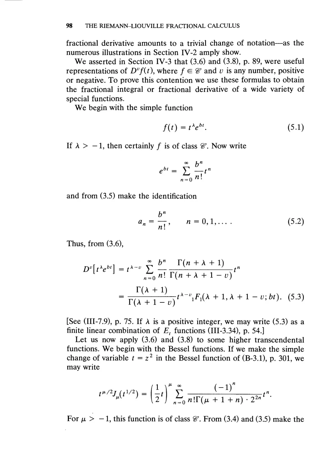
5. Some Further Examples, 97
6. The Law of Exponents, 104
7. Integral Representations, 111
8. Representations of Functions, 116
9. Integral Relations, 118
10. Laplace Transform of the Fractional Derivative, 121
V. Fractional Differential Equations 126
1. Introduction, 126
2. Motivation: Direct Approach, 128
3. Motivation: Laplace Transform, 133
4. Motivation: Linearly Independent Solutions, 136
5. Solution of the Homogeneous Equation, 139
6. Explicit Representation of Solution, 145
7. Relation to the Green's Function, 153
8. Solution of the Nonhomogeneous Fractional
Differential Equation, 157
9. Convolution of Fractional Green's Functions, 165
10. Reduction of Fractional Differential Equations
to Ordinary Differential Equations, 171
11. Semidifferential Equations, 174

CONTENTS ix
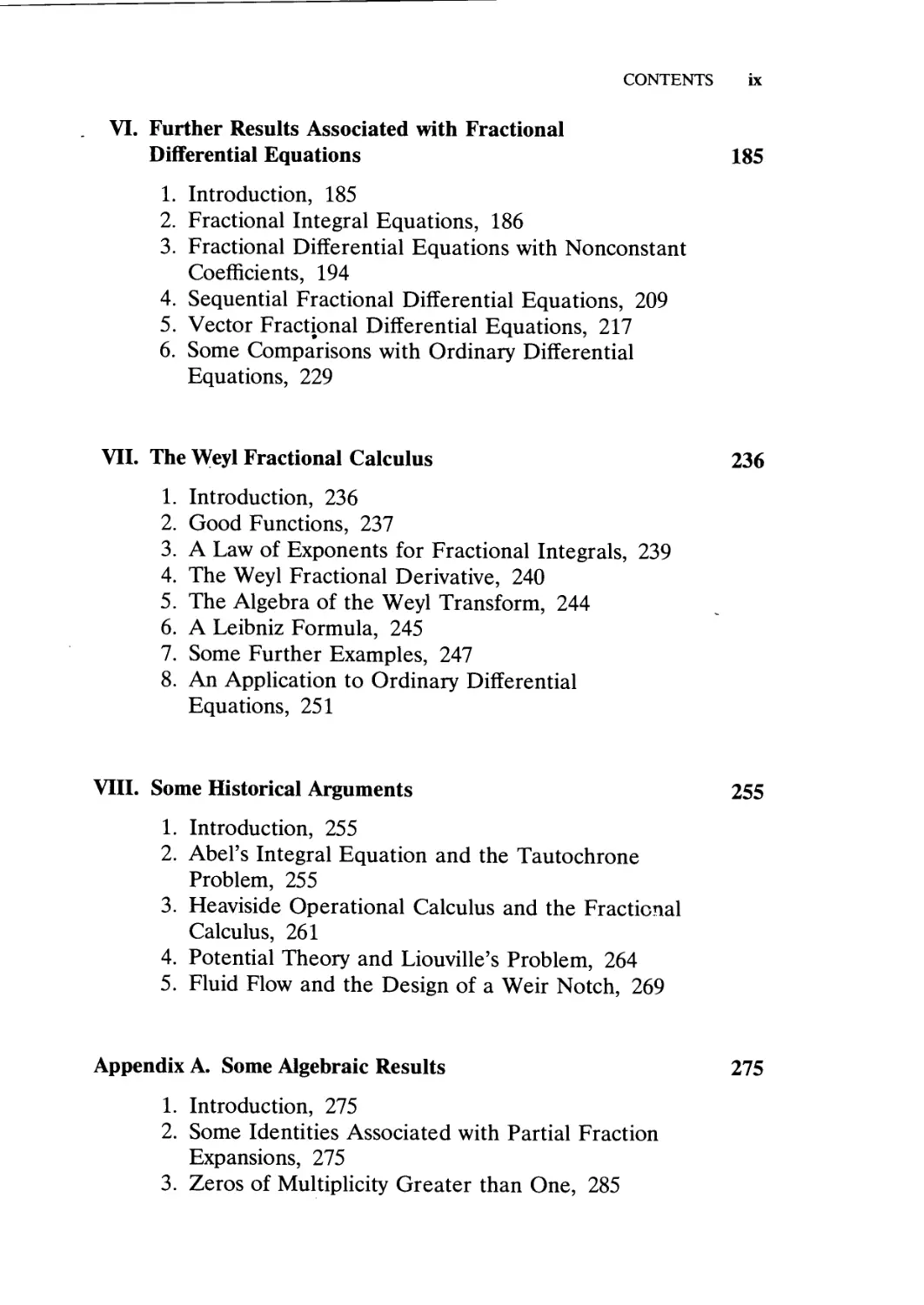
VI. Further Results Associated with Fractional
Differential Equations 185
1. Introduction, 185
2. Fractional Integral Equations, 186
3. Fractional Differential Equations with Nonconstant
Coefficients, 194
4. Sequential Fractional Differential Equations, 209
5. Vector Fractional Differential Equations, 217
6. Some Comparisons with Ordinary Differential
Equations, 229
VII. The Weyl Fractional Calculus 236
1. Introduction, 236
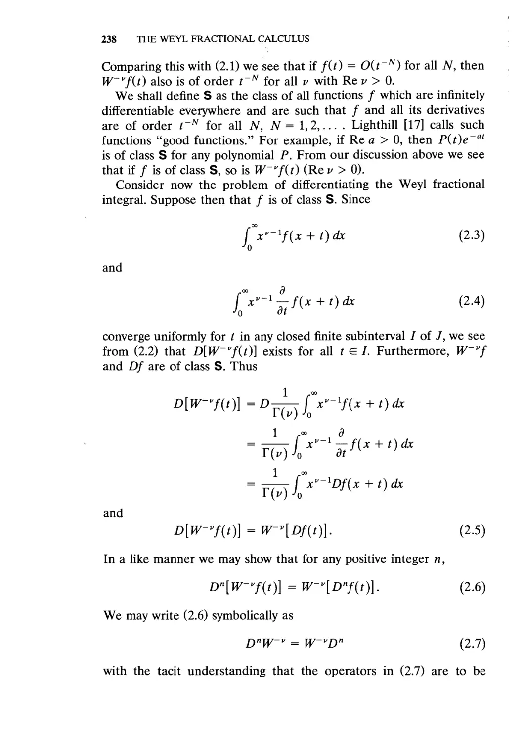
2. Good Functions, 237
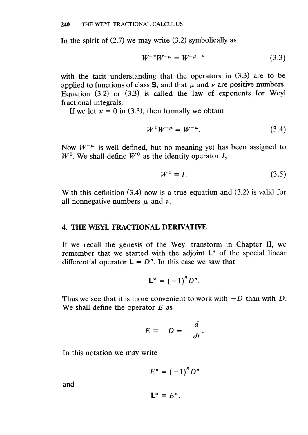
3. A Law of Exponents for Fractional Integrals, 239
4. The Weyl Fractional Derivative, 240
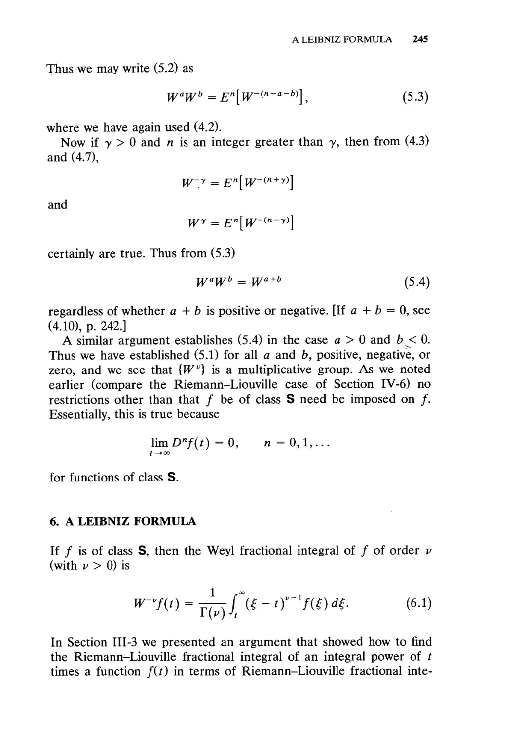
5. The Algebra of the Weyl Transform, 244
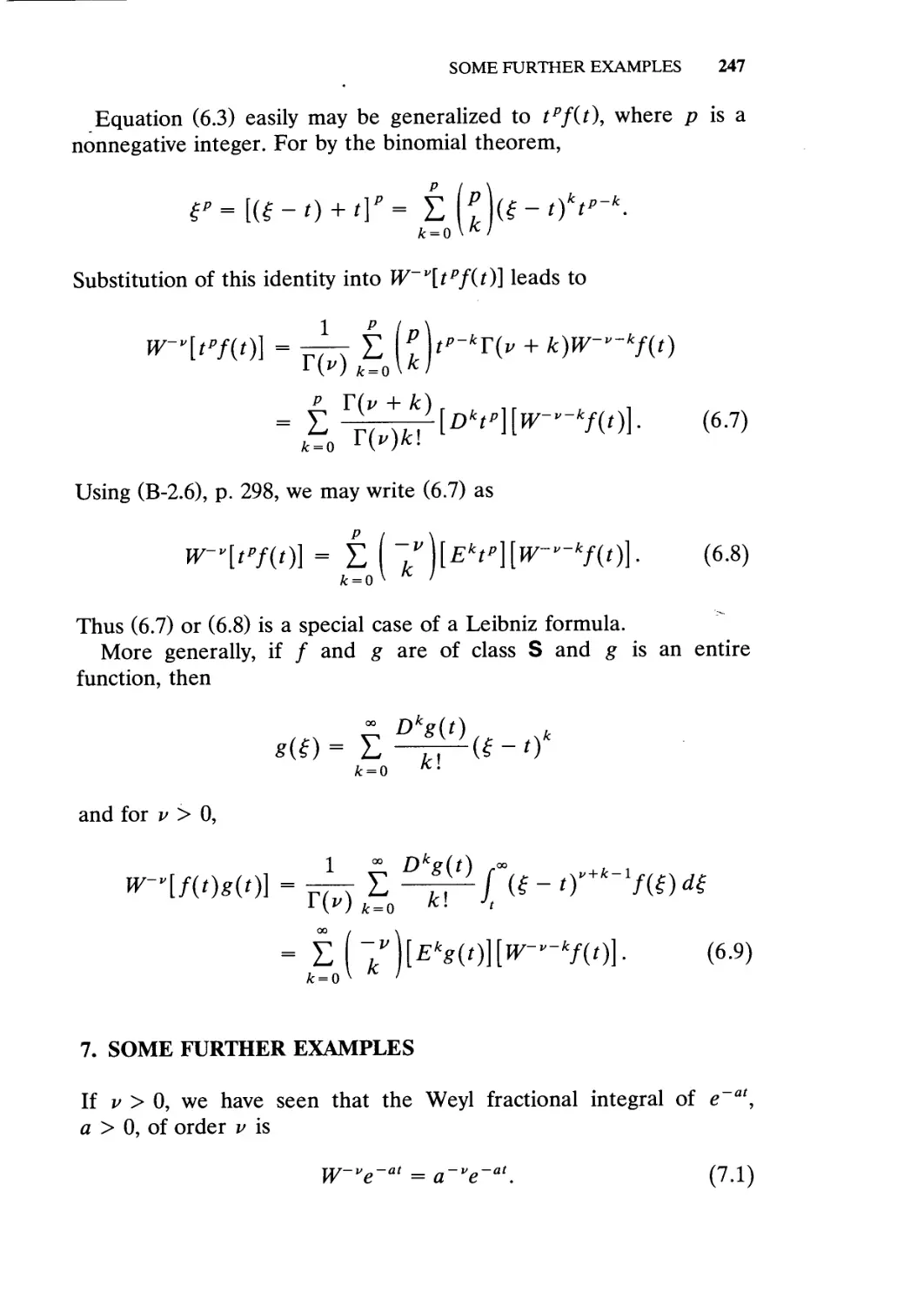
6. A Leibniz Formula, 245
7. Some Further Examples, 247
8. An Application to Ordinary Differential
Equations, 251
VIII. Some Historical Arguments 255
1. Introduction, 255
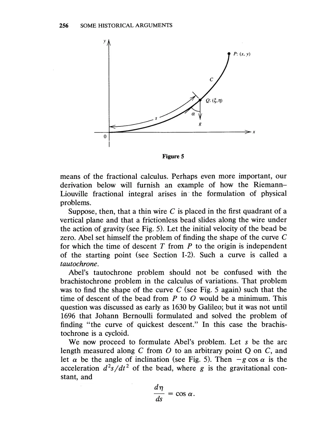
2. Abel's Integral Equation and the Tautochrone
Problem, 255
3. Heaviside Operational Calculus and the Fractional
Calculus, 261
4. Potential Theory and Liouville's Problem, 264
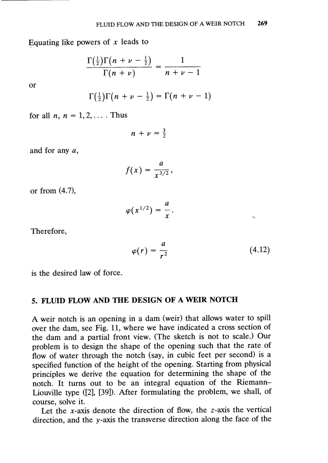
5. Fluid Flow and the Design of a Weir Notch, 269
Appendix A. Some Algebraic Results 275
1. Introduction, 275
2. Some Identities Associated with Partial Fraction
Expansions, 275
3. Zeros of Multiplicity Greater than One, 285

x CONTENTS
4. Complementary Polynomials, 290
5. Some Reduction Formulas, 292
6. Some Algebraic Identities, 294
Appendix B. Higher Transcendental
-#¦ Functions 297
1. Introduction, 297
2. The Gamma Function and Related Functions, 297
3. Bessel Functions, 301
4. Hypergeometric Functions, 303
5. Legendre and Laguerre Functions, 307
Appendix C. The Incomplete Gamma Function and
Related Functions 308
1. Introduction, 308
2. The Incomplete Gamma Function, 309
3. Some Functions Related to the Incomplete Gamma
Function, 314
4. Laplace Transforms, 321
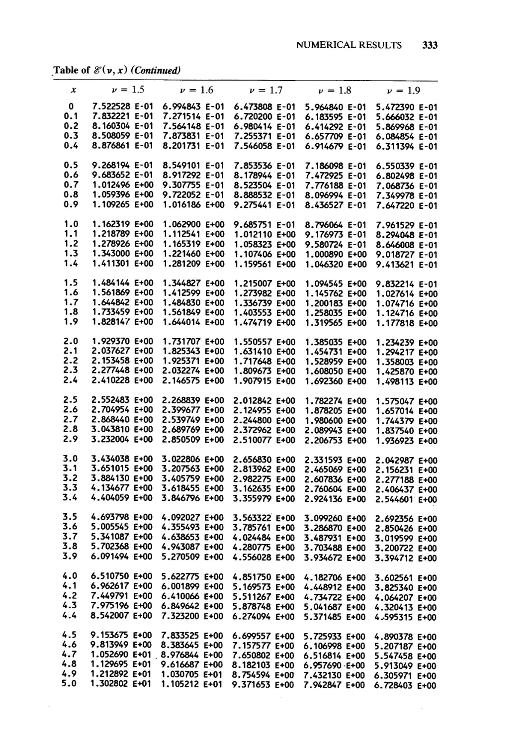
5. Numerical Results, 330
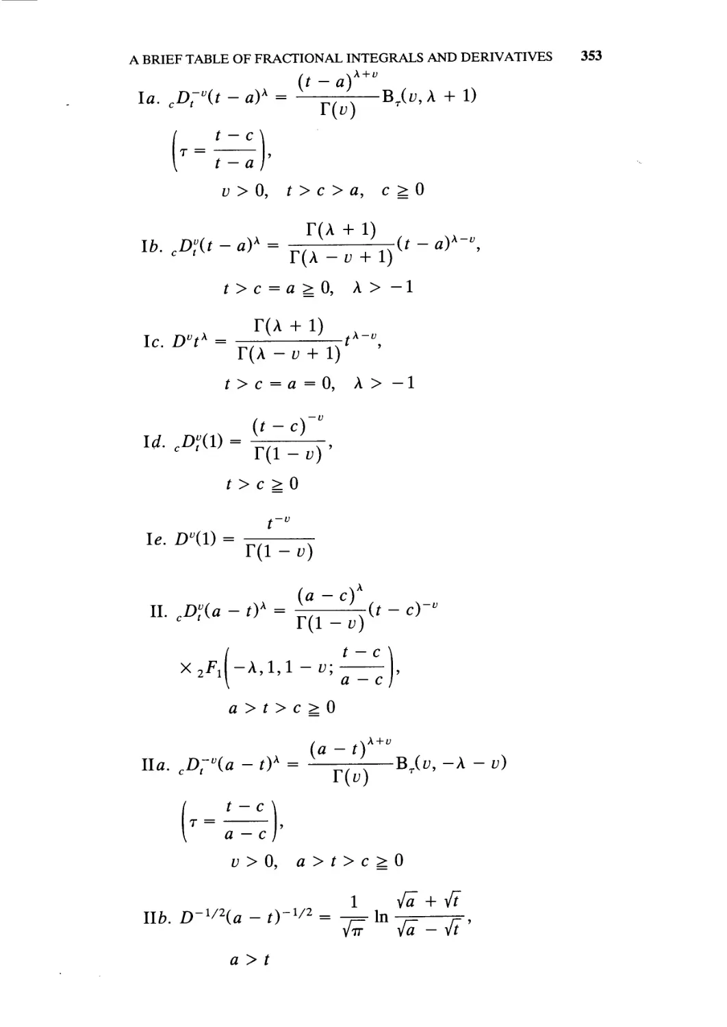
Appendix D. A Brief Table of Fractional Integrals
and Derivatives 352
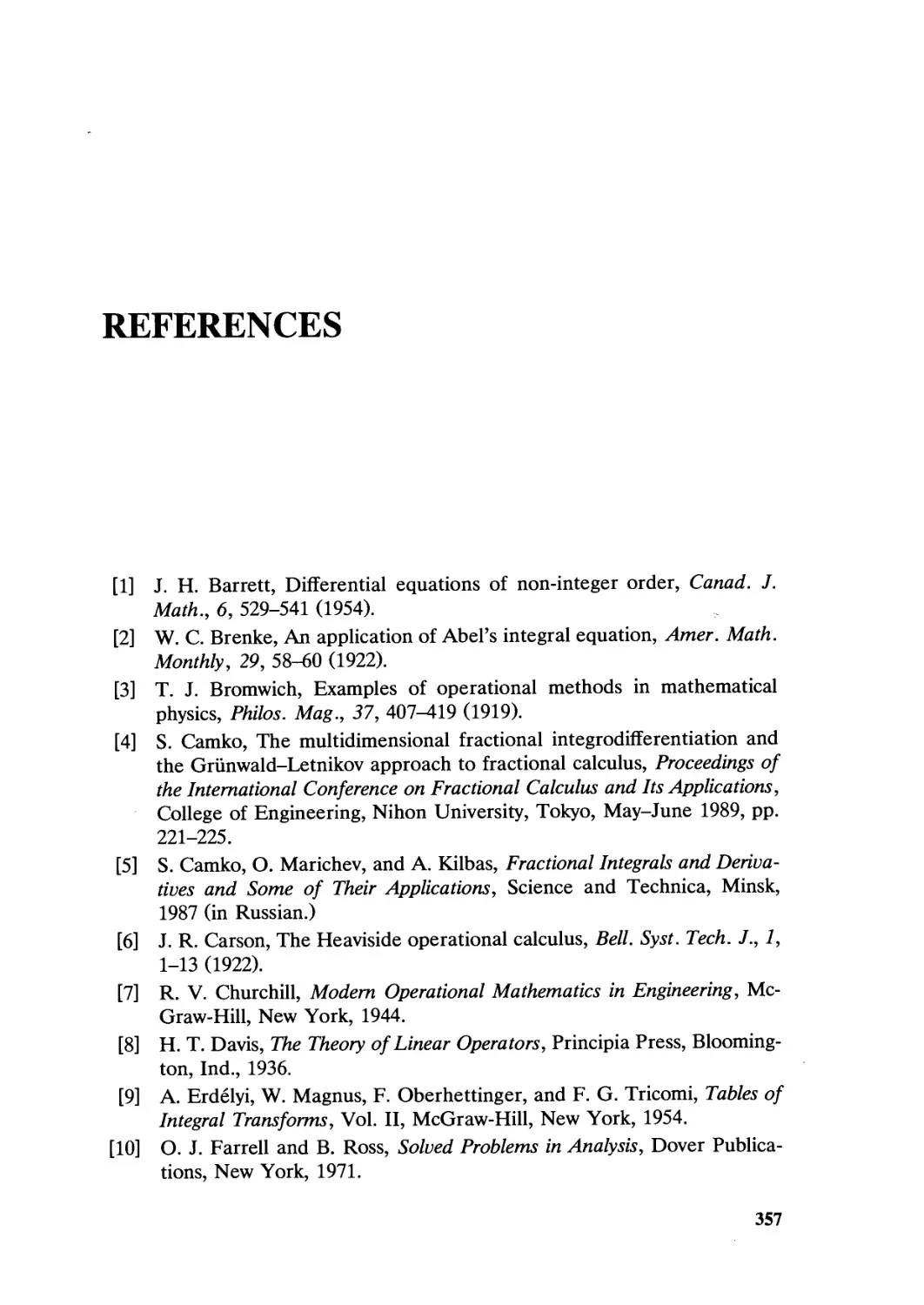
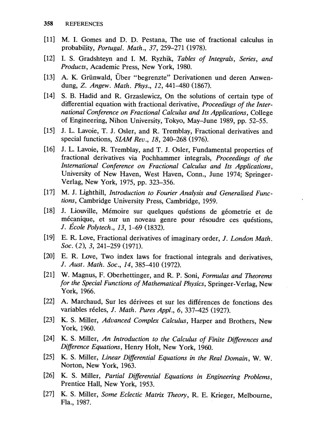
References 357
Index of Symbols 361
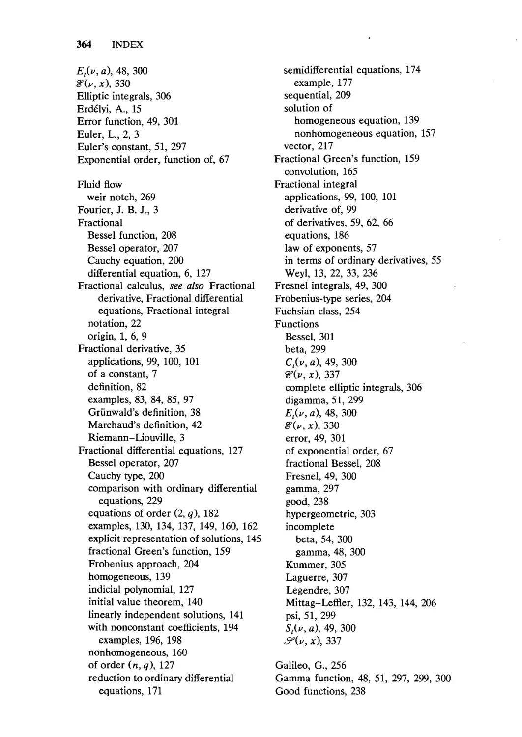
Index 363

PREFACE
The concept of the differentiation operator D = d/dx is familiar to
all who have studied the elementary calculus. And for suitable func-
functions /, the nth. derivative of /, namely Dnf(x) = dnf(x)/dxn is well
defined—provided that n is a positive integer. In 1695 L'Hopital
inquired of Leibniz what meaning could be ascribed to Dnf if n were
a fraction. Since that time the fractional calculus has drawn the
attention of many famous mathematicians, such as Euler, Laplace,
Fourier, Abel, Liouville, Riemann, and Laurent. But it was not until
1884 that the theory of generalized operators achieved a level in its
development suitable as a point of departure for the modern mathe-
mathematician. By then the theory had been extended to include operators
Dv, where v could be rational or irrational, positive or negative, real
or complex. Thus the name fractional calculus became somewhat of a
misnomer. A better description might be differentiation and integration
to an arbitrary order. However, we shall adhere to tradition and refer
to this theory as the fractional calculus.
In Chapter I we briefly trace the historical development of the
fractional calculus from Euler to the present, and in Chapter II we
describe numerous heuristic and mathematical arguments that lead to
the present definitions of fractional integrals and fractional deriva-
derivatives.
The mathematical theory of the fractional calculus is developed in
Chapters III and IV. We pay particular attention to what is now
XI

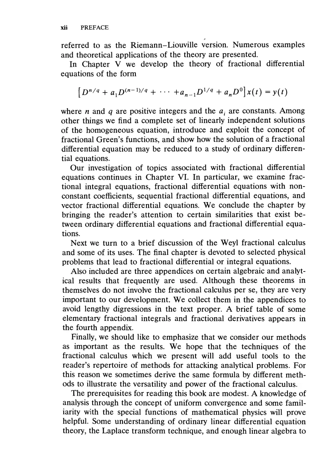
xii PREFACE
referred to as the Riemann-Liouville version. Numerous examples
and theoretical applications of the theory are presented.
In Chapter V we develop the theory of fractional differential
equations of the form
[Dn/q + axD^n~l)/q + • • • +an_1D1/q + anD°]x(t) = y(t)
where n and q are positive integers and the at are constants. Among
other things we find a complete set of linearly independent solutions
of the homogeneous equation, introduce and exploit the concept of
fractional Green's functions, and show how the solution of a fractional
differential equation may be reduced to a study of ordinary differen-
differential equations.
Our investigation of topics associated with fractional differential
equations continues in Chapter VI. In particular, we examine frac-
fractional integral equations, fractional differential equations with non-
constant coefficients, sequential fractional differential equations, and
vector fractional differential equations. We conclude the chapter by
bringing the reader's attention to certain similarities that exist be-
between ordinary differential equations and fractional differential equa-
equations.
Next we turn to a brief discussion of the Weyl fractional calculus
and some of its uses. The final chapter is devoted to selected physical
problems that lead to fractional differential or integral equations.
Also included are three appendices on certain algebraic and analyt-
analytical results that frequently are used. Although these theorems in
themselves do not involve the fractional calculus per se, they are very
important to our development. We collect them in the appendices to
avoid lengthy digressions in the text proper. A brief table of some
elementary fractional integrals and fractional derivatives appears in
the fourth appendix.
Finally, we should like to emphasize that we consider our methods
as important as the results. We hope that the techniques of the
fractional calculus which we present will add useful tools to the
reader's repertoire of methods for attacking analytical problems. For
this reason we sometimes derive the same formula by different meth-
methods to illustrate the versatility and power of the fractional calculus.
The prerequisites for reading this book are modest. A knowledge of
analysis through the concept of uniform convergence and some famil-
familiarity with the special functions of mathematical physics will prove
helpful. Some understanding of ordinary linear differential equation
theory, the Laplace transform technique, and enough linear algebra to

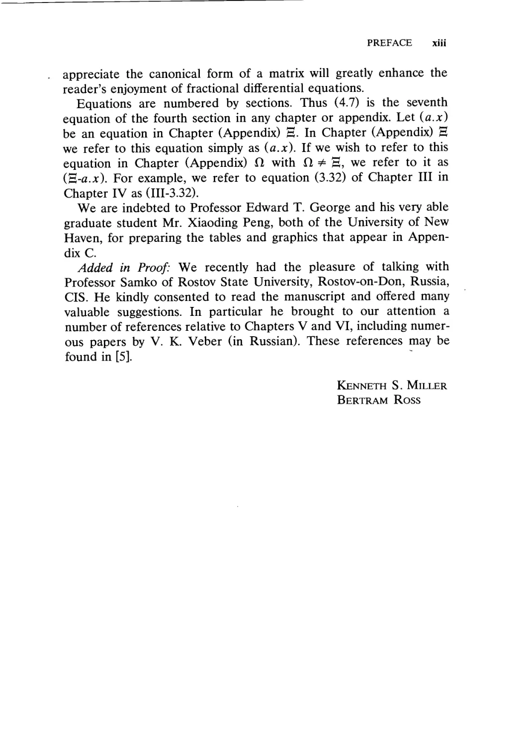
PREFACE xiii
appreciate the canonical form of a matrix will greatly enhance the
reader's enjoyment of fractional differential equations.
Equations are numbered by sections. Thus D.7) is the seventh
equation of the fourth section in any chapter or appendix. Let (a.x)
be an equation in Chapter (Appendix) H. In Chapter (Appendix) H
we refer to this equation simply as (a.x). If we wish to refer to this
equation in Chapter (Appendix) Cl with fl =? E, we refer to it as
(E-a.x). For example, we refer to equation C.32) of Chapter III in
Chapter IV as (III-3.32).
We are indebted to Professor Edward T. George and his very able
graduate student Mr. Xiaoding Peng, both of the University of New
Haven, for preparing the tables and graphics that appear in Appen-
Appendix C.
Added in Proof: We recently had the pleasure of talking with
Professor Samko of Rostov State University, Rostov-on-Don, Russia,
CIS. He kindly consented to read the manuscript and offered many
valuable suggestions. In particular he brought to our attention a
number of references relative to Chapters V and VI, including numer-
numerous papers by V. K. Veber (in Russian). These references may be
found in [5].
Kenneth S. Miller
Bertram Ross

I
HISTORICAL SURVEY
1. THE ORIGIN OF THE FRACTIONAL CALCULUS
The original question that led to the name fractional calculus was:
Can the meaning of a derivative of integer order dny/dxn be ex-
extended to have meaning when n is a fraction? Later the question
became: Can n be any number: fractional, irrational, or complex?
Because the latter question was answered affirmatively, the name
fractional calculus has become a misnomer and might better be called
integration and differentiation to an arbitrary order.
Leibniz invented the notation dny/dxn. Perhaps it was a naive play
with symbols that prompted L'Hopital in 1695 to ask Leibniz: "What
if n be |?" Leibniz [1695a] replied: "You can see by that, sir, that one
can express by an infinite series a quantity such as d1/2xy or d1:2xy.
Although infinite series and geometry are distant relations, infinite
series admits only the use of exponents that are positive and negative
integers, and does not, as yet, know the use of fractional exponents."
Later, in the same letter, Leibniz continues prophetically: "Thus it
follows that d1/2x will be equal to xyldx : x. This is an apparent
paradox from which, one day, useful consequences will be drawn."
In his correspondence with Johann Bernoulli, Leibniz [1695b] men-
mentions derivatives of "general order." In Leibniz's correspondence with
John Wallis, in which Wallis's infinite product for \rr is discussed,
Leibniz [1697] states that differential calculus might have been used to

2 HISTORICAL SURVEY
achieve this result. He uses the notation d1/2y to denote the deriva-
derivative of order \.
The subject of fractional calculus did not escape Euler's attention.
In 1730 he wrote: "When n is a positive integer, and if p should be a
function of x, the ratio dnp to dxn can always be expressed alge-
algebraically, so that if n = 2 and p = x3, then d2x3 to dx2 is 6jc to 1.
Now it is asked what kind of ratio can then be made if n be a fraction.
The difficulty in this case can easily be understood. For if n is a
positive integer dn can be found by continued differentiation. Such a
way, however, is not evident if n is a fraction. But yet with the help of
interpolation which I have already explained in this dissertation, one
may be able to expedite the matter" [Euler, 1738].
J. L. Lagrange [1849] contributed to fractional calculus indirectly.
In 1772 he developed the law of exponents (indices) for differential
operators of integer order and wrote:
m jn jm+n
dn
n J
dxm dxn dxm+n
In modern notation the dot is omitted, for it is not a multiplication.
Later, when the theory of fractional calculus developed, mathemati-
mathematicians were interested in knowing what restrictions had to be imposed
on y(x) so that an analogous rule held true for m and n arbitrary.
In 1812, P. S. Laplace [1820, vol. 3, pp. 85 and 186] denned a
fractional derivative by means of an integral, and in 1819 the first
mention of a derivative of arbitrary order appears in a text. S. F.
Lacroix [1819, pp. 409-410] devoted less than two pages of his 700-page
text to this topic. He developed a mere mathematical exercise general-
generalizing from a case of integer order. Starting with y = xm, m a positive
integer, Lacroix easily develops the nth derivative
dny m\
— = rrxm~n, m>n. A.1)
dxn (m - n)\ ~ v ;
Using Legendre's symbol for the generalized factorial (the gamma
function), he gets
dny Tim + 1)
= —xm'n A 2)
dxn T(m-n + l) " K }

THE CONTRIBUTIONS OF ABEL AND LIOUVILLE
He then gives the example for y = x and n = \, and obtains
d1/2y 2)/x~
A.3)
It is interesting to note that the result obtained by Lacroix, in the
manner typical of the classical formalists of this period, is the same as
that yielded by the present-day Riemann-Liouville definition of a
fractional derivative. Lacroix's method offered no clue as to a possible
application for a derivative of arbitrary order.
Joseph B. J. Fourier [1822] was the next to mention derivatives of
arbitrary order. His definition of fractional operations was obtained
from his integral representation of fix):
1 -oo oo
f(x) = -— f(a)da cos p(x -a) dp.
ZTT •'-oo •'-oo
Now
dn
-— cos p(x -a) = pn cos[p(x - a) + \mr\
for n an integer. Formally replacing n with u (u arbitrary), he obtains
the generalization
Fourier states: "The number u that appears in the above will be
regarded as any quantity whatsoever, positive or negative."
2. THE CONTRIBUTIONS OF ABEL AND LIOUVILLE
Leibniz, Euler, Laplace, Lacroix, and Fourier made mention of
derivatives of arbitrary order, but the first use of fractional operations
was made by Niels Henrik Abel in 1823 [Abel, 1881]. Abel applied the
fractional calculus in the solution of an integral equation that arises in
the formulation of the tautochrone problem (i.e., the problem of
determining the shape of the curve such that the time of descent of a
frictionless point mass sliding down the curve under the action of
gravity is independent of the starting point). The formulation of

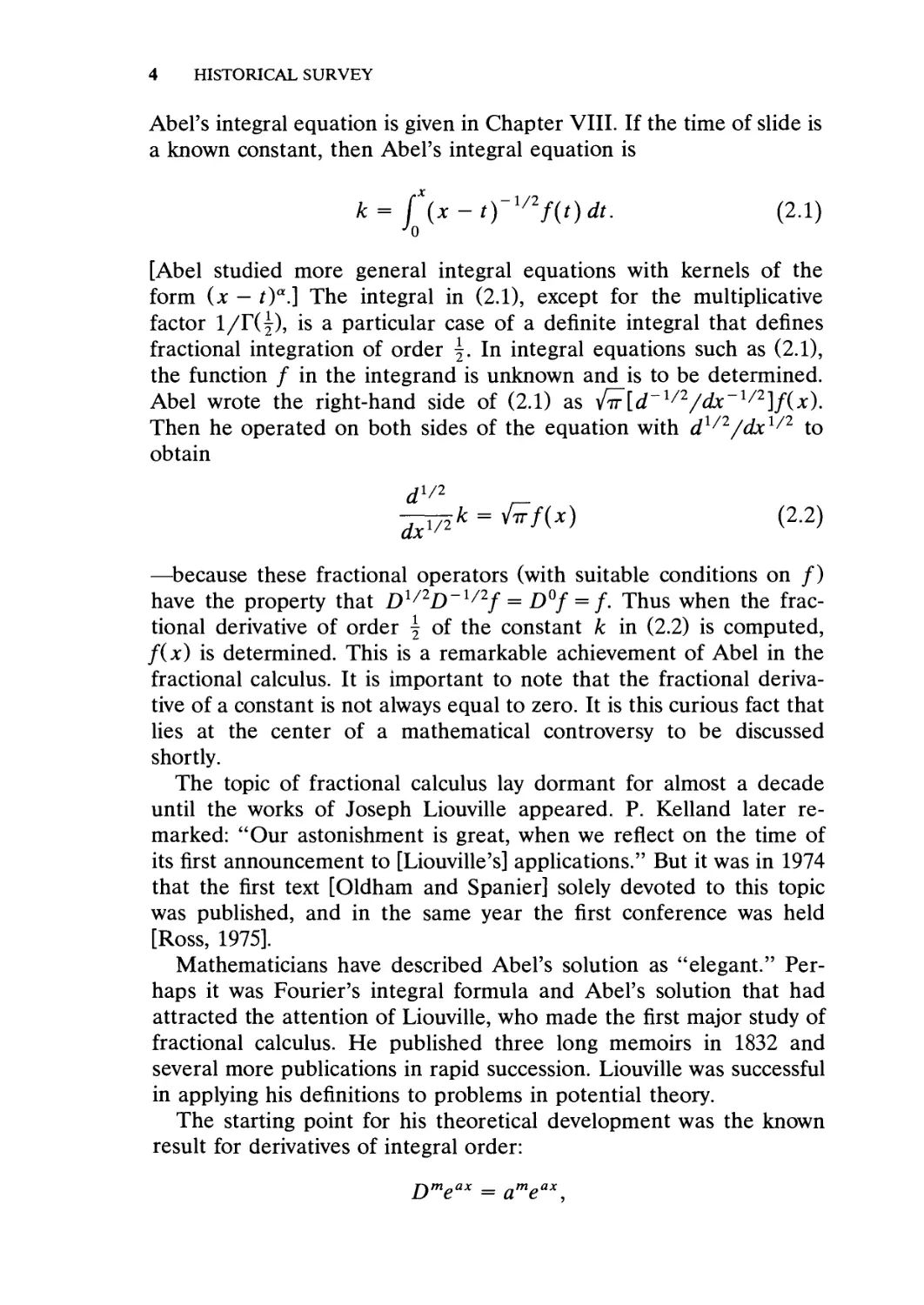
HISTORICAL SURVEY
Abel's integral equation is given in Chapter VIII. If the time of slide is
a known constant, then Abel's integral equation is
k = f(x-ty1/2f(t)dt. B.1)
•'o
[Abel studied more general integral equations with kernels of the
form (x - t)a.] The integral in B.1), except for the multiplicative
factor 1/F(|), is a particular case of a definite integral that defines
fractional integration of order \. In integral equations such as B.1),
the function / in the integrand is unknown and is to be determined.
Abel wrote the right-hand side of B.1) as yfrr\d-x/2/dx~x/2\j{x).
Then he operated on both sides of the equation with d1/2/dx1/2 to
obtain
B.2)
—because these fractional operators (with suitable conditions on /)
have the property that D1/2D~1/2f = D°f = f. Thus when the frac-
fractional derivative of order \ of the constant k in B.2) is computed,
f(x) is determined. This is a remarkable achievement of Abel in the
fractional calculus. It is important to note that the fractional deriva-
derivative of a constant is not always equal to zero. It is this curious fact that
lies at the center of a mathematical controversy to be discussed
shortly.
The topic of fractional calculus lay dormant for almost a decade
until the works of Joseph Liouville appeared. P. Kelland later re-
remarked: "Our astonishment is great, when we reflect on the time of
its first announcement to [Liouville's] applications." But it was in 1974
that the first text [Oldham and Spanier] solely devoted to this topic
was published, and in the same year the first conference was held
[Ross, 1975].
Mathematicians have described Abel's solution as "elegant." Per-
Perhaps it was Fourier's integral formula and Abel's solution that had
attracted the attention of Liouville, who made the first major study of
fractional calculus. He published three long memoirs in 1832 and
several more publications in rapid succession. Liouville was successful
in applying his definitions to problems in potential theory.
The starting point for his theoretical development was the known
result for derivatives of integral order:

THE CONTRIBUTIONS OF ABEL AND LIOUVILLE 5
which he extended in a natural way to derivatives of arbitrary order
Dveax = aveax. B.3)
He assumed that the arbitrary derivative of a function fix) that may
be expanded in a series of the form
/(*)= Evv, Refl|I>0 B.4)
is
cnaya"x. B.5)
n = 0
Formula B.5) is known as Liouville's first formula for a fractional
derivative. It generalizes in a natural way a derivative of arbitrary
order v, where v is any number: rational, irrational, or complex. But it
has the obvious disadvantage of being applicable only to functions of
the form B.4). Perhaps Liouville was aware of these restrictions, for
he formulated a second definition.
To obtain his second definition he started with a definite integral
related to the gamma function:
I = f ua-xe~xudu, a > 0, x> 0.
•'o
The change of variable xu = t yields
= x~a Cta-Xe-1dt
or
Then Liouville operates with Dv on both sides of the equation above,
to obtain, according to Liouville's basic assumption [see B.3)],
Dvx~a =
(-1)"
T(a)
-4-/" ua+v-xe~xu du. B.6)
a) Jo

6 HISTORICAL SURVEY
Thus Liouville obtains his second definition of a fractional derivative:
Dvx~a = '—±r -x~a-\ a > 0. B.7)
I»
But Liouville's definitions were too narrow to last. The first definition
is restricted to functions of the class B.4), and the second definition is
useful only for functions of the type x~a (with a > 0). Neither is
suitable to be applied to a wide class of functions.
Liouville was the first to attempt to solve differential equations
involving fractional operators. A complementary function, familiar to
those who have studied differential equations, was the object of some
of his investigations. In one of his many memoirs [1834], to justify the
existence of a complementary function, he wrote: "The ordinary
differential equation dny/dxn = 0 has the complementary solution
yc = co + cxx + c2x2 + ¦ ¦ ¦ +cn_1xn~1. Thus duy/dxu = 0 (u arbi-
arbitrary) should have a corresponding complementary solution."
Liouville did publish his version of the complementary solution.
Further mention of it is made later, for it played a role in planting the
seeds of distrust in the general theory of fractional operators. George
Peacock [1833] and S. S. Greatheed [1839] published papers which, in
part, dealt with the complementary function. Greatheed was the first
to call attention to the indeterminate nature of the complementary
function.
3. A LONGSTANDING CONTROVERSY
Essentially different definitions of fractional operations have been
given which have different domains of usefulness. One definition was
the generalization of a case of integral order used by Lacroix and Abel
for functions of the type xa for a > 0 [see A.2) and A.3)]. The other
was Liouville's definition, useful for functions of the type x~a for
a > 0 [see B.7)]. Peacock supported Lacroix's version and spoke of
Liouville's definition as being erroneous in many points. P. Kelland,
who published two works on this topic in 1839 and 1846, supported
Liouville's definition useful for functions of the type x~a (a > 0).
William Center [1848] observed that the fractional derivative of a
constant, according to the Lacroix-Peacock method, is unequal to
zero. Using x° to denote unity, Center finds the fractional derivative

RIEMANN'S CONTRIBUTION, ERRORS BY NOTED MATHEMATICIANS 7
of unity of order \, by letting m = 0 and n = \ in A.2) (even though
Lacroix assumed that m ^ n) to obtain
d1/2 r(i) 1
r0 _ V ' -1/2 _
But as Center points out, according to Liouville's "system" [referring
to Liouville's second definition given in formula B.7)], by letting a = 0
(even though Liouville assumed that a > 0), the fractional derivative
of unity equals zero because F@) = <». He continues: "The whole
question is plainly reduced to what is dux°/dxu. For when this is
determined we shall determine at the same time which is the correct
system."
Augustus De Morgan [1840] devoted three pages to fractional
calculus: "Both these systems may very possibly be parts of a more
general system, but at present I incline (in deference to supporters of
both systems) to the conclusion that neither system has any claim to
be considered as giving the form Dnxm, though either may be a
form."
The state of affairs complained about by De Morgan and Center is
now thoroughly cleared up. De Morgan's judgment proved to be
correct, for the two systems that Center thought led to irreconcilable
results have now been incorporated into a more general system. It is
only fair to state that mathematicians at that time were aiming for a
plausible definition of generalized integration and differentiation.
4. RIEMANN'S CONTRIBUTION, ERRORS
BY NOTED MATHEMATICIANS
G. F. Bernhard Riemann developed his theory of fractional integra-
integration in his student days, but he withheld publication. It was published
posthumously in his Gesammelte Werke [1892]. He sought a general-
generalization of a Taylor series and derived
dt + ?(*). D.1)
Because of the ambiguity in the lower limit of integration c, Riemann
saw fit to add to his definition a complementary function ^(x). This

HISTORICAL SURVEY
complementary function is essentially an attempt to provide a mea-
measure of the deviation from the law of exponents. For example, this law,
as mentioned later, is
[where the subscripts c and x on D refer to the limits of integration
in D.1)] and is valid when the lower terminals c are equal. Riemann
was concerned with a measure of deviation for the case cD~^c,D~vf{x)
when c =? d.
A. Cayley [1880] remarked: "The greatest difficulty in Riemann's
theory, it appears to me, is the question of the meaning of a comple-
complementary function containing an infinity of arbitrary constants." Any
satisfactory definition of a fractional operation will demand that this
difficulty be removed. Indeed, the present-day definition of fractional
integration is D.1) without the complementary function.
The question of the existence of a complementary function caused
considerable confusion. Liouville made an error when he gave an
explicit evaluation of his own interpretation of a complementary
function. He did not consider the special case for x = 0, which led to
a contradiction [Davis, 1936, p. 71]. Peacock made two errors in the
topic of fractional calculus. These errors involved the misapplication
of what he called the principle of the permanence of equivalent forms.
Although this principle is stated for algebra, Peacock assumed this
principle valid for all symbolic operations. He considered the exis-
existence of a complementary function and developed an expansion for
D~mx, m a positive integer. He erred when he naively concluded that
he could formally replace m with a fraction. Peacock made another
error of the same kind when he developed the expansion for the
derivative of integer order Dm(ax + b)n and then sought to extend his
result to the general case [Davis, 1936, p. 71].
In addition to the errors of Liouville and Peacock, there was a long
dispute as to whether the Lacroix-Peacock version or the Liouville
version of a fractional derivative was the correct definition. Later,
Cayley noted, as already mentioned, that Riemann was hopelessly
entangled in his version of a complementary function. Thus we sug-
suggest that when Oliver Heaviside published his work in the last decade
of the nineteenth century, he was met with disdain and haughty
silence not only because he exacerbated the situation with his hilari-
hilarious jibes at mathematicians, but also because mathematicians had a
general distrust of the theory of fractional operators.

THE ORIGIN OF THE RIEMANN-LIOUVILLE DEFINITION 9
5. THE MID-NINETEENTH CENTURY
Liouville [1832a] and later C. J. Hargreave [1848] wrote on the
generalization of Leibniz's nth derivative of a product when n is not a
positive integer. In modern form
D*f{x)g{x) = E (*)D»f(x)D''-'g(x), E.1)
— n
where Dn is the ordinary differentiation operator of order n, Dv
a fractional operator, and [v\ the generalized binomial coefficient
T(v + l)/n\T(v — n + 1). The generalized Leibniz rule may be found
in many modern applications [Ross, 1975, p. 32]. H. R. Greer [1858]
wrote on finite differences of fractional order. Surprisingly, a recent
access to a fractional derivative is by means of finite differences
[Mikolas, 1974]. Mention should also be made of a paper by W.
Zachartchenxo [1861]. He improves on the work of Greer, and he
ends his paper with an amusing note, which no modern mathematician
would admit, concerning his research on a topic: "I know that Liouville,
Peacock and Kelland have written on this topic, but I have had no
opportunity to read their works." H. Holmgren [1868] wrote a long
monograph on the application of fractional calculus to the solution of
certain ordinary differential equations. In the introduction to this
work, he asserts that his predecessors Liouville and Spitzer had
obtained results that were too restrictive. Holmgren, taking Liouville's
work as his point of departure, states that his aim in this paper is to
find a complete solution not subject to the restrictions on the indepen-
independent variable that his predecessors had made. He proceeds along
formal lines. For example, the index law is used:
Dvy" = DvD2y = Dv+2y.
Although this rule is valid for v a positive integer, modern mathemati-
mathematicians would seek to justify this rule when v is arbitrary.
6. THE ORIGIN OF THE RIEMANN-LIOUVILLE DEFINITION
The earliest work that ultimately led to what is now called the
Riemann-Liouville definition appears to be the paper by N. Ya. Sonin
[1869] entitled "On differentiation with arbitrary index." His starting

10 HISTORICAL SURVEY
point was Cauchy's integral formula. A. V. Letnikov wrote four papers
on this topic from 1868 to 1872. His paper "An explanation of the
main concepts of the theory of differentiation of arbitrary index"
[1872] is an extension of Sonin's paper. The nth derivative of Cauchy's
integral formula is given by
Dnf(z) = -r—.( — H+1 d?. F.1)
There is no problem in generalizing n\ to arbitrary values since
v\ = T(v + 1). However, when n is not an integer, the integrand in
F.1) no longer contains a pole, but a branch point. An appropriate
contour would then require a branch cut which was not included in
the work of Sonin and Letnikov, although it was discussed.
It was not until H. Laurent [1884] published his paper that the
theory of generalized operators achieved a level in its development
suitable as a point of departure for the modern mathematician. The
theory of the fractional calculus is intimately connected with the
theory of operators. The operators D or d/dx and D2 or d2/dx2
denote a rule of transformation of a function into other functions
which are the first and second ordinary derivatives. The rule of
transformation is familiar to all those who have studied the calculus.
Laurent's starting point also was Cauchy's integral formula. His con-
contour was an open circuit on a Riemann surface, in contrast to the
closed circuit of Sonin and Letnikov. The method of contour integra-
integration produced the definition
CD-Vf(x) = Tjyjj'i* ~ 0"~7@ dt, Re v > 0 F.2)
for integration to an arbitrary order.
When x > c in F.2), we have Riemann's definition D.1) but with-
without a complementary function. The most used version occurs when
c = 0,
. F.3)
This form of the fractional integral often is referred to as the
Riemann-Liouville fractional integral. A sufficient condition that F.3)

THE ORIGIN OF THE RIEMANN-LIOUVILLE DEFINITION 11
converge is that
/(-) =O(x1~e), e>0. F.4)
Integrable functions with the property above are sometimes referred
to as functions of Riemann class. For example, constants are of
Riemann class, as is
xa, a > -1. F.5)
When c is negative infinity, F.2) becomes
Re* > 0. F.6)
A sufficient condition that F.6) converge is that
f(-x) = O(x-v'e), e > 0, x-^oo. F.7)
Integrable functions with the foregoing property are sometimes re-
referred to as functions of Liouville class. For example,
x'a, a > v > 0 F.8)
is of Liouville class. A constant is not. However, if a is between 0 and
-1, then depending on the value of v, the two classes may overlap.
If we let fit) = eat, Re a > 0, in F.6), then
D~veax = a~veax. F.9)
— oo X
If we assume that the law of exponents D[D~vfix)] = D1~vfix)
holds (see Theorem 4 of Chapter III, p. 65), then if 0 < v < 1, we
have /a = 1 — v > 0 and F.9) becomes
_J)»eax-=atkeaxi Re a > 0.
Thus we see that Liouville's first definition [see B.3) and B.5)] is
subsumed under F.6).

12 HISTORICAL SURVEY
However, if f(x) = x~a, a > v > 0 [see F.8) and F.6)], then
_v Via - v)
for x < 0, and if 0 < v < 1, then ft = 1 - v > 0 and
F.11)
This is the same as Liouville's second definition, B.7), except that he
assumed that x > 0. If x > 0, F.10) is true only for the narrow range
of parameters 0 < v < a < 1.
For /(x) = xa and ^ > 0, we have from F.3) that
and again assuming that D[D vf(x)]=D1 vf(x), we see that if
0 < v < 1,
It is worth noting that for fix) = x and v = \, eq. F.13) yields the
same result as given by Lacroix in A.3). We also may consider
Center's observation concerning the derivative of arbitrary order of a
constant. For if fix) = 1 and v = \, then F.13) yields
L F.14)
TTX
which is C.1). But Center was incorrect when he said that the
Liouville definition yields zero for the arbitrary derivative of a con-
constant. For he used B.7) [see also F.11)]. But 1 = x° = i-x)° is not in
the Liouville class. [Of course, as we observed earlier (see p. 7), even
though he incorrectly applied Lacroix's formula A.2) he obtained the
right answer because a constant is of Riemann class.]

THE LAST DECADE OF THE NINETEENTH CENTURY 13
In recent years it has become customary to use the Weyl fractional
integral
, F.15)
(based on a definition of Weyl [1917]) in place of F.6). If we start with
F.6) and make the change of variable t = — r, then
1
dt
Now let x = —?. Then the expression above becomes
and if we let /( — ?) = g(?), this formula (with the obvious changes in
notation) becomes the right-hand side of F.15).
P. A. Nekrassov [1888] and A. Krug [1890] also obtained the
fundamental definition F.2) from Cauchy's integral formula, their
methods differing in choice of a contour of integration. However,
these generalized operators of integration and their connection with
the Cauchy integral formula have succeeded for themselves, to this
day, in getting only passing references in standard works in the theory
of analytic functions.
7. THE LAST DECADE OF THE NINETEENTH CENTURY
Oliver Heaviside [1892] published a number of papers in which he
showed how certain linear differential equations may be solved by the
use of generalized operators. Heaviside was an untrained scientist, a
fact that may explain his lack of rigor. His methods, which have
proved useful to engineers in the theory of the transmission of
electrical currents in cables, have been collected under the name
Heaviside operational calculus. (See also [Hadamard, 1892].)
The Heaviside operational calculus is concerned with linear func-
functional operators. He denoted the differentiation operator by the letter

14 HISTORICAL SURVEY
p and treated it as if it were a constant in the solution of differential
equations. For example, the heat equation in one dimension is
d2u du
—j = a2 — G.1)
dx2 dt V ;
where a2 is a constant and u is the temperature. If we let
then G.1) becomes
D2u = a2p. G.2)
D. F. Gregory [1841], said to be the founder of what was then called
the calculus of operations, had put the solution of G.1) into symbolic
operator form:
u(x,t) =Aexapl/2 + Be~xapl/2.
This is exactly what you would get if you solved G.2) assuming p a
constant.
But it was Heaviside's brilliant applications that accelerated the
development of the theory of these generalized operators. He ob-
obtained correct results by expanding the exponential in powers of p1/2,
where p1/2 = d1/2/dx1/2 = D1/2. In the theory of electrical circuits,
Heaviside found frequent use for the operator p1/2. He interpreted
p1/2 -> 1, that is, ?>1/2A), to mean (ttO~1/2, as in F.14). Since
/@ = 1 is a function of Riemann class, it is clear that Heaviside's
operator must be interpreted in the context of the Riemann operator
ojD*. [In modern operational calculus, pF(p) is replaced by F(s),
where s is the Laplace transform variable. Therefore, p1/2 is replaced
by s~1/2, and the inverse Laplace transform of s~1/2 is (ttO~1/2,
which is D1/2(l).]
His results were correct, but he was unable to justify his proce-
procedures. Kelland, earlier, remarked on the ten-year interval between
Fourier's publication and Liouville's applications. A similar situation
followed Heaviside's publications, except that in this case, a much
longer time elapsed before his procedures were justified by T. J.
Bromwich [1919].

THE TWENTIETH CENTURY 15
Harold T. Davis [1936] said: "The period of the formal develop-
development of operational methods may be regarded as having ended by
1900. The theory of integral equations was just beginning to stir the
imagination of mathematicians and to reveal the possibilities of opera-
operational methods."
We discuss Heaviside's methods in more detail in Chapter VIII.
8. THE TWENTIETH CENTURY
In the period 1900-1970 a modest amount of published work ap-
appeared on the subject of the fractional calculus. Some of the contribu-
contributors were M. Al-Bassam, H. T. Davis, A. Erdelyi, G. H. Hardy, H.
Kober, J. E. Littlewood, E. R. Love, T. Osier, M. Riesz, S. Samko, I.
Sneddon, H. Weyl, and A. Zygmund.
The year 1974 saw the first international conference on fractional
calculus, held at the University of New Haven, Connecticut, and was
sponsored by the National Science Foundation. The proceedings of
the conference were published by Springer-Verlag [Ross, 1975]. Many
distinguished mathematicians attended. These luminaries included R.
Askey, M. Mikolas, and many of the distinguished mathematicians
mentioned above. The topics covered were quite eclectic, including
papers on the fractional calculus and generalized functions, inequali-
inequalities obtained by use of the fractional calculus, and applications of the
fractional calculus to probability theory.
It is quite possible that the conference stimulated a spate of
publications. In the period 1975 to the present, about 400 papers have
been published relating to the fractional calculus. {A chronological
bibliography with commentary covering the period 1695-1974 may be
found in the book by Oldham and Spanier [1974]. See also [Samko,
1987].}
In 1984 the second international conference on fractional calculus
was sponsored by the University of Strathclyde, Glasgow, Scotland
[McBride and Roach, 1985]. The contributors to the proceedings
included (among others) P. Heywood, S. Kalla, W. Lamb, J. S.
Lowndes, K. Nishimoto, P. G. Rooney, and H. M. Srivastava, as well
as some of the mathematicians who took part in the 1974 New Haven
conference. Some of the still-open questions are intriguing. For exam-
example: Is it possible to find a geometric interpretation for a fractional
derivative of noninteger order?
Considerable mathematical activity in the fractional calculus in the
1980's developed in Japan with publications by S. Owa [1990],

16 HISTORICAL SURVEY
M. Saigo [1980], and K. Nishimoto. The last-mentioned author pub-
published a four-volume work [1984, 1987, 1989, 1991] devoted primarily
to applications of the fractional calculus to ordinary and partial
differential equations. In the Soviet Union three mathematicians, S.
Samko, O. Marichev, and A. Kilbas, wrote an encyclopedic text on the
fractional calculus and some of its applications [1987]. It is now being
translated into English by the Gordon and Breach Publishing Com-
Company. In India, R. K. Raina and R. K. Saxena have produced many
papers; in Canada, H. M. Srivastava; in Venezuela, S. Kalla; and in
Scotland, A. McBride have all become well known for their contribu-
contributions to the fractional calculus.
The third international conference was held at Nihon University in
Tokyo in 1989 [Nishimoto, 1990]. Some of the many contributors were
M. Al-Bassam, R. Bagley, Y. A. Brychkov, L. M. B. C. Campos, R.
Gorenflo, J. M. C. Joshi, S. Kalla, E. R. Love, M. Mikolas, K.
Nishimoto, S. Owa, A. P. Prudnikov, B. Ross, S. Samko, H. M.
Srivastava.
The fractional calculus finds use in many fields of science and
engineering, including fluid flow, rheology, diffusive transport akin to
diffusion, electrical networks, electromagnetic theory, and probability.
Some papers by P. C. Phillips [1989, 1990] have used the fractional
calculus in statistics. R. L. Bagley [1990]; Bagley and Torvik [1986]
have found use for the fractional calculus in viscoelasticity and the
electrochemistry of corrosion.
It seems that hardly a field of science or engineering has remained
untouched by this topic. Yet even though the subject is old, it is rarely
included in today's curricula. Possibly, this is because many mathe-
mathematicians are unfamiliar with its uses.
BIBLIOGRAPHY
Abel, N. H., 1881. Solution de quelques problemes a l'aide d'integrales
definies, Oeuvres Completes, Vol. 1, Gr0ndahl, Christiania, Norway, pp.
16-18.
Bagley, R., 1990. On the fractional order initial value problem and its
engineering applications, Proceedings of the International Conference on
Fractional Calculus and Its Applications, College of Engineering, Nihon
University, Tokyo, May-June 1989, pp. 12-20.
Bagley, R., and Torvik, P. J., 1986. On the fractional calculus model of
visoelastic behavior, /. Rheol., 30, 133-155.

BIBLIOGRAPHY 17
Bromwich, T. J., 1919. Examples of operational methods in mathematical
' physics, Philos. Mag., 37, 407-419.
Campos, L. M. B. C, 1984. On a concept of derivative of complex order with
applications to special functions, IMA J. Appl. Math., 33, 109-133.
Cayley, A., 1990. Note on Riemann's paper, Math. Ann., 16, 81-82.
Center, W., 1848. On the value of (d/dx)ex° when 6 is a positive proper
fraction, Cambridge Dublin Math. J., 3, 163-169.
Davis, H. T., 1927. The application of fractional operators to functional
equations, Amer. J. Math., 49, 123-142.
, 1936. The Theory of Linear Operators, Principia Press, Bloomington,
Ind.
De Morgan, A., 1840. The Differential and Integral Calculus Combining
Differentiation, Integration, Development, Differential Equations, Differ-
Differences, Summation, Calculus of Variations ... with Applications to Algebra,
Plane and Solid Geometry, Baldwin and Craddock, London; published in
25 parts under the superintendence of the Society for the Diffusion of
Useful Knowledge, pp. 597-599.
Erdelyi, A., 1975. Fractional integrals of generalized functions, Proceedings
of the International Conference on Fractional Calculus and Its Applications,
University of New Haven, West Haven, Conn., June 1974; Springer-Verlag,
New York, pp. 151-170.
Euler, L., 1738. De progressionibus transcendentibus, sev quarum termini
generates algebraice dari nequent, Commentarii Academiae Scientiarum
Imperialis Scientiarum Petropolitanae, 5, p. 55.
Fourier, J. B. J., 1822. Theorie analytique de la chaleur, Oeuvres de Fourier,
Vol. 1, Firmin Didot, Paris, p. 508.
Gorenflo, R., and Vessella, S., 1991. Abel Integral Equations, Springer-Verlag,
New York.
Greatheed, S. S., 1839. On general differentiation, Cambridge Math. J., 1,
11-21, 109-117.
Greer, H. R., 1858. On fractional differentiation, Quart. J. Pure Appl. Math.,
3, 327-330.
Gregory, D. F., 1841. Examples of the Processes of the Differential and Integral
Calculus, Deighton, Cambridge, p. 350, 2nd ed., 1846, p. 354.
Hadamard, J., 1892. Essai sur l'etude des fonctions donnees par leur devel-
oppement de Taylor, Journal Math. Pures Appl., 8, 101-186.
Hargreave, C. J., 1848. On the solution of linear differential equations,
Philos. Trans. Roy. Soc. London, 148, 31-34.
Heaviside, O., 1892. Electrical Papers, Macmillan, London.
Holmgren, H., 1868. Sur l'integration de l'equation differentielle (a2 + b2x
+ c2x2)d2y/dx2 + (ax + bxx)dy/dx + aoy = 0, K. Svenska Ventensk.
Acad. Handl., 7,3-58.

18 HISTORICAL SURVEY
Kelland, P., 1839. On general differentiation, Trans. Roy. Soc. Edinburgh, 14,
567-618.
, 1846. On general differentiation, Trans. Roy. Soc. Edinburgh, 16,
241-303.
Krug, A., 1890. Theorie der Derivationen, Wien Denkenschr., Math. Natur-
wissensch. Classe, 57, 151-228.
Lacroix, S. F., 1819. Traite du calcul differentiel et du calcul integral, 2nd ed.,
Courtier, Paris, pp. 409-410.
Lagrange, J. L., 1849. Sur un nouvelle espece de calcul relatif a la differenti-
differentiation et a l'integration des quantities variables, Oeuvres de Lagrange, Vol.
3, Gauthier-Villars, Paris, pp. 441-476.
Laplace, P. S., 1820. Theorie analytique des probabilities, Courcier, Paris.
Laurent, H., 1884. Sur le calcul des derivees a indices quelconques, Nouv.
Ann. Math., 5C), 240-252.
Leibniz, G. W., 1695a. Letter from Hanover, Germany, to G. F. A. L'Hopital,
September 30, 1695, in Mathematische Schriften, 1849; reprinted 1962,
Olms Verlag, Hildesheim, Germany, 2, 301-302.
, 1695b. Letter from Hanover, Germany, to Johann Bernoulli, De-
December 28, 1695, in Mathematische Schriften; reprinted 1962, Olms Verlag,
Hildesheim, Germany, 3, 226.
, 1697. Letter from Hanover, Germany, to John Wallis, May 28,
1697, in Mathematische Schriften; reprinted 1962, Olms Verlag,
Hildesheim, Germany, 4, 25.
Letnikov, A. V., 1872. An explanation of the main concepts of the theory of
differentiation of arbitrary index, Moskow Mat. Sb., 6, 413-445.
Liouville, J., 1832a. Memoire sur le calcul des differentielles a indices
quelconques, /. Ecole Poly tech., 13, 71-162.
, 1832b. Memoire sur l'integration de l'equation (mx2 + nx +
p)d2y/dx2 + (qx + r)dy/dx + sy = 0 a l'aide des differentielles a in-
indices quelconques, /. Ecole Polytech., 13, 163-186.
., 1834. Memoire sur le theoreme des fonctions complementaires,
/. ReineAngew. Math. (Crelle's J.), 11, 1-19.
Love, E. R., 1972. Two index laws for fractional integrals and derivatives,
/. Aust. Math. Soc, 14, 385-410.
Lowndes, J. S., 1985. On two new operators of fractional integration, in
Fractional Calculus, University of Stratchclyde, Glasgow, August 1984
(Pitman Advanced Publishing Program), pp. 87-98.
McBride, A. C, 1985. A Mellin transform approach to fractional calculus on
@, oo), in Fractional Calculus, University of Stratchclyde, Glasgow, August
1984 (Pitman Advanced Publishing Program), pp. 99-139.

BIBLIOGRAPHY 19
McBride, A. C, and Roach, G. F., editors, 1985. Fractional Calculus, Univer-
University of Stratchclyde, Glasgow, August 1984 (Pitman Advanced Publishing
Program).
Mikolas, M., 1974. On the recent trends in the development, theory and
applications of fractional calculus, Proceedings of the International Confer-
Conference on Fractional Calculus and Its Applications, University of New Haven,
West Haven, Conn., June 1974; Springer-Verlag, New York, pp. 357-375.
Nekrassov, P. A., 1888. General differentiation, Moskow Mat. Sb., 14, 45-168.
Nishimoto, K., 1984-1991. Fractional Calculus, Vols. I-IV, Descartes Press,
Koriyama, Japan.
, editor, 1990. Proceedings of the International Conference on Frac-
Fractional Calculus and Its Applications, College of Engineering, Nihon Univer-
University, Tokyo, May-June 1989.
Oldham, K., and Spanier, J., 1974. The Fractional Calculus, Academic Press,
New York.
Osier, T. J., 1970. Leibniz rule for fractional derivatives generalized and an
application to infinite series, SIAM J. Appl. Math., 18, 658-674.
Owa, S., 1990. On certain generalization subclasses of analytic functions
involving fractional calculus, Proceedings of the International Conference on
Fractional Calculus and Its Applications, College of Engineering, Nihon
University, Tokyo, May-June 1989, pp. 179-184.
Peacock, G., 1833. Report on the recent progress and present state of affairs
of certain branches of analysis. In Report to the British Association for the
Advancement of Science, pp. 185-352.
Phillips, P. C, 1989. Fractional matrix calculus and the distribution of
multivariate tests, Cowles Foundation Paper 767, Dept of Economics, Yale
University, New Haven, Conn.
, 1990. Operational calculus and regression f-tests, Cowles Founda-
Foundation Paper 948, Dept. of Economics, Yale University, New Haven, Conn.
Riemann, B., 1892. Versuch einer allgemeinen Auffassung der Integration
und Differentiation, Gesammelte Werke, published posthumously, Teub-
ner, Leipzig, pp. 353-366.
Ross, B., editor, 1975. Proceedings of the International Conference on Frac-
Fractional Calculus and Its Applications, University of New Haven, West
Haven, Conn., June 1974; Springer-Verlag, New York.
Saigo, M., 1980. On the Holder continuity of the generalized fractional
integrals and derivatives, Math. Rep. (College of General Education,
Kyushi University), 11B), 55-62.
Samko, S., Marichev, O., and Kilbas, A., 1987. Fractional Integrals and
Derivatives and Some of Their Applications, Science and Technica, Minsk
(In Russian).

20 HISTORICAL SURVEY
Saxena, R. K., Gupta, O. P., and Kumblat, R. K., 1989. On two-dimensional
Weyl fractional calculus, C. R. Acad. Bulg. Sci., 42G), 11-14.
Sneddon, I. N., 1972. The Use of Integral Transforms, McGraw-Hill, New
York, pp. 271, 293, 384.
Sonin, N. Ya., 1869. On differentiation with arbitrary index, Moscow Mat.
Sb., 6, 1-38.
Srivastava, H. M., and Saigo, M., 1987. Multiplication of fractional calculus
operators and boundary value problems involving the Euler-Darboux
equation, /. Math. Anal. Appl., 121, 325-369.
Weyl, H., 1917. Bemerkungen zum Begriff des Differentialquotienten ge-
brochener Ordnung, Vierteljahresschr. Naturforsch. Ges. Zurich, 62,
296-302.
Zachartchenxo, W., 1861. On fractional differentiation, Quart. J. Pure Appl.
Math., 4, 237-243.

II
THE MODERN APPROACH
1. INTRODUCTION
The reader who has followed the sometimes tortuous birth pangs of
the fractional calculus described in Chapter I is aware that more than
one version of the fractional integral exists. For convenience we shall
call
the Riemann version and
(x - ty~lf{t)dt A.2)
the Liouville version. The case where c = 0 in A.1), namely,
0D-"f(x) = ~f(x - ty-'fit) dt A.3)
will be called the Riemann-Liouville fractional integral. Most of our
efforts in this book are centered on this version. We have also
21

22 THE MODERN APPROACH
introduced the Weyl fractional integral
This transform is studied more fully in Chapter VII. We have also
noted that the formula
??- zyn- 7@ di A.5)
in the complex domain (derived from the Cauchy integral formula)
bears a striking resemblance to our fractional integral definitions.
In A.1) to A.4) we assume that Re v > 0 and observe that the class
of functions to which / must belong is not necessarily the same in our
various versions. For example, if f(x) is a constant, then A.1) and
A.3) are meaningful, but A.2) and A.4) are not. (Recall our earlier
discussion in Section 1-6 of functions of Riemann class and functions
of Liouville class.)
Our main objective in this chapter is to present various arguments
which should convince the reader that the definitions of the fractional
integrals that we have introduced are feasible entities. Equation A.5)
also will be employed to arrive at this same conclusion.
So far we have mentioned only fractional integrals. Naturally, we
also shall define the fractional derivative of a function. More than one
such definition of the Riemann fractional derivative will be given. The
Weyl fractional derivative is defined in Chapter VII.
One trivial observation we may make even at this early stage is that
if D represents any of the operators in A.1) to A.4), then for
appropriate functions / and g, and any scalars a and /3,
D[af(t) + pg(t)} = aDf(t) + pDg(t).
That is, they are all linear operators. After we have defined the
fractional derivatives, it will be easy to see that they too are linear
operators.
However, before we embark on this program we should say a word
about notation. Various authors have used different notations. The
one we have adopted is due to H. T. Davis [8]. For example, as we
mentioned in Section 1-4,
cD-"f(x) = Wrf(x - t)v-lf(t)dt, Re* > 0 A.6)
(for x > c and suitable functions /) denotes integration to an arbi-
arbitrary order v along the real axis from c to x. Similarly, when we

THE ITERATED INTEGRAL APPROACH 23
define the fractional derivative, we shall use the notation cD^f(x),
Re v > 0, to denote differentiation to an arbitrary order v. Although
this notation is not free from ambiguity, it is sufficient for our
purposes.
The choice of a precise notation for the fractional calculus cannot
be minimized. For as we shall see, some of the power and elegance of
the fractional calculus rests in its simplified notation. The abridged
manner of representing these defining integrals may seem to be a
trivial matter; but the advantage of a simple notation has been the
source of many profound discoveries not obvious by other means.
2. THE ITERATED INTEGRAL APPROACH
The first argument that we shall give which leads to a definition of the
fractional integral begins with a consideration of the /t-fold integral
B.1)
The function / in B.1) will be assumed to be continuous on the
interval [c, b], where b > x. We assert that B.1) may be reduced to a
single integral of the form
f*Kn(x,t)f(t)dt, B.2)
where the kernel Kn(x, t) is a function of n, x, and t. It will be shown
that Kn(x, t) is a meaningful function even when n is not a positive
integer. Thus we shall define cD~vf{x) as
cDx-f(x) = j\v(x,t)f{t)dt B.3)
for all v with Re v > 0.
To prove this conjecture we start by recalling that if G(x, t) is
jointly continuous on [c, b] X [c, b], where b > x, then from the
elementary theory of functions we have
fdjc1f1G(xut)dt = fdtfG(xl,t)dxv B.4)

24 THE MODERN APPROACH
If, in particular,
G(Xl,t)=f(t),
that is, if G(xv t) is a function only of the variable t, then B.4) may
be written as
= ff{t)dtfdx,
Jc Jt
= f(x-t)f(t)dt.
c
B.5)
Thus we have reduced the two-fold iterated integral to a single
integral.
If n = 3, then B.1) becomes
:Dx-if(x) = fdx1f1dx2(X2f(t)dt
c c
= fdx1 (Xldjc2f2f(t)dt
Jc Y c Jc
If we apply the identity of B.5) to the pair of integrals in brackets,
there results
= fdx1\f\x1-t)f(t)dt
Another application of B.5) to the formula above leads to
- ty
dt.
Iterating this process n times reduces B.1) to B.2), where
n-\
Kn(x,t) =
(/i-l)! *

THE DIFFERENTIAL EQUATION APPROACH 25
Hence we may write cD~nf{x) as
f t. B.6)
Clearly, the right-hand side of expression B.6) is meaningful for any
number n whose real part is greater than zero. We shall call
V
the fractional integral of / of order v and denote it by the symbol
3. THE DIFFERENTIAL EQUATION APPROACH
We now show how the theory of linear differential equations may be
exploited to arrive at our fundamental definition
Drf(x) = ^-rf(x - ty~lf{t)dt, Re* > 0 C.1)
1 \V) J
of the fractional integral. Suppose, then, that
L = Dn + p^D"-1 + ¦¦¦ +pn(x)D° C.2)
is a linear differential operator whose coefficients pt{x) are continu-
continuous on some interval /. Then if f(x) is continuous on /, and if c is
any point in /, we may consider the linear differential system
Ly(x)=f(x)
Dky(c) = 0, Q^k^n-l. C.3)
The unique solution of C.3) for all x e / is given by
y(x) = fXH(x,Z)f(Z)dt, C.4)

26 THE MODERN APPROACH
where H is the one-sided Green's function associated with L (see
[25]).
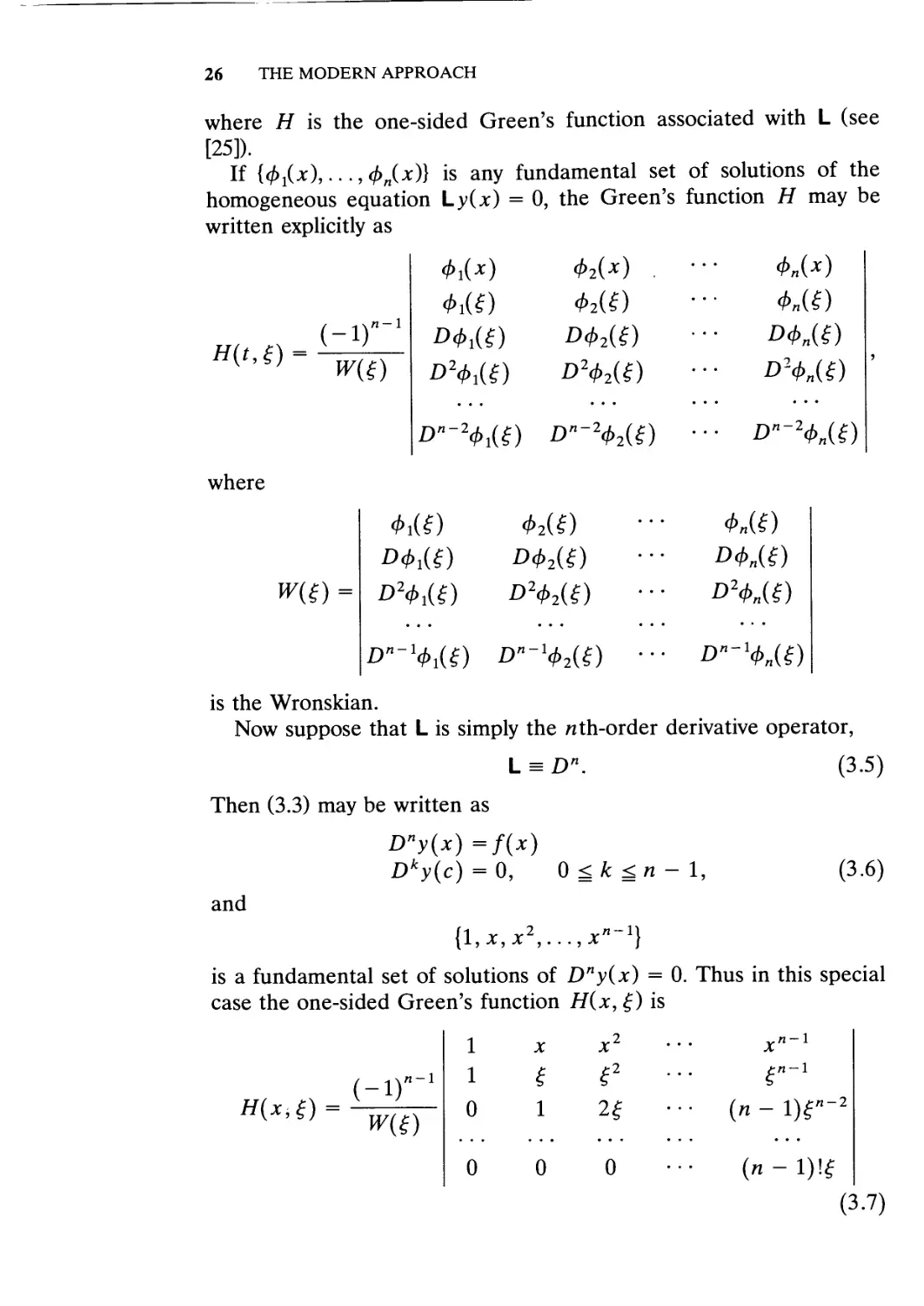
If {(f>1(x),...,(f>n(x)} is any fundamental set of solutions of the
homogeneous equation Ly(x) = 0, the Green's function H may be
written explicitly as
(-i)
n-\
UZ)
where
UZ)
is the Wronskian.
Now suppose that L is simply the /ith-order derivative operator,
L = Dn. C.5)
Then C.3) may be written as
Dny(x)=f(x)
Dky(c) = 0,
C.6)
and
is a fundamental set of solutions of Dny(x) = 0. Thus in this special
case the one-sided Green's function H(x, g) is
(-1)
n-\
1
1
0
o
n~l
i
0
0
C.7)

THE DIFFERENTIAL EQUATION APPROACH 27
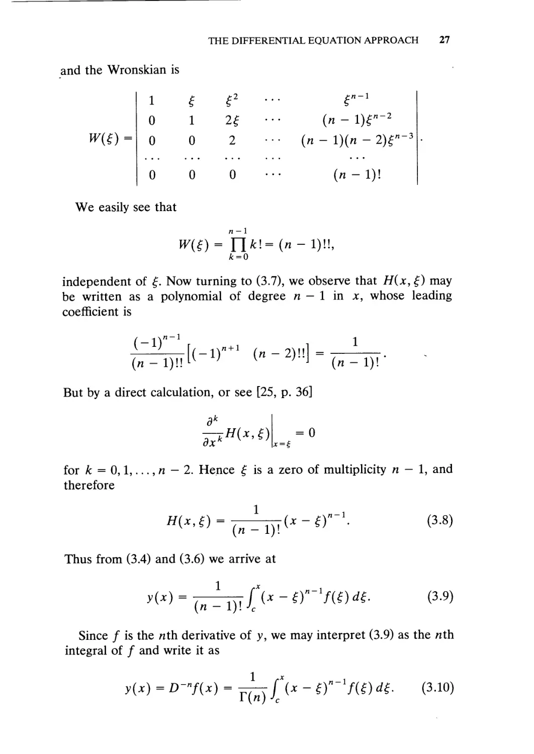
and the Wronskian is
1
0
0
0
i
0
0
e •
2?
2
0
(«
¦¦ (n-
~ 1)^"~2
l)(n - 2)r~3
(n-l)\
We easily see that
n-\
independent of ?. Now turning to C.7), we observe that H(x, ^) may
be written as a polynomial of degree n — 1 in x, whose leading
coefficient is
(n-l)\
But by a direct calculation, or see [25, p. 36]
= 0
dx'
for k = 0,1,..., n — 2. Hence ? is a zero of multiplicity n — 1, and
therefore
1
C.8)
Thus from C.4) and C.6) we arrive at
1
C.9)
Since / is the nth derivative of y, we may interpret C.9) as the nth
integral of / and write it as
y(x) = D~»f(x) =
C.10)

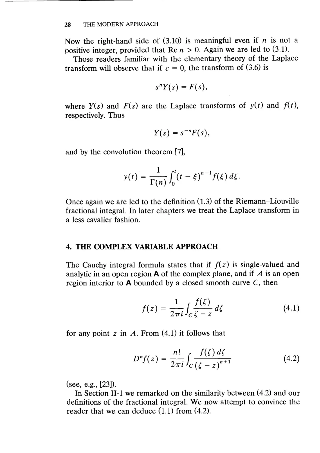
28 THE MODERN APPROACH
Now the right-hand side of C.10) is meaningful even if n is not a
positive integer, provided that Re n > 0. Again we are led to C.1).
Those readers familiar with the elementary theory of the Laplace
transform will observe that if c = 0, the transform of C.6) is
snY(s)=F(s),
where Y(s) and F(s) are the Laplace transforms of y(t) and f(t),
respectively. Thus
Y(s) = s-"F(s),
and by the convolution theorem [7],
Once again we are led to the definition A.3) of the Riemann-Liouville
fractional integral. In later chapters we treat the Laplace transform in
a less cavalier fashion.
4. THE COMPLEX VARIABLE APPROACH
The Cauchy integral formula states that if /(z) is single-valued and
analytic in an open region A of the complex plane, and if A is an open
region interior to A bounded by a closed smooth curve C, then
D.1)
for any point z in A. From D.1) it follows that
— f K J H+1 D.2)
2TTiJC(C-z)
(see, e.g., [23]).
In Section II-l we remarked on the similarity between D.2) and our
definitions of the fractional integral. We now attempt to convince the
reader that we can deduce A.1) from D.2).

THE COMPLEX VARIABLE APPROACH
29
Branch
cut
Figure \a
If n is an arbitrary number, say v, we may replace n\ by T{v + 1) in
D.2). But if v is not an integer, the point z is now a branch point and
not a pole of the integrand of D.2). The simple closed curve C is
therefore no longer an appropriate contour. To overcome this diffi-
difficulty we make a branch cut along the real axis from the point z to
negative infinity. (See Fig. la, where we have assumed that z is a
positive real number, say x.) We are thus invited to define cD^f(x) as
the loop integral (x > c)
,
nodt =
\
D.3)
Figure la may be redrawn as Fig. \b—less colorful than Fig. la,
perhaps, but more convenient for computation. The loop J? is then
the union of L2, y, and Ll5 where y is a circle of radius r with center
at x and Lx and L2 are the line segment [c, x — r]. These line
segments coincide with a portion of the real axis in the ?-plane but are
on different sheets of the Riemann surface for (? - x)~v~l. For
purposes of visualization we have drawn them as distinct.
If ? — x is a positive number, we define ln(? — x) as a real number
(the arithmetical logarithm). Thus on y (see Fig. \b)
-„-!

30 THE MODERN APPROACH
Im
Since 6 = it on Lv
Figure \b
on Lx, and since 6 = -tt on L2,
(f-
on L2.
Returning to D.3), we see that if Re v < 0,
+/ + /
L2 Jy JLX
x — r
x — r

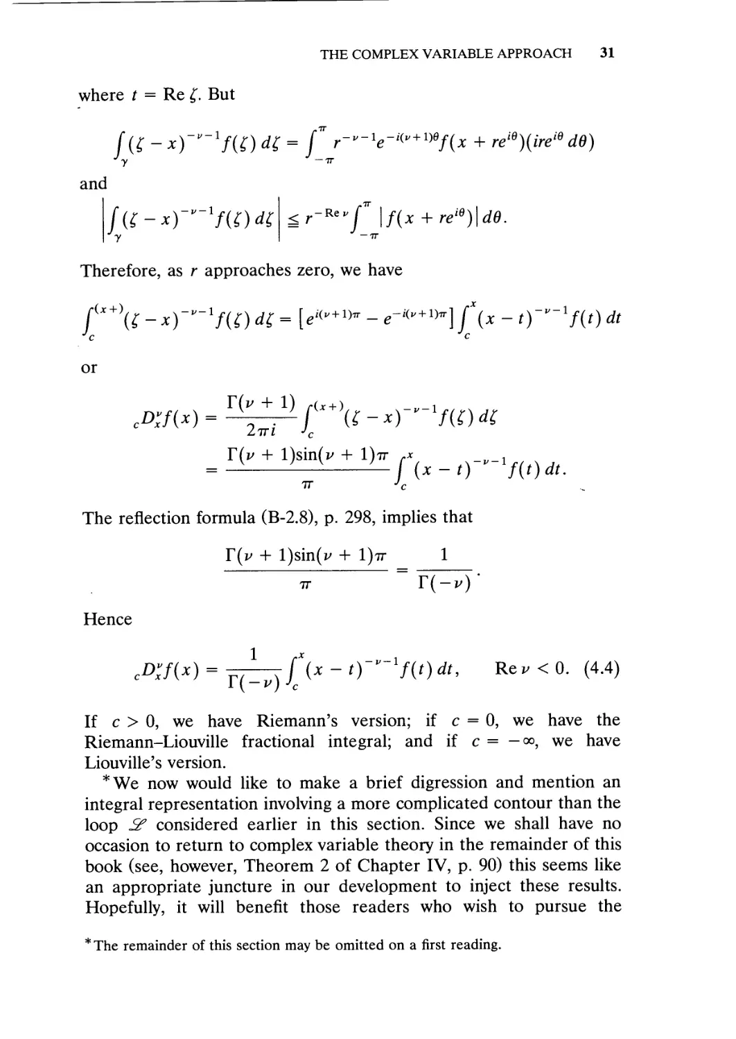
THE COMPLEX VARIABLE APPROACH 31
where t = Re ?. But
y
and
- x)~v~lf{C) d? = f r-v-le-*v+X)df{x + reie){ireie dO)
— ir
txyf(t)t ? \f( reie)\dd.
y J-tt
Therefore, as r approaches zero, we have
or
TT Jc
The reflection formula (B-2.8), p. 298, implies that
Y(v +
Hence
:Dxf(x) = ^ r / (x ~ t)—f(t)dt, Rev < 0. D.4)
c
-,-1
If c > 0, we have Riemann's version; if c = 0, we have the
Riemann-Liouville fractional integral; and if c = — oo, we have
Liouville's version.
*We now would like to make a brief digression and mention an
integral representation involving a more complicated contour than the
loop 5f considered earlier in this section. Since we shall have no
occasion to return to complex variable theory in the remainder of this
book (see, however, Theorem 2 of Chapter IV, p. 90) this seems like
an appropriate juncture in our development to inject these results.
Hopefully, it will benefit those readers who wish to pursue the
* The remainder of this section may be omitted on a first reading.

32 THE MODERN APPROACH
Im z
Figure 2
fractional calculus further from the complex variable point of view.
Since a detailed analysis would probably take us too far afield, we
shall content ourselves by merely stating certain important results.
Let a and /3 be two branch points of F(z). Then a Pochhammer
contour & may be illustrated as in Fig. 2 (see [15, p. 255], [23, p. 163],
[48, p. 257]). It is also sometimes called a double loop. A crucial
feature of this contour is that the multivalued function F(z) returns
to its original value after traversing &.
The key formulas we wish to present are given below in Theorem 1.
Theorem 1. Let M be a simply connected open region in the complex
z-plane, containing the origin. Let ^0 be the region <% with the origin
deleted. Then for z e^n, v # -1, -2,..., and A not an integer,
Dvzkf(z) =
and
Duz\\nz)f(z) =
T(v
4-tt sin 7rA
D.5)
T(u
, — ivX
Air sin it A
jt\t-zyv-\\nt)f{t)dt
4 sin2 it A
D.6)
where /(z) is analytic in ^ and & is a Pochhammer contour with
respect to the branch points 0 and z.

THE WEYL TRANSFORM 33
This and other results, together with proofs, may be found in [15].
One of the noteworthy facts about the representations above is that
Dv may be a fractional integral operator or a fractional differential
operator depending on whether Re v < 0 or Re v > 0 (provided that
v is not a negative integer.)
5. THE WEYL TRANSFORM
In previous sections of this chapter we have presented various argu-
arguments that led to the definition
c*>rf(*) = T^T f (* " t)v-lf{t)dt, Rev > 0 E.1)
1 \V) Jc
of the fractional integral. The Weyl fractional integral
- x)v-xf{t)dt, Rev>0, *>0 E.2)
was introduced in Section 1-6. We shall now attempt to convince the
reader that it is indeed a logical choice.
The arguments in Section II-3 that led to E.1) started with a linear
differential operator
L = Dn + px{x)Dn-x + •-¦ +pn(x)D°. E.3)
We now shall show that starting with the adjoint operator L*, we shall
be led to the definition E.2) of the Weyl fractional integral.
The equation adjoint to Ly(jc) = Ois
L*y(x) = (-l)"D" + (-l)"-1D"-1[p1(J:
°[} =0
Then, of course, the solution of the nonhomogeneous equation
L*y(x) = f(x) with the initial conditions Dky{c) = 0, 0 ? k ? n - 1,
is given by
E.4)

34 THE MODERN APPROACH
where H* is the one-sided Green's function associated with the
adjoint operator L*.
But if H(x,?;) is the Green's function of L, then (see [25, pp.
36-37])
) E.5)
and we may write E.4) as
? E.6)
Suppose that now (as in Section II-3) we let L be the rcth-order
derivative operator,
L = Dn. E.7)
Then its adjoint L* is
L* = (-1)"DW. E.8)
As we saw in C.8),
and hence from E.6) we arrive at
Now the right-hand side of E.9) is also meaningful for other than
positive integral values of n. Thus if we replace n by v and let c = oo,
E.9) becomes
E-10)
Of course, if E.10) is to exist, we certainly must require that Re v > 0
in order that E.10), considered as an improper integral, converge.
Also, if E.10) is to exist, considered as an infinite integral, some
restrictions must be placed on /.

THE FRACTIONAL DERIVATIVE 35
The problem of choosing a suitable class of functions is discussed in
Chapter VII when we examine some of the properties and uses of the
Weyl fractional integral. However, to convince the reader that our
theory is not vacuous, we find the Weyl fractional integral of a few
simple functions. Suppose first that
f(x)=e-ax,
where Re a > 0. From the definition of the Weyl transform E.2),
1
An elementary integration establishes the result that
xW-"[e-ax] = a-ve~ax, Re v > 0, Re a > 0. E.11)
Note the similarity of E.11) to Liouville's first formula for the frac-
fractional derivative, A-2.3), p. 5.
Also, from [12, p. 424], we have
xW~v[cosax] = a~vcos(ax + \irv) E.12)
and
in ax] = a~v sin(ax + \irv) E.13)
provided that a > 0 and 0 < Re v < 1, while an elementary calcula-
calculation yields
X oo
V^, 0 < Re v < Re /a, x > 0. E.14)
For a table of Weyl fractional integrals, see [9].
6. THE FRACTIONAL DERIVATIVE
If D = d/dx is the differentiation operator, and if n is a positive
integer, the meaning of Dnf(x), the nth derivative of f(x) (provided
that it exists) is well-known. However, if n is not a positive integer, we
see that while we may ascribe a meaning to D~v for Re v > 0, we
have yet to assign a meaning to the symbol D" for Re v > 0. We shall
undertake this task in the present section.

36 THE MODERN APPROACH
Suppose that Re v > 0. Let n be the smallest integer greater than
Re u, and let v = n - v. Then
0 < Rev ^ 1.
We shall define the fractional derivative of fix) of order u as
D°J(x) =
F.1)
for x > 0 (provided that it exists).
For example, if c = 0 and /(*) = x^, \l > — 1, then from F.1)
F.2)
But as we have seen before,
lt>xdt =
-IX + V
IV +
F.3)
provided that Re v > 0, x > 0. Thus from F.2),
'A — LJ
+ v - n + 1)
Since v = n — v, we may write F.4) as
- — n
F.4)
QUx
IV +
x^ = — -x'
, x > 0. F.5)
r(/i - u + 1)
A comparison of F.3) and F.5) leads to the interesting conclusion that
IV + 1)
F.6)
for fi > — 1, x > 0, and for any not purely imaginary number u. We
shall elaborate on this confluence in Section IV-3.

THE FRACTIONAL DERIVATIVE 37
Now let us turn to the question of the existence of the fractional
derivative, F.1). If
cD;-f(x) = -L j\x - t)-'f(t) dt F.7)
is the Riemann fractional integral, it certainly exists if Re v > 0 and if
/ is continuous. However, this is not sufficient to guarantee the
existence of the fractional derivative. For example, let / be continu-
continuous but not differentiable (e.g., a Weierstrass-type function) and let
v = 1. Then
= ff(t)dt.
c
Now if v = 1, then n = 2 (since v = n — u) and formally, by F.1),
cDlf(x) =cD
= D2fj(t)dt
= Df(x).
But by hypothesis, fix) is not differentiable.
On the other hand, if / has n continuous derivatives, then F.1)
does exist for x > 0. To prove this contention, make the change of
variable
t=x-yk F.8)
in F.7) where A = 1/v. Then we may write F.7) as
and [see F.1)]
«-i Dkf(c)
n\ D~vf(xS\ = Y -^ (x - cY~n+k
(x-c)"
exists for x > c since Dnf(x) has been assumed to be continuous.

38 THE MODERN APPROACH
7. THE DEFINITIONS OF GRUNWALD AND MARCHAUD
In this section we consider two additional definitions of the fractional
operator. One is due to Grunwald and one is due to Marchaud.
Grunwald defines the result of operating on a function with a frac-
fractional operator as the limit of a certain sum. Marchaud's definition of
a fractional derivative is defined as an integral.
We begin with Griinwald's definition. Suppose then that a function
/ is defined on an interval, and that x0 is any fixed point interior to
the interval. Let u be any number, positive, negative, or zero. Then
Grunwald defines the value of the fractional operator Du acting on
fix) at x = x0 as
1 vn1 T(k ) xn\
-*-f GJ)
(provided that the limit exists). See [4], [5], [13], [15], and [32].
First let us show that if v is a positive integer, say p, then G.1)
reduces to the limit of the pth finite difference quotient of f(x)
evaluated at x = x0. For, from the identity (B-2.3), p. 298,
<7'2»
we see that if v = p, then G.1) becomes
D>f(xo)- limj^
\ n
-^). G.3)
n j
Now let
h = —
n
Then we may write G.3) as
Griinwald's definition is very appealing in that it makes no assump-
assumptions other than that f(x) be defined. On the negative side, it is very

THE DEFINITIONS OF GRUNWALD AND MARCHAUD 39
difficult to calculate the limit in concrete cases. En revanche it has the
virtue (as pointed out by Prof. Samko in a private communication)
that it may be used to calculate approximately the fractional deriva-
derivative. For, for n large,
- v) i xo\
We shall content ourselves with establishing that for u arbitrary and
fix) = xm, m = 0,1,2,..., eq. G.1) yields
Tim + 1)
Dvxm = — -—xm~v G.4)
T(m + l-v) v '
as the fractional derivative (or integral) of xm. This result, of course,
coincides with our earlier calculations [see F.3), F.4), and F.6)].
We begin by calculating Dufix) when fix) is a constant (i.e.,
m = 0). Then from G.1) with u arbitrary,
vn-} T(k - v)
For convenience we have dropped the subscript 0 on x0. Now the sum
in G.5) may be written in closed form by use of the identity
Thus G.5) becomes
x~u
i)
Dvl = — lim nv ' . . G.7)
T(l - v) n-oc Tin) v '
Before continuing we remark that G.6) (which easily may be proved
by a simple induction) is a special case of
( -
r(A)
The identity G.8) is useful in the theory of the fractional difference
calculus (see [29]).

40 THE MODERN APPROACH
Returning to G.7), we see that our remaining problem is to calcu-
calculate the limit. Now if n is large and a and b are fixed numbers, then
from (B-2.10), p. 299, we have the asymptotic formula
n
T(n + a)
b-a
T(n
= 1 + O{n~x) G.9)
for the ratio of two gamma functions. Applying G.9) to G.7) immedi-
immediately yields our desired (and expected) result,
x~v
for v arbitrary [see G.4)].
We turn now to the more general case where
f{x)=xm, m = l,2,... .
With this choice of / (where we have again dropped the subscript on
x0) we may write G.1) as
xm-v
x (v)t \
Duxm = — lim nv E -wr, f 1 " - • G-11)
T(-v) »-. ?or(k + l)\ n) v
If we expand A — k/n)m by the binomial theorem, G.11) becomes
n~l T(k — u)
V~rEhkr
xm~u m
\ nl T(k — u)
limnV~rEThrrTikr- G12)
The next stage in our analysis is to simplify the sum over k in
G.12), namely,
"-1 T(k -v)
K-Rm^kr
To do this most efficiently, it is convenient to recall a few elementary
facts from the calculus of finite differences.
If y is an indeterminate and if j is a positive integer, then y, j
factorial is defined as
y(i) = y(y - i)(y - 2) • • • (y -y + l) G.14)

THE DEFINITIONS OF GRUNWALD AND MARCHAUD . 41
[and y@) is defined as unity]. Furthermore, an integral power of y
may be expressed as a factorial polynomial. Explicitly,
yr =
G.15)
where the S?- are the Stirling numbers of the second kind (see [24]).
Now it follows from G.14) that
T(y + l)=yU)T(y-j
and from G.15),
G.16)
Letting y = k in G.16) and substituting in G.13) leads to
K=
T(k-v)
G.17)
If we replace n by n - j and v by v - j in G.6), we see that
T(n - v)
[since the sum in G.17) is vacuous for k < j] and hence
' T(n - v) 1
The manipulations above reduce G.12) to
.m-v m
1 r uJ(n-v)
lim n
j — v n
T(n-j)-
G.18)

42 THE MODERN APPROACH
If we write
T(n-v)
= nJ'r
n
v-j
n ~ v)
T(n -;)
we again see from the asymptotic formula of G.9) that
T(n-v) 11, if j = r
lim nv~r —t f = '
T(n-j) \0, if;<r.
We thus may write G.18) as
G.19)
m~u m
G.20)
Now <5^r = 1 for all r, and by another induction we establish the
identity
m
r=0
l
G.21)
Therefore,
Dvxm =
T(m + 1)
T(m + 1 -v)
.m — v
G.22)
for all v, positive, negative, or zero, and m = 0,1,2,... [see G.4)].
We turn now to Marchaud's definition of the fractional derivative.
H. Weyl [47] considered the fractional derivative in the form
a
0 < a < 1 G.23)
ten years before Marchaud [22]. Marchaud introduced the generaliza-
generalization of G.23) for any a > 0 and considered its properties. Equation
G.23) and its generalizations are referred to as the Marchaud frac-
fractional derivative. Now for suitable functions
r(i-«) K (x-t)a
dt =
/(*)
« r*/W-/@
- G'24)

THE DEFINITIONS OF GRUNWALD AND MARCHAUD 43
Professor Samko calls the right-hand side of G.24) an analog of
Marchaud's derivative for a finite interval.
We shall take
G.25)
as our definition of Marchaud's fractional derivative. Samko [5] has
shown that G.1) and G.25) are equivalent.
We shall show that Duf(x) as given by G.25) is, indeed, the
fractional derivative of order u for
/(*)=*", u > 0.
For this choice of / we may write G.25) explicitly as
V fx XU ~tU
V f
-v)J0
Dx T{\-v) + T(i-v)J0
If we make the change of variable t = x(l - ?), then
G'26)
Now an integration by parts yields
1 - A - f)" 1 u
and G.26) becomes
Some simple algebra reduces the above form to
T(u + 1)
Dvxu = \ xu-v, u>0,
T(u + 1 - v)
which is the L>th fractional derivative of x11.

Ill
THE RIEMANN-LIOUVILLE
FRACTIONAL INTEGRAL
1. INTRODUCTION
After the lengthy justifications of Chapter II, we begin our mathemati-
mathematical development of the fractional calculus. We start with a formal
definition of the Riemann-Liouville fractional integral, carefully de-
delineating the class of functions to which this fractional operator may
be applied. Numerous examples, some trivial and some not so elemen-
elementary, are given and discussed. This analysis provides a convenient
vehicle for introducing certain new functions such as Et{v, a),
Ct{v, a), St(v, a) that play a forward role in the fractional calculus and
fractional differential equations. (Properties of these functions are
examined in some detail in Appendix C.)
Certain techniques are developed that enable us to find fractional
integrals of more complicated functions. In Section III-4 we consider
the Dirichlet formula and analyze some of its consequences. Most
prominent is its use in the proof of the law of exponents for fractional
integrals. That is, we shall show that 0?>,-%,?>-") = QD~lt-v for all
positive \x and v (Theorem 1). It also will be used to obtain the
fractional integrals of certain nonelementary functions.
In later sections we examine the relations that exist between
(ordinary) derivatives of fractional integrals and fractional integrals of
derivatives. Many ancillary results in the theory of the fractional
calculus may be deduced from these theorems. The penultimate
section is devoted to the problem of finding the Laplace transform of
44

DEFINITION OF THE FRACTIONAL INTEGRAL 45
fractional integrals, together with the inevitable consequences. The
Laplace transform frequently will be exploited in remaining chapters,
especially in our study of fractional differential equations. In the final
section we discuss Leibniz's formula for fractional integrals and give
some interesting applications of this rule.
2. DEFINITION OF THE FRACTIONAL INTEGRAL
As we have stated before, our objective is to investigate various
aspects of the Riemann-Liouville fractional integral. We begin with a
formal definition (see Definition 1 below).
Let X be a positive number and let / be continuous on [0, X].
Then if v ^ 1,
exists as a Riemann integral for all t <e [0, X]. Of course, B.1) will
exist under more general conditions. For example, if / is continuous
on @, X] and behaves like tA for —l<A<0ina neighborhood of
the origin and/or if 0 < Re v < 1, then B.1) exists as an improper
Riemann integral. The following definition, however, is sufficiently
broad for our purposes.
Definition 1. Let Re v > 0 and let / be piecewise continuous on
/' = @, o°) and integrable on any finite subinterval of / = [0, oo). Then
for t > 0 we call
B-2)
the Riemann-Liouville fractional integral of / of order v.
Let us discuss this definition. As we have observed above, B.2) is an
improper integral if 0 < Re v < 1. We require / to be piecewise
continuous only on /' = @, oo) (the interval / excluding the origin) to
accommodate functions that behave like In t or t^ (for -1 < \l < 0)
in a neighborhood of the origin. We shall denote by C the class of
functions described in Definition 1. [One readily may generalize C to
include, for example, such functions as /(?) = |? - a|A, A > -1, 0 <
a < t. We seldom shall have occasion to do so.]

46 THE RIEMANN-LIOUVILLE FRACTIONAL INTEGRAL
For example, if f(t) = t* with /x > -1, then [see (II-6.3), p. 36]
TU + 1)
Drv^ ^^ ' >°
B-3)
[since B.2) is now essentially the beta function]. Because \x + Re v
may be negative, we see from this example why we must include the
caveat t > 0 in our definition of the fractional integral. [Of course, if
ix 7t 0, then B.3) is continuous on /.] To avoid minor mathematical
complications not related to the fractional calculus, and with little loss
of generality, we shall, as a practical matter, assume that v is real.
Occasionally, we indicate that certain formulas are valid for Re v > 0
rather than just for v > 0. A discussion of fractional operators when v
is purely imaginary may be found in [19].
If we write B.2) as the Stieltjes integral
where
" B.4)
is a (continuous) monotonic increasing function of ? on [0, t], then if
/ is continuous on [0, t], the first mean value theorem for integrals
[45, p. 107] implies that
ff(?)da(Z)=f(x)r
'0
for some x e [0, t]. Hence
lim0D,-7@ = 0. B.5)
If / is not continuous (but still of class C), then B.5) need not be
true. In fact, we see from B.3) with v > 0, \x > -1, that
@, ix + v > 0
+ v < 0.

SOME EXAMPLES OF FRACTIONAL INTEGRALS 47
Furthermore, we also conclude from B.3) that even the continuity of /
at the origin does not guarantee the differentiability of 0D~vf(t) at
t = 0. (For example, let \x > 0 and jx + v < 1.)
At times it may be expedient to consider certain subclasses of C.
For instance, in Chapter IV we introduce a class of functions that
includes functions of the form
where A > — 1 and rj(t) is analytic. At other times we shall find it
convenient to take the Laplace transform of the fractional integral. In
such cases we require that / be of exponential order. Since we mainly
shall be considering integrals of the form B.2), the notation will be
simplified by dropping the subscripts 0 and t on 0D~", as was done in
Section II-7. Occasionally, we shall use them for emphasis, or if there
is a possibility of ambiguity, or if we wish to consider a fractional
integral whose lower limit is not zero.
3. SOME EXAMPLES OF FRACTIONAL INTEGRALS
Before we embark on a theoretical analysis of the fractional integral,
let us calculate the fractional integrals of a few elementary functions.
We already have shown in B.3) that
In particular, if /x = 0, the fractional integral of a constant K of order
v is
' v>0- C-2)
Perhaps the reader may have wondered why we did not give a few
additional examples of fractional integrals. The answer is simple—
fractional integrals, even of such elementary functions as exponentials
and sines and cosines, lead to higher transcendental functions—as we
shall now demonstrate.
Suppose that
— o"t

48 THE RIEMANN-LIOUVILLE FRACTIONAL INTEGRAL
where a is a constant. Certainly, eat is of class C, and by Definition 1,
^f v > 0. C.3)
If we make the change of variable x = t - ?, C.3) becomes
eat rt
veat = —— \ xv~xe-axdx, v > 0. C.4)
F(v) -Jo
D
Clearly, C.4) is not an elementary function. But it is closely related to
the transcendental function known as the incomplete gamma function
[(B-2.19), p. 300, Section C-2]. For Re v > 0 the incomplete gamma
function y*(v, t) may be defined as
C-5)
Thus we may write C.4) as
D~veat = tveaty*(v,at). C.6)
Since the right-hand side of C.6) is the fractional integral of an
exponential, it is not surprising that this function frequently arises in
the study of the fractional calculus. We shall call it Et(v, a),
Et(v,a)=tveaty*(v,at). C.7)
Some of the elementary properties of y* and Et are examined in
Appendix C.
A direct application of the definition of the fractional integral leads
to
1 /•' 1
D~v cos at = —— / ?" cos a(t - f) d?, v > 0 C.8)
1 (^) Jo
and
1 /¦' 1
D~v sin at = TTT / * sin

SOME EXAMPLES OF FRACTIONAL INTEGRALS 49
We find it convenient to define the right-hand sides of C.8) and C.9)
as Ct{v, a) and St(v, a), respectively. Properties of these functions also
are studied in Appendix C.
Thus from C.7), C.8), and C.9) we have for v > 0 the compact
formulas
D~veat = Et{y,a)
D~v cos at = Ct(v, a) C.10)
D~v sin at = St(v,a).
In the special case v = \,
= a-^2eat Erf (at)l/2, C.11)
where Erf* is the error function (B-2.25), p. 301. Also,
D~1/2 cos at = Ct(\,a)
= V - [(cos at)C(x) + (sin at)S(x)] C.12)
, y a
and
D~1/2 sin at = St(\,a)
= y - [(sin at)C(x) - (cos at)S(x)], C.13)
where
and C(x) and S(x) are the Fresnel integrals (B-2.27) and (B-2.28),
p. 301.
Simple trigonometric identities may be used to calculate other
fractional integrals of trigonometric functions. For example, from
cos 26 = 2cos20 -1 = 1- 2sin20,
{3M)

50 THE RIEMANN-LIOUVILLE FRACTIONAL INTEGRAL
and
IT" sin2 at = _ ' n - \ct(v,2a). C.15)
We consider some slightly more complicated functions. Suppose
that
f(t) = (a - t)\ a > t > 0.
Then /gC, and by definition,
a - tf = ^V
Re i/ > 0, a > f > 0. C,16)
If we make the bilinear transformation
t-Z
in the integrand of C.16), we obtain
. .'fl — t) ft/a _ _,_i
D-'(a - 0 = r/ ( f x-^l-xy-^dx.
But the integral above is just the incomplete beta function (B-2.24),
p. 300. Thus
1 l ^B,/a(,,-A-,). C.17)
If, in particular, a = 1, v = \, and A = — \, direction integration
leads to
1 + l/
0 < f < 1. C.18)
Z)^r = T^ln
vl — t vtt 1 —
As our next example we consider the logarithm. Certainly, In t is of
class C, and its fractional integral of order v is
D~v \nt = —— \\t - if-1 In Zd?, v> 0.
1 \y) Jo

SOME EXAMPLES OF FRACTIONAL INTEGRALS 51
^•r|f we make the change of variable ? = tx, then
But from [12, p. 538],
\l - xI \nxdx = B(fx, v)[^(fi) - if/((i + v)},
> 0, Rei/ > 0, C.20)
where B is the beta function and \jj is the digamma function (B-2.11),
p. 299. Thus if we let fi = 1 in C.20),
ln ' = r(/+ 1} [In ^ - 7 - *(y + !I, C-21)
where y is Euler's constant.
If in particular v = \, then
[21, p. 15] and
It
D~1/2\nt = -T^[ln4f - 2]. C.22)
V7T
More generally, from C.20) we have
r(A +
A > -1, v > 0 C.23)
and with v = \. and A = — \,
[see (B-2.13), p. 299].
Another function, which we shall encounter in our future work, is
fit) = e~x/t. [If we define /@) as zero, all the derivatives of / vanish

52 THE RIEMANN-LIOUVILLE FRACTIONAL INTEGRAL
at the origin. Thus / is not analytic at t = 0.] We shall calculate the
fractional integral in the more general case where fit) = tKe~a/t,
A > -1. By definition
1 (v) Jo
1 (v)
for v > 0 and t > 0. The change of variable of integration
immediately leads to
D-v[txe~a/t] = tx + ve~a/tU(v, -\,a/t) C.24)
for v > 0, A > -1, t > 0. If Re a > 0, then U has the integral
representation of (B-4.12), p. 305.
Our ability to calculate explicitly the fractional integral of a func-
function / frequently depends on our proficiency in performing the
integration
C.25)
However, because of the nature of the kernel (t - ?)"~1 in C.25), it is
possible to develop certain analytical techniques that allow us to
calculate the fractional integral of a large class of functions with
minimal effort. We discuss one such technique now.
The procedure we have in mind will allow us to express the
fractional integral of an integral power of t times a function f(t) in
terms of fractional integrals of /. Using this argument we may show,
for example, that
D~v[teat] = tEt(v, a) - vEt{v + 1, a). C.26)
If / e C, then from Definition 1, p. 45,
v > 0. C.27)

SOME EXAMPLES OF FRACTIONAL INTEGRALS 53
If we replace the term in brackets in the integrand of C.27) by the
identity
(i.e., we have added and subtracted t), then C.27) becomes
D-"[tf(t)\ = tD-"f(t) - vD-"-lf(t). C.28)
In the case f(t) = eat, formula C.28) becomes C.26) [see C.10)].
Similarly, C.28) implies that
D~v[t cos at] = tCt(v,a) - vCt(y + I, a), v>0 C.29)
and
D~v[t sin at] = tSt(v, a) - vSt(y + 1, a), v > 0. C.30)
Equation C.28) may readily be generalized. For if p is a nonnega-
tive integer, then
^y/o v > o C.31)
and
Substituting this expression in C.31), we obtain
= ^yEo(-l)*(^"-VV-
C.32)
Using (B-2.6), p. 298, we also may write C.32) as
D-V[tpf(t)] = ? ( -/)[DV][])-*/(r)]. C.33)

54 THE RIEMANN-LIOUVILLE FRACTIONAL INTEGRAL
For example,
E
E
1 \v) A: = 0
+ k)t>-kEt{v + k,a). C.34)
As we develop further techniques we shall be able to find fractional
integrals of still more complicated functions. For example, we show in
the next section that for v > 0 and \i > -1,
D-»Et(iL,a)=Et(p + v,a). C.35)
Now let us give a few examples of fractional integrals when the
lower limit of integration is not necessarily zero. Consider, then,
cDrf(t) = -r-[t(t-ty-1f(?)dt, v>o, o^c<t,
1 \V) Jc
C.36)
where / is of class C on [c, oo).
The change of variable
in C.36) leads to
where
For example, suppose that
t - c
r=—. C.38)
where fi > — 1 if c = 0, and fi is arbitrary if c > 0. Substitution in
C.37) leads to
.V-\
xv~1(l - xI1 dx

SOME EXAMPLES OF FRACTIONAL INTEGRALS
55
But the integral in the expression above is simply the incomplete beta
function. Thus
C.39)
and if we let c = 0, formula C.39) reduces to C.1), as it should.
Furthermore, if we let fit) be eat or cos at or sin at, then C.37)
yields
CD~V cos at = (cos ac)Ct_c(v, a) - (sin ac)St_c(v, a) C.40)
CD~V sin at = (sin ac)Ct_c(v, a) + (cos ac)St_c(v, a),
which reduce to our previous formulas, C.10), when c = 0. For a table
of Riemann-Liouville fractional integrals, see [9] and Appendix D.
We conclude this section with a theoretical result. Suppose that / is
continuous on [0, X]. Then the Riemann-Liouville fractional integral
of / of order v is
If, furthermore, we require that fix) be analytic at x = a for all
a e [0, X], the power series
f(t-x)-f(t)+
k\
xk.
C.42)
converges for all x in an interval that properly contains [0, t]. Thus it
converges uniformly on [0, t].
Now substitute C.42) in C.41),
1
.k-l
A: =
k\
dx. C.43)

56 THE RIEMANN-LIOUVILLE FRACTIONAL INTEGRAL
By the uniform convergence we may interchange the order of summa-
summation and integration to obtain
1 " (-l)kDkf(t)
i' • °='=x- C-44)
Thus we have expressed the fractional integral of an analytic
function in terms of ordinary derivatives of that function. If we recall
that
D~v~k(l) = tv+k
we also may write C.44) as
0-7@ = E (-i)k(v + \ ~ x\\D
= ?[~kV)[Dkf(t)][D-»-'<(l)] C.45)
[see (B-2.6), p. 298].
4. DIRICHLET'S FORMULA
If G(x, y) is jointly continuous on [a, b] X [a, b], we know from the
elementary theory of functions that
jbdxfG(x, y) dy = fdy /*G(x, y) dx. D.1)
If, however, G is not continuous, but the integrals // G dy and
jy G dx exist as ordinary or improper Riemann integrals, general
conditions under which the order of integration may be interchanged
are difficult to obtain. Dirichlet's formula [48, p. 77] furnishes an
example of a function for which D.1) is true even though G may not
be continuous. Because of the form of the integrand, this formula is
well suited to the fractional calculus.

DIRICHLET'S FORMULA 57
Dirichlet's Formula. Let F be jointly continuous on the Euclidean
plane, and let A, fi, v be positive numbers. Then
\\t - xf-1 dx f(y - a?-\x - y)v-lF{x, y) dy
J a a
= j\y - a)"'1 dy j\t - xY~\x - y)v-lF(x, y) dx. D.2)
a Jy
Certain special cases are of particular interest. If a = 0, A = 1, and
F(x, y) = g(x)f(y), then D.2) becomes
j\t - xY~lg(x) dx f(x - yy-'fiy) dy
= ff(y) dy (\t - xf~\x - y)v~xg{x) dx. D.3)
^0 Jy
Furthermore, if g{x) = 1, D.3) assumes the form
D.4)
where B is the beta function.
As an important illustration of the usefulness of Dirichlet's for-
formula, we shall prove the law of exponents for fractional integrals.
Theorem 1. Let / be continuous on /, and let fi, v > 0. Then for
all t,
D.5)
Proof. By definition of the fractional integral,
i
D-[D-»f(<)] =
r(ju.)
f (x-yf-'fMdy
dx

58 THE RIEMANN-LIOUVILLE FRACTIONAL INTEGRAL
and
Equation D.4) now implies the truth of D.5). ¦
An alternative proof of this important theorem may be given by
noting that
for any polynomial P, and then applying the Weierstrass approxima-
approximation theorem, see [45].
If we wish Theorem 1 to be true when fi (or v) is zero (which we
do), we see that D° must be denned as the identity operator /. We
shall make this identification.
For any positive integer p and continuous function /, we have seen
that
D~pf(t) = j^TtyjXt - *r 7« dx D.6)
is the /7-fold integral of f(t). Thus if we let \i = p in D.5), we have
D-p[D~vf(t)] = D~(p+l/)f(t) =D-v[D-pf{t)}. D.7)
We see, therefore, that the /7-fold integral of the fractional integral
D~vf(t) is the fractional integral of / of order p + v, and that they
are both equal to the fractional integral of the /7-fold integral of / of
order v.
As we have observed before, the fractional integral of an elemen-
elementary function need not be elementary. We thus may use Theorem 1 to
find the fractional integral of certain nonelementary functions. For
example, if fit) = eat, then since eat is continuous, Theorem 1 implies
that
at D.8)
for positive fi and v. But from C.10), D~*eat = Et(fi, a) and
= Et(fi + v,a).

FRACTIONAL INTEGRAL AND DERIVATIVES 59
Thus with little effort we have established the formula
D-"Et(ti,a)=Et(ti + v,a), /*>-l, v>0 D.9)
[see C.35)]. Similar arguments yield
D~vCt(n,a) = Ct(ti + v,a), /x > -1, v>0 D.10)
and
fi > -2, v > 0. D.11)
Further formulas may be obtained by the use of C.28) and C.32) [or
C.33)]. For example, if we apply C.28) to D.9),
D-v[tEt(fi, a)] = tEt{fi + v,a)- vEt(fi + v + 1, a),
fi > -2, v > 0. D.12)
5. DERIVATIVES OF THE FRACTIONAL INTEGRAL AND
THE FRACTIONAL INTEGRAL OF DERIVATIVES
In Section III-4 we showed that the integral of the fractional integral
was the fractional integral of the integral. We now develop similar
formulas involving derivatives. Unfortunately, the relations are not
quite as simple. The basic rules for manipulating these quantities are
given below in Theorem 2. Some examples of Dp[D~vf(t)] and
D~v[Dpf(t)] (where p is a positive integer) will be given.
Theorem 2. Let / be continuous on / and let v > 0. Then:
(a) If Df is of class C, then
=D~»f(t) -
^
and
(b) If Df is continuous on /, then for t > 0,
D[D-»f(t)] = D-[Df(t)]

60 THE RIEMANN-LIOUVILLE FRACTIONAL INTEGRAL
Proof. To prove part (a), let e > 0, t/ > 0 be assigned. Then (t - ?)"~1
and /(?) are continuously different!able on [17, t — e]. Thus an inte-
integration by parts establishes
Jv Jv
+ evf(t -€)-(t-'
Now take the limit as e and 17 independently approach zero and
divide by Y{v + 1) to obtain part (a).
To prove part (b), make the change of variable
f-t-x" E.1)
(where A = 1/v) in
to obtain
Then for t > 0,
1 [ —1 /"'" d
+ 1) [ ^0 dt
Now reversing the transformation E.1), that is, letting t — xK
proves part (b). ¦
If we apply Theorem 2 to the special case
f(t) = t», fJL> 0,
then both parts (a) and (b) yield identities.
Now let /@ = eat. Then part (a) implies that
tv
D-V~l[aeat] =D~v[eat] -
T(v + 1)'

FRACTIONAL INTEGRAL AND DERIVATIVES 61
and using C.10),
aEt{y + 1, a) = Et(v, a) - *+ , E.2)
a recursion formula for the Et function that may be found in Appen-
Appendix C. If we apply part (b) to eat, then
DEt(v,a)=aEt(v,a)
and using E.2) we see that
DEtiv,a)=E\iv-l,a), E.3)
a differentiation formula for Et that also may be found in Appendix C.
Thus we see that an application of Theorem 2 results in a painless
derivation of such formulas as E.2) and E.3).
If fit) = cos at, then using C.10), p. 49, we see that parts (a) and
(b) of Theorem 2 yield
-aSt{y + 1, a) = Ct(v, a) - *+ E.4)
and
DCtiv,a) = -aStiv,a
respectively. Replacing v by i/ — 1 in E.4) and substituting in the
equation above yields the differentiation formula
t(v,a) = Ct(v-l,a). E.5)
Similarly, we see that if we apply Theorem 2 to fit) = sin at, we
obtain
aCt{y + I, a) = St(v,a) E.6)
and
DSt(v,a) =St{v~l,a). E.7)
Formulas E.4), E.5), E.6), and E.7) also may be found in Appen-
Appendix C.

62 THE RIEMANN-LIOUVILLE FRACTIONAL INTEGRAL
Using E.4), we may write C.15) in the neat form
D~v sin2 at = aSt(y + 1,2a). E.8)
We may generalize Theorem 2 to derivatives of higher order.
Theorem 3. Let /? be a positive integer. Let Dp~xf be continuous on
/, and let v > 0. Then:
(a) If Dpf is of class C, then
D-Vf(t) = D—p[Dpf(t)] + Qp(t, v)
and
(b) if Dpf is continuous on /, then for t > 0
D>[D-"f(t)\ =D-»[Dpf{t)} +Qp(t,v-p),
where
p—\ tv+k
E-9)
Proof. Replacing v by v + 1 and / by Df in part (a) of Theorem 2
yields
Now replace D~v~1[Df(t)] in the expression above by part (a) of
Theorem 2 to obtain
Repeated iterations establish part (a).
To prove part (b), differentiate part (b) of Theorem 2 to obtain (for
t > 0)
D2[D-»f(t)] =D{D-»[Df(t)]}
Now the term in braces is given by part (b) of Theorem 2 with /

FRACTIONAL INTEGRAL AND DERIVATIVES 63
replaced by Df. Hence
D2[D-f(t)] =D
Repeated iterations establish part (b). ¦
Since Qp(t, v) may be expressed as a fractional integral, that is,
Qp(t,v)=D-»[Rp(t)], E.10)
where
"-1 Dkf@)
K
we may write part (a) of Theorem 3 as
D~"[f(t) - Rp(t)] = D-'-'lD'fit)]. E.12)
As a corollary to Theorem 3, we see that if Dkf@) = 0, k =
0,1,..., p - 1, then
D~vf(t) = D~v-p[Dpf(t)] E.13)
and
Dp[D~vf(t)] =D-"[Dpf(t)]. E.14)
These formulas are generalized in Chapter IV.
Before continuing our theoretical development, let us consider
some consequences of Theorem 3. If we apply part (a) to the function
fit) = eat, then
+ Qp(t, v), E.15)
where
p-\ tv+k
Thus from C.10) we see that E.15) reduces to the recursion formula
Et(v,a) = a*Et{y +p,a) + *? a" ' E.16)

64 THE RIEMANN-LIOUVILLE FRACTIONAL INTEGRAL
[see (C-3.4), p. 315]. On the other hand, part (b) implies that
p-\
E.17)
see (C-3.5), p. 316]. If we replace v by v - p in E.16) and substitute
in E.17), we have the elegant formula
DpEt(v, a) = Et(v -p,a), p = 0,1,... E.18)
[which also could have been obtained by iterating E.3)].
Similar arguments, of course, establish that
A/2)/?-
if p is even, and
Ct(v,a) = (-
if p is odd, and
if p is even, and
St(v,a) = (-
+ E ()Jfl2J'+1r(y'+2y + 2) E>22)
if p is odd; while
DpCt(v,a) = Ct(v-p,a) E.23)

FRACTIONAL INTEGRAL AND DERIVATIVES 65
and
DpSt(v,a) = St(v~P,a) E.24)
for p = 0,1,....
In the spirit of Theorems 2 and 3 and E.13) and E.14) we shall
prove a theorem that expresses the derivative of a fractional integral
of a function as a fractional integral of that function.
Theorem 4. Let / have a continuous derivative on /. Let p be a
positive integer and let v > p. Then for all fe/,
Dp[D~vf(t)] =D-(v-p)f(t). E.25)
Proof. By Definition 1,
and
1[] (O E.26)
since v > p. Differentiation of the expression above leads to
Dp[D~vf(t)] =D[Dp-1~l'f(t)].
If we replace v by v - p + 1 in part (b) of Theorem 2, and then
substitute this result for the right-hand side of the formula above, we
get
Dp[D-*f(t)\ = Dp~1-'[Df(t)] + f^ -f-». E.27)
1 (v + 1 - p)
Now replace v by v - p in part (a) of Theorem 2 and substitute in
E.27). ¦
Suppose that q is a positive integer and let \i > q. Then from
Theorem 4,
E.28)

66 THE RIEMANN-LIOUVILLE FRACTIONAL INTEGRAL
Suppose further that
p — v = q — (i. E-29)
Then we have the interesting corollary that
Dp[D-"f(t)] =Dq[D-»f{t)}. E.30)
In the next theorem we generalize this result by showing that E.30)
is true even if p > v and q > fi, and also exhibit the relation between
D~v[Dpf(t)] and D~
Theorem 5. Let p and q be positive integers and let fi and v be
positive numbers such that
p - v = q - (i. E.31)
Let / have r continuous derivatives on / where r = max(/?, q). Then
for all t g /,
r-\
where s = minip, q), and for all t e /',
=Dp[D~vf(t)]. E.33)
Proof. If p = q, the theorem is trivial. Suppose then that q > p. Let
cr = q — p > 0. Then from E.31) we have
li = v + a > 0.
From part (a) of Theorem 3
D-»[D>f(t)] = D-»-
Now recall that v + a = \i and a + p = q. Thus we have proved
E.32).

LAPLACE TRANSFORM OF THE FRACTIONAL INTEGRAL 67
To prove E.33) we have from Theorem 4 that
=D~vf{t). E.34)
If we differentiate E.34) p times,
Dp+<r[D-"-<rf(t)] =DP[D-Vf{t)}.
But p + a = q and v + a = fi. Thus we have established E.33). ¦
6. LAPLACE TRANSFORM OF THE FRACTIONAL INTEGRAL
The Laplace transform will prove to be an indispensable tool, espe-
especially in our study of fractional differential equations. We briefly
inaugurate our discussion of this powerful method in the present
section. In future chapters as well as in Appendix C we consider
additional information about, and applications of, this important
technique.
We recall that a function fit) defined on /' is said to be of
exponential order a if there exist positive constants M and T such
that
e—|/@l ^M
for all t ^ T. If f(t) is of class C and of exponential order a, then
ffit)e-stdt F.1)
exists for all s with Re s > a. We shall call F.1) the Laplace trans-
transform of fit) and write
Sometimes it is convenient to denote the Laplace transform of /
byF,

68 THE RIEMANN-LIOUVILLE FRACTIONAL INTEGRAL
We shall also have occasion to write
to indicate that / is the (unique) inverse Laplace transform of F.
If / and g are of exponential order, then clearly f(t)g(t) is of
exponential order. We also assert that if / is continuous on / and Df
is of class C, then if Df is of exponential order, so is /. To demon-
demonstrate this we first note that if e > 0, then
j'[Df(t)}dt=f(t)-f(e),
and since / is continuous on /,
By hypothesis Df is of exponential order. Hence there exists an a
(which we shall assume to be positive) and constants T and M such
that
\e~atDf(t)\ <M F.2)
for all t > T. Now if we write
f(t)=f(O)+ f'e°t[e-
Jo
(i.e., we have multiplied the integrand by 1 = ea^e~a^), then
f(t) =/@) + (TDf(?) di + f'eat[e-atDf(Z)] d?, t > T,
J0 JT
and by F.2),
T
where A is a positive constant. But
OL

LAPLACE TRANSFORM OF THE FRACTIONAL INTEGRAL 69
Thus for all t ^ T,
\f(t)\<M'e«t
for some M'. Hence f(t) is of exponential order.
If a function of class C has compact support, then the condition
that / be of exponential order is vacuous.
The functions t* (fi > -1), eat, t*~xeat (fi > 0), cos at, and sin at
all are of class C and of exponential order. Some elementary calculus
then shows that
T(fi + )
\ + 1 , H>~1 F3a)
__ F.36)
)
J fi>0 F.3c)
E -a)
at} = —2 j F3d)
a
?f{s\nat\ = -5 =-. F3e)
1 J s2 + a2 v }
One of the most useful properties of the Laplace transform is
embodied in the convolution theorem (see [7]). The theorem states
that the Laplace transform of the convolution of two functions is the
product of their Laplace transforms. Thus if F(s) and G(s) are the
Laplace transforms of fit) and g(t), respectively, then
= F(s)G(s). F.4)
Now if / is of class C, the fractional integral of / of order v is
0-7@ = frr/'('" *)"~1/(*:) d*> v > °>
l{v) jo
which is a convolution integral. Thus if / is of exponential order
{65a)
= s~vF{s), v > 0, F.5b)

70 THE RIEMANN-LIOUVILLE FRACTIONAL INTEGRAL
where F is the Laplace transform of /. We observe that F.56) is valid
even if v = 0, but that F.5a) is indeterminate. However,
F.6)
As examples of F.5) we see from F.3) that
Tin +
v>0, n>-l {6.7a)
2'{D~vt^-xeat} = —" v'"/ „ , v > 0, fi > 0 F.7c)
sv(s - a)
v cos at] = v_x 2 2—, v > 0
sin ^} = ^, 2^ ,, , v > 0.
We turn now to the problem of finding the Laplace transform of
the fractional integral of the derivative and the Laplace transform of
the derivative of the fractional integral. Suppose then that / is
continuous on / and Df is of class C and of exponential order. Then,
by F.5),
&{D-"[Df(t)\) = s
= s-»[sF(s)-f@)], v>0, F.8)
where F{s) is the Laplace transform of f(t). Since f(t) is continuous
on / by hypothesis, /@) exists. Thus we have found the Laplace
transform of the fractional integral of the derivative. This formula is
obviously also valid if v = 0.
Now we consider the problem of finding the Laplace transform of
the derivative of the fractional integral. From part (b) of Theorem 2,
P-60,
= s-[sF(s)-f@)] +5-
= sl~vF(s), v>0 F.9)

LAPLACE TRANSFORM OF THE FRACTIONAL INTEGRAL 71
[where we have used F.8)]. Now we know that if v = 0,
J7{Df(t)}=sF(s)-f@). F.10)
But this is not the same result we would get if we let v = 0 in F.9).
This "discontinuity" arises from the fact that
r
lim —¦ = 0, F.11)
v-*o T(v)
and comparing with F.6) we see that "Jz?" and "lim" do not com-
commute.
Returning to F.7) and recalling C.10), we see that
v>0
We elaborate on these formulas in Section C-4. Thus we see that with
the aid of the fractional calculus, we have found, with little effort, the
Laplace transforms of some nonelementary functions.
For completeness, from F.7c),
Thus from (B-4.8), p. 305, we have
v > 0, fx > 0. F.13)
[If fx is a positive integer, see C.34), p. 54 and (C-4.5), p. 323.]
Finally, we wish to mention a phenomenon that some readers might
not have noticed. Although this phenomenon is prevalent in all of
mathematics, we wish to emphasize it in our dealings with the Laplace
transform. Depending on the method used, it is sometimes possible to

72 THE RIEMANN-LIOUVILLE FRACTIONAL INTEGRAL
weaken a set of hypotheses and still arrive at the same conclusion. For
example, if
1
s
and
then G(s) is meaningful only if v > 0, but F(s)G(s) is meaningful if
v > — 1. Thus if we find the inverse transform of F(s)G(s) directly,
namely
we need require only the weaker hypothesis, v > -1. But if we use
the convolution approach, namely,
tit
F15)
then since the integral is meaningful only for v > 0, we have proved
our result only with the stronger hypothesis v > 0 (even though we
know that the result is valid for v > — 1).
As another more subtle example, let
x(t) =tx~l
and as our problem let it be required to find the inverse Laplace
transform of
s2X(s)
Now
r(A)
X(s) = -y- F.16)

LEIBNIZ'S FORMULA FOR FRACTIONAL INTEGRALS 73
provided that A > 0 and
T(A)
is meaningful if A > 0. Thus
y(f) = r(A)S,(A-2,l), A>0. F.17)
On the other hand, if we write
s2X(s) =5?{D2x(t)} + sx@) + Dx@), F.18)
then Y(s) may be expressed as
} sx@) + Dx@)
Y(s) = —^—— +
K J s2 + 1 xl + 1
But from F.16),
T(A)
which is meaningful only for A > 2. If this is the case, x@) = 0 = Dx@)
and by the convolution theorem
y(t) = f
= r(AM,(A-2,l)
[see (C-3.20), p. 320]. Thus we have proved our result only for A > 2,
while we know from F.17) that it is valid for A > 0.
7. LEIBNIZ'S FORMULA FOR FRACTIONAL INTEGRALS
A Leibniz-type formula expresses the result of operating on the
product of two functions as a sum of products of operations per-
performed on each function. The classical Leibniz rule or formula of

74 THE RIEMANN-LIOUVILLE FRACTIONAL INTEGRAL
elementary calculus is
Dn[f(t)g(t)\ = t (l)[Dkg(t)][D"-kf(t)]t G.1)
where / and g are assumed to be n-fo\d differentiate on some
interval. Now we wish to extend G.1) to fractional operators.
We have seen in Section III-3 that if / is of class C and g(t) = tp,
where p is a positive integer, then the fractional integral of the
product fg of order v > 0 may be written as
D-"[f(t)g(t)] = E ( -v)[Dkg(t)][D—kf(tj\ G.2)
[see C.33), p. 53]. The resemblance of this formula to G.1) is obvious.
The immediate problem we wish to address is the extension of G.2) to
the case where g is not just a simple polynomial. Later, in Chapter
IV, we extend these formulas to fractional derivatives.
Suppose then that / is continuous on [0, X] and that g is analytic
at a for all a e [0, X]. Then fg is certainly of class C, and for v > 0,
the fractional integral
G.3)
exists. We may write
,Dkg(t
, N " ,kDkg(t) ,*
= *(') + ?(-i) .,('-?)• C7-4)
The series G.4) converges for all ? in an interval that properly
contains [0, t], and hence uniformly on [0, t].
Now substitute G.4) into G.3) to obtain
D-[f(t)g(t)] = g(t)D-f(t) + ~f\t ~
G.5)

LEIBNIZ'S FORMULA FOR FRACTIONAL INTEGRALS 75
Since / is continuous on [0, X] and v > 0,
is bounded on [0, t]. Hence we may interchange the order of integra-
integration and summation in G.5) to obtain
= t (-
= LQ(~kV)[Dkg(t)][D-v-kf(t)} G.6)
[see (B-2.6), p. 298].
Thus we have shown:
Theorem 6. Let / be continuous on [0, X], and let g be analytic at a
for all a e [0, X]. Then for v > 0 and 0 < t ^ X,
D-"[f(t)g(t)\ = ? ( ~kv)[Dkg(t)][D—kf(t)]. ^G.7)
We call G.7) the Leibniz formula for fractional integrals. Equation
G.2) is a special case.
Note: The only reason we assumed g analytic for all points a in
[0, X] was to guarantee the uniform convergence of G.4) for ? e [0, t].
As our first application of the Leibniz rule, let fit) = tk, A ^ 0,
and let g{t) = e*. Then from Theorem 6
r(A 4
T(A + v + k + 1)
G.8)
r(A + v +
Using this result we may deduce a useful identity involving the
confluent hypergeometric functions [see G.11)]. For, from the defini-
definition of the fractional integral,
r(A
r(A + 1)
~" + 1,A + v + l;t) G.9)

76 THE RIEMANN-LIOUVILLE FRACTIONAL INTEGRAL
by F.13) [see also C.34), p. 54]. Comparing G.8) and G.9) establishes
the identity
e\Fx(v,k + v + 1; -t) =1F1(A + 1, A + v + l;t). G.10)
Or if we let
a = A + 1
c = A + v + 1,
we have, in more conventional notation,
^(fl, c; t) = e\Fx(c - a, c; -t) G.11)
[see (B-4.10), p. 305].
As a second example, let f(t) = tx, A ^ 0, and let g{t) = A - t)~a.
Let X be a fixed positive number less than 1. Then A - t)~a is
analytic at every point of [0, X], and by Theorem 6,
- I)-] =
for 0 < t ^ X. But
and
r(A
?)---*(¦> =
r(A
Thus
r(v + k)T(a + k) I t \k
x y ( )( ) t
r(A
v
r(A + v +
X2FL,a,A+v + l;j^jY G.12)

LEIBNIZ'S FORMULA FOR FRACTIONAL INTEGRALS 77
On the other hand, since
A-0 =lF0(a; t) =
r(a +k)
~k\
for \t\ < 1 [see (B-4.13), p. 305],
D->[t\l -
f; r±±*t>«
k\
E
T(A + 1)
r(A + v +
Comparing G.12) and G.13) leads to
A-0 a2F\v,a,X +i/
;^
Or in more conventional notation with
a = A + 1
b = a
c = A + v + 1,
we have established the identity
l,a,A + v
=2Fl(X + l,a,A
G.13)
-b
A-0 2FAc - a,b,c;
t - 1
G.14)
between hypergeometric functions [see (B-4.6), p. 304].
Another interesting result that we may establish using the Leibniz
rule is the identity
,Fx(a,b,c;l) =
T(c)T(c -a - b)
Y(c - a)T(c - b)
[sometimes called Laurent's formula; see (B-4.4), p. 304].
G.15)

78 THE RIEMANN-LIOUVILLE FRACTIONAL INTEGRAL
To prove G.15) we start with the trivial identity
0.
Now for v > 0 and A + n > — 1,
T\
T(A + fl + V + 1)
G.16)
G.17)
We shall show that if A, (i ^ 0, we may apply Leibniz's formula to the
product of f(t) = tk and g(t) = t*. This result may then be com-
compared with G.17) to establish G.15).
We begin by expanding g(g) in powers of (? — 0- By the binomial
theorem
= €" = [t
?-
G.18)
Considered as a power series in (? — t)/t, the radius of convergence
is 1. Using Raabe's test we see that the series converges absolutely for
= ±1.
Furthermore, it converges to ?M. Since
for all (^ - i)/t in [ — 1,1], the Weierstrass M-test implies that the
convergence is uniform in the closed interval [ — 1,1]. Thus G.18)
converges uniformly for ? e [0, i\.
It therefore follows (see the note after Theorem 6, p. 75) that
G.19)
k\T(v)

LEIBNIZ'S FORMULA FOR FRACTIONAL INTEGRALS 79
is valid for v > 0, t > 0, A, fi ^ 0. Thus
r(-A + k)T(v + k) 1
k\
If we equate this result to G.17), we obtain
T77T7
r(A + ju, + v +
G.20)
In more conventional notation let a = -A, b = v, c = fi + v + 1.
Then G.20) becomes
T(c)T(c-a -b)
for
a ^ 0, c-l^Z?>0. G.22)
Now G.21) is the same as G.15). And we know that this formula is
valid for
c - a - b > 0 G.23)
with c unequal to a nonpositive integer. Thus we have established
G.21) only under the more restrictive conditions of G.22). But we have
encountered this phenomenon before (see pp. 71-73).

IV
THE RIEMANN-LIOUVILLE
FRACTIONAL CALCULUS
1. INTRODUCTION
The idea of a fractional derivative was introduced in Section II-6. We
make a more extensive study of this concept in the present chapter. In
order to have a class of functions to which both the fractional integral
and the fractional derivative may be applied, we find it convenient to
define a new class of functions, 9\ This class will be a subspace of the
class C used in Chapter III, and will be sufficiently broad for our
purposes. Thus the results, examples, and theorems we proved for the
fractional integral in Chapter III will a fortiori be valid for functions
of class <&. Our definition of class 9* is motivated by certain examples
of fractional derivatives derived in Section IV-2.
The functions of class g7 have the property that if D~uf(t) = F(t,u)
for any function / of this class [where the domain of F is @, oo) x
(-00,00)], then Dvf(t) = F(t, -v). For example, we saw in Chapter
III that for v > 0
D~veat = Et(v,a).
(We shall show that eat is of class 9\) Then
Dveat = Et(-v,a).
80

INTRODUCTION 81
However, the integral representation
~°eat = fT
D~°eat =
is valid only for v > 0. That is, the domain of the right-hand side of
A.1) is @,oo) x @,oo) and not @,oo) x (-00,00). Therefore, the equa-
equation
/ ? — V -
r(-u)
is meaningless for v ^ 0.
Thus if D~vf (v > 0) is the fractional integral of / of order v, the
fractional derivative Dvf (v > 0) of / of order v may be obtained
from D~vf simply by changing the sign of v.
Next we derive Leibniz's formula for the product of suitable func-
functions. Using functions of class g7 we may also deduce many more
fractional integrals/derivatives involving more complicated functions.
We used the Dirichlet formula to prove the law of exponents for
fractional integrals (Theorem 1 of Section III-4, p. 57). In Section
IV-6 we give precise conditions under which the law of exponents
Du[Duf(t)] = Du+Uf(t) A.2)
holds for /eg7 and u and v arbitrary (Theorem 3). Readers are
warned that A.2) as well as the Leibniz rule do not hold for all
functions. Thus one must make sure that the functions to which these
formulas are applied satisfy the stated conditions.
In Sections IV-7 to IV-9 we embark on a lengthy program that we
hope will convince readers of the power of the fractional calculus. We
determine numerous integral representations (i.e., we express a "com-
"complicated" function in terms of the definite integral of an "elementary"
function. Poisson's formula is such an example.) Also, we find many
integral relations. (Sonin's formula is such an example.) These meth-
methods are applied to a wide variety of classical functions, including
hypergeometric functions, Legendre functions, generalized Laguerre
polynomials, and of course, more Bessel functions. We also show how
one may express these functions and others (such as the psi function,
incomplete beta function, error function, Fresnel integrals) as frac-
fractional integrals or fractional derivatives of "simple" functions.

82 THE RIEMANN-LIOUVILLE FRACTIONAL CALCULUS
In anticipation of our lengthy study of fractional differential equa-
equations in Chapter V, we demonstrate how to calculate the Laplace
transform of fractional derivatives. This treatment is indispensable in
our study of such equations.
2. THE FRACTIONAL DERIVATIVE
The fractional derivative was introduced in Section II-6 and some
alternative versions were considered in Section II-7. We shall take the
definition given in Section II-6 as our starting point. Formally:
Definition 1. Let / be a function of class C and let fx > 0. Let m be
the smallest integer that exceeds fx. Then the fractional derivative of /
of order fx is defined as
D»f(t)=Dm[D-vf(t)}, fi>0, t>0 B.1)
(if it exists) where v = m - fx > 0.
Of course, if fx is a positive integer, say p, then Dpf(t) may exist
for t > 0 even if f(t) is not of class C. For example, let f(t) = t~l.
But if / has p continuous derivatives on /, certainly it is of class C
and from
we see that B.1) agrees with the usual definition of the ordinary
derivative. Sometimes (see Section IV-10) it is convenient to define m
as the smallest integer greater than or equal to fx rather than simply
as greater than fx. But if m = \x, then v = 0, and B.1) becomes a
trivial identity. Later we shall introduce a subclass of C for which B.1)
holds for all functions of this subclass.
Let us give some examples. Suppose that f(t) = tx with A > -1.
Let fx be a positive number and m the smallest integer greater than
ix. Then the fractional derivative of tk of order fx is, by definition,
=Dm[D-vtk] B.2)

THE FRACTIONAL DERIVATIVE 83
where v = m — fi > 0. But
r(A + )
D~vtk = —± —ztk + v, t>0 B.3)
and hence from B.2),
T(A + 1)
Dmt
T(A + 1)
Dmtx
T(A + 1)
'*-' '> °- B-4)
as we saw in (II-6.5), p. 36.
Next suppose that f(t) = eat. Then the fractional derivative of eat
of order i± is
Dneat = Dm[D-veat\, B.5)
where ix, v, and m have the same meaning as above. From (III-3.10),
p. 49,
D~veat = Et(v,a) B.6)
and from (C-3.5), p. 316,
DmEt(v, a) = Et{y -m,a)= Et{-n,a) B.7)
since \i = m — v. Thus we conclude that
D»eat = Et(-iJi,a), t > 0. B.8)
Similarly, the fractional derivatives of cos at and sin at are
D» cos at = Ct(-fi, a) B.9)
and
D^s'mat = St(-fi,a), B.10)
where we have used
D~v cos at = Ct(v,a) B.11)

84 THE RIEMANN-LIOUVILLE FRACTIONAL CALCULUS
and
D~v sin at = St(v,a) B.12)
[see (III-3.10)], p. 49, and
DmCt{v,a) = Ct(v-m,a)
DmSt(v,a) = St(v -m,a)
[see (C-3.18), p. 319]. Again we remember that i±, v, and m have the
same meanings as in Definition 1.
The fractional derivatives of Et(X, a), Ct(X, a), St(X, a) also are easy
to calculate. For with A > — 1,
D»Et(X, a) = Dm[D'vEt(X,a)\ B.13)
and from (III-4.9), p. 59,
D~vEt(X, a) = Et(X + v, a). B.14)
An application of B.7) then yields
D»Et(X,a)=Et(X-fJi,a). B.15)
Similarly, the fractional derivatives of Ct and St are
D»Ct(X, a) = Ct(X - fi, a) B.16)
and
B.17)
where we have used
D~vCt(X, a) = Ct(X + v, a) B.18)
and
D~vSt(X,a) = St(X + v, a) B.19)
[see (III-4.10) and (III-4.11), p. 59]. In the formulas in this paragraph
(i, v, and m again have the same meaning as in Definition 1 and
A > -1.
As our final example, for the present, we shall find the fractional
derivative of tx In t, where A > -1. This is a more difficult task.

THE FRACTIONAL DERIVATIVE 85
Again from Definition 1
D»[tx\nt] =Dm[D-"tx\nt], B.20)
where fi, v, and m are as defined in the definition of the fractional
derivative. We recall from (III-3.23), p. 51, that
T(A + 1)
A ln '1 =
B.21)
is the fractional integral of tk ln t of order v for t > 0. Thus
. . T(A + 1) .
D^ ln '1 = wi -l. /n^i' 011 ' + *)]' B-22)
1 (A I V T" 1J
where for simplicity we have introduced the temporary notation
^ = «/r(A + 1) - iff(X + v + 1),
which is a constant, independent of t.
By the Leibniz rule for the mth derivative of the product of two
functions, we may write B.20) as
B.23)
Now
r(A + v + 1)
2'
— m+k
T(A + v - m + k + 1)
for k = 0,1,..., m, while
D°[ln f + ^] = ln t + V
and
Dk[\nt + V] = (-l)k~\k - l)\rk

86 THE RIEMANN-LIOUVILLE FRACTIONAL CALCULUS
for k = 1,2,..., m. Thus B.23) becomes
In f] =
r(A
T(A + v - m + 1)
X
X
m
in*
m\T(X + v -m + 1)
k(m - k)\T(X +v-m
or since v = m — \x,
T(A + 1)
—-± j
1 (A — fi +
X
In t + »/f(A + 1) - »A(A - (x + m + 1)
-E
(-1) m\Y(X - fi + 1)
m - k)\T(X - i± +k +
• B-24)
From Corollary A.2, p. 295, we have the identity
+ 1) - i}f(x + 1 + m) = T(x + 1)
(-l)km\
- k)\T(x
B-25)
provided that x > — (m + 1), where m is a positive integer. Now let
x = X — (i.
Then since A > -1 we have A + 1 > 0, and since m > \x we have
ix - m < 0. Thus A + l>jii-mor
(A - fi) + 1 > -(m + 1).

A CLASS OF FUNCTIONS 87
Using B.25), we may write B.24) as
r(A +
I (A — fi +
X {In t + »/f(A + 1) - »/f(A - ix + m + 1)
- [«/r(A - fi + 1) - iff(X - fi + 1 +m)]}.
Thus the fractional derivative of tk In t of order jit is
HA + 1)
D»[tx In t] = r(A^ + 1)?A^[ln t + <A(A + 1) - «A(A - fi + 1)]
B.26)
for t > 0.
3. A CLASS OF FUNCTIONS
If we examine the pairs B.3), B.4) and B.6), B.8) and B.11), B.9) and
B.12), B.10) and B.14), B.15) and B.18), B.16) and B.19), B.17) and
B.21), B.26) of Section IV-2, we see that the functions involved all
have the property that the fractional derivative of order fi may be
obtained from the fractional integral of order v by replacing v by — \x.
That is, if f(t) represents any of the eight functions examined, then if
D~vf{t) is the fractional integral of / of order v, then the fractional
derivative D*f{t) of / of order i± may be written as
d<Y@=[?>-7@1U-,- C-1)
However, as we observed in Section II-6, this conclusion is not
necessarily true for all functions of class C.
If we look more closely at the functions analyzed in Section IV-2,
we see that they all are of the form
C.2fl)
or
'A(ln t)V{t), {3.2b)
where A > -1 and r/U) is an entire function.

88 THE RIEMANN-LIOUVILLE FRACTIONAL CALCULUS
Motivated by the foregoing observations we define a space of
functions %? (a subclass of C) such that if / is any member of ?f, then
/ has both a fractional integral and a fractional derivative of any
order. This space %', which was alluded to briefly in Section III-2, will
be sufficient for most of our purposes. Suppose then that r\(t) is a
function analytic in a neighborhood of the origin. Let f(t) be of the
form C.2). We shall define ^ as the space of all functions of the form
C.2). For example, tk with A > — 1, polynomials, exponentials, and
the sine and cosine functions all belong to ^, as do Et(\, a), C,(A, a),
and S,(A,a)for A > -1.
Now if r\(t) has a finite radius of convergence, fit) is not of class C
since it is not defined on /. We may overcome this difficulty in the
following manner. Suppose that R is the (finite) radius of conver-
convergence of
V(t) = E ant\ C.3)
«=o
Let X be a positive number less than R. Then if we define r\{t) as
zero for t ^> R,we see that fit) is now of class C. And, for example,
the fractional integral
of / of order v > 0 is meaningful for all t e @, X].
To avoid clumsy wording we shall say that ^ is a subclass of C,
using the artifice described above if r\{t) is not an entire function.
Clearly, any finite linear combination of functions of the form C.2)
belongs to &.
Using the analyticity of 77, we may express the fractional derivative
and the fractional integral in a more explicit form. Suppose then that
v is any number, positive or negative. If f(t) is given by C.2a),
/(') = txv@, C-4)
where A > — 1, and
00
V(t) = E "ntn C-5)

A CLASS OF FUNCTIONS 89
is analytic, then from B.3) and B.4),
If f(t) is given by C.2b),
= t\\nt)v(t), C.7)
where A > -1 and r\(t) is as in C.5), then from B.21) and B.26),
From C.6) and C.8) we conclude that if v < 0, then Dvf(t) also is of
class g?, but D~vf(t) may fail to be of class 9\ If u = 0 in C.6) or
C.8), we see that D° is the identity operator I. We shall find that C.6)
and C.8) are very useful representations of Dvf(t).
Before continuing, let us show that the infinite series in C.6) and
C.8) converge. First we observe that
ilf(n + A + 1) - ifr(n + A - v + 1)
f 1
^i (« + A + fc)(n + A - v + k)
and for n sufficiently large there exists a constant M such that
\if/(n + A + 1) - if/(n + A - v + 1)| < M.
Thus it suffices to prove
Theorem 1. Let
«=0

90 THE RIEMANN-LIOUVILLE FRACTIONAL CALCULUS
have a radius of convergence R > 0. Let
T(n+a)
where a and /3 are fixed constants with a > 0. Let 5 be any positive
number less than R. Then g(t) converges uniformly and absolutely for
all t g [-5,5].
Proo/. Let 71 be a positive number satisfying the inequalities
0 < S < T <R.
Then we easily see that for n sufficiently large
T(n + a)/5\" T(n + a + l) IS \n + 1
>
Thus there exists an N such that for all n ^ N and all t with \t\ <? S,
T(n + a)
ajn
s\n
\**n\ \j
T(N + a)
qrn
(since 71 > S). Since T < R, the series
converges, and by the Weierstrass M-test, ?(t) converges uniformly
and absolutely for all t with \t\ ^ S. ¦
One also may be concerned with the analyticity of Dvf{t) as a
function of v. In this connection we have the more sophisticated
Theorem 2 below. A proof may be found in [16].
Theorem 2. Let 77B) be analytic in a simply connected open region
M. Let the point 2 = 0 be an interior point of &. Let <^0 be the

A CLASS OF FUNCTIONS 91
region <% with the origin deleted, and let 77@) i= 0. Then:
(a) If 2 e^0 and A is not a negative integer, then Dvzkt](z) is an
entire function of v (for fixed 2 and A).
(b) If ze<f0 and v is a nonnegative integer, then Dvzxt){z) is an
entire function of A (for fixed 2 and v).
(c) If A is not a negative integer, then Duzxr](z) = zx~ug(v,\, 2)
where g(v, A, 2) is an analytic function of 2 on <^.
(d) If 2 e^0 and v is not a negative integer, then Duzx(\n 2O7B)
is an entire function of v (for fixed 2 and A).
(e) If 2 e^0 and v is a nonnegative integer, then Dt;2A(ln 2O7B)
is an entire function of A (for fixed 2 and v).
(f) If A is not a negative integer, then Dvz A(ln 2O7B) =
zx~u[(\n z)h(v, A, 2) + &(i>, A, 2)], where Mi>, A, 2) and &(i>, A, 2) are
analytic functions of 2 on ^.
As with most mathematical formulas, reasonable care must be
exercised in applying C.1). For example, if v > 0, then
fy1e t>0, A>-1 C.9)
o
r(A 1)
tx+v
r(A + v
tx+v. C.10)
An application of C.1), that is, replacing v by —/x (/x > 0) in C.10)
leads to
"
which is the correct result [see B.4) and (II-6.5), p. 36]. However, if we
replace v by — /jl in C.9), we get
= — (\t - ?)-M-y d?, C.12)
1 (-A) •'o
which is absurd. Of course, we realize that C.10) is meaningful for all
v (positive or negative), while the integral representation of C.9) is
meaningful only for v > 0.
We conclude this section with a word of caution. Some readers
might be under the erroneous impression that if one can find the nth

92 THE RIEMANN-LIOUVILLE FRACTIONAL CALCULUS
derivative of the function fit), namely Dnfit), n = 1,2,..., then one
can find the integral of fit). For if we replace n by -1 in Dnfit) we
have
This is patently false.
For suppose that
f(t) = sint,
an analytic function. Then
Dnf(t) = sin(f + \mr), n = 1,2,... . C.13)
Following the spurious argument of the preceding paragraph, that is,
replacing n by — 1 in C.13), yields
D1 sin t = I sin ? d? = sin(t - \tt) = -cos t.
o
But we know that
rt
I sin ? dt; = 1 — cos t.
Jo
Something is wrong.
Even more disturbing is the example
Certainly In t is of class ?f, and
Dn\nt = - ' ^ , « = 1,2,.
If we let n = — 1, then
= I - 1 )t = oo

A CLASS OF FUNCTIONS 93
Thus we are off not just by a constant as in the case of the integration
of the sine; we're not even in the ballpark.
The apparent paradox stems from the fact that we are computing
only ordinary derivatives (i.e., derivatives of integral order) and then
attempting to deduce a result based on replacing the order of the
derivative by a negative integer. What we must do is compute Duf(t)
for all v. For example, in the case f(t) = sin t, we know that
Dvsint = St(~v,l). C.14)
If v = -1,
D~lf(t)= f sin td? = St(l A)
= 1 - cost, C.15)
by (C-3.16), p. 318, which of course is the correct answer.
In the case fit) = In t,
n t ~ y ~ *A" v)]' C16)
Note that it is more difficult to find Du sin t and Du In t for v
arbitrary than it is to find Dv sin t and Dv In t when n is an integer. If
v = —1 in C.16), then
D-1 In t = f In ? d? = -?- [In t - y - <AB)]
= t{\nt-l) C.17)
since from (B-2.15), p. 299,
1
ifj(z + 1) =<A(z) + -. C.18)
Again we recognize C.17) as the correct expression.
To complete the argument, let v = 1 in C.14). Then
Dsint = S,(-l,l) = cost C.19)
by (C-3.16), p. 318. Certainly C.19) is correct. If we let v = 1 in C.16),

94 THE RIEMANN-LIOUVILLE FRACTIONAL CALCULUS
the right-hand side of this equation becomes indeterminate. However,
using C.18) with z = 1 - v and
T(v)
r(i - v) =
1 - v
we see that
1
D\nt = -,
which again is the correct result.
At the risk of belaboring the point, consider the case f(t) = el.
Then
oo fk oo
z>v = d- E 77 = E
[which, of course, is Et(-v,l)] for arbitrary v. Now if v is not a
nonnegative integer, we cannot substantially simplify C.20). But if v is
a nonnegative integer, say v = n, then
oo j. k—n oo * j
k = 0T(k-n + l) j=oj\
(which, of course, is el) independent of n. Thus if we replace v by — 1
in C.20) we get
'-1' C-22)
while if we replace n by — 1 in C.21) we get
D~ V = e'. C.23)
Clearly, C.22) and not C.23) is the correct answer,

LEIBNIZ'S FORMULA FOR FRACTIONAL DERIVATIVES 95
4. LEIBNIZ'S FORMULA FOR FRACTIONAL DERIVATIVES
Leibniz's formula for fractional integrals was discussed at some length
in Chapter III. Our basic result was Theorem 6 of that chapter, which
stated that if / were continuous on [0, X] and g analytic at a for all a
in [0, X], then
D-[f(t)g(t)} = E ( -v)[Dkg(t)][D-»-kf(t)], v > 0. D.1)
However, in many concrete cases, (III-7.2), p. 74, is more convenient
to use (when g is a polynomial) because the conditions on / are less
severe. This result states that
D~v[tpf{t)\ = E ( -kv)[Dkt»][D->>-kf(t)\, v > 0, D.2)
where p is a positive integer and / is of class C.
Now we shall attempt to prove analogous results for fractional
derivatives. That is, we would like to deduce under what conditions
the formula
= E (^ WjKO][0m-*/(O]. /* > ° D-3)
k=o \ K I
is valid.
We consider the following case. Suppose that \x > 0 and that p is a
positive integer. Then certainly the fractional integral of tpf(t) exists
for any function / of class C. And if m is the smallest integer greater
than fx, then by definition the fractional derivative of tpf(t) of order
fi > 0 (if it exists) is given by
D»[tpf(t)\ =Dm[D-{m->J-)tpf(t)}. D.4)
But from D.2) with v replaced by m — /jl > 0,
( m). D.5)

96 THE RIEMANN-LIOUVILLE FRACTIONAL CALCULUS
To calculate DfJ-[tpf(t)] it is now necessary to find the mth (ordinary)
derivative of D.5) [see D.4)]. Trivially,
Dn[Dktp] = Dn+ktp, n = 0,1,...
and as we shall see in Theorem 3 of Section IV-6, p. 105,
Dn[D-m+t*-kf(t)] = Dn-m+t*-kf(t), n = 0,1,...
provided that / e ?f. If we impose this condition on /, we may write
D.4) as
~m
Dm{[Dkt'\[D
\ m t
t \
E " [o^'p'-H/w], D.6)
y=o\ J I
where we have used (III-7.1) p. 74.
The change of dummy indices of summation
r = j + k
s = k
allows us to write D.6) as
D»[tpf{t)\ = E
E
- m m
s }\r - s
D.7)
(the other two sums being vacuous). To evaluate the inner sum
consider the algebraic identity
If we expand the terms in parentheses by the binomial theorem and
compare coefficients of corresponding powers of x, we see that
[Equation D.8) is known as the Vandermonde convolution formula.]

SOME FURTHER EXAMPLES 97
Thus D.7) becomes
E [fL) n > 0, D.9)
provided that p is a positive integer, / is of class ?f, and t > 0.
If we compare D.9) with D.2), we see that they are identical with v
replaced by — \± except for the fact that the latter is valid for functions
of class C, while the former is valid only for a particular proper
subclass of C.
If / e gf, we can obtain the fractional derivative of tpf(t) simply by
changing the sign of v. For example, from (III-3.28), p. 53, we
immediately see that
D»[tf(t)\ = tD*f(t) + iJiD^fit), ii > 0 D.10)
is the fractional derivative of tf(t) of order fi. [It is interesting to
observe that if 0 < \x < 1, then the last term in D.10) is a fractional
integral and not a fractional derivative.] In particular, the fractional
derivative of tEt{w, a) of order fi is
ZP[f?;,(n>,a)] = tEt(w - f±,a) + fiEt(w - \x + I, a), w > -1
D.11)
(although it can be shown to be valid for w > — 2).
Equation D.9) is adequate for our purposes. Oldham and Spanier
[32] have used D.3) when both / and g are analytic. In a private
communication, Prof. E. Russell Love has informed us that in some
unpublished work he has extended Leibniz's formulas. He shows that
both D.1) and D.3) are true under weaker conditions than the
assumption of the analyticity of g. The conditions on / and g are not
the same in these two cases. One also should mention the work of
Osier, see [15].
5. SOME FURTHER EXAMPLES
Many of the functions considered in Chapter III were of class & as
well as of class C. Thus, as we elaborated upon in Section IV-3, the
fractional derivative of such functions of order /jl may be obtained
readily by the simple expedient of replacing v by -fi in the frac-
fractional integral of these functions of order v. Thus if we know the
fractional integral of a function of class ?f, the calculation of its

98 THE RIEMANN-LIOUVILLE FRACTIONAL CALCULUS
fractional derivative amounts to a trivial change of notation—as the
numerous illustrations in Section IV-2 amply show.
We asserted in Section IV-3 that C.6) and C.8), p. 89, were useful
representations of Dvf(t), where /eg7 and v is any number, positive
or negative. To prove this contention we use these formulas to obtain
the fractional integral or fractional derivative of a wide variety of
special functions.
We begin with the simple function
f(t) = txebt. E.1)
If A > — 1, then certainly / is of class g\ Now write
ebt =
*=
and from C.5) make the identification
bn
an = —, « = 0,1,.... E.2)
nl
Thus, from C.6),
bn T(n+X
r(A )
tx~vF(* + 1A + 1 - v;bt). E.3)
r(A + i -
[See (III-7.9), p. 75. If A is a positive integer, we may write E.3) as a
finite linear combination of Et functions (III-3.34), p. 54.]
Let us now apply C.6) and C.8) to some higher transcendental
functions. We begin with the Bessel functions. If we make the simple
change of variable t = z1 in the Bessel function of (B-3.1), p. 301, we
may write
ti,/ij
1 J>
>
For jjl > — 1, this function is of class ?f. From C.4) and C.5) make the

SOME FURTHER EXAMPLES 99
identification A = fi, and
(-1)"
Then C.6) implies that
(-Dntn
t
= y
2* r
y
nr0 22nn\T(n -v+n +
E.4)
for Re fi > — 1.
Some special cases are worthy of note. Since
and
J-\/i(x) =
[see (B-3.5) and (B-3.6), p. 302], it follows from E.4) that
D»[sin * V] = ^B^2f/2)~vJil/2)_v(t^2) E.5)
and
D"[r1'2 cos 11'2\ = {^{2tx/2yv~xnJ_v_l/2(tx/2). E.6)
The same arguments may be applied to the modified Bessel func-
functions of the first kind. For, from (B-3.7), p. 302,
U
Using C.6) with fi > — 1 leads, as before, to
)] =
fV~ u oo
i/2
q 2n\r(v. -v+n
E.7)

100 THE RIEMANN-LIOUVILLE FRACTIONAL CALCULUS
Also, from (B-3.11) and (B-3.12), p. 303,
Thus we have the special cases
^f/1)°1 E.8)
and
i] ^('/2>° E-9)
The modified Bessel function of the second kind, (B-3.10), p. 303,
involves the logarithm. Thus to find its fractional integral or fractional
derivative we must invoke C.8) as well as C.6). We may write [see
(B-3.10)]
°° [In2 + ib(n + 1I 
K0(t1/2) = E , 2 tn - (lnr) E -t—; 2*"-
E.10)
If we apply C.6) to the first sum in E.10) and C.8) to the second sum
in E.10), we obtain
x")]
E.11)
Let us now turn our attention to hypergeometric functions. We
begin with
= t\F1(a,b,c,t), \t\<l, E.12)
where 2F1 is the classical hypergeometric function. If A > — 1 and if c

SOME FURTHER EXAMPLES 101
is not a nonpositive integer, then E.12) represents a function of class
V. To find D"f(t) we again use C.6). In the notation of C.5),
T(c) T(a+n)T(b+n)
a" T(a)T(b) X T(c + n)nl
and hence C.6) implies that
T(c)
Dvf(t) = ——tk~v
» T(a + n)T(b + n)T(X + 1 + n) tn
X ,~0 T(c + n)T(X + 1 - v + n) ~n\
or
HA + 1)
X3F2(A + 1, a, b, c, A + 1 - v; t) X5-13)
for A > -1 and c ?= 0, -1, -2,... and \t\ < 1.
Formula E.13) may be generalized. Suppose that B is a ^-dimen-
^-dimensional vector, none of whose components is a nonpositive integer, and
A is a ^-dimensional vector with p <^ q + 1. Then for A > — 1 and
r(A
r(A + i - v,
¦f l,A,B,X + 1 - v;t). E.14)
Thus we see that if a function may be expressed as a hypergeometric
function (as may many of the classical functions of mathematical
physics), its fractional integral or fractional derivative may be written
down by inspection.
For example, if p = 1 and q = 0, then E.14) becomes
T(A + 1)
DD[t\F0(a;t)] = V+ ^ _' t^F^X + l,a,A + 1 - v;t).

102 THE RIEMANN-LIOUVILLE FRACTIONAL CALCULUS
But from (B-4.13), p. 305,
(l-tya=1Fo(a;t), \t\ <1.
Thus
T(A +
E.15)
and we have another derivation of (III-7.13), p. 77.
Equation E.14) also admits further generalizations. For example,
we shall show that if the argument of the hypergeometric function is
t2, then
Dv[t\Fq(A,B;at2)]
r(A + i -
\ \ 2) E.16)
provided that A > — 1 and \at2\ < 1 and no component of B is
0, — 1, — 2,... . In the hypergeometric representation of E.16) it is
probably better to use the duplication formula for the gamma function
in order to write the multiplicative factor as
T(A + 1) 2T(i(A + l))r(i(A + 2))
r(A + i - v) r(|(A -v + i))r(?(A -v
To prove E.16), we can, of course, employ C.5) and note that
an = 0 for n odd. A simpler method, however, is to show that if H(t)
is an even analytic function, say
n = 0
and if
= txH(t), A> -1,

SOME FURTHER EXAMPLES 103
.then
T(A + 1 + In) „
for all v.
As a simple application of E.16) let
f(t) = eat
Then
From E.16),
1
t
TBn
h TBn + 1 - „) n\ ¦
A less trivial example is furnished by the Bessel function JJ^t) [see
(B-4.19), p. 306]. Then if /* > -1,
|(M + 1), ^(/i, + 2), /i, + 1, |(m + 1 - v),
E.18)
is the hypergeometric function representation of DvJj,t). We also may
write E.18) as
i-l)nTU + 1 +2n) 1 A
Dvj(t) = rv Y —- — - \-t
11 r(/i + 1 - v + 2/i)r(/i, + 1 + n) n\ \ 2
E.19)
with the obvious expression for DvI^t) [i.e., omit the (-1)" factor in

104 THE RIEMANN-LIOUVILLE FRACTIONAL CALCULUS
E.19)]. In the hypergeometric function representation of E.18) it is
probably better to use the duplication formula for the gamma function
and write Tifi + 1 - v) as
+ 2-v))
as was suggested when we discussed E.16).
6. THE LAW OF EXPONENTS
In Section III-4, using Dirichlet's formula, we proved the rule of
composition for fractional integrals. That is, if /jl, v > 0 and if / is
continuous on /, we showed that
?>-/*[?>-"/(*)] = D-^ + v)f(t) = D-v[D-»f(t)\ F.1)
(Theorem 1 of Chapter III, p. 57). We sometimes call this rule the law
of exponents (for fractional integrals). Now F.1) may be generalized
to the case where Re fi > 0, Re v > 0, and / is piecewise continuous
on /. However, it may not be generalized to the case where fi and/or
v are negative without imposing some additional restrictions on /.
To show that F.1) does not necessarily hold for all \x and v, let
/(r) =
Then
Du[t
Dv[t
Du[Dvt
u
V
1/2]
1/2]
1/2]
1
~~ 2
_ 3
~~ 2 •
= I
= 0
= 0
D»[D»tl/2] = -I
For this example we see that
Du[Dvf(t)] i=Du+uf(t).

THE LAW OF EXPONENTS 105
In Theorem 3 below we shall state precise conditions under which
the law of exponents holds for arbitrary fractional operators.
Theorem 3. Let f(t) be of class g7. That is, f(t) is of the form
tXv(t) F.2)
or
where A > -1 and
v(t) = E «„<"
« = 0
has a radius of convergence R > 0. Let X be a positive number less
than R. Then
D"[Duf(t)] =DU+Uf(t) F.4)
for all t in @, X] if:
(a) u < A + 1 and i> is arbitrary
or
(b) w ^ A + 1, v is arbitrary, and a^ = 0 for k = 0,1,..., m — 1,
where m is the smallest integer greater than or equal to u.
Proof of Part (a). If f(t) = txr](t), then from C.6)
V"- F-5)
and if /@ = ?A(ln 0^@, then from C.8)
+ a
+ A + 1 - u)]
n = Q
T(n + A + 1)
Since by hypothesis u < A + 1, it follows that A - u > -1 and hence
in both cases Duf(t) e g7.

106 THE RIEMANN-LIOUVILLE FRACTIONAL CALCULUS
Thus from F.5)
D»[D»f(t)} =
X
T(n +A + 1)
lnT(n + A + 1 - i
T(n + A + 1 - u)
Y(n + A + 1 - u - v)
« + A + 1)
j.n+k — m — v
« = o
which is precisely Du+Uf(t).
From F.6), using B.26), p. 87, we have
D"[Duf(t)] = ? an
T(n + A + 1) r(« + A + 1 - u)
n^o n r(« + A + 1 - u) T(n + A + 1 - u - v)
x[\nt + if/(n + A + 1 - u)
-if/(n + A + 1 - (u + v))]tn+x-(u+v)
00
- if/(n + A + 1 - u)]
X
X
T(n + A + 1)
T(n + A + 1 - u)
T(n + A + 1 - u)
T(n + A + 1 - (u + v))
T(n + A + 1)
x{ln t + [i//(n + A + 1 - u) - if/(n + A + 1 - (u + u))]
+ [if/(n + A + 1) - i//(n + A + 1 - u)]}
= t
+ t'
n 0 ? an
n
V n
tn
T(n + A + 1)
X [il/(n + A + 1) - ilf(n + A + 1 - (u + v))]tn,
which, again, is precisely Du+Vf(t).
Thus the proof of part (a) is complete.

THE LAW OF EXPONENTS 107
Proof of Part (b). Now suppose that u ^ A + 1. Since ak = 0 for
k = 0,1,..., m - 1 we see from F.5) that
- <>- E ".
r(« + a + 1 -
V(d + m + X + 1)
P F-7)
n =m
T(p + m + A
and from F.6) that
00
\ —u(\ +\ V^
n=m
00
an[iff(n + A + 1) - iff(n + A + 1 - u)]
n —m
T(n + A + 1)
tn
r(« + a + i - u)
T(p +m + A + 1)
n 0 E fl
+m
/ +m + A + 1)
X—-^- ^-^. F.8)
T(p + m+\ + l-u) x J
Thus in both cases Duf(t) is of class ?P.
If we let A' = m + A, then F.7) and F.8) become identical with
F.5) and F.6), respectively (with A replaced by A' and an replaced by
an+m). The proof now proceeds as in part (a). ¦
Theorem 3 is always true for any function of class ?f, with no
restrictions on / if Duf is a fractional integral. For in this case u is
negative and hence part (a) always applies.
If u satisfies the hypotheses of part (a) (i.e., if u satisfies the
inequality u < A + 1), then Duf is of class g7. But if u ^ A + 1, then
Duf is not necessarily of class ?f. However, under the hypotheses of
part (b), (i.e., u ^ A + 1 and ak = 0 for k = 0,1,..., m — 1, where m

108 THE RIEMANN-LIOUVILLE FRACTIONAL CALCULUS
is the smallest integer greater than or equal to u), Duf also is of
class ?f.
At the beginning of this section we gave an example of a function /
and constants u and v such that Du[Duf(t)] and Du[Dvf(t)] both
existed but were not equal. Things could be worse. We now shall give
an example where Du[Duf(t)] exists, but where Du[Dvf(t)] does not
even exist. Towards this end let
and let
u = — \, v = 1.
Then
Dv[Duf(t)\ = 0.
But
Duf(t) = -±r3/2
and thus Du[Duf(t)] does not exist since the integral
does not converge.
However, under certain conditions we can prove that both
Dv[Duf(t)] and Du[Dvf(t)] exist, and furthermore, that they are
equal.
Let / e gf. In the notation of Theorem 3, let m be the smallest
integer greater than or equal to u if u ^ A + 1, and let n be the
smallest integer greater than or equal to v if v ^ A + 1. Then we
readily see that
Du[Duf(t)] = Du[Dvf(t)\ = Du+Uf(t) F.9)
if
u < A + 1 and v < A + 1
or
u < A + 1 and v ^ A + 1 provided that aQ = a1 = • • • = an_x = 0

THE LAW OF EXPONENTS 109
or
u ^ A + 1 and v < A + 1 provided that aQ = a1 = • • • = am_x = 0
or
u ^ A + 1 and v ^ A + 1 provided that aQ = ax = • • • = ap_1 = 0
where p = max(m, n).
In Section III-5 we considered various relations that existed among
fractional integrals of ordinary derivatives and ordinary derivatives of
fractional integrals. For example, in part (b) of Theorem 3 of that
section we showed that if Dsf were continuous on /, where s was a
positive integer, then for v > 0 and t > 0,
D'[D-Vf(t)\ = D-*[Dsf{t)\ + Qs(t, v - s), F.10)
where
We now wish to establish some analogous results relating Dr(Duf)
and Du(Drf) where u > 0 and r is a positive integer.
Suppose then that / is of class C, u > 0, and m is the smallest
integer that exceeds u. Then by Definition 1 the fractional derivative
of / of order u (if it exists) is given by
Duf(t) = Dm[D-<m-u)f(tj\, t > 0. F.12)
If, furthermore, the expression above is r-fold differentiable, we have
Dr[Duf(t)] = Dr+m[D'im-u)f(t)]. F.13)
Now again by definition, the fractional derivative of / of order r + u
(if it exists) is given by
Dr+Uf(t) = Dp[D-<p-r-u)f(tj\, F.14)
where p is the smallest integer greater than r + u.
But
p = m + r.

110 THE RIEMANN-LIOUVILLE FRACTIONAL CALCULUS
Therefore, F.13) and F.14) are the same. Thus if either Dr[Duf(t)] or
Dr+Uf(t) exists, then so does the other, and they are equal:
Dr[Duf(t)] =Dr+uf(t). F.15)
We now shall obtain a relation between Du[Drf(t)] and Dr+Uf(t).
[Note that Du(Drf) is the fractional derivative of the ordinary deriva-
derivative, while the left-hand side of F.15) is the ordinary derivative of the
fractional derivative.] If ra and u are as above [see F.12)] and if / has
r continuous derivatives on /, then from F.10)
+ Qr(t, m-u-r). F.16)
Now DmQr{t,m -u - r) exists for t > 0. Thus if either
Dm{Dr[D-im-u)f(t)]} =Dr[Duf(t)]
or
Dm{D-(m-u)[Drf(t)]} =Du[Drf(t)]
exists, so does the other, and the rath derivative of F.16) is
D'[Duf(t)] = D»[DJ(t)] + Qr(t, -u - r) F.17)
since
DmQr(t, m-u-r) = Qr(t, -u - r).
But from F.15) we see that Dr[Duf(t)] = Dr+Uf(t). Thus we have
proved:
Theorem 4. Let / have r continuous derivatives on /. Let u > 0.
Then if either Du[Drf(t)] or Dr+Uf(t) exists,
D'+»f(t) = D»[Drf(t)] + t r,_'_. uD'-'f@), t > 0.
F.18)
One also may write F.18) as
D»+r[f(t)-Rr(t)]=D»[DJ(t)], F.19)

INTEGRAL REPRESENTATIONS 111
where
RM ~ R TT
If we let
v = u + r > 0,
then F.19) becomes
D»[f(t) - Rr(t)] =D»-'[D'f{t)\,
which stands in striking analogy with the equation
D~"[f(t) - Rr(t)] = D—r[Drf(t)]
of (III-5.12), p. 63.
7. INTEGRAL REPRESENTATIONS
If we may express a function h(t) in the form
h(t)= (bK(t,?)dt G.1)
a
where K is a known function, then we call G.1) an integral represen-
representation of h. In this section we show how the fractional calculus may
be used to construct a number of nontrivial integral representations
useful in both pure and applied mathematics.
Suppose then that / is of class W. Then we may write
F(v,t) =D~vf{t), Rev> 0
or, more explicitly,

112 THE RIEMANN-LIOUVILLE FRACTIONAL CALCULUS
Equation G.2) is an example of an integral representation of F. This
formula is particularly elegant if / is a "simple" function (say, an
elementary function) and F is a "useful" function (say, one of the
classical functions of mathematical physics). For example, Poisson's
formula (B-3.3), p. 302, is an example of an integral representation of
a Bessel function.
Some simple integral representations are immediately available
from (III-3.10), p. 49; namely,
Et(v, a) = -!r-r [\l - x)v~leatx dx, Re v > 0
Ct{v, a) = ~—( (I -x)v~x cos atxdx, Re v > 0 G.3)
1 (v) Jo
tv ,i „_!
ij t\ Is , U I — , . I II A, } Sill UIX CUi , -TVC Is s* \J.
Let us consider now some more interesting examples. From E.3)
(with A > -1)
+ 1)
A"" "'* fl,A + l + v;kt). G.4)
For Re v > 0 the expression above becomes
T(A + 1 + v)
G.5)
In more conventional notation make the change of notation
A + 1 = a
A + 1 + v = c.
Then G.5) reduces immediately to
- a
"

INTEGRAL REPRESENTATIONS 113
for
Re c > Re a > 0 G.7)
[see (B-4.8), p. 305]. Equation G.6a) is a classical integral representa-
representation of the confluent hypergeometric function. Equivalently, by mak-
making the transformation ? = tx we may write G.6a) as
[with the same restrictions of G.7)].
We also may use G.4) to express the generalized Laguerre function
as a fractional derivative. The generalized Laguerre function [see
(B-5.6), p. 307], may be written in terms of the confluent hypergeomet-
hypergeometric function as
G.8)
for a > — 1. Now if we let v = —v,\=a + v,k= — 1, then we may
write G.4) as
T(a + v + 1)
or, using (B-4.10), p. 305,
, . T(a + v + 1) . .
D"[ta+Ue-'] = -————ta[e'\F1(-v,a + l;t)}.
Thus from G.8)
a > -1. G.9)
If in particular l> is a nonnegative integer, say n, then
Lln\0 = ——Dn[tn+ae-1], a > -1, G.10)

114 THE RIEMANN-LIOUVILLE FRACTIONAL CALCULUS
which is a Rodrigues type of formula for the generalized Laguerre
polynomials L^\t).
After this brief digression let us return to our main theme of finding
integral representations. As our next example we shall use the frac-
fractional calculus to deduce Poisson's formula. Starting with E.6) we may
write, for Re v > — \,
i(v + 2) Jo
G.11)
Now replace t by z2 and make the change of variable ? = z2x2 in the
integral G.11) to obtain
Rev > -\. G.12)
This is Poisson's formula [see (B-3.3), p. 302].
Equation D.10) or E.15) yields another classical formula for an
integral representation of the hypergeometric function. In more con-
conventional notation, let
in
we
E.15). Then
obtain
if
Rec
A + 1 =
a: =
v =
> Re a >
= a
--b
- a
0,
— c
\t\ < 1,
G.13)
[see (B-4.3), p. 304].
We also may use E.15) to express the Legendre function of the first
kind [see (B-5.3), p. 307], as a fractional derivative. (Recall our earlier
discussion of the Laguerre function.) The Legendre function Pv(t) of

INTEGRAL REPRESENTATIONS 115
the first kind and degree u (for t real) may be written in terms of the
hypergeometric function as
\t\ < I- G-14)
Now if we let A = v and a = — v, we may write E.15) as
Dv[tv{\ - t)v) = T(v + l^F^v + l,-v, 1; 0- G-15)
Thus, from G.14),
/ G.16)
If in particular u is a nonnegative integer, say n, then Pv becomes the
well-known Legendre polynomial Pn,
Pn(l - 2x) = —Dnxn(l -x)\
Now make the change of variable t = 1 — 2x. Then the equation
above becomes
2 "
Equation G.17) is Rodrigues' formula for the Legendre polynomials
Again, let us return to the problem of finding integral representa-
representations. From E.14) and E.16) we immediately have
B(A + l,v) p+1Fq+1(\ + 1,A,B,X + v + l;
= (lx\\ - xy-\Fq(A, B; tx) dx G.18)
•'o
and
B(A + 1, v) p+2Fq+2(\{\ + 1), i(A + 2), A,B,
\(X + v + l),i(A + v + 2); at2)
-x)v-\Fq{A,B;at2x2)dx G.19)

116 THE RIEMANN-LIOUVILLE FRACTIONAL CALCULUS
provided that p ^ q + 1, A > -1, Re v > 0; and \t\ < 1 in G.18) and
\at2\ < 1 in G.19). The change of variable x = sin2 6 enables us to
write the right-hand sides of G.18) and G.19) as
2 r/2cos21'-1 0 sin2A + 1 0pFq(A,B, t sin2 0) dd G.20)
and
2 r/2cos2" 0 sin2A + 1 6 F (A,B; at2 sin4 0) d0, G.21)
•'o
respectively.
8. REPRESENTATIONS OF FUNCTIONS
In our previous work we have amused ourselves by calculating frac-
fractional integrals and fractional derivatives of numerous functions. We
also have exploited the fractional calculus to deduce various other
intriguing mathematical relations. In this section we slightly change
our point of view and seek interesting functions that may be expressed
as fractional integrals or fractional derivatives of more elementary
functions. Of course, by "interesting functions" we have in mind the
classical functions of mathematical physics. Many of these relations
may be deduced by a slight change of notation from formulas scat-
scattered throughout this and earlier chapters. Some of the most promi-
prominent of these are enumerated below.
The labeling of equations in this section (and only in this section)
has been changed. The numbering refers to the chapter-section.num-
ber of the equation from which the indicated formula was deduced.
Incomplete Gamma and Related Functions
y*{v, t) = f-'e-'D-V (III-3.6), p. 48
Et{y, a) = D~veat (III-3.10), p. 49
Ct(v, a) = D~v cos at (III-3.10), p. 49
St(v, a) = D~v sin at (III-3.10), p. 49
= In t - y - T(v)t-v+1D-"+1 In t (III-3.21), p. 51
I, p. 55

REPRESENTATIONS OF FUNCTIONS 117
Error and Related Functions
Erf?1/2 = e-'D-^e' A11-3.11), p. 49
CB1/27r-1/2t1/2) = 2-1/2[(cos t)D~1/2 cos t + (sin t)D~^2 sin t]
SB1/2rr-1/2t^2) = 2-1/2[(sin t)D~1/2 cos t - (cos t)D^2 sin t]
Bessel Functions
1/2) = -n--V2B^/2)-"r>-^-i/2f-i/2 cos f 1/2 (iv-5.6), p. 99
= 2TT/2Bf 1/2)""D-'+1/2 sin tx/2 (IV-5.5), p. 99
= ^-1/2B^i/2)""z)-''-i/2r 1/2 cosh f 1/2 (iv-5.9), p. 100
= 2ir-1/2Bf 1/2)""D-'+1/2 sinh t1/2 (IV-5.8), p.. 100
Hypergeometric Functions
c)
^1-cZ>fl-cffl-1(l -0
r(c) 1
(III-7.9),p.75
Legendre Function
Laguerre Function
rae%
4)@ (-7.9), p. 113

118 THE RIEMANN-LIOUVILLE FRACTIONAL CALCULUS
9. INTEGRAL RELATIONS
If the functions on both sides of G.1) are of the same form, we call
G.1) an integral relation. For example, Sonin's formula (B-3.4), p. 302,
is an example of an integral relation. In this section we show how to
obtain integral relations via the fractional calculus. We begin by first
proving a general principle, (9.2) below, and then we consider various
applications. Since the statement "functions of the same form" is
somewhat vague, the distinction between integral representations and
integral relations is blurred.
Suppose that f(t) is of class %'. Then if Re fi > 0 and Re v > 0, we
have seen that
(9.1)
If we write
then since F(n,t) is of class ^, (9.1) implies that
or
x. (9.2)
Let us exploit this formula to obtain certain interesting integral
relations. We consider first the simple equations of (III-4.9), (III-4.10),
and (III-4.11), p. 59. An examination of the reasoning used to estab-
establish these formulas shows that it is exactly the same argument we used
to prove (9.2) for arbitrary functions of class &. Thus we immediately
have, for v > 0, fi > -1,
v,a) = frrj A " *)" Etx(/x, a) dx
(9.3)

INTEGRAL RELATIONS 119
As a more interesting example we now shall deduce Sonin's for-
formula. Suppose that
Then f(t) is certainly of class ?f, and from E.4),
Thus (9.2) becomes
Now let t = z2 and make the change x = sin2 6 of the dummy
variable of integration. Then the formula above becomes
r^21 6 sin^ + 1 0/M(z sin 6) dd.
It is customary to replace v by v + 1 in the equation above. If we do
so, we may write it as
2^1^1^1^1^^- (9-4)
This is Sonin's formula (B-3.4), p. 302, and is valid for Re fi > -1,
Rei/ > -1.
Let us now apply our arguments to the generalized hypergeometric
function. Suppose that
/@ = ta-\_xFq_x(A, B; t), Re a > 0,
where y4 is a (/? — l)-dimensional vector, B is a (<? — l)-dimensional
vector none of whose components is a nonpositive integer, and p ^
4 + 1. Then, from E.14), p. 101,
I»
*¦ ' . /l4-ll 1 n / J T"fc ¦ . \ / C\ C \

120 THE RIEMANN-LIOUVILLE FRACTIONAL CALCULUS
and from (9.2),
T(a + ii + v)
X
dx.
The change of notation
A = a + ix
c = a + ii + v
then yields
,Fq(a,A,B,c;t) =
T(c)
r(A)r(c-A)
X
x)c-K-\Fq(a, A,B,\; tx) dx
(9.6)
provided that p ? q + 1, Rec>ReA>0, \t\ < 1. Equation (9.6) is
thus an integral relation for the generalized hypergeometric func-
function pFq.
pq
If p = 2 and q = 1 in (9.6) then pFq becomes the standard hyper-
hypergeometric function 2F1 and (9.6) yields the integral relation
2F1(a,a,c;t) =
T(c)
T(A)r(c-A)
X f xx-\l -x)c A 12F1(a,a,\;tx)dx (9.7)
•'o
for the hypergeometric function provided that Re c > Re A > 0,
\t\ < 1 (see [21, p. 55]).

LAPLACE TRANSFORM OF THE FRACTIONAL DERIVATIVE 121
Also, if p = 1 = q in (9.6), we obtain the confluent hypergeometric
function 1F1, and the integral relation
iy~1{1 )c~^\F^a>A;tx) J*'
r(A)r(c-A)
Rec>ReA>0 (9.8)
(see [21, p. 281]).
10. LAPLACE TRANSFORM OF THE FRACTIONAL DERIVATIVE
In Chapter III we introduced the Laplace transform and found the
Laplace transform of the fractional integral. Our objective was (and
still is) to show how this technique may be employed to handle
problems in the fractional calculus. We continue this program by
investigating the Laplace transform of fractional derivatives.
Suppose, then, that / is a function of class %'. Then from C.2) we
see that fit) is either of the form
/@ ='A ?««'"> a>-i,
n=0
or of the form
If / is given by A0.1a), then from C.6),
+ A + i)
" do.2.)
for all v and if / is given by A0.1ft), then from C.8)
_
-. A0.26)

122 THE RIEMANN-LIOUVILLE FRACTIONAL CALCULUS
If / also is of exponential order, its Laplace transform F exists. If / is
given by A0.1a),
E "" A0.3a)
S n=0
and if / is given by A0.1ft),
1
F(s) = "m E flnr(" + A + 1)[^(" + A + 1) - In j] j-«. A0.3ft)
5
The Laplace transform of Dvf(t) exists if A - u > — 1. In this case
or
n=0 S
= - TI^TT E ««r(n + A + 1M-"
S n=0
^TT E ««r(n + A + l)^r(n + A + 1M"",
S n=0
A0.4ft)
depending on whether fit) is given by A0.1a) or A0.1ft). In either
case
&{Duf(t)} = svF(s), v < A + 1. A0.5)
If v < 0, A0.5) is just the statement that suF(s) is the Laplace
transform of the fractional integral—a result we established in (III-
6.5ft), p. 69. Furthermore, A0.5) certainly is true if v = 0, a case also
covered by A0.5) since A > -1.
Now suppose that v exceeds zero, and let m be the smallest integer
greater than or equal to v. Then v — m ^ 0. Thus if / e C, Definition
1, p. 82, implies that
A0.6)

LAPLACE TRANSFORM OF THE FRACTIONAL DERIVATIVE 123
(if it exists). If / e ?f, from part (a) of Theorem 3, p. 105, we know
that A0.6) always exists.
As we observed in Section IV-3, the fractional integral of a function
of class %" is again of class %", but the fractional derivative of a
function of class ^ need not be of class %'. Thus if we desire Dvf to
be of class ?f we must require that A — v > — 1 [see C.6) and C.8)].
The Laplace transform of a function g(t) may exist even if g is not
of class ^. For example,
g(t) =
is certainly not of class %', yet its Laplace transform G(s) exists,
G(s) =
(see [7, p. 299]).
Let us assume for the moment that the Laplace transform of f(t)
exists. Then, from A0.6),
m-1
sm5?{D-(m-u)f(t)} - ? sm-k-1Dk[D-(m-v)f(t)]
k = 0
m-1
U)FEI - Y\
k = 0
m-1
,m — k— lr\k — m + v.
= svF(s)- ? sm~k-1Dk-m+vf@), A0.7)
k = 0
where m - 1 < v ^ m, for m = 1,2,.... Thus we have found the
Laplace transform of the fractional derivative.
If in particular f(t) is of class %', say
then
where r\ and 77* are analytic [see C.4) to C.6), pp. 88-89]. If we also

124 THE RIEMANN-LIOUVILLE FRACTIONAL CALCULUS
assume that A - v > -1, so that D"f{t) e &, then
where 17** is also analytic. Since A - (k - m + v) > 0 for k
0,1,..., m - 1, we see that
() = 0, k = 0,1,..., m - 1,
and hence
Special cases of A0.7) corresponding torn = 1 and ra = 2, respec-
respectively, are
&{D"f(t)} = svF(s) - D-A-v)f@), 0 < v ^ 1, A0.8)
and
3>{Dvf(t)} = svF(s) - sD-V-v)f@) - D-V-v)f@), 1< v S 2.
A0.9)
Thus we see that the Laplace transform A0.7) of the fractional
derivative is a more complicated expression than the corresponding
formula A0.5) for the fractional integral. For in the former case we
must add a linear combination of powers of s to svF(s).
There is, of course, a slight overlap between the formulas A0.5) and
A0.7), depending on the value of A. For example, depending on A, we
could have 0 < u < 1 in A0.5). But then we also could use A0.7).
There is no paradox since in this case D~^~v)f@) = 0, and the two
formulas are identical.
We also observe from A0.7) that
@, if A - k + m - v > 0
Dk-m-vf@) = finite constant, ifA-fc + m-<; = 0
100, if A - k + m - v < 0.
Note that if A + 1 - v < 0, then Dvf(t) is not a function of class ?\
In addition to merely calculating transforms of various functions we
may use the Laplace transform to prove some useful identities. For
example, if w > (a + j3) — 1, 0 < j3 ^ 1 and if x(t) is analytic and of

LAPLACE TRANSFORM OF THE FRACTIONAL DERIVATIVE 125
exponential order, then for a ;> 0,
-x@)Et(w -a, a), A0.10)
as may be verified by taking the Laplace transform of both sides of
A0.10). For example, if w = 0, a = 0, and /3 = \, then
at
= x(t)e
Jo
A0.11)
From (C-3.11), p. 317, we also see that A0.10) and A0.11) are true
if E is replaced by C or S.

V
FRACTIONAL DIFFERENTIAL
EQUATIONS
1. INTRODUCTION
We presume that the reader has some knowledge of ordinary differ-
differential equations and is aware that the problem of finding a solution to
such equations is in general not an easy task. For example, even to
solve so "simple" an equation as the second-order linear differential
equation
t2D2y(t) + tDy(t) + (t2 - v2)y{t) = 0, t ^ 0,
(Bessel's equation) requires substantial effort. In fact, the only class of
equations for which we can find an explicit solution without too much
work is the class of linear differential equations with constant coeffi-
coefficients (or equations reducible to this form).
For example, consider the linear differential equation
D2y{t) + aDy(t) + by(t) = 0 A.1)
where a and b are constants. Then if a and /3 are distinct zeros of the
indicial polynomial
P(x) =x2 + ax + b, A.2)
we know that
eat and e^
126

INTRODUCTION 127
are linearly independent solutions of A.1), while if a = ft, then
eat and teat
are linearly independent solutions of A.1).
As a first attempt to define a fractional differential equation, let
rm,rm_1,...,r0 be a strictly decreasing sequence of nonnegative num-
numbers. Then if b1,b2,...,bm are constants,
[Dr™ + bxDr^ + '•• + bmDr°]y(t) = 0 A.3)
is a candidate. But even this equation is a little too complex. We shall
impose the additional requirement that the r- be rational numbers.
Thus if q is the least common multiple of the denominators of the
nonzero r;, we may write A.3) as
[Dnv + fljD^-1^ + • • • +anD°]y(t) = 0, t ^ 0, A.4)
where
If q = 1, then v = 1, and A.4) is simply an ordinary differential
equation.
We shall call A.4) a fractional linear differential equation with
constant coefficients of order (n,q), or more briefly, a fractional
differential equation of order (n,q). For convenience introduce
P(x) =xn + axxn~x + ••• +an A.6)
(the "indicial" polynomial). Then
P(DV) = Dnv + axD{n~l)v + ¦-¦ +anD° A.7)
is a fractional differential operator, and we may write A.4) compactly
as
P(D»)y(t)=0. A.8)
To show that our theory is not vacuous, consider the simple
fractional differential equation of order D,3)
D4vy(t) = 0. A.9)

128 FRACTIONAL DIFFERENTIAL EQUATIONS
Then if C1 and C2 are arbitrary constants,
y(t) = Clt" + C2r2°
is a solution of A.9).
We begin our development by indicating how one might approach
the problem of finding a solution of a homogeneous fractional differ-
differential equation. Two arguments are presented: one involving a direct
approach, and one based on the Laplace transform. Now we know
that an nth-order ordinary linear differential equation has n linearly
independent solutions. So motivated by some appropriate arguments
from ordinary differential equation theory, we show how to construct
linearly independent solutions of homogeneous fractional differential
equations (Theorem 1). Since much of our theory parallels the corre-
corresponding theory in ordinary differential equations, we occasionally
shall find it expedient to make slight digressions in order to recall
certain appropriate facts from that theory. One particularly useful tool
is the one-sided Green's function associated with an ordinary linear
differential operator. Exploring the relation of the Green's function to
fractional differential equations, we are led to the definition of the
fractional Green's function. In terms of the fractional Green's func-
function we may find the unique solution of a nonhomogeneous fractional
differential equation with homogeneous boundary conditions (Theo-
(Theorem 3).
Next we prove certain results (Theorem 4) regarding the convolu-
convolution of fractional Green's functions. This in turn leads us to an
important result that shows how the solution of a fractional differen-
differential system may be reduced to a problem in ordinary differential
equations. The only time the fractional calculus is invoked is when we
must compute fractional derivatives of certain known functions. If
q = 2 (and hence u = \) we call A.4) a semidifferential equation of
order n. Semidifferential equations form an important subclass of all
fractional differential equations. We devote Section V-ll to the treat-
treatment of such equations.
2. MOTIVATION: DIRECT APPROACH
How shall we go about finding a solution to A.4) or [A.8)]? Well, if we
had an ordinary differential equation with constant coefficients, say
[Dn + axDn~l + "¦ +anD°]y(t) = 0, B.1)

MOTIVATION: DIRECT APPROACH 129
the elementary textbooks tell us to try y(t) = ect. If we do so, we find
that
P(D)ect = P(c)ect,
where
P(x) =xn + axxn~x + ¦-¦ +an
is the indicial polynomial. Thus if c is a root of the indicial equation
P(x) = 0, then ect is a solution of B.1). However, if we apply the
fractional differential operator Du to ect, we get [see (IV-2.8), p. 83]
Duect = Et(-u,c), B.2)
which does not appear to be too helpful. [The function Et(w, c) is
defined, and some of its elementary properties examined, in Section
C-3.] Now, the reason ect worked so well in B.1) was because the
derivatives of ect were of the same form:
DPect = cpect B.3)
(where p is a nonnegative integer). This does not seem to be the case
in B.2). However, we do have the formula [see (IV-2.15), p. 84]
DuEt(w, c) = Et(w - u, c). B.4)
Although B.4) is not as nice as B.3), it certainly has possibilities.
(After all, the fractional derivative of a constant, is, in general, not
zero.) We also know that
DutEt(w, c) = tEt(w - u,c) + uEt(w - u + 1, c), w > -2
B.5)
[see (IV-4.11), p. 97]. These two formulas look somewhat similar to
Dect = cect
and
Dtect = ctect + ect,

130 FRACTIONAL DIFFERENTIAL EQUATIONS
respectively. We can even bring B.2) into the family if we recall that
Et@,c)=ect B.6)
[see (C-3.3), p. 315], so that B.2) may be written as
DuEt@,c)=Et(-u,c), B.7)
which is of the same form as B.4).
Thus we are invited to try functions of the form Et(ku, c) (where k
is an integer) as candidates for a solution of A.4). To try out this
conjecture let us consider a simple fractional differential equation, say
[D1 + aD1'2 + bD°]y(t) = 0 B.8)
[which is of order B,2)] with indicial polynomial
P(x) =x2 + ax + b. B.9)
It does not seem unreasonable to consider a linear combination of
?,@, c), Et{— \, c), Et{\, c) as a potential solution of B.8). Some
calculations demonstrate that Et{\,c) is superfluous. Thus we shall
assume that
^(t)=AEt@,c)+Et(-\,c) B.10)
(where A and c are constants to be determined) is a possible candi-
candidate. Some arithmetic shows that the operator
P(D1/2) = D1 + aD1/2 + bD°
applied to B.10) yields
(r) = (cA + ac + bA)Et@,c)
+ (c + aA + b)Et(-±,c) + -—^r^2 B.11)
1
where we have used some properties of the Et function (see Section
C-3).

MOTIVATION: DIRECT APPROACH 131
. Now let A = A and c = A2, where A is an arbitrary, perhaps
complex, number. Then B.11) may be written as
2)
B.12)
If, in particular, A is a zero of P(x), then P(A) = 0 and B.12)
assumes the form
B-13)
1 V 2
independent of the roots of P(x) = 0. While ijj^t) is still not a
solution of B.8), we are getting close.
Suppose that a and B are the zeros of P(x). Then if A = a,
() B.14)
If we define «A2@ as
then from B.13) (with a replaced by B) we see that
Thus if we let
+ Et(-\,a2) -Et{-\,B2)
B.15)
it follows that
[D1 + aDl/2 + bD°]V(t) = 0, B.16)
and if a ?= B, we see that ^(t) is a nontrivial solution of B.8). No one
said that the solution would be simple. Using the properties of the Et

132 FRACTIONAL DIFFERENTIAL EQUATIONS
function, we may write B.15) in terms of the error function as
=aea2'Erfc(-at1/2) - peph Erfc(-/3f1/2). B.17)
[See (C-3.3), p. 315; the error function Erf z is defined in (B-2.25),
p. 301, and Erfc z = 1 - Erf z.]
We also observe that
?@) =a-p
?-1/2^@) = 0
D1/2?@) = oo
= oo. B.18)
As we have just seen, the function ?(*) as given by B.15) or B.17)
is a solution of B.8) if the roots a and /3 of the indicial equation
P(x) = 0 [see B.9)] are not equal. What if a = /3? If we recall our
earlier discussion of A.1), we saw that in this case (for ordinary
differential equations) eat and teat were distinct solutions of
P(D)y(t) = 0. So, referring to B.5), it appears that a linear combina-
combination of terms of the form
E,{-\,a2), tEt@,a2), /
is a likely candidate for a solution of B.8) when the roots of P(x) = 0
are equal.
If we make this assumption, then proceeding as above we find that
+ 2a2t)Et@,a2) +aEt(\,a2) + 2atEt(-\,a2)
2at1/2
= A + 2a2t)ea2' Erfc( -at1/2) + —^- B.19)
1 B)
is a solution of B.8) when a = /3.
We mention in passing that the classical Mittag-Leffler function
=

MOTIVATION: LAPLACE TRANSFORM 133
bears some resemblance to our Et(w, c) function
[see (C-3.2), p. 314]. In fact, we even have the readily verified identity
Dw-l[DEw{ctw)] =cEw(ctw)
[see B.4)], and if w = 1/q, where q is a positive integer, then
B.22)
To prove B.22) we start with B.20) and write
(ctw)n
= Et@, cq) + cEt(w, cq) + • • • +cq~lEt({q ~ l)w, c9)
B.23)
where we have used B.21). But this is precisely B.22). Some authors
(see, e.g., [1]), use B.20); but for our purposes we find B.21) more
convenient.
3. MOTIVATION: LAPLACE TRANSFORM
Since we know how to take the Laplace transform of fractional
derivatives, we may entertain the idea of calculating the Laplace

134 FRACTIONAL DIFFERENTIAL EQUATIONS
transform of a fractional differential equation, solving for the trans-
transform of the unknown function, and then inverting. It sounds simple;
let us see if it is feasible.
We shall test this method on B.8) of Section V-2. If we take the
transform of both sides of this equation, we obtain
[sY(s) - y@)] + a[&[Dl'2y{t))\ + bY(s) = 0, C.1)
where Y(s) is the Laplace transform of y(t). Since [see (IV-10.8),
p. 124]
J?{D1/2y(t)} =s1/2Y(s) -D'1/2y@),
we may write C.1) as
[s + asl/2 + b]Y(s) - y@) - aD'1/2y@) = 0.
Thus
J^Jy C-2)
where
C=y@) +aD-1'2y@) C.3)
and as in B.9),
P(x) = x2 + ax + b = (x- a)(x - p)
is the indicial polynomial.
Two problems arise in connection with C.2): A) How do we know
that y@) and D~1/2y@) will be finite? and B) How do we find the
inverse transform of C.2)? The first problem is more serious. If C is
not finite, our approach is meaningless. If C = 0, then by the unique-
uniqueness of the Laplace transform, the only solution of B.8) is the trivial
solution y(t) = 0. However, bolstered by the results of Section V-2,
we know that B.8) has a nonidentically zero solution. Thus, for the
present, let us assume that C is a finite nonzero constant.

MOTIVATION: LAPLACE TRANSFORM 135
Turning to the second problem, what about the inverse Laplace
transform of C.2)? If we expand P~1(x) into partial fractions,
1
1
1
and
P(x) a - p\x - a x - C
1 1/1 1
P(s1/2) a-p\s
1/2 _
a s
1/2 _
C.4)
C.5)
Our problem is thus reduced to one of finding the inverse Laplace
transform of (s1/2 - a). In writing C.4) and C.5) we have tacitly
assumed that a and /3 (the zeros of the indicial polynomial P) are
distinct. From the algebraic identity
1
1
a
s1/2 -a s 1/2(s - a2) s — a2
we see from (C-4.1), p. 321, that
/ 1 \
+¦ aEt@,a2)
C.6)
with a similar expression involving /3. Thus from C.2)
y(t) =J?-1
a -
+ Et(-\,a2)-Et(-\,fS2)], C.7)
which, except for a multiplicative factor, is B.15).
Now suppose that the roots a and /3 of the indicial equation
P{x) = 0 are equal. Then [see C.2)]
Y(s) =
C
E1/2 - a)
2 •
But, from C.6),
- af
a
s ' (s — a ) s — a'

136 FRACTIONAL DIFFERENTIAL EQUATIONS
Thus in the case of equal roots [see (C-4.6), p. 323],
y(t) = C[(l + 2a2t)E,@, a2) + aE,(\, a2) + 2atE,( - |, a2)],
C.8)
which, except for the multiplicative factor C, is B.19).
4. MOTIVATION: LINEARLY INDEPENDENT SOLUTIONS
In Sections V-2 and V-3 we explicitly found a solution of the frac-
fractional differential equation of order B,2)
[D1 + aD1/2 + bD°]y(t) = 0 D.1)
[see B.15), B.19), C.7), and C.8)]. It must be the only nontrivial
solution, for if we had a = 0, D.1) would be a first-order ordinary
differential equation, and we know that such equations have but one
nontrivial solution.
Now suppose that we had a fractional differential equation of order
(n, q) with n > q. Then we might conjecture that perhaps there exists
more than one independent solution. [In fact, if q = 1, we would have
an ordinary differential equation of order n, and we know that such a
linear equation has precisely n linearly independent solutions.] In this
section we consider two arguments that support this conjecture.
First, consider the second-order ordinary differential equation
D2y(t) + aDy(t) + by(t) = 0 D.2)
[eq. A.1)]. If a is a zero of the indicial polynomial P(x) = x2 + ax + b,
we know that
is a solution of D.2). We also see that
Dgl(t) = ae
at
as well as higher derivatives of gx@, are again solutions of D.2)—but
not linearly independent ones. If ft is the other zero of P(x), then

MOTIVATION: LINEARLY INDEPENDENT SOLUTIONS 137
also is a solution of D.2), as are its derivatives. If we suppose that
a ?= C, then g1 and g2 are two linearly independent solutions of D.2).
Now let
8(t)=8i(t) +g2@-
Then both g(t) and Dg{t) are obviously solutions. But g(t) and Dg(t)
are linearly independent. (Of course, higher derivatives of g are lin-
linearly dependent on gx and g2.) In fact, we may write
Cg(t)-Dg(t)
8i@ = Z
p — a
and
_ Dg(t) -ag(t)
C - a
(Similar remarks apply if a = C, for in this case we replace g2(t) by
teat)
Let us see if this argument is applicable to fractional differential
equations. Toward this end, consider the equation of order C,2),
[D3/2 - 2D1 - Dl/2 + 2D°] y(t) = 0. D.3)
Using the arguments of previous sections we see that
= i[ -Et{\, 1) + 4?,(i 4) - 2?,@,1) + 2?,@,4)] D.4)
is a solution of D.3) [and y^O) = 0]. Furthermore, if y2(t) is the
derivative of
y2(t) = DyM = i[ -Et(\, 1) + \6Et(\, 4) - 2Et{0,1) + 8?,@,4)]
r-l/2
+ wTT' D-5)
then y2(t) also is a solution of D.3) [although y2@) = 00]. Further-

138 FRACTIONAL DIFFERENTIAL EQUATIONS
more, y^t) and y2(t) are linearly independent. Thus any linear combi-
combination, say,
*@ = Ciyi(t) + C2y2(t), D.6)
where Cx and C2 are arbitrary constants, is a solution of D.3).
However, one may not generate additional solutions by this method.
For example,
y3(t)=Dy2(t)=D2yi(t)
= i["?,(?, 1) + 64?,(i,4) - 2?,(<U) + 32?,@,4)]
,-1/2 ,-3/2
+ 5
and [?>3/2 - 2ZI - ZI/2 + 2D0]y3(t) does not exist.
Let us see if we can arrive at the same conclusion by using the
Laplace transform technique. If Y(s) is the Laplace transform of y(t),
then taking the Laplace transform of D.3) leads to
[s3/2Y(s) -sD-^2y@) -D1/2y@)] - 2[sY(s) - y@)]
-[sl/2Y(s) - D-1/2y@)] + 2[Y(s)] = 0
or
A Bs
where
P(x) = x3 - 2x2 - x + 2
is the indicial polynomial associated with D.3), and
A = D1/2y@) - 2y@) - D~1/2y@)
B =D~1/2y@).
Thus
y(t) = AS?-x{p-\sl/2)} +BS?-l{sP-\sl/2)}. D.8)

SOLUTION OF THE HOMOGENEOUS EQUATION 139
But
and
where y^t) and y2(t) are given by D.4) and D.5), respectively. Since
y/0) = 0 we may write D.8) as
y(t)=Ayi(t)+By2(t), D.9)
which agrees with D.6).
5. SOLUTION OF THE HOMOGENEOUS EQUATION
Using some of the ideas that we have gleaned from previous sections,
we now shall prove that a fractional differential equation of order
(n, q) [see A.4)] has TV linearly independent solutions where N is the
smallest integer greater than or equal to nv.
Formally stated:
Theorem 1. Let
[Dnv + aiD{n-1)v + •-¦ +anD°]y(t) = 0 E.1)
be a fractional differential equation of order (n,q), and let
P(x) =xn + axxn~x + ••• +an E.2)
be the corresponding indicial polynomial. Let
yi(t) =5f-\p-\s»)}. E.3)
Then if N is the smallest integer with the property that N ^ nv,
where
are TV linearly independent solutions of E.1).

140 FRACTIONAL DIFFERENTIAL EQUATIONS
Proof. If we take the Laplace transform of E.1), we have
S?{P(Dv)y(t)} = 0. E.4)
But if Y{s) is the Laplace transform of y(t), then
N-l
= P{s")Y{s) - Z Br(yMr, E.5)
where Br(y) is a linear combination of terms of the form
Dkv~{r+1)y@), k = rq + 1,..., n, r = 0,1,..., TV - 1.
In particular,
B0(y) = PiD^D-'yiO) - anD~l
From E.4) and E.5),
N-l
E B,(y)*'
and
y(t) =
is the solution of E.1).
Let
yi@ =^{P-\s»)}. E.6)
Then
<?{P(D»)yi(t)} = PWY^s) - t Br(yiM'. E.7)
r = 0
A slight extension of the initial value theorem for Laplace transforms
states that if
= L
S —^ 00
then
Dvf@) = L

SOLUTION OF THE HOMOGENEOUS EQUATION 141
for all v, positive, negative, or zero. Thus
B0(yi) = l and Br(yi) = 0, r > 1. E.8)
Hence E.7) becomes
J7{P(D»)y1(t)}=P(s»)Y1(s)-l.
But Y^s) = P-\su). Thus y^t) is a solution of E.1).
Again from the initial value theorem
Dkyi@) = 0, k = 0,1,..., TV -2. E.9)
Thus
Du[D%(tj\ = Di[Duyi(t)]
for j = 0,1,..., TV - 1 and all u [see (IV-6.17), p. 110]. Hence
P(D»)[D>'yi(tj\ =Di[P(D")yi(t)].
But PiD^y^t) = 0. Therefore,
yj+1(t)=Djyi(t), j = 0,l,...,N-l
are solutions of E.1).
We now assert that y^t),..., yN(t) are linearly independent. By
virtue of E.9),
SJ
; = 0,1,..., TV-2,
and thus y^t),..., yN_x(O are linearly independent. But
and if TV = nv, then
while if TV > nv,
yN@) = oo. E.11)

142 FRACTIONAL DIFFERENTIAL EQUATIONS
Now 3^@, • • •, )V_i@ all vanish at t = 0. So since 3^@ is a
solution of E.1), we must have yN{t) linearly independent of
y!,... ¦
Let us consider an example. Suppose that E.1) is a fractional
differential equation of order B, q). Then explicitly we may write
[D2v + axDv + a2]y(t) = 0 E.12)
and the corresponding indicial polynomial is
P(x) = x2 + axx + a2 = (x — ax)(x — a2).
In this case TV = 1, so that E.12) has only one solution y^t). From
E.3)
But
V) =
fu — a2) ax — a2 \ su — ax su — a2
if ax ?= a2 and
1
5" ) =
s» - aj
if ax = a2.
Now let
Then from (C-4.12), p. 326,
-l
1
- a;
= et(t) E.14)

SOLUTION OF THE HOMOGENEOUS EQUATION 143
while from (C-4.16), p. 326,
1 )=ei(t)*ei(t), E.15)
where et(t) * ef,t) represents the convolution of et(t) with itself.
Thus from E.3) we see that
E-16)
is the solution of E.12) if a1 ?= a2, while
y1(t)=Ae1(t)*e1(t) E.17)
is the solution of E.12) if a1 = a2. In both equations above, A is an
arbitrary constant.
An explicit representation of et{t) * et{t) in terms of the Et func-
functions is given by (C-4.16).
We also may write et(t) in terms of the Mittag-Leffler function [see
B.20)]. For with the aid of (C-3.4), p. 315 [see also B.23), p. 133]
et(t) = arlEu(att") + (a.-r) E ^"f, E.18)
and from E.14),
s
<?{Ett{alt°)} =——. E.19)
s a.
This formula suggests the (easily directly verified) relations
DEu(att") = 0^.@ E.20)
and
Ev(ain = a.D-'eM + 1, E.21)
which show a more intimate connection between et{t) and the
Mittag-Leffler function.

144 FRACTIONAL DIFFERENTIAL EQUATIONS
One may also deduce the formulas above by noting that from B.22)
k = 0
and from (C-3.5), p. 316,
An application of the identity [see (C-3.3), p. 315]
Et(-l,a) =aEt@,a)
reduces E.22) to
which is E.20).
We also observe the interesting fact that [see E.13)]
D%(t) = *? <*?-"-%{-(k + l)v,af)
E.22)
k = Q
E.23)
E.24)
a result that will be used frequently. In terms of the Mittag-Leffler
function we see that E.24) implies that
y(t) = DEv(ct") E.25)
is a solution of the fractional differential equation
Dvy(t) - cD°y(t) = 0. E.26)

EXPLICIT REPRESENTATION OF SOLUTION 145
6. EXPLICIT REPRESENTATION OF SOLUTION
An explicit calculation of the solutions y^t),..., yN(t) of E.1), p. 139
[say in terms of the Et(w, c) functions] is not an easy task. However, if
the zeros of the indicial polynomial P(x) [see E.2)] are distinct, it is
possible without too much effort to obtain a rather simple representa-
representation for such solutions. We shall do so by two different methods (see
Theorems 2 a and 2b below). The first proof uses the Laplace trans-
transform.
Theorem 2a. Let
[Dnv + axD{n-^v + • • • +anD°]y(t) = 0 F.1)
be a fractional differential equation of order (n,q), and let
P(x) = xn + axxn~l + • • • +an F.2)
be the corresponding indicial polynomial. Let a1,...,an with at-?= a;
for i ?= j be the zeros of P(x) and let
A^=DP{am), m = l,2,...,Ai. F.3)
Then
F.4)
m=\ k=Q
is a solution of F.1).
Proof. From E.3) we know that
yi(t) = <?-*{P-\s°)}, v = - F.5)
is a solution of F.1). But
p-\su) = — + — + ••• + —, F.6)
V ; sv - a, sv -a2 sv -aH' K J

146 FRACTIONAL DIFFERENTIAL EQUATIONS
and from (C-4.12), p. 326,
\s a I y=i
If we make the change of dummy index of summation k = q — j in
the sum above,
s ~
Using this formula we see that the inverse Laplace transform of F.6)
yields F.4). ¦
From Theorem 1 we know that
yj(t)=Dj-1y1(t), ; = 1,2,...,TV F.7)
are TV linearly independent solutions of F.1). Thus using the second
of equations (C-3.5), p. 316, and Theorem A.I, p. 276, we see that
F.7) may be written as
j ; = 1,2,...,TV. F.8)
m = \ k = 0
By using the first of equations (C-3.4), p. 315, we may write F.8) in the
form where the first argument in the Et functions is positive, namely,
t "t
S(') = t Am
m = l k = 0
; = 1,2,...,TV-1 F.9a)
and
F.9b)
m = \
if TV = nu. If TV > nv, say TV = (n + cr)v, where a is some integer

EXPLICIT REPRESENTATION OF SOLUTION 147
between 1 and q — 1 inclusive, then
= t Am"
We recall from (C-3.3), p. 315, that Eq(v, a) = 0 if Re v > 0. Thus
from the form of F.9) it is easy to see directly that
yN@) = 1 if TV = nv
yN@) = oo ifN>m;.
Some trivial manipulations allow us to write F.9b) as
= t Am t ar+l)-k~%{l ~ kv, a*m). F.10)
m = \ k=\
For those who would prefer a direct approach—that is, a construc-
construction of the function y-^t) and a proof that it satisfies F.1) without
using the Laplace transform—we offer Theorem 2b below. Its hy-
hypotheses are identical with those of Theorem 2a, but for complete-
completeness we repeat them here.
Theorem 2b. Let
[Dnu + axD{n~^v + "• +anD°]y(t) = 0 F.11)
be a fractional differential equation of order (n,q), and let
P(x) =xn + axxn~x + "• +an F.12)
be the corresponding indicial polynomial. Let ax,... ,an with at ?= a}
for i ?= j be the zeros of P{x) and let
A^=DP{am), m = l,2,...,n. F.13)

148 FRACTIONAL DIFFERENTIAL EQUATIONS
Then
= t AmZ<-k-%(-to,a*m) F.14)
m=\ k=0
is a solution of F.11).
Proof. The function y1 of F.14) is the y1 of Theorem 1. Hence
y2, y3, • • •, yN of that theorem may be constructed from F.14).
We begin our proof by recalling that
DpvEt(-kv,a) =Et(-(k +p)v,a) F.15)
provided that ku < 1, which it is for k = 0,1,..., q — 1. If we define
e{t) as
e(t)= Y,^q~k~XEt{-kv,a'i) F.16)
k = 0
(where for the moment a is an arbitrary constant), then F.15) implies
that [see also E.24)]
Dve(t) =ae(t)
[since Et(-qv, <xq) = ?,(-1, a9) = aqEt(Q, <xq) by (C-3.3), p. 315]. For
p a positive integer greater than 1,
p-l ap-\-kj-\-kv
D>»e{t) = a>e(t) + ? . F.17)
Formula F.17) is also valid for p = 0 or 1, since in these cases the
sum in F.17) is vacuous. Thus if we write
P(D")e(t) = | ZaH-pDpv\e(t)t a0 = 1, F.18)
F.17) implies that
n p-l ap-l-kf-l-kv
P(D»)e(t) = P(a)e(t) + ? an_p ? . F.19)
p — z* fc — x v /

EXPLICIT REPRESENTATION OF SOLUTION 149
Now if «!,..., an are the distinct zeros of P(x), and if
9-1
F.20)
then certainly, from F.19),
P(DU)
= E CmP(am)em(t)
m = l
n n p—1
+ E cm E «._, E
m=l p=2 *=1
F.21)
for any arbitrary constants Cl5 ...,CM. But since av...,an are the
roots of P(x) = 0, the first term on the right-hand side of F.21)
vanishes and
P(DU)
E Cmem(t)
lm=l
n p-1 f-1-
= E ««-
'
y C ap~1~A:
F.22)
Thus if we can choose the Cm such that the right-hand side of F.22)
vanishes, then
cmem(t)
F.23)
will be a solution of F.11).
Ignoring the trivial solution Cx = C2 = • • • = Cn = 0, we see that
if we let Cm =Am, where the Am are given by F.13), then Theorem
A.I implies that the sum in brackets in F.22) is zero. Thus
= E
is a solution of F.11). But this is precisely F.14).
F.24)
As a concrete example, consider the fractional differential equation
of order G,3)
[D
7v
a2D5v + a3D4u + a4D3u
+ a5D2u + a6Dv + a7D°] y(t) = 0. F.25)

150 FRACTIONAL DIFFERENTIAL EQUATIONS
Then from Theorem 2,
7
yM = E Am[a2mEt@,a3m) + amEt(-v,a3m) + Et(-2v,a3m)]
m = \
F.26)
(where v = j) is a solution of F.25) and ax,..., a7 are the distinct
zeros of the indicial polynomial P(x) = x1 + axx6 + a2x5 + a3x4 +
a4x3 + a5x2 + a6x + a7.
To calculate y2 we differentiate y1 to obtain
y2(t) = DyM =
m=\ k=0
m = \
But from Theorem A.I, p. 276,
7
E <Am = 0, y = 0,l,2,3,4,5.
Thus a second independent solution of F.25) is
F.27)
A similar argument establishes
y3(t) = D2yi(t)
7
= E ^MaJ,[a2,^@, a3m) + amEt(-v, a3m) + Et(-2v, a3m)]
m = l
F.28)
as a third linearly independent solution of F.25).
In an attempt to construct explicit solutions of a fractional differ-
differential equation when the indicial polynomial has multiple zeros, the

EXPLICIT REPRESENTATION OF SOLUTION 151
pleader will find that Theorem A.4, p. 285, and its generalizations are
For example, let
[D3u + axD2v + a2Dv + a3D°] y(t) = 0 F.29)
be a fractional differential equation of order C, q). Let ax be a simple
zero and a2 a double zero of the indicial polynomial
P(x) =x3 + axx2 + a2x + a3. F.30)
From Theorem 1 we know that
1{1} F.31)
is a solution of F.29). We shall determine y^t) explicitly.
The polynomial P(x) may be written in factored form as
P(x) = (x-a1)(x-a2f, F.32)
and the partial fraction expansion of P~1(sv) is
1 B1 B2 C1
+ +
» - a2f "
By Theorem A.4 and (A-3.9), p. 288,
<#! + a^B2 + ma2n~1C1 = 0, m = 0,1
ajB1 + a\B2 + 2a2C1 = 1. F.34)
But the inverse Laplace transform of P~1(su) is
VM = Biei(t) + B2e2(t) + C^2@ * e2(t), F.35)
where
ei(t)=S?-'{{s»-aiyl)= Y,«rk~%(-kv,a?), i = 1,2
k = 0
F.36)
[see (C-4.12), p. 326] and e2(t) * e2(t) is the convolution of e2(t) with
itself. Thus y^t) as given by F.35) is the desired solution of F.29). If
q>2,it is the only solution.
To be even more explicit, we easily see that in this concrete
example the solution of the three simultaneous linear equations F.34)

152 FRACTIONAL DIFFERENTIAL EQUATIONS
is
F.37)
a2 -
We also have an explicit representation of e@ * e{t) in terms of the
Et functions, namely,
*
7 = 0 A: = 0
+ (j + k)vEt(l - (j + k)v,a«)}
F.38)
[see (C-4.16), p. 326].
If desired, the reader may compute the fractional derivatives of e(t)
and e(t) * e(t). From F.17) we have
Dve(t) = ae(t)
D2ve(t) = a2e(t)
rl-u
T(-v) F.39)
D3ve(t) = a3e(t)
r1-2"
T(-v) T(-2v)-
Some additional algebra also establishes the identities
Dve(t) * e(t) = ae(t) * e(t) + e(t)
D2ve(t) * e(t) = a2e(t) * e(t) + 2ae(t)
t
D3ve(t) * e(t) = a3e(t) * e(t) + 3a2e(t) +
One may then apply P{DV) to yx{t) and with the help of F.37) verify
explicitly that P(Z)u)y1(O vanishes, that is, that F.35) is indeed a
solution of F.29).

RELATION TO THE GREEN'S FUNCTION 153
7. RELATION TO THE GREEN'S FUNCTION
In Sections V-5 and V-6 we considered the fractional differential
operator of order (n,q)
Dnv + axD^n~X)v + ¦ • ¦ + anD°. G.1)
If P(x) = xn + a1xn~1 + ••• +an is the indicial polynomial associ-
associated with G.1), then we found N linearly independent solutions of
P(Du)y(t) = 0 (where N was the smallest integer with the property
that N ^ nu). These solutions were
yi@, Dyx(t), D2yx(t), ..., DN~lyx(t), G.2)
where
y,@ =J?-'{/-V)}- G-3)
In particular, if av ..., an are distinct zeros of P(x), then
yM = t Am*Z a«m-k-%(-kv,al), G.4)
m = \ k = Q
where A^1 = DP(am), m = 1,2, ...,n (see Theorems 1 and 2, pp.
139 and 145).
Now suppose that q = 1. Then v = 1 and G.1) becomes an ordi-
ordinary linear differential operator of order n,
Dn + axDn~l + ¦ ¦ ¦ + anD°. G.5)
In this section we show that for distinct zeros of P(x), the function
y^t) is precisely the one-sided Green's function of G.5). This result is
generalized and exploited in subsequent sections.
First, however, it is necessary to recall some facts about ordinary
linear differential equations (see [25, Chap. 3]). Our discussion will
return to fractional differential equations after G.15).
Let
L = po(t)Dn + Px(t)Dn~l + ¦¦- +Pn(t)D° G.6)
be an ordinary linear differential operator of order n. We assume that
the coefficients pt{t) are continuous on some closed finite interval /
and that po(t) > 0 on /. If {0/0,..., <f>n(t)} is a fundamental set of

154 FRACTIONAL DIFFERENTIAL EQUATIONS
solutions associated with L [i.e., the cf>i are linearly independent and
L0;(O = 0 for i = 1,2, ...,n], the corresponding one-sided Green's
function H{t,^) is
(-1)
n-\
G.7)
where
G.8)
is the Wronskian of the
The Green's function enjoys many interesting properties. For exam-
example,
dtk
dn-\
dtn~l
and if t0 is any point in /,
dk
= 0, k = 0,1, ...,n- 2
1
Po(?)
G.9)
0 < k < n - 1
G.10)
form a fundamental set of solutions of Ly(t) = 0.
However, the most prominent use of the one-sided Green's func-
function is its application to the solution of nonhomogeneous linear
differential equations. Thus if x(t) is continuous on /, it is easy to

RELATION TO THE GREEN'S FUNCTION 155
verify that
y(t)= fH(t,{)x({)d{, to,tel G.11)
is a solution of
Ly@=*@ G.12)
[see G.6)]. Thus if we can solve the homogeneous equation Ly(t) = 0,
the solution of the nonhomogeneous equation may be written down as
a quadrature, namely G.11). Furthermore, we see that G.11) satisfies
the homogeneous initial conditions
y(t0) = Dy(t0) = ¦•• = Dn-'y{tQ) = 0. G.13)
Of course, since {^(O,..., 4>n(t)} is a fundamental system
7,@ = fH(t, €)x(€) d€ + CxUt) + ••• + CH4>H(t)
Jt0
also is a solution of G.12) where C1,...,Cn are arbitrary constants.
The initial conditions of G.13) will then no longer be zero (unless, of
course, all the Ct are chosen as zero).
If, in particular, the pt{t) of G.6) are constants, say
[with a0 = 1], then H(t, ?) is a function only of the difference of its
arguments:
In this case we may write G.6) as
L = Dn + a1Dn~1 + ••• +anD°
and if the zeros a1,...,an of the indicial polynomial P(x) = xn +
a1xn~1 + ¦ • • + an are all distinct, the
4>k(t) = ea*1, l^k^n
form a fundamental system. Thus [see G.7) and G.8)] we may write

156 FRACTIONAL DIFFERENTIAL EQUATIONS
the Green's function as
~>"'Tm, G-14)
m = \
where Tm is the ratio of two Vandermonde determinants. Some
algebraic manipulations then yield
1
n
n—m
n («.-«,
l
Hence substituting in G.14) we obtain
n
= (-!)""' E {-\)-\-l)"-mAme'->
G.15)
m = \
After this rather long digression on ordinary differential equations,
let us return to fractional differential equations. We see that G.4) is a
solution of the fractional differential equation of order (n, q),
[Dnv + a1Z)("-1)w + ••• +anD°]y(t) =0
provided that the zeros of the indicial polynomial are distinct. If we

NONHOMOGENEOUS FRACTIONAL DIFFERENTIAL EQUATION 157
.let q = 1 in G.4), then
m = \
But ?,@, aj = e"™'. Thus if q = 1,
which is the result we were striving for.
Furthermore, from G.10) with t0 = 0,
M=—kH(t-
= (-l)kDkH(t)
and [see G.2)]
Dkyx(t) = (-l)kDkH(t), k = O,l,...,/i - 1. G.17)
Also compare G.9) with E.9) and E.10), p. 141.
8. SOLUTION OF THE NONHOMOGENEOUS FRACTIONAL
DIFFERENTIAL EQUATION
We have seen in Section V-7 that the solution to the nonhomoge-
neous ordinary differential equation
[D"+a1DH-1+ ••• +an]y(t)=x(t) (8.1)
[say when x(t) is continuous on /] is given by
i@-
¦'o
+ C2DH(t)
where the C, are arbitrary constants. Of course, if we let the C{ all be

158 FRACTIONAL DIFFERENTIAL EQUATIONS
zero, then
f (8.2)
f
'o
is still a solution of (8.1), but with the homogeneous initial conditions
y@)=Dy@)= ••• = D^VW = 0. (8.3)
We now turn to the problem of finding solutions to the nonhomoge-
neous fractional differential equation of order (n,q)
[Dnv +a1D(n-1)u + ••• +anD°]y(t) = x(t), (8.4)
where x(t) will be assumed to be piecewise continuous and of expo-
exponential order. As usual, we shall let
P(x) = xn + axxn~x + ••• +an
be the indicial polynomial. We shall develop a solution of (8.4) that
will stand in striking analogy to (8.2) for ordinary differential equa-
equations.
We begin by taking the Laplace transform of (8.4), namely
X(s) "-1 sr
+ RBM (8-5)
[see E.5)], where, as expected, we have let Y(s) and X(s) be th
Laplace transforms of y(t) and x(t), respectively.
Now let
K(t) ^-'{P-V)}. (8.6)
Then taking the inverse transform of (8.5) leads to
N-\
Kit - ?)xtt)d? +
'o
Using E.9), we may write the equation above as
y{t) = fK(t -
C2DK(t) + ¦¦¦ + CNDN~lK(t), (8.7)

NONHOMOGENEOUS FRACTIONAL DIFFERENTIAL EQUATION 159
.where the C, are constants. [Note that K(t), given by (8.6), is just the
y^t) of Theorems 1 and 2, pp. 139 and 145.]
In particular, suppose that we desire the solution of (8.4) together
with the homogeneous boundary conditions
y@)=Dy@)= ••• = 1)^^@) = 0. (8.8)
We assert that
y(t)= f'K(t-Z)x(Z)dZ (8.9)
•'o
is the desired solution.
Certainly, (8.9) satisfies (8.4) since (8.7) does. Now from (8.9)
y@) = 0
and
Dy(t) = K@)x(t) + fDK(t - ?)*(?) d?. (8.10)
•'o
But from E.9) we recall that
DJK@) = 0, j = 0,l,..-,N-2. (8.11)
Thus
Dy@) = 0.
Similarly,
f'D>'K(t -
f
o
by (8.11) and hence
Dky@) = 0, k = 0,l,.-.,N - 1.
Comparing (8.9) with (8.2), we are invited to call K{t - ?) the
fractional Green's function associated with P(DU).

160 FRACTIONAL DIFFERENTIAL EQUATIONS
We thus have proved:
Theorem 3. Let x(t) be piecewise continuous on /' and integrable
and of exponential order on /. Let
[Dnv + a1D(n-1)u + ••• +anD°]y(t) = x(t)
i = 0, j = 0,l,...,N-l (8.12)
be a fractional differential system of order in,q), where N is the
smallest integer greater than or equal to nv. Let
P(x) =xn + axxn~l + ¦¦¦ +an
be the indicial polynomial and let
K(t) =
be the fractional Green's function. Then
y{t)= fK{t-Z)x{Z)dZ (8.13)
is the unique solution of (8.12).
As an example, consider the fractional differential equation of
order B,4):
[D2v - aDv]y(t) =x(t) (8.14a)
(where v = \) together with the single (since N = 1) initial condition
y@) = 0. (8.146)
We shall find explicitly the solution of (8.14) [see (8.17)].
Now according to our general theory, the fractional Green's func-
function K(t) is given by
(8.15)

NONHOMOGENEOUS FRACTIONAL DIFFERENTIAL EQUATION 161
where P(x) = x2 -ax is the indicial polynomial. Thus
K{t) =
Using (C-4.15), p. 326, we see that
3
K(t) = 2s a Et[(J ~ 2)v,a ). (8.16)
Hence the solution of (8.14) is given by
y(t)= fK(t-Z)x(Z)dt, (8.17)
•'o
where K is defined by (8.16).
To be even more concrete, let us assume that the forcing function
x{t) is
x(t) = sin bt. (8.18)
From (8.17) [see (8.15.)],
X(s)
where
X(s) =
We choose not to use the convolution theorem.
Now
X(s) b
Y(s) =
P{su) su(su -a)(s2 +b2)
and from (C-4.28), p. 330,
)
-bCt((k +
-aASt({k + l)v - l,b)] (8.19)

162 FRACTIONAL DIFFERENTIAL EQUATIONS
(where v = \) is the solution of the fractional differential system
(8.14). As we remarked earlier, we never said that the solution of a
fractional differential equation would be simple.
Using some of the properties of the Et, Ct, and St functions (see
Appendix C), we may perform some cosmetic manipulations on (8.19)
to obtain
TI E aj-2[a%(jv, a4) - a4Ct(Jv, b) + bSt(jv, b)].
TT
(8.20)
In this form it is easier to see that the boundary condition [eq. (8.146)]
is satisfied, that is, that
y@) = 0.
As another simple example, consider the nonhomogeneous frac-
fractional differential equation of order F,6)
[D6v +Dv]y(t) =x(t) (8.21a)
(where v = \) together with the single (since N = 1) initial condition
y@) = 0. (8.216)
We shall, as before, explicitly find the solution of (8.21) [see (8.24)].
In our usual notation, P(x) = x6 + x is the indicial polynomial.
Thus the fractional Green's function K(t) of (8.21a) is given by
(8-22)
Now for r, w > 0, we may use the convolution theorem to write
sw(sr-a)\ T(w) \sr-a\'
and if r is a (positive) rational number, 2>~\{sr — a)} is given by

NONHOMOGENEOUS FRACTIONAL DIFFERENTIAL EQUATION 163
.(C-4.22), p. 328. Thus we may write (8.22) as
K(t) = - \ E E <Et{(j + l)v - l,al), (8.23)
3 k=ij=\
where ax, a2, a3, aA, and a5 are the five fifth roots of negative one.
Hence the solution of (8.21) is
y(t)= fK(t-Z)x(Z)dt, (8.24)
where K is given by (8.23). [Note that K@) = 1.]
If, in particular,
x(t) = t\ A > -1, (8.25)
then
y(t) =K(t) * x{t) =K(t) * tx
T(A + 1) s 6
= ~ , E L<Et((j + l)v+X,-ak). (8.26)
(Recall that a6k = —ak for all k since a5k = —1.)
We could also solve (8.21) by first taking the Laplace transform of
(8.21) to obtain
X(s)
where X(s) is the Laplace transform of x(t) (assuming that it exists)
and Y(s) is the Laplace transform of y(t). The inverse transform of
(8.27) is (8.24).
If, in particular, x(t) = tx as in (8.25), then (8.27) becomes
r(A + 1) 1
whose inverse transform, of course, is (8.26).

164 FRACTIONAL DIFFERENTIAL EQUATIONS
We mention one other facet of this problem. Suppose that instead
of x(t) = tx we use (the obviously trumped up choice)
x(t)=A
55t
36
nv
TEv)
where A is an arbitrary constant. Then
55,4
(8.29)
and from (8.27),
Y(s) =
55,4
whose inverse transform is
55A
-t2.
(8.30)
Certainly, this was a pleasant exercise. We also may obtain (8.30)
from (8.24) [or (8.26)] at the expense of some additional algebraic
manipulations. From (8.26)
y(t)=K(t)* A
55t +
36
36,4
lv
= 55AD~2K(t) + ——T(llv)D-17uK(t)
= 55A[D-2K(t) + D-17vK(t)].
(8.31)
Of course, we would not have the representation of y(t) above as a
sum of fractional integrals if x(t) were not a sum of powers of t; but
then neither would (8.29) be as simple.
Using K(t) as given by (8.23) reduces (8.31) to
=iy=i
5 6
? ? a{Et(jv + 2,- ak).
A:=l ; = 1
(8.32)

CONVOLUTION OF FRACTIONAL GREEN'S FUNCTIONS 165
From (C-3.4), p. 315,
aEt(v + l,a)= Et(v,a) - *+ . (8.33)
Using this identity in the second double sum of (8.32) (with v = ju +
1, a = —ak), we find that
y(t) = \\A ? [Et(v + 1,- ak) + akEt(v + 2,- ak)]
k=\
Again using (8.33), but this time with v = v + 1 (and a = —ak, as
before), the expression above reduces to
Thus from Theorem A.I, p. 276, and the fact that a5k = —1, indepen-
independent of k, we see that (8.34) becomes
y(t) = 55A
T(u + 2)
5 ,2 5
55A
which is (8.30).
9. CONVOLUTION OF FRACTIONAL GREEN'S FUNCTIONS
In this section we prove some interesting results involving fractional
Green's functions. We begin by showing that the convolution of two
fractional Green's functions is again a fractional Green's function.

166 FRACTIONAL DIFFERENTIAL EQUATIONS
Theorem 4. Let
P(DV) = Dnv + axD{n~l)v + • • • + anD° (9.1)
be a fractional differential operator of order (n,q) with fractional
Green's function KP(t), and let
Q(DV) = Dmv + bxD^m-l)v + • • • + bmD° (9.2)
be a fractional differential operator of order (m,q) with fractional
Green's function KQ{t). Let
R(x) = Q(x)P(x) (9.3)
and let
R(DU) = D(m+n)u + c1Dim+n-1)u + ¦¦¦ + cn+mD°, (9.4)
a fractional differential operator of order (m + n, q). Then if KR{t) is
the fractional Green's function associated with R(DV),
(9.5)
Proof. We know that (see Theorem 3, p. 160)
and from (9.3)
R(sv) = Q(sv)P(sv).
But R~Ksv) is the Laplace transform of KR(t). Thus
J?[KQ(t)}J?[KP(t)} =^{KR(t)},
and by the convolution theorem of the Laplace transform,
KR(t) = / KM - €)KP(?) d?. ¦ (9.6)

CONVOLUTION OF FRACTIONAL GREEN'S FUNCTIONS 167
By Theorem 1 we see that (9.6) implies that
Q{D»)KR{t)=KP{t). (9.7)
Of course, we may interchange the roles of P and Q. Thus we have
proved:
Corollary 1. If P(DV), Q(DV), and R(DV) are the fractional operators
of (9.1), (9.2), and (9.4) and KP, KQ, and KR are their respective
fractional Green's functions, then
Q{D»)KR(t) = KP(t)
and
P{D»)KR{t)=KQ{t).
Now from Theorem A.5, p. 290, if P(x) is a polynomial of degree
n ^ 1, and if q is any positive integer, there exists a polynomial Q of
degree n(q — 1) such that
Q(x)P(x)
is a polynomial of degree n in xq.
If P and Q of Theorem 3 are the P and B of Theorem A.5, then,
of course,
R(DV) = Q(DV)P(DV),
but, in addition, Theorem A.5 implies that
R(DV) = T(D) = Dn + dxDn-x + ¦¦¦ + dnD°.
That is, T(D) is an ordinary differential operator.
Let H(t) be the one-sided Green's function associated with T.
Then from Theorem 4, p. 166,
Q (9.8)
¦'o
Thus we have shown:
Corollary 2. If P(DV) is a fractional differential operator of order
(n,q), there exists a fractional differential operator Q(DV) of order

168 FRACTIONAL DIFFERENTIAL EQUATIONS
(n(q - 1), q) such that the convolution of their fractional Green's
functions is a one-sided Green's function of an ordinary differential
operator of order n.
In particular, Corollary 1 implies that
Q(D»)H(t) = KP(t) (9.9a)
and
P(D»)H(t) = KQ(t) (9.9b)
[see (9.8)].
Let us give a concrete illustration of the foregoing ideas. Let
D2v + bDv + cD° (9.10)
be a fractional differential operator of order B,3), and let
P(x) = x2 + bx + c
be the corresponding indicial polynomial. Then from Theorem A.5 we
know that there exists a polynomial, say Q, of order n(q — 1) = 4
such that
T(x3) = Q(x)P(x)
is a polynomial of degree 2 in x3. From (A-4.4), p. 292, we see that
Q(x) = x4 - bx3 + (b2 - c)x2 - bcx + c2 (9.11)
and
T(x3) =x6 + b(b2 -3c)x3 + c3.
Suppose that a and /3 are the roots of P(x) = 0. Then we know
that a3 and f33 are the roots of T(x) = 0. Thus the one-sided Green's
function H associated with the ordinary differential operator
T(D) = D2 + b(b2 - 3c)D + c3D°
is
H(t) =-^(e°''- ee3') if a3 # p3 (9.12a)

CONVOLUTION OF FRACTIONAL GREEN'S FUNCTIONS 169
and
H(t) = teah if a3 = /33 (9.12b)
[see G.7) and G.8)]. [A word of caution: In the general case, if a and
j8 are distinct zeros of P(x), it may be that aq = (Sq. Thus aq and Eq
are not necessarily distinct zeros of T(x).]
From (9.9a)
Q(D°)H(t) = KP(t).
Let us verify this statement in this concrete case. From (9.11)
Q(DV) = D4v - bD3v + (b2 - c)D2v - bcDv + c2D°.
Thus for any constant k,
Q(Dv)(ekt) = Et(-4v,k) - bEt(-3v,k) + (b2 - c)Et(-2v,k)
-bcEt(-v,k) + c2Et@,k)
and using the elementary properties of the Et(w, k) function, we see
that
Q(Dv)(ekt) = (c2 -bk)Et@,k) + (k-bc)Et(-u,k)
2 ^ (9.13)
Since a and /3 are the zeros of P(x), it follows that
b = -(a +0)
c = aC.
Replacing b and c in terms of a and /3 in (9.13) yields
Q{D»){ekt) = [a2f32 + k(a + j8)]?,@, k)
+ [aC(a+p)+k]Et(-v,k)
t-v-\
t
[a2 + ap + p2]Et(-2v,k) + —--. (9.14)

170 FRACTIONAL DIFFERENTIAL EQUATIONS
To be specific, let us assume that a3 ?= /33. Then the Green's
function H is given by (9.12 a). Thus
Q{D°)H(t) = ^TZ-^[Q(Dv)(ea3t) ~ Q(D")(ep% (9.15)
If we replace k by a3 and /33 in (9.14), then eq. (9.15) may be written
as
Q{D»)H{t) = ^ ]_ ^ i(a2 +ap+ 02)[a2Et(O, a3) + aEt(-v, a3)
+ Et(~2u,a3)]
r-1
T(-v)
x[p2E,@,p3)+pE,(-v,p3)
+ [aEt(-v,a3)-[lEt@,p3)]
+ [Et(-2v,a3)-Et{-2v,p3)]}, (9.16)
which according to (9.9a) is Kp{t).
So we see that to obtain a fractional Green's function we merely
have to calculate some fractional derivatives of a known function. We
exploit this fact further in Section V-10.
Now from Theorem 3, p. 160,
and from (9.10),
P(su) =s2u + bsu + c.
Let us find the inverse Laplace transform of P'^s") and establish

FRACTIONAL EQUATIONS TO ORDINARY DIFFERENTIAL EQUATIONS 171
that it is indeed the same as (9.16). The usual partial fraction expan-
expansion yields
1 1
P(su) a-p\su-a
and from (C-4.12), p. 326,
[Et(v - l,a3) + aEtBu - l,a3)
+ a2Et@,a3)-Et(v-l,p3)
-pEtBv - 1, /33) - &Et@, /33)]. (9.17)
Since q = 3, v = \ and
v - 1 = -2v
2v — 1 = — v
we see that (9.17) is identical with (9.16).
10. REDUCTION OF FRACTIONAL DIFFERENTIAL EQUATIONS
TO ORDINARY DIFFERENTIAL EQUATIONS
We assert that the results of Section V-9 demonstrate how the
solution of a fractional differential system may be reduced to a
problem in ordinary differential equations. The only time the frac-
fractional calculus enters into the picture is in the calculation of fractional
derivatives of known functions. The procedure is outlined below.
Suppose that we wish to solve the fractional differential system of
order {n, q),
[Dnv + a1Z><"-1>1' + • • • + anD°] y(t) = x(t) A0.1a)
y@)=Dy@)= ••• = Z)"-1);^) = 0, A0.1b)
where N is the smallest integer with the property that N ^ nu, and
x(t) is piecewise continuous on /', and integrable and of exponential
order on /. Let
P(x) =xn + axxn~x + ¦¦¦ +an A0.2)

172 FRACTIONAL DIFFERENTIAL EQUATIONS
be the indicial polynomial. [Then we may write A0.1a) as P(DV)
y(t)=x(t).]
By Theorem A.5, p. 290, given a polynomial P of degree n in x, we
may construct two polynomials, T and Q, such that
T(x«) = Q(x)P(x), A0.3)
where Q is a polynomial of degree n{q — 1) in x, and T is a
polynomial of degree n in jc*. Choose P as the P(jc) of A0.2).
For the ordinary differential operator
T(D) = Dn + dxDn~l + •¦• + dnD° A0.4)
we may construct its one-sided Green's function, say H{t). Then from
(9.9a) we see that
Q(D")H(t)=KP(t). A0.5)
Thus we have obtained the fractional Green's function KP of P(DV)
by applying the fractional operator to the known function H(t). From
Theorem 3 the solution of A0.1) is then given by
y(t)= f'KP(t-e)x(e)d?. A0.6)
•'o
So we see that the only place where we needed the fractional calculus
was when we had to compute fractional derivatives of a known
function.
As an example of this procedure, consider the fractional differential
system of order B,3),
[D2u - 4DU + 4D°]y(t) = x(t) A0.7a)
y@) = 0. A0.7ft)
(Here N = 1.) Then
P(x) =x2 - 4x + 4 A0.8)
is the indicial polynomial associated with A0.7a). Using A0.8) as the
polynomial "P(jc)" of Theorem A.5, we see that
Q(x) = x4 + 4x3 + 12x2 + 16* + 16

FRACTIONAL EQUATIONS TO ORDINARY DIFFERENTIAL EQUATIONS 173
and
R(x) = Q(x)P(x) = x6 - 16*3 + 64
T(x) =R(xv) = Q(xv)P(xv)
= x2 - 16* + 64.
[see (9.10) and (9.11)].
The one-sided Green's function H{t) associated with the ordinary
differential operator
T(D) = D2 - 16D + 64D°
is
H(t) = te8t
[see (9A2b)].
Now recall that
Dv{tekt) = tEt{~v,k) + vEt{l ~v,k).
Hence
Q(Du)H{t) = [D4v + 4D3v + 12D2v + 16DV + 16] (te8t)
= t[Et(~4v,8) + 6Et(~3v,8) + 12Et(-2v,8)
+ 16Et(~v,8)] + 4v[Et(-v,8)
+ 6Et(v,8) +
We see from A0.5) that the expression above is Kp{t). Therefore,
= f{{t - €)[Et_{(-4v,8) + 6Et_f(-3v,8)
+ 16Et_s(-v,8)\ + 4v[Et_i(-v,8)
is the solution given by A0.6).
As a check we shall show that

174 FRACTIONAL DIFFERENTIAL EQUATIONS
Now
1 1
P(sv) s2u-4su + 4 (su-2J'
and from (C-4.16), p. 326,
S?-x{P-\sv)) = tEt(-4v,8) + 4vEt(~v,8)
+ 4[tEt(-l,8)+Et@,8)}
+ 12[tEt(-2v,8) + 2vEt{v,8)]
+ 16[tEt(~v,8) +vEtBv,8)\ + 16[tEt@,8)}.
i
Rearranging terms, we see that the expression above is precisely the
right-hand side of A0.9).
11. SEMIDIFFERENTIAL EQUATIONS
A fractional differential equation of order (n, q) where q = 2 is
sometimes called a semidifferential equation of order n. For example,
[Dn/2 + aiD(n-^2 + ••• +anD°]y(t) = 0 A1.1)
is such an equation. Naturally, all the results on fractional differential
equations of order (n, q) developed previously in this chapter hold
mutatis mutandis. For example, if the zeros of the indicial polynomial
associated with A1.1) are distinct, then from Theorem 2, p. 145, we
may prove:
Theorem 5. Let
[Z)"/2+fl1Z)("-1)/2+ ••• +anD°]y(t) = 0 A1.1)
be a semidifferential equation of order n and let
P(x) =xn + axxn~l + ¦¦¦ +an A1.2)
be the corresponding indicial polynomial. Let a1,a2,...,an with

SEMIDIFFERENTIAL EQUATIONS 175
at ?* ctj for i ?* j be the zeros of P(x) and let
A-J=DP{am), m = l,2,...,n. A1.3)
Let N = \n if n is even, and let N = \{n + 1) if n is odd. Then
yi(t),y2(t),...,yN(t),
where
y*@= E^-^I^^-' + ^-i^)]' ^ = 1,2,..., at
m=\
A1.4)
are A^ linearly independent solutions of A1.1).
If n is even, then
y*@) = 0, ik = 1,2,... N- 1 and >v@) = 1. A1.5)
If n is odd, then
yk@) = 0, k = l,2,...,N-l and yN@) = ex. (n.6)
Proof. From F.8) with q = 2we have
^-^o^y+^-^-i,^)] (n.7)
m = l
for A: = 1,2,..., N. But
Et@,c) = ect. A1.8)
Using this formula reduces A1.7) to A1.4), and
yk(t), k = l,2,...,N A1.9)
are Af linearly independent solutions of A1.1).
An appeal to F.9) establishes A1.5) and A1.6). ¦

176 FRACTIONAL DIFFERENTIAL EQUATIONS
We also may write yk(t) as
= t al'-lA^E,®, al) + «.„,?,(*,«?)] A1.10)
m=\
for
k = 1,2,..., N (n even)
k = 1,2,..., N - 1 (nodd),
whereas if n is odd,
. A1.11)
[That is, we have let k = N in A1.10) and added (ttO/2.]
From (C-3.3), p. 315,
Et(\,c) = c-1'2ec'Ert(ctI/2.
Hence we may write A1.4) [or A1.10) and A1.11)] as
m = \
for
k = 1,2,..., N (n even)
k = 1,2,..., N - 1 (nodd)
and
= t AmalN-'e^[l + Erf amft\ + {^tyl/2 A1.12)
if « is odd.
If we wish to solve the nonhomogeneous semidifferential equation
associated with A1.1), we must compute the fractional Green's func-
function Kp(t) associated with P(D1/2) [see A1.2)]. But as we have seen
(Theorem 3, p. 160)
=5f-1{p-\s1/2)}. A1.13)

SEMIDIFFERENTIAL EQUATIONS 177
Thus the solution of the semidifferential system
P{D^2)y{t)=x{t)
Dky@) = 0, k = 0,1,..., N - 1
is
y(t)= fKP(t-{)x({)d{. A1.14)
In the computation of KP(t), for a concrete case, equations (C-4.13),
(C-4.18), and (C-4.19), pp. 326 and 327, should prove useful.
Let us briefly interrupt our theoretical development to consider a
simple example. We shall return to our main theme after equation
A1.24). Suppose, then, that
[D1'2-aDo]y(t)=x(t), a * 0, A1.15a)
is a semidifferential equation of order 1. We shall solve
together with the homogeneous boundary condition
y@) = 0.
First we see from A1.7) that the solution of the homogeneous
equation
[D1/2-oD0.]77@ = 0 A1.16)
is
V(t)=aEt@,a2)+Et(-ha2)- A1.11 a)
Alternative forms obtained with the aid of (C-3.3), p. 315, are
77@ = aEt@, a2) + a2Et(\, a2) + {irtyl/1 A1.17ft)
and
~l/2
ri{t) = aeah + ae' Erf ayfi + {irt)~l/2. A1.17c)
In particular, 17@) = oo? which is most easily verified from A1.17c).

178 FRACTIONAL DIFFERENTIAL EQUATIONS
Now let us return to the nonhomogeneous equation of A1.15a).
The indicial polynomial P is linear:
P(X)=X-a, A1.18)
and from A1.13) the fractional Green's function K associated with
PiD1'2) is
1l^
— a )
From (C-4.13), p. 326,
K(t)=aEt@,a2)+Et(-±,a2) A1.19)
and hence from A1.14)
y@-
= K{t)*x{t)
= f[aEf@,a2)+Ef(-\,a2)]x(t
= x(t) * [aEt@, a2) + Et(~l2,a2)] A1.20)
is the solution of A1.15).
To be even more concrete, let
x(t) = ta, a> -1. A1.21)
Then
= r * K(t)
= Y(cr + l)[aEt(<r + 1, a2) + Et(a + \, a2)] A1.22)
is the desired solution of A1.15) when x(t) is given by A1.21). We

SEMIDIFFERENTIAL EQUATIONS 179
may use (C-3.3), p. 315, to write A1.19) as
K(t) = aea2'(l + Erf aft) + {irt)~l/2 A1.23)
and in the trivial case a = 0 [see A1.21)] we may write A1.22) as
y(t) = -[ea2t(l + Erf aft) - l]. A1.24)
Returning to the general case, we see that if we wish to use the
techniques of Section V-10, we also must calculate the polynomials
Q(x) and T(x2) associated with
P(x) =xn + axxn~l + •¦¦ +an A1.25)
(see Theorem A.5, p. 290). Since in this case q = 2, it is easy to see
that
A1.26)
Also,
T(x2) = Q(x)P(x) = t c^xv, A1.27)
where
n
k
C2(n-j)= L I; aka2(n-j)-k-
k = 0
In writing the equations above we recall that a0 = 1, and we have
assumed that
aj = 0 if j < 0 or j > n.
If av..., an are the (not necessarily distinct) zeros of P(x), we also
have the representation
n
-2\ _
T(x2)= U{x2-<*1) (H-28)
k = 1
[see A1.27)].

180 FRACTIONAL DIFFERENTIAL EQUATIONS
Thus [see (9.8)] the one-sided Green's function Hit) associated
with T(D) is
A1.29)
where KP and KQ are the fractional Green's functions associated
with P(D1/2) and Q(D1/2), respectively.
The Green's function Hit) may be calculated directly from the
theory of ordinary differential equations (see Section V-7) or by use of
the convolution integral of A1.29). We shall construct H by both
methods for the case of distinct roots.
If a1,...,an are the zeros of Pix) [see A1.25)], then a2,..., a\
are the zeros of Tiz) [see A1.28)]. We shall assume that a2 ?* a2 for
i ?= j. Then from G.15) we have
Hit) = E Cme°~', A1.30)
m — 1
where
c-'= nw-4
k = 1
The convolution proof is longer, but it is more instructive. Initially,
we assume that the zeros av... ,an of Pix) are distinct. (This is a
less stringent requirement than the assumption made above that the
a2 be distinct.) Let
P~\x) = E —Z- A1.32)
X a
k=\ X ak
[see A1.25)] be the partial fraction expansion of P~\x). Then the
partial fraction expansion of Q~\x) is
A133)
t
=1 X
In this case the fractional Green's functions KP and Kn of PiD1/2)

SEMIDIFFERENTIAL EQUATIONS 181
and Q(D1/2), respectively, are
KP(t)= tAm[amEt(O,a2m)+Et(-±,a2m)} A1.34)
and
KQ{t) = (-1)" t Am[amEt(O,a2m)-Et(-±,a2m)]. A1.35)
m = \
The one-sided Green's function H(t) is then given by A1.29) as
n n
m=\p = \
) (IJ)] A1.36)
To evaluate the integrals in A1.36) we see from (C-4.10), (C-4.8),
and (C-3.3), pp. 324, 323 and 315 that
I Et_f@,
J0
ext -
A — fJL
f Et_i(-\,
J0
0 A — fl
fi()i() A + Xt)ext.
o
Hence if we assume that a2^ # ai for m ?* p, then A1.36) becomes
Al(l + alt)e<-
n n A A *y *y
+ LL —2 t~ (e ~e
am ap
- EE
m=\ p = l am ap

182 FRACTIONAL DIFFERENTIAL EQUATIONS
Some arithmetic now yields
H(t)= -2(-
<*p
a.
A1.37)
Equation (A-2.26), p. 284, then implies that
H(t) = t Cme°2-', A1.38)
m = \
where Cw is given by (A-2.24), p. 283—which is the same as A1.31).
Thus, comparing A1.38) with A1.30), we see the equality of the two
methods of computing H{t).
We have just studied fractional differential equations of order
(n, 2). For contrast, let us briefly consider equations of order B, q),
[D2v + aDv + bD°]y(t) = 0. A1.39)
If q = 1, then A1.39) is an ordinary differential equation of order 2. If
q > 1, then N, the smallest integer greater than or equal to nv = 2v,
is 1. Thus A1.39) has one linearly independent solution, say y(t). If a
and j8 are the zeros of the indicial polynomial P(x) = x2 + ax + b,
then if a # /3,
y(t) =
a P k = o
A1.40)
is the solution of A1.39). In particular, if q = 2, then
y(t) = ^^[()
2(\2J{\2)\ A1.41)
which is B.15); and y@) = 1.

SEMIDIFFERENTIAL EQUATIONS 183
If a = /3, then y(t) is the inverse Laplace transform of(sv — a)~2.
Thus from (C-4.16), p. 326,
; = 0 k = 0
+ (j + k)vEt(l-(j + k)v,a«)} A1.42)
is the solution of A1.39). Since the summand in A1.42) is a function of
j and k only through their sum j + k, some algebra reduces A1.42) to
the single sum
y{t) = *? a'-1+k[q - \k\]{tEt(-l + (k + l)v,a*)
k=-(q-l)
+ (q - 1 - k)vEt((k + l)v,aq)}. A1.43)
In particular, if q = 2, then
y{t) = A + 2a2t)Et(Q,a2) + 2atEt(-\,a2)
which is B.19), p. 132; and y@) = 1.
For completeness we mention that if a # 0 and j8 = 0, then A1.40)
explicitly becomes
^
y(t) =-j: a«-l~kEt{-kv,a«) - -^r, A1.44)
a k=0 a l(v)
whereas if a = 0 = /3, then A1.43) explicitly becomes
Also, it is sometimes convenient to write A1.40), A1.43), and
A1.45), respectively, in terms of fractional derivatives as
1 <?-!
y(t) = —~; E Dku[aq-l-keaqt - p*" V], A1.46)
E «*(«- \k\)D1-(k+1^[tea"t], A1.47)

184 FRACTIONAL DIFFERENTIAL EQUATIONS
and
y(t)=D2-2u[t]. A1.48)
In particular, if q = 2, eqs. A1.46) to A1.48) become
y(t) = ——- [{aeah - pe?2') + D1/2(ea2< - e^)\, A1.49)
y(t) = [D + 2aD1/2 + a2D°][tea2'}, A1.50)
and
V(t) = 1, A1.51)
respectively.

VI
FURTHER RESULTS ASSOCIATED
WITH FRACTIONAL DIFFERENTIAL
EQUATIONS
1. INTRODUCTION
In Chapter V we investigated some properties of fractional linear
differential equations with constant coefficients of order (n,q). We
now consider some topics closely related to fractional differential
equations. Specifically, we analyze fractional integral equations, frac-
fractional differential equations with nonconstant coefficients, sequential
fractional differential equations, and vector fractional differential
equations. The final section is devoted to examining some striking
analogies between sequential fractional differential equations and
ordinary linear differential equations with constant coefficients.
By a fractional integral equation, we mean a nonhomogeneous
equation of the form (V-1.4), p. 127, where the exponents are nega-
negative. Various techniques are developed for solving such equations. We
then define and briefly discuss certain classes of fractional differential
equations with nonconstant coefficients. A number of interesting
special cases are solved.
The next two sections are concerned with sequential fractional
differential equations and vector fractional differential equations. By a
sequential fractional differential operator we mean an operator of the
form (V-1.7), p. 127, where Dkv is replaced by
A.1)
185

186 FRACTIONAL DIFFERENTIAL EQUATIONS—FURTHER RESULTS
We show that fractional differential equations and sequential frac-
fractional differential equations are not the same. We then proceed to
find an explicit solution of the general sequential fractional differen-
differential equation. A vector fractional differential equation is an equation
of the form
D°Y(t) =AY(t) A.2)
where Y(t) is an «-dimensional vector and A is an n X n matrix of
constants. Solutions of such equations are given. In particular, we
show that a sequential fractional differential equation may be written
as a vector fractional differential equation.
2. FRACTIONAL INTEGRAL EQUATIONS
Let m and q be positive integers and let v = l/q. Then we are
invited to consider equations of the form
[D° + b1D-»+ ¦¦¦ +bmD-mv\y(t)=x(t). B.1)
Note that the exponents of the D's in B.1) are nonpositive. For lack of
a better name we shall call B.1) a fractional integral equation. If x{t)
is of class C and of exponential order, we may solve B.1) by the
Laplace transform method. Thus if Y{s) is the Laplace transform of
y(t) and X(s) the Laplace transform of x(t), the transform of B.1) is
since the Laplace transform of D~puy{t) for p > 0 is s~pvY(s). This is
a much simpler equation than in the fractional differential equation
case. For in the latter case the Laplace transform of Druy(t), r > 0,
was srvY(s) plus a linear combination of powers of s.
If we let
R(x) =xm + bxxm-x + ¦¦¦ +bm, B.3)
then from B.2)
B-4)

FRACTIONAL INTEGRAL EQUATIONS 187
and y(t), the solution of B.1), is given by the inverse Laplace
transform of B.4).
If we wish to be more explicit and express y(t) in terms of x(t), we
have to make some further assumptions. From B.3) we see that
R(DU) is a fractional differential operator of order (m,q), and if K{t)
is its fractional Green's function,
K(t) =-2-{/r V))- B-5)
Now let M be the smallest integer greater than or equal to mv,
M - 1 < mv S M. B.6)
We shall make the additional assumptions on x(t) that Dpx{t) be
piecewise continuous on / for p = 0,1,..., M — 1 and that DMx{t)
be of class C and of exponential order. Then we may write
M-\
smvX(s) =5?{Dmvx(t)} + ? sM-k-1[Dk-M+mux@)] B.7)
>t=o
and from B.4),
M-k-l
5{x(t)} \
We also have
p-1
and from the initial value theorem (see Section V-5)
DjK@) = 0, ; = 0,l,...,M-2.
Thus
&{DpK(t)} = sp5?{K(t)}, p = 0,1,..., M - 1
and we may write B.8) as
Y(s) = V

188 FRACTIONAL DIFFERENTIAL EQUATIONS—FURTHER RESULTS
If we take the inverse Laplace transform of the equation above, we
obtain
y(t)= f
M-\
+ ? [Dk-M+mux@)][DM-k-1K(t)]. B.9)
? = 0
Now recall that M ^ mu. Thus D~M+mux(t) is a fractional integral
if M > mu, and since x{t) is continuous,
D-M+mux@) = 0,
while if M = mu,
D-M+mux@) =x@).
Thus from B.9) we have the desired solution of B.1):
t M-2
'0 j = 0
B.10)
if M > mu, and
M-\
B.11)
if M = mu.
For the case M = 1, the above eqs. B.10) and B.11) reduce to
y(t) = f*K(t - ?)[Dmvx(?)] d? if mu < 1
0 B.12)
y(t) = fK(t - ?)[Dx(?)\ d? + x@)K(t) if mu = 1.
•'o
As an example, let us consider the fractional integral equation
^ + bD-2»\y{t)=x{t). B.13)

FRACTIONAL INTEGRAL EQUATIONS 189
Then R(x) = x2 + b, and the fractional Green's function is
\szv + bj
For arbitrary q, Kq(t) is given by (C-4.26) or (C-4.27), p. 329.
If q = 2, and hence v = \, the fractional Green's function is
K2(t) =^-1|-l^| = Et@,~ b) = e~bt. B.14)
If q = 3, and hence v = \, the fractional Green's function is
= Ct(~v,- bq/2) + b~1/2St(-2u,- bq/2)
But from Section C-3,
Ct(v,a) = Ct{v,~ a)
St{v,a) = -St(v,~ a).
Hence we may write
^s@ = Ct(-v, bq/2) - b~1/2St(-2u, bq/2)
B.15)
(where v = j, q = 3).
If q = 4, and hence u = \, the fractional Green's function is
For q = 2we see that B.12) becomes
y(t) = /Vfe('-^Dx(?) d? + x@)e-bt B.17)
•'o
and that K2 is an ordinary Green's function.

190 FRACTIONAL DIFFERENTIAL EQUATIONS—FURTHER RESULTS
For q = 3 we see that B.12) becomes
y(t) - fy
,_(@, b«'2)\ [D2»x(t)] d{, B.18)
which is a generalization of a problem considered by Ross and
Sachdeva [44],
For q = 4 we see that B.12) becomes
y(t) = {[?,-,( -h b2) -bEt_s@, b2)] [D^x(i)]di, B.19)
a result that will be used in a physical application in Chapter VIII.
Equation B.17) may be simplified by an integration by parts:
B.20)
Equation B.19) may be simplified by using (IV-10.11), p. 125, to
write
y(t)=x(t)-beb2'['[D1'2x(€)-hx(€)]e-b2td€. B.21)
To be even more concrete, let
x{t) = t\
Then
Thus we may write B.20) as
But from (C-4.1), p. 321,
+ l)Et(v + /* + !,«). B.23)

FRACTIONAL INTEGRAL EQUATIONS 191
Thus
y(t) = tx -bT(\ +
or, using (C-3.4), p. 315,
q = 2, A > -1 B.24a)
= 2,
Therefore, B.24) is the solution of B.13) for q = 2.
With xit) = t\ and using B.22), we may write B.18) as
y{t) =
B.24b)
. B.25)
If the integral above is to converge, we must have A — 2v > — 1 or
A > -\.
Now from (C-4.2) and (C-4.3), pp. 321 and 322,
t_t(v, a)^ d? = T{i± + l)St(v + fi + 1, a), Re v > -2
for Re ii > -1. Thus B.25) becomes
y(t) = T(A
v,
= 3, A > -1.B.26)
Therefore, B.26) is the solution of B.13) for q = 3.
With x{t) = tx, and using B.22), we may write B.21) as
y(t) = tK - beb2t T
r(A
:A-l/2 _
e~bHd?. B.27)
If the integral above is to converge, we must have A - \ > -1 or
.

192 FRACTIONAL DIFFERENTIAL EQUATIONS—FURTHER RESULTS
Using B.23) we may write B.27) as
y(t) = tx+ bY(\ + l)[bEt(\ + 1, b2) - Et(X + i b2)},
q = A, A > -\ B.28a)
and using (C-3.4), p. 315,
') — bEiX + \, b2\\, q = 4, A > — \.
B.28 b)
Therefore, B.28) is the solution of B.13) for q = 4.
We noted before that y(t), the solution of B.1), may be obtained by
taking the inverse Laplace transform of Y(s) as given by B.4). For the
example of B.13), this transform is
s2uX(s)
Noteifx@ = tx, A > -1, its Laplace transform isX{s) = T(A + 1) X
5~A~1 and
T(A +
Thus we may solve B.13) by directly taking the inverse Laplace
transform of B.29). Let us do this for the three cases considered
earlier, corresponding to q = 2, 3, and 4, and compare the results
with B.24b), B.26), and B.28b), respectively.
For q = 2 (u = \), eq. B.29) becomes
T(A + 1)
For q = 3 (u = }) we find with the aid of Theorem A.6, p. 293, that
Y(s) = r(A
sx+u{s2 + b
B.31)

FRACTIONAL INTEGRAL EQUATIONS 193
For q = 4 (u = \), with the aid of Corollary A.I, p. 293,
1 b
Y(s) = r(A
sx{s-b2) sx + 1/2(s-b2)
. B.32)
Using the formulas from Section C-4 for the inverse Laplace
transforms, we obtain
+ l)Et(\,-b), ReA>-l, q = 2, v = \
B.33)
y(t) = T(A + 1)[C,(A, b^2) + b1/2St(\ + v, b<*/2)
Re A > -1, q = 3, v = \ B.34)
y(t) = T(A + \)[Et(X,b2)-bEt(X + \,b%
Re A > -1, q = 4, v = \. B.35)
Now compare B.246), B.26), B.286) with B.33), B.34), B.35f and
refer to the discussion at the end of Section III-6.
Returning to our original equation B.1), let us suppose that D°y(t)
is not effectively present. More generally, we may be faced with the
problem of solving the equation
» + ¦¦¦ +bmD-mo\y(t) = x(t), B.36)
where bp # 0 and m ^ p > 0. If we let
D-^y(t)=z(t), B.37)
then from B.36) we obtain
[bpD° + bp + 1D~» +¦¦¦ +bmD-<m-'»]z(t) = x(t), bp * 0,
B.38)
which is the same form as B.1). Of course, in this case we have the
additional task of solving B.37) [with z(t) known from the solution of
B.38)].
But this equation may fail to have a solution [and then, of course,
neither will B.36) have a solution]. For from B.4) we see that the

194 FRACTIONAL DIFFERENTIAL EQUATIONS—FURTHER RESULTS
Laplace transform of B.38) is
s(m-p)vX(s)
where
T( x) = b xm~p ¦+- h xm~p~~l + • • • +b
Thus from B.37) and B.39),
Y(s) = spvZ(s)
smvX(s)
B.40)
and the inverse Laplace transform will not exist unless
X(s) = O(s-pu~e) B.41)
for some e > 0.
3. FRACTIONAL DIFFERENTIAL EQUATIONS
WITH NONCONSTANT COEFFICIENTS
Consider the fractional differential equation of order (n,q)
+pn(t)D°}y(t) = 0, C.1)
where, as usual, v = l/q and where, not as usual, the coefficients
Pj(t) are not necessarily constants. Even if the Pj(t) are simply
polynomials in t, the study of such equations is not a trivial undertak-
undertaking. We recall that the investigation of second-order ordinary linear
differential equations with polynomial coefficients is not a closed book
—and this class includes all the important equations of mathematical
physics.
If the coefficients pj(t) in C.1) are polynomials in t, it is a simple
matter to take the Laplace transform of C.1). The result yields an
ordinary differential equation on the transform Y{s) of y(t). The
order of this linear differential equation is the maximum of the
degrees of the polynomials pQ(t), p^t),..., pn(t). Even if we are

NONCONSTANT COEFFICIENTS 195
fortunate enough to be able to solve the resulting differential equation
on Y(s), we are still faced with the task of finding the inverse Laplace
transform y(t) of Y(s). This approach does not appear to be too
promising.
Suppose now that the coefficients Pj(t) in C.1) are not polynomials
in t, but instead, are polynomials in tv. Actually, polynomials in t are
a subclass. For example, we always may write t3 as tCq)u. However,
certain other subclasses may prove to be more amenable to analytical
techniques. For example, suppose that Pj(t) = ajt(n~J)u, where the ai
are constants. In this case, for obvious reasons, we shall call C.1) a
fractional Cauchy equation. Some examples of this equation will be
analyzed. Suppose, however, that we have a fractional differential
equation whose coefficients are polynomials in tv, but the equation is
not a fractional Cauchy equation. For some such classes of equations
we might attempt to find a solution in the form of an infinite series.
This variation on the method of Frobenius also will be examined in
this section.
It is not our objective, however, to attempt a detailed investigation
of fractional differential and integral equations with nonconstant
coefficients. We shall content ourselves with giving a number of
simple, but we believe interesting, illustrations. As our first example
we consider the equation
tD'/2y(t) - y(t) = 0, C.2)
mainly because of its mildly historical interest.
In a 1918 issue of the American Mathematical Monthly
O'Shaughnessy [33] studied the fractional differential equation
y
which in our notation is C.2). (See also [35].)
We solve C.2) by first taking its Laplace transform, namely,
-D[s1/2Y(s) - D-l/2y{$)\ - Y{s) = 0. C.4)
Carrying out the differentiation operation indicated in C.4) and rear-
rearranging terms leads to
DY(s) + (K1 + 5-1/2)yE) = 0, C.5)

196 FRACTIONAL DIFFERENTIAL EQUATIONS—FURTHER RESULTS
which is just a first-order linear differential equation on Y(s). The
solution of C.5) is
Y(s) =ks~1/2e-2^, C.6)
where A; is a constant of integration. Thus the inverse Laplace
transform of C.6), namely,
y(t)=Kr1/2e-1/t, t>0 C.7)
is the desired solution of C.2) (where K is an arbitrary constant).
The function y(t) of C.7) is of class C but not of class &. Yet
D1/2y(t) exists. So in treating a fractional differential equation with
nonconstant coefficients we arrive at a fractionally differentiable func-
function that is not of class W. But as we frequently have implied, W was
introduced as a class of functions sufficient for most of our purposes.
It is of some interest to attempt to solve C.2) by manipulating
fractional operators. The reader may recall that in solving ordinary
differential equations one did not have to justify rigorously the mathe-
mathematical steps used in arriving at a candidate for a solution provided
that one could justify a posteriori that the function arrived at was
indeed a solution of the original equation. In the following, such
arguments will be used.
If we assume that operating on C.2) with D1/2 is valid, we obtain
D1/2[fD1/2y(f)] =Dl/2y{t). C.8)
Assuming the legitimacy of applying Leibniz rule, p. 95, to the
left-hand side of C.8) yields
Assuming the legitimacy of employing the law of exponents, we may
reduce the expression above to
C.9)
But from C.2)

NONCONSTANT COEFFICIENTS 197
and thus C.9) becomes the ordinary differential equation
p C.10)
The solution of this first-order linear differential equation is
y{t)=Krl/2e~l/t, t>0 C.11)
[which is the same as C.7)], where K is a constant of integration. Now
the more difficult part of the problem is to prove that C.11) satisfies
C.2).
The fractional derivative of y{t) of order \, if it exists, is defined by
Dl/2y{t) =D[D-l/2y{t)}. C.12)
Thus our first task is to calculate the fractional integral D~1/2y(t).
While we already have calculated the fractional integral of a more
general function [see (III-3.24), p. 52], it is convenient in this concrete
case to obtain a more explicit formula. By definition
C.13)
and the change of variable
€ = T-— C-14)
1 + tu v J
reduces C.13) to
K ,°°u
D-WyU) = -j=rrl/2e-l/t I du, t > 0.
V ; Vtt Jo u + 1/t
From [12, pp. 319 and 942]
C- 6— du = irtl/2el/t Erfc r1/2. C.15)
Jo u + l/t v y

198 FRACTIONAL DIFFERENTIAL EQUATIONS—FURTHER RESULTS
Thus the fractional integral of y(t) of order \ is
D-l/2y{t) = Kyf^Erfc r1/2
and [see C.12)]
D1/2y(t) =Kr3/2e~l/t.
Returning to our original equation C.2) we see that
and we have shown that C.11) is indeed a solution of C.2).
As a second example, consider the integral equation
f
o
which, in the notation of the fractional calculus, we may write as
[tD° - y^D-1'2] y{t) = 0. C.16&)
If we take the Laplace transform of C.16), we obtain the first-order
linear differential equation
DY(s) + tt1/2s-1/2Y(s) = 0
on the Laplace transform Y(s) of y(t). The solution of this differential
equation is
Y(s) = Ke-^s)l/2 C.17)
(where K is a constant of integration) and the inverse transform of
C.17) yields
y{t) =Kr3/2e-"/t C.18)
as the desired solution of C.16):
Alternatively, we could proceed as in the previous problem using
fractional operators. Operating on C.16) with Dl/1 yields

NONCONSTANT COEFFICIENTS 199
.and by virtue of Leibniz's rule,
tD1/2y(t) + \D~l/2y{t) =
Using C.16) we may replace D~1/2y(t) by
to obtain
^2 ^ C.19)
+ T7=
ZVTT
Now if we take the ordinary derivative of C.16) there results
tDy(t) + y(t) = y[^Dl/2y{t). C.20)
Algebraically eliminating D1/2y from C.19) and C.20) leads to the
ordinary differential equation
t2Dy(t) + (\t - Tr)y(t) = 0 C.21)
for y(t). Its solution is
y(t) =Kr2>/2e-*/t C.22)
[which is the same as C.18)].
It remains but to verify that C.22) is indeed the solution of C.16).
By definition
Under the transformation C.14) this equation reduces to
and our proof is complete.

200 FRACTIONAL DIFFERENTIAL EQUATIONS—FURTHER RESULTS
We now turn our attention to certain special cases of fractional
Cauchy equations. Let
OnO
M = t"Dv + ctuD
be a fractional Cauchy operator of order A, q). Then
= [g(\)+c]t\ A > -1,
where
T(A + 1 -v) '
Now if we can find a A, say A = Al5 such that
C.23)
C.24)
C.25)
C.26)
then C.24) implies that y(t) = tXl is a solution of My(t) = 0. But
A = —1 is an asymptote for g(A), and as A increases without limit,
g(A) approaches \v (see Fig. 3). Thus for any c, positive, negative, or
Figure 3

NONCONSTANT COEFFICIENTS 201
zero, there exists a real \1 such that C.26) holds. Thus y(t) = tXl is
indeed a solution of My(t) = 0.
As an example, suppose that M is of order A,5). Then u = 0.2 and
r(A +
r(A + 0.8) "
Thus if we choose
c = -1.5
some algebra shows that C.26) is true for X1 = 7.18849. That is,
gG.18849) = 1.5.
Thus f7-18849 is a solution of My(f) = 0. If
c = 2.5,
then Aj = -0.9481192 and MfAl = 0.
A more interesting class is furnished by the special fractional
Cauchy operator of order B, q),
N = t2uD2u + btuDu. C.27)
Then proceeding as before,
Utx=g(\)[h(\)+b]t\ A> -1,
where
r(A + 1 - v)
h^ = r(A + 1_.A C-28)
and g(A) is given by C.25).
Now A = — A — v) is an asymptote for both branches of h{\) and
MA) approaches Xv as A increases without limit (see Fig. 4). Thus for
q > 2 we see that if
-b * fhk C-29)

202 FRACTIONAL DIFFERENTIAL EQUATIONS—FURTHER RESULTS
A
Figure 4
then there exist two real values of A, say A1 and A2, such that
i)+b = 0, 1 = 1,2.
C.30)
and hence
and
are independent solutions of Ny(f) = 0. In the case
-ft <
C.31)
Ny(f) = 0 has only one real solution.
If q = 2 (and hence v = \) we observe from Fig. 4 that Ny(O
has only one real solution if
= 0
b > 0
and two real solutions if
b < 0.

NONCONSTANT COEFFICIENTS 203
As a numerical example of C.27) let N be of order B,5). Then
v = 0.2 and the value of MA) [see C.28)] at A = -1 is
Thus for
-b ^ 1.56357 C.32)
there exist two solutions of Ny@ = 0, while if
-b < 1.56357 C.33)
there exists one solution.
For example, if we let
b= -2,
then C.32) holds and there exist two values of A, say X1 and A2, such
that C.30) holds (with b = -2). An arithmetical calculation yields
\1 = 31.798750
and
A 2 = -0.93588884.
Thus tXl and tXl are solutions of the fractional Cauchy equation
[,o.4Do.4 _ 2t°-2D0-2}y(t) = 0. C.34)
If we let
b= -1,
then C.33) holds, and we see that
A = 0.76318
satisfies C.30) with b = -1. Thus
[t0AD0A _ ,0.2/H.2] ,0.76318 = Q C35)
Figures 3 and 4 have been plotted quantitatively; and we have used
their monotonic properties intuitively. We have not given a mathemat-
mathematically rigorous proof of the fact that g is monotonic in the interval

204 FRACTIONAL DIFFERENTIAL EQUATIONS—FURTHER RESULTS
(-1, oo) and that h is monotonic in [ -1, - A - v)) and (-A - v), oo).
But, on the other hand, we are considering only special cases. {Taking
the derivative of g and h will yield a simple proof that g is monotonic
in [-A - v),oo) and that h is monotonic in [-A - 2v),oo).}
Let us consider now the fractional differential operator
P = DV -ct(r-1)vD°, C.36)
where c is a nonzero constant and r is a positive integer. Clearly, P is
not a fractional Cauchy operator. Suppose that we attempt to solve
Py(t) = Oby assuming a solution y(t) of the form
y(t) = t" ? aktk\ C.37)
Then the problem is to choose the constants ak, k = 0,1 and A
(subject to the constraint A > -1) such that with this choice of
parameters
Clearly, C.37) is a Frobenius-type series.
Formally applying P to C.37) yields
+ A +
C.38)
To simplify the notation, let
T(mu + A + 1)
01
Then the first sum in C.38) may be written as
k=r
j-o

NONCONSTANT COEFFICIENTS 205
(where we have made the change j = k — r in the dummy index of
summation in the second sum). Thus C.38) assumes the form
+ L, [ar+jJr+AA) Cfl;Jf ¦ {3AU)
y=o
If we let all the fly, ; = 0,1,... be zero, then y(t) = 0, and
certainly it is a solution of Py(t) = 0. However, if we want a nontrivial
solution, we must assume that at least one ak is nonzero. We shall
suppose that
a0 # 0.
Now the first term on the right-hand side of C.40) is
T(A 4
To make this term vanish, recalling that aQ ?* 0, we may let
A =v - 1.
(Note that since v > 0, the condition A > -1 is satisfied.) We also
choose
a1=a2= -¦¦ =ar_x = 0
and let
Then certainly
and we have our desired solution.
More explicitly, from C.41),
ar =
ca0
car
f2r(v - 1) fr(v - I)f2r(v -

206 FRACTIONAL DIFFERENTIAL EQUATIONS—FURTHER RESULTS
and in general,
amr =
cma0
for m = 1,2,... while ay = 0 for j not an integral multiple of r. Thus
we may write the solution y(f)ofPy@ = 0as
y(t) = V"
It is interesting to consider the case r = 1. Then C.36) becomes
, C.43)
which is a fractional differential operator with constant coefficients of
order A, q). Such equations have been studied extensively in Chapter
V. In fact, from (V-6.8), p. 146, we see that
q-\
y(t) =KY,cq-k-lEt(-kv,c<1) C.44)
is the solution of Py@ = 0 [where P is given by C.43)] and K is an
arbitrary nonzero constant.
On the other hand, if we let r = 1 in C.36), then this operator
becomes the P of C.43) and the solution C.42) reduces to
C-45)
If our analyses are correct, C.44) and C.45) must differ by at most a
nonzero multiplicative factor. We shall show that this is indeed the
case.
To prove our contention we first observe that the form of C.45) is
similar to that of the Mittag-Leffler function Ev{ctv). From (V-2.20),
p. 132,
(ct")n
Eu(ct°)- E
nv)

NONCONSTANT COEFFICIENTS 207
and its derivative is
Comparing the formula above with C.45), we see that we may write
y(t) as
y(t) = —T(v)DEv(ctv). C.46)
But from (V-5.23), p. 144, we may express the Mittag-Leffler function
in terms of the Et(v, a) functions, namely,
q-\
DEv(ct»)= Y,cq-kEt(-kv,c«). C.47)
k=o
So we see that C.44) and C.46) differ only by a nonzero multiplicative
constant—as we wished to prove [see also (V-5.25) and (V-5.26),
p. 144].
We shall consider one final example. The reader may recall that
occasionally we have referred to the classical Bessel equation
d2w dw
z2 —5- + z — + (z2 - fi2)w = 0. C.48)
dzL dz v
Motivated by this equation we now shall define the fractional differ-
differential operator Q as
Q = t2vD2v + tvDv + (t2v - fi2) C.49)
and attempt to find a solution y(t) of Qy(t) = 0. By analogy with
C.48), Q might be called a fractional Bessel operator.
If, as before, we let
00
y(t) = tx T,aktkv, A > -1, C.50)
the same manipulations as those performed above show that
Qy@ = aofoWtx + «i/i(A)^A+y
a + a f (\Wt(J+2)v + x n SI ^
/=o~

208 FRACTIONAL DIFFERENTIAL EQUATIONS—FURTHER RESULTS
where
T(ru + A +
T(ru + A + 1)
T((r- 2)v + A + 1) r((r- l)u + A + 1)
-At2. C.52)
Now
flo/o(A) = ao
r(A
r(A + i -
r(A
r(A + i -
and if we suppose that aQ # 0, then in order that ao/o(A) vanish, we
must choose a value of A such that
r(A
r(A
+
r(A
C.53)
But for 0 < v < 1, the left-hand side of C.53), as a function of A,
varies from — oo to +oo. Thus if fi2 is real, there certainly exists a
Ao > — 1 such that C.53) is identically true with A replaced by Ao. (If
v = 1, then A = ±fi.)
Then with A = Ao and
/y+2(A0) ' ' '
ay = 0, j odd
we see that
where
y(t) = tx° E a2kt
k = 0
2kv
= «o^ ° L
C.54)
One might propose C.54) as a candidate for the title fractional Bessel
function.

SEQUENTIAL FRACTIONAL DIFFERENTIAL EQUATIONS 209
To show the relation between C.54) and the classical Bessel func-
functions, let v = 1 in C.49). Then C.53) implies that Ao = (i, and some
pleasant arithmetic reduces C.54) to
(-i)V
V*
where Jj^t) is the Bessel function of the first kind and order
4. SEQUENTIAL FRACTIONAL DIFFERENTIAL EQUATIONS
Let
Dnu + a1?>("-1*' + • • • +an_1Du + anD° D.1)
be a fractional differential operator of order (n,q) where v = \/q
and the at are constants. In most of the previous sections of this
chapter we have studied fractional differential equations of the form
[Dnu + aiD(n-1)u + -¦- +anD°]y(t) = 0 D.2)
together with related topics such as the nonhomogeneous equation
corresponding to D.2) and the fractional Green's function. If
P(x) =xn + axxn~l + ••• +an D.3)
is the indicial polynomial, we may write D.2) succinctly as
P(Dv)y(t) = 0. D.4)
In this section we wish to study sequential fractional differential
equations.
Let v be fixed and define nf=1Dv as 3lkv. Thus
^rO = DQ = j
3>v = Dv

210 FRACTIONAL DIFFERENTIAL EQUATIONS—FURTHER RESULTS
and so on. We shall call 3 a sequential operator. Corresponding to
D.1) we call
3fno + a^n-X)v + ¦¦¦ +an_1&v + an&° D.5)
a sequential fractional differential operator of order (n,q). Symboli-
Symbolically, we shall write D.5) as PBsv). Thus [compare with D.4)] we call
PCfv)y(t) = 0 D.6)
a homogeneous sequential fractional differential equation of order
(n,q).
We first shall demonstrate that D.2) and D.6) are not the same.
Then we shall proceed to solve D.6).
To prove our contention, it suffices to consider the case where D.2)
and D.6) are of order B, q). Then D.2) becomes
[D2v + axDv + a2]y(t) = 0 D.7)
and D.6) becomes
[2t2v + ax2Sv + a2]y(t) = 0 D.8a)
or
[DVDV + axDv + a2]y(t) = 0. D.86)
Now let
q-\
e(t) = ? a*-l-kEt(-kv,a*). D.9)
k = 0
Since e(t) is of class W, our usual manipulations show that
D°e(t) =ae(t)
and hence
D°[D°e(t)\ =a2e(t),
whereas, on the other hand,
D2°e(t) = a2e(t) + ^-^. D.10)

SEQUENTIAL FRACTIONAL DIFFERENTIAL EQUATIONS 211
Thus we conclude that
3f2ue(t) =Dv[Dve(t)] * Dv+Ve(t) = D2ve(t),
which is to be expected since the conditions of Theorem 3 of Chapter
IV, p. 105, are violated.
If we apply the operator in D.8) to e(t), then
[DVDV + axDv + a2]e(t) = (a2 + axa + a2)e(t)
= P(a)e(t),
where
P(x) =x2 + axx + a2 D.11)
is the indicial polynomial. Thus if a = ax, where ax is a zero of P(x),
[DVDV + axDv + a2]ex(t) = 0,
where
eM= HcLrl-kEt(-kv,al). D.12)
k = 0
Thus we have found a solution of P(&v)y(t) = 0, where P is given by
D.11).
If a2 (# ax) is the other zero of P(x), then, of course,
[DVDV +axDv + a2]e2(t) = 0,
where
e2(t)= Y,otrx-kEt(-kv,al). D.13)
Thus for arbitrary constants Cx and C2
cp(t) = Cxex(t) + C2e2(t), D.14)
is the solution of D.8). On the other hand, we know that D.7) has the
solution
D-15)

212 FRACTIONAL DIFFERENTIAL EQUATIONS—FURTHER RESULTS
where Ajx = DP{a^, i = 1,2. Thus while D.8) has two linearly
independent solutions since C1 and C2 are arbitrary, D.7) has only
one solution since A2 = —Av
Let us examine the foregoing conclusions when a1 is a double zero
of D.11). First we recall that if e(t) * e(t) represents the convolution
of e{t) with itself, then
Dve(t) * e(t) = ae(t) * e(t) + e(t) D.16)
[see (V-6.40), p. 152]. Using this formula we find that
[DVDV + axDv + a2] [e(t) * e(t)]
= P(a)[e(t) * e(t)] + [DP(a)]e(t), D.17)
and if a = ax is a double root of P(x) = 0,
P{3f")[ex{t) * ex(t)\ - 0. D.18)
Thus we see that for arbitrary constants Cx and C2
* ex{t) + C2ex(t) D.19)
is the solution of D.8) when the zeros of P(x) are equal, [cf. D.14)].
On the other hand [see (V-5.15), p. 143],
*@ =^@*^@ D-20)
is the solution of D.7) when the zeros of P(x) are equal (A an
arbitrary constant) [cf. D.15)].
We turn now to the problem of solving the general sequential
fractional differential equation of D.6), namely,
[3fnv + ax&{n-X)v + ¦•¦ +an2°\y(t) = 0. D.21)
If av a2,.. .,an are the n (not necessarily distinct) zeros of the
indicial polynomial P [see D.3)], we may write D.21) as
U(D"-ak)
y{t) = 0. D.22)
It is easy to see that the factors Dv - ak in the expression above

SEQUENTIAL FRACTIONAL DIFFERENTIAL EQUATIONS 213
commute. We shall solve D.22) recursively. Let
k=j+\
- ak)
y(t), j=l,2,...,n-l. D.23)
Then from D.22) we may write
= o
° - a2)w2(t) = Wl(
° - a3)w3(t) = w2(t)
(D»-an_x)wn_x(t)=wn_2(t)
° - an)wn(t) = wn_
D.24)
where for uniformity in notation we have written
From our previous studies we know that if
q-\
D.25)
k = 0
then
is the solution of the first of equations D.24), where C1 is an arbitrary
constant. The solution of the second of equations D.24) is
w2(t) = C.e^t) * e2(t) + C2e2(t),
where C2 is another arbitrary constant. Continuing this process we
find that
y@=
D.26)
is the desired solution of D.21) or D.22). The C1,C2,...,Cn are n
arbitrary constants, and we have used the notation Fl* to indicate the

214 FRACTIONAL DIFFERENTIAL EQUATIONS—FURTHER RESULTS
convolution of the functions. That is,
n
*
«.•(') =«;@* «;+i@* ¦¦¦ * «»(')¦
While D.26) is the solution of the sequential fractional differential
equation D.21), regardless of whether the zeros of P are distinct or
not, a more elegant form may be obtained if we take into account
their multiplicities.
Suppose then that a1,a2,...,ar with r ^ n are the distinct zeros
of P with multiplicities m1,m2,...,mr, respectively. Then m1 +
m2 + • • - +mr = n. In this case we may write D.22) as
\{jy - «,)""(Of ~ «2P ¦ ¦ ¦ (D° - <*,)m-\y(t) = 0. D.27)
Analogous to our earlier arguments, let
"
•>(') =
(B"-ak)
mk
k=j+l
Then as before, the solution of
y(t), j = 1,2,. ..,r - 1.
is
ml
-i@ = E <V,
1 = 1
where the Cn are arbitrary constants and we have used the notation
to indicate the /-fold convolution of ejit) with itself:
ei(tY* = eM * eM * • • • * ex{t) (i factors). D.28)
For an explicit representation of e^t)'*, see (C-4.21), p. 328.
Similarly, the solution of
is
co2(t) = e2(t)m* * Wl@ + E Ci2e2(tf, D.29)

SEQUENTIAL FRACTIONAL DIFFERENTIAL EQUATIONS 215
where the Ci2 are arbitrary constants. But since a1 and a2 are
distinct,
D30)
[which may be proved by a direct calculation or by use of the Laplace
transform; see (C-4.12), p. 326]. Thus D.29) may be reduced to
m, j "z 2
^2@ = H Ci'igi@'* + E ^1-2^2@'* >
where C-2 and C'i2 are arbitrary constants.
Continuing this program we arrive at
r mi
y(t) = E E <Vy@'* D.31)
y=i;=i
as the solution of D.27) when ajt j = 1,..., r, is a root of P(x) = 0 of
multiplicity ra;. (We also have dropped the primes on the C,7.)
Equation D.31) is the "more elegant" solution of D.21) [see also
D.26)].
For example, if all the at are distinct, that is, if r = n and
m1 = m2 = • • • = mr = 1, then
y(t) = t Cljej(t) D.32)
is the desired solution. In the case where a1 is a root of multiplicity n
of PU) = 0, then
y{t) = t Cnex(tt D-33)
i=\
is the desired solution. For the even more concrete case of n = 7,
with a1 a zero of multiplicity 3, and a2 and a3 each of multiplicity 2,
the solution of D.21) is
. D.34)

216 FRACTIONAL DIFFERENTIAL EQUATIONS—FURTHER RESULTS
Let us now investigate the nonhomogeneous sequential fractional
differential equation of order (n,q),
\2fnv +ai&(n-1)v + ••• + an&°]y(t) =x(t), D.35)
where x(t) will be assumed to be piecewise continuous on /. We wish
to solve D.35) and also show its relation to the solution of the
nonhomogeneous fractional differential equation of order (n,q),
[Dnv + aiD(n-1)v + ••• +anD°]y(t) = x(t) D.36)
considered in Section V-8.
We saw in D.26) that
yc@ = L Cj
y=i
n
D.37)
was the solution of D.21), the homogeneous equation associated with
D.35). We have placed the subscript c on y(t) in D.37) to indicate
that it is the "complementary" solution.
To solve D.35) we return to the Wj(t) functions of D.23). Then the
first of equations D.24) is replaced by
(D»-a1)w1(t)=x(t) D.38)
while all the remaining equations remain the same. The solution of
D.38) is
* x(t) + Cx
and the solution of the second of equations D.24) is
w2@ = «i@ * e2(t) * x(t) + Cxex(t) * e2(t) + C2e2(t)
(where C1 and C2 are arbitrary constants). Thus we find that
y(t) = ex(t) * e2(t) • • • • • en(t) * x(t) + yc(t) D.39)
is the solution of D.35) where yc{t) is given by D.37).

VECTOR FRACTIONAL DIFFERENTIAL EQUATIONS 217
Now the solution of D.36) was accomplished by (V-8.7), p. 158,
y(t) = K(t) * x(t) + BxK{t) + B2DK(t) + • • • +BNDN~1K(t)
D.40)
where Kit) is the fractional Green's function associated with PiDv).
But
K(t) = ex(t) * e2(t) * • • • * en(t) = U et(t). D.41)
Thus we may write D.40) as
N
y(t) =K(t)*x(t)+ LBjW
y=i
e,(t)
D.42)
and D.39) as
y(t)= K(t)* x(t)+
n *«,
D.43)
The definition of N, we recall, was that it was the smallest integer
greater than or equal to nv. Thus while D.43) has n arbitrary
constants Cl5 C2,..., Cn, D.42) has only N arbitrary constants
Bv B2, ¦ ¦ ¦, BN.
If we impose homogeneous boundary conditions on D.35) and
D.36), the B/s and C/s all are zero and the solutions of D.35) and
D.36) are identical.
5. VECTOR FRACTIONAL DIFFERENTIAL EQUATIONS
If n is a column vector, we denote its transpose by placing a prime on
H. Thus fT is a row vector. Let
>.-. >?„(')}
E.1)
and let A be an n X n square matrix of constants. Then if v = 1/q,

218 FRACTIONAL DIFFERENTIAL EQUATIONS—FURTHER RESULTS
where q is a positive integer, we call
DvY(t) =AY(t)
E.2)
a vector fractional differential equation of order (n, q).
Before attempting to solve E.2) we shall show that sequential
fractional differential equations are a special case of vector fractional
differential equations. Consider then the sequential fractional differ-
differential equation
nu
\3
of order (n, q). Let
an&°]y1(t) = 0
E.3)
= y2
= y3
D»yn-X = yn.
Then from E.3) we see that
D"yn = -K>>i +an-iy2+ ••• +^
We thus may write the above n scalar equations as
DvY(t) =AY(t),
where Y(t) is given by E.1) and
E.4)
A =
0
0
0
1
0
0
0
1
0
0
0
0
0
0
-fli
E.5)
Clearly, E.4) is a special case of E.2).
We now turn to the problem of solving E.2). Our approach will be
first to make an appropriate transformation on Y that will convert
E.2) into a vector fractional differential equation where A is replaced
by its canonical form. It will be seen that we already have developed
all the machinery necessary to solve this transformed equation. We
then transform back to the vector Y, which will be the desired solution
of E.2). If, in particular, A is of the form E.5), then yjit), the first
component of Y(t), will be the solution of E.3).

VECTOR FRACTIONAL DIFFERENTIAL EQUATIONS 219
. Let us explicitly carry out the program enunciated above. If A is the
Jordan normal form of A, there exists a nonsingular n X n matrix, say
Q, such that
= A. E.6)
E.7)
E.8)
Thus if we make the transformation
Y(t) = QZ(t)
and substitute into E.2), there results
D"Z(t) = AZ(t).
We propose to solve this equation.
The eigenvalues of the matrix A are the roots of the characteristic
equation
\A - A/| = 0 E.9)
(where / is the identity matrix). Suppose now that Al5A2,...,Ar, with
r ^ n are the distinct eigenvalues of A, say of multiplicities
m1,m2,...,mr, respectively. Then
m1 + m2
= n.
Define R(X, p) as the p X p square matrix with A's on its main
diagonal, ones on its superdiagonal, and zeros elsewhere,
R{X,p) =
A
0
0
1
A
0
0
1
A
0
0
0
0
0
0
Then corresponding to each distinct eigenvalue A; there exist n-
blocks
E.10)
(where pn + pj2 + • • • +pjn. = rrij) and the Jordan normal form A of
A is a block diagonal matrix with the

220 FRACTIONAL DIFFERENTIAL EQUATIONS—FURTHER RESULTS
submatrices on its main diagonal. We have
r r nJ
n = Em;= E HPjk-
y=i y=i k=\
Let Zjk(t) be a /?;A.-dimensional vector, ; = 1,..., r, k = 1,..., «;
and let
) {]} E.11)
Then Zj(t) is an
k = \
dimensional vector, and the original /t-dimensional vector Z(t) may
be written as
Z' = {Z\,Z'2,...,Z'r}. E.12)
Thus E.8) may be written as the v uncoupled vector fractional
differential equations
DvZjk(t) = * (A,, Pjk)Zjk(t), j = 1,..., r, k = l,...,nj,
E.13)
where
v =
y=i
If zv z2,..., zn are the n scalar components of Z, then the
components of Zjk are
where a = (m1 + m2 + • • ¦ +mJ_1) + (pn + pj2 + • • • +pJjk_1) and
p = pjk. Thus we may write E.13) as the p scalar equations
= za+2
E.14)
p
» - Xj)za+P = 0.
If we let
q-\

VECTOR FRACTIONAL DIFFERENTIAL EQUATIONS 221
it follows as in Section VI-4 [see D.24) et seq., p. 213] that
E.16)
is the solution of the last of equations E.14), where Cpj is an arbitrary
constant. Also,
E.17)
is the solution of the penultimate equation of E.14), where Cp_1 y is
another arbitrary constant. Continuing this process we find that
z<r+P-s+M=
Thus Zjk(t), the solution of ($.13), is
Pjk
= 1,2,...,p. E.18)
E.19)
and we see from E.11) and E.12) that Z(t) is now explicitly deter-
determined. The solution Y(t) of our original equation E.2) is then given
by E.7).
If the matrix A is of the special form given by E.5), this additional
information allows us to obtain an even more explicit form for the
solution of the vector fractional differential equation DvY{t) = AY{t).
Suppose then that A is given by E.5). If
P(x) =xn + axx
n~x
+a
is the indicial polynomial associated with A5.3), we have
\A-\I\ =(-l)"P(A).
E.20)
Thus the eigenvalues of A are the roots of the indicial equation
P(A) = 0. Suppose, as before, that Al5 A2,..., Ar with r ^ n are the

222 FRACTIONAL DIFFERENTIAL EQUATIONS—FURTHER RESULTS
distinct eigenvalues of A with multiplicities m1,m2,...,mr, respec-
respectively. Then the Jordan normal form A of A is
A =
0
0
0
R(\2,m2)
0
0
0
R{Xr,mr)
It is not difficult to verify for matrices of the form E.5) that only
submatrices of the form R(\j, rrij) appear in A. That is, we cannot
have more than one block corresponding to the same eigenvalue.
If we partition the vector Z{t) as
where the subvectors Zj(t) are ra;-dimensional, then E.8) may be
written as the r uncoupled vector fractional differential equations
D»Zj(t)=R(Xj,mj)Zj(t),
As we have just seen [cf. E.19)],
j =
E.22)
j*
E C,ve;(O
,—1
Ci+ljej(t)
i*
i=\
**
E.23)
Eci+m,-2,A
is the solution of E.22) for j = 1,2,..., r. Since Z(t) is given by
E.21), we have found the solution Z(t) of E.8).
To explicitly find Y(t), the solution of E.4), a knowledge of the
diagonalizing matrix Q is required. If we let
= m
m
E.24)
then the
ij + 1, fij + 2, fij + 3, ...,
+

VECTOR FRACTIONAL DIFFERENTIAL EQUATIONS 223
columns of Q, for j = 1,2,..., r are
1
A.
n-\
0
1
— 1
mj
, — 2
:—\
n - 1
AJ
n-2
0
0
m- — 1
m,
, — 3
- 1
AT
0
0
0
m-
m- — 1
- 1
m.-\
knrm'
E.25)
respectively. Thus the solution Y(t) = QZ(t) of E.4) is
M Ci+k,Mt)
no-
r 0 mi~'
E E E
; = 1 A: = 0 i = l
r 1 mi ~ ¦
E E E \lWkCl+k.lel«)'
j=l k=0 i=l
r 2 mj~t
E E E
y=l^=o /=i
' m,: — 1
E E E '", A7'-'-*cl+i.y«y(»)'
-. /7Z .- 171: — k
m,
E E E ?|A
I*
r n-\
EE E ("l^r^c^.Mt)'
. E.26)

224 FRACTIONAL DIFFERENTIAL EQUATIONS—FURTHER RESULTS
Note that if k }> m-, the sum is vacuous. The first component of Y(t),
namely,
yi@= E
y=i1=1
E.27)
is then the solution of E.3), which, of course, is the same as D.31). In
fact, every component of Y{t) is a solution of the sequential fractional
differential equation E.3).
We consider some special cases of E.4). Suppose first that all the
eigenvalues X1,X2,...,Xn of A are distinct. That is, r = n and m1 =
ra2 = - — = mr = 1. Then the Jordan normal form of A is a diago-
diagonal matrix, the diagonalizing matrix Q is a Vandermonde matrix, and
from E.26)
Y(t) =
T C e-i
y=i
E.28)
is the solution of E.4). The solution yjit) of E.3) is
= E Ci;e;@,
y=i
E.29)
which is D.32). All other components of Y{t) also are solutions of
E.3).
As our second example, we consider the other extreme; that is, we
suppose that X1 is an eigenvalue of A of multiplicity n. Then r = 1

VECTOR FRACTIONAL DIFFERENTIAL EQUATIONS 225
and m1 = n. The Jordan normal form A of A is
A =
0
0
0
1
A!
0
0
0
0
• • • A,
0
0
0
1
A
E.30)
the diagonalizing matrix Q is a lower triangular matrix, and from
E.26),
Y(t) =
0
Eq
1
E
k = 0
2
n-k
E
n-k
E
i = l
n-k
i*
E E
« — 1 « — k
n -
E.31)
is the solution of E.4). Of course, the first component of Y(t), namely,
E.32)
is the solution of E.3)—which is D.33). As before, so are all the other
components of Y{t).
In the first example we considered the case where the eigenvalues
Al5 A2,..., Xn of A were all distinct. The Vandermonde diagonalizing
matrix Q may be written explicitly as
Q =
1
Ai
i
1
A2
Xn-\
A2
1
••¦ K
... A--l
[see E.25)]. The inverse of this matrix is known [27, p. 69].

226 FRACTIONAL DIFFERENTIAL EQUATIONS—FURTHER RESULTS
In the second example, where X1 was an eigenvalue of A of
multiplicity n, the lower triangular diagonalizing matrix Q also may be
written explicitly as
0
o
o
o
o
o
k-> (vk2 (
n - 1
2
[see E.25) again]. One easily may show that the inverse Q 1(X1) of
Naturally, our next task will be to solve the nonhomogeneous vector
fractional differential equation. Let Y(t) and A be as in E.2). Note
that we are now returning to a consideration of the general case
where A is arbitrary and not necessarily of the form given in E.5). If
we let
= {x1(t),x2(t),...,xn(t)}
E.33)
be an n-dimensional vector, all of whose components are piecewise
continuous on /, then
DvY(t) =AY(t) +X(t)
E.34)
is called a nonhomogeneous vector fractional differential equation of
order (n, q).
Before attempting to solve E.34) we observe that the nonhomoge-
nonhomogeneous sequential fractional differential equation of order (n, q)
\9Snv +ax^n-l)v + ••• +an2°\y(t) = x(t), E.35)
where x(t) is piecewise continuous on /, is a special case of E.34),
where A is given by E.5) and
= @,0,..., 0,
E.36)
Our approach to the problem of finding the solution to E.34)
parallels that employed in solving the corresponding homogeneous
version E.2). If A is the Jordan normal form of A, and if Q is the

VECTOR FRACTIONAL DIFFERENTIAL EQUATIONS 227
diagonalizing matrix of A, we may write E.34) as
D°Z(t) = AZ(t) + a(t), E.37)
where
Y(t) = QZ(t), E.38)
X(t) = QE(t), E.39)
and
A = Q-'AQ.
Proceeding as before we see that E.37) may be written as the v
uncoupled nonhomogeneous vector fractional differential equations
D°ZJk(t) = R(\j, pJk)ZJk(t) + BJk(t) E.40)
[see E.13)], where
Equation E.40) is equivalent to the p ( = pjk) scalar equations
E.42)
The solution of the last of equations E.42) is
WO = ^+P@ * */@ + CpM
and the solution of the next-to-last equation of E.42) is
* ej(t) * e}{t) +
* e
where Cpj and Cp_1 y are arbitrary constants. Recursively, we find that
s = 1,2,..., p. E.43)

228 FRACTIONAL DIFFERENTIAL EQUATIONS—FURTHER RESULTS
Note that the second sum in E.43) is precisely the right-hand side of
E.18). Thus we may write the solution Zjk{t) of E.40) as
= Zfk(t) +
Pjk-1
E ?r+,-+i(O * ej(t)
I*
I*
E.44)
t'+P^) * ej
where Zjk(t) is the right-hand side of E.19). The superscript c refers
to the "complementary solution," that is, the solution of the homoge-
homogeneous equation. We see from E.11) and E.12) that Y(i) may be
determined through the use of E.38). To express the ?k(t) functions
in terms of the original Xj(t) functions, we may use the relation
e/ + \ — n-i
= Q~lX{t)
E.45)
[see E.39)].
Now let us assume that A is of the special form given by E.5). In
this case Z{t) is given by E.21) and
Zj(t) = Zj(t)
m;
E&+J0*
rrij— 1
Z.^ 3|+ 1 ¦
i=\
J*
j = 1,2,..., r,
E.46)

SOME COMPARISONS WITH ORDINARY DIFFERENTIAL EQUATIONS 229
where Zc-(i) is the right-hand side of E.23). Thus we have found the
solution of E.37).
The solution Y{t) of E.34) when A is given by E.5) is therefore
Y(t) = Yc{t)
r 0 mj
m-. —
0
EEI *
y=lfc=0 i=l \K
EEL (l
J=i k=0 i=i \K
r 2 ml-k ,
LEE (I
y=l A: = 0 i=l \K
r m-l rrij-k ,
E E E'
)•«>(')
y=i * =
r
—k
E E E |™'|A7
y=i *=<
E EQ E
I*
i*
* e
j*
E.47)
where yc@ is the right-hand side of E.26) and we have used E.25).
Thus we have found the solution of E.34) when A is given by E.5). To
express the ?k(t) functions in terms of the original Xj(t) functions, we
may use E.45).
6. SOME COMPARISONS WITH ORDINARY
DIFFERENTIAL EQUATIONS
We would be remiss if we did not bring to the reader's attention
certain analogies between sequential fractional differential equations
and ordinary linear differential equations with constant coefficients. In
Section VI-4 we analyzed the homogeneous sequential fractional

230 FRACTIONAL DIFFERENTIAL EQUATIONS—FURTHER RESULTS
differential equation
1)v + ••• +an2fQ\y{t) = 0 F.1)
of order (n,q). We wish to compare the solutions of F.1) with the
solutions of the homogeneous ordinary linear differential equation
[Dn + a1Dn~1 + ••• +anD°]y(t) = 0. F.2)
The most striking coincidence is that they both have n linearly
independent solutions, while we recall that the fractional differential
equation
[Dnv + aiD(n'1)v + • • • +anD°]y(t) = 0 F.3)
of order (n,q) has only N linearly independent solutions (where N is
the smallest integer greater than or equal to nv). Of course, the
indicial polynomial
P(x) = xn + a^"-1 + ••• +an F.4)
is common to all three of the differential equations above.
If av ..., an are the (not necessarily distinct) zeros of P(x), and if
](]) j = l,2,-..,n, F.5)
k = 0
then we saw in Section VI-4 that
ex{t) * e2(t)
••• * en{t)
were n linearly independent solutions of F.1). On the other hand, if
«!,..., ar (r ^ n) are the distinct roots of P(x) = 0 of multiplicities
mlt..., mr, respectively, where
m1 + m2 + • • - +mr = n,

SOME COMPARISONS WITH ORDINARY DIFFERENTIAL EQUATIONS 231
then
e2(t) ••• er{t)
e2(tJ* ••• er{tt
F.7)
also are n linearly independent solutions of F.1) equivalent to F.6).
Furthermore, the solution of the nonhomogeneous sequential frac-
fractional differential equation
P(^)y(t)=x(t), F.8)
where x is piecewise continuous on J, is given by
y(t)=K(t)*x(t)+yc(t). F.9)
In this equation
K(t)=e1(t)* e2(t)* ••• * en{t)
is the fractional Green's function associated with P(DU), and yc(t) is
the solution of the homogeneous equation F.1). That is, yc(t) is an
arbitrary linear combination of the functions in F.6) or F.7).
Now let us look at the very familiar ordinary linear differential
equation with constant coefficients given by F.2). If a is a zero of
P(x), we know that
eat
is a solution of F.2). And if C =/= a,
is another solution of F.2) linearly independent of eat. But if we recall
that the convolution of eat and e^' is
eat -
a - p '
then eat and eat * ept (or ept and eat * ept) also are a pair of linearly
independent solutions of F.2) equivalent to the pair eat and ept.

232 FRACTIONAL DIFFERENTIAL EQUATIONS—FURTHER RESULTS
Furthermore, if y is a root of P(x) = 0 of multiplicity m, then
eyt,teyt,...,tm~xeyt F.10)
form m linearly independent solutions of F.2). But
Thus
2VT* F-n)
are m linearly independent solutions of F.2) fully equivalent to F.10).
Therefore we see that if a1,...,an are the n (not necessarily
distinct) zeros of P(x), and if we introduce the notation
cj(t) = *«'', F.12)
then
are n linearly independent solutions of F.2). On the other hand, if
«!,..., ar, with r <> n, are the distinct zeros of P(jc) with multiplici-
multiplicities mx,...,mr, respectively, where
m1 + m2 + • • • +mr = n,
then
F,4)
also are n linearly independent solutions of F.2) equivalent to F.13).
Compare F.13) with F.6) and F.14) with F.7).

SOME COMPARISONS WITH ORDINARY DIFFERENTIAL EQUATIONS 233
Furthermore, the one-sided Green's function H(t) associated with
P(D) may be written as
H(t) = 6,@ * 62@ * ••• *6B@.
Thus the solution of the nonhomogeneous ordinary differential equa-
equation
P(D)y(t) = x(t)
is
y(t) = H(t) * x(t) + Vc(t) F.15)
where r\c{t), an arbitrary linear combination of the functions of F.13)
or F.14), is a solution of the homogeneous equation F.2). Compare
F.15) with F.9).
To carry our parallel even further, we recall first that
Deat = aeat F.16a)
D(teat) = ateat + eat F.16b)
and in general
D(tne°") = atneat + ntn~leat, F.16c)
whereas if we use the "epsilon" notation of F.12),
then
De(t) = ae(t) F.17a)
D[e(t) * e@] = ae@ * e@ + e@ F.17b)
and for n > 1,
De(t)"* = ct€(ty* + e@(At}*. F.17c)

234 FRACTIONAL DIFFERENTIAL EQUATIONS—FURTHER RESULTS
On the other hand, if we write
e(t)=
then
Dve(t) =ae(t),
whereas from (V-6.40), p. 152,
Dv[e{t) * e(t)\ = ae(t) * e(t) + e(t),
and as we shall prove below,
Dve(t) "* = ae(tY* + e(t)Kn~m
for n > 1. Now compare F.16), F.17), and F.18).
To prove F.18) we first recall that
«*
= O{tnv~l)
as t approaches zero. Also,
n = 1
n > 1.
Hence from (IV-10.8), p. 124,
sv -a
- 1, n = 1
« > 1,
F.18a)
F.18c)
which immediately yields F.18).
If the reader desires a more computational approach, then, for
example, one may use (C-4.17), p. 327, and
Dv[t2Et(ti, a)] = t2Et(v -v,a) + 2vtEt(» - v + 1, a)
+ v(v - l)Et(fi - v + 2,d).

SOME COMPARISONS WITH ORDINARY DIFFERENTIAL EQUATIONS 235
We make one last analogy. If the zeros au...,an of P(x) are
distinct, then
T
TTej(t)= tAmem(t) F.19)
and
F.20)
i=l m = \
where
(see Theorem A.I, p. 276).

VII
THE WEYL FRACTIONAL CALCULUS
1. INTRODUCTION
In previous chapters we have dealt almost exclusively with the
Riemann-Liouville fractional calculus. Here we concentrate on the
Weyl fractional calculus. The Weyl fractional integral
W-"f(t) = -— f(? - ty-'fi^dt, Re*>0, t>0 A.1)
was introduced in Section II-5. As we did in Sections II-7 and III-2,
we have simplified the notation by dropping the subscripts t and <» on
tW~". In an effort to convince the reader that we were not dealing
with a vacuous concept, we explicitly calculated the Weyl fractional
integral for certain concrete functions [see (II-5.11) to (II-5.14),
p. 35]. The present brief chapter is devoted to a study of various
properties and applications of the Weyl fractional calculus.
We begin by defining a sufficient class of functions S with the
property that W~"f(t) exists for all / e S and all v with Re v > 0.
After we have defined the Weyl fractional derivative (Section VII-4) it
will be seen that Wvf(t) exists for all / e S and all v with Re v > 0.
Using functions of class S we shall be able to prove, for example, that
Wa[W*f(t)] = Wa+fif(t) for all / e S and all a and p.
Besides the law of exponents alluded to above, we shall prove a
Leibniz-type formula. Certain arguments that simplify the calculation
236

GOOD FUNCTIONS 237
of fractional integrals and derivatives are also presented. Finally, a
technique is developed that shows how the Weyl fractional calculus
may be employed to simplify the solution of certain ordinary differen-
differential equations.
2. GOOD FUNCTIONS
If / is integrable on any finite subinterval of J = [0, <»), and if f(t)
behaves like t~* for t large, then the Weyl fractional transform A.1)
of / of order v will exist if
0 < Re v < Re fx
[see, e.g., (II-5.14), p. 35]. However, if we wish W~vf{t) to exist for all
v with Re v > 0, we must require f(t) to be of order t~N for all
positive integers N. [We recall that if <p{t) = O(t~n) as t increases
without limit, then certainly cp{t) = O{t~m) for m < n.]
Now suppose that / is integrable on any finite subinterval of J and
that fit) = O(rn). Let
g(t) = f xv~lf(x + t)dx, «>Rej^>0. B.1)
•'o
Then for t large, g(t) behaves like
fxv~\x + t)~n dx.
But a simple integration shows that
f xv~\x + t) " dx = B(« - v, v)r(n-v)
Jo
where B is the beta function. Thus g{t) is of order t~(n~Rev\ Hence if
fit) = O(r(N+p)), where p = [Re v] + 1, then git) = O{t~N).
If we make the trivial change of variable ? = t + x in A.1), then
W()
f(t) = -L-fx>>-if(x + t) dx. B.2)

238 THE WEYL FRACTIONAL CALCULUS
Comparing this with B.1) we see that if f(t) = O{t~N) for all N, then
Wvf(t) also is of order rN for all v with Re v > 0.
We shall define S as the class of all functions / which are infinitely
differentiate everywhere and are such that / and all its derivatives
are of order t~N for all N, N = 1,2,... . Lighthill [17] calls such
functions "good functions." For example, if Re a > 0, then P(t)e~at
is of class S for any polynomial P. From our discussion above we see
that if / is of class S, so is W~vf(t) (Re v > 0).
Consider now the problem of differentiating the Weyl fractional
integral. Suppose then that / is of class S. Since
f B.3)
and
f x B.4)
converge uniformly for t in any closed finite subinterval / of J, we see
from B.2) that D[W~vf(t)] exists for all t e /. Furthermore, W~vf
and Df are of class S. Thus
D[w-»f(t)\ = z>J_ rV-1/^ + t)dx
dx
and
D[W-"f(t)] =W-"[Df(t)\. B.5)
In a like manner we may show that for any positive integer n,
Dn[W~vf(t)] = W-v[Dnf(t)\. B.6)
We may write B.6) symbolically as
DnW~v = W~vDn B.7)
with the tacit understanding that the operators in B.7) are to be

A LAW OF EXPONENTS FOR FRACTIONAL INTEGRALS 239
applied to functions of class S, that n is a positive integer, and that
Re v > 0.
3. A LAW OF EXPONENTS FOR FRACTIONAL INTEGRALS
For simplicity in wording and visualization, and with little loss of
generality, we shall assume that the order of integration is real (see
Section III-2). We shall now establish the law of exponents [see C.2)
and C.3) below] for fractional Weyl integrals. Let /eS. Then we
have seen that
0, t > 0
also is of class S. Hence the Weyl transform of g{t) of order v exists
for any v > 0. Therefore, we may write
h(t) = W~vg{t) =
r (
¦ C-1)
From the Dirichlet formula of (III-4.2), p. 57, we have
If we let a increase without limit and substitute in C.1), we obtain
W-[W-»f(t)] =
V)
or
C.2)

240 THE WEYL FRACTIONAL CALCULUS
In the spirit of B.7) we may write C.2) symbolically as
with the tacit understanding that the operators in C.3) are to be
applied to functions of class S, and that /jl and v are positive numbers.
Equation C.2) or C.3) is called the law of exponents for Weyl
fractional integrals.
If we let v = 0 in C.3), then formally we obtain
W°W-» = W~». C.4)
Now W~* is well defined, but no meaning yet has been assigned to
W°. We shall define W° as the identity operator /,
W° = I. C.5)
With this definition C.4) now is a true equation and C.2) is valid for
all nonnegative numbers /jl and v.
4. THE WEYL FRACTIONAL DERIVATIVE
If we recall the genesis of the Weyl transform in Chapter II, we
remember that we started with the adjoint L* of the special linear
differential operator L = Dn. In this case we saw that
L* = (-l)nDn.
Thus we see that it is more convenient to work with — D than with D.
We shall define the operator E as
d
E=-D= - — .
dt
In this notation we may write
En = (-l)nDn
and
L* = En.

THE WEYL FRACTIONAL DERIVATIVE 241
Now let / be of class S, and let v > 0. Then from B.6) it follows
that for any positive integer n,
En[Wvf(t)\ = W~v[Enf(t)\, D.1)
or in the spirit of B.7) and C.4), we may write D.1) in the symbolic
form
EnW~v = W~vEn. D.2)
Before defining the Weyl fractional derivative, it is convenient to
consider a slight generalization of D.2). Suppose that v > 0 and that
m and n are nonnegative integers. Then if / is of class S, an rc-fold
integration by parts of
leads to
W~vf(t) = W~
and from D.1) we deduce that
W~vf(t) = En[W-(v+n)f(t)]. D.3)
If we take the mth derivative of both sides of D.3), the result is
Em[W-vf{t)\ = Em+n[W-(v+n)f(t)]. D.4)
We are now prepared to define the fractional derivative. Let v > 0,
and let n be the smallest integer greater than v. Then
v = n - v D.5)
is positive. If / is a function, not necessarily of class S, for which
exists and has n continuous derivatives; then we define Wvf{t) as
W»f(t)=E»[W-»f(t)] D.6)

242 THE WEYL FRACTIONAL CALCULUS
and call it the Weyl fractional derivative of / of order v. If / is of
class S, then Wvf{t) always exists. In symbolic notation D.6) becomes
Wv = EnW~v = EnW~(n~v). D.7)
If we interchange m and n in D.4), then
En[W~vf(t)] =En+m[W-(v+m)f(t)}.
Now let q = m + n and use D.5) and D.6) to obtain
Wvf(t) = Eq[W-(q~v)f{t)\. D.8)
Since q may be any integer greater than v, we see that D.8) is a slight
generalization of D.7).
If v is a nonnegative integer, say p, we assert that
Wp = Ep. D.9)
For if we let v = p and q = p + 1 in D.8), then
Wpf(t) =
= Epf(t)
for / e S.
We now shall prove that for any v,
W~VWV = I = WVW~V. D.10)
If p is a positive integer,
W~p[Epf(t)] =
A /7-fold integration by parts then yields
W-p[Epf{t)\ =f(t).
An appeal to D.9) and D.2) then establishes D.10) when v is an

THE WEYL FRACTIONAL DERIVATIVE 243
integer, namely,
W~PWP = I = WPW~P. D.11)
To continue, let v be positive and let q be any integer greater than v.
Then, from D.8),
Wv[W-vf(t)\ =
= Eq[W~qf(t)]
= Wq[W~qf{t)\
= f(t) D.12)
and we have used C.3), D.9), and D.11). Also, from D.8),
W-v[Wvf(t)\ = W-
= Eq[W~vW-(q-u)f(t)]
= Eq[W~qf(t)]
and we have used D.2), C.3), D.9), and D.11). Equations D.12) and
D.13) then establish D.10).
We turn now to the problem of proving the law of exponents for
Weyl fractional derivatives. This rule already has been proved for
fractional integrals [see C.2) and C.3)]. Suppose that u and v are
positive numbers and p and q are integers that exceed u and v,
respectively. Then, by D.8),
WVWU =
where fi = p — u > 0 and v = q — v > 0. Using D.2),
WVWU = W-
= W-v[(W~ILEq)Ep\
Since /jl and v are positive, C.3) may be used to write the expression
above as
WVWU = W~

244 THE WEYL FRACTIONAL CALCULUS
and another application of D.2) leads to
WVWU =
An appeal to D.8) completes the proof. We have therefore shown that
if u and v are positive numbers, and if / is of class S, then
Wv[Wuf(t)\ = Wu+Uf(t). D.14)
If we let v = 0 in D.14), then formally
w°wu = wu.
But we have defined W° as the identity operator / [see C.5)]. Thus
D.14) is valid for all nonnegative numbers u and v.
Equation D.14) is a simpler formula than the corresponding rule
for the Riemann-Liouville fractional derivative (see Theorem 3 of
Section IV-6, p. 105). In that case conditions had to be imposed on /
in order that DVDU be equal to Du+V with u positive (for functions of
class %').
5. THE ALGEBRA OF THE WEYL TRANSFORM
If a and b are both positive or both negative, we have shown that
Wa[Wbf{t)\ = Wa+bf{t) = Wb[Waf{t)\ E.1)
for all functions / of class S. The equations above are also true if a or
b or both are zero. Therefore, it remains but to show that E.1) is valid
if a and b are not of the same sign.
Suppose first that b > 0 and a = — c < 0. Then
WaWb = W~cWb = W-c[EnW~(n-b)] E.2)
by D.8), where n is any integer greater than b. By D.2) and C.3)
W-c[EnW~(n~b)] = W-c

A LEIBNIZ FORMULA 245
Thus we may write E.2) as
wawb = En[w-(n-a-b)], E.3)
where we have again used D.2).
Now if y > 0 and n is an integer greater than y, then from D.3)
and D.7),
and
Wy = En[W~in~y)]
certainly are true. Thus from E.3)
WaWb = Wa+b E.4)
regardless of whether a + b is positive or negative. [If a + b = 0, see
D.10), p. 242.]
A similar argument establishes E.4) in the case a > 0 and b < 0.
Thus we have established E.1) for all a and b, positive, negative, or
zero, and we see that {Wv} is a multiplicative group. As we noted
earlier (compare the Riemann-Liouville case of Section IV-6) no
restrictions other than that / be of class S need be imposed on /.
Essentially, this is true because
\im Dnf(t) = 0, « = 0,1,...
for functions of class S.
6. A LEIBNIZ FORMULA
If / is of class S, then the Weyl fractional integral of / of order v
(with v > 0) is
^/@ = ^7T (?-0 /(?)<*?• F.1)
In Section III-3 we presented an argument that showed how to find
the Riemann-Liouville fractional integral of an integral power of t
times a function f(t) in terms of Riemann-Liouville fractional inte-

246 THE WEYL FRACTIONAL CALCULUS
grals of /. We may apply the same reasoning to the Weyl fractional
integral.
For example, we may write
1 [v)
f ' " 0 + l]f(()d(, F.2)
where we have added and subtracted t in the integrand as indicated
above. Since we know that tf(t) is of class S if f(t) is, we may write
F.2) in the form
W-V[tf{t)\ = vW-v~lf{t) + tW~vf(t). F.3)
In particular, if
f(t) = e~at, a > 0,
then F.3) becomes
= v\a-v-xe-at\ + t[a-ve~at]
= a~v-\v + at)e~at, F.4)
[see (II-5.11), p. 35].
Now one might be tempted to use F.3) to find the Weyl fractional
integral of t sin t. Substitution in F.3) formally yields
W~v[t sin t] = vW~v-x sin t + tW~v sin t F.5)
and we have shown in (II-5.13), p. 35, that
W~» sin t = sin(f + ±ttm) F.6)
But the Weyl fractional integral of sin t of order /jl is valid only if
0 < ijl < 1. From F.5) we see that it is impossible to have both v and
v + 1 satisfy the required inequality. Thus F.5) is meaningless and the
Weyl fractional integral of t sin t does not exist. The reason, of
course, is that t sin t is not bounded as t increases without limit.

SOME FURTHER EXAMPLES 247
Equation F.3) easily may be generalized to tpf(t), where p is a
nonnegative integer. For by the binomial theorem,
()
k=o\KI
Substitution of this identity into W~"[tpf(t)] leads to
1\v) k=o
v + k)W—kf(t)
p T(v + k)
= E T(v,J[Dktp][W—kf(t)]. F.7)
Using (B-2.6), p. 298, we may write F.7) as
t
= t ( ~u)[Ekt>\[W-»-kf{t)\. F.8)
Thus F.7) or F.8) is a special case of a Leibniz formula.
More generally, if / and g are of class S and g is an entire
function, then
Dkg(t)
and for v > 0,
k =
7. SOME FURTHER EXAMPLES
If v > 0, we have seen that the Weyl fractional integral of e~at,
a > 0, of order j^ is
W-Ve~at = a~ve-at. G.1)

248 THE WEYL FRACTIONAL CALCULUS
The Weyl fractional derivative of e~at, a > 0, of order v was denned
in Section VII-4 as
Wve~at = En[W-(n-v)e-at], G.2)
where n was the smallest integer greater than v > 0. Let
v = n - v > 0. G.3)
Now using G.1)
Wve~at =En\W-ve~at\ = En[a~ve-at]
= a-v[ane~at] = ave-at G.4)
by G.3). If we compare G.1) and G.4) we see that the Weyl fractional
derivative of e~at of order v may be obtained from the Weyl frac-
fractional integral by interchanging the sign of the exponent on W, that is,
by replacing v by —v. This is the same phenomenon we observed in
Section IV-3 for the Riemann-Liouville fractional derivatives and
integrals of functions of class W. In particular, see (IV-3.1), p. 87.
We have also seen that
at] = a~v cos(at + \ttv) G.5)
for a > 0 and 0 < v < 1. The Weyl fractional derivative of cos at of
order v is
Wv[cosat] =E[W-V-V) cos at]. G.6)
Let v = 1 - v. Then from G.5) we see that
E[W-A~U) cos at] =aucos(at - jirv).
Thus
Wv[cos at] = av cos(at - ^
which is the same as G.5) with v replaced by —v. But of course in this
case we have 0 < v < 1 and 0 < v < 1. Thus W~A~u) cos at [see
G.6)] exists. Similarly, from
W~v[sin at] = a~v sm(at + \ttv)

SOME FURTHER EXAMPLES 249
follows
Wv[sin at] = av s\n[at - \ttv)
provided that both v and v lie between 0 and 1 exclusively.
Along this same line of reasoning we recall from (II-5.14), p. 35,
that
- v)
V~*, t > o, G.7)
provided that 0 < v < /jl. The fractional derivative of t~* of order v,
if it exists, is
WT"- = En[W-{n-v)r»\, G.8)
where n is the smallest integer exceeding u. However, in this case we
see from G.7) that W'^-^r^ will exist only if
0 <n - v < ix. G.9)
This is not necessarily the same as the restriction 0 < v < /jl in G.7).
If G.9) is true, then from G.8) and G.7) we see that
f + v)
wvr» = . . 'r"-*, G.10)
f(m)
which is G.7) with v replaced by —v.
If we remember that
0 < n - v ^ 1
since n is the smallest integer exceeding v, we see that both G.7) and
G.10) always exist for t > 0 provided that
0 < v <m > 1. G.11)
Other examples that may be obtained by simple integrations are (as
we shall prove below)
G.12)

250 THE WEYL FRACTIONAL CALCULUS
and
>0, Rea>0 G.13)'
where Kv_l/2 is the modified Bessel function of the second kind and
order v - 1/2 (see Section B-3).
To prove G.12) make the bilinear transformation
x =
in
and observe that the resulting integral is a beta function. To prove
G.13) make the transformation
? = t cosh2 x
in
and note that the resulting integral is Kv_1/2, [see (B-3.9), p. 303].
More complicated integrals may be obtained by an appeal to an
extensive table of integrals (e.g., [12]). Using [12, pp. 425, 424, 319,
538] we have
r-1 cos at] = ±Trl'
x[(cos$at)Y1/2_v(±at) - (sin \
and
^^^,-1/2
x
[(cos \
for a > 0 and 0 < Re v < \, where Jx and YA are the Bessei functions
of the first and second kind, respectively, of order A.

r
AN APPLICATION TO ORDINARY DIFFERENTIAL EQUATIONS 251
For Re a > 0 and Re v > 0 we also have
JB
"and for Re \l > Re v > 0,
lnf] =
where if/ is the digamma function (see Section B-2). See also [9] for
these and other examples.
8. AN APPLICATION TO ORDINARY
DIFFERENTIAL EQUATIONS
Previous chapters have dealt with various, mostly theoretical, prob-
problems in the Riemann-Liouville fractional calculus. For example, we
showed how the fractional calculus could be used to obtain integral
representations and relations, as well as indicating its role in^the
development of the theory of fractional differential equations. Chap-
Chapter VIII is devoted to further applications of a more physical nature,
such as Abel's integral equation for the tautochrone (see Section 1-2).
Here, in our less extensive treatment of the Weyl fractional calculus,
we demonstrate how it may be exploited to solve certain ordinary
differential equations.
As an illustration we show how the Weyl fractional calculus may be
employed advantageously to find a solution of the adjoint of Kummer's
equation. We recall from (B-4.9), p. 305, that
Ky(t) = tD2y(t) + (c - t)Dy(t) - aD°y{t) = 0 (8.1)
is Kummer's differential equation. Hence
K*y@ = tE2y{t) + (c - 2 - t)Ey(t) + A - a)y(t) = 0 (8.2)
is the adjoint equation.
To solve (8.2) we let y(t) be the Weyl transform of z(t), say
y(t) = W-"z(t). (8.3fl)
We assume for the moment that z(t) exists and that v is arbitrary.

252 THE WEYL FRACTIONAL CALCULUS
Our arguments will lead to a first-order linear differential equation on
z{t). After solving this equation we shall be able to compute y(t), a
solution of (8.2), from (8.3a).
From (8.3 a) we see that
Ey[t) = W~v+lz(t) (83b)
and
E2y(t) = W~v+2z(t). (8.3c)
The special case of Leibniz's rule, F.3), then enables us to write the
terms in (8.2) as
tE2y = tW~v+2[z(t)]
= tW~v+1[Ez(t)]
= W-v+l[tEz(t)\ - (v - l)W'v[Ez(t)]
= W~v+l[tEz(t)\ -{v-
and
(c - 2 - t)Ey(t) = (c- 2)W~v+l[z(t)\ - tW~v+1[z(t)]
= (c - 2)W~^[z(t)]
-{W-^[tz(t)} - (v -
Trivially,
If we substitute these relations in (8.2), there results
K*y = W~v+l[tEz - (v - l)z + (c - 2)z - tz]
+ W~v[(v - l)z + A - a)z] = 0. (8.4)
Now v is arbitrary. Let us use this degree of freedom to eliminate
the second term in (8.4) by choosing v to be a. Thus if v = a, (8.4)
reduces to
or
W~v+l[tEz - (v - l)z + (c - 2)z -tz] =0
tEz + (c - a - 1 - t)z = 0. (8.5)

AN APPLICATION TO ORDINARY DIFFERENTIAL EQUATIONS 253
But (8.5) is a first-order linear differential equation on z whose
solution is
z(t) = ktc-a~1e-t, (8.6)
k being a constant of integration.
Thus we see from (8.3 a) that
y(t) = W~vz(t)
= W~az(t).
Hence if Re a > 0,
(8.7)
by definition of the Weyl fractional integral. Now make the trivial
change of variable ? = t + tx and let k = 1. Then (8.7) becomes
I (a)
Rea>0, t > 0, (8.8)
a solution of (8.2).
But from (B-4.12), p. 305,
U{a,c,t) = —- fxa-\l +x)c-a~1e-txdx,
1 {a) Jo
Re a > 0, Re t > 0.
Thus
y@ = ^c-V'I/(fl,c,0 (8.9)
is a solution of K*y@ = 0.
It is interesting to observe that if Y(t) has a second derivative, then
K*[fc-VY(f)] = rc-^-'K[7(r)]. (8.10)
One may prove (8.10) by a direct calculation, or use the more general
result
L*[po(t)W*(t)y(t)] = [po(t)W*(t)]Ly(t),

254 THE WEYL FRACTIONAL CALCULUS
where L = po(t)D2 + px(t)D + p2(t)I and W* is the Wronskian asso-
associated with L*.
Thus we may conclude that U(a, c, t) is a solution of Kummer's
equation (see Section B-4). From the fact that the confluent hypergeo-
metric function xF^a, c; t) also is a solution of Ky(t) = 0, we see
from (8.10) that
is a solution of the adjoint of Kummer's equation.
For an extensive treatment of the applications of the fractional
calculus to the solution of equations of the Fuchsian class, we refer
the reader to [31].

VIII
SOME HISTORICAL ARGUMENTS
1. INTRODUCTION
This brief chapter is written in the spirit of Chapter I. That is, most of
it is more interesting for its historical perspective than for its mathe-
mathematical content. We consider some approaches and arguments used
by early researchers in their attempts to use the fractional calculus as
a tool to grapple with physical problems.
We begin, as is fitting, with Abel's tautochrone problem. Abel was
the first to attack a physical problem using the techniques of the
fractional calculus. Next we consider Heaviside's unorthodox uses of
the fractional derivative to solve certain problems in partial and
ordinary differential equations. While his arguments often flout math-
mathematical logic, his results turn out to be valid. Liouville considers a
curious attraction problem in mechanics. His reasoning led him to
what is now called a Weyl fractional integral equation. The actual
physical significance of his problem in terms of the real world seems
somewhat obscure. The final problem, involving the design of a weir
notch, results in a Riemann-Liouville fractional integral of order f. It
is of more recent vintage, 1922.
2. ABEL'S INTEGRAL EQUATION AND THE
TAUTOCHRONE PROBLEM
Our purpose in treating Abel's problem is twofold. First is its histori-
historical significance: Abel was the first to solve an integral equation by
255

256 SOME HISTORICAL ARGUMENTS
P: (x, v)
Figure 5
means of the fractional calculus. Perhaps even more important, our
derivation below will furnish an example of how the Riemann-
Liouville fractional integral arises in the formulation of physical
problems.
Suppose, then, that a thin wire C is placed in the first quadrant of a
vertical plane and that a frictionless bead slides along the wire under
the action of gravity (see Fig. 5). Let the initial velocity of the bead be
zero. Abel set himself the problem of finding the shape of the curve C
for which the time of descent T from P to the origin is independent
of the starting point (see Section 1-2). Such a curve is called a
tautochrone.
Abel's tautochrone problem should not be confused with the
brachistochrone problem in the calculus of variations. That problem
was to find the shape of the curve C (see Fig. 5 again) such that the
time of descent of the bead from P to O would be a minimum. This
question was discussed as early as 1630 by Galileo; but it was not until
1696 that Johann Bernoulli formulated and solved the problem of
finding "the curve of quickest descent." In this case the brachis-
brachistochrone is a cycloid.
We now proceed to formulate Abel's problem. Let s be the arc
length measured along C from O to an arbitrary point Q on C, and
let a be the angle of inclination (see Fig. 5). Then — g cos a is the
acceleration d2s/dt2 of the bead, where g is the gravitational con-
constant, and
dr\
ds
= cos a.

ABEL'S INTEGRAL EQUATION AND THE TAUTOCHRONE PROBLEM 257
Hence we have the differential equation
d2s dr\
~dt* = ~8~ds~'
With the aid of the integrating factor ds/dt, we see immediately that
(ds\2
where A: is a constant of integration. Since the bead started from rest,
ds/dt is zero when r\ = y, and thus k = 2gy. We therefore may write
B,1) as
ds
— = -}/2g(y -77).
The negative square root is chosen since as t increases, s decreases.
Thus the time of descent T from P to O is
1 co 1
T = - -==¦ ( ds.
\2g Jp yy - T]
== (
\2g Jp
Now the arc length s is a function of 77, say
s =h(r]),
where h depends on the shape of the curve C. Therefore,
or
-y
'0
where
= i\y - v)~l/2h'(v) dv, B.2)
B3)

258 SOME HISTORICAL ARGUMENTS
If we let
B-4)
then the integral equation of B.2) may be written in the notation of
the fractional calculus as
B.5)
m
But the right-hand side of B.5) is the Riemann-Liouville fractional
integral of / of order \. This is our desired formulation. It remains
then to solve B.5) and then find the equation of C.
Abel attacked the first problem by applying the fractional operator
Dl/2 to both sides of B.5) and writing
D1/2\ — T-f(y). B.6)
Now we know from Theorem 3 of Chapter IV, p. 105, that this is
legitimate if / and T are of class %'. But a constant is certainly of class
?f, and since
T
D1/2T =
'Try
we see that / also is of class W. Thus B.6) becomes
f(y) = ±V-Ty-^, B.7)
which is the solution of B.5) [or B.2)].
We also could have solved B.5) by the Laplace transform technique
since B.2) is a convolution integral [see (III-6.4), p. 69]. But we have
opted to proceed as Abel did.
Now to solve the second part of the problem, that is, to find the
equation of C, we begin by using B.4) and B.3) to write
ds

ABEL'S INTEGRAL EQUATION AND THE TAUTOCHRONE PROBLEM 259
Thus
dx
or
= / V—2 ldT| + c. B.8)
But c = 0 since at the origin x = 0 = y.
If we let
_gT2
a — 7T,
then the change of variable of integration
r\ = 2a sin2 ?
reduces B.8) to
¦P 2
x = 4a / cos
= Aa I
'o
where
B = arc
These last two equations then imply that
x = 2a(C + \ sin 2)8)
y = 2asin2j3,
and if we make the trivial change of variable 6 = 2C, the parametric
equations of C become
x =aF + sin 6)
y=a(l-cos0)
The solution of our problem is now complete

260 SOME HISTORICAL ARGUMENTS
= 2fl
na
Figure 6
We see from B.9) that C is a cycloid. Geometrically, it is the locus
of the point O on a circle of radius a rolling without slippage on the
line y = 2 a (see Fig. 6).
One may also formulate the more general problem of determining
C such that the time of descent T, instead of being constant, is a
specified function of r\, say \\s(r\). Then B.5) becomes
and under suitable conditions on if/, the solution of the fractional
integral equation above is
Although this problem may seem to be a trivial exercise in elemen-
elementary mechanics and differential equations, it turned out to be of
greater mathematical significance. Although the tautochrone problem
was attacked and solved by mathematicians long before Abel, it was
Abel who first solved it by means of the fractional calculus. (Huygens
used the solution a hundred years before Abel to construct a cycloidal
pendulum.) Abel's work also helped to stimulate the study of integral
equations among mathematicians.

HEAVISIDE OPERATIONAL CALCULUS AND THE FRACTIONAL CALCULUS 261
3. HEAVISIDE OPERATIONAL CALCULUS AND THE
FRACTIONAL CALCULUS
G. W. Hill had the daring to publish in 1877 a paper on the problem
of the moon's perigee in which he used determinants of infinite order.
Hill's novel method was open to serious questions from the standpoint
of rigorous analysis until H. Poincare in 1886 proved the convergence
of infinite determinants.
A somewhat similar history followed Oliver Heaviside's publication
in 1893 of certain methods for solving linear differential equations
(known today as the Heaviside operational calculus) except that in this
case, a much longer period elapsed before his procedures were put on
a firm foundation by T. J. Bromwich in 1919 and J. R. Carson in 1922
(see [3] and [6]).
We illustrate Heaviside's methods by applying them to a particular
partial differential equation. The partial differential equation we
consider is
d2u du
—-=a2—. C.1)
dx2 dt -V ;
If u is interpreted as temperature, then C.1) is the heat equation in
one dimension. If u is interpreted as voltage or current, C.17 is called
the submarine cable equation.
More specifically, consider the temperature distribution u(x, t) in a
semi-infinite thin bar oriented along the x-axis and perfectly insulated
laterally (see Fig. 7). We assume that heat flows only in one direction
(the x-axis). Then the temperature u(x, t) satisfies C.1) with
a2 =
c8
where k is the thermal conductivity, c the specific heat, and 8 the
linear density (mass/unit length). If we interpret u as voltage or
u (x, 0) = 0
Figure 7

262 SOME HISTORICAL ARGUMENTS
current, then
a2=RC
where R is the series resistance in ohms/loop-mile and, C is the
shunt capacitance in farads/mile. The derivation from first principles
of both of these equations may be found in [26].
To fix our ideas, let us assume that C.1) is the heat equation. Let
u(x,0) = 0, x>0 C.2a)
be the initial condition and
u@,t) = u0 C.2b)
(where u0 is a given constant) be the boundary condition.
We shall solve C.1) together with C.2) using Heaviside's arguments.
He introduced the letter p to represent d/dt:
In this notation we may write C.1) as
d2u
dx-
= a pu. C-3)
Now he assumed that p was a constant and treated C.3) as an
ordinary differential equation in x. The solution is therefore
u(x, t) = Ae~apl/2x + Beapl/2x, C.4)
where A and B are independent of x. On physical grounds he was led
to choose B as zero. If we do so, the boundary condition of C.2b)
implies that A = u0. Thus
u(x,t) = e~axpl/2u0.
Expanding the exponential in a power series, we obtain
(-ax)n
u(x,t) = uo+

HEAVISIDE OPERATIONAL CALCULUS AND THE FRACTIONAL CALCULUS 263
.Now Heaviside ignored positive integral powers of p and wrote u as
u(x t) = u + Y - — nn/2u
n odd n •
~ (^Jm+I ,
At this point he assumed that
C.6)
TTt
Although formula C.6) is certainly the correct expression for the
fractional derivative of a constant of order \, Heaviside did not record
how he arrived at C.6). One may speculate on how he deduced this
result; however, we choose not to second-guess a genius.
Substituting C.6) into C.5) immediately yields
Performing the indicated differentiation and making use of (B-2.7)
and (B-2.8), p. 298, yields
uQ ^ (-1) {ax)
^0 m! Bm + lJ2mtm + 1/2 '
If we note that
Bm
then C.7) reduces to
C.8)
which is the solution to our problem.

264 SOME HISTORICAL ARGUMENTS
Even a sophomore would cringe at many of the "mathematical"
arguments we have employed in the past few paragraphs. Neverthe-
Nevertheless, C.8) is absolutely correct (see [46, p. 169]).
Let us also examine the equation
1/2
e(t) = Cov(O C.9)
considered by Heaviside in his study of the submarine cable equation
C.1) (see [8]). In C.9) the forcing function v(t) is a known voltage, Co
represents a known capacitance (expressed in farads) and R and C
are as described earlier. Of course, p is the Heaviside operator d/dt.
The problem is to determine the voltage e(t).
We see that C.9) is a fractional integral equation of the type
studied in Section VI-2. In our usual notation we may write it as
° + bD~1/2]e(t) = v(t), C.10)
where
Since C.10) is the same as (VI-2.13), p. 188, with q = 4, its solution
is given by (VI-2.19), p. 190, or (VI-2.21), p. 190. For example, if
v(t) = ktx with A > - \, then [see (VI-2.28fr), p. 192]
e(t) = kT(X +
If, in particular, v(t) is a constant, then A = 0 and
e(t)=k[Et@,b2)-bEt(±,b2)]
= keb2t Erfc by/t .
4. POTENTIAL THEORY AND LIOUVILLE'S PROBLEM
The rather grandiose title of this section refers to a simple problem
considered by Liouville [18]. Our interest stems from the fact that he
formulated the problem in terms of fractional integrals, which he then
proceeded to solve by means of a series expansion. We first state the

POTENTIAL THEORY AND LIOUVILLE'S PROBLEM
265
M
B
Figure 8
problem and then derive its analytical formulation from first princi-
principles. Of course, we also determine the solution. ^
Suppose then that AB and CD are two thin wires. Let AB be
semi-infinite in length extending from x = 2L > 0 to +00 along the
x-axis, and let CD be of infinite extent coinciding with the y-axis (see
Fig. 8). To quote Liouville: " ... au milieu de OA on place une petite
masse M, qu'on suppose attiree par les molecules de AB, CD, avec
une force representee par une fonction <p{r) de la distance." His
problem was to determine <p such that the attraction of the mass M
by CD would be twice the attraction of the mass M by AB.
To formulate the problem mathematically, we first refer to Fig. 9.
The incremental force exerted by the mass M on an element of AB is
AFAB = <p(L + s) ds
and hence
FAB = f<p(L+s)ds.
D.1)
The change of variable r\ = L + s enables us to write D.1) as
AB
/¦°°
JL
D.2)

266
SOME HISTORICAL ARGUMENTS
M
ds
B
Figure 9
To determine the force FCD, we now refer to Fig. 10. Since the
projection of ds on r is cos 6 ds, we see that the incremental force
exerted by M on an element of CD is
= (p(r)cos 6 ds.
D
Figure 10

POTENTIAL THEORY AND LIOUVILLE'S PROBLEM 267
The total force is
fcd = / <p(r)cosdds.
J -00
But cos 6 = L/r, so that we may write
/oo (pyr/
ds
— 00 T
and by symmetry
>)
-00 yy. , .
FCD = 2Ll —^-ds. D.3)
•'o r
Also from Fig. 10 we see that
r2 = s2 + L2
and hence
r00 <Pv)
FCD = 2LI . V ; dr. D.4)
CD jL yjr2 - L2 V ^
The change of dummy variable of integration r = ?1/2 and the change
of notation
L=x1/2 D.5)
allow us to write D.4) as
cd - -* I ?i/2 V& ~A; "&• D-6)
Now define / as
-1/2

268 SOME HISTORICAL ARGUMENTS
In this notation D.6) becomes
D.8)
where W~v is the Weyl fractional integral of / of order v. Also, using
D.5) and D.7) we may write D.2) as
FAB = f v
The simple change of variable ? = t]2 then implies that
= l2W-lf(x). D.9)
Now Liouville's problem was to determine <p such that
F = IF
From D.8) and D.9) this condition becomes
(vxI/2W-1/2f(x) = W~lf{x). D.10)
Equation D.10) is a fractional integral equation involving the Weyl
transform.
Physical arguments convinced Liouville that the attraction between
M and AB or CD decreased the larger r. Thus he was motivated to
assume that / could be expressed in the form
f(x)= E«^"""v, *>0, D.11)
n = \
where the an are constants. This function is of Liouville class. If we
substitute it into D.10) we obtain, formally,
1/2 y^ x V" ' " 2) 1 = ^,
2~i an !-./„ i _.\ ..n + v-l/2 ~ L a
xn + v-\/2 i-~i nn _i_ v _ 1 yB+v-1 *

FLUID FLOW AND THE DESIGN OF A WEIR NOTCH 269
Equating like powers of x leads to
T(\)T(n + v - \) _ 1
T(n + v) n + v - 1
or
r(i)r(n + v - \) = r(n + v -
for all n, n = 1,2,... . Thus
and for any a,
or from D.7),
n
]
0 =
_ 3_
a
a
X
a
71
Therefore,
D.12)
is the desired law of force.
5. FLUID FLOW AND THE DESIGN OF A WEIR NOTCH
A weir notch is an opening in a dam (weir) that allows water to spill
over the dam, see Fig. 11, where we have indicated a cross section of
the dam and a partial front view. (The sketch is not to scale.) Our
problem is to design the shape of the opening such that the rate of
flow of water through the notch (say, in cubic feet per second) is a
specified function of the height of the opening. Starting from physical
principles we derive the equation for determining the shape of the
notch. It turns out to be an integral equation of the Riemann-
Liouville type ([2], [39]). After formulating the problem, we shall, of
course, solve it.
Let the x-axis denote the direction of flow, the z-axis the vertical
direction, and the y-axis the transverse direction along the face of the

270 SOME HISTORICAL ARGUMENTS
Surface of water
Notch
7
(a)
(b)
Figure 11
dam. See Fig. 12, where we have drawn an enlarged view of a portion
of Fig. 11. The axes are oriented as indicated, and h is the height of
the notch.
The solid square at point I and the solid square at point II are
supposed to indicate the same element of fluid as it moves from point
I [with coordinates (x0, y0, z0)] to point II [with coordinates @, y0, z0)]
along the same "tube of flow." Then by Bernoulli's theorem from
hydrodynamics
E.1)
Z
/
]
0
•7
h
<
X
h
pn
\f/////// /.
0
nnn
i
<
V
(fl)
Figure 12

FLUID FLOW AND THE DESIGN OF A WEIR NOTCH 271
where p is the density of water, g the acceleration of gravity, and P1
and V1 are the pressure and velocity at point I while Pu and Vu are
the corresponding quantities at point II.
If we assume that point I is far enough upstream, V1 is negligible
and we may write E.1) as
E.2)
Now
P1 = (atmospheric pressure) + (the pressure exerted by a
column of water of height h - z0)
and since point II is in the plane of the notch (the shaded area of
Fig. 12b)
Pu = atmospheric pressure.
Thus P1 - Pu is a constant (namely, pg) times (h - z0) and E.2)
implies that
va =
1/2
- z0y/2.
E.3)
Referring to Fig. 13, we see that the element of area dA (the
shaded region in Fig. 13) is
dA = 2\y\dz
E.4)
-v =f(z)
y=f(z)
Figure 13

272 SOME HISTORICAL ARGUMENTS
where we have assumed that the shape of the notch is symmetrical
about the z-axis. Now \y\ is some function of z, say
and we may write E.4) as
dA = 2f(z)dz.
Thus the incremental rate of flow of water through the area dA is
dQ = VdA,
where V is the velocity of flow at height z, and from E.3)
The total flow of water through the notch is thus
Q = fhdQ(z) = 2^2g f\h - zI/2f(z) dz. E.6)
Equation E.6) is the desired integral equation for the determina-
determination of / when Q is given. In the notation of the fractional calculus
we may write it as
Q(h) = }[2^D-^f{h). E.7)
To solve E.7) we first observe that if / e g7, then certainly Q also is
of class W. Hence
and by Theorem 3 of Chapter IV, p. 105,
f(h) = -jL-D^Qih), E.8)
which is the desired solution.
For example, suppose that
Q(z)=kz
=kzx

FLUID FLOW AND THE DESIGN OF A WEIR NOTCH 273
(where A; is a constant with dimensions [L3~A][T~1]). Then certainly
Q e <g if A > -1 and
kT(\
1lA ~ 2
But for E.8) to be a valid solution of our problem we require that
/eg7. This then implies that A must be subject to the more restrictive
condition that
A - 4 > -1.
We see, therefore, that if
Q{z)=kz\
then
kTik + 1)
indicates the shape of the notch.
In particular, if A = 2, that is,
Q{z)=kz\
8V27
Figure 14

274 SOME HISTORICAL ARGUMENTS
then the notch is parabolic in shape (approximately as shown in
Fig. 13). If A = f, that is, if
Q{z) = kz5'2,
then
kT(\) 15k
f(z) = K2} z = - z
M ; V2g^rB) Sy/2g
and the notch is V-shaped (Fig. 14).

APPENDIX A
SOME ALGEBRAIC RESULTS
1. INTRODUCTION
We shall have occasion to use various elementary identities involving
polynomials. Although these formulas do not involve the fractional
calculus per se, they nevertheless form an integral part of our develop-
development of the subject. For convenience, and also so as not to interrupt
the main thread of our arguments, we have collected these results in
this appendix.
2. SOME IDENTITIES ASSOCIATED WITH PARTIAL
FRACTION EXPANSIONS
If P(x) = x3 + ax2 + bx + c is a cubic with distinct zeros a, /3, and
y, the partial fraction expansion of P~\x) is
1 A B C
P(x) x - a x-/3 x - y
where A'1 = DP(a) = (a - 0)(a - y), B~l = DP(p) = (j8 - a) X
(j8 - y), C = DP(y) = (y - a) (y - j8). With little effort we see
that
A + B + C = 0 B.1)
275

276 SOME ALGEBRAIC RESULTS
and
aA + fiB + yC = 0. B.2)
A generalization of these formulas is established next in Theorem A.I.
Theorem A.l. Let
n
P(x) = xn + a^" + • • • +an = Y\(x ~ olj)
7=1
be a polynomial of the nih degree whose zeros al,...,an are all
distinct. Let
= E —— B-3)
P(x)
where
A-kl-DP(ak) =
be the partial fraction expansion of P~\x). Then
fC fC * lit \ /
k = l
Proof. Let
~ aj) = xn~l + b[k)xn~2 + • • •
7=1
7>A:
n-1
= E^"' B.5)
7 = 0
[where b(ok) = 1 for all k\ Then
.) = {x- ak)Q«\x), k = l,2,...,n B.6)

SOME IDENTITIES ASSOCIATED WITH PARTIAL FRACTION EXPANSIONS 277
and
as = bjk> - akb}% ; = 1,2,...,n-l
Inverting B.7) leads to
aj
= l,2,...,#i. B.8)
If we multiply both sides of B.3) by P(x) and use B.6), we obtain
the identity
1=
k=l
and from B.5)
/ = 0 \A:=1
Thus
A:=l
^^1 = 1. B.9)
k=\
Using the representation B.8) of bjk) in B.9) implies that
n
E Ak(aj + a^.^ + • • • +a?) = 0
k=l
for y = 0,1,... ,n — 2.
Successively, letting j = 0,1,..., n - 2 in the equation above es-
establishes B.4). ¦
Returning to the simple example of the cubic considered at the
beginning of this section, some more arithmetic shows that
a2A + P2B + y2C = 1

278 SOME ALGEBRAIC RESULTS
and
a
3A + B3B + y3C = -a.
We shall generalize these results in Theorem A.2. The hypotheses of
this theorem are identical with those of Theorem A.I.
Theorem A.2. Let
n
P(x} = xn + a xn~l + • • • +a = FT (x — a )
be a polynomial of the rcth degree with the n distinct zeros a1,...,an.
If
J{x)= J:xx-ak
is the partial fraction expansion of P~l(x), then
A: = l
n
A: = l
n
Enn + lA _ n2 _ n
iXu -ii-lr — t*i tin
A:=l
E ak+2Ak = ~ai + 2a1a2 - a3
k=l
and so on, and
n
n V n,~lA - -1
n ' ' k ~^ k —
n
2 y —2a
un L~i ak k n—\
k=\
n
<*l E <*k~*Ak = -al-l + anan-2
k = l
and so on.

SOME IDENTITIES ASSOCIATED WITH PARTIAL FRACTION EXPANSIONS 279
Proof. Let
Ba= t«%Ak, B.10)
A: = l
where a is an integer, positive, negative, or zero. We show below that
Bn+(r + «A+CT-! + • • • +«„-A+i + <*mBa = 0. B.11)
That is, we have a linear relation between n + 1 consecutive values of
Bm. Thus if we know n consecutive values of Bm, we can compute Bp
recursively for any p.
From Theorem A.I we known Bo, Bv ..., Bn_2. (In fact, they are
all zero.) We also show below that
anB_,= -\. B.12)
Thus we have knowledge of
B_l,BQ,Bl,...,Bn_2,
which are n consecutive values of Bm.
For example, if a = -1, eq. B.11) becomes
or
If <i = 0, eq. B.11) becomes
Bn + axBn_x = 0
or
Bn = -a,.
If a = 1, eq. B.11) becomes
Bn + i + axBn + a2Bn_, = 0
or
= a\ - a2.

280 SOME ALGEBRAIC RESULTS
Similarly, if <r = 2,
B \ 2a2 - a3,
and so on.
Also, if we let a = -2, eq. B.11) becomes
or
and if a = — 3,
<*3nB_3 = -a\_x +anan_2,
and so on.
Thus it remains but to prove B.11) and B.12).
The proof of B.12) is trivial: Let x = 0 in B.3). Equation B.12) is
true even if some ak is zero [and at most one root of P(x) = 0 can be
zero since the roots are distinct] because an is the product of the zeros
of P(x).
To prove B.11) we see that since the ak are the zeros of P(x), we
have
P(ak) = 0, k = 1,2,...,n,
and hence
E CkP{ak) = 0 B.13)
A:=l
no matter what the constants Ck may be. If we write P(x) in
summation form, namely
P(x)= tajxn~j (ao=l),
y-o
substitute in B.13), and interchange the order of summation, there
results
n n
E as E Cka"k~j = 0. B.14)
7 = 0 A:=l

SOME IDENTITIES ASSOCIATED WITH PARTIAL FRACTION EXPANSIONS 281
Now B.14) is true, regardless of the values of the Ck. Thus if we let
Ck = akAk, where a is arbitrary, B.14) becomes
B + a,B ^ , + - •• +a ,B ., + a B = 0,
which is B.11). ¦
Other interesting and useful formulas may be deduced from the
basic equation
Au
= 1 x
For example, if we multiply both sides of B.15) by the indeterminate
x, then
x n x
L
P(x) ^ Kx-ak
(x -ak) +at
n
A .
k
n A A akAk
k=l k=l X ak
But the first term on the right is zero. Hence
— A
X
= E
P(x) k = lx-ak
This formula may be generalized.
Theorem A.3. Let P(x) be a polynomial of degree n whose zeros
av ... ,an are distinct. Let
1 JL Ak
= E
P(x) k = lx-ak'
Then
xm
a^Ak
= E ——=-, m = 0,l,...,«-1 B.16)

282 SOME ALGEBRAIC RESULTS
and
P(x)
= 1+ L
x — a.
Proof. If m is any nonnegative integer, we may write
or
.m
P(x)
n YmA
E *
= 1 x -ak
k=l
x — a.
B.17)
P(x)
k=l
X
B.18)
But for m = 1,2,..., n — 1 we see by Theorem A.I that the first sum
on the right-hand side of B.18) is zero, and for m = n, we see by
Theorem A.2 that this sum is unity. ¦
Let us further exploit B.15). We shall show that if a? ?= aj for
i =? j, then
1
1
1
x -ak x + ak
B.19)
Now if
P(x\ = xn + a xn~l + • • • +a
? y*,) a, -r uxa, -r ~uni
then
P(-x) = (-1)"[*" - a.x"-1 + ¦¦¦ +(-l)nan]
and P(x)P( —x) is an even function of x. Let al,...,ctn be the zeros

SOME IDENTITIES ASSOCIATED WITH PARTIAL FRACTION EXPANSIONS 283
of P(x). Then
7=1
and
B.20)
7 =
Under the usual assumption that at ?= a^ for / =?; we have the partial
fraction expansion B.15) of P~l(x):
1
P(x)
= E
» A,
- a
where
B.21)
k = l,2,...,n
7=1
k
B.22)
and
7 = 1
If we also require the more stringent condition that af i= aj for
/ ?=;, then the partial fraction expansion of the reciprocal of
P(x)P(-x)is
P(x)P(-x)
x2-al
B.23)
where
7 = 1
k
n (a* ~ aj
II K + «y)
7 =
B.24)

284 SOME ALGEBRAIC RESULTS
But from B.20),
7=1
Thus B.22) and the formula above imply that
B5)
and B.23) becomes
which
We
1
P(x)P(-x)
is B.19).
also may deduce
Cm
L
k =
n
the
— —;
, 2akAk
\H-«k)
, Ak
\n-«k)
identity
n
k =
)x2
[
1 al
1
— a
1
— a
rAm
« +
2
k
k '
Ak
ak '
1 )
B.26)
For if we multiply B.21) by am and then let x = —am, we get
But from B.25)
B.28)
Substituting B.27) in this formula yields B.26).

ZEROS OF MULTIPLICITY GREATER THAN ONE 285
3, ZEROS OF MULTIPLICITY GREATER THAN ONE
An attempt to generalize Theorem A.I when the roots of P(x) = 0
are not distinct becomes quite involved. We consider only the special
case where P has r simple zeros, s double zeros, and t triple zeros.
Theorem A.4. Let
P(x) =xn + axxn~l + ¦ ¦ ¦ +an
be a polynomial of the nth degree. Let P have r simple zeros,
av..., ar; and s double zeros, ar+1,...,ar+s; and t triple zeros,
atr+s+i, • • •, otr+s+t. (Then n = r + 2s + 3t.) Let
Ck < D
k + < Dk
P(x) tx x~"k ti (x - ar+kf tx (x - ar+s+kf
C.1)
be the partial fraction expansion of P~\x). Then
r+s+t s+t t
<?* + m E <+~kCk + \m{m - 1) E <+~2+kDk = 0 C.2)
A:=l A: = l A:=l
for m = 0,1,... ,n — 2.
Proof. Let
P(x) = (x -ak)Rik\x), k = l,2,...,r+ 5 + t
P(x) = (x- akJSik\x), k = r + l,...,r + s + t C.3)
P(x) = (x - akKTik\x), k = r + s + l,...,r + s + t,
where
Rik\x) = E
; = o
n-2
<f>*"-''-2 C.4)
T(k\x) = "E
7 = 0

286 SOME ALGEBRAIC RESULTS
and b(ok) = c(ok) = d(ok) = 1 for all k. From C.1) we obtain the identity
n-\ / r + s + t \ n-2
i = E E BtfAx-'-1 + E
s + t
i-/-2
n-3 I t
+ E E ok
j = 0 \A:=1
and from C.3) and C.4)
xn~j-\
C.5)
aj = b}*> - akb}%
= 0,1, ..
_ o
r+kcj_l
a
r+kCj_2
= i,...,/, y = o,i /i - 3,
where fl0 = 1 and bf^, c!r+ife), dj^^^ are zero if i < 0.
Inverting the expressions above leads to
jk) = a- + akaj_1 + • • • + aJk~la1 + a{, j = 0,1,..., n - 1
Ar+k) _
^(r+s+k) = a
where a; = 0 if / < 0.
Now substitute the expressions above into C.5) to obtain
C.6)
i= E
7 = 0
r+s+t j
k=l i=0
.n—j—1
n-2
+ E
7 = 0
n-3
+ E
7 = 0
s + t
+ i)<+kaj_t
i=0
.n-j-2
E Dk E i
i-j-3

ZEROS OF MULTIPLICITY GREATER THAN ONE 287
If we let j = m, j = m — 1, j = m — 2 in the first, second, and third
terms of C.7), respectively, this identity implies that
r + s + t
y b
k=\
m
*E<4«*
i — Q
S + t
i-i + E c
k — 1
m-1
:* E ('
j = 0
+ l)a
r + kam-l-i
t m-2
+ E Dk E W + !)('• + lia^a^t = 0 C.8)
A:=l j = 0
for m = 0,1,..., n — 2.
Successively letting m = 0,1,..., n — 2 in C.8) establishes C.2).
Theorem A.I is a special case of Theorem A.4. For if s = 0 = t in
Theorem A.4, then P(x) has only simple zeros and C.2) reduces
to B.4).
A generalization of Theorem A.4 to the case where P(x) has ri
zeros of multiplicity j for j = 1, 2, ..., p (so that n = rx +
2r2 + • • • +prp) is of course possible—although it becomes a iiota-
tional nightmare. To aid the reader who desires to embark on such a
proof, we make the following observations. A) The coefficients of the
sums in C.2) are the binomial coefficients. B) The generalization of
the inverse formulas of C.6) is
1 )alaj-i> ; = 0,l,...,/i-r,
where
P(x) = (x-a)rQ(x)
and
P(x) = xn + axxn~l + ¦¦• +an
Q(x) = xn~r + bxxn-r'x + ¦¦¦ +b
n_r.
Results analogous to those given in Theorem A.2 also may be
obtained for polynomials with multiple zeros. We shall content our-

288 SOME ALGEBRAIC RESULTS
selves with proving that under the hypotheses of Theorem A.4
r+s+t s+t
<~XBk + (#1 - 1) E a<l~lCk + i(n - l)(n - 2)
A:=l
X Y an~3 D = 1 C 9^)
If we write P(x) as
P(*) = E a,*"-*, a0 = 1, C.10)
then since ak, k = 1,2,..., r + s + t is a zero of P(x),
<= ~ Efl/*JTy, ^ = l,2,...,r + 5 + /. C.11)
Thus if we divide C.11) by ak, namely,
7, * = l,2,...,r + 5 + f, C.12)
we see that the term ank l in the first sum in C.9) may be replaced by
one involving lower powers of ak. We do the same for the second and
third sums of C.9). Then we shall be in a position to use the results of
Theorem A.4.
Since ar+k, k = i, 2,..., s + t is a double root of P(x) = 0 we
know that ar+k is a zero of DP(x). Hence from the derivative of P(x)
evaluated at x = ar+k we have
n
n — 1 \ ' / «\ w — i — 1 i -i r\ i. /'^-i'^\
rt rv ^ — > In i i/j /v ' Ir ^ \ / t> -X- t i-slsi
»ict^._|_^ / j yri' j iM:i*.r_i_k , a, x, z<, . . . , ij i^ t . I J.ij I
If we write C.12) as
n
ar + k L*i ujar + k ' K- I,4,...,Jt(, ^J.lHj
7 = 1
we see that k has the same range as in C.13). Now subtract C.14)

ZEROS OF MULTIPLICITY GREATER THAN ONE 289
from C.13) and divide by ar+k, to obtain
(n - l)anr~2k = -t(n-j~ l)^<+r2, k = 1,2,..., s + t.
C.15)
The term (n - l)a"~k in the second sum in C.9) may then be
replaced by C.15), which involves only lower powers of ar+k.
In a similar manner, we deduce that
n(n - lK
7=1
k = 1,2,..., t C.16)
from D2P(x). Also, from C.12) and C.13) we have
n
ntn~3 = — V a ntn~J'~3 ?=12 t H 17^
7=1
and
A: = 1,2,...,?. C.18)
7 =
Hence if we subtract C.18) from C.17) and add one-half of C.16)
there results
\{n - l)(n - 2)<+-3+, = -\ E (n -j - \){n -j - 2)aja«r+l
C.19)
We now may use this identity in the third sum of C.9).
Thus, substituting C.12), C.15), and C.19) into the left-hand side of
C.9) leads to
r+s+t s+t t
E «TxBk + (h - 1) E <ZlCk + \{n - l)(n - 2) E a^s3+kDk
k=l A: = l k = l
r+s+t n s+t n
= - E skEajar'1 - EctE(«-i- iK<+T2
A:=l j=\ k=\ j=\
C.20)
A:=l ; = 1

290 SOME ALGEBRAIC RESULTS
If we introduce the notation
r+s+t s+t t
<r E «XiCk + \v(<r - 1) E <*Xs\k*>k, C.21)
where cr is any integer, positive, negative, or zero, we may write C.20)
compactly as
But from Theorem A.4
Ga = 0, a = 0,l,...,n-2 C.23)
and if we let x = 0 in C.1),
^-1=-!- C.24)
Using these results in C.22) implies that
But by definition of Ga [see C.21)], the equation above is pre-
precisely C.9).
4. COMPLEMENTARY POLYNOMIALS
Let q be a positive integer, and let v = 1/q. We shall prove that if P
is a polynomial in powers of xv, there always exists a complementary
polynomial Q, also in powers of xv, such that their product is a
polynomial in integral powers of x. Its usefulness stems from the fact
that in a certain sense, we may convert a fractional differential
operator into an ordinary differential operator.
Theorem A.5. Let P be a polynomial of degree n ^ 1 in x. Then for
every positive integer q, there exists a polynomial Q of degree
n(q - 1) in x such that
Q(x)P(x)
is a polynomial of degree n in jc9.

COMPLEMENTARY POLYNOMIALS 291
Proof.
and let
Let
P(x
T(z
\ = x" + n,xn~l +
) x -r uxx -r
\ 1 1 / Q \
i — i 1G — tY I
•••+*„ =
Then
T(xq) n q
(If ak = 0, then Z'j^a^x'1^ is xq~\) Thus we see that the right-
hand side of D.1) is a polynomial in x of degree n(q — 1). Call
it Q(x),
f
Q(x) = fl E <~'x^. D.2)
Thus
= Q(x)P(x).
If we write Q(x) [see D.2)] as
Q(x) =l
then
fex = —ax if ^ > 1
°2 = ai ~ a2 if Q > 2
and
<l(*1>«r1 if
and so on.

292 SOME ALGEBRAIC RESULTS
In particular, if q = 2, then
Q(x) = (-l)nP(-x), D.3)
and for example, if n = 2 and q = 3,
P(x) = x2 + axx + a
2
Q{x) = x4 - axx3 + (a2 - a2)x2 - axa2x + a\ D.4)
T(x3) = x6 + (a\ - 3a1a2)x3 + a\,
while if n = 2 and q = 4 [with P(x) as in D.4)], then
Q(x) = x6 - axx5 + (a2 - a2)xA - (a\ - 2a1a2)x3
+ (a2a2 - a\)x2 - axa\x + a\
T(x4) =x8- (a4 - 4aja2 + 2a2)x4 + a\.
5. SOME REDUCTION FORMULAS
The inverse Laplace transform of functions such as
sn - a
E.1)
is readily determined—provided that n is a positive integer. However,
to find the inverse Laplace transform of E.1) when n is not an
integer, is a more difficult task. We show in Theorem A. 6 that
E.2)
sr - a
where r is a positive rational number, may be expressed in terms of
the form
E3)
whose inverse Laplace transform is more readily attainable. Such
results are used in our study of fractional differential equations, where

SOME REDUCTION FORMULAS 293
we sometimes have need to find the inverse Laplace transform of
functions such as E.2).
Theorem A.6. Let p and q be relatively prime positive integers
and let
P 1
r = -, v = -.
Q Q
Let a # 0 be a real or complex number, and let ak, k = 1,2,..., p be
the p, pih roots of a. Then
1 1 a{
vr — n ~ ^rn *-" *-" s;Jv~1(si n/q} ' ^ '
s a ap k = l j = l s {s a)
Proof. The partial fraction expansion of (xp — a) Ms
1 ' ak
E —— E-5)
xp - a ap k = 1 x - ak
and we may factor xq — aq as
xq - aq = (x - a) ? a^x*-*. E.6)
Now substitute x — a from E.6) (with a replaced by ak) in E.5), and
let x = sv to obtain E.4). ¦
The most useful version of Theorem A. 6 occurs when p = 1. That
is, when
1
r = v = —
Q
is the reciprocal of an integer. In this case we have:
Corollary A.l. If p = 1, then r = v = \/q and
1 9 aJ-i
^a ? si°-\s - aq) •

294 SOME ALGEBRAIC RESULTS
6. SOME ALGEBRAIC IDENTITIES
We conclude this appendix with the proof of some useful algebraic
identities involving binomial coefficients, the gamma function, and the
psi function (B-2.11), p. 299. Our first result is trivial.
Theorem A.7. Let v be arbitrary. Then
v + k)
L0 «11
Proof. Expand A - x)n by the binomial theorem and multiply by
xv~1 to obtain
\k)x • F-2)
The rath derivative of F.2) evaluated at x = 1 yields F.1). ¦
We now proceed to prove an interesting formula expressing the psi
function as an infinite series of gamma functions.
Theorem A.8. Let Re c > Re b. Then
T(c) " T(b + k)
Hc) ~ *A(C - b) = —rr Jl 7"F7—TTT-
i(o) k = l kY(c + k)
Proof. We start with the identity
T(c)T(c-a -b)
T(c -a)T(c -b)
= 2F1(a,b,c;l) F.4)
[see (B-4.4), p. 304, valid for Re(a + b - c) < 0. Now the hypergeo-
metric function may be represented by the infinite series

SOME ALGEBRAIC IDENTITIES 295
. If we explicitly write out the first term,
2F1(a,b,c;l) =
then from F.4)
T(a + k)T(b + k) T(a)T(b)
k\T(c
T(c)
T(c -a -b)T(c)
T(c - a)T(c - b)
- 1
F.5)
Now let a approach zero. Then
- T(b + k)
tr kT(c + k)
= T(b) lim
1
X
a^o T(c — a)
T(c - a - b)/T(c - b) - T(c - a)/T(c)
F.6)
where we have rearranged the terms on the right-hand side of F.5).
We see that the term in brackets above is indeterminate. If we apply
L'Hopital's rule, then F.6) reduces to F.3). [Observe that
D
1
T(a)
= D
a
T(a + 1)
1 - ail/(a + 1)
and as a approaches zero, the expression above approaches unity.]
Also as a approaches zero, the condition Re(<z + b — c) < 0 on the
parameters of the hypergeometric function reduces to Re c > Re b.
The following corollary to Theorem A. 8 also is needed in our work.
Corollary A.2. Let m be a positive integer. Then for any x such that
x > -{m + 1),

296 SOME ALGEBRAIC RESULTS
Proof. We may write F.3) as
(b + k- 1Mb + k-2)--(b)
and
(b + k-
x(-b - k + 1).
Now substitute the above in F.8) and let
c = x + 1, b = —m
(so Rec > Reb). Equation F.8) then becomes
+ 1 + m) = T(x
kT(x
which reduces immediately to F.7). ¦

APPENDIX B
HIGHER TRANSCENDENTAL
FUNCTIONS
1. INTRODUCTION
Besides elementary functions such as polynomials, exponentials, and
trigonometric functions, certain higher transcendental functions fre-
frequently will make their appearance during the course of our studies.
For convenience, and to avoid numerous minor analytical digressions,
we find it both useful and convenient to gather together many of the
definitions and elementary properties of those functions most com-
commonly used. A more extensive analysis may be found in such books as
[21].
2. THE GAMMA FUNCTION AND RELATED FUNCTIONS
Even though the reader is probably familiar with the gamma function,
we begin with a formal definition. The gamma function T(z) is a
meromorphic function of z and its reciprocal,
r(z)
k=\
(where y = 0.57721566 ... is Euler's constant) is an entire function. If
297

298 HIGHER TRANSCENDENTAL FUNCTIONS
Re z > 0, then F(z) has the familiar integral representation
Y(z) = ft'-^e-'dt. B.2)
•'o
Besides the obvious formula T(z + 1) = zT(z), we observe that if n is
an integer, then
T(z + n)T(-z - n + 1) = (-l)"r(z)r(l - z) B.3)
for all n.
Sometimes we opt to use the factorial notation
a\=T(a + l) B.4)
even when a is not a positive integer. Then, for example, we may
write the binomial coefficient as
If in particular ? is a nonnegative integer, say n, then using B.3) we
see that
n!r(z)
B.6)
Other properties of the gamma function worthy of particular men-
mention are the duplication formula
rBz) = 7r~1/2222-1r(z)r(z + |) B.7)
and the reflection formula
We also recall that for x > 0, r(jc + 1) is asymptotic to
B.9)

THE GAMMA FUNCTION AND RELATED FUNCTIONS 299
.(Stirling's formula) and
The derivative of the gamma function also is of interest. The psi
function is defined as the logarithmic derivative of the gamma func-
function,
B.11)
One also calls \jj{z) the digamma function. In particular,
<AA) =  B.12)
and
? B.13)
If z is not a negative integer, if/(z + 1) may be expressed as the
infinite series
The psi function satisfies the recurrence relation
B.15)
In the special case where z is a positive integer, say z = n, then B.14)
reduces to a finite sum,
-. B.16)
k = \ K
The beta function B{x,y), which also is probably familiar to the
reader, is closely related to the gamma function. If Re x > 0 and
Re y > 0, it has the integral representation
B(jc, y) = Ctx~\l - t)y~l dt. B.17)

300 HIGHER TRANSCENDENTAL FUNCTIONS
Clearly, it is a symmetric function of its arguments. It may be written
in terms of the gamma function as
Prominent among higher transcendental functions that appear in a
study of the fractional calculus is the incomplete gamma function and
functions closely related to it. The incomplete gamma function y*(v, z)
may be defined by
It is an entire function of both z and v. If Re z > 0, then y*(v, z) has
the integral representation
B-20)
We define Ez(v, a) as
Ez(V,a)=zveazy*(v,az) B.21)
and
C2(v, a) = \[Ez(v, ia) + E2(v, -ia)] B.22)
Sz(v, a) = ^[Ez{v, ia) - Ez(v, -ia)}. B.23)
Since these functions play such a forward role in our study of
fractional differential equations, we have devoted Appendix C to a
more extensive development of their properties.
We also shall have occasion to consider the incomplete beta func-
function Bt(jc, y). It is defined for Re x > 0 as
Br(*> y) = ftx~\l ~ t)y~l dt, 0 < r < 1. B.24)
•'o
Besides the gamma and beta functions, the reader also undoubtedly
has studied the error function and the closely related Fresnel inte-
integrals. These functions also appear at various times in our study of the

BESSEL FUNCTIONS 301
fractional calculus. The error function is defined as
Erf x= ~j= /"V'2 dt B.25)
V7T •'0
and in terms of the incomplete gamma function
Erf x=xy*(\,x2).
Since Erf oo = 1, the complementary error function is defined as
Erfcx = 1 - Erf x. B.26)
The Fresnel integrals are
C(x) = fX cos ~TTt2dt B.27)
•'o
and
S(x) = f sin \vt2dt. B.28)
•'o
3. BESSEL FUNCTIONS
Perhaps among all higher transcendental functions the Bessel func-
functions are the most ubiquitous. They appear with amazing frequency in
both theoretical and practical problems associated with pure mathe-
mathematics and mathematical physics. Thus it is not surprising that they
also arise in the discipline of the fractional calculus.
The Bessel function Jv(z) of the first kind and order v may be
denned by the infinite series
The power series (\z)~vJv{z) has an infinite radius of convergence,
and for a fixed nonzero z, Jv{z) is an entire function of v. The
function Jv(z) is a solution of Bessel's equation
z2D2w + zDw + (z2 - v2)w = 0. C.2)

302 HIGHER TRANSCENDENTAL FUNCTIONS
The Bessel function Yv(z) of the second kind and order v also is a
solution of C.2) linearly independent of Jv{z). We shall have little
occasion to use this function.
There exist a plethora of integral representations involving Bessel
functions. We mention Poisson's formula [21, p. 79]
C.3)
and Sonin's formula [21, p. 88],
/Q
Re/x, > -1, Rev > -1. C.4)
Some special values in terms of elementary functions are
C.5)
and
/_ 1/2B) = 1/ — cosz. C.6)
The modified Bessel function Iv(z) of the first kind and order v
may be defined by the infinite series
It is a solution of the modified Bessel equation
z2D2w + zDw - (z2 + v2)w = 0. C.8)
The modified Bessel function Kv(z) of the second kind and order v
also is a solution of C.8) linearly independent of Iv(z). For Re v > — \

HYPERGEOMETRIC FUNCTIONS 303
and Re z > 0 it has the integral representations
C 9)
= rcoshvee-zcoshede.
Jo
In particular, if v is a nonnegative integer we may write Kv(z) as an
infinite series. For example, if v = 0,
K0(z) = - (In ±z)/0(z) + E 7(fz) . C.10)
Some special values in terms of elementary functions are
C.11)
C.12)
If T7~Z
and
K1/2(z) = K_1/2(z) = /^V2. C.13)
4. HYPERGEOMETRIC FUNCTIONS
The hypergeometric function and its generalizations encompass an
extensive class of analytic functions. After enumerating some of their
multitudinous properties we shall show how many functions, including
some we have just mentioned, may be expressed in terms of hypergeo-
hypergeometric functions.
The generalized hypergeometric series pFq is defined as
pFq(a1,...,ap,b1,...,bq;z)
T(b1)---T(bq) - r(fll+*)•¦• r(ap+ *) z*
K) • • • T(ap) k% T^ +*)••• T(bq + k)k\

304 HIGHER TRANSCENDENTAL FUNCTIONS
(provided that the bi are not nonpositive integers). The series con-
converges for all z if p ^ q, converges for |z|<lif/? = <?+l, and
diverges for all nonzero z if p > q + 1.
If p = 2 and q = 1, then
00 T(a + k)T(b + k) zk
, !(fl,fe,c;z) = „,,„,,. L t,/ , 7x 77 D-2)
and all its analytic continuations are called the hypergeometric func-
function. The series converges for all z with \z\ < 1. If Re c > Re a > 0,
we have the integral representation
D.3)
In particular, if Re c > Re(a + b) and c is not a nonpositive integer,
-a -b)
One also has the identities
2Fx(a, b, c; z) = A - z)c~a~b2Fl{c -a,c -b,c; z) D.5)
and
2Fx(a,b,c;z) = A - z)~a2FJa,c - fe,c; ——I. D.6)
If p = 1 = q, then
z*
77 D-7)
is the confluent hypergeometric function. It converges for all z pro-
provided that c i= 0, -1, -2,... . The name stems from the fact that it
may be defined by the limit
1F1(fl,c;z)= lim 2F1 \a,b,c; - .

HYPERGEOMETRIC FUNCTIONS 305
If Re c > Re a > 0, we have the integral representation
One also calls XFX the Kummer function since it satisfies Kummer's
differential equation
zD2w + (c - z)Dw - aw = 0. D.9)
We also have the identity
xFx{a, c; z) = e\Fx{c - a,c; -z) D.10)
and the differentiation formula
a^z) = -^(fl + l,c + l;z). D.11)
The function U(a,c, z), linearly independent of ^F^a, c; z), also is
a solution of Kummer's equation. If Re a > 0 and Re z > 0, then U
has the integral representation
c> z) = FTT fxa~\l + xY~a~le~zx dx D.12)
1 («j •'o
[21, p. 277].
As we mentioned earlier, many well-known functions may be ex-
expressed in terms of hypergeometric functions. For example, the ele-
elementary functions
a=lF^a-Jz), \z\<\ D.13)
1 +x
In = 2x F (- 1 -• r2\ 0 < x < 1 (A 14Y

306 HIGHER TRANSCENDENTAL FUNCTIONS
the incomplete gamma and beta functions,
1
T(v +
e-\FJLl, v + l;z) D.15)
BT(x, y) = x-'r^F^x, I - y, x + I; r)
= jr V(l - tJ^F^jc + y, I, x + I; r), D.17)
the error function,
"C-f ., o_. —1/2v_ — x2 17 /i 3 . V2\
xiri a — ztt x6 l-^il ' 'J' /
_ T^-1/2V it/I 3. 2\ //i io\
the Bessel functions of the first kind,
1 iz\v .
D.19)
the complete elliptic integrals,
,i dt
K(z)= / , (first kind)
^ ^o V(l-.2)(l-z2/2) ^
D.21)
/•Wl -z2^2
:(z) = I —j==—dt (second kind)
D-22)

LEGENDRE AND LAGUERRE FUNCTIONS 307
5. LEGENDRE AND LAGUERRE FUNCTIONS
Of all the special functions of mathematical physics that we have not
mentioned, we shall have occasion to touch only upon those associ-
associated with the names of Legendre and Laguerre.
The reader undoubtedly is familiar with the Legendre polynomials
Pn(x), which may be defined by Rodrigues' formula,
More generally, the Legendre function Pv{x) of the first kind and
degree v is a solution of Legendre's equation
- x2)D2w - 2xDw + v(v + l)w = 0, E.2)
where x is real and |jc| < 1. We may write
E-3)
The Legendre function Qv(x) of the second kind and degree v also is
a solution of E.2) linearly independent of Pv(x). We shall have no
occasion to use this function. If v is a nonnegative integer, say n, then
Pn(x) is the Legendre polynomial, E.1).
The generalized Laguerre polynomial L("\x), a > — 1, may be
defined by the Rodrigues' type formula
x~aex
nl
¦Dn[xn+ae-x]. E.4)
More generally, the generalized Laguerre function L("\z) satisfies the
Laguerre differential equation
zD2w + A + a - z)Dw + vw = 0. E.5)
If we identify c and a of Kummer's equation, D.9), with 1 + a and
— v, respectively, of Laguerre's equation, E.5), we see that they are
identical. Thus ^F-^ — v, 1 + a; z) is a solution of E.5). We may define
the generalized Laguerre functions, for a > -1, as
E.6)
If v is a nonnegative integer, say n, then L("\z) are the generalized
Laguerre polynomials, E.4).

APPENDIX C
THE INCOMPLETE GAMMA
FUNCTION AND
RELATED FUNCTIONS
1. INTRODUCTION
The elementary calculus is very comfortable with exponentials and
trigonometric functions. Similarly, factorial polynomials and Bernoulli
polynomials are well adapted to the calculus of finite differences; and,
of course, analytic functions play a distinguished role in the complex
calculus. Thus it is not surprising that certain special functions are
admirably suited to the fractional calculus. In this appendix we define
and discuss some elementary properties of these particular functions.
The incomplete gamma function y*, or more precisely, certain
functions intimately related to y*, are of paramount interest in our
study of the fractional calculus. Thus it is natural to begin our study by
defining and examining some of the fundamental properties of the
incomplete gamma function. After this has been accomplished, we
introduce the functions Et{v, a), Ct(v, a), and St(v, a) (all defined
later), which are associated with y*. Their properties, which naturally
parallel those of the incomplete gamma function, also are considered
in some detail.
The penultimate section is devoted to a study of the Laplace
transform as applied to the Et, Ct, and 5, functions. It will form a
convenient source of reference. Finally, we consider briefly some
numerical results, and present a short table of t~vEt(v, a), t~vCt{v, a)
and t~vSt{v, a) for various values of the parameters as well as graphs
of these functions.
308

THE INCOMPLETE GAMMA FUNCTION 309
2. THE INCOMPLETE GAMMA FUNCTION
Many of the special functions that frequently arise in the study of the
fractional calculus are intimately related to the classical incomplete
gamma function. This section is devoted to a brief study of this
important function.
We recall that the incomplete gamma function [see (B-2.19),
p. 300] may be defined by
It is an entire function of both v and t. In terms of the confluent
hypergeometric function 1F1 we may express y*(v, t) as
An alternative form is
In particular, if t = 0, then
B-4)
for all v.
It is sometimes convenient to consider the incomplete gamma
function in the form y*(v, at), where a is an arbitrary constant. We
shall do so frequently.
If p is a nonnegative integer, we readily deduce from B.1) the
special cases
(at)
k-P
k\
and
y*(-p,at) = (at)P.

310 THE INCOMPLETE GAMMA FUNCTION AND RELATED FUNCTIONS
In particular we mention
1 -e
-at
at
y*@, at)
y*(-l, at)
Also,
= 1
= at.
-1/2
where
Erfz =
is the error function, (B-2.25), p. 301.
If Re v > 0 and A: is a nonnegative integer, then
ik + v
T(v)k\t
k + v
where B is the beta function. Hence we may write
B.5)
B.6)
B.7)
T(v)kU'J0
I>
and from B.1) [after an integration by parts]
E
y=o
c -
j\
Thus we see that for Re v > 0, the incomplete gamma function has

THE INCOMPLETE GAMMA FUNCTION 311
the integral representation
r >0 B-8)
T(v)t
and
lim tvy*(v,t) = 1.
We now shall deduce some elementary relations that exist among
incomplete gamma functions. From the definition B.1) we may write
00
— e~'
Thus replacing t by at we are led to the basic recursion formula
e-at
y*(v - \,at) - (at)y*(v,at) = —. B.9)
Iterating B.9) p — 1 times, we arrive at
y*(v,at) = (at)Py*(v+p,at) + e-'^ _i^__. B.10)
Again from B.1) we may write
and taking the pth derivative with respect to t of B.11) leads to
dP r , " (atf
\tvealy*(v,at)] = t"-» E

312 THE INCOMPLETE GAMMA FUNCTION AND RELATED FUNCTIONS
or
dp
[tveaty*(v,at)] = tv~peaty*(v - p, at). B.12)
dtp
Combining B.10) and B.12), we obtain the formula
[tveaty*{v9 at)] = ap[tv eat y* {v, at)]
p
- B.13)
In this form we see that the incomplete gamma function on both sides
of the equation has the same arguments.
If we iterate the identity
d b
— xFx{b,c\z) = ~iFi
[see (B-4.11), p. 305] we obtain
dp p\T(v
^A,* + l;at) =
and hence [see B.2)]
V +p + l)'l(P + l'V +P + V'
B.14)
Other convenient forms of B.14) are
dp
U.
x[eaty*(v-p + k,at)] B.15)

THE INCOMPLETE GAMMA FUNCTION 313
and
dp
a
p p
k p
x[e"'y*(v + k,at)\
B.16)
To prove B.15) we write
and invoke B.12). To prove B.16) we use the identity B.10) to show
that the right-hand side of B.15) is the right-hand side of B.16) plus
T, where
T =
?(-!)
\
(at)j.
By Theorem A.7, p. 294, the coefficients of (at)j in T all are zero.
Thus T = 0.
We have found
dp
[tveaty*(v,at)\
[see B.12)] and
dp
dtp
[eaty*(v,at)]
[see B.15) and B.16)]. Trivially,
dp
~dTp
y*(v,at) =
B.17)
For
d
~dt
= Jt[e-at][eaty*{v,at)}

314 THE INCOMPLETE GAMMA FUNCTION AND RELATED FUNCTIONS
and from B.16) we see that
d T(v + 1)
-~y*(v,at) = (-a) w , y*(v
dt
I»
B.18)
Now iterate B.18) to obtain B.17).
Briefly we mention integrals. From B.12), with p = 1, we find that
= tv+1ea'y*(v
From B.16) with p = 1,
-1. B.19)
and from B.18)
v - 1
= teaty*(v + 1, at)
y*{v,at)-
T{v)
B.20)
¦ B.21)
3. SOME FUNCTIONS RELATED TO THE INCOMPLETE
GAMMA FUNCTION
Let
t(v,a) = tveaty*(v,at)
C.1)
where y* is the incomplete gamma function. This function, which
repeatedly appears in our study of the fractional calculus, is worthy of
our study. Since ea'y*(v, at) is an entire function, Et{v, a) is a
function of class %" if v > —1.
Because of its intimate relation to the incomplete gamma function,
many of the properties of Et{v, a) may be determined by inspection
from the formulas of Section C-2. For example, from B.1), p. 309,
?,(".<*) = '"
(at)'
f o
C.2)

FUNCTIONS RELATED TO THE INCOMPLETE GAMMA FUNCTION 315
We also see immediately that:
Special Values
Et@, a) = eat
E0(v,a) = 0, Rei>>0
Et(-l,a)=aEt@,a)
Et( -p, a) = apEt@, a), p = 0,1,2,... C.3)
_ Et@, a) - 1
a
Et(\,a)=a-l/2eat Erf (atI/2
.-1/2
Et(v,0) =
T(v + 1)
Recursion Relations
Et{v,a)=apEt(v+p,a)
k=0
Et(v,a)-Et(v,b)=aEt(v + l,a)-bEt(v + \,b) C.4)
Et(v, a) - Et(v, b) = 11^A; +p,a)- bpEt{y + p, b)
p~l (ak - bk)tv+k
0l2
= l T(v

316 THE INCOMPLETE GAMMA FUNCTION AND RELATED FUNCTIONS
Differentiation Formulas
DEt{v,a)=Et(v-l,a)
DpEt(v, a) = Et{y -p,a), p = 0,1,2,...
p-i aktv+k~p
D[tEt{v, a)} = tEt(v - 1, a) + Et(v, a) C.5)
D[t*Et(v, a)] = t»Et{y - 1, a) + nt»-%(v, a)
Integrals
f
o
Et_f(v, a) d? = T(w + l)Et(v + w + l,
Rev > -1, Rew > -1 C.6)
ffpf
Q J0 JQ J0
= Et{y +p,a), Rev > -
Integral Representation
v) Jo
Re v > 0 C.7)
Differential Equations
Et(v, a) is a solution of the ordinary differential equation
r-i
Dy - ay = ——, v > 0

FUNCTIONS RELATED TO THE INCOMPLETE GAMMA FUNCTION 317
. Now let us look at some less trivial results. Suppose that we replace
a by ia in C.1), where / = V- 1 is the imaginary unit. Then, from
C.2),
Et(v,ia) = tv
k/2/~*\k
(-!)*"(«)
. C.8)
Define the first sum on the right-hand side of C.8) as Ct(v, a),
k/\atf
C,(v,a) =
(-l)k/\at
+ *
C.9)
and the second sum as
a~1)/2(at)k
(-\)«-»'\at)
In this notation we may write C.8) as
Et{y, id) = Ct(v, a) + iSt(v, a).
C.10)
C.11)
If we make the change of dummy variable of summation k = 2/ in
C.9), then
{-\)\aty
2/
C.12)
The duplication formula for the gamma function:
C.13)
[see (B-2.7), p. 298] allows us to write C.12) as the hypergeometric
function
Ct{v,a) =

318 THE INCOMPLETE GAMMA FUNCTION AND RELATED FUNCTIONS
Similar arguments applied to C.10) yield
atv+x
If v > -1, we see that Ct{v, a) is of class ^, and if v > -2, we see
that St(v, a) is of class %'. We also observe that t~vCt{v, a) is an even
function of t and that t~vSt{v, a) is an odd function of t. Also,
Ct{v,a) = Ct{v, -a) and St{v, a) = -St(v, -a). We shall leave the
verification of formulas C.16) to C.20) to the reader.
Special Values
C,@, a) = cos at
5,@, a) = sin at
C0(v,a) = 0, Rei>>0
S0(v,a) = 0, Rev > -1
C,(-l, a) = -a sin at
St(-1, a) = a cos at
Ct(~P, a) = (-1)P/2 ap cos at, p = 0,2,4,...
St(-p,a) = (-l)p/2 ap sin at, p = 0,2,4,... C.16)
Ct(-p,a) = (-lfp+1)/2ap sin at, p = 1,3,5,...
St(-p,a) = (- lfp~1)/2 ap cos at, p = 1,3,5,...
1
Cil, a) = — sin at
a
2
5,A, a) = — sin2 \at
FT
Ct(\, a) = W - [(cos at)C(z) + (sin
,(|, a) = y -
where z = yjlat/ir and C(z) and S(z) are the Fresnel integrals,

FUNCTIONS RELATED TO THE INCOMPLETE GAMMA FUNCTION 319
(B-2.27) and (B-2.28), p. 301]
,-1/2
ITT
St(-\,a)=aCt{\,a)
tv
St(v,0) = 0
Recursion Relations
Ct{y - I, a) = -aSt{v,a) + ——-
St(v-\,a)=aCt{v,a) C.17)
St(v-l,a) + a2St(v
atv
+ 1)
Differentiation Formulas
DCt(v,a) = Ct(v- I, a)
DSt(v,a) = St(v- I, a)
DpCt(v, a) = Ct{y -p,a), p = 0,1,2,...
DpSt(v, a) = St(v - p, a), p = 0,1,2,... C.18)
D[tCt{v, a)] = tCt{y - 1, a) + Ct(v, a)
D[tSt{v,a)\ = tSt(v -l,a) + St(v,a)
D[t»Ct{v,a)} = t»Ct{y -l,a)+ fit^'C^v,
D[t»St{v, a)] = t»St(v -!,«)+ ^~lSt(v, a)

320 THE INCOMPLETE GAMMA FUNCTION AND RELATED FUNCTIONS
Integrals
f'c€(v,a)d? = Ct(v + I, a), Rev > -1
0 C.19)
v, a) d? = St(v + 1, a), Re v > -2
Integral Representation
Ct(v, a) = -— /Y cos a(t - €) d?, Re v > 0
1 \v) Jo
V ; C.20)
St(v, a) = —— ft"'1 sin a(t - ?) d?, Re v > 0
i (^; •'o
Differential Equations
St(v, a) [or aCt{v + 1, a)] is a solution of the ordinary differential
equation
D2y + a2y = ——, v > 0.
I»
The similarity between the exponential, cosine, and sine functions,
and Et,Ct, and St has not escaped the notice of the reader (especially
when we compare integral representations). In the same spirit, one
may construct functions analogous to the hyperbolic cosine and hyper-
hyperbolic sine, namely:
1 r' i
HCAv, a) = . . / ?v 1 cosh a(t - ?) d?, Re v > 0
and
1 ,,
HSt(v, a) = —-— / ?v~l sinh ait - ?) d?, Re v > 0.
F(i>) •'o
Properties of these functions paralleling those given in this section for
Ct and St readily may be established.

LAPLACE TRANSFORMS 321
4. LAPLACE TRANSFORMS
The Laplace transform is a powerful tool that we shall exploit in our
investigation of fractional differential equations. Our purpose in this
section is to derive some transforms and inverse transforms of
functions that frequently arise in this study. We denote the Laplace
transform of a function fit) by the symbol Sf{f{t)}, or when conve-
convenient, by F(s).
We begin by finding the Laplace transform of Et{v, a). The simplest
approach is to use the integral representation of Et{v, a) given by
C.7) and invoke the convolution theorem. Then
sv(s -a)'
Re v > 0.
The range Re v > 0 may be extended to Re v > -1 by the following
argument. Write [sv(s — a)] as
1 1 / a \
1 +
sv(s - a) sv+ \ s — a )
Then the inverse Laplace transform of the right-hand side of the
equation above is
r
+ aEt(y + 1, a), Re(v + 1) > 0.
But by C.4) the expression above is Et(v, a). Thus we have the basic
formula
-1. D.1)
Similar arguments establish that

322 THE INCOMPLETE GAMMA FUNCTION AND RELATED FUNCTIONS
and
^-2. D.3)
For example, to prove D.2), we start with the integral representation
C.20) of Ct{v, a) and invoke the convolution theorem to obtain
which is valid for Re v > 0. To increase the range of validity to that
indicated in D.2) we use the identity
a2
sv{s2 + a2) sv+1\ s2 + a
The inverse Laplace transform of the right-hand side of the equation
above is
- C,(v
v + 1)
valid for Re(v + 1) > 0. But from C.17) we see that the expression
above is Ct{v, a). Thus D.2) is verified. Similarly, we deduce D.3).
We turn now to the problem of finding inverse transforms of
slightly more complicated functions. If Re \l > 0 and Re v > 0, the
ubiquitous convolution theorem implies that
In particular, if /a is a positive integer, say n, then if we expand
(t - On~l [in the integrand of D.4)] by the binomial theorem we are
led to
x

LAPLACE TRANSFORMS 323
But from C.7), the integral in the expression above is
T(v + k)Et(v + k,a).
Thus
1
-l
sv(s - a)
D.5)
While our derivation only establishes D.5) for Re v > 0, the same
arguments used in deriving D.1) and D.2) will show that D.5) is valid
for
Re v > —n.
In particular if we let n = 1,2,3,... in D.5) we obtain D.1),
1
=tEt(v,a)-vEt(v + l,a), Re v > -2
sv(s - a)'
D.6)
w v3f = ?2Et{y,d)-vtEt{y + 1,0
s (s — a)
+ \v{v + l)Et{v + 2, a), Rev> -3 D.7)
and so on.
Other useful formulas may be derived from the transforms above.
For example, if we recall that the Laplace transform of the convolu-
convolution of Et{v, a) with Et{ii, a) is
1
2' Re/i> -1, Rev> -1,
sv+»(s - a)
then from D.6) we see that
(% Av.a
+ v + l,
> -1, Rev > -1. D.8)

324 THE INCOMPLETE GAMMA FUNCTION AND RELATED FUNCTIONS
If a =? b, the Laplace transform of the convolution of Et{v, a) and
Etiii, b) is
1
-a)(s-b)
From the partial fraction expansion
5 1 / a b
(s - a)(s - b) a-b\s — a s-bj
it follows that
aEt{[x + v + 1, a) - bEt(fi + v + 1, b)
f Et_^v,a
v> -1, a*b. D.9)
A useful equivalent form of D.9) may be obtained by use of the third
of equations C.4), namely,
v, a) — Et(/ji + v, b)
a-b
Re)u>-1, Rei>>-1, a ± b. D.10)
Alternatively, one may write D.8) and D.10) as
f/X
Re()Lt + i/) > 0
and
(a - b)T(n + v + l) 'lFl^' P + v + 1>at)
Re(/i + i/) > 0

LAPLACE TRANSFORMS 325
.respectively, where * denotes the convolution of the indicated func-
functions. More generally, if Re vl > — 1, / = 1,2,...,«, and if
v = vx + v2 + ••• +vn,
then for Re v > 0,
Et(v1,a)*Et(v2,a)* ••• *Et(vn,a)
(n - 1)! F(^) A)
¦xFx(n,n + v;at),
T(n + v)
and if at, i = l,2,...,n are distinct numbers,
Et(v1,a1)*Et(v2,a2)* ••• *Et(vn,an)
Ak xFx(l,v + l;akt),
where the Ak are defined in Theorem A.I, p. 276.
We consider now some more difficult problems. In particular, we
wish to find the inverse Laplace transform of functions of the form
w '
s — a
where w is not a (positive) integer. Such problems arise in a natural
fashion in a study of the fractional calculus. Let q be a positive
integer and let v = \/q. We begin our analysis by first finding the
inverse Laplace transform of
1
sv - a

326 THE INCOMPLETE GAMMA FUNCTION AND RELATED FUNCTIONS
By Corollary A.I, p. 293, we may write
1 « as~x
An application of D.1) then yields
In particular, if we let ^ = 1,2,3,... (v = 1, 5,3, • • •),
5 — a
=?,(-f,a3)+«?,(-i«3)+«2?,@,«3). D-14)
and so on.
From D.11) and D.12) we also infer that for Re(« + v) > 0,
D.15)
The inverse transform of integral powers of D.11) may also be
written down explicitly. For example, the square of D.11) is
1 q q aJ+k~2
y y
° - aJ yfi k
and using D.6) gives
,2
-[(; + k)v - 2)Et{{j + k)v - l,fl«)}, D.16)

LAPLACE TRANSFORMS 327
- while the cube of D.11) is
I q Q Q ah+j + k-3
' - of = „?,? h J»+i**»-\s - a-f
and using D.7) yields
Q Q
x{\t2Et{{h +j + k)u - 3,a
3]?r((/z +j + k)v - 2,aq)
- 3][(h +j + k)v - 2]
xEt((h + j + k)v - 1, aq)). D.17)
In particular, if q = 2 (and hence v = \), then from D.16) and
D.17)
2\ 2
( D.18)
E1/2 - a
+ atBa2t + 3)?,@, a2) + ^Da2t + l)Et(\, a2)
-\a2Et(\,a2). D.19)
Finally, we see that the problem of finding the inverse Laplace
transform of
1
n ¦>
su{sv - a)
where v = 1/q, q, and n are positive integers and u is arbitrary
[subject to the constraint that Re(« + nu) > 0] poses no theoretical

328 THE INCOMPLETE GAMMA FUNCTION AND RELATED FUNCTIONS
difficulties. For from D.11)
1 a-" « « aJ
*"(*" - «r*-(* - ««r ,Sh ^D'20)
where
j = i
and the inverse transform of D.20) is given by D.5) as
( 1 \ aJ~n
n~l-kEt(u -n+Ju + k,aq). D.21)
We consider one last generalization. Suppose that p and q are
relatively prime positive integers. Let
P
r = —
Q
and, as before, let v = 1/q. Then, from Theorem A.6, p. 293,
D'22)
where «l5..., ap are the /?, pth roots of a.
For example, if p = 2, then
x-A-x
,s2v-aj 2aLj_^
D.23)
where, of course, a1 and a2 are the square roots of a.

LAPLACE TRANSFORMS 329
For this case we have the more explicit formulas
k
D.24)
k=l
if q is even and
if q is odd. Furthermore,
if ^ is even and
1
J2"
-l
x[Et(kv - I,j8«) + (-l)kEt(ku - 1, -j8
D.25)
A:=l
D.26)
= E (-l)k+1/32k-2CtBkv - l,(-
E (-l)":y82jfc~15,(B/: + l)u- 1,(-1)D)/2^) D.27)
if q is odd.
Using the various elementary techniques we have illustrated, and
the resources of Appendix A, we may calculate a wide variety of
inverse Laplace transforms in terms of the Et, Ct, and St functions.

330 THE INCOMPLETE GAMMA FUNCTION AND RELATED FUNCTIONS
For example,
-l
su(sv - a)(s2 + C
= ^(Jq-TW)^aiEt{u+iV~1'at
Ct(u +ju - I,j8) - aq+iSt(u +ju - 1,0)] D.28)
for Re(w + v) > -2, where u = 1/q, q a positive integer. For we
need merely use Corollary A.I, p. 293, and the elementary partial
fraction expansion
1 1/1 s aq
,1 c2 -I- ft2 c2 -I- R2
(s -aq)(s2 + j82) a2q + C2\s - aq s2 + j32 s
together with D.1), D.2), and D.3).
The few transforms we have indicated in this section by no means
exhaust our possible repertoire. However, the list above is adequate
for our purposes.
5. NUMERICAL RESULTS
Except for special values of the arguments t, v, and a, one cannot
calculate the numerical values of Et{v, a) by elementary methods. The
construction of a table of values of Et{v, a) is further complicated by
the fact that the function involves three parameters. However, from
the integral representation C.7), p. 316, of Et(v, a) we may write
e
(atI
= eaty*
at
T<
("
v)
,at
r
¦'o
)¦
0
E.1)
Now the right-hand side of E.1) is a function of a and t only through
the product of a and t. Thus if we let
ex

NUMERICAL RESULTS 331
we see that ^(v, x) is a function only of two arguments, and from
E.1),
r"Et(v,a)=?(v,x), E.3)
where x = at.
We shall tabulate the function g{v, x) for 0 <. x ^ 10 and 1 <. v <
2. If x exceeds 10, one may use the asymptotic expansion [21, p. 341]
ex
11 1
E.4)
as x increases without limit. For v a positive integer, the asymptotic
formula E.4) yields the exact value, namely,
1
x
1
and so on.
The recursion formula of C.5) implies that for p a positive integer,
x^(v+p,x)=^{v,x)-PT, I E.6)
from which we may draw the obvious conclusion that the value of
&(v, x) need be known only for v in a semiclosed interval of length 1.
We have chosen this interval as [1,2).
The table of &{v, x) on pages 332-335 has been constructed for
x = 0@.1I0 and v = 1@.1I.9. Note that the first row is simply
+ 1) *
The qualitative behavior of % as a function of its arguments may be
seen from the graph of % in Fig. 15a. In Fig. 15& we have magnified
the region 0 ^ x ^ 5 to show more clearly the variation of % with
small x.

332 THE INCOMPLETE GAMMA FUNCTION AND RELATED FUNCTIONS
Table of Wtv,x)
X
0
0.1
0.2
0.3
0.4
0.5
0.6
0.7
0.8
0.9
1.0
1.1
1.2
1.3 -
1.4 J
1.5 -
1.6 <
1.7 ,
1.8 <
1.9 <
2.0 :
2.1 :
2.2 :
2.3 :
2.4 <
2.5 -
2.6 <
2.7
2.8
2.9
3.0 (
3.1 <
3.2
3.3
3.4 I
3.5 «
3.6 *
3.7
3.8
3.9
4.0
4.1
4.2
4.3
4.4
4.5
4.6 ,
4.7 J
4.8 i
4.9 .
5.0 I
v =
I.000000
1.051709
1.107014
1.166196
1.229562
1.297443
1.370198
1.448218
1.531926
I.621781
1.718282
1.821969
1.933431
2.053305
2.182286
2.321126
2.470645
2.631734
2.805360
2.992576
5.194528
5.412462
5.647733
5.901818
4.176323
4.472998
4.793745
5.140641
5.515945
5.922119
S.361846
5.838049
7.353916
7.912921
3.518853
?.175843
?.888398
1.066143
1.150031
1.241088
1.339954
1.447324
1.563960
1.690693
1.828429
1.978158
2.140963
2.318025
2.510634
2.720200
2.948263
1.0
E+00
E+00
E+00
E+00
E+00
E+00
E+00
E+00
E+00
E+00
E+00
E+00
E+00
E+00
E+00
E+00
E+00
E+00
E+00
E+00
E+00
E+00
E+00
E+00
E+00
E+00
E+00
E+00
E+00
E+00
E+00
E+00
E+00
E+00
E+00
E+00
E+00
E+01
E+01
E+01
E+01
E+01
E+01
E+01
E+01
E+01
E+01
E+01
E+01
E+01
E+01
v = 1
9.555789
1.002587
1.052756
1.106327
1.163563
1.224747
1.290185
1.360210
1.435182
1.515491
1.601560
1.693846
1.792848
1.899104
2.013198
2.135766
2.267496
2.409137
2.561498
2.725463
2.901990
3.092117
3.296978
3.517800
3.755920
4.012791
4.289993
4.589244
4.912415
5.261540
5.638834
6.046706
6.487781
6.964917
7.481224
8.040092
8.645214
9.300612
1.001067
1.078017
1.161431
1.251877
1.349975
1.456400
1.571887
1.697240
1.833335
1.981129
2.141663
2.316078
2.505614
.1
E-01
E+00
E+00
E+00
E+00
E+00
E+00
E+00
E+00
E+00
E+00
E+00
E+00
E+00
E+00
E+00
E+00
E+00
E+00
E+00
E+00
E+00
E+00
E+00
E+00
E+00
E+00
E+00
E+00
E+00
E+00
E+00
E+00
E+00
E+00
E+00
E+00
E+00
E+01
E+01
E+01
E+01
E+01
E+01
E+01
E+01
E+01
E+01
E+01
E+01
E+01
v = 1.2
9.076036
9.501788
9.955252
1.043850
1.095376
1.150345
1.209019
1.271681
1.338635
1.410213
1.486773
1.568701
1.656419
1.750380
1.851076
1.959042
2.074855
2.199143
2.332584
2.475918
2.629943
2.795527
2.973612
3.165222
3.371465
3.593547
3.832778
4.090581
4.368500
4.668216
4.991554
5.340500
5.717212
6.124038
6.563530
7.038467
7.551872
8.107034
8.707533
9.357268
1.006048
1.082180
1.164625
1.253932
1.350698
1.455574
1.569269
1.692557
1.826280
1.971357
2.128789
E-01 1
E-01 I
E-01 <
E+00 <
E+00
E+00
E+00
E+00
E+00
E+00
E+00
E+00
E+00
E+00
E+00
E+00
E+00
E+00 i
E+00 ;
E+oo ;
E+oo ;
E+00 .
E+00 ,
E+00 <
e+oo :
e+oo :
e+oo :
e+oo :
e+oo :
E+00 '
E+00 '
E+00 '
E+00 !
E+00
E+00 !
E+00 <
E+00 <
E+00 '
E+00 '
E+00 I
E+01 1
E+01 <
E+01
E+01
E+01
E+01
E+01
E+01
E+01
E+01
E+01
v= 1.3
3.571096
3.955312
?.363762
?.798210
1.026056
1.075288
1.127738
1.183646
1.243272
1.306895
1.374818
I.447368
1.524898
1.607792
1.696464
1.791360
1.892967
2.001809
2.118454
2.243519
2.377670
2.521631
2.676185
2.842181
5.020541
5.212264
5.418434
5.640227
5.878919
4.135895
4.412660
4.710846
5.032228
5.378733
5.752453
S.155664
5.590838
7.060662
7.568060
3.116208
3.708562
?.348882
1.004126
1.079014
1.160037
1.247721
1.342642
1.445423
1.556745
1.677349
1.808041
E-01 1
E-01 I
E-01 1
E-01 <
E+00 <
E+00
E+00
E+00
E+00
E+00
E+00
E+00
E+00
E+00
E+00
E+00
E+00
E+00
E+00
E+00 J
e+oo ;
e+oo ;
E+00 <
e+oo ;
E+00 ,
e+oo ;
e+oo :
e+oo :
e+oo :
e+oo :
e+oo :
E+00 i
E+00 '
E+00 i
E+00 !
E+00 !
E+00 !
E+00 <
E+00 t
E+00 '
E+00 '
E+00 I
E+01 I
E+01 <
E+01 <
E+01
E+01
E+01 '
E+01
E+01
E+01 '
v = 1.4
3.050432
3.395961
3.762626
?.151934
?.565506
1.000509
1.047257
1.096998
1.149950
I.206352
1.266458
1.330543
1.398906
1.471868
1.549776
1.633006
1.721965
1.817090
1.918857
2.027779
2.144413
2.269359
2.403268
2.546846
2.700857
2.866126
5.043552
5.234103
5.438835
5.658887
5.895498
4.150010
4.423880
4.718686
5.036145
5.378118
5.746624
S. 143859
S.572205
7.034250
7.532807
3.070929
3.651939
?.279444
?.957369
I.068998
1.148191
I.233822
I.326438
I.426638
I.535070
E-01
E-01
E-01
E-01
E-01
E+00
E+00
E+00
E+00
E+00
E+00
E+00
E+00
E+00
E+00
E+00
E+00
E+00
E+00
E+00
E+00
E+00
E+00
E+00
E+00
E+00
E+00
E+00
E+00
E+00
E+00
E+00
E+00
E+00
E+00
E+00
E+00
E+00
E+00
E+00
E+00
E+00
E+00
E+00
E+00
E+01
E+01
E+01
E+01
E+01
E+01

NUMERICAL RESULTS 333
Table of ^(v, x) (Continued)
X
0
0.1
0.2
0.3
0.4
0.5
0.6
0.7
0.8
0.9
1.0
1.1
1.2
1.3
1.4
1.5
1.6
1.7
1.8
1.9
2.0
2.1
2.2
2.3
2.4
2.5
2.6
2.7
2.8
2.9
3.0
3.1
3.2
3.3
3.4
3.5
3.6
3.7
3.8
3.9
4.0
4.1
4.2
4.3
4.4
4.5
4.6
4.7
4.8
4.9
5.0
v =
7.522528
7.832221
8.160304
8.508059
8.876861
9.268194
9.683652
1.012496
1.059396
1.109265
1.162319
1.218789
1.278926
1.343000
1.411301
1.484144
1.561869
1.644842
1.733459
1.828147
1.929370
2.037627
2.153458
2.277448
2.410228
2.552483
2.704954
2.868440
3.043810
3.232004
3.434038
3.651015
3.884130
4.134677
4.404059
4.693798
5.005545
5.341087
5.702368
6.091494
6.510750
6.962617
7.449791
7.975196
8.542007
9.153675
9.813949
1.052690
1.129695
1.212892
1.302802
1.5
E-01
E-01
E-01
E-01
E-01
E-01
E-01
E+00
E+00
E+00
E+00
E+00
E+00
E+00
E+00
E+00
E+00
E+00
E+00
E+00
E+00
E+00
E+00
E+00
E+00
E+00
E+00
E+00
E+00
E+00
E+00
E+00
E+00
E+00
E+00
E+00
E+00
E+00
E+00
E+00
E+00
E+00
E+00
E+00
E+00
E+00
E+00
E+01
E+01
E+01
E+01
v = 1.6
6.994843
7.271514
7.564148
7.873831
8.201731
8.549101
8.917292
9.307755
9.722052
1.016186
1.062900
1.112541
1.165319
1.221460
1.281209
1.344827
1.412599
1.484830
1.561849
1.644014
1.731707
1.825343
1.925371
2.032274
2.146575
2.268839
2.399677
2.539749
2.689769
2.850509
3.022806
3.207563
3.405759
3.618455
3.846796
4.092027
4.355493
4.638653
4.943087
5.270509
5.622775
6.001899
6.410066
6.849642
7.323200
7.833525
8.383645
8.976844
9.616687
1.030705
1.105212
E-01
E-01
E-01
E-01
E-01
E-01
E-01
E-01
E-01
E+00
E+00
E+00
E+00
E+00
E+00
E+00
E+00
E+00
E+00
E+00
E+00
E+00
E+00
E+00
E+00
E+00
E+00
E+00
E+00
E+00
E+00
E+00
E+00
E+00
E+00
E+00
E+00
E+00
E+00
E+00
E+00
E+00
E+00
E+00
E+00
E+00
E+00
E+00
E+00
E+01
E+01
v = 1
6.473808
6.720200
6.980414
7.255371
7.546058
7.853536
8.178944
8.523504
8.888532
9.275441
9.685751
1.012110
1.058323
1.107406
1.159561
1.215007
1.273982
1.336739
1.403553
1.474719
1.550557
1.631410
1.717648
1.809673
1.907915
2.012842
2.124955
2.244800
2.372962
2.510077
2.656830
2.813962
2.982275
3.162635
3.355979
3.563322
3.785761
4.024484
4.280775
4.556028
4.851750
5.169573
5.511267
5.878748
6.274094
6.699557
7.157577
7.650802
8.182103
8.754594
9.371653
.7
E-01
E-01
E-01
E-01
E-01
E-01
E-01
E-01
E-01
E-01
E-01
E+00
E+00
E+00
E+00
E+00
E+00
E+00
E+00
E+00
E+00
E+00
E+00
E+00
E+00
E+00
E+00
E+00
E+00
E+00
E+00
E+00
E+00
E+00
E+00
E+00
E+00
E+00
E+00
E+00
E+00
E+00
E+00
E+00
E+00
E+00
E+00
E+00
E+00
E+00
E+00
v = 1.8
5.964840
6.183595
6.414292
6.657709
6.914679
7.186098
7.472925
7.776188
8.096994
8.436527
8.796064
9.176973
9.580724
1.000890
1.046320
1.094545
1.145762
1.200183
1.258035
1.319565
1.385035
1.454731
1.528959
1.608050
1.692360
1.782274
1.878205
1.980600
2.089943
2.206753
2.331593
2.465069
2.607836
2.760604
2.924136
3.099260
3.286870
3.487931
3.703488
3.934672
4.182706
4.448912
4.734722
5.041687
5.371485
5.725933
6.106998
6.516814
6.957690
7.432130
7.942847
E-01
E-01
E-01
E-01
E-01
E-01
E-01
E-01
E-01
E-01
E-01
E-01
E-01
E+00
E+00
E+00
E+00
E+00
E+00
E+00
E+00
E+00
E+00
E+00
E+00
E+00
E+00
E+00
E+00
E+00
E+00
E+00
E+00
E+00
E+00
E+00
E+00
E+00
E+00
E+00
E+00
E+00
E+00
E+00
E+00
E+00
E+00
E+00
E+00
E+00
E+00
v = 1.5
5.472390
5.666032
5.869968
6.084854
6.311394
6.550339
6.802498
7.068736
7.349978
7.647220
7.961529
8.294048
8.646008
9.018727
9.413621
9.832214
1.027614
1.074716
1.124716
1.177818
1.234239
1.294217
1.358003
1.425870
1.498113
1.575047
1.657014
1.744379
1.837540
1.936923
2.042987
2.156231
2.277188
2.406437
2.544601
2.692356
2.850426
3.019599
3.200722
3.394712
3.602561
3.825340
4.064207
4.320413
4.595315
4.890378
5.207187
5.547458
5.913049
6.305971
6.728403
)
E-01
E-01
E-01
E-01
E-01
E-01
E-01
E-01
E-01
E-01
E-01
E-01
E-01
E-01
E-01
E-01
E+00
E+00
E+00
E+00
E+00
E+00
E+00
E+00
E+00
E+00
E+00
E+00
E+00
E+00
E+00
E+00
E+00
E+00
E+00
E+00
E+00
E+00
E+00
E+00
E+00
E+00
E+00
E+00
E+00
E+00
E+00
E+00
E+00
E+00
E+00

334 THE INCOMPLETE GAMMA FUNCTION AND RELATED FUNCTIONS
Table of g{v,x) (Continued)
X
5.0 <
5.1 2
5.2 2
5.3 2
5.4 i
v =
i.948263
(.196508
5.466774
5.761072
».081600
5.5 4.430762
5.6 t
5.7 I
5.8 I
5.9 (
f.811186
5.225744
5.677579
i. 170127
6.0 6.707147
6.1 "
6.2 '
6.3 1
6.4 <
6.5 '
6.6
6.7 1
6.8 '
6.9 '
7,0 '
7.1 '
7.2 '
7.3 \
7.4 \
7.5 3
7.6 \
7.7 ;
7.8 :
7.9 :
8.o :
8.1 t
8.2 l
8.3 1
8.4 :
8.5 !
8.6 (
8.7 (
8.8 "
8.9 1
9.0 <
9.1 <
9.2 '
9.3 '
9.4 '
9.5 '
9.6 '
9.7 '
9.8 '
9.9 \
10.0 ;
r. 292750
r.931436
5.628126
7.388204
1.021756
1.112265
.211053
1.318893
I.436630
1.565190
I.705587
I.858932
2.026438
2.209438
2.409390
2.627889
2.866686
5.127695
5.413016
5.724947
f.066010
f.438964
f.846834
5.292937
5.780905
i.314720
i.898750
7.537777
J.237049
J.002315
7.839882
I.075666
1.176024
I.285892
.406182
I.537894
1.682124
I.840076
2.013068
2.202547
1.0
E+01
E+01
E+01
E+01
E+01
E+01
E+01
E+01
E+01
E+01
E+01
E+01
E+01
E+01
E+01
E+02
E+02
E+02
E+02
E+02
E+02
E+02
E+02
E+02
E+02
E+02
E+02
E+02
E+02
E+02
E+02
E+02
E+02
E+02
E+02
E+02
E+02
E+02
E+02
E+02
E+02
E+02
E+03
E+03
E+03
E+03
E+03
E+03
E+03
E+03
E+03
v =
2.505614
2.711630
2.935606
3.179158
3.444054
3.732220
4.045765
4.386988
4.758404
5.162759
5.603054
6.082570
6.604892
7.173937
7.793989
8.469732
9.206286
1.000925
1.088474
1.183947
1.288075
1.401659
1.525576
1.660786
1.808336
1.969376
2.145161
2.337067
2.546598
2.775403
3.025284
3.298215
3.596359
3.922081
4.277973
4.666873
5.091889
S.556424
6.064208
6.619323
7.226245
7.889873
8.615579
9.409245
1.027732
1.122686
1.226562
1.340208
1.464553
1.600618
1.749518
1.1
E+01
E+01
E+01
E+01
E+01
E+01
E+01
E+01
E+01
E+01
E+01
E+01
E+01
E+01
E+01
E+01
E+01
E+02
E+02
E+02
E+02
E+02
E+02
E+02
E+02
E+02
E+02
E+02
E+02
E+02
E+02
E+02
E+02
E+02
E+02
E+02
E+02
E+02
E+02
E+02
E+02
E+02
E+02
E+02
E+03
E+03
E+03
E+03
E+03
E+03
E+03
v= 1.2
2.128789
2.299669
2.485189
2.686647
2.905462
3.143180
3.401488
3.682230
3.987414
4.319236
4.680090
5.072591
5.499595
5.964221
6.469874
7.020275
7.619485
8.271946
8.982506
9.756466
1.059962
1.151829
1.251940
1.361052
1.479990
1.609659
1.751048
1.905236
2.073405
2.256849
2.456981
2.675347
2.913639
3.173708
3.457579
3.767467
4.105798
4.475225
4.878651
5.319256
5.800519
6.326249
6.900616
7.528184
8.213954
8.963397
9.782508
1.067785
1.165661
1.272667
1.389665
E+01
E+01
E+01
E+01
E+01
E+01
E+01
E+01
E+01
E+01
E+01
E+01
E+01
E+01
E+01
E+01
E+01
E+01
E+01
E+01
E+02
E+02
E+02
E+02
E+02
E+02
E+02
E+02
E+02
E+02
E+02
E+02
E+02
E+02
E+02
E+02
E+02
E+02
E+02
E+02
E+02
E+02
E+02
E+02
E+02
E+02
E+02
E+03
E+03
E+03
E+03
v = 1.3
1.808041
1.949701
2.103288
2.269843
2.450506
2.646515
2.859223
3.090102
3.340760
3.612947
3.908576
4.229730
4.578683
4.957915
5.370133
5.818290
6.305610
6.835610
7.412132
8.039368
8.721896
9.464715
1.027328
1.115356
1.211207
1.315591
1.429285
1.553140
1.688082
1.835126
1.995379
2.170052
2.360469
2.568077
2.794458
3.041342
3.310618
3.604356
3.924817
4.274474
4.656033
5.072452
5.526969
6.023125
6.564795
7.156219
7.802036
8.507322
9.277635
1.011905
1.103824
E+01
E+01
E+01
E+01
E+01
E+01
E+01
E+01
E+01
E+01
E+01
E+01
E+01
E+01
E+01
E+01
E+01
E+01
E+01
E+01
E+01
E+01
E+02
E+02
E+02
E+02
E+02
E+02
E+02
E+02
E+02
E+02
E+02
E+02
E+02
E+02
E+02
E+02
E+02
E+02
E+02
E+02
E+02
E+02
E+02
E+02
E+02
E+02
E+02
E+03
E+03
v = 1.4
1.535070
1.652442
1.779523
1.917152
2.066240
2.227781
2.402856
2.592644
2.798428
3.021606
3.263702
3.526375
3.811435
4.120854
4.456782
4.821564
5.217754
5.648140
6.115762
6.623936
7.176277
7.776733
8.429609
9.139603
9.911842
1.075192
1.166595
1.266060
1.374315
1.492154
1.620447
1.760140
1.912269
2.077966
2.258464
2.455114
2.669391
2.902905
3.157418
3.434852
3.737311
4.067093
4.426711
4.818911
5.246696
5.713349
6.222460
6.777955
7.384127
8.045672
8.767724
E+01
E+01
E+01
E+01
E+01
E+01
E+01
E+01
E+01
E+01
E+01
E+01
E+01
E+01
E+01
E+01
E+01
E+01
E+01
E+01
E+01
E+01
E+01
E+01
E+01
E+02
E+02
E+02
E+02
E+02
E+02
E+02
E+02
E+02
E+02
E+02
E+02
E+02
E+02
E+02
E+02
E+02
E+02
E+02
E+02
E+02
E+02
E+02
E+02
E+02
E+02

NUMERICAL RESULTS
335
Table of Wiv,x) (Continued)
X
5.0
5.1
5.2
5.3
5.4
5.5
5.6
5.7
5.8
5.9
6.0
6.1
6.2
6.3
6.4
6.5
6.6
6.7
6.8
6.9
7.0
7.1
7.2
7.3
7.4
7.5
7.6
7.7
7.8
7.9
8.0
8.1
8.2
8.3
8.4
8.5
8.6
8.7
8.8
8.9
9.0
9.1
9.2
9.3
9.4
9.5
9.6
9.7
9.8
9.9
10.0
v =
1.302802
1.399995
1.505088
1.618754
1.741723
1.874792
2.018824
2.174762
2.343631
2.526545
2.724719
2.939474
3.172249
3.424612
3.698270
3.995083
4.317075
4.666454
5.045624
5.457208
5.904060
6.389296
6.916309
7.488800
8.110805
8.786725
9.521360
1.031995
1.118819
1.213233
1.315916
1.427610
1.549124
1.681342
1.825228
1.981836
2.152314
2.337917
2.540016
2.760106
2.999822
3.260949
3.545435
3.855410
4.193202
4.561350
4.962634
5.400087
5.877026
6.397075
6.964198
1.5
E+01
E+01
E+01
E+01
E+01
E+01
E+01
E+01
E+01
E+01
E+01
E+01
E+01
E+01
E+01
E+01
E+01
E+01
E+01
E+01
E+01
E+01
E+01
E+01
E+01
E+01
E+01
E+02
E+02
E+02
E+02
E+02
E+02
E+02
E+02
E+02
E+02
E+02
E+02
E+02
E+02
E+02
E+02
E+02
E+02
E+02
E+02
E+02
E+02
E+02
E+02
v =
1.105212
1.185649
1.272510
1.366334
1.467707
1.695702
1.823768
1.962280
2.112128
2.274279
2.449785
2.639790
2.845539
3.068386
3.309807
3.571405
3.854927
4.162276
4.495522
4.856921
5.248927
5.674218
6.135706
6.636567
7.180260
7.770557
8.411565
9.107763
9.864033
1.068570
1.157856
1.254895
1.360377
1.475054
1.599747
1.735352
1.882847
2.043296
2.217863
2.407818
2.614547
2.839560
3.084509
3.351196
3.641588
3.957833
4.302276
4.677480
5.086241
5.531614
1.6
E+01
E+01
E+01
E+01
E+01
E+01
E+01
E+01
E+01
E+01
E+01
E+01
E+01
E+01
E+01
E+01
E+01
E+01
E+01
E+01
E+01
E+01
E+01
E+01
E+01
E+01
E+01
E+01
E+01
E+01
E+02
E+02
E+02
E+02
E+02
E+02
E+02
E+02
E+02
E+02
E+02
E+02
E+02
E+02
E+02
E+02
E+02
E+02
E+02
E+02
E+02
V = ]
9.371653
1.003695
1.075445
1.152849
1.236374
1.326531
1.423871
1.528995
1.642554
1.765259
1.897877
2.041247
2.196277
2.363955
2.545356
2.741649
2.954104
3.184104
3.433152
3.702882
3.995076
4.311668
4.654768
5.026668
5.429865
5.867080
6.341271
6.855663
7.413765
8.019403
8.676742
9.390319
1.016508
1.100641
1.192019
1.291282
1.399126
1.516313
1.643672
1.782106
1.932603
2.096236
2.274179
2.467711
2.678226
2.907248
3.156436
3.427605
3.722730
4.043970
4.393682
1.7
E+00
E+01
E+01
E+01
E+01
E+01
E+01
E+01
E+01
E+01
E+01
E+01
E+01
E+01
E+01
E+01
E+01
E+01
E+01
E+01
E+01
E+01
E+01
E+01
E+01
E+01
E+01
E+01
E+01
E+01
E+01
E+01
E+02
E+02
E+02
E+02
E+02
E+02
E+02
E+02
E+02
E+02
E+02
E+02
E+02
E+02
E+02
E+02
E+02
E+02
E+02
v = 1
7.942847
8.492781
9.085124
9.723331
1.041115
1.115266
1.195227
1.281476
1.374535
1.474966
1.583382
1.700449
1.826888
1.963485
2.111090
2.270631
2.443111
2.629626
2.831361
3.049609
3.285772
3.541378
3.818086
4.117701
4.442185
4.793675
5.174494
5.587171
6.034455
6.519342
7.045091
7.615249
8.233679
8.904587
9.632552
1.042256
1.128005
1.221094
1.322167
1.431927
1.551140
1.680638
1.821333
1.974213
2.140361
2.320952
2.517272
2.730720
2.962822
3.215244
3.489802
.8
E+00
E+00
E+00
E+00
E+01
E+01
E+01
E+01
E+01
E+01
E+01
E+01
E+01
E+01
E+01
E+01
E+01
E+01
E+01
E+01
E+01
E+01
E+01
E+01
E+01
E+01
E+01
E+01
E+01
E+01
E+01
E+01
E+01
E+01
E+01
E+02
E+02
E+02
E+02
E+02
E+02
E+02
E+02
E+02
E+02
E+02
E+02
E+02
E+02
E+02
E+02
v = 1.9
6.728403
7.182701
7.671422
8.197332
8.763431
9.372969
1.002947
1.073675
1.149896
1.232057
1.320648
1.416195
1.519273
1.630503
1.750561
1.880179
2.020154
2.171349
2.334702
2.511233
2.702047
2.908348
3.131441
3.372747
3.633807
3,916300
4.222047
4.553032
4.911408
5.299520
5.719916
6.175370
6.668897
7.203779
7.783588
8.412208
9.093871
9.833178
1.063514
1.150522
1.244936
1.347401
1.458624
1.579372
1.710479
1.852858
2.007501
2.175487
2.357997
2.556313
2.771835
E+00
E+00
E+00
E+00
E+00
E+00
E+01
E+01
E+01
E+01
E+01
E+01
E+01
E+01
E+01
E+01
E+01
E+01
E+01
E+01
E+01
E+01
E+01
E+01
E+01
E+01
E+01
E+01
E+01
E+01
E+01
E+01
E+01
E+01
E+01
E+01
E+01
E+01
E+02
E+02
E+02
E+02
E+02
E+02
E+02
E+02
E+02
E+02
E+02
E+02
E+02

336 THE INCOMPLETE GAMMA FUNCTION AND RELATED FUNCTIONS
1000-
a.o
Figure 15a
The function &(v, x) readily may be programmed on any hand-held
calculator that has an integration routine. In practical problems where
only a few numerical values of <g{v, x) (not explicitly in the table) are
required, we have found that a direct calculation is preferable to
interpolation.
However, as a simple example of the calculation of Et(v, a) when v
is outside the range [1,2), we consider the problem of calculating
?3B -5,2).
From E.3)
3~2-5?3B.5,2) =#B.5,6),
and from E.6), with p = 1,
6#B.5,6) = #A.5,6) -
1
rB.5) *

NUMERICAL RESULTS 337
1.9
0 1
2.0
Figure
But from the tables of %(v, x),
rA.5,6) = 27.24719.
Thus
>2.5
?3B.5,2) = —-[27.24719 - 0.75225]
= 68.83587.
Similar arguments apply to Ct(v, x) and St(v, x). Let
1
and
x
{5Ja)
E.7b)
where again we have set x equal to at. Then from the integral
representations C.20), p. 320, of Ct{v, a) and St(v, a) we have
E.8a)

338 THE INCOMPLETE GAMMA FUNCTION AND RELATED FUNCTIONS
and
E.8*)
where x = at.
The recursion relations of C.17), p. 319, then imply that
1
v, x) + x^(v + 1, x) = + E.9a)
and
v, x) = x%(v + 1, x). E.9b)
From these formulas, using finite differences or complete induction,
we readily see that for p a positive integer
E.10)
and
p-1 (-x2)k
% T(v +
E.11)
Equations E.9), E.10), and E.11) enable us to evaluate ^(v + p, x)
and <y(v +p,x) for any p provided that ^(v,x) and <9*(v, x) are
known for v in a semiclosed interval of length one.
From C.16) we also easily establish the trivial relations
T(v + 1)
<y(v,o) = o
sin x
1 — cos x
x
1 -

NUMERICAL RESULTS 339
Again ^{v, x) and <y(v, x) are readily programmable. Tables of
these functions for x = 0@.1I0 and v = 1@.1I.9 appear on pages
340-343 and 344-347, while their graphs are shown in Figs. 16 and 17.
It is interesting to examine some qualitative function theoretic
properties of the If, W, and S" functions. For example, if we look at
the integral representation E.2) for ^(v, x), we see that the integrand
is positive for x =? 0. Thus <g{v, x) > 0 for all v > 0 and x > 0. Since
,0) = T~\v + 1) when x = 0 we conclude that
&(v,x)>0, x^0, v>0. E.13)
The behavior of & and S? is not so obvious. For example, from their
integral representations of E.7) we see that their integrands are not
necessarily always of the same sign. However, from the tables of ?f
and 5? we see that for the range of parameters considered, S"(v, x) is
always nonnegative, while &{v, x) takes on both positive and negative
values. The observation concerning S?(v, x) leads to the conjecture
that perhaps it is nonnegative for all v and x. We shall show below
that
-y(v,x)^0, x^0, v^l. E.14)
Now even though the table of values of ^{v, x) suggests that it may
be oscillatory in nature, {5.9b) combined with E.14) implies that
&(v,x)^0, x^0, v^2. E.15)
To prove E.14) we start with the integral representation E.7&) of
y(v, x) and make the change of variable t = x — ?. Then
^(v' *) = ~TFT\ f (* " 0" sin tdt, v> 0, E.16)
a form more convenient for our present purposes. We begin our
analysis by dividing the interval [0, x] of integration into subintervals
of length 2rr (except perhaps for the last subinterval) and show that
the integral over every subinterval is nonnegative.
Suppose then that
x = Irrnr + a, E-17)
where m is a nonnegative integer, and 0^a<27rifm>0 while

340 THE INCOMPLETE GAMMA FUNCTION AND RELATED FUNCTIONS
Table of
0
0.1
0.2
0.3
0.4
0.5
0.6
0.7
0.8
0.9
.0
.1
.2
1.3
1.4
1.5
1.6
1.7
1.8
1.9
2.0
2.1
2.2
2.3
2.4
2.5
2.6
2.7
2.8
2.9
3.0
3.1
3.2
3.3
3.4
3.5
3.6
3.7
3.8
3.9
4.0
4.1
4.2
4.3
4.4
4.5
4.6
4.7
4.8
4.9
5.0
v =
1.000000
9.983342
9.933467
9.850674
9.735459
9.588511
9.410708
9.203110
8.966951
8.703632
8.414710
8.101885
7.766992
7.411986
7.038927
6.649967
6.247335
5.833322
5.410265
4.980527
4.546487
4.110521
3.674984
3.242197
2.814430
2.393889
1.982698
1.582888
1.196386
8.249977
4.704000
1.341312
-1.824192
-4.780173
-7.515915
-1.002238
-1.229223
-1.431990
-1.610152
-1.763503
-1.892006
-1.995798
-2.075180
-2.130618
-2.162732
-2.172289
-2.160198
-2.127496
-2.075343
-2.005005
-1.917849
1.0
E+00
E-01
E-01
E-01
E-01
E-01
E-01
E-01
E-01
E-01
E-01
E-01
E-01
E-01
E-01
E-01
E-01
E-01
E-01
E-01
E-01
E-01
E-01
E-01
E-01
E-01
E-01
E-01
E-01
E-02
E-02
E-02
E-02
E-02
E-02
E-01
E-01
E-01
E-01
E-01
E-01
E-01
E-01
E-01
E-01
E-01
E-01
E-01
E-01
E-01
E-01
v = '.
9.555789
9.541117
9.497187
9.424249
9.322721
9.193185
9.036381
8.853201
8.644689
8.412025
8.156526
7.879628
7.582884
7.267949
6.936568
6.590569
6.231845
5.862345
5.484060
5.099007
4.709220
4.316735
3.923576
3.531740
3.143190
2.759834
2.383522
2.016028
1.659042
1.314158
9.828673
6.665475
3.664559
8.372253
-1.806554
-4.258184
-6.510484
-8.557712
-'
-'
_-
-'
-'
-
-
-
-
1.039558
1.202126
1.343339
1.463201
1.561861
1.639603
I.696845
1.734131
1.752126
1.751610
I.733467
I.698678
1.648314
.1
E-01
E-01
E-01
E-01
E-01
E-01
E-01
E-01
E-01
E-01
E-01
E-01
E-01
E-01
E-01
E-01
E-01
E-01
E-01
E-01
E-01
E-01
E-01
E-01
E-01
E-01
E-01
E-01
E-01
E-01
E-02
E-02
E-02
E-03
E-02
E-02
E-02
E-02
E-01
E-01
E-01
E-01
E-01
E-01
E-01
E-01
E-01
E-01
E-01
E-01
E-01
v = 1
9.076036
9.063150
9.024562
8.960484
8.871268
8.757402
8.619509
8.458342
8.274777
8.069810
7.844551
7.600212
7.338104
7.059624
6.766251
6.459530
6.141067
5.812516
5.475569
5.131944
4.783376
4.431605
4.078363
3.725367
3.374303
3.026823
2.684527
2.348959
2.021594
1.703834
1.396994
1.102301
8.208832
5.537642
3.018603
6.597469
-1.532060
-3.551136
-5.393006
-7.054409
-8.533295
-9.828818
-'
-'
-
-
1.094132
1.187230
I.262438
1.320129
I.360777
I.384955
1.393329
I.386650
I.365747
.2
E-01
E-01
E-01
E-01
E-01
E-01
E-01
E-01
E-01
E-01
E-01
E-01
E-01
E-01
E-01
E-01
E-01
E-01
E-01
E-01
E-01
E-01
E-01
E-01
E-01
E-01
E-01
E-01
E-01
E-01
E-01
E-01
E-02
E-02
E-02
E-03
E-02
E-02
E-02
E-02
E-02
E-02
E-01
E-01
E-01
E-01
E-01
E-01
E-01
E-01
E-01
v = 1.3
8.571096
8.559808
8.526004
8.469863
8.391678
8.291860
8.170933
8.029529
7.868384
7.688337
7.490321
7.275357
7.044549
6.799077
6.540187
6.269186
5.987432
5.696326
5.397302
5.091822
4.781359
4.467398
4.151417
3.834887
3.519255
3.205941
2.896327
2.591751
2.293497
2.002788
1.720781
1.448560
1.187129
9.374090
7.0C2323
4.763388
2.663729
7.088160
-1.096878
-2.749884
-4.247742
-5.588997
-6.773186
-7.800825
-8.673380
-9.393242
-9.963685
-1.038883
-1.067360
-1.082365
-1.084534
E-01
E-01
E-01
E-01
E-01
E-01
E-01
E-01
E-01
E-01
E-01
E-01
E-01
E-01
E-01
E-01
E-01
E-01
E-01
E-01
E-01
E-01
E-01
E-01
E-01
E-01
E-01
E-01
E-01
E-01
E-01
E-01
E-01
E-02
E-02
E-02
E-02
E-03
E-02
E-02
E-02
E-02
E-02
E-02
E-02
E-02
E-02
E-01
E-01
E-01
E-01
v = l.<
8.050432
8.040570
8.011035
7.961976
7.893640
7.806370
7.700606
7.576878
7.435805
7.278090
7.104516
6.915942
6.713298
6.497574
6.269822
6.031143
5.782685
5.525630
5.261193
4.990612
4.715138
4.436032
4.154555
3.871961
3.589489
3.308357
3.029755
2.754836
2.484713
2.220450
1.963059
1.713492
1.472639
1.241319
1.020282
8.102021
6.116750
4.252163
2.512600
9.015688
-5.782593
-1.925047
-3.137787
-4.216291
-5.161171
-5.973820
-6.656385
-7.211733
-7.643419
-7.955642
-8.153207
\
E-01
E-01
E-01
E-01
E-01
E-01
E-01
E-01
E-01
E-01
E-01
E-01
E-01
E-01
E-01
E-01
E-01
E-01
E-01
E-01
E-01
E-01
E-01
E-01
E-01
E-01
E-01
E-01
E-01
E-01
E-01
E-01
E-01
E-01
E-01
E-02
E-02
E-02
E-02
E-03
E-03
E-02
E-02
E-02
E-02
E-02
E-02
E-02
E-02
E-02
E-02

NUMERICAL RESULTS
341
Table of ^(v,x) (Continued)
0
0.1
0.2
0.3
0.4
0.5
0.6
0.7
0.8
0.9
I.O
1.1
1.2
1.3
1.4
1.5
1.6
1.7
1.8
1.9
2.0
2.1
2.2
2.3
2.4
2.5
2.6
2.7
2.8
2.9
3.0
3.1
3.2
3.3
3.4
3.5
3.6
3.7
3.8
3.9
4.0
4.1
4.2
4.3
4.4
4.5
4.6
4.7
4.8
4.9
5.0
v =
7.522528
7.513934
7.488195
7.445434
7.385859
7.309758
7.217498
7.109523
6.986351
6.848572
6.696843
6.531883
6.354473
6.165447
5.965687
5.756121
5.537714
5.311466
5.078400
4.839564
4.596019
4.348832
4.099075
3.847816
3.596112
3.345005
3.095514
2.848633
2.605322
2.366502
2.133054
1.905810
1.685553
1.473009
1.268846
1.073674
8.880354
7.124091
5.472064
3.927702
2.493744
1.172234
3.547016
1.128697
2.107447
2.972375
3.724775
4.366555
4.900209
5.328786
5.655860
1.5
E-01
E-01
E-01
E-01
E-01
E-01
E-01
E-01
E-01
E-01
E-01
E-01
E-01
E-01
E-01
E-01
E-01
E-01
E-01
E-01
E-01
E-01
E-01
E-01
E-01
E-01
E-01
E-01
E-01
E-01
E-01
E-01
E-01
E-01
E-01
E-01
E-02
E-02
E-02
E-02
E-02
E-02
E-04
E-02
E-02
E-02
E-02
E-02
E-02
E-02
E-02
v = \
6.994843
6.987373
6.964997
6.927820
6.876014
6.809819
6.729544
6.635558
6.528296
6.408250
6.275970
6.132060
5.977173
5.812007
5.637305
5.453845
5.262439
5.063927
4.859173
4.649061
4.434484
4.216350
3.995564
3.773035
3.549661
3.326331
3.103916
2.883269
2.665214
2.450547
2.240032
2.034391
1.834311
1.640429
1.453340
1.273587
1.101660
9.379989
7.829859
6.369481
5.001556
3.728210
2.551001
1.470915
4.883777
-3.967353
-1.185085
-1.877854
-2.476719
-2.983839
-3.401818
.6
E-01
E-01
E-01
E-01
E-01
E-01
E-01
E-01
E-01
E-01
E-01
E-01
E-01
E-01
E-01
E-01
E-01
E-01
E-01
E-01
E-01
E-01
E-01
E-01
E-01
E-01
E-01
E-01
E-01
E-01
E-01
E-01
E-01
E-01
E-01
E-01
E-01
E-02
E-02
E-02
E-02
E-02
E-02
E-02
E-03
E-03
E-02
E-02
E-02
E-02
E-02
v = 1.7
6.473808
6.467330
6.447926
6.415681
6.370741
6.313306
6.243631
6.162027
6.068856
5.964529
5.849505
5.724290
5.589429
5.445508
5.293147
5.133000
4.965748
4.792097
4.612773
4.428519
4.240090
4.048251
3.853769
3.657411
3.459942
3.262117
3.064679
2.868355
2.673854
2.481859
2.293028
2.107990
I.927339
1.751637
1.581404
1.417123
1.259235
1.108136
9.641768
8.276646
6.988578
5.779683
4.651608
3.605527
2.642146
1.761714
9.640263
2.484433
-3.860980
-9.410654
1.418312
E-01
E-01
E-01
E-01
E-01
E-01
E-01
E-01
E-01
E-01
E-01
E-01
E-01
E-01
E-01
E-01
E-01
E-01
E-01
E-01
E-01
E-01
E-01
E-01
E-01
E-01
E-01
E-01
E-01
E-01
E-01
E-01
E-01
E-01
E-01
E-01
E-01
E-01
E-02
E-02
E-02
E-02
E-02
E-02
E-02
E-02
E-03
E-03
E-03
E-03
E-02
5
5
5
5
5
5
5
5
5
5
5
5
5
5
k
k
k
k
k
k
k
•
•
¦
¦
¦
<
i
(
t
i
v = 1.
.964840
.959236
.942448
.914549
.875657
.825942
.765615
.694934
.614202
.523762
.423996
.315327
.198209
.073133
.940616
>.801207
>.655474
>.504011
>.347426
>.186344
>.021401
5.853239
5.682506
5.509852
5.335922
5.161358
2.986790
2.812840
2.640111
2.469190
2.300642
2.135010
I.972809
1.814528
I.660623
1.511519
I.367608
I.229245
I.096750
?.704035
J.504494
f.370923
S.304978
i.307926
;.380646
5.523635
2.737012
2.020531
1.373588
f.952386
2.842085
8
E-01
E-01
E-01
E-01
E-01
E-01
E-01
E-01
E-01
E-01
E-01
E-01
E-01
E-01
E-01
E-01
E-01
E-01
E-01
E-01
E-01
E-01
E-01
E-01
E-01
E-01
E-01
E-01
E-01
E-01
E-01
E-01
E-01
E-01
E-01
E-01
E-01
E-01
E-01
E-02
E-02
E-02
E-02
E-02
E-02
E-02
E-02
E-02
E-02
E-03
E-03
5
5
5
5
5
5
5
5
5
5
5
k
k
k
k
t
k
k
t
¦
¦
•
•
t
t
<
i
<
¦
i
i
v = 1.9
.472390
.467553
.453063
.428979
.395401
.352468
.300357
.239284
.169499
..091288
».004969
>. 910894
>.809443
>•701024
>•586070
*.465038
> .338404
> .206664
».070328
5.929920
5.785974
5.639029
5.489631
5.338328
5.185665
5.032184
2.878420
2.724902
2,572142
2.420643
2.270889
2.123345
I.978457
I.836649
1.698317
I.563834
I.433547
1.307770
1.186791
1.070865
?.602184
J.550435
f.555016
S.617217
>.738008
+.918041
i.157655
$.456882
2.815456
2.232821
1.708145
E-01
E-01
E-01
E-01
E-01
E-01
E-01
E-01
E-01
E-01
E-01
E-01
E-01
E-01
E-01
E-01
E-01
E-01
E-01
E-01
E-01
E-01
E-01
E-01
E-01
E-01
E-01
E-01
E-01
E-01
E-01
E-01
E-01
E-01
E-01
E-01
E-01
E-01
E-01
E-01
E-02
E-02
E-02
E-02
E-02
E-02
E-02
E-02
E-02
E-02
E-02

342 THE INCOMPLETE GAMMA FUNCTION AND RELATED FUNCTIONS
Table of ^(v, x) (Continued)
X
5.0
5.1
5.2
5.3
5.4
5.5
5.6
5.7
5.8
5.9
6.0
6.1
6.2
6.3
6.4
6.5
6.6
6.7
6.8
6.9
7.0
7.1
7.2
7.3
7.4
7.5
7.6
7.7
7.8
7.9
8.0
8.1
8.2
8.3
8.4
8.5
8.6
8.7
8.8
8.9
9.0
9.1
9.2
9.3
9.4
9.5
9.6
9.7
9.8
9.9
10.0
v =
_'
-'
-'
-'
-'
_ *
-¦
.917849
.815323
.698951
.570316
.431045
.282801
.127262
-9.661150
-8.010382
-6.336893
-4.656925
-2.986271
-1.340152
2.668873
1.821081
3.309538
4.720324
6.042536
7.266373
8.383185
9.385523
1.026717
1.102316
1.164982
1.214470
1.250667
1.273579
1.283335
1.280184
1.264483
1.236698
1.197395
1.147232
1.086954
1.017380
9.393966
8.539501
7.620336
6.646786
5.629448
4.579094
3.506575
2.422716
1.338220
2.635684
-7.910644
-1.815904
-2.801656
-3.739583
-4.621575
-5.440211
1.0
E-01
E-01
E-01
E-01
E-01
E-01
E-01
E-02
E-02
E-02
E-02
E-02
E-02
E-03
E-02
E-02
E-02
E-02
E-02
E-02
E-02
E-01
E-01
E-01
E-01
E-01
E-01
E-01
E-01
E-01
E-01
E-01
E-01
E-01
E-01
E-02
E-02
E-02
E-02
E-02
E-02
E-02
E-02
E-02
E-03
E-03
E-02
E-02
E-02
E-02
E-02
v = 1
-¦
-¦
-¦
-¦
-'
-¦
.648314
.583521
.505515
.415570
.315007
.205180
.087471
-9.632754
-8.339909
-7.010081
-5.656992
-4.294084
-2.934416
-1.590578
-2.745972
1.002137
2.228950
3.395951
4.494090
5.515208
6.452085
7.298472
8.049117
8.699786
9.247267
9.689375
1.002494
1.025380
1.037677
1.039559
1.031293
1.013232
9.858072
9.495274
9.049689
8.527701
7.936241
7.282711
6.574909
5.820947
5.029174
4.208093
3.366278
2.512302
1.654651
8.016531
-3.859494
-8.582973
-1.650024
-2.406771
-3.122017
.1
E-01
E-01
E-01
E-01
E-01
E-01
E-01
E-02
E-02
E-02
E-02
E-02
E-02
E-02
E-03
E-02
E-02
E-02
E-02
E-02
E-02
E-02
E-02
E-02
E-02
E-02
E-01
E-01
E-01
E-01
E-01
E-01
E-02
E-02
E-02
E-02
E-02
E-02
E-02
E-02
E-02
E-02
E-02
E-02
E-02
E-03
E-04
E-03
E-02
E-02
E-02
v = 1
-1.365747
-1.331520
-1.284931
-1.226997
-1.158781
-1.081381
-9.959241
-9.035569
-8.054355
-7.027175
-5.965530
-4.880764
-3.783983
-2.685975
-1.597137
-5.274066
5.138049
1.517669
2.475994
3.381272
4.226721
5.006317
5.714821
6.347802
6.901648
7.373576
7.761625
8.064659
8.282344
8.415135
8.464247
8.431625
8.319905
8.132376
7.872930
7.546015
7.156579
6.710012
6.212093
5.668919
5.086852
4.472448
3.832398
3.173462
2.502407
1.825947
1.150680
4.830334
-1.707909
-8.048684
-1.413600
.2
E-01
E-01
E-01
E-01
E-01
E-01
E-02
E-02
E-02
E-02
E-02
E-02
E-02
E-02
E-02
E-03
E-03
E-02
E-02
E-02
E-02
E-02
E-02
E-02
E-02
E-02
E-02
E-02
E-02
E-02
E-02
E-02
E-02
E-02
E-02
E-02
E-02
E-02
E-02
E-02
E-02
E-02
E-02
E-02
E-02
E-02
E-02
E-03
E-03
E-03
E-02
v = 1.3
-1.084534
-1.074565
-1.053213
-1.021284
-9.796251
-9.291210
-8.706849
-8.052518
-7.337712
-6.571996
-5.764941
-4.926045
-4.064674
-3.189990
-2.310893
-1.435960
-5.733905
2.690445
1.084051
1.864850
2.605222
3.299530
3.942753
4.530503
5.059046
5.525305
5.926871
6.262002
6.529612
6.729267
6.861162
6.926106
6.925496
6.861283
6.735945
6.552446
6.314198
6.025018
5.689082
5.310879
4.895165
4.446908
3.971242
3.473416
2.958743
2.432552
1.900138
1.366715
8.373723
3.170307
-1.895982
E-01
E-01
E-01
E-01
E-02
E-02
E-02
E-02
E-02
E-02
E-02
E-02
E-02
E-02
E-02
E-02
E-03
E-03
E-02
E-02
E-02
E-02
E-02
E-02
E-02
E-02
E-02
E-02
E-02
E-02
E-02
E-02
E-02
E-02
E-02
E-02
E-02
E-02
E-02
E-02
E-02
E-02
E-02
E-02
E-02
E-02
E-02
E-02
E-03
E-03
E-03
v = l.t
-8.153207
-8.241471
-8.226301
-8.114015
-7.911332
-7.625311
-7.263301
-6.832873
-6.341771
-5.797844
-5.208997
-4.583127
-3.928068
-3.251540
-2.561093
-1.864060
-1.167509
-4.781974
1.974656
8.534583
1.484179
2.084475
2.649669
3.175577
3.658530
4.095381
4.483515
4.820854
5.105854
5.337501
5.515303
5.639274
5.709923
5.728227
5.695613
5.613930
5.485417
5.312676
5.098637
4.846519
4.559799
4.242165
3.897489
3.529776
3.143130
2.741716
2.329715
1.911294
1.490560
1.071534
6.581072
I
E-02
E-02
E-02
E-02
E-02
E-02
E-02
E-02
E-02
E-02
E-02
E-02
E-02
E-02
E-02
E-02
E-02
E-03
E-03
E-03
E-02
E-02
E-02
E-02
E-02
E-02
E-02
E-02
E-02
E-02
E-02
E-02
E-02
E-02
E-02
E-02
E-02
E-02
E-02
E-02
E-02
E-02
E-02
E-02
E-02
E-02
E-02
E-02
E-02
E-02
E-03

NUMERICAL RESULTS
343
Table of &(v, x) (Continued)
X
5.0
5.1
5.2
5.3
5.4
5.5
5.6
5.7
5.8
5.9
6.0
6.1
6.2
6.3
6.4
6.5
6.6
6.7
6.8
6.9
7.0
7.1
7.2
7.3
7.4
7.5
7.6
7.7
7.8
7.9
8.0
8.1
8.2
8.3
8.4
8.5
8.6
8.7
8.8
8.9
9.0
9.1
9.2
9.3
9.4
9.5
9.6
9.7
9.8
9.9
10.0
5
5
-6
-6
-6
-5
-5
-5
-5
-4
-4
-3
-3
-2
-2
-1
-1
-8
-2
2
7
1
1
2
2
3
3
3
3
4
4
4
4
4
4
4
4
4
4
4
4
3
3
3
3
2
2
2
1
1
1
v =
.655860
.885491
.022184
.070852
.036770
.925533
.743005
.495278
.188620
.829431
.424191
.979420
.501625
.997259
.472676
.934090
.387535
.388288
.935350
.430662
.660087
.270666
.752777
.208459
.634233
.027030
.384203
.703533
.983232
.221939
.418721
.573062
.684854
.754383
.782314
.769672
.717820
.628439
.503497
.345231
.156110
.938812
.696192
.431250
.147101
.846945
.534033
.211640
.883031
.551435
.220016
1.5
E-02
E-02
E-02
E-02
E-02
E-02
E-02
E-02
E-02
E-02
E-02
E-02
E-02
E-02
E-02
E-02
E-02
E-03
E-03
E-03
E-03
E-02
E-02
E-02
E-02
E-02
E-02
E-02
E-02
E-02
E-02
E02
E-02
E-02
E-02
E-02
E-02
E-02
E-02
E-02
E-02
E-02
E-02
E-02
E-02
E-02
E-02
E-02
E-02
E-02
E-02
v = 1
-3.401818
-3.733684
-3.982857
-4.153116
-4.248565
-4.273596
-4.232859
-4.131214
-3.973702
-3.765503
-3.511897
-3.218226
-2.889858
-2.532148
-2.150403
-1.749846
-1.335586
-9.125818
-4.856158
-5.926441
3.621266
7.744656
1.173936
1.557014
1.920484
2.261452
2.577355
2.865969
3.125415
3.354156
3.551000
3.715099
3.845938
3.943327
4.007396
4.038576
4.037587
4.005423
3.943330
3.852788
3.735492
3.593327
3.428347
3.242747
3.038847
2.819059
2.585869
2.341807
2.089428
1.831284
1.569905
.6
E-02
E-02
E-02
E-02
E-02
E-02
E-02
E-02
E-02
E-02
E-02
E-02
E-02
E-02
E-02
E-02
E-02
E-03
E-03
E-04
E-03
E-03
E-02
E-02
E-02
E-02
E-02
E-02
E-02
E-02
E-02
E-02
E-02
E-02
E-02
E-02
E-02
E-02
E-02
E-02
E-02
E-02
E-02
E-02
E-02
E-02
E-02
E-02
E-02
E-02
E-02
v = 1
-1.418312
-1.820055
-2.148852
-2.407573
-2.599379
-2.727690
-2.796157
-2.808633
-2.769140
-2.681843
-2.551011
-2.380997
-2.176195
-1.941020
-1.679871
-1.397107
-1.097018
-7.837964
-4.615138
-1.340974
1.946927
5.212833
8.423066
1.154616
1.455302
1.741702
2.011413
2.262295
2.492483
2.700385
2.884687
3.044351
3.178609
3.286966
3.369185
3.425284
3.455524
3.460397
3.440614
3.397090
3.330927
3.243400
3.135940
3.010112
2.867600
2.710187
2.539733
2.358162
2.167438
1.969545
1.766473
.7
E-02
E-02
E-02
E-02
E-02
E-02
E-02
E-02
E-02
E-02
E-02
E-02
E-02
E-02
E-02
E-02
E-02
E-03
E-03
E-03
E-03
E-03
E-03
E-02
E-02
E-02
E-02
E-02
E-02
E-02
E-02
E-02
E-02
E-02
E-02
E-02
E-02
E-02
E-02
E-02
E-02
E-02
E-02
E-02
E-02
E-02
E-02
E-02
E-02
E-02
E-02
2
-1
-5
-8
-1
.. *
-'
-'
-'
-'
-
-
-9
-7
-5
-2
-4
1
4
6
9
1
1
1
1
2
2
2
2
2
2
2
2
2
2
3
2
2
2
2
2
2
2
2
2
2
2
1
v = 1.8
.842085
.610875
.425278
.622643
.122702
.326476
.476431
.575592
.627149
.634423
.600846
.529937
.425271
.290463
.129135
.448983
.413280
.219411
.901757
.937097
.972519
.466066
.957582
.419373
.182553
.415203
.637687
.848008
.044385
.225254
.389271
.535313
.662478
.770082
.857657
.924943
.971882
.998612
.005457
.992914
.961645
.912464
.846323
.764298
.667576
.557440
.435256
.302454
.160513
.010953
.855310
E-03
E-03
E-03
E-03
E-02
E-02
E-02
E-02
E-02
E-02
E-02
E-02
E-02
E-02
E-02
E-03
E-03
E-03
E-03
E-04
E-03
E-03
E-03
E-03
E-02
E-02
E-02
E-02
E-02
E-02
E-02
E-02
E-02
E-02
E-02
E-02
E-02
E-02
E-02
E-02
E-02
E-02
E-02
E-02
E-02
E-02
E-02
E-02
E-02
E-02
E-02
v = 1.9
1.708145
1.240327
8.280201
4.696370
1.633725
-9.278164
-3.010181
-4.636956
-5.833192
-6.625206
-7.040384
-7.106977
-6.853899
-6.310525
-5.506495
-4.471520
-3.235187
-1.826782
-2.751112
1.391668
3.146204
4.96210V
6.814055
8.677980
1.053112
1.235217
1.412132
1.582038
1.743280
1.894375
2.034015
2.161064
2.274568
2.373746
2.457993
2.526873
2.580121
2.617632
2.639455
2.645791
2.636978
2.613488.
2.575912
2.524955
2.461420
2.386203
2.300276
2.204677
2.100501
1.988882
1.870990
E-02
E-02
E-03
E-03
E-03
E-04
E-03
E-03
E-03
E-03
E-03
E-03
E-03
E-03
E-03
E-03
E-03
E-03
E-04
E-03
E-03
E-03
E-03
E-03
E-02
E-02
E-02
E-02
E-02
E-02
E-02
E-02
E-02
E-02
E-02
E-02
E-02
E-02
E-02
E-02
E-02
E-02
E-02
E-02
E-02
E-02
E-02
E-02
E-02
E-02
E-02

344 THE INCOMPLETE GAMMA FUNCTION AND RELATED FUNCTIONS
Table of
X
0
0.1
0.2
0.3
0.4
0.5
0.6
0.7
0.8
0.9
I.O
1.1
1.2
1.3
1.4
1.5
1.6
1.7
1.8
1.9
2.0
2.1
2.2
2.3
2.4
2.5
2.6
2.7
2.8
2.9
3.0
3.1
3.2
3.3
3.4
3.5
3.6
3.7
3.8
3.9
4.0
4.1
4.2
4.3
4.4
4.5
4.6
4.7
4.8
4.9
5.0
v =
0.000000
4.995835
9.966711
1.488784
1.973475
2.448349
2.911073
3.359397
3.791166
4.204334
4.596977
4.967308
5.313685
5.634624
5.928806
6.195085
6.432497
6.640262
6.817789
6.964682
7.080734
7.165934
7.220460
7.244678
7.239140
7.204574
7.141880
7.052119
6.936508
6.796407
6.633308
6.448823
6.244671
6.022666
5.784701
5.532733
5.268773
4.994865
4.713073
4.425467
4.134109
3.841034
3.548240
3.257672
2.971211
2.690657
2.417723
2.154018
1.901044
1.660179
1.432676
1.0
E+00
E-02
E-02
E-01
E-01
E-01
E-01
E-01
E-01
E-01
E-01
E-01
E-01
E-01
E-01
E-01
E-01
E-01
E-01
E-01
E-01
E-01
E-01
E-01
E-01
E-01
E-01
E-01
E-01
E-01
E-01
E-01
E-01
E-01
E-01
E-01
E-01
E-01
E-01
E-01
E-01
E-01
E-01
E-01
E-01
E-01
E-01
E-01
E-01
E-01
E-01
v =
0.000000
4.546798
9.072149
1.355474
1.797355
2.230794
2.653784
3.064382
3.460727
3.841046
4.203671
4.547045
4.869731
5.170425
5.447961
5.701315
5.929617
6.132150
6.308355
6.457835
6.580356
6.675843
6.744385
6.786229
6.801776
6.791580
6.756341
6.696897
6.614219
6.509401
6.383655
6.238296
6.074732
5.894460
5.699047
5.490119
5.269356
5.038470
4.799200
4.553294
4.302504
4.048565
3.793190
3.538054
3.284787
3.034959
2.790074
2.551557
2.320749
2.098896
1.887142
1.1
E+00
E-02
E-02
E-01
E-01
E-01
E-01
E-01
E-01
E-01
E-01
E-01
E-01
E-01
E-01
E-01
E-01
E-01
E-01
E-01
E-01
E-01
E-01
E-01
E-01
E-01
E-01
E-01
E-01
E-01
E-01
E-01
E-01
E-01
E-01
E-01
E-01
E-01
E-01
E-01
E-01
E-01
E-01
E-01
E-01
E-01
E-01
E-01
E-01
E-01
E-01
v = 1
0.000000
4.122403
8.226417
1.229377
1.630641
2.024663
2.409716
2.784131
3.146302
3.494700
3.827878
4.144485
4.443270
4.723090
4.982917
5.221844
5.439089
5.633999
5.806053
5.954866
6.080188
6.181904
6.260035
6.314737
6.346297
6.355128
6.341769
6.306878
6.251225
6.175687
6.081242
5.968957
5.839986
5.695556
5.536958
5.365542
5.182702
4.989869
4.788501
4.580070
4.366056
4.147931
3.927157
3.705170
3.483372
3.263126
3.045741
2.832469
2.624497
2.422937
2.228824
.2
E+00
E-02
E-02
E-01
E-01
E-01
E-01
E-01
E-01
E-01
E-01
E-01
E-01
E-01
E-01
E-01
E-01
E-01
E-01
E-01
E-01
E-01
E-01
E-01
E-01
E-01
E-01
E-01
E-01
E-01
E-01
E-01
E-01
E-01
E-01
E-01
E-01
E-01
E-01
E-01
E-01
E-01
E-01
E-01
E-01
E-01
E-01
E-01
E-01
E-01
E-01
v = 1
0.000000
3.723938
7.432143
1.110897
1.473898
1.830699
2.179820
2.519827
2.849340
3.167041
3.471681
3.762091
4.037184
4.295961
4.537523
4.761066
4.965894
5.151416
5.317154
5.462740
5.587920
5.692555
5.776617
5.840194
5.883483
5.906788
5.910519
5.895188
5.861403
5.809862
5.741351
5.656735
5.556952
5.443004
5.315954
5.176915
5.027042
4.867527
4.699586
4.524453
4.343373
4.157594
3.968353
3.776875
3.584363
3.391989
3.200888
3.012152
2.826820
2.645879
2.470251
.3
E+00
E-02
E-02
E-01
E-01
E-01
E-01
E-01
E-01
E-01
E-01
E-01
E-01
E-01
E-01
E-01
E-01
E-01
E-01
E-01
E-01
E-01
E-01
E-01
E-01
E-01
E-01
E-01
E-01
E-01
E-01
E-01
E-01
E-01
E-01
E-01
E-01
E-01
E-01
E-01
E-01
E-01
E-01
E-01
E-01
E-01
E-01
E-01
E-01
E-01
E-01
v = 1.
0.000000
3.352105
6.690777
1.000266
1.327455
1.649348
1.964678
2.272217
2.570780
2.859236
3.136510
3.401591
3.653537
3.891482
4.114638
4.322298
4.513846
4.688751
4.846577
4.986979
5.109709
5.214612
5.301630
5.370798
5.422244
5.456189
5.472940
5.472891
5.456520
5.424379
5.377098
5.315372
5.239961
5.151685
5.051411
4.940054
4.818571
4.687945
4.549192
4.403340
4.251435
4.094524
3.933656
3.769869
3.604189
3.437619
3.271137
3.105688
2.942178
2.781473
2.624388
4
E+00
E-02
E-02
E-01
E-01
E-01
E-01
E-01
E-01
E-01
E-01
E-01
E-01
E-01
E-01
E-01
E-01
E-01
E-01
E-01
E-01
E-01
E-01
E-01
E-01
E-01
E-01
E-01
E-01
E-01
E-01
E-01
E-01
E-01
E-01
E-01
E-01
E-01
E-01
E-01
E-01
E-01
E-01
E-01
E-01
E-01
E-01
E-01
E-01
E-01
E-01

NUMERICAL RESULTS
345
Table of 5*(v,x) (Continued)
c
c
c
c
c
c
(
(
(
0
1.1
1.2
1.3
1.4
1.5
).6
).7
).8
).9
.0
.1
.2
.3
1.4
1.5
1.6
1.7
1.8
1.9
2.0
2.1
2.2
2.3
2.4
2.5
2.6
2.7
2.8
2.9
S.O
5.1
5.2
5.3
5.4
5.5
5.6
5.7
5.8
5.9
4.0
4.1
4.2
4.3
4.4
4.5
4.6
4.7
4.8
4.9
5.0
0.
3.
6.
8.
1.
1.
1.
2.
2
2.
2
3
3
3
3
3
4
4
4
4
4
4
4
4
4
5
5
5
5
5
4
4
4
4
4
4
4
4
4
4
4
3
3
3
3
3
3
3
2
2
2
v =
000000
007101
002755
975580
191432
480791
764553
041670
311126
571952
823224
064072
293683
511306
716254
.907909
085726
249234
.398036
.531815
.650333
.753429
.841024
.913117
.969784
.011180
.037532
.049141
.046378
.029679
.999543
.956531
.901254
.834378
.756611
.668702
.571438
.465632
.352125
.231773
.105450
.974033
.838405
.699444
.558019
.414985
.271181
.127418
.984484
.843129
.704071
1.5
E+00
E-02
E-02
E-02
E-01
E-01
E-01
E-01
E-01
E-01
E-01
E-01
E-01
E-01
E-01
E-01
E-01
E-01
E-01
E-01
E-01
E-01
E-01
E-01
E-01
E-01
E-01
E-01
E-01
E-01
E-01
E-01
E-01
E-01
E-01
E-01
E-01
E-01
E-01
E-01
E-01
E-01
E-01
E-01
E-01
E-01
E-01
E-01
E-01
E-01
E-01
v = 1.6
0.000000
2.688700
5.367666
8.027216
1.065777
1.324992
1.579443
1.828237
2.070507
2.305423
2.532194
2.750073
2.958360
3.156404
3.343611
3.519441
3.683416
3.835117
3.974190
4.100343
4.213354
4.313062
4.399375
4.472268
4.531777
4.578008
4.611124
4.631354
4.638982
4.634350
4.617855
4.589942
4.551105
4.501880
4.442843
4.374607
4.297816
4.213139
4.121270
4.022921
3.918818
3.809693
3.696287
3.579337
3.459579
3.337739
3.214.529
3.090647
2.966767
2.843541
2.721592
E+00
E-02
E-02
E-02
E-01
E-01
E-01
E-01
E-01
E-01
E-01
E-01
E-01
E-01
E-01
E-01
E-01
E-01
E-01
E-01
E-01
E-01
E-01
E-01
E-01
E-01
E-01
E-01
E-01
E-01
E-01
E-01
E-01
E-01
E-01
E-01
E-01
E-01
E-01
E-01
E-01
E-01
E-01
E-01
E-01
E-01
E-01
E-01
E-01
E-01
E-01
0
2
4
7
9
1
1
1
1
2
2
2
2
2
2
3
3
3
3
3
3
3
3
4
4
4
4
4
4
4
4
4
4
4
4
4
4
3
3
3
3
3
3
3
3
3
3
3
2
2
2
v = 1
000000
.396328
.784395
.155981
.502954
.181731
.409122
.631705
.848743
.059529
.263385
.459672
.647787
.827172
.997311
.157735
.308026
.447815
.576786
.694676
.801277
.896435
.980052
.052084
.112543
.161493
.199051
.225387
.240717
.245310
.239474
.223566
.197981
.163149
.119538
.067647
.008000
.941147
.867661
.788127
.703149
.613336
.519306
.421679
.321071
.218097
.113360
.007455
.900958
.794432
.688414
.7
E+00
E-02
E-02
E-02
E-02
E-01
E-01
E-01
E-01
E-01
E-01
E-01
E-01
E-01
E-01
E-01
E-01
E-01
E-01
E-01
E-01
E-01
E-01
E-01
E-01
E-01
E-01
E-01
E-01
E-01
E-01
E-01
E-01
E-01
E-01
E-01
E-01
E-01
E-01
E-01
E-01
E-01
E-01
E-01
E-01
E-01
E-01
E-01
E-01
E-01
E-01
0
2
4
6
8
1
1
1
1
1
2
2
2
2
2
2
2
3
3
3
3
3
3
3
3
3
3
3
3
3
3
3
3
3
3
3
3
3
3
3
3
3
3
3
3
3
2
2
2
2
2
v = 1.8
.000000
.129133
.251266
.359438
.446756
.050643
.253182
.451644
.645404
.833856
.016426
.192565
.361758
.523525
.677421
.823040
.960018
.088030
.206798
.316085
.415700
.505498
.585380
.655291
.715222
.765211
.805337
.835724
.856537
.867981
.870300
.863773
.848716
.825475
.794427
.755975
.710548
.658595
.600585
.537001
.468341
.395111
.317824
.236998
.153150
.066797
.978448
.888607
.797766
.706404
.614985
E+00 (
E-02 1
E-02 2
E-02 !
E-02 ;
E-01 ^
E-01
E-01
E-01
E-01
E-01
E-01
E-01 I
E-01 ,
E-01 ,
E-01 ,
E-01 ,
E-01 ,
E-01 ,
E-01
E-01 i
E-01 :
E-01 :
E-01 :
E-01 :
E-01
E-01
E-01
E-01
E-01
E-01
E-01
E-01
E-01
E-01
E-01
E-01
E-01
E-01
E-01
E-01
E-01
E-01
E-01
E-01
E-01
E-01
E-01
E-01
E-01
E-01
v = l.<
). 000000
.886044
5.766170
>.634491
r.485175
J.312479
1.111077
I.287457
I.459855
I.627758
1.790677
1.948144
2.099718
2.244989
2.383573
2.515122
2.639317
2.755877
2.864554
2.965139
5.057459
5.141378
5.216799
5.283662
5.341945
5.391665
5.432872
5.465657
5.490140
5.506481
5.514867
3.515521
3.508690
3.494652
3.473710
3.446189
3.412438
3.372822
3.327724
3.277542
3.222685
3.163572
3.100628
3.034283
2.964970
2.893121
2.819165
2.743527
2.666624
2.588863
2.510641
)
E+00
E-02
E-02
E-02
E-02
E-02
E-01
E-01
E-01
E-01
E-01
E-01
E-01
E-01
E-01
E-01
E-01
E-01
E-01
E-01
E-01
E-01
E-01
E-01
E-01
E-01
E-01
E-01
E-01
E-01
E-01
E-01
E-01
E-01
E-01
E-01
E-01
E-01
E-01
E-01
E-01
E-01
E-01
E-01
E-01
E-01
E-01
E-01
E-01
E-01
E-01

346
THE INCOMPLETE GAMMA FUNCTION AND RELATED FUNCTIONS
Table of 5"(v, x) (Continued)
X
5.0 1
5.1 1
5.2 1
5.3 fi
5.4 6
5.5 5
5.6 4
5.7 2
5.8 1
5.9 1
6.0 t
6.1 2
6.2 5
6.3 2
6.4 1
6.5 1
6.6 7
6.7 1
6.8 1
6.9 2
7.0 2
7.1 i
7.2 I
7.3 t
7.4 ;
V —
.432676
.219651
.022083
1.408031
..764947
.296913
.007752
!. 899776
.973801
.229179
>. 638286
!. 742879
(.577263
!.243867
.064856
!.601904
r. 540516
.277863
.920625
'.670651
5.515682
i. 443005
i.439565
>.492089
r. 587198
7.5 8.711529
7.6 <
7.7 1
7.8 1
7.9 '
8.0 '
8.1
8.2 '
8.3 '
8.4
8.5
8.6 '
8.7 \
8.8 ;
8.9 ;
9.0 ;
9.1 ;
9.2 ;
9.3 ;
9.4 ;
9.5 ;
9.6 ;
9.7 ;
9.8
9.9
10.0
7.851844
.099514
.212878
I.324053
1.431875
I.535240
1.633116
I.724550
I.808677
I.884720
I.952000
2.009939
'.058060
2.095995
2.123478
2.140353
2.146569
2.142178
2.127333
2.102286
2.067383
2.023057
1.969823
1.908274
1.839072
1.0
E-01 1
E-01 1
E-01 1
E-02 1
E-02 1
E-02 1
E-02 G
E-02 7
E-02 6
E-02 5
E-03 <
E-03 <
E-04 2
E-05 3
E-03 2
E-03 2
E-03 2
E-02 2
E-02 k
E-02 i
E-02 !
E-02 !
E-02 t
v = 1
.887142
.686527
.497976
.322298
.160184
.012199
1.787870
'.602668
>. 568331
.685586
>. 953959
>. 371809
[.936369
..643796
E. 489229
L466846
L569945
(.791010
> .121797
>.553418
».076430
».680923
>.356620
E-02 7.092965
E-02 I
r.879221
E-02 8.704562
E-02 9.558170
E-01 1
E-01 1
E-01 '
E-01 '
E-01 '
E-01 '
E-01 '
E-01
E-01
E-01
E-01
E-01
E-01
E-01
E-01
E-01
E-01
E-01
E-01
E-01
E-01
E-01
E-01
E-01
.042932
.130748
1.218238
1.304411
1.388318
I.469060
I.545795
1.617744
1.684194
I.744506
1.798118
I.844544
1.883382
1.914315
1.937108
1.951610
1.957757
1.955563
1.945127
1.926622
1.900299
1.866475
1.825537
1.777931
.1
E-01 2
E-01 2
E-01 1
E-01 1
E-01 1
E-01 1
E-02 1
E-02 1
E-02 1
E-02 <
E-02 I
v = 1.2
!.228824
1.043106
.866645
.700207
.544462
.399982
.267236
.146593
.038319
>. 425794
1.594388
E-02 7.888644
E-02 7.307282
E-02 t
E-02 t
E-02 (
E-02 t
>. 848106
>.508044
>.283196
>.168887
E-02 6.159724
E-02 6.249656
E-02 6.432043
E-02 t
E-02 ¦
E-02 "
E-02 "
E-02 t
E-02 <
E-02 <
E-01
E-01
E-01
E-01
E-01
E-01
E-01
E-01
E-01
E-01
E-01
E-01
E-01
E-01
E-01
E-01
E-01
E-01
E-01
E-01
E-01
E-01
E-01
E-01
i.699722
r.045079
r.460125
r.936568
J.465890
7.039423
7.648426
1.028416
I.093794
1.160126
I.226580
1.292351
1.356670
1.418806
1.478071
1.533830
1.585498
1.632550
1.674518
1.710999
1.741655
1.766213
1.784465
1.796274
1.801566
1.800333
1.792632
1.778580
1.758355
1.732190
1.700369
E-01 2
E-01 2
E-01 2
E-01 1
E-01 1
E-01 1
E-01 1
E-01 1
E-01 1
E-02 1
E-02 1
E-02 1
E-02 1
E-02 <
E-02 <
v = 1.
1.470251
!. 300793
1.138293
.983461
.836932
.699262
.570923
.452306
.343716
.245376
.157428
.079929
.012857
>.561151
>.095290
E-02 8.728548
E-02 I
1.457811
E-02 8.279337
E-02 8.188800
E-02 8.181344
E-02 I
5.251636
E-02 8.393916
E-02 I
E-02 t
E-02 <
E-02 ^
E-02 ^
E-01
E^01 '
E-01
E-01
E-01
E-01
E-01
E-01
E-01
E-01
E-01
E-01
E-01
E-01
E-01
E-01
E-01
E-01
E-01
E-01
E-01
E-01
E-01
E-01
J.602064
5.869650
7.190001
7.556257
7.961437
I.039849
I.086038
1.134009
I.183074
1.232561
1.281820
1.330225
1.377183
1.422137
I.464565
1.503991
1.539983
1.572153
1.600169
1.623744
1.642646
1.656695
1.665764
1.669779
1.668717
1.662605
1.651520
1.635586
1.614969
3
E-01 2
E-01 2
E-01 2
E-01 2
E-01 2
E-01 1
E-01 1
E-01 1
E-01 1
E-01 1
E-01 1
E-01 1
E-01 1
E-02 1
E-02 '
E-02 1
E-02 1
E-02 '
E-02 i
E-02 \
E-02 i
E-02 i
E-02 <
E-02 i
E-02 <
E-02
E-02
E-01
E-01
E-01
E-01
E-01
E-01
E-01
E-01
E-01
E-01
E-01
E-01
E-01
E-01
E-01
E-01
E-01
E-01
E-01
E-01
E-01
E-01
E-01
E-01
v = 1.4
!.624388
5.471689
'.324085
5.182227
5.046703
.918039
.796693
.683058
.577456
.480143
.391306
.311064
.239470
.176512
1.122115
.076143
.038403
I.008648
7.865789
7.718506
7.640744
7.628228
7.676343
7.780178
7.934573
1.013417
I.037345
1.064681
I.094857
1.127306
1.161465
1.196778
1.232702
1.268712
1.304302
1.338992
1.372327
1.403884
1.433273
1.460140
1.484168
1.505076
1.522628
1.536626
1.546915
1.553380
1.555948
1.554588
1.549308
1.540155
1.527213
E-01
E-01
E-01
E-01
E-01
E-01
E-01
E-01
E-01
E-01
E-01
E-01
E-01
E-01
E-01
E-01
E-01
E-01
E-02
E-02
E-02
E-02
E-02
E-02
E-02
E-01
E-01
E-01
E-01
E-01
E-01
E-01
E-01
E-01
E-01
E-01
E-01
E-01
E-01
E-01
E-01
E-01
E-01
E-01
E-01
E-01
E-01
E-01
E-01
E-01
E-01

NUMERICAL RESULTS
347
Table of 5*(v,x) (Continued)
X
5.0 2
5.1 2
5.2 2
5.3 2
5.4 2
5.5 2
5.6 1
5.7 1
5.8 1
5.9 1
6.0 1
6.1 1
6.2 1
6.3 1
6.4 1
6.5 1
6.6 1
6.7 1
6.8 1
6.9 1
7.0 1
7.1 1
7.2 '
7.3 '
7.4 '
7.5
7.6
7.7
7,8
7.9
8.0
8.1
8.2
8.3
8.4
8.5
8.6
8.7
8.8
8.9
9.0
9.1
9.2
9.3
9.4
9.5
9.6
9.7
9.8
9.9
10.0
v —
.704071
.567986
.435507
.307220
.183663
.065323
.952634
.845975
.745671
.651990
.565144
.485292
.412534
.346918
.288439
.237042
.192620
.155023
.124054
.099476
.081014
.068358
1.061167
1.059071
1.061678
I.068574
1.079330
1.093504
1.110646
1.130300
1.152010
1.175323
1.199793
1.224982
1.250465
1.275835
1.300703
1.324700
1.347482
1.368731
1.388157
1.405500
1.420527
1.433041
1.442875
1.449895
1.453999
1.455120
1.453222
1.448298
1.440376
1.5
E-01 2
E-01 2
E-01 2
E-01 2
E-01 2
E-01 2
E-01 2
E-01 1
E-01 1
E-01 1
E-01 1
E-01 1
E-01 1
E-01 1
E-01 '
E-01 '
E-01 '
E-01
E-01
E-01
E-01
E-01
E-01
E-01
E-01
E-01
E-01
E-01
E-01
E-01
E-01
E-01
E-01
E-01
E-01
E-01
E-01
E-01
E-01
E-01
E-01
E-01
E-01
E-01
E-01
E-01
E-01
E-01
E-01
E-01
E-01
v = 1
.721592
.601515
!. 483867
!.369172
!. 257915
». 150540
5.047448
.948998
.855503
.767233
.684410
.607211
.535769
.470170
.410458
I.356632
I.308653
I.266438
I.229869
1.198792
1.173019
1.152333
1.136486
1.125207
1.118201
1.115154
1.115737
1.119607
1.126408
1.135782
1.147363
1.160786
1.175686
1.191706
1.208492
1.225704
1.243012
1.260102
1.276676
1.292454
1.307178
1.320611
1.332538
1.342770
1.351139
1.357508
1.361760
1.363808
1.363588
1.361063
1.356220
.6
E-01 2
E-01 2
E-01 2
E-01 2
E-01 2
E-01 2
E-01 2
E-01 2
E-01 1
E-01 1
E-01 1
E-01 1
E-01 1
E-01 1
E-01 '
E-01 1
E-01 1
E-01 1
E-01 '
E-01 '
E-01 '
E-01
E-01
E-01
E-01
E-01
E-01
E-01
E-01
E-01
E-01
E-01
E-01
E-01
E-01
E-01
E-01
E-01
E-01
E-01
E-01
E-01
E-01
E-01
E-01
E-01
E-01
E-01
E-01
E-01
E-01
v = 1
.688414
'.583421
!. 479943
!. 378443
!. 279351
!.183068
'.089961
5.000359
.914561
.832824
.755372
.682388
.614022
.550384
.491549
.437556
.388408
.344076
1.304499
I.269585
1.239213
1.213235
1.191479
1.173748
1.159828
1.149484
1.142467
1.138512
1.137348
1.138690
1.142252
1.147741
1.154864
1.163331
1.172854
1.183150
1.193944
1.204971
1.215978
1.226724
1.236984
1.246545
1.255216
1.262820
1.269201
1.274222
1.277766
1.279734
1.280050
1.278657
1.275518
.7
E-01 2
E-01 2
E-01 2
v = 1.
.614985
'.523955
!.433740
E-01 2.344746
E-01 2
E-01 2
!. 257352
».171916
E-01 2.088766
E-01 2
E-01 1
E-01 1
E-01 1
E-01 1
E-01 1
E-01 1
E-01 1
E-01 1
E-01 1
E-01 1
E-01 '
E-01 '
E-01 '
E-01
E-01
E-01
E-01
E-01
E-01
E-01
E-01
E-01
E-01
E-01
E-01
E-01
E-01
E-01
E-01
E-01
E-01
E-01
E-01
E-01
E-01
E-01
E-01
E-01
E-01
E-01
E-01
E-01
E-01
».008205
.930507
.855914
.784642
.716875
.652766
.592439
.535986
.483473
.434934
.390375
I.349777
1.313093
I.280253
1.251162
I.225704
I.203743
1.185125
1.169680
1.157221
1.147550
1.140458
1.135727
1.133132
1.132444
1.133430
1.135856
1.139488
1.144097
1.149457
1.155346
1.161552
1.167870
1.174108
1.180080
1.185618
1.190563
1.194772
1.198117
1.200483
1.201774
1.201906
1.200813
1.198444
8
E-01 2
E-01 2
E-01 2
E-01 2
E-01 2
E-01 2
E-01 2
E-01 1
E-01 1
E-01 1
E-01 1
E-01 1
E-01 1
E-01 1
E-01 1
E-01 1
E-01 1
E-01 1
E-01 1
E-01 1
E-01 1
E-01 1
E-01 '
E-01 '
E-01 '
E-01
E-01
E-01
E-01
E-01
E-01
E-01
E-01
E-01
E-01
E-01
E-01
E-01
E-01
E-01
E-01
E-01
E-01
E-01
E-01
E-01
E-01
E-01
E-01
E-01
E-01
v = l.<
.510641
.432342
.354335
.276970
'.200581
!. 125483
!.051968
.980308
.910753
.843526
.778830
.716841
.657712
.601570
.548518
.498636
.451977
.408573
.368433
.331544
.297870
.267359
I.239937
1.215513
1.193981
1.175220
1.159094
1.145457
1.134152
1.125013
1.117866
1.112534
1.108833
1.106578
1.105583
1.105662
1.106630
1.108307
1.110516
1.113086
1.115853
1.118661
1.121362
1.123818
1.125901
1.127494
1.128492
1.128801
1.128339
1.127038
1.124840
J
E-01
E-01
E-01
E-01
E-01
E-01
E-01
E-01
E-01
E-01
E-01
E-01
E-01
E-01
E-01
E-01
E-01
E-01
E-01
E-01
E-01
E-01
E-01
E-01
E-01
E-01
E-01
E-01
E-01
E-01
E-01
E-01
E-01
E-01
E-01
E-01
E-01
E-01
E-01
E-01
E-01
E-01
E-01
*-01
E-01
E-01
E-01
E-01
E-01
E-01
E-01

348 THE INCOMPLETE GAMMA FUNCTION AND RELATED FUNCTIONS
6 8 10
Figure 16
0 < a < 2v if m = 0. We then may write E.16) as
where
Xk= /"Z/C7r^Z7r(x - t)v l sintdt
J2kv
and
R = j m7T "(x - t)v l sintdt.
Some trivial changes of variable allow us to write Xk as
E.18)
E.19)
E.20)
[
*k = j [(* "
l - (x - 2kir - Tr -

NUMERICAL RESULTS 349
4 6 8 10
2.0
Figure 17
But for v ^ 1, the integrand is nonnegative. Hence
m-l
E xk ^ o.
We now examine the remaining term R. The change of variable
u = t - 2mv reduces E.20) to
R = I (a — u)v sin udu.
If 0 ^ a ^ tt, then certainly R > 0. If v ^ a < 2v, then
R= I (a — u) sm udu,

350 THE INCOMPLETE GAMMA FUNCTION AND RELATED FUNCTIONS
where a = tt + C and 0 <; /3 < tt. In this case we may write
R = f (a - u)v l sin udu - f (j8 — u)v sin u
du
¦' 1 "^
'0
= fP\(a - uI - (/3 - uY~l}sm udu
JQ
+ I (a — u)v sin udu,
which is also nonnegative since 0 <; /3 < tt. Therefore, we see that
R ^ 0 for all a, 0 ^ a < 2tt.
Hence we have shown that E.14) is indeed true for x > 0 and
v ^ 1- Equation E.12) completes the proof of E.14).
We consider now some properties of d?, %', and S? for x large and
v fixed. From E.2) and E.7) a simple change of variable enables us to
write
du
E.22a)
i1 -uI sin xudu. E.22b)
(See also [12, pp. 318 and 424].) Thus we see that for v fixed and
positive, &(v, x) is a strictly monotone increasing function of x as x
increases without limit, while an application of the Riemann-Lebesgue
lemma to E.22) implies that for v fixed and greater than or equal to 1,
lim W(v, x) = 0 = lim S*(y, x).
X —* oo x —* oo
Furthermore, the identities of C.17), p. 319, yield
1
i5\v,x) ¦+¦ x wyv -i- z, X) - — ——
I> + 1)
and
V + 2,X)= T^v + 2y

NUMERICAL RESULTS 351
from which we conclude that for v fixed and greater than or equal
to 1,
lim x2W(v + 2, x) = — —
x^oo r(^ + i)
1
limx^(^ + 2,x) =
x^°o r(^ + 2)
v + 2 x) 1
lim
i^ + 2,x) v

APPENDIX D
A BRIEF TABLE OF FRACTIONAL
INTEGRALS AND DERIVATIVES
In this appendix we collect a number of elementary examples of
fractional integrals and fractional derivatives. Many of them have
been derived in the text proper.
For simplicity we assume that all quantities are real and that t is
positive, t > 0. The exponent v of the fractional operators is assumed
to be arbitrary (positive or negative or zero) unless stated explicitly to
the contrary. The constants a, c, A, jjl are assumed to be unrestricted
unless otherwise indicated. All special functions such as 2F1, Et, Jv,
etc. have been defined and discussed in Appendices B and C.
Our formulas are labeled with capital Roman numerals. Below each
formula the quantifiers (if needed) as to the range of the parameters
are indicated. Certain formulas, which are special cases, say, of
formula H are labeled aa, ab and so on.
X2F1 -A,1,1 -u;-
t > c > a, c ^ 0
352

A BRIEF TABLE OF FRACTIONAL INTEGRALS AND DERIVATIVES 353
(t -a)'
la. cD;v{t - aV = ' B>,A + 1)
t - c
T =
t-ay
v > 0, t > c > a, c^
r(A +
t > c = a ^ 0, A > -1
(t-c)
— v
t > c > 0
"¦ c^(- " 0^ - ^^(t - O-
a > t > c ^ 0
\+U
lla. cD;v{a - tY = ^ j — BT(u, -A -
a - c f
v > 0, a>f>c^0
1 {a +
a - O'1/2 = -7= In
7= In 7=
a > t

354 A BRIEF TABLE OF FRACTIONAL INTEGRALS AND DERIVATIVES
He. D1/2(a - t)~1/2 =
a~ 1
a — t
a > t
III. Dveat =Et(-u,a)
Ilia. D~1/2eat = a-l/2eat Erf (atI/2,
a > 0
F(A + 1)
± J--tx-v1
— V + Ij
IV. D°tkeat =
A > -1
IVa. Dvteat = tEt(-u, a) + uEt(l - u, a)
V. D»Et(fL, a) = Et(fi - v, a),
fi > -1
r(A + fi 4
X 2F2( A
- v
Via.
A + /a > -1
, a)] = tEt
> -2
- v,a) + uEt(fi - v + 1, a),
VII. Dv cos at = Ct(-u,a)
Vila. D 1/2 cos at = \ - [C(x)cos a^ + S(jt)sin at]
V a
x =
a > 0
VIII. D" cos
2 a^ =
1
Ct(-v,2a)

A BRIEF TABLE OF FRACTIONAL INTEGRALS AND DERIVATIVES 355
IX. D"[t cos at] = tCt(-u,a) + vCt(l - v,a)
X. DuCt(fi,a) = Ct(fi -v,a),
/x > —1
XI. Du[tCt(iL, a)] = tCt(fi -u,a) + vCt(fi - v + 1, a),
IX > -2
XII. D°[t~1/2 cos t1^2] = ^Bt1/2)-1/2-vJ_l/2_u(t1/2)
xiii. zni/2i/2 ^l/2l/2
XIV. D^sin^ = St(-u,a)
XlVfl. ZT1/2 sin at = \ - [C(x)sin at - S{x)cos at]
x =
a > 0
XV. Dv sin2 at = aSt(l - v, 2a)
XVI. Dv[t sin at] = tSt(-u, a) + uSt(l - u, a)
XVII. DvSt(fi, a) = St(fi - v, a),
At > -2
XVIII. Dv[tSt(fi, a)] = tSt(fi -v,a) + vSt{yi - v + 1, a),
At > -3
XIX. D^sin t1/2] = \
XX. Dv
XXI. Dv
In r] =
r(A
r(A -
- v + 1)],
A > -1

356 A BRIEF TABLE OF FRACTIONAL INTEGRALS AND DERIVATIVES
XXIfl. D° In t = —- -[In t - y - «AA - v)]
r(i u)
XXI*. D~1/2[r1/2 In t] = i/w In ±f
XXIc. D~1/2 In f = ^_ (In 4t - 2)
xxii. z)i/A/1 1 r + ^
XXIII. Dv[tx/2JxUl/2)]
A > -1
XXIV. Dv[tx/2h(tl/2)]
A > -1
] w
r(A - v +
- v + I)]2 + D^(A + 1) - D*lf(\ - v
A > -1

REFERENCES
[1] J. H. Barrett, Differential equations of non-integer order, Canad. J.
Math., 6, 529-541 A954).
[2] W. C. Brenke, An application of Abel's integral equation, Amer. Math.
Monthly, 29, 58-60 A922).
[3] T. J. Bromwich, Examples of operational methods in mathematical
physics, Philos. Mag., 37, 407^19 A919).
[4] S. Camko, The multidimensional fractional integrodifferentiation and
the Griinwald-Letnikov approach to fractional calculus, Proceedings of
the International Conference on Fractional Calculus and Its Applications,
College of Engineering, Nihon University, Tokyo, May-June 1989, pp.
221-225.
[5] S. Camko, O. Marichev, and A. Kilbas, Fractional Integrals and Deriva-
Derivatives and Some of Their Applications, Science and Technica, Minsk,
1987 (in Russian.)
[6] J. R. Carson, The Heaviside operational calculus, Bell. Syst. Tech. J., 1,
1-13 A922).
[7] R. V. Churchill, Modem Operational Mathematics in Engineering, Mc-
McGraw-Hill, New York, 1944.
[8] H. T. Davis, The Theory of Linear Operators, Principia Press, Blooming-
ton, Ind., 1936.
[9] A. Erdelyi, W. Magnus, F. Oberhettinger, and F. G. Tricomi, Tables of
Integral Transforms, Vol. II, McGraw-Hill, New York, 1954.
[10] O. J. Farrell and B. Ross, Solved Problems in Analysis, Dover Publica-
Publications, New York, 1971.
357

358 REFERENCES
[11] M. I. Gomes and D. D. Pestana, The use of fractional calculus in
probability, Portugal. Math., 37, 259-271 A978).
[12] I. S. Gradshteyn and I. M. Ryzhik, Tables of Integrals, Series, and
Products, Academic Press, New York, 1980.
[13] A. K. Griinwald, Uber "begrenzte" Derivationen und deren Anwen-
dung, Z. Angew. Math. Phys., 12, 441^80 A867).
[14] S. B. Hadid and R. Grzaslewicz, On the solutions of certain type of
differential equation with fractional derivative, Proceedings of the Inter-
International Conference on Fractional Calculus and Its Applications, College
of Engineering, Nihon University, Tokyo, May-June 1989, pp. 52-55.
[15] J. L. Lavoie, T. J. Osier, and R. Tremblay, Fractional derivatives and
special functions, SIAM Rev., 18, 240-268 A976).
[16] J. L. Lavoie, R. Tremblay, and T. J. Osier, Fundamental properties of
fractional derivatives via Pochhammer integrals, Proceedings of the
International Conference on Fractional Calculus and Its Applications,
University of New Haven, West Haven, Conn., June 1974; Springer-
Verlag, New York, 1975, pp. 323-356.
[17] M. J. Lighthill, Introduction to Fourier Analysis and Generalised Func-
Functions, Cambridge University Press, Cambridge, 1959.
[18] J. Liouville, Memoire sur quelques questions de geometrie et de
mecanique, et sur un noveau genre pour resoudre ces questions,
/. Ecole Poly tech., 13, 1-69 A832).
[19] E. R. Love, Fractional derivatives of imaginary order, /. London Math.
Soc. B), 3, 241-259 A971).
[20] E. R. Love, Two index laws for fractional integrals and derivatives,
/. Aust. Math. Soc, 14, 385^10 A972).
[21] W. Magnus, F. Oberhettinger, and R. P. Soni, Formulas and Theorems
for the Special Functions of Mathematical Physics, Springer-Verlag, New
York, 1966.
[22] A. Marchaud, Sur les derivees et sur les differences de fonctions des
variables reeles, /. Math. Pures Appl., 6, 337^25 A927).
[23] K. S. Miller, Advanced Complex Calculus, Harper and Brothers, New
York, 1960.
[24] K. S. Miller, An Introduction to the Calculus of Finite Differences and
Difference Equations, Henry Holt, New York, 1960.
[25] K. S. Miller, Linear Differential Equations in the Real Domain, W. W.
Norton, New York, 1963.
[26] K. S. Miller, Partial Differential Equations in Engineering Problems,
Prentice Hall, New York, 1953.
[27] K. S. Miller, Some Eclectic Matrix Theory, R. E. Krieger, Melbourne,
Fla., 1987.

REFERENCES 359
[28] K. S. Miller, The Weyl fractional calculus, Proceedings
of the International Conference on Fractional Calculus and Its Applica-
Applications, University of New Haven, West Haven, Conn., June 1974;
Springer-Verlag, New-York, 1975, pp. 80-89.
[29] K. S. Miller and B. Ross, Fractional difference calculus, Proceedings of
the International Symposium on Univalent Functions, Fractional Calcu-
Calculus and Their Applications, Nihon University, Koriyama, Japan,
May 1988; Ellis Horwood, Chichester, West Sussex, England, 1989,
pp. 139-152.
[30] K. S. Miller and B. Ross, Fractional Green's functions, Indian J. Pure
Appl. Math., 22,163-161 A991).
[31] K. Nishimoto, Fractional Calculus, Vols. I-IV, Descartes Press,
Koriyama, Japan, 1984, 1987, 1989, 1991.
[32] K. B. Oldham and J. Spanier, The Fractional Calculus, Academic Press,
New York, 1974.
[33] L. O'Shaughnessy, Problem 433, Amer. Math. Monthly, 25, 112 A918).
[34] E. Pitcher and W. E. Sewell, Existence theorems for solutions of
differential equations of non-integral order, Bull. Amer. Math. Soc,
44, 100-107 A938).
[35] E. L. Post, Discussion of Problem 433, Amer. Math. Monthly, 26,
37-39 A919).
[36] B. Ross, editor, Fractional calculus and its applications, Proceedings of
the International Conference on Fractional Calculus and Its Applications,
University of New Haven, West Haven, Conn., June 1974; Springer-
Verlag, New York, 1975.
[37] B. Ross, Methods of Summation, Descartes Press, Koriyama, Japan,
1987.
[38] B. Ross, The psi function, Math. Mag., 51, 176-179 A978).
[39] B. Ross, Brief note: The Riemann-Liouville transformation, /. Math.
Modeling, 2, 233-236 A981).
[40] B. Ross, Serendipity in mathematics, Amer. Math. Monthly, 90,562-566
A983).
[41] B. Ross, The use of fractional calculus in obtaining Legendre polynomials
of arbitrary index, Publicationes Mathematicae, Debrecen, Hungary,
26, 183-186 A979).
[42] B. Ross and S. L. Kalla, The Method of Fractional Operators Applied to
Summation, Real Analysis Exchange, Michigan State University, East
Lansing, Mich., 11, 271-282 A985-86).
[43] B. Ross and F. Northover, A use for a derivative of complex order in
the fractional calculus, Indian J. Pure Appl. Math., 9, 400-406 A978).
[44] B. Ross and B. K. Sachdeva, The solution of certain integral equations
by means of operators, Amer. Math. Monthly, 97, 498-503 A990).

360 REFERENCES
[45] W. Rudin, Principles of Mathematical Analysis, McGraw-Hill, New
York, 1953.
S. Samko (see S. Camko)
[46] I. N. Sneddon, Fourier Transforms, McGraw-Hill, New York, 1951.
[47] H. Weyl, Bemerkungen zum Begriff des Differentialquotienten
gebrochener Ordnung, Vierteljahresschr. Naturforsch. Ges. Zurich, 62,
296-302 A917).
[48] E. T. Whittaker and G. N. Watson, A Course of Modem Analysis,
Cambridge University Press, Cambridge, 1965.
[49] S. J. Wolfe, On moments of probability distribution functions, Proceed-
Proceedings of the International Conference on Fractional Calculus and Its
Applications, University of New Haven, West Haven, Conn., June 1974;
Springer-Verlag, New York, 1975, pp. 306-316.

INDEX OF SYMBOLS
Symbol Page Where Defined
Ct(v, a)
&
&(v, x)
C
D
et(t)
E
Kit)
Et{v, a)
g{v, x)
J
r
5?
&~x
in,q)
«A(z)
St(v, a)
<9>{v, x)
sr;
s
*
V
276
49
88
337
45
35
142
240
132
48
330
45
45
67
68
127
299
49
337
41
238
143
127
361

INDEX
Abel, N. H., 3, 4, 6, 255
Abel's
integral equation, 3, 255
tautochrone problem, 3, 255
Asymptotic expansions
gamma function, 40, 298, 299, 331
Bagley, R., 16
Bernoulli, J., 1, 256
Bernoulli's theorem, 270
Bessel
equation, 126, 207, 301, 302
function, 301
fractional, 308
operator
fractional, 207
Beta function, 54, 299, 300
Brachistochrone, 256
Bromwich, T. J., 14, 261
Brychkov, Y. A., 16
C,(v, a), 49, 300
C,45
r, 88
&(v, x), 337
Camko, see Samko
Campos, L. M. B. C, 16
Carson, J. R., 261
Cauchy integral formula, 22
Cayley, A., 8
Center, W., 6, 7, 12
Complementary polynomials, 290
Complete elliptic integrals, 306
Complex variables, 28
Convolution, 143
of fractional Green's functions, 165
Davis, H. T., 8, 15, 22
De Morgan, A., 7
Derivatives of fractional integrals, 59, 62,
65
Design of a weir notch, 269
Differential equations, see also Fractional
differential equations
adjoint operator, 33
Bessel, 126, 207, 302
indicial polynomial, 127
Kummer, 251, 305
Laguerre, 307
Legendre, 307
linear, 126
one-sided Green's function, 26, 154
Wronskian, 26, 154
Digamma function, 51, 299
Dirichlet's formula, 57
Double loop, 32
363

364
INDEX
E,(v, a), 48, 300
g(v, x), 330
Elliptic integrals, 306
Erdelyi, A., 15
Error function, 49, 301
Euler, L., 2, 3
Euler's constant, 51, 297
Exponential order, function of, 67
Fluid flow
weir notch, 269
Fourier, J. B. J., 3
Fractional
Bessel function, 208
Bessel operator, 207
Cauchy equation, 200
differential equation, 6, 127
Fractional calculus, see also Fractional
derivative, Fractional differential
equations, Fractional integral
notation, 22
origin, 1, 6, 9
Fractional derivative, 35
applications, 99, 100, 101
of a constant, 7
definition, 82
examples, 83, 84, 85, 97
Griinwald's definition, 38
Marchaud's definition, 42
Riemann-Liouville, 3
Fractional differential equations, 127
Bessel operator, 207
Cauchy type, 200
comparison with ordinary differential
equations, 229
equations of order B, q), 182
examples, 130, 134, 137, 149, 160, 162
explicit representation of solutions, 145
fractional Green's function, 159
Frobenius approach, 204
homogeneous, 139
indicial polynomial, 127
initial value theorem, 140
linearly independent solutions, 141
with nonconstant coefficients, 194
examples, 196, 198
nonhomogeneous, 160
of order (n, q), 121
reduction to ordinary differential
equations, 171
semidifferential equations, 174
example, 177
sequential, 209
solution of
homogeneous equation, 139
nonhomogeneous equation, 157
vector, 217
Fractional Green's function, 159
convolution, 165
Fractional integral
applications, 99, 100, 101
derivative of, 99
of derivatives, 59, 62, 66
equations, 186
law of exponents, 57
in terms of ordinary derivatives, 55
Weyl, 13, 22, 33, 236
Fresnel integrals, 49, 300
Frobenius-type series, 204
Fuchsian class, 254
Functions
Bessel, 301
beta, 299
Ct(v, a), 49, 300
W(v, x), 337
complete elliptic integrals, 306
digamma, 51, 299
Et(v, a), 48, 300
g(v, x), 330
error, 49, 301
of exponential order, 67
fractional Bessel, 208
Fresnel, 49, 300
gamma, 297
good, 238
hypergeometric, 303
incomplete
beta, 54, 300
gamma, 48, 300
Kummer, 305
Laguerre, 307
Legendre, 307
Mittag-Leffler, 132, 143, 144, 206
psi, 51, 299
S,(v, a), 49, 300
, x), 337
Galileo, G., 256
Gamma function, 48, 51, 297, 299, 300
Good functions, 238

INDEX
365
Gorenfio, R., 16
Greatheed, S. S., 6
Green's function, 153
Greer, H. R., 9
Gregory, D. F., 14
Hadamard, J., 13
Hardy, G. H., 15
Hargreave, C. J., 9
Heaviside, O., 8, 13, 15, 261
Heaviside
operational calculus, 13, 261
solution of differential equations, 262,
264
Heywood, P., 15
Hill, G. W., 261
Holmgren, H., 9
Homogeneous fractional differential
equation, 139
Huygens, C, 260
Hypergeometric function, 77, 303
Incomplete beta function, 55, 300
Incomplete gamma function, 48, 300
functions related to, 314
Laplace transforms of, 321
properties of, 315, 316, 318, 319, 320
properties of, 309
Indicial polynomial, 127
Initial value theorem, 140
Integral equation, Abel's, 3, 255
Integral of the fractional integral, 58
Integral relations, 118
Integral representations, 111
Interchange of sign of the order, 87, 91,
248
Iterated integrals, 23
Jordan normal form, 219
Joshi, J. M. C, 16
Kalla, S., 15, 16
Kelland, P., 4, 6, 9, 14
Kernel, 23
Kilbas, A., 16
Kober, H., 15
Krug, A., 13
Kummer
differential equation, 251, 305
function, 305
Lacroix, S. F., 2, 3, 6, 7, 8, 12
Lagrange, J. L., 2
Laguerre
differential equation, 307
function, 307
Lamb, W., 15
Laplace, P. S., 2, 3
Laplace transform, 28, 321
of fractional derivative, 121
of fractional integral, 69
examples, 70
initial value theorem, 140
Laurent, H., 10
Laurent's formula, 77
Law of exponents
for fractional integrals, 57
for fractional operators, 104, 108, 110
for Weyl transform, 239, 244
Legendre, A. M., 2
Legendre
differential equation, 307
function, 307
Leibniz, G. W., xi, 1, 3
Leibniz's rule, 9
for fractional derivatives, 95, 97
for fractional integrals, 75
applications, 76, 77
for Weyl fractional integral, 247
Letnikov, A. V., 10
L'Hopital, G. F. A., xi, 1
Linear differential equations, 126
Linear operators, 22
Liouville, J., 4, 6, 7, 8, 9
Liouville
class, 11
first definition, 5
fractional differential equations, 6
fractional integral, 21
second definition, 5
Littlewood, J. E., 15
Loop integral, 29
Love, E. R., 15, 16, 97
Lowndes, J. S., 15
Marichev, O., 16
Matrix
canonical form, xiii, 219
McBride, A. C, 15, 16
Mikolas, M., 9, 15, 16
Mittag-Leffler function, 132, 143, 144,
206

366
INDEX
Nekrassov, P. A., 13
Nishimoto, K, 15, 16
Nonhomogeneous fractional differential
equations, 160
Numerical tables, 332-335, 340-347
Oldham, K. B., 4, 15, 97
One-sided Green's function, 26, 154
Operational calculus, 13, 261
Ordinary differential equations, 126
Green's function, 154
Wronskian, 154
O'Shaughnessy, L., 195
Osier, T. J., 15, 97
Owa, S., 15, 16
Peacock, G., 6, 8, 9
Phillips, P. C, 16
Pochhammer contour, 32
Poincare, H., 261
Poisson's formula, 302
Polynomial
complementary, 290
Potential theory
Liouville's problem, 265
Prudnikov, A P., 16
Psi function, 51, 299
Raina, R. K., 16
Representations of functions, 116
Riemann, G. F. B., 7, 8, 10
Riemann
class, 11
fractional integral, 21
Riemann-Liouville
definition, 9, 45
fractional
calculus, 80
derivative, 3
integral, 9, 21
examples, 46, 47, 48, 50, 52
Riesz, M., 15
Roach, G. F., 15
Rodrigues' formula, 115, 307
Rooney, P. G., 15
Ross, B., 4, 9, 15, 16, 190
St(v, a), 49, 300
S, 238
f(v, x), 337
Sachdeva, B. K., 190
Saigo, M., 16
Samko, S., 15, 16, 39, 43
Saxena, R. K, 16
Semidifferential equations, 174
Sequential fractional differential
equations, 209
Sneddon, I. N., 15
Sonin, N. Ya., 9, 10
Sonin's formula, 302
Spanier, J., 4, 15, 97
Spitzer, S., 9
Srivastava, H. M., 15, 16
Stirling numbers, 41
Stirling's formula, 298, 299
Table of formulas, 352
Tables
numerical, 332-335, 340-347
Tautochrone problem, 3, 255
Torvik, P. J., 16
Vandermonde
convolution formula, 96
determinant, 156
matrix, 225
Vector fractional differential equations,
217
Wallis, J., 1
Weir notch, 269
Weyl, H., 13, 15
Weyl
fractional derivative, 241
fractional integral, 13, 22, 33, 236
examples, 35, 248, 249, 250
transform, 33
application to ordinary differential
equations, 251
Wronskian, 26, 154
Zachartchenxo, W., 9
Zygmund, A., 15