ORDINARY DIFFERENTIAL
EQUATIONS IN THE
COMPLEX DOMAIN
EINAR HILLE
Yale University,
Viiiversity of California,
San Diego
A WII.EY-INTERSCIRNCE PUBIJCATION
JOHN WILEY & SONS New York ■ London Sydney ■ Toronto

Copyright © 1976 by John Wiley & Sons, Inc.
All rights reserved. Published simultaneously in Canada.
No part of this hook may be reproduced by any means,
nor transmitted, nor translated into a machine language
without the written permission of the publisher.
Library of Congress Cataloging in Publication Data:
Hille, Einar, 1894-
Ordinary differential equations in the complex
domain.
(Pure and applied mathematics)
"A Wiley-Interscience publication."
Bibliography: p.
Includes index.
1. Differential equations. 2. Functions of
complex variables. I. Title.
QA372.H56 515'.352 75-44231
ISBN 0^71-39964-7
Printed in the United States of America
10 987654321

To the Memory of My Parents
and
the Welfare of My Sons

PREFACE
A friend recently wrote: "Mathematics is the creation of flesh and blood,
not just novelty-curious and wise automatons. We ought to devote some
part of our efforts to increasing understanding of the observable
universe." This book is a contribution to these efforts. We praise famous
men, men who created beautiful structures and directed the course of
mathematics. A quotation from the Edda may be appropriate: "One thing I
know that never dies, the call after a dead man."
The structures that the masters built are not just beautiful to the eye;
they are also eminently useful. In these days when the need is felt for
"applicable mathematics" and "utilitas mathematica," it is fitting to recall
that few domains of mathematics are so widely applicable as the theory of
ordinary differential equations. This range of ideas is dear to my heart: for
close to 60 years much of my time has been given to the cultivation of
differential equations.
The book deals with ordinary differential equations in the complex
domain. It covers the usual ground, more or less. Here and there features
are introduced that are less canonical. There is a general emphasis on
growth questions: the dominants and minorants of Section 2.7 constitute a
variation of the majorant theme. The Nevanlinna theory of value
distribution plays an important role: it is applied to the Malmquist-Wittich-Yosida
theorem (Sections 4.5 and 4.6) and to Boutroux's investigations (Sections
11.2 and 12.3). The Papperitz-Wirtinger account of Riemann's lectures on
hypergeometric functions and their uniformization by elliptic modular
functions has been rescued from oblivion (Section 10.5). Finally, the
second half of Chapter 12 presents the Emden-Fowler and the Thomas-
Fermi equations, quadratic systems, and Russell Smith's recent work on
polynomial autonomous systems, all matters of some novelty.
The reader is expected to have some knowledge of complex variables, a
subject in which our students are frequently weak: they comprehend
little, and often their knowledge is too abstract and is of the wrong kind.
Elementary manipulative skill is too often atrophied. Hence the second
half of Chapter 1 of this book is devoted to complex analysis. Chapter 11
has an appendix on elliptic functions, and modular and theta functions are

vui PREFACE
discussed at some length in Sections 7.3 and 10.5. These sections should
help the reader.
Each chapter has a list of references to the literature, and there is a
bibliography at the end of the book. The exercises at the ends of sections
comprise some 675 items.
The book was written at the behest of Harry Hochstadt, who scoffed at
my misgivings and attempts to escape; he has aided and abetted my
efforts, and I owe him hearty thanks. May the book live up to his
expectations. Thanks are also due to numerous friends who have helped
with advice, bibliographical and biographical information, and
constructive criticism. Specific mention should be made of L. V. Ahlfors, O.
Boruvka, W. N. Everitt, C. Frymann, Ih-Ching Hsu, S. Kakutani, Z.
Nehari, D. Rosenthal, I. Schoenberg, R. Smith, H. Wittich, C. C. Yang and
K. Yosida. J. A. Donaldson and H. Hochstadt have kindly helped with the
proofreading. Further, I am grateful to Addison-Wesley Publishing Co. and
to the R. Society of Edinburgh for permission to use copyrighted material.
I am also indebted to the Department of Mathematics of the University of
California at San Diego for Xerox copying and to the National Science
Foundation for support (Grant GP 41127). Finally, I owe much to my
family, wife and sons, for encouragement, help, interest, and patience.
ElNAR HlLl.E
La Jolla, California
February 1976

CONTENTS
Chapter 1. Introduction 1
I. Algebraic and Geometric Structures 1
1.1. Vector Spaces 1
1.2. Metric Spaces 3
1.3. Mappings 5
1.4. Linear Transformations on C into Itself; Matrices 6
1.5. Fixed Point Theorems 9
1.6. Functional Inequalities 12
II. Analytical Structures 17
1.7. Holomorphic Functions 17
1.8. Power Series 21
1.9. Cauchy Integrals 24
1.10. Estimates of Growth 31
1.11. Analytic Continuation; Permanency of Functional
Equations 33
Chapter 2. Existence and Uniqueness Theorems 40
2.1. Equations and Solutions 40
2.2. The Fixed Point Method 44
2.3. The Method of Successive Approximations 47
2.4. Majorants and Majorant Methods 51
2.5. The Cauchy Majorant 57
2.6. The Lindelof Majorant 60
2.7. The Use of Dominants and Minorants 63
• 2.8. Variation of Parameters 67
Chapter 3. Singularities 76
3.1. Fixed and Movable Singularities 76
3.2. Analytic Continuation; Movable Singularities 81
3.3. Painleve's Determinateness Theorem; Singularities 87
3.4. Indeterminate Forms 96
ix

X CONTENTS
Chapter 4. Riccati's Equation 103
4.1. Classical Theory 103
4.2. Dependence on Internal Parameters; Cross Ratios 106
4.3. Some Geometric Applications 110
4.4. Abstract of the Nevanlinna Theory, I 114
4.5. Abstract of the Nevanlinna Theory, II 121
4.6. The Malmquist Theorem and Some Generalizations 129
Chapter 5. Linear Differential Equations: First and Second
Order 144
5.1. General Theory: First Order Case 144
5.2. General Theory: Second Order Case 148
5.3. Regular-Singular Points 155
5.4. Estimates of Growth 162
5.5. Asymptotics on the Real Line 171
5.6. Asymptotics in the Plane 178
5.7. Analytic Continuation; Group of Monodromy 192
Chapter 6. Special Second Order Linear Differential Equations 200
6.1. The Hypergeometric Equation 200
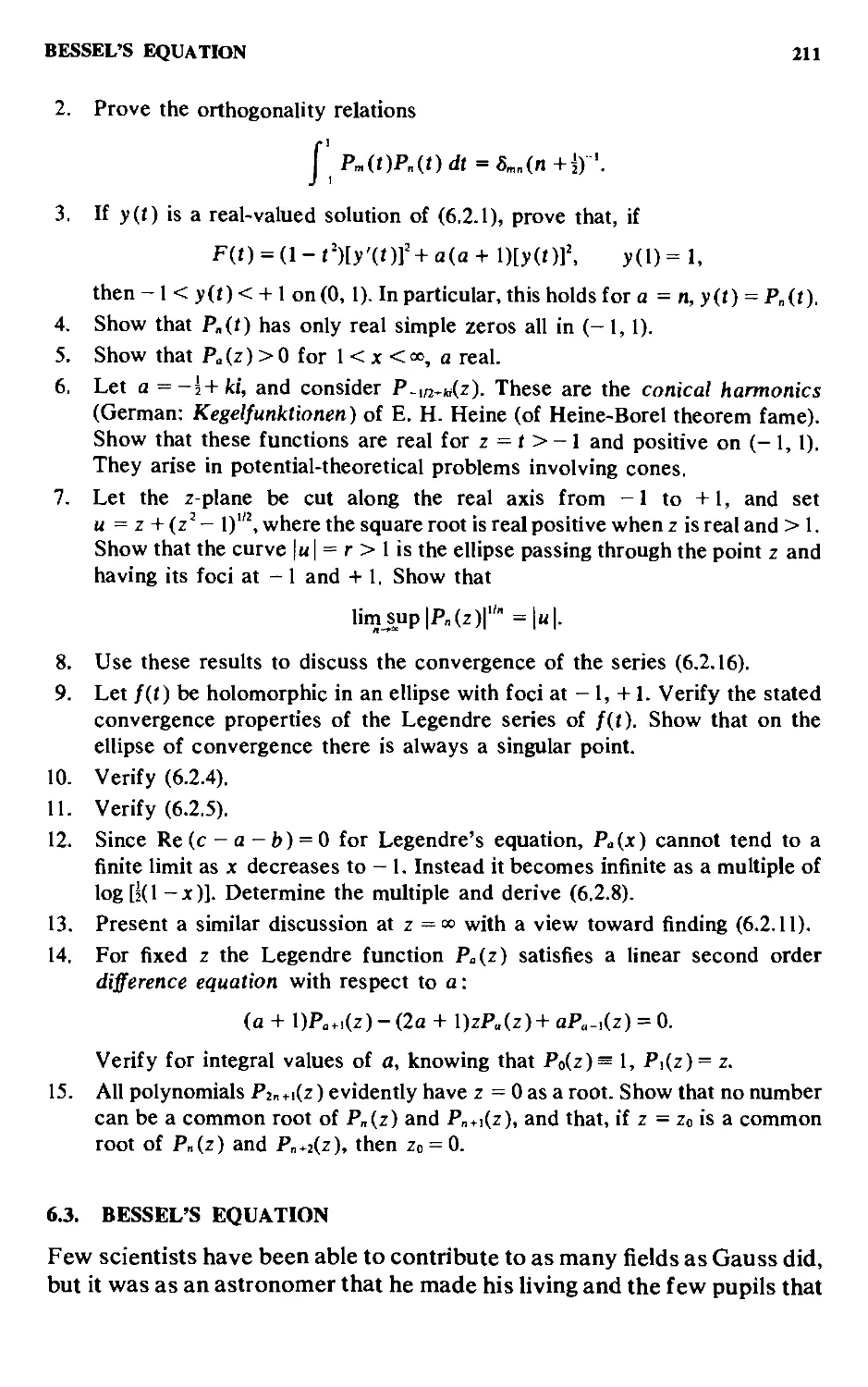
6.2. Legendre's Equation 208
6.3. Bessel's Equation 211
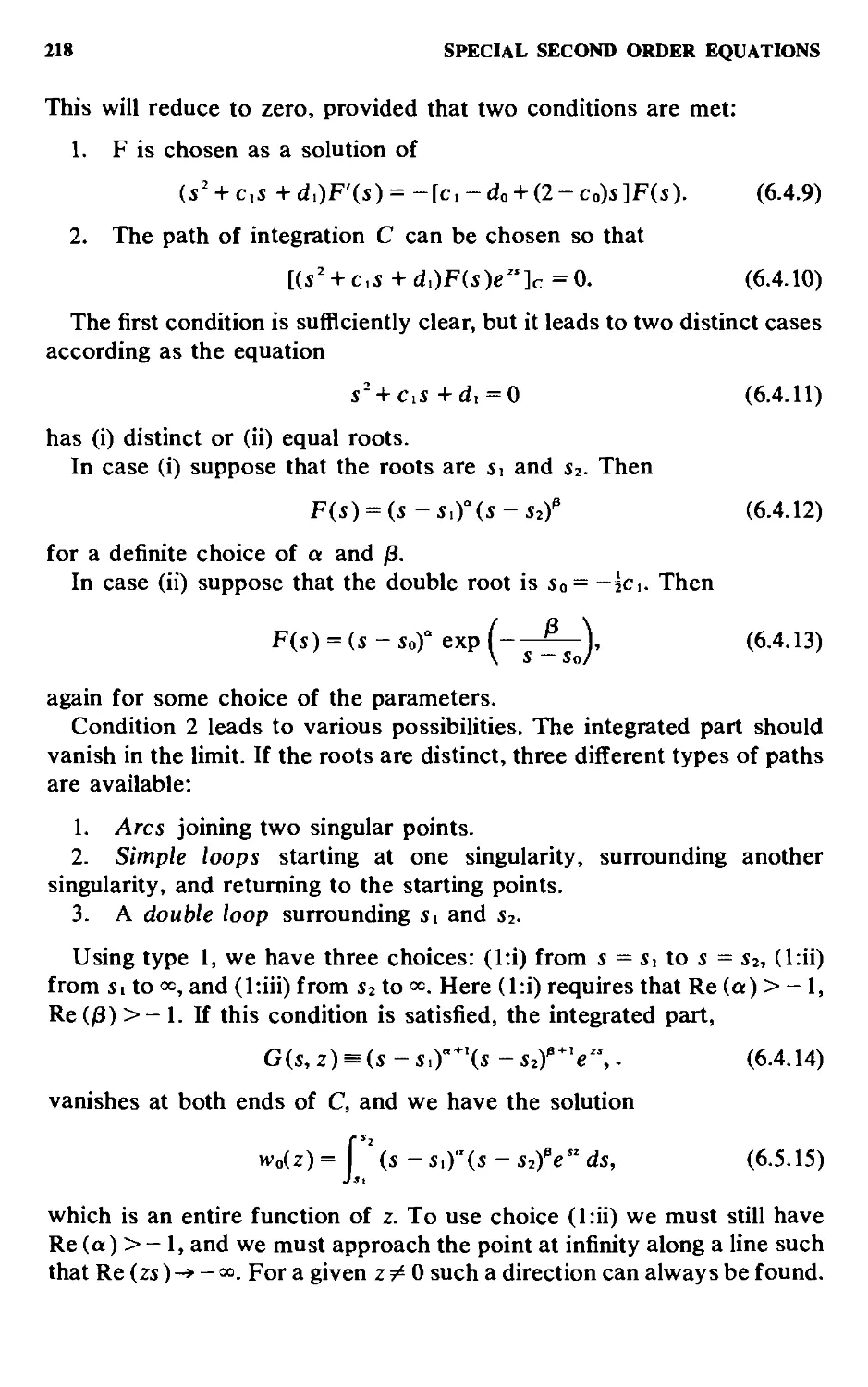
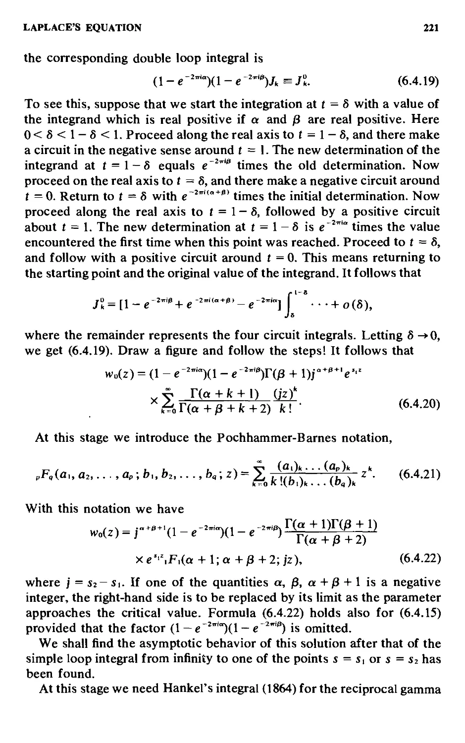
6.4. Laplace's Equation 216
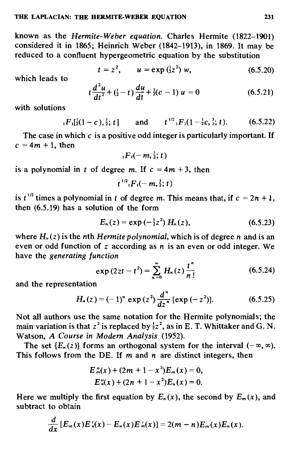
6.5. The Laplacian; the Hermite-Weber Equation;
Functions of the Parabolic Cylinder 228
6.6. The Equation of Mathieu; Functions of the Elliptic
Cylinder 234
6.7. Some Other Equations 242
Chapter 7. Representation Theorems 249
7.1. Psi Series 249
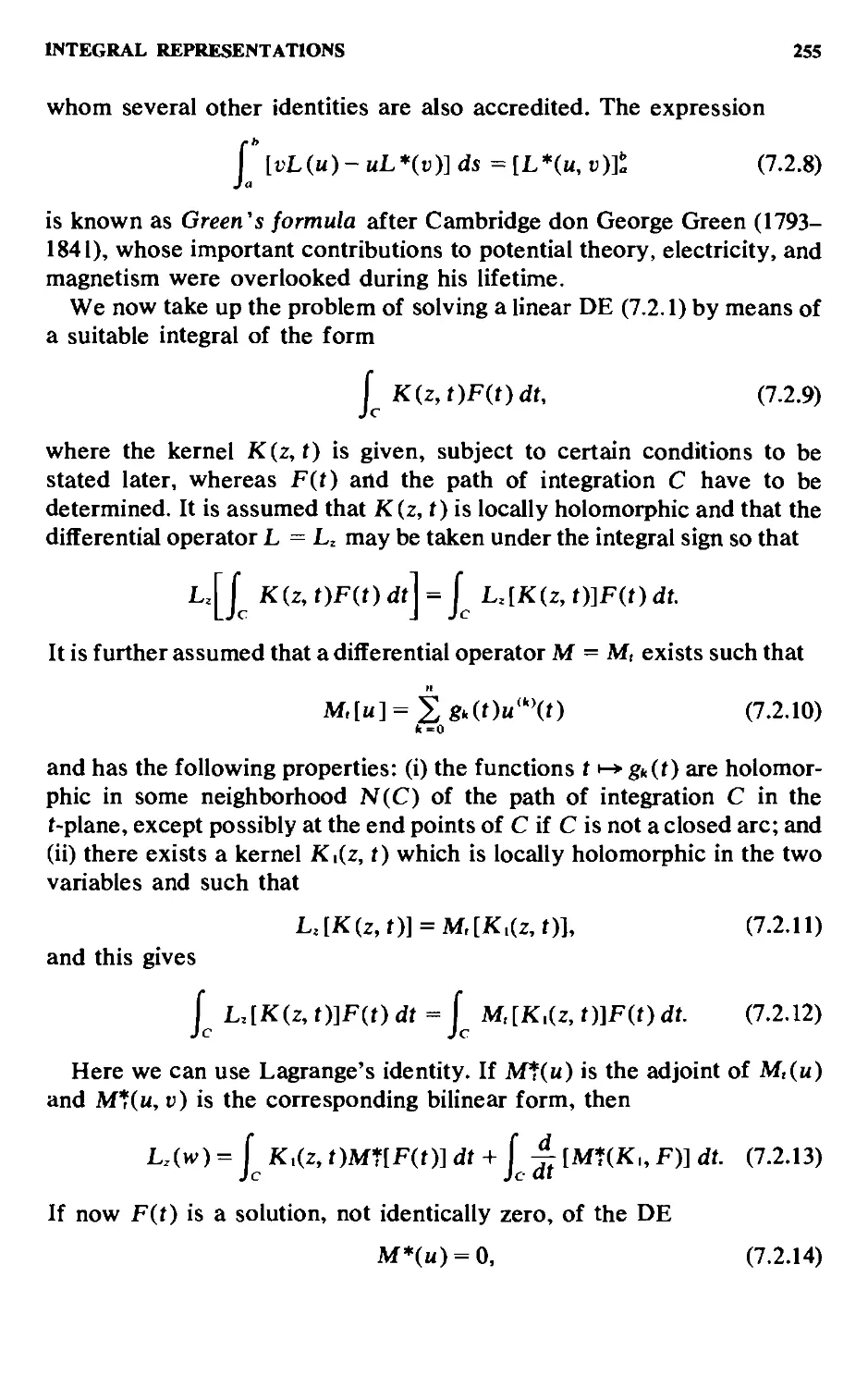
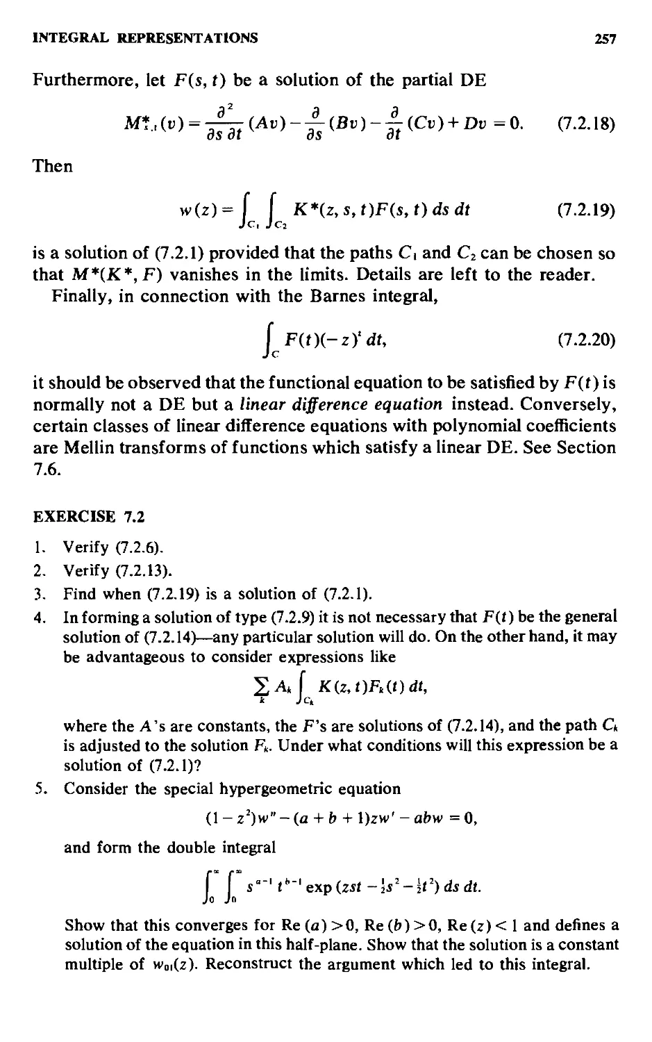
7.2. Integral Representations 253
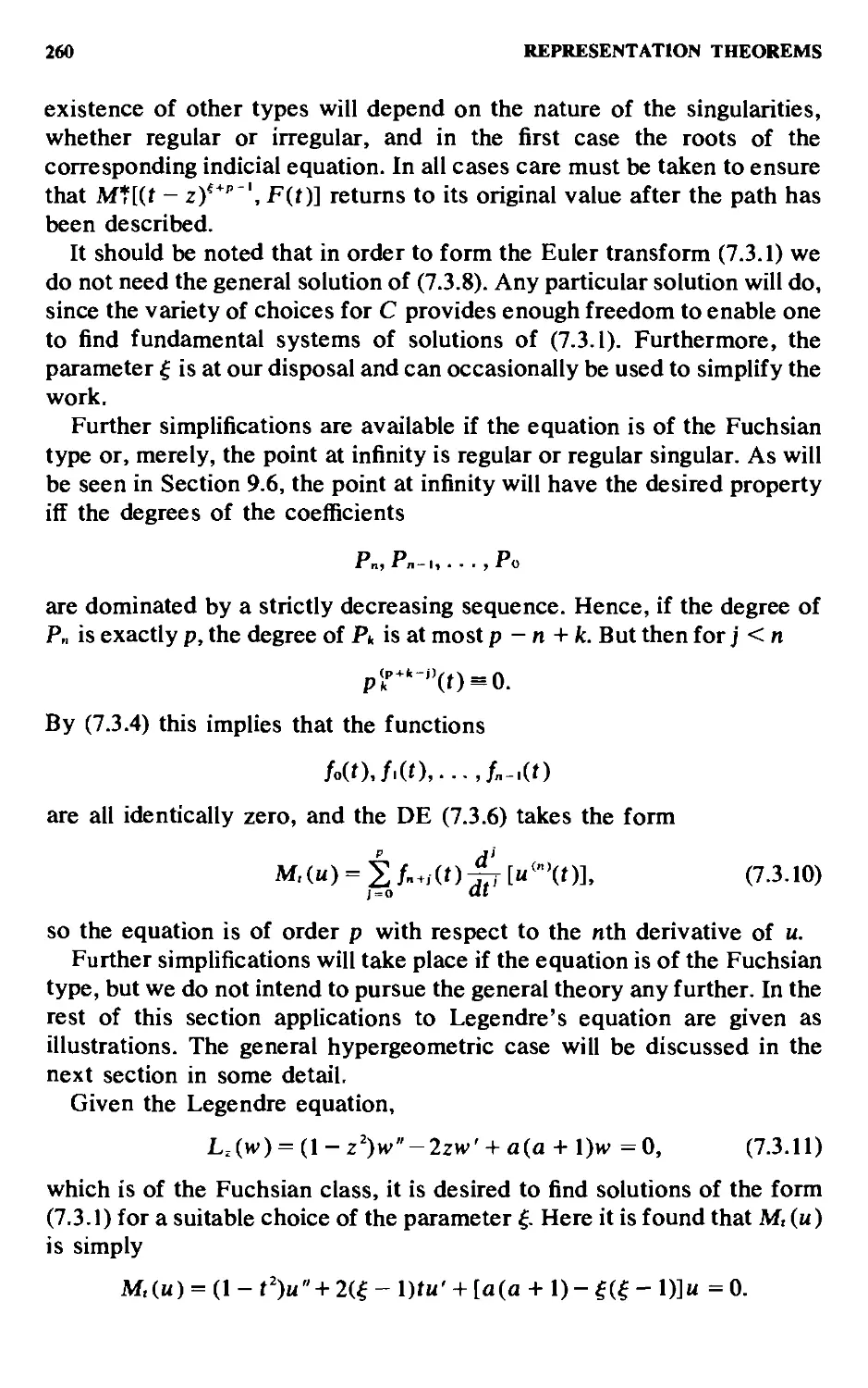
7.3. The Euler Transform ' 258
7.4. Hypergeometric Euler Transforms 265
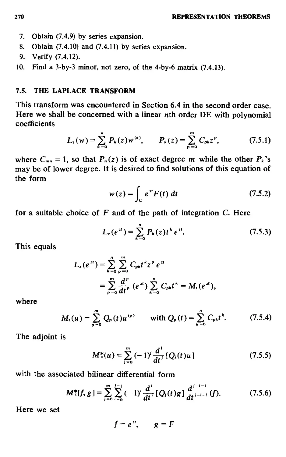
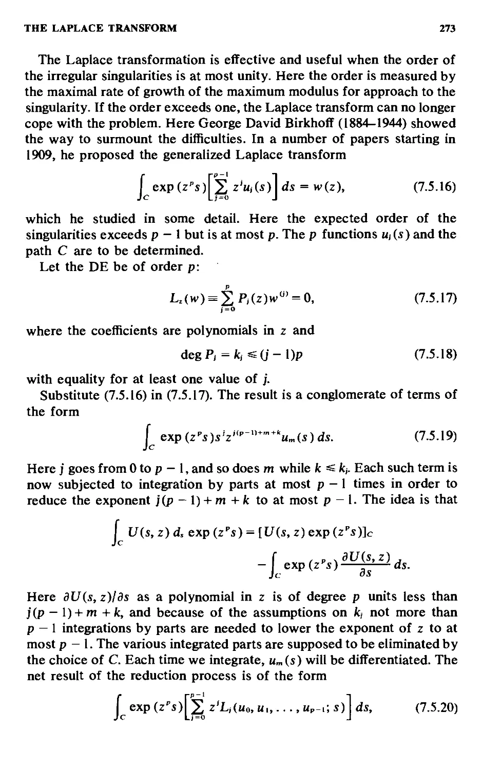
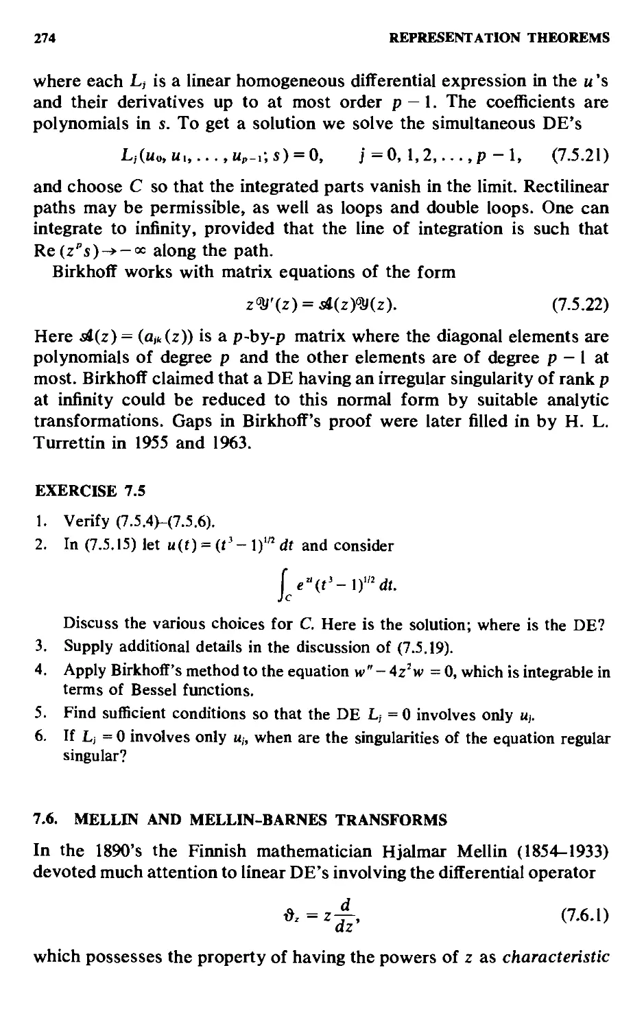
7.5. The Laplace Transform 270
7.6. Mellin and Mellin-Barnes Transforms 274
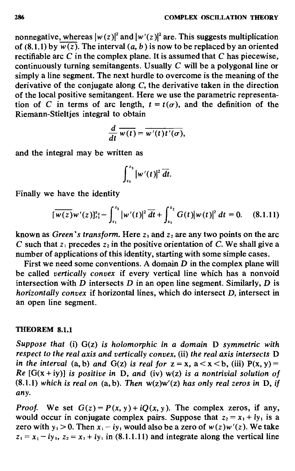
Chapter 8. Complex Oscillation Theory 283
8.1. Sturmian Methods; Green's Transform 284
8.2. Zero-free Regions and Lines of Influence 292

CONTENTS xi
8.3. Other Comparison Theorems 300
8.4. Applications to Special Equations 308
Chapter 9. Linear nth Order and Matrix Differential Equations 321
9.1. Existence and Independence of Solutions 321
9.2. Analyticity of Matrix Solutions in a Star 326
9.3. Analytic Continuation and the Group of Monodromy 328
9.4. Approach to a Singularity 333
9.5. Regular-Singular Points 342
9.6. The Fuchsian Class; the Riemann Problem 353
9.7. Irregular-Singular Points 360
Chapter 10. The Schwarzian 374
10.1. The Schwarzian Derivative 374
10.2. Applications to Conformal Mapping 377
10.3. Algebraic Solutions of Hypergeometric Equations 383
10.4. Univalence and the Schwarzian 388
10.5. Uniformization by Modular Functions 394
Chapter 11. First Order Nonlinear Differential Equations 402
11.1. Some Briot-Bouquet Equations 402
11.2. Growth Properties 408
11.3. Binomial Briot-Bouquet Equations of Elliptic
Function Theory 416
Appendix. Elliptic Functions 427
Chapter 12. Second Order Nonlinear Differential Equations and
Some Autonomous Systems 433
12.1. Generalities; Briot-Bouquet Equations 434
12.2. The Painleve Transcendents 439
12.3. The Asymptotics of Boutroux 444
12.4. The Emden and the Thomas-Fermi Equations 448
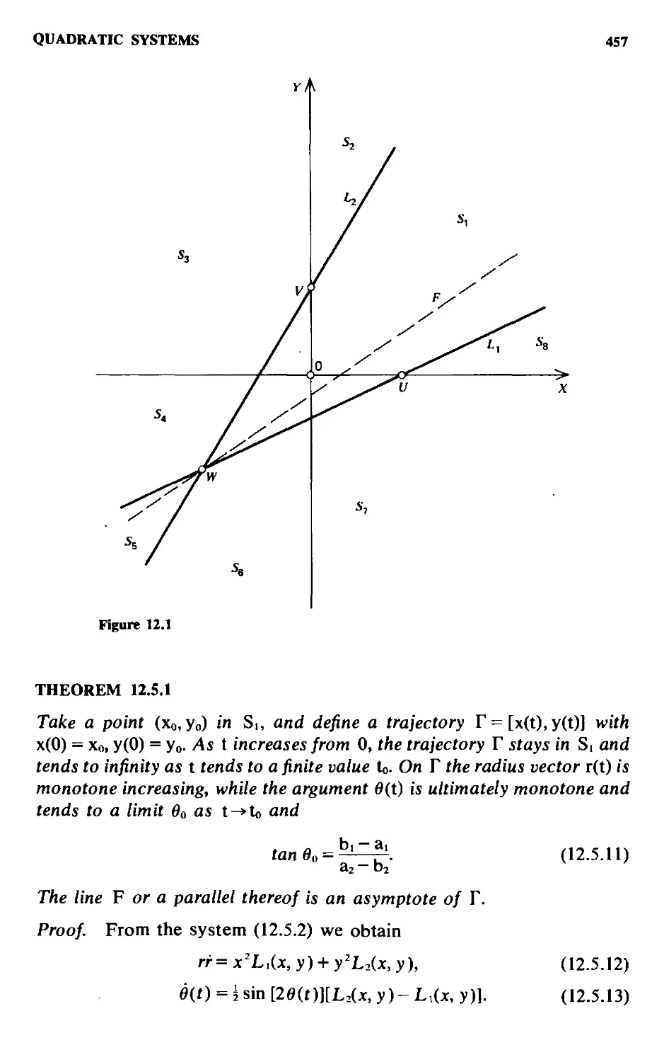
. 12.5. Quadratic Systems 455
12.6. Other Autonomous Polynomial Systems 460
Bibliography 468
Index 471

INTRODUCTION
In this chapter we shall list, with or without proof, various facts which
will be used in the following. They will fall under two general headings: (I)
algebraic and geometric structures, and (II) analytic structures. Under I
we shall remind the reader of abstract spaces, metrics, linear vector
spaces, norms, fixed point theorems, functional inequalities, partial
ordering, linear transformations, matrices, algebras, etc. Under II we
discuss analytic functions: analyticity, Cauchy's integral, Taylor and
Maclaurin series, entire and meromorphic functions, power series, growth,
analytic continuation, and permanency of functional equations. This is
quite an ambitious program, and the reader may find the density of ideas
per page somewhat overwhelming. He is advised to skim over the pages in
the first reading and to return to the relevant material as, if, and when
needed.
I. Algebraic and Geometric Structures
1.1. VECTOR SPACES
The term abstract space is often used as a synonym for set or point set,
but the term usually indicates that the author intends to endow the set
with an algebraic or geometric structure or both. If a Euclidean space R"
Serves as a prototype of a space, we obtain an abstract space by
abstracting (= withdrawing) some of its properties while keeping others.
Incidentally, property is an undefined term (we can obviously not use the
definition ascribed to Jean Jacques Rousseau: La propriete c'est le vol!).
We denote our space by X and its elements by x, y, z, We say that the
space has an algebraic structure if one or more algebraic operations can
be performed on the elements, or if a notion of order is meaningful at least
for some elements.

2 INTRODUCTION
The set is a linear vector space if the operations of addition and scalar
multiplication can be performed. It is required that the set be an Abelian
group under addition, that is, x + y is defined as an element of X, addition
is associative and commutative, there is a unique neutral element 0 such
that X + 0 = X for all x, and every element x has a unique negative, - x, with
X + (- x) = 0.
To define scalar multiplication we need a field of scalars, which is
almost always taken to be the real field R or the complex field C. For any
scalar a and element x there is a unique element ax; scalar multiplication
is associative, it is distributive with respect to addition, and 1 - x = x,
where 1 is the unit element of the scalars.
We speak of a real or a complex vector space according as the scalar
field is R or C. The elements of X are now called vectors. A linear vector
space which also contains the product of any two of its elements is called
an algebra. The set of all polynomials in a variable t is obviously an
algebra, and so is the set of all functions t y-* f{t) which are continuous at
a point (o-
Consider a set of n vectors x, in X, and let the underlying scalar field be
denoted by F. Then the vectors x, are linearly independent over F if
aiX,+ a2X2+-• • + a„x„ =0 A.1.1)
implies that all the a's are zero. They are linearly dependent over F if
multipliers a, can be found so that A.1.1) holds with |ai| + |a2| + - • -f
|a„| >0. Emphasis should be placed on "over F," for restricting F to a
subfield F" or extending it to a larger field F* affects the independence
relations. Thus 1 and 2'" are linearly independent over Q, the field of
rational numbers, but not over A, the field of algebraic numbers. The
space X is said to be of dimension n if it contains a set of n linearly
independent vectors while any n + 1 vectors are linearly dependent. It is
of infinite dimension if n linearly independent vectors can be found for
any n.
The notion of partial ordering is another form of algebraic structure.
We say that X is partially ordered if for some pairs x, y of X there is an
ordering relation x =€ y (equivalently, y 5= x) which is reflexive, proper,
and transitive, that is, (i) x « x for all x, (ii) x =« y and y « x imply x = y, (iii)
x'Sy, y^z imply x'Sz. If X is linear as well as partially ordered, we
should have
x«y implies x + a«y + a for all a, A.1.2)
x«y implies ax^ay fora>0. A1.3)
In this case X has a positive cone X*, defined as the set of all elements
X e X such that 0 ^ x. This positive cone is invariant under addition and

METRIC SPACES 3
multiplication by positive scalars. It contains 0, the neutral element,
usually referred to as the zero element. We now have x«yify-x£ X*.
The set of real valued continuous functions on the closed interval [0,1],
say C[0,1], is an algebra. We define its positive cone X* as the set of
functions t >-»/@ whose values on [0, 1] are nonnegative. We have /«g
if g{t)-fit) is nonnegative in [0,1].
A more prosaic example may be helpful: the fowl in a hen-yard are
partially ordered under the pecking order.
EXERCISE 1.1
1. Consider the space of all polynomials P(r) in a real variable which take on
real values. Show that X is an algebra,
2. An order relation P < Q is established in X by defining P as positive if its
values are positive for all large positive values of t. Show that this ordering is a
trichotomy in the sense that for a given P there are only three possibilities: (i)
P is positive, (ii) - P is positive, or (iii) P = 0.
3. An order relation is said to be Archimedean if x < y implies the existence of
an integer n such that y < nx. (The natural ordering of the reals is
Archimedean.) Show that the order defined in Problem 2 is non-Archimedean
inasmuch as the elements fall into rank classes Rt, where jRj consists of all
polynomials of exact degree k, each Rk is Archimedean, but if / is a positive
element of Rj and g a positive element of Rt with / < k, then f <g and nf <g
for all n. Verify.
4. Prove that l,t,t\... ,t° are linearly independent over R. What is the
dimension of the space formed by these elements?
1.2. METRIC SPACES
A metric space is one in which there is defined a notion of distance
subject to the following conditions;
D|. For any pair of points P and Q of X a number d{P, 0M=0 is
defined, called the distance from P to Q such that d(P, Q) = 0 iff P = Q.
. D,. d(P, 0) = d@, P).
D,. For any R we have d(P, Q)« d(P, R) + d{R, Q).
These notions go back to the work in the 1890's of Hermann Minkowski
A864-1909) on what he called the "geometry of numbers." He was chiefly
concerned with the extremal properties of linear and of quadratic forms, for
which he found altemativedefinitions of distance, adjusted to the problem in
hand. Minkowski did not always require D2. Condition D3 is the triangle
inequality.

4 INTRODUCTION
We say that a linear vector space is normed if the following conditions
hold:
Ni- For each x £ X there is assigned a number ||x{| 2= 0 such that ||x|| = 0
iff X = 0.
N2. ||ax|| = |al||x|| for each a in the scalar field.
N,. ||x + yH||x|| + ||y||.
A normed linear vector space becomes a metric space by setting
d(x,y) = ||x-y||. A.2.1)
In a metric space we can do analysis since the fundamental operation of
analysis, that of finding limits of a sequence, becomes meaningful. If {x,,}
is a sequence in the metric space X, we say that x„ converges to Xo and
Xfl = limx„ if lim d(xfl,x„) = 0. A.2.2)
We say that {x„} is a Cauchy sequence if, given any e > 0, there exists an
N such that
d(x„, x„)<€ form, n>N. A,2.3)
If A.2.2) holds, it follows that {x„} is a Cauchy sequence, but the converse
is not necessarily true, for there may be gaps in the space, A metric space
X is said to be complete if all Cauchy sequences converge to elements of
the space. Euclidian spaces are complete, and so are various function
spaces that will be encountered in the following. The space Q of rational
numbers is not complete.
Various notions of real analysis are meaningful in complete metric
spaces, such as the concepts of closure, open set, closed set, and
e-neighborhood. The Bolzano-Weierstrass theorem need not be valid in a
complete metric space, that is, there may be bounded infinite point sets
without a limit point. Incidentally, "bounded" means that the set can be
enclosed in a "sphere" d(x,Q)<R. The topological diameter d{S) of a
subset of X is the least upper bound of the distances d(x, y) for x and y in
S-
EXERCISE 1.2
1. The Euclidean norm ||x||2 of X in C is [2;., |Xjpl"^, wherex = (x,,X2,., .,x„)and
the x's are complex numbers. Alternative norms are ||x||, = 2(=i |x,| and
||x||. = sup|x,|. Show that they are indeed acceptable norms. Between what
limits do they lie if ||x||2= 1?
2. How do you define an open set in these three normed topologies? Show that a
set open in one of them is also open with respect to the others. Verify that C"
is complete in all three metrics.

MAPPINGS 5
3. Let X = C[0, 1] be the set of all functions, 11-^ f{t), continuous in the closed
interval [0, 1], Define a Cauchy sequence if ||/|| = supo„si |/(f )|. and show that
the space is complete.
1.3. MAPPINGS
We shall study mappings from a metric space X into a metric space Y,
both being complete. Wc shall often have Y = X.
The mapping T is a pairing of points x of X with points y of Y, say (x, y).
Here to every x of X is ordered a unique y of Y. To Xi 9^ \2 correspond the
two values y, and y^, which may or may not be distinct, in fact every x e X
may be mapped on the same point yoEY. The mapping is onto (a
surjection in the Bourbaki language) if every point of Y is the image y of
at least one x in X. It is A,1) (read "one to one") if
X, ?^X2 implies yi = T(x,) ?^ T(x2) = y2. A.3.1)
The mapping is hounded if there exists a finite M such that
d[T(x,),T(x2)]«Md(x„X2). A.3.2)
This is a generalized Lipschitz condition and implies continuity of T(x)
with respect to x.
If X and Y are linear vector spaces over the same scalar field, and if
T(a,x, + 02X2) = a,T(x,)+ a2T(x,), A.3.3)
then T is called a linear transformation. It is bounded iff
d[T(x),0]^Md(x,0). A.3.4)
The most important case is that in which X and Y are complete normed
linear vector spaces, in which case the spaces are called Banach spaces
after the Polish mathematician Stefan Banach A892-1945), who termed
them B-spaces. In this case A.3.4) takes the form
||T[x]H M||x||. A.3.5)
If T is a linear transformation, then T@) = 0 and the transformation is
('l.l)if
T(x) = 0 implies x = 0.
If X and Y are B-spaces, the set E(X, Y) of linear bounded
transformations on X to Y is also a B-space under the norm
||T|| = sup||T[x]||, A.3.6)
the supremum being taken with respect to all elements x of X of norm 1. The

6 INTRODUCTION
algebraic operations in E(X, Y) are defined in the obvious manner by
[T, + T,][x] = T,[xl + Ux], (aT)[x] = aT[x]. A.3.7)
If Y = X, we write E[X] for E[X, X] and note that products are definable in
the obvious manner by
(T,T.)[x]=T,(T2[xl). A.3.8)
This gives
l|7'.T.H||T,||||T.||. A.3.9)
It may be shown that E(X, Y) and E(X) are complete in the normad metric,
so they are B-spaces. Also, E(X), which is a normed algebra, actually is a
B-algebra since it is a B-space and satisfies A.3.9).
If T £ E(X) and is A,1), there is an inverse transformation T~' such that
T-'[T[xll = x, Vx, T[T-'[y]] = y ify=T[x]. A.3.10)
EXERCISE 1.3
1. Show that E(C") is complete. Use any of the metrics for C listed in Problem
1.2: 1.
2. If T is a linear transformation, verify that T@) = 0. Here on the right stands
the zero element of Y, while on the left we operate on the zero element of X.
[Hint: T@ + 0)= 7@).]
3. If T is A,1), why does T(x) =0 imply x = 0 and vice versa?
4. Why is A.3.6) a norm? Show that it is the least value that M can have in
A.3.5).
5. Prove A.3.9).
1.4. LINEAR TRANSFORMATIONS ON C"
INTO ITSELF; MATRICES
The simplest of all 1 inear transformations are those which map C" into itself.
If T is such a transformation, then T is uniquely determined by linearity and
its effect on the basis of C". Any set of n linearly independent vectors would
serve as a basis, but we may just as well use the unit vectors
e,=(8i<,), A.4.1)
where 8^ is the Kronecker delta, that is, the vector whose jth component is
one, all others being zero. This gives
x = x,e, + X2e2+-■ •+x„e„, A.4.2)
if X = (x 1, X 2,..., x„) in the coordinate system defined by the vectors e/. Now

TRANSFORMATIONS ON C"; MATRICES
T takes vectors into vectors, so there are n ^ complex numbers a^ such that
T[ek] = a,ke,+ a2)<e2 + -• • +a„>,e„, k = 1,2,...,«. A.4.3)
The linearity of T then gives
T[x]=T(^x,e,) = ^x,T[e,]
\k=l I fc-l
or
A.4.4)
from which we can read off the components of the vector y.
The quadratic array
flu 0,2 • • • ai„
Oji 022 • • • a2„
Onx a„2 • • • fln
A.4.5)
is known as a matrix—more precisely, the matrix of the transformation T
with respect to the chosen basis. We can now write T symbolically as
y = T[x] ^d-x,
A.4.6)
where the last member may be considered as the product of the matrix d
with the column vector x, the result being the column vector y.
We have to decide when the mapping defined by T is A,1). Here the
condition T[x] = 0 implies that x = 0 now takes the form that the
homogeneous system
Sa,-,x, =0, ; = 1,2,...,«, A.4.7)
must have the unique solution
Xi = X2 = • • • = x„ =0.
This will happen as long as
del (d) 9^0. A.4.8)
In this case the mapping is also onto, since for a given vector y we can
solve the system
^a,kX, = y„ / = 1,2,...,«, A.4.9)
k = l
uniquely for x = (x,, X2,..., x„). It follows that T has a unique inverse,

8 INTRODUCTION
also an element of E[C, i.e., a linear bounded transformation of C" into
itself. With this transformation goes a matrix si~\ which we refer to as the
inverse of d. The fact that its elements may be computed from A.4.9)
shows that the element in the place (j,k) is Ak,/A, where A/t is the
cofactor of 0,^ in the determinant i = det (d).
We can define algebraic operations and a norm in the set Wt„ of n-by-«
matrices in terms of which the set becomes a Banach algebra. This
follows from the fact that there is a A,1) correspondence between the
linear transformations T in £@") and their matrices. Then to Ti + T2, aT,
and TiTz correspond
(%+fo;,)^5H-g5, A.4.10)
(aOjO^a^l, A.4.11)
(S aimfcm.)^54g5. A.4.12)
A number of different but equivalent norms may be defined for 3Jt„. A
suitable one for analysis is
M = maxX|a,.|. A.4.13)
' k=l
We have then
Since 3K„ is complete in the normed metric (why?), it follows that 3K„ is a
B-algebra.
We have seen that si has an inverse iff det (si) 9^ 0. If this is the case, si
is said to be regular; otherwise, singular. Together with the given matrix
d we consider the family of matrices
k%-d,
where A runs through the complex field C and % = {Sjk) is the «-by-n unit
matrix. These matrices are normally regular, but there exist n values of A
for which A'i - si is singular: the n roots of the characteristic equation of
det(A^-5l) = 0. A.4.14)
The roots Ai, A2,..., A„ form the spectrum a-(d) of d. They are known as
characteristic values, latent roots, or eigenvalues. For these values of A
one can find vectors x^ in C" of norm 1 such that
d-Xi, = AtXfc. A.4.15)
The characteristic vectors Xt are linearly independent and may be chosen
so that they form an orthogonal system; in this case the inner product

FIXED POINT THEOREMS 9
(x,y) = ^Xjyj=0 A.4.16)
for X = Xk, y = x„, k^ m. This holds even if A.4.14) has multiple roots. A
matrix si is singular iff zero belongs to the spectrum.
EXERCISE 1.4
1. Find the elements of i4 ' when A is regular.
2. Verify the inequality for the norm of the matrix product.
3. Prove the Hamilton-Cay ley theorem, which asserts that the matrix A satisfies
its own characteristic equation.
1.5. FIXED POINT THEOREMS
The Dutch mathematician L. E. J. Brouwer proved in 1912 that a
continuous map of the unit ball in R" into itself must necessarily leave at
least one point invariant. Such a point is known as a fixed point, and an
assertion about the existence of fixed points is known as a fixed point
theorem. We shall prove some theorems of this nature. We start with a
theorem proved by S. Banach in his Krakow dissertation of 1922. It refers
to mappings of a complete metric space by a contraction, i.e., a bounded
transformation of the space X into itself such that
d[T{x),T(y)]^kd(x,y), A.5.1)
where fe is a fixed constant, 0 < ik < 1. Such a mapping evidently tries to
shrink the object. Banach's theorem states that there is a point which does
not move.
THEOREM 1.5.1
// T IX a contraction defined on a complete metric space X, then there is
one and only one fixed point.
Proof. The triangle inequality plays a basic role here. We start with an
arbitrary point x, ^X and form its successive transforms under T:
x„., = T(x„), « = 1,2,.... A.5.2)
These elements form a Cauchy sequence, and X being a complete metric
space, Xo = lim x„ exists and is to be proved to be a fixed point—in fact,
the only such point. Now it is sufficient to prove that, given any £ > 0,
there is an N such that
d(x,„x„,p)<£, n>N, p = l,2,

10 INTRODUCTION
To this end we note that by the triangle inequality the left member does
not exceed
d(x„,x„^,) + d(x„+„x„+j)+- • • + d(x„+p_,,x„+p).
Now, using the contraction hypothesis, we see that
d(x„, x„.,)« fed(x„,-,, x„,) ^ • • • ^ fe'" "'d(x,, xj)
and thus
d(x„, x„.p) ^(fe"-' + fe" + • • • + fe''*''-')d(x„ X,)
1-fe
d(x„X2).
This expression can be made as small as we please by choosing n large
enough. Hence {x„} is a Cauchy sequence regardless of the choice of x,,
and the limit Xo exists. Since
x„+, = T(x„),
we conclude that
Xo = limx,,*, = lim T(x„)= T[limx„] = T(Xo),
where we have used the continuity of T. It is seen that Xo is indeed a fixed
point.
Suppose that y„ is a fixed point. Then
d(x„, yo) = d[T(x„), T(yo)] ^ fed(x„, yo).
Since fe < 1, this implies that d(Xo, yo) = 0 or yo = Xo, so there is one and
only one fixed point. ■
The restriction to contraction operators is a drawback, but it can
occasionally be avoided by observing the following.
COROLLARY
There is a unique fixed point if some power of T is a contraction.
Proof. If T" is a contraction, then there exists a fixed point Xo such that
T"'(Xo) = Xo. We have also
limCT-rCxO^Xo
for any choice of Xi. Here we set Xi = T(Xo) and find that
(T")" [T(Xo)] = TUT-rCxo)] = T(x.,).
When n becomes infinite, the first member tends to Xo, so we have
T(Xo) = Xo or T admits Xo as a fixed point. Since any fixed point of T is a

FIXED POINT THEOREMS 11
fixed point of T" and the latter has a unique fixed point, it follows that Xo
is the unique fixed point of T. ■
Vito Volterra A860-1940), in his discussion of integral equations with
variable upper limits of integration, proved the uniqueness of the
solutions. From his work in the 1890's we can distill a fixed point theorem
which is rather useful.
THEOREM 1.5.2
Let \ he a B-space. Let Zo he a given element of X, and let S belong to
E(X) and he such that
l:i|Sl|<oc. A.5.3)
0.
Then the transformation
T(x) = z„ + S[x] A.5.4)
has a unique fixed point Xo given hy
x„ = Zo+|:S"[z<,]. A.5.5)
It is enough to observe that the series converges in norm by A.5.3) and
S can be applied termwise to the series and shows that T(Xo) = Xo. The
uniqueness proof is left to the reader.
Consider, in particular, Volterra's equation
f(t)^g(t)+l' K(s,t)f(s)ds. A.5.6)
Jo
Here the kernel K(s, t) and g{t) are known and f(t) is to be found. We
consider the particular case in which the kernel is a function of s alone.
THEOREM 1.5.3
Suppose that g(t) e C[0, a] and K(s) e L@, a). Then the equation
f(t) = g(t)+ f'K(s)f(s)ds A.5.7)
Jo
has a unique solution in C[0, a], namely,
f(t) = g(t)+ £ K(s) exp [!' K(u)du]g(s)ds. A.5.8)
The verification is left to the reader.

12 INTRODUCTION
COROLLARY
For K(t) - K the equation
f(t) = g(t) + Kf'f(s)ds A,5,9)
Jo
has the unique solution
f(t) = g(t) + K f' exp [K(t - s)]g(s) ds. A.5.10)
Jo
EXERCISE 1.5
1. Verify Theorem 1.5.2.
2. Verify Theorem 1,5.3.
3. Verify the corollary.
4. If Tl/KO = K U /(s) ds, find T\ Is T a contraction? What are the conditions?
For a given interval [0, a] find m so that T" is a contraction.
5. Let C*[0,a] denote the set of nonnegative functions continuous in [0, a]. The
mapping
T[/1@= I' {t - s)f{s) ds
Ju
is clearly a mapping of X into itself. Is it a contraction? Find T", and study its
contractive properties. Find a fixed point by inspection.
1.6. FUNCTIONAL INEQUALITIES
This is afield of increasing importance. We shall consider inequalities of
the form
f{t)^T[f](t). A.6.1)
We consider a complete metric space X, the elements of which are
mappings from some interval [a,h] in R'. Here T is a mapping of X into
itself, and the problem is to discuss the inequality. Can it be satisfied by
elements / of X? Is it trivial in the sense that it is satisfied by all /'s in X?
If neither of the above is true, characterize the elements of X for which
A.6.1) holds. Is it so restrictive that it holds for one and only one /? It can
be seen that there are a number of pertinent questions.
The discussion in Section 1,5 leads to several functional inequalities
which are categorical or determinative in the sense that there is a single
element of the space under consideration which satisfies the inequality. If
in A.5.7) and A.5.9) we assume g to be identically zero, then / is
identically zero. This suggests

FUNCTIONAL INEQUALITIES 13
THEOREM 1.6.1
Let X he the positive cone of C[0,a], 0<a<=c. Let K(t)eL@,a),
continuous and nonnegative on the half-open interval @, a]. // f eX and
if for O'St'Sa
f(t)«f'K(s)f(s)ds, A.6.2)
Jo
then f is identically zero.
Proof. This functional inequality is very important for the theory of
differential equations (DE's) since it underlies uniqueness proofs based
on a Lipschitz or, more generally, a Carath6odory condition. We shall
obtain the theorem as a consequence of more general theorems, but in
view of its importance it is desirable to give a direct short proof. Set
F{t)=\' K{s)f(s)ds. A.6.3)
Jo
This is an element of X and F@) = 0. Furthermore, for 0 < f
F'(t) = K{t)f(t)^K(t)F(t),
so that A.6.2) implies that
F'(t)-K{t)F(t)^0. A.6.4)
This we multiply by the positive function exp[-/o K{u)du], and the
result is an exact derivative so that
d^
dt
{F(Oexp[-|'x(H)dH]}^0.
Since F@) = 0, this shows that F(t)^0 for 0<f «a. But we already
know that F{t)^0. To satisfy both inequalities we must have F{t) = 0.
This implies that /(O = 0, as asserted. ■
A uniqueness theorem due to Mitio Nagumo A926) goes back to the
following functional inequality:
THEOREM 1.6.2
Let X he the suhspace of C*[0, a], the elements of which satisfy f@) = 0,
/imhiof(h)/h = 0. Then, if (EX, and if
f(t)«f'f(s)^,
Jo s
then
f(t)^0. A.6.5)

14 INTRODUCTION
A proof may be given using A.6.3) with K(s) replaced by s~', which is
not integrable down to the origin. The proof is left to the reader.
There are several other uniqueness theorems which also go back to
functional inequalities. We shall not pursue these cases any further but
instead proceed to the use of fixed point theorems in the discussion of
functional inequalities. We have
THEOREM 1.6.3
Let X he a complete metric space which is partially ordered in such a
manner that if {x„} is an increasing sequence in X, so that \„« x„+i for all
n, and if lim„^^ x„ = Xo exists in the sense of the metric, then x„ =« Xo for all
n. Let T he an order-preserving mapping of X into X such that T" is a
contraction for some m. Let fo he the unique fixed point of T. Then
f«T[f] implies f«fo. A.6.6)
Proof We say that T is order-preserving if for /,, /z e X
/,^/2 implies T[/,]«T[/d. A.6.7)
Suppose that / e Xo, the subset of X for which the inequality is
meaningful. Since Xo contains fa at least, it is not void. Then
/«r[/]«r[/i^---^r'[/]«•••.
Now T" [/] tends to the limit /o as n ^ <» for
lirn^ r- [r (/)] = /o, / = 0,1,..., wi -1,
since T" is a contraction and the limit is the same for all elements of X. It
follows that the increasing sequence {T"[/]} converges to fo. Since order
is preserved under the limit operation, we have / «/o and the theorem is
proved. ■
If T[f] is defined by A.6.3), T is order-preserving since the kernel K{s)
is nonnegative and the space X is linear. Here T usually does not define a
contraction, but all powers T" with a sufficiently large m are contractions
for
8)
T''[m)^-~^j'^ K{s)[j'^ K{u) duj' f(s)ds, A.6.
the norm of which goes rapidly to zero as n becomes infinite. This
provides another proof for Theorem 1.6.1.
We can also apply the Volterra fixed point theorem to functional
inequalities.

FUNCTIONAL INEQUALITIES 15
THEOREM 1.6.4
Let \ he a partially ordered B-space such that the positive cone X* is a
closed point set. Let S he a linear hounded positive transformation on X
to X and such that
i||Sl|<oc. A.6.9)
n=l
Let g he a given element of X*, and U the unique fixed point of
T[f] = g + S[f]. A.6.10)
Then
f«g + S[f] implies f^U. A.6.11)
Proof. That S is positive means that it maps X* into itself. All the
powers of S are then also positive and S is order-preserving. The
existence of a unique fixed point follows from Theorem 1.5.2. We have
lim„_^ T"[/] = /o for any /—in particular, for an / satisfying the first
inequality under A.6.11). Now we have
T"[/] «g + S[g] + S\g] + ■■■ + S"-'[g] + S"[/]. A.6.12)
This is an increasing sequence which goes to the limit /o as n becomes
infinite. This, combined with / « T\J] and the order-preserving properties
of limits, leads to the desired result. ■
We state a couple of applications of this theorem which are of special
importance to the theory of DE's.
THEOREM 1.6.5
Let K G C*(a, b) D L(a, b), and let g and f belong to C*[a, b]. Suppose
that for all t in [a, b]
f(t)«g(t)+f'K(s)f(s)ds. A.6.13)
Then
f(t) «g(t) + I' K(s) exp I' K(u) du]g(s) ds. A.6.14)
The proof is left to the reader. We see that if g(t) = 0; then f{t) = 0 and
Theorem 1.6.1 is again obtained. It is worth while stating the case
K{t) = K as a separate result.

16 INTRODUCTION
THEOREM 1.6.6
// K(t) = K and f and g are in C*[a, b], then
implies that
if g(t) IS also
implies that
f(t)«g(t) + K|'f(s)ds
f(t) ^ g(t) + K 1' exp [K(t - s)lg(s) ds.
a constant, then
f(t)«g+K|^'f(s)ds
f(t)^gexp[K(t-a)].
(i.6.15)
A.6.16)
A.6.17)
A.6.18)
The inequalities listed under Theorems 1.6.5 and 1.6.6 are known as
Gronwairs lemma after the Swedish-American mathematician Thomas
Hakon Gronwall A877-1932), who found a special case in 1918 when
investigating the dependence of a system of DE's with respect to a
parameter. Gronwall was a pupil of Gosta Mittag-Leffler A846-1927),
who also taught Ivar Bendixson A861-1935), Ivar Fredholm A866-1927),
Helge von Koch A870-1924), and Johannes Malmquist A888-1952). All
of them will figure somewhere in this treatise; the first three were among
the teachers of the present author. A theorem proved by Bendixson in
1896 (see Theorem 2.8.2) may be regarded as a forerunner of Gronwall's
lemma.
EXERCISE 1.6
1. Prove Theorem 1.6.2.
2. Prove the following analogue of Theorem 1.6.5 for Nagumo's kernel. Let X
be the space of functions / defined on [0, a] so that (i) fBC*[0,a], (ii)
lim,i„/(O = 0, (iii) lim,io/@/f =0, (iv) f(t)lfBL{0,a). Define a norm in
terms of which X becomes a complete metric space. If / and g belong to X (g
fixed), then
f{t)^g(t)+ \ f{s)s-'ds implies f{t)^g{t') + t\ g{s)s-'ds.
3. Verify A.6.8).
4. Prove Theorem 1.6.5.
5. Prove Theorem 1.6.6.
6. Prove the following theorem. If / and g E C*[a, b], iand if
f{t)^ g(t)+ K' ^\t - S)fis) dS!,

HOLOMORPHIC FUNCTIONS 17
then
fit) ^g{t) + KJ' sinh [Kit - s)]g(s) ds.
7. Show that the inequality
f{t)^-i-U{t)Y
is absurd for real-valued elements of C[a,b].
8. Show that the inequality 4/(f) ^ 3 + IfiOY is trivial for real-valued elements of
C[a,b].
9. Show that 6/Ff) ^ 3/C0 + 2/B0 is determinative for / e C*[0, a], 0 < a ^
+ 00. Show that there Eire solutions unbounded for approach to zero of the form
t'" if p >Po. the positive root of a certain transcendental equation. There are
also solutions of the form - r" for q < po- Can such solutions be combined? If
so, how?
II. Analytical Structures
1.7. HOLOMORPHIC FUNCTIONS
There are three essentially different approaches to analytic function
theory, associated with the names of Bernhard Riemann A826-1866),
Augustin Louis (Baron) Cauchy A789-1857), and Karl Weierstrass A815-
1897), respectively. Riemann's approach was largely geometric and
physical (potential theory). His conformal mapping theorem will figure
later, particularly in Chapter 10, but in the main our approach will be a
mixture of that of Cauchy and that of Weierstrass.
The complex variable z = x + iy is represented geometrically by the
points of R^, the euclidean plane, so that to Zo = Xo+ lyo in C corresponds
the point (Xo, yo) of R\ We have
z = r{cose + i sme) = re", A7.1)
where
r = +(x' + y')"', tanfl = -^. A.7,2)
We write x = Re B) (read "x is the real part of 2"), y = Im B) (read "y is
the imaginary part of 2")- Furthermore, r = |2| is the absolute value of z,
and d = arg 2 is the argument of 2, which is determined only up to
multiples of 2it. We have
|^, + 2,|«|2,| + N, |a2| = |a||2|, |2,2,| = |2,||2,|, A-7,3)
so that (assuming a higher standpoint) C is a B-algebra, the simplest of the
species.

18 INTRODUCTION
The equation \z - 2„| = r represents a circle in the complex plane with
center at 2„ and radius r. The interior and the exterior of this circle are
given by the inequalities \z - Zo\<r and \z - Zn\ > r, respectively. The
former will often be called a circular disk in the following discussion and
is a circular neighborhood of 2o. The upper half-plane is given by
Im B) >0; the left half-plane, x < a, by Re B) < a. If lim \zo- 2„ | = 0, we
say that lim z„ = 2o and {z„} is a Cauchy sequence. The complex plane is a
complete metric space in terms of the norm defined by the absolute value.
Every bounded infinite point set S has at least one limit point (theorem of
Bolzano-Weierstrass). A set which contains its limit points is said to be
closed. A set G is open if, whenever Za E G, there is an e-neighborhood,
\z ~ Zu\ < €, the points of which belong to G. We shall call a set S in the
complex plane connected if for any two of its points, 2,, 22 say, there is a
polygonal line joining 2, with 22 all the points of which are in S. An open
connected set is called a domain and will be denoted by D. The term
region is also used, but we reserve this term for sets which have a
nonempty interior Int (S) ^ 0 and contain some of their boundary points.
So far we have dealt with the finite plane. We extend this by adjoining
an ideal point: the point at infinity. Stereographic projection makes it
possible to visualize this addition. Take a sphere of radius 5 tangent to the
2-plane at the origin, the "south pole" on the sphere. Join the point 2 in the
plane with the "north pole" by a straight line. This line has a second
intersection P with the surface of the sphere, and P is taken as the spherical
representative of 2. The finite plane is mapped on the sphere omitting the
north pole, and the latter becomes the representative of the point at infinity.
The chordal distance between two points, 21 and 22, in the plane is the length
of the chord joining their representatives, P, and P2, on the sphere. Chordal
distances are bounded, being equal at most to one.
We have now a sufficient set of notions in terms of which we can define
holomorphic functions. Let D be a domain in the 2-plane and consider a
A, 1) mapping of D into C. This mapping T defines a function 2 >-»/B),
where f{z) denotes the image of 2. The mapping is continuous at
2 = 2o G D if for every €-neighborhood of/Bo), there is a S-neighborhood of
2o whose image is restricted to an e-neighborhood of /Bo). We can say that
lim/B„) exists and equals/Bo) if lim z„ = 2o. Or, again, Cauchy sequences in
the 2-plane correspond to Cauchy sequences in the w-plane, w = f{z).
We now go one step further. Suppose that f{z) is defined and
continuous in D, and that
lim|[/B + ;i)-/B)] A.7.4)
exists and is independent of the manner in which li -»0. Then f{z) has a

HOLOMORPHIC FUNCTIONS 19
unique derivative everywhere in D. Such a function is said to be
holomorphic in D.
The usual rules of the calculus apply. Thus sums, constant multiples,
and products of differentiable functions are differentiable. A quotient is
differentiable at all points where the denominator is not zero. This enables
us to assert that polynomials in z are holomorphic in the finite plane,
while rational functions are holomorphic except at the zeros of the
denominator. In particular, a fractional linear function,
2^£i±5=H', ad-be9^0, A.7.5)
cz + d '
is holomorphic except at 2 = -die. The mapping of the extended 2-plane
into the extended w-plane is A, 1), and the family of circles and straight
lines in the 2-plane goes into the family of circles and straight lines in the
w-plane. The formula contains three essential constants and is completely
determined if the images of three points are given.
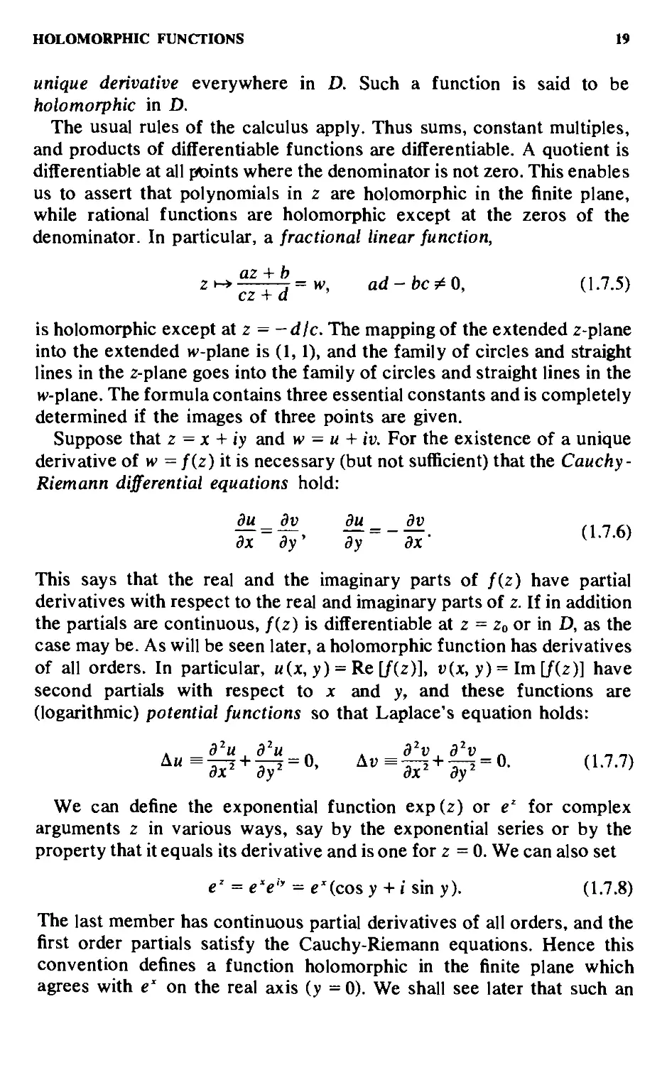
Suppose that 2 = x + iy and w - u + iv. For the existence of a unique
derivative of w = f{z) it is necessary (but not sufficient) that the Cauchy-
Riemann differential equations hold:
du _ dv du dv ,, _ ,,
This says that the real and the imaginary parts of f{z) have partial
derivatives with respect to the real and imaginary parts of 2. If in addition
the partials are continuous, f{z) is differentiable at 2 = 2o or in D, as the
case may be. As will be seen later, a holomorphic function has derivatives
of all orders. In particular, «(x, y) = Re [/B)], r(x, y) = Im [/B)] have
second partials with respect to x and y, and these functions are
(logarithmic) potential functions so that Laplace's equation holds:
We can define the exponential function expB) or e' for complex
arguments 2 in various ways, say by the exponential series or by the
property that it equals its derivative and is one for 2=0. We can also set
e' = e'e" = e'(cos y + i sin y). A.7.8)
The last member has continuous partial derivatives of all orders, and the
first order partials satisfy the Cauchy-Riemann equations. Hence this
convention defines a function holomorphic in the finite plane which
agrees with e" on the real axis (y = 0). We shall see later that such an

20 INTRODUCTION
extension by a holomorphic function is unique. We see that e' is periodic
with period 2m.
Formula A.7.8) shows that we can define a logarithm by
log 2 = log (re") = log r + id, A.7.9)
and this is a holomorphic function in any simply connected domain
(roughly without holes) which does not contain the origin. The point 2=0
is obviously singular since the real part (i.e., log r) goes to -<» when r-»0.
Moreover, the function is not single valued in any domain containing the
origin since the argument is then free to take on infinitely many values for
a fixed 2. There are two ways to cope with this difficulty. One method is to
restrict the variability of z by introducing a cut, not to be crossed, say
along the negative real axis, and define log z so that - tt < Im (log z) < it.
Instead, we can extend the domain of definition to be a surface with
infinitely many sheets, with passage from one sheet to the next along the
negative real axis: up (increasing values of 0) by crossing from positive
values of y to negative, down by going in the opposite direction.
We have of course the same difficulties with roots. The nth root of z
has n determinations. If 2 = r e'", then
2"" = r""expr^(fl + 2ik7r)i-l, ik = 0, 1,...,«-1. A.7.10)
Here the extended domain of definition is a Riemann surface with n
sheets, and passage from one to the next is across, say, the negative real
axis. Here we run into visual difficulties. By going around the origin n
times in the positive sense, we are in the top sheet and one more turn
takes us back to the first sheet.
EXERCISE 1.7
1. What is arg B,22)?
2. Construct the sum of two vectors, Z\ and 22, in the complex plane.
3. The vector z = x - iy is known as the complex conjugate of 2. Show that
|2|'= 22. Find arg 2.
4. Mark the four points 0, 2,, 2, + z-., and 22, and draw the parallelogram with
these points as vertices. Prove the parallelogram law (the sum of the squares
of the lengths of the diagonals equals the sum of the squares of the lengths of
the sides).
5. From the definition of an ellipse derive its equation in complex variables.
6. Show that chordal distances define a metric for C.
7. Derive the Cauchy-Riemann equations and Laplace's equation.

POWER SERIES 21
8. Verify that log r is harmonic, i.e., satisfies A.7.7), Is any power of r
harmonic?
9. Verify that A.7.5) maps circles and lines into circles and lines.
1.8. POWER SERIES
Power series served as the foundation of the function theory developed
by Weierstrass. He did not invent them, but he perfected their theory. Let
there be given a sequence {a„} of complex numbers; form the series
S an2". A.8.1)
n=0
Suppose that the series does not diverge for all Z9^0. The basic
observation of Weierstrass is
THEOREM 1.8.1
Suppose that there is a Zo ?' 0 such that the sequence {|a„zS|} is bounded.
Then the series A.8.1) is absolutely convergent for |z| < |zo|, uniformly for
|z|«|zo|-5, 5>0. •*
This means that the positive reals fall into two classes:
1. K, contains those numbers r for which {|a„|r"} is a bounded
sequence,
2. Ki contains the remaining positive numbers.
There is a number R which is the supremum of the numbers in class Ki
(equivalently, the infimum of the numbers in K2), and now it is seen that
the series converges absolutely for |2| < i? and diverges for |2| > iJ. For R
we have the expression
4- = limsup|a„|"". A.8.2)
The sequence {|a„|""} may have a single limit, in which case we have llR.
This was the case considered by Cauchy. The sequence may, however,
have more than one limit point, even infinitely many. In any case there is a
largest limit point, and this is the superior limit. The general formula is
due to Jacques Hadamard A865-1%3). This R is the radius of convergence
of the power series. It can take any value in [0, <»].
If JR > 0, the sum of the series is evidently a continuous function of 2 in
the circle of convergence |2| < JR, say f{z). Moreover, we can differentiate

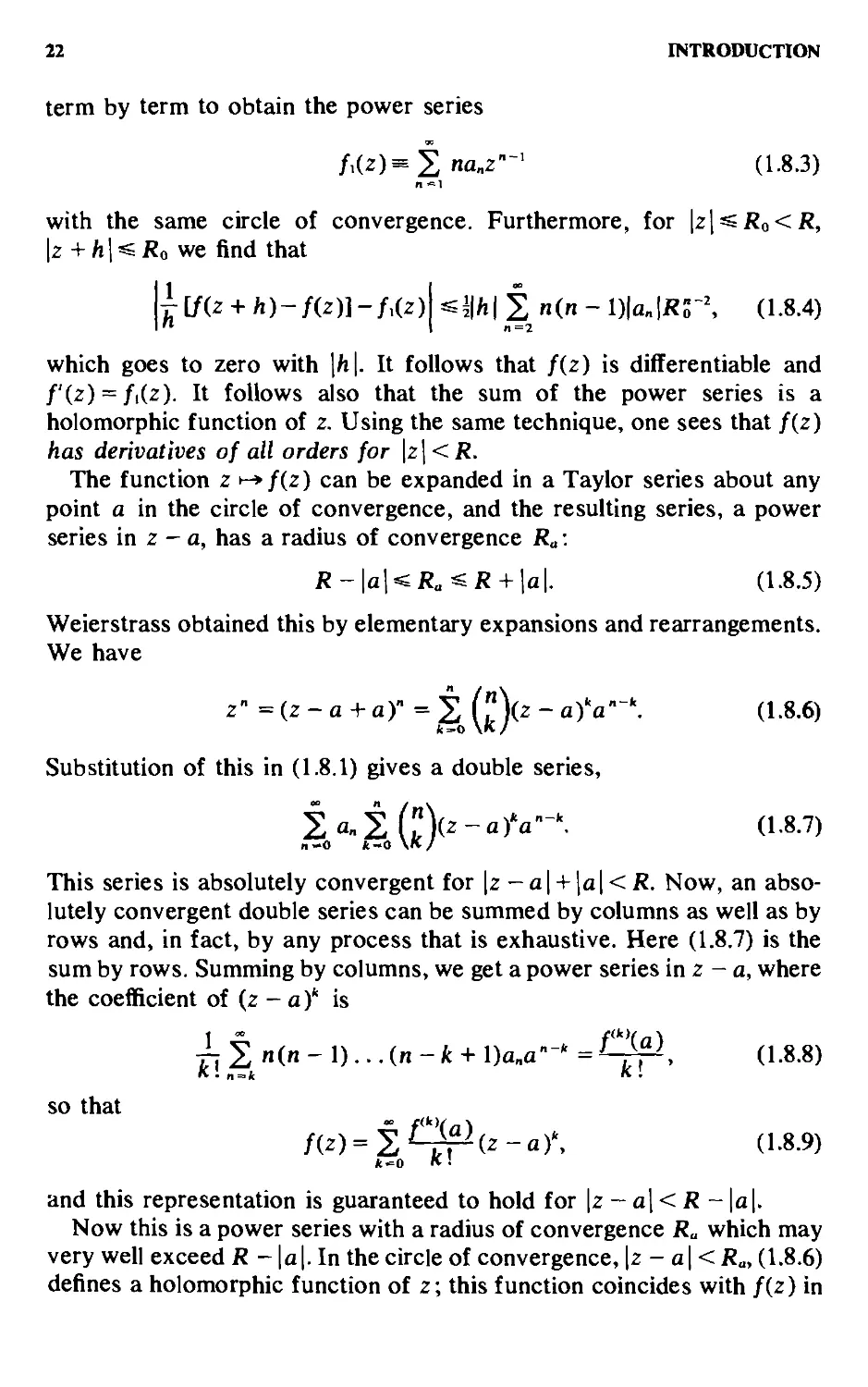
22 INTRODUCTION
term by term to obtain the power series
/,B)= J;«a„2"- A.8.3)
with the same circle of convergence. Furthermore, for \z\^Ro<R,
\z + h\^ Ro we find that
^[/B + ll)-/B)]-/,B)
«^|;i|t n(n-I)k|i?r', A.8.4)
which goes to zero with \h\. It follows that /(z) is differentiable and
/'B) = /iB). It follows also that the sum of the power series is a
holomorphic function of 2. Using the same technique, one sees that f{z)
has derivatives of all orders for \z\<R.
The function z y-^ f{z) can be expanded in a Taylor series about any
point a in the circle of convergence, and the resulting series, a power
series in 2 - a, has a radius of convergence R^:
R-\a\^R.^R + \a\. A.8.5)
Weierstrass obtained this by elementary expansions and rearrangements.
We have
z"={z-a+ar = E (fe)B - a/a""'- A-8-6)
Substitution of this in A.8.1) gives a double series,
la„±{"){z-aU'-\ A.8.7)
This series is absolutely convergent for |2 -a| + la|< i?. Now, an
absolutely convergent double series can be summed by columns as well as by
rows and, in fact, by any process that is exhaustive. Here A.8.7) is the
sum by rows. Summing by columns, we get a power series in 2 - a, where
the coefficient of B - a)' is
j-.^nin-\)...{n-k + l)a„a"-'' = =Qf^, A.8.8)
SO that
fiz)=t^^{z-a)\ A.8.9)
and this representation is guaranteed to hold for |2 - aj < i? - |a|.
Now this is a power series with a radius of convergence i?„ which may
very well exceed R - |a|. In the circle of convergence, \z - a\<R^, A.8.6)
defines a holomorphic function of 2; this function coincides with f{z) in

POWER SERIES 23
the lens-shaped region of intersection of the two disks, where they are
defined, and the union of the two disks is the domain of definition of a
single holomorphic function which is represented by A.8.1) in one disk
and by A.8.9) in the other. We can repeat this process for all points a with
|a|<i?. We obtain a family of power series A.8.9) which represent the
same holomorphic function in their domains of convergence. The union
of all the disks is the domain of definition that can be reached by direct
rearrangements. There is at least one point on the circle of convergence
I2I = i? which stays outside of all disks \z - a\<R^ with |a| < iJ. This is a
singular point, and every power series admits of at least one singular point
on its circle of convergence.
It is possible for all points on the boundary to be singular. This will
happen iff R^ = R - \a\ for all a with |a| < iJ. We then say that z = R is
the natural boundary of f{z). An extreme example of this phenomenon is
furnished by the series
n=o n\
with R = \. Here the series, as well as all tlje derived series, converge
absolutely on |2| = 1. The unit circle nevertheless is the natural boundary.
Such natural boundaries are typical for so-called lacunary series, where
there are long and widening gaps in the expansion.
The German mathematician Alfred Pringsheim A850-1941) proved
that, if the coefficients a„ are nonnegative and infinitely many are
positive, then z = R is a singular point of the function defined by the
series. Since this theorem has important applications to the theory of
DE's, we shall sketch a proof. If the theorem were false, then for ana<R
but close to R the series A.8.9) would be convergent for a value of 2 on
the real axis beyond z = R; i.e., the series
i B-ai?)"|:(")a„(««)"-', 0<a<l,
for a suitable choice of a near to one would converge for a 2 = i?(l + 5)
for some S > 0. Thus
i(l-a + S)'i?'i(")a„(ai?)"
would converge. But this double series has positive terms, so we can
interchange the order of summation, leading to the absurd conclusion that
the series
Sa„[(l + 5)i?r

24 INTRODUCTION
would converge. It follows that for 0 < a < i? we have always R^ = R, so
z = R is a singular point.
EXERCISE 1.8
1. Verify that /(z) and its derived series /iB) have the same radius of
convergence.
2. How is A.8.2) obtained?
3. Give examples of power series where i? = 0, 1, or «.
4. Verify A.8.4).
5. Fill in missing details in the proof of A.8.9).
6. Why does A.8.8) hold?
7. For the function z >-* fiz) defined by A.8.10) the point z = 1 is singular by
Pringsheim's theorem. Show that 2 = -1 is singular and that z = i and z --i
are singular. Extend to 2"th roots of unity, the union of which is dense on the
unit circle.
8. Fill in missing details in the proof of Pringsheim's theorem.
9. In a power series A.8.1) all the coeificients a„ where n is not a multiple of 3,
are zero while Ujt ^ 0 with infinitely many larger than zero. What can be said
about singularities on |2| = i??
10. Why is R„«R+|a|?
1.9. CAUCHY INTEGRALS
Our three founders of analytic function theory differed in almost all
respects and not least in their attitude toward publication. Weierstrass,
who was a perfectionist and late in gaining acclaim, published sparingly;
his fame rests mainly on his lectures at the University of Berlin,
1864-1892. Riemann was a man of genius but was shy and plagued by
poor health; a considerable part of his work was published after his death.
Cauchy, on the other hand, overwhelmed the periodicals with his notes.
His first publication on integration between imaginary limits dates from
1825, but he seems to have had the basic ideas as early as 1814. Consider a
function z >-* f{z), holomorphic in a simply connected domain D. Set
/B)=[/B)+jVB), A.9.1)
and define the integral
l^' F{z)dz= r [Udx - Vdy]+ i (' [Udy + Vdx], A.9.
J Z-[ J Z| Jz|
2)
where the path of integration is a curve joining 2i with 2^ in D and the
integrals are line integrals in the sense of the calculus. Since U and V

CAUCHY INTEGRALS 25
satisfy the Cauchy-Riemann equations A.7.6), Cauchy claimed that the
integral is independent of the path joining 2, and 22, or, in other words, the
integral along a closed contour C is 0:
J /B)d2 = 0. A.9.3)
There are many questionable points in this argument, and objections go
back to the 1880's; desirable precision and generality were reached
around 1900. It is required that the curve C have an arc length (= be
rectifiable) which requires a representation
2=2@, O^f^L, A.9.4)
where L is the length of C and t>-* z{t) is a continuous function of
hounded variation. The integral then becomes a so-called Riemann-
Stieltjes integral:
[''/[2@]d2@, A.9.5)
Jo
which is the limit of Riemann-Stieltjes sums.
The limit exists for any continuous integrand f and integrator 2 of
bounded variation.
In this setting one proves the theorem for / = 1 and / = 2. Then one
observes that (i) C may be approximated arbitrarily closely by a closed
polygon, (ii) a polygon may be triangulated, (iii) the theorem is proved for
a small triangle, and (iv) hence is true for a polygon and an arbitrary
rectifiable curve.
The integral is additive with respect to the path and linear with respect
to the integrand. If D is not simply connected, the integral along C equals
a sum of integrals around the holes that are inside C.
The Cauchy integral is an exceedingly powerful tool. If z >-^ f{z) is
holomorphic in a simply connected domain D and on its rectifiable
boundary C, then
2m Jc
f{t)dt ^ r 0 if 2 is outside C, r 1 9 ?>
c t-z ~{f{z) if 2 is inside C.
We can differentiate under the sign of integration as often as we please,
and the formal nth derivative represents f"\z):
2m Jc
^^^\?.. = r'B)- A.9.8)
{t-zy

26 INTRODUCTION
Thus a holomorphic function has derivatives of all orders, a property
proved for power series in Section 1.8. It has been observed that the
property of defining a holomorphic function of z inside C resides, not in
the factor f{t) in the integral, but in the Cauchy kernel Hit ~ z), for we
can replace f{t) by any continuous function F{t) without losing analytic-
ity of the integral, which, however, may not be zero outside of C in this
case. It is the Cauchy kernel which is a holomorphic function of z as long
as 2 is kept away from the contour of integration C. We can expand the
kernel in powers of z or of I/2, multiply by f{t), and integrate term by
term, as is usually permitted by uniform convergence of the series. The
linearity in / often implies continuity with respect to /. Among the many
results obtainable by such considerations we list
THEOREM 1.9.1
// z i-> f(z) is holomorphic in D, if the disk |z - a| < R lies in D, then f(z)
can be expanded in the Taylor series
f(z)=i^(z-a)S A.9.9)
the series being absolutely convergent in the disk.
Proof. We have
_L_ = 1 y iz-a)' A9 10)
t-z {t-a)-{z-a) k{t-ar'' ^'•'^•'"^
which converges uniformly in 2 and t if \z - al'^ R—S,\t - a\ = R.
Multiplication by f{t) and termwise integration yields A.9.9) in view of
A.9.8), where 2 is replaced by a. ■
In a similar manner one obtains the Laurent series, discovered by Pierre
Alphonse Laurent A813-1854) in 1843 and known to Weierstrass in 1841.
THEOREM 1.9.2
// zi->f(z) is holomorphic in an annulus.
0^R,<|z-a|<R2««>, A.9.11)
then
f(z)=ia„(z-a)", a„ = 2iil(r^' ('-^-l^)
where C: |t-a| = r, R, <r< R^.
We shall not give the proof but mention that in addition to A.9.10) there
is needed

CAUCHY INTEGRALS 27
t-z t^a{z~ay*
which is valid for |2 - a| > |f - a|.
The case in which z = a is an isolated singularity is particularly
important. Here R\ = Q, and the negative powers in A.9.12) constitute the
principal part of the singularity. There are three different possibiUties.
1. No negative powers. We define /(a) = ao, the singularity is
removable.
2. A finite number of negative powers, a„ = 0 for « < - m but a-„ ^ 0.
This is a pole of order m, and B - a)"'f{z) is holomorphic at 2 = a.
3. Infinitely many negative powers. Here 2 = a is an essential
singularity. In any neighborhood of 2 = a the function 2 >-* f{z) assumes any
preassigned value c infinitely often with at most two exceptions (theorem
of Emile Picard).
The property of being holomorphic may be said to be hard to acquire,
but once acquired it persists. It can be expected to survive a passage to
the limit. The simplest case is
THEOREM 1.9.3
Suppose that {f„(z)} is a sequence of functions, holomorphic in a domain
D, which converges uniformly to a function f(z) in D; then f(z) is
holomorphic.
The functions holomorphic in D form a normed algebra under the sup
norm ||/|| = sup^eo |/B)|. Convergence in the norm is uniform
convergence in the ordinary sense and the algebra is complete, so the
theorem follows. This case is almost trivial, but we can greatly weaken
the assumptions by using induced convergence. Here is an example.
Instead of assuming convergence in a domain, we can assume it in a
subset from which it spreads to the whole domain.
THEOREM 1.9.4
Let {f„(z)} be a sequence of functions holomorphic in a domain D. Let C
be a simple, closed, rectifiable oriented curve which, together with its
interior, lies in D. Suppose that the sequence {f„(t)} converges uniformly
with respect to t on C. Then there exists a function z >-* f(z) holomorphic
in the interior of C such that f„(z) converges to f(z) uniformly in the
interior of C. Moreover, if S is any subset of the interior of C having a
positive distance from C, and if p is any positive integer, then the
sequence {f„'"(z)} converges uniformly to fXz) in S.

28 INTRODUCTION
We shall not prove this theorem, but we call attention to the fact that
the principle of the maximum (see below) implies that a Cauchy sequence
{/„@} on C is also a Cauchy sequence inside and on C.
A zero of f{z) is by definition a point where the function is zero. It is of
order m if the Taylor expansion starts with the term a„{z - a)", a„^0.
The zeros of a holomorphic function can not have a cluster point in the
interior of a domain where f{z) is holomorphic except when the function
is identically zero. If 2 = a is a limit point of zeros of f{z), then in the
Taylor expansion
/B)= ao+a,B -a)+ 02B -af+---
the constant term Oo = /(a) is zero by the continuity of the function. But
then
/,B)= 01 + 02B -a) +03B -a)'+- • •
also has infinitely many zeros with 2 = o as a limit point. This forces oi to
be zero and so on; all coefficients are zero, and f{z) is identically zero.
This implies that, if two functions f{z) and g{z) holomorphic in a
domain D coincide for infinitely many values of 2 with a limit point in D,
they are identical in all of A for h{z) = f{z)-g{z) has infinitely many
zeros and is thus identically zero. This is known as the identity theorem.
Instead of zeros we may of course consider any other fixed value of the
function. We see that limit points of zeros or of a value c are singular
points of the function.
The calculus of residues occupied a central position in Cauchy's work.
Suppose that 2 = o is an isolated singular point of a function 2 >-* f{z) in
the neighborhood of which f{z) is single valued. There is then an
associated Laurent expansion A.9.12). The coefficient o-i is the residue of
f{z) at 2 = o. The reason for the name is that o-i is all that is left when we
form
2i[l/('>
dt.
where C is a small circle, \t - a\ = r, for we can substitute the Laurent
series and integrate termwise since the series is uniformly convergent on
the circle. We have
j {t - a)-"-' dt = r"i r^ expi- nie) de A.9.14)
and the integral is zero unless re = 0, when it equals Ini. This gives the
residue theorem.

CAUCHY INTEGRALS 29
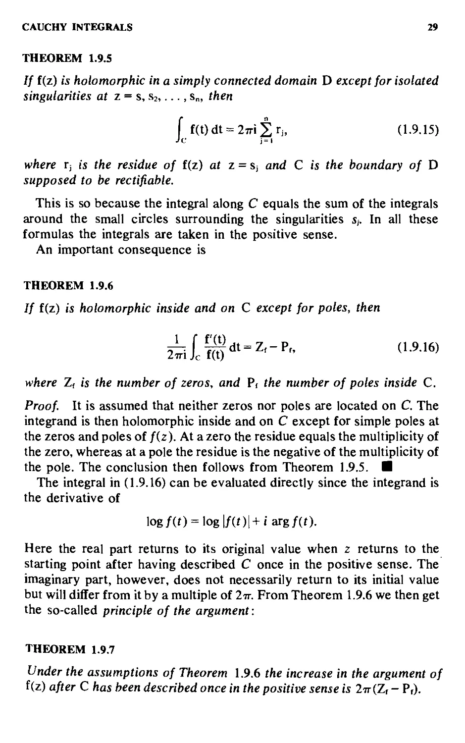
THEOREM 1.9.5
// f(z) IS holomorphic in a simply connected domain D except for isolated
singularities at z = s, Sj,..., s„, then
f f(t)dt = 27ri^rj, A.9.15)
where r, is the residue of f(z) at z = s, and C is the boundary of D
supposed to be rectifiable.
This is so because the integral along C equals the sum of the integrals
around the small circles surrounding the singularities Sj. In all these
formulas the integrals are taken in the positive sense.
An important consequence is
THEOREM 1.9.6
// f(z) is holomorphic inside and on C except for poles, then
where Z, is the number of zeros, and P, the number of poles inside C.
Proof It is assumed that neither zeros nor poles are located on C. The
integrand is then holomorphic inside and on C except for simple poles at
the zeros and poles of f{z). At a zero the residue equals the multiplicity of
the zero, whereas at a pole the residue is the negative of the multiplicity of
the pole. The conclusion then follows from Theorem 1.9.5. ■
The integral in A.9.16) can be evaluated directly since the integrand is
the derivative of
log/@ = log 1/@1 +/arg/@.
Here the real part returns to its original value when z returns to the
starting point after having described C once in the positive sense. The
imaginary part, however, does not necessarily return to its initial value
but will differ from it by a multiple of 2it. From Theorem 1.9.6 we then get
the so-called principle of the argument:
THEOREM 1.9.7
Under the assumptions of Theorem 1.9.6 the increase in the argument of
f(z) after C has been described once in the positive sense is 1it{Z, - ?,).

30 INTRODUCTION
A useful addition to Theorem 1.9.6 is given by
THEOREM 1.9.8
Under the assumptions of Theorems 1.9.6 and 1.9.7, suppose in addition
that g(z) is holomorphic inside and on C. Then
where the summation is extended over the zeros a, and poles bk of f(z),
and each summand is repeated as often as the multiplicity of the zero or
pole requires.
The zeros and poles of f{z) are still simple poles of the integrand, and at
a zero of / of multiplicity /i, the residue is fijgiaj), and similarly at the
poles.
Cauchy's formula A.9.7) invites some comments. Replace z by Zo, and
let the path of integration be the circle t = Zo+ re", where 6 goes from
zero to In. The result is
f{Zo) = ~ rf{Zo+re")de. A.9.18)
ZTT Jo
The right-hand side is the mean value in the sense of the integral calculus
over the interval @,27r) of the integrand. This is a basic property of
holomorphic functions but is shared with harmonic (logarithmic) potential
functions. From A.9.18) we also get
|/Bo)|« max 1/BI for|2-2„|=:r. A.9.19)
In this relation the inequality normally holds, equality can hold iff \f{z)\
equals its maximum for all z—to start with, all z on the circle and
ultimately all z in the plane, and f{z) = Me'", where M is the maximum
and a is real, fixed. This is a form of the principle of the maximum. The
principle asserts that the absolute value of a holomorphic function f{z)
cannot have a local maximum unless it is a constant. If in 3-space we plot
the surface
u = \f{x + iy)\\ A.9.20)
where / is not a constant, if /(xo + iyo) = f{Zo) ^ 0, there are paths on the
surface leading from z = Zo, u = Uo along which u is strictly increasing,
and also paths along which u is strictly decreasing. The latter type of path
naturally is missing if «o = 0. We formulate a form of the principle which
is sufficient for our purposes.

ESTIMATES OF GROWTH 31
THEOREM 1.9.9
// f(z) IS holomoq)hic inside and on the rectifiable curve C, and if M(f, C)
IS the maximum of |f(z)| on C, then for all z inside C
|f(z)|«M(f,C). A.9.21)
Proof The use of Cauchy's integral below is due to Edmund Landau
A877-1938), a German mathematician who made profound contributions
to function theory and analytic number theory. We have
whence
|/B)|" ^ [27rdB, C)]-'L[M(/, or.
Here d{z,C) is the distance of C from the point z in its interior, and L is
the length of C. We extract the feth root and pass to the limit with k to
obtain A.9.21), ■
EXERCISE 1.9
1. If C is rectifiable, then 2"=, |2(fy)-2(fy_,)| ^ L and the sums in A.9.6) are
dominated by M(/, C)L. Verify.
2. Verify A.9.7) and A.9.8). For n = l verify that the difference quotient
(l//i)[/B +h)-fB)] tends to the formal derivative uniformly if z and z + h
have a distance from C which exceeds a 6 > 0.
3. Fill in details in the proofs of Theorems 1.9.1 and 1.9.2.
4. Use the principle of the maximum to prove that a Cauchy sequence {/„(f)} on
C generates a Cauchy sequence {/„B)} in the interior.
5. Verify Theorems 1.9.5 and 1.9.6.
6. Show that a harmonic function, not a constant, cannot have a local maximum.
1.10. ESTIMATES OF GROWTH
Given a power series
f{z)='Za„z" A.10.1)
with radius of convergence JR > 0, let M{r, f) be its maximum modulus:
M{r,f)= max [/(re'")!. A.10.2)
Formula A.9.8) then gives the Cauchy estimates,
|a„|^M(r,/)r-", r < R. A.10.3)

32 INTRODUCTION
Here r is arbitrary, so the question of optimizing the estimate arises. If
i?<<», the choice r = [l -{lln)]R is often a good one.
The maximum principle shows that for a nonconstant holomorphic
function M{r, f) is an increasing function of r. For i? < <» it may very well
be bounded. This is not the case for R = <», however, as shown by Joseph
Liouville A809-1882). A sharper form of his theorem is
THEOREM 1.10.1
Suppose that R = <» and that there are positive constants A, B, and c such
that
M(r,f)«A + Br' A.10.4)
for all r. Then z i-> f(z) is a polynomial in z of degree not exceeding c.
Proof By A.10.3) we have
\a„\^{A+Br')r ",
and this goes to zero as r -> «= if « >c. This means that all coefficients a„
are zero for « > c, so z ►-» /(z) is a polynomial of degree not exceeding c
as asserted. B
A power series with i? = oo is called an entire function {integral function
in Great Britain). Such a function may be algebraic or transcendental,
according as it is a polynomial or not. In the transcendental case M{r,f)
grows faster than any power of r by Liouville's theorem, but there is
neither a slowest nor a fastest possible growth of the maximum modulus.
Given an increasing function r*-^G{r) such that log G(r)/log r becomes
infinite with r, one can find an entire function whose maximum modulus
grows faster than G{r) and an entire function whose maximum modulus
grows slower than G{r), so that
H^Ml^.,., lim^^ = 0,
respectively.
More properties of entire functions will be encountered in Chapters 4
and 5. In addition to entire functions, we shall also ultimately have to
consider meromorphic functions, i.e., functions having no other
singularities than poles in the finite domain. Again we have two types,
algebraic and transcendental meromorphic functions. The first is the class
of rational functions, functions which are meromorphic in the extended
plane. A function of the second class either has a finite number of poles
plus an essential singularity at z = <» or infinitely many poles which have
no limit point in the finite part of the plane.

ANALYTIC CONTINUATION; FUNCTIONAL EQUATIONS 33
In Chapter 4 we shall encounter various generalizations of the
maximum modulus which are suitable for a study of meromorphic functions.
Here we shall consider just a generalization of Liouville's theorem for an
isolated singular point.
THEOREM 1.10.2
Suppose that z = a is an isolated singularity of z^-*f{z), where f(z) is
holomorphic in a punctured disli, 0 < |z - a| < R. Set
M.(r,f)=max |f(a +re")|, 0<r<R. A.10.5)
Suppose there exist positive numbers A, B, and c such that
Mad, f)« A + Br ^ A.10.6)
Then z = a is either a removable singularity or a pole of order «c.
Proof The assumptions imply that there is a Laurent expansion A.9.12),
and we have
\a-,\^MAr,f)r'<{A+Br-nr'';
this goes to zero with r if fe > c. It follows that 2 = a is either a removable
singularity or a pole of order not exceeding c, as asserted. ■
Exercises bearing on this section will be found after Section 1.11.
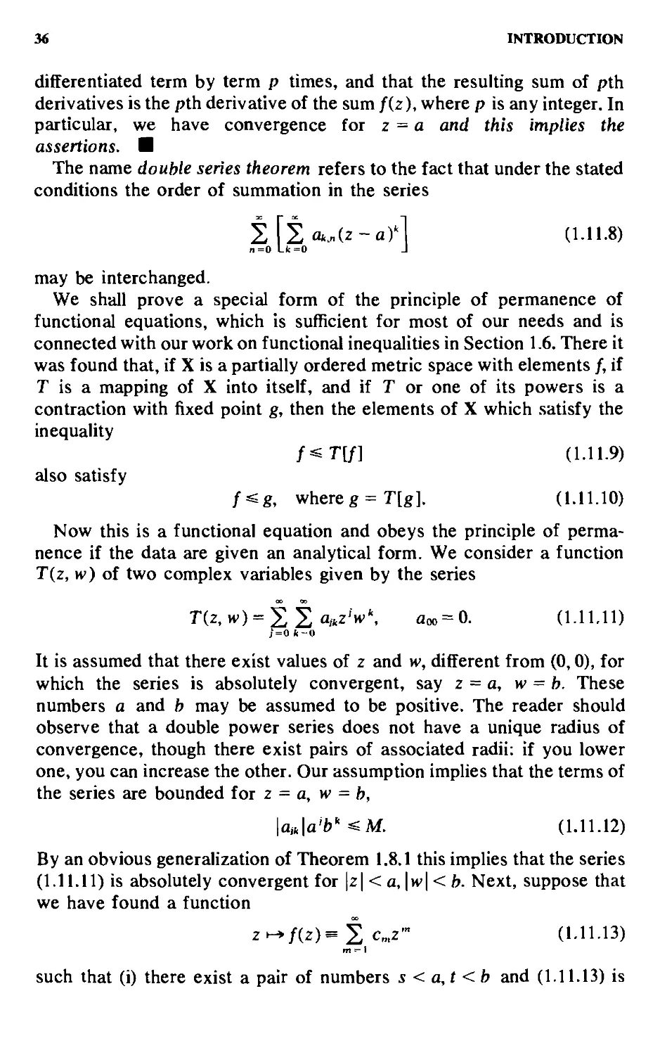
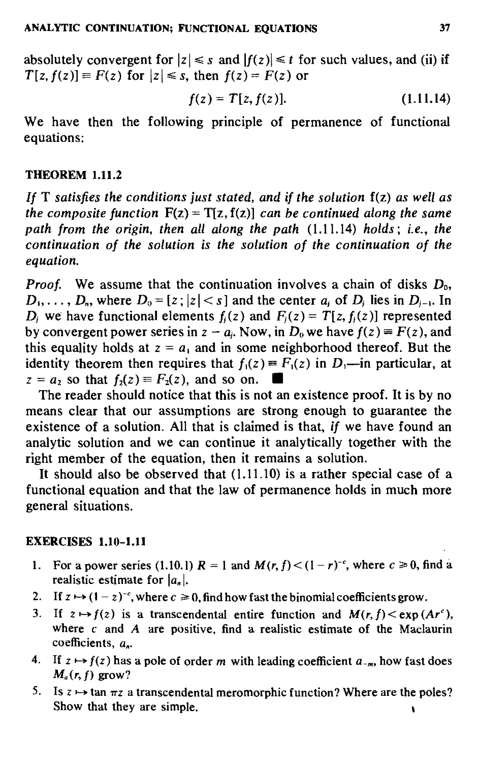
1.11. ANALYTIC CONTINUATION; PERMANENCY OF
FUNCTIONAL EQUATIONS
Analytic continuation is a concept introduced by Weierstrass and basic
for his attack on function theory. A function 2 ►-» /(z) is defined originally
by a power series, say,
f{z)^'Za„z- A.11.1)
n=0
with a radius of convergence R.UR=^ and the function is entire, there
is no continuation problem. Also, i? =0 is out (we disregard the possibility
that the series may be summable by some method or other). If 0< i? <^,
there is a continuation problem. We saw in Section 1.8 that f{z) admits of
expansions in a Taylor series,
/B;a)=S^TT^U-a)\ A-11-2)
obtained by direct rearrangement of A.11.1) after setting z - a +{z - a)
and expanding. The series f{z;a) converges for \z-a\<Ra, where

34 INTRODUCTION
i?-|a|=si?„ «i? +|a|.If i?„ = i? - |a|, the point of contact of |2-a| = i?„
with Izl = i? is a singular point of f{z) and analytic continuation in the
direction arg z = arg a is not possible. On the other hand, if R -\a\<Ra,
the disk \z-a\<Ra is partly outside |2|<R, and in the lens-shaped
overhang f{z; a) defines an analytic continuation of f{z). This process is
repeated for all a with |a| < i?. If for all such a's we get R^ = R -\a\, no
analytic continuation is possible and |2| = i? is the natural boundary of
/U).
If, on the other hand, R„ > R -\a\ for some values of a, the union of
the disks \z-a\<Ra is a simply connected domain D, in which our
function is defined by one of the series f{z; a) with |a| < i?. Moreover, if a
point ZoGDiy it belongs to infinitely many disks \z-a\<Ra and the
corresponding series f{z; a) all assign the same value to /(z) at 2 = Zo. We
now repeat the process for points ai in Di with |ai| s^ i?. This gives a set of
power series f{z;a,aO obtained by double rearrangements: of the
original series at 2 = a with |a| < i?, and of the series /B; a) at 2 = Oi.
This gives a definition of / in the union of all the disks. Since this set may
be self-overlapping, we are no longer assured of the consistency of the
definition but have to keep account of the steps involved.
Suppose that we can find a sequence of points Oo, a,,..., a„ such that
power series in terms of 2 — Oj are obtained by repeated rearrangements
of A.11.1). Suppose that
\ao\<R, |a,-ao|<i?^, ..., |a„ - a„-,| <«„„_,. A.11.3)
Here
/;B) = ^ a,.fcB - Qif, \z-ai\< Rj.
There is then defined a branch of /(z) at z = a„ obtained by analytic
continuation of f{z) using the intermediary points Oo, Oi,..., a„.
According to Weierstrass, the totality of such series constitutes an analytic
function f{z). To these regular elements of / are further adjoined the
following;
1. Polar elements B - a)"" Sr=o hjiz - a)', one for each pole.
2. Algebraic elements (z - a)""" 27=oC)(z - a)*'" for algebraic
branch points.
3. Elements at infinity. These may be regular: Sr=ocijZ"', polar:
z" S; diZ'\ or algebraic: z"" So djZ-""".
Essential singular points are not considered as belonging to the domain
of definition of the function and contribute no functional elements.
Logarithmic singularities also are noncontributing.
At a given point z = a there are normally infinitely many elements.

ANALYTIC CONTINUATION; FUNCTIONAL EQUATIONS 35
regular and/or singular. Henri Poincare A854-1912) was a famous French
mathematician whose name will be encountered again and again in this
book. At this stage we need a result of his according to which the distinct
elements of /(z) at 2 = a form a countable set. This we see as follows. An
element at 2 = a is the end product of a chain of rearrangements. We can
order these first according to the number of steps involved, say n. For
each n we have rearrangements at points an, a,,..., a„. Without loss of
generality we may assume that the a's used have rational coordinates
(these numbers are dense in C). Now the points with rational coordinates
form a denumerable set. Thus we are dealing with a countable number of
countable sets, and such a set is itself countable. Hence the different
determinations at 2 = a form either a finite set or a countable one.
Leaving these general considerations, we turn to the principle of
permanence of functional equations, which is a very important fact in the
theory of DE's. It is hard to find a definition of the term functional
equation, and the mathematicians who deal with the subject normally
exclude differential and integral equations from consideration, so we
cannot expect much help from that quarter. Before going any further we
have to prove the double series theorem of Weierstrass, which will be
needed here and later.
THEOREM 1.11.1
Suppose that the functions z ►-» f„(z), n = 0,1,2,..., are holomorphic in a
disk |z - a| < R and that the series
2uz)^m A.11.4)
n = 0
converges uniformly in |z-a|=spR for each p with 0<p <1. Suppose
also that
f„(z)=iaUz-a)^ A.11.5)
k=0
Then each of the series
J:a..„^A„ k = 0,1,2,..., A.11.6)
converges and, for |z - a| < R,
f (z) = S A.(z - a)^ A.11.7)
Proof This follows from Theorem 1.9.4, which implies that the sum of
the series A.11.4) is a holomorphic function f{z), that the series may be

36 INTRODUCTION
differentiated term by term p times, and that the resulting sum of pth
derivatives is the pth derivative of the sum f{z), where p is any integer. In
particular, we have convergence for z = a and this implies the
assertions. B
The name double series theorem refers to the fact that under the stated
conditions the order of summation in the series
tltihAz-af] A.11.8)
n=0 Lt=0 J
may be interchanged.
We shall prove a special form of the principle of permanence of
functional equations, which is sufficient for most of our needs and is
connected with our work on functional inequalities in Section 1.6. There it
was found that, if X is a partially ordered metric space with elements /, if
T is a mapping of X into itself, and if T or one of its powers is a
contraction with fixed point g, then the elements of X which satisfy the
inequality
f^nn A.11.9)
also satisfy
f^g, whereg = T[g]. A.11.10)
Now this is a functional equation and obeys the principle of
permanence if the data are given an analytical form. We consider a function
TB, w) of two complex variables given by the series
TB,H') = Sia/«2'w'. aoo = 0. A.11.11)
j=0 A-0
It is assumed that there exist values of z and w, different from @,0), for
which the series is absolutely convergent, say z = a, w = ft. These
numbers a and h may be assumed to be positive. The reader should
observe that a double power series does not have a unique radius of
convergence, though there exist pairs of associated radii: if you lower
one, you can increase the other. Our assumption implies that the terms of
the series are bounded for z = a, w = h,
lortla'fc'^M. A.11.12)
By an obvious generalization of Theorem 1.8.1 this implies that the series
A.11.11) is absolutely convergent for \z\ < a,\w\ < h. Next, suppose that
we have found a function
z^f{z)^'Zc„,z"' A.11.13)
m-l
such that (i) there exist a pair of numbers s < a,t <h and A.11.13) is

ANALYTIC CONTINUATION; FUNCTIONAL EQUATIONS 37
absolutely convergent for |2| =s s and |/B)| =s t for such values, and (ii) if
T[2,/B)] = FB) for \z\^s, then /B)=FB)or
/B)=T[2,/B)]. A.11.14)
We have then the following principle of permanence of functional
equations:
THEOREM 1.11.2
// T satisfies the conditions just stated, and if the solution f(z) as well as
the composite function F(z) = T[z, f(z)] can he continued along the same
path from the origin, then all along the path A.11.14) holds; i.e., the
continuation of the solution is the solution of the continuation of the
equation.
Proof We assume that the continuation involves a chain of disks Do,
D,,..., D„, where D(, = [2; |2| < s] and the center Qj of D, lies in D;-,. In
D; we have functional elements f{z) and Fj{z) = T[2,/jB)] represented
by convergent power series in 2 - O/. Now, in Do we have f{z) = F{z), and
this equality holds at 2 = a, and in some neighborhood thereof. But the
identity theorem then requires that /iB)= F,{z) in D,—in particular, at
z = 02 so that fiiz) = Fniz), and so on. ■
The reader should notice that this is not an existence proof. It is by no
means clear that our assumptions are strong enough to guarantee the
existence of a solution. All that is claimed is that, // we have found an
analytic solution and we can continue it analytically together with the
right member of the equation, then it remains a solution.
It should also be observed that A.11.10) is a rather special case of a
functional equation and that the law of permanence holds in much more
general situations.
EXERCISES 1.10-1.11
1. For a power series A.10.1)/? = 1 and M(r,/)<(!-r)"', where cs=0, finda
realistic estimate for \a„ \.
2. If z i-> (I - 2 y, where c s^ 0, find how fast the binomial coefficients grow.
3. If 2i->/B) is a transcendental entire function and M(r,f)<e\p{Ar''),
where c and A are positive, find a realistic estimate of the Maclaurin
coefficients, a„.
4. If z i-> /(z) has a pole of order m with leading coefficient «-„, how fast does
Ma{r,f)erow?
5. Is z i-> tan ttz a transcendental meromorphic function? Where are the poles?
Show that they are simple. \

38 INTRODUCTION
6. Show that cosz =5[exp(iz) + exp(-iz)]. Show that for this function the
maximum modulus is attained on the imaginary axis and equals cosh r (the
hyperbolic cosine of r).
7. Show that |sin (x + 'iy)f = sin^ x + sinh^ y.
8. If e' = 1 +27z"/n!, prove by series multiplication or otherwise that e' -
9. If P(f) = a +bt + ct', express 2n=o P(n)z" In \ in terms of the exponential
function.
10. Where in the complex plane is sin (x + ly) real, and where purely imaginary?
11. What is the limit, if any, of tan {x + ly) as y -> + », y -> - <»?
12. What is the series expansion for f{z, a) if /U) = A - z)"' and |a| < 1? How
does Ra vary with a?
13. Show that in this case the domain D, where the first rearrangements
converge is bounded by a cardioid with the cusp at 2 == 1 and passing through
2 =-3.
14. Prove that the same curve gives the boundary of D, for all the binomial
functions A - zY, where c is not a positive integer.
15. Take c = 1, and consider second rearrangements f(z;a,a,). Try to form
some notion of what part of the plane is covered by Dj and show that there
are two distinct elements of the function with center at 2 = 2.
16. Consider the analytic function z i->[(l-2;)'"-(l+2)"-]"\ Where are the
branch points? Describe the functional elements with centers at the branch
points. What are the elements at infinity? The roots are given all possible
determinations.
17. Two power series have radius of convergence = 1. Express the product of
the two series as a simple series, and determine its radius of convergence.
Can it be greater than one?
18. When are the following series absolutely convergent: (i) STCzw)", (ii)
^l(z + w)\ (iiiJJ2j2'2"?
19. Let T{z, w) = U2 + 2? (z + w)"]. Let / = T(z, f) be the solution which is 0 at
2=0. Show that the solution is holomorphic except for two branch points.
Find their locations and natures.
20. State the conditions under which the principle of permanence would apply to
the functional equation involved in Problem 1.6:6.
LITERATURE
As collateral reading for Chapter 1 the author may perhaps be permitted
to refer to three of his own books:
Hille, E. Lectures on Ordinary Differential Equations. Addison-Wesley, Reading, Mass.
1969.
. Methods in Classical and Functional Analysis. Addison-Wesley, Reading, Mass. 1970.

LITERATURE 39
Analytic Function Theory. Vols. I, and II, 2nd ed. Chelsea, New York, 1973; 1st ed.,
Ginn, Boston, 1959.
These books will be referred to hereafter as LODE, MCFA, and AFT,
respectively.
For Section 1.1 consult MCFA, Chapters 1 and 2, or LODE, Chapter 1.
The latter can be used also for Sections 1.2-1.6. Matrices and mappings
are discussed in both books.
For Sections 1.5 and 1.6 consult Chapters 5 and 12 of MCFA. For
differential and integral inequalities the basic work is:
Walter, W. Differential- und Integralungleichungen. Springer Tracts on Natural Philosophy,
Vol. 2. Springer-Verlag, Berlin, 1966.
The original Gronwall Lemma occurs in:
Gronwall, T. H. Note on the derivative with respect to a parameter of the solutions of a
system of differential equations. Ann. Math., B), 20 A918), 292-296.
See also:
Bendixson, I. Demonstration de I'existence de I'intSgral d'une equation aux deriv6es
partielles lin6aires. Bull. Soc. Math. France, 24 A896), 220-225.
For this question see also Chapter 3 of LODE.
For Part II consult AFT. For Section 1.7 Chapters 1-4 will round out
the presentation. Section 1.8 and Chapter 5 go together. For Section 1.9
consult Chapters 7-9. Functions of bounded variation and the Riemann-
Stieltjes integral are treated in Appendix C. Analytic continuation is
discussed in Chapters 5 and 10 of Vol. II, where also the principle of
permanence of functional equations is treated under different
assumptions.
The standard treatise on functional equations is:
Aczel, J. Lectures on Functional Equations and Their Applications. Academic Press, New
York, 1964.

EXISTENCE AND
UNIQUENESS
THEOREMS
This chapter is devoted to generalities about differential equations (DE's)
and their solutions. The main subject matter will be existence and
uniqueness theorems for analytic DE's: the use of fixed point methods,
successive approximations, majorant methods, the Cauchy majorant, the
majorant of Lindelof, and dominants and minorants. We shall also
consider variations of parameters, internal and external.
2.1. EQUATIONS AND SOLUTIONS
Our first question is, What is meant by a DE and by a solution? A crude
definition of a DE would be a functional equation (also undefined!)
involving derivatives of unknown functions. Such derivatives may be
ordinary or partial, according to whether the number of independent
variables is one or more. We restrict ourselves to functions of a single
variable. This does not exclude the possibility that the equation involves
one or more parameters which occur explicitly in it.
We have now excluded partial DE's from consideration. But not every
functional equation involving derivatives of the unknown with respect to
a single variable (which need not occur explicitly in the equation) is a
bona fide ordinary DE. To clarify the ideas, let us consider the following
equations from the point of view of their being acceptable for study in this
book:
w'{z) = U{z) + fMw{z) + U{z)[w{z)]\ B.1.1)
^'B) = 2-^B), B.1.2)
zw"{z) = [w{z)]\ B.1.3)
40

EQUATIONS AND SOLUTIONS 41
^'B)= ^B + 1), B.1.4)
w'{z)=r{l + [w{s)r}ds, B.1.5)
Jo
w{z)=f {[w'{s)f + [w{z)Y}"^ds. B.1.6)
Jo
The notation is intended to suggest that the functions involved are
analytic functions of a complex variable. The first three equations are
acceptable; the others are not. The first is a nonlinear first order (Riccati)
equation, discussed in Chapter 4, the second is a trivial first order
equation (Chapter 5), and the third is a nonlinear second order equation, a
special case of Emden's equation (Chapter 12). Equation B.1.4) is
rejected because the unknown is subjected to a translation of the
independent variable besides the differentiation. The remaining equations
are excluded because of the integral operators. Equation B.1.5), however,
leads to a bona fide second order DE:
w"{z) = \+[w{z)f B.1.7)
upon differentiation. However, the two equations are not equivalent: all
solutions of B.1.5) satisfy B.1.7), but not conversely.
In the following we shall consider only ordinary DE's or systems of
such equations. Up to and including Chapter 4 the equations will be of the
first order and of the form
H''B)=F[2, ^B)]. B.1.8)
Here there are two alternatives: F{z, w) is an analytic function of the two
variables z and w, holomorphic in a given dicylinder in C^ or (second
alternative) w B) is vector valued in C", 2 is a complex variable, and F is a
holomorphic mapping of C"*' into C". The latter alternative enables us to
treat nth order DE's as a special case of B.1.8). Note that a DE is of
order n if the order of the highest derivative entering into the equation is
n.
The notion of what is meant by a solution of a DE has varied
considerably over the three centuries that have elapsed since Isaac
Newton made the first classification of what he called fluxional equations
in 1671. He even invented the method of series expansions with
indeterminate coefficients. However, since Newton's work was not published
until 1736, long after his death, it had no influence on the development of
the subject. The first published paper on DE's is due to Jacob Bernoulli in
his study of the isochrone A696); this was rapidly followed by a number
of investigations by Johann and Daniel Bernoulli, Clairaut, Euler,

42 EXISTENCE AND UNIQUENESS THEOREMS
Leibniz, Riccati, and others during the eighteenth century. To these early
founding fathers of calculus and analysis, the problem was to find a
function of two variables (z, h')i->GB, w) such that
GAz, w) dz + GAz, w) dw = 0 B.1.9)
is implied by B.1.8) and vice versa. This would require
FB,,v) = -f^,
B.1.10)
and the solution would be
G{z,w)=C. B.1.11)
In B.1.9) and B.1.10) the subscripts z and w indicate partial
differentiation with respect to z and w, respectively. Since in those days the only
acceptable functions were those built up by composition of a finite
number of what later became known as elementary functions, i.e.,
powers, exponentials, logarithms, trigonometric functions, and their
inverses, the integrable types were soon exhausted. Just as most
functions could not be integrated, most DE's were insolvable.
Here Cauchy showed the way out of the difficulty. The founding fathers
had asked too much: they had demanded global solutions in terms of
elementary functions. This was an algebraic straitjacket that was not
suitable and prevented further progress. The typical operation of analysis
is the limit process, which is very powerful but can require a local point of
view.
Let us return to B.1.8). Suppose that B, w) i-> F{z, w) is holomorphic in
a neighborhood of B0, Wo)~ Cauchy asked. Is there a function of 2, say
w ==w{z;zo,Wo), B.1.12)
such that it is holomorphic in some neighborhood of 2 = 2o and for all 2 in
the neighborhood, with ^0= ^B0; Za, Wo),
w'{z-Zn, Wo) = F[z, w{z; Zo, Wo)]? B.1.13)
Cauchy showed the existence and uniqueness of such a solution. To this
end he developed several ingenious devices. For the real case he worked
out a step-by-step method using linear approximations. For the complex
domain he employed series expansions and the majorant method.
The global problem still remains. Here the method of analytic
continuation used by Weierstrass provided at least a partial solution. A local
solution given by a power series at 2 = 2o is continued analytically along a

EQUATIONS AND SOLUTIONS 43
path C from Zoto 2,. If F[z, w{z)] can also be continued analytically along
C, then by the law of permanence of functional equations (see Section
1.10) the continuation of the solution is the solution of the continuation of
the equation.
This leaves out of consideration the singularities. They are either fixed,
given by the equation, or movable, i.e., dependent on the initial values.
Thus B.1.2) has only fixed singularities, namely, 0 and <», whereas B.1.1)
has both kinds. There the singularities of fa, /i, /z and the zeros of f^ are
fixed. The movable singularities are simple poles. This is illustrated by the
special example
w' = \ + w\ B.1.14)
which is satisfied by w = tan B - 20) with poles at 2 = 2o + 2B« + lOr.
Equation B.1.3) has fixed singularities at 2 = 0 and <» and movable
singularities, which may be placed anywhere in the plane and are of very
complicated nature.
For a further study of B,1.8) we must determine the fixed singularities
and the nature of the solutions at such a point. We must also decide why,
when, and where movable singularities occur and what the actual natures
of these singularities are-
Some equations can be characterized by postulating the position and
nature of the singularities together with the relations joining these
elements. This problem was first posed by Riemann for the hypergeomet-
ric equation. There is a Riemann problem for linear DE's, one of the
many Riemann problems. This involves global characterization of
equations and solutions. Usually global information is hard to get; there are,
however, equations for which we can assert that the only movable
singularities are poles, and equations of which the solutions are single
valued.
A solution of B.1.8) which involves an arbitrary constant is called the
general solution. A solution obtained by giving the constant a particular
value is known as a particular solution. Thus B.1.14) has the general
solution tan B - Za), and tan 2 is a particular solution. This equation has
also two singular solutions, w{z) = i and w{z) = -i. They are not
obtainable from the general solution by specifying the constant 2o.
oVvfi-^ ;>--;.. - ■• \ ay- "^^
EXERCISE 2.1
Find the fixed singularities of the following DE's, and discuss how the nature of
the singularity varies with the parameters. All the equations are elementary.
1. zw' - aw.
2. {z - a)w'= {z - b)w.

44 EXISTENCE AND UNIQUENESS THEOREMS
3. {z-afw" + {z-a)w'-b-w=0.
4. The functional equation (not a DE)
Jo
has solutions of the form /(z) = Cz (why?). Determine the value of C if
1"' = + 1.
Determine the DE of the lowest order which is satisfied by the following conies:
6, (x-ay + (y-aY= a' + a\
1. {x-af + (y-bf=\.
Obtain the envelope of the curve family when it exists and show that it is also
a (singular) solution.
8. Find the general solution of w' = w--\, and find the singular solutions.
Discuss the movable singularities (nature, frequency, and dependence on the
constant of integration).
2.2. THE FIXED POINT METHOD
Historically this is the most recent method proposed for proving
existence and uniqueness theorems for ordinary DE's. It goes back to a paper
by G. D. Birkhoff and O. D. Kellogg in 1922. They used a fixed point
theorem by L. E. J. Brouwer. That Banach's fixed point theorem
(Theorem 1.5.1) could be applied for the same purpose was pointed out by
R. Cacciopoli in 1930.
We are concerned with the equation
w'=F{z,w), B.2.1)
where B, h')i->FB, w) is holomorphic in the dicyUnder
D:\z=Zo\^a, \w-Wo\'^h. B.2.2)
It is required to find a function z t^ w{z; 2,1, Wq), holomorphic in some
disk I2 - 2o| < r < a, such that
w'{z; 2o, Wo) = F[z, ^B; 2o, Wo)],
. B.2.3)
^B0:20, ^0)= Wa.
To apply Theorem 1.5.1 we have to exhibit a complete metric space X
consisting of functions 2 i-> gB) and define an operator T which maps X
into itself and is a strict contraction. Also, X has to be chosen so that the
existing unique fixed point is the desired solution. As a first step we

THE nXED POINT METHOD 45
replace B.2.1) by the integral equation
/B)=H'„+f" F[sJ{s)]ds. B.2.4)
If this equation has a unique solution /, then /(z) also satisfies B.2.1)
including the initial condition. This suggests defining an operator T by
T[g]B) =w„+r F[s,g{s)] ds, B.2.5)
where T operates on a space to be defined. We note first that F satisfies
two conditions used in the following, namely,
\F{z,w)\<M, B.2.6)
\F{z,u)-F{z,v)\<K\u-vl B.2.7)
for suitably chosen constants K and M and (z, w), (z, «), and (z, v) in D.
Since D is closed, F is certainly bounded in D and so is F^.{z, w), the
partial of F with respect to w. The Lipschitz condition B.2.7) is implied
by the boundedness of the partial derivative. We can now state and prove
THEOREM 2.2.1
Under the stated assumptions on F, in the disk Do." |z - Zo| < r, where
r<mm(a,—,^j, B.2.8)
B.2.1) has a unique holomorphic solution satisfying the initial-value
condition w(Zo; Zo, w,,) = Wo.
Proof Let X be the set of all functions z>-^g(z), holomorphic and
bounded in Do so that
g(zo) = vvo and ||g - WoU«ft, B.2.9)
where
||g - Well = sup |gB) - Wo\. B.2.10)
zeDo
Under these assumptions the composite function z*^F[z,g{z)] exists
and is holomorphic in Do, and its norm is at most M. The holomorphism
follows from an applications of the double series theorem (Theorem
l.ll.l) plus analytic continuation. This implies that z i-> Tlg]{z) is also
holomorphic (the integral from Zo to z of a holomorphic function is
holomorphic); it takes the value w„ at z = Zo and
\\T[g]-w„\\^Mr^h

46 EXISTENCE AND UNIQUENESS THEOREMS
by B.2.8). Hence T maps X into itself. The contraction property follows
from the Lipschitz condition, for we have
|T[8]B)-T[/i 1BI =11' {FUg(s)]-F[s,/i(s)]}ds
«k|£ |g(s)-h(s)||ds|j^Kr||g-h||.
Since Kr<l by B.2.8), it is seen that
\\ng]~T[h]\\^Kr\\g-h\\ = k\\g-hl B.2.11)
where fe = Kr < 1. Also, X is a metric space under the sup norm; it is
complete, for if a sequence {g„} of X is Cauchy, then limg„B) = gB)
exists uniformly in Do. Furthermore, g is holomorphic in Do, gBo) = Wo,
and ||g - H'oll'S h. Thus g £X and X is complete. All the assumptions of
Theorem 1.5.1 are satisfied, and we conclude that X has a unique fixed
point under 7". This function 2v-»/B) satisfies B.2.4) and hence is our
required solution w{z; Za, Wo) of B.2.1).
By the proof of Theorem 1.5.1 we could start with any element g of X
and obtain the invariant element / as
/ = limT"[g]. B.2.12)
The convergence of this sequence is comparatively slow. Convergence as
the geometric series '2' k" is all that this method gives. The method of
successive approximations of Picard gives convergence as an exponential
series and also dispenses with the obnoxious condition Kr <l. ■
The fixed point method also applies to the vector case referred to above
in connection with B.1.8). We state the result without proof.
THEOREM 2.2.2
Let (z, w) i-> F(z, w) he a mapping of C"*' into C" defined in an (n+ 1)-
cylinder:
D: |z - zol < a, |w, - w,o|« b,,..., |w„ - w„o| « bn, B.2.13)
where w = (w,, W2,..., w„), and we set (wio, Wm, ..., w^o) = wo. We set
F = (F,, F2,..., Fn). In C" and C"*' we use the maximum coordinate norm,
i.e.,
IHI = max |wj, ||(z. w)|| = max (|z|, |w,|...., |w„|). B.2.14)
Assume that F(z, w) is holomorphic in D and also that
max ||F(z, w)|| = M, ||F(z, u) - F(z, v)||« K||u - v|| B.2.15)

SUCCESSIVE APPROXIMATIONS 47
for (z, w), (z, u), and (z,v) in D. Define a disk Do: |z-z<,|=sr, where
r<m/«{a,^,^,...,^,l}. B.2.16)
Then there exists uniquely a vector function zi-> w(z; Zo, Wo), defined and
holomorphic in Do, such that
w'(z; Zo, Wo) = F[z, w(z, Zo, Wo)] B.2.17)
and
w(zo; Zo, Wo) = Wo. B.2.18)
Note that the derivative of a vector function is the vector whose
components are the derivatives of the components of the given vector.
Similarly, by definition the integral of a vector function is the vector
whose components are the integrals of the components.
EXERCISE 2.2
For the following autonomous equations (i.e., DE's in which the independent
variable does not occur explicitly), find a value of r for which Theorem 2.2.1
guarantees a solution. Take z„ = 0.
1. ^'B)= ^B), Wa9^0.
2. w'{z)=l + [w{z)f.
3. [Optimization] What are the best values of r obtainable in Problems 1 and 2?
Would removal of the condition rK < 1 lead to better values?
4. What is the justification for the Lipschitz condition in Theorem 2.2.2?
5. Write a complete proof of Theorem 2.2.2.
6. Reduce w" - zw' + z^w = 0, m'(O) = 0, ^'(O) = 1 to vector form, and estimate r
by Theorem 2.2.2. Take a = 1, b, = bj = b.
2.3 THE METHOD OF SUCCESSIVE APPROXIMATIONS
Going back in time to 1890, we find an important memoir by Emile Picard
A856-1941), introducing the method of successive approximations. This
rapidly became the basic tool for proving the existence of solutions of
DE's as well as other functional equations including various forms of the
implicit function theorem. Basically it is the old method of trial and error,
which dates back to Sir Isaac Newton. There is a profound difference,
however: Picard systematized the trial and estimated the error.
We again consider
W' = F{Z,W), W{Zo)=Wa. B.3.1)
Here (z, w)>-* F{z, w) is holomorphic in the closed dicylinder
D:\z-z\^a,\w-Wo\^h, B.3.2)

48 EXISTENCE AND UNIQUENESS THEOREMS
and, with 1 « K,
\F{z,w)\^M, B.3.3)
\F{z,u)-F{z,v)\^K\u-v\ B.3.4)
for B, w), B, h), and (z, t>) in D. We introduce a disk,
Do: \z - 2o| ^ r with r < min {a, -r^ j. B.3.5)
Note that the condition rX < 1 is no longer imposed.
THEOREM 2.3.1
Under the stated conditions B.3.1) has a unique holomorphic solution in
Do.
Proof. The desired solution must satisfy
w{z)=WB+r F[s,w{s)]ds. B.3.6)
We now define a sequence of approximations w„{z) recursively by
H'oB)=H'„, H'„B)=H'„+| F[S, ^^..(S)]^^, « > 0. B.3.7)
Jin
It should now be shown that the definitions make sense for 2 in Dq. This
involves showing that the approximations exist as holomorphic functions
in Do and that |h'„B)- iVqI =s h. Suppose that this has been achieved for
n <m. The implication is that h'„-iB) exists in Do, where it is
holomorphic and satisfies |h'„-,B) - Wo\ ^ b. This in turn implies that the
composite function 2 •-> F[z, w„-i{z)] exists and is holomorphic in Do. It follows
that the integral exists and is a holomorphic function of 2 in Do.
Furthermore,
I/:
F[s, w„^,{s)] ds
M\z - 2o| ^Mr<h, B.3.8)
so that ^^B) is holomorphic in Do and \w„,{z)~ Wol'^b. Thus the
approximations exist for all «, are holomorphic in Do, and take the value Wo at
2 = 2o.
Convergence must now be proved. This follows from the Lipschitz
condition, which has not been used so far. Now we have
1^,B) - Wo\ « M\Z - 2o| < KM\Z - 2o|,
so that
^2B)-^,B)= r {F[s,w,{s)]-F[s,Wo\}ds

SUCCESSIVE APPROXIMATIONS
and
49
\w,iz)-w,{z)\^K\l |H',(s)-H'„||ds|l
iJ'o 1
^K'mU' \s-z<,\\ds\
= X'Mi|2-2op.
[To evaluate the integral, set s = Zq + {z - zo)t, where t goes from zero to
one.] This suggests taking as induction hypothesis the assumption
rK'
1^1B)- Wfc.,BI «M-^|2 -20!',
which holds for fe = 2, giving
|vv,.,B)- ^,BI = I f {F[s, w,{s)]-F[s, w,^,{s)]}
^kU \w,{s)-w,-,{s)\\ds
\f \s-z„t\ds\\
B.3.9)
ds\
k\
Thus B.3.9) holds for all fe, and it follows that the series
W{Z)^W„+ ^ [h'„B)-H'„-,B)]
B.3.10)
converges absolutely and uniformly in Do. This implies also that ^B) is
holomorphic, at least in Int(Do), and continuous on the boundary.
Furthermore,
limH'„B)= VVB), limF[2, H'„-,B)] = F[2, ^B)],
and finally
^B)= wo+ I F[s, w{s)]ds
as desired. This is clearly a solution of B.3.1).
It remains to show that the solution is unique. This may be proved in a
number of different ways by invoking the Lipschitz condition again.
Suppose that f{z) is a solution; we may assume that it is also holomorphic
in Do. Again we have
/B) = 2o+f' F[S, f{s)]ds.

50
EXISTENCE AND UNIQUENESS THEOREMS
From B.3.7) we obtain
f{z)-w„{z)= r {F[s,f{s)]-F[z,w„.,{s)]}ds,
whence
B.3.11)
\f{z)-w„{z)\^K
.K'lJlw
= K
'\l>-
- w„-,{s)\\ds\\
f |/@->Vn-2@ \dt\
J 20 1
2o \f{s)- H'„-2(s)||ds|
B.3.12)
Repeated use of the same device finally gives
K"
1/B)-)V„BI =
f' |s-2or-|/(S)->Vo||ds||.
(«-l)!
Here we may assume that |/(s)- ^0!=^ h, so that
|/B)-H'„B)|^^fc,
B.2.13)
and this goes to zero as n becomes infinite. Hence f{z)= w{z) and the
solution is unique, thus proving the theorem. ■
We can get another uniqueness proof from Theorem 1.6.1. If we have
two solutions, ^B) and f{z), their difference satisfies
f{z)-w{z)=r {F[s,f{s)]-F[s,w{s)]}ds, B.3.14)
and if \f{z) - ^B)! = gB) then
g{z)^K
f g(s)|ds
Here we set, with 6 = arg B - 20),
s^Zo+te'", 2 = 2„ + He'", g{s) = h{t), g{z)--h{u)
and obtain the inequality
h{u)^Kr h{t)dt.
J I)
B.3.15)
Here h{t) is continuous and nonnegative. But by Theorem 1.6.1 the only
solution of this inequality in C*[0, a] is hit) = 0. This gives 5B) = 0 and
f{z)^w{z).

MAJORANTS AND MAJORANT METHODS SI
Finally, the same type of argument applies to the vector case. We can
drop the condition rK < 1 there also. The result will be cited as
Theorem 2.3.2 in the following.
EXERCISE 2.3
1. Find a sequence of successive approximations for the case w' = w,w{0)= \.
2. Consider w'=l + w^ with m'@) = 0. The successive approximations are
polynomials in z. Find the degree of the nth polynomial. Take Wo{z) = z.
3. Prove that the only continuous nonnegative solution of B.3.15) is identically
zero by the method of successive substitution:
0^ft(«)^K( ft(Od/^K'[ dt[ g{v)dv^---.
Jo Jo Jo
4. C. Caratheodory in 1918 proved existence and uniqueness theorems, replacing
B.3.3) by |FB, w/)|^MK(|2-2o|) and B.3.4) by |F(s,/,)-FE,/,)|«
X(|s-Zo|)l'.-M. Here K(«)&0 and X(«)e C@, a] U L@, a). Carry
through the proof, and use Theorem 1.6.1 for uniqueness and the method of
successive approximations.
2.4. MAJORANTS AND MAJORANT METHODS
Given the DE
H''B) = F[2, ^B)], ^B0)= Wo, B.4.1)
where FB, w) is holomorphic in the dicylinder
D:|2-2o|«a,|H'-H'o|«fo, B.4.2)
it is natural to try to satisfy the equation by a power series
w
-H'o=^C„B-2o)". B.4.3)
Here the coefficients c„ have to be chosen so that the series formally
satisfies B.4.1). "Formally" means that, if the series is substituted in
B.4.1) and the right-hand member is written as a power series in 2 -2o,
then for all k the coefficient on the right of B - 20)'' equals (k + l)Ck+,,
which is the coefficient of B -20)'' on the left. As we shall see, the Ck's
can be determined successively and uniquely.
This method of indeterminate coefficients was discovered by Isaac
Newton in 1671 and published in 1736. The method was rediscovered on
the continent and was commonly used by the analysts of the eighteenth
century. The procedure involves a number of doubtful steps, all of which
go back to the question of whether or not the resulting series is absolutely

52 EXISTENCE AND UNIQUENESS THEOREMS
convergent in some disk Do: \z - Za\ < r. Such finicky questions did not
bother the founding fathers, who believed that a well-defined analytic
expression always has a sense. That this is not necessarily true was
discovered much later.
As a case in point we may take the equation
zw' = {\ + z)w-z B.4.4)
with the formal series
2{-\rn\z", B.4.5)
A-1)
which diverges for all finite values of z. The equation can be solved by
elementary methods, and one solution is
ze
'l^-'f, B.4.6)
which is actually represented asymptotically by the series.
Divergent series were banished from serious consideration by Abel and
Cauchy in the 1820's (they were resurrected by Poincare in the 1880's).
Cauchy, who had laid solid foundations for analytic function theory as
well as for the theory of DE's, also made the method of indeterminate
coefficients rigorous by his culcul des limites. In this connection limites
should be understood as "bounds" rather than "limits." It is a method of
majorants, a term introduced by Poincare, who also was the first to use
the symbol <i for the relation between the given function and one of its
majorants.
Let
f{z)^2cnz" B.4.7)
n=0
be a power series with a positive radius of convergence, and let
g(z)=icz" B.4.8)
n=0
be a power series with nonnegative coefficients and the radius of
convergence R.
DEFINITION 2.4.1
g(z) is a majorant of f(z), symbolized by
f(z)<«g(z), B.4.9)
|c„|«C„, Vn. B.4.10)

MAJORANTS A^a) MAJORANT METHODS 53
This clearly implies that the radius of convergence of B.4.7) is at least
R. The relation -* is transitive, i.e.,
f<g and g<h imply f<h. B.4.11)
LEMMA 2.4.1
// m is a positive integer and if f<ig, then
[f(z)r «[g(z)r. B.4.12)
Furthermore,
f""(z)<«g'""(z), B.4.13)
f'f(t)dt«f'g(t)dt. B.4.14)
Jo Jo
Repeated integration also preserves the majorant relation.
The proof is left to the reader.
The majorant relation is also preserved by some composite mappings.
LEMMA 2.4.2
Let
h(w) = 2h„w", H(w)=|;H„w" wif/i h(w)«H(w), B.4.15)
n-O n-l)
the series being convergent for |w| < Ro. Suppose that f <« g, f@) = g@) = 0,
and |g(z)l < Ro for |z| < R. Then
h[f(z)]« H[g(z)]. B.4.16)
Proof Suppose that f and g„ j = 1,2,..., m, are power series, the g;'s
being absolutely convergent for |z| </?, and suppose that
f<gi, i = l,2,...,m. B.4.17)
Let a„ a2,... ,a„ be arbitrary numbers, and let |a)| « A,. Then
a,fi + a2fi+- ■ ■ + a4,„ <S A,g, + A2g2+• • ■ + A,„g,„. B.4.18)
Since the right member is a power series in z convergent for |z| </?, the
same holds for the left member.
We now apply this to the case
fj(z) = mz)V, gi{z) = [g(z)V, a> = h„ Ai=H,. B.4.19)
Then for each m
hj{z)+hjif(z)r+---+h,„mz)r
«if,g(z) + H2[g(z)r + --+H„[g(z)r. B.4.20)

54 EXISTENCE AND UNIQUENESS THEOREMS
Here the right-hand member is the mth partial sum of the series 2? H„w"
with w replaced by g{z). In the disk |z| « /? - S we can find an e >0 such
that \g{z)\ </?o- €. Since the series ST H„(Ro- e)" converges, the series
ST H„[g(z)]" converges uniformly in |z| ^Ro- S to a holomorphic
function L(z) with nonnegative coefficients in its Maclaurin expansion. The
series
K(z)=ih„[/(z)r B.4.21)
is also convergent for |z| <Ro, and the majorant relation B.4.20), which
holds for the partial sums, holds also in the limit so that K(z) <S L(z), as
asserted. ■
The majorant concept extends to functions of several variables.
Suppose, in particular, that
F(z, w) = 2 2 c^^'w'' B.4.22)
is a holomorphic function of (z, w) in the dicylinder
D: \z\^a,\w\^b.
Suppose that
G{z, w) = 'Z2 Ci.z'w" B.4.23)
i ~a k =0
is also holomorphic in D. We say that G is a majorant of F:
Fiz,w)<G{z,w) if|c;k|«Q„ Vj,Jt. B.4.24)
We now consider B.4.1), where for simplicity we take Zo = Wo = 0. Here
the fundamental fact is that a majorant relation for the right-hand sides
implies the corresponding majorant relation for the solutions. We state
and prove
THEOREM 2.4.1
Let F(z, w) be defined by the series B.4.22), and let G(z, w) be a majorant
of F(z, w) defined by B.4.23) and B.4.24). Suppose that
W'(z) = G[z,W(z)], W@) = 0 B.4.25)
has a solution
W(z) = 2 CiZ' B.4.26)
convergent for |z| < r. Let
w(z) = i CiZ* B.4.27)

MAJORANTS AND MAJORANT METHODS 55
be a formal solution of
w'(z) = F[z, w(z)], w@) = 0. B.4.28)
Then
w(z) <S W(z), B.4.29)
and the series B.4.27) is absolutely convergent for |z| < r and is the unique
solution of B.4.28).
Proof The derivation of B.4.27) involves a number of operations on
power series which are legitimate iff the series are absolutely convergent.
The series are "formal" if the required operations have been performed
without regard to legitimacy, the justification being given a posteriori
when it is found that the series are indeed absolutely convergent.
We have to form the composite series
i i c,.z'f £ c.z-'J. B.4.30)
Here we start by forming the kth powers by using Cauchy's product
formula (valid for absolutely convergent series and leading to absolutely
convergent series). The kth series is multiplied by CjkZ', and the result is
summed for j and it. We then rearrange the result as a power series in z.
This can be justified with the aid of the double series theorem of
Weierstrass, provided that we have absolute convergence. In the result
the coefficient of z" will be a multinomial in the C/x 's and the Cp 's, say,
M„[cji;cp]. B.4.3!)
Here the big question is. What C/^'s occur, and what Cpl To the first
question we can reply that a necessary condition for Cyt to occur in M„ is
that j + k ^n. This is gratifying, for it means that c„+, depends only on a
finite number of the known coefficients c,*, at most K« + l)(n+2) in
number. Furthermore, the only Cp's that can enter are c,, Cz,.. ., c„, all of
which have been determined by the time the (n + l)th coefficient is
considered. This means that the coefficients Cp can be determined
successively and uniquely. The numerical constants which enter when the
kth powers are formed are positive integers, a fact which is also
important. The series B.4.27) is a formal solution if
(n + l)c„+, = M^ic,^; Cp) B.4.32)
for all n. The first three coefficients are
C\ — Coo,
c-2 = f(cio+C(„Coo), B.4.33)
C} — ilC-io'^ C\tC(,o+Co2(Caa) + sCoiCm + 2(Ccii) Coo].

56 EXISTENCE AND UNIQUENESS THEOREMS
This means that all coefficients Cp are ultimately determined in terms of
the coefficients of F(z, w).
If the same procedure is applied to the majorant equation B.4.25), we
get exactly the same formulas for determining the C„'s, provided that we
replace the lower case letters in M„ by the corresponding capitals. It is
then clear that
|c„|«C„, Vn, B.4.34)
so M^(z) is a majorant for m'(z) provided that the series B.4.26) has a disk
of convergence. If we know that this is the case, it follows that B.4.27)
has a radius of convergence at least as large as that of M^(z). And now all
the operations performed to get the coefficients are justified, and the
formal series is an actual solution.
The coefficients c„ are uniquely determined so that B.4.27) is the only
solution which is holomorphic in some neighborhood of z = 0. There is
still the possibility of the existence of a nonholomorphic solution. If this
would be given by a series in terms of fractional powers of z, either the
series itself or some derivative thereof would become infinite as z-*0.
This cannot be a bona fide solution of an equation of type B.4.1), for a
solution of such an equation must possess derivatives of all orders
continuous at z = 0. Nonanalytic solutions can also be excluded by one of
the uniqueness theorems of Section 2.3. ■
What remains to be done with the series is to find a suitable majorant
equation having an absolutely convergent solution series. This problem
will be taken up in the next two sections.
Before leaving the general majorant problem, let us consider another
variant of the majorant method which leads, not necessarily to a majorant
series, but rather to a dominant function which may give alternative
convergence proofs.
It was seen above that positivity plays an important role in our
problems. If the coefficients c,k are nonnegative, the solution coefficients
are also nonnegative. This means in the first place that, for z real positive,
z = X >0; then the sequence of partial sums
S„{x) = ^CiX' B.4.35)
forms a nondecreasing sequence, so that it is sufficient to show that it is
bounded for some x. The supremum of the x's for which the partial sums
are bounded gives the radius of convergence of the series.
In the second place we have the Pringsheim theorem (see the end of
Section 1.8), which states that for a power series with positive coefficients
the point z = J? is a singularity of the function defined by the series. If the

THE CAUCHY MAJORANT 57
coefficients are increased, the radius of convergence cannot increase and
the singularity either stays put or moves toward the origin. Both
observations show the importance of having a convenient dominant for F{z, w) at
one's disposal. This question will be examined in greater detail in Section
2.7.
EXERCISE 2.4
1. Show that the function B.4.6) equals
l-2"' + 2!z"' +(-l)"n!2"''-(-l)"(n + l)!2e'[ t"" ' e ' dt.
Use integration by parts. Estimate the remainder.
2. Verify Lemma 2.4.1.
3. Take the system w' = z^+ w', w(,0) = 0, and verify that the formal solution at
the origin is z' times a power series in i'. What does this imply for the
singularities of the solution?
4. In problem 3 w'{x) > [h'(jc)]^ if z = jc >0. Deduce from this that h'(jc) cannot
stay bounded for all x > 0 and that there is a finite lo such that h'(x) t +°° as
X ^ o). Furthermore, (w — x)w(,x)< 1 for 0< jc < w.
5. We have w'(x)<a)^+[w(x)]' for 0<jc<w. Deduce from this that
arc tan [w{x)lio] < lox and lo > (\rr)"^. Thus the radius of convergence of the
series giving the solution of Problem 3 is at least (sir)'".
2.5. THE CAUCHY MAJORANT
We consider the system
w'(z) = F[z,w(z)], M'@) = 0, B.5.1)
with
Fiz,w) = 2 2cikz'w'. B.5.2)
j=0 )(=0
Here the double series is absolutely convergent in the dicylinder
D:\z\^a, \w\^b. B.5.3)
It is desired to prove the convergence of the formal solution
2 c.z" B.5.4)
by exhibiting a suitable majorant G{z, w) of F(z, w) for which the system
W'(z)=G[z,Wiz)], V^@) = 0. B.5.5)

58 EXISTENCE AND UNIQUENESS THEOREMS
has an absolutely convergent series solution,
W{z)=2 C„z\ B.5.6)
n = l
To this end we note that the series
M{a,h)^^%WWh' B.5.7)
j=0 k=0
is convergent. In particular its terms are bounded; M{a,b^ = M is
trivially a bound so that
|c,k|«Ma-'b-\ Vj,Jt. B.5.8)
Thus we can take
G(z, w) = Mi E (^y(^)' ^, ^,t , B.5.9)
Now the system
V^'(z) = Mab(a-z) '[b-V^(z)r', V^@) = 0 B.5.10)
can be solved explicitly. We have
W -)-WW = -^'^
and
whence
b a- z
W(z) -2^ [V^(z)r = -Ma log (l "f),
V^(z) = b-rb' + 2abMlog(l-|)l . B.5.11)
Here the logarithm has its principal value (log u real if m > 0) and
(b^)"^ = \h. The majorant series is the Maclaurin series for z •-» M^(z). It
has positive coefficients, and the series converges for lz| < /?, where R is
the singularity on the positive real axis nearest to the origin. The
singularities of V^(z) are (i) singularities of the logarithm and (ii)
singularities of the square root. Here z = a is the only finite singularity of
the logarithm. The square root becomes singular at the point where the
expression inside the square root is zero; this occurs for
since it is < a. Thus we have proved

THE CAUCHY MAJORANT 59
THEOREM 2.5.1
The system B.5.1) has a series solution B.5.4), which is absolutely
convergent in the disk |z| < R with R defined by B.5.12). The coefficients
are uniquely defined by B.4.32).
The quantity R is defined by B.5.12) in terms of a, b, and M. These
quantities are not uniquely determined by F(z, w), as observed in Section
1.11 in the discussion of the transformation T{z, w). Here we have two
alternatives. We can regard the result as a pure existence proof: there
exists a disk Do: |z| < r in which the formal series solution is absolutely
convergent and defines an actual solution. Or we can try to find the
optimal choice of a and b (which determine M), i.e., a choice that gives
the largest possible value for R. This is usually a difficult problem, and one
may have to be satisfied with something less than the best result.
As an illustration, let us take
F(z, w) = A - z - w)-' = 2 2 ^^7T# z'w". B.5.13)
Here we take a = p, b = \-p, 0<p<l. The series diverges for this
choice, but the terms are bounded. In fact, we may take M = 1 since
This choice gives
r(p) = p[l-expg-2^)],
and now the problem is to maximize r(p) by a proper choice of p. Now
r(p) has a unique maximum, and
0.211< max r(p)< 0.213. B.5.14)
How close is this value to the actual radius of convergence of the series?
Since the coefficients of F(z, w) are positive, those of the series solution-
will have the same property and z = /? is the singularity nearest to the
origin. This means that the essential features of the solution are
discernible in the real domain. Now the solution curve
y=f{x) B.5.15)
goes from the origin to a point Pa on the line x + y = 1. Its slope is 1 at the
origin and +<» at Pi)(Xi,, 1-x„). This means that the integral curve is
confined to the triangle
A:x<y<l-x, and R = Xa<i B.5.16)

60 EXISTENCE AND UNIQUENESS THEOREMS
As we shall see later, the singularity at z = Xo is a branch point of order 1:
y^l-Xo-[2{Xo-x)V"+---. B.5.17)
As a matter of fact, we can determine R = Xo exactly, for x as a function
of y satisfies the linear DE
dx ,
and the solution with the initial value x = 0 for y = 0 equals
;f=2-y-2e->. B.5.18)
For y = yo the slope of the curve B.5.18), i.e., ^'(yo), is 0 since y'(Xo) =
+ 00, and this shows that yo = log2, Xo= 1 - log 2 = 0.30685. Since this is
the value of R, the estimate B.5.14) is rather far off the mark.
EXERCISE 2.5
1. Verify B.5.18).
2. Find a lower bound for R in the system w' = z^+w^, w(.0) = 0, and compare
your result with that obtained in Problem 2.4:5.
3. It is desired to extend Theorem 2.5.1 to systems (compare Theorem 2.2.2).
Take zo = JVio = jvio = • • • = w„a ~ 0 and
/v(z, H') = 2ci>,'.., .i^zVt' ■■•w''„; l«m «n.
Suppose that the terms of these series are uniformly bounded by M for
z = a, jvi = ■ • • = jv, = b, where a and b are positive numbers. Show that each
F„ admits of
-HTH)'
as a majorant. Use this fact to find a common majorant for the solution series
and corresponding lower bounds for the radii of convergence.
2.6. THE LINDELOF MAJORANT
Cauchy's calcul des limites goes back to 1839, and for almost 60 years it
remained the only method of majorants. In 1896 Ernst Lindelof A870-
1940) observed that the best majorant of F(z, w) is obtained by replacing
the coefficients c,* by their absolute values, thus taking
Q. =|cy.|, Wj,k. B.6.1)
He also found that the whole discussion can then be carried out in the real
domain and the question of convergence can be replaced by questions of

THE LINDELOF MAJORANT 61
boundedness, which are simpler to handle. This shows again the
importance of positivity.
Lindelof's attack on this problem was simple, direct, and based on first
principles, an approach characteristic of his life work. He became the
founder of the school of analysis in Finland and had a number of eminent
pupils. Among them were L. V. Ahlfors and F. and R. Nevanlinna, whose
work will be discussed in Chapter 4.
As usual we set
G{x,y)=2 2Q^x'y' B.6.2)
;=o k=o
for the majorant of F(x,y). Here the variables are real positive. Consider
the «th partial sum,
P„(x)= 2 C^x-, B.6.3)
of the formal series solution of the problem
y'(x)=G[x,y{x)], y@) = 0. B.6.4)
Suppose that the series B.6.2) is convergent for x = a, y = b, and set
i 2 QkO'b' ^ M(a, b)<=c. B.6.5)
j=0 k=0
Next we note that
P;...(x)«iic,a'[P„(x)]\ V«. B.6.6)
This follows from the structure of the recursion formulas for the
coefficients which define Cp. From the discussion in Section 2.4 we recall
that Cp depends on d, C2,..., Cp-i and the C,* with O^j + k^p. This
means that all the terms on the left will cancel against terms on the right.
The right member would normally involve additional positive terms not
canceled by terms on the left.
Suppose now that
'■=™4"'M(!rb)]- ^^-^-^^
Suppose that it is known that for some n
P„(x)^b forO«x«r. B.6.8)
We have then
P'nAx)^2t Q,r'[P„{r)Y
;=o k=o
^2 2 Ci,a'b'^M{a,b).

62 EXISTENCE AND UNIQUENESS THEOREMS
For O'^x ^ r this gives
P„^,{x)^xMia,b)^rM(a,b)^b. B.6.9)
Now
P,(x) = C«oX<rM(a, b)«b,
so that the estimate for P„ holds for all n.
Now the sequence P„(x) is nondecreasing for fixed x, and since it is
bounded for 0 « x « r the partial sums P„(x) of the formal solution series
converge to a finite limit, i.e., the formal solution is an actual solution and
its radius of convergence is at least equal to r defined by B.6.7).
Again we have an optimization problem on our hands. How should a
and b be chosen to get the best possible result? Unless other information
is available, it may be advantageous to choose a and b so that
aM{a,b) = b B.6.10)
and then to maximize with this side condition.
We apply this technique to the system defined in B.5.13):
w' = {l-z-w)-'w, M'@) = 0. B.6.11)
Here M(a, b) = {l- a - b)~\ and condition B.6.10) gives
a=j^, B.6.12)
the maximum of which is attained for b = 2'" - 1. Then a„Kix = 3 - 2 • 2"^ =
0.1716.... This is max r{a,b) as obtained by this device, and it is
considerably worse than B.5.14).
As a second example consider the system
w' = 2z'+w\ w@) = 0. B.6.13)
Here
b ^ b
M{a,b) 2a'+b"
For a fixed a >0 the maximum of this ratio is ia"^ Hence the optimal
choice is a =la~^OTa = 3~"' = 0.693 This estimate is not too bad. The
method of the next section (see Problem 2.6:5) gives as a lower bound for R
2"'3-"V"= 1.316.
In 1899 Lindelof extended his method to give a proof of the implicit
function theorem, which we state without proof. Given the equation
w = F(z, w) = b,oZ + S S' M'wN B-6-14)
where the prime indicates that j+ Jt > 1, it is desired to solve B.6.14)

THE USE OF DOMINANTS AND MINORANTS 63
for w. We set
G(z, w) = B„z + 22 Bi,z'w\ 5,. = |b,-.|. B.6.15)
i k
THEOREM 2.6.1
Let a and b be positive numbers such that the series B.6.15) converges for
z = a, w = b. Then the formal series solution of w = F(z, w), w@) = 0,
converges absolutely for |z| < Ra,b, where
^-='"'"{4G(irbjJ}- ^'-'-''^
Lindelof showed how to find the exact radius of convergence when
Giz,w) is an entire function of z and w, either a polynomial of degree 5=2
or transcendental in w. We shall not consider this question; Theorem 2.6.1
is good enough for our purposes. One further remark about Lindelof: his
monograph, Le Calcul des Residues et ses Applications a la Theorie des
Fonctions (Gauthier-Villars, Paris, 1909; Chelsea reprint, New York,
1947), is still the best book in this field.
EXERCISE 2.6
1. Determine an admissible r for w' = z'+ w-, w(,0) = 0.
2. For the system of simultaneous equations in Problem 2.5:3 find Lindelof
majorants and corresponding lower bounds for the radii of convergence of the
solution series.
Find admissible values of r for each of the following systems:
3. W\ = — JVj, W\ - JV,, H',@) = 1, H'2@) = 0.
4. JV', = H'jH',, H'2= - H'jH'i, JV; = -A:"H'|H'2, H'i(O) = 0, H'2@) = H'3@) = I,0< A: < 1.
5. For the solutions of Problems 3 and 4 show that
[»V,(ztf + [»V2(Z)]- = 1, k\w^{zy[^ + [H',B)r ^ 1.
\Remark: These three functions are the elliptic functions of Jacobi or, in
Gudermann's notation, sn(z;k), cn(z;A:), and dn(z;A:).]
6. Solve the system in Problem 3.
7. What is the simplest differential equation satisfied by e"? Use a uniqueness
theorem to show that eVO for all z.
2.7. THE USE OF DOMINANTS AND MINORANTS
A power series has a finite radius of convergence, R say, iff the function
defined by the series

64 EXISTENCE AND UNIQUENESS THEOREMS
has no singularity in |z| < /? but has a singular point on the rim of the disk
|z|^/?. Naturally this applies also to the solution of the DE
w' = F{z, w) with >v@) = 0, B.7.2)
but neither the method of Cauchy nor that of Lindelof gives much
information about the distance to the nearest singularity, much less about
its nature.
These defects may be partly remedied for the class of DE's
w' = Piz,w), w@) = 0, B.7.3)
where P(z, w) is a polynomial in z and w with positive coefficients. In this
case the solution
w{z) = 'Zc„z" {2.7 A)
also has nonnegative coefficients, and the point z = /? is a singularity of
w(z). Suppose that
P{z,w) = 22Ci.z'w\ B.7.5)
where only a finite number of the coefficients are different from zero.
More precisely, we assume the existence of integers m, n, p such that
Qk^O, Vj,Jt; C,k=0, j>m >l, Jt>n >l; B.7.6)
Cyn = 0, 0«j<p«m, Cpo>0; C„„>0. B.7.7)
The first result in this setting is now
THEOREM 2.7.1
Under the stated assumptions on P(z, w) the radius of convergence R of
the solution B.7.4) is finite. The solution tends to +"> as z \ R along the
real axis. Moreover, there exists numbers A and B depending only on m,
n, p, Cpo, and C^n such that
0<A<R<B<=c. B.7.8)
Proof. We take z = x, w = y as real positive; then with w{z) = y{x) we
have
y'{x) > Cp„x", 0<x<R, B.7.9)
so that
>'(^)>-^^''". B.7.10)
Next we note that y(x) increases with x and tends to a limit as x tends
to R. If R should be infinite, then obviously

THE USE OF DOMINANTS AND MINORANTS 65
lim>'(x) = +=o. B.7.11)
But this is true also if R is finite, for if lim^ t« y (x) is finite, equal to yo say,
then P{z,w) is holomorphic at (/?, yo) and the initial-value problem
w'(z) = P[z,w{z)], w{R) = yo
has a unique solution holomorphic in some disk |z - /? | < S. This solution
must coincide with the solution B.7.2) on the interval (R-8,R) and
hence furnish the analytic continuation of w{z) in the disk \z - R\<S.
This contradicts the fact that z = R is a singularity of w{z).
Thus B.7.11) holds whether or not R is finite. We proceed to prove that
R is finite. Since
y\x)>C,„„x-[y{x)r, B.7.12)
we have, for 0<x,<X2<R,
lyix,)]'-" -[yix,)]'-" >^-T\c,nn{xr'-xT'\ B.7.13)
Here the left-hand side is less than the first term, while the right member
becomes infinite with Xj. This shows that R must be finite.
We can now let Xj increase to R. Then for all x, in @,R)
R-*' ^ xT*' + '~^iCr„n)-'ly{x,)V-':
For the last term we get an upper bound from B.7.10). The result is of the
form
R"-*' ^xT" + C(x,)-'"-""'*", B.7.14)
where C is independent of x,. This holds for all x,, 0<x,<R, and, in
particular, for the value Xi = A, for which the right member becomes a
minimum. Here 0 < A < R. Now define B by
B"-'' = A""'+ CA-'"-"«"". B.7.15)
We have then clearly 0< A <R < B, and the theorem is proved. ■
We have shown that y (x) -»+ =c as x increases to R. We can actually get
an estimate of the rate of growth. To this end we consider B.7.13) once
more. We set x, = x, and let X2-» /?. This gives
\-y(x)V'">~^c,„n(R'"^'-x'"^^)
m + 1
= (n-l)C„„Xo"'(/?-x).
Here the mean value theorem has been used, and x < Xo<R. Hence
y{x)<[{n - l)C„„Xo"l "'"""(/? -X)-'"" " B.7.16)

66 EXISTENCE AND UNIQUENESS THEOREMS
and
lim sup [{R -xY""- "y{x)] « [(n - 1)C„„/?'"]-'"-". B.7.17)
On the other hand, for a small S > 0 we can find an € > 0 such that, for
R-8<x <R,
y\x) < A + €)C,„„R- [y{x)r. B.7.18)
This gives
[y{x)V-''<{\ + €)in-l)C„.„R-iR-x)
and
y(x)>[{\ + €){n - 1)C„„/?"'] "^"-^\R -xr""-'\ B.7.19)
whence
lim^inf (/? -xy""-"y{x)^[{n - \)C^„R'"]"""". B.7.20)
Combining B.7.17) and B.7.20), we obtain
\im[(R -x)""'-">'(x)] = [(n- 1)C„„/?'"]-""'-". B.7.21)
Thus we have proved ■
THEOREM 2.7.2
Under the stated assumptions on P(z, w) the solution w(z) of B.7.3) has a
singularity at z = R, where
lim [(R - z)"'"-"w(z)] = [(n - 1)C„,„R'"]-'"" ", B.7.22)
at least for radial approach of z to R.
The right-hand members of B.7.9) and B.7.12) may be referred to as
minorants of P{x,y), while the right member of B.7.18) ranks as a
dominant. We can obviously find other useful dominants and minorants
for this class of equations. Thus P{R,y) is evidently a dominant, and
from
y'{x)^P[R,yix)l Q<x<R B.7.23)
we get
Since the left side is a function of R alone, say Q{R), we have the
inequality
QiR)^R. B.7.25)

VARIATION OF PARAMETERS 67
Now Q{R) is evidently a decreasing function of R, so the equation
Q(r) = r B.7.26)
has one and only one positive root, ro say, and this implies
To« R. B.7.27)
This inequality is sometimes a useful one.
EXERCISE 2.7
1. Is it essential for the discussion given above that /'(CO) = 0 and that P(z, 0)is
not identically zero? What modifications in the argument are needed if these
assumptions are dropped?
2. Instead of h'(O) = 0, would h'(O) = yo>0 be manageable?
3. The restriction of P(,z, w) to be a polynomial in z and w is evidently
undesirable. Can some modification of the method be applicable to the DE
w'(.z) = [1 + w\z)V"[\ + k'w\z)V'\ 0<k<l,
with H'@) = 0? This is an elliptic DE satisfied by -i sn(iz;fc).
4. Consider the equation w' = 1 + w^, h'(O) = 0. What information is obtainable
from Theorems 2.7.1 and 2.7.2 in this case? Does B.7.27) give reasonable
results? Note that R = l-rr.
5. Apply the methods of this section to the system
H'' = 2z'+H'', H'@) = 0.
In particular, use y '(jc) < 2R' + y' for 0 < x <R. The gamma function satisfies
r(p)r(l - p) = TT cosec pir, which may prove useful.
2.8. VARIATION OF PARAMETERS
As usual we are concerned with an equation
w' = Fiz, w), B.8.1)
where (z, m')i-»F(z, w) is holomorphic in some dicylinder D of C^ We
plan to examine the dependence of the solution on parameters.
Parameters are of two kinds: internal and external. A parameter is
internal if its value characterizes a particular solution or possibly a class
of solutions but does not occur explicitly in the equation.
As an orientation consider the trivial Riccati equation
w' = a + bw\ B.8.2)
Here a and b are external parameters. Suppose that the solution

68 EXISTENCE AND UNIQUENESS THEOREMS
w(z;za. Wo) is under consideration. Here D = C^ Now
w{z;0,0) = {£j"\an[(aby'^z]. B.8.3)
For a = 0 the solution is identically zero. For b = 0 it reduces to az. In
both cases B.8.3) reduces to the indicated solution if we pass to the limit
with the parameter in question, keeping z and the other parameter fixed.
The formula shows that wiz; 0,0) is an analytic function of each of the
parameters once the determination of the square root has been fixed so
that ^(ziO.O) is single valued. Suppose that both square roots are real
positive when a and b are real positive. Now keep z and b fixed, neither
being zero, and consider the solution as a function of a. It is clearly a
meromorphic function of a in the finite complex a-plane. Similar results
hold if we fix a and z and vary b.
On the other hand,
w(z;zo, ^0)= (|)"'tan{(ab)"^(z -z„) + arctan [(^)"'v^o]}. B-8.4)
This is clearly an analytic function of Zo as well as of Wo when the other
varieties are kept fixed.
There are many other internal parameters. Constants of integration
play a remarkable role in the advanced theory of nonlinear DE's, as will
be seen later. In the present case the general solution of B.8.2) may be
written as
P(f^P^-Cp cos pz) (^^).. B.8.5)
b(cos pz+ C sm pz) i- ^ >
where C is an arbitrary constant of integration. The solution is evidently a
fractional linear (= Mobius) transform of C, and this property is
characteristic of Riccati's equation (see Section 4.1). Again we see that the
solution is an analytic function of the internal parameter C for fixed a, b,
and z. Many other types of internal parameters could be shown and will
be presented in later contexts.
Generally speaking, if the case B.6.2) is at all typical we would expect
the solution of B.8.1) to be an analytic function of whatever parameters,
external or internal, may enter into the problem of determining a solution.
This is indeed the case. We obtain numerous results along such lines from
Gronwall's lemma; see Theorems 1.6.5 and 1.6.6.
We start by getting information about the dependence of w{z;za, Wo)
on the initial value wo. Here the basic fact is that, if F{z,w) is
holomorphic in D, it has a partial derivative F„{z, w) with respect to w
which is also holomorphic in D. Shrinking D if necessary, we may assume

VARIATION OF PARAMETERS 69
that the partial derivative is bounded:
|F.(z, w)\^B for (z,w)e D. B.8.6)
This implies a Lipschitz condition,
|F(z, wd - F{z, W2)\« S| w, - w,|. B.8.7)
Furthermore, we have
F(z, w.) - F{z, w^) = F^z, M',)(w, - w^) + o(|w, - w^l). B.8.8)
Let us now consider the so-called variational system for the solution
M'(z;zo, Wo):
W'{z) = FAz,w{z;zo,Wo)\W{z), W{zo) = \, B.8.9)
with the unique solution
W{z; Zo, 1) = exp | J F^. [s, w{s; Zo, wo)] d*
B.8.10)
Since D is convex, we may take the integrals here and in the following
along a straight line.
Consider two solutions, w{z;zo, Wo) and w{z;zo, w,), of B.8.1). Hereof
course (zo, Wo) and (zo, w,) are in D. Let Do be a disk in the z-plane with
center at z = Zo in which the two solutions are holomorphic and bounded.
We note first that the two solutions are proximate if Iw,- ^2! is small.
More precisely, we have
THEOREM 2.8.1
There exists a disk D* in the w-plane such that, if Wo and w, are both in
D* and z lies in Do, then
|w(z; Zo, w,) - w(z; Zo, Wo)| « |w, - Wo| exp [B|z - Zo|]. B.8.11)
Proof To simplify the formulas we write Wi{z) and vvoCz) for the two
solutions. Then
M'i(z)-M'o(z)= M',-M'o+ {F[S, Wi{s)]- F[S, Wo{s)]} ds.
Jzi,
By the Lipschitz condition B.8.7) this gives
\w,(z)- Wu{z)\^\wi-wo\ + B\ \w,{s)-w„{s)\ dr ,
where r is the arc length on the rectilinear path of integration. We can

70 EXISTENCE AND UNIQUENESS THEOREMS
easily reduce this inequality to the form A.6.15) by setting
fit) = \w,{z« + t e")- Wo{z«+ t e'')\, 6 =arg(z-zo),
g@ = k,-wol, and Kit)^B.
We then get B.8.11) by substituting in A.6.18). ■
Much more may be said, however.
THEOREM 2.8.2
The solution w(z; Zo, Wo) is a differentiable function of the complex
variable Wo and hence locally holomorphic. We have
w(z; Zo, w,) - w(z; z,,, w,,) = W(z; Zo, l)(w, - Wo) + o(|w, - w„|) B.8.12)
and
—— w(z; Zo, Wo) = exp I FJs, w(s; Zo, Wo)] ds . B.8.13)
Proof We revert to the abridged notation used above. The problem is to
show that
A(z) = w,iz)- M'o(z) - W{z){w, - Wo) = o(\w, - wol). B.8.14)
Now the second member of this equation reduces to
f {F[s, w,(s)]-F[s, w„ts)]-iw,-w„)F^ls, w,(s)]W{s)} ds.
By B.8.8) this becomes
F^[5, M'oE)][m',E)- W„{s)-iw,-Wa)Wis)'\ ds^Oi\Wi- W„|).
Thus we have
|A(z)|«o(|w,-Wo|) + b|J^ |AE)|d5. B.8.15)
This can also be reduced to the standard form A.6.15) in an obvious
manner and yields the inequality
|A(z)| « o(|w, - w„|) exp {B\z - Zo|], B.8.16)
which implies B.8.12) and B.8.13). Note that the difference quotient tends
to W{z; Zo, 1), no matter how w, tends to Wo. The analyticity is implied by
this fact. ■
This theorem was discovered in 18% by Ivar Bendixson, using a
function-theoretical argument. The use of Gronwall's inequality is of later
date. Theorem 2.8.2 is in a certain sense a forerunner of the
inequality. The theorem extends to systems of n first order DE's in n
unknowns. Here Jacobians come into play and the formulas become fairly

VARIATION OF PARAMETERS 71
complicated. See Halanay A966); the first extension was given by G.
Peano in 1897.
We turn now to the dependence of w(z;zo,Wo) on the internal
parameter z,,. We have analogues of Theorems 2.8.1 and 2.8.2 for this
case. Since the proofs follow the same lines, the argument will merely be
sketched. We assume that
\F(z,w)\^M, iz,w)€D. B.8.17)
Consider two solutions of B.8.1):
w(z;zuWo) = Wi(z), w(,z;z2,Wo)=W2iz), B.8.18)
where z, z,, and Z2 are restricted to a disk Da with center at z = Zo, in
which M'i(z) and W2(z) are holomorphic and bounded.
THEOREM 2.8.3
With the stated assumptions
|w(z;z„Wo)-w(z;z2,Wo)|«M|z,-Zjlexp [B S(z)], B.8.19)
where 8(z) = min [|z - Zi|, |z - Z2I].
Proof (sketch). Suppose that z is nearer to z, than to Zj. Then
Wiiz) = M'„+ I Fls, w,(s)] ds,
Wiiz) = Wo+ I F[s, w^is)] ds - I F[s, Wiis)] ds,
where we have used the fact that the integral of F[s, wiis)] along the
perimeter of a triangle with vertices at z, Zi, and Z2 is zero. Now the last
integral in the displayed formulas is less than M|zi - Z2I in absolute value.
Using the Lipschitz condition B.8.7), we get
\w,iz) - w,(z)| « M|z2- z.l + b\1 \w2(s) - w,(s)\\ds\
I JZ]
By A.6.18) this gives
\w2(z)- w,(z)\ « |z2- z,| exp [B\z - z,|].
Since S(z) = |z -zj in this case B.8.19) is verified. ■
THEOREM 2.8.4
With the stated assumptions, let W(z) = W(z;Z(,, 1) be the solution of
B.8.9). Then w(z;zo, Wo) is a differentiable function of the complex

72 EXISTENCE AND UNIQUENESS THEOREMS
parameter Zo and
-^ w(z; Zo, Wo) = - F(z,„ Wo)W(z). B.8.20)
OZo
Proof (sketch). Consider two solutions of B.8.1), namely, W(iz) =
w{z;zo, Wo) and w,iz) = w{z; Zi, Wo), where z, Zo, Zi are in the disk Do. Set
D(z)^ w,{z) ~ Wo(z) + F{Zo, M'o)V^(z)(z,- Zo). B.8.21)
It is required to prove that D{z) = o (|z, - Zo|) for any z, in Do. We have
Wiiz)- Wo{z) = F[s, Wiis)] ds - F[s, wJis)] ds
= r {F[s, w,{s)] - F[s, wois)]} ds - f'' F[s, w,(s)] ds.
Here the first integral is by B.8.8)
FAs, Wo{s)][w,{s)- wois)] ds +Ei.
The error term £, is small by B.8.8) and B.8.19), for £, goes to zero with
IZ1-Z2I faster than
II' ^.(i)-^*)!!^*! «M|z,-z„|||" exp[SE)]ld5|
so that £1 = o(|zi-z„|).
Next, note that
V^(z) = 1 + r FAs, w,{s)]W{s) ds.
F[s,W„{s)]ds + F{Zo,Wa){Zi~Za)
Hence
{F[s, w„{s)] - F(zo, Wo)} ds,
the absolute value of which does not exceed
b\ r \w„{s)- wJi\ds\\ ^ b\ r \ds\\ I' \F[t, Wo(()]||dfill «|Slz,- ZoP.
\Jz„ I IJ^o IJ20 II
Combining the various loose ends, we get
D{z)^ r FAs,w„(s)]D{s)ds+E2 with £2= o(|z,-z„|), B.8.22)

VARIATION OF PARAMETERS 73
and this implies the diif erentiability of wiz; Zo, Wo) with respect to Za and
gives the value of the derivative as in B.8.20). ■
The remaining remarks in this section are devoted to external
parameters. We are now concerned with an equation
w' = F{z,w,\), wCzo, Ao) = Wo, B.8.23)
where (z, w, A)i-» F(z, w, A) is holomorphic in some tricylinder D in C^
We may assume that D is centered at the origin and that
F{z, w, A) = I: I; I; c,,z'w'\" B.8.24)
0 0 0
convergent in D. It is then natural to take Zo = Wo = Ao = 0, to assume a
power series solution
w
(AA) = tZc«nZ'"A", B.8.25)
and to prove convergence using Cauchy's majorant method. We can find
positive numbers a, b, c, M such that
Hence
G(z,w,A) = M(l-f)"'(l-|^)"'(l-A)"' B.8.26)
is a majorant of F{z, w,\), and the solution of
V^' = G(z, V^,A), V^@,0) = 0 B.8.27)
will be a majorant of B.8.25). This majorant is easily found to be
W{z,X) = b - [b^ + M£M,og (l -f)]". B.8.28)
This is a holomorphic function of (z,A) in a dicylinder in C^ and, in
particular, for a fixed small value of \z | it is a holomorphic function of A in
a disk. Thus we have proved ■
THEOREM 2.8.5
The system B.8.25) with Zo = w„ = Ao = 0 has a unique solution B.8.25)
which is a holomorphic function of (z, A) in any dicylinder in C^ where
W(z,A) is holomorphic.
This is a powerful theorem and may, in fact, be considered too
powerful for applications where the external parameters are normally
linear. In such a case the solution would usually be an entire function of A

74 EXISTENCE AND UNIQUENESS THEOREMS
of low order or else a meromorphic function, also of low order. In
conclusion let us remark that expansion in powers of a parameter is
commonly used, for instance, in celestial mechanics, where Poincare put
this useful device on a rigorous basis in his lectures on this subject in the
I890's.
EXERCISE 2.8
1. Complete the proofs of Theorems 2.8.3 and 2.8.4.
2. In B.8.28) for W(,z,\) we have \z\<a and |A|< c. If A is fixed and |A| <c,
find the singularities of W(z, A) as a function of z. Which singularity is nearest
to the origin?
3. The equation A - z)h'' = Ajv, h'(O) = 1, VA, has a solution holomorphic in the
unit disk of the z-plane for all A. For a fixed z, |z| < 1, verify that the solution is
an entire function of A. Estimate the maximum modulus, and compare
log M[r; H'(A)] with powers of r = |A|.
4. Apply Poincare's method to the equation
h'"-B+A)h'=0, h'@)=1, h''@) = 0, VA.
This involves setting jvCz) = H'„B)+2r h'„B)A" with h'o@)=1, H'i@) = 0,
H'„@)= H';,@) = 0, n>0. Here h'c(z) = zjVoCz) and may be assumed to be
known. Furthermore, w';,(z)= w„ ,(z), n >0. For a fixed 2 = x >0, try to
estimate IogAf[r; jvCA)]. It should grow as ^"^
LITERATURE
The presentation is based largely on the author's LODE. Chapter 2 of
LODE has a bearing on Sections 2.1-2.6; Chapter 3 goes with Section 2.8.
In this treatise essentially only the analytic case is considered. Section 2.7
contains some new material, though the basic idea is inherent in earlier
work by the author and others. Further references are:
Banach, S. Sur les operations dans les ensembles abstraits et leur application aux equations
integrales. Fundamenta Math., 3 A922), 133-181.
Bendixson, 1. Demonstration de I'exi.stence de I'integral d'une equation aux deriv6es
partlelles liniaires. Bull. Soc. Math. France, 24 A896) 220-225.
Birkhoff, G. D. and O. D, Kellogg. Invariant point-s in function space. Trans. Amer. Math.
Soc, 23 A922), 96-115.
Brouwer, L. E. J. On continuous vector distributions on surfaces. Verh. Konikl. Akad. Wet.
Am.'iterdam, 11 A909); 12 A910).
Cacciopoli, R. Un teorema generale .sull'essistenza di elementi uniti in una trasformazione
funzionale. Rend. Accad. Lincei Roma, F), 11 A930), 98-115.
Cauchy, A. Memoire sur I'emploi du nouveau calcul, appele calcul des limites, dans
I'intigration d'un systeme d'equalions diff6rentielles. Compt. Rend. Acad. Sci. Paris,
15 A842); Oeuvres A), 7 A898), 5-17.

LITERATURE 75
Halanay, A. Differential Equations: Stability, Oscillations, Time Lags. Academic Press,
New York, 1966. (Re Theorem 2.8.2.)
Lindelof, E. Demonstration 61ementaire de I'existence des integralcs d'un systcme
d'6quations differentielles ordinaires. Acta Soc. ScL Fenn., 21, No. 7 A897), 13 pp.
Demonstration elementaire de I'existence des fonctions implicites. Bull. Sci. Math., B),
23 A899), 68-75.
Picard, E. M6moire sur la theorie des equations aux deriv6es particlles et la mithode des
approximations successives. /. math, pures appl., D), 6 A890), 145-210.
Poincare, H. Les methodes nouvelles de la mecanique celeste. 3 vols. Gauthier-Villars, Paris,
1892, 1893, 1898.

SINGULARITIES
In Chapter 2 our study of the equation
W'(Z) = F[Z,W(Z)], M'(Zo)=M'o
led to the conclusion that there is a unique holomorphic solution
whenever the mapping (z, w)-* F(z, w) is holomorphic at (zo, Wo). In this
chapter we shall study what happens at a point where this assumption
does not hold. Such a point is a singularity at least for the solution which
approaches Wo when 2->Zo. But there are other possibilities. Solutions
may become infinite as z -»Zo or may not tend to any limit, finite or
infinite. Usually the point at infinity is a fixed singularity. We have to
examine these various possibilities and try to bring some order into the
confusion. Pioneering work in this field was done by Lazarus Fuchs
A833-1902), whose name will be encountered in various later chapters.
Here we shall be concerned mostly with the work of Paul Painleve
A863-1933).
3.1. FIXED AND MOVABLE SINGULARITIES
Singularities of DE's are of two types: fixed and movable. Fixed
singularities are external in the sense that they are given position and
nature by the DE, and at least the position should be obtainable in a finite
number of steps without knowledge of the solutions. Movable
singularities, on the other hand, depend on internal parameters, and normally
such a point can be put anywhere in the complex plane by manipulating an
internal parameter. Shift the parameter and the singularity moves. Thus
the equation
W' = w'-TT'cOt^TTZ C.1.1)
has fixed singularities at the integers and at infinity. The finite singularities
are simple poles for some solutions, but the general solution has
transcendental branch points where infinitely many branches are permuted. The
76

FIXED AND MOVABLE SINGULARITIES 77
movable singularities are simple poles and may be placed anywhere in the
complex plane.
The nature of a movable singularity will depend on the nature of the
equation. Thus the equations
w'+ €"=() and t;' + t> log't> =0 C.1.2)
are satisfied by
w = log G37) and v = exp G37). C.1.3)
respectively. In the first case there is a movable logarithmic branch point;
in the second, a movable essential singularity.
In the following discussion such cases will be excluded. In the first
order case (but not for systems) this can be achieved by assuming that
F{z, w) is a rational function of w with coefficients which are algebraic
functions of z. This restriction makes the number of fixed singularities
finite and permits only algebraic movable singularities. During most of our
work we shall make the further restriction that the coefficients are single
valued; this implies that they may be assumed to be polynomials. We
consider equations of the form
"^ Q{z,w) ^^■^•^'
with
P{z,w) = f,Mz)w', Q(z,w) = 2Bdz)w\ C.1.5)
/-O )(=0
where the A's and B's are algebraic functions of z.
It is appropriate to provide the reader with a brief abstract of the theory
of algebraic functions. We shall need some of the properties of such
functions for the discussion of the fixed singularities of C.1.4). For each
algebraic function z i-» A(z) there is a unique irreducible polynomial in
two variables:
V{z, u) = p^z)u" +p,(z)M"-' + • ■ ■ + p„.,iz)u+p„(z), C.1.6)
such that V[z,A{z)] = 0. Here the p's are polynomials in z without a
common factor. Conversely, every such polynomial V{z,u) defines an
algebraic function. The zeros of A(z) are the zeros of p„(z); the
infinitudes, the zeros of Po{z). The point at infinity may be a singular point
of A(z). Additional singularities may be furnished by the zeros of the
discriminant equation
Do(z) = 0. C.1.7)

78 SINGULARITIES
If z = Zo is a root of this equation, then the equation
V(zo,M) = 0 C.1.8)
has multiple roots and z = Zo is an algebraic branch point of AU). Here
Do(z) is the resultant of eliminating u between the two equations
V(z, M) = 0 and V„{z,u) = 0. Since the number of multiple roots is at most
equal to the total number of roots, which is n, we see that the number of
singular points of A(z) is finite and is at most n + 1 + degp(,.
It should be noted that the algebraic functions of one complex variable
form a field over C: if Ai and A2 are algebraic functions, then so are their
sum, product, and quotients.
We can now start an enumeration of the possible fixed singular points
of the DE C.1.4). The first subset of such points is formed by the
singularities of the A's and the B's, say,
Si:s„S2,...,s^,<x>. C.1.9)
This is a finite set. The second subset S2 is the set of points tj, if any, such
that Qitj, w) is identically zero, say,
S,:tut2,...,t.. C.1.10)
At z = tj all the algebraic functions B„,Bu...,B^ are zero, and this
means that the corresponding polynomials Vy(z,0) are zero, where
Vy(z, m) is the defining polynomial for By(z). Now the common roots of a
number of polynomials can be found, for instance by the method of
Bezout. We can affirm, however, that the number of common roots cannot
exceed min^ (m;), where m,- is the degree of V((z,0).
The third subset,
Si:e„e2,...,e^, C.1.11)
is formed by the roots of another discriminant D,(z), the vanishing of
which expresses the existence of numbers Wo such that
P(e„M'o) = 0, Q(ey, wo) = 0, C.1.12)
so that PIQ takes on the indeterminate form 0/0 at (zo, Wo). Now the
condition for P(z,w) = 0,Q{z,w) = 0 to have a common root is the
vanishing of a determinant with p + q rows and columns, the entries
being the p + ^ + 2 coefficients Aj and B^ with the rows filled out with
zeros. Now D,iiz) is an algebraic function of z obtained by expanding the
determinant, and as an algebraic function it satisfies a polynomial

FIXED AND MOVABLE SINGULARITIES 79
equation V(z, m) = 0. Thus the e's are the roots of the polynomial V(z, 0).
Hence the set S3 is also finite.
In studying the infinitudes of the solutions of C.1.4), we use the
transformation w = IIv, which transforms C.1.4) into
t;"P(z, l/t;)^Pi(z,t;)
Q{z,llv) Q,U,vy
C.1.13)
where P, and Q, are polynomials in v with the A/'s and B/s as
coefficients. The fixed singularities of this equation are also fixed
singularities of C.1.4). The sets Si and 82 are unchanged, but the result of
eliminating v between P, = 0 and Q, = 0 is not necessarily the same as
that of eliminating w between P = 0 and Q = 0, since now the common
roots of P,(z, 0) = 0 and Q,(z, 0) = 0 are relevant. Thus we have possibly
an additional set of fixed singularities,
8,:i„i2,...,L C.1.14)
The set C.1.14) is a finite one, and the union of the four sets S,-S4 is a
finite set S. This is the set of potential fixed singularities of C.1.4).
A point of the set S need not be a singularity of all or any of the
solutions, as is illustrated by the following DE's:
u' = l + z"'u-z"^u\ w' = fiwlz. C.1.15)
In both cases z = 0 as a singularity of the coefficients is a potential
singularity. The first equation has the particular solution u = z, which is
holomorphic at z = 0. The general solution has a branch point of order 1
there (order 1 means two branches). The second equation has the general
solution Cz", which is holomorphic at z = 0 iff /i is a positive integer.
There is a pole if /i is a negative integer, an algebraic branch point if /i is a
rational number, and a transcendental critical point in all other cases.
Here the nature of the singularity depends essentially on the algebraic
nature of the external parameter /i.
This enumeration of potential fixed singularities is due to Paul Painleve
in the 1890's, and we shall see in the next section how important it is for
the problem of analytic continuation of the solutions of the equation.
Before considering this question, let us mention that Painleve could look
back on a long line of French mathematicians who had contributed to one
phase or another of the theory of nonlinear DE's. Besides E. Picard and
H. Poincare special mention should be made of Charles Briot A817-1882)
and Jean Claude Bouquet A819-1885). In the 1850's they were writing a
treatise on elliptic functions (the first of its kind). An elliptic function is a
doubly periodic meromorphic function. They showed that, if / and g are
both elliptic and have the same periods, there exists a polynomial

80 SINGULARITIES
P{Z„Z2) such that
In particular, if /(z) is elliptic so is f'{z), and the two have the same
periods so that there exists a polynomial DE,
P{w,w')^^Ci,{w)'{w')'' =0, C.1.16)
which is satisfied by f{z) and, more generally, by /(z + a), where a is an
arbitrary constant since C.1.16) is autonomous, i.e., does not contain z
explicitly. Similar equations of the second or higher orders also hold for
elliptic functions.
Not all equations of this type are satisfied by elliptic functions, and
Briot and Bouquet set themselves the task of finding all equations of type
C.1.16) which have elliptic solutions. We shall take up this problem in
Chapter 11 for first order equations and in Chapter 12 for second order
equations. Briot and Bouquet also studied first order DE's with a fixed
singular point at the origin; see Section 11.1.
At this juncture we merely add that the search for elliptic equations is a
special case of finding equations of type C.1.16) whose movable
singularities are poles. To this problem we can give at least a partial solution,
which permits eliminating a number of equations from the list of suspects;
see Section 3.3.
EXERCISE 3.1
1. Suppose that z i->/B) is a solution of C.1.1) with a simple pole at z = 2o.
Show that the equation also has a solution with a simple pole at z = z„ + n.
Here 2o is an arbitrary complex number, and n is an arbitrary integer. [If z^ is
an integer, there exist two distinct solutions which have a simple pole at
2 = 2o. The general solution has a transcendental critical point at each integer
involving the powers (z - z^Y, where r is a root of the equation r^ - r = I.]
2. With the aid of the theory of symmetric functions, prove that the sum of two
algebraic functions is algebraic.
3. Solve Problem 2 for the product.
4. Find the discriminant Dj^z) of C.1.7), given that
VB, M) = ZM' + 2z'tt' + 2+2.
5. Determine the fixed singularities of the DE
(Z + H')H'' -Z + JV =0.
Show that only the point at infinity qualifies and that it is a pole of order 2 for
all solutions. Show that there are mobile branch points of order 1. (The
equation has elementary solutions.)

ANALYTIC CONTINUATION; MOVABLE SINGULARITIES 81
6. In the equation
JV'= P„B) + P,B)H'+ • • • + P„B)H'"
the P's are polynomials in 2 and « > 1. Show that the fixed singular points are
the zeros of P„(z) and the point at infinity.
7. In Problem 6 suppose that the P's are constants. Try to show that, if the
equation is satisfied by an entire function w(z), then w(z) must be a constant.
Show that there are always singular constant solutions, and describe them.
What happens for « = 1?
3.2. ANALYTIC CONTINUATION; MOVABLE SINGULARITIES
We consider again the system
M,' = F(Z,M') = ^||^, w{Zo)=W,, C.2.1)
with the unique solution w{z; Zo, Wo). Here P and Q are polynomials in w
of degree p and q, respectively, and the coefficients are algebraic
functions of z. Furthermore, (z, w)*-* F(z, w) is holomorphic at (zo, Wo).
In particular, Zo does not belong to the set S of fixed singularities.
Starting at z = Zo, we continue w{z; Zo, Wo) analytically along a path C.
We continue F[z, w{z; Zo, Wo)] along the same path. This means that z has
to avoid the singularities of the coefficients Aj and Bk, as well as points
where Q(z, w) could vanish. If w{z; Zo, Wo) admits of analytic
continuation, so do its powers of finite order; i.e., both P[z, w(z; Zo, Wo)] and
Q [z, w (z; Zo, Wo)] can be continued along any path along which
^[z, Zo, Wo) can be continued, but their quotient may possibly impose
some conditions on the path C. At any rate, under the stated assumptions
the law of permanence of functional equations (Theorem 1.11.2) permits
us to conclude that the analytic continuation of the solution m'(z;zo, Wo)
satisfies the DE all along C. Moreover, if z = z* is a point on C and if
w(z*;zn,Wa)-w*, there exists a disk, its center at z*, in which
w(z; Zo, Wo) coincides with the local solution w{z; z*, w*).
We now suppose that w(z; zo, Wo) has been continued analytically along
C from z = Zo to z = z,, and ask what will happen to the solution as z -»z,.
There are various possibilities.
1. w(z; Zo, Wo)-» w, and F(z, w) is holomorphic at (zi, w,).
2. F{z, w) is not holomorphic at (z,, w,), but [F(z, w)]"' is
holomorphic there and Q(zi, w)^0.
3. As in possibility 2, but Q(zi, w) = 0.
4. P{z, w) and Q(z, w) are holomorphic at (z,, w,), but both are zero
there.

82 SINGULARITIES
5. At least one of the functions P and Q is not holomorphic at (z„ w,).
6. As z ->z,, w-^oo.
7. w{z;zo, Wo) does not tend to any limit, finite or infinite, as z -»Zi.
We list here the results to be proved. In case:
1. The point z = Zi is not a singularity,
2. The point is a movable algebraic branch point.
3-5 and 7. The point z = z, belongs to the set S of fixed singular points.
6. The point is a singularity which may be fixed or movable.
Let us start with case 1.
THEOREM 3.2.1
// analytic continuation of a given solution of C.2.1) leads to a point Zi
and a function value w = w, and if F(z, w) is holomorphic at (z,, w,), then
the local solution w(zk,, w,) gives the analytic continuation of the given
solution in the disk where w(z; z,, w,) is holomorphic.
Proof. In this case a local solution w(z;z*,w*) exists for all z* on C,
including the point z = z,, where we can take w*= w,. Now w(z; Zi, w,)
is holomorphic in some disk \z - z,| < r, and this disk contains the end of
C. If z*EC and \z,-z*\<r, then at z = z* we have two solutions,
w{z; z*, w*) and w{z; z,, w,). They are identical provided that they take
on the same value at z = z*. In this case m'(z;zi, w,) is the analytic
continuation of w{z; z*,w*) and vice versa. Now along C the radius of
convergence of the power series representing w (z; z *, w *) is a continuous,
positive function of z * and is bounded away from zero. This follows from
Cauchy's formula B.5.12) if we observe that F(z, w) is holomorphic at each
point (z*, w*) for z* on C and w*= w{z*; Zn, Wo), except possibly at the
end point, where w * = w,. We may assume that C is rectifiable and that
C:z=z*it), O^t^L, C.2.2)
where L is the length of C. This is a compact set in the plane. At each
point z*(() on C there are corresponding quantities a{t), b{t), and M(().
These quantities refer to the local expansion of F{z, w) in powers of
z ~ z*it) and w - w*{t) and may be assumed to vary continuously with (.
Formula B.5.12) then asserts that the local solution w[z; z*((), M'*(()lhas
an expansion which converges at least for
\z-z*{t)\<r{t), O^t^L, C.2.3)
where
r@^a@{l-exp[-2^|i^]}. C.2.4)

ANALYTIC CONTINUATION; MOVABLE SINGULARITIES 83
Now we can cover C by a set of disks defined by C.2.3), and since C is
compact the Heine-Borel theorem ensures the existence of a finite
subcovering corresponding to
(o = 0<(,<B<- • •<(„ <L.
We may assume that the subcovering is so dense that the center of the
0' + l)th disk lies in the jth one. This implies that the nth disk contains z,,
so that w[z; z*(t„), w*{t„)] is holomorphic at z = Zi. Since this solution is
the result of n successive rearrangements [see Section 1.11, formula
A.11.3)] of the solution w{z; z„, Wo) at the points z*{tj),j = 1,2,..., n, its
value at z = z, is w„ the postulated limit of the solution for analytic
continuation along C Thus we have two solutions of the DE at z = z, with
the same value w, there. Hence they are identical, and the theorem is
proved. ■
This theorem is due to Painleve and is often called by his name. We
shall encounter deeper theorems, however, which also bear his name. We
now consider case 2.
THEOREM 3.2.2
// w(z;zo, Wo)-»w, as z-»z,, if P and Q are holomorphic at (z,,Wi), if
P(zi, w,) ^ 0, and if Q(z,, w) has a zero of exact multiplicity k at w- w,,
then z = z, is an algebraic branch point of order k for w(z; Zo, Wo).
Proof The assumptions evidently imply that F{z, w) is not holomorphic
at (zi, w,), while [F(z, w)] ' = G{z, w) is holomorphic and not zero at all
points (zi, w). We now consider the solution of the DE,
-^=G(z,w), z(M',) = z,. C.2.5)
This equation has a unique solution by the existence and uniqueness
theorems, say,
z(w; M',,z,) = Zi+ X Cn{w- w,)". C.2.6)
n = I
Since G{zu w) has a multiple zero at w = w,, a certain number of the
coefficients c„ are zero. To make this precise, suppose that G{z,w) is
presented to us in the form
G{z,w)^'Zg„iw){z-Zrr, C.2.7)
where the functions w t-* g„{w) are holomorphic in one and the same

84 SINGULARITIES
disk, \w - w,\ < r. For z = Zi this reduces to go(w), so that
G(z,, w) = go(w) = 2 g-o(w - w.r. C.2.8)
Now by assumption Q(zi, w) has a zero of order k at w = Wi, and, since
P(zi, w,) 7^ 0,this implies thesamepropertyforG(zi, w). It follows that
goo = gio= • • • = gk-i.o = 0, gkoT^O.
We have now from C.2.5)
£ mc„(w - w,)"'-' = £ g«(w)[£ c„(m' - w,rT. C.2.9)
m=I n=0 Lm=0 J
Suppose that in the expansion C.2.6) the series starts with the power
(w - w,)". This means that in C.2.9) we have on the left (w - w)""' as the
lowest power, while on the right (w - w^f furnishes the lowest power.
Hence
P=k + l, (fc + l)C,,, = gko7^0.
Thus we have
z-z, = (w-w,r' f, c,,,Uw-Wrr. C.2.10)
Since the power series does not vanish for w - w,, we can extract the
(it + l)th root on both sides and obtain
(z-Z,)""'"" = (m'-M',) I; d,,,Uw-Wrr. C.2.11)
Here di,+, = (Ck+i)'"*^" 7^0, and the power series has a positive radius of
convergence by the double series theorem of Weierstrass. We set
(Z-Z,)""'^"^*, W-Wr^t,
and want to solve the equation
5 = (Ed,n..r C.2.12)
m =0
for (. This we can do with the aid of the implicit function theorem
(Theorem 2.6.1), the assumptions of which are satisfied. Hence
t = i b,s>
/--I
with a positive radius of convergence. Reverting to the old variables, we
get
w-M', = |;by(z-z,)""'"". C.2.13)
This means that the analytic continuation of ^(z; Zn, Wo) along C has led

ANALYTIC CONTINUATION; MOVABLE SINGULARITIES 85
to a branch point of order k of the solution where k + I branches are
permuted cyciicaiiy. ■
Here a question arises: In what sense is this a movable singularity, or
would it have to rate as a fixed one? To elucidate this point let us examine
the conditions for this type of singularity to occur. Give z a value z", not
belonging to the set S of fixed singularities, and examine the equation
Q{z\w)=f,B,(z')w'=Q. C.2.14)
k=0
This is an algebraic equation for w of degree q unless fl<,(z'^ = 0.
Normally there are q roots w?, w",..., w". If w" is one of these roots, the
event w (z)-»«'''as z-»z" gives rise to a branch point for m'(z) at z = z",
and normally the branch point is of order 1 with two permuting branches.
Now the roots of C.2.14) are continuous (even analytic) functions of z", so
a small change in z" imposes a smaU change in w". This means that there is a
solution w*{z) close to m'(z) which has a branch point z°* near to z", and
normally this branch point is also of order 1. In this sense we can speak of
movable branch points.
We now consider cases 3-5. The point Zi is a fixed singularity in each of
the three cases, and almost anything and everything can happen at such a
point. Some examples were given in the preceding section, C.1.15) and
Exercise 3.1. More examples are to be found in Exercise 3.2.
As for case 6, here we set w = llv. The transformed equation is
^' = -'^'q[1'XI]' '^(^)^O as z^z,. C.2.15)
Again we assume that z, g S. There are two distinct subcases according to
whether ^ + 2 - p is > 0 or « 0.
Case 6:1. If q + 2>p, C.2.15) becomes
,' = -^^^^-^^ ^^ C.2.16)
Here Pi(Zi,0) = 0 and <?i(z,,0) = fl,(z,), which is 5^0 since z, is not a
fixed singularity. For the same reason all the coefficients A; and Bx are
holomorphic at z = z,. Since it follows that the last member of C.2.16) is
holomorphic at (z,,0), C.2.16) has a unique solution which takes the value
0 at z = z,. By inspection one sees that t;(z) = 0 is that solution, and this
means that case 6:1 cannot occur.
Case 6:2. Suppose first that q +2 = p. Then C.2.16) takes the form
v' = G{z,v), where G(z„0) = -44^- C.2.17)

86 SINGULARITIES
Now G(z, w) is holomorphic at (zi, 0), so there is a unique solution which
vanishes at z = Zi. If Ap{Zi) 5^ 0, this is a simple zero; but if Ap{z) has a
zero of multiplicity m at z = Zi, then v(z; z,,0) has a zero of multiplicity
m + 1 at z = z,. This means a pole of multiplicity m + 1 for wCz; Za, Wo).
Next, suppose that q +2<p. Then we replace C.2.16) by
^=v^-''-'H(v,z), z@) = z„ C.2.18)
with obvious notation. Here we may assume H{v, z) to be holomorphic at
@, Zi) and different from zero. In this case Ap(Zi) 7^ 0 since Zi does not
belong to S, and this guarantees the holomorphism of H. Now H(Q, Zi) = 0
iflf fl,(z,) = 0, so our assumption implies that B^(z,) 7^ 0. If this assumption
is not satisfied, the following argument has to be modified along the lines
used in the proof of Theorem 3.2.2. Under the stated assumption, C.2.18)
has a unique solution of the form
z-z, = v--''-\co+c,v+ ■■■), Co 7^0. C.2.19)
Here we extract the {p-q- l)th root and invert the result to obtain
f(z) = |)d,(z-z,)""'"'' ", di5^0, C.2.20)
Now w{z) is the reciprocal of this, so that
w(z) = (z - z,)-'""-"-" i e,{z - z,)'"'-"-", C.2.21)
i-O
where ea 5^ 0 and the series has a positive radius of convergence. If fl<,(zi)
should be zero and, more generally, H{v, Z\) has a zero of order k, then in
C.2.21) p-q-\ should be replaced by p - q-\-^ k, as is seen by
imitating the argument used in the proof of Theorem 3.2.2. Thus we have
proved: ■
THEOREM 3.2.3
Equation C.2.1) has no movable infinitudes if p<q + 2. There are
movable poles 1/ p = q + 2. The poles are simple unless accidentally Ap(z)
vanishes at the point in question. If p > q + 2, there are movable branch
points where the solution becomes infinite. Normally p-q- 1 branches
are permuted at such a point.
The behavior of the solutions of C.2.1) as z -*<» was studied by Pierre
Boutroux A880-1922) in a monograph published in 1908. (French
mathematicians are often related: Boutroux was a nephew of Poincare.)
If p = q + l, the integrals are of exponential growth (at least if the

PAINLEVE'S DETERMINATENESS THEOREM; SINGULARITIES 87
coefficients are polynomials, the only case considered by Boutroux). If
P5^ ^ + 1, the solutions grow as powers of z, omitting neighborhoods of
the infinitudes when p-q>l. We shall take up such questions in
Sections 4.6 and 11.2.
EXERCISE 3.2
1. Discuss the fixed singularities of w' = z"^ + z"^w - w-.
2. The solution of w' = z' + w', h'(O) = JVo, has movable branch points. Find the
order. If W(, > 0, the branch point nearest to the origin lies on the positive real
axis. How does it move if w^ increases?
3. The equation jv' = 2^ + H'^ h'(O) = 0, has movable poles (of what order?). If
H'„>0, there are positive poles (why?). How does the pole nearest to the
origin move when jVo increases?
4. What fixed singularities, if any, do the equations in Problems 2 and 3 have?
5. How should w„ be chosen in order for the equation in Problem 3 to possess
solutions with poles on the imaginary axis?
6. Fill in the missing details in the proof of Theorem 3.2.2.
7. Solve the same Problem for Theorem 3,2.3. In particular, carry out a proof
for the case when B,B,) = 0 and H(v, 2,) has a zero of order A: at u = 0.
Show that the following equations have fixed singularities, where for suitable
approach the solutions tend to no limit.
8.
9.
0.
w' = z~^w.
W = i(l -z
w' = w.
3.3. PAINLEVE'S DETERMINATENESS THEOREM; SINGULARITIES
We have to show that case 7 can occur only at a fixed singular point of the
DE. Note that our conclusions have always been based on a pair of values
(Zi, w,), where M'i = limM'(z) as z-»Zi and where the limit is finite or
infinite. If there is no limit, the point of departure for an attack on the
problem is lost. Painlev6 was the first to call attention to this difficulty in
1888 and to show that it cannot arise for a DE of type C.1.4) and C.1.5) as
long as Zi does not belong to the singular set S. Here the restrictive
assumptions on P and Q are essential, and the result does not hold for
systems of first order equations or equations of second or higher order.
THEOREM 3.3.1
If the solution z >-» w(z; Zo, Wo) of C.1.4) is continued analytically along a
rectifiable arc C from z = Zo to z = z,, avoiding the set S of fixed

88 SINGULARITIES
singularities, and if z, ^ S, then the solution tends to a definite limit, finite
or infinite, as z->Zi.
An equivalent and shorter formulation is
THEOREM 3.3.2
// F(z, w) is a rational function of w with coefficients which are algebraic
functions of z, then the movable singularities of the solutions are poles
andlor algebraic branch points.
Proof Suppose that the analytic continuation has been achieved along C
and that as z approaches z„ not in S, the solution tends to no limit. It will
be shown that this assumption leads to a contradiction. Mark in the
w-plane the q roots, w,, w,,..., w,, of the equation
Q(zuw) = 0. C.3.1)
For each k let yk be a small circle with center at w^. Then there exists a
p >0 such that for \z - Zi| < p the equation
Qiz,w) = 0
has one and only one root inside each circle y^ and none outside the
circular disks. This implies the existence of a constant M such that on the
rim of each circle yk and for \z - z,\< p we have
Pjz, w)
Q(z,w)
< M. C.3.2)
Furthermore, we take a circle T with center at z = 0 and a large radius. We
can take M so large that C.3,2) holds also on T and |z - Zi| < p. Let T be
the domain in the w-plane inside F and outside all circles yk. Then C.3.2)
will also hold for w in T and \z - Zi| < p by the principle of the maximum.
As z describes C, we have several possibilities for the behavior of
w{z;zo,Wa). If ultimately w gets outside T and stays outside, then
w{z; Zo, Wa) tends to infinity. If the path traced by the solution ultimately
gets inside one of the circles y^ and stays inside, the solution tends to the
limit Wt. By assumption none of these events takes place. This means that
on the arc C there is an infinite sequence of points {z;} such that
w{z,;z». Wo) = VV;- lies in T and Z) -^ z,. If |zi - z,| < p, then at the point
(z„ W)) the function F{z, w) is holomorphic and less than M in absolute
value. The local solution w{z; Z), Wj), which coincides with the analytic
continuation of w{z; Zo, Wo), is holomorphic in a disk of positive radius r,.
The bounded infinite sequence {W)} has at least one limit point, M^o say.
Now at (Zi, M^o) there is a local solution m'(z;Zi, Wo), holomorphic in a

PAINLEVE'S DETERMINATENESS THEOREM; SINGULARITIES 89
disk \z -Zi|<ro. This disk contains infinitely many points z, for which
Wi -» Wo. It follows that, if the analytic continuation of w(z; Zo, Wo) along
C is via the function elements w{z; Zj, Wi), using only those values of j
for which Wi^Wa, then lim w(z; Zo,Wo)= Wo. Then Theorem 3.2.1
shows that the continuation of our solution is holomorphic at z = Zi and
has the definite limit Wo. This is a finite quantity, and F{z, w) is
holomorphic at (zi, Wo). This shows that the hypothesis that the analytic
continuation tends to no limit as z -> Zi is untenable, and the theorems are
proved. ■
Consider, in particular, the equation
w'{z) = Pdiz) + P,(z)M'(z) + • • ■ + P„(z)[M'(z)r, C.3.3)
where the P's are polynomials in z and m > 1. The coefficients admit
2 = 00 as the only singularity. Here Q(z, w) = 1, so cases 2-5 cannot occur.
Case 6 will occur and give movable infinitudes. If P„(ziM^0, the
corresponding expansions take the form
M'(z) = [-A(z - z,)r"""""[l + 2 Ci(z - z,)"""""l, C.3.4)
where A =(m - l)P„(zi). Thus, if m = 2, the singularity is a movable
pole; if m>2, a movable branch point where the solution becomes
infinite and m - \ branches are permuted when z makes a circuit about
the point. The fixed singularities of this equation are the point at infinity
and the zeros of Pm{z).
The point at infinity is usually a singularity of a higher order: a limit
point of poles if m = 2, of infinitary branch points if m > 2. A it-fold zero
of P,„{z), say at z = a, permits the existence of solutions holomorphic at
z = a, and also solutions with a branch point where the solution becomes
infinite and the order of infinitude is at most {k + l)/(m - 1). The case
m = 2 is known as the Riccati equation.
We may conclude from the preceding discussion that the equations
whose movable singularities are poles are Riccati equations. In view of the
importance of this fact we shall give a formal proof in the setting of C.1.4)"
and C.1.5).
THEOREM 3.3.3
Consider the equation
where P and Q are polynomials in w of degree p and q, respectively, with
coefficients which are algebraic functions of z. // no solution of the

90 SINGULARITIES
equation can have a branch point at a nonsingular point of the equation,
then F(z, w) is a quadratic polynomial in w, that is, C.3.5) is a Rlccati
equation,
w'(z) = Ao(z) + A,(z)w(z) + A2(z)[w(z)]^ C.3.6)
Proof. We start by noting that Q(z, w) must be of degree 0 in w.
Otherwise, setting z = Zo with Za not in S, we find that the equation
Q(zo, w) = 0 has q roots. If w^ is one of the roots, then by Theorem 3.2.2
there is a solution taking on the value Wo at z = Zo and this solution has a
branch point there. Hence we must have ^ = 0, and we may take
Q{z, M') = 1. Thus the equation is of the form C.3.3), where the
coefficients are algebraic functions rather than polynomials. Hence we are
dealing with
W = P{z, w) = Ao(z) + A,(z)M' + • • • + Ap(z)H'^ C.3.7)
If now p > 2, we set w = \lv and obtain
v'iz) = - {Ao{z)v' + AAz)v'-' + • • • + A,(z)]!;'"''.
Here Qi(z, t;) = v"'^, which vanishes for t; = 0 regardless of the value of
z. Taking a nonsingular value Zo for z, we have Ap(zoO^0 and the
transformed equation has a solution which vanishes at z = Zo and has a
branch pojnt there. Hence the original DE has a solution w{z) - [tJ(z)]"'
with a branch point at a nonsingular point Zo contrary to the assumption.
Thus we must have p « 2. ■
Riccati's equation has a number of interesting properties, which will be
discussed at some length in Chapter 4.
The rest of this section will be devoted to further discussion of
singularities, fixed or movable, of C.1.16), C.3.3), C.3.7), and related
types of equations. The basic tool is the test-power test. This is most
effective in the case of movable singularities but can be used also with
fixed ones, at least for purposes of orientation. The simple idea is that, if a
first order DE has a solution which at some point Zi becomes infinite as
aiz-z,)-' while M''(z)~-aa(z-z,)-"-', C.3.8)
in both cases up to terms of lower order, then a and a must be so chosen
that terms of highest order cancel when C.3.8) is substituted in the
equation. Let us try this out on some simple examples where the facts are
known.
For the tangent equation
w' = l + w' C.3.9)
we find a = 1, a = -1, and in this case z = z, is a movable simple pole
with residue - 1. This is indeed the situation for w{z) = tan (z - Zi - jtt).

PAINLEVE'S DETERMINATENESS THEOREM; SINGULARITIES 91
For the Jacobi equation
w' = [{l-w')(l-k'w-)V" C.3.10)
we get a = 1, a = ± 1/Jt, values which agree with known facts.
Since these results are rather encouraging, we shall try to apply the
method to equations where we do not know the true situation in advance.
The Briot-Bouquet equation C.1.16) is a good testing ground [actually
C.3.10) is a Briot-Bouquet equation]. If we are looking for solutions with
prescribed types of singularities and if the test-power test shows that a
given equation cannot have such singularities, the test is conclusive. On
the other hand, if the test shows that the equation could possibly admit
solutions with such and such singularities, an examination of the
appropriate series expansion becomes necessary before we can accept the
evidence. Thus in the case of the very simple second order nonlinear
equation
w-'^zw' C.3.11)
the test for movable singularities gives a =2, a -6, but the point Zi is not
a double pole. See Section 12.4.
We return to C.1.16). It contains aggregates of the form
CikW'(w')\
With each such product we associate a straight line
y^(j + k)x + k. C.3.12)
We are interested in the points of intersection of such lines (see Figure
3.1). Their coordinates are rational numbers and candidates for the value
of a. There are essentially two different cases.
I. All points of intersection are located in the closed left half-plane.
II. Some intersections fall in the open right half plane.
THEOREM 3.3.4
In case I the equation can have no movable infinitudes of type C.3.8). In
case II, if (xo, yo) is a point of intersection of lines C.3.12) such that (i)
Xo > 0, y„ > 0, (ii) the vertical line x = Xo has no intersection with the system
C.3.12) above the point (xo, yo), and (iii) (xo, yo) is the only point of
intersection with these properties, then a - Xa gives the only admissible
movable infinitude of type C.3.8). In case I an intersection in the left
half-plane will give movable branch points where the solution is zero,
provided that the transformation w = 1/v leads to an equation in which the
condition under II holds.

92
SINGULARITIES
A.
/
//
//
f/i
'i
10)
//
//
/ /
/
/
/
Figure 3.1
Proof. Suppose that case I is present. We substitute the test powers
C.3.8) in the DE
'Zc,,w'(wr-0. C.3.13)
If there exists a solution with an infinitude of this type, it must be possible
to determine a (and a) so that the terms of highest order are of equal
weight and can be made to cancel. This requires, in particular, that there

PAINLEVE'S DETERMINATENESS THEOREM; SINGULARITIES 93
be two points, 0, ^) and (m,«), such that the equation
0' + k)a + k = (m + n)a + n
is satisfied by a positive number a. This is clearly impossible if all lines
C.3.12) intersect in the left half-plane.
Suppose now that case II is present. Then there are two lines in the set
C.3.12) which intersect at a point (Xo, yo) in the open right half-plane.
Suppose that these are the lines
y = ij + k)x + k and y = {m + n)x + n.
If they are to intersect, one line must have the larger y -intercept, the other
the greater slope. Suppose that k < n, j > m. Then
n - k
Xn = TT- r—7 p-. C.3.14)
This is a positive rational number. Hence for a suitable choice of a the
terms
{-x^Ya'^'Ci.iz-Zrr'*'""-'' and (-Xo)"a'"*''c„„(z-z,)"""""""-"
are the largest and will cancel. Condition (ii) of Theorem 3.3.4 guarantees
that in the interval @, jCo) all the other lines of the system lie below the line
y = (j + k)x + k and that possible intersections in this area need not be
considered. Intersections (x,, y,) with Xa < x, are not excluded, and this is
why condition (iii) is needed. Thus we see that C.3.13) has movable
infinitudes.
For such an infinitude to be a pole, say of order N, we must have
{n - k){N + I) - {j - m)N. This implies the existence of an integer M
such that
j-m^M{N + l), n-k = MN. C.3.15)
If no such integers M and N can be found and Xo > 0, the singularity is not
polaroid but algebroid. In the case under consideration logarithmic
perturbations cannot occur, so a polaroid singularity is a pole and an
algebroid singularity is algebraic.
Let us now return to case I for a moment. If the transformation w = 1/t;
is applied to C.3.13), we obtain after multiplication by t;'', where
p = maxO" + 2k),
2 (- lYq,v--'-"'{v'f = 0, C.3.16)
which is of type C.3.13). Any intersection of lines of system C.3.12), say
{x„ y,) with Xi < 0, will correspond to intersections of lines of the system
y^{p-j-k)x + k. C.3.17)

94 SINGULARITIES
In particular, (x,, y,) will go into a point (- x,, yi) in the first quadrant. If
this point satisfies the conditions under case II, then C.3.16) has a mobile
infinitude at z = z, and C.3.13) has a solution with a movable zero at Zi. If
-Xi is a positive integer, this is a regular zero where the solution is
holomorphic, otherwise an algebraic branch point. This completes the
proof. ■
We have also proved ■
THEOREM 3.3.5
A necessary condition that C.3.13) be satisfied by an elliptic function is that
among the exponents one can find two pairs (j, k) and (m, n) such that the
Xo defined by C.3.14) is a positive integer which satisfies conditions (ii) and
(iii) of Theorem 3.3.4.
The various cases encountered above are typified by the following
equations:
A + m'^)m''= 1, no finite infinitudes, movable zeros; i
(m'')^= 1 +w', movable double poles; [ C,3.18)
w' = 1 + w', movable branch points, order 1. J
Our theorems leave open the question of what happens if the conditions
under case II hold neither for C.3,13) nor for C.3.16). Here no singularity
of type C,3.8) seems to be possible. A case in point is the equation
{l + w){w'f-w'w' + w' = 0. C.3.19)
Here we can solve the equation for w', obtaining two roots. One leads to a
solution asymptotic to e\ the other to z. Here, however, z is an
elementary function of w, having a logarithmic singularity.
The test-power test can be applied to first order equations with variable
coefficients and to equations of higher order. Here it becomes imperative
to test the result by other means. Equation C.3.11) may serve as a warning
in this connection.
In a discussion of C.3.13) it is useful to observe that w' is an algebraic
function of w, the singularities of which can be read off from the
discussion at the beginning of Section 3.1. The question of infinitudes of
solutions of C.3.13) is now reduced to the question of the behavior of w'
for large values of w. This is a classical problem in the theory of algebraic
functions. The method is variously known as Newton's diagram or
polygon, as the algebraic or the analytical triangle, or as the method of
Puisseux (after V. A. Puisseux, 1820-1883). It is closely related to the
method used above, which led to the line C.3.12). Here instead we plot the
points (j, k) in the {x, >')-plane and draw the least convex polygon which

PAINLEVE'S DETERMINATENESS THEOREM; SINGULARITIES
95
y
X ^
Figure 3.2
contains these points. See Figure 3.2, which illustrates the case
{wy+w\w'Y^2{wy-w{w'f-w'' = Q. C.3.20)
The sides of the polygon which face infinity give asymptotic relations of
the form
w'~aw\ C.3.21)
where - 1//3 is the slope of one of the boundary lines. In the figure /3 = 2
or i The first value corresponds to a solution with simple poles, and the
second to a solution ~ az* for large values of z. If so desired, we can
elaborate C.2.21) into a convergent series
w
2 a,w\
but C.3.21) is sufficient for our present purpose. According to the value of
j3, we have various possibilities:
1. /3 = 1 + 6, 6>0, gives
w
{8{z-z,)r
C.3.22)
This is a mobile infinitude, a pole of order N ii 8 = UN.
2. p = l, w~ Ce"\

96 SINGULARITIES
3. 0</3 < 1. We have
w~l{l-p)a{z-z,)]""-'\ C.3.23)
a mobile branch point where w -0.
4. /3 = 0, w ~ a{z - Zi), a mobile zero.
EXERCISE 3.3
1. Equation C.3.3) with m >2 has movable branch points so that the general
solution has at least m - 1 determinations. Show by an example that it need
not have more than m - 1 determinations.
2. Apply the test-power test to B.7.3), and compare the result with B.7.22).
3. Apply the test to the equation w' = 1 + z^jv' at the fixed singularity z = 0. Try
to verify the result.
4. Show that the general solution of w' = I + 2"^h'' is single valued on the
Riemann surface of z"^ Try to generalize to other cases involving algebraic
coefficients.
5. Suppose that the coefficients of a Riccati equation are polynomials in z.
Show that the general solution is single valued.
6. Verify C.3.2).
Assuming the validity of the test-power test, apply it to the following DE's:
7. (h'')- = 4(h' - ei){w - e2)(.w -e,), €1 + 62+ e, =0.
8. w" = 6w^-\g2-
9. w" = z-'w\
The equations in Problems 7 and 8 are satisfied by the p-function of
Weierstrass, and the movable singularities are double poles. The equation in
Problem 9 is a special Thomas-Fermi equation, and the movable singularities
look like double poles but are not. The discrepancy shows up in the sixth
term of the proposed Laurent series.
10. In the proof of Theorem 3.3.1 does the assumption that the coefficients A-,
and Bfc are algebraic functions play an essential role in the argument? Could
it be replaced by a less restrictive assumption without jeopardizing the
conclusion?
11. Consider the equation
az + bw(z)
^ ' cz + dw{zy
where a, b, c, d are arbitrary fixed constants with ad- bc^^0. What is the
nature of the fixed singularities? Of the movable singularities?
3.4. INDETERMINATE FORMS
Except for a problem in Exercise 3.3, there has been no mention of case 4.
This type of fixed singularity has been the object of much work for close

INDETERMINATE FORMS 97
to a century and has had a great direct and indirect influence on the
development of mathematics. What started with Poincare in 1878 as a
scrutiny of the properties of functions defined by an ordinary DE
developed in his fertile mind into a theory of the curves defined by a DE
A879, 1881, 1885, 1886), which laid the foundation of the geometric theory
of differential equations. Moreover, it led him to the creation of what he
called analysis situs, now known as topology.
A fixed singularity z = Zo exhibits case 4 if there is a point w = Wo such
that in the quotient
Qiz, w)
C.4.1)
both numerator and denominator are holomorphic at (zo, Wo), but
P{zo, Wo) = Q{zo, Wo) = 0 SO that PIQ becomes an indeterminate form 0/0
at (zo, Wo). We place the singularity at @,0), and in this chapter we shall
consider only the case in which both P and Q are linear homogeneous
functions of z and w. More general considerations are postponed until
Chapter 12. Thus
w' = S^.±^ with ad - be 7^ 0. C.4.2)
cz +dw
Together with this equation, it is occasionally convenient to consider the
system of autonomous equations
z{t) = cz{t) + dw{t), w{t) = az{t) + bw{t), C.4.3)
where t is an arbitrary parameter and the dot indicates differentiation
with respect to ( (Newton's notation). The word "autonomous" refers to
the fact that ( does not occur explicitly in the equation. If [z{t), w{t)] is a
solution of C.4.3) and p is an arbitrary number, [z(f +p),w{t +p)] is also
a solution. Furthermore,
hKO ^ az{.t) + bw{,t)
z{t) cz{t) + dw{t)' ^ •^'
so [z{t), w{t)] is a parametric representation of the solution of C.4.2).
In Chapter 12 we shall be concerned, at least briefly, with the case in
which
P{z,w) = ^ai,z'w\ Q{z, w) = 2 f>,kz'w\ C.4.5)
There is an old tradition in applied as well as pure mathematics of
linearizing a difficult problem in the hope that the linear case will give a
reasonable approximation of the nonlinear problem. The results so
obtained are often misleading, and if the equations involve no linear terms
at all the method fails.

98 SINGULARITIES
After these words of warning let us take a look at C.4.2), where we
want a solution w{z) that tends to zero with z. The equations are solvable
by elementary means, but it is usually difficult to obtain the desired
information from the elementary solution. There are a couple of cases,
however, in which explicit solutions of w in terms of z are available and
are of interest to our problem. Take c = 1, d =0 and the equation
w' = a+b-. C.4.6)
If b 7^ 1, the general solution is
w^-^^z + Cz", C.4.7)
while, if b = 1, the solution becomes
w = z{a log z-C), C.4.8)
where C is an arbitrary constant. In the second case all solutions go to
zero with z. In the first case this will be true iff Re (b) > 0. If Re (b) =s 0,
there is one and only one solution that goes to zero with z. These special
cases are of interest both for the nature of the solution and for the
conditions that have to be imposed on the constants a to d.
We now return to the general case in the form of the system C.4.3). An
equivalent form is the matrix-vector DE
v@ = ^v((), C.4.9)
with
'<"=[:^?)} h: ']•
and the derivative of a vector is defined as the vector of the derivatives of
the components. Here the characteristic values and the characteristic
vectors of M become important (see the end of Section 1.4), and the
characteristic equation is
1""'^ ^^,1=0 or \^-{a+d)\+ad-bc=0. C.4.11)
I c a —A I
Since ad -bcT^ 0, no root can be zero, i.e., .^ is a regular (= nonsingular)
matrix and has a unique inverse Mr'. The roots of C.4.11) may be distinct
or equal, and the solutions of C.4.9) are essentially different in the two
cases. If the roots are distinct, they are numbered Ai, A2 with the
convention that Re (A,) > Re (A2). If the sign of equality should hold here,
it is required that Im(Ai)> Im(A2). If the roots are equal, the common
value is {{a + d).

INDETERMINATE FORMS 99
Let 3K2 denote the space of all 2-by-2 matrices. We make it into a metric
space by defining a norm for si — (flyk):
M=max(|a;,| + |a,,|). C.4.12)
J
In this metric
||-^"HIW. C.4.13)
We define the exponential function by the power series (with 'ig the unit
matrix)
Here the sum of the norms is at most exp(||.4<.|| |(|), so the series is
absolutely convergent in norm. It is a differentiable function of ( with
derivative M exp (tM), as is seen by (permissible!) term-by-term
differentiation of the series C.4.14).
It follows that the solution of C.4.9) with the initial value vo is
\{t)^&xp{Mt)\o. C.4.15)
This is not quite the solution that we want. Indeed, we want a solution
which goes to the zero vector when t approaches some limit. What can be
achieved in this direction will depend on the characteristic values of Ji.
If AI 7^ A2, the normal form of the matrix M is
2)^
[0 l\ "■"■'"
and there exists a nonsingular matrix si such that
M = si-'^si or 2) = sJjltsJ"'. C.4.17)
We can transform C.4.9) into an equivalent equation by multiplying both
sides on the left by si to obtain
si\{t) = dMd-'si\(t). C.4.18)
Hence, if we set sJv@ = u(f), then
u@ = 2)u@. C.4.19)
This has now the solution
u@ = exp (SOuo with u,, = sJvo. C.4.20)
Now the powers of 9) are found to be
LO A"J'

100 SINGULARITIES
and this shows that the solution may be written as
u@ = [^o' ^v]iio. C.4.21)
If now the components of u(() and u<i are, respectively, u,{t), U2{t) and
M(n, Mo2, we have
M,@ = wo.e*-', U2{t) = Uoze'^'. C.4.22)
Now, if Re (Ai) and Re (A^) are both positive, Ui{t) and Uiit) go to zero as
(->-«>. If both signs are negative, u,(t) and U2{t) go to zero as (-> + «>.
Since in either case
limu(O = 0,
it follows that
lim v(t) = lim sJ"'u@ = s4"' lim u{t) = 0 C.4.23)
when ( tends to plus or minus infinity, as the case may be. This means that
the system C.4.3) has a solution that goes to zero and hence also that
there is a solution of C.4.2) which exhibits case 4 at @,0). For 0>
Re (Ai) > Re (A2) we have
w{z)^Cz[l + o{l)] C.4.24)
as z -> 0. Here C is an arbitrary constant since Vo is an arbitrary vector.
On the other hand, if Re (A,) > 0 > Re (A2), we get a different picture. As
above, we obtain C.4.22) for u,(t) and Uiit); but now, letting (-> + «>, we
get the limit zero for one coordinate and plus or minus infinity for the
other, and the same is true for (->-«>. We notice, however, that
M,(() = A,M,@, M2@ = A2M2@.
and this gives
A2M2(OW>(O-A,M,(O«2(O = 0,
whence
[uMYHuADY'^ C. C.4.25)
If the A's are real. A, > 0 > A2, this is a system of hyperbola-like curves in
the (mi, M2)-plane, and the coordinate axes are members of the family, the
only members that pass through the origin. We can make an orthogonal
transformation of the coordinates, carrying (m,, M2) into {x„X2) to get
[Xr{t) + x,it)r^[x,{t)~X2{t)r' = Cr, C.4.26)
and then the solutions that pass through the origin become
X2 = Xi and X2 = -x,. C.4.27)

INDETERMINATE FORMS 101
We have next the case of a double root. A,, = 5@ +d) of C.4.11). Here
we can take as the normal form
^-[0 A.] <'•"'»'
Again there is a nonsingular matrix si such that
M = si-'$d or $ = slMd'\ C.4.29)
Here
and this gives
whence
^ Lo AS J'
«p«„=[-^<^"" '"^ii:;!], C.4.30,
M,@ = (M«i + Mo20e*"', M2(f)=W02e*°'. C.4.31)
If Re (Ao) 7^ 0, all solutions go to @,0) as f -> + «> or - «>. If Re (Ao) = 0, the
solutions will still go to zero if f -> =c along a suitably chosen ray in the
complex f-plane.
We say that two vector-matrix equations are equivalent:
y{t) = Miy{t) equivalent to \(t) = MMt) C.4.32)
if the matrices .^i and .^2 are equivalent in the sense of matrix algebra,
i.e., there is a regular matrix 98 such that
gsjit, ^jit^ga. C.4.33)
This means that .^i and M2 have the same characteristic values, and all
equations in the equivalence class have a singularity of type 4 at @,0).
EXERCISE 3.4
1. Prove that equivalent matrices have the same spectra.
find characteristic values and vectors.
3. Prove C.4.13).
4. Verify the statements concerning the convergence properties of C.4.14) and
the differentiability of the series.
5. Verify C.4.21) and C.4.22).
6. Verify C.4.24).

102 SINGULARITIES
7. If 98 is an orthogonal matrix (i.e., its row vectors are orthogonal as well as the
column vectors) and ® was used in passing from C.4.25) to C.4.26), show
that SSi4v@ is a solution of a vector-matrix DE equivalent to C.4.9).
8. Verify C.4.30) and C.4.31).
9. Show that C.4.7) goes into C.4.8) when b >-* 1 and C is chosen as an
appropriate function of h = b - I.
10. If ( is eliminated between the two equations in C.4.32) and w = i;i@,
z = Viit), show that a result is obtained similar to C.4.8).
11. Solve w' = {zlw)-, which exhibits case 4 at @,0),
LITERATURE
As a general reference for this chapter see the author's LODE, Section
12.1.
For the theory of algebraic functions see the author's AFT, Vol. II,
Chapter 12. For details consult:
Bliss, G. A. Algebraic Functions. Colloquium Publications, American Mathematical Society,
New York, 1933.
Painleve's Stockholm Lectures are not easily available but were
published as:
Painleve, P. Legons sur la theorie analytique des equations differentielles^ profess^es a
Stockholm, 1895. Hermann, Paris, 1897.
See also:
Boutroux, P. Legons sur les fonctions definies par les equations differentielles du premier
ordre. Gauthier-Villars, Paris, 1908.
For the theory of elliptic functions, see AFT, Vol. II, Chapter 13.
The Briot-Bouquet publications referred to are:
Briot, Ch. and J. CI. Bouquet. Theorie des fonctions elliptiques. 2nd ed. Paris, 1875.
Integrations des equations differentielles au moyen des fonctions elliptiques. J. Ecole
Polytech., 21: 36 A856).
For the geometric theory of DE's see:
Lefschetz, S. Differential Equations: Geometric Theory. Interscience, New York, 1957; 2nd
ed., 1%3 and the literature cited there.
Further references are:
Fuchs, L. Uber Differentialgleichungen deren Integrate feste Verzweigungspunkte besitzen.
Sitzungsber. Akad., Berlin A884), 699-720.
Poincare, H. Sur un theoreme de M. Fuchs. Acta Math., 7 A885), 1-32.

RICCAXrS EQUATION
In the beginning there was a Riccati—to wit, Conto Jacopo Riccati
A676-1754). In the Acta Eruditorum A723, pp. 502-574, and Supplemen-
tum VIII, 1724, pp. 68-74) he treated a DE which Daniel Bernoulli (ibid.,
1725, pp. 473-475) reduced to the form
y'{x) + ay\x) + bx"' =0.
It is closely related to Bessel's equation (Section 6.3).
This is the origin of what later became known as Riccati's equation. Its
unique character in the theory of first order nonlinear DE's and its
importance for first and second order linear DE's became clear much
later. In this chapter we shall discuss various aspects of the theory at
some length. We shall treat the elementary theory, the nature of the
singularities, the dependence of the solutions on internal parameters, and
some geometric consequences of the situation. The equation has some
extremal properties in the class of all nonlinear first order DE's expressed
by the Malmquist-Wittich-Yosida theorem. This calls for a sketch of the
Nevanlinna value distribution theory for meromorphic functions. This
theory plays an important role in the present chapter and later ones.
4.1. CLASSICAL THEORY
We take the Riccati equation in the form
y'iz)^Uz) + f,{z)y(z) + f2iz)[y{z)]\ D.1.1)
where the coefficients are holomorphic functions of z in the domain under
consideration. The equation is closely related to the linear second order
DE
w"iz) + Piz)w'{z) + Q{z)w{z) = 0, D.1.2)
for if we set
yiz)^-[f2{z)]-'w'{z)[w{z)]-', D.1.3)
103

104 RICCATI'S EQUATION
then w{z) will be a solution of
w"(z)-mz)[l2{z)r+f,(z)}w'{z) + f,U)f2{z)w{z) = 0. D.1.4)
This is of the form D.1.2) with
P(z) = -/2(z)[/2(z)r'-/,(z), QU) = Uz)Uz). D.1.5)
This is the passage from the Riccati equation to a second order linear
DE. But we can of course reverse the process and get a Riccati equation
corresponding to a given second order linear equation. Suppose that the
given equation is D.1.2), where P and Q are holomorphic in some
domain. Here we set
y(z) = -^ D.1.6)
w{z)
and obtain the Riccati equation
y'(z) = -Q(z) + P{z)y(z) + [y(z)Y. D.1.7)
It is clear that the correspondence between the two classes of equations
D.1.1) and D.1.2) is not one to one. To a given Riccati equation
corresponds infinitely many linear second order equations, and vice
versa.
The case where /o(z) = 0 is a special Bernoulli equation and hence
reducible to a first order linear DE, which is solvable by quadratures. The
equation
y'{z) = f(z)y(z) + g{z)[y(z)r, D.1.8)
where n t^ 0 and 1 but is not necessarily an integer, is reduced to
v'(z) = (l-n)[f(z)v(z) + g(z)] D.1.9)
via the substitution
viz) = [yiz)V-". D.1.10)
Equation D.1.8) was proposed by Jacob Bernoulli (uncle of the Daniel
Bernoulli mentioned above) in 1695 and was solved by his brother Johann
and by C. W. Leibniz in 1697, using different methods.
Since the solution t; (z; Zo, Va) of the linear equation
v'(z) + P,iz)v(z) = Riz) D.1.11)
is
t;(z)= t;oexp[-J P,(s) di]+ |' /?(s) exp [J P,@ df] d*, D.1.12)

CLASSICAL THEORY 105
it follows that the solution of
y'{z) = f,{z)y{z) + h{z)[y{z)r D.1.13)
IS
>'(z)= |t;„expj-J /iE)d5|
This is of the form
1
VoC(z) + D{zr
D.1.15)
i.e., a fractional linear transformation operating on the internal parameter
t;o. As will be shown in the next section, the general solution of Riccati's
equation can always be written as a fractional linear (= Mobius)
transformation of an internal parameter with coefficients which are functions of z
and are expressible in terms of particular solutions of the equation.
A Riccati equation is formally invariant under a Mobius transformation
operating on the dependent variable. Take an arbitrary set of four
constants, a, b, c, d, with ad - be 7^0 and substitute
a + bv
D.1.16)
•^ c + dv
in D.1.1). Then v satisfies the Riccati equation
(be - ad)v' = (cYo+ acf, + a^f2)
+ [2cdU + {ad + bc)f, + 2abf2]v
+ (d% + bdf, + b'f2)v\ D.1.17)
In particular, l/y satisfies
-v'^h{z)+f,{z)v+Uz)v\ D.1.18)
We recall from Chapter 3 that the movable singularities of solutions of a
Riccati equation are simple poles. Since the zeros of y are poles of v, the
solution of D.1.18), it is seen that the zeros of y{z), not located at a fixed
singularity, are also simple.
A Riccati equation may have a rational function as a solution. Thus
2z
satisfies -y'= , 2_n + sy'. D.1.19)
z'-\ ~ ^ z(z^-l)
EXERCISE 4.1
Verify D.1.12).
Interpret D(z) in D.1.15).

106 RICCATI'S EQUATION
3. Show that the general solution of D.1.19) may be written as
y =2z(z^-ir'"[(z'-l)'"-C] '.
Each particular solution with Cs^O has two simple poles on the Riemann
surface of (z'- 1)"^, and in this case 2 = ± 1 are simple branch points of the
solution. The special case C =0 is the one figuring in D,1.19).
4. The equation y'=l-y" has a solution which becomes infinite as z = jc
decreases to zero. Show that jcy(jc)-* 1. Show that this solution is positive and
decreases to + 1 as x -> + <». Does the equation have any constant solutions?
5. [H. Wittich] Show that the function z i-» 2 "'tanz'" satisfies the equation
, 1 1 , , .
y =27-2? >'+^^'-
Find the general solution. Discuss the distribution of the poles,
6. [H. Wittich] Show that the equation
y' = (z'-l)'z-'' + (z' + 2)(z''-z)-'y + y=
has a general solution of the form
y(z) = (z - z~^) tan (Jz- + 2"' + C).
7. The function z t-^ tan 2 is a solution of y' = 1 + y^ Apply the transformation
D.1.10) to this equation, and choose the constants a, b, c, d in such a manner
that the resulting equation becomes v' = I + v^. Use this device to obtain the
addition theorem for the tangent function.
8. The equation in Problem 7 has two constant solutions, y = +1 and y = -1.
Use the existence and uniqueness theorems to show that tan z assumes the
values +1 and -1 nowhere in the finite plane.
9. Let y,, y^, y.i, yj be four distinct solutions of
y'-/<.-/,y-/.y^ = 0.
Substitution of these particular values of y leads to a system of four linear
homogeneous equations which are known to have the nontrivial solution 1,
~/i). ~fi, "fi- Discuss the resulting determinant condition. Compare Problem
4.2:1.
4.2. DEPENDENCE ON INTERNAL PARAMETERS; CROSS RATIOS
We shall show that the solution of
y'{z) = Uz) + f,{z)y{z) + Uz)ly{z)]\ y(z«) = yo, D.2.1)
is a fractional linear function of y^ with coefficients which are analytic
functions of z. Compare formula D.1.15) for the special case when
/o(z)-0.
In the complex plane we mark the fixed singularities of the equation,

DEPENDENCE ON INTERNAL PARAMETERS; CROSS RATIOS 107
say Cu ^2,..., fm. These points are joined to the point at infinity by cuts
which have no finite points in common. Let T stand for the plane less the
cuts, so that T is a domain. Let ZoE T, and choose yn arbitrarily. This
gives a unique solution y(z;zo, yo) of D.2.1). If y,) is finite, this is a
holomorphic function of z in some disk \z - Zo\ < r. It can be continued
analytically along any rectifiable arc C in T. Since there are no movable
branch points, the continuation is analytic save for poles.
Let z, G C, and consider y(z,; Zo, yo) — yi, where y, is either a definite
finite number or infinity. Thus y(zi; Zo, yo) is analytic save for poles in the
finite yo-plane, so that yi is a meromorphic function of yo. But this holds
also in the extended plane, for y(z;zo,t») = [t;(z; Zo, 0)]"', where v is the
solution of D.1.18). Now a function which is meromorphic in the
extended plane is a rational function, so that
y, = y(z,;zo, yo) = /?i(yo). D.2.2)
But here we can interchange the roles of Zo and z,. We consider
y(z;z„y,), D.2.3)
i.e., the solution which takes the value y, at z = z,. This solution can be
continued analytically along C from z = z, to z = Zo, and since every
solution is single valued in T we have
y(zo;z„y,) = yo. D.2.4)
Here y(zo;zi, y,) is a meromorphic function of y, in the extended
y,-plane, i.e., a rational function of yi, so that
yo = /?2(y,). D.2.5)
Now, if a mapping m -»t; of the extended M-plane onto the extended
t;-plane is rational and has a rational inverse, it is one to one and is given
by a Mobius transformation
V = ^^^, ad-bc^ 0. D.2.6)
cu +a
Applying this to the case on hand, we get
THEOREM 4.2.1
The solution y(z; Zo, yo) is the result of applying a Mobius transformation
to y,,:
vr7-7 , ^-yoA(z) + B(z)
Now a fractional linear transformation is determined by three of its

108 RICCATI'S EQUATION
transforms, uniquely up to a common factor. Let the transformation be
given by D.2.6). Give u four complex values, m,, M2, «?, , and let the
corresponding values of v be t;,, V2, v^, V4. We introduce the cross ratio
H(z„z.,Z3,zO = 7^:~T, D.2.8)
Zi ~ Z4 Z2 ~ Z4
and find after a lengthy but elementary computation that
^{v„ V2, v^, Vt) = ^(u„ U2, Ui, M4). D.2.9)
This implies that the cross ratio of four solutions of D.2.1) is a constant.
To see this we give yo four values, ym, ^02, ^03, ^(m, in D.2.7) and denote the
corresponding solutions by y,, yj, ^3, ^4, so that
I^yi, yz, >'3, >'4) = I^yoi, >'o2, >'o3, ym)- D.2.10)
This means that, knowing three solutions of a Riccati equation, y,, ^2, ^3,
we know all solutions. The general solution may be written as
^[-. ^ [y.(^) - y^iz)^y2(z)- C[y2(z) - y3(z)]y,(z) /a,,,.
^^' lyr(z)-y.(z)]-C[y2(z)-y,(z)] ' ^^■^■'''
where C is an arbitrary constant (theorem due to Eduard Weyr, 1875). We
note that the solution is a fractional linear function of the internal
parameter C.
There is another way of tackling this problem which is also quite
instructive. It is based on the representation of the solution of a Riccati
equation in terms of solutions of an associated linear second order DE;
see D.1.1)-D.1.5). The discussion will involve several concepts which
belong to the next chapter but undoubtedly are familiar to the reader from
the elementary theory of DE's. Let w,{z) and w^iz) be two linearly
independent solutions of D.1.4). Then the general solution of this
equation is
M'(z)=C,M',(z) + C2M'2(z), D.2.12)
where C, and C2 are arbitrary constants. This means that the general
solution of the Riccati equation is given by
1 C,w\{z) + C2w'2{z)
f2{z)' C,W,{Z)+C2W2{Z)'
Actually the solution does not depend on two arbitrary constants; only
their ratio, C1/C2 = C, is significant. Hence
y(,) = __LCvvi(z)±2vi(z)
^^' /a(z)CM',(z)+W2(z)- ^^-^'^^

DEPENDENCE ON INTERNAL PARAMETERS; CROSS RATIOS 109
In this setting the general solution is a linear fractional transform of C. We
see that the zeros of y{z) are the zeros of
w'Az) + Cw\{z), D.2.14)
while the poles are the zeros of
wAz) + Cw,{z). D.2.15)
Since both zeros and poles of y{z) are simple, we conclude that the
functions D.2.14) and D.2.15) have simple zeros.
In D.2.13) it is permissible to let C become infinite. The limit exists and
is a solution of the Riccati equation.
We have seen that the general solution of the Riccati equation is a
fractional linear transform of an internal parameter with coefficients
which are functions of z. Conversely, let A(z), B{z), C{z), D(z) be four
functions holomorphic in a domain of the z-plane. Let K be an arbitrary
parameter, and form the family of functions
^-,,, .-. A{z) + KB{z)
'^y-(')-c{z)+KD{zy ^^-^-^^^
These functions satisfy a Riccati equation, for we have
y' = {{A'C-AC') + [(B'C + A'D)-(AD' + BC')]K
+ (B'D - BD')K^KC + DK)-\
We solve D.2.16) for K to obtain
J. Cy-A
Furthermore,
Substitution now gives
{AD - BCfy'^iA'C - AC')(B - Dyf
+ [BC - B'C + AD' -A'D]{A - Cy){B - Dy)
+ (B'- BD')(A - Cyf, D.2.17)
which clearly is a Riccati equation.
EXERCISE 4.2
1. In Problem 4.1:8 it was found that a certain determinant had to be zero. Show
that this determinant is the numerator in the derivative of the cross ratio
R(yi. yj. Vi, y*) and hence that the cross ratio is a constant.

no RICCATI'S EQUATION
2. The symmetric group on four letters has 24 elements. If the group operates on
the cross ratio of these four, how many different cross ratios are obtained?
3. For what values of C in D.2.11) are the initial solutions y,, y,, y, obtained?
Verify the formula.
4. Verify that the only rational functions with a rational inverse are the
fractional linear functions.
5. The Schwarzian derivative
, , w'" d/wy
is a differential invariant of the group of fractional linear transformations
acting on w, i.e.,
[W,z} = {w,z} [fW = ^^^^, ad-bc^O,
where a, b, c, d are constants. Verify.
6. Show that the third order nonlinear DE
{w,z}=P(z)
is a Riccati equation for the logarithmic derivative of w'(.z).
4.3. SOME GEOMETRIC APPLICATIONS
Cross ratios are a fundamental concept of projective geometry. Let /, and
/2 be two lines in R', the points on /, being given by a parameter s, and those
on I2 by a parameter t. Let A, B, C, D be any four constants with
AD-BC^: 0. The mapping
, As+B /x o 1 ^
defines a one-to-one correspondence between the points of the two lines,
and this correspondence is the most general projective relation. Such a
relation is characterized by the fact that the cross ratio of four points on /i
is the same as the cross ratio of the four corresponding points on I2. Thus,
if the points on /, are given by the values Si, S2, s^, 54 of the parameter 5
and if the corresponding points on I2 are given by ( = f 1, ^2. ^3. ^4, then
RE„ S2, s„ 54) = R(f„ t2, t„ D). D.3.2)
For the Riccati equation D.2.1) we have seen that the cross ratio of four
solutions, y, y,, ^2, ^3, is a constant:
^(y, yi, ^2, ^3) = ^(yo, yoi, yo2, yo3) = K, D.3.3)
where ya, yai, yoz, ym are the initial values of the solutions at some point Zo,

SOME GEOMETRIC APPLICATIONS 111
not a fixed singularity. By D.2.11) this gives
y-^'r''^Tl?''''\'\ D.3.4)
and K is an arbitrary constant. We note that the general solution ^(x) is a
rational function—more precisely, a fractional linear function of each of
three arbitrarily chosen particular solutions.
Thus we see that Riccati's equation leads to projectivities. Conversely,
various problems in differential geometry lead to Riccati equations. We
shall discuss two such problems.
The Formulas of Frenet
Let r be a rectifiable curve in 3-space, 5 its arc length, R - R{s) the
radius of curvature, T = T{s) the radius of torsion. Let X, Y, Z be
running coordinates. Let the orientation of the axes be such that an
ordinary right-hand screw placed along the Z-axis will advance in the
positive Z-direction when rotated from the positive X-direction to the
positive y-direction. Let Xi{s), X2{s), x,E) be the moving trihedral of unit
vectors taken along the tangent, the principal normal, and the binormal of
r at s. The trihedral is supposed to be oriented in the same manner as the
coordinate axes. Let T be given by the vector equation
x = gE). D.3.5)
Then the tangent vector is x,E) = g'{s), which is of length 1. Furthermore,
g"(.^) is the curvature vector. It is not normalized (i.e., of length 1), but
^2{s) = g"(*)||g"(*)H ' is the principal normal. The binormal is a unit vector
orthogonal to the tangent and the principal normal and properly oriented.
The formulas of Frenet we can interpret as simultaneous first order
vector DE's satisfied by the moving trihedral. They are named after Jean
Frederic Frenet A816-1900), who discovered them (in component form)
in 1847. They were rediscovered by Alfred Serret A819-1885) in 1850.
The vector equations are as follows:
„,,,._ X2(£j .j._ Ms) x^ „'/,^^_2^ D.3.6)
""'^'^-RisY ''^*^""lRG)+T(F)' "'^^^ T{sy
Let the components of the vector x,E) be x,kE), and introduce the
unitary matrix
011E) =
Xu{s)
xAs)
_Xm{s)
X^2{S)
X22{S)
Xi2{s)
Xn{s)
X2i{s)
Xii{s)_
D.3.7)

112 RICCATI'S EQUATION
We can multiply D.3.6) on the left or on the right by an arbitrary matrix,
and the resulting vector equations are valid as long as the original
equations are. In particular, we can get the system of three scalar DE's for
the first column of D.3.7):
^"^*^"/?E)' ""^'^^^ R(s)^ nsy ''''^'>~ nsY ^^-^-^^
Since the sum of the squares of the elements in a column of 'U{s) equals
one, we can set
Xn + iX2\ 1+X„
1 _ • "'
i — X31 X\i 1X2]
X^^-iX2^ \ + Xn 1
D.3.9)
I-X3, Xii + ix2, v'
From these relations we get
I- UV . \ + UV U+V rA -, in^
JCi, = , X2x = i , X3, = . D.3.10)
If these expressions are substituted in D.3.8), we obtain the DE
du
ds
and the same Riccati equation is satisfied by t;. Hence u and v are distinct
solutions of the same Riccati equation.
Now if a solution u{s) of D.3.11) has been found, then
t;E) = -[ME)]- D.3.12)
is found to satisfy D.3.11). Here the bar indicates, as usual, the complex
conjugate. Knowing u{s) and v{s), we can compute the first column of
''11E). The same DE is found if we apply this procedure to the second or
the third column.
This discussion implies that a rectifiable space curve is completely
determined by initial conditions: (i) for s = So the point (xo, yo, Zo) is on the
curve, and at this point the moving trihedral is given; (ii) the radii of
curvature and of torsion are given functions of the arc length 5; C) /?(*)
and T{s) are differentiable functions of 5 with bounded derivatives. Then
the existence theorems of Chapter 2 applied to D.3.11) show that the
matrix '^{s) is uniquely determined and hence also the curve itself. This
observation and this method date back to the Norwegian mathematician
Marius Sophus Lie A842-1899) in 1882.

SOME GEOMETRIC APPLICATIONS 113
Relations of the form
R=F,(s), T^F^is) D.3.13)
are known as the natural equations of a curve.
The problem of determining a surface in R' from a knowledge of its
fundamental forms,
E {du f.+ 2F dudv+G (dv )\
D.3.14)
L {du f + 2mdudv+N {dv f,
also leads ultimately to the integration of an ordinary Riccati equation.
The formulas are too complicated to be given here.
Asymptotic Lines of a Ruled Surface
As a second differential geometric application of Riccati's equation we
take the problem of finding the asymptotic lines on a ruled surface S in R\
The surface is given by a vector equation
\ = G{u,v) D.3.15)
in terms of two parameters, u and t;. In the case of a ruled surface this
takes the form
x = G(M) + t;H(M). D.3.16)
Here the system m = C is the family of the rectilinear generators (the
"rulers"). The asymptotic lines are the curves which annihilate the second
fundamental form. In the present case N is identically zero, M is a
function of u alone, and L is quadratic in t;. The form reduces to
du{Ldu+2Mdv) = 0.
Setting du = 0, we get the generators m = C as one set of asymptotic
lines, while the second set satisfies the Riccati equation
^ = A+Bv+Cv\ D.3.17)
where the coefficients are functions of u alone. We may assume the
coefficients to be continuous. In this case the right-hand side satisfies a
Lipschitz condition with respect to t;, and through each point (mo, t^o)
passes a unique solution of D.3.17). If v,, V2, v^, Vt are four solutions of
D.3.17), their cross ratio is a constant. This says that, if the four solutions
are real curves, they cut each rectilinear generator in four points having a
constant cross ratio. In turn, this says that the rectilinear generators are
cut by the second family of asymptotic lines in projective point sets.

114 RICCATI'S EQUATION
In the case of a hyperboloid of one sheet the second set of asymptotic
lines is also a family of straight lines, and it is a known fact that the two
sets of rectilinear generators cut each other in projective point sets.
We refrain from further geometric applications of Riccati's equation.
EXERCISE 4.3
1. Two vectors in R^ are orthogonal if their dot product x ■ y = Sj JCyy^ = 0. Find
the components of the binormal vector, knowing that it is orthogonal to the
tangent and principal normal vectors.
4.4. ABSTRACT OF THE NEVANLINNA THEORY, I
In the 1920's the brothers Frithiof and Rolf Nevanlinna, pupils of Ernst
Lindelof, developed an extensive theory of the value distribution of
entire and meromorphic functions, aimed at sharpening the theorem of
Picard. In 1933 the Japanese mathematician Kosaku Yosida gave an
elegant application of this theory to nonlinear DE's by presenting a new
proof and extensions of a striking theorem by Johannes Malmquist
A882-1952) dating from 1913. A systematic study of the implications of
the Nevanlinna theory for DE's was undertaken by Hans Wittich, starting
in 1950. We shall give some of the results of Wittich and Yosida in Section
4.6 and in later chapters. It is clear that such a program requires at least a
brief review of the salient points in the value distribution theory. The
basic concepts and formulas are given in the present section; the
proximity function of the logarithmic derivative, the second fundamental
theorem, and the defect relations, in the next section.
It is customary to start with the theorem of Jensen [J. L. V. W. Jensen,
A859-1925), Danish mathematician and telephone engineer]. We shall
however, go further back and begin with a modified form of Cauchy's
integral which was a useful tool in the Hadamard theory of entire
functions of finite order.
Let 2 i-> G(z) be a function holomorphic in the disk |z| ^ J? < 0°, and set
Giz)= U{z)+ iV(z), where U and V are real potential functions. We
have then
Giz) = -Gm + ^iT^dt, D.4.1)
G{z) = 'G@)+ ^jy^dt. D.4.2)
Here the path of integration is the circle |f | = i? described in the positive
sense, and the bar indicates the complex conjugate. The proof is left to
the reader.

NEVANLINNA THEORY, I llS
Now let a be a complex number, 0<|a|<J?, and form the Mobius
function:
Q{z-a,R)^^^^. D.4.3)
It is holomorphic in the extended plane except for a simple pole at
2 = i?^a"'; it maps the whole plane into itself in a one-to-one conformal
manner. Here z = a goes into w = 0, z = i?-a ' into 1^=00. The circle
|z| = i? goes into the unit circle |w| = 1; the interior (exterior) of the first
circle goes into the interior (exterior) of the second circle.
Suppose now that z i-> /(z) is meromorphic in |z| ^ J? and has neither
zeros nor poles at z = 0 or on the circle |z| = i?. Let the zeros be
a,, a2,..., flj with \a„ \ = r„, D.4.4)
and the poles
bub2,...,h with l&flI = Ph. D.4.5)
Here multiple zeros or poles are counted as often as indicated by their
multiplicity. We now construct a function z i-> H(z) which has neither
zeros nor poles in \z\ ^ R and for which \H{z)\ = \f(z)\ on \z\ = R. This we
can do by multiplying /(z) by a product of Q-functions and their
reciprocals so as to eliminate the zeros and poles of / without affecting
the absolute value on |z| = R. We take
H(z) = /(z)n[QB;a„,J?)] ' fl Qiz;b„R), D.4.6)
which clearly has all the desired properties.
Next let
L(z) = log H(z). D.4.7)
This function is holomorphic in |z| ^ i? once we have chosen the value of
the logarithm at some particular point. Since H{z) 7^ 0, ac in the disk, its
logarithm is single valued and hence holomorphic. We now use D.4.1)
with G(z) = L{z). Here f/(z) = log |H(z)|, V(z) = arg H(z), and |H(z)| =
|/(z)| on |z| = i?. Hence
\ogH{z) = -logHW) + ^V-~^^dt, D.4.8)
TTl J t ~ Z
and by D.4.6)
log /(z) = - log tf @) + -1 '°f l^^^^l dt
m } t ~ z
+ E log Q(z; a„, J?) - X log Q(^; K R)- D.4.9)

U6 RICCATI'S EQUATION
The logarithms in the left member and in the sums have not been defined.
For the time being, this information is immaterial and any ambiguity will
disappear when derivatives are taken with respect to z. At this juncture
we set 2 = 0 and obtain
log /(O) = - log H@) + - f'" log |/(/? e " )| dfl
77 Jo
.i.o«(-|)-i,o.(-|).
Here we equate the real parts and get Jensen's formula,
^ r\o^\me'%dQ = log 1/@I + i log^- t log^. D.4.
Now we are ready for Rolf Nevanlinna. He got his first fundamental
theorem by the following argument. For t real, set
r = max(r,0). D.4.11)
Then
logl/hlog^l/l-log-jii
and
»^f'"log|/(re"')|<ifl = m(r,«>;/)-m(r,0;/). D.4.12)
The expressions in the right member are the proximity functions of / with
respect to the values 0° and 0. If a 5^ <», we set
10)
m
while
m
ir,^;f)= :^ f'"log* |/(re")| dft D.4.14)
iTT Jo
To cope with the sums in the right member of D.4.10) we introduce
enumerative functions. Let n{s,a; f) be the number of times that /(z) = a
for |z| ^ 5, multiple roots counted with the proper multiplicity. If /(O) ^ a,
we set
N(r,a;f)=r n{s,a;f)^. D.4.15)
Jo S
This can also be written as a Riemann-Stieltjes integral,
r log ^dMs, a-J), D.4.16)
Jo S

NEVANLINNA THEORY, I 117
and this observation shows that the difference of the two sums in D.4.10)
equals
NiR,^;f)-N{R,0;f).
This gives
[m (R, 0; /) + NiR, 0; /)] - [m (R, «=; /) + NiR, x; /)] = log |/@)|. D.4.17)
If f{z) is meromorphic in the finite plane, R may be taken arbitrarily large.
The expression
T(r;/)=m(r,oc;/) + N(r,oc;/) D.4.18)
is then defined for all r > 0. It is the characteristic function of / in the
sense of Nevanlinna. It measures the affinity of / for the value «>, for
^ir,°°;f) measures the frequency of the poles and m(r,<»;/) gets its
contribution from the arcs of \z\ = r, where \f{z)\ is large. Now D.4.17)
states that
r(r;y)-r(r;/) = log|/@)|. D.4.19)
In other words the affinity of / for the value 0 differs from its affinity for
the value oo by a constant. Replacing fhyf-a,a finite, we see that the
affinity for all values is essentially the same:
r(r;/-a)=r(r;/)+0(Iogr). D.4.20)
For fixed a, the deviation is normally 0{\), but the larger O(Iogr) is
required if /(O) = a.
Similar formulas hold if f(z) is single valued and meromorphic for
0<ri,^|z|<oc and is different from zero and infinity on |z| = Tq. The
proximity functions are unchanged but with To < r. In the enumerative
functions the lower limit of integration is To instead of zero. T{r; f) is still
defined by D.4.18), and D.4.20) holds.
These various relations constitute Nevanlinna's first fundamental
theorem.
Among the various inequalities satisfied by T{r;f) we list the
following:
T(r;/,/,.../„)^ 2 nr ;/;■). D.4.21)
i-i
tU; tf)^t nr; f) + log m. D.4.22)
A Mobius transformation applied to a meromorphic function / leads to
another meromorphic function F, and the difference of T{r;f) and
T{r; F) is at most 0(Iog r).

118 RICCATI'S EQUATION
A meromorphic function / such that T{r;f) = 0(log r) forces / to be
rational. To see this, set
liminf V^'^^^c. D.4.23)
log r
Here c > 0 unless / is a constant. It is desired to prove that c is finite and
equal to a positive integer iff / is a rational function, in which case
"liminf" becomes "lim."
To perceive this, suppose that / has a total number of m poles in the
finite plane and that f{z)~ Az" for large values of z. Then nir, oc; f) = m
for r >pm, so that N(r,oo;/) lies between m log r and m log r + C and
hence lim N{r, <»; /)/(log r) = m. If n > 0, then m (r, <»; /) = n log r + 0A),
so that
lim '^y'^f^ = m+n, D.4.24)
log r
where the term n is omitted if n < 1.
Conversely, suppose that 0 < c <«>, and it is to be proved that /is a
rational function. Let a be an arbitrary complex number or infinity.
Suppose that /(O) 5^ a, and consider
Nir,a;f)= l' nis,a;f)^> f nis,a;f)^,
Jo S Jr'"' S
where k is any real number ^2. The last member is at least
^n(r'",a;/)logr.
Here(fc - l)/fc ^{, and r'" sweeps the interval A, r"')as k goes from two
to infinity. By assumption there exists a sequence {r„}, r„ ] «>, such that
Tir„; f)<2c log r„. Since every r is ultimately included in some interval
(L r'J^), it follows that nir, a;/) <4c for all a and all large r. The only
meromorphic function that could and does possess such a property is a
rational function.
In addition to the Nevanlinna characteristic function we have to
consider the spherical characteristic T"{r;f), introduced in 1929 by
Tatsujiro Shimizu in Japan and Lars Ahlfors in Finland independently of
each other. Consider the mapping defined by z i-> /(z) of the disk |z| ^ 5
on the iv-plane; it is the germ of a Riemann surface R, which covers parts
of the iv-plane several times; in fact, n{s, a; /) measures how many times
the particular value w = a is covered. We make a stereographic
projection of R, on a sphere of radius {, tangent to the iv-plane at the origin. The
area of the projection is

NEVANLINNA THEORY, I 119
where da) is the surface element in the z-plane. We now define
nr;f)=r Ais;f)^. D.4.26)
Jo J
This function is strictly increasing and its second derivative with respect
to log r is positive, so that r"(r;/) is logarithmically convex. Here this
property is evident; the Nevanlinna characteristic has the same property,
but in that case the proof is fairly intricate. The logarithmic convexity is
equivalent to the inequality
T\r's'-'; /) ^ cr(r; /) + {\-c)T{s;f). D.4.27)
It turns out that the difference between the two characteristics is a bounded
function of r, so they are interchangeable.
Order and type of meromorphic functions are defined by means of the
characteristic. Thus the order of / is
pif) = lim sup i^^j^^^. D.4.28)
and if 0 < p < oc the type is
T(/) = limsupr-''r(r;/). D.4.29)
The type is normal if 0 < t(/) < ac, minimal if t(/) = 0, maximal if
r(J) = + oc. In the case of entire functions this notion of order agrees with
the classical definition in terms of the maximum modulus,
p(/) = limsupi2£i2iMLii). D.4.30)
The notion of type is also the same (i.e., normal, minimal, maximal), but in
the case of normal type the numerical value will depend on which
definition is used.
For entire or meromorphic functions of finite order p the three integrals
f s-"d,n{s,a;f), f s" 'n{s; a ; f) ds,
,. D.4.31)
I s " 'Nis,a;f)ds
are equiconvergent and do converge for any a > p. If the roots of the
equation /(z)=a form the set {z„{a)} and |z„(a)| = r„(o), the con-

120 RICCATI'S EQUATION
vergence of the first integral implies convergence of the series
i [r„(a)]-". D.4.32)
PI = I
The exponent of convergence of the series is that number a such that the
series converges for all a > cr and diverges for all a < a, while a = a may
yield either convergence or divergence. In the present case cr ^ p, and it
may be shown that cr < p can hold for at most two values of a. These
convergence properties clearly imply that the series
t nr„(a);/r" D.4.33)
11 = 1
has a convergence exponent not exceeding one and this holds also if / is
of infinite order. If in the integrals D.4.31) the factor s~" is replaced by
[T\s;f)y", integrals are obtained for which similar equiconvergence
theorems hold.
EXERCISE 4.4
1. It is desired to prove D.4.1) and D.4.2). To this end note that on the circle
|2| = 1? the function zt-*G{z) is a Fourier power series. Prove that the
Fourier coefficients are
1 f"^ J fO, m <0, ., _, , V
Furthermore, Co+Co= 21/@), Co-Co = 2iV@). Complete the proof.
2. The function z •-» cos z is entire. Determine n{r, 0; /), m(r, 0; /), m(r,»; /),
and T{r;f). Find order and type.
3. Solve problem 2 for the logarithmic derivative -tan2.
4. Verify the stated properties of Q(z, a,R).
5. Complete the proof of D.4.10).
6. Prove the properties of log' which justify D.4.21) and D.4.22).
7. If u !-♦ F{u) is a fractional linear transformation on u with constant
coefficients, show that T[r; F(/)] = T{r\ f) + 0(log r).
8. Verify the statements made about D.4.31) and D.4.32). Use the function e'
to show that the exponent of convergence in D.4.32) can be less than one for
two values of a.
9. Why does the condition n{r,a;f)<4c for all a and all large r imply that a
meromorphic function / is rational?
10. The generalized equiconvergence theorem mentioned at the end of the
section involves the following items:
f[T\s-f)r°dMs,aJ), r[T\s:f)Vn{s,a;f)^,

NEVANLINNA THEORY, II 121
[T\s;f)yN{s,a-f)f, ^{T[rAa); f]}".
To prove equiconvergence, start with the second integral.
11. Show that the Laplacian of log [1 + |/B)p] equals 4|/'B)r-[l + |/B)p]-^
12. Temporarily, let us say that a value >v = a is exceptional for a meromorphic
function / if
lim sup N{r, a; f)[T\r;f)] ' = Tj(a) < 1.
It is a Picard value if Tj(a) = 0. Show that for z >-» Jo exp (- s') ds there are
three exceptional values, ±2Vi7, «>. Find the values of Tj(a).
13. An exceptional value may be asymptotic in the sense that f{z)^a as z -»■»
in some sector of the 2-plane. Show that this is the case for the function in
Problem 12, and find the sectors. (To be an exceptional value, however, it
is neither necessary nor sufficient to be asymptotic.)
4.5. ABSTRACT OF THE NEVANLINNA THEORY, II
In this section we continue the study of the Nevanlinna theory. The main
object will be the proximity functions of the logarithmic derivative of a
meromorphic function, but the second fundamental theorem and the
defect relations will also be presented.
The starting point is D.4.9):
log/(z) = -i^iH@) + ^|i5fJ^dr
TTJ J t — Z
+ ElogQ(^fla,i?)-E logQU.&^,-R). D.5.1)
The logarithms in the left member and in the sums may be specified by
analytic continuation, but actually the chosen determinations are
immaterial for our purposes since we are going to take derivatives, thus
removing the ambiguities. We may clearly differentiate the integral with
respect to z under the integral sign and obtain
Jo it Z)
fiz)
D.5.2)
is different from all zeros and poles of z i-> /(z) in the disk,
and r <R. We aim to estimate this expression with the ultimate view of
obtaining an upper bound for the proximity function m(r,oo;/'//). Let d
be the distance of z from the nearest zero or pole, so that \z - a„\^ d.

122
\z ~ bs\^ d. Then
RICCATI'S EQUATION
R^-az
has its greatest value when dz is real positive, so that
- az
R
1
R^~rR J?-r
The total number of terms in the sums is n(i?, 0; /) + n(J?, oo; /), so that the
sums contribute at most
{^ + -^)[n(R,0;f) + n{R,co;f)]
to the estimate. The integral gives at most
2R
(R - ry
[m(J?,0;/) + m(J?,«>;/)].
All told, we get
f'iz)
fiz)
IR
;[m(J?,0;/) + m(i?,=o;/)]
+ (^ + ;RZ7)[«(i?,0;/) + n(J?,co;/)]. D.5.3)
Let 8 be any small positive number, d ~ [r"(r; /)] ' *, and R = r + d.
We have then
f'iz)
fiz)
: 2(r + d)d-\m (r + d, 0; /) + m (r + d, «=; /)]
+ 2d-'lnir + d, 0; /) + nir + d, «=; /)].
D.5.4)
Here z = re'", and values of r must be excluded around each p„ and r„.
Since d = dir) may be chosen as a decreasing function of r, the excluded
values may be adjusted so that the total length of the excluded intervals is
dominated by the sum of the convergent series.
2 E {[HPn;/))-'"+ [r(r„;/)]-'»}.
D.5.5)
So far, we have been able to keep the discussion perfectly general, but
now we shall assume that z >-^ f(z) is a meromorphic function of finite
order p. Let a be any number > p. Then
m{r + d,0;f) + mir + d,^;f)^2T\r + d;f)+ Oilogr)
^2{r + dT + 0{\ogr)<3r" D.5.6)

NEVANLINNA THEORY, II 123
for sufficiently large values of r. This crude estimate is also valid for
[n(r + d, 0; /) + n(r + d, oo; /)], as may be concluded from the convergence
of the first integral under D.4.31). Assuming r + d<2r and combining,
we get an upper bound
This gives
THEOREM 4.5.1
// z i-> f(z) is a meromorphic function of finite order p and if y is any
number y >\ + 'ip, then
f'(z)
18|z|^ D.5.7)
f(z)
for |z| outside of intervals of finite total length.
This estimate is probably very poor, but it is good enough for our main
purpose, which is stated by
THEOREM 4.5.2
Under the assumptions of Theorem 4.5.1
m(r,oo;|) = 0(/ogr) D.5.8)
for r outside the exceptional intervals which are of finite total length.
As a matter of Tact, all values are admissible when p(/) is finite. For a
function of infinite order we have instead
m
(r, «=; ^) = 0(log r) + 0[log T\r; /)], D.5.9)
but now for r outside a set of finite logarithmic measure [i.e., a set E such
that /b (,drlr) < <»]. We shall not need these refinements, but we do need
THEOREM 4.5.3
If f IS of finite order and if m(r, oo; f) = 0(/og r), then m(r, <»; f') = 0(/og r).
This is so because
m(r,oo; /') = m(r,°°; j/) ^ m(^r,'^;YJ + m(r,«=;/) + log2 = 0(log r).
We have now all the material that is needed for Wittich's proof of the

124 RICCATrS EQUATION
Malmquist-Yosida theorem. But we have also what is required for a proof
of the second fundamental theorem and the defect relations for the case
in which p(f) <oc. Here we can get along without putting restrictions on
m (r, oo; /). The following argument is based on Wittich A955, pp. 17-18).
It is a question of estimating r"(r; /') from above and from below when
/ is a meromorphic function of finite order. We introduce a new set of
enumerative functions,
NAr,a;f)=r n,{s,a;f)^, fiO)^a, D.5.10)
Jo J
where the enumeration extends over the multiple roots of the equation
f(z) = a, but a fe-fold root is counted only k - 1 times. Hence
N(r,«,;/')-2N(r,=o;/)-N,(r,«>;/)^2N(r,«>;/). D.5.11)
Thus, omitting reference to infinity when no ambiguity is likely, we
have
r(r;/') = N(r;/') + m(r;/') = 2N(r;/)-N,(r;/) + m(r;/')
= 2N(r;/)-N,(r;/) + m(r;^/)
<2N(r;/)-N,(r;/) + m(r;^) + m(r;/) + log2
^r(r;/) + N(r;/)-N,(r;/) + 0(logr)
and finally
r(r;/')^2r(r;/). D.5.12)
The estimate from below is harder to get but yields a number of
valuable results. Let a,, a^,..., a, he q (> 1) complex numbers and form
the polynomial
Piw) = tliw~a,).
Here we replace w by /(z) and get a composite meromorphic function
Hiz) = P[fiz)]. We have
^, = t-^^- D.5.13)
P(W) ^tW-Oi
Since m{r;llH)^m{r;llf') +mir; f'lH), it is seen that T\r;f')^
N(r;l//') + m(r;l/H)-m(r;/7H)+0(l). By D.5.13)
4;^) = 4;|7^) = |4;^) + o(i)=o(iogr)

NEVANLINNA THEORY, 11 125
by Theorem 4.5.2. The first fundamental theorem gives
m(r;-^) = N(r;H)-N(r;-ir) + m(r;H) + 0(l).
Furthermore, we have
m{r;H) = qm{r;f) + 0{\),
so that
m[r;jj) = qN{r;f)-iNir,ar,f) + qm{r;f) + 0{l).
It is now seen that
T'>ir;n^N(^r;j;yqN{r;f)~t^(r,ar,f) + qm{r;f)-0(.\ogr)
= N(r;-^) +i m(r, «,;/) + 0(log r),
or
N[r;jryim{r,ar,f)-0{logr)^T'>{r;n
^ Nir; n + m (r; /) + 0(log r). D.5.14)
We can now dispense with the services of T^rif) and are then left
with the inequality
im(r,aj;/)^m(r,=o;/) + N(r;/')-N(r;J7) + 0(logr). D.5.15)
Here we add 2 Nir, ay; /) on both sides to obtain
qT'ir; f)^t ^ir, ar, f) + m{r,'=o; f) + 2N{r,^; f)
-N,(^,oc;/)-^^(r,oc;I)
or
(q-2)nr;/)^Em'-,a;;/)-N,(r,oc;/)-m(r,x;/)
1
-N(r,oc;i) + O(logr)
and finally
iq - 2)r(r; /) < J N{r, a,; /) - N,(r,«,; /) + 0(log r). D.5.16)
This inequality is the second fundamental theorem of R. Nevanlinna.

126 RICCATI'S EQUATION
Here q is any integer > 1. The case q = 2 is obviously trivial. The a,'s are
any distinct complex numbers, infinity being permitted. An alternative
form of the inequality is
im(r,ar./)<2r(r;/)-N,(r,oo;/)+0(logr). D.5.17)
From D.5.17) we get
|liminf^^^^ + liminf^^^^^2. D.5.18)
Set
liminf "'rv'l'/f - ' -"tn sup ^jol^!'/^^ = 8{a^, D.5.19)
lim inf ^^:^.''J? = *• D.5.20)
These quantities are called the defect of a, and the total algebraic
ramification of /, respectively. "Ramification" refers to the Riemann
surface defined by the mapping /(z) = w. Formula D.5.20) then gives the
defect relation,
^8(ai) + 4>^2, D.5.21)
1
for any finite value of q. This implies that 5(a) 5^ 0 for at most a countable
set of values of a. Although meromorphic functions with any prescribed
finite number of defective values are known, no example with an infinite
number is known as yet.
It is clear from D.5.19) that the maximal defect that any value can have
is one, and D.5.21) shows that there can be at most two values of maximal
defect one. This is Picard's theorem. The function 2 i-> tan 2 shows that
this number can be reached.
One can also introduce a local ramification index, ^(a):
^(a)-liminf ^jfo^jP- D.5.22)
This index measures the frequency of algebraic branch points located
over iv = a on the Riemann surface. The value a is completely ramified if
the equation f{z) = a has no simple roots. This means that the roots are at
least double roots and the corresponding ramification index 2=5. Since the
sum of the ramification indices is at most two, it follows that a
meromorphic function can have at most four completely ramified values. There are
functions having four completely ramified values: the U-function of
Weierstrass is perhaps the simplest and the best known (see Problem

NEVANLINNA THEORY, H 127
3.3:7). This is the solution of the DE
[w'Y = A{w - e,)iw - e,){w - e,), D.5.23)
where Ci + 62 + ^3 = 0 and the solution which has a pole at the origin is
chosen. Here the four values e,, gj, e?, and «> are completely ramified.
The theorem on complete ramification has an important bearing on
algebraic geometry and uniformization. Here a classical theorem due to
Picard A887) asserts that an algebraic plane curve does not admit of a
parametric representation in terms of meromorphic functions if its genus
(= deficiency) is p > I, Equivalently, an algebraic relation Fiz, h') = 0
cannot be uniformized globally by functions meromorphic in the finite
plane if the genus exceeds one. The genus of an algebraic curve is a
positive integer or zero invariant under birational transformations of the
coordinates. An algebraic curve of order N can have at most |(/V- l)x
(N - 2) singularities (nodes and cusps). If there are actually n nodes and c
ordinary cusps, the deficiency is p = i{N - \)(N - 2) - n - c, and this is
the genus.
For the curves
y'^aflix-ai) and y'= bflix - b,), D.5.24)
where the ay's and b^'s are distinct, we have i{N - 1){N - 2) equal to one
and three, respectively, and n + c is zero in the first case and two in the
second, so that p = 1 in both cases. If two of the numbers a, or two of the
hk should coincide, then p = 0 and parametric representations in terms of
rational functions-of t are available. If the fly's are distinct, a preliminary
affine transformation of the coordinates will reduce the equation to the
form
i;' = 4(tt-e,)(«-e2)(tt-e,) D.5.25)
with 61 + 62+63 = 0, and we can set u = p(t), v = p'{t).
For the second equation in D.5,24) the Jacobi normal form,
v'= i\ ~ u')il - k'u'), D.5.26)
may be more appropriate. Here a fractional linear transformation can be
used to reduce the equation in question to the form of D.5.26), where k is
an essential parameter depending on the original configuration. After the
reduction a parametric representation u = sn@. v = cn(Odn@ in terms
of the Jacobi functions is available. Thus both equations under D.5.24)
admit of parametric representations by functions meromorphic in the
finite plane.
So much for the elliptic case p = 1. For the hyperelliptic case we have

128 RICCATI'S EQUATION
two alternative normal forms,
y'= a^fi {X ~ a;) and y^ = b'fl ix - h). D.5.27)
J"=1 1 = 1
These curves are of genus p, and any algebraic curve of genus p can be
transformed into one or the other of the normal forms by a birational
transformation, i.e.,
x=J?,(m,i;), y=R2(u,v), u=R,ix,y), v = R4x,y), D.5.28)
where the R's are rational functions of the indicated variables. Now, if the
coordinates x, y of the first curve under D.5.27) could be represented
globally by, let us say, x = fi{t), y = ^(O. where /, and /j are
meromorphic functions of t in the finite plane, then
[/2@r=n'[/.@-a/], D.5.29)
and the values ai, flj,..., a2p+i, °° must be completely ramified for fi{t) in
order to make ^(O single valued. But if p > 1, we cannot have 2p +2
completely ramified values. This proves Picard's theorem. The curves in
question may be uniformized; however, x = A,{t), y = ^2@, where Ai
and A2 are automorphic functions which are meromorphic but have only
a restricted domain of existence with a natural boundary.
We return briefly to the main theme of this section. We plan to apply the
formulas to functions which are single valued and meromorphic in a
neighborhood of infinity, say, for \z\^R>0. The main difference
between this case and that of i? = 0 resides in the definition of the
enumerative and proximity functions, the area function A{s;f) and the
characteristics where now the lower limit of integration is R instead of
zero. We can justify this extension by noting that /(z) may be split into
the sum of two functions f{z) = /i(z) + /2B), where /i is holomorphic for
I21 ^ i? and zero at infinity, while fi is meromorphic in the finite plane. Our
previous considerations apply unchanged to /,, and in forming the
relevant integrals for / with I2I > i? the contributions coming from /i are
at most 0(log r).
EXERCISE 4.5
1. Justify D.5.5).
2. Justify Theorem 4.4.1.
3. How should D.5.10) be modified if the equation /(z) = a has a multiple root
at 2 = 0?

THE MALMQUIST THEOREM GENERALIZATIONS 129
4. If / = tan 2, find the limit of the quotient of N(r, cc; /') and N{r,«;; /) as r -»oo.
Compare D.5.11).
5. Does 2 •-♦ cos 2 have any defective values? Are there any completely
ramified values? Compute O of D.5.20).
6. Consider z •-» tan z for defective values. Are there any ramified values?
7. Estimate m{r,a;f) for / = tan2. The values +i and -i require special
treatment.
8. For an entire function, T(r;f) < log M{r;f) + 0A). Why? What happens to
this inequality if / is meromorphic and becomes infinite a.s r T ^ and |z| = /?
contains one or more poles?
9. Show that the mean square modulus
is piecewise logarithmically convex and has at most one minimum for
p„ <r <Pn^\. [Hint: Use the Laurent series for /(z) in the annulus under
consideration.]
10. Could the DE {w'f = aU.Y.V(.w - a,) for p > 1 be satisfied by a function
meromorphic in some domain?
11. Given the curve y^ = a(x - ai)(x - a2)(x - a,), how should the constants c, d,
e be chosen so that the transformation x = cs + d, y — et take the curve into
the normal form D.5.25)?
12. Find a change of variables which takes the second equation in D.5.24) into
the Jacobi normal form D.5.26).
13. Determine the genus of the ellipse, and find a parametric representation by (i)
rational functions, and (ii) trigonometric functions.
14. Solve Problem 13 for the hyperbola.
15. The cubic y' — a{x - b)\x - c), C7^ b, has a double point at x = fc. Find a
rational representation by laying a pencil of straight lines y = t{x - b)
through the double point.
4.6. THE MALMQUIST THEOREM AND SOME GENERALIZATIONS
The Malmquist theorem of 1913 may be formulated as
THEOREM 4.6.1
Let R(z, w) be a rational function of z and w. Suppose that the DE
w' = R(z,w) D.6.1)
has a solution z i-» w(z) which is a transcendental meromorphic function
with infinitely many poles. Then R(z, w) is a polynomial in w of degree 2,

130 Rice ATI'S EQUATION
i.e., the DE is a Riccati equation
w' (z) = Rfl(z) + R,(z) w(z) + R2(z)[ w(z)]', D.6.2)
where the R'5 are rational functions of z.
Proof. In the main we shall follow Wittich's proof A954) except for the
trivial but useful Lemma 4.6.1, which may possibly be new in this
connection and appears to be essential for the generalizations.
As in Chapter 3 let
where
P{z,w) = f^p,{z)w\ D.6.4)
Q{z,w)^f^Q,{z)w\ D.6.5)
where the P/s and the Qk's are polynomials in z.
We have assumed that the postulated solution has infinitely many poles.
The case in which there is only a finite number would lead to the
conclusion that D.6.2) is actually linear. This was shown by C. C. Yang
A971) using Yosida's results.
Now the existence of a single distant pole, distant in the sense that
Pp(z)Q,(zM^0, implies that
p=q+2 D.6.6)
and that the pole is simple. For suppose that z = Zo is a distant pole of
w{z) of multiplicity a and leading coefficient Co. Then
J?(z, H.) = J^ cS-''(z -zo)"-"'!! + 0A)]. D.6.7)
while
w'(z) = - aco(z - Zo)—'[1 + 0A)]. D.6.8)
The DE requires that
(p-q-l)a = l. D.6.9)
Since a is a positive integer, we must have a = 1 and D.6.6) holds.
We can then reduce the DE to the form
W ^ at{z)w^ + a,(z)H> + a^{z) + ^'g^' ^j D.6.10)
by dividing P{z, w) by Q{z, w). The a's are rational functions of z, and the
degree of Pi{z, w) with respect to w is at most q - 1. Here a further

THE MALMQUIST THEOREM GENERALIZATIONS 131
simplification can be made. We may assume that atiz) = \, for if this is
not the case at the outset, the substitution u(z) = a2iz)w{z) leads to a DE
for V of the same type as D.6.10), where now the coefficient of uMs
identically one. If this simplification has already been made, we are
dealing with the DE
w'^w'+a,iz)w + ao{z) + ^^y D.6.11)
We shall now study the solution h'(z) in the neighborhood of a pole.
Write
y^^^^oM + ^oiz)^^ D6.12)
w w w w Q
Our first objective is to find conditions on z and w{z) so that the right
member of this equation is of the form \ + h{z), where |/t(z)| < ^ Now the
coefficients are rational functions which behave as integral powers of z
for large values of \z\. Let J? be a large positive number, and consider the
set
S = [z;\z\>R,\w{z)\>\z\'], D.6.13)
where g will be determined in a moment. Now for z E. S we can find
numbers a, b, c such that
atjz)
w{z)
<\z\'-
aijz)
[wiz)]
<\z\
h-2«
ir i^^i^'Z^^ M<\zr"- D.6.14)
Now choose g subject to the two conditions
g>max[a,iMc], D.6.15)
maLxlR'-^R" ^'',R'-"']<i. D.6.16)
The principle of the maximum shows that, with this choice of g and for
2 £ S, each of the three quotients in D.6.14) is less than g. Thus for z e S
^^^=l + /t(z) with|ftB)|<i D.6.17)
If now Zi and Zj are in S and can be joined by a line segment also in S,
then
-T-T }-^=f''[\ + h{s)]ds, D.6.18)
w{z,) wiz^) J.,
where the absolute value of the integral lies between 5 and l of \z, - z,]. In
particular, if z = Zo is a pole of w{z) and if we take Zi = Zo and let z be any

132 RICCATI'S EQUATION
point in S "visible" from Zo, then
l\z - Zol"' <\w{z)\ < 2\z - Zo\-\ D.6.19)
It is clear that every pole of 1^B) belongs to S and also some
neighborhoods of the poles. It is necessary to subject S to a closer
scrutiny. It is an open, unbounded set. It contains a countable number of
maximal components, S, say, i.e., open connected subsets not contained
in any larger open connected subset. Each S, contains at least one pole,
and if Sy is convex, so that every point of S, is visible from any other point
in S„ then Sy contains one and only one pole. The same conclusion holds if
any two points of S/ may be joined by a path in S; of length less than twice
the distance between the points, for then the right-hand side of D.6.18)
cannot be zero.
We now define a polar neighborhood for the point z„ as the set
f/B„) = {2;|2-2„|<l|2„|-''}. D.6.20)
The problem is to show that U{z„)CS. This requires some delicate
considerations. If all the points of the circle |2-2„| = |2„|" satisfy
1^BI >|2|", then by the theorem of the maximum the inequality also
holds inside the circle and the whole disk is in S and so does f/B„). On
the other hand, if the inequality does not hold everywhere on the circle,
we can find a concentric circle of a smaller radius passing through a point
2 = t such that \w{z)\ > {zl' in the smaller disk and \w{t)\ = \t\^. Thus the
smaller disk is a polar neighborhood of the pole 2„ and lies in S. It is
required to show that it contains f/B„). Here D.6.18) may be used, where
we take 2i = 2,, and 22 = t. Thus
\t-z„\>i\w{t)r=i\t\\
and we have to show that |f - 2„| >5|2„|'''. Now |r| ^ |2„| + |/- 2„| <
|2„| + |2„|" so that
|r - 2„ I > |{|2„ I + \z„\-'}-' = l\z„ r^ii +12„ \-'-T'-
We shall show that the last factor exceeds i for all g > 0 and all \z„ \ > e.
Now
{i + x-'-'y
is an increasing function of x for positive g and x, so it takes its minimum
for e ^ X ^ 00 at X = e. Thus we have to show that
A + e " ')-''>i or \+ £-"-'<it)"" ^i\+i)"'.
Now for 1 ^g the last member exceeds 1 + 3""", and we have
for 1 ^ g.

THE MALMQUIST THEOREM GENERALIZATIONS 133
On the other hand, if 0 < g < 1 we have
ilog^>e ' '>log(l + e '")
so the required inequality is true for all g > 0 and \z„ | ^ e. It follows that
all polar neighborhoods with \z„\^ e are subsets of S.
Polar neighborhoods can have no points in common, for if they did then
one pole would be "visible" from the other in S, and this contradicts
D.6.18).
Suppose that at a certain point z = Zo we have [^(Zi,)! >|zo|"*'. This
implies that Za belongs to a polar neighborhood. By the argument given
above we may show that the disk
D={z;\z-Zo\<\\zo\-''} D.6.21)
belongs to S. Then for any z in D
1 f r, , w ^, J , 1
[' [\ + h{s)]ds+-
W(Z) J,„ WiZuY
Here the two expressions involving z are holomorphic in D, and the
integral has a simple zero at z = Zo. On the rim of D
J 20
[\ + h{s)]ds\>i\z-Zo\ = i\zo\-',
while |h'(Zo)|"'^|zo| *"'<?|zo|"'' if |zo|>4. We may now invoke the
theorem of Rouche, which says that livCz)]"' has the same number of
zeros in D as the integral has, i.e., just one simple zero. This in turn
implies that w{z) has a simple pole in D, proving the assertion. See
Lemma 5.6.1.
Outside S we have
|H'(z)|<|zh D.6.22)
i.e., outside the polar neighborhoods the solution grows at most as a
power of z. This is in agreement with a general theorem of Pierre
Boutroux A908) for equations of type D.6.1) with p > q + \.
Our next task is a question of polar statistics. We have to estimate the
characteristic function T{r; w), which requires estimating n{r,'x>; w) and
m{r, =o; w). The first of these functions gives the number of poles of the
solution z 1-^ H'(z) in the disk |zl < r, while the second receives its main
contributions from those arcs of the circle \z\ = r which belong to polar
neighborhoods of w{z). The whole problem reduces to a geometric
problem of counting polar neighborhoods. Since they do not intersect, the
question becomes one of closest packing: How many small disks of
diameter r"" can be placed with their centers on a circle of radius r when

134 RICCATI'S EQUATION
no overlapping is permitted? The answer is given by the trivial but useful
LEMMA 4.6.1
On the circle |z| = r > R there are at most
27rr*"'[l+o(l)] F.4.23)
poles, while in the disk |z| ^ r the number of poles is at most
4r'*"'[l + o(l)]. D.6.24)
Proof. The first estimate is obvious, since this is the solution of the
closest packing problem. The disk \z\^r presents a slightly different
problem. The diameter of a polar neighborhood with center at z = Zo with
\za\ = s is 5"", a decreasing function of s. This means that the smallest of
the small disks are those centered on the rim of the big disk. Thus we get
an upper bound for the packing of the polar neighborhoods by finding how
many disks with diameter r" can be packed into a disk of diameter 2r.
Taking the quotient of the areas, we get D.6.24). ■ This gives
LEMMA 4.6.2
N(r,co;w)<^r'»*^[l + o(l)],
for this is the integral of n(s, 0°; w)/s.
LEMMA 4.6.3
m(r,oo;w)=0(/ogr) and T(r; w)<r"'*^
so that w(z) is of finite order not exceeding 2g + 2.
Proof. The crux of the matter is to estimate the proximity function,
mir,'^,w) = :^( log* |H'(re")| <i0. D.6.25)
ZTT Jo
Now, for z not belonging to a polar neighborhood, we have |h'(z)| <|z1''
so the contribution to D.6.25) from such arcs is 0(log r). It is thus
obvious that major contributions to D.6.25) can come only from the polar
neighborhoods which happen to have points in common with the circle
|z| = r, and the biggest contributions should come from polar
neighborhoods centered on the circle. Suppose that N(zn) is such a neighborhood.
There is a pole at 2 = 2o with residue - 1. Then N(Zo) subtends an angle w
of opening r~*~'[l + o(l)] at the origin. If d is the angle which the bisector
of w makes with the radius vector, then on the intersection y of N(zo)

THE MALMQUIST THEOREM GENERALIZATIONS 135
with |z| = r we have
H'(z)<2[r|0|r', D.6.26)
so the arc y makes a contribution less than
-(g+2)r-''-logr.
TT
Since no more than 27rr**'[l + o(l)] polar neighborhoods can be centered
on \z\ = r, we get
m(r,oo;H')<2(g + 2)logr D.6.27)
and the lemma is proved, since T{r; w) = N{r, oo; w) + m{r, <»; w). ■
We recall that for a meromorphic function of finite order, D.6.27)
implies
m(r, oo;w') = 0(log r). D.6.28)
Incidentally our estimate for the order, 2g +2, is about twice the correct
order, as we shall see. At this stage all we need is that the order is finite.
We are now ready for the last step in the proof of Theorem 4.6.1. Set
^g-^ = F[z, w{z)] = F{z), D.6.29)
so that
F{z)=w'{z)-[w{z)Y-at{z)w{z)-ao{z). D.6.30)
Every pole of w{z) is a zero of F{z), since P, is of lower degree in w than
Q. It is clear that F{z) is holomorphic for all values of z with |z| > i?. Now
for|z|>J?
m(r, oo;F)^m(r, oo; H'') + 3m(r, <»; w)+ 0(log r)= 0(log r).
The first fundamental theorem gives
N(r, oo;-^) = Tir; F) + 0(log r) = m(r, x; F)+ 0(log r)
since N{r, <»; F) = 0. This implies
N^r, «>; ■i) = 0(log r). D.6.31)
From this we conclude that F cannot actually depend on w{z), for if it did
then the infinitely many poles of w are also poles of 1/F and N{r, oo; 1/F)
would be of the same order of magnitude as N{r, 0°; w). If F is
independent of w and is a rational function of z alone, it can be incorporated with
ao{z). It follows that the equation is actually a Riccati DE, and the
Malmquist-Wittich-Yosida theorem is proved. ■

136 RICCATI'S EQUATION
COROLLARY
If D.6.1) is not a Riccati equation but has a meromorphic solution, then
the solution is a rational function of z.
The following result due to Wittich is of interest in this connection.
THEOREM 4.6.2
A meromorphic solution of D.6.1) which is of order <{ is a rational
function.
Proof. We may assume that the equation is Riccati, say,
w' = Roiz) + R,iz)w +R2iz)w\
since otherwise the assertion follows from the corollary of Theorem 4.6.1.
We may assume that R2{z) ^ 0, for otherwise w{z) must be rational. We
may also assume that w{z) has infinitely many poles, since otherwise
again i?2B) = 0 and w{z) is rational. With at most a finite number of
exceptions the poles are simple. Next we remove the first order term and
make the coefficient of the quadratic term equal to one. All this can be
done by setting
which gives a result of the form
u'^A{z) + u\ D.6.33)
where z i-> A(z) is a rational function of z. We can then find a rational
function R{z) such that v{z)^ u{z)- R{z) is meromorphic in the finite
plane with infinitely many poles, all simple and of residue -1. Such a
function must be the logarithmic derivative of an entire function. We
define
and find that z i-» E{z) satisfies
E"~2RE' + {A+R^-R')E = 0. D.6.34)
Now viz) is of finite order (say by Lemma 4.6.3); hence E must also be of
finite order so that
E{z) = e'"''Piz).
By a theorem due to Jacques Hadamard h{z) is a polynomial in z and
P{z) is a canonical product for the zeros of E{z), i.e., the poles of v{z);

THE MALMQUIST THEOREM GENERALIZATIONS 137
P{z) also satisfies a second order linear DE,
P" + 2ih'-R)P' + iA+R^-R'- 2Rk' + ih'f + h")P = 0. D.6.35)
Now an entire function which satisfies a linear second order DE cannot
have an order <i, and the function cos(z"'), which is of order ? and
satisfies zw" + 51^' + ^ =0, shows that the lower limit for the order can be
reached. This is under the assumption that the coefficients are rational
functions of z. For such questions consult Section 5.4. Now N{r,°°; w) -
N{r, oc; 1/P)+ 0(log r), so that w{z) must be of the same order as P{z),
i.e., ^5- This proves the theorem. ■
For a Riccati equation with polynomial coefficients
w' = Poiz) + P,{z)w + P2{z)w\ D.6.36)
H. Wittich has given a direct, elegant proof that the meromorphic
solutions are of finite order. This follows from a use of the spherical
characteristic D.4.26) with
|.|.:r
and by D.6.36)
\wf^\Po\'+---+\P2\'\w\*;
and for / =0,1,... ,4,
W'" :<1
sothat A(r; w)<Kr'' and hence also r"(r; H')<(/ii:/fe)r'. Thus the order
of the solution is at most k, and the assertion is proved. It is worth while
observing that k =2 max [deg |Pj1, j =0,1,2]+ 2. This estimate is
independent of that of Lemma 4.6.2. Wittich has also attacked the order
problem from a different angle. The following theorem will be proved in
Section 5.4.
THEOREM 4.6.3
// the Riccati equation
w' = Rfl(z) + R,(z)w + w' D.6.38)
has rational coefficients, if the limits
/fm Ro(z)|z|-" and /fm R,(z)|zM D.6.39)
exist and are neither zero nor infinity, if the equation has a solution w(z)

138 RICCATI'S EQUATION
which is single valued and meromorphic outside a circle \z\ = R, and if the
solution has infinitely many poles, then w(z) is of finite order p[w], which
is an integral multiple of 5, and
p[w] = I + max [P,ia]. D.6.40)
Note that a and j3 are integers, and at least one of the inequalities
/3 >-!,«>-2 must hold. The reason for this restriction is that a
transformation of type D.1.6), which leads from the Riccati equation to a
second order linear DE, must lead to an equation with an irregular-
singular point at infinity.
Theorem 4.6.2 is of course a corollary of this result.
In his 1933 paper K. Yosida proved several generalizations of Malm-
quist's theorem. We shall state some of these.
THEOREM 4.6.4
// R(z, w) is a rational function of z and w, and if the DE
(w'r = R(z,w) D.6.41)
has a transcendental meromorphic solution, then R(z, w) must be a
polynomial in w of degree not exceeding 2n. More precisely, p =
n[l+ (!/«)].
Here the test-power test shows that
a{p -q -n)= n, D.6.42)
where, as usual, p is the degree in w of the numerator of R{z, w) while q
is the degree of the denominator. It is seen that a, the order of the poles, is
a divisor of n. Since a is at least one and at most n, one gets
n + \^p ~q^2n. D.6.43)
On the other hand, Yosida derives an inequality from the Nevanlinna
theory, which in the present case takes the form 2n ^ p. He also finds
2n^2n+ q, so that q = 0.
In principle we can use the argument of Wittich to prove this result.
We shall sketch the case n =2. Before doing so, let us remark that there is
a great difference between the cases n = 1 and n > 1. A Riccati equation
with polynomial coefficients will always have transcendental
meromorphic solutions with poles clustering at infinity. This need not be true,
however, for equations
iw'y = f,P,{z)w'. D.6.44)

THE MALMQUIST THEOREM GENERALIZATIONS 139
Here the equations
(h.')^ = 2''Dh''-1) D.6.45)
are instructive. The solution is
HtTT^^'^'V' '^'^; tKlog2 + C;0,1), fc = -2. D.6.46)
If the solution is to be single valued, k must be a nonnegative even
integer. If fc < - 2, the poles do not cluster at infinity even if fc is an even
integer.
We now return to the DE D.6.41) with n -2. Here we have
ip-q-2)a=2 D.6.47)
with two solutions in terms of integers: (i) a = 1, p = q + 4, and (ii) a = 2,
p=q+3.
We consider only the first case, in which all distant poles are simple.
Proceeding as above, we get
(^')^^i«.(z)-'>§g^. D.6.48)
where the a,B) are rational functions of z, and the degree of Pi with
respect to w is at least one unit less than that of Q. Here we assume that
Oiiz) = 1. If this were not the case at the outset, we could make a change
of the dependent variable by setting
viz) = [a^iz)V"wiz). D.6.49)
It should be noted, however, that to preserve the rational character of the
coefficients in the transformed equation, [ai{z)]"^ must be rational and the
result for D.6.45) suggests that ^4B) must be the square of a polynomial.
Assuming a^{z)= 1, we can define a number g and corresponding polar
neighborhoods as in the case n = 1. Suppose that |2| > i?, and set
S = [z;\w{z)\>\z\']. D.6.50)
For \z\ > R and 2 G S we have
[w{z)r'
Choose g so that
^1^1 ' \Q[z,w{z)][w{z)rr\'\ ■ ^^-^-^'^
max[a;-D-/)g]<0, j= 0,1,2,3 and ^-5g<0,
max[RT^'-''\R''-'']<OA. D.6.52)

140 RICCATI'S EQUATION
With this choice of g and for z G S it is seen that
(~\ = 1 + h„(z) with |h„(z)| <l D.6.53)
Here we extract the square root, taking 1"' = + 1, to obtain
^=l + ft(z) with|h(z)|<i D.6.54)
whence
t\z - z„|-' < |h'(z)| < %z - Zo|- D.6.55)
if Za is a pole of w{z). The positive square root corresponds to a pole with
residue - 1; the negative, to a pole with residue + 1. Both are possible, and
the estimate is the same in the two cases.
We can define polar neighborhoods by D.6.20), and they will be subsets
of S. Actually we could replace the factor ? by a somewhat larger number,
but that fact is immaterial. The polar statistics carry over unchanged,
and we find that w{z) is of finite order, <2g+2. The proof is then
completed as in the case n = 1. This proves the case n = 2, a = 1. The
procedure for the case a = 2 is the same. In principle the method works
for any value of n and any admissible a, so that p = n[l+(!/«)].
Furthermore, it is assumed that the coefficient of the highest power of w
is the nth power of a polynomial.
Yosida A933a) also considered more complicated nonlinear DE's of first
and higher orders. We refer to his paper for further results. See also a
paper by A. A. Gol'dberg A956). Yosida's results have been extended by
Ilpo Laine A971-1974) and Chung-Chun Yang A972). They allow the
coefficients to be transcendental entire or meromorphic functions of
lower order than that of the solution under consideration. (The author is
indebted to Professors H. Hochstadt, I.-C. Hsu, and H. Wittich and to Dr.
Yang for numerous bibliographical references on these questions.) The
methods here used would not seem capable of coping with such a
situation, at least not in its full generality. Meromorphic solutions would
normally be of infinite order, but this difficulty can be surmounted in some
cases at least. In particular, the entire function case is amenable. If the
coefficients are actually meromorphic with infinitely many poles, there
will be infinitely many fixed singularities and the existence of
meromorphic solutions is doubtful. See Problems 16-22 below.
EXERCISE 4.6
1. Find the value of Co in D.6.7) and D.6.8).
2. The discussion in the text naturally applies to a Riccati equation. Consider

THE MALMQUIST THEOREM GENERALIZATIONS 141
w' = \ + z'w + zw^. Remove the coefficient z of w', and find the resulting
coefficients Oo and a,. Find safe bounds for R and g.
3. If h >0, is A + h)"- < 1 +5h? More generally, if g is a real number, g > 1, is
(l + h)"''<l + h/g?
4. Verify the calculation that justifies defining a polar neighborhood by D.6.20).
5. If w' - Pa+ P,w + Pjiv^ + Piw\ the P's being polynomials, how should the
dependent variable be transformed so that (i) the quadratic term disappears
from the equation, and (ii), in addition, the coefficient of the cubic term
becomes identically one?
6. The equation {w'f — 4^' has rational solutions. Find them, and find a change
of variables z = cs, w = ay which leaves the equation invariant.
7. Solve Problem 6 for ^" = 4^'.
8. Suppose that Pa, Pi, P2 are polynomials in z. Show that the equation
H-' = Po(z) + P,B)h' + P2B)h''- z'lv'
cannot be satisfied by a rational function unless it be a polynomial.
9. Show that the DE
H'' = 4+3z'+z'-zH''
has a particular rational solution. Show that the general solution has movable
algebraic singularities, and determine their nature.
10. Verify the calculations that led to D.6.27).
11. Determine A (z) in D.6.33).
12. Why must v(,z) be the logarithmic derivative of an entire function?
13. How is the estimate fe «2max(degP,) + 2 obtained in the discussion of
D.6.37)?
14. Verify D.6.46).
15. If the change of variable D.6.49) is applied to D.6.48), find the transformed
equation.
The equation
H''=/(Z)A + H'')
is integrable by quadratures. Discuss the nature of the singularities if/(z) equals
16. e\
17. 2', fe#-l.
18. z~'.
19. 2A+2-)-'.
20. sec' z.
21. Which of the preceding equations possess solutions that are single valued in
a neighborhood of infinity and have the point at infinity as the only cluster
points of its poles?

142 RICCATI'S EQUATION
22. If /(z) is an entire function, show that
r(r;H')^exp[rr-(r;/)],
using D.6.37), for instance.
LITERATURE
Sections C.l and 12.1 of the author's LODE have a bearing on this
chapter.
Frenet's formulas and the moving trihedral are discussed in Sections
15.4 and 15.5 of another book of the author's:
Hille, E. Analysis, Vol. II, Ginn-Blaisell, Waltham, Mass., 1966.
For connections between the Riccati equation and differential geometry
see p. 186 (Vol. 1) and pp. 54 and 11% (Vol. 3) of:
Strubecker, Karl. Differentiatgeometrie. 3 vols. Walther de Gruyter, Berlin, 1964.
The Nevanlinna theory is discussed at some length in Chapter 14 of
Vol. II of the author's AFT. See also:
Hayman, W. Meromorphic Functions. Oxford University Press, 1964.
Nevanlinna, Rolf. Le theoreme de Picard-Borel et ta theorie des fonctions meromorphes.
Gauthier-Villars, Paris, 1929; Chelsea, New York, 1973.
Sario, Leo and Kiyoshi Noshiro, Value Distribution Theory. Van Nostrand, Princeton, N.J.,
1966.
The Malmquist theorem is discussed in:
Bieberbach, Ludwig. Theorie der gewohnlichen Differentialgleichungen. Grundlehren, No.
86. Springer-Verlag, Berlin, 1953, pp. 86-101.
Wittich, Hans. Neuere Untersuchungen iiber eindeutige analytische Funktionen. Ergebnisse
of Math., N.S., No. 8. Springer-Verlag, Berlin, 1955, pp. 73-«0; 2nd ed., 1%8,
Further references for Section 4.6 are:
Boutroux, Pierre. Legons sur les fonctions defines par les equations differentielles du premier
ordre. Gaulhier-Villars, Paris, 1908, pp. 47-54.
Gol'dberg, A. A. On single-valued solutions of first-order differential equations. Ukrain.
Mat. iumal, 8:3 A956), 254-261. (Russian; NRL Translalion 1224, 1970.)
Hille, Einar. Finiteness of the order of meromorphic solutions of some non-linear ordinary
differential equations. Proc. Roy. Soc. Edinburgh, (A) 72:29 A973/74), 331-336.
Laine, Ilpo. On the behaviour of the solutions of some first order differential equations. Ann.
Acad. Sci. Fenn., Ser. A, I, 497 A971), 26 pp.
Admissible solutions of Riccati differential equations. Publ. Univ. Joensuu., Ser. B, 1
A972).
Admissible solutions of some generalized algebraic differential equalions. Publ. Univ.
Joensuu., Ser. B, 10 A974), 6 pp.

LITERATURE 143
Malmquisi, Johannes. Sur les fonctions a un nombre fini des branches d^finies par les
equations differentielles du premier ordre. Ada Math., 36 A913), 297-343.
Sur les fonctions a un nombre fini de branches satisfaisantes a une equation
differentielle du premier ordre. Acta Math. 42 A920), 433-450.
Wittich, Hans. Ganze transzendente Losunger algebraischer DiiTerentialgleichungen. Math.
Ann., 122 A950), 221-234.
Zur Theorie der Riccatischen Differentialgleichung. Math. Ann., 127 A9.54), 433-450.
Einige Eigenschaflen der Losungen von w' = aB)+ bB)w + c(,z)w'. Arch. Math., 5
A954), 226-232.
Zur Theorie linearer DiiTerentialgleichungen im Komplexen. Ann. Acad. Sci Fenn.,
Ser. A, I, Math., 379 A966), 19 pp.
Yang, Chung-Chun. On deficiencies of differential polynomials. I, II. Math. Zeit., 116A970),
197-204; 125A972), 107-112.
A note on Malmquist's iheorem on first-order differential equations. NRL-MRC
Conference on Ordinary Differential Equations, edited by L. Weiss, Academic Press,
New York, 1972, pp. 597-607. Also Yokohama Math. J., 20 A972), 115-125.
On meromorphic solutions of generalized algebraic differential equations. Annat. Mat.
pura appL (IV) 91, A972), 41-52,
Yosida, Kosaku. A generalization of a Malmquist's theorem. Japan. J. Math., 9 A933),
253-256.
A nole on Riccati's equation. Proc. Phys.-Math. Soc. Japan, C) IS, A933), 227-237.
On the characteristic function of a transcendental meromorphic solution of an
algebraic differential equation of the first order and the first degree. Proc. Phys.-Math.
Soc. Japan, C) IS, A933), 337-338.
On algebroid solutions of ordinary differential equations. Japan. J. Math., 10 A934),
119-208.
ADDENDUM
The modified Weierstrass DE
(w'f = [nz)]\w - e,){w - e,)(w - e,)
is satisfied by 1^B) = p[fiz); 2wi, 2^3]. The reader is urged to discuss the
nature of the singularities of 1^B) and the existence of meromorphic
solutions if f(z), e.g., is a power of z. The case f'{z) = {z^ - 1)"'", wi = 5,
a>3 = m, is treated by Stevens B. Bank and Robert P. Kaufman in a
forthcoming paper. Here the finite fixed singularities are only apparent,
w{z) is single valued and meromorphic in the finite plane, of order zero, and
T(r; H') = 0[log^r]. Verify! S. Bank has many important papers on
nonlinear DE's but seems to pass by the Malmquist theorem cycle.

LINEAR DIFFERENTIAL
EQUATIONS: FIRST
AND SECOND ORDER
In this chapter and the next four we shall be concerned with linear DE's.
It is appropriate to start with the first and second order cases which have
been considered here and there in preceding chapters. The second order
case is the most important for the applications and exhibits most of the
phenomena that we aim to study in the nth order case. It also presents
fewer algebraic difficulties.
Our previous existence theorems apply at nonsingular points. All
singularities are fixed; they are the singularities of the coefficients and the
zeros of the coefficient of the highest derivative plus the point at infinity.
The singularities are of two types: regular and irregular. In the case of a
regular singular point, expansions valid in a full neighborhood of the point
will be given. They involve ordinary power series with multipliers which
are fractional powers and/or logarithms. Similar expansions involving
Laurent series could be given at the irregular singularities, if any, but they
are normally of little use in studying the analytical properties of the
solution. They will not be discussed here. Instead we devote considerable
space to questions of growth and asymptotic integration. There is also a
brief mention of the group of the equation.
5.1. GENERAL THEORY: FffiST ORDER CASE
An nth order DE is linear and homogeneous if it is the sum of terms of
the form Pt{z)w^"'''\z) equated to zero; thus
P„(z)h''"'(z) + Piz)w'"- "B) + • • • + P„{z)w(z) = 0. E.1.1)
It is often convenient to write L{z,w) or simply L{w) for the left
144

GENERAL THEORY: HRST ORDER CASE 145
member. The linearity implies that the sum of two solutions is a solution,
and a constant multiple of a solution is also a solution, for
LiCWi + C2W2) = C.LCivO + C.Liw.) = 0.
The general solution of E.1.1) involves n arbitrary constants and is a
linear homogeneous function of the constants. The initial-value problem
H'(Z„)=H'„, w'{Zn)=Wu ..., H''"""(Z„)= H'„ , E.1.2)
has a unique solution when z = Zo does not belong to the fixed
singularities of the equation.
The equation
L(w) = QB) E.1.3)
is said to be linear and nonhomogeneous. Its solution is of the form
W{z) + Viz), where W{z) is the general solution of E.1.1) and V(z) is a
particular solution of E.1.3). Any particular solution will do unless some
selective condition has to be satisfied. Thus in the case of
w'+ w = z E.1.4)
there is one and only one solution which is a polynomial, namely, z - 1,
and there is one and only one solution which is zero for z =0, namely,
e"~ +z - 1.
Let us consider the first order case which figured in Section 4.1. The
equation
H''B) = FoB) + F,B)h'B) E.1.5)
can be solved by "quadratures," i.e., by explicit integration. To achieve
this, set w = MU.'Then
iuv)' = uv' + vu' = Fo + FlUV.
A condition may be imposed on one of the factors. Take
v'= FiV so that uB) = exp [|F,(s)d5] E.1.6)
and vu' = Fo. Hence
mB) = C + J Fo@exp I - J F,E) ds\ dt.
Suppose that it is desired to find 1^B; 2o, Wu), the solution that takes on
the value iv,, when 2 = 2o. This gives
^B; 20,1^0) = exp J F,(s)d5
xfivo + l' Fo(Oexp[-r F,E) C/5I drl. E.1.7)

14« FIRST AND SECOND ORDER EQUATIONS
This expresses the fact that wiz; Zq, w„) is the sum of the solution of the
homogeneous equation which is ivo at z = Zo plus the particular solution of
the nonhomogeneous equation which is zero for z = Zo.
This discussion has been of a somewhat formal nature, but if z •-» Fo(z)
and z i-> Fi(z) are holomorphic with a common domain of holomorphy D,
to which Zo belongs, every step makes sense and is justified. The
integrations may be performed along any path C in D, and the resulting
solution is locally holomorphic. It is holomorphic in the large if D is
simply connected. The solution cannot have any movable singularities, as
is obvious from its form. The fixed singularities are those of Fo and Fi
plus the point at infinity.
We shall scrutinize in more detail the function v{z) defined by E.1.6).
Suppose that Fi(z) is single valued and holomorphic except for isolated
singularities, one of which is located at z = a. Here we have a Laurent
series
F,{z) = f,F,„{z-ar. E.1.8)
The question is now. What happens to w{z; Zo, Wa) in a neighborhood of
z ~ a. Here the first question is: What happens when z describes a closed
path r in the positive sense around z = a, leaving all other singularities, if
any, on the outside? Suppose that we start at a poinl z = z, on F with a
function element Va{z), and we return to z, with a function element v,{z),
possibly distinct from Uo(z). But both elements are solutions of the
equation v' = F,v, all the solutions of which are constant multiples of an
arbitrarily chosen solution, not identically zero. It follows that there is a
number w such that v,{z) = wtJo(z) and w5^ 0. Set
P=ifjf, E.1.9)
where, to start with, the determination of the logarithm is left open. This
means that *a is determined only modulo I. The power (z-a)" is
multiplied by
e""" = w
as z describes F, and
V(z) = (z-a)-''u(z)
is single valued in the neighborhood of z = a and as such may be
represented by a Laurent series convergent in a disk 0 < |z - a | < i?, so that
v{z)^{z-aY'^bn{z-aT. E.1.10)
Here there are essentially two distinct possibilities. If z = a is actually

GENERAL THEORY: FIRST ORDER CASE 147
a singular point of Fi{z), some powers with negative exponents occur in
E.1.8) and there are two possibilities: (i) a finite number, and (ii) infinitely
many, of such powers. In the first case Fi(z) has a pole; in the second, an
essential singular point. We have a similar situation for V{z). We now
want to know what condition Fi(z) must satisfy in order that V(z) tends
to a finite definite limit as z -»a. If this is the case, then
viz) = iz - anb,,+ b,iz - a) + ■ ■ ■], E.1.11)
where now p is a definite real or complex number. To find what condition
this imposes on F,, we note that u(z) is the logarithmic derivative of Fj{z),
so that
p bj + lbijz -a) +
z-a bo+biiz-a)+b2{z-af +
(z-a) '[c-, + Co(z-a)+ c,(z-«)- + • ■ •]. E.1.12)
F,{z) = [log viz)Y = ——-r irviTT. --T^x?^^:^
Thus Fi must have a simple pole at z = a with residue c , = p.
If this condition is satisfied, we say that z = a is a regular-singular point
of E.1.6). The first study of singularities of linear DE's was made by
Lazarus Fuchs in 1866 and was followed by the work of G. Frobenius
A849-1917) in 1873. Fuchs referred to such a singularity as a Bes-
timmtheitsstelle; later German terminology is schwach singulare Stelle,
and the term stark singulare Stelle is used for an irregular-singular point.
For E.1.6) such a singularity would correspond to a pole of higher order
than the first of F|(z) or an essential singular point. A point of the second
kind is z = 0 for the equation
w' = z V
with H'(z) = Cexp(--^Y E.1.13)
The origin is evidently an essential singular point of the solution which
goes to zero as z-^0 in the sector |argz|<57r, and to infinity in
|arg(-z)| <5 7r. Furthermore, w{z) takes on every value 5^0 and =» in
6-sectors centered on the imaginary axis. This is typical for irregular
singularities of finite rank or grade, terms which will be defined in Section
5.4. The DE
w' = e'w withH'(z) = Cexp(e') E.1.14)
has z = =0 as an irregular-singular point of infinite rank and exhibits a
correspondingly more complicated behavior at infinity. Instead of sectors
we have now to consider half-strips.
The equation E.1.6) belongs to the Fuchsian class if there is only a
finite number of singular points, each of which is a regular-singular point
including the point at infinity. This forces F|(z) to be a rational function

148 FIRST AND SECOND ORDER EQUATIONS
with simple poles, say,
Uiz-a^)
F,{z)= „ ^^^^ . E.1.15)
In order that the point at infinity also be regular-singular, the degree of
P{z) cannot exceed n - \. Let the partial fraction expansion of F,iz) be
F,(z) = S^
so that
v{z) = fl{z~a;)\ E.1.16)
EXERCISE 5.1
1. When is viz) as defined by E.1.16) single valued?
2. What does it look like at 2 = »? What conditions should the exponents satisfy in
order that uB) be single valued in a neighborhood of z = <»?
3. Verify the statements concerning the behavior of the solutions of E.1.13).
Show also that in the disks |2 - i2~''| <2~""^ n =0, 1,2,... ,the solution takes
on every value except zero and infinity infinitely often [Gaston Julia, 1924].
4. Discuss limits and value distributions for the solutions of E.1.14). There are
two Picard values.
5. Suppose that Fi(z) has two simple poles only, one at z = a, the other at z = fa.
Suppose that Fo(z) is a polynomial in z of degree not exceeding two. Find the
nature of w (z; zo, wo) at z = a.
6. Discuss the equation iv' = i(z - 1)"'^. Herez = 1 is a regular-singular point.
7. Explain the conditions for belonging to the Fuchsian class.
5.2. GENERAL THEORY: SECOND ORDER CASE
It was observed in Section 4.1 that there is a close connection between
Riccati's equation,
y'B) = FoB) + F,B)yB) + F,iz)[yiz)]\ E.2.1)
and the linear second order DE,
w'\z) + Piz)w'{z) + Qiz)w{z) = 0. E.2.2)
Setting
we proceed from E.2.1) to a DE of type E.2.2), while setting

GENERAL THEORY: SECOND ORDER CASE 149
w\z).
w{z)
= yiz) E.2.4)
takes E.2.2) into a Riccati equation. As a matter of fact the theories of
these two types of equations are essentially equivalent.
Now Riccati's equation has no movable branch points, but it does have
movable poles. The first property clearly carries over to the second order
linear case, but what happens to the movable poles in the transit? Suppose
that y(z) has a pole at z = a, not one of the fixed singularities, i.e., the
zeros of F2, the singularities of Fo, F,, F2, and the point at infinity. Thus
F2(aO^0, so that
yiz) = - -—-^ (^4^ n + «'(^ - «) + «^(^ - ^y +•••]• E.2.5)
This follows from setting y = 1/u and finding the solution of the
corresponding Riccati equation D.1.16), which has a zero at z = a. Now F2(z) is
holomorphic at z = a and has a convergent power series expansion there.
It follows that
- J F2it)yit) dt=j[it-ar' + bo+b,it -a) + ---]dt
= log(z-a) + P,(z-a),
where P,{u) is a power series in u. Since h'(z) is the exponential function
of this expression, it is of the form
w{z) = ciz-a)Pz{z-a),
where Piiu) is a power series in u and ^2@)= 1. Convergence follows
from the double series theorem of Weierstrass. Thus a pole of y(z)
becomes a zero of w{z), and this function is holomorphic at z = a.
With a slight change of notation, suppose that h',(z) and h'2(z) are
solutions of the DE
P,iz)w"iz) + PAz)w'iz) + P2iz)wiz) = 0, E.2.6)
and that h'2(z) is not a constant multiple of w,{z). It is assumed that z is
restricted to a domain D, where the coefficients Pj are holomorphic and
P(,(zM^0. We have then two more equations:
Poiz)w';iz) + P>iz)w\{z) + P2(Z)H',(Z) = 0,
P„(Z)H''2'(Z) + P,(z)h'Kz) + P2(Z)H'2(Z) = 0.
These equations, together with E.2.6), form a system of three linear
homogeneous equations which are satisfied by Pn(z), Pi(z), P2(z) not all

150
FIRST AND SECOND ORDER EQUATIONS
identically zero. It follows that the determinant of the system
w
w'
w
w,
W2
= 0
E.2.7)
must be identically zero. Next, the coefficients P, are proportional to the
minors of the first row, i.e..
Po:Pr.P.=
W2
\w'i
E.2.8)
This shows that it must be possible to find a system iv,, W2 such that the
first minor is not zero and is a holomorphic function of z in D. Such
systems were introduced by Fuchs in 1868 under the name fundamental
systems.
For the purpose of orientation, suppose that the first minor is
identically zero so that
w,w'2— W2w\ =0.
We may assume that Wi 5^0; then division by w] gives
dz \wi)
or W2IW, = c, a constant. In this case 1^2B) is a constant multiple of Wi{z),
so that Wi and W2 are linearly dependent [see A.1.1) and below]. Thus for
a fundamental system we must choose linearly independent solutions of
E.2.6). Now, if Za is not a singular point, the initial conditions:
1^,B0) = 0,
H'',Bo)=l,
W2iZa) = 1,
WiiZo) = 0,
E.2.9)
determine uniquely a pair of solutions which cannot be constant multiples
of each other. We shall see in a moment that the first minor is nowhere
zero in D if it is not zero at z = z«.
If iv,, 1^2 form a fundamental system, the DE can be recovered from
E.2.8) by expanding the determinant E.2.7) according to the elements of
the first row. This gives
Pi _ WiWa- 1^2^';
Po W,W'2- W2W\
P2
WiWj- W2W I
WiW'2~ W2W\ '
E.2.10)
Here the numerator of the first quotient is the derivative of the
denominator. Let W{z;wuW2) denote the denominator. It is called the
Wronskian after the Polish mathematician known as Wronski, whose real
name appears to have been Josef Maria Hoene A778-1853). From

GENERAL THEORY: SECOND ORDER CASE 151
-P,/P„= W'lW it follows that
lV(z) = IVB„) exp [-J" j^^dtj, E.2.11)
a formula due to Niels Henrik Abel A802-1829). It occurs in one of his
five memoirs in Vol. 2 A827) of Crelle's Journal (= Journal der reine und
angewandte Mathematik, dubbed J. d. unangewandte Math, by Crelle's
hecklers). In E.2.11) we may integrate along any rectifiable path in D. If
W{Zo) ¥" 0, the same is true of \V(z) everywhere in D. On the other hand,
if \V(z„) = 0, then W(z) is identically zero in D. Thus we see that E.2.9)
determines a fundamental system.
Going back to E.2.7), we assume that iv,, iv, form a fundamental
system and that w is any solution of E.2.6). Then the fact that the
determinant is identically zero implies that the first row is linearly
dependent on the second and third rows. Hence there exist two constants,
Ci and C2, such that
H'(z) = C,H',(z) + C2H'2(z). E.2.12)
We say that n functions, F,, Fj, ..., F„, are linearly dependent if n
constants, Ci, d, ..., C„, exist, not all zero, such that
C,F,iz) + C^F^iz) + ■■■ + C„F„(z) ^0 E.2.13)
in the common domain of definition of the functions. They are linearly
independent if such a relation can hold iff all the C's are zero. In this
terminology any three solutions of a linear second order DE are linearly
dependent, while" two solutions which form a fundamental system are
linearly independent.
The solutions are locally holomorphic in any domain D in which the
quotients P,IPo and P2IP0 are holomorphic. We come now to the question
of what happens in a neighborhood of a singular point, and start with the
problem of analytic continuation along a closed path Y surrounding an
isolated singularity z = a. We start at z = Zi with a fundamental system
Wi, W2. Analytic continuation along F back to Zi will lead to a system ivf,
vv* which is still fundamental. Since any three solutions are linearly
dependent, there are constants Qt such that
H't= C||W| + C12W2,
w?=C2,H', + C22W2. E.2.14)
These equations must be solvable for iv,, iv, so that
CmC22-C,2C2, /O.

152 FIRST AND SECOND ORDER EQUATIONS
This means that the matrix
is nonsingular. This matrix M governs the analytic continuation of the
fundamental system (ivi, w^) along the path F. Using the notation of the
matrix calculus, we may write
v* = ^v, E.2.16)
where v and v* are the column vectors
Here the transit matrix M obviously depends on the choice of the
original fundamental system. However, changing to another fundamental
system {w„, Woo) merely replaces jM, by a similar matrix, i.e., a matrix M*
such that there exists a nonsingular matrix 98 with M* = 38jM.S6~', for if
(wo. Woo) is a fundamental system there must exist a nonsingular matrix ^1
such that
['"'•l = ^h'l or M = 4-'['^»l.
LWooJ LwJ IWii LWooJ
In the second equality we operate on the left by M to obtain
LwzJ Lw?J LwooJ'
Here we operate with si. on the left in the last two members to obtain
as the result of the circuit applied to {wo, Woo). Here the matrices M and
sAJisi~' are clearly similar in the sense of matrix theory.
By A.4.14) the characteristic equation of M is
dtt[M-(o%] = 0, E.2.18)
where % is the 2-by-2 unit matrix. This gives
w'- (C„ + C22)io + C,,C22- C.^C, = 0. E.2.19)
Since
3iM3i-' -u)%= 3iM^-' - sla)%sl-' = ^{M - (o%)A-'
and the determinant of a product of matrices equals the product of the
determinants of the factors, and since det(si~') = [detEl)]~', the
characteristic equations of similar matrices are identical. This shows also that

GENERAL THEORY: SECOND ORDER CASE 153
the characteristic roots of E.2.18) are numerical invariants associated
with the path F. Since det(jM,) ^ 0, the roots are different from zero.
There are two cases: (i) the roots w,, wj are distinct, and (ii) the
equation has a double root. In case (i) we can find two linearly
independent solutions, ivo and ivoo, which are multiplied by a constant when z
describes F, for among the matrices similar to M. there is also the diagonal
matrix
2) is clearly similar to Jl, and we can find a regular matrix A such that
'2b = A~'M.A. E.2.21)
We start at z = Zi with the fundamental system ivi, iv,, and apply
successively the matrices A, jH., and ,s4~'. The result is a fundamental
system iVy, ivoo, and a circuit along F takes it into
a
Although the fundamental system which transforms in this manner is not
uniquely determined, the multipliers are unique and are the two roots of
E.2.19).
We can now discuss the analytical nature of the multiplicative solutions
along the lines pursued in Section 5.1 in the discussion of u (z). We set
again leaving the logarithms arbitrary up to multiples of IttL It is found
that
H'„(z) = (z-a)^-V,(z), wUz) = (z-apV2iz). E.2.24)
Here V, and Vj are single valued in the neighborhood of z = a and may
be represented by convergent Laurent series in z - a. It will be
determined later under what circumstances the Laurent series may be replaced
by ordinary power series.
Let us first settle the case in which the characteristic equation has a
double root w,. A solution Wa{z) can obviously be found, which Is
multiplied by w i when z describes F. Take any solution ivoo which is linearly
independent of iv,,, and suppose that describing F takes Woo into
wS) = Pwo + yWoo.

154 FIRST AND SECOND ORDER EQUATIONS
Thus the fundamental system Wo, Woa has the transit matrix
with respect to the path F. Its characteristic equation is
W| — w 0
j3 -y - w
= (wi — (o){y — co) = 0.
Since M^ and M are similar matrices, we must have -y = wi and
It follows that the quotient Wm/wo is transformed into
j3 ^ Woo
as z describes F. This means that the quotient has an additive period j3 /w i.
Now the function
Z 1-^ — :r—r log (Z -a)
has the same property, since the logarithm increases by 2m along the
circuit. Hence
^-^j-:\og^z-a)=VAz),
Wo W| ZTTl
where Vi{,z) is single valued in a neighborhood of z = a and may be
expanded in a convergent Laurent series in terms of z - a. Thus in the
case of a double root of E.2.19) a fundamental system can be found of the
form
H'o(z) = (z-a)''.V,(z),
where
„(z) = (z -ar\vAz) + -^7^, V,(z) log(z - a)\ E.2.25)
V,(z)= V,(z)V,(z)
and the Vs are convergent Laurent series in z - a.
EXERCISE 5.2
1, If the Wronskian of two locally holomorphic functions F, and Fi vanishes In a
set S with a limit point in the common domain of holomorphism of F, and Fj,
show that the Wronskian vanishes identically in D and Fj = CF^, C a
constant.

REGULAR-SINGULAR POINTS 155
2. A 2-by-2 matrix z >-^M{z) is holomorphic in a domain D iff the four entries
m;t(z) are holomorphic there. Suppose that det [^(z)] vanishes in a set S with
the properties as in Problem 1. Show that M{z) is algebraically singular in D,
i.e,, has no inverse anywhere in D.
3. If cos z'" and sin z "^ form a fundamental system for a linear second order DE,
find the equation.
4. Solve Problem 3 for the system z'", z "^ log z.
5. The DE's in Problems 3 and 4 have 2=0 and z = oc as only singularities. Find
the transit matrix for a circuit about the origin in the positive sense. Find the
characteristic equations and its roots. The singularities are obviously regular
singular. How would you choose the p's?
5.3. REGULAR-SINGULAR POINTS
In Section 5.2 it was shown that at an isolated singularity 2 = a of PjPa
and/or PjPo it is possible to find a fundamental system of the form
E.2.24) if the roots of the characteristic equation are distinct, and of the
form E.2.25) if they are equal.
The next problem is to determine if the singularity is regular singular or
irregular singular. In the first case the functions z •-» V;(z) are
holomorphic at 2 = a for a suitable choice of the pj 's. This problem can be solved
with the aid of formulas E.2.10), which express the coefficients of the DE
in terms of a fundamental system. The question is now to find necessary
and sufficient conditions at 2 = a for the presence of a regular-singular
point at 2 = a.
THEOREM 5.3.1
A point z = a is a regular-singular point of the DE
w"(z) + P(z)w'(z) + Q(z)w(z) = 0 E.3.1)
iff (i) at least one of the coefficients P and Q has an isolated singularity at
z = a, (ii) P(z) either is regular or has a simple pole at z = a, and (iii) Q(z)
either is regular or has a pole of order ^2.
Proof. One can proceed directly from E.2.10), but a slight modification
saves labor. We write the fundamental system in the form
w,(z) = {z-ar-V,{z),
w,{z) = iz-a)'^V2iz) + Aiz-ar-V,iz)\og(z-a)
with the following conventions: (i) A = 0 if p, ^pj (mod 1), while (ii) if
pi~p2, then A = 8 = {plu),)j{lm) and V2 - Vj in our previous notation.

156 FIRST AND SECOND ORDER EQUATIONS
Now
PB) = —Tjyj —^=-~r^og\wi~r-l—^]\, E.3.3)
QB) = _^-PB)^, E.3.4)
where the second relation follows from the fact that w, is a solution of
E.3.1). In E.3.3) and E.3.4) the p's are now definite complex numbers and
the V's are ordinary power series with Vi(a) = V-ia)= 1. Now
— = A \og{z-a) + {,z~aT-''^Vlz),
where Vi= Vj/V, and Vi,(,a)= 1 if A = 0. In any case the derivative
equals
j~+{p,-p;){z - «)"=-'[! + 0(|2 -a\)l
Next
H'^^(^) = A(z-a)'".-[l + 0(|z-a|)]
+ (p,-p,)B-a)''.^''^ '[l + 0(|2-fl|)].
Now, if A = 0, p, ^pi, the logarithm of the last member is
(p, + p,-l)logB-fl) + 0(|2-a|),
and its derivative equals
P'^P^"^ + 0A) = -PB). E.3.5)
z ~ a
This expression is also valid if A 5^ 0 and p, = p2.
Next we have
where PB) is given by E.3.5) and
-+o(i).
Wi ^ Pi
iVi 2 - a
We take p, 5^ 0 for the time being. Then
H'',B) = p,B-«)"■-'[!+ 0(|2-a|)],
log w\iz) = (p, - 1) log B - a) + 0( 1),
so that
:^ = P2jiI+o(i).

REGULAR-SINGULAR POINTS 157
Combining and substituting in E.3.4), we get
QB) = (jT^+0(|2-ar'), c=p,p2, E.3.6)
which is seen to be true also for p, = 0. This proves that the conditions of
the theorem are necessary and shows also that
lim B - a) PB) = -(p, +p.-1)
and E.3.7)
limB -af QB) = p,p2
are necessary conditions.
To prove sufficiency we write the DE in the form
B-a)'H'"B) + B-a)pB)H''B)+qB)H'B) = 0, E.3.8)
following the precept of G. Frobenius. Here pB) and qiz) are holomor-
phic in some neighborhood of 2 = a. The quadratic equation
/o(s) = sis - l) + pia)s 4 q(a) = 0 E.3.9)
is known as the indicial equation at 2 = a, and by E.3.7) its roots are pi
and p2. It is required to show that E.3.8) has at least one solution of the
form B - ayViz - a) and two such solutions if pi and pa are incongruent
(modulo 1). To simplify the notation we take a = 0. We also assume that
the singularities of pB) and qiz) lie outside the unit circle. If this is not
the case at the outset, an affine transformation z >-* az + b will lead to the
desired situation.
We have thus the equation
z'H'"(z)+zp(z)H''B) + q(z)H'(z) = 0 E.3.10)
with
piz)=f,PnZ", q(z)=|:q„z". E.3.11)
n=n n-n
Here we substitute
H'(z)=|:c„z"^ E.3.12T
where p and the coefficients c„ are to be determined. Here various formal
processes are involved, as we know from the discussion in Section 2.4.
The series E.3.12) is differentiated twice termwise, the formal first
derivative is multiplied by the series for piz), using Cauchy's product
theorem, and similarly the series for qiz) and for wiz) are multiplied; the
three series are then combined, terms with equal powers of 2 are
collected, and their coefficients are equated to zero. All this is justified if
we are actually dealing with absolutely convergent series. We have to
prove the convergence a posteriori; nothing in our previous work tells us

158 FIRST AND SECOND ORDER EQUATIONS
that the series are convergent, although this is a very plausible guess. First
we have to find the series, however. The indicated procedure leads to an
infinite set of conditional equations:
Co/o(p) = 0,
C,/o(p + l)+Co/,(p) = 0,
CiUp + 2) + C^f^{p + 1) + Co/o(p) =0,
cJo(p + fc) + Cy.,fAp + fe - 1) + • • • + cMp) = 0,
Here fdp) is given by E.3.9) and
f>ip) = PPi + Q^, 0</. E.3.14)
We may assume that Co= 1. Then the first condition under E.3.13)
requires that /o(p) = 0, so that p has to be one of the roots of the indicial
equation E.3.11). The latter has two roots, p, and pj, where the numbering
is such that Re (p,) ^ Re (p,). After p has been chosen, E.3.13) determine
successively Ci, Cj,..., c*,..., provided that /o(p + fe) 7^ 0 for all fe > 0.
This will certainly be the case for p = p,, the root with the greater real
part. For p = pi there are four possibilities: (i) if p2 — p\ is not zero or a
positive integer, the procedure works also for p = pi; (ii) if pj - pi = fe > 0,
we come to an impasse unless accidentally
c, .,/,(p, + fe - 1) + • • • + c„A (p,) = 0, E.3.15)
in which case c* may be chosen arbitrarily and all coefficients c„ with
n > k are uniquely determined in terms of the preceding coefficients: in
this case we obtain a one-parameter family of solutions corresponding to
p = Pi, the parameter being c^; (iii) pj - pi = fe > 0, and E.3.15) does not
hold; in this case and in (iv) pt = pi only one solution is obtainable in this
manner and some other device is needed to produce a second linearly
independent solution. Let us first settle the convergence question.
Suppose that in case (i) or (ii) we have computed a formal solution. It is
desired to prove that it is convergent in some punctured neighborhood of
the origin. Here the assumed properties of pB) and q{z) come into play.
Since these functions are holomorphic in a disk I2I < r, where r > 1, we
can find constants K>0,R>\ such that for all n
\p„\<K{n + l)-'R-", \q„\<K{n + \r'R-". E.3.16)
Furthermore, it is possible to find a <i > 0 such that
|/o(p + n)|>d(n + l)^ E.3.17)

REGULAR-SINGULAR POINTS iS9
This is to hold for p = p\ and pi for all n > 0 in case (i) and for n > fe in
case (ii). The assumption E.3.16) implies that
|/;(p + k)|<^^-^i?-', />0, fe^O, E.3.18)
where a = max (|p,|, Ip^l). Now
\Cn\\Up + n)\ < \c„ ,1 |/,(p + n - 1I + • • • + |co| |/„(p)|.
Suppose that an integer m and a constant M have been found such that
/ + 1
J?-', / = 0, l,...,m-l. E.3.19)
Such a choice can always be made, but here we want to show that if m
and M satisfy certain conditions, E.3.19) holds also for j = m and hence,
by induction, for all /.
In fact, from E.3.17)-E.3.19) it follows that
KM ^.
d{m + \f
Iff+m Iff+m—1
_ ^ ^ • • • H
2 m 3 m -1 m
1 ff + n
+ 1 1 r
Here the fraction (<t + fe)/fe decreases as fe increases, so for fe between 1
and m it has its largest value (<t + 1) for fe = 1. Hence
Here the quantity .between the braces is <log(m + 1). Hence
1^-" I < ^^^ l«Si^ MR "•, E.3.20)
' dim + \) m +1
and E.3.19) will hold also for j = m provided m is chosen so that
X(ff + l)log(m + l) ^^ E.3.21)
d m +1 ■
Now d, K, a are fixed numbers, so that this condition can always be
satisfied. Once m has been chosen, we can find an M such that E.3.19) is
satisfied for / < m. A finite number of conditions are involved so that M
can be found. Once this has been accomplished, complete induction
shows that E.3.19) holds for all /. Thus the formal solution is absolutely
convergent for 0 < z < J?, and the formal solution is then the actual
solution.
In case (i) we have then two convergent series solutions, and they are

160 FIRST AND SECOND ORDER EQUATIONS
linearly independent for
^^ = 2P.-^.M^ = 2».-^.V.iz), E.3.22)
w,iz) Viz)
where the V/s are absolutely convergent power series and Vj@)= 1. If
Re (pi) < Re (pz) the quotient tends to zero with z, while if Re (pi) =
Re (p^) there is no limit. In neither case can the quotient be a constant, so
the two solutions are linearly independent.
The same argument applies in case (ii), the only difference being that
the integer m of E.3.19) must also satisfy m > k.
In cases (iii) and (iv), p2 - pi = fe, a nonnegative integer. Here we use a
method for reducing the order of a linear DE by one unit. In our case,
n =2, this means that the reduced equation is of order 1 and the
discussion in Section 5.1 applies. We know one solution, w^iz),
corresponding to p = p2. For the moment let u{z) denote the known solution,
and set
w =
u\vdt, E.3.23)
where i; is to be found. Then
w' = u' vdt + uv, w"= u" vdt + 2u'v + uv'.
Thus i; satisfies the equation
^^_2«:i£J_pU) E 3 24)
viz) u{z) z '
so that
dt
or
logi; = -21ogtt-J^
i;B) = C[M B)]-' exp [- J' ^ dr]. E.3.25)
Here we take u{z) = ^,B) = 2*^ V2B), and note that the second factor
in E.3.25) equals
2"''"VB) with-po=pi + pj-l. E.3.26)
Here V and Vt are convergent power series, and V@) = 1. In the case of
VB) we use the fact that exp [P{z)] is a convergent power series if PB)
has this property, this by virtue of the Weierstrass double series theorem.
Hence
viz) = z-^-^'"'*"^-' V„{Z) = 2-*-' V<,B),

REGULAR-SINGULAR POINTS 161
where Voiz) is also a convergent power series and Vo@) = 1. Suppose that
v{z) = z ' 'tbnZ". E.3.27)
Then
jvit)dt = 'Zj^z" ^+&, log;
where the prime indicates that n 7^ fe. Hence
w,iz) = w,iz) 2~tz"~' + b,w,iz) log 2
or
^,B) = 2"' V,B) + 4)^^2B) log 2. E.3.28)
This qualifies as the second solution in the fundamental system where
W2iz) is the first component. It should be noted that normally bi,9^ 0. If
bk = 0, case (ii) is present instead of case (iii). Furthermore, if fc = 0, so
that the indicial equation has a double root, bo ¥" 0. Thus logarithms
always occur in case (iv). In addition, it should be noted that ^2B) is a
multiplier of log 2. This completes the proof of Theorem 5.3.1. ■
EXERCISE 5.3
1. The equation z"w"-3zw'+4w =0 has z' as a solution. Find a second linearly
independent solution, using E.3.23).
2. If a and fa are constants, what is the indicial equation of z'w" + azw' + faw =
0? If the roots p\ and pi are distinct, then
Pi - P:
is a solution. What is the limit of this solution as pj -»pi ? Is the limit a solution
of the limiting equation, and if so why?
3. The equation z^w" + (z' - fe" + J)^ = 0 is closely related to Bessel's equation.
Find the indicial equation at z = 0 and its roots. They differ by an integer if Ik
is zero or an integer. If fe = 0 or a positive integer, a logarithm is present in the'
general solution, but not if fe = n + \. The latter statement is trivial if n = 0,
k=\. Verify it for n. = \, k -\, given that (z cos z - sin z)\z is a solution.
4. Prove that when the indicial equation has a double root the second solution
always involves a logarithm. Suppose that z describes a closed circuit in the
positive sense about the origin (an isolated regular-singular point). Find the
transit matrix.
5. Verify E.3.16).
6. Justify E.3.17).
7. Apply the transformation E.3.23) to a third order linear DE.

162 FIRST AND SECOND ORDER EQUATIONS
5.4. ESTIMATES OF GROWTH
Our study of irregular-singular points will proceed along three different
lines which complement each other. The singularity is placed at infinity.
In this section we try to estimate the rate of growth of a solution when
rates of growth for the coefficients are known, the equation being
w" + Piz)w' + Qiz)w^O. E.4.1)
In Section 5.5 we shall consider asymptotics on the real line for real
coefficients, and in Section 5.6 we shall use a method of asymptotic
integration in sectors of the complex plane.
The coefficients are supposed to be single valued and holomorphic for
O^R <|2|<a', and at least one of the functions
zP(z) and z'Qiz) E.4.2)
has a singularity at infinity. It will be assumed that the solution w {z) under
consideration is single valued for |2| > i? and that it behaves as an entire
function of z for |z| > i?. With the notation borrowed from the Nevan-
linna theory, we define the order of w{z) to be
, . ,. log T{r; w) .. , ,.
p(>v) = Imjup ^jp^^ \ E.4.3)
where J? < r and
r(r;H') = m(r,«>;r) = ^ ['"log^ ^(re")! dfl. E.4.4)
LTt Jo
Furthermore, when 1^B) ranges over the solutions of E.4.1), we define
the grade of the singularity of the equation as
g = supp(H'). E.4.5)
Note that the grade is not the same as what is usually referred to as the
rank of an irregular singular point: the rank is an integer (or infinity),
whereas the grade may very well be a fraction. In fact, for an nth order
linear DE the grade must be an integral multiple of 1/n, as first observed by
the Swedish mathematician Anders Wiman A865-1959) in 1916.
Although the conditions on PB) and Q{z) stated above guarantee that
2=00 is an irregular-singular point, they do not exclude, for instance, a
polynomial solution. Thus the equation
w" - 2 QB)h'' +0B)^=0 E.4.6)
is satisfied by ^B) = 2 for any choice of Q{z).
An early attempt to estimate the grade of the irregular singularity for
the case of an nth order linear DE with polynomial coefficients is due to

ESTIMATES OF GROWTH 163
Helge von Koch A870-1924) in 1918, followed a year later by Oscar
Perron A880-), who removed an e from the estimate. If a personal note
may be permitted, the author heard von Koch present his solution in a
course on infinite determinants at the University of Stockholm in 1917-
1918. It was infinitely complicated. We shall sketch a proof here; the
general theorem for nth order equations will be given in Section 9.4.
THEOREM 5.4.1
Suppose that
P(z) = z''V,(z), Q(z) = z" V,(z) E.4.7)
where we set p = -oo i/P(z) = 0. The functions V, and V^ are assumed to
be holomorphic for |z| > R and to tend to finite limits ^^ 0 as z-*«>. Set
g„= 1 + max (p, Iq). E.4.8)
Then the grade of w(z) is at most go, and there are bounds B = B(w), and
K independent of w, such that
|w(r e'')| ^ B(w) exp (Kr«»). E.4.9)
Proof The idea of the proof is to reduce the second order linear DE to a
linear first order vector-matrix equation, to take norms, and to cast the
result in a form to which Gronwall's lemma applies Theorem 1.6.5. To
carry out this program we set
Wt = z''w, W2 = z^w', E.4.10)
where a and j3 are real numbers to be chosen. The result of the
substitution is
w\ = -w, + z''-^W2,
H'i=-2''-"QB)H', + [|-PB)])
This may be written as a vector-matrix equation,
V'B) = ^B)VB), E.4.11)
with obvious notation. The norm of ^1B) is taken to be
\\d{z)\\ = max [|a„B)| + |a,2B)|, |a2,B)| + |a22B)|]
and
||vB)|| = max [1^,BI,1^,BI1.
The problem is now to choose a and j3 in such a manner that \\si\\ is as
small as possible for large values of \z\, taking into account the assump-

164 FIRST AND SECOND ORDER EQUATIONS
tion E.4.7) on the behavior of P and Q for large \z\. It is clear that the
behavior of ai2{z) = z"'" and a2\{z) = -z'^'"Qiz) is decisive. They
become approximately equal if a- ^ =\q^~\. Some simplification is
gained by choosing a = Iq, j3 = 0. The final choice leads to the matrix
^(^)=[-z-Q(z) -pTz)]' ''-'-'^^
the norm of which is Oir"), y = max(p, ^q) and r = |2|.
From the resulting equation we then get
VB)
= vB„)+ [" si{s)y{s)ds. E.4.13)
Here R < \z(\ <\z\, arg Zu = arg 2, 0 ^ arg Zo < 27r, and |2o| = fa. After
integrating radially from Zo to 2, we can find constants C and M such that
||vB„)||<C, HB)||^Mr\ z^re'\ E.4.14)
Then if ||vB)|| =/(r) we have the inequality
/(r)<C + Mf rf(,t)du E.4.15)
which is of the form A.6.13). This implies that
/(r)<C + CJ Mr t\x>{\ Mu^du\dU
which simplifies to
/(r) < C exp [^ (r^*' - rj*')]. E.4.16)
Since -y + 1 = go and max [1^,BI,1^2B)!] </(r), it follows that
|H'(re")|<B(H')r"'"'exp('—r^Y E.4.17)
B(H') = Cexp(- —rg°).
This is E.4.9) in a sharper form. If the factor r ''^ is omitted, we obtain
an estimate for I^Xz)]. This proves Theorem 5.4.1. ■
This is a best possible result in various ways. Thus, if the coefficients P
and Q are polynomials, we have always g = go and ga is the normal order
of a transcendental entire solution. Note that there may be a polynomial
solution in addition to the transcendental solution. Thus consider E.4.6),
where QB) is a polynomial of exact degree q. Here ga = q +2, and using
the order reducing transformation E.3.23) with u = z it is seen that the
order of the transcendental solution is indeed q + 2.
where
B{w) = C e.\ni-

ESTIMATES OF GROWTH 165
The following observation illustrates one sense in which the result is
optimal:
THEOREM 5.4.2
// g = jk, k a positive integer, then there exist a second order linear DE for
which z = 3c is an irregular-singular point of grade g and a solution w(z)
such that
lim |2|-Mog 1^BI >0 E.4.18)
for a radial approach to infinity, a finite number of directions excepted.
Proof It suffices to produce the example
w{z) = Mexp B") + exp (-2")], E.4.19)
which is clearly of order g and satisfies the DE
H'"-^^H''-g'2"''H' =0. E.4.20)
Here 2g -2 = k ~2 is an integer and p = -\,\q = g -\, so that g =
l + max(p, jq). The exceptional directions in E.4.18) are arg 2 =
im/k)-7T,m = l,2,...,k. These rays divide the plane into k sectors in the
interior of which either Re B'-') or Re (-2") goes to +x. ■
The orders of the transcendental entire functions which satisfy second
order linear DE's with polynomial coefficients have been investigated by
K. Poschl A953) and H. Wittich A952). With our previous notation, let
p ^ q + \. Then all transcendental solutions are of the order 1 + p = g„. If
p ^ Iq, all transcendental solutions are of the order I +\q = g„. Deviation
from this pattern can occur only ii {q < p ^ q. Here go = 1 + P, and there
are always solutions of this order; under certain circumstances, however,
a lower order q - p + I may also be present.
In the case last mentioned the solution of lower order admits w = 0 as a
Picard value. If this is understood in the strict sense to mean that
^,B) 7^0 for all 2, then ^,B) = exp[BB)], where BB) is a polynomial,
say of degree d. Taking this observation as our point of departure, we can
construct infinitely many linear second order DE's which have exp [B{z)]
as particular solutions, while the order of the general solution is > d. Let
C{z) be any polynomial of degree m. Then w^iz) satisfies the equation
w" - [B'{z) + C{z)]w' - [B'Xz) -B'iz)Ciz)]w = 0. E.4.21)
A linearly independent solution is given by
H'2B) = exp[BB)] ['exp[r C{s)ds~B{t)]dt. E.4.22)

166 FIRST AND SECOND ORDER EQUATIONS
If now m + 1 > <i, the order of Wj is m + 1. Here p = m, q = m+<i-l>
m, so that
iq = i{m + d - l)<m =p<m+d-l = q.
Thus the stated conditions are satisfied. Furthermore, go= m + 1 and
p(w) = go except for constant multiples of ^1B).
Using Theorem 5.4.1, we can now give the proof of Theorem 4.6.3,
omitted in the preceding chapter.
Proof of Theorem 4.6.3. Given the Riccati equation
w' = R„{z) + R,{z)w + w\ E.4.23)
where Ra and Rt are rational functions of 2 such that
J?„B)=0(|2|"), J?,B)-0(|2h as2-^«,, E.4.24)
it is supposed that E.4.23) has a solution w{z), single valued and
meromorphic for |21 > J? ^ 0 and with infinitely many poles clustering at
infinity. It is to be shown that w{z) is of finite order, p(h'), which is a
positive multiple of 2—more precisely,
p(h')= l+max(j3,5a). E.4.25)
We restrict ourselves to the case in which Ro is a polynomial of degree a
and J?, a polynomial of degree j3.
Set
W
SO that
W" + R,{z)W' + Roiz)W = 0 E.4.26)
and - w is the logarithmic derivative of W. Now W is an entire function
of 2 of finite order, the order being go, the right member of E.4.25). We
know that there is only one possibility for a lower order: if 5a < j3 ^ a,
there is a solution of E.4.26) of order a - j3 + 1 < go. We may disregard
such a solution, however, since it has zero as a Picard value and its
logarithmic derivative can have only a finite number of poles. Thus
p[^] = go. We have now
m(r,a'; w) = mir,'^;~^] = O(logr)
and
N(r, 00; w) = Nir, 0; W) = T{r; W) + 0(log r) = 0{r'^),
so that
T{r;w) = 0{r'^),
as asserted. I

ESTIMATES OF GROWTH 167
We return now to Theorem 5.4.1. If P or Q is an entire transcendental
function instead of a polynomial, we may expect the transcendental
solutions of E.4.1) to be of infinite order. This is indeed the case.
Equation E.4.6) shows that such a situation does not preclude the
presence of a polynomial solution.
THEOREM 5.4.3
If in E.4.1) either P or Q is an entire transcendental function while the
other is a polynomial, then every transcendental solution of E.4.1) is an
entire function of infinite order. This is not necessarily true, however, if
both P and Q are entire.
Proof Suppose that Q is transcendental while P is a polynomial. The
proof is an application of the Nevanlinna theory. If the assertion were
false, there is a solution wiz) which is an entire function of finite order so
that T{r; w) = Oir") and Tir; w) = m(r, <»; w). Then
QB) = - —-PB) —= --^ —- PB) —, E.4.27)
W W WW W
and a consideration of proximity functions gives
mir, «=; Q) ^ m(r, «=;-^j + 2m(r, oo;^\+m(r, x; P) E.4.28)
with an error of at most 0(log r). Here each of the terms on the right is
O(logr), and this leads to a contradiction since T{r;Q) = mir,'^;Q)
goes to infinity faster than any constant multiple of log r.
To get a counter example for the case in which both P and Q are entire
transcendental functions, we use E.4.21). If B B) is a polynomial in 2 of
degree d and if Ciz) is entire transcendental, both B'{z) + C{z) and
B'Xz)- B'iz)Ciz) are entire and ^1B) is of finite order while ^2B) is of
infinite order. ■
The following theorem due to H. Wittich A948) may be regarded as a-
converse of Theorem 5.4.3.
THEOREM 5.4.4
In E.4.1) suppose that P and Q are entire functions, and suppose that the
equation has a fundamental system Wi(z), W2(z), where Wi and W2 are
entire functions of order pi and p2, respectively. Then P and Q are
polynomials.
Proof Let Wiz) = W{z; w,, w,) be the Wronsklan of the system. This is

168 FIRST AND SECOND ORDER EQUATIONS
an entire function of order p = max (p,, p,). But
Piz) = --j^[\ogWiz)].
It follows that
m (r, oo; p) = m{r, «>; -^^ = 0(log r). E.4.29)
Now P is an entire function, so this gives Tir\ P) = 0(log r) and P must
be a polynomial. From E.4.27) we then obtain the fact that Q is also a
polynomial. ■
THEOREM 5.4.5
For the DE
w" = Q(z)w, E.4.30)
where Q(z) is an entire function, if it is known that the equation has a
solution w(z) which is an entire function of finite order, then Q(z) is a
polynomial.
Proof We have
m(r,«=;Q) = m(^r,«=;-^j = m(^r,^;^^j = 0(logr),
which again implies that Q is a polynomial. ■
In his investigations Wittich has made extensive use of the so-called
central index and the corresponding maximal term in the Maclaurin series
of an entire function,
E{z)=f,a„z". E.4.31)
Let r = \z\>Ohe fixed. Since the terms \aj\r' tend to zero as /->3c, there
is a largest member of the sequence {|a,|r'}. If there are several
contestants for this distinction, the one with the highest index / is designated as
the maximal term, m{r) = m{r;E), and its index / is the central index
vir) = v{r; E). These notions were introduced by A. Wiman A914-1916)
and amplified by Georges Valiron in 1923. Wiman showed that there is a
close relation between the maximal term and the maximal modulus of an
entire function. Let Mir, E) = max |E(r e**)]; then
m(r;E)<M(r; E)<m(r;E)[logm(r;E)]"'^*, 0<8, E.4.32)
and
v{r; E)< [log m(,r;E)Y'^*\ E.4.33)
where the first part of E.4.32) holds for all r, while the second half

ESTIMATES OF GROWTH l69
together with E.4.33) holds for r outside an exceptional set of finite
logarithmic measure, i.e., a set where the total variation of log r is finite.
These relations extend also to the derivatives of E{r). Thus, if i/j(r; E) is
the central index of E"\z) and Mj(r) = M{r; E''*)> then, for r outside sets
of finite logarithmic measure,
I'M = Hr)[\ + ey(r)], 0 < e,(r) = OlHr)'"^'], E.4.34)
MM = [^jM(r)[l + o(l)]. E.4.35)
We shall not prove any of these statements; the interested reader is
referred to Wittich A955, pp. 9-10) and the literature therein cited.
At this juncture we call attention to another of Wiman's observations.
In the case of the DE E.4.30), where Q{z) is a polynomial of degree d, it is
found that
log Mir; w)'~vir;w)~ i'[Q{t)V" dt E.4.36)
Jo
up to terms of lower order. Suppose now that we are given an nth order
linear DE
h''"' + P,B)h''"-" + --- + P„B)h' = 0, E.4.37)
where the coefficients are polynomials in z (or, more generally, functions
holomorphic for 0<i?<|2|<«' with poles at infinity). Consider the
algebraic equation
W + PMW"'' + • ■ • + P„(z) = 0. E.4.38)
If the P's are polynomials, this equation defines an algebraic function
normally with n determinations
W,B), W2B),..., W„B) E.4.39)
at infinity. According to Wiman, the corresponding functions
exp[J W,E)<i5l,...,exprj W„E)<i5l E.4.40)
are approximate solutions of E.4.37). Details were worked out in an
Uppsala dissertation A924) by Mogens Matell.
EXERCISE 5.4
1. Verify the statements concerning E.4.21). In particular, prove that the order
of ^2B) is infinite when C{z) is an entire transcendental function, assuming
that the coefficients of the Maclaurin series are nonnegative. Prove that in

170 FIRST AND SECOND ORDER EQUATIONS
this case
»V2(r) > [C(r)r' |exp [ j^' C{t) dtj - l}.
2. Consider the equation w" = z'w with w@) = 1, w'@) = 0. Find its Maclaurin
series. Compute v{r;w) from the series, and show that log M(r;w) =
ir'+0(logr).
3. Let Qi@ and Q,@ be positive and continuous for 0 s ( < ». Consider the
three DE's
u'Xt) - (?,@«@ = 0. v'Xt) - QAt)v{t) = 0,
w'Xt)-[QM + Q,{t)]w{t) = 0,
with u@) = uCO) = H-CO) = 1, «'@) = a, i;'@) = b, u-'CO) = c, where a, fa, c are
positive and c <a + b. Show that
u(Of@>»v@. t>0.
4. Determine other solutions of E.4.6) besides w = z.
5. In Theorem 5.4.4 what bounds can be obtained for the degrees of the
polynomials P and Q?
6. In E.4.21) take B{z)- jz', C(z) = z' and determine the functions Wi(z) and
W2{z) of E.4.38). Compare exp [f W,@ dt] and exp [/' W.Xt) dt] with the
known solutions of the DE.
7. For the equation zw" + lw' +1^ = 0 we have R-0, p = q=-\, and go = {.
Show that cos z"^ is a particular solution which is of order'. Find the general
solution.
In the following six problems the function t i^G{t) is positive and
continuous on [0,»). It is desired to study the solutions w{t) of the DE
w'Xt) = G{t)w{t), where w{t) is real and not identically zero. A useful tool is
the identity
[h'@»v'@]*= j lw'{t)Y dt + r G{t)[w{t)Y dt.
8. Verify the identity.
9. Show that w{t)W{t) can be zero at most once in [0,«).
10. From the point @,1) draw the graphs of the solutions corresponding to
H'(O) = 1, ^'@) = a, -00 < a < oc. Show that no two graphs can have a point
in common except for the starting point. Show that any solution with a 3= 0
becomes infinite with t.
11. Suppose that a < 0. Show that the solutions separate into three mutually
exclusive classes: (i) solutions with a positive minimum, which go to infinity
with t; (ii) a solution which goes to a finite limit L, 0 ^ L < 1; (iii) solutions
which have a positive zero and go to - oo when ( ^ <». There is only one solution
in class (ii), and its graph separates those of class (i) from those of class (iii).
12. Show that, if there is a solution such that lim ^@ = 1 and lim tw'{t) = 0,
then tG{t)BL{0,x).
13. Show the existence of a solution such that ^'@ and [G{t)]'"w{t) are both
U{0, =0).

ASYMPTOTICS ON THE REAL LINE 171
5.5. ASYMPTOTICS ON THE REAL LINE
Before starting to study this section, the reader should familiarize himself
with Problems 5.4:8-13. In this section we plan an inquiry into the
behavior for large positive values of t of the real solutions of the DE
w"{t) = G{t)w{t), E.5.1)
where G(f) is positive and continuous in [0, ac). The results of Exercise
5.4 indicate that the general solution becomes infinite with t but that an
exceptional solution tends to a finite limit as f ^ + oc. In this setting the
exceptional solution is known as a subdominant, while the general
solution, which involves two arbitrary constants, is termed the dominant.
Normally a subdominant tends to zero as f ^ + <». The case in which
tG{t) £ L@, oo) is exceptional. Here the dominant satisfies for some a the
conditions
lijn-5^ = a^0, lim w\{t) = a, E.5.2)
while, if suitably normalized, the subdominant satisfies
lijn 1^0@ = 1, \\m fH'i@ = 0. E.5.3)
Conversely, the existence of such solutions implies that tG{t)E L@, oo).
Actually this is true under the weaker condition that G{t) ultimately
keeps a constant sign.
We now assume that tG{t)^L{0,<X'). Define Wtit) by 1^1@)= 1 and
H' !@) = 0. Then iv, is increasing, and E.5.2) is replaced by
l\m^^^ = + <^, limH'',@ = +==. E.5.4)
We now define a subdominant solution by
Wo{t)=wMl\w,{s)rds. E.5.5)
the integral clearly exists, since w,{t) ultimately exceeds at for any
positive a. Furthermore, 1^0@ is decreasing since
W'M = W\it) I [1^,E)]-' ds - [w,it)V
<j^ w\{s)[wMr'ds-[w,it)r' = 0. E.5.6)
This implies that H'o(f) decreases to a nonnegative limit as f ^ + 00. The
limit cannot be positive, for then tG{t) would be L@, <»), contrary to
assumption.

172 FIRST AND SECOND ORDER EQUATIONS
The subdominant solution also has the property that w'a{t) and
[G{t)y'^w{t) both are L2@,=»). It is clear that no dominant solution can
satisfy this condition. On the other hand, the identity
H'„@w<'@-wo(a)wfl(a)= f' [w'^s)fds+ [' G{s)[wo{s)f ds E.5.7)
shows that the left member tends to the limit - Woia)w'oia) as f ^ + oc. It
follows that each of the integrals must then tend to a finite limit
< - Wv(a)w'a{a) as f ^oc, and this proves the stated integrability
properties.
We now set
Mit,w)=\ [w'{s)]-ds, NU>w)=\' G{s)[wis)fds, E.5.8)
Jo Jo
L{t,w)= Mit,w) + Nit,w). E.5.9)
As a curiosity we note that
M{t,w)^N{t,w) iffwit)=wiO)exp{i'[Gis)V"ds\. E.5.10)
For a solution of E.5.1) this can hold iff G(f) is a constant. For a general
continuous and positive G{t) it can hold only asymptotically. Actually,
for dominant solutions and under mild restrictions on G it holds in the
weak sense
lim^-77;—T= 1- E.5.11)
,-.» N(t, w)
Let G{t), in addition to being positive and continuous, also be strictly
increasing. The classification of the solutions given in Problem 5.4:11
implies the existence of (i) solutions with a zero, (ii) solutions with an
extremum (maximum or minimum), (iii) dominant solutions with
w{t)w'it) 5^ 0 for 0 ^ f, (iv) subdominant solutions.
We now transfer the problem to a study of the Riccati equation
y'(f) = G@-[y(Or withy@ = ^. E.5.12)
The integral curves of this equation also exhibit tetrachotomy. If w{t)
belongs to class (i) and has a zero at f = a, then the y-curve of (i) has a
vertical asymptote for f = a and y(f) <0 to the left of the asymptote and
y(O>0 to the right of the asymptote. If 1^@ belongs to class (ii) and
H''(fo) = 0,then y(f)<Ofor t < fo, positive for fo< f. These y-curvesform
class (ii). If w{t) belongs to class (iii), the y-curves of (iii) have positive
ordinates for all t >0. Finally, there is one and only one y-curve of class
(iv):

ASYMPTOTICS ON THE REAL LINE
173
C: y = yo@.
E.5.13)
which corresponds to the subdominant solution Wa{t) of E.5.5). This
curve lies in the fourth quadrant and separates the curves of class (i) from
those of class (ii). All y-curves below Co have vertical asymptotes; they
escape from the lower half-plane by going to - <» as f t ^ and reappear at
the upper end of the asymptote in the upper half-plane, where they spend
the rest of their existence. See Figure 5.1.
Figure 5.1
We shall examine the y-curves for large values of t, aiming to show that
yo@ is approximately -[G(f)]"^ for large values of t, while for all other
y-curves y is approximately +[G{t)f^. In a (f, y)-plane we mark the
curves
r:y = [G(f)]'", r-:y = -[G@]"'. E.5.14)
These curves, together with the positive f-axis, divide the plane into four
regions, D^-Dt. Figure 5.1 gives a schematic view of the regions and some
of the integral curves. The figure brings out the fact, already clear from
the preceding discussion, that all curves, with the sole exception of Co,
ultimately enter D,, where y'{t) > 0. The curves must stay there, for T* is
an entrance boundary where the slope is zero. Since G(t) is strictly
monotone, an integral curve cannot cross from D, into Dt. This means
that ultimately
y@<[G(Or. E.5.15)

174 FIRST AND SECOND ORDER EQUATIONS
We shall estimate the difference between the two sides
D{t) = [Git)Y"-yit). E.5.16)
THEOREM 5.5.1
// G(t) IS continuous, positive, and strictly increasing, and if y(t) is a
solution of E.5.12), increasing and positive for 0^c<t, then
[
D(s) ds <Uog G(t)- ^ log y(c), E.5.17)
8£ D(s)[/og G(s)] = ds < [log y(c)]-' if y(c) > 1, E.5.18)
lim sup D(t) ^ ^ lim sup §^. E.5.19)
Proof We have
y'(t) = G{t)-[y{t)f = {[Git)r + y{t)} D(t)>2y{t)D{t)
so that
£ D(s) ds<\j'^ds = i log y(f) -^ log y(c)
<ilogG@-5logy(c),
as asserted. Next, if y(c)> 1,
1 _ f- y'@<if ^. r"_D(IIdL^o r"_D(£Wf_
logy(c) J, y@[logy(f)]' Jc [logy(Of L [logG(O)"
and this is E.5.18).
For the proof of E.5.19) we add the assumption that G(t) has a
continuous derivative everywhere; the existence of a derivative almost
everywhere follows from the assumed strict increase. Under this
assumption D{t) is differentiable and satisfies a Riccati equation
D'it) + 2[Git)V'^Dit) - [D(f)]' = 2-G'@[G(f)]"'". E.5.20)
Now 0<D(f)<[G(O]"\ since y@ satisfies this inequality. It follows
that
[G(O]"'£>(f)-[£>(f))'>0,
so that
D'(f) + VGit)\'^D(t)<\G'{t)\G{t)\'\
The left member of this inequality becomes an exact derivative upon
multiplication by
E(f) = exp{£[G(s)]'«<is}.

ASYMPTOTICS ON THE REAL LINE 175
Integration gives
1 fG'is)
D(OE@-£»(c)<i j^ ^^dEis)
whence
^k&up^^[E{t)-\], E.5.21)
cs,.;, (j(S)
D(f) < D(c)[£(f)]"' + ^ sup ^^{\ - [£(f)]"'}.
,.s,«, 0(s)
If here G'{s)lG(s) is unbounded, its supremum is +0° and E.5.19) is
trivially true. On the other hand, if the fraction is bounded, we note that c
can be taken as arbitrarily large, E(c) = 1, and E@ t °° with t. Now the
supremum is arbitrarily close to the lim sup, and again E.4.19) follows and
Theorem 5.5.1 is proved. ■
Various comments and corollaries are in order.
COROLLARY 1
If G 15 increasing and has a continuous derivative, if
lim G'(t)[G(t)]""' = 0, E.5.22)
and if w(t) 15 a dominant solution of E.5.1), then
/<m[G(t)r-^=l. E.5.23)
Proof. If y(f) is the corresponding solution of E.5.12), the problem is to
prove that
y(f)[G(or"' = i-£»@[G(or"'
tends to one as t becomes infinite, and this is equivalent to showing that
D@[G@]""" tends to 0. Now from E.5.21) one obtains that
D@[G@r'"E@<£»(c)[G@]""' + KG@r"'|'~^<iEE)
< D(c)[G(f)]"'" + \ £ [G(l)f' <^^(^)' E.5.24)
since GE) is strictly increasing. Then E.5.22) implies that the integral is
o[E{t)] and thus proves E.5.23). ■
COROLLARY 2
Under the assumptions of Corollary 1 E.5.11) holds.
Proof Apply the rule of L'Hospital to the quotient MjN. The quotient

176 FIRST AND SECOND ORDER EQUATIONS
of the derivatives is
[vv'(Of
G(t)[w(t)r
and this tends to one by E.5.23). ■
COROLLARY 3
Under the original assumptions on G(t) and for all dominant solutions
with w(c)>0, w'(c)>0
w(t)>[w(c)w'(c)]'"[G(t)]-""'exp f [G(s)]"'ds. E.5.25)
Proof. This is a consequence of E.5.17), for we have
w'@.
w@
whence
= [G@]" -D@,
log-^ = J' [Gis)]'" ds - £ D{s) ds
>J [G(s)]"'ds-4-log G@ + i log y(c),
and this implies E.5.25). ■
An asymptotic relation of the form
w
@ = [1 + o(l)][G@]' "* exp |£ [G{s)]"' ds^ E.5.26)
holds if, for instance, G has continuous first and second order derivatives
and
[Git)]'"~-A[G(t)T"'}GL@,^). E.5.27)
This follows from an application of the Liouville transformation. See the
next section.
The subdominant is harder to pin down, but we have the following
results.
THEOREM 5.5.2
7/G(t) IS continuous, positive, and strictly increasing, then the
subdominant solution of E.5.12) has these properties:
1. yo(t)<-[G(t)]"'/or a// t.
2. 1 + [G(t)]"nyo(t)]-' G L@, «=).

ASYMPTOTICS ON THE REAL LINE 177
3. /imsMpyo(t)[G(t)]""' = -l.
t-»oo
4. The measure of the set where yo(t)[G(t)]~"^ < -1 - e is finite for
every e > 0,
Proof. Assertion 1 is that the graph Co of y = yo@ lies in the region D,.
It is certainly located in the lower half-plane for
where Wo@ is defined by E.5.5) and has a negative derivative. In Dz the
integral curves have positive slopes and are increasing so that such a
curve ultimately crosses the positive (-axis and gets into the upper
half-plane. All this is out of the question for Co- Hence y = yo@ stays in
Di, and point 1 is verified.
Set yo@ = -Zo@. and note that
zi@ = [Zo(Of-G@,
whence
Jo [Zo(s)] J„ I [Zeis)] J
Both integrands are positive, and as ( tends to infinity, the left member
tends to the finite limit [Zo@)] '. Thus the right member must also tend to a
finite limit, as asserted in point 2. Now a bounded continuous positive
function in L @, «=) can exceed a given e >0 only on a set of finite measure.
The factor 1 + [G@]yo(Or' lies between 1 and 2, so it must be the other
factor, 1 - [G@]"^|yo(Ol '»that is small on the average. This is expressed
by points 3 and 4. ■
COROLLARY
We have
""?-^e"P[G(tRt)^-^' ^'-'-''^
and the set of values t for which the quotient is less than - 1 - e is of finite
measure.
EXERCISE 5.5
1. Suppose that wn(t)>0 is a subdominant solution of E.5.1), and form
»v(r) = w„(r) ( [»V(,(s)] 'ds.
Jo
Show that »v'(r)>0 and that w{t) is a dominant solution.

178 FIRST AND SECOND ORDER EQUATIONS
2. If 11-> /(t) is positive and continuous together with its first and second order
derivatives, find the equation of type E.5.1) which is satisfied by exp [/(r)].
3. Suppose that G and H are continuous increasing functions and 0< G(r)<
H(t). Consider the systems
w"=GU)w, W"=H{t)W, withO«w@)= W@), 0^w'@)< W'@).
Show that w (r) < W(r) for 0 < r.
4. The function t ^ [G{t)T"' exp {/J [G(s)]"'- ds} satisfies the DE w" = Q{t)w.
Find Q{t) if G{t) is positive and continuous, together with its first and
second order derivatives.
5. If 5[G'(r)]'>4G(r)G"((), show that E.5.1) has a dominant solution
satisfying
»v(r)<[G(t)] "'exp|£ [GE)r dsj.
[Hint; Use Problems 3 and 4. For the opposite inequality see E.5.25).]
6. If Q is defined as in Problem 4 and if G(r) = r', O^k an integer, find
Q{t)-G(t). Show that the condition of Problem 5 is satisfied, and give the
corresponding estimates for dominant solutions.
7. Let 11-> F(t) be positive and continuous. The equation w"(t) + F{t)w(t) = 0
is said to be oscillatory in (a, b) if every real solution has at least one zero in
(a, b). If c >0, is every solution of w" + ct~'w =0 oscillatory in @,«)?
8. If F(r)>M>0 for all r>0, prove that any interval of length ttM "'
contains at least one zero of any given real solution.
9. Why is it necessary to specify "real" in these cases?
10. Given the equation y' = G(t)- y', 0^ t, let T be the curve Y: y = [G(r)]"\
Here G is supposed to be positive, continuous, strictly increasing, and
unbounded. Discuss the integral curves in a way similar to that used for
E.5.12).
11. If a solution exists for t > a > 0 but becomes infinite as t decreases to a,
show that y(t)(t -a)"' tends to a limit, and find this limit.
12. Show that each solution is ultimately less than [G(r)]"'. Set y(r) =
[G(r)]'"-D(t), and show that D{t)&L{a,'^) for large a.
13. If lim,,.G'(r)[G(r)r-" = 0, show that
limy(r)[G(r)r'"=l.
5.6. ASYMPTOTICS IN THE PLANE
We now return to the case of analytic coefficients and will be concerned
with a linear second order DE with the point at infinity as an irregular-
singular point normally of finite grade. The method to be used is a
reduction of the equation to a quasi-Bessel form with the aid of the

ASYMPTOTICS IN THE PLANE 179
transformation of Liouville (Joseph Liouville, 1809-1882), dating from
1837. This has a strong smoothing effect and leads to a transformed
equation which is a perturbed sine equation. It applies to formally
self-adjoint equations:
[Kiz)w'iz)]' + G(z)w(z) = 0. E.6.1)
We can use it for'the equation
y" + P,(z)y' + Q,(z)y = 0, E.6.2)
where the coefficients are polynomials in z or, more generally, functions
holomorphic for |z| > i? except for poles at infinity. Condition E.4.2) is
supposed to be satisfied; it is the necessary condition on the coefficients in
order for z =«» to be irregular singular. It is convenient, however, to
reduce the equation to a form where the first derivative is missing. This is
done by setting
y(z) = w{z) exp [- ^ j' Pis) ds^, E.6.3)
which leads to
w"(z) + Q(z)w(z) = 0, E.6.4)
where
Q(z) = Q^z) - \lPiz)f - {P ;(z). E.6.5)
Note that, if Pi and Qi are polynomials, so is Q. Moreover, the grade of
the singularity of E.6.4) is the same as that of E.6.2), namely,
g = l + max(p,,5q,) E.6.6)
with obvious notation. Note that the multiplier of w{z) in E.6.3) is of the
order p,+ 1 «g.
New variables are introduced in E.6.4) by setting
Z = j' [Q(s)y" ds, W = [Q{z)]"'w. E.6.7)
The result is of the form
W"+[1-F(Z)]W=0, E.6.8)
where differentiation is with respect to Z. Various expressions are
available for F(Z). Setting
[Giz)]"* = H{Z), E.6.9)
we get
F(Z) = ^|^. E.6.10)

180 FIRST AND SECOND ORDER EQUATIONS
In terms of the original variable z we have
1 Q"(z) 5 [Q'(z)f
where now differentiation is with respect to z. An alternative expression is
F(Z) = -[Q(z)]-"^^{[Q(z)l-n. E.6.12)
Compare E.5.27).
As an illustration consider the case in which Q(z) is a polynomial of
degree m, say,
Q(z) = aoz"'+--. E.6.13)
Then for lz|>R
Z(z) = (ac)"^^^^^ [1 + 0A)]. E.6.14)
Here R is the absolute value of the zero of Qiz) furthest away from the
origin. The remainder in E.6.14) is an ordinary power series in 1/z without
a constant term if m is odd, while if m is even, m = 2k, the (k + l)th term
can be a constant times z" ' log z, the other terms being negative powers
of z. For simplicity it will be assumed here and in the following discussion
that no logarithms occur. Then Z(z) will have a pole at z = <» of order
k + 1 if m = 2k, and a branch point if m is odd. Furthermore,
F(Z) ^ - ^(^ + ^) z-"-^[i + 0B-')]. E.6.15)
Now, if there is no logarithmic term in E.6.14), we can invert the series
and expand z in fractional powers of Z. Set
u = [km + 2)a„-"'Z]^'"""^'. E.6.16)
Then
z = m[1 + 0(h-')], E.6.17)
and, finally,
F(Z) = - "^^ Z~\\ + 0(Z-^'"""')]. E.6.18)
The important thing here is that Z'FiZ) is bounded at infinity and that
Z~^ is integrable out to infinity. This motivates a study of the solutions of
the DE E.6.8) under suitable assumptions on FiZ), which are patterned
on the particular case just considered. Although not the most general that
could be handled, they are sufficient for the cases of interest here.
Hypothesis F. It is assumed that z>-^F(z) is an analytic function
such that:

ASYMPTOTICS IN THE PLANE 181
1. F{z) is holomorphic in a domain D extending to infinity and located
on the Riemann surface of logz. D contains a sector S: -lir <argz <
2iT, R <\z\. For e such that -Itt « 0 « Ztt we denote by Da that part of S
where, if z G S, the ray z + r e'* is in S.
2. lim,^rF(re'°) = 0.
3. For each z in De the integral
[ \Fiz + re"')\dr E.6.19)
exists, and the set of all such integrals is bounded for all admissible values
of z and 0, the least upper bound being M.
This hypothesis holds if, e.g., Fiz) is a rational function of z having its
poles inside the circle lz| = i? and having a zero at infinity of at least the
second order. It is also satisfied by the function Z t-^ F(Z) obtained in
E.6.18) from E.6.13) by the Liouville transformation.
The investigation proceeds by a number of steps.
THEOREM 5.6.1
Let w(z) he a solution not identically zero of the DE
w"(z) + [1 - F(z)]w(z) = 0, E.6.20)
where F satisfies Hypothesis F and w(z) is defined in Do. Then there exists
a solution Wo(z) of the sine equation
w"(z) + w(z) = 0 E.6.21)
such that for all z = x + iy in Do
lw(x + iy)-w„(x + iy)|«M(y)lexp[f |F(s + iy)| dsl - l|, E.6.22)
where M(y) = max, |wo(s + iy)|.
Proof Choose a point X(,> R on the real axis in Do. Let z be any point in
Dn. There is then a 0, -itt < 0 <57r, such that xa and z both belong to D«.
We can then join xo and z by a path T composed of, at most, two straight
line segments, one parallel to the real axis, the other parallel to the ray
arg z = 0. See Figure 5.2. No matter how 0 is chosen subject to the stated
conditions, we have
I |F(s)l|ds|«2M,
and by condition FC) this holds uniformly for z in Do.

182
FIRST AND SECOND ORDER EQUATIONS
Figure 5.2
Next, there is a unique solution Wi(z) of E.6.21) such that
w,(xo)= w(xo), w',(xo)= w'(xo). E.6.23)
We have then, if F is oriented from xo to z,
wiz)=w,iz)+ I sin (z~t)F{t)w it) dt. E.6.24)
This is verified by twofold differentiation with respect to z combined with
the initial conditions E.4.23). Let Do(c) be that part of Do whose distance
from the real axis is at most c >0. Suppose now that \w,{z)\^K,
lsin((-z)l«K for ( and z in Do(c). Then
Iw(z)|« lw,(z)| + I Isin (( - z)l 1F@| Iw(Ol \dt\
or
1w(zI«K + k| lF(Ol|w(Olldt|.
If now t is expressed in terms of arc length on Y, it is seen that the
inequality is one to which Gronwall's lemma applies (Theorem 1.6.5), so
that

ASYMPTOTICS IN THE PLANE 183
lw(z)|«KexprK f |F@l|d(ll«KexpBKM). E.6.25)
Thus |w(z)| is uniformly bounded in Do(c).
Let us now form
wiz)~\ sin{t-z)F{t)wit)dt^Woiz). E.6.26)
Here the integral is taken along the line f=z + r, 0«r<^. The integral
exists by FC) plus E.6.25), which is valid as long as z is confined to Do(c).
It follows that Wo(z) is defined and holomorphic in Do and bounded in any
Do(c). Twofold differentiation shows that Wo(z) is a particular solution of
E.5.21). Thus
wiz)=Woiz) + j sin{t-z)Fit)wit)dt. E.6.27)
This is a singular Volterra integral equation which has a unique
solution, namely, the solution of E.6.20), from which we started. Here we
have
\w(x + iy)-Wo(x + iy)\ =s J |F(s + iy)l |w(s + iy)| dy,
and this implies E.6.22) by Gronwall's lemma.
The Volterra equation may be solved by the method of successive
approximations, and the estimate
lw„(z)-w„_,(z)|«M(y)^[| lF@|d(J E.6.28)
shows that the approximations converge rapidly to w(z). H
In this manner we get a correspondence between the solutions of
E.6.20), on the one hand, and those of E.6.21), on the other. It is a
one-to-one correspondence which is type preserving. Now E.6.21) has
solutions of three different types:
1. Solutions which go exponentially to zero in the upper half-plane,
type e".
2. Solutions which go exponentially to zero in the lower half-plane,
type e~'\
3. Oscillatory solutions, type sin(z -Zo).
Once a particular Wo(z) has been chosen, it is to be expected that the
corresponding solution w{z) will inherit the asymptotic properties of
Wo(z), and this is indeed the case.

184 FIRST AND SECOND ORDER EQUATIONS
THEOREM 5.6.2
Equation E.6.20) has a unique solution E*(z) asymptotic to e" in the
sector -IT < arg z<Ztt in the sense that
|E*(z)e'^ - H « exp [| |F(t)| |dtl] - 1, E.6.29)
where the path of integration is arg (t - z), equal to
0/or zG Do, i7r/or zGD„/2, and it for zGD„.
We recall that, e.g., D^n is that part of S for which z GS implies that
the points z + ir GS for any positive r.
Proof. Set
E\z)e-" ^ U(z). E.5.30)
Here l/(z) satisfies the integral equation
l/(z) = l+^J^ [e'''-''-l]F(t)Uit)dt, E.6.31)
where the path of integration is arg (t - z) = 0. Since the kernel satisfies
|^[e^'"-''-l]|«l,
Gronwall's lemma applies and gives
|l/(z)-ll«exp[J^ |F(z + r)|dr]-l E.6.32)
for all z in Do. This is the first inequality listed above. It shows that l/(z)
is bounded in Do since the integral cannot exceed M, by FC).
For the next step it is necessary to swing the path of integration through
an angle of 90°. This is permitted for z G Do fl D^n- The integral taken
along a quarter-circle with center at z and radius p plus two radii, one
parallel to the real and the other to the imaginary axis, is obviously zero.
The integrand is bounded uniformly with respect to p and is o(p ') as
p -> «>, by FB). It follows that the integral along the curvilinear part tends
to zero as p -> «> and
r Z-t-foo
r-i:
The resulting integral equation is valid for all z in D„/2. Since now the
kernel is < 5 in absolute value along the new path of integration, we have
the preliminary inequality

ASYMPTOTICS IN THE PLANE 185
|l/B)-l|«|J"' |F@||l/@|M(|,
and by Gronwall's lemma
|l/(z)-l|«exp[|J' ' |F(t)lld(|]-l. E.6.33)
This is actually a sharper inequality than what is stated in the theorem for
this case.
Again we can turn the path of integration through an angle of 90°,
provided that z e D^n n D^. The discussion follows the same lines as
above, and for any z G D„ we have a new integral equation,
l/(z)=l+:^f' [e"'-''-l]Fit)U(t)dt, E.6.34)
valid for all z in D„, and the resulting estimate
|l/(z)-l|«exp[J' |F@||d(|]-l. E.6.35)
This is the last assertion.
No further turns of the path of integration are permitted, since the
kernel of E.6.31) is not bounded in the lower half-plane. This completes
the proof. H
The theorem asserts that
|l/(z)-l|«e"-l E.6.36)
for z in Do U D^,2 U D„, and M is the bound postulated by FC). This
estimate is rather poor if M is large, but it may be sharpened by trimming
the domain along the edges. This can obviously be done in such a manner
that M can be replaced by a smaller number. Set
J(z,0)=[ \F{z+re")\dr, 0^6^ it.
By suitable trimming we can obtain the fact that in the resulting region D*
min J(z, 0)<log2.
If this has been done, then for z G D*
\U{z)-\\<\ and l/(zO'0. E.6.37)
The same method can be used to prove that
|£"(z)e"-l|«exp
JjF(t)||dt|]-
1 E.6.38)

186 FIRST AND SECOND ORDER EQUATIONS
in the sector ~2ir < arg z < tt for suitable choice of the path of
integration. Again, by trimming the sector along the edges, we may obtain a
domain D~ in which
l£'(z)e'*'-l|<l and E(z)¥0.
This result will be referred to as THEOREM 5.6.3. The proof is left to the
reader.
The case in which Wo(z) is oscillatory requires several steps.
THEOREM 5.6.4
Equation E.6.20) has a solution w,(z) which is asymptotic to sin (z-Zo),
Zo = Xo + iyo, in Do so that
[cosh (y - y„)] ' |w,(z) - sin (z - Zo)| « exp [ [ |F(z + s)| dsl - 1. E.6.39)
There is also a solution W2(z), which is asymptotic to sin (z- Zo) in D^ in
the sense that
[cosh (y - yo)] ' |w2(z) - sin (z - Zo)| =s exp |F(z - s)| ds - 1. E.6.
40)
Normally w,(z) ¥ Wiiz). Both solutions are oscillatory, w, in the right
half-plane, and Wj in the left. Furthermore, Wi(z) may be continued
analytically into D„ as well as into D-^, and the continuations may be
expected to be oscillatory in both regions. In particular, Wi(z) is
oscillatory in D„ if yo is sufficiently large positive, and in D-^ if yo is sufficiently
large negative.
Remark. Here we say that a solution is oscillatory in a region which
extends to infinity if it has infinitely many zeros in the region. The next
theorem will provide estimates of the number of zeros.
For the proof we need the theorem of Rouche (Eugfene Rouche,
1832-1910), which may be stated as follows:
LEMMA 5.6.1
Let the rectifiahle simple closed curve C hound a simply connected
domain D. Let f, g, h he functions holomorphic in D U C such that (i)
h = f -l-g, and (ii) |f(z)| > |g(z)| everywhere on C. Then f(z) and h(z) have
the same numher of zeros in D.
The proof is left to the reader.
Proof of Theorem 5.6.4. Formula E.6.39) is read off directly from

ASYMPTOTICS IN THE PLANE 187
E.6.22) since in the present case M(y) = cosh (y — yo)- The existence and
properties of W2(z) follow from the analogue of Theorem 5.6.1 for the
region D„. A proof is obtained by replacing z by — z, which preserves the
form of the equation.
The analytic continuation of w,(z) from Do to the adjacent regions D„
and D-„ clearly exists. Let us consider D„. By the analogue of Theorem
5.6.1 there exists a solution Wo(z) of E.6.21) to which the continuation is
asymptotic in D„. Here Wo(z) may be expected to be oscillatory in D„.
Now Wo(z) cannot be a constant multiple of e", for this would make Wi(z)
bounded in the upper half-plane, contradicting E.6.39). We can exclude
the possibility that Wo(z) is a constant multiple of e~" if w,(z) is
oscillatory in the intersection of Do, D„, and D*, and this would be the
case if yo is large positive. Similar considerations hold for the
continuation of Wi(z) into D-„ and for the continuations of W2(z). H
We shall now discuss the zeros of
w,(z) = sin (z-Zo) + R(z) E.6.41)
in the right half-plane, where
|R(z)|«cosh(y-y„)|exp[J^ |F(z-I-s)| ds]-l}
for zGDo. Let S be given, 0<S<57r, and let He be a half-plane
Re (z) > So, such that z G Do and
exp[j;|F(z + s)|ds]<l+3^ E.6.42)
is satisfied. We assume that Zo and Ha are such that Zo - S G Hs, while
Zo - TT -I- S does not. We now introduce a set of square boxes Q„.6, where
\x- xo- mT\<8, |y-yo|<8, Zo = Xo + iyo, E.6.43)
and n =0, 1,2,
We aim to prove that each box contains one and only one zero of Wi(z)
and that there are no other zeros in the half-plane Hs. On the boundary of-
Q„.« we have |sin(z - Zo)|^ sin S, the lower bound being reached for
z = zo+n7r±S. On the other hand, the estimate for \R(z)\ on the
boundary reaches its maximum at the four vertices of the square, and
there |i?(z)l<sin S. This shows that the conditions of Lemma 5.6.1 are
satisfied by
/(z) = sin(z-Zo), g(z) = R(z)
on the perimeter of Q„.«. Now sin (z - Zo) has a simple zero in the square,
so w,(z) has one and only one zero in each square.

188 FIRST AND SECOND ORDER EQUATIONS
Next, it is required to show that there are no zeros in Hs outside the
squares. We have
|sin (z - Zo)p = sin^ (x - Xa) + sinh^ (y - yo).
Thus, if |y - yo| > S, we get |sin (z - zo)| > sinh jy - yo|, while
\R(z)\ < cosh (y - yo) r-z < cosh (y - yo) tanh S.
Since sinh jy - yo| > cosh (y - yo) tanh S for |y-yo|>S, it is seen that
|sin(z - Zo)|>|i?(z)|, so that w,{z) cannot be zero outside the strip
|y - yo| < 8 for z in Hs. The rectangles between the squares remain for
examination. But here we have |sin (z - Zo)| > sin 8 and |i?(z)| < sin 8 in
any one of the rectangles. Thus we have proved
THEOREM 5.6.5
The solution Wi(z) is oscillatory in the half-plane Hs defined above. It has
one and only one zero in each of the squares Q„.», n = 0,1,2,..., and no
zeros in Hs outside the squares.
Let us now return to our starting point, the DE E.6.4), to which we
applied the Liouville transformation and obtained E.6.8), where F{Z) is
given by any one of the three expressions E.6.10)-E.6.12). In the case
where Qiz) is a polynomial of degree m as in E.6.13), we have to
scrutinize the conformal mapping defined by the Abelian integral
/■; ^ (m/2)n
Z(z) = J [Q{s)V" ds = (flo)'" ^^j^py [1 + o(l)]. E.6.44)
If m is odd, the remainder is an ordinary power series in 1/z; if m is even,
m = 2k, there may be a term of the form z^'Mogz. The function
z •-> Z(z) maps partial neighborhoods of z =«» onto partial
neighborhoods of Z = 00, To apply the preceding theory we must determine what
regions in the z-plane correspond to approximate half-planes in the
Z-plane.
To illustrate let us consider the DE
w"iz) + ia'-z*)w{z) = 0, 0<a. E.6.45)
A singular boundary value problem was considered by Edward Charles
Titchmarsh A899-1%3) in 1946 for this equation. It involved subdomi-
nant solutions, and Titchmarsh conjectured that such a solution had only
real (finite in number) and purely imaginary (infinitely many) zeros. This
can be proved as follows (Hille, 1966). Here for |z|>a and up to an
additive constant.

ASYMPTOTICS IN THE PLANE 189
Z(z) = |z'[l + |:_b„(^y"], E.6.46)
z =(-3iZ)"'[l + 2 c„a"i-3iZ)-*""\ E.6.47)
whence
There are six regions Di-Ds in the z-plane which correspond to
approximate upper or lower half-planes. These are sketched in Figure 5.3, and the
Figure 5.3. At the four points a, — a, ai, — ai the curve tangents make angles of 120° with each
other. The six curve bundles have asymptotes that make 30°, 90°, 150°, 210°, 270°, and 330°
angles with the horizontal.
"half-planes" corresponding to Di and D^ are indicated in Figure 5.4.
These two "half-planes" are connected along the real Z-axis from
'4a^B{l,i) to +<=o, where B{p,q) is the Euler beta function. There is a
subdominant solution Ei,(z) for each Dk, and the solution E,{z) is
E,(z) = Z-' exp (-5z')[l + o(l)] E.6.48)
in D,. By Theorem 5.6.2 this solution has the same asymptotic form in the
three domains Ds, D,, and D^ and has only a finite number of zeros, if any.

190
FIRST AND SECOND ORDER EQUATIONS
Figure 5.4
in any right half-plane, x > b > 0. The situation is similar for the other
domains, Dt. Oscillatory solutions have their zeros normally in six strings
asymptotic to the separation curves of the Dk's. The number of zeros (all
simple) of absolute value =s r in a string is C7r)~'r'[l + o(l)]. Thus for a
solution which is dominant in all six regions we have
N(r,0;w) = —r'[l + o(l)l.
E.6.49)
On the other hand, a subdominant solution normally lacks two strings,
those associated with the boundary lines of Dk, so that
N(r,0;EO = 5-r'[l + o(l)l.
E.6.50)
It should be noted that E.6.45) is invariant under the substitution z ^-z.
The Titchmarsh functions T„{z) are the solutions of the singular
boundary value problem
T,„(x)eL2(-oo,cx,),
m
1,2,3,...
E.6.51)
and correspond to a sequence of spectral values a = a™, where 0 < a„, <
flm+i t ^- The integrability condition shows that T„(z) must be
subdominant in Di and in D4. Furthermore, T„,{z) is an even or odd function of z
according as m is an even or odd integer. The symmetry forces the two
remaining strings to lie on the imaginary axis outside the interval
{-ia„„ + iflr,,). Problem 5.4:9 shows that T„, can have no zeros on the real
axis outside the interval (- a„„ + a„,). That there are no zeros off the axes
is indicated in Problem 8.4:20. We have

ASYMPTOTICS IN THE PLANE 191
N(r,0;T„.) = 5^r'[l+ 0AI. E.6.52)-
For T„ the value 0 has the defect I, while for an ordinary Et the defect is
only 5-
EXERCISE 5.6
1. Verify E.6.6).
2. Verify E.6.7)-E.6.12).
3. Verify E.6.13)-E.6.18).
4. Show that
[ |z + r|'dr =
argz
y
1
x'
z= X + iy, y 5^ 0.
y = 0, X > 0.
A
5. Discuss JT |z + re'"I ' dr.
6. Gronwall's lemma was invoked repeatedly in the proofs of Theorems 5.6.1
and 5.6.2. Show that it applies, and verify the inequalities.
7. If F{z) = z"\ how is the "trimming" to be done in E.6.38) for the
corresponding solution? Here U{z) is a power of z times a Bessel-Hankel function
of order iV5.
8. Prove the theorem of Rouche. [Hint: h = f{l+ gif). If z describes C, where is
l+glf located?]
9. Verify the various inequalities between |sinB - 2o)| and \R{z)\ used in the
proof of Theorems 5.6.4 and 5.6.5.
10. If Q(.z)= z, determine the domains D*. Show that the equation is invariant
under a positive rotation about the origin through an angle of 120°. What does
this imply for the solutions? If D, is the sector containing the positive real
axis, how does a dominant (subdominant) solution behave in Di? Determine
N(r,0; w) and N(r,0; Et). What is the defect of the value 0 for Et?
11. Verify the formulas relating to the Titchmarsh equation. How does the beta
function enter the problem?
12. What is the asymptotic form of Ei in D«l
13. If k is a positive integer, the DE
w"B)-[k'2""'+k(k-lJ'"']M'B) = 0
exhibits 2k sectors. Show that there is a solution for which w = 0 is a Picard
value.
14. Discuss Q(z)= a" - z". There are m +2 sectors and corresponding sub-
dominants. For m > 1 there may be values of a for which a subdominant
lacking more than two strings exists. If m is even, there is a Titchmarsh
problem.

192 FIRST AND SECOND ORDER EQUATIONS
5.7. ANALYTIC CONTINUATION; GROUP OF MONODROMY
Consider the DE
w"{z) + P{z)w'{z) + Q{z)w{z) = 0, E.7.1)
where P and Q are single-valued analytic functions of z,
DEFINITION 5.7.1
If z = Za is a point where P and Q are holomorphic, we define the
Mittag-Leffler star A(Zo;P,Q) to he the set of all points z, in the finite
plane such that P(z) and Q(z) are holomorphic at all points of the straight
line segment joining Zo with z„ including the end points.
Thus, if Zz lies on the boundary of A(zo; P, Q), either Zj is singular for at
least one of the functions P and Q or analytic continuation from Zo in the
direction of Z2 encounters a singularity before reaching Z2. As an example
take P(z) = (l-z)-', Q(z) = (l + zr', Zo = 0. Here A@; P, Q) has as its
boundary the line segments (-<==,-!] and [+!,«), and only the points
z = - 1 and z = + 1 are actual singularities.
Suppose now that W|(z), W2(z) is a fundamental system of E.7.1) at
z = Zo, and form the Wronskian
w,iz) W2iz)
W(z; w„ W2) =
W',(z) W':^Z)
E.7.2)
which is different from zero at z = Zo and in some neighborhood thereof.
We introduce also the Wronskian matrix
This is an element of 3JI2, the algebra of 2-by-2 matrices; it is nonsingular
at s = Zo, and we shall see that it is nonsingular in A(Zo; P, Q).
We shall need some additional notation and terminology. An n-hy-n
matrix sA{z) = (ajfc(z)) is an element of the matrix algebra 3K„. We often
find it convenient to say the a matrix si has the property P if the elements
a,k have the property. We shall use this convention if P stands for
analyticity, continuity, differentiability, holomorphy, integrability,
measurability, or positivity.
We introduce a metric in Wl„ by defining a norm of si by
HI = max [|a„| + la^l + • • • + \a,^\]. E.7.4)
With this definition the norm of a product does not exceed the product of
the norms. Under this norm 3R„ is a complete metric space and is actually

ANALYTIC CONTINUATION; GROUP OF MONODROMY 193
a Banach algebra. The algebra has a unit element, the matrix (Sjk) of norm 1.
A simple calculation shows that the Wronskian matrix satisfies
W(z) = 3^(z)°W^(z), E.7.5)
where 3^ is the matrix
with determinant Qiz). This could be expected from E.2.11). Now 3^(z) is
holomorphic in A(Z(); P, Q) by the definition of the star and the definition
of holomorphy for a matrix. It is to be expected that the property will
carry over to the solution of E.7.5), and this is indeed the case.
THEOREM 5.7.1
If 'W(z) IS the solution of E.7.5) with initial value 'W(zo), a nonsingular
matrix, at z = Zo, then the unique solution is holomorphic in A(Zo; P, Q).
Proof. This follows from the argument used in Section 2.3, the method
of successive approximations, with minor changes. First let Ao(Zo) be a
star domain with respect to z = Zo contained in A(Zo; P, Q) but bounded
and closed. Then there exist constants p and M such that
P(z)||«Af, |z-z„|«p, zGA„.
Set 'W(zo) = TVo, and define the successive approximations by
W„(z) = W„+ r 9^(s)W„-,(s)di-. E.7.7)
This makes sense in Ao and shows that the approximations are
holomorphic in Afl. Moreover, the usual estimates and the classical induction
argument show that
\\w„(z)-w„.xz)\\^\m\^ipMr,
so that the series
W„+J:[W„(z)-W„-,(z)] E.7.8)
converges uniformly in Ao to an element of SRz which is holomorphic in
Ao. Since clearly
Wiz) = Wo+r &^{s)W{s)ds, E.7.9)
it is seen that Wiz) is a solution of E.7.5) satisfying the initial condition.
Uniqueness is proved in the usual manner. The extension to A(z; P, Q) is
obvious. ■

194 FIRST AND SECOND ORDER EQUATIONS
The same method may be used to show that the system
T'(z) = -T(z)9^(z), Y(Zo) = To E.7.10)
has a unique solution holomorphic in A(zo; P, Q). We shall use this fact to
prove
THEOREM 5.7.2
The solution 1^B; Zo, TVo) of E.7.5) is a regular (= nonsingular) element
of 3R, iff Wo is regular.
Proof The following argument is due to W. A. Coppel. Let us first take
TV,, = %2, the unit element of M2. Then
W(Z) = 9^(Z)W(Z), W(Zo) = «2,
y'(z) = -T(z)F(z), Y(zo) = «2.
Here "^B) and Y(z) are holomorphic in A(Zo; P, Q), and
T(z)'W'(z)+T'(z)'W(z) = 0. E.7.11)
Now, if a matrix product has a derivative which is identically zero, the
product is a constant matrix and
T(z)'W(z)=«,
since this holds for z = Zo. Thus Wiz) has 'V(z) as left inverse everywhere
in A(z«; P, Q). On the other hand, since W{zo) = W2 the matrix ')r(z) must
have a two-sided inverse in some neighborhood of z = z„, and in this
neighborhood
['W(z)r' = T(z), T(z)'W(z) = 'W(z)T(z) = «2. E.7.12)
Now the last relation is a functional equation satisfied by T(z) and "Wiz),
and, by the law of permanency of functional equations, it must hold as
long as W{z) and T(z) can be continued analytically along the same
path—in particular, everywhere in A(Zo; P,Q). ■
If the initial matrix is Wn, a nonsingular matrix, we have
W(z; Zo, Wo) = W(z; z,„«2) Tfo, E.7.13)
for both sides are solutions of E.7.5) and have the same initial value at
z = z<i. Here both factors on the right have inverses; hence the left
member does also.
COROLLARY 1
A fundamental system defined at z = Zo remains a fundamental system
everywhere in A(Z(i;P,Q).

ANALYTIC CONTINUATION; GROUP OF MONODROMY 195
This of course agrees with our previous remarks concerning the
Wronskian (determinant).
COROLLARY 2
For any choice of points z and z, in A(Zo; P, Q)
W(z; z<„ %) = W(z; z„ %) W(z,; Zo, %). E.7.14)
This follows immediately from E.7.13).
We can now tackle the problem of analytic continuation of the
solutions of the DE E.7.5). It is clearly sufficient to solve this problem for
W(z; Zo, ^2). We shall drop the subscript 2 and simply write ^ for the unit
element. Now let z, 6 A(zo; P, Q), z, # Zo, and set Wizr, zo,^) = Wi.
There is then a unique solution "Jf (z; z,, ^) which is defined in A(zi; P, Q)
and where
W(z;zo,'i^) = W(z;z„'S)W, E.7.15)
for z e A(Z(i; P, Q) PI A(z,; P, Q). The right member of this equation gives
the analytic continuation of W{z; Zo, ^) in A(z,; P, Q). Given a finite set of
points {Zk} with
z. eA(zi ,;P, Q),
we obtain a sequence of analytic continuations of the form
W(z;z„«)W.-,---W.W„ E.7.16)
which represent the original solution in A(zt; P,Q) for k = 1,2,... ,m
for analytic continuation along the polygonal line with vertices at
Z(i, Z], . . . , Z,„.
Suppose that Zi, e A(z„; P, Q). Thus, after describing a closed polygon
with vertices Zo, z,,..., z„, Zo, we arrive at z = Zo with the value
which may very well be distinct from the original value ^. Since each W,,
is regular, so is the product. Consider now the set of all closed rectifiable
curves C beginning and ending at z = Zo along which ^(z; Zo, ^) may be
continued analytically. Here we may limit ourselves to polygonal lines,
which, however, may be self-intersecting. This is no restriction. On the
other hand, we shall assume that ^{z) has only a finite number of
singularities, poles or essential singularities. This is a restriction, but since
the most interesting case is that in which 9^(z) is a rational function, i.e., P
and Q are rational scalar functions, the limitation is not serious.
C is to be given an orientation. If C is a simple closed polygon, the
Jordan curve theorem asserts that C separates the plane into an interior
of C and an exterior. These parts have C as a common boundary.

196 FIRST AND SECOND ORDER EQUATIONS
Moreover, any polygonal line which joins a point in the interior with a
point in the exterior must intersect C at least once—in any case, an odd
number of times. If z = a is a point not on C and if z describes C once,
arg(z -a) has an increment which is a multiple of lir, say, lirn. The
integer n is known as the index or winding number of C with respect to a.
Here n = 0 if a is exterior to C. If C is simple and if a lies in the interior
of C, then n = +1 or - 1, depending on how we describe C. We say that
the orientation of C is positive if n = + 1; otherwise, negative. To
distinguish, we denote the curve with the positive orientation by C and let
- C stand for the corresponding curve with the opposite orientation.
If C is self-intersecting, we use a parametric representation z = z(t),
0<t<l, z@) = z(l) = Zo. Here z{t) is continuous and piecewise linear.
This induces an orientation of C in which z(/i) precedes z(t2) if t, < t^. This
will be accepted as the positive orientation of C provided that it agrees with
the positive orientation of the least simple subpolygon of C that begins and
ends at C, where the positive orientation is defined by the index. If the two
disagree, we change the orientation of C.
Now with every curve C there is associated a transit matrix "W^C) such
that analytic continuation along C carries
W(z;zo,^ intoT(z;zo,«)V(C), E.7.17)
while continuation along - C carries
W(z;zo,«) intoW(z;zo,"g)[W(C)r'. E.7.18)
The set of all these transit matrices forms a group ®, known as the
group of monodromy of the equation. It is clear that the unit matrix is an
element of ®. It may be shown that, if a path C can be contracted to Zo
without passing over a singularity, ^{C) = %. Furthermore, for every
matrix WiC) there is an inverse matrix ['W(C)]"' = "W(- C). If we describe
first C, and then C2, 'W(z;za,'i) will be multiplied on the right by
°IV@2I^@, where order is essential. The number of elements of @ is
countable (possibly finite) if the number of singularities is finite. With
each path, there is associated a continuum of equivalent paths Y for which
W{C) = 'W(r). Two paths are equivalent if C, - C2 bounds a region
containing no singular points. Thus the paths break up into a countable
(possibly finite) number of equivalence classes.
The assumption that the DE has only a finite number of singularities
implies that the group is finitely generated, i.e., Wi^C) can be written as an
aggregate of positive and negative powers of the generators (at most one
generator for each singular point), where the order is essential and powers

ANALYTIC CONTINUATION; GROUP OF MONODROMY 197
of the same generator cannot be collected. Finally the group is
independent of the choice of Zo. There is only one abstract monodromy group. The
various realizations are isomorphic.
EXERCISE 5.7
1. Determine the star A@; P, Q) if P = A - z') ' and Q{z) = tanh z.
2. If norms are defined by E.7.4), verify that the norm of a product is at most
equal to the product of the norms. Is ||j4"|| necessarily equal to \\sl\\"l
3. Let {sl„} be a sequence of matrices in 9Jl„. What is the relation between
convergence in the sense of the metric and convergence of the entries a„;,,4 ?
4. Consider the matrix DE E.7.10). What second order linear DE do v,(.z) and
V2{z) satisfy?
5. Showthat,if j4isamatrixina7J„ andif ||sl-'ig|| = k < 1, then si has a two-sided
inverse given by the convergent matrix series '^ + 1.' {% — si)".
6. Try to justify the appeal to the law of permanency of functional equations
made in the proof of Theorem 5.7.2. The law i.s valid for scalar functions, but
here we are concerned with matrices.
7. Consider the equation
'W'B) = j4(l-2)-"lf(z), where sl
'[: i\-
A fundamental solution (algebraically regular) can be found as a linear
combination of B-1)° and B - 1)"" with matrix coefficients. Find the latter
(not unique).
8. Show that the group of monodromy of the equation in Problem 7 has a single
generator. If'a is an integer, the solution is single valued and the group
reduces to the identity (the unit element). If a is not an integer, the group is
cyclic (all elements are powers of the generator). The group is finite if! a is
rational. Verify.
9. In Problem 7 replace sJ by the nilpotetit matrix
c ;]•
Find a solution matrix and the group. (A matrix is nilpotent if its powers are
the zero matrix from a certain point on.)
10. Suppose that E.7.5) has singularities at 2 = 0,1, «=, and nowhere else. Take
Zo = i and lay loops around zero and one. Let 'lf(Cy) = "Wy,; = 1,2. Find a
path C such that
'W{C) = 'w,(,'Wor\'Wd "¥„.
Draw a figure. Such double loops play an important role in the integration of
linear DE's by definite integrals. See the next chapter.

198 FIRST AND SECOND ORDER EQUATIONS
LITERATURE
This chapter corresponds to Appendix B of the author's LODE,
supplemented with various selections from Chapters 6, 7, and 9. All these
have extensive bibliographies to which the reader is referred. Also see, in
particular. Chapters 4 and 5 of:
Coddington, E. A. and Norman Levinson. Theory of Ordinary Differential Equations.
McGraw-Hill. New York, 1955.
Section 5.1 is partly based on pp. 66-90 of:
Schlesinger, Ludwig, Digerentialgleichungen. 2nd ed. Sammlung Schubert, Vol. 13.
Goschen. Leipzig, 1904.
For Sections 5.2 and 5.3, pp. 91-121 of the same treatise served as
inspiration, together with pp. 108-138 of:
Bieberbach, Ludwig, Theorit der gewohniichen Differentiaigieichungen. Grundlehren, No.
66. Springer-Verlag, Berlin, 1953.
Some references for Section 5.4 are:
Koch, H. von. Un theordme sur les int6grales irregulieres des equations differentielles
lineaires et son application au probleme de I'integration. Ark Mat., Astr., Fys., 13, No.
15 A918), 18 pp.
Matell, M. Asymptoti.<!che Eigenschaften gewisser linearer Differentiaigieichungen. Uppsala,
1924, 67 pp.
Perron, 0. Uber einen Satz des Herrn Helge von Koch iiber die Integrate linearer
Differentiaigieichungen. Math. Zeit., 3 A919), 161-174.
Poschl, Klaus. Zur Frage des Maximalbetrages der Losungen linearer
Differentiaigieichungen zweiter Ordnung mit Polynomkoeffizienten. Math. Ann., 125 A953), 344-
349.
Valiron, G. Lectures on the General Theory of Integral Functions. Edouard Privat, Toulouse,
1923; Chelsea, New York, 1949.
Wiman, Anders. Uber den Zusammenhang zwischen dem Maximalbetrage einer analytis-
chen Funktion und dem grossten Glied der zugehorigen Taylorschen Reihe. Acta
Math., 37 A914), 305-326.
Uber den Zusammenhang zwischen dem Maximalbetrage einer analytischen Funktion
und dem grossten Betrage bei gegebenem Argument der Funktion. Acta Math., 41
A916), 1-28.
Wittich, Hans. Ganze transzendente Losungen algebraischer Differentiaigieichungen. Gott,
Nachrichten, A952), 277-288.
Neuere Untersuchungen iiber eindeutige analytische Funktionen. Ergebnisse d. Math,
N. S., No. 8. Springer-Verlag, Berlin, 1955; 2nd ed., 1968.
Zur Theorie linearer Differentiaigieichungen im Komplexen. Ann. Acad. Sci. Fenn.,
Ser. A, I, Math., 379 A966).
Section 5.5 is based essentially on LODE, Chapter 9. The results go
back to:

LITERATURE 199
Wiman, Anders. Uber die reellen Losungen der linearen Differentialgleichungen zweiter
Ordnung. Arte. Mat., Astr., Fys., 12, No. 14 A917), 22 pp.
A survey of the field is given by:
Coppel, W. A. Asymptotic solutions of second order linear differential equations. MRC
Technical Summary Report, No. 555, March 1965.
Section 5.6 is based on Section 7.4 of LODE. It goes back to work done
by the author in 1920-1924. The use of Gronwall's lemma is a late
interpolation. For the Titchmarsh problem see Chapters VII and VIII of:
Titchmarsh, E. C. Eigenfunction Expansions Associated with Second Order Differential
Equations. Clarendon Press, Oxford, 1946. (Page 147 for the conjecture.)
Section 5.7 is related to LODE, Sections 6.1 and 6.2.

SPECIAL SECOND
ORDER LINEAR
DIFFERENTIAL
EQUATIONS
E. Kamke published in 1944 a magnificent monograph on DE's entitled
Differentialgleichungen, Losungsmethoden und Losungen. Of a total of
666 pages, he devoted over 200 to special second order linear equations
and listed some 450 equations. Our projected coverage is much more
modest. There are some equations which must be included in any
account. Others are mentioned because at some time or other the author
had occasion to study them; the reader who is not satisfied with the
selection here is referred to Kamke.
We include the hypergeometric equation, the equations of Bessel,
Laplace (as a sample of the confluent hypergeometric case), and
Legendre, the equations of elliptic and of parabolic cylinders, and some
odds and ends.
6.1. THE HYPERGEOMETRIC EQUATION
No other DE has such a venerable history as the hypergeometric
equation: Euler, Gauss, Kummer, and Riemann all contributed to the
theory, and fresh contributions are still being offered. It is an equation
that appears in many situations, and the theory has a high degree of
formal elegance. It is connected with conformal mapping, difference
equations, continued fractions, and automorphic functions, to mention
only a few.
Equations of the Fuchsian class with only two singularities lead to
200

2;(Ak+MJ=l. F.1.3)
THE HYPERGEOMETRIC EQUATION 201
trivial Euler equations. Three singularities lead to the hypergeometric
case. Here we have a choice between the normal form of Gauss:
z(l-z)w" + [c-(a + b + l)z]w'-abw =0, F.1.1)
where the singular points are 0, 1, =o and the solutions are expressible in
terms of the hypergeometric series,
F(a,b,c;z) = \ + t^-%^^^, F.1.2)
where (p)n = p (p + 1) (p +2) • • • (p + n - 1), and the alternative: the
Riemann P-function,
fa h c
PA, A2 A,z.,
|/ii /12 /!}
The P-function has three singular points, a, b, c; the roots of the indicial
equations are A„ /i, at z = a, A2, /12 at z = b, and A?, /13 at z = c, with the
consistency relation requiring that the sum of the roots be one. The
coefficients of the equation are uniquely determined by these data. This
form of the equation dates from 1857. Like most of the things that
Riemann touched, this led to a Riemann problem: if the singular points
and the monodromy group are given, does there always exist a DE of the
Fuchsian class with these singularities and this group? Answers to this
question were given by G. D. Birkhoff A884-1944), David Hilbert
A862-1943), and Josef Plemelj A873-1%7). See Section 9.4.
We return to the normal type of Gauss. Although Gauss published an
exhaustive discussion of the hypergeometric series in 1812, his work on
the DE itself appeared only after his death.
The DE has three singular points at z = 0, 1, and oc with the
corresponding roots of the indicial equations
0,l-c;0,c-a-b;a,b. F.1.4)
Note that logarithmic singularities are to be expected
at z = 0 if c is an integer,
at z = 1 if a -(- b - c is an integer, and
at z = =0 if a - b is an integer.
At z = 0 and for c not equal to zero or a negative integer,
w„,iz)=Fia,b,c;z) F.1.5)
is the holomorphic solution. The series converges for |z| < 1, i.e., up to the
nearest singularity. We shall see later what happens on the unit circle. The

202 SPECIAL SECOND ORDER EQUATIONS
Mittag-Leffler star A@; Wm) of this solution is the finite plane less the line
segment [1, =»). Analytic continuation is possible along any path that does
not pass through any of the singular points. A closed path, starting and
ending at z =0 and surrounding z = 1, would normally lead to a
determination of Woi(z) which has a singularity at z = 0 because the second solution
at the origin has a singular point there. To find the second solution, we
may use the fact that there is a set of 24 transformations of the variables
which carry a hypergeometric equation into such an equation with a
different set of parameters. These 24 solutions were found in 1834 by
Eduard Kummer A810-1893). One of these transformations is w = z' ^m,
which gives a hypergeometric equation for u with parameters
a~c + \, h-c + \, 2-c. F.1.6)
This gives the second solution at z = 0 as
Wo2(z) = z '■ "^ F(a - c + 1, b - c + 1,2 - c-; z). F.1.7)
Here c is not an integer, and the two solutions are obviously linearly
independent.
It is of some interest to detour at this point with a view to discussing
very briefly the corresponding matrix equation of the Fuchsian class with
singularities at z = 0, 1, =o. It is
W(z)=[y + Yr7]T*'(z), F.1.8)
where si and ^ are constant matrices. This equation is formally invariant
under the transformations of the anharmonic group 21 with the six
elements
s = z, 1-z, -, 7—-, —7, ——. F.1.9)
z 1-z z- 1 z
Each of these transformations leads to an equation of type F.1.8) though
the matrix "parameters" are changed according to fairly simple laws.
Actually the group ?l enters also into the transformation of the coefficient
"vector" (a 2-vector with matrix entries). The point of departure is a set
of six 2-by-2 matrices which form a group under matrix multiplication.
They are as follows:
Hr^- H-ri} -nil
F.1.10)

THE HYPERGEOMETRIC EQUATION 203
There are various identities:
^ = 'S^ = %^ {yT)' = {?ry^' = %, STEPsr = £P9'£P. F.1.ii)
We shall also need a notion of conjugacy. If ''U, E ?l, set
%* = STEPg-'OlSrEPS". F.1.12)
Then, if % £ ?l and
we define
Here a, h, c, d have values in the set - 1, 0, 1, while si, ^ are the matrix
coefficients of F.1.8). We then have
THEOREM 6.1.1
The transformations
s = ^(z), g:] = ^*g] F.1.14)
carry F.1.8) into
Tf'(s) = r^ + ^V(s). F.1.15)
The proof is left to the reader.
Thus if we know one solution of F.1.8) we know six. Unfortunately the
transformation theory of the classical DE is not quite that simple. Of the
six anharmonic transformations on the independent variable, only the
identity and s = I- z lead to hypergeometric equations. Thus the
reflection s = 1 — z gives a new equation with parameters
a,b, a + b + I- c.
This gives a fundamental system at z = 1:
Wuiz) = Fia,b,a + b + 1 - c; 1 - z), F.1.16)
w,2(z) = A - zY "-"Fie - a, c - b, c + 1 - a - b; 1 - z). F.1.17)
For the other solutions it is necessary to proceed as in F.1.7) by setting
w=2*A-z)'m F.1.18)
and choosing S and e properly. We list the following cases:
1. Solutions at infinity: set s = 1/z, S = - a, e = 0. The new parameters

204 SPECIAL SECOND ORDER EQUATIONS
are
a, a-c + 1, a -h + I,
and the solution
{z) = z-'F(a,a-c + l,a-h + U~\ F.1.1
Now F.1.1) does not change if a and b are interchanged so that a second
solution at infinity is given by
w
,a(z) = z-''F(h, b - c + 1, b - a + 1; jV F.1.20)
One of the solutions breaks down if a - b is an integer. If not, they are
obviously linearly independent and form a fundamental system at infinity.
These series converge for |z|> 1, while the series F.1.16) and F.1.17)
converge for |z - 1| < 1. We can also get solutions converging for |z - 1| >
1. Of more interest are solutions converging in a half-plane, either
Re(z)<j or Re(z)>i
2. Set s =iz — l)/z, S = - a, € = 0. The parameters are a, a —c + I,
a + b + 1 - c, and the solutions are
w,j(z) = z-'fU, a-c + 1, a + b + 1- c;^^\ F.1.21)
w,.5(z) = z'^pfh, b-c + 1, a+b + 1- c;^^\ F.1.22)
The numbering refers to the fact that both solutions are holomorphic at
z = 1, where they have the value 1. This means that
w^Az) = w,M) = vv,,5(z), F.1.23)
one of Kummer's 24 relations. The solutions with subscripts 1,3 and 1, 5
give analytic continuation of w,,,{z) in the half-plane Re(z)>i Similar
analytic continuations may be obtained for Wiaiz) in the half-plane:
wUz) = z'"i\ - zy—'F(c - b, 1 - b, 1 + c - a " b;^Y^)' F.1.24)
w,.^iz) = z°-"^(l - zY-'-'fL -a, 1-a, 1+c-a-b; ^^^X F.1.25)
giving another Kummer relation, w,.2= w,,*- Wi^. For Wo.i and Wo.2 we
can get representations in the half-plane Re (z) < 5 in a similar manner.
Thus all the solutions of F.1.1) are expressible in terms of
hypergeometric series in one of the six "anharmonic" z-variables
multiplied by a power of z or/and a power of 1 - z. The parameters are linear
functions of a, b, c, and so are the exponents of the powers. It is clear that

THE HYPERGEOMETRIC EQUATION 205
the solutions are analytic functions of the parameters, as well as of z. This
implies further that in the transit formulas such as
Wo.,(z) = A w,,,(z) + Bw,.2{z) F.1.26)
the coefficients A, B are also analytic functions of a, b, c—in fact,
meromorphic functions, for we can differentiate F.1.26) with respect to z
and set z = 5 in the result as well as in F.1.26). We have now two linear
equations for A and B with locally holomorphic coefficients. Actually
this gives
^^WiHWV^ F.1.27)
W(w,,,w,2)
in terms of the Wronskians of the solutions evaluated at z = 5. Now a
Wronskian can become zero iff the two solutions become linearly
dependent for some particular choice of the parameters; it becomes
infinite (since z = I is not a singular point) if one of the solutions becomes
identically infinity. This representation shows that A is a meromorphic
function of the parameters and tells us something about the zeros and
poles of A. Thus A has poles at the points c = 0, - 1, -2,... because Wo,
has poles at such points. Furthermore, c-a-b=0, -l,...are poles
because vvn and w,2 become linearly dependent. The positive integers
congruent to c —a —b drop out of consideration since WiiE) becomes
infinite. Finally, if c — a or c - b is zero or a negative integer, then woi
and W12 become linearly dependent, so these values should be zeros of A.
All these observations will be found to be correct once we get the explicit
formula for A. We note, however, that for Re(c - a - b)>0 we have
A =limF(a, b,c;z) = /(a, b, c) F.1.28)
as follows from F.1.26), since Wi,(z)-» 1 and Wiz{z)-*0. This function of
three parameters enters into all the basic transit relations; hence the
finding of f{a, b,c) becomes paramount.
Let us observe in passing that the hypergeometric series F.1.2) is
absolutely convergent for |z| < 1 for any choice of the parameters except
c equal to zero or a negative integer. The series is absolutely convergent
for |z I = 1 provided Re (c - a - b) > 0. It converges but not absolutely for
|z| = 1,Z7^ 1, as long as -1 <Re(c -a - b)«Oand diverges on |z| = 1 if
Re(c -a -b)«-l.
LEMMA 6.1.1
For Ke (c - a - b) > 0 we have
ffa h c\- r(c)r(c-a-b)
^(^'''''^>-r(c-a)r(c-b)- (^-^-^^^

206 SPECIAL SECOND ORDER EQUATIONS
Proof. We note that the gamma quotient on the right is the simplest
meromorphic function having poles and zeros at the points indicated in
the discussion above, but this is no proof. We shall use a device which is
worked out in much more detail in Sections 7.3 and 7.4. The gamma
quotient suggests bringing in the Euler beta function;
r
,,-.,._ r(x)r(y)
t-(l-ty-'dt=f^^, F.1.30)
valid for Re(x)>0, Re(y)>0. If now
g(w) = |)a-.M", |w|<l, F.1.31)
71=0
then for \z\ < 1
Giz)^j\'-'{l-tY''g{zt)dt
= 2 anz" f r*"-'{i-tY-'dt
71=0 Jo
r^o r(x +y +n)
by uniform convergence. Here we set
X = a, y = c-a, g(u) = (l-a)".
Since
we get
so that
A-m) = ZttT" '
G(z) = r(c-«)g^^^^^^^^^^z
= ^^^^^gf^F(a,b,c;z),
"-<^^ = r(c-«)V(«)r '°"'<» - ^)^"°"'<» - ''">'' ''■ ^'-'-''^
Here the convergence of the integral requires that Re(a)>0,
Re (c - a )> 0. If in addition Re (c - a - b) > 0, we can let z -» I from the
left, and the Lebesgue theorem on dominated convergence shows that the
resulting integral converges. Thus we get
r(c) r(a)r(c-a-b)
r(c-a)r(a) r(c-b)

THE HYPERGEOMETRIC EQUATION 207
which is the required result. In F.1.33) and the following formula we may
interchange a and h. ■
We have found the expression for A in F.1.26). We can now also find
B. If in this relation z decreases to zero along the real axis, then wo.i -» 1,
w,.i-»/(a, b, a + b-c + 1) while Wia^* f(.c - a, c - b, c-a-fe + l),
and simplification gives
^- namb) ' ^^-^-^^^
again a meromorphic function of a, b, c. This is rather important, for
A (a, b,c) and B(a, b,c) are defined everywhere in C\ certain lower
dimensional varieties excepted. We can then resort to the law of
permanency of functional equations to conclude that the expressions for
A and B are independent of the previously assumed restrictions on the
parameters.
The same method may be used to find the other transit relations. All
that one needs is convergent series expansions valid in a domain with two
singular points on the boundary. Here the half-plane solutions are useful.
A second method based on integral representations of one type or another
will be given in Chapter 7.
EXERCISE 6.1
Verify the following relations:
1. (dldz)F{,a, b, c;z) = {ablc)F{a + 1, b + 1, c + 1; z).
2. (l-z)'° =F(a,b,b;z).
3. arc sin z = zF(j, 5,5;z").
4. arc tanz = zF(l,5,5",-z^).
5. lim F(a, 1,1; z/a) = e'.
6. The elliptic normal integrals of Jacobi are
K = I A - sY'W - k'sY" ds, iK' = I A - sY'W - k'sY" ds,
where k ?^ - 1,0, +1, «>. Show that
K=|TrF(|,i \;k\ K' =iTrF(U, U\-k\
7. Prove the invariance of F.1.8) under the anharmonic group.
8. Verify that the matrices F.1.10) form a group under matrix multiplication,
and verify F.1.9).
9. Prove Theorem 6.1.1.
10. Determine the set of self-conjugate matrices in the set F.1.8).
11. The characteristic values of the anharmonic matrices are roots of unity.
What roots occur, and how are they reflected in F.1.9)?

208 SPECIAL SECOND ORDER EQUATIONS
12. Construct a fundamental system with convergent series expansions in
|z —1| > 1. Express these solutions in terms of w^,, and tv^j.
13. Verify F.1.23) and F.1.27).
14. If a =j, b = 1, c-{, show that ^02B)= h'i2(z)= ^,1B) is an algebraic
function. Find this function. Are there any other algebraic solutions of the
equation?
15. With the parameters as in Problem 14, show that q(z) = H'o2(z)/H'm(z) maps
the upper z-half-plane on the interior of a curvilinear triangle (possibly
degenerate) bounded by straight lines and circular arcs. Describe the
triangle, and find the sides and the angles.
16. The equation tv' + 2^ —z =0 has a root that goes to zero with z. Express the
root as a hypergeometric function.
17. Show also that the equation ^' + 3^-2=0 is satisfied by
w=izF{,UA;-izWz\<2.
18. What are the singularities of the function z>-^w{z) of the equation in
Problem 17, and what is their nature? Use a transit relation to express the
solution in a neighborhood of z = 2i.
19. Generalize to arbitrary trinomial equations.
20. Show that the hypergeometric equation may be written as
d
z(,{t + a){.^ + b)w =d{^-l + c)w, ^ = ^d7-
6.2. LEGENDRE'S EQUATION
This is the DE
A - z') w"(z) - 2z w'(z) + a(a + 1) wiz) = 0 F.2.1)
or
^[(l-z')|^] + a(a+l)w=0. F.2.2)
It is named after the French mathematician Adrien Marie Legendre
A752-1833), who considered the case a = n, an integer, in 1785. Here the
equation has a polynomial solution, the nth Legendre polynomial, Pniz)-
The substitution u =5(l-z) reduces the equation to hypergeometric
form with parameters a + 1, - a, 1. The roots of the indicial equations are
0,0;0,0: a + l,-a.
Thus at both z = -1 and +1 logarithms must appear.
The holomorphic solution at z = +1 is
P.iz) = F[a + 1, - a, 1; kl - 2)]. F.2.3)
If a is an integer, a = n, the hypergeometric series breaks off and a

LEGENDRE'S EQUATION 209
polynomial of degree n results. The equation is unchanged if z is replaced
by -z and a +5 by -(a +5). In particular,
p„(z)=(-irp„(-z).
The second solution at 2 = + 1, which involves a logarithm, may be
written as
P.AZ-) = P.iz^ log [Kl - z)] + i (« + ')"<-«)"
.1-1 i^i;„i,i;/i
xrKjTTTT-r^rTT-JTT)]^'-).-. («.4)
as the reader may verify.
A rather useful analytic continuation of Wo,(z), i.e., F.2.3), is furnished
by the representation
P.{z^ = [4A - z)Y'-^F(a + 1, - a, 1; |^) F.2.5)
valid in the right half-plane, the analogue of Wi,.i(z).
Formula F.2.4) involves a pair of finite sums,
5(;rTTTT-7TT) + |(^-JTT)-''-<")- «•■"'
It is seen that each individual difference is O0'~^), so that as n ->=o each
sum converges to a finite limit when a is not an integer. It is not surprising
that the limits are expressible in terms of the logarithmic derivative of the
gamma function:
*<'>-T^=-'^4-.?,C-T7r4> <"■')
where C is the Euler-Mascheroni constant 0.57721 This gives
lim D„ (a) = *■(« +1)+ *■(-a)-2C = D(a).
This leads ultimately to a transit formula
P„B) = sin Gra)[D(a)P„(- z) + P«.i(-2)]. F.2.8)
The solutions Pu(z) and Pa.i(z) are linearly independent and form a
fundamental system. At infinity we have the fundamental system
Q.{z^ and Q-,-„(z), F.2.9)
where
Q..(z) = ^il^^".V^ Bz)-'-F(k +.-, ^a + 1, a +1; z'^). F.2.
1 (.a "T 2^
10)

210 SPECIAL SECOND ORDER EQUATIONS
The transit formula from P„ to the Q's has the elegant form
P„(z) = tanGra)[Q„(z)-Q-,-„B)]. F.2.11)
Here it is assumed that la is not an integer.
The rest of this section is devoted to the properties of Legendre
polynomials. The set {P„{z)} is an orthogonal system for the interval
(-1, 1), and
Wn(t) = (n+^y"P„(t) F.2.12)
is an orthonormal system. Moreover, this sytem is complete in
L2(— 1, +1). This property may be defined in several different but
equivalent ways: (i) the only element of L2(- 1,1) whose Legendre-Fourier
coefficients
/„ = J '/@P-.@ df F.2.13)
are zero for all n is the zero element; (ii) the finite linear combinations of
the P„'s are dense in Lii- 1,1); and (iii) the closure relation
l:(n+l)|/»r= f Ifisfds F.2.14)
n=0 J-1
holds for all / in LzC-l.l).
If z is not real and located in (-1,1), then (i->(z - () ' belongs to
Lz(— 1, 1), and the corresponding Legendre-Fourier coefficients,
Ij'^^dt^QAz), F.2.15)
are obviously analytic functions of z. That the integral equals Q^iz) was
proved by F. Neumann A848). We have then
—^ = i Bn + l)P„(OQ.(z), F.2.16)
Z I n = 0
to start with, in the sense of L2-convergence. But the terms of the series
tend to zero so rapidly that there is absolute convergence not merely for
- 1 « ( « +1 but also in the complex plane for ( insidean ellipse with foci
at - 1 and + 1 and passing through z. Moreover, any function holomorphic
inside such an ellipse may be represented by a series of Legendre
polynomials absolutely convergent inside the ellipse.
EXERCISE 6.2
1. Prove that
p^^')-jj_£^i^''-^n

BESSEL'S EQUATION 211
2. Prove the orthogonality relations
P„{t)P„(,t) dt =5„„(n+i) '.
/,
3. If y@ is a real-valued solution of F.2.1), prove that, if
Fit) = A - r)ly\t)f+a(a + l)[y{t)]\ y(l) = 1,
then-1 < y(t)< + l on@, 1). In particular, this holds for a = n,y(t) = P„U).
4. Show that P„(t) has only real simple zeros all in (-1, 1).
5. Show that P„ (z) > 0 for 1< x < «>, a real.
6. Let a =-i+W, and consider P-i/2.«(z). These are the conical harmonics
(German: Kegelfunktionen) of E. H. Heine (of Heine-Borel theorem fame).
Show that these functions are real for z = f > -1 and positive on (- 1, 1).
They arise in potential-theoretical problems involving cones.
7. Let the z-plane be cut along the real axis from -1 to +1, and set
u = z +{z^- 1)'", where the square root is real positive when z is real and > 1.
Show that the curve |« | = r > 1 is the ellipse passing through the point z and
having its foci at -1 and + 1. Show that
lim^suplPaz)!"" =|m|.
8. Use these results to discuss the convergence of the series F.2.16).
9. Let /(f) be holomorphic in an ellipse with foci at - 1, + 1. Verify the stated
convergence properties of the Legendre series of /(f). Show that on the
ellipse of convergence there is always a singular point.
10. Verify F.2.4).
11. Verify F.2.5).
12. Since Re (c - a - b) = 0 for Legendre's equation, P„{x) cannot tend to a
finite limit as x decreases to - 1. Instead it becomes infinite as a multiple of
log[kl -x)]. Determine the multiple and derive F.2.8).
13. Present a similar discussion at z = » with a view toward finding F.2.11).
14. For fixed z the Legendre function Po{z) satisfies a linear second order
difference equation with respect to a:
(a + l)P..,(z)-Ba + l)zP„(z)+aP„-,(z) = 0.
Verify for integral values of a, knowing that Po(z)= 1, Pi(z)= z.
15. All polynomials P2„+i(z) evidently have z = 0 as a root. Show that no number
can be a common root of P^iz) and P„+i(z), and that, if z = Zo is a common
root of P«{z) and P„*2(z), then Zo = 0.
6.3. BESSEL'S EQUATION
Few scientists have been able to contribute to as many fields as Gauss did,
but it was as an astronomer that he made his living and the few pupils that

212 SPECIAL SECOND ORDER EQUATIONS
he had were trained as astronomers and became good ones. But it was no
accident that they also gained fame for mathematical contributions.
August Ferdinand Mobius A790-1868) is a case in point: one volume of
his collected works is on astronomy, the remaining three deal with
mathematics. Friedrich Wilhelm Bessel A784-1848) is another. In 1824 he
studied the perturbations in the orbits of the planets and in this
connection developed the theory of the DE
z^w" + zw'+(z^-a^)w =0, F.3.1)
the parameter a being zero or a positive integer. G. Schlomilch A857) and
R. Lipschitz A859) proposed to name the equation after Bessel. Special
instances of F.3.1), however, were known long before Bessel. In this
connection we can mention the contributions of Jacob Bernoulli A703),
Daniel Bernoulli A725, 1732), L. Euler A764), J. L. Lagrange A769), and
J. Fourier A822). These were investigations into applied mathematics,
involving such varied topics as oscillations of heavy chains, vibrations of
circular membranes, elliptic motion, and heat conduction in cylinders.
There is no doubt that Bessel functions have enjoyed wide popularity
and been of great use. During the 250 years that have elapsed since the
start, the literature has grown enormously. G. N. Watson's Theory of
Bessel Functions, the modern standard treatise on the subject, has 36
pages of bibliography.
Equation F.3.1) has a regular-singular point at z = 0 with roots of the
indicial equation equal to a and - a. The point at infinity is irregular
singular of grade 1 = 1-1- sup (- 1,0).
The roots of the indicial equation differ by 2a, and as long as 2a is not
an integer, the two functions 7„(z) and 7-„(z) form a fundamental system
with
■^"^"^^Snk + Dna + k + i)© • ^^-^-^^
Here the series converge for 0 < |z| < =o.
If a-n + '2, the roots of the indicial equation differ by 2n -I-1 and
logarithmic terms could be expected but are actually missing. For n —0
we have
/ 2 y« / 2 \'"
/i/2(z) = l—j sinz, J-m(z)=i — j cos z F.3.3)
with no logarithms. It may be shown that
7„+i/2(z) = A„(z) cos z + B„iz) sin z, F.3.4)
where An and B„ are polynomials in z~'".
On the other hand, if a is zero or an integer, logarithms do appear, and

BESSEL'S EQUATION 213
in addition to the Bessel function Ja{z) of the first kind we have also to
consider Bessel functions of the second kind. Various definitions are
commonly used; they differ only by constant multiples of J„ (z). If a is not
an integer, set
Y^{z) = cosec {'ira)lJa{z) cos (ira) - J-a{z)]. F.3.5)
This is obviously a solution of F.3.1). We now let a ^n and find that a
limit exists, denoted by Y„ (z). It is a Bessel function of the second kind of
order n. A tedious calculation gives
y^(z) = -s'^"~^"^^'(k)-'-^^^
k=0 K 1
+ |.in£Tb<'^'""[^">«<!^'*^C--|l-ii], F.3.6,
where C, as usual, is the Euler constant.
The function (a, z)'->7o(z) satisfies a number of functional equations
with respect to a and/or z. Note, in particular, the second order difference
equation
z7„+,(z)-2aJ„(z) + z7«-,(z) = 0. F.3.7)
We also note
7L(z) = 5[7„-,(z)-7„>,(z)]- F.3.8)
The difference equation shows that the sequence {Jn{x)} for x real >0
forms a so-called Sturmian chain; i.e., if there is an n and an aco > 0 such
that Jn(xa) = 0, then 7„-i(xoOn+i(xo) < 0. In particular, two consecutive J„ 's
cannot have a positive root in common.
Equation F.3.1) is formally real if z is purely imaginary and a is real,
for if we set z = iy, 0 < y, the result is
y-^ + y^-(y +a )w =0. F.3.9)
For a real, two real solutions of this equation are Jra(y) and I-a(y), where
and this differs from Jaiiy) by a constant multiplier. These solutions form
a fundamental system for F.3.9) unless a equals zero or a positive
integer, in which case logarithms enter and a second solution may be
found along the lines indicated above.
There is a Laurent series expansion
exp[k{t-jjj = '2Mz)t\ F.3.11)

214 SPECIAL SECOND ORDER EQUATIONS
Here the left member may be considered as a generating function of the
system {7„(z)}. The left member is the product of expiht) and
exp(-iZt~'). To derive F.3.11) one expands the factors in exponential
series, multiplies termwise, and rearranges according to powers of t. The
expansion was found by Schlomilch and implies a number of important
relations and inequalities.
Take first z = iy, t = ~i, which gives
e'=Jo(y) + 2 2 J„(y) F.3.12)
convergent for all y. If y > 0, all terms are positive and we get
Io(y)<e^ Iniy)<ie\ F.3.13)
If y < 0, replace y by |y | in the inequalities. Next take t = e " to obtain
e''""' ^'2,Mz)e'"'' F.3.14)
convergent for all z and real d. It follows that Jn (z) is a Fourier coefficient,
7„(z) = 3^ r\"'''""-•"" do. F.3.15)
27r j-„
Here we can take the "formally real part" to obtain
J„(z) = — f cos(z sine-n0)d0, F.3.16)
IT Jo
which happens to be Bessel's definition of 7„(z). Note that the "formally
imaginary part" is zero.
Now, if z = X > 0, it is seen that
|7„(x)|<l, Vx,Vn. F.3.17)
Next observe that the function 0'-^e"'"*eL2(-7r, tt), so that for
2 = X + /y one obtains
f |g""n»|2^0=r e-^''-«d0=27r7„Biy)_=27rJ„By).
The closure relation for the orthogonal system {e"'°} then gives
IoBy) = XU'.(x + /y)p. F.3.18)
This yields
|7o(x+iy)|«e''', |7„(x+iy)|«2-"'e''', 0<n. F.3.19)
Note that F.3.18) suggests the identity

BESSEL'S EQUATION 215
[Mz)f + 2'ZlMz)f^l F.3.20)
for all z. By F.3.18) the relation is true for z real, y = 0, and the series
F.3.20) is a uniformly convergent series of holomorphic functions, so the
sum is holomorphic. Now, if a holomorphic function is identically one on
the real axis, it is identically one in its domain of existence—in this case,
the finite plane.
Integral representations of Bessel functions will be considered later.
Here we have only to mention Bessel functions of the third kind,
introduced by Hermann Hankel A839-1873), a brilliant mathematician
and classical scholar, in 1869. Besides the Bessel functions, his name is
attached to an integral for the reciprocal of the gamma function and a
class of determinants. He codified the field postulates and wrote a history
of early mathematics; most of this work was published after his untimely
death.
To get the proper background for the Bessel-Hankel functions we have
to go back to Section 5.6. The substitution
w(z) = z-"^W(z) F.3.21)
takes F.3.1) into
(-^)
W"(z)+^l-^jW(z) = 0, F.3.22)
an equation which satisfies Hypothesis F. From the discussion in Section
5.6 we know of the existence of a solution El{z), which is asymptotic to
e" in the sector -it <arg z <27r, and a solution E~a{z) asymptotic to e""
in the sector - 27r < arg z < tt. These solutions correspond to the Bessel-
Hankel functions HT(z) and H'^^\z); we have
H':'{z)=a{a)z '"Eliz), HTiz)=C2ia)z-"'E-.(z), F.3.23)
and the constants are chosen so that
Mz) = i[H'„"(z) + Hf ]. F.3.24)
Thus 7„(z) must be an oscillatory solution of F.3.1), and it may be shown
that
Mz) = (^y cos [z - 'iiria +\)] + 0{\z\-'\ F.3.25)
EXERCISE 6.3
The first four problems deal with the expansion of the Cauchy kernel (f - z)'' in
terms of Bessel functions /n(z). This is in analogy with F.2.16) and one of the
many expansions of this kind.

216 SPECIAL SECOND ORDER EQUATIONS
1. Prove that
and show that the series is absolutely convergent for all z and u. Prove that
the coefficient of /^(z) is actually a polynomial in u of degree n.
2. For Re @ > 0 show that
0„@=^| e--{[u+{u'+\y"Y+lu+{u'+iy"T}du
exists as a polynomial of degree n in lit.
3. Show that the series
Oo@/o(z) + 2 2 0„(t)/„(z)
converges absolutely for |z|<|f| and uniformly for |z|« a <b «|f|.
4. Multiply both sides of the identity in Problem 1 by e'", and integrate with
respect to u from zero to infinity. By Problems 2 and 3 the right member
equals the series in Problem 3, so that
7^ = Oo(t )Uz) + 2 2 0„ @/- (z).
Show that the procedure is justified, say for 0 < z < f, and then extend it to
0<|z|<|f| by analytic continuation.
5. Carl Neumann found in 1867 the expansion
/(z) = 2 a„/„(z), a, =:r^ f f{tH„{t) dt,
where z>^f{z) is holomorphic in a disk |z| < r, and C is the circle \t\ = p <r.
Verify.
6. Otto Schlomilch in 1857 studied expansions in terms of Bessel functions, of
which the following is typical:
2 aJo{.nx), 0 < X < TT.
u
Show that the series converges if \a„\ is bounded and, further, the series
Sr n"^|a„ - a„+i| converges. When does the series convei^e for x = 0?
7. Given F.3.25), where the remainder is <C(a)x""^ find intervals on the
positive X-axis in each of which /»(x) has a single zero and outside the union
of which there are at most a finite number of zeros.
6.4. LAPLACE'S EQUATION
Pierre Simon Laplace A749-1827) in his treatise Theorie analytique des
prohahilitees of 1817 considered a DE which carries his name and may be

LAPLACE'S EQUATION 217
written as
(a2 + b2x)^ + (a, + b,x)^ + (ao+ba)w =0, F.4.1)
where the a's and b's are given numbers. We set
02 + fejx = z F.4.2)
and obtain
A(w) = zw"(z) + (Co + c^z)w'(z) + (do + d,z)w(z) = 0. F.4.3)
This equation has z = 0 and z = <» as singular points, the former regular
singular, the latter irregular singular. The indicial equation at the origin is
r(r-l) + Cor =0, r, = 0, r2=l-Co. F.4.4)
If Co is not an integer, one solution is an entire function of z, while the
other is z'"" times an entire function. Omitting some trivial cases, we find
that the point at infinity is irregular singular with grade
g = l + max@,0)= 1. F.4.5)
It is desired to study this DE for large values of z. More precisely, we
want asymptotic representations of the solutions in sectors of the plane,
and the method developed in Section 5.6 is not satisfactory in this fringe
case. Laplace was faced with this problem, and he invented what was
later known as the Laplace transform to cope with the difficulty.
Actually, a number of integrals go under this name. They are of the form
j e"F{s)ds, F.4.6)
where the weight function F{s) and the path of integration C have to be
chosen so that F.4.6) becomes a solution of F.4.2). Assuming the right to
apply the differential operator Dz under the sign of integration, we get
where
Dz(e") = (zs' + CoS +do + d.z)e"
, .. d
= (s' + c,s +d,)^(e") + (do + Cos)e".
Substitution in F.4.7) and integration by parts leads to
[(s' + cs +d^)F(s)e"^c-\ {{s^ + c,s+d{)F'{s)
-[do-c,+(co-2)s]F(s)}e"ds. F.4.8)

218 SPECIAL SECOND ORDER EQUATIONS
This will reduce to zero, provided that two conditions are met:
1. F is chosen as a solution of
{s^ + c,s +d,)F'(s) = -[c,-do + B-Co)s]F(s). F.4.9)
2. The path of integration C can be chosen so that
[(s' + c,s +d,)F(s)e"]c=0. F.4.10)
The first condition is sufficiently clear, but it leads to two distinct cases
according as the equation
s' + cis+d, = 0 F.4.11)
has (i) distinct or (ii) equal roots.
In case (i) suppose that the roots are Si and $2. Then
F(s) = is-sO''is-S2f F.4.12)
for a definite choice of a and j8.
In case (ii) suppose that the double root is So = — iCi. Then
F(s) = (s-so)°exp( ^), F.4.13)
\ S — So/
again for some choice of the parameters.
Condition 2 leads to various possibilities. The integrated part should
vanish in the limit. If the roots are distinct, three different types of paths
are available:
1. Arcs joining two singular points.
2. Simple loops starting at one singularity, surrounding another
singularity, and returning to the starting points.
3. A double loop surrounding Si and $2.
Using type 1, we have three choices: (l:i) from s — Si to s = Sz, (l:ii)
from Si to <», and (l:iii) from $2 to <^. Here (l:i) requires that Re (a) > - 1,
Re(j8)>— 1. If this condition is satisfied, the integrated part,
G(s, z)^(s- s,y*\s - S2f*'e", - F.4.14)
vanishes at both ends of C, and we have the solution
Wo(z) = f ' (s - s,)"is - S2fe" ds, F.5.15)
which is an entire function of z. To use choice (l:ii) we must still have
Re (a) > - 1, and we must approach the point at infinity along a line such
that Re (zs) -» - 00. For a given z 5^ 0 such a direction can always be found.

LAPLACE'S EQUATION
219
For such a choice, G{.s,z) will again vanish at the end points and a
solution is obtained. The situation is similar for choice (l:iii).
A simple loop from infinity and surrounding s = s, is shown in Figure
6.1. It is supposed that the line arg(s - Si) = (o, is permissible at infinity.
Figure 6.1
The loop starts at infinity, follows one edge of the line, makes a S -circuit
in the positive sense about s = Si, and retreats to infinity along the other
edge. The asymptotic representation of this integral at infinity will be
derived.
A double loop is shown in Figure 6.2. When s describes C, it surrounds
each of the points s, and Si twice but in the opposite direction, so that
Gis, z) returns to its original value and the integrated part vanishes.
Figure 6.2

220 SPECIAL SECOND ORDER EQUATIONS
In case (ii) of condition 1 the weight function F{s) is given by F.4.13).
There is a straight line through s = So along which j8(s - So) is purely
imaginary, and the exponential function is bounded to one side of the line
and unbounded to the other. There are essentially two different paths at
our disposal, both shown in Figure 6.3. One starts and ends at s = So,
where it has a cusp. It is a closed path which passes from the half-plane
Figure 6.3
where the exponential function is bounded, through the half-plane where
it is unbounded, and then back again. This solution is an entire function.
The second choice starts at s = so in the bounded half-plane and proceeds
to infinity in a permissible direction. We shall not pay any further
attention to case (ii).
Returning to case (i) and the double loop integral around s, and Si, we
set $2- Si = / and s = Si + j(. Then
Wo(z) = r"^*'e''4 e'"r(l-0'df, F.4.16)
J Co
where Co is a double loop around zero and one. Hence
Wo(z) = j°**"e''^|;^ f r^'il-tfdt. F.4.17)
k=0 k! Jcn
Here the double loop integral exists for all values of a and j8. It is then
enough if we evaluate the integrals, say for Re (a) > - 1, Re (j8) > - 1, and
use analytic continuation. Under the stated conditions the integrals may
be explicitly evaluated, and if
=r

LAPLACE'S EQUATION 221
the corresponding double loop integral is
A - e'^-'-Xl - e'^^Vk ^ /". F.4.19)
To see this, suppose that we start the integration at f = S with a value of
the integrand which is real positive if a and j8 are real positive. Here
0<S<1-S<1. Proceed along the real axis to ( = 1 - S, and there make
a circuit in the negative sense around t = \. The new determination of the
integrand at t = 1-8 equals e'^^"* times the old determination. Now
proceed on the real axis to ( = S, and there make a negative circuit around
( = 0. Return to ( = S with g~^'"<°**> times the initial determination. Now
proceed along the real axis to t = I- 8, followed by a positive circuit
about f = 1. The new determination at f = 1 - S is e'^™" times the value
encountered the first time when this point was reached. Proceed to f = S,
and follow with a positive circuit around t = 0. This means returning to
the starting point and the original value of the integrand. It follows that
/" = [l-e''"'*+e"'""°**'-e''n f • ■■ + 0(8),
where the remainder represents the four circuit integrals. Letting S ->0,
we get F.4.19). Draw a figure and follow the steps! It follows that
w^iz) = A - e'""")(l - e''""')r(j8 + l)j''*^*'e'''
,. ^ r(a + k + 1) {jzf
^^oTia+p + k+l) k\ ■ F.4.20)
At this stage we introduce the Pochhammer-Barnes notation,
r- /• LI. L \ V {Ol)k . . . {ap)k k
p^,(ai, 02,.. , flp; Oi, 02,..., o«, z) = 2y FFTTn TTTT' ^ ■
F.4.21)
With this notation we have
w„B) = r^^W - e''-n(\ - e""^^^r(aiy2)^^
xe''^F,(a + l;a + j8+2; jz), F.4.22)
where j = S2- Si. If one of the quantities a, /3, a + j8 + 1 is a negative
integer, the right-hand side is to be replaced by its limit as the parameter
approaches the critical value. Formula F.4.22) holds also for F.4.15)
provided that the factor A - e'^'Kl - e'^"^ is omitted.
We shall find the asymptotic behavior of this solution after that of the
simple loop integral from infinity to one of the points s = s, or s = S2 has
been found.
At this stage we need Hankel's integral A864) for the reciprocal gamma

222 SPECIAL SECOND ORDER EQUATIONS
function:
Cut the M-plane along the negative real axis, and define m" =g-°'°8"^
where the imaginary part of log u lies between - v and + it. The contour
of integration is a simple loop surrounding the negative real axis. It
follows the lower edge of the cut from - oo to - S, 0 < S, a positive S-circuit
around the origin, and then along the upper edge of the cut back to - =o.
The integral exists for every finite value of a, and using, for instance, the
theorem of Morera one proves that the integral defines an entire function
of a. That this function is l/r(a) is proved along lines now familiar to the
reader.
Let us consider
w,(z)=f e"{s-s,y{s-s^fds, F.4.24)
where Lisa simple loop to be defined. Mark a ray from s = s i to infinity
such that the ray does not pass through s = $2 and along the ray
Re (zs)-» — =0 as s -> oo. L is now a simple closed loop surrounding the ray
in the positive sense. Start at infinity with the value 0, and follow the
appropriate edge of the ray until a point is reached at a distance S from s i,
where S < |j|. Make a positive circuit around s - Si, and return to infinity
along the other edge of the cut. As above, set s = si + jt. This maps the
loop L onto a loop L, and
Wi(z)
= j"**^'e''' f e'"r(\-tfdt. F.4.25)
The loop L, surrounds ( =0, it does not pass through ( = 1, and the
integral out to infinity exists. Expand (l-f)** in binomial series
This series converges for |(| < 1, but for the time being we disregard this
restriction and consider the formal series.
t=o K\ Jl,
Here we make the change of variable jzt = u. The resulting integral in the
kth term of the formal series becomes
Uzy-'-'j^ e"u'^
■du.

LAPLACE'S EQUATION 223
where C is the loop occurring in the Hankel integral F.4.23). The value of
the integral then is
2^' =(-l)'2i sinGra)r(a+k + l).
n-k-a)
where we have used the symmetry formula for the gamma function,
rix)ri\-x) = ^^^^—,
sin TTX
and the periodicity properties of sin irx. Furthermore,
r(a + l+k) = r(a + l)(a + l)i,.
This gives finally
26)
w,iz) = 2i sin Gra)r(a + l)j'**'z'"''e''' iFoia + 1, - j8; -^V F.4.
The series naturally diverges, but it is an asymptotic representation in the
sense of H. Poincare A886). He defined a formal power series to be
asymptotic to F(m):
F(M)~Za.M" F.4.27)
0
for approach to the origin along a ray or in a sector if, for all n,
limM'"rF(M)-2;^a,M''l = 0. F.4.28)
To prove that F.4.26) has such asymptotic properties it is necessary to
go back to the point where divergent series entered the argument. We can
always write
A-0'= S^4^f''+R-.@. F.4.29)
From the obvious relation
(l-0''-l = -j8[ (l-sY'ds
we can obtain an expression for J?„@ by repeated integration by parts.
The result may be written as
R.@=^^n \\t-sn\-sY""'ds
= ^=^ nf" j\\ - rr(\ - rtr—' dr.

224 SPECIAL SECOND ORDER EQUATIONS
Now, if f = R e'", then 0^0 since L, does not go through f = 1.
Furthermore,
min|l -rt\ = |sin e\,
and there exists an M independent of n such that
IJ A - r)"(l - rtf'"" dr\ < M|cosec ep'*"" f' (l - r)" dr.
Hence
R.it) = ^^^f*'Pn(t) and |P„@| «M|cosec el""'*"". F.4.30)
In the integral F.5.25) we now replace A - ()* by F.4.29). Here the
finite sum gives an expression involving a partial sum of the 2Fo-series, so
we have to estimate the remainder using F.4.30). Here
11 e'"rJ?„(OdfU^^I[ e'^'f^'^-PM) dt\
^l(z^jVf|cosec0r'*""| f e'^Y*'*"dt .
Here we can choose Li so that jzt becomes real negative. Thus jzt =
-\jz\ \t\ and |r| < A|f|'"'. The integral is then dominated by
2A j\xp[-\jz\\t\]\tr'^^']dt\ = 2Arin +2 + \a\)\jz\""''''-K
This gives
I f e'"rj?„(Od(|<M,|cosec0r'*""-^r(|j8| + n)
IJ J., I ni
xr(|a| + n +2)|yz|'"'''i'''. F.4.31)
Set
2f sin (a';r)r(a + 1);" = K. F.4.32)
Then
lx"(jz)'""e '■v,(z)-2in(" + i)^(-^)-(-iz)^i
<M,|cosec0r"'"""^r(|j8| + n)r(|a| + n +2)|yz|'"'''''''. F.4.33)
After multiplication by \zj\" the right-hand member still goes to zero as
z-*°o, SO the 2F,-series is indeed asymptotic to X '0'z)~"''e~'''wi(z). It is
seen that Wi(z) goes to infinity in the half-plane Re {s,z) > 0 and to zero in
Re (s iz) < 0 when z^^.
Let W2(z) be the solution corresponding to a simple loop about s = S2

LAPLACE'S EQUATION
225
from and to infinity. This solution has the same type of asymptotic
expansion as F.4.26), where now s, is replaced by Sj, / by -/, and a and /3
are interchanged. Thus
w,{z) ~ 2i sin (j87r)r(j8 + 1)(-j)"(-J•z)-*-
x 2F0 (-a, ^ + 1; ^V
F.4.34)
We can now also get the asymptotic representation of Wo(z), defined by
F.4.16). Since the solutions are meromorphic functions of a and j8, we
may assume that Re (a) > - 1, Re (j8) > - 1, so that the loop integrals may
be replaced by straight line integrals as in Figure 6.4. The three straight
Figure 6.4
lines are closed by an arc of a circle of large radius. The integral along the
closed contour is zero, and for suitably restricted values of z the integral
along the arc goes to zero as the radius becomes infinite. This implies that
f'.f-f.
Jsi J5| JS2
F.4.35)
If now the straight line integrals are expressed in terms of the loop
integrals, we get the relation between Wo(z), Wiiz), and w^iz) and obtain
the asymptotic formula for Wo(z) from F.4.26), F.4.34), and F.4.35). The
unpleasantly difficult details are left to the diligent reader.
To illustrate we consider Bessel's equation
z^w"+zw' + (z^-a^)w =0,
F.4.36)

226 SPECIAL SECOND ORDER EQUATIONS
which is reduced to the form F.4.2) by setting w = z^v. Thus
zr" + Ba+ l)i;' + zi; =0, F.4.37)
so that Co = 2a + l,Ci = 0, do = 0, di = 1. The equation for F(s) becomes
(s' + l)F'(s) = Ba - l)sF(s), F.4.38)
so that
F(s) = (s'+1)"'"' F.4.39)
and
viz)^l
e"(s'+l)'""'ds. F.4.40)
Here C may be a loop integral or a straight line integral. The latter choice
is admissible if Re (a) > -i There are then three choices: an integral from
s = i to infinity or from — i to infinity or from — i to + i. The first choice
leads to an asymptotic expansion,
{-2ir"^Y{a +^)z'"""e%Fo(a +i-a +^;-^)- F.4.41)
Multiplication by z° gives the Bessel-Hankel function H^a\z), the second
choice leads to HT{z), and the integral from -i to + f gives /^(z), in all
three cases up to a multiplicative constant.
Assuming z = x to be real positive and taking only the first terms of the
two asymptotic series, we obtain an expression which implies that
/a(x)~l^j cos[x-?7r(a+5)] F.4.42)
in the first approximation.
The equations studied in this section go under the name of confluent
hypergeometric equations. The hypergeometric equation
xi\-x)j^+[c -(a +b + l)x]^+aby =0 F.4.43)
has three singular points, 0, 1, «=. If we now set x - zib, a transformed
equation is obtained with the singular points 0, b, =o..Here we let b ->oo,
and find that the limiting equation may be written as
zw"{z) + ic -z)w'iz) + awiz) = 0 F.4.44)
with the solution
,F,{a; c ; z) = l^im zF, (a, h, c;-r]. F.4.45)
A second solution may be obtained by applying the same process to the
solution Wo2(x) of F.4.43). It is

LAPLACE'S EQUATION 227
z''',F,(a-c+ 1;2-c;z). F.4.46)
Equation F.4.44) is the typical confluent hypergeometric equation.
It is clear that, if a =-n, a negative integer, then ,F,{a;c;z) is a
polynomial of degree n in z. We write
,F,(-n;l + a:z)=("^")L'„"'(z) F.4.47)
and refer to L'^^Xz) as the nth (Abel-) Laguerre polynomial of order a. If
a = 0, the superscript is usually dropped and L„{z) is the nth Laguerre
polynomial, named for Edmond Laguerre A834-1886), a brilliant
Frenchman who enriched algebra, analysis, and complex geometry.
These polynomials have a number of important and interesting
properties. We list only two, and ask the reader to verify them. The expansion
2 L„ix)t'' = A - 0" exp (- -j^) ■ F.4.48)
may be regarded as a generating function of the polynomials.
Furthermore, we have the orthogonality property
f
e''LAx)L„{x) dx = S„„. F.4.49)
The set {e"'^L„(x)} is a complete orthonormal system for £2@, =»).
EXERCISE 6.4
1. Determine the values of a and /3 in F.4.12).
2. Why is Wb{z) of F.4.15) an entire function of z?
3. Consider the equation zw" + w =0, which is a Laplace equation satisfied by
Bessel functions. Evaluate the loop integral of Figure 6.3 for this case
(calculus of residues or otherwise). Express it as a Bessel function.
4. Verify F.4.20).
5. Verify F.4.22).
6. Verify the Hankel integral F.4.23).
7. Verify F.4.34).
8. Find the asymptotic representation for wa(.z)-
9. Express the integral
j' {\ + sr""e"ds
in terms of /o(z).
10. Explain how F.4.42) is obtained.
11. Carry through the derivation of F.4.46).
12. Prove that e\F,ic - a, c; - z) = ,F,{a, c; z).

228 SPECIAL SECOND ORDER EQUATIONS
13. Show that
n!L„(z) = e'-^B"e"')
az
and obtain similar formulas for the nth polynomial of order a.
14. Show that the zeros of Laguerre polynomials are real positive.
15. Try to prove F.4.48). Note that the right member is holomorphic in |f | < 1 for
any value of z and may be expanded in a power series for |f|< 1 with
coefficients which are functions of z. Discuss the coefficients.
16. Prove F.4.49). [Hint: Try using F.4.48).]
17. In Bessel's equation F.4.36) set t = -2iz, w = z° e"u. The resulting equation
for H as a function of t is of form F.4.44). Find the parameters.
6.5. THE LAPLACIAN: THE HERMITE-WEBER EQUATION;
FUNCTIONS OF THE PARABOLIC CYLINDER
The DE's of classical mathematical physics usually arise from a boundary
value problem involving one or an other of the partial DE's: Laplace's
equation, Poisson's equation, the wave equation, or the heat equation.
Frequently the problem suggests a change of variables which affects the
Laplacian.
The two-dimensional Laplacian is
-T-r + -T-r = A„C7. F.5.1)
dx dy
The basic formula for the change of variables is given by
LEMMA 6.5.1
Let U(x, y) = U(z) be defined and twice continuously differentiahle in a
domain D of the z-plane, and let D be the one-to-one image of a domain
Do under the conformal mapping
z = f(u), u = s + it, F.5.2)
where f(u) is holomorphic in Do. Then
A„U = |f'(u)pA„U. F.5.3)
Proof Straightforward computation shows that

THE LAPLACUN: THE HERMITE-WEBER EQUATION 229
Here each of the last two brackets is zero since x and y are harmonic
functions of s, t. By the Cauchy-Riemann equations each of the first two
brackets equals |/'(")!", so that F.5.3) holds. ■
In particular, if [7 is a harmonic function of x, y, then [/[/(«)] is a
harmonic function of s, (.
There are three problems in potential theory involving cylinders and
axial symmetry. The cylinders are circular, parabolic, and elliptic, and
they give rise to the functions of the circular cylinder, the parabolic
cylinder, and the elliptic cylinder, respectively. The reader has already
encountered the circular cylinder functions; they are the Bessel
functions, but at this juncture it may be desirable to justify the name "circular
cylinder functions."
It is required to find a solution of the Poisson equation [Simeon Denis
Poisson, 1781-1840]:
A., U + U = 0, F.5.5)
which is a function of r and 6 alone, z = re'", twice continuously
differentiable for |zp = x^ + y^<R^, and which satisfies a given boundary
condition on |z| = J? ; for instance, Uire'") converges to a given functidti
/@) in the LziO, 27r)-metric as r \ R. The problem calls for polar
coordinates, and then F.5.5) becomes
l!^^m+^^+[;=0. F.5.6)
ar^ r dr r 36
Here it is possible to separate the variables. The equation has solutions of
the form Uire"') = /(r)g@). If we perform the indicated differentiations
and divide the result by f(r)g{d), it is seen that
r' fir) + rf'ir) + (r^ - c)fir) = 0, F.5.7)
g"@) + cg@) = O, F.5.8)
where c is a constant, but not an arbitrary constant, for /(r)g@) must
satisfy F.5.6) and be twice continuously differentiable. This requires g to
be periodic with period lir, so that c must be the square of an integer,
c = n^ Then / must satisfy
r'f'ir) + rf'ir) + (r' -n')fir) = 0, F.5.9)
i.e., fir) is a Bessel function of integral order n. The continuity condition
forces the solution to be a constant multiple of /„ (z). Thus we see that
(c„e"" + c_„e'""')/„(r) F.5.10)
is a solution of F.5.6) for arbitrary integral values of n and arbitrary

230 SPECIAL SECOND ORDER EQUATIONS
constants c„, c „. Since the problem is linear, the general solution is
CoJo(r)+ 2 /„(r)(c„e"^' +c-„e-"'«). F.5.11)
n-l
This should be L2 with respect to 0 uniformly in r for 0 « r « J?, and since
Jn{r) = {\rr-^^[\+0{n''%
the L2-condition is satisfied iff
J:(;^ya«)"[|c„r+ic-„r] F.5.12)
is convergent. Here the boundary values must be given by the L2-series,
/@)~ CoJo(J?)+ i; h{R){c. e"" + c_„ e'""). F.5.13)
n-l
On this note we leave the functions of the circular cylinder.
Our main task in this section is to study the corresponding problem for
a domain bounded by a parabolic cylinder,
y' = 4i?(J?-x) F.5.14)
as a right-hand boundary. The domain bounded by the parabola and cut
along the negative real axis is mapped conformally on a vertical strip,
0<s<BR)"', by
z^f(s + it) = 5m' = ks' - f') + ist. F.5.15)
We now take the partial DE in the form
A,, [/-[; = 0. F.5.16)
so that the transformed equation is
A„C;-(s' + (')C; = 0. F.5.17)
Here again the variables may be separated. The equation has solutions of
the form /(s)g(O and
r(s)-(c + s')/(s) = 0, g"it) + (c-t')g(t) = 0, F.5.18)
so the equations are almost identical. The solutions are the functions of
the parabolic cylinder.
We take the equation in the normal form
w"(z) + (c-z')w(z) = 0, F.5.19)
where z is a complex variable and c an arbitrary constant. This DE is also

THE LAPLACIAN: THE HERMITE-WEBER EQUATION 231
known as the Hermite-Weher equation. Charles Hermite A822-1901)
considered it in 1865; Heinrich Weber A842-1913), in 1869. It may be
reduced to a confluent hypergeometric equation by the substitution
f = z', M = exp (k") w, F.5.20)
which leads to
with solutions
,F,[|(l-c),l;(] and t"\F,(l-k,ht). F.5.22)
The case in which c is a positive odd integer is particularly important. If
c = 4m + 1, then
.F,(-m,-2;0
is a polynomial in t of degree m. If c = 4m +3, then
("',F,(-m,l;0
is f "^ times a polynomial in ( of degree m. This means that, if c = 2n + 1,
then F.5.19) has a solution of the form
£„(z) = exp(-k')H„(z), F.5.23)
where H„{z) is the nth Hermite polynomial, which is of degree n and is an
even or odd function of z according as n is an even or odd integer. We
have the generating function
expBz(-(')=|;H„(z)-^ F.5.24)
and the representation
H„(z) = (-1)" exp (z')^ [exp (-z^)]. F.5.25)
Not all authors use the same notation for the Hermite polynomials; the
main variation is that z^ is replaced by kz^, as in E. T. Whittaker and G. N.
Watson, A Course in Modem Analysis A952).
The set {£„(z)} forms an orthogonal system for the interval (-=o, =o).
This follows from the DE. If m and n are distinct integers, then
EZ{x) + Bm + 1 - x")£„(x) = 0,
£'„'(x) + Bn + l-x')£„(x) = 0.
Here we multiply the first equation by £„(x), the second by Em{x), and
subtract to obtain
^ [£„(x)£;(x)- £„(x)£:(x)] = 2(m - n)E„,{x)E„(x).

232 SPECIAL SECOND ORDER EQUATIONS
This is integrated from -oo to +00. it follows from F.5.25) that the left
member is integrable and the integral is zero:
J E„(x)E„{x) ds ^ \ exp(-x')H™(x)H„(x)dx =0 F.5.26)
if m¥' n. It may be shown that
J exp(-x')[H„(x)f dx = -;r"'2"n!. F.5.27)
The same technique gives
£„(:»:) £n(x) +J {E'^(s)fds+^ [s'-2n-l][£„(s)f ds=0. F.5.28)
The identity implies that
£„(x)£Ux)<0 forx'2=2n + l. F.5.29)
In particular, the product cannot be zero for such values of x, and this
extends to the interval (-«=, -Bn + 1)"^] since the product is an odd
function of x. Thus all real zeros of H„(x) belong to the interval
{-{In + l)"\Bn + 1)"^). Formula F.5.25) implies that
H„.,(z) - 2zH„{z) + 2nH„_,(z) = 0. F.5.30)
This, in turn, implies that the set {H„{x)} forms a Sturmian chain. Hence,
if H„(xo) = 0, then H„-.,(xo)H„_i(xo) < 0. Since Ho{x) = 1 and H2i,+i@) = 0
for all k, we conclude that sgn H2i<@) = (-1)'' for all k. Furthermore, it is
known that H„ [{2n + 1)"^] > 0 for all n. From these facts we conclude step
by step or by induction that all the zeros of H„{z) are real and that the
zeros of H„+i(x) alternate with those of H„(x). The verification is left to
the reader.
The asymptotic behavior of the solutions of F.5.19) for large values of z
may be concluded from the results for confluent hypergeometric
equations via F.5.21) or by the method of asymptotic integration of Section
5.6. The results will be reviewed briefly. We have
Z(z)=\ (c-s')'"ds =5iz' +sic logz + 0(z''). F.5.31)
The lines y = ± x divide the plane into four sectors, in each of which there
is a subdominant solution. For the sector |arg z| < jtt this takes the form
Er(z) = z'^ ""exp(-iz')[l + o(l)], F.5.32)
and the same formula represents El{z) in the sector lir < arg z < iir. Here
£T(z) has no distant zeros in |arg z\ < W, while £3(z) has no distant zeros
in |arg (- z)| < \it. For these two solutions, which are entire functions, the

THE LAPLACIAN: THE HERMTTE-WEBER EQUATION 233
defect of the value 0 is normally |. The zeros of E*(z) satisfy lim arg z„ =
iTT or -Itt, and N(r,0; ED = (l/7r)r' + 0(r). The value c=2n + l is
exceptional. Here Ei{z) and £^B) coincide and become multiples of
£„(z), which has only n zeros, so the defect of zero is one and zero is a
Picard value. A similar situation holds when c is a negative odd integer,
for then
H„(iz)exp(|z') F.5.33)
is a solution for c = -2n - I and the subdominants £2B) and £4B) are
linearly dependent. No other values of the parameter c can give rise to
such phenomena. We note that the set {£„(z)} corresponds to a Titch-
marsh problem for F.5.19).
EXERCISE 6.5
1. Show that a solution of the problem
A«l7-(s' + f')[/ = 0, Q<s<{2R)"\ lim l/(s, 0 = F@,
where F{t)E. Lii-«,«) and convergence is in the Z^-metric, is of the form
i;c, exp[^(f^-s^)]H„(s)H„(Jt).
2. If w{z,a) is a solution of F.5.21), show that w(,iz,-a) is also a solution.
3. If c = - 1, show that w{z) = exp (jz^) JT exp (- s^) ds is a subdominant in the
sector |argz|<?7r, and find subdominants for the other sectors.
4. Find the DE satisfied by H„ (z), and show that it is confluent hypergeometric.
5. Prove F.5.27).
6. Verify F.5.29).
7. Find H2i,@) and HJi+i@), and show that they are 0{k'"^). (Hint: The formula
for IT as the limit of factorials due to John Wallis may come in handy.)
8. Prove the statements in the text regarding the zeros of H„(x).
9. Since there are n zeros of H„(x) in the interval {-A,A), where A =
Bn + 1)'", the average distance between consecutive zeros is ~2"^n"'".
Show that the minimum distance is about TrBn)~"^.
10. Define two quadratic differential forms by
F„(x) = [E'J[x)f + {2n + 1 - x')[E.{x)]\
G„(x) = ^^^^^+[E.(x)f.
Zn + I — X
Show that the ordinates |E,(xt)| at the consecutive extrema of E„{x) form an
increasing sequence in [0, Bn + l)"'] and that {2n + \ - xiy'^\E„{xt)\ is a
decreasing sequence.
11. Use the results of Problems 7 and 10 to show that on any fixed interval
{-b,b) the set n'"|E„(x)| is uniformly bounded.

234 SPECIAL SECOND ORDER EQUATIONS
6.6. THE EQUATION OF MATHIEU; FUNCTIONS OF THE
ELLIPTIC CYLINDER
We have left for consideration the elliptic cylinder. Let the axis of the
cylinder be perpendicular to the z-plane at the origin, and let the
intersection of the cylinder with the z-plane be the ellipse
The foci of E are at the points z = -1 and z = +1. We cut the domain
bounded by E along the real axis from the left end point of the major
axis to the left focus and from the right focus to the right end point of the
major axis. The cut domain is the conformal image under the mapping
z = sin M, M = s + If F.6.2)
of the rectangle
-^7r<s<^7r, -c<t<c, c=log[R+(R'+l)"']. F.6.3)
We have
z = X + ly, X = sin s cosh (, y = cos s sinh t
and
|/'(M)r = cos's+sinh'(.
Consider now the partial DE,
A,, C; + Kl/=0, F.6.4)
where K is a positive parameter. The transformed equation is
^s,U + K (cos' s + sinh' 0 ^^ = 0. F.6.5)
Here again the variables may be separated, and the equation admits of
solutions of the form /(s)g(O, which satisfy the equations
/"(s) + (C + Xcos's)/(s) = 0, F.6.6)
g"{t) + i-C + K sinh' Og@ = 0. F.6.7)
We shall consider the first equation in the normal form
w"(z) + (a+ b cos 2z)w(z) = 0. F.6.8)
This is known as Mathieu's equation after Emile L6onard Mathieu
A835-1890), who in 1868 studied the vibration of an elliptic membrane. It
leads to another equation of type F.6.4) after the time coordinate has
been eliminated from the wave equation. Mathieu's name is also attached
to a class of finite groups investigated by him.
Equation F.6.8) contains two parameters, a and h. In the physical

THE EQUATION OF MATHIEU 235
problem just mentioned, a and h must be real, and it is also seen that the
solution must be periodic with ir as a period or a half-period to be
physically significant. This raises the question of the existence of periodic
solutions of a DE with periodic coefficients. We shall have something to
say about this general problem in the next section; here we shall present
some aspects of the problem as posed by Mathieu's equation.
Equation F.6.8) does not change if z is replaced by z + kir, where k is
an integer. This means that if wiz) is a solution so is w{z + kir). The
problem facing us is to decide under what conditions on the parameters a
and h there exists a solution w(z) with period kir,
w(z + k'7r)= w(z). F.6.9)
For the physical problem it is enough to treat the cases k - I and 2.
In passing, we note that if w{z) is a solution so is wi-z) and
'2[wiz) + w{-z)] and kw(z) - w{-z)].
The first is an even function of z; the second, an odd function. This means
that the search for periodic solutions may be restricted to the subsets of
even and of odd solutions. A further simplification arises from the fact
that the existence of even or odd periodic solutions is equivalent to the
fact that certain boundary value problems have solutions. Now the
existence of such solutions follows either from the general theory of such
problems or from function-theoretical considerations. The second
alternative is appropriate in a treatise on DE's in the complex plane and will be
used here.
Suppose that w{z) is an even solution of primitive (= least) period lir.
Then w'{z) is odd and of period lir. We have w'@) = 0 and w'{-Tr)-
w'Gr) by the periodicity, while w'(-7r) = - w'Gr) since the function is
odd. Thus w'{7r) = 0. Hence our solution must satisfy the two boundary
conditions,
w'(b) = 0, w'('n-) = 0. F.6.10)
Suppose conversely that a solution of F.6.8) satisfies F.6.10). In the DE
F.6.8) the factor {a + h cos 2z) is even, so a solution with w@) = Cr^O,
w'@) = 0 is an even function of z. By the same token w{z) is an even
function of z - tt. Now wiir - s)= wiir + s) implies successively that
wB7r+ z) = ^(-z)^ w(z) or w(z+27r) = w(z),
so that our solution does have the period lir.
Suppose instead that w{z) is an odd solution of primitive period lir.
Then w@) = 0 and w(- tt) = -w{ir), since the solution is odd, while, on
the other hand, w{-it) = wGr) by the periodicity. Hence wGr) = 0, and

23« SPECIAL SECOND ORDER EQUATIONS
our solution satisfies the conditions
w@) = 0, wGr) = 0. F.6.11)
Conversely, if w{z) is a solution satisfying these conditions, then the
argument given above shows that w(z) is an odd function of z as well as
of z — TT. From wGr — s) = — w{7r + s) we infer that with s = tt — z we
have w(z) = -wB7r-z)= w(z-27r) and, finally, w(z+27r) = w(z).
Thus F.6.11) Implies that w{z) is odd and has the period 2tt.
Next we consider the case in which w{z) is odd and has the period tt.
This implies, in the first place, that w@) = 0. Since w(rz) = - w{z) and
w{z -\- 7t)- w{z)-, this gives w(-|7r)= wE7r) by the periodicity and
w(-^7r) = - w{W) by the oddness, so that w(J7r) = 0. Thus
w@) = 0, w(k) = 0. F.6.12)
Conversely, suppose that a solution satisfies these conditions. Then we
see that w{z) is an odd function of z as well as of z — Itt. Now from
wE7r -s) = - w(j7r + s) we infer that w(z + ir) =-H'(-z) = w{z). Thus
F.6.12) implies that w{z) is odd and has period it.
Finally, if w{z) is even and has period it, we show that
w'@) = 0, w'E'n-) = 0; F.6.13)
and conversely, if these equations hold, then w{z) is even and has period
IT.
If solutions of these four boundary value problems exist, they may be
expanded in Fourier series, and corresponding to the four conditions we
have the expansions
(i) 2 c \.n cos Bn + l)z, (ii) 2 ^L sin {In + l)z,
F.6.14)
(iii) 2'^^.n sin 2nz, (iv) ^ c^nCo^lnz.
These four types of periodic solutions are denoted by
(i) ce2i,+i(z), (ii) se2k+,(z"), ,. . ,c^
@.0. Ij)
(iii) se2k(z), (iv) ccijz),
and the notation is such that
lim ce„ (z) = cos mz, lim se„ (z ) = sin mz
when b -»0.
In the applications b is given and a has to be determined so that one or
another of the four sets of boundary conditions is satisfied.

THE EQUATION OF MATHIEU 237
We shall indicate a function-theoretical argument to prove the
existence of infinitely many values of a such that for a given b one of the
boundary value problems, e.g., F.6.11), has a solution. The existence of a
solution of F.6.9) such that
^@ = 0, w'@)=l,
is obvious and this holds for all values of a and b. Let this solution be
w(z; a, b); it satisfies the Volterra integral equation
w(z) = z-l (z-s)(a+ b COS 2s)w(s) ds. F.6.16)
The problem is now to show that for a given value of b r^ 0 it is possible to
find values of a such that wGr; a, b) = 0. To do this we need, in the first
place, an estimate of the rate of growth of wGr; a, b) as a function of a
for fixed b. It is clearly an entire function of a. We take z = x as real
positive, and set |w(x)| = m(x). This gives
u(x)^x+i\a\ + \b\)( (x-s)u(s)ds. F.6.17)
From F.6.17) we get, for example by successive substitutions,
M(x)«(|a| + |b|)-"^sinh[(|a| + |b|)'«x]
and finally
|wGr; a, b)\ «(|a| + Ibl)""" sinh [(|a| + |b|)"V]. F.6.18)
It follows that w(tt ; a, b) for fixed b is an entire function of a of order j
and normal type. An entire function of order at most j either reduces to a
polynomial and the order becomes 0, or has infinitely many zeros {a„(b)}
with an exponent of convergence «j, i.e.,
Z \an(b)r F.6.19)
ti=i
converges for any a>\. The corresponding solutions w(z;an(b),b) are
the functions se2„+i(z) which satisfy F.6.12). The probability of the
function w{iT,a,b) reducing to a polynomial in a would seem to be (and
actually is) zero, but the author knows of no elementary argument that
establishes this. With this reservation we have proved what we set out to
do. We have, furthermore,
THEOREM 6.6.1
If b IS real, the characteristic values of the boundary value problems
F.6.10>-F.6.13) are real and the functions ce2„+i(x), se2„+i(x), semix), and
ce2„(x) form an orthogonal system for L2@, it).

238 SPECIAL SECOND ORDER EQUATIONS
Proof Consider one of the functions Wm (x) corresponding to a = a„.
Then, for z = x real,
w '^{x ) = -ia„,+bcos2x)w„,ix). F.6.20)
Suppose that a„, is not real, so that w„(x) is complex valued. Multiply
both sides by the conjugate of w„ (x), and integrate from 0 to tt. Thus
I w„.ix)w':,ix)ds =- f (a,„ + bcos2x)\w„(xfdx. F.6.21)
Jo Jo
Integration by parts gives
[wM)wUxW = I \wUxt dx - J^ (a„ + b cos 2x)|w„(x f dx. F.6.22)
Here the integrated part vanishes in both limits by virtue of the boundary
conditions. Since the first integral is real positive, the second integral must
be real, as is the case iff a,„ is real.
A glance at F.6.14) shows that se„(jc) and ce„(jc) are orthogonal on
@, tt) regardless of the values of m and n. It remains to prove the
orthogonality of sem(jc) and se„(jc), m¥'n, and of ce„,{x) and ce„(jc).
Suppose that w„, {x) with characteristic value a„ satisfies F.6.20), and
let Wn{x) with characteristic value a„ satisfy
w"Xx) = -{a„+b co%2x)Wn(,x), m^tn. F.6.23)
Multiply F.6.20) by Wn{x) and F.6.23) by w„,(x), subtract, and integrate
from 0 to TT, obtaining
[Wn(x)w'^(x)~w,„(x)w';ix)\dx =(an-a,n)\ w,„{x)w„{x) ds.
The integral on the left can be carried out and gives
[Wn{,x)wL{,x) ~ w„,(x)w'n{x)\Z,
which is zero by the boundary conditions. Since a™ ^ a„ we see that, as
asserted.
Jo
w„{x)Wn{x) dx =0.
The periodic solutions of F.6.8) and, in particular, the functions ce„ (z)
and se™ (z) are known as Mathieu functions of the first kind. There are also
associated Mathieu functions which are essentially the solutions of
F.6.7). Suppose that a and b are real. Then for any integer fe or 0 F.6.8) is
formally real on all the lines
z = kkiT + iy, - oo<y < + DO, F.6.24)

THE EQUATION OF MATHIEU 239
the transformed equations being
44-[a+(-l)''bcosh2y]M'=0. F.6.25)
dy
The solutions of these equations are the associated Mathieu functions.
Their behavior depends on the sign of b and the parity of fe. If b > 0, fe
even, the real solutions of F.6.25) go hyperexponentially to infinity or,
exceptionally, to zero. If b > 0, fe odd, the real solutions exhibit very
rapid, strongly damped oscillations. If b < 0, the parity of k should also
be changed in this description.
To study the asymptotic behavior of these solutions or, equivalently,
the behavior of w{z) in the complex plane, we use the transformation of
Liouville. Set
ZB)= f (a + bcos2s)"'ds, W(Z) = (a + b cos 22)"''m'B). F.6.26)
The lines x =(k + Ott, together with the real axis, divide the complex
plane into infinitely many half-strips,
D:: [212 = jc + ly, (fe -^Or < jc < (fe + iOr, 0 < y ], .g ^ ,71
Dk: [2|2 = :c + iy, (fe -^Or <;c < (fe+5Or, y <0].
In each of these half-strips there is a unique normalized subdominant
furnished by the discussion in Section 5.6. Let the subdominant in D? be
denoted by E(z). We know that its asymptotic form for z restricted to Do
is, for b > 0,
EB) = exp[-Eby"e-'^+5J2][Co + 0(e'0], Coj^O. F.6.28)
The symmetry properties of F.6.8) show that E(-z) is subdominant in
Do, and, more generally, the subdominants are given by
EB-fe7r) inDk and Eikir - z) inDk,
for E(z -few) is clearly subdominant in Dt and, since the normalized
subdominant is unique, the conclusion follows.
These properties have important consequences. Eiz) is an entire
function defined in the whole finite plane. It goes to zero in Do and to
infinity in the adjacent half-strips, D-i and D7. This implies, among other
things, that £B) and E(z + tt) are linearly independent; in particular,
Eiz) cannot have the period tt.
The solutions £B) and E(-z) are linearly independent. To prove this,
set
\[Eiz) + E(-z)] = CB), {[Eix)-E(-z)] = S(z).
Here CB) is even while SB) is odd. If £(—2) were a constant multiple of

240
SPECIAL SECOND ORDER EQUATIONS
£B), then S{z) would be a constant multiple of C(z), and this is absurd.
The possibility that £B) itself is even or odd is excluded by F.6.32)
below.
From these properties it follows that for no values of a and b can there
exist two linearly independent solutions with the period tt or the period
27r. To have two solutions with period tt is impossible, for this would
require E B) to have the period ir—an impossibility. If the solutions had
period 27r but not ir, one solution could be taken as ce2„+iB) while the
other was se2„+iB). Then these solutions would have the property
/B + TT) = - /B), and ultimately this would lead to -E B) and £ (- 2) being
linearly dependent—another absurdity.
To complete the discussion we must justify F.6.28), and this requires a
discussion of the mapping 2 i-*ZB) defined by F.6.26). The discussion
can be restricted to the mapping of the half-strip Do. See Figure 6.5 for
a — plane
W^////mm^
Z — plane
«^i
y////////////////y//^^
Z(zO W///////////////y
. y////////////M y////////y/////f^,
zr^jr;
Figure 6.5.
the geometry of the mapping. We assume a > b > 0 and 2o = 0. Then there
are two branch points of ZB) on the vertical boundaries, given by
:57r + i5log|[a+(a'-b')"'].
0
F.6.29)
Then Z = ZB) maps the interior of Do on the interior of a region I/'
which contains an upper half-plane and is bounded by five line segments,
two vertical and three horizontal. There are four vertices, two
corresponding to the points 2 = ±i7r, and two with interior angles of 270°
corresponding to the branch points.
Using the symmetry principle of H. A. Schwarz, we can continue ZB)

THE EQUATION OF MATHIEU 241
analytically across each of the five boundary lines of Do. Let us enter Dt
by crossing the right vertical boundary of Do, above the branch point if
a > b > 0. The image of DT under this determination of ZB) is a domain
l/r, the mirror image of L/^ with respect to the horizontal line segment
furthest to the right. Similarly we get an image U-i of Dm by reflecting L/*
in the horizontal line segment furthest to the left.
In the three domains Do, Dt, and D-i, the function z >-* Z(z) has the
same asymptotic character,
Z(z) = iiiby'^e"' + 0A), F.6.30)
and the corresponding function FiZ) is found to satisfy Hypothesis F of
Section 5.6, so the asymptotic integration theory applies. We have
F(Z) = -iZ-^+0(Z-'). F.6.31)
It follows that the subdominant solution EB) in Do is indeed given by
F.6.28), as asserted. The estimate for the remainder holds uniformly for
-Itt + e «jc «jTT - e, 0< y. In particular, on the lines x = ±tt we have
E(±7r + jy) = exp[(^b)"'e' -^,y][±iCo+ Oie')]. F.6.32)
Finally, in Do we have
EB) = exp [(iby'e" -iiz][C, + 0(e")] F.6.33)
as y -*-oo. Thus E(z) is a dominant solution in Do.
EXERCISE 6.6
1. Are there any Mathieu functions having the primitive period Stt?
2. Why do the boundary conditions F.6.10)-<6.6.13) imply Fourier series of
type F.6.14)?
3. If b is real, show that the Fourier coefficients are real.
4. It is desired to estimate the rate of decrease of the Fourier coefficients. Show
that
If
ce2„E)e'''"d5 <M(Oe "', 0<k,
where M{t) - max |ce2„(z)| in the rectangle with vertices at 0, ir, ir + it, it.
[Hint: Integrate along the perimeter of the rectangle.]
5. A reasonable estimate of M{t) is C(n) exp [(lfc)'"e' - U]. How should t be
chosen so that the estimate in Problem 4 will be as small as possible for a
given k > 0, and what is the resulting estimate?
6. Using this estimate and Stirling's formula, show that the Fourier coefficients
in F.6.14) go to zero as
Cin)ikbY*"\2k +^)""'[rBk +k)]\

242 SPECIAL SECOND ORDER EQUATIONS
7. Show that ce„(z) and se„(z) are either real or purely imaginary on each of
the lines x - (k +iOr.
8. Describe the map obtained when z crosses one of the other three boundaries
of Do.
9. Find the explicit expression for F(Z) in terms of z.
10. Why can an entire function of order 5 have no Picard values?
11. Suppose that a >fc >0 and that w(x) is a real solution of
w"(x) + ia + b cos2x)wix) = 0.
Show that w{x) has infinitely many real zeros, and try to estimate the
number in the interval [0, R],
6.7. SOME OTHER EQUATIONS
Mathieu's equation is a special case of a linear DE with simply periodic
coefficients. We have seen that such an equation may have a periodic
solution for a given value of b and a suitable choice of a. What we have
not seen is that the equation always has solutions of the form e'"P(z),
where c is a constant and PB) is periodic—this regardless of the values
of a and b. This is a special case of a theorem discovered in 1883 by
Gaston Floquet A847-1920) for systems of linear DE's with periodic
coefficients. We shall prove this theorem in matrix form. The proof
requires more matrix theory than was developed in Section 1.4, however,
so the first item on the agenda is matrix-valued analytic functions. In
particular, we need the fact that a regular matrix has a logarithm.
If 5le2R„, the algebra of n-by-n matrices, then a matrix ^e3W„ is
called a logarithm of si if
exp(SS) = 54. F.7.1)
Now exp (^) has an inverse, exp (-^), so we see that the existence of a
logarithm of sA requires that si have an inverse, i.e., be regular. This
condition is also sufficient, but to show this fact a more elaborate
argument is required. It is fairly simple if the characteristic values of sA
are simple, more complicated if there are multiple roots. Suppose that
s = Sj is a i/-fold root of the minimal equation (this may be less than the
multiplicity as a root of the characteristic equation); then there exist two
matrices, %j and }(-,. The former is an idempotent, and the latter a
nilpotent. They commute and we have
(%y=%, %%,
«,jr,-=>r,«y =j^i.
= %,%=€, j^k.
j^r"Vc, j^r-c.
F.7.2)
F.7.3)
Suppose now that /(s) is an analytic function which is holomorphic on the

SOME OTHER EQUATIONS 243
spectrum of si, i.e., for s = s,> V j. Then f(sA) can be defined, and we have
/(^)=E Uis,)% +/'(s,)>r,/i! + • • • +r-\s,)}fr'Ki' - m. F.7.4)
In particular, this formula is valid for /(s) = log s when si is regular. Thus
a regular matrix has a logarithm. The reader who wants an exercise in
matrix calculus is invited to prove that this definition of the logarithm
satisfies condition F.7.1). We can now state and prove the theorem of
Floquet.
THEOREM 6.7.1
Let 9'(z) be an n-by-n matrix of functions fjk(z) holomorphic in the strip
S:—oo<x<oo, -b<y<b, and periodic with the real period w. Then the
matrix DE
Wiz) = 9{zWiX) F.7.5)
has a fundamental solution matrix of the form
If (z) = ^(z) exp (<«z), F.7.6)
where 9^(z) is holomorphic in the strip S and of period w. If si is the
transit matrix from 'W(z) to 'W(z + w), so that ^(z + io) = 'W(zM4, then si
is nonsingular and "^ = (log si)lo}.
Proof. The matrix Wiz) is a fundamental solution matrix if it is a
solution matrix and nonsingular. If ^B) has this property, every other
solution matrix is of the form 'Wo(z) = °W(z)Ji, where .XI is a constant
matrix and Wdz) is fundamental iff M, is nonsingular. Since the DE is
unchanged if z is replaced by z + w, it follows that "W^z + w) is
fundamental iff 'W(z) is fundamental. In this case the matrix si is uniquely defined
by Wiz +0)) = Wizysl and si is nonsingular. Now si has a logarithm. We
can obviously assume that F.7.5) has a solution of the form F.7.6), but the
problem here is to determine what properties ^ and 9" must have in view
of the periodic character of S*.
Now exp (Mx + M2) = exp (M,) exp (Mi) iff M, commutes with M,2. We
now set ^ = A/w) log si and observe that
exp [<«B +w)] = exp (<«z) exp C^w) = exp (^z)si.
Furthermore,
Wiz +w) = <3'{z + w) exp [^B + w)] = <3'{z + w) exp C«2M4.
Comparing with W^z + w) = 'W{z)si,, we see that F.7.6) is a solution if
g>B +w) = 9*B), as asserted. ■
Mathieu's equation is a special case of what is known as Hill's

244 SPECIAL SECOND ORDER EQUATIONS
equation,
w"(z) + (E flk cos2kz\w(z) = 0, F.7.7)
named after the American astronomer G. W. Hill A838-1914), who
encountered such equations in lunar theory in 1877. In his study he was
led to the use of infinite determinants, a field in which he was the pioneer.
Hill's heuristic considerations were put on a firm basis by Henri Poincare
in his revision of celestial mechanics in the 1890's. G. Mittag-Leffler
succeeded in having Hill's paper reproduced in Acta Mathematica, Vol. 8
A886), and he suggested to one of his pupils, Helge von Koch, that the
latter work in this new field. It was a labor of love, and in the 35 years of
his scientific life von Koch produced general theories of infinite
determinants and numerous applications to linear equations in infinitely many
unknowns and to the theory of linear DE's.
In the early papers von Koch considered determinants of the form
D=det(S;k+ajk), F.7.8)
where
EEI«/^I F.7.9)
is convergent. Such determinants are absolutely convergent in a sense
familiar from the theory of infinite products. The minors formed by the
elements with subscripts «n form a convergent sequence the limit of
which is by definition the value of the determinant. All the elements of
this sequence are dominated by
n(l + EKl). F.7.10)
which is then a bound for D. It is also a bound for all minors of D. The
linear system
2 (Sik + ai,)x, = y„ i = 0,1,2,..., F.7.11)
k
has a unique solution in the space of bounded sequences iS D^O, while
the homogeneous system is solvable if D = 0.
Several problems posed by Mathieu's equation and the more general
Hill's equation lead to linear equations in infinitely many unknowns and
hence to infinite determinants. Thus by the Floquet theory Hill's equation
ought to have solutions of the form
e"'Zc.e""\ F.7.12)
and here we have the problem of determining c and the c„'s. If the series
is substituted in F.7.7) and the absolutely convergent series is multiplied

SOME OTHER EQUATIONS 245
out, one gets a system of homogeneous equations of the form
(c+2ni)'c„+ 2 a„c„-„=0, n = ...,-2, - 1,0,1,2,.... F.7.13)
m ——oe
If here the nth equation is divided by [{c + 2nif + Oo], the resulting
system has an absolutely convergent determinant, D{ic) say. It follows
that c has to be determined from the equation
D(ic) = 0. F.7.14)
In this case it turns out that D(ic) is an elementary function of c, and c
has to satisfy
sinh^ Ittc = C,
where C is a specific constant. Once c is determined, the c„'s are
uniquely determined in terms of Co and the cofactors of D(ic).
Another problem that leads to similar considerations is to determine the
values of a in terms of b if, say, se„B) is to be a solution of Mathieu's
equation and the corresponding Fourier coefficients. We refrain from
further details.
Linear DE's with doubly periodic coefficients have also been studied.
There does not seem to exist a strict analogue of the theorem of Floquet,
the difficulty being that the equation now has infinitely many fixed
singularities at the poles of the coefficients, and these may be irregular
singular or, if regular singular, may lead to branch points possibly
involving logarithms.
The linear second order case leads to Lame's equation, named after
Gabriel Lame A795-1870). Important Lame equations arise in Newtonian
potential theory when elliptical coordinates are introduced in the Lapla-
cian. Consider a family of confocal central quadrics:
Through a given point (x, y, z) in 3-space pass three quadrics of the
system corresponding to the three roots r, s, ( of F.7.15), regarded as a
cubic equation in s. The roots are real; if 0< a < b < c, then -c^<r<
-b^< s < — a^<( <oo. The three roots are the confocal coordinates of
(x, y, z). The transformed equation has solutions of the form f(r)g(s)h(t).
The factors satisfy a linear second order DE of the Fuchsian class. These
equations can be written in several different forms, algebraic or elliptic.
One algebraic form is
d^u 1/ I 1 , I \du n(n + l)s + C rf;7l/;^
'dP 2W + S b' + s c' + sJds'Aia' + sKb^ + sXc^ + s)"' ^ ^ ^

246 SPECIAL SECOND ORDER EQUATIONS
where n is the degree of the ellipsoidal harmonic in (x, y, z) and C is a
constant. This equation has four singular points, — a^,-b^,-c^, and «>, all
regular singular. The indicial equations have roots 0, 5 at the first three
points and —{n, j(n + 1) at infinity. A simple linear translation will shift the
finite singularities into new positions, Ci, Ci, e^, with sum 0. In fact.
We can now introduce the Weierstrassian })-function corresponding to the
equation (v'f = 4(v ~ e,)(v - e2)iv - e^) as a new independent variable
and obtain the elliptic form of Lame's equation:
w"iz) = [nin + l)Viz) + B]w(z), F.7.17)
where B is a parameter. Here the singular points are the double poles of
the })-function, points congruent to zero modulo period. The roots of the
indicial equation at such a point are n +\ and - n. Thus at every
singularity there exists a holomorphic solution corresponding to the root
n + 1. Since the difference of the indicial roots is an odd integer, we may
expect the second solution in the local fundamental system to involve a
logarithm. Actually, however, this does not happen. Suppose that the
holomorphic solution is denoted by h'iB); then a linearly independent
solution vviCz) is given by
'f
w,(z)\ [M',(M)]"'dM. F.7.18)
In the neighborhood of the singularity, say at m = 0, the integrand is an
even function of u, so no logarithms can arise from the integration of the
negative powers in the Laurent expansion. This means that the solutions
are all locally meromorphic and can be continued analytically along any
path in the plane which avoids the singular points.
The solution is normally not a doubly periodic function, but for
particular values of B and n one solution may be doubly periodic. A case
in point is furnished by the equation
H'" = [e, + 2pB)]H', F.7.19)
where the solutions are as follows:
[pf;)-(';]''- and lPB)-t',r''U(M+w,)-^t',z], F.7.20)
the first of which is doubly periodic whereas the second is not. Here the
Weierstrass zeta function is —/p(t)df.

LITERATURE 247
EXERCISE 6.7
1. A possible way of defining log si is by the logarithmic series
For what values of si does the series converge?
2. Give examples of idempotents and nilpotents in the matrix algebra 3R,.
3. Suppose that Wiz) is a fundamental solution of F.7.5). Show that
multiplication on the right of "Wiz) by a constant matrix yields a solution which is
fundamental iff the multiplier is nonsingular.
4. Verify that exp {sl + '^) = exp (si) exp (^) if the matrices sl and ^ commute.
Try to find two noncommuting matrices in SWj for which the addition formula
breaks down.
5. Suppose that D =det(Sjk + Ujk) is an infinite determinant with nonnegative
elements satisfying the convergency condition F.7.9). Form the sequence of
principal minors {M„}, where only elements with subscripts ^ n occur in M„.
Show the convergence of the sequence, using the bound F.7.10).
6. Verify that the roots of the indicial equations for F.7.16) and F.7.17) have
the stated values.
7. Verify that F.7.18) defines a solution of F.7.17). If wi(z) is holomorphic at
z = 0, verify that wi(z) is single valued at z = 0.
The equation
il+zyw"iz) + aw(z)^0
is known as Halm's equation [J. Halm, Trans. Roy. Soc. Edinburgh 41
A906), 651-676].
8. Show that z = ± i are regular-singular points, and find the roots of the
indicial equation. What is the nature of the point at k>?
9. Find the general solution by the substitution
t - aretan ;, v - (\ + r) '"u'.
10. l.ct z = .X be real. Kind (he solution that tends to one as (i) x^-^-, (ii)
A-^*'^-. When are these solutions identical?
IJTFRATLRE
This chapter corresponds to Chapter 7 of the author's LODE, which has
an extensive bibliography. Special reference should be made to:
Whittukcr, [{. r. Mnd G. N. Watson. .4 Course in Modern Analysis. 4th ed. Ciimbridge
University Press. London, 1^52.
The general theory of second order linear DE's starts in Chapter X, where
Section 10.6 is devoted to the DE's of mathematical physics and where,
following investigations of Felix Klein and Maxime Bocher A894), a

24« SPECIAL SECOND ORDER EQUATIONS
certain second order DE with five singular points is singled out as the
common source of the six equations of Bessel, Hermite, Lame, Legendre,
Mathieu, and Stokes, through confluence and choice of parameters. The
program is carried out in Chapter XVIII. Chapters XIV-XVII deal with
the hypergeometric case, Legendre's equation, the confluent
hypergeometric case, and Bessel functions. There are a large number of
exercises.
Much information is to be found in the following books:
Ince, E. L. Ordinary Differential Equations. Dover, New York, 1944.
Kamke, E. Differentialgleichungen: Losungen und Losungemethoden. Vol. 1, 3rd ed.
Chelsea, New York, 1948.
See also the Bateman papers and:
Erdelyi, A., W, Magnus, F. Oberhettinger, and F. Tricomi, Higher Transcendental
Functions. 3 vols. McGraw-Hill, New York, 1953-1955.
The standard treatise on Bessel functions is:
Watson, G. N. Theory of Bessel functions. 2nd ed. Cambridge University Press, London,
1962.
There is a large literature on confluent hypergeometric equations. In
addition to Chapter XVI of Whittaker and Watson (loc. cit.), there are
several books by Tricomi. See in particular:
Tricomi, F. G. Fonctions hypergeometriques confiuentes. Gauthier-Villars, Paris, 1960.
The discussion in Sections 6.5 and 6.6 is based partly on papers by the
author in Ark. Mat., Astr., Fys., 18, 26 A924) and Proc. London Math.
Soc. B), 23, A924),
For the Floquet theory see the author's paper:
Floquet, G. Sur les equations differentielles llneaires a coefficients periodiques. Ann. Sci.
Ecole norm., Sup. B), 12 A883), 47-«9.
For the theory of infinite determinants see:
Hill, G. W. On the part of the motion of the lunar perigee which Is a function of the mean
motions of the sun and the moon. Acta Math., 8 A886), 1-36.
Koch, H. von. Sur les determinants infinis et les equations differentielles lin^alres. Acta
Math., 16 A892), 217-295,

REPRESENTATION
THEOREMS
In this chapter we shall be concerned with the question of analytic
representations of solutions of DE's not necessarily linear of the second
order. Here the classical expansions in Taylor or Laurent series, with or
without a multiplicative power and/or a logarithm, come to mind and are
fairly obvious. Some problems lead to expansions in fractional powers for
algebraic or algebroid solutions: these are perhaps less trivial. But for
nonlinear equations we have also to allow expansions of one of the types
X a^zS S S ^"."Z """*", S S a".n2*"(log2)".
n — O m —O n — O m =0 rt=0
Such series will be called psi series in the following discussion; the third
type, in particular, is a logarithmic psi series.
Integral representations of the form
I
K(z,s)fis)ds
are particularly important for the linear theory. The kernel Kiz, s)-
(s —2)" is associated with the name of Euler; e", with Laplace. Double
and multiple integrals have also been pressed into service.
7.1. PSI SERIES
In the theory of nonlinear first-order DE's we may encounter equations
with solutions having infinitely many algebraic branch points, all but a
finite number of which are of the same order. The trivial equation
^' = ^(^'-1) with wB)= C(C'-e''r'" G.1.1)
is a case in point. There are branch points, all of order 1, at the points
249

250 REPRESENTATION THEOREMS
2„ = log C + nm, where n is any integer. For the class
w' = RB,w), G.1.2)
where R is a rational function of z and w, the numerator a polynomial in
w of degree p and the denominator one of degree q, the typical branch
point is of the type
cB-ar'""-«-", G.1.3)
with at most a finite number of exceptions.
For more spectacular singularities we have to consider second order
nonlinear equations. The deceptively simple special Emden equation,
zw"=w\ G.1.4)
has a whole gallery of peculiar solutions and series expansions. Here
2=0 and oo are the fixed singularities. The function 2/2 is a solution with a
simple pole at the origin and a simple zero at infinity. This elementary
solution is embedded in two one-parameter families of solutions of the
form
-f2+Xc„a-"''| and -{2+X d„b"|, G.1.5)
21, '1 = 1 J Z ( n = i J
where
(ji .—
'±3).
:}.KVT7:
The first series converges for large values of |2|; the second, for small
values. Here a and b are the arbitrary parameters. These are rather
simple types of psi series.
At the origin we also encounter logarithmic psi series. There are
expansions of the form
i:p„(iog|J", G.1.6)
n»0 \ 2/
where P„{s) is a polynomial in s of degree [i{n + 1)]; furthermore, Po@)
and Pi@) are arbitrary constants.
All this happens at the fixed singularities. Naturally the mobile ones are
no better. Suppose that 2 = a is such a point, say a real positive. The
test-ratio test shows that w(z) becomes infinite as 60B - a)~^[l + o(l)],
but the singularity is not a pole of order 2. Lacking a better term, we may
call it a pseudopole of (apparent) order 2. At such a point we have
logarithmic psi series of the form
i:P„[logB-a)]B-a)''-^ G.1.7)

PSl SERIES 251
where now P„(s) is a polynomial of degree [in] and PeCO) is arbitrary.
This survey indicates that psi series are indispensable for the theory of
nonlinear DE's. Such series are known from the theory of systems of the
type
dx, dx2_ _dxk_ , ,-
where the Xj's are functions of xi,x^,...,Xk,t holomorphic for small
values of the variables and vanishing for jci = jci = • • • = JCk = 0. See the
monograph of H. Dulac A934) and pp. 315-347 of J. Horn A905).
Psi series give rise to a number of general questions in the mind of an
analyst. Here are some:
1. What analytic functions may be represented by a psi series of a
given type?
2. Given a psi series, what is its domain of absolute (nonabsolute,
uniform) convergence?
3. Does the function represented by the series necessarily have a
singularity on the boundary of the domain of convergence?
It is easy to ask questions, but answering them is another matter. To the
basic question 1 an obvious and trivial answer is: certain classes of
solutions of selected nonlinear DE's. We obviously bypass the heart of
the question, namely. What analytic properties of the solutions demand
representations of this type? The author does not know the answer.
In regard to question 2, a little more can be said. Given a series
i: a.z\ G.1.9)
0
where the A„'s form a strictly increasing sequence of nonnegative real
numbers such that
logn
G.1.10)
with n, an obvious extension of the Cauchy-Hadamard criterion shows
that if
limsup|a„r"" = ju„ G.1.11)
the series G,1.9) converges absolutely for
|2|<-7. G.1.12)
and the terms are unbounded for \z | > 1/ju,. Nonabsolute convergence may

252 REPRESENTATION THEOREMS
possibly take place for a z with \z\ = 1/ju.. The function represented by the
series is normally infinitely many valued but becomes single valued on the
Riemann surface of the logarithm of z.
If 2 >-^f(z) admits of a representation of type G.1.9), it is unique, i.e.,
there is no nontrivial representation of zero by a series of type G.1.9).
This is proved in the same manner as for an ordinary power series by
showing successively that all coefficients must be zero.
The same type of argument applies to series of the form
i:ia„„2'""\ G.1.13)
m—O n-0
where the A„'s satisfy the conditions listed above. If the series has
bounded terms for some value of Zr^O, say z — a, it is absolutely
convergent for |2|<|a|; hence the domain of absolute convergence is
again of the form |21 < R, - oo < arg 2 < + o°, for if
|a„„||ar*'"<M and |2| = r|a|, G.1.14)
where 0 < r < I, then
|a„„ I |2r*'"< Mr""*" G.1.15)
and
i ir'"**^=(I-r)-'ir\ G.1.16)
m -0 /t=0 n =0
Here the A-series is convergent by the A-root test by virtue of G.1.10).
Again the representation of a function by a series of type G.1.13), if at
all possible, is unique, at least if no A„ is an integer, for if now f{z) is
identically zero and is represented by a series of type G.1.13), each of the
series 2)^=1 am„2*" must be a null series and this requires that all
coefficients a„,„ be zero. If the \„ 's can be integers, the representation is not
necessarily unique.
We come finally to series of the form
iF„(logjJ", G.1.17)
where the functions F„{s) are entire functions of order ^ <1. More
precisely, there should exist positive numbers a, fi. A, and B, independent
of n, such that
|F„(re"')|<(A+r)""exp(nBr''), 0</3<l, G.1.18)
for all n. Such a condition is obviously satisfied if the F„ 's are polynomials
in s of a degree which is dominated by a linear function of n. To discuss

INTEGRAL REPRESENTATIONS 253
such a series we make the change of variables
s = log - or z = e .
z
The series then becomes
X^n(s)e-"\ G.1.19)
Set z = X + iy, s = u + iv, and note that the interval 0 < jc < 1 corresponds
to 0< M <=o. The series G.1.19) will be absolutely convergent if
(A+ r)" exp (Br"-r cos 9) <1, 9 = arg s,
or
a log (A + r) + Br" < r cos 9. G.1.20)
This inequality determines a domain D in the s-plane. Any ray arg s = 6
with -{tt <B <+{tt has the property that its distant part belongs to D.
The transformation z - e ' maps D conformally on a domain S spread
out on the Riemann surface of log(l/2). Each sheet of the surface
contains a disk IzI < r„ which belongs to S. Here r„ goes to zero with l/|n|.
If a function /(z) admits a representation by a series of type G.1.18), it
is unique, for if the sum of the series is identically zero, then each
function Fn{s) must be identically zero; this requires that the Taylor
coefficients of each F„ (s) be zero so only a trivial null series can exist.
Question 3 remains. For series of type G.1.9) condition G.1.10) is
necessary for the existence of singularities on the boundary of the domain
of convergence; however, it is not clear whether this condition is
sufficient, and for the two other types of psi series no information appears
to be available.
EXERCISE 7.1
1. Try to derive G.1.6). Set log A/z) = s.
2. Verify the claims of uniqueness for the series G.1.9), G.1.13), and G.1.17).
7.2. INTEGRAL REPRESENTATIONS
We encountered several integral representations in Chapter 6. Here a
general theory will be given, and as preparation some definitions and
identities are needed. We shall be concerned with linear nth order DE's.
The variables are complex, though with suitable restrictions the notions
are meaningful also for real variables and are particularly useful for

254 REPRESENTATION THEOREMS
boundary value problems. Let the DE be
L(w)=Xp>.B)w"" = 0, G.2.1)
k-O
where the coefficients are locally analytic functions. The expression
I^*(H')=X(-l)'"[P-B)wf' G.2.2)
k=0
will be called the adjoint of L(w). We observe in passing that in the
theory of boundary values the coefficients Pk are normally replaced by
their conjugates in defining the adjoint. We shall not do so here. L(m') is
self-adjoint if L{w) = L*(w), and anti-self-adjoint if L*(w) = -L(w).
We have by partial integration
f U""Vds = (-1)" f UV"" ds+ X (-1)' t/" V\ G.2.3)
J J /+k=p-i
This gives
J vL{u)ds =j[Z Pxvu'"'^ ds = S / """(P*t;) ds
= X "*'"V.t;)-S/"""Vkt;)'ds
+ X/""'""(Pkt;)"ds. G.2.4)
After n integrations by part we have
[ t;L(M)ds = {uL*(,v)ds +L*(.u,v), G.2.5)
where L*(u, u) is a bilinear form in the m's, the u's, and their derivatives.
We have
L*(«.t;)=X S i-D'iPn^vru"". G.2.6)
m =1 j+fc =m-l
The corresponding relation
vLiu)-uL*(v)^-£L*(u,v) G.2.7)
is known as Lagrange's identity after J. L. Lagrange A736-1813), to

INTEGRAL REPRESENTATIONS 255
whom several other identities are also accredited. The expression
lvL(,u)-uL*iv)]ds =[L*(,u,v)t G.2.8)
I
is known as Green's formula after Cambridge don George Green A793-
1841), whose important contributions to potential theory, electricity, and
magnetism were overlooked during his lifetime.
We now take up the problem of solving a linear DE G.2.1) by means of
a suitable integral of the form
L
Kiz,t)Fit)dt, G.2.9)
where the kernel K{z,t) is given, subject to certain conditions to be
stated later, whereas F{t) artd the path of integration C have to be
determined. It is assumed that K{z, t) is locally holomorphic and that the
differential operator L = L^ may be taken under the integral sign so that
L.^j^ K{z,t)F{t)dtj = j^ LdK{z,t)]F(t)dt.
It is further assumed that a differential operator M = M, exists such that
M,[M] = 2;gk@M""@ G.2.10)
and has the following properties: (i) the functions 11-> gk(.t) are
holomorphic in some neighborhood N(C) of the path of integration C in the
f-plane, except possibly at the end points of C if C is not a closed arc; and
(ii) there exists a kernel K,{z, t) which is locally holomorphic in the two
variables and such that
LJKB,0] = M,[K,B,f)L G.2.11)
and this gives
J^ LAK(z,t)]Fit)dt^j^ M.[K,iz,t)]F(t)dt. G.2.12)
Here we can use Lagrange's identity. If Aft(M) is the adjoint of M,(m)
and Mt(M, u) is the corresponding bilinear form, then
Uiw) = J^ K,B, OMt[F@] dt + £ J: [MliK,, F)] dt. G.2.13)
If now Fit) is a solution, not identically zero, of the DE
M*(m) = 0, G.2.14)

256 REPRESENTATION THEOREMS
and if the second integral in G.2.13) vanishes for a suitable choice of C,
then the function w(z) of B.7.9) is a solution of the DE G.2.9).
Among the special kernels KB, f) used in this connection, the
following are the most important:
B - 0*-
e"
K{zt)
(-2)'
Euler,
Laplace
Mellin,
Barnes.
Various observations are in order concerning the choice of the path of
integration C. Here C may be an open arc or a closed curve. Suppose that
C is open and goes from t = a to t = b, where one or both points may be
infinity. If MT(Ki,F)|,=„ is to be zero, this requires that t = a be a
singular point of G.2.14), for
M*(K„ F) = i: ^ [K,B, t)]" X ' (- D"(g,....F)"",
m-O 01 p-0
and if the partials of K, with respect to t actually depend on z, then
M*(Ki,F)|,.„ can be identically zero iff
"S'(-l)''(gp.»...Ff' = 0 G.2.15)
holds for t = a and m = 0, 1,2,..., n - 1. If g„{a) ¥" 0, this requires that
F{a) = F\d)^- ■ • = F'"""(a) = Oand F@ = 0 contrary to the
assumption. If the path C extends to infinity, so that b = °°, a similar argument
shows that f = =c is a singularity of G.2.14) if it is required that Mt(X,, F)
vanish as f ^ oo.
If C is a closed contour instead, C must surround a singular point of X
or of F, for if the integrand in G.2.9) is single valued and holomorphic
inside C, the integral is identically zero and is of no interest for our
problem. If the integrand is not single valued, it is essential that the
integrand return to its original value after X has described C. Here double
loops may be useful (see Figure 6.2).
Double integrals have also been pressed into service for the
representation problem. Here naturally the associated DE is a partial DE, say,
A(s,O^ + B(s,o|^+C(s,oS' + D(s,O"=0. G.2.16)
OS 01 OS ot
We denote the differential operator by M,.,. Suppose that two kernels,
K{z, s, t) and K*{z, s, t), exist such that
L.[KB,s, 0] = M,.,[X*B,s,r)]. G.2.17)

INTEGRAL REPRESENTATIONS 257
Furthermore, let F(s, t) be a solution of the partial DE
M*Av)^-^^(Av)-^{Bv)-j^(Cv) + Dv =0. G.2.18)
Then
>vB)=f f K*{z,s,t)F(s,t)dsdt G.2.19)
Jc, JC2
is a solution of G.2.1) provided that the paths C, and C2 can be chosen so
that M*{K*,F) vanishes in the limits. Details are left to the reader.
Finally, in connection with the Barnes integral.
L
F@(-2)'df, G.2.20)
it should be observed that the functional equation to be satisfied by F(f) is
normally not a DE but a linear difference equation instead. Conversely,
certain classes of linear difference equations with polynomial coefficients
are Mellin transforms of functions which satisfy a linear DE. See Section
7.6.
EXERCISE 7.2
1. Verify G.2.6).
2. Verify G.2.13).
3. Find when G.2.19) is a solution of G.2.1).
4. In forming a solution of type G.2.9) it is not necessary that F{t) be the general
solution of G.2.14)—any particular solution will do. On the other hand, it may
be advantageous to consider expressions like
XA f K(z,t)Fdt)dt,
where the A's are constants, the F's are solutions of G.2.14), and the path G,
is adjusted to the solution Ft. Under what conditions will this expression be a
solution of G.2.1)?
Consider the special hypergeometric equation
A - z')w" -(a + b + l)zw' - abw = 0,
and form the double integral
ff
' expizst -iS^-it^)dsdt.
Show that this converges for Re (a) >0, Re (b) >0, Re (z) < I and defines a
solution of the equation in this half-plane. Show that the solution is a constant
multiple of WoiB). Reconstruct the argument which led to this integral.

258 REPRESENTATION THEOREMS
7.3. THE EULER TRANSFORM
Quite an extensive theory is built around the Euler transform; Ludwig
Schlesinger A864-1933) devotes 120 pages to this topic in his monumental
Handbuch der Theorie der Unearen Differentialgleichungen, Vol. 2, 1897.
Incidentally, he coined the term Euler transform in imitation of "Laplace
transform," introduced by Poincare. Here we are forced to squeeze an
abstract of the theory and some of its applications into a fraction of the
space that Schlesinger had at his disposal.
We write the transform
I
{t-zf-'F{t)dt^w{z), G.3.1)
where £ is an arbitrary parameter at our disposal, and the problem is how
to choose the path C, the function F, and £ so that w{z) becomes a
solution of the linear DE:
n
L{w)^^P,{z)w"" = 0. G.3.2)
The Pk 's are polynomials in z of a degree at most equal to the integer p.
Further restrictions will be introduced later.
We start by forming
U lit - 2)* '] = i: (- D'fe !Pk B)C,_,..(f - zy-'-', G.3.3)
where Q-n is the feth binomial coefficient of | - 1. Here we expand Pi, (z)
in powers of t — z:
^*B)=S^HrT^(-ir(f-2)"'-
,^0 m!
This gives
L. [(f - 2)*-']=i: i (- ir-Q-,., ^^ it - zy-'"'-'.
We set
fit) - (- 1)"-' i Ci^J, fc.p),^'Cl '\l G.3.4)
k=o (P + K — ])l
with
(g-l)(|-2)--(g-fc)
Ci£,j,k,p) =
i£+p)i^+p-l)-i£+p-j)

THE EULER TRANSFORM 259
and obtain
Ld(t - zr'] = '''Z f>(t)~r[{t - zr-'l G.3.5)
We then set
This gives
M,(t;)=X//(Ot;'"@. G.3.6)
L.[{t - zy-'] = M,[(( - 2)*^'-]. G.3.7)
Lifting a term from the theory of Abelian integrals, Schlesinger refers to
this formula as the theorem on interchange of argument and parameter,
for on the left side t is the argument and z the parameter, while on the
right side z is the argument and t the parameter.
It follows that the associated function F of G.3.1) should be a solution
of the linear DE
M?(t;) = 0, G.3.8)
which is of order n + p.
The singular points of G.3.1) are the zeros of the polynomial P„B),
while those of G.3.6) and hence also of G.3.8) are the zeros of fn*p(t).
Now G.3.4) shows that /p+„@ is a constant multiple of P„@, so the two
equations have the same singular points.
Suppose then that F{t) is a solution, not identically zero, of G.3.8). It
follows that w{z), defined by G.3.1), is a solution of G.3.2) provided that
the path C can be chosen so that
/,
-I Ml[{t - zT"", F{t)\ dt = 0, G.3.9)
c dt
for in that case we have
lJ f (f - 2)*"'F(f) dt\ = f (f - 2)*"''-'MT[F@] dt = 0.
Various types of paths of integration C are at our disposal. They all
involve the singular points of the DE's, i.e., the zeros of P^{z) and the
point at infinity. Let the distinct zeros of Pn{z) be Oi, 02,..., a^. Mark
these points and the point 2 in the complex plane. Denote by [x, y] an
integral from t - x to t = y, denote by [jc, y) a simple loop starting at f = jc
and surrounding f = y in the positive sense, and, finally, let {x, y) stand
for a double loop surrounding x and y. Here x and y take on values from
the set S: Oi, Oi,..., a., 2,00. Double loop integrals always exist. The

260 REPRESENTATION THEOREMS
existence of other types will depend on the nature of the singularities,
whether regular or irregular, and in the first case the roots of the
corresponding indicial equation. In all cases care must be taken to ensure
that M^[{t - zf*"'', F{t)] returns to its original value after the path has
been described.
It should be noted that in order to form the Euler transform G.3.1) we
do not need the general solution of G.3.8). Any particular solution will do,
since the variety of choices for C provides enough freedom to enable one
to find fundamental systems of solutions of G.3.1). Furthermore, the
parameter ^ is at our disposal and can occasionally be used to simplify the
work.
Further simplifications are available if the equation is of the Fuchsian
type or, merely, the point at infinity is regular or regular singular. As will
be seen in Section 9.6, the point at infinity will have the desired property
iff the degrees of the coefficients
Pn, Pn-I, . ■ . , Po
are dominated by a strictly decreasing sequence. Hence, if the degree of
P„ is exactly p, the degree of Pk is at most p - n + k. But then for j <n
By G.3.4) this implies that the functions
/„(f),/.@,...,/.-.@
are all identically zero, and the DE G.3.6) takes the form
M,(M) = J:/„„@;^["'"'@]. G.3.10)
so the equation is of order p with respect to the nth derivative of u.
Further simplifications will take place if the equation is of the Fuchsian
type, but we do not intend to pursue the general theory any further. In the
rest of this section applications to Legendre's equation are given as
illustrations. The general hypergeometric case will be discussed in the
next section in some detail.
Given the Legendre equation,
L,{w) = {l-z^)w"-2zw' + a{a + l)w^0, G.3.11)
which is of the Fuchsian class, it is desired to find solutions of the form
G.3.1) for a suitable choice of the parameter ^. Here it is found that M, (m)
is simply
M,(M) = A - P)m" + 2(^ - l)tu' + [aia + 1)- ^(^ - 1)]m = 0.

THE EULER TRANSFORM 261
If we choose ^ so that the multiplier of u is 0, which means either ^ = a + 1
or - a, we get for ^ = -a
M,(m) = A - t^)u"- 2(a + l)tu' = 0, G.3.12)
and the adjoint equation becomes
MT(t;) = (l-(')t;" + 2(a-l)ft;' + 2at; =0. G.3.13)
This expression is an exact derivative and
Ml{w) = [A - t')v' + 2atv]' = 0. G.3.14)
a particular solution of which is our F(ty.
F{t) = {]-ty. G.3.15)
Thus, if the path C satisfies the appropriate conditions,
w{z)^f (f-2)""'(l-f')"df G.3.16)
is a solution of Legendre's equation. If Re (a) > -1, we can take [—1,1]
for C If a is not an integer, we cut the plane along the real axis from -1
to +1; the integral is taken along the upper edge of the cut with
A - (^)° = 1 for f = 0 and (t - z)""' defined in an obvious manner. Now
(t
-2)—' = (-2)-'-'(l-|)" ', |2|>1,
and here the second factor may be expanded in a binomial series.
Multiplication by A - P)° and term-by-term integration are permitted.
The result is of the form (—z)""' times a power series in z'^, so the
integral is a constant multiple of Qaiz). To get a representation of this
function valid for all values of a, one may use a double loop (-1,1), but
actually it is sufficient to use a lemniscate-shaped contour surrounding
f = + 1 in the positive sense and f = — 1 in the negative. The right half of
the circuit multiplies the integrand by e^"", and the left half by e"^"'°, so
that we return to the starting point, say f = 0, with the original value of the
integrand.
If a = n, a nonnegative integer, one may take for C the circle
|f I = r > 1. For 2 inside the contour of integration, Cauchy's formula for
the nth derivative, together with Problem 6.2:1, shows that
The case a =-i is important on account of its connection with the
theory of elliptic functions and modular functions. It is convenient to

262 REPRESENTATION THEOREMS
make a change of variables, so that the integral is taken to be
f )(f - 2)]"'" df. G.3.18)
Ij'^'-'
Here all paths of integration are permissible. If s is an arbitrary point in
the 2-plane, then [1, s] is an elliptic integral of s of the first kind in the
terminology of Legendre, who, however, spoke of elliptic functions in his
Traite des fonctions elliptiques of 1825. Two years later N. H. Abel and C.
G. J. Jacobi A804-1851) showed independently of each other that,
while the integral
/:
[til-t)it-z)V"dt = u G.3.19)
is an infinitely many-valued function of s, the inverse function s = s (u) is
a single-valued meromorphic and doubly periodic function of u. For this
class of functions the name elliptic function is commonly accepted, while
G.3.19) has become known as an elliptic integral. It is of the first kind in
the sense that it is everywhere bounded. Integrals of the second kind are
obtained, for instance, by inserting a factor t in the integrand. Such
integrals become infinite with s. The inverse function is single valued; it is
not doubly periodic but has additive periods. The third kind has
logarithmic singularities.
The periods of G.3.19) are of the form 4mK +2niK', where
2X = J [t(t-m-z)Y"^dt, G.3.20)
2iK'= f [t{t-l){t-z)r"^dt. G.3.21)
Here K = K(z) and K' = K'B) are holomorphic functions of z, real
positive for z real between zero and one. More precisely,
XB) = i7rF(iil;2), G.3.22)
K'iz) = K(l - 2) = iirFii,i, 1; 1 - z). G.3.23)
That the periodicity modules satisfy a Legendre equation for a = -I was
first proved by Legendre.
The quantity
T = ^ I G.3.24)
has a positive imaginary part, for any 2 t^ 0, 1,0°. This is obvious for the
case here considered, where 2 is real and between zero and one, but it is

THE EULER TRANSFORM 263
also generally true. Set
q = e"\ G.3.25)
Since Im (t) > 0, it is seen that |q | < 1, so that series expansions in powers
of q converge rapidly. Such expansions are basic for the theory of theta
functions, introduced by Jacobi in 1829. A typical theta series is
Mz,q)^l+2'2, q"'cos2nz, G.3.26)
which is an entire function of z. All the theta functions have a bearing on
the theory of heat conduction—dj, in particular, with the so-called ring of
Fourier. Jacobi proved further that z"* is the quotient of the theta null
series,
./4^i»2@.q)
In the Jacobi theory z"^ is known as the modulus of the corresponding
elliptic functions, usually denoted by k. The function defined by G.3.27),
known as the elliptic modular function, is a single-valued function of t
defined and holomorphic in the upper r-half-plane. It is obtained by
inversion of the quotient of two fundamental solutions of Legendre's
equation. It is invariant under the so-called modular group, a group of
Mobius transformations of the upper half-plane into itself. Fuchs called
attention to the fact that similar considerations apply to more general
equations of the Fuchsian class. Poincare elaborated this question into an
extensive theory of automorphic functions: single-valued functions,
invariant under a group of Mobius transformations, and normally with a
natural boundary invariant under the group. Poincare, always generous in
naming the problems he considered after the author whose work had
inspired him to delve deeper into the matter, termed these functions
fonctions Fuchsiennes. Felix Klein A849-1925) protested against that
name, claiming that Fuchs had not considered such functions whereas
he (Klein) had. Poincare responded by calling the next class of
automorphic functions which he discovered fonctions kleiniennes, since Klein had
not considered them!
Incidentally, Picard built the proof of his theorem on the properties of
the elliptic modular function G.3.27): the existence of an entire function
omitting the values 0, 1, oc would imply the existence of an entire function
whose values have a positive imaginary part—an obvious impossibility.
All this goes to show the importance of Legendre's equation and of the
Euler transform. The latter also adds to the understanding of hyperelliptic
and more general Abelian integrals. Thus, if the integer p > 1 and if the

264 REPRESE^fTAT10N THEOREMS
a's are 2p distinct complex numbers, then
[ [(f - adit - a^) • • • (( - a.,-,)it - a^pKf - 2)]"'" dt G.3.28)
is a hyperelliptic integral of 5 of the first kind and of genus p. It is
infinitely many valued, and so is the inverse. The periodicity modules are
integrals of the form [a^, a;+i],j =0,1,... ,2p - 1, where ao=2. They
satisfy a linear DE of order 2p and of the Fuchsian class. The interested
reader is referred to Schlesinger's Handbuch, Vol. 2, pp. 489-524, for
further details.
EXERCISE 7.3
1.
2.
3.
4.
5.
6.
Verify G.3.3)-G.3.5).
Verify G.3.10) and preceding matters,
Verify G.3.12H7.3.15).
Verify G.3.22) and G.3.23).
What is the DE satisfied by G.3.18)?
Verify that
I {t-zy'o-t'Ydt
is a function of a times Qo(z). Find the multiplier.
7. Consider G.3.16) for a not an integer and a > -5. Let C be a simple loop
starting and ending at t = -\ and surrounding t = 1 and t = z once in the
positive sense. Assuming that |z - 11 < 2, expand the integral in powers of
1 - 2. Show that it is a constant multiple of Po(z), and find the multiplier.
8. Show that FE,il;2)?*0 for z real, 0<z<l.
9. Consider the quotient
, , .K(l-z)
^(^^='-K(ir-
Show that it maps the upper z-half-plane conformally upon a curvilinear
degenerate triangle above the circle |t - 3] = 5 and between the lines Re (t) =
0 and Re (t) = I. There are three horn angles.
10. The theta function ^Az, q) is defined by G.3.26). The other Jacobi thetas are
tJ,(z, ^) = 2 2 (- D" ^'=-"« sin B« + \)z,
d2(z,q) = 2icj""^'>^'*cosB« + lJ,
tJ4B, ^) = 1 + 2 i; (- D" ^"' COS 2nz.

HYPERGEOMETRIC EULER TRANSFORMS 265
Show that all four functions are entire functions of z of order 2 for fixed
n. Estimate T(r, F) for tJ,(z, ^) if ^ is real, 0< ^ < 1.
12. Show that the thetas have period tt or lir. Show that ^i{z + TrT,q) =
q ' e~'" &iiz, q), and find similar relations for the other thetas.
13. Show that the quotient of two thetas is an elliptic function.
14. The theta null series are obtained by setting 2 = 0 in the expression for
^jB. l), i - 2, 3,4. They are analytic functions of t, defined in the upper t-
half-plane. If t is purely imaginary, try to estimate the rate of growth of
^3@,^) as ^-^1.
7.4. HYPERGEOMETRIC EULER TRANSFORMS
Let us consider the hypergeometric DE
z(\-z)w" + [c-(a + b + l)z]M''-abM' =0. G.4.1)
Here we know that the solutions are representable as Euler transforms.
The object of the present section is threefold: (i) to derive the integrals by
a more elementary method, (ii) to identify the various integrals with the
known series solutions, and (iii) to use the integrals to obtain some of the
transit formulas.
For these problems the Euler beta function is essential. For Re (m) > 0,
Re(t;)>0 we have
r
'<>-"-*-Tg^- <'■«>
If instead of an integral [0, 1] we use a double loop @,1), we get
f s"-(l-sr ■ds=(l-e-'"")(l-e-""")^^^^^P^. G.4.3)
J(<>. 1) l\U + V )
This becomes indeterminate if m or t; or both are negative integers or
zero. We get the correct value by replacing the right-hand member by its
limit as M Or t; approaches the value in question. In either case it is finite,
and it is zero if both u and t; approach nonpositive integers.
As in the proof of Lemma 6.1.1, we start by finding an integral
representation for the hypergeometric series F(a,b,c;z) when |2|<1
and c is not a negative integer or zero. We note that for |2.| < 1
(l-2S)-"=i^"BS)".
n-O \l)n
For a fixed z, |2|< 1, this converges uniformly with respect to s on the
interval [0,1], and the series may be multiplied by an integrable function

266 REPRESENTATION THEOREMS
of s and integrated term by term between zero and one. We choose this
function as s""'(l - s)"'', where u and t; are to be disposed of later and
for the moment only satisfy Re(M)>0, Re(t;)>0. This gives
successively
f's" '(i-sr-'(i-2sr*ds=i^2"f's"*"-'(i-sr-
Jo n =0 \i)n Jo
ds
_y (a)„r(M+n)r(t;)
„4'o(l)„ r(M + t;+n)
^r(M)r(t;)v, (a)„(M)„ ,
r(M+t;)„4o(l)„(M + t;)„
Here we choose u-b, v=c-b to get
I
s-'-d-sr" '(l-2srds=^^^^-p^^F(a,b,c;2), G.4.4)
where we have to assume that Re (b) >0, Re (c - b) >0. If these
conditions are not satisfied, the integral [0,1] must be replaced by a double loop
@,1) with corresponding modification of the multiplier.
The result is not yet of the Euler transform type but becomes of the
canonical form by the change of variable ( = 1/s. This gives
f
t''-^(^t-\Y-"-\t-z)-''dt=^^^^^;^^^F(a,b,c;z). G.4.5)
The conditions on the parameters are unchanged. Now this representation
is valid in the whole z-plane cut along the positive real axis from one to
plus infinity.
We can now consider the integrals
[x, y
= r t"' (t - ly-'-'it - zy dt. G.4.6)
Here we have six possible choices for [x, y], valid under different
conditions on the parameters. The list below gives the different choices of
path and the corresponding conditions on the parameters:
[0,1] Re(a-c)>-l,Re(c-b)>0;
[0,2] Re(a-c)>-l,Re(a)<l;
[-°°,0] Re(a-c)>-l,Re(b)>0;
[1,°°] Re(c)>Re(b)>0;
[1,2] Re(a)<l,Re(b)<Re(c);
[2,°°] Re(a)<l,Re(b)>0.

HYPERGEOMETRIC EULER TRANSFORMS 267
We start our survey with a brief look at the integral [0,1]. For large
values of z it is clearly 0(z~°), which suggests that it is a constant
multiple of m'„,(z). It is easy to confirm this by series expansion, and the
multiplier is obtained by multiplying the integral by z° and passing to the
limit with z, thus obtaining
[0,1] = e"—"- ^^''rCa-b+V^^ '''■'^'^- ^'^■'^■'^
The DE is not altered if a and b are interchanged, and this shows that
an interchange of a and b in an analytic expression for a solution
preserves the property of being a solution. This procedure does not
always give a new solution. In the present case, however, it does, and we
have
r
^"-A _()'-"->(( _2)-»df
Hc-.->-i)r(b -c + l)r(c - a)
Our next item is the integral [0, z]. Here a change of the variable of
integration, setting t — zs, gives
[0, z] = z'-' f s°-\sz - \y-'"\s - Xy ds,
Jo
and the integral is a holomorphic function of z at the origin. This shows
that [0, z] is a constant multiple of Wo^Cz). Letting z -»0 in the integral
gives the multiplier and shows that
[0, z] = ,^.^-->->r(a-c^^^_l)r(l-a)^^^^^^ (^ 4 ^^
The fact that the integral [-o°, 0] tends to a finite limit as z ^ 1 and
appears to be holomorphic there would indicate that [-=», 0] is a constant
multiple of m',,(z). This is indeed the case, and
[-^ 0] ^ e'-'o-nna - c + l)r(b)
The case [l,oo] served as our starting point, so we can pass to the
integral [l,z]. Here the substitution t-l = s(z-l) gives (l-z)'"°"
times a function holomorphic and different from zero at z = 1. The usual
steps give
n_l _ „Ti<<:-i>-l) 1 (C ~ 0)r(l ~ a) ,. /-TJ11\
.^]-« r(c-a-b + i)^-''(">- (^-^-^^^

268 REPRESENTATION THEOREMS
Our final item is [2, <»]. Here the transformation t = zls shows that
[2,00] is a multiple of w^^iz). Thus
[2, oc] = e-<■-"-"-'gffii^w«,.B). G.4.12)
1 (p — a + 1)
Again, by interchanging a and b in the integral, we get an alternative
representation of m'„,,B). This finishes the discussion of the six (eight)
individual integrals.
We can also obtain transit formulas from the integral representations.
For this see Figure 7.1. There are six paths of integration for 2 nonreal.
They divide the f-plane into four triangular regions, of which three are
degenerate. If Re (b) > 0, integrals along arcs of the circle |f | = 1? go to
zero as /?-»<». By the usual argument in complex integration it follows
that the sum of the integrals along each of the four triangular boundaries
is zero. This gives four sets of homogeneous linear equations between six
unknowns, each involving three terms. We can write the set as follows:
/. = [0,1],
7, + 0+/, + /4 + 0 +0 =0, h = [0,z],
1,-/2 + 0+0 +/5 + O =0, /, = [-oc,0],
0 +l2 + h + 0 +0 +L = 0, /4=[1,«:],
0 +0 +0 +h-h + h^O. /5 = [1,2],
h = [2, c»].
In the 4-by-6 matrix all 4-by-4 minors are zero, but there are 3-by-3
minors which are not zero. There are obviously only three independent
equations. This means that we get relations between three solutions, each
of a different fundamental system. These are not transit formulas in the
ordinary sense, nor do they readily lend themselves to the obtaining of
ordinary transit formulas.
Before leaving the applications of the Euler transformation to the
hypergeometric equation, let us note that G.4.5) yields the value of
/(a, h, c) when Re (c - a - b) > 0. We can then let 2 ^ 1 to obtain
G.4.13)
Here the left member equals
nb)r{c-a-b)
T(c - a) '

HYPERGEOMETRIC EULER TRANSFORMS
269
Figure 7.1
SO that
/(a, b, c) =
r(c)r(c-a-b)
r(c-a)r(c-b)'
G.4.14)
in agreement with F.1.29).
For a representation of hypergeometric functions based on uniformiza-
tion by theta functions, see Section 10.5.
EXERCISE 7.4
1. Assuming G.4.2), prove G.4.3) when both are meaningful and use analytic
continuation.
2. If G.4.4) is replaced by a double loop @,1), how should the right member be
changed?
3. The integral [!,«=] of G.4.5) satisfies the hypergeometric DE by construction.
Why do the other integrals [x, y] satisfy? The three integrals involving z in
one of the limits may require special consideration.
4. Verify the limits on the parameters needed for the existence of the
integrals [x,y].
5. Discuss G.4.7).
6. Try to find some justification for the interchange principle used in deriving
G.4.8). Permanency of functional equations?

270 REPRESENTATION THEOREMS
7. Obtain G.4.9) by series expansion.
8. Obtain G.4.10) and G.4.11) by series expansion.
9. Verify G.4.12).
10. Find a 3-by-3 minor, not zero, of the 4-by-6 matrix G.4.13).
7.5. THE LAPLACE TRANSFORM
This transform was encountered in Section 6.4 in the second order case.
Here we shall be concerned with a linear nth order DE with polynomial
coefficients
LAw)^ip,(z)w"'\ P,B)= 2:Cpk2^ G.5.1)
fc-O p=0
where C.„„ = 1, so that P„(z) is of exact degree m while the other P/s
may be of lower degree. It is desired to find solutions of this equation of
the form
w(z)^\ e"F(t)dt G.5.2)
for a suitable choice of F and of the path of integration C. Here
L.(e")='ZP^(z)t''e". G.5.3)
k=0
This equals
fc=0 p=0
= ^4^(e")J:C,j''=M,ie"),
p=oUl k=0
where
M,(m) = X Qp(t)M"" withQp(t)= X C,J\ G.5.4)
p-O k -O
The adjoint is
Mt(M) = i:(-l)';^[Q,@«] G.5.5)
with the associated bilinear differential form
Mt[/,g] = g;S(-iy^[Q,(Og]|^(/). G.5.6)
Here we set
/ = e", g = F

THE LAPLACE TRANSFORM 271
and apply Lagrange's identity,
FL.{e--')-e''M*(F) = J; M*(e", F),
to obtain
If now F is chosen as a solution of
Mt(M) = 0, G.5.7)
and if C can be chosen so that
L
^^[Mt(e^F(O]d(=0, G.5.8)
then G.5.2) will furnish a solution of G.5.1) of the desired type. We note
that it is not necessary to find the general solution of G.5.7); any solution,
the simpler the better, will do as long as it is not identically zero.
The path C has to be adjusted to the singularities of the adjoint
equation. These are the zeros of
Q».@ = EC„pr G.5.9)
p=0
plus the point at infinity. The use of the Laplace transform is normally not
advisable when m ^n; only when the order of M* is less than that of L
can one expect a simplification of the integration problem. If m < n, the
point at infinity cannot be regular singular; in fact, we may expect some
transcendental entire solutions.
The case considered by Laplace in 1812 involved m = 1, so that the
adjoint equation is solvable by quadratures. Let the DE of Laplace be
X(C„2 + C«,)m'"" = 0. G.5.10)
k-O
Q.@ = S c.pr, Qo@ = i Copr, G.5.11)
Here
p-O
so that
Here QolQi should be written as the sum of partial fractions, and there the
relation between the degrees of Qo and Q, becomes important. Let the

272 REPRESENTATION THEOREMS
degrees of Qo and Qi be qo and qi, respectively. If qo- qj = q, the partial
fraction expansion will be of the form
^ = i Cit' +'Z^bAt- a,y, q^O, G.5.13)
K^A^) 1=0 i=Op-i
where IKf - O;)"' = Q,it). This gives
/tg]^s = C.g^.-.|..loga-a,)
j-lp-2
whence
k
"@ = n(f-ai)''"""''
xexp [J c;0- + ly't'^' + 'Zi Kip - ir'(( -a/)'""]. G.5.14)
Thus, if either q ^0 or Q, = 0 has multiple roots, u(t) will have (isolated)
essential singularities at infinity and/or at the multiple roots.
Here the simplest case is obviously q = 0, and Q, = 0 has only simple
roots. In this case we have
UiO^flit-a,)"'-', G.5.15)
i = i
where bj is the residue of Qo/Qi at t = a;. With this choice of F(t) we can
take for C one of the line segments [Uj, a,+i] or the corresponding double
loop (Oj, flj+i). The first choice is permissible if both residues, b, and b,+i,
have positive real parts. The double loop is always permissible. We can
also consider simple loops around the points a,, where the loop begins and
ends at f = oo and the path approaches infinity in such a manner that
Re B0-*-°°. This gives a fairly large choice of paths of integration.
We note that G.5.1) has only one finite singularity, z = - Co„/Cu, and
this point is obviously a regular singularity. The corresponding indicial
equation has the roots
0,1,2,...,n-2
and an nth root which is ordinarily not an integer. To the n - 1 integral
roots correspond n - 1 linearly independent transcendental entire
functions, while to the nth root corresponds a power of z times an entire
function. All these entire functions are of order 1. For exceptional values
of the parameters Cpk polynomial solutions may occur.

THE LAPLACE TRANSFORM 273
The Laplace transformation is effective and useful when the order of
the irregular singularities is at most unity. Here the order is measured by
the maximal rate of growth of the maximum modulus for approach to the
singularity. If the order exceeds one, the Laplace transform can no longer
cope with the problem. Here George David Birkhoff A884-1944) showed
the way to surmount the difficulties. In a number of papers starting in
1909, he proposed the generalized Laplace transform
£expB''s)[5 2'"'(*)] <^* = »*'B). G-5.16)
which he studied in some detail. Here the expected order of the
singularities exceeds p — 1 but is at most p. The p functions mj(s) and the
path C are to be determined.
Let the DE be of order p:
L.(H') = XPiB)w"' = 0, G.5.17)
1=0
where the coefficients are polynomials in z and
degP, = fe,«y-l)P G.5.18)
with equality for at least one value of j.
Substitute G.5.16) in G.5.17). The result is a conglomerate of terms of
the form
/.
expB''s)s'2'"'-'*'"*''M„(s)ds. G.5.19)
Here j goes from 0 to p - 1, and so does m while k =s k,. Each such term is
now subjected to integration by parts at most p - 1 times in order to
reduce the exponent ]{p - \) + m + k to at most p - 1. The idea is that
j U{s,z)ds expB''s) = [L/(s, 2)expB''s)]c
f , p , ai/(s, 2) .
_J expB''.)^^ds.
Here dU(s,z)lds as a polynomial in z is of degree p units less than
Up - \) + m +k, and because of the assumptions on k, not more than
p - 1 integrations by parts are needed to lower the exponent of z to at
most p - 1. The various integrated parts are supposed to be eliminated by
the choice of C. Each time we integrate, m„(s) will be differentiated. The
net result of the reduction process is of the form
J exp B''s)| 2 z'Liiuo, Ml,..., Mp-i; s) ds, G.5.20)

274 REPRESENTATION THEOREMS
where each Lj is a linear homogeneous differential expression in the u 's
and their derivatives up to at most order p —1. The coefficients are
polynomials in s. To get a solution we solve the simultaneous DE's
L;(m«, Ml Mp-,; s) = 0, i =0, 1,2, ...,p-1, G.5.21)
and choose C so that the integrated parts vanish in the limit. Rectilinear
paths may be permissible, as well as loops and double loops. One can
integrate to infinity, provided that the line of integration is such that
ReCz^s)-*-* along the path.
Birkhoff works with matrix equations of the form
z«y'(z) = 54(z)«y(z). G.5.22)
Here sl(z) = (atkiz)) is a p-by-p matrix where the diagonal elements are
polynomials of degree p and the other elements are of degree p - 1 at
most. Birkhoff claimed that a DE having an irregular singularity of rank p
at infinity could be reduced to this normal form by suitable analytic
transformations. Gaps in Birkhoff's proof were later filled in by H. L.
Turrettin in 1955 and 1963.
EXERCISE 7.5
1. Verify G.5.4H7.5.6).
2. In G.5.15) let u(t) = (t'-1)"'dt and consider
L
e"(t'-l)'"dt.
Discuss the various choices for C. Here is the solution; where is the DE?
3. Supply additional details in the discussion of G.5.19).
4. Apply Birkhoff's method to the equation w"- 4z'm' = 0, which is integrable in
terms of Bessel functions.
5. Find sufficient conditions so that the DE Lj =0 involves only u,.
6. If Lj = 0 involves only u„ when are the singularities of the equation regular
singular?
7.6. MELLIN AND MELLIN-BARNES TRANSFORMS
In the 1890's the Finnish mathematician Hjalmar Mellin A854-1933)
devoted much attention to linear DE's involving the differential operator
d. =z^, G.6.1)
which possesses the property of having the powers of z as characteristic

MELLIN AND MELLIN-BARNES TRANSFORMS 275
functions in the sense that
^.z'^az' G.6.2)
for any constant a. The powers of the operator are defined recursively by
^; = ^.^r'. G.6.3)
Thus d"B'') = a''2°.
Now let F(m) and G(m) be polynomials in u with constant coeflRcients,
let n be a positive integer, and consider the DE
L.(M') = 2"F(d.)M'+G(d.)M'=0. G.6.4)
Let H(m) be any polynomial and K(z) any solution of the DE
2"F(d.)M - H(d.)M = 0; G.6.5)
then K(zt) satisfies the partial DE
{2"[F(d.)] + G(d.)}L/={G(d,) + r''H(d,)}l/, G.6.6)
so that
LJK B01 = M,[K B0]
with obvious notation. Hence the integral
w(z) = j K(zt)v(t)dt G.6.7)
is a solution of G.6.4), provided that t;@ is a solution of
M*(t;) = 0, G.6.8)
where Mt is the adjoint operator of M„ and provided that the
corresponding associated bilinear form can be nullified. We refrain from further
details.
Let (•-» /(O be defined and continuous for 0 « f «oo, and suppose that
G@ G L@, a>) for - 1< p < w <oo. Then the Mellin transform
2«[/](s) = J^ t'-'f(t)dt^v(s) G.6.9)
exists for 0<Re(s)< w + 1 and is a holomorphic function of s in this
strip and also bounded on vertical lines. The inverse transformation is
3R
'[u]@ = :=r^[ v(s)t-'ds, 0<c<w + l. G.6.10)
Here the integral may have to be taken as a Cauchy principal value or,
possibly, in the (C, l)-sense. The Mellin transform has a number of
interesting properties, some of which are presented as problems below.

276 REPRESENTATION THEOREMS
The most elegant application of the Mellin transform to DE's was made
in 1908 by the Cambridge don Ernest William Barnes A874-1955), later
the Right Reverend the Lord Bishop of Birmingham, who studied the
hypergeometric DE by this method. By Problem 6.1:24 the equation may
be written as
2(d.+ a)(d, +b)w = d,(t?z +c -l)w. G.6.11)
This is now to be satisfied by an integral of the form
wiz)=:r~l vis)i-zyds, G.6.12)
where C is a vertical line (with possible deviations to avoid singularities).
Here v(s) has to be determined so that w (z) satisfies G.6.11). Assuming the
right to apply the operator dr and its powers under the sign of integration,
we obtain
-j (s+a)is + b)vis)i-zy*'ds= j s(s + c - l)v(s)(-zy
ds.
In the right member we replace s by f + 1, and write again s instead of t.
This gives
f [(s+a)(s+b)t;(s)+(s+l)(s+c)t;(s + l)](-2)'*'ds =0. G.6.13)
This is legitimate, and the shift of the line of integration back to C is
allowed, provided that for the appropriate v(s) we have
lims't;(s)(-2)'=0. G.6.14)
This replaces the bilinear form condition for the previously examined
transforms. Equation G.6.14) should hold uniformly in finite vertical
strips as |t| -*oo, s = or + it, for fixed z.
Thus G.6.12) will be a solution of G.6.11) if (i) v(s) is a solution of the
difference equation
and (ii) condition G.6.14) is satisfied for the solution of G.6.15) that has
been selected.
The difference equation G.6.15) evidently is solvable in terms of gamma
functions. A solution of
u(s + \)^is+d)u{s) isr(s+d). G.6.16)

MELLIN AND MELLIN-BARNES TRANSFORMS 2T7
The equation
m(s + 1) = -^ G.6.17)
has various solutions, but r(-s) is the most suitable for our purposes.
Combining, we see that
is a solution of G.6.15).
We have now to verify condition G.6.14). Here we need to use various
properties of the gamma function. We have
r(f)r(l-0 = ;7;r-7,
sin TTf
which shows that
l^<^^-)l = (^^f^)"<B.)-exp(-^.|x|).
Furthermore,
Y{s + d)
s'r(s)
lim^^VT7=l
for s tending to infinity in such a manner that its distance from the
negative real axis becomes infinite. If -z = re'*, |0| < tt, and s = or + h,
then
|(-2)'| = r''e-^
Combining, we see that there are numbers m and M depending on a, b,
c, and X = sup |or| so that
|s't;(s)(-2)M « M(|t| + \rr' exp [-(tt - |0|)|t|]; G.6.19)
and if |0| < TT - e, 0 < €, and r =s R < oo, the right member of G.6.19) goes
to zero as |t|-*oo, uniformly with respect to r, 6, and or. Thus G.6.14) is
satisfied, and a solution of G.6.11) is given by
H,(.).-L r—r(..a)r(s.b) .^^
ZTTI J-l«-i- r(s+C)
Here it is assumed that the points - a and - b lie to the left of the path of
integration. If this is not so at the outset, the line may be deformed locally
to achieve it.

278 REPRESENTATION THEOREMS
Here w(z) is a multiple of Woxiz),
w(z) = ^^^^^F(a,b,c;z). G.6.21)
This can be verified for \z\ < 1 by contour integration. If in G.6.21) the
integral is taken along a rectangle with vertices at s ^-j±iT and
-5 + N±iT, the integral is the sum of the residues inside, i.e.,
f Via + n)nb + n) „
„4'o r(l+n)r(c + n) ^ ■
Here we can let first T and then N go to infinity. For |2| < 1 the sum of the
residues converges to G.6.21), and the integrals along t-±T and
(T = - J + N go to zero as T and N become infinite. The details are left to
the reader.
From G.6.20) we can also find the expression of m'oiB) in terms of
M'o=iB) and w^2(z), assuming |2|>1 and a-b not congruent to zero
(modulo 1). This requires another contour integration argument. This time
we integrate along the boundary of a rectangle with vertices at s -—\± iT
and s =-5-N±iT. Here it assumed that the poles of T(a + s) and
r(b + s) are avoided by the contour, so that all poles are ultimately inside
the contour. The integral is the sum of the residues. At s = -a - n the
residue is
(- i)"!:i^""""i;:;":"^-2)— G.6.22)
T(c — a — n)T(n + I)
Interchanging a and b, we get the residue at s - -b - n. We let T and N
tend to infinity; this makes the integrals along t - ±T and or = -5-N go
to zero, while the sum of the residues converges. The various gamma
functions of the type Tiu - n) are reduced to
i'(w — n) — (— 1)"*' —■ TT.——r^—V
^ sin HTT 1 (w + 1 + n)
For n =i) the same formula is used to eliminate the sine functions in the
final result. After much simplification we emerge with the final result:
+ ^^t^!^^-"^(-z) "F(b,b -c + l. b -a +l;z '). G.6.23)
r(b -c)
Barnes could also obtain the transit formula expressing ^,,1B) in terms
of w,^(z) and wi^Cz), but for this the reader is referred to the presentation
in Whittaker and Watson, A Course in Modern Analysis, Chapter XIV.

MELLIN AND MELLIN-BARNES TRANSFORMS 279
The Barnes integral representations for hypergeometric functions have
been extended to the abstract case of F.1.8) by Hans Wilhelm Burmann
A971), who also derived the transit formulas which the present author
was unable to find in his discussion in 1968.
The use of the Mellin-Barnes transform is not limited to the
hypergeometric equation. In fact, any equation of the form G.6.4) can be
handled in this manner, though the corresponding difference equation for
v(s) may become puzzling. We shall illustrate both facts by Bessel's
equation. This may be written as
(■&^-a^)w+z^w=0, G.6.24)
and the corresponding difference equation is
t;(s +2) = -r-ZTT^^^^ ^• C^-^-ZS)
(s +2 + a)is +2-a)
Here the span is two, but it may be reduced to one by setting 2s = t,
vBs)^u{t); this gives
a solution of which is
Thus
um-r^;^^''-'^
r(f + l+5a)"
and finally
^^^'-^'n^ali)' ^'■'■''^
vv(;)-y-^-. f '"' 2-'^^S'l/'[\A-zyds. G.6.28)
2'n-i J „.- ... 1 bs + ifl + 1)
Contour integration shows that this is ^""XCr). The formula does not
seem to add much to our knowledge of Bessel functions.
We have seen that the use of the Barnes transform in the theory of
linear DE"s leads to a ditference equation for the weight function t;(j).
Conversely, certain classes of linear difference equations can be solved
by the use of the inverse transformation. This mode of attack was
initiated and developed by Niels Erik Norlund in a number of papers in
the I9I0's. We shall illustrate by considering the difference equation
satisfied by the Legendre functions. See Problem 6.2:14. We write it as
{a +2)X{a +2)-Ba +^)zX(a + \) + (a +l)X(a) = 0, G.6.29)

280 REPRESENTATION THEOREMS
and try to solve it by an integral
Xia) = j f-'Yit)dt. G.6.30)
It is found that y@ has to be a solution of
t(t^-2zt + l)Y'(t) + (zt-l)Y(,t) = 0. G.6.31)
We can take
Y(t)=t(t^-2zt + l)"\ G.6.32)
We set
i = z-(z'-iy'\ ^ = z+(z'-iy'\ G.6.33)
where the square root is real positive for z = x real and > 1. Let C, be a
closed curve surrounding ( = f and ( = 1/f in the positive sense, leaving
r = 0 on the outside. Let C2 be the ray from ( = 0 to ( = ^. Then for
Re(a)>-1
^°(^>--2^L(r--L'li)-^- (^•^•3^>
Q°(^>-L(r--2zfll)-^- (^•^•35>
EXERCISE 7.6
1. Justify G.6.6).
2. Why is G.6.9) bounded on vertical lines in the strip?
3. Justify G.6.10).
4. Prove G.6.15), G.6.18), and G.6.19).
5. Give a detailed proof of G.6.23).
6. Prove that for arg (- z) < tt
r(a)(l-z)-"=T^ f " ' T(s + a)n-s){-zyds.
7. Fill in the missing details in the discussion leading to G.6.28).
8. Prove G.6.34) and G.6.35). Is it clear that the integrals define solutions of
Legendre's equation F.2.1) as functions of z? If so, why is the first integral
holomorphic at z = 1 and the second integral goes to zero as z becomes
infinite? What is the limit of f ?
9. According to F.3.7), the Bessel function /„(z) satisfies the second order linear
difference equation
zX{a+2)-2aX{a + l) + zX{a}=0.
Try to solve this equation by an integral of type G.6.30). Determine Y{s) and
suitable paths of integration C.

LITERATURE 281
LITERATURE
For psi series see:
Dulac, M, Points singuliers des equations differentielles. Memorial des Sci. Math, No. 61.
Gauthier-Villars, Paris, 1934.
Hille, E- On a class of series expansions in the theory of Emden's equation. Proc. Roy. Soc.
Edinburgh, (A) 71:8 A972/73), 95-110.
A note on quadratic systems. Proc. Roy. Soc. Edinburgh, (A) 72:3 A972/73), 17-37.
Horn, J. Gewohnliche Differentialgleichungen beliebiger Ordnung. Sammlung Schubert, 50.
Goschen, Leipzig, 1905.
Smith, R. Singularities of solutions of certain plane autonomous systems. Proc. Roy. Soc.
Edinburgh, (A) 72:26 A973/74), 307-315.
General surveys of integral representations of solutions of linear DE's
are found in Chapter VIII of:
Ince, E. L. Ordinary Differential Equations. Dover, New York, 1944;
and on pp. 90-100 of
Kamke, E. Differentialgleichungen: Losungsmethoden und Lbsungen. 3rd ed. Chelsea, New
York, 1944.
Euler and Laplace transforms are well presented by Ince, loc. cit. A
detailed account of Laplace transforms is given also on pp. 401-435 of
Vol. 1 and of Euler transforms on pp. 405-534 of Vol. 2 of:
Schlesinger, L. Handbuch der Theorie der linearen Differentialgleichungeru Teubner,
Leipzig, 1896-1897.
Further references for Sections 7.3-7.5 are:
Birkhoff, G. D. Singular points of ordinary differential equations. Trans. Amer. Math. Soc,
10 A909), 436-470.
Equivalent singular points of ordinary linear differential equations. Math. Ann., 74
A913), 134-139.
Laplace, P. S. Theorie analytique des probabilities. Vol. 1, 1812.
Poincar6, H. Sur les integrales irreguli^res des equations lin6aires- Acta Math., 8 A885),
295-344.
Turrettin, H. L. Convergent solutions of ordinary linear homogeneous differential equations
in the neighborhood of an irregular singular point. Acta Math., 93 A955), 27-66.
Reduction of ordinary differential equations to the Birkhoff canonical form. Trans.
Amer. Math. Soc, 107 A963), 485-507.
See also pp. 198-209 and 266-272 of the author's LODE and the literature
quoted therein. The discussion of the Birkhoff-Laplace transform there in
Section 6.9 is based on:
Miller, J. B. Solution in Banach algebras of differential equations with irregular singular
points. Acta Math., 110 A963), 209-231,

282 REPRESENTATION THEOREMS
The Mellin transform is discussed in Ince, loc. cit. For the Barnes-
Mellin transform, see Chapter XIV of:
Whittaker, G. T. and G. N. Watson, A Course in Modem Analysis. 4th ed. Cambridge
University Press, London, 1952.
The original papers are:
Barnes, E. W. A new development of the theory of the hypergeometric functions. Proc.
London Math. Soc. B), 6 A908), 141-177.
Burmann, H. W. Die hypergeometrische Differentialgleichung uber Banachalgebren.
Habilitationsschrift, Gottingen, 1971; Math. Zeit., 125 A972), 139-176.
Mellin, Hj. Uber die fundamentale Wichtigkeit des Satzes von Cauchy fur die Theorien der
Gamma- und der hypergeometrischen Funktionen. Ann. Sci. Soc. Fenn., 20 A895), No.
12, 115 pp.
Tables of Mellin transforms are given in:
Colombo, S- and J. Lavoine. Transformations de Laplace et de Mellin. Memorial des Sci.
Math., No. 160. Gauthier-Villars, Paris, 1972.
The standard treatise on difference equations is:
Norlund, N. E. Vorlesungen Uber Differenzenrechnung. Grundlehren, No. 13. Springer-
Verlag, Berlin, 1924.

COMPLEX
OSCILLATION THEORY
We shall be concerned with second order linear DE's and, more
specifically, with the oscillatory behavior of solutions in the complex domain
when the coefficients of the DE are analytic functions. This is essentially
a question of the distribution in the plane of zeros and extrema of the
solution. In a few cases boundary value problems make sense in the
complex plane. This is in contrast to the behavior of real solutions on the
real line, where since the days of Joseph LiouviUe A809-1882) and
Jacques Charles Fran90is Sturm A803-1855), effectively from the 1830's,
boundary value problems and oscillatory properties of the solutions have
been the objects of much research.
That there could be interesting oscillation problems for the complex
plane was not realized until much later. The pioneer was Adolf Hurwitz
A859^1919), who in 1889 examined the zeros of the Bessel function Ja(z)
for real values of a. This was followed by work on the hypergeometric
equation by E. B. Van Vleck in 1902, by Hurwitz again in 1907, and by P.
Schafheitlin in 1908. Their methods were essentially function theoretical.
The Bessel functions or, rather, their logarithmic derivatives were
considered by Pierre Boutroux in his profound investigation of the Painleve
transcendents in 1913-1914. The displacement of the poles (zeros of
Bessel functions) with changing initial conditions served as prototype for
the much more profound problem posed by the Painleve functions.
From 1918 to 1924 the present author re-examined these problems,
using a variety of methods (Sturmian, Green's transform, transformation
of LiouviUe, asymptotic integration, variation of parameters), and applied
these methods to Legendre's, the Hermite-Weber, and Mathieu's
equations.
The Schwarzian derivative and univalence were brought to bear on the
problem by Z. Nehari A949) and by his pupUs P. Beesack and B.
Schwartz, while C-T. Taam used comparison theorems in 1952.
283

284 COMPLEX OSCILLATION THEORY
8.1. STURMIAN METHODS; GREEN'S TRANSFORM
We shall be concerned mainly with second order linear DE's of the form
M'"+0B)^=0, (8.1.1)
where G(z) is holomorphic except for poles in the finite plane. Our
general object is to obtain information about the distribution of the zeros
and extrema of solutions of such an equation. Here extremum denotes a
zero of the derivative.
Our first observation is that complex oscillation theory is essentially
nonoscillation theory: such a solution cannot have zeros on a certain
curve or in a domain of the complex plane or in a neighborhood of a given
point. But rarely do we obtain positive information regarding the
existence of zeros. This negative character has been apparent from the very
beginning of the theory. Thus Hurwitz proved that J^{z) can have no
complex zeros if a > -1. There is an old result of A. R. Forsyth A900),
according to which a solution of (8.1.1) with a zero at a nonsingular point
2 = a can have no other zero in the domain
|2-anGB)|<4. (8.1.2)
No information on the rate of growth of |GB)| or on argGB) can
exclude solutions of the form
PB)e<^<'', (8.1.3)
where P and Q are polynomials in z. We can assert, however, that (8.1.1)
cannot have two linearly independent solutions of this form unless GB)
is a constant, for the Wronskian is a constant, and if P e*^ and Re^ are the
solutions, then
e<i-'<[PR- - PR + pRE' _ Q')] = c, (8.1.4)
leads to the stated conclusion.
Here Q + S and the expression between brackets are polynomials.
The latter expression cannot be zero for any value of z. Thus it must be a
constant. Now, if e^*^ is a constant, the exponent must also have this
property. From Q + S ^ K we get S' = - Q', and this gives
RP'-PR'-2Q'PR = Cu (8.1.5)
Here there are several possibilities. If both P and R are constants, there
exists a constant a 5^ 0 such that Q' = a and the solution is
Ae"+Be-'", GB) = -a'. (8.1.6)

STURMIAN METHODS; GREEN'S TRANSFORM 285
If P is a constant but not R, then
PoR'B)-2Q'B)PoKB) = X.
If Q' is not identically zero, this is impossible, for the degree of R' is one
unit less than the degree of R and hence at least two units less than that of
Q'R. If, on the other hand, Q' =0, there exists a constant b such that
R'iz) = b and the solution is
a + bz withGB) = 0. (8.1.7)
Finally, if neither P nor i? is a constant, one sees that Q'f^O is
impossible. // Q' =0, then
PR'-RP' = C. (8.1.8)
Since P and R are at least of degree 1, PR' and RP' must be of the same
degree, and this requires that P and R be of the same degree, say k. From
(8.1.8) it follows that the zeros of P and R are simple and they have no
zeros in common. On the other hand, we have
-GB) = - = -^.
This shows that any zero of P must be a singular point of the DE. Since
there are no finite singularities, P" must vanish at all the zeros of P. But
P" has only fe - 2 zeros and cannot vanish at the k zeros of P. Hence P" is
identically zero, so that PB) is linear. This shows also that G{z) = 0. The
assertion is now proved: G(z) must be a constant.
In a general way we can say that the modulus of G(z) controls the
frequency of the oscillation, while the argument of G(z) governs the
orientation and twist of the zeros. This vague statement will be made
more precise later.
Keeping in mind the negative character of the expected information, let
us see how the venerable methods of Sturm can be adjusted to
explorations in the complex plane. The prototype is the identity E.5.7), i.e.,
[wiDw'im- j\w'(t)f dt - j'^^ G(t)[w(t)f dt ^0, (8.1.9)
which shows that for G@>0 in the interval (a, b) the equation
w"~G(t)w=0 (8.1.10)
can have no nontrivial real solution for which m'(Oh''@ vanishes more
than once in (a, b). Here (8.1.9) is obtained from (8.1.10) by multiplying by
^@, integrating from r, to t2, and integrating once by parts.
Consider now (8.1.1). Here [w{t)f and [w'{t)Y are normally not real.

286 COMPLEX OSCILLATION THEORY
nonnegative, whereas |m'B)P and Iw^z)!^ are. This suggests multiplication
of (8.1.1) by w(z). The interval (a, b) is now to be replaced by an oriented
rectifiable arc C in the complex plane. It is assumed that C has piecewise,
continuously turning semitangents. Usually C will be a polygonal line or
simply a line segment. The next hurdle to overcome is the meaning of the
derivative of the conjugate along C, the derivative taken in the direction
of the local positive semitangent. Here we use the parametric
representation of C in terms of arc length, t = t(a), and the definition of the
Riemann-Stieltjes integral to obtain
^w(t)=w'(t)t'(cr).
and the integral may be written as
r\w'(tfjt.
Finally we have the identity
i^yw'izm- \ ^ \w-itfJt+ r Git)\w(tt dt = 0. (8.1.11)
known as Green's transform. Here z, and Z2 are any two points on the arc
C such that Zi precedes Zi in the positive orientation of C. We shall give a
number of applications of this identity, starting with some simple cases.
First we need some conventions. A domain D in the complex plane will
be called vertically convex if every vertical line which has a nonvoid
intersection with D intersects D in an open line segment. Similarly, D is
horizontally convex if horizontal lines, which do intersect D, intersect in
an open line segment.
THEOREM 8.1.1
Suppose that (i) G(z) is holomorphic in a domain D symmetric with
respect to the real axis and vertically convex, (ii) the real axis intersects D
in the interval (a, b) and G(z) is real /or z = x, a < x < b, (iii) P(x, y) =
Re [G(x + iy)] is positive in D, and (iv) w(z) is a nontrivial solution of
(8.1.1) which is real on (a,b). Then w(z)w'(z) has only real zeros in D, if
any.
Proof We set G(z) = P(jc, y)+iQ(jc, y). The complex zeros, if any,
would occur in conjugate complex pairs. Suppose that Z2 = JCi + iyi is a
zero with yi > 0. Then Xt - iyi would also be a zero of m'(z)m''(z). We take
z, = jci-iyi, Z2 = Xj + iyi in (8.1.1.11) and integrate along the vertical line

STURMIAN METHODS; GREEN'S TRANSFORM 287
joining these two points. We have
iT \w'(x^ + iyfdy+ r [P(x^,y)+iQ{x^,y)]\w(x, + iytdy =0.
J-yi J->i
(8.1.12)
By assumption the real part of this is positive, and we have a
contradiction. Since Gix) = P(jc) is positive in (a, b), there may be real zeros. If by
any chance b - a> 7r[min P(x, 0)]"^, there are certainly solutions with
zeros in (a, b). ■
The same method gives
THEOREM 8.1.2
Let G(z) be holomoqyhic in a vertically convex domain D, let P(x, y) =
Re [G(x + iy)]>0 in D, and let w(z) be a nontrivial solution of (8.1.1).
Then no two zeros of w(z)w'(z) can lie on the same vertical line in D. The
same result holds if Q(x, y) = Im [G(z)] keeps a constant sign in D.
Another vertical line result of some interest is
THEOREM 8.1.3
Let G(z) be holomorphic in a vertically convex domain D, symmetric to
the real axis, on which G(z) is supposed to be real. Let Q(x, y) keep a
constant sign in the upper half of D, the lower boundary of which is the
interval (a, b) of the real axis. Let w(z) be a nontrivial solution of (8.1.1),
real on the interval (a, b) so that w(x)w'(x) is real on (a, b), where it keeps
a constant sign the same as that of Q(x, y) above the axis. Then w(z)w'(z)
has no complex zeros in D.
Proof If the theorem were false, there would be a zero Xo + iyo with
yo>0, and the following expression must vanish:
w(x„)w'(xo)-i\ \w\xo+iy)\'dy-i\ (P + iQ)\w{xo + iy)\-dy.
The assumptions imply that the real part of this cannot be zero, so the
assumption of complex zeros evidently leads to a contradiction. ■
An important consequence of Theorem 8.1.2 is that in a vertically
convex domain D where either P (jc, y) > 0 or Q(x,y) keeps a constant
sign the zeros of m'B)m''B) can be ordered in a finite or infinite sequence
according to increasing values of the abscissa.
Similar results hold for horizontally convex domains D in which either
P(x,y)<0 or Q(x,y) keeps a constant sign. We shall denote as
THEOREM 8.1.4 the result obtained by replacing in the wording of

288 COMPLEX OSCILLATION THEORY
Theorem 8.1.2 the expressions "vertically convex," "P(jc, y)>0," and
"vertical line" by "horizontally convex," "P <0," and "horizontal line,"
respectively.
Analogous results hold for solutions real on a segment of the imaginary
axis. Here is one such result, the proof of which is left to the reader.
THEOREM 8.1.5
Let G(z) be holomorphic in a horizontally convex domain D symmetric
with respect to the imaginary axis on which G(z) is real negative. Suppose
that P(z) < 0 in D. Let w(z) be a nontrivial solution of (8.1.1) which is real
on that part of the imaginary axis between ci and di which lies in D. Then
w(z)w'(z) may have zeros between ci and di on the imaginary axis but
nowhere else in D.
Note that w'(z) is purely imaginary on the imaginary axis.
We note further that in a horizontally convex domain where either
P(x,y)<0 or Q(x,y) keeps a constant sign we may order the zeros of
w(z)w '(z) according to increasing ordinates, for under the stated
assumptions there can be at most one zero on each horizontal line. Now, if the
domain is convex and hence both horizontally and vertically convex, we
have two orderings of the zeros, one by increasing abscissas and the other
by increasing ordinates. Are these orders consistent? The answer is that
either the two orders agree or one is the reverse of the other. This follows
from
THEOREM 8.1.6
Suppose that G(z) is holomorphic in a convex domain D where di <
arg G(z) < ^2 and ^2 - ^i < n. Let z = a and z = h be two zeros in D of
w(z)w'(z). Then either arg (b-a) or arg (a-b) lies between -5^2 and
Proof This follows from (8.1.11), where Zi = a, Z2 = b, t = a + se",
e = arg (b -a), and r = |b - a|. We have then that
e^'"
f G(a + se'')\w(a + se"fds
is real positive. The argument of this expression, however, lies between
di + 26 and ^2 + 26, so that
^, + 26<0<-d2 + 26,
from which the assertion follows. ■
We can now compare the two orderings of the zeros of m'(z)m''(z) in D.

STURMIAN METHODS; GREEN'S TRANSFORM 289
If Q(x, y) > 0 in D, we have
di = 0, ^2=7r, whence-57r <arg(b-a)<0.
If the zeros in D have been ordered by increasing abscissas, and if
z„ = x„ + iy„, 2„+i = Jc„+i+iy„+i
are "consecutive" zeros of »vB)m''B), then
jc„<jc„+,, y„>y„4i (8.1.13)
by the inequality proved for the argument of 2„+i - z„. In this case, the
order by increasing ordinates is opposite to the order by increasing
abscissas. If instead Q{x,y)<0, then 0<arg(b -a)<i7r and
x„<x„+t, y„ < y„+,, (8.1.14)
SO the two orderings are consistent.
For the next theorem we need the notion of a curve being an indicatrix,
a notion that will reappear again and again in the following. It is supposed
that G(z) has no other singularities than poles in the finite plane and that
2 = 2o is not singular. Consider
ZB)=f [G(t)]"''dt = X(,z)+iY(,z). (8.1.15)
In general, this is an infinitely many-valued function. At the zeros of GB)
the function Z(z) has in general algebraic branch points, while the poles
give algebraic and/or logarithmic branch points. The determinations of
Z(z) are of the form
±Ziz)+a,
where a is a number depending on the path leading from 2o to z. It will be
zero if Z(z) has at most one algebraic branch point and no logarithmic
ones.
For the following it is essential to consider the curve net
XB) = C„ yB)=C2. (8.1.16)
Curves of the first family will be referred to as anticlincds, and those of
the second as indicatrices for, as we shall see, they indicate the direction
to nearby zeros. These curves should be traced on the Riemann surface of
ZB). Actually the net is the same on all sheets of the surface, but the
labeling of individual curves may differ from one sheet to another.
Through a point z,, which is neither a zero nor a pole of G(z), passes one
and only one curve of each family. The situation is different at poles and
zeros of G{z).

290 COMPLEX OSCILLATION THEORY
For the discussion immediately following, the crucial property of the
indicatrix is the value of its slope. At a point Zi, neither a zero nor a pole
of G(z), the local indicatrix
yB)=yB.)
has a unique tangent and its slope is tan Ot, where
0, = -jargGB.) (modTT). (8.1.17)
With this background we can state a convexity theorem:
THEOREM 8.1.7
Suppose that D is a convex domain where G(z) is holomorphic and =^ 0.
In D suppose that d, < arg G(z) < di, where ^2- ^i < it. Furthermore, no
indicatrix shall have a point of inflection in D. Let w(z) be a nontrivial
solution of (8.1.1) with a finite number of zeros and extrema in D. Then
these points form the vertices of a convex polygon.
Proof Without loss of generality we may assume that di = 0 so that
Qix,y)>OinD. If this is not so at the outset, we can bring it about by a
suitable change of independent variable: a rotation about the origin will
preserve convexity, indicatrices, and the nonexistence of points of
inflection.
Now the absence of points of inflection means that each individual
indicatnx has a curvature of the same sign, and the continuity of GB) and
the condition GB) 7^ 0 mean that the sign of the curvature is the same for
all indicatrices in D. There are then only two possibilities:
1. The indicatrices are concave upward and lie above the local curve
tangent.
2. The indicatrices are concave downward and lie below the curve
tangent.
It is enough to discuss one of these cases, and we take the first.
Mark the zeros of m'B)m''B), say 2i, 22,..., 2„ with 2k = JCk + iyk, where
now
jCk<JCk+i, yk > yk+i, fe = 1,2,..., n - 1.
Suppose that the indicatrices through the points 2k are plotted as
/k:yB)=yBk),
and let Tk be the tangent of Ik at 2 = 2k. Then Tk divides D into two
complementary parts: Dk above Tk and Dk below and on Tk. It is claimed
that no point in one of the regions Dk can be a zero or extremum of our

STURMIAN METHODS; GREEN'S TRANSFORM 291
solution w(z). If this were false, we could find an r > 0 and a 0, 0k - tt «
e « 0k, 0k = -iarg GBk), such that
-J^ \w'(z, + se"'fds + e^"'{ Giz, + s e"')\w(z, + s e''^ ds ^0.
Here we take the imaginary part and obtain
f sin[2e + yis)]g(,s)\wiz, + s e"f ds ^0, (8.1.18)
where
g(s) = |GBk + s e")\, y(s) = arg GBk + s e").
Now (8.1.18) is clearly not true as long as sin [26 + y(s)] keeps a constant
sign. For it to change its sign, there must be a value s where 20 + 'y(s) = O
(mod tt). At such a point, according to (8.1.17), the line would have to be
tangent to the local indicatrix, so a question arises: Is it possible to draw a
tangent from 2 = 2k to an indicatrix in Dk? Now all these indicatrices turn
their concave side toward 2k so no tangent can be drawn, and this means
that (8.1.18) cannot hold for points in Di. From this fact we conclude that
no zeros or extrema of m'B) can be located in U Dk and all points Zj are in
n Dk. Now this implies convexity of the polygonal line 2i, 22,..., z„, 21
unless all 2k's lie on a straight line so that the polygon degenerates. This
can happen iff GB) is a constant. Excluding this fairly trivial case, we
have a nondegenerate polygon and the angle between the sides joining
2k-i with 2k and 2k with 2k+i is less than tt, so all interior angles at the
vertices are < tt. This proves the convexity. ■
Now in the chain 21, 22,..., 2„ some points are zeros, whereas others
are extrema. Do they alternate? This question was posed by the author
over 50 years ago and remains unanswered. In some cases, however, it is
possible to answer the question in the affirmative by an argument based
on variation of parameters. We shall encounter some such instances later.
In the statement of the convexity theorem the condition regarding no
points of inflection is puzzling and leads naturally to the question of how
one can verify such a condition. Now the system of indicatrices is the set
of integral curves of a certain linear homogeneous first order DE, and it is
well known that for such DE's one can determine various loci where this
or that phenomenon occurs. The points of inflection present such a
phenomenon, and for the family Y(z) + C we get the inflection locus
Im{G'B)[GB)r"'} = 0. (8.1.19)
This says that the derivative of [GB)] "^ is real along the locus. It is a part

292 COMPLEX OSCILLATION THEORY
of the locus
Im{[G'B)f[GB)]-'} = 0, (8.1.20)
the other part of which is the inflection locus of the anticlinals.
EXERCISE 8.1
1. Verify the assertions concerning solutions of the form P e °. Find an
expression for G{z) when such a solution occurs.
2. A convex domain is horizontally and vertically convex. Is the converse true?
3. Use (8.1.11) to show that, if G(z) = a', a constant, and if w(z) is a nontrivial
solution with a zero at z = Zo, then all its zeros and extrema lie on a straight
line through Zo. Find the line.
4. How should co be chosen, {cu| = 1, so that the rotation z = cut leads to a DE
with the properties used in the proof of Theorem 8.1.7?
5. If G'" = 17 + iV, show that the indicatrices satisfy the DE Udy + Vdx =0,
while the anticlinals satisfy U dx — V dy - 0.
6. Use this fact to verify (8.1.19).
7. Why does (8.1.19) imply (8.1.20)? Find the inflection locus of the anticlinals.
8. If G(z) = z - a, sketch the indicatrices and find their inflection locus.
9. In Problem 8 take a=0 and the solutions determined by (i) wi@) = 0,
w\@) = 1, (ii) wAQ) = 1, w5@) = 0. Find where their zeros are located.
8.2. ZERO-FREE REGIONS AND LINES OF INFLUENCE
Various zero-free regions have been encountered in Section 8.1. A region
S(Zfl) in the complex plane is a zero-free region with respect to a solution
w(z) satisfying a condition at z = Zo if w(z)w'(z) 7^ 0 in S(zo). There are
various ways of constructing such regions.
We may consider (8.1.1) as the equation of motion of a "particle" w(z)
when 2 describes a path C and as a consequence w(z) describes an orbit
r in the w-plane. A zero of w(z) encountered by C corresponds to a
passage of F through the origin. A zero of w'{z) is another story. If
w(z) = R(z)e'^'\ (8.2.1)
then
w'iz)^[R\z) + iRiz)e'(z)]e"'''\ (8.2.2)
If this is to be zero at 2 = 2i, we must have
R'B,) = 0'B>) = O, (8.2.3)
and normally these are simple zeros where R' and 0' change their signs.

ZERO-FREE REGIONS AND LINES OF INFLUENCE 293
The orbit F has a cusp for this value of z, and both branches of T lie to the
same side of the cusp tangent.
Now it is clear that between consecutive passages through the origin of
r there must be a point where Riz) has a maximum, but there is no reason
why this should correspond to a cusp and a zero of w'iz). Let us now note
the equations of motion. We have
w"(z) = {R"(,z)-R(z)[&(z)f + i[2R'(z)&(,z) + R{z)&"(z)]}e"^'\
(8.2.4)
If z = re'" and the diiferentiations are with respect to r for fixed 0, the
DE takes the from
R"(r)-R(r)[&(r)f+i[2R'(r)&(,r) + R(,rW(,r)]
+ g(r)e""''*"'R(r) = 0, (8.2.5)
where
G(z) = g(r)e''"\
Here we separate reals and imaginaries and obtain the real-valued
equations of motion:
R'Xr) + {g{r)cos[y(r) + 2e]-[&ir)f}R(r) = 0, (8.2.6)
{&ir)[R(r)fy + g(r) sin [y(r) + 2e][Rir)f = 0, (8.2.7)
where the second equation has been multiplied by Rir) to bring it into
self-adjoint form.
These equations are satisfied by
R(r)=\w(za+re")\ and ©(z) = arg ^(zo-t-re")
for small positive values of r. The functions are continuous together with
their first and second order derivatives. As r increases, various things
may happen. We mark on the ray arg (z - Zo) = 0 the points where one of
the following events takes place: the point is (i) a zero of G(z), (ii) a
singularity of Giz), (iii) a zero of w(z), (iv) a zero of w'{z).
Let zi = rj e'" be the first such point. The first two categories may be
considered as known, but disregarding these points, we need a lower
bound for an r, corresponding to categories (iii) and (iv). We suppose
M'(z) to be fixed by the conditions
M'(Zo) = 0, M''(Zo)=l.
Equation (8.2.6) leads to the observation that
g(r) cos [y(r) + 26] - [&(r)f « g(r),
and this, in turn, leads to the following question. Equation (8.2.6) is

2»4 COMPLEX OSCILLATION THEORY
satisfied by R (r) in the interval @, r,) and K @) = K (r,) = 0. Consider the
equation
u"(r) + g(r)t;(r) = 0, t;@) = 0, t;'@)=l. (8.2.8)
Suppose that the least positive zero of t;(r) is ro. If
g.(r) = g(r) cos [y(r) + 20] - [0'(r)]^
we have
Rir<,)v'iro)- R'iro)viro) + jj [gis)- gM]vis)Ris) ds =0.
Here t;(ro) = 0, v'(ro) < 0, and the bracket is nonnegative. It follows that
K (r) > 0 for 0 < r < ro. This gives
THEOREM 8.2.1
Let v(r) = v(r, 6) be the solution of
v"(r) + |G(Zo + re'')|v(r) = 0, v@) = 0, v'@)=l. (8.2.9)
Let the least positive zero of v(r, 6) be ro@). Then the solution w(z) of
(8.1.1) with w(zo) = 0, w'(zo)=l, has no zeros on the open interval
(zo,zo + ro@)e'').
COROLLARY
Let G(z) be holomorphic in the disk |z- Zo| < R and satisfy |G(z)| « tt^R"^
there; then the solution w(z) with w(zo) = 0, w'(zo) = 1 has no other zeros
in |z - Zfl| < R.
Here we have the comparison equation
v"(r)+(jjv(r)^0 (8.2.10)
with
v(r) = sin y^rj
and the only zero in (-R, R) is r = 0.
An alternative formulation of the corollary is:
// G(z) is holomorphic in |z - Zo| < R and if |G(z)| « M there, then w(z)
has no zeros in the punctured disk,
0<|z-zo|<mi>i (R, ttM'"). (8.2.11)
This should be compared with Forsyth's bound, given in (8.1.3).

ZERO-FREE REGIONS AND LINES OF INFLUENCE 295
We obtain similar results when wiz) has an extremum at z = Zo, but
here the zero-free region is smaller.
THEOREM 8.2.2
// G(i) is holomorphic in |a - Zo| < R and if |G(z)| « M there, then the
solution of (8.1.1) with w(zo) = 1, w'(Zo) = 0 has no zeros in
|z-Zo|<min (RJttM"'"). (8.2.12)
The comparison equation is still (8.2.10), but now the solution is
cos
(f')-
and the least positive zero is lirR. Theorems 8.2.1 and 8.2.2 are due to
Choy-Tak Taam A952).
So far the zero-free regions have been obtained using comparison
theorems, a classical Sturmian device.
The conclusion to be drawn from (8.2.7) is of a different nature, as we
have already seen in the proof of Theorem 8.1.7. We consider a solution
for which m'(Zo)m''(zo) = 0. This implies 0'(O)K(O) = O. We now integrate
(8.2.7) with respect to r, keeping 6 fixed:
@'(r)[R(r)f +j g(s)sin[y(s) + 2e][R(s)fds=0. (8.2.13)
This shows that we cannot have &ir)[Rir)Y = 0 as long as
sin[y(s)-(-20]
has a constant sign in 0 < s < r. Let us now mark the first point,
Zi = Zi(r, 6) ¥' Zo, where either G(z) is singular or
argG(z„+re") + 20^O (mod tt). (8.2.14)
We have then
THEOREM 8.2.3
A solution of (8.1.1) for which w(zo)w'(zo) = 0, where G(z) is holomorphic
at Zo, admits the set
So(Zo) = {z;z = Zo+a[z,(r, 0)-Zo],O<a «l,O«0<27r} (8.2.15)
as a zero-free star in which w(z)w'(z) ^ 0.
Condition (8.2.14) is familiar to us from the proof of Theorem 8.1.7. It
asserts that at the point Zi in question the ray arg (z - Zo) = 0 is tangent to

296 COMPLEX OSCILLATION THEORY
the local indicatrix Y{z) = Yiz,). If Zo is not a zero of G{z), then there is
one and only one indicatrix through Zo; and if in addition Zo is not on the
indicatrix inflection locus (8.1.19), then in some partial neighborhood of
2 = Zo the indicatrices turn their concave side toward Zo. Let To be the
tangent of the indicatrix Y(z) = Yizo). Then one side of To belongs to
Sa(zo), whereas the other does not (compare the situation encountered in
the proof of Theorem 8.1.7). Let us call the two sides the "on side" and
the "oif side," respectively. On the oif side of To we can draw tangents to
the indicatrices from Zo. From this we get the following
COROLLARY
The boundary of So(Zo) is the locus of the nearest points oftangency between
the pencil of straight lines through z = Zo and the system of indicatrices plus
part of the tangent To, and possibly also parts of lines beyond the singular
points.
As observed above, this picture will have to be modified if z = Zo is a
zero of Giz) or belongs to the indicatrix inflection locus.
We turn to the construction of zero-free regions based on the use of the
corresponding Green's transform (8.1.7). We start by finding a zero-free
star. Suppose that m'(z) is a solution of (8.1.1) such that m'(zo)m''(zo) = 0,
where, as usual, Zo is not a singular point of the DE. We integrate along
the ray arg (z - Zo)= 6 to obtain
eVG)H''(z)= {'iw'itfds - f g(s)e"''>*^"]w{tfds. (8.2.16)
Jo Jo
Here
t = Zo+ se'", z = Zo-t- r e",
g(s) = |G@|, y(s) = argG@-
The first integral on the right is positive; the second one has an argument
which lies between
min-y(s)-t-20 and maxy(s) + 2e,
provided the difference between the maximum and the minimum is < tt.
Let us mark on the ray arg(z - Za)= 6 the first point where (i) Giz) is
singular or (ii) arg G(z)-(-20 =0 (mod tt) or (iii) max arg G(z)
- min arg G(z) = TT. Here the maximum and the minimum refer
to the points on the ray from z = Zo to the point in question. Let the
marked point correspond to s = r@), and define
S(zo) = [z;z=Zo-t-se'*,0<s « r@),O« 0 <27r]. (8.2.17)

ZERO-FREE REGIONS AND LINES OF INFLUENCE 297
This is a star containing the star Soizo), and the inclusion may be proper.
We have \
THEOREM 8.2.4
If w(z) is a solution of (8.1.1) such that w(Zfl)w'(zo) = 0, where Zo is
nonsingular, then w(z)w'(z) =?^ 0 in S(Zfl).
The proviso that Zo be nonsingular may be disregarded if w(z) is a
holomorphic solution at z = zo or m'(z)m''(z) tends to the limit 0 as z -» Zo
and the integrals in (8.2.16) exist for the lower limit 0.
This is only one of the ways in which the restrictions involving the use
of Green's transforms may be relaxed. We are not restricted in the
discussion to the use of rays; any oriented rectifiable arc C will do if it
leads to a definite vector field in a sense to be clarified. We start by taking
a solution w(z) defined at the nonsingular point zo by the initial parameter
^ = K. (8.2.18)
H'(Zo)
This may be zero, infinity, or a complex number. In the third case set
(o = arg A. Consider the identity
'(z)m''(z) = w(zo)w'(zo) + f |m''@|' dt-f G@|H'(Or dt. (8.2.
19)
The first term on the right either is zero or is a nonzero vector whose
argument is a>. It is assumed that C is piecewise smooth and has a
continuously turning positive semitangent except for a finite number of
points. Let the slope angle of the semitangent be 0(z). With the first
integral is then associated the set of vectors
{e-"'"; z e C}, (8.2.20)
while
{exp i [arg Giz) - tt + 0(z)]; z E C} (8.2.21)
goes with the second integral. The union of these two sets and the vector
e"" is the vector field of C with respect to w(z). The vector field is definite
if all three components are confined to an angle of opening < tt, and in this
case C is called a line of influence of the solution w{z) with respect to
Z = Zo.
Thus C is an li (-line of influence) if there exists a d such that
(i) ^<(i)<-d+iT, (ii) ^<-eiz)<-9+ 7r, ZE.C, and further
(iii) ^ < arg G{z) - tt + 0(z) < ^ -(- tt, z £ C.
If the vector field is definite, the sum of the three vectors in the
right-hand member of (8.2.19) cannot be zero, so m'(z)m''(z) cannot vanish

298 COMPLEX OSCILLATION THEORY
at the upper end point of C. In the three inequalities we can replace "<"
by "«" provided "<" holds either in (i) or in a subset of C of positive
measure in (ii) and (iii).
The totality of points z which can be reached by an li from 2 = 20 with
respect to the given solution w{z) is defined as the domain of influence
DI (w, 2o) of wiz) with respect to 20. It is clearly a zero-free region.
THEOREM 8.2.5
The solution w(z) specified by condition (8.2.18) satisfies w(z)w'(z) 9^ 0 in
DI (w, zo).
The search for lines of influence can be standardized to some extent.
Various curve nets present themselves as possibilities, and one can
always try polygonal lines, where the sides are parallel to the coordinate
axes.
As an example take the equation
w" + 2^ = 0, 2o = a > 0, A real. (8.2.22)
Let C be the line from a to b, b real > a, followed by the vertical from
z = b to 2 = b + iy, 0< y. This is an li. For w = 0 or tt, the set (8.2.20)
consists of two vectors, one of argument -Itt and the other 0, while the
set (8.2.21) has one vector along the negative real axis and the others in
the fourth quadrant. The vector field is then definite, so the solution can
have neither zeros nor extrema jc, + lyi with a « xi, 0 < y,. Note that the
segment (a, b) is not an li. It is recommended that the reader plot the
vector field.
Another suitable net is formed by the curves
GB) = [ G(t) dt = G,B) + 162@, (8.2.23)
G,B) = C„ 62B) = C2. (8.2.24)
This is the G-net; the two sets are orthogonal trajectories of each other,
and through a point 2 which is neither a zero nor a pole of GB) passes
one and only one curve of each family. If we integrate along a member of
the G,-family, then
-{G{t)\witfdt=-i{ \witfdG2 (8.2.25)
is purely imaginary, whereas the integral along a G2-curve gives
-[ 1^@1'dG„ (8.2.26)

ZERO-FREE REGIONS AND LINES OF INFLUENCE 299
which is real. These are useful paths of integration as long as the vectors
{e""'''; 2 e C} give a definite vector field in conjunction with (8.2.25) or
(8.2.26), as the case may be.
As an illustration of the use of this net let us take the Hermite-Weber
equation in the form
m'"B) + (c'-2')m'B) = 0, 0<c. (8.2.27)
Here
G.(:c,y):c'y-jc'y+b =C2.
Let us consider a solution of (8.2.27) which on the real axis is real and on
the imaginary axis satisfies a restriction on the initial parameter,
to the eifect that its argument a> = w(iy(i) will not fall in the first quadrant
for yo > 0 or in the fourth quadrant for yo < 0. If these conditions can be
satisfied for all yo, there exist two domains, D and D, in which
m'B)m''B)?^0. Here D is bounded by the hyperbola jc^-sy^ = c^,x <-c,
0 < y, the segment (- c, 0) of the real axis and the positive imaginary axis.
D is the conjugate domain.
We can integrate along a G2-curve from ( = iyo to t = z E. D, where
yo > 0. We have then
'^)w\z) = k{iy,)\w(iyot+ r \w'(tt'dt
Jiya
1^@1'dG,@. (8.2.30)
Here A(iyo) does not lie in the first quadrant, the first integral lies in the
third quadrant, and the third term is real negative. The resultant of the
three vectors cannot be the zero vector, no matter what value -V(iyo) has,
as long as it is not in the first quadrant. This proves the assertion for D.
The same type of argument works if yo < 0.
EXERCISE 8.2
1. Verify (8.2.2H8-2.7).
2. Why does a zero of w'{z) correspond to a cusp of the orbit, and why do the
two branches lie to the same side of the cusp tangent?
3. At a zero ro of R{r) this function changes its sign. Does this mean that the
absolute value of w (z) becomes negative? At such a point 8(r) is discontinu-

300 COMPLEX OSCILLATION THEORY
ous. Show that there are finite left- and right-hand limits which differ by an
odd multiple of ir. Show that 0'(/-o + O) = 0'(ro-O) = 0.
4. Verify Theorem 8.2.3.
5. Let D be a convex domain in the z-plane, where G{z) is holomorphic and
7^ 0. Take Za e D, and consider the pencil of straight lines through zo. Find the
locus of tangency of the lines with the indicatrices in D. Show that this locus
is a part of Im [(z - ZuyG(z)] = 0, and show that the rest is the tangent locus
of the anticlinals.
6. For the equation zw"—w =0 and zo = 1 + i, determine the star S(zo) with
respect to a solution for which h'Bo)h''(zcp) = 0.
7. The equation in Problem 6 has a regular-singular point at the origin where
there is a solution which is an entire function of z. Show that it is possible to
define the star S@) for this solution, and determine it.
8. For the same equation take a solution real on the positive real axis and a
point z = a, 0<a, and w{a)>0, H''(a)<0. Take the path z = a+re",0<r,
0^6 < In. Determine the vector field of the path. Are there any limitations
on rl
9. In (8.2.30) show that the first integral is a vector in the third quadrant, as
asserted.
10. Verify that the condition imposed regarding A(iyo) in the discussion of
(8.2.30) is satisfied by £„(z), where c' = 2a + 1.
8.3. OTHER COMPARISON THEOREMS
The results to be proved or stated in this section are due to Z. Nehari and
his school, P. R. Beesack and B. Schwarz, as well as V. V. Pokarnyi and
C. T. Taam. They are mostly nonoscillation theorems with a bearing on
the theory of univalence of analytic functions (cf. Chapter 10). We start
with a result obtained by Taam A953), for which we give a proof due to
Beesack A956) involving a generalization of Green's transform and
another quadratic integral identity.
Consider the equation
w"+G(z)w=0 (8.3.1)
and the corresponding Green's transform,
[M^)w'{z)t-j \w'{tfdt+j^G{t)\w{tfdt^O. (8.3.2)
Here a and b are two zeros of w{z)w'{z) in a convex domain D where
G{z) is holomorphic, t ^ a + re'", and 0< r « ri = |b — a|. Hence
f'lwfdr^ f''e^"G|wpdr- f'ig^ + igdMdr.
Jo Jo Jo

OTHER COMPARISON THEOREMS 301
This gives
Jo Jo Jo
Next let A and yx be real numbers, A^ + yx^ =»* 0. Multiply the first equation
by A and the second by fi, and add to obtain
J^ ' (Ag, + fig2)\w\' dr = KJ^' \w'f dr. (8.3.3)
This is Beesack's modification of Green's identity. The second required
identity we state as a lemma:
LEMMA 8.3.1
Let F(r) be real and continuous in the interval (a, b), and let (t —a)^x
(t - b)^F(t) be bounded in (a, b). Suppose that the Riccati equation
Y'(t) = F(t) + [Y(t)f (8.3.4)
has a solution Y(t) continuous together with its first derivative and such
that (t - a)(b - t)Y(t) is bounded in (a, b). If y(t) is a piecewise smooth
function and y(a) = y(b) = 0, then
[ {[y'(t)]' - F(t)[y(t)]^} dt = I' [y'(t) + Y(t)y(t)]^ dt. (8.3.5)
Proof (sketch). The integral in the left member exists since the
assumptions on y{t) imply that |y@|«X(b -t){t-a), so that F{t)[y{t)f is
bounded and continuous; further left- and right-hand derivatives exist
everywhere and are bounded and equal with a finite number of
exceptions. If the right-hand integral exists, it equals
f [y'{t)fdt+2f y{t)y'{t)Y{t)dt+\ [Y{t)y{t)f dt. (8.3.6)
Jti Ja Ja
The first integral exists and is also present in the left member of (8.3.5).
An integration by parts, using the vanishing of Y{t)[y{t)f in the limits,
reduces the second integral to
-[ [y{t)fY'{t)dt = - J^ [y(OfF@ dt-j' ly{t)Y{t)f dt.
Here the first integral on the right exists, and the second integral cancels
the third integral in (8.3.6). Hence the right member of (8.3.5) exists and
equals the left member, so the lemma is proved. The important thing here
is that the right member is nonnegative and can be zero iff the integrand is
identically zero. ■

302 COMPLEX OSCILLATION THEORY
THEOREM 8.3.1
Let G(z) be holomorphic in a domain D containing the line segment
z^Zo + T e'% 0 « r « R. Set
e'"'G(zo + r e'") = g,(r, 6) + ig2(r, 0). (8.3.7)
Let Q(r) be continuous in @, R), and suppose that the DE
v"(r) + Q(r)v(r) = 0 (8.3.8)
has a solution with a zero at x-Q and no zeros in @, R). Suppose that real
numbers A, (x can be found, A ^ 0, A ^ + (x ^ > 0, such that
Ag,(r,0) + ^g.(r,0)«AQ(r), 0«r«R. (8.3.9)
Then any nontrivial solution of (8.3.1) with w(zo) = 0 is unequal to zero on
the segment (zo, Zo + R e'") unless g2(r, 6) = 0.Evenifg2{T, 0) should be =0,
the statement holds, provided that A > 0. Moreover, if strict inequality holds
in (8.3.9) at a single point, then w(z) has no zeros in (zo, Zo + Re'*).
Proof Suppose that h'B,) = 0, 2, = 2o+r, e", 0<r, <R. Now (8.3.3)
with (8.3.9) gives
. [ |w'pdr«A [ Q{r)\w\'dr.
Since A may be zero, this case must be settled before we can proceed. If
A = 0, then fi^O, and (8.3.9) shows that either g2{r, d) has a constant sign
opposite to that of fi, or else gzir, e) = 0. In the first case, (8.3.3) has a
negative left member while the right one is zero—a clear contradiction.
From this it follows that w{z) can have no zero in {zo,Zo+ Re'"). The
second alternative, giir, 0) = 0, cannot arise if strict inequality holds in
(8.3.9) for at least one value of r and hence in some interval.
Suppose now that strict inequality holds nowhere and giir, 0) =0; then
for A >0 (8.3.9) shows that gi(r, d) = Q(r) and the desired conclusion is
immediate. Suppose now that g2(r, 0)^0 and that A >0. Note that
f Iw'pdf « f ' Q{r)\w\'dr,
JO Jo
and set
\w{zo+re")\^W(r).
We observe that W'{r) exists for 0<r<ri. Moreover, by (8.2.1) and
(8.2.2), we see that W'ir) = R'(r), so that
|W'(r)|«|w'B)|, z=Zo+re
IS

OTHER COMPARISON THEOREMS 303
and
[ ' [W'ir)f dr^r Q{r)[W{r)f dr. (8.3.10)
We can now use Lemma 8.3.1 to obtain the opposite inequality and a
contradiction. Take
a=0, b=n, yit)=W(t), F@ = Q@, ^^t^--^-
Since v{t) has no zeros in @, R), Y{t) satisfies the Riccati equation
Y'{t) = Q{t) + [Y{t)f
in @, R), and t{R - 0^@ is bounded. Furthermore, W{t) is smooth and
W@) = W{rt) = 0. Since the assumptions of the lemma are satisfied, we
get
j'^' [W'{t)f dt = p Q{t)[W{t)f dt
+ { ' [W'{t)+Y(t)W{t)]^dt
Q{t)[W{t)f dt, (8.3.11)
/:
and here equality can hold iff
W'{t)+Y{t)W{t) = 0, W@ = Cu@.
If this should happen, W{t) ?^ 0 for 0< f < R. Finally, if W{t) is not a
constant multiple of v{t), the resulting inequality (8.3.11) contradicts
(8.3.10). It follows in either case that w{z)¥'Q on {zo, Zo +R e'°), as
asserted. B
As special cases of this theorem we list the following:
1. Q{r)=W^R-\
2. A = l,^=O,C(r) = g,(r,0).
3. A =0,g2(r, 0)?^Oon(O,R), (x =-sgng2.
4. A = l, ^=0, C(r) = g,(r,0)<O.
Here case 1 is related to the Corollary of Theorem 8.2.1 and to Theorem
8.2.2. The result is due to Z. Nehari A949). We state it here as
THEOREM 8.3.2
Let G(z) be holomorphic in |z - Zo| < R and satisfy |G(z)| « W^R"^. Then
no solution of (8.3.1) can have more than one zero in the disk.

304 COMPLEX OSCILLATION THEORY
Since we have gi(r, 0)« |e'''GBo+re'')| «?7^'R"^ we can take A =
I, fi =0 and the majorant equation
There are real solutions with equidistant real zeros, and the distance
between consecutive zeros equals the diameter of the disk.
Case 2 follows from (8.2.6) since
g{r) cos [y{r) + 20]- [0'(r)f ^ g,{r, 6).
This case is essentially covered by Theorems 8.2.1 and 8.2.3. Case 3
follows from (8.2.6) and the proof of Theorem 8.2.1, while case 4 is
essentially Theorem 8.2.2.
Beesack has combined comparison theorems with fractional linear
transformations to obtain
THEOREM 8.3.3
Let G(z) be holomorphic in the unit disk, |z|<l, and let M(r) be the
maximum modulus of G(z), i.e., M(r) = ma;c |G(re")|. Suppose that
A -r^)^M(r) is nonincreasing in @,1) and that the DE
v" + M(r)v = 0 (8.3.12)
has a solution without zeros in the interval (—1,1). Then no solution of
(8.3.1) can have more than one zero in |z|< 1.
Proof Suppose that there is a solution of (8.3.3) with two zeros, a and b
in the unit disk. By a suitable Mobius transformation we can bring it about
that a transformed DE has two zeros in the interval (- 1, 1). If a and b are
already real, the next step is to be omitted. If not, we observe that there is
a unique circle T passing through a and b and orthogonal to the unit
circle. We may assume this circle to be symmetric to the imaginary axis,
for if this is not so at the outset we can use a rotation to achieve it. This
means replacing GB) by w^G(w2), where |w| = 1. It does not change the
maximum modulus or any of the hypotheses.
Suppose now that T intersects the imaginary axis at z = /3i, 0 < /3 < 1.
The transformation
z-^i
1 + /3i2
(8.3.13)
will then map the arc of T in the unit disk on the interval -1< ^ < + 1, and
the points z = a and z = b go into points on the interval (-1,1), say

OTHER COMPARISON THEOREMS 305
- 1 < ^, < ^2< 1. The Mobius transformation (8.3.13) takes (8.3.1) into
where Y{C,) = w{z) and the primes denote differentiation with respect to
C,. Here we can remove the first derivative by setting «(^) = A - i/3^) Y(^),
which leads to the DE
dr A - mr u - i^u ~ ^ ^ ^
Here we are interested in real values of ^ between - 1 and +1. We have
then
\\-ipC\ U + ^'^7 "
Now (8.3.15) has a solution with two zeros in the interval (- 1, 1). We are
thus led to the comparison equation
and an auxiliary hypothesis which will be eliminated afterward.
Hypothesis H. No solution of the DE (8.3.16) can have more than one
zero in the interval (-1,1) for any value of /3, 0 < /3 < 1.
Our discussion has shown that the DE (8.3.15) has a solution with two
zeros in (- 1,1), and if Hypothesis H holds this contradicts Theorem 8.2.1,
which allows a solutionof (8.3.15) to have at most one zero in (-1,1).
To complete the proof of Theorem 8.3.3 we have to show that
Hypothesis H is equivalent to the condition that A — r^Mir) is nonin-
creasing. We shall show that
for 0« /3 < 1, 0« r < 1. To prove the equivalence of the two conditions,
assume first that (l-r')'Af(r) is nonincreasing. Set x^ =
(^'+r")(l + ^VV. Then r'«;c'«l and
{l-xyM{x)^{l-ryM{r),
and this reduces to (8.3.17). Conversely, suppose that (8.3.17) holds, and
let r and x be such that 0«r«;c<l. Define p^ so that x^ =
(/3'+ r')(l + /3V')-';then/3, r satisfy condition(8.3.17). The inequality now

306 COMPLEX OSCILLATION THEORY
reduces to
{l-ryM{r)^il-x')M(x), (8.3.18)
and since r «;c this proves the nonincreasing property of the product. This
completes the proof of Theorem 8.3.3. ■
COROLLARY
No solution of (8.3.1) can have more than one zero in |z| < 1 i/ A - r^)^M(r)
is nonincreasing in @, 1) and if the DE
y" + M(r)y = 0 (8.3.19)
has a solution which does not vanish in — 1 <r< 1.
In other words, all the solutions of (8.3.1) are univalent in the unit disk.
This result is due to Nehari A954), who pointed out that it includes three
sharp special cases: (i) M{r) = iir\ (ii) Af (r) = 2A - r')"', (i") M(r) =
A - r^)~^ The first and the third case had been proved earlier by Nehari
A949). The second case is contained in a theorem stated by V. V.
Pokornyi A951). Beesack showed that the entire theorem of Pokornyi is
covered by Theorem 8.3.3.
To apply the theorem one must be able to refer to a majorant equation
y" + M{r)y = 0 with the desired properties. For case (i) we can refer to
the corollary of Theorem 8.2.1. For case (iii) we note that the equation
w" + A-2T'h'=0 (8.3.20)
has the general solution
w{z) = A -zy"{c, + C. log|^), (8.3.21)
which has at most one zero in (- 1, 1) and no zeros if Ci = 1, C2 = 0. Here
we cannot introduce a constant multiplier a > I before the factor
A - 2^)"^ without getting solutions with infinitely many zeros in (-1,1).
The general Beesack-Pokarnyi theorem involves
^^'^)-12-^A-rr\ 1«A^2, ^^-^-^^^
for 0 « r < 1. The majorant equations are fairly complicated, and we refer
to the original article for details.
Beesack has some interesting results concerning zeros in a
neighborhood of a regular-singular point, a problem broached by the present
author in 1925, using the Liouville transformation and the Green
transform. Beesack proves

OTHER COMPARISON THEOREMS 307
THEOREM 8.3.4
Let G(z) be holomorphic except for a double pole at z = 0. Suppose that
|G(z)l ^-Ijzr + A Izl"' - A' (8.3.23)
for all z and some fixed A 3= 0. J/ z = a ?^ 0 is a zero of w(z), a solution of
(8.3.1), then w(z) can have other zeros neither in the half-plane |a+r e"| 3=
r nor in the disk jz - a| < |a|.
For details the reader is referred to the original paper (Beesack, 1956).
Beesack considers a number of other problems such as bounds for the
distance between zeros, nonoscillation in sectors, and strips or circles.
Some of these may be reducible to cases already settled by the use of
conformal mapping. As a sample we consider a special result due to B.
Schwarz A955).
THEOREM 8.3.5
Let G(z) be holomorphic in the right half-plane, where it satisfies
|G(x + iy)l«jx"'. (8.3.24)
Then no solution of (8.3.1) can have more than one zero in the right
half-plane.
Proof. The transformation
t^lff. w{z)^{\ + t)-'Y{t)
1 + 2
maps the right z-half-plane into the unit disk of the Nplane and carries
(8.3.1) into
Y"@ + 4A + 0"g(|^)y@ = 0. (8.3.25)
Here the coefficient of Y(t) does not exceed in absolute value
(l-MV, (8.3.26)
so we are back to the corollary of Theorem 8.3.3. B
We end this discussion with a result of the present author, which is
stated without proof.
THEOREM 8.3.6
Let G(z) be holomorphic in a sector S: \arg z|« a < tt. Let G(x + iy) be

308 COMPLEX OSCILLATION THEORY
integrable out to infinity for fixed y and satisfy
I
z G(t) dt
■p<-4, zeS, (8.3.27)
where the path of integration is parallel to the positive real axis. Then
(8.3.1) has a solution without zeros in S.
For proof see Hille A948), pp. 695-698.
In view of this result one might be inclined to believe that all solutions
have only a small number of zeros in S. That this is not the case is shown
by an example used by Beesack for a similar purpose:
w" + e-^'w^O, (8.3.28)
which is satisfied by any Bessel function of order 0 in the variable e~'.
Any sector S with a <i7r will do. We choose a solution of (8.3.28) with a
large positive zero ;co. This solution also has complex zeros ;co + km, k =
0, ± 1, ±2,.... The larger ;co, the more zeros are in S. There is no solution
with infinitely many zeros in S, but there is obviously no finite upper bound
on the number of zeros that a solution can have in S.
EXERCISE 8.3
1. Verify the various statements about the circle in the proof of Theorem 8.3.3.
2. Verify (8.3.14H8.3.16).
3. Check the equivalence proof in Theorem 8.3.3.
4. Let w" + a{l- z^y^w =0 with a real >1. Show the existence of solutions
with infinitely many zeros in (-1,1).
5. Verify (8.3.25) and (8.3.26).
6. Give an example of a function satisfying (8.3,24).
7. Answer Problem 6 for (8.3.27).
8. Determine the half-plane \a +re"\9r.
9. Show that the function Y{t) = \-it'' satisfies Y'{t) = [Y{t)y +F{t) with
F{t) = U'^ + M''-\- so that F{t) and Y{t) satisfy the hypotheses of
Lemma 8.3.1. How does this lead to condition (8.3.23)?
10. Show that the inequality |G(a + re")| ^ir'' +Ar"'- A^ is satisfied if
|a+re"'|>r. Conclusion? How does the condition |2-a|<|a| lead to a
zero-free region?
8.4. APPLICATIONS TO SPECIAL EQUATIONS
The methods developed in the preceding sections will now be applied to
some special equations. Some of the equations treated in Chapter 6 are
considered again here from this point of view.

APPLICATIONS TO SPECIAL EQUATIONS 309
The Hypergeometric Equation
The equation
z{\-z)u"+[c -{a+b + l)z]u'-abu =0 (8.4.1)
is not in a form suitable for our consideration and is replaced by the
invariant form
w" + \[{l-a])z'^ + {l-al){z-iy^ + {a] + a] + al-al-l)
X2-'B-l)-']w=0. (8.4.2)
Here
w{z)=z-{l-zru{z), p=Kl-«.), o-=Kl-«2). ^g^^^
a =i(l — ai - a2+ttj), b - i{\ - Ui-a^-aj), c = !-«].
In 1907 A. Hurwitz got results for Uo\{z) = F{a, b,c;z). Here we shall aim
at «=o.iB) = {-zy"F{a, a-c + l,a-b+l;2~') and large neighborhoods
of infinity. For this choice of u{z) we must assume that h'B)^0 as z
becomes infinite. If the coefficients are real, as we suppose in the
following, we must have a —b — aj>\.
We can now use Green's transform and integration to infinity along
vertical or horizontal lines. If the coefficient of w in (8.4.2) is denoted by
G{z) = P{x, y) + iQ{x, y), z ^ x + iy, we have
[w{t)w'{t)]:-j^ \w'{tfJt + j^ (P + iQ)\w\'dt^O.
Now H'B) goes to zero as 2'"°*'' as 2 becomes infinite. This implies that
the integrated part goes to zero and the first integral exists. The second
integrand is o (z~^), so again the integral exists. If now the integral is taken
along a vertical line in the upper half-plane, the sign of Qix,y) along the
path of integration is decisive for the success of this mode of attack. We
have
Q{x, y) = -2y{Ax\zr + B{x - \)\z - \r+C{x-',)\znz - \\-'},
A = Kl-«?), B=i{\-al), C=k{a]+al-al-\).
To fix the ideas, suppose that all three coefficients. A, B, C, are of the
same sign or are zero; then Q{x, y) keeps a constant sign in the four
quarter-planes
;c«0,y«0; ;c«0,y3=0; x3=l,y3=0; ;c&l,y«0.
These quadrants are thus zero-free regions for
{-zypia, a-c + l,a-b + \; 2"')

310 COMPLEX OSCILLATION THEORY
under the stated conditions on A, B, C. The strip 0 < ;c < 1 is in doubt. If,
however, A ^ B 3= 0, C ^ 0, the right half of the strip is zero-free.
Here we get better results by integrating radially from a hypothetical
zero to infinity. Now
-[ \wfdr + j Gire")e'''\w\'dr = 0.
Then the imaginary part of Gire'") e^'' is
sin e{lB\r- e""\-\r + cos 0) + Cr-'\r - e"^"!"'}. (8.4.5)
If B and C have the same sign and if 0 < 0 < jtt, the expression is not zero
and we see that there can be no zeros in the open first and fourth
quadrants. With these fragmentary results we leave the hypergeometric
equation.
Legendre's Equation
Here more satisfactory results are obtainable. We start by considering
P„B) = F[a + l,-a, l;Kl-z)],
which satisfies the equation
^r(l-2')^l + a(a + l)w =0. (8.4.6)
It is assumed that either a is real 3= — 5ora = -5 + mi, 0 < m. In either
case P^{z) is real for z real, z > - 1. We know that Pn{z) is a polynomial
of degree n, all the zeros of which are real and located in the interval
(- 1,1). For a nonintegral value of a the z-plane should be cut along the
real axis from - «> to - 1 in order to deal with a single-valued function. We
shall show that in the cut plane Pa(z) has only real zeros; for a real -5 ^ a
the zeros lie in the interval (-1,1), and for a = -5 + im they lie in A, «=)
and are infinitely many. In the real case the number of zeros is (a], where
this symbol denotes the least integer > a but less than a + 1. To show the
reality of the zeros we use Green's transform—more precisely, the
zero-free star Sod).
We have then, for w = P^{z), z = 1 + re", and supposing that 1 + Re"
is a zero of P^P'^, we obtain
J Bre-'' + r')\wfdr + a{a + l){ |wpdr = 0, (8.4.7)
the imaginary part of which is
2 sine I r\wfdr.

APPLICATIONS TO SPECIAL EQUATIONS 311
This is zero iff 6 is congruent to zero (modulo tt). Thus the zeros under
consideration are real. If 6 -0 and a &0, the left member of (8.4.7) is
positive and no zeros can belong to A,«>). If 6 - it, R <2, a{a + 1) <0,
we have again a contradiction. If a is real, there can be no zeros on the
edges of the cut, for on the cut the imaginary part of P«{z) is
± iriPa (- 2) ?^ 0. One way of establishing the number of zeros in (-1,1) of
Pa{z), —j< a, is to find the change in the argument when z describes a
great semicircle in the upper half-plane. For the case a --i + mi, the
Liouville transformation maps (8.4.6) on a perturbed sine equation. Since
Z{z) = {i + my^log [z+{z'-iy% (8.4.8)
the number of zeros of P<.(;c),a =-j+mi, in the interval A,A) is
approximately
-(-i+m")"Mog2A. (8.4.9)
TT
We turn now to the function
Q.B)-^^^Pf^4r^B2) '-''Fi^a+i,{a + \,a+l,z-') (8.4.10)
where a is real, —5 < a. To make the function single valued we cut the
plane along the real axis from - «> to + 1. We can restrict ourselves to the
closed right half-plane since if Zo is a zero so is - zo. Here we use the
Green's transform and integration along rays from the origin, starting at a
hypothetical zero Zo and going to 00. From the behavior of Q^iz) for large
values of 2 we see that Qa{z)Q'a{z){l-z^)-*0 as 2^00. Furthermore,
|QoB)p(l -2') and \Q.{z)\^ are integrable out to infinity. We thus get
-f {€-''' -r^)\w'fdr + aia + \){ \w\^dr = 0. (8.4.11)
and here the imaginary part is
-sin20 f Iwfdr,
which is zero iff sin 20 = 0 or 0 is a multiple of {v. For 6 ^iv and a 3= 0
this leads to a contradiction, as shown by (8.4.11). For 0 = 0, ro > 1, a > 0
we again get a contradiction. We conclude that for a^O the function
Qa{z) can have no zeros in the cut 2-plane. For — j < a < 0 we are in doubt
concerning the existence of real zeros > 1. But for such values of a the
coefficients of Qa{z) in the representation (8.4.10) are all positive, so that
there can be no zeros on the interval (l,oo). Thus we have shown that
Q„{z) for a>—j has no zeros in the cut plane.

312 COMPLEX OSCILLATION THEORY
BessePs Equation
We start by proving Hurwitz's theorem, stating that Ja(z) for a > -1 has
only real zeros. Suppose contrariwise that 2 = c is a nonreal zero of Ja(z).
The function J^ict) in its dependence on t satisfies the DE
(f«')' + (c'f-a'r')« =0. (8.4.12)
Here we multiply by « and integrate from f = fi > 0 to f = 1. An
integration by parts gives
[tuu']],-{^ t\u'(tf dt + ( {c't-a't-')\u{tfdt=0. (8.4.13)
Here «A) = L{c) = 0 by assumption, so the equation reduces to
-hu(Ji)u'{h)- ( t\u'iOl'dt + f ic^t-a't')\u{tfdt=0.
Now, if a complex number is zero, its conjugate is also zero and so is their
difference. In forming the latter, the first integral drops out and in the
second integral the term involving a^f~' also drops out; therefore we are
left with
-h[u{h)u'{h)-u{h)u'(h)] + {c^-c')f t\u{tfdt^O. (8.4.14)
Here the first expression is
F(a)\c\"-(c'-cWV + 0(h% (8.4.15)
and this goes to zero with h for any a >-l. Here F{a) is an analytic
real-valued function of a of no importance for the following. Hence we
are left with
{c^-c') j t\u{t)\'dt=0.
The integrand is 0(f^°*'), and hence the integral exists. Since the integral
cannot be zero, the only way for the result to hold is that
c^ = c^ or either c=c or c--c.
In the first case the zero would be real; in the second, purely imaginary.
The second alternative cannot hold, however, if a> —1, for in the
expansion
JAiy) = exp Ci^ia) ir(fc + i)r(k + a + i) B) (^-^-'^^
all the coefficients are positive. This proves Hurwitz's theorem.

APPLICATIONS TO SPECIAL EQUATIONS 313
Hurwitz also discussed the case of a < — 1, where in addition to the real
zeros there are complex zeros. If—n — l<a< — n, there are n pairs of
conjugate complex zeros symmetrically located with respect to the origin.
If n is odd, there is one and only one pair of purely imaginary zeros.
Next we take up the complex zeros of a solution C^{z) of Bessel's
equation such that Ca{z) is not real on the real axis (or a complex number
times a real solution). Suppose that z — Z\ = Xt + iy, is a zero of Ca{z) in
the first quadrant. To study the implications of such a zero we consider
the DE
w" + [l-(a'-iJ ']w =0, (8.4.17)
which is satisfied by z^'^Caiz). Here there are three cases according as
a ^ < i, = 3, or > I. The case a ^ = i does not pose any problem, since here
(8.4.17) is a pure sine equation and the solution which has a zero at z = Zi
is C sin (z - 2i) with the zeros Zi ± rnr.
Let a^ 9^k, multiply (8.4.18) by w, and integrate along the line y = yi.
For ;c 3= 0 there can be no other zeros on the horizontal line through
2 = 2i, for if ;c2 = X2 + iyi were a second zero, then
- f ' Iw'p dx+l\p + iQ)|wp dx = 0, (8.4.18)
where
P{x,y)=l-{a'-l)\zl\x'-y'), Q{x,y)^{a'-\)\z\'*2xy, (8.4.19)
and y = yi. The imaginary part of (8.4.18) is then
2y,(a'-i) f \\w{x+iy,)\'dx^O
for ;C2 3= 0. In the same manner it is proved that no two zeros in the first
quadrant can have the same abscissas.
Suppose now that 22 = :t2 + iy2, ;ci < ;c2, is a second zero of C. B) in the
first quadrant. Here yi < y2 or y, > y2 according as a^ —j<0 or >0. This
follows from Theorem 8.1.6, for the sign of Q{x,y) is the same as that of
a^-l. Thus
0<argG<7r, --><-iarg G <0 ifa'>i
-7r<argG<0, 0<-5argG<i7r if a^<i,
whence the result follows.
In any case, if the zeros Zn = Xn + iy„ are ordered according to
increasing abscissas, Xn <Xnt,, the ordinates form a bounded monotone
sequence of positive numbers which tend to a positive limit as n-*aa.
Furthermore, lim(;c„ + i-.jc„) = tt. This follows from the discussion in

314 COMPLEX OSCILLATION THEORY
Section 5.6, since Hypothesis F is satisfied. If w{z) is an oscillatory
solution of (8.4.17), there is, by Theorem 5.6.1, an associated asymptotic
sine function, C sin (z - Zo), such that lim {z„ - Zo- nir) = 0, and here Zo
cannot be real, for there is a one-to-one correspondence between
solutions C<.B) and Zo, reduced modulo v, and real values of Zo
correspond to solutions real on the real axis.
It is natural to ask whether the convexity theorem. Theorem 8.1.7,
applies in the present case to the zeros in the first quadrant. Now the
argument of G (z) lies between 0 and v if a ^ — ? > 0 and between - v and
0 if m =a^-i<0. This is satisfactory, but the inflection locus of the
indicatrices places restrictions on what part of the quadrant is admissible.
By (8.1.19) this curve is
Im{G'(z)[G(z)r"'} = 0, (8.4.20)
which forms a part of the combined inflection locus
Im{[G'(z)r[G(z)n = 0. (8.4.21)
The sign of m affects the system of indicatrices in various ways. Thus the
origin, which is a topological singularity of the system, is a center
(= vortex) of the system if m >0 but a star point if m <0. The curve
(8.4.21) is a sextic which factors into xy =0, i.e., the axes, times the
quartic
Qx'- y'){\x' - y') -2m{x'-y') + m' = 0. (8.4.22)
The case m >0 is sketched roughly in Figure 8.1. For m <0 the graph is
obtained by interchanging x and y, i.e., a rotation of the figure through an
angle of 90°. If m > 0, there are double points with real tangents at
z^m'" and z=-m"\ The lines y=±3"';c and y=±3""';c are
asymptotes. Now in the upper half-plane the two branches of (8.4.22)
whose asymptotes make the angles 30° and 150° with the horizontal
belong to the inflection locus of the indicatrices. They divide the upper
half-plane into three curvilinear sectors in each of which the convexity
theorem holds. In the middle sector the indicatrices are concave
downward; in the other sectors, concave upward. It may be shown that a
solution C^{z) which has infinitely many zeros in the first quadrant can
have at most a finite number in the fourth quadrant.
We still have to consider the Bessel-Hankel functions which
correspond to the solutions e" and e" of the associated sine equation. It
is enough to consider the first case, H'^\z), which is z "^ times a
subdominant solution of (8.4.17). If Zo = ;co+ lyo is a zero, then, using the
Green's transform and integration along the vertical line from Zo to

APPLICATIONS TO SPECIAL EQUATIONS
315
\\
\ \
\\
\ \
\ \
\ ^ \
\\ ^ \
\^\^ \
v'^A
~(m)'^\
• \
0
//
//
//
/ /
/ ^ ^
\^^y^
\/
/rw/=
/ \
Figure 8.1
2o+ i°o, we see that
In the upper half-plane the first of these identities holds only on the
imaginary axis, while the second one cannot hold in the part of the plane,
visible from i «>, where P > 0. The curve P = 0 is the lemniscate
■\
m = a
(x^ + yy ^ mix^ - y-
The foci of this curve are at z = ±{im)"^ if m >0 and at ±i(i|m|)"^ if
m < 0. For m > 0 this means no zeros in y & 0 or in the parts of the third
and fourth quadrant to the left of the line x = - m'" and to the right of the
line X - m'", respectively. For m < 0 the segment of the imaginary axis
between 0 and i|m|"^ remains in doubt, while the rest of the upper
half-plane is zero-free. The regions in the lower half-plane are now
bounded by ;c = ±iF|m|)'". Here we leave Bessel's equation.
The Hermite-Weber Equation
This equation is written in the form
w"-l-Ba-l-l-2^)w =0, (8.4.23)

316 COMPLEX OSCILLATION THEORY
where a is real and >-j. We recall the existence of four subdominant
solutions, £0B), E-<,^i(-i2), E<,(-2), £^„^i(i2), for the four sectors
bounded by the lines y ^ ±x.
We note first that a solution which is either even or odd cannot vanish
anywhere in the two sectors that contain the imaginary axis. This follows
from a construction of the zero-free star S@), which is left to the reader.
Part of this result is true also for a solution whose initial parameter A @) is
real. If A @) > 0, the left halves of these sectors are zero-free. If, however,
A @)< 0, we get the sectors iir <e <iv and -Itt < 0 < -itt. The first
result is practically the best of its kind, but for A @) < 0 it is less than
satisfactory, for the Liouville transformation shows that the indicatrices
have the lines y = ±x as asymptotes, and this means that an oscillatory
solution has infinitely many zeros forming four strings such that the
distance of the nth zero from the asymptote goes to zero as n becomes
infinite. See also (8.2.27)-(8.2.30) and the adjacent discussion.
Let us now take up the zeros of E^iz). Here we see first that the right
half-plane can contain no zeros of E^(z)E'„{z) except real ones on the
interval [0, Ba +1)'"]. We use the Green transform and integrate along
horizontal lines, applying the fact that E„{z)E'^{z) goes exponentially to
zero as 2 ^ 00 in the sector |arg 21« itt - e. Since £<, {0)E'„{0) < 0, we get in
addition no zeros in jtt < 0 ^ lir and the symmetric sector in the lower
half-plane. A more painstaking examination would enable us to extend the
zero-free regions, but it is not worth the effort. As a matter of fact, the
solution E^a-i{- iz) is easier to study from this point of view. Here there
are no zeros in the upper half-plane. The zeros in the third quadrant lie in
a region bounded by the hyperbola
x'-y' = a+i 0>x, 0>y,
by the cubic
x'-3xy^-3{2a + \)x+2{2a + \y'^ = 0, 0>x, 0>y,
and a segment of the real axis from -(a +1)"^ to -Ba -I-1)"^.
Normally a solution of (8.4.22) has four strings of zeros, one in each
quadrant. Let Sj stand for the string in the jth quadrant. Then Ea{z) lacks
the strings Si and S<, while £-<, i(—12) lacks Si and S2, and so on. If a is a
nonnegative integer, Ea{z) is a constant multiple of £„(-2) and
consequently lacks all four strings. Similar results hold for E^a^,{-iz)
when a is a nonnegative integer.
In the case of this equation is it possible to study the composition of the
strings by the method of variation of the parameter, in this case variation
of a. We recall that the string is the string of zeros of w B) w'B), so that it
contains both zeros and extrema of h'B), and one problem is to decide

APPLICATIONS TO SPECIAL EQUATIONS 317
whether or not they alternate. To fix the ideas, let us start with a - -^,
i.e., the DE
w"-2'w=0, (8.4.24)
and the solution, which is zero at 2 = 0. This solution is z times a power
series in z* with positive coefficients. Hence on the four rays
arg 2 = Bk + l)kv it is of real character (i.e., a complex constant times a
real-valued function). If we set 2 - exp {iirOt, (8.4.3) becomes
.2
-j^+t\=0, v{t) = exp{-im)w{t).
It follows that the solution is oscillatory on this ray, as well as on the three
other rays. Since there is a zero at the origin, the nearest zeros of
h'B)h''B) on the four rays are extrema of h'B). Hence on all four rays
the pattern is E — Z — E — • • •, where E stands for an extremum and Z for
a zero. Now the zeros and extrema are analytic functions of a—in
particular, continuous functions, and they are also continuous functions
of the initial parameter A@). It follows that, if we vary either of these
parameters, the configuration will change continuously, and since no two
zeros or extrema can have the same (nonzero) abscissas or ordinates, the
pattern is preserved unless A@) tends to a limit for which two or four
strings are missing, the corresponding points having moved off to infinity.
New zeros are fed into the system, one at a time, from infinity. Extrema,
on the other hand, appear on the real axis by coalescence of a pair of
complex extrema at a point ±Ba + 1)'", where they separate and march
off in opposite directions. It is quite a fascinating study, which should be
pursued by any reader who is curious to know where zeros and extrema
come from and go to.
The Equation of Mathieu
In the normal form
w"{z) + {a + b cos22)wB) = 0, (8.4.25)
we assume 0 < b < a. The Liouville transformation will then map the
half-strips Dt and D^ of F.6.26) conformally on domains containing an
upper or a lower half-plane, as in Figure 6.5. The equation (8.4.25) is real
in nature on each of the lines x = jkir. If k is odd, there are oscillatory
solutions with infinitely many zeros and extrema on the line and the
extrema alternate with the zeros. Variation of an initial parameter may
push one of these points off the line. Then they will all go and to the same
side of the line. According as the string is left of the line, on it, or to the

318 COMPLEX OSCILLATION THEORY
right of it, we speak of /-, r-, or d-strings {laevus, rectus, or dexter). The
Mathieu functions, ce„B) and se„B), have all their complex zeros on the
lines X ={k -i)Tr, so they are all r-strings. Zeros and extrema alternate,
and the point nearest to but not on the real axis is an E or a Z according as
2 = (k - {)ir is a Z or an E. In addition to the complex zeros, there are also
infinitely many real zeros. If the string Si is a d-string and if h'B) is real
on the real axis, then S^ is also a d-string, but to what extent these facts
influence the nature of the other strings is unknown so far. The author
A924) has given a complete description for the case a < b < 0.
EXERCISE 8.4
1. From (8.4.1) derive (8.4.2) and (8.4.3).
2. Verify (8.4.4) and (8.4.5). Why is it permissible to integrate to infinity?
3. In studying the variation of the argument of Pa{z) the following path is
considered: (i) real axis from 1 to R, (ii) semicircle |z| = R, 0^ arg z =s tt, (iii)
real axis from -R to - 1 -e, (iv) semicircle |z + 1| = e, (v) real axis from
- 1 + e to 1, avoiding the zeros by small semicircles in the upper half-plane.
The total variation should be zero. Find the variation along (i)-(iv) with an
error < tt, and use this to determine the number of zeros of P„{z) in (- 1,1).
4. Verify (8.4.8) and (8.4.9).
5. Show that it is permissible to use infinity as the upper limit in (8.4.11).
6. Verify (8.4.12) and the proof of Hurwitz's theorem.
7. Show that for a >] the function xi-*J^{x) has no zeros in the half-open
interval @, m ""], m = a^ — I.
8. Suppose that m >0 and that z„ is a distant zero of C„{z) in the first quadrant.
Set m\z„\~' = P„, /3„ = arcsin P„. Show that (i) |argG(z„)| «i3„, (ii) ^„^,</3„,
(iii) 2T p„ < «>.
9. Discuss the shape of the indicatrices of (8.4.17) in a neighborhood of the
origin.
10. Derive (8.4.21) from (8.4.20), and determine the various parts of the inflection
locus.
11. Verify the statements about the zeros of the Hankel-Bessel function.
12. Discuss the zero-free regions of a solution of (8.4.23) for which the initial
parameter A@) is real.
13. Discuss the zero-free regions of E^{z).
14. Show that £-<,_,(-iz) is of real nature on the imaginary axis, and show for
this solution A@) = bi, b>0.
15. Discuss the zero-free regions of E-<,-i(-iz).
16. Verify the results stated for (8.4.24).
17. Suppose that for this equation the initial parameter A @) > 0. For A @) = -H «
there is a zero at the origin. How does this zero move when A @) decreases
from +00? How are the four strings pushed?

LITERATURE 319
18. When A @) = 0, there is a triple extremum at the origin. What happened to the
zero? Indicate how the triple extremum was generated.
19. Discuss the singular boundary value problem
w'Xx) + Ba + \-x')w{x) = 0, n'(x)eL2(-°c,a>).
20. In a discussion of the singular boundary value problem
w"{x) + {b-x')w{x) = 0, H'(x)eL2(-«>,«>),
E, C. Titchmarsh A899-1963) conjectured that the solutions would have real
zeros in the interval (- b "\ b ""), infinitely many purely imaginary zeros, and
no other complex zeros. Verify that this is so by discussing the equation in
the complex plane. Verify the existence of six sectors bounded by the rays
arg z = iBk - lOr, in each of which there is a subdominant solution that goes
to zero in the interior of the sector as r"'exp(-3»'') as r-*«' and
consequently lacks the two adjacent strings. The solutions of the boundary
value problem correspond to those values of b for which the subdominants
in the sectors |arg2|<i7r and |arg(-z)| <s7r are linearly dependent. In this
case four strings are missing, and only the strings in the direction of the
imaginary axis are left. Fill in the details.
21. Show that, if w{z) is a solution of (8.4.25) which is oscillatory in Do, is real
on the real axis, and has a single zero or extremum in (-itt, jtt), then the
string in Da is /-, r-, or d-, according as the real zero or extremum <0, = 0, or
>0.
22. Discuss the nature of the string in Dn when that of the string in Do is known.
23. Can a singular boundary value problem
d'y
-jp + {a-b cosh 2t)v^0, v{t)GL2{-^,°°),
have a solution? Here b is a given positive number.
LITERATURE
See, in particular. Chapter 11 of the author's LODE, which has an
extensive bibliography. See also Chapter 21 of:
Ince, E. L. Ordinary Differential Equations. Dover, New York, 1944,
For the papers mentioned in the text see:
Beesack, P. E. Non-oscillation and disconjugacy in the complex domain. Trans. Amer.
Math. Soc, 81 A956), 211-242,
and B. Schwarz, On the zeros of solutions of second order linear differential equations.
Can. J. Math., 9 A956), 504-515,
Boutroux, P, Recherches sur les transcendentes de M. Painleve et I'etude asymptotique des
equations differentielles du second ordre, Ann. Ecole Nonn. Super, C), 30 A913),
255-375; 31 A914), 99-159.

320 COMPLEX OSCILLATION THEORY
Forsyth, A. R. Theory of Differential Equations. Part 1, Vol. II. Cambridge University Press,
London 1900, pp. 275-276.
Hurwitz, A, Uber die Nullstellen der Bessel'schen Funktion. Math. Ann., 33 A889), 246-266.
Uber die Nullstellen der hypergeometrischen Funktion. Math. Ann., 64 A907),
517-560,
Nehari, Z. The Schwarzian derivative and schlicht functions. Bull. Amer. Math. Soc, 55
A949), 545-551.
On the zeros of solutions of second-order linear differential equations. Amer. J. Math.,
76A954), 689-697,
Some criteria of univalence. Proc, Amer. Math. Soc, 5 A954), 700-704,
Univalent functions and linear differential equations. Lectures on Functions of a
Complex Variable. University of Michigan Press, Ann Arbor, 1955, pp. 148-151,
Pokarnyi, V, V, On some sufficient conditions for univalence (Russian). Doklady Akad.
Nauk SSSR, N.S., 79 A951), 743-746.
Schafheitlin, P. Uber die Nullstellen der hypergeometrischen Funktion. Sitzungsber.
Berliner Math. Gesell. 7 A908), 19-28.
Schwarz, B. Complex non-oscillation theorems and criteria of univalence. Trans. Amer.
Math. Soc, 80 A955), 159-186.
Taani, C-T, Oscillation theorems. Amer. J. Math., 74 A952), 317-324.
On the complex zeros of functions of the Sturm-Liouville type. Pacific J. Math., 3
A953), 837-845.
Schlicht functions and linear differential equations of the second order. /. Rat. Mech.
AnaL 4 A955), 467-480.
On the solutions of second-order linear differential equations. Proc. Amer. Math. Soc,
4 A953), 876-879.
Van Vleck, E. B, A determination of real and imaginary roots of the hypergeometric series.
Trans. Amer. Math. Soc, 3 A902), 110-131.
Mention should also be made of six papers of the author, results of
which are cited in the text:
Hille, E. On the zeros of Legendre functions. Ark. Mat., Astr., Fys., 17, No, 22 A923), 16 pp.
On the zeros of Mathieu functions. Proc London Math. Soc, B), 23 A924), 185-237.
On the zeros of the functions of the parabolic cylinder. Ark. Mat., Astr., Fys., 18, No,
26 A924), 56 pp.
A note on regular singular points. Ark. Mat., Astr., Fys., 19A, No. 2 A925), 21 pp,
Non-oscillation theorems. Trans. Amer. Math. Soc, 64 A948), 234-252,
Remarks on a paper by Zeev Nehari. Bull. Amer. Math. Soc, 55 A949), 445-457,

LINEAR nth ORDER
This chapter is devoted to the theory of linear DE's of order n, normally
greater than 2. For many purposes it is more convenient to consider an
equivalent matrix equation. The passage from an nth order linear DE to a
first order matrix DE or vice versa is elementary. Among the various
problems to be considered are (i) existence and independence of
solutions, (ii) existence and analyticity in a star, (iii) the group or
monodromy, (iv) global representation and the Riemann problem, (v) rate
of growth for approach to a singular point, (vi) regular-singular points,
(vii) the Fuchsian class, (viii) irregular singularities.
9.1. EXISTENCE AND INDEPENDENCE OF SOLUTIONS
We start with an nth order linear DE,
PoB)W<"'B) + P,B)w<"-"B)+ ■ • ■ + P„B)WB) = 0, (9.1.1)
where the P/'s are holomorphic in the domain D under consideration and,
furthermore, PoB) 9^0. Some DE's are conveniently expressed in terms
of the differential operator:
d/B)=2/'B), #"=#(#'-), (9.1.2)
with a corresponding DE
d"w +Q,{z)-a"-'w +■ ■ ■ + Q„{z)w =0. (9.1.3)
321

322 LINEAR nth ORDER EQUATIONS
We can also replace the nth order DE (9.1.1) by a matrix DE:
W'{z) = si{z)W{z), ^B)= [a,. B)], W{z) = [w„{z)]. (9.1.4)
Here si and W are elements of the Banach algebra M„ of n-by-n
matrices, and the entries ajkB) are holomorphic in D, while the Wj^'s are
locally holomorphic there.
To pass from (9.1.1) to (9.1.3) we should note that
zT\z) = ^(^ -1){^ - 27)... [d - (k - l)J]/B), (9.1.5)
where I denotes the identity operator, and fc = 1, 2,..., n. We now divide
the equation by PoB), and in the term involving the kth derivative we
write
W""B) = 2-''2''W""B).
Using (9.1.5), we get a result of the form
2 B„-.B)d(d - 7)(t? - 27)... [d -(fc - l)/]w + Bn{z)w = 0, (9.1.6)
where the B's are holomorphic functions of z in D, except possibly for
the origin, if 2=0 belongs to D. Here we expand the operator
polynomials and collect terms in order to obtain (9.1.3).
The passing from (9.1.1) to (9.1.4) may be achieved in various ways.
The simplest one is to set
H> = W,, W' = W2, ..., H'*"""=H'„. (9.1.7)
We form the column vector w, whose components are w,,W2,...,w„, and
the vector-matrix DE,
vf' = d{z)vf, (9.1.8)
where si{z) = (aykB)) and
auAz)= 1
\, J = 1,2,..., n - 1,
a,,B) = 0, k^j + l]
«".-B) = -%7^, k = \,2,...,n.
PoB)
(9.1.9)
Other transformations are possible and may be preferable for particular
problems. We shall encounter such cases in the following.
From the vector-matrix equation we can proceed to a pure matrix DE in
the following manner. Take a point zo in D, and determine n solutions of
(9.1.8) by the initial conditions
wfBo) = Si..>, J =0,1 n-U k = \,2,...,n. (9.1.10)
These conditions determine uniquely n distinct solution vectors of (9.1.8)

EXISTENCE AND INDEPENDENCE OF SOLUTIONS 323
in some neighborhood of 2 = 20. The solution vectors Wk B) are linearly
independent as elements of C". We take these n column vectors as
column vectors of a matrix W(z), and this matrix satisfies (9.1.4).
Equation (9.1.1) has the property that, if Woiz) and h'ooB) are two
solutions and C, C2 any two constants, then C,Wo{z) + C2Wao{z) is also a
solution, and similarly for the vector-matrix equation. For the matrix DE
we have a more general situation: whenever Wniz) is a solution and M is
an n-by-n matrix, then 'WoB )M. is also a solution. This follows from the fact
that
['Wo{z)M]' = iriB)ii = sliz)['Wo{z)M],
since matrix multiplication is associative. It is normally noncommutative,
so that Msl{z) ¥" i4B)JA and ii°li'"oB) is normally not a solution.
A solution matrix °M'"oB) of (9,1.4) is called fundamental if every
solution of the DE is of the form °li'"oB)^.
THEOREM 9.1.1
A solution °Wa{z) of (9.1.4) is fundamental iff Wdz) is a regular element of
the matrix algebra, i.e., has a unique inverse, and this is the case iff
o){z) = det ['Wo(z)]5^0.
Proof. Suppose that for some z-Zo^D the determinant w B0) 5^0.
Since wB) is a holomorphic function of 2 in D, there is a neighborhood
NBo) of 2o in which wBM^0. It follows that [°li'"B)] ' exists and is
holomorphic in N{zo). Now let °W{z) be any nontrivial solution of (9.1.4),
and set °W{zo) = Mo. Here it is assumed that 'WB) is defined and
holomorphic in N{zv). Then
°Wo{z)['vr„{zo)V'yr{zo) (9.1.11)
is a solution of (9.1.4) holomorphic in N{Zn), and at 2 = 2o it takes the
value °W{zo). Now there is one and only one solution of (9.1.8) with these
properties, namely, "W^z), so we must have °W{z) represented by (9.1.11);
i.e., the arbitrary solution "WB) admits of a representation of the form
"^0B)^1. Thus the condition (a{z) 5^0 is sufficient to make °li'"oB)
fundamental.
It is also necessary, for if every solution of (9.1.4) is of the form
°W^z)M, this applies also to the solution whose initial value at 2 = 2o is %,
the unit matrix of the algebra 2R„. Then
°li^oBo)^ =«, det [°Wo{zo)] det [Mo] = 1. (9.1.12)
Since wB) is holomorphic at 2 = 2o, we must have wBo) 5^ 0, so that the
condition is also necessary. ■

324 LINEAR nth ORDER EQUATIONS
This theorem suggests that a solution matrix defined in the domain D is
regular either everywhere in D or nowhere. That this is indeed the case
follows from the explicit representation of wB), a formula which for the
nth order linear DE goes back to N. H. Abel.
We shall consider a general matrix equation (9.1.8) not necessarily
obtained from a linear nth order DE. The matrix sl{z) = [aikiz)] shall be
holomorphic in D; i.e., the a,k shall be holomorphic in the sense of
Cauchy. We recall that the trace of a matrix is the sum of the diagonal
elements:
tTd = 'Za, if id = [a,,]. (9.1.13)
We have now
THEOREM 9.1.2
Let W(z) be a solution of (9.1.8), defined, holomorphic, and regular in
some neighborhood N(Zo) of z = ZoGD. Then
det Wz)] = w(z) = w(Zo) exp f P tr [sl(t)] dtj. (9.1.13)
The function w(z) defined by this formula is locally holomorphic in all of
D, and the formula is trivially valid also if 'W(z) is singular at Zo.
Proof. Take z in NBo), and choose 8 so small that all points z + h with
|/i| < 5 are also in N{za). We have then
°M^B +/l) = °M^B) +/l'W'B) + O(fl') = ^^(z) + flslB)°M^B) + 0(fl")
= [^ + hsi{z)Wiz) + 0{h^)
= {g + hsi{z) + o(fi')['rB)]""}'rB),
where we used the algebraic regularity of the solution. We now form
determinants to obtain
wB + fi) = w [g + fi^B) + 0(fi')]wB),
whence
r[wB + fi)-wB)]=|{w[g + fi^B)] + 0(fi')-l}wB).
n n
Here
w[g + fi^B)] = 1 + fi tr [^B)] + O(fi').
It follows that
o)'iz) = tT[d{z)]a,{z),
and formula (9.1.13) results.
The function o){z) defined by the formula evidently exists everywhere

EXISTENCE AND INDEPENDENCE OF SOLUTIONS 325
in D and is locally holomorphic there. It is holomorphic in D if D is
simply connected or, more generally, if o){z) is single valued. If "WBo) is a
singular matrix, so that wBo) = 0, the formula still defines a function
holomorphic in D, namely, the zero function.
It is not clear from the results obtained so far that o){z), be it 5^ 0 or = 0,
gives the determinant of °W{z) in all of D or in the domain of existence of
°W{z), whichever is larger. The main difficulty here is that our solution is
defined only locally, namely, in N{zo)- It is essentially a question of the
analytic continuation of the matrix-valued function 2 i-» °W{z), on the one
hand, and the Cauchy holomorphic function, 2 >-» wB), on the other. In
both cases we may appeal to the law of permanency of functional
equations. The matrix function °W{z) satisfies the DE (9.1.8) in N{zo)- The
matrix sl{z) exists and is holomorphic in D. Now start from 2 = 20 along a
path L in D. The analytic continuation of sl{z) exists everywhere along L.
Since sl{z) is holomorphic everywhere on L, the existence theorems
show that (9.1.8) has analytic solutions at all points of L. If 2 = 2i is such a
point, and if the analytic continuation of °W{z) along L gives the value
°W{Zi) at 2 = 2i, the analytic continuation of °W{z) along L agrees at 2 = 2i
with the local solution, which takes on the value "WBi) at 2 = 2,. It follows
that °W{z) exists in all of D and is a solution of (9.1.8). It is locally
holomorphic and will be holomorphic in D if it is single valued.
On the other hand, the function 2 ^-> wB) defined by (9.1.13) exists and
is locally holomorphic in D. If wBo) 5^0, we have
det [¥"B)] = wB), 2GArBo). (9.1.14)
Now, if ^ G Tin, then a = det [^] defines a mapping of the algebra 2JJ„
onto the space C of complex numbers. The mapping function
a = f{^)
is called a functional—in the present case a multiplicative functional,
since
/(^98) = /(^)/(SS).
Here also (9.1.14) is a functional equation to which the permanency
principle applies. Both sides of the equation may be continued
analytically everywhere in D. It follows that, if both sides are continued
analytically along the same path L in D, the determinant of the
continuation of °W{z) equals the continuation of the determinant, so that (9.1.14)
holds everywhere in D.
The case wBo) = 0 remains. Here we are faced with two possibilities:
either wB) = 0, or else there are points in D where wBM^0, say,
wBi) 5^ 0. If this is the case, we can replace 2o and N{Zo) by 21 and N{zt),

326 LINEAR nth ORDER EQUATIONS
respectively, in the preceding argument. It then follows that o){zO^0
along all paths in D, (9.1.14) holds, and the assumption wBo) = 0, together
with wBi) 5^ 0, is untenable.
COROLLARY
The solution matrix °W{z) is algebraically regular either everywhere in D or
else nowhere.
EXERCISE 9.1
1. Write the equation z"(d - aI)[-9 + {a + l)I]w = d(d -I)w in more
conventional form.
2. Find a matrix DE equivalent to Legendre's equation.
3. Show that the solution 14'"B)il is singular whenever M is.
4. Discuss any doubtful points in the proof of Theorem 9.1.2.
5. Show that any positive integral power of det (sJ) is a multiplicative functional
onm„.
9.2. ANALYTICITY OF MATRIX SOLUTIONS IN A STAR
We consider the matrix DE
°W'{z) = ^{z)'W{z). (9.2.1)
Here sl{z) is assumed holomorphic in the finite plane save for a finite
number m of poles. The point at infinity may be an essential singulary.
Let 2 = 2o be a point where sl{z) is holomorphic, and let Msl; Zu] be the
Mittag-Leffler star of sl{z) with respect to 2o. A point 2 = 2i belongs to the
star if sl{z) is holomorphic at all points 2 = aZo+ (l-aJi,0«a«l. The
boundary of the star is composed of at most m rays joining the poles with
the point at infinity so that the prolongations of the rays intersect at 20. We
have now
THEOREM 9.2,1
Equation (9.2.1) with initial condition "W(Z(i) = ^, the unit matrix, has a
unique solution holomorphic in \[sl; Zo].
Proof. Let Ao be a star with respect to 2 = 2o, which is a subset of
A[i4; 2o], bounded and bounded away from the boundary. Then there are
two numbers such that
\\diz)\\« M, I2 - 2o| « R for 2 G A.,. (9.2.2)
Here the matrix norm may be taken as

ANALYTICITY OF MATRJX SOLUTIONS IN A STAR 327
\\d{z)\\ = max2Widz)\, (9.2.3)
and similarly for other matrices in 2R„. Then ||'i8|| = 1. The matrix DE is
equivalent to the matrix integral equation of the Volterra type,
°W{z) = %+r ditWit) dt, (9.2.4)
and this may be solved by the method of successive approximations. Thus
we obtain a sequence {°W„{z)} of functions defined and holomorphic in
Alsl; Zo]- For z G Ao the usual estimates give
||'Vr„„B)-"M^„B)H^^, (9.2.5)
which shows that the sequence converges absolutely and uniformly in Ao
to a limit function °W{z). By the arbitrariness of the choice of Ao, it follows
that "^B) exists in all of A[^; 20] and is holomorphic in any star domain
like Afl. ■
We denote this solution by "WB; 2o,'8). Similarly, "WB; 2o, "Wo) stands
for the solution of (9.2.1), which at 2 = 20 takes the value "Wo. By (9.1.11)
we have
'W{z;zo,°Wo) = 'W{z;zo,%)'Wo. (9.2.6)
This formula and its generalizations play an important role in the theory.
Suppose that 2 = 2i isapointin A[.s4; 2o] and that'WB,; 2,, W) = "W^i.The
matrix function z^-^si{z) has a Mittag-Leffler star with respect to 21,
which is denoted by A[sl; 2i].
THEOREM 9.2.2
// z G A[sl; Zo] n A[sl; z,], then
^{z; Zo,«) = ^{z; z„%yvr{z„ Zo,«). (9.2.7)
Proof. The second factor on the right is simply "Wi, and at 2 = 2i both
sides take on the value "W,; hence the solutions are identical. M
Actually the right-hand side of this formula gives the analytic
continuation of °W{z; 2o,'8) in \[si; 21]. Moreover, there is no need to stop at this
point. Suppose that 2 = 22 lies in \[si; 21]. We can then obtain the analytic
continuation of °W{z; 2o, ^) in \[sl; 22] by forming
VB; 2o,«) = ^{z; 22, '^Wiz^; z„ 'e)'W{zu zo, '^, (9.2.8)
and this process can be repeated as often as we please. This is the basis

328 LINEAR nth ORDER EQUATIONS
for the method of analytic continuation, which will be discussed more
fully in the next section.
Before taking up these matters, let us look at the matrix DE
V'iz) = Viz'm{z), V{zo) = %. (9.2.9)
Here 2SB) has the same analyticity properties as sl{z). The method used
above can be applied also to the present case and proves the existence
and analyticity of V{z) in A[2S; Zo]. Here we have
nz;zo,Vo) = ronz;zo,m. (9.2. lo)
The analogue of (9.2.8) now proceeds with left-hand multipliers.
Consider the equations
Wiz) = diz)'Wiz), ^{zo)-%
V'{z)=~Y{z)d{z), yB„) = «. ^ • • ^
We have
V{z)'W{z) = % (9.2.12)
as shown by W. A. Coppel (private communication). This shows that V{z)
is the left inverse of 'Vif{z) in \[3l; Zo]. On the other hand, from °W{zo) — %
it follows that "WB) has a two-sided inverse in some neighborhood of
2 = 2o. In this neighborhood
[yf{z)V = r{z), Y{zW{z) = °M^B)'VB) = %. (9.2.13)
We now appeal to the law of permanency of functional equations, which
shows that the relation must hold in the common domain of analyticity of
'VB) and yfiz), particularly in A[sl; 2o].
EXERCISE 9.2
1. Carry through the proof of Theorem 9.2.1 in detail.
2. Fill in details in the discussion of (9.2.7) and (9.2.8).
3. Obtain the analogue of (9.2.8) for (9.2.9).
4. Prove (9.2.12) and (9.2.13).
5. 2, is a nilpotent element of 2t„ if some power of 2, is the zero matrix. Prove
that the singular DE 9lW{z) = °W{z) has the zero matrix as its only solution.
9.3. ANALYTIC CONTINUATION AND THE GROUP OF
MONODROMY
In Section 9.2 we presented a method of analytic continuation. The
solution "Wiz; Zo, ^) of the equation
•W'{z)--d{z)'V{z) (9.3.1)

ANALYTIC CONTINUATION GROUP OF MONODROMY 329
can be extended consecutively in a sequence of Mittag-Leffler stars,
A[sl;2„], A[sl; 2,], A[sl; z,], ..., X[d; z„], (9.3.2)
where each Zj+i is a point in the preceding star, \[sl; zy]. There is no need
of considering analytic continuation along an arbitrary rectifiable oriented
arc C since such an arc may be approximated arbitrarily closely by a
polygonal line.
Suppose now that after n steps we find that Zo lies in \[sl; z„], and at
2 = 2o the continuation takes on the value "Wo. Here "W,, may be equal to ^,
but also it may very well be different. If this is the case, the analytic
continuation along the closed polygon 11: Zu, z,, Zz,..., z„, Zo multiplies
the solution matrix on the right by "Wo:
^{z; Zo, "8) -^ °W^(z; 2o, ^Wo. (9.3.3)
We see that with each closed polygon 11 with 2o as beginning and end, and
not going through any of the singular points 0^,02,... ,a„„ there is a
unique associated transition matrix "Wn, and the continuation of
^■B; 2o, '^ along 11 carries it into the multiple 'WB; 20, ^)'Wn. It is
necessary to assign an orientation to the path 11. If 11 does not intersect
itself, then by the Jordan curve theorem 11 separates the plane into two
parts, an interior and an exterior. If 2 = c belongs to the interior, 11 has a
winding number of either + 1 or — 1 with respect to 2 = c. If the winding
number is + 1, then 11 will be said to have the positive orientation; if — 1,
the negative orientation. The winding number is by definition A/2tt) times
the change in the argument of 2 - c as 2 describes 11. A path 11 described
in the opposite sense will be denoted by -11, and (9.3.3) is replaced by
■W(z; Zo, %) -^ WB; 2o, «)(°M^„)-'. (9.3.4)
It should be noted that a transition matrix is necessarily algebraically
regular, since "WB; 2o, ^ is regular and regularity is preserved under
analytic continuation.
So much for the case in which 11 is a simple closed polygon; if this is not
so, several possibilities arise. If 11 returns to 2o several times before
ending there, each subpolygon formed by consecutive passages of 2
through 2o has to be treated separately. We can thus restrict ourselves to
polygons beginning and ending at 2 = 20 with no intermediary passages
through 2o. Such a polygon may still intersect itself either at a vertex or
between two vertices. In any case there is a least subpolygon Hi with 2o as
beginning and end point. This will be a simple polygon for which an
orientation is given by the previous rules; this orientation is assigned to all
of n. In this manner all polygons with Zo as a vertex are oriented. They
form the set nBo).

330 LINEAR nth ORDER EQUATIONS
We now consider the set S of all transition matrices Wn. We say that
two paths, IIo and I!,, are topologically equivalent with respect to the DE
(9.3.1), the initial point z - Zo, and the initial value '8 if all the members of
the family of closed polygons,
n„ =an„ + (l-a)n„ 0«a«l, (9.3.5)
are admissible paths in the sense that none of them passes through one of
the singular points ay of the equation. If this is the case, the path Flo can be
deformed continuously into 11, without striking a singular point. In the set
nBo) we introduce the notion of an equivalence class: two paths belong to
the same class iff they are topologically equivalent in the sense defined
above. For each equivalence class we select in an arbitrary manner one of
its elements as the representative of the class. Let PBo) be the set of
equivalence classes. To each equivalence class corresponds a unique
transition matrix, since all the paths of an equivalence class produce the
same transition matrix. The set of all transition matrices, one for each
equivalence class of paths, is a group of matrices under the operation of
matrix multiplication. This group @ is the group of monodromy of (9.3.1).
It is justifiable to say the group of the equation, for, as we shall see later,
groups based on different initial points 2o are isomorphic.
At the present juncture it is perhaps more important to show that we
are really dealing with a group. Now the unit matrix is evidently an
element of the set. For every matrix "Wo in the set there is an inverse
matrix CWo)"', for if "Wo corresponds to the path Flo its inverse corresponds
to -IIo. Finally the product of two transition matrices, "W, and "W,, is a
transition matrix, for if °W, goes with the path Hi and "Wj with the path 112,
then 'Wi'Wi (in this order) goes with the path 112 followed by the path 11,.
This shows that ® is indeed a group.
The group is finitely generated; i.e., there is a finite number of elements,
the generators, such that every element of the group is the product of
generators in some order. Factors are repeated in the product any (finite!)
number of times, but since matrices normally do not commute, it is not
permissible to combine equal matrices if they are separated by other
matrices. Thus
®,@2®, ^ &'&, # &2&i
We may assume without loss of generality that arg (aj - 2o) 5^ arg {at - Zo),
for jV fc, and that the singularities are numbered so that arg (Aj - 2o) is an
increasing function of j. We now take a set of simple loops L„ [20, flj) in
our previous notation, starting at 2 = 2o and surrounding 2 = Oj once in
the positive sense, leaving all other singularities on the outside. We may
take Lj as composed of a line segment described twice in opposite senses

ANALYTIC CONTINUATION GROUP OF MONODROMY
331
Figure 9.1
plus a small circle with center at a,. See Figure 9.1. With each Lj there is
associated a unique transition matrix ©,-. We assume ®j ^ &k if J ^ k.
These matrices form the set of m generators @i, ®2,..., ®m.
Suppose now that the path 11 belongs to Jl{zo). There exists then an
equivalent path made up of linear combinations of the loops L,. We write
such a combination as
kiL„ + -kiLj, + •■■■ + -kpLi^.
(9.3.6)
Here the order is essential, as is indicated by the dot following the plus
sign. The /c's are integers, positive if the loop is to be described in the
positive sense and negative if described in the negative sense. The
formula is to be understood in the following manner. First the loop L,-, is
to be described ki times, then the loop Ljj described fc, times, and so on.
The subscripts j„ take values from the set 1,2,..., m, and consecutive
loops are distinct but may be repeated later. To this representation of the
path n corresponds a representation of the transition matrix.
°W^M = (%)''K®/.->-...(®/,r'.
(9.3.7)
This representation serves to establish the fact that the group is finitely
generated, since every transition matrix admits of a representation in
terms of the @'s. It is not claimed that (9.3.7) is minimal or unique, since
there may be relations between the generators. If the generators are of

332 LINEAR nth ORDER EQUATIONS
finite order, a power of a generator equals the unit matrix; more generally,
some product of generators equals the unit matrix.
Finally we have to settle the dependence of the group on the initial
point 2o. Suppose that Zo is replaced by some other point z,, nonsingular
for the equation. Then we can proceed as above and get a group ®Bi)
which is normally different from ©(zo). But there exists a regular matrix
M. such that
®B,) = ^-'®Bo)^, (9.3.8)
so the two groups are isomorphic and hence abstractly the same. To see
this we join Zo and Zi by a rectifiable arc C, a straight line segment if
possible. Describing this arc from 2, to Za carries
'WB;2„'8) into °Vf{z;z„,%)M.
for some regular matrix M., which may depend on the arc. Now let 2
describe the loop L,. We return to 20 with the new determination
yf{z;z^,%)®iM,
and then return to 2i along C We return with the determination
yf{z\z„'^Mr'®,M.
Now C +• Lj +• (- C) is a loop Lf with respect to 2 = z^. This shows that
the transition matrices
Mr'Q^iM., /=1,2 m,
form a set of generators for the group @(z,). Thus the group ®Bi) is the
transform of the group ®Bo) under the transformation M.. The two groups
are isomorphic, since for all j and k
M.''®i%^M. = M.-'%,JiUL-'%^M.. (9.3.9)
Thus the underlying abstract group is unique.
EXERCISE 9.3
1. Consider the equation in SJi,:
'W\z) = A{z-\y"Mf{z) withst=P pi.
Show that
{{%+^J){z-\r+\[^-]iSiyz-\)-'
is a fundamental solution.
2. Show that the group of the equation in Problem 1 has a single generator
® = exp (^tiiSl), where the exponential function is defined by the exponential
series. Sum the series. If a is an integer, the solution is single valued and the

APPROACH TO A SINGULARITY 333
group reduces to the identity ?. If a is not an integer, the group is cyclic and is
finite iff a is rational.
3. In Problem 1 replace ^ by the nilpotent matrix
95
Lo oj-
Find a solution matrix and the group.
4. Suppose that (9.3.1) has the singular points 0, 1, », and no others. Take Zo = 5
and lay loops Lo and L, around 0 and 1. Let the corresponding transition
matrices be ®o and %,. Find a path corresponding to the transition matrix
®,®ci'®i'®o. Draw a figure.
9.4. APPROACH TO A SINGULARITY
For the study of this problem it is desirable to allow the matrix equation to
have somewhat more general coefficients. In the DE
yf'{z) = si{z)'W{z) (9.4.1)
the entries ajk{z) shall be analytic but not necessarily single valued. The
singularities shall be isolated, however, and we place one at the origin. Let
a solution "WB) of (9.4.1) be determined by its initial value at z = To, and
let the interval @, ro) be free of singularities. We intend to approach the
origin—to start with, along the positive real axis. It turns out that the
behavior of ||"W(r)|| for r i 0 is essentially determined by the rate of
growth and the integrability properties of ||i4(r)|| for r i 0. The basic result
is
THEOREM 9.4.1
For r i 0 we have
imro)|| exp (- |'° ||^(t)|| dt} ^ pr{j)\\«||nV(r„)|| exp [\'° M(t)|| dt}. (9.4.2)
Proof. Let 0 < a < b < ro, and note that
yf{b)-'Vf{a)=\''A{tW{t)dt, (9.4.3)
Ja
whence
||nV(b)H||nV(a)||+ f ||^(t)||||°M^(t)|| dt,
Ja
and by Gronwall's lemma (Theorem 1.6.5) this implies that
||°W^(b)N||°M^(a)||exp{|j|^(r)Mr].

334 LINEAR nth ORDER EQUATIONS
In particular, for a = r, b = To we get
WWirot exp {- I'" \\d{t)\\ dt] « WWirt,
which is the lower bound in (9.4.2).
To get the upper bound we make a change of variables. We set
r = r„-x, 'W{r) = 'H{x), si{r) = 2S(;c)
to obtain
<^'{x) = -m{x)'H{x) (9.4.4)
and
<y{x) = '^{0) - I ^is)'H{s) ds. (9.4.5)
Jo
This implies that
||qy(;c)||«||qy@)||+f'||ss(s)||||qy(s)||ds,
Jo
and again by Gronwall's lemma
||qy(;c)H|NO)|| exp [|j|SS(s)|| ds}.
Changing back to the old variables, we obtain the upper bound in
(9.4.2). ■
COROLLARY
// as r i 0
||nV(ro)|| exp [f" \\d{t)\\ dt} ^ 0. (9.4.6)
then 'W{t) = 0.
Similar results hold if z tends to zero in a sector
S:a<arg2</3, 0<|2|«R,
in which sl{z) is holomorphic. We can apply Theorem 9.4.1 to each ray,
arg z = e, in S. This gives
WWiR e-)|| exp {- J" \\d{te'')\\ dt] «l^r e'")!!
«||'W(Re"')|| exp {|''||^(fe''')|| df}. (9.4.7)
Similar relations hold for the approach to infinity in a sector or in a
strip. One can usually find a compact subset of (a, /3) on which ||"W(R e'°)||

APPROACH TO A SINGULARITY 335
is bounded away from zero and infinity, and on such a subset it may be
possible to find majorants and minorants for ||i4(re'")||, independent of 0,
and thus obtain simpler estimates of [["^(re'")!!.
Before discussing several such cases, let us consider briefly approach
to the point at infinity in a strip. This becomes significant when sl(z) is an
entire periodic function of z so that the solution 'WB) is an entire function
of 2 of infinite order. Without loss of generality we may assume that the
period equals one and study the bounds of \\W{x + iy)\\ for 0 «;c « 1 as
y -» + 00. If sl{z) is of finite order, a reasonable assumption on the norm of
3l{z) is
ae"'«||sl(;c + iy)||«be'"' (9.4.8)
for some k & 0 and some positive numbers a and b and for 0 «;c « 1,
0 « y. We take an initial matrix "Wixo) for an ;co in [0,1], The general result
is given by
THEOREM 9.4.2
// 3l{z) is holomorphic in the closed half-strip 0 « x « 1, 0 « y, and 'W(z)
is a solution of (9.4.1), then
\\W{x)\\ exp {- £ \\d{x + it)|| dtj «||W(x + iy)||
« mx)\\ exp {£ ||^(x + it)|| dt}. (9.4.9)
The proof is left to the reader. It follows, mutatis mutandis, the
argument used above for Theorem 9.4.1.
Suppose, in particular, that the norm of sl{z) is bounded by (9.4.8) and
that
min||'r(;c)|| = A, max p-WCjc)!! = B forO«;c«l.
Then for k>0
A exp [-1 (e*^ - 1)] « WWix + iy)\\« B exp [^ (e"^ - 1)], (9.4.10)
while for k = 0 we have
A e "' « pTix + iy)|| ^Be"'. (9.4.11)
Let us return to the case in which the singular point is at the origin. The
preceding theorems show that the case in which the norm of s^{z) is
integrable down to the origin plays an exceptional role. We proceed to an
analysis of this case. The basic result is

336 LINEAR nth ORDER EQUATIONS
THEOREM 9.4.3
// ||sl(t)|| G L@, R), then the equation
'W'{t) = 3l{t)°Wit), 0<t«R, (9.4.12)
with the boundary condition 'W(t)->'ig as t|0, has a unique solution.
Proof. Apply the method of successive approximations to the integral
equation
"Wit) = %+f 3l(sW{s) ds (9.4.13)
with
°Wo(t) = %, °Wn(t) = %+l ^(syWn^,{s)ds.
Here the integrability condition implies the existence of °Wi{t). The
existence of the higher approximations and the convergence proof are left
to the reader. ■
COROLLARY
Under the assumption that ||sl(t)|| G L@, R), all solutions of (9.4.12) tend
to a finite limit as t i 0, and this limit is the zero matrix iff Wit) = 0.
Proof. Consider the solution "Wit; R, %). It is a fundamental solution,
and so is the solution 'W{t;0,'€.) constructed above. It follows that each
one is a multiple of the other, giving
yrU; R, %) = -WU; 0, ^)rW(R; 0, ^)r',
since this is true for f = R. Hence
lim yf{t; R, %) = ['WiR; 0, %)y\ (9.4.14)
Since 'W{t;R,'Wa) = 'W{t;R,%)'Wo, the existence of a limit holds for all
solutions. ■
The extension to the complex plane simplifies if one assumes the
existence of a uniform dominant for the integral. This is what is done in
THEOREM 9.4.4
Suppose that sl{z) is holomorphic in the sector S defined above and there
exists a function ri-^K(r) belonging to C@, R] Pi L@, R) such that
\\^{Te"')\\^K{T),\e\<a. (9.4.15)
Then (9.4.1) has a unique solution 'W{z;0,'E) such that

APPROACH TO A SINGULARITY 337
/im'r(re'";0, ??) = g (9.4.16)
uniformly in S. Moreover, every solution of (9.4.1) tends to a finite limit as
r 10, and the limit is independent of 6 and exists uniformly with respect to
e.
The proof is left to the reader. It follows the pattern of previous
arguments. The uniform convergence follows from the estimate
||irB;0,^)-^||«exp|| K{r)dr\-\. (9.4.17)
As the last item under the integrable case we list
THEOREM 9.4.5
// ||^(t)|| G L(R, oo), then every solution of (9.4.12) tends to a finite limit as
t f °° and the limit is the zero matrix iff "W(t) = 0.
The essential step in the proof is to show that the integral equation
'W{t) = %-1 3l{s)°W{s)ds (9.4.18)
has a unique solution 'W(f; £», g), which tends to 'i as f t °°- This solution
is fundamental, and every solution of (9.4.12) is a multiple thereof, the
multiplier figuring on the right and being an element of 3K„.
Suppose now that ||^B)|| is not integrable down to zero.. The
possibilities are legion, but outstanding cases correspond to sl{z) having a
pole at the origin. Here there is a great difference between a simple pole
and a multiple one. For a simple pole we have.
THEOREM 9.4.6
Let S5(z) = Z3l{z) be holomorphic in a disk \z\ < R, and let SS@) ^ 0, so
that sl{z) has a simple pole at z = 0 with residue 2S@). For \arg z\< a we
can find positive numbers b(a), c(a), and M such that
b(a)|zr«||°M^(z)||«c(a)|z|-". (9.4.19)
Proof. This follows from (9.4.7). For R sufficiently small and |2| = r « R
we have
11^BI1 «111^@I11
so we can take Af =I||2S@)||, b{a) = R'" mt\fW{re'')\\, and c{a) =
R" sup||T<''(re")|| for d restricted to the interval (-a,a). ■

338 LINEAR nth ORDER EQUATIONS
An estimate of this type was first given in 1913 by G. D. BirkhofT
A884-1944), who was inspired by ideas of Alexander Mikailovic
Liapoonov A857-1919). Similar estimates based on product integration
were presented by L. Schlesinger at about the same time.
We have similar results at infinity.
THEOREM 9.4.7
// ^(z) = zsi{z) is holomorphic af z = oc and if 2S(oo) 5^ 0, then z = =0 is a
regular-singular point of (9.4.1) and the solutions satisfy estimates of the
form
b(a)|zr « mz)\\« c(a)|zr, (9.4.20)
where M > ||S5(oo)|| and \arg z\ < a.
We shall return to regular-singular points in the next two sections. But
first we have to consider growth properties at an irregular-singular point,
which it is convenient to place at infinity. It is also convenient to consider
the situation in a sector and to allow a more general rate of growth of
||i4(re'°)|| so as to permit fractional powers of r. The basic result follows
immediately from Theorems 9.4.1 and 9.4.2 by a suitable modification of
the argument.
THEOREM 9.4.8
// si{z) is holomorphic in a truncated sector S\arg z| < a, R < |z| < <», if
||j!«(re"')||«Mr''-', 0<fjL, (9.4.21)
and if "W(z) is any solution of (9.4.1) in S, then there are positive numbers
b(a) and c(a) such that
b(a) exp {- — r") «||°M^(z)||« c(a) exp (— r"^). (9.4.22)
The proof is left to the reader.
We now consider the H. von Koch-0. Perron theorem, an extension of
Theorem 5.4.1. We start with a lemma needed for the proof.
LEMMA 9.4.1
Let mi, mi,..., m„ be n given real numbers, and set
m = max^. (9.4.23)
Then for any choice of n real numbers ai,a2,... ,a„, the largest of the
2n- 1 numbers.

APPROACH TO A SINGULARITY 339
Sii ai, Sij a2, ♦ • ♦» ^n an-i,
mi, m2-(a„-a„-i), m, - (a„ - a„-2), ..., (9.4.24)
m„ - (a„ - ai),
is not less than m and there is at least one choice of the a's for which the
maximum equals m.
Proof Let M be the infimum of the maximum of (9.4.24) for any choice
of the a's. It is clear that M 3= mi. Now, if j ^ 2, the larger of the two
numbers
wij — (a„ — a„-j+i) and an-j.2 —fln-j+i
is at least equal to
j[mi - (a„ - a„-;+2)],
for if both were less than this number, adding the resulting inequalities
would give 0<0. Next, if /3=3, the larger of this number and
a., j+i —fln j+2 at least equals
5[mj-(a„-a„-;+3)].
Again, if both were less than this bound, the first number plus half the
second would give 0 < 0, and so on. In this manner we show that Af s: my //
for J = 1,2,..., n.
Suppose now that
mk
and that, if there are several possible values for k, we take the least one.
Next, we choose
at=(j-l)m, j=l,2,...,n. (9.4.25)
Thus
m; - (a„ - a„H+,) = m, - {j - l)m « m,
i.e., a choice for which M — m. H
This is now to be applied to the nth order linear DE
^'"'BL-2 PiB)H'"'""B) = 0, (9.4.26)
j-1
where the P; 's are holomorphic for R < |21 < «> and have at most a pole at
infinity. The order of Pi{z) at infinity is to be defined. If PjB) = 0, we set
the order mj = -oc; otherwise the order mj is defined so that
PyB)=2>,B), (9.4.27)
where Pj(z) is holomorphic at infinity and different from zero there.

340 LINEAR nth ORDER EQUATIONS
Setting
g = 1 + max -^, (9.4.28)
we have now
THEOREM 9.4.9
Every solution of (9.4.26) satisfies
|w(z)| « B exp (K|z|') (9.4.29)
for \z\ large and suitably chosen constants B and K.
Proof We change the nth order DE (9.4.26) into a vector matrix DE by
setting
w, =2-"-'""^"-", j = l,2,...,n, (9.4.30)
where m is defined by (9.4.23). If v/{z) is a column vector with the Wj 's as
entries, then v/{z) satisfies the equation
W'B) = S1B)WB), (9.4.31)
where the matrix sl{z) has the elements
aj/B)=-(J-l)j, auMz) = z'", J = l,2,...,n-l,
a„A2)=-2"'" ""P"-i*.B), j = 1,2,..., n-1,(9.4.32)
a„,„B)=-(n-l)y-P.B),
all other elements being zero. We may assume that m > -1.
The order at infinity of the elements of sl{z) in the first n — 1 rows is at
most m, and of the elements above the main diagonal exactly m. The
order of a„.jB) is
m„-,+,-(n -i)m «m
by lemma 9.4.1. This holds also for j = n. Hence we can find M and R so
that aik{z) is holomorphic for R < |2| = r < «>, |arg 2| < tt, and
|ai.B)|«Mr", (9.4.33)
so that
||slB)||«nMr'". (9.4.34)
Now let 2o be chosen with R < \zo\, let the initial value wBo) be given,
and integrate radially from 2o to z to obtain
wB) = wBo)+| sl(s)Yf{s)ds

APPROACH TO A SINGULARITY 341
SO that
||WB)N||WB0)||+[^||^(S)||||W(S)||MS|
«H2o)|| + nM['|sn|w(s)|||ds|.
In passing, let us observe that it is immaterial here what norm we use for
the vectors: I,, h, or L. By Gronwall's lemma the inequality gives
||wB)||«11^B0I1 exp {^ [Ur*- - |2„r*']}, (9.4.35)
and this implies (9.4.29) if we take
^^-^y B=max||H'(roe"')||exp(-Kr„-*'). ■
Lemma 9.4.1 implies that the choice of multipliers in (9.4.30) is the best
possible one in the sense of producing the lowest estimate for ||wB)||. It
should be noted that the estimate for the norm of the solution vector is
also an upper bound for 1^,BI and that ^,B)= w{z) is a solution of
(9.4.26).
We call g the grade of the irregular-singular point of (9.4.26) at infinity,
as well as of the essential singularity of the entire functions which satisfy
the equation. It is evidently a positive rational number p Ik with 1 « k « n,
and simple examples show that the minimal value 1/n can be taken on.
There is no difficulty in constructing a DE of given order and polynomial
coefficients and a preassigned grade g. There is, however, a Riemann-
BirkhofT problem which does not seem perfectly trivial: given the order of
the equation and the degrees of the polynomial coefficients so that the
number g is also given, find an equation for which the grade of the
solutions is exactly g.
EXERCISE 9.4
Fill in missing details or give proofs of the following:
1. Corollary of Theorem 9.4.1.
2. Theorem 9.4.2, including formulas (9.4.10) and (9.4.11).
3. Theorem 9.4.3.
4. Theorem 9.4.4, particularly (9.4.17).
5. Theorem 9.4.5, including (9.4.18).
6. Theorem 9.4.6.
7. Theorem 9.4.7.

342 LINEAR nth ORDER EQUATIONS
8. Theorem 9.4.8.
9. Lemma 9.4.1.
10. Theorem 9.4.9.
11. Transform the DE >v"-l-(l-2')>v =0 into vector-matrix form. Find the
estimate of 111^BI1, and determine g and K. The DE has a particular solution
which is an exponential function. Find it, and compare the estimate with the
actual rate of growth. How good is your value of K ?
12. Given the family of DE's
w'" + Azw" + Bz'w' + Cz^w =0,
Show that the solutions are of grade 2. If a is given, aj^O, show that there
are values of A, B, C for which e°'^ is a solution. Here A is uniquely
determined, while B and C have to satisfy a linear equation.
9.5. REGULAR-SINGULAR POINTS
A point z = a is a regular singularity of the matrix DE
'V'{z) = d{z)°W{z) (9.5.1)
if (z — a)sl(z) is a holomorphic matrix function at z = a:
B-a)i4B) =2^4^B-0)', (9.5.2)
k-O
where sio is not the zero matrix. The point at infinity is a regular-singular
point of (9.5.1) if 25^B) is holomorphic at infinity and
zd{z) = 2 98.2"', (9.5.3)
where 2So may be the zero matrix.
These conventions are of course of much more recent date than the
original definitions for linear nth order DE's, which go back to Lazarus
Fuchs A866) and G. Frobenius A873). Suppose that
w"'\z) + PAzW~'\z) + ■■■ + P.,{z)wiz) = 0, (9.5.4)
where the coefficients are meromorphic in some neighborhood of 2 = a
and at least one has a pole. We can put (9.5.4) into matrix form by setting
>Vi = w, W2 = (z - a)w', w^-{z - afw", ...,
, , , (9.5.5)
H'„=B-a)" 'w'"".
The resulting matrix sl{z) = {a,kiz)) then has the entries:
a^iz) = ij - \){z - ay\ au^iiz) = {z - ay\ j = l,2, n-1;
a,aB) = -B-a)"-''P„_,.,B), k = l,2,...,n-l; (9.5.6)
a„.„B) = (n-l)B-a)"'-P,B);

RECTANGULAR-SINGULAR POINTS 343
all other entries being zero. This matrix will have a simple pole at 2 = a iff
B-aMB) (9.5.7)
is holomorphic at 2 = a, for k = 1,2,..., n. Hence this condition is
necessary in order that z = a be a regular-singular point. This does not
imply that the point is a function-theoretical singularity of any of the
solutions. They may all be holomorphic there, and this implies that the
corresponding solution matrix is a holomorphic function of 2. The point
2 = a is, however, an algebraic singularity: the matrix °W{a) turns out to
be singular. For (9.5.4) it is customary to speak of an inessential
singularity. We shall see that the Wronskian vanishes at 2 = a.
We have similar results at infinity. Suppose that the coefficients of
(9.5.4) are holomorphic for large values of \z\ except possibly for poles at
2 = 00. We can reduce to the matrix case via the substitution (9.5.5)
provided that we take a =0. The matrix i4B) is the same at infinity as at
zero. The matrix zsi{z) will be holomorphic at infinity iff each of the
functions
z'P,{z) (9.5.8)
is holomorphic there. The matrix ^0 is clearly not the zero matrix (why?).
The singularity may be inessential in the sense that all solutions are
holomorphic at 2 = «>. We have proved ■
THEOREM 9.5.1
The point z = a is a regular-singular point, possibly inessential, if
(z - a)''Pk(z) IS holomorphic at z = d for each k. The point at infinity is a
regular-singular point, possibly inessential, if z''Pk(z) is holomorphic at =0
for each k.
We shall make a study of the solutions in a neighborhood of a
regular-singular point, which, for convenience, we place at the origin. It is
also convenient to rewrite the equation in the form
2"w'"'B) + 2QiBJ""'w'" *'B) = 0, (9.5.9)
j-i
where
GB)=2'PiB). (9.5.10)
By assumption the coefficients Qi{z) are holomorphic at 2=0.
If every Q, B) is a constant c„ the DE becomes an Euler equation with
solutions of the form z\ where r is a root of the algebraic equation
n
r{r - l)(r -2) ■ • • (r - n + 1) + 2 cAr - 1) • • ■ (r - n + j + 1) = 0. (9.5.11)

344 LINEAR nth ORDER EQUATIONS
If this equation has multiple roots, say r = ro is a k-tuple root, an aggregate
of the form
2'°[Co+ C, log 2 + • • • + a-,(log 2)'-'] (9.5.12)
appears in the solution. These facts were of course well known to Fuchs
and could serve as a pattern. Equation (9.5.9) is a perturbed Euler
equation, and perhaps the solution could be obtained by a similar
perturbation of the solution of the Euler equation. Be that as it may,
Fuchs substituted a series
B)= 2 0,2^*" (9.5.13)
t-o
W
in the equation and proceeded to a determination of the coefficients. Let us
denote the left member of (9.5.11) by fir). Fuchs found that for r in (9.5.13)
one must take a root of the equation
/(r) = 0, (9.5.14)
which he referred to as determinierende Fundamentalgleichung and which
in English is known as indicial equation. He found that, if the roots of this
equation are distinct and do not differ by integers, it is possible to
determine n linearly independent convergent series solutions. The case of
integral differences of the roots and, in particular, of equal roots was
settled by Frobenius 7 years later. A number of arguments are available in
the literature all of them more or less "corny" (slang or Milton). What I
shall give here is not the corniest; it is adapted to the matrix case and is
closely related to arguments given by J. A. Lappo-Danilevskij A896-1931)
for the matrix case and by the present writer for DE's in Banach algebras.
It involves the notion of the commutator operator in the matrix algebra
3K„, which is next on our agenda.
Let si be an arbitrary matrix in 3K„, distinct from the zero and the unit
matrices. We define three operators on 3R„ into itself; left-hand
multiplication by si, right-hand multiplication by d, and the commutator, which
is the difference between the two. Thus
L^?e = sl9f, R^9f = 9f6d, C^9f = L^9f-R^2f = 6d9f-?e.s4. (9.5.15)
These are obviously bounded operators, and
IM = 1|RJ = H, IIC.N2H1. (9.5.16)
Next, we have to consider the spectra of these operators and of si. The
spectrum of si, written as a{sl), is the set of numbers A, which are roots
of the equation
det[A^-sl] = 0 (9.5.17)

RECTANGULAR-SINGULAR POINTS 345
or, equivalently, the values of A for which the matrix X.'E — siis singular.
The spectrum of the operator L^ is the set of values A for which the
matrix equation
\^-si^ = °H (9.5.18)
cannot be solved with respect to 9f for a\\°y. A similar definition holds for
or(R:.):
LEMMA 9.5.1
or(L^) = or(R^) = aid).
Proof. If A G a{si), then K'E-siis a singular matrix, so (9.5.18) can be
solvable for 9f only when 'H belongs to a linear subspace of singular
elements. This shows that A G a(L,i) and, by the same token, A G or(Rrf).
On the other hand, if A G or(Lrf), then K'E-si cannot have an inverse, for
if it did one would have ^ = {X.sl-%y'°H for all 'H, which is absurd. It
follows that A G (risl), and the lemma is proved. ■
The spectrum of Cm calls for more elaborate considerations. Here the
buffer condition of N. Jacobson is basic. In his terminology 3K„ is a prime
ring. What we need is
LEMMA 9.5.2
// Sf and °y are nonzero elements of 3K„, then there exist elements 3£ such
that ^%^ is not the zero element.
Proof. This is trivial if %'^ is not the zero element, for then any multiple
of % will do as a buffer. If 9f<?y = 0, then 9f and '^ as divisors of zero are
both singular. But we can find an entry Xi„ in the matrix 9f and an entry y^k
in '^ which are not zero. Hence the matrix 2E, which has a one in the entry
{m,p), will do, for then ^S^'H has the entry Xj„ypk 5^ 0 in the entry (j, k). ■
LEMMA 9.5.3
Let a and /3 belong to a-{sl), and let 9f and 'H be nonzero matrices such
that si^^a^, 'Hsi = P'H; then either 9f<iy = 0 or a-/3Go-(C^) and
Proof. This follows immediately from
c^(9f^iy) = 6d9fqy - afqy^d = (« - /s wn. ■ (9.5.19)
Since
c^Be3tqy) = ^daessqy - ^^insi = (« - /s )'Be%<^,
it follows from the buffer condition that the spectrum of C^ is the
difference set of the spectrum of si:

346 LINEAR nth ORDER EQUATIONS
LEMMA 9.5.4
cr{C,t) = (t{31) — or(s4), i.e., the set of n^ differences of the spectral values of
si.
Here each difference is repeated as often as it occurs. In particular,
A = 0 is at least an n-fold spectral value of the commutator, and if A is a
spectral value so is — A. Various properties of the characteristic values
and elements are found in Exercise 9.5.
We shall need further analytic matrix theory for our considerations.
They center around the resolvent of si, i.e., the inverse of X'E — si, which
is denoted by ^{X.;sl). It is a rational matrix function with poles at the
roots of (9.5.17). These numbers have several names: latent roots,
characteristic values, and eigenvalues are the most common. The
equation is known as the characteristic equation. The Cayley-Hamilton
theorem asserts that si satisfies its own characteristic equation. Actually
it may satisfy an equation of lower degree, known as the minimal
equation. The distinct roots of the characteristic equation satisfy the
minimal equation, but multiple roots may occur with a lower multiplicity
in the minimal equation. Suppose that A = a is a characteristic value
which is a root of multiplicity fi of the minimal equation. Then at A = a
the principal part of the resolvent is
7^^+ -^ +••■+/ (9.5.20)
A - a (A - a) (A - a)
Here 9* is an idempotent, also known as a projection, i.e., 9*^ = 9*, 2, is a
nilpotent such that 2," V 0, and 2," = 0. The resolvent vanishes at A = =o
and equals the sum of its principal parts:
•^ r ^ 9)i 2"'"' 1
^^^^^)=|[i^"(X^----"u^} ^'■'■''^
The number of projections equals the number of distinct roots. Here
known as a resolution of the identity. Furthermore,
^ = X.,9, + X.2^2+- ■ • + Ap3>p +a,+2,2+-- -+2,^.
Only multiple roots Aj of the minimal equation contribute to the 2,-sum. It
should be noted that
9, a, = % <3>i - 5,, %, % % =0 if jV k. (9.5.22)
With the aid of these formulas an exponential function of z^ becomes

RECTANGULAR-SINGULAR POINTS 347
exp(zs^) = 2 [^1 + a,z +1[ 2^ + ■ • ■ + ^^riji ^''^"'] e''^ (9.5.23)
Replacing z by log «, we obtain an expression for the power u"":
u" = t [S"/ +ay log « +^(log «)^ +. . • +(^^ziji(log urr'y\
(9.5.24)
We have also to consider the resolvent of C^, 9l(A; C^). This is an
operator-valued rational function of A with poles at the points of the
difference set of cr{sl), i.e., the points aj - /3k where «; and /3k G <j(A).
That these points are actually poles of the resolvent follows, for instance,
from results due to Yu. L. Daletzky A953) and S. R. Foguel A957). Since
C^af = 6d9f - 9f6d G 2R„, when Sf does, <3<i\; C^W G 2R„ whenever it exists,
i.e., except for A in the difference set of a-(si). This makes it rather
plausible that 9l(A; C^) has no other singularities than poles, and since it
vanishes at infinity it is a rational operator-valued function of A. Daletzky
gave an explicit representation of 3l(A; C^), from which this can be
proved rigorously. It is also evident from the results of Foguel, from
which one can read off that the rational character of 9l(A; si) implies the
same property of 3i(A ; C«). Moreover, Foguel proved that, if Ao is a pole
of 9l(A; Csj), its order equals max (wij + Wk - 1) if Ao = or, - ^k and «; is a
pole of 9l(A; -sd) of order m, while /3k is a pole of order rik; the "max"
refers to the fact that Ao may be expressible in several ways as a difference
of spectral values of si. See Exercise 9.5 for some further details. For the
following discussion we need only the fact that the spectral singularities
of 3l(A; Crf) are poles.
We return now to (9.5.1) with a regular-singular point at the origin. By
analogy with (9.5.9), where we attempted the series solution (9.5.13), we
shall here attempt a matrix series solution of the form
°»VB) = |)<«k2''*^ (9.5.25)
k=0
Here the coefficients '^k and si (all elements of 2R„) are to be determined.
The power z"* is defined by (9.5.24), and the exponent k + id is to be read
as k% + sl whenever needed. We have 2i4(z) = 2S(z) represented by
(9.5.3), where SSos^O. Substitution of (9.5.25) in the DE gives
m =0 \k=0 /

348 LINEAR nth ORDER EQUATIONS
assuming convergence in norm of the series involved. This must of course
be justified a posteriori.
The term of lowest order on the left is ^oSlz'*; on the right, ^o^oz'*. The
convenient choice of ^ois^o = '^, though later on we have to replace this
by a scalar multiple of '&. This shows that
The equations for the determination of the coefficients then become
(9.5.26)
m<€„-(ao'«„,-<«^ao)= ^^n,-,"^^, m = 1,2,3,....
Here the first equation is satisfied by taking ^^o = 'iS, as already mentioned.
In trying to solve the second set of equations for '€„, we are confronted by
the spectral properties of the operator C3„. If the spectrum contains no
positive integers, all is plain sailing and the coefficients %^ may be
obtained successively by applying the operators '3t{m;C^). If, on the
other hand, there are positive integers in o-(C9s„), such a procedure breaks
down. Now there will be positive integers in the spectrum of Ca„ iff there
are spectral values of 2So which differ by an integer. This is the matrix
version of the difficulty which beset Fuchs in his discussion of the linear
nth order DE. There it was the roots of the indicial equation which, when
they differed by integers, caused trouble. It is advisable to separate the
two cases and give first the analogue of Fuchs's result.
THEOREM 9.5.1
Suppose that (9.5.1) has a regular-singular point at z = 0, where si(z) has
a simple pole with residue 2So. Suppose that no two spectral values of 2So
differ by a positive integer. Then the equation has a unique solution of form
(9.5.25) with ^o = '^, and the series converges in norm in the largest
punctured disk, 0 < |z| < R, in which si{z) is holomorphic. The solution is
fundamental for 0 < |z| < R,
Proof. We have already seen that the coefficients ^„, are uniquely
determined, so all that is to be done is to prove convergence of the series.
This can be done by the usual device of a majorant series. Set
S(z)-ib.z', fc. =p.||. (9.5.27)
By (9.5.16) we have
||C«„||«2|W = 2fc„; (9.5.28)

RECTANGULAR-SINGULAR POINTS 349
and since
we get
which is nontrivial for m > 2bo. Let r be chosen so that 0 < r < i?. Then
(m -2bo)|N.||r'"«5' b^-.r-'-'lf^^r'
«[S(r)-b„] max i\K\\r").
We now choose N> B{r) + bo, and see that tor m > N
||<€„||r'"«max(||<€,||r'') = M(r).
k ^N
This shows that for all k
||<€,||r''«M(r), (9.5.29)
or the terms of the formal solution series are bounded in norm for |z| = r.
Since r is arbitrary, 0 < r < i?, a well-known theorem due to Weierstrass
shows that the series converges in norm for 0«|z|<i? and the formal
solution is an actual solution. This proves the theorem. ■
We have now to consider the case in which spectral values of 2So differ
by an integer. We treat this by a suitable modification of the method of
Frobenius. We shall prove
THEOREM 9.5.2
Suppose that the spectrum of C5t„ contains the positive integers
ni, n2,..., nn and no others, where
1 « ni < n2 < • • • < nit < 2bo,
to which correspond poles of 9i(A; C^J of orders m,, mj,..., mn,
respectively, and set
m, + m2 + • • • + m^ = p. (9.5.30)
Then there are p + 1 power series such that
S (log z)'2 <€„,,z"'*'*« (9.5.31)
j=0 m=0
IS a solution of (9.5.1). The series converge in norm for 0 < |z| < R, and the
solution is fundamental in the punctured disk.

350 LINEAR nth ORDER EQUATIONS
Proof. There exists a positive S such that each disk |A-n|<5forn>0
contains at most one spectral singularity of C3„, For n = n,,n2,.., ,ni,
there is a pole of i?(A; CaJ at the center of the disk, and for all other
values of n there is no point of the spectrum in the disk.
Now take a complex number o- with 0 < |or| < S, and consider the series
°»V(z, a) =2 %Acr)z-^''*"'*". (9.5.32)
m =0
Since a^ 0, this cannot be a solution of the matrix DE, but we may
choose the coefficients ^„, (a-) so that °W{z, a) satisfies a nonhomogeneous
linear equation such that the perturbation term is small in norm when |or|
is small. To this end, let us form
l^-m{z)]W{z,cr), ^=z-^'
and substitute the relevant series, multiply out, and rearrange according
to ascending powers of z. This gives
2 k„(o-)(SS„+ m + or) - S SS„_;<€;(o-)l^^"*'"*"-
m-O L J=() J
For m = 0 the coefficient of the power is
We choose
'^o{a) = a'"E, (9.5.33)
with p given by (9.5.30). For m>0 we choose ^„{a) so that the
coefficient of z^"*'"'"' is zero. This calls for
(m +or)<€„(or)-SS„<€„,(or) + <€„(or)ao= 2 2S„,-,%(or), (9.5.34)
Since the resolvent exists for 0< |or| < 8, we get
'^n,icr) = mm+(T;C^)^'2^n,-i%icr)^, m = 1,2,3,.... (9.5.35)
These coefficients can be determined successively, and if the resulting
series converges it satisfies the equation
z^°W(z, a) = mzWiz, a) + a"''z^"'". (9.5.36)
az
The time has come to examine the analytical nature of the coefficients
^Acr) as functions of a. For 1 < n, we observe that 91A + cr; C«„) is a
holomorphic function of a in |or| < 5 so that

RECTANGULAR-SINGULAR POINTS 351
<€,(or) = gi(l + or; C^)[SS,t7''] = or''gi(l + (t; Ca„)[98,]
is holomorphic and has a zero of order p at or = 0, The same result holds
for m = 2,3,..,, n, - 1. Something new happens for m = rix, where we
have
?„,(o-) = 3l(n, + o-;C«„) T^^ ^^.-^^(o-)].
Here the operand has a zero at or = 0 at least of order p, but the resolvent
operator has a pole of order m,. This shows that "^nXcr) is holomorphic in
the disk and has a zero of order at least p - trii at the origin. For
n,«m«n2-l, the resolvent is holomorphic and operates on a
holomorphic function of o- which has a zero of order s: p - m, at the
origin. Thus these coefficients are holomorphic for cr in the disk and have
a zero at the origin of order at least p - m,. At m = ^2 the resolvent has a
pole of order nir at the origin, and it operates on a matrix-valued function,
holomorphic in or and with a zero of order p - m, at or = 0. The result is a
coefficient ^„:,{ct) holomorphic in the disk and with a zero of order
s:p - mi - m2. In this manner we proceed, until finally for m - rit, the
orders of poles and zeros just balance and for m s= n,, the coefficients
'€„(or) normally do not vanish at the origin.
It is desired to show that the series
I; <«„(or)z'" (9.5.37)
m-O
converges for \z\ < R, \ct\ < S, uniformly on compact subsets. To this end
it suffices to show that the sequence of terms is bounded for \z\ = r <R,
uniformly with respect to a for |or|« c < 8. This can be proved by the
method used to prove (9,5.29). For |or|« c we have
(m -c-2MK.Mk'" «[S(r)-bo]max[||<€,(or)||r'],
and for m > N ^ B(r) + bo+e we obtain
||<€„(or)||r'" « max max ||<€,(or)||r^ ^ M{r, e).
This shows that the terms of the series (9.5.37) are bounded, uniformly
with respect to z and a for |z|«r<i?, |or|«c <S. This in turn implies
convergence of the series and shows that °W{z, a) satisfies (9.5.36). The
uniform convergence with respect to z and o- implies that °W(z, a) is a
holomorphic function of both variables and, moreover, that the series
(9,5.37) may be differentiated termwise as often as we please with respect
to 2 as well as with respect to cr. Furthermore, we have mixed partials and

352 LINEAR nth ORDER EQUATIONS
relations of the form
The question of how we can utilize these various facts in the search for
a solution of (9,5.1) now arises. We can let or -»0 in the series for W{z, a).
The uniform convergence of the series, as well as of its partials, shows
that there is a limit and that this limit satisfies the DE. The chances are,
however, that the limit is identically zero, and, if not, it is likely to be a
nonfundamental solution. Here we resort to the time-honored device of
differentiation with respect to a parameter, a in the present case. In fact,
this device was used by Frobenius in his memoir of 1873.
The perturbation term or''*'z^''*"' vanishes for or = 0, together with its
partials with respect to a of order «p. Differentiating (9,5,36) p times
with respect to o- and using (9.5.38), we get
Here we let cr tend to zero, the perturbation term vanishes, and it is seen
that
[^nV(z,o-)] ^^-Wiz) (9.5.39)
is a solution (and actually a fundamental solution) for z^ 0.
Obviously (?) °W(z) has the structure predicted in (9.5.31). In fact, each
time we differentiate a power z^"*""*"^ with respect to or a factor log z
appears. Since p
lim/^(or''z*o*'') = p!z*",
it is seen that
<€oo = p!^5^0 (9.5.40)
and a regular matrix. The first logarithmic factor appears when the term
with index n, is differentiated; for m = n; a further factor will appear and
(log z)" will correspond to m = n^. No higher powers of log z will appear.
Our solution °W(z) is fundamental since the leading term p Iz*" is a regular
matrix for z^O. This completes the proof of Theorem 9.5.2. ■
EXERCISE 9,5
1. Verify (9.5.6).
2. Verify the corresponding results at ».
3. Derive the indicial equation (9.5.11).
4. How is (9.5.16) obtained, and what does it mean?

THE FUCHSIAN CLASS; THE RIEMANN PROBLEM
353
7.
8.
9,
10.
11.
12.
13.
14.
15.
16.
17.
18.
19.
20.
Show that, if C^Sf = ASf, ^^0, then Sf is nilpotent.
If A, and A, are nonzero points in the spectrum of C^i, and if C^Sf = A.Sl? and
C^'^ = \,'H, then either SK'SJ = Oor A, + A, e o-(C^) and C^a?«y = (A, + A^
Given the matrices
2 0 o'
0 1 0
0 1 1
S8 =
2 0 0
0 0 0
0 0 2
find (i) the characteristic and (ii) the minimal equations of these matrices.
Obtain the corresponding resolutions of the identity.
What form does exponential formula (9.5,23) take for these special matrices?
Derive (9.5.23),
Verify Daletzky's formula,
■a +/3
a(A;C^)af =
{2my
LL
■ da dp.
where the contours of integration surround the spectrum of si once in the
positive sense. [Hint: Operate with A?-Cj to verify that
(A«-C^)9l(A;C^)af = af for all %. Then replace % in the formula by
\Se - sdS£ + $esi to get the inverse formula. Remember further that
For the matrix S5 defined in Problem 6 the operator Ca has a positive integer
in its spectrum. What does Foguel's theorem say about the multiplicity of
this pole? Try to verify this result with the aid of Daletzky's formula.
Verify (9.5.26).
Why does (9.5.29) imply convergence?
Verify (9.5.36).
Supply missing details in convergence proofs.
Discuss the differentiation process to get (9.5.31).
Are there any coefficients %jt which have to be zero?
Solve zW{z) = (\% + siz)W{z), where A is a complex number and sJ E Tl„.
Find the resolvent of sJ and z'* if
-[? il-
With this sJ study the commutator C^. Show that {C^f = 40^, and use this to
find the resolvent 9l(A: C.j).
9.6. THE FUCHSIAN CLASS; THE RIEMANN PROBLEM
A linear DE belongs to the Fuchsian class if all its singularities are regular
singular points. This implies that there are only a finite number of such

354 LINEAR nth ORDER EQUATIONS
points and that the point at infinity is either regular or regular singular. For
the case of a matrix DE this tells us right away the equation is of the form
TV'B) = fy-^lwB), (9.6.1)
where the a,'s are distinct complex numbers, and the 2S,'s are elements of
2R„, not necessarily distinct.
In the nth order linear case the situation is less obvious. Theorem 9.5.1
gives us, however, the structure at each of the singularities; and, piecing
these items of information together, we get the following picture. Set
Piz) = B - a,)iz - a,) • • • (z - a„,), (9.6.2)
and let Qp(z) denote a polynomial of degree not exceeding p; then an
equation of the class must have the form
w""(z)+%^w""-"(z) + ^^g^W<"-'B)
+ ---+^^g^w(z)-0. (9.6.3)
This form is necessary as well as sufficient for all the singularities to be
regular singular.
In the matrix case the point at infinity is not a singular point if
2S, + SS2+--+SS„ =0, (9.6.4)
the zero matrix. For the nth order linear case the condition is much more
involved. The standard method of studying this case is to use an inversion
z = 1/s. If the transformed DE in s has the origin as a regular point, then
by definition the original DE admits the point at infinity as a regular point.
The calculations become more complicated the larger n is, but for n = 3
the work is manageable. Set
„ (.. ■ Q..-1(Z) _ (..Q2n,-2{Z) f. Q,.„ ,{Z)
Then the transformed equation is
d^^[6 1 /Uld'w
Here the three coefficients have to be holomorphic at s = 0. This

THE FUCHSIAN CLASS; THE RIEMANN PROBLEM 355
condition places rather severe restrictions on the coefficients. Thus
PiU) = - + p + ---,
, . 6 la
P2B) = p-p+---, (9.6.7)
P,B)=0(Z-^).
For the Q-polynomials this implies that
Q„, ,(z) = 6z'"-' + b2- '+•••,
Q,,„.,{z) = 62^-^ - Ibz'-' + ■■■, ^^-^-^^
while Q„„_3(z) actually has to reduce to Q3„-s(z), which presupposes
m > 1.
For (9.6.1) it is possible to obtain a representation of the solutions valid
in the entire domain of analyticity. Indications of such a possibility occur
in papers of Fuchs and of Poincar6, and the representation was worked
out in detail by J. A. Lappo-Danilevskij. The work of this brilliant author
was collected and published by the Akademia Nauk after his death.
Mark the points a,, 02, ■. ■, flm in the complex plane and denote by S
the universal covering surface of the extended plane, punctured at
z = fli, 02,..., flm and infinity. On this surface each of the functions
log B - a,) is holomorphic, and it is the least surface with this property.
Let b be a point on the surface, and define the family of hyperlogarithms
LtiOi,, Qi, a,/, z), where
U(ai;z)=\ —-^ = log|—^,
Jh s - a, b - flj
U(ai„ ..., a,„, a,„„; z) = Lb(aj,,..., a,„; s) ———.
(9.6.9)
The subscripts j'l,... Jp take on the values 1, 2,,.., m. These functions
are zero at z = fc and are single valued and holomorphic on S. If C is any
rectifiable path on S from b of length L and if its distance from the
branch points of S is S, then
\Uiar,,.,, flj,.; 2I «^ (I) . (9.6,10)
This is clearly true for p = 1 and is easily verified by complete induction.
The representation theorem of Lappo-Danilevskij A928) reads as follows:

356 LINEAR nth ORDER EQUATIONS
THEOREM 9.6.1
For any z on S
Tr(z;b,«) = « + |:{2aiA.---%U(ai„ai,. ,a,;z)}, (9.6.11)
where the second summation is extended over all ordered products of p
factors formed from the matrices SS,, 2^2,..., 2S„.
Proof For the convergence proof we start by estimating the sum for a
fixed value of p. We have
2 ^i,^h • • • ^i,L,{ai^, a„_„ ..., fl;,; z)||
This shows that the series is convergent and that
pTiz; b,^-n «exp [I i ||S8;||] - 1. (9.6.12)
That this function W^z; b, ^) is a solution of (9.6.1) is shown by the
following argument. By (9.6.9)
-^ Lhiaj^,..., flj^, fl;,; z) = jzr^ ^(.(flip. • ■ •, «»; z).
The series can obviously be differentiated term by term, giving
•W'iz; b,%) = 2 73T-SS;,^i. • • • ^/,U(a;„ • • •, a,,; z).
Z flji
In this multiple series we collect the terms for which j, has the fixed value
k. It is seen that the coefficient of (z - at)"' equals ^^W{z; b, %), so that
the series (9.6.11) satisfies (9.6.1) and has the initial value '58 at z = fc. ■
At this juncture it is appropriate to make some remarks on the Riemann
problem for DE's of the Fuchsian class. The original Riemann problem of
1857 concerned his P-function. It is required to determine a function
a b c 1
zy^P a /3 y z[ (9.6.13)
PL' /3' y' J
such that (i) it is analytic throughout the whole plane except for the
singular points a, b, c; (ii) any three determinations of this function are
linearly dependent; and (iii) at each of the singular points a, b, c there are
two distinct determinations,

THE FUCHSIAN CLASS; THE RIEMANN PROBLEM 357
(z - z„)'''/,(z; z„), (z - ZoPhiz; z.,),
where /i and /i are holomorphic at z = Zo and ^ 0 there. Here for
Zu=a, pi = 01, p2=a',
Zo = b, p, = /3, P2=/3', (9.6.14)
Zo=c, Pi = % P2=7'-
These conditions determine the P-function uniquely, provided that
a +a' + P+P' + y +y' = 1.
This satisfies a linear second order DE reducible to the hypergeometric
equation. The six special determinations will be of the prescribed type if
none of the differences a - a', p - p', y - y' is zero.
For the early history of the Riemann problem, see Section 10.5. It did
not appear in print until the publication of Riemann's Gesammelte Werke:
Nachlass in 1876, and for almost 30 years afterward the Riemann
problem slumbered in peace. In 1905 it caught the attention of David
Hilbert A862-1943), who may have been inspired by a lecture given by
Wirtinger at the 1904 Heidelberg Congress on part of the Riemann
Nachlass. Be that as it may, Hilbert found the problem amenable to the
new theory of integral equations. He first solved as a preparation the
problem of constructing inner and outer matrix functions with respect to a
given analytic matrix sl{z) and a given simple closed rectifiable curve C
such that ^(z) = siiz)'il{z) on C, Here ^(z) is holomorphic inside C, while
%(z) is holomorphic outside, ^(z) is holomorphic in a ribbon containing
C, and C has to satisfy fairly severe restrictions. These, however, made
no difference to the original Riemann problem, which Hilbert solved for
the case of 2-by-2 matrices. The problem was then to determine a DE of
the Fuchsian class, knowing the location of its singular points and the
generators of its group of monodromy.
Soon afterward A906,1907) Josip Plemelj A873-1%7) took up both
problems in 2R„ with simpler methods and fewer restrictions on C. George
David BirkhofT A884-1944) tackled the problems in 1913; moreover, he
generalized them so as to deal also with DE's having irregular-singular
points. He also considered Riemann problems for linear difference and
cf-difference equations.
A new mode of attack was found by Lappo-Danilevskij in 1928. For a
DE of the Fuchsian class his general representation theorem (Theorem
9.6.1) gives the value of the solution at every nonsingular point of the
Riemann surface S. We are dealing here with the matrix DE (9.6.1) and
the solution °W(z; b, ^). The representation is in terms of a power series in
m noncommuting matrix variables with complex coefficients. The

358 LINEAR nth ORDER EQUATIONS
generators of the monodromic group are the values of "W at 2 =
bt,b2, ■ ■ ■ ,b„, where b, is congruent to b modulo a closed circuit Lj,
beginning and ending at 2 = b (in the plane) so that Lj surrounds the
singular point z = Qj and no other singularity. In this setting the problem
becomes one of inverting m simultaneous power series in m unknowns—
obviously not a trivial task.
If the generators of the group @ are denoted hy^,,%,..., ^m, we have
the system of simultaneous equations
%=% + 27ri^!+2 [2 ^n^n ■ ■ ■ %,U{a,.,..., aj,; b,)},
j = l,2,...,m. (9.6.15)
Note that for each j there is a single first degree term. Its multiplier is the
increment of Lh(aj;z) when 2 describes the loop L^; all the other
Lb{ak; 2) are assigned the increment zero when L, is described if fc 5^;'. To
make the system more amenable to a function-theoretical argument, we
set
%-% = Mi, j = l,2,...,m. (9.6.16)
Equation (9.6.15) then becomes
S6i = 2^ (j(Ai - i {S S6i,S6fc ... S6i,L,(a;,,..., a„; b,)}), (9.6.17)
where ; takes on the values from 1 to m.
It pays to rewrite this equation in vector form. Set
V = (T„T„...,T„,) with||V|| = max|n/-i||, (9.6.18)
so that the vectors M and B are well defined. We also define a
vector-valued function of vectors F(B), whose fcth component is the
matrix-valued function
2 {2 ^i,^h ■ ■ • ^,.L,{a;^,..., a„; b,)}. (9.6.19)
In this manner we obtain the functional equation
B = z^[M-F(B)]. (9.6.20)
ZTTI
Here F(B) satisfies a Lipschitz condition,
||F(B)-F(C)|| «A/N)[expBmLN/5)- 1 -2mLNlS]\\B - C\\, (9.6.21)
where N is an upper bound for the matrix vectors to be considered. We
denote the multiplier by X(N).

THE FTJCHSIAN CLASS; THE RIEMANN PROBLEM 359
We now define a complete metric space X and a contraction operator T,
whose unique fixed point is the desired solution. We consider all vectors
V = (Ti,... ,T„) subject to the following conditions. Let
T[V] = r^ [M - F(V)]. (9.6.22)
ZTTI
Let No be the positive root of the equation
K(N) = 27r, (9.6.23)
and let N, be a fixed positive number < No.
We have then
||T(U) - T(V)||« 2^ X(N,)||U - V|| ^ fc ||U - V||, (9.6.24)
where fc < 1. Thus the mapping V ^->T(V) is a pure contraction. Let 3£ be
the space of all vectors V of norm <N,. If VeX, then by (9.6.22)
l|T[V]H ji;: [||M|| + ||F(V)||] ^2^ [||M| + fc||V||].
Here ||V|| < N,, so ||T[V]|| < N, provided that
||M||<B7r-k)N,. (9.6.25)
If M satisfies (9.6.25), then V G X implies that T[V] € X. Since the space 1
is complete (why?), there is a unique fixed point and (9.6.20) has a unique
solution.
It remains to prove the Lipschitz condition (9.6.21). Consider the terms
of weight p in (9.6.19), i.e., disregarding scalar factors, terms of the form
a;,a>,.. . %^. (9.6.26)
Here the first factor can be selected in m different ways, and the choice
does not affect the choice of the following factors. Thus we have m''
terms of weight p. Furthermore, the difference
can be estimated by writing 95,-^ = ^j, + %, so that \\dbi, || «||B - C|| = D.
Since ||S8;J| and ||<igjj|< N, we have for D <N,
||28, • • • 28„ - %, ■■■%A = ||(%, + %)■■■ {%, + ®,„ )-%,••■ %„ II
«(N, + D)" - NV = D\{N^ + D)""' + (N, + DY'^N, + ■ • • + NP']
<Nr'[2''"'+2''"' + - ■ +l]D = N'r'2''D.

360 LINEAR nth ORDER EQUATIONS
Thus in the norm of F(B) - F(C) the terms of weight p contribute at most
Bm)"N''-'i^(|)''||B-C||.
Summing for p from 2 to oo, we get (9.6.21).
We have thus proved ■
THEOREM 9.6.2
For ||M||<B7r-k)Ni the functional equation (9.6.20) has a unique
solution B = (S8i, S82,..., S8„). To this solution corresponds a DE (9.6.1)
with coefficients S8j and having '^j= ^ + Mi, j = 1, 2,..., m, as generators
of its group of monodromy.
This result seems to be the best obtainable by this method. Every
transit matrix is regular, but not every regular matrix can figure as a
transit matrix for a particular DE of the Fuchsian class. Here the evidence
is somewhat conflicting. On the one hand, L. Bieberbach A953, p. 251)
claims that the matrices
[0 al' ^^^' together with H ^1, C5>« 1, ac5>« 1, (9.6.27)
cannot be transit matrices of a hypergeometric equation. On the other
hand, for m = 2, n = 2, Lappo-Danilevskij seems to have proved that the
functional equation (9.6.20) is solvable for B in terms of M no matter how
M is chosen. The solution is no longer necessarily unique and need not be
single valued (Lappo-Danilevskij, Memoires, 1936, Vol. Ill, pp. 77-97).
EXERCISE 9.6
1. Verify (9.6.3).
2. Verify condition (9.6.4).
3. Obtain the transformed equation (9.6.6), and verify condition (9.6.8).
4. Verify (9.6.10).
5. Expand L(,(a/|, a^,,.,., Oj/, z) in powers of z - b.
6. Prove that
^M<' «fl «/.; 2) = S U{ai„ ..., fl;.; c)L,{ai„„..., O;,; 2).
9.7. IRREGULAR-SINGULAR POINTS
Let us now consider a matrix linear DE with an irregular singularity which
we place at infinity. Thus the equation is

irregular-singular points 361
z'^'{z) = z'''ZM,z-''H(z), (9.7.1)
where the ii/s are constant matrices in 2R„ and Mo 5^ 0. The series is
supposed to be convergent in norm for large values of \z\. Also, p is a
positive integer, the rank of the singularity. It is desired to find a solution
in 2R„ holomorphic in some sector abutting at infinity. We shall take the
equation in the Birkhoff canonical form,
z'W'(z) = z'''ZsijZ'"Wiz). (9.7.2)
j=o
In two papers A909, 1913) G. D. Birkhoff attempted to show that it is
always possible to reduce (9.7.1) to the form (9.7.2) by a change of
dependent variable. In both cases he put
yr = mz)^, (9.7.3)
where the matrix 2SB) is holomorphic in some neighborhood of infinity.
In the first case he assumed det2S(oo) ^ 0. In the second case
SSB) = 2''2SSj2 ' (9.7.4)
convergent for /? « |2| <«>. Here detSSo may = 0 but det2SB) should 9^ 0
for R «|2|. Furthermore, g is an integer.
Birkhoff's argument was questioned; in 1953 F. R. Gantmacher and in
1959 P. Masani gave counterexamples for p -0 (the regular-singular
case). In 1963 H. L. Turrittin came to the rescue. He showed that it is
always possible to find an equivalent matrix,
^(z) = z'''Zsi,z-\ (9.7.5)
)=0
with a finite q which, however, may have to exceed p. If p = 0, Birkhoff's
first method would have given q = I while the second one could have
given q - p =0. More generally, when p > 0 and the second type of
transformation is used, Turrittin could show that q = p is obtainable
provided that the characteristic roots of slo are distinct. When there are
multiple roots the situation is still obscure. Turrittin could prove,
however, the following theorem, which we state without proof.
THEOREM 9.7.1
// n = 2, (9.7.1) may be reduced to the form (9.7.2) with q = p by a
transformation of the second type, provided that the asymptotic solution
of (9.7.1) does not contain fractional powers of z"'.

362 LINEAR nth ORDER EQUATIONS
This is true for p = 0, and Turrittin's proof is essentially induction on
the rank.
Turrittin has also proved that it is always possible to reduce the rank
from p to 1 at the price of increasing the order of the matrix algebra from
n to np.
Fractional powers may very well appear. Thus the equation
2'¥'(z)=[? f]ll/-(z) (9.7.6)
is of rank 1, and a solution matrix is given by
rexpB"=) exp(-2"^) ] .g7 7.
U2-'"expB"^) -i2-'«exp(-2"^)J- ^ • ■'
Formal, (possibly asymptotic) solutions have figured in the study of
irregular-singular points since 1872, when Ludwig Wilhelm Thom6 A841-
1910) introduced what he called normal series. For a second order linear
DE such a solution would be of the form
e'''''z"(co+c,z ' + ■•■)• (9.7.8)
Here P(z) is a polynomial in z of degree p, the rank of the singularity, p is
a constant, and the coefficients Cy have to be determined. This can be done
step by step if the coefficients of the DE are rational functions of z. The
expansion is normally divergent, but the series So c,z"' represents
e-"'''z-''w(z)
asymptotically in the sense of Poincare.
Now we recall that, when « = 2, the grade of the singularity in the
sense of Section 5.4 is an integral multiple of |. If in the present case the
grade is an odd multiple of I, the asymptotic behavior is sharply changed.
Now P(z) will be a polynomial in z"', and the series will proceed by
powers of z"'". Such variants of the normal series, known as subnormal
series, date back to the 1885 Paris thesis of Eugene Fabry A856-1944),
whose name is also attached to a theorem on noncontinuable gap series.
For the matrix case (9.7.2) we have the following result, which will be
stated without proof:
THEOREM 9.7.2
// the characteristic roots of do are all distinct, say Si, S2,..., s„, there
exist n scalar polynomials pk(z) and n exponents o-,, 0-2,..., o-„ such that
Wiz) = J{(z)<3>{..., €"'<'>"■'''"' ^ ...} (9.7.9)

IRREGULAR-SINGULAR POINTS 363
is a fundamental solution of (9.7.2). Here
Pk(z) = -SkZ''+- •• + Sk,z''-' + -- • + Skk.|Z. (9.7.10)
P
2!{...} IS fl diagonal matrix with the stated element in the kth place. The
curvilinear sectors are bounded by infinite branches of the curves
CiK:i?e[Pi(z)] = ^e[P.(z)]. (9.7.11)
For each sector there is a matrix series J^(z) in powers of 1/z which is
asymptotic to the function.
If there are multiple characteristic roots of s^o, the representation
changes in nature. There is a polynomial P,, for each of the distinct roots,
but this may be a polynomial in a fractional power of z. The .K(z) series
may proceed after negative fractional powers. Finally, instead of the
diagonal matrix 2! we obtain a diagonal block matrix. We omit further
details.
The divergent series J^(z) may be replaceable by a convergent/acfoWa/
series,
F{z) = ao+ S , ^ , ^/"l, 7T-F' c>0. (9.7.12)
Such a series has a half-plane of absolute convergence, Re(z) > (r„, and in
addition possibly a half-plane of ordinary convergence, Re(z) > o-o, where
0 "^ (Ta - (To ^ c. Such a representation of F{z) presupposes that F(z) can
be represented by a Laplace integral,
Fiz)=r
Jo
e-''G{t)dt + a„, (9.7.13)
Jo
with
G@=|; fl-.d-e")'", (9.7.14)
where the series converges in a domain D extending to infinity, the
conformal image under the mapping v = e" of the disk |t; - l| < 1 and
having the lines lm@ = ±57rc~' as asymptotes. If Fiz) is not bounded in a
half-plane but has this property in a sector, we may get a valid series
representation by replacing z by z*" in (9.7.12) and (9.7.13) for some
positive integer k.
The use of factorial series for the purpose of obtaining convergent
representation in a partial neighborhood of an irregular singularity dates
back to Jakob Horn A867-1946), who considered such representations in
1915. In 1924 he also examined binomial series for the same purpose.
Such representations were again studied in great detail by the Russo-

364 LINEAR nth ORDER EQUATIONS
American mathematician W. J. Trjitzinsky in 1935. He showed that not all
formal series arising in formal integration of a linear DE at an irregular-
singular point could be replaced by factorial series in some variable z*.
In this part of the discussion we have dealt with series having scalar
coefficients. We get similar results if the coefficients are n -by-n matrices.
Turrittin A964) considered linear DE's of the form
^'(^>=^^[iz(z^i7..'';z^^)K>' ^'-'-''^
where p = 0 or 1. The d's are constant matrices, and the lead matrix do
has, for instance, the form
do = {S,ip,^ :+$,)). (9.7.16)
Then (9.7.15) has a fundamental solution of the form
where the series converges in norm in some half-plane if the series in the
right member of (9.7.15) has such a half-plane of convergence. Here
p -0, the .?,'s are unit matrices, one for each distinct root p, of the
characteristic equation of do, and the sum of the orders of the .^^'s is
equal to n. Finally the ^I's are square matrices of the same order as .?,
with zeros and ones running down the first subdiagonal, all other elements
being zero.
Mention was made in Theorem 9.7.1 of sectors in the plane abutting at
infinity, in which the solution has different asymptotic behavior. This is
Stokes's phenomenon, named after the Cambridge don George Gabriel
Stokes A819-1903), who also made important contributions to optics and
hydrodynamics. We have already encountered this phenomenon for
second order linear DE's—more precisely, in our study of Bessel's, the
Hermite-Weber, and Laplace's equations.
Stokes's phenomenon leads to further difficult questions—in particular,
the problem of finding the relation between different asymptotic
solutions. The general theory of equations of type (9.7.1) tells us that, if °Wt{z)
and °W2(z) are distinct fundamental solutions, °W(z) = °Wi(z)^, where C is
a nonsingular constant matrix. This applies also to the Stokes problem.
Let us, with Turrittin A964), consider (9.7.2), the Birkhoff canonical
form. Suppose that the neighborhood of infinity is covered by m sectors
Si, Si,-.., S„, where the numbering is counterclockwise and S^ contains
the end of the positive real axis. Two adjacent sectors, Sj and S,+, (with
Sm+i = Si), have a narrow strip in common. For each sector S; a
fundamental solution °Wj will be given, and the problem is to determine

IRREGULAR-SINGULAR POINTS 365
the Stokes multiplier ^,:
'¥,.„B)='¥;B)%. (9.7.18)
In principle, though but seldom in practice, this is possible since Sj and
S,+i intersect. If z = Zo is a point common to both sectors, we find that
^,=['W^/(zo)]-°M^;.,(Zo). (9.7.19)
Equation (9.7.2) has z = 0 as its only finite singularity, and this is a
regular-singular point (why?). It follows that the equation has a
fundamental solution °W'"o(z) which involves powers of z and possibly also
powers of log z, each multiplied by an entire function. This means that
'Wo(z) is defined for all finite values of Z5^ 0. The domain of definition of
"Wo thus contains each of the sectors Sj. We have now Stokes's matrices
such that °Wj{z) = 'Wo(z)^,o, and we have ^, = (^;,,)"'^,.i.«. Again this is
more easily said than done. In some cases, however, we have seen that
the divergent asymptotic series may be replaced by convergent factorial
series, so at least the determination of the Stokes matrices will involve
convergent expansions.
We shall now discuss the application of the Laplace transformation to
the case p = 1 and the Birkhoff canonical form
z'W(z) = [sloZ + d,]'Wiz), (9.7.20)
where do and d, are «-by-« constant matrices and a solution in 3K„ is
desired. We set
'¥(z) = I <^{t)e''dt, (9.7.21)
where the weight function '^@ and the path of integration are to be
determined. Substitution and integration by parts gives
{t^
-sio)e"\c^\ [t^-si«)'U'{t) + {si^ + J-)'U{t)]e"dt
To satisfy this we can find a solution of
{tJ--sioW{t) + (si, + ^)%@ = 0 (9.7.22)
and a path C such that the integrated part
(f^-s^o)e'''|c=0. (9.7.23)
Now, if t does not belong to the spectrum of do, the matrix (ti- da) has
a unique inverse, the resolvent '3i(t; do), and the auxiliary DE becomes
<^'(t) = - S^it; si«)isi, + ■^)°Uit). (9.7.24)
To satisfy (9.7.23) the path C would normally surround a part of the

3«6 LINEAR nth ORDER EQUATIONS
spectrum of s^o and extend to infinity in a direction such that
lime"=0. (9.7.25)
This condition can be satisfied for any given value of z ^^ 0.
The singular points of (9.7.24) are the point at infinity and part or all of
the spectrum of s^o- Normally the whole spectrum would be singular, but
the factor si, + S' may possibly annihilate the projection operator 9" and
hence also the nilpotent SJ. that belong to a particular spectral value. See
formula (9.5.21) and the following ones. We omit the trivial case si, = -3',
where the solution is elementary and may be read off by inspection. If R
is so large that the spectrum of do lies in the disk \t\<R,'we can expand
the coefficient of 1@ in (9.7.24) in powers of r' to obtain
f^'it) = - Ts^, + J + ^ •s^oEi. + ^)r'"l«li,@. (9.7.26)
Referring to Section 9.5, we see that, if the difference set
[y; 7 = a - j3, a e aid,), j3 G o-(s4,)]
does not contain any positive integers, (9.7.26) has a solution
'^@ = (^ +1) ^*r') r^'-*, (9.7.27)
where the series converges for \t\ > r{do), the spectral radius of do, i.e.,
the radius of the least circle with center at f = 0 which contains the
spectrum of do. Furthermore, a-id,) is the spectrum of d, and the power
t-^'-* is defined as in (9.5.27).
We can use this solution to form the integral (9.7.21). Suppose that
Re(z) > 0, and take for C a loop surrounding the spectrum of do and the
negative real axis. More precisely, let C be the semicircle \t\ - r{do)+ 1,
Re(O>0, and the two lines lm@ = ±[r(s4i))+ 1], Re(O=^0, described in
the positive sense so that arg t goes from - tt to + tt. The integral will then
exist, for on C
fHiOW^Mltl", fc=K||-l (9.7.28)
and
\\t3-d4piit)\\exp[Rc(zt)]^0.
To derive the series expansions for this solution, we need to define the
reciprocal gamma function of a matrix d G 3K„. In the scalar case [r(A)]"'
is representable by a power series convergent for all A, an infinite product,
and Hankel's integral F.4.23). In each of these expressions it is
permissible to replace the scalar A by a matrix d in 3K„ and thus obtain a definition
of A ir)id). The infinite product shows that A /r)(^) is a singular element of

IRREGULAR-SINGULAR POINTS 367
3K„ iff one of the elements sA, si + 3,..., .d + n 3,... is singular. It also
gives relations like
i (s4) ^ (.? - 5i) = - sin (TTsi), (9.7.29)
11 TT
where the sine function is defined by the power series or the infinite
product. It is also seen that
dY(d + 3) = Y^d). (9.7.30)
Hankel's integral is what is particularly needed here. It gives
where C is a loop surrounding the spectrum of sl and the negative real
axis; f* is defined as in (9.5.27). It should be noted that the three
definitions of l/F given above are consistent. Moreover, the extension of
1/r from C to 3K„ is unique in the sense that this is the only definition that
leads to matrix functions with components holomorphic in the sense of
Cauchy.
Let us now substitute the series (9.7.27) in the integral (9.7.21) and
integrate termwise, as is permitted by the uniform convergence. The
result is
W(z) = 2m E ^, ^ M, + (fc + l)i]^^■"^ (9.7.32)
This is an entire function of z of order 1 multiplied by z"*'. It is a
fundamental solution unless sd, +.? is singular. The order is obtained by a
direct estimate of the terms of the series, using (9.7.31). Although it is a
solution, the representation gives no idea of its asymptotic behavior.
To explore this we have to examine the spectrum of do. The method to
be used presupposes that the spectrum has certain properties to be stated,
and we shall see later what simpler assumptions will ensure that these
properties hold. We assume the following:
51. The spectrum of do contains a value s, which is a simple pole of
'3iit; do).
52. If SP, is the corresponding idempotent, the difference set of the
spectrum of 9,{d, + 3) contains no integer 5^ 0.
We have then
gi(n5io)(^. + i) = ^4~^+ i) ^"'"'id, + 3'Ks,-tr. (9.7.33)

368 LINEAR nth ORDER EQUATIONS
Here 3>,38 = ^SP, = 0. This follows from (9.5.21), for we have now
t ~ Si i-2
Since SPiSP, = 0 for yV 1, we see that the series in (9.7.33) is annihilated by
SP,, and this will hold also if the factor (d, + 3') is omitted. Since this holds
for all t for which the series converges, it also holds for t = s,, which
means that SP3 = 0. Since 9", commutes with SB, we have also ^SP, = 0.
Now the auxiliary DE (9.7.24) may be written as
'^\t)
^l^J^l±ll+ f^ g8"*'(s4, + .?)(s,-0"'K@- (9.7.34)
This shows that f = s, is a regular-singular point of the DE, and condition
S2, by Theorem 9.5.1, ensures that the equation has a solution of the form
'^@= E 38«(f-5.)"'''^'"*'""', 380 = ^. (9.7.35)
Here the series converges in the same disk as the resolvent series (9.7.33).
Now (9.7.24) has the point at infinity as a regular-singular point. The finite
singularities are poles at most n in number. It follows that the solution
(9.7.35) may be continued analytically to infinity along any path that
avoids the finite singularities. Here the part of the path outside a large
circle is at our disposal and may be chosen so that Re(zO-*-°°-
We can take C as a loop in the resolvent set of slo, i.e., the set where
13-do is regular. If Re(z)> 0, we can take the infinite part of the loop to
be two horizontal lines going to the left. This will ensure that Re(zO -» - °°>
and condition (9.7.23) is ensured, so that the corresponding integral
(9.7.21) is a solution.
To get the asymptotic representation of this solution we proceed as in
the discussion of Laplace's equation in Section 6.4, formulas F.4.24)-
F.4.34). In other words, we substitute the series (9.7.35) in the integral
(9.7.21) and integrate termwise. Since the series that enters in the integral
diverges for all large values of t, the series obtained by integration will
also diverge, but it gives an asymptotic representation of the solution in
the sense of Poincare.
We start by assuming Si to be real positive. This is not as restrictive as it
may seem, for (9.7.21) admits of transformations which preserve the form
but shift the "parameters" do and d^. The substitution
'W(z) = qy(z)e^°^z^' (9.7.36)
has this property and replaces do and di by
do-l3o3' and 5ii-j3i.*, (9.7.37)

IRREGULAR-SINGULAR POINTS 369
respectively. Here the j3's are arbitrary complex numbers. The spectral
values of sio - SS.J' are i, - po- Here po is at our disposal and may be
chosen so that the singularity under consideration is real positive. The
transformation obviously carries simple poles into simple poles. Consider
now one of the integrals obtained by the process,
L
(t-^,)-*,*^,-)--^-^^.
We take Re (z) > 0 and deform C into a loop surrounding the line segment
(-00, Si) of the real axis. We set t = 3^ + sjz to obtain
'■' f s"*''"*'*^
^*,M,.,,-k-.g,,, s""''^'*^'*" e'ds
= iTTiY [9»i(^, + i) - /c^lz*''^'"^'""" e''\
where we use (9.7.31) and, if necessary, a suitable rotation of the path of
integration. Multiplying by 0ik and summing for fc, we obtain the formal
series
'Wiz)- 2m i; SSk^ [SP,(.9i, + 3')- /c^Jz*''^'""-'- e'■^ (9.7.38)
The series is likely to be divergent, for the factor involving the reciprocal
gamma function grows as a factorial. The series is asymptotic in the sense
of Poincare and represents the solution in the right half-plane. In the first
approximation it behaves as
z*''^'"^'-'e''-'. (9.7.39)
The proof that this is indeed an asymptotic representation follows the
same general lines as the argument in Section 6.4 for the special scalar
case. It is long and involved and will be omitted here.
The same type of argument applies to the left half-plane; the same
series is obtained, but normally it represents a different solution. The
solutions may be expected to be singular elements of 3K„, since SPiEii + 3')
is a singular matrix and hence also the reciprocal gamma function. If there
are several spectral values of do satisfying conditions S, and S2, each will
give an asymptotic representation of a particular integral, making the
appropriate change of the coefficients 28„, the idempotent SP,, and the
spectral value s, in (9.7.35). If, in particular, the n spectral values of sity
are all distinct and hence simple poles of 0t{t; sia), then we have n linearly
independent solutions which may be combined to form a fundamental
system. In this case the solution (9.7.32) will be the sum of solutions of
known asymptotic behavior.
Suppose now that the matrix 64o has distinct characteristic roots

370 LINEAR nth ORDER EQUATIONS
s,,S2,..., s„. We can then transform siio into a diagonal form. There
exists a regular matrix M such that MdoMT' = So = Si(... Sj...), and
%z) ^ M'W{z)M-' satisfies
zqy'(z) = (aoz+^,)^(z), %^Md,M,-\ (9.7.40)
We have now
-'3'i{d, + 3')^-%ji% + 3'), (9.7.41)
where 'iSj is the matrix which has a one in the place (;,;) and zeros
elsewhere. If ^i = {Cjk), the right member of (9.7.41) is the matrix whose
jth row is
— S,k — Cjk,
while all other elements are zero. The characteristic values of this matrix
are 0, repeated n - 1 times, and -1 - c,j. It is permitted to assume that the
last number is not an integer or zero, for if this should turn out not to be
the case we could use a transformation of type (9.7.36), now affecting only
si,. The preceding discussion applies and gives n linearly independent
solution vectors for the right half-plane and n for the left. The elements of
the jth column vector behave asymptotically as constant multiples of
z^'e^'% ft = c,-.
Equations of type (9.7.20) are of considerable importance for the set of
applicable DE's where the associated matrix algebra is normally 2)'22. This
includes the confluent hypergeometric case. For « >2, K. Okubo A%3)
has done valuable work, but nontrivial problems remain unsolved in this
field.
For the case p > 1 we refer to Section 6.9 of LODE and the memoirs of
Turrittin, in particular.
EXERCISE 9.7
In 1913 G. D. Birkhoff examined as a by-product the case p = 1, n = 2 and, in
particular, the canonical form of the second order DE
zw" + (z - a)w' + bzw =0.
Let o and /3 be two roots of the equation
\- + (a -l)A+b =0,
where o — /3 is not zero or an integer.
1. Show that the equation has the solutions
z"iF,(o, o-/3; 2) and z^F,(/3,/3 - o; 2).
2. If o and o — /3 are real positive, estimate the maximum modulus of the first
solution.

LITERATURE 371
3. Prove the existence of asymptotic solutions of the form
2Fofo,/3;-|) and e'z'SFoA-o, 1 -/3;^Y
4. Show that, if the series (9.7.12) converges for z =jto>0, it converges for
every z with Re B) > jto.
5. Why is the width of the strip of nonabsolute convergence at most c?
6. Use the properties of the gamma function to show that, if the series
converges for z = xo > 0, then
a„ = olc"" exp [(^"- l)log ml}.
7. Verify the form of G(t) in (9.7.14).
8. With G(f) as in (9.7.14) find the Laplace transform of G\f).
9. Why is the origin a regular-singular point of (9.7.20)?
10. Show that the point at infinity is a regular-singular point of (9.7.24).
11. Verify (9.7.32).
12. Try to verify the asymptotic character of (9.7.38).
13. Take SWi and the matrices
^«=[^^ i} ^•=K ?]'
where /3 is real positive. Determine the spectrum of .slo, and find the residue
idempotents, the spectrum of 3'Eli + $), and the leading terms in the
asymptotic expansions.
Solve Problem 13 if
LITERATURE
The relevant parts of the author's LODE are Appendix B and Chapter 6
See also Chapters 3-5 of:
Coddington, E. A. and Norman Levinson. Theory of Ordinary Differential Equations
McGraw-Hill, New York, 1955.
Also see Chapters 15-20 of:
Ince, E. L. Ordinary Differential Equations. Dover, New York, 1944,
This treatise has a brief discussion of the monodromic group on p. 389.
In connection with Theorem 9.4.6 see:

372 LINEAR nth ORDER EQUATIONS
Birkhoff, G. D. A simplified treatment of the regular singular point. Trans. Amer. Math.
Soc, 11 A910), 199-202.
For Leinma 9.4.1 and Theorem 9.4.9 see:
Koch, H. von. Un theoreme sur les intcgrales irregulieres des equations differentielles
lineaires et son application au problcme de I'integration. Ark. Mat., Astr., Fys., 13, No.
15, A918), 18 pp.
Perron, O. Ober einen Satz des Herrn Helge von Koch uber die Integrate linearer
Differentialgleichungen. Math. Zeit., 3 A919), 161-174.
The discussion In Section 9.5 Is an adaptation to the matrix case of
Section 6.6 of LODE, and this goes back to three papers of the author.
See:
Hille, E. Linear differential equations in Banach algebras. Proceedings of the International
Symposium on Linear Spaces. Jerusalem, 1960, pp. 263-273.
Remarks on differential equations in Banach algebras. Studies in Mathematical
Analysis and Related Topics: Essays in Honor of George Polya. Stanford University
Press, 1962, pp. 140-145.
Some aspects of differential equations in B-algebras. Functional Analysis: Proceedings
of the Conference at Univer.<!ity of California, Irvine, 1966, edited by B. R. Gelbaum.
Thompson Book Co., Washington, D.C., 1967, pp. 185-194.
For a fuller discussion of the commutator operator, including the
integral of Yu. L. Daletsklj and the theorem of S. R. Foguel, see Section
4.6 of LODE.
There is an extensive literature on the Fuchsian class and the Rlemann-
Hllbert and Riemann-Blrkhoff problems. The matrix theory is developed
in great detail in:
Lappo-Danilevskij, I. A. Memoires sur la theorie des systemes des equations differentielles
lineaires. 3 vols. Trav. Inst. Phys.-Math. Stekloff, 1934, 1935, 1936; Chelsea, New York,
1953.
Though not perfect, a convenient, readable presentation of the
Rlemann-Hilbert and Riemann-Blrkhoff problems is found in:
Birkhoff, G. D. The generalized Riemann problem for linear differential equations and the
allied problems for linear difference and q-difference equations. Proc. Amer. Acad. Arts
Sci., 49, No. 9 A913), 521-568.
This paper has a good account of the earlier work on these problems. Of
later papers we mention:
Gamier, R, Sur le probleme de Riemann-Hilbert. Compositio Math., 8 A951), 185-204,
Helson, H. Vectorial function theory. Proc. London Math. Soc, C), 17 A967), 499-504.
Helson extends Blrkhoff's equivalence problem for analytic matrices to
analytic operator functions operating in a Hllbert space.
References for Section 9.7 are:

LITERATURE 373
Birkhoff, G. D. Singular points of ordinary differential equations. Trans. Amer. Math. Soc,
10 A909), 436-470,
Equivalent .singular points of ordinary linear differential equations. Math. Ann., 74
A913), 134-139.
A simple type of irregular singular point. Trans. Amer. Math. Soc, 14 A913), 462-476.
Fabry, E. Sur les integrales des equations differentielles a coefficients rationnels. Thesis,
Paris, 1885.
Gantmacher, F. R. The Theory of Matrices. Vol, 2, Chelsea, New York, 1959; Russian
original, Moscow, 1953,
Horn, J, Integration linearer Differentialgleichungen durch Laplacesche Integrale und
Fakultatenreihen, Jahresb. Deut. Math. Ver., 24 A915), 309-329,
Laplacesche Integrale, Binomialkoeffizientenreihen und Gammaquotientenreihen.
Math. Zeit., 21 A924), 85-95.
Hukuhara, M. Sur les points singuliers des equations differentielles lineaires. 11. J. Fac. Sci.
Hokkaido Imp. Univ., S A937), 123-166. IIL Mem. Fac. Sci. Univ. Kyit.syu, \2 A942),
127-137,
Masani, P. On a result of G, D, Birkhoff on linear differential systems. Proc. Amer. Math.
Soc, 10 A959), 696-698,
Okubo, K, A global representation of a fundamental set of solutions and a Stokes
phenomenon for a system of linear ordinary differential equations. J. Math. Soc Japan,
15 A963), 268-288.
Thome, L. W. Zur Theorie der linearen Differentialgleichungen. J. Math., 74 A872); 75, 76
A873); and many later volumes. Summaries in 96 A884) and 122 A900).
Trjitzinsky, W. J. Analytic theory of linear differential equations. Acta Math., 62 A934),
167-227.
Laplace integrals and factorial series in the theory of linear differential and difference
equations. Trans. Amer. Math. Soc, 37 A935), 80-146
Turrittin, H. L. Stokes multipliers for asymptotic solutions of certain differential equations.
Trans. Amer. Math. Soc, 68 A950), 304-329.
Convergent solutions of linear homogeneous differential equations in the
neighborhood of an irregular singular point. Acta Math., 93 A955), 27-66.
Reduction of ordinary differential equations to the Birkhoff canonical form. Trans.
Amer. Math. Soc, 107 A963), 485-507.
Reducing the rank of ordinary differential equations. Duke Math. J., 30 A963), 271-274.
Solvable related equations pertaining to turning point problems. Symposium on
Asymptotic Solutions of Differential Equations and Their Applications. Publication No.
13, Mathematical Research Center, U.S. Army, University of Wisconsin, John Wiley,
New York, 1964, pp. 27-52.

THE SCHWARZIAN
The Schwarzian derivative enters into several branches of complex
analysis. It plays an important role in the theory of linear second order
DE's, in conformal mapping, and in the study of univalence and of
uniformization. We shall have something to report on all these aspects.
First a historical note is in order: the first "Schwarzian" seems to have
occurred in a paper by Kummer listed in a Liegnitz Gymnasialprogramm
of 1834. The paper, "De generali aequatione differentiali tertii ordinis,"
was reprinted in Crelle, Vol. 100, 1887, As we shall see in Section 10,5, the
operator was also known to Riemann as early as 1857.
10.1. THE SCHWARZIAN DERIVATIVE
Hermann Amandus Schwarz A843-1921) was Weierstrass's most brilliant
pupil and ultimately became his successor at the University of Berlin. In
the late I860's he was engrossed in the problem of mapping circular
polygons conformally. This led him to his famous principle of symmetry
and also, in 1869, to the differential operator which later became known as
the Schwarzian derivative or the differential parameter or, simply, the
Schwarzian. What he wanted was a differential operator invariant under
the group of all fractional linear transformations, also known as the
projective group.
We denote the Schwarzian of w with respect to z by {w, z}. It is defined
hfL[i('-f)r
This is obviously
d^
dz
374

THE SCHWARZIAN DERIVATIVE 375
and may also be written as
H^ _ 3 /H^N
w' 2\w'
The primes denote differentiation with respect to z. There are of course
other differential operators invariant under the projective group, but in
1%9 the late Israeli mathematician Meira Lavie showed that such an
operator of order n operating on a function /, under mild restrictions on /,
is expressible rationally in terms of {/, z} and its derivatives of order
« « - 3. There are various considerations which lead to this operator, but
in a treatise on ordinary differential equations perhaps the following mode
of approach is the most natural one.
THEOREM 10.1.1
Let y, and y^ be two linearly independent solutions of the equation
y" + Q(z)y = 0, A0.1.3)
which are defined and holomorphic in some simply connected domain D in
the complex plane. Then
w(z) = ^ A0.1.4)
y^w
satisfies the equation
{w,z} = 2Q(z) A0.1.5)
at all points of D where y2(z) 5^ 0. Conversely, if w(z) is a solution of
A0.1.5), holomorphic in some neighborhood of a point ZoSD, then one
can find two linearly independent solutions, u(z) and v(z), of A0.1.3)
defined in D so that
w(z) = Hg, A0.1.6)
and if v(zo) = 1 the solutions u and v are uniquely defined.
Proof We may assume that the Wronskian of yi and yi is identically
one. Then
H''(z) = [y.(z)r,
so that
H'"(z)_ yKz)
w'iz) y,(z)

376 THE SCHWARZIAN
and
rH'"B)T_ ^yKz), .ry2B)f _,^. ., 1 rH'"B)f
Wu)\ -"^^^^H^ -2^(^)^2l^;^J'
from which the first assertion follows.
Next suppose that a solution of A0.1.5) is given by its initial values
w{za),w'{zo),w"{zo) at a point zo in D. Here we may assume that
w'izo) ^ 0 since otherwise Q{z) could not be holomorphic at z = Zo. We
can now choose two linearly independent solutions, u{z) and v{z), of
A0.1.3) so that at z = Zo the quotient h'i(z) = M(z)/t;(z) has the initial
values H'(zo), h''(zo), jv'Xzo), the same as h'(z). If t;(zo) = I, the solutions
u{z) and v{z) are uniquely determined, and we must have h'(z) = h'i(z).
The details are left to the reader. ■
Since A0.1.5) is of the third order, its general solution should involve
three arbitrary constants. Such a solution can be found via A0.1.3). If
yi(z) and yi{z) are linearly independent solutions, if a,b,c,d are
constants such that ad - be = I, then ay,{z) + by2(z) and cy,(z) + dy-iiz) are
also linearly independent, and their quotient
ayi(z) + by2(z)_ , nn i 7^
, . , ,—;—r-H'(Z) A0.1.7)
cy,(z) + dy2(z)
is a solution of A0.1.5) involving three arbitrary constants. This situation
suggests the truth of
THEOREM 10.1.2
The Schwarzian is invariant under fractional linear transformations
acting on the first argument
The proof is a matter of a computation and is left to the reader. Thus
the Schwarzian is a differential invariant of the projective group. A
change of independent variable obeys the law
{w,z} = {w,t}[j^'j + {t,z}. A0.1.9)
We may apply a Mobius transformation to the second argument instead
of the first. The result is
f az + h\{ad-hcf . . /m i ion
r'^7Trfl(cz+rf)--^^'^^- ('^•'■'«)

APPLICATIONS TO CONFORMAL MAPPING 377
The second factor on the left is the square of the derivative of the second
argument with respect to z.
We have expressed the general solution of A0.1.5) in terms of solutions
of A0.1.3). The converse is also possible, for if yi.yz are solutions of
(lO.I.3)of Wronskianequaltoone.andif jv = yi/yj, then, as we have seen,
y2B) = [H''B)]-'^
and yi(z)= w{z)y2iz) = [w'{z)]~"'w{z), so that the general solution of
A0.1.3) is
Ay,(z) + By2(z)=[H''(z)r'"[AH'(z) + B]. A0.1.11)
In the domain D where Q(z) is holomorphic, the solutions of A0.1.5)
are evidently meromorphic with simple poles (why?) and these are
movable singularities.
EXERCISE 10.1
1. If {w, 2} is identically 0, show that w is a linear fractional function of z.
2. If /(z) is holomorphic at infinity, show that z*{f, z} is holomorphic there.
3. In the second half of the proof of Theorem 10.1.1, determine the initial
values of «(z) and v(z) subject to the stated conditions.
4. Prove Theorem 10.1.2.
5. Prove A0.1.9).
6. If/(z) = 4z(l + z) ',showthat{/, z} = -6(l-2-)''andintheunitdiskz, 7^ Z2
imphes /(Zi) 5^ /(zO. so that / is univalent there.
7. If /(z) = log [(z -a)Kz -b)],a9tb, find {/, z} = 20(z).
8. What is the general solution of y"+ (?(z)y = 0 with Q as in Problem 7?
9. Prove that {w, z} = -{z, w}(^) •
10. Prove A0.1.9).
10.2. APPLICATIONS TO CONFORMAL MAPPING
The conformal mapping problem was formulated by Bernhard Riemann in
the (later) famous dissertation of 1851. He based his existence proof on
Dirichlet's principle in the calculus of variations. Weierstrass showed that
the existence of a minimizing function could not be concluded in this way,
and the mapping problem remained an open question until 1913, when
rigorous proofs were given by Caratheodory, Koebe, and Osgood. In the
meantime numerous attempts were made either to provide an existence
proof under less general assumptions or to find explicit solutions for
important special cases. In both attempts Schwarz was a pioneer.

378 THE SCHWARZIAN
Particularly important for the later development was his solution of the
problem of mapping the upper half-plane conformally on the interior of a
circular polygon A869). It revealed a close connection between mapping
problems and linear DE's of the Fuchsian class, which in its turn led to
Henri Poincare's discovery of automorphic functions, i.e., analytic
functions Fiz) such that
F(S2) = FB), A0.2.1)
where S belongs to a given group ® of fractional linear transformations
on z. Special examples already known before Poincare's work in the
I880's are doubly periodic functions and elliptic modular functions.
Under suitable assumptions regarding ®, there exists a circular polygon
n, the interior of which acts as a fundamental region of the group, in the
sense that the images of this region under the elements of the group cover
without overlapping the domain of existence of z •-» F{z). Moreover, the
inverse of the mapping function of the fundamental region is an
automorphic function under the group.
With this background information, let us proceed to the specific
mapping problem. There is given a simple, closed polygon n in the finite
jv-plane with vertices A^, Ai,..., A„ numbered in such a way that the
interior of 11 lies to the left of an observer proceeding from w = A, to
Aj+i, where A„+i = A, and j = 1,2,..., «. The sides of the polygon are
circular arcs or straight line segments. At jv = A, the two adjacent sides
make an angle of a,7r with each other in the interior of n, where 0 < a, < 2
and Oj?^ I.
It is possible to map the upper half of the z-plane conformally on the
interior of 11, and the mapping function is unique up to a fractional linear
transformation which leaves the upper half-plane invariant. Here the
boundaries are in a one-to-one correspondence. To the vertex Aj
corresponds a point fl, on the real axis, and, without loss of generality, we may
suppose that
fll < fl2< • • • < fl„.
Actually it is possible to fix three of these points, say the first three, at
preassigned points by a suitable choice of the mapping function. The
remaining points are then uniquely determined. Let this choice of the
mapping function be z i-»/(z).
Whereas /(z) is normally rather complicated, its Schwarzian {/, z} is a
simple rational function, with double poles at the points oj, which
vanishes at least to the fourth order at infinity. This implies that /(z) is the
quotient of two linearly independent solutions of a second order linear
DE of the Fuchsian class. More precisely, we have

APPLICATIONS TO CONFORMAL MAPPING 379
THEOREM 10.2.1
// the a's and a's satisfy the above restrictions, then there exist real
numbers ft such that
where
I 1
2[fta? + (l-«?)ai] = 0.
A0.2.3)
Proof (sketch). The correspondence between the upper z-half-plane and
the interior of n is one-to-one. This implies that /'(z) ^^ 0 for Im (z) >0
and, thus, that {/, z} exists and is holomorphic in the upper half-plane. On
the open intervals (oj, fl,+i) the mapping function /(z) is continuous and
takes values on the arc (Aj, Aj+i) of 11. The original formulation of
Schwarz's principle of symmetry states that, if a function z "-^gCz) is
holomorphic in a domain D in the upper half-plane bounded below by a
segment (a, b) of the real axis on which the boundary values are real and
continuous, then g admits of an analytic extension across (a, b) into the
symmetric domain D and giz) = giz). The extended symmetry principle
is obtained by applying a Mobius transformation to the jv-plane. The
principle then states that /(z) can be continued into the lower half-plane
across any of the line segments (oj, fl,+i), and its value at z is obtained
from its value at z by reciprocation in the arc (Aj, Aj+i). Thus, if the
center of the circle is at jv = b and its radius is R, then
/(z)-b
The values of /(z) in the lower half-plane obtained by crossing (oj, 0,+,)
fill out the interior of a polygon llj similar to 11 and obtained from it by a
reciprocation in the arc (Aj, Aj+i). We can obtain the analytic continuation
of /(z) across each of the arcs (Aj, A,+i), including (A„, A,), and the result
is a set of n polygonal regions attached to the n sides of 11. Each of these
regions is the conformal image of a copy of the lower z-half-plane. The
derivative /'(z) 5^ 0 in each of these half-planes, and, since the
correspondence of the boundaries is one to one, f'{z) also ^^ 0 in each of the open
intervals (oj, fl;+i). This means that {/, z} is holomorphic for each
continuation.
This reciprocation process can now be repeated for each of the n lower

380 THE SCHWARZIAN
half-planes. From the yth lower half-plane we can cross n - I intervals
(fli„flk+i) with k^^j. This gives rise to « - 1 polygons attached to the
previously free sides of the polygon n,. Over the z-plane a Riemann
surface is generated, normally with infinitely many sheets, each sheet
consisting of an upper and a lower half-plane joined along one of the line
segments (Oj, a,, i). The values of /(z) at conjugate points are related by a
reciprocation in one of the circular arcs. If z describes a closed path in the
plane surrounding one or more of the points Oj, the mapping function will
normally not return to its original value but /(z) is locally holomorphic in
the finite plane except at the points a,. It is also holomorphic at infinity,
which on the sphere is an interior point of the arc of the great circle which
joins fl„ with a,. The Schwarzian {/, z} is holomorphic everywhere in the
finite plane, the points a, excepted. It is also holomorphic at infinity, since
/(z) has this property. Moreover, by Problem 10.1:2, z*{f, z} is
holomorphic at infinity, and this requires that {/, z} have a zero at infinity at least
of order 4.
We have to show that {/, z} is holomorphic in the whole plane, again
excepting the points Gj—in fact, that {/, z} is a rational function of z with
poles at z = fl„ 7 = 1, 2,..., «. First let us note that {/, z} is real on each of
the intervals (a,, Oj+i) regardless of the determination of the mapping
function. This follows from Theorem 10.1.2, for the values of / in the
interval (o;, fl,+i) lie on some circular arc, and we can find constants
a, h, c, d with ad — be -\ such that
af{z)+b _ /'m^';^
c/(z) + d=^^"^ A0.2.5)
is real on the interval under consideration. We recall that a Mobius
transformation maps circles and straight lines into circles and straight
lines. In particular, we can find a transformation which carries the circular
arc that is the carrier of the values of /(z) into the real axis. But if F is real
on (flj, flj+i), so are all its derivatives and hence also {F, z} = {/, z}.
We come finally to a discussion of the singular points Oj, which
correspond to the vertices A, of the original polygon. Here we know that
the adjacent arcs meet aX w - A,, forming an angle a,7r with each other.
For the discussion of the local properties of {/, 2} at z = Uj it would be
simpler if the sides were straight line segments rather than circular arcs.
Again this can be achieved with the aid of a transformation of type
A0.2.5), which does not change the Schwarzian. We take
F(z) = e"°(^4—^- A0-2-6)
/(Z)-H'i
Here Wa is the vertex under consideration, the original A, or one of its

APPLICATIONS TO CONFORMAL MAPPING 381
homologues in the repeated reciprocation process. The two circles
intersect at Wo and at w,, and w is so chosen that one of the arcs {wo, w,) is
mapped on the positive real axis, while the other is mapped on a ray which
makes the angle OjTt with the positive real axis. The corresponding
mapping function F(z) is then of the form
F{z) = {z-ajPHj(z), A0.2.7)
where H,(z) is holomorphic at z = a, and different from zero there, and
the power series expansion of H,(z) in powers of z - «> has real
coefficients. This gives
where normally b, 5^ 0 and is real. This shows that in a neighborhood of
z = fl, we have
{f,z} = {F,z} = ^jl^^, + -\ + hM, A0.2.8)
z (z — fl,) z — flj
where hjiz) is holomorphic at z = O;, and its only singularities are the
points Ok with fc?^ j. From this we conclude that {/, z} is holomorphic in
the extended plane except for double poles at the points a,.
It remains to prove that {/, z}, which is a rational function of z, actually
equals the sum of its principal parts. To this end we form the difference
This difference is holomorphic at each of the points Oj, regardless of the
determination of the mapping function considered. It is also holomorphic
at infinity. This means that Diz) is a constant, and since D{z) is zero at
infinity, it must be identically zero.
Now {/, z} vanishes at least to the fourth order at infinity, and if the
right-hand side of A0.2.2) is expanded in powers of 1/z, conditions A0.2.3)
express the fact that the terms in l/z" are missing for m = 1, 2, 3.
If {/, z} is given by A0.2.2), the equation
y"B) + ^{/,z}y(z) = 0 A0.2.10)
is clearly of the Fuchsian class. Its only singularities are the points
fli, fl2, •. •, fln, and they are regular-singular points. ■
EXERCISE 10.2
1. Find the general form of a fractional linear transformation which leaves the
upper half-plane invariant. What is the image of the real axis?

382 THE SCHWARZIAN
2. Consider
/(z)= i'o-
Jo
n"\4-t'r''^dt.
where the radical equals + 5 at t =0. Show that this function maps the upper
half-plane conformally on the interior of a rectangle in the upper half-plane
with two vertices on the real axis.
3. Find the Schwarzian of the mapping function in Problem 2.
4. Show that the inverse of the mapping function in Problem 2 is a doubly
periodic elliptic function, and find integrals representing the primitive
periods, one real, the other purely imaginary.
5. Make a similar study of the mapping function
/(z)= l\i-tr"'dt.
which is associated with an equilateral triangle.
6. Generalize so as to obtain a mapping function for a general circular polygon.
7. Consider the function /(z) = 2z(l + z^)"'. Show that it maps the upper
half-plane conformally on the whole H>-plane cut along the line segment
(-1, + 1). This is a mapping of the upper half-plane on the exterior of a
degenerate polygon, namely, the double line from - 1 to + 1. Here there are
two angles, each of opening 27j- in the "interior" of the degenerate polygon.
8. Show that
log z + fei
with log z = log r + i6, 0 « 6 « TT, maps the upper half-plane conformally on
the interior of a circular polygon bounded by two tangent circles, one inside
the other. This is a case with o, = 02 = 0 (horn angles).
9. Find the Schwarzian of this mapping function.
10. Find the general solution of the equation
y''(z) + H/,z}y=0.
11. Find the general solution of
{w,z} = {S,z},
where again / is defined as in Problem 8.
12. Construct a mapping function for a domain outside of two externally tangent
circles.
13. Let y,(z) = FG,^, l;z), y^Cz) = iF(^,^, 1; 1 - z). Verify that the quotient
w{z) = yi{z)ly,{z) satisfies
(the Schwarzian equation for the modular function).

ALGEBRAIC SOLUTIONS OF HYPERGEOMETRIC EQUATIONS 383
14. Show that w(z) maps the upper half-plane conformally on a "triangle"
bounded by two parallel vertical lines and a half-circle joining the end points
of the lines on the real axis, the triangle lying in the upper half-plane. There
are three horn angles. The inverse of the mapping function is an automorphic
function invariant under the group generated by the transformations
z-*z + 1, z-*-.
z
10.3. ALGEBRAIC SOLUTIONS OF HYPERGEOMETRIC EQUATIONS
The problem of finding when a hypergeometric DE has algebraic solutions
was the point of departure of Schwarz's investigations, which led to so
many profound results. This is of course only a special case of the more
general problem of determining when an equation of the Fuchsian class of
any order has algebraic solutions. The results are more striking and easier
to grasp, however, in the hypergeometric case, to which we restrict
ourselves.
There are really two problems:
1. When does a hypergeometric DE admit of an algebraic solution?
2. When are all solutions algebraic?
We start with the first problem.
1. Let the equation
zi\-z)w"+[y-ia +P + \)z]w'-apw =0 A0.3.1)
have an algebraic integral w{z). This would normally not be single valued,
but we may assume that the various functional elements that belong to the
same center z - Za have a constant ratio. This implies that the logarithmic
derivative w'{z)lw{z) is single valued, and being an algebraic function of
z it is in fact rational:
^^ = Riz). A0.3.2)
There can obviously be no logarithmic terms in the expansions of w{z) at
the singular points 0, 1, i». If h'(z) should be holomorphic at z = 0 and 1,
then w{z) must be a polynomial, and the indicial equation at infinity
shows that one of the parameters a or ^ is then required to be a negative
integer or zero. Suppose that a=-«. Then the solution is w{z) =
CF{-n,p,y;z). Various special cases occur in Exercise 10.3.
Suppose that h'(z) is not a polynomial. We can then find rational
numbers a and b such that
H'(Z) = Z'"(Z- 1)^B), A0.3.3)

384 THE SCHWARZIAN
where p(z) is a polynomial, for the rational function Riz) can only have
simple poles and it vanishes at z = oo. Hence
Indeed a multiple pole would imply an irregular singularity, which is
absurd. Integration gives
w
(z) = 2'-B-l)''n(Z-fliP,
and here the exponents must be positive integers, since otherwise there
would be additional singularities. It is clear that a and b must be rational
if w(z) is to be algebraic. Again the indicial equations impose some
conditions on a, b and the degree N of p(z). We leave these
considerations to the reader.
2. Suppose now that all solutions are algebraic and that wiiz) and
H'2(z) are h'nearly independent solutions. Their quotient
W(z) = -5^ A0.3.5)
is then also algebraic and satisfies the Schwarzian equation
Wz} = ^p- + 2^^ + -^j^y^^^y-, A0.3.6)
where the relations between the two sets of parameters are
A = l-7, /i, = 7-a-p, v = a-^, A0.3.7)
and
a = 2(I - A -/i, + v),
p = 5(l-A-/i.-v), A0.3.8)
7= 1-A.
The general solution of A0.3.6) is then also algebraic, and it has the form
cW^(z) + rf' «^-^^=l- ('0-3-9)
If we start at some point z = Zo where W(z) is holomorphic and describe a
closed path returning to Zo, all determinations of the solution are of the
form A0.3.9). Now, if the solution is to be algebraic, only a finite number
of determinations can exist at z = Za. This implies and is implied by the
group of monodromy of A0.3.1) being finite. To each element of the group

ALGEBRAIC SOLUTIONS OF HYPERGEOMETRIC EQUATIONS 385
of monodromy corresponds a Hnear fractional transformation
aw + b
w^ -—7. A0.3.10)
cs + a
Now (and this is the crucial observation), a group of linear fractional
transformations can be interpreted as a group of rotations of the sphere
via the stereographic projection of the plane on the sphere. Here the word
"rotation" can be taken in the sense of either Euclidean or non-Euclidean
geometry. Finite groups of rotations of the sphere are of the following
types: (i) the identity, (ii) cyclic groups, (iii) dihedral groups, (iv) the
tetrahedral group, (v) the octahedral group, and (vi) the icosahedral group.
It would take us too far afield to attempt a rigorous proof of these
statements, but we shall try to indicate the various considerations
involved and will enumerate the sets of parameters a, p, y for which the
hypergeometric DE has all-algebraic solutions.
The point of departure is Schwarz's triangular functions s(A, /i, v; z),
i.e., the solutions of A0.3.6). From the discussion in Section 10.2 we know
that any determination of such a function maps the upper half-plane into a
circular triangle with angles Att, /itt, vtt. The mapping is one to one and
conformal if the (real) parameters satisfy the inequalities |A | « 2, |/i,|« 2,
|j/|«2. If all solutions of A0.3.1) are to be algebraic, there can be no
logarithmic terms in the expansions at the singular points. This implies, in
particular, that 1 - 7, y - a - p, and a - p cannot be zero; i.e., the
parameters A, /i, t^ are not zero, so no horn angles can be present. The
monodromy group of A0.3.1) now appears as the group of
transformations which are composed of an even number of reflections in the three
circles that carry the circular arcs bounding the triangle in question. We
may assume that these circles are distinct. If all three should coincide, the
group is the identity. The case with two coincident circles and a third
distinct from them is also trivial. Therefore let all three circles be distinct.
We now map the plane on the surface of a sphere by stereographic
projection. Then the three circles in the plane are mapped on three circles
on the sphere, and the group of monodromy becomes a group of
colUneations leaving the sphere invariant. Our three circles on the sphere
are obtainable as intersections of three planes with the surface of the
sphere. Here there are three separate cases according as the planes
intersect in a point outside, on, or inside the sphere. In the first case the
three circles in the plane have a common orthogonal circle which is left
invariant by the monodromy group, and the latter becomes a group of
motions in the non-Euclidean plane (the Lobatsevskij geometry as
realized by Poincare). In the second case the common point of the three
circles can be sent to infinity by a suitable linear transformation. The

386 THE SCHWARZIAN
monodromy group then becomes a group of motions in the Euclidean
plane. In the third case the point of intersection of the three planes can be
sent to the center of the sphere by a suitable collineation. Now the
monodromy group appears as a group of rotations of the sphere. The
exceptional cases in which two or all three circles coincide can be brought
under this heading as a group of rotations of the sphere. Here the finite
groups of rotations of a sphere are well known. They may be cyclic or
leave a dihedron on one of the regular polyhedra invariant. Note that the
cube and the octahedron have the same group, and so also is the case with
the dodecahedron and the icosahedron.
The finite groups of motion of the non-Euch'dian geometry are cyclic.
This is seen as follows. Linear fractional transformations are classified
according to the nature of their fixed points and the motion around these
points. There are loxodromic, hyperbolic, parabolic, and elliptic
transformations. Only the last type can occur if the group is to be finite.
Moreover, the group is generated by a single element ©. If there is an
element of the group, say %, which does not commute with S, it may be
shown that E3;S~'5t~' has a fixed point on the orthogonal circle, and this
element of the group is either hyperbolic or parabolic, which is nonadmis-
sible. A similar argument applies to a group of motions in the plane: if a
group is not cyclic, it must contain a translation and this violates the
assumption that the group is finite.
Once the finite rotation groups of the sphere are known, one can
proceed to further study of the problem on hand. The mapping of the
z-plane on the s-plane is obtained by analytic continuation of the function
which maps the upper half-plane conformally on the basic circular
triangle with angles Att, /itt, j^tt, the continuation being achieved by
repeated reflections in the sides of the original and the image triangles.
The resulting Riemann surface over the s-plane must cover it a finite
number of times if the solutions of A0.3.6) are algebraic. If the s-plane has
nowhere more than one covering, the mapping is one-to-one and z is a
single-valued function of s. The values of \, fi, f for which such a
single-valued inverse exists are listed in the table.
Identical group
Cyclic group (n positive integer)
Dihedron (n positive integer)
Tetrahedron
Cube (octahedron)
Icosahedron (dodecahedron)
A
1
1
1/2
1/2
1/2
1/2
M
1
1/n
1/2
1/3
1/3
1/3
v
1
1/n
1/n
1/3
1/4
1/5

ALGEBRAIC SOLUTIONS OF HYPERGEOMETRIC EQUATIONS 387
It is now possible to handle the general situation in which the solutions
are algebraic but s(z) does not have a single-valued inverse. Suppose that
the general integral of A0.3.1) is algebraic, and consider the
corresponding Schwarzian equation
{s,Z}^RiZ), A0.3.11)
where R (Z) is rational. If the general solution of A0.3.1) is algebraic, so is
the general solution of A0.3.11). Let s = A (Z) be an algebraic solution of
A0.3.11). Together with these equations, consider an equation of type
A0.3.6), say,
{s,z} = r{z). A0.3.12)
It is assumed that this equation has the same group as A0.3.11) and that
the parameters A, /i, v coincide with one of the sets listed in the table. It
has then an algebraic integral s = s{z) with single-valued inverse. Thus
s(z) is an automorphic function of the monodromy group of A0.3.11). We
can then form
2 = 2[A(Z)]^Q(Z), A0.3.13)
which is algebraic and single valued and hence is a rational function. This
implies that A0.3.1) is obtainable from A0.3.12) by making the
substitution z = QiZ). From these considerations we obtain
THEOREM 10.3.1
All algebraically integrable D£'s of the Fuchsian class and second order
can be obtained by taking an equation of type A0.3.6) with A, /i, v taken
from the table and setting z = Q(Z) in the equation, where now Q(Z) is an
arbitrary rational function.
We have to restrict ourselves to these brief indications of this beautiful
theory, discovered and developed by H. A. Schwarz around 1870.
EXERCISE 10.3
1. Why is a single-valued algebraic function necessarily rational?
2. What light does A0.3.3) throw on the roots of the indicial equations and on
permissible values of a and fe?
Among the hypergeometric equations having polynomial solutions, the following
should be noted:
3. o=-n, /3=n + l, 7 = 1: Legendre polynomial in ( = i(l - z).
4. o = -n, /3 = p + n, 7 = a, f = i(l - z): Jacobi polynomial.
5. For p = 0, <j = 5 we obtain the nth Cebysev polynomial of the first kind:
T„(z) = 2'-"F[-n,n,l;Kl-z)]-

388 THE SCHWARZIAN
6. What orthogonality properties do these polynomials have on the interval
(-1,1)?
7. Show that for all polynomials P„{x) = x" +■ ■ ■ of degree n and for x
restricted to (-1,1) the maximum of the absolute value of Pn(x) is a
minimum for P„ = T„.
8. A "dihedron" is a double pyramid with the base a regular polygon of n sides.
The top and the bottom vertices are at a vertical distance 1 from the center of
the polygon. The dihedral group are the rotations about the diameter joining
the top and bottom vertices. What is the order of the group?
9. What are the orders of the octahedral and the icosahedral groups?
10. Why are the groups of the cube and of the octahedron the same?
11. Answer the question of Problem 10 for the dodecahedron and the
icosahedron.
12. In principle it would seem to be possible for the planes which have circular
intersections with the sphere to have a line in common instead of a single
point. Why can this situation not arise?
13. Find the values of o, /3, 7 which correspond to the parameters A, /j,, v of the
table.
10.4. UNIVALENCE AND THE SCHWARZIAN
Suppose that /(z) is holomorphic and univalent in a domain D in the
sense that Zi 7^ Z2, both in D, implies that /(z,) 5^/(z2). A necessary
condition for univalence is that /'(z) t^O in D. Now, if / is holomorphic
and univalent in D, then {/, z} exists and is holomorphic in D. Under
special assumptions on D, it is possible to find other necessary or
sufficient conditions on {/, z} which imply univalence.
There are two domains which are usually considered in problems
involving univalence, namely, the interior K and the exterior Y of the
unit circle. Let S denote the class of functions
zi-^/(z) = z + fl2z' + fl,z'+- ■ • A0.4.1)
which are univalent in K, and let U denote the functions
zi^Fiz)^z+Aa + A,z" + A2z''+-- ■ A0.4.2)
which are holomorphic and univalent in Y. There is a one-to-one
correspondence between the elements of the two classes, for if
/(z)e®, then [/(i)] eU A0.4.3)
and vice versa. If F(z) = [/A/z)]"', then
A: = al-a,. A0.4.4)

UNIVALENCE AND THE SCHWARZIAN 389
This will be useful below. We shall also need
LEMMA 10.4.1
// F(z)eU, then |A,|«1.
This follows from Gronwall's area theorem,
i;«|A„P«l. A0.4.5)
n-l
Actually this inequality also shows that the inequality |Ai| « 1 is the best
possible, since
z +Ao+e"'z"'eU
for any choice of 9. For a proof of the lemma consult Exercise 10.4.
The basic result here is a theorem proved by Z. Nehari A949).
THEOREM 10.4.1
// f(z) IS univalent in K, then
|{f,z}|«6(l-|z|T' A0.4.6)
and 6 is the best possible constant.
Proof. Take an arbitrary point z = a in K, and consider the Mobius
transformation,
Z = p~- = fl + A - |flp)(z - az^-d-z' + ---)^a + w, A0.4.7)
which maps K in a one-to-one manner on itself. It follows that /(Z) is
univalent in K. It does not belong to @, but
giz)-^^^^^^^^^ = z+a.z'+a,z'+--- A0.4.8)
does. The assertion of the theorem follows from a comparison of 02 and
flv By Taylor's theorem
fia+w)^fia) + f'ia)w+if"ia)w' + if"'ia)w'+---.
Here we substitute the power series for w, expand the powers of w, and
collect terms. By the Weierstrass double series theorem this is allowed for

390 THE SCHWARZIAN
small values of z. We obtain
A0.4.9)
Thus
,3.,^_,mi(,_|arLfg^(i-i«iY.
fl. fl3- .(l-|a|) G(^-2 L/'(a)Jl
= -i(i-iflrmfl}.
By A0.4.4) and Lemma 10.4.1 this expression is at most one in absolute
value. Since a is arbitrary in X, inequality A0.4.6) follows. ■
That the constant 6 is the best possible follows from Problem 10.1:4,
according to which z "-^/(z) = z(l + z)"^ is an element of © and {/, z} =
-6(l-zV-
COROLLARY
// f (z) IS holomorphic and univalent in the upper half-plane y > 0, then
\{f,z}\^ly'\ z = x + iy, A0.4.10)
and the constant I is the best possible.
Proof. This follows from A0.1.9). The upper z-half-plane is mapped on
the interior of the unit circle in the s-plane by
z - i
= s.
Z + l
Univalence of /(z) in the upper z-half-plane implies and is implied by
univalence of the transformed function in the disk K, and a simple
calculation gives A0.4.10). The function z "-^ zMs univalent in the upper
half-plane, and {z^,z}^ \z'^.
A simpler necessary condition for univalence in K is
|/"B)
l/'U)
iHzf
A0.4.11)
Here also the constant is the best possible, for
tt \ z ■ /"(z) 2z -4
and the numerator goes to - 6 when z goes to -1.
These various conditions are necessary for univalence in the domain

UNIVALENCE AND THE SCHWARZIAN 391
under consideration. Sufficient conditions are normally obtained by
lowering the constant figuring in the inequality. Thus Theorems 8.3.3 and
8.3.4 and the comments thereon show that
|{/,2}|«2(l-|z|V, |2|<1, A0.4.12)
and
Uz}\ ^iy'\ z = x+iy, 0<y, A0.4.13)
are sufficient for univalence of / in the indicated domain. Condition
A0.4.12) was found to be of importance in the theory of quasi-conformal
mapping by L. Ahlfors and G. Weill in 1962.
Again by (8.3.19) and comments
|{/,2}|«-V, |2|<1, A0.4.14)
is a sufficient condition, as shown by Nehari. In all these cases the
sufficient condition is the best of its kind in the sense that for any larger
numerical constant there are nonunivalent functions satisfying the
condition in question. We also note the Pokarnyi-Beesack condition:
\{f,z}\^20-a)il-\z\r\ l«a«2, |2|<1 A0.4.15)
for univalence in the unit disk. See also (8.3.22).
S. Friedland and Z. Nehari A970) have generalized this range of ideas
by proving that, if R (r) is a nonincreasing nonnegative function for which
r
Rir)dr^U A0.4.16)
Jo
then the condition
\{f,z}\^2Rir)il-r'y\ \z\<r, A0.4.17)
is sufficient for univalence of / in the unit disk. This condition is also
sufficient if i?(r)(l- r^)"' is nonincreasing in [0, I).
Other relations between the Schwarzian and univalence were explored
by Rolf Nevanlinna in 1932. The results may be regarded as a partial
converse of his second fundamental theorem as expressed by D.5.19). It
is a construction of meromorphic functions with preassigned defects. He
posed and solved the following problem:
Given q E= 2) points ai, a2,..., a, and q positive integers m,, mi,. .., nu
with X? mj = p, find all analytic function z(w) with the following properties:
The function W)->z(w) is meromorphic in the w-plane punctured at a,,
a2,..., a^.
2. z(w) is univalent.

392 THE SCHWARZIAN
3. Over each of the points a, there are m, distinct logarithmic elements
and possibly also regular elements.
4. The range of z(w) is a simply connected domain D.
If q — 2, we must have mi = m2 = 1, p = 2, and
z(h') = Alog^^^^^^ + B A0.4.18)
w - a2
with arbitrary constants A and B. For q > 2 the problem is solvable iff
2mj ^ p for each j. In this case the range of z(h') must be the finite plane,
so a unique single-valued inverse function wiz) is defined in the finite
plane. Furthermore, there exists a polynomial P(z) of degree p -2 such
that
{h',z} = 2P(z). A0.4.19)
Conversely, any choice of such a polynomial leads to functions z(h') with
such a set of properties.
Thus we have
H'(z) = ^, A0.4.20)
where yi and y^ are two linearly independent solutions of the DE
y"(z) + P(z)y(z) = 0. A0.4.21)
The discussion in Section 5.4 shows that yi and y2 are entire functions of z
of order [jp] and of the normal type of this order. Thus w{z) is a
meromorphic function of the same order. Any choice of yi and y2 subject
to the stated conditions will generate a function wiz) with the desired
properties. The corresponding numbers Oj are simply the values of C for
which the solution
y,(z)-Cy2(z) A0.4.22)
is subdominant in one of the p sectors at infinity (see Section 5.6). If for
C = flj the solution is subdominant in m; sectors, the inverse function
z(h') has m, distinct logarithmic elements over w - a,. If p > 2, there are
in addition always infinitely many regular elements at Oj. The condition
m, «5p expresses the fact that the solution can be subdominant in at most
half of the sectors. For the equation
y"(z) = «[«z'"-' + («-2)z"""']y(z) A0.4.23)
we have p = 2«, and the solution e'" is subdominant in n sectors. Thus
the bound m, «jp is sharp.

UNIVALENCE AND THE SCHWARZIAN 393
The value of q « p and the integers mt are uniquely determined by the
coefficients of P(z). On the other hand, the points Gj depend on the choice
of yi and y2. In this case passing from one fundamental system to another
involves a fractional linear transformation of the jv-plane and the points
fl/. If p = q = 3, the fl,'s can be assigned prescribed values and P{z) may
be chosen as -z. For p =4 we have q = 3 or 4, and A0.4.21) may be
reduced to the Hermite-Weber equation involving a single arbitrary
parameter. The exceptional case q = 3 arises iff the equation is
y"(z) + B« + l-z')y(z) = 0,
where n is an integer. For nonintegral values the cross ratio of the four
critical points a, is a simple function of the parameter.
For further details we refer the reader to Nevanlinna's paper.
EXERCISE 10.4
1. Verify A0.4.3) and A0.4.4).
2. The area theorem may be proved as follows. Let F{z)€. U and r > 1; then
the circle |z| = >" is mapped by F{z) on a simple closed analytic curve C The
area enclosed by C can be obtained by the methods of the calculus, say by
using polar coordinates. A somewhat more sophisticated expression is
A(r) = ^£"[^1^-v||^}de, F(z)-U(re'")+iV(re"').
Show that this integral is the imaginary part of
Jl
2
3. Show that
[ F(z)F'(z)dz.
Ji-'i-^
A(r)= 7rr»---2 n|A„|V-^"j>0
for all r > 1, and use this to prove A0.4.5).
4. Verify A0.4.7)-A0.4.9).
5. Verify the corollary.
6. How is A0.4.11) obtained?
7. Show that /(z) is univalent in the upper half-plane if
[Jc' + (y + l)-mz}|«2, z=x+iy, 0<y.
8. Show that another sufficient condition is
y[x' + {y + \fm.z}\^4.
9. For q = 2, z(h') is given by A0.4.18). Verify that this function has the desired
properties. Find the corresponding equation A0.4.21). Show that P(z) =
-A~', independently of a,, a^, and B. Determine these quantities if

394 THE SCHWARZIAN
yi = sinh(z/2A), yj = cosh(z/2A). What happens if y,, y2 = exp(±z/2A)
instead?
10. For what values of A (> W^) can there exist a function which is holomorphic
and univalent in the unit disk where the supremum of \{f,z}\ = Al
lO.S. UNIFORMIZATION BY MODULAR FUNCTIONS
In 1904 the Austrian mathematician Wilhelm Wirtinger A865-1945)
addressed the Third International Mathematical Congress at Heidelberg
regarding Riemann's lectures on the hypergeometric series and their
importance. Riemann lectured twice on this topic at Gottingen, in the
Wintersemesters of 1856-1857 and 1858-1859, and lecture notes exist of
both courses. As could be expected, the two courses abounded in new
ideas, most of which were to bear fruit much later.
In the first course the P-function was introduced, represented by Euler
transform integrals, which were to appear in print in a posthumous paper
by Jacobi in 1859. In the second course Riemann solved the special
Riemann problem by constructing a system of functions which transform
in a given manner when z makes a circuit around given singular points,
two or three in number. This was preceded by a brief exposition of the
composition and reduction of linear substitutions, terra incognita to most
mathematicians of the time. He also used the Schwarzian; he probably did
not know of Kummer's paper of 1834, and in any case this was 10 years
before Schwarz used it. Riemann treated conformal mapping of
curvilinear triangles on the sphere (he seems to have been the first to use
stereographic projection) or in the plane, the mapping function being the
quotient of two linearly independent solutions of the DE. He noticed that
the independent variable z can be a single-valued function of the quotient,
and that what later became known as the monodromy group implies that z
is invariant under a group of linear fractional transformations of the
quotient. Riemann used the symmetry principle long before Schwarz. In
his lectures he carried out the mapping of the fundamental region for the
elliptic modulus k^ effected by the quotient of the periods of the elliptic
integral of the first kind. In addition, he determined some cases in which
the mapping properties indicate that the solutions are algebraic functions
of z.
Wirtinger's address must have been a splendid lecture. The printed
paper, however, puts rather heavy demands on the reader and suffers
from a lack of formulas and bibliographical references.
We shall take up here an investigation dating from 1888 by Erwin
Papperitz A857-1938), who carried out part of the Riemann program of
which he could have had no direct knowledge. He considered the

UNIFORMIZATION BY MODULAR FUNCTIONS 395
hypergeometric DE for the P-function which involves six parameters, the
sum of which is one. The quotient of two linearly independent solutions is
a solution of the equation
{...)^"-^''"»'">';-:'-.'>'""-^'>''. ,.0.5.0
where the left member is the Schwarzian with respect to z of the integral
quotient si\, fi, v; z). Here the three parameters are the differences
A - a - a', /Lt=j8-p', I'^y-y'.
Felix Klein proved in 1878 that, if a new variable fc\T) = z is
introduced in the equation, s(A, fjL, v: z) becomes a single-valued function of
T = iK'IK, where
K = -j7rF(i 11; k\ K' = knF(l ^, 1; 1 - fc')
by G.3.22) and G.3.23). Actually, T(fc^) is an s-function corresponding to
the parameters 0, 0, 0. The inverse function fc^(T) is single valued. This
theorem also occurs in Riemann's second course, unknown to Klein and
to Papperitz. The latter gave a simple direct proof for Klein's theorem
based on the properties of the group @ operating on t which leaves
z = fc^(T) unchanged. This group is a subgroup of the modular group 9?t,
which contains all mappings of the upper r-half-pIane into itself of the
form
^^OT + b ad-hc = \, A0.5.2)
cr + d
where a, b, c, d are integers. Here 3K is generated by
5(t) = t + 1, Uir)^--,
T
and the subgroup @ is generated by
1 — Zt
and (USfir) = t. Here a and d are odd integers, while b and c are even
and of course subject to the condition ad - be = I. The fundamental
region B of @ is depicted in Figure 10.1, which also shows the image of B
in the z-plane under the mapping
fc'(T) = z. A0.5.4)
We have
Int(B)={T;|T-h^|>i|T-^|>L-I<Re(T)< l,0<Im(T)}. A0.5.5)
To complete B we add that part of the boundary where Re(T)«0.

396
THE SCHWARZIAN
@)
@)
@)
plane
+ 1
(-)
plane
Figure 10.1
incidentally this important figure occurs in Riemann's lecture notes for
the second course.
That B is indeed the fundamental region for & follows from the fact
that for any choice of z in its plane there is one and only one root of
A0.5.4).
Let us add some comments on the Klein-Riemann problem. For a given
value of T we have a unique value of z but normally infinitely many
determinations of s(A, ju.,»/; z). The latter are related via elements of Ti.
Any determination of s can be obtained from a fixed other determination
in one of two ways: either analytically by letting z describe a suitable
closed path in the z-plane surrounding one or more singular points of
A0.5.1), or by applying a Mobius transformation belonging to ® operating
on T. Now to each completed circuit in the z-plane corresponds an
element V of ® such that
k'[Vir)] = k\r).
A0.5.6)
Thus, if there should be a value of t such that to it would correspond two
distinct values, St and sj, of s[A, ju., i^; fc^(T)], then we can carry one into
the other, say S2 into Si, by one of the two operations indicated above.
Here we must have V(t) = t. Papperitz concludes that this is impossible.

UNIFORMIZATION BY MODULAR FUNCTIONS 397
since @ does not contain any periodic transformations. Both U and US
are periodic, since U^ = I and (USf = /, but neither U nor US belongs to
@, though both belong to 9K.
Actually we have here a solution of the uniformization problem, since
fc^(T) = z and s[A, ju., v; k\T)] are single-valued functions of t.
Papperitz goes much further, however. We denote the right member of
A0.5.1) by i?(A, ju., f, z), so that the equation becomes
{s,2} = i?(A,/Li, «^;z). A0.5.7)
But we have also
{t,z} = /?@,0,0;z), z = fc'(T), A0.5.8)
as observed above. Now we introduce t as a new variable in A0.5.7) with
the aid of A0.1.9), obtaining
{5,z} = {5,t}@ + {t,z}.
It follows that s(A, ju., i^; z) as a function of t satisfies the DE
{s, t} = {R [A, /Li,,.; k\r)] - R[0,0,0; fc'(T)]}[^^J. A0.5.9)
We denote the right member of this equation by F(A, ju., i^; t).
The analogue of A0.1.3) is now
^+5i?(A,/Li, «^;z)y =0. A0.5.10)
flZ
If yi and y2 are two linearly independent solutions of this equation, their
quotient is a solution of A0.5.7). We can introduce t as a new independent
variable in this equation. We do not state the form of the resulting
equation; instead we note the DE
^+|F(A,/Li, «';T)y = 0. A0.5.11)
If y is any solution of this equation, then
= [^]
1/2
3' = Fw^^ y (JO.5.12)
is a solution of A0.5.11).
For the F-function we get by substitution

398 THE SCHWARZIAN
Here we need the theta null functions, for which see Exercise 7.3. We
have
Furthermore, it may be shown that
^Iogfc'=7rid:@,T). A0.5.14)
Combining, we find that
F(A, ijl.,v;t) = W\\^^*^4- iJL.^^t&t+ f'-^l^^), A0.5.15)
where we have omitted the @, t) for the sake of brevity.
The further substitution
q=expGnT) A0.5.16)
leads to the equation
Here F(...) may be expanded in positive powers of q convergent for
|q| < 1; this means for t in the upper half-plane. Indeed, the formulas in
Exercise 7.3 show that the theta null functions are power series in q with
a factor q"^ added in the case of ^i and ^2- Since we are concerned with
fourth powers, we see that F is a power series in q. Actually
;r^F(A,/a,,.; T) = U'+4 i [A Vq)"+(-1)V'+'''iM'-j-^.
A0.5.18)
It follows that the indicial equation of A0.5.17) is
pip - \) + p -iA^ = 0 withrootsjA and-|A.
Hence, if A is not an integer, equation A0.5.17) has two linearly
independent solutions,
y, = q*"G(A,/Li,«^,q),
y,= q-'"G(-A,/Li,«^,q).
Here G is a power series in q, convergent for |q| < 1, i.e., Im (t) > 0, and
G(A, ju., j^, 0) = 1. The coefficients are rational functions of A, ju., j^ and
G(A, ju., f, q) = G(A, f, yi.,-q)
identically.
-*«^_/ . .. .. ^^ A0.5.19)

UNIFORMIZATrON BY MODULAR FUNCTIONS 399
Since
by A0.5.13) and A0.5.14) we get two solutions of the hypergeometric
equation A0.5.10):
y.(T) = Gn-)'"{^[q^"G(A,;a,^,q),
y.(T) = GrO'"{^}\-^"G(-A, ;a, v, q).
A0.5.21)
Here the theta quotient is, aside from a factor q"^, a holomorphic
function of q in |q| < 1 for which we have the infinite product
4q'" n A - q'-y[U A + q^")(l - q""') ]'[]! d + Q^"")]'^- (^0-5-22)
Here all four products are absolutely convergent for |q| < 1, and, since the
last factor does not become zero, the quotient is holomorphic for |q| < 1.
As T-» + i<», q-»0, and we see that
y,(T) = q"**ni + 0(q)],
,.-M«r, , ^._.. A0.5.23)
y2ir) = q''-'"V+Oiq)l
Now we have
z = k\r)=\6q[\ + Oiq)l
Combining these formulas, we see that, if we set
a=l(l+A), a'=l(l-A),
then yi and y2 must be constant multiples of the two branches of the
P-function which are prescribed at the origin. These two determinations
of P(.. .) are then represented by formulas A0.5.21) in the whole z-plane,
cut as indicated in the right half of Figure 10.1.
We can get similar representations for the two branches of P at z = 1
and at z = 00. For this purpose it is necessary to invoke more theory of
theta functions, namely, how these functions transform if t is replaced by
r(T), where T is an element of the modular group. To study the solutions
of A0.5.1) in a neighborhood of z = 1, we take T = U, i.e., t -»- 1/t. We
write i>j@, - 1/t) = 9) and have the basic transformation formula
■di=i-iT)-"'e^.-, A0.5.24)
This is now used to express F(A, ju., f, T)asafunctionof the ft's. If weset
Q.exp(-f!),

400 THE SCHWARZIAN
we can expand F(A, ju., j^; t) in powers of Q. In the resulting equation
A0.5.17) q is replaced by Q, and the corresponding indicia! equation has
the roots {jjl. and -i/u.. There will be solutions analogous to A0.5.19) with q
replaced by Q and A by ju.. In the analogue of A0.5.21) the new theta
quotient will also admit of a product expansion of type A0.5.22). Here we
have
fc'(T)=l-16Q[l + 0(Q)], A0.5.25)
which shows that we are dealing with the branches prescribed at z = 1.
We refrain from further elaboration of this theme.
The function s[A, ju., v; k^ir)] has the real r-axis as a natural boundary.
Papperitz examines in great detail the behavior of the function as t
approaches a rational real value t along a path not tangent to the real axis.
The s-function becomes infinite for such an approach, but the rate of
growth depends on the arithmetical nature of t. Again we have to abandon
the pursuit.
EXERCISE lO.S
1. Show that the modular group is generated by S and U.
2. Show that the subgroup ® is generated by S^ and USW.
3. Try to show that the equation fe ^(t) = z has a solution in B which is unique.
4. Verify A0.5.8).
5. Verify that A0.5.12) is a solution of A0.5.10).
6. Assuming the validity of A0.5.13) and A0.5.14), verify A0.5.15).
7. Verify A0.5.17).
8. Prove the absolute convergence of the infinite product in A0.5.22).
9. Verify A0.5.23) and the expression for fe^(T).
10. Discuss Q and A0.5.25).
LITERATURE
We refer to Appendix D of the author's LODE.
The subject matter of Section 10.3 is treated at great length on pp.
40-147, Vol. II: 2, of:
Schlesinger, L. Handbuch der Theorie der linearen Differentialgleichungen. Teubner,
Leipzig, 1898.
See also pp. 232-245 of:
Bieberbach, L. Theorie der gewohnlichen Differentialgleichungen. Springer-Verlag, Berlin,
1953.
The references in the Handbuch are in the list of contents but lack titles

LITERATURE 401
and year; those of Bieberbach are very scanty, not to say, in some cases,
lacking.
For Section 10.2 see also Section 17.6 of Vol. II of the author's AFT.
Other references are:
Beesack, P. E. Non-oscillation and disconjugacy in the complex domain. Trans. Amer.
Math. Soc, 81 A956) 211-242.
Friedland, S. and Z. Nehari. Univalence conditions and Sturm-Liouville eigenvalues. Proc.
Amer. Math. Soc, 24 A970), 595-603.
Hille, E. Remarks on a paper by Zeev Nehari. Bull. Amer. Math. Soc, 55 A949), 552-553.
Lavie, M. The Schwarzian derivative and disconjugacy of nth order linear differential
equations. Can. J. Math., 21 A969), 235-249.
Nehari, Z. The Schwarzian derivative and schlicht functions. Bull. Amer. Math. Soc, 55
A949), 544-551.
Some criteria of univalence. Proc. Amer. Math. Soc, S A954), 700-704.
Univalent functions and linear differential equations. Lectures on Functions of a
Complex Variable. University of Michigan Press, Ann. Arbor, 1955, pp. 148-151.
Nevanlinna, R. Uber Riemannsche Flachen mit endlich vielen Windungspunkten. Acta
Math., 58A932), 295-373.
Pokarnyi, V. V. On some sufficient conditions for univalence (Russian). Doklady Akad.
Nauk SSSR, N.S., 79 A951), 743-746.
Robertson, M. S. Schlicht solutions of W" + pW =0. Trans. Amer. Math. Soc, 76 A954),
254-274.
Schwarz, H. A. Uber einige Abbildungsaufgaben. J. reine angew. Math., 70 A869), 105-120;
Ges. Math. Abhandl., 2 A890), 65-83.
References for Section 10.5 are:
Klein, F. Ueber die Transformation der elliptischen Functionen und die Auflosung der
Gleichungen fiinften Grades. Math. Ann., 14 A878).
Papperitz, E. Ueber die Darstellung der hypergeometrischen Transcendenten durch ein-
deutige Functionen. Math. Ann., 34 A889), 247-296.
Wirtinger, W. Riemanns Vorlesungen uber die hypergeometrische Reihe und ihre Be-
deutung. Sitzungsberichteder3ten Intemat. Math. Kongress, Heidelberg, 1904. 19pp.
The notation for theta functions varies; Papperitz used ^o where we
have ■&4. Also, he wrote SU where we have US. Papperitz has another
paper fairly closely related to the paper here discussed.
Papperitz, E. Untersuchungen uber die algebraische Transformation der
hypergeometrischen Functionen. Math. Ann., 27 A886), 315-356.

FIRST ORDER
NONLINEAR
DIFFERENTIAL
EQUATIONS
We shall consider some problems relating to first order nonlinear DE's in
this chapter. Second order nonlinear DE's will be discussed in Chapter 12.
In both cases the theory is too extensive and has too many at least
seemingly unrelated features to be covered in the space available; we
have to be satisfied with a glance here and a nibble there. Before
proceeding any further in this chapter, the reader is advised to review the
first three sections of Chapter 3, where he or she will encounter a
discussion of fixed and mobile singularities, the problem of continuing a
solution analytically, and various results obtained by Paul Painleve in
respect to such questions. In the present chapter investigations by
Charles Briot and Jean Claude Bouquet and by Pierre Boutroux will
occupy the foreground.
11.1. SOME BRIOT-BOUQUET EQUATIONS
In Section 3.1 mention was made of equations of the form
^Q.w'{w'Y=0 A1.1.1)
with constant coefficients encountered by the brilliant French research
team of Briot and Bouquet in their work on elliptic functions. We shall
consider such equations again in this chapter, but at this juncture we shall
examine another class of equations also considered by Briot and Bouquet
402

SOME BRIOT-BOUQUET EQUATIONS 403
A856). We take
zw'= pz + qw + F(z,w), A1.1.2)
where
F(z,w) = 'Z 2 ct,z'w\ A1.1.3)
a function holomorphic in some dicylinder |z| < i?i, jivl < i?2. Here z = 0,
jv = 0 is a fixed singularity of the equation and is class 4 in the Painleve
classification (see Section 3.2). Here we have
Piz,w) = pz + qw+Fiz,w), Qiz,w) = z. A1.1.4)
Both P and Q are holomorphic at @,0), where both are zero.
Now the first question which the DE A1.1.2) poses is whether or not
there are solutions holomorphic at z = 0. We prove
THEOREM 11.1.1
If q IS not a positive integer, then A1.1.2) has a unique solution z "-^ w(z)
which is holomorphic at z = 0 and w@) = 0.
Proof. Let us first note that, if there is a solution holomorphic at z = 0,
then zw'iz) is also holomorphic and obviously zero there. If we replace z
by zero in the right member of A1.1.2), the result is a power series in w
starting with the term qw. It follows that a holomorphic solution at z = 0
must have the initial value h'(O) = 0. Suppose that such a solution exists,
and set
w(z) = 2a>z-. A1.1.5)
Substitution gives
t,iaiZ'=pz + qf,ajz' + 'Z E c,.z'(j;, a„z'')\ A1.1.6)
1 = 1 /=l i+fcse2 \n = l /
Expanding, rearranging, and collecting terms, we get
(l-q)fli = p,
B-q)fl2 = C2o+C||fll + Co2(fll)^ A1 17)
(« - q)a„= M„(c;i<; a,,..., a„-i),
where M„ is multinomial in the indicated quantities, and j + fc =s «. Since q
is not a positive integer, the a's may be found successively and uniquely.
Convergence of the formal series is proved by a Cauchy majorant
argument involving an implicit function rather than a DE. Consider an
equation of the form
BY = Giz,Y), A1.1.8)

404 FIRST ORDER NONLINEAR EQUATIONS
where B is a suitably chosen number, and
pz + qw+F(z,w)<$G{z,w). A1.1.9)
We can take
Bmin|«-q|=l, A1.1.10)
n
GB,h')=m(i-|) (l-f) -A^- A1.1.11)
Here 0<fl<Ri,0<b<R2, and M > max {Bb, Mo), where
Mo = maxlcjjfl'b*, c,o = p, Coi = q. A1.1.12)
Equation A1.1.8) is now a quadratic in Y, and the root which is zero for
where the roots are real positive for z = 0. This function is holomorphic
for
Let us now set
Y(z)=f,A„z" A1.1.15)
n = l
and determine the A's so that A1.1.8) is satisfied by the series A1.1.15)
identically. We have
BA„ =MAQ,;Au..., A„-,). A1.1.16)
Here M„ is the same multinomial in the Cik, and the A„ 's and all numerical
coefficients are positive. We have |cjfc|=sC;k for all j and k. Since
BA, = C,o, BA2=C2o+CnA, + Cc2iA,f,
we have clearly |fli|«Ai, |fl2|^A2, and by complete induction
|fl„|«A„, V«. A1.1.17)
It follows that the series A1.1.5) converges absolutely for |z| < d and is a
solution of A1.1.2), holomorphic at the origin. Since the coefficients O; are
uniquely determined, this is the only solution holomorphic at the
origin. ■
It is not, however, the only solution that is zero for z —0. This is shown
by the simple example
zw' =pz+qw, 0<q. A1.1.18)

SOME BRIOT-BOUQUET EQUATIONS 405
Here the general solution is
--^z + Cz" ifq^l,
Cz + pz log z if q = 1.
If q = 1, p 5^ 0, there is no solution holomorphic at z = 0, whereas if q is a
positive integer > 1, there are infinitely many solutions holomorphic at the
origin and vanishing there.
We shall now examine the excluded case of q a positive integer and
F(z, w)^0. We start with q = 1.
THEOREM 11.1.2
The equation
zw'= pz + w+F(z,w) A1.1.19)
has no solution holomorphic at z — 0 if p^O.
Proof. If w(z) = 1,0 Ujz' is a holomorphic solution, it must vanish for
z = 0, so that
ZW'{Z)-W{Z) = 'Z{i- l)fl;Z' = 0{Z').
Similarly F{z, w) = O(z'), so we must have p = 0 for the existence of a
holomorphic solution. As we have seen above, there may exist
nonholomorphic solutions which vanish at z = 0. ■
We still have the problem of finding the general analytic,
nonholomorphic solution at the origin. The special cases considered above make it
plausible that the general solution admits of a representation in terms of
psi series (see Section 7.1), a double series in z and z" if q is not a
positive integer and a logarithmic psi series if q is a positive integer. The
existence of such expansions was proved in 1921 by Johannes Malmquist,
whose work on the Riccati equation occupied us in Section 4.6. We state
the result without proof.
THEOREM 11.1.3
In a neighborhood of z — O the general solution of A1.1.2) is given by a
convergent psi series of the form
w(z) = 2 2 a.„c"z-""^ A1.1.20)
if q is not a positive integer and by
w(z) = E E a.„z'""'"'(c + h log z)" A1.1.21)

406 FIRST ORDER NONLINEAR EQUATIONS
in the integral case. Here c is an arbitrary constant and h is a fixed
constant.
Although we shall not prove this theorem (see Problem 14 below,
however), we shall have more to say about the existence of holomorphic
solutions in exceptional cases. We start with
THEOREM 11.1.4
The equation
zw'=w + F(z,w) A1.1.22)
has infinitely many solutions holomorphic at the origin. Here w'@) is
arbitrary.
Proof. We assume the existence of a solution given by the power series
A1.1.5). The coefficients can be determined from A1.1.7), but since q = 1
the leading coefficient a, is arbitrary. Once it has been chosen, all other
coefficients are uniquely determined. The convergence proof carries over,
and A1.1.10) shows that B = I. The majorant requires M to be chosen so
large that a\a,\'^M. The rest of the proof carries over without
change. ■
If q is a positive integer > 1, we can make a change of dependent
variable so as to get an equation of the same type but with a lower value
of q. We set in A1.1.2)
w=-r^^ + zv. A1.1.23)
1-q
The result is
z'v' = (q - lJt; + F^z, G3^+ «^L
Here the F-term is divisible by z (actually by z^), so we obtain
zv' ^Pxz +{q-\)v +Fx{z,v), A1.1.24)
an equation of the same form as A1.1.2) but with q replaced by q - 1. If
q > 2, we repeat this type of substitution and after q - 1 steps we have an
equation with q = 1. Here there are two possibilities.
1. In the final equation the coefficient p,-i = 0. In this case Theorem
11.1.4 applies and yields infinitely many solutions holomorphic at the
origin. This gives, of course, infinitely many holomorphic solutions for the
original equation A1.1.2). This case will arise iff the final coefficient
Pq-i = 0—something that is not very likely to happen.
2. In the final equation p,-, 5^ 0. There are now no solutions which are
holomorphic at the origin.

SOME BRIOT-BOUQUET EQUATIONS 407
To round off the discussion, let us consider a very simple equation of
the Briot-Bouquet type with an abominable solution. We take
z^'w'= pz + qw, q5^0. A1.1.25)
The solution is elementary:
^(.)-exp(-f)[p/exp(f)f.4
If p =0, the solutions have an essential singularity at the origin. If p 5^ 0, a
logarithm is present and the solution takes the form
w
(z) = exp(-f)[p(logz-j^-^-...) + c].
Thus there are no solutions which are holomorphic in a domain containing
the origin.
EXERCISE 11.1
1. Is there any value of p for which the equation
zw' = pz +'iw + w'
has solutions holomorphic at the origin?
2. In utilizing the lower bound A1.1.14) for the radius of convergence of the
series A1.1.5), the choice of a and b is usually quite arbitrary. In the case
where the right member of A1.1.2) is a polynomial in 2 and w, this is
particularly the case and a problem of optimization presents itself. Try to find
a reasonable bound for the equation zw' = 2B + w) +B + wf.
3. The equation zw' = aw + 2", where n is a positive integer and 09^ n, has a
unique solution holomorphic at the origin. Find this solution explicitly. What
happens when a-^n"}
4. Show that, if ^B) is an entire function satisfying
w' = P(w),
where P(w) is a polynomial in w of degree >2 having constant coefficients,
^B) is a constant. Specify the constants which can give solutions.
In the following we consider some nonlinear matrix DE's, mostly generalized
Riccati equations:
«y'B) = siB)+g8B)«yB)+«y(z)'«B)«yB),
and the associate:
T'B) = <€B)+TBJSB)+T(z)slB)TB).
Here all matrices shall be elements of the algebra 3Kn of n-by-n matrices, and si,
35, % shall be holomorphic except for poles in the finite plane which form a finite
set S of fixed singularities of the equations.

408 FIRST ORDER NONLINEAR EQUATIONS
5. Show that, if '^(z) has an inverse in the domain of consideration, T(z) =
-[^(z)y' is a solution of the associate equation.
6. The substitution ^(z) = -['€(z)Y"W'(z)['W(z)y' carries the first Riccati
equation into a linear second order matrix equation for °W(z). Find this DE.
7. The movable singularities of '^{z) are poles located at the points where °W(z)
is singular, and similarly for T(z), the poles of which occur where °W'B) is
singular, ^(z) and TB) may have poles in common. There is no limitation on
the order of the poles. Try to verify these assertions.
8. Show that the equation "S/'Cz) =-[/B)]^ is satisfied by all resolvents
0i(z, si) = [zS -siy' wherever the inverse exists. Here si is any constant
matrix in $P?„, regular or singular.
9. If S5 is any regular matrix in 3R„, find the solution of the equation in Problem
8 which takes the value S5 at z = 2o.
10. Show that the movable singularities of the equation in Problem 8 are poles
and the sum of their orders is n.
11. If 9> is an idempotent matrix, a a nilpotent one, ^f^ = 3>, 3>a = aS* = a, 1" = 0,
show that a solution is given by
SP2"'+az"'+---+a""'z"".
12. The equation (k - l)<^l'(z) = - [°HB)]', fc > 1, may be reduced to the form of
the equation in Problem 8 by setting <'ll'"' = '^. What is now the nature of the
movable singularities?
13. With the notation of Problem 11, but with n replaced by m « « and z by
z - a, the resulting matrix ^B) is a solution of Problem 8. Find the
expression for [^B)]"^ What DE does it satisfy?
14. If <j in A1.1.2) is neither a positive integer nor a real negative number and if
yB) is the holomorphic solution at 2=0, then the solution A1.1.20) is
obtainable by setting ^B) = yB) + z''v(z). If
zv' = v'ZJ,a„„z"'*-'v" (*)
and
2S|a»."|a"'*"*'''" =M<«>, |<j|<0, integer,
then (*) has a solution t;(z) = 2 2 c^.z"*"' where the c„„ are uniquely
determined once Cai has been chosen and the series for p(z) has as a majorant
the solution V(z) with V@)= Coo of the algebraic equation
H( V - Coo) = MV{A - zla) '[1 - z'^VKa'^b)]-' - 1}.
Here H is suitably chosen and Coo> |coo|. Verify!
11.2. GROWTH PROPERTIES
We shall now consider the equation
H'' = i?B,H') = ^^^ A1.2.1)
Q{z, w)

GROWTH PROPERTIES 409
with
P(z,w) = f,P>(z)w', Qiz,w)='ZQ,iz)w\ A1.2.2)
j=0 k=0
where Pj and Qy are polynomials in z. This is the equation which figured
in Chapters 3 and 4. The fixed singularities of the equation are the zeros of
Pp(z) and Q<,(z). These are finite in number, and R is so chosen that all
the finite fixed singularities will lie in the disk |z| < i?. The nature of the
movable singularities will depend on the relation between the orders p
and q. We start with the case
p=q + l. A1.2.3)
The discussion in Section 4.6 [see in particular D.6.7) and D.6.8)] shows
that there can be no movable infinitudes. On the other hand, there may be
movable branch points where the solution approaches a finite limit.
Dividing P{z,w) by Q(z, w), we obtain an expression of the form
where So(z) is a rational function of z, and S,{z, w) is a polynomial in z
and w of degree at most q — 1 in jv. In the following it will be assumed that
the degree of Pq+i is at least equal to that of Q,. We let /i ^=0 be the
difference in the degrees and set
where
E(z)= f £o(s)ds=^-^+---, A1.2.6)
J 0/1 + 1
P,+,(z) = flz"'+---, Q,(z) = bz" + ---. A1.2.7)
Here Eo{z) is clearly a rational function, and all its poles are inside the
circle |z| = R. We may assume R so large that the arcs
Re[E(z)] = 0 A1.2.8)
consist of 2/i, + 2 separate arcs which proceed from the circle |z| = i? to
infinity with no finite intersections. The arcs divide the z-plane beyond the
circle into 2/1+2 sectors Sj, where Re [E{z)] keeps a constant sign. We
number these cyclically S,, S2,..., Sj^+j, where Re [E(z)] is positive or
negative in Sj, according as ; is even or odd.
We have now
^-£o(z) = ^ + -%^. A1.2.9)
w(z) H'(z) w{z)Qiz,w) ^ '
Let z = zo be a point in S^^ for some ;. Further restrictions will be

410 FIRST ORDER NONLINEAR EQUATIONS
imposed on Zo when they become meaningful. Let g be a positive number
which will also be restricted later. Let Sj, be the set
Sy = {z;seS2(,|H'(z)|>|zn. A1.2.10)
We shall see later that Slj is not void; in fact, it occupies the greater part
of S21.
We now proceed to an estimate of the right member of A1.2.9),
assuming that z eSl,. For \z\>R,>R,
So(z) = c„z''[l + o(l)], A1.2.11)
so that
l^<lzr-^ A1.2.12)
|h'(z)| ' I '
where a > max @, fc, + 1).
The second fraction on the right in A1.2.9) is more intricate. The degree
of Si(z, jv) as a polynomial in w is at most q - 1; to fix the ideas, suppose
that it is exactly q - 1 and that
S,iz, w) = Foiz) + F,{z)w + •■•+ F,-,(z)h'''-'
and also
maxdeg[Fj] = fcz.
Then for large values of z, say for |z| > i?i,
I J^lnr^' ,|<|H>(z)nzr<z^-% A1.2.13)
|h'(z)| |Q(z, H')| 1 ^ '1 1 1
where p > ki.
We now choose g so that
g>a+2, 2g>p+4, A1.2.14)
and ZoeS2j. The right-hand side of A1.2.9) is now less than 2|z|"^ for
z e Slj. There is then a neighborhood of Zo where A1.2.10) is satisfied. We
now integrate A1.2.9) along a straight line from Zo to z in Slj. Here we
may assume that £(zo) = 0. Thus
log-^-£(z) = h(z,z„),
where the right-hand side is bounded and less than 4|zo|~' in absolute value
if |z|>|zo|. It follows that
H'(z)=H'(zo)exp[£(z)]H(z). A1.2.15)
If |zo|>4, the factor H(z) is bounded and lies between e and e~' in
absolute value. To start with, this holds in a neighborhood of Zo where

GROWTH PROPERTIES 411
|w(z)| > |z|^ On the boundary of the subset of Sr, where this inequality
holds we must have equality. But we have also equality in A1.2.15). This
requires that
|wBo)||exp[£B)]||HB)| = |2r
Here h'Bo) is a fixed number, and |HB)| lies between e and e~\ It follows
that the boundary of Sli must be asymptotic to the boundary of 82;. Since
H'B) becomes infinite as an exponential function when 2 recedes to
infinity in the interior of the even-numbered sectors, Boutroux refers to
this case as one of exponential growth. The analysis gives no information
about what happens in the odd-numbered sectors.
Here we have supposed that /i = m - « 5= 0. If this is not the case, the
solutions may very well be bounded at infinity. An example is given by
A1.1.25) with p =0, i.e.,
z^w'= qw with H'B)= C exp (--J.
Even if p 5^ 0 in A1.1.25), the logarithmic rate of growth is not impressive.
We state the proved results as
THEOREM 11.2.1
(/ P = q + 1 ^i^d if ii. = deg Pq+i — deg P, 5= 0, then all solutions of A1.2.1)
are of exponential growth in the even-numbered sectors Szj."
w(z) = exp [E(z)]H(z, Zo), A1.2.16)
where H(z, Zo) is bounded away from zero and infinity, provided that
|exp[E(z)]|>C|zr. A1.2.17)
1/ /i, < 0, the solutions may be bounded in the neighborhood of infinity.
We now turn to the case in which p?^ q + 1. There are actually two
cases according as p < q + 1 or p > q + 1. In the first instance there are no
mobile infinitudes, while in the second there are such. See Section 4.6,
where the case p = q + 2 is treated.
We start with
Case 1: q = p + m, m > 1.
Here
where
S=|(g)>v- r = 'T{^)w--r A1.2.19)

412 FIRST ORDER NONLINEAR EQUATIONS
We set
RoCz)^/"^^/ i?(z)= f'R„(s)d5. A1.2.19)
Qp*m{Z) J
Here i?o(z) is a rational function of z, all the poles of which are inside the
circle \z\ = R. If necessary, we make R(z) single valued by radial cuts
from the poles to infinity. We suppose that
degPp-degQp+^ =/i.5=0. A1.2.20)
To simplify matters still further, we restrict ourselves to the case in which
deg Pi =s deg P„ deg Q, « deg Q,^„ A1.2.21)
for all /, k under consideration.
Equation A1.2.18) may now be written as
h''"h''-R„(z) = Ro(z)|^. A1.2.22)
Let g be a positive integer to be disposed of later, and consider the set
@ = {z;R<|z|,|H'(z)|>|zn. A1.2.23)
Let
M = supfl|M,^^l i=0.1 P-U (,1.2.24)
l\Pr(z)\ |Qp+™(z)|J fc =0, l,...,p + m-1
and z be restricted to |z|>2R. Since the ratios tend to constant limits
when z ^ 3c, it is seen that M is finite. Hence for z e ©
\S - T\<2M[\z\~' + Izl"'" + • • • + IzT'-'^'T
<2M|z| "[1 - IzTr' <2M(|z|" - 1)-' <4M|zr
if |zp >2. Furthermore,
|1 + T| 5= 1 - |T| > 1 - 2M[|z|^ - ir' >5
if |zp >4Af + 1. It follows that the right member of A1.2.22) for z in ©
does not exceed
8M|Ro(z)||zr. A1.2.25)
Suppose that Zo e S and z is a point of © visible from z,,. We integrate
A1.2.22) along the line segment from zo to z and obtain
-nrT{['*'(^)]'""-['*'(^<')J"'"} = C>[|zr^'-n A1.2.26)
so that
H'(z)=0[|zr"'-'""-. A1.2.27)

GROWTH PROPERTIES 413
This estimate will contradict our basic hypothesis A1.2.23) unless
m + 1 ^*
Here we can take equality so that g = (/i + l)/(m + 2) and
H'B) = 0[|2r *'""-""]. A1.2.28)
This estimate holds in E. Outside © the inequality A1.2.23) is reversed.
Thus we have proved
THEOREM 11.2.2
If A = p + m,\<m, and if the degrees of the polynomials Pj and Qk satisfy
the conditions A1.2.20) and A1.2.21), then as z becomes infinite the
solutions satisfy
|w(z)|<C|zr *'"""'". A1.2.29)
Boutroux refers to this case as one of rational growth. We shall say that
the equation is of the power type.
We turn now to
Case 2: p = q + m, 1 < m.
Here we have movable branch points where the solutions become
infinite. By D.6.9) at such a point
H'(z) = fl(z-Zo)-"'"'-"[l + o(l)], A1.2.30)
where a depends on m, P,+„,(zo), and Qq{za). We divide Piz,w) by
Q(z,w) and obtain
w' = Ao(z)H>- + • • • + A„(^)+q[1[ I]- A1.2.31)
Here the A's are rational functions of z, and Pi(z, w) is a polynomial in z
and w of degree at most q — I in w. Compare Section 4.6, where m = 2.
Since h'(z) is not single valued, we have to apply a system of radial cuts
from the fixed singularities and from the branch points of the solution.
The cuts extend to infinity.
We have now
7K;^ = AJl + ^+■■^+-r^^ + -T-/$7^P-—^ A1.2.32)
iw) I AoW An(w)" Ao(w)"Q(z, w)]
and proceed as in Section 4.6, the object being to make the right-hand side
of A1.2.32) into an expression of the form Aa[l + h(z)], where |h(z)| <5in
a subset of the distant part of the cut plane. Let g be a constant to be

414 FIRST ORDER NONLINEAR EQUATIONS
determined, and set
S=[z;R <|z|,|H'(z)|>|z|n. A1.2.33)
This set S obviously contains the infinitudes in the domain under
consideration. To find the desirable limitations on g we proceed as in
earlier discussions of this nature. We can find numbers a,, 02,..., flm+i
such that for z e S
i-Ji^<|zr'-'«, i = l,2,...,m, A1.2.34)
\wnAo\\Qiz,w)\ 1^1
It is now assumed that g is so large that (i) all the exponents in the right
members of these inequalities are negative, and (ii)
R "r« < 1
2(m + 1)
Then for z e.S
p^^ = Ao(z)[l + h(z)], A1.2.35)
where |/i(z)| <|. Here we assume that
Ao(z) = %^ = Az'^[l + o(l)], M>-1, A1.2.36)
Quiz)
so that
f
Ao(a)ds =^^(z''"'-z?"')[l + o(l)].
Thus for Zo and z in S, z visible from Zo in S, we get
Km - l)|A(z)-A(z„)|<|[H'(z)]'- -[H'(zo)]'-'"|
<i(m-l)|A(z)-A(zo)|. A1.2.37)
In particular, if Za is an infinitude of w(z), the term [h'(zo)]'~"' drops out,
and we have an inequality for [h'(z )]'"".
We can now introduce infinitudinal neighborhoods of the form
U„ = [z;\z-z„\<K\zn\-'"'-"''l. A1.2.38)
It is possible to choose constants K and Ro so that these neighborhoods
do not overlap. The argument is analogous to that given in Section 4.6 for
m = 2 but considerably more complicated. The only case of interest is
that in which there are infinitudes clustering at infinity. We can then find a
point Zo where
|H'(Zo)|>|zor'.

GROWTH PROPERTIES 415
If all the points on the circle \z - Zo\ = Izd"" satisfy the inequality |h'(z)| >
|z|^ we may assume that the inequality holds also inside the circle. This
means that the disk \z - Zo\ < \zo\~^ belongs to S. If this is not the case, we
can find a concentric circle with a smaller radius passing through a point
z = t such that |h'(z)| > Izl" in the smaller disk and |h'@| = M*- Then the
smaller disk belongs to S, and we can use A1.2.37) with z = t. Here
|A@-A(zo)|<2|A|[|z„| + |r-z„|r|r-zo|
<2|A|[|zo| + |zorr|f-Zo|
= 2|A||zo|''[l + |zor"T|r-z„|.
From A1.2.37) we then get
\t - Zo\>C\A\)-'\z»["[l + \z»\-''-'r"
x(m-l)-'|zor "«{|^
Here the factor [1 + |zo| * '] " exceeds 5 when |zo| exceeds some number
depending on g and /a. The same is true for the last factor, since the
maximum of |r/zo| = 1 + |zo|'* and |zo|'""""" is small. This means that we
can find an Ro depending on g, m, /i such that for |zo| > Ro A1.2.38) will
hold with K >[12|A|(m - 1)] '. If K and Ro have been chosen in this
manner, then [/„, the infinitudinal neighborhood of the infinitude at z„,
belongs to S and by A1.2.37) these neighborhoods cannot overlap. We
have thus proved ■
THEOREM 11.2.3
V P = Q +1"» 1 < m, and ifdeg Pq+m — deg Qq = ju. > — 1, then the solutions
of A1.2.1) have (movable) infinitudes where w(z) becomes infinite as
indicated by A1.2.30). With each infinitude z = Zn there is an infinitudinal
neighborhood given by A1.2.38). These neighborhoods do not overlap in
the same sheet of the Riemann surface on which the solution is single
valued. The diameter of Un goes to zero as n-*oc. Outside these
neighborhoods w(z) satisfies an inequality of the form |w(z)| < \z\'. The infinitudes
are branch points where m— 1 branches commute.
This is again a case of equations of the power type, in the modified
terminology of Boutroux.
EXERCISE 11.2
1. For the equation w' = z^- w^ we have p = 3, q = 0. Show that the finite
singularities are algebraic branch points where (z - 2o)"VB)^±2~"' as
Z-*Za.

416 FIRST ORDER NONLINEAR EQUATIONS
2. Show that the equation in Problem 1 has a solution which tends to +«> when
z = X i 0. Show that this solution is positive for x >0, has a single positive
minimum, and becomes infinite with x.
3. More precisely, show that w(x) - x -jA[~' + 0(a["').
4. Find a suitable g for this equation, and estimate K and Ro in A1.2.38).
5. Try to estimate the rate of growth of |vt'(z)| as z-^<», avoiding the branch
points. Problem 3 suggests 0(|z|) for the growth. Is this right or wrong?
6. Another equation of Boutroux's power type is ^t'' = zV-^t'^ This is a
Bernoulli equation and hence reducible to a linear equation and solvable by
elementary methods. The solution with ^@)= 1 is
H'(z) = exp(l2')ri + 2j expEs')djl
Here the branch points are given by the zeros of the second factor. Define six
sectors, S^ = [2;iBA;-3Or <argz <sBA; - lOr], A; = l,2 ,6. Show that
the branch points lie in 5i, 5), 55 and that the sequences of the infinitudes
approach the boundary lines of the sectors. Show that ^B) goes
exponentially to zero in Si,Si,Sf. and h'B)/z-»1 in the interior of the remaining
sectors, omitting small neighborhoods of the branch points.
Next we present two DE's with elementary integrals which are of the exponential
type.
7. Take
, zw'+l
w' =—z
Iw
with
H'B) = expEz')rj exp(-55')ds+cl'
Verify. The lines y =±x divide the plane into four sectors. Determine the
behavior of the solutions in each sector. Where are the branch ptoints?
Determine their nature, and find roughly how many there are in the disk |z| < r
as r-*a;.
8. Take
^,^lH;_+^^VjtZ_ ^jjj^ H'(z) = 2[-l±Bl0gC2 + l)"-].
2^+2 V o
Verify. Determine the behavior of the solutions for large values of 2. Where
are the branch points, and what is their nature?
11.3. BINOMIAL BRIOT-BOUQUET EQUATIONS OF ELLIPTIC
FUNCTION THEORY
We consider equations of the form
(JV')" =P(H'), A1.3.1)
where P(h') is a polynomial in w of degree m and with constant

BINOMIAL BRIOT-BOUQUET EQUATIONS 417
coefficients. It is assumed that P(h') is not the fcth power of a polynomial
where fc is a divisor of m. We want to determine the equations of this type
which have a single-valued solution and, in particular, the equations which
are satisfied by elliptic functions (= doubly periodic meromorphic
functions). There are a number of trivial cases to put aside.
For « = 1 we know that the equation must be a Riccati equation. There
are essentially three subcases:
1:1. P(h') = A(jv-fl) with the solution
w(z) = a + (w„- a) e\p [A(z - zo)], A1.3.2)
which is single valued and periodic and is an entire function.
1:2. Piw) = Aiw - a)iw - b), 0 9^ b, with a solution which is periodic
and meromorphic but not elliptic.
1:3. P(H') = A(H'-a)^ with a solution which is rational with a single
pole.
For « = 2 we have a greater variety and even encounter elliptic
functions. By Yosida's extension of Malmquist's theorem, m is at most 4
if the solution is to be single valued and meromorphic. For m = 1, the
solution is a quadratic polynomial. For m =2, P(w) = Aiw - a)(w -b),
tt'^b, the solution is simply periodic and meromorphic. For m = 3, we
can discard the DE's
(h'')'=h'' and {w'f ^{w - a){w-bf. A1.3.3)
The first one is satisfied by a rational function 4(z — C)~^ while the second
has the solution
jv (z) = b + {exp [(b - a )'"(z - zo)] - 1 + ( jvo - b) '"}"'.
If the cubic polynomial P{w) has three distinct roots, a linear
transformation on z and on w will bring the equation into the form
{w'f = A{w-e,){w-e2){w-e^), 6, +62 + 63 = 0, A1.3.4)
the general solution of which is p(z - Zo; gz, gj), the Weierstrass p-
function where g2 and gi are symmetric functions of the roots e,. In all
three cases there are double poles.
We can also have m =4; the poles are now simple. Here the case
P{w) = {w - a){w - bf is trivial, a rational function of z with a single
pole. The case with two double roots reduces to subcase 1:2. If P(h') has
four distinct roots, we can use a linear transformation to reduce the
equation to the Jacobi normal form:
(H'')' = (l-H'')(l-fc'H''), A1.3.5)
where the modulus k^^ ±\. The solution is the Jacobi sine amplitude.

418 FIRST ORDER NONLINEAR EQUATIONS
sn (z - Z(,; fc) in the Gudermann notation. Christopher Gudermann A798-
1851), among other distinctions, was the teacher of Weierstrass.
Actually Yosida's extension of Malmquist's theorem is not needed to
prove that m « 4 when n =2. This follows from the test-power principle
of Section 3.3. See D.6.47), which here becomes
(p-2)a=2, A1.3.6)
a a positive integer. If a = 1, then p = 4, and if a = 2, then p = 3; these
are the only possibilities, in agreement with the statements made above.
We can continue in this manner to test the various possibilities for the
nonexistence of mobile branch points, but it is helpful to derive some
general results. We start with a binomial equation
(H'T=R(H'), '^('*') = ^7^' A1-3-7)
where P and Q are polynomials in w without a common factor, P of
degree p and Q of degree q. Here we find
THEOREM 11.3.1
A necessary condition in order for A1.3.7) to have no mobile branch
points is that R(w)= P(w), a polynomial of degree «2n.
Proof If this is not true, Qiw) will admit at least one factor, say
Qiw) — (w -cYQ,(w), where Qi(cM^0 and fc is a positive integer. For
small values of | jv - c | we have then
w' = (w-cy'""'ZMw-cy
or
^b,(w-cy"""w' = \
and
whence by inversion
w-c=j:c,(z-zor "'*"'.
j-i
Thus, if Qiz) is not identically one, there are mobile branch points.
If Q{w)=l, we make the inversion w = Ifv and obtain
-invr = v"'p[l).

BINOMIAL BRIOT-BOUQUET EQUATIONS 419
Here the right member must be a polynomial in t;, to avoid branch points,
and this is the case iff deg(P)=s2«. ■
Furthermore, the factors of Piw) are subject to severe restrictions.
Suppose that (w - af is a factor of Piw) so that
Piwy^iw-ayP^iw), P,(flM^0.
Then for small values of liv - fl|
(w-a)'= iw-af"^Ciiw-ay, Co^O.
j-o
Here we set jv - a = m" to obtain
«M"-'M' = i;cjM''*'". A1.3.8)
f=o
There are three different possibilities. The first case is fc = « - 1, and
then
nu'iz) = Co + ^Ciu'", Co 5^0,
so that
"(z) = E biiz - ZoV, wiz) = a + [uiz)]".
1=1
This function is holomorphic in a neighborhood of z = Zo where w{zo) = a.
The second case is fc ^ «, and then
with the unique holomorphic solution m(z) = 0, so that w{z) = a.
Finally, suppose that fc < « - 1. Then
bou"-''-' + b,u""'"' + --- = z'iu),
so that
or
(z-z„)"'"-'" = M(do + d,M"+ •••).
This gives
M(z) = do'(z - z„)""'-'"[l + i e,(z - zoy"""-"'],
wiz) = fl + do"(Z - Zo)""-"'[l + i /(Z - Zo)'"""-"'].
A1.3.9)

420 FIRST ORDER NONLINEAR EQUATIONS
This solution has a branch point at z = Zo unless
n
n-k
= P.
an integer &2. This gives
fc=2—ln^\n, A1.3.10)
P
where p is a divisor of n. Thus we have proved ■
THEOREM 11.3.2
A factor (w - a)'' leads to solutions with movable branch points unless
either k & m - 1 or k = [(p - l)/p]n, where p & 2 is a divisor of n.
Suppose now that the degree of P(h') is exactly 2m, and let (w - a)'' be
a factor of Piw) with fc > «. The equation P(h') = 0 can have only one
root distinct from a, for if there were two other roots, then
Piw) = (JV - fl)''(H' - b)'(H' - C)".
Here k ^ n, and by A1.3.10) both / and m must be at least in, so the
degree of Piw) would exceed 2«. This would lead to movable branch
points and hence is not admissible. Therefore / = 2« — fc and m = 0.
There are two possibilities: (i) / = « - 1, and (ii) / = [(p - l)/p]«, where
p s= 2 is a divisor of n. The second alternative leads to a contradiction, for
we would have
n 11
n -in-k)~ fc'
an integer > 1, and this is impossible since k ^n.
The resulting equation is thus
iw'T =iw-a)"*'iw-bT-'. A1.3.11)
The general solution of this equation is a rational function of z of degree n
and with simple poles. This follows from setting
w-a=^, A1.3.12)
leading to the equation
iW'T =i-lT[l+ia-b)WT-\ A1.3.13)
which has polynomial solutions. If in A3.3.12) we replace a by b, we
obtain an equation of the form
iW'T =AiW-cr*\ A1.3.14)
which also has polynomial solutions.

BINOMIAL BRIOT-BOUQUET EQUATIONS 421
We can take k - n, but this offers very few admissible equations. In this
case with (w - a)" as a factor, the other factors of P(h') are either
(w-bT or {w-b)"'\w-cy"\
The first choice works iff « = 1 and the corresponding equation is subcase
1:2. Larger values of n are ruled out, for the corresponding equations are
reducible. The second choice is admissible iif n =2; this leads to the
equation
(H'')' = (H'-fl)(H'-b), A1.3.15)
which was mentioned above. The solutions are simply periodic entire
functions.
We have left the case in which the exponents are of the form A1.3.10).
Here the problem is to find positive fractions of the form jIn which add
up to 2. There are only four possibilities:
iiJi „ — 1. 2|2 „_-3.
3,2,2,2, fl — Z, 3, 3, J, n —J,
3Ji „ — A. 521 „_«
4,4,2, ""''■, 6,3,2, fl — J.
The corresponding equations are as follows:
iw'f = dw - a)iw - bXw -c)iw - d), A1.3.16)
{w'f = C{w - a)\w -b)\w - cf A1.3.17)
{w'Y = C{w - a)\w - b)\w -cf, A1.3.18)
{w'f=C{w-a)\w-b)\w-cf. A1.3.19)
This exhausts the list of binomial equations of the form {w'Y = P(h'),
where P is a polynomial of degree 2n and the solution has no branch
points and is hence single valued. We shall discuss some of these
equations below in more detail.
First let us observe, however, that there are also admissible binomial
equations where the degree m of P(h') is less than 2«. We have seven
admissible equations at the outset, namely, subcase 1:2, i.e.,
H'' = C(H'-fl)(H'-b), A1.3.20)
A1.3.11), and A1.3.15)-A1.3.19). From each of these seven equations we
can get more admissible equations by suppressing one of the factors in the
right member. The suppression is achieved with the aid of the
transformation A1.3.12), the power of which we have already seen in carrying
A1.3.11) into A1.3.13). We take a more general case. Suppose that we are
given
(h;')" = Co(H'-fly(H'-b)''(H'-c)', / + fc+/ = 2«, A1.3.21)
and make the change of dependent variable defined by A1.3.12). The

422 FIRST ORDER NONLINEAR EQUATIONS
result is
(W'T =KiW-B)''iW-C)', A1.3.22)
where
X=(-l)"co(fl-b)''(fl-c)', B=(b-fl)"', C = (c-fl)-'.
This proves the assertion.
Of the seven original equations only four, A1.3.16)-A1.3.19), lead to
elliptic functions. So do the reduced equations. Quite generally the
equations are formally invariant under fractional linear transformations
on w, and this can be used to bring the equations into a desirable normal
form. For A1.3.16) we have already shown the Jacobi normal form
A1.3.5). In this setting the Weierstrass normal form A1.3.4) can be
regarded as a reduced form of A1.3.16) followed by a translation
W t-^W + D to ensure that the sum of the roots of the cubic polynomial
is zero. The factor 4 can be introduced by a dilation of the independent
variable z i-» kz.
All the equations A1.3.16)-A1.3.19) have solutions which are rational
functions of a suitably chosen p-function and its derivative. We shall
study A1.3.17) and A1.3.19) from this point of view. We start with
(w'f = iw- afiw -bfiw - cf, A1.3.23)
where a, b, c are distinct complex numbers. We remove the third factor
on the right by setting w - c ^ l/W. The result is
iWy^KiW-AfiW-Bf A1.3.24)
with
K = -ic-afic-by, A^ia-cy\ B=(b-c)-'.
The solutions of this equation have triple poles, and so has the derivative
of the p-function. Our next step calls for the differential equation satisfied
by p'. Now differentiating
(p')' = 4»3'-g,p-g„
we obtain, after cancellation,
p" = 6p^-|g.. A1.3.25)
The case in which g2 = 0 is known as equiharmonic. Here the roots
e,,e2, €:, form the vertices of an equilateral triangle, and so do the points
0,2wi, 2@3, where 2wi, 2w3 form a pair of primitive periods of p. In this
case we have
p" = 6p\ (p')' = 4p'-g,. A1.3.26)
We eliminate p between these two equations and obtain

BINOMIAL BRIOT-BOUQUET EQUATIONS 423
ip"y='i[ip'y+g.f. A1.3.27)
This shows that p'iz; 0, gj) satisfies the equation
iv'y = 'iiv' + g,)\ A1.3.28)
This can be brought to the form A1.3.24) by a linear transformation of
both variables. The result is that
mp'iz+k:0,g,) + {iA+B) with m=j^, m'g,=-|(A - B)'
is a solution of A1.3.24), and to get the solution of A1.3.23) we have
simply to note that w = c +IIW, which is clearly also an elliptic function
but with simple poles.
We now consider A1.3.19), which we first reduce to the form
iW'f = KiW-ByiW-Cf. A1.3.29)
Here we set
W = B + U'
and get
3'L/"(L/')' = KU'\U' + B- Cy.
We cancel the factor U" and extract a cube root to obtain
iU'y^hK"\W + B-C), A1.3.30)
which is satisfied by an elliptic function of the type ap(j3z + y, 0, g}). This
shows that all nonconstant solutions of A1.3,19) are fractional linear
transforms of p'(j3z + g; 0, g,).
Equation A1.3.18) is integrable in terms of the Jacobi sine amplitude.
Details are left to the reader.
We end this discussion by showing that every elliptic function satisfies
a Briot-Bouquet equation. This is a by-product of a result, also proved by
Briot and Bouquet, to the effect that any two elliptic functions with the
same periods are algebraic functions of each other. In other words, if /(z)
and g(z) are elliptic functions of periods 2wi and 2w3, there exists a
polynomial F(Zi, Zt) in two variables with constant coefficients such that
F[/(z),g(z)]^0. A1.3.31)
Now, if H'(z) is an elliptic function with periods 2wi,2w3, so is w'iz).
Hence we have a DE
F[w{z),w'iz)] = 0. A1.3.32)
This equation has a somewhat special structure.

424 FIRST ORDER NONLINEAR EQUATIONS
THEOREM 11.3.3
The differential equation satisfied by an elliptic function of order m is of
the form
(wr+ZPXw)(w'r-' = 0, A1.3.33)
i = i
where Pj(w) is a polynomial in w with constant coefficients and of degree
«2j. Furthermore, P„,-i(w) = 0.
Proof. For properties of elliptic functions used in the following see the
Appendix of this section, and for further details Chapter 13 of Vol. 2 of
AFT.
The order of an elliptic function f(z) is the number of roots of the
equation f(z) = a in the period parallelogram. It is independent of a.
Suppose now that the DE satisfied by w(z) is
'ZPi(w)(wr~'-0. A1.3.34)
That n has to be equal to m will become apparent from the proof.
Our first task is to show that Poiw) must be a constant. If not, the
equation Po(m') = 0 has at least one root, say w = a. This implies by a
well-known property of algebraic functions that the equation F(Zi, Z2) =
0 has a solution Z2 = G(Zi) which becomes infinite as Zi -» a. But this is
impossible, for in our case Z, = w(z), Z^^ w'(z) and they are cofinite,
i.e., if one is finite so is the other. This shows that Poiw) must be a
constant which we may take to be equal to one.
Next we have the degrees of the coefficient polynomials. These can be
estimated in one way or another by the infinitary behavior of the solution.
Here a difficulty arises from the fact that an elliptic function may have
poles of various degrees so that the order of the poles is not unique, a
phenomenon which we have not encountered before. That it can happen
is shown by the elliptic function
p'iz)+[p(z)-e,]-\ p(w,) = e„ A1.3.35)
which is of order 5 and has a triple pole at the origin, a double pole at
2 = w 1, and congruent points modulo period. We can use the test-power
test of Section 3.3 to study this matter, but for a complete discussion we
have to invoke the method of Puisseux or a similar argument.
Suppose that 2 = Zo is a pole of w(z) of order a so that
wiz)~ a(z -2o)"°, w'(z) aa(z -Zo)"""'.
We denote the degree of Pjiw) by pi and substitute in A1.3.34). It is seen

BINOMIAL BRIOT-BOUQUET EQUATIONS 425
that we have to balance expressions of the form
boiz - Zor"*"\ ..., bi(z - z„yr'"-''''*"\ ....
Suppose initially that the first term is the heaviest. There will then be an
integer j such that
n(l + a) = Pja+(n-i)(l + a), A1.3.36)
whence
j<p,=^j^2j. A1.3.37)
If the terms with subscripts 0 and j are the only ones which are of
maximum order, we find that Pk <2k for all other subscripts.
The situation is less satisfactory when the first term is not of maximum
order. Then there are two integers, j and k, such that
n(\ + a)<Pia+(n-j)(l + a)=pM+(n-k)(\ + a),
and the inequalities give
a + \ . a + 1 ,
Thus, if the theorem is correct, this contingency could arise only for
multiple poles. The equality and the other inequalities do not provide
enough information to give useful upper bounds for the p's. Here we get
more help from the method of Puisseux, which was also sketched at the
end of Section 3.3.
In an (x, y)-plane we mark the points (j, k) corresponding to the terms
w'(w'f actually present in the DE. Next we plot the least convex
polygon n which encloses these points. Here 11 has points on the positive
axes; the point X = ip„,0) is furthest away on the x-axis, and the point
Y -@,n) furthest on the y-axis. We are interested in that part of 11 which
faces infinity. It is a broken line segment joining X and Y and lying above
or on the straight line segment (X, Y). See Figure 11.1.
Now the equation F(Z,, Z2) = 0 has all its infinitary branches of the
form
Z2=CZ',"*'"°[l + o(l)], A1.3.38)
since at a pole w'iz) - C[h'B)]""'""[! + o(l)] and w(z) has only polar
infinitudes. Here, as observed in connection with C.3.18), the negative of
the reciprocal of the exponent is the slope of one of the boundary lines of
II. The polygon lies above or on the line XY of the equation
y-n=-f~x. A1.3.39)

426
FIRST ORDER NONLINEAR EQUATIONS
6
S
Figure 11.1. Puiseux diagram for (iv')'-(l + w')(w')^- iv'- iv' = 0, a, = 2, «, = 3, m = 5.
Now, if the point (Pj, n - j) lies above the line, it is seen that
Pn n
But n also lies below or on the line through Y parallel to the side of 11 of
largest slope. This is the line
y -n = -
ao+1
X,
A1.3.40)
where ao = infa, the infimum of the order of the poles of wiz). This
shows that the point (p„ n - j) lies below or on the line A1.3.40), so that
n--—r7Pi^n-) or p, <——-j«2j,
CXo T^ 1 Oto
and this now holds for all j. Note that no side of 11 can have slope -1
(why?).
Next, the number of poles is m = 2 ai, where the a's are the numbers
read off from the slopes —al(a + 1) of the sides of 11, starting from Y. On
the other hand, the geometry of the polygon shows that 2 a^ = n, so that
n = m.
It remains to show that P„-,(w) = 0. We have

APPENDIX: ELLIPTIC FUNCTIONS 427
Pn.(w)
equal to the sum of the reciprocals of the roots of A1.3.34) regarded as an
algebraic equation for w'. Thus
P.-.(w)^y 1
where Zi, 22,..., Zm are the points in the period parallelogram where wiz)
assumes the value w, an arbitrary complex number. Now
and by a basic property of elliptic functions
is independent of w and hence a constant. Its derivative with respect to w
then is zero or Pm-i(w) = 0, as asserted. This completes the proof.
Appendix
ELLIPTIC FUNCTIONS
An elliptic function is a single-valued doubly periodic function whose
only singularities in the finite plane are poles. That/(z) is doubly periodic
means the existence of two complex numbers, 2to, and Ito,, such that
f{z+2co0^f{z), /B+2w3) = /(z). (A.l)
The ratio ws/wi = t is necessarily nonreal, and it is customary to assume
its imaginary part to be positive. If the ratio is real, the function is simply
periodic if t is a rational number, and a constant if t is irrational. There
are no triply periodic functions except constants. The numbers
2mcDi + 2ncD3, m, n =0, ± 1, ±2,...
are periods of /(z). The parallelogram with vertices at
0, 2wi, 2w2 = 2wi+2w3, 2AK
is known as the period parallogram of /(z). The series
2 S' |2mw, + 2ruo3\", (A.2)

428 FIRST ORDER NONLINEAR EQUATIONS
where the prime indicates that (m, n) ?^ @,0), is convergent for s > 2 and
diverges for s < 2.
It follows that the series
z-'+'Z'Z iz-2rruo,-2nw,r' (A.3)
is absolutely convergent for all values of z different from one of the
points 2mwi + Inw^. It clearly admits these numbers as periods, and it has
no other finite singularities than triple poles at the periods. Thus it is an
elliptic function and, in fact, minus one half of the derivative of the
Weierstrass p-function. The latter has the representation
2"' + E E' [B - W-".")" - i^n,..)-'], (A.4)
where w,„.„ = 2mw, + 2nwi.
Thus we know that there are elliptic functions. In studying their
properties Briot and Bouquet found Cauchy's integral theorem very
useful. In applying the latter, it is convenient to assume that there are no
poles on the boundary of the period parallelogram. We have then
J.[g^dz=0, (A.5)
2m J /(z)
where the integral is taken along the boundary. The integral is zero by the
double periodicity. On the other hand, the value of the integral is the sum
of the residues of the poles inside the contour. This says that the sum of
the residues is zero. One consequence thereof is that the order of /(z)
must exceed one, the order m being the sum of the orders of the poles.
Consideration of the integral
f f'(z)
nj f(z)-a
2771
shows that the function assumes every value a in the period
parallelogram m times if multiple roots are counted with their proper multiplicities.
Similarly the integral
equals a period of /(z). Here the c's are the m roots of the equation
/(z) = a and the p's are the m poles of /(z). This implies that 2 c; is
independent of a, a fact used above.
We have more to say about the p-function. We expand (A.4) in powers
of z. Since
p(-z) = p(z), (A.7)

APPENDIX: ELLIPTIC FUNCTIONS 429
the expansion will involve only even powers of z:
PB) = 2"' + Ao + A,2' + A22''+- • •.
Now
1 1 _22 , 32' 42-\ 52*
(Z — W) W W (D W W
so that
Ao = 0, A, = 3 2E (W".-.)"'' A2 = 5 2E (w-'.r,....
Next, we define
g2 = 60 2 2 (^'"•'■) '. S^ = 140 E E (c^-n.n)"*, (A.8)
so that
P'B) = -p + reg22+lg32' + ---.
Our object is to derive the DE satisfied by pB). To this end we look for a
combination of p and p' which is nonsingular at 2=0. Here
[p'B)]^-4[pB)]' looks promising. We have
[P'(z)r = p-lg2p-'7g3+0B^
4[pB)r=p+ig2p+?g3+oB^
the difference of which is
-g2p-g3+0B')=-g2pB)-g3+0B^
It follows that
FB) = [p'B)f-{4[pB)r-g.pB)-g3}
is not singular at 2 = 0. Since FB) is obviously doubly periodic, it follows
that F{z) has no singularities and is hence a constant. Since F@) = 0, it is
seen that FB) = 0, and we conclude that pB) is a solution of the DE
(H'')' = 4M''-g.M'-g3, (A.9)
as expected.
If we set 2 = w;, j = 1,2, 3, in (A.3), it is seen that all terms cancel, so
that
P'(W,) = P'(W2) = P'(W3) = 0.
The corresponding values of p are denoted by Ci, e^, d. Their sum is zero.
It is possible to recover the periods from the values of g2 and gj via the

430 FIRST ORDER NONLINEAR EQUATIONS
theta functions. For us, however, it is more natural to use the DE. For the
sake of simplicity suppose that the e's are real and that e, < Cz < e,. We
have then
w, = [ [4(s - e,)(s - edis - edV" ds,
•';:. (A.10)
W3 = [4(s - e,)(s - e^Xs - e,)]"'" ds,
where the argument of the integrand is zero in the first integral and iir in
the second. These formulas are valid for all values of ci and Cs with
€2 = -e,- Ci and define analytic functions of e,, e-s. We mention (but have
no need of the fact) that pB) has an algebraic addition theorem in the
sense that/(M + u) is a rational function of/(«),/'(«),/(u), and/'(i;).
The Jacobi elliptic functions can be defined as the solutions of the
system of nonlinear first order equations:
M'',B) = M'2B)m',B), M',@) = 0,
M'2B) = -W3B)M',B), ^2@)=!, (A.ll)
M'iB) = -fc'M'iB)M'2B), M',@)=1.
Here k is an external parameter known as the modulus. The solutions are
analytic functions of z as well as of k. The complementary modulus is
defined as
k'^+il-ky. (A.12)
By elementary manipulations we obtain
[H'.B)f+[H'.B)r=l, k'[H',B)r + [H',B)]^=l. (A.13)
Combining with the DE's, it is seen that ^1B) satisfies the DE
(M'')' = (l-M'')(l-k'M''). (A.14)
We have w,{z)^ sn B, k), ^2B) = en B, k), Wi(z) = dn B, k) in the Guder-
mann notation. The periods are 4K and 2iK', where
K^j\{l-s')il-k's')V'"ds,
K'=( [(l + s')(l + k's')r'"ds.
(A.15)
As observed earlier, they are hypergeometric functions of k^ The points
iK' and 2K + iK' are poles of sn 2 with residues 1/k and - 1/k,
respectively. The poles are simple, and the sum of the residues in the period
parallelogram is zero, as it should be.
This brief survey should give the reader some idea of the properties of
elliptic functions.

LITERATURE 431
EXERCISE 11.3
1. Solve w' = A(w -a)(»v - b) and (w'f = A\w - a)(»v -b).
2. Solve (»v')- = (»v-a)(»v-b)'.
3. How is the equation {w'f = (»v - a){w -b){y) - c)(»v - d) reduced to the
Jacobi normal form?
4. Solve A1.3.13) and A1.3.14).
5. Solve A1.3.18).
6. Transform Jacobi's and Weierstrass's normal forms into each other.
7. Use the result of Problem 6 to express the p-function in terms of a sine
amplitude. Keep good track of the parameters.
8. Derive A1.3.28), and reduce it to the form A1.3.24).
9. If the order of an elliptic function is m, what are the bounds for the order of
the derivative? Give examples.
10. Suppose that weights are assigned to the terms of equations of type A1.3.24)
or higher order in such a manner that »v is of weight 1, »v' of weight 2,...,
w'" of weight fc + 1. The weight of a product is to be the sum of the weights
of the factors; the weight of a sum, equal to the maximal weight of any term
(if there is a single dominating term, otherwise ^ the maximum). Show that
Theorem 11.3.1 expresses the fact that no term can have a heavier weight
than that of the leading term (w')". This is a special case of a theorem of Jean
Chazy A911) for DE's with fixed critical points.
11. pBz) is a rational function of p(z). The function [P(z)]''[p'(z)]'^ has the same
poles as pBz), but the principal parts do not coincide. How should the
expression be modified in order to represent pBz)?
12. Given '^{z-V a)■^-X>(a), where a is not congruent to zero modulo period,
construct an expression involving p(z), P'(z), P(a), and p'(a) with the same
poles and principal parts, so that the difference is a constant and the addition
theorem results.
13. Prove the formulas (A. 13).
14. Find the DE's for »V2(z) and y/Ai).
15. Prove that >V|(z) becomes infinite as z tends to \K' along the imaginary axis,
if 0<fc<l.
16. Show that sn (K) = 1 and sn BK) = 0.
LITERATURE
The author's LODE, Section 12.3, and AFT, Vol. II, Chapter 13, have a
bearing on Section 11.3.
There is an extensive literature relating to Section 11.1. We cite:
Briot, Ch. and J. CI. Bouquet. Recherches sur les propri6tes des fonctions d£finies par des
equations difTerentielles. J. Ecole Imp. Polylech., 21 A856), 133-197.
Dulac, H. Solutions d'un systeme d'equations difTerentielles dans le voisinage de valeurs
singulieres. Bull. Soc. Math. France, 40 A912), 324-383.

432 FIRST ORDER NONLINEAR EQUATIONS
Points singuUers des equations differentielles. Memorial des Sci. Math., No. 61.
Gauthier-Villars, Paris, 1934.
Hukuhara, M. Sur la generalisation des th^oremes de M. T. (sic\) Malmquist. /. Fac. Sci.
Univ. Tokyo, 6 A949), 77-84.
, T. Kimura, and T. Matuda. Equations differentielles du premier ordre dans le champ
complexe. Publ. Math. Soc. Japan, 7 A961).
Malmquist, J, Sur les points singuliers des equations differentielles. Ark Mat., Astr., Fys., IS,
Nos. 3, 27 A921).
Sansone, G, and R. Conti. Non-linear Differential Equations (translated by A. H. Diamond),
Pergamon Pre.ss, Macmillan, New York, 1964,
Trjitzinsky, W, J. Analytic Theory of Non-linear Differential Equations. Memorial des Sci.
Math,, No. 90, Gauthier-Villar.s, Paris, 1938,
Valiron,G, Equatioru fonctionnelles: Applications. 2nded. Masson, Paris, 1950,pp. 268-274,
For Section 11.2 the main source is Chapters 1 and 2 of:
Boutroux, P. Legons sur les fonctions definies par les equations differentielles du premier
ordre. Gauthier-Villars, Paris, 1908.
The use of infinitudinal neighborhoods, implicit in Boutroux's work, was
strongly influenced by the work of Hans Wittich; see Section 4.6.
Section 11.3 goes back to:
Briot, Ch. and J. CI. Bouquet. Integration des Equations differentielles au moyen des
fonctions elliptiques. /. Ecole Imp. Polytech., 21: 36 A856).

12
SECOND ORDER
NONLINEAR
DIFFERENTIAL
EQUATIONS AND
SOME AUTONOMOUS
SYSTEMS
This chapter also considers an assortment of loosely related topics which
center on nonlinearity, usually of higher order than the first. Some
attention will be paid to Briot-Bouquet equations of second and higher
order. At the end of the nineteenth century Painleve determined all
nonlinear second order DE's with single-valued solutions. He found some
50 different types, all but 6 of which could be reduced to equations with
already known solutions. Six types led to new transcendental meromor-
phic functions; we shall discuss briefly the simplest of these types. Some
60 years ago Boutroux showed that the solutions of this equation are
asymptotic in a certain sense to the Weierstrass p-function. Here again
our discussion will just skim the surface. We shall take up the Emden and
the Thomas-Fermi equations, which lead to rather peculiar solutions of
the psi-series type. Finally we shall consider quadratic and higher order
polynomial autonomous systems. They may be regarded as nonlinear first
order equations, but some are closely related to the second order Emden
DE. Here work by the author and by the British mathematician Russell
Smith provides most of the material. These investigations have appeared in
the Proceedings of the Royal Society of Edinburgh; the Society has
graciously permitted the use of this material here.
433

434 SECOND ORDER NONLINEAR EQUATIONS
12.1. GENERALITIES; BRIOT-BOUQUET EQUATIONS
For first order equations Painleve proved that mobile singularities are
necessarily algebraic (see Section 3.3), provided that the coefficients
satisfy certain restrictions. This property no longer holds, however, for
second or higher order equations, again as demonstrated by Painleve.
Here we can have movable essential singularities, as shown by the
equation
[^©/""^(^^^ withw = C,exp(z-Cr. A2.1.1)
Here there is a movable essential singularity at z = C2. Similarly the DE
{a-l){w'y-aww" = 0 with m'(z) = C,(z - Cj)" A2.1.2)
has a movable singularity at z = C2 which is a transcendental critical point
unless a is a rational number. We can also find second order equations
with movable logarithmic branch points or movable cluster points of
poles.
The situation becomes considerably more complicated for third order
equations. Here we may have movable natural boundaries. To show this,
we may use the properties of the modular function. Consider the w-plane,
and mark the points 0, 1, oc. Let S be the universal covering surface of the
w-plane punctured at these points. This surface can be mapped confor-
mally on any simply connected domain of the z-plane. In particular, we
may map S on the upper z-half-plane. Let the mapping function be z(w).
Its inverse w(z) is the modular function. Then z(w) satisfies
{z,w} = R{w), A2.1.3)
where {z, w} is the Schwarzian and i?(M') is a rational function of w with
poles at ^=0 and w - I. The Schwarzian is invariant under any
fractional linear transformation applied to the first argument. Hence for
any choice of constants a, b, c, d with ad - be = I the function
,^Z(.)^^^j^ A2.1.4)
cziw) + d
is a solution of A2.1.3). This function maps the real axis in the z-plane on a
circle C, and the upper z-half-plane goes into the interior or the exterior of
C, depending on the choice of the constants. Since they are at our
disposal, C is an arbitrary circle in the z-plane. By Problem 10.1:9
{w,z}=-R(w)(w'f, A2.1.5)
and this is a third order nonlinear DE satisfied by the functions

GENERALITIES; BRIOT-BOUQUET EQUATIONS 435
for any choice of the constants a, b, c, d satisfying ad - be = I. The
domain of existence of w(Z) has the circle C as a natural boundary. This
means that the domain of existence of the solutions varies with the three
essential constants of integration.
Returning to the second order case, we start with some remarks in
connection with Section 11.3. There it was observed that, if two elliptic
functions / and g have the same periods, then one is an algebraic function
of the other. This was used to show that each elliptic function w(z)
satisfies a first order nonlinear DE because w(z) and w'iz) are coelliptic
and have the same periods. But the same evidently holds for w(z) and
w"(z) or, for that matter, for w{z) and ^""B) for any k. We sketch a
proof of an analogue of Theorem 11.3.1 for the second order case.
THEOREM 12.1.1
The second order nonlinear DE satisfied by an elliptic function w(z) of
order m is of the form
(w'T + E PiiwXw")"-' = 0. A2.1.7)
Here p, - deg (Pj)« 3j and n « m.
Proof. That the coefficient of the highest power of w" is a constant
which may be taken to be one is proved in the same manner as in the first
order case. The statements about pj can be proved in various ways. If the
theorem of Chazy is accepted (see Problem 11.3:10), then
3n»p,+ 3(n - j) or p; =s 3/, Vj.
We can also use the test-power test if
n(a+2)>Pja+(n-j)(a+2), Vj
with the same result.
For the inequality between m and n we need the method of Puisseux.
Let p =maxp„ and let X = (p, 0), Y -@,n). There is a least convex
polygon n that encloses all the points (j, k) for which there are terms
w'iw")'' in the equation. As usual, we are interested only in that part of
the polygon which joins X and Y and faces infinity. The various sides of
this part have slopes, going from the left to the right,
ai+2' a2 + 2' "' a^+2

436 SECOND ORDER NONLINEAR EQUATIONS
and
ai<a2<-■ •<«., A2.1.8)
by the convexity of the polygon. The a's are the different orders of the
poles in the period parallelogram of w(z). Their sum is m. The polygon 11
lies on or below the line
y-n=--~zx A2.1.9)
and above or on the line
y-n=--x, A2.1.10)
which joins X and Y. All the terms involved in Pi{w){w'T~' give rise to
lattice points interior to n with the possible exception of (pi, n - j), which
may be a vertex of 11 or lie on one of the sides. From the fact that the
point (Pj, n -j) lies on or below the line A2.1.9) it follows again that
Pi « 3j, and now for all j.
Suppose that all poles are of the same order k 5= 1. The part of the
polygon that faces infinity now reduces to a single straight line from Y to
X having the equation
y-n=-^x. A2.1.11)
It intersects the x-axis at x = p = (k +2)n/k. This must be an integer.
Hence there are three possibilities: (i) k = 1, (ii) k - 2, (iii) k divides n.
The line passes through the lattice points
[(k+2)i,n-kj], j = 0, l,...,p A2.1.12)
Here the last point must be (p, 0), so that k divides n. This makes sense as
long as n 5= k. But if k > n, we must have k = 1 or 2. Here the case k = 1,
n < k is clearly excluded, so we are left with k = 2, n = 1. This means an
equation of the form
w" = ao + aiW+a2w'' A2.1.13)
with constant a's, which is satisfied by Co + C[p(c2z) for suitable choice of
the constants. We cannot allow a third order term, since this would lead to
simple poles whereas we want double poles. Any higher power would lead
to branch points.
Let us return to the case of k « n and k a divisor of n. Now m, the
order of w{z), equals the number p of distinct poles in the period
parallelogram multiplied by their common order k, so that m = pk. On the
other hand, the lattice points A2.1.12) with j >0 are nik in number and
are connected with the algebraic meaning of the Puisseux diagram. The

GENERALITIES; BRIOT-BOUQUET EQUATIONS 437
equation F(Zi, Z2) = 0 has nik solutions of the form
Z, = Z"r'"''(ax + ij flxyZr''"), A2.1.14)
A = 1,2,..., n /k, at infinity. Now there are p distinct poles in the period
parallelogram, and if
w(z)-A(z- 2o)"\ w"iz) ~ Ak{k + 1)B - Zo)"'"',
we should have
aM-=k(fc + l), A = [M^f
This implies that nIk ^ p and hence n « m. It is seen that both m and n
are divisible by k and n ^k.
Here it is assumed that all poles have the same order k. Now, if the
polygon has v sides facing infinity and the enumeration is such that the
orders a/ satisfy A2.1.8), we can essentially repeat the argument for each
side. If there are ttj poles of order Uj and k, lattice points on the jth side,
we have ky « ttj for each j and
1-1 /=i
so the theorem is proved. I
As illustrations we take up some special cases. We have already
considered the Weierstrass p-function, which leads to a DE with k = 3,
m = 2, n = 1. For the elliptic functions defined by
(w'y = (w-a)\w-b)\w-cf A2.1.15)
we find {w"f = Piiw), where P2 is of degree 6. Here k = 1, m = 4, n = 2.
Similarly for the functions satisfying
(w'f = (w - afiw - b)\w - cf, A2.1.16)
we find that («'")' = P^{w), where Pj is a polynomial of degree 9, not a
perfect cube; in fact, P4w) = iw - b)(w-cf[Q(w)y, where Q is a
quadratic polynomial. Here k = 1, m = 6, n = 3. Finally for
(w'y = (w-a)\w-bf A2.1.17)
we obtain
iw"f = ^w - aXw - b)[w-ka + b)f
with k = m = n = 3.
We can extend the discussion to equations of higher order than the

438 SECOND ORDER NONLINEAR EQUATIONS
second and prove analogues of Theorem 12.1.1 for equations
n
lw""r +^ Piiw)lw""]'-' =0. A2.1.18)
i = i
We observe only that deg (Pj) = p^ « (k + l)j. For the binomial equations
[w""]"=P(w) A2.1.19)
the discussion is still not too complicated, but we refrain from further
excursions in this direction.
Equations of the form
w"^R{z,w) A2.1.20)
have been studied from various points of view. If the problem is to find
necessary conditions for the existence of solutions holomorphic in the
distant part of the plane save for movable poles, we can start with the
test-power test. If
^'^ Q(z,wy
where P and Q are polynomials in z and w, and if P is of degree p, Q of
degree q in w, the substitution wiz)~ A(z - Zo)'" leads to the condition
(p-q-l)a=2. A2.1.21)
If a is to be an integer, there are two possibilities: (i) a = 2, p = q + 2, and
(ii) a = I, p = q +3.
Though it is not obvious that we must have q = 0 in order to exclude
branch points, we shall assume this to be the case. Thus we have the
equations
w
" = 'ZMz)w', A2.1.22)
where p = 2 or 3. Paul Painleve, who made a general study of the problem
of finding nonlinear second order DE's without movable branch points, did
find two equations of type A2.1.22) which define new transcendental
meromorphic functions, one corresponding to p = 2 and the other to p =3.
See Sections 12.2 and 12.3.
It should be observed, however, that our conditions are merely
necessary for the existence of poles, not sufficient. This is shown in a
glaring manner by the special Emden equation
zw"=w\ A2.1.23)
where the solutions have movable logarithmic pseudopoles. This case and
related ones will be discussed in Section 12.4 and following.

THE PAINLEVE TRANSCENDENTS 439
EXERCISE 12.1
1. Verify A2.1.1) and A2.1.2).
2. How should the constants a, b, c, d be chosen in order that the circle C will be
|z-2i| = l?
3. Why does A2.1.8) hold?
4. Why do the points {a,n - j), a integer <p/, lie inside the polygon n if
{P), n -j) lies inside or on n?
5. Find the second order DE satisfied by Jacobi's sine amplitude.
6. Find the first order DE satisfied by p'(z; 0,4). Here, to simplify, we take
g2 = 0, gj = 4. Show that the second order equation satisfied by this function is
so that k = m = n = 3.
7. Verify the conclusion for A2.1.15).
8. Solve Problem 7 for A2.1.16).
9. Solve Problem 7 for A2.1.17).
10. Verify that in A2.1.18) we have p, ^(k + l)j. The task is trivial on the basis of
Chazy's theorem, so do it the hard way.
11. Verify A2.1.21).
12.2. THE PAINLEVE TRANSCENDENTS
Consider DE's of the form
w"=F{z,w,w'), A2.2.1)
where F is rational in w and w', and analytic in z. In 1887 Emile Picard
raised the question of when such an equation has fixed critical points. Here
"critical points" includes branch points and essential singular points for the
sake of convenience. The problem was solved by P. Painleve in a series of
papers starting in 1893. R. Gambier made important contributions from
1906 to 1910, and R. Fuchs (the son of Lazarus Fuchs) in 1905. Extensions
to third order equations were made by J. Chazy A911) and Rene Garnier
A912-16). The general method, due to Painleve, consists in finding two
necessary conditions (this is fairly easy) and then verifying that these
conditions are also sufficient. This part of the argument involves
considering a large number of separate cases and showing that the corresponding
equations either are reducible to equations known to have the desired
property or define new transcendents. This part is very laborious.
Painleve's basic device is his a-method. He introduced a parameter a in
the equation such that for a = 0 the resulting equation can be seen by
inspection to be with or without movable critical points. If now the

440 SECOND ORDER NONLINEAR EQUATIONS
equation has single-valued solutions for small \a\ with the possible
exception of a = 0, then a = 0 can be no exception. Using this artifice,
Painleve showed that F must actually be a polynomial in w' of degree « 2
so that the equation is of the form
w" = L{z, w){w'f + Miz, w)w' + N{z, w), A2.2.2)
where L, M, N, are rational in w. If now z = c is not a fixed singular point,
he showed that the equation
W"=L(c,WXW'f
must have fixed critical points. This will be the case if L =0, but there are
also five other possibilities, obtained by applying logarithmic
differentiation to the Briot-Bouquet equations of Section 11.3 and replacing the
constants by functions of z.U L = 0, then M must be linear in w, while N is
a polynomial in w of degree «3. If L ?^ 0, M and N take the forms
^^'^ D(z,wy ^^^'**'^ D{z,wy (^^-^-i)
Here D{z, w) is the least common denominator of the partial fractions in
L(z,w) and is a polynomial of vv of degree d, 2 « d « 4, while m and n are
polynomials in w of degrees ^d + l and ^d+3, respectively. This
exhausts the necessary conditions and leads to 50 possible types. Only 6 of
these lead to new classes of functions, the Painleve transcendents. These
equations are as follows:
A) w" = 6w^ + z,
B) w" = 2w^ + zw +a,
C) w" = — {w'f--w'+-(aw^ + b) + cw' + —,
w z z w
D) w" = :^(w-f + ^ w' + 4zw' + 2{z'- a)w +-,
E) W = (~ + —^\w'f -- w' + z-\w ' \f(aw +-)
\2w w - IP z \ w/
2 W - I
F)
2\w w-\ w-zj \z 2-1 w-z/
, wiw-l){w-z)\ bz (z-l) ,ziz-l)l
L w (w-\) {w-z)i
z\z - \r
Equation F) is the master type and was added to the list by R. Fuchs. The
other equations may be obtained from it by passage to the limit and

THE PAINLEVE TRANSCENDENTS 441
coalescence. Equations D) and E) were added by Gambier. There are no
critical points at all in the first three cases. If the substitution z — e' is made
in D) and E), the solutions become single-valued functions of t. For type F)
0,1,00 are fixed critical points.
We shall discuss equation A), which is the simplest and has very
interesting properties. Here we start by showing that the only algebraic
singularities are movable double poles. There is a unique solution
w(z; Zo, Wo, w'o), which satisfies the equation and is holomorphic in some
neighborhood of z = Zo, where it takes on the value Wo while its derivative
equals w'o. It follows that, \t z = Zo is to be an algebraic singularity, at least
one of the quantities w{z) and w'{z) must become infinite when z
approaches Zo- Now the equation shows that the three quantities w(z),
w'{z), w"{z) are cofinite, so for an algebraic branch point we must have
both lim w{z) and lim w'{z) infinite.
This being the case, we may postulate a formal series solution
w{z)='2an(z-Zo)\ A2.2.4)
where the a's form a strictly increasing sequence tending to oo and ao < 0.
Such an expansion will exist at an algebraic branch point but also if a
nonlogarithmic psi series is hidden. The argument to be given will show,
however, that the a's have to be integers so that at least some pathological
phenomena cannot occur. Since we are not going to give Painleve's proof
of the meromorphic character of the solutions, and psi series will occur in
Section 12.4 and later, some reassurance is due the reader.
Substitution in the equation gives
2 «n(a„ - l)a„B -Zo)"""' = 6[2 ^"B - Zo)"-] +Zo + (z- Zo).
n=0 \_n=0 J
Here the terms of lowest order must cancel. Thus
ao(ao- l)aoB - 2o)°""' = 6aSB - Zof^
so that
ao= -2, ao= 1.
This is in agreement with our expectations. After these terms have been
canceled, the lowest term on the left is
a,(a.-l)a.B-2o)°'"S ai>-2,
while on the right we have two terms,
12a.B-2or"' + 2o.
If Zo ^ 0, the two terms on the right are of the same order iff a i = 2, and for

442 SECOND ORDER NONLINEAR EQUATIONS
this value the term on the left is also constant. This gives a i = 2, a, = - xoZo,
which is true also if Zo = 0.
At the next stage we should have
a2(a2 - 1H2B - ZoT' ' = 12aoB - Zo)"^"' + B - Zo),
which gives
a2 = 3, a2=-i.
For n = 3 we should have
a,ia, - l)a,B - Zo)"''^ = 12a,B - Zo)"'"',
and this shows that a, = 4 and leaves 03 = h arbitrary. We are thus going to
get a one-parameter family of solutions. In this manner we prove
successively that all exponents a„ are integers. Moreover we have
a„^ n +1 for n > 0. The expansion of the solution starts out
W(Z) = {Z- Zo)"' - raZo(Z - Zo)' - S(Z - Zo)' +h(z- Zo)"
+ 55oZo(Z - Zo)* + T5oZo(Z " Zo)'+ • ' •. A2.2.5)
This formal series should now be proved convergent in some
neighborhood of z = Zo. We start by choosing a number Af > 1 such that
|zo|<10M, \h\<M\ A2.2.6)
A look at the series A2.2.5) shows that we have then
\a,\<M\ 0«k«6. A2.2.7)
Now the coefficients Uk are determined from the recurrence relation
la„{a.-l)-l2]a„=6'Za,a„ A2.2.8)
where j and k are positive integers < n whose sum j + k ^ n. The sum on
the right in A2.2.8) contains at most n — 1 terms because for a given /,
1 «J « n - 1, there is at most one k in the same range such that a;ai, is
actually present in the sum. The bracket in the left member equals
(n -3)(n + 4) at least, since a„ 3= n + 1. If A2.2.7) holds for the j'sand k's
under consideration, we have
IflnN, ^^""'l.,M"gM" for6«n.
' (n -3)(n +4)
Since the inequality holds for n < 6, it holds for all n. This shows that the
formal series A2.2.5) converges for
0<|z-Zo|<M-'
and represents a solution of the Painleve equation A) in this punctured
disk.

THE PAINLEVE TRANSCENDENTS 443
From this point on we shall accept Painleve's result that the solutions of
the equation
m'" = 6m'' + 2 A2.2.9)
are transcendental meromorphic functions with double poles. Hans
Wittich A953) considered these functions from the point of view of the
Nevanlinna theory. The following remarks have a similar trend but veer off
in a slightly different direction. To fix the ideas, let Zo ?^ 0 and consider the
solution w{z',20,0,0), which is holomorphic in some neighborhood of
z = Zo- Multiply the equation by 2^', and integrate from Zo to z along a path
which avoids the poles. In view of the initial conditions the result is
[w'iz)f = 4[wiz)y + zwiz)-{ w{t)dt. A2.2.10)
J 20
Here we divide by 4[m'B)]' to obtain
Sip=^^^i^-Hi; -(Od0v.(zL A2.2.11)
Consider a set S, defined as follows:
S={z; \w{z)\ > |2|'^ \J{z)\ < 1}, A2.2.12)
where J{z) — [^(z)]"' //„ ^@ dt. All poles of w{z) belong to S. It is clear
that the first condition is satisfied at a pole. Since /B)-*0 as z tends to a
pole, the second condition is also satisfied. If z e S, both fractions in the
right member of A2.2.11) are less than i in absolute value, so the right-hand
side is of the form 1 + ho(z), where \ho{z)\ < {. Next we extract the square
root and obtain
2^^^^=l + h(z), Hz)\<\ forzeS. A2.2.13)
If now zi and Z2 are two points in S which may be joined by a line segment
in S, integration gives
[^(z.)]-'" - [w{z,)V^ =\\\ + h{t)] dt. A2.2.14)
If now Z2 = z„, a pole of w{z), we obtain the inequality
i|z-z„r<|M'(z)|<flz-z„r A2.2.15)
for any point z which is "visible" in S from z„.
We can now introduce polar neighborhoods,
[/„={z;|z-z„|<s|z„r"^. A2.2.16)
That the constant ? is admissible is proved in the same manner as was used
in Section 4.6, and the proof may be left to the reader. No two polar
neighborhoods can intersect, as is shown using A2.2.14).

444 SECOND ORDER NONLINEAR EQUATIONS
We can then use the polar statistics of Section 4.6 with g =i. This gives
n(r,oo; w) = O(r^), mir,^; w) = 0(log r), and
T(r;w) = 0(r'). A2.2.17)
This estimate is surprisingly good for, as will be shown in the next
section, wiz) is of order i We have found the estimate piw)-3 for the
solution w (z; Zo, 0,0). Although the assumption m'(zo) = 0, m''(zo) = 0
makes the formulas neater, the same result holds if this assumption is
dropped.
Wittich has proved that the Nevanlinna defect S (a) = 0 for all values of
a. The value a = oo is completely ramified for all solutions, but no other
value can have this property.
EXERCISE 12.2
1. Show that a solution of A2.2.9) can have a triple zero at z = Zo iff Zo = 0.
2. Let z =x >Q, and take a solution »v(z;0, »Vo, w,) with »Vo>0, (»Vi)^>4(»Vo)'.
Show that w{x) becomes infinite for some x =xi with 0<jci <(»Vo)''".
3. Let »v(z) be a solution of A2.2.9), Zo not a pole of »v(z), and form
£(z) = exp [-//, //„ w{t) dt ds]. Show that £(z) is an entire function of z, and
express »v(z) in terms of E(z) and its derivatives. Show that a pole of »v(z) is a
zero of E(.z). This function £(z) plays a role in the Painleve theory analogous
to that of the sigma function in the theory of the Weierstrass p-function.
4. Consider a Painleve equation of type B). Show that its movable singularities
are simple poles. Find the Laurent expansion at one of the poles, and give a
convergence proof for the expansion. Take a = 1.
5. Show that the neighborhoods defined by A2.2.16) are actually contained in S
and hence do not overlap.
12.3. THE ASYMPTOTICS OF BOUTROUX
In 1913-1914 Boutroux published a memoir A80 pp.!) in which he examined
the properties of the Painleve transcendents from the point of view of
complex function theory and also developed a method of asymptotic
integration for a class of second order nonlinear DE's including those of
Painleve. We shall discuss briefly his results for equations of type A), to
which he gave the form
m'" = 6m''-6z. A2.3.1)
This may be obtained from A2.2.9) by dilation of the variables.
The equation is unchanged under the rotation
z^wz, w-*w'w, w=exp-r-. A2.3.2)

THE ASYMPTOTICS OF BOUTROUX 445
This implies that, if wCz) is a solution, so is
It also shows that A2.3.1) admits of the fifth roots of unity as distinguished
directions, so that a study of the equation in one of these directions gives
global information.
This observation suggests the following change of variables:
Z=-,z"\ W^z"'w, A2.3.3)
and the resulting equation
W 4 W
W"-6W^ + 6 = -^ + j^Y'. A2.3.4)
This equation is asymptotic to the elliptic equation
Wi-6Wl + 6 = 0, A2.3.5)
which is satisfied by p(Z - Zo; 12, g,) for any choice of Zo and g,. This is
analogous to the situation encountered in Section 5.6, where the sine
equation
r,;+Yo = o A2.3.6)
was found to be asymptotic to the generalized Bessel equation
Y"+[1-F(Z)]Y=0 A2.3.7)
under suitable assumptions on F{Z).
The first integral of A2.3.5) is
iWof = 4Wl-l2Wo-g^ A2.3.8)
with integrals as stated above. Normally the solution is doubly periodic
with an array of poles at the points
Zo + 2mwi + 2nw3,
where the periods wi, wj may be computed from the value of gj. The case
where the cubic in the right member of A2.3.8) has equal roots, g, = ±8, is
exceptional. Here solutions degenerate into simply periodic solutions:
l+3[sinh3"'(Z-Zo)r or - 1+3[sin 3"'(Z - Zo)]"' A2.3.9)
with a single string of poles instead of a double array. This behavior of
Wo(Z) is reflected as asymptotic properties of W{Z).
Now take a solution W(Z)of A2.3.4) given by its initial values, -rjo and -rj i,
at a distant point Zo, set
£> = (^.)'-4G,o)'+12t>o?^±8.

446 SECOND ORDER NONLINEAR EQUATIONS
and let Wo(Z) be the solution of
iW'of = 4(Wof-l2Wo + D, A2.3.10)
which has the same initial values as W(Z) at Z = Zo. This is an elliptic
function of Z. Let a, b, c be the distinct roots of the cubic
4s'-12s + D = 0.
At this stage it is convenient to work with the inverse functions Z( W) and
Zo(W). Now let W describe a loop Li, starting and ending at tjo and
surrounding a and b but not c.KXW = i)o both inverses start with the value
Zo, and at the end point of Li we have
Zo(W) = Zo + 2w,, Z(VV) = Zo„
where 2wi is the period
2wi= { Ds'-12s+D)"'"ds
of Wo{Z\\2,D). Moreover,
|Z(W)-Zo(W)| A2.3.11)
is small for all W on L i. In the same manner we can let W describe a loop
Li surrounding b and c but not a. Here the terminal values are,
respectively,
Zo + 2w, and Z,o, 2w, = f Ds'-12* + D)"'" ds.
These operations may now be repeated at Zoi and Zm, where in each case
the initial values, the parameter D, the roots of the cubic, and the loops are
given their local values. It follows from A2.3.11) that these values change
by small amounts only when we go from Zo to Zio or Zoi. Suppose that at Zoi
we use the Lj-operation and at Zio the Li-operation. For the class of DE's
asymptotic to A2.3.5) distinct though nearby points would normally be
obtained. But in the case under consideration we get the same point, Zn.
Now the four points
Zo, Zoi, Zii, and Zio
form the vertices of a curvilinear quadrilateral Qn, the sides of which are
traced by different determinations of Z{W) when the loops are traced.
This construction can now be repeated at the new vertices and leads to an
array of lattice points {Z^k}, obtained by j applications of the Li-operation
and k applications of the Lj-operations. The four points
Z).k, Zj+i.k, Z;i-i,k+i, and Zj,k+i

THE ASYMPTOTICS OF BOUTROUX 447
form the vertices of the curvilinear quadrilateral Q^.k. These quadrilaterals
form approximate period parallelograms. Each Qj,t contains a single
double pole of W(Z) and three zeros of W'iZ). Furthermore,
|W(Z)-Wo(Z;12,D,k)| A2.3.12)
is small everywhere in Q,.k except for small neighborhoods of the poles. We
have
D,k = [W'(Z,k)]'-4[W(Z;.0f + 12W(Z;,k).
Here j and k are positive; but if the imaginary part of Zo is large, Z,,k can be
defined for negative values of j, and if the real part is large, for negative
values of k.
It should be noticed that the approximation is local and shifts from one
quadrilateral to the next. It is true, however, that
lim Dim and lim Dj.k
exist. Furthermore,
lim(Zj+i.k — Zj.t) and lim(Zj.k + i — Z/.k)
exist, and the first is real, the second purely imaginary.
If Di.k keeps away from the critical values ± 8, the poles of W(Z) form a
net {Zj,k} which at a distance from the origin is approximately rectangular.
The number of poles inside a big circle |Z I = R satisfies Ai? ^ < n(r) < BR^.
Now, if D has one of the critical values ± 8, Boutroux shows that there is an
ultimate string of poles approximately horizontal or vertical, beyond which
there are no poles and W{Z) tends to + 1 or — 1 as Z -»<» in the pole-free
half-plane.
Now the mapping Z =*z^'* takes Z-half-planes into sectors. There are
five such sectors,
ks7r<arg2<(k + lM7r, k =0,1,2,3,4. A2.3.13)
Since the order of W{Z) is 2, that of w(z) will be j. Normally there will be a
curvilinear net of poles of w(z) in each of the sectors A2.3.13). There are,
however, infinitely many truncated solutions where an ultimate string of
poles exists in one sector or such a string extends through two adjacent
sectors. Such a truncated solution ordinarily lacks one fifth of the normal
allotment of poles. But it is not merely shorn of poles: every value a is
taken on with the same lowered frequency. There are, in addition, five
triply truncated solutions related by the transformation A2.3.2). Such a
solution has a net of poles in only one of the five sectors; each of the
remaining sectors has at most a finite number of poles, and there
Iim2-'"M'B) = + 1. A2.3.14)

448 SECOND ORDER NONLINEAR EQUATIONS
EXERCISE 12.3
1. Show that A2.3.14) is consistent with A2.2.12).
2. Verify A2.3.4).
3. The equation w" = 2w^-2zw + a is reducible to Painleve's type B). How?
Show that the transformation
transforms the equation into
W" = 2W'-2W-—— + -—, + —
4. The (Z, W)-equation in Problem 3 has, as asymptotic elliptic equation,
Wi = 2Wl-2W, or iW',y=Wt-2Wl + D.
Express the solution of the second equation in terms of a Jacobi elliptic
function. What are the critical values of D for which the solutions become
degenerate, and what are the degenerate solutions?
5. Show that the order of the Jacobi functions is two and hence that the order of
w(z) is three.
6. Discuss Nevanlinna defects and complete ramifications for w{z).
12.4. THE EMDEN AND THE THOMAS-FERMI EQUATIONS
The equations encountered so far in this chapter have fairly simple
solutions. We shall now consider a class of equations which presents a
more complicated picture: the Emden-Fowler and Thomas-Fermi
equations. First we have something to say about the background of these
equations.
In 1907 R. Emden published a book entitled Gaskugeln, in which he
developed a theory of gas spheres with applications to cosmology and
stellar dynamics. In this theory the equation
y"B) = -x'-"'[y(x)r, l<m<3, A2.4.1)
plays a fundamental role. Further developments are due to R. H. Fowler in
1914 and 1931.
In the following we shall attach Emden's name to the equation
y"(x) = x-'"[y(x)r, A2.4.2)
an equation with much more interesting and spectacular properties. Set
m=P±2^ |<p<<», A2.4.3)
P

THE EMDEN AND THE THOMAS-FERMI EQUATIONS 449
SO that the equation becomes
w"iz)^z-^''lwiz)r*'"''. A2.4.4)
In the physical theory the variables are normally real positive, but the
various series which satisfy the equation (and which have been developed
largely by physicists) call for complex variables.
The special case p = 4 is known as the Thomas-Fermi equation. This DE
was encountered in 1927 by the American physicist L. H. Thomas, then
working at Cambridge, England, on the potential field around an atom, and,
independently, by the Italian Enrico Fermi, later of atom bomb fame, but in
1927 still working in Rome. Fermi encouraged two of his Italian
mathematical colleagues, A. Mambriani and G. Scorza Dragoni, to provide rigorous
proofs of the existence of solutions of a singular boundary value problem
which he had encountered in the work. The Thomas-Fermi equation
„," = 2-"^M''" A2.4.5)
has quite an extensive literature. Additional references are given below
and at the end of the chapter.
Equation A2.4.4) is algebraic iff p > 1 is an integer, when it may be
written as
Since it does not belong to any of the Painleve classes, its movable
singularities cannot be poles, though there are algebraic branch points.
The only rational case occurs for p = 2:
w"=z-'w\ A2.4.6)
which repeatedly has served as a bugbear in earlier chapters.
If A2.4.4) has a solution wiz) and if k is any constant, then
k''''wikz) A2.4.7)
is also a solution. This can be used to place movable singularities where it
is convenient, to normalize boundary conditions, etc.
The equation has an elementary solution,
wAz) = lpip-l)T"z'-'', A2.4.8)
which normally is singular at both the fixed singularities, zero and infinity.
This solution may be embedded in two systems of solutions, one valid
in a neighborhood of infinity, and the other in a neighborhood of zero. The
first system has the form
H'.B)(l + Z A„C""}. A2.4.9)

450 SECOND ORDER NONLINEAR EQUATIONS
Here c is an arbitrary parameter, and cr is the negative root of the
equation
s'-Bp-lM-2(p-l) = 0, A2.4.10)
i.e.,
o- = p-|-[(p+l)'-2]"". A2.4.11)
The series converges for large values of |z |. At z = 0 we have the second
embedding system,
w.{z)[\ + ^B„c"z"\ A2.4.12)
where t is the positive root of A2.4.10). The series converges for small
values of |z|. For the Thomas-Fermi case these series are associated with
the names of C. A. Coulson and N. H. March A950).
We shall sketch how the series A2.4.9) is obtained. Set
w{x)=w,ix)v{x). A2.4.13)
Here i;(x) is monotone and converges to + 1 as x -><». Furthermore, v(x)
satisfies the DE
x'i;"-2(p - l)xi;'+p(p - l)i; =p{p - 1I;"""^ A2.4.14)
which has the solution u = 1. To get other solutions we set u = 1 + u. The
resulting equation can be brought to the form
x'm"-2(p - 1)xm'-p(p - Dm = F{u), A2.4.15)
where F{,u) is holomorphic for |m| < 1, and its Taylor series at the origin
starts with a term in «^ Now the homogeneous DE
xW'-2(p - \)xU'-p(p -\)U = 0
is an Euler equation with the two linearly independent solutions
X" and X \
To get the system A2.4.9) we expand the solution of A2.4.15) in powers of
x". The system A2.12) is obtained by expanding u in powers of x\
Convergence is shown by a suitable application of Lindelof's majorant
method.
There is no real-valued integral which tends to +oc with x. It is not
known whether there are other unbounded integrals at infinity. At zero we
have a large number of additional integrals besides A2.4.12). For p > 2 the
boundary value problem
limy(x)=l, \{my'{x)=a A2.4.16)
has a unique solution given by a series of the form

THE EMDEN AND THE THOMAS-FERMI EQUATIONS 451
y(x)=l+ajc + 2c„x''", A2.4.17)
where the fi 's form an increasing sequence taken from the semimodule
k, + 2k2[l -A/p)], where ki and kj are nonnegative integers. For p =4,
the Thomas-Fermi case, this series is known as the Baker series (E. B.
Baker, 1930). The coefficients c„ are rational functions of p, and the set of
coefficients has infinitely many poles. In particular, the values
2k
P=2Fm
are poles, and these are precisely the values for which the initial value
problem lim^ 11 y(jc) = 1 does not have a unique solution and a logarithmic
psi series appears. This series is of the form
yU) = Z^"(iog^)^""' P^wh- A2.4.18)
Here P„@ is a polynomial in t of degree [(n + l)/(k + 1)], Po(t) = y,>>0,
and Pk+i@) = b is arbitrary. The series is convergent for small values of
|x|. Actually there is a solution which is holomorphic at the origin and has
the form
w(z) = 'Zhz''*\ A2.4.19)
0
This solution is unique.
So much for the fixed singularities. The point where a solution vanishes
is obviously a singularity, and since the initial-value problem
w{zo) = 0, w-{zo) = b A2.4.20)
has a unique solution, we have movable branch points. The corresponding
expansion is
w(z) = 'Za„(z-z„T'; A2.4.21)
ai = b, Ai = l, A2 = Cp-I-2)/p, and generally {A„} is an increasing
sequence taken from the same semimodule as the /a's.
But we have also movable infinitudes, and if 2p is an integer they
involve logarithmic psi series. Of the real-valued solutions only those
whose graphs lie below or on that of the elementary solution A2.4.8) do
not become infinite somewhere. The following case is typical.
THEOREM 12.4.1
Let y(x) be a solution of A2.4.4) with y(a) = b, y'(a) = c, where a, b, c are
positive numbers such that
(p -I- l)c' ^ pa-"''b'"'"""'. A2.4.22)

452 SECOND ORDER NONLINEAR EQUATIONS
Then there exists an X with a<X such that /im,txy(x) =+00 and
X.-./P<a'-"p + (p_ i)^P±iyV'^ A2.4.23)
and for a < x < X
y(x) < [p(p + 1 )rX(X - x)-". A2.4.24)
Proof (sketch). Since
2y"(Oy'@ = 2r^"'[y(Or"'"''y'@,
integration from t = a to t = x gives
ly'(x)Y-c' = 2 r t-^''[y(t)Y''*''"'y'{t)dt.
J a
Here we integrate by parts to obtain
iVP + D/p
[y'(x)r = c^-^a-^"'b^^^""'+^x-^"'[y(x)]
+ 2^ f%-<''*'>"'[y(Of''*""'df.
P + I Ja
By virtue of A2.4.22) we have
[y'(s)r>^^s-^"'[y(s)f''*'^ a^s, A2.4.25)
and since y'E)>0 we get
[yE)r'""''y'(s)>(^)""s-r A2.4.26)
Integration gives
{b-"''-[y(x)]-"''}>(^)"'^(x'-"'-a-"').
Here the left-hand side is bounded for all x > a, whereas the right side is
not. It follows that there is a finite X>a to the left of which the
inequalities hold, but not to the right. This shows that lim^ ^x y(jc) = +<».
If in A2.4.25) we integrate from x to X instead, we get an inequality; and
if we apply the mean-value theorem of the differential calculus to the right
member, A2.4.24) results. The solution ceases to be real for x > X. The
constant in the right member of A2.4.24) is the best one possible. I
We come now to the expansions at a movable infinitude. In view of
A2.4.7) we can place this infinitude anywhere we choose. It simplifies the
work somewhat to take X = I. We now set
x = \-e; t<0, A2.4.27)

THE EMDEN AND THE THOMAS-FERMI EQUATIONS 453
in the DE and obtain
Y"_ Y' = e"(\ - e-y^'-'Y''"", A2.4.28)
where the primes denotes differentiation with respect to t. We postulate
the existence of a solution of the form
Y(t)='ZP.(t)e'""", A2.4.29)
n=0
where the P„'s are polynomials in t which may possibly reduce to
constants. The degree and coefficients of P„ are to be determined. If the
series A2.4.29) has a domain of absolute convergence extending to -<»,
we can differentiate the series, substitute the result in A2.4.28), multiply
by e"', expand A - e')"^'" in powers of e', collect terms, and equate the
coefficient of e"' to zero for all h. For n = 0 we get
Pj;@ -Bp + \)Pm + P(P + l)Po@ = [Po@]'"'^
which has a unique polynomial solution, namely, the constant
Poit) = [p(p+\)]'"',
which we recognize as the factor occurring in the right member of
A2.4.24).
We are finally led to an infinite system of linear nonhomogeneous
second order DE's for the successive determination of the P„'s. These
equations are of the form
P'^@ + Bn-2p-l)P:@ + (n + l)(n-2p-2)P„@=Qn@, A2.4.30)
where Q„ is a multinomial in P,, P2,..., Pn-i, 0<n. Here it makes a
difference whether or not 2p is an integer. Suppose that 2p is not an
integer, and that for n < fc the coefficients P„ have been found to be
specific constants. This means that the Q„'s with n « fc are constants, and
A2.4.30) then gives for n == k the unique polynomial solution
P.(t) =
(fc + l)(fc-2p-2)'
again a well-determined constant since the denominator cannot vanish for
any value of k. The solution is then of the form
Y(t) = S P. e"-"", y(x) = Z ^*A - xf--'.
This solution has a branch point at x = 1 which is algebraic iff p is
rational.
If 2p is an integer, the situation changes radically. Then the coefficients

454 SECOND ORDER NONLINEAR EQUATIONS
are constants only for n <2p +2. For n = 2p + 2 A2.4.30) takes the form
P!;p.2@ + Bp + \)P'2Mt) = Q.Mt)-
Here the right member is a constant, and the equation has the polynomial
solution
where B is an arbitrary constant. For 2p+2<n<4p+4 the Q„'s are
first degree polynomials, and so are the P„'s. For n =4p +4 there is a
change, since Q4piA{t) involves the square of Pjp+j and hence P4p+4(f) is a
quadratic polynomial and so on. Each time that n passes a multiple of
2p +2 the degree of P„(t) increases by 1 unit.
The resulting series A2.4.29) may be shown to have a domain of
absolute convergence extending to -<» in the t-plane or a punctured
neighborhood of z = 1 on the Riemann surface of log(l - z). The various
proofs are nasty, and considerations of space require their omission.
We formulate the results as
THEOREM 12.4.2
The equation A2.4.4) has movable singularities. If 2p is not an integer
>2, then there is a solution at z= I of the form
w(z)=|;P.(l-z)''-''. A2.4.31)
// 2p IS an integer >2, then the solution is given by the logarithmic psi
series
w(z) = I; P„[log A - z)](l - z)"-^ A2.4.32)
where P„(t) is a polynomial in t of degree [n/Bp + 2)]. Here P2p^2@) = B is
an arbitrary constant, and Pn(t) is a polynomial in B as well as in t.
EXERCISE 12.4
1. Verify A2.4.7).
2. Verify A2.4.8).
3. Prove that the function x >-> v{x) defined by A2.4.13) has the stated property
of monotony and existence of limit.
4. Verify A2.4.14) and A2.4.15), and find the leading term of F(«).
5. Show that the graphs of two solutions of A4.4.14) cannot intersect and hence
that a solution whose graph contains a point {a,b) above the graph of
y = w,{x) stays above the latter and is monotone decreasing to its limit.

QUADRATIC SYSTEMS 4SS
6. Find the first two coefficients and exponents in Baker's series.
7. Show that the coefficients c„ are rational functions of p and that the point
2fc/Bfe - 1) is a pole for some coefficients.
8. Discuss the series A2.4.12). Show that this solution exists also for p < 1,
P5^0.
9. Verify doubtful points in the proof of Theorem 12.4.1.
10. Solve Problem 9 for Theorem 12.4.2.
12.5. QUADRATIC SYSTEMS
The term quadratic system was introduced by the Australian
mathematician W. A. Coppel in 1%6 for a pair of autonomous DE's of the form
x = Q,(x,y), y = Q2(x,y), A2.5.1)
where Qi and Q, are quadratic polynomials in x and y with constant
coefficients, and the dot indicates differentiation with respect to the
variable t. We shall take the equations in the normal form
x=xLix,y), y = yL2(x, y), A2.5.2)
where Li and L^ are first degree polynomials,
L, = flo + flix + fljy, L2 = bo + b^x + b^y. A2.5.3)
The coefficients and the variables are assumed to be real.
Coppel's paper was essentially devoted to the topological nature of the
integral curves, singularities, closed cycles, etc. Although such questions
will be considered in the following, our main task will be the existence and
nature of the movable singularities. In particular, we shall consider the
question, Are there solutions which are singular when t -> to, an arbitrary
finite value?
Quadratic systems are not artificial constructs; as a matter of fact,
Coppel lists no fewer than 13 problems in applied mathematics that lead
to such systems, either directly or as the result of applying a suitable
transformation to a nonlinear DE, usually of the second order. Thus
quadratic systems arise in the theory of the struggle for life of two
competing species (Lotka, 1925; Volterra, 1931). The second order
nonlinear DE
w"=z'-'w'' A2.5.4)
reduces to the quadratic system
i = l-x+y, y=i+kx-y A2.5.5)

456 SECOND ORDER NONLINEAR EQUATIONS
via the substitution
w' , w'
x = z—, y = 2'—7, t=log2.
w w
Here Emden's equation corresponds to j = 1 - 2/p, k = \ + 2/p. The more
general Emden-Fowler equation of astrophysics,
[z'w'Y+z'w" =0, A2.5.6)
corresponds toao = ai = 02 = -l,bo = Q + l,b, = n,b2 = 1. The equation
z^w"=w", ninteger>l, A2.5.7)
has been encountered by Kurt Mahler (private communication).
The system A2.5.2) has one and only one integral curve passing through
any given point (xo, yo), with normally four exceptions, namely, the points
where x and y vanish simultaneously. There are four straight lines which
determine these points: the coordinate axes X and Y and the lines Li = 0,
L2 = 0. We denote the points by O, U, V, and W. See Figure 12.1. In
addition, there are normally three infinitary topological singularities, X^,
Y„ and F„, which are the end points of the axes and the line
F = L,-L, =0. A2.5.8)
For our present purposes it is convenient to restrict the discussion to
the class E, for which the layout is given schematically by the figure; i.e.,
U lies on the positive X-axis, V lies on the positive y-axis, O is the
origin, and W lies in the third quadrant. In addition it is required that both
L, and Lj be positive at the origin. The assumptions on the critical points
imply that O, U, V, W are the vertices of a nonconvex quadrilateral. For
this case Coppel has proved that the critical points are either three saddle
points and one nonsaddle point or the other way around. For the class E
the origin is always a node, but the other phase portraits, in the sense of
Poincare (see S. Lefschetz, 1%3), may vary. Analytically the class E is
determined by the inequalities
ao>0, a,<0, 02 >0, b„>0, b,>0, b2<0. A2.5.9)
The four lines X, Y, Li, L2 divide the plane into 11 sectors St-Sn, in
each of which the four functions
x(t), y{t), x(t), y{t) A2.5.10)
keep a constant sign and at least one signature is changed when a
boundary line is crossed. We are chiefly interested in solutions such that
x{t) and/or y{t) becomes infinite as t approaches a finite value. Such a
solution has a graph which approaches one of the infinitary critical points
Xoo, Y„, or F>. The last case is the most interesting one.

QUADRATIC SYSTEMS
457
Figure 12.1
THEOREM 12.5.1
Take a point (xo, Vo) in Si, and define a trajectory T = [x(t),y(t)] with
x@) = Xo, y@) = Yo. As t increases from 0, the trajectory T stays in Si and
tends to infinity as t tends to a finite value to. On F the radius vector r(t) is
monotone increasing, while the argument d(t) is ultimately monotone and
tends to a limit do as t->to and
tan do =
bi-a,
32 - bz'
The line F or a parallel thereof is an asymptote of F.
Proof From the system A2.5.2) we obtain
rr= x'L,(x, y) + y'L.U, y),
dit) = \ sin [20(O][L,_(x, y) - L,(x, y)].
A2.5.11)
A2.5.12)
A2.5.13)

458 SECOND ORDER NONLINEAR EQUATIONS
In Si both Li and L2 are positive, and so are the four functions of
A2.5.10). It follows that x(t), y(t), and r(t) are strictly increasing as long
as r stays in Si. But T cannot get out of S, without crossing one of the
lines Li and L2, and the curve tangent would have to be vertical on Li and
horizontal on L2; neither alternative agrees with the geometry of the
situation. It follows that x(t), y(t), and rit) tend to +<» as t increases
toward a limit which may possibly be +00.
We now look at A2.5.12). Here the sine factor >0 in Si and bounded
away from zero. L2-L1 is zero on the line F, negative above F, and
positive below. If (xo, yo) lies on F, then T has to remain on F Note that
the slope of F is tan do. If {x„, y„) lies in Si below F, 't has to stay below,
and d(t) is increasing and tends to a limit di« do. On the other hand, if
(xo, yo) lies above F in Si, there is a possibility for F to cross F, provided
that at the crossing one can have a curve tangent passing through the
origin. At most one crossing is permissible. Thus d(t) is certainly
ultimately monotone. To prove that the limit of 6A) is do, we note that
0{t) is integrable, and the factor sin [26{t)] is also integrable so L2- L^
must be an integrable function of t along T. Now L2- Li is proportional
to the distance of (x, y) from F, so the distance function must be bounded;
and since it is ultimately monotone, it must tend to a limit 5=0. If to is
infinite, the limit must be zero.
We have left to prove that to is finite. To this end we observe that
A2.5.12) implies that r~V is bounded away from zero and infinity.
Integration gives an inequality,
mt<[r@)]-'-[r(t)]-'<Mt.
When t I to, this yields mta< [r@)]~' < Mto, so to is finite. Integration of
['■(s)]~V'(s) from s = t to s = to gives
"i(to-t)<[r(t)r'<M(to-t),
suggesting a simple pole of r(t), x(t), and y(t) at t = to. This proves the
theorem. I
Similar arguments may be given for solutions which are asymptotic to
the X-axis or the y-axis.
It is time to start the analytical discussion and consider the various
series expansions. Here we must first examine the case where there are
solutions with a singularity of x(t) and y(t) which is a simple pole. To
assure this a certain parameter q should not be a positive integer. But in
addition to the polar solution we obtain also nonlogarithmic psi series.
Since the system is autonomous, we can place the singularity anywhere.
The choice t = 0 simplifies the exposition.

A2.5.17)
QUADRATIC SYSTEMS 459
THEOREM 12.5.2
The system will have a solution of the form
x(t) = at-' + S aX,
A2.5.14)
y(t) = Kt' + E K.,t",
iff
(a.-b.)(a.-b.)
(aibj-ajbi)
IS not a positive integer. Then the coefficients are uniquely determined, and
a=—r T-, p=—r 7-. A2.5.16)
aib2-a2bi a,b2-a2bi
In addition, there are solutions of the form
x(t, c) = S S a^nC-r ""\
0 0
y(t,c)=|;|;b^„c"t"-'*"%
0 0
where c is an arbitrary parameter.
We omit the proof. The existence of additional solutions in psi series
was noted by Russell Smith. Such nonlogarithmic psi series also arise in
the discussion of the solutions whose trajectories are associated with X«
and Y^. Here the exponents are taken from the set
M-(j-^;j=-l,0,l,...,fc=0,l,2,...}.
If 4 is a positive integer we have
THEOREM 12.5.3
// q is a positive integer and if
is a solution which becomes infinite when t decreases to zero, then
z(t) = S V„[/og {\)]("~\ A2.5.18)
where V„(s) is a vector-valued polynomial in s of degree «[n/q]. There

460 SECOND ORDER NONLINEAR EQUATIONS
exists a K > 0 such that the series
Ev„(s)e"'-'" A2.5.19)
11=0
converges in norm for s real and greater than the positive root of the
equation K(s + 2) = e'".
Since the Emden equation may be transformed into a quadratic system
A2.5.5), the convergence proofs for Theorems 12.5.2 and 12.5.3 will also
constitute convergence proofs for the expansions listed in Theorem
12.4.2.
EXERCISE 12.5
1. Verify the reduction of A2.5.4) to the system A2.5.5).
2. What are the coordinates of U, V, Wl
3. Verify that the stated properties of L, and Li imply A2.5.9).
4. Discuss the question of F escaping from Si. Discuss also the geometry of the
intersection of F with F = 0.
5. Fill in missing details in the proof of the limit of (l{t) and for the finiteness of
6. Set up the recurrence relations for the coefficients of A2.5.14). How does the
fact that q is not a positive integer come into play? Verify A2.5.17).
12.6. OTHER AUTONOMOUS POLYNOMIAL SYSTEMS
This section is devoted to a discussion of higher polynomial systems, in
the main reproducing recent results of Russell Smith. In the system of
DE's
i = P(x,y), y = Q(x,y) A2.6.1)
P and Q are polynomials in x, y with constant coefficients, and the dot
denotes differentiation with respect to a variable t. Both P and Q are of
degree n >2. The problem is again to study the movable singularities,
their nature, and the associated series expansions.
We write P and Q as the sum of homogeneous polynomials
Pix,y)='ZpAx,y), Q{x,y)='ZqAx,y), A2.6.2)
u-a „ -a
where p„ and q, are homogeneous of degree v. The leading polynomials p„
and q„ contribute most to the behavior of the solutions. Smith defines two
accompanying polynomials viz) and 7r*B):
7rB) = 2P„(l,2)-<?„(l,2), A263)
7r*B) = 2<?„B, l)-p„B, 1).

OTHER AUTONOMOUS POLYNOMIAL SYSTEMS 461
They are related by the identity
7r*B)=-2"*'7rB-'). A2.6.4)
Since n > 2, there are no longer single-valued solutions having simple
poles. We do have algebraic solutions, however, provided that a certain
parameter A is not a positive integer. For n = 2, A reduces to the
parameter q of A2.5.15).
Suppose that viz) has a root z = K for which p„(l, K) ?^ 0. Then set
^^J^^rh' M=[(n-l)p„(l,K)(t„-0]'""-", A2.6.5)
THEOREM 12,6.1
//A is not a positive integer, then A2.6.1) has one and only one solution of
the form
x = u '(l+|;a,u'), y = u '(l+ljbjU'), A2.6.6)
where the power series have positive radii of convergence. If k > 0, then
A2.6.1) has also a family of solutions
X = u~'{l + P,[u, u^ic + hlog u)]},
' A2.6.7)
y = u"'{l+P2tu,u'(c + h/ogu)]},
where c is an arbitrary constant and Pi(u, v), P2(u, v) are convergent
power series without constant terms, whose coefficients are independent of
c. Here h = 0 unless A is a positive integer, and then h is a rational
function of A and the coefficients of P and Q.
Proof (sketch). We use Ptiu,v) as generic notation for a convergent
power series in u, v without a constant term. Smith uses several changes
of variables and inversions to reduce the system A2.6.1) to a form to
which known results on Briot-Bouquet equations will apply (see Section
11.1). The first substitution is ^ = 1/x, z = ylx, which leads to
Here we take ^ as an independent variable to get
dt _ -1 dz_zP{lli,zli)-Q{lli,zli)
The virtue of this system is that the second equation involves only two
variables, z and ^. Given any solution of this equation, we can substitute it
into the first equation and integrate to obtain a solution t(|), z(|) of

462 SECOND ORDER NONLINEAR EQUATIONS
A2.6.9). By inverting t = t(|), we get a solution |@, z(t) of A2.6.8), from
which we can obtain a solution x(t),y(t) of A2.6.1) via the relation
X = 1/1, y = zU.
We substitute A2.6.2) into A2.6.9) and use the homogeneity to get
4^ = ——^ ^7^^" ", TTTi—, A2.6.10)
dz ^{zp„ -q„) + |(zp„-i-q„-i)+- • • + |"(zpo-qo) A2611)
^d| p„+|p„-. + |'p„-2 + -•• + !"?„
in which p;, <j; are understood to mean p,(l, z), <};A, z). The polynomial
Bp„-<}„) in A2.6.11) equals 77B), whose root is K. We substitute
2 = K + ^ in A2.6.11), and expand its right-hand side in powers of | and ^
by Taylor's theorem to get
where
||^=A^ + /Li| + B(|,a A2.6.12)
, _ 7r'(K) j3p„-,(l,K)-q„_.(UK)
p„(l,K)' ^ p„(l,K)
and the power series B(|, ^) involves all terms of the Taylor expansion of
degree > 1. The same procedure applied to A2.6.10) gives
with the usual convention on the series. Equations A2.6.12) and A2.6.13)
form a system equivalent to A2.6.9). Here we use the results on
Briot-Bouquet equations as given in Section 11.1. Theorem 11.1.3 applied
to A2.6.12) gives
C = P.[i, e(c+h log i)], A2.6.14)
provided that A > 0. Here /i = 0 unless A is a positive integer. In the
power series P^iu, v) = 2,./, GjkU'v'' we have a^ = 0, Ooi = 1, and the ajt are
independent of c. When substituted in A2.6.13), this expression for ^
gives
-Pn(l,K)^=|" V+P^[ie{c+h\ogO]}. A2.6.15)
When this is integrated with respect to |, the result is of the form
(n - l)p„(l, K)(to- 0 = |'-'{1 + P.U, ^ic + h log I)]}. A2.6.16)
Something will be said later in justification of this step. Here tn is a
constant of integration. Next we take the (n - l)th root on both sides of

OTHER AUTONOMOUS POLYNOMIAL SYSTEMS 463
A2.6.16) and expand A+ ?»)'""" in powers of P,. by the binomial
theorem. The powers of P^ are expanded in powers of | and of
|^(c + /i log I); the terms are collected and the result is
u = i{l+ P,[|, i\c+h log I)]} A2.6.17)
with u as defined above. By inversion we express | as a function of u to
obtain
I = m{1 + P,[u, u'(c + h log «)]}, A2.6.18)
and now x = 1/| gives the first equation under A2.6.7). Next we note that
y = I '2 = |-'(K + O = |-'{K + P.[i, e(c + log I)]},
where we have now to substitute the value of | in terms of u as given
by A2.6.18). ■
This completes the proof of Theorem 12.6.1 except for some comments
on the admittedly very heavy analytical machinery. At various stages we
are dealing with double series of the form
V =^^ q^s'^'ls^ic + h logs)]\ A2.6.19)
On such series essentially three different operations are performed: (i)
substitution of one double series into another of the same type,
expansion, rearranging, and collecting terms; (ii) termwise integration and
rearrangement and collecting terms; and (iii) inverting A2.6.19), i.e.,
solving for s in terms of v. All these operations preserve the form of the
series and preserve convergence for small values of the variables.
Ad (i). This follows from repeated application of the double series
theorem of Weierstrass.
Ad (ii). Here the formulas
J'i'(c + /ilogs)'ds=rx'^'[/i' + E gm(c+ /i logx)"],
A2.6.20)
r = (- D'jKj +1)-"-', g„ = (- irh'-'-iu + \y"(m -1)!]-'
carry the burden of the proof plus again the Weierstrass double series
theorem.
Ad (iii). This is too complicated for inclusion here, so the reader is
referred to the original paper of Smith.
Smith remarks that one can interchange the roles of the symbols x and
y in A2.6.1); this gives a new system but of the same type. In the new
system the polynomials playing the roles of p„ and tt in the old are simply

464 SECOND ORDER NONLINEAR EQUATIONS
the original q„(x,y) and 7r*B). Here ^ is replaced by a, the root of
7r*(z) = 0, now with the condition q„(,a, 1) ^ 0. The new parameter A and
the independent variable are now
'^*=^T^' M* = [(n-l)q„(a,l)]"'"-". A2.6.21)
Qnia, 1)
In terms of these quantities we get expansions for x and y of the types
A2.6.6) and A2.6.7) with A and u replaced by A* and «*, respectively.
The reader is encouraged to formulate the result in detail. It is referred to
below as THEOREM 12.6.2.
If a is a nonzero root of ir*(z) = 0, then K = a ' is a nonzero root of
7rB) = 0 by virtue of A2.6.4), and calculation shows that the solution
given by Theorem 12.6.2 is essentially the same as that of Theorem 12.6.1.
It is only when a = 0 that something new is obtained.
At this juncture the question arises in A2.6.1) whether the two
theorems obtained exhaust the finite singularities. Here Smith proves the
following results, which we shall state without proof.
THEOREM 12.6.3
Suppose that (i) [p„(x, y)]' + [q„(x, y)]^ > 0 for all real (x, y) 9^ @,0), (ii) at
least one of the polynomials v(z), v*(z) has a real root, and (iii) all the
real roots of tt{z), 7r*(z) are simple roots. Then the real solutions of
A2.6.1) can have singularities at t = to only of the types given by Theorems
12.6.1 and 12.6.2.
Here the crux of the argument involves the existence of real roots of
77B), 7r*B). These are real polynomials of degree n + 1, so a real root
must exist if n is even. If n is odd, n + 1 even, it is possible that there are
no real roots. In this case Smith shows that the argument function must
tend to ±00. This is the result:
THEOREM 12.6.4
Suppose that neither of the polynomials 7r(z), 7r*(z) has a real root. If a
real solution x(t), y(t) has a singularity at t = to, then both the functions
x(t), y(t) oscillate as t-» to and their limits of indetermination are ±00.
The possibility is not excluded that the solutions tend to infinity with t,
even spirally. With this remark we end the discussion of Dr. Smith's basic
paper.

LITERATURE 465
EXERCISE 12.6
1. Verify A2.6.4).
2. Interpret A and the condition on p„(l,/3).
3. Show that for n = 2 we have A = q as given by A2.5.15), and find p and
P:(l,^).
4. Verify A2.6.8).
5. Verify A2.6.12).
6. Find the trajectories if r^ = x'+ y^ and P, Q are given by (i) yr^ -xr, (ii)
yr* + JJcr^ iyr^ - xr\ and (iii) \x + yr*, \y - xr'.
LITERATURE
Section 12.4 of the author's LODE has a bearing on the first three sections
of this chapter. The higher order elliptic Briot-Bouquet equations are
scarcely considered in the literature. Advanced treatises on elliptic
functions list the higher derivatives of pB) in terms of pB) and p'B).
Since p""'B) and [p'^'^"(z)]^ are polynomials in pB), these expressions
give examples of higher order elliptic Briot-Bouquet equations. See, for
instance, the first collection of formulas in:
Tannery, J. and J. Molk. Elements de la theorie des fonctions elliptiques. Vols. I-IV.
Gauthier-Villars, Paris, 1893-1902; 2nd ed., Chelsea, New York, 1972.
For an excellent and detailed presentation of the Painleve
transcendents and the 50-odd equations discussed see Chapter 14 of:
Ince, E. L. Ordinary Differential Equations. Dover, New York, 1944.
See also:
Boutroux, P. Recherches sur les transcendents de M. Painleve et I'^tude asymptotique des
equations differentielles du second ordre. Ann. Ecole Norm. Super., C), 30 A913),
255-375; 31 A914), 99-159.
Chazy, J. Sur les equations differentielles du troisieme ordre et d'ordre superieur dont
rint6grale gen6rale a ses points critiques fixes. Acta Math., 34 A211), 317-385.
Fuchs, R. Compt. Rend. Acad. Sci. Paris, 141 A905), 555.
Gambier, B. Sur les Equations differentielles du second ordre et du premier degre dont
I'integrale est a points critiques fixes. Acta Math. 33 A910), 1-55.
Gamier, R. Ann. Ecole Norm. Sup., C), 27 A912).
Compt. Rend. Acad. Sci. Paris, 162 A916), 937; 163 A916), 8, 118.
Horn, J. Gewohnliche Differentialgleichungen heliehiger Ordnung. Sammlung Schubert, Vol.
50. Goschen, Leipzig, 1905, Chapter 14.
Painleve, P., Memoire sur les Equations differentielles dont I'integrale est uniforme, Bull.
Soc. Math. France, 28 A900), 201-261.
Sur les Equations differentielles du second ordre et d'ordre superieur dont I'integrale
g6n6rale est uniforme. Acta Math.. 25 A902), 1-82.

466 SECOND ORDER NONLINEAR EQUATIONS
Picard, E. Remarques sur les equations differentielles. Acta Math., 17 A893), 297-300.
Valiron, G. Equations Fonctionnelles. Applications. Mas.son, Paris, 1950. Chapter 8.
The literature on Emden's and the Thomas-Fermi equations is vast. A
few of the papers of more mathematical interest are:
Baker, E. B. Applications of the Thomas-Fermi statistical model to the calculations of
potential distribution.s in positive ions. Phys. Rev., 36 A930), 630-647.
Coulson, C. A. and N. H. March. Moments in atoms using the Thomas-Fermi method. Proc.
Phys. Soc, (A) 63 A950), 367-374.
Emden, R. Gaskugeln: Anwendungen der mechanischen Warmetheorie auf Kosmologie und
meteorologischen Prohleme. Teubner, Leipzig, 1907.
Fermi, E. Un metodo statistico par la determinazione di alcune proprieta dell'atome. Rend.
Accad. Naz. Lincel CI. Sd. Fis. Mat. Nat., F), 6 A927), 602-607,
Fowler, R. H. The form near infinity of real continuous solutions of certain differential
equations of the second order. Quart. J. Pure Appl. Math., 45 A914), 289-350.
Further studies of Emden's and similar differential equations. Quart. J. Pure Appl.
Math., Oxford Ser. 2 A931) 239-258.
Hille, E. Some aspects of the Thomas-Fermi equation. J. Analyse Math., 23 A970), 147-170.
Aspects of Emden's equation. J. Fac. Sci. Tokyo, Sec. I, 17 A970), 11-30.
On a class of non-linear second order differential equations. Rev. Union Mat.
Argentina, 25 A971), 319-334.
On a class of series expansions in the theory of Emden's equation. Proc. Roy. Soc.
Edinburgh, (A) 71 A972/73), 95-110.
Karamata, J. Sur I'application des theoremes de nature tauberienne a I'etude des equations
differentielles. Puhl. Inst. Math. Beograd., 1 A947), 93-107.
and V. Marie. On some solutions of the differential equation y"{x) =/(.x)y'(jr). Rev.
Fac. Arts Nat. Sci., Novi Sad, S (I960), 415-422.
Mambriani, A. Sur un teorema relativo alle equazioni differential! ordinaric del 2* ordine.
Rend. Accad. Naz. Lincei, CI. Sci. Fis. Mat. Nat.. F) 9 A929), 142-144, 620-625.
Marie, V. and M. Skendzic. Unbounded solutions of the generalized Thomas-Fermi
equation. Math. Balkanica, 3 A973), 312-320.
Rijnierse, P. J. Algebraic solutions to the Thomas-Fermi equation for atoms. Thesis, St.
Andrews University, 1968, 127 pp.
Thomas, L. H. The calculation of atomic fields. Proc. Cambridge Phil. Soc, 13 A927),
542-548.
For quadratic systems we can restrict ourselves to:
Coppel, W. A. A survey of quadratic systems. J. Diff. Equations, 2 A966), 295-304.
Dulac, H. Points singuliers des Equations differentielles. Memorial des Sci. Math., No. 61.
Gauthier-Villars, Paris, 1934.
Hille, E. A note on quadratic systems. Proc. Roy. Soc. Edinburgh, (A) 72 A972/73), 17-37.
Lefschctz, S. Differential Equations: Geometric Theory. 2nd ed. Wiley-Interscience, New
York, 1963.
Lotka, A. J. Elements of Physical Biology, Williams and Wilkins, Baltimore, 1925.
Volterra, V. La lutte pour la vie. Gauthier-Villars, Paris, 1931.

LITERATURE 467
For higher polynomial autonomous systems we refer to Dulac, lot: cit.,
and also to:
Dulac, H. Solutions d'un systfeme d'equation.s differentielles dans le voisinage de valeurs
singulieres. Bull. Soc. Math. France, 40 A912), 324-383.
Ince, E. L. Loc. cit.. Chapter 13.
Malmquist, J. Sur les points singuliers des equations differentielles. Ark. Mat., Astr. Fys.. 15,
Nos. 3, 27 A921).
Sansone, G. and R. Conti. Non-linear Differential Equations (translated by A. H. Diamond).
Pergamon Press. Macmillan, New York, 1964.
Smith, R. A. Singularities of solutions of certain plane autonomous systems. Proc. Roy. Soc.
Edinburgh, (A) 72:26 A973/74), 307-315.

Bellman, Richard. A Survey of the Theory of Boundedness, Stability, and Asymptotic
Behavior of Solutions of Linear and Non-linear Differential and Difference Equations.
Office of Naval Research, NAVEXOS P-596. Washington, D.C, A949),
Stability Theory of Differential Equations. McGraw-Hill, New York, 1953.
Bieberbach, Ludwig, Theorie der gewdhnlichen Differentialgleichungen auf funktionen-
theoretischen Grundlage dargestellt. Springer-Verlag, Berlin, 1953,
Bocher, Maxime. Lemons sur les methodes de Sturm dans la theorie des Equations
differentielles lineaires et leurs developments modemes. Gauthier-Villars, Paris, 1917.
BoriSvka, Otakar. Lineare Differentialtransformationen 2. Ordnung, VEB Deutscher
Verlag der Wissenschaften, Berlin, 1967,
Bourbaki, N, Elements de mathematiques. Vol, IV: Fonctions d'une variable reelle. Chapter
IV: Equations differentielles. Actualitis scientifiques et industrielles, 1132, Hermann,
Paris, 1951,
Boutroux, Pierre. Legons sur les fonctions difinies par les equations differentielles du
premier ordre, Gauthier-Villars, Paris, 1908,
Briot, Charles and Jean Claude Bouquet. Theorie des fonctions elliptiques. 2nd ed. Paris,
1875.
Cesari, Lamberto. Asymptotic Behavior and Stability Problems in Ordinary Differential
Equations. Ergebnisse d. Math,, N.S., No, 16, Springer-Verlag, Berlin, 1959.
Coddington, E, A, and Norman Levinson, Theory of Ordinary Differential Equations.
McGraw-Hill, New York, 1955.
Coppel, W. A. Stability and Asymptotic Behavior of Differential Equations. Heath, Boston,
1965.
Disconjugacy. Lecture Notes in Mathematics, No. 220. Springer-Verlag. Berlin, 1971.
Dulac, Henri, Points singuliers des equations differentielles. Memorial des Sci. Math., No. 61,
Gauthier-Villars, Paris, 1934.
Emden, R. Gaskugeln: Anwendungen der mechanischen Wdrmetheorie auf Kosmologie
und meteorologischen Probleme. Tcubner, Leipzig, 1907.
Erdeiyi, A., W. Magnus, F. Oberhettinger, and F. Tricomi. Higher Transcendental
Functions. 3 vols. McGraw-Hill, New York, 1953-1955.
Forsyth, A. R. Theory of Differential Equations. 6 Vols. Cambridge University Pres.s.
London, 1900-1902.
468

BIBLIOGRAPHY 469
Hartman, Philip. Ordinary Differential Equations. Wiley, New York, 1964.
Hayman, W. K. Meromorphic Functions. Clarendon Press, Oxford, 1964.
Hilb, Emil. Lineare Differentialgleichungen im komplexen Gebiet. Encyklopddie der
mathemetischen Wissenschaften, Vol, 11:2. Teubner, Leipzig, 1915.
Hille, Einar, Analytic Function Theory. 2 vols, Ginn, Boston, 1959, 1962; Chelsea, New
York, 1973,
Analysis. Vol. II. Ginn-Blaisdell, Waltham, Ma.ss., 1966, Chapter 20.
Lectures on Ordinary Differential Equations. Addison-Wesley, Reading, Mass., 1969.
Methods in Classical and Functional Analysis. Addison-Wesley. Reading, Mass., 1970.
Horn, Jakob. Gewohnliche Differentialgleichungen heliehiger Ordnung. Sammlung Schubert,
Vol. 50. Goschen, Leipzig, 1905.
Hukuhara, M., T. Kimura, and T. Matuda. Equations differentielles ordinaires du premier
ordre dans le champ complexe. Publications of the Mathematical Society of Japan, No.
7, 1961.
Ince, E. L. Ordinary Differential Equations, Dover. New York, 1944.
Kamke, E. Differentialgleichungen: Losungen und Losungsmethoden. Vol. 1, 3rd ed,
Chelsea, New York, 1948.
Klein, Felix. Vorlesungen iiher die hypergeometrische Funktion. Springer-Verlag, Berlin,
1933.
Lappo-Danilevskij, J. A. Thiorie des systemes des equations differentielles lineaires. Chelsea,
New York, 1953.
Lefschetz, Solomon. Differential Equations: Geometric Theory. 2nd ed. Wiley-Interscience,
New York, 1%3.
Massera, J. L. and J. J. Schaffer. Linear Differential Equations and Function Spaces.
Academic Press, New York, 1966.
Nevanlinna, Rolf. Le theoreme de Picard-Borel et la theorie des fonctions miromorphes.
Gauthier-Villars, Paris, 1929.
Painleve, Paul. Legons sur la theorie analytique des equations differentielles, profesees a
Stockholm, 1895. Hermann, Paris, 1897.
Poincare, Henri. Les methodes nouvelles de la mechanique celeste. 3 vols. Gauthier-Villars,
Paris, 1892, 1893, 1899.
Sansone, G. and R. Conti. Non -linear Differential Equations (translated by A, H. Diamond).
Pergamon Press, Macmillan, New York, 1964.
Schlesinger, Ludwig. Handhuch der Theorie der linearen Differentialgleichungen. VoLs. 1,
2:1, 2:2. Teubner, Leipzig, 1895, 1897, 1898.
Einfiihrung in die Theorie der Differentialgleichungen mit einer unahhdngigen Veritih-
len. 2nd ed. Sammlung Schubert, Vol. 13. Goschen, Leipzig, 1904.
Titchmarsh, E. C. Eigenfunction Expansions Associated with Second Order Differential
Equations. Clarendon Press, Oxford, 1947,
Tricomi, Francesco. Fonctions hypergiometriques confluentes. Gauthier-Villars, Paris, 1960.
Equazioni differenziale. Einudi, Turin, 1965.
Trjitzinsky, W. J. Analytic Theory of Non-linear Differential Equations. Memorial des
Sci. Math., No. 90. Gauthier-Villars, Paris, 1938.
Valiron, Georges. Equations fonctionnelles: Application.^. 2nd ed. Masson, Paris, 1950.

470 BIBLIOGRAPHY
Walter, Wolfgang. Differential- und Integralungleichungen. Springer-Verlag, Berlin, 1964.
Watson, G. N. Theory of Bessel Functions. 2nd ed. Cambridge University Press, London,
1962.
Weiss, Leonard. Ordinary Differential Equations: 1971 NRL-MRC Conference. Academic
Press, New York, 1972.
Whittaker, E. T. and G. N. Watson. A Course in Modem Analysis. 4th ed. Cambridge
University Press, London, 1952.
Wittich, Hans. Neuere Uniersuchungen iiher eindeutige analytische Funktionen. Ergebnisse
d. Math,, N.S., No. 8. Springer-Verlag, Berlin, 1955; 2nd ed., 1968.
Yosida, Kosaku. Lectures on Differential and Integral Equations. Wiley-Interscience, New
York, 1960.

INDEX
To facilitate the use of the Index it is partly analytical. Thus, e.g., Bessel's equation is listed
under BESSEL and Differential Equations, Linear but not under Equations.
ABEL, Niels Henrik A802-29), 52, 151
elliptic functioas, 262
-ian integrals, 263
Wronskian, 324
ACZEL, Jdnos, 39
Addition, 2
of matrices, 8
of operators, 6
theorems for:
elliptic functions, 430-1
tangent function, 106
Adjoint, 254
anti, 254
self, 254
Affinity, 117
AFT (Analytic Function Theory), 39
AHLFORS, Lars V., viii, 61
characteristic function, 118-9
Schwarztan and conformal mapping, 391
Algebra, 2
Banach, 6
Analysis situs (topology), 97
Anticlinal, 289
Argument, 17
interchange of, and parameter, 254
principle of, 29
Asymptotics:
Boutroux, 444-8
in the plane, 178-191
on the real line, 171-178
of cubic equation, 178
Autonomous:
equation, 47, 80
polynomial system, 455-465
BAKER, E.B:
series 451, 466
BANACH, Stefan A892-1945), 5
algebra, 6
fixed point theorem, 9
space,5
BANK, Steven S., 143
BARNES, I'rnest William A874-1955), 276
integral for Bessel function, 279
integral for hypergeometric function,
276-8
Pochhammer - notation, 221
Basis, 6
Bateman papers, see ERDELYI; MAGNUS;
OBERHETTINGER; and TRICOMI
BEESACK, Paul R., 283, 300-1, 304, 306-8,
320,391,401
BELLMAN, Richard, 468
BENDIXSON, Ivar A861-1935), 16, 74
theorem, 16, 39, 70, 74
BERNOULLI:
Daniel, 41, 1034,212
Jakob, 41, 104
Johann, 41, 104
equation, 104
BESSEL, Friedrich Wilhelm A784-1848):
equation, 103, 211-6, 279, 312-7
quasi, 178
functions, 1st kind, 21 2
2nd kind, 213
3rd kind (Hankel), 215
Bestimmtheitsstelle, 147
BEZOUT, 78
method, 78
BIEBERBACH, Ludwig, 198, 360, 400,
468
Binormal, 111
471

472
INDEX
BIRKHOFF, George David A884-1944),
44,74
canonical form, 361, 378
generalized Laplace transform, 271-4
regular singular point, 337-8, 372
Riemann problem, 201, 357, 370-2
second order linear DE, 370-1, 373
BLISS, Gilbert Ames, 102
BOCHER, Maxime, 247,468
BOLZANO, Bernhard A781-1848):
Weierstrass theorem, 4
BORUVKA, Otakar, viii, 468
Boundary:
of domain a (D), 18
entrance, 173
natural, 23
movable, 434
BOUQUET, Jean-Claude A819-85), 79,402
Briot-elliptic functions, 79-80, 102,418-
428,431,435-9,468
1st order equations singular at the origin,
402416
BOURBAKl,N.,468
BOUTROUX, Pierre A880-1922), 86, 102,
135,402,411,432-3,468
asymptotics, 283, 319,444-8,468
solutions, of exponential type, 86, 312
of power type 87, 413, 415-6
Branch point:
algebraic, 34
movable, 83-5
logarithmic, 77
transcendental, 76, 79
BRIOT, Charles A817-82), see Bouquet
BROUWER, L.E.J.:
, fixed point theorem, 9, 44, 74
BURMANN, Hans-Wilhelm, 279, 282
CACC10POLI,R.,44, 74
Calcul des limites, 51, 74
Calculus of residues, 28-30
Lindelof, 83
CARATHEODORY, Constantin A873-
1950);
condition, 13
conformal mapping, 377
uniqueness theorem, 51
CAUCHY, Augustine-Louis, Baron de
A789-1857), 17,24,42,52
calcul des limites, 51, 74
Hadamard formula, 21
extension, 251
integral, 24, 31
theorem, 25
kernel, 22, see also Kernel
majorant, 57-60
Riemann equations, 19
sequence, 4
CAYLEY, Arthur A821 -95):
Hamilton - theorem, 9
Center = vortex, 314
CESARl,Lamberto, 468
CEBYSEV, Pafnutij Livovic A821-94):
polynomials, 387-8
minimax property, 388
Characteristic function:
of rational function, 118
of R. Nevanlinna, 117
spherical of Shimizu and Ahlfors, 118-9
CHAZY, Jean, 431, 439, 465
CLAIRAUT, Alexis-Oaude, 41
Closure,4
relation, 210
CODDINGTON, Earl A., 198, 371, 468
COLOMBO, Serge, 282
Commutator, 344
Daletzskij's formula, 347, 353
Foguel's theorem, 347
re.solvent, 347, 353
spectrum, 344
Comparison theorems, 300-8
Component, maximal, 132
Condition:
Carathdodory, 13
Li'pschitz, 5
Cone:
positive conal harmonics, 211
Conformal Mapping:
application of Schwarzian to, 377-383
of circular polygons, 378-383
by modular functions, 397-8
Conjugacy, 203
of complex numbers, 20
Connectedness, 18
simple, 20
CONTI, R., 432, 469
Continuation, analytic, 33-8
of solution, 81-96, 1924, 327-333
Continuity, 18
Contraction, 9

INDEX
473
fixed point theorem, 9-11
Convergence:
absolute, 21
equi-, 119-121
exponent of, 120
holomorphy preserving, 27-8
induced, 27
in norm, 99
radius of, 21
uniform, 27
Convexity:
horizontal, 286
theorem, 290-1
vertical, 286
Coordinates, confocal, 245
COPPEL, W. A., 194, 199, 328, 425, 466,
468
COULSON, C. A.,450,466
CRELLE, August Leopold A780-1855),
Journal, 151
Curvature:
radius of, 111
vector. 111
Cut, 20
Cylinder functions;
circular (= Bessel), 229-230
elliptic, 234-242
parabolic, 230-3
DALETZKIJ, Yu, L., 347, 353, 372
Defect, 126
relation, 126
Dependence:
linear, 2, 151
linear in-, 2, 151
Derivative, 19
Determinant, 7
infinite, 248
Diameter, topological, 4
Dicylinded, 44
Difference equation, 257, 277, 279, 281
of Bessel functions, 213, 280
of Legendre functions, 211, 274
Difference set of spectrum, 346, 367
Differential equation = DE, 40
linear, 144
homogeneous, 144
nonhomogeneous, 145
self-adjoint, 179, 254
anti, 254
singular, 328
nonlinear, 41
order of, 41
solution, 41
general, 43
particular, 43
singular, 43
Differential equations, linear, 144-373
first order, 144-8
matrix DE, 322-373
second order, 148-153
nth order, 321-373
complex oscillation theory, 283-320
integral representation, 253-283
special second order, 200-248
Bessel, 211-216, 278, 312-5
r-loquet, 242-3
Halm, 247
Hermite-Weber, 228-238, 315-7
Hill, 244
hypergeometric, 200-8, 265-270, 308-
310,399-400
confluent, 226
Laguerre, 227
Lamd, 245-6
Laplace, 216-228
Legendre, 208-211, 2604, 279-280,
310-5
Mathieu, 234-242,317-8
Titchmarsh, 188-191,319
Differential equations, nonlinear, 40-143,
374467
autonomous 1st order Briot-Bouquet, 80,
91-6, 102,416432
autonomous 2nd order Briot-Bouquet,
435-9
autonomous polynomial systems, 460-7
autonomous quadratic systems, 455-460
Lmden and Thomas-f'ermi DKs, 448-455
existence and uniqueness of solutions, 40-
75
first order Briot-Bouquet DEs singular at
z = 0,402416
Painlevi transcendents, 439-448
asymptotics of Boutroux, 444-8
RiccatiDF's, 103-143
generalizations, 1 38-143
singularities, 76-102
Differential forms, quadratic, 21 1, 233
Differential operators;

474
INDEX
linearL,L*,M,M*, 254-6
a = zd/dz, 203,276,321-2
Dimension, 2
Discriminant equation, 77
Disk(s);
circular, 1 8
closest packing of, 133-4
Distance, 1
chordal, 18
postulates, 1
Domain, 18
boundary of, 18
Dominant, 56, 63-67, 171-6
sub-, 171-7
Dot:
Newton's symbol, 97
product (= inner product), 9, 114
DULAC, Henri, 251, 281,431-2,467-8
Eigenvalue, 8
Elements, 1
algebraic, 34
infinitary, 34
logarithmic, 392
negative, 2
neutral, 2
regular, 34
zero, 3
Elliptic functions, 79, 80, 91, 102,427431
DEssatisfiedby, 126-7,143,416427,
434-9
of Jacobi, 91, 127, 207, 262
of Weierstrass, 96, 126-7, 143
EMDEN, R.:
equation, 433, 448453, 456, 466
Gaskugeln, 448,466, 468
Equation(s);
Cauchy-Riemann, 19
characteristic, of matrix, 8
defining algebraic function, 77
difference see under Difference equation
differential, see above under Differential
equation; Differential equation,
linear; Differential equation,
nonlinear; or under the appropriate
author
discriminant, 77-8
indicial, 157, 344
Laplacian, 19
minimal, of matrix, 244, 346
natural, of curve, 118
Equi-convergencc, 119, 120, 121
Equivalence of:
matrices, 101
paths, 330
KRDELYI, A.:
Bateman papers, 248, 468
EULER, Leonard A707-83):
Bessel'sDE, 212
beta function, 109, 206, 265
DE, 343
Mascheroni constant, 209
transform, 258-265
hypergeometric, 265-270
Legendre DE, 260-1
Existence theorems, 40-75
concept of solutions, 404
dominants and minorants, 63-7
fixed point method, 44-7
indeterminate coefficients, 41-51
majorants, 51-7
calcul des limites, 52
Cauchy majorant, 57-60
Lindelof majorant, 60-3
successive approximations, 47-51
Carath^odory condition, 51
variation of parameters, 67-74
Exponential function, 19
of matrices, 99
Exterior, 195
Extremum, 284
FABRY, Eugdne A856-1944):
subnormal series, 362, 373
lERMI,Enrico, 449, 466
Thomas-F. equation, 96, 433, 446453
Field:
complex, 2
real, 2
definite vector, 297
Fixed point, 9
theorems:
Banach, 9
Brouwer, 9
Volterra, 11
applied to DEs, 44-7
applied to functional inequalities, 14-6
Fluxion:
al equations, 41
FLOOUET, Gaston A847-1920):

INDEX
475
theorem, 245, 248
HOGUEL, R, S,:
theorem, 347, 372
Forms:
indeterminate, 96-102
quadratic differential, 211, 233
FORSYTH, A, R,:
zero-free region, 284-5, 320, 468
FOURIER, Joseph A768-1830):
coefficients, 214, 241
Legendre coefficients, 210
ring, 262
ThlSorie analytique de la chaleur, 21 2
FOWLER, R, H,, 456,466
FRF.DHOLM, Ivar A866-1927), 16
FRENET, Jcan-Fr^d^ric A816-1900):
formulas, 111-3
FRIEDLAND, S,,391
FROBENIUS.Georg A849-1917), 147,
342, 344, 349, 352
FUCHS, Lazarus A833-1902), 76, 102,
147-8,263,342,344,355,439
Bestimmthetsstelle, 147
-ian class, 147, 353-360
Fundamentalgleichung, determinierende,
344
fundamental system, 148
indicial equation, 157, 344
fonctions Fuchsiennes, 263
FUCHS, R., 439, 440, 465
Function(s):
algebraic, 32, 77-8, 102, 383-8
analytic, 34
automorphic, 128, 263
Bessel, 211-6,278, 312-5
beta, 189, 200
branch of, 34
characteristic, see above under
Characteristic function
confluent hypergeometric, 226
cylinder-, see above under Cylinder
functions
elliptic, see above under Elliptic
functions
entire, 32
exponential, 19
of matrices, 99
fractional linear = Mbbius, 19
gamma, reciprocal, 222
of matrices, 366-7
generating of:
Bessel functions, 213
Hermite polynomials, 231
Laguerre polynomials, 227
Legendre polynomials, 210
Harmonic, 21
Holomorphic, 17
hypergeometric, 200-8, 260-270, 276-280,
309-311, 383-8,394401
f(a,b,c), 205-6, 269
meromorphic, 32
value distribution, 114-1 29
modular, 263,394-401
potential, 19
rational, 32
theta, 263-5
null, 265
transcendental, 32
Functional, 325
equation, 37
inequalities, 12-7
multiplicative, 325
GAMMBIER, B,, 439,441,465
Gamma function;
Hankel's integral, 222, 366
logarithmic derivative of, 209
reciprocal, 222
of matrices, 366-7
GANTMACHKR, F. R., 361, 373
GARNIER, R.,439, 465
Riemenn-Hilbert problem, 372
Gaskugeln, 448,466
GAUSS, Carl Friedrich A 775-1855), 200-1,
211
hypergeometric series, 201
Generators:
of group, 196
rectilinear, 113
Geometry:
of numbers, 3
of solutions of DEs, 97
Genus = deficiency, 127
Picard's - theorem, 127-8
elliptic case, 127
hyperelliptic case, 128
G-net, 298
GOL'DBERG, A. A., 140, 142
Grade of singularity, 162, 341
GRELN, George A791-1841):

476
INDEX
formula, 255
transform, 286-292
GRONWALL, Thomas Hakvin A872-1932):
area theorem, 389, 393
lemma, 15-6, 39
GROUP:
anharmonic, 202
conjugate element, 203
generators, 330
finitely generated, 196, 330
isomorphic, 332
modular, 395
monodromic, 192-8, 330-3
motions in the plane, 383
projective, 374
rotations of the sphere, 384
cyclic, 383
dihedral, 383
icosahedral, 383
octahedral, 383
tetrahedral, 384
Growth:
for approach to singularity, 333-342
estimates of, 31-2, 162-170, 333-343
exponential, 411
Liouville's theorem, 32
power type, 41 3-8
properties, 420-6
V. Koch-Perron theorem, 163-4, 198, 333-
341,372
in vertical strip, 335
GUDERMANN,Christoffer A798-1851),
63,430
HADAMARD, Jacques A865-1963), 21
Cauchy- formula, 21
extension, 251
entire functions of finite order, 138
version of Cauchy's integral. 114. 120
:)Ai v. J.
HAM:i rC\. Sir v^iljam Rwv,:::i ■ l>^l^-^!^
:;\^>)vy ihc.:-or:i. y
liANK:-'., M.-:-ii;.ii n • IH}-'^';}'■
spheroidal, 211
HARTMAN, Philip, 469
HAYMAN,W. K.,469
HEINE, E. H.:
Borel theorem, 211
Kegelfunktionen, 211
HELSON, Henry, 372
HERMITE, Charles A822-1900), 231
polynomials, 231
Weber DE, 228-233,315-7
HILB, Emil, 469
HILBERT, David A862-1943):
Riemann problem, 201, 357
HILL, G. W.:
equation, 244
infinite determinants, 244, 248
HILLE, Einar, 38-9, 188, 308, 318, 320,
372
psi series, 249-253, 281
zeros of Hermite-Weber and Mathieu
functions, 248
HOCHSTADT, Harry, viii, 140
HORN, Jakob, 251, 281, 363, 373, 469
Horn angles, 362-3
Hyperboloid, 114
Hypothesis F, 180
HSU, Ih-Ching, viii, 140
HUKUHARA, M.,432,469
HURWITZ, Adolph, 2834, 309, 312, 320
Idempotent, 242, 367
Identity theorem, 28
Implicit function theorem, 63, 75
INCE, E. L., 248, 281, 320, 371, 465, 469
Index = winding number, 196
Indicatrices, 289
Inequality:
functional, 12-17
CHtCHorics! — <isfftrTT!iTii?tsvp 1 2
'. ii-Ni;hi./. '. }
.\a;nwr\-., 1 :■■. [t
lAc oi fi\i-J pijir.t jicorv:ri. AM 7
(.>l'u:lV:;!r-, 'lAAr;;. '. .--'■,
Harmonics:
conical, 211
solutions of Laplace's equation, 21
elliptic, 262, 267
hyperelliptic, 264
integrand, 25

INDEX
477
integrator, 25
line, 24
Riemann-Stieltjes, 25
Interior, 18, 195
Isochrone, 41
JACOBl, Carl Gustav Jacob A804-51), 394
elliptic functions, 63, 91, 1 27, 262
theta functions, 263-5
JACOBSON, N.:
buffer condition, 345
prime ring, 345
JENSEN, J. L. V. W.:
formula, 114, 116
JORDAN, Camille A838-1922):
curve theorem, 195, 329
JULIA, Gaston, 148
KAMKI^, E., 200, 248, 281, 469
KARAMATA, Jovan, 466
KELLOGG, Oliver Dimon, 44
Kernel;
Cauchy, 25-6
representation by Bessel functions,
215-6
representation by Legendre functions,
210
of integral equation, 11
of integral transform, 255
KIMURA, T.,432,469
KLKIN, Felix A849-1925), 247
automorphic functions, 263
fonctions kleinienncs, 263
hypergeometric functions, 461
uniformization of, 395, 401
KOCH, Helge von A870-1924), 16
infinite determinants, 244-5, 248
ord-pr cst!;Tiat«, 163. !98. 3?8 341. 372
KO!.U) . I-::jI I 1>'k:.-:'!-'-S:. -7?
KK(lNI'f K: •■'.. !..;-01-.o|.i I I ■;:: v-i^I |-
generating function, 227
LAINE, Ilpo, 140, 142
LAMl':. Gabriel A795-1870):
Dts, 245-6
with doubly periodic solution, 246
LANDAU, Edmund A877-1938), 31
LAPLACE, Pierre-Simon A749-1827):
DE, 216-223
partial DF, 19
integral, 217
Th^orie analytique des probabiUtds, 216,
281
transform, 270-8, 217
transformation, 228
Laplacian, 19
change of variables in, 228
Laplace-Birkhoff transform, 365-371
LAPPO DANILEVSKIJ, J. A., 344, 469
representation theorem, 356, 372
Riemann problem, 356-360, 373
LAURENT, Pierre-Alphonse A 813-54):
series, 26
LAVIE, Meira, 375,401
LAVOINF, J., 282
Law, parallelogram, 20
LI-I'SCHETZ, Solomon, 102, 456, 466, 469
LEGKNDRE, Adrien-Marie A752-1835):
elliptic integrals, 262
equation, 208-211, 2604, 310-1
polynomials, 208-211
LIEBNIZ, Gottfried Wilhelm A646-1716),
42, 104
LEVINSON, Norman A912-75), 198,371,
469
LIAPOONOV, Alexander Mikailovil:, 338
LIE, MariusSophus( 1842-99), 112
Frenct formulas, 111-2
ixjrjV-! di
rrns? !! 070-1 040
I.if-.
■ll'N'MI- h. I rii -• l-ii'i.ir'.:
!.Av.!.:aVi
Bessel functions, 212
identity, 250
LAGUERRL, Edmond A834-86):
polynomials, 227
I K.Kjvin : , .:.!x;-:-.i. •;:^::';i■>;:■. ^:
LIPSCHITZ, Rudolf A832-1903), 5
Bessel funetions. 21 2
condition. 5

478
INDEX
LOBAT§EVSKlJ, Nikolaj IvanoviJ A773-
1856):
geometry, 385
L0TKA,A.J.,455,466
Locus:
of inflection, 291-2
of tangency, 300
LODE (Lectures on Ordinary Differential
Equations), 39
Logarithm, 20
hyper, 355
logarithmic derivative of gamma function,
209
logarithmic derivative of meromorphic
function, 123
estimate thereof, 123
estimate of proximity function, 1 23
of regular matrix, 244, 247
Loop:
double, 197,219
simple, 218
MAGNUS, W.:
Bateman papers, 248, 268
MAHLER, Kurt, 456
MALMQUIST, Johannes A888-1952), 16,
103
Briot-Bouquet DE, 405, 432
theorem, 113, 129-137, 143
generalizations, 138-143,417
Majorant, 52
methods, 51-7
Cauchy's, 57-60
Lindelofs, 60-3
MAMBRIANI, A., 449,466
Mapping, 5
bounded,5
conformal, 377-383, 365-7, 395-6
Onto (= surjection), 15
order preserving, 14
MARCH, N. H., 450,466
MARIC, V.,466
MASANI, P., 361,373
MASSERA, J.L., 469
MAXELL, Mogens, 169, 198
MATHIEU femile A835-90), 234
equation, 234-242
functions, 236
associated, 336
boundary value problem, 235-8
Matrix(ces), 7
algebraic operations on, 8
analytic functions of, 243, 347
exponential functions of, 99
logarithm, 244, 247
power, 347
characteristic equation, 8, 98, 346
characteristic values, 8
characteristic vector, 8
equivalent, 99
Hamilton-Cayley theorem, 9
idempotent, 346
inverse, 8, 197
minimal equation of, 244, 346
nilpotent, 197
norm of, 8
of linear transformation in C", 7
property P, 192
regular, 8
resolvent of, 346
similar, 152
singular, 8
space SKn, 8
spectrum, 8
trace, 324
transit, 152, 196
unit, 99
Matrix differential equation, 193
first order in SKn, 322-371
fundamental solution of, 327
analytic continuation, 326-8
monodromic group, 126-8, 330-3
Wronskian, 150-1, 324-8
hypergeometric, 202-3
with periodic coefficient matrix, 243-4
of resolvent, 408
Riccati, 407-8
vector, 163
MATUDA,T.,469
Maximum:
modulus, 31
principle of, 30
MCTA (Methods in Classical and Functional
Analysis), 39
Mean:
square modulus, 129
value, 30
MELLIN, Hjalmar A854-1933):
integrals, 256
transform, 274-280, 282

INDEX
479
MILLER, John Boris, 281
Minimal equation, 244
MINKOWSKY, Hermann, 3
Minorant, 63-7
MITTAG-LEFFLER, Gosta A846-1927),
16
star, 192
MOBIUS, August Ferdinand A790-1868):
function, 115
linear fractional function, 19, 21 2
Modular:
function, 263, 395
group, 395
Modulo (up to multiples of), 146
Modulus:
of a Jacobi elliptic function, 263, 430
complementary, 430
maximum, 31
mean square, 1 29
MOLK,J.,465
Multiplication:
matrix, 8
left right:
commutator, 344
by a matrix, 394
spectra, 345
scalar, 2
NAGUMO, Mitio:
inequality, 13, 16
uniqueness theorem, 13
Negative, 2
NEHARI, Zeev, 288, 300
number of zeros in disk, 303, 306, 320
Schwarzian and univalence, 320, 391,
401
Neighborhood, 4, 18
infinitudinal, 414
polar, 132, 139
NEUMANN, Cart A832-1925), 213
NEUMANN, F., 210
NEVANLINNA, Frithiof, 61
NEVANLINNA, Rolf, 61
abstract of theory, 114-1 29
characteristic function, 117
enumerative function, 116, 124
fundamental theorems, 117, 125
partial converse, 391, 401
proximity function, 116
NEWTON, Sir Isaac A642-1727):
diagram, 94
fluxional equations, 41
indeterminate coefficients, 41
trial and error, 47
NORLUND, Niels Erik:
difference equations, 279-280, 282
Norm, 4
ot matrix, 8
Normal:
bi. Ill
principal, 111
series, 362
type of meromorphic function, 118
NOSHIRO, Kiyoshi, 142
OBLRHFTTINGER, F. Bateman papers,
248, 468
OKUBO, K. A., 370, 373
Optimization of majorant, 39
Order(ing):
Archimedean, 3
of branch point, 79
of DF, 41
of elliptic function, 424,428
of entire function, 11 9
of meromorphic function, 119
partial, 2
proper, 2
reflexive, 2
transitive, 2
solution, 162
of zeros of ww', 268-9
Orientation, 195, 329
OSGOOD, William Fogg, 377
Packing, closest, 133
PAINLEVt, Paul A863-1933), 76, 79, 87,
102,439440,465,469
theorem on:
algebraic branch points, 83-5
determinateness, 87-90
infinitary solutions, 85-7
transcendents, 438-44
asymptotics (Boutroux), 444-8
PAPPERITZ, Erwin A857-1933):
uniformization of hypergeometric
functions by modular functions, 394-
401
Parallelogram:
law, 20

480
INDEX
period, 427
Parameter:
analytic dependence on, 73-4
expansion in powers of a, 74-5
external, 67
initial, 297
interchange of argument and, 259
internal, 67
matrix, 202
transformation of, 203
variation of, 67-74, 314-5
Part:
imaginary, 17
principal, 27
real, 17
PEANO, Guiseppe A858-1932), 71
Period:
additive, 154
of elliptic functions, 427, 430
of expomemtial functions, 20
parallelogram, 427
approximate, 447
PERRON, Oskar:
order estimate, 163, 198, 338, 372
Phase portraits, 456
PICARD, tmile A856-1941):
genus theorem, 127
method of successive approximations, 47-
51,75
second order nonlinear DK's with only
fixed critical points, 439, 466
theorem, 27, 126, 263
value, 1 26
PLEMELJ, Josip A873-1967):
Riemann-Hilbert problem, 201, 357,
372
POCHHAMMER, L.:
Barnes notation, 231
POINCARt, Henri A854-1912), 35, 53,
97, 102, 355
analysis situs, 97
asymptotic power series, 52, 57, 223
automorphic functions, 128, 263, 378
celestial mechanics, 75-5, 469
countability of elements, 35
curves defined by DE's, 97
infinite determinants, 244
majorants, 52
noncuclidean geometry, 388
phase portraits, 456
Point:
fixed, 9
at infinity, 18
singular, 76
star, 314
transcendental critical, 79
POISSON, Simeon-Denis A781-1840):
equation, 229, 230, 234
POKARNYI, V. v., 300, 306, 391, 401
Pole, 27
Polynomial:
Cebysev, 387
minimax property, 388
Hermite, 231
Jacobi, 387
Laguerrc, 227
Legendrc, 210,387
POSCHL, Klaus:
growth of solutions, 165, 198
Potential:
logarithmic, 19
Newtonian, 245
Postulates:
distance, 3
norm, 4
Power:
fractional, 20
with matrix exponent, 347
type (rational by Boutroux), 87, 41 3, 415
416
Principle:
argument, 29
maximum, 28, 30-1
permanence of functional equations, 37
PRINGSHEIM, Alfred A850-1941), 23
theorem, 23
Product:
dot- = inner, 8
of linear transformations, 6
of matrices, 8
Projection:
idempotent, 346
stereogrphic, 18, 118, 394
Projectivity, 141
relation, 110
Property, 1
P of matrix, 192
Pseudopole, 250
psi scries, 249-253, 405, 408, 454, 459-
468

INDEX
481
logarithmic, 249, 451, 454, 460-3
PUISSEUX,V. A. A820-83):
method of, 94, 434
Quadratures, 104, 141
Quadrics, central confocal, 247
Radius:
of convergence, 21
associated radii, 36
of curvature. 111
of torsion. 111
RAINIERSE, Petrus Joannes, 466
Ramification:
completely ramified value, 126
index, 126
total algebraic, 126
Rank of irregular singularity, 162
Rearrangement of power series:
direct, 22-3
repeated, 34-5
Reciprocation, 374
Reduction of order of DE, 160
Region, 18
fundamental, 378
zero-free, 292-300
Removal of first derivative, 179
Representation:
asymptotic, 52, 57, 220-6, 369
by double integrals, 256-7
Euler transforms, 258-265
hypergeometric, 265-270
Laplace transforms, 270-4
Mellin and Mellin-Barnes transforms,
274-280
by integrals, 253-282
Lappo-Danilevskij's, theorem, 386
by psi series, 249-253
theorems, 249-282
Resolution of the identity, 346
RICCATI, Conto Jacopo A676-1754), 42,
103
Acta Eruditorum, 103
DE, 89-90, 103-143
geometric applications, 110-4
Malmquist's theorem, 129-138
generalizations, 138-140, 143
matrix, DE's, 407-8
RIEMANN, Bernhard A826-66), 17, 24,
200
Cauchy, equations, 19
hypergeometric integrals, 304
lectures, 394
P-function, 201, 394
problem, 43, 356-360, 372, 394
surface, 20
Stieltjes integral, 25
sums, 25
Riemann-Birkhoff problem, 341
Riemann problem, 43, 356-360
history, 357, 394
ROBERTSON, M.S., 401
Residue(s), 28
calculus of, 28, 63
theorem, 28-9
Resolvent of:
commutator, 353
matrix, 346
Resultant, 78
Roots:
characteristic, 8
latent, 8
nth, 20
of trinomial equation, 208
ROUCHt, Eugdne A832-1910), 186
theorem, 186
ROUSSEAU, Jean-Jaques, 1
SANSONE, G., 432, 467, 469
SARIO, Leo, 142
SCHAFFER, Juan Jorge, 469
SCHAFHEITLIN, P., 283
SCHLESINGER, Ludwig A864-1933), 198
469
algebraic hypergeometric functions, 400
Eulcr transform, 258, 264, 281
Laplace transform, 281
regular-singular points, 338
SCHLOMILCH, Otto, 212, 216
SCHWARZ, Binyamin, 283, 300, 307, 320
SCHWARZ, Hermann Amandu.s A843-
1921):
on algebraic hypergeometric functions,
383-8
on conformal mapping, 377-383
differential invariant (Schwarzian), 374-
401
symmetry principle, 240, 379, 394
triangular functions, 385, 395
Schwarzian. 374-401

482
INDEX
applications to:
algebraic solutions, 383-8
conformal mapping, 377-383
uniforraization, 394-400
univalence, 388-393
derivative, 110, 374
invariants of projective group, 374-5
Lavie, 375
Kummer, 374, 394
Riemann, 374, 394
SCORZA-DRAGONI, Guiseppc, 449
Separation of variables in Laplace-Poisson
equations, 229, 230, 234
Sequence, Cauchy, 4
Scries:
asymptotic, 52, 57, 223, 362
Baker, 451,456
binomial, 363
Coulson-March, 450, 466
divergent, 52
factorial, 363-4
Fourier power, 120
hypergeometric, 201
lacunary, 23
Laurent, 26
normal, 362
subnormal, 362
power, 21-4
psi, 249-256
SERRET, Alfred A819-85), 111
Set, 1
closed, 4
open, 4
Sheet, 20
Shift of matrix parameters, 368-9
SHIMIZU, Tatsujiro:
spherical characteristic, 118
Sine equation, asymptotic, 183
Singularities:
algebraic, 34
on circle of convergence, 23
essential, 27
fixed, of DE, 43,76-81
irregular, of DE, 144, 147
logarithmic, 34
matrix, 8
movable, of DE, 43, 76-81,86-7
pole, 27
regular, of DE, 144, 147, 155-161, 342-
363
topological, of curve system, 456
SKENDZlt, M,, 466
SMITH, Russell, 433,467
autonomous polynomial systems, 460-5
quadratic system, psi series, 459
Solution:
existence and uniqueness of, 40-75
history, 40-44
dependence on parameters, 67-74
expansion in powers of a parameter, 74
general, 43
oscillatory, 178, 182
particular, 43
singular, 43
matrix, 323-6
algebraically regular, 326
transit matrix, 329
Space:
abstract, 1
Banach, 5
complete, 4
metric, 3
normed, 4
vector, 1
Spectrum of:
commutator, 345
matrix, 8
multiplication operators, 345
Star:
Mittag-Lefflcr, 328
point, 314
Statistics:
polar, 134-5, 140
STIELTJES, Thomas Jan A856-94):
Riemann, integral, 25
STOKES, George Gabriel A819-1900), 248
phenomenon, 364-5
String of zeros, 190
d,l,r,318
STRUBECKER, Karl, 142
Structure:
algebraic and geometric, 1
analytical, 17
STURM, JaqueS-Charles-I-ran^ois A805-55),
283
Sturmian chain, 213, 233
3turmian methods, 284-292
Surface:
fundamental forms of, 113
Riemann, 20, 118

INDEX
483
ruled, 113
Symmetry principle, 240, 379, 394
System:
autonomous polynomial, 460-4
autonomous quadratic, 455-460
fundamental, 150
orthogonal, 210, 227
orthonormal, 210
TAAM, Choy-Tak, 283, 300, 320
Tangent:
of curve, 111
function, 48
locus, 300
vector, 111
TANNERY, J., 465
Testpower test, 90
Theorem:
Bolzano-Weierstrass, 4,18
double series, 35-6
fixed point, 9-1 2
Hamilton-Cay ley, 9
Heine-Borel, 211
identity, 28
Painlev^, 83, 87
Pringsheim, 23
Theta functions, 263-5
null, 265, 398400
THOMAS, Llewellyn Hilleth, 449, 466
Fermi DE, 448453
THOME, Ludwig Wilhelm A841-1910):
normal series, 362, 375
TITCHMARSH, Edward Charles A899-
1963), 469
singular boundary value problem, 188-
191, 199,319,320
Trace, 324
Transformation:
C"intoC", 6
inverse, 6
Kummer, 202
linear, 5
Liouville, 174
Mobius (fractional linear), 19
order preserving, 15
positive, 14
Triangle:
analytical, 94
axiom, 3
functions, 385, 395
Trichotomy, 3
TRICOMI, Francesco:
Bateman papers, 248, 468
confluent hypergeometric functions, 247,
469
Trihedral, moving, 111
TRJITZINSKI, W. J., 364, 373, 432, 469
TURRITTIN, Hugh L.:
Birkhoff problem, 274, 281, 361, 372
factorial matrix coefficients, 364
Stokes phenomenon, 364-5
Type:
exponential growth, 411
of meromorphic function of finite order,
119
power, 41 3
Uniformization:
by automorphic functions, 128
by meromorphic functions, 127
by modular functions, 400
by rational functions, 1 29
Uniqueness of:
fixed point, 9-12
solution of DE, 4047
Univalence:
classes ©and U , 388
in a half-plane, 390, 393
use of the Schwarzian, 388-394
VALIRON, Georges, 432, 469
central index, maximal term, 168, 198
Value:
absolute, 21
asymptotic, 121
distribution, 114-129
eigen, 8
exceptional, 1 21
VAN VLECK, E. B., 283, 320
Variation:
bounded, 25
of parameters, 314-5
variational system, 69
Vector, 2
characteristic, 8
field, 297
space, 2
tangent, 11 1
VOLTERRA, Vito, 11
fixed point theorem, 11

484
INDEX
integral equation, 11
struggle for life, 455, 466
WALLIS, John, 233
WALTER, Wolfgang, 39,470
WATSON, G. N.:
Bessel functions, 21 2, 248
Whittaker, Modern Analysis, 231, 247,
282,470
WEBER, Heinrich A849-1913), 231
Hermite equation, 228-233
WKIERSTRASS, Karl A815-97), 17, 21,
24,26,33,34,35,36,42
analytic continuation, 33-5
double series theorem, 35-36
pe-function, 96, 126-139
power series, domain of convergence, 31
zeta-function, 246
WEILL, G., 391
WEISS, Leonard, 143,470
WEYR, Eduard, 108
WHITTAKER, E. T.;
Watson, 231, 247, 281,
470
WIMAN, Anders A865-1954):
approximate solutions of linear DE, 169,
198
central index, maximum term, 168
estimates of w'/w, 175-7, 199
grade, 162
Winding number (index), 329
WIRTINGER, Wilhelm A865-1945):
Heidelberg lecture, 394
WITTICH, Hans, 103, 106, 140, 143
growth of solutions of 2nd order linear
DE, 165-8, 198
Malmquist theorem, 129-138
Painlevd transcendents, 443-5
WRONSKI (Hoenc, Josef Maria) A778-
1853):
Wronskian, 150-1
Wronskian matrix, 192
YANG, Chung-Chun, 130, 140, 143
YOSIDA, Kosaku, 103, 114, 130, 138, 140,
143,417,470
Zero, element, 3
free region, 292-300
of function, 28